Institut für Regelungs- und Automatisierungstechnik Technische Universität Graz

19. Steirisches Seminar über Regelungstechnik und Prozessautomatisierung

07. – 09. September 2015, Schloss Retzhof

CONFERENCE PROGRAMME

Monday 07.09.2015

17:00 – 18:00 Registration 18:00 Dinner

Tuesday 08.09.2015 08:30 - 09:10 Alexander Barth

Lyapunov-based Design of Adaptive Sliding Mode Controller 09:10 - 09:50 Leonid Fridman HOSM Based Observation, Identification and Output Based Control 09:50 - 10:30 Coffee Break 10:30 - 11:10 Jaime A. Moreno Discontinuous integral control for mechanical systems 11:10 - 11:50 Stefan Koch

On Discretization of Sliding Mode Based Control Algorithms 12:00 – 13:30 Lunch SOCIAL PROGRAMME

Wednesday 09.09.2015

08:30 - 09:10 Robel Besrat Observers for non-linear MIMO descriptor systems 09:10 – 09:50 Alexander Schirrer; Stefan Jakubek Optimization-based formulations of absorbing boundary conditions in discrete-time wave propagation problems 09:50 - 10:30 Johann Reger Estimating Parameters and States Using Modulating Functions 10:30 - 11:00 Coffee Break

11:00 – 11:40 Mikulas Huba Comparing model-free and disturbance observer based control 11:40 – 12:20 Georg Stettinger

Stability Analysis of interconnected Linear Systems with Coupling Imperfections

12:30 – 14:00 Lunch

14:00 – 14:40 Stefan Doczy Design and Validation of an SOH-Algorithm for Lithium Ion Batteries 14:40 – 15:20 Gernot Druml Effects of the nonlinear Arc of a 20-kV-net single-line cable fault on the Earth-Fault-Detection and -Control 15:20 – 15:50 Coffee Break 15:50 – 16:30 Christopher Zemann Model based control of a biomass fired steam boiler 16:30 – 17:10 Markus Freistätter Control-oriented Turbocharger Modeling 17:10 – 17:50 Soultana Vasileiadou

Philon of Byzantium and his work on Pneumatic and Hydraulic Control Systems

Dinner

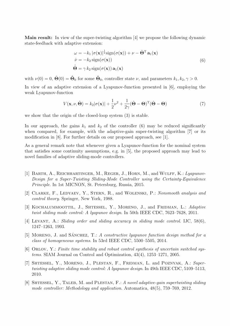
Lyapunov-based Design of Adaptive Sliding Mode Controllers

Alexander Bartha Markus Reichhartingerb Johann Regera Martin Hornb Kai Wulffa

Consider the nonlinear system

x = f(x) + g(x)(∆(x, t) + u

)(1)

where x(t) ∈ Rn is the state, u(t) ∈ R a scalar control input, f and g are known differentiablevector fields. Assume that the matched uncertainty ∆ may be decomposed as per

∆(x, t) = ∆s(x) + ∆u(x, t) = ΘTφ(x) + ∆u(x, t) (2)

such that ∆s(x) = ΘTφ(x) represents the structured uncertainty, with unknown parametervector Θ and known base function φ, and ∆u(x, t) comprises the unstructured uncertaintyand external disturbances.

Let a sliding variable σ = σ(x) be selected such that a desired dynamics is imposed on thesliding manifold σ ≡ 0. Further, let σ be of relative degree one wrt. the input u and assumethe associated internal dynamics to be stable. Thus, along the solution the derivative reads

σ = ΘTa1(x) + a2(x, t)︸ ︷︷ ︸=φ(x,t)

+ω(x, u) (3)

where a1(x), a2(x, t) as well as ω(x, u) may be expressed in terms of equations (1) and (2).Clearly, expression φ(x, t) captures the entire uncertainty and ω is a known function, thatgiven x, is bijective wrt. the control input u.

The goal is to devise a controller ω that stabilizes the origin of (3).

Neglecting the knowledge about the structure within the uncertainty and requiring that theentire uncertainty be uniformly bounded according to

|φ(x, t)| ≤ Ωφ|σ(x)|12 (4)

for some Ωφ > 0 Shtessel et al. gave a solution to this problem [7, 8]. However, the square-rootgrowth bound on the uncertainty may be restrictive in many practical situations.

Therefore, we propose to treat the structurally known part ΘTa1(x) of the uncertainty φ(x, t)separately from the unstructured part a2(x, t). This allows to relax the requirement (4)considerably such that no upper bound is needed for the uncertainty φ(x, t). Only for theunstructured part a2(x, t) we still require that

|a2(x, t)| ≤ Ωa2 |σ(x)|12 (5)

uniformly for some Ωa2 > 0.

aFachgebiet Regelungstechnik, Technische Universitat Ilmenau, Helmholtzplatz 5, D-98693 Ilmenau,E-Mail: alexander.barth,johann.reger,kai.wulff@tu-ilmenau.de

bInstitut fur Regelungs- und Automatisierungstechnik, Technische Universitat Graz, Kopernikusgasse 24/II,8010 Graz, E-Mail: markus.reichhartinger,martin.horn@tugraz.at

Main result: In view of the super-twisting algorithm [4] we propose the following dynamicstate-feedback with adaptive extension:

ω = −k1 |σ(x)|12 sign(σ(x)) + ν − ΘT a1(x)

ν = −k2 sign(σ(x))

˙Θ = γ k2 sign(σ(x)) a1(x)

(6)

with ν(0) = 0, Θ(0) = Θ0 for some Θ0, controller state ν, and parameters k1, k2, γ > 0.

In view of an adaptive extension of a Lyapunov-function presented in [6], employing theweak Lyapunov-function

V (x, ν, Θ) = k2|σ(x)|+ 1

2ν2 +

1

2γ(Θ−Θ)T(Θ−Θ) (7)

we show that the origin of the closed-loop system (3) is stable.

In our approach, the gains k1 and k2 of the controller (6) may be reduced significantlywhen compared, for example, with the adaptive-gain super-twisting algorithm [7] or itsmodification in [8]. For further details on our proposed approach, see [1].

As a general remark note that whenever given a Lyapunov-function for the nominal systemthat satisfies some continuity assumptions, e.g. in [5], the proposed approach may lead tonovel families of adaptive sliding-mode controllers.

[1] Barth, A., Reichhartinger, M., Reger, J., Horn, M., and Wulff, K.: Lyapunov-Design for a Super-Twisting Sliding-Mode Controller using the Certainty-EquivalencePrinciple. In 1st MICNON, St. Petersburg, Russia, 2015.

[2] Clarke, F., Ledyaev, Y., Stern, R., and Wolenski, P.: Nonsmooth analysis andcontrol theory. Springer, New York, 1988.

[3] Kochalummoottil, J., Shtessel, Y., Moreno, J., and Fridman, L.: Adaptivetwist sliding mode control: A lyapunov design. In 50th IEEE CDC, 7623–7628, 2011.

[4] Levant, A.: Sliding order and sliding accuracy in sliding mode control. IJC, 58(6),1247–1263, 1993.

[5] Moreno, J. and Sanchez, T.: A constructive lyapunov function design method for aclass of homogeneous systems. In 53rd IEEE CDC, 5500–5505, 2014.

[6] Orlov, Y.: Finite time stability and robust control synthesis of uncertain switched sys-tems. SIAM Journal on Control and Optimization, 43(4), 1253–1271, 2005.

[7] Shtessel, Y., Moreno, J., Plestan, F., Fridman, L. and Poznyak, A.: Super-twisting adaptive sliding mode control: A lyapunov design. In 49th IEEE CDC, 5109–5113,2010.

[8] Shtessel, Y., Taleb, M. and Plestan, F.: A novel adaptive-gain supertwisting slidingmode controller: Methodology and application. Automatica, 48(5), 759–769, 2012.

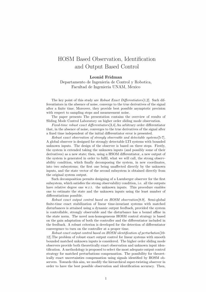
HOSM Based Observation, Identification

and Output Based Control

Leonid FridmanDepartamento de Ingenieria de Control y Robotica,

Facultad de Ingenieria UNAM, Mexico

The key point of this study are Robust Exact Differentiators[1,2]. Such dif-ferentiators in the absence of noise, converge to the true derivatives of the signalafter a finite time. Moreover, they provide best possible asymptotic precisionwith respect to sampling steps and measurement noise.

The paper presents The presentation contains the overview of results ofSliding Mode Control Laboratory on higher order sliding mode observation.

Fixed-time robust exact differentiators[3,4].An arbitrary order differentiatorthat, in the absence of noise, converges to the true derivatives of the signal aftera fixed time independent of the initial differentiator error is presented.

Robust exact observation of strongly observable and detectable systems[5-7].A global observer is designed for strongly detectable LTI systems with boundedunknown inputs. The design of the observer is based on three steps. Firstly,the system is extended taking the unknown inputs (and possibly some of theirderivatives) as a new state; then, using a HSOM differentiator, a new output ofthe system is generated in order to fulfil, what we will call, the strong observ-ability condition, which finally decomposing the system, in new coordinates,into two subsystems; the first one being unaffected directly by the unknowninputs, and the state vector of the second subsystem is obtained directly fromthe original system output.

Such decomposition permits designing of a Luenberger observer for the firstsubsystem, which satisfies the strong observabiliry condition, i.e. all the outputshave relative degree one w.r.t. the unknown inputs. This procedure enablesone to estimate the state and the unknown inputs using the least number ofdifferentiations possible.

Robust exact output control based on HOSM observation[8.9]. Semi-globalfinite-time exact stabilization of linear time-invariant systems with matcheddisturbances is attained using a dynamic output feedback, provided the systemis controllable, strongly observable and the disturbance has a bound affine inthe state norm. The novel non-homogeneous HOSM control strategy is basedon the gain adaptation of both the controller and the differentiator included inthe feedback. A robust criterion is developed for the detection of differentiatorconvergence to turn on the controller at a proper time.

Robust exact output control based on HOSM identification of perturbation[10-12].The problem of robust exact output control for linear systems with smoothbounded matched unknown inputs is considered. The higher order sliding modeobservers provide both theoretically exact observation and unknown input iden-tification. A methodology is proposed to select the most adequate output controlstrategy for matched perturbations compensation. The possibility for theoret-ically exact uncertainties compensation using signals identified by HOSM ob-servers. Towards this aim, we modify the hierarchical super-twisting observer inorder to have the best possible observation and identification accuracy. Then,

1

two controllers are compared. The first one is an integral sliding mode con-troller based on the observed values of the state variables. The other strategyis based on the direct compensation of matched perturbations using their iden-tified values. The performance of both controllers is estimated in terms of thedeterministic noise upper bounds, sampling step and execution time. Based onthese estimations, the designer may select the proper controller for the system.

A collection of the papers with different type of HOSM based observers, canbe found on the web site http://verona.fi-p.unam.mx/˜lfridman/

REFERENCES

1.Levant, A. (1998). Robust exact differentiation via sliding mode technique.Automatica, 34(3), 379–384.

2.Levant, A. (2003). High-order sliding modes: differentiation and outputfeedback control. International Journal of Control, 76(9–10), 924–941.1

3.Cruz-Zavala, E.; Moreno, J.; Fridman, L. Uniform Robust Exact Differen-tiator, IEEE TRANSACTIONS ON AUTOMATIC CONTROL, 2011, v.56, no.11, pp.2727-2733, doi:10.1109/TAC.2011.2160030

4.M. T. Angulo, J. Moreno, and L. Fridman. Robust Exact Uniformly Con-vergent Arbitrary Order Differentiator, Automatica, Volume 49, Issue 8, August2013, Pages 2489-2495,doi:10.1016/j.automatica.2013.04.034

5.F J Bejarano, L. Fridman. High order sliding mode observer for linearsystems with unbounded unknown inputs, International Journal of Control 2010,v.83, no. 9, pp.1920 — 1920.

6. L. Fridman, J. Davila, A. Levant. High-order sliding-mode observationfor linear systems with unknown inputs, Nonlinear Analysis: Hybrid Systems,v.5, no. 2, 189-205,2011.

7. L. Fridman, Y. Shtessel, C. Edwards and Xing-Gang Yan. Higher-ordersliding-mode observer for state estimation and input reconstruction in nonlinearsystems International Journal of Robust and Nonlinear Control 18(4-5), 2008,pp. 399-413

8.M. T. Angulo, L. Fridman and A. Levant. Output-feedback finite -timestabilization of disturbed LTI systems; Automatica, Volume 48, Issue 4, April2012, Pages 606-611 doi:10.1016/j.automatica.2012.01.003.

9. M. T. Angulo, L. Fridman, and J. Moreno. Output feedback finite-timestabilization of distributed feedback linearizable nonlinear systems, Automatica,49(9),2767-2773, http://dx.doi.org/10.1016/j.automatica.2013.05.013

10.A. Ferreira,F. J. Bejarano, L. Fridman. Robust Control With ExactUncertainties ompensation: With or Without Chattering? IEEE TRANSAC-TIONS ON CONTROL SYSTEMS, TECHNOLOGY, 2011, 19(5), p. 969 –975

11. A. Ferreira de Loza, E. Punta, Leonid Fridman, G. Bartolini, S. Del-prat. Nested backward compensation of unmatched perturbations via HOSMobservation. Journal of Franklin Institute,2014, v. 351, no 4, pp.2397–2410,doi:/10.1016/j.jfranklin.2013.12.011

12. Ferreira, Alejandra; Cieslak, Jerome ; Henry, David; Zolghadri, Ali;Fridman, L.Output tracking of systems subjected to perturbations and a classof actuator faults based on HOSM observation and identification, Automatica,v. 51.

2

Discontinuous integral control for mechanical systems

Jaime A. Moreno

Eléctrica y Computación, Instituto de Ingeniería,Universidad Nacional Autónoma de México,

04510 México D.F., Mexico, JMorenoP@ii.unam.mx

RESUMÉ

We consider a second order system

ξ1 = ξ2ξ2 = f (ξ1, ξ2, t) + ρ (t) + τ

(1)

where ξ1 ∈ R and ξ2 ∈ R are the states, τ ∈ R is the control variable, f (ξ1, ξ2, t) is some knownfunction, while the term ρ (t) corresponds to uncertainties and/or perturbations. System 1 can representa mechanical system, where ξ1 is the position and ξ2 is the velocity. An important control task is to tracka smooth time varying reference r (t), i.e. if one defines the tracking error z1 = ξ1 − r and z2 = ξ2− rthe objective is to asymptotically stabilize the origin of system

z1 = z2z2 = f (ξ1, ξ2, t) + ρ (t)− r (t) + τ .

(2)

With the control τ = u− f (ξ1, ξ2, t) + r (t) the system becomes

x1 = x2x2 = u+ ρ (t) ,

(3)

where the perturbation ρ (t) is a time varying signal, not vanishing at the origin (i.e. when x = 0 theperturbation can still be acting). We notice that it is possible not to feed the second derivative of thereference r (t) to the control τ . In this case it will be considered as part of the perturbation term ρ (t).

Under the stated hypothesis it is well known that a continuous, memoryless state feedback u = k (x) isnot able to stabilize x = 0. This is so, because the controller has to satisfy with the condition k (0) = 0,since the closed loop has to have an equilibrium at the origin for vanishing perturbation. But if theperturbation does not vanish, then the origin cannot be anymore an equilibrium point. Discontinuouscontrollers, as the first order Sliding Mode (SM) ones [3], [2] are able to solve the problem for nonvanishing (or persistently acting) bounded perturbations. However, they require the design of a slidingsurface that is reached in finite time, but the target x = 0 is attained only asymptotically fast, andat the cost of a high frecuency switching of the control signal (the so called chattering), that has anegative effect in the actuator, and excites unmodelled dynamics of the plant. Higher Order SlidingModes (HOSM) [4], [7], [6], [5], [9] provide a discontinuous controller for systems of relative degreehigher than one to robustly stabilize the origin x = 0 despite of bounded perturbations, but again at theexpense of chattering. A natural alternative consists in adding an integrator, i.e. defining a new statez = u+ ρ (t), with z = v and designing a third order HOSM controller for the new control variable v.This allows to reach the origin in finite time, and it will be insensitive to Lipschitz perturbations, i.e.with ρ (t) bounded. In this form a continuous control signal u will be obtained, so that the chatteringeffect is reduced. However, this requires feedback not only the two states x1 and x2 but also the statez, which is unknown due to the unknown perturbation. Moreover, to implement an output feedback

controller (assuming that only the position x1 is measured) it is necessary to differentiate two times theposition x1, with the consequent noise amplification effect.

In the case of (almost) constant perturbations ρ (t) a classical solution to the robust regulation problemis the use of integral action, as for example in the PID control [1]. The linear solution would consist of astate feedback plus an integral action, u = −k1x1− k2x2+ z , z = −k3x1. This controller requires onlyto feedback the position and the velocity. For an output feedback it would be only necessary to estimatethe velocity (with the D action for example). In contrast to the HOSM controller this PID control isonly able to reject constant perturbations, instead of Lipschitz ones, and it will reach the target onlyexponentially fast, and not in finite time. By the Internal Model Principle it would be possible to rejectexactly any kind of time varying perturbations ρ (t), for which a dynamical model (an exosystem) isavailable. However this would increase the complexity (order) of the controller, since this exosystemhas to be included in the control law.

Here we provide a solution to the problem, that is somehow an intermediate solution between HOSMand PID control. Similar to the HOSM control our solution uses a discontinuous integral action, it cancompensate perturbations with bounded derivative (ρ (t) is Lipschitz) and the origin is reached in finitetime. So it can solve not only regulation problems (where ρ is constant) but also tracking problems(with ρ time varying) in finite time and with the same complexity of the controller. Similar to thePID control the proposed controller provides a continuous control signal (avoiding chattering) and itrequires only to feedback position and velocity. We also provide for a (non classical) D term, i.e. afinite time converging observer, to estimate the velocity. This basic idea has been already presented inour previous work [10]. In the present one we give a much simpler Lyapunov-based proof, and we alsoinclude an observer in the closed loop together with its Lyapunov proof. Our solution can be seen asa generalization of the Super Twisting control for systems of relative degree one [9], [4], [7], [5], [8]to systems with relative degree two. Extensions to arbitrary order is also possible and it will be brieflydiscussed.

REFERENCES

[1] Khalil, H. K. (2002). Nonlinear Systems. Prentice Hall[2] Utkin, V. (2009).Sliding Mode Control in Electro-Mechanical Systems. CRC Press. Second edition. Automatic and Control Enineering.[3] Utkin, V. (1992). Sliding Modes in Control and Optimization. Springer-Verlag.[4] Fridman, L. y A. Levant (2002).Sliding Mode in Control in Engineering. Marcel Dekker, Inc. High Order Sliding Modes.[5] Levant, A. (2007). Principles of 2-sliding mode design. Automatica. 43, 576–586.[6] Levant, A. (2005). Homogeneity approach to higher-order sliding mode design. Automatica. 34, 576–586.[7] Levant A. Higher order sliding modes: differentiation and output feedback control. \emphInt. J. of Control; nov 2003; \textbf76

(9-10):924–941.[8] Moreno, Jaime A.; M. Osorio (2012). Strict Lyapunov functions for the super-twisting algorithm. IEEE Transactions on Automatic

Control. 54, 1035–1040.[9] Levant, A. (1993). Sliding order and sliding accuracy in sliding mode control. International Journal of Control. 6, 1247–1263.

[10] Zamora, Cesar; Moreno, J. A.; Kamal, Shyam. Control Integral Discontinuo Para Sistemas Mecánicos. Congreso Nacional deControl Automático 2013. Asociación de México de Control Automático (AMCA). Ensenada, Baja California, 16-18 Octubre 2013.Pp. 11—16. http://eventos.cicese.mx/amca2013/52.html

On Discretization of Sliding Mode Based Control Algorithms

Stefan Kocha

Variable structure control techniques are one proper method to deal with control problemsfor uncertain or disturbed systems. In the last decades especially sliding mode concepts whichcan be used in controllers or observers have stood out over classical approaches, due to theirsimplicity and advantages such as robustness and finite time convergence. In order to achievean ideal sliding mode, it is assumed that the switching of a discontinuous control input takesplace at an infinitely high frequency. However, when it comes to digital implementations ofsuch controllers this assumption cannot hold true anymore and switching delays limit theexistence of a true sliding mode. Consequently, in a time discretized sliding mode system,the invariance property of the sliding manifold is deteriorated and trajectories form limitcycles around the sliding surface. The characteristics of this effects, which often are referredto as discretization chattering, are influenced by the discretization method, the selectedsampling frequency as well as the choice of parameters [3, 4]. In order to maintain goodcontrol performance or estimation precision after digitization, the discrete time sliding modesystem may be modified compared to its explicit discretized continuous time counterpart[1, 2].

This talk will focus on discretization effects in conventional (first-order) and super-twistingbased sliding mode control systems. Recent approaches involving various discretization sche-mes of equivalent control based methods are summarized. The influence of the choice of thesampling frequency and controller parameters on the control precision are discussed.

[1] Huber, O., V. Acary und B. Brogliato: Comparison between explicit and impli-cit discrete-time implementations of sliding-mode controllers. In: Decision and Control(CDC), 2013 IEEE 52nd Annual Conference on, Seiten 2870–2875, Dec 2013.

[2] Livne, M. und A. Levant: Homogeneous discrete differentiation of functions with un-bounded higher derivatives. In: Decision and Control (CDC), 2013 IEEE 52nd AnnualConference on, Seiten 1762–1767, Dec 2013.

[3] Qu, Shaocheng, Xiaohua Xia und Jiangfeng Zhang: Dynamical Behaviors of anEuler Discretized Sliding Mode Control Systems. Automatic Control, IEEE Transactionson, 59(9):2525–2529, Sept 2014.

[4] Yan, Yan, Xinghuo Yu und Changyin Sun: Discretization behaviors of a super-twisting algorithm based sliding mode control system. In: Recent Advances in SlidingModes (RASM), 2015 International Workshop on, Seiten 1–5, April 2015.

aInstitute of Automation and Control, Graz University of Technology, Kopernikusgasse 24/II, 8010 Graz,E-Mail: stefan.koch@tugraz.at

Observers for non-linear MIMO descriptor systems

Robel Besrata Felix Gauscha Nenad Vrhovacb

This article presents non-linear observers for exact I/O-linearizable descriptor systems witha specific focus on the semi-explicit form:

x = a(x, z) +B(x, z)u (1a)

0 = p(x, z,u) (1b)

y = c(x, z) (1c)

where x ∈ Rn and z ∈ Rp denote the vectors of the differential and the algebraic variablesrespectively. Furthermore, we assume that there are the same number of input variablesu ∈ Rm and output variables y ∈ Rm.

In addition to the constraints explicitly specified in (1b) the differential algebraic equations(1a, 1b) include further implicit constraints for higher-index systems. All these constraintscontained in (2) describe the manifold M, where the solutions x(t) and z(t) of (1a, 1b) arelocated:

0 = p(x, z,u) . (2)

Following the preliminary work in [1] and [3], as part of the exact I/O-linearization for des-criptor systems, an observer is developed that incorporates the impact of all the constraintsduring the estimation process.

To determine the observer structure, the explicit representation (3) of the non-linear des-criptor system (1):

w =

[xz

]=

a(x, z) +B(x, z)u

−[∂pk−1∂z

]−1 ∂pk−1∂x

(a(x, z) +B(x, z)u)

= f(w) +G(w)u

y = c(w)

(3)

is transferred to Byrnes-Isidori normal form by choosing a suitable transformation (diffeomor-

phism) ξ = ϕ (w) =[ζT ,ηT

]Tand subsequently introducing a state feedback u = (ζ,η,v)

with new inputs v:

ζ = Aζ +Bv (4a)

η = ϑ (ζ,η) (4b)

y = Cζ . (4c)

The linear subsystem (4a, 4c) is observable independent of v and ϑ, while the non-linearsubsystem (4b) describes the non-observable internal dynamics. In case of a asymptotic

aInstitut fur Elektrotechnik und Informationstechnik, Universitat Paderborn, Pohlweg 47-49, 33098 Pader-born, E-Mail: robel.besrat@uni-paderborn.de, gausch@uni-paderborn.de

bFormer member of the ”‘Steuerungs- und Regelungstechnik”’ workgroup at the above

minimum-phase system (3) the overall system (4) is detectable, and it is appropriate todesign a high-gain observer for subsystem (4a, 4c) using the Luenberger method (5):

˙ζ = Aζ +Bv +K (y − y)

˙η = ϑ(ζ, η

)y = Cζ .

(5)

In the original coordinates (w = ϕ−1(ξ)), the observer gain KHGR is determined via theMoore-Penrose inverse of the reduced observability matrix, which is calculated from the timederivatives of the (known) output variables (4c):

˙w = f (w) +G (w)u+KHGR (w) (y − c (w))

y = c (w) .(6)

With the correction approach suggested in [2] the convergence of the high-gain observersolution, against that of the system, can be improved. To achieve this, the observer (6) isextended by the implicit and explicit constraints contained in the vector p (w):

˙w = f (w) +G (w)u−∆PM (w)Mp (w) +KHGR (w) (y − c (w))

y = c (w) .(7)

In this equation M denotes a free design parameter, while ∆PM describes an orthogonalprojection of the deviations in the constraints on the tangent bundle of the solution manifoldM.

Finally the extended observer (7) is implemented using a suitable example, and the resultsare discussed.

[1] Gausch, F. und N. Vrhovac: Feedback Linearization of Descriptorsystems - A Classi-fication Approach. IJAA - International Journal Automation Austria, 18(1):1–18, 2010.

[2] Vrhovac, N.: Beobachtungsaufgabe bei nichtlinearen Deskriptorsystemen. Dissertation,Universitat Paderborn, 2015.

[3] Vrhovac, N. und F. Gausch: Beobachterentwurf fur nichtlineare SISO-Deskriptor-systeme vom Index k=1. In: Horn, M., M. Hofbaur und N. Dourdoumas (Her-ausgeber): 16. Steirisches Seminar uber Regelungstechnik und Prozessautomatisierung,Seiten 16–28, Schloss Retzhof - Leibniz/Osterreich, 2009. Institut fur Regelungs- undAutomatisierungstechnik, Technische Universitat Graz.

Optimization-based formulations of absorbing boundary conditions in

discrete-time wave propagation problems

Alexander Schirrera Stefan Jakubeka

This contribution shows methods to generate absorbing boundary conditions or layers intime-discrete dynamic systems with wave propagation phenomena. Such boundary condi-tions are useful when problems given on large or infinite domains should only be studiedlocally at confined regions of interest, such as the near-field solution in acoustic problemsor local interaction effects near contact points in catenaries or cable dynamics. We considertime-discrete approximations of the solution represented by explicit time-marching schemes.This system representation is particularly useful for time-domain simulations or model-basedcontrol design.

A historic overview on developments in absorbing boundary conditions and the method of“perfectly matched layers” (PMLs) is given in [2]. Absorbing boundary conditions for variouscontinuous as well as discretized forms of wave equations have been derived analytically, e.g.[3, 4]. A PML formulation for an Euler-Bernoulli bending beam with elastic support has beenderived for a finite-element discretization in [1]. These results, however, are highly specificto the considered problem and may be computationally expensive. In this contribution, theoptimization-based methods to construct absorbing boundary conditions or layers are genericin the sense that they essentially only require knowing the underlying dispersion relation.

The first method generates absorbing boundary conditions by direct optimization of thecoefficients of the boundary stencil such that the reflection coefficient is optimized [6]. Sta-bility criteria are proposed and considered either as constraint or as penalty term in theoptimization problem in order to obtain optimal and stable boundary conditions.

The second method shown is inspired by the “perfectly matched layer”. An optimal controlproblem is posed based on a modal decomposition of the current solution, where an optimal,spatially distributed feedback law is computed to emulate the impedance of a PML in theboundary region [5]. This convex optimization problem can be solved optimally in a closedform and shows high absorption performance even on badly conditioned discretization grids(see Fig. 1). Additionally, it allows the controlled modification of impedance in the boundaryregion, which is not realizable with other concepts such as traditional absorbing boundaryconditions.

The proposed methods are widely applicable for linear system dynamics having wave pro-pagation and lead to simple and computationally efficient model structures with the desiredabsorbing properties. These features are crucial in problems with real-time requirements, e.g.when creating design models of online model predictive control. One current industrial app-lication for these models are real-time control tasks related to railway pantograph/catenaryinteraction.

aInstitute of Mechanics and Mechatronics, Workgroup of Control and Process Automation, Techni-sche Universitat Wien, Getreidemarkt 9, 1060 Vienna, E-Mail: alexander.schirrer@tuwien.ac.at,stefan.jakubek@tuwien.ac.at

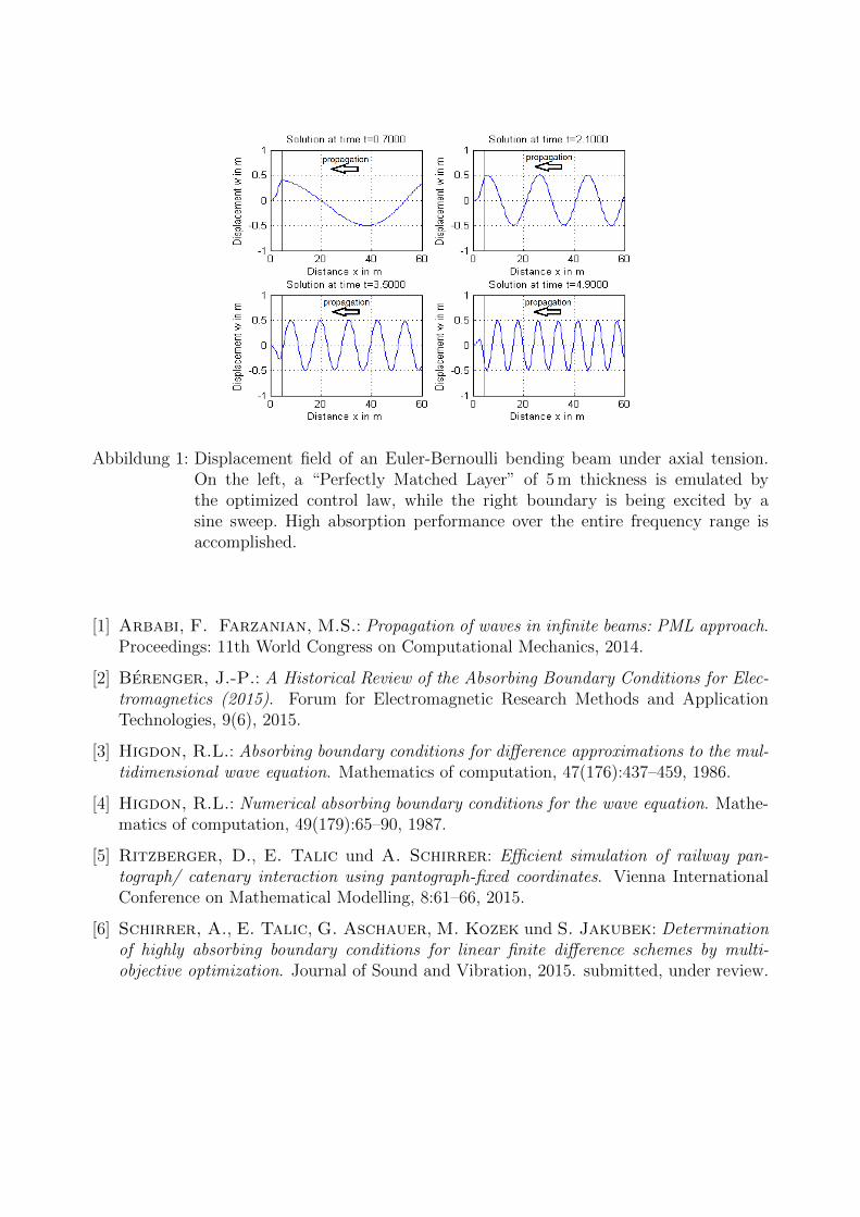
Abbildung 1: Displacement field of an Euler-Bernoulli bending beam under axial tension.On the left, a “Perfectly Matched Layer” of 5 m thickness is emulated bythe optimized control law, while the right boundary is being excited by asine sweep. High absorption performance over the entire frequency range isaccomplished.

[1] Arbabi, F. Farzanian, M.S.: Propagation of waves in infinite beams: PML approach.Proceedings: 11th World Congress on Computational Mechanics, 2014.

[2] Berenger, J.-P.: A Historical Review of the Absorbing Boundary Conditions for Elec-tromagnetics (2015). Forum for Electromagnetic Research Methods and ApplicationTechnologies, 9(6), 2015.

[3] Higdon, R.L.: Absorbing boundary conditions for difference approximations to the mul-tidimensional wave equation. Mathematics of computation, 47(176):437–459, 1986.

[4] Higdon, R.L.: Numerical absorbing boundary conditions for the wave equation. Mathe-matics of computation, 49(179):65–90, 1987.

[5] Ritzberger, D., E. Talic und A. Schirrer: Efficient simulation of railway pan-tograph/ catenary interaction using pantograph-fixed coordinates. Vienna InternationalConference on Mathematical Modelling, 8:61–66, 2015.

[6] Schirrer, A., E. Talic, G. Aschauer, M. Kozek und S. Jakubek: Determinationof highly absorbing boundary conditions for linear finite difference schemes by multi-objective optimization. Journal of Sound and Vibration, 2015. submitted, under review.

Estimating Parameters and States Using Modulating Functions

Johann Regera Jerome Jouffroyb

We consider SISO-LTI systems of order n, given in input-output representation

y(n) + an−1y(n−1) + · · ·+ a1y + a0y = bn−1u

(n−1) + · · ·+ b1u+ b0u , (1)

or as often more compactly written with Y=(−y,−y, . . . ,−y(n−1), u, u, . . . , u(n−1))T along

y(n) = YTθ . (2)

There θ=(a0, a1, . . . , an−1, b0, b1, . . . , bn−1)T holds unknown system parameters to be identi-

fied. For avoiding direct differentiation of probably noisy signals y(t) we employ the methodof modulating functions [8]. We propose to slightly modify the definition given in [4, 5].

Let ϕ : R× R → R be a sufficiently smooth function and denote ϕ(i)(t, t1) := ∂iϕ∂τ i

(τ, t1)|τ=t.A function ϕ(·, ·) is called a modulating function (of order k) if for t0 < t1 it satisfies

ϕ(i)(t0, t1) · ϕ(i)(t1, t1) = 0, ∀i ∈ 0, 1, . . . , k − 1. (3)

A modulating function for which ϕ(i)(t0, t1) = 0 and ϕ(i)(t1, t1) 6= 0 is called a left modulatingfunction, while a modulating function for which ϕ(i)(t0, t1) 6= 0 and ϕ(i)(t1, t1) = 0 is calleda right modulating function. A modulating function whose boundaries verify ϕ(i)(t0, t1) =ϕ(i)(t1, t1) = 0 is called total modulating function.

In view of (3) for total modulating functions we may then enjoy the fundamental property∫ t1

t0

ϕ(τ, t1)ξ(i)(τ)dτ =

∫ t1

t0

(−1)iϕ(i)(τ, t1)ξ(τ)dτ (4)

which allows both to avoid computing signal derivatives of ξ explicitly and to get rid of itsunknown initial and final conditions [1, 2]. This way we may replace (2) with

z = wTθ (5)

where z and the vector w consists of integrals of the shape in (4). In order to obtain an

estimate θ of θ, we may gather a collection of mφ ≥ n equations (5), each of them using adifferent modulating function ϕk(t). We then get

z = WTθ (6)

with z = (z1, z2, . . . , zm)T and regressor W = (w1,w2, . . . ,wm). An estimate θT

= (aT, bT)is finally obtained by simple application of linear least squares, see for example [7, 6, 3]:

θ =(WWT

)−1Wz . (7)

aFachgebiet Regelungstechnik, TU Ilmenau, Helmholtzplatz 5, D-98693 Ilmenau, E-Mail: reger@ieee.orgbMads Clausen Institute, University of Southern Denmark, DK-6400 Alsion 2, Sønderborg, E-Mail:jerome@mci.sdu.dk

Main result: Consider a state space representation of (1) where x1 = y(t), x2 = y(t), . . .Given a set of mϕ ≥ n left modulating functions, the state vector x(t1), as well as a and b,can be estimated in finite-time if W and ∆ have full rank. In this case, a state estimate is

x(t1) =(∆∆T

)−1∆(UTb−QTa− γ

)(8)

with a, b in (7), U=(u1,u2, . . . ,umϕ), Q=(q1,q2, . . . ,qmϕ), γ=(γ1, γ2, . . . , γmϕ)T as per

∆ =

ϕ1(t1, t1) + ΓT1 a

ϕ2(t1, t1) + ΓT2 a

...

, γi =

∫ t1

t0

(−1)nϕ(n)i (τ, t1)y(τ)dτ

uTi =

∫ t1

t0

ϕi(τ, t1)(u(τ), u(τ), . . . , u(n−1)(τ)

)dτ .

qTi =

∫ t1

t0

ϕi(τ, t1), −ϕ(1)i (τ, t1), . . . , (−1)n−1ϕ

(n−1)i (τ, t1))y(τ)dτ

ϕTi (t1, t1) =

((−1)n−1ϕ

(n−1)i (t1, t1), (−1)n−2ϕ

(n−2)i (t1, t1), . . . , ϕi(t1, t1)

).

Γi =

0 0 · · · 0

ϕi(t1, t1) 0 · · · 0

−ϕ(1)i (t1, t1) ϕi(t1, t1) · · · 0

......

. . ....

(−1)n−2ϕ(n−2)i (t1, t1) (−1)n−3ϕ

(n−3)i (t1, t1) · · · 0

[1] Loeb, J.M. und Cahen, G.M.: More about process identification. IEEE Transactionson Automatic Control, Vol. 10, No. 3, 359–361, 1965.

[2] Mathew, A.V. und Fairman, F.W.: Identification in the presence of initial conditions,IEEE Transactions on Automatic Control, Vol. 17, No. 6, 394–396, 1972.

[3] Medvedev, A. und Toivonen, H.T.: Directional sensitivity of continuous least-squaresstate estimators, Systems & Control Letters, Vol. 59, 571–577, 2010.

[4] Pearson, A.E. und Lee, F.: On the identification of polynomial input-output differen-tial systems, IEEE Transactions on Automatic Control, Vol. 30, No. 8, 778–782, 1985.

[5] Preisig, H.A. und Rippin, H.W.: Theory and application of the modulating functionmethod–I. Review and theory of the method and theory of the spline-type modulatingfunctions, Computers and Chemical Engineering, Vol. 17, No. 1, 1–16, 1993.

[6] Reger, J. und Jouffroy, J.: On algebraic time-derivative estimation and deadbeatstate reconstruction, IEEE Conf. on Decision and Control, Shanghai, 1740–1745, 2009.

[7] Rao, G.P. und Unbehauen, H.: Identification of continuous-time systems, IEE ControlTheory and Applications, Vol. 153, no. 2, 185–220, 2006.

[8] Shinbrot, M.: On the analysis of linear and nonlinear systems, Trans. ASME, Vol. 79,No. 3, 547–542, 1957.

Comparing model-free and disturbance observer based control

Mikulas Hubaa Peter Tapaka Stefan Chamraza

The iP controller [1] represents the simplest intelligent (model free) PID controller. Basedon the flatness theory, it may successfully be used for control of broad spectrum of nonlinearsystems. Though, to demonstrate its properties, it will be analyzed in control of a simpleintegrator with an input disturbance.

Similarly, in Motion Control the frequently used control structures may be characterized asdisturbance observer (DO) based PI control [5, 6, 10, 9, 7]. These are still explored fromvarious points of view as robustness, or noise attenuation [8, 2, 3, 4]. Again, in the simplestcase they may be illustrated by control of a single integrator with an input disturbance.

The paper deals with comparison of both types of control with focus on the performanceand noise attenuation trade off.

[1] Fliess, Michel und Cedric Join: Model-free control. International Journal of Con-trol, 86(12):2228–2252, 2013.

[2] Huba, M.: Performance Portrait Method: a new CAD Tool. In: 10th Symposium onAdvances in Control Education (ACE). IFAC, Sheffield, UK, 2013.

[3] Huba, M.: Robustness analysis of a disturbance-observer based PI control. In: 8th Int.Conf. and Exposition on Electrical and Power Eng. - EPE, Iasi, Romania, 2014.

[4] Huba, M.: Robustness versus performance in PDO FPI Control of the IPDT plant. In:IEEE/IES International Conference on Mechatronics, ICM2015, Nagoya, Japan, 2015.

[5] Ohishi, K.: A new servo method in mechantronics. Trans. Jpn. Soc. Elect. Eng., 107-D:83–86, 1987.

[6] Ohishi, Kiyoshi, Masato Nakao, Kouhei Ohnishi und Kunio Miyachi:Microprocessor-Controlled DC Motor for Load-Insensitive Position Servo System. IEEETrans. Industrial Electronics„ IE-34(1):44 –49, feb. 1987.

[7] Radke, A. und Zhiqiang Gao: A survey of state and disturbance observers for prac-titioners. In: American Control Conference, 2006, june 2006.

[8] Sariyildiz, Emre und Kouhei Ohnishi: Analysis the robustness of control systemsbased on disturbance observer. International Journal of Control, 86(10):1733–1743, 2013.

[9] Schrijver, Erwin und Johannes van Dijk: Disturbance Observers for Rigid Mecha-nical Systems: Equivalence, Stability, and Design. ASME, J. Dyn. Sys., Meas., Control,124 (4):539–548, 2002.

aInstitut of Automotive Mechatronics, Slovak University of Technology in Bratislava, Faculty of ElectricalEngineering and Information Technology, mikulas.huba@stuba.sk, peter.tapak@stuba.sk

[10] Umeno, T. und Y. Hori: Robust speed control of dc servomotors using modern two-degree-of-freedom controller design. IEEE Trans. Ind. Electr., 38:363–368, 1991.

Stability Analysis of interconnected Linear Systems with Coupling

Imperfections

Georg Stettingera Martin Benedikta Martin Hornb Christian Potzschec

Josef Zehetnerd

This contribution deals with the stability analysis of interconnected systemsusing a model-based coupling approach to reduce effects of coupling imperfecti-ons. Analysis issues are discussed for linear SISO subsystems: first for the time-invariant case, second for the time-invariant in combination with present nonli-nearities and third for the time-varying case.

1 Introduction

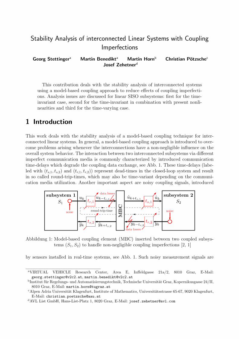
This work deals with the stability analysis of a model-based coupling technique for inter-connected linear systems. In general, a model-based coupling approach is introduced to over-come problems arising whenever the interconnections have a non-negligible influence on theoverall system behavior. The interaction between two interconnected subsystems via differentimperfect communication media is commonly characterized by introduced communicationtime-delays which degrade the coupling data exchange, see Abb. 1. These time-delays (labe-led with (ts,1, ts,2) and (tr,1, tr,2)) represent dead-times in the closed-loop system and resultin so called round-trip-times, which may also be time-variant depending on the communi-cation media utilization. Another important aspect are noisy coupling signals, introduced

Abbildung 1: Model-based coupling element (MBC) inserted between two coupled subsys-tems (S1, S2) to handle non-negligible coupling imperfections [2, 1]

by sensors installed in real-time systems, see Abb. 1. Such noisy measurement signals are

aVIRTUAL VEHICLE Research Center, Area E, Inffeldgasse 21a/2, 8010 Graz, E-Mail:georg.stettinger@v2c2.at, martin.benedikt@v2c2.at

bInstitut fur Regelungs- und Automatisierungstechnik, Technische Universitat Graz, Kopernikusgasse 24/II,8010 Graz, E-Mail: martin.horn@tugraz.at

cAlpen Adria Universitat Klagenfurt, Institute of Mathematics, Universitatsstrasse 65-67, 9020 Klagenfurt,E-Mail: christian.poetzsche@aau.at

dAVL List GmbH, Hans-List-Platz 1, 8020 Graz, E-Mail: josef.zehetner@avl.com

problematic especially if signal-based coupling schemes are used. In this case the noise le-vel is typically amplified, which in turn potentially leads to unstable simulations. Couplingdata losses (see Abb. 1), caused by disturbances or overload of communication capacity areadditional phenomena occurring in coupled systems [2].

2 Model-based coupling approach

The model-based coupling scheme in form of a coupling element (labeled with MBC) isinserted between two coupled subsystems, see Abb. 1. To ensure a time-correct couplingthe output signal uk of subsystem 1 (S1) should arrive at the input of subsystem 2 (S2)without any delay. This is also true for the output yk of subsystem 2. However, significantdead-times due to imperfect communication media impose a serious limitation on the controlperformance of closed-loop systems. To overcome this limitation the proposed model-basedcoupling algorithm extrapolates the coupling signals

(uk−tr,1 , yk−tr,2

)to

(uk+ts,1 , yk+ts,2

)ba-

sed on recursively identified subsystem models. Therefore, at discrete time instant k theextrapolated values uk and yk are already present at the subsystem inputs. This way, theeffect of the round-trip-time is compensated. Coupling data losses have a very similar effectas dead-times and can therefore be compensated via additional model-based extrapolationsaccording to the amount of lost data. Furthermore, noise corrupted coupling signals can beconsidered via adequate parametrizations of the recursive system identification algorithmsto perform model-based filtering [1].

3 Stability Analysis

Important questions via the use of the model-based coupling approach arise: How do theintroduced MBC elements effect the stability of the closed-loop? Can the closed-loop stabilityproperties, without the coupling element, be preserved? In general this stability analysisis a complex task since one has to deal with nonlinear control loops independent of theintroduced coupling elements. Therefore, in a first step, the stability analysis is restricted tolinear closed-loop dynamics including the proposed coupling elements. The stability analysisis divided into three parts with increasing complexity: first MBC using time-invariant (pre-identified) subsystem models, second the influence of additional nonlinearities at the plantinput together with these pre-identified internal models and finally time-varying closed-loopdynamics caused by parameter adaptations of the subsystem models and/or time-varyingsubsystem dynamics.

[1] Stettinger, G., M. Horn, M. Benedikt und J. Zehetner: A Model-Based Ap-proach for Prediction-Based Interconnection of Dynamic Systems. In: Decision and Con-trol (CDC), 2014 IEEE 53rd Annual Conference on, Seiten 3286–3291, December 2014.

[2] Stettinger, G., M. Horn, M. Benedikt und J. Zehetner: Model-based CouplingApproach for non-iterative Real-Time Co-Simulation. In: Control Conference (ECC),2014 European, Seiten 2084–2089, June 2014.

Design and Validation of an SOH-Algorithm for Lithium Ion Batteries

Stefan Doczya Wolfgang Topplera

The usage of modern lithium ion batteries in the hybrid powertrain of buses and commercialvehicles allows significant fuel savings. Therefore the reliable prediction of the usable energywindow and the power limits over life time of the battery is very important for the optimalenergy management of the vehicle.

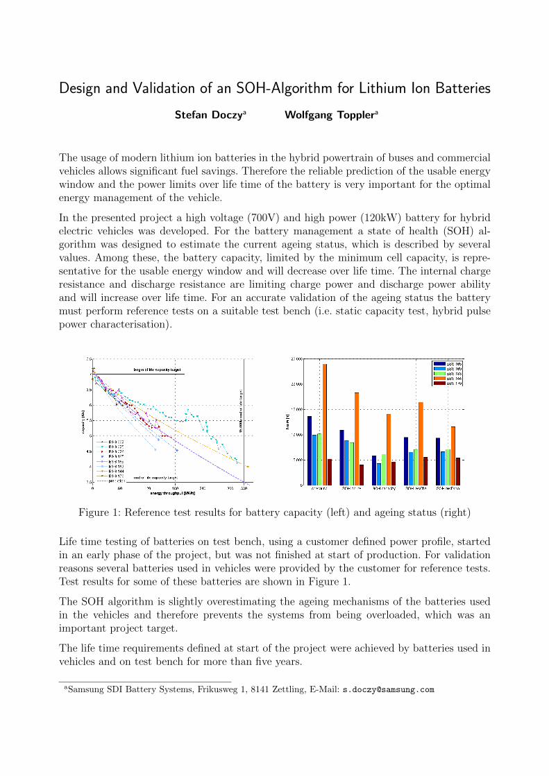
In the presented project a high voltage (700V) and high power (120kW) battery for hybridelectric vehicles was developed. For the battery management a state of health (SOH) al-gorithm was designed to estimate the current ageing status, which is described by severalvalues. Among these, the battery capacity, limited by the minimum cell capacity, is repre-sentative for the usable energy window and will decrease over life time. The internal chargeresistance and discharge resistance are limiting charge power and discharge power abilityand will increase over life time. For an accurate validation of the ageing status the batterymust perform reference tests on a suitable test bench (i.e. static capacity test, hybrid pulsepower characterisation).

Figure 1: Reference test results for battery capacity (left) and ageing status (right)

Life time testing of batteries on test bench, using a customer defined power profile, startedin an early phase of the project, but was not finished at start of production. For validationreasons several batteries used in vehicles were provided by the customer for reference tests.Test results for some of these batteries are shown in Figure 1.

The SOH algorithm is slightly overestimating the ageing mechanisms of the batteries usedin the vehicles and therefore prevents the systems from being overloaded, which was animportant project target.

The life time requirements defined at start of the project were achieved by batteries used invehicles and on test bench for more than five years.

aSamsung SDI Battery Systems, Frikusweg 1, 8141 Zettling, E-Mail: s.doczy@samsung.com

Effects of the nonlinear Arc of a 20-kV-net single-line cable fault on the Earth-Fault-Detection and -Control

Gernot Druml Trench Austria GmbH Linz Austria g.druml@ieee.org

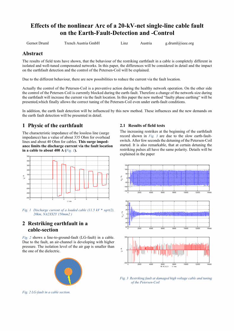
Abstract The results of field tests have shown, that the behaviour of the restriking earthfault in a cable is completely different in isolated and well-tuned compensated networks. In this paper, the differences will be considered in detail and the impact on the earthfault detection and the control of the Petersen-Coil will be explained. Due to the different behaviour, there are new possibilities to reduce the current via the fault location. Actually the control of the Petersen-Coil is a preventive action during the healthy network operation. On the other side the control of the Petersen-Coil is currently blocked during the earth-fault. Therefore a change of the network-size during the earthfault will increase the current via the fault location. In this paper the new method “faulty phase earthing“ will be presented,which finally allows the correct tuning of the Petersen-Coil even under earth-fault conditions. In addition, the earth fault detection will be influenced by this new method. These influences and the new demands on the earth fault detection will be presented in detail. 1 Physic of the earthfault The characteristic impedance of the lossless line (surge impedance) has a value of about 335 Ohm for overhead lines and about 40 Ohm for cables. This surge imped-ance limits the discharge current via the fault location in a cable to about 400 A (Fig. 1).

Fig. 1 Discharge current of a loaded cable (11.5 kV * sqrt(2),

20km, NA2XS2Y 150mm2 )

2 Restriking earthfault in a cable-section

Fig. 2 shows a line-to-ground-fault (LG-fault) in a cable. Due to the fault, an air-channel is developing with higher pressure. The isolation level of the air gap is smaller than the one of the dielectric.

Fig. 2 LG-fault in a cable section.

2.1 Results of field tests The increasing restrikes at the beginning of the earthfault record shown in Fig. 3 are due to the slow earth-fault-switch. After few seconds the detuning of the Petersen-Coil started. It is also remarkable, that at certain detuning the restriking pulses all have the same polarity. Details will be explained in the paper

Fig. 3 Restriking fault at damaged high voltage cable and tuning

of the Petersen-Coil

0 1 2 3 4 5 6 7-400

-300

-200

-100

0

100

200

300

400

500

t / ms

i E / A

0 2000 4000 6000 8000 10000 12000 14000-150

-100

-50

0

50

100

150

U0 /

%

0 2000 4000 6000 8000 10000 12000 14000-60

-40

-20

0

20

40

60

UL1

/ %

0 2000 4000 6000 8000 10000 12000 14000-500

0

500

I F / A

18: K,V,L1: t / ms

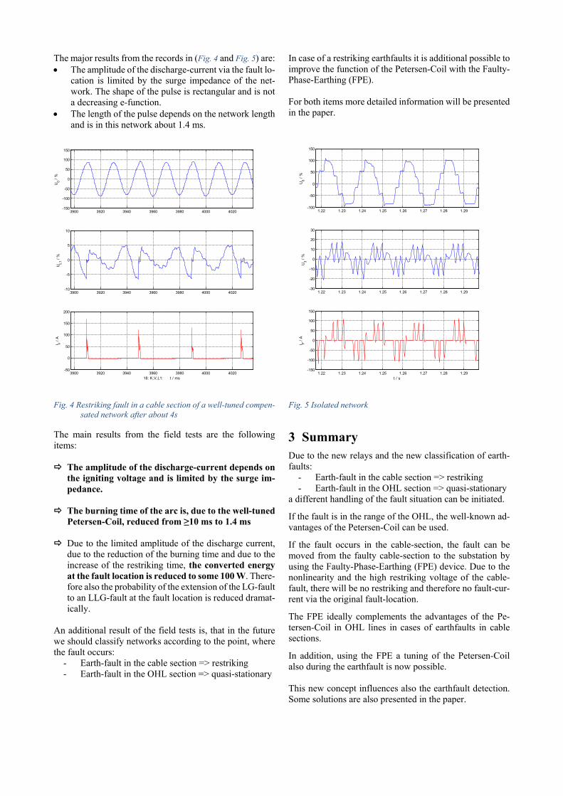
The major results from the records in (Fig. 4 and Fig. 5) are: • The amplitude of the discharge-current via the fault lo-

cation is limited by the surge impedance of the net-work. The shape of the pulse is rectangular and is not a decreasing e-function.

• The length of the pulse depends on the network length and is in this network about 1.4 ms.

Fig. 4 Restriking fault in a cable section of a well-tuned compen-

sated network after about 4s

The main results from the field tests are the following items: The amplitude of the discharge-current depends on

the igniting voltage and is limited by the surge im-pedance.

The burning time of the arc is, due to the well-tuned

Petersen-Coil, reduced from ≥10 ms to 1.4 ms

Due to the limited amplitude of the discharge current, due to the reduction of the burning time and due to the increase of the restriking time, the converted energy at the fault location is reduced to some 100 W. There-fore also the probability of the extension of the LG-fault to an LLG-fault at the fault location is reduced dramat-ically.

An additional result of the field tests is, that in the future we should classify networks according to the point, where the fault occurs:

- Earth-fault in the cable section => restriking - Earth-fault in the OHL section => quasi-stationary

In case of a restriking earthfaults it is additional possible to improve the function of the Petersen-Coil with the Faulty-Phase-Earthing (FPE). For both items more detailed information will be presented in the paper.

Fig. 5 Isolated network

3 Summary Due to the new relays and the new classification of earth-faults:

- Earth-fault in the cable section => restriking - Earth-fault in the OHL section => quasi-stationary

a different handling of the fault situation can be initiated.

If the fault is in the range of the OHL, the well-known ad-vantages of the Petersen-Coil can be used.

If the fault occurs in the cable-section, the fault can be moved from the faulty cable-section to the substation by using the Faulty-Phase-Earthing (FPE) device. Due to the nonlinearity and the high restriking voltage of the cable-fault, there will be no restriking and therefore no fault-cur-rent via the original fault-location.

The FPE ideally complements the advantages of the Pe-tersen-Coil in OHL lines in cases of earthfaults in cable sections.

In addition, using the FPE a tuning of the Petersen-Coil also during the earthfault is now possible. This new concept influences also the earthfault detection. Some solutions are also presented in the paper.

3900 3920 3940 3960 3980 4000 4020-150

-100

-50

0

50

100

150

U0 /

%

3900 3920 3940 3960 3980 4000 4020-10

-5

0

5

10

UL1

/ %

3900 3920 3940 3960 3980 4000 4020-50

0

50

100

150

200

I F / A

18: K,V,L1: t / ms

1.22 1.23 1.24 1.25 1.26 1.27 1.28 1.29-100

-50

0

50

100

150

U0 /

%

1.22 1.23 1.24 1.25 1.26 1.27 1.28 1.29-30

-20

-10

0

10

20

30

U3 /

%

1.22 1.23 1.24 1.25 1.26 1.27 1.28 1.29-150

-100

-50

0

50

100

150

t / s

I F / A

Model based control of a biomass fired steam boiler

Christopher Zemanna,b Viktor Unterbergera,b Markus Gollesa

Introduction

In terms of system theory, a biomass furnace with steam boiler is a non-linear, coupled mul-tivariable system with several inputs and outputs. Conventional control strategies currentlyapplied to these plants usually consist of decoupled linear sub-controllers, just partially oreven not at all considering the coupled and non-linear behaviour of furnace and boiler. Thegoal of this work was to develop a new control strategy that utilizes a mathematical mo-del of the process to improve the plant’s operating behaviour and apply this control to anindustrial plant for the production of process steam.

Plant description

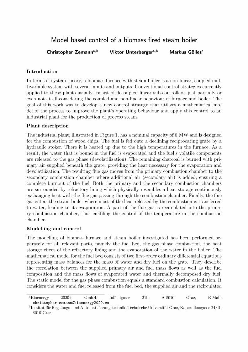
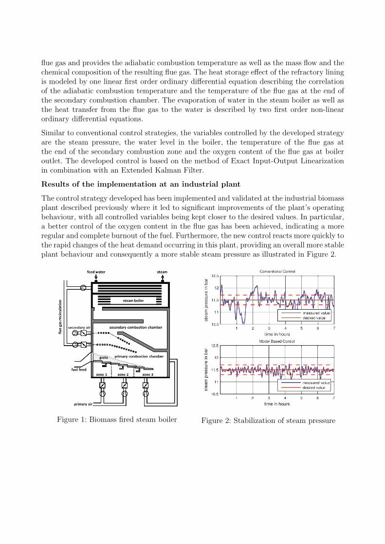
The industrial plant, illustrated in Figure 1, has a nominal capacity of 6 MW and is designedfor the combustion of wood chips. The fuel is fed onto a declining reciprocating grate by ahydraulic stoker. There it is heated up due to the high temperatures in the furnace. As aresult, the water that is bound in the fuel is evaporated and the fuel’s volatile componentsare released to the gas phase (devolatilization). The remaining charcoal is burned with pri-mary air supplied beneath the grate, providing the heat necessary for the evaporation anddevolatilization. The resulting flue gas moves from the primary combustion chamber to thesecondary combustion chamber where additional air (secondary air) is added, ensuring acomplete burnout of the fuel. Both the primary and the secondary combustion chambersare surrounded by refractory lining which physically resembles a heat storage continuouslyexchanging heat with the flue gas passing through the combustion chamber. Finally, the fluegas enters the steam boiler where most of the heat released by the combustion is transferredto water, leading to its evaporation. A part of the flue gas is recirculated into the prima-ry combustion chamber, thus enabling the control of the temperature in the combustionchamber.

Modelling and control

The modelling of biomass furnace and steam boiler investigated has been performed se-parately for all relevant parts, namely the fuel bed, the gas phase combustion, the heatstorage effect of the refractory lining and the evaporation of the water in the boiler. Themathematical model for the fuel bed consists of two first-order ordinary differential equationsrepresenting mass balances for the mass of water and dry fuel on the grate. They describethe correlation between the supplied primary air and fuel mass flows as well as the fuelcomposition and the mass flows of evaporated water and thermally decomposed dry fuel.The static model for the gas phase combustion equals a standard combustion calculation. Itconsiders the water and fuel released from the fuel bed, the supplied air and the recirculated

aBioenergy 2020+ GmbH, Inffeldgasse 21b, A-8010 Graz, E-Mail:christopher.zemann@bioenergy2020.eu

bInstitut fur Regelungs- und Automatisierungstechnik, Technische Universitat Graz, Kopernikusgasse 24/II,8010 Graz

flue gas and provides the adiabatic combustion temperature as well as the mass flow and thechemical composition of the resulting flue gas. The heat storage effect of the refractory liningis modeled by one linear first order ordinary differential equation describing the correlationof the adiabatic combustion temperature and the temperature of the flue gas at the end ofthe secondary combustion chamber. The evaporation of water in the steam boiler as well asthe heat transfer from the flue gas to the water is described by two first order non-linearordinary differential equations.

Similar to conventional control strategies, the variables controlled by the developed strategyare the steam pressure, the water level in the boiler, the temperature of the flue gas atthe end of the secondary combustion zone and the oxygen content of the flue gas at boileroutlet. The developed control is based on the method of Exact Input-Output Linearizationin combination with an Extended Kalman Filter.

Results of the implementation at an industrial plant

The control strategy developed has been implemented and validated at the industrial biomassplant described previously where it led to significant improvements of the plant’s operatingbehaviour, with all controlled variables being kept closer to the desired values. In particular,a better control of the oxygen content in the flue gas has been achieved, indicating a moreregular and complete burnout of the fuel. Furthermore, the new control reacts more quickly tothe rapid changes of the heat demand occurring in this plant, providing an overall more stableplant behaviour and consequently a more stable steam pressure as illustrated in Figure 2.

Figure 1: Biomass fired steam boiler Figure 2: Stabilization of steam pressure

Control-oriented Turbocharger Modeling

Markus Freistatterab Robert Bauerb Nicolaos Dourdoumasa

Wilfried Rosseggerb

The use of turbochargers in the automotive industry has grown significantly over the pastyears. Almost every Diesel engine and an increasing number of gasoline engines are equippedwith a turbocharger. Research and testing of turbochargers is often done using hot gas testbeds. In such an unit a mixture of natural gas and air is burnt in a combustion chamber andthe hot burnt gas is used to drive the turbine. Models are needed of the test bench itself aswell as of the device under test (the turbocharger).

There already exists a variety of turbocharger models of differing complexity. Kessel presentsin [1] very detailed models for turbine and compressor. However, they don’t fit the measureddata obtained on the test bench very well. The newly developed model resembles one ofthe methods of Moraals overview in [2] as physical modeling is combined with curve fitting.The modeled quantities include mass flow, pressure ratio, efficiency and temperatures ofcompressor and turbine. Compressor instabilities, the influence of Wastegate valves andVariable Geometry Turbines are considered as well.

[1] Kessel, Jens-Achim: Modellbildung von Abgasturboladern mit variabler Turbinengeo-metrie an schnellaufenden Dieselmotoren. Doktorarbeit, TU Darmstadt, Mai 2004.

[2] Moraal, Paul und Ilya Kolmanovsky: Turbocharger modeling for automotive con-trol applications. Technischer Bericht, SAE Technical Paper, 1999.

aInstitut fur Regelungs- und Automatisierungstechnik, Technische Universitat Graz, Kopernikusgasse 24/II,8010 Graz, E-Mail: markus.freistaetter@tugraz.at, nicolaos.dourdoumas@tugraz.at

bKristl, Seibt & Co GmbH, Baiernstraße 122a, 8052 Graz, E-Mail: robert.bauer@ksengineers.at,wilfried.rossegger@ksengineers.at

Philon of Byzantium and his work

on Pneumatic and Hydraulic Control Systems

Prof. Emer. Dimitrios Kalligeropoulos1 Appl. Prof. Soultana Vasileiadou2

Philon of Byzantium lived in the third century B.C. in Alexandria and taught in its famous

Museum. He is credited with being the author of the most important technical handbook of

Hellenistic antiquity, the so-called Μητανική Σύνταξις – Mechanical Syntaxis, i.e., a

compendium of mechanical sciences. This manual contained nine books, from which the only

surviving book of Pneumatics includes some of the most important applications of pneumatic

and hydraulic mechanisms.

Indicative examples are the following:

1. Proof of the materiality of air

The invisible air has a material substance, which becomes apparent through its pressure. So, if

someone inverts a vessel and plunges it into the water, no water penetrates into the vessel [3,

II, pp.458-461].

2. Regulation of water level by means of air

The proof of the materiality of air allowed Philon to design a pneumatic-hydraulic control

system, which regulates the water level of a vessel, despite the outflow of water, by means of

the air pressure. Philon introduces here the important invention of closed loop control systems

with feedback, as first Ktesibios and later Heron have also described [3, XII, pp.482-485].

3. A woman servant offers automatically wine and water

Philon describes an automatic control mechanism in the form of a woman servant, made from

bronze or silver, who offers wine and water. She holds with her right hand a pitcher, while the

left hand remains free, until someone places on it an empty cup. Immediately wine and water,

in a prescribed proportion, flow from the pitcher in this cup. The entire pneumatic-hydraulic

control mechanism is hidden in the inner hollow space of the woman servant. This space

includes a wine and a water chamber, whose air pressure is mechanically controlled by valves

and tubes [4, 30]. This example is a notable inventive idea that opens the way to robotics.

1 Piraeus University of Applied Sciences, Department of Automation Engineering, Petrou Ralli & Thivon 250,

12244 Athens, Greece, E-mail: dkal@teipir.gr 2 Piraeus University of Applied Sciences, Department of Automation Engineering, Petrou Ralli & Thivon 250,

12244 Athens, Greece, E-mail: svasil@teipir.gr

Historical Bibliography

[1] The original work of Philon of Byzantium “Περί Πνεσματικών - About Pneumatics” in

ancient Greek is not saved.

[2] It is followed by an Arabic translation and the Latin editions of Constantinople and Oxford,

entitled “Liber de Philonisch ingeniis spiritualibus – Philon’s Book about Inventions of

Pneumatics”.

[3] A part of the above mentioned work is translated in German and included in the book “Heron

of Alexandria, Volume 1” by Wilhelm Schmidt, Leipzig, Teubner Verlag, 1899, under the title

“Die Druckwerke Philons von Byzanz”.

[4] It is followed by the French translation by Baron Carra de Vaux, in Paris, 1903, published

under the title “Le livre des appareils Pneumatique et des machines hydrauliques”.

Only this French translation includes the issue of the House Servant (Theme 30).