41 Three-dimensional Analysis of Genome Topology · 860 41 Three-dimensional Analysis of Genome...

41 Three-dimensional Analysis ofGenome Topology

Harald Bornfleth1,2, Peter Edelmann1,2, Daniele Zink3, andChristoph Cremer1,2

1Institut für Angewandte Physik, Universität Heidelberg2Interdisziplinäres Zentrum für Wissenschaftliches Rechnen,Universität Heidelberg3Institut für Anthropologie und Humangenetik, Universität München

41.1 Introduction . . . . . . . . . . . . . . . . . . . . . . . . . . . . . . . . 859

41.1.1 Overview of methodologies . . . . . . . . . . . . . . . . . 860

41.2 Analysis of large- and small-scale chromatin structure . . . . 863

41.2.1 Morphological parameters of chromosome territories 863

41.2.2 Topological parameters of subchromosomal targets . 865

41.2.3 Biological experiments and data acquisition . . . . . . 870

41.2.4 Performance tests of morphology analysis . . . . . . . 871

41.2.5 Bias reduction in distance measurements . . . . . . . . 872

41.2.6 Cell-cycle specific morphology . . . . . . . . . . . . . . . 873

41.2.7 Cluster analysis of early- and late-replicating foci . . 873

41.3 Discussion and outlook . . . . . . . . . . . . . . . . . . . . . . . . . 874

41.4 References . . . . . . . . . . . . . . . . . . . . . . . . . . . . . . . . . 877

41.1 Introduction

The advances in light microscopy that have been achieved in recentyears have allowed biologists to obtain 3-D images of cell nuclei via the“optical sectioning” technique. Using this technique, which is offeredby confocal laser scanning microscopy (CLSM), a stack of image sectionsis recorded by scanning a focused laser beam through a 3-D specimenwithout destruction of the objects under observation (Chapter 21.4).Alongside these developments in microscopy, recent improvements influorescent staining techniques have enabled the differential visualiza-tion of whole human chromosomes (chromosome “painting” [1], and

859Handbook of Computer Vision and Applications Copyright © 1999 by Academic PressVolume 3 All rights of reproduction in any form reserved.Systems and Applications ISBN 0–12–379773-X/$30.00

860 41 Three-dimensional Analysis of Genome Topology

chromosomal subregions, such as early-replicating and late-replicatingDNA [2]. The combination of both techniques now allows analysis ofrelationships between structural and functional features in 3-D con-served interphase cell nuclei, which has become an important issue inbiomedical research (see also Chapter 12).

The analysis of confocal microscopic images of structural detailsin the cell nucleus can contribute greatly to an understanding of rela-tionships between chromosome topology and function. However, theoptical sectioning capability of CLSM is limited by the optical resolu-tion in axial direction, which is given by the full width at half maximum(FWHM) of the point-spread function (PSF) (approximately 750 nm un-der biologically relevant conditions). Nevertheless, it is desirable toobtain information about smaller structural units in the chromosome.An important example for such biological systems are replication foci,that is, domains of DNA that are replicated before the division of thecell, and are labeled during the replication process. Such foci havediameters of approximately 400 to 800 nm [3, 4] and represent struc-tural features that are conserved during the cell cycle. Interestingly,gene-rich foci are replicated earlier than gene-poor foci. Because early-replicating foci hold the vast majority of the active genes, investigat-ing the distribution of the different types of foci inside chromosometerritories yields important information about the correlation betweenfunctional properties and the topology of the genome.

41.1.1 Overview of methodologies

For the analysis of morphological or positional parameters of fluores-cently stained objects in 3-D images of cell nuclei, different types ofsegmentation approaches were taken. The size of the objects analyzedinfluenced the method of choice. Chromosomes represent large ob-jects compared to the microscopic observation volume (the observa-tion volume is defined as the volume of an ellipsoid, where the radiiare given by half the FWHMs of the PSF in the three scanning direc-tions [5]). After lowpass filtering of the images, a global thresholdingprocedure with subsequent labeling of connected image voxels gave anestimator of the volume of the painted chromosomes (Cavalieri estima-tor) [6, 7]. A somewhat different approach stems from computationalgeometry. The application of Voronoi diagrams to image data uses ran-domly distributed seeds to tessellate the image objects into polyhedra[8] (Chapter 25). As for the Cavalieri estimator, a user-defined thresh-old is required to separate polyhedra belonging to the object of interestfrom background. The smooth outer surfaces given by the polyhedraat the object edges enable the calculation of morphological parameterssuch as the roundness factor (RF) of an object [9]. The Cavalieri esti-mator is not directly suited for surface estimates because the rough

41.1 Introduction 861

edges of parallelepipeds representing image voxels artificially increasethe object surface. A calibration of the factor by means of test objectsof known roundness (e.g., spheres) can correct for these systematic er-rors.

When the object volume is in the range of the observation volume,the gray-value distribution inside the object is no longer homogeneous,but depends strongly on the microscopic PSF. The Voronoi approach isno longer valid. A voxel-based approach that labeled connected compo-nents in images of replication foci was developed by Baumann et al. [10].They used an interactively defined global threshold and the 26 connec-tivity condition of foreground image voxels to label different connectedregions. They also extracted the number of objects and their volumes.However, for images containing many objects of varying size and shape,a global thresholding procedure is not the method of choice. Instead,many applications use the approach of finding local maxima of inten-sity in the images. The segmentation of the individual objects can thenbe performed by using the “anti-watershed” procedure. A discussionof watershed algorithms is presented in Volume 2, Section 21.5.4.

The procedure assigns every point in an image to an object. Thus,watershed algorithms are well suited for the segmentation of datasetswith closely adjoining objects, for example, in medical applications [11].However, in images with large background volumes, many segmentedvoxels will represent background and thus reduce the accuracy of com-putation of object loci.

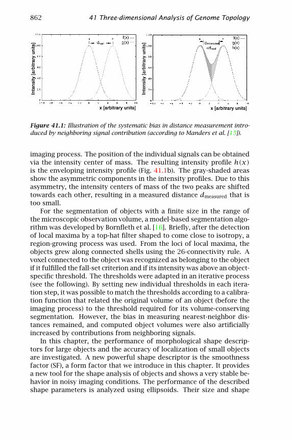
The precise localization of objects is a mandatory requirement forcomputing distance distributions, which provide a very useful tool tocharacterize datasets with a multitude of signals. Nearest-neighbor dis-tributions between signals of the same type can describe the amount ofclustering, the regularity of patterns or randomness [12]. In biologicalexperiments, different fluorochromes are often used to visualize dif-ferent types of cellular compartments. Here, co-localization of objectsdescribed by the distance between signals in different color channels[13] can suggest attachment sites between compartments [14]. For thispurpose, the positions of fluorescent objects had to be determined withsubvoxel accuracy. An approach described by Manders et al. [15] usesdetection of local maxima and defines the largest contour for each ob-ject that contains only one maximum of intensity. All voxels inside thevolume described by the contour are used for the calculation of thecenter of intensity (the center of intensity is the analogon to the centerof mass in mechanics, replacing mass density by intensity). However,Manders et al. [15] found that for closely neighbored objects, a system-atic error in the localization of each object is introduced by the out-of-focus contribution of intensity from the respective neighbor. Thisbias is illustrated in Fig. 41.1a showing intensity profiles f(x) and g(x)of two point-like signals with a distance dreal that are found after the


Figure 41.1: Illustration of the systematic bias in distance measurement intro-duced by neighboring signal contribution (according to Manders et al. [15]).

imaging process. The position of the individual signals can be obtainedvia the intensity center of mass. The resulting intensity profile h(x)is the enveloping intensity profile (Fig. 41.1b). The gray-shaded areasshow the asymmetric components in the intensity profiles. Due to thisasymmetry, the intensity centers of mass of the two peaks are shiftedtowards each other, resulting in a measured distance dmeasured that istoo small.

For the segmentation of objects with a finite size in the range ofthe microscopic observation volume, a model-based segmentation algo-rithm was developed by Bornfleth et al. [16]. Briefly, after the detectionof local maxima by a top-hat filter shaped to come close to isotropy, aregion-growing process was used. From the loci of local maxima, theobjects grew along connected shells using the 26-connectivity rule. Avoxel connected to the object was recognized as belonging to the objectif it fulfilled the fall-set criterion and if its intensity was above an object-specific threshold. The thresholds were adapted in an iterative process(see the following). By setting new individual thresholds in each itera-tion step, it was possible to match the thresholds according to a calibra-tion function that related the original volume of an object (before theimaging process) to the threshold required for its volume-conservingsegmentation. However, the bias in measuring nearest-neighbor dis-tances remained, and computed object volumes were also artificiallyincreased by contributions from neighboring signals.

In this chapter, the performance of morphological shape descrip-tors for large objects and the accuracy of localization of small objectsare investigated. A new powerful shape descriptor is the smoothnessfactor (SF), a form factor that we introduce in this chapter. It providesa new tool for the shape analysis of objects and shows a very stable be-havior in noisy imaging conditions. The performance of the describedshape parameters is analyzed using ellipsoids. Their size and shape

41.2 Analysis of large- and small-scale chromatin structure 863

was matched to that found for chromosome 15 territories. The ellip-soids were subjected to a simulated imaging process including photonshot noise. For spots with a size comparable to the observation vol-ume, we describe an approach that performs the segmentation of eachindividual spot in an image in a 3-D sub-volume, where the intensitycontributions of neighboring spots can be subtracted. Thus, a precisedetermination of spot volumes even below the microscopic observationvolume, and the measurement of spot-spot distances is now possiblewith enhanced accuracy. The influence of the bias in distance measure-ment is investigated using model images with randomly distributedspots. These images underwent a simulated imaging process includingconvolution with the measured microscope PSF of the fluorochromesused, and the application of both additive and multiplicative noise.

The image analysis tools described here were applied to investigatethe distribution of replication foci in the chromosome 15 in humanfibroblast cell nuclei. The morphology of chromosome 15 was analyzedin metabolically active and inactive cells. A non-random organization ofchromatin at the sub-chromosomal level was observed. Apart from theapplication shown here, the image analysis procedures can be used fora wide variety of applications in morphological and topological analysisof biological structures (e. g., [14, 17]).

41.2 Analysis of large- and small-scale chromatin struc-ture

41.2.1 Morphological parameters of chromosome territories

For the morphological analysis of chromosome territories, the voxel-based representation was used because it corresponds to the experi-mental setup. After 3-D filtering of the data, the chromosome territo-ries were segmented by interactive setting of a global threshold. Aftersegmentation, the features of interest were extracted by a labeling pro-cedure, which identified all connected voxels of an object using the 26-connectivity rule. To avoid a user-dependent bias in the threshold cho-sen, the features (chromosome territories) were segmented for a wholerange of reasonable thresholds, and for each threshold in this rangeall the morphological parameters were computed and then averaged.Volumes were computed using the Cavalieri estimator (for definition,see [7]). In addition, the surface area of the chromosome territories andtwo shape parameters were evaluated:

1. The roundness factor (RF) has previously been used for the anal-ysis of morphological differences between the active and inactiveX-chromosome territory in human female amniotic cell nuclei [18].The dimensionless RF is computed from the volume and the surface


area of the object

RF = 36π volume2

surface area3 (41.1)

The RF yields a value of RF=1 for a perfect sphere with a smoothsurface, and lower values for elongated objects and/or objects witha rough surface. However, in some cases this dimensionless ratiobetween volume and surface area is not dominated by the elongationof the object. Fuzzy boundaries of territories or low signal-to-noiseratios may significantly increase the measured surface area of theterritories (see the following), while the computation of the volumesof chromosome territories shows less sensitivity to the fuzziness oftheir boundary or the signal-to-noise ratio.

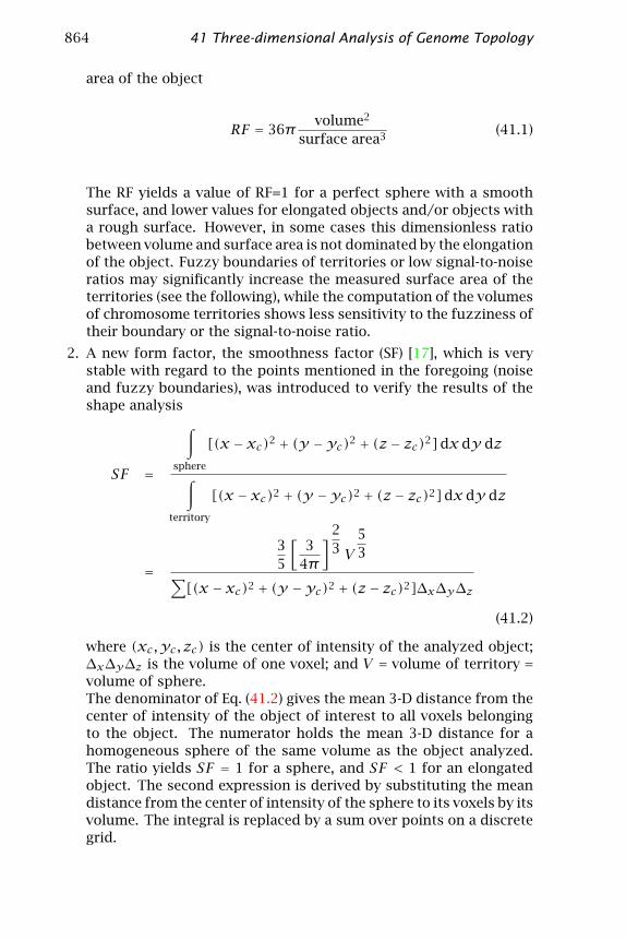
2. A new form factor, the smoothness factor (SF) [17], which is verystable with regard to the points mentioned in the foregoing (noiseand fuzzy boundaries), was introduced to verify the results of theshape analysis

SF =

∫sphere

[(x −xc)2 + (y −yc)2 + (z − zc)2]dx dy dz

∫territory

[(x −xc)2 + (y −yc)2 + (z − zc)2]dx dy dz

=35

[3

4π

]23 V

53∑

[(x −xc)2 + (y −yc)2 + (z − zc)2]∆x∆y∆z(41.2)

where (xc,yc, zc) is the center of intensity of the analyzed object;∆x∆y∆z is the volume of one voxel; and V = volume of territory =volume of sphere.The denominator of Eq. (41.2) gives the mean 3-D distance from thecenter of intensity of the object of interest to all voxels belongingto the object. The numerator holds the mean 3-D distance for ahomogeneous sphere of the same volume as the object analyzed.The ratio yields SF = 1 for a sphere, and SF < 1 for an elongatedobject. The second expression is derived by substituting the meandistance from the center of intensity of the sphere to its voxels by itsvolume. The integral is replaced by a sum over points on a discretegrid.


0

0.5

1 epsilon x

0 0.2 0.4 0.6 0.8 1

epsilon y

0

0.2

0.4

0.6

0.8

1

SF

Figure 41.2: Value of SF for an ellipsoid, where two half-axes are elongated, andthe third half-axis is adjusted to maintain the volume of the ellipsoid: Half-axes:rx = R(1− εx),; ry = R(1− εy),; rz = R/[(1− εx)∗ (1− εy)].

41.2.2 Topological parameters of subchromosomal targets

A model-based algorithm for the volume-conserving segmentation ofsignals with volumes comparable to the observation volume of the mi-croscope PSF was described in Bornfleth et al. [16]. The algorithm foundlocal maxima of intensity in 3-D image stacks. These were the centersof fluorescence signals (“spots”). Starting from these spot centers, aregion-growing process along connected shells was performed. Eachvoxel had to meet four criteria to be labeled as belonging to an object:

i. the exclusion criterion stating that the tested voxel had not beenpreviously labeled by another object in the image;

ii. the 26-connectivity criterion;

iii. the fall-set criterion that the voxel intensity was not higher than thatof the nearest voxel towards the spot center; and

iv. the threshold-criterion that the voxel intensity was higher or equalto an object-specific threshold.

This threshold depended on the volume that the spot originally had,that is, on the volume of the fluorochrome distribution of the spot.By means of model calculations, a calibration function Trel(V) was ob-tained. For each original spot volume V (i. e., the volume before theimaging process), this function gave the corresponding threshold T


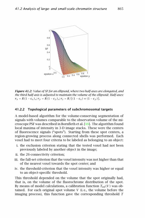
Figure 41.3: Threshold-volume function found for three different fluo-rochromes. The segmentation thresholds are approximately constant abovea volume of 5.5× the observation volume. Thresholds were obtained from nu-merical calculations of cube-shaped spots.

that was required to obtain this original volume after segmentation.However, the original spot volume was not known a priori for a givenspot. Therefore, the threshold was reduced in each iteration, start-ing from a threshold that corresponded to a point-like spot. Aftereach iteration, the resulting spot volume was determined. This volumewas assumed to be the “true” volume, and the corresponding volume-conserving threshold Trel(V) for a spot of that size was obtained fromthe calibration curve. This threshold was used in the next iteration.After 5-10 iterations, a fixed point on the curve was obtained, that is,the volume did not change after application of the new threshold. Thefunction Trel(V) for the parameters used in the experiments describedhere is shown in Fig. 41.3. It shows the relative threshold needed forvolume-conserving segmentation vs the original spot volume (abscissa)in voxels. The voxel size assumed was 80×80× 250 nm3. The volume-intensity functions were fitted by second-degree polynomials. An ear-lier version of this plot, showing the results for just two fluorochromes,was published elsewhere [19].

From Fig. 41.3, it is apparent that higher thresholds are required forthe segmentation of a spot exhibiting Cy5-fluorescence than for oneexhibiting FITC-fluorescence. This is due to the longer wavelength atwhich Cy5 emits fluorescence light (approximately 670 nm vs 520 nmfor FITC). With the small volumes examined, the greater width of the PSFfor Cy5 causes more blurring of the signal than that for FITC, that is, thesame energy is smeared out over a greater volume for a Cy5 object. Thisleads to higher thresholds that are needed if the original volume is tobe recovered. The model-based segmentation approach was extendedto improve the accuracy of volume and distance measurements even in


cases where signal overlap lead to an artificial increase in the signal (seeFig. 41.1). After the local maxima in the image had been found, a 3-Dvoxel cube slmn was created for each spot1. The voxels of the cube wereassigned the intensities of the noise-filtered image in the volume rangearound the spot center (see Fig. 41.4 a), and the cubes were grouped inthe new image matrix Sjlmn. The gray values in the new, 4-D subvol-ume matrix S, with the elements {0..J = Nspots−1; 0..L; 0..M ; 0..N} wereassigned as

Sj,L/2+l,M/2+m,N/2+n := g′zj+l,yj+m,xj+n, where

0 ≤ j < Nspots

−L2 ≤ l < L2

−M2 ≤m< M2

−N2 ≤ n < N2

(41.3)

with the number of spots Nspots and the coordinates { xj,yj, zj} of thelocal maximum found for spot j; g′lmn is the image matrix of the prepro-cessed image. A second 4-D matrix Tjlmn contained 3-D subvolumeswith the labeled voxels for each spot #j. Initially, only the location ofthe central voxel, that is, T.,L/2,M/2,N/2, was labeled for all spots. Eachspot was then allowed to grow inside its cube in shells around the spotcenter according to criteria (ii) to (iv) described in the foregoing. Thesegmentation threshold was initially set to 82 % of the maximum inten-sity of a spot, because this corresponded to the threshold necessaryfor segmentation of a point-like object. A growth shell was completedfor all spots before the next shell was tested to give all spots equalpossibilities for expansion. To prevent an overlap between spots in thesame color channel, each labeled voxel was marked not only in the labelmatrix T, but also in the original image. If a voxel tested in a growthshell had already been labeled in the original image as belonging to an-other spot, it was rejected. Thus it was possible to prevent spots frommerging with neighboring spots (see criterion (i)). After the growthprocess was completed for all spots, the labeled voxels were used fora least-squares fit of spot intensity. According to the assumption ofa constant fluorochrome distribution inside the spot, each voxel of aspot labeled in the label matrix T was convoluted with the microscopicmedian-filtered PSF hm

Fj = Tj ∗hm, where ∗ denotes the 3-D convolution (41.4)

Fj denotes the 3-D subvolume of the 4-D matrix F containing the con-voluted intensities for spot #j. In order to reproduce the intensity dis-tribution of the spot #j after imaging, a least-squares fit of the resulting

1The subvolume had fixed dimensions in x-, y-, and z-direction. As the number ofelements was smaller in z-direction due to the larger pixel size, it is not entirely correctto speak of an image cube. However, this nomenclature is used for simplicity.


model image cube Fj to the original data in Sj was performed accordingto Brent’s method [20] for each spot (j ∈ [0..Nspots −1] ). This resultedin F holding the fitted intensities. In a final step, the image cubes Sjwere reloaded from the original image, and for each spot #j, the fittedintensities were used to subtract the intensity contributions of neigh-boring spots in the image cubes of individual spots (see Fig. 41.4 b)

F ′jlmn =Nspots−1,κ≠j∑

κ=0

{Fκλµν, if

λ := l− (zκ − zj) ∈ [0..L]µ :=m− (yκ −yj) ∈ [0..M]ν := n− (xκ −xj) ∈ [0..N]

}(41.5)

S′jlmn = Sjlmn − F ′jlmn (41.6)

The condition behind the sum holds the overlap condition: Onlyif the spacing between the local maxima of two spots is sufficientlysmall (e. g., the value of xκ − xj for the x-direction), is a subtractionof intensities performed for the spot #κ . Otherwise, intensity contri-butions from spot #κ are not subtracted from spot # j. The 4-D arrayS′ holds the corrected intensities. Because in the first iteration thespots had not yet acquired their final volume due to the initial highthreshold, the accuracy of the fitting process increased only graduallyduring the iterations, along with the accuracy of the subtraction proc-ess. The least-squares fitting was mandatory to obtain a guess aboutthe intensity distribution that resulted from the expected spot geom-etry. If a fit did not reproduce the experimental data with sufficientaccuracy (defined as a value of χ2/n > 30, where n is the number ofvoxels used for the fit, and χ2 is the sum over the squares of the devi-ations of intensities), the fitted intensities for the respective spot werenot subtracted from other spots in that iteration. The resulting inten-sity distributions in the cubes were used in the next iteration step (seeFig. 41.4 c), where new individual thresholds were defined accordingto the function Trel(V), based on the volume that a spot had acquiredin the last growth step. The process converged after 5-10 iterations.The process of fitting spot intensities after segmentation to the origi-nal data allowed the mean brightness of a spot as well as its volume andposition to be evaluated. Because the value for the mean brightness wasobtained by the fit after convoluting a segmented volume with the PSF,it gave a measure for the fluorochrome density inside the probe, whichyielded rather more accurate results than simply adding up intensitiesin the image.

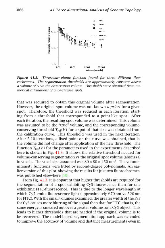
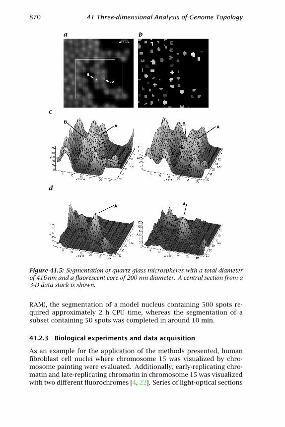
An example for the reduction of neighboring spot signals by theuse of individual subvolumes is given in Fig. 41.5 showing the proce-dure for an image of touching microspheres with a quartz glass shell


Figure 41.4: Schematic diagram of the steps taken by the subtraction algo-rithm.

around a fluorescent core. The quartz glass microspheres had an over-all diameter of 416 nm, with a fluorescent core 200 nm in diameter, wellbelow the microscopic observation volume. This placed great demandson the volume-conserving segmentation. A central section from a 3-Ddata stack is presented. The contour plots show the intensity distribu-tions in the central section surrounding example beads A (left) and B(right). The situation at the beginning (c) and after the subtraction ofneighboring intensities ((d), after seven iterations) is shown. Figure 41.5shows that volumes are recovered after segmentation. For the quartzglass spheres, the gap between cores is clearly visible ((b); different grayshades denote different objects). Using the approach described in [16]without subtraction, the segmented cores touched after segmentation(not shown). The distance between the two example spots A and B wasdetermined to be 359.4 nm with the first algorithm, and 432.1 nm withthe subtraction of intensities. Because the manufacturer reported asize of the spheres as 416±22 nm [21], this example demonstrates thebias effect and its reduction using the new approach.

The evaluation time for spot growth and fitting increased linearlywith the number of spots, whereas the subtraction time was moreclosely related to (number of spots)2 (for the worst-case scenario thatall spots had mutual intensity contributions). The total evaluation timewas proportional to (number of spots)a,a ∈ [1,1.5]. On a SiliconGraphics workstation (SGI IRIS INDIGO, CPU R4400, 200 MHz, 96 MB


a b

c

d

Figure 41.5: Segmentation of quartz glass microspheres with a total diameterof 416 nm and a fluorescent core of 200-nm diameter. A central section from a3-D data stack is shown.

RAM), the segmentation of a model nucleus containing 500 spots re-quired approximately 2 h CPU time, whereas the segmentation of asubset containing 50 spots was completed in around 10 min.

41.2.3 Biological experiments and data acquisition

As an example for the application of the methods presented, humanfibroblast cell nuclei where chromosome 15 was visualized by chro-mosome painting were evaluated. Additionally, early-replicating chro-matin and late-replicating chromatin in chromosome 15 was visualizedwith two different fluorochromes [4, 22]. Series of light-optical sections


0 . 0 0 1

0 . 0 1

0 . 1

1

1 0

2 0 4 0 6 0 8 0 1 0 0 1 2 0

n u m b e r o f d e t e c t e d p h o t o n s p e r v o x e l o f m a x i m u m i n t e n s i t y

true value / determ

ined value

v o l u m e

s u r f a c e

S F

R F

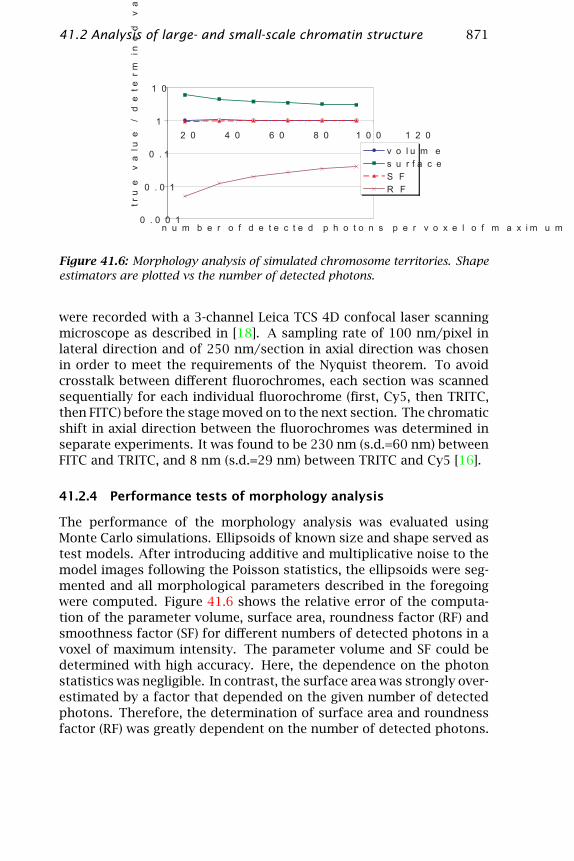
Figure 41.6: Morphology analysis of simulated chromosome territories. Shapeestimators are plotted vs the number of detected photons.

were recorded with a 3-channel Leica TCS 4D confocal laser scanningmicroscope as described in [18]. A sampling rate of 100 nm/pixel inlateral direction and of 250 nm/section in axial direction was chosenin order to meet the requirements of the Nyquist theorem. To avoidcrosstalk between different fluorochromes, each section was scannedsequentially for each individual fluorochrome (first, Cy5, then TRITC,then FITC) before the stage moved on to the next section. The chromaticshift in axial direction between the fluorochromes was determined inseparate experiments. It was found to be 230 nm (s.d.=60 nm) betweenFITC and TRITC, and 8 nm (s.d.=29 nm) between TRITC and Cy5 [16].

41.2.4 Performance tests of morphology analysis

The performance of the morphology analysis was evaluated usingMonte Carlo simulations. Ellipsoids of known size and shape served astest models. After introducing additive and multiplicative noise to themodel images following the Poisson statistics, the ellipsoids were seg-mented and all morphological parameters described in the foregoingwere computed. Figure 41.6 shows the relative error of the computa-tion of the parameter volume, surface area, roundness factor (RF) andsmoothness factor (SF) for different numbers of detected photons in avoxel of maximum intensity. The parameter volume and SF could bedetermined with high accuracy. Here, the dependence on the photonstatistics was negligible. In contrast, the surface area was strongly over-estimated by a factor that depended on the given number of detectedphotons. Therefore, the determination of surface area and roundnessfactor (RF) was greatly dependent on the number of detected photons.


a

- 0 . 3

- 0 . 2

- 0 . 1

0

0 . 1

0 . 2

0 . 3

1.3

1.5

1.7

1.9

2.1

2.3

2.5

2.7

2.9

3.1

3.3

n e a r e s t - n e i g h b o r d i s t a n c e i n u n i t s o f e f f e c t i v e F W H M s

med

ian shift towards

neares

t neighbor [FWHM]

F I T C : n = 4 2

T R I T C : n = 4 2

C Y 5 : n = 4 2

b

- 0 . 3

- 0 . 2

- 0 . 1

0

0 . 1

0 . 2

0 . 3

1.3

1.5

1.7

1.9

2.1

2.3

2.5

2.7

2.9

3.1

3.3

n e a r e s t - n e i g h b o r d i s t a n c e i n u n i t s o f e f f e c t i v e F W H M s

med

ian shift towards nea

rest

neighbor [FWHM]

F I T C : n = 4 2

T R I T C : n = 4 2

C y 5 : n = 4 2

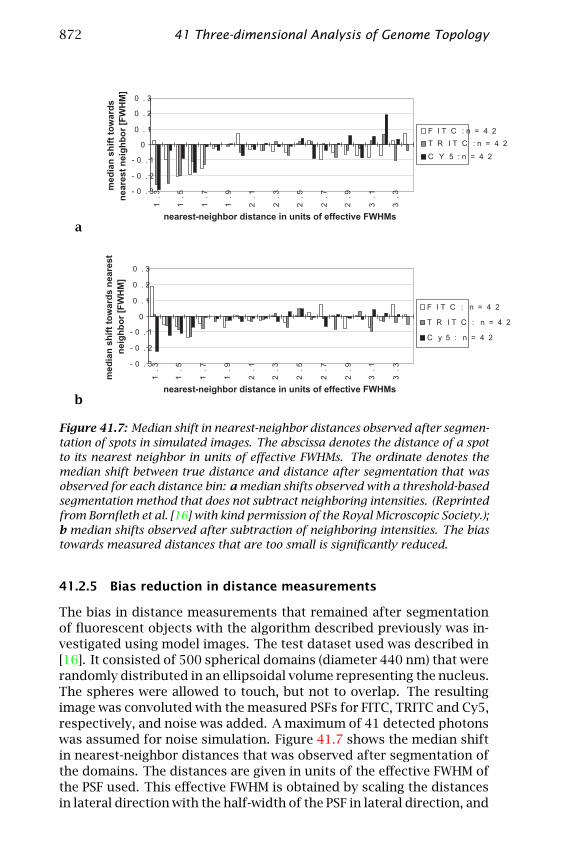
Figure 41.7: Median shift in nearest-neighbor distances observed after segmen-tation of spots in simulated images. The abscissa denotes the distance of a spotto its nearest neighbor in units of effective FWHMs. The ordinate denotes themedian shift between true distance and distance after segmentation that wasobserved for each distance bin: a median shifts observed with a threshold-basedsegmentation method that does not subtract neighboring intensities. (Reprintedfrom Bornfleth et al. [16] with kind permission of the Royal Microscopic Society.);b median shifts observed after subtraction of neighboring intensities. The biastowards measured distances that are too small is significantly reduced.

41.2.5 Bias reduction in distance measurements

The bias in distance measurements that remained after segmentationof fluorescent objects with the algorithm described previously was in-vestigated using model images. The test dataset used was described in[16]. It consisted of 500 spherical domains (diameter 440 nm) that wererandomly distributed in an ellipsoidal volume representing the nucleus.The spheres were allowed to touch, but not to overlap. The resultingimage was convoluted with the measured PSFs for FITC, TRITC and Cy5,respectively, and noise was added. A maximum of 41 detected photonswas assumed for noise simulation. Figure 41.7 shows the median shiftin nearest-neighbor distances that was observed after segmentation ofthe domains. The distances are given in units of the effective FWHM ofthe PSF used. This effective FWHM is obtained by scaling the distancesin lateral direction with the half-width of the PSF in lateral direction, and


by scaling the distances in axial direction with the axial PSF half-width.Because the measured distances are smaller than the real distances forclosely neighbored targets, the median shift is negative. Compared tothe results from Bornfleth et al. [16], (Fig. 41.7 a), the bias is signifi-cantly reduced. It is only marginally higher than the fluctuations ofthe shift that are due to statistical variations (Fig. 41.7 b). This meansthat clustering can be investigated using the nearest-neighbor statisticswithout a significant distortion of the results due to systematic errors.As the spots had a size of 440 nm, distances below 1.3 effective FWHMs,where no correct segmentation was possible, were not evaluated.

41.2.6 Cell-cycle specific morphology

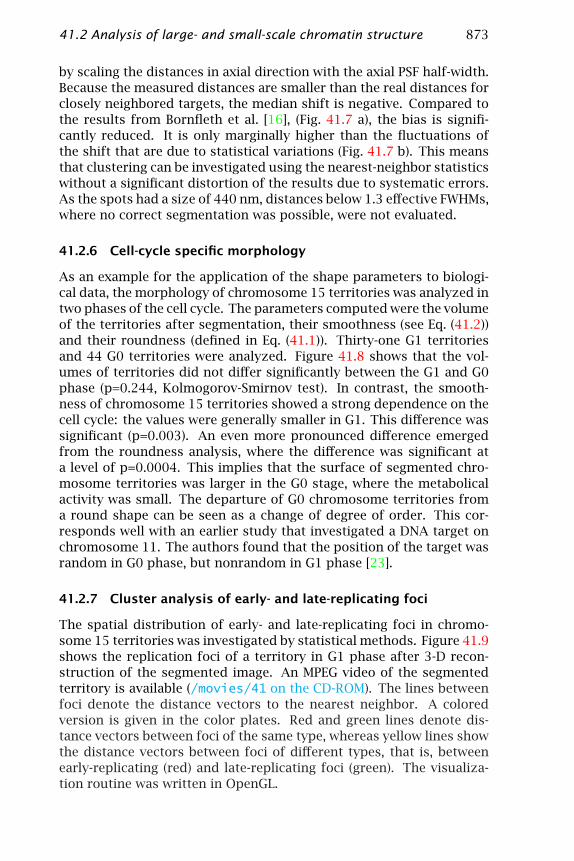
As an example for the application of the shape parameters to biologi-cal data, the morphology of chromosome 15 territories was analyzed intwo phases of the cell cycle. The parameters computed were the volumeof the territories after segmentation, their smoothness (see Eq. (41.2))and their roundness (defined in Eq. (41.1)). Thirty-one G1 territoriesand 44 G0 territories were analyzed. Figure 41.8 shows that the vol-umes of territories did not differ significantly between the G1 and G0phase (p=0.244, Kolmogorov-Smirnov test). In contrast, the smooth-ness of chromosome 15 territories showed a strong dependence on thecell cycle: the values were generally smaller in G1. This difference wassignificant (p=0.003). An even more pronounced difference emergedfrom the roundness analysis, where the difference was significant ata level of p=0.0004. This implies that the surface of segmented chro-mosome territories was larger in the G0 stage, where the metabolicalactivity was small. The departure of G0 chromosome territories froma round shape can be seen as a change of degree of order. This cor-responds well with an earlier study that investigated a DNA target onchromosome 11. The authors found that the position of the target wasrandom in G0 phase, but nonrandom in G1 phase [23].

41.2.7 Cluster analysis of early- and late-replicating foci

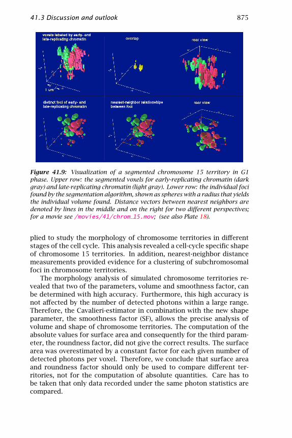
The spatial distribution of early- and late-replicating foci in chromo-some 15 territories was investigated by statistical methods. Figure 41.9shows the replication foci of a territory in G1 phase after 3-D recon-struction of the segmented image. An MPEG video of the segmentedterritory is available (/movies/41 on the CD-ROM). The lines betweenfoci denote the distance vectors to the nearest neighbor. A coloredversion is given in the color plates. Red and green lines denote dis-tance vectors between foci of the same type, whereas yellow lines showthe distance vectors between foci of different types, that is, betweenearly-replicating (red) and late-replicating foci (green). The visualiza-tion routine was written in OpenGL.


a b

c

Figure 41.8: Morphological parameters computed for chromosome 15 terri-tories in G1 phase and in G0 phase. Cumulative plots are presented: a thevolumes computed do not show significant differences; b the smoothness fac-tors show a significant difference between territories in G1 phase and G0 phase;c the difference is even more pronounced using the roundness parameter.

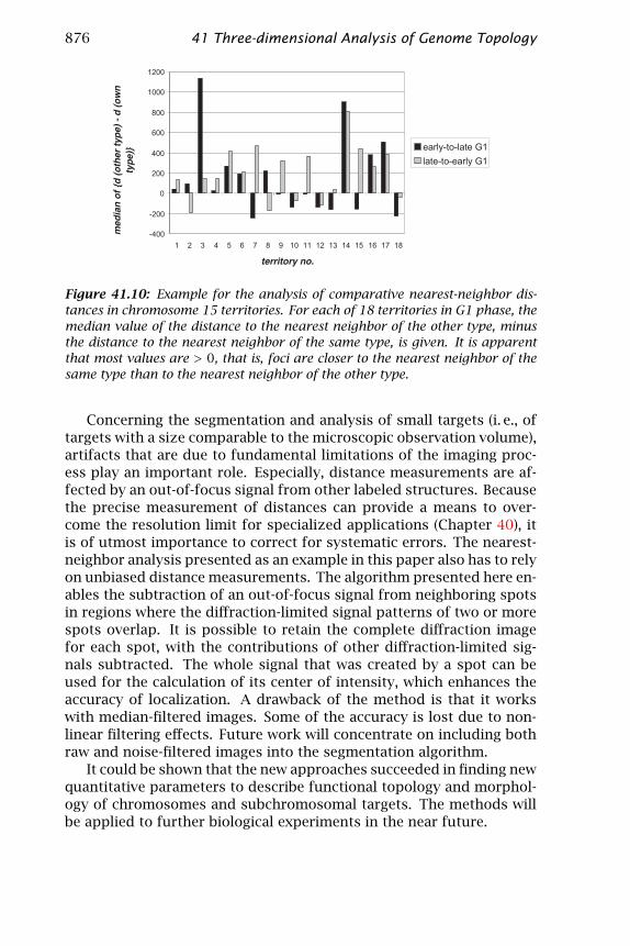
Figure 41.10 shows the median values of comparative nearest-neigh-bor distances obtained for 18 territories in G1 cells. For both early-and late-replicating foci, the distance to the nearest neighbor in theother color channel was on average greater than the distance to theneighbor in the original color channel. This means that on average,early-replicating foci were closer to other early-replicating foci than toother late-replicating foci. This is surprising as it is expected that early-replicating foci and late-replicating foci alternate on the condensedmetaphase chromosomes. This observed clustering of foci of the samefunctional state is not due to artifacts introduced by the segmenta-tion algorithm because the algorithm reduces the bias in distance mea-surements effectively. It suggests that early-replicating foci and late-replicating foci form higher-order clusters in interphase nuclei.

41.3 Discussion and outlook

In this chapter, new image analysis tools to investigate morphologi-cal and topological features of chromosomes were introduced. Theirperformance was tested with regard to statistical and systematic er-rors. As an example of the usefulness of the methods, they were ap-

41.3 Discussion and outlook 875

Figure 41.9: Visualization of a segmented chromosome 15 territory in G1phase. Upper row: the segmented voxels for early-replicating chromatin (darkgray) and late-replicating chromatin (light gray). Lower row: the individual focifound by the segmentation algorithm, shown as spheres with a radius that yieldsthe individual volume found. Distance vectors between nearest neighbors aredenoted by lines in the middle and on the right for two different perspectives;for a movie see /movies/41/chrom 15.mov; (see also Plate 18).

plied to study the morphology of chromosome territories in differentstages of the cell cycle. This analysis revealed a cell-cycle specific shapeof chromosome 15 territories. In addition, nearest-neighbor distancemeasurements provided evidence for a clustering of subchromosomalfoci in chromosome territories.

The morphology analysis of simulated chromosome territories re-vealed that two of the parameters, volume and smoothness factor, canbe determined with high accuracy. Furthermore, this high accuracy isnot affected by the number of detected photons within a large range.Therefore, the Cavalieri-estimator in combination with the new shapeparameter, the smoothness factor (SF), allows the precise analysis ofvolume and shape of chromosome territories. The computation of theabsolute values for surface area and consequently for the third param-eter, the roundness factor, did not give the correct results. The surfacearea was overestimated by a constant factor for each given number ofdetected photons per voxel. Therefore, we conclude that surface areaand roundness factor should only be used to compare different ter-ritories, not for the computation of absolute quantities. Care has tobe taken that only data recorded under the same photon statistics arecompared.


Figure 41.10: Example for the analysis of comparative nearest-neighbor dis-tances in chromosome 15 territories. For each of 18 territories in G1 phase, themedian value of the distance to the nearest neighbor of the other type, minusthe distance to the nearest neighbor of the same type, is given. It is apparentthat most values are > 0, that is, foci are closer to the nearest neighbor of thesame type than to the nearest neighbor of the other type.

Concerning the segmentation and analysis of small targets (i. e., oftargets with a size comparable to the microscopic observation volume),artifacts that are due to fundamental limitations of the imaging proc-ess play an important role. Especially, distance measurements are af-fected by an out-of-focus signal from other labeled structures. Becausethe precise measurement of distances can provide a means to over-come the resolution limit for specialized applications (Chapter 40), itis of utmost importance to correct for systematic errors. The nearest-neighbor analysis presented as an example in this paper also has to relyon unbiased distance measurements. The algorithm presented here en-ables the subtraction of an out-of-focus signal from neighboring spotsin regions where the diffraction-limited signal patterns of two or morespots overlap. It is possible to retain the complete diffraction imagefor each spot, with the contributions of other diffraction-limited sig-nals subtracted. The whole signal that was created by a spot can beused for the calculation of its center of intensity, which enhances theaccuracy of localization. A drawback of the method is that it workswith median-filtered images. Some of the accuracy is lost due to non-linear filtering effects. Future work will concentrate on including bothraw and noise-filtered images into the segmentation algorithm.

It could be shown that the new approaches succeeded in finding newquantitative parameters to describe functional topology and morphol-ogy of chromosomes and subchromosomal targets. The methods willbe applied to further biological experiments in the near future.

41.4 References 877

Acknowledgments

We are grateful to Rainer Heintzmann for assistance in computer pro-gramming, to Dr. Michael Hausmann and Prof. Dr. Thomas Cremerfor helpful discussions. This project was supported by the DeutscheForschungsgemeinschaft, the Federal Minister of Education, Science,Research and Technology (BMBF) and the European Union.

41.4 References

[1] Cremer, T., Lichter, P., Borden, J., Ward, D. C., and Manuelidis, L., (1988).Detection of chromosome aberrations in methaphase and interphase tu-mor cells by in situ hybridization using chromosome specific libraryprobes. Hum. Genet., 80:235–246.

[2] Fox, M. H., Arndt-Jovin, D. J., Jovin, T. M., Baumann, P. H., and Robert-Nicoud, M., (1991). Spatial and temporal distribution of DNA replica-tion sites localized by immunofluorescence and confocal microscopy inmouse fibroblasts. J. Cell Sci., 99:247–253.

[3] Berezney, R., Mortillaro, M. J., Ma, H., Wei, X., and Samarabandu, J., (1995).The nuclear matrix: a structural milieu for genomic function. Int. Rev.Cytology, 162A:1–65.

[4] Zink, D., Cremer, T., Saffrich, R., Fischer, R., Trendelenburg, M., An-sorge, W., and Stelzer, E. H. K., (1998). Structure and dynamics of humaninterphase chromosome territories in vivo. Hum. Genet., 102:241–251.

[5] Lindek, S., Cremer, C., and Stelzer, E. H. K., (1996). Confocal theta fluo-rescence microscopy with annular apertures. Appl. Optics, 35:126–130.

[6] Bischoff, A., Albers, J., Kharboush, I., Stelzer, E. H. K., Cremer, T., andCremer, C., (1993). Differences of size and shape of active and inactiveX-domains in human amniotic fluid cell nuclei. J. Micr. Res. Techn., 25:68–77.

[7] Gundersen, H. J. and Jensen, Z. B., (1987). The efficiency of systematicsampling in stereology and its prediction. J. Microsc., 147:229–263.

[8] Bertin, E., Parazza, F., and Chassery, J. M., (1993). Segmentation andmeasurement based on 3D voronoi diagram: application to confocal mi-croscopy. Computerized Medical Imaging and Graphics, 17:175–182.

[9] Eils, R., Bertin, E., Saracoglu, K., Rinke, B., Schröck, F., E.and Parazza, Us-son, Y., Robert-Nicoud, M., Stelzer, E. H. K., Chassery, J. M., Cremer, T.,and Cremer, C., (1995). Application of confocal laser microscopy andthree-dimensional Voronoi diagrams for volume and surface estimatesof interphase chromosomes. J. Microsc., 177:150–161.

[10] Baumann, P. H., Schormann, T., and Jovin, T., (1992). Three-dimensionalcomponent labeling of digital confocal microscope images enumeratesreplication centers in BrdUrd labeled fibroblasts. Cytometry, 13:220–229.

[11] Wegner, S., Harms, T., Oswald, H., and Fleck, E., (1996). Medical imagesegmentation using the watershed transformation on graphs. In IEEEInternational Conference on Image Processing. Lausanne.


[12] Schwarz, H. and Exner, H. E., (1983). The characterization of the arrange-ment of feature centroids in planes and volumes. J. Microsc., 129:155–169.

[13] Manders, E. M. M., Verbeek, F. J., and Aten, J. A., (1993). Measurement ofco-localization of objects in dual-colour confocal images. J. Microsc., 169:375–382.

[14] Eggert, M., Michel, J., Schneider, H., S. Bornfleth, Baniahmad, A., Fackel-mayer, F. O., Schmidt, S., and Renkawitz, R., (1997). The glucocorticoidreceptor is associated with the RNA ninding nuclear matrix protein hn-RNP U. Jour. Biological Chemistry, 272:28471–28478.

[15] Manders, E. M. M., Hoebe, R., Strackee, J., Vossepoel, A. M., and Aten, J. A.,(1996). Largest Contour Segmentation: A tool for the localization of spotsin confocal images. Cytometry, 23:15–21.

[16] Bornfleth, H., Sätzler, K., Eils, R., and Cremer, C., (1998). High-precisiondistance measurements and volume-conserving segmentation of objectsnear and below the resolution limit in three-dimensional confocal mi-croscopy. J. Microsc., 189:118–136.

[17] Edelmann, P., Bornfleth, H., Dietzel, S., Hausmann, M., Cremer, T., andCremer, C., (1997). Dreidimensionale Mehrfarben-Bildrekonstruktion zurUntersuchung der Position der Gene ANT2 und ANT3 auf menschlichenX-Chromosomenterritorien. In 10. Heidelberger Zytometrie Symposium,Kurzfassung der Beiträge, pp. 23, ISSN 0949–5347.

[18] Eils, R., Dietzel, S., Bertin, E., Schröck, E., Speicher, M. R., Ried, T., Robert-Nicoud, M., Cremer, C., and Cremer, T., (1996). Three-dimensional recon-struction of painted human interphase chromosomes: Active and inactiveX chromosome territories have similar volumes but differ in shape andsurface structure. J. Cell Biol., 135:1427–1440.

[19] Bornfleth, H., Zink, D., Sätzler, K., Eils, R., and Cremer, C., (1996). Mod-ellgestützte Segmentierung von Replikationsdomänen in dreidimension-alen konfokalen Mikroskopiebildern. In Mustererkennung 1996, B. Jähne,P. Geissler, H. Haussecker, and F. Hering, eds., pp. 408–419. HeidelbergNew York Tokyo: Springer.

[20] Press, W. H., Teukolsky, S. A., Vetterling, W. T., and Flannery, B., (1992).Numerical Recipes in C: The Art of Scientific Computing. Second edition.Cambridge New York: Cambridge University Press.

[21] Verhaegh, N. A. M. and van Blaaderen, A., (1994). Dispersions ofrhodamine-characterization, and fluorescence confocal scanning lasermicroscopy. Langmuir, 10:1427–1438.

[22] Zink, D., Bornfleth, H., Visser, A., Cremer, C., and Cremer, T., (1998b). In-terphase chromosome banding: Approaching the functional organizationof human chromosome territories. Exp. Cell Res. (Manuscript submitted).

[23] Hulspas, R., Houtsmuller, A., Krijtenburg, P., Bauman, J., and Nanninga, N.,(1994). The nuclear position of pericentromeric DNA of chromosome 11appears to be random in G0 and non-random in G1 human lymphocytes.Chromosoma, 103:286–292.

41 Three-dimensional Analysis of Genome Topology · 860 41 Three-dimensional Analysis of Genome...

Documents

Transcript of 41 Three-dimensional Analysis of Genome Topology · 860 41 Three-dimensional Analysis of Genome...