A few fundamentals of NMRA few fundamentals of NMR

Dieter Freude

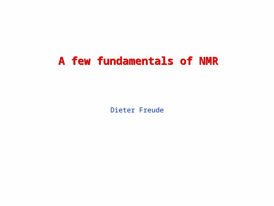
Harry Pfeifer's NMR-Experiment 1951 in LeipzigHarry Pfeifer's NMR-Experiment 1951 in Leipzig

H. Pfeifer: Über den Pendelrückkoppelempfänger (engl.: pendulum feedback receiver) und die Beobachtungen von magnetischen Kernresonanzen, Diplomarbeit, Universität Leipzig, 1952

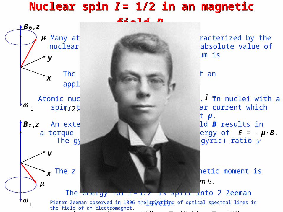
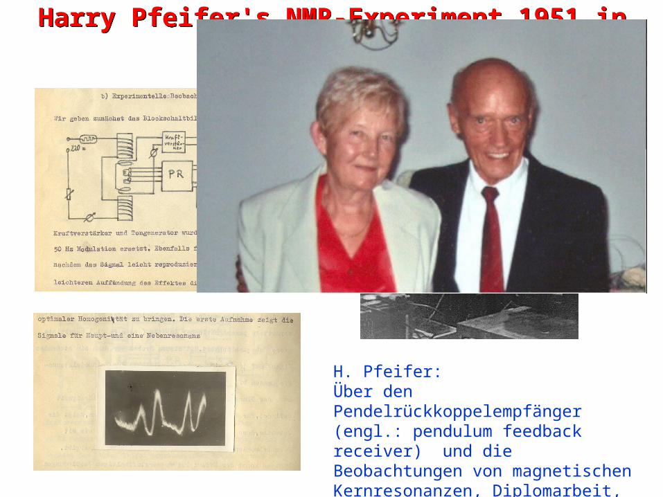
Nuclear spin I = 1/2 in an magnetic field B0Nuclear spin I = 1/2 in an magnetic field B0 B0, z

y

x

L

B0, z

y

x

L

Many atomic nuclei have a spin, characterized by the nuclear spin quantum number I. The absolute value of the spin angular momentum is

The component in the direction of an applied field is

  Lz = Iz  m = ½ for I = 1/2.

.)1( IIL

Atomic nuclei carry an electric charge. In nuclei with a spin, the rotation creates a circular current which produces a magnetic moment µ.

An external homogenous magnetic field B results in a torque T = µ B  with a related energy of  E =  µ·B.

The gyromagnetic (actually magnetogyric) ratio is defined by

µ =  L.

The z component of the nuclear magnetic moment is

µz =  Lz =  Iz    m .

The energy for I = 1/2 is split into 2 Zeeman levels

Em =  µz B0 =  mB0 = B0/2 = L/2.Pieter Zeeman observed in 1896 the splitting of optical spectral lines in the field of an electromagnet.

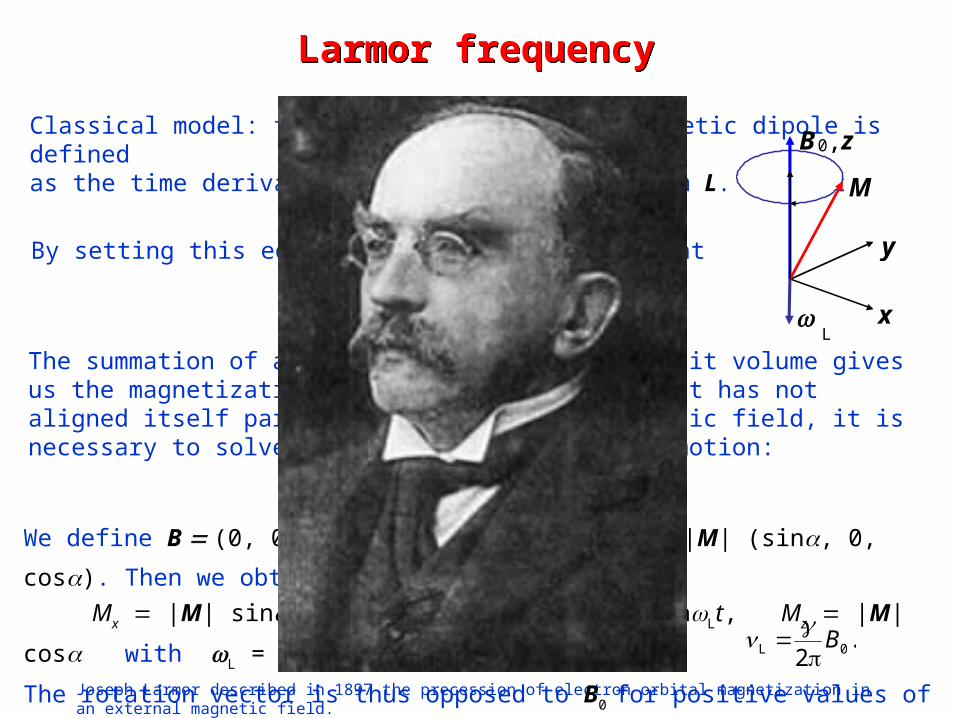
Larmor frequencyLarmor frequency

Joseph Larmor described in 1897 the precession of electron orbital magnetization in an external magnetic field.

Classical model: the torque T acting on a magnetic dipole is defined as the time derivative of the angular momentum L. We get

By setting this equal to T = µ B , we see that

The summation of all nuclear dipoles in the unit volume gives us the magnetization. For a magnetization that has not aligned itself parallel to the external magnetic field, it is necessary to solve the following equation of motion:

.dd1

dd

ttμL

T

.dd

Bμμ

t

.dd

BMM t

B0, z

M

y

x L

We define B  (0, 0, B0) and choose M(t  0)  |M| (sin, 0, cos). Then we obtain

Mx  |M| sin cosLt, My  |M| sin sinLt, Mz  |M| cos with L = B0.

The rotation vector is thus opposed to B0 for positive values of . The Larmor frequency

is most commonly given as an equation of magnitudes: L =  B0 or.

2 0L B

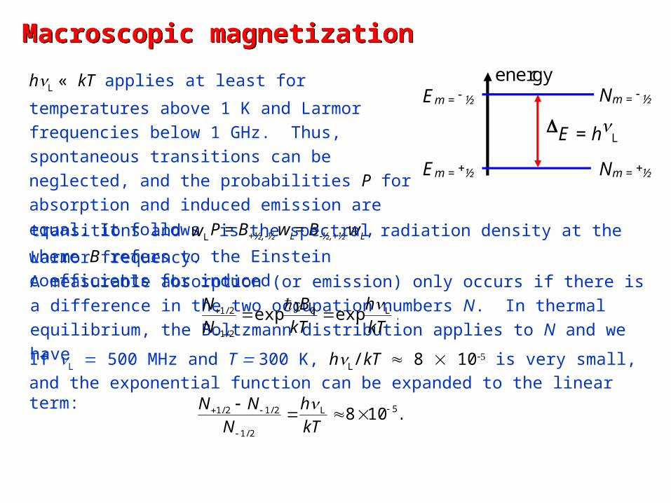
Macroscopic magnetizationMacroscopic magnetization energy Em = ½

E = hL

Em = ½

Nm = ½

Nm = ½

hL « kT applies at least for temperatures above 1 K

and Larmor frequencies below 1 GHz. Thus,

spontaneous transitions can be neglected, and the

probabilities P for absorption and induced emission

are equal. It follows P = B+½,½ wL= B½,+½ wL, where B

refers to the Einstein coefficients for inducedtransitions and wL is the spectral radiation density at the Larmor frequency.

A measurable absorption (or emission) only occurs if there is a difference in the two

occupation numbers N. In thermal equilibrium, the Boltzmann distribution applies to

N and we have .expexp L0

2/1

2/1

kTh

kTB

NN

If L  500 MHz and T  300 K, hL/kT 8 10 is very small, and the exponential

function can be expanded to the linear term:

.108 5L

2/1

2/12/1

kTh

NNN

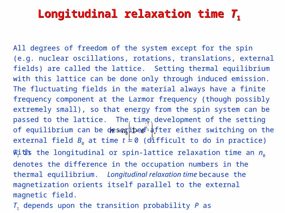
Longitudinal relaxation time T1Longitudinal relaxation time T1

All degrees of freedom of the system except for the spin (e.g. nuclear oscillations,

rotations, translations, external fields) are called the lattice. Setting thermal

equilibrium with this lattice can be done only through induced emission. The

fluctuating fields in the material always have a finite frequency component at the

Larmor frequency (though possibly extremely small), so that energy from the spin

system can be passed to the lattice. The time development of the setting of

equilibrium can be described after either switching on the external field B0 at time

t  0 (difficult to do in practice) with,1 1

0

T

t

enn

T1 is the longitudinal or spin-lattice relaxation time an n0 denotes the difference in

the occupation numbers in the thermal equilibrium. Longitudinal relaxation time

because the magnetization orients itself parallel to the external magnetic field.

T1 depends upon the transition probability P as 

1/T1 = 2P  2B½,+½ wL.

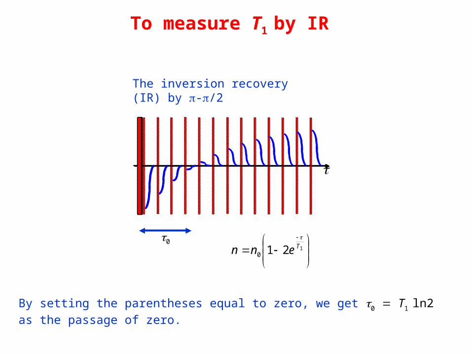
To measure T1 by IR

The inversion recovery (IR) by -/2

1210Tenn

By setting the parentheses equal to zero, we get 0  T1 ln2 as the passage of

zero.

0

Rotating coordinate system and the offsetRotating coordinate system and the offset

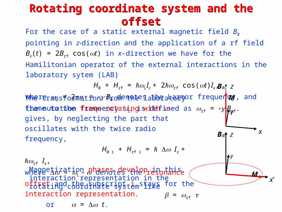
For the case of a static external magnetic field B0 pointing in z-

direction and the application of a rf field Bx(t) = 2Brf cos(t) in x-

direction we have for the Hamilitonian operator of the external interactions in the laboratory sytem (LAB)

H0 + Hrf = LIz + 2rf cos(t)Ix,

where L = 2L = B0 denotes the Larmor frequency, and the

nutation frequency rf is defined as rf = Brf.The transformation from the laboratory frame to the frame rotating with gives, by neglecting the part that oscillates with the twice radio frequency,

H0 i + Hrf i = Iz +

rf Ix,

where = L denotes the resonance offset

and the subscript i stays for the interaction representation.

B0

M

x

y

z

B0

M x’

y

z

Magnetization phases develop in this interaction representation in the rotating coordinate system like = rf or = t.

Quadratur detection yields value and sign of .

Bloch equation and stationary solutions Bloch equation and stationary solutions

We define Beff  (Brf, 0, B0 /) and introduce the Bloch equation:

1

0

2

effd

d

T

MM

T

MM

tzx zyyx eee

BMM

Stationary solutions to the Bloch equations are attained for dM/dt  0:

.

1

1

,21

,21

0

212rf

222

2

L

22

2

L

rf0rf

212rf

222

2

L

2

rf0rf

212rf

222

2

L

22L

MTTBT

TM

HMBTTBT

TM

HMBTTBT

TM

z

y

x

Correlation time c, relaxation times T1 and T2Correlation time c, relaxation times T1 and T2

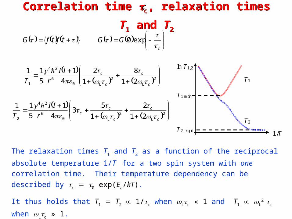
tftfG

c

GG

exp0

2

L

2

L06

24

1 21

8

1

2

4

1

5

11

c

c

c

cII

rT

2

L

2

L06

24

2 21

2

1

53

4

1

5

11

c

c

c

cc

II

rT

T1

T2

ln T1,2

1/T

T1 min

T2 rigid

The relaxation times T1 and T2 as a function of the reciprocal absolute temperature

1/T for a two spin system with one correlation time. Their temperature dependency

can be described by c  0 exp(Ea/kT).

It thus holds that T1  T2 1/c when Lc « 1 and T1 L2 c when Lc » 1.

T1 has a minimum of at Lc 0,612 or Lc 0,1.

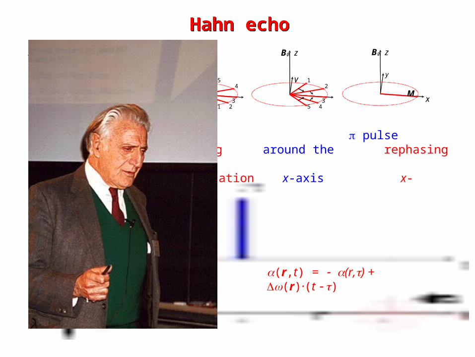
Hahn echoHahn echo B0

M

x

y

z B0

M x

y

z B0

x

y

z

5 4

1 2

3

B0

x

y

z

1 2

5 4

3

B0

M x

y

z

/2 pulse FID, pulsearound the dephasing around the rephasing echo y-axis x-magnetization x-axis x-magnetization

(r,t) = (r)·t (r,t) = (r,) + (r)·(t )

Line width and T2Line width and T2

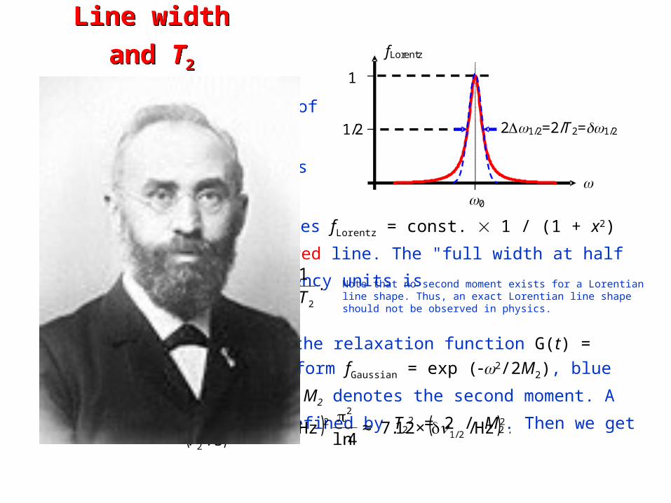
A pure exponential decay of the free induction (or of the envelope of the echo, see next page) corresponds to

G(t) = exp(t/T2).

The Fourier-transform gives fLorentz = const. 1 / (1 + x2) with x = ( 0)T2,

see red line. The "full width at half maximum" (fwhm) in frequency units is

.1

22/1 T

Note that no second moment exists for a Lorentian line shape. Thus, an exact Lorentian line shape should not be observed in physics.

Gaussian line shape has the relaxation function G(t) = exp(t2 M2 / 2) and a line

form fGaussian = exp (2/2M2), blue dotted line above, where M2 denotes the

second moment. A relaxation time can be defined by T22 = 2 / M2. Then we get

21/2=2/T2=1/2

0

fLorentz

1

1/2

( ) ( ) ( ) .Hz/×12.74ln

Hz/=s/

2=s/ 2

2/1

22

2/122

2-2

≈

TM

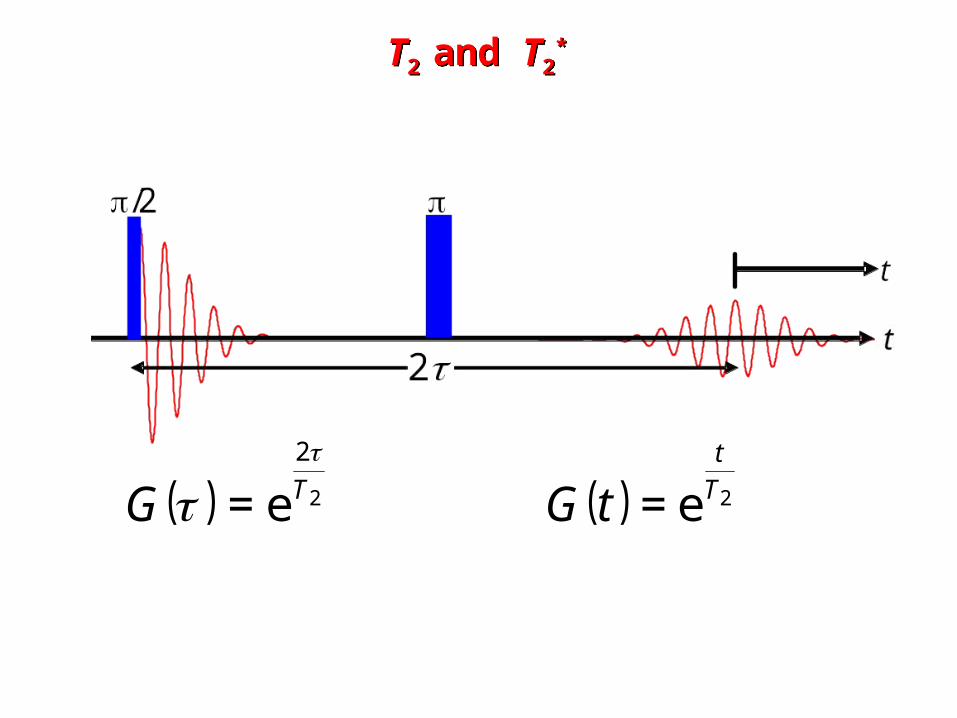
T2 and T2*T2 and T2*

( ) 2

2

e= TG

( ) 2e= Tt

tG

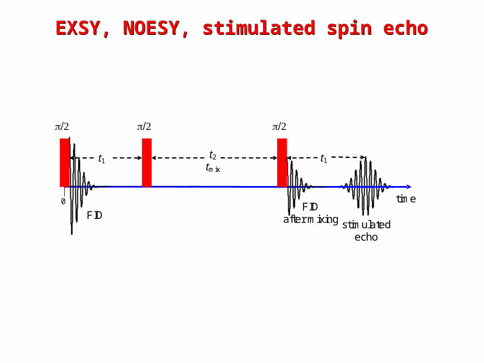
EXSY, NOESY, stimulated spin echoEXSY, NOESY, stimulated spin echo

stimulated echo

0

t1 t2 tmix

t1

time

FID FID

after mixing

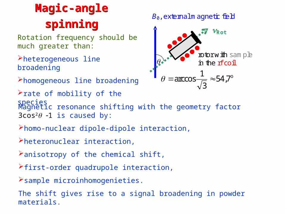
Magic-angle spinningMagic-angle spinning

B0, external magnetic field

Rot

rotor with sample in the rf coil

o7,543

1cosarc

Rotation frequency should be much greater than:

heterogeneous line broadening

homogeneous line broadening

rate of mobility of the species

Magnetic resonance shifting with the geometry factor 3cos2 1 is caused by:

homo-nuclear dipole-dipole interaction,

heteronuclear interaction,

anisotropy of the chemical shift,

first-order quadrupole interaction,

sample microinhomogenieties.

The shift gives rise to a signal broadening in powder materials.