A Generic Approach to Solving the Steiner Tree Problem and ...
185
A Generic Approach to Solving the Steiner Tree Problem and Variants Masterarbeit bei Prof. Dr. Thorsten Koch vorgelegt von Daniel Markus Rehfeldt 1 Fachbereich Mathematik der Technischen Universit¨ at Berlin Berlin, den 9. November 2015 1 Konrad-Zuse-Zentrum f¨ ur Informationstechnik Berlin, [email protected]
Transcript of A Generic Approach to Solving the Steiner Tree Problem and ...
A Generic Approach to Solving the Steiner Tree
Problem and Variants
Masterarbeitbei Prof. Dr. Thorsten Koch
vorgelegt von Daniel Markus Rehfeldt1
Fachbereich Mathematik derTechnischen Universitat Berlin
Berlin, den 9. November 2015
1Konrad-Zuse-Zentrum fur Informationstechnik Berlin, [email protected]
1
Eidesstattliche Erklarung (German Affidavit)
Hiermit erklare ich, dass ich die vorliegende Arbeit selbststandig und eigenhandigsowie ohne unerlaubte fremde Hilfe und ausschließlich unter Verwendung deraufgefuhrten Quellen und Hilfsmittel angefertigt habe.
Die selbstandige und eigenhandige Anfertigung versichert an Eides statt
Berlin, den 9. November 2015
(Daniel Rehfeldt)
Contents 2
Contents
Eidesstattliche Erklarung (German Affidavit) 1
Acknowledgments 5
1 Introduction 71.1 Preliminaries and Definitions . . . . . . . . . . . . . . . . . . 91.2 Background and Complexity . . . . . . . . . . . . . . . . . . . 11
1.2.1 A Brief History . . . . . . . . . . . . . . . . . . . . . . 111.2.2 Complexity . . . . . . . . . . . . . . . . . . . . . . . . 11
2 The Steiner Tree Problem in Graphs 132.1 Formulating the Problem: Integer Programming . . . . . . . 14
2.1.1 Cut Formulations . . . . . . . . . . . . . . . . . . . . . 142.1.2 Flow Formulations . . . . . . . . . . . . . . . . . . . . 152.1.3 Flow Balance Inequalities . . . . . . . . . . . . . . . . 17
2.2 Simplifying the Problem: Reduction Techniques . . . . . . . . 182.2.1 Definitions . . . . . . . . . . . . . . . . . . . . . . . . 182.2.2 Basic Reductions . . . . . . . . . . . . . . . . . . . . . 192.2.3 Alternative Based Reductions . . . . . . . . . . . . . . 202.2.4 Bound Based Reductions . . . . . . . . . . . . . . . . 262.2.5 Implementation . . . . . . . . . . . . . . . . . . . . . . 29
2.3 Finding a Solution: Primal Heuristics . . . . . . . . . . . . . 322.3.1 Constructive Heuristics . . . . . . . . . . . . . . . . . 322.3.2 Local Search Heuristics . . . . . . . . . . . . . . . . . 342.3.3 Recombination Heuristics . . . . . . . . . . . . . . . . 35
2.4 Solving to Optimality: Branch and Cut . . . . . . . . . . . . 372.4.1 Separation Methods . . . . . . . . . . . . . . . . . . . 372.4.2 Branching . . . . . . . . . . . . . . . . . . . . . . . . . 38
2.5 Implementation . . . . . . . . . . . . . . . . . . . . . . . . . . 392.5.1 SCIP-Jack: A General Purpose Solver for Steiner
Tree Problems . . . . . . . . . . . . . . . . . . . . . . 392.5.2 Parallel Computing . . . . . . . . . . . . . . . . . . . . 41
2.6 Computational Results and Discussion . . . . . . . . . . . . . 432.6.1 Impact of Reduction Techniques . . . . . . . . . . . . 452.6.2 Impact of Primal Heuristics . . . . . . . . . . . . . . . 482.6.3 Branching . . . . . . . . . . . . . . . . . . . . . . . . . 50
3 Variants of the Steiner Tree Problem 533.1 The Steiner Arborescence Problem . . . . . . . . . . . . . . . 54
3.1.1 Reductions . . . . . . . . . . . . . . . . . . . . . . . . 553.1.2 Heuristics . . . . . . . . . . . . . . . . . . . . . . . . . 653.1.3 Implementation and Computational Results . . . . . . 65
Contents 3
3.2 The Node Weighted Steiner Problem . . . . . . . . . . . . . . 673.2.1 Transformation . . . . . . . . . . . . . . . . . . . . . . 673.2.2 Implementation and Computational Results . . . . . . 68
3.3 The Rectilinear Steiner Minimum Tree Problem . . . . . . . . 703.3.1 Transformation . . . . . . . . . . . . . . . . . . . . . . 703.3.2 Implementation and Computational Results . . . . . . 71
3.4 The Prize Collecting Steiner Tree Problem . . . . . . . . . . . 733.4.1 Transformation . . . . . . . . . . . . . . . . . . . . . . 733.4.2 Reductions . . . . . . . . . . . . . . . . . . . . . . . . 783.4.3 Heuristics . . . . . . . . . . . . . . . . . . . . . . . . . 993.4.4 Implementation and Computational Results . . . . . . 101
3.5 The Maximum Weight Connected Subgraph Problem . . . . . 1083.5.1 Transformation . . . . . . . . . . . . . . . . . . . . . . 1083.5.2 Reductions . . . . . . . . . . . . . . . . . . . . . . . . 1103.5.3 Implementation and Computational Results . . . . . . 122
3.6 The Degree Constrained Steiner Tree Problem . . . . . . . . 1273.6.1 Primal Heuristics . . . . . . . . . . . . . . . . . . . . . 1273.6.2 Implementation and Computational Results . . . . . . 127
3.7 The Group Steiner Tree Problem . . . . . . . . . . . . . . . . 1293.7.1 Transformation . . . . . . . . . . . . . . . . . . . . . . 1293.7.2 Implementation and Computational Results . . . . . . 129
3.8 The Hop Constrained Directed Steiner Tree Problem . . . . . 1313.8.1 Reductions . . . . . . . . . . . . . . . . . . . . . . . . 1313.8.2 Primal Heuristics . . . . . . . . . . . . . . . . . . . . . 1353.8.3 Implementation and Computational Results . . . . . . 135
4 Final Computational Results and Comparisons 1374.1 The Steiner Tree Problem in Graphs . . . . . . . . . . . . . . 138
4.1.1 Parallel Computing . . . . . . . . . . . . . . . . . . . . 1394.2 Variants of the Steiner Tree Problem . . . . . . . . . . . . . . 141
4.2.1 The Prize Collecting Steiner Tree Problem . . . . . . 1414.2.2 The Maximum Weight Connected Subgraph Problem 1434.2.3 The Degree Constrained Steiner Tree Problem . . . . 1444.2.4 The Hop Constrained Directed Steiner Tree Problem . 144
4.3 Using SoPlex . . . . . . . . . . . . . . . . . . . . . . . . . . 146
5 Conclusions and Outlook 149
A Zusammenfassung (German Summary) 160
B Notation and Abbreviations 162B.1 General Mathematical Notation . . . . . . . . . . . . . . . . . 162B.2 Steiner Problem Variants . . . . . . . . . . . . . . . . . . . . 162
Contents 4
C Detailed Experimental Results 163C.1 The Steiner Tree Problem in Graphs . . . . . . . . . . . . . . 163C.2 The Steiner Arborescence Problem . . . . . . . . . . . . . . . 172C.3 The Rectilinear Steiner Minimum Tree Problem . . . . . . . . 173C.4 The Prize Collecting Tree Problem . . . . . . . . . . . . . . . 175C.5 The Maximum Weight Connected Subgraph Problem . . . . . 179C.6 The Degree Constrained Steiner Tree Problem . . . . . . . . 181C.7 The Group Steiner Tree Problem . . . . . . . . . . . . . . . . 182C.8 The Hop Constrained Directed Steiner Tree Problem . . . . . 183
Contents 5
Acknowledgments
I would like to thank my parents for their support and encouragement, notonly during my academic studies, but furthermore during my entire life. Hadit not been for the – for want of a better word – relentless efforts of my motherthroughout my childhood and adolescence to focus my attention on studying,this thesis would not have found its way into existence. I would like tothank Gerald Gamrath for his support and patience in the face of numerousquestions and requests, throughout my time at Zuse Institute Berlin. Noteven safe from me on parental leave, he would support and encourage mewith this thesis until the last minute before submission. I would like tothank Thorsten Koch for coming up with the idea of developing a general-purpose Steiner tree solver and his support throughout the realization. Iwould like to thank Stephen Maher for his support and suggestions for thisthesis. I would like to thank Yuji Shinano for his feedback and help. I wouldlike to thank Gerald, Stephen and Yuji for the great time in Boston, wherewe enjoyed the endless opportunities of American shopping and watchednone other than Kobe Bryant himself play in the TD Garden; and where aprevious version of the solver described in this thesis competed in the 11thDIMACS Challenge. Last but certainly not least, I would like to thank CeesDuin who relieved me from my struggles to get hold of an electronic versionof his dissertation, which had indeed been written in the old pre-PDF days,by sending my a hard copy from the Netherlands.
Contents 6
7
1 Introduction
The Steiner tree problem in graphs (SPG) is one of the classical NP-hard problems [Kar72] and has been extensively studied both theoreticallyand practically. Given an undirected connected graph G = (V,E), weightsc : E → Q+ and a set T ⊂ V of terminals, the problem is to find a minimum-weight tree S ⊂ G that spans T . While the SPG is commonly cited to entaila variety of practical applications [Dui93, HRW92, Pol04, PS02, VD04],problems representable by the classic SPG are rarely encountered in practice.This assertion is evidenced by the fact that from the more than 1, 000 SPGinstances collected in the standard benchmark library SteinLib [KMV01]less than a fifth can claim practical origins and even of those most are moresuitably formulated as a rectilinear Steiner minimum tree problem. Still,real-world applications can be found in problems such as for instance thedesign of fiber-optic networks [LLL+14].
However, when the focus is widened to also consider variations of theSPG, a different picture emerges: Numerous applications can be found thatinclude the SPG as a subproblem or that are formulated as a modified versionof it (as will be evinced in the course of this thesis). Despite the strongrelationship between the different Steiner tree problem variants, solutionapproaches employed so far have been prevalently problem specific.
In contrast, the aim of this thesis is to devise and implement a generalpurpose approach, resulting in a solver that is able to solve both the clas-sical Steiner tree problem and many of its variants without modification.Pursuing this approach, a further objective of this thesis is to solve a widerange of benchmark instances, by means of both known and newly developedmethods.
The origins of our thesis can be traced to the announcement of the 11thDIMACS Challenge, dedicated to practical solving methods for the Steinertree problem and variants. A base was provided by the model and code ofthe SPG solver Jack-III described in [KM98]. However, being more than15 years old, Jack-III lacked many modern developments regarding SPGsolution methods and did not provide a general MIP framework for easilyincorporating additional variants of the Steiner problem. Our resolution toovercome these limitations of Jack-III was to combine the model of [KM98]with the state-of-the-art MIP-framework SCIP [Ach09].
Furthermore, we have developed several Steiner variant specific methodsconcerning preprocessing and heuristics. These developments have been mo-tivated by the endeavour to render our approach competitive with problemspecific state-of-the art solvers. By virtue of the plugin-based structure ofSCIP, these adaptations can be easily implemented without modifying theunderlying generic solving methods.
The major contributions of this thesis to the existing literature are asfollows:
8
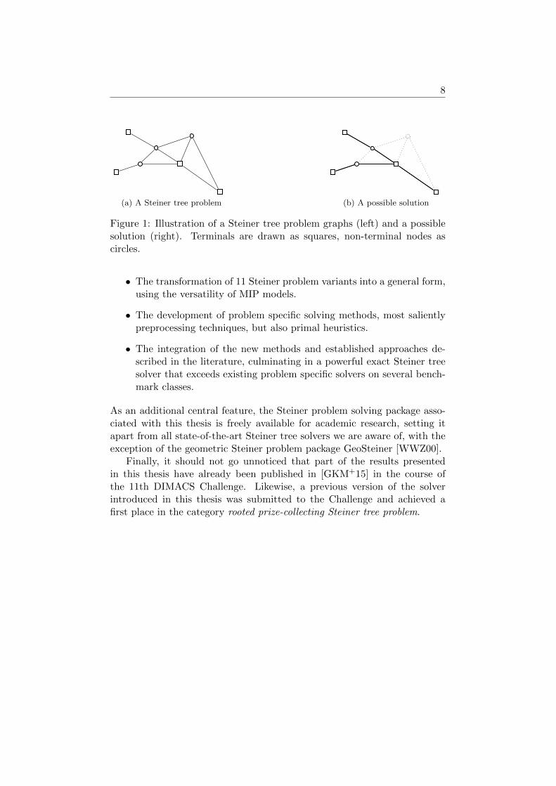
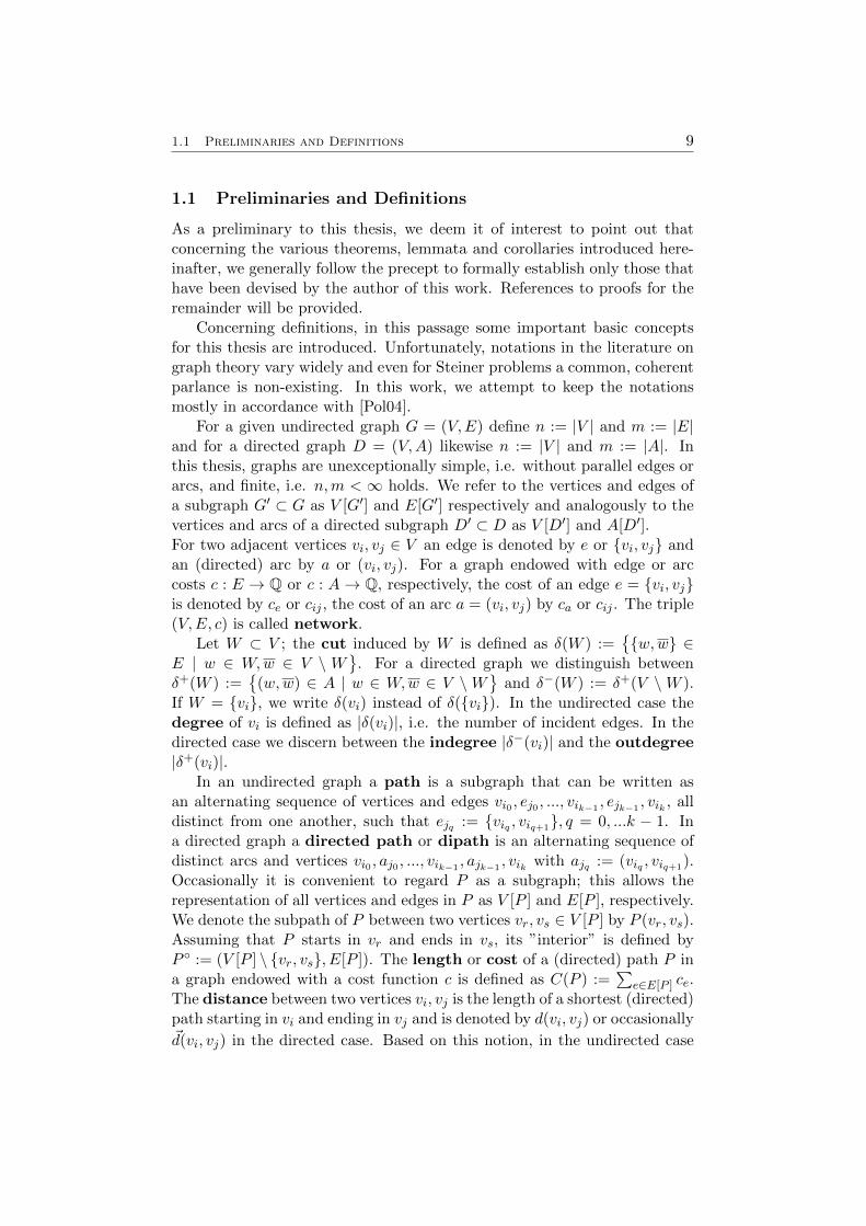
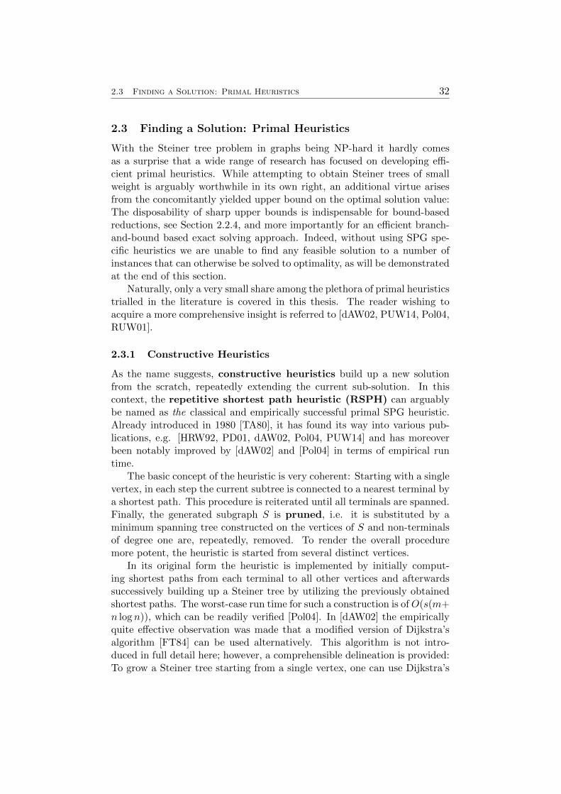
(a) A Steiner tree problem (b) A possible solution
Figure 1: Illustration of a Steiner tree problem graphs (left) and a possiblesolution (right). Terminals are drawn as squares, non-terminal nodes ascircles.
• The transformation of 11 Steiner problem variants into a general form,using the versatility of MIP models.
• The development of problem specific solving methods, most salientlypreprocessing techniques, but also primal heuristics.
• The integration of the new methods and established approaches de-scribed in the literature, culminating in a powerful exact Steiner treesolver that exceeds existing problem specific solvers on several bench-mark classes.
As an additional central feature, the Steiner problem solving package asso-ciated with this thesis is freely available for academic research, setting itapart from all state-of-the-art Steiner tree solvers we are aware of, with theexception of the geometric Steiner problem package GeoSteiner [WWZ00].
Finally, it should not go unnoticed that part of the results presentedin this thesis have already been published in [GKM+15] in the course ofthe 11th DIMACS Challenge. Likewise, a previous version of the solverintroduced in this thesis was submitted to the Challenge and achieved afirst place in the category rooted prize-collecting Steiner tree problem.
1.1 Preliminaries and Definitions 9
1.1 Preliminaries and Definitions
As a preliminary to this thesis, we deem it of interest to point out thatconcerning the various theorems, lemmata and corollaries introduced here-inafter, we generally follow the precept to formally establish only those thathave been devised by the author of this work. References to proofs for theremainder will be provided.
Concerning definitions, in this passage some important basic conceptsfor this thesis are introduced. Unfortunately, notations in the literature ongraph theory vary widely and even for Steiner problems a common, coherentparlance is non-existing. In this work, we attempt to keep the notationsmostly in accordance with [Pol04].
For a given undirected graph G = (V,E) define n := |V | and m := |E|and for a directed graph D = (V,A) likewise n := |V | and m := |A|. Inthis thesis, graphs are unexceptionally simple, i.e. without parallel edges orarcs, and finite, i.e. n,m < ∞ holds. We refer to the vertices and edges ofa subgraph G′ ⊂ G as V [G′] and E[G′] respectively and analogously to thevertices and arcs of a directed subgraph D′ ⊂ D as V [D′] and A[D′].For two adjacent vertices vi, vj ∈ V an edge is denoted by e or {vi, vj} andan (directed) arc by a or (vi, vj). For a graph endowed with edge or arccosts c : E → Q or c : A→ Q, respectively, the cost of an edge e = {vi, vj}is denoted by ce or cij , the cost of an arc a = (vi, vj) by ca or cij . The triple(V,E, c) is called network.
Let W ⊂ V ; the cut induced by W is defined as δ(W ) :={{w,w} ∈
E | w ∈ W,w ∈ V \ W}
. For a directed graph we distinguish betweenδ+(W ) :=
{(w,w) ∈ A | w ∈ W,w ∈ V \W
}and δ−(W ) := δ+(V \W ).
If W = {vi}, we write δ(vi) instead of δ({vi}). In the undirected case thedegree of vi is defined as |δ(vi)|, i.e. the number of incident edges. In thedirected case we discern between the indegree |δ−(vi)| and the outdegree|δ+(vi)|.
In an undirected graph a path is a subgraph that can be written asan alternating sequence of vertices and edges vi0 , ej0 , ..., vik−1
, ejk−1, vik , all
distinct from one another, such that ejq := {viq , viq+1}, q = 0, ...k − 1. Ina directed graph a directed path or dipath is an alternating sequence ofdistinct arcs and vertices vi0 , aj0 , ..., vik−1
, ajk−1, vik with ajq := (viq , viq+1).
Occasionally it is convenient to regard P as a subgraph; this allows therepresentation of all vertices and edges in P as V [P ] and E[P ], respectively.We denote the subpath of P between two vertices vr, vs ∈ V [P ] by P (vr, vs).Assuming that P starts in vr and ends in vs, its ”interior” is defined byP ◦ := (V [P ] \ {vr, vs}, E[P ]). The length or cost of a (directed) path P ina graph endowed with a cost function c is defined as C(P ) :=
∑e∈E[P ] ce.
The distance between two vertices vi, vj is the length of a shortest (directed)path starting in vi and ending in vj and is denoted by d(vi, vj) or occasionally~d(vi, vj) in the directed case. Based on this notion, in the undirected case
1.1 Preliminaries and Definitions 10
for W ⊂ V the distance network to (G, c) can be defined as: DG(W ) =(W,W ×W,d).
Now consider a Steiner tree problem (V,E, T, c). Thereupon, we de-fine s := |T | and for the sake of simplicity V := {v1, ..., vn} as well asT := {t1, ..., ts}. Note that in the literature the vertices in T are commonlyreferred to as terminals, while vertices in V \ T are called Steiner ver-tices. Furthermore, we define the distance function d(vi, vj) as the lengthof a shortest path between vi and vj without intermediary terminals. Ona related note, in [Dui93] an O(m + n log n) algorithm was introduced tocompute for each non-terminal vi a constant number of d-nearest terminalsvi,1, vi,2, ..., vi,k (if existent) along with the corresponding paths. We willrefer to this procedure as Duin’s nearest terminals algorithm.
A somewhat less basic concept, which will frequently recur in the courseof this thesis, is the following: A Voronoi diagram to G is a partition{N(t) | t ∈ T} of V (i.e. V =
⋃t∈T N(t) and N(t) ∩N(t′) = ∅ for t, t′ ∈ T ,
t 6= t′) such that:
v ∈ N(t)⇒ d(v, t) ≤ d(v, t′) for all t′ ∈ T.
If vj ∈ N(ti), ti is called the base of vj , denoted by base(vj). The set N(ti)is called Voronoi region of ti and an edge {vj , vk} such that base(vj) 6=base(vk) is called Voronoi-boundary edge. Given G, T and c, the Voronoidiagram can be computed in O(m+ n log n) by slightly adapting Dijkstra’salgorithm [FT84] in such a way that all terminals are considered as startvertices of distance zero [Meh88]. The concept of Voronoi diagrams can beused to compute a minimum spanning tree SD(T ) to the Distance NetworkDG(T ) in O(m+ n log n) [Meh88].
Finally, the directed equivalent of the SPG the Steiner arborescenceproblem (SAP) [HRW92] is defined as follows: Given a directed graphD = (V,A), costs c : A→ Q≥0, a set T ⊂ V of terminals and a root r ∈ T ,a directed tree (or arborescence) S = (VS , AS) ⊂ D is required such that:first, for all t ∈ T the tree S contains exactly one directed path from rto t and second,
∑a∈AS
ca is minimized. We define T r := T \ {r}. AnSPG can be transformed to an SAP by replacing each edge by two anti-parallel arcs of the same cost and distinguishing an arbitrary terminal asthe root. This procedure results in a one-to-one correspondence betweenthe respective solution sets; more details will be provided in Section 3.1.
1.2 Background and Complexity 11
1.2 Background and Complexity
The focus of this thesis is set on practical solving methods for the SPG andvariants. Therefore, results of more theoretical nature such as tight approx-imation algorithms (which have been shown to be of little practical value[CGSW14, GHNP01]) are only touched upon. Surveys on such theoreticalaspects can be found in [CGSW14, PS02].
1.2.1 A Brief History
Historically, the Steiner problem in graphs is derived from a problem thathas become known as the Euclidean Steiner tree problem: Given k ∈N points in the plane, connect them by lines of minimum total length ina manner such that any two points are interconnected by line segmentseither directly or using intermediary points. Its history can be traced backto the 17th century when P. Fermat formulated the special case of k =3. With Fermat’s name already linked to a more renowned problem, J.Steiner, who would pose the same problem more than one hundred yearslater, eventually became its namebearer [Dui93, Pol04]. However, since pasta certain point the clarity of history inevitably falls victim to the fog oflegend, no absolute certitude can be claimed. Notwithstanding, the Steinerproblem in graphs as it is known today can be found in a publication byS. Hakimi in 1971 [Hak71]. Since then, hundreds of articles concerningthe Steiner tree problem in graphs and variants have been published; see[HRW92] for a comprehensive, albeit somewhat outdated survey, or [Hau]for an up-to-date one.
A more detailed account of the history of the Steiner tree problem canbe found in [BGTZ14].
1.2.2 Complexity
The decision variant of the SPG, with edge weights in the natural numbers, isstrongly NP-complete and the optimization variant NP-hard [Kar72]. How-ever, there are several polynomially solvable special cases, the arguably twomost important ones being |T | = 2, which corresponds to finding a short-est path between two vertices, and |T | = n, which corresponds to findinga minimal spanning tree in G. Further polynomially solvable special casescan be found in [HRW92].
Concerning approximability, it has been demonstrated that the SPG isAPX-complete, even with its edge weight being in {1, 2} [BP89]. This meansthat there exists an ε > 0 (which in the case of the SPG can be chosen as9695 [CC08]) such that finding a (1 + ε)-approximation to the problem is NP-hard. Although approximation algorithms have been designed that come asclose as 1.39 to an optimal solution value [BGRS13], their empirical resultsare distinctly inferior to heuristic methods, see [CGSW14].
1.2 Background and Complexity 12
For the Steiner problem variants many complexity results can be derivedfrom the SPG (more detail is provided in the respective subsections). A com-prehensive compilation concerning both the complexity and approximabilityof Steiner problem variants can be found in [Hau].
13
2 The Steiner Tree Problem in Graphs
Being the archetype of all variants discussed in this thesis, the Steiner treeproblem in graphs will be presented in the comparatively most detail. Thisproceeding is further justified by the fact that the approach described in thefollowing establishes a blueprint for solving the different Steiner variantsintroduced in Section 3.
Based upon an integer programming formulation of the SPG, our solvingapproach encompasses three major components:
• First, preprocessing in the shape of reduction techniques; key to theperformance of our solver.
• Second, primal heuristics; indispensable to find good or even optimalsolutions to hard problems.
• Third, a branch-and-cut procedure used to compute a lower boundand prove optimality; the core of our solver.
2.1 Formulating the Problem: Integer Programming 14
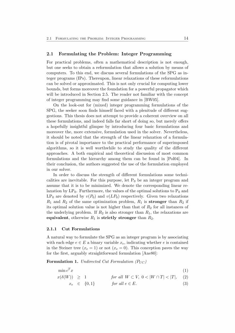
2.1 Formulating the Problem: Integer Programming
For practical problems, often a mathematical description is not enough,but one seeks to obtain a reformulation that allows a solution by means ofcomputers. To this end, we discuss several formulations of the SPG as in-teger programs (IPs). Thereupon, linear relaxations of these reformulationscan be solved or approximated. This is not only crucial for computing lowerbounds, but forms moreover the foundation for a powerful propagator whichwill be introduced in Section 2.5. The reader not familiar with the conceptof integer programming may find some guidance in [BW05].
On the look-out for (mixed) integer programming formulations of theSPG, the seeker soon finds himself faced with a plenitude of different sug-gestions. This thesis does not attempt to provide a coherent overview on allthese formulations, and indeed falls far short of doing so, but merely offersa hopefully insightful glimpse by introducing four basic formulations andmoreover the, more extensive, formulation used in the solver. Nevertheless,it should be noted that the strength of the linear relaxation of a formula-tion is of pivotal importance to the practical performance of superimposedalgorithms, so it is well worthwhile to study the quality of the differentapproaches. A both empirical and theoretical discussion of most commonformulations and the hierarchy among them can be found in [Pol04]. Intheir conclusion, the authors suggested the use of the formulation employedin our solver.
In order to discuss the strength of different formulations some techni-calities are inevitable. For this purpose, let P0 be an integer program andassume that it is to be minimized. We denote the corresponding linear re-laxation by LP0. Furthermore, the values of the optimal solutions to P0 andLP0 are denoted by v(P0) and v(LP0) respectively. Given two relaxationsR1 and R2 of the same optimization problem, R1 is stronger than R2 ifits optimal solution value is not higher than that of R2 for all instances ofthe underlying problem. If R2 is also stronger than R1, the relaxations areequivalent, otherwise R1 is strictly stronger than R2.
2.1.1 Cut Formulations
A natural way to formulate the SPG as an integer program is by associatingwith each edge e ∈ E a binary variable xe, indicating whether e is containedin the Steiner tree (xe = 1) or not (xe = 0). This conception paves the wayfor the first, arguably straightforward formulation [Ane80]:
Formulation 1. Undirected Cut Formulation (PUC)
min cTx (1)
x(δ(W )) ≥ 1 for all W ⊂ V, 0 < |W ∩ T | < |T |, (2)
xe ∈ {0, 1} for all e ∈ E. (3)
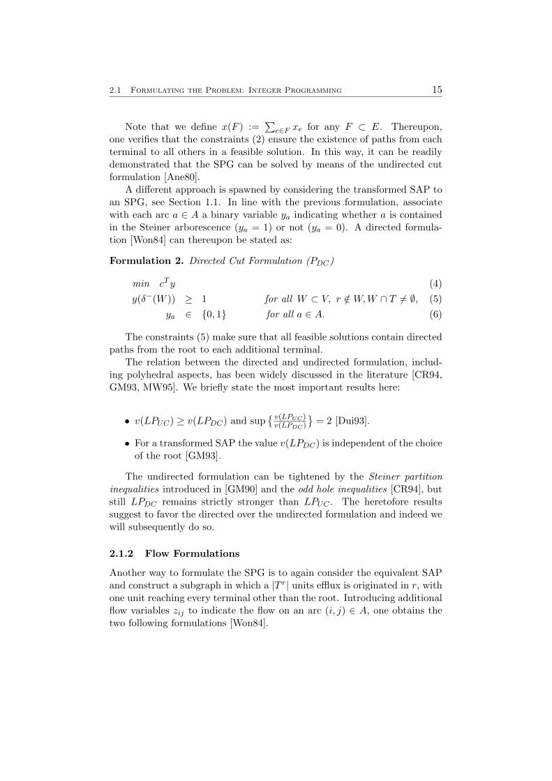
2.1 Formulating the Problem: Integer Programming 15
Note that we define x(F ) :=∑
e∈F xe for any F ⊂ E. Thereupon,one verifies that the constraints (2) ensure the existence of paths from eachterminal to all others in a feasible solution. In this way, it can be readilydemonstrated that the SPG can be solved by means of the undirected cutformulation [Ane80].
A different approach is spawned by considering the transformed SAP toan SPG, see Section 1.1. In line with the previous formulation, associatewith each arc a ∈ A a binary variable ya indicating whether a is containedin the Steiner arborescence (ya = 1) or not (ya = 0). A directed formula-tion [Won84] can thereupon be stated as:
Formulation 2. Directed Cut Formulation (PDC)
min cT y (4)
y(δ−(W )) ≥ 1 for all W ⊂ V, r /∈W,W ∩ T 6= ∅, (5)
ya ∈ {0, 1} for all a ∈ A. (6)
The constraints (5) make sure that all feasible solutions contain directedpaths from the root to each additional terminal.
The relation between the directed and undirected formulation, includ-ing polyhedral aspects, has been widely discussed in the literature [CR94,GM93, MW95]. We briefly state the most important results here:
• v(LPUC) ≥ v(LPDC) and sup{ v(LPUC)v(LPDC)
}= 2 [Dui93].
• For a transformed SAP the value v(LPDC) is independent of the choiceof the root [GM93].
The undirected formulation can be tightened by the Steiner partitioninequalities introduced in [GM90] and the odd hole inequalities [CR94], butstill LPDC remains strictly stronger than LPUC . The heretofore resultssuggest to favor the directed over the undirected formulation and indeed wewill subsequently do so.
2.1.2 Flow Formulations
Another way to formulate the SPG is to again consider the equivalent SAPand construct a subgraph in which a |T r| units efflux is originated in r, withone unit reaching every terminal other than the root. Introducing additionalflow variables zij to indicate the flow on an arc (i, j) ∈ A, one obtains thetwo following formulations [Won84].
2.1 Formulating the Problem: Integer Programming 16
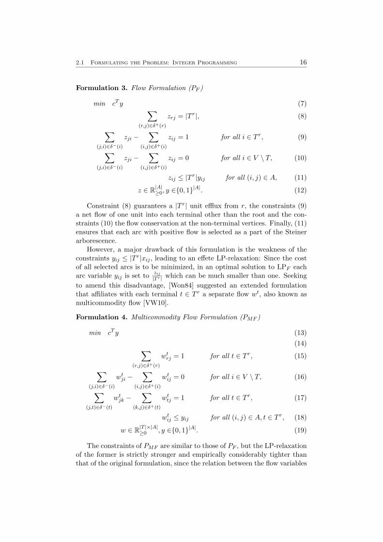
Formulation 3. Flow Formulation (PF )
min cT y (7)∑(r,j)∈δ+(r)
zrj = |T r|, (8)
∑(j,i)∈δ−(i)
zji −∑
(i,j)∈δ+(i)
zij = 1 for all i ∈ T r, (9)
∑(j,i)∈δ−(i)
zji −∑
(i,j)∈δ+(i)
zij = 0 for all i ∈ V \ T, (10)
zij ≤ |T r|yij for all (i, j) ∈ A, (11)
z ∈ R|A|≥0, y ∈{0, 1}|A|. (12)
Constraint (8) guarantees a |T r| unit efflux from r, the constraints (9)a net flow of one unit into each terminal other than the root and the con-straints (10) the flow conservation at the non-terminal vertices. Finally, (11)ensures that each arc with positive flow is selected as a part of the Steinerarborescence.
However, a major drawback of this formulation is the weakness of theconstraints yij ≤ |T r|xij , leading to an effete LP-relaxation: Since the costof all selected arcs is to be minimized, in an optimal solution to LPF eacharc variable yij is set to
zij|T r| which can be much smaller than one. Seeking
to amend this disadvantage, [Won84] suggested an extended formulationthat affiliates with each terminal t ∈ T r a separate flow wt, also known asmulticommodity flow [VW10].
Formulation 4. Multicommodity Flow Formulation (PMF )
min cT y (13)
(14)∑(r,j)∈δ+(r)
wtrj = 1 for all t ∈ T r, (15)
∑(j,i)∈δ−(i)
wtji −∑
(i,j)∈δ+(i)
wtij = 0 for all i ∈ V \ T, (16)
∑(j,t)∈δ−(t)
wtjk −∑
(k,j)∈δ+(t)
wttj = 1 for all t ∈ T r, (17)
wtij ≤ yij for all (i, j) ∈ A, t ∈ T r, (18)
w ∈ R|T |×|A|≥0 , y ∈{0, 1}|A|. (19)
The constraints of PMF are similar to those of PF , but the LP-relaxationof the former is strictly stronger and empirically considerably tighter thanthat of the original formulation, since the relation between the flow variables
2.1 Formulating the Problem: Integer Programming 17
(z and w, respectively) and the arc variables (y) is more accurately modelledby the constraint (18).
An interesting result is that not only v(LPMF ) = v(LPDC) holds, buteven a bijection can be established between the feasible solutions (y, w) toLPMF and y to LPDC , see [Won84].
2.1.3 Flow Balance Inequalities
In [KM98] a new group of flow based constraints was suggested to strengthenthe directed cut formulation. Although not all of them improve the LP-relaxation, these constraints lead to a considerable advantage in practicalsolving by column generation and have been frequently employed in ad-vanced Steiner problem solvers [KM98, LLL+14, Lju04, Pol04].
Formulation 5. Flow-Balance Directed Cut Formulation (PCF )
min cT y (20)
y(δ−(W )) ≥ 1 for all W ⊂ V, r /∈W,W ∩ T 6= ∅, (21)
y(δ−(v))
==≤
0, if v = r;1, if v ∈ T r;1, if v ∈ N ;
for all v ∈ V, (22)
y(δ−(v)) ≤ y(δ+(v)) for all v ∈ V \ T, (23)
y(δ−(v)) ≥ ya for all a ∈ δ+(v), v ∈ V \ T, (24)
ya ∈ {0, 1} for all a ∈ A. (25)
By adding the constraints (23) to PDC the corresponding LP-relaxationis rendered stronger than that of PDC , see [Dui93]. The remainder of the ad-ditional constraints do not improve the value of the LP-relaxation as shownin [Pol04].
Formulation PCF is the one used in our solver. However, due to theexponential number of constraints (21), the problem is solved by a branch-and-cut approach that is elaborated in Section 2.4.
2.2 Simplifying the Problem: Reduction Techniques 18
2.2 Simplifying the Problem: Reduction Techniques
When it comes to solving NP-hard problems, reductions can play a cru-cial role as a preprocessing tool, as for example with the travelling sales-man problem [ABCC11]. The SPG is no exception: With various publica-tions [BP87, Bea84, DV89, HRW92], most saliently Duin’s magnum opus[Dui93], having set the stage, reduction techniques were often a pivotal in-gredient in practical solving techniques in the 1990’s decade. In the wakeof those developments, several techniques were again improved in terms ofboth efficiency and capability by Polzin and Daneshmand [Pol04, VD04],additionally closing some gaps that had been left open. The methods de-ployed by them could reduce the number of edges for the tested instances (allfrom the SteinLib) by 78 percent. Furthermore, their solver, which heavilyrelies on reduction techniques, has remained until today the fastest SPGsolver described in the literature (except for certain artificially constructedinstances as in the PUC test set, designed to defy preprocessing).
Being one of its three main components (besides heuristics and branch-and-cut), reduction techniques likewise occupy a prominent position in thesolving approach described in this thesis, not only for the SPG, but also forits variants. Subsequently, several important reduction techniques from theliterature are introduced (and several extensions are suggested). Naturally,they fall far short of being exhaustive; for further representations we refer to[Dui93, Pol04, VD04]. However, many of the techniques introduced in theliterature are special cases of other ones [Dui93, HRW92]. In this context,we attempt to avoid any redundancy in the presented methods.
Finally, it should be marked that the subsequently introduced reductiontechniques are not only important for solving the Steiner tree problem ingraphs, but furthermore pave the way for several of the Steiner variantspecific, novel reduction methods described in the sections 3.1.1, 3.4.2, 3.5.2and 3.8.1.
2.2.1 Definitions
Reduction techniques, in general, strive to reduce the size of a given instancewhile allowing a re-transformation of all solutions to the reduced problemback to the original one and preserving at least one optimal solution (if thereexists one). In the case of the SPG this means reducing the number of bothedges and nodes. Several additional definitions are necessary to conceive thetechniques described in this section. They are largely stated in accordancewith [Pol04]. In the following, let (V,E, T, c) be an SPG and select twoarbitrary but distinct vertices vi ∈ V and vj ∈ V .Let {vi, vj} ∈ E, thereupon vj can be contracted into vi by performing thefollowing steps:
• For each edge {vj , vk} ∈ E, k 6= i: if {vi, vk} /∈ E, add this edge
2.2 Simplifying the Problem: Reduction Techniques 19
endowed with costs cjk to E; if {vi, vk} ∈ E and additionally cik > cjk,set cik = cjk. Denote the set of all newly inserted or modified (withrespect to their costs) edges by EL ⊂ δ(vi).
• If vj ∈ T , add vi to T .
• Delete vj and all incident edges.
Let (V,E, T, c) be an SPG, {vi, vj} ∈ E and (V ′, E′, T ′, c′) the problemresulting from contracting vj into vi. A solution S′ to the problem resultingfrom such a contraction can be easily transformed to a solution S to theoriginal problem: If EL ∩ E[S′] = ∅, then S′ can be adopted unaltered;otherwise, first add {vi, vj} and vj to S′ and second extract each el ∈ EL ∩E[S′], concurrently inserting the corresponding original edge. Further, if vjis a terminal in the original graph, then {vi, vj} is included in S.
Anther important concept that is pivotal to several reduction techniquesis a generalization of the ”regular” distance (i.e. the length of a shortestpath between two vertices): First, define an elementary path as a pathcontaining terminals only (but not necessarily) at its endpoints. A pathP in G can be broken into one or more elementary paths. The lengthof a longest elementary path in P is called the Steiner distance of P .Accordingly, the bottleneck Steiner distance (also referred to as specialdistance [KM98]) s(vi, vj) between two (distinct) vertices vi, vj ∈ V is theminimum Steiner distance taken over all paths between vi and vj . Similarly,the restricted bottleneck Steiner distance s(vi, vj) is the bottleneckSteiner distance between vi and vj excluding the edge {vi, vj}. A picturesquedescription of the bottleneck Steiner distance was given in [KM98]: Consider(V,E, T, c) as a road system, with the terminals T as petrol stations and cthe length of the roads E. Imagine a driver who acquires to reach vi startingfrom vj (or vice versa). In this case, s(vi, vj) is the minimum distance heor she needs to be able to drive without replenishing their tank in order toreach their destination,
2.2.2 Basic Reductions
The subsequent five tests originate from [Bea84] and [Dui93]:Non-terminal of Degree one (NTD1): A non-terminal of degree one
and its incident edge can be deleted.Non-terminal of Degree two (NTD2): A non-terminal vi of degree
two and its incident edges {vi, vj}, {vi, vk} can be substituted by a singleedge {vj , vk} of cost cjk := cij + cik. If this results in two parallel edges,only the one of smaller cost, or in the case of equal costs an arbitrary one,is retained.
Terminal of Degree one (TD1): If there is a terminal ti ∈ T of degreeone with adjacent vertex vj , the latter can be contracted into ti.
2.2 Simplifying the Problem: Reduction Techniques 20
Terminal of Degree two (TD2): Let ti, tj ∈ T , such that δ(ti) ={ek, el} with cek ≤ cel and ek = {ti, tj}. Then tj can be contracted into ti.
Minimum Terminal Edge (MTE): If there is a {ti, tj} ∈ E thatis of minimum weight among all edges incident to ti and further satisfiesti, tj ∈ T , then tj can be contracted into ti.
The successive execution of those five tests will be referred to as DegreeTest (DT). Since in each of the first four tests only vertices of maximumdegree two are checked and in MTE each edge needs to be scrutinized at mostonce, the worst-case complexity of DT is of O(m); under the assumption thatdeleting, inserting and contracting an edge can be realized in O(1).
2.2.3 Alternative Based Reductions
In this subsection several tests are introduced that utilize the existence ofalternative solutions. They can be dichotomized into exclusion and inclusiontests: The former use the argument that for any solution containing a spec-ified part of the graph (e.g. an edge) there is a solution not containing thispart of smaller or equal cost. The latter use the converse argumentation:For any solution not containing a specified part of the graph an additionalsolution can be found that contains this part and is of less or equal cost.First, the exclusion tests are introduced. Remarkably enough, all followingalternative-based tests can be realized in O(m+ n log n) [Pol04].
The first and arguably most effective alternative-based test is spawnedby the following lemma. Due to its significance and to offer some insightinto the concept of the bottleneck Steiner distance, which will resurface invarying shapes throughout the remainder of this thesis, we for once aberratefrom our precept not to provide proofs already available in the literature.
Lemma 1. Every edge {vi, vj} ∈ E with cij > s(vi, vj) can be discarded.
Proof. Suppose that a minimum Steiner tree contains an edge {vi, vj} withcij > s(vi, vj) and let S be such a tree. Removing {vi, vj} leaves S dividedinto two components S1 and S2. By definition of s, there is at least onepath P between vi and vj with Steiner distance s(vi, vj). Furthermore, onthis path there is at least one elementary path P ′ that joins S1 and S2.Since cij > s(vi, vj), incorporating S1, S2 and P ′ yields a Steiner tree ofsmaller cost than S. But this contradicts the initial assumption that S is ofminimum weight.
The lemma was first introduced in [DV89]. Since computing all exactbottleneck Steiner distances can be very time consuming, we use a testworking with upper bounds that was suggested in [Pol04] and is delineatedin the following:
For two terminals ti and tj , the bottleneck Steiner distance s(ti, tj) can becalculated by determining a longest edge on the fundamental path between
2.2 Simplifying the Problem: Reduction Techniques 21
ti and tj in the spanning tree SD(T ), which can be constructed in O(m +n log n), see Section 1.1. By transforming the problem of finding such anedge for each pair of adjacent terminals to an instance of the off-line nearestcommon ancestor problem [Tar79], an overall bound of O(m + n log n) canbe preserved.
For two non-terminals vi and vj an upper bound on s(vi, vj) is used: Toeach non-terminal vr the (constant) k d-nearest terminals vr,1, ..., vr,k areinitially computed and the upper bound
s(vi, vj) := mina,b∈{1,...,k}
{max{d(vi, vi,a), s(vi,a, vi,b), d(vj , vi,b)}
}is used instead of s(vi, vj). The s values are not pre-computed since thiscould destroy the O(m+n log n) bound and usually not all of the k2 possiblecombinations have to be examined: For instance, this is the case if the testcondition is already satisfied before the end of the computation. Moreover,one can for example utilize the lower bound:
s(vi, vj) := max{d(vi, base(vi)), d(vj , base(vj))}.
If vi and vj are part of the same Voronoi region, s(vi, vj) = s(vi, vj) holds. Ifvi and vj belong to different Voronoi region and additionally cij < s(vi, vj)holds, the test condition cannot be satisfied. The associated test is calledBottleneck Steiner Distance (SD).
An affiliated lemma gives rise to an often fast test [Pol04]:
Lemma 2. Let cmax be the maximum cost of an edge in SD(T ). Every edge{vi, vj} ∈ E such that cij > cmax can be discarded.
The associated test is occasionally very effective and can moreover elim-inate edges that cannot be removed by the (original) SD test [Pol04].
Scrutinizing the tests described so far, one observes that for examiningwhether an edge can be deleted, only paths containing at least one ter-minal are considered. Therefore, a simple test, just computing a shortestpath between the endpoints of an edge [HRW92] might lead to additionaleliminations. Since this test is rather time consuming, we suggest a moreefficient version, which moreover can find paths that contain exactly oneintermediary terminal and are at the same time of smaller Steiner distancethan any path found by the SD test. Given an edge el := {vi, vj}, we run amodified version of Dijkstra’s algorithm, terminating as soon as a predefined(constant) number of edges has been processed or the distance of a scannedvertex exceeds cij . The further modifications are as follows: Starting fromvi, the edge el is continually ignored and the algorithm does not proceedfrom terminals (other than vi). If vj has been labelled and the length of thecorresponding path between vj and vi is not higher than cij , the edge el canalready be eliminated. Otherwise, we run the analogous limited version of
2.2 Simplifying the Problem: Reduction Techniques 22
Dijkstra’s algorithm from vj , additionally stopping at all vertices that werescanned in the course of the first run. Finally, we iterate over all vertices
v(k)i labelled or scanned during the first execution of Dijkstra’s algorithm. If
a v(k)i was labelled or scanned during the second run and further the Steiner
distance of the corresponding path (from vj to v(k)i to vi) is not higher than
cel , the edge el can be deleted. We will henceforth refer to this, novel,procedure as Bottleneck Steiner Distance Circuit (SDC) test.
Another observation is that both Lemma 1 and 2 can be extended tothe case of equality [Pol04, VD04]. For Lemma 1 this is achieved by usingthe restricted bottleneck distance: An edge {vi, vj} ∈ E can be discardedif cij ≥ s(vi, vj). But deleting this edge may result in altered restrictedbottleneck distances, which would require a recalculation of all distancesafter each elimination. However, all cases that allow the elimination of anedge without changing the (restricted) Steiner bottleneck distances can beidentified; to avoid tedious argumentation we refer to [Pol04] for this. ForLemma 2 the situation is similar, but has, to the best of our knowledge,not been discussed in the literature yet. Therefore, we establish a corollaryin order to eliminate edges ei ∈ E such that cei = cmax. For this purpose,let SG(T ) be the subgraph of G corresponding to a minimum spanning treeSD(T ) of the distance network (T, T × T, d).
Corollary 3. Let cmax be the maximal cost of an edge in SD(T ). Every edgeei ∈ E not contained in SG(T ) and satisfying cei ≥ cmax can be discarded.
Proof. Suppose that there is a minimum Steiner tree S containing ei. Byremoving ei the tree S is divided into two components S1 and S2. As S hasbeen assumed to be of minimum weight, there is at least one terminal tjcontained in S1 and one terminal tk contained in S2. Let P be a path in Gcorresponding to the path in SD(T ) between tj and tk. Since P connects S1
and S2, there are vertices v′1 ∈ V [S1]∩V [P ] and v′2 ∈ V [S2]∩V [P ] such thatP (v′1, v
′2) includes no additional vertices of S1 or S2. In particular, P (v′1, v
′2)
does not contain any terminals. Therefore, the length of P (v′1, v′2) is at most
cmax. Further, due to the premises of the corollary, P (v′1, v′2), which is a
subset of SG(T ), does not contain ei. Hence, S1 and S2 can be reconnectedby P (v′1, v
′2) to an optimal Steiner tree not containing ei.
The associated test is denoted by bottleneck Steiner Distance Span-ning Tree (SDST) test. Since after its execution the graph might be un-connected, we subsequently delete all vertices that are not reachable from aterminal.
The bottleneck Steiner distance can further be utilized for another clas-sical reduction test: Non-Terminals of Degree k (NTDk) which wasintroduced in [DV89] and is based on the following lemma:
2.2 Simplifying the Problem: Reduction Techniques 23
Lemma 4. Let vi ∈ V \ T . The vertex vi is of degree at most two in atleast one minimum Steiner tree if for each set ∆, with |∆| ≥ 3, of verticesadjacent to vi it holds that: the (summed) cost of all edges in δ(vi) ∩ δ(∆)is not less than the weight of a minimum spanning tree for the network(∆,∆×∆, s).
A prove is provided in [DV89]. If the condition is satisfied, vi and all in-cident edges can be discarded, while for each two vertices vk and vj adjacentto vi an edge {vk, vj} with cost cik+cij is inserted. In the case of two paralleledges, only one of minimum cost is retained. Albeit allowing the eliminationof a vertex, the NTDk test might concurrently require additional edges to beadded. However, these edges can often be removed by the SD test [Pol04].To avoid the, possibly computationally non-trivial, insertion and subsequentelimination of an edge, it is sensible to enquire beforehand whether a newedge could be eliminated by the SD test.
Having introduced several exclusion test, we go on to discuss inclusiontests, the first one [HRW92] being:
Lemma 5. Let ti be a terminal of degree at least two and let {ti, v′i} and{ti, v′′i } be a shortest and a second shortest edge incident to ti. The edge{ti, v′i} is contained in at least one minimum Steiner tree if there is a ter-minal tj such that tj 6= ti and:
c{ti,v′′i } ≥ c{ti,v′i} + d(v′i, tj). (26)
In [Pol04] an efficient computation of the distances d(v′i, tj) is given,based once again on Voronoi regions: Let distance(ti) be the length of ashortest path from ti to a terminal tk with tk 6= ti, containing the edge{ti, v′i}. By initially setting distance(ti) := ∞ for i = 1, ..., s, these valuescan be easily computed while building the Voronoi diagram: Each time aVoronoi-boundary edge {vq, vr} with vq ∈ N(ti) and vr ∈ N(tj), tj 6= ti isvisited, it is checked whether vq is a successor of v′i in the shortest pathstree rooted in ti (which can be realized by marking the successors of v′i whilecomputing the Voronoi diagram). If this is the case, distance(ti) is updatedto min{distance(ti), d(ti, vq)+cqr+d(vr, tj)}. Also, although not mentionedin [Pol04], in case of ties during the computation of the Voronoi region N(ti),the vertices having vq as a successor should be favoured, since otherwise thedistance(ti) value might get larger than necessary. These deliberations giverise to the following [Pol04]:
Lemma 6. Assume that the premises of Lemma 5 hold. Condition (26) issatisfied for a terminal tj distinct from ti if and only if
c{ti,v′′i } ≥ c{ti,v′i} + d(v′i, base(v′i))
2.2 Simplifying the Problem: Reduction Techniques 24
if v′i /∈ N(ti) and
c{ti,v′′i } ≥ distance(ti)
otherwise.
The affiliated test, which contracts v′i into ti if successful, is denoted byNearest Vertex (NV). By virtue of Lemma 6, its worst-case complexityis of O(m+ n log n), see [Pol04]. Additionally, we suggest a novel extensionof the NV test that can be implemented with minimal extra work and doesnot alter the complexity (nor the empirical run time).
Lemma 7. Let ti be a terminal of degree at least two, e′i = {ti, v′i} a shortestedge and e′′i = {ti, v′′i } a distinct second edge incident to ti. The edge e′i iscontained in at least one minimum Steiner tree if there is a terminal tj withtj 6= ti and tj 6= v′′i such that
ce ≥ ce′i + d(v′i, tj) ∀e ∈ δ({ti, v′′i }) \ {e′i} (27)
is satisfied.
Proof. Suppose that there is a Steiner tree S = (VS , ES) such that e′i /∈ ES .Let e be the first edge on the unique path from ti to tj in S such that e 6= e′′i .Removing e one obtains a tree S1 containing ti and a tree S2 containing tj .These two trees can be reconnected by a path consisting of e′i and a shortestpath between v′i and S2. Denote the thereby obtained tree (after possiblydeleting cycle edges) by S′. By virtue of (27) one can acknowledge thatce ≥ ce′i + d(v′i, tj) holds and go on to infer:
C(S′) ≤ C(S) + ce′i + d(v′i, tj)− ce ≤ C(S).
Consequently, there is at least one minimum Steiner tree containing e′i.
In order to verify condition (27), we introduce an approach that is similarto the one described in Lemma 6:
Lemma 8. Assume that the premises of Lemma 7 hold. Condition (27) issatisfied for a tj ∈ T \ {ti, v′′i } if and only if
ce ≥ c{ti,v′i} + d(v′i, base(v′i)) (28)
if v′i /∈ N(ti) and
ce ≥ distance(ti) (29)
otherwise for all e ∈ δ({ti, v′′i }) \ {e′i}.
2.2 Simplifying the Problem: Reduction Techniques 25
Proof. Let e ∈ δ({ti, v′i}) \ {e′i}.Sufficiency. Suppose that condition (28) or (29) of Lemma 8 is satisfied
for a terminal ti: If v′i /∈ N(ti), let tj := base(v′i). Because of v′i /∈ N(ti), itholds that tj = base(v′i) 6= ti. Furthermore, a shortest path between v′i andtj , being of length d(v′i, base(v
′i)), cannot contain any edge incident to v′′i ,
since first (28) holds and second no intermediary terminal can be containedin the path. Hence, v′′i 6= tj and condition (27) is satisfied.
On the other hand, if v′i ∈ N(ti), a terminal tj exists with c{ti,v′i} +d(v′i, tj) = distance(ti) ≤ ce. Moreover, a path corresponding to distance(ti)cannot contain any edge incident to v′′i , as (29) has been posited. Conse-quently, condition (27) holds for tj .
Necessity. Suppose that condition (27) of Lemma 7 holds for verticesti, tj ∈ T and v′i, v
′′i ∈ V , satisfying the premises of the lemma. If v′i /∈ N(ti),
it can be inferred that:
ce ≥ ce′i + d(v′i, tj) ≥ ce′i + d(v′i, base(v′i)).
Hence, condition (28) is satisfied. Finally, consider the case v′i ∈ N(ti). Thepath P corresponding to distance(ti) includes the edge e′i by definition andits length is therefore at most ce′i + d(v′i, tj). Consequently:
ce ≥ ce′i + d(v′i, tj) ≥ distance(ti),
and condition (29) is satisfied.
We incorporate this condition into the NV test as follows: For eachterminal ti ∈ T , the third shortest edge e′′′i = {ti, v′′′i } is computed as well.If the NV test is successful, we proceed as before. Otherwise, if ti is of degreetwo or it holds that the edge e′′′i satisfies condition (28) or (29), respectively,we check for each edge e ∈ δ(v′′i ) ∩ δ({ti, v′′i }) whether (28) or (29) holds.If this is the case, we contract e′i into ti. By restricting the extended testto terminals ti such that |δ(ti)| ≥ K ∗ |δ(v′′i )| with K ∈ N constant, theadditional costs are of O(m), preserving the total worst-case complexity ofO(m+ n log n).
A similar idea can be used for an additional inclusion test denoted byShort Links (SL) [Pol04]:
Lemma 9. Let ti ∈ T and {v1, v′1} and {v2, v
′2} be a shortest and a sec-
ond shortest Voronoi-boundary edge of N(ti). The edge {v1, v′1} belongs
to at least one minimum Steiner tree if c{v2,v′2} ≥ d(ti, v1) + c(v1, v′1) +
d(v′1, base(v′1)).
SL can likewise be performed in O(m + n log n). Furthermore, the testcan be extended similarly to NV, but since the accompanying experimentalresults were predominantly poor, no elaboration is provided here.
2.2 Simplifying the Problem: Reduction Techniques 26
2.2.4 Bound Based Reductions
Voronoi regions can be a potent tool in the context of Steiner problems,as has already become evident with the SL test. Subsequently, they areemployed to determine a lower bound for an optimal solution that is assumedto satisfy certain additional constraints (e.g. containing a specific edge).
Prelusively, given a Voronoi decomposition N and a terminal ti ∈ T , wedefine radius(ti) to be the cost of a shortest path containing ti and leav-ing N(ti) [Pol04]. These values can be obtained while building the Voronoidiagram, by updating them whenever an edge with endpoints in differentVornonoi regions is being processed. For the sake of notation, it will hence-forth be assumed that the terminals are ordered according to non-decreasingradius values. Further, recall that for each vi ∈ V \T the variables vi,1, vi,2and vi,3 represent the nearest, second nearest and third nearest terminal tovi without using intermediary terminals.
All subsequent lemmata except for the novel Lemma 12 can be foundin [Pol04]. It should be mentioned that these lemmata were originally statedby using the customary distance function d. However, the proofs providedin [Pol04] can be reused to verify the hereinafter stated, stronger versionsusing the d-distance.
Lemma 10. Let vi ∈ V \T . If there is a minimum Steiner tree S = (VS , ES)such that vi ∈ VS, then d(vi, vi,1) + d(vi, vi,2) +
∑s−2q=1 radius(tq) is a lower
bound on the weight of S.
Each Steiner node vi such that the affiliated lower bound stated inLemma 10 exceeds a known upper bound can be eliminated. Moreover,if a solution S corresponding to the upper bound is given and vi is not con-tained in it, the latter can already be eliminated if the lower bound statedin Lemma 10 is equal to the cost of S. A similar proposition holds for edgesin a minimum Steiner tree:
Lemma 11. Let {vi, vj} ∈ ES. If there is a minimum Steiner tree S =(VS , ES) such that {vi, vj} ∈ ES, then c{vi,vj} + d(vi, vi,1) + d(vj , vj,1) +∑s−2
q=1 radius(tq) is a lower bound on the weight of S.
Furthermore, a stronger version of the antecedent lemma holds, whichhas not been stated in the literature yet:
Lemma 12. Let {vi, vj} ∈ E. If there is minimum Steiner tree S = (VS , ES)such that {vi, vj} ∈ ES, then L defined by
L := c{vi,vj} + d(vi, vi,1) + d(vj , vj,1) +
s−2∑q=1
radius(tq) (30)
2.2 Simplifying the Problem: Reduction Techniques 27
if base(vi) 6= base(vj) and
L := c{vi,vj} + min{d(vi, vi,1) + d(vj , vj,2), d(vi, vi,2) + d(vj , vj,1}
+s−2∑q=1
radius(tq) (31)
otherwise, is a lower bound on the weight of S.
Proof. Let S = (VS , ES) be a minimum Steiner tree with {vi, vj} ∈ ES .Denote the set of all paths in S between vi and terminals reachable withoutusing the edge {vi, vj} by Pvi , and analogously the set of all paths in Sbetween vj and the remaining terminals by Pvj . Additionally, set P :=Pvi ∪ Pvj and denote by Pr ∈ P, r ∈ {1, ..., s}, the path to terminal tr(starting in either vi or vj).
First, note that a path in Pvi cannot have edges in common with anypath in Pvj , and vice versa, since S is cycle-free. Second, two distinct pathsin Pvi can only have a subpath containing vi in common, but no additionaledges, since this would likewise require a circle in S. The analogous propertyholds for two paths that are both in Pvj .
Having stated those preliminaries, one can go on to validate the actualstatement of the lemma: Choose two paths Pk ∈ Pvi and Pl ∈ Pvj such thatthey jointly include a minimum number of Voronoi-boundary edges. For allr ∈ {1, ..., s}\{k, l}, denote by P ′r the subpath of Pr between tr and the firstvertex not in N(tr). Suppose that Pk has an edge ep ∈ ES in common with aP ′r: According to the prelusive observations, this would imply the existenceof a joint subpath including vi and ep. But in this case Pk would containat least one more edge with endpoints in different Voronoi regions (in orderto be able to reach tk which is by definition not in N(tr)). Furthermore, Prcannot have any edge in common with Pl, as S is cycle-free. Consequently,Pr would have initially been chosen instead of Pk. Following the same line ofargumentation, one validates that likewise Pl has no edge in common withany P ′r.
Conclusively, the paths Pk, Pl and all P ′r are edge-disjoint and theircombined cost is therefore a lower bound on the weight of S. To see that Lis a lower bound on the combined cost of Pk, Pl and all P ′r, and thereforeon S, note that the summed cost of all P ′r is at least
∑s−2q=1 radius(tq) and
differentiate between two cases:First, in the case of base(vi) 6= base(vj), the cost of Pk plus the cost of
Pl is at least d(vi, vi,1) + d(vj , vj,1), so:
2.2 Simplifying the Problem: Reduction Techniques 28
C(S) =∑e∈ES
ce
≥ c{vi,vj} + C(Pk) + C(Pl) +
( ∑r∈{1,...,s}\{k,l}
C(P ′r)
)
≥ c{vi,vj} + C(Pk) + C(Pl) +
s−2∑q=1
radius(tq)
≥ c{vi,vj} + d(vi, vi,1) + d(vj , vj,1) +
s−2∑q=1
radius(tq).
Therefore, (30) is a lower bound on the weight of T .Second, in the complementary case of base(vi) = base(vj), let tb :=
base(vi) = base(vj) and note that d(vi, vi,1) = d(vi, tb) and d(vj , vj,1) =d(vj , tb). Since not both Pk and Pl can contain tb (since this would require acycle in S), their combined cost is at least min{d(vi, vi,1)+d(vj , vj,2), d(vi, vi,2)+d(vj , vj,1}. Therefore:
C(S) ≥ c{vi,vj} + C(Pk) + C(Pl) +
s−2∑q=1
radius(tq)
≥ c{vi,vj} + min{d(vi, vi,1) + d(vj , vj,2), d(vi, vi,2) + d(vj , vj,1)
}+
s−2∑q=1
radius(tq).
Consequently, L as defined in (31) is a lower bound on the weight of S.
Besides attempting to directly eliminate a vertex or an edge, one cantest whether it is possible to substitute vertices by new edges, analogouslyto the NTDk test. As before, this procedure can be extended to the case ofequality if a solution corresponding to the upper bound is known. The basisis provided by the following lemma:
Lemma 13. Let vi ∈ V \T . If there is a minimum Steiner tree S such thatvi is of degree at least three in S, then d(vi, vi,1) + d(vi, vi,2) + d(vi, vi,3) +∑s−3
q=1 radius(tq) is a lower bound on the weight of S.
Although the antecedent four lemmata already allow for considerablereductions of a number of instances, sometimes an even stronger bound canbe achieved:
Lemma 14. Let G′ = (T,E′) be graph in which two vertices ti and tj (whichcorrespond to terminals in G) are adjacent if and only if there is an edge
2.2 Simplifying the Problem: Reduction Techniques 29
{vk, vl} ∈ E such that vk ∈ N(ti) and vl ∈ N(tj). Additionally, define acost function d′ on E′ by
d′(ti, tj) := min{min{d(ti, vk), d(tj , vl)}+ ckl
| {vk, vl} ∈ E ∩ (N(ti)×N(tj))}.
The weight, with respect to d′, of a minimum spanning tree for G′ is a lowerbound on the weight of any Steiner tree for (V,E, T, c)
The lemma can be extended to test conditions: Let vi be a Steinervertex. The weight of a minimum spanning tree for G′ minus the length ofits longest edge plus d(vi, vi,1) + d(vi, vi,2) is a lower bound on the weightof any minimum Steiner tree containing vi. Analogously, a lower bound onthe weight of any minimum Steiner tree containing an edge {vi, vj} can beobtained. The graph G′ can be determined while computing the Voronoiregions, and a corresponding minimum spanning tree can be computed inO(m+ s log s) time.
For computing an upper bound we use the RSP heuristic that will beintroduced in Section 2.3. The use of the heuristic on the one hand de-molishes the O(m + n log n) time bound so far retained for all tests in thissection, but is on the other hand empirically fast for almost all instancesthat we tested, see Section 2.6. We denote the test associated with the in-troduced bound-based reduction approaches by Bound (BND1) test. Sincea heuristic solution is available, the test also covers the case of lower andupper bound being equal.
2.2.5 Implementation
For the implementation an adjacency representation of the graph is used,with all arcs stored in a single array, see [Koc95]. This representation al-lows to quickly insert, in O(1), and delete, in O(max(δ(vi), δ(vj)), any arc(vi, vj). The technical details of the realization of the various reduction testsare omitted here, but it should be noted that for each test all actions areperformed in a single pass (and not restarted after each operation, e.g. theelimination of an edge).
Reiteration and Ordering
Studying different combinations and orderings of reduction techniques, Polzinconcluded in [Pol04] that the tests are not very sensitive to the order of theirexecution. However, this assumption is not true for the total reduction time.
The underlying precept for the ordering of the reduction methods is toperform the faster ones first so that the more expensive tests are applied to,hopefully, substantially reduced graphs. Furthermore, it seems reasonable
1Any resemblance of the abbreviation to existing organizations is purely coincidental.
2.2 Simplifying the Problem: Reduction Techniques 30
to perform the two SD test variants prior to the NTDk tests, since the formerreduces, if successful, the degrees of vertices. Additionally, first performingthe SD test allows to reuse the computed d-distances for the NTDk tests, see[Dui93]. Similarly, due to the NTDk and SD variant tests deleting edges (andpossibly replacing pairs of edges by a single one), they are performed priorto the NV and SL tests. Also, the latter two can be empirically relativelyexpensive, since they result in the contraction of edges.
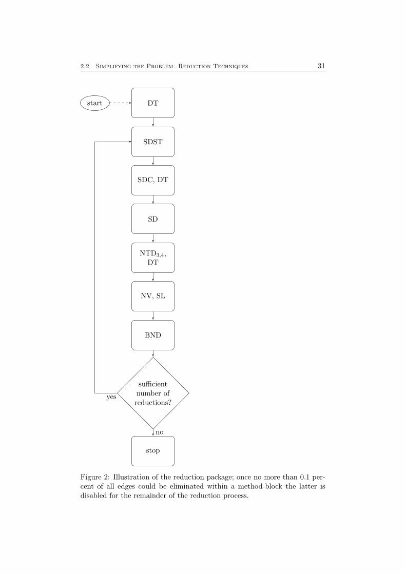
All reduction tests are arrayed in a loop that is reiterated as long asa constant proportion (for our solver 0.5 percent) of edges was eliminatedduring the last run. Thereby, one obtains the same asymptotic time boundas the most expensive performed reduction test; with the exception of theBND test this bound is of O(m+n log n). Furthermore, during a succeedingloop each test is performed only if it could eliminate a constant proportion(0.1 percent) of edges during the previous run. For the BND test, the (time-consuming) computation of an upper bound is only performed during thefirst run. Additionally, the BND test is executed if and only if at mostthree percent of all vertices are terminals; we have observed that the test isotherwise of very little effect.
The ordering that is by default used in our solver is reported in Figure 2.
2.2 Simplifying the Problem: Reduction Techniques 31
DTstart
SDST
SDC, DT
SD
NTD3,4,DT
NV, SL
BND
sufficientnumber ofreductions?
stop
yes
no
Figure 2: Illustration of the reduction package; once no more than 0.1 per-cent of all edges could be eliminated within a method-block the latter isdisabled for the remainder of the reduction process.
2.3 Finding a Solution: Primal Heuristics 32
2.3 Finding a Solution: Primal Heuristics
With the Steiner tree problem in graphs being NP-hard it hardly comesas a surprise that a wide range of research has focused on developing effi-cient primal heuristics. While attempting to obtain Steiner trees of smallweight is arguably worthwhile in its own right, an additional virtue arisesfrom the concomitantly yielded upper bound on the optimal solution value:The disposability of sharp upper bounds is indispensable for bound-basedreductions, see Section 2.2.4, and more importantly for an efficient branch-and-bound based exact solving approach. Indeed, without using SPG spe-cific heuristics we are unable to find any feasible solution to a number ofinstances that can otherwise be solved to optimality, as will be demonstratedat the end of this section.
Naturally, only a very small share among the plethora of primal heuristicstrialled in the literature is covered in this thesis. The reader wishing toacquire a more comprehensive insight is referred to [dAW02, PUW14, Pol04,RUW01].
2.3.1 Constructive Heuristics
As the name suggests, constructive heuristics build up a new solutionfrom the scratch, repeatedly extending the current sub-solution. In thiscontext, the repetitive shortest path heuristic (RSPH) can arguablybe named as the classical and empirically successful primal SPG heuristic.Already introduced in 1980 [TA80], it has found its way into various pub-lications, e.g. [HRW92, PD01, dAW02, Pol04, PUW14] and has moreoverbeen notably improved by [dAW02] and [Pol04] in terms of empirical runtime.
The basic concept of the heuristic is very coherent: Starting with a singlevertex, in each step the current subtree is connected to a nearest terminal bya shortest path. This procedure is reiterated until all terminals are spanned.Finally, the generated subgraph S is pruned, i.e. it is substituted by aminimum spanning tree constructed on the vertices of S and non-terminalsof degree one are, repeatedly, removed. To render the overall proceduremore potent, the heuristic is started from several distinct vertices.
In its original form the heuristic is implemented by initially comput-ing shortest paths from each terminal to all other vertices and afterwardssuccessively building up a Steiner tree by utilizing the previously obtainedshortest paths. The worst-case run time for such a construction is ofO(s(m+n log n)), which can be readily verified [Pol04]. In [dAW02] the empiricallyquite effective observation was made that a modified version of Dijkstra’salgorithm [FT84] can be used alternatively. This algorithm is not intro-duced in full detail here; however, a comprehensible delineation is provided:To grow a Steiner tree starting from a single vertex, one can use Dijkstra’s
2.3 Finding a Solution: Primal Heuristics 33
algorithm, pausing whenever a terminal has been scanned and joining theshortest path to this terminal with the incumbent tree. Throughout theexecution of Dijkstra’s algorithm, with each vertex vi ∈ V an upper boundπi on the distance between the current subtree and vi is associated.
The decisive consideration made in [dAW02] was that it is not necessaryto reset the π values whenever a terminal has been connected to the currentsubtree, since the tentative distances are still valid upper bounds on thedistances from the new subtree. Instead, one merely needs to reinsert everyvertex vi on the path between the previous tree and the newly incorporatedterminal into the priority queue of Dijkstra’s algorithm (setting πi = 0).Although the worst-case complexity remains at O(s(m + n log n)), empiri-cally the run time is drastically improved [dAW02, Pol04]. We denote thisvariant, also using different starting points, by one-phase RSPH.
A different approach was suggested in [PD01], based on the followingconsiderations: Let ti ∈ T , vj ∈ V \ {ti} and consider a shortest path Pbetween ti and vj computed in the first phase of the original RSPH imple-mentation. Aspiring to find an a priori criterion for P to not be requiredduring the second phase of RSPH, the following observations can be made:If P contains an intermediary terminal tk, inserting either the subpath be-tween vj and tk or ti and tk is always preferable to inserting the whole pathP . Similarly, if vj is contained in a Voronoi region of a terminal tk 6= ti andd(ti, tk) ≤ d(ti, vj) is satisfied, instead of inserting P , one could insert thesubpath between vj and tk or the subpath between ti and tk respectively,both of them being of not higher cost than P . Consequently, it is not neces-sary to obtain shortest paths from each terminal ti to all other vertices, butone may terminate Dijkstra’s algorithm, starting from ti, as soon as N(ti)and all neighbouring terminals have been scanned. Furthermore, no pathscontaining intermediary terminals need to be considered. This variant isdenoted by two-phase RSPH. We omit the implemental details and referto [PD01] for this purpose.
Another important observation [KM98] is that the heuristic may notonly be used initially, but moreover, with altered edge weights, during thebranch-and-cut: Given an optimal LP solution x ∈ QE , the heuristic iscalled with the edge weights (1 − xe) · ce for all e ∈ E. In this way, astimulus for the heuristic to choose edges contained in the LP solution isprovided.
In our implementation one-phase RSPH is customarily used, the two-phase variant is only preferred if at least one third of the vertices are termi-nals (which rarely is the case for most published test instances). Further-more, terminals are preferred as starting points as for example suggested in[KM98]. We perform the initial run of the heuristic, with no LP solutionavailable, with 100 start vertices, preferring terminals.
Additionally, the heuristic is called, with altered edge weights, beforeand after the processing of a branch-and-bound node, after each cut loop
2.3 Finding a Solution: Primal Heuristics 34
and after each LP solving during a cut loop; each with 16 start vertices.For this purpose we use a novel preference criterion: Given an optimal LPsolution x ∈ QE , we affiliate with each vertex vi the value αi :=
∑e∈δ(vi) xe.
Let αTmax := maxvi∈T αi. Thereupon, we associate with each terminal vi ∈T the value α′i, which is obtained by adding a pseudo-random uniformlydistributed number in [0, αTmax] to αi. Thereby, it is attempted to givea preference to terminals of high αi value, but still allowing the selectionof each terminal. Having set these values, we restrict the first ten runs toterminals, selecting the ones of highest α′i amount. For the next five runs thenot yet selected vertices of highest αi values are used. Finally, the last run isconducted with the start vertex that has led to the best incumbent solutionfound by RSPH in the course of the whole heretofore solving process.
Furthermore, ties occurring during the computation and the selection ofthe shortest paths are broken pseudo-randomly and when no new LP solutionis available, each edge cost is additionally multiplied by a pseudo-randomuniformly distributed number between 1.0 and 2.5 (the sole exception beingthe initial run).
2.3.2 Local Search Heuristics
Instead of constructing a solution de novo, as done by RSPH, a differentheuristic approach is to improve already existent solutions. Such localsearch heuristics [KV07] have successfully been applied to numerous hardcomputational problems. A prominent example is the Helsgaun implemen-tation of the Lin-Kernigham heuristic for the travelling salesman problem.This heuristic was not only able to produce optimal solutions to all solvedproblems it was tested on (as of October 2015, [Hel]), but furthermore al-lowed to improve the best known solutions for a series of large-scale instanceswith unknown optima, among them a 1, 904, 711-cities instance [Hel09].
Given a solution S to a problem, a local search algorithm examines aneighborhood of S, i.e. a set of solutions obtainable from S by performinga predefined set of operations. This examination encompasses finding animproving solution, i.e. one of smaller cost in the case of a minimizationproblem, or proving that no such solution exists. Subsequently, three localsearch heuristics from [UW10] that have been incorporated into our solverare sketched. Their, intricate, implementation will not be discussed here,but it should be noted that all of them can be performed with a worst-casecomplexity of O(m + n log n). The easiest one is vertex insertion (V),which examines whether an additional vertex vi can be merged with an ex-isting Steiner tree S = (VS , ES) in such a way that the minimum spanningtree on VS ∪{vi} (which likewise constitutes a Steiner tree) is of smaller costthan S. The last two heuristics use the concept of key-vertices, which areterminals or vertices of degree at least three in S. Correspondingly, a key-path is a path in S connecting two key-vertices and otherwise containing
2.3 Finding a Solution: Primal Heuristics 35
only non-key-vertices. In key-path exchange it is attempted to replace ex-isting key-paths by less costly ones. Similarly, for key-vertex eliminationin each step a non-terminal key-vertex and all adjoining key-paths (exceptfor the key-vertices at their respective ends) are extracted and an attempt ismade to reconnect the disconnected subtrees at a lower cost. As in [UW10],the execution of vertex insertion followed by the joint execution of key-pathexchange and key-vertex elimination is denoted by VQ. In our solver, VQ iscalled for a newly found solution whenever the latter is among the five bestknown solutions. This number is dynamically reduced if VQ is displayinglittle effectiveness on the instance being solved.
2.3.3 Recombination Heuristics
Recombination heuristics, better known as genetic algorithms (sincethey are said to mimic the process of evolutionary natural selection), havebeen widely applied to a vast number of optimization and search problems[ES03, Hin08]. Broadly speaking, solutions out of given pool are, repeatedly,altered and combined, with the ultimate goal of obtaining a new solutionthat excels all of its predecessors.
Accordingly, we developed a heuristic, denoted simply by recombina-tion heuristic (RCH), for the SPG that comprises in essence a recombi-nation of several known solutions. In the following, RCH is described in thecontext of an SPG, but it can be naturally extended to cover the differentSteiner problem variants discussed in this thesis. Preliminarily, we definethe set of solutions to be considered for recombination by L; in the case ofour solver L comprises the, at most 50, best found solutions of the currentsolving process.
The heart of RCH is the n-merging (n ≥ 2) operation, subsequently de-fined for a given solution S: This solution is merged with pseudo-randomlyselected n − 1 solutions out of L \ {S} to form a new graph GS consistingof all edges and vertices that are part of at least one of the n solutions. Ap-plying the reduction techniques introduced in Section 2.2 to GS , we obtaina reduced graph G′S . Next, a solution to G′S is computed in two steps.
First, the cost of each edge is pseudo-randomly reduced for each solutionit appears in, as suggested by [RUW01] and RSPH is employed. To this end,we compute the αi values to each vertex vi of G′S (considering the new edgeweights as an LP solution) and perform 50 runs of RSPH using the verticesof highest αi values as starting points. Thereupon, denote the best foundsolution by S′.
Second, after retrieving the original edge costs, VQ is employed on S′.Finally, S′ is re-transformed to the original solution space.
The RC heuristic is clustered around the n-merging operation: Given anew solution S, in one run consecutively three 2-, two 3- and 4-, and one 5-merges are performed. When a solution S′ is generated during an i-merging
2.3 Finding a Solution: Primal Heuristics 36
with a smaller cost than S, we set S := S′ and attempt to add S′ to L.Moreover, in this case a new run is started after the conclusion of the currentone. The total number of runs is limited to ten. RCH is called whenever rnew solutions have been found compared to its last execution. Initially, r isset to 5 (the minimum number of solutions to be available before executingRCH) and modified throughout the solution process, setting r := 0 if asolution has been improved during the execution of RCH and r := r + 1otherwise.
Finally, it should not go unmentioned that recombination heuristics forthe SPG were already suggested in [RUW01] and [PUW14]. Nevertheless,they differ widely from the heretofore introduced RC heuristic: First, inneither of these publications reduction techniques were used. Additionally,the authors merge merely two solutions and furthermore deviate in severaldetails, e.g. they do not apply a criterion for selecting start vertices forRSPH.
2.4 Solving to Optimality: Branch and Cut 37
2.4 Solving to Optimality: Branch and Cut
Since the employed model PCF potentially contains an exponential num-ber of constraints, see Section 2.1, starting with the associated LP relax-ation becomes prohibitive already for medium-seized instances. Therefore,a branch-and-cut algorithm is employed. In general, branch-and-cut canbe seen as a modification of branch-and-bound, starting with only a subsetof the model constraints and employing cutting planes at each (or certaindesignated) branch-and-bound nodes to tighten the LP relaxations [Mit02].
The algorithm employed in this thesis is largely in accordance with theapproach described in [KM98].
2.4.1 Separation Methods
The initialization of the branch-and-cut solving process at the root node isdone be setting up an LP that contains the constraints (23) and the trivialinequalities 0 ≤ ya ≤ 1 for all a ∈ A. Thereafter, separation routines for thecut inequalities (21) are deployed. For this purpose, four types of methodsare implemented in both Jack-III and SCIP-Jack; a more detailed reportcan be found in [KM98].
Generic Cuts
Considering the edge values of an LP solution as capacities, we only needto check for each ti ∈ T r whether a minimal (r, ti)-cut is less than one, inorder to find violated inequalities. If such a cut exists, it corresponds to aviolated inequality, otherwise there is none. When using the highest labelpreflow-push algorithm described in [GT88], the overall running time fordetermining minimal (r, ti)-cuts for each ti ∈ T r is of O(
√m+ n2).
Back Cuts
The number of separated inequalities can be increased by reversing the flowof each arc and additionally examining the (ti, r)-cuts for each ti ∈ T r.On the downside, however, the above mentioned highest label preflow-pushalgorithm cannot be used, because for each (ti, r)-cut the source vertex ischanged.
Nested Cuts
The number of separated inequalities can also be increased by nesting thecuts: Having found a minimal cut between the root and a ti ∈ T r, allcorresponding variables in the current LP solution are temporarily lockedto one and another attempt to find a (r, ti)-cut is initiated. The procedureis reiterated until the flow between r and ti is at least one. This nestingapproach can be combined with the back-cuts.
2.4 Solving to Optimality: Branch and Cut 38
Creep Flow
A different strategy is to attempt to determine a cut of minimal cardinal-ity. This can be done by adding a very small capacity ε > 0 (which isdefined by SCIP) to all arcs. While this deteriorates the empirical runningtime for computing a minimal cut, as more arcs have to be considered, thetime required for re-optimizing the linear program is substantially decreased[KM98, Pol04].
2.4.2 Branching
Despite the tightness of the employed model, for certain hard instancesbranching is still necessary. For this purpose we have developed a simpleSPG specific branching-rule, which is nevertheless empirically stronger thanits refined generic counterparts natively implemented in SCIP. For a moregeneral discussion on branching we refer to [AKM04].
As opposed to customary approaches, instead of branching on vari-ables, i.e. in the case of the SPG on arcs, we employ vertex branch-ing [HRW92]. This means that during the branch-and-bound procedure apredefined Steiner vertex is rendered a terminal in one child node and ex-cluded in the complementary node. To determine such a Steiner vertex wesuggest the following criterion:
Let y ∈ [0, 1]A be an LP solution at the current node during the branch-and-cut. Select a vertex vi ∈ V \ T to branch upon, such that:∣∣ ∑
e∈δ−(vi)
ye − 0.5∣∣ (32)
is minimal among all Steiner vertices. The idea underlying (32) is to keep thebranch-and-bound tree balanced. Also, branching on vertices as comparedto arcs exerts more influence on the model, since excluding a vertex forcesthe solver to ignore all of its incident arcs, while just discarding a single arcbears a lower impact. Furthermore, including a vertex as opposed to an edgeleads to an enhanced flexibility, since the vertex can usually be contained indifferent ways in a feasible solution, possibly setting the stage for a better(local) upper bound.
2.5 Implementation 39
2.5 Implementation
Since this thesis is considered to be of prevalently mathematical nature, weconfine ourselves to presenting a synopsis of the implementation and referto the online documentation [Reh] of SCIP-Jack for more details.
2.5.1 SCIP-Jack: A General Purpose Solver for Steiner TreeProblems
SCIP
The foundation of our Steiner problem package is the academic MIP solverSCIP. Besides being one of the fastest non-commercial MIP solvers [Mit15],SCIP is a general branch-and-cut framework. Its plugin-based design pro-vides a simple method of extension to handle a variety of specific problemclasses. Furthermore, SCIP renders ubiquitous mastery of the solving pro-cedure possible and allows the access to detailed processual information.
SCIP is implemented as a C callable library (although C++ wrapperclasses are provided for user defined plugins). It should be noted that SCIPdoes not come with a native LP solver. However, an interface is providedinstead, allowing the usage of common commercial solvers such as CPLEX2
or Gurobi3. Furthermore, the LP solver SoPlex [Wun96] is distributedalong with SCIP in the SCIP optimization suite [BGG+12], which is likewisefreely available for academic purposes.
For more information on SCIP see [Ach09].
Jack
Jack, or more precisely Jack-III, is a solver for Steiner tree problems ingraphs described by Thorsten Koch and Alexander Martin [KM98] in 1998.It uses a branch-and-cut approach based on Formulation 5. Furthermore,it comprises several preprocessing techniques, e.g. DT and computationallyexpensive but more effective versions of the SD and BD3 tests. Also, theoriginal version of RSPH, see Section 2.3, is used. At the time of publishingJack-III was able to solve all problem instances that had hitherto beendiscussed in the literature to optimality. Since then it has frequently beenreferred to and the separation approach using Formulation 5 has successfullybeen reutilized for several different solvers, e.g. [Lju04, Pol04].
Jack-III was prevalently hand-tailored and implemented in C. However,for solving linear programs CPLEX 4.0 was used.
2http://www-01.ibm.com/software/commerce/optimization/cplex-optimizer/3http://www.gurobi.com/products/gurobi-optimizer/
2.5 Implementation 40
SCIP-Jack
SCIP-Jack was spawned by the endeavour to embed the hand-tailoredJack-III into a state-of-the-art MIP-framework. The use of a general MIPsolver renders the model to be solved highly pliant, which is of pivotal impor-tance to the generic solving approach employed in this thesis. Furthermore,a general framework was presumed to facilitate the incorporation of both,algorithms published in the literature since the creation of Jack-III andad hoc developed methods (as for example the numerous novel techniquesdescribed in this thesis). SCIP, being freely available for academic researchand providing the above described features, was a natural choice. Anotheradvantage of this decision comes with the general solution methods nativelyimplemented in SCIP, e.g. cutting planes, being perpetually kept up-to-date by the continuous improvements of the framework.
Concerning the implementation of SCIP-Jack, it indubitably bearsmentioning that the original embedding of Jack-III into SCIP was car-ried out by Gerald Gamrath, Thorsten Koch and Michael Winkler. How-ever, the resulting initial version of SCIP-Jack did not include any of themodifications and extensions described in this thesis. Furthermore, GeraldGamrath, Stephan Maher and Yuji Shinano were involved in the furtherdevelopment of SCIP-Jack; in this context, each solving method that wasnot implemented or developed by the author of this thesis is marked as such.
The first plugins to be implemented were a reader to read problem in-stances and problem data to store the graph and build the model withinSCIP. Within these plugins the reading methods and data structures ofJack-III could be adopted largely unaltered. However, for handling thedifferent Steiner variants introduced in Section 3, extensions were necessary.The heart of the new implementation is a constraint handler that checkssolutions for feasibility and separates any violated model constraints. Theseparation methods already existent in Jack-III are deployed for this pur-pose, while SCIP provides a filtering of cuts to improve numerical stabilityand dynamic ageing of the generated cuts. By default, only the creep flowstrategy (together with the flow inequalities) is used, since it proved to beempirically superior to other combinations, evidenced by both experimentsconducted with SCIP-Jack and results reported in [KM98] for Jack-III.However, by means of parameters, each separation method introduced inSection 2.4.1 can be deployed at will by the user.
Additionally, native general-purpose separation methods of SCIP suchas Gomory and mixed-integer rounding cuts are employed.
Jack-III already included a large number of reduction methods for theSPG, as described in [KM98]. However, with the developments described inSection 2.2, only the, basic, DT reductions were reused for SCIP-Jack.
For the branch-and-bound search a new plugin was implemented thatincludes the Steiner specific vertex branching introduced in Section 2.4.2.
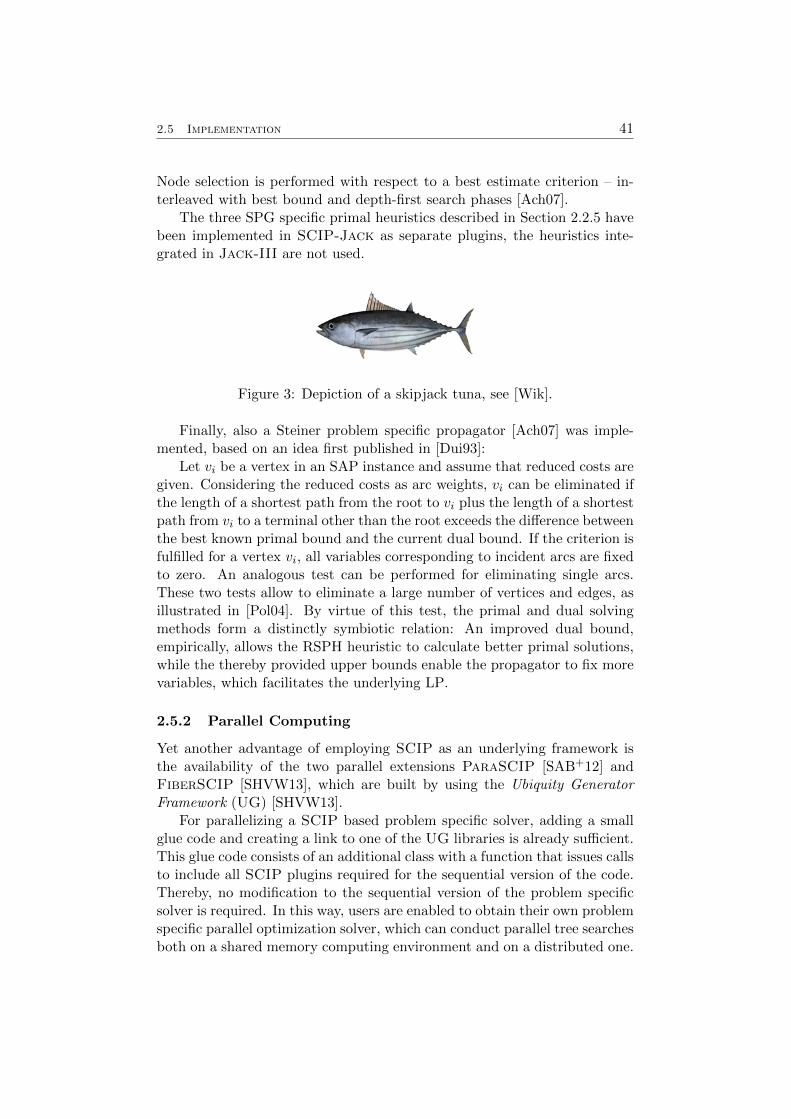
2.5 Implementation 41
Node selection is performed with respect to a best estimate criterion – in-terleaved with best bound and depth-first search phases [Ach07].
The three SPG specific primal heuristics described in Section 2.2.5 havebeen implemented in SCIP-Jack as separate plugins, the heuristics inte-grated in Jack-III are not used.
Figure 3: Depiction of a skipjack tuna, see [Wik].
Finally, also a Steiner problem specific propagator [Ach07] was imple-mented, based on an idea first published in [Dui93]:
Let vi be a vertex in an SAP instance and assume that reduced costs aregiven. Considering the reduced costs as arc weights, vi can be eliminated ifthe length of a shortest path from the root to vi plus the length of a shortestpath from vi to a terminal other than the root exceeds the difference betweenthe best known primal bound and the current dual bound. If the criterion isfulfilled for a vertex vi, all variables corresponding to incident arcs are fixedto zero. An analogous test can be performed for eliminating single arcs.These two tests allow to eliminate a large number of vertices and edges, asillustrated in [Pol04]. By virtue of this test, the primal and dual solvingmethods form a distinctly symbiotic relation: An improved dual bound,empirically, allows the RSPH heuristic to calculate better primal solutions,while the thereby provided upper bounds enable the propagator to fix morevariables, which facilitates the underlying LP.
2.5.2 Parallel Computing
Yet another advantage of employing SCIP as an underlying framework isthe availability of the two parallel extensions ParaSCIP [SAB+12] andFiberSCIP [SHVW13], which are built by using the Ubiquity GeneratorFramework (UG) [SHVW13].
For parallelizing a SCIP based problem specific solver, adding a smallglue code and creating a link to one of the UG libraries is already sufficient.This glue code consists of an additional class with a function that issues callsto include all SCIP plugins required for the sequential version of the code.Thereby, no modification to the sequential version of the problem specificsolver is required. In this way, users are enabled to obtain their own problemspecific parallel optimization solver, which can conduct parallel tree searchesboth on a shared memory computing environment and on a distributed one.
2.5 Implementation 42
Using these means, we have created a parallel version of SCIP-Jack.Since this extension has been obtained in corporation with Yuji Shinano,the creator of UG, we do not provide more detailed information, but referto [GKM+15] instead. However, we note that by using this approach, it ispossible to employ large supercomputing resources to solve computationallydifficult Steiner tree problems with SCIP-Jack. Some results, includingimproved bounds for several unsolved problem instances from the literature,will be provided in Section 4.1.1.
2.6 Computational Results and Discussion 43
2.6 Computational Results and Discussion
When attempting to evaluate the quality of algorithms for NP-hard problems(like primal heuristics) one is commonly faced with a predicament: On theone hand, just assessing the algorithms on a (confined) set of test instancesmight be incomplete, since with other types of problem structure ostensiblyprolific methods might fail dismally. On the other hand, establishing guar-anteed performance ratios cannot be regarded a valid substitute, since suchresults are prevalently too pessimistic from an empirical point of view, dueto their worst-case character or a lack of suitable proving techniques.
Since this thesis is focused on practical solving methods, we have de-cided for empirical evaluation using benchmark instances, but try to keepthe range of problem types reasonably wide, as to cover many disparatestructures within the instances. The probably most extensive and frequentlyused [KM98, Pol04, VD04, PUW14] SPG benchmark library is the Stein-Lib [KMV01]. However, in the course of the 11th DIMACS Challenge addi-tional, often real-world derived, test sets were made publicly available. Sinceusing all available instances in each section would result in an unreasonablylengthy and likely tedious work, a confined set of test instances has beenselected for intermediary results. However, a testing on a more compre-hensive set of instances, using the complete SCIP-Jack package with itsfinal default configurations as well as comparisons with other state-of-the-artsolvers, is provided in Section 4.
For testing the computational results of SCIP-Jack, the focus in thissection lies on the impact of the reduction techniques and the primal heuris-tics. To this end, three sets from the library SteinLib and one published inthe 11th DIMACS Challenge are used. Table 1 provides a brief descriptionof the used instance classes. In each line the name of the corresponding testset is given in the first column. The next column lists the number of in-stances within the test set, thereafter the range of the number of vertices forthe individual instances within the class is given. Furthermore, the Statusindicates whether all instances of a class have been solved in the literature.Conclusively, some elementary characteristics including the origins of thetest set are provided. It should be noted that the vienna-I instances comealready preprocessed by methods described as being ”simple” in [LLL+14].
All computational experiments were performed on a cluster of Intel XeonX5672 CPUs with 3.20 GHz and 48 GB RAM, running Kubuntu 14.04 andusing SCIP 3.2. Underlying, CPLEX 12.6.2 is employed as LP solver sinceit is empirically faster than the academic LP solver SoPlex, see [Mit15].For all computations a time limit of two hours is set.
If an instance is not solved to optimality within the time limit, thegap is reported, which is defined as 100 · pb−db
pb % for the final primal anddual bound pb and db, respectively. If no lower or upper bound has beencomputed, the gap is set to 100 percent. The average gap is obtained as an
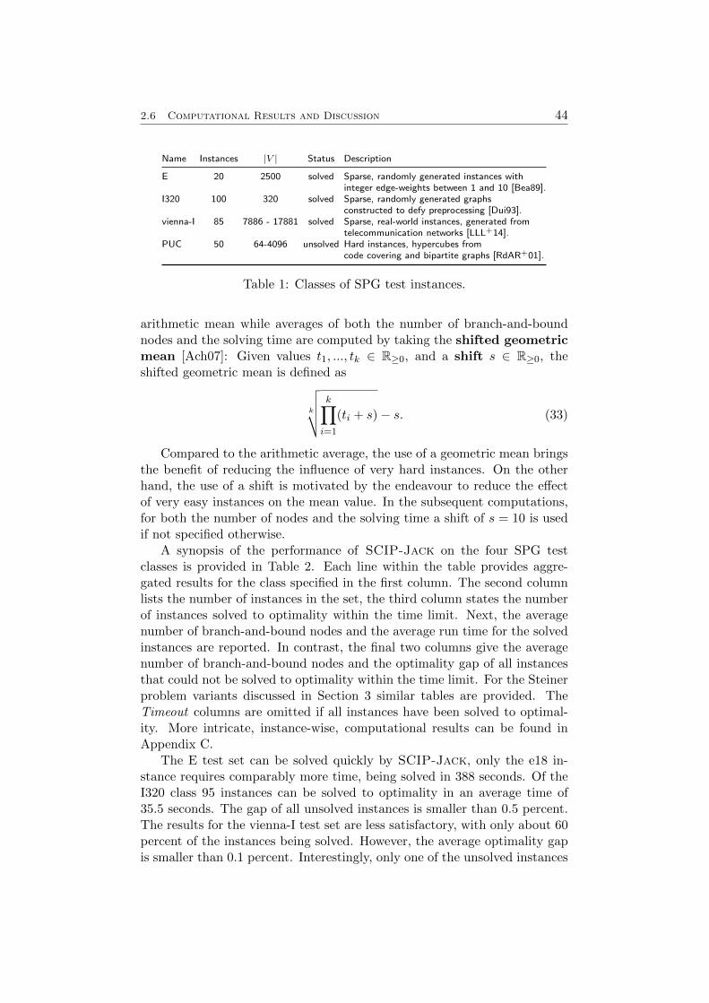
2.6 Computational Results and Discussion 44
Name Instances |V | Status Description
E 20 2500 solved Sparse, randomly generated instances withinteger edge-weights between 1 and 10 [Bea89].
I320 100 320 solved Sparse, randomly generated graphsconstructed to defy preprocessing [Dui93].
vienna-I 85 7886 - 17881 solved Sparse, real-world instances, generated fromtelecommunication networks [LLL+14].
PUC 50 64-4096 unsolved Hard instances, hypercubes fromcode covering and bipartite graphs [RdAR+01].
Table 1: Classes of SPG test instances.
arithmetic mean while averages of both the number of branch-and-boundnodes and the solving time are computed by taking the shifted geometricmean [Ach07]: Given values t1, ..., tk ∈ R≥0, and a shift s ∈ R≥0, theshifted geometric mean is defined as
k
√√√√ k∏i=1
(ti + s)− s. (33)
Compared to the arithmetic average, the use of a geometric mean bringsthe benefit of reducing the influence of very hard instances. On the otherhand, the use of a shift is motivated by the endeavour to reduce the effectof very easy instances on the mean value. In the subsequent computations,for both the number of nodes and the solving time a shift of s = 10 is usedif not specified otherwise.
A synopsis of the performance of SCIP-Jack on the four SPG testclasses is provided in Table 2. Each line within the table provides aggre-gated results for the class specified in the first column. The second columnlists the number of instances in the set, the third column states the numberof instances solved to optimality within the time limit. Next, the averagenumber of branch-and-bound nodes and the average run time for the solvedinstances are reported. In contrast, the final two columns give the averagenumber of branch-and-bound nodes and the optimality gap of all instancesthat could not be solved to optimality within the time limit. For the Steinerproblem variants discussed in Section 3 similar tables are provided. TheTimeout columns are omitted if all instances have been solved to optimal-ity. More intricate, instance-wise, computational results can be found inAppendix C.
The E test set can be solved quickly by SCIP-Jack, only the e18 in-stance requires comparably more time, being solved in 388 seconds. Of theI320 class 95 instances can be solved to optimality in an average time of35.5 seconds. The gap of all unsolved instances is smaller than 0.5 percent.The results for the vienna-I test set are less satisfactory, with only about 60percent of the instances being solved. However, the average optimality gapis smaller than 0.1 percent. Interestingly, only one of the unsolved instances
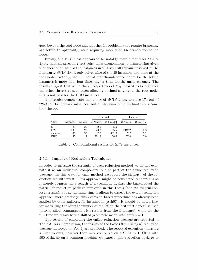
2.6 Computational Results and Discussion 45
goes beyond the root node and all other 14 problems that require branchingare solved to optimality, none requiring more than 65 branch-and-boundnodes.
Finally, the PUC class appears to be notably more difficult for SCIP-Jack than all preceding test sets. This phenomenon is unsurprising giventhat more than half of the instances in this set still remain unsolved in theliterature. SCIP-Jack only solves nine of the 50 instances and none at theroot node. Notably, the number of branch-and-bound nodes for the solvedinstances is more than four times higher than for the unsolved ones. Theresults suggest that while the employed model PCF proved to be tight forthe other three test sets, often allowing optimal solving at the root node,this is not true for the PUC instances.
The results demonstrate the ability of SCIP-Jack to solve 174 out of225 SPG benchmark instances, but at the same time its limitations comeinto the open.
Optimal Timeout
Class Instances Solved ∅Nodes ∅Time [s] ∅Nodes ∅Gap [%]
E 20 20 2.0 5.0 – –I320 100 95 23.7 35.5 1342.2 0.3vienna-I 85 50 2.8 431.8 2.2 0.1PUC 50 9 581.3 88.5 137.0 3.9
Table 2: Computational results for SPG instances.
2.6.1 Impact of Reduction Techniques
In order to measure the strength of each reduction method we do not eval-uate it as an individual component, but as part of the entire reductionpackage. In this way, for each method we report the strength of the re-duction set without it. This approach might be considered tendentious asit merely regards the strength of a technique against the backdrop of theparticular reduction package employed in this thesis (and its eventual id-iosyncrasies), but at the same time it allows to dissect the overall reductionapproach more precisely; this exclusion based procedure has already beenapplied by other authors, for instance in [Ach07]. It should be noted thatfor measuring the average number of reduction the arithmetic mean is used(also to allow comparisons with results from the literature), while for therun time we resort to the shifted geometric mean with shift s = 1.
The results of employing the entire reduction package are reported inTable 3. As a comparison, the results of the basic O(m+ n log n) reductionpackage employed in [Pol04] are provided. The reported execution times aresimilar to ours, however they were computed on a SPARC-III CPU with900 MHz, so on a common machine we expect their reduction package to
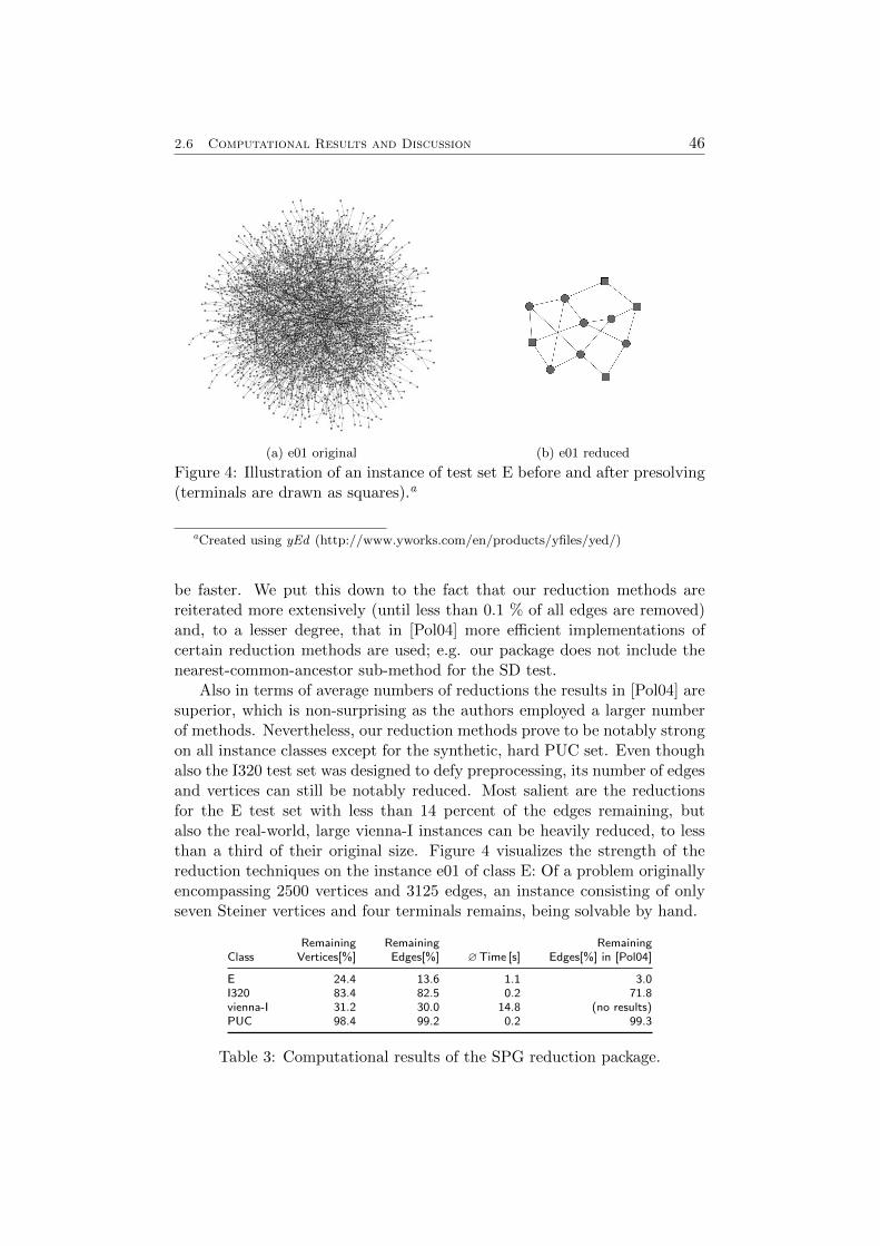
2.6 Computational Results and Discussion 46
(a) e01 original (b) e01 reduced
Figure 4: Illustration of an instance of test set E before and after presolving(terminals are drawn as squares).a
aCreated using yEd (http://www.yworks.com/en/products/yfiles/yed/)
be faster. We put this down to the fact that our reduction methods arereiterated more extensively (until less than 0.1 % of all edges are removed)and, to a lesser degree, that in [Pol04] more efficient implementations ofcertain reduction methods are used; e.g. our package does not include thenearest-common-ancestor sub-method for the SD test.
Also in terms of average numbers of reductions the results in [Pol04] aresuperior, which is non-surprising as the authors employed a larger numberof methods. Nevertheless, our reduction methods prove to be notably strongon all instance classes except for the synthetic, hard PUC set. Even thoughalso the I320 test set was designed to defy preprocessing, its number of edgesand vertices can still be notably reduced. Most salient are the reductionsfor the E test set with less than 14 percent of the edges remaining, butalso the real-world, large vienna-I instances can be heavily reduced, to lessthan a third of their original size. Figure 4 visualizes the strength of thereduction techniques on the instance e01 of class E: Of a problem originallyencompassing 2500 vertices and 3125 edges, an instance consisting of onlyseven Steiner vertices and four terminals remains, being solvable by hand.
Remaining Remaining RemainingClass Vertices[%] Edges[%] ∅Time [s] Edges[%] in [Pol04]
E 24.4 13.6 1.1 3.0I320 83.4 82.5 0.2 71.8vienna-I 31.2 30.0 14.8 (no results)PUC 98.4 99.2 0.2 99.3
Table 3: Computational results of the SPG reduction package.
2.6 Computational Results and Discussion 47
Having established the overall picture, the results illustrated in Table 4allow us to cut through the surface and analyze the impact of the individualcomponents within the reduction package: The first four rows list the per-centual change in the number of remaining edges resulting from successivelyexcluding each reduction method; the last four lines provide the correspond-ing percentual change with respect to the run time of the entire reductionpackage. In this way, the first column of each line states the test set to beconsidered. Ensuing, each of the next seven columns provides the result ofexcluding the affiliated reduction method specified in the head of the table.It should be noted that positive values signify a favourable impact of therespective reduction method on the overall package: With respect to thereduced edges a positive value denotes a higher amount of remaining edgeswhen disabling the specified method; likewise, a positive percentage for theoverall preprocessing time indicates that the reduction package requires moretime as a consequence of excluding the respective method.
First, it can be remarked that each exclusion of a method diminishesthe strength of the reduction package. However, the leverage varies widely.The strongest impact is exerted by the DT test: Concerning the reduction ofedges it outnumbers all other methods on each of the four test sets. However,for the E set it is also notably time-consuming. Next is the SD test: Whileit is not effective on the I320 and PUC sets (designed to defy preprocessing),it demonstrates its strength on the other two. Not only is it the second mosteffective test in terms of reduced edges, but it also decreases the executiontime of the reduction package for both E and vienna-I.
Shifting the point of view towards the other end, the SDC test inevitablecatches the attention. Although it can claim credit for a certain reduction ofedges, it is also notably time-consuming. A decrease of the constant upperbound or a later execution of the method within the reduction loop mightseem reasonable, but also decreases its strength. Of even less effect is theSDST test with only 0.2 percent on the E class and less than 0.1 otherwise.
Addressing efficiency, the BND test sticks out: It manifests a solid ef-fectiveness at minimal extra cost, defying its poor theoretical worst-casecomplexity.
Finally, having performed additional experiments to evaluate our novelextensions, we note that the modification of the NV test described in Sec-tion 2.2.3 eliminates eight percent more edges, compared to the original test.Additionally, the extension of the BND test, see Lemma 12, allows to elimi-nate around 13 percent more edges on average, as compared to the originaltest. For both extensions less than one percent of additional execution timeis required (compared to the original NV and BND tests).
Concluding, the employed reductions are notably efficient (and indeedindispensable for the overall exact solving results) on all but one of the testedinstance sets. Nevertheless, several additional reduction methods could beincorporated, see [Pol04] and computational enhancements of existing ones
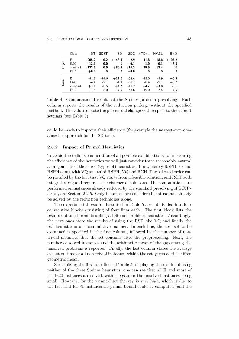
2.6 Computational Results and Discussion 48
Class DT SDST SD SDC NTD3,4 NV,SL BND
Edges
E +205.2 +0.2 +148.8 +2.9 +41.8 +18.6 +105.2I320 +12.1 +0.0 0 +0.1 +1.0 +0.1 +7.8vienna-I +132.5 +0.0 +86.4 +14.3 +35.9 +12.4 0PUC +0.8 0 0 +0.0 0 0 0
Tim
e E -41.7 -14.6 +12.2 -34.4 -22.0 -9.9 +0.9I320 -4.4 -2.1 -4.9 -68.7 -8.4 -2.1 +0.7vienna-I +1.6 -0.5 +7.2 -10.2 +4.7 +3.8 -0.1PUC -7.8 -8.0 -17.5 -68.6 -19.0 -7.4 -7.5
Table 4: Computational results of the Steiner problem presolving. Eachcolumn reports the results of the reduction package without the specifiedmethod. The values denote the percentual change with respect to the defaultsettings (see Table 3).
could be made to improve their efficiency (for example the nearest-common-ancestor approach for the SD test).
2.6.2 Impact of Primal Heuristics
To avoid the tedious enumeration of all possible combinations, for measuringthe efficiency of the heuristics we will just consider three reasonably naturalarrangements of the three (types of) heuristics: First, merely RSPH, secondRSPH along with VQ and third RSPH, VQ and RCH. The selected order canbe justified by the fact that VQ starts from a feasible solution, and RCH bothintegrates VQ and requires the existence of solutions. The computations areperformed on instances already reduced by the standard presolving of SCIP-Jack, see Section 2.2.5. Only instances are considered that cannot alreadybe solved by the reduction techniques alone.
The experimental results illustrated in Table 5 are subdivided into fourconsecutive blocks consisting of four lines each. The first block lists theresults obtained from disabling all Steiner problem heuristics. Accordingly,the next ones state the results of using the RSP, the VQ and finally theRC heuristic in an accumulative manner. In each line, the test set to beexamined is specified in the first column, followed by the number of non-trivial instances that the set contains after the preprocessing. Next, thenumber of solved instances and the arithmetic mean of the gap among theunsolved problems is reported. Finally, the last column states the averageexecution time of all non-trivial instances within the set, given as the shiftedgeometric mean.
Scrutinizing the first four lines of Table 5, displaying the results of usingneither of the three Steiner heuristics, one can see that all E and most ofthe I320 instances are solved, with the gap for the unsolved instances beingsmall. However, for the vienna-I set the gap is very high, which is due tothe fact that for 31 instances no primal bound could be computed (and the
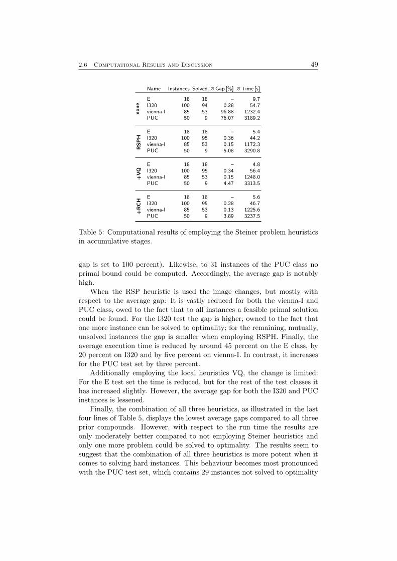
2.6 Computational Results and Discussion 49
Name Instances Solved ∅Gap [%] ∅Time [s]
none
E 18 18 – 9.7I320 100 94 0.28 54.7vienna-I 85 53 96.88 1232.4PUC 50 9 76.07 3189.2
RSPH
E 18 18 – 5.4I320 100 95 0.36 44.2vienna-I 85 53 0.15 1172.3PUC 50 9 5.08 3290.8
+VQ
E 18 18 – 4.8I320 100 95 0.34 56.4vienna-I 85 53 0.15 1248.0PUC 50 9 4.47 3313.5
+RCH
E 18 18 – 5.6I320 100 95 0.28 46.7vienna-I 85 53 0.13 1225.6PUC 50 9 3.89 3237.5
Table 5: Computational results of employing the Steiner problem heuristicsin accumulative stages.
gap is set to 100 percent). Likewise, to 31 instances of the PUC class noprimal bound could be computed. Accordingly, the average gap is notablyhigh.
When the RSP heuristic is used the image changes, but mostly withrespect to the average gap: It is vastly reduced for both the vienna-I andPUC class, owed to the fact that to all instances a feasible primal solutioncould be found. For the I320 test the gap is higher, owned to the fact thatone more instance can be solved to optimality; for the remaining, mutually,unsolved instances the gap is smaller when employing RSPH. Finally, theaverage execution time is reduced by around 45 percent on the E class, by20 percent on I320 and by five percent on vienna-I. In contrast, it increasesfor the PUC test set by three percent.
Additionally employing the local heuristics VQ, the change is limited:For the E test set the time is reduced, but for the rest of the test classes ithas increased slightly. However, the average gap for both the I320 and PUCinstances is lessened.
Finally, the combination of all three heuristics, as illustrated in the lastfour lines of Table 5, displays the lowest average gaps compared to all threeprior compounds. However, with respect to the run time the results areonly moderately better compared to not employing Steiner heuristics andonly one more problem could be solved to optimality. The results seem tosuggest that the combination of all three heuristics is more potent when itcomes to solving hard instances. This behaviour becomes most pronouncedwith the PUC test set, which contains 29 instances not solved to optimality
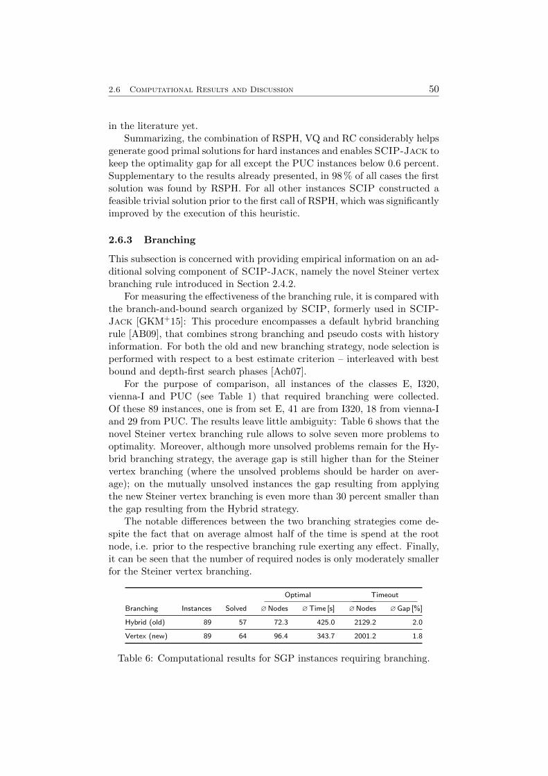
2.6 Computational Results and Discussion 50
in the literature yet.Summarizing, the combination of RSPH, VQ and RC considerably helps
generate good primal solutions for hard instances and enables SCIP-Jack tokeep the optimality gap for all except the PUC instances below 0.6 percent.Supplementary to the results already presented, in 98 % of all cases the firstsolution was found by RSPH. For all other instances SCIP constructed afeasible trivial solution prior to the first call of RSPH, which was significantlyimproved by the execution of this heuristic.
2.6.3 Branching
This subsection is concerned with providing empirical information on an ad-ditional solving component of SCIP-Jack, namely the novel Steiner vertexbranching rule introduced in Section 2.4.2.
For measuring the effectiveness of the branching rule, it is compared withthe branch-and-bound search organized by SCIP, formerly used in SCIP-Jack [GKM+15]: This procedure encompasses a default hybrid branchingrule [AB09], that combines strong branching and pseudo costs with historyinformation. For both the old and new branching strategy, node selection isperformed with respect to a best estimate criterion – interleaved with bestbound and depth-first search phases [Ach07].
For the purpose of comparison, all instances of the classes E, I320,vienna-I and PUC (see Table 1) that required branching were collected.Of these 89 instances, one is from set E, 41 are from I320, 18 from vienna-Iand 29 from PUC. The results leave little ambiguity: Table 6 shows that thenovel Steiner vertex branching rule allows to solve seven more problems tooptimality. Moreover, although more unsolved problems remain for the Hy-brid branching strategy, the average gap is still higher than for the Steinervertex branching (where the unsolved problems should be harder on aver-age); on the mutually unsolved instances the gap resulting from applyingthe new Steiner vertex branching is even more than 30 percent smaller thanthe gap resulting from the Hybrid strategy.
The notable differences between the two branching strategies come de-spite the fact that on average almost half of the time is spend at the rootnode, i.e. prior to the respective branching rule exerting any effect. Finally,it can be seen that the number of required nodes is only moderately smallerfor the Steiner vertex branching.
Optimal Timeout
Branching Instances Solved ∅Nodes ∅Time [s] ∅Nodes ∅Gap [%]
Hybrid (old) 89 57 72.3 425.0 2129.2 2.0
Vertex (new) 89 64 96.4 343.7 2001.2 1.8
Table 6: Computational results for SGP instances requiring branching.
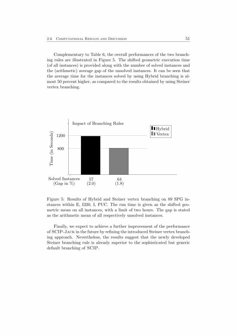
2.6 Computational Results and Discussion 51
Complementary to Table 6, the overall performances of the two branch-ing rules are illustrated in Figure 5. The shifted geometric execution time(of all instances) is provided along with the number of solved instances andthe (arithmetic) average gap of the unsolved instances. It can be seen thatthe average time for the instances solved by using Hybrid branching is al-most 50 percent higher, as compared to the results obtained by using Steinervertex branching.
HybridVertex
800
1200
Impact of Branching Rules
Tim
e(i
nS
econ
ds)
Solved Instances(Gap in %)
57(2.0)
64(1.8)
Figure 5: Results of Hybrid and Steiner vertex branching on 89 SPG in-stances within E, I320, I, PUC. The run time is given as the shifted geo-metric mean on all instances, with a limit of two hours. The gap is statedas the arithmetic mean of all respectively unsolved instances.
Finally, we expect to achieve a further improvement of the performanceof SCIP-Jack in the future by refining the introduced Steiner vertex branch-ing approach. Nevertheless, the results suggest that the newly developedSteiner branching rule is already superior to the sophisticated but genericdefault branching of SCIP.
2.6 Computational Results and Discussion 52
53
3 Variants of the Steiner Tree Problem
With SCIP-Jack being able to cope with SPG instances, the next step isto extend the scope and set about solving Steiner problem variants morefrequently derived from real-world applications. In order to verify the va-lidity of the hereinafter introduced transformations, it will be continuallyproceeded as follows:
First, a one-to-one correspondence between the solution sets of the orig-inal and the transformed problem is demonstrated. Second, a linear relationbetween the respective solutions values is established. This relation impliesthat a problem can be solved on its transformed solution space.
The time limit for the computational experiments within this section isset to two hours.
3.1 The Steiner Arborescence Problem 54
3.1 The Steiner Arborescence Problem
Observing that the SPG can be solved as a Steiner arborescence problem, itcan be verified that the SAP is NP-hard as well. Further theoretical results,such as on hardness and approximability, can be found in [CCC+98, HK03].Since it constitutes the backbone for solving both the Steiner problem ingraphs, see Section 2, and most Steiner problem variants discussed in theremainder of this thesis, the SAP occupies a central position in our genericsolving approach. For this reason, a formalized description of the trans-formation already introduced in Section 2.1 is provided subsequently. Incontrast to the SPG, arcs can be of zero cost, since such arcs can in generalnot be contracted without loosing optimal solutions.
Transformation 1 (SPG to SAP).Input: An SPG P = (V,E, T, c)Output: An SAP P ′ = (V ′, A′, T ′, c′, r′)
1. Set V ′ := V , T ′ := T , A′ := {(v, w) ∈ V ′ × V ′ : {v, w} ∈ E}.
2. Define c′ : A′ → Q≥0 by c′a = c{v,w}, for a = (v, w) ∈ A′.
3. Choose a root r′ ∈ T ′ arbitrarily.
4. Return (V ′, A′, T ′, c′, r′).
Although the transformation is well-known, e.g. [KM98], it has appar-ently not been formally established yet.
Lemma 15 (SPG to SAP). Let P = (V,E, T, c) be an SPG and P ′ =(V ′, A′, T ′, c′) an SAP obtained by applying Transformation 1 on P . Denoteby S and S ′ the sets of solutions to P and P ′ respectively. Thereupon, S ′ canbe mapped bijectively onto S by assigning each (V ′S′ , A
′S′) ∈ S ′ a (VS , ES) ∈ S
such that
VS := {v ∈ V : v ∈ V ′S′}, (34)
ES := {{v, w} ∈ E : (v, w) ∈ A′S′ or (w, v) ∈ A′S′}. (35)
The objective value is preserved.
Proof. First, it can be observed that (34) and (35) form indeed a mappingS ′ → S: Each arc of a solution to P ′ is substituted by its undirected coun-terpart and the vertices are maintained. Since for an SAP all terminalshave to be spanned by an directed tree, the corresponding undirected treelikewise contains all terminals.
To see the one-to-one correspondence, let S = (VS , ES) ∈ S and proceedas follows:
3.1 The Steiner Arborescence Problem 55
Surjective. In the following, a tree S′ = (V ′S′ , A′S′) ∈ S ′ is constructed
that is mapped by (34) and (35) to S, demonstrating that the mapping isa surjection. Initially, set V ′S′ := VS and A′S′ := ∅. Traverse (VS , ES), e.g.using breadth-first search, starting from r′ and add for each w ∈ VS visitedfrom v ∈ VS the arc (v, w) to A′S′ . S
′ := (V ′S′ , A′S′) is a solution to P ′ as it
consists of directed paths from r′ to all terminals and by applying (34) and(35) we obtain S.
Injective. S′ is the only solution to P ′ that is mapped by (34) and (35) toS: Each S′ ∈ S ′ \{S′} contains at least one arc (v, w) such that (v, w) /∈ A′S′and (w, v) /∈ A′S′ , since only substituting arcs in A′S′ by there anti-parallelcounterparts would not allow directed paths from the root to all verticesV ′S′ . Consequently, the solution S ∈ S corresponding to S′ contains theedge {v, w}, whereas S does not. Therefore, S′ is not mapped onto S.
Finally, since for each {v, w} ∈ ES either (v, w) ∈ A′S′ or (w, v) ∈ A′S′and vice versa, the costs of S′ and S are equal.
3.1.1 Reductions
Although various publications have addressed the Steiner arborescence prob-lem, surprisingly we could not find any that discussed reduction techniques.The reason for this phenomenon might be sought in a lack of publicly avail-able and computationally challenging test instances. However, it might alsobe due to the, at first glance perhaps surprising, fact that developing strongreduction techniques for the SAP is much more delicate than for its undi-rected kinsman, the SPG. The orientation of the tree renders the SAP muchless pliant to strategies such as alternative-based reduction, as will becomeevident in the course of this section. Nevertheless, we have succeeded indeveloping several, novel, reduction methods, which will be presented here-inafter.
Throughout this subsection it will be presupposed that an SAP instancePSAP = (V,A, T, c, r) is given and that r = t1. Furthermore, the reader isreminded of the consistently used notation T r := T \ {r}.
Basic Reductions
By observing that to each non-terminal contained in an optimal solutionthere is at least one incoming and one (non anti-parallel) outgoing arc,the first four reduction techniques ensue forthwith. Although not explicitlymentioned, these four reductions were already used in [GKM+15].
Non-terminal of in-degree zero (NTI0): A non-terminal vi with δ−(vi) =∅ can be deleted along with all incident arcs.
Non-terminal of out-degree zero (NTO0): A non-terminal vi withδ+(vi) = ∅ can be deleted along with all incident arcs.
3.1 The Steiner Arborescence Problem 56
Non-terminal with one neighbour (NTN1): A non-terminal vi withexactly one adjacent vertex can be deleted along with its incident arcs.
Non-terminal with two neighbours (NTN2): A non-terminal vi with1 ≤ |δ−(vi)| ≤ 2 as well as 1 ≤ |δ+(vi)| ≤ 2 and exactly two adjacent verticesvj , vk can be deleted, adding:
1. The arc (vk, vj) of cost cki + cij if (vk, vi) ∈ A and (vi, vj) ∈ A.
2. The arc (vj , vk) of cost cji + cik if (vj , vi) ∈ A and (vi, vk) ∈ A.
In the case of two parallel arcs, one of minimal cost is retained.
Proof. If an arc in |δ−(vi)|, say (vj , vi), is contained in an optimal solution,so is (vi, vk), since otherwise vi and (vj , vi) could be deleted to obtain asolution of smaller weight.
Apart from these four methods, all reduction tests presented for the SAPare newly developed. The first of them can be readily devised by consideringthat each Steiner arborescence contains by definition directed paths from theroot to all further terminals:
Terminal of in-degree one (TI1): Let ti ∈ T r. If δ−(ti) = {(vj , ti)},then (vj , ti) can be contracted into ti.
Similarly, there can be no path in a Steiner arborescence ending in rsince this would imply the existence of a cycle. Therefore, the followingreduction method is valid:
In-root arc (IRA4): All incoming arcs δ−(r) of the root can be deleted.
Finally, one can dispose of those vertices that cannot be part of alloptimal solutions:
Unreachable non-terminal (UNT): Let vi ∈ V \ T . If there is no di-rected path from r to vi or no directed path from vi to a tj ∈ T r, then vi canbe deleted.
Proof. If vi is not contained in any directed path from r, it cannot be con-tained in any Steiner arborescence. On the other hand, if there is no directpath from vi to a terminal other than the root, then to any Steiner arbores-cence S that contains vi there is one of no higher cost obtained by removingvi and its ingoing arc and considering the connected component containingr. Hence, there is at least one minimal Steiner arborescence not containingvi.
4Any resemblance of the abbreviation to existing organizations is purely coincidental.
3.1 The Steiner Arborescence Problem 57
The UNT test can be implemented by running a breadth-first searchstarting from r, only considering outgoing arcs for each vertex being pro-cessed and finally deleting all unvisited vertices. Thereafter, a breadth-firstsearch using all terminals except for the root as start vertices and onlyconsidering incoming arcs is performed. Finally, all vertices that were notvisited in the course of the search are deleted.
The successive execution of the above tests in the listed order is denotedBasic Reduction (BR). All tests other than UNT process each vertexand each arc at most once, but the latter requires executing a breadth-firstsearch. Hence, the overall worst-time complexity is of Θ(m), assuming thatthe underlying graph is connected.
Alternative Based Reductions
For the remaining reduction methods to the SAP it will be presupposedthat the given instance PSAP is feasible. This assumption is tantamountto the condition that for each non-root terminal ti ∈ T r there is at leastone directed path from r to ti. The latter can be easily validated whileperforming the UNT test.
Lemma 16. Let ti ∈ T r, ~Pi a (directed) path from r to ti and a′i the last
arc of ~Pi. If
C(~Pi) ≤ mina∈δ−(ti)\{a′i}
ca (36)
holds, then there is at least one minimal Steiner arborescence that containsa′i.
Proof. Suppose the existence of a Steiner arborescence S = (VS , AS) notcontaining a′i. Consequently, there is an arc a′′i ∈ AS ∩ δ(ti), a′′i 6= a′i.By removing a′′i from S one obtains an arborescence S1 rooted in r and anarborescence S2 rooted in ti. Denote by S′ = (VS′ , AS′) the subgraph yieldedfrom reconnecting S1 and S2 by ~Pi and removing all arcs anti-parallel to arcsof ~Pi. Ensuing, to each vertex vk of S there is a directed path from r to vkin S′. To render S′ cycle-free, which is not necessarily the case, repeatedlyremove from each vertex of S′ endowed with at least two incoming arcsone of the latter. Since each arc is of non-negative weight, this procedurecannot increase the cost of S′. As soon as for each vl ∈ VS′ the condition|δ−S′(vl)| ≤ 1 is satisfied, S′ has become a tree.
Since S′ additionally contains all terminals, it is a Steiner arborescence.Finally, (36) implies that
C(~Pi) ≤ ca′′i ,
so C(S′) ≤ C(S) can be inferred.
3.1 The Steiner Arborescence Problem 58
The affiliated test, denoted by Root Proximity Terminal (RPT), firstruns Dijkstra’s algorithm from the root until all terminals are scanned. Next,for each terminal ti ∈ T r it is checked whether the premises of Lemma 16 aresatisfied and if so, the corresponding arc is contracted into ti. The worst-case complexity is dominated by Dijkstra’s algorithm and is therefore ofO(m + n log n). Empirically, the run time can be improved by terminatingDijkstra’s algorithm as soon as the minimal distance between the root andany scanned vertex is higher than:
maxi∈{2,...,s}
{min
{a′1,a′2}⊂δ-(ti){max{ca′1 , ca′2}}
}. (37)
This value can be easily computed in Θ(m) by checking the two incomingarcs of smallest cost to each terminal.
Lemma 17. Let ti, tj ∈ T r such that both (ti, tj) ∈ A and (tj , ti) ∈ A. If
c(ti,tj) ≤ mina∈δ−(tj)
ca (38)
and
c(tj ,ti) ≤ mina∈δ−(ti)
ca, (39)
then ti can be contracted into tj.
Proof. Let S be a Steiner arborescence containing neither (ti, tj) nor (tj , ti).
Further, denote by ~Pi the directed path in S from r to ti and by ~Pj the onebetween r and tj . Due to S being cycle-free, three cases can be distinguished:
1. V [~Pi] ∩ V [ ~Pj ] = {r},
2. V [~Pi] ⊂ V [ ~Pj ],
3. V [~Pi] ⊃ V [ ~Pj ].
By virtue of symmetry, only the first two cases need to be considered. Sosuppose that ~Pi and ~Pj have only the root in common. Removing the,
unique, arc of ~Pi going into ti, one can divide S into an arbrorescence S1
rooted in r, and containing tj , and an arborescence S2 rooted in ti. Byinserting the arc (tj , ti), which is due to the premises of the claim of nothigher cost than the removed arc, a new arborescence S′ is obtained andC(S) ≥ C(S′) holds.Now suppose that ~Pi is a subpath of ~Pj . By removing the arc of ~Pj incidentto tj , the Steiner arborescence S is divided into an arborescence S1 rootedin r and an arborescence S2 rooted in tj . Those can again be incorporatedto a Steiner arborescence of equal or smaller cost than S by inserting thearc (ti, tj).
3.1 The Steiner Arborescence Problem 59
We refer to the test based upon Lemma 17 as Close Terminals (CT).It can be performed by first computing the shortest incoming arc to eachterminal and subsequently checking to each terminal all incoming arcs. Sincethereby each arc is processed at most twice, the overall worst-case complexityis of Θ(m).
Unfortunately, the concept of the bottleneck Steiner distance cannot bedirectly transferred to the SAP: Consider an arc (vi, vj) ∈ A. One mightwonder whether, analogously to Lemma 1, this arc can be deleted if there is adirected path from vi to vj other than (vi, vj) such that the distance betweentwo subsequent terminals (or between a terminal and one of the endpointsof the path) is smaller than c(vi,vj). However, this is not true: Assume thatthere is a Steiner arborescence S containing (vi, vj). Removing (vi, vj) wouldsegment S into one arborescence Sr rooted in r and one arborescence Svjrooted in vj . Reconnecting the trees by a directed path that ends in a vertexof Svj other than vj would require to reorientate Svj , which could lead toadditional costs or might even be impossible due to a missing bi-direction.Hence, the bottleneck Steiner distance approach is not valid for the SAP.
However, at least a degenerate, but considerably less potent, version ofthe bottleneck Steiner distance test holds for the SAP:
Lemma 18. Let (vi, vj) ∈ A. If there is a directed path ~P from vi to vj of
cost C(~P ) ≤ cij, then (vi, vj) can be discarded.
Proof. Suppose that there is a Steiner arborescence S containing the arc(vi, vj). By removing (vi, vj), S can be divided into an aborescence S1 rootedin r and containing vi and and aborescence S2 rooted in vj . Reconnect S1
and S2 to a subgraph S′ = (VS′ , AS′) by inserting ~P and removing all arcsin AS anti-parallel to arcs of ~P . Thereupon, S′ contains to each vertexvk ∈ VS′ a directed path from r to vk. If S′ is not cycle-free, remove fromeach vertex vk ∈ V ′S′ of in-degree greater than one in S′ one of its incomingarcs. By continuing until each vertex of S′ is of in-degree at most one, S′
is rendered a Steiner aborescence. Since all arcs are of non-negative weight,removing any of them cannot increase the cost of S′. Therefore, it can beinferred from C(~P ) ≤ cij that C(S′) ≤ C(S) holds.
We realize the corresponding test by adapting SDC, see Section 2.2.3,in a straightforward way: Consider each arc (vi, vj) ∈ A. First, executea limited run of Dijkstra’s algorithm starting from vi, ignoring (vi, vj) andusing outgoing arcs only. Second, initiate the algorithm anew starting fromvj , this time considering exclusively ingoing arcs and ignoring (vj , vi). Ifduring this second run, a vertex is labelled that was labelled in the first run,check whether the corresponding path between vi and vj is of no higher costthan cij . In this case, (vi, vj) is eliminated.
3.1 The Steiner Arborescence Problem 60
Bound Based Reductions
Owed to the orientation of paths in the SAP, we adapt a few definitions: Letvi, vj ∈ V . Next, let ~d(vi, vj) be the length of a shortest directed path from
vi to vj not containing any intermediary terminal. We set ~d(vi, vj) := ∞if such a path does not exist. For a digraph D = (V,A) we denote byGD = (V D, ED) an undirected graph such that V D := V , ED :=
{{vi, vj} ∈
V × V | (vi, vj) ∈ A ∨ (vj , vi) ∈ A}
. Further, we define edge costs c suchthat c{vi,vj} := min{c(vi,vj), c(vj ,vi)} for {vi, vj} ∈ E (we set c(vi,vj) := ∞ if(vi, vj) /∈ A but (vj , vi) ∈ A ). Furthermore, we stipulate that all leaves ofa Steiner arborescence need to be terminals. Otherwise, due to zero-costarcs being admissible, a minimum Steiner arborescence might contain non-terminal vertices of degree one, which would thwart the following lemmata.For practical purposes this precondition is of no relevance, since a Steinervertex that occurs as a leaf in at least one minimum Steiner arborescencecan be forthwith discarded.
Having performed the UNT test, one can start from the premise that toeach non-terminal vertex there is at least one directed path to a terminal inT r. These preliminaries allow to define a variation of the Voronoi diagramintroduced in Section 1: A rooted inward Voronoi diagram to D is apartition
{N(t) | t ∈ T
}of V such that:
N(r) := {r}
and
v ∈ N(t)⇒ ~d(v, t) ≤ ~d(v, t′) for all t′ ∈ T r.
Note that if the IRA test has been performed, no path corresponding to~d(v, t) with v ∈ V \ {r} and t ∈ T r can contain r.
The heretofore considerations already set the stage for implementing asimple reduction criterion:
Lemma 19. Let vi ∈ V \ T . If there is a minimum Steiner arborescenceS = (VS , AS) such that vi ∈ VS, then ~d(r, vi) + mint∈T r ~d(vi, t) is a lowerbound on the cost of S.
Proof. Assume that the premises of the lemma are satisfied and let S be aminimum Steiner arborescence containing vi. This assumption implies theexistence of a directed path from r to vi in S of cost at least d(r, vi) and anadditional, arc-disjoint, directed path in S, starting in vi and leading to aterminal other than r (since otherwise there would be a non-terminal leaf inS). Consequently, it can be inferred that ~d(r, vi) + mint∈T r ~d(vi, t) is indeeda lower bound on the cost of S.
Given an upper bound, the associated test can be realized by first us-ing Dijkstra’s algorithm with source r to obtain ~d(r, vi) to each vi ∈ V \
3.1 The Steiner Arborescence Problem 61
T and second computing the rooted inward Voronoi diagram to obtainmint∈T r ~d(vi, t) = ~d(vi, base(vi)) (assuming that the IRA test was performedpriorly). If the upper bound is exceeded, vi can be deleted. The test is de-noted by Prohibitive Non-Terminal (PNT).
Based on this rooted inward Voronoi diagram we denote by inradius(ti)the length of a shortest directed path ending in a terminal ti ∈ T r andhaving its starting point outside of N(ti). With this concept at hand, weare in a position to develop a reduction method similar to the BND test forthe SPG, see Section 2.2.
Hereinafter, in an attempt to set bounds to a runaway notation, it shallbe assumed that for k ∈ {2, ..., s} the inradius(tk) values are non-decreasing(recall that t1 = r). Furthermore, in the remainder of this section it willbe assumed that D is endowed with a rooted inward Voronoi diagram, itsregions denoted by N , and that the IRA test has been performed. Thesepreliminaries finally enables us to establish two lemmata that allow to ex-amine whether certain specified vertices or arcs can possibly be part of anoptimal solution (and to eliminate them if this is not the case).
Lemma 20. Let vi ∈ V \ T . If there is a minimum Steiner arborescenceS = (VS , AS) such that vi ∈ VS, then
d(vi, vi,1) + d(vi, vi,2) +s−2∑q=2
inradius(tq), (40)
with d denoting the distances in GD, is a lower bound on the weight of S.
Proof. Let vi ∈ V \T and assume that this vertex is contained in a minimumSteiner tree S = (VS , AS). This solution can be easily transferred to a tree Sin GD by replacing each arc (vi, vj) ∈ AS by the edge {vi, vj}. We call eachedge of S such that its corresponding arc in S has its endpoints in differentVoronoi regions induced Voronoi-boundary edge.
Thereupon, denote an undirected path in S between vi and a tj ∈ T r byPj and the collection of all such paths by P. Analogously to the proof ofLemma 10 it can be verified that there are at least two edge-disjoint pathsin P. Let Pj and Pk be two such paths, with a minimal combined numberof induced Voronoi-boundary edges. Moreover, for all u ∈ {2, ..., s} \ {j, k}denote by ~Pu the directed path in S between r and tu. Further, let ~P ′u =~P (vq, tu) such that V [~P (vq, tu)] \ N(tu) = {vq}. Since the Voronoi regions
are pairwise arc- (and vertex-) disjoint, the ~P ′u are arc-disjoint as well. Givena directed path ~P in D, denote its undirected equivalent in GD by P , i.e.V D[P ] = V [~P ], ED[P ] =
{{vi, vj} ∈ ED | (vi, vj) ∈ A[~P ] ∨ (vj , vi) ∈ A[~P ]
}.
Suppose that Pj has an edge in common with a path P ′u. Since S iscycle free this would imply that the subpaths of Pj and Pu up to this edgewere identical. For the same reason Pk cannot have an edge in common
3.1 The Steiner Arborescence Problem 62
with Pu. However, in this case Pj would contain more induced Voronoi-boundary edges than P ′u (to reach tj which is by definition not in N(tu)).Consequently Pu would have initially been selected instead of Pj .
Following the same line of argumentation, one verifies that likewise Pkcannot have any edge in common with a P ′u. Hence, Pj , Pk and all P ′u areedge-disjoint and therefore:
C(S) ≥ C(Pj) + C(Pk) +∑
u∈{2,...,s}\{j,k}
C(~P ′u)
≥ C(Pj) + C(Pk) +
s−2∑q=2
inradius(tq)
≥ d(vi, vi,1) + d(vi, vi,2) +
s−2∑q=2
inradius(tq).
Thereby the claim is established.
Lemma 21. Let (vi, vj) ∈ A. If there is a minimum Steiner arborescenceS = (VS , AS) such that (vi, vj) ∈ AS, then L defined by
L := cij + d(vi, vi,1) + d(vj , vj,1) +
s−2∑q=2
inradius(tq) (41)
if vi,1 6= vj,1 and
L := cij + min{d(vi, vi,1) + d(vj , vj,2), d(vi, vi,2) + d(vj , vj,1)
}+s−2∑q=2
inradius(tq) (42)
otherwise, is a lower bound on the weight of S. Again, the d-distances arestated with respect to GD.
Proof. Let (vi, vj) ∈ A and assume that this arc is contained in a minimumSteiner arborescence S = (VS , AS). As in the proof to Lemma 20, denoteby S the corresponding tree in GD. Thereupon, denote for each terminaltk ∈ T r the, unique, undirected path not containing the edge {vi, vj} in Sto either vi or vj by Pk and the collection of all such paths by P.
Analogously to the proof of Lemma 11 it can be verified that there areat least two edge-disjoint paths in P. Let Pk and Pl be two such paths,with a minimal combined number of induced Voronoi-boundary edges. Forall u ∈ {2, ..., s} \ {k, l} define ~Pu, ~P ′u and P ′u analogously to the proof ofLemma 20. In the same manner it can be verified that Pk, Pl and all P ′u areedge-disjoint.
3.1 The Steiner Arborescence Problem 63
In the case of vi,1 6= vj,1 the combined cost of Pk and Pl is at leastd(vi, vi,1) + d(vj , vj,1), so:
C(S) ≥ cij + C(Pk) + C(Pl) +∑
u∈{2,...,s}\{k,l}
C(~P ′u)
≥ cij + C(Pk) + C(Pl) +s−2∑q=2
inradius(tq)
≥ cij + d(vi, vi,1) + d(vj , vj,1) +s−2∑q=2
inradius(tq).
On the other hand, considering that not both Pj and Pk can containbase(vi) if base(vi) = base(vj), the combined cost of Pj and Pk is at least:
min{d(vi, vi,1) + d(vj , vj,2), d(vi, vi,2) + d(vj , vj,1)
}.
Hence:
C(S) ≥ cij + C(Pk) + C(Pl) +∑
u∈{2,...,s}\{k,l}
C(~P ′u)
≥ cij + C(Pk) + C(Pl) +s−2∑q=2
inradius(tq)
≥ cij + min{d(vi, vi,1) + d(vj , vj,2), d(vi, vi,2) + d(vj , vj,1)
}+
s−2∑q=2
inradius(tq).
Consequently, the lemma is established.
The test associated with Lemma 20 and Lemma 21 is denoted by Bound(BND) test. The required upper bound is computed using the RSP heuris-tic. As in Section 2.2, the BND test covers the case of an equal lower andupper bound.
Ordering
In consistency with the procedure for the SPG, tests of low run time aregenerally performed prior to expensive ones. Likewise, all reduction testsare arrayed in a loop that is reiterated as long as a constant proportion (0.5percent) of arcs or vertices has been eliminated during the last run. Finally,for the BND test an upper bound is only computed during the first run.The final ordering is reported in Figure 6.
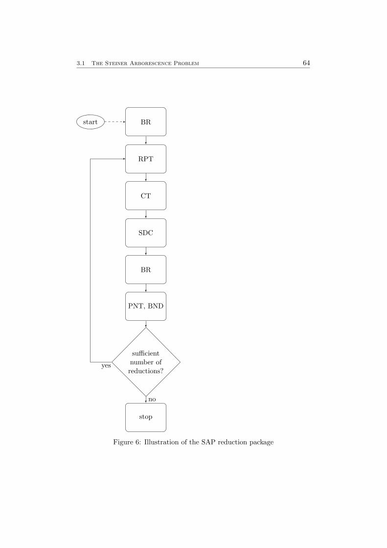
3.1 The Steiner Arborescence Problem 64
BRstart
RPT
CT
SDC
BR
PNT, BND
sufficientnumber ofreductions?
stop
yes
no
Figure 6: Illustration of the SAP reduction package
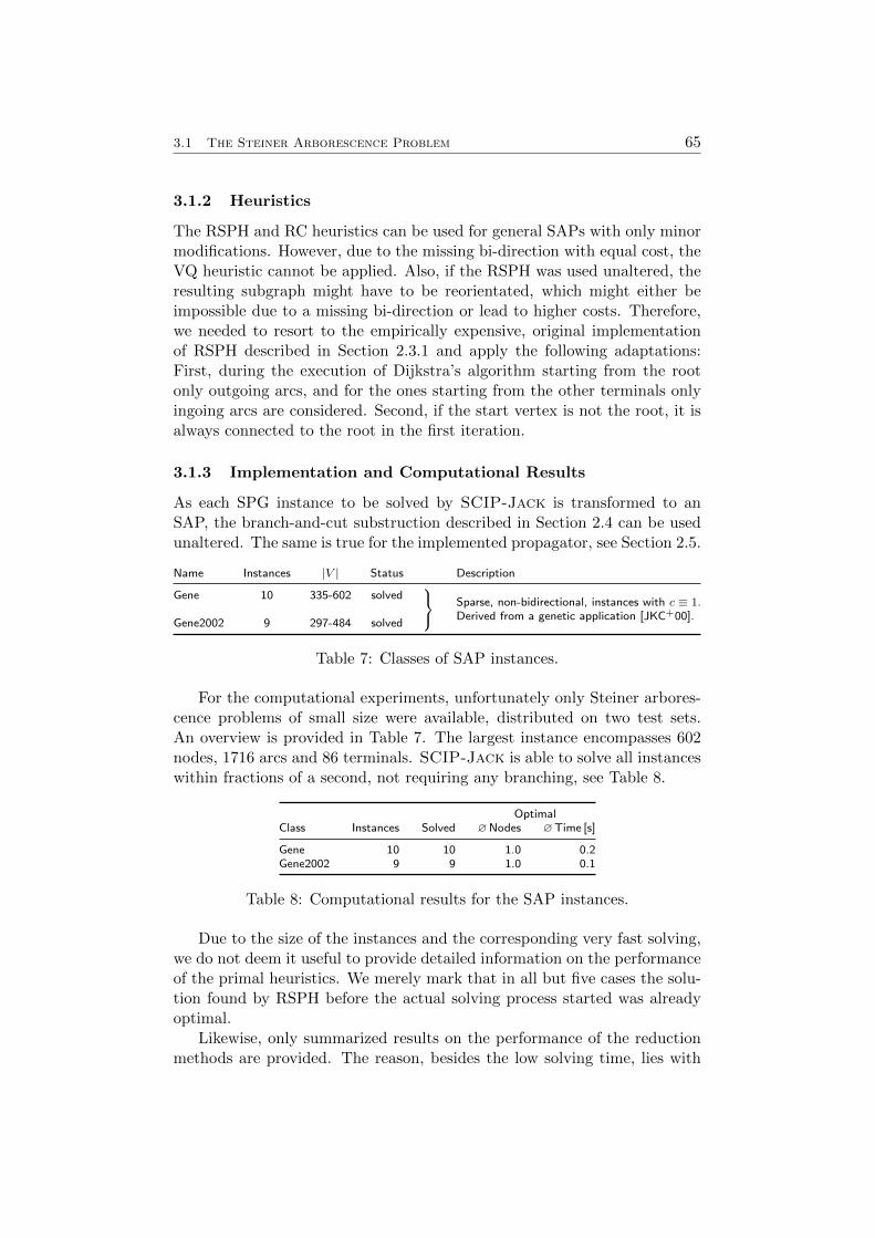
3.1 The Steiner Arborescence Problem 65
3.1.2 Heuristics
The RSPH and RC heuristics can be used for general SAPs with only minormodifications. However, due to the missing bi-direction with equal cost, theVQ heuristic cannot be applied. Also, if the RSPH was used unaltered, theresulting subgraph might have to be reorientated, which might either beimpossible due to a missing bi-direction or lead to higher costs. Therefore,we needed to resort to the empirically expensive, original implementationof RSPH described in Section 2.3.1 and apply the following adaptations:First, during the execution of Dijkstra’s algorithm starting from the rootonly outgoing arcs, and for the ones starting from the other terminals onlyingoing arcs are considered. Second, if the start vertex is not the root, it isalways connected to the root in the first iteration.
3.1.3 Implementation and Computational Results
As each SPG instance to be solved by SCIP-Jack is transformed to anSAP, the branch-and-cut substruction described in Section 2.4 can be usedunaltered. The same is true for the implemented propagator, see Section 2.5.
Name Instances |V | Status Description
Gene 10 335-602 solved Sparse, non-bidirectional, instances with c ≡ 1.
Derived from a genetic application [JKC+00].Gene2002 9 297-484 solved
Table 7: Classes of SAP instances.
For the computational experiments, unfortunately only Steiner arbores-cence problems of small size were available, distributed on two test sets.An overview is provided in Table 7. The largest instance encompasses 602nodes, 1716 arcs and 86 terminals. SCIP-Jack is able to solve all instanceswithin fractions of a second, not requiring any branching, see Table 8.
OptimalClass Instances Solved ∅Nodes ∅Time [s]
Gene 10 10 1.0 0.2Gene2002 9 9 1.0 0.1
Table 8: Computational results for the SAP instances.
Due to the size of the instances and the corresponding very fast solving,we do not deem it useful to provide detailed information on the performanceof the primal heuristics. We merely mark that in all but five cases the solu-tion found by RSPH before the actual solving process started was alreadyoptimal.
Likewise, only summarized results on the performance of the reductionmethods are provided. The reason, besides the low solving time, lies with
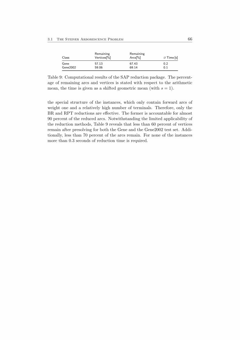
3.1 The Steiner Arborescence Problem 66
Remaining RemainingClass Vertices[%] Arcs[%] ∅Time [s]
Gene 57.13 67.43 0.2Gene2002 59.06 69.14 0.1
Table 9: Computational results of the SAP reduction package. The percent-age of remaining arcs and vertices is stated with respect to the arithmeticmean, the time is given as a shifted geometric mean (with s = 1).
the special structure of the instances, which only contain forward arcs ofweight one and a relatively high number of terminals. Therefore, only theBR and RPT reductions are effective. The former is accountable for almost90 percent of the reduced arcs. Notwithstanding the limited applicability ofthe reduction methods, Table 9 reveals that less than 60 percent of verticesremain after presolving for both the Gene and the Gene2002 test set. Addi-tionally, less than 70 percent of the arcs remain. For none of the instancesmore than 0.3 seconds of reduction time is required.
3.2 The Node Weighted Steiner Problem 67
3.2 The Node Weighted Steiner Problem
The node-weighted Steiner tree problem (NWSTP) is a generalizationof the Steiner tree problem in graphs in such a way that, in addition to theedges, also the vertices are assigned non-negative weights. The objectiveis to interconnect all terminals while minimizing the weight summed overboth vertices and edges spanned by the corresponding tree. First introducedin [Seg87], it has been the subject of several publications [DHK14, GK99,MR01], although mostly of theoretical nature.
The NWSTP is formally stated by: Given an undirected graph G =(V,E), vertex costs p : V → Q≥0, edge costs c : E → Q≥0, and a set T ⊂ Vof terminals, the objective is to find a tree S = (VS , ES) that spans T whileminimizing:
C(S) :=∑e∈ES
ce +∑v∈VS
pv.
3.2.1 Transformation
The key prerequisite for transforming an NWSTP to an SAP is the obser-vation that in a directed tree there cannot be more than one arc going intothe same vertex. Otherwise, two directed paths starting in the root wouldend in the same vertex, hence forming a cycle (in the undirected sense).Exploiting this consideration, we first substitute each edge of a given SPGby two anti-parallel arcs and second add the weight of each vertex to all ofits ingoing incident arcs:
Transformation 2 (NWSTP to SAP).Input: An NWSTP P = (V,E, T, c, p)Output: An SAP P ′ = (V ′, A′, T ′, c′, r′)
1. Set V ′ := V , T ′ := T , A′ := {(v, w) ∈ V ′ × V ′ : {v, w} ∈ E}.
2. Define c′ : A′ → Q≥0 by c′a = c{v,w} + pw, for a = (v, w) ∈ A′.
3. Choose a root r′ ∈ T ′ arbitrarily.
4. Return (V ′, A′, T ′, c′, r′).
Lemma 22 (NWSTP to SAP). Let P = (V,E, T, c, p) be an NWSTP andP ′ = (V ′, A′, T ′, c′) an SAP obtained by applying Transformation 2 on P .Denote by S and S ′ the set of solutions to P and P ′ respectively. S ′ can bebijectively mapped onto S by assigning each (V ′S′ , A
′S′) ∈ S ′ a (VS , ES) ∈ S
such that
VS :={v ∈ V : v ∈ V ′S′
}(43)
ES :={{v, w} ∈ E : (v, w) ∈ A′S′ or (w, v) ∈ A′S′
}. (44)
3.2 The Node Weighted Steiner Problem 68
Furthermore, it holds that:
c′(A′S′) + pr′ = c(ES) + p(VS). (45)
Proof. Proving that (43) and (44) form a bijection is equivalent to the pro-cedure in the proof of Lemma 15, since compared to the latter only theweights are altered. Now let S′ ∈ S ′ and S be the solution to P obtained byapplying the mapping (43) and (44) on S′. To acknowledge (45) one readilyobserves that for each node of S′ except for the root there is exactly oneincoming arc. Since for each arc (v, w) of S′ it holds that c′(v,w) = c{v,w}+pw,one infers that:∑
(v,w)∈A′S′
c′(v,w) =∑
(v,w)∈A′S′
(c{v,w} + pw
)=
∑{v,w}∈ES
c{v,w} +∑w∈VS
pw − pr′ ,
which implies (45).
The resulting problem is an SAP, which can be handled by SCIP-Jackusing the configurations described in the Steiner arborescence section. Itshould be noted that a transformation of an NWSTP to an SAP was alreadysuggested in [Fis91], but only for negative node weights.
3.2.2 Implementation and Computational Results
In our implementation, reductions are only applied to the transformed SAP.Although we would claim that NWSTP specific reduction techniques, whichcould be designed similarly to the ones for the PCSPG, would be moreeffective. Yet, due to limited time and the absence of a large number of, real-world, test instances, we have not developed any problem specific presolving.However, several generic reduction techniques described in [GKM+15] areused. Furthermore, the subsequent results have already been published inthe same publication.
Two NWSTP instances derived from a computational biology applica-tion published as part of the DIMACS Challenge were tested. The two in-stances differ drastically in their size: While the first one contains more than200,000 nodes—55,000 of them terminals—and almost 2.5 million edges, thesmaller instance comprises merely 386 nodes, 1477 edges, and 35 terminals.
The size of the first instance proves to be prohibitive for SCIP-Jack.The large number of edges significantly degrades the performance of thepreprocessing routines. Additionally, the memory requirements of this in-stance quickly exceeds the limits of SCIP-Jack when applying the defaultsettings within our heretofore used computational environment. To evaluatethe ability of SCIP-Jack to solve this particular instance, a run time of 72hours was used on a machine with 386 GB memory. After the applicationof the reduction techniques, the resulting graph contains 187,933 nodes and
3.2 The Node Weighted Steiner Problem 69
986,703 edges. This equates to a 8.6 % and 60.4 % decrease in the numberof nodes and edges respectively. SCIP-Jack fails to solve this instance tooptimality, but it manages to come as close as 0.0049% or closer to an op-timal solution. The much smaller second instance is solved by SCIP-Jackin the root node within 0.1 seconds.
3.3 The Rectilinear Steiner Minimum Tree Problem 70
3.3 The Rectilinear Steiner Minimum Tree Problem
The rectilinear Steiner minimum tree problem (RSMTP) can bestated as follows: Given a number of k ∈ N points in the plane, find a short-est tree consisting just of vertical and horizontal line segments and contain-ing all k points. The RSMTP is NP-hard, as proven in [GJ77]. Perhapsthe most famous of all Steiner variants, it has been the subject of variouspublications, e.g. [Ema10, HRW92, WWZ00, ZR00]. Furthermore, a gener-alization of the problem to the d-dimensional case, with natural d ≥ 2, hasbeen introduced, involving real-world applications in up to eight dimensions,e.g. in cancer research [CSHH+13].
A variant of the RSMTP is the obstacle-avoiding rectilinear Steinerminimum tree problem (OARSMTP). This problems includes the ad-ditional condition that the minimum-length rectilinear tree does not passthrough the interior of any specified axis-aligned rectangles, denoted as ob-stacles.
3.3.1 Transformation
Already in 1966, Hanan [Han66] suggested to reduce the RSMTP to theHanan grid obtained by constructing vertical and horizontal lines througheach given point of the RSMTP. Thereby, the RSMTP can be reduced to anSPG, since there is at least one solution to an RSMTP that is a subgraph ofthe grid. In the remainder of this subsection, both this construction and itsmulti-dimensional generalisation [Sny92] will be exploited in order to adaptthe RSMTP to our solver.
Given a d-dimensional, d ∈ N\{1}, RSMTP instance represented by a setof k ∈ N points in Qd, the first step on our way to solving the problem is toconstruct a d-dimensional Hanan grid. Thereupon, an SPG P = (V,E, T, c)can be built up in a straightforward way: The vertex set V is constructedby assigning each intersection point of the grid a vertex. Analogously, E isobtained by interconnecting the vertices V according to the grid structure,i.e. in such a way that two vertices in V are adjacent if and only if theircorresponding intersection points are adjacent in the grid. The set of ter-minals T consists of all vertices in V corresponding to one of the original kRSMTP points. Finally, the cost of an edge {vi, vj} ∈ E is defined by the(Euclidean) distance of the two d-dimensional points in the grid correspond-ing to vi and vj respectively. In [Sny92] it was demonstrated that at leastone optimal solution is preserved by this procedure and that the RSMTPcan be solved on the resulting SPG. Employing SCIP-Jack to do so, weobtain a solution S. Finally, S is re-transformed to a solution SRSMT to theRSMTP by adding for each edge in S the corresponding line segment (inQd) to SRSMT .
SCIP-Jack is easily extended to solve the obstacle-avoiding rectilinear
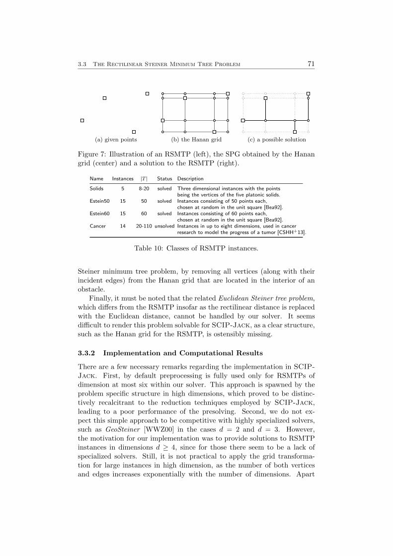
3.3 The Rectilinear Steiner Minimum Tree Problem 71
(a) given points (b) the Hanan grid (c) a possible solution
Figure 7: Illustration of an RSMTP (left), the SPG obtained by the Hanangrid (center) and a solution to the RSMTP (right).
Name Instances |T | Status Description
Solids 5 8-20 solved Three dimensional instances with the pointsbeing the vertices of the five platonic solids.
Estein50 15 50 solved Instances consisting of 50 points each,chosen at random in the unit square [Bea92].
Estein60 15 60 solved Instances consisting of 60 points each,chosen at random in the unit square [Bea92].
Cancer 14 20-110 unsolved Instances in up to eight dimensions, used in cancerresearch to model the progress of a tumor [CSHH+13].
Table 10: Classes of RSMTP instances.
Steiner minimum tree problem, by removing all vertices (along with theirincident edges) from the Hanan grid that are located in the interior of anobstacle.
Finally, it must be noted that the related Euclidean Steiner tree problem,which differs from the RSMTP insofar as the rectilinear distance is replacedwith the Euclidean distance, cannot be handled by our solver. It seemsdifficult to render this problem solvable for SCIP-Jack, as a clear structure,such as the Hanan grid for the RSMTP, is ostensibly missing.
3.3.2 Implementation and Computational Results
There are a few necessary remarks regarding the implementation in SCIP-Jack. First, by default preprocessing is fully used only for RSMTPs ofdimension at most six within our solver. This approach is spawned by theproblem specific structure in high dimensions, which proved to be distinc-tively recalcitrant to the reduction techniques employed by SCIP-Jack,leading to a poor performance of the presolving. Second, we do not ex-pect this simple approach to be competitive with highly specialized solvers,such as GeoSteiner [WWZ00] in the cases d = 2 and d = 3. However,the motivation for our implementation was to provide solutions to RSMTPinstances in dimensions d ≥ 4, since for those there seem to be a lack ofspecialized solvers. Still, it is not practical to apply the grid transforma-tion for large instances in high dimension, as the number of both verticesand edges increases exponentially with the number of dimensions. Apart
3.3 The Rectilinear Steiner Minimum Tree Problem 72
from the described modifications, a transformed RSMTP instance is han-dled equivalently to a usual SPG instance by SCIP-Jack.
An alternative SPG based solving method for the RSMTP is the fullSteiner tree (FST) generation [Zac99]. The concatenation of FSTs, andthus the solving of the underlying RSMTP, can be reduced to an SPG,as done in [Pol04]. Thereby, the tested RSMTP instances could be solvedsignificantly faster than by the well-known, specialized solver GeoSteiner.
Optimal Timeout
Class Instances Solved ∅Nodes ∅Time [s] ∅Nodes ∅Gap [%]
Solids 5 5 32.0 17.7 – –Estein50 15 14 2.6 1408.3 107.0 0.3Estein60 15 9 1.0 3641.8 12.9 0.3Cancer 14 11 1.0 25.5 1.0 2.3
Table 11: Computational results for RSMTP instances.
The experimental results, summarized in Table 11, show that all of theSolids instances can be solved, four of them within a few seconds and atthe root node. For the Estein50 class only one instance remains unsolvedafter two hours. Further, 13 of the instances can be solved at the root node.Regarding the related, but in terms of problem size larger, Estein60 test set,a notable decrease of the performance is evident: Only nine instances canbe solved to optimality. However, the average gap remains the same. Fur-thermore, the number of branch-and-bound nodes of the unsolved problemsis almost ten times smaller than for the Estein50 class.
Finally, the cancer class manifests the ability of SCIP-Jack to handleand solve instances in up to eight dimensions. Of the 14 instances 11 aresolved at the root node. To the best of our knowledge, we are the firstto solve those instances to optimality. Of the solved instances seven finishwithin 10 seconds and none takes longer than eight minutes. However, theinstance 11 8D demonstrates the limits of the grid approach: The instanceis transformed into a problem containing almost five million nodes and 65million edges, a scale that is prohibitive for employing SCIP-Jack on amodest machine. As a result, SCIP-Jack quickly runs out of memorywhile solving this instance. Similarly, for the 12 8D problem, encompassingmore than 12 million edges, SCIP-Jack stops short of computing a dualbound within the time limit, since it spends 98 percent of the time in thelocal heuristic (VQ).
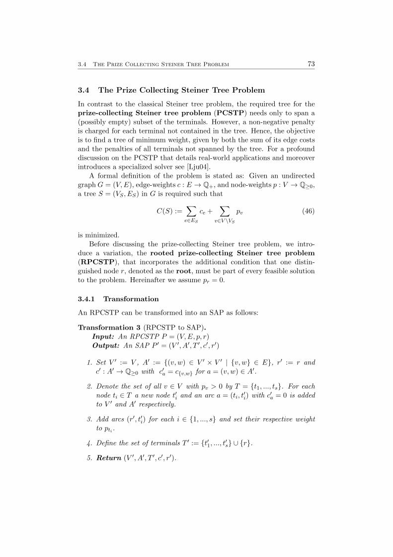
3.4 The Prize Collecting Steiner Tree Problem 73
3.4 The Prize Collecting Steiner Tree Problem
In contrast to the classical Steiner tree problem, the required tree for theprize-collecting Steiner tree problem (PCSTP) needs only to span a(possibly empty) subset of the terminals. However, a non-negative penaltyis charged for each terminal not contained in the tree. Hence, the objectiveis to find a tree of minimum weight, given by both the sum of its edge costsand the penalties of all terminals not spanned by the tree. For a profounddiscussion on the PCSTP that details real-world applications and moreoverintroduces a specialized solver see [Lju04].
A formal definition of the problem is stated as: Given an undirectedgraph G = (V,E), edge-weights c : E → Q+, and node-weights p : V → Q≥0,a tree S = (VS , ES) in G is required such that
C(S) :=∑e∈ES
ce +∑
v∈V \VS
pv (46)
is minimized.Before discussing the prize-collecting Steiner tree problem, we intro-
duce a variation, the rooted prize-collecting Steiner tree problem(RPCSTP), that incorporates the additional condition that one distin-guished node r, denoted as the root, must be part of every feasible solutionto the problem. Hereinafter we assume pr = 0.
3.4.1 Transformation
An RPCSTP can be transformed into an SAP as follows:
Transformation 3 (RPCSTP to SAP).Input: An RPCSTP P = (V,E, p, r)Output: An SAP P ′ = (V ′, A′, T ′, c′, r′)
1. Set V ′ := V , A′ := {(v, w) ∈ V ′ × V ′ | {v, w} ∈ E}, r′ := r andc′ : A′ → Q≥0 with c′a = c{v,w} for a = (v, w) ∈ A′.
2. Denote the set of all v ∈ V with pv > 0 by T = {t1, ..., ts}. For eachnode ti ∈ T a new node t′i and an arc a = (ti, t
′i) with c′a = 0 is added
to V ′ and A′ respectively.
3. Add arcs (r′, t′i) for each i ∈ {1, ..., s} and set their respective weightto pti.
4. Define the set of terminals T ′ := {t′1, ..., t′s} ∪ {r}.
5. Return (V ′, A′, T ′, c′, r′).
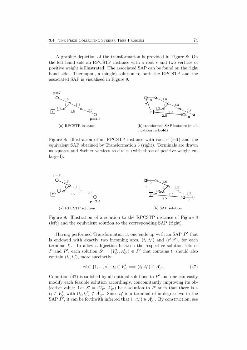
3.4 The Prize Collecting Steiner Tree Problem 74
A graphic depiction of the transformation is provided in Figure 8: Onthe left hand side an RPCSTP instance with a root r and two vertices ofpositive weight is illustrated. The associated SAP can be found on the righthand side. Thereupon, a (single) solution to both the RPCSTP and theassociated SAP is visualised in Figure 9.
r
p=2.5
p=7
1.22.3
1.6
1 1.3
1.5
(a) RPCSTP instance
r1.2
2.3
1.6
1 1.3
1.52.5
7
0
0
(b) transformed SAP instance (mod-ifications in bold)
Figure 8: Illustration of an RPCSTP instance with root r (left) and theequivalent SAP obtained by Transformation 3 (right). Terminals are drawnas squares and Steiner vertices as circles (with those of positive weight en-larged).
r
p=2.5
p=7
1.22.3
1.6
1 1.3
1.5
(a) RPCSTP solution
r1.2
2.3
1.6
1 1.3
1.52.5
7
0
0
(b) SAP solution
Figure 9: Illustration of a solution to the RPCSTP instance of Figure 8(left) and the equivalent solution to the corresponding SAP (right).
Having performed Transformation 3, one ends up with an SAP P ′ thatis endowed with exactly two incoming arcs, (ti, ti
′) and (r′, t′), for eachterminal t′i. To allow a bijection between the respective solution sets ofP and P ′, each solution S′ = (V ′S′ , A
′S′) ∈ P ′ that contains ti should also
contain (ti, ti′), more succinctly:
∀i ∈ {1, ..., s} : ti ∈ V ′S′ =⇒ (ti, ti′) ∈ A′S′ . (47)
Condition (47) is satisfied by all optimal solutions to P ′ and one can easilymodify each feasible solution accordingly, concomitantly improving its ob-jective value: Let S′ = (V ′S′ , A
′S′) be a solution to P ′ such that there is a
ti ∈ V ′S′ with (ti, ti′) /∈ A′S′ . Since ti
′ is a terminal of in-degree two in theSAP P ′, it can be forthwith inferred that (r, ti
′) ∈ A′S′ . By construction, see
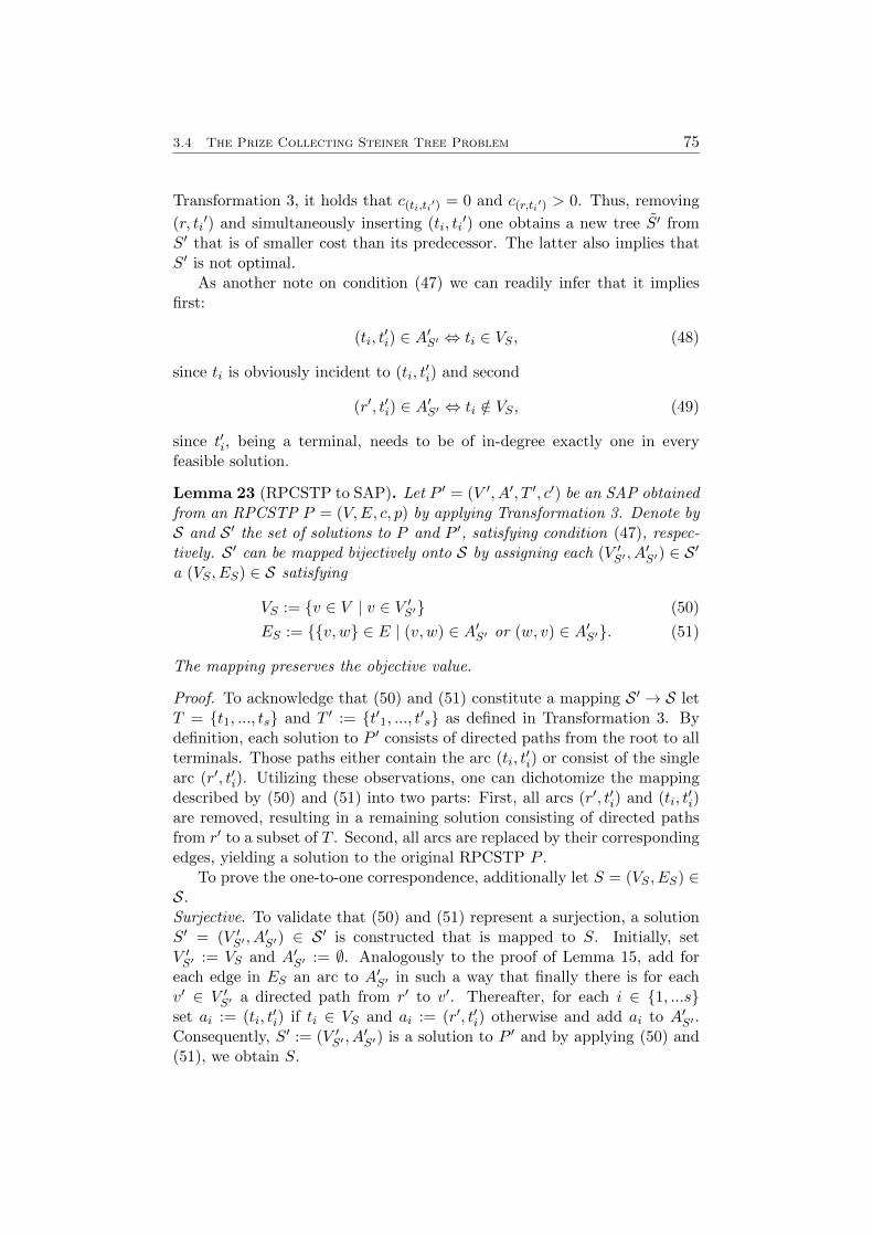
3.4 The Prize Collecting Steiner Tree Problem 75
Transformation 3, it holds that c(ti,ti′) = 0 and c(r,ti′) > 0. Thus, removing
(r, ti′) and simultaneously inserting (ti, ti
′) one obtains a new tree S′ fromS′ that is of smaller cost than its predecessor. The latter also implies thatS′ is not optimal.
As another note on condition (47) we can readily infer that it impliesfirst:
(ti, t′i) ∈ A′S′ ⇔ ti ∈ VS , (48)
since ti is obviously incident to (ti, t′i) and second
(r′, t′i) ∈ A′S′ ⇔ ti /∈ VS , (49)
since t′i, being a terminal, needs to be of in-degree exactly one in everyfeasible solution.
Lemma 23 (RPCSTP to SAP). Let P ′ = (V ′, A′, T ′, c′) be an SAP obtainedfrom an RPCSTP P = (V,E, c, p) by applying Transformation 3. Denote byS and S ′ the set of solutions to P and P ′, satisfying condition (47), respec-tively. S ′ can be mapped bijectively onto S by assigning each (V ′S′ , A
′S′) ∈ S ′
a (VS , ES) ∈ S satisfying
VS := {v ∈ V | v ∈ V ′S′} (50)
ES := {{v, w} ∈ E | (v, w) ∈ A′S′ or (w, v) ∈ A′S′}. (51)
The mapping preserves the objective value.
Proof. To acknowledge that (50) and (51) constitute a mapping S ′ → S letT = {t1, ..., ts} and T ′ := {t′1, ..., t′s} as defined in Transformation 3. Bydefinition, each solution to P ′ consists of directed paths from the root to allterminals. Those paths either contain the arc (ti, t
′i) or consist of the single
arc (r′, t′i). Utilizing these observations, one can dichotomize the mappingdescribed by (50) and (51) into two parts: First, all arcs (r′, t′i) and (ti, t
′i)
are removed, resulting in a remaining solution consisting of directed pathsfrom r′ to a subset of T . Second, all arcs are replaced by their correspondingedges, yielding a solution to the original RPCSTP P .
To prove the one-to-one correspondence, additionally let S = (VS , ES) ∈S.Surjective. To validate that (50) and (51) represent a surjection, a solutionS′ = (V ′S′ , A
′S′) ∈ S ′ is constructed that is mapped to S. Initially, set
V ′S′ := VS and A′S′ := ∅. Analogously to the proof of Lemma 15, add foreach edge in ES an arc to A′S′ in such a way that finally there is for eachv′ ∈ V ′S′ a directed path from r′ to v′. Thereafter, for each i ∈ {1, ...s}set ai := (ti, t
′i) if ti ∈ VS and ai := (r′, t′i) otherwise and add ai to A′S′ .
Consequently, S′ := (V ′S′ , A′S′) is a solution to P ′ and by applying (50) and
(51), we obtain S.
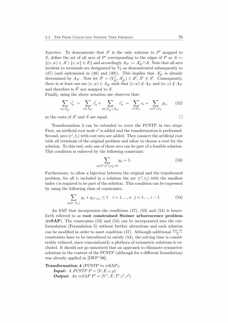
3.4 The Prize Collecting Steiner Tree Problem 76
Injective. To demonstrate that S′ is the only solution to P ′ mapped toS, define the set of all arcs of P ′ corresponding to the edges of P as A :={(v, w) ∈ A′ | {v, w} ∈ E} and accordingly AS′ := A′S′∩A. Note that all arcsincident to terminals are designated by VS as demonstrated subsequently to(47) (and epitomized in (48) and (49)). This implies that A′S′ is alreadydetermined by AS′ . Now let S′ = (V ′
S′, A′
S′) ∈ S ′, S′ 6= S′. Consequently,
there is at least one arc (v, w) ∈ AS′ such that (v, w) /∈ AS′ and (w, v) /∈ AS′and therefore is S′ not mapped to S.Finally, using the above notation one observes that:∑
a∈A′S′
c′a =∑a∈AS′
c′a +∑
a∈A′S′\AS′
c′a =∑e∈ES
ce +∑
v∈V \VS
pv, (52)
so the costs of S′ and S are equal.
Transformation 3 can be extended to cover the PCSTP in two steps:First, an artificial root node r′ is added and the transformation is performed.Second, arcs (r′, ti) with cost zero are added. They connect the artificial rootwith all terminals of the original problem and allow to choose a root for thesolution. To this end, only one of these arcs can be part of a feasible solution.This condition is enforced by the following constraint:∑
a∈δ+(r′),c′a=0
ya = 1. (53)
Furthermore, to allow a bijection between the original and the transformedproblem, for all ti included in a solution the arc (r′, ti) with the smallestindex i is required to be part of the solution. This condition can be expressedby using the following class of constraints:∑
a∈δ−(tj)
ya + y(r′,ti) ≤ 1 i = 1, ..., s; j = 1, ..., i− 1. (54)
An SAP that incorporates the conditions (47), (53) and (54) is hence-forth referred to as root constrained Steiner arborescence problem(rcSAP). The constraints (53) and (54) can be incorporated into the cut-formulation (Formulation 5) without further alterations and each solution
can be modified in order to meet condition (47). Although additional s(s−1)2
constraints have to be introduced to satisfy (54), the solving time is consid-erably reduced, since concomitantly a plethora of symmetric solutions is ex-cluded. It should not go unnoticed that an approach to eliminate symmetricsolutions in the context of the PCSTP (although for a different formulation)was already applied in [LWP+06].
Transformation 4 (PCSTP to rcSAP).Input: A PCSTP P = (V,E, c, p)Output: An rcSAP P ′ = (V ′, A′, T ′, c′, r′)
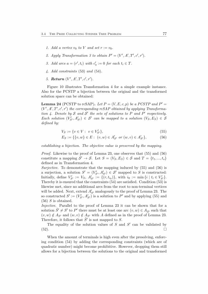
3.4 The Prize Collecting Steiner Tree Problem 77
1. Add a vertex v0 to V and set r := v0.
2. Apply Transformation 3 to obtain P ′ = (V ′, A′, T ′, c′, r′).
3. Add arcs a = (r′, ti) with c′a := 0 for each ti ∈ T .
4. Add constraints (53) and (54).
5. Return (V ′, A′, T ′, c′, r′).
Figure 10 illustrates Transformation 4 for a simple example instance.Also for the PCSTP a bijection between the original and the transformedsolution space can be obtained:
Lemma 24 (PCSTP to rcSAP). Let P = (V,E, c, p) be a PCSTP and P ′ =(V ′, A′, T ′, c′, r′) the corresponding rcSAP obtained by applying Transforma-tion 4. Denote by S and S ′ the sets of solutions to P and P ′ respectively.Each solution (V ′S′ , A
′S′) ∈ S ′ can be mapped to a solution (VS , ES) ∈ S
defined by:
VS := {v ∈ V : v ∈ V ′S′}, (55)
ES := {{v, w} ∈ E : (v, w) ∈ A′S′ or (w, v) ∈ A′S′}, (56)
establishing a bijection. The objective value is preserved by the mapping.
Proof. Likewise to the proof of Lemma 23, one observes that (55) and (56)constitute a mapping S ′ → S. Let S = (VS , ES) ∈ S and T = {t1, ..., ts}defined as in Transformation 4.Surjective. To demonstrate that the mapping induced by (55) and (56) isa surjection, a solution S′ = (V ′S′ , A
′S′) ∈ S ′ mapped to S is constructed:
Initially, define V ′S′ := VS , A′S′ := {(r, ti0)}, with i0 := min {i | ti ∈ V ′S′}.Thereby it is ensured that the constraints (54) are satisfied. Condition (53) islikewise met, since no additional arcs from the root to non-terminal verticeswill be added. Next, extend A′S′ analogously to the proof of Lemma 23. Theso constructed S′ := (V ′S′ , A
′S′) is a solution to P ′ and by applying (55) and
(56) S is obtained.Injective. Parallel to the proof of Lemma 23 it can be shown that for asolution S′ 6= S′ to P ′ there must be at least one arc (v, w) ∈ AS′ such that(v, w) /∈ AS′ and (w, v) /∈ AS′ with A defined as in the proof of Lemma 23.Therefore, it follows that S′ is not mapped to S.
The equality of the solution values of S and S′ can be validated by(52).
When the amount of terminals is high even after the presolving, enforc-ing condition (54) by adding the corresponding constraints (which are ofquadratic number) might become prohibitive. However, dropping them stillallows for a bijection between the solutions to the original and transformed
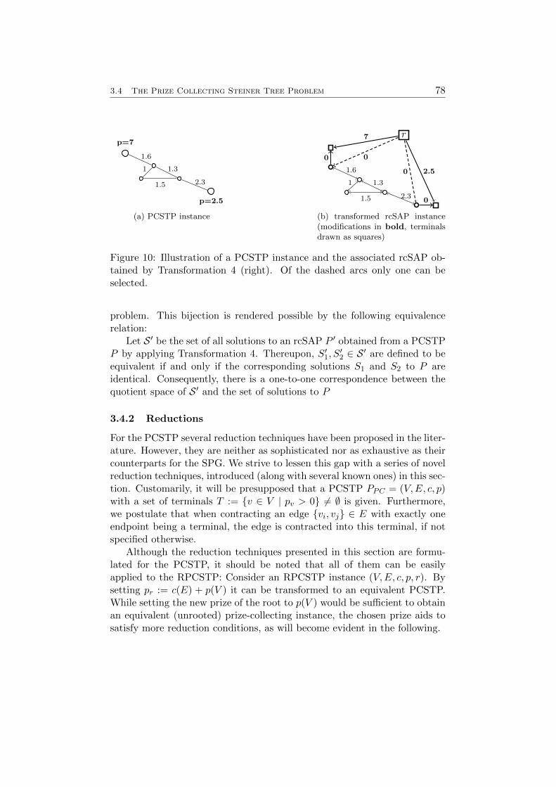
3.4 The Prize Collecting Steiner Tree Problem 78
p=2.5
p=7
2.3
1.6
1 1.3
1.5
(a) PCSTP instance
r
0
0
2.5
7
0
0
2.3
1.6
1 1.3
1.5
(b) transformed rcSAP instance(modifications in bold, terminalsdrawn as squares)
Figure 10: Illustration of a PCSTP instance and the associated rcSAP ob-tained by Transformation 4 (right). Of the dashed arcs only one can beselected.
problem. This bijection is rendered possible by the following equivalencerelation:
Let S ′ be the set of all solutions to an rcSAP P ′ obtained from a PCSTPP by applying Transformation 4. Thereupon, S′1, S
′2 ∈ S ′ are defined to be
equivalent if and only if the corresponding solutions S1 and S2 to P areidentical. Consequently, there is a one-to-one correspondence between thequotient space of S ′ and the set of solutions to P
3.4.2 Reductions
For the PCSTP several reduction techniques have been proposed in the liter-ature. However, they are neither as sophisticated nor as exhaustive as theircounterparts for the SPG. We strive to lessen this gap with a series of novelreduction techniques, introduced (along with several known ones) in this sec-tion. Customarily, it will be presupposed that a PCSTP PPC = (V,E, c, p)with a set of terminals T := {v ∈ V | pv > 0} 6= ∅ is given. Furthermore,we postulate that when contracting an edge {vi, vj} ∈ E with exactly oneendpoint being a terminal, the edge is contracted into this terminal, if notspecified otherwise.
Although the reduction techniques presented in this section are formu-lated for the PCSTP, it should be noted that all of them can be easilyapplied to the RPCSTP: Consider an RPCSTP instance (V,E, c, p, r). Bysetting pr := c(E) + p(V ) it can be transformed to an equivalent PCSTP.While setting the new prize of the root to p(V ) would be sufficient to obtainan equivalent (unrooted) prize-collecting instance, the chosen prize aids tosatisfy more reduction conditions, as will become evident in the following.
3.4 The Prize Collecting Steiner Tree Problem 79
Basic Reductions
Once again, the straightforward reduction techniques are very reminiscentof those for the SPG:
Non-terminal of degree one (NTD0): A non-terminal of degree zerocan be deleted.
Non-terminal of degree one (NTD1): A non-terminal of degree oneand its incident edge can be deleted.
Non-terminal of degree two (NTD2): A non-terminal vi of degree twoand its incident edges {vi, vj}, {vi, vk} can be substituted by a single edge{vj , vk} with cjk := cij + cik. In the case of two parallel edges, one of lowestcost is retained.
Terminal of degree zero: (TD0) If there are terminals ti, tj ∈ T , suchthat δ(ti) = ∅ and pti ≤ ptj , then ti can be deleted from V (and pti has to beadded to the solution value of each feasible solution to PPC).
Proof. Since the only solution that contains ti (i.e. {ti}) is of higher or equalcost than the feasible solution {tj}, there is at least one optimal solutionthat does not contain ti.
Terminal of degree one (TD1): If there are terminals ti, tj ∈ T , suchthat δ(ti) = {el}, pti ≤ ptj and additionally
a) pti ≤ cel, then ti and el can be discarded;
b) pti > cel, then ti and el = {ti, vk} can be discarded, concurrently settingpvk := pvk + pti − cel.
In case a) pti and in case b) cel has to be added to the objective value of eachfeasible solution to PPC to obtain the value of the corresponding originalsolution.
Proof. Since pti ≤ pt′ , {ti} cannot be the unique optimal solution.a) Each solution which contains el (and ti) can be reduced to a solution of nothigher cost by removing el as well as ti. Hence, there is at least one optimalsolution containing neither el nor ti. Since in the transformed problem, ticannot be part of any solution, pti has to be added to the objective value.b) Each solution containing vk but not ti can be extended to a solution ofsmaller cost by adding el and ti. So each optimal solution is preserved by theoperation. To demonstrate that the stated relation between the respectivecosts hold, denote by P ′PC = (V ′, E′, c′, p′) the problem obtained from PPCby removing ti and el and setting p′vk := pvk +pti−cel . Let S′ = (V ′S′ , E
′S′) be
3.4 The Prize Collecting Steiner Tree Problem 80
a solution to P ′PC not containing vk and denote the corresponding solutionto PPC by S = (VS , ES). Thereupon:
C ′(S′) =∑e∈E′
S′
c′e +∑
v∈V ′\V ′S′
p′v
=∑e∈E′
S′
c′e +∑
v∈V ′\(V ′S′∪{vk})
p′v + pvk + pti − cel
=∑e∈ES
ce +∑
v∈V \VS
pv − cel = C(S)− cel .
If, on the other hand, vk is contained in S′, then S comprises both el andti, hence:
C ′(S′) =∑e∈E′
S′
c′e +∑
v∈V ′\V ′S′
p′v
=∑e∈ES
ce − cel +∑
v∈V \VS
pv = C(S)− cel .
Hence, the relation C ′(S′) = C(S)− cel is established.
Terminal of degree two (TD2): Let ti, tj ∈ T , such thatδ(ti) = {{ti, vk}, {ti, vl}} and pti ≤ min{c{vk,ti}, c{ti,vl}, ptj}. If a new edge{vk, vl} of cost c{ti,vk} + c{ti,vl} − pti is added, {vk, ti}, {vl, ti} and ti canbe deleted. For a solution S′ to the so transformed problem P ′PC and thecorresponding solution S to the original problem the relation C ′(S′) + pti =C(S) holds.
Proof. If ti is of degree one in a solution, then both ti and its incident edgein this solution can be removed to obtain a solution of smaller or equal cost.On the other hand, if ti is of degree zero in a solution, then it is of equal orhigher cost than the feasible solution {tj}. Conclusively, if ti is containedin an optimal solution, there is at least one optimal solution in which ti isof degree two. If a solution S′ to P ′PC contains the new edge {vk, vl}, thecorresponding solution S to PPC contains both original edges of, summed,cost c{ti,vk} + c{ti,vl}, hence C ′(S′) + pti = C(S). On the other hand, if{vk, vl} is not contained in S′, then pti is not contained in S and thereforeC ′(S′) + pti = C(S) holds as well.
Both NTD1 and NTD2 were already proposed in [LR04]. However, tothe best of our knowledge, the tests TD0, TD1 and TD2 have not beendescribed in the literature yet: TD1 b) and TD2 were suggested in [Uch06],but without the condition ∃tj : ptj ≥ pti . The absence of the latter, or acomparable condition, renders both tests erroneous, since a unique optimalsolution consisting only of ti could then be discarded. We denote by Degree-Test (DT) the successive execution of those five tests. Since in each of them
3.4 The Prize Collecting Steiner Tree Problem 81
only vertices of maximal degree two are checked, the worst-case complexityof DT is of O(n), assuming that deleting or inserting an edge can be realizedin O(1).
Furthermore, noting that a PCSTP graph is not necessarily connected,we suggest the following simple test:
Unreachable non-terminal (UNT): Each non-terminal vertex that can-not be connected by a path to any terminal can be removed along with allincident edges.
We realize this test in linear time (with respect to the number of nodesand edges) by running a breadth-first search on the transformed graph ob-tained by Transformation 4 and deleting all vertices (and incident edges)that are not visited.
Alternative Based Reductions
The pivotal concept of the bottleneck Steiner distance which gives rise tostrong reduction techniques for the SPG fails with the PCSTP in its originalform. The reason is that a terminal need not be part of any optimal solution,so it cannot a priori be used as the endpoint of an alternative path. However,a redefinition of the bottleneck Steiner distance has been proposed in thecontext of the PCSTP [Uch06]:
Let vi, vj ∈ V be two distinct vertices, P(vi, vj) the set of all simple pathsbetween vi and vj and P ∈ P(vi, vj). Furthermore, denote by P (vk, vl) thesubpath between two vertices in P . The local prize-collecting Steinerdistance of P (vk, vl) is defined as
sdloc(P (vk, vl)) =∑
e∈E[P (vk,vl)]
ce −∑
v∈V [P (vk,vl)]\{vk,vl}
pv. (57)
Built upon this definition, the prize-collecting Steiner distance of (thewhole path) P is:
sd(P ) = maxvk,vl∈V [P ]
sdloc(P (vk, vl)). (58)
Finally, the bottleneck prize-collecting Steiner distance betweenvi and vk can be defined as
spc(vi, vk) = min{sd(P ) | P ∈ P(vi, vk)}. (59)
The two most salient tests spawned by the Steiner bottleneck distancein the context of the SPG find their equivalent for the PCSTP:
Lemma 25. Every edge {vi, vj} ∈ E with cij > spc(vi, vj) can be discarded.
3.4 The Prize Collecting Steiner Tree Problem 82
Lemma 26. A non-terminal vertex vi is of degree at most two in a least oneminimum Steiner tree if for each set ∆, with |∆| ≥ 3, of vertices adjacent tovi it holds that: the (summed) cost of all edges δ(vi) ∩ δ(∆) is not less thanthe weight of a minimum spanning tree for the network (∆,∆×∆, spc).
Both Lemma 25 and Lemma 26 were formulated and proved in [Uch06].In the same publication it was demonstrated that computing the bottleneckprize-collecting Steiner distance is NP-hard and the application of heuristicswas suggested. However, no information was provided on how to actuallyproceed in order to obtain those distances. Thereupon, we propose two noveltests to calculate an upper bound on the bottleneck prize-collecting Steinerdistance:
First, an adaptation of the SDC test, see Section 2.2.3 is employed. Onlyone addition to the original test is necessary: To eliminate an edge {vi, vj},for an alternative path P between vi and vj containing exactly one interiorterminal tk, the inequality C(P )− ptk ≤ c{vi,v} needs to be satisfied as well.In the context of the (R)PCSTP we likewise denote this test by SDC.
For the second test some spadework is necessary. We wish to obtain fora given α ∈ N to each terminal its α d-nearest terminals. Unfortunately,Duin’s nearest terminals algorithm utilized in Section 2.2 merely allows tocompute the d-nearest terminals vi,1, vi,2, ... to a non-terminal vi. Remedyis provided by the following, novel, lemma:
For ease of presentation, we subsequently assume for each {vj , vk} ∈δ(N(ti)
)that vj ∈ N(ti) holds.
Lemma 27. Let α ∈ N, 1 ≤ α < |T |, ti ∈ T and assume that for eachvj ∈ V \ T the α + 1 d-nearest terminals vj,1, vj,2, ..., vj,α+1 exist and their
d-distances to ti are available. Thereupon, setting t(0)i := ti, the remainder
of the α+ 1 d-nearest terminals t(1)i , ..., t
(a)i to ti can be computed as follows:
Set t(1)i := vk,1 with k such that:
d(ti, vk,1) = min{vj ,vk}∈δ(N(ti))
{d(ti, vj) + cjk + d(vk, vk,1)}. (60)
Having computed t(1)i , ..., t
(r)i (r < α), we set t
(r+1)i := vk,l with k, l such that:
d(ti, vk,l) = min{vj ,vk}∈δ(N(ti))
{d(ti, vj) + cjk
+ min{d(vk, vk,l) | l = 1, ..., r + 2 : vk,l 6= t(q)i , q = 0, ..., r}
}. (61)
Proof. First, note that both of the minima attained in (60) and (61) corre-
spond to a path. Next, let t(1)min ∈ T \ {ti} such that d(ti, t
(1)min) is minimal.
The corresponding path between ti and t(1)min contains an edge {vj , vk} ∈
δ(N(ti)) and since the path is of minimum d-length its cost is d(ti, vj) +
3.4 The Prize Collecting Steiner Tree Problem 83
cjk + d(vk, vk,1). Hence:
min{vj ,vk}∈δ(N(ti))
{d(ti, vj) + cjk + d(vk, vk,1)} ≤ d(ti, t(1)min).
Furthermore, for {vj , vk} ∈ δ(N(ti)) let P be a path consisting of a shortestpath between ti and vj , the edge {vj , vk} and a shortest path between vkand vk,1. Since vj lies in N(ti) and vk,1 is a d-nearest terminal to vk, thepath P contains no intermediary terminal vertices. Consequently it is ofcost at least d(ti, vk,1), so:
min{vj ,vk}∈δ(N(ti))
{d(ti, vj) + cjk + d(vk, vk,1)} ≥ d(ti, vk,1) ≥ d(ti, t(1)min).
The validity of the claim for r > 1 can be demonstrated similarly: Denote
by t(r)min the r’th d-nearest terminal to ti, if such a terminal exists. Let r ∈
N, 1 < r < α and assume that there is a t(r+1)min . Additionally, let P be a path
corresponding to d(ti, t(r+1)min ). This path contains an edge {vj , vk} ∈ δ(N(ti))
and can therefore be dissected into the subpath P (ti, vj), the edge {vj , vk}and the subpath P (vk, t
(r+1)min ). The first subpath is of length d(ti, vj), since
otherwise it could be substituted by a shorter one. The second subpath is
of length at least min{d(vk, vk,l) | l = 1, ..., r + 2 : vk,l 6= t(q)i , q = 0, ..., r, },
because this is the minimum length between vk and a terminal other than
t(0)i , t
(1)i , ..., t
(r)i and without intermediary terminals. Note that vk itself can
be a terminal, so just scrutinizing all vk,l with l ∈ {1, ..., r + 1} is not
sufficient, since these r + 1 terminals could be identical to t(0)i , t
(1)i , ..., t
(r)i .
This discussion implies:
min{vj ,vk}∈δ(N(ti))
{d(ti, vj) + cjk
+ min{d(vk, vk,l) | l = 1, ..., r + 2 : vk,l 6= t(q)i , q = 0, 1, ..., r}
}≤ d(ti, t
(r+1)min ).
To see the converse, note that each path P associated with the set in (61)is composed of the components P (ti, vj), {vj , vk} and P (vk, vk,l), for some l
such that vk,l /∈ {t(0)i , t
(1)i , ..., t
(r)i }. By construction none of these components
contain intermediary terminals, thus the same holds for P . Hence, C(P ) ≥d(ti, vk,l) and therefore:
min{vj ,vk}∈δ(N(ti))
{d(ti, vj) + cjk
+ min{d(vk, vk,l) | l = 1, ..., r + 2 : vk,l 6= t(q)i , q = 0, 1, ..., r}
}≥ d(ti, t
(r+1)min ).
Consequently, the lemma is established.
3.4 The Prize Collecting Steiner Tree Problem 84
Corollary 28. Let α ∈ N, 0 < α < |T |. The α d-nearest terminals to eachterminal can be computed with worst-case complexity of O(m+ n log n) if αis considered a constant.
Proof. Compute to each non-terminal the α + 1 d-nearest terminals, in atotal of O(m+n log n). Subsequently, traverse each Voronoi-boundary edge{vi, vj} ∈ E, with tk := base(vi) and tl := base(vj), and update the d-nearest
terminals t(1)k and t
(1)l as well as the corresponding d-distances according to
(60). Thereafter, successively traverse all Voronoi-boundary edges {vi, vj} ∈E for α − 1 additional times, updating in each iteration z both the values
t(z)k and t
(z)l and the corresponding d-distances according to (61). In the z’th
iteration for each edge at most z d-nearest terminals have to be checked. Asa is assumed to be a constant and z ≤ α holds, the worst-case complexityfor all iterations is of O(m). In total this amounts to the overall bound ofO(m+ n log n).
Having established Lemma 27, we are in a position to propose a modifica-tion of the SD test introduced in Section 2.2.3: As with the SPG, we computethe four d-nearest terminals to each non-terminal vi (or as many as exist).
For each terminal ti we compute, three d-nearest terminals t(1)i , t
(2)i , t
(3)i .
Additionally, we determine a further terminal t(4)i that is not necessarily a
fourth d-nearest to ti, but reasonably close empirically. The reason behindthis procedure is that for an exact computation, the fifth d-nearest near-est terminals vj,5 to all Steiner vertices vj are necessary. We proceed bychoosing to each ti a terminal vk,l such that:
d(ti, vk,l) = min{vj ,vk}∈δ(N(ti))
{d(ti, vj) + cjk
+ min{d(vk, vk,l) | l = 1, ..., 4 : vk,l 6= t(q)i , q = 0, 1, ..., 3}
}.
For all (both non-terminal and terminal) vertices vi we denote the set ofthe so obtained (up to four) close terminals by Li. Next, we scrutinize eachedge ek = {vi, vj} ∈ E:
Mark each vertex of tq ∈ Li satisfying d(vi, tq) < cij . Thereafter, proceedfor each tl ∈ Lj such that d(vj , tl) < cij as follows: If tl has been marked and
d(vi, tl) + d(vj , tl) − ptl < cij , delete ek. Otherwise, if a t(r)l , r = 1, ..., 4 has
been marked, we have found a path between vi and vj , containing exactly
two intermediary terminals, namely tl and t(r)l . Next, we examine whether
the prize-collecting Steiner distance of this path is smaller than the costof the edge {vi, vj}. For this purpose, we need to check whether the fourinequalities
1. d(tl, t(r)l ) < cij ,
2. d(tl, t(r)l ) + d(vj , tl)− ptl < cij ,
3.4 The Prize Collecting Steiner Tree Problem 85
3. d(tl, t(r)l )− d(vi, t
(r)l )− p
t(r)l
< cij ,
4. d(tl, t(r)l ) + d(vj , tl) + d(vi, t
(r)l )− ptl − pt(r)
l
< cij
are satisfied. If this is the case, cij > spc(vi, vj) holds and we consequentlyremove ek. The above procedure is reiterated vice versa, starting from vjand marking all vertices in Lj , to detect additional vi− vj paths containingexactly two intermediary vertices. We denote the described test by SD.Since the up to four close terminals are readily available, the foregoing ex-amination of an edge can be performed in constant time. Therefore, this canbe accomplished for all edges in Θ(m). Consequently, the SD test can be re-alized with worst-case complexity of O(m+n log n). With upper bounds onthe bottleneck Steiner distances being available, we can now also extend theNTD3 test (see Section 2.2.3) to cover the PCSTP, based upon Lemma 26.
Not only exclusion, but also inclusion tests are possible for the PCSTP:For both Lemma 6 and Lemma 9 introduced in Section 2.2.3 we proposean extension for the PCSTP, yielding a different but not less powerful re-sult. A somewhat intricate theorem, which may at first glance appear tooconstraining to be of practical importance, sets the stage:
Theorem 29. Let ti, tj ∈ T , W ⊂ V , with ti ∈W , tj /∈W and |δ(W )| ≥ 2.Further let e1 = {v1, v
′1}, e2 = {v2, v
′2}, with v1, v2 ∈ W , be two distinct
edges in δ(W ) such that ce1 ≤ ce2 and ce2 ≤ ce for all e ∈ δ(W ) \ {e1}.Assume that the following three conditions hold:
ce2 ≥ d(ti, v1) + ce1 + d(v′1, tj), (62)
ptj ≥ d(ti, v1) + ce1 + d(v′1, tj), (63)
pti ≥ d(ti, v1) + ce1 . (64)
Thereupon, for each feasible solution S to P containing ti, v1, or v′1 (or acombination of them), there is a solution S′ of lesser or equal cost containingboth ti and the edge e1 = {v1, v
′1}.
Proof. Let S = (VS , ES) be feasible solution to P . Throughout this proofthe subsequent procedure will be referred to as cycle-pruning:Let G′ = (V ′, E′) be a connected subgraph of G. Until G′ is cycle-free (andtherefore a tree), repeatedly select a cycle CG′ and remove an arbitrary edgeof CG′ other than e1 from G′. It should be noted that the prize-collectingcost P (G′) =
∑e∈E′ ce+
∑v∈V \V ′ pv of G′ is not increased by this procedure,
since only edges are removed, which are by definition of non-negative cost.In the remainder of this proof three cases will be differentiated, the first
one being ti ∈ VS , the second v1 ∈ VS and the third v′1 ∈ VS .i) Suppose ti ∈ VS , but {v1, v
′1} /∈ ES .
If tj ∈ VS , there is a unique path in S between ti and tj that contains an
3.4 The Prize Collecting Steiner Tree Problem 86
edge {w,w}, w ∈ W , w /∈ W of cost at least ce2 . Removing {w,w} oneobtains a tree S1 containing ti and a tree S2 containing tj . By including ashortest path P1 between ti and v1 as well as a shortest path P2 betweenv′1 and tj and including the edge {v1, v
′1}, a new subgraph S′ is obtained.
However, S′ is not necessarily a tree, since P1◦ or P2
◦ may contain a vertex ofS, resulting in a cycle. Nevertheless, this possible blemish can be remediedby cycle-pruning S′. Thereby S′ becomes a tree and, containing VS , it is ofcost:
C(S′) ≤ C(S)− ce2 + d(ti, v1) + ce1 + d(v′1, tj)(62)
≤ C(S).
In the complementary case tj /∈ VS , construct a tree S′ by once again in-cluding P1 and P2 and inserting the edge {v1, v
′1}, followed by cyle-pruning.
The tree S′ is of cost:
C(S′) ≤ C(S) + d(ti, v1) + ce1 + d(v′1, tj)− ptj(63)
≤ C(S).
ii) Suppose v1 ∈ VS .If ti /∈ VS , adding a shortest path between ti and S a tree S′ of cost:
C(S′) ≤ C(S)− pti + d(ti, v1)(64)
≤ C(S)
is obtained. Using this tree, case ii) can be reduced to case i).iii) Suppose v′1 ∈ VS . If ti ∈ VS but e1 /∈ ES , there is a unique path in
S between v′1 and ti that contains an edge {w,w}, w ∈ W , w /∈ W of costat least ce2 . The tree S′ obtained from S by removing {w,w} and insertinge1 as well as including a shortest path between v1 and ti (and if necessaryperforming cycle-pruning) is of cost:
C(S′) ≤ C(S) + ce1 + d(v1, ti)− ce2(62)
≤ C(S).
If, on the other hand, ti /∈ VS , adding a shortest path between v1 and tiand, if is not yet contained, the edge e1, ti is connected to S. After habitualcycle-pruning a tree S′ of cost:
C(S′) ≤ C(S) + ce1 + d(v1, tj)− pti(64)
≤ C(S)
is obtained.
Contrary to the NV and SL tests for the SPG, for the PCSTP we cannotassume that {v1, v
′1} is part of at least one minimum Steiner tree. However
the following corollary allows to contract the edge nevertheless:
3.4 The Prize Collecting Steiner Tree Problem 87
Corollary 30. Assume that the premises of Theorem 29 are fulfilled andfurthermore, that inequality (64) holds strictly or v1 = ti is satisfied. LetP ′ = (V ′, E′, c′, p′) be the PCSTP obtained by contracting e1 = {v1, v
′1} and
setting p′v := pv for v ∈ V ′ \ {ti}. If both v1 = ti and v′1 = tj, we setp′(ti) := pti + ptj − ce1; otherwise we define p′(ti) := pti − ce1. Thereupon,for each optimal solution S′ to P ′ the corresponding solution S to P is alsooptimal.
Proof. Let S′ = (V ′S′ , E′S′) be a solution to P ′ and S the corresponding
solution to P . Additionally, assume that e1 = {v1, v′1} is contracted into v1
(the opposite case is analogous).First, suppose v1, ti /∈ V ′S′ . In this case S′ and S consist of exactly the
same edges and nodes, which implies that∑
e∈E′S′c′e′ =
∑e∈ES
ce. Recall
that if both v1 = ti and v′1 = tj hold, then p′(ti) = pti + ptj − ce1 andotherwise p′(ti) = pti − ce1 . Thereupon it can be further inferred that∑
v/∈V ′S′p′v =
∑v/∈VS pv − ce1 . These deliberations amount to the equation:
C ′(S′) + ce1 = C(S).
Second, if v1, ti ∈ V ′S′ , then∑
e∈E′S′c′e′ + ce1 =
∑e∈ES
ce and∑v/∈V ′
S′p′v =
∑v/∈VS pv, so likewise:
C ′(S′) + ce1 = C(S).
Now assume that S′ is an optimal solution to P ′. We claim that onlythe two cases discussed above can occur: This assertion is certainly true ifti = v1, since this excludes additional cases. Otherwise, assume ti ∈ V ′S′ ,but v1 /∈ V ′S′ . Then
∑e∈E′
S′c′e′ =
∑e∈ES
ce and∑
v/∈V ′S′p′v =
∑v/∈VS pv
so C ′(S′) = C(S). Furthermore, according to Lemma 29 there would asolution S of cost C ′(S′) ≤ C(S), containing ti, v1 and v′1. Utilizing thatthe corresponding solution S′ to P ′ would be of cost C(S) − ce, it wouldfollow that:
C ′(S′) = C(S) ≥ C(S) = C ′(S′) + ce > C ′(S′),
contradicting the inital assumption that S′ is optimal.Conversely, suppose v1 ∈ V ′S′ but ti /∈ V ′S′ . Due to the initial assumption
pti > d(ti, v1) + ce1 , S′ could be connected to ti (in G′) by a path of cost atmost
d(v1, ti) < pti − ce1 = p′(ti), (65)
which would give rise to a solution of smaller cost.Next, suppose that there was a solution S to P such that C(S) < C(S).
According to Lemma 29, it may be assumed that S contains either ti, v1,
3.4 The Prize Collecting Steiner Tree Problem 88
and v′1 or none of them. In both cases, the corresponding solution S′ to P ′
would be of cost
C ′(S′) = C(S)− ce < C(S)− ce = C ′(S′),
contradicting the earlier assumption that S′ is optimal. Concludingly, S hasto be an optimal solution to P .
In the case of |δ(W )| ≤ 1, a corresponding result can be obtained:
Lemma 31. Let W ⊂ V and ti ∈ W , tj /∈ W . If δ(W ) = ∅, W ∩ T = {ti}and ptj ≥ pti, there is an optimal solution S? = (VS? , ES?) with VS?∩W = ∅.If δ(W ) = {e1} = {v1, v
′1}, v1 ∈ W , and the conditions (63) and (64) of
Lemma 29 hold, then for each feasible solution S to P containing ti, v1, orv′1 (or a combination of them), there is a solution S′ of lesser or equal costcontaining both ti and the edge e1 = {v1, v
′1}.
Proof. Let δ(W ) = ∅. The only optimal solution that might contain ti is{ti}, which is of equal or higher cost than the feasible solution {tj}.
Let δ(W ) = {e1} = {v1, v′1}, v1 ∈ W , and assume that the conditions
(63) and (64) of Lemma 29 hold. Differentiate between three cases:First, let ti ∈ VS . If tj /∈ VS , adding a shortest path between ti and tj
if e1 /∈ ES or a shortest path between ti and tj otherwise, a subgraph S′ isobtained. Analogously to the proof of Lemma 32, by applying cycle-pruningon S′ the latter becomes a tree. It contains ti and e1 and is of cost:
C(S′) ≤ C(S) + d(ti, v1) + ce1 + d(v′1, tj)− ptj(63)
≤ C(S).
Second, let vi ∈ VS . If ti ∈ VS but e1 /∈ ES , then tj /∈ VS . We caninclude a shortest path between ti and tj (containing e1) and proceed as inthe first case to obtain a tree S′ of cost C(S′) ≤ C(S). If ti /∈ VS , we caninclude a shortest path between S and ti, yielding a tree of S′ of cost:
C(S′) ≤ C(S) + d(ti, v1)− ptj(63)< C(S).
Third, let v′i ∈ VS . If ti /∈ VS we can include a shortest path between tiand v′i (containing e1) and obtain, after cycle-pruning, a tree S′ of cost:
C(S′) ≤ C(S)− pti + ce1 + d(ti, v1)(64)
≤ C(S). (66)
On the other hand, if ti is contained in S, so is e1, since this is the only wayto connect v′i and ti.
With those rather general results at hand, we are now able to formulateextended forms of the NV and SL test for the PCSTP.
3.4 The Prize Collecting Steiner Tree Problem 89
Lemma 32. Let ti be a terminal of degree at least two and let {ti, v′i} and{ti, v′′i } be a shortest and a second shortest incident edge, respectively. As-sume that there is a terminal tj 6= ti such that:
c{ti,v′′i } ≥ c{ti,v′i} + d(v′i, tj), (67)
ptj ≥ c{ti,v′i} + d(v′i, tj), (68)
pti ≥ c{ti,v′i}. (69)
Thereupon, for each feasible solution S to P containing ti or v′i, there is asolution S′ of lesser or equal cost containing {ti, v′i}.
Proof. Defining W := {ti}, one readily recognizes the lemma as a specialcase of Theorem 29.
Condition (67) of Lemma 32 can be verified analogously to the NV testintroduced in Section 2.2 by using Lemma 6. Note that it can be realized inO(m + n log n) since with d(v′i, tj) available, the additional conditions (68)and (69) can be verified trivially by checking all incident edges of ti. Sinceeach edge is thereby checked at most twice, this procedure can be realizedfor the entire set of terminals in Θ(m). As with the SPG, the test can beextended based on the subsequent lemma.
Lemma 33. Let ti be a terminal of degree at least two and let e′i = {ti, v′i}be a shortest edge incident to ti. Assume that there is a second edge e′′i ={ti, v′′i } incident to ti with v′′i /∈ T . If there is a terminal tj 6= ti such that:
ce ≥ c{ti,v′i} + d(v′i, tj) for all e ∈ δ({ti, v′′i }) \ {e′i}, (70)
ptj ≥ c{ti,v′i} + d(v′i, tj), (71)
pti ≥ c{ti,v′i}, (72)
then for each feasible solution S to P containing ti or v′i, there is a solutionS′ of lesser or equal cost containing {ti, v′i}.
Proof. DefiningW := {ti, v′′i }, one readily verifies that the lemma is a specialcase of Theorem 29.
We denote the test associated with Lemma 32 and Lemma 33 that con-tracts edges as described in Corollary 30 by Nearest Vertex (NV) test.Since Lemma 33 can be realized with additional costs of O(m), NV is ofO(m+ n log n).
Theorem 29 can be further put to use to verify the following two lem-mata, which in turn set the stage for a Voronoi based inclusion test:
3.4 The Prize Collecting Steiner Tree Problem 90
Lemma 34. Let ti be a terminal and let {v1, v′1} and {v2, v
′2} be a shortest
and a second shortest Voronoi-boundary edge of N(ti) (satisfying v1, v2 ∈N(ti) and v′1, v
′2 /∈ N(ti)). Let tj := base(v′2) and assume:
c{v2,v′′2 } ≥ d(ti, v1) + c{v1,v′1} + d(v′1, tj), (73)
ptj ≥ d(ti, v1) + c{v1,v′1} + d(v′1, tj), (74)
pti ≥ c{v1,v′1} + d(ti, v1). (75)
Thereupon, for each feasible solution S to P containing ti, v1 or v′1 there isa solution S′ of lesser or equal cost containing both {v1, v
′1} and ti.
Proof. Defining W := N(ti), one readily verifies that the lemma is a specialcase of Theorem 29.
Lemma 35. Let ti be a terminal and let e′1 := {v1, v′1} be a shortest shortest
Voronoi-boundary edge of N(ti). Assume that there is a second Voronoi-boundary edge of N(ti), namely e′2 = {v2, v
′2}, with v′2 /∈ T ∪ {v′1}. Further,
let tj := base(v′2) and assume:
ce ≥ d(ti, v1) + ce′1 + d(v′1, tj), ∀ e ∈ δ({ti, v′′i }) \ {e′1}, (76)
ptj ≥ d(ti, v1) + ce′1 + d(v′1, tj), (77)
pti ≥ d(ti, v1) + ce′1 . (78)
Then for each feasible solution S to P containing ti, v1 or v′1 there is asolution S′ of lesser or equal cost containing both {v1, v
′1} and ti.
Proof. Defining W := N(ti) ∪ {v′2}, one readily verifies that the lemma is aspecial case of Theorem 29.
We denote the test associated with the lemmata 34 and 35 that contractsedges as described in Corollary 30 by Short Links (SL). Additionally, thistest checks whether the conditions of Lemma 31 are satisfied. SL can berealized in O(m+n log n): The computation of the Voronoi diagram requiresO(m+n log n) [Meh88] and a shortest and second shortest Voronoi-boundaryedge to all terminals can be computed by traversing all Voronoi region,in a total of Θ(m). The extension of the test affiliated with Lemma 35is restricted to terminals ti such that |δ(ti)| ≥ 2 ∗ |δ(v′′i )|, bounding theadditional costs to O(m). Note, that the distances d(v1, ti) and d(v′1, tj) arecomputed during the build up of the Voronoi regions.
Bound Based Reductions
All reduction techniques described in this subsection have, to the best ofour knowledge, not been introduced in the literature so far. Preliminarily,
3.4 The Prize Collecting Steiner Tree Problem 91
based on the radius introduced in Section 2.2 we define an equivalent forthe (rooted) prize-collecting Steiner tree problem as follows:
pcradius(ti) := min{radius(ti), pti}, ti ∈ T. (79)
This definition sets the stage for a series of lemmata and corollaries pre-sented hereinafter that allow to eliminate vertices and edges analogouslyto the BND test introduced in Section 2.2. For ease of understanding,it is presupposed that all terminals are ordered such that pcradius(t1) ≤pcradius(t2) ≤ ... ≤ pcradius(ts).
Lemma 36. Let vi ∈ V \ T . If a minimum Steiner tree S = (VS , ES) withvi ∈ VS exists, then d(vi, vi,1) + d(vi, vi,2) +
∑s−2q=1 pcradius(tq) is a lower
bound on the cost of S.
Proof. Denote the (unique) path in S between vi and a terminal tj ∈ VSby Pj and the set of all such paths by P. First, note that |P| ≥ 2, becauseotherwise, with P = {Pl}, the tree {tl} would be of smaller cost than S,contradicting the initial assumption that the latter is of minimum cost.Second, two distinct paths in P can only have a subpath containing vi incommon, but no additional edges, since this would require a cycle in S.Additionally, there are at least two paths in P having only the vertex viin common: Otherwise, due to the precedent observation, all paths wouldhave one edge {vi, v′i} in common which could be discarded, yielding a treeof smaller cost than S.
Now, choose two distinct paths Pk ∈ P and Pl ∈ P such that theircombined number of Voronoi-boundary edges is minimal and V [Pk]∩V [Pl] ={vi} holds. Further, define P− := P \ {Pk, Pl}. For all Pr ∈ P−, denote byP ′r the subpath of Pr between tr and the first vertex not in N(tr). Supposethat Pk has an edge e ∈ ES in common with a P ′r: Consequently, Pl cannothave any edge in common with Pr, because S is cycle-free. Furthermore,according to the prelusive observations, Pk and Pr have to contain a jointsubpath including vi and e. But in this case, Pk would need to contain atleast one additional Voronoi-boundary edge (in order to be able to reach tk,which is by definition not in N(tr)). Therefore, and due to Pl and Pr beingedge disjoint, Pr would have initially been selected instead of Pk.
Following the same line of argumentation, one validates that likewise Plhas no edge in common with any P ′r. Conclusively, the paths Pk, Pl and allP ′r are edge disjoint. Using their combined cost, a lower bound on the cost
3.4 The Prize Collecting Steiner Tree Problem 92
of S can be obtained by:
C(S) =∑e∈ES
ce +∑
v∈V \VS
pv
≥( ∑Pr∈P−
C(P ′r)
)+ C(Pk) + C(Pl) +
∑v∈V \VS
pv
≥s−2∑q=1
pcradius(tq) + C(Pk) + C(Pl)
≥s−2∑q=1
pcradius(tq) + d(vi, vi,1) + d(vi, vi,2)
where C(P ) :=∑
e∈E[P ] ce. Ergo, the lemma is proven.
A Steiner vertex vi can be discarded if its associated lower bound, spec-ified in Lemma 36, exceeds a known upper bound U of the underlying prob-lem. If a solution S of cost U is available, vi can eliminated in the case ofequality of both bounds if additionally vi /∈ V [S] is satisfied. Analogous testsare possible for all subsequent lemmata and corollaries in this subsection.
A similar approach can be applied to probe whether a terminal is part of
any optimal solution. Recall that to each terminal ti we denote by t(1)i 6= ti
a terminal of shortest distance to ti.
Corollary 37. Let ti ∈ T and assume that a minimum Steiner tree S =(VS , ES) other than {ti} exists such that ti ∈ VS. Additionally, let φ :{1, .., s} → {1, .., s} be a bijection, such that φ(i) = 1 and all tφ(j) are orderedsuch that the pcradius(tφ(j)) values are non-decreasing in j = 2, ..., s. In this
case, d(ti, t(1)i ) +
∑s−1q=2 pcradius(tφ(q)) is a lower bound on the cost of S.
Proof. For each terminal tj ∈ (VS ∩ T ) \ {ti} denote by Pj the (unique)path in S between ti and tj . Further, denote the collection of all such pathsby P. Let Pk ∈ P be a path with a minimal number of Voronoi-boundaryedges. Let P− := P \ {Pk}. If P− is non-empty, denote for each Pr ∈ P−the subpath of Pr between tr and the first vertex not in N(tr) by P ′r.
Using the same argumentation as in the proof to Lemma 36, one validatesthat Pk and all P ′r are edge disjoint. Therefore, the cost of S can be bounded
3.4 The Prize Collecting Steiner Tree Problem 93
from below as follows:
C(S) =∑e∈ES
ce +∑
v∈V \VS
pv
≥( ∑Pr∈P−
C(P ′r)
)+ C(Pk) +
∑v∈V \VS
pv
≥s−1∑q=2
pcradius(tφ(q)) + C(Pk)
≥s−1∑q=2
pcradius(tφ(q)) + d(ti, t(1)i ),
with the last line yielding the desired result.
If a terminal cannot be eliminated by means of the conditions of theantecedent corollary, another approach based on the following lemma canbe attempted:
Lemma 38. Let ti ∈ T and assume that a minimum Steiner tree S =(VS , ES) exists such that ti is of degree at least two in S. Additionally, letφ : {1, .., s} → {1, .., s} be a bijection, such that φ(i) = 1 and all tφ(j) areordered such that the pcradius(tφ(j)) values are non-decreasing in j = 2, ..., s.
In this case, d(ti, t(1)i ) + d(ti, t
(2)i ) +
∑s−2q=2 pcradius(tφ(q)) is a lower bound
on the cost of S.
Proof. Define P accordingly to the proof of Corollary 37. Additionally,denote by Pk, Pl ∈ P two edge disjoint paths such that their combinednumber of Voronoi-boundary edges is minimal and define P− := P\{Pk, Pl}.Define for each Pr ∈ P− the subpath of Pr between tr and the first vertexnot in N(tr) by P ′r. Proceeding as in the proof to Lemma 36 it can beverified that Pk, Pl and all P ′r are edge disjoint. Hence:
C(S) =∑e∈ES
ce +∑
v∈V \VS
pv
≥( ∑Pr∈P−
C(P ′r)
)+ C(Pk) + C(Pl) +
∑v∈V \VS
pv
≥s−2∑q=2
pcradius(tφ(q)) + C(Pk) + C(Pl)
≥s−2∑q=2
pcradius(tφ(q)) + d(ti, t(1)i ) + d(ti, t
(2)i ).
Thereby the claim is established.
3.4 The Prize Collecting Steiner Tree Problem 94
The last result can be utilized for a simple reduction test that checkswhether a terminal that has been proven to be of degree at most one in atleast one minimum Steiner tree can be discarded:
Lemma 39. Let ti ∈ T and assume pti ≤ ce for all e ∈ δ(ti). If ti is notcontained or of degree one in at least one minimum Steiner tree, there existsa minimum Steiner tree not containing ti.
Proof. Suppose that there is a minimum Steiner tree such that ti is of degreeone in S (otherwise the claim is already established). Deleting ti and itsincident edge in S, one obtains a new minimum Steiner tree.
If the premises of Corollary 37 or Lemma 39 are fulfilled, ti and allincident edges can be deleted. To obtain the original solution value, pti needsto be added to the objective value of each feasible solution (analogously tothe TD0 test).
Lemma 40. Let {vi, vj} ∈ E. If there is a minimum Steiner tree S =(VS , ES) such that {vi, vj} ∈ ES, then L defined by
L := c{vi,vj} + d(vi, vi,1) + d(vj , vj,1) +s−2∑q=1
pcradius(tq) (80)
if base(vi) 6= base(vj) and
L := c{vi,vj} + min{d(vi, vi,1) + d(vj , vj,2), d(vi, vi,2) + d(vj , vj,1)
}+
s−2∑q=1
pcradius(tq) (81)
otherwise, is a lower bound on the cost of S.
Proof. Initially, define TS := VS ∩ T and denote the set of all paths in Sbetween vi and vertices in TS reachable without using the edge {vi, vj} byPvi , and analogously the set of all paths in S between vj and the remainingvertices in TS by Pvj . Additionally, set P := Pvi ∪ Pvj . Note, that singlevertices are considered a path in this proof. Therefore, both Pvi and Pvjare non-empty, since otherwise the edge {vi, vj} could be removed from Sto obtain a Steiner tree of smaller cost.
As in the proof to Lemma 11 one easily verifies that: first, a path in Pvicannot have edges in common with any path in Pvj (and vice versa); second,two distinct paths that are both in either Pvi or Pvj can only have a subpathcontaining vi or vj respectively in common, but no additional edges.
Having set the stage, we choose two paths Pk ∈ Pvi and Pl ∈ Pvj suchthat their combined number of Voronoi-boundary edges is minimal. Further,define P− := P \ {Pk, Pl}. For Pr ∈ P, denote its subpath between tr
3.4 The Prize Collecting Steiner Tree Problem 95
and the first vertex not in N(tr) by P ′r. Following precisely the line ofargumentation utilized in the proof to Lemma 11, one validates that thepaths Pk, Pl and all P ′r are edge disjoint. Likewise, it can be demonstrated,that in the case of base(vi) 6= base(vj) the cost of Pk plus the cost of Pl is atleast d(vi, vi,1) + d(vj , vj,1). With these results at hand one readily verifiesthat:
C(S) =∑e∈ES
ce +∑
v∈V \VS
pv
≥( ∑Pr∈P−
C(P ′r)
)+ C(Pk) + C(Pl) + c{vi,vj} +
∑v∈V \VS
pv
≥s−2∑q=1
pcradius(tq) + C(Pk) + C(Pl) + c{vi,vj}
≥s−2∑q=1
pcradius(tq) + d(vi, vi,1) + d(vj , vj,1) + c{vi,vj}
Likewise in the case of base(vi) = base(vj) the combined cost of Pk andPl is at least min{d(vi, vi,1)+d(vj , vj,2), d(vi, vi,2)+d(vj , vj,1}. Consequently:
C(S) ≥s−2∑q=1
pcradius(tq) + C(Pk) + C(Pl) + c{vi,vj}
≥s−2∑q=1
pcradius(tq) + min{d(vi, vi,1) + d(vj , vj,2), d(vi, vi,2) + d(vj , vj,1)
}+ c{vi,vj}.
So overall, L as defined in (81) is a lower bound on the weight of S.
Lemma 41. Let vi ∈ V \ T, δ(vi) ≥ 3. If there exists a minimum Steinertree S such that vi is of degree at least three in S, then d(vi, vi,1)+d(vi, vi,2)+d(vi, vi,3) +
∑s−3q=1 pcradius(tq) is a lower bound on the weight of S.
Proof. Initially, define P as in the proof to Lemma 36. One readily observesthat there are at least three edge disjoint paths in P: There are at leastthree distinct edges ei,1, ei,2, ei,3 ∈ ES incident to vi. For z = 1, 2, 3 thereexists a path Pz ∈ P containing ei,z, since otherwise the edge ei,z could bediscarded to obtain a tree S′ containing the same terminals as S and beingtherefore of smaller cost. Since S is by definition cycle-free, the three pathscannot have a vertex other than vi in common.
Having verified their existence, let Pj , Pk, Pl ∈ P be three edge disjointpaths in S such that they jointly contain a minimal number of Voronoi-boundary edges. For all remaining Pr ∈ P, define P ′r as the subpath between
3.4 The Prize Collecting Steiner Tree Problem 96
tr and the first vertex not in N(tr). Analogously to the proof of Lemma 36,one validates that Pj , Pk, Pl and all P ′r are edge disjoint. Therefore, withP− := P \ {Pj , Pk, Pl}:
C(S) =∑e∈ES
ce +∑
v∈V \VS
pv
≥( ∑Pr∈P−
C(P ′r)
)+ C(Pj) + C(Pk) + C(Pl) +
∑v∈V \VS
pv
≥s−3∑q=1
pcradius(tq) + C(Pj) + C(Pk) + C(Pl)
≥s−3∑q=1
pcradius(tq) + d(vi, vi,1) + d(vi, vi,2) + d(vi, vi,3),
which proves the lemma.
This lemma can be likewise modified to handle terminals. Recall thatfor a terminal ti ∈ T we denote by t
(2)i and t
(3)i the terminals being second
and third nearest to ti with respect to d.
Corollary 42. Let ti ∈ T, δ(ti) ≥ 3 and assume the existence a minimumSteiner tree S such that vi is of degree at least three in S. Furthermore, letφ : {1, .., s} → {1, .., s} be a bijection, such that φ(i) = 1 and all tφ(j) areordered such that the pcradius(tφ(j)) values are non-decreasing in j = 2, ..., s.
Thereupon, d(ti, t(1)i )+d(ti, t
(2)i )+d(ti, t
(3)i )+
∑s−3q=2 pcradius(tφ(q)) is a lower
bound on the weight of S.
Proof. For each terminal tj ∈ (VS ∩T )\{ti} denote by Pj the (unique) pathin S between ti and tj , and the collection of all such paths by P. As inthe proof to Lemma 41 it can be verified that there are at least three edgedisjoint paths in P . Once again, choose three such paths Pj , Pk, Pl ∈ P ,each with a minimal number of Voronoi-boundary edges. Denoting P− :=P \ {Pj , Pk, Pl} and defining for all Pr ∈ P−, P ′r as the subpath betweentr and the first vertex not in N(tr), one analogously yields that Pj , Pk, Pland all P ′r are edge disjoint. Therefore, the cost of S can be bounded from
3.4 The Prize Collecting Steiner Tree Problem 97
below as follows:
C(S) =∑e∈E
ce +∑
v∈V \VS
pv
≥( ∑Pr∈P−
C(P ′r)
)+ C(Pj) + C(Pk) + C(Pl) +
∑v∈V \VS
pv
≥s−3∑q=2
pcradius(tφ(q)) + C(Pj) + C(Pk) + C(Pl)
≥s−3∑q=2
pcradius(tφ(q)) + d(ti, t(1)i ) + d(ti, t
(2)i ) + d(ti, t
(3)i ).
Unfortunately, it appears to be difficult to translate Corollary 42 to areduction test, only a special case is covered here:
Lemma 43. Let ti ∈ T, δ(ti) = 3 and assume that there is no minimum
Steiner tree S such that ti is of degree three in S. Let e(1)i , e
(2)i , e
(3)i be the
three incident edges to ti with ce(1)i
≤ ce(2)i
≤ ce(3)i
. Further, assume that
pti ≤ ce(1)i
and pti ≤ ptj for a tj ∈ T . Additionally, let v(1)i , v
(2)i , v
(3)i ∈ V
such that e(k)i = {ti, v(k)
i } for k = 1, 2, 3. Construct a new PCSTP instanceP ′PC = (V ′, E′, c′, p′) from PPC as follows:
1. Initially, set V ′ := V , E′ := E and remove ti and δ(ti) from V ′ andE′ respectively. For all remaining e ∈ E′ and v ∈ V ′ set c′e := ce andp′v := pv.
2. For k = 1, 2, 3: Define edges e′k := {v(k)i , v
((k mod 3)+1)i } of cost c′e′k
:=
ce(k)i
+ce((k mod 3)+1)i
−pti. If there is no edge {v(k)i , v
((k mod 3)+1)i } ∈ E′,
add e′k to E′; if there is such an edge being of higher cost than e′k,replace it by e′k. Otherwise discard e′k.
Thereupon, each solution S′ to P ′PC can be transformed to a solution S to
PPC by replacing each e′k (k = 1, 2, 3) contained in S′ by the edges e(k)i and
e((k mod 3)+1)i . If S is optimal, S is optimal as well and C ′(S′) + pti = C(S)
holds.
Proof. Let S′ be an optimal solution to P ′PC . The subgraph S yielded fromS′ by the described transformation is indeed a solution to PPC : Since Sis connected and edges are substituted by paths, the same holds for S′.Furthermore, for the same reason, if there was a cycle in S′, there would beone in S as well.
3.4 The Prize Collecting Steiner Tree Problem 98
Note that any solution S to PPC such that ti is either not contained orof degree two, can be reduced to a solution S′ to P ′PC by replacing the two
edges e(k)i and (e
((k mod 3)+1)i , if contained in S, by the edge e′k. Subsequently,
distinguish three cases:First, if S′ does not contain any of the newly inserted edges, its cost can
be calculated by:
C ′(S′) =∑e∈E′
c′e +∑v/∈V ′
S′
p′v
=∑e∈E
ce +∑v/∈VS
pv − pti
= C(S)− pti .
Second, if S′ contains exactly one newly inserted edge c′e′k, of cost c
e(k)i
+
ce((k mod 3)+1)i )
− pti , S contains the edges e(k)i and e
((k mod 3)+1)i instead and
likewise the vertex ti. Therefore, the cost of S′ can be stated as:
C ′(S′) =∑e∈E′
c′e +∑v/∈V ′
S′
p′v
=∑e∈E
ce − pti +∑v/∈VS
pv
= C(S).
Third, suppose S′ contained two of the newly inserted edges c′e′kand
c′e′l. Their combined cost would be c
e(1)i
+ ce(2)i
+ ce(3)i
+ ce(l)i
− 2pti for some
l ∈ {1, ..., 3}. Moreover, ti would be of degree three in S and since Scould consequently not be optimal, there would be a solution S to P withC(S) > C(S) and ti either not contained or of degree two. Hence:
C ′(S′) =∑
e∈E∩E′S′
c′e + ce(1)i
+ ce(2)i
+ ce(3)i
+ ce(l)i
− 2pti +∑v/∈V ′
S′
p′v
=∑e∈E
ce + ce(l)i
− 2pti +∑v/∈VS
pv
≥∑e∈E
ce − pti +∑v/∈VS
pv
= C(S)− pti> C(S)− pti= C ′(S′),
contradicting the premise that S′ is of minimum cost. Finally, note thatthere is no fourth case, since S′ is by definition cycle-free and can thereforenot contain all three newly inserted edges.
3.4 The Prize Collecting Steiner Tree Problem 99
It remains to be demonstrated that S is of minimum cost: Suppose thatthis was not true. Consequently there would be a solution S to PPC ofcost C(S) < C(S) such that ti was either not contained or of degree two.Denoting the corresponding solution to P ′ by S′, it could be inferred that:
C ′(S′) = C(S)− pti > C(S)− pti = C ′(S′).
Hence, S is indeed of minimum cost.
The test associated with the introduced bound-based reduction approachesis denoted by Bound (BND) test. It works with an upper bound computedby the constructive heuristic that will be introduced in Section 3.4.3. Theworst-case complexity, which would otherwise be of O(m+n log n), is dom-inated by the heuristic.
Ordering
The underlying principles for the disposition of the reduction methods withinan overall loop are the same as for the SPG, see Section 2.2.5. Likewise,each method block other than the easy DT tests is disabled in a successiveiterations as soon as less than 0.1 percent of all edges could be eliminated.The condition of truncation for the whole loop remains the same. Note thatthe ordering reported in Figure 11 is used for both the rooted and unrootedprize-collecting Steiner tree problem.
3.4.3 Heuristics
For the RPCSTP the one-phase RSP heuristic introduced in Section 2.3.1can be employed on the corresponding SAP obtained from Transformation 3,using outgoing arcs instead of edges. Considering the PCSTP, we suggestan adaptation of one-phase RSPH: Given a PCSTP consider the rcSAP ob-tained by Transformation 4. Instead of commencing from different vertices,the starting point is invariably the (artificial) root. In each run all arcsbetween the root and non-terminals (denoted by (r′, t) in Transformation4) are temporarily removed, except for one. A tree is then computed onthis new graph, using the same process as the original RSP heuristic, butonly considering outgoing arcs. Instead of starting from a new terminal,the arc to remain in the graph is varied. Analogously to the use of RSPHfor the SPG, in the course of the solving process the arc costs are modifiedaccording to the values of the best available LP solution.
The VQ heuristic requires an adaptation for both the RPCSTP andthe PCSTP: All terminals are temporarily removed from the (transformed)graph and VQ is executed with all ti, as defined in Transformation 3, markedas key vertices. Finally, the pruning has to be slightly adjusted such that(47), and for the PCSTP also (54), is satisfied by each solution.
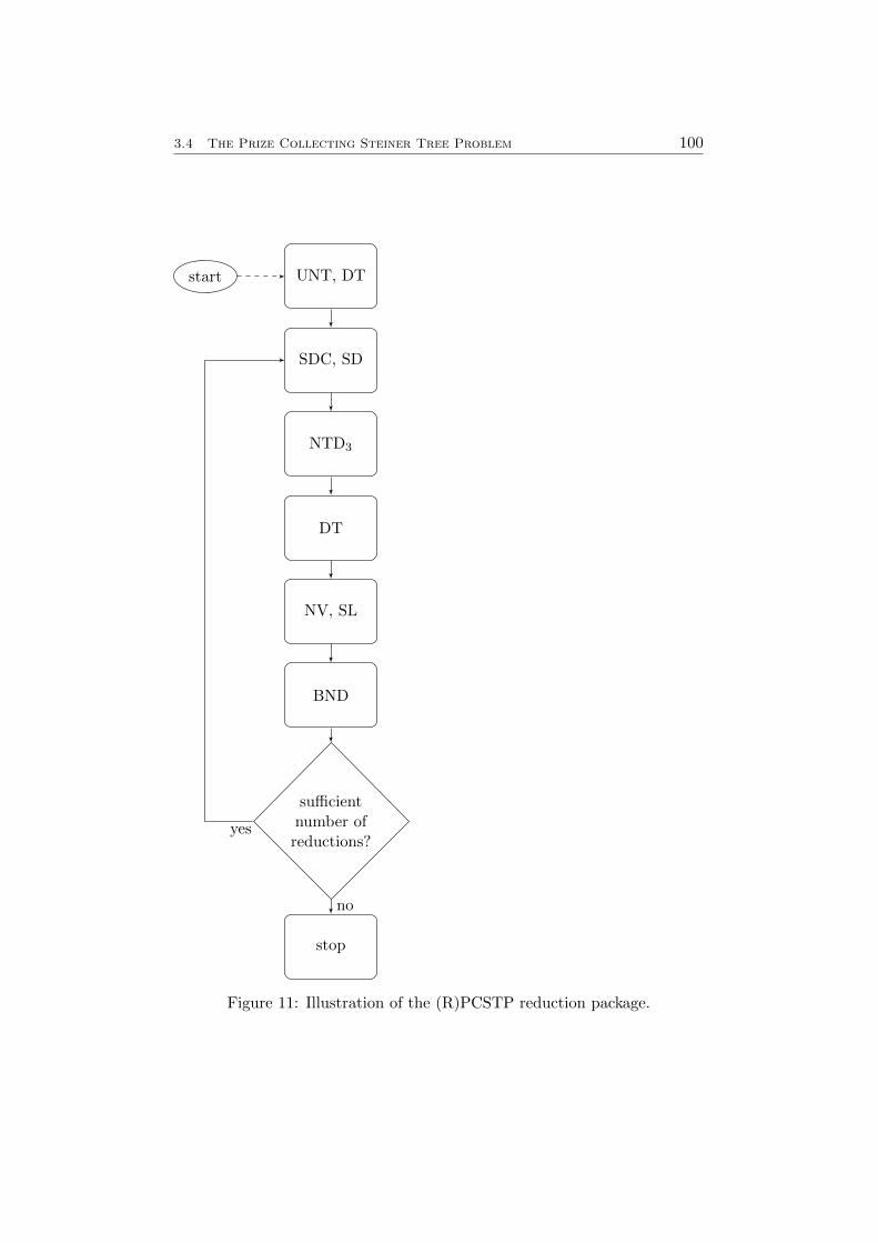
3.4 The Prize Collecting Steiner Tree Problem 100
UNT, DTstart
SDC, SD
NTD3
DT
NV, SL
BND
sufficientnumber ofreductions?
stop
yes
no
Figure 11: Illustration of the (R)PCSTP reduction package.
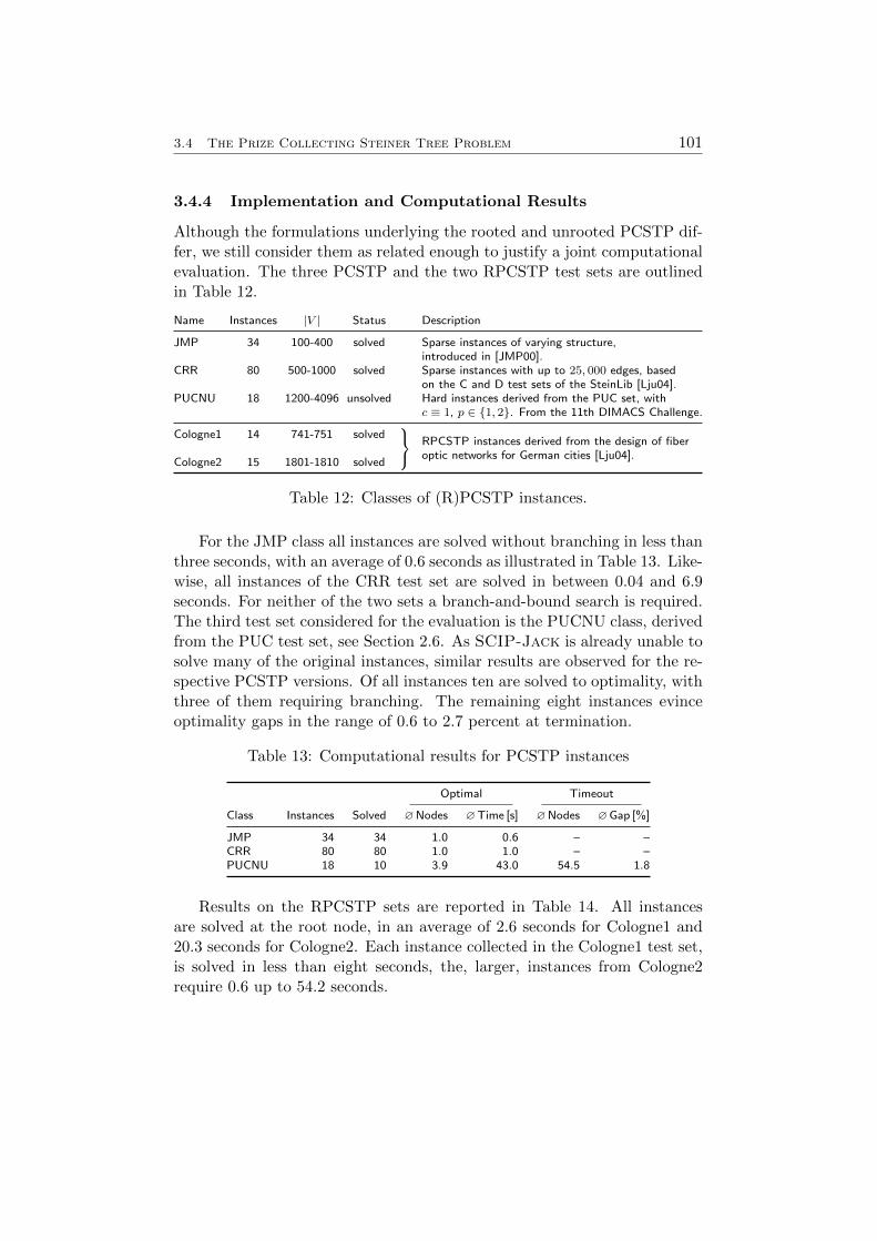
3.4 The Prize Collecting Steiner Tree Problem 101
3.4.4 Implementation and Computational Results
Although the formulations underlying the rooted and unrooted PCSTP dif-fer, we still consider them as related enough to justify a joint computationalevaluation. The three PCSTP and the two RPCSTP test sets are outlinedin Table 12.
Name Instances |V | Status Description
JMP 34 100-400 solved Sparse instances of varying structure,introduced in [JMP00].
CRR 80 500-1000 solved Sparse instances with up to 25, 000 edges, basedon the C and D test sets of the SteinLib [Lju04].
PUCNU 18 1200-4096 unsolved Hard instances derived from the PUC set, withc ≡ 1, p ∈ {1, 2}. From the 11th DIMACS Challenge.
Cologne1 14 741-751 solved RPCSTP instances derived from the design of fiber
optic networks for German cities [Lju04].Cologne2 15 1801-1810 solved
Table 12: Classes of (R)PCSTP instances.
For the JMP class all instances are solved without branching in less thanthree seconds, with an average of 0.6 seconds as illustrated in Table 13. Like-wise, all instances of the CRR test set are solved in between 0.04 and 6.9seconds. For neither of the two sets a branch-and-bound search is required.The third test set considered for the evaluation is the PUCNU class, derivedfrom the PUC test set, see Section 2.6. As SCIP-Jack is already unable tosolve many of the original instances, similar results are observed for the re-spective PCSTP versions. Of all instances ten are solved to optimality, withthree of them requiring branching. The remaining eight instances evinceoptimality gaps in the range of 0.6 to 2.7 percent at termination.
Table 13: Computational results for PCSTP instances
Optimal Timeout
Class Instances Solved ∅Nodes ∅Time [s] ∅Nodes ∅Gap [%]
JMP 34 34 1.0 0.6 – –CRR 80 80 1.0 1.0 – –PUCNU 18 10 3.9 43.0 54.5 1.8
Results on the RPCSTP sets are reported in Table 14. All instancesare solved at the root node, in an average of 2.6 seconds for Cologne1 and20.3 seconds for Cologne2. Each instance collected in the Cologne1 test set,is solved in less than eight seconds, the, larger, instances from Cologne2require 0.6 up to 54.2 seconds.
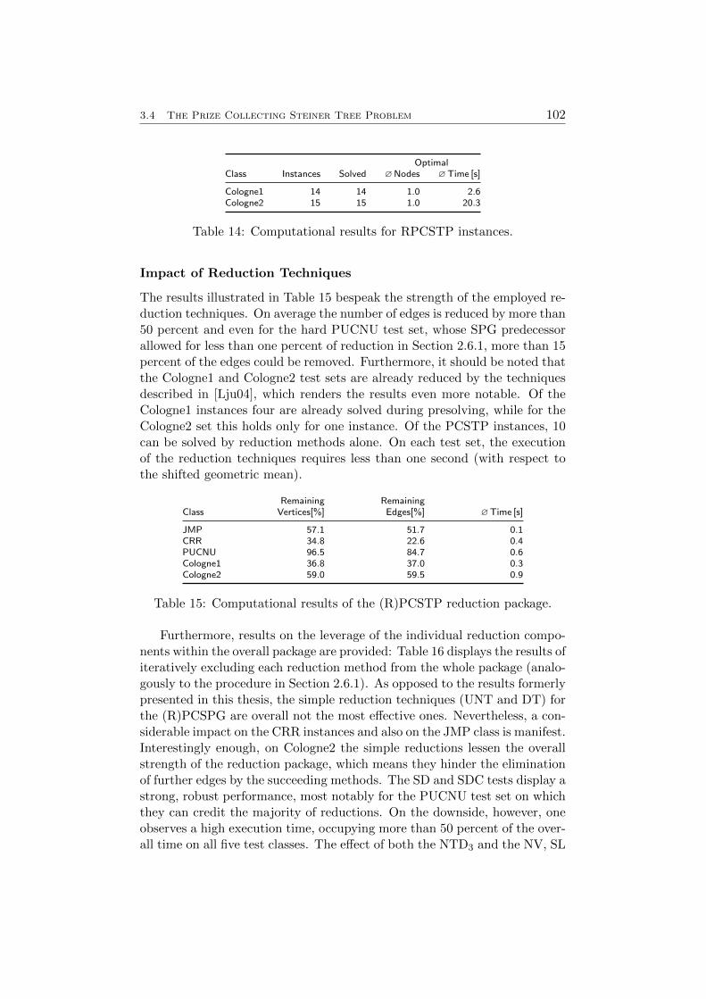
3.4 The Prize Collecting Steiner Tree Problem 102
OptimalClass Instances Solved ∅Nodes ∅Time [s]
Cologne1 14 14 1.0 2.6Cologne2 15 15 1.0 20.3
Table 14: Computational results for RPCSTP instances.
Impact of Reduction Techniques
The results illustrated in Table 15 bespeak the strength of the employed re-duction techniques. On average the number of edges is reduced by more than50 percent and even for the hard PUCNU test set, whose SPG predecessorallowed for less than one percent of reduction in Section 2.6.1, more than 15percent of the edges could be removed. Furthermore, it should be noted thatthe Cologne1 and Cologne2 test sets are already reduced by the techniquesdescribed in [Lju04], which renders the results even more notable. Of theCologne1 instances four are already solved during presolving, while for theCologne2 set this holds only for one instance. Of the PCSTP instances, 10can be solved by reduction methods alone. On each test set, the executionof the reduction techniques requires less than one second (with respect tothe shifted geometric mean).
Remaining RemainingClass Vertices[%] Edges[%] ∅Time [s]
JMP 57.1 51.7 0.1CRR 34.8 22.6 0.4PUCNU 96.5 84.7 0.6Cologne1 36.8 37.0 0.3Cologne2 59.0 59.5 0.9
Table 15: Computational results of the (R)PCSTP reduction package.
Furthermore, results on the leverage of the individual reduction compo-nents within the overall package are provided: Table 16 displays the results ofiteratively excluding each reduction method from the whole package (analo-gously to the procedure in Section 2.6.1). As opposed to the results formerlypresented in this thesis, the simple reduction techniques (UNT and DT) forthe (R)PCSPG are overall not the most effective ones. Nevertheless, a con-siderable impact on the CRR instances and also on the JMP class is manifest.Interestingly enough, on Cologne2 the simple reductions lessen the overallstrength of the reduction package, which means they hinder the eliminationof further edges by the succeeding methods. The SD and SDC tests display astrong, robust performance, most notably for the PUCNU test set on whichthey can credit the majority of reductions. On the downside, however, oneobserves a high execution time, occupying more than 50 percent of the over-all time on all five test classes. The effect of both the NTD3 and the NV, SL
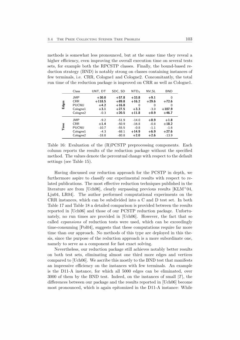
3.4 The Prize Collecting Steiner Tree Problem 103
methods is somewhat less pronounced, but at the same time they reveal ahigher efficiency, even improving the overall execution time on several testssets, for example both the RPCSTP classes. Finally, the bound-based re-duction strategy (BND) is notably strong on classes containing instances offew terminals, i.e. CRR, Cologne1 and Cologne2. Concomitantly, the totalrun time of the reduction package is improved on CRR as well as Cologne1.
Class UNT, DT SDC, SD NTD3 NV,SL BND
Edges
JMP +30.0 +57.8 +33.8 +9.1 0CRR +118.5 +89.8 +16.2 +29.6 +72.6PUCNU +4.2 +16.8 0 0 0Cologne1 +3.1 +27.5 +3.3 -3.0 +107.9Cologne2 -0.3 +20.5 +11.8 +0.9 +46.7
Tim
e
JMP -9.2 -51.9 -14.0 +8.9 +1.8CRR +1.4 -50.9 -16.8 -0.8 +18.2PUCNU -10.7 -55.5 -0.8 -1.1 -1.6Cologne1 -4.3 -68.1 +14.9 +6.9 +27.6Cologne2 -18.8 -80.8 +2.0 +2.6 -13.9
Table 16: Evaluation of the (R)PCSTP preprocessing components. Eachcolumn reports the results of the reduction package without the specifiedmethod. The values denote the percentual change with respect to the defaultsettings (see Table 15).
Having discussed our reduction approach for the PCSTP in depth, wefurthermore aspire to classify our experimental results with respect to re-lated publications. The most effective reduction techniques published in theliterature are from [Uch06], clearly surpassing previous results [KLM+04,Lju04, LR04]. The author performed computational experiments on theCRR instances, which can be subdivided into a C and D test set. In bothTable 17 and Table 18 a detailed comparison is provided between the resultsreported in [Uch06] and those of our PCSTP reduction package. Unfortu-nately, no run times are provided in [Uch06]. However, the fact that socalled expansions of reduction tests were used, which can be exceedinglytime-consuming [Pol04], suggests that these computations require far moretime than our approach. No methods of this type are deployed in this the-sis, since the purpose of the reduction approach is a more subordinate one,namely to serve as a component for fast exact solving.
Nevertheless, our reduction package still achieves notably better resultson both test sets, eliminating almost one third more edges and verticescompared to [Uch06]. We ascribe this mostly to the BND test that manifestsan impressive efficiency on the instances with few terminals. An exampleis the D11-A instance, for which all 5000 edges can be eliminated, over3000 of them by the BND test. Indeed, on the instances of small |T |, thedifferences between our package and the results reported in [Uch06] becomemost pronounced, which is again epitomized in the D11-A instance: While
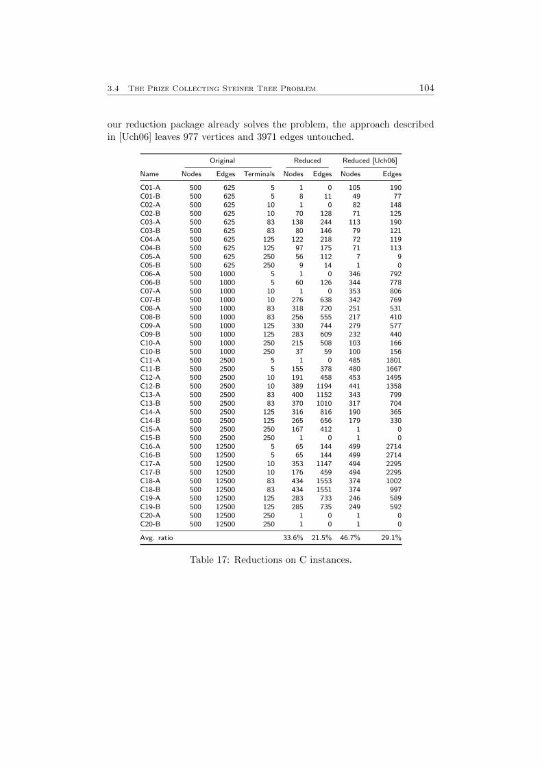
3.4 The Prize Collecting Steiner Tree Problem 104
our reduction package already solves the problem, the approach describedin [Uch06] leaves 977 vertices and 3971 edges untouched.
Original Reduced Reduced [Uch06]
Name Nodes Edges Terminals Nodes Edges Nodes Edges
C01-A 500 625 5 1 0 105 190C01-B 500 625 5 8 11 49 77C02-A 500 625 10 1 0 82 148C02-B 500 625 10 70 128 71 125C03-A 500 625 83 138 244 113 190C03-B 500 625 83 80 146 79 121C04-A 500 625 125 122 218 72 119C04-B 500 625 125 97 175 71 113C05-A 500 625 250 56 112 7 9C05-B 500 625 250 9 14 1 0C06-A 500 1000 5 1 0 346 792C06-B 500 1000 5 60 126 344 778C07-A 500 1000 10 1 0 353 806C07-B 500 1000 10 276 638 342 769C08-A 500 1000 83 318 720 251 531C08-B 500 1000 83 256 555 217 410C09-A 500 1000 125 330 744 279 577C09-B 500 1000 125 283 609 232 440C10-A 500 1000 250 215 508 103 166C10-B 500 1000 250 37 59 100 156C11-A 500 2500 5 1 0 485 1801C11-B 500 2500 5 155 378 480 1667C12-A 500 2500 10 191 458 453 1495C12-B 500 2500 10 389 1194 441 1358C13-A 500 2500 83 400 1152 343 799C13-B 500 2500 83 370 1010 317 704C14-A 500 2500 125 316 816 190 365C14-B 500 2500 125 265 656 179 330C15-A 500 2500 250 167 412 1 0C15-B 500 2500 250 1 0 1 0C16-A 500 12500 5 65 144 499 2714C16-B 500 12500 5 65 144 499 2714C17-A 500 12500 10 353 1147 494 2295C17-B 500 12500 10 176 459 494 2295C18-A 500 12500 83 434 1553 374 1002C18-B 500 12500 83 434 1551 374 997C19-A 500 12500 125 283 733 246 589C19-B 500 12500 125 285 735 249 592C20-A 500 12500 250 1 0 1 0C20-B 500 12500 250 1 0 1 0
Avg. ratio 33.6% 21.5% 46.7% 29.1%
Table 17: Reductions on C instances.
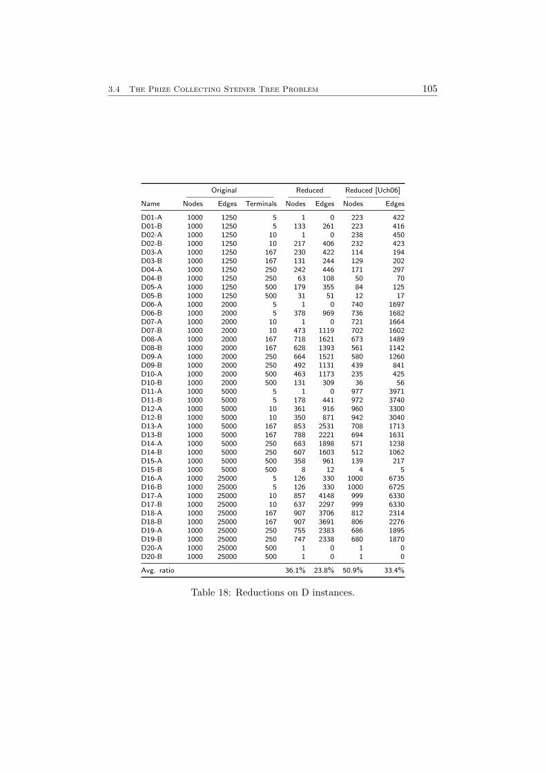
3.4 The Prize Collecting Steiner Tree Problem 105
Original Reduced Reduced [Uch06]
Name Nodes Edges Terminals Nodes Edges Nodes Edges
D01-A 1000 1250 5 1 0 223 422D01-B 1000 1250 5 133 261 223 416D02-A 1000 1250 10 1 0 238 450D02-B 1000 1250 10 217 406 232 423D03-A 1000 1250 167 230 422 114 194D03-B 1000 1250 167 131 244 129 202D04-A 1000 1250 250 242 446 171 297D04-B 1000 1250 250 63 108 50 70D05-A 1000 1250 500 179 355 84 125D05-B 1000 1250 500 31 51 12 17D06-A 1000 2000 5 1 0 740 1697D06-B 1000 2000 5 378 969 736 1682D07-A 1000 2000 10 1 0 721 1664D07-B 1000 2000 10 473 1119 702 1602D08-A 1000 2000 167 718 1621 673 1489D08-B 1000 2000 167 628 1393 561 1142D09-A 1000 2000 250 664 1521 580 1260D09-B 1000 2000 250 492 1131 439 841D10-A 1000 2000 500 463 1173 235 425D10-B 1000 2000 500 131 309 36 56D11-A 1000 5000 5 1 0 977 3971D11-B 1000 5000 5 178 441 972 3740D12-A 1000 5000 10 361 916 960 3300D12-B 1000 5000 10 350 871 942 3040D13-A 1000 5000 167 853 2531 708 1713D13-B 1000 5000 167 788 2221 694 1631D14-A 1000 5000 250 683 1898 571 1238D14-B 1000 5000 250 607 1603 512 1062D15-A 1000 5000 500 358 961 139 217D15-B 1000 5000 500 8 12 4 5D16-A 1000 25000 5 126 330 1000 6735D16-B 1000 25000 5 126 330 1000 6725D17-A 1000 25000 10 857 4148 999 6330D17-B 1000 25000 10 637 2297 999 6330D18-A 1000 25000 167 907 3706 812 2314D18-B 1000 25000 167 907 3691 806 2276D19-A 1000 25000 250 755 2383 686 1895D19-B 1000 25000 250 747 2338 680 1870D20-A 1000 25000 500 1 0 1 0D20-B 1000 25000 500 1 0 1 0
Avg. ratio 36.1% 23.8% 50.9% 33.4%
Table 18: Reductions on D instances.
3.4 The Prize Collecting Steiner Tree Problem 106
Impact of Heuristics
To measure the impact of the primal heuristics, we proceed as in Section 2.6and deploy them in accumulative stages. As with the SPG, one observes asteady decline of the average gap when stepping up the employed heuris-tics. This ranges from 72.81 percent when using no Steiner heuristics to1.84 percent for their full-fledged employment; the sharpest descent can beobserved when enabling the RSP heuristic, which reduces the average gapby 69.4 percent. Furthermore, the results presented in Table 19 display thatalso the execution time is considerably reduced when the heuristics comeinto play.
However, one notes that excluding the average gap the differences be-tween the accumulative stages of employed heuristics are diverse: On theJMP, CRR and Cologne2 class the execution times increase with the de-ployment of VQ as compared to using RSPH alone. On the other hand,by using both RSPH and VQ an additional PUC instance can be solved.Comparing the full-fledged heuristic package with RSPH, one sees that thelatter prevails on the JMP as well as on the Cologne2 class, albeit with alow margin. On a related note, the additional instance solved by RSPH/VQis also solved using all heuristics when the time limit is prolonged by fivepercent.
Summing up, the deployment of problem specific heuristics has beendemonstrated to notably help improve the execution time and, to a fargreater extent, the average gap for both the rooted and unrooted prize-collecting Steiner tree problem. While with respect to the overall executiontime the impact of additionally employing the VQ and RC heuristic on topof RSPH is a minor, and partially even negative, one, the results on the,hard, PUC instances show a notable reduction of the average gap.
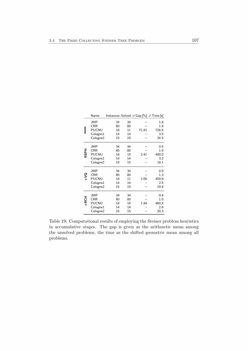
3.4 The Prize Collecting Steiner Tree Problem 107
Name Instances Solved ∅Gap [%] ∅Time [s]
none
JMP 34 34 – 1.6CRR 80 80 – 1.8PUCNU 18 11 71.81 726.5Cologne1 14 14 – 3.5Cologne2 15 15 – 34.5
RSPH
JMP 34 34 – 0.5CRR 80 80 – 1.0PUCNU 18 10 2.41 480.0Cologne1 14 14 – 3.2Cologne2 15 15 – 18.1
+VQ
JMP 34 34 – 0.9CRR 80 80 – 1.3PUCNU 18 11 2.00 459.9Cologne1 14 14 – 2.5Cologne2 15 15 – 19.6
+RCH
JMP 34 34 – 0.6CRR 80 80 – 1.0PUCNU 18 10 1.84 460.8Cologne1 14 14 – 2.6Cologne2 15 15 – 20.3
Table 19: Computational results of employing the Steiner problem heuristicsin accumulative stages. The gap is given as the arithmetic mean amongthe unsolved problems, the time as the shifted geometric mean among allproblems.
3.5 The Maximum Weight Connected Subgraph Problem 108
3.5 The Maximum Weight Connected Subgraph Problem
At first glance, the maximum-weight connected subgraph problem(MWCSP) bears little resemblance to the Steiner problems introduced sofar: Given an undirected graph (V,E) with (possibly negative) node weightsp, the objective is to find a tree that maximizes the sum of its node weights.However, it is possible to transform this problem into a prize-collectingSteiner tree problem. One transformation is given in [DKR+08]. In thisthesis an alternative transformation is presented that leads to a significantreduction in the number of terminals for the resulting problem, as comparedto the approach described in [DKR+08]. For our model the reduced amountof terminals leads to a substantial decrease of constraints (of the form (54)),as will become evident in this section.
In the following it is assumed that at least one vertex is assigned anegative and one a positive weight. In the case of only non-negative vertex-weights, the problem reduces to finding a spanning tree; in the case of onlynon-positive vertex-weights, the empty set constitutes an optimal solution.For a given solution S to an MWCSP we denote its weight by C(S) :=∑
v∈V [S] pv.
3.5.1 Transformation
Transformation 5 (MWCSP to rcSAP).Input: An MWCSP P = (V,E, p)Output: An rcSAP P ′′ = (V ′′, A′′, T ′′, c′′, r′′)
1. Set V ′ := V , A′ := {(v, w) ∈ V ′ × V ′ | {v, w} ∈ E}.
2. Set c′ : A′ → Q≥0 such that for a = (v, w) ∈ A′:
c′a =
{−pw, if pw < 0
0, otherwise
3. Set p′ : V ′ → Q≥0 such that for v ∈ V ′:
p′v =
{pv, if pv > 00, otherwise
4. Perform Transformation 4 to (V ′, A′, c′, p′), slightly changed in such away, that in step 2 instead of constructing a new arc set, A′ is beingused. The resulting rcSAP gives us P ′′ = (V ′′, A′′, T ′′, c′′, r′′).
An illustration of Transformation 5 on an MWCS instance consisting oftwo connected components can be found in Figure 12.
A bijection between the solution spaces of the MWCS and the rcSAPobtained by applying Transformation 5 is established in the following lemma:
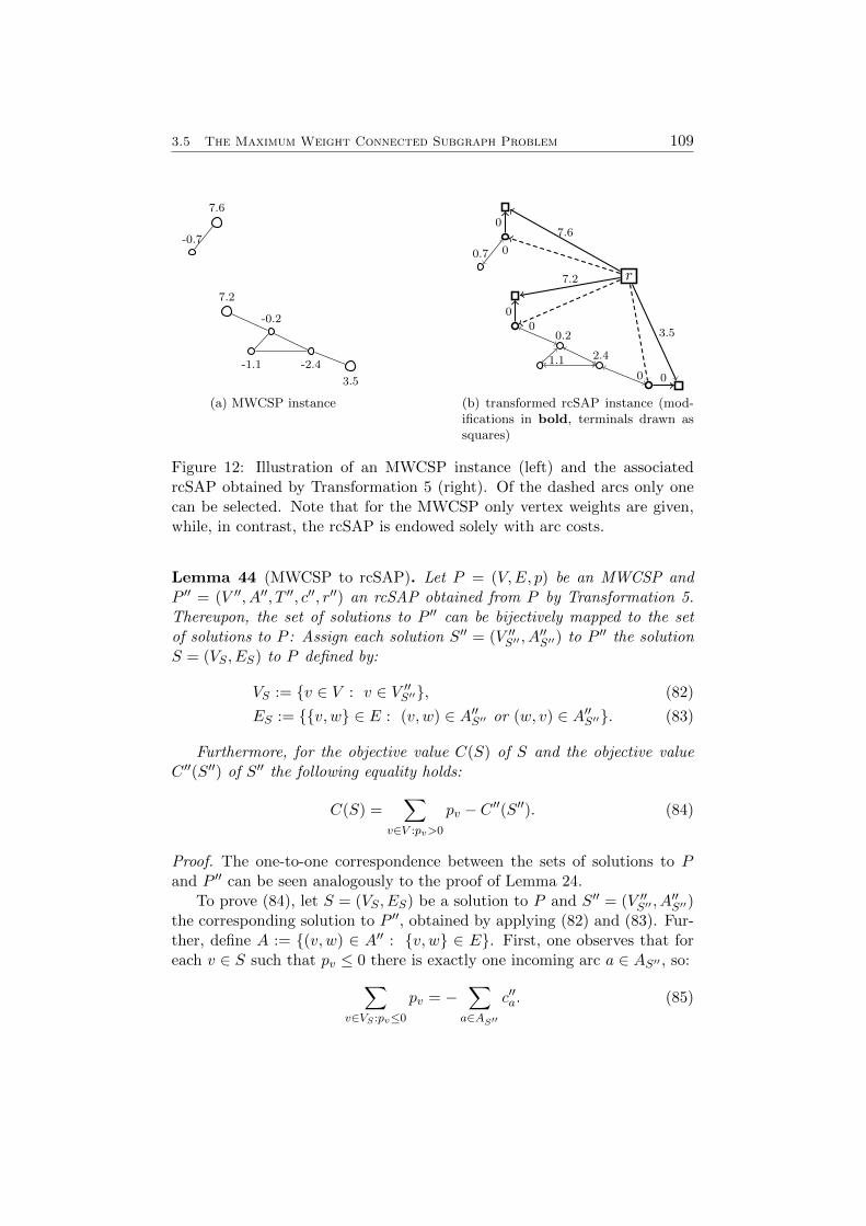
3.5 The Maximum Weight Connected Subgraph Problem 109
3.5
7.2
7.6
-0.7
-1.1 -2.4
-0.2
(a) MWCSP instance
r
0
00.7
1.1 2.4
0.2
0
0
0
3.5
7.2
7.6
0
(b) transformed rcSAP instance (mod-ifications in bold, terminals drawn assquares)
Figure 12: Illustration of an MWCSP instance (left) and the associatedrcSAP obtained by Transformation 5 (right). Of the dashed arcs only onecan be selected. Note that for the MWCSP only vertex weights are given,while, in contrast, the rcSAP is endowed solely with arc costs.
Lemma 44 (MWCSP to rcSAP). Let P = (V,E, p) be an MWCSP andP ′′ = (V ′′, A′′, T ′′, c′′, r′′) an rcSAP obtained from P by Transformation 5.Thereupon, the set of solutions to P ′′ can be bijectively mapped to the setof solutions to P : Assign each solution S′′ = (V ′′S′′ , A
′′S′′) to P ′′ the solution
S = (VS , ES) to P defined by:
VS := {v ∈ V : v ∈ V ′′S′′}, (82)
ES := {{v, w} ∈ E : (v, w) ∈ A′′S′′ or (w, v) ∈ A′′S′′}. (83)
Furthermore, for the objective value C(S) of S and the objective valueC ′′(S′′) of S′′ the following equality holds:
C(S) =∑
v∈V :pv>0
pv − C ′′(S′′). (84)
Proof. The one-to-one correspondence between the sets of solutions to Pand P ′′ can be seen analogously to the proof of Lemma 24.
To prove (84), let S = (VS , ES) be a solution to P and S′′ = (V ′′S′′ , A′′S′′)
the corresponding solution to P ′′, obtained by applying (82) and (83). Fur-ther, define A := {(v, w) ∈ A′′ : {v, w} ∈ E}. First, one observes that foreach v ∈ S such that pv ≤ 0 there is exactly one incoming arc a ∈ AS′′ , so:∑
v∈VS :pv≤0
pv = −∑a∈AS′′
c′′a. (85)
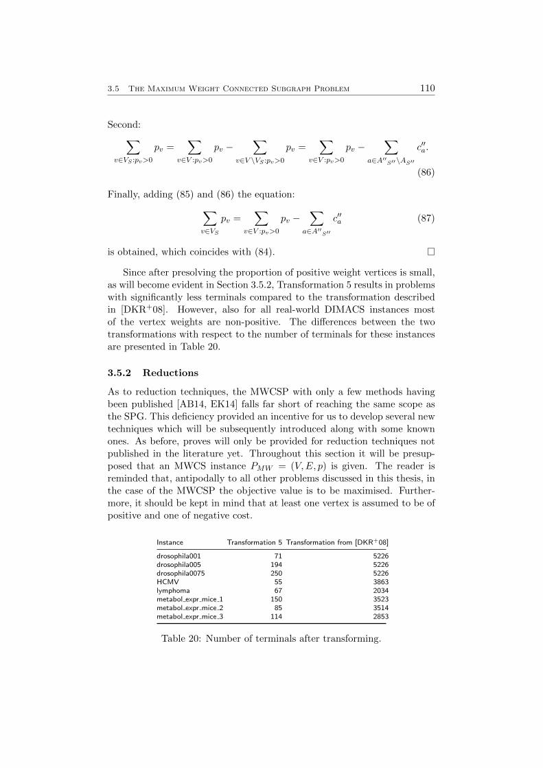
3.5 The Maximum Weight Connected Subgraph Problem 110
Second:∑v∈VS :pv>0
pv =∑
v∈V :pv>0
pv −∑
v∈V \VS :pv>0
pv =∑
v∈V :pv>0
pv −∑
a∈A′′S′′\AS′′
c′′a.
(86)
Finally, adding (85) and (86) the equation:∑v∈VS
pv =∑
v∈V :pv>0
pv −∑
a∈A′′S′′
c′′a (87)
is obtained, which coincides with (84).
Since after presolving the proportion of positive weight vertices is small,as will become evident in Section 3.5.2, Transformation 5 results in problemswith significantly less terminals compared to the transformation describedin [DKR+08]. However, also for all real-world DIMACS instances mostof the vertex weights are non-positive. The differences between the twotransformations with respect to the number of terminals for these instancesare presented in Table 20.
3.5.2 Reductions
As to reduction techniques, the MWCSP with only a few methods havingbeen published [AB14, EK14] falls far short of reaching the same scope asthe SPG. This deficiency provided an incentive for us to develop several newtechniques which will be subsequently introduced along with some knownones. As before, proves will only be provided for reduction techniques notpublished in the literature yet. Throughout this section it will be presup-posed that an MWCS instance PMW = (V,E, p) is given. The reader isreminded that, antipodally to all other problems discussed in this thesis, inthe case of the MWCSP the objective value is to be maximised. Further-more, it should be kept in mind that at least one vertex is assumed to be ofpositive and one of negative cost.
Instance Transformation 5 Transformation from [DKR+08]
drosophila001 71 5226drosophila005 194 5226drosophila0075 250 5226HCMV 55 3863lymphoma 67 2034metabol expr mice 1 150 3523metabol expr mice 2 85 3514metabol expr mice 3 114 2853
Table 20: Number of terminals after transforming.
3.5 The Maximum Weight Connected Subgraph Problem 111
Basic Reductions
The first of the following two simple tests was already suggested in a lessgeneral form in [EK14] (namely only for negative vertices of degree zero):
Vertex of degree zero (VD0): A vertex vi of degree zero can be discardedif there is a vertex vmax such that both pvmax ≥ pvi and vmax 6= vi.
Proof. The only solution vi might be contained in is {vi}, which is of equalor less cost than the feasible solution {vmax}.
Vertex of degree one (VD1): If there is vertex vi of degree one withincident edge ek = {vi, vj}, a vertex vmax satisfying both pvmax ≥ pvi andvmax 6= vi and it moreover holds that
a) pvi ≤ 0, then vi and ek can be discarded;
b) pvi > 0, then vi and ek can be discarded while adding pvi to the weightof vj.
Proof. Since pvi ≤ pvmax and vmax 6= vi hold, {vi} cannot be the uniqueoptimal solution.
a) Each solution that contains ek (and vi) can be reduced to solution ofnot higher cost by removing ek as well as vi. Hence, there is at least oneoptimal solution containing neither ek nor vi.
b) If vj is contained in an optimal solution, vi is as well, since pvi > 0.Hence, at least one optimal solution is preserved by the reduction describedin part b) of the test.
The next two reduction tests can be found in both [AB14] and [EK14].
Non-negative incident vertices (NNIV): An edge {vi, vj} such thatpvi ≥ 0, pvj ≥ 0 can be contracted if the weight of the remaining vertex isset to pvi + pvj .
Non-positive chain (NPC): A path P between two vertices vi, vj, con-taining only non-positive interior vertices of degree two and fulfilling |V [P ]| >3 can be replaced by a node v′ with pv′ :=
∑v∈V [P ◦] pv and the two edges
{v′, vi}, {v′, vj}.
The joint execution of the four forgoing tests, in the specified order, willbe hereinafter referred to as Basic Test (BT).
Recalling that connectivity is not postulated for the MWCSP, one readilydevises the following test:
Unreachable non-positive vertex (UNPV): Each non-positive vertexvi that is not connected to any positive vertex can be deleted along with allincident edges.
3.5 The Maximum Weight Connected Subgraph Problem 112
Proof. Since there is at least one vertex of positive cost, vi cannot be con-tained in any optimal solution.
We realize this test by running a breadth-first search from the (artificial)root on the transformed graph yielded by Transformation 5 and discardingall vertices that have not been visited in the course of the search.
Alternative Based Reductions
For the avoidance of doubt, we point out that apart from the subsequenttest all MWCSP reduction methods introduced hereinafter have been newlydevised for this thesis. The subsequent reduction test was tentatively sug-gested in [EK14], to be later generalized in [AB14]. Only the latter versionis stated here:
Adjacent Neighbourhood Subset (ANS) 5 Let vi and vj be two distinctvertices. If pvi ≤ 0, pvi ≤ pvj and{
v ∈ V \ {vj} | {vi, v} ∈ E}⊂{v ∈ V | {vj , v} ∈ E
},
then vi and all incident edges can be removed.
However, even this revised version can be notably generalized:
Lemma 45. Let vi ∈ V and W ⊂ V \ {vi}, W 6= ∅ such that (W,E[W ]) isconnected and
∑w∈W :pw<0 pw ≥ pvi holds. If:{
v ∈ V \W | {vi, v} ∈ E}⊂{v ∈ V \W | {w, v} ∈ E,w ∈W
}, (88)
then there is at least one optimal solution that does not contain vi (or anyof its incident edges).
Proof. Suppose that there is an optimal solution S = (VS , ES) containingvi. From
∑w∈W :pw<0 pw ≥ pvi it can be inferred that pvi ≤ 0. Therefore, it
can be assumed that vi is of degree at least two in S (if vi is of degree one inS, it can be simply discarded without deteriorating the objective value). Let∆S ⊂ VS be the vertices adjacent to vi in S. Removing vi and all incidentedges from S and inserting all vertices in W \S as well as all edges betweenW and ∆S∪W , one obtains a connected subgraph S′ = (VS′ , ES′) such that:
C(S′) =∑v∈VS′
pv ≥∑w∈Wpw<0
pw + C(S)− pvi ≥ C(S). (89)
5The reduction test was originally named ”Neighbourhood Subset”, abbreviated ”NS”,test in [AB14], but owned to rather obvious historical considerations we have decided tosubstitute it.
3.5 The Maximum Weight Connected Subgraph Problem 113
However, S′ is not necessarily a tree, but this issue can be remedied withoutchanging the weight of S′ by repeatedly removing an edge on a cycle as longas there exists any. Due to (89) the resulting tree is of cost at least C(S)and therefore optimal. Furthermore, it does not contain vi, so the statementof the lemma is established.
By processing for each node vi only a limited amount of neighbours thatare moreover of degree not higher than a given constant, the ANS test can beperformed in Θ(m). Affiliated to Lemma 45 we implemented the followingreduction test: For each vertex vj of negative weight we consider as W theunion of vj and a limited amount of non-negative weight vertices adjacentto vj . By again considering only neighbours vi to vj of bounded degree,this test can likewise be implemented in Θ(m). In the following, this testis referred to as Connected Neighbourhood Subset (CNS). Althoughit dominates the ANS test in its unbounded version, this is not true forthe actually implemented test if the bound on the number of vertices to beprocessed differs. So we use both the restricted ANS and the restricted CNStest, but with a higher upper bound on the admissible vertex degrees forthe less expensive ANS test.
The perhaps most intuitive, but nonetheless effective, of the reductiontests introduced hereinafter is based on the following lemma:
Lemma 46. Let ek = {vi, vj} ∈ E. If there is a path P between vi and vjsuch that ek /∈ E[P ] and pvp ≥ 0 for all vp ∈ V [P ◦], then there is at leastone optimal solution that does not contain ek.
Proof. Suppose that there is a solution S to PMW containing ek. By remov-ing ek from S one obtains two trees S1, S2 such that vi ∈ S1, vj ∈ S2. SinceP connects vi and vj , there are vertices vr ∈ V [S1]∩V [P ], vs ∈ V [S2]∩V [P ]such that P (vr, vs) does not include any additional vertices of S1 or S2. Re-connecting S1 and S2 by P (vr, vs) one yields a new tree S of weight at leastC(S).
These considerations prove the lemma, since they imply that to eachoptimal solution that contains ek, an optimal solution not containing ek canbe constructed.
We suggest a reduction test based on Lemma 46, designed as follows: Byfirst executing the NNIV test, each path containing only interior vertices ofnon-negative weight is reduced to a path consisting of three vertices (withan interior vertex of non-negative weight). Thereafter, for each edge ek ={vi, vj} we mark all non-negative adjacent vertices of vi, except for vj . Ifno vertex of non-negative cost has been marked, we can already progress tothe next edge. Otherwise, we traverse all non-negative neighbours of vj . Ifin the course of the second search a marked vertex is visited, we eliminateek. By bounding the number of adjacent vertices to be visited from vi and
3.5 The Maximum Weight Connected Subgraph Problem 114
vj by a constant, the test can be performed for all edges in a total of Θ(m).We denote this test Non-Negative Paths (NNP).
The development of the next reduction strategy was spawned by theobservation that after having performed the NPC test, each non-positivechain is reduced to a single non-positive vertex of degree two. Naturally,one aspires to dispose of those as well. To set the stage for such a reductionmethod we define a function on two vertices, evocative of the bottleneckSteiner distance: Let vi, vj ∈ V be two distinct vertices and P(vi, vj) the setof all simple paths between vi and vj . Further, for P ∈ P(vi, vj) let P (x, y)be the subpath between two vertices x, y in P . In the context of the MWCSwe define the interior cost of such a subpath as
C◦(P (x, y)) :=∑
v∈V [P (x,y)]\{x,y}
pv. (90)
Furthermore, we define the vertex weight bottleneck length of P as:
lvw(P ) := minx,y∈V [P ]
C◦(P (x, y)). (91)
Given two disjoint trees that can be connected by a subpath of a givenpath P , by lvw(P ) a lower bound on the additional vertex weights is pro-vided.
The two preceding definitions pave the way for the vertex weight bot-tleneck distance between vi and vj , which we define as
dvw(vi, vj) = max{lvw(P ) | P ∈ P(vi, vj)}. (92)
With this new definition at hand, a lemma bearing some commonalitieswith the Steiner distance based exclusion tests can be formulated.
Lemma 47. Let vi ∈ V such that pvi ≤ 0 and |δ(vi)| = 2 with incidentedges {vi, vj} and {vi, vk}. If
dvw(vj , vk) > pvi (93)
holds, then there is at least one optimal solution not containing vi.
Proof. Suppose that there is an optimal solution S that contains vi. Inthis case, due to vi being of non-positive weight, we can assume that bothincident edges of vi are likewise part of the solution. Otherwise, vi couldsimply be removed, to yield another optimal solution. Removing vi as wellas its incident edges from S, we obtain two subtrees S1 and S2. Let P bea path between vj and vk such that lvw(P ) = dvw(vj , vk). Additionally, letP (v′1, v
′2) be a subpath of P between v′1 ∈ V [S1] and v′2 ∈ V [S2] such that no
3.5 The Maximum Weight Connected Subgraph Problem 115
additional vertices of either S1 or S2 are contained. By including P (v′1, v′2)
a new tree S′ is obtained which is of cost:
C(S′) = C(S) + C◦(P (v′1, v′2))− pvi
≥ C(S) + lvw(P )− pvi= C(S) + dvw(vj , vk)− pvi(93)> C(S).
This proves the lemma.
We suggest the following reduction test to utilize Lemma 47: First per-form step 1 and step 2 of Transformation 5 to obtain a directed graphD′ = (V ′, A′) with, non-negative, arc costs c′. Following, a modified versionof the SDC test can be used on D′ to find alternative paths containing atmost one interior vertex of positive weight: Let vi ∈ V be non-positive andof degree two with adjacent vertices vj and vk. Similar to the original SDCtest, a limited execution of Dijkstra’s algorithm is performed first from vjand then from vk, ignoring vi and its incident edges. For each vertex be-ing processed during Dijkstra’s algorithm, only outgoing arcs are consideredand the computation does not proceed from vertices of positive weights. Ifdirected paths ~P ′k and ~P ′j from vk and vj respectively to a vertex vl ∈ V havebeen found, denote by Pjk the corresponding undirected path in G betweenvj and vk (over vl) and distinguish two cases (note that we denote by p thevertex weights in the original graph G):
1. if pvl > 0, then lvw(Pjk) = min{−C ′(~P ′j),−C ′(~P ′k),−C ′(~P ′j)−C ′(~P ′k)+pvl};
2. if pvl ≤ 0, then lvw(Pjk) = −C ′(~P ′j)− C ′(~P ′k)− pvl .
In the first case, we consider the interior costs of the two subpaths be-tween each endpoint of Pjk and the intermediary vertex of positive weightas well as the interior cost of the whole path. The minimum among thosethree is equal to the vertex weight bottleneck length of Pjk. In the secondcase, Pjk does not contain any intermediary vertex of positive weight, solvw(Pjk) = C◦(Pjk) holds.
If lvw(Pjk) ≥ pvi , the vertex vi and its incident edges are deleted. Wedenote this procedure by Non-Positive Vertex of Degree two (NPV2)test.
The concept of the vertex weight distance not only gives rise to Lemma47 and the affiliated NPV2 test, but furthermore leads the way to a far moregeneral and powerful result:
Lemma 48. Let vi ∈ V such that pvi ≤ 0 and denote by ∆ the set ofall vertices adjacent to vi. Furthermore, for ∆′ ⊂ ∆ denote by K∆′ :=
3.5 The Maximum Weight Connected Subgraph Problem 116
(∆′,∆′×∆′, dvw) the complete graph on ∆′, with edge weight dvw(vj , vk) foran edge {vj , vk} ∈ ∆′ × ∆′. If for each ∆′ ⊂ ∆ of cardinality at least twoit holds that the weight of a maximum spanning tree on K∆′ is greater thanpvi, then there is at least one optimal solution that does not contain vi (orany of its incident edges).
Proof. It can be readily verified that in the cases |∆| = 0, 1, 2 the claim hasalready been established by the proofs to VD0, VD1 and Lemma 47 respec-tively. So suppose |∆| > 2 and let S = (VS , ES) be a tree such that vi is ofdegree k > 0 in S. If k < 2, the claim can be established analogously to thehereinbefore referred to proofs. Otherwise, denote by ∆′ = {v′1, ..., v′k} ⊂ VSthe vertices incident to vi in S. With the premises of the lemma being sat-isfied, there is maximum spanning tree T∆′ on K∆′ of weight greater thanpvi . The solution S can be segmented into k trees S1, .., Sk such that vj ∈ Sjfor j = 1, ..., k, by removing vi and δ(vi). In the following we will iterativelyrejoin these k trees to obtain a new tree not containing vi and being of nolesser weight than S.
First, one observes that each edge of T∆′ corresponds to a path in Gbetween two vertices of ∆′. Let Prs with r, s ∈ {1, ..., k} be such a pathconnecting v′r and v′s. Since the edge between v′r and v′s is a spanning treefor the subset {v′r, v′s} ⊂ ∆, it holds that dvw(v′r, v
′s) > pvi . Consequently,
vi is not contained in Prs. Analogously to the proof of Lemma 47, Sr andSs can be connected to a tree S′1 by a subset of Prs, which is of cost atleast dvw(v′r, v
′s). Thereupon, S′1 can be linked in the same way to a tree
Sl, k ∈ {1, ..., k} \ {r, s}, bringing forth a tree S′2 that once more does notcontain vi. Reiterating in this manner, one can rejoin S′2 with all not yetincorporated trees Sq, finally yielding a tree S′k−1. This tree does not containvi and is of cost:
C(S′k−1) ≥∑
l={1,...,k}
C(Sl) +
( ∑{vq ,vl}∈E[T∆′ ]
dvw(vq, vl)
)− pvi ≥ C(S)
Consequently, the claim is established.
Corollary 49. Let vi ∈ V such that pvi ≤ 0 and denote by ∆ the set ofall vertices adjacent to vi. Denote the vertex weight bottleneck distanceson the graph G− := (V −, E−) with V − := V \ {vi}, E− := E[V −] by d−vw.Further, for ∆′ ⊂ ∆ define K∆′ := (∆′,∆′×∆′, d−vw). If for each ∆′ ⊂ ∆ ofcardinality at least two it holds that the weight of a maximum spanning treeon K∆′ is not less than pvi, there is at least one optimal solution that doesnot contain vi (or any of its incident edges).
Proof. The proposition can be verified largely in line with the proof toLemma 48. As the sole amendment, to demonstrate that for joining thesubtrees S1, ..., Sk the vertex vi can be disregarded one simply uses the factthat all paths corresponding to d−vw do not include vi by definition.
3.5 The Maximum Weight Connected Subgraph Problem 117
We use reduction tests based on the antecedent corollary only for non-positive vertices of degree three, four and five and refer to the correspond-ing methods as Non-Positive Vertex of Degree k (NPVk) test (k ∈{3, 4, 5}). In line with the proceeding for the bottleneck based tests to boththe SPG and the PCSTP, the vertex weight distances are not pre-computedand are furthermore substituted by ad-hoc calculated lower bounds to eachpair of vertices in ∆. To this end, the procedure deployed in the NPV2 test isutilized. If a vertex has been verified to satisfy the premises of Corollary 49,it is removed along with all incident edges.
Bound Based Reductions
Throughout this subsection, the connected components of G are denoted byG1, ..., Gl. Utilizing the UNPV test we can assume that to each componentGi = (Vi, Ei) there is at least one vertex vj ∈ Vi such that pvj > 0. Fortwo distinct vertices vi, vj ∈ V denote by Pij the set of all simple pathsbetween vi and vj only containing non-positive interior vertices. We definethe non-positive vertices distance from vi to vj as:
dnpv(vi, vj) :=
{maxP∈Pij
{∑v∈V [P ] pv
}if Pij 6= ∅
−∞ otherwise.(94)
Note that this definition includes the weights of the endpoints of a path,in contrast for instance to the interior cost C◦.
Furthermore, denote by T = {t1, ..., ts} the set of all vertices in G ofpositive weight and by Tr = {tϕ(1), ..., tϕ(sr)} the corresponding, non-empty,set of positive vertices of a connected component Gr. Ensuing, we denote apartition {N(t) | t ∈ T} of V such that
vi ∈ N(t)⇒ dnpv(vi, t) ≥ dnpv(vi, t′), ∀t′ ∈ T (95)
by maximum-weight Voronoi diagram, in the context of the MWCSsimply called Vornonoi diagram.
For computing such a Voronoi diagram we associate with each vertexvi ∈ V the following three values (which are also used for customary Voronoidiagrams [Meh88]):
• base(vi): the positive vertex tj ∈ T such that vi ∈ N(tj);
• pred(vi): the predecessor of vi on the path from base(vi) to vi, set to−1 if pvi > 0;
• dist(vi): the non-positive vertices distance dnpv(base(vi), vi).
Those values can be computed by the subsequent algorithm:
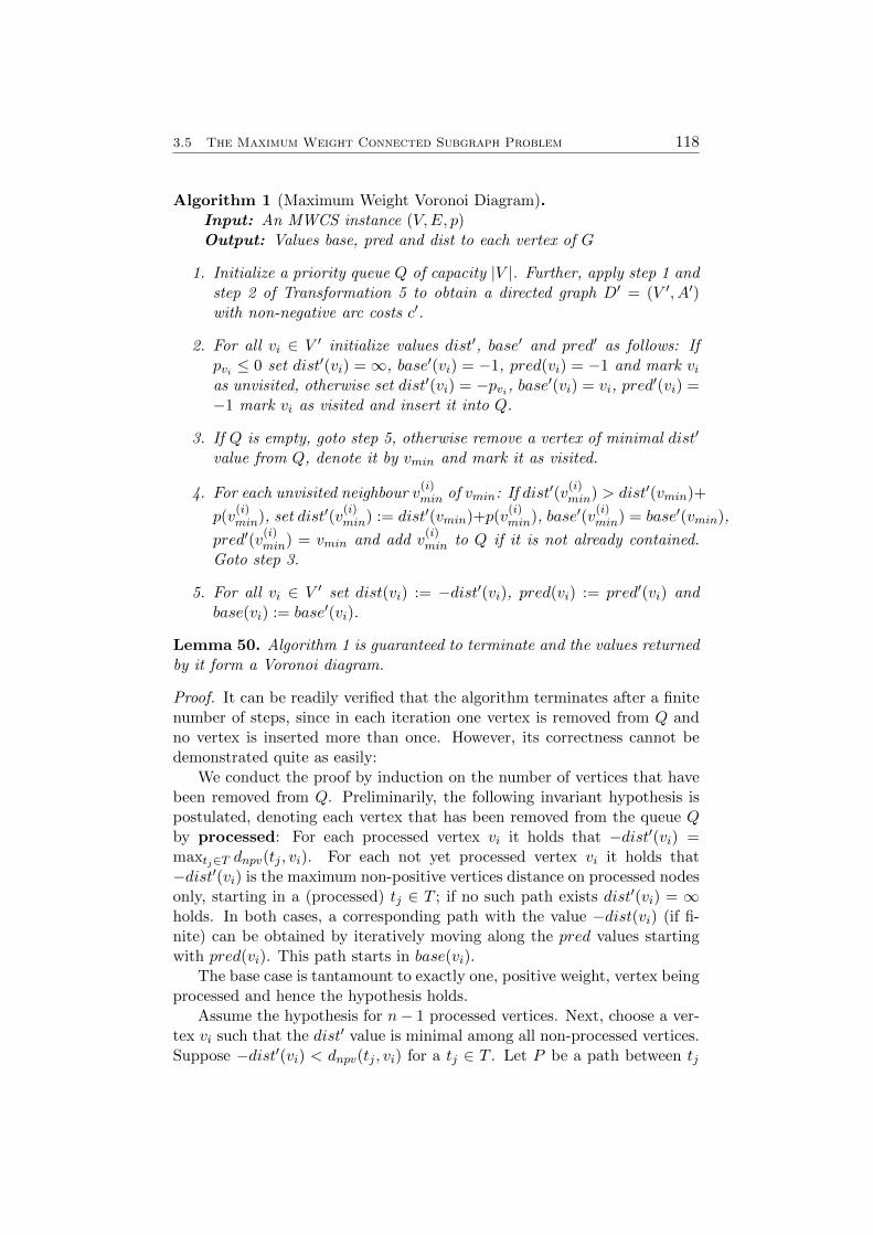
3.5 The Maximum Weight Connected Subgraph Problem 118
Algorithm 1 (Maximum Weight Voronoi Diagram).Input: An MWCS instance (V,E, p)Output: Values base, pred and dist to each vertex of G
1. Initialize a priority queue Q of capacity |V |. Further, apply step 1 andstep 2 of Transformation 5 to obtain a directed graph D′ = (V ′, A′)with non-negative arc costs c′.
2. For all vi ∈ V ′ initialize values dist′, base′ and pred′ as follows: Ifpvi ≤ 0 set dist′(vi) =∞, base′(vi) = −1, pred(vi) = −1 and mark vias unvisited, otherwise set dist′(vi) = −pvi, base′(vi) = vi, pred
′(vi) =−1 mark vi as visited and insert it into Q.
3. If Q is empty, goto step 5, otherwise remove a vertex of minimal dist′
value from Q, denote it by vmin and mark it as visited.
4. For each unvisited neighbour v(i)min of vmin: If dist′(v
(i)min) > dist′(vmin)+
p(v(i)min), set dist′(v
(i)min) := dist′(vmin)+p(v
(i)min), base′(v
(i)min) = base′(vmin),
pred′(v(i)min) = vmin and add v
(i)min to Q if it is not already contained.
Goto step 3.
5. For all vi ∈ V ′ set dist(vi) := −dist′(vi), pred(vi) := pred′(vi) andbase(vi) := base′(vi).
Lemma 50. Algorithm 1 is guaranteed to terminate and the values returnedby it form a Voronoi diagram.
Proof. It can be readily verified that the algorithm terminates after a finitenumber of steps, since in each iteration one vertex is removed from Q andno vertex is inserted more than once. However, its correctness cannot bedemonstrated quite as easily:
We conduct the proof by induction on the number of vertices that havebeen removed from Q. Preliminarily, the following invariant hypothesis ispostulated, denoting each vertex that has been removed from the queue Qby processed: For each processed vertex vi it holds that −dist′(vi) =maxtj∈T dnpv(tj , vi). For each not yet processed vertex vi it holds that−dist′(vi) is the maximum non-positive vertices distance on processed nodesonly, starting in a (processed) tj ∈ T ; if no such path exists dist′(vi) = ∞holds. In both cases, a corresponding path with the value −dist(vi) (if fi-nite) can be obtained by iteratively moving along the pred values startingwith pred(vi). This path starts in base(vi).
The base case is tantamount to exactly one, positive weight, vertex beingprocessed and hence the hypothesis holds.
Assume the hypothesis for n− 1 processed vertices. Next, choose a ver-tex vi such that the dist′ value is minimal among all non-processed vertices.Suppose −dist′(vi) < dnpv(tj , vi) for a tj ∈ T . Let P be a path between tj
3.5 The Maximum Weight Connected Subgraph Problem 119
and vi of vertex weight dnpv(tj , vi). Starting from tj let vk be the first vertexin P not processed yet. If vk = vi, this would contradict the hypothesis forunprocessed vertices. Otherwise, since all vertices on P except for tj are ofnon-positive weight, it can be inferred that dnpv(tj , vk) ≥ dnpv(tj , vi). Hence,vk would have been selected instead of vk, contradicting the initial assump-tion. Consequently, −dist′(vi) = maxtj∈T dnpv(tj , vi) is satisfied. Moreover,as the dist, pred and base values of vi endure unaltered, a path correspond-ing to the value −dist(vi) and ending in base(vi) can still be obtained bymeans of the pred values.
Finally, when step 4 of the algorithm has been performed, it is still truethat for each unprocessed vertex vr the value −dist′(vr) is the maximal non-positive vertices distance on processed nodes starting in a tj ∈ T : If therewas a path of higher weight (in G) not containing vi, the vertex vr wouldhave been selected previously and there cannot be a path of higher weightcontaining vi, since it would have been updated while processing vi. Further-more, since by the hypothesis a path corresponding to the −dist(vi) valueand starting in base(vi) can be obtained by the pred values, the accordingproperty holds true for each unprocessed vr updated while processing vi.
To conclude the demonstration, it remains to be verified that after thetermination of the algorithm all vertices of G are processed: Suppose thatthis is not true and let be vi be a non-processed vertex in a connectedcomponent Gk. Further, let tj ∈ Tk and P a path from tj to vi. The terminalvertex is processed, since it is inserted into Q in step 2 of the algorithm.Let v′0 be the first unprocessed vertex in P . However, v′0 would have beeninserted into Q (and subsequently processed) while the predecessor of v′0 inP was being processed.
Still, some definitions are necessary to conclusively pave the way forthe MWCS bound-based reduction techniques: For a vi ∈ V \ T denoteby vi,1, vi,2 two positive vertices such that dnpv(vi, vi,1) ≥ dnpv(vi, vi,2) anddnpv(vi, vi,2) ≥ dnpv(vi, tj) for all tj ∈ T \ {vi,1}. If only one terminal isreachable from vi, set vi,2 := −1. The vi,1 values can be computed byAlgorithm 1, the vi,2 values by a simple adaption of Duin’s nearest terminalsalgorithm, see Section 1.1.
Based on the preceding discussion, for ti ∈ T we define:
mwradius(ti) := max{
0,
max{dnpv(ti, vj) | {vj , vk} ∈ E : vj ∈ N(ti), vk /∈ N(ti)}}
(96)
Once again succumbing to the convenience of a lucid notation, it will be sup-posed that for each i = 1, ..., r, all tj ∈ Ti are mapped by ϕ in such a mannerthat mwradius(tϕ(t1)) ≤ mwradius(tϕ(t2)) ≤ ... ≤ mwradius(tϕ(tsr )).
Lemma 51. Let vi ∈ V with pvi ≤ 0 and assume that an optimal solutionS = (VS , ES) to PMW exists such that vi ∈ VS. Let Gr be the connected
3.5 The Maximum Weight Connected Subgraph Problem 120
component containing vs. The value
dnpv(vi, vi,1) + dnpv(vi, vi,2)− pvi +
sr∑l=3
mwradius(ϕ(tl)) (97)
is an upper bound on the weight of S.
Proof. Denote the (unique) path in S between vi and a tj ∈ T ∩ V [Gr] byPj and the set of all such paths by P.
Analogously to the proof of Lemma 36, two distinct paths Pk ∈ P andPl ∈ P can be selected such that they jointly contain a minimal number ofVoronoi-boundary edges and V [Pk] ∩ V [Pl] = {vi}. Likewise, define P− :=P \ {Pk, Pl}. For all Pu ∈ P−, denote by P ′u the subpath of Pu starting intu and ending in the last vertex still in N(tu) (so that P ′u lies completely inN(tu)).
Suppose that Pk has a vertex vq ∈ VS in common with a P ′u. As aconsequence, Pl cannot have any vertex but vi in common with Pu, becausethis would require a cycle in S. For the same reason, Pk and Pu contain ajoint subpath between vi and vq. However, the existence of such a subpathimplies that Pk includes at least one additional Voronoi-boundary edge (inorder to be able to reach tk which is by definition not in N(tu)). Therefore,Pu would have initially been selected instead of Pk.
Following the same line of argumentation, one validates that likewise Plcannot share a vertex with any P ′u. Conclusively, the paths Pk, Pl and allP ′u are vertex disjoint except for vi which is contained in both Pk and Pl.Using their combined weight, one obtains an upper bound on the cost of Sas follows:
C(S) =∑v∈VS
pv
≤( ∑Pu∈P−
C(P ′u)
)+ C(Pk) + C(Pl)− pvi
≤sr∑q=3
mwradius(tϕ(q)) + C(Pk) + C(Pl)− pvi
≤sr∑q=3
mwradius(tϕ(q)) + dnpv(vi, vi,1) + dnpv(vi, vi,2)− pvi .
Thereupon, the claim is established.
Lemma 52. Let {vi, vj} ∈ E and let Gr be the connected component con-taining {vi, vj}. If there is an optimal solution S = (VS , ES) containing{vi, vj}, then U defined by
U := dnpv(vi, vi,1) + dnpv(vj , vj,1) +
sr∑q=3
mwradius(tϕ(q)) (98)
3.5 The Maximum Weight Connected Subgraph Problem 121
if base(vi) 6= base(vj) and
U := max{dnpv(vi, vi,1) + dnpv(vj , vj,2), dnpv(vi, vi,2) + dnpv(vj , vj,1
}+
sr∑q=3
mwradius(tϕ(q)) (99)
otherwise, is an upper bound on the weight of S.
Proof. Define TS := VS ∩ T and denote the set of all paths in S betweenvi and vertices in TS reachable without using the edge {vi, vj} by Pvi , andanalogously the set of all paths in S between vj and the remaining vertices inTS by Pvj . Additionally, set P := Pvi∩Pvj . In line with the proof to Lemma40, both Pvi and Pvj are non-empty. Likewise, choose two paths Pk ∈ Pviand Pl ∈ Pvj such that each of them contains a minimal number Voronoi-boundary edges. Further, let P− := P \ {Pk, Pl} and for Pr ∈ P− defineP ′r ∈ P as the longest subpath of Pr starting from vr and lying completely inN(vr). Analogously to the proof of Lemma 51, one validates that the pathsPk, Pl and all P ′r are vertex disjoint. In the case of base(vi) 6= base(vj) theweight of Pk plus the weight of Pl is at most dnpv(vi, vi,1) + dnpv(vj , vj,1).With these results at hand one readily verifies that:
C(S) =∑v∈VS
pv
≤( ∑Pr∈P−
C(P ′r)
)+ C(Pk) + C(Pl)
≤sr∑q=3
mwradius(tϕ(q)) + C(Pk) + C(Pl)
≤sr∑q=3
mwradius(tϕ(q)) + dnpv(vi, vi,1) + dnpv(vj , vj,1).
In the case of tb := base(vi) = base(vj) the combined weight of Pk andPl is at most min
{dnpv(vi, vi,1) +dnpv(vj , vj,2), dnpv(vi, vi,2) +dnpv(vj , vj,1)
},
since by definition: dnpv(tb, vi) = dnpv(vi, vi,1) and dnpv(tb, vj) = dnpv(vj , tj,1.Consequently:
C(S) ≤sr∑q=3
mwradius(tϕ(q)) + C(Pk) + C(Pl)
≤sr∑q=3
mwradius(tϕ(q))
+ min{dnpv(vi, ti,1) + dnpv(vj , tj,2), dnpv(vi, vi,2) + d(vj , vj,1}
Consquently, U as defined in (81) is an upper bound on the weight ofS.
3.5 The Maximum Weight Connected Subgraph Problem 122
We apply a Bound (BND) reduction test in line with heretofore ap-proaches for bound-based reduction tests; i.e. by first computing an upperbound by means of a constructive, shortest path based primal heuristic andthen attempting to eliminate vertices and edges.
In addition to the methods described formulated in this section, furtherreduction tests can be conceived, which have, owed to limited time, neitherbeen particularised nor implemented for this thesis:
First, the bound-based reduction tests could be naturally extended tocover vertices of positive cost, as patterned by the bound-based lemmata tothe PCSTP.
Second, one might utilize the bound-based tests not only to eliminateedges, but moreover to dispose of non-positive chains that could not beeliminated by the NPV2 test: This approach would result in a test similar tothe one affiliated with Lemma 52, but instead of the endpoints vi and vj of anedge, one would consider the endpoints of a non-positive chain. Moreover,a bound-based test comparable to the one associated with Lemma 13 inSection 2.2.4 could be used to prove that a vertex of both non-positiveweight and small degree is of degree at most two in at least one optimalsolution. This vertex could then possibly be eliminated by a simplifiedversion of the NPVk test, only considering ”maximum spanning trees” forsubsets of cardinality two.
Finally, it can be observed that the maximum-weight Voronoi decompo-sition, is potentially very unbalanced, e.g. in the case of one or two verticesbeing of comparatively high weight, most vertices might be assigned to thecorresponding one or two Voronoi regions. Hence, a different decompositionleading to small
∑srq=3mwradius(tϕ(q)) values seems to be preferable.
Ordering
The settings for the reiteration of the reduction methods within the overallloop as well as for the truncation of the latter are as heretofore, see forexample Section 2.2.5.
Naturally, empirically less expensive tests are performed first. In thisway, the BND test, which requires the computation of an upper bound, isperformed at the end of the loop. Moreover, all other tests are performedprior to the execution of the NPVk test, in order to reduce the degree ofvertices. The final ordering is illustrated in Figure 13.
3.5.3 Implementation and Computational Results
The computational settings of SCIP-Jack are identical to those of thePCSTP, except for the use of VQ, as the latter cannot so easily be adaptedto handle anti-parallel arcs of different weight and is therefore disabled.Instead, we have implemented a simple improvement heuristic that attempts
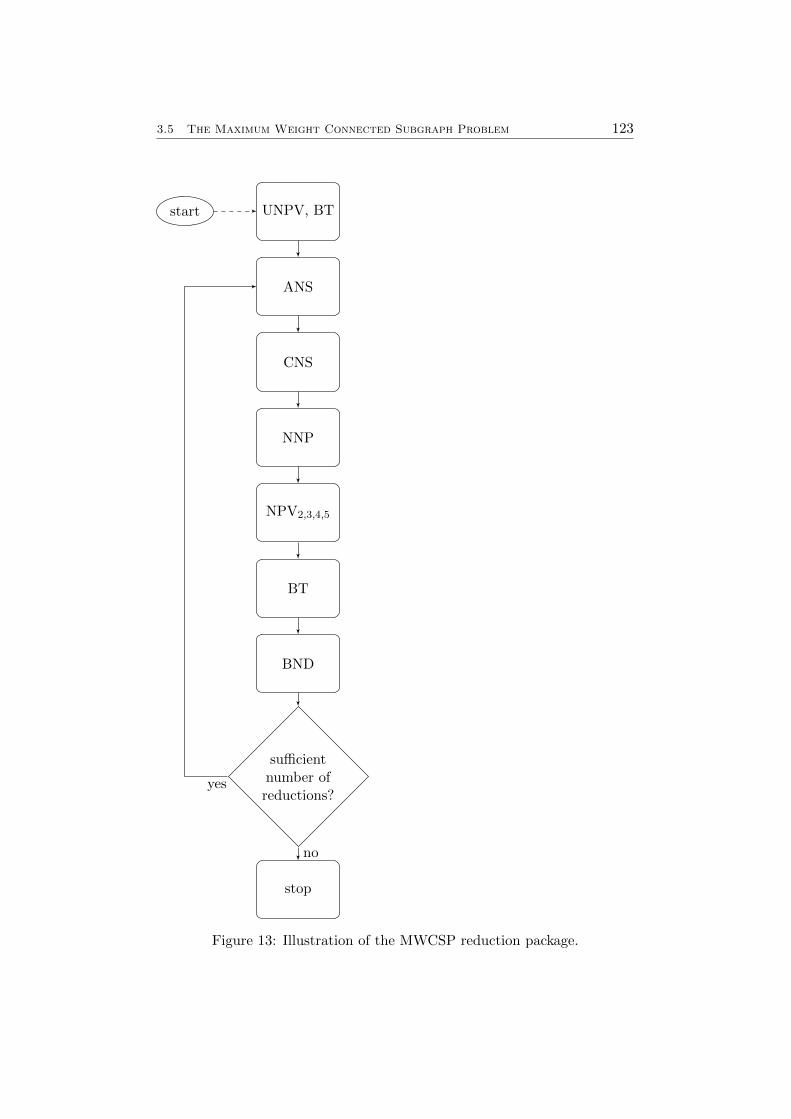
3.5 The Maximum Weight Connected Subgraph Problem 123
UNPV, BTstart
ANS
CNS
NNP
NPV2,3,4,5
BT
BND
sufficientnumber ofreductions?
stop
yes
no
Figure 13: Illustration of the MWCSP reduction package.

3.5 The Maximum Weight Connected Subgraph Problem 124
to connect vertices of positive weight to the current Steiner tree using onlyone edge.
Name Instances |V | Status Description
ACTMOD 8 2034-5226 solved Real-world instances derived from integrativebiological network analysis [DKR+08].
JMPALMK 72 500-1500 solved Euclidean, randomly generated instancesintroduced in [AMLM13].
Table 21: Classes of MWCSP instances.
For the computational experiments merely two classes of instances wereavailable which vary widely in their scope, with the JMPALMK set contain-ing nine times as many instances as the ACTMOD class, see Table 21.
Of the JMPALMK test set all but two instances are solved to optimalitywithin one second, more than 90 percent of them even in less than 0.4seconds. For the ACTMOD class more time is required, but SCIP-Jackstill manages to solve all of them within 20 seconds. Neither the JMPALMKnor the ACTMOD instances require branching. The summarized results areprovided in Table 22.
OptimalClass Instances Solved ∅Nodes ∅Time [s]
ACTMOD 8 8 1.0 5.6JMPALMK 72 72 1.0 0.3
Table 22: Computational results for MWCS instances.
Since almost all instances of the JMPALMK are solved during prepro-cessing, as will be demonstrated subsequently, and the ACTMOD instancesare solved very fast, we refrain from presenting detailed results on the im-pact of the primal heuristics, but merely mark that without problem specificprimal heuristics the time required for solving the ACTMOD instances isalmost two times as high on average. In line with the experimental resultsto the heretofore introduced Steiner problem variants, the recombinationheuristic does not improve the run time of the, easy, MWCSP test instances;on the contrary, the execution time is prolonged by four percent on average.
Impact of Reduction Techniques
Within the MWCS section, a considerable weight has been given to develop-ing efficient reduction techniques. The results illustrated in Table 23 provetheir strength. Not only 67 of all 72 JMPALMK instances are solved dur-ing presolving, but furthermore on average the ACTMOD instances containless than a third of their original vertices and edges after reduction. Weascribe the considerably stronger performance on the JMPALMK class to
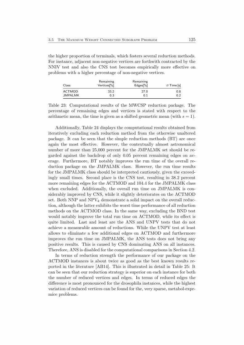
3.5 The Maximum Weight Connected Subgraph Problem 125
the higher proportion of terminals, which fosters several reduction methods.For instance, adjacent non-negative vertices are forthwith contracted by theNNIV test and also the CNS test becomes empirically more effective onproblems with a higher percentage of non-negative vertices.
Remaining RemainingClass Vertices[%] Edges[%] ∅Time [s]
ACTMOD 33.2 27.0 0.8JMPALMK 0.3 0.1 0.2
Table 23: Computational results of the MWCSP reduction package. Thepercentage of remaining edges and vertices is stated with respect to thearithmetic mean, the time is given as a shifted geometric mean (with s = 1).
Additionally, Table 24 displays the computational results obtained fromiteratively excluding each reduction method from the otherwise unalteredpackage. It can be seen that the simple reduction methods (BT) are onceagain the most effective. However, the contextually almost astronomicalnumber of more than 25,000 percent for the JMPALMK set should be re-garded against the backdrop of only 0.05 percent remaining edges on av-erage. Furthermore, BT notably improves the run time of the overall re-duction package on the JMPALMK class. However, the run time resultsfor the JMPALMK class should be interpreted cautiously, given the exceed-ingly small times. Second place is the CNS test, resulting in 38.2 percentmore remaining edges for the ACTMOD and 104.4 for the JMPALMK classwhen excluded. Additionally, the overall run time on JMPALMK is con-siderably improved by CNS, while it slightly deteriorates on the ACTMODset. Both NNP and NPVk demonstrate a solid impact on the overall reduc-tion, although the latter exhibits the worst time performance of all reductionmethods on the ACTMOD class. In the same way, excluding the BND testwould notably improve the total run time on ACTMOD, while its effect isquite limited. Last and least are the ANS and UNPV tests that do notachieve a measurable amount of reductions. While the UNPV test at leastallows to eliminate a few additional edges on ACTMOD and furthermoreimproves the run time on JMPALMK, the ANS tests does not bring anypositive results. This is caused by CNS dominating ANS on all instances.Therefore, ANS is disabled for the computational comparisons in Section 4.2.
In terms of reduction strength the performance of our package on theACTMOD instances is about twice as good as the best known results re-ported in the literature [AB14]. This is illustrated in detail in Table 25: Itcan be seen that our reduction strategy is superior on each instance for boththe number of reduced vertices and edges. In terms of reduced edges thedifference is most pronounced for the drosophila instances, while the highestvariation of reduced vertices can be found for the, very sparse, metabol-expr-mice problems.
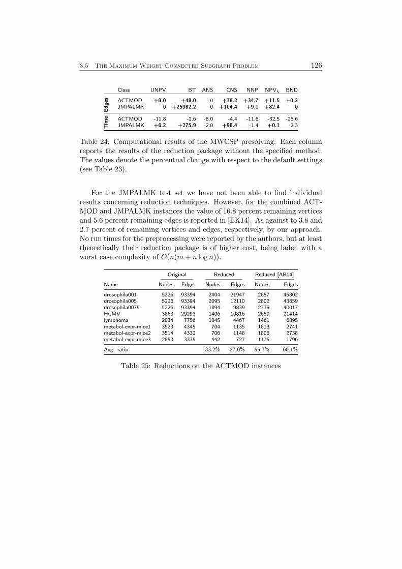
3.5 The Maximum Weight Connected Subgraph Problem 126
Class UNPV BT ANS CNS NNP NPVk BND
Edges ACTMOD +0.0 +48.0 0 +38.2 +34.7 +11.5 +0.2
JMPALMK 0 +25982.2 0 +104.4 +9.1 +82.4 0Tim
e ACTMOD -11.8 -2.6 -8.0 -4.4 -11.6 -32.5 -26.6JMPALMK +6.2 +275.9 -2.0 +98.4 -1.4 +0.1 -2.3
Table 24: Computational results of the MWCSP presolving. Each columnreports the results of the reduction package without the specified method.The values denote the percentual change with respect to the default settings(see Table 23).
For the JMPALMK test set we have not been able to find individualresults concerning reduction techniques. However, for the combined ACT-MOD and JMPALMK instances the value of 16.8 percent remaining verticesand 5.6 percent remaining edges is reported in [EK14]. As against to 3.8 and2.7 percent of remaining vertices and edges, respectively, by our approach.No run times for the preprocessing were reported by the authors, but at leasttheoretically their reduction package is of higher cost, being laden with aworst case complexity of O(n(m+ n log n)).
Original Reduced Reduced [AB14]
Name Nodes Edges Nodes Edges Nodes Edges
drosophila001 5226 93394 2404 21947 2857 45802drosophila005 5226 93394 2095 12110 2802 43859drosophila0075 5226 93394 1894 9839 2738 40017HCMV 3863 29293 1406 10816 2659 21414lymphoma 2034 7756 1045 4467 1461 6895metabol-expr-mice1 3523 4345 704 1135 1813 2741metabol-expr-mice2 3514 4332 706 1148 1808 2738metabol-expr-mice3 2853 3335 442 727 1175 1796
Avg. ratio 33.2% 27.0% 55.7% 60.1%
Table 25: Reductions on the ACTMOD instances
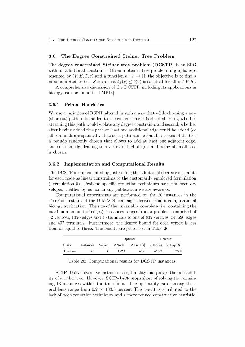
3.6 The Degree Constrained Steiner Tree Problem 127
3.6 The Degree Constrained Steiner Tree Problem
The degree-constrained Steiner tree problem (DCSTP) is an SPGwith an additional constraint: Given a Steiner tree problem in graphs rep-resented by (V,E, T, c) and a function b : V → N, the objective is to find aminimum Steiner tree S such that δS(v) ≤ b(v) is satisfied for all v ∈ V [S].
A comprehensive discussion of the DCSTP, including its applications inbiology, can be found in [LMP14].
3.6.1 Primal Heuristics
We use a variation of RSPH, altered in such a way that while choosing a new(shortest) path to be added to the current tree it is checked: First, whetherattaching this path would violate any degree constraints and second, whetherafter having added this path at least one additional edge could be added (orall terminals are spanned). If no such path can be found, a vertex of the treeis pseudo randomly chosen that allows to add at least one adjacent edge,and such an edge leading to a vertex of high degree and being of small costis chosen.
3.6.2 Implementation and Computational Results
The DCSTP is implemented by just adding the additional degree constraintsfor each node as linear constraints to the customarily employed formulation(Formulation 5). Problem specific reduction techniques have not been de-veloped, neither by us nor in any publication we are aware of.
Computational experiments are performed on the 20 instances in theTreeFam test set of the DIMACS challenge, derived from a computationalbiology application. The size of the, invariably complete (i.e. containing themaximum amount of edges), instances ranges from a problem comprised of52 vertices, 1326 edges and 35 terminals to one of 832 vertices, 345696 edgesand 407 terminals. Furthermore, the degree bound for each vertex is lessthan or equal to three. The results are presented in Table 26.
Optimal Timeout
Class Instances Solved ∅Nodes ∅Time [s] ∅Nodes ∅Gap [%]
TreeFam 20 7 162.8 40.6 413.9 25.9
Table 26: Computational results for DCSTP instances.
SCIP-Jack solves five instances to optimality and proves the infeasibil-ity of another two. However, SCIP-Jack stops short of solving the remain-ing 13 instances within the time limit. The optimality gaps among theseproblems range from 0.2 to 133.3 percent This result is attributed to thelack of both reduction techniques and a more refined constructive heuristic.
3.6 The Degree Constrained Steiner Tree Problem 128
However, without using the constructive heuristic the average gap amongthe unsolved instances is more than twice as high.
3.7 The Group Steiner Tree Problem 129
3.7 The Group Steiner Tree Problem
The group Steiner tree problem (GSTP) is another generalization ofthe Steiner tree problem, originating from VLSI design [HRW92], where theconcept of terminals as a set of vertices to be interconnected is extendedto a set of vertex groups: Given an undirected graph G = (V,E), edgecosts c : E → Q+ and a series of vertex subsets T1, ..., Ts ⊂ V , s ∈ N, aminimum cost tree spanning at least one vertex of each subset is required.By interpreting each terminal t as a subset {t}, every SPG can be consideredas a GSTP. Therefore, the latter is likewise NP-hard.
3.7.1 Transformation
Not only can an SPG be considered a GSTP, but also it is possible totransform each GTSP instance (V,E, T1, .., Ts, c) to an SPG by means ofthe following scheme:
Transformation 6 (GSTP to SPG).Input: A GSTP P = (V,E, T1, ...Ts, c)Output: An SPG P ′ = (V ′, E′, T ′, c′)
1. Set V ′ := V , E′ := E, T ′ = ∅, c′ := c, K :=∑
e∈E ce + 1.
2. For i = 1, ..., s add a new node t′i to V ′ and T ′ and for all vj ∈ Ti addan edge e = {t′i, vj} , with c′e := K.
3. Return (V ′, E′, T ′, c′).
Let (V,E, T1, ...Ts, c) be a GSTP and P ′ = (V ′, A′, T ′, c′) an SPG ob-tained by applying Transformation 6 on P . A solution S′ to P ′ can bereduced to a solution S to P by deleting all vertices and edges of S not in(V,E). The GSTP P can in this way be solved on the SPG P ′ as shown in[HRW92] and [Vos88].
This approach has already been deployed by [DVV04] to solve groupSteiner tree problems and demonstrated to be competitive with specializedsolvers at the time of publishing.
3.7.2 Implementation and Computational Results
For SCIP-JACK to solve a GSTP, first Transformation 6 is applied. Theresulting problem is treated as a normal SPG, which is solved without anyalteration.
Computational results for two test sets of unpublished group Steinertree instances derived from a industry wire routing problem are presentedin Table 28. SCIP-Jack solves all but two of the first test set, with runtimes ranging from 1.8 to 434.1 seconds. Five of the instances solved to
3.7 The Group Steiner Tree Problem 130
Name Instances |V | Status Description
GSTP1 8 349-1253 unsolved Sparse instances derived from a
problem in VLSI design.GSTP2 10 838-3177 unsolved
Table 27: Classes of GSTP instances.
optimality only require a single node, with the remaining instance solvedusing 614 nodes. Two instances of this set are terminated at the time limitof two hours, exhibiting optimality gaps of 1.1 and 4.2 percent, respectively.The performance on the second test set is notably weaker. Five instancesare solved within the time limit (with one requiring seven branch-and-boundnodes), whereas all other instances terminate with 54.7 branch-and-boundnodes on average. The best optimality gap among the unsolved instances ofGSTP2 is 0.8, the worst 2.9 percent.
Optimal Timeout
Class Instances Solved ∅Nodes ∅Time [s] ∅Nodes ∅Gap [%]
GSTP1 8 6 11.6 39.2 178.2 2.7GSTP2 10 5 2.0 3196.0 54.7 1.6
Table 28: Computational results for GSTP instances.
3.8 The Hop Constrained Directed Steiner Tree Problem 131
3.8 The Hop Constrained Directed Steiner Tree Problem
The hop-constrained directed Steiner tree problem (HCDSTP) canbe considered as an SAP incorporating additional conditions [BDK14]: First,the arc costs are required to be positive. Second, the additional constraintthat the number of selected arcs must not exceed a predetermined boundH, called hop limit, is incorporated. Finally, all terminals except theroot are necessarily leaves in each feasible solution. The flow-balance cutformulation (Formulation 5) used by SCIP-Jack is easily extended to coverthis variation by adding one extra linear inequality bounding the sum of allbinary arc variables and removing all incoming arcs to each terminal otherthan the root.
Still, the hop limit brings significant implications for the preprocessingand the heuristics in its wake: Many of the reduction techniques removeor include edges from the graph if a less costly alternative can be found,regardless of whether this alternative includes a greater number of edgesand possibly violates the hop constraint. Likewise, the so far employedheuristics do not consider the number of included edges, but merely theircosts.
Real-world applications of the HCDSTP include the three dimensionalplacement of drones for multi-target surveillance, see [OKD+10].
3.8.1 Reductions
For the HCDSTP no reduction techniques that we are aware of have beenpublished yet. Several approaches that are effective for other Steiner prob-lems, like the alternative-based reductions, are rendered prohibitive by thehop constraint. Therefore, this section encompasses merely bound-based re-duction techniques. Subsequently, it will be supposed that an HCDSTPPHC = (V,A, T, c, r,H) is given. As with the SAP, the representationT r := T \ {r} is used and r = t1 is presupposed.
Bound Based Reductions
Hereinafter, we reuse the concept of the rooted inward Voronoi diagram,introduced in Section 3.1.1. Additionally, for each i = 2, ..., s we definecimin := mina∈δ−(ti) ca.
Lemma 53. Let vi ∈ V \T and define tb := base(vi). If there is an optimalsolution S = (VS , AS) to PHC such that vi ∈ VS, then
~d(r, vi) + ~d(vi, tb) +
s∑q=2
cimin − maxq=2,...,n
cqmin (100)
is a lower bound on the weight of S.
3.8 The Hop Constrained Directed Steiner Tree Problem 132
Proof. Since S is an arborescence rooted in r, it contains a path P1 from rto vi that is of cost at least ~d(r, vi). Additionally, at least one path P2 fromvi to a terminal tj other than the root is contained in S, since the latter has
been assumed to be optimal. P2 is of cost at least ~d(vi, base(vi)) and due toS being cycle free, P1 and P2 are arc-disjoint. Since for all tk ∈ T \ {r, tj}it holds that δ+
S (tk) = ∅, none of their incoming arcs can be contained inP1 or P2. However, as all of them are contained in S, for each terminal inT \ {r, tj} one of its incoming arcs has to be part of S as well. Hence:
C(S) ≥ C(P1) + C(P2) +
s∑q=2,q 6=tj
cqmin
≥ ~d(r, vi) + ~d(vi, tj) +s∑
q=2,q 6=tj
cqmin
≥ ~d(r, vi) + ~d(vi, base(vi)) +s∑q=2
cimin − maxq=2,...,n
cqmin
The last term is tantamount to (100), so the lemma is established.
Not only the rooted inward Voronoi diagram, but also the associatedlemmata can be adopted from the SAP. To this end, assume the setting forthe lemmata 20 and 21 in Section 3.1.1.
Lemma 54. Let vi ∈ V \ T . If there is an optimal solution S = (VS , AS)such that vi ∈ VS, then
d(vi, vi,1) + d(vi, vi,2) +s−2∑q=2
inradius(tq), (101)
where the d-distances are affiliated with GD, is a lower bound on the weightof S.
Proof. Analogous to the proof of Lemma 21.
Lemma 55. Let (vi, vj) ∈ A. If there is an optimal solution S = (VS , AS)such that (vi, vj) ∈ AS, then L defined by
L := cij + d(vi, vi,1) + d(vj , vj,1) +
s−2∑q=2
inradius(tq) (102)
if vi,1 6= vj,1 and
L := min{d(vi, vi,1) + d(vj , vj,2), d(vi, vi,2) + d(vj , vj,1)
}+
s−2∑q=2
inradius(tq)
(103)
3.8 The Hop Constrained Directed Steiner Tree Problem 133
otherwise, is a lower bound on the weight of S. The d-distances are statedwith respect to GD.
Proof. Analogous to the proof of Lemma 21.
We denote the reduction test combining the antecedent three lemmataby Cost Bound (CBND) test: First, a solution S is computed by theheuristic introduced in Section 3.8.2. Second, we traverse each vertex vi ∈ V .If vi is a non-terminal and the bound (100) or (101) is higher than C(S) (orequal in the case of vi /∈ VS), the vertex vi can be deleted. Otherwise, wetraverse each outgoing arc δ+(vi) and attempt to eliminate it in the sameway using the bounds (102) and (103) respectively.
While the idiosycracy of the HCDSTP in the shape of the hop constraintimpedes numerous reduction techniques, it concomitantly gives rise to testsof a novel type. In the remainder of this section, denote by ~d1 the directeddistance function with respect to the arc costs 11. Consequently, ~d1(vi, vj) isequal to the minimal number of arcs necessary to reach the vertex vj fromthe vertex vi. Further, let N1 be a rooted inward Voronoi diagram on (V,A)with respect to d1.
Lemma 56. Let vi ∈ V \ T and tb ∈ T r such that vi ∈ N1(tb). If
~d1(r, vi) + ~d1(vi, tb) + |T | − 2 > H (104)
is satisfied, vi cannot be contained in any optimal solution.
Proof. Let S = (VS , AS) be an optimal solution and suppose vi ∈ VS . Analo-gously to the proof of Lemma 53 it can be verified that S contains arc-disjointpaths P1, from r to vi and P2, from vi to a tj ∈ T r. Considering the defini-
tion of d1 one readily acknowledges that at least ~d(r, vi) arcs are containedin P1 and at least ~d1(vi, tj) arcs are contained in P2. Furthermore, both P1
and P2 contain exactly one terminal, since to all terminal other than theroot there are no outgoing arcs. Noting that to each terminal in T \ {r, tj}there is at least one arc included in S, one obtains that
|As| ≥ ~d1(r, vi) + ~d1(vi, tj) + |T | − 2
≥ ~d1(r, vi) + ~d1(vi, tb) + |T | − 2
(104)> H.
Hence it can be inferred that, violating the hop constraint, S is not a feasiblesolution.
Furthermore, by exploiting the hop constraint property, both Lemma 54and Lemma 55 can be reshaped. To this end, denote for ti ∈ T r byinradius1(ti) the inradius(ti) value with respect to N1 and assume that
3.8 The Hop Constrained Directed Steiner Tree Problem 134
the ti ∈ T r are ordered in such a way that the corresponding inradius1
values are non-decreasing in i. Further, the d1-distances are stated withrespect to GD with edge costs 11.
Lemma 57. Let vi ∈ V \ T . If
d1(vi, vi,1) + d1(vi, vi,2) +s−2∑q=2
inradius1(tq) > H (105)
is satisfied, vi cannot be contained in any optimal solution.
Proof. Assume that (105) is satisfied for a vi ∈ V \ T . Using d1 as thedistance function d, one can be infer from Lemma 20 that for an optimalsolution S = (VS , AS) containing vi it would hold that
|AS | = C(S) ≥ d1(vi, vi,1) + d1(vi, vi,2) +
s−2∑q=2
inradius1(tq)(105)> H.
Therefore, no such S = (VS , AS) can exist.
Lemma 58. Let (vi, vj) ∈ A. If
1 + d1(vi, vi,1) + d1(vj , vj,1) +s−2∑q=2
inradius1(tq) > H (106)
in the case of vi,1 6= vj,1 or
1 + min{d1(vi, vi,1) + d1(vj , vj,2), d1(vi, vi,2) + d1(vj , vj,1)
}+s−2∑q=2
inradius1(tq) > H (107)
otherwise, (vi, vj) cannot be contained in any optimal solution.
Proof. Let (vi, vj) ∈ A. Suppose that (vi, vj) was contained in an optimalsolution S = (VS , AS). Using Lemma 21 this would imply in the case ofvi,1 6= vj,1 that:
|AS | = C(S) ≥ 1 + d1(vi, vi,1) + d1(vj , vj,1) +
s−2∑q=2
inradius1(tq)(106)> H
and in the case of vi,1 = vj,1 that:
|AS | = C(S)
≥ 1 + min{d1(vi, vi,1) + d1(vj , vj,2), d1(vi, vi,2) + d1(vj , vj,1)
}+
s−2∑q=2
inradius1(tq)
(107)> H.
Hence, no such S can exist and the lemma is established.
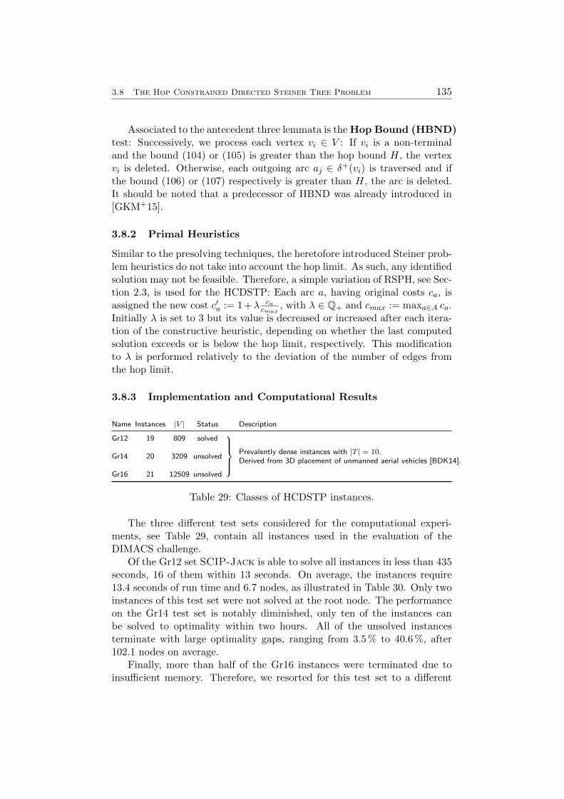
3.8 The Hop Constrained Directed Steiner Tree Problem 135
Associated to the antecedent three lemmata is the Hop Bound (HBND)test: Successively, we process each vertex vi ∈ V : If vi is a non-terminaland the bound (104) or (105) is greater than the hop bound H, the vertexvi is deleted. Otherwise, each outgoing arc aj ∈ δ+(vi) is traversed and ifthe bound (106) or (107) respectively is greater than H, the arc is deleted.It should be noted that a predecessor of HBND was already introduced in[GKM+15].
3.8.2 Primal Heuristics
Similar to the presolving techniques, the heretofore introduced Steiner prob-lem heuristics do not take into account the hop limit. As such, any identifiedsolution may not be feasible. Therefore, a simple variation of RSPH, see Sec-tion 2.3, is used for the HCDSTP: Each arc a, having original costs ca, isassigned the new cost c′a := 1 +λ ca
cmax, with λ ∈ Q+ and cmax := maxa∈A ca.
Initially λ is set to 3 but its value is decreased or increased after each itera-tion of the constructive heuristic, depending on whether the last computedsolution exceeds or is below the hop limit, respectively. This modificationto λ is performed relatively to the deviation of the number of edges fromthe hop limit.
3.8.3 Implementation and Computational Results
Name Instances |V | Status Description
Gr12 19 809 solved
Prevalently dense instances with |T | = 10.Gr14 20 3209 unsolved
Derived from 3D placement of unmanned aerial vehicles [BDK14].
Gr16 21 12509 unsolved
Table 29: Classes of HCDSTP instances.
The three different test sets considered for the computational experi-ments, see Table 29, contain all instances used in the evaluation of theDIMACS challenge.
Of the Gr12 set SCIP-Jack is able to solve all instances in less than 435seconds, 16 of them within 13 seconds. On average, the instances require13.4 seconds of run time and 6.7 nodes, as illustrated in Table 30. Only twoinstances of this test set were not solved at the root node. The performanceon the Gr14 test set is notably diminished, only ten of the instances canbe solved to optimality within two hours. All of the unsolved instancesterminate with large optimality gaps, ranging from 3.5 % to 40.6 %, after102.1 nodes on average.
Finally, more than half of the Gr16 instances were terminated due toinsufficient memory. Therefore, we resorted for this test set to a different
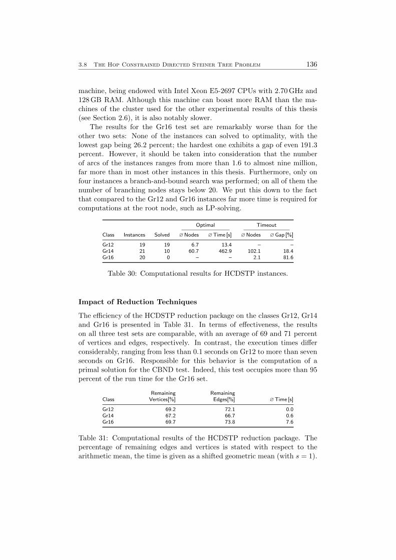
3.8 The Hop Constrained Directed Steiner Tree Problem 136
machine, being endowed with Intel Xeon E5-2697 CPUs with 2.70 GHz and128 GB RAM. Although this machine can boast more RAM than the ma-chines of the cluster used for the other experimental results of this thesis(see Section 2.6), it is also notably slower.
The results for the Gr16 test set are remarkably worse than for theother two sets: None of the instances can solved to optimality, with thelowest gap being 26.2 percent; the hardest one exhibits a gap of even 191.3percent. However, it should be taken into consideration that the numberof arcs of the instances ranges from more than 1.6 to almost nine million,far more than in most other instances in this thesis. Furthermore, only onfour instances a branch-and-bound search was performed; on all of them thenumber of branching nodes stays below 20. We put this down to the factthat compared to the Gr12 and Gr16 instances far more time is required forcomputations at the root node, such as LP-solving.
Optimal Timeout
Class Instances Solved ∅Nodes ∅Time [s] ∅Nodes ∅Gap [%]
Gr12 19 19 6.7 13.4 – –Gr14 21 10 60.7 462.9 102.1 18.4Gr16 20 0 – – 2.1 81.6
Table 30: Computational results for HCDSTP instances.
Impact of Reduction Techniques
The efficiency of the HCDSTP reduction package on the classes Gr12, Gr14and Gr16 is presented in Table 31. In terms of effectiveness, the resultson all three test sets are comparable, with an average of 69 and 71 percentof vertices and edges, respectively. In contrast, the execution times differconsiderably, ranging from less than 0.1 seconds on Gr12 to more than sevenseconds on Gr16. Responsible for this behavior is the computation of aprimal solution for the CBND test. Indeed, this test occupies more than 95percent of the run time for the Gr16 set.
Remaining RemainingClass Vertices[%] Edges[%] ∅Time [s]
Gr12 69.2 72.1 0.0Gr14 67.2 66.7 0.6Gr16 69.7 73.8 7.6
Table 31: Computational results of the HCDSTP reduction package. Thepercentage of remaining edges and vertices is stated with respect to thearithmetic mean, the time is given as a shifted geometric mean (with s = 1).
137
4 Final Computational Results and Comparisons
Although several computational results have been presented in the course ofthis work, they have been primarily focused on evaluating the performance ofseparate components and have therefore not been collated with other exactsolving results from the literature. In contrast, in the following SCIP-Jackis compared on several Steiner variants with the best problem specific solversdescribed in the literature. To this end, the heretofore computational envi-ronment is used. These settings are identical to the ones that were used toevaluate the solvers competing in the 11th DIMACS Challenge, which allowsfor an equitable comparison with the results obtained there. In this contextit should be noted that the results described in this thesis are significantlybetter than those obtained by the previous version of SCIP-Jack that wassubmitted to the DIMACS Challenge. However, we do not provide com-parisons between the current and just mentioned version of SCIP-Jack,but merely report the results yielded by the latest version. Besides in theDIMACS Challenge, results for a previous version of SCIP-Jack can befound in [GKM+15].
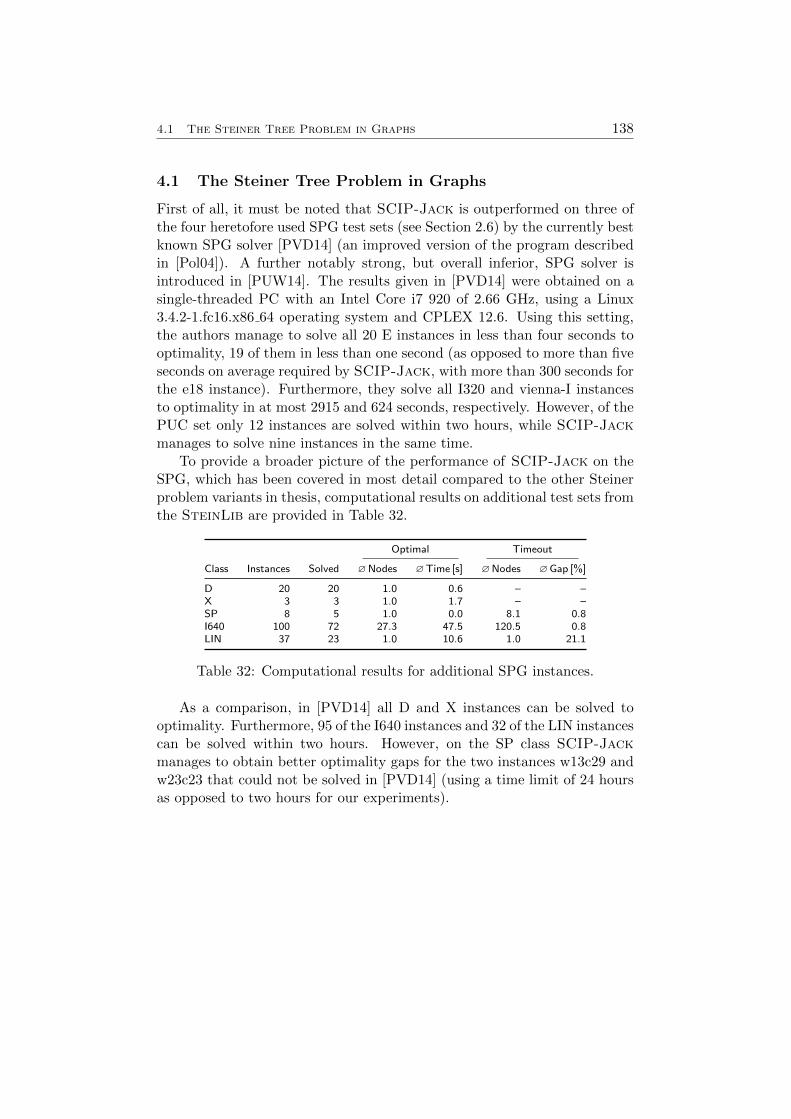
4.1 The Steiner Tree Problem in Graphs 138
4.1 The Steiner Tree Problem in Graphs
First of all, it must be noted that SCIP-Jack is outperformed on three ofthe four heretofore used SPG test sets (see Section 2.6) by the currently bestknown SPG solver [PVD14] (an improved version of the program describedin [Pol04]). A further notably strong, but overall inferior, SPG solver isintroduced in [PUW14]. The results given in [PVD14] were obtained on asingle-threaded PC with an Intel Core i7 920 of 2.66 GHz, using a Linux3.4.2-1.fc16.x86 64 operating system and CPLEX 12.6. Using this setting,the authors manage to solve all 20 E instances in less than four seconds tooptimality, 19 of them in less than one second (as opposed to more than fiveseconds on average required by SCIP-Jack, with more than 300 seconds forthe e18 instance). Furthermore, they solve all I320 and vienna-I instancesto optimality in at most 2915 and 624 seconds, respectively. However, of thePUC set only 12 instances are solved within two hours, while SCIP-Jackmanages to solve nine instances in the same time.
To provide a broader picture of the performance of SCIP-Jack on theSPG, which has been covered in most detail compared to the other Steinerproblem variants in thesis, computational results on additional test sets fromthe SteinLib are provided in Table 32.
Optimal Timeout
Class Instances Solved ∅Nodes ∅Time [s] ∅Nodes ∅Gap [%]
D 20 20 1.0 0.6 – –X 3 3 1.0 1.7 – –SP 8 5 1.0 0.0 8.1 0.8I640 100 72 27.3 47.5 120.5 0.8LIN 37 23 1.0 10.6 1.0 21.1
Table 32: Computational results for additional SPG instances.
As a comparison, in [PVD14] all D and X instances can be solved tooptimality. Furthermore, 95 of the I640 instances and 32 of the LIN instancescan be solved within two hours. However, on the SP class SCIP-Jackmanages to obtain better optimality gaps for the two instances w13c29 andw23c23 that could not be solved in [PVD14] (using a time limit of 24 hoursas opposed to two hours for our experiments).
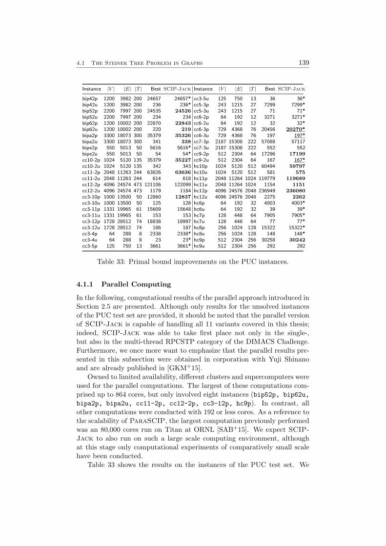
4.1 The Steiner Tree Problem in Graphs 139
Instance |V | |E| |T | Best SCIP-Jack Instance |V | |E| |T | Best SCIP-Jack
bip42p 1200 3982 200 24657 24657* cc3-5u 125 750 13 36 36*bip42u 1200 3982 200 236 236* cc5-3p 243 1215 27 7299 7299*bip52p 2200 7997 200 24535 24526 cc5-3u 243 1215 27 71 71*bip52u 2200 7997 200 234 234 cc6-2p 64 192 12 3271 3271*bip62p 1200 10002 200 22870 22843 cc6-2u 64 192 12 32 32*bip62u 1200 10002 200 220 219 cc6-3p 729 4368 76 20456 20270*bipa2p 3300 18073 300 35379 35326 cc6-3u 729 4368 76 197 197*bipa2u 3300 18073 300 341 338 cc7-3p 2187 15308 222 57088 57117bipe2p 550 5013 50 5616 5616* cc7-3u 2187 15308 222 552 552bipe2u 550 5013 50 54 54* cc9-2p 512 2304 64 17296 17199cc10-2p 1024 5120 135 35379 35227 cc9-2u 512 2304 64 167 167*cc10-2u 1024 5120 135 342 343 hc10p 1024 5120 512 60494 59797cc11-2p 2048 11263 244 63826 63636 hc10u 1024 5120 512 581 575cc11-2u 2048 11263 244 614 618 hc11p 2048 11264 1024 119779 119689cc12-2p 4096 24574 473 121106 122099 hc11u 2048 11264 1024 1154 1151cc12-2u 4096 24574 473 1179 1184 hc12p 4096 24576 2048 236949 236080cc3-10p 1000 13500 50 12860 12837 hc12u 4096 24576 2048 2275 2262cc3-10u 1000 13500 50 125 126 hc6p 64 192 32 4003 4003*cc3-11p 1331 19965 61 15609 15648 hc6u 64 192 32 39 39*cc3-11u 1331 19965 61 153 153 hc7p 128 448 64 7905 7905*cc3-12p 1728 28512 74 18838 18997 hc7u 128 448 64 77 77*cc3-12u 1728 28512 74 186 187 hc8p 256 1024 128 15322 15322*cc3-4p 64 288 8 2338 2338* hc8u 256 1024 128 148 148*cc3-4u 64 288 8 23 23* hc9p 512 2304 256 30258 30242cc3-5p 125 750 13 3661 3661* hc9u 512 2304 256 292 292
Table 33: Primal bound improvements on the PUC instances.
4.1.1 Parallel Computing
In the following, computational results of the parallel approach introduced inSection 2.5 are presented. Although only results for the unsolved instancesof the PUC test set are provided, it should be noted that the parallel versionof SCIP-Jack is capable of handling all 11 variants covered in this thesis;indeed, SCIP-Jack was able to take first place not only in the single-,but also in the multi-thread RPCSTP category of the DIMACS Challenge.Furthermore, we once more want to emphasize that the parallel results pre-sented in this subsection were obtained in corporation with Yuji Shinanoand are already published in [GKM+15].
Owned to limited availability, different clusters and supercomputers wereused for the parallel computations. The largest of these computations com-prised up to 864 cores, but only involved eight instances (bip52p, bip62u,
bipa2p, bipa2u, cc11-2p, cc12-2p, cc3-12p, hc9p). In contrast, allother computations were conducted with 192 or less cores. As a reference tothe scalability of ParaSCIP, the largest computation previously performedwas an 80,000 cores run on Titan at ORNL [SAB+15]. We expect SCIP-Jack to also run on such a large scale computing environment, althoughat this stage only computational experiments of comparatively small scalehave been conducted.
Table 33 shows the results on the instances of the PUC test set. We
4.1 The Steiner Tree Problem in Graphs 140
list the number of vertices, edges and terminals, as well as the best primalbound known at the beginning of the challenge (August 2014), and theprimal solution value obtained by our experiments with the parallel versionof SCIP-Jack, which employs the LP solver of CPLEX 12.6. Prior tothe experiments performed with SCIP-Jack, 32 instances of the PUC testset remained unsolved. Three of these instances have been solved by SCIP-Jack to proven optimality. These instances are underlined and marked withan asterisk in Table 33. For a further 16 instances SCIP-Jack improvedthe best known solution. All instances for which the best known primalbound has been improved are marked in bold. Finally, all previously solvedinstances of the PUC test set have also been solved by SCIP-Jack to provenoptimality; signified by an asterisk (without underline).
In summary, the heretofore reported results demonstrate an overall strongperformance of the parallel version of SCIP-Jack in solving computation-ally difficult instances.
4.2 Variants of the Steiner Tree Problem 141
4.2 Variants of the Steiner Tree Problem
In the following, for several Steiner problem variants comparisons are drawnbetween the results presented in this thesis and the best known ones fromthe literature. For this purpose, results obtained in the course of the 11thDIMACS Challenge are used predominantly. However, also other results re-ported in the literature are provided. Once again, we want to point out thatin our thesis an improved version of SCIP-Jack is used as compared to theone that competed in the DIMACS Challenge. Preliminarily, some remarkson the Steiner problem variants not covered hereinafter are necessary:
For the Steiner arborescence problem merely very easy instances wereavailable, solvable in fractions of a second. Therefore, comparisons withother results from the literature do not seem reasonable.
For the node-weighted Steiner tree problem only two instances have beencovered in this thesis (and published in the course of the DIMACS Chal-lenge); unfortunately we could not find any publication reporting results forthese instances.
The rectilinear Steiner minimum tree instances of dimension two canbe solved by the geometric Steiner problem solver GeoSteiner, which wasalready mentioned in Section 3.3. As described in the same section, moreadvanced modifications would be necessary to render SCIP-Jack competi-tive with this solver. Nevertheless, we are not aware of any other solver beingable to handle the high dimensional RMST instances that can be solved bySCIP-Jack as demonstrated in Section 3.3.2.
Finally, the group Steiner tree problem instances have not been madepublicly available yet and can therefore not be used for computational com-parisons.
To the best of our knowledge, for all Steiner problem variants coveredhereinafter no results published in the literature exceed those achieved inthe course of the DIMACS Challenge.
4.2.1 The Prize Collecting Steiner Tree Problem
Both the Cologne1 and Cologne2 class were used as test sets in the DIMACSChallenge. In the following two tables we compare our results with the bestknown other ones. These were achieved by the solver Mozartballs [FLL+14].The best results reported for the RPCSTP instances outside the DIMACSChallenge can be found in [LWP+06]. Requiring more than 40,000 secondsof run time for several instances, these results are clearly inferior to the onesof the best two groups competing in the challenge.
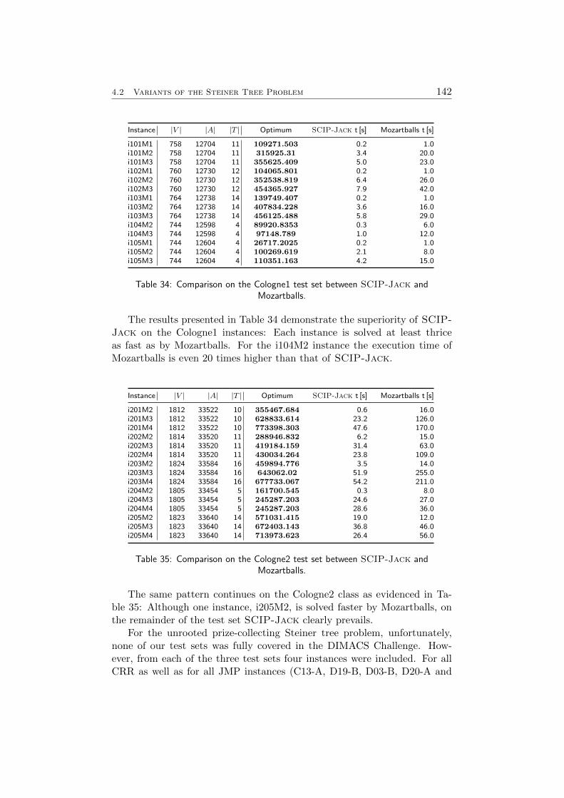
4.2 Variants of the Steiner Tree Problem 142
Instance |V | |A| |T | Optimum SCIP-Jack t [s] Mozartballs t [s]
i101M1 758 12704 11 109271.503 0.2 1.0i101M2 758 12704 11 315925.31 3.4 20.0i101M3 758 12704 11 355625.409 5.0 23.0i102M1 760 12730 12 104065.801 0.2 1.0i102M2 760 12730 12 352538.819 6.4 26.0i102M3 760 12730 12 454365.927 7.9 42.0i103M1 764 12738 14 139749.407 0.2 1.0i103M2 764 12738 14 407834.228 3.6 16.0i103M3 764 12738 14 456125.488 5.8 29.0i104M2 744 12598 4 89920.8353 0.3 6.0i104M3 744 12598 4 97148.789 1.0 12.0i105M1 744 12604 4 26717.2025 0.2 1.0i105M2 744 12604 4 100269.619 2.1 8.0i105M3 744 12604 4 110351.163 4.2 15.0
Table 34: Comparison on the Cologne1 test set between SCIP-Jack andMozartballs.
The results presented in Table 34 demonstrate the superiority of SCIP-Jack on the Cologne1 instances: Each instance is solved at least thriceas fast as by Mozartballs. For the i104M2 instance the execution time ofMozartballs is even 20 times higher than that of SCIP-Jack.
Instance |V | |A| |T | Optimum SCIP-Jack t [s] Mozartballs t [s]
i201M2 1812 33522 10 355467.684 0.6 16.0i201M3 1812 33522 10 628833.614 23.2 126.0i201M4 1812 33522 10 773398.303 47.6 170.0i202M2 1814 33520 11 288946.832 6.2 15.0i202M3 1814 33520 11 419184.159 31.4 63.0i202M4 1814 33520 11 430034.264 23.8 109.0i203M2 1824 33584 16 459894.776 3.5 14.0i203M3 1824 33584 16 643062.02 51.9 255.0i203M4 1824 33584 16 677733.067 54.2 211.0i204M2 1805 33454 5 161700.545 0.3 8.0i204M3 1805 33454 5 245287.203 24.6 27.0i204M4 1805 33454 5 245287.203 28.6 36.0i205M2 1823 33640 14 571031.415 19.0 12.0i205M3 1823 33640 14 672403.143 36.8 46.0i205M4 1823 33640 14 713973.623 26.4 56.0
Table 35: Comparison on the Cologne2 test set between SCIP-Jack andMozartballs.
The same pattern continues on the Cologne2 class as evidenced in Ta-ble 35: Although one instance, i205M2, is solved faster by Mozartballs, onthe remainder of the test set SCIP-Jack clearly prevails.
For the unrooted prize-collecting Steiner tree problem, unfortunately,none of our test sets was fully covered in the DIMACS Challenge. How-ever, from each of the three test sets four instances were included. For allCRR as well as for all JMP instances (C13-A, D19-B, D03-B, D20-A and
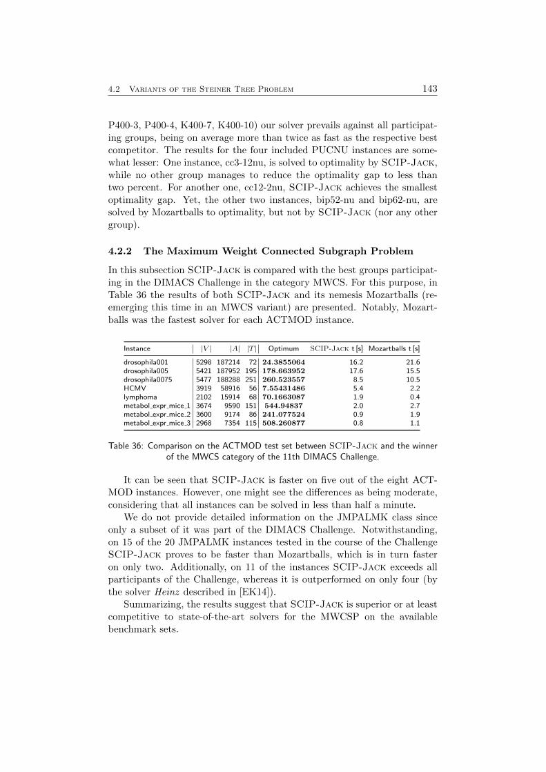
4.2 Variants of the Steiner Tree Problem 143
P400-3, P400-4, K400-7, K400-10) our solver prevails against all participat-ing groups, being on average more than twice as fast as the respective bestcompetitor. The results for the four included PUCNU instances are some-what lesser: One instance, cc3-12nu, is solved to optimality by SCIP-Jack,while no other group manages to reduce the optimality gap to less thantwo percent. For another one, cc12-2nu, SCIP-Jack achieves the smallestoptimality gap. Yet, the other two instances, bip52-nu and bip62-nu, aresolved by Mozartballs to optimality, but not by SCIP-Jack (nor any othergroup).
4.2.2 The Maximum Weight Connected Subgraph Problem
In this subsection SCIP-Jack is compared with the best groups participat-ing in the DIMACS Challenge in the category MWCS. For this purpose, inTable 36 the results of both SCIP-Jack and its nemesis Mozartballs (re-emerging this time in an MWCS variant) are presented. Notably, Mozart-balls was the fastest solver for each ACTMOD instance.
Instance |V | |A| |T | Optimum SCIP-Jack t [s] Mozartballs t [s]
drosophila001 5298 187214 72 24.3855064 16.2 21.6drosophila005 5421 187952 195 178.663952 17.6 15.5drosophila0075 5477 188288 251 260.523557 8.5 10.5HCMV 3919 58916 56 7.55431486 5.4 2.2lymphoma 2102 15914 68 70.1663087 1.9 0.4metabol expr mice 1 3674 9590 151 544.94837 2.0 2.7metabol expr mice 2 3600 9174 86 241.077524 0.9 1.9metabol expr mice 3 2968 7354 115 508.260877 0.8 1.1
Table 36: Comparison on the ACTMOD test set between SCIP-Jack and the winnerof the MWCS category of the 11th DIMACS Challenge.
It can be seen that SCIP-Jack is faster on five out of the eight ACT-MOD instances. However, one might see the differences as being moderate,considering that all instances can be solved in less than half a minute.
We do not provide detailed information on the JMPALMK class sinceonly a subset of it was part of the DIMACS Challenge. Notwithstanding,on 15 of the 20 JMPALMK instances tested in the course of the ChallengeSCIP-Jack proves to be faster than Mozartballs, which is in turn fasteron only two. Additionally, on 11 of the instances SCIP-Jack exceeds allparticipants of the Challenge, whereas it is outperformed on only four (bythe solver Heinz described in [EK14]).
Summarizing, the results suggest that SCIP-Jack is superior or at leastcompetitive to state-of-the-art solvers for the MWCSP on the availablebenchmark sets.
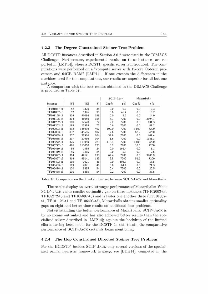
4.2 Variants of the Steiner Tree Problem 144
4.2.3 The Degree Constrained Steiner Tree Problem
All DCSTP instances described in Section 3.6.2 were used in the DIMACSChallenge. Furthermore, experimental results on these instances are re-ported in [LMP14], where a DCSTP specific solver is introduced. The com-putations were performed on a ”compute server with 12-core Opteron pro-cessors and 64GB RAM” [LMP14]. If one excepts the differences in themachines used for the computations, our results are superior for all but oneinstance.
A comparison with the best results obtained in the DIMACS Challengeis provided in Table 37.
SCIP-Jack Mozartballs
Instance |V | |E| |T | Gap % t [s] Gap % t [s]
TF101057-t1 52 1326 35 0.0 0.0 0.0 0.3TF101057-t3 52 1326 35 0.0 46.7 0.0 0.7TF101125-t1 304 46056 155 0.0 4.6 0.0 14.0TF101125-t3 304 46056 155 3.7 7200 0.0 3194.1TF101202-t1 188 17578 72 2.2 7200 0.0 131.3TF101202-t3 188 17578 72 0.6 7200 0.0 87.2TF102003-t1 832 345696 407 102.0 7200 >100 7200TF102003-t3 832 345696 407 7.6 7200 62.2 7200TF105035-t1 237 27966 104 32.8 7200 0.0 407.4TF105035-t3 237 27966 104 1.6 7200 0.0 1181.3TF105272-t1 476 113050 223 113.1 7200 >100 7200TF105272-t3 476 113050 223 8.2 7200 10.5 7200TF105419-t1 55 1485 24 0.0 161.4 0.0 1.1TF105419-t3 55 1485 24 0.0 5.9 0.0 2.6TF105897-t1 314 49141 133 62.4 7200 0.0 3206.9TF105897-t3 314 49141 133 2.5 7200 51.6 7200TF106403-t1 119 7021 46 0.0 493.3 0.0 15.5TF106403-t3 119 7021 46 0.0 64.4 0.0 71.3TF106478-t1 130 8385 54 0.4 7200 0.0 20.5TF106478-t3 130 8385 54 0.2 7200 0.0 37.5
Table 37. Comparison on the TreeFam test set between SCIP-Jack and Mozartballs.
The results display an overall stronger performance of Mozartballs: WhileSCIP-Jack yields smaller optimality gap on three instances (TF102003-t3,TF105272-t3 and TF105897-t3) and is faster one another three (TF101057-t1, TF101125-t1 and TF106403-t3), Mozartballs obtains smaller optimalitygaps on eight and better time results on additional four problems.
Notwithstanding the better performance of Mozartballs, SCIP-Jack isby no means outranked and has also achieved better results than the spe-cialized solver described in [LMP14]; against the backdrop of the limitedefforts having been made for the DCSTP in this thesis, the comparativeperformance of SCIP-Jack certainly bears mentioning.
4.2.4 The Hop Constrained Directed Steiner Tree Problem
For the HCDSTP, besides SCIP-Jack only several versions of the special-ized primal heuristic framework Stephop, see [BDK14], competed in the
4.2 Variants of the Steiner Tree Problem 145
DIMACS Challenge. Therefore, no detailed information is provided here.Nevertheless, it should not go unnoticed that for the 20 instances of theGr12 and Gr14 sets being part of the Challenge, the upper bounds com-puted by SCIP-Jack within two hours are equal for three and better for 13instances, as compared to the results achieved by the competing heuristics.
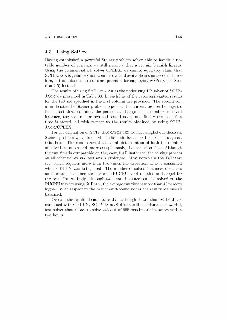
4.3 Using SoPlex 146
4.3 Using SoPlex
Having established a powerful Steiner problem solver able to handle a no-table number of variants, we still perceive that a certain blemish lingers:Using the commercial LP solver CPLEX, we cannot equitably claim thatSCIP-Jack is genuinely non-commercial and available in source code. There-fore, in this subsection results are provided for employing SoPlex (see Sec-tion 2.5) instead.
The results of using SoPlex 2.2.0 as the underlying LP solver of SCIP-Jack are presented in Table 38. In each line of the table aggregated resultsfor the test set specified in the first column are provided. The second col-umn denotes the Steiner problem type that the current test set belongs to.In the last three columns, the percentual change of the number of solvedinstance, the required branch-and-bound nodes and finally the executiontime is stated, all with respect to the results obtained by using SCIP-Jack/CPLEX.
For the evaluation of SCIP-Jack/SoPlex we have singled out those sixSteiner problem variants on which the main focus has been set throughoutthis thesis. The results reveal an overall deterioration of both the numberof solved instances and, more conspicuously, the execution time. Althoughthe run time is comparable on the, easy, SAP instances, the solving processon all other non-trivial test sets is prolonged. Most notable is the JMP testset, which requires more than two times the execution time it consumedwhen CPLEX was being used. The number of solved instances decreaseson four test sets, increases for one (PUCNU) and remains unchanged forthe rest. Interestingly, although two more instances can be solved on thePUCNU test set using SoPlex, the average run time is more than 40 percenthigher. With respect to the branch-and-bound nodes the results are overallbalanced.
Overall, the results demonstrate that although slower than SCIP-Jackcombined with CPLEX, SCIP-Jack/SoPlex still constitutes a powerful,fast solver that allows to solve 443 out of 555 benchmark instances withintwo hours.
4.3 Using SoPlex 147
Class Type Solved Instances Nodes Time
E – +32.2 +30.2I320
SPG-3.2 -6.7 +16.2
vienna-I -14.0 +46.0 +44.8PUC -11.1 -48.6 +10.9
GeneSAP
– – +4.7Gene2002 – – -9.9
JMPPCSTP
– – +120.0CRR – – +32.0PUCNU +20.0 +41.8 +42.8
Cologne1RPCSTP
– – +52.3Cologne2 – – +63.7
JMPALMKMWCSP
– – -26.9ACTMOD – +21.4 +10.3
Gr12HCDSTP
– +50.1 +25.4Gr14 -30.0 -83.2 +65.1
Table 38: Computational results of SCIP-Jack/SoPlex. In each line thepercentual changes with respect to the results obtained by using CPLEXare reported.
4.3 Using SoPlex 148
149
5 Conclusions and Outlook
In this thesis an approach has been presented that allows to solve 11 differentSteiner problems within a single framework, standing in stark contrast tothe problem specific strategy of other state-of-the-art Steiner tree solvers.This achievement has been rendered possible by employing various, oftennovel, methods to transform the problems into a general form, which canbe solved by a branch-and-cut based procedure using the academic MIPframework SCIP. Two advantages of employing this generic approach areimmediately conspicuous:
First, the amount of problem specific code is notably reduced. While forthe SPG around 20,000 lines of code (with more than 10 percent being com-ments) were needed, each additional problem variant required only about500 lines on average. As a comparison, the pure SPG solver described in[Pol04] is reported to encompass ”roughly thousand pages” of code, whichamounts to about 60,000 lines of code taking the size of each page in [Pol04]as a reference.
Second, a number of general solution methods natively implemented inSCIP, e.g. cutting planes (being notably effective for several hard instancessuch as in the PUC class), are available and will be kept up-to-date auto-matically by the continuous improvements in the framework.
Moreover, not entirely in line with the overall generic approach, vari-ous novel reduction techniques have been introduced that surpass existingmethods for several Steiner problem variants such as the maximum-weightconnected subgraph problem. Likewise, several heuristics have been devised,although they can all be seen as variations of three basic versions, the RSP,VQ and RC heuristics. Albeit both the reduction techniques and, partly,the heuristics are problem specific, they easily assimilate within our generalframework, also by virtue of the plugin-based structure of SCIP.
In this way, the combination of the generic branch-and-cut based ap-proach and problem specific techniques has enabled us to achieve our initialgoal to be able to handle a large variety of Steiner problem variants, butto allow at the same time for fast solving: The exact solver SCIP-Jack(the offspring of embedding the pure SPG solver Jack-III into SCIP) ac-companying this work is capable of solving several problem classes, e.g. the(real-world) RPCSTP instances, faster than any other solver we are awareof. Furthermore, it should be marked that the opportunity to solve instancesin a massively parallel distributed memory environment has been added atminimal cost.
Still, there surely is potential for further improving the performance ofthe solver. Concerning the Steiner tree problem in graphs, additional meth-ods described in the literature, most notably in [Pol04], such as dual heuris-tics and additional reduction tests are expected to bear a high capability forimproving the run time of SCIP-Jack.
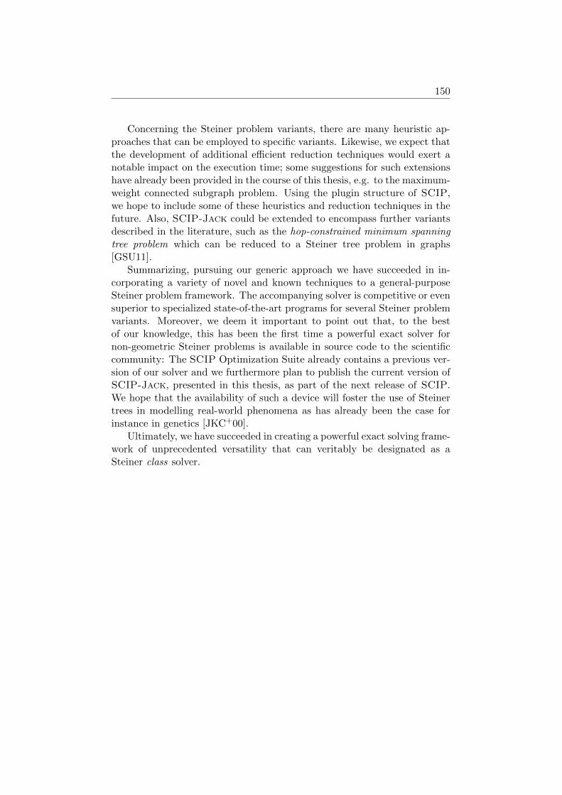
150
Concerning the Steiner problem variants, there are many heuristic ap-proaches that can be employed to specific variants. Likewise, we expect thatthe development of additional efficient reduction techniques would exert anotable impact on the execution time; some suggestions for such extensionshave already been provided in the course of this thesis, e.g. to the maximum-weight connected subgraph problem. Using the plugin structure of SCIP,we hope to include some of these heuristics and reduction techniques in thefuture. Also, SCIP-Jack could be extended to encompass further variantsdescribed in the literature, such as the hop-constrained minimum spanningtree problem which can be reduced to a Steiner tree problem in graphs[GSU11].
Summarizing, pursuing our generic approach we have succeeded in in-corporating a variety of novel and known techniques to a general-purposeSteiner problem framework. The accompanying solver is competitive or evensuperior to specialized state-of-the-art programs for several Steiner problemvariants. Moreover, we deem it important to point out that, to the bestof our knowledge, this has been the first time a powerful exact solver fornon-geometric Steiner problems is available in source code to the scientificcommunity: The SCIP Optimization Suite already contains a previous ver-sion of our solver and we furthermore plan to publish the current version ofSCIP-Jack, presented in this thesis, as part of the next release of SCIP.We hope that the availability of such a device will foster the use of Steinertrees in modelling real-world phenomena as has already been the case forinstance in genetics [JKC+00].
Ultimately, we have succeeded in creating a powerful exact solving frame-work of unprecedented versatility that can veritably be designated as aSteiner class solver.
References 151
References
[AB09] Tobias Achterberg and Timo Berthold. Hybrid Branching. InWillem Jan van Hoeve and John N. Hooker, editors, Integra-tion of AI and OR Techniques in Constraint Programming forCombinatorial Optimization Problems, 6th International Con-ference, CPAIOR 2009, volume 5547 of Lecture Notes in Com-puter Science, pages 309–311. Springer, May 2009.
[AB14] Ernst Althaus and Markus Blumenstock. Algorithmsfor the Maximum Weight Connected Subgraph and Prize-collecting Steiner Tree Problems. Unpublished manuscript athttp://dimacs11.cs.princeton.edu/workshop.html, 2014.
[ABCC11] David L Applegate, Robert E Bixby, Vasek Chvatal, andWilliam J Cook. The Traveling Salesman Problem: A Com-putational Study. Princeton University Press, Princeton, NewJersey, 2011.
[Ach07] Tobias Achterberg. Constraint Integer Programming. PhD the-sis, Technische Universitat Berlin, 2007.
[Ach09] Tobias Achterberg. SCIP: Solving constraint integer programs.Mathematical Programming Computation, 1(1):1–41, 2009.
[AKM04] Tobias Achterberg, Thorsten Koch, and Alexander Martin.Branching rules revisited. Operations Research Letters, 33:42–54, 2004.
[AMLM13] Eduardo Alvarez-Miranda, Ivana Ljubic, and Petra Mutzel. Themaximum weight connected subgraph problem., pages 245–270.Berlin: Springer, 2013.
[Ane80] Yash P. Aneja. An integer linear programming approach to theSteiner problem in graphs. Networks, 10(2):167–178, 1980.
[BDK14] Oleg Burdakov, Patrick Doherty, and Jonas Kvarnstrom. Lo-cal Search for Hop-constrained Directed Steiner Tree Problemwith Application to UAV-based Multi-target Surveillance. InButenko, S., Pasiliao, E.L., Shylo, and V., editors, ExaminingRobustness and Vulnerability of Networked Systems, volume 37of NATO Science for Peace and Security Series - D: Infor-mation and Communication Security, pages 26–50. IOS Press,2014.
[Bea84] J. E. Beasley. An algorithm for the Steiner problem in graphs.Networks, 14(1):147–159, 1984.
References 152
[Bea89] J.E. Beasley. An SST-based algorithm for the Steiner problemin graphs. Networks, 19:1–16, 1989.
[Bea92] J.E. Beasley. A heuristic for Euclidean and rectilinear Steinerproblems. European Journal of Operational Research, 58:284–292, 1992.
[BGG+12] Timo Berthold, Gerald Gamrath, Ambros M. Gleixner, StefanHeinz, Thorsten Koch, and Yuji Shinano. Solving mixed inte-ger linear and nonlinear problems using the SCIP OptimizationSuite. Technical Report 12-27, ZIB, Takustr.7, 14195 Berlin,2012.
[BGRS13] Jaroslaw Byrka, Fabrizio Grandoni, Thomas Rothvoß, andLaura Sanita. Steiner Tree Approximation via Iterative Ran-domized Rounding. The Journal of the ACM, 60(1):6, 2013.
[BGTZ14] M. Brazil, R. L. Graham, D. A. Thomas, and M. Zachariasen.On the History of the Euclidean Steiner Tree Problem. Archivefor History of Exact Sciences, 68:327–354, 2014.
[BP87] Anantaram Balakrishnan and Nitin R. Patel. Problem reduc-tion methods and a tree generation algorithm for the Steinernetwork problem. Networks, 17(1):65–85, 1987.
[BP89] Marshall W. Bern and Paul E. Plassmann. The Steiner Problemwith Edge Lengths 1 and 2. Information Processing Letters,32(4):171–176, 1989.
[BW05] Dimitris Bertsimas and Robert Weismantel. Optimization overintegers. Athena Scientific, 2005.
[CC08] Miroslav Chlebık and Janka Chlebıkova. The Steiner tree prob-lem on graphs: Inapproximability results. Theoretical ComputerScience, 406(3):207–214, 2008.
[CCC+98] Moses Charikar, Chandra Chekuri, To-yat Cheung, Zuo Dai,Ashish Goel, Sudipto Guha, and Ming Li. Approximation Al-gorithms for Directed Steiner Problems. In Proceedings of theNinth Annual ACM-SIAM Symposium on Discrete Algorithms,SODA ’98, pages 192–200, Philadelphia, PA, USA, 1998. Soci-ety for Industrial and Applied Mathematics.
[CGSW14] Krzysztof Ciebiera, Piotr Godlewski, Piotr Sankowski, and Pi-otr Wygocki. Approximation Algorithms for Steiner Tree Prob-lems Based on Universal Solution Frameworks. Computing Re-search Repository, abs/1410.7534, 2014.
References 153
[CR94] Sunil Chopra and M. Rao. The Steiner tree problem I: For-mulations, compositions and extension of facets. MathematicalProgramming, 64(2):209–229, 1994.
[CSHH+13] Salim Akhter Chowdhury, Stanley Shackney, KerstinHeselmeyer-Haddad, Thomas Ried, Alejandro A. Schaffer, andRussell Schwartz. Phylogenetic analysis of multiprobe fluores-cence in situ hybridization data from tumor cell populations.Bioinformatics, 29(13):189–198, 2013.
[dAW02] Marcus Poggi de Aragao and Renato F. Werneck. On the Im-plementation of MST-based Heuristics for the Steiner Problemin Graphs. In Proceedings of the 4th International Workshop onAlgorithm Engineering and Experiments, pages 1–15. Springer,2002.
[DHK14] Erik D. Demaine, Mohammad Taghi Hajiaghayi, and Philip N.Klein. Node-Weighted Steiner Tree and Group Steiner Tree inPlanar Graphs. ACM Transactions on Algorithms, 10(3):13:1–13:20, 2014.
[DKR+08] Marcus T. Dittrich, Gunnar W. Klau, Andreas Rosenwald,Thomas Dandekar, and Tobias Muller. Identifying functionalmodules in protein-protein interaction networks: an integratedexact approach. In ISMB, pages 223–231, 2008.
[Dui93] C. Duin. Steiner Problems in Graphs. PhD thesis, Universityof Amsterdam, 1993.
[DV89] C. W. Duin and A. Volgenant. Reduction tests for the Steinerproblem in graphs. Networks, 19(5):549–567, 1989.
[DVV04] C. W. Duin, A. Volgenant, and S. Voss. Solving group Steinerproblems as Steiner problems. European Journal of OperationalResearch, 154(1):323–329, 2004.
[EK14] Mohammed El-Kebir and Gunnar W. Klau. Solving theMaximum-Weight Connected Subgraph Problem to Optimal-ity. Computing Research Repository, abs/1409.5308, 2014.
[Ema10] Nahit Emanet. The Rectilinear Steiner Tree Problem. LambertAcademic Publishing, 2010.
[ES03] Agoston E. Eiben and J. E. Smith. Introduction to EvolutionaryComputing. Springer, 2003.
[Fis91] M. Fischetti. Facets of two Steiner arborescence polyhedra.Mathematical Programming, 51:401–419, 1991.
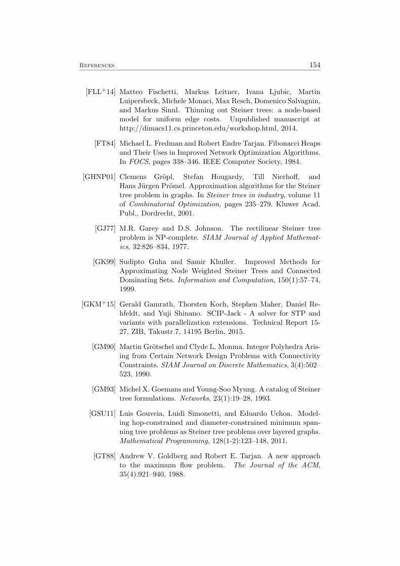
References 154
[FLL+14] Matteo Fischetti, Markus Leitner, Ivana Ljubic, MartinLuipersbeck, Michele Monaci, Max Resch, Domenico Salvagnin,and Markus Sinnl. Thinning out Steiner trees: a node-basedmodel for uniform edge costs. Unpublished manuscript athttp://dimacs11.cs.princeton.edu/workshop.html, 2014.
[FT84] Michael L. Fredman and Robert Endre Tarjan. Fibonacci Heapsand Their Uses in Improved Network Optimization Algorithms.In FOCS, pages 338–346. IEEE Computer Society, 1984.
[GHNP01] Clemens Gropl, Stefan Hougardy, Till Nierhoff, andHans Jurgen Promel. Approximation algorithms for the Steinertree problem in graphs. In Steiner trees in industry, volume 11of Combinatorial Optimization, pages 235–279. Kluwer Acad.Publ., Dordrecht, 2001.
[GJ77] M.R. Garey and D.S. Johnson. The rectilinear Steiner treeproblem is NP-complete. SIAM Journal of Applied Mathemat-ics, 32:826–834, 1977.
[GK99] Sudipto Guha and Samir Khuller. Improved Methods forApproximating Node Weighted Steiner Trees and ConnectedDominating Sets. Information and Computation, 150(1):57–74,1999.
[GKM+15] Gerald Gamrath, Thorsten Koch, Stephen Maher, Daniel Re-hfeldt, and Yuji Shinano. SCIP-Jack - A solver for STP andvariants with parallelization extensions. Technical Report 15-27, ZIB, Takustr.7, 14195 Berlin, 2015.
[GM90] Martin Grotschel and Clyde L. Monma. Integer Polyhedra Aris-ing from Certain Network Design Problems with ConnectivityConstraints. SIAM Journal on Discrete Mathematics, 3(4):502–523, 1990.
[GM93] Michel X. Goemans and Young-Soo Myung. A catalog of Steinertree formulations. Networks, 23(1):19–28, 1993.
[GSU11] Luis Gouveia, Luidi Simonetti, and Eduardo Uchoa. Model-ing hop-constrained and diameter-constrained minimum span-ning tree problems as Steiner tree problems over layered graphs.Mathematical Programming, 128(1-2):123–148, 2011.
[GT88] Andrew V. Goldberg and Robert E. Tarjan. A new approachto the maximum flow problem. The Journal of the ACM,35(4):921–940, 1988.
References 155
[Hak71] S. Louis Hakimi. Steiner’s problem in graphs and its implica-tions. Networks, 1(2):113–133, 1971.
[Han66] M. Hanan. On Steiner’s problem with rectilinear distance.SIAM Journal of Applied Mathematics, 14(2):255–265, 1966.
[Hau] Karpinski Hauptmann. A Compendium on Steiner TreeProblems. http://theory.cs.uni-bonn.de/info5/
Steinerkompendium/. Accessed: Sep. 18, 2015.
[Hel] Keld Helsgaun. Helsgaun’s Lin-Kernighan heuristic. http://
www.akira.ruc.dk/~keld/research/LKH/. Accessed: Sep. 18,2015.
[Hel09] Keld Helsgaun. General k-opt submoves for the Lin-KernighanTSP heuristic. Mathematical Programming Computation, 1(2-3):119–163, 2009.
[Hin08] Michalewicz Hingston, Barone, editor. Design by Evolution.Natural computing series. Springer, New York, 2008.
[HK03] Eran Halperin and Robert Krauthgamer. Polylogarithmic inap-proximability. In Lawrence L. Larmore and Michel X. Goemans,editors, STOC, pages 585–594. ACM, 2003.
[HRW92] F.K. Hwang, D.S. Richards, and P. Winter. The Steiner TreeProblem. Annals of Discrete Mathematics. Elsevier Science,1992.
[JKC+00] J.J. Johnston, R.I. Kelley, T.O. Crawford, D.H. Morton,R. Agarwala, T. Koch, A.A. Schaffer, C.A. Francomano, andL.G. Biesecker. A novel nemaline myopathy in the Amishcaused by a mutation in troponin T1. American Journal ofHuman Genetics, pages 814–821, October 2000.
[JMP00] David S. Johnson, Maria Minkoff, and Steven Phillips. ThePrize Collecting Steiner Tree Problem: Theory and Practice. InProceedings of the Eleventh Annual ACM-SIAM Symposium onDiscrete Algorithms, SODA ’00, pages 760–769, Philadelphia,PA, USA, 2000. Society for Industrial and Applied Mathemat-ics.
[Kar72] R. Karp. Reducibility among combinatorial problems. InR. Miller and J. Thatcher, editors, Complexity of ComputerComputations, pages 85–103. Plenum Press, 1972.
[KLM+04] Gunnar W. Klau, Ivana Ljubic, Andreas Moser, Petra Mutzel,Philipp Neuner, Ulrich Pferschy, Gunther R. Raidl, and Rene
References 156
Weiskircher. Combining a Memetic Algorithm with Integer Pro-gramming to Solve the Prize-Collecting Steiner Tree Problem.In Kalyanmoy Deb, Riccardo Poli, Wolfgang Banzhaf, Hans-Georg Beyer, Edmund K. Burke, Paul J. Darwen, DipankarDasgupta, Dario Floreano, James A. Foster, Mark Harman,Owen Holland, Pier Luca Lanzi, Lee Spector, Andrea Tetta-manzi, Dirk Thierens, and Andrew M. Tyrrell, editors, GECCO(1), volume 3102 of Lecture Notes in Computer Science, pages1304–1315. Springer, 2004.
[KM98] Thorsten Koch and Alexander Martin. Solving Steiner treeproblems in graphs to optimality. Networks, 32:207–232, 1998.
[KMV01] Thorsten Koch, Alexander Martin, and Stefan Voß. SteinLib:An updated library on Steiner tree problems in graphs. In D.-Z. Du and X. Cheng, editors, Steiner Trees in Industries, pages285–325. Kluwer, 2001.
[Koc95] Thorsten Koch. Jack-III: Ein Branch & Cut-Verfahren zurLosung des gewichteten Steinerbaumproblems in Graphen.Master’s thesis, Technische Universitat Berlin, 1995.
[KV07] Bernhard Korte and Jens Vygen. Combinatorial Optimization:Theory and Algorithms. Springer Publishing Company, Incor-porated, 4th edition, 2007.
[Lju04] Ivana Ljubic. Exact and Memetic Algorithms for Two NetworkDesign Problems. PhD thesis, Vienna University of Technology,2004.
[LLL+14] M. Leitner, I. Ljubic, M. Luipersbeck, M. Prossegger, andM. Resch. New Real-world Instances for the Steiner Tree Prob-lem in Graphs. Technical report, ISOR, Uni Wien, 2014.
[LMP14] Frauke Liers, Alexander Martin, and Susanne Pape. SteinerTrees with Degree Constraints: Structural Results and an ExactSolution Approach. Technical report, Department Mathematik,2014.
[LR04] Abilio Lucena and Mauricio G. C. Resende. Strong lowerbounds for the prize collecting Steiner problem in graphs. Dis-crete Applied Mathematics, 141(1-3):277–294, 2004.
[LWP+06] Ivana Ljubic, Rene Weiskircher, Ulrich Pferschy, Gunnar W.Klau, Petra Mutzel, and Matteo Fischetti. An Algorith-mic Framework for the Exact Solution of the Prize-CollectingSteiner Tree Problem. Mathematical Programming, 105(2-3):427–449, 2006.
References 157
[Meh88] Kurt Mehlhorn. A Faster Approximation Algorithm for theSteiner Problem in Graphs. Information Processing Letters,27(3):125–128, 1988.
[Mit02] J. E. Mitchell. Branch-and-cut algorithms for combinatorialoptimization problems. In P. M. Pardalos and M. G. C. Re-sende, editors, Handbook of Applied Optimization, pages 65–77.Oxford University Press, January 2002.
[Mit15] Hans Mittelmann. Benchmarks for optimization software, Ac-cessed Sep. 18, 2015. http://plato.asu.edu/bench.html.
[MR01] Anna Moss and Yuval Rabani. Approximation algorithms forconstrained for constrained node weighted Steiner tree prob-lems. In Jeffrey Scott Vitter, Paul G. Spirakis, and MihalisYannakakis, editors, STOC, pages 373–382. ACM, 2001.
[MW95] Thomas L. Magnanti and Laurence A. Wolsey. Handbooks inOperations Research and Management Science, volume Volume7, chapter Chapter 9 Optimal trees, pages 503–615. Elsevier,1995.
[OKD+10] Per-Magnus Olsson, Jonas Kvarnstrom, Patrick Doherty, OlegBurdakov, and Kaj Holmberg. Generating UAV communicationnetworks for monitoring and surveillance. In In Proceedings ofthe International Conference on Control, Automation, Roboticsand Vision (ICARCV, 2010.
[PD01] Tobias Polzin and Siavash Vahdati Daneshmand. Improved Al-gorithms for the Steiner Problem in Networks. Discrete Appl.Math., 112(1-3):263–300, September 2001.
[Pol04] Tobias Polzin. Algorithms for the Steiner problem in networks.PhD thesis, Saarland University, 2004.
[PS02] Hans-Jurgen Promel and Angelika Steger. The Steiner TreeProblem: A Tour Through Graphs, Algorithms, and Complex-ity. Advanced Lectures in Mathematics. Vieweg, 2002.
[PUW14] Thomas Pajor, Eduardo Uchoa, and Renato F. Werneck. A Ro-bust and Scalable Algorithm for the Steiner Problem in Graphs.Computing Research Repository, 2014.
[PVD14] Tobias Polzin and Siavash Vahdati-Daneshmand. The SteinerTree Challenge: An updated Study. Unpublished manuscriptat http://dimacs11.cs.princeton.edu/downloads.html, 2014.
References 158
[RdAR+01] I. Rosseti, M.P. de Aragao, C.C. Ribeiro, E. Uchoa, and R.F.Werneck. New benchmark instances for the Steiner problem ingraphs. In Extended Abstracts of the 4th Metaheuristics Inter-national Conference (MIC’2001), pages 557–561, Porto, 2001.
[Reh] Daniel Rehfeldt. SCIP-JACK documentation. http://scip.
zib.de/doc/applications/STP/. Accessed: Sep. 18, 2015.
[RUW01] Celso C. Ribeiro, Eduardo Uchoa, and Renato F. Werneck. AHybrid Grasp With Perturbations For The Steiner Problem InGraphs. Informs Journal on Computing, 14:200–2, 2001.
[SAB+12] Yuji Shinano, Tobias Achterberg, Timo Berthold, Stefan Heinz,and Thorsten Koch. ParaSCIP: a parallel extension of SCIP.In Christian Bischof, Heinz-Gerd Hegering, Wolfgang Nagel,and Gabriel Wittum, editors, Competence in High PerformanceComputing 2010, pages 135 – 148, 2012.
[SAB+15] Yuji Shinano, Tobias Achterberg, Timo Berthold, Stefan Heinz,Thorsten Koch, and Michael Winkler. Solving Open MIP In-stances with ParaSCIP on Supercomputers using up to 80,000Cores. Technical Report 15-53, ZIB, Takustr.7, 14195 Berlin,2015.
[Seg87] Arie Segev. The node-weighted Steiner tree problem. Networks,17(1):1–17, 1987.
[SHVW13] Yuji Shinano, Stefan Heinz, Stefan Vigerske, and Michael Win-kler. FiberSCIP - a shared memory parallelization of SCIP.Technical Report 13-55, ZIB, Takustr.7, 14195 Berlin, 2013.
[Sny92] Timothy Law Snyder. On the Exact Location of Steiner Pointsin General Dimension. SIAM Journal of Applied Mathematics,21(1):163–180, 1992.
[TA80] H. Takahashi and Mastsuyama A. An approximate solution forthe Steiner problem in graphs. Mathematica Japonicae, 24:573– 577, 1980.
[Tar79] Robert Endre Tarjan. Applications of Path Compression onBalanced Trees. The Journal of the ACM, 26(4):690–715, Oc-tober 1979.
[Uch06] Eduardo Uchoa. Reduction Tests for the Prize-collecting SteinerProblem. Oper. Res. Lett., 34(4):437–444, July 2006.
[UW10] Eduardo Uchoa and Renato Fonseca F. Werneck. Fast LocalSearch for Steiner Trees in Graphs. In Guy E. Blelloch and
References 159
Dan Halperin, editors, ALENEX, pages 1–10. SIAM Journal ofApplied Mathematics, 2010.
[VD04] Siavash Vahdati-Daneshmand. Algorithmic approaches to theSteiner problem in networks. PhD thesis, University ofMannheim, 2004.
[Vos88] S. Voss. A survey on some generalizations of Steiner’s prob-lem. 1st Balkan Conference on Operational Research Proceed-ings, 1:41–51, 1988.
[VW10] Francois Vanderbeck and Laurence A. Wolsey. Reformulationand Decomposition of Integer Programs. In Michael Junger,Thomas M. Liebling, Denis Naddef, George L. Nemhauser,William R. Pulleyblank, Gerhard Reinelt, Giovanni Rinaldi,and Laurence A. Wolsey, editors, 50 Years of Integer Program-ming, pages 431–502. Springer, 2010.
[Wik] Wikipedia. Skipjack tuna. https://en.wikipedia.org/wiki/Skipjack_tuna. Accessed: Sep. 18, 2015.
[Won84] R.T. Wong. A dual ascent approach for Steiner tree problemson a directed graph. Mathematical Programming, 28:271–287,1984.
[Wun96] Roland Wunderling. Paralleler und objektorientierter Simplex-Algorithmus. PhD thesis, Technische Universitat Berlin, 1996.
[WWZ00] D.M. Warme, P. Winter, and M. Zachariasen. Exact algorithmsfor plane Steiner tree problems: A computational study. In D.-Z. Du, J.M. Smith, and J.H. Rubinstein, editors, Advances inSteiner Trees, pages 81–116. Kluwer, 2000.
[Zac99] Martin Zachariasen. Rectilinear full Steiner tree generation.Networks, 33(2):125–143, 1999.
[ZR00] M. Zachariasen and A. Rohe. Rectilinear group Steiner treesand applications in VLSI design. Technical Report 00906, In-stitute for Discrete Mathematics, 2000.
160
A Zusammenfassung (German Summary)
Das Steinerbaumproblem in Graphen ist ein klassisches NP-schweres Opti-mierungsproblem. Sei G = (V,E) ein ungerichteter, zusammenhangenderGraph mit Kantengewichten c : E → Q+ und einer Menge T ⊂ G von Ter-minalen. Gesucht ist ein Baum in G, der alle Terminale enthalt und dieSumme seiner Kantengewichte minimiert.
Ungeachtet der Pradominanz des klassischen Steinerbaumproblems inder Literatur findet sich dieses in praktischen Anwendungen meist in abge-wandelter Form wieder. Obwohl diese Variationen untereinander eine starkeVerwandtschaft aufweisen, sind moderne (exakte) Losungsanansatzeuberwiegend problemspezifisch. Dem entgegengestellt wird in dieser Arbeitein generisches Konzept eingefuhrt, das schließlich das exakte Losen von 11verschiedenen Steinerbaum Varianten mit Hilfe eines einzigen Programmsermoglicht. Dies wird realisiert durch die Transformation der verschiedenenVarianten in eine allgemeine Form. Im Zuge der Umsetzung dieses Ansatzeswurde der Steinerbaumloser Jack-III in das MIP-Framework SCIP einge-bettet und grundlegend erweitert. Neben den Transformationen liegt einewesentliche Erweiterung in neu entwickelten Reduktionstechniken und Heuris-tiken fur eine Vielzahl der behandelten Probleme.
Nach einer Einfuhrung in Abschnitt 1 behandelt Abschnitt 2 einen Ansatzzum exakten Losen des Steinerbaumproblems in Graphen, der gleichzeitigdie Grundlage fur die behandelten Variationen bildet. Im Wesentlichenlassen sich hier drei Komponenten unterscheiden:
• Reduktionen, die eine Reduzierung der Große (Anzahl an Knoten,Kanten und Terminalen) des Problems ermoglichen.
• Primale Heuristiken, die das Berechnen guter zulassiger Losungen er-leichtern.
• Branch and Cut, welches das exakte Losen eines Problems erlaubt.
In Abschnitt 3 wird der beschriebene Ansatz auf 10 Variationen desklassischen Steinerbaumproblems ubertragen. Hierzu werden diese mit Hilfevon Transformationen oder zusatzlicher (linearer) Nebenbedingungen aufeine Form gebracht, die vom generischen Branch and Cut Ansatz gelostwerden kann. Im Zuge dessen wird weiterhin demonstriert, dass die neuentwickelten Reduktionstechniken existierenden Methoden uberlegen sind,siehe etwa Abschnitt 3.5.
Abschließend erfolgt in Abschnitt 4 ein Vergleich des entwickelten LosersSCIP-Jack auf mehreren Steinerbaum Varianten mit den jeweils bestenbekannten problemspezifischen Programmen. Wenngleich SCIP-Jack furdas klassischen Steinerbaumproblem in Graphen dem besten Loser auf denmeisten Problemklassen unterlegen ist, erzielt er fur mehrere Varianten,
161
am deutlichsten fur das RPCSTP, bessere Ergebnisse als alle bekanntenLoser. Dies ist umso bemerkenswerter vor dem Hintergrund der generischenAusrichtung des Losungsansatzes. Weiterhin wird eine Parallelisierung vonSCIP-Jack vorgestellt, mit deren Hilfe drei Benchmark Instanzen erstma-lig gelost und die besten bekannten oberen Schranken fur mehrere weitereverbessert werden konnten. Schließlich wird gezeigt, dass der akademischeLP-Loser SoPlex anstelle des zuvor verwendeten kommerziellen CPLEXverwendet werden kann. Dies erlaubt das Losen von Steinerbaumproblemenohne Verwendung kommerzieller Programme.
162
B Notation and Abbreviations
B.1 General Mathematical Notation
Symbol Definition
N the natural numbers N = {1, 2, 3, . . . }Z the integers Z = {. . . ,−3,−2,−1, 0, 1, 2, 3, . . . }Z≥0 the non-negative integers Z≥0 = N ∪ {0}Q the rational numbersQ≥0 the non-negative rational numbers: Q≥0 = {x ∈ Q | x ≥ 0}Q+ the positive rational numbers: Q+ = {x ∈ Q | x > 0}R the real numbersR≥0 the non-negative real numbers: R≥0 = {x ∈ R | x ≥ 0}R+ the positive real numbers: R+ = {x ∈ R | x > 0}
B.2 Steiner Problem Variants
Abbreviation Name
DCSTP Degree-constrained Steiner tree problemGSTP Group Steiner tree problemHCDSTP Hop-constrained directed Steiner tree problemMWCSP Maximum-weight connected subgraph problemNWSTP Node-weighted Steiner tree problemPCSTP Prize-collecting Steiner tree problemRPCSTP Rooted PCSTPRSMTP Rectilinear Steiner minimum tree problemOARSMTP Obstacle-avoiding RSMTPSAP Steiner arborescence problemSPG Steiner tree problem in graphs
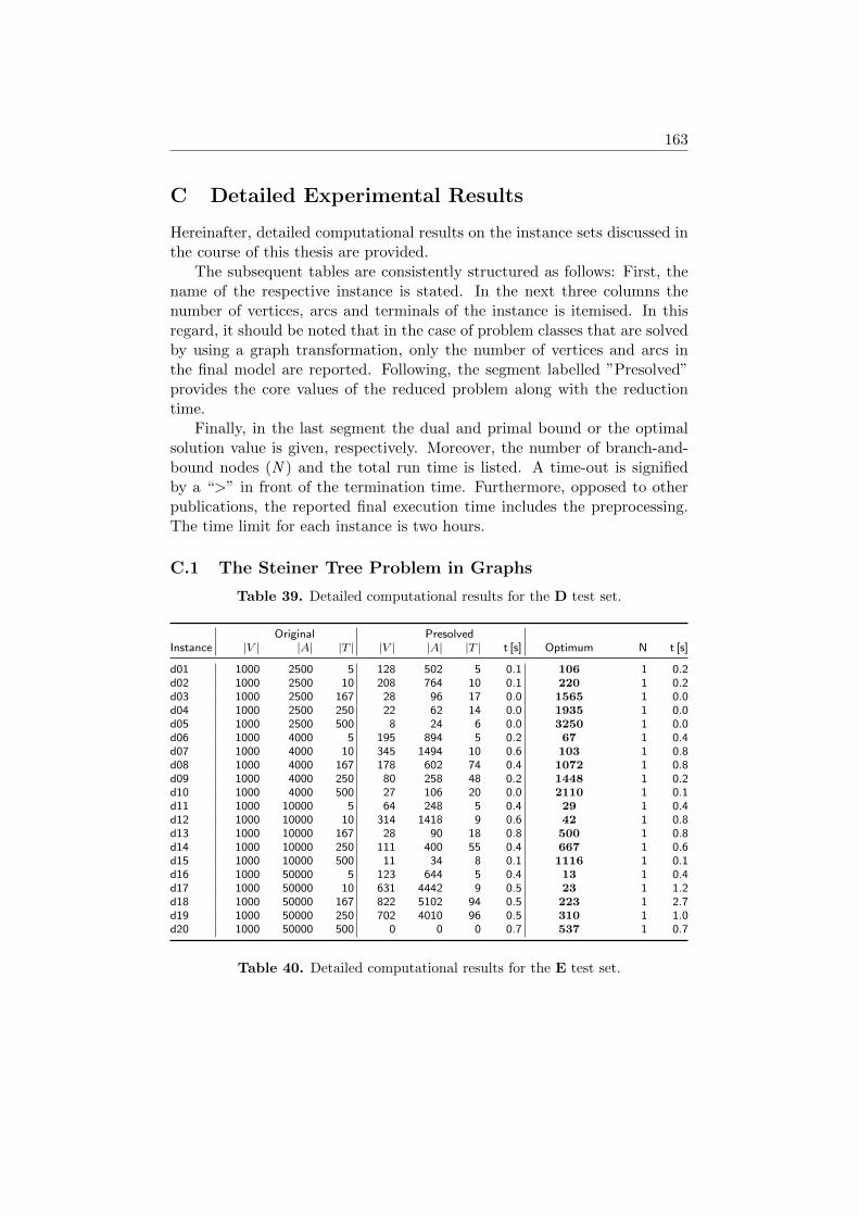
163
C Detailed Experimental Results
Hereinafter, detailed computational results on the instance sets discussed inthe course of this thesis are provided.
The subsequent tables are consistently structured as follows: First, thename of the respective instance is stated. In the next three columns thenumber of vertices, arcs and terminals of the instance is itemised. In thisregard, it should be noted that in the case of problem classes that are solvedby using a graph transformation, only the number of vertices and arcs inthe final model are reported. Following, the segment labelled ”Presolved”provides the core values of the reduced problem along with the reductiontime.
Finally, in the last segment the dual and primal bound or the optimalsolution value is given, respectively. Moreover, the number of branch-and-bound nodes (N ) and the total run time is listed. A time-out is signifiedby a “>” in front of the termination time. Furthermore, opposed to otherpublications, the reported final execution time includes the preprocessing.The time limit for each instance is two hours.
C.1 The Steiner Tree Problem in Graphs
Table 39. Detailed computational results for the D test set.
Original PresolvedInstance |V | |A| |T | |V | |A| |T | t [s] Optimum N t [s]
d01 1000 2500 5 128 502 5 0.1 106 1 0.2d02 1000 2500 10 208 764 10 0.1 220 1 0.2d03 1000 2500 167 28 96 17 0.0 1565 1 0.0d04 1000 2500 250 22 62 14 0.0 1935 1 0.0d05 1000 2500 500 8 24 6 0.0 3250 1 0.0d06 1000 4000 5 195 894 5 0.2 67 1 0.4d07 1000 4000 10 345 1494 10 0.6 103 1 0.8d08 1000 4000 167 178 602 74 0.4 1072 1 0.8d09 1000 4000 250 80 258 48 0.2 1448 1 0.2d10 1000 4000 500 27 106 20 0.0 2110 1 0.1d11 1000 10000 5 64 248 5 0.4 29 1 0.4d12 1000 10000 10 314 1418 9 0.6 42 1 0.8d13 1000 10000 167 28 90 18 0.8 500 1 0.8d14 1000 10000 250 111 400 55 0.4 667 1 0.6d15 1000 10000 500 11 34 8 0.1 1116 1 0.1d16 1000 50000 5 123 644 5 0.4 13 1 0.4d17 1000 50000 10 631 4442 9 0.5 23 1 1.2d18 1000 50000 167 822 5102 94 0.5 223 1 2.7d19 1000 50000 250 702 4010 96 0.5 310 1 1.0d20 1000 50000 500 0 0 0 0.7 537 1 0.7
Table 40. Detailed computational results for the E test set.
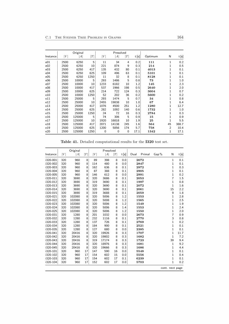
C.1 The Steiner Tree Problem in Graphs 164
Original PresolvedInstance |V | |A| |T | |V | |A| |T | t [s] Optimum N t [s]
e01 2500 6250 5 11 34 4 0.2 111 1 0.2e02 2500 6250 10 221 874 9 0.3 214 1 0.5e03 2500 6250 417 135 432 80 0.1 4013 1 0.1e04 2500 6250 625 109 496 63 0.1 5101 1 0.1e05 2500 6250 1250 11 32 8 0.1 8128 1 0.1e06 2500 10000 5 293 1486 5 0.8 73 1 1.0e07 2500 10000 10 1233 6182 10 1.2 145 1 2.3e08 2500 10000 417 537 1966 198 0.5 2640 1 2.0e09 2500 10000 625 214 722 124 0.3 3604 1 0.7e10 2500 10000 1250 52 202 36 0.2 5600 1 0.2e11 2500 25000 5 293 1474 5 0.7 34 1 0.8e12 2500 25000 10 2455 19838 10 1.0 67 1 6.4e13 2500 25000 417 1076 4500 251 1.2 1280 1 12.7e14 2500 25000 625 282 1092 140 0.6 1732 1 1.0e15 2500 25000 1250 24 72 16 0.3 2784 1 0.3e16 2500 125000 5 74 306 5 0.9 15 1 0.9e17 2500 125000 10 1920 16818 10 1.9 25 1 5.5e18 2500 125000 417 2071 14138 245 1.6 564 45 388.7e19 2500 125000 625 1200 5856 174 5.7 758 2 10.4e20 2500 125000 1250 0 0 0 17.1 1342 1 17.1
Table 41. Detailed computational results for the I320 test set.
Original PresolvedInstance |V | |A| |T | |V | |A| |T | t [s] Dual Primal Gap % N t [s]
i320-001 320 960 8 89 398 8 0.0 2672 1 0.1i320-002 320 960 8 114 480 8 0.0 2847 1 0.1i320-003 320 960 8 162 636 8 0.1 2972 1 0.3i320-004 320 960 8 87 388 8 0.1 2905 1 0.1i320-005 320 960 8 146 612 8 0.0 2991 1 0.2i320-011 320 3690 8 320 3686 8 0.1 2053 7 1.5i320-012 320 3690 8 319 3690 8 0.1 1997 1 0.8i320-013 320 3690 8 320 3690 8 0.1 2072 1 1.6i320-014 320 3690 8 320 3690 8 0.1 2061 15 2.2i320-015 320 3690 8 319 3688 8 0.1 2059 9 1.8i320-021 320 102080 8 320 5006 8 1.2 1553 1 2.8i320-022 320 102080 8 320 5008 8 1.2 1565 1 2.5i320-023 320 102080 8 320 5006 8 1.2 1549 1 1.9i320-024 320 102080 8 320 5006 8 1.4 1553 1 2.4i320-025 320 102080 8 320 5006 8 1.2 1550 1 2.0i320-031 320 1280 8 201 1032 8 0.0 2673 7 0.9i320-032 320 1280 8 232 1116 8 0.1 2770 3 0.8i320-033 320 1280 8 137 726 8 0.1 2769 1 0.2i320-034 320 1280 8 184 900 8 0.1 2521 1 0.1i320-035 320 1280 8 127 680 8 0.0 2385 1 0.1i320-041 320 20416 8 320 19926 8 0.3 1707 1 11.7i320-042 320 20416 8 320 19802 8 0.3 1682 1 7.2i320-043 320 20416 8 319 17174 8 0.3 1723 39 9.4i320-044 320 20416 8 320 18976 8 0.3 1681 1 9.2i320-045 320 20416 8 320 19666 8 0.3 1686 1 4.4i320-101 320 960 17 147 590 16 0.0 5548 1 0.1i320-102 320 960 17 154 602 15 0.0 5556 1 0.4i320-103 320 960 17 154 602 17 0.1 6239 1 0.1i320-104 320 960 17 152 602 17 0.0 5703 1 0.2
cont. next page
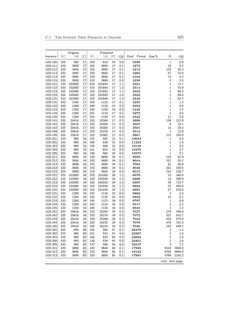
C.1 The Steiner Tree Problem in Graphs 165
Original PresolvedInstance |V | |A| |T | |V | |A| |T | t [s] Dual Primal Gap % N t [s]
i320-105 320 960 17 158 618 16 0.0 5928 1 0.6i320-111 320 3690 17 320 3690 17 0.1 4273 19 5.2i320-112 320 3690 17 320 3690 17 0.1 4213 125 16.3i320-113 320 3690 17 320 3690 17 0.1 4205 57 10.0i320-114 320 3690 17 320 3690 17 0.1 4104 13 4.2i320-115 320 3690 17 319 3688 17 0.0 4238 5 2.5i320-121 320 102080 17 320 101844 17 1.1 3321 1 73.7i320-122 320 102080 17 320 101840 17 1.3 3314 1 75.9i320-123 320 102080 17 320 101842 17 1.1 3332 1 84.3i320-124 320 102080 17 320 101840 17 1.4 3323 1 89.0i320-125 320 102080 17 320 101846 17 1.3 3340 1 82.7i320-131 320 1280 17 250 1132 17 0.1 5255 1 1.3i320-132 320 1280 17 249 1126 15 0.0 5052 1 0.9i320-133 320 1280 17 240 1108 16 0.0 5125 1 1.4i320-134 320 1280 17 241 1118 17 0.1 5272 1 0.5i320-135 320 1280 17 254 1144 17 0.0 5342 11 2.2i320-141 320 20416 17 320 20386 17 0.3 3606 139 121.9i320-142 320 20416 17 320 20400 17 0.2 3567 9 24.1i320-143 320 20416 17 320 20388 17 0.3 3561 13 29.3i320-144 320 20416 17 320 20378 17 0.3 3512 1 12.0i320-145 320 20416 17 320 20382 17 0.3 3601 121 105.0i320-201 320 960 34 155 592 33 0.1 10044 1 0.3i320-202 320 960 34 168 638 31 0.0 11223 1 1.5i320-203 320 960 34 156 606 32 0.0 10148 1 0.2i320-204 320 960 34 161 624 33 0.0 10275 1 0.7i320-205 320 960 34 148 560 29 0.0 10573 1 0.1i320-211 320 3690 34 320 3690 34 0.1 8039 110 42.9i320-212 320 3690 34 320 3690 34 0.1 8044 107 35.7i320-213 320 3690 34 320 3686 34 0.1 7984 82 56.9i320-214 320 3690 34 319 3688 34 0.1 8046 281 150.5i320-215 320 3690 34 319 3684 34 0.0 8015 752 236.7i320-221 320 102080 34 320 101050 34 1.2 6679 13 340.4i320-222 320 102080 34 320 101036 34 1.3 6686 13 389.0i320-223 320 102080 34 320 101032 34 1.5 6695 39 719.7i320-224 320 102080 34 320 101036 34 1.2 6694 25 494.6i320-225 320 102080 34 320 101030 34 1.4 6691 27 578.5i320-231 320 1280 34 243 1116 32 0.0 9862 3 3.4i320-232 320 1280 34 245 1120 34 0.0 9933 15 6.2i320-233 320 1280 34 245 1122 34 0.0 9787 1 0.8i320-234 320 1280 34 242 1110 34 0.0 9517 1 2.2i320-235 320 1280 34 249 1126 34 0.0 9945 1 2.2i320-241 320 20416 34 320 20240 34 0.3 7027 279 766.8i320-242 320 20416 34 320 20276 34 0.3 7072 527 932.7i320-243 320 20416 34 320 20268 34 0.3 7044 426 974.0i320-244 320 20416 34 320 20232 34 0.3 7078 479 791.5i320-245 320 20416 34 320 20224 34 0.3 7046 167 449.7i320-301 320 960 80 155 566 57 0.1 23279 1 1.2i320-302 320 960 80 151 542 53 0.0 23387 1 1.0i320-303 320 960 80 166 620 60 0.0 22693 1 1.6i320-304 320 960 80 139 534 45 0.0 23451 1 1.4i320-305 320 960 80 137 508 56 0.0 22547 3 1.2i320-311 320 3690 80 320 3648 80 0.1 17945 5518 2894.0i320-312 320 3690 80 320 3608 80 0.1 18122 8700 3694.0i320-313 320 3690 80 320 3600 80 0.1 17991 4769 2243.2
cont. next page
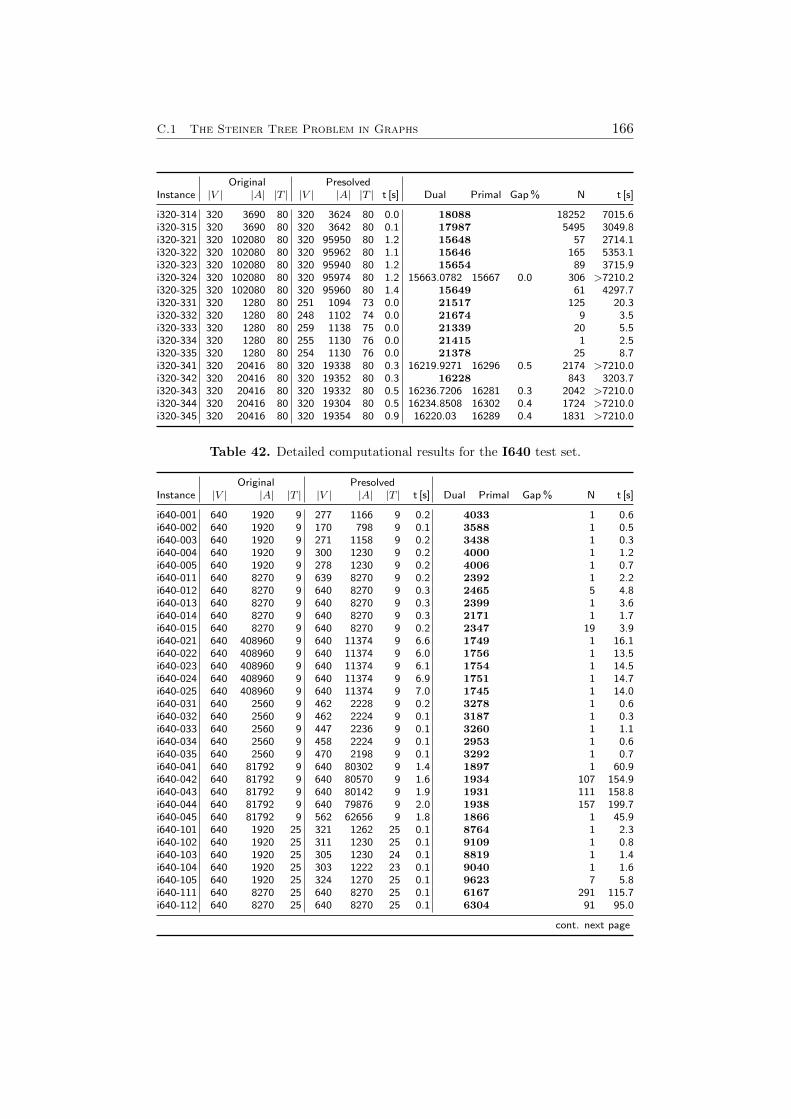
C.1 The Steiner Tree Problem in Graphs 166
Original PresolvedInstance |V | |A| |T | |V | |A| |T | t [s] Dual Primal Gap % N t [s]
i320-314 320 3690 80 320 3624 80 0.0 18088 18252 7015.6i320-315 320 3690 80 320 3642 80 0.1 17987 5495 3049.8i320-321 320 102080 80 320 95950 80 1.2 15648 57 2714.1i320-322 320 102080 80 320 95962 80 1.1 15646 165 5353.1i320-323 320 102080 80 320 95940 80 1.2 15654 89 3715.9i320-324 320 102080 80 320 95974 80 1.2 15663.0782 15667 0.0 306 >7210.2i320-325 320 102080 80 320 95960 80 1.4 15649 61 4297.7i320-331 320 1280 80 251 1094 73 0.0 21517 125 20.3i320-332 320 1280 80 248 1102 74 0.0 21674 9 3.5i320-333 320 1280 80 259 1138 75 0.0 21339 20 5.5i320-334 320 1280 80 255 1130 76 0.0 21415 1 2.5i320-335 320 1280 80 254 1130 76 0.0 21378 25 8.7i320-341 320 20416 80 320 19338 80 0.3 16219.9271 16296 0.5 2174 >7210.0i320-342 320 20416 80 320 19352 80 0.3 16228 843 3203.7i320-343 320 20416 80 320 19332 80 0.5 16236.7206 16281 0.3 2042 >7210.0i320-344 320 20416 80 320 19304 80 0.5 16234.8508 16302 0.4 1724 >7210.0i320-345 320 20416 80 320 19354 80 0.9 16220.03 16289 0.4 1831 >7210.0
Table 42. Detailed computational results for the I640 test set.
Original PresolvedInstance |V | |A| |T | |V | |A| |T | t [s] Dual Primal Gap % N t [s]
i640-001 640 1920 9 277 1166 9 0.2 4033 1 0.6i640-002 640 1920 9 170 798 9 0.1 3588 1 0.5i640-003 640 1920 9 271 1158 9 0.2 3438 1 0.3i640-004 640 1920 9 300 1230 9 0.2 4000 1 1.2i640-005 640 1920 9 278 1230 9 0.2 4006 1 0.7i640-011 640 8270 9 639 8270 9 0.2 2392 1 2.2i640-012 640 8270 9 640 8270 9 0.3 2465 5 4.8i640-013 640 8270 9 640 8270 9 0.3 2399 1 3.6i640-014 640 8270 9 640 8270 9 0.3 2171 1 1.7i640-015 640 8270 9 640 8270 9 0.2 2347 19 3.9i640-021 640 408960 9 640 11374 9 6.6 1749 1 16.1i640-022 640 408960 9 640 11374 9 6.0 1756 1 13.5i640-023 640 408960 9 640 11374 9 6.1 1754 1 14.5i640-024 640 408960 9 640 11374 9 6.9 1751 1 14.7i640-025 640 408960 9 640 11374 9 7.0 1745 1 14.0i640-031 640 2560 9 462 2228 9 0.2 3278 1 0.6i640-032 640 2560 9 462 2224 9 0.1 3187 1 0.3i640-033 640 2560 9 447 2236 9 0.1 3260 1 1.1i640-034 640 2560 9 458 2224 9 0.1 2953 1 0.6i640-035 640 2560 9 470 2198 9 0.1 3292 1 0.7i640-041 640 81792 9 640 80302 9 1.4 1897 1 60.9i640-042 640 81792 9 640 80570 9 1.6 1934 107 154.9i640-043 640 81792 9 640 80142 9 1.9 1931 111 158.8i640-044 640 81792 9 640 79876 9 2.0 1938 157 199.7i640-045 640 81792 9 562 62656 9 1.8 1866 1 45.9i640-101 640 1920 25 321 1262 25 0.1 8764 1 2.3i640-102 640 1920 25 311 1230 25 0.1 9109 1 0.8i640-103 640 1920 25 305 1230 24 0.1 8819 1 1.4i640-104 640 1920 25 303 1222 23 0.1 9040 1 1.6i640-105 640 1920 25 324 1270 25 0.1 9623 7 5.8i640-111 640 8270 25 640 8270 25 0.1 6167 291 115.7i640-112 640 8270 25 640 8270 25 0.1 6304 91 95.0
cont. next page
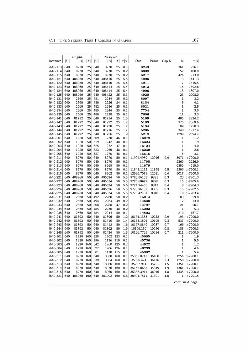
C.1 The Steiner Tree Problem in Graphs 167
Original PresolvedInstance |V | |A| |T | |V | |A| |T | t [s] Dual Primal Gap % N t [s]
i640-113 640 8270 25 640 8270 25 0.1 6249 361 226.1i640-114 640 8270 25 640 8270 25 0.2 6308 152 100.9i640-115 640 8270 25 640 8270 25 0.2 6217 426 213.0i640-121 640 408960 25 640 408416 25 5.5 4906 3 1441.3i640-122 640 408960 25 640 408416 25 5.4 4911 7 1615.5i640-123 640 408960 25 640 408414 25 5.4 4913 15 1592.6i640-124 640 408960 25 640 408414 25 5.4 4906 13 1807.0i640-125 640 408960 25 640 408422 25 5.3 4920 23 2008.0i640-131 640 2560 25 481 2234 25 0.2 8097 1 3.2i640-132 640 2560 25 480 2226 24 0.1 8154 5 4.1i640-133 640 2560 25 482 2236 25 0.1 8021 1 2.5i640-134 640 2560 25 485 2244 25 0.1 7754 1 3.0i640-135 640 2560 25 480 2228 25 0.1 7696 11 3.3i640-141 640 81792 25 640 81714 25 1.5 5199 485 2224.2i640-142 640 81792 25 640 81722 25 1.7 5193 375 2369.6i640-143 640 81792 25 640 81728 25 1.7 5194 189 1250.3i640-144 640 81792 25 640 81716 25 1.7 5205 340 1917.4i640-145 640 81792 25 640 81726 25 1.9 5218 1299 2694.7i640-201 640 1920 50 309 1230 46 0.1 16079 1 1.2i640-202 640 1920 50 319 1242 48 0.1 16324 1 1.9i640-203 640 1920 50 325 1272 47 0.1 16124 1 4.0i640-204 640 1920 50 323 1266 48 0.1 16239 1 2.6i640-205 640 1920 50 327 1270 48 0.1 16616 5 3.1i640-211 640 8270 50 640 8270 50 0.1 11904.4959 12016 0.9 5971 >7200.0i640-212 640 8270 50 640 8270 50 0.1 11795 2360 2226.9i640-213 640 8270 50 640 8268 50 0.1 11879 6350 4615.0i640-214 640 8270 50 640 8270 50 0.1 11843.1152 11898 0.5 5396 >7200.1i640-215 640 8270 50 640 8262 50 0.1 12030.7071 12081 0.4 9017 >7200.0i640-221 640 408960 50 640 406624 50 5.5 9788.06153 9821 0.3 23 >7201.3i640-222 640 408960 50 640 406634 50 5.5 9770.69979 9798 0.3 15 >7205.6i640-223 640 408960 50 640 406624 50 5.6 9774.94465 9813 0.4 8 >7204.3i640-224 640 408960 50 640 406626 50 5.5 9778.96187 9805 0.3 15 >7202.5i640-225 640 408960 50 640 406634 50 5.5 9775.42781 9810 0.4 10 >7203.4i640-231 640 2560 50 492 2260 50 0.2 15014 183 59.8i640-232 640 2560 50 494 2264 49 0.2 14630 17 13.0i640-233 640 2560 50 508 2288 47 0.2 14797 21 26.1i640-234 640 2560 50 485 2230 48 0.2 15203 1 5.3i640-235 640 2560 50 484 2244 50 0.1 14803 210 157.7i640-241 640 81792 50 640 81396 50 1.2 10161.1383 10252 0.9 193 >7200.0i640-242 640 81792 50 640 81410 50 1.4 10163.1505 10195 0.3 537 >7200.0i640-243 640 81792 50 640 81412 50 1.6 10167.8849 10237 0.7 166 >7200.0i640-244 640 81792 50 640 81362 50 1.6 10166.136 10246 0.8 188 >7200.3i640-245 640 81792 50 640 81424 50 1.5 10166.7729 10234 0.7 211 >7200.0i640-301 640 1920 160 328 1202 123 0.1 45005 1 1.9i640-302 640 1920 160 296 1136 110 0.1 45736 1 5.5i640-303 640 1920 160 342 1260 125 0.2 44922 1 1.2i640-304 640 1920 160 327 1206 126 0.1 46233 1 4.6i640-305 640 1920 160 301 1110 115 0.1 45902 1 5.4i640-311 640 8270 160 640 8068 160 0.1 35365.8747 36108 2.1 1256 >7200.1i640-312 640 8270 160 639 8064 160 0.1 35356.474 36176 2.3 1250 >7200.0i640-313 640 8270 160 640 8086 160 0.1 35237.914 35751 1.5 1351 >7200.1i640-314 640 8270 160 640 8076 160 0.1 35165.0635 35849 1.9 1361 >7200.1i640-315 640 8270 160 640 8060 160 0.1 35367.3911 36016 1.8 1335 >7200.0i640-321 640 408960 160 640 383902 160 5.8 30991.7511 31301 1.0 1 >7201.5
cont. next page
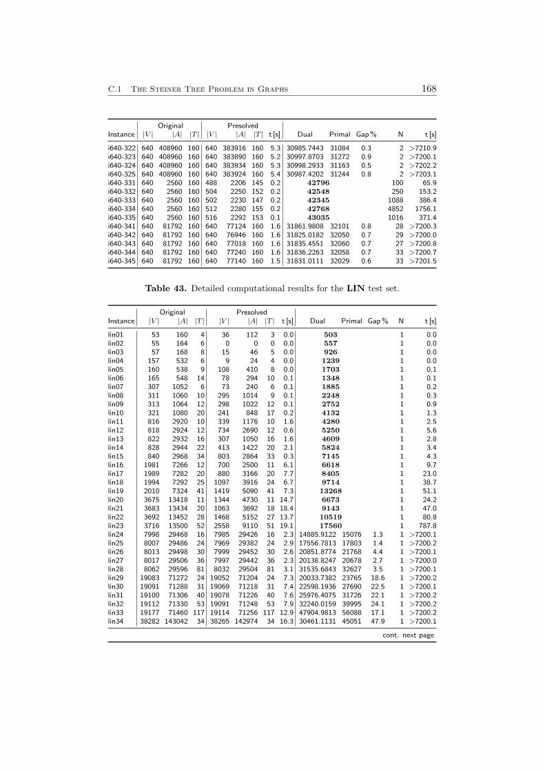
C.1 The Steiner Tree Problem in Graphs 168
Original PresolvedInstance |V | |A| |T | |V | |A| |T | t [s] Dual Primal Gap % N t [s]
i640-322 640 408960 160 640 383916 160 5.3 30985.7443 31084 0.3 2 >7210.9i640-323 640 408960 160 640 383890 160 5.2 30997.8703 31272 0.9 2 >7200.1i640-324 640 408960 160 640 383934 160 5.3 30998.2933 31163 0.5 2 >7202.2i640-325 640 408960 160 640 383924 160 5.4 30987.4202 31244 0.8 2 >7203.1i640-331 640 2560 160 488 2206 145 0.2 42796 100 65.9i640-332 640 2560 160 504 2250 152 0.2 42548 250 153.2i640-333 640 2560 160 502 2230 147 0.2 42345 1088 386.4i640-334 640 2560 160 512 2280 155 0.2 42768 4852 1756.1i640-335 640 2560 160 516 2292 153 0.1 43035 1016 371.4i640-341 640 81792 160 640 77124 160 1.6 31861.9808 32101 0.8 28 >7200.3i640-342 640 81792 160 640 76946 160 1.6 31825.0182 32050 0.7 29 >7200.0i640-343 640 81792 160 640 77018 160 1.6 31835.4551 32060 0.7 27 >7200.8i640-344 640 81792 160 640 77240 160 1.6 31836.2263 32058 0.7 33 >7200.7i640-345 640 81792 160 640 77140 160 1.5 31831.0111 32029 0.6 33 >7201.5
Table 43. Detailed computational results for the LIN test set.
Original PresolvedInstance |V | |A| |T | |V | |A| |T | t [s] Dual Primal Gap % N t [s]
lin01 53 160 4 36 112 3 0.0 503 1 0.0lin02 55 164 6 0 0 0 0.0 557 1 0.0lin03 57 168 8 15 46 5 0.0 926 1 0.0lin04 157 532 6 9 24 4 0.0 1239 1 0.0lin05 160 538 9 108 410 8 0.0 1703 1 0.1lin06 165 548 14 78 294 10 0.1 1348 1 0.1lin07 307 1052 6 73 240 6 0.1 1885 1 0.2lin08 311 1060 10 295 1014 9 0.1 2248 1 0.3lin09 313 1064 12 298 1022 12 0.1 2752 1 0.9lin10 321 1080 20 241 848 17 0.2 4132 1 1.3lin11 816 2920 10 339 1176 10 1.6 4280 1 2.5lin12 818 2924 12 734 2690 12 0.6 5250 1 5.6lin13 822 2932 16 307 1050 16 1.6 4609 1 2.8lin14 828 2944 22 413 1422 20 2.1 5824 1 3.4lin15 840 2968 34 803 2864 33 0.3 7145 1 4.3lin16 1981 7266 12 700 2500 11 6.1 6618 1 9.7lin17 1989 7282 20 880 3166 20 7.7 8405 1 23.0lin18 1994 7292 25 1097 3916 24 6.7 9714 1 38.7lin19 2010 7324 41 1419 5090 41 7.3 13268 1 51.1lin20 3675 13418 11 1344 4730 11 14.7 6673 1 24.2lin21 3683 13434 20 1063 3692 18 18.4 9143 1 47.0lin22 3692 13452 28 1468 5152 27 13.7 10519 1 80.8lin23 3716 13500 52 2558 9110 51 19.1 17560 1 787.8lin24 7998 29468 16 7985 29426 16 2.3 14885.9122 15076 1.3 1 >7200.1lin25 8007 29486 24 7969 29382 24 2.9 17556.7813 17803 1.4 1 >7200.2lin26 8013 29498 30 7999 29452 30 2.6 20851.8774 21768 4.4 1 >7200.1lin27 8017 29506 36 7997 29442 36 2.3 20138.8247 20678 2.7 1 >7200.0lin28 8062 29596 81 8032 29504 81 3.1 31535.6843 32627 3.5 1 >7200.1lin29 19083 71272 24 19052 71204 24 7.3 20033.7382 23765 18.6 1 >7200.2lin30 19091 71288 31 19069 71218 31 7.4 22598.1936 27690 22.5 1 >7200.1lin31 19100 71306 40 19078 71226 40 7.6 25976.4075 31726 22.1 1 >7200.2lin32 19112 71330 53 19091 71248 53 7.9 32240.0159 39995 24.1 1 >7200.2lin33 19177 71460 117 19114 71256 117 12.9 47904.9813 56088 17.1 1 >7200.2lin34 38282 143042 34 38265 142974 34 16.3 30461.1131 45051 47.9 1 >7200.1
cont. next page
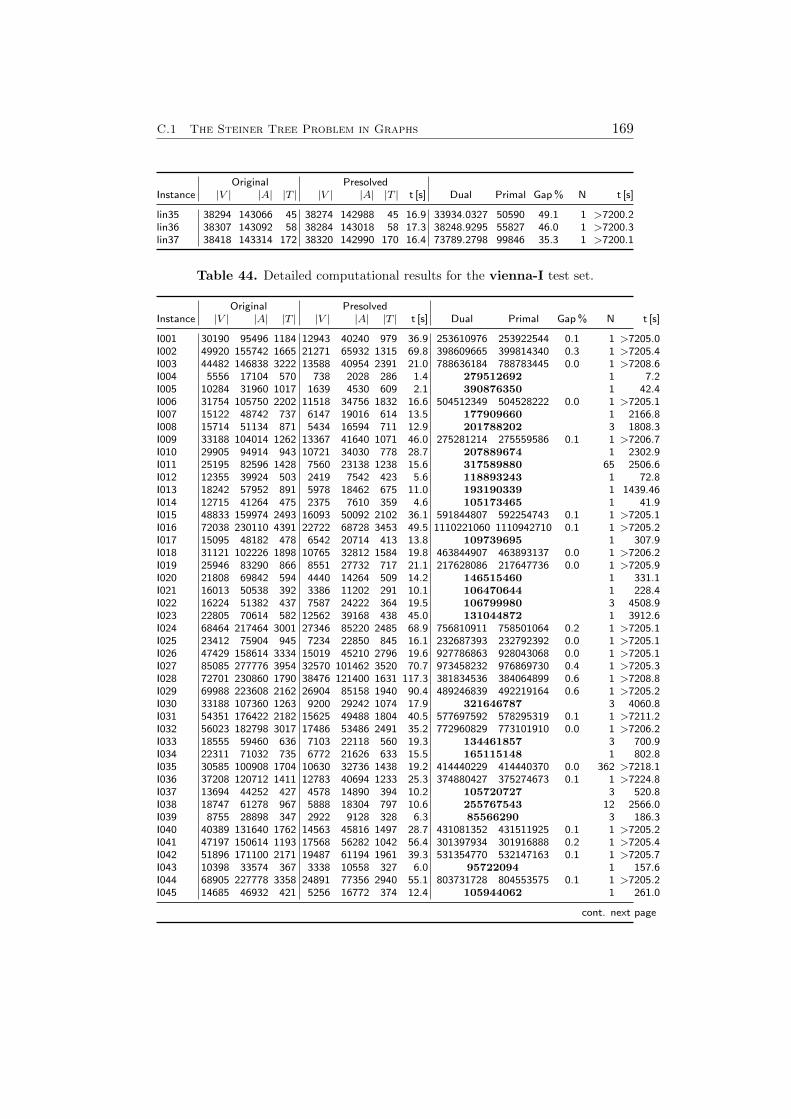
C.1 The Steiner Tree Problem in Graphs 169
Original PresolvedInstance |V | |A| |T | |V | |A| |T | t [s] Dual Primal Gap % N t [s]
lin35 38294 143066 45 38274 142988 45 16.9 33934.0327 50590 49.1 1 >7200.2lin36 38307 143092 58 38284 143018 58 17.3 38248.9295 55827 46.0 1 >7200.3lin37 38418 143314 172 38320 142990 170 16.4 73789.2798 99846 35.3 1 >7200.1
Table 44. Detailed computational results for the vienna-I test set.
Original PresolvedInstance |V | |A| |T | |V | |A| |T | t [s] Dual Primal Gap % N t [s]
I001 30190 95496 1184 12943 40240 979 36.9 253610976 253922544 0.1 1 >7205.0I002 49920 155742 1665 21271 65932 1315 69.8 398609665 399814340 0.3 1 >7205.4I003 44482 146838 3222 13588 40954 2391 21.0 788636184 788783445 0.0 1 >7208.6I004 5556 17104 570 738 2028 286 1.4 279512692 1 7.2I005 10284 31960 1017 1639 4530 609 2.1 390876350 1 42.4I006 31754 105750 2202 11518 34756 1832 16.6 504512349 504528222 0.0 1 >7205.1I007 15122 48742 737 6147 19016 614 13.5 177909660 1 2166.8I008 15714 51134 871 5434 16594 711 12.9 201788202 3 1808.3I009 33188 104014 1262 13367 41640 1071 46.0 275281214 275559586 0.1 1 >7206.7I010 29905 94914 943 10721 34030 778 28.7 207889674 1 2302.9I011 25195 82596 1428 7560 23138 1238 15.6 317589880 65 2506.6I012 12355 39924 503 2419 7542 423 5.6 118893243 1 72.8I013 18242 57952 891 5978 18462 675 11.0 193190339 1 1439.46I014 12715 41264 475 2375 7610 359 4.6 105173465 1 41.9I015 48833 159974 2493 16093 50092 2102 36.1 591844807 592254743 0.1 1 >7205.1I016 72038 230110 4391 22722 68728 3453 49.5 1110221060 1110942710 0.1 1 >7205.2I017 15095 48182 478 6542 20714 413 13.8 109739695 1 307.9I018 31121 102226 1898 10765 32812 1584 19.8 463844907 463893137 0.0 1 >7206.2I019 25946 83290 866 8551 27732 717 21.1 217628086 217647736 0.0 1 >7205.9I020 21808 69842 594 4440 14264 509 14.2 146515460 1 331.1I021 16013 50538 392 3386 11202 291 10.1 106470644 1 228.4I022 16224 51382 437 7587 24222 364 19.5 106799980 3 4508.9I023 22805 70614 582 12562 39168 438 45.0 131044872 1 3912.6I024 68464 217464 3001 27346 85220 2485 68.9 756810911 758501064 0.2 1 >7205.1I025 23412 75904 945 7234 22850 845 16.1 232687393 232792392 0.0 1 >7205.1I026 47429 158614 3334 15019 45210 2796 19.6 927786863 928043068 0.0 1 >7205.1I027 85085 277776 3954 32570 101462 3520 70.7 973458232 976869730 0.4 1 >7205.3I028 72701 230860 1790 38476 121400 1631 117.3 381834536 384064899 0.6 1 >7208.8I029 69988 223608 2162 26904 85158 1940 90.4 489246839 492219164 0.6 1 >7205.2I030 33188 107360 1263 9200 29242 1074 17.9 321646787 3 4060.8I031 54351 176422 2182 15625 49488 1804 40.5 577697592 578295319 0.1 1 >7211.2I032 56023 182798 3017 17486 53486 2491 35.2 772960829 773101910 0.0 1 >7206.2I033 18555 59460 636 7103 22118 560 19.3 134461857 3 700.9I034 22311 71032 735 6772 21626 633 15.5 165115148 1 802.8I035 30585 100908 1704 10630 32736 1438 19.2 414440229 414440370 0.0 362 >7218.1I036 37208 120712 1411 12783 40694 1233 25.3 374880427 375274673 0.1 1 >7224.8I037 13694 44252 427 4578 14890 394 10.2 105720727 3 520.8I038 18747 61278 967 5888 18304 797 10.6 255767543 12 2566.0I039 8755 28898 347 2922 9128 328 6.3 85566290 3 186.3I040 40389 131640 1762 14563 45816 1497 28.7 431081352 431511925 0.1 1 >7205.2I041 47197 150614 1193 17568 56282 1042 56.4 301397934 301916888 0.2 1 >7205.4I042 51896 171100 2171 19487 61194 1961 39.3 531354770 532147163 0.1 1 >7205.7I043 10398 33574 367 3338 10558 327 6.0 95722094 1 157.6I044 68905 227778 3358 24891 77356 2940 55.1 803731728 804553575 0.1 1 >7205.2I045 14685 46932 421 5256 16772 374 12.4 105944062 1 261.0
cont. next page
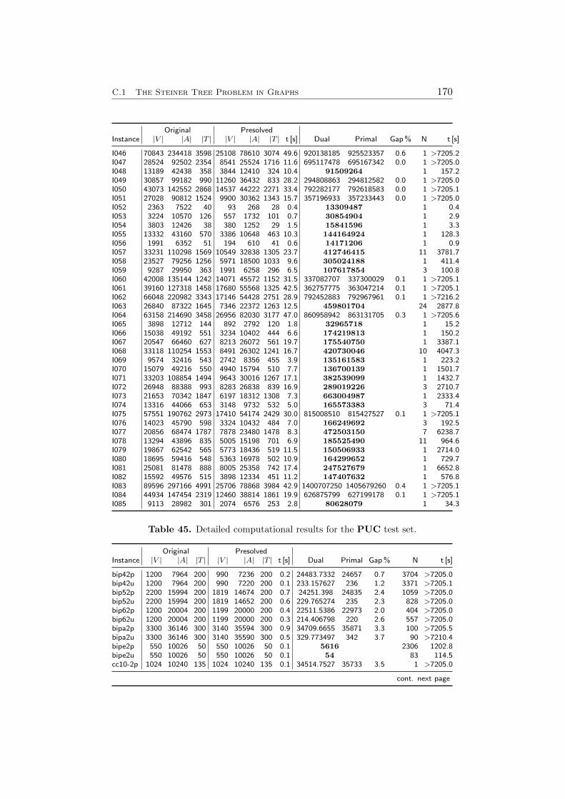
C.1 The Steiner Tree Problem in Graphs 170
Original PresolvedInstance |V | |A| |T | |V | |A| |T | t [s] Dual Primal Gap % N t [s]
I046 70843 234418 3598 25108 78610 3074 49.6 920138185 925523357 0.6 1 >7205.2I047 28524 92502 2354 8541 25524 1716 11.6 695117478 695167342 0.0 1 >7205.0I048 13189 42438 358 3844 12410 324 10.4 91509264 1 157.2I049 30857 99182 990 11260 36432 833 28.2 294808863 294812582 0.0 1 >7205.0I050 43073 142552 2868 14537 44222 2271 33.4 792282177 792618583 0.0 1 >7205.1I051 27028 90812 1524 9900 30362 1343 15.7 357196933 357233443 0.0 1 >7205.0I052 2363 7522 40 93 268 28 0.4 13309487 1 0.4I053 3224 10570 126 557 1732 101 0.7 30854904 1 2.9I054 3803 12426 38 380 1252 29 1.5 15841596 1 3.3I055 13332 43160 570 3386 10648 463 10.3 144164924 1 128.3I056 1991 6352 51 194 610 41 0.6 14171206 1 0.9I057 33231 110298 1569 10549 32838 1305 23.7 412746415 11 3781.7I058 23527 79256 1256 5971 18500 1033 9.6 305024188 1 411.4I059 9287 29950 363 1991 6258 296 6.5 107617854 3 100.8I060 42008 135144 1242 14071 45572 1152 31.5 337082707 337300029 0.1 1 >7205.1I061 39160 127318 1458 17680 55568 1325 42.5 362757775 363047214 0.1 1 >7205.1I062 66048 220982 3343 17146 54428 2751 28.9 792452883 792967961 0.1 1 >7216.2I063 26840 87322 1645 7346 22372 1263 12.5 459801704 24 2877.8I064 63158 214690 3458 26956 82030 3177 47.0 860958942 863131705 0.3 1 >7205.6I065 3898 12712 144 892 2792 120 1.8 32965718 1 15.2I066 15038 49192 551 3234 10402 444 6.6 174219813 1 150.2I067 20547 66460 627 8213 26072 561 19.7 175540750 1 3387.1I068 33118 110254 1553 8491 26302 1241 16.7 420730046 10 4047.3I069 9574 32416 543 2742 8356 455 3.9 135161583 1 223.2I070 15079 49216 550 4940 15794 510 7.7 136700139 1 1501.7I071 33203 108854 1494 9643 30016 1267 17.1 382539099 1 1432.7I072 26948 88388 993 8283 26838 839 16.9 289019226 3 2710.7I073 21653 70342 1847 6197 18312 1308 7.3 663004987 1 2333.4I074 13316 44066 653 3148 9732 532 5.0 165573383 3 71.4I075 57551 190762 2973 17410 54174 2429 30.0 815008510 815427527 0.1 1 >7205.1I076 14023 45790 598 3324 10432 484 7.0 166249692 3 192.5I077 20856 68474 1787 7878 23480 1478 8.3 472503150 7 6238.7I078 13294 43896 835 5005 15198 701 6.9 185525490 11 964.6I079 19867 62542 565 5773 18436 519 11.5 150506933 1 2714.0I080 18695 59416 548 5363 16978 502 10.9 164299652 1 729.7I081 25081 81478 888 8005 25358 742 17.4 247527679 1 6652.8I082 15592 49576 515 3898 12334 451 11.2 147407632 1 576.8I083 89596 297166 4991 25706 78868 3984 42.9 1400707250 1405679260 0.4 1 >7205.1I084 44934 147454 2319 12460 38814 1861 19.9 626875799 627199178 0.1 1 >7205.1I085 9113 28982 301 2074 6576 253 2.8 80628079 1 34.3
Table 45. Detailed computational results for the PUC test set.
Original PresolvedInstance |V | |A| |T | |V | |A| |T | t [s] Dual Primal Gap % N t [s]
bip42p 1200 7964 200 990 7236 200 0.2 24483.7332 24657 0.7 3704 >7205.0bip42u 1200 7964 200 990 7220 200 0.1 233.157627 236 1.2 3371 >7205.1bip52p 2200 15994 200 1819 14674 200 0.7 24251.398 24835 2.4 1059 >7205.0bip52u 2200 15994 200 1819 14652 200 0.6 229.765274 235 2.3 828 >7205.0bip62p 1200 20004 200 1199 20000 200 0.4 22511.5386 22973 2.0 404 >7205.0bip62u 1200 20004 200 1199 20000 200 0.3 214.406798 220 2.6 557 >7205.0bipa2p 3300 36146 300 3140 35594 300 0.9 34709.6655 35871 3.3 100 >7205.5bipa2u 3300 36146 300 3140 35590 300 0.5 329.773497 342 3.7 90 >7210.4bipe2p 550 10026 50 550 10026 50 0.1 5616 2306 1202.8bipe2u 550 10026 50 550 10026 50 0.1 54 83 114.5cc10-2p 1024 10240 135 1024 10240 135 0.1 34514.7527 35733 3.5 1 >7205.0
cont. next page
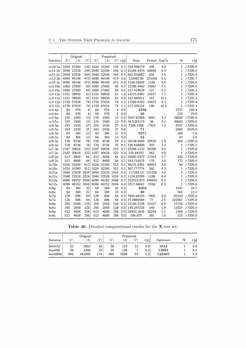
C.1 The Steiner Tree Problem in Graphs 171
Original PresolvedInstance |V | |A| |T | |V | |A| |T | t [s] Dual Primal Gap % N t [s]
cc10-2u 1024 10240 135 1024 10240 135 0.1 334.498719 346 3.4 1 >7205.9cc11-2p 2048 22526 244 2048 22526 244 0.3 62166.4479 64846 4.3 1 >7206.0cc11-2u 2048 22526 244 2048 22526 244 0.3 602.818662 624 3.5 1 >7205.4cc12-2p 4096 49148 473 4096 49148 473 0.8 118482.56 124348 5.0 1 >7205.7cc12-2u 4096 49148 473 4096 49148 473 0.8 1149.03005 1195 4.0 1 >7205.5cc3-10p 1000 27000 50 1000 27000 50 0.7 12198.4462 13067 7.1 1 >7205.5cc3-10u 1000 27000 50 1000 27000 50 0.5 117.414634 127 8.2 1 >7205.2cc3-11p 1331 39930 61 1331 39930 61 1.0 14773.8367 15917 7.7 1 >7205.4cc3-11u 1331 39930 61 1331 39930 61 0.8 142.640411 157 10.1 1 >7205.3cc3-12p 1728 57024 74 1728 57024 74 1.2 17769.6393 19422 9.3 1 >7205.4cc3-12u 1728 57024 74 1728 57024 74 1.1 172.205224 190 10.3 1 >7205.3cc3-4p 64 576 8 64 576 8 0.0 2338 7217 189.4cc3-4u 64 576 8 64 576 8 0.0 23 219 23.8cc3-5p 125 1500 13 125 1500 13 0.0 3547.62569 3661 3.2 28060 >7205.0cc3-5u 125 1500 13 125 1500 13 0.0 34.5383179 36 4.2 30693 >7205.0cc5-3p 243 2430 27 243 2430 27 0.0 7206.3399 7303 1.3 4707 >7205.0cc5-3u 243 2430 27 243 2430 27 0.0 71 2885 4570.0cc6-2p 64 384 12 64 384 12 0.0 3271 165 7.8cc6-2u 64 384 12 64 384 12 0.0 32 47 3.6cc6-3p 729 8736 76 729 8736 76 0.1 20139.9549 20525 1.9 304 >7205.0cc6-3u 729 8736 76 729 8736 76 0.1 195.638889 202 3.3 1 >7205.1cc7-3p 2187 30616 222 2187 30616 222 0.7 55296.1132 58286 5.4 1 >7205.6cc7-3u 2187 30616 222 2187 30616 222 0.3 535.84192 562 4.9 1 >7205.6cc9-2p 512 4608 64 512 4608 64 0.1 16892.5375 17343 2.7 320 >7205.0cc9-2u 512 4608 64 512 4608 64 0.1 163.718525 170 3.8 172 >7205.0hc10p 1024 10240 512 1024 10240 512 0.1 59231.0381 60983 3.0 54 >7205.0hc10u 1024 10240 512 1024 10240 512 0.1 567.777778 592 4.3 1 >7205.0hc11p 2048 22528 1024 2048 22528 1024 0.3 117383.13 121326 3.4 5 >7205.0hc11u 2048 22528 1024 2048 22528 1024 0.2 1124.87009 1186 5.4 1 >7205.9hc12p 4096 49152 2048 4096 49152 2048 0.7 232522.973 244676 5.2 1 >7206.5hc12u 4096 49152 2048 4096 49152 2048 0.4 2217.66667 2358 6.3 1 >7205.6hc6p 64 384 32 64 384 32 0.0 4003 1547 24.7hc6u 64 384 32 64 384 32 0.0 39 541 12.2hc7p 128 896 64 128 896 64 0.0 7845.68193 7905 0.8 92143 >7205.0hc7u 128 896 64 128 896 64 0.0 75.0990594 77 2.5 102661 >7205.0hc8p 256 2048 128 256 2048 128 0.0 15194.7194 15327 0.9 17155 >7205.0hc8u 256 2048 128 256 2048 128 0.0 145.247228 148 1.9 11027 >7205.0hc9p 512 4608 256 512 4608 256 0.0 29933.1635 30254 1.1 1369 >7205.0hc9u 512 4608 256 512 4608 256 0.0 286.875 292 1.8 213 >7205.0
Table 46. Detailed computational results for the X test set.
Original PresolvedInstance |V | |A| |T | |V | |A| |T | t [s] Optimum N t [s]
berlin52 52 2652 16 36 214 13 0.0 1044 1 0.0brasil58 58 3306 25 20 134 7 0.0 13655 1 0.0world666 666 442890 174 480 5588 93 1.0 122467 1 5.9
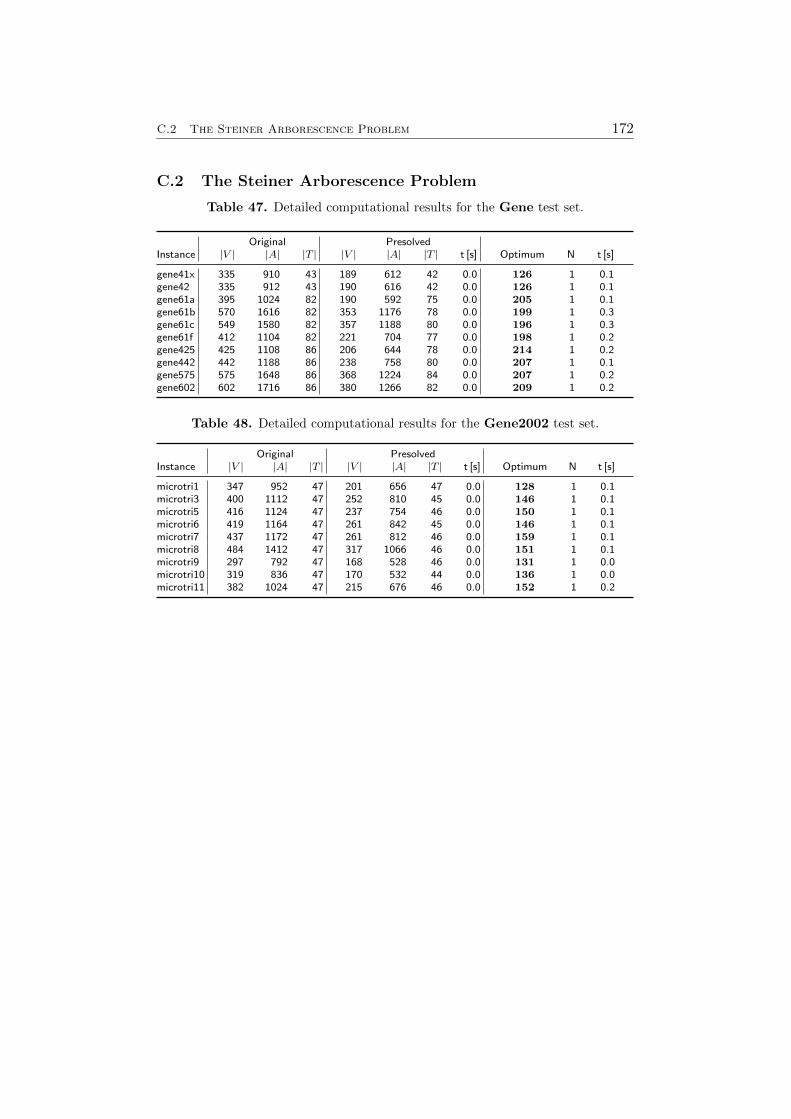
C.2 The Steiner Arborescence Problem 172
C.2 The Steiner Arborescence Problem
Table 47. Detailed computational results for the Gene test set.
Original PresolvedInstance |V | |A| |T | |V | |A| |T | t [s] Optimum N t [s]
gene41x 335 910 43 189 612 42 0.0 126 1 0.1gene42 335 912 43 190 616 42 0.0 126 1 0.1gene61a 395 1024 82 190 592 75 0.0 205 1 0.1gene61b 570 1616 82 353 1176 78 0.0 199 1 0.3gene61c 549 1580 82 357 1188 80 0.0 196 1 0.3gene61f 412 1104 82 221 704 77 0.0 198 1 0.2gene425 425 1108 86 206 644 78 0.0 214 1 0.2gene442 442 1188 86 238 758 80 0.0 207 1 0.1gene575 575 1648 86 368 1224 84 0.0 207 1 0.2gene602 602 1716 86 380 1266 82 0.0 209 1 0.2
Table 48. Detailed computational results for the Gene2002 test set.
Original PresolvedInstance |V | |A| |T | |V | |A| |T | t [s] Optimum N t [s]
microtri1 347 952 47 201 656 47 0.0 128 1 0.1microtri3 400 1112 47 252 810 45 0.0 146 1 0.1microtri5 416 1124 47 237 754 46 0.0 150 1 0.1microtri6 419 1164 47 261 842 45 0.0 146 1 0.1microtri7 437 1172 47 261 812 46 0.0 159 1 0.1microtri8 484 1412 47 317 1066 46 0.0 151 1 0.1microtri9 297 792 47 168 528 46 0.0 131 1 0.0microtri10 319 836 47 170 532 44 0.0 136 1 0.0microtri11 382 1024 47 215 676 46 0.0 152 1 0.2
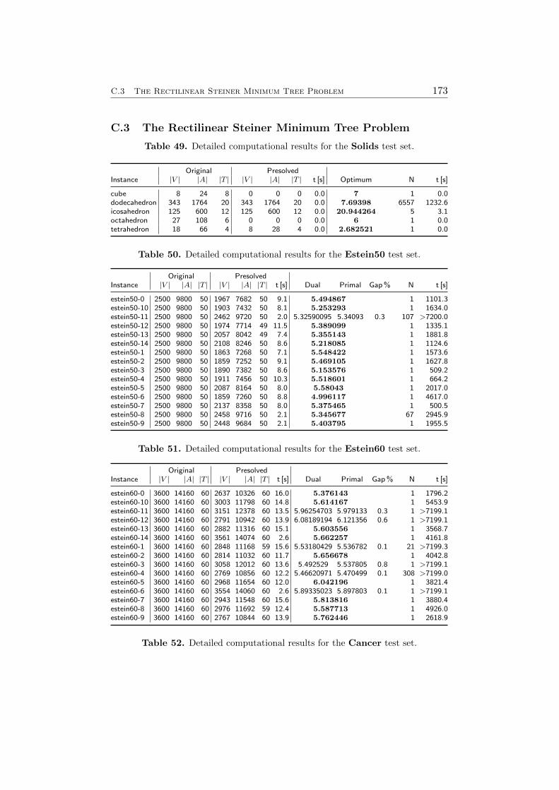
C.3 The Rectilinear Steiner Minimum Tree Problem 173
C.3 The Rectilinear Steiner Minimum Tree Problem
Table 49. Detailed computational results for the Solids test set.
Original PresolvedInstance |V | |A| |T | |V | |A| |T | t [s] Optimum N t [s]
cube 8 24 8 0 0 0 0.0 7 1 0.0dodecahedron 343 1764 20 343 1764 20 0.0 7.69398 6557 1232.6icosahedron 125 600 12 125 600 12 0.0 20.944264 5 3.1octahedron 27 108 6 0 0 0 0.0 6 1 0.0tetrahedron 18 66 4 8 28 4 0.0 2.682521 1 0.0
Table 50. Detailed computational results for the Estein50 test set.
Original PresolvedInstance |V | |A| |T | |V | |A| |T | t [s] Dual Primal Gap % N t [s]
estein50-0 2500 9800 50 1967 7682 50 9.1 5.494867 1 1101.3estein50-10 2500 9800 50 1903 7432 50 8.1 5.253293 1 1634.0estein50-11 2500 9800 50 2462 9720 50 2.0 5.32590095 5.34093 0.3 107 >7200.0estein50-12 2500 9800 50 1974 7714 49 11.5 5.389099 1 1335.1estein50-13 2500 9800 50 2057 8042 49 7.4 5.355143 1 1881.8estein50-14 2500 9800 50 2108 8246 50 8.6 5.218085 1 1124.6estein50-1 2500 9800 50 1863 7268 50 7.1 5.548422 1 1573.6estein50-2 2500 9800 50 1859 7252 50 9.1 5.469105 1 1627.8estein50-3 2500 9800 50 1890 7382 50 8.6 5.153576 1 509.2estein50-4 2500 9800 50 1911 7456 50 10.3 5.518601 1 664.2estein50-5 2500 9800 50 2087 8164 50 8.0 5.58043 1 2017.0estein50-6 2500 9800 50 1859 7260 50 8.8 4.996117 1 4617.0estein50-7 2500 9800 50 2137 8358 50 8.0 5.375465 1 500.5estein50-8 2500 9800 50 2458 9716 50 2.1 5.345677 67 2945.9estein50-9 2500 9800 50 2448 9684 50 2.1 5.403795 1 1955.5
Table 51. Detailed computational results for the Estein60 test set.
Original PresolvedInstance |V | |A| |T | |V | |A| |T | t [s] Dual Primal Gap % N t [s]
estein60-0 3600 14160 60 2637 10326 60 16.0 5.376143 1 1796.2estein60-10 3600 14160 60 3003 11798 60 14.8 5.614167 1 5453.9estein60-11 3600 14160 60 3151 12378 60 13.5 5.96254703 5.979133 0.3 1 >7199.1estein60-12 3600 14160 60 2791 10942 60 13.9 6.08189194 6.121356 0.6 1 >7199.1estein60-13 3600 14160 60 2882 11316 60 15.1 5.603556 1 3568.7estein60-14 3600 14160 60 3561 14074 60 2.6 5.662257 1 4161.8estein60-1 3600 14160 60 2848 11168 59 15.6 5.53180429 5.536782 0.1 21 >7199.3estein60-2 3600 14160 60 2814 11032 60 11.7 5.656678 1 4042.8estein60-3 3600 14160 60 3058 12012 60 13.6 5.492529 5.537805 0.8 1 >7199.1estein60-4 3600 14160 60 2769 10856 60 12.2 5.46620971 5.470499 0.1 308 >7199.0estein60-5 3600 14160 60 2968 11654 60 12.0 6.042196 1 3821.4estein60-6 3600 14160 60 3554 14060 60 2.6 5.89335023 5.897803 0.1 1 >7199.1estein60-7 3600 14160 60 2943 11548 60 15.6 5.813816 1 3880.4estein60-8 3600 14160 60 2976 11692 59 12.4 5.587713 1 4926.0estein60-9 3600 14160 60 2767 10844 60 13.9 5.762446 1 2618.9
Table 52. Detailed computational results for the Cancer test set.
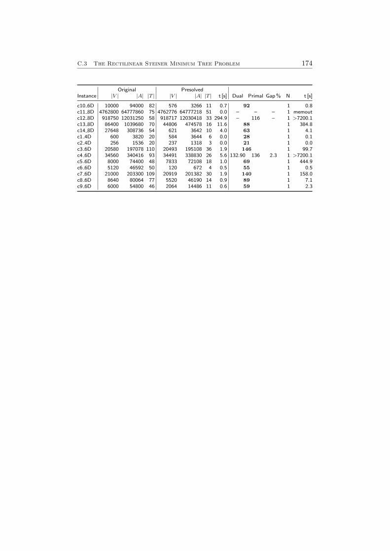
C.3 The Rectilinear Steiner Minimum Tree Problem 174
Original PresolvedInstance |V | |A| |T | |V | |A| |T | t [s] Dual Primal Gap % N t [s]
c10 6D 10000 94000 82 576 3266 11 0.7 92 1 0.8c11 8D 4762800 64777860 75 4762776 64777218 51 0.0 – – – 1 memoutc12 8D 918750 12031250 58 918717 12030418 33 294.9 – 116 – 1 >7200.1c13 8D 86400 1039680 70 44806 474578 16 11.6 88 1 384.8c14 8D 27648 308736 54 621 3642 10 4.0 63 1 4.1c1 4D 600 3820 20 584 3644 6 0.0 28 1 0.1c2 4D 256 1536 20 237 1318 3 0.0 21 1 0.0c3 6D 20580 197078 110 20493 195108 36 1.9 146 1 99.7c4 6D 34560 340416 93 34491 338830 26 5.6 132.90 136 2.3 1 >7200.1c5 6D 8000 74400 48 7833 72108 18 1.0 69 1 444.9c6 6D 5120 46592 50 120 672 4 0.5 55 1 0.5c7 6D 21000 203300 109 20919 201382 30 1.9 140 1 158.0c8 6D 8640 80064 77 5520 46190 14 0.9 89 1 7.1c9 6D 6000 54800 46 2064 14486 11 0.6 59 1 2.3
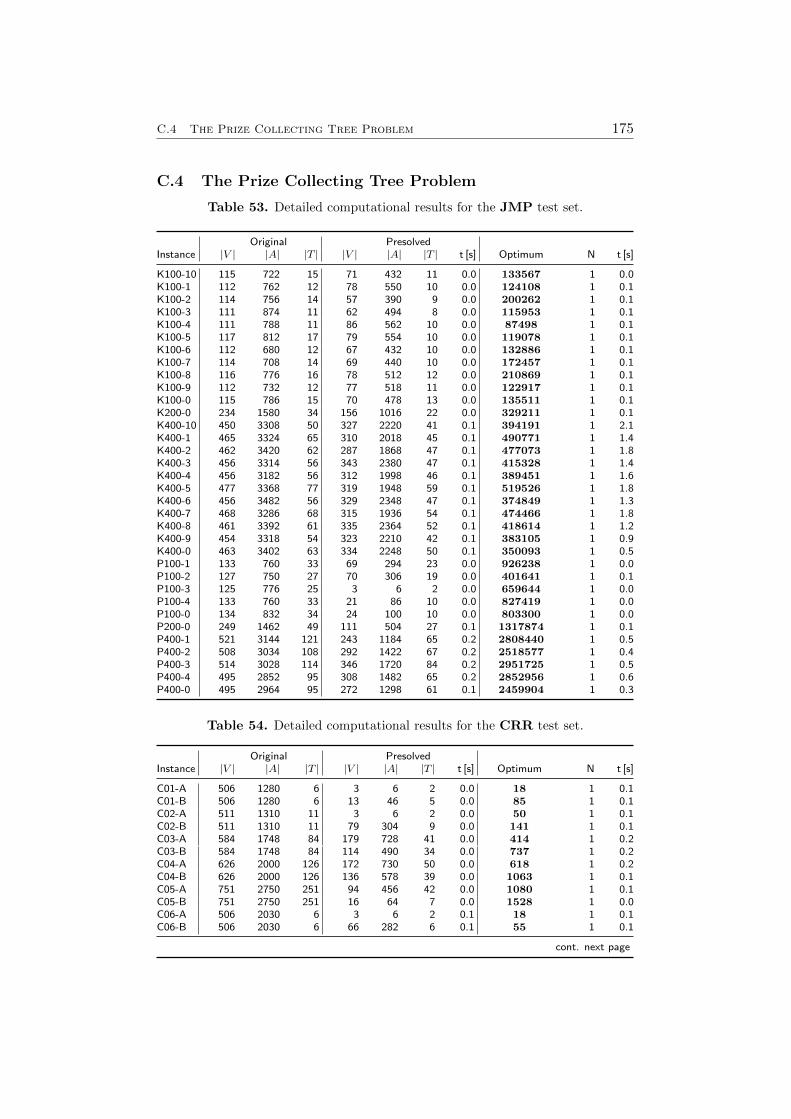
C.4 The Prize Collecting Tree Problem 175
C.4 The Prize Collecting Tree Problem
Table 53. Detailed computational results for the JMP test set.
Original PresolvedInstance |V | |A| |T | |V | |A| |T | t [s] Optimum N t [s]
K100-10 115 722 15 71 432 11 0.0 133567 1 0.0K100-1 112 762 12 78 550 10 0.0 124108 1 0.1K100-2 114 756 14 57 390 9 0.0 200262 1 0.1K100-3 111 874 11 62 494 8 0.0 115953 1 0.1K100-4 111 788 11 86 562 10 0.0 87498 1 0.1K100-5 117 812 17 79 554 10 0.0 119078 1 0.1K100-6 112 680 12 67 432 10 0.0 132886 1 0.1K100-7 114 708 14 69 440 10 0.0 172457 1 0.1K100-8 116 776 16 78 512 12 0.0 210869 1 0.1K100-9 112 732 12 77 518 11 0.0 122917 1 0.1K100-0 115 786 15 70 478 13 0.0 135511 1 0.1K200-0 234 1580 34 156 1016 22 0.0 329211 1 0.1K400-10 450 3308 50 327 2220 41 0.1 394191 1 2.1K400-1 465 3324 65 310 2018 45 0.1 490771 1 1.4K400-2 462 3420 62 287 1868 47 0.1 477073 1 1.8K400-3 456 3314 56 343 2380 47 0.1 415328 1 1.4K400-4 456 3182 56 312 1998 46 0.1 389451 1 1.6K400-5 477 3368 77 319 1948 59 0.1 519526 1 1.8K400-6 456 3482 56 329 2348 47 0.1 374849 1 1.3K400-7 468 3286 68 315 1936 54 0.1 474466 1 1.8K400-8 461 3392 61 335 2364 52 0.1 418614 1 1.2K400-9 454 3318 54 323 2210 42 0.1 383105 1 0.9K400-0 463 3402 63 334 2248 50 0.1 350093 1 0.5P100-1 133 760 33 69 294 23 0.0 926238 1 0.0P100-2 127 750 27 70 306 19 0.0 401641 1 0.1P100-3 125 776 25 3 6 2 0.0 659644 1 0.0P100-4 133 760 33 21 86 10 0.0 827419 1 0.0P100-0 134 832 34 24 100 10 0.0 803300 1 0.0P200-0 249 1462 49 111 504 27 0.1 1317874 1 0.1P400-1 521 3144 121 243 1184 65 0.2 2808440 1 0.5P400-2 508 3034 108 292 1422 67 0.2 2518577 1 0.4P400-3 514 3028 114 346 1720 84 0.2 2951725 1 0.5P400-4 495 2852 95 308 1482 65 0.2 2852956 1 0.6P400-0 495 2964 95 272 1298 61 0.1 2459904 1 0.3
Table 54. Detailed computational results for the CRR test set.
Original PresolvedInstance |V | |A| |T | |V | |A| |T | t [s] Optimum N t [s]
C01-A 506 1280 6 3 6 2 0.0 18 1 0.1C01-B 506 1280 6 13 46 5 0.0 85 1 0.1C02-A 511 1310 11 3 6 2 0.0 50 1 0.1C02-B 511 1310 11 79 304 9 0.0 141 1 0.1C03-A 584 1748 84 179 728 41 0.0 414 1 0.2C03-B 584 1748 84 114 490 34 0.0 737 1 0.2C04-A 626 2000 126 172 730 50 0.0 618 1 0.2C04-B 626 2000 126 136 578 39 0.0 1063 1 0.1C05-A 751 2750 251 94 456 42 0.0 1080 1 0.1C05-B 751 2750 251 16 64 7 0.0 1528 1 0.0C06-A 506 2030 6 3 6 2 0.1 18 1 0.1C06-B 506 2030 6 66 282 6 0.1 55 1 0.1
cont. next page
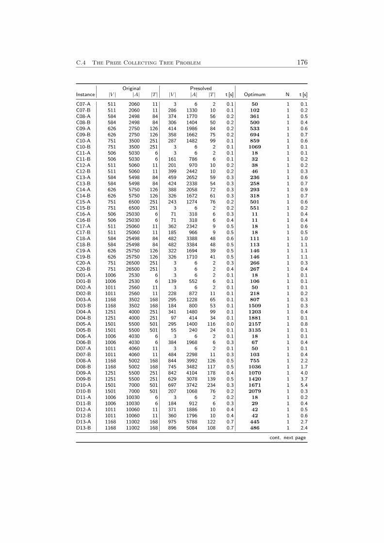
C.4 The Prize Collecting Tree Problem 176
Original PresolvedInstance |V | |A| |T | |V | |A| |T | t [s] Optimum N t [s]
C07-A 511 2060 11 3 6 2 0.1 50 1 0.1C07-B 511 2060 11 286 1330 10 0.1 102 1 0.2C08-A 584 2498 84 374 1770 56 0.2 361 1 0.5C08-B 584 2498 84 306 1404 50 0.2 500 1 0.4C09-A 626 2750 126 414 1986 84 0.2 533 1 0.6C09-B 626 2750 126 358 1662 75 0.2 694 1 0.7C10-A 751 3500 251 287 1482 99 0.1 859 1 0.6C10-B 751 3500 251 3 6 2 0.1 1069 1 0.1C11-A 506 5030 6 3 6 2 0.1 18 1 0.1C11-B 506 5030 6 161 786 6 0.1 32 1 0.2C12-A 511 5060 11 201 970 10 0.2 38 1 0.2C12-B 511 5060 11 399 2442 10 0.2 46 1 0.3C13-A 584 5498 84 459 2652 59 0.3 236 1 0.6C13-B 584 5498 84 424 2338 54 0.3 258 1 0.7C14-A 626 5750 126 388 2058 72 0.3 293 1 0.9C14-B 626 5750 126 326 1672 61 0.3 318 1 0.7C15-A 751 6500 251 243 1274 76 0.2 501 1 0.6C15-B 751 6500 251 3 6 2 0.2 551 1 0.2C16-A 506 25030 6 71 318 6 0.3 11 1 0.4C16-B 506 25030 6 71 318 6 0.4 11 1 0.4C17-A 511 25060 11 362 2342 9 0.5 18 1 0.6C17-B 511 25060 11 185 966 9 0.5 18 1 0.5C18-A 584 25498 84 482 3388 48 0.6 111 1 1.0C18-B 584 25498 84 482 3384 48 0.5 113 1 1.1C19-A 626 25750 126 322 1694 39 0.5 146 1 1.1C19-B 626 25750 126 326 1710 41 0.5 146 1 1.1C20-A 751 26500 251 3 6 2 0.3 266 1 0.3C20-B 751 26500 251 3 6 2 0.4 267 1 0.4D01-A 1006 2530 6 3 6 2 0.1 18 1 0.1D01-B 1006 2530 6 139 552 6 0.1 106 1 0.1D02-A 1011 2560 11 3 6 2 0.1 50 1 0.1D02-B 1011 2560 11 228 872 11 0.1 218 1 0.2D03-A 1168 3502 168 295 1228 65 0.1 807 1 0.3D03-B 1168 3502 168 184 800 53 0.1 1509 1 0.3D04-A 1251 4000 251 341 1480 99 0.1 1203 1 0.4D04-B 1251 4000 251 97 414 34 0.1 1881 1 0.1D05-A 1501 5500 501 295 1400 116 0.0 2157 1 0.8D05-B 1501 5500 501 55 240 24 0.1 3135 1 0.1D06-A 1006 4030 6 3 6 2 0.1 18 1 0.1D06-B 1006 4030 6 384 1968 6 0.3 67 1 0.4D07-A 1011 4060 11 3 6 2 0.1 50 1 0.1D07-B 1011 4060 11 484 2298 11 0.3 103 1 0.4D08-A 1168 5002 168 844 3992 126 0.5 755 1 2.2D08-B 1168 5002 168 745 3482 117 0.5 1036 1 1.7D09-A 1251 5500 251 842 4104 178 0.4 1070 1 4.0D09-B 1251 5500 251 629 3078 139 0.5 1420 1 3.7D10-A 1501 7000 501 697 3742 234 0.3 1671 1 5.4D10-B 1501 7000 501 207 1068 76 0.2 2079 1 0.3D11-A 1006 10030 6 3 6 2 0.2 18 1 0.2D11-B 1006 10030 6 184 912 6 0.3 29 1 0.4D12-A 1011 10060 11 371 1886 10 0.4 42 1 0.5D12-B 1011 10060 11 360 1796 10 0.4 42 1 0.6D13-A 1168 11002 168 975 5788 122 0.7 445 1 2.7D13-B 1168 11002 168 896 5084 108 0.7 486 1 2.4
cont. next page
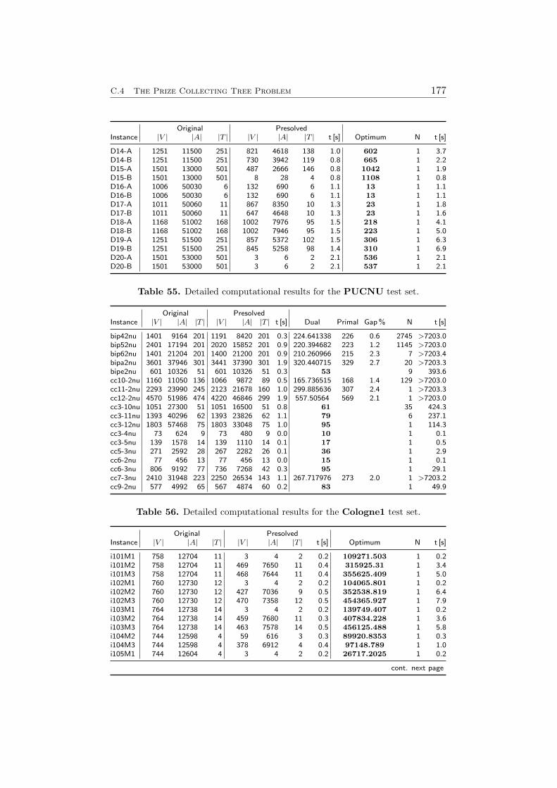
C.4 The Prize Collecting Tree Problem 177
Original PresolvedInstance |V | |A| |T | |V | |A| |T | t [s] Optimum N t [s]
D14-A 1251 11500 251 821 4618 138 1.0 602 1 3.7D14-B 1251 11500 251 730 3942 119 0.8 665 1 2.2D15-A 1501 13000 501 487 2666 146 0.8 1042 1 1.9D15-B 1501 13000 501 8 28 4 0.8 1108 1 0.8D16-A 1006 50030 6 132 690 6 1.1 13 1 1.1D16-B 1006 50030 6 132 690 6 1.1 13 1 1.1D17-A 1011 50060 11 867 8350 10 1.3 23 1 1.8D17-B 1011 50060 11 647 4648 10 1.3 23 1 1.6D18-A 1168 51002 168 1002 7976 95 1.5 218 1 4.1D18-B 1168 51002 168 1002 7946 95 1.5 223 1 5.0D19-A 1251 51500 251 857 5372 102 1.5 306 1 6.3D19-B 1251 51500 251 845 5258 98 1.4 310 1 6.9D20-A 1501 53000 501 3 6 2 2.1 536 1 2.1D20-B 1501 53000 501 3 6 2 2.1 537 1 2.1
Table 55. Detailed computational results for the PUCNU test set.
Original PresolvedInstance |V | |A| |T | |V | |A| |T | t [s] Dual Primal Gap % N t [s]
bip42nu 1401 9164 201 1191 8420 201 0.3 224.641338 226 0.6 2745 >7203.0bip52nu 2401 17194 201 2020 15852 201 0.9 220.394682 223 1.2 1145 >7203.0bip62nu 1401 21204 201 1400 21200 201 0.9 210.260966 215 2.3 7 >7203.4bipa2nu 3601 37946 301 3441 37390 301 1.9 320.440715 329 2.7 20 >7203.3bipe2nu 601 10326 51 601 10326 51 0.3 53 9 393.6cc10-2nu 1160 11050 136 1066 9872 89 0.5 165.736515 168 1.4 129 >7203.0cc11-2nu 2293 23990 245 2123 21678 160 1.0 299.885636 307 2.4 1 >7203.3cc12-2nu 4570 51986 474 4220 46846 299 1.9 557.50564 569 2.1 1 >7203.0cc3-10nu 1051 27300 51 1051 16500 51 0.8 61 35 424.3cc3-11nu 1393 40296 62 1393 23826 62 1.1 79 6 237.1cc3-12nu 1803 57468 75 1803 33048 75 1.0 95 1 114.3cc3-4nu 73 624 9 73 480 9 0.0 10 1 0.1cc3-5nu 139 1578 14 139 1110 14 0.1 17 1 0.5cc5-3nu 271 2592 28 267 2282 26 0.1 36 1 2.9cc6-2nu 77 456 13 77 456 13 0.0 15 1 0.1cc6-3nu 806 9192 77 736 7268 42 0.3 95 1 29.1cc7-3nu 2410 31948 223 2250 26534 143 1.1 267.717976 273 2.0 1 >7203.2cc9-2nu 577 4992 65 567 4874 60 0.2 83 1 49.9
Table 56. Detailed computational results for the Cologne1 test set.
Original PresolvedInstance |V | |A| |T | |V | |A| |T | t [s] Optimum N t [s]
i101M1 758 12704 11 3 4 2 0.2 109271.503 1 0.2i101M2 758 12704 11 469 7650 11 0.4 315925.31 1 3.4i101M3 758 12704 11 468 7644 11 0.4 355625.409 1 5.0i102M1 760 12730 12 3 4 2 0.2 104065.801 1 0.2i102M2 760 12730 12 427 7036 9 0.5 352538.819 1 6.4i102M3 760 12730 12 470 7358 12 0.5 454365.927 1 7.9i103M1 764 12738 14 3 4 2 0.2 139749.407 1 0.2i103M2 764 12738 14 459 7680 11 0.3 407834.228 1 3.6i103M3 764 12738 14 463 7578 14 0.5 456125.488 1 5.8i104M2 744 12598 4 59 616 3 0.3 89920.8353 1 0.3i104M3 744 12598 4 378 6912 4 0.4 97148.789 1 1.0i105M1 744 12604 4 3 4 2 0.2 26717.2025 1 0.2
cont. next page
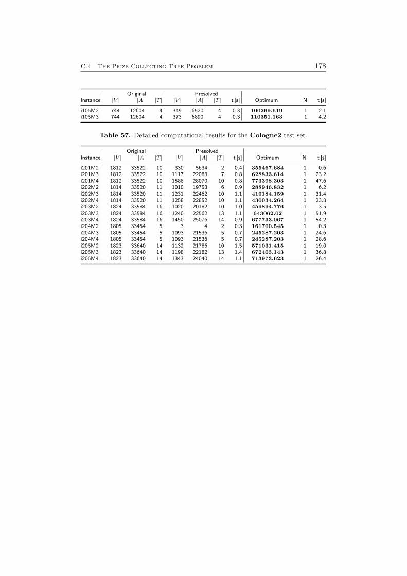
C.4 The Prize Collecting Tree Problem 178
Original PresolvedInstance |V | |A| |T | |V | |A| |T | t [s] Optimum N t [s]
i105M2 744 12604 4 349 6520 4 0.3 100269.619 1 2.1i105M3 744 12604 4 373 6890 4 0.3 110351.163 1 4.2
Table 57. Detailed computational results for the Cologne2 test set.
Original PresolvedInstance |V | |A| |T | |V | |A| |T | t [s] Optimum N t [s]
i201M2 1812 33522 10 330 5634 2 0.4 355467.684 1 0.6i201M3 1812 33522 10 1117 22088 7 0.8 628833.614 1 23.2i201M4 1812 33522 10 1588 28070 10 0.8 773398.303 1 47.6i202M2 1814 33520 11 1010 19758 6 0.9 288946.832 1 6.2i202M3 1814 33520 11 1231 22462 10 1.1 419184.159 1 31.4i202M4 1814 33520 11 1258 22852 10 1.1 430034.264 1 23.8i203M2 1824 33584 16 1020 20182 10 1.0 459894.776 1 3.5i203M3 1824 33584 16 1240 22562 13 1.1 643062.02 1 51.9i203M4 1824 33584 16 1450 25076 14 0.9 677733.067 1 54.2i204M2 1805 33454 5 3 4 2 0.3 161700.545 1 0.3i204M3 1805 33454 5 1093 21536 5 0.7 245287.203 1 24.6i204M4 1805 33454 5 1093 21536 5 0.7 245287.203 1 28.6i205M2 1823 33640 14 1132 21786 10 1.5 571031.415 1 19.0i205M3 1823 33640 14 1198 22182 13 1.4 672403.143 1 36.8i205M4 1823 33640 14 1343 24040 14 1.1 713973.623 1 26.4
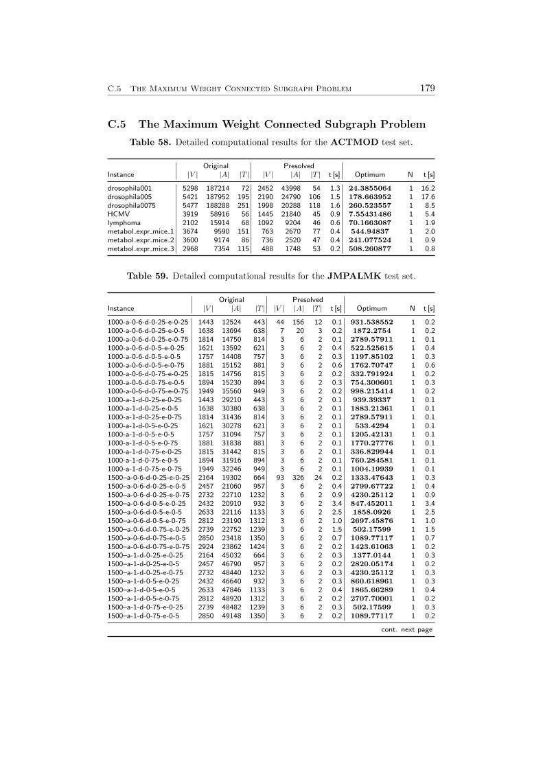
C.5 The Maximum Weight Connected Subgraph Problem 179
C.5 The Maximum Weight Connected Subgraph Problem
Table 58. Detailed computational results for the ACTMOD test set.
Original PresolvedInstance |V | |A| |T | |V | |A| |T | t [s] Optimum N t [s]
drosophila001 5298 187214 72 2452 43998 54 1.3 24.3855064 1 16.2drosophila005 5421 187952 195 2190 24790 106 1.5 178.663952 1 17.6drosophila0075 5477 188288 251 1998 20288 118 1.6 260.523557 1 8.5HCMV 3919 58916 56 1445 21840 45 0.9 7.55431486 1 5.4lymphoma 2102 15914 68 1092 9204 46 0.6 70.1663087 1 1.9metabol expr mice 1 3674 9590 151 763 2670 77 0.4 544.94837 1 2.0metabol expr mice 2 3600 9174 86 736 2520 47 0.4 241.077524 1 0.9metabol expr mice 3 2968 7354 115 488 1748 53 0.2 508.260877 1 0.8
Table 59. Detailed computational results for the JMPALMK test set.
Original PresolvedInstance |V | |A| |T | |V | |A| |T | t [s] Optimum N t [s]
1000-a-0-6-d-0-25-e-0-25 1443 12524 443 44 156 12 0.1 931.538552 1 0.21000-a-0-6-d-0-25-e-0-5 1638 13694 638 7 20 3 0.2 1872.2754 1 0.21000-a-0-6-d-0-25-e-0-75 1814 14750 814 3 6 2 0.1 2789.57911 1 0.11000-a-0-6-d-0-5-e-0-25 1621 13592 621 3 6 2 0.4 522.525615 1 0.41000-a-0-6-d-0-5-e-0-5 1757 14408 757 3 6 2 0.3 1197.85102 1 0.31000-a-0-6-d-0-5-e-0-75 1881 15152 881 3 6 2 0.6 1762.70747 1 0.61000-a-0-6-d-0-75-e-0-25 1815 14756 815 3 6 2 0.2 332.791924 1 0.21000-a-0-6-d-0-75-e-0-5 1894 15230 894 3 6 2 0.3 754.300601 1 0.31000-a-0-6-d-0-75-e-0-75 1949 15560 949 3 6 2 0.2 998.215414 1 0.21000-a-1-d-0-25-e-0-25 1443 29210 443 3 6 2 0.1 939.39337 1 0.11000-a-1-d-0-25-e-0-5 1638 30380 638 3 6 2 0.1 1883.21361 1 0.11000-a-1-d-0-25-e-0-75 1814 31436 814 3 6 2 0.1 2789.57911 1 0.11000-a-1-d-0-5-e-0-25 1621 30278 621 3 6 2 0.1 533.4294 1 0.11000-a-1-d-0-5-e-0-5 1757 31094 757 3 6 2 0.1 1205.42131 1 0.11000-a-1-d-0-5-e-0-75 1881 31838 881 3 6 2 0.1 1770.27776 1 0.11000-a-1-d-0-75-e-0-25 1815 31442 815 3 6 2 0.1 336.829944 1 0.11000-a-1-d-0-75-e-0-5 1894 31916 894 3 6 2 0.1 760.284581 1 0.11000-a-1-d-0-75-e-0-75 1949 32246 949 3 6 2 0.1 1004.19939 1 0.11500–a-0-6-d-0-25-e-0-25 2164 19302 664 93 326 24 0.2 1333.47643 1 0.31500–a-0-6-d-0-25-e-0-5 2457 21060 957 3 6 2 0.4 2799.67722 1 0.41500–a-0-6-d-0-25-e-0-75 2732 22710 1232 3 6 2 0.9 4230.25112 1 0.91500–a-0-6-d-0-5-e-0-25 2432 20910 932 3 6 2 3.4 847.452011 1 3.41500–a-0-6-d-0-5-e-0-5 2633 22116 1133 3 6 2 2.5 1858.0926 1 2.51500–a-0-6-d-0-5-e-0-75 2812 23190 1312 3 6 2 1.0 2697.45876 1 1.01500–a-0-6-d-0-75-e-0-25 2739 22752 1239 3 6 2 1.5 502.17599 1 1.51500–a-0-6-d-0-75-e-0-5 2850 23418 1350 3 6 2 0.7 1089.77117 1 0.71500–a-0-6-d-0-75-e-0-75 2924 23862 1424 3 6 2 0.2 1423.61063 1 0.21500–a-1-d-0-25-e-0-25 2164 45032 664 3 6 2 0.3 1377.0144 1 0.31500–a-1-d-0-25-e-0-5 2457 46790 957 3 6 2 0.2 2820.05174 1 0.21500–a-1-d-0-25-e-0-75 2732 48440 1232 3 6 2 0.3 4230.25112 1 0.31500–a-1-d-0-5-e-0-25 2432 46640 932 3 6 2 0.3 860.618961 1 0.31500–a-1-d-0-5-e-0-5 2633 47846 1133 3 6 2 0.4 1865.66289 1 0.41500–a-1-d-0-5-e-0-75 2812 48920 1312 3 6 2 0.2 2707.70001 1 0.21500–a-1-d-0-75-e-0-25 2739 48482 1239 3 6 2 0.3 502.17599 1 0.31500–a-1-d-0-75-e-0-5 2850 49148 1350 3 6 2 0.2 1089.77117 1 0.2
cont. next page
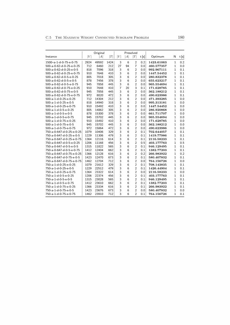
C.5 The Maximum Weight Connected Subgraph Problem 180
Original PresolvedInstance |V | |A| |T | |V | |A| |T | t [s] Optimum N t [s]
1500–a-1-d-0-75-e-0-75 2924 49592 1424 3 6 2 0.2 1423.61063 1 0.2500-a-0-62-d-0-25-e-0-25 712 6460 212 27 94 7 0.0 460.577357 1 0.0500-a-0-62-d-0-25-e-0-5 818 7096 318 3 6 2 0.0 992.967111 1 0.1500-a-0-62-d-0-25-e-0-75 910 7648 410 3 6 2 0.0 1447.54452 1 0.1500-a-0-62-d-0-5-e-0-25 805 7018 305 3 6 2 0.0 280.832378 1 0.1500-a-0-62-d-0-5-e-0-5 878 7456 378 3 6 2 0.0 655.623217 1 0.1500-a-0-62-d-0-5-e-0-75 945 7858 445 3 6 2 0.0 965.554694 1 0.1500-a-0-62-d-0-75-e-0-25 910 7648 410 7 20 3 0.1 171.628785 1 0.1500-a-0-62-d-0-75-e-0-5 945 7858 445 3 6 2 0.0 362.188212 1 0.1500-a-0-62-d-0-75-e-0-75 972 8020 472 3 6 2 0.0 490.623986 1 0.1500-a-1-d-0-25-e-0-25 712 14304 212 3 6 2 0.0 471.393285 1 0.0500-a-1-d-0-25-e-0-5 818 14940 318 3 6 2 0.0 995.313181 1 0.0500-a-1-d-0-25-e-0-75 910 15492 410 3 6 2 0.0 1447.54452 1 0.0500-a-1-d-0-5-e-0-25 805 14862 305 3 6 2 0.0 286.920868 1 0.0500-a-1-d-0-5-e-0-5 878 15300 378 3 6 2 0.0 661.711707 1 0.0500-a-1-d-0-5-e-0-75 945 15702 445 3 6 2 0.0 965.554694 1 0.0500-a-1-d-0-75-e-0-25 910 15492 410 3 6 2 0.0 171.628785 1 0.0500-a-1-d-0-75-e-0-5 945 15702 445 3 6 2 0.0 362.188212 1 0.0500-a-1-d-0-75-e-0-75 972 15864 472 3 6 2 0.0 490.623986 1 0.0750-a-0-647-d-0-25-e-0-25 1079 10406 329 3 6 2 0.1 702.644057 1 0.1750-a-0-647-d-0-25-e-0-5 1229 11306 479 3 6 2 0.1 1419.77986 1 0.1750-a-0-647-d-0-25-e-0-75 1364 12116 614 3 6 2 0.1 2116.58233 1 0.1750-a-0-647-d-0-5-e-0-25 1206 11168 456 3 6 2 0.5 403.177763 1 0.5750-a-0-647-d-0-5-e-0-5 1315 11822 565 3 6 2 0.1 946.129495 1 0.1750-a-0-647-d-0-5-e-0-75 1412 12404 662 3 6 2 0.1 1382.77203 1 0.1750-a-0-647-d-0-75-e-0-25 1366 12128 616 3 6 2 0.2 266.983922 1 0.2750-a-0-647-d-0-75-e-0-5 1423 12470 673 3 6 2 0.1 580.407832 1 0.1750-a-0-647-d-0-75-e-0-75 1462 12704 712 3 6 2 0.0 764.156726 1 0.0750-a-1-d-0-25-e-0-25 1079 21612 329 3 6 2 0.1 708.143835 1 0.1750-a-1-d-0-25-e-0-5 1229 22512 479 3 6 2 0.1 1426.44904 1 0.1750-a-1-d-0-25-e-0-75 1364 23322 614 3 6 2 0.0 2116.58233 1 0.0750-a-1-d-0-5-e-0-25 1206 22374 456 3 6 2 0.1 403.177763 1 0.1750-a-1-d-0-5-e-0-5 1315 23028 565 3 6 2 0.1 946.129495 1 0.1750-a-1-d-0-5-e-0-75 1412 23610 662 3 6 2 0.1 1382.77203 1 0.1750-a-1-d-0-75-e-0-25 1366 23334 616 3 6 2 0.1 266.983922 1 0.1750-a-1-d-0-75-e-0-5 1423 23676 673 3 6 2 0.0 580.407832 1 0.0750-a-1-d-0-75-e-0-75 1462 23910 712 3 6 2 0.1 764.156726 1 0.1
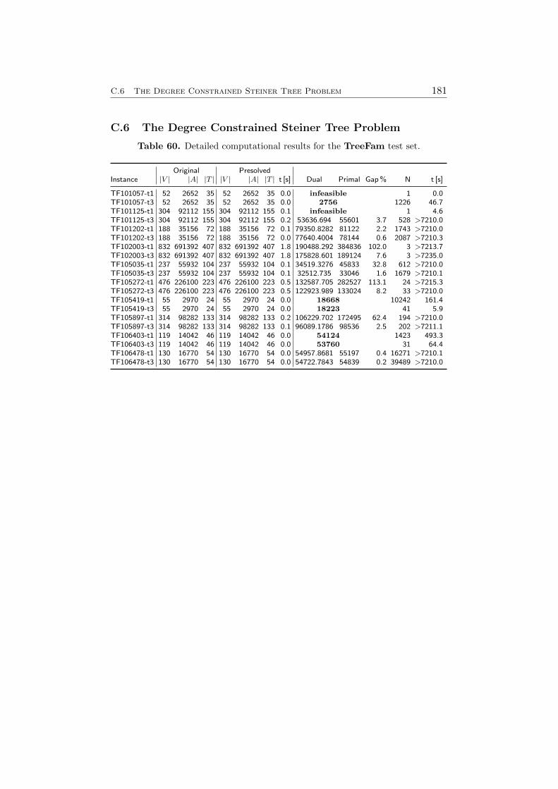
C.6 The Degree Constrained Steiner Tree Problem 181
C.6 The Degree Constrained Steiner Tree Problem
Table 60. Detailed computational results for the TreeFam test set.
Original PresolvedInstance |V | |A| |T | |V | |A| |T | t [s] Dual Primal Gap % N t [s]
TF101057-t1 52 2652 35 52 2652 35 0.0 infeasible 1 0.0TF101057-t3 52 2652 35 52 2652 35 0.0 2756 1226 46.7TF101125-t1 304 92112 155 304 92112 155 0.1 infeasible 1 4.6TF101125-t3 304 92112 155 304 92112 155 0.2 53636.694 55601 3.7 528 >7210.0TF101202-t1 188 35156 72 188 35156 72 0.1 79350.8282 81122 2.2 1743 >7210.0TF101202-t3 188 35156 72 188 35156 72 0.0 77640.4004 78144 0.6 2087 >7210.3TF102003-t1 832 691392 407 832 691392 407 1.8 190488.292 384836 102.0 3 >7213.7TF102003-t3 832 691392 407 832 691392 407 1.8 175828.601 189124 7.6 3 >7235.0TF105035-t1 237 55932 104 237 55932 104 0.1 34519.3276 45833 32.8 612 >7210.0TF105035-t3 237 55932 104 237 55932 104 0.1 32512.735 33046 1.6 1679 >7210.1TF105272-t1 476 226100 223 476 226100 223 0.5 132587.705 282527 113.1 24 >7215.3TF105272-t3 476 226100 223 476 226100 223 0.5 122923.989 133024 8.2 33 >7210.0TF105419-t1 55 2970 24 55 2970 24 0.0 18668 10242 161.4TF105419-t3 55 2970 24 55 2970 24 0.0 18223 41 5.9TF105897-t1 314 98282 133 314 98282 133 0.2 106229.702 172495 62.4 194 >7210.0TF105897-t3 314 98282 133 314 98282 133 0.1 96089.1786 98536 2.5 202 >7211.1TF106403-t1 119 14042 46 119 14042 46 0.0 54124 1423 493.3TF106403-t3 119 14042 46 119 14042 46 0.0 53760 31 64.4TF106478-t1 130 16770 54 130 16770 54 0.0 54957.8681 55197 0.4 16271 >7210.1TF106478-t3 130 16770 54 130 16770 54 0.0 54722.7843 54839 0.2 39489 >7210.0
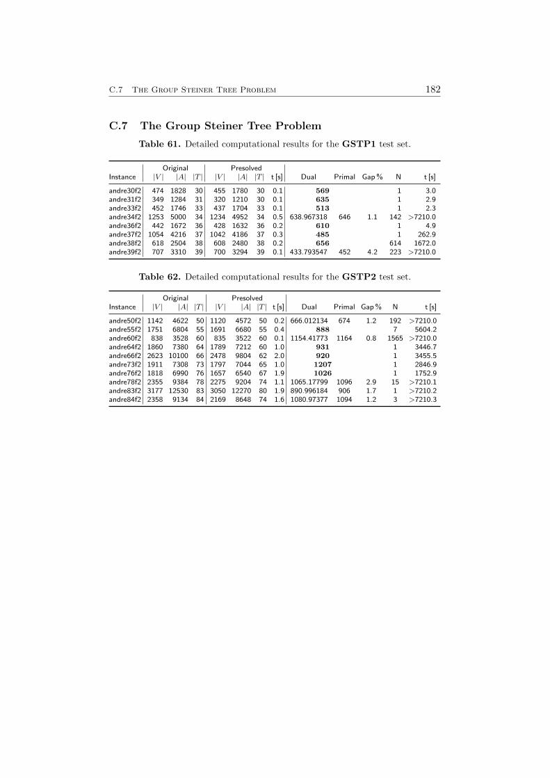
C.7 The Group Steiner Tree Problem 182
C.7 The Group Steiner Tree Problem
Table 61. Detailed computational results for the GSTP1 test set.
Original PresolvedInstance |V | |A| |T | |V | |A| |T | t [s] Dual Primal Gap % N t [s]
andre30f2 474 1828 30 455 1780 30 0.1 569 1 3.0andre31f2 349 1284 31 320 1210 30 0.1 635 1 2.9andre33f2 452 1746 33 437 1704 33 0.1 513 1 2.3andre34f2 1253 5000 34 1234 4952 34 0.5 638.967318 646 1.1 142 >7210.0andre36f2 442 1672 36 428 1632 36 0.2 610 1 4.9andre37f2 1054 4216 37 1042 4186 37 0.3 485 1 262.9andre38f2 618 2504 38 608 2480 38 0.2 656 614 1672.0andre39f2 707 3310 39 700 3294 39 0.1 433.793547 452 4.2 223 >7210.0
Table 62. Detailed computational results for the GSTP2 test set.
Original PresolvedInstance |V | |A| |T | |V | |A| |T | t [s] Dual Primal Gap % N t [s]
andre50f2 1142 4622 50 1120 4572 50 0.2 666.012134 674 1.2 192 >7210.0andre55f2 1751 6804 55 1691 6680 55 0.4 888 7 5604.2andre60f2 838 3528 60 835 3522 60 0.1 1154.41773 1164 0.8 1565 >7210.0andre64f2 1860 7380 64 1789 7212 60 1.0 931 1 3446.7andre66f2 2623 10100 66 2478 9804 62 2.0 920 1 3455.5andre73f2 1911 7308 73 1797 7044 65 1.0 1207 1 2846.9andre76f2 1818 6990 76 1657 6540 67 1.9 1026 1 1752.9andre78f2 2355 9384 78 2275 9204 74 1.1 1065.17799 1096 2.9 15 >7210.1andre83f2 3177 12530 83 3050 12270 80 1.9 890.996184 906 1.7 1 >7210.2andre84f2 2358 9134 84 2169 8648 74 1.6 1080.97377 1094 1.2 3 >7210.3
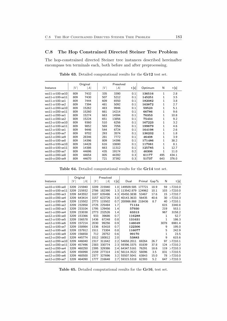
C.8 The Hop Constrained Directed Steiner Tree Problem 183
C.8 The Hop Constrained Directed Steiner Tree Problem
The hop-constrained directed Steiner tree instances described hereinafterencompass ten terminals each, both before and after preprocessing.
Table 63. Detailed computational results for the Gr12 test set.
Original PresolvedInstance |V | |A| |V | |A| t [s] Optimum N t [s]
wo11-cr100-se10 809 7432 335 3390 0.1 136516 1 2.8wo11-cr100-se11 809 7430 507 5212 0.1 145251 1 3.5wo11-cr100-se1 809 7444 609 6550 0.1 182082 1 3.8wo11-cr100-se2 809 7394 481 5092 0.1 163872 1 2.7wo11-cr200-se10 809 15262 483 9946 0.1 59523 1 5.1wo11-cr200-se11 809 15260 661 14214 0.1 66786 1 9.6wo11-cr200-se1 809 15274 663 14594 0.1 76353 1 10.8wo11-cr200-se2 809 15224 651 13856 0.1 75434 1 9.2wo12-cr100-se10 809 9360 510 6256 0.1 167223 1 3.2wo12-cr100-se11 809 9852 569 7056 0.1 199679 1 4.6wo12-cr100-se1 809 9446 544 6724 0.1 164198 1 2.6wo12-cr100-se7 809 9702 293 3574 0.1 136232 1 1.8wo12-cr200-se9 809 28346 281 7772 0.1 46408 1 3.9wo10-cr100-se0 809 14396 809 14396 0.1 171486 1 38.2wo10-cr100-se10 809 14428 616 10690 0.1 117081 1 8.1wo10-cr100-se11 809 14386 663 11312 0.1 125785 1 12.7wo10-cr200-se7 809 44696 435 19174 0.2 46306 1 11.0wo10-cr200-se8 809 44654 805 44392 0.3 61177 495 434.1wo10-cr200-se9 809 44670 721 37392 0.3 51737 643 376.0
Table 64. Detailed computational results for the Gr14 test set.
Original PresolvedInstance |V | |A| |V | |A| t [s] Dual Primal Gap % N t [s]
wo10-cr100-se0 3209 215940 3209 215940 1.0 149509.585 177721 18.9 59 >7210.0wo10-cr100-se11 3209 215932 2786 182390 1.3 113542.879 124962 10.1 103 >7210.0wo10-cr200-se3 3209 643552 3187 635486 4.3 45450.3838 53467 17.6 15 >7210.7wo10-cr200-se4 3209 643414 3157 622726 3.8 40143.3633 56435 40.6 30 >7210.3wo11-cr100-se6 3209 115502 2773 115502 0.7 200986.868 218436 8.7 40 >7210.1wo11-cr200-se2 3209 232858 2725 225484 1.7 71134 615 3340.8wo11-cr200-se3 3209 233104 1795 129456 1.4 57930 219 553.1wo11-cr200-se4 3209 233038 2773 232526 1.4 63313 967 3158.2wo12-cr100-se0 3209 153366 933 39686 0.7 116288 1 52.7wo12-cr100-se5 3209 156578 1436 67248 0.8 131631 1 186.3wo12-cr100-se6 3209 157214 2030 99256 0.9 146049 3078 6981.4wo12-cr100-se7 3209 158984 1336 63418 0.7 122306 9 195.0wo12-cr100-se8 3209 157912 1511 73304 0.8 116077 5 242.9wo12-cr100-se9 3209 156658 712 28752 0.6 99170 1 23.5wo12-cr200-se0 3209 445774 1512 180812 2.0 53883 9 615.6wo12-cr200-se10 3209 446040 2317 311642 2.2 54658.2011 69264 26.7 97 >7210.1wo12-cr200-se11 3209 457496 2383 330774 2.3 59396.3375 81839 37.8 124 >7210.2wo12-cr200-se4 3209 460250 2395 329386 2.4 64347.5161 76291 18.6 119 >7210.3wo12-cr200-se5 3209 456998 2159 277314 2.6 56114.3522 58096 3.5 831 >7210.5wo12-cr200-se6 3209 460500 2377 327696 3.2 55507.5041 63843 15.0 78 >7210.0wo12-cr200-se7 3209 464090 1777 216648 2.7 59315.5318 62393 5.2 647 >7210.3
Table 65. Detailed computational results for the Gr16, test set.
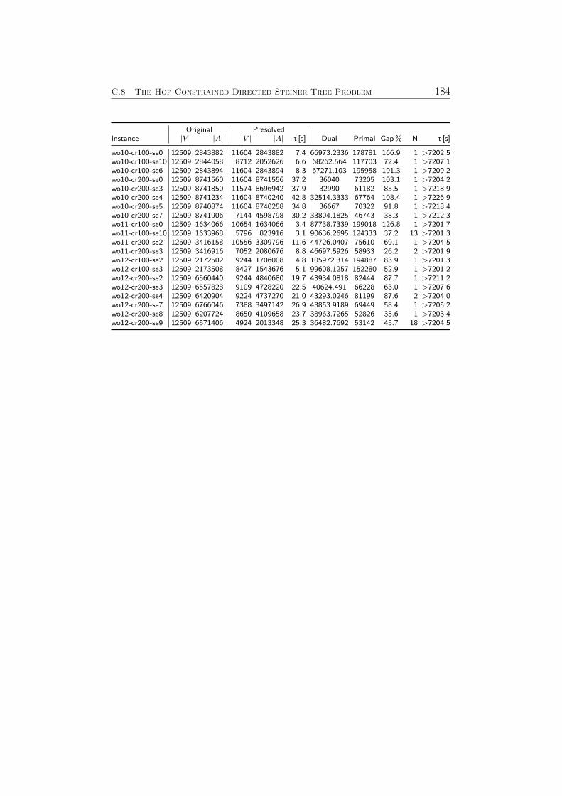
C.8 The Hop Constrained Directed Steiner Tree Problem 184
Original PresolvedInstance |V | |A| |V | |A| t [s] Dual Primal Gap % N t [s]
wo10-cr100-se0 12509 2843882 11604 2843882 7.4 66973.2336 178781 166.9 1 >7202.5wo10-cr100-se10 12509 2844058 8712 2052626 6.6 68262.564 117703 72.4 1 >7207.1wo10-cr100-se6 12509 2843894 11604 2843894 8.3 67271.103 195958 191.3 1 >7209.2wo10-cr200-se0 12509 8741560 11604 8741556 37.2 36040 73205 103.1 1 >7204.2wo10-cr200-se3 12509 8741850 11574 8696942 37.9 32990 61182 85.5 1 >7218.9wo10-cr200-se4 12509 8741234 11604 8740240 42.8 32514.3333 67764 108.4 1 >7226.9wo10-cr200-se5 12509 8740874 11604 8740258 34.8 36667 70322 91.8 1 >7218.4wo10-cr200-se7 12509 8741906 7144 4598798 30.2 33804.1825 46743 38.3 1 >7212.3wo11-cr100-se0 12509 1634066 10654 1634066 3.4 87738.7339 199018 126.8 1 >7201.7wo11-cr100-se10 12509 1633968 5796 823916 3.1 90636.2695 124333 37.2 13 >7201.3wo11-cr200-se2 12509 3416158 10556 3309796 11.6 44726.0407 75610 69.1 1 >7204.5wo11-cr200-se3 12509 3416916 7052 2080676 8.8 46697.5926 58933 26.2 2 >7201.9wo12-cr100-se2 12509 2172502 9244 1706008 4.8 105972.314 194887 83.9 1 >7201.3wo12-cr100-se3 12509 2173508 8427 1543676 5.1 99608.1257 152280 52.9 1 >7201.2wo12-cr200-se2 12509 6560440 9244 4840680 19.7 43934.0818 82444 87.7 1 >7211.2wo12-cr200-se3 12509 6557828 9109 4728220 22.5 40624.491 66228 63.0 1 >7207.6wo12-cr200-se4 12509 6420904 9224 4737270 21.0 43293.0246 81199 87.6 2 >7204.0wo12-cr200-se7 12509 6766046 7388 3497142 26.9 43853.9189 69449 58.4 1 >7205.2wo12-cr200-se8 12509 6207724 8650 4109658 23.7 38963.7265 52826 35.6 1 >7203.4wo12-cr200-se9 12509 6571406 4924 2013348 25.3 36482.7692 53142 45.7 18 >7204.5


![TREE ACCESS EVO MANUALE r0 mai stampatodoc.camp.it/Manuali/TREE ACCESS EVO_MANUALE r0.pdf · Para colocar el arnés con perneras “Tree Access Evo” [A], siga las instrucciones](https://static.fdokument.com/doc/165x107/5e5ec5a8532dd513ab691868/tree-access-evo-manuale-r0-mai-access-evomanuale-r0pdf-para-colocar-el-arns.jpg)