safety

Article

An Examination of the Strava Usage Rate—A Parameter to EstimateAverage Annual Daily Bicycle Volumes on Rural Roadways

Francisco Javier Camacho-Torregrosa *, David Llopis-Castelló , Griselda López-Maldonado and Alfredo García

�����������������

Citation: Camacho-Torregrosa, F.J.;

Llopis-Castelló, D.; López-Maldonado,

G.; García, A. An Examination of the

Strava Usage Rate—A Parameter to

Estimate Average Annual Daily Bicycle

Volumes on Rural Roadways. Safety

2021, 7, 8. https://doi.org/10.3390/

safety7010008

Received: 29 October 2020

Accepted: 23 January 2021

Published: 27 January 2021

Publisher’s Note: MDPI stays neutral

with regard to jurisdictional claims in

published maps and institutional affil-

iations.

Copyright: © 2021 by the authors.

Licensee MDPI, Basel, Switzerland.

This article is an open access article

distributed under the terms and

conditions of the Creative Commons

Attribution (CC BY) license (https://

creativecommons.org/licenses/by/

4.0/).

Highway Engineering Research Group, Institute of Transportation and Territory, Universitat Politècnica deValència, 46022 Valencia, Spain; dallocas@upv.es (D.L.-C.); grilomal@tra.upv.es (G.L.-M.);agarciag@tra.upv.es (A.G.)* Correspondence: fracator@tra.upv.es; Tel.: +34-963-877-374

Abstract: In Spain, a new challenge is emerging due to the increase of many recreational bicyclistson two-lane rural roads. These facilities have been mainly designed for motorized vehicles, so thecoexistence of cyclists and drivers produces an impact, in terms of road safety and operation. In orderto analyze the occurrence of crashes and enhance safety for bicycling, it is crucial to know the cyclingvolume. Standard procedures recommend using data from permanent stations and temporary shortcounts, but bicycle volumes are rarely monitored in rural roads. However, bicyclists tend to tracktheir leisure and exercise activities with fitness apps that use GPS. In this context, this research aims atanalyzing the daily and seasonal variability of the Strava Usage Rate (SUR), defined as the proportionof bicyclists using the Strava app along a certain segment on rural highways, to estimate the AnnualAverage Daily Bicycle (AADB) volume on rural roads. The findings of this study offer possiblesolutions to policy makers in terms of planning and design of the cycling network. Moreover, the useof crowdsourced data from the Strava app will potentially save costs to public agencies, since publicdata could replace costly counting campaigns.

Keywords: two-lane rural roads; bicycle volume; cyclist safety; Strava app; short count; road safety

1. Introduction

In the European Union, although the number of cyclist deaths has decreased by27% between 2006 and 2015, cyclist fatalities account for a large percentage (8%) of thetotal fatalities on road crashes [1]. Over the same period of time, the number of cyclistdeaths has raised by 6% in the United States, reaching a total of 818 fatalities in 2015 [2].Therefore, cycling safety is becoming more and more important in our society.

In 2018, 7598 fatal-and-injury crashes involving bicyclists occurred in Spain, resultingin 58 deaths, 620 serious injuries, and 6633 minor injuries [3]. Although most of thesecrashes took place on urban areas (74%), 40 of the total number of fatalities occurred ontwo-lane rural roads, which are used by many recreational bicyclists for leisure and fitness.This type of road accounts for 90% of the Spanish road network, being three times morelikely to have fatal-and-injury crashes compared to urban roads.

Road crashes are very connected to risk exposure. Every single interaction amongcyclists and/or with motor vehicles increases the likelihood of having a road crash. A motorvehicle overtaking a bicycle has been reported as the most dangerous maneuver due tothe higher relative speed difference [4]. There are many other aspects that do influence thesafety outcome of a road facility, but an adequate determination of the number of cyclists(“exposure to risk”) is considered by many researchers as the most challenging one [5].

An adequate estimation of risk exposure would allow road agencies and researchersto determine crash rates (i.e., number of crashes per exposure estimator) to compare therisk level across facilities and prioritize actions. A more advanced methodology is throughSafety Performance Functions (SPFs) (Equation (1)). A SPF is a function that relates risk

Safety 2021, 7, 8. https://doi.org/10.3390/safety7010008 https://www.mdpi.com/journal/safety

Safety 2021, 7, 8 2 of 20

exposure and other explanatory variables (e.g., geometric design indexes or the postedspeed limit) to the number of road crashes [6,7].

y = eβ0 ·AADTβ1 ·Lβ2 ·e∑ βi ·xi (1)

where y is the number of road crashes, AADT is the Annual Average Daily Traffic Vol-ume, L is the length of the road segment, xi are the explanatory variables, and βi are thecorresponding regression coefficients.

Although many recent studies focused on calibrating SPFs only considering motorizedtraffic volumes [8–10], the current increase of cycling demand on two-lane rural roadssuggests the inclusion of the interaction of both motorized and bicycle traffic to assess roadsafety in a more accurate way [5].

In this context, the Annual Average Daily Bicycle (AADB) volume is considered oneof the most important volume metrics for bicycle traffic [11]. AADB is of great interest formany applications, such as economic evaluation of cycling projects, prioritization of cyclinginfrastructure investments, and road safety analyses. Furthermore, the spatial distributionof cycling demand, represented by AADB, allows engineers to better plan and design thecycling network.

Nevertheless, there is no technology that can perfectly measure AADB. Existing equip-ment for continuously counting bicyclists, such as inductive loops, pneumatic tubes,infrared detection, and automated video processing, present errors due to occlusion,i.e., the masking of bicyclists that are traveling in platoons [12]. Additional errors canalso arise due to equipment malfunction over prolonged outdoor use that spans 24 h aday for 365 days a year. To overcome these data gaps, El Esawey [11] proposed the useof either count data models (log-linear and negative binomial models) or an autoencoderneural network model, which relate weather-specific and time-specific attributes to thedaily cycling demand, instead of historical average methods, which do not incorporateweather effects.

The Traffic Monitoring Guide (TMG), published by the Federal Highway Adminis-tration (FHWA) [13], describes current technologies for monitoring nonmotorized traffic,the volume variability of nonmotorized traffic, and proposed data collection programs.

The guide recommends using data from permanent stations and temporary short-count sites to characterize the spatial variability of nonmotorized traffic. Continuous countsare used to classify sites into different groups, in which monthly and daily adjustmentfactors are calculated. These adjustment factors are then applied to a larger number ofshort duration counts to estimate the annual average daily traffic of nonmotorized traffic ata network level through Equation (2).

AADB = D·Fm·Fd (2)

where D is the short-duration count, Fm is an adjustment factor for the month, and Fd is theday-of-week factor.

The estimation of cycling traffic volumes and the development and application of adjust-ment factors have been thoroughly studied in recent years [14–22]. Additionally, different mod-els currently exist for the estimation of bicycle traffic volumes [11,23–29]. Although thesemodels differ in terms of their procedures, data needs, and reported accuracy, most of themrelate hourly/daily bicycle volumes to either weather conditions or land-use characteristics.The results of these studies are generally consistent, though the magnitude of the impactmight vary from one city/country to another. Cycling demand has been found to increasewith moderate-warm temperatures (<30 ◦C). Likewise, the rain and wind induce lowercycling demands.

Besides that, the growth in the number of users of fitness apps, such as Strava,establishes a good opportunity to analyze the potential of these naturalistic data. Strava tal-lows their users to track athletic activity via satellite navigation and upload and share themafterwards. It can be used for several sporting activities, being cycling one of the most

Safety 2021, 7, 8 3 of 20

popular. Although Strava sells their data in an anonymized and aggregated way, they alsoprovide a portion of their data for free [30].

Cintia et al. [31] analyzed trajectories, average speed, track duration, and heartrate ofnearly 30,000 bicyclists to study fitness performance. Clarke and Steele [32] used Stravadata to improve transportation design and urban planning, whereas Jónasson et al. [33]studied cycle route choice patterns.

Some researchers have cautioned about the lack of accuracy of Strava and similar datasources that might lead to biased estimates. Goodchild et al. [34] reported user-bias forfitness apps. Watkins et al. [35] also reported bias towards male and younger riders whencomparing Strava with another smartphone app called CycleTracks. While Jestico et al. [36]found only moderate relationship between Strava volumes and observed counts, Haworthet al. [37] identified a close relationship between Strava data and those provided by theLondon Cycle Census. Finally, Hochmair et al. [38] concluded that Strava data can beconsidered a useful supplement to other bicycle count systems.

However, most of these studies focused on urban areas where, presumably,recreational cycling, especially for fitness and training, is only a small proportion ofthe total volume. On rural highways, the majority of bicycling is most likely for recre-ational purposes and exhibits different characteristics, such as time of day, trip length,bicyclist demographics, and Strava usage. Regarding this, García et al. [39] defined theStrava Usage Rate (SUR) as the proportion of bicyclists using Strava along a certain roadsegment. The pilot study showed that the SUR was around 25% on this type of roads.Likewise, López-Maldonado et al. [40] collected bicycle volumes in three different ruralareas in the Province of Valencia (Spain). These data, which resulted in 27,000 observed bi-cyclists, were compared with Strava data for each day of observation. In this case, the SURranged from 15% to 30%. This was considered as a too wide range, so further research wasrecommended to explore the reasons behind.

This study goes a step further in the analysis of the evolution of the Strava Usage Rate(SUR), looking at its temporal variability, and proposing a methodology for its calibration.As stated before, the use of apps like Strava is highly correlated to amateur-professionalusers. Therefore, higher SUR parameters might be linked to more demanding routes.Like in previous research, SUR will be estimated by comparing the observed bicyclists withthe uploaded tracks to Strava database. Confidence intervals for the SUR parameter willbe given, based on the bicycle hourly volume. This provides a first reliability measure ofthis factor which will allow the estimation of the Annual Average Daily Bicycle (AADB)volume on two-lane rural roads.

In this way, the paper is structured in four main sections. Section 2 has been divided intotwo subsections. Section 2.1 describes the methodology, including the SUR definition andhow confidence intervals and its robustness are determined. Section 2.2 includes the datacollection campaign: field data collection and the Strava data download. Afterwards, Section 3shows the results for the SUR parameter and its variability. Section 3.1 explores its re-gional variability, while Section 3.3 analyzes the hourly variation using the sliding windowmethod. To do so, Section 3.2 is first introduced to explore the different sliding windowoptions. In Section 4, a new methodology to estimate AADB is presented and the appli-cation of this estimation is discussed. Finally, Section 5 includes the main conclusions ofthe research.

2. Methods and Data Description

This section is divided into two subsections. In the first one (Methodology), the SURconcept is introduced. Information to determine its robustness, by means of confidenceintervals, is also provided. The second subsection (data collection) comprises the differentobservation points that have been selected for the study, as well as the two data collectioncampaigns: one in field and another one downloading data from the Strava platform.

Safety 2021, 7, 8 4 of 20

2.1. Methodology

The SUR rate can be obtained for a single road facility by dividing the amount ofStrava tracks uploaded to the platform by the observed cyclists (Equation (3)), for a certainperiod of time.

SUR =VStrVobs

(3)

where VStr is the amount of Strava tracks and Vobs is the number of observed bicyclists.Both volumes correspond to the same time period.

Like for traffic volume estimation, observed and Strava counts must be consideredaggregated in periods of time (e.g., 5, 15, or 60 min). This integration is performed throughthe sliding window methodology, which can also be used to determine the daily SUR orSUR variations within a day.

However, it is important to highlight that any SUR determination following Equation (3)will provide an observed Strava Usage Rate, i.e., the instantaneous or time-aggregated rate.This rate might vary, but a hypothesis of this research is that a certain SUR value existsand can be calibrated for any location. To this regard, the SUR might present regional,seasonal, or hourly variations.

2.1.1. Confidence Intervals

Let us assume that the probability of a cyclist to upload their track to Strava is knownfor a given location and time (SUR). Let us also assume that this probability remains thesame for all cyclists that ride throughout that position at that time. Thus, for this specificposition and time, the probability of having x cyclists tracking their session with Stravain a global count of n cyclists, follows a Binomial Distribution. This probability can becalculated with Equation (4).

P(

B(n, SUR

)= x

)=

(nx

)·SURx·

(1− SUR

)n−x (4)

As an example, in a global count of 120 cyclists, assuming SUR = 0.25, the probabilityof 36 of them using Strava is 0.03676.

However, the actual value of SUR is unknown. With observation and Strava tracks wecan only estimate SUR as x/n. Nevertheless, this value can be used to get the confidenceintervals for SUR. Since the binomial distribution is discrete, the cumulative probabilityfunction must be calculated prior to any confidence interval determination (Equation (5)).

P(

B(n, SUR

)≤ x

)=

x

∑m=0

P(

B(n, SUR

)= m

)=

x

∑m=0

(nm

)·SURm·

(1− SUR

)n−m (5)

Equations (6) and (7), which are based on Equation (5), allow the calculation of aninterval for the expected cyclists using Strava (x).

xl ∈ N |xl

∑m=0

(nm

)·SURm·

(1− SUR

)n−m ∼=1− Z

2(6)

xu ∈ N |xu

∑m=0

(nm

)·SURm·

(1− SUR

)n−m ∼= 1− 1− Z2

(7)

where xl and xu are the lower and upper bounds of this interval and must be integer. Z isthe confidence value, normally assumed as 0.95.

Note that since these boundaries are discrete, it is impossible to equal the final term.In addition, we are entering in these equations with the SUR parameter, which still remains

Safety 2021, 7, 8 5 of 20

unknown. However, we can rearrange these expressions to obtain the confidence intervalsfor any observed SUR = x/n (Equations (8) and (9)).

SURl ∈ R |x

∑m=0

(nm

)·SURl

m·(1− SUR−

)n−m= 1− 1− Z

2(8)

SURu ∈ R |x

∑m=0

(nm

)·SURu

m·(1− SUR+

)n−m=

1− Z2

(9)

where SURl and SURu are the lower and upper confidence intervals for a given numberof observed cyclists (n) and a given number of Strava tracks (x). Z is the confidence level(0.95 is proposed). Note that SUR is a continuous, decimal parameter, so these confidenceintervals equal the final term.

This calculation can be done for any period of time, either a sliding window, a wholeday/week, or even a year. As a result, not only can we manage the measured SUR valuebut also the range within the actual SUR that is expected. This range will vary in magnitudeand amplitude along the day and date, which will be explored in the Results section.

2.1.2. SUR Robustness

The SUR factor has been proven to be unstable, presenting variations that need to beexplored. Thus, it is necessary to perform adequate calibrations to estimate AADB.

SUR stability can be defined as how reliable a certain SUR factor is, according to itscalibration conditions. Regarding this, an important question arises: how should a SURfactor be calibrated to be reliable?

Calibration conditions could be set as a function of observed cyclists or observationtime. As previously mentioned, the binomial distribution controls the likelihood of xcyclists tracking their activities, from n observed cyclists, given a certain SUR. Figure 1shows the sampling likelihood distribution for SUR = 0.25, i.e., the likely sample SUR thatwe can determine at a 95% confidence level, given a global SUR = 0.25.

Safety 2021, 7, x FOR PEER REVIEW 5 of 21

Note that since these boundaries are discrete, it is impossible to equal the final term. In addition, we are entering in these equations with the 𝑆𝑈𝑅 parameter, which still re-mains unknown. However, we can rearrange these expressions to obtain the confidence intervals for any observed 𝑆𝑈𝑅 = 𝑥/𝑛 (Equations (8) and (9)).

𝑆𝑈𝑅 ∈ ℝ | 𝑛𝑚 · 𝑆𝑈𝑅 · 1 − 𝑆𝑈𝑅 = 1 − 1 − 𝑍2 (8)

𝑆𝑈𝑅 ∈ ℝ | 𝑛𝑚 · 𝑆𝑈𝑅 · 1 − 𝑆𝑈𝑅 = 1 − 𝑍2 (9)

where 𝑆𝑈𝑅 and 𝑆𝑈𝑅 are the lower and upper confidence intervals for a given number of observed cyclists (𝑛) and a given number of Strava tracks (𝑥). 𝑍 is the confidence level (0.95 is proposed). Note that 𝑆𝑈𝑅 is a continuous, decimal parameter, so these confidence intervals equal the final term.

This calculation can be done for any period of time, either a sliding window, a whole day/week, or even a year. As a result, not only can we manage the measured 𝑆𝑈𝑅 value but also the range within the actual 𝑆𝑈𝑅 that is expected. This range will vary in magni-tude and amplitude along the day and date, which will be explored in the Results section.

2.1.2. SUR Robustness The SUR factor has been proven to be unstable, presenting variations that need to be

explored. Thus, it is necessary to perform adequate calibrations to estimate AADB. SUR stability can be defined as how reliable a certain SUR factor is, according to its

calibration conditions. Regarding this, an important question arises: how should a SUR factor be calibrated to be reliable?

Calibration conditions could be set as a function of observed cyclists or observation time. As previously mentioned, the binomial distribution controls the likelihood of 𝑥 cy-clists tracking their activities, from 𝑛 observed cyclists, given a certain 𝑆𝑈𝑅. Figure 1 shows the sampling likelihood distribution for 𝑆𝑈𝑅 = 0.25, i.e., the likely sample SUR that we can determine at a 95% confidence level, given a global 𝑆𝑈𝑅 = 0.25.

For low number of cyclists (e.g., 100 cyclists), the SUR determination becomes very weak. Field SUR direct estimations might even result in 0.12 to 0.36, or even more.

On the other hand, the SUR estimation becomes much more robust as the number of observed cyclists increases. For instance, for 200 cyclists the SUR does not differ more than 0.05 from the actual SUR value, which is a very good approach.

Figure 1. Reliability intervals for SUR (x/n) equal to 0.25. Two lines depict each boundary since the exact threshold cannot be defined for an integer distribution.

Figure 1. Reliability intervals for SUR (x/n) equal to 0.25. Two lines depict each boundary since theexact threshold cannot be defined for an integer distribution.

For low number of cyclists (e.g., 100 cyclists), the SUR determination becomes veryweak. Field SUR direct estimations might even result in 0.12 to 0.36, or even more.

On the other hand, the SUR estimation becomes much more robust as the number ofobserved cyclists increases. For instance, for 200 cyclists the SUR does not differ more than0.05 from the actual SUR value, which is a very good approach.

Safety 2021, 7, 8 6 of 20

It is important to highlight the relationship between the SUR and existing cyclingdemand on the road. Some roads have very a reduced demand, thus preventing us fromgetting an accurate SUR parameter. However, a lower demand makes these roads lessimportant for AADB estimation.

2.2. Data Collection

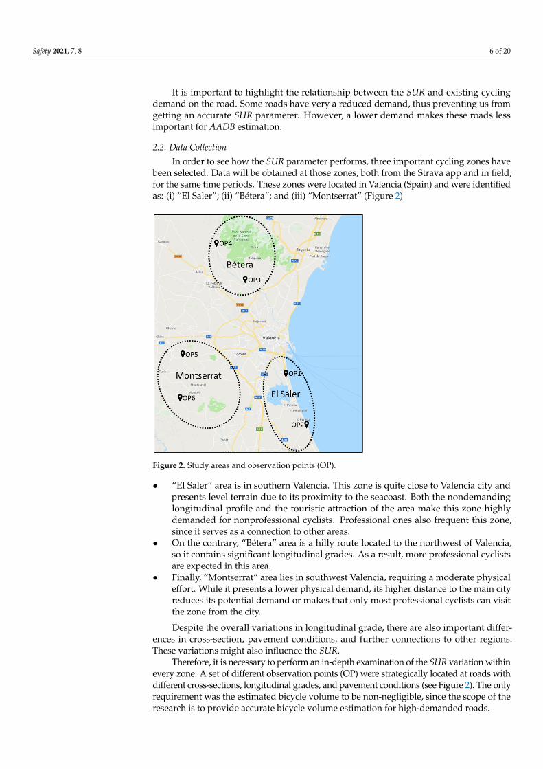
In order to see how the SUR parameter performs, three important cycling zones havebeen selected. Data will be obtained at those zones, both from the Strava app and in field,for the same time periods. These zones were located in Valencia (Spain) and were identifiedas: (i) “El Saler”; (ii) “Bétera”; and (iii) “Montserrat” (Figure 2)

Safety 2021, 7, x FOR PEER REVIEW 7 of 21

Figure 2. Study areas and observation points (OP).

Since the bicycle volume remains constant along a single road segment, road inter-sections allowed the control of at least three different road segments, hence being an ap-propriate location for the observation points. Six observation points were proposed, two per study area, allowing the observation of 16 road segments (32 directions in total). Fig-ure 3 presents the aerial view of all observation points and road segments.

OP1 is a roundabout close to Valencia city (which is located at north, connected to In1/Off1 (noted I1/O1 in Figure 3). Road segments I1, O1, I4, and O4 present similar char-acteristics, being the only difference that the bike lane adjacent to I4 and O4 stops abruptly a few hectometers southwards. As a result, more professional cyclists are expected in I4 and O4.

OP2 corresponds to the same road, several kilometers southwards, further from Va-lencia city. Although also being in level terrain, cycling demand is quite lower, so higher SUR variability is expected. The most common route included I1/O1 (connecting to Va-lencia) and I4/O4.

OP3 is a T intersection with high traffic volumes of cyclists and motor vehicles. This is a major junction, providing connection to many important roads.

OP4 is located northwest several kilometers away. This is a roundabout connecting two important roads, all of them with separated bike lanes. Traffic volume is quite low in this roundabout, so less professional cyclists are expected. In addition, being further away from Valencia induces a lower overall demand.

OP5 and OP6 correspond to a roundabout and a T intersection that connect four and three roads, respectively. Both are located in a mountainous area at western Valencia, far away to identify any clear route pattern.

Figure 2. Study areas and observation points (OP).

• “El Saler” area is in southern Valencia. This zone is quite close to Valencia city andpresents level terrain due to its proximity to the seacoast. Both the nondemandinglongitudinal profile and the touristic attraction of the area make this zone highlydemanded for nonprofessional cyclists. Professional ones also frequent this zone,since it serves as a connection to other areas.

• On the contrary, “Bétera” area is a hilly route located to the northwest of Valencia,so it contains significant longitudinal grades. As a result, more professional cyclistsare expected in this area.

• Finally, “Montserrat” area lies in southwest Valencia, requiring a moderate physicaleffort. While it presents a lower physical demand, its higher distance to the main cityreduces its potential demand or makes that only most professional cyclists can visitthe zone from the city.

Despite the overall variations in longitudinal grade, there are also important differ-ences in cross-section, pavement conditions, and further connections to other regions.These variations might also influence the SUR.

Therefore, it is necessary to perform an in-depth examination of the SUR variation withinevery zone. A set of different observation points (OP) were strategically located at roads withdifferent cross-sections, longitudinal grades, and pavement conditions (see Figure 2). The onlyrequirement was the estimated bicycle volume to be non-negligible, since the scope of theresearch is to provide accurate bicycle volume estimation for high-demanded roads.

Safety 2021, 7, 8 7 of 20

Since the bicycle volume remains constant along a single road segment, road inter-sections allowed the control of at least three different road segments, hence being anappropriate location for the observation points. Six observation points were proposed,two per study area, allowing the observation of 16 road segments (32 directions in total).Figure 3 presents the aerial view of all observation points and road segments.

Safety 2021, 7, x FOR PEER REVIEW 8 of 21

OP1 OP2

OP3 OP4

OP5 OP6

Figure 3. Observation points and segments under analysis.

2.2.1. Field Study All data collections were carried out under favorable weather conditions between

April and October 2017. While a data collection along the entire year and considering more days would have been desirable to capture the seasonal variability of SUR, it was not possible due to budgetary constraints. Therefore, the data collection campaigns fo-

Figure 3. Observation points and segments under analysis.

Safety 2021, 7, 8 8 of 20

OP1 is a roundabout close to Valencia city (which is located at north, connected toIn1/Off1 (noted I1/O1 in Figure 3). Road segments I1, O1, I4, and O4 present similarcharacteristics, being the only difference that the bike lane adjacent to I4 and O4 stopsabruptly a few hectometers southwards. As a result, more professional cyclists are expectedin I4 and O4.

OP2 corresponds to the same road, several kilometers southwards, further fromValencia city. Although also being in level terrain, cycling demand is quite lower, so higherSUR variability is expected. The most common route included I1/O1 (connecting toValencia) and I4/O4.

OP3 is a T intersection with high traffic volumes of cyclists and motor vehicles. This isa major junction, providing connection to many important roads.

OP4 is located northwest several kilometers away. This is a roundabout connectingtwo important roads, all of them with separated bike lanes. Traffic volume is quite low inthis roundabout, so less professional cyclists are expected. In addition, being further awayfrom Valencia induces a lower overall demand.

OP5 and OP6 correspond to a roundabout and a T intersection that connect four andthree roads, respectively. Both are located in a mountainous area at western Valencia,far away to identify any clear route pattern.

2.2.1. Field Study

All data collections were carried out under favorable weather conditions betweenApril and October 2017. While a data collection along the entire year and considering moredays would have been desirable to capture the seasonal variability of SUR, it was not pos-sible due to budgetary constraints. Therefore, the data collection campaigns focused wherethe highest cycling demand was expected (weekday and weekend mornings). Some af-ternoon data collections were also performed, to get insight about the SUR performance.Table 1 summarizes the field data collection.

Table 1. Field data collection.

StrategicLocation

ObservationCode *

Date **(mm/dd/yy) Day of Week Start Time Finish Time Observed

CyclistsCyclists

Using Strava

OP1

1.1 05/17/17 W 7:15 11:00 201 47

1.2 05/17/17 W 15:00 17:00 81 25

1.3 07/20/17 Th 7:00 10:30 242 56

1.4 07/23/17 Su 7:45 11:30 465 82

1.5 09/28/17 Th 8:00 12:30 599 89

1.6 10/28/17 Sa 8:25 12:15 945 233

OP2

2.1 05/17/17 W 15:00 17:00 174 30

2.2 05/17/17 W 7:15 11:00 41 25

2.3 07/20/17 Th 7:00 10:30 260 29

2.4 07/23/17 Su 8:00 11:20 536 115

2.5 09/28/17 Th 10:20 11:55 242 40

2.6 10/28/17 Sa 8:45 11:50 792 215

OP3

3.1 04/05/17 Th 8:00 12:00 206 53

3.2 04/05/17 Th 15:00 16:15 58 32

3.3 06/27/17 Tu 7:00 12:00 555 145

3.4 07/09/17 Su 7:00 10:45 960 276

Safety 2021, 7, 8 9 of 20

Table 1. Cont.

OP4

4.1 04/05/17 Th 8:00 11:45 82 17

4.2 04/05/17 Th 15:00 16:30 26 12

4.3 06/27/17 Tu 7:45 11:30 304 66

4.4 07/09/17 Su 7:15 10:15 594 168

OP5

5.1 06/03/17 Sa 7:30 12:15 345 102

5.2 08/01/17 Tu 7:00 11:30 186 29

5.3 10/19/17 Th 8:00 12:35 115 25

OP6

6.1 06/03/17 Sa 9:00 12:00 164 50

6.2 08/01/17 Tu 7:30 11:00 101 27

6.3 10/19/17 Th 8:45 12:00 68 25

TOTAL 8141 2013

* Observation code is used as unique identifier instead of date because some days present two data collections. ** nonworking day in bold.

2.2.2. Strava Data

Strava data were obtained from the Strava segment database, which contains the traveltimes of everyone who has ever covered a specific segment. The number of cyclists and theirtimestamp were obtained through an ArcGIS tool developed by the Highway EngineeringResearch Group using modifiable Python programming code based on the Strava API [39].This tool allows downloading specific information of the cyclists who had passed througha Strava segment during a certain period of time. The most remarkable information ofthe downloaded data was the timestamp associated with each cyclist, which was used forthe analysis.

3. Results

In this section, the SUR results are presented. First, the outcomes for each observationprocess are shown. Some interpretation about the variability in volumes and SUR thresh-olds are provided. Afterwards, the hourly and regional variation of SUR are explored.To do so, the aggregation time period has to be determined first, through the slidingwindow method.

3.1. Variability across Observation Points

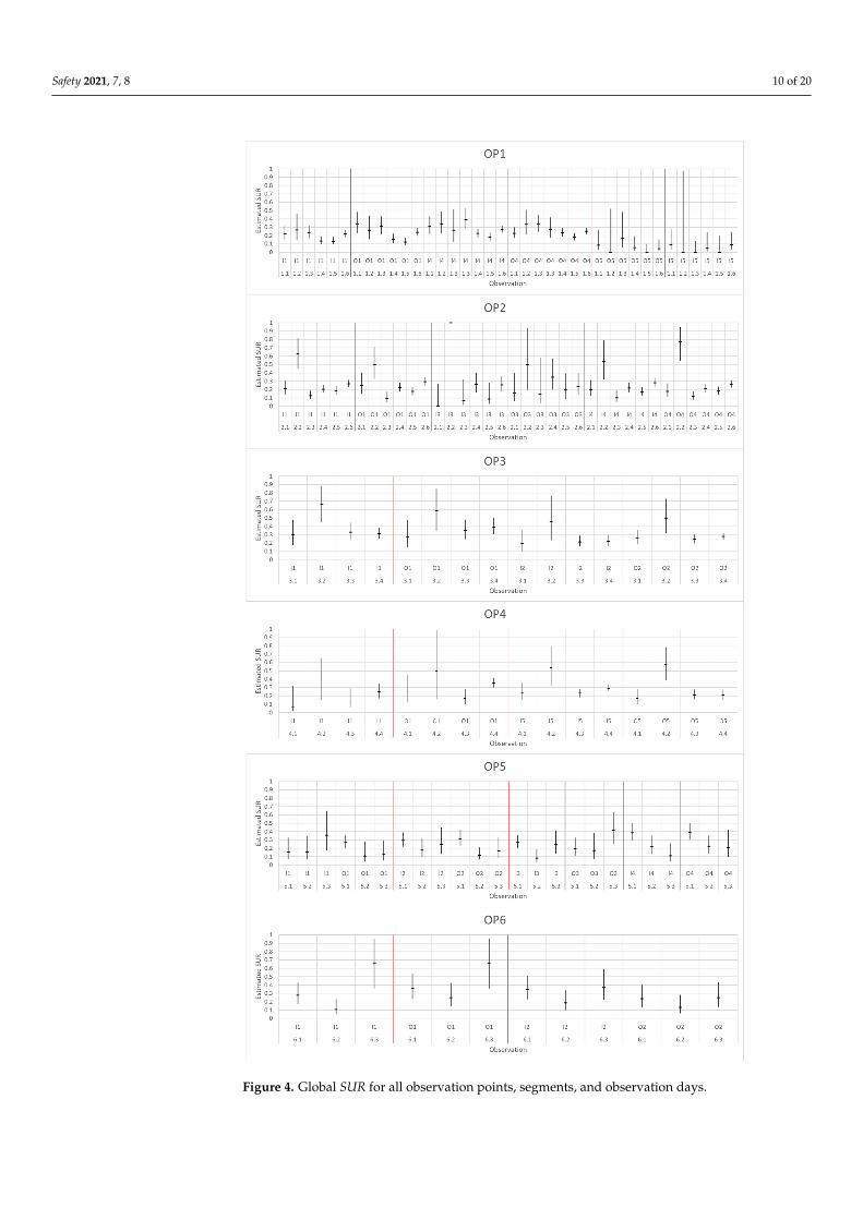
A first analysis of SUR was performed for all road segments, determining the SURconfidence intervals for all sessions. Figure 4 shows the SUR estimations, grouped byobservation point. There are two horizontal axes for each plot: the upper one indicatesthe specific measurement location (e.g., I1, O4, etc.). The lower axis shows the observationcode (see Table 1). The date was not shown instead because some days presented two datacollections (i.e., in the morning and in the afternoon).

Some interesting facts can be seen about bicycle volumes and SUR patterns, which canbe explained based on the location of the observation points and how cyclists performalong these roads (see Section 2.2: Data Collection).

OP1: Most cyclists coming from I1 leave the roundabout through O4. As expected,several nonprofessional cyclists enter the roundabout throughout I1, turn 180◦, and return toValencia using O1. Therefore, O4 is left for more professional cyclists. Accordingly, a higherSUR can be observed with wider intervals (i.e., lower bicycle volumes).

Safety 2021, 7, 8 10 of 20Safety 2021, 7, x FOR PEER REVIEW 11 of 21

Figure 4. Global SUR for all observation points, segments, and observation days. Figure 4. Global SUR for all observation points, segments, and observation days.

Safety 2021, 7, 8 11 of 20

The observation code 1.2 corresponds to an afternoon determination of the SUR.This presents a very similar value than in the morning. In fact, the SUR for the wholeobservation point is quite stable, compared to other locations. A possible explanation isthat Valencia city is very close to OP1. All connections to the beach (I5 and O5) presenteda low cycling demand and very low SUR intervals, corresponding to people who are notwilling to track their activities since their goal is just going to the seacoast.

OP2: The average SUR parameter was about 20% for all these four road segments.Less accurate estimations could be performed for I3/O3 segments, which presented quite alow demand.

OP3: The high volume of motor vehicles makes this zone undesirable for occasionalcyclists. Therefore, the Strava Usage Rate is a bit higher than in other zones. Being a majorjunction is a key factor to explain its SUR behavior. While other observation points areoccasionally covered by cycling groups, OP3 connects to many routes and therefore it is farmore regularly visited. As a result, its SUR is quite stable, around 0.3 for I1/O1 and about0.2-0.25 for I2/O2.

OP4: Due to the lower demand compared to OP3, here the SUR presents big variability,between 0.15 and 0.40 in some cases.

OP5 and OP6, both far away from Valencia and a relative low demand, present strongSUR variations depending on the day.

As a result, some factors that have proven to be related to the SUR are traffic volumeand proximity to the urban zone. Previous studies on rural roads indicated that SUR rangedbetween 15% and 30% [39,40]. The findings confirm this range and provide additionalinformation about the variation patterns. One important conclusion is that there doesnot exist a single SUR value for all road types. Moreover, the SUR also varies for a roadsegment within a single day, even for roads presenting high bicycle volumes.

Higher SUR values have been found at roads with a higher rate of professional cyclists.Since there is not a way to measure the professional level of a cyclist, this has been inferredfrom the authors’ experience and secondary aspects such as the grouping pattern of cyclists.It is in line with the findings of previous research and with the lower SUR values found byother researchers [31–33], who estimated the use of Strava at urban zones, where very fewprofessional cyclists are expected).

3.2. Determination of the Sliding Window Integration

In the previous section, the Strava Usage Rate variation across locations has beenexamined. For that analysis, the SUR was obtained for all observed cyclists within a sessionat once. It is also of interest to analyze how SUR varies within a day. The sliding windowmethodology was selected.

While motorized traffic is pretty stable and 15–60 min aggregation is normally suitable,cyclists do not behave that smoothly. Short integrations would present a noisy behavior,while very long ones would not give accurate data. Hence, it is necessary to determine whichtemporal aggregation provides an adequate balance between accuracy and representativity.

SUR confidence intervals profiles were determined for several road segments of thestudy, using different periods of time for the sliding window (Figure 5). A sliding windowevery second was created. These profiles were the representation of the confidence intervalsof this parameter along the observation time.

Very short sliding windows led to frequent situations with no observed cyclists (Figure 5a),making difficult the determination of any SUR threshold. In addition, sliding windowswith few cyclists led to very wide confidence intervals, which are not useful for theestimation of bicycle volumes. In addition, there are some moments with no cyclists at allwhich present abnormal confidence intervals. This can be seen in Figure 5a at about 10:09 h.

Safety 2021, 7, 8 12 of 20

Safety 2021, 7, x FOR PEER REVIEW 12 of 21

3.2. Determination of the Sliding Window Integration In the previous section, the Strava Usage Rate variation across locations has been

examined. For that analysis, the SUR was obtained for all observed cyclists within a ses-sion at once. It is also of interest to analyze how SUR varies within a day. The sliding window methodology was selected.

While motorized traffic is pretty stable and 15–60 min aggregation is normally suita-ble, cyclists do not behave that smoothly. Short integrations would present a noisy behav-ior, while very long ones would not give accurate data. Hence, it is necessary to determine which temporal aggregation provides an adequate balance between accuracy and repre-sentativity. 𝑆𝑈𝑅 confidence intervals profiles were determined for several road segments of the study, using different periods of time for the sliding window (Figure 5). A sliding window every second was created. These profiles were the representation of the confidence inter-vals of this parameter along the observation time.

(a)—Time window: 20 min (b)—Time window: 30 min

(c)—Time window: 1 h (d)—Time window: 2 h

Figure 5. Time window preliminary analysis (SL4 on June 27 of 2017 is shown as an example, but more locations were considered providing similar results): (a) Time window of 20 min; (b) Time window of 30 min; (c) Time window of 1 h; (d) Time window of 2 h.

00.10.20.30.40.50.60.70.80.9

1

07:45:00 08:57:00 10:09:00 11:21:00

SUR

Time

SUR Upper SUR Lower

00.10.20.30.40.50.60.70.80.9

1

07:45:00 08:57:00 10:09:00 11:21:00

SUR

Time

SUR Upper SUR Lower

00.10.20.30.40.50.60.70.80.9

1

07:45:00 08:57:00 10:09:00 11:21:00

SUR

Time

SUR Upper SUR Lower

00.10.20.30.40.50.60.70.80.9

1

07:45:00 08:57:00 10:09:00 11:21:00

SUR

Time

SUR Upper SUR Lower

Figure 5. Time window preliminary analysis (SL4 on June 27 of 2017 is shown as an example, but more locations wereconsidered providing similar results): (a) Time window of 20 min; (b) Time window of 30 min; (c) Time window of 1 h;(d) Time window of 2 h.

On the contrary, very long sliding windows tend to smooth subtle SUR variations(Figure 5d).

A sliding window of one hour (Figure 5c) was finally proposed as an adequate balancebetween these situations. However, longer windows might also be suitable for low cyclingdemand roads or when no important SUR variations are expected.

3.3. Hourly SUR Variation

SUR profiles were depicted for all road segments under analysis. Confidence intervalswere found to present important variations within every observation, due to differentreasons. Figure 6 shows some relevant findings.

Safety 2021, 7, 8 13 of 20

Safety 2021, 7, x FOR PEER REVIEW 13 of 21

Very short sliding windows led to frequent situations with no observed cyclists (Fig-ure 5a), making difficult the determination of any 𝑆𝑈𝑅 threshold. In addition, sliding windows with few cyclists led to very wide confidence intervals, which are not useful for the estimation of bicycle volumes. In addition, there are some moments with no cyclists at all which present abnormal confidence intervals. This can be seen in Figure 5a at about 10:09 h.

On the contrary, very long sliding windows tend to smooth subtle 𝑆𝑈𝑅 variations (Figure 5d).

A sliding window of one hour (Figure 5c) was finally proposed as an adequate bal-ance between these situations. However, longer windows might also be suitable for low cycling demand roads or when no important 𝑆𝑈𝑅 variations are expected.

3.3. Hourly SUR Variation SUR profiles were depicted for all road segments under analysis. Confidence inter-

vals were found to present important variations within every observation, due to different reasons. Figure 6 shows some relevant findings.

Figure 6a,b compare both directions for the same road segment, which is near Valen-cia. Regarding this, there is a huge cycling demand in the early morning for road segment I1 (exiting from Valencia), which is quite similar to a demand peak in the late morning for road segment O1 (return to Valencia). It can be observed how very low cycling demands produce wide or unstable SUR estimations. However, the SUR estimation for both peaks is very low (0.1 to 0.2 for the first case, 0.02–0.1 for the second). This is in line with the low SUR global value estimated for the whole day in the previous section.

(a) (b)

Safety 2021, 7, x FOR PEER REVIEW 14 of 21

(c) (d)

Figure 6. Cycling demand (blue line = observed demand; orange line = Strava demand) and SUR determination: (a) OP1, E1: observation code 1.5; (b) OP1, S1: observation code 1.5; (c) OP2, S1: observation code 2.4; (d) OP3, S2: observation code 3.4.

Figure 6c shows how cycling demand is almost negligible in the very early morning, thus leading to too wide SUR intervals. As the morning advances, a higher demand is observed, and narrower SUR ranges are identified. Stabilization is around 0.15–0.30, indi-cating a more professional type of cyclist.

Figure 6d shows the SUR evolution for the hub intersection. The high and durable peak of demand produces a very stable SUR. As previously said, more professional cy-clists are expected in this area, which is connected to the higher SUR values (ranging from 0.2 to 0.3 and even more).

Additionally, there is a huge variability of the SUR when it comes to analyzing a road segment. Sudden demand variations, discrete route choices by groups, and other factors influence this variability and prevent us from giving a standard procedure to estimate a valid SUR for a single road segment.

However, this uncertainty can be partially overcome by considering not the SUR for an individual road segment but all road segments belonging to an observation point, i.e., a road junction. This partially stabilizes minor SUR variations. Figure 7 plots some exam-ples of this aggregation for all observation points.

Figure 6. Cycling demand (blue line = observed demand; orange line = Strava demand) and SUR determination: (a) OP1, E1:observation code 1.5; (b) OP1, S1: observation code 1.5; (c) OP2, S1: observation code 2.4; (d) OP3, S2: observation code 3.4.

Figure 6a,b compare both directions for the same road segment, which is near Valencia.Regarding this, there is a huge cycling demand in the early morning for road segment I1(exiting from Valencia), which is quite similar to a demand peak in the late morning forroad segment O1 (return to Valencia). It can be observed how very low cycling demandsproduce wide or unstable SUR estimations. However, the SUR estimation for both peaks isvery low (0.1 to 0.2 for the first case, 0.02–0.1 for the second). This is in line with the lowSUR global value estimated for the whole day in the previous section.

Safety 2021, 7, 8 14 of 20

Figure 6c shows how cycling demand is almost negligible in the very early morning,thus leading to too wide SUR intervals. As the morning advances, a higher demandis observed, and narrower SUR ranges are identified. Stabilization is around 0.15–0.30,indicating a more professional type of cyclist.

Figure 6d shows the SUR evolution for the hub intersection. The high and durablepeak of demand produces a very stable SUR. As previously said, more professional cyclistsare expected in this area, which is connected to the higher SUR values (ranging from 0.2 to0.3 and even more).

Additionally, there is a huge variability of the SUR when it comes to analyzing a roadsegment. Sudden demand variations, discrete route choices by groups, and other factorsinfluence this variability and prevent us from giving a standard procedure to estimate avalid SUR for a single road segment.

However, this uncertainty can be partially overcome by considering not the SURfor an individual road segment but all road segments belonging to an observation point,i.e., a road junction. This partially stabilizes minor SUR variations. Figure 7 plots someexamples of this aggregation for all observation points.

Safety 2021, 7, x FOR PEER REVIEW 15 of 21

(a) (b)

(c) (d)

(e) (f)

Figure 7. Confidence intervals for the node-aggregated SUR estimations: (a) Observation code 1.1; (b) Observation code 2.4; (c) Observation code 3.3; (d) Observation code 4.4; (e) Observation code 5.2; (f) Observation code 6.1.

4. Discussion 4.1. Estimation of AADB Using SUR

The main goal of having an accurate SUR parameter for a certain road facility is to estimate its bicycle volume. Thus, the Average Annual Daily Bicycle (AADB) volume can be estimated using SUR as expressed in Equation (10). 𝐴𝐴𝐷𝐵 = 𝑉365 · 𝑆𝑈𝑅 (10)

where 𝑉 is the total amount of Strava tracks in a year, and 𝑆𝑈𝑅 the calibration factor for the location.

Figure 7. Confidence intervals for the node-aggregated SUR estimations: (a) Observation code 1.1; (b) Observation code 2.4;(c) Observation code 3.3; (d) Observation code 4.4; (e) Observation code 5.2; (f) Observation code 6.1.

Safety 2021, 7, 8 15 of 20

4. Discussion4.1. Estimation of AADB Using SUR

The main goal of having an accurate SUR parameter for a certain road facility is toestimate its bicycle volume. Thus, the Average Annual Daily Bicycle (AADB) volume canbe estimated using SUR as expressed in Equation (10).

AADB =VStr

365·SUR(10)

where VStr is the total amount of Strava tracks in a year, and SUR the calibration factor forthe location.

However, a single SUR factor cannot be designated for any given specific location, since itpresents hourly, seasonal, and random variations. In addition, Camacho-Torregrosa et al. [41]suggested that weekday and weekend cycling demand patterns differed significantly fromeach other, so a separated calibration was preferred instead of using weekend adjust-ment factors.

Therefore, it would be desirable to have as many SUR calibrations as possible. At firstproposal of eight SUR determinations for a certain location is suggested, two per season,one at weekdays, the other at weekends. This distribution might vary depending on re-gional conditions, or further research that could find a SUR distribution pattern. With theseeight SUR calibrations, Equation (11) allows the estimation of AADB.

AADB =5·AADBWD + 2·AADBWE

7(11)

where AADBWD is the Annual Average Daily Bicycle volume for weekdays, and AADBWEfor weekends (bicycles/day). They are determined by Equations (12) and (13), respectively.

AADBWD =VStr,I,WD

nI,WD·SURI,WD+

VStr,I I,WD

nI I,WD·SURI I,WD+

VStr,I I I,WD

nI I I,WD·SURI I I,WD+

VStr,IV,WD

nIV,WD·SURIV,WD(12)

AADBWE =VStr,I,WE

nI,WE·SURI,WE+

VStr,I I,WE

nI I,WE·SURI I,WE+

VStr,I I I,WE

nI I I,WE·SURI I I,WE+

VStr,IV,WE

nIV,WE·SURIV,WE(13)

where VStr,i,j is the Strava volume for season i, j being weekdays or weekends; ni,j isthe number of days for every situation, and SURi,j is the corresponding SUR factor.

Further research is still needed to determine how the SUR varies in terms of roadand region. While important SUR variations might exist across road segments and lo-cations, cycling demands have been proven to be more stable [41]. From these patterns,weekdays normally present two peaks, while weekends normally present a single peakin the morning. This information could help road authorities to plan data collectioncampaigns in order to calibrate SUR and bicycle volumes.

Some locations presented important SUR variations with no clear pattern. However, those witha higher demand were more stable. This is an important strength of the proposed method-ology since AADB of the most important roads are more accurately estimated, providing amore accurate analysis of road safety and operation.

This study did not cover all SUR variations along a year. Data collection campaignsfocused at the moments when the highest demand was expected, given their highest impacton the final AADB estimation. This implies that there are no SUR estimations for winterand bad-weather conditions. However, much lower demand has been detected for thesame region, so extrapolating the SUR parameter would presumably not produce AADBsmuch far from reality. In any case, further research is desirable to capture this variationand provide more reliable estimations.

At weekdays, the SUR parameter might vary between the morning and the afternoon.This should be explored in further research, but it is recommended to observe bicyclesduring the whole session at weekdays. On the other hand, the only peak at weekends,located in the mornings, simplifies the observation session, since the morning covers most

Safety 2021, 7, 8 16 of 20

of the cycling demand. The afternoon/evening demand is nearly negligible. It is importantto highlight that these are preliminary conclusions and might vary in other regions.

4.2. AADB Applications

An adequate estimation of AADB presents important advantages related to both roadsafety and traffic performance.

A major goal for every road traffic authority is the reduction of traffic crashes andcasualties. The Valencian regional government is already tracking road crashes involvingbicycles (Figure 8), which can be used to orientate mitigation measures. However, this in-formation is not complete, since the bicycle exposure (i.e., the bicycle volume per each roadfacility) should be used to compare among segments.

Safety 2021, 7, x FOR PEER REVIEW 17 of 21

information is not complete, since the bicycle exposure (i.e., the bicycle volume per each road facility) should be used to compare among segments.

Figure 8. Road accidents involving cyclists (2012–2016). Each circle corresponds to one crash (green: PDO crash, yellow: slight injury crash, orange: serious injury crash, red: fatal crash). Source: General Directorate of Public Works and Transportation of the Valencian Government.

Although not linear, there is a relationship between exposure and the number of crashes, which can be expressed as a Safety Performance Function (SPF). Once calibrated for a certain region, this function is useful for both new and existing road segment facili-ties: (a) For new road segments, the SPF can be used to estimate the expected number of

crashes involving bicycles (AADB should be estimated first). This estimation would be more accurate if more factors are included in the SPF.

(b) For existing road segments, the SPF outcome can be compared to the observed crashes. If there are more crashes than estimated by the SPF, the road segment pro-duces more crashes than expected, so special countermeasures should be applied. On the contrary, if the SPF estimation exceeds reality, the road segment should be stud-ied to determine which factors are enhancing safety. In both cases, only extreme dif-ferences should be considered, provided that the SPF is fitting real data and therefore presents some error. SPFs, thus, are a powerful tool but a large amount of data is required. If not present,

Highway Administrations could use AADB and crash data to determine the average crash rate for a given type of roads. Again, road segments showing a crash rate above the aver-age should be targeted by these administrations to enhance road safety. An effective coun-termeasure prioritization should be made in terms of potential for improvement (i.e., ef-fective number of crashes that could be saved thanks to a given intervention).

To express this concept, Figure 9 shows how road crashes and bicycle exposure (AADB) are related. Every single point represents the AADB-crash relationship for a sin-gle road segment. These are not real data and have just been provided to show the con-cept. Moreover, real data remains unknown to us due to the lack of accurate AADB data for an extensive part of the road network.

Figure 8. Road accidents involving cyclists (2012–2016). Each circle corresponds to one crash(green: PDO crash, yellow: slight injury crash, orange: serious injury crash, red: fatal crash).Source: General Directorate of Public Works and Transportation of the Valencian Government.

Although not linear, there is a relationship between exposure and the number ofcrashes, which can be expressed as a Safety Performance Function (SPF). Once calibratedfor a certain region, this function is useful for both new and existing road segment facilities:

(a) For new road segments, the SPF can be used to estimate the expected number ofcrashes involving bicycles (AADB should be estimated first). This estimation wouldbe more accurate if more factors are included in the SPF.

(b) For existing road segments, the SPF outcome can be compared to the observed crashes.If there are more crashes than estimated by the SPF, the road segment produces morecrashes than expected, so special countermeasures should be applied. On the contrary,if the SPF estimation exceeds reality, the road segment should be studied to determinewhich factors are enhancing safety. In both cases, only extreme differences shouldbe considered, provided that the SPF is fitting real data and therefore presents someerror.

SPFs, thus, are a powerful tool but a large amount of data is required. If not present,Highway Administrations could use AADB and crash data to determine the average crashrate for a given type of roads. Again, road segments showing a crash rate above theaverage should be targeted by these administrations to enhance road safety. An effective

Safety 2021, 7, 8 17 of 20

countermeasure prioritization should be made in terms of potential for improvement(i.e., effective number of crashes that could be saved thanks to a given intervention).

To express this concept, Figure 9 shows how road crashes and bicycle exposure(AADB) are related. Every single point represents the AADB-crash relationship for a singleroad segment. These are not real data and have just been provided to show the concept.Moreover, real data remains unknown to us due to the lack of accurate AADB data for anextensive part of the road network.

Safety 2021, 7, x FOR PEER REVIEW 18 of 21

Among all different road segments, three of them have been highlighted to show how a road administration should proceed, as a function of their AADB-crash relationship: • Road segment A presents a high AADB and a higher-than-the-average number of

crashes. This segment should be a priority for road authorities, since it presents quite more crashes than the average road segment with the same AADB. The difference between the observed crashes and the average crashes for the same AADB is the potential for improvement.

• Road segment B presents also a high AADB, but the number of crashes is quite below the average for the same AADB. The road authorities should analyze why this happens and export the conclusions to other road segments (if possible).

• Road segment C presents a very high crash rate (slope of the arrow connecting this point to the origin). Although this crash rate is even higher than for road segment A, road segment C should not be a priority compared to road segment A, given its lower potential for improvement.

Figure 9. Comparison of the number of crashes to the cycling exposure. Each point represents different a road segment facility (simulated, not based on real data). This plot provides additional information than just using crash rates.

This analysis is a little bit simple since it does not consider other factors such as the cost of the measures and the actual potential for improvement (which can only be obtained by estimating the safety outcome of the implemented countermeasures). In addition, the motorized traffic volume and all other crash types should also be considered to take the actions. However, it provides a general overview of how cycling exposure could be considered to improve safety.

Roads that present high bicycle volumes might also present problems on traffic performance, due to the speed disparity to motor vehicles. Thus, an adequate calculation of AADB would help road authorities better estimate traffic performance and level of service.

5. Conclusions

Figure 9. Comparison of the number of crashes to the cycling exposure. Each point represents different a road segmentfacility (simulated, not based on real data). This plot provides additional information than just using crash rates.

Among all different road segments, three of them have been highlighted to show howa road administration should proceed, as a function of their AADB-crash relationship:

• Road segment A presents a high AADB and a higher-than-the-average number ofcrashes. This segment should be a priority for road authorities, since it presents quitemore crashes than the average road segment with the same AADB. The differencebetween the observed crashes and the average crashes for the same AADB is thepotential for improvement.

• Road segment B presents also a high AADB, but the number of crashes is quite belowthe average for the same AADB. The road authorities should analyze why this happensand export the conclusions to other road segments (if possible).

• Road segment C presents a very high crash rate (slope of the arrow connecting thispoint to the origin). Although this crash rate is even higher than for road segment A,road segment C should not be a priority compared to road segment A, given its lowerpotential for improvement.

This analysis is a little bit simple since it does not consider other factors such as thecost of the measures and the actual potential for improvement (which can only be obtainedby estimating the safety outcome of the implemented countermeasures). In addition,the motorized traffic volume and all other crash types should also be considered to takethe actions. However, it provides a general overview of how cycling exposure could beconsidered to improve safety.

Safety 2021, 7, 8 18 of 20

Roads that present high bicycle volumes might also present problems on traffic per-formance, due to the speed disparity to motor vehicles. Thus, an adequate calculation ofAADB would help road authorities better estimate traffic performance and level of service.

5. Conclusions

To enhance road safety and operation on two-lane rural roads where the numberof bicyclists is constantly rising, it is necessary to know or estimate cycling demand.Although the use of the bike in urban areas is very heterogeneous (e.g., leisure or commut-ing), bicyclists ride on two-lane rural roads mainly for fitness training, often using sportcrowdsourcing apps such as Strava to save and share their activities.

This research presents a novel methodology based on the analysis of the daily evo-lution of the Strava Usage Rate (SUR) on two-lane rural roads in order to enhance theestimation of the Annual Average Daily Bicycle (AADB) volume.

Specifically, an analytic analysis of the SUR confidence intervals was carried out.It was identified that the SUR reliability largely depends on the number of observed cyclists.In this way, the greater the cycling demand, the more accurate the SUR determination and,consequently, the estimation of AADB.

The SUR variation on 32 road segments was studied. Some important conclusionswere obtained: (1) locations with higher cycling demand are expected to present morestable SUR, (2) higher SUR values are connected to a higher rate of professional cyclists,and (3) determining SUR for an entire road junction might provide more stable SURestimations than for single road segments.

Based on these findings, some indications to calibrate the SUR and to use it for AADBestimation can be provided. A first SUR ranging between 20% and 30% could be first setto estimate AADB solely based on data from the web of Strava. This would help identifythe target locations where the cycling volume might be remarkable. Road authoritiescould then focus on these road facilities, establishing specific count campaigns to calibratethis parameter, where needed. A reasonable number of eight counts have been proposed.The count duration should vary according to the proximity to important cities or the roadtype. It is important to highlight that the objective of having a SUR calibrated is to estimatecycling without the need to perform additional counts, which would be too time consuming.This parameter should be updated along the years. In addition, Strava has been used dueto its popularity, but other platforms might be used as well, with different representativity.

A good AADB estimation would help road authorities to take better decisions incycling network planning, design, and management. Specific safety measures for cyclistscould be applied to the most demanding roads; or the crash/AADB ratio could be usedas an indicator of cycling safety. Further research would be desirable to examine seasonalSUR patterns, including more observation points.

Author Contributions: Conceptualization, F.J.C.-T., D.L.-C., G.L.-M., and A.G.; methodology, F.J.C.-T.and D.L.-C.; formal analysis, F.J.C.-T., D.L.-C., and G.L.-M.; data collection, F.J.C.-T., D.L.-C., and G.L.-M.;writing—original draft preparation, F.J.C.-T. and D.L.-C.; writing—review and editing, F.J.C.-T., G.L.-M.,and A.G.; supervision, A.G. All authors have read and agreed to the published version of the manuscript.

Funding: This research was funded by the Ministry of Science, Innovation, and Universities,grant number TRA2016-80897-R and the General Directorate of Education, Research, Culture andSport of the Valencian Government, grant number GV/2017/038.

Institutional Review Board Statement: Not applicable.

Informed Consent Statement: Data downloaded from Strava was used according to Strava PrivacyPolicy (https://www.strava.com/legal/privacy). No personal information was gathered.

Data Availability Statement: Data, models, and code that support the findings of this study areavailable from the corresponding author upon reasonable request.

Safety 2021, 7, 8 19 of 20

Acknowledgments: The authors would like to thank the General Directorate of Public Works andTransportation of the Valencian Government, the Road Department of the Valencian ProvincialCouncil, and the Ministry of the Interior, especially the General Directorate of Traffic of Spain,for their cooperation in field data gathering.

Conflicts of Interest: The authors declare no conflict of interest. The funders had no role in the designof the study; in the collection, analyses, or interpretation of data; in the writing of the manuscript,or in the decision to publish the results.

References1. European Commission. Traffic Safety Basic Facts on Cyclists; European Commission, Directorate General for Transport: Brussels, Belgium,

June 2017.2. National Center for Statistics and Analysis (NCSA). Bicyclists and Other Cyclists: 2015 Data; Traffic Safety Facts; Report No.

DOT HS 812 382; National Highway Traffic Safety Administration: Washington, DC, USA, March 2017.3. Dirección General de Tráfico. Las Principales Cifras de la Siniestralidad Vial: España 2018; Dirección General de Tráfico: Madrid, Spain, 2019.4. Llorca, C.; Ángel-Doménech, A.; Agustín-Gómez, F.; García, A. Motor vehicles overtaking cyclists on two-lane rural roads:

Analysis on speed and lateral clearance. Saf. Sci. 2017, 92, 302–310. [CrossRef]5. Reynolds, C.; Harris, M.A.; Teschke, K.; Cripton, P.A.; Winters, M. The impact of transportation infrastructure on bicycling

injuries and crashes: A review of the literature. Environ. Health 2009, 8, 47. [CrossRef] [PubMed]6. Oh, J.; Lyon, C.; Washington, S.; Persaud, B.; Bared, J. Validation of FHWA Crash Models for Rural Intersections: Lessons Learned.

Transp. Res. Rec. J. Transp. Res. Board 2003, 1840, 41–49. [CrossRef]7. Lord, D.; Mannering, F. The statistical analysis of crash-frequency data: A review and assessment of methodological alternatives.

Transp. Res. Part A Policy Pract. 2010, 44, 291–305. [CrossRef]8. Montella, A.; Imbriani, L.L. Safety performance functions incorporating design consistency variables. Accid. Anal. Prev. 2015,

74, 133–144. [CrossRef]9. Garach, L.; de Oña, J.; López, G.; Baena, L. Development of safety performance functions for Spanish two-lane rural highways on

flat terrain. Accid. Anal. Prev. 2016, 95, 250–265. [CrossRef]10. Llopis-Castelló, D.; Camacho-Torregrosa, F.J.; García, A. Development of a global inertial consistency model to assess road safety

on Spanish two-lane rural roads. Accid. Anal. Prev. 2018, 119, 138–148. [CrossRef]11. El Esawey, M. Daily Bicycle Traffic Volume Estimation: Comparison of Historical Average and Count Models. J. Urban Plan. Dev.

2018, 144, 04018011. [CrossRef]12. Ryan, S.; Lindsey, G. Counting Bicyclists and Pedestrians to Inform Transportation Planning; Active Living Research, Robert Wood

Johnson Foundation: San Diego, CA, USA, 2013.13. Federal Highway Administration. Traffic Monitoring Guide; Federal Highway Administration: Washington, DC, USA, 2016.14. Nordback, K.; Marshall, W.E.; Janson, B.N.; Stolz, E. Estimating annual average daily bicyclists: Error and accuracy. Transp. Res. Rec.

J. Transp. Res. Board 2013, 2339, 90–97. [CrossRef]15. Miranda-Moreno, L.F.; Nosal, T.; Schneider, R.J.; Proulx, F. Classification of Bicycle Traffic Patterns in Five North American Cities;

Transportation Research Board: Washington, DC, USA, 2013.16. Lindsey, G.; Chen, J.; Hankey, S. Adjustment Factors for Estimating Miles Traveled by Non-Motorized Traffic; Transportation Research

Board: Washington, DC, USA, 2013.17. El Esawey, M.; Lim, C.; Sayed, T.; Mosa, A. Development of daily adjustment factors for bicycle traffic. J. Transp. Eng. 2013,

139, 859–871. [CrossRef]18. El Esawey, M. Estimation of annual average daily bicycle traffic with adjustment factors. Transp. Res. Rec. J. Transp. Res. Board

2014, 2443, 106–114. [CrossRef]19. El Esawey, M. Toward a better estimation of annual average daily bicycle traffic: Comparison of methods for calculating daily

adjustment factors. Transp. Res. Rec. J. Transp. Res. Board 2016, 2593, 28–36. [CrossRef]20. Hankey, S.; Marshall, J.L. Day-of-year scaling factors and design considerations for non-motorized traffic monitoring programs.

Transp. Res. Rec. J. Transp. Res. Board 2014, 2468, 64–73. [CrossRef]21. Figliozzi, M.; Johnson, P.; Monsere, C.; Nordback, K. Methodology to characterize ideal short-term counting conditions and

improve AADT estimation accuracy using a regression-based correcting function. J. Transp. Eng. 2014, 140, 04014014. [CrossRef]22. El Esawey, M.; Mosa, A. Determination and application of standard K factors for bicycle traffic. Transp. Res. Rec. J. Transp. Res. Board

2015, 2527, 58–68. [CrossRef]23. Niemeier, D.A. Longitudinal analysis of bicycle count variability: Results and modeling implications. J. Transp. Eng. 1996, 122, 200–206.

[CrossRef]24. Nankervis, M. The effect of weather and climate on bicycle commuting. Transp. Res. Part A Policy Pract. 1999, 33, 417–431.

[CrossRef]25. Thomas, T.; Jaarsma, R.; Tutert, B. Temporal Variations of Bicycle Demand in the Netherlands: Influence of Weather on Cycling;

Transportation Research Board: Washington, DC, USA, 2009.26. Miranda-Moreno, L.; Nosal, T. Weather or not to cycle: Temporal trends and impact of weather on cycling in an urban environment.

Transp. Res. Rec. J. Transp. Res. Board 2011, 224, 42–52. [CrossRef]

Safety 2021, 7, 8 20 of 20

27. Lewin, A. Temporal and Weather Impacts on Bicycle Volumes. In Proceedings of the Transportation Research Board AnnualMeeting, Washington, DC, USA, 23–27 January 2011; Transportation Research Board: Washington, DC, USA, 2011.

28. Tin, S.T.; Woodward, A.; Robinson, E.; Ameratunga, S. Temporal, seasonal and weather effects on cycle volume: An ecologicalstudy. Environ. Health 2012, 11, 12. [CrossRef]

29. Gallop, C.; Tse, C.; Zhao, J. A Seasonal Autoregressive Model of Vancouver Bicycle Traffic Using Weather Variables; Transportation ResearchBoard: Washington, DC, USA, 2012.

30. Strava. Connecting the World’s Athletes. Available online: www.strava.com (accessed on 31 March 2017).31. Cintia, P.; Pappañardo, L.; Pedreschi, D. Engine matters: A first large scale data driven study on bicyclists’ performance. In Proceedings

of the 13th International Conference on Data Mining Workshops, Dallas, TX, USA, 7–10 December 2013; pp. 147–153.32. Clarke, A.; Steele, R. How personal fitness data can be re-used by smart cities. In Proceedings of the 7th International Conference

on Intelligent Sensors, Sensor Networks and Information Processing, Adelaide, Australia, 6–9 December 2011; pp. 395–400.33. Jónasson, Á.; Eiríksson, H.; Eovarosson, I.; Helgason, K.; Saemundsson, T.; Sigurgeirsson, D.B.; Vilhjalmsson, H. Optimizing Expenditure

on Cycling Roads Using Bicyclists’ GPS Data; School of Computer Science, Reykjavik University: Reykjavik, Iceland, 2013.34. Goodchild, M.F.; Linna, L. Assuring the quality of volunteered geographic information. Spat. Stat. 2012, 1, 110–120. [CrossRef]35. Watkins, K.; Ammanamanchi, R.; LaMondia, J.; Dantec, C.A.L. Comparison of Smartphone-Based Bicyclist GPS Data Sources;

Transportation Research Board: Washington, DC, USA, 2016.36. Jestico, B.; Nelson, T.; Winters, M. Mapping ridership using crowdsourced cycling data. J. Transp. Geogr. 2016, 52, 90–97.

[CrossRef]37. Haworth, J. Investigating the potential of activity tracking app data to estimate cycle flows in urban area. Int. Arch. Photogramm. Remote

Sens. Spat. Inf. Sci. 2016, 41, 515–519. [CrossRef]38. Hochmair, H.H.; Bardin, E.; Ahmouda, A. Estimating Bicycle Trip Volume from Miami-Dade County from Strava Tracking Data;

Transportation Research Board: Washington, DC, USA, 2017.39. García, A.; Lowry, M.; López, G.; Camacho-Torregrosa, F.J. Estimating cyclist volumes on two-lane rural roads using Strava data.

In Proceedings of the Road Safety and Simulation International Conference, Den Hague, The Netherlands, 17–19 October 2017.40. López-Maldonado, G.; Camacho-Torregrosa, F.J.; Moll-Montaner, S.; García, A. Estimación de la demanda ciclista en carretera usando

datos de la plataforma Strava. In Proceedings of the XIII Congreso de Ingeniería del Transporte, Gijón, Spain, 6–8 June 2018.41. Camacho-Torregrosa, F.J.; López-Maldonado, G.; Moll-Montaner, S.; Pérez-Zuriaga, A.M.; Llopis-Castelló, D.; Lowry, M.

Identification of cyclist volume patterns in Spain using observations and Strava data. In Proceedings of the 7th InternationalCycling Safety Conference, Barcelona, Spain, 10–11 October 2018.