
Analysis of Magnetic Excitations in Molecular Nanomagnets
208
Analysis of Magnetic Excitations in Molecular Nanomagnets Von der Fakultät Mathematik und Physik der Universität Stuttgart zur Erlangung der Würde eines Doktors der Naturwissenschaften (Dr. rer. nat) genehmigte Abhandlung Vorgelegt von Nadejda Kirchner, geb. Kounakova Geboren in Voronezh Hauptberichter: Prof. Dr. M. Dressel Mitberichter: Prof. Dr. U. Weiss Tag der mündlichen Prüfung: 5. Mai 2006 1. Physikalisches Institut Universität Stuttgart 2006
Transcript of Analysis of Magnetic Excitations in Molecular Nanomagnets

Analysis of Magnetic Excitations in Molecular
Nanomagnets
Von der Fakultät Mathematik und Physik der Universität Stuttgart
zur Erlangung der Würde eines Doktors der Naturwissenschaften (Dr. rer. nat)
genehmigte Abhandlung
Vorgelegt von Nadejda Kirchner, geb. Kounakova
Geboren in Voronezh
Hauptberichter: Prof. Dr. M. Dressel Mitberichter: Prof. Dr. U. Weiss
Tag der mündlichen Prüfung: 5. Mai 2006
1. Physikalisches Institut Universität Stuttgart
2006

Contents
1 General Introduction 1 2 Single molecular magnets (SMMs) 5 2.1 Prerequisites for SMM behaviour 5 2.2 Magnetization quantum tunneling 7 2.3 Mn12Ac as an illustrative example of SMMs 11 2.4 Symmetry and energy spectrum 18 2.5 Outline of the PhD-thesis 20 3 Quantum theory of angular momentum: main results 22
3.1 Action of a symmetry group of transformations on a quantum mechanical system 22 3.2 Total, orbital and spin angular momentum operators 24 3.2.1 Total angular momentum operator 24 3.2.2 Orbital angular momentum operator 25 3.2.3 Spin angular momentum operator 25 3.3 Clebsch-Gordan coefficients, 3j-, 6j- and 9j symbols 27
3.4 Irreducible Tensor Operators (ITOs), Wigner-Eckart theorem 30 4 Spin Hamiltonians of molecular nanomagnets 36 4.1 Spin Hamiltonians: an introduction 36 4.2 Crystal field potential and the single-spin Hamiltonian model 39 4.3 Exchange interactions in molecular nanomagnets and the generalized effective
spin Hamiltonian model 43
5 Classification of the splittings of exchange-coupled multiplets 49 5.1 Role of the group theory by modeling of spectroscopic data on molecular
magnets 49
5.2 Representations and characters 51 5.3 Splitting of energy levels by perturbation; formula for reduction of
representations 52
5.4 Clebsch-Gordan series 52 5.5 Projection operators 53 5.6 Group-theoretical classification of the exchange-coupled multiplets 53 6 Simulation of polycrystalline Frequency-Domain Magnetic Resonance Spectra
(FDMRS) in terms of the single-spin Hamiltonian model 59
6.1 Spectral simulations of the EPR spectra: a general logic 59 6.2 Description of the FDMRS spectrometer and formation of the FDMR-spectrum 60 6.3 Mathematical formalism used for FDMR-spectral simulation 64 6.4 Description of the data flow in the program for FDMRS spectral simulations 67 7 Zero-field splittings of some high-spin molecules studied by FDMRS 74 7.1 ZFSs of (PPh4)[Mn12O12(O2CEt)16(H2O)4] 74

7.2 ZFSs of [Mn9O7(OAc)11(thme)(py)3(H2O)2] 81 7.3 ZFSs of [Ni-(HIM2-py)2NO3]NO3 85 7.4 ZFSs of [Ni4(MeOH)4L4] 89 8 Origin of the magnetic anisotropy in [Ni4(MeOH)4L4] complex 95 8.1 Motivation 95 8.2 Group-theoretical classification of exchange-coupled multiplets in S4 point
group
99
8.3 Spin-orbit splitting of many-electron terms in the Ni4-cluster 106 8.4 Generalized effective spin Hamiltonian for Ni4-cluster 110 8.4.1 Antisymmetric exchange 118 8.4.2 Local anisotropy 126 8.4.2A How to relate the cluster D-tensor of a certain coupled spin state to the
local D-tensors of arbitrary orientations 126
8.4.2B How to express parameters of LA-term in the cluster coordinate system 131 8.5 Results of the INS-spectrum simulation 136 8.5.1 Structure of the calculated Hamiltonian matrix 136 8.5.2 Antisymmetric exchange acting within 7E-term 139 8.5.3 Hamiltonian ASLAISO Η+Η+Η=Η acting within 9B-term 140 8.5.4 Hamiltonian LAISO Η+Η=Η acting within 9B, 7E and 7A –terms 142 8.5.5 Hamiltonian LAISO Η+Η=Η acting within 9B, 7E and 7A –terms 144 8.5.6 Fitting the INS experiment with Hamiltonian ASLAISO Η+Η+Η=Η
acting within 9B and 7E- multiplets 148
8.5.7 Analysis of the energy spectrum calculated in the full Hilbert space 155 8.5.8 Conclusion 160 9 Summary and outlook 163 Appendix 168 Bibliography 181 Zusammenfassung 192 List of publications 201 Curriculum Vitae 202 Acknowledgements 203

I
General introduction
Magnetism is a field of research that is clearly enjoying a renaissance due to the rapid
development of the molecule-based chemistry last decades. A worldwide interest in molecule-based magnets has arisen for both fundamental scientific and technological reasons. They make it possible to expand the properties associated with the conventional inorganic magnets, i.e. to include low density, transparency, electrical insulation, low-temperature fabrication and to combine magnetic ordering with other properties like photo-responsiveness. They provide also new opportunities for processing technologies, since these magnets are based on molecules as building blocks. Several classes of molecule-based magnets were reported recently [Miller, 2000], where a variety of new phenomena have been observed. Many molecule-based magnets contain metal ions; however the organic moieties presented in these molecules play a key role in their magnetic behavior. Unlike conventional organic-free magnets used in human society since the 12th century, the organic species of molecule-based magnets can either provide spins or (if they are spinless) couple the spins of metal centers into fixed solitary fragments. Therefore they exhibit a wide variety of bonding and structural motifs. These include isolated molecules (zero-dimensional, 0D), and those with extended bonding within chains (1D), within layers (2D), and within 3D network structures. Molecule-based magnets are usually grouped into families by two features: either by the orbitals, where the spins reside, or by chemical bonding connecting the neighboring spins. A further classification into subgroups is performed according to the exhibited type of magnetic ordering. Thus, in addition to ferri- and ferromagnetic behavior, other magnetic-ordering phenomena may occur in molecule-based magnets: metamagnetism, canted antiferromagnetism, spin-glass behavior. A special class of molecule based magnets is associated with the small molecular clusters that act as magnets, i.e. molecular nanomagnets, which possess no long-range magnetic ordering. There are equivalents to the name “molecular nanomagnets” like “magnetic nanoclusters” or “high-nuclearity spin clusters” for reasons that will be explained in the Chapter 2. Some of them demonstrate physical effects that are not usual for conventional magnetic materials: hysteresis of pure molecular origin and quantum tunneling of magnetization. This family of magnetic nanoclusters is referred to single-molecule magnets (SMMs). They are in the focus of this PhD thesis.
Magnetic nanoclusters are molecules consisting of metal ions linked by organic ligands. The energy spectrum of each ion constituting the cluster is determined by electronic configuration in the surrounding ligand field of certain symmetry. Coupling of the single-ion spins gives rise to the energy spectrum composed of several multiplets with definite total spin values. A non-compensated ground-state spin is typical for molecular nanomagnets. Thus, each energy manifold originates from competing exchange interactions in a many-spin system. The energetically degenerate spin multiplets arise as a result of the isotropic Heisenberg exchange interactions between spin centers.
CHAPTER 1: GENERAL INTRODUCTION 2
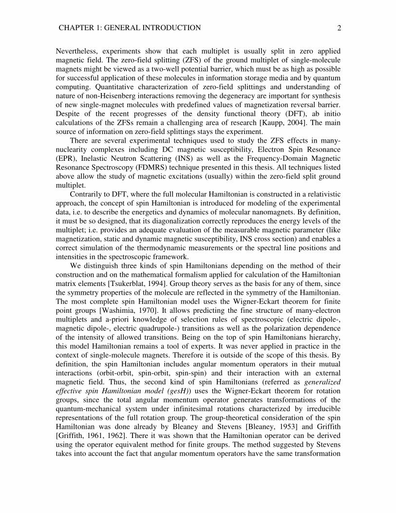
Nevertheless, experiments show that each multiplet is usually split in zero applied magnetic field. The zero-field splitting (ZFS) of the ground multiplet of single-molecule magnets might be viewed as a two-well potential barrier, which must be as high as possible for successful application of these molecules in information storage media and by quantum computing. Quantitative characterization of zero-field splittings and understanding of nature of non-Heisenberg interactions removing the degeneracy are important for synthesis of new single-magnet molecules with predefined values of magnetization reversal barrier. Despite of the recent progresses of the density functional theory (DFT), ab initio calculations of the ZFSs remain a challenging area of research [Kaupp, 2004]. The main source of information on zero-field splittings stays the experiment.
There are several experimental techniques used to study the ZFS effects in many-nuclearity complexes including DC magnetic susceptibility, Electron Spin Resonance (EPR), Inelastic Neutron Scattering (INS) as well as the Frequency-Domain Magnetic Resonance Spectroscopy (FDMRS) technique presented in this thesis. All techniques listed above allow the study of magnetic excitations (usually) within the zero-field split ground multiplet.
Contrarily to DFT, where the full molecular Hamiltonian is constructed in a relativistic approach, the concept of spin Hamiltonian is introduced for modeling of the experimental data, i.e. to describe the energetics and dynamics of molecular nanomagnets. By definition, it must be so designed, that its diagonalization correctly reproduces the energy levels of the multiplet; i.e. provides an adequate evaluation of the measurable magnetic parameter (like magnetization, static and dynamic magnetic susceptibility, INS cross section) and enables a correct simulation of the thermodynamic measurements or the spectral line positions and intensities in the spectroscopic framework.
We distinguish three kinds of spin Hamiltonians depending on the method of their construction and on the mathematical formalism applied for calculation of the Hamiltonian matrix elements [Tsukerblat, 1994]. Group theory serves as the basis for any of them, since the symmetry properties of the molecule are reflected in the symmetry of the Hamiltonian. The most complete spin Hamiltonian model uses the Wigner-Eckart theorem for finite point groups [Washimia, 1970]. It allows predicting the fine structure of many-electron multiplets and a-priori knowledge of selection rules of spectroscopic (electric dipole-, magnetic dipole-, electric quadrupole-) transitions as well as the polarization dependence of the intensity of allowed transitions. Being on the top of spin Hamiltonians hierarchy, this model Hamiltonian remains a tool of experts. It was never applied in practice in the context of single-molecule magnets. Therefore it is outside of the scope of this thesis. By definition, the spin Hamiltonian includes angular momentum operators in their mutual interactions (orbit-orbit, spin-orbit, spin-spin) and their interaction with an external magnetic field. Thus, the second kind of spin Hamiltonians (referred as generalized
effective spin Hamiltonian model (gesH)) uses the Wigner-Eckart theorem for rotation groups, since the total angular momentum operator generates transformations of the quantum-mechanical system under infinitesimal rotations characterized by irreducible representations of the full rotation group. The group-theoretical consideration of the spin Hamiltonian was done already by Bleaney and Stevens [Bleaney, 1953] and Griffith [Griffith, 1961, 1962]. There it was shown that the Hamiltonian operator can be derived using the operator equivalent method for finite groups. The method suggested by Stevens takes into account the fact that angular momentum operators have the same transformation

CHAPTER 1: GENERAL INTRODUCTION 3
properties as the corresponding spherical harmonics required in the expansion of the potential due to a crystal electric field of the appropriate symmetry [Abragam, 1970], [Sugano, 1970]. This method allowed the determination of the quantum mechanical equivalent of a given spherical harmonic as an explicit function of the total angular momentum operator J within a selected J-manifold, i.e. the so called Stevens operators tabulated e.g. in [Abragam, 1970]. Thus, the third kind of the spin Hamiltonians is represented by the effective spin Hamiltonian expressed through the Stevens operators introduced for each of the spin multiplets. Selection of the appropriate spin Hamiltonian for modelling of experimental data depends on the specific features of the energy spectrum of the system under study. Thus, if the isotropic Heisenberg exchange dominates, the strong exchange limit is valid. In this case the spin multiplets are grouped into well separated blocks so that the interaction of ground multiplet with the excited ones can be neglected in the first approximation. It is a typical situation for majority of the reported single-molecule magnets [Sessoli, 2003], where the excited spin states are usually experimentally inaccessible at low temperatures and therefore can be disregarded. This fact opens the way for spectroscopic simulations by using only the effective spin Hamiltonian of the ground multiplet referred to the single-spin or giant-spin Hamiltonian model [Waldmann, 2005]. It coincides with zero-field splittings expressed in terms of the Stevens operators in absence of an external magnetic field.
Any spin Hamiltonian can be factorized into two parts. The first part depends on the symmetry only; the second one originates from the practical physical behavior of the system. It is treated as an adjustable (semiempirical) parameter that can be extracted from experiment. Thus, a set of the zero-field splitting (ZFS) parameters will be obtained by application of the single-spin Hamiltonian model to the experimental data analysis on molecular nanomagnets. They give a fingerprint (i.e. a relative location) of energy levels constituting the ground multiplet. The generalized effective spin Hamiltonian model is used in order to analyze the nature of physical mechanisms responsible for formation of the cluster magnetic anisotropy. It includes parameters of isotropic exchange and of non-Heisenberg interactions. Their magnitude points to the role and specific behavior of the corresponding type of intracluster interaction. The obtained information is of principal importance for synthesis of new molecules with predefined properties. Thus, the single-spin and generalized effective spin Hamiltonian models are complementary tools by analysis of energetics of one and the same molecular magnet. The first enables a soon (due to its simplicity) answer to the question: “how is the energy spectrum of the molecule organized?”, the second one is dealing mainly with the problem: “why does the energy spectrum have the structure detected experimentally?”.
This PhD-thesis has two important results. We present the computer code developed for simulation of Frequency Domain Magnetic Resonance Spectra (FDMRS) on molecular nanomagnets in terms of the single-spin Hamiltonian model. The program enables an automatic and high precision determination of the zero-field splitting parameters of mono- and many-nuclear complexes with high spin ground state. It was successfully applied to the ZFS studies by FDMRS on various molecular magnets.
Another result of this work is the new development of the generalized effective spin Hamiltonian model. Interactions of non-Heisenberg type (single-ion crystal fields and antisymmetric exchange) were introduced into the model for the first time being expressed through non-collinear tensors. The model gives reasonable results by explanation of the

CHAPTER 1: GENERAL INTRODUCTION 4
origin of magnetic anisotropy of a tetrameric Ni(II) cluster possessing S4 symmetry. It indicates the pronounced role of the non-compensated orbital moment in the system accompanied by collective action of the single-ion crystal fields.
Thus, this PhD-thesis is about methods of modeling- and analysis of experimental data on molecular nanomagnets.

II
Single Molecule Magnets (SMMs)
Single-molecule magnets (SMMs) represent a special class of the magnetic nanoclusters. They show some physical effects that are not usual for conventional magnetic materials: single molecule hysteresis and quantum tunneling of magnetization. Whether or not these quantum effects will be observed depends on the coupling scheme for a given cluster and on how the resulting spin state can be influenced by external magnetic field. In this chapter we review the main properties of SMMs and show why they attract the interest of the scientific community.
2.1 Prerequisites for SMM behaviour Molecular nanomagnets are molecules consisting of metal ions of the same or different
valence linked by organic ligands (Figure 2.1a). The spin ground state of each metal ion constituting the molecule is deduced from the analysis of its electron configuration in the surrounding ligand field of certain symmetry (Figure 2.1b). The single-ion spins are so strongly bound together by exchange interactions that the magnetic molecule can be
considered as the unity (cluster) possessing a single macrospin. The energy spectrum of magnetic nanoclusters originates from competing exchange interactions in a many-spin system. It consists of more than one multiplet with definite total spin values (S, S-1,…) as it is shown in Figure 2.1c. The total spin value of each multiplet is derived from the coupling of the single ion spins according to the rule of addition of angular momenta.
S
S-1
…
S1+ S2=S12
S3+ S4=S34
S12+ S34=S12-34
S5+S12-34=S
d2n
d2n
d1n
d1n
S4
S5
S1
S2
S3
(a) (b) (c) (d)
Figure 2.1 Molecular magnets are molecules consisting of a finite number of metal ions with the same or different valence (e.g. d1
n and d2n) linked usually by organic ligands depicted here as dotted areas (a). The
spin ground state of each ion Si (i=1,…,5) is deduced from the analysis of its electron configuration in the surrounding ligand field of certain symmetry (b). Due to exchange interactions between these ions the energy spectrum of the molecule consists of many multiplets with the definite total spin values S, S-1 etc (c). The allowed total spin value of each multiplet is derived by coupling of the single ion spins according to the rule of addition of angular momenta (d).
d1n

CHAPTER 2: SINGLE MOLECULE MAGNETS 6
Each multiplet consists of the states SMS;α , where MS=-S,…,+S are the allowed spin
projections for the total spin value S and α indicates additional quantum numbers arising from intermediate spins. Figure 2.1d presents one of the possible coupling schemes valid for a pentanuclear cluster with α=S12,S34,S12-34 that was chosen here exclusively as an example. As already mentioned in the introduction, high ground-state spin values ( 1≥S )
are typical for molecular nanomagnets. In addition, the strong exchange approximation is successfully applied to describe their energetics. There it assumed that isotropic (Heisenberg) exchange interactions between spin centres dominate over interactions of non-Heisenberg type. For that reason the complete spectrum contains well separated manifolds. Each magnetic molecule behaves like a single spin, since only the ground-state multiplet is relevant at low temperatures. Finally, the intramolecular interactions are usually much stronger than interactions between molecules. The whole system in solid state can be imagined as an array of weakly interacting spin clusters.
The high negative anisotropy values of uniaxial type are a prerequisite for single-
molecule magnet behavior of a spin cluster. That means that the resulting magnetic moment of the cluster maintains its spatial orientation and cannot be easily rotated due to thermal fluctuations. Magnetic anisotropy reflects in general the energy difference for different possible orientations of the spin with respect to the crystallographic axes of molecule. In the special case of uniaxial anisotropy, the energy depends only on the angle with a certain axis, irrespective of the directions of other two. This selected axis is usually called the unique axis of the molecule. For negative (positive) axial zero-field splitting parameter (see Chapter 4.2) it is called the easy (hard) axis. The plane perpendicular to the easy (hard) axis is denoted as the hard (easy) plane in presence of uniaxial anisotropy. It is convenient to choose the molecular coordinate system so, that the cluster z-axis coincides with the easy axis. In this case the angle of the magnetic moment with the easy axis is characterized by the spin projections MS on the quantization axis of the molecule. Thus,
Ea=|DS|S2
π/2 π 0
Single domain particle with uniaxial anisotropy
Magnetization angle θ (a)
-MS +MS
E
n
e
r
g
y
Ea
θ
Magnetization
Spin projection to the quantization axis (b)
Figure 2.2 Energy spectrum of a single-domain particle with uniaxial anisotropy depends only on the angle of the magnetic moment with the easy axis, i.e. the magnetization angle (Fig. 2a). The angle dependence is equivalent to the energies of the spin projections MS allowed for the total spin value S of the ground spin multiplet (Fig.2b). The zero-field split ground manifold of the magnetic cluster might be viewed as a double well potential energy curve. The height of the anisotropy barrier between the MS=±S states is given by Ea=|D|S2
SMS;α SMS −;α
1; −SMSα 1; +− SMSα

CHAPTER 2: SINGLE MOLECULE MAGNETS 7
the angle dependence of the energy spectrum becomes equivalent to the dependence on the allowed spin projections. The zero-field split ground multiplet of the spin cluster with the single-magnet behavior might be viewed as a double well potential energy curve, (Figure 2.2). In fact, the high total spin value S of the ground multiplet gives rise to the manifold consisting of 2S+1 levels. The levels with MS=±S are lowest in energy due to uniaxial anisotropy characterized by the negative axial zero field splitting parameter DS (s. also Section 4.2). The activation energy of the anisotropic barrier between the spin states of opposite orientations is the direct function of the DS and the ground state spin value S. Thus, the combination of the high ground-state spin and the negative uniaxial anisotropy produces the energy spectrum characteristic for the tunneling system.
A well known example of single-molecule magnets is the
Mn12Ac=[Mn12O12(O2CCH3)16(H2O)]·4H2O·2HO2CCH3 molecule shown in the Figure 2.3 [Sessoli, 2003]. It consists of two spin sublattices originating from the groups of eight Mn(III)- and four Mn(IV) ions which have the spin ground terms with S=2 and S=3/2, respectively. They are bound together ferrimagnetically through oxygen bridges via the superexchange leading to the formation of the cluster with ground state spin value S=10 possessing S4 symmetry with the S4 axis chosen as the quantization axis. We illustrate the properties of single-molecule magnets in this chapter using the example of Mn12Ac.
2.2 Magnetization Quantum Tunneling The reason why single-molecule magnets have received so much attention recently is
that they show some physical effects that are not usual for conventional magnetic materials: hysteresis of a purely molecular origin and quantum tunneling of magnetization. In many ways single-molecule magnets behave like classical magnets in that they exhibit
44 MMnn44++
ss==33//22 88 MMnn
33++ ss==22
ooxxyyggeenn
hhyyddrrooggeenn
ccaarrbboonn
Figure 2.3 The molecular structure (top) and the cluster (bottom) of Mn12Ac. Twelve Mn-ions with different valence (eight Mn(III) and four Mn(IV)) are coupled by oxygen bridges via the superexchange interactions leading to formation of the ground multiplet with the total spin value S=10

CHAPTER 2: SINGLE MOLECULE MAGNETS 8
magnetic hysteresis at low temperature. At the same time these hysteresis loops show evidence of quantum tunneling in the form of steps at regular intervals of magnetic field, (Figure 2.4). Whether or not quantum mechanical tunneling will be observed, depends on
the properties of the states SMS;α constituting the ground multiplet of the cluster. Thus,
the wave functions are strictly localized in the left ( SMS;α , where MS is negative) or in
the right ( SMS;α , where MS is positive) well of the barrier for the systems with axial
crystal field. Some perturbation (e.g. a transverse crystal field and/or an external magnetic field) can destroy the stable/localized states and create admixed combinations. In other words, the perturbed wave function contains contributions of many unperturbed states
SMS;α of approximately the same magnitude. Under certain conditions the resulting
wave functions become symmetric/antisymmetric superposition of the stable states
( ( )SS MSMS +±− ;;2
1αα , with MS>0). They will be distributed between two wells
with equal probabilities and resonant tunneling can take place. The single-molecule magnets exhibit only two stable states of magnetization, which
can represent digital bits. Each cluster behaves like a qubit. The switching of the states can be produced by application of the external magnetic field that induces the resonant spin tunneling. Spin clusters with single-molecule magnet behavior are magnetically bistable and therefore of high technological interest for implementation of quantum computational operations [Leuenberger, 2003 and references therein]. In addition single-molecule magnets are systems where permanent magnetization and magnetic hysteresis can be achieved not through a three-dimensional magnetic ordering, but as a purely one-molecule phenomenon. The strong magnetic coupling inside of the cluster and the high magnetic uniaxial anisotropy are responsible for the fact that the resulting spin of the cluster cannot be easily rotated due to thermal fluctuations. Therefore SMMs are very promising for application in magnetic storage devices. If one molecule can store one bit of information,
No tunneling
H
M
Tunneling
Figure 2.4 Molecular magnets exhibit magnetic hysteresis at low temperature (right: hysteresis loops of a monocrystalline grain of Mn12Ac measured in longitudinal field at different temperatures, from [Barbara, 2001]) At the same time these hysteresis loops show evidence of quantum tunneling in the form of steps at regular intervals of magnetic field (left).

CHAPTER 2: SINGLE MOLECULE MAGNETS 9
then a much higher information storage density can be achieved in comparison to the present-day storage media with microdomains [Blügel, 2005 and references therein].
Studies on single-molecule magnets are also interesting from a fundamental scientific point of view. They provide a better understanding of phenomena occurring on the mesoscopic scale: at the boundary between classical and quantum physics [Wernsdorfer, 2001]. At macroscopic sizes, a magnetic system is described by magnetic domains that are separated by domain walls. Here magnetization reversal occurs via nucleation, propagation and annihilation of domain walls. For system sizes well below the domain wall width, one must take into account explicitly the magnetic moments (spins) and their coupling. SMMs are the systems, which size is of the order of magnitude of the domain wall width, where the magnetization remains in a so called single-domain state. The mesoscopic scale corresponds to the sizes of nanometers; for this reason the prefix “nano” is often used relative to the single-molecule magnets: magnetic nanoclusters or molecular nanomagnets.
Magnetization quantum tunneling in single-molecule magnets is fundamentally different from the particle-like picture of tunneling widespread in nature. There are many physical and chemical systems that can be described by generalized coordinates associated with an effective potential energy function with two separate minima at roughly the same energy [Esquinazi, 1998], [Weiss, 1993]. Some of them are listed below.
• Amorphous materials (and glasses). Here the tunneling systems are the atoms, small groups of atoms or more complicated clusters that have the possibility to “move” between two similar energy states separated by a barrier. Experimental observables like thermal conductivity and specific heat are a convenient source of information about their low temperature anomalies.
• The tunneling of light particles like small polarons, hydrogen isotopes or muons in solids has been also studied since several decades. While earlier work was mainly concerned with the significance of polaron effects, more recent attention has focused on the singular transistient response of the fermionic environment in metals at lower temperatures. Here the particle can tunnel either randomly or coherently between particular interstitial states.
• Electron transfer reactions are ubiquitous in chemical and biological systems. In its simplest form, an electron localized at it donor site is tunneling to the acceptor site.
• Josephson junction systems. The phenomenon of incoherent tunneling of a macroscopic variable has become most clearly visible in superconducting quantum interference devices (SQUIDs), where the phase difference of the Cooper pair wave function across the Josephson junction plays the role of the tunneling coordinate.
For all these systems, tunneling follows in straightforward manner from basic laws of quantum mechanics: these systems have a particle-like Hamiltonian and the tunneling is
driven by the kinetic energy term of the Hamiltonian [Friedman, 2003]: M
p
2
2
=Η . The
position of the center of mass of a particle or the flux in SQUID can be chosen as the generalized coordinates in the particle-like system. The only way to “turn off” the tunneling in these systems is to make their mass as large as possible. But, doing so, the density of levels becomes quasicontinuous and the system becomes classical.

CHAPTER 2: SINGLE MOLECULE MAGNETS 10
In molecular magnets the tunneling occurs in angular space, where the magnetization vector rotates from one potential minimum to another: the generalized coordinate is the angle of the magnetic moment with the quantization axis as it is shown in Figure 2.2. Spin systems have no explicit kinetic degrees of freedom. The simplest Hamiltonian for a spin system with uniaxial anisotropy takes the form: '2 HHSgDS ZZBZ +−−=Η µ . Here the first term describes an axial anisotropy of the system; the second term is the Zeeman coupling between the spin and a magnetic field. 'H contains all terms that do not
commute with ZS . Unlike in the “particle” case, it is possible for a spin to retain quantum
properties (having well separated energy levels) and have 0'→H . In this limit, ZS is a
conserved quantity and no transitions between eigenstates of ZS are allowed. Tunneling can be “turned off” without the spin system becoming classical. The driving force behind the tunneling in spin systems is associated with the term 'H , which can include an external magnetic field or transverse anisotropy or something else. Because different mechanisms have different symmetries, it is possible to determine the dominant tunneling mechanisms by looking for tunneling selection rules associated with the symmetry.
Tunneling is greatly modified by coupling to the environment. If we consider a system, which is completely isolated from environment, then the tunneling does not need additional energy, because it occurs between levels of the same energy. The coupling with the environment leads to the loss of energy by tunneling. The interactions with the environment will tend to localize the spin; it makes one well more attractive as another. In other words, the spin motion between the two wells will be not equally damped. Thus, environmental effects may suppress the tunneling. Therefore the studies of relaxation processes in molecular magnets are the focus of intensive research (s. e.g. [Garanin, 1997], [Leuenberger, 2000-1], [Leuenberger, 2003], [Prokof’ev, 1998], [Prokof’ev, 2000], [Pohjola, 2000]). Notably, molecular magnets can relax via a hybrid process that mixes quantum tunneling with thermal relaxation. This is a surprising result, since many of original theoretical works on tunneling in macroscopic systems predicted, that as temperature is raised, there should be a crossover between pure quantum relaxation and pure thermal (over barrier) relaxation. There are several regimes of magnetization quantum tunneling in single-molecule magnets. They are listed below and illustrated in Figure 2.5.
• Thermally activated tunneling is possible on upper paths. For the excited levels the barrier is transparent: tunneling is so fast that it short-circuits the top of the barrier. Thus, thermally activated tunneling is equivalent to the effective reduction of the barrier. This kind of tunneling is sometimes referred to as the phonon-assisted mechanism, because the phonons may be absorbed to populate the higher states involved in the tunneling process.
• Thermally assisted tunneling happens between the intermediate paths. This mechanism is treated in the theoretical articles, where the spin levels are considered as continuous spectrum.
• Resonant quantum tunneling is transition from one metastable minimum to another side of the barrier followed by the relaxation to the ground state that is accompanied with phonon emission.
CHAPTER 2: SINGLE MOLECULE MAGNETS 11
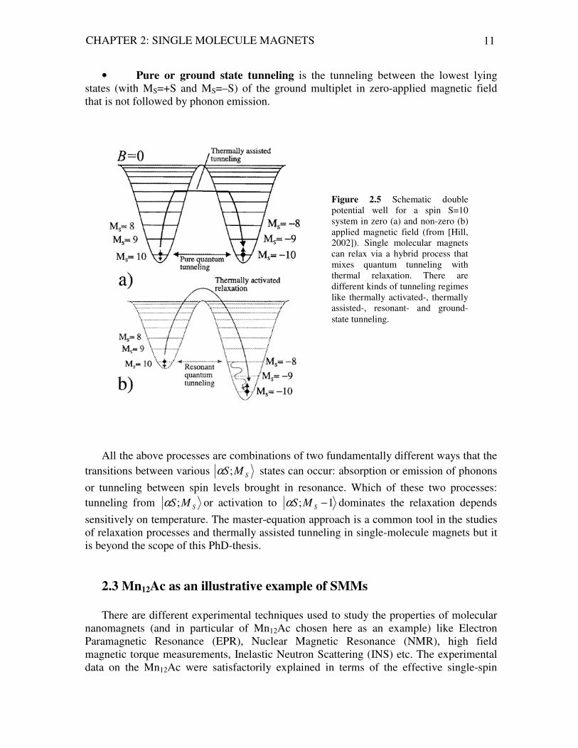
• Pure or ground state tunneling is the tunneling between the lowest lying states (with MS=+S and MS=–S) of the ground multiplet in zero-applied magnetic field that is not followed by phonon emission.
All the above processes are combinations of two fundamentally different ways that the
transitions between various SMS;α states can occur: absorption or emission of phonons
or tunneling between spin levels brought in resonance. Which of these two processes: tunneling from SMS;α or activation to 1; −SMSα dominates the relaxation depends
sensitively on temperature. The master-equation approach is a common tool in the studies of relaxation processes and thermally assisted tunneling in single-molecule magnets but it is beyond the scope of this PhD-thesis.
2.3 Mn12Ac as an illustrative example of SMMs There are different experimental techniques used to study the properties of molecular
nanomagnets (and in particular of Mn12Ac chosen here as an example) like Electron Paramagnetic Resonance (EPR), Nuclear Magnetic Resonance (NMR), high field magnetic torque measurements, Inelastic Neutron Scattering (INS) etc. The experimental data on the Mn12Ac were satisfactorily explained in terms of the effective single-spin
Figure 2.5 Schematic double potential well for a spin S=10 system in zero (a) and non-zero (b) applied magnetic field (from [Hill, 2002]). Single molecular magnets can relax via a hybrid process that mixes quantum tunneling with thermal relaxation. There are different kinds of tunneling regimes like thermally activated-, thermally assisted-, resonant- and ground-state tunneling.

CHAPTER 2: SINGLE MOLECULE MAGNETS 12
Hamiltonian typical for the S4 symmetry, which includes the Stevens operators with k=0 and k=4 (for details see Chapter 4). These operators are shown below.
2222404 )1(3)1(625)1(3035 +++−++−= SSSSSSSSSO zzz
)(21 444
4 −+ += SSO ,
here S is the total spin value of the ground multiplet ( 10=S for the Mn12Ac molecule), zS is the z-component of the spin operator, +S and −S are raising and lowering operators (for details see Chapter 3).
Finally, the following single-spin Hamiltonian was defined to describe the experimental observables on Mn12Ac molecule:
( ) )(13
ˆ 44
44
04
04
2BSgOBOBS
SSD Bz
rr⋅−++
+−=Η µ (2.3-1)
where D is the axial ZFS parameter, 04B and 4
4B are the single-spin Hamiltonian parameters of the 4th order (see Chapter 4). The last term of Eq. (2.3-1) indicates the
Zeeman interaction of the cluster spin Sr
and the external static magnetic field Br
. The first three terms of Eq. (2.3-1) completely characterize the zero-field split ground multiplet, i.e. the first two terms represent the axial cluster anisotropy; the third one reflects the fourth order transverse magnetic anisotropy. The zero-field splitting parameters extracted from various experiments are summarized in Table 2.1.
They provide understanding of the steps in hysteresis loops (see Figure 2.4) at regular intervals of the magnetic field (~0.45 T) as the result of magnetization quantum tunneling. Thus, Figure 2.6a shows the energy spectrum of the ground multiplet (S=10) calculated as the function of the spin-projection in zero-applied magnetic field for the ZFS-parameters listed in the Table 2.1.
Table 2.1: ZFS parameters for Mn12Ac in cm-1
D B40 B4
4 Experimental technique Ref.
-0.46(2) -2.2(2)*10-5 ±4(1)*10-5 High-frequency EPR [Barra, 1997] -0.457(2) -2.33(4)*10-5 ±3.0(5)*10-5 INS [Mirebeau,
1999] -0.47 -1.5*10-5 -8.7*10-5 Multifrequency EPR
on single crystals [Hill, 1998]

CHAPTER 2: SINGLE MOLECULE MAGNETS 13
The axial part of the Hamiltonian (Formula 2.3-1)
( ) 04
04
2 13
ˆ OBSS
SD z
axial +
+−=Η gives rise to the doubly-degenerate energy levels
021 =−=∆ EE , where ( )SMSEE += ;1 α and ( )SMSEE −= ;2 α with the wave functions
strictly localized in the left and right wells of the barrier: SMS −= ;1 αψ , SMS += ;2 αψ ,
0>SM . The transverse term 44
44
ˆ OBtransverse =Η acting in addition to the axial one removes
the degeneracy 021 ≠−=∆ EE1. The eigenstates become symmetric and antisymmetric
combinations of the initial states: ( )SS MSMS −++= ;;2
11 ααψ
and ( )SS MSMS −−+= ;;2
12 ααψ , 0>SM . The condition for occurence of
magnetization quantum tunneling is fulfilled in zero external magnetic field. Inclusion of Zeeman term changes the eigensystem of the single-spin Hamiltonian Eq. (2.3-1) completely. The tunneling conditions can be lost and created again for definite values and orientations of the applied magnetic field. The space orientation of the external magnetic field is characterized by the spherical coordinates, i.e angles θ and φ with the easy axis of the molecule. Application of a longitudinal magnetic field (θ=0, φ=0) brings the system out of the resonance, since it shifts the left-well levels up and the right-well ones down (see Figure 2.6b). The tunneling conditions will be restored at the resonance values of the
longitudinal magnetic field B
kg
DkB
µ= ( ...2,1,0 ±±=k is the number of the resonance),
which puts pairs of levels in coincidence (+Ms and +MS-k).
1 1114 10...10~ −−∆ cm-1 for the lowest lying states, i.e. with large MS
MS
B=0
energy
MS
B~0.45 T, θ=0, φ=0
energy
MS -MS-k
Figure 2.6 The energy spectrum of the ground spin multiplet of Mn12Ac is shown for zero (a) and the 1st resonance longitudinal magnetic field (b). The calculations were performed by using the single-spin Hamiltonian Eq. (2.3-1) and the zero-field splitting parameters listed in the Table 2.1. k is the number of the resonance.
(a) (b)
[cm-1] [cm-1]

CHAPTER 2: SINGLE MOLECULE MAGNETS 14
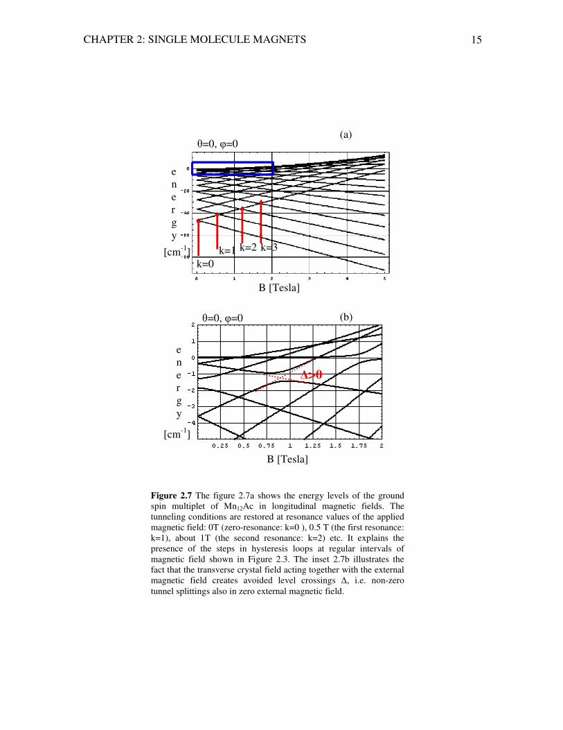
The Figure 2.7 illustrates the behaviour of the ground multiplet (S=10) of Mn12Ac in the external fields applied along the easy axis of the molecule. The inset shows the avoided level crossing denoted in literature as the tunnel splitting. The tunneling probability between the levels brought in resonance depends directly on the tunnel splitting, as follows from the Landau-Zener-Stückelberg theory (for details see [Sessoli, 2003] and references therein). There the expression for the tunnel probability is given
by
−
∆−−=
dt
dBMM
constP
S
M
MS
S
'exp1
S
2',M
',MS
S. Here ',MS SM∆ is the tunnel splitting between
the levels ',S SMM , dt
dBis the constant field sweeping frequency. Therefore, if the tunnel
splitting is zero, then 0',MS=
SMP and no tunneling occurs. Non-zero tunnel splittings allow
tunneling.
CHAPTER 2: SINGLE MOLECULE MAGNETS 15
Figure 2.7 The figure 2.7a shows the energy levels of the ground spin multiplet of Mn12Ac in longitudinal magnetic fields. The tunneling conditions are restored at resonance values of the applied magnetic field: 0T (zero-resonance: k=0 ), 0.5 T (the first resonance: k=1), about 1T (the second resonance: k=2) etc. It explains the presence of the steps in hysteresis loops at regular intervals of magnetic field shown in Figure 2.3. The inset 2.7b illustrates the fact that the transverse crystal field acting together with the external magnetic field creates avoided level crossings ∆, i.e. non-zero tunnel splittings also in zero external magnetic field.
B [Tesla]
energy
θ=0, φ=0
k=0 k=1 k=2 k=3
energy
B [Tesla]
θ=0, φ=0
∆>0
[cm-1]
[cm-1]
(a)
(b)

CHAPTER 2: SINGLE MOLECULE MAGNETS 16
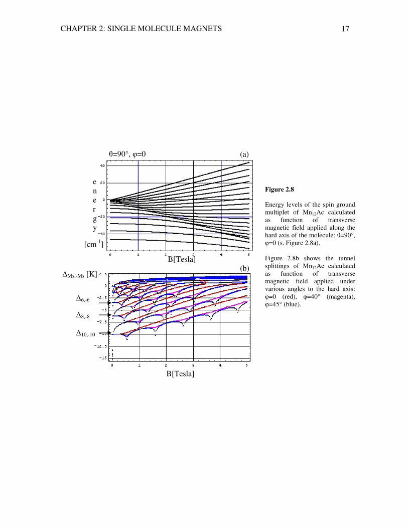
Very interesting effects can be observed experimentally in transverse magnetic fields. It turns out, that the tunnel splitting depends on the Haldane topological (Berry-) phase originating from the quantum interference of possible tunnel paths (around the hard axis) between two potential minima (MS=+S and MS=-S). For detailed explanations we refer the reader to [Tupitsyn, 2002],[Leuenberger, 2000-2],[Sessoli, 2003], [Blügel, 2005], since the path-integral formalism is outside of the scope of this thesis. The topological phase can be changed by an external magnetic field causing oscillations of the tunnel splittings2. The calculations show (Figure 2.8b and Figure 2.9) that the tunnel splitting has a non-zero value in absence of the external magnetic field (B=0 T) only for the pairs of levels with even Ms, i.e. Ms=10,8,6 etc. The tunnel splittings of the levels with odd Ms are zero in zero-applied magnetic field. This result illustrates a spin parity effect, which forbids the spin tunneling between pairs of odd levels in zero-field. In terms of the coherent spin-state path integral model [Leuenberger, 2000-2] these oscillations and their associated spin-parity effects can be elucidated as a result of interfering Berry phases, produced by spin-tunneling paths of opposite winding, which are modified by external transverse magnetic field. Thus, suppression of tunnel splittings (∆Ms,-Ms → 0) arises as destructive interference between the paths of opposite winding at definite values of the transverse magnetic field
2 It was even experimentally observed in a system similar to Mn12Ac, namely Fe8 cluster [Sessoli, 2003].
CHAPTER 2: SINGLE MOLECULE MAGNETS 17
θ=90°, φ=0
B[Tesla]
energy
B[Tesla]
∆Ms,-Ms [K]
∆10,-10
∆8,-8
∆6,-6
Figure 2.8 Energy levels of the spin ground multiplet of Mn12Ac calculated as function of transverse magnetic field applied along the hard axis of the molecule: θ=90°, φ=0 (s. Figure 2.8a). Figure 2.8b shows the tunnel splittings of Mn12Ac calculated as function of transverse magnetic field applied under various angles to the hard axis: φ=0 (red), φ=40° (magenta), φ=45° (blue).
[cm-1]
(a)
(b)

CHAPTER 2: SINGLE MOLECULE MAGNETS 18
Due to the fourth order transverse anisotropy (term O44) in the single-spin Hamiltonian
Eq. (2.3-1), the Mn12Ac molecule has one easy axis and two intermediate axes. The easy axis coincides with the quantization axis (z) along S4, the intermediate ones lie in the hard plane (xy) along the φ=±45° direction. Thus, the amplitude of the oscillations becomes smaller and vanishes at φ=0° by application of the transverse magnetic field at various azimuth angles φ (see Figure 2.9).
The properties of single molecular magnets illustrated above on the example of
Mn12Ac give rise to a very rich spectrum of research. Single molecule magnets represent the unique systems to study quantum effects on mesoscopic level. They can also serve as model systems to study exchange interactions. Finally, they are of high interest for possible technological applications in quantum computers and information storage devices. Nevertheless, all these studies have one and the same starting point: the magnetic anisotropy barrier. It must be as high as possible in order to use the SMM complexes in practice at normal temperatures. Therefore, quantitative characterisation of the cluster magnetic anisotropy (in terms of the zero-field splitting parameters) and understanding of its origin are the tasks of importance for the synthesis of new compounds with SMM properties.
2.4 Symmetry and energy spectrum. We present in this PhD-thesis the mathematical formalism and the computer code
developed for the ZFS studies on molecular nanomagnets by Frequency-Domain Magnetic Resonance Spectroscopy (FDMRS) and for those spectral simulations in terms of the single-spin Hamiltonian approach. The final part (Chapter 8) is devoted to investigation of the physical mechanisms responsible for the formation of magnetic anisotropy of a tetrameric Ni(II) cluster. For this aim the generalized effective spin Hamiltonian model was applied and developed, which is usually combined with the Irreducible Tensor Operators (ITOs) technique. The ITO method of calculations provides unique computational advantages, since it allows evaluation of Hamiltonian matrix elements
∆10,-10 [K]
θ=90°
B [Tesla]
φ=0
φ=30° Figure 2.9 Tunnel splittings as function of transverse magnetic field calculated for the lowest levels of the ground multiplet (∆10,-10) of Mn12Ac for different azimuth angles φ.
φ=40°
φ=45°

CHAPTER 2: SINGLE MOLECULE MAGNETS 19
without construction of many-particle wave functions of the system of interacting ions. Thus, all results of this PhD-thesis were obtained by using of the spin Hamiltonian concept.
Like any quantum mechanical operator, the spin Hamiltonian can not be discussed apart of the symmetry considerations. Like any quantum-mechanical system, the spin nanoclusters are described by a certain symmetry group or their combination [Hamermesh, 1989] [Inui, 1990]. As already mentioned, the mechanism of the magnetization quantum tunneling in SMMs is associated with the symmetry, which is reflected in the model spin Hamiltonian. By definition it contains the angular momentum operators in their mutual interactions. From this point of view, the energy spectrum can be characterized by irreducible representations of the full rotation group. Otherwise, complete symmetry of the molecule given by point group predefines special properties of the Hamiltonian under finite rotations. When dealing with exchange interactions in high-nuclearity spin clusters we have to keep in mind the fact that electrons are indistinguishable. Thus, the corresponding Hamiltonian must be invariant to any permutation (exchange) of the electron coordinates and therefore it must incorporate the properties of symmetric group. Various magnetic systems may have different physical properties, since they are described by different combinations of symmetry groups. Thereby the group representation theory is applied to classify the energy levels (both the calculated and spectroscopically determined), their degeneracy and how they will be changed when symmetry is reduced.
In order to clarify the last paragraph we recall the classification of symmetry groups
given in [Inui, 1990]. First of all let us consider a particle-like Hamiltonian ( )rVm
p+=Η
2ˆ
2
,
of a particle with mass m in a spherically symmetric potential ( )rV . If this Hamiltonian is invariant with respect to all rotations about the origin, then the set of such rotations is called the rotation group. The quantum mechanical equivalent of the momentum operator is expressed through the total angular momentum operator, which generates transformations of quantum-mechanical system under infinitesimal rotations. Therefore the rotation group describes wave functions of electrons for a certain configuration (for given values of spin- and orbital angular momentum) in the spherically symmetric Coulomb potential of the crystal field.
The potential experienced by an electron in a molecule has symmetry resulting from the atomic arrangement. The Hamiltonian is then invariant with respect to those symmetry operations that bring the atomic arrangement into coincidence with itself. The set of these operations is called a point group. The point groups are necessary to characterize the electronic states of molecules and molecular vibrations that can be experimentally studied by infrared absorption and Raman scattering.
Electron wave functions (Bloch functions) extended in a perfect crystal should feel a periodic potential. The Hamiltonian is then invariant with respect to all lattice translations, which form a translation (space) group. The space groups provide us understanding of physical nature of electronic states in crystals, lattice vibrations, scattering of an electron by lattice vibrations, interband optical transitions, excitons in molecular crystals.
If the system described by a space group is additionally invariant with respect to time reversal then a nonunitary group describes it. A well known example of a nonunitary group is a magnetic space group. By considering this group, the symmetry of magnons

CHAPTER 2: SINGLE MOLECULE MAGNETS 20
(spin waves) and excitons in magnetic compounds and selection rules for their excitation can be treated in the same way as excitons in molecular crystals. Representation theory of space groups plays also an essential role in the Landau’s theory of phase transitions.
If we consider a system of n electrons then we have to deal with the symmetric group. Since n electrons are identical particles, the Hamiltonian is invariant to any permutation of the n electron coordinates. The set of these permutations is called the symmetric group. The theory of the symmetric groups is important in understanding the wave functions of many-electron atoms with a definite magnitude of the spin. The spin permutational symmetry is used to classify the exchange coupled multiplets in molecular nanoclusters.
Molecular nanomagnets have no long–range magnetic ordering. For that reason the translation (space) groups are completely excluded from our considerations. Energy spectrum and the corresponding spin Hamiltonian of any many-nuclearity cluster are characterized by rotation-, point- and symmetric groups.
2.5 Outline of the PhD-thesis This thesis consists of two parts. The aim of the first one (Chapters 3-5) is to prepare
the reader for understanding the results of this works summarized in the second part (Chapters 6-8). Our goal is to present various methods of analysis and interpretation of spectroscopic data on molecular nanomagnets. An important result of this work is the developed computer code for simulation of Frequency-Domain-Magnetic Resonance Spectra (FDMRS), i.e. resonance absorption of microwave radiation by spin angular momenta of ions constituting the molecular magnet. Therefore the main results of the quantum theory of angular momenta will be reviewed in the Chapter 3. There we make a brief overview of the formal rules for manipulating the angular momentum operators, because they form the kernel of the effective spin Hamiltonian model. These rules were explicitly integrated into the program for FDMRS spectral simulations. We describe also the various ways of combining two (or more than two) angular momentum eigenstates to form a product state that is also an angular momentum eigenstate. We introduce the Clebsch-Gordan coefficients, 3j-, 6j- and 9j symbols. Finally we present the concept of Irreducible Tensor Operators (ITOs) and the Wigner-Eckart theorem. They will be used for the explanation of magnetic anisotropy of a tetrameric Ni(II) cluster.
The spin Hamiltonian will be introduced in Section 4.1. There we consider two complementary kinds of spin Hamiltonians. We start from the crystal field potential, since the metal ions constituting molecular magnet can not be considered independent of their ligand surrounding. This ligand environment gives rise to an electric field of certain symmetry that affects the energy spectrum of the cluster. The spectral terms of the complex will be spit, shifted and admixed in a manner that depends on the symmetry of the crystal field and on the total values of angular momentum for a given manifold. Therefore the main results of the semiempirical crystal field theory will be summarized in Section 4.2, where we obtain the single-spin Hamiltonian model expressed by the equivalent (or Stevens) operators. Main aspects of generalized effective spin Hamiltonian (gesH) model will be considered in the Section 4.3 and applied to practical calculations in the Chapter 8. GesH model is an instrument used for modelling of exchange interactions in molecular magnets. Since the group representation theory enables a-priori selection of

CHAPTER 2: SINGLE MOLECULE MAGNETS 21
the dominant terms of the generalized effective spin Hamiltonian, we recall the important results of the group theory in Chapter 5.
Chapter 6 describes the logic, the mathematical formalism and the data flow of the developed program for FDMRS spectral simulations and determination of zero-field splitting parameters by using the single-spin Hamiltonian approach.
Chapter 7 contains the results of application of this program by ZFS-studies on several molecular nanomagnets: the one-electron reduced Mn12: (PPh4)[Mn12O12(O2CEt)16(H2O)4], the Mn9-molecule: [Mn9O7(OAc)11(thme)(py)3(H2O)2], the molecule [Ni-(HIM2-py)2NO3]NO3, which is a possible building block of single-molecule magnets and the tetrameric Ni4 = [Ni4(MeOH)4L4] cluster that does not show the SMM-behavior in spite of the high ground-state spin value and the negative axial magnetic anisotropy.
In Chapter 8 we try to analyze the physical origin of the cluster magnetic anisotropy in terms of the generalized effective spin Hamiltonian approach. The gesH model was applied for the first time to describe the collective action of the single-ion crystal fields and Dzyaloshinskii-Moriya (antisymmetric exchange) interactions expressed in terms of non-collinear tensors.
The discussion of our results is given in the conclusion.

III
Quantum theory of angular momentum:
main results
Magnetic nanoclusters can be imagined as systems of interacting angular momenta, localized on definite sites of the molecular complex. Therefore the quantum theory of angular momentum is of principal importance for the analysis of spectroscopic data (like FDMRS) on molecular nanomagnets. In this chapter we describe the basic concepts used for the estimation of the zero-field splitting parameters and for the analysis of the physical mechanisms lying behind the cluster magnetic anisotropy.
3.1 Action of a symmetry group of transformations on a quantum mechanical system As already discussed in Section 2.4, the energy spectrum of any quantum-mechanical
system (including magnetic nanoclusters) reflects its symmetry. In other words, the eigensystem of the Hamiltonian must satisfy the rules valid for the symmetry group describing this quantum-mechanical system. Symmetry can be defined as an essence that the situation possesses the possibility of a change that nevertheless leaves some aspect of the situation unchanged [Rosen, 1995]. The action of symmetry operations on quantum systems induces transformation of the quantum mechanical wave function [Heine, 1960], [Tinkham, 1964], [Jones, 1998], [Tsukerblat, 1994]. Usually the concept of “representation” is introduced to explain the transformation of the wave function of a physical system under rotation. Thereby any wave function can be imagined as a vector in a multi-dimensional space. Thus, the representations of the full rotation group characterize the transformation of wave functions under infinitesimal rotations, while the representations of point groups are used to describe the transformation of the eigensystem under finite rotations. Rotation of a whole quantum mechanical system can be achieved experimentally by e.g. the application of a magnetic field. As we have seen in the example of Mn12Ac, an external magnetic field mixes the strictly localized wave functions; this result can be interpreted as a rotation of the initial state in a multi-dimensional vector space.
Generally speaking, after a rotation R the system will have a new wave function ( )rr
'ψ
with ( ) 2|'| rr
ψ concentrated around the rotated axis: ( ) ( )rRrrr 1' −=ψψ . Here the rotation R in
the physical space has induced a transformation in the vector space of quantum mechanical wave function. That means that any wave function in space can be expressed as a linear combination of a standard set of wave functions (called the basis). The number of wave functions needed to form a basis is infinite. However, in essentially every case of physical interest, the transformations induced by a group of symmetry operations such as rotations, operate not on the complete space of all possible wave functions but rather on finite-

CHAPTER 3: QUANTUM THEORY OF ANGULAR MOMENTUM 23
dimensional subspaces, and in these subspaces they constitute a finite-dimensional representation of the group.
Molecular nanomagnets are systems of several interacting metal ions with more than one electron localized on the unfilled electronic shells. In the simplest case of a free ion with one electron (a hydrogen atom) the wave function is called an “atomic orbital”. It can be separated into radial and angular parts ( ) ( ) ( )ϕθψ ,lmnlnlm YrRr =
r, where n =0,1,2… is the
principal quantum number, l =0,1,2,…, 1−n is the orbital quantum number and lllm ++−−= ,...,1, is a magnetic quantum number. The radial part ( )rRnl depends only on
the radius-vector of an electron; the spherical harmonics ( )ϕθ ,lmY reflect the dependence on the angular variables. The transformation of an atomic orbital under rotation R leads to a new wave function. Thus, the transformed wave functions ( )rnlm
r'ψ can be expressed as a
linear superposition of the old wave functions with the same values of n and l but different values of m : ( ) ( ) ( )RDrr l
mm
m
nlmnlm ''
'' ∑=rr
ψψ , here the indices m and 'm are restricted to the
range between l− and l+ . The matrix ( )RDl
mm ' is a square matrix of
dimensions ( )( )1212 ++ ll . Such matrices are called rotation matrices (or Wigner D-matrices for the angular momentum l and rotation R). By considering two successive rotations, they satisfy an important property ( ) ( ) ( )2121 RDRDRRD = and constitute a representation of dimension ( )12 +l of the group of 3-dimensional rotations. The situation becomes more complicated for high-nuclearity clusters, i.e. to the systems of several interacting ions with a few electrons in each open electron shell.
For a general symmetry group of transformations acting on a general quantum mechanical system we have to know how to classify and enumerate the possible representations, how to combine the representations (this is needed for the characterization of the energy spectrum of interacting ions) and how to relate the representations of a subgroup to those of the whole group (it is important in the cases of removing the degeneracy). The explicit expressions for the representations of the rotation group can be constructed from the matrices of angular momentum operator, which describes infinitesimal rotations. Therefore, we give a short summary of the main properties of angular momentum operator (Section 3.2). Then we show how to find the eigenstates of a system of several coupled angular momenta in terms of products of the individual angular momentum eigenstates (Section 3.3). Finally, we discuss how quantum-mechanical operators transform under rotations and how to use these transformation properties for calculation of the operator matrix elements (Section 3.4). The entire Chapter 3 helps the reader to understand the background of modeling the spectroscopic data on molecular nanomagnets.

CHAPTER 3: QUANTUM THEORY OF ANGULAR MOMENTUM 24
3.2 Total, orbital and spin angular momentum operators. 3.2.1 Total angular momentum operator
In quantum mechanics the total angular momentum operator Jr
is defined as an operator, which generates transformations of wave functions and quantum operators under infinitesimal rotations of the coordinate system [Messian, 1965], [Varshalovich, 1988], [Commins, 1996], [Johnson, 2002]. The transformation of an arbitrary wave function Ψ under rotation of the coordinate system with an infinitesimal angle δω around an axis nr
may be written as
Ψ⋅−=Ψ→Ψ )ˆ1(' Jni rr
hδω , (3.2.1-1)
where Jr
is the total angular momentum operator. Many of the important quantum mechanical properties of the angular momentum
operator are consequences of the commutation relations (see any textbook on quantum mechanics) that can be obtained using the definition of the total angular momentum operator and equations for the rotation addition.
Symbolically the commutation relations of the total angular momentum Jr
and its Cartesian components can be written as shown below.
JiJJˆˆˆ rrr
=
× (3.2.1-2)
[ ] liklki JiJJ ˆˆ,ˆ ε= , (3.2.1-3)
[ ] 0ˆ,ˆ 2 =iJJ (i,k,l =x,y,z)
where iklε is the so called Levi-Civita tensor, such that
0=iiiε , (i=x,y,z)
0=== kiiikiiik εεε (i,k =x,y,z)
1=−=−=−=== zyxyxzxzyzxyyzxxyz εεεεεε
The square of the total angular momentum may be expressed in terms of Cartesian components as shown below
222
,,
22 ˆˆˆˆˆzyx
zyxi
i JJJJJ ++== ∑=
.
The raising and lowering operators yx JiJJ ˆˆˆ ±=± also commute with the angular
momentum squared: [ ] 0ˆ,ˆ 2 =±JJ . Moreover ±J satisfy the following commutation
relations with ZJ : [ ] ±± ±= JJJ Zˆˆ,ˆ .
The properties of the operators 2J , zJ , ±J are of practical importance for e.g. the
application of quantum theory of angular momentum to the analysis of the magnetic resonance phenomena and many other subjects. Their eigenstates and the eigenvalues are given by:

CHAPTER 3: QUANTUM THEORY OF ANGULAR MOMENTUM 25
>+>= mjjjmjJ ,|)1(,|2)
, (3.2.1-3)
>>= mjmmjJ z ,|,|ˆ ,
>++−+>=+ 1,|)1()1(,|ˆ mjmmjjmjJ ,
>−−−+>=− 1,|)1()1(,|ˆ mjmmjjmjJ . In the most general case of a system consisting of N entities with angular
momenta )(ˆ)...,2(ˆ),1(ˆNjjj
rrr, the total angular momentum is defined as a vector sum:
∑=
=N
n
njJ1
)(ˆˆ rr. At the same time the total angular momentum operator is the sum of the
orbital angular momentum operator Lr
and the spin angular momentum operator Sr
:
SLJˆˆˆ rrr
+= . 3.2.2 Orbital angular momentum operator Classically, the angular momentum of a particle is the vector product of its position
vector rr
and its momentum vector pr
: prLrrr
×= . The quantum mechanical orbital angular momentum operator is defined in the same way with p
r replaced by the momentum
operator ∇−→ ipr
. Therefore the orbital angular momentum operator is expressed in the
coordinate representation as follows: [ ]∇×−= riLrr
.
The orbital angular momentum operator Lr
satisfies the same commutation relations as the total angular momentum operator (for details see e.g. [Messian, 1965]). It generates transformations of scalar (spinless) wave functions under rotations of the coordinate system. A rotation with an infinitesimal angle δω around the axis n
r transforms the
position vector rr
into rrrr
δ+ , with [ ]rnrrrr
×−= δωδ . The corresponding transformation of the scalar wave function is written as:
)()ˆ1()()1()()( rLni
rrrrrrrr
h
rrrrrΨ⋅−=Ψ∇⋅+=+Ψ→Ψ δωδδ .
Finally, we mention that the eigenfunctions of the operators 2Lr
and ZL are spherical
harmonics ),( ϕϑlmY , which depend on the polar angles ϕϑ, . We refer the reader to [Varshalovich, 1988] for a detailed review of properties of the orbital momentum operator.
3.2.3 Spin angular momentum operator
The spin angular momentum operator Sr
is usually represented by a set of three (since
the vector Sr
has three components: zyx SSS ˆ,ˆ,ˆ ) square (2S+1)(2S+1) matrices, where S is
the total spin value of the system. These matrices act on the spin functions and satisfy the same commutation relations as the components of total angular momentum. The spin functions )(σχ may be treated as functions of the discrete variableσ , which is the spin

CHAPTER 3: QUANTUM THEORY OF ANGULAR MOMENTUM 26
projection on the z-axis. The quantity 2|)(| σχ gives the probability that the spin projection
on the z-axis in a given state is equal σ . The interpretation of 2|)(| σχ as the probability for the spin projection on the z-axis to be equal to σ is possible only if )(σχ satisfies the
normalization condition: 1|)(| 2 =∑−=
S
Sσ
σχ . The variable σ takes 2S+1 values,
SSS ++−−= ,...,1,σ . Therefore the spin functions are written as column matrices that contain 2S+1 elements:
−
−=
)(
...
)1(
)(
S
S
S
χ
χ
χ
χ
In addition, the concept of the basis spin functions is introduced. By definition, the basis spin functions describe the states with definite spin and spin projection on the z-axis.
The basis spin functions are eigenfunctions of operators 2Sr
and ZS given by equations:
SmSm SSS χχ )1(ˆ 2 +=r
and SmSSmZ mS χχ =ˆ ; their dependence on the spin variable is
expressed by Kronecker delta: σδσχ mSm =)( . Thus, the basis spin functions can be written as column matrices of 2S+1 elements
=
0
...
0
1
SSχ ,
=−
0
...
1
0
1SSχ , …,
=−
1
...
0
0
SSχ
The collection of 2S+1 basis functions Smχ (m=S,S-1,…,-S) forms a complete orthonormal set of functions. It makes it possible to expand a spin function of a system
with the total spin S in sum of the basis spin functions Smχ : ( ) ∑−=
=S
Sm
SmmaS χχ , where
ma are expansion coefficients.
Finally, the Cartesian components of the spin operator iS (i=x,y,z) have only a finite number of non-zero matrix elements expressed as follows:
)1)((21ˆ
1 +±=+± mSmSS SmxSm mχχ , (3.2.3-1)
)1)((2
ˆ1 +±=+
± mSmSi
S SmySm mmχχ ,
mS SmzSm =+± χχ ˆ
1 .
CHAPTER 3: QUANTUM THEORY OF ANGULAR MOMENTUM 27
3.3 Coupled Systems. Addition of angular momenta. Clebsch-Gordan coefficients, 3j-, 6j-, 9j-symbols. As mentioned above, the magnetic nanoclusters arise as a result of the coupling of a
finite number of angular momenta. Therefore we have to deal with the question of how to find the eigenstates of the sum of two (or more) angular momenta in terms of products of the individual angular momentum eigenstates. It is a common problem occurring in atomic physics calculations that is described in many standard textbooks on quantum mechanics [Messian, 1965], [Varshalovich, 1988], [Edmonds, 1974]. Here we outline the concepts of Clebsch-Gordan coefficients, 3j-, 6j- , 9j-symbols and Irreducible Tensor Operators (ITOs) and show the most important facts needed for practical applications without going into mathematical details.
Let us suppose that we have two commuting angular momentum vectors: 1Jr
and 2Jr
.
The eigensystems of the operators 21J ,
zJ1ˆ and 2
2J ,z
J 2ˆ are given by the equations as
follows: >+>= 111111
21 ,|)1(,|ˆ mjjjmjJ
>>= 111111 ,|,|ˆ mjmmjJz
>+>= 2222222
2 ,|)1(,|ˆ mjjjmjJ
>>= 222222 ,|,|ˆ mjmmjJz
We set 21 JJJrrr
+= and attempt to construct the eigenstates of 2J , zJ as linear
combination of the product states >11,| mj and >22 ,| mj :
>⊗>>= ∑ 2211 ||,|21
2211mjmjCmj
mm
jm
mjmj . (3.3-1)
In other words, if a quantum mechanical system has some fixed angular momentum j and its projection m consists of two subsystems with given angular momenta 1j and 2j respectively, then the resulting wave function >mj,| can be constructed from the wave functions of subsystems according to the relation Eq. ( 3.3-1), where
⊗ indicates the tensor product. The expansion coefficients jm
mjmjC2211
are called the Clebsch-
Gordan coefficients. They can be evaluated using the formula shown below [Messian, 1965], [Varshalovich, 1988], [Tsukerblat, 1994], [Boca, 1999]:
∑+−−++−−+−−−−+
−+−+−+−×
+++
+−+−+−+>=≡< +
k
k
mmm
jm
mjmj
kmjjkmjjkmjkmjkjjjk
mjmjmjmjmjmj
jjj
jjjjjjjjjjjmmjmjC
)!()!()!()!()!(!
)!()!()!()!()!()!()1(
)1()12()!()!()!(
|
2112221121
22221111
21
122121,2211 212211
δ
.
The only non-vanishing Clebsch-Gordan coefficients are those for which mmm =+ 21 . Below we shall see that the Clebsch-Gordan coefficients are used in calculations
related to absorption and emission of radiation. The selection rules of spectroscopic transitions follow directly from the symmetry relations between the Clebsch-Gordan

CHAPTER 3: QUANTUM THEORY OF ANGULAR MOMENTUM 28
coefficients. These expressions connect the Clebsch-Gordan coefficients by permutations of their arguments. They become more transparent by introducing the so called Wigner 3j symbols, defined by:
>−<+
−=
−−
mjmjmjjm
j
m
j
m
j mjj
|12
)1(2211
2
2
1
121
The Wigner 6j symbols arise when we consider coupling of three states to give a state of definite angular momentum. Clearly, we can couple three states with angular momenta
321 ,, jjj to a total angular momentum Jr
( 321 JJJJrrrr
++= ) in various ways. The three possible coupling schemes with the resulting wave functions are shown below.
I: 1221 jjj =+ , jjj =+ 312 >jmjjjj 31221 )(|
II: 2332 jjj =+ , jjj =+ 123 >jmjjjj 12332 )(|
III: 1331 jjj =+ , jjj =+ 213 >jmjjjj 21331 )(| The resulting states are characterized by one and the same total angular momentum
value j , but they have different intermediate values of the angular momenta )( 12j , )( 23j
and )( 13j for the schemas I,II and III, respectively. The states obtained from either of these schemes can be expressed as linear combinations of states obtained using other scheme. Thus, for example we may write:
>><>=∑ jmjjjjjmjjjjjmjjjjjmjjjjj
12332312213122112332 )(|)()(|)(|12
The resulting recoupling coefficient >< jmjjjjjmjjjj 1233231221 )(|)( will be
independent on m and can be expressed as follows:
++−>=< +++
23
122
3
123121233231221 )12()12()1()(|)( 321
j
j
j
j
j
jjjjmjjjjjmjjjj
jjjj ,
where the expression in curly brackets is a 6j symbol. The 6j symbol is usually calculated according to the formula shown below [Edmonds, 1974]
−+++−+++×
×−+++−−−−−−
×
×
−−−−−−
+−×
×∆∆∆∆=
∑
)!()!(1
)!()!()!(1
)!()!()!1()1(
)()()()(
kjjjjkjjjj
kjjjjjjjkjjjk
jjjkjjjk
k
jjjjjjjjjjjjj
j
j
j
j
j
dfacfecb
edbacedfbd
k feacba
k
cedfbdfeacba
f
c
e
b
d
a
where
)!1(
)!()!()!()(
+++
++−+−−+=∆
cba
cbacbacbacba
jjj
jjjjjjjjjjjj

CHAPTER 3: QUANTUM THEORY OF ANGULAR MOMENTUM 29
The coupling of four angular momenta can be performed also by several routes using various sets of intermediate angular momenta. Obviously, we can obtain two different states, e.g.: >jmA;| and >jmB;| characterized by one and the same resultant total angular momentum and its projection ( jm ).
A: 1221 jjj =+ , 3443 jjj =+ , jjj =+ 3412
>>= jmjjjjjjjmA );()(|;| 34431221
B: 1331 jjj =+ , 2442 jjj =+ , jjj =+ 2413
>>= jmjjjjjjjmB );()(|;| 24421331 The states obtained using the coupling scheme A can be expressed as linear
combination of the states resulting from the scheme B:
∑ >><>=B
jmBjmAjmBjmA ;|;;|;|
In other words, the state corresponding to the scheme A is expressed through the state of the scheme B using the summation over intermediate sets of angular momenta 13j and
24j :
><>>=∑∑ jmBjmAjmBjmAj j
;|;;|;|13 24
.
Finally, the states A and B are interrelated through the recoupling coefficients >< jmBjmA ;|; , which are expressed via the 9j- symbols. The 9j symbols in the formula are the terms in curly brackets.
[ ]
++++=
>=<
j
j
j
j
j
j
j
j
j
jjjj
jmjjjjjjjmjjjjjj
34
12
24
4
2
13
3
12/1
24133412
2442133134431221
)12)(12)(12)(12(
);()(|);()(
The 9j symbol can be evaluated using a product of 6j symbols:
+−=
∑= j
j
j
j
j
j
j
j
j
j
j
j
j
j
j
j
j
jj
j
j
j
j
j
j
j
j
jj
jj
j 13
11
23
12
3322
23
32
21
1231
33
21
32
112
33
23
13
32
22
12
31
21
11max
min
)1()1(
where the summation is done over j -values running from minj to maxj , which are calculated as follows:
|||,||,|min 231221323311min jjjjjjj −−−=
231221323311max ,,max jjjjjjj +++= Clearly, with increasing the number of angular momenta constituting the cluster, the
number of possible coupling schemes will dramatically increase. Each coupling scheme can be associated with a certain representation of the interacting angular momenta. The unitary transformations that relate various representations and describe the recoupling of angular momenta are realized by matrices expressed in terms of 6j, 9j - and other 3nj symbols of higher order tabulated in [Varshalovich, 1988]. As we will see in the following section, the energy spectrum of any high-nuclearity cluster can be calculated by using the Wigner-Eckart theorem combined with the Irreducible Tensor Operator (ITO) method. An

CHAPTER 3: QUANTUM THEORY OF ANGULAR MOMENTUM 30
important feature of this technique is that the result of calculations does not depend on the choice of the coupling scheme.
3.4 Irreducible Tensor Operators (ITOs) and the Wigner-Eckart theorem In the previous section we have seen how to produce the wave function of a system
constituted from the finite number of centers with known angular momenta. In the following discussion we try to show how operators transform under rotations and how these transformation properties can be put to use in evaluating their matrix elements [Commins, 1996], [Silver, 1976].
First we have to define what we mean by a rotated operator. We do know how the quantum state transforms under rotations. For a state ψ , the rotated ket is defined by
( )ψψ RU=' , where ( )RU is the unitary3 rotation operator. Now let A be an operator,
and 'A the rotated operator to be defined. The rotated operator 'A can be determined under the following assumption: the expectation value of the rotated operator with the respect to the rotated state must be equal to the expectation value of the original operator with respect to the original state. We require '|'|'|| ψψψψ AA = for all states ψ . This implies that
( ) ( )+= RAURUA' , (3.4-1)
This is the definition of the rotated operator. Now it is of interest to classify operators according to their transformation properties under rotations.
The scalar operator K must be invariant under all rotations ( )RU . It satisfies the
relation: ( ) ( ) KRUKRU ˆˆ =+ .
A vector operator is really a vector of operators like the three components of the position operator ( )zyxr ˆ,ˆ,ˆ
)r, which have certain transformation properties under rotations.
Generally, we say Vr
is a vector operator if
( ) ( ) VRRUVRUˆˆ 1rr
−+=
or, in components, ( ) ( ) ∑=
+
j
jiji VRRUVRU ( zyxji ,,, = )
This transformation law is justified by requiring the expectation value of a vector operator to transform as a classical vector under rotations.
A tensor operator is a mathematical construction that describes in a most general form the transformation properties of the scalar-, vector operators and the tensor products of two vector operators under rotations. A scalar is considered as a tensor operator of the rank 0, a vector is considered as a tensor of rank 1, the tensor product of two vector operators is a tensor of rank 2. A tensor operator of the rank 2 is a matrix of operators with 9 components ijT , which are required to transform according to
3 A linear operator whose inverse is its adjoint is called unitary

CHAPTER 3: QUANTUM THEORY OF ANGULAR MOMENTUM 31
( ) ( ) ∑=+
kl
klljkiij TRRRUTRU or in matrix language ( ) ( ) RTRRUTRU ˆˆ 1−+=
The definitions of scalar, vector and tensor operators are required to hold arbitrary
rotations ( )RU , including the infinitesimal. The total angular momentum operator Jr
generates transformations of wave functions and quantum operators under infinitesimal rotations of the coordinate system. Therefore the unitary rotation operator ( )RU is defined
as ( ) Jni
RUˆ1rr
h⋅−= δω . Comparing this result with Eq. ( 3.2.1-1), we conclude that the
commutation relation 0ˆ,ˆ=
KJr
is valid for a scalar operator. The components of the
vector operator commute with the components of the angular momentum [ ] kijkji ViVJ ˆˆ,ˆ εh= ,
where ijkε is the Levi-Civita tensor defined above Eq. ( 3.2.1-3). Similar commutation
relations can be worked out for tensor operators of any rank. It can be shown that Jr
is a
vector operator in any Hilbert space upon which the angular momentum is defined. A spherical basis must be introduced when working with tensor operators. We
motivate the use of a spherical basis by the problem of dipole radiative transitions for simplicity in the hydrogen atom, in which we must evaluate the matrix elements of the form '''|| mlnrnlm
r, where the energy eigenfunctions are ( ) ( ) ( )ϕθψ ,lmnlnlm YrRr =
r as
shown above. The spherical basis is a complex basis of unit vectors in ordinary 3-dimensional (physical) space. It is always possible to express any real vector ( )zyxr ˆ,ˆ,ˆ
)r in
terms of spherical harmonics lmY for 1=l . Then the real components of any vector acting in 3-dimensional space can be expressed through the complex components with respect to spherical basis ( 1e , 0e , 1ˆ
−e ) that is introduced as follows:
( )yixe ˆˆ2
11 +−=
ze ˆˆ0 =
( )yixe ˆˆ2
1ˆ 1 −=−
Concluding our discussion on the spherical basis, we state that it is a standard basis in ordinary 3-dimensional space, which is equivalent to the Cartesian one. It can be shown that:
• the spherical basis vectors are also vectors of the standard angular momentum basis;
• the vectors of the spherical basis must transform under rotations R according to equation ( )∑=
'
1''ˆˆ
q
qqqq RDeeR , where 1,0', ±=qq indicate components of the
spherical basis. Here the matrices R and 1D represent the same operator in two different bases (the Cartesian and spherical, respectively). 1D is a Wigner D-function for j=1 already mentioned in Section 3.1.
Now we have to turn to the problem of reducibility versus irreducibility. The vector spaces representing the quantum-mechanical systems are the ket-spaces. Let us imagine

CHAPTER 3: QUANTUM THEORY OF ANGULAR MOMENTUM 32
that the set of rotation operators ( )RU act on this ket-space. Thus, we speak about the space as being invariant under rotations if every vector in this space is mapped into another vector of the same space under the action of every rotation operator. However, a given invariant space may possess subspaces which are also invariant under rotations. If so, then the given space is reducible. If there are no invariant subspaces (apart from null subspace), then the given space is said to be irreducible. If the space is reducible (irreducible) under the action of the rotation operators, then it is also reducible (irreducible) under the action of the three components of angular momentum J
r, because the infinitesimal rotations suffice
to determine the issue of reducibility. Tensor operators can be also reducible and irreducible. It can be shown that the 3-
dimensional space of operators spanned by the three components of any vector operator (e.g. ( )zyxr ˆ,ˆ,ˆ
)r) is irreducible under rotations. Such a space of operators is a single
irreducible space of the tensor of a rank 1 ( )1(T ). Let us now consider a tensor product of two three-dimensional vectors V
randW
r. The
components of the corresponding tensor operator T are defined by equation jiij WVT = ,
zyxji ,,, = . It turns out that the 9-dimensional space of operators spanned by the
components of T possesses 3 invariant (irreducible) subspaces. Therefore this 9-dimensional space is reducible. It consists of 3 irreducible parts. These 3 parts are
(1) a scalar ( )0(T ), which is the trace of T ; (2) a vector ( )1(T ), which is the antisymmetric part of T ; (3) the symmetric, traceless part of T : )2(T . These three parts constitute invariant irreducible subspaces of the 9-dimensional space
of operators spanned by the components of T with dimensionalities of 1, 3 and 5, respectively. In other words these invariant subspaces are described with help of irreducible tensor operators of the ranks 2,1,0=k ( )0(T , )1(T , )2(T ).
We call a set of 12 +k operators )(ˆ k
qT , for kkq +−= ,..., , an irreducible tensor operator
of the rank (order) k , if they satisfy the equation:
( )UDTUTUq
k
k
q
k
q ∑=+
''
)('
)( ˆˆ (3.4-2)
for all finite rotation operators U , where the matrix kD represents all rotations defined
by U in the spherical basis. In other words, we can define operators )(ˆ k
qT as irreducible
tensor operators, if after a finite rotation ( )RU the corresponding operators of the rotated
system are given by Eq. (3.4-2), where kD is an irreducible representation of the given point group. The irreducible tensor operator itself is denoted as )(ˆ kT , and its
12 +k components as )(ˆ k
qT . This definition shows that the components of an irreducible
tensor operator transform under rotations just like a standard angular momentum basis vectors of an irreducible subspace. Thus, the rank k of an irreducible tensor operator behaves like an angular momentum quantum number j , and q behaves like m .
CHAPTER 3: QUANTUM THEORY OF ANGULAR MOMENTUM 33
In other words, the components )(ˆ k
qT of an irreducible tensor operator form a standard
basis in an irreducible vector space of operators. In particular, it turns out that the Cartesian
components of the spin angular momentum operator Sv
can be expressed in the spherical basis as components of the irreducible tensor operator of the rank 1 ( )ST
r)1(ˆ as follows:
( ) ( )yx SiSST ˆˆ2
1ˆ )1(1 +−=
r
( ) zSST ˆˆ )1(0 =
r
( ) ( )yx SiSST ˆˆ2
1ˆ )1(1 −=−
r
By building up finite rotations out of infinitesimal, the following commutation relations can be derived from equation Eq. ( 3.4-2)
[ ] )()( ˆˆ, k
q
k
qz TqTJ =
[ ] )(1
)( ˆ))(1(ˆ, k
q
k
q TqkqkTJ ±± +±= m (3.4-3)
The commutation relations Eq. ( 3.4-3) are even introduced in many textbooks as the
definition of irreducible tensor operators. The Wigner-Eckart theorem is applied, in order to evaluate the matrix elements of
irreducible tensor operators '';'|ˆ|; )(mjTjm
k
q αα with respect to the standard angular
momentum basis. As even mentioned in [Commins, 1996], “the Wigner-Eckart theorem is easier to remember and use than it is to prove”. For a detailed study we refer the reader to [Griffith, 1962 and Edmonds, 1974], where it is proved using the properties of rotations and the angular momentum operator. We motivate the interest for further reading with the remark that the Wigner-Eckart theorem is of principal importance for understanding of the Chapter 8; it is the usual tool for calculating the matrix elements which commonly occur when dealing with the emission and absorption of radiation. Generally speaking, to find the energy eigenvalues of any quantum mechanical system we must diagonalize its Hamiltonian. This Hamiltonian can be expressed in terms of the irreducible tensor operators. Therefore, the Wigner-Eckart theorem gives a method to calculate the matrix elements of the Hamiltonian.
The general idea of the Wigner-Eckart theorem can be understood after further considerations. If we apply the q-component of the irreducible tensor operator to the ket
'';'| mjα ( '';'|ˆ )(mjT
k
q α ), then ( )( )1'212 ++ jk kets arise by letting q and 'm by vary over
their respective ranges. It turns out that multiplying an irreducible tensor operator )(ˆ k
qT by a
ket '';'| mjα is the same as forming the tensor product of two kets with the same angular
momentum quantum numbers qmkjkqmj ''|''| =⊗ . It is a tensor product of two kets in
the uncoupled basis4. The kets of the uncoupled basis can be expressed as linear
4 Any ket constructed with help of intermediate quantum numbers (see Figure 2.1) is referred as the state of coupled basis; the states characterized only by the total value of its angular momentum and the corresponding projection are known as the states of uncoupled basis.

CHAPTER 3: QUANTUM THEORY OF ANGULAR MOMENTUM 34
combination of the kets >mj,| of the coupled basis using the Clebsch-Gordan coefficients (see Section 3.3) as follows
>=⊗ ∑ jmCkqmjjm
jm
qkmj |''| '' (3.3-1)
Conversely, the kets of the coupled basis can be expressed as linear combinations of the kets of the uncoupled basis,
>⊗>>=∑ kqmjCmjqm
jm
qkmj |''|,|'
'' .
The common feature of the products kqmj ⊗''| and '';'|ˆ )(mjT
k
q α is that they both
have the same transformation properties under rotations. The ket '';'|ˆ )(mjT
k
q α can be also
expressed as a linear combination of eigenkets of 2J and zJ with the same Clebsch-
Gordan coefficients. To construct the desired matrix element '';'|ˆ|; )(mjTjm
k
q αα , we
must left-multiply the ket '';'|ˆ )(mjT
k
q α by bra jm;α . Doing so, we will select out a
single term in a series, which looks like Eq. ( 3.3-1) and that term will be proportional to the Clebsch-Gordan coefficient. This Clebsch-Gordan coefficient reflects all the
dependence of the matrix element '';'|ˆ|; )(mjTjm
k
q αα on the magnetic quantum
numbers qmm ,', . This fact is mathematically expressed by the Wigner-Eckart theorem. Thus, the Wigner-Eckart theorem states, that the matrix element of q-component of
the irreducible tensor operator )(ˆ k
qT can be written as a product of the Clebsch-Gordan
coefficient times a quantity that is independent on qmm ,',
';'||ˆ||;12
1'';'|ˆ|; )(
'')(
jTjCj
mjTjmkjm
qkmj
k
q αααα+
=
The Wigner-Eckart theorem is some times expressed using Wigner 3j-symbols as
follows:
( ) ';'||ˆ||;'
'1'';'|ˆ|; )()(
jTjm
j
q
k
m
jmjTjm
kmjk
q αααα
−−=
−
The value ';'||ˆ||; )(jTj
k αα is called the reduced matrix element; it is independent
on qmm ,', . The reduced matrix element depends only on the irreducible tensor operator )(ˆ kT and on the two irreducible subspaces ( )jαΕ and ( )'' jαΕ which it links. One of the most frequent applications of the Wigner-Eckart theorem is that it allows
an easy determination of the selection rules for a given set of matrix elements based on the selection rules (i.e. symmetry relations) of the Clebsch-Gordan coefficients. The Wigner-
Eckart theorem provides us with all selection rules which follow from the rotational
symmetry. In the next chapters we introduce the concept of the spin Hamiltonian and show that the Wigner-Eckart theorem is a powerful tool for construction of the single-spin

CHAPTER 3: QUANTUM THEORY OF ANGULAR MOMENTUM 35
Hamiltonian model and for evaluation of the energy matrix elements by working with the generalized effective spin Hamiltonian model.
IV
Spin Hamiltonians of molecular magnets
In the previous chapter we have introduced the basic concepts and rules that help to manipulate the spin angular momentum operator. We have seen how to describe the rotation of the wavefunctions and the operators, how these transformation properties can be used to evaluate the matrix elements (the Wigner-Eckart theorem). Keeping the mathematics in mind, we discuss now another problem: how to construct the Hamiltonian reproducing the energetics of a molecular nanomagnet? Which terms must be included and what is the explicit form of these operators? These questions are discuissed in the present chapter.
4.1 Spin Hamiltonians: an introduction A quantum mechanical Hamiltonian is introduced to describe the energetics and
dynamics of molecular nanomagnets. By definition, it must be so designed, that its diagonalization reproduces correctly the energy levels of the spin multiplets. The full molecular Hamiltonian including relativistic effects is used for ab initio calculations with help of Density Functional Theory (DFT). There the parameters of the zero-field split spin multiplets (ZFS-parameters) of high-nuclearity spin clusters can be obtained as the energy difference along the certain directions of the molecule. Despite of the recent progress of DFT, ab initio calculations of the ZFSs remain a challenging area of research [Kaupp, 2004].
For the experimental data analysis the full molecular Hamiltonian is not needed; it is sufficient to include only the relevant energy terms into the model Hamiltonian. This simplification is called the spin Hamiltonian model. The spin Hamiltonian contains only the angular momentum operators in their mutual interaction (orbit-orbit, spin-orbit, spin-spin) as well as their interaction with the magnetic field (the Zeeman terms: orbit-magnetic field, spin-magnetic field) [Boca, 1999].
As already mentioned, magnetic nanoclusters consist of a finite number of metal ions with unfilled electronic shells coupled together through the organic ligands by superexchange interactions (see also Section 4.3). Therefore the microscopic spin Hamiltonian includes the Zeeman term, the (crystal-) ligand-field interactions, the isotropic Heisenberg exchange and other anisotropic effects (antisymmetric, biquadratic exchange etc.) We exclude the Zeeman term from our further considerations, since the spin Hamiltonian model will be applied to the analysis of spectral data obtained by a zero-field experimental technique (FDMRS).
We distinguish three kinds of spin Hamiltonians [Tsukerblat, 1994] that are closely related one to another (see Chapter 1). They differ in mathematical formalism used to derive the final expressions of the spin Hamiltonian terms and in the calculation method

CHAPTER 4: SPIN HAMILTONIANS OF MOLECULAR MAGNETS 37
applied for evaluation of the Hamiltonian matrix elements. Each of these spin Hamiltonians can be factorized into two parts. The first part depends on the symmetry only; the second one originates from the practical physical behavior of the system. It is treated as an adjustable (semiempirical) parameter that can be extracted from the experiment.
Any spin Hamiltonian must satisfy three requirements independent on the method, how it was constructed. First of all it must reflect the point symmetry of the molecule: it must be invariant under all point symmetry operations. Since energy is expressed by real values, the spin Hamiltonian must be Hermitian (i.e. transposition simultaneously with complex conjugation leaves the operator unchanged) because the eigenvalues of Hermitian are real. An important issue is the invariance of the spin Hamiltonian under time inversion. In fact, any spin Hamiltonian contains products of spin angular momentum
operators βαα SSS ˆˆ,ˆ 2 , zyx ,,, =βα and their higher powers. Each spin operator αS reverses
the sign under time inversion, whereas the quadratic terms βα SS ˆˆ do not. It is sufficient to
take into account only the terms of even degree for any case of practical interest (see Sections 4.2 and 4.3). Therefore the spin Hamiltonian must be invariant under time inversion.
In the next chapters we consider the single-spin- and the generalized effective spin Hamiltonians. The single-spin Hamiltonian contains the tabulated Stevens (or equivalence) operators [Abragam, 1970]. They were obtained by using the operator equivalent method of finite groups. This method uses the fact that angular momentum operators have the same transformation properties as the spherical harmonics required in the expansion of the potential due to a crystal electric field of the appropriate symmetry [Abragam, 1970], [Sugano, 1970]. There the quantum mechanical equivalent of a given spherical harmonic was determined as an explicit function of the spin angular momentum operator S within the selected S-multiplet. The experimental observables of molecular nanomagnets are usually well described by the spin Hamiltonian constructed with help of the Stevens operators that is applied to the ground multiplet (i.e. the single-spin Hamiltonian model, see Section 4.2). It makes it possible to reproduce the relative positions of the energy levels constituting the spin ground multiplet and analyze the admixture of the corresponding wave functions. Nevertheless, the single-spin Hamiltonian model describes well the experiments only on those molecular magnets, which satisfy the strong exchange limit. In this case the splitting within each selected S-multiplet is much smaller than the energy gap between manifolds of different total spins. That means physically that the isotropic Heisenberg exchange interaction between the spin centres constituting the cluster dominates over the non-Heisenberg ones, which are treated in the first order of perturbation theory. The main advantage of the single-spin Hamiltonian is its simplicity. The ready expressions of the equivalence operators are used. The Hamiltonian matrix is built in a simple basis SMS, , where the total spin value of the ground multiplet
is S , SM are allowed 12 +S spin projections to the quantization axis of molecule. If the interaction between the ground multiplet with the excited ones can not be
neglected, the generalized effective spin Hamiltonian model (i.e. gesH model, Section 4.3) must be used. It is based on the microscopic Hamiltonian constructed for the exchange-coupled cluster that is expressed in terms of irreducible tensor operators (see Section 3.4).

CHAPTER 4: SPIN HAMILTONIANS OF MOLECULAR MAGNETS 38
The Hamiltonian matrix elements are calculated by using the Wigner-Eckart theorem in the coupled spin basis (see Section 3.3). A great benefit of the generalized effective spin Hamiltonian model is that it takes advantage of application of the tensor methods that makes it possible to evaluate the Hamiltonian matrix elements without complicated calculations of many particle wave functions of the system of interacting ions (as it is needed in the case of Density Functional Theory). The generalized effective spin Hamiltonian formalism has found many practical applications with the development of magnetochemistry and spectroscopy on exchange-coupled compounds [Tsukerblat, 1983], [Tsukerblat, 1987], [Bencini, 1990], [Kahn, 1993], [Tsukerblat, 1994],[Boca, 1999]. There it was shown that it provides a good understanding of the exchange interactions in high-nuclearity spin systems and gives a direct access to the cluster magnetic anisotropy. Nevertheless, the universal usage of this model stays up to now nontrivial because it requires calculations in the full Hilbert space by using the 3nj-symbols and group-theoretical classification of the spin multiplets for a-priori selection of the dominant Hamiltonian terms.
We distinguish two close lying directions in the modern trends of the gesH-model. The aim of the first one is to generate a computer code providing an automatically calculation of the complete energy spectrum for the magnetic cluster of any symmetry and any number of the spin sites. Since the dimension of the Hamiltonian matrix grows enormously with increasing number of spin centers and spin quantum numbers, an exact diagonalization of the Hamiltonian matrix quickly exceeds the capabilities of any computer. Thus, a general procedure was suggested [Gatteschi, 1993-1], [Gatteschi, 1993-2] for calculation of the energy levels of the clusters coupled only by isotropic exchange interactions. Later [Waldmann, 2000] presented a general approach for block factorizing the Hamiltonian matrix using the spin permutational symmetry, which is applicable to any arbitrary spin Hamiltonian and allows an essential reduction of the computational efforts. The recently reported program MagPack [Borrás-Almenar, 2001] incorporates the gesH-formalism described in [Borras-Almenar, 1999] including both Heisenberg and non-Heisenberg terms. It can be applied for calculations of the bulk magnetic properties and inelastic neutron scattering spectra. A main disadvantage of the formalism given in [Borras-Almenar, 1999] is the requirement for the non-Heisenberg terms to be expressed by collinear tensors. It is an essential simplification that is not always valid for molecular nanomagnets (Chapter 8). On the other hand, the gesH matrix is constructed in the coupled basis including the excited spin states. This fact opens a way for analysis of the many-spin effects in the spectroscopic data on molecular nanomagnets that originate from the mixing between the different spin multiplets, i.e. the S-mixing effect [Liviotti, 2002], [Waldmann, 2005]. Thus, the second trend of the gesH model is development of the formalism for analysis of the S-mixing effect.
The single-spin- and the generalized effective spin Hamiltonians compliment one another. The first is used as an easy tool giving information about relative localization of the energy levels constituting the spin manifold. Nevertheless, the single-spin Hamiltonian model is not able to get insight into origin of the cluster magnetic anisotropy. The gesH model requires much more complicated calculations, but it is a powerful instrument by explanation of the physical mechanisms leading to formation of the energy spectrum of exchange-coupled compounds.

CHAPTER 4: SPIN HAMILTONIANS OF MOLECULAR MAGNETS 39
4.2 Crystal field potential and the single-spin Hamiltonian model. The theoretical foundations of the modern spectro- and magnetochemistry originate
from the publication of Hans Albrecht Bethe „Term splitting in crystals“, Ann. Phys., 5,
133-208 (1929) [Inui, 1990],[Tsukerblat, 1994], [Jones, 1998]. There the formalism of quantum mechanics was applied for the first time to calculation of the spectra of metal ions in a crystal lattice. Therefore the theory was then called crystal field theory. There it was assumed that an atom or ion with an unfilled electron shell is surrounded by point charges/point dipoles. The electric field of these charges, called crystal field, influences the electron shell of the metal ion and partially or completely removes the degeneracy of the atomic levels. In terms of the crystal field theory the role of the entire crystal that surrounds the central ion is to produce a static crystal field of the correct symmetry. A point-ion model of the crystal field does not take into account the real electronic structure of ligands, the effects of covalent chemical bonding and many other factors. They are included into ligand field- and molecular orbital theory. In ligand field theory the electrostatic approximation is dropped; the fact that the radial part of the central ion wavefunction overlaps with the ligand is recognized. Molecular orbital theory takes as a starting point the fact that the overlap is important. When this is done, electronic wavefunctions of the molecule including excited states are obtained. However, since the symmetry aspects of all these theories are the same, the labelling of the eigenfunctions in terms of irreducible representations is the same for all the theories.
(Crystal-) Ligand-field interactions play the most pronounced role in the removing of the “accidental” degeneracy of the spin multiplets of molecular nanomagnets in absence of the external magnetic field. Therefore the crystal field potential is accepted as a starting point by analysis of magnetic excitations within the zero-field split ground manifold of molecular magnets.
The crystal field potential of the system of ions consisting of N electrons and N’ nuclei with charges kq ( '...1 Nk = ) is expressed as follows [Tsukerblat, 1994]:
∑∑= = −
=N
i
N
k ki
kCF
Rr
eqV
1
'
1
rr ,
where it is assumed that the atomic nuclei have fixed positions kRr
in space and the
distance between i-th electron and k-th nucleus is given by ki Rrrr
− . The crystal field
potential is usually rewritten as an expansion of spherical harmonics
( ) ( )∑ ∑ ∑∞
= −=
=0
,k
k
km i
iikm
k
i
k
m
CFYrArV ϕϑ
r, where iiir ϕϑ ,, are spherical coordinates of the i-th
electron and the coefficients k
mA depend on the ligand coordinates, i.e. on the geometry of the complex. It can be also rewritten as a linear combination of irreducible tensor operators using the properties of the spherical harmonics (s. e.g. [Tsukerbalt, 1994],[Boca, 1999]):
( ) ( )∑ ∑∞
= −=
=0
)(ˆˆk
k
km
k
m
k
m
CFrTArVrr
(4.2-1)

CHAPTER 4: SPIN HAMILTONIANS OF MOLECULAR MAGNETS 40
The crystal field symmetry imposes restrictions to the possible values of k and m in the expression Eq. (4.2-1). It turns out that Eq. (4.2-1) has non-zero summands
( ( ) 0ˆ )( ≠rTk
m
r) for k=0,2,4,6, only. The “geometric parameters” k
mA depend both on the crystal field symmetry and the distances between ions constituting the cluster. Their evaluation from the first principles is a task of quantum chemistry that remains a challenging area of research. They are treated as adjustable parameters by modelling the spectroscopic data on exchange-coupled compounds. The splitting values of the energy multiplets are usually obtained by fitting of these adjustable parameters to the experimentally recorded spectra (INS, EPR etc.). On the other hand, the experimental findings depend directly on the total angular momentum of the multiplet, where transitions are observed. Therefore it is convenient to express the crystal field potential Eq. (4.2-1) in terms of the equivalent (or Stevens) operators ( )±JJO z
m
kˆ,ˆˆ , which are constructed of the z-
projection-, raising- and lowering angular momenta operators. They are listed in [Abragam, 1970] for all possible combinations of m and k. The passage from Eq. (4.2-1) to the linear combination of the equivalent operators is performed using the Wigner-Eckart and the replacement theorems, [Boca, 1999]. The Wigner-Eckart theorem was introduced above (see Section 3.4). The replacement theorem states that a matrix element of any irreducible operator can be expressed with the help of the matrix elements formed from the angular momenta and a ratio of the reduced matrix elements denoted here as
( )Jk,α
( ) ( ) 'ˆ,ˆˆ,'ˆ )(JMJJOJMJkJMTJM z
k
q
k
q ±= α
( )JOJ
JTJJk
k
k
||ˆ||
||ˆ||,
)(
)(
=α
Finally, the crystal field potential can be expressed through the Stevens operators as follows
( ) ( )∑ ∑=
+
=±=
6,4,2,0 0
ˆ,ˆˆˆk
k
m
z
m
k
m
k
CFJJOBrV
r (4.2-2)
This formula is of principal importance for analysis of the electron-paramagnetic resonance (EPR) or inelastic neutron scattering spectra in terms of the single-spin Hamiltonian approach. Since the magnetic resonance method is in the focus of this thesis, we introduce the single-spin Hamiltonian model in context with EPR.
Definition: Electron paramagnetic resonance (EPR) or electron spin resonance (ESR) is the resonant absorption of electromagnetic waves by electron spins in oscillating magnetic field.
This definition is somewhat simplified, since the spin of an electron is coupled with its orbital angular momentum in the crystal field and it interacts with the spins of other electrons, nuclear spins etc. Magnetic resonance occurs when the energy difference between the eigenstates of the Hamiltonian describing the system is equal to the quantum of the incident microwave radiation.
The interaction of the free ion in the LSJ state (in other words: coupling of the spin- and orbital angular momenta of the free ion) with the external magnetic field B
ris given

CHAPTER 4: SPIN HAMILTONIANS OF MOLECULAR MAGNETS 41
by the Zeeman Hamiltonian: JBgSgLB BeB
Z ˆˆˆˆrrrrr
⋅−=
+−=Η µµ , where J
r is the total
angular momentum, Bµ is the Bohr magneton, g is the Lande factor (for the free electron
eg =2.0023). In the Russel-Saunders scheme the g factor depends on the quantum
numbers JSL ,, as:
)1(2)1()1()1(
1+
+++−++=
JJ
SSLLJJg .
The operators of the spin-orbit coupling ( SLˆˆ rr
⋅λ ) and possibly of the hyperfine
(electron-nuclear) interactions ( JIAˆˆ rr
⋅ ) must be included into the Hamiltonian of a free
ion additionally to the Zeeman term: JIASLZ ˆˆˆˆˆ'ˆ
rrrr⋅+⋅+Η=Η λ ,where I
ris the nuclear spin
operator. The spin-orbit coupling of transition metal ions in crystal fields is relatively small and
can be treated as a perturbation to the Zeeman term. The energy levels of paramagnetic ions with quenched orbital momentum are referred as pure spin multiplets. They are described by one-dimensional representation of the crystal field point group AS 12 + or
BS 12 + (see Chapter 5). In the absence of a magnetic field, the spin-orbit interaction in second (or higher order) of perturbation theory splits the spin multiplets. This phenomenon is known as zero-field splitting.
The perturbation theory applied to orbitally non-degenerate levels shows there is an
operator SΗ (referred to as the spin Hamiltonian) acting only on the spin kets SMS, ,
whose eigenvalues are equal to the eigenvalues of 'Η acting on the full set of variables SL MSML ,,,;α . This spin Hamiltonian is expressed as follows:
SDSSIASgBBB B
Srrrrrrrr
⋅⋅+⋅+⋅⋅−⋅⋅=Η µκˆ , here Br
is an externally applied static magnetic field, κ is the κ -tensor (reduced, temperature independent paramagnetic
susceptibility tensor), g is the g -tensor (magnetogyric ratio tensor), D is the D -tensor (spin-spin interaction tensor). One can meet in literature the first and the last summands
differing from those shown above by sign and coefficient21
. This discrepancy arises from
the way how the exchange integral is introduced. In magnetochemistry the hyperfine interaction (i.e. the term SIA
rr⋅ ) is neglected [Boca, 1999] and the temperature
independent paramagnetic term is omitted (since its influence can be included in the empirical correction of experimental data). Then the spin Hamiltonian becomes the form
common in EPR-spectroscopy: SDSSgBB
Srrrr
⋅⋅+⋅⋅−=Η µˆ . In zero-applied magnetic field, the spin Hamiltonian coincides with the spin-spin
interaction term, which is referred to the zero-field splitting Hamiltonian ( ZFSΗ ). Assuming that the principal axes of the D -tensor are identical with the molecular coordinate axes, the only diagonal terms contribute to ZFSΗ :
2'2'2'' ˆˆˆˆˆˆzzzyyyxxxba
a b
ab
ZFSSDSDSDSSDSDS ++==⋅⋅=Η ∑∑
rr

CHAPTER 4: SPIN HAMILTONIANS OF MOLECULAR MAGNETS 42
Another form of the ZFS-Hamiltonian is achieved by introducing new parameters
[Boca, 1999]: ( )''' 221
zzyyxx DDDD +−−= , ( )''
21
yyxx DDE −= and ( )'''
31
zzyyxx DDDK ++= .
Thus, the equivalent form of the ZFSΗ is ( ) ( ) 2222 ˆˆˆ131ˆˆ SKSSESSSD yxz
ZFS +−+
+−=Η .
Notably that the D and E parameters remain unchanged when the same constant term is added (subtracted) to the diagonal elements of the D -tensor. The ZFS-Hamiltonian shown above transforms to 2
222
02
02
00
00
ˆˆˆˆ OBOBOBZFS ++=Η by using the explicit form of the
Stevens operators 22
02
00
ˆ,ˆ,ˆ OOO tabulated in [Abragam, 1970]. Then the parameters D , E and K can be expressed through the parameters standing in
Eq. (4.2-2) before the Stevens operators: 023BD = , 2
2BE = , 00BK −= . The constant 2
SK is usually dropped from considerations since it uniformly shifts all the energy levels. The omission of the constant term corresponds to the subtraction of one-third of the trace of the D -tensor from its diagonal elements
( ) abzzyyxxabab DDDDD δ''''
31~
++−=
Now the D -tensor becomes traceless: 0~~~
=++ zzyyxx DDD . Then the ZFS-Hamiltonian
can be expressed as follows
( ) ( ) 222222 ˆ~ˆ~ˆ~ˆˆ131ˆˆ
zzzyyyxxxyxz
ZFSSDSDSDSSESSSD ++=−+
+−=Η
Here the zero-field splitting parameters ( D and E ) are connected to the D -tensor components by relations:
( )yyxxzz DDDD~~
23~
23
+−==
( )yyxx DDE~~
21
−=
and
EDDxx +−=31~
; EDDyy −−=31~
; DDzz 32~
= .
For practical applications a new parameter D
E=λ is introduced, which is restricted to
the interval31
31
≤≤− λ . The transverse zfs-parameter E is fixed as positive [Boca, 1999]
and the sign of λ determines the sign of the axial zfs-parameter D. A more general form of the ZFS-operator coincides with the crystal field potential
written using the equivalents operators including the higher-order terms:
( ) ( ) ( ) ( )∑ ∑∑ ∑=
+
=±
=
+
=± +−+
+−==Η
6,4 06,4,2,0 0
222 ˆ,ˆˆˆˆ131ˆˆ,ˆˆˆ
k
k
m
z
m
k
m
k
k
k
m
yxzz
m
k
m
k
ZFS SSOBSSESSSDSSOB
(4.2-3)
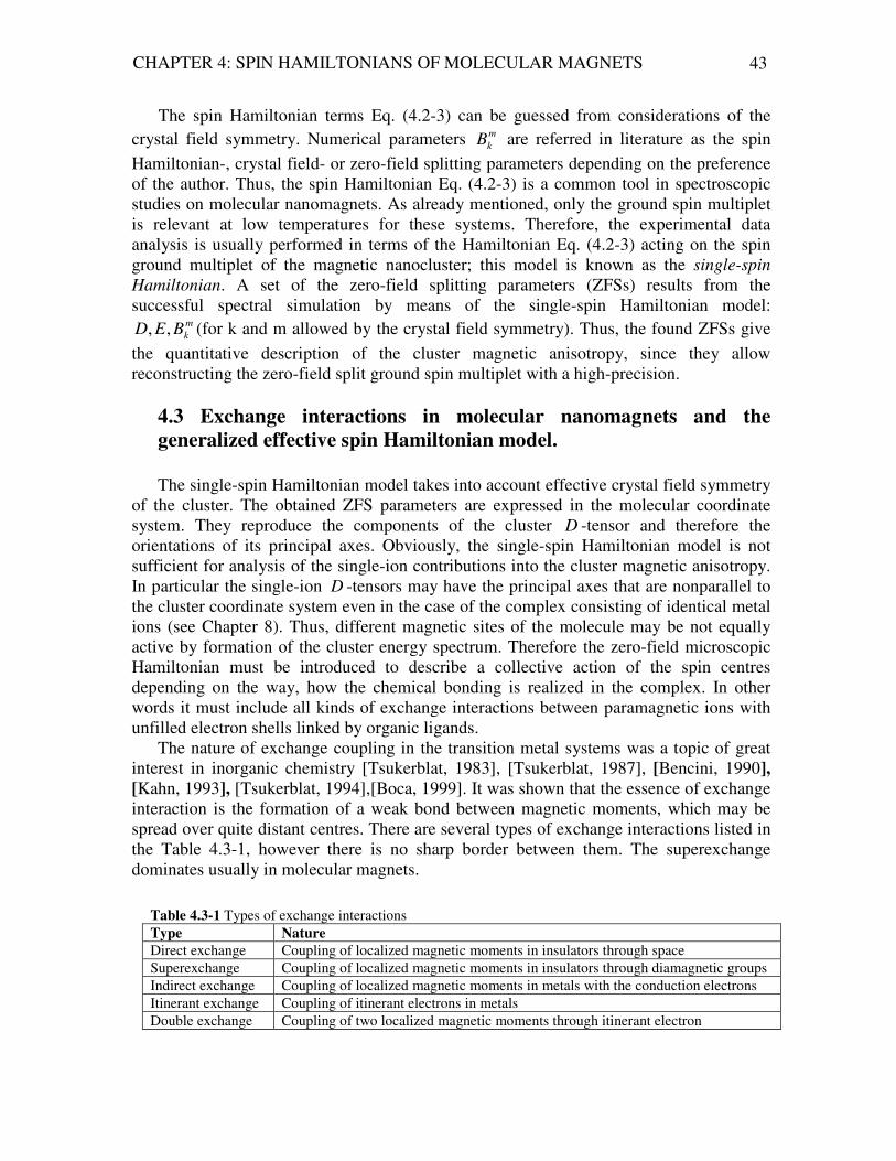
CHAPTER 4: SPIN HAMILTONIANS OF MOLECULAR MAGNETS 43
The spin Hamiltonian terms Eq. (4.2-3) can be guessed from considerations of the crystal field symmetry. Numerical parameters m
kB are referred in literature as the spin Hamiltonian-, crystal field- or zero-field splitting parameters depending on the preference of the author. Thus, the spin Hamiltonian Eq. (4.2-3) is a common tool in spectroscopic studies on molecular nanomagnets. As already mentioned, only the ground spin multiplet is relevant at low temperatures for these systems. Therefore, the experimental data analysis is usually performed in terms of the Hamiltonian Eq. (4.2-3) acting on the spin ground multiplet of the magnetic nanocluster; this model is known as the single-spin
Hamiltonian. A set of the zero-field splitting parameters (ZFSs) results from the successful spectral simulation by means of the single-spin Hamiltonian model:
m
kBED ,, (for k and m allowed by the crystal field symmetry). Thus, the found ZFSs give the quantitative description of the cluster magnetic anisotropy, since they allow reconstructing the zero-field split ground spin multiplet with a high-precision.
4.3 Exchange interactions in molecular nanomagnets and the generalized effective spin Hamiltonian model. The single-spin Hamiltonian model takes into account effective crystal field symmetry
of the cluster. The obtained ZFS parameters are expressed in the molecular coordinate system. They reproduce the components of the cluster D -tensor and therefore the orientations of its principal axes. Obviously, the single-spin Hamiltonian model is not sufficient for analysis of the single-ion contributions into the cluster magnetic anisotropy. In particular the single-ion D -tensors may have the principal axes that are nonparallel to the cluster coordinate system even in the case of the complex consisting of identical metal ions (see Chapter 8). Thus, different magnetic sites of the molecule may be not equally active by formation of the cluster energy spectrum. Therefore the zero-field microscopic Hamiltonian must be introduced to describe a collective action of the spin centres depending on the way, how the chemical bonding is realized in the complex. In other words it must include all kinds of exchange interactions between paramagnetic ions with unfilled electron shells linked by organic ligands.
The nature of exchange coupling in the transition metal systems was a topic of great interest in inorganic chemistry [Tsukerblat, 1983], [Tsukerblat, 1987], [Bencini, 1990],
[Kahn, 1993], [Tsukerblat, 1994],[Boca, 1999]. It was shown that the essence of exchange interaction is the formation of a weak bond between magnetic moments, which may be spread over quite distant centres. There are several types of exchange interactions listed in the Table 4.3-1, however there is no sharp border between them. The superexchange dominates usually in molecular magnets.
Table 4.3-1 Types of exchange interactions Type Nature
Direct exchange Coupling of localized magnetic moments in insulators through space Superexchange Coupling of localized magnetic moments in insulators through diamagnetic groups Indirect exchange Coupling of localized magnetic moments in metals with the conduction electrons Itinerant exchange Coupling of itinerant electrons in metals Double exchange Coupling of two localized magnetic moments through itinerant electron

CHAPTER 4: SPIN HAMILTONIANS OF MOLECULAR MAGNETS 44
The expression j
ij
iji SSˆˆˆrr
∑ Τ=Η represents the spin Hamiltonian of pairwise exchange
interactions between the spin centres iS and jS , where ijΤ is Cartesian spin-spin
interaction tensor. The relevant contributions to ijΤ are spin-(own) orbit-, spin-other orbit-,
electron-electron spin-orbit-, spin-spin dipolar- and spin-spin contact interactions [Boca, 1999]. The spin-spin interaction tensor can be decomposed into its irreducible components. Thus, the microscopic zero-field spin Hamiltonian of a magnetic nanocluster is usually expressed in a quite general form as follows:
∑∑∑≠<
⋅Π⋅+⋅⋅+⋅−=Ηji
jiji
i
iii
ji
jiij SSSDSSSJˆˆˆˆˆˆ2ˆrrrrrr
(4.3-1)
Here the first term is isotropic Heisenberg exchange interaction5, ijJ is the isotropic
exchange coupling constant that we discuss also in the Chapter 5.6. The second term is the symmetric part of the pairwise spin-spin interaction. It
represents the single-ion ligand fields (denoted in some publications as the local
anisotropy), where iD are single-ion (local) traceless D -tensors. As we have seen above, each single-ion ligand field term is given by
( ) ( )2,
2,
2,
ˆˆ131ˆˆˆˆ
yixiiiiziiiii
ZFS
i SSESSSDSDS −+
+−=⋅⋅=Η
rr, where iD and iE are the single-
ion ZFS parameters in the single-ion coordinate system. The cluster anisotropy is essentially determined by the single-ion ligand field contributions for many molecular nanomagnets like Mn12Ac studied by HF-EPR technique [Barra, 1997] and Cr8 antiferromagnetic ring studied by inelastic neutron scattering [Carretta, 2003] and EPR [van Slageren, 2002].
The last term of Eq. (4.3-1) includes the dipole-dipole interaction, anisotropic intracluster spin-spin interaction and antisymmetric exchange. The anisotropic part of the exchange interaction is expected to be negligible for the systems consisting of the metal ions with orbitally nondegenerate ground states [Guidi, 2004]. Therefore we rewrite the last term of Eq. (4.3-1) as the sum of dipole-dipole interaction and the antisymmetric
exchange:∑≠
− Η+Η=⋅Π⋅ji
ASdd
jiji SS ˆˆˆˆ rr. Thus, the dipole-dipole interactions are described
with the operator: ∑∑≤
− ⋅⋅=ΗN
i
N
ij
jiji
ddSDSˆˆˆrr
, where ijD are the pair-interaction D -tensors.
The dipole-dipole interaction was found to be responsible for more than 60% of the total anisotropy in Mn(II)-[3x3] grid [Guidi, 2004].
The antisymmetric exchange (AS) was initially introduced to explain the weak ferromagnetism of mainly antiferromagnetic crystals like α-Fe2O3 by Dzialoshinski [Dzialoshinski, 1958]. Later Moriya has given a detailed analysis of its origin [Moryia,
5 There is a disagreement in literature about the prefactor for the isotropic exchange term. The isotropic exchange
Hamiltonian is assumed as ∑<
⋅−=Ηji
jiij
ISOSSJˆˆ2ˆrr
throughout the text of this PhD thesis

CHAPTER 4: SPIN HAMILTONIANS OF MOLECULAR MAGNETS 45
1960]. This term is expressed by the vector product
× jiij SSG
ˆˆ rrr , where ijG
ris a constant
vector for a pair of spins ji SSrr
, . Moryia has noted for the first time that this expression is
the antisymmetric part of the most general expression for bilinear spin-spin interaction. He has also shown that some components of the symmetric and antisymmetric coupling tensors vanish because of the crystal symmetry. We present the rules for selection of the
ijGr
-vector orientation in Section 8.4. They follow from the crystal (molecular) symmetry
and essentially simplify the calculations. In the case of high-nuclearity clusters the AS-
exchange interaction is given by the sum ∑∑≤
×=Η
N
i
N
ij
jiij
ASSSGˆˆˆrrr
, where ijGr
are
antisymmetric exchange parameters and
× ji SS
ˆˆ rr is a vector product. The physical origin
of the vector jiij GGGrrr
−= is the admixture of excited states into the ground state through
spin-orbit coupling (for overview see [Owen, 1972], [Tsukerblat, 1987]). The publication [Yoon, 2004] is one of the latest works devoted to the role of antisymmetric exchange in the trimeric Cu(II) cluster. We recommend [Yoon, 2004 and refs therein] as a good tutorial for readers interested in understanding of the orbital origin of the antisymmetric exchange and in analysis of the AS-exchange contribution into the spectroscopic (magnetic circular dichroism and powder/single-crystal EPR) observation of the zero-field splitting. There it was shown that the AS-exchange is the largest non-Heisenberg term available for trinuclear Cu(II)-systems.
Summarizing all said above, we can imagine the zero-field Hamiltonian of a molecular nanomagnet consisting of N spin centres as an interplay of the relevant terms: the dominant isotropic Heisenberg exchange and non-Heisenberg terms (i.e. single-ion ligand fields, dipole-dipole interactions and antisymmetric exchange). We shall use this Hamiltonian for calculations on a Ni4-cluster (s. Chapter 8). There the dipole-dipole interactions can be omitted, since their contribution into the cluster anisotropy is much weaker than the contribution arising from the AS-exchange and the single-ion ligand fields. Therefore, we rewrite the ZFS-Hamiltonian as the sum of three terms: isotropic exchange, local anisotropy and antisymmetric exchange:
The non-Heisenberg terms are small relatively to the Heisenberg one and can be
considered in a perturbation way for exchange-coupled systems. Nevertheless, they play a crucial role in understanding the experimental observations on molecular nanomagnets.
The spin-spin interaction is not necessary restricted to quadratic terms in the spin operators,[Borras-Almenar, 1999][Waldmann, 2005]. Nevertheless, we exclude the higher-order terms (like biquadratic exchange) from considerations for convenience, since
( ) ( ) ∑∑∑∑∑≤≤
×+
−+
+−+⋅−=Η
N
i
N
ij
jiij
N
i
yixiiiizii
N
i
N
ij
jiij SSGSSESSSDSSJˆˆˆˆ1
31ˆˆˆ2ˆ 2
,2,
2,
rrrrr
(4.3-2)

CHAPTER 4: SPIN HAMILTONIANS OF MOLECULAR MAGNETS 46
their influence on the energy spectrum of Ni4-cluster (Chapter 8) is negligible in comparison to the quadratic terms.
The microscopic Hamiltonian of exchange-coupled compound can be expressed in terms of irreducible-tensor operators. Then it is called the generalized effective spin
Hamiltonian operating in the spin space of the whole system. It has the following general form [Tsukerblat, 1983], [Tsukerblat, 1987], [Bencini, 1990], [Tsukerblat, 1994], [Borras-Almenar, 1999]:
where ( )kkkkkkkC NN
k
q 12121)( ~
...~~
... − are adjustable parameters that originate from the practical
physical behavior of the system (they are related to the isotropic exchange coupling parameters ijJ , to the single-ion crystal field parameters ii ED , and to the parameters of
antisymmetric exchange ijGr
etc.). ( )kkkkkkkT NN
k
q 12121)( ~
...~~
...ˆ− is the qth component of the
irreducible tensor operator of the order (rank) k composed from the ITOs acting in the space of the individual spins [Borras-Almenar, 1999]:
( )
( ) ( ) ( ) ( ) ( )
)(
)(
)~
(
1)(
)~
(
3)()
~(
2)(
1)(
12121)(
SˆSˆ...SˆSˆSˆ...
~...
~~...ˆ
1
1
2
31
21
k
q
N
k
k
N
kk
kkkk
NN
k
q
N
N
N TTTTT
kkkkkkkT
⊗
⊗
⊗⊗=
=
−
−
−
−
where ⊗ is a tensor product, ik are the ranks of ITOs acting in the space of individual
spins iS ( ii Sk 2,...1,0= ), ik~
are the ranks of (intermediate) ITOs obtained by coupling of
spin angular momenta in the cluster. Obviously, the concrete values of the ranks ik~
depend on the nature of interaction represented by ITO and the coupling scheme chosen for the concrete cluster. The number of various coupling schemes increases extremely with increasing number of spins centres constituting the cluster (s. Chapter 3.3). Nevertheless, the spin states obtained from either of the schemes valid for the cluster can be expressed as linear combinations of the states obtained using other schemes. Therefore, the result of calculation of the matrix elements Eq. (4.3-3) does not depend on the chosen coupling scheme. The coupled spin states are usually labelled as
SNNS MSSSSSSSMS ;~
...~~
...; 12121 −≡α
where iS are the spins of magnetic centres constituting the cluster, iS~
are intermediate spin values obtained by coupling the spins according the rules of angular momentum
( ) ( )kkkkkkkTkkkkkkkC NN
k
qNN
k
q
kqkkkkk NN
12121)(
12121)(
~...
~...
~...
~~...ˆ~
...~~
...ˆ1121
−− ×=Η ∑∑∑−
(4.3-3)

CHAPTER 4: SPIN HAMILTONIANS OF MOLECULAR MAGNETS 47
addition, S is the total spin value of the spin multiplet, SM is the corresponding magnetic quantum number.
The matrix elements of the generalized spin Hamiltonian Eq. (4.3-3) are calculated using the Wigner-Eckart theorem (s. Chapter 3). The calculation of the many-electron spin
states SNNS MSSSSSSSMS ;~
...~~
...; 12121 −≡α is not needed for evaluation of the matrix
elements of Eq. (4.3-3) by using the ITO method. That is the main advantage of the generalized spin Hamiltonian model in comparison to the Density Functional Theory (DFT) calculations. If the chain of the individual and intermediate spin values is known, the matrix elements of the exchange Hamiltonian are easily evaluated by application of the Wigner-Eckart theorem:
where ( ) >>=<< − SkkkkkkkTSMSRS NN
k αααα ||~
...~~
...ˆ||'';||'' 12121)( is the reduced matrix
element of the compound ITO ( )kkkkkkkT NN
k
12121)( ~
...~~
...ˆ− . It is calculated for the coupled
spin states Sα and ''Sα and does not depend on the magnetic quantum numbers. The
last fact allows a significant reduction in calculation time in the full Hilbert space. We present the explicit formulas used for evaluation of the Hamiltonian matrix elements Eq. (4.3-3) with help of Eq. (4.3-4) in the Section 8.3, since there are fine disagreements in some formulas for calculation of the energy spectrum of high-nuclearity spin clusters by ITO method presented in the publications of the leading groups in this field: Tsukerblat/Gatteschi/Boca (the value of some parameters equal to 0 or 1 and their sign significantly influences the result of calculations).
The complete energy spectrum and the spin states are obtained by diagonalization of the Hamiltonian matrix Eq. (4.3-3) calculated by using Eq. (4.3-4). The dimension of Hamiltonian matrix grows enormously with increasing number of spin centres and spin quantum numbers. Therefore its exact diagonalization becomes a difficult task even for modern computers. There are two ways to overcome the problem. The block factorizing of the Hamiltonian matrix can be achieved by using the symmetry adapted wave functions [Waldmann 2000 and references therein]. Another way (presented in this thesis) requires the group-theoretical classification of the exchange-coupled multiplets. It allows the pre-selection of the dominant terms of the generalized effective spin Hamiltonian suitable for the cluster under study. The Hamiltonian matrix Eq. (4.3-3) contains well defined blocks, if it is calculated by Eq. (4.3-4) in the basis of states SSMα with the total spin
value S varying subsequently in the range allowed by the rules of angular momenta addition and SSM S +−= ... . The spin manifolds Sα are characterized by representations
of the full rotation group that can be reduced to the representations of the cluster point group. The cluster point group representations linked to the spin states Sα and ''Sα
allow a-priori analysis of the structure of the Hamiltonian matrix block calculated in the
( ) ><+
−>=< − SRSC
SMSkkkkkkkTMS
MS
SMkq
k
NN
k
q αααα ||''1'2
)1(;|
~...
~~...ˆ|';'' ''
2
12121)(
(4.3-4)

CHAPTER 4: SPIN HAMILTONIANS OF MOLECULAR MAGNETS 48
basis Sα , ''Sα , i.e. to determine, whether or not the block will be filled and where are
the positions of the non-zero elements of the filled block. Since the symmetry aspects play an important role by modelling of spectroscopic data in terms of the generalized effective spin Hamiltonian model, we devote the next chapter to the results of group representation theory that were put in use in Chapter 8.

V
Group theoretical classification of exchange-
coupled multiplets
Two kinds of spin Hamiltonians were introduced in the previous chapter to describe the properties of molecular nanomagnets. One of the requirements for any spin Hamiltonian is its invariance under point symmetry of the molecule: its explicit form follows directly from the symmetry considerations. In the Chapter 8 we show that the group theoretical classification of exchange-coupled multiplets allows an a priori identification of the dominant non-Heisenberg interactions responsible for the removing the degeneracy of the energy multiplets in molecular magnets, i.e. the dominant physical mechanisms leading to the formation of the cluster magnetic anisotropy. In this chapter we summarize the most important facts needed for practical application of group-theory to the classification of the splittings of atomic levels and exchange-coupled multiplets in crystal fields. We try to give explanations using a “down-to-earth” approach in a manner understandable for non-theoreticians. For further details we refer the reader to the textbooks [Rosen, 1995], [Heine, 1960], [Tinkham, 1964], [Jones, 1998], [Inui, 1990], [Burns, 1977], [McWeeny, 2002], [Butler, 1981].
5.1 The role of the group theory in modeling of spectroscopic data on molecular magnets In this chapter we show why group theory is important for modeling of spectroscopic
data on molecular magnets and how to paraphrase the requirements for the spin Hamiltonian from the group-theoretical point of view.
Any kind of spectroscopy is dealing with interaction of molecules with electromagnetic wave that leads to absorption or emission of the photons. In the case of magnetic resonance technique (see Section 4.2), the resonant absorption of microwave radiation by electron spins of the molecule is observed experimentally as spectral lines induced by magnetic-dipole transitions. In the context of molecular magnets these magnetic excitations take place within the zero-field split exchange-coupled spin multiplets. The quantum-mechanical operator characterizing the electron-photon
interaction leading to a magnetic-dipole transition is given by MuVphe
rr⋅=−ˆ [Tsukerblat,
1994], where ur
is the magnetic polarization vector and Mr
is magnetic moment operator. It
can be expressed by ( )∑ +−=i
ii slmc
eM ˆ2ˆ
2hr
, where il and is are the orbital and spin
angular momenta of i th electron and the sum is carried out over all electrons of the molecule, h is Planck’s constant, e and m are the charge and mass of the electron and c is the velocity of light. The spectral line positions and selection rules of spectroscopic

CHAPTER 5: GROUP THEORETICAL CLASSIFICATION OF MULTIPLETS 50
transitions are determined by the difference if εε − and the matrix
elements i
phe
f V εε |ˆ| − , respectively, where fε and iε are the energy levels of final and
initial states. The group representation theory is used in order to characterize the energy levels of molecule (see Section 5.2). Each energy level can be identified by irreducible representations of the molecule point group, i.e the irreducible representations fΓ and iΓ
of final and initial states, respectively. Thus, intensity of the spectral line is proportional to
the matrix element i
phe
f V ΓΓ − |ˆ| . It is finite for allowed- and zero for forbidden
transitions. Here, the operator of electron-photon interaction pheV
−ˆ has transformation properties under rotation of the coordinate system reflected in a certain representation Γ . In the case of magnetic dipole transitions it has the same transformation properties as the electron orbital and spin angular momentum operators. Now we introduce an important
theorem (without proof) for determination of the selection rules of the operator pheV
−ˆ : the
matrix of pheV
−ˆ contains non-zero elements if the direct product of three irreducible representations if Γ×Γ×Γ contains the fully symmetric irreducible representations of the
molecule point group A (or 1Γ ). Obviously, in the context of molecular magnetism fΓ and
iΓ are irreducible representations that refer to exchange-coupled multiplets of a high-nuclearity spin cluster, whose crystal field symmetry is characterized by a certain point group.
Summarizing all said above, we can rewrite the requirements for the spin Hamiltonian (see Chapter 4) of a high-nuclearity cluster characterized by a given point group as follows: the eigenfunctions of the spin Hamiltonian belonging to a degenerate level form a basis for an irreducible representation of the cluster point group. The degeneracy of the energy multiplet is equal to the dimension of this representation. Besides the requirement to be invariant under time reversal, the spin Hamiltonian must be invariant under all symmetry operators of the cluster point group. Thus, in order to construct the spin Hamiltonian valid for the cluster, we must find in the character table (see Section 5.2) all possible types of functions that transform according to the fully symmetric representation of the cluster point group and their quadratic terms (or terms of higher even degree). All those terms that do not change the sign under the time reversal must be included into the spin Hamiltonian.
Thus, the type of irreducible representation and the total spin value of the exchange-coupled multiplet predefine unambiguously the explicit form of the spin Hamiltonian acting within this multiplet, the splitting of energy manifolds and the probabilities of experimentally observed spectroscopic transitions.

CHAPTER 5: GROUP THEORETICAL CLASSIFICATION OF MULTIPLETS 51
5.2 Representations and characters The concept of “representation” was already indirectly introduced and the problem of
irreducibility versus reducibility was also briefly discussed in Chapter 3. Representations are simply the matrices describing transformation of operators under rotations. In the context of the crystal field theory we mean with rotations the symmetry operations of a point group characterizing the crystal field. It turns out that the irreducible representations (degenerate energy levels) can be classified (by characters) and therefore enumerated.
The character of a representation D of a group G is defined as the set of ( ) Ggg ∈= |χχ , where ( )gχ is the trace of the representation matrix )(gD ,
i.e. ( ) ( )[ ]gDTrg =χ , which defines the symmetry operator g belonging to the group G . The characters of 32 point groups are tabulated for all possible irreducible representations in the character tables [Koster, 1963]. A representation of dimension n+m is said to be
reducible if )(gD takes the form ( )( ) ( )
( )
=
gB
gC
O
gAgD , Gg ∈∀ , where A ,C and B are
submatrices of dimensions mm× , nm× and nn× respectively. O denotes the null matrix of dimension mn× . If the matrix C is equal to the null matrix, then the representation is said to be completely reducible or decomposable and we
write ( ) ( ) ( )( )
( )
=⊕=
gB
O
O
gAgBgAgD .
It may be that the representations A and B are themselves decomposable; in this case it is natural to continue the process, which will be terminated when we reach the level of irreducible representation, namely representations which can not be further reduced.
For a finite group, any reducible representation ( ( ) DgD ≡ ) is completely reducible
into a direct sum of irreducible representations, i.e. ( ) ( )νν DgD ≡ , where ν is an integer
counter that identifies various irreducible representations of the finite group. The representation matrices can be cast in block diagonal form, where the non-zero diagonal blocks are matrices of irreducible representations. A given irreducible representation may appear more than once in this decomposition. In the general case the decomposition is written ( )ν
ν DaD ∑⊕
= . Here νa denotes the number of times the irreducible representation
( )νD appears in the decomposition. The coefficients νa can be found using the formula for
reduction of representations (Section 5.3). It is of principal importance for the classification of atomic states split in crystal fields by perturbation as well as for the classification of zero-field split multiplets of magnetic nanoclusters.

CHAPTER 5: GROUP THEORETICAL CLASSIFICATION OF MULTIPLETS 52
5.3 Splitting of energy levels by a perturbation; formula for reduction of representations
If the symmetry of a perturbation 1Η applied to an original Hamiltonian
0Η (characterized by the symmetry group 0G ) is not lower than the symmetry of 0Η , then
the perturbed Hamiltonian 10ˆˆ Η+Η has the same symmetry as 0Η . In this case the
symmetry group stays unchanged and the eigenfunctions of the Hamiltonian remain the basis for the same irreducible representation. The perturbation causes only a shift of the energy levels and leaves the degeneracy unchanged.
When 1Η has lower symmetry than 0Η , then the symmetry group of the perturbed
Hamiltonian G is a subgroup of the original symmetry group 0G . Such a perturbation of lower symmetry can lift the degeneracy.
Consider a degenerate unperturbed level that forms an irreducible representation 0Γ of
the group 0G . Under a small perturbation 1Η , the wavefunctions belonging to this level
form the basis for a representation of the subgroupG . The representation 0Γ may be
irreducible as the representation of 0G , but it is not necessarily irreducible under its
subgroup G . Regarding 0Γ as a representation of the subgroup G and reducing it into
irreducible representations ofG , we can find the level splitting. If the result of this, the reduction ...0 +Γ+Γ→Γ βα contains n irreducible representations, the irreducibility
requirement tell us that the level is split into n sublevels. The number of times the irreducible representation iΓ with ,..., βα=i appears in the decomposition 0Γ is
calculated as follows:[ ]
( ) ( ) ( ) ( )RRG
aR
ˆˆ1
ˆ0
0 νν χχ ΓΓ∑= . Here the order of the group 0G is
denoted as [ ]0G , ( )( )R0Γχ is the character of rotations R in the reducible representation
0Γ of 0G , ( ) ( )Rνχ Γ is a character of the irreducible representation νΓ of G for the operation
R . The summation is performed over all rotations R constituting the lower symmetry group G .
5.4 Clebsch-Gordan series The concept of the Clebsch-Gordan series is very important in physical applications of
representation theory. It gives the decomposition of the direct product of two irreducible representations with certain multiplicities respective to some symmetry group. This is the same as the problem of addition of angular momentum in quantum mechanics, where one
is dealing with the algebra of operators Jr
rather than with the group itself. The addition of two angular momenta with eigenvalues j1 and j2 gives all j values spaced integrally
between j1+j2 and |j1-j2|. In terms of the groups this means: ( ) ( ) ( )∑+
−
⊕=⊗21
21
21
||
jj
jj
jjjDDD .

CHAPTER 5: GROUP THEORETICAL CLASSIFICATION OF MULTIPLETS 53
Thus, the exchange-coupled multiplets of molecular magnets can be characterized by irreducible representations of the full rotation group, i.e. the energy spectrum of molecular magnet in the full Hilbert space is given by a Clebsch-Gordan series describing the coupling of spin angular momenta localized at different sites of the magnetic cluster, see also Chapter 8.
5.5 Projection operators The projection operator method is used to find the one-to-one correspondence between
the states SSM;α (see Section 4.3) constituting the energy −S manifold of a molecular
magnet and the irreducible representation of the cluster point group describing this −S multiplet. This method is also of importance for construction of the symmetry adapted
basis functions for a given matrix ( )αD of an irreducible representation. As mentioned above, the basis functions ( )αψ m of an irreducible representation ( )αD of a group G are
transformed as ( ) ( ) ( ) ( ) ( )∑=≡'
'''m
mmnlmnlmnlm RDR αααα ψψψ by symmetry operations R belonging to
G . Thus, the projection operator is defined by [ ]
( ) ( )∑=R
lmml RRDG
dP
*)()(
βββ , where [ ]G is the
order of the group G . In many applications, the diagonal projection operators )(
)(βllP are used, where the
projection operator is constructed using the characters ( ) ( )Rβχ of the rotations in the β -
irreducible representation ( )
[ ]( ) ( )∑∑ =≡
Rl
ll RRG
dPP
ˆ
*)()(
ˆˆββββ χ , βd is the dimension of the
β -irreducible representation. The application of the projection operator ( )βP to the state
SSM;α reproduces it, if the state is characterized by β -irreducible representation; if not ( ) 0; =SSMP αβ . Thus, the symmetry adapted wavefunctions are the states SSM;α that
satisfy the condition ( )SS SMSMP ;; ααβ = (see Chapter 8).
5.6 Group-theoretical classification of exchange coupled multiplets We start this section with a short summary in order to avoid a jump in the logic and
link Section 5.6 to all the previous chapters of this thesis. Our aim is to apply the projection operator method for group-theoretical classification of energy levels of a multinuclear system, i.e. a system of several ions with unfilled electronic shells coupled by chemical bonding (by exchange interactions). Our goal is to introduce the connection between the wavefunctions SSM;α built in the spin basis and the Heitler-London
wavefunctions known in quantum chemistry and adapt the states SSM;α to the cluster
point group. The concept of exchange coupling was born in the Heitler-London theory of the
chemical bond [Heitler, 1927]. Later it was applied by Heisenberg in his theory of
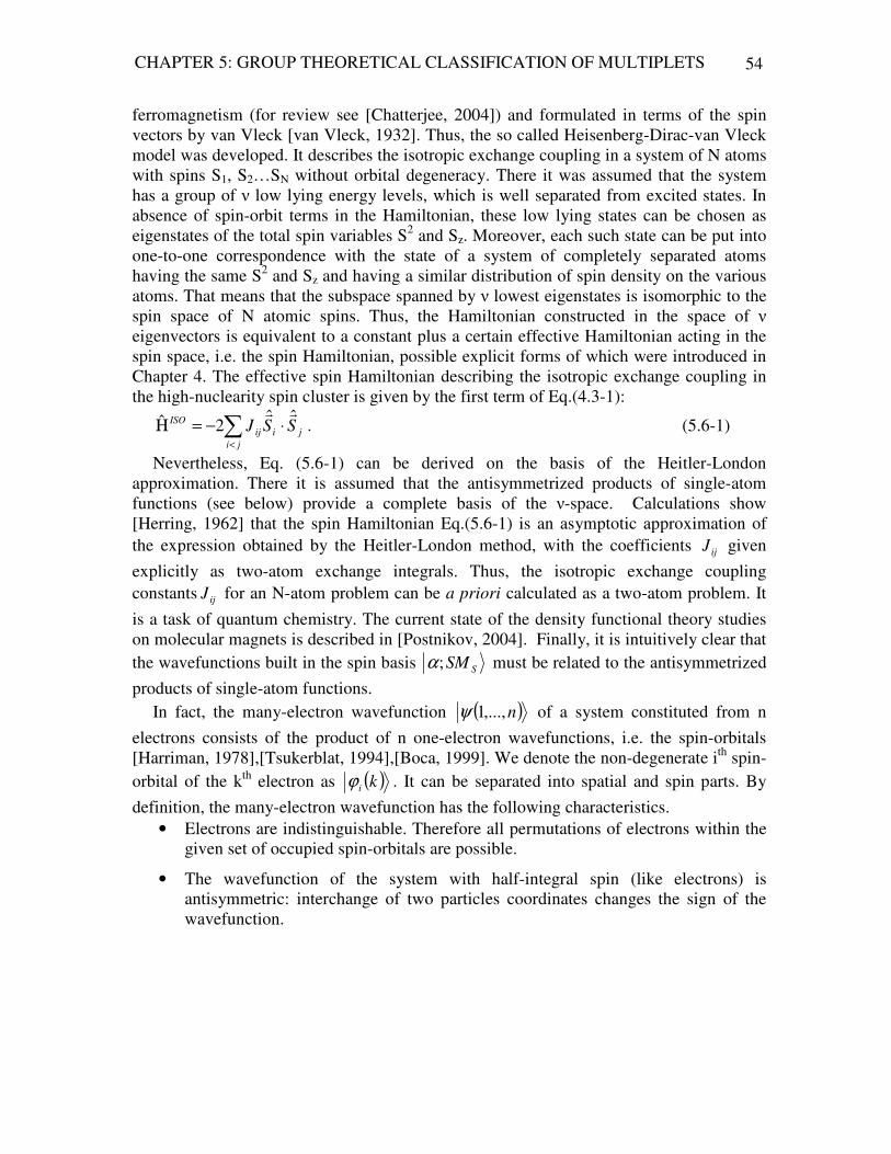
CHAPTER 5: GROUP THEORETICAL CLASSIFICATION OF MULTIPLETS 54
ferromagnetism (for review see [Chatterjee, 2004]) and formulated in terms of the spin vectors by van Vleck [van Vleck, 1932]. Thus, the so called Heisenberg-Dirac-van Vleck model was developed. It describes the isotropic exchange coupling in a system of N atoms with spins S1, S2…SN without orbital degeneracy. There it was assumed that the system has a group of ν low lying energy levels, which is well separated from excited states. In absence of spin-orbit terms in the Hamiltonian, these low lying states can be chosen as eigenstates of the total spin variables S2 and Sz. Moreover, each such state can be put into one-to-one correspondence with the state of a system of completely separated atoms having the same S2 and Sz and having a similar distribution of spin density on the various atoms. That means that the subspace spanned by ν lowest eigenstates is isomorphic to the spin space of N atomic spins. Thus, the Hamiltonian constructed in the space of ν eigenvectors is equivalent to a constant plus a certain effective Hamiltonian acting in the spin space, i.e. the spin Hamiltonian, possible explicit forms of which were introduced in Chapter 4. The effective spin Hamiltonian describing the isotropic exchange coupling in the high-nuclearity spin cluster is given by the first term of Eq.(4.3-1):
∑<
⋅−=Ηji
jiij
ISO SSJˆˆ2ˆrr
. (5.6-1)
Nevertheless, Eq. (5.6-1) can be derived on the basis of the Heitler-London approximation. There it is assumed that the antisymmetrized products of single-atom functions (see below) provide a complete basis of the ν-space. Calculations show [Herring, 1962] that the spin Hamiltonian Eq.(5.6-1) is an asymptotic approximation of the expression obtained by the Heitler-London method, with the coefficients ijJ given
explicitly as two-atom exchange integrals. Thus, the isotropic exchange coupling constants ijJ for an N-atom problem can be a priori calculated as a two-atom problem. It
is a task of quantum chemistry. The current state of the density functional theory studies on molecular magnets is described in [Postnikov, 2004]. Finally, it is intuitively clear that the wavefunctions built in the spin basis SSM;α must be related to the antisymmetrized
products of single-atom functions. In fact, the many-electron wavefunction ( )n,...,1ψ of a system constituted from n
electrons consists of the product of n one-electron wavefunctions, i.e. the spin-orbitals [Harriman, 1978],[Tsukerblat, 1994],[Boca, 1999]. We denote the non-degenerate ith spin-orbital of the kth electron as ( )kiϕ . It can be separated into spatial and spin parts. By
definition, the many-electron wavefunction has the following characteristics. • Electrons are indistinguishable. Therefore all permutations of electrons within the
given set of occupied spin-orbitals are possible.
• The wavefunction of the system with half-integral spin (like electrons) is antisymmetric: interchange of two particles coordinates changes the sign of the wavefunction.

CHAPTER 5: GROUP THEORETICAL CLASSIFICATION OF MULTIPLETS 55
• The many-electron wavefunction must be normalized to unity. The normalized many-electron wavefunction is described by the Slater determinant:
( )
( ) ( ) ( )( ) ( ) ( )
( ) ( ) ( )nnn
nn
n
n
n
ϕϕϕ
ϕϕϕ
ϕϕϕ
ψ
...
............
2...22
1...11
!
1,...,1
21
21
21
= .
Different antisymmetric functions ( )n,...,11ψ , ( )n,...,12ψ , …, ( )np ,...,1ψ are possible
for a many-electron system, if two projections of electron spin are taken into account (sz=±1/2). Therefore the true eigenvectors of an exchange-coupled cluster
SMS;α satisfying the Pauli principle must be given by a linear combination of
( )n,...,11ψ , ( )n,...,12ψ , …, ( )np ,...,1ψ , i.e. there is a link between the states SMS;α
and the products of Slater determinants. Group representation theory gives an answer, how to find this link using the properties of symmetric (permutational) groups mentioned in the Chapter 2.4.
The symmetric (permutational) group nS6 is defined as the group of all permutations
on n symbols (for details see [Hamermesh, 1989]). There are many systems in mathematics, physics and chemistry described by the symmetric groups. In mathematics, the tensors can be classified into irreducible sets with respect to any group of linear transformations in n dimensions, as soon as the representations of the symmetric groups are known. In physics, we are often dealing with systems of n identical particles with the Hamiltonian which is invariant under interchange of the particles (e.g. high-nuclearity spin clusters). The method of treating the symmetric groups suggested F.Hund [Hund,1927] is usual in physics and chemistry. The basic point of this method is
connected with the behavior of the eigenfunctions of the Hamiltonian under permutations
of the particle coordinates. If ( )n,...,1ψ belongs to a given eigenvalue of the Hamiltonian, then any one of the !n permutations of the particle coordinates will yield an eigenfunction belonging to the same energy. By continuous permutations of pairs of particles in ψ one can construct the functions that are symmetric (antisymmetric) in larger sets of particles. For this aim the so called Young operators/Young tableaus are used, which are out of the scope of this thesis; the interested reader is referred to [Hamermesh, 1989]. Nevertheless, it is important to mention that the product wavefunctions (product of the single-particle states) of a given symmetry can be constructed by using the Young operators. Obviously, the constructed many-electron wavefunctions of the high-nuclearity cluster must “feel” the symmetry of the ligand environment surrounding the spin centers. In other words, they must be adapted to the cluster point group.
The general group-theoretical procedure was given in [Tsukerblat, 1983], [Tsukerblat, 1987] for classification of the energy levels of a high-nuclearity spin cluster under the given point group. It uses the mathematics of the unitary groups7. Below we try to explain the results of this method in a simple manner.
6 It is not the same as a point group 7 Unitary group is represented by an unitary matrix, i.e. the complex conjugate of the matrix gives its inverse.

CHAPTER 5: GROUP THEORETICAL CLASSIFICATION OF MULTIPLETS 56
We consider an exchange-coupled cluster consisting of n spin centers: si, i=1…n. The cluster is described by the point group G with the irreducible representations
jΓ ,
...,γβ=j . Coupling of the spin angular momenta gives rise to the energy spectrum consisting of more than one manifold (the number of manifolds is given by K, K>1). Each manifold is characterized by the total spin value S (allowed by the rules of angular momenta addition) and therefore contains 2S+1 sublevels in accordance to the magnetic quantum numbers MS. The wavefunction of each sublevel of S -manifold is labeled by SMS;α . Here α indicates the set of additional quantum numbers arising in the chosen
coupling scheme: 12121~,...,~,
~,...
~,
~−−= nN mmSSSα , where the successive coupling scheme of
spins and their projections is given by chains: 121
~SSS =+ , 221
~mmm =+ ;
231
~~SSS =+ , 332
~~ mmm =+ ;,…, SSS nn =+−1
~, Snn Mmm =+−1
~ . The state SMS;α is the
many-electron wavefunctions of the real (“physical”) Hamiltonian of the high-nuclearity system, which involves the kinetic energy of electrons, inter- and intra-atomic interactions (i.e. the Heitler-London states). The wavefunctions of a given total spin value S can be expressed in terms of linear combinations of Slater determinants [Borras-Almenar, 1999]:
|...|...;| 21~~~~
~~~~
...11
33
3322
11
2211
21
n
SM
mSmS
mS
mSmS
mS
mSmS
mmm
S mmmCCCSM S
nnnn
n
−−∑>=α (5.6-2)
here the expressions jm
mjmjC2211are the Clebsch-Gordan coefficients introduced in the
Section 3.3. If a many-electron wavefunction SMS;α belongs to a given eigenvalue of
the Hamiltonian: SE , then any one of the !n permutations of the particle coordinates will yield an eigenfunction belonging to the same energy. Therefore all products of the single-particle states correspond to the same energy SE . Since the isotropic exchange Hamiltonian is symmetric relative to interchanges of identical particles, its wavefunctions will be transformed according to irreducible representations of the permutation
(symmetric) group of the cluster. At the same time, the irreducible representations labeling the energy levels of the system, which consists of many identical particles, can be expressed through the irreducible representations
jΓ , ...,γβ=j of the point group
G characterizing the cluster. On the other hand, the energy spectrum of exchange-coupled cluster is described by the Clebsch-Gordan series valid for the cluster under consideration. That means that the energy multiplets can be classified by irreducible representations of the full rotation group, which can be reduced (decomposed) to irreducible representations of the cluster point group. This decomposition is given by ( )∑ Γ=⊗⊗⊗
jS
S
jjS
sssnDDD n
,,
)()()( ...21 ,
where )( isD is an irreducible representation of the full rotation group for the individual
spins si, ⊗ indicates the direct product, ( )S
jΓ is the j -irreducible representation of the
point group G that characterizes the multiplet with the total spin value S ; jSn , is the
number of identical irreducible representations ( )S
jΓ describing different multiplets with
one and the same total spin value S (and different α ). This decomposition is reflected in the structure of the Hamiltonian matrix: it will be blocked according to the total spin

CHAPTER 5: GROUP THEORETICAL CLASSIFICATION OF MULTIPLETS 57
value S , its projection SM and the irreducible representations jΓ , ...,γβ=j of the
cluster point group. The structure of each block is illustrated in Figure 5.6-1 for degenerate (Figure 5.6-1a) and non-degenerate (Figure 5.6-1b) multiplets.
The projector operator method is used to obtain the symmetry-adapted wavefunctions.
In fact, each operator R of the point group G applied to the spin states >SM;|α gives rise to permutations of the orbitals in the Slater determinants and mixes the states >SM;|α with different α mapped to one and the same SM space:
( ) >>=∑ SMRDSMR ;'|ˆ;|ˆ'
' ααα
αα
where ( )RD ˆ'αα are the matrix elements of the representation of the operator R calculated
as follows: ( ) SMRSMRD ;ˆ;'ˆ' αααα = .
Application of the symmetry operator R to each determinant of the many-electron
wavefunction Eq.(5.6-2) gives the matrices ( )RD ˆ for each SM;α representation. Using the projection operator method presented above, we can obtain all energy terms (states) corresponding to the total spin value S and the irreducible representation βΓ of the
reducible one ( )RD ˆ : ( )
[ ]( ) ( )∑=
R
RRG
dP
ˆ
* ˆˆβββ χ .
Thus, the symmetry-adapted wavefunctions will be given by the non-zero results of the projector application to the states attacked by the operators of the cluster point group:
( ) ( ) >∑ SMRDP ;'|ˆ'
' αα
ααβ , i.e. they might be viewed as linear combination of the initial
SMS;α
a b
Figure 5.6-1 The (2S+1)-degenerate multiplet
SMS;α is represented by the
strictly diagonal matrix of the dimension (2S+1)x(2S+1) with equal diagonal elements (a). Removing the degeneracy of the energy multiplet is reflected in non-zero off-diagonal terms of the representation matrix (b). In both cases (a) and (b) the block matrix is constructed by using the wavefunctions of one of the irreducible representations of the
cluster point group G: ( )S
jΓ .
( )S
jΓ

CHAPTER 5: GROUP THEORETICAL CLASSIFICATION OF MULTIPLETS 58
determinants |...| 21 nmmm . The obtained wavefunctions reflect the properties of the rotation-, point- and symmetric groups as it is required for molecular magnets, s. Section 2.4. Application of this method to classification of the exchange coupled multiplets of a tetrameric cluster 1=is ( 4,...,1=i ) with the point group S4 will be shown in the Chapter 8.
Finally, the matrix of any spin Hamiltonian can be block-factorized using the symmetry-adapted wavefunctions as the basis of each S -block. Doing so, the dimension of the matrices to be diagonalized will be essentially reduced leading to a decrease in calculation time [Waldmann, 2000].
Moreover, classification of the states >S;|α in terms of the irreducible representations of the cluster point group allows an a priori analysis of the dominant non-Heisenberg interactions in the cluster. Thus, presence of a two-dimensional representation E in the decomposition of the first excited multiplet points to pronounced role of the spin-orbit interaction in the cluster and therefore to antisymmetric exchange as the most probable mechanism leading to the cluster magnetic anisotropy, see Chapter 8.
VI
Simulation of FDMR-spectra
The theoretical formalism needed for the analysis of the spectroscopic data on molecular nanomagnets was introduced in the Chapters 3-5. Here we present the experimental technique used for studying the zero-field splittings of mono- and many-nuclearity complexes with high spin ground state: the Frequency-Domain Magnetic Resonance Spectroscopy (FDMRS). An important result of this PhD-thesis is the computer code developed for the FDMR-spectral simulations in terms of the single-spin Hamiltonian formalism. In this chapter we show the measurement geometry, the general logic of EPR-spectral simulations, the mathematical formalism used for evaluation of the quantities measurable by FDMRS and description of the developed program.
6.1 Spectral simulations of EPR spectra: the general logic Electron paramagnetic resonance (EPR) phenomenon was introduced in the Chapter 4.2.
The EPR technique is a powerful and useful tool in probing the magnetic interactions in solids, since the EPR absorption is proportional to the imaginary part of the dynamic susceptibility characterizing the sample under study. As already mentioned, magnetic resonance occurs when the energy difference between the eigenstates of the Hamiltonian describing the system is equal to the quantum of the incident microwave radiation regardless of whether this condition is achieved by varying the external magnetic field or by varying the frequency of the microwave radiation. Therefore there are two alternative techniques of obtaining an EPR spectrum: field-swept and frequency-swept EPR. The microwave frequency is kept fixed and the external magnetic field is swept over a chosen range in the case of the field-swept EPR. Thus, all the transitions are recorded in an appropriate magnetic-field sweep interval. The magnetic field is kept fixed (or no external magnetic field is applied) and the frequency of the microwave radiation is varied over an appropriate frequency interval by frequency-swept EPR so that all the transitions are recorded.
Usually the measurements of EPR spectra are performed in the field-swept modus e.g.: continuous wave EPR, transient EPR, pulsed-EPR etc [Kammel, 2003]. The Frequency-Domain Magnetic Resonance Spectroscopy (FDMRS) is a unique experimental method to obtain the EPR spectra of high-spin molecules in the frequency-swept mode.
Simulations of the EPR spectra have begun to appear in the 1950s. Since then many successful spectral simulations were published for paramagnetic species in liquid solution, in glassy media, in powders and single crystals. The earliest algebraic and numerical calculations were carried out on mainframe computers with strong computer time limitations. The majority of them used perturbation theory solutions to the spin Hamiltonian. Development of PC’s and Workstations in the middle of 1980s opened new possibilities for exploration of simulation methods and statistical analysis. The modern computer simulations exploit various numerical algorithms, where the limitations of

CHAPTER 6: SIMULATION OF FDMR-SPECTRA 60
perturbation theory are removed by full matrix diagonalization [Smith, 1994],[Pilbrow, 1996],[Weil, 1999], [Misra, 1999]. The latest trend is incorporation in the programs of more realistic lineshape models that Lorentzian/Gaussian ones [Howarth, 2003].
When simulating a multi-line EPR spectrum, the main parameters of interest are the number of lines, the exact position of each line on the x-scale (i.e. frequency- or field-scale), the lineshape, width and intensity of each. Notably, the EPR spectra measured in the field swept modus give information about the relative intensities, whereas the FDMRS gives access to absolute intensity values.
The dynamic magnetic susceptibility is an EPR-measurable magnetic parameter, since the magnetic resonance absorption is proportional to its imaginary part. The complete energy spectrum of the molecule is needed for exact calculation of this magnetic parameter. Nevertheless, it can be good approximated by computing only over the ground spin multiplet for many molecular magnets as soon as the strong exchange approximation is valid and the excited multiplets can be disregarded. Then the single-spin Hamiltonian is constructed (Chapter 4.2) for spectral simulations. As we have already seen, the single-spin Hamiltonian is a convenient quantum mechanical operator, which contains some semiempirical parameters. Generally they can be imagined as a set of various scalars like the components of the g -tensor (magnetogyric ratio tensor), the crystal field parameters or the hyperfine splitting parameters. The extraction of the complete parameter set from the
experimental data with maximal accuracy is a prime goal of EPR spectrum simulation. The Zero-Field Splittings (ZFSs) of molecular nanomagnets can be easily obtained
from the FDMR-spectrum measured in zero-applied magnetic field. An essential advantage of the FDMRS versus field-swept EPR is the reduced number of adjustable parameters, since the Zeeman term is omitted from the spin Hamiltonian. They are restricted by parameters of the crystal field potential ( k
mBED ,, ), s. (Formula 4.2-3):
( ) ( ) ( ) ( )∑ ∑∑ ∑=
+
=±
=
+
=± +−+
+−==Η
6,4 06,4,2,0 0
222 ˆ,ˆˆˆˆ131ˆˆ,ˆˆˆ
k
k
m
z
m
k
m
k
k
k
m
yxzz
m
k
m
k
ZFS SSOBSSESSSDSSOB .
The EPR spectrum (i.e. positions and intensities of the absorption lines) will be fully reconstructed by the diagonalization of the single-spin Hamiltonian acting on the ground multiplet of a molecular nanomagnet only for those ZFS parameters that unambiguously characterize the molecule. A small deviation in the values of ZFS parameters of those characteristic for the molecule leads to calculated magnetic parameter, which does not coincides with the experimental observables.
6.2 Description of the FDMRS spectrometer and formation of the FDMR-spectrum The spectrometer used for FDMRS is shown in the Figure 6.2-1. The Backward Wave
Oscillators (BWO) generators are used as a radiation source. Varying the BWO-high voltage allows to sweep the frequency of microwave radiation, which is linearly polarized and focused on the sample. The signal is detected by the Golay-cell. We refer the reader to [van Slageren, 2003] for further experimental details. FDMR-spectra are spectra of transmission versus frequency. Usually they are recorded on the plane parallel samples at various

CHAPTER 6: SIMULATION OF FDMR-SPECTRA 61
temperatures in zero applied magnetic field. The measurable parameter is the transmission that is dependent on the magnetic parameter (dynamic magnetic susceptibility).
The shape of the transmission spectra is determined by two effects (Figure 6.2-2). An oscillating magnetic field of the microwave radiation interacts with the spin angular momentum of each molecule of the powder sample. The frequency dispersion of the dynamic susceptibility or static magnetic permeability ( '''* µµµ i−= ) of the sample describes the magnetic resonance phenomenon. Secondly, the electromagnetic wave interacts with the plane parallel surfaces of the sample causing interference of the transmitted radiation. The frequency dispersion of the dielectric permittivity ( '''* εεε i−= ) reflects this effect.
Therefore two features are observed in the FDMRS spectra on molecular magnets, which are illustrated in Figure 6.2-3. Narrow temperature-dependent absorption lines in the FDMRS-spectra are associated with the allowed magnetic dipole transitions between spin states of the ground multiplet of each molecule. Their intensity decreases essentially with increasing temperature. The second feature is an oscillating and temperature-independent baseline caused by the interference of the radiation between the parallel surfaces of the sample. The frequency dispersion of dielectric permittivity is fitted directly to the baseline measured at high temperatures, where the magnetic dipole transitions are not observed.
Figure 6.2-1 (with kindly permission of Joris van Slageren) Schematic layout of the spectrometer used for the Frequency-Domain Magnetic Resonance Spectroscopy. FDMR-spectra can be also recorded in an external static magnetic field Hext applied perpendicular to the magnetic polarisation vector h of microwave radiation (as usually in EPR). If Hext is perpendicular to vector of propagation of the electromagnetic wave q, then one speaks about the Voigt geometry. If Hext is parallel to q, then the spectra are measured in Faraday geometry. No external magnetic field is needed to study the ZFS on molecular magnets.

CHAPTER 6: SIMULATION OF FDMR-SPECTRA 62
Figure 6.2-2 The frequency dispersion of dielectric permittivity
( '''* εεε i−= ) is fitted directly to the oscillating baseline caused by interference of the radiation (with the wavelength λ) between the parallel surfaces of the sample of the thinness d (left). The frequency dispersion of the magnetic permeability ( '''* µµµ i−= ) describes the magnetic resonance phenomenon, i.e. interaction of an oscillating magnetic field with the spin angular momenta of each magnetic molecule (right)
'''* εεε i−= '''* µµµ i−=
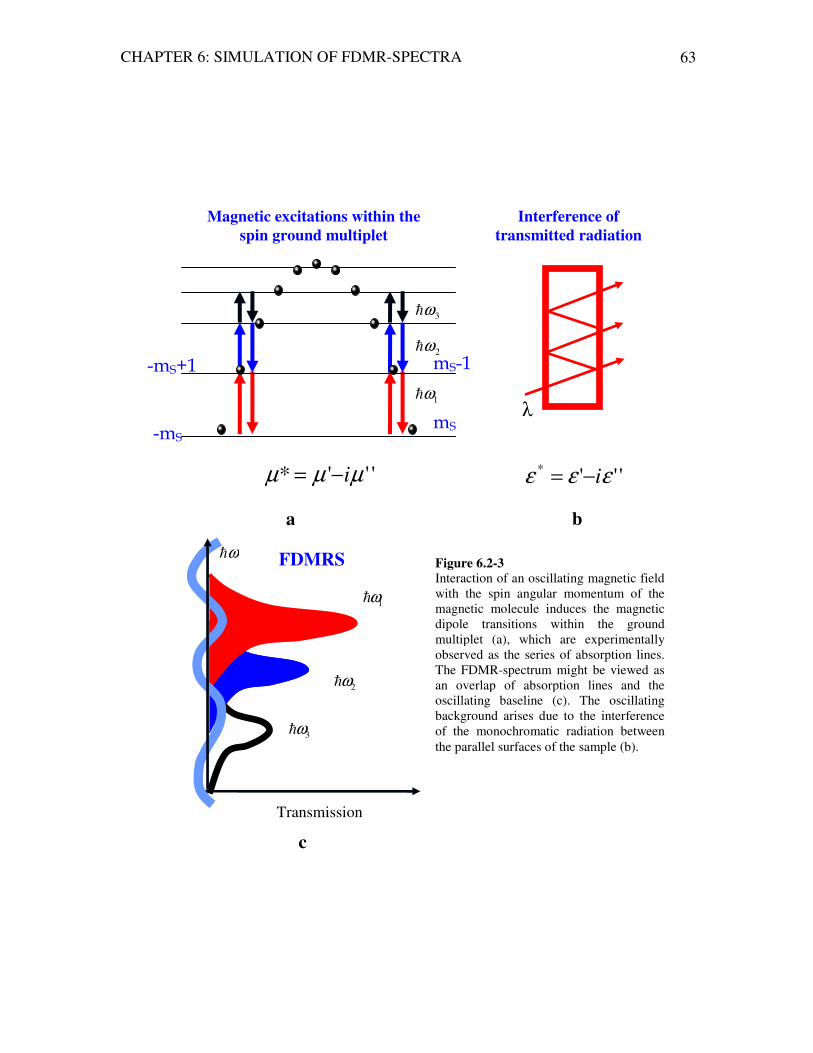
CHAPTER 6: SIMULATION OF FDMR-SPECTRA 63
mS
mS-1
Magnetic excitations within the
spin ground multiplet
-mS
-mS+1
1ωh
2ωh
3ωh
Interference of
transmitted radiation
1ωh
2ωh
3ωh
ωh
Transmission
FDMRS
'''* µµµ i−= '''* εεε i−=
Figure 6.2-3 Interaction of an oscillating magnetic field with the spin angular momentum of the magnetic molecule induces the magnetic dipole transitions within the ground multiplet (a), which are experimentally observed as the series of absorption lines. The FDMR-spectrum might be viewed as an overlap of absorption lines and the oscillating baseline (c). The oscillating background arises due to the interference of the monochromatic radiation between the parallel surfaces of the sample (b).
λ
a b
c
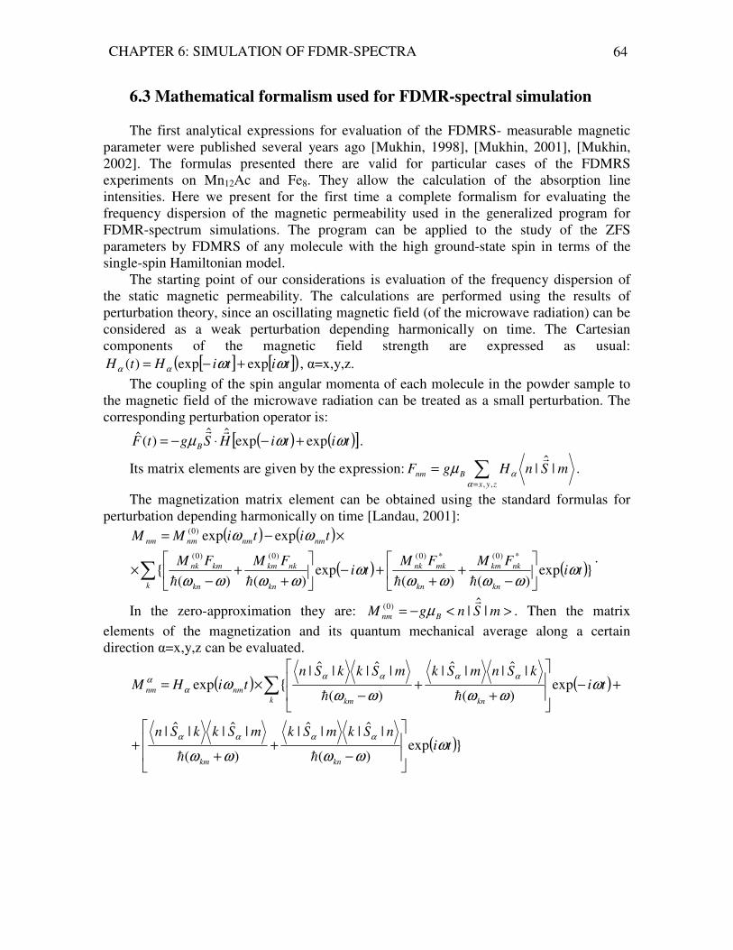
CHAPTER 6: SIMULATION OF FDMR-SPECTRA 64
6.3 Mathematical formalism used for FDMR-spectral simulation The first analytical expressions for evaluation of the FDMRS- measurable magnetic
parameter were published several years ago [Mukhin, 1998], [Mukhin, 2001], [Mukhin, 2002]. The formulas presented there are valid for particular cases of the FDMRS experiments on Mn12Ac and Fe8. They allow the calculation of the absorption line intensities. Here we present for the first time a complete formalism for evaluating the frequency dispersion of the magnetic permeability used in the generalized program for FDMR-spectrum simulations. The program can be applied to the study of the ZFS parameters by FDMRS of any molecule with the high ground-state spin in terms of the single-spin Hamiltonian model.
The starting point of our considerations is evaluation of the frequency dispersion of the static magnetic permeability. The calculations are performed using the results of perturbation theory, since an oscillating magnetic field (of the microwave radiation) can be considered as a weak perturbation depending harmonically on time. The Cartesian components of the magnetic field strength are expressed as usual:
[ ] [ ]( )titiHtH ωωαα expexp)( +−= , α=x,y,z. The coupling of the spin angular momenta of each molecule in the powder sample to
the magnetic field of the microwave radiation can be treated as a small perturbation. The corresponding perturbation operator is:
( ) ( )[ ]titiHSgtF B ωωµ expexpˆˆ)(ˆ +−⋅−=rr
.
Its matrix elements are given by the expression: ∑=
=zyx
Bnm mSnHgF,,
|ˆ|α
αµr
.
The magnetization matrix element can be obtained using the standard formulas for perturbation depending harmonically on time [Landau, 2001]:
( ) ( )
( ) ( )exp)()(
exp)()(
expexp*)0(*)0()0()0(
)0(
tiFMFM
tiFMFM
titiMM
kn
nkkm
kn
mknk
k kn
nkkm
kn
kmnk
nmnmnmnm
ωωωωω
ωωωωω
ωω
−+
++−
++
−×
×−=
∑hhhh
.
In the zero-approximation they are: ><−= mSngM Bnm |ˆ|)0(r
µ . Then the matrix elements of the magnetization and its quantum mechanical average along a certain direction α=x,y,z can be evaluated.
( ) ( )
( )exp)(
|ˆ||ˆ|
)(
|ˆ||ˆ|
exp)(
|ˆ||ˆ|
)(
|ˆ||ˆ|exp
tinSkmSkmSkkSn
tikSnmSkmSkkSn
tiHM
knkm
k knkm
nmnm
ωωωωω
ωωωωω
ω
αααα
αααα
αα
−+
++
+−
++
−×= ∑
hh
hh
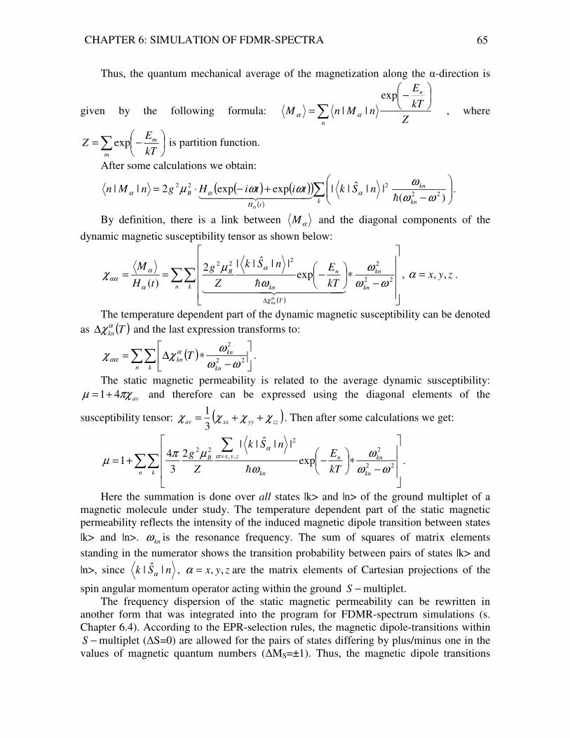
CHAPTER 6: SIMULATION OF FDMR-SPECTRA 65
Thus, the quantum mechanical average of the magnetization along the α-direction is
given by the following formula: ∑
−
=n
n
Z
kT
E
nMnM
exp|| αα , where
∑
−=
m
m
kT
EZ exp is partition function.
After some calculations we obtain:
( ) ( )( )( )
∑
−+−⋅=
k kn
kn
tH
B nSktitiHgnMn)(
||ˆ||expexp2||22
222
ωω
ωωωµ ααα
α
h4444 34444 21.
By definition, there is a link between αM and the diagonal components of the
dynamic magnetic susceptibility tensor as shown below:
( )
∑∑
−∗
−==
∆
n k kn
kn
T
n
kn
B
kn
kT
EnSk
Z
g
tH
M22
2222
exp||ˆ||2
)( ωω
ω
ω
µχ
αχ
α
α
ααα
444444 3444444 21h
, zyx ,,=α .
The temperature dependent part of the dynamic magnetic susceptibility can be denoted as ( )Tkn
αχ∆ and the last expression transforms to:
( )∑∑
−∗∆=
n k kn
kn
kn T 22
2
ωω
ωχχ α
αα .
The static magnetic permeability is related to the average dynamic susceptibility:
avπχµ 41+= and therefore can be expressed using the diagonal elements of the
susceptibility tensor: ( )zzyyxxav χχχχ ++=31
. Then after some calculations we get:
∑∑∑
−∗
−+=
=
n k kn
knn
kn
zyxB
kT
EnSk
Z
g22
2,,
2
22
exp
||ˆ||2
34
1ωω
ω
ω
µπµ α
α
h.
Here the summation is done over all states |k> and |n> of the ground multiplet of a magnetic molecule under study. The temperature dependent part of the static magnetic permeability reflects the intensity of the induced magnetic dipole transition between states |k> and |n>. knω is the resonance frequency. The sum of squares of matrix elements standing in the numerator shows the transition probability between pairs of states |k> and
|n>, since nSk |ˆ| α , zyx ,,=α are the matrix elements of Cartesian projections of the
spin angular momentum operator acting within the ground −S multiplet. The frequency dispersion of the static magnetic permeability can be rewritten in
another form that was integrated into the program for FDMR-spectrum simulations (s. Chapter 6.4). According to the EPR-selection rules, the magnetic dipole-transitions within
−S multiplet (∆S=0) are allowed for the pairs of states differing by plus/minus one in the values of magnetic quantum numbers (∆MS=±1). Thus, the magnetic dipole transitions

CHAPTER 6: SIMULATION OF FDMR-SPECTRA 66
between pairs of the states belonging to the ground multiplet of a magnetic molecule and satisfying the EPR selection rules result in a series of the absorption lines observed experimentally in FDMRS spectrum. There each absorption line is caused by transitions in two directions: from the initial state to the final one and back. Therefore it makes sense to express the intensity of the resulting absorption line in terms of the population difference of the initial and the final states. Remembering that the single EPR/FDMRS line can be simulated using the lineshape function centred at the absorption line position, we obtain the following expression for evaluation of the multi-line spectra:
( )∑∑= ∈
−∆+=N
n nif
nifnif R1
,,1 ωωµµ (6.3-1)
−−
−=∆
∑=
kT
E
kT
EiSfg
Z
N nfni
nfi
zyx
B
nif
,,
,
,,
222
0, expexp
||ˆ||
38
ω
µπ
µ αα
h (6.3-2)
here R is the lineshape function, 0N is the number of paramagnetic ions in the sample and
nif ,µ∆ is the power absorbed during the induced magnetic dipole transition expressed
through the population difference between the initial and final states. nfi ,ωh is the transition
frequency if → that contribute into the n -absorption line. Matrix elements iSf |ˆ| α ,
zyx ,,=α are calculated according to Eq.(3.2.3-1). The summation in Eq.(6.3-1) is carried out over all absorption lines observed experimentally.
We have integrated the Lorentzian and the Gaussian lineshape functions used in Eq.(6.3-1). Thus, the explicit expression for static magnetic permeability '''* µµµ i−= Eq.(6.3-1) has the form Eq.(6.3-3) for Lorentzian lineshape function and Eq.(6.3-4) for the Gaussian one.
∑∑= ∈ ∆+−
∆+=
N
n nif nnif
nifnif
i122
,
2,,1)(*
ωωωω
ωµωµ (6.3-3)
∑∑= ∈
+
−+−
−∆
=N
n nif n
nif
n
nif
n
nif
12
2,
2
2,, )
2
)(exp()
2
)(exp(
8)(''
σ
ωω
σ
ωω
σ
µπωωµ (6.3-4a)
''
)'('''21)('
022 ω
ωω
ωµω
πωµ d∫
∞
−+= (6.3-4b)
Here nω∆ and nσ are the Lorentzian and Gaussian linewidths, respectively. As soon as the analytical expression for the magnetic permeability is known, the
FDMRS spectra can be simulated using the Fresnel formulas for the transmission of a plane parallel sample [Volkov, 1985]:
)(sin4)1(
sin4)1(22
22
ψ
ψ
++−
+−=
NRERE
RRETr (6.3-5)
−=
λ
πkdE
4exp ,
λ
πndN
2= ,
22
22
)1(
)1(
ba
baR
++
+−= ,
1
2arctan
22 −+=
ba
bψ ,

CHAPTER 6: SIMULATION OF FDMR-SPECTRA 67
** µε=+ ikn , **
ε
µ=+ iba .
HereTr is the transmission coefficient, E , N , R and ψ are parameters connecting Tr to the frequency dispersion of the complex magnetic permeability *µ and the dielectric permittivity *ε . Parameters n , k , a and b were introduced additionally to underline the multilevel structure of the Eq.(6.3-5). From physical point of view, parameters n and k have meaning of the refractive index and the extinction coefficient, respectively. λ is the wavelength of microwave radiation. d is the thickness of the sample.
6.4 Description of the data flow in the program for FDMRS spectral simulation The code of the program for FDMR-spectral simulations is written using the
Mathematica language (version 5.1, http://documents.wolfram.com/). We have decided for Mathematica because it is one of the fully integrated environments for technical computing [Wolfram, 1999]. The current version of Mathematica includes a reach library of packages for specific numerical, algebraic, graphical and other tasks. One of the most important features of Mathematica is that it is an extensible system. It is always possible to add more functionality by using the Mathematica language. For many kinds of calculations the standard version of Mathematica is quite sufficient. However, the FDMRS spectral simulations are related to a particular specialized area. We have created new packages that use certain functions built into Mathematica to incorporate into the program some specific things like e.g. spin Hamiltonian. The developed FDMRS-code uses also the standard Mathematica packages listed below.
The standard package Utilities`MemoryConserve` optimizes Mathematica’s use of memory whenever memory usage increases by a specified amount. It makes faster memory-intensive calculations like those of the Kramers-Krönig integral, which are needed for the evaluation of the magnetic permeability with the Gaussian lineshape function, the calculation of the Hamiltonian matrix elements using the Wigner-Eckart theorem, the diagonalization of the Hamiltonian matrix constructed in the full Hilbert space.
The matrix diagonalization is a central point of any kind of spectral simulations. In EPR we are dealing with the energy matrix never mind how it was constructed: in terms of the single-spin or the generalized effective spin Hamiltonian models. Mathematica allows a simple matrix diagonalization since various mathematical libraries like LAPACK, UMFPACK, ARPACK are already integrated into the standard packages related to the approximate numerical linear algebra: LinearAlgebra`MatrixManipulation`.
The package NumericalMath`PolynomialFit` was used for determination of the absorption line positions automatically with high precision.
The packages of the group “Statistics” like `DataManipulation`, `DescriptiveStatistics`, `NonlinearFit` were also integrated into the FDMRS-code, since they essentially simplify the access to- and treatment of the experimental data (e.g. by the normalization of the spectra, their interpolation, mugging of the data measured in different or overlapping frequency ranges).

CHAPTER 6: SIMULATION OF FDMR-SPECTRA 68
The new created packages are listed in the Table 6.4-1 together with the description of their functionality. Here an important comment is needed. Mathematica produces an easy visualization of the analytical expressions like the calculated frequency dispersion of the magnetic permeability or transmission, the temperature dependence of the absorption line intensity. Nevertheless, the algorithms for calculations using the Lorentzian and Gaussian lineshape functions are not the same. In the case of the Lorentzian lineshape model the user sees the resulting curve without the access to the numerical values of the generated function )(* ωµ in particular points. Contrarily, the evaluation of )(* ωµ with the Gaussian lineshape function requires the calculation of the Kramers-Krönig integral that is performed from point to point by the frequency sweeping. Therefore we evaluate first the imaginary part of the magnetic permeability (absorption) as an analytical expression (package: PermeabilityImGauss). Then the resulting function is mapped into a grid in the frequency interval defined by the user. Finally the frequency dispersion of the complex magnetic permeability is calculated as an array consisting of three columns: frequency, real part- and imaginary part of *µ (package: PermeabilityGauss).
Table 6.4-1: The new developed packages for the FDMR-spectral simulations and their functionality
Package Functionality PhysConstants All physical constants and conversion factors are
gathered here that link the parameters expressed in SI and CGS systems. Usage of this package enables an automatically conversion of the data from SI to CGS and vise a versa in any point of the program.
SxSySzMatrixconstruction The matrices of operators αS , zyx ,,=α are constructed for any spin value introduced by the user
StevensOperatorMatrix Construction of the matrices ( )±SSO z
m
kˆ,ˆˆ ; currently the
matrices 44
34
04
ˆ,ˆ,ˆ OOO are integrated into the program, since they were of prime importance for the analysis of experimental data. The module can be easily extended by any other m
kO .
StevensOperatorsToEvaluate Construction of the sum:
( ) ( )
( )∑ ∑=
+
=±+
+−+
+−=Η
6,4 0
222
ˆ,ˆˆ
ˆˆ131ˆˆ
k
k
m
z
m
k
m
k
yxz
ZFS
SSOB
SSESSSD
ZeemanTerm Evaluating of the term SBg B
rr⋅− µ
EnWFFreqForGivenSHP Construction of the energy matrix for the Hamiltonian:
( )
( ) ( )∑ ∑=
+
=±+−+
+
+−+⋅−=Η
6,4 0
22
2
ˆ,ˆˆˆˆ
131ˆˆˆ
k
k
m
z
m
k
m
kyx
zB
SSOBSSE
SSSDSBgrr
µ
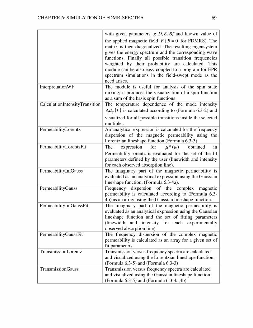
CHAPTER 6: SIMULATION OF FDMR-SPECTRA 69
with given parameters m
kBEDg ,,, and known value of
the applied magnetic field B ( 0=B for FDMRS). The matrix is then diagonalized. The resulting eigensystem gives the energy spectrum and the corresponding wave functions. Finally all possible transition frequencies weighted by their probability are calculated. This module can be also easy coupled to a program for EPR spectrum simulations in the field-swept mode as the need arises.
InterpretationWF The module is useful for analysis of the spin state mixing; it produces the visualization of a spin function as a sum of the basis spin functions
CalculationIntensityTransition The temperature dependence of the mode intensity ( )Tifµ∆ is calculated according to (Formula 6.3-2) and
visualized for all possible transitions inside the selected multiplet.
PermeabilityLorentz An analytical expression is calculated for the frequency dispersion of the magnetic permeability using the Lorentzian lineshape function (Formula 6.3-3)
PermeabilityLorentzFit The expression for )(* ωµ obtained in PermeabilityLorentz is evaluated for the set of the fit parameters defined by the user (linewidth and intensity for each observed absorption line).
PermeabilityImGauss The imaginary part of the magnetic permeability is evaluated as an analytical expression using the Gaussian lineshape function, (Formula 6.3-4a).
PermeabilityGauss Frequency dispersion of the complex magnetic permeability is calculated according to (Formula 6.3-4b) as an array using the Gaussian lineshape function.
PermeabilityImGaussFit The imaginary part of the magnetic permeability is evaluated as an analytical expression using the Gaussian lineshape function and the set of fitting parameters (linewidth and intensity for each experimentally observed absorption line)
PermeabilityGaussFit The frequency dispersion of the complex magnetic permeability is calculated as an array for a given set of fit parameters.
TransmissionLorentz Transmission versus frequency spectra are calculated and visualized using the Lorentzian lineshape function, (Formula 6.3-5) and (Formula 6.3-3)
TransmissionGauss Transmission versus frequency spectra are calculated and visualized using the Gaussian lineshape function, (Formula 6.3-5) and (Formula 6.3-4a,4b)

CHAPTER 6: SIMULATION OF FDMR-SPECTRA 70
The source code developed for FDMRS spectral simulations consists of three blocks (Figure 6.4-1).
The first block is responsible for the primary treatment of the experimental data. As
the result we obtain the exact position and the full width at a half of maximum (FWHM) of each absorption line in frequency at various temperatures. The second block performs the fitting of the spin Hamiltonian parameters to the absorption line positions. As soon as the spin Hamiltonian parameters have been determined, the transmission versus frequency
Block 1 Block 2 Block 3
Absorption line positions
Spin Hamiltonian parameters
Full width on the half of maximum for each observed line
FDMRS experiment
FDMR-spectral simulation displayed together with the
experiment
Figure 6.4-1: The source code of the program for FDMR-spectral simulations consists of three blocks. Block 1 reads out the experimental data and estimates the absorption line positions and their FWHMs. Block 2 performs the fitting of the spin Hamiltonian parameters to the absorption line positions. Block 3 displays the experimental data together with the spectral simulation obtained for the fit parameters defined by the user.

CHAPTER 6: SIMULATION OF FDMR-SPECTRA 71
spectra are evaluated and displayed together with the experimentally recorded ones (the third block). Each block is described below in the Table 6.4.-2.
Table 6.4-2: Description of each block of the program for FDMR-spectral simulations in a step-by step manner Block 1: Determination of the absorption line positions and their FWHMs
from the experiment.
• Readout of the experimental data measured at various temperatures, which are then saved in .txt files (ASCII format)
• Sorting of the experimental points frequency, transmission in increasing order of magnitude, averaging in the regions with overlapping frequencies. The data are finally saved in new files with the ending: _final.txt
• Interpolation of the prepared data ( files: “name_final.txt”) in the frequency interval selected by user
• Normalization of the spectra: a logarithmical subtraction of the baseline from all the spectra. The highest temperature spectrum is taken as the baseline.
• A high-degree polynomial fitting is performed over all the normalized spectra. The local minimum of the resulting polynomial function ( ( ) α
αα xaxP ∑= ) in
the region of resonance is automatically determined with a high precision. The x-coordinate of the found minimum gives the absorption line position on the frequency-scale. The y-coordinate of the local minimum points to the maximal intensity of the absorption line ( I ). By solving the equation ( ) 2/IxP = the full width on a half of maximum is determined. Calculation of the absorption line positions and their FWHMs is performed automatically for all the normalized spectra.
• Preparation of the output file, which contains the found values of the absorption line positions and the FWHMs. The absorption line positions are then used in the Block 2 to extract the spin Hamiltonian parameters from the experiment with maximal accuracy. The found FWHMs are used for a preliminary analysis of the linewidth temperature dependence. They are accepted to be the Lorentzian linewidth values nω∆ (, which are related to the
Gaussian ones by[ ]222 Ln
nn
⋅
∆=
ωσ ) for evaluation of )(* ωµ in zero-
approximation.
Block 2: Determination of the spin Hamiltonian parameters from the
experimental data.
• Input of the initial parameters (total spin value S , magnetic field in spherical coordinates ( ) ( )0,0,0,, =ϕϑB
8, experimentally observed absorption line positions)
• Input of the ranges for possible values of the spin Hamiltonian parameters
8 0=B . Nevertheless the spin Hamiltonian is integrated into the program in its general form including the Zeeman term. Therefore the block can be used for fitting the spin Hamiltonian parameters from swept-field EPR spectra.

CHAPTER 6: SIMULATION OF FDMR-SPECTRA 72
(SHPs) and number of points inside of each interval. Present version of the program is able to work with 5 parameters simultaneously: 4
434
04 ,,,, BBBED .
This set can be extended if necessary.
• Construction of the table D(k), E(k), B40(k), B4
3(k), B44(k) for ∏
=
=5
1~
~,...,1k
kNk ,
where k
N ~ is the number of points in k~
-interval selected by user. The
calculations become very much time consuming by increasing ofk
N ~ -values.
We recommend to choose the number of points in each interval so
that 20005
1~
~ ≤∏=k
kN , otherwise the user must wait more than one hour.
• The Hamiltonian matrix is diagonalized for each kth set of parameters D(k),
E(k), B40(k), B4
3(k), B44(k). Thus the energy eigenvalues are obtained, which
differences must coincide with the transition frequencies observed spectroscopically. The calculated transition frequencies )(calc
ifωh are weighted
by their probability 2
,,
||||∑= zyx
fSiα
α for all possible initial and final states
inside of the selected multiplet: 12...1, += Sfi . Weak transitions are omitted, which are characterized by a probability less than the value defined by user. The rest frequencies are compared with the absorption line positions. Those of
them, which satisfy the inequality: frequencycalc
if
n εω
ω<− |1|
exp
h
h (where frequencyε is
defined by user and expnωh is the experimentally observed position of n -
absorption line), are associated in the groups )(,
calc
nifωh . The experimentally
observed absorption line is approximated as an overlap of the calculated transitions with nearly coinciding frequencies. The discrepancy factor is introduced as the sum of squares of the relative deviations:
∑∈
−=
N
nifcalc
nif
calc
nifnn
NR
2
)(,
)(,
(exp))( 1
ω
ωω
h
hhfor all N transitions contributing to the n -
absorption line. Finally each kth set of SHPs is characterized by the mean
value of the relative deviations calculated for all experimentally observed
absorption lines: ∑=
=n
n
nkR
nm
~
1
)()(
~1
. The minimal value m extracted from the set
∏==
5
1~
~,...,1)(
kk
Nk
km points to the best SHPs in zero approximation.
• The best set of SHPs for a given experiment is obtained using a full grid search by subsequent narrowing the SHP-ranges around the zero-approximation. The final SHP set must reproduce the absorption line positions as well as possible.
Block 3: FDMRS spectral simulation
CHAPTER 6: SIMULATION OF FDMR-SPECTRA 73
• Readout of the experimental data from the files “name_final.txt”; input of the parameters of the sample/molecule, positions of the experimentally observed absorption lines and FWHMs resulting from Block 1 and the spin Hamiltonian parameters obtained in Block 2.
• Fitting the dielectric permittivity to the oscillating baseline is performed by visual comparison of the experiment with the simulation “transmission versus frequency” for Lorentzian lineshape model and the magnetic permeability selected as: 0'';1' == µµ . Thus, the values '',' εε are obtained. They are keept fixed for further calculations.
• The complete energy spectrum and the temperature dependence of the intensity for each absorption line ( )Tnif ,µ∆ are calculated using the introduced set of the
spin Hamiltonian parameters. • The FDMRS experiment to be fitted is selected. Temperature of the
measurements is fixed for further simulations. Thus, we have two sets of fit parameters: intensity and linewidth of each absorption line, because the absorption line positions are reproduced automatically for the known spin Hamiltonian parameters. The intensity of the observed absorption lines is calculated for the temperature of measurements. The resulting values are chosen as a zero-approximation of the fitting procedure in the “intensity”-dimension. The FWHMs introduced above give the zero-approximation of the fitting procedure in the “linewidth”-dimension.
• FDMRS spectra are calculated using the zero-approximation of the fitting parameters for Lorentzian and Gaussian linewidths, independently.
• The best fit parameters are those that satisfy three requirements. 1) The calculated transmission versus frequency spectrum (Formula 6.3-5) reproduces well the experiment by the visual comparison. 2) The resulting from fit FWHMs correlate well with the FWHM zero-approximation obtained in the Block 1 3) The spectral line intensity resulting from fit is in a good agreement with the intensity calculated according to the (Formula 6.3-2)
• The lineshape function model is selected that gives a best conformance with the experiment. The obtained temperature dependence of the linewidth enables a further analysis of the mechanisms of spectral line broadening.
In the next chapter we present the application of the program to the analysis of the FDMRS experiments on some molecules with non-compensated ground spin value.

VII
Zero-Field Splittings (ZFSs) of molecular
magnets studies by FDMRS
The computer code presented in the previous chapter was successfully applied to the ZFS-studies by FDMRS on several molecular magnets. Some of them are presented in this chapter: the one-electron reduced Mn12: (PPh4)[Mn12O12(O2CEt)16(H2O)4], one member of the Mn9-class: [Mn9O7(OAc)11(thme)(py)3(H2O)2], the molecule [Ni-(HIM2-py)2NO3]NO3, which is a possible building block of single-molecule magnets and the tetrameric Ni4 = [Ni4(MeOH)4L4] cluster that does not show the SMM-behavior in spite of the high ground-state spin value and the negative axial magnetic anisotropy.
7.1 ZFSs of (PPh4)[Mn12O12(O2CEt)16(H2O)4]
Introduction. The first and the most carefully investigated single molecular magnet is [Mn12O12(O2CCH3)16(H2O)]·4H2O·2HO2CCH3 called Mn12Ac (see Chapter 2). Studies on Mn12Ac have motivated the search for some new single molecule magnets in the group of dodecanuclear manganese complexes. Work within the area of Mn12 coordination chemistry has led to the development of methods for major alteration of the chemical environment of the Mn12 core. Various PPh4
+ derivatives of the Mn12Ac cluster were obtained recently. One of them is the MnIV
4MnIII7MnII valence trapped salt of
(PPh4)[Mn12O12(O2CEt)16(H2O)4] noted in the following as compound 1. Here PPh4 plays a role of donating an electron to the Mn12 molecule; so the Mn12 molecule becomes anionic compared to the well-known Mn12-acetate. The synthesis, the molecular structure and magnetization relaxation behavior of this complex were described already ten years ago [Eppley, 1995], but the spin Hamiltonian parameters were not well known. A ferrimagnetic ground state with the half integer value (S=19/2) and g=1.96 was derived from the temperature dependence of the solid-state dc magnetic susceptibility. This fact caused an additional interest in this half-integer spin complex, because the spin parity effect forbids magnetization quantum tunneling in zero magnetic fields. Nevertheless, the presence of steps in the magnetization hysteresis loops was reported [Aubin, 1999]. The work presented here gives information complementary to the studies of ZFS’s in various one-electron reduced Mn12 complexes published in the literature. Results and analysis. FDMRS-Spectra were recorded on a polycrystalline powder pellet (mass=0.4857 g, thickness = 0.3449 cm; diameter = 1 cm) of compound 1 using linearly polarized radiation in the frequency range 2.3…12.5 cm-1 at temperatures 1.8…30 K in absence of an external magnetic field. The normalized FDMRS-spectra are summarized in the Figure 7.1-1. Six absorption lines were observed in the experiment, with the lowest frequency one being much more weakly than the other ones. They are located at 7.65, 7.04, 6.31, 5.41, 4.71, 3.8 cm-1, respectively.

CHAPTER 7: ZFSs OF MOLECULAR MAGNETS STUDIED BY FDMRS 75
A simple estimation of the axial ZFS-parameters was performed according to the
formula[ ]22
exp
)1( −−=
nn
n
nMM
Dωh . Here exp
nωh are the spectral line positions associated to the
transitions between the states 1−→ nn MM . Thus the possible D-values were found to
lie inside the interval -0.475…-0.425 cm-1 with the corresponding transverse ZFSs restricted by 158.00 ≤≤ E cm-1. The best agreement with the experiment was achieved by fitting with the single-spin model Hamiltonian acting on the spin ground state with S=19/2 shown below:
04
04
2 ˆ)1(31ˆ OBSSSDH Z
ZFS +
+−⋅= (7.1-1).
Contrary to the case of Mn12Ac, introduction of transverse terms into the above Hamiltonian does not improve the fit. The resulting ZFS parameters are D=-0.454±0.003 cm-1 and B4
0=(+1.01±0.25)x10-5 cm-1. This estimate provides a very good description of all six observed absorption lines with the resulting mean relative deviation m=7.60769*10-5 (see Table 7.1-1). Figure 7.1-2 illustrates formation of the FDMRS spectrum as a series of absorption lines caused by magnetic dipole transitions inside of the spin ground multiplet restricted by the selection rule 1±=∆ SM .
Figure 7.1-1 Normalized FDMRS spectra measured on 1 at various temperatures with the six absorption lines indicated.
3.0 3.5 4.0 4.5 5.0 5.5 6.0 6.5 7.0 7.5 8.0 8.5 9.0
-1.6
-1.4
-1.2
-1.0
-0.8
-0.6
-0.4
-0.2
0.0
0.2
0.4
6: 3.8 5: 4.71 4: 5.41 3: 6.31
2: 7.041: 7.65
Tra
nsm
issio
n (
a.u
)
Wave number (cm-1)
(2-30)K
(5-30)K
(10-30)K
(15-30)K
(20-30)K

CHAPTER 7: ZFSs OF MOLECULAR MAGNETS STUDIED BY FDMRS 76
Table 7.1-1 Comparison of the observed absorption line positions with the calculated ones predicted by the single-spin Hamiltonian model (Formula 7.1-1) with D=-0.454 cm-1 and B4
0 = +1.01x10⁻⁵ cm-1, respectively.
Nr. absorption
line
Transition
between states
Calculated
resonance frequency [cm-1]
Experimentally
observed position of absorption line [cm-1]
Relative deviations
1
217
219
±→± 7.66655 7.65 4.67*10-6
2
215
217
±→± 7.00777 7.04 2.09*10-5
3
213
215
±→± 6.28086 6.31 2.13*10-5
4
211
213
±→± 5.49432 5.41 2.42*10-4
5
29
211
±→± 4.65668 4.71 1.28*10-4
6
27
29
±→± 3.77645 3.8 3.84*10-5
Mean relative deviation 7.60769*10-5
Figure 7.1-2 The energy diagram calculated using the single-spin Hamiltonian model Eq.(7.1-1) and ZFSs extracted from the FDMRS experiment on the compound 1 (black points). Arrows indicate the magnetic dipole transitions between the spin microstates that constitute six experimentally observed spectral lines.
-17/2-13/2 -9/2 -5/2 -1/2 3/2 7/2 11/2 15/2 19/2-30
-20
-10
0
10
20
6: 3.8
5: 4.71
4: 5.41
3: 6.31
2: 7.04
En
erg
y (
cm
-1)
1: 7.65
2zS
2
19±
217
±
215
±
213
±
211
±
29
±
2
7±

CHAPTER 7: ZFSs OF MOLECULAR MAGNETS STUDIED BY FDMRS 77
The ZFS parameters were studied recently in several one-electron reduced Mn12 compounds with different ligands: ((PPh4)[Mn12O12(O2CEt)16(H2O)4] denoted below as 1 and (PPh4)[Mn12O12(O2CCHCl2)16(H2O)4] noted as 2) by various experimental methods like reduced magnetization, HF-EPR, DC susceptibility and INS. Table 7.1-2 summarizes the published results. Zero field techniques (FDMRS and INS) indicate the non-zero axial ZFS’s of the fourth order, whereas the HFEPR measurements point to the axial ZFS’s with the remark: “inclusion of the B4
0 term does not lead to improvement of the least square fit of the HFEPR data” [Aubin, 1999]. A discrepancy factor (defined in Chapter 6.4) of 10-2 was obtained by fitting the FDMRS spectra using only the D term. Inclusion of the axial quadratic zero field term led to a three order of magnitude reduction of this value down to 10-5. The compound 1 was studied by FDMRS and HF-EPR with the approximately the same resulting D-parameters: -0.453 versus -0.4 cm-1, respectively. It is a little bit less than the axial ZFS of the neutral Mn12Ac (there D = -0.47 cm-1 [Sessoli, 2003]). This fact serves as an experimental proof of the idea discussed in [Basler, 2005] that the added electron decreases the axial anisotropy parameter D. The decrease of the cluster anisotropy was explained by the decrease in number of Mn3+ from eight in the neutral Mn12Ac molecule to seven in the samples 1 and 2. Converting a Mn3+ to a Mn2+ ion effectively quenches the single-ion anisotropy in this site, leading to a decrease of the cluster anisotropy.
Notably, the B40 parameters obtained in the compounds 1 and 2 by FDMRS and INS
have the same order of magnitude, but opposite signs. The B40 parameter extracted from
the FDMRS done for 1 gives a lower (compared to INS) discrepancy factor (s. Table 7.1-2).
Since the spin Hamiltonian describing the compound 1 contains no transverse terms,
the states with opposite spin orientations are degenerate. Contrary to the Mn12Ac where ground state magnetization quantum tunneling (MQT) is allowed by the cluster symmetry, the mechanism of tunneling in the one-electron reduced Mn12 compounds must have another origin. It is probably connected with the presence in each molecule of effective internal magnetic fields due to the nuclear spins on the Mn atoms or the dipolar
Table 7.1-2 Comparison of the zero-field splitting parameters in two one-electron reduced Mn12 complexes studied by different experimental methods. Here (PPh4)[Mn12O12(O2CEt)16(H2O)4] is noted 1, (PPh4)[Mn12O12(O2CCHCl2)16(H2O)4] is noted 2.
Complex D [cm-1] B40[cm-1] χ
2 Experimental
technique
Publication
1 -0.453 +1.014·10-5 7.6*10-5 FDMRS [Kirchner, 2005]
1 +0.4 - - reduced magnetization
[Eppley, 1995]
1 -0.4 - - HFEPR [Aubin, 1999]
2 -0.34 - - DC magnetic susceptibility
[Soler, 2003]
-0.368 -1.59*10-5 4*10-4 2 -0.332 -1.8*10-5 3.8*10-3
INS [Basler, 2005]

CHAPTER 7: ZFSs OF MOLECULAR MAGNETS STUDIED BY FDMRS 78
interactions. To prove these versions additional experiments are required. The FDMRS-spectra of the one-electron reduced Mn12 sample (compound 1) were better simulated using a Lorentzian lineshape function (see Figure 7.1-3a), while the FDMRS experiment on the neutral Mn12Ac was reproduced using a Gaussian one [Mukhin, 2002]. An analysis of the EPR-linewidth temperature dependence is usually performed to study the relaxation processes and mechanisms of the spectral line broadening in the high-spin molecules. It is generally a difficult task in the case of the FDMRS, since the spectral linewidth can only be estimated with a relatively low precision. The reason is twofold. The FDMRS spectra are very much sensitive to the standing waves in the cryostat that lead to the broad distribution of the output signal on the intensity-scale, i.e. to measurement artefacts in the spectrum (s. Figure 7.1-3b). The magnitude of the error introduced into the FWHM-estimation depends on the quality of the experiment. This value is about 0.05 cm-1 in the case of the experiment on compound 1. Secondly, the intensity of the spectral lines becomes weaker and weaker with increasing temperature as it is illustrated in the Figure 7.1-3c. This is the result of the Boltzman distribution for populations of the energy levels. If the intensity of the absorption line is comparable to the amplitude of the baseline oscillations than the linewidth analysis becomes impossible. Table 7.1-3 summarizes the resulting FWHM-values and the Lorentzian linewidths that were obtained by simulation of the experimental spectra.
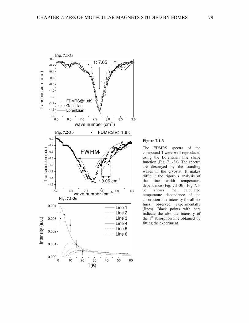
CHAPTER 7: ZFSs OF MOLECULAR MAGNETS STUDIED BY FDMRS 79
6.0 6.5 7.0 7.5 8.0 8.5 9.0-1.8
-1.6
-1.4
-1.2
-1.0
-0.8
-0.6
-0.4
-0.2
0.0
Tra
nsm
issio
n (
a.u
.)
wave number (cm-1)
Gaussian
Lorentzian
1: 7.65
0 10 20 30 40 50 600.000
0.001
0.002
0.003
0.004
Inte
nsity (
a.u
.)
T(K)
Line 1
Line 2
Line 3
Line 4
Line 5
Line 6
7.2 7.4 7.6 7.8 8.0 8.2
-1.6
-1.4
-1.2
-1.0
-0.8
-0.6
-0.4
-0.2
FDMRS @ 1.8K
Tra
nsm
issio
n (
a.u
)
wave number (cm-1
)
FWHM
~0.06 cm-1
Fig. 7.1-3a
Fig. 7.2-3b
Fig. 7.1-3c
Figure 7.1-3
The FDMRS spectra of the compound 1 were well reproduced using the Lorentzian line shape function (Fig. 7.1-3a). The spectra are destroyed by the standing waves in the cryostat. It makes difficult the rigorous analysis of the line width temperature dependence (Fig. 7.1-3b). Fig 7.1-3c shows the calculated temperature dependence of the absorption line intensity for all six lines observed experimentally (lines). Black points with bars indicate the absolute intensity of the 1st absorption line obtained by fitting the experiment.
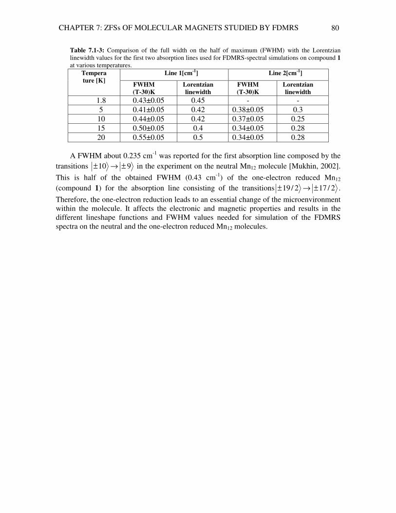
CHAPTER 7: ZFSs OF MOLECULAR MAGNETS STUDIED BY FDMRS 80
Table 7.1-3: Comparison of the full width on the half of maximum (FWHM) with the Lorentzian linewidth values for the first two absorption lines used for FDMRS-spectral simulations on compound 1 at various temperatures.
Line 1[cm-1] Line 2[cm-1] Tempera
ture [K] FWHM
(T-30)K
Lorentzian
linewidth
FWHM
(T-30)K
Lorentzian
linewidth
1.8 0.43±0.05 0.45 - - 5 0.41±0.05 0.42 0.38±0.05 0.3
10 0.44±0.05 0.42 0.37±0.05 0.25 15 0.50±0.05 0.4 0.34±0.05 0.28 20 0.55±0.05 0.5 0.34±0.05 0.28
A FWHM about 0.235 cm-1 was reported for the first absorption line composed by the
transitions 910 ±→± in the experiment on the neutral Mn12 molecule [Mukhin, 2002].
This is half of the obtained FWHM (0.43 cm-1) of the one-electron reduced Mn12 (compound 1) for the absorption line consisting of the transitions 2/172/19 ±→± .
Therefore, the one-electron reduction leads to an essential change of the microenvironment within the molecule. It affects the electronic and magnetic properties and results in the different lineshape functions and FWHM values needed for simulation of the FDMRS spectra on the neutral and the one-electron reduced Mn12 molecules.
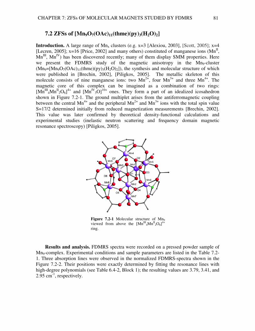
CHAPTER 7: ZFSs OF MOLECULAR MAGNETS STUDIED BY FDMRS 81
7.2 ZFSs of [Mn9O7(OAc)11(thme)(py)3(H2O)2]
Introduction. A large range of Mnx clusters (e.g. x=3 [Alexiou, 2003], [Scott, 2005]; x=4 [Lecren, 2005]; x=16 [Price, 2002] and many others) constituted of manganese ions (MnII, MnIII, MnIV) has been discovered recently; many of them display SMM properties. Here we present the FDMRS study of the magnetic anisotropy in the Mn9-cluster (Mn9=[Mn9O7(OAc)11(thme)(py)3(H2O)2]), the synthesis and molecular structure of which were published in [Brechin, 2002], [Piligkos, 2005]. The metallic skeleton of this molecule consists of nine manganese ions: two Mn2+, four Mn3+ and three Mn4+. The magnetic core of this complex can be imagined as a combination of two rings: [MnIII
4MnII2O6]
4+ and [MnIV3O]10+ ones. They form a part of an idealized icosahedron
shown in Figure 7.2-1. The ground multiplet arises from the antiferromagnetic coupling between the central Mn4+ and the peripheral Mn2+ and Mn3+ ions with the total spin value S=17/2 determined initially from reduced magnetization measurements [Brechin, 2002]. This value was later confirmed by theoretical density-functional calculations and experimental studies (inelastic neutron scattering and frequency domain magnetic resonance spectroscopy) [Piligkos, 2005].
Results and analysis. FDMRS spectra were recorded on a pressed powder sample of
Mn9-complex. Experimental conditions and sample parameters are listed in the Table 7.2-1. Three absorption lines were observed in the normalized FDMRS-spectra shown in the Figure 7.2-2. Their positions were exactly determined by fitting the resonance lines with high-degree polynomials (see Table 6.4-2, Block 1); the resulting values are 3.79, 3.41, and 2.95 cm-1, respectively.
Figure 7.2-1 Molecular structure of Mn9 viewed from above the [MnIII
4MnII2O6]
4+ ring.

CHAPTER 7: ZFSs OF MOLECULAR MAGNETS STUDIED BY FDMRS 82
Table 7.2-1 Parameters of the sample and conditions of the FDMRS experiment on Mn9-complex
Sample
mass 0.17916 g thickness 0.1456 cm diameter 1 cm
Experimental setup
Radiation/ frequency range
Linearly polarized/ 2.8-5.0 cm-1
Temperatures 1.8-30 K
3.0 3.5 4.010
-1
100
2.8 3.0 3.2 3.4 3.6 3.8 4.0 4.2
10-1
100
Tra
nsm
issio
n r
atio
Frequency (cm-1)
T = 1.8 K
T = 5.0 K
T = 10 K
Tra
nsm
issio
n
Figure 7.2-2 Normalized FDMRS-spectra on Mn9-complex measured at various temperatures indicate three absorption lines at 3.79, 3.41, and 2.95 cm-1, respectively. The inset shows the non-normalized FDMRS spectrum at 1.8K together with the simulations assuming Gaussian (solid line) and Lorentzian (dotted line) line shape functions

CHAPTER 7: ZFSs OF MOLECULAR MAGNETS STUDIED BY FDMRS 83
The spectra were treated in terms of the effective single-spin Hamiltonian model applied to the ground multiplet with the total spin value S=17/2. The observed resonances correspond to the magnetic dipole transitions between pairs of the states ( )1;; −±→± SS MSMS αα , where S=17/2, MS=17/2, 15/2 and 13/2, and α denotes
additional quantum numbers. The best agreement with the experiment was obtained by using the Eq. (7.2-1)
04
04
2 ˆ)1(31
OBSSSDH Z
ZFS +
+−⋅= (7.2-1).
The negative sign of the axial zero-field splitting parameter D was immediately defined from the fact that the highest frequency resonance line has highest intensity at lowest temperatures. A number of the single-spin Hamiltonian models with various adjustable parameters were tested. The quality of the fit was characterized by the minimal discrepancy factor resulting by comparing of the experimentally observed absorption line positions with the calculated ones (s. Table 6.4-2, Block 2). Nearly the same discrepancy factors were obtained by fitting the experiment to the ZFS-Hamiltonian including only the axial ZFS-term and both (axial and transverse) ZFS terms with a negligible resulting E-parameter about 10-2 cm-1. An essential improvement of the fit was achieved with help of the model that contains the axial ZFSs and 0
404 OB term, i.e. Eq.(7.2-1). Adding transverse
anisotropy in fourth order (i.e. the term 34
34OB allowed by trigonal symmetry) also did not
improve the fit. Finally, the best adjustable parameters were determined to be D = -0.247±0.005 cm-1 and B4
0 = (+4.6±0.1)×10-6 cm-1 (s. Table 7.2-2). Therefore the system is an easy-axis system with a magnetic anisotropy barrier of about 18 cm-1 (or 26 K).
Finally, we would like to stress here that the ZFS parameters extracted from the FDMRS experiment on the Mn9-cluster are in excellent agreement with the outcome of other magnetic studies using the inelastic neutron scattering, bulk and single-crystal measurements, and theoretical density functional calculations (see Table 7.2-3).

CHAPTER 7: ZFSs OF MOLECULAR MAGNETS STUDIED BY FDMRS 84
Table 7.2-2 FDMRS experiment on the Mn9-complex: comparing the observed absorption line positions and the calculated ones resulting from the effective single-spin Hamiltonian model with the adjustable parameters D=-0.247 cm-1 and B4
0 = =+4.6×10⁻⁶ cm-1.
Nr.
absorption
line
Transition between states
( )1−±→± SS MM
Calculated
resonance
frequency
[cm-1]
Experimentally
observed
absorption line
position [cm-1]
Relative
deviations
1
215
217
±→± 3.79744 3.79 3.85*10-6
2
213
215
±→± 3.39038 3.41 3.3*10-5
3
211
213
±→± 2.95627 2.95 4.52*10-6
Mean relative deviation 1.38*10-5
Table 7.2-3 Comparison of the ZFS parameters obtained by FDMRS, INS, Reduced Magnetization versus H/T Measurements and single-crystal measurements on Mn9-complex ZFS
[cm-1]
FDMRS INS magnetization µ-SQUID DFT
D -0.247±0.005 -0.249(5) -0.29(3) -0.258 -0.235 B4
0 (+4.6±0.1)×10-6 +7.4×10⁻⁶

CHAPTER 7: ZFSs OF MOLECULAR MAGNETS STUDIED BY FDMRS 85
7.3 ZFSs of [Ni-(HIM2-py)2NO3]NO39
Introduction. High magnetic anisotropy of a uniaxial type in the spin ground
multiplet is a prerequisite for single-magnet behavior in exchange-coupled systems. There are several physical mechanisms that change the magnitude of the experimentally observed ZFSs in high-nuclearity spin clusters. One of them is the single-ion anisotropy. Even in the case of compounds with the spin centers arising from identical ions substituted into intermediate ligand fields of the same symmetry, the principal axes of the single-ion D-tensors may have a space orientation differing from the cluster D-tensor. Thus, the different spin sites characterized by equal single-ion ZFS parameters produce different contributions to the cluster magnetic anisotropy. There the magnitude of the single-ion contribution for a given site depends on the total molecular symmetry. The search for the mononuclear complexes acting as building blocks of single-molecule magnets is a current task of synthesic chemistry. Transition metal ions (e.g. NiII, MnII, MnIII, MnIV, FeIII) have high spin-ground states in intermediate ligand fields and therefore are frequently used for this end. The ZFS studies on isolated ions listed above help to design the high-nuclearity complexes with a desired magnetic anisotropy. FDMRS was applied to investigate the zero-field splittings of a mononuclear complex [Ni-(HIM2-py)2NO3]NO3, of which the molecular structure is shown in Figure 7.3-1.
9 HIM2-py: 2-(2-pyridyl)-4,4,5,5-tetramethyl-4,5-dihydro-1H-imidazolyl-1-hydroxy
Figure 7.3-1 Molecular structure of [Ni-(HIM2-py)2 NO3]NO3

CHAPTER 7: ZFSs OF MOLECULAR MAGNETS STUDIED BY FDMRS 86
Results and analysis. FDMRS spectra were recorded on a powder pellet of the [Ni-(HIM2-py)2 NO3]NO3 complex under conditions listed in the Table 7.3-1. The spin center of this compound arises due to octahedrally coordinated Ni(II) (d8)-ion. The ground state of each Ni(II) ion is the orbital F-state with L=3 and S=1, [Abragam, 1970]. In nearly octahedral crystal field each F-state is split into ground spin triplet state ( 2Γ , S=1)
and two exited orbital states ( 5Γ and 4Γ ) with fictitious orbital momentum L=1 as shown in Figure 7.3-2. The contribution from exited orbital states to the energy spectrum is usually
omitted in the explanation of the experimental data, since the states ( 5Γ and 4Γ ) are lying
much above the 2Γ state. The isolated NiII ion in octahedral ligand field gives rise to a ground state with the total spin value S=1, see Figure 7.3-2. Therefore only two magnetic resonance modes were expected by studying the magnetic excitations in this triplet using FDMRS. In fact, magnetic dipole transitions are restricted by the selection rule 1±=∆ SM ,
so that only two are allowed for S=1: 0;1; SS → and 0;1; SS →− with the
corresponding transition frequencies |D|+E and |D|-E. Nevertheless, the FDMRS spectra shown in Figure 7.3-3 indicate one absorption line. A slight asymmetry of the absorption line was observed at the lowest temperatures. It originates from the overlap of two modes with the experimentally distinguishable transition frequencies (ν1=10.3±0.01 cm-1 and ν2=9.7±0.01 cm-1) and different intensities.
The experimental data were analyzed in terms of the standard ZFS Hamiltonian model
( ) ( )222 ˆˆ131ˆˆ
yxz
ZFSSSESSSD −+
+−=Η leading to the following parameters: D=-10.0±0.01
cm-1 and E=0.3±0.01 cm-1. These results are in a very good agreement (within 10 %) with those found from the field-dependent magnetization- and HF-EPR measurements, which were confirmed theoretically by ZFS calculations based on the angular overlap model (Table 7.3-2).
Table 7.3-1 Parameters of the sample and conditions of the FDMRS experiment on [Ni-(HIM2-py)2 NO3]NO3 complex
Sample
mass 0.155 g thickness 0.182 cm diameter 1 cm
Experimental setup
Radiation/ in the frequency range
Linearly polarized/ 6-18 cm-1
Temperatures 1.8-60 K
Table 7.3-2 Comparison of the ZFS parameters [cm-1] obtained by FDMRS, field-dependent magnetization-, HF-EPR measurements and AOM calculations on [Ni-(HIM2-py)2 NO3]NO3 complex [Rogez, 2005] ZFS
[cm-1]
FDMRS Magne-
tization
HF-
EPR
AOM
D -10.00±0.01 -11.2 -10.15 -10.1 E/|D| ~0.03 0 0.01 0.1

CHAPTER 7: ZFSs OF MOLECULAR MAGNETS STUDIED BY FDMRS 87
8 9 10 11 12
-0.35
-0.30
-0.25
-0.20
-0.15
-0.10
-0.05
0.00
0.05
T=60 K
T=7 K
T=2 K
9.7 cm-1
Lo
g1
0 (
Tra
nsm
issio
n)
Frequency (cm-1)
10.3 cm-1
Figure 7.3-3 FDMRS-spectra on [Ni-(HIM2-py)2 NO3]NO3-complex at various temperatures are shown (points: experiment, solid lines: simulations). The spectra were simulated using the Gaussian line shape function for the ZFS Hamiltonian with the parameters: D=-10.0 cm-1 and E=0.3 cm-1.
|1,0>
|1,+1>
|1,-1> |D|+E
|D|-E
F
S=1,L=3
S=1
Γ2
Γ5
Γ4
Figure 7.3-2 Splitting of the triplet orbital state of a Ni(II) ion with d8-electronic configuration in octahedral crystal field. The triplet Γ2 was studied by FDMRS, where two magnetic resonance modes were expected.
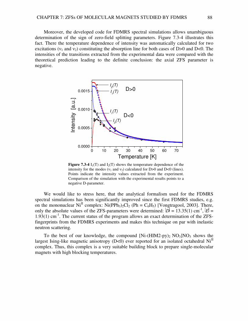
CHAPTER 7: ZFSs OF MOLECULAR MAGNETS STUDIED BY FDMRS 88
Moreover, the developed code for FDMRS spectral simulations allows unambiguous determination of the sign of zero-field splitting parameters. Figure 7.3-4 illustrates this fact. There the temperature dependence of intensity was automatically calculated for two excitations (ν1 and ν2) constituting the absorption line for both cases of D>0 and D<0. The intensities of the transitions extracted from the experimental data were compared with the theoretical prediction leading to the definite conclusion: the axial ZFS parameter is negative.
We would like to stress here, that the analytical formalism used for the FDMRS spectral simulations has been significantly improved since the first FDMRS studies, e.g. on the mononuclear NiII complex: Ni(PPh3)2Cl2 (Ph = C6H5) [Vongtragool, 2003]. There, only the absolute values of the ZFS-parameters were determined: D = 13.35(1) cm-1, E = 1.93(1) cm-1. The current status of the program allows an exact determination of the ZFS-fingerprints from the FDMRS experiments and makes this technique on par with inelastic neutron scattering.
To the best of our knowledge, the compound [Ni-(HIM2-py)2 NO3]NO3 shows the largest Ising-like magnetic anisotropy (D<0) ever reported for an isolated octahedral NiII complex. Thus, this complex is a very suitable building block to prepare single-molecular magnets with high blocking temperatures.
0 10 20 30 40 50 60 700.0000
0.0005
0.0010
0.0015
D<0I1(T)
I1(T)
I2(T)
Inte
nsity [a
.u.]
Temperature [K]
I2(T)
D>0
Figure 7.3-4 I1(T) and I2(T) shows the temperature dependence of the intensity for the modes (ν1 and ν2) calculated for D>0 and D<0 (lines). Points indicate the intensity values extracted from the experiment. Comparison of the simulation with the experimental results points to a negative D-parameter.

CHAPTER 7: ZFSs OF MOLECULAR MAGNETS STUDIED BY FDMRS 89
7.4 ZFSs of [Ni4(MeOH)4L4] 10
Introduction. Since early 90s the transition-metal complexes consisting of four NiII
ions were of interest in scientific community. Thus, in [Mlynarski, 1991] the Ni4 cluster was chosen as a model to study the electronic properties of transition-metal surfaces using different versions of the density-functional method of calculations. Later the melting behavior of Ni4 clusters (i.e., the solid-to-liquid phase transition) was studied theoretically by molecular dynamics and Monte-Carlo simulations [Güven, 1999]. A variety of publications on Ni4 clusters has appeared in literature since discovery of the specific quantum properties of single molecular magnets (s. e.g. [Karmakar, 2002], [Nakano, 2002], [Yang, 2003], [Aromi, 2003], [Moragues-Canovas, 2004], [del Barco, 2004]). These studies are devoted usually to the synthesis, structure and investigation of magnetic phenomena in various tetrameric NiII clusters, which are arranged under different geometries and contain different kinds of ligands.
In this section we present the FDMRS experiment on the Ni4-cluster of the complex [Ni4(MeOH)4L4]. The molecular structure of this compound is shown in Figure 7.4-1; it was precisely described in [Sieber, 2005].The cluster symmetry is slightly distorted from the S4 symmetry. The magnetic subsystem of this compound consists of four Ni(II) ions leading to the formation of a spin ground state with a total spin value S=4. The complex [Ni4(MeOH)4L4] is of high interest, since the whole family of the similar Ni4 compounds containing the ethyl and methyl groups as ligands have shown single magnet behavior [Edwards, 2003], only the complex under study does not show it down to 40mK.
10 L = salicylidene - 2 - ethanolamine
Figure 7.4-1 Molecular structure of the [Ni4(MeOH)4L4] complex

CHAPTER 7: ZFSs OF MOLECULAR MAGNETS STUDIED BY FDMRS 90
Results and analysis. FDMRS spectra were recorded on the complex [Ni4(MeOH)4L4] in powder form (Table 7.4-1.)
The experiment was well explained in terms of single-spin Hamiltonian acting on the
spin ground state with the total spin value S=4:
( ) ( ) 44
44
04
04
222 ˆˆˆˆ131ˆˆ OBOBSSESSSD yxz
ZFS ++−+
+−=Η (7.4-1).
The axial D and B40 terms of the model split the ground multiplet in the set of five
degenerate levels: SMS ±, , where S=4, MS=0,1,…,4. The E-term, not expected in view of
thes S4 symmetry, removes degeneracy of the states 1,±S . Due to the B44 term, the
eigenstates of the ground manifold represent the symmetric
( )SSSS MSMSMS −++= ,,2
1, and antisymmetric
( )SSAS MSMSMS −−+= ,,2
1, linear combinations of the respective MS functions.
On the basis of the 1±=∆ SM selection rule, nine transitions were expected within the S=4 ground state in the FDMRS and Inelastic Neutron Scattering (INS) spectra. Three of them were observed in the FDMRS (see Figure 7.4-2) and eight in the INS experiment (see Figure 8.1-1 and [Sieber, 2005]).
Table 7.4-1 Parameters of the sample and conditions of the FDMRS experiment on [Ni4(MeOH)4L4] complex
Sample
mass 0.31364 g thickness 0.2792 cm diameter 1 cm
Experimental setup
Radiation / in the frequency range
Linearly polarized / 2-8 cm-1
Temperatures 1.8-30 K

CHAPTER 7: ZFSs OF MOLECULAR MAGNETS STUDIED BY FDMRS 91
3 4 5 6 7 8
-1.5
-1.0
-0.5
0.0I
Lo
g1
0[T
ran
sm
issio
n]
Frequency [cm-1]
(1.8-30)K
(5-30)K
(10-30)K
(20-30)K
III II
Figure 7.4-2 The normalized FDMRS spectra taken at various temperatures indicate three absorption lines (I,II,III) located at 7.33, 4.79 and 3.99 cm-1, respectively
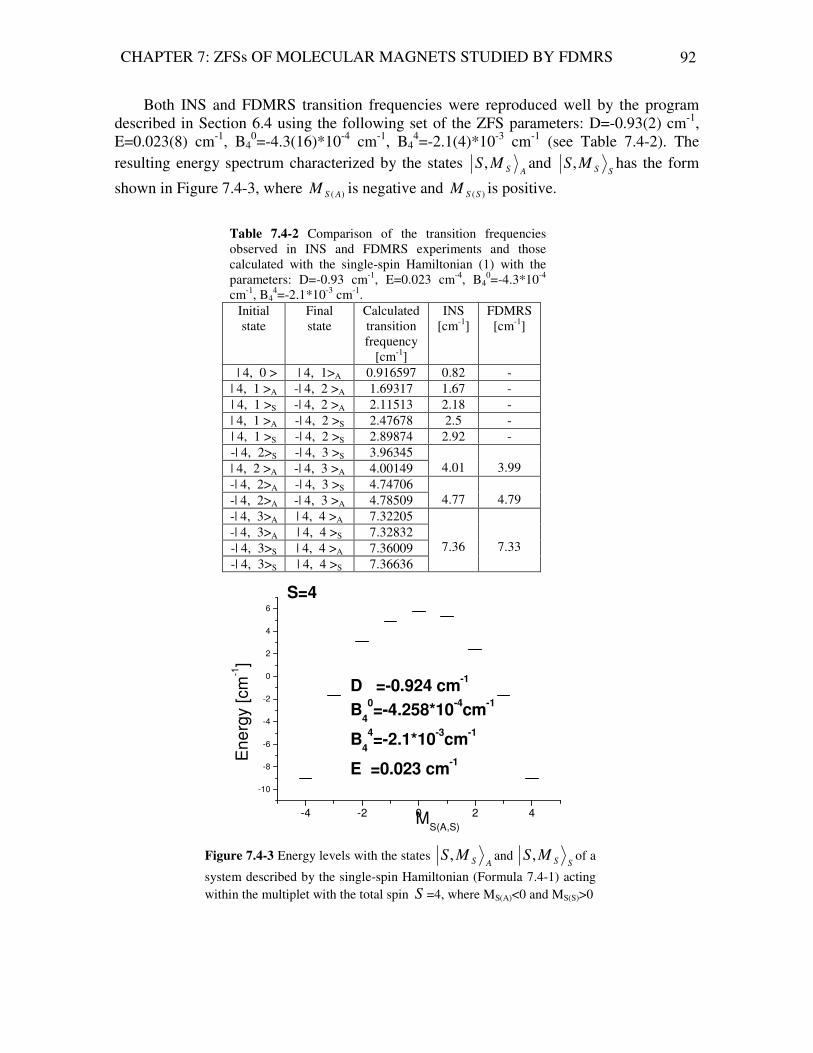
CHAPTER 7: ZFSs OF MOLECULAR MAGNETS STUDIED BY FDMRS 92
Both INS and FDMRS transition frequencies were reproduced well by the program described in Section 6.4 using the following set of the ZFS parameters: D=-0.93(2) cm-1, E=0.023(8) cm-1, B4
0=-4.3(16)*10-4 cm-1, B44=-2.1(4)*10-3 cm-1 (see Table 7.4-2). The
resulting energy spectrum characterized by the states ASMS, and
SSMS, has the form
shown in Figure 7.4-3, where )( ASM is negative and )(SSM is positive.
Table 7.4-2 Comparison of the transition frequencies observed in INS and FDMRS experiments and those calculated with the single-spin Hamiltonian (1) with the parameters: D=-0.93 cm-1, E=0.023 cm-4, B4
0=-4.3*10-4 cm-1, B4
4=-2.1*10-3 cm-1. Initial state
Final state
Calculated transition frequency
[cm-1]
INS [cm-1]
FDMRS [cm-1]
| 4, 0 > | 4, 1>A 0.916597 0.82 - | 4, 1 >A -| 4, 2 >A 1.69317 1.67 - | 4, 1 >S -| 4, 2 >A 2.11513 2.18 - | 4, 1 >A -| 4, 2 >S 2.47678 2.5 - | 4, 1 >S -| 4, 2 >S 2.89874 2.92 - -| 4, 2>S -| 4, 3 >S 3.96345 | 4, 2 >A -| 4, 3 >A 4.00149
4.01
3.99
-| 4, 2>A -| 4, 3 >S 4.74706 -| 4, 2>A -| 4, 3 >A 4.78509
4.77
4.79
-| 4, 3>A | 4, 4 >A 7.32205 -| 4, 3>A | 4, 4 >S 7.32832 -| 4, 3>S | 4, 4 >A 7.36009 -| 4, 3>S | 4, 4 >S 7.36636
7.36
7.33
-4 -2 0 2 4
-10
-8
-6
-4
-2
0
2
4
6
S=4
D =-0.924 cm-1
B4
0=-4.258*10
-4cm
-1
B4
4=-2.1*10
-3cm
-1
E =0.023 cm-1
En
erg
y [cm
-1]
MS(A,S)
Figure 7.4-3 Energy levels with the states ASMS, and
SSMS, of a
system described by the single-spin Hamiltonian (Formula 7.4-1) acting within the multiplet with the total spin S =4, where MS(A)<0 and MS(S)>0

CHAPTER 7: ZFSs OF MOLECULAR MAGNETS STUDIED BY FDMRS 93
These ZFSs give also an excellent agreement between the calculated temperature dependence of the absorption line intensities and the absolute intensity values extracted from the FDMRS experiment (see Figure 7.4-4).
The origin of the fourth order axial and transverse terms will be analyzed in detail in the Chapter 8.
Finally, we mention that the FDMRS spectra were successfully simulated using the Lorentzian lineshape function as shown in Figure 7.4-5. Interestingly, the FDMRS linewidth is temperature independent. This fact cannot be explained neither in terms of the direct nor the two-phonon spin-lattice relaxation processes. The large value of the linewidth 0.33 cm-1 together with the Lorentzian type of the lineshape exclude dipole-dipole interaction as the only source for the spectral line broadening. This situation is typical for the systems where the temperature independent exchange interaction inside of the cluster dominates over the purely dipole interaction [Abragam, 1970]. The next chapter of this thesis is devoted to the study of the dominant mechanisms of exchange interactions in Ni4 cluster responsible for the cluster anisotropy.
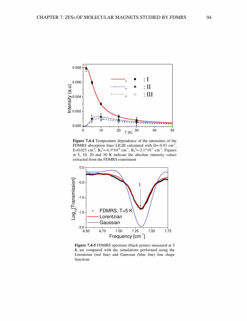
CHAPTER 7: ZFSs OF MOLECULAR MAGNETS STUDIED BY FDMRS 94
0 10 20 30 40 50
0.000
0.002
0.004
0.006
0.008
Inte
nsity (
a.u
)
T (K)
, : I, : II, : III
6.50 6.75 7.00 7.25 7.50 7.75-2.0
-1.5
-1.0
-0.5
0.0
Lo
g1
0[T
ran
sm
issio
n]
Frequency [cm-1]
FDMRS: T=5 K
Lorentzian
Gaussian
I
Figure 7.4-4 Temperature dependence of the intensities of the FDMRS absorption lines I,II,III calculated with D=-0.93 cm-1, E=0.023 cm-4, B4
0=-4.3*10-4 cm-1, B44=-2.1*10-3 cm-1. Figures
at 5, 10, 20 and 30 K indicate the absolute intensity values extracted from the FDMRS experiment
Figure 7.4-5 FDMRS spectrum (black points) measured at 5 K are compared with the simulations performed using the Lorentzian (red line) and Gaussian (blue line) line shape functions

VIII
Origin of magnetic anisotropy in
[Ni4(MeOH)4L4] complex
In previous chapters we have seen how to study the zero-field splittings of molecular magnets by the FDMRS-technique in terms of the single-spin Hamiltonian approach. In this chapter we try to explain the physical mechanisms responsible for experimentally detected energy spectrum of the compound [Ni4(MeOH)4L4] (see Section 7.4). We start from the group-theoretical analysis of the exchange-coupled multiplets of this tetrameric Ni(II) cluster possessing S4 point group symmetry, because the symmetry considerations allow an priori selection of the dominant non-Heisenberg terms of the microscopic spin Hamiltonian suitable for the cluster. The microscopic spin Hamiltonian expressed through irreducible tensor operators (see Section 3.4) is known as the generalized effective spin Hamiltonian, i.e. gesH model (see Section 4.3). In this chapter we show how to construct the gesH model to study the origin of magnetic anisotropy of the [Ni4(MeOH)4L4] complex.
8.1 Motivation
The interpretation of the FDMRS- and INS- data presented in Section 7.4 was
performed in terms of an effective spin Hamiltonian acting within the multiplet characterized by the total spin value 4=S , see [Sieber, 2005]. The positions of the INS lines, i.e.: I(I’),II (II’) and III (III’) are in a very good agreement with the positions of the FDMRS spectral lines (see Figure 8.1-1, Figure 7.4-2 and Table 7.4-2). The INS experiment is much more informative than the FDMRS one in the low-frequency part of the spectrum. Nevertheless, it was impossible to explain unambiguously the INS spectrum in terms of the single-spin Hamiltonian model: it describes well the INS-lines IV(IV’), V(V’), VI(VI’), VII(VII’) and VIII(VIII’), but does not clarify the origin of a weak spectral line located at ~3.5 cm-1 (see Figure 8.1-1). The zero-field splitting of the S = 4 ground state of [Ni4(MeOH)4L4] with the parameters D=-0.93 cm-1, E=0.023 cm-1, B4
0=-4.3*10-4 cm-1, B4
4=-2.1*10-3 cm-1 is shown in Figure 8.1-2 and in Figure 7.4-3. The parameters D and B4
0 describe the shift of energy levels constituting the 4=S multiplet (Figure 8.1.-2a), whereas the non-zero transverse ZFS parameter E and the fourth order transverse parameter B4
4 reflect the splitting of the levels and the admixture of the corresponding wavefunctions (see Figure 8.1-2c and Figure 7.4-3). Thus, the obtained zero-field splitting parameters allow a satisfactory simulation of both the INS- and the FDMRS experiments. However, they give no information about the origin of the cluster magnetic anisotropy, i.e. about the physical mechanisms leading to the shift, splitting and admixture of the energy levels described quantitatively by non-zero values of the single-spin Hamiltonian parameters. Finally, the single-spin Hamiltonian

CHAPTER 8: ORIGIN OF MAGNETIC ANISOTROPY IN [Ni4(MeOH)4L4] 96
model can not explain a weak spectral line situated between the lines III and IV, which can be associated with the transition between the multiplets differing in the total spin value by one (as follows from INS-selection rules 1,0=∆S , 1±=SM ). The aim of the Chapter 8 is to construct the microscopic spin Hamiltonian for the tetrameric Ni(II) cluster of S4 symmetry, which allows an unambiguous interpretation of the INS experiment.
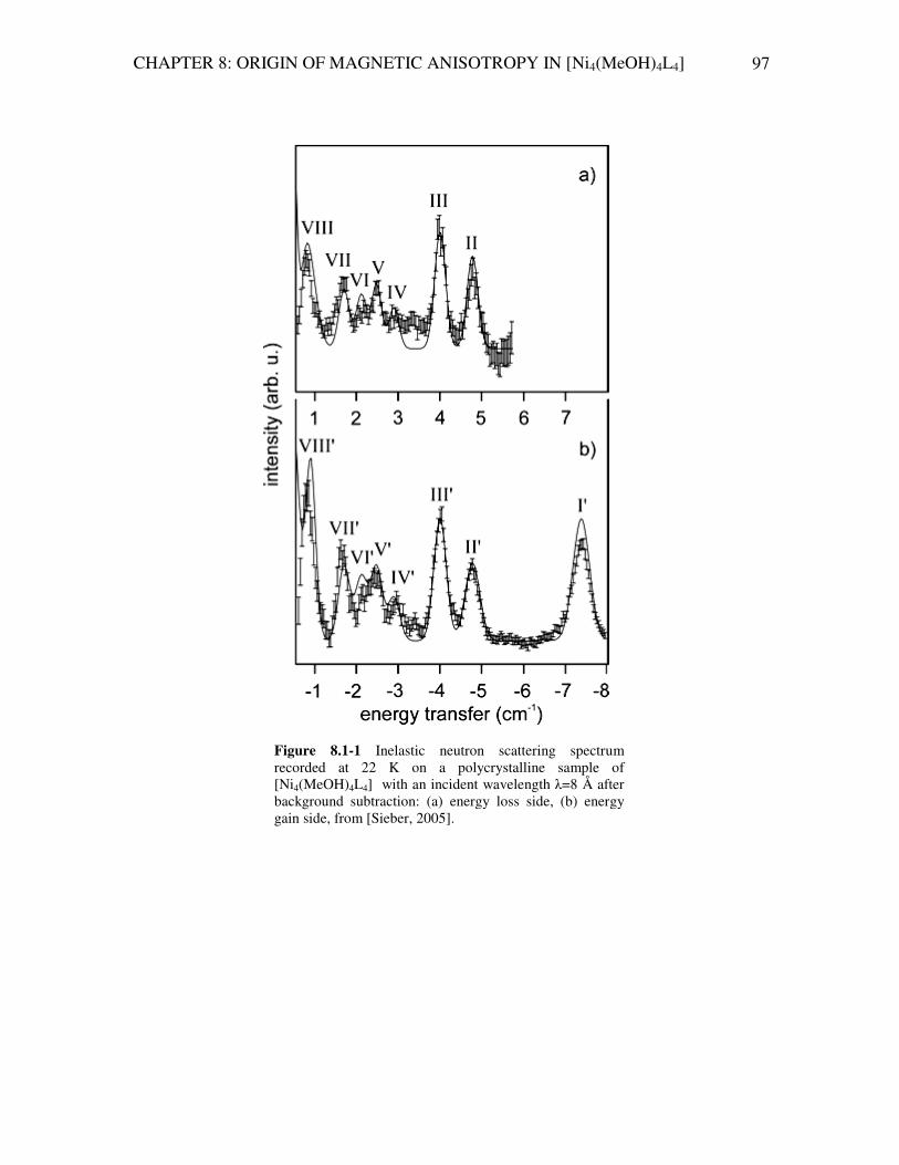
CHAPTER 8: ORIGIN OF MAGNETIC ANISOTROPY IN [Ni4(MeOH)4L4] 97
Figure 8.1-1 Inelastic neutron scattering spectrum recorded at 22 K on a polycrystalline sample of [Ni4(MeOH)4L4] with an incident wavelength λ=8 Å after background subtraction: (a) energy loss side, (b) energy gain side, from [Sieber, 2005].

CHAPTER 8: ORIGIN OF MAGNETIC ANISOTROPY IN [Ni4(MeOH)4L4] 98
Figure 8.1-2: Zero-field splitting of the S = 4 ground state of [Ni4(MeOH)4L4] using the parameters D=-0.93 cm-1, E=0.023 cm-1, B4
0=-4.3*10-4 cm-1, B44=-2.1*10-3 cm-1. (a)
First two terms of eq (7.4-1). (b) Including the E term in eq (7.4-1). (c) Including B4
4 in eq (7.4-1). The double arrows show the observed INS-transitions, from [Sieber, 2005].

CHAPTER 8: ORIGIN OF MAGNETIC ANISOTROPY IN [Ni4(MeOH)4L4] 99
8.2 Group-theoretical classification of exchange-coupled multiplets for a tetrameric cluster characterized by S4 point group The complex [Ni4(MeOH)4L4] consists of four octahedrally coordinated Ni(II) ions
with d8-electronic configurations. The energy spectrum of a Ni(II)-ion in an octahedral crystal field was described in Section 7.3 (see Figure 7.3-2). There it was shown that the contribution from excited orbital states into the energy spectrum of single-ion can be omitted by the interpretation of the experimental data, since the orbital states are lying much above the ground pure spin state (see Section 7.3 and Section 4.2). Thus, the complex [Ni4(MeOH)4L4] can be approximated by an exchange-coupled tetrameric cluster formed by four magnetic sites with the local spins S1=S2=S3=S4=1 (see also Figure 8.4-1). As already mentioned in Section 7.4, the symmetry of [Ni4(MeOH)4L4] is slightly distorted from the S4 point group11. However, we will assume S4 as the cluster point group for our analysis.
Due to the interaction of four Ni(II) ions through the diamagnetic ligands, the local spins Si=1 (i=1…4) are no longer good quantum numbers. Instead, good quantum numbers are the total spin values calculated according to the coupling scheme chosen for the cluster (see Section 3.3). These total spin values characterize the degeneracy of the exchange-coupled multiplets, where notation SSM;α is used throughout this PhD-thesis to identify
the coupled spin states of each energy level, which belong to an −S multiplet. The coupling of the spins is performed according to the rules of angular momentum
addition (see Section 3.3). Thus, the complete energy spectrum of Ni(II) tetrameric cluster is described by the following Clebsch-Gordan series (see Section 5.4):
( ) ( ) ( ) ( ) ( ) ( ) ( ) ( ) ( )432101111 36634321 ========= ++++=⊗⊗⊗ SSSSSSSSSDDDDDDDDD (8.2-1)
Eq. (8.2-1) shows that the energy spectrum constituted from 19 multiplets
(3+6+6+3+1=19) arises due to the coupling of four spin angular momenta 1=iS , 4...1=i .
There are three singlets with total spin 0=S , six triplets with 1=S , six quintets with 2=S , three septets with total spin 3=S and one nonet with total spin 4=S . Thus, the exchange-coupled multiplets of the tetrameric Ni(II) cluster are characterized by the irreducible representations of the full rotation group ( )SD with 4,3,2,1,0=S , where each −S manifold consists of 12 +S levels. The excited states with one and the same total spin value S have different intermediate spin values (see Eq. (8.2-2)). This kind of degeneracy according to intermediate spin numbers is known as “accidental” degeneracy, i.e. the degeneracy for reasons other than symmetry [Inui, 1990],[Tsukerblat, 1994]. This degeneracy is removed by interactions of non-Heisenberg type in high-nuclearity spin clusters. Thus, the group-theoretical classification of the exchange-coupled multiplets in terms of the irreducible representations of the cluster point group reflects the physical nature of non-Heisenberg interactions removing the “accidental” degeneracy, i.e. it allows a pre-selection of the dominant non-Heisenberg terms of the microscopic Hamiltonian of the cluster.
11 Similar Ni4 compounds containing the ethyl and methyl groups as ligands are strictly described by the S4 point group [Edwards, 2003]

CHAPTER 8: ORIGIN OF MAGNETIC ANISOTROPY IN [Ni4(MeOH)4L4] 100
According to Eq. (8.2-1) each multiplet is characterized by an irreducible representation of the full rotation group ( )SD describing the effective spin angular momentum operator acting within the −S manifold, which generates the transformation of the quantum-mechanical system under infinitesimal rotations. Otherwise, the complete symmetry of the molecule is reflected in its point group, which determines the properties of the quantum-mechanical system under finite rotations. Obviously, any finite rotation can be achieved after a series of infinitesimal rotations. Thus, there is a link between the irreducible representations of the full rotation group ( )SD and the irreducible representations of the cluster point group. This connection follows directly from the structure of the (point group) symmetry adapted Heitler-London many-electron wavefunctions, which satisfy the properties of the symmetric group. In fact, we have shown in Section 5.6 that the coupled spin states SSM;α are closely related to the
Heitler-London wavefunctions, which can be adapted to the cluster point group symmetry by using the projection operator method (see Section 5.5). Thus, the aim of this section is to find an unambiguous connection between the coupled spin states SSM;α and the
irreducible representations of the S4 point group describing the Ni4 cluster. In our further calculations we use the coupling scheme given by the chains:
1221 SSS =+ , 1221 mmm =+ , 3443 SSS =+ , 3443 mmm =+ , SSS =+ 3412 , sMmm =+ 3412 ,
where 1=iS are the single-ion spins and ,0=im 1± are the corresponding magnetic
quantum numbers, 4...1=i is an integer counter of the spin centres in the cluster, 12S and
34S are the intermediate spin values12, 12m and 34m are additional magnetic quantum
numbers13, S is the total spin and SM is the magnetic quantum number identifying each
level of the −S manifold. Obviously, each state SSM;α is unequivocal characterized by
the chain:
sMSSSSSSSmmmmmm ,,,,,,,,,,,,, 3412432134124321 (8.2-2).
Thereby, the kets SMSSS ,3412 are of importance for evaluation of the Hamiltonian
matrix elements by using the Wigner-Eckart theorem, i.e. for calculation of the spectroscopic transition frequencies and their intensities. Otherwise, the symmetry dependence of the states SMSSS ,3412 follows from the structure of the symmetry adapted
Heitler-London wavefunctions satisfying the Pauli principle. As we have seen in Section 5.6, the Heitler-London wavefunctions are expressed in terms of the Slater determinants constructed form the one-electron spin-orbitals localized on each spin center of the cluster. They are calculated according to Eq.(5.6-2) and they have the following form for a tetrameric cluster and the coupling scheme introduced above:
432134,12
4,3,2,1
3412 34341212
3434
4433
1212
2211, mmmmCCCMSSS SM
mSmS
mS
mSmS
mS
mSmS
mmmmmm
∑∑= (8.2-3)
12 )34,12(,..., =+−= ijSSSSS jijiij
13 );4,...,1(,,..., =+−= iSSm iii )34,12(,,..., =+−= ijSSm ijijij

CHAPTER 8: ORIGIN OF MAGNETIC ANISOTROPY IN [Ni4(MeOH)4L4] 101
here the expressions jm
mjmjC2211are the Clebsch-Gordan coefficients and 4321 mmmm are
the Slater determinants. The character table (see e.g. [Koster, 1963]) of the cluster point group must be known
in order to perform the group theoretical classification. The character table of the point group S4 is shown in Table 8.2-1. Thus, the point group S4 contains three irreducible representations (two one-dimensional: A (or Γ1) and B (or Γ2) and one two-dimensional: E, which consists of two complex conjugate one-dimensional representations Γ3, Γ4)14. The last column of the Table 8.2-1 shows the transformation rules of the basis states according to the irreducible representations of the point group. Thus, e.g. the z-component of the axial vector, i.e. the spin- or orbital angular momentum operator, transforms according to the irreducible representation A (or Γ1), while the raising (lowering) operator transforms according to one of the one-dimensional representations constituting the two-dimensional representation E: Γ3 (Γ4). These transformation properties are of importance e.g. for analysis of the spin-orbit splitting of many-electron (exchange-coupled) terms, see Section 8.3.
The generators of the S4 group are the rotation operators 3
442ˆ,ˆ,ˆ,ˆˆ SSCER = . These
symmetry operations induce permutations of the localized spin orbitals (Figure 8.2-1). Each wave function MSSS ,3412 contains a finite number ( 1≥n ) of Slater determinants
4321 mmmm corresponding to all possible combinations of
SSSmmmmmm ,,,,,,,, 341234124321 resulting in a certain value of M . Thus, the action of
each symmetry operator 3442
ˆ,ˆ,ˆ,ˆˆ SSCER = on the wavefunction MSSS ,3412 is equivalent to
the action of this point group generator on each determinant constituting MSSS ,3412 , i.e.
each i -determinant 4,,3,2,1 iiii mmmm , ni ,...,1= will be transformed according to the rules
presented in Figure 8.2-1.
14 The irreducible representations of any point group can be expressed in terms of Milliken notations (A,B,E) or by using the Bethe notations (Γ1, Γ2, Γ3, Γ4 etc.)
Table 8.2-1: Character table of the point group S4 S4 E S4 C2 S3
4 Bases A 1 1 1 1 Sz
B 1 -1 1 -1 z or xy E 1
1 i -i
-1 -1
-i i
-S+
+S-

CHAPTER 8: ORIGIN OF MAGNETIC ANISOTROPY IN [Ni4(MeOH)4L4] 102
341243212ˆ mmmmmmmmC =
43214321ˆ mmmmmmmmE =
213443214ˆ mmmmmmmmS −−−−=
1243432134
ˆ mmmmmmmmS −−−−=
m4
m1
m2
m3
m4
m1
m2
m3
2C
m1
m1 m2
m2
m3
m3
m4
m4
4S 34S
Figure 8.2-1: Symmetry operations ( 3442
ˆ,ˆ,ˆ,ˆ SSCE ) of the point group S4 induce permutations of the localized spin-orbitals. Components of the Slater determinant transform according to the rules shown in this Figure.
E
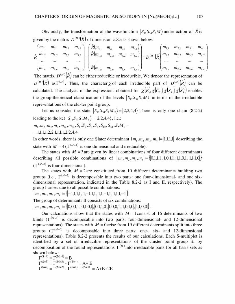
CHAPTER 8: ORIGIN OF MAGNETIC ANISOTROPY IN [Ni4(MeOH)4L4] 103
Obviously, the transformation of the wavefunction MSSS ,3412 under action of R is
given by the matrix ( ) ( )RD M ˆ of dimension nn× as shown below:
( )( )
( )
( ) ( )
=
=
nnnn
M
nnnnnnnn mmmm
mmmm
mmmm
RD
mmmmR
mmmmR
mmmmR
mmmm
mmmm
mmmm
R
,4,3,2,1
2,42,32,22,1
1,41,31,21,1
,4,3,2,1
2,42,32,22,1
1,41,31,21,1
,4,3,2,1
2,42,32,22,1
1,41,31,21,1
............ˆ
ˆ............
ˆ
ˆ
............ˆ
The matrix ( ) ( )RD M ˆ can be either reducible or irreducible. We denote the representation of ( ) ( )RD M ˆ as ( )MΓ . Thus, the character χ of each irreducible part of ( ) ( )RD M ˆ can be
calculated. The analysis of the expressions obtained for ( ) ( ) ( ) ( )3442
ˆ,ˆ,ˆ,ˆ SSCE χχχχ enables
the group-theoretical classification of the levels MSSS ,3412 in terms of the irreducible
representations of the cluster point group. Let us consider the state 4,4,2,2,3412 =SMSSS .There is only one chain (8.2-2)
leading to the ket 4,4,2,2,3412 =SMSSS , i.e.:
4,4,2,2,1,1,1,1,2,2,1,1,1,1
,,,,,,,,,,,,, 3412432134124321
=
=sMSSSSSSSmmmmmm
In other words, there is only one Slater determinant 1,1,1,1|,,,| 4321 =mmmm describing the
state with 4=M ( ( )4=Γ M is one-dimensional and irreducible). The states with 3=M are given by linear combinations of four different determinants
describing all possible combinations of 0,1,1,1,1,0,1,1,1,1,0,1,1,1,1,0|,,,| 4321 =mmmm
( ( )3=Γ M is four-dimensional). The states with 2=M are constituted from 10 different determinants building two
groups (i.e., ( )2=Γ M is decomposable into two parts: one four-dimensional- and one six-dimensional representation, indicated in the Table 8.2-2 as I and II, respectively). The group I arises due to all possible combinations:
1,1,1,1,1,1,1,1,1,1,1,1,1,1,1,1|,,,| 4321 −−−−=mmmm .
The group of determinants II consists of six combinations: 0,0,1,1,0,1,0,1,1,0,0,1,0,1,1,0,1,0,1,0,1,1,0,0|,,,| 4321 =mmmm .
Our calculations show that the states with 1=M consist of 16 determinants of two kinds ( ( )1=Γ M is decomposable into two parts: four-dimensional- and 12-dimensional representations). The states with 0=M arise from 19 different determinants split into three groups ( ( )0=Γ M is decomposable into three parts: one-, six- and 12-dimensional representations). Table 8.2-2 presents the results of our calculations. Each S-multiplet is identified by a set of irreducible representations of the cluster point group S4 by decomposition of the found representations ( )MΓ into irreducible parts for all basis sets as shown below: Γ
(S=4) = Γ(M=4) = B Γ
(S=3) = Γ(M=3) - Γ(S=4) = A+ E Γ
(S=2) = Γ(M=2) - Γ(S=4)- Γ(S=3) = A+B+2E

CHAPTER 8: ORIGIN OF MAGNETIC ANISOTROPY IN [Ni4(MeOH)4L4] 104
Γ(S=1) = Γ(M=1) - Γ(S=4)- Γ(S=3)- Γ(S=2) = A+B+2E Γ
(S=0) = Γ(M=0) - Γ(S=4)- Γ(S=3)- Γ(S=2)- Γ(S=1) =A+2B Finally we conclude that the energy levels of the Ni4 cluster are given by the following decomposition:
B D
E A 3D
E2B A 6D
E 2BA 6D
B 2A 3D
9(4)
77(3)
555(2)
333(1)
11(0)
=
+=
++=
++=
+=
(8.2-4)
We see that the ground state (S=4) of the Ni4 cluster is an orbital singlet B9 , i.e. the “spin-only” state. The first excited state with S=3 consisting of three manifolds ( SSS 3412 = 3,2,2 , 3,1,2 , 3,2,1 ) involves two irreducible representations: the orbital
singlet A7 and the orbital doublet E7 . The projector operator method is usually employed to find the one-to-one
correspondence between the coupled spin states with different intermediate spin values and the irreducible representations of the cluster point group. If this problem is solved, the symmetry-adapted wavefunctions MSSS ,3412 expressed in terms of the Slater
determinants are automatically obtained. By definition (see Section 5.5,5.6), the projection operator is constructed using the
characters ( ) ( )RΓχ of the symmetry operators of the cluster point group in the Γ -
irreducible representation: ( )
[ ]( ) ( )∑ ΓΓΓ =
R
RRG
dP
ˆ
* ˆˆχ , where [ ]G is the order of the group G ,
Γd is the dimension of the Γ -irreducible representation. The application of the projection
operator ( )ΓP to the state MSSS ,3412 reproduces it, if the state belongs to Γ ; if not, then
application of ( )ΓP to MSSS ,3412 gives a zero-result:
( )
Γ∉
Γ∈=Γ
MSSS
MSSSMSSSMSSSP
,,0
,,,,
3412
341234123412 .
This method was applied to the problem of classification of the exchange-coupled multiplets in terms of the irreducible representations of the S4 point group for a tetrameric cluster ( 4,...,1,1 == iSi ). The results are summarized in the Table 8.2-3. Thus, the method of group-theoretical classification links the many-electron Heitler-London wavefunctions to the states of the Heisenberg exchange model. It turns out that the ground state of Ni4 cluster, i.e. 4,2,2)4( ==SD , is the pure spin multiplet 9B. The excited multiplets with total
spin S=3 consist of three states: 3,1,2,3,2,1,3,2,23 )3( ==SD . There the state 3,2,2 is an
orbital singlet A7 , i.e. a pure spin multiplet. The states with one and the same total spin S=3 and different intermediate spins are degenerate: the pair of the coupled spin states
3,2,1 and 3,1,2 is described by one orbital doublet 7E.
The calculated symmetry-adapted wavefunctions for the ground- and the first excited multiplets of the Ni4 cluster are shown in Appendix 1.

CHAPTER 8: ORIGIN OF MAGNETIC ANISOTROPY IN [Ni4(MeOH)4L4] 105
Table 8.2-2: The characters of S4 point group generators for all basis sets (columns 2-5).
Decomposition of the representations ( ) ( )RD M ˆ into irreducible parts (column 1) S4 E S4 C2 S3
4 A 1 1 1 1 B 1 -1 1 -1 E 1
1 i -i
-1 -1
-i i
B 1 -1 1 -1 χ
(M=4)
A+B+E 4 0 0 0 χ(M=3)
A+B+E 4 0 0 0 χ(M=2) I
2(A+B)+E 6 0 2 0 χ(M=2) II
A+B+E 4 0 0 0 χ(M=1) I
3(A+B)+3E 12 0 0 0 χ(M=1) II
B 1 -1 1 -1 χ(M=0) I
2(A+B)+E 6 0 2 0 χ(M=0) II
3(A+B)+3E 12 0 0 0 χ(M=0) III
Table 8.2-3: Spin states of the tetrameric cluster (Si=1, i=1,…,4) characterized by irreducible representations of the point group S4.
(S12 S34 S) SΓ(S4 ) (2 2 4) 9B (2 2 3) 7A (2 1 3) 7E (1 2 3) 7E (2 2 2) 5B (2 1 2) 5E (2 0 2) 5E (1 2 2) 5E (1 1 2) 5A (0 2 2) 5E (2 2 1) 3A (2 1 1) 3E (1 2 1) 3E (1 1 1) 3B (1 0 1) 3E (0 1 1) 3E (0 0 0) 1B (1 1 0) 1A
(2 2 0) 1B
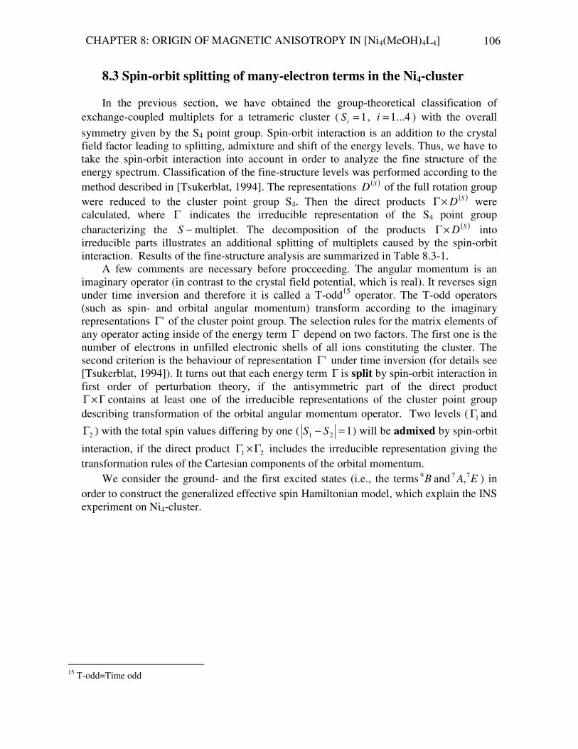
CHAPTER 8: ORIGIN OF MAGNETIC ANISOTROPY IN [Ni4(MeOH)4L4] 106
8.3 Spin-orbit splitting of many-electron terms in the Ni4-cluster In the previous section, we have obtained the group-theoretical classification of
exchange-coupled multiplets for a tetrameric cluster ( 1=iS , 4...1=i ) with the overall symmetry given by the S4 point group. Spin-orbit interaction is an addition to the crystal field factor leading to splitting, admixture and shift of the energy levels. Thus, we have to take the spin-orbit interaction into account in order to analyze the fine structure of the energy spectrum. Classification of the fine-structure levels was performed according to the method described in [Tsukerblat, 1994]. The representations ( )SD of the full rotation group were reduced to the cluster point group S4. Then the direct products ( )SD×Γ were calculated, where Γ indicates the irreducible representation of the S4 point group characterizing the −S multiplet. The decomposition of the products ( )SD×Γ into irreducible parts illustrates an additional splitting of multiplets caused by the spin-orbit interaction. Results of the fine-structure analysis are summarized in Table 8.3-1.
A few comments are necessary before procceeding. The angular momentum is an imaginary operator (in contrast to the crystal field potential, which is real). It reverses sign under time inversion and therefore it is called a T-odd15 operator. The T-odd operators (such as spin- and orbital angular momentum) transform according to the imaginary representations 'Γ of the cluster point group. The selection rules for the matrix elements of any operator acting inside of the energy term Γ depend on two factors. The first one is the number of electrons in unfilled electronic shells of all ions constituting the cluster. The second criterion is the behaviour of representation 'Γ under time inversion (for details see [Tsukerblat, 1994]). It turns out that each energy term Γ is split by spin-orbit interaction in first order of perturbation theory, if the antisymmetric part of the direct product
Γ×Γ contains at least one of the irreducible representations of the cluster point group describing transformation of the orbital angular momentum operator. Two levels ( 1Γ and
2Γ ) with the total spin values differing by one ( 121 =− SS ) will be admixed by spin-orbit
interaction, if the direct product 21 Γ×Γ includes the irreducible representation giving the transformation rules of the Cartesian components of the orbital momentum.
We consider the ground- and the first excited states (i.e., the terms B9 and EA 77 , ) in order to construct the generalized effective spin Hamiltonian model, which explain the INS experiment on Ni4-cluster.
15 T-odd=Time odd

CHAPTER 8: ORIGIN OF MAGNETIC ANISOTROPY IN [Ni4(MeOH)4L4] 107
Table 8.3-1: Splitting of exchange-coupled multiplets of the Ni4-cluster in the S4 point group caused by spin-orbit interaction. Column 1 contains results of the group-theoretical classification of many-electron terms in the crystal field of S4 symmetry. Column 2 shows the
representations ( )SD of the full rotation group reduced to the point group S4. Column 3 gives
the decomposition of the direct product ( )SD×Γ into irreducible representations. Exchange-coupled
multiplets of Ni4-cluster
in the crystal field of S4 symmetry
Representations ( )SD
of the full rotation
group reduced to the
point group S4
( )SD×Γ
BAD11)0( 23 += ( ) AD =0 ( ) ADA =× 0
( ) BDB =× 0 ( )
EBAD3331 26 ++=
( ) EAD +=1 ( ) EADA +=× 1 ( ) EBDB +=× 1 ( ) EBADE ++=× 221
( )EBAD
5552 26 ++=
( ) EBAD ++= 22 ( ) EBADA ++=× 22 ( ) EABDB ++=× 22 ( )
EBADE 3222 ++=× ( )
EAD7733 +=
( ) EBAD 223 ++= ( ) EBADA 223 ++=× ( )
EBADE 3443 ++=× ( ) BD 94 = ( )
EBAD 2234 ++= ( )EABDB 2234 ++=×

CHAPTER 8: ORIGIN OF MAGNETIC ANISOTROPY IN [Ni4(MeOH)4L4] 108
We start our analysis from the term E7 . It is of special interest, since it is an orbitally
degenerate doublet. It is a non-Kramers doublet, since the total spin values are integer. The wavefunctions of such doublets form the basis of two-fold degenerate ordinary representation E of the point group S4. We got the following result for the direct product: ExE=2A+2B with the antisymmetric part E2=A and the symmetric one [E2]= A+2B. The antisymmetric part is the one-dimensional representation A. As follows from the character table for the point group S4 (see Table 8.2-1), the zL component is transformed according to this representation. Thus, the effective Hamiltonian of spin-orbit interaction acting inside of the term E7 includes only the longitudinal term zz LS ˆˆλ (, where λ is the spin-orbit
coupling constant). Thus, the term E7 will be split by spin-orbit interaction in the first order of perturbation theory into 14 energy levels (eight one-dimensional representations and three two-dimensional ones: EBA 344 ++ ). This result can be well explained under assumption that 1=L and 1±=LM for the term E7 . In fact, we obtain 14 energy levels
according to the projections of the total angular momentum JM , i.e. there are 14 allowed
states according to 0,1,2,3 ±±±=SM , 1±=LM and resulting 4,3,2,1,0,1,2 +++−−=JM and
2,1,0,1,2,3,4 +−−−−=JM .
What happens with the term A7 under the action of spin-orbit interaction? The direct product EEA =× is the two-dimensional representation E with the basis functions ( )
yx iLL ±m . Thus, the transverse components of the orbital angular momentum
operator transforms according to E in the S4 point group. Therefore A7 will be admixed with E7 by transverse components of the effective spin-orbit operator: ( )
yyxx LSLS +λ .
Notably, spin-orbit interaction will admix only the states with the same JM of the terms
A7 and E7 . Thus, we expect: 2S+1=7 (S=3) levels according to 0,1,2,3 ±±±=SM .
Since 0=LM , we get 7 energy levels with 0,1,2,3 ±±±=JM . This fact is reflected in
decomposition ( ) EBADA 223 ++=× giving rise to three singlets and two doublets (, i.e. seven energy levels).
Now we analyze, whether the states with S=3 (terms A7 and E7 ) and S=4 (term B9 ) will be admixed by spin-orbit interaction or not. We get the following direct products EBE =× and BBA =× . Since EBE =× ( E is two-dimensional representation according which yx LL , components transform), the term E7 will be admixed with the term
B9 by transverse components of the orbital angular momentum. The direct product BA× is the one-dimensional representation B , which does not describe the transformation
of any axial vector (, i.e. vector operator of angular momentum) in the point group S4. Therefore, the A7 term will be shifted by spin-orbit interaction and admixed with E7 as it was described above.
Finally we get the diagram shown in the Figure 8.3-1 for the fine structure of the terms B9 and EA 77 , caused by the spin-orbit interaction.
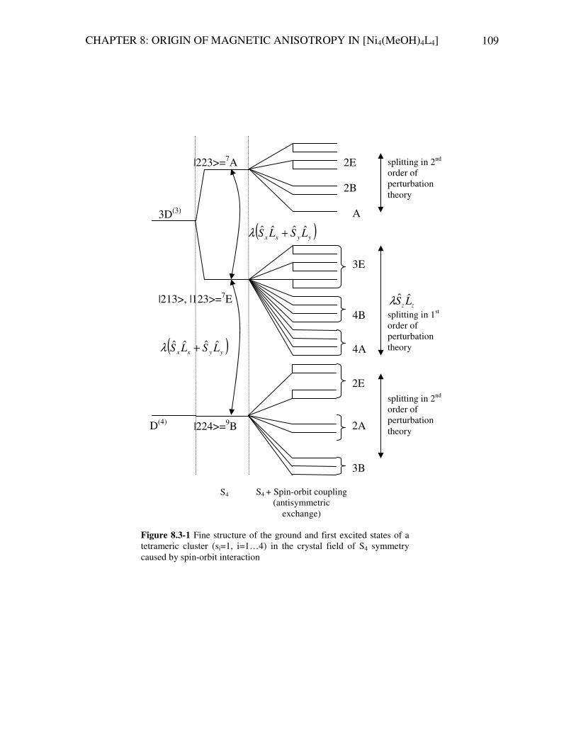
CHAPTER 8: ORIGIN OF MAGNETIC ANISOTROPY IN [Ni4(MeOH)4L4] 109
D(4)
3D(3)
|224>=9B
|213>, |123>=7E
|223>=7A
S4 S4 + Spin-orbit coupling (antisymmetric
exchange)
3B
2A
2E
4A
4B
3E
( )yyxx LSLS ˆˆˆˆ +λ
A
2B
2E
zz LS ˆˆλ splitting in 1st order of perturbation theory ( )yyxx LSLS ˆˆˆˆ +λ
Figure 8.3-1 Fine structure of the ground and first excited states of a tetrameric cluster (si=1, i=1…4) in the crystal field of S4 symmetry caused by spin-orbit interaction
splitting in 2nd order of perturbation theory
splitting in 2nd order of perturbation theory

CHAPTER 8: ORIGIN OF MAGNETIC ANISOTROPY IN [Ni4(MeOH)4L4] 110
8.4 Generalized effective spin Hamiltonian model for Ni4-cluster The aim of this section is to construct the microscopic spin Hamiltonian for the
[Ni4(MeOH)4L4] complex and to rewrite it in terms of irreducible tensor operators, i.e. to construct the generalized effective spin Hamiltonian model (gesH, see Section 4.3) suitable for this tetrameric Ni(II) cluster. The Heisenberg-Dirac-van Vleck (HDvV) model mentioned in Section 5.6 was developed to describe the spin-spin interactions of polynuclear orbitally degenerate clusters. In section 8.3 we have shown, that the spin-orbit interaction cannot be neglected in the case of the tetrameric Ni(II) cluster with the overall symmetry given by S4 point group. Thus, the microscopic spin Hamiltonian of [Ni4(MeOH)4L4] complex must contain some terms additional to the isotropic exchange interactions expressed by HDvV Hamiltonian (see Eq.(5.6-1)).
In fact, the molecular structure of [Ni4(MeOH)4L4] can be approximated by the tetrahedral tetrameric cluster shown in Figure 8.4-1 with the isotropic exchange coupling constants JA=-3 cm-1 and JB=8 cm-1 estimated from susceptibility measurements [Sieber, 2005].
The isotropic exchange Hamiltonian of this system is given by [Bencini, 1990],
[Tsukerblat, 1994], [Boca, 1999]:
( ) ( )423241314321ˆˆˆˆˆˆˆˆ2ˆˆˆˆ2 ssssssssJssssJ BA
iso rrrrrrrrrrrr+++−+−=Η (8.4-1).
In presence of S4 symmetry, the isotropic exchange interactions between spin centres give rise to the energy spectrum consisting of 19 degenerate multiplets (see Eq. (8.2-1)) characterized by irreducible representations of the S4 point group (see Table 8.2-3). It is easy to find the eigenvalues of the Hamiltonian Eq.(8.4-1). They are calculated according to the following formula [Tsukerblat, 1994], [Boca, 1999]:
S1
S2
S3
S4
JB
JB
JB
JB
JA
JA
Figure 8.4-1: The tetrameric spin cluster (Si=1, i=1,…,4) of the molecular complex [Ni4(MeOH)4L4] of with the overall symmetry S4.
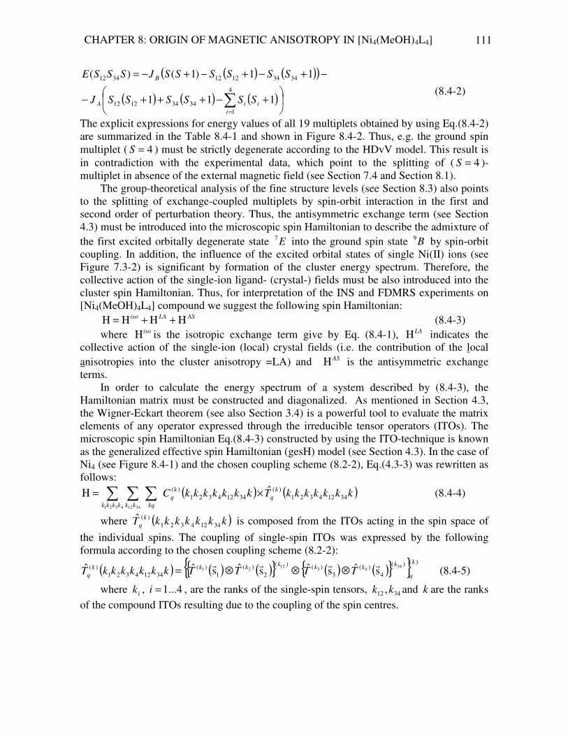
CHAPTER 8: ORIGIN OF MAGNETIC ANISOTROPY IN [Ni4(MeOH)4L4] 111
( ) ( )( )
( ) ( ) ( )
+−+++−
−+−+−+−=
∑=
4
134341212
343412123412
111
11)1()(
i
iiA
B
SSSSSSJ
SSSSSSJSSSE
(8.4-2)
The explicit expressions for energy values of all 19 multiplets obtained by using Eq.(8.4-2) are summarized in the Table 8.4-1 and shown in Figure 8.4-2. Thus, e.g. the ground spin multiplet ( 4=S ) must be strictly degenerate according to the HDvV model. This result is in contradiction with the experimental data, which point to the splitting of ( 4=S )-multiplet in absence of the external magnetic field (see Section 7.4 and Section 8.1).
The group-theoretical analysis of the fine structure levels (see Section 8.3) also points to the splitting of exchange-coupled multiplets by spin-orbit interaction in the first and second order of perturbation theory. Thus, the antisymmetric exchange term (see Section 4.3) must be introduced into the microscopic spin Hamiltonian to describe the admixture of the first excited orbitally degenerate state E7 into the ground spin state B9 by spin-orbit coupling. In addition, the influence of the excited orbital states of single Ni(II) ions (see Figure 7.3-2) is significant by formation of the cluster energy spectrum. Therefore, the collective action of the single-ion ligand- (crystal-) fields must be also introduced into the cluster spin Hamiltonian. Thus, for interpretation of the INS and FDMRS experiments on [Ni4(MeOH)4L4] compound we suggest the following spin Hamiltonian:
ASLAiso Η+Η+Η=Η (8.4-3) where isoΗ is the isotropic exchange term give by Eq. (8.4-1), LAΗ indicates the
collective action of the single-ion (local) crystal fields (i.e. the contribution of the local anisotropies into the cluster anisotropy =LA) and ASΗ is the antisymmetric exchange terms.
In order to calculate the energy spectrum of a system described by (8.4-3), the Hamiltonian matrix must be constructed and diagonalized. As mentioned in Section 4.3, the Wigner-Eckart theorem (see also Section 3.4) is a powerful tool to evaluate the matrix elements of any operator expressed through the irreducible tensor operators (ITOs). The microscopic spin Hamiltonian Eq.(8.4-3) constructed by using the ITO-technique is known as the generalized effective spin Hamiltonian (gesH) model (see Section 4.3). In the case of Ni4 (see Figure 8.4-1) and the chosen coupling scheme (8.2-2), Eq.(4.3-3) was rewritten as follows:
( ) ( )kkkkkkkTkkkkkkkCk
q
k
q
kqkkkkkk
34124321)(
34124321)( ˆ
34124321
×=Η ∑∑∑ (8.4-4)
where ( )kkkkkkkTk
q 34124321)(ˆ is composed from the ITOs acting in the spin space of
the individual spins. The coupling of single-spin ITOs was expressed by the following formula according to the chosen coupling scheme (8.2-2):
( ) ( ) ( ) ( ) ( ) )()(
4)(
3)()(
2)(
1)(
34124321)( 34
4312
21 sˆsˆsˆsˆˆk
q
kkkk
kkk
q TTTTkkkkkkkTrrrr
⊗⊗⊗= (8.4-5)
where ik , 4...1=i , are the ranks of the single-spin tensors, 3412 ,kk and k are the ranks of the compound ITOs resulting due to the coupling of the spin centres.
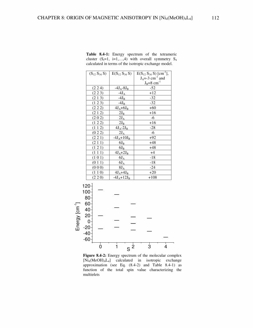
CHAPTER 8: ORIGIN OF MAGNETIC ANISOTROPY IN [Ni4(MeOH)4L4] 112
0 1 2 3 4
-60
-40
-20
0
20
40
60
80
100
120
Ene
rgy [cm
-1]
S
Table 8.4-1: Energy spectrum of the tetrameric cluster (Si=1, i=1,…,4) with overall symmetry S4 calculated in terms of the isotropic exchange model.
(S12 S34 S) E(S12 S34 S) E(S12 S34 S) [cm-1], JA=-3 cm-1 and
JB=8 cm-1 (2 2 4) -4JA-8JB -52 (2 2 3) -4JA +12 (2 1 3) -4JB -32 (1 2 3) -4JB -32 (2 2 2) 4JA+6JB +60 (2 1 2) 2JB +16 (2 0 2) 2JA -6 (1 2 2) 2JB +16 (1 1 2) 4JA-2JB -28 (0 2 2) 2JA -6 (2 2 1) -4JA+10JB +92 (2 1 1) 6JB +48 (1 2 1) 6JB +48 (1 1 1) 4JA+2JB +4 (1 0 1) 6JA -18 (0 1 1) 6JA -18 (0 0 0) 8JA -24 (1 1 0) 4JA+4JB +20 (2 2 0) -4JA+12JB +108
Figure 8.4-2: Energy spectrum of the molecular complex [Ni4(MeOH)4L4] calculated in isotropic exchange approximation (see Eq. (8.4-2) and Table 8.4-1) as function of the total spin value characterizing the multiplets

CHAPTER 8: ORIGIN OF MAGNETIC ANISOTROPY IN [Ni4(MeOH)4L4] 113
The matrix elements of the Hamiltonian Eq. (8.4-4) were evaluated by using the Wigner-Eckart theorem:
><+
−>=Η< SSSRSSSC
SSMSSMSSS
MS
SMkq
k
34123412''
2
34123412 ||'''1'2
)1(||'''' (8.4-6)
where ''MS
SMkqC are the Clebsch-Gordon coefficients and >< SSSRSSS 34123412 ||''' is the
symbol used to indicate the reduced matrix element of the compound ITO’s ( )kkkkkkkT
k
q 34124321)(ˆ in the basis set of the coupled spin states.
The reduced matrix elements were calculated with help of single-spin reduced matrix elements and 9j symbols as shown below (see Section 4.3):
( )( )( )[ ]
( )( )( )[ ]
( )( )( )[ ]
+++×
×
+++×
×
+++×
××
×=
>=<
k
k
k
S
S
S
S
S
S
kSS
k
k
k
S
S
S
S
S
S
kSS
k
k
k
S
S
S
S
S
S
kSS
SSTSSSTS
SSTSSSTS
SSSRSSS
kk
kk
34
12
34
12
34
122/1
34
4
3
34
4
3
34
4
32/1
343434
12
2
1
12
2
1
12
2
12/1
121212
44)(
433)3(
3
22)(
211)(
1
34123412
'
'
'
12121'2
'
12121'2
'
12121'2
||)(ˆ||||)(ˆ||
||)(ˆ||||)(ˆ||
||'''
4
21
(8.4-7)
We have used in our considerations the rules for calculation of the single-spin reduced matrix elements published in [Borras-Almenar, 1999]:
=
=
=
−+++
++
+
=
2
1
0
,)12)(1()12)(32(6
1,)12)(1(
,12
||)(ˆ||'
'
'
')(
k
k
k
SSSSS
SSS
S
SSTS
SS
SS
SS
k
δ
δ
δ
(8.4-8)
As follows from Eq.(8.4-7) and Eq.(8.4-8) the reduced matrix element does not depend on magnetic quantum numbers. Thus, the matrix R , of which the elements are calculated by Eq. (8.4-7) in the coupled spin basis, has dimension 19x19, i.e. 361 elements. In contrast, the complete Hamiltonian matrix constructed in the full Hilbert space contains 81x81=6561 elements. The evaluation of only one reduced matrix element is needed to construct the block of the Hamiltonian matrix describing interaction of the states
''' 3412 SSS and SSS 3412 consisting of MM ×' states. Due to this fact reduction in
calculation time by a factor of almost 20 is achieved. The next step in our considerations is to map Eq. (8.4-3) into Eq. (8.4-4), i.e. to
express the terms isoΗ , LAΗ and ASΗ (see Eq. (8.4-3)) through ITOs of the correct ranks.
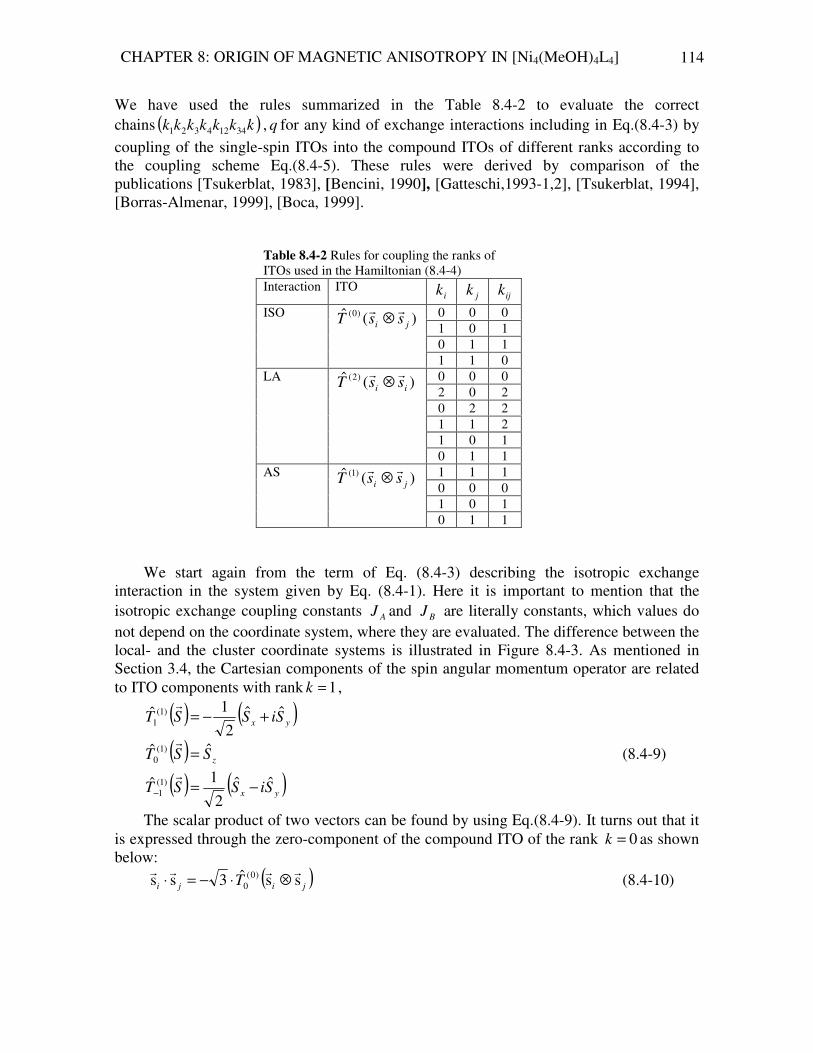
CHAPTER 8: ORIGIN OF MAGNETIC ANISOTROPY IN [Ni4(MeOH)4L4] 114
We have used the rules summarized in the Table 8.4-2 to evaluate the correct chains ( )kkkkkkk 34124321 , q for any kind of exchange interactions including in Eq.(8.4-3) by coupling of the single-spin ITOs into the compound ITOs of different ranks according to the coupling scheme Eq.(8.4-5). These rules were derived by comparison of the publications [Tsukerblat, 1983], [Bencini, 1990], [Gatteschi,1993-1,2], [Tsukerblat, 1994], [Borras-Almenar, 1999], [Boca, 1999].
We start again from the term of Eq. (8.4-3) describing the isotropic exchange
interaction in the system given by Eq. (8.4-1). Here it is important to mention that the isotropic exchange coupling constants AJ and BJ are literally constants, which values do not depend on the coordinate system, where they are evaluated. The difference between the local- and the cluster coordinate systems is illustrated in Figure 8.4-3. As mentioned in Section 3.4, the Cartesian components of the spin angular momentum operator are related to ITO components with rank 1=k ,
( ) ( )yx SiSST ˆˆ2
1ˆ )1(1 +−=
r
( ) zSST ˆˆ )1(0 =
r (8.4-9)
( ) ( )yx SiSST ˆˆ2
1ˆ )1(1 −=−
r
The scalar product of two vectors can be found by using Eq.(8.4-9). It turns out that it is expressed through the zero-component of the compound ITO of the rank 0=k as shown below:
( )jiji T ssˆ3ss )0(
0
rrrr⊗⋅−=⋅ (8.4-10)
Table 8.4-2 Rules for coupling the ranks of ITOs used in the Hamiltonian (8.4-4) Interaction ITO
ik jk ijk
0 0 0 1 0 1 0 1 1
ISO )(ˆ )0(ji ssTrr
⊗
1 1 0 0 0 0 2 0 2 0 2 2 1 1 2 1 0 1
LA )(ˆ )2(ii ssTrr
⊗
0 1 1 1 1 1 0 0 0 1 0 1
AS )(ˆ )1(ji ssTrr
⊗
0 1 1

CHAPTER 8: ORIGIN OF MAGNETIC ANISOTROPY IN [Ni4(MeOH)4L4] 115
Figure 8.4-3 The z-axis of the cluster coordinate system (the body of a man) is shown in the figure left; the space orientation of the z-axes of the local coordinate systems (arms and legs) is shown right. The explicit expressions of non-Heisenberg terms of Eq.(8.4-3) depend on the coordinate system, where they are calculated. The isotropic exchange (see Eq.(8.4-1)) is given by multiplication of the scalar constant and the scalar product of two vectors. Therefore its explicit expression in terms of ITOs is independent on the coordinate system (whether the cluster- or the local coordinate systems), in which it was calculated.
1
3
4
2
x
y
z
Figure 8.4-4 xyz is the cluster coordinate system chosen for calculations on [Ni4(MeOH)4L4] complex

CHAPTER 8: ORIGIN OF MAGNETIC ANISOTROPY IN [Ni4(MeOH)4L4] 116
Substituting Eq.(8.4-10) into Eq. (8.4-1) we obtain the isoΗ term as the sum of the compound ITOs in accordance to the structure of Eq.(8.4-4):
( )jiij
i ij
ISOTJ ssˆ32 )0(
0
4
1
4 rr⊗=Η ∑∑
= <
(8.4-11)
The parameters ( )kkkkkkkC k
q 34124321)( for pairwise isotropic exchange interactions
between the spin centres and the coupling of the ranks of single-spin ITOs are shown in Table 8.4-3.
The explicit forms of the microscopic Hamiltonians describing the terms LAΗ and ASΗ depends on the mutual orientation of the cluster- and local coordinate systems.
If the orientation of the single-ion iD -tensors, i=1…4, is parallel to the cluster coordinate system then the collective action of the local crystal fields of four spin centres in formation of the cluster magnetic anisotropy is given by [Tsukerblat, 2001], [Palii, 2004]:
( ) ( )( )∑∑==
−+
+−=Η
4
1
224
1
2 ˆˆ131ˆ
i
local
iyixi
i
local
iiizi
LAssEsssDrrr
(8.4-12)
where Di ,Ei are zero-field splitting parameters of individual Ni-ions related to the
diagonal components of the local iD -tensors, i=1…4, the word local shows that the expression is written in the local coordinate system.
As mentioned in Section 4.3, the term ASΗ describing antisymmetric exchange interactions between the spin centres is given by Eq. (8.4-13), if the local AS-tensors for each pair of interacting spins are collinear with the cluster coordinate system:
( ) [ ]( )∑∑∑∑= <= <
×=Η=Η4
1
4
1
4
1
4
1 i j
local
jiij
i j
localAS
ij
ASssGrrr
(8.4-13)
Table 8.4-3
Isotropic exchange
i j 1k 2k 3k 4k 12k 34k k q )(k
qC expressed in cluster coordinate system
2 1 1 1 0 0 0 0 0 0 AJ32
4 3 0 0 1 1 0 0 0 0 AJ32
3 1 1 0 1 0 1 1 0 0 BJ32
4 1 1 0 0 1 1 1 0 0 BJ32
3 2 0 1 1 0 1 1 0 0 BJ32
4 2 0 1 0 1 1 1 0 0 BJ32

CHAPTER 8: ORIGIN OF MAGNETIC ANISOTROPY IN [Ni4(MeOH)4L4] 117
where ijGr
are antisymmetric exchange parameters, [ ]ji ss ˆˆ rr× is a vector product. The
physical origin of the vector jiij GGGrrr
−= is the admixture of excited states into the ground
state through spin-orbit coupling. Thus, under assumption of colinearity of the local and the cluster coordinate systems,
the terms LAΗ and ASΗ can be expressed by ITOs as follows [Borras-Almenar, 1999], [Boca, 1999]:
( ) ( ) ( )( )∑∑=
−=
⊗+⊗+
⊗=Η
4
1
)2(2
)2(2
4
1
)2(0 ssˆssˆssˆ
32
i
iiiii
i
iii
LATTETD
rrrrrr (8.4-14)
( ) ( )jiqijq
i ij q
qASTGi ssˆ12 )1()1(
,
4
1
4 rr⊗−−=Η −
= <
∑∑∑ (8.4-15)
where parameters )1(,ijqG are given by the following relation:
( )0,
1,2
1)1(
,=
±=
±
=q
q
G
iGGG
z
ij
y
ij
x
ij
ijq
m (8.4-16)
Obviously, the parameters ( )kkkkkkkC k
q 34124321)( of the generalized effective spin
Hamiltonian (see Eq. (8.4-4), compare Eq.(8.4-4) and Eq.(8.4-11),Eq.(8.4-14), Eq.(8.4-15)) are linked to the isotropic exchange interaction parameters ijJ , to the single-ion ZFS
parameters ( ii ED , ) and to the parameters of pairwise antisymmetric exchange
interaction ijGr
. It is important to mention that ii ED , and ijGr
in Eq.(8.4-14) and Eq.(8.4-15)
are expressed in local coordinate systems. The calculations according to Eq. (8.4-4) are straightforward for a system, where the
principal axes of the local iD -tensors and the vector parameters of antisymmetric
exchange ijGr
coincide with the cluster coordinate axes. This is obviously not the case for
the Ni4-cluster. Clearly, the evaluation of each summand in Eq. (8.4-4) must be performed in one and the same coordinate system to obtain the correct result.
Thus, the aim of the next sections is to find the correct orientations of the single-
ion iD -tensors and the vectors ijGr
that follow from the molecular structure of the
[Ni4(MeOH)4L4] complex. If they are found, we can derive the expressions for ( )kkkkkkkC k
q 34124321)( in the cluster coordinate system as well as the explicit form of
Eq.(8.4-3) in terms of ITOs Eq.(8.4-4). To the best of our knowledge, the method presented in this PhD thesis was applied for the first time to construct the gesH model in presence of non-collinear tensors describing the exchange interactions of non-Heisenberg type.
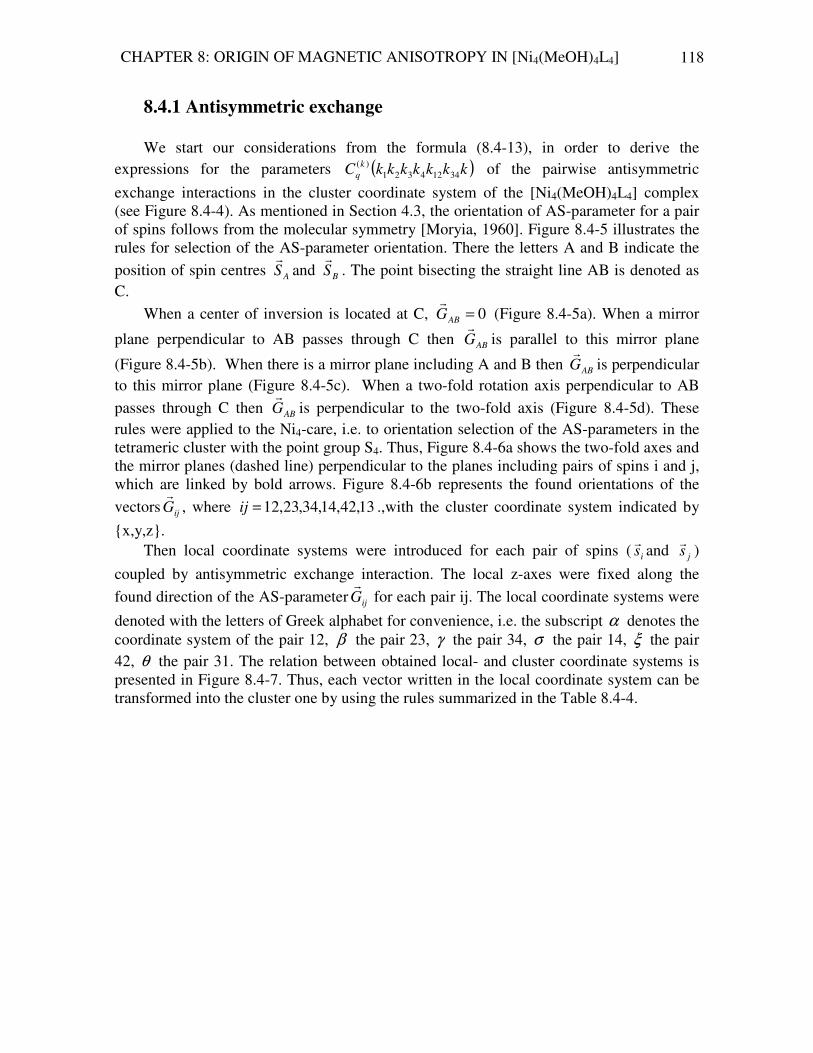
CHAPTER 8: ORIGIN OF MAGNETIC ANISOTROPY IN [Ni4(MeOH)4L4] 118
8.4.1 Antisymmetric exchange
We start our considerations from the formula (8.4-13), in order to derive the expressions for the parameters ( )kkkkkkkC k
q 34124321)( of the pairwise antisymmetric
exchange interactions in the cluster coordinate system of the [Ni4(MeOH)4L4] complex (see Figure 8.4-4). As mentioned in Section 4.3, the orientation of AS-parameter for a pair of spins follows from the molecular symmetry [Moryia, 1960]. Figure 8.4-5 illustrates the rules for selection of the AS-parameter orientation. There the letters A and B indicate the position of spin centres AS
rand BS
r. The point bisecting the straight line AB is denoted as
C. When a center of inversion is located at C, 0=ABG
r (Figure 8.4-5a). When a mirror
plane perpendicular to AB passes through C then ABGr
is parallel to this mirror plane
(Figure 8.4-5b). When there is a mirror plane including A and B then ABGr
is perpendicular to this mirror plane (Figure 8.4-5c). When a two-fold rotation axis perpendicular to AB passes through C then ABG
ris perpendicular to the two-fold axis (Figure 8.4-5d). These
rules were applied to the Ni4-care, i.e. to orientation selection of the AS-parameters in the tetrameric cluster with the point group S4. Thus, Figure 8.4-6a shows the two-fold axes and the mirror planes (dashed line) perpendicular to the planes including pairs of spins i and j, which are linked by bold arrows. Figure 8.4-6b represents the found orientations of the
vectors ijGr
, where 13,42,14,34,23,12=ij .,with the cluster coordinate system indicated by
x,y,z. Then local coordinate systems were introduced for each pair of spins ( is
rand js
r)
coupled by antisymmetric exchange interaction. The local z-axes were fixed along the
found direction of the AS-parameter ijGr
for each pair ij. The local coordinate systems were
denoted with the letters of Greek alphabet for convenience, i.e. the subscript α denotes the coordinate system of the pair 12, β the pair 23, γ the pair 34, σ the pair 14, ξ the pair 42, θ the pair 31. The relation between obtained local- and cluster coordinate systems is presented in Figure 8.4-7. Thus, each vector written in the local coordinate system can be transformed into the cluster one by using the rules summarized in the Table 8.4-4.

CHAPTER 8: ORIGIN OF MAGNETIC ANISOTROPY IN [Ni4(MeOH)4L4] 119
A B C
C is a center of inversion 0=ABGr
A B
C
ABGr
C is a mirror plane perpendicular to AB CGAB ||r
C is a mirror plane including A and B
C
A B
ABGr
CGAB ⊥r
A B
C
C is a two-fold axis perpendicular to AB CGAB ⊥
r
ABGr
Figure 8.4-5 Rules for selection of the antisymmetric coupling parameter. C is a symmetry element located at the point bisecting the straight line AB
(a)
(b)
(c)
(d)

CHAPTER 8: ORIGIN OF MAGNETIC ANISOTROPY IN [Ni4(MeOH)4L4] 120
Figure 8.4-6a shows the symmetry elements of the point group S4 of the tetrameric cluster used for the selection of the orientation of the
pair-wise AS-vectors ijGr
, ij=12,
23, 34, 14, 42, 13 (bold arrows). The two-fold axes are indicated with the symbols C2, the four-fold improper rotation axis with the symbol S4 as usual in crystallography. The black dashed lines are the intersections of the mirror planes perpendicular to the line connecting a pair of centres ij with the face of the cube.
1
2
3
4
z
y x
34Gr
42Gr
14Gr
12Gr
23Gr
13Gr
Figure 8.4-6b Orientation of the antisymmetric
exchange vector parameters ijGr
,
ij=12, 23, 34, 14, 42, 13 derived from the Moryia rules. x,y,z is the cluster coordinate system.
1
2
3
4
C2
C2
C2
S4

CHAPTER 8: ORIGIN OF MAGNETIC ANISOTROPY IN [Ni4(MeOH)4L4] 121
Figure 8.4-7. Relation between cluster- and local coordinate systems. Bold arrows show the local coordinate systems of the pairwise antisymmetric exchange interaction xlocal, ylocal, zlocal, local=α , β , γ ,σ ,ξ ,θ chosen according to the Moriya rules. The dotted arrows indicate the cluster coordinate system x,y,z. The bottom figures show the projections of the cluster- and local coordinate systems on the planes including the pair of interacting spins, where white circles indicate vectors pointing out of the plane and black circles vectors pointing into the plane.
4
3
zγ
x
y z
xγ
yγ
4
1
zσ
x y
z
xσ
yσ
x
4
2
zξ
z
yξ
y
x ξ
x
1
3
z
y
z θ
x θ
y θ
z
zα
y 1
2
x
xα
yα
2
3 x y
z
zβ
xβ
yβ
1
2
3
4
xα
yα zα
zβ
xβ
yβ
zγ
zσ
xσ
yσ zξ
xξ
yξ
zθ yθ
xθ
yγ
xγ
x
y
z

CHAPTER 8: ORIGIN OF MAGNETIC ANISOTROPY IN [Ni4(MeOH)4L4] 122
Table 8.4-4 Antisymmetric exchange: transformation rules from local- to cluster coordinate system
−
=
z
y
x
z
y
x
02
1
2
1
02
1
2
1100
α
α
α
−
−−
=
z
y
x
z
y
x
2
10
2
1010
2
10
2
1
β
β
β
−−
−
−
=
z
y
x
z
y
x
2
10
2
10102
10
2
1
σ
σ
σ
−
−−
=
z
y
x
z
y
x
2
1
2
10
0012
1
2
10
ξ
ξ
ξ
−−
−
−
=
z
y
x
z
y
x
02
1
2
1
02
1
2
1100
γ
γ
γ
−
−
=
z
y
x
z
y
x
2
1
2
10
2
1
2
10
001
θ
θ
θ

CHAPTER 8: ORIGIN OF MAGNETIC ANISOTROPY IN [Ni4(MeOH)4L4] 123
As soon as we know how to link the cluster- and local coordinate systems, we can construct the antisymmetric exchange Hamiltonian for the Ni4-cluster. This term has the following form in the local coordinate system for each pair of spins involved in the AS exchange interaction, see Eq. (8.4-13):
( ) [ ]( ) [ ] [ ] [ ]localzji
localz
ijlocalyji
localy
ijlocalxji
localx
ij
local
jiij
localAS
ij ssGssGssGssG,
,
,
,
,
, rrrrrrrrr×+×+×=×=Η ,
where localk
ijG , are the projections of the AS vector parameters and [ ]localkji ss
,
rr× are the
projections of the vector product [ ]ji ssrr
× on the −k axis of the local coordinate system
( zyxk ,,= ). The perpendicular components of the antisymmetric exchange can be omitted
in the first approximation, since 0,, == localy
ij
localx
ij GG for tetragonal systems and localz
ij
localy
ij
localx
ij GGG ,,, , <<< if symmetry is slightly broken (see [Tsukerblat, 1983]). Thus, we
use only the axial component of the antisymmetric exchange interaction in our further calculations, i.e. the formula shown below:
( ) [ ] ( )local
x
j
y
i
y
j
x
i
localz
ijlocalzji
localz
ij
localAS
ij ssssGssG −=×=Η ,
,
, rr (8.4-17)
where yx
jis ,, are x- and y- projections of the spins is
r and js
r expressed in the local coordinate
system. As mentioned in Section 3.4, the Cartesian basis can be linked to the spherical one and vice versa. Thus, the Eq. (8.4-9) can be rewritten as Eq. (8.4-18):
( ) ( )( )iTiTs x
i
)1(1
)1(1
ˆˆ2
1+− −=
( ) ( )( )iTiTi
s y
i
)1(1
)1(1
ˆˆ2
+− += (8.4-18)
( )iTs z
i
)1(0=
i.e. each Cartesian component of the vector isr
can be expressed through components of the irreducible tensor operator of rank one acting in the space of i-spin center.
Thus, each term ( )localAS
ijΗ , see Eq. (8.4-17), can be rewritten by using Eq. (8.4-18)
and transformed into the cluster coordinate system with help of the rules summarized in the Table 8.4-4. The obtained results were significantly simplified by introduction of the compound irreducible tensor operators of rank one tabulated e.g. in [Boca, 1999], i.e.:
( ))(ˆ)(ˆ)(ˆ)(ˆ2
1)(ˆ)(ˆ )1(
1)1(
0)1(
0)1(
1
)1(
1)1()1( jTiTjTiTjTiT −=⊗
( ))(ˆ)(ˆ)(ˆ)(ˆ2
1)(ˆ)(ˆ )1(
1)1(
1)1(
1)1(
1
)1(
0)1()1( jTiTjTiTjTiT −− −=⊗ (8.4-19)
( ))(ˆ)(ˆ)(ˆ)(ˆ2
1)(ˆ)(ˆ )1(
0)1(
1)1(
1)1(
0
)1(
1)1()1( jTiTjTiTjTiT −−− −=⊗
Finally we got the following expressions for pairwise AS-exchange interactions in the Ni4 cluster:
( ) ( )
⊗
++⊗
+−=Η −
)1(
1)1()1(
12
)1(
1)1()1(
1221 )1()2(22
1)1()2(2
21
TTGi
iTTGi loclocAS

CHAPTER 8: ORIGIN OF MAGNETIC ANISOTROPY IN [Ni4(MeOH)4L4] 124
⊗+⊗−⊗−=Η −
)1(
1)1()1(
23
)1(
0)1()1(
23
)1(
1)1()1(
2332 )2()3(22
)2()3()2()3(22
TTiGTTiGTTiGlocloclocAS
( ) ( )
⊗
++⊗
+−=Η −
)1(
1)1()1(
34
)1(
1)1()1(
3443 )3()4(22
1)3()4(2
21
TTGi
TTGi
iloclocAS
⊗+⊗+⊗−=Η −+
)1(
0)1()1(
14
)1(
1)1()1(
14
)1(
1)1()1(
1441 )1()4()1()4(22
)1()4(22
TTiGTTGi
TTGi locloclocAS
⊗−⊗−⊗−=Η −+
)1(
0)1()1(
42
)1(
1)1()1(
42
)1(
1)1()1(
4242 )2()4()2()4(221
)2()4(221
TTiGTTGTTGlocloclocAS
⊗−⊗+⊗=Η −+
)1(
0)1()1(
31
)1(
1)1()1(
31
)1(
1)1()1(
3131 )1()3()1()3(221
)1()3(221
TTiGTTGTTGlocloclocAS
From these formulas we derived the expressions for ( )kkkkkkkC k
q 34124321)( in the cluster
coordinate system by comparing the last result with the general expression of the effective spin Hamiltonian describing the antisymmetric exchange in the tetrameric cluster, i.e. Eq. (8.4-4) and Eq.(8.4-15). The outcome is summarized in the Table 8.4-5.

CHAPTER 8: ORIGIN OF MAGNETIC ANISOTROPY IN [Ni4(MeOH)4L4] 125
Table 8.4-5
Antisymmetric exchange
i j 1k 2k 3k 4k 12k 34k k q )(k
qC expressed in cluster
coordinate system 2 1 1 1 0 0 1 0 1 -1
( ) locGi 122
21+−
4 3 0 0 1 1 0 1 1 -1 ( ) loc
Gii 3422
1+−
3 1 1 0 1 0 1 1 1 -1 loc
G3122
4 1 1 0 0 1 1 1 1 -1 loc
Gi 1422
3 2 0 1 1 0 1 1 1 -1 loc
Gi 2322
4 2 0 1 0 1 1 1 1 -1 loc
G4222
−
2 1 1 1 0 0 1 0 1 0 0 4 3 0 0 1 1 0 1 1 0 0 3 1 1 0 1 0 1 1 1 0 loc
iG31−
4 1 1 0 0 1 1 1 1 0 lociG14
3 2 0 1 1 0 1 1 1 0 lociG23−
4 2 0 1 0 1 1 1 1 0 lociG42−
2 1 1 1 0 0 1 0 1 1 ( ) loc
Gii 1222
1+
4 3 0 0 1 1 0 1 1 1 ( ) loc
Gi 3422
1+
3 1 1 0 1 0 1 1 1 1 loc
G3122
4 1 1 0 0 1 1 1 1 1 loc
Gi 1422
−
3 2 0 1 1 0 1 1 1 1 loc
Gi 2322
−
4 2 0 1 0 1 1 1 1 1 loc
G4222
−

CHAPTER 8: ORIGIN OF MAGNETIC ANISOTROPY IN [Ni4(MeOH)4L4] 126
8.4.2 Local anisotropy
The task of this section is to find the expressions for the parameters ( )kkkkkkkC k
q 34124321)( in the cluster coordinate system of those summands in Eq. (8.4-4) that
describe the contribution of the single-ion anisotropy to the cluster anisotropy. For clarity, we have divided this section into two parts. The task of subsection 8.4.2A is to show how
to relate the cluster D -tensor of a certain state SSS 3412 to the local (single-ion) iD -tensors
of arbitrary orientation with respect to the cluster coordinate system (given by Euler
angles) for a tetrameric cluster of S4 symmetry. In subsection 8.4.2B we demonstrate how to calculate ( )kkkkkkkC k
q 34124321)( in the cluster coordinate system from the single-ion zero-
field splitting parameters fixed in the local (=single-ion) coordinate systems. 8.4.2A How to relate the cluster D-tensor of a certain state SSS 3412 to
the local (single-ion) iD -tensors of arbitrary orientations for a
tetrameric cluster of S4 symmetry? Let us start our considerations from Figure 8.4-8, where we see a tetrameric cluster
with the cluster coordinate system denoted as x,y,z and four local coordinate systems
that indicate the principal axes of the single-ion iD -tensors. The space orientation of the local coordinate systems with respect to each other and to the cluster coordinate system depends on the nature and geometry of ligands surrounding the spin centres. In order to derive the rules that link these five coordinate systems, we have to analyze the site symmetry resulting from the cluster point group. The situation becomes rather simple if the tetrameric cluster is described by the S4 point group. Below we show how to relate the
cluster D -tensor of a certain state SSS 3412 to the local (single-ion) iD -tensors of
arbitrary orientations for a tetrameric cluster of S4 symmetry.
The cluster D -tensor can be constructed with help of the local iD -tensors and the
combination coefficients for any ket SSS 3412 by using the replacement theorem (see
[Bencini, 1990],[Boca, 1999] and Section 4.2). The dipole-dipole interaction is omitted from considerations, since it is much weaker than the single-ion ligand fields. Then the
total D -tensor of the state SSSSSSS 34124321 can be written as follows:
( ) ( ) ( )
( ) ( ) 43412432143341243213
234124321213412432113412
DSSSSSSSCDSSSSSSSC
DSSSSSSSCDSSSSSSSCSSSDtotal
++
++= (8.4-20)

CHAPTER 8: ORIGIN OF MAGNETIC ANISOTROPY IN [Ni4(MeOH)4L4] 127
1
3
4
2
x2
x1
x3 x4
y1
y2
y3 y4
z1 z2
z3
z4
x
y
z
Figure 8.4-8: Principal axes of the
single-ion iD -tensors xi,yi,zi,
i=1,…,4 of arbitrary orientations and the cluster coordinate system x,y,z (dotted arrows).
Figure 8.4-9 Euler angles ( )ψθϕ ,, : the first rotation is by an angle ϕ about the z-axis,
the second is by an angle [ ]πθ ,0∈ about the x-axis, and the third is by an angle ψ
about the z-axis (again)

CHAPTER 8: ORIGIN OF MAGNETIC ANISOTROPY IN [Ni4(MeOH)4L4] 128
We obtain the formulas for the total D -tensor of the state SSS 3412 shown below by
using the combination coefficients in dinuclear systems [Boca, 1999], i.e.:
( ) ( ) ( ) ( ) ( )( )224224224224281
224 4321DDDDDtotal +++= (8.4-21)
( ) ( ) ( )4321 151
101
123 DDDDDtotal +++−=
( ) ( )4321301
223 DDDDDtotal +++= etc.
It is important to mention that each iD -tensor is written in the local coordinate system
in the formulas above. Thus, we have to express iD in the cluster coordinate system
because the calculations are performed under assumption that the principal axes of the iD -tensors are not parallel to the cluster coordinate system.
In order to solve the problem we use the Euler's rotation theorem [Wolfram, 1999]. According to this theorem any rotation may be described using three angles, see Figure 8.4-9. If the rotations are written in terms of rotation matrices then a general rotation can
be written also as (Euler-) matrix A . The three angles giving the three rotation matrices are called Euler angles. There are several conventions for Euler angles, depending on the axes about which the rotations are carried out. The so-called "x-convention," illustrated in the Figure 8.4-9, is the most common definition. In this convention, the rotation is given by Euler angles ( )ψθϕ ,, , where the first rotation is by an angle ϕ about the z-axis, the second is by an angle [ ]πθ ,0∈ about the x-axis, and the third is by an angle ψ about the z-axis (again). The Euler-Matrix is usually expressed as follows:
( )ψθϕ ,,AA = = (8.4-22)
−
+−−−
+−
θϕθθϕ
ψθψϕθψϕψϕθψϕ
ψθψϕθψϕψϕθψϕ
CosCosSinSinSin
CosSinCosCosCosSinSinCosSinCosSinCos
SinSinSinCosCosCosSinSinSinCosCosCos
Keeping in mind that each iD -tensor is given by diagonal matrix (see Section 4.2) in the local coordinate system:
−−
+−
=
3
200
03
0
003
i
ii
ii
local
D
ED
ED
D
(8.4-23)
we can calculate the iD -components in the cluster coordinate system by using the Euler
matrix: ADAD localcluster 1−= . Our calculations are simplified for two reasons. First of all, single-ions constituting the cluster and symmetry of their sites are identical and we assume local
i DD = and local
i EE =
for all 4...1=i . Thus, 1D has the form shown below:
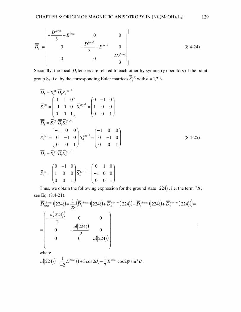
CHAPTER 8: ORIGIN OF MAGNETIC ANISOTROPY IN [Ni4(MeOH)4L4] 129
−−
+−
=
32
00
03
0
003
1
local
locallocal
locallocal
D
ED
ED
D (8.4-24)
Secondly, the local iD tensors are related to each other by symmetry operators of the point
group S4, i.e. by the corresponding Euler matrices )(4
kS with 3,2,1=k .
1)1(41
)1(42
−= SDSD
−=
100
001
010)1(
4S
−
=−
100
001
0101)1(
4S
1)2(41
)2(43
−= SDSD
−
−
=
100
010
001)2(
4S
−
−
=−
100
010
0011)2(
4S (8.4-25)
1)3(41
)3(44
−= SDSD
−
=
100
001
010)3(
4S
−=−
100
001
0101)3(
4S
Thus, we obtain the following expression for the ground state 224 , i.e. the term B9 ,
see Eq. (8.4-21):
( ) ( ) ( ) ( ) ( )( )( )
( )
( )
−
−
=
=+++=
22400
02
2240
002
224
224224224224281
224 4321
a
a
a
DDDDDclusterclusterclusterclustercluster
total
,
where
( ) ( ) θψθ 2sin2cos71
2cos31421
224 locallocalEDa −+= .

CHAPTER 8: ORIGIN OF MAGNETIC ANISOTROPY IN [Ni4(MeOH)4L4] 130
Remembering that ( ) ( )SSSaSSSD 34123412 23
= (see Section 4.2), we can link the single-
ion ZFS parameters with the axial ZFS parameter of the ground state of a tetragonal tetrameric cluster, constituted by 4...1,1 == isi .
( ) ( )
( ) 0224
sin2cos143
2cos31281
224 2
=
−+=
E
EDDlocallocal θψθ
(8.4-26)
We substitute the results obtained in [Yang, 2005] in the Eq. (8.4-26), in order to
prove the correctness of the last expression. There it was reported the high-field electron paramagnetic resonance (HFEPR) on single crystal of a similar complex [Zn3.91Ni0.09(hmp)4(dmb)4Cl4]. The Euler angles were determined experimentally to be equal to ( ) ( )°°°= 70,15,0,, ψθϕ with the Ni(II) single-ion ZFS parameters
3.5)( −=IINiD cm-1 and 2.1)( ±=IINiE cm-1. The resulting axial ZFS parameter of the
ground state with the total spin S=4 was reported to be D=-0.69 cm-1. We get the same result D= -0.69426 cm-1(-0.6678 cm-1) assuming )(IINiE as negative (positive) by
substitution of ( ) ( )°°°= 70,15,0,, ψθϕ into the eq. (8.4-26). Thus, the Eq. (8.4-26) is general. It can be applied for evaluation of the D-parameter of the ground state of any tetrameric cluster with S4 symmetry and the single spin sites 4...1,1 == isi . Finally we can relate the axial ZFS parameter obtained by fitting the FDMRS-experiment on [Ni4(MeOH)4L4] in terms of the single-spin Hamiltonian model to the ZFS parameters of single Ni(II) ion. Thus, we get from the Eq. (8.4-26):
( ) )()(3412 143
141
IINiIINi EDSSSD +−= (8.4-27)
for orientation of the principal axes of single-ion iD -tensors assumed in [Sieber, 2005] and
illustrated on the Figure 8.4-10, i.e. ( )
=
2,
2,0,,
ππψθϕ . The transverse ZFS is by
convention less than the axial one: 3D
E ≤ (see Section 4.2), in particular for mononuclear
Ni(II)-complexes (see Section 7.3 and [Vongtragool, 2003]) )()( IINiIINi DE << . In the first
approximation we get 02.13)( =IINiD cm-1 assuming 0~)( IINiE from the axial ZFS of the
ground state (D=-0.93 cm-1, see Section 7.4 and Section 8.1) obtained by FDMRS and INS studies on [Ni4(MeOH)4L4] complex.
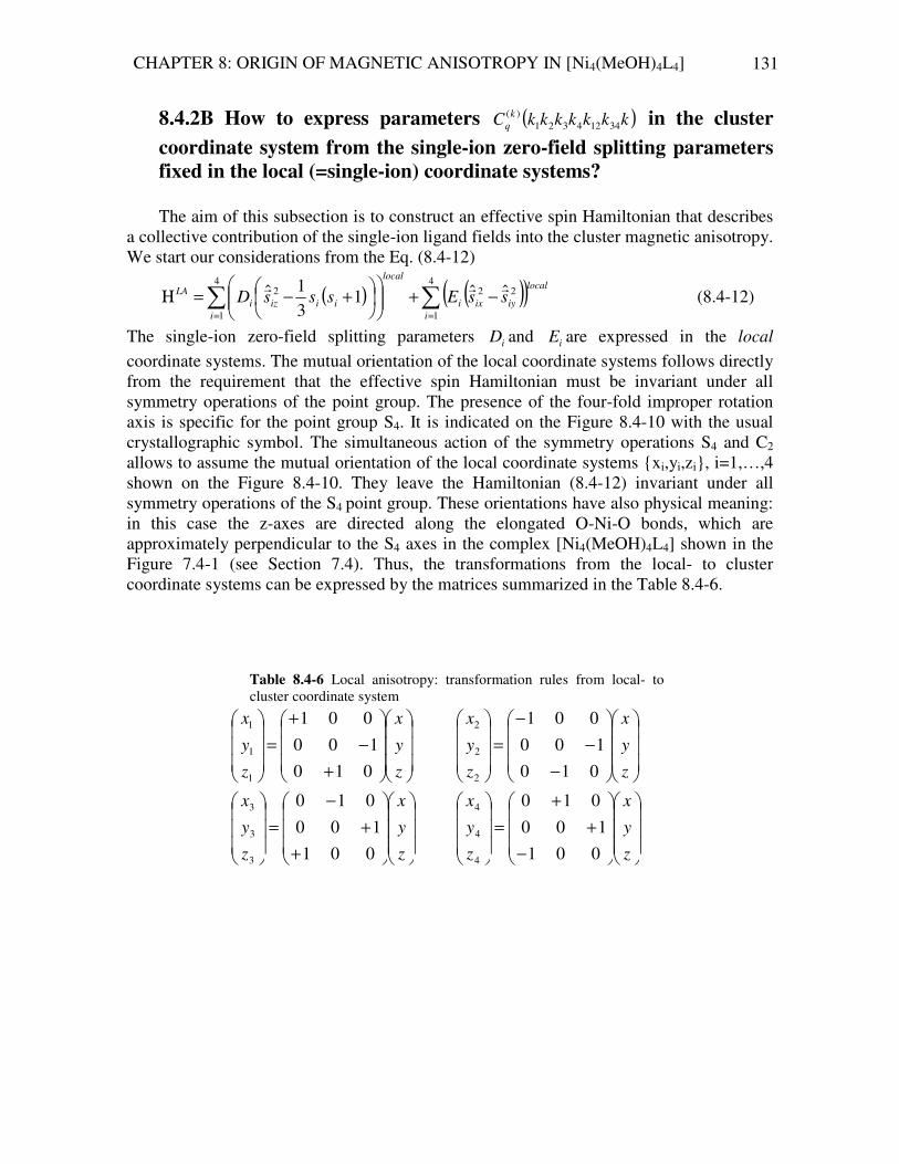
CHAPTER 8: ORIGIN OF MAGNETIC ANISOTROPY IN [Ni4(MeOH)4L4] 131
8.4.2B How to express parameters ( )kkkkkkkC k
q 34124321)( in the cluster
coordinate system from the single-ion zero-field splitting parameters fixed in the local (=single-ion) coordinate systems?
The aim of this subsection is to construct an effective spin Hamiltonian that describes
a collective contribution of the single-ion ligand fields into the cluster magnetic anisotropy. We start our considerations from the Eq. (8.4-12)
( ) ( )( )∑∑==
−+
+−=Η
4
1
224
1
2 ˆˆ131ˆ
i
local
iyixi
i
local
iiizi
LAssEsssDrrr
(8.4-12)
The single-ion zero-field splitting parameters iD and iE are expressed in the local coordinate systems. The mutual orientation of the local coordinate systems follows directly from the requirement that the effective spin Hamiltonian must be invariant under all symmetry operations of the point group. The presence of the four-fold improper rotation axis is specific for the point group S4. It is indicated on the Figure 8.4-10 with the usual crystallographic symbol. The simultaneous action of the symmetry operations S4 and C2 allows to assume the mutual orientation of the local coordinate systems xi,yi,zi, i=1,…,4 shown on the Figure 8.4-10. They leave the Hamiltonian (8.4-12) invariant under all symmetry operations of the S4 point group. These orientations have also physical meaning: in this case the z-axes are directed along the elongated O-Ni-O bonds, which are approximately perpendicular to the S4 axes in the complex [Ni4(MeOH)4L4] shown in the Figure 7.4-1 (see Section 7.4). Thus, the transformations from the local- to cluster coordinate systems can be expressed by the matrices summarized in the Table 8.4-6.
Table 8.4-6 Local anisotropy: transformation rules from local- to cluster coordinate system
+
−
+
=
z
y
x
z
y
x
010
100
001
1
1
1
−
−
−
=
z
y
x
z
y
x
010
100
001
2
2
2
+
+
−
=
z
y
x
z
y
x
001
100
010
3
3
3
−
+
+
=
z
y
x
z
y
x
001
100
010
4
4
4

CHAPTER 8: ORIGIN OF MAGNETIC ANISOTROPY IN [Ni4(MeOH)4L4] 132
3
y3
y4
1
4
2
z1
z3
z2
x1
y1
x3
y2
x2
z4
x4
1
2
3
4
z1
z3
z2
z4
x1
y1
y3 x3
x2
y2
x4 y4
Figure 8.4-10: The top figure shows the cluster coordinate system. Improper rotation axes S4 (dashed lines) and symmetry axes C2 (dotted lines) are illustrated on the figure left. They define the rules for transformation of the local coordinate systems one into another. Figure right shows projections of the local coordinate systems on the horizontal plane, where white circles indicate vectors pointing out of the plane and black circles vectors pointing into the plane.
4
3
2
x
y z
1
x
z x,y,zis the cluster coordinate system

CHAPTER 8: ORIGIN OF MAGNETIC ANISOTROPY IN [Ni4(MeOH)4L4] 133
Now we can recall the crystal field term of each single-ion written in the local coordinate system:
( ) ( ) 4,...,1ˆˆ131ˆ 222 =−+
+−=Η issEsssD iyix
loc
Niiiiz
loc
Ni
LA
i
rrr (8.4-28)
and rewrite them in the cluster coordinate system. Doing so, we obtain the following formulas:
( ) ( )
( ) ( )
=−+
+−
=−+
+−
=Η
4,3131
2,1131
2,
2,
2,
2,
2,
2,
issEsssD
issEsssD
ziyi
loc
Niiixi
loc
Ni
zixi
loc
Niiiyi
loc
NiLA
i (8.4-29)
Then we express each Cartesian component of the vector isr
through components of the rank one irreducible tensor operator acting in the space of spin center i (see Eq. (8.4-18)) and rewrite them by using the compound ITOs. It is convenient to express the obtained result via additional parameters ( ) ( ) ( )iCiBiA ,, :
( ) ( )
)2(
2)1()1()2(
0)1()1(
)2(
2)1()1()0(
0)1()1(
2)1(1
)1(1
)(ˆ)(ˆ)(ˆ)(ˆ32
)(ˆ)(ˆ)(ˆ)(ˆ3
2
)(ˆ)(ˆ
iTiTiTiT
iTiTiTiT
iTiTiA
⊗+⊗+
+⊗+⊗=
=+≡
−
−
(8.4-30)
( ) ( )
)2(
2)1()1()2(
0)1()1(
)2(
2)1()1()0(
0)1()1(
2)1(1
)1(1
)(ˆ)(ˆ)(ˆ)(ˆ32
)(ˆ)(ˆ)(ˆ)(ˆ3
2
)(ˆ)(ˆ
iTiTiTiT
iTiTiTiT
iTiTiB
⊗+⊗−
⊗+⊗−=
=−≡
−
−
(8.4-31)
( ) )2(
0)1()1()0(
0)1()1()1(
0)1(
0 )(ˆ)(ˆ32
)(ˆ)(ˆ3
1)(ˆ)(ˆ iTiTiTiTiTiTiC ⊗+⊗−=≡ (8.4-32)
( ) ( ) )0(
0)1()1( )(ˆ)(ˆ
3
11
31
iTiTssiD ii ⊗−=+−≡ (8.4-33)
Thus, Eq. (8.4-29) becomes the form shown below:
( ) ( ) ( ) ( )
( ) ( ) ( ) ( )
=
−−+
−
=
−+
−−
=Η
4,321
21
2,121
21
iiCiAEiDiBD
iiCiBEiDiAD
loc
Ni
loc
Ni
loc
Ni
loc
NiLA
i (8.4-34)
After some calculations we obtain Eq. (8.4-29) written as the sum of components for compound ITOs with ranks zero and two:

CHAPTER 8: ORIGIN OF MAGNETIC ANISOTROPY IN [Ni4(MeOH)4L4] 134
2,1=i
( )
( )
( ) )2(
2)1()1(
)2(
0)1()1(
)2(
2)1()1(
)(ˆ)(ˆ21
)(ˆ)(ˆ36
1
)(ˆ)(ˆ21
iTiTED
iTiTED
iTiTED
loc
Ni
loc
Ni
loc
Ni
loc
Ni
loc
Ni
loc
Ni
LA
i
⊗−−
−⊗+−
⊗−−=Η −
(8.4-35)
4,3=i
( )
( )
( ) )2(
2)1()1(
)2(
0)1()1(
)2(
2)1()1(
)(ˆ)(ˆ21
)(ˆ)(ˆ36
1
)(ˆ)(ˆ21
iTiTED
iTiTED
iTiTED
loc
Ni
loc
Ni
loc
Ni
loc
Ni
loc
Ni
loc
Ni
LA
i
⊗−+
+⊗+−
−⊗−=Η −
(8.4-36)
Finally, we can extract ( )kkkkkkkC k
q 34124321)(
parameters from the last result, i.e from
Eq. (8.4-35) and Eq. (8.4-36). They are summarized in the Table 8.4-7. They allow calculation of the single-ion crystal field contributions in to the cluster magnetic anisotropy according to the formula Eq.(8.4-4).
Concluding the Section 8.4 we mention, that the generalized effective spin Hamiltonian model is constructed in agreement with the symmetry properties of the
molecular complex [Ni4(MeOH)4L4]. The non-Heisenberg terms LAΗ and
ASΗ were included into the model in accordance with the group-theoretical analysis of the exchange-coupled multiplets (see Sections 8.2 and 8.3). All parameters needed for evaluation of the Hamiltonian (see Eq.(8.4-3)) matrix elements (see Eq.(8.4-4)) are listed in the Table 8.4-3 (isotropic exchange), Table 8.4-5 (antisymmetric exchange) and Table 8.4-7 (local anisotropy).

CHAPTER 8: ORIGIN OF MAGNETIC ANISOTROPY IN [Ni4(MeOH)4L4] 135
Table 8.4-7
Local anisotropy i j
1k 2k 3k 4k 12k 34k k q )(k
qC expressed in cluster
coordinate system 1 1 2 0 0 0 2 0 2 0
( )loc
Ni
loc
Ni ED 36
1+−
2 2 0 2 0 0 2 0 2 0 ( )loc
Ni
loc
Ni ED 36
1+−
3 3 0 0 2 0 0 2 2 0 ( )loc
Ni
loc
Ni ED 36
1+−
4 4 0 0 0 2 0 2 2 0 ( )loc
Ni
loc
Ni ED 36
1+−
1 1 2 0 0 0 2 0 2 2 ( )loc
Ni
loc
Ni ED −−21
2 2 0 2 0 0 2 0 2 2 ( )loc
Ni
loc
Ni ED −−21
3 3 0 0 2 0 0 2 2 2 ( )loc
Ni
loc
Ni ED −21
4 4 0 0 0 2 0 2 2 2 ( )loc
Ni
loc
Ni ED −21
1 1 2 0 0 0 2 0 2 -2 ( )loc
Ni
loc
Ni ED −−21
2 2 0 2 0 0 2 0 2 -2 ( )loc
Ni
loc
Ni ED −−21
3 3 0 0 2 0 0 2 2 -2 ( )loc
Ni
loc
Ni ED −21
4 4 0 0 0 2 0 2 2 -2 ( )loc
Ni
loc
Ni ED −21

8.5 Results of the INS-spectrum simulation 8.5.1 Structure of the calculated Hamiltonian matrix The aim of this section is to calculate the Hamiltonian matrix according to Eq.(8.4-3)
and Eq.(8.4-4) with the parameters listed in the Tables 8.4-3, 8.4-5 and 8.4-7, to diagonalize it and to find the values of the AS parameters and the single-ion ZFS parameters ( loc
NiD and loc
NiE ) that provide a good understanding of the INS-experiment on the [Ni4(MeOH)4L4] complex, see Section 8.1. Since the INS selection rules are restricted by
1,0 ±=∆S and 1±=∆ SM , we have performed our calculation within the ground ( 4=S )
multiplet B9 and the first two excited multiplets A7 and E7 with the total spin value ( 3=S ) .
The whole Hamiltonian Eq.(8.4-3) rewritten as Eq.(8.4-4) contains 8 adjustable parameters: six for the antisymmetric exchange term and two for the local anisotropy term, assuming that the isotropic exchange coupling constants AJ and BJ are known from the susceptibility measurements, see [Sieber, 2005]. Strictly speaking, there are ten adjustable parameters (including AJ and BJ ) that must be fit simultaneously, what makes the model over-parameterized. The fitting of ten parameters over nine INS spectral lines is by definition impossible.
To reduce the number of adjustable parameters, let us recall again the information concerning the antisymmetric exchange. As already mentioned in the Section 8.3, the results of the group-theoretical analysis of the fine-structure levels can be well explained only by introduction of the pseudoangular momentum L=1 acting within the orbital doublet E7 . This orbital momentum operator defines two principal directions in the cluster coordinate system: the longitudinal- (determined by zL ) and the transverse one (determined
by the collective action of the transverse components xL and yL ). For that reason two kinds
of antisymmetric exchange parameters were applied in our calculations, since the antisymmetric exchange term calculated in the spin model corresponds to the effective spin-orbit operator acting in the Heitler-London scheme, i.e. the AS vector parameters
ijGr
indicate the admixture of the excited states into the ground state through spin-orbit
coupling (see Section 8.3). Thus, we can divide six pairwise AS vector parameters ijGr
into
two groups. The first one is analogous to axial- ( ||G ) and the second one is analogous to
transverse ( ⊥G ) parts of the effective spin-orbit coupling operator. If the pair of interacting spins is linked by a line lying perpendicular to the cluster z-axis (coinciding with the axis S4 as shown in Figure 8.4-6a), then ⊥≡= GGG
locloc
3412 . If it is located in the plane including
the cluster z-axis, then ||23241431 GGGGG locloclocloc ≡=== . Doing so we obtain the model
including six semiempirical parameters: AJ , BJ , ||G , ⊥G and the pair of the single-ion Ni(II)
ZFS parameters, i.e.: Ni
loc
Ni DD ≡ and Ni
loc
Ni EE ≡ . In our further calculations we have fixed
AJ and BJ at the values determined by susceptibility measurements, i.e. AJ =-3 cm-1 and
BJ =+8 cm-1, see [Sieber, 2005]. Thus, our model Hamiltonian contains four adjustable

CHAPTER 8: ORIGIN OF MAGNETIC ANISOTROPY IN [Ni4(MeOH)4L4] 137
parameters: ||G , ⊥G , NiD and NiE , which we have tried to fit over nine INS spectral lines,
see Figure 8.1-1. The Hamiltonian matrix Eq.(8.4-4) was calculated in the basis of the coupled spin
states |224> (the term B9 ), |223> (the multiplet A7 ) and the pair of the states |123>, |213> (the orbital doublet E7 ) by using the Wigner-Eckart theorem Eq. (8.4-6), where the reduced matrix element was evaluated according to Eq.(8.4-7). The structure of the calculated Hamiltonian matrix is presented in the Figure 8.5-1.
The diagonal blocks (K,L,M) of the Hamiltonian matrix (see Figure 8.5-1) correspond to spin multiplets with the total spins S=4 (K) and S=3 (L,M), respectively. These multiplets are separated in energy by isotropic exchange interaction and split by anisotropic terms caused by single-ion crystal fields and antisymmetric exchange interactions. The non-zero off-diagonal blocks (N,O,P, where the blocks N’,O’,P’ are interrelated through a transposition and differing from N,O,P only in sign) show mixing of the states with different total spin values (the so called S-mixing effect [Liviotti, 2002]). Thus, an analysis of non-zero off-diagonal elements in the energy-matrix allows the understanding of the nature of the zero-field splittings in the selected multiplets B9 , A7 and E7 . All calculated blocks are collected in Appendix 2. In the next sections we show, that the results of our calculations are in agreement with those predicted by the group-theoretical classification of exchange-coupled multiplets in the presence of spin-orbit coupling in the tetrameric Ni(II) cluster with the overall symmetry given by the S4 point group (see Section 8.3).

CHAPTER 8: ORIGIN OF MAGNETIC ANISOTROPY IN [Ni4(MeOH)4L4] 138
9B
7A
7E
Figure 8.5-1 Structure of the energy matrix
calculated for the terms B9 , A7 and E7 . The diagonal blocks (K,L,M) correspond to each spin multiplet with the total spins S=4, and S=3 (two times), respectively. These multiplets are separated in energy by isotropic exchange interaction and split by anisotropic terms caused by single-ion crystal fields and antisymmetric exchange interactions. The non-zero off-diagonal blocks (N,O,P) show mixing of the states with different total spin values (S-mixing effect). The non-zero elements of each block depend on the set of parameters given in round brackets.
9B=|224> 7A=|223> 7E=|123>,|213>
L: 7A ( )NiNiA EDJ ,,
M: 7E ( )||,,, GEDJ NiNiB
P:
Mixing of 7A and 7E
( )||, GG⊥
O: Mixing of 9B and 7E
( )||, GG⊥
N: Mixing of 9B
and 7A ( )||,, GED NiNi
P’: Mixing of 7A and 7E
( )||, GG⊥
|123> |213>
M1: |123>
( )NiNiB EDJ ,,
R: Mixing
|123> and |213> ( )||G
O1
O2
9B=|224>
7E
P1
P2
7A=|223>
|123>
|213>
7E
M2: |213>
( )NiNiB EDJ ,,
K: 9B ( )NiNiBA EDJJ ,,, O’:
Mixing of 9B and 7E
( )||, GG⊥
N’: Mixing of 9B
and 7A ( )||,, GED NiNi
R’: Mixing
|123> and |213> ( )||G

CHAPTER 8: ORIGIN OF MAGNETIC ANISOTROPY IN [Ni4(MeOH)4L4] 139
8.5.2 Antisymmetric exchange ( ASΗ=Η ) acting within 7E-term
Group-theoretical analysis of the fine-structure levels predicts the splitting of the
orbital doublet E7 by the longitudinal component of the effective spin-orbit operator
zz LS ˆˆλ with 1±=LM acting in the E7 basis. That means that the multiplet E7 will be split
into 14 states according to >>=SLSL MMSLMMzz EMMESL ||ˆˆ λλ with the resulting energy
of each sublevel SLMM MMSL
λε =, . Thus, the energy spectrum of the zero-field split orbital
doublet E7 is represented by seven pairs of energy levels expressed through the spin-orbit coupling constant λ :
λε 331 =±±
λε 221 =±± λε =±± 11
00,1 =±ε
λε −=± 11m
λε 221 −=± m
λε 331 −=± m From another point of view, the diagonalization of the block M (see Figure 8.5-1 and
Appendix 8.5) constructed for the Hamiltonian including only the antisymmetric exchange terms (see Table 8.4-5) gives also 14 eigenvalues, i.e. seven pairs of the levels with
energies expressed through ||G : ||G , ||32
G , ||31
G , 0, ||31
G− , ||32
G− , ||G− , respectively (see
Figure 8.5-2). This fact confirms the correctness of the developed model for antisymmetric exchange part of the effective spin Hamiltonian and indicates the connecting link between
the spin-orbit coupling constant and the axial AS-parameter: ||31
G=λ .
Figure 8.5-2: Splitting of the orbital doublet 7E by axial component of the effective
spin-orbit operator zz LS ˆˆλ
with 1±=LM is equivalent to the action of the axial part of antisymmetric exchange term of the effective spin Hamiltonian. The spin-orbit coupling constant is linked to the axial AS-parameter:
||31
G=λ
λ3
λ2
λ
0
λ3− λ2−
λ−
||G
0
3/2 ||G−
||G−
3/2 ||G
3/||G−
3/||G
7E
3E+4B+4A

CHAPTER 8: ORIGIN OF MAGNETIC ANISOTROPY IN [Ni4(MeOH)4L4] 140
8.5.3 Hamiltonian ASLAiso Η+Η+Η=Η acting within 9B-term
The group-theoretical classification of the exchange-coupled multiplets (see Section
8.2) predicts that the ground state |224> is the orbitally non-degenerate (i.e. “pure” spin-) multiplet indicated by the one-dimensional representation B of the cluster point group S4. In fact, the magnetic anisotropy of the state |224> is given by the effective spin Hamiltonian:
( )
−+
+−=Η 222 ˆˆ1
31ˆ
yxz
LASSESSSDrrr
(8.5-1)
where ( )>= 224|DD and ( )>= 224|EE are the zero-field splitting parameters of the
D -tensor acting within the state |224>(, i.e 4=S ) and expressed in the cluster coordinate system. The cluster transverse ZFS parameter of a pure spin state is zero for S4 symmetry, see Section 8.4.2A and Eq.(8.4-26): ( )>224|E =0. Therefore, Eq. (8.5-1) transforms to:
( )
+−=Η 1
31ˆ 2
SSSD z
LAr
(8.5-2)
The Hamiltonian Eq. (8.5-2) is represented by the diagonal matrix constructed in the basis |224 4=SM >, 4=SM =±4, ±3, ±2, ±1,0, which have nine eigenvalues given by 2
4=⋅ SMD .
Thus, the zero-field ground multiplet B9 must be described by the energy spectrum consisting of four degenerate doublets and one singlet |2240> without the mixing of the corresponding wavefunctions. Since those transition frequencies are of importance for INS/FDMRS spectral simulations, which are differing by 14 ±=∆ =SM , we expect that:
( ) DD 734 221 =−⋅=ν for >±>↔± 3224|4224| ,
( ) DD 523 222 =−⋅=ν for >±>↔± 2224|3224| ,
( ) DD 312 223 =−⋅=ν for >±>↔± 1224|2224| ,
( ) DD =−⋅= 224 01ν for >±>↔± 0224|1224| .
In other words, the relation between the frequencies of the allowed magnetic dipole transitions within the ground spin multiplet must be given by Eq.(8.5-3):
1:3:5:7::: 4321 =νννν (8.5-3) On the other hand our calculations show, the block K (see Figure 8.5-1) is the diagonal
matrix (see Appendix 8.5). The diagonal elements of K are expressed through ( )NiNiBA EDJJ ,,, , i.e. it does not contain the parameters of antisymmetric exchange. The orbital moment is quenched within the state |224>. This result is in agreement with the group-theoretical classification of the exchange-coupled multiplets, which subscribes the one-dimensional representation B9 to the coupled spin state |224>. The splitting of this multiplet is caused by the collective action of the local crystal fields, as it follows from our calculations, see Eq.(8.5-4) shown below. Results of calculations are visualized on the diagram of Figure 8.5-3. The calculated frequencies of the allowed
magnetic dipole transitions inside of this multiplet are: ( ) αν 73,4, 991 =±→± BB ,
( ) αν 52,3, 992 =±→± BB , ( ) αν 31,2, 99
3 =±→± BB and ( ) αν =±→± 0,1, 994 BB ,
i.e. 1:3:5:7::: 4321 =νννν (compare with Eq. (8.5-3)).
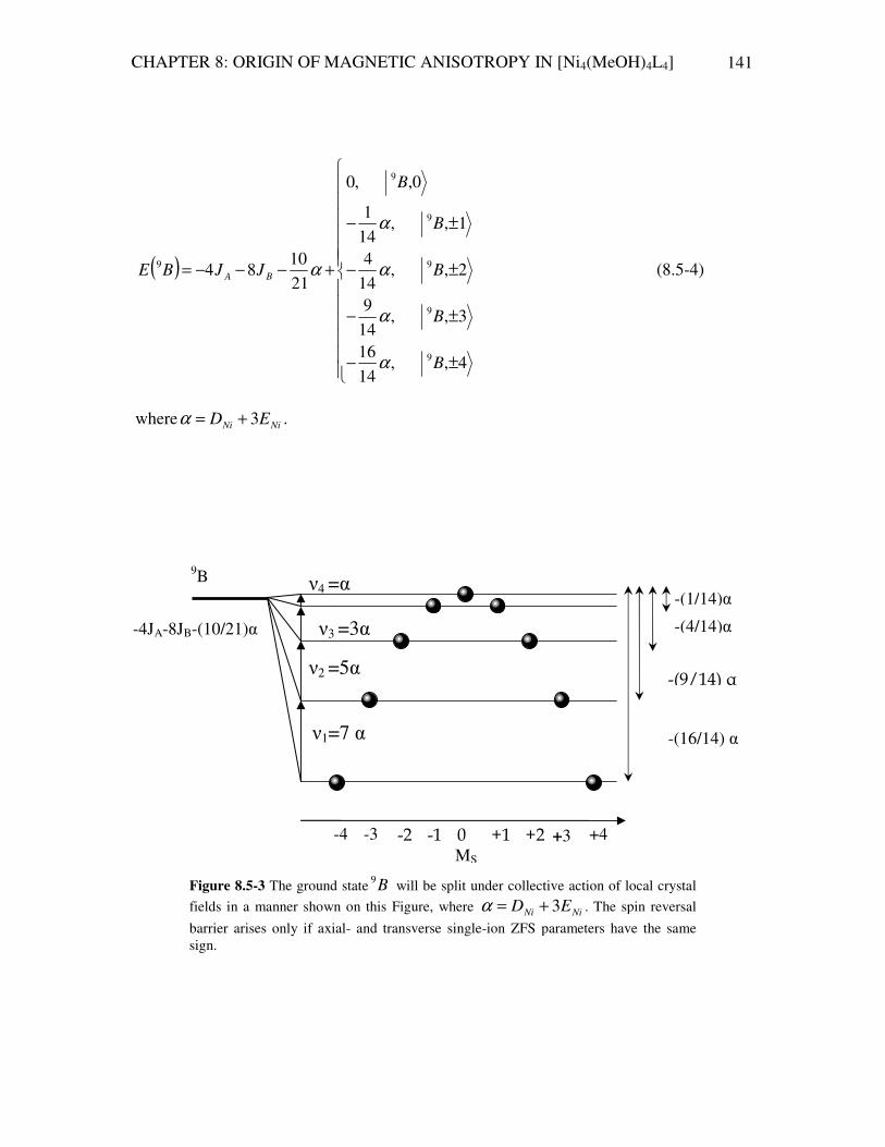
CHAPTER 8: ORIGIN OF MAGNETIC ANISOTROPY IN [Ni4(MeOH)4L4] 141
Figure 8.5-3 The ground state B9 will be split under collective action of local crystal
fields in a manner shown on this Figure, where NiNi ED 3+=α . The spin reversal
barrier arises only if axial- and transverse single-ion ZFS parameters have the same sign.
-4JA-8JB-(10/21)α
-4 -3 -2 -1 0 +1 +2 +3 +4
-(16/14) α
-(9/14) α
-(4/14)α
-(1/14)α
MS
ν1=7 α
ν2 =5α
ν3 =3α
ν4 =α 9B
( )
±−
±−
±−
±−
+−−−=
4,,1416
3,,149
2,,144
1,,141
0,,0
2110
84
9
9
9
9
9
9
B
B
B
B
B
JJBE BA
α
α
α
α
α (8.5-4)
where NiNi ED 3+=α .
CHAPTER 8: ORIGIN OF MAGNETIC ANISOTROPY IN [Ni4(MeOH)4L4] 142
Thus, the results presented in the Sections 8.5.1 and 8.5.2 show that our calculations in terms of the generalized effective spin Hamiltonian model give the correct results for the complete set of the input parameters collected in the Tables 8.4-3, 8.4-5 and 8.4-7. The computer code developed to perform the calculations according to Eq. (8.4-4)-Eq.(8.4-8) contains no computational mistake.
8.5.4 Hamiltonian LAiso Η+Η=Η acting within
9B,
7E and
7A terms
Since the INS transitions are restricted by selection rules 1,0=∆S and 1±=∆ SM , we
expect that the spectral lines associated with the transitions EB79 ↔ and AB
79 ↔ may contribute to the measured INS spectrum recorded in the frequency range 0…22 cm-1 (see Section 8.1), where no spectral lines were observed above 7.36 cm-1. As shown in Table 8.4-1 and in Figure 8.4-2, the multiplet A7 (+12 cm-1) is lying much above the multiplets
E7 (-32 cm-1) and B9 (-52 cm-1) for the isotropic exchange coupling constants AJ =-3 cm-
1 and BJ =+8 cm-1. In this section we analyze the limiting case, when the antisymmetric exchange interactions are much weaker than the action of the local crystal fields, i.e. we assume ||G , 0~⊥G . For such a situation the blocks O(O’) and P(P’) (see Figure 8.5-1) will
be zero: if the effective spin-orbit coupling operator is completely quenched then the pairs of the states A7 and E7 and E7 and B9 will be not admixed. The block N(N’) will still contain the non-zero terms expressed through the Ni(II) zero-field splitting parameters. In other words, the multiplets A7 and B9 remain admixed by the single-ion crystal fields even in the absence of antisymmetric exchange. The aim of the present section is to investigate the relative positions of the multiplets B9 , E7 and A7 as function of the single-ion zero-field splitting parameters in order to conclude, whether the contribution from the term A7 into the experimentally recorded INS spectrum should be included or not.
The result of diagonalization of the Hamiltonian matrix (see Figure 8.5-1) calculated for ||G , 0=⊥G and various values of the Ni(II) axial ZFS parameter NiD is shown in
Figure 8.5-4. There the calculated energy levels of the terms B9 , E7 and A7 are shown as
function of the transverse single-ion ZFS parameter 3
|| NiNi
DE ≤ for possible NiD fixed at
5,10,15 and 20 cm-1. Thus, even for large Ni(II) ZFS parameters, the energy gap between the multiplets B9 and A7 is larger than 20 cm-1. The transition AB
79 ↔ would not be observed in the experimental INS spectrum, if the action of the local crystal fields dominates over the antisymmetric exchange interactions in the system.

CHAPTER 8: ORIGIN OF MAGNETIC ANISOTROPY IN [Ni4(MeOH)4L4] 143
E [cm-1]
e
n
er
g
y
[cm-1]
e
n
er
g
y
[cm-1]
e
n
er
g
y
[cm-1]
e
n
er
g
y
[cm-1]
-7.5 +7.5 -5 +5 -2.5 +2.5 0
20 0 -80
20 0 -80
20 0 -80
20 0 -80
(a)
(b)
(c)
(d)
Figure 8.5-4 The energy spectrum of multiplets 9B, 7E and 7A as function of the single-ion transverse ZFS parameter E [cm-1] calculated in absence of the antisymmetric exchange interactions for various values of the axial Ni(II) ZFS parameter: D=5 cm-1 (a), D=10 cm-1 (b), D=15 cm-1 (c), D=20 cm-1 (d).
9B
7E
7A
7A
7A
7A
7E
9B
7E&9B
7E&9B
CHAPTER 8: ORIGIN OF MAGNETIC ANISOTROPY IN [Ni4(MeOH)4L4] 144
8.5.5 Hamiltonian ISOLAiso Η+Η+Η=Η acting within 9B,
7E and
7A terms
It was impossible to diagonalize in analytical form the Hamiltonian matrix (see Figure
8.5-1) calculated in the basis of the states B9 , E7 and A7 for the Hamiltonian including simultaneously the isotropic and antisymmetric exchange interactions as well as the local anisotropy term (see Table 8.4-3,8.4-5,8.4-7). Therefore we have calculated the diagrams: eigenvalues as function of the axial AS parameter for three cases:
I. NiD = 5,10,15,20 cm-1, NiE = 0 and ⊥G = 0 (see Figure 8.5-5);
II. NiD = 5,10,15,20 cm-1, 3Ni
Ni
DE = and ⊥G = 0 (see Figure 8.5-6);
III. NiD = 15 cm-1, 3Ni
Ni
DE = and ⊥G = 5,10,15,20 cm-1 (see Figure 8.5-7).
In the first two cases the transverse component of AS exchange is switched off; the
calculations were performed at fixed values of the axial Ni(II) ZFS parameter for the
minimal possible ( NiE = 0) and maximal possible (3Ni
Ni
DE = ) transverse ZFS parameter.
In the third case we analyze the behavior of the energy spectrum under simultaneous action of the axial and transverse AS components at fixed non-zero values of the local crystal fields.
In all three cases the energy gap between the terms B9 (S=4) and A7 (S=3) is larger than 20 cm-1. Thus, the allowed transitions between B9 and A7 do not contribute into the INS spectrum recorded in the frequency range up 22 cm-1. We exclude A7 from our further considerations.
Increasing of the axial Ni(II) ZFS parameter leads to the broadening of the energy dispersion zone of each multiplet B9 and E7 . Non-zero transverse part of the local crystal fields enforces this effect. For NiD >10 cm-1 and 0≠NiE the energy gap between the terms
B9 and E7 becomes smaller and smaller: the multiplets even overlap for ≤|| ||G 10 cm-1
(see Figures 8.5.-5 and 8.5-6). The large parameters of AS exchange: >|| ||G 10 cm-1 and
⊥G >5 cm-1 induce the repulsion of the terms B9 and E7 , i.e. they lead to the formation of the energy gap between these multiplets larger than 3.5 cm-1. Thus, the parameters of AS exchange must be lower than 10 cm-1, otherwise the INS spectral line at 3.5 cm-1 (see Figure 8.1-1) can not be explained as the transition between two multiplets differing in the total spin values by one.

CHAPTER 8: ORIGIN OF MAGNETIC ANISOTROPY IN [Ni4(MeOH)4L4] 145
en
e
r
g
y [cm-1]
en
e
r
g
y [cm-1]
en
e
r
g
y [cm-1]
en
e
r
g
y [cm-1]
20 0 -80 20 0 -80 20 0 -80 20 0 -80
Figure 8.5-5 The energy spectrum of multiplets 9B, 7E and 7A as function of the axial component of the antisymmetric exchange G|| [cm-1] calculated for various values of the axial Ni(II) ZFS parameter: D=5 cm-1 (a), D=10 cm-1 (b), D=15 cm-1 (c), D=20 cm-1 (d), if the transverse Ni(II) ZFS parameter and the transverse AS parameter are fixed at zero-values, i.e. ENi=0 and G_|_=0.
(a)
(b)
(c)
(d)
G|| [cm-1] -20 +20 -10 +10 0

CHAPTER 8: ORIGIN OF MAGNETIC ANISOTROPY IN [Ni4(MeOH)4L4] 146
en
e
r
g
y [cm-1]
en
e
r
g
y [cm-1]
en
e
r
g
y [cm-1]
en
e
r
g
y [cm-1]
40 0 -90 40 0 -90 40 0 -90 40 0 -90
Figure 8.5-6 The energy spectrum of multiplets 9B, 7E and 7A as function of the axial component of the antisymmetric exchange G|| [cm-1] calculated for various values of the Ni(II) ZFS parameters: D=5 cm-1 and ENi=1.66 cm-1 (a), D=10 cm-1 and ENi=3.33 cm-1 (b), D=15 cm-1 and ENi=5 cm-1 (c), D=20 cm-1 and ENi=6.66 cm-1 (d), if the transverse AS parameter is fixed at zero-value, i.e. and G_|_=0.
(a)
(b)
(c)
(d)
G|| [cm-1] -20 +20 -10 +10 0
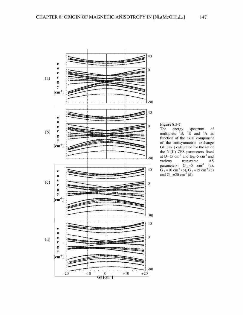
CHAPTER 8: ORIGIN OF MAGNETIC ANISOTROPY IN [Ni4(MeOH)4L4] 147
e
n
er
g
y [cm-1]
e
n
er
g
y [cm-1]
e
n
er
g
y [cm-1]
e
n
er
g
y [cm-1]
40 0 -90 40 0 -90 40 0 -90 40 0 -90
Figure 8.5-7 The energy spectrum of multiplets 9B, 7E and 7A as function of the axial component of the antisymmetric exchange G|| [cm-1] calculated for the set of the Ni(II) ZFS parameters fixed at D=15 cm-1 and ENi=5 cm-1 and various transverse AS parameters: G_|_=5 cm-1 (a), G_|_=10 cm-1 (b), G_|_=15 cm-1 (c) and G_|_=20 cm-1 (d).
(a)
(b)
(c)
(d)
G|| [cm-1] -20 +20 -10 +10 0
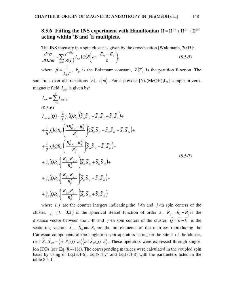
CHAPTER 8: ORIGIN OF MAGNETIC ANISOTROPY IN [Ni4(MeOH)4L4] 148
8.5.6 Fitting the INS experiment with Hamiltonian ISOLAiso Η+Η+Η=Η acting within
9B and
7E multiplets.
The INS intensity in a spin cluster is given by the cross section [Waldmann, 2005]:
( )( )∑
−−
Ω
−
mn
nmnm
E EEQI
TZ
e
dd
d n
,
2
~h
ωδω
σ β
, (8.5-5)
where TkB
1=β , Bk is the Bolzmann constant, ( )TZ is the partition function. The
sum runs over all transitions mn → . For a powder [Ni4(MeOH)4L4] sample in zero-
magnetic field nmI is given by:
∑=
=4
1,
,ji
ijnmnm II
(8.5-6)
( ) ( )( )
( ) ( )
( ) ( )
( ) ( )
( ) ( )
( ) ( )jyizjziy
ij
zijyij
ij
jxizjzix
ij
zijxij
ij
jxiyjyix
ij
yijxij
ij
jyiyjxix
ij
ijxij
ij
jyiyjxixjziz
ij
ijzij
ij
iziziyiyjxixijijnm
SSSSR
RRQRj
SSSSR
RRQRj
SSSSR
RRQRj
SSSSR
RRQRj
SSSSSSR
RRQRj
SSSSSSQRjQI
~~~~
~~~~
~~~~
~~~~21
~~~~~~2
3
61
~~~~~~32
2
,,2
2
,,2
2
,,2
2
22,
2
2
22,
2
0,
+
+
++
+
++
+
+−
−+
+−−
−+
+++=
(8.5-7)
where ji, are the counter integers indicating the i -th and j -th spin centers of the
cluster, kj ( 2,0=k ) is the spherical Bessel function of order k , jiij RRRrrr
−= is the
distance vector between the i -th and j -th spin centers of the cluster, 'kkQrrr
−= is the
scattering vector. ixS~
, iyS~
and izS~
are the nm-elements of the matrices reproducing the
Cartesian components of the single-ion spin operators acting on the site i of the cluster,
i.e.: njSmmiSnSS ji |)(ˆ||)(ˆ|~~
βαβα = . These operators were expressed through single-
ion ITOs (see Eq.(8.4-18)). The corresponding matrices were calculated in the coupled spin basis by using of Eq.(8.4-6), Eq.(8.4-7) and Eq.(8.4-8) with the parameters listed in the table 8.5-1.

CHAPTER 8: ORIGIN OF MAGNETIC ANISOTROPY IN [Ni4(MeOH)4L4] 149
Table 8.5-1
SX SY
i j 1k 2k 3k 4k 12k 34k k q )(k
qC )(k
qC
1 1 1 0 0 0 1 0 1 1
2
1−
2
i
2 2 0 1 0 0 1 0 1 1
2
1−
2
i
3 3 0 0 1 0 0 1 1 1
2
1−
2
i
4 4 0 0 0 1 0 1 1 1
2
1−
2
i
1 1 1 0 0 0 1 0 1 -1
2
1
2
i
2 2 0 1 0 0 1 0 1 -1
2
1
2
i
3 3 0 0 1 0 0 1 1 -1
2
1
2
i
4 4 0 0 0 1 0 1 1 -1
2
1
2
i
SZ
i j 1k 2k 3k 4k 12k 34k k q )(k
qC 1 1 1 0 0 0 1 0 1 0 1 2 2 0 1 0 0 1 0 1 0 1 3 3 0 0 1 0 0 1 1 0 1 4 4 0 0 0 1 0 1 1 0 1
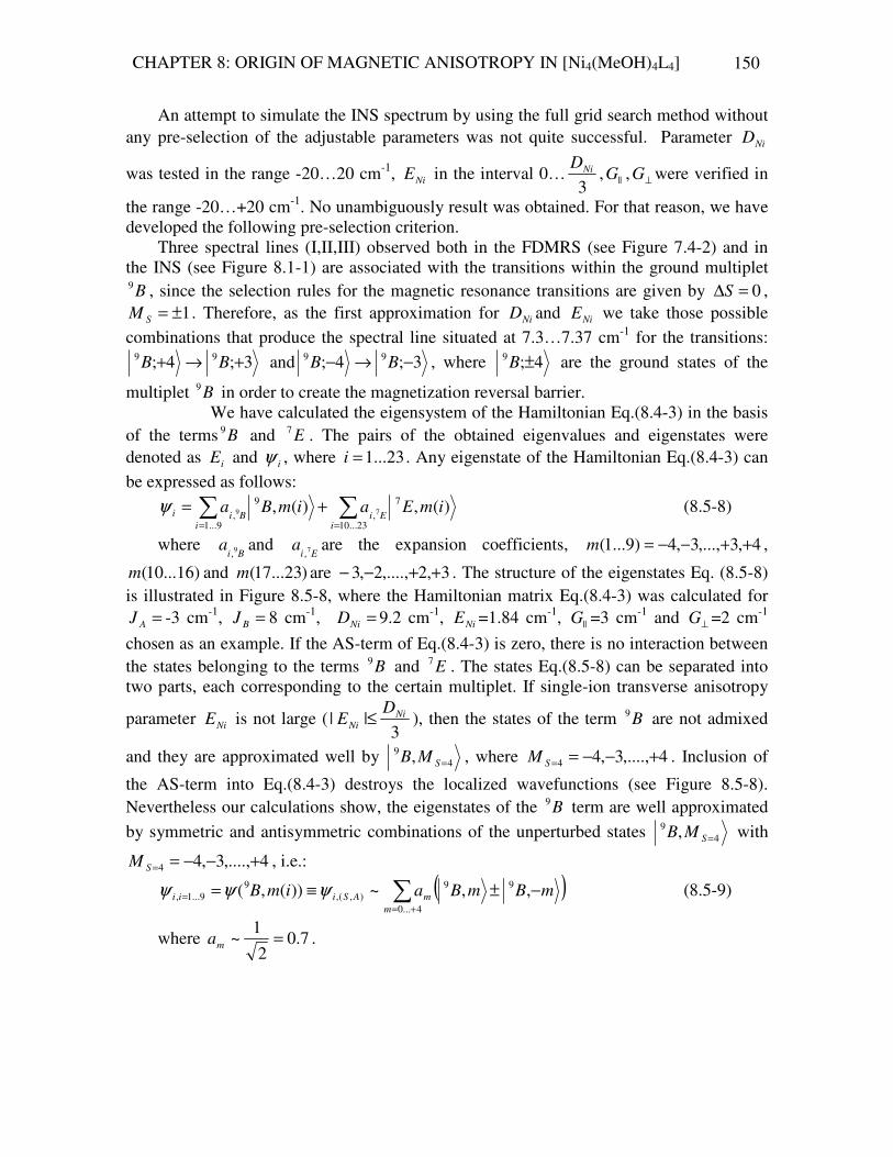
CHAPTER 8: ORIGIN OF MAGNETIC ANISOTROPY IN [Ni4(MeOH)4L4] 150
An attempt to simulate the INS spectrum by using the full grid search method without any pre-selection of the adjustable parameters was not quite successful. Parameter NiD
was tested in the range -20…20 cm-1, NiE in the interval 0…3NiD
, ||G , ⊥G were verified in
the range -20…+20 cm-1. No unambiguously result was obtained. For that reason, we have developed the following pre-selection criterion.
Three spectral lines (I,II,III) observed both in the FDMRS (see Figure 7.4-2) and in the INS (see Figure 8.1-1) are associated with the transitions within the ground multiplet
B9 , since the selection rules for the magnetic resonance transitions are given by 0=∆S , 1±=SM . Therefore, as the first approximation for NiD and NiE we take those possible
combinations that produce the spectral line situated at 7.3…7.37 cm-1 for the transitions: 3;4; 99 +→+ BB and 3;4; 99 −→− BB , where 4;9 ±B are the ground states of the
multiplet B9 in order to create the magnetization reversal barrier. We have calculated the eigensystem of the Hamiltonian Eq.(8.4-3) in the basis
of the terms B9 and E7 . The pairs of the obtained eigenvalues and eigenstates were denoted as iE and iψ , where 23...1=i . Any eigenstate of the Hamiltonian Eq.(8.4-3) can be expressed as follows:
∑∑==
+=23...10
7
,9...1
9
,)(,)(, 79
iEi
iBii imEaimBaψ (8.5-8)
where Bi
a 9,and
Eia 7,
are the expansion coefficients, 4,3,...,3,4)9...1( ++−−=m ,
)16...10(m and )23...17(m are 3,2,....,2,3 ++−− . The structure of the eigenstates Eq. (8.5-8) is illustrated in Figure 8.5-8, where the Hamiltonian matrix Eq.(8.4-3) was calculated for
=AJ -3 cm-1, =BJ 8 cm-1, =NiD 9.2 cm-1, NiE =1.84 cm-1, ||G =3 cm-1 and ⊥G =2 cm-1
chosen as an example. If the AS-term of Eq.(8.4-3) is zero, there is no interaction between the states belonging to the terms B9 and E7 . The states Eq.(8.5-8) can be separated into two parts, each corresponding to the certain multiplet. If single-ion transverse anisotropy
parameter NiE is not large (3
|| NiNi
DE ≤ ), then the states of the term B9 are not admixed
and they are approximated well by 49 , =SMB , where 4,....,3,44 +−−==SM . Inclusion of
the AS-term into Eq.(8.4-3) destroys the localized wavefunctions (see Figure 8.5-8). Nevertheless our calculations show, the eigenstates of the B9 term are well approximated by symmetric and antisymmetric combinations of the unperturbed states 4
9 , =SMB with
4,....,3,44 +−−==SM , i.e.:
( )∑+=
= −±≡=4...0
99),(,
99...1, ,,~))(,(
m
mASiii mBmBaimB ψψψ (8.5-9)
where 7.02
1~ =ma .

CHAPTER 8: ORIGIN OF MAGNETIC ANISOTROPY IN [Ni4(MeOH)4L4] 151
9B 7E
Figure 8.5-8: The eigenstates of the Hamiltonian Eq.(8.4-3), i.e. the absolute values of Bi
a 9,and
Eia 7,
as function of i (see Eq. (8.5-8)) calculated for DNi=9.2 cm-1, ENi=1.84 cm-1, G||=3 cm-1 and G_|_
=2 cm-1 as an example.

CHAPTER 8: ORIGIN OF MAGNETIC ANISOTROPY IN [Ni4(MeOH)4L4] 152
We assume the strong exchange limit, i.e. that the non-Heisenberg interactions are weaker than the isotropic one. Thus, to find the preselection rule for adjustable parameters, we construct the Hamiltonian matrix Eq.(8.4-3) in absence of the AS-term ( ||G and ⊥G =0)
and sweep the single-ion ZFS parameters in the possible ranges: NiD =-20…+20 cm-1 and
3
|| NiNi
DE ≤ . Then we select those combinations NiNi ED , that give the expansion
coefficients of Eq. (8.5-9): 6.0>ma and the spectral line associated to the transitions
SSBB 3;4; 99 → and
AABB 3;4; 99 → situated at 7.3…7.37 cm-1, i.e.
37.7...33.7)3,()4,( ,9
,9 =− ASAS BEBE cm-1. The result of our calculations is visualized on
the Figure 8.5-9. There is a linear dependence between the single-ion ZFS parameters NiE
and NiD that satisfy the conditions described above. Moreover, only positive values of the
parameter NiD give rise to the multiplet B9 with the lowest lying states originating from
the pure wavefunctions 4;9 ±B . It turns out that the dependence )( NiNi DE can be
approximated by the function: =NiE 4.889(3)-0.333(2)* NiD (8.5-10)
The value of the axial local anisotropy term must be larger that 6 cm-1, otherwise the transverse Ni(II) ZFS-parameter satisfying the preselection condition will be more than
3
|| NiD. Then we have tried to find those parameters of the AS-term that reproduce the
energy gap ~0.76 cm-1 between the INS lines II and III (see Figure 8.1-1) caused by the
transitions SS
BB 2;3; 99 → and AA
BB 2;3; 99 → (see Figure 8.1-2). Again, no
unambiguous solution was obtained. All our attempts to simulate the INS spectrum point to the very large values of the parameters of the antisymmetric exchange interactions. One of the reasonable INS-simulations was obtained for the set of parameters: AJ =-3 cm-1, BJ = 8
cm-1, NiD =9.3 cm-1 , =NiE 1.79 cm-1, ⊥G =13.8 cm-1 and ||G = 9.8 cm-1 (see Figure 8.5-10).
It explains the lines I,II,III, IV and VIII (see Figure 8.1-1) as well as the weak line situated at ~3.5 cm-1. This set of parameters gives rise to the set of eigenvalues of the model Hamiltonian Eq. (8.4-3) that produces no INS spectral lines in the frequency range 8…22
cm-1
as it is expected from the experiment. Otherwise, these parameters induce some spectral lines in the range between 5…7 cm-1, which were experimentally not observed.
In conclusion to this section we would like to mention, that the presented model explains well the origin of the parameter 4
4B obtained by fitting the INS experiment according to the single-spin Hamiltonian (see Sections 7.4 and 8.1): it is caused by the collective action of the axial and transverse parts of the antisymmetric exchange interactions expressed in the cluster coordinate system. The model gives reasonable results up to the constant that is equivalent to the action of the term 0
404 OB of single-spin
Hamiltonian. To improve the result, we have to calculate the energy matrix in the full Hilbert space, i.e. to perform the calculations according to Eq. (8.5-5) over all multiplets (see Table 8.4-1 and 8.4-2, not only 9B,7E), since the contribution of the excited pure spin levels into the value of 0
4B have different sign.

CHAPTER 8: ORIGIN OF MAGNETIC ANISOTROPY IN [Ni4(MeOH)4L4] 153
-30 +30 -20 +20 -10 +10 0
-15
-5
-10
0
+5
+10
+15
DNi [cm-1]
ENi [cm-1]
Figure 8.5-9: The diagram ENi versus DNi calculated over the terms 9B and 7E: points show those combinations of the Ni(II) ZFS parameters that lead to the spectral line situated at ν1=7.3..7.37 cm-1,
which is associated with the transitions 3;4; 99 ±→± BB . Our analysis indicates that the
magnetization reversal barrier arises only for the positive values of the axial ZFS parameter DNi .
ν1
|9B,3>S |9B,3>A
|9B,4>A |9B,4>S
|9B,4>S |9B,4>A
|9B,3>A |9B,3>S ν1

CHAPTER 8: ORIGIN OF MAGNETIC ANISOTROPY IN [Ni4(MeOH)4L4] 154
Figure 8.5-10: The INS spectrum (lines with points) calculated according to the model described in Section 8.4 in the basis of the manifolds 9B and 7E for the following parameters: JA=-3 cm-1, JB=8 cm-1, DNi=9.3 cm-1 , ENi=1.79 cm-1, G_|_=13.8 cm-1 and G||=9.8 cm-1 at T=22K. The calculated spectrum contains no spectral lines in the range 8…22 cm-1. The solid lines indicate the experimentally observed INS-line positions.
1 8 7 2 3 4 5 6
Frequency [cm-1]
0.05
0.2
0.1
0.15
INS
intensity [a.u.]
0.00

CHAPTER 8: ORIGIN OF MAGNETIC ANISOTROPY IN [Ni4(MeOH)4L4] 155
8.5.7 Analysis of the energy spectrum of the Ni4 cluster calculated in the full Hilbert space We have calculated the Hamiltonian matrix of Eq. (8.4-3) according to Eq. (8.4-4) for
all 19 manifolds (see Eq.(8.2-1)) in the coupled spin basis (see Table 8.2-3), in order to analyze the influence of the excited spin multiplets other than E7 and A7 on the resulting cluster energy spectrum. Our calculations show that the multiplets are admixed in a very complicated manner. Admixture of the states is visualized in Figure 8.5-11 (without their zero field splitting). The interaction between the low-lying multiplets with different spin values (like EAEB 7531 ,,, and B9 ) is especially important for interpretation of the experimental data. Non-zero values of the model parameters can cause approach or repulsion of the levels of the manifolds in a very tricky way. We illustrate it with a few diagrams. Figure 8.5-12 shows eigenstates as function of the axial component of the AS-term was calculated for the limiting case of zero local crystal fields and in absence of the transverse AS part. For small ||G , the results of our calculations are in agreement with
those given by the isotropic exchange model Eq. (8.4-2). Increasing of the absolute value of the axial AS-parameters couples the neighbouring multiplets 7E, 5A, 1B, 3E ,5E,3E,7A,5E and 1A into one energetic zone and converge them to the ground state. Introduction of the single-ion ZFS parameters broadens additionally the energetic zone of each multiplet and makes it possible (from theoretical point of view) the experimental observation of the transitions within the excited multiplets. The energetic structure becomes even more complicated, if it is considered under the simultaneous action of the antisymmetric exchange and the local crystal fields as it is illustrated in Figure 8.5-13, where the diagram is presented calculated for AJ =-3 cm-1, BJ = 8 cm-1, NiD =10.2 cm-1 , =NiE 1.49 cm-1,
⊥G =2 cm-1. For || ||G >6 cm-1 complete overlap of the ground and the excited multiplets
takes place. We have made numerous attempts to model the INS spectrum of [Ni4(MeOH)4L4]
complex for various values of NiD , NiE , ⊥G and ||G . The isotropic exchange coupling
constants were fixed at the values obtained by fitting of the temperature dependence of the magnetic susceptibility in terms of the isotropic exchange model AJ =-3 cm-1, BJ = 8 cm-1.
Despite all of our efforts, we have not found a satisfactory description of the INS spectrum. One of the possible results is shown in diagram Figure 8.5-14 calculated for
AJ =-3 cm-1, BJ =8 cm-1, NiD =9 cm-1, NiE =1.89 cm-1, ⊥G =3.2 cm-1 and ||G =3.4 cm-1. In
this case the calculated spectrum reproduces well experimentally observed INS-line positions, including the weak peak at 3.5 cm-1. Nevertheless these model parameters can not be accepted as the ideal ones, since the calculated spectrum contains two features at 4.5 cm-1 and 6.5 cm-1 as well as the tail of weak lines in the range 8…22 cm-1, which were experimentally not observed.
In the next section we discuss the obtained results.
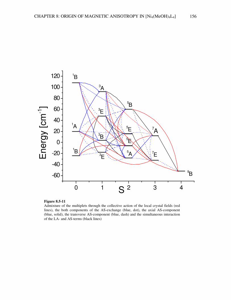
CHAPTER 8: ORIGIN OF MAGNETIC ANISOTROPY IN [Ni4(MeOH)4L4] 156
0 1 2 3 4
-60
-40
-20
0
20
40
60
80
100
120 1B
1A
1B
3A
3E
3B
3E
5B
5E
5E
5A
7A
7EE
ne
rgy [cm
-1]
S
9B
Figure 8.5-11 Admixture of the multiplets through the collective action of the local crystal fields (red lines), the both components of the AS-exchange (blue, dot), the axial AS-component (blue, solid), the transverse AS-component (blue, dash) and the simultaneous interaction of the LA- and AS-terms (black lines)

CHAPTER 8: ORIGIN OF MAGNETIC ANISOTROPY IN [Ni4(MeOH)4L4] 157
Figure 8.5-12 The complete energy spectrum of the Ni4-cluster calculated as function of the axial component of the antisymmetric exchange G|| [cm-1] in absence of the local crystal fields for the transverse AS parameter: G_|_=0 cm-1 (a). The inset on the bottom (b) illustrates the fine structure of the levels selected on the figure (a) by the bracket.
7E, 5A, 1B, 3E, 5E,3E,7A,5E,1A
e
n
er
g
y [cm-1]
G|| [cm-1] -20 +20 -10 +10 0
100 0 -100
9B
3E
5B
3A
1B
G|| [cm-1]
-6 +6 -4 -2 0 +2 +4
e
n
er
g
y [cm-1]
20 0 -20 -60
9B
7E
5A
1B
3E
5E
3E 7A
5E
1B
(a)
(b)
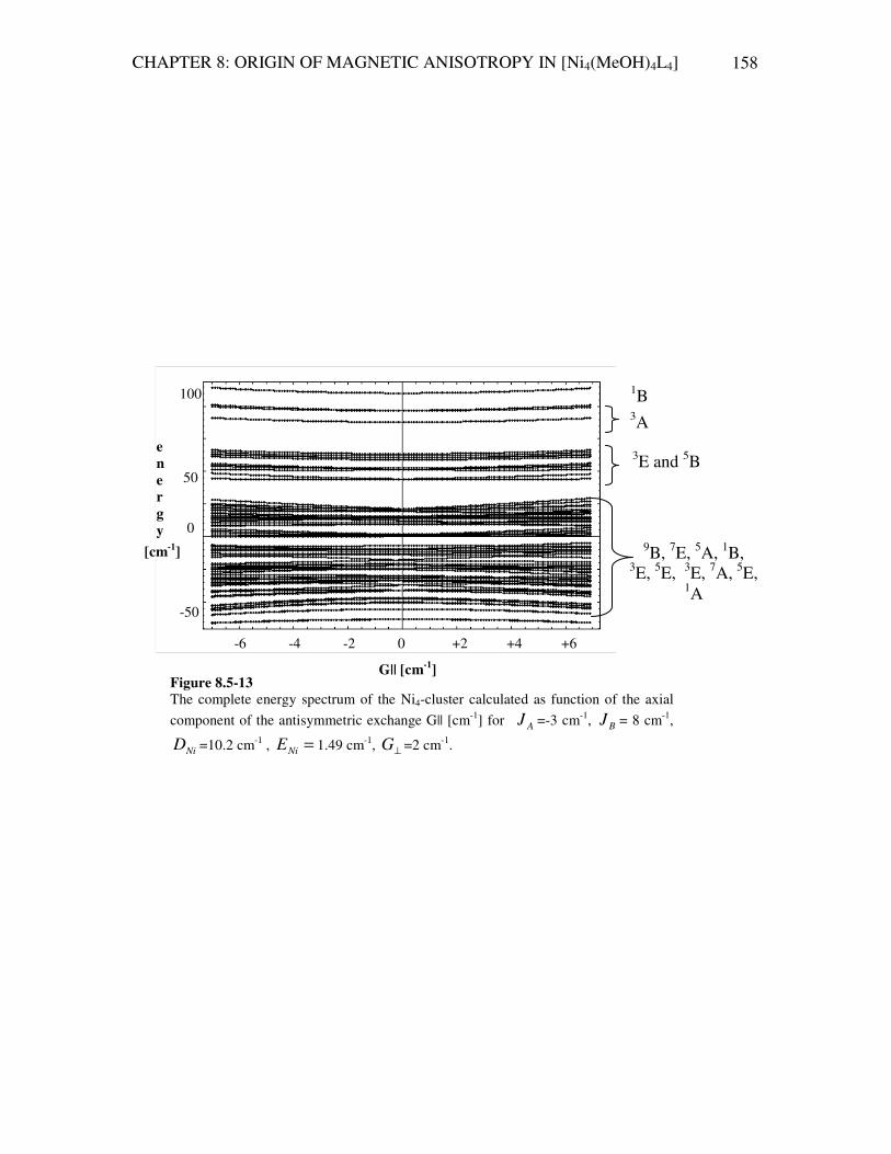
CHAPTER 8: ORIGIN OF MAGNETIC ANISOTROPY IN [Ni4(MeOH)4L4] 158
Figure 8.5-13 The complete energy spectrum of the Ni4-cluster calculated as function of the axial
component of the antisymmetric exchange G|| [cm-1] for AJ =-3 cm-1, BJ = 8 cm-1,
NiD =10.2 cm-1 , =NiE 1.49 cm-1, ⊥G =2 cm-1.
100 50 0 -50
e
n
er
g
y [cm-1]
G|| [cm-1]
-6 +6 -4 -2 0 +2 +4
9B, 7E, 5A, 1B, 3E, 5E, 3E, 7A, 5E,
1A
3E and 5B
3A
1B

CHAPTER 8: ORIGIN OF MAGNETIC ANISOTROPY IN [Ni4(MeOH)4L4] 159
Figure 8.5-14: The INS spectrum (lines with points) calculated according to the model described in Section 8.4 in the full Hilbert space for the following parameters: JA=-3 cm-1, JB=8 cm-1, DNi=9 cm-1 , ENi=1.89 cm-1, G_|_=3.2 cm-1 and G||=3.4 cm-1. The calculated spectrum contains the tail of spectral lines in the range 8…22 cm-1. The solid lines indicate the experimentally observed INS-line positions.
INS
intensity [a.u.]
1 7 2 3 4 5 6
Frequency [cm-1]
0.05
0.2
0.1
0.15
0.00

CHAPTER 8: ORIGIN OF MAGNETIC ANISOTROPY IN [Ni4(MeOH)4L4] 160
8.5.8 Conclusion The nature of exchange coupling in polynuclear metal complexes remains a topic of
great interest in inorganic chemistry and physics. High-spin magnetic molecules like Mn12Ac (see Chapter 2) show specific magnetic properties, which follow directly from the physical mechanisms realizing the coupling of the spin centers into the cluster. Despite the recent progress in understanding their magnetic behavior, it is still a challenge to give a theoretical interpretation of the model parameters describing the experimental data. The Heisenberg isotropic exchange model is usually applied for theoretical evaluation of the low-temperature properties of the systems with large number of metal ions like Mn12Ac [Regnault, 2002] or Mo72Fe30 [Schnack, 2001], since the large number of the high-spin ions per molecule increases dramatically the dimension of the corresponding Hamiltonian leading to essential difficulties in the diagonalization of the Hamiltonian matrix. Nevertheless, the interactions of non-Heisenberg type provide understanding of the fine-structure of the zero-field split multiplets of the polynuclear metal complexes and their behaviour in magnetic fields. It was already shown that the single-ion ligand-field contributions are the origin of the cluster magnetic anisotropy in Mn12Ac [Barra, 1997] or in Cr8 [Carretta, 2003], [van Slageren, 2002]. The dipole-dipole interaction was found to be responsible for more than 60% of the total anisotropy in Mn(II)-[3x3] grid [Guidi, 2004]. The pronounced role of the antisymmetric exchange in the trimeric Cu(II) cluster was indicated in [Yoon, 2004]. The role of the orbitally degenerate Mn(III) ions in the single magnet behaviour of the cyanide Mn5 cluster was analyzed in [Palii, 2004].
The tetrameric Ni(II) complexes serve as good model systems to study the non-Heisenberg exchange interactions due to their simple chemical and magnetic structure. Magnetization and magnetic torque measurements were well explained in some of them in terms of the model Hamiltonian including the symmetric part of the spin-spin interaction term (local anisotropy term) besides of the isotropic next-neighbour exchange interactions and the Zeeman term [Koch, 2003]. It was shown in [Waldmann, 1998], that the biquadratic exchange acting additionally to single-ion anisotropy is a significant non-Heisenberg part of the microscopic Hamiltonian, which enables modelling of magnetization measurements of the Ni-[2x2] grid containing four Ni(II) ions in a square type arrangement. Recently the bulk magnetic, electron paramagnetic and magneto-optical properties of the tetrahedral Ni4Mo12 complex with zero-ground state spin were investigated both experimentally and theoretically [Schnack, cond-mat/0509476]. The non-Heisenberg zero-field part of microscopic Hamiltonian suggested there includes the single-site anisotropic (ligand-field) term as well as the biquadratic exchange, where the field dependence of the model parameters was indicated.
Despite of intensive research in area of polynuclear metal complexes, it is still a challenge to deduce the underline spin Hamiltonian [Schnack, cond-mat/0509476]. The only classification of principles for selection of non-Heisenberg terms of the model Hamiltonian valid for exchange-coupled compounds is given in [Tsukerblat, 1994]. These selection rules are based on the group-theoretical classification of spin multiplets. They were applied in Sections 8.4-2 – 8.4.-4 to construct the model for interpretation of the spectroscopic studies (INS- and FDMRS-) on [Ni4(MeOH)4L4]. We have performed the group-theoretical analysis of exchange coupled multiplets of this tetrameric Ni(II) cluster under assumption that the cluster point group is S4. Nevertheless, the real magnetic

CHAPTER 8: ORIGIN OF MAGNETIC ANISOTROPY IN [Ni4(MeOH)4L4] 161
structure of [Ni4(MeOH)4L4] is based on a distorted cubane [Sieber, 2005] and can not be strictly characterized by the S4 point group. Our model does not take into account the effect of symmetry lowering. However, the suggested microscopic spin Hamiltonian can be applied for simulation and interpretation of the low-temperature experimental data on many other tetrameric Ni(II) systems possessing the S4 symmetry [Edwards, 2003]. The group theoretical analysis points unambiguously to the admixture of the excited states into the ground multiplet through the spin-orbit coupling (antisymmetric exchange term) accompanied by the collective action of the local crystal fields. The spin-orbit coupling was introduced in the spin basis according to the Moriya rules. To avoid over-parameterization of the model describing six pairwise antisymmetric exchange interactions (i.e. 18 model parameters arising due to three Cartesian components of each vector AS-parameter in six local coordinate systems), we have assumed the axial AS model. According to this simplification the local transverse AS-components are negligible in comparison to the axial ones. It was shown in [Tsukerblat, 1983] that the axial AS-model gives good results for tetragonal systems even in the cases of slightly broken symmetry. To the best of our knowledge we have developed for the first time the method and the mathematical formalism describing the non-Heisenberg exchange interactions expressed in terms of non-collinear tensors both for antisymmetric exchange and the single-site anisotropy terms. We have derived a general formula that links the cluster axial ZFS parameter with the single-ion ZFS parameters as function of the Euler angels connecting the principal axes of any local D-tensor to the cluster coordinated system under the overall S4 symmetry. The formula allows the analysis of contributions of the local crystal fields to the cluster axial ZFS parameter in absence of antisymmetric exchange interactions. Moreover, the suggested method for calculation of the LA-term takes into account the real orientation of the local D-tensors realized in [Ni4(MeOH)4L4] molecule. It can be extended and generalized for any orientation of the single-site D-tensors, which is not necessary parallel to the cluster coordinate system.
The model developed in Section 8.4 gives numerical results, which are in agreement with the group theoretical predictions. Thus, we present the analysis of the possible limiting cases of the model. We have found the connection between the spin-orbit coupling
and the AS model parameter ||G : ||31
G=λ . The behavior of the ground spin multiplet and
the first excited doublet was considered analytically. Our analysis indicates overlap of the multiplets E7 and B9 for some combinations of AS-parameters, which is reflected in non-zero value of the transverse ZFS parameter of the fourth order 4
4B obtained in terms of the single-spin Hamiltonian model. Moreover, the mentioned overlap may be the reason of the weak INS-line situated at 3.5 cm-1 associated with the transition restricted by 1=∆S . In Section 8.5.6 we suggest the method for preselection of the single-site anisotropy parameters and try to apply it for the INS-spectral simulation. Despite all our efforts, it was impossible to obtain a complete reconstruction of the INS spectrum working in the basis of the ground- and the first excited states. However there are some combinations of the model parameters like AJ =-3 cm-1, BJ =8 cm-1, NiD =9.3 cm-1 , =NiE 1.79 cm-1, ⊥G =13.8 cm-1
and ||G = 9.8 cm-1 that reconstruct six INS lines out of eight (or nine including the peak at
3.5 cm-1) observed experimentally without lines calculated in the range 8…22 cm-1. The obtained AS parameters are unacceptable large. Therefore we have performed the same

CHAPTER 8: ORIGIN OF MAGNETIC ANISOTROPY IN [Ni4(MeOH)4L4] 162
calculations in full Hilbert space, which indicate a very complicated admixture of the excited states into the ground manifold. It was succeeded to find the possible set of parameters AJ =-3 cm-1, BJ =8 cm-1, NiD =9 cm-1, NiE =1.89 cm-1, ⊥G =3.2 cm-1 and
||G =3.4 cm-1, which reconstruct all the experimentally observed INS lines, but induces
some unclear features at 4.5 cm-1 and 6.5 cm-1 as well as the tail of the weak lines in the range 8…22 cm1. Thus, the obtained model parameters give reasonable, but not quite satisfactory description of the INS-spectrum. As the possible sources of this discrepancy we would like to mention the distortion from S4 symmetry as well as the simplification of the axial model of the local antisymmetric exchange interactions. All our calculations were performed at fixed values of the isotropic exchange coupling constants AJ =-3 cm-1, BJ =8
cm-1 determined by fitting the temperature dependence of susceptibility. Fitting AJ and
BJ simultaneously with NiD , NiE , ⊥G and ||G makes the model over-parameterized. Finally,
we would like to underline the time-consuming nature of the INS intensity calculations in full Hilbert space, what makes the fit procedure very inflexible.
To conclude, we would like to point to the fact that the developed gesH model gives analytically correct results. To refine the model parameters, it must be applied for simulation of other than INS experimental data on [Ni4(MeOH)4L4].

IX
Summary and outlook
This PhD-thesis is devoted to the analysis of the spectral data on molecular magnets. This
work was motivated by the need to develop a generalized computer code for simulation and interpretation of the Frequency-Domain Magnetic Resonance spectra (FDMRS) on molecular magnets as well as to understand the physical origin of zero-field splitting parameters. Therefore, after a short introduction into the problem given in Chapter 1, we have dedicated Chapter 2 to the description of the main properties of the molecular magnets. There we have shown that these molecules consist of a finite number of the metal ions, providing the spins to the system, which are coupled into fixed structural motifs by the diamagnetic ligands. The coupling of the spin angular momenta localized on the different spin sites of the molecule gives rise to the energy spectrum composed of several multiplets with varying total spin values. The ground multiplet of molecular magnets can have a large spin. This property together with the high negative uniaxial symmetry of these quantum mechanical systems is responsible for observation of specific phenomena unusual for conventional magnetic materials in some of them (i.e. in the single molecular magnets, SMM): hysteresis of purely molecular origin and quantum tunneling of magnetization. The prerequisites for single-molecule behavior are summarized in Section 2.1. Since molecular magnets belong to category of spin tunneling systems, we discuss the similarities and distinctions between the particle-like- and the spin tunneling systems (Section 2.2). The first and most studied single molecular magnet is Mn12Ac, which we have used as an illustrative example of an SMM. The behavior of the energy levels and the corresponding wavefunctions of the ground spin multiplet of Mn12Ac under the influence of the overall cluster crystal field of S4 symmetry and of the external magnetic field was analyzed in Section 2.3. There we have shown that the crystal field symmetry is the main force lying behind the tunneling mechanism in Mn12Ac molecule. The Section 2.4 presents the link between the symmetry of the quantum mechanical system and its energy spectrum. Rotation-, point- and symmetric groups are introduced, since the energetics of molecular magnets can be estimated analytically and numerically by using of the properties of these groups. The quantum theory of angular momentum is a common tool for the description of the spin coupling in magnetic nanoclusters and of the symmetry properties of their energy spectrum. We have summarized the most important results of the quantum theory of angular momentum in Chapter 3. Thus, in Section 3.1 we describe how to characterize the action of the transformations of a symmetry group on a quantum mechanical system. The total, orbital and spin angular momentum operators were introduced in Section 3.2, where the rules were presented, which are used for the calculation of the matrix elements of these operators, their Cartesian components, and the raising and lowering operators. The coupling of angular momenta is of importance in the context of molecular magnetism. Thus, in Section 3.3 we show how to calculate the eigenstates of the sum of several angular momenta in terms of the products of individual angular momentum eigenstates. The Clebsch-Gordan coefficients, 3j-, 6j- and 9j-symbols were also presented there, since they are used for the evaluation of the matrix elements of the microscopic Hamiltonian valid for the magnetic cluster. Section 3.4 deals with the concept of the irreducible tensor operators (ITOs), which completely characterizes the transformation properties of the angular
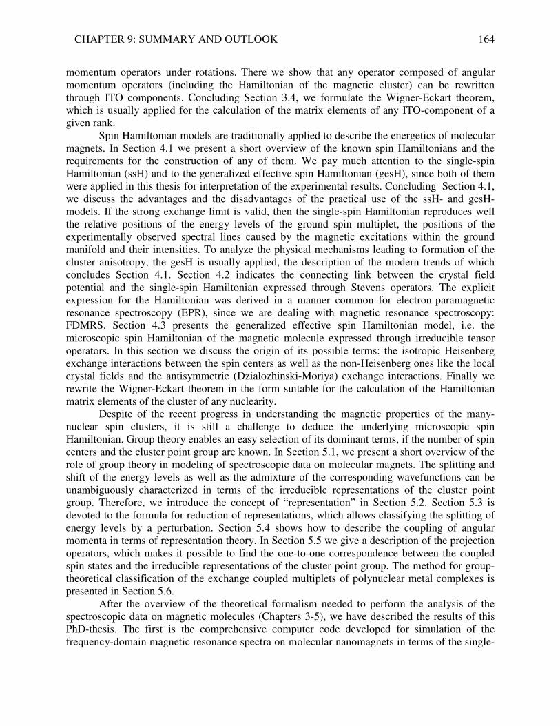
CHAPTER 9: SUMMARY AND OUTLOOK
164
momentum operators under rotations. There we show that any operator composed of angular momentum operators (including the Hamiltonian of the magnetic cluster) can be rewritten through ITO components. Concluding Section 3.4, we formulate the Wigner-Eckart theorem, which is usually applied for the calculation of the matrix elements of any ITO-component of a given rank.
Spin Hamiltonian models are traditionally applied to describe the energetics of molecular magnets. In Section 4.1 we present a short overview of the known spin Hamiltonians and the requirements for the construction of any of them. We pay much attention to the single-spin Hamiltonian (ssH) and to the generalized effective spin Hamiltonian (gesH), since both of them were applied in this thesis for interpretation of the experimental results. Concluding Section 4.1, we discuss the advantages and the disadvantages of the practical use of the ssH- and gesH-models. If the strong exchange limit is valid, then the single-spin Hamiltonian reproduces well the relative positions of the energy levels of the ground spin multiplet, the positions of the experimentally observed spectral lines caused by the magnetic excitations within the ground manifold and their intensities. To analyze the physical mechanisms leading to formation of the cluster anisotropy, the gesH is usually applied, the description of the modern trends of which concludes Section 4.1. Section 4.2 indicates the connecting link between the crystal field potential and the single-spin Hamiltonian expressed through Stevens operators. The explicit expression for the Hamiltonian was derived in a manner common for electron-paramagnetic resonance spectroscopy (EPR), since we are dealing with magnetic resonance spectroscopy: FDMRS. Section 4.3 presents the generalized effective spin Hamiltonian model, i.e. the microscopic spin Hamiltonian of the magnetic molecule expressed through irreducible tensor operators. In this section we discuss the origin of its possible terms: the isotropic Heisenberg exchange interactions between the spin centers as well as the non-Heisenberg ones like the local crystal fields and the antisymmetric (Dzialozhinski-Moriya) exchange interactions. Finally we rewrite the Wigner-Eckart theorem in the form suitable for the calculation of the Hamiltonian matrix elements of the cluster of any nuclearity. Despite of the recent progress in understanding the magnetic properties of the many-nuclear spin clusters, it is still a challenge to deduce the underlying microscopic spin Hamiltonian. Group theory enables an easy selection of its dominant terms, if the number of spin centers and the cluster point group are known. In Section 5.1, we present a short overview of the role of group theory in modeling of spectroscopic data on molecular magnets. The splitting and shift of the energy levels as well as the admixture of the corresponding wavefunctions can be unambiguously characterized in terms of the irreducible representations of the cluster point group. Therefore, we introduce the concept of “representation” in Section 5.2. Section 5.3 is devoted to the formula for reduction of representations, which allows classifying the splitting of energy levels by a perturbation. Section 5.4 shows how to describe the coupling of angular momenta in terms of representation theory. In Section 5.5 we give a description of the projection operators, which makes it possible to find the one-to-one correspondence between the coupled spin states and the irreducible representations of the cluster point group. The method for group-theoretical classification of the exchange coupled multiplets of polynuclear metal complexes is presented in Section 5.6. After the overview of the theoretical formalism needed to perform the analysis of the spectroscopic data on magnetic molecules (Chapters 3-5), we have described the results of this PhD-thesis. The first is the comprehensive computer code developed for simulation of the frequency-domain magnetic resonance spectra on molecular nanomagnets in terms of the single-

CHAPTER 9: SUMMARY AND OUTLOOK
165
spin Hamiltonian approach. The program enables automatic and high-precision determination of the zero-field splitting parameters of mono- and poly-nuclear metal complexes. Thus, Section 6.1 explains the general logic of spectral simulations of magnetic resonance spectra. Section 6.2 describes the FDMRS spectrometer and clarifies the formation of the FDMRS spectrum. In Section 6.3 we have presented for the first time the mathematical formalism used for FDMR-spectral simulations. Finally, Section 6.4 delineates in detail the data flow in the developed program for FDMRS-spectral simulations consisting of three blocks. The first one serves for the determination of the absorption line positions and their full width at a half maximum by high-degree polynomial fitting in the region of resonance. The second block affords the fit of the single-spin Hamiltonian parameters to the absorption line positions using a full grid search, where the varying interval of the model parameters and the number of points within it is defined by the user. The current version of the program allows the simultaneous fit of five single-spin Hamiltonian parameters, although the precision of the ZFS-determination decreases and the calculation time increases with the increase of the total spin value of the ground multiplet. The third block is conduced to calculation of intensity of induced magnetic dipole transitions for the set of obtained ZFS parameters as function of temperature and its comparison with the experimentally observed values. Finally, the transmission versus frequency spectra are computed with Lorentzian and Gaussian lineshape functions. Adjusting the spectral line intensities and their linewidths to the experimental observables allows the complete reconstruction of the FDMRS spectra. This computer code was successfully applied to the zero-field splitting studies by FDMRS on several magnetic molecules. The results were summarized in the Chapter 7.
Studies on Mn12Ac have motivated the search for some new single molecule magnets in the group of dodecanuclear manganese complexes. Work within the area of Mn12 coordination chemistry has led to the development of methods for major alteration of the chemical environment of the Mn12 core. Various PPh4
+ derivatives of the Mn12Ac cluster were obtained recently. One of them is the one-electron reduced Mn12 complex [Mn12]
-1 =(PPh4)[Mn12O12(O2CEt)16(H2O)4] with the half integer spin ground state. The ZFS studies on this complex (see Section 7.1) are interesting, because the spin parity effect forbids magnetization quantum tunneling in half-integer spin complexes in zero magnetic fields. Nevertheless, the presence of steps in the magnetization hysteresis loops was reported. The ZFS study on [Mn12]
-1 by FDMRS was complementary to the same studies by other experimental techniques like inelastic neutron scattering (INS), reduced magnetization, HF-EPR and DC magnetic susceptibility. The experimental observables were well reproduced using the spin Hamiltonian model, which contains only the axial terms. Thus the obtained ZFS parameters are: D=-0.454±0.003 cm-1 and B4
0=(+1.01±0.25)x10-5 cm-1. This fact excludes the crystal field symmetry as the possible source of the tunneling mechanism in [Mn12]
-1 complex. A large range of Mnx clusters (e.g. x=3, 4, etc.) constituted of manganese ions (MnII,
MnIII, MnIV) exhibiting the SMM properties has been discovered recently. One of them is the Mn9–molecule, i.e. the [Mn9O7(OAc)11(thme)(py)3(H2O)2] complex. The ZFS parameters extracted from the FDMRS experiment on it are in excellent agreement with the outcome of other magnetic studies using the inelastic neutron scattering, bulk and single-crystal measurements, and theoretical density functional calculations (see Section 7.2). They are: D = -0.247±0.005 cm-1 and B4
0 = (+4.6±0.1)×10-6 cm-1. In Section 7.3 we present the ZFS study on the mononuclear Ni(II) complex [Ni-(HIM2-
py)2NO3]NO3, which is a possible building block of single-molecule magnets. It has the largest

CHAPTER 9: SUMMARY AND OUTLOOK
166
negative axial ZFS reported for mononuclear complexes to date D=-10.0±0.01 cm-1 and E=0.3±0.01 cm-1.
In Section 7.4 we consider the FDMRS experiment on the tetrameric Ni4 = [Ni4(MeOH)4L4] complex, which is of high interest, since the whole family of the similar Ni4 compounds containing the ethyl and methyl groups as ligands have shown single magnet behavior. Only the complex [Ni4(MeOH)4L4] does not show magnetic hysteresis down to 40mK. Although the single-spin Hamiltonian including the axial and transverse terms of the fourth order is acceptable for simulation of the FDMRS and INS experiments (D=-0.93(2) cm-1, E=0.023(8) cm-1, B4
0=-4.3(16)*10-4 cm-1, B44=-2.1(4)*10-3 cm-1), it is not able to explain well some fine
features in the low-frequency range of the INS-spectrum. Moreover, very importantly the single-spin Hamiltonian model is not able to clarify the nature of the physical processes leading to non-zero ZFS parameters of the fourth order. The local crystal fields contribute in to the cluster ZFS parameters of the second order (i.e. D and E ). The non-zero 0
4B and 44B indicate the influence of
the excited spin states to the ground multiplet, i.e. the many-spin effects. The most interesting result of this thesis is the new development of the generalized effective spin Hamiltonian model applied to the study of the origin of magnetic anisotropy in a tetrameric Ni(II) cluster (see Chapter 8). Small magnetic molecules like [Ni4(MeOH)4L4], with their simple chemical and magnetic structure, are the best candidates to study the dependence of the magnetic observables on the model parameters. To derive the microscopic spin Hamiltonian, we have performed the group-theoretical classification of the exchange-coupled multiplets for the S4 cluster point group (see Section 8.2). It turns out that the first excited multiplet is an orbital doublet. This fact points to a pronounced role of non-compensated orbital moment in this system. In Section 8.3 we have presented the group-theoretical analysis of the spin-orbit splitting of many-electron terms in the Ni4-cluster possessing the overall S4-symmetry. Our analysis qualitatively predicts the splitting of exchange-coupled multiplets caused by the spin-orbit interaction in the first and second order of perturbation theory as well as the admixture of excited states into the ground manifold through spin-orbit coupling. For that reason we have included into the microscopic spin Hamiltonian, in addition to isotropic exchange, non-Heisenberg interactions of two types. The first term is related to antisymmetric exchange interactions, which models the spin-orbit coupling operator within the orbital doublet. The second one describes the collective action of the local crystal fields, which were treated on the same level with the antisymmetric exchange interactions due to the high spin value of the ground multiplet. The generalized effective spin Hamiltonian was constructed in Section 8.4. For the first time to the best of our knowledge, we have treated the AS-vector parameters and the local crystal fields as non-collinear tensors. The presented methodology applied to the concrete case of the [Ni4(MeOH)4L4 can be extended and generalized. The sections 8.5.1-8.5.6 present the arguments speaking for the correctness of the developed model and the analytical description of the calculated energy spectrum as function of the model parameters. The first attempts to simulate the INS-spectrum (also in the full Hilbert space) are shown in the section 8.5.6 and 8.5.7. So far no excellent agreement between the calculated and the experimentally observed INS-spectra was obtained. The reasons of this discrepancy were analyzed in the section 8.5.8. Nevertheless, the new development of the generalized effective spin Hamiltonian model presented in this thesis sheds new light on the field of molecular magnetism. As the possible direction of further work we suggest the improvement of the gesH-model, i.e. the introduction of e.g. the biquadratic exchange term into the microscopic spin Hamiltonian. It would be interesting to apply the developed model for simulation of the temperature

CHAPTER 9: SUMMARY AND OUTLOOK
167
dependence of the magnetic susceptibility. The non-Heisenberg terms included in our model were not regarded by estimation of the exchange coupling constants fixed in our calculations. The matrices for transformation of the single-ion crystal fields to the cluster coordinate system can be expressed in a general manner in terms of the Euler angles (see e.g. Section 8.4.2A) corresponding to the spin-site symmetry. It would enable the application of the model to analysis of the contributions of the local crystal fields to the cluster anisotropy for any tetrameric system. Finally, we would like to mention the technical difficulties of calculations: they are too much time consuming. The algorithm for evaluation of the matrix elements according to the Wigner-Eckart theorem can not be essentially improved from our point of view. The current version of the program for calculation of the gesH-matrix is written in Mathematica, which calculates about one hour the Hamiltonian matrix including 36 tensors of the model presented in this thesis in the full Hilbert space on the fastest computer available in the institute. Calculation of the INS spectrum for one set of the model parameters takes about twenty seconds and even more depending on the number of spectral lines produced by the given set of the model parameters. It makes the fitting procedure in terms of the full grid search very inflexible. Thus, Mathematica is good enough for the first test of the model. Nevertheless, we would suggest e.g. C/C++ for Windows or Visual Fortran for development of the generalized computer code for simulation of the spectral data on molecular magnets by using the gesH-model. Regarding the ssH model, the minimization fitting algorithm is sufficient for the present quality of the experiment essentially destroyed by the standing waves especially in the low frequency range. The only thing that can be introduced is the broader likelihood interval for simulation of the lower frequency lines in comparison to those situated in the high-frequency range.

Appendix
Appendix 1
The calculated symmetry-adapted wavefunctions for the multiplets 9B, 7E and 7A.
MSSS ,3412
4,4,2,2 − 1,1,1,1 −−−−
3,4,2,2 − ( )1,1,1,01,1,0,11,0,1,10,1,1,121
−−−+−−−+−−−+−−−
2,4,2,2 − ( )
−−+−−+−−+
+−−+−+−−+
+−−−+−−−+−−−+−−−
1,1,0,01,0,1,00,1,1,0
1,0,0,10,1,0,10,0,1,1
7
1
1,1,1,11,1,1,11,1,1,11,1,1,172
1
1,4,2,2 − (
)
( )1,0,0,00,1,0,00,0,1,00,0,0,17
1
1,1,0,11,1,1,01,0,1,10,1,1,1
1,0,1,10,1,1,11,1,1,01,1,1,0
1,1,0,11,1,0,10,1,1,11,0,1,172
1
−+−+−+−+
−−+−−+−−+−−+
+−−+−−+−−+−−+
+−−+−−+−−+−−
0,4,2,2 (
)
( )
(
)1,1,1,11,1,1,1
1,1,1,11,1,1,11,1,1,11,1,1,170
1
0,0,0,0352
2
1,0,0,10,1,0,11,0,1,00,1,1,0
0,0,1,11,1,0,01,1,0,00,0,1,1
0,1,1,01,0,1,00,1,0,11,0,0,1352
−−+−−+
+−−+−−+−−+−−+
++
−+−+−+−+
+−+−+−+−+
+−+−+−+−
1,4,2,2 + (
)
( )1,0,0,00,1,0,00,0,1,00,0,0,17
1
1,0,1,10,1,1,11,1,0,11,1,0,1
1,1,1,01,1,1,00,1,1,11,0,1,1
0,1,1,11,0,1,11,1,1,01,0,1,172
1
++++
−+−+−+−+
+−+−+−+−+
+−+−+−+−
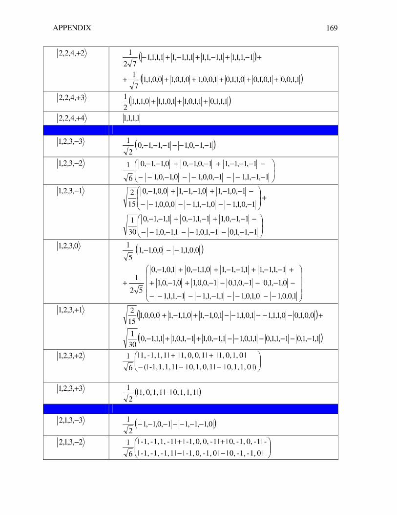
APPENDIX
169
2,4,2,2 + ( )
( )1,1,0,01,0,1,00,1,1,01,0,0,10,1,0,10,0,1,17
1
1,1,1,11,1,1,11,1,1,11,1,1,172
1
++++++
+−+−+−+−
3,4,2,2 + ( )1,1,1,01,1,0,11,0,1,10,1,1,121
+++
4,4,2,2 + 1,1,1,1
3,3,2,1 − ( )1,1,0,11,1,1,02
1−−−−−−−
2,3,2,1 −
−−−−−−−−−−
−−−−+−−+−−
1,1,1,11,0,0,10,1,0,1
1,1,1,11,0,1,00,1,1,0
6
1
1,3,2,1 −
−−−−−−−−−
−−−+−−+−−
+
−−−−−−−−
−−−+−−+−
1,1,1,01,1,0,11,1,0,1
1,1,0,11,1,1,01,1,1,0
30
1
1,0,1,10,1,1,10,0,0,1
1,0,1,10,1,1,10,0,1,0
15
2
0,3,2,1 ( )
−−−−−−−−−−
−−−−−−+−+
+−−+−−+−+−
+
−−−
1,0,0,10,1,0,11,1,1,11,1,1,1
0,1,1,01,0,1,01,0,0,10,1,0,1
1,1,1,11,1,1,10,1,1,01,0,1,0
52
1
0,0,1,10,0,1,15
1
1,3,2,1 + ( )
( )1,1,1,01,1,1,01,1,0,11,1,0,11,1,0,11,1,1,0301
0,0,1,00,1,1,11,0,1,11,0,1,10,1,1,10,0,0,1152
−−−−−−−+−+−
+−−−−−−+−+
2,3,2,1 +
−−− |)0 1, 1, 0,| |1 0, 1, 0,| |1 1, 1, -1,(|
|0 1, 0, 1,| +|1 0, 0, 1,| +|1 1, 1,- 1,|
6
1
3,3,2,1 + ( )|1 1, 1, 0,|-|1 1, 0, 1,|
2
1
3,3,1,2 − ( )0,1,1,11,0,1,12
1−−−−−−−
2,3,1,2 −
−−
++
|0 1,- 1,- 0,| |0 1,- 0, -1,| |1 1,- 1,- -1,|
-|1- 0, 1,- 0,| |1- 0, 0, -1,| |1- 1, 1,- -1,|
6
1

APPENDIX
170
1,3,1,2 −
−
++
+
−−
++
|0 1,- 0, 0,| |1 1,- 1,- 0,|- |1 1,- 0, -1,|-
-|0 1,- 0, 0,| |1 1,- 1,- 0,| |1 1,- 0, -1,|
15
2
|0 1,- 1,- 1,| |0 1,- 1, -1,| |1 0, 1,- -1,|-
-|1- 0, 1,- 1,| |1- 0, 1, -1,| |0 1, 1,- -1,|
30
1
0,3,1,2 ( )
−−−
−−−
+++
+++
+
|0 1,- 0, 1,| |0 1,- 1, 0,| |1 1,- 1,- 1,|
|1 1,- 1, -1,| |1 0, 1,- 0,| |1 0, 0, -1,|-
-|1- 0, 0, 1,| |1- 0, 1, 0,| |1- 1, 1,- 1,|
|1- 1, 1, -1,| |0 1, 1,- 0,| |0 1, 0, -1,|
52
1
|1 1,- 0, 0,|-|1- 1, 0, 0,|5
1
1,3,1,2 +
++
+
−−
++
|1 1,- 0, 1,|- |1 1,- 1, 0,|- |1 0, 0, 0,|-
-|1- 1, 0, 1,| |1- 1, 1, 0,| |0 1, 0, 0,|
15
2
|0 1,- 1, 1,| |1 0, 1,- 1,| |1 0, 1, -1,|-
|1- 0, 1, 1,| |0 1, 1,- 1,| |0 1, 1, -1,|
30
1
2,3,1,2 +
−−−
++
|)1 1,- 1, 1,| |1 0, 0, 1,| |1 0, 1, 0,|
-|1- 1, 1, 1,| |0 1, 0, 1,| |0 1, 1, 0,|
6
1
3,3,1,2 + ( )|1 0, 1, 1,||0 1, 1, 1,|2
1−
3- 3, 2, 2,
−
−+
|1- 0, 1,- -1,|-|0 1,- 1,- -1,|
|1- 1,- 1,- 0,||1- 1,- 0, -1,|
21
2- 3, 2, 2, ( )
−
+
+−
|1- 1, 1,- -1,||1 1,- 1,- -1,|-
-|1- 1,- 1,- 1,||1- 1,- 1, -1,|
32
1
|0 0, 1,- -1,||1- 1,- 0, 0,|3
1
1- 3, 2, 2,
−−−
+++
+
+
+
−−
−+
|1- 1, 1,- 0,||1 1,- 1,- 0,||1- 1, 0, -1,||1 1,- 0, -1,|-
-|1- 0, 1,- 1,||0 1,- 1,- 1,||1- 0, 1, -1,||0 1,- 1, -1,|
152
1
|0 0, 1,- 0,|-|0 0, 0, -1,|-
-|1- 0, 0, 0,||0 1,- 0, 0,|
15
1
|0 1, 1,- -1,||1 0, 1,- -1,|
|1- 1,- 0, 1,||1- 1,- 1, 0,|
52
3
0 3, 2, 2,
−−−−
−−++
+++
|0 1, 1,- 0,||1 0, 1,- 0,||0 1, 0, -1,||1 0, 0, -1,|
|1 1, 1,- -1,||1- 1,- 1, 1,||1- 0, 0, 1,|
|0 1,- 0, 1,||1- 0, 1, 0,||0 1,- 1, 0,|
10
1

APPENDIX
171
1 3, 2, 2, +
−−−
+++
+
−
+
+
−−
−+
||0 1, 1,- 1,||1 0, 1,- 1,||0 1, 1, -1,||1 0, 1, -1,|-
-|1- 1, 0, 1,||1 1,- 0, 1,||1- 1, 1, 0,||1 1,- 1, 0,|
152
1
|0 1, 0, 0,||1 0, 0, 0,|-
-|0 0, 0, 1,||0 0, 1, 0,|
15
1
|1 1, 1,- 0,||1 1, 0, -1,|
|1- 0, 1, 1,||0 1,- 1, 1,
52
3
2 3, 2, 2, + ( )
−
+
+−
|1 1, 1,- 1,||1 1, 1, -1,|-
-|1- 1, 1, 1,||1 1,- 1, 1,|
32
1
|1 1, 0, 0,||0 0, 1, 1,|3
1
3 3, 2, 2, +
+−
−+
|1 1, 0, 1,||1 1, 1, 0,|
|0 1, 1, 1,||1 0, 1, 1,|
21

APPENDIX
172
Appendix 2
Hamiltonian matrix, which structure is shown in Figure 8.5-1.
Block K: |224>,|224> characterizes the zero-field splitting of the ground state B9 the non-zero elements are
expressed through parametersα and β , where BA JJ 84 −−=α and NINi ED 3+=β .
SM -4 -3 -2 -1 0 1 2 3 4
-4 βα
32
− 0 0 0 0 0 0 0 0
-3 0 βα
61
− 0 0 0 0 0 0 0
-2 0 0 βα
214
+ 0 0 0 0 0 0
-1 0 0 0 βα
4217
+ 0 0 0 0 0
0 0 0 0 0 βα
2110
+ 0 0 0 0
1 0 0 0 0 0 βα
4217
+ 0 0 0
2 0 0 0 0 0 0 βα
214
+ 0 0
3 0 0 0 0 0 0 0 βα
61
− 0
4 0 0 0 0 0 0 0 βα
32
−

APPENDIX
173
Block L |223>,|223> characterizes the zero-field splitting of the state A7 , where the
non-zero elements are expressed through parametersα and β , where AJ4−=α
and NiNi ED 3+=β .
SM -3 -2 -1 0 1 2 3
-3 βα
61
− 0 0 0 0 0 0
-2 0 α 0 0 0 0 0 -1 0 0
βα101
+ 0 0 0 0
0 0 0 0 βα
152
+ 0 0 0
1 0 0 0 0 βα
101
+ 0 0
2 0 0 0 0 0 α 0 3 0 0 0 0 0 0
βα61
−

APPENDIX
174
Blocks M1|123>,|123> and M2|213>,|213>: characterizes the zero-field splitting of the states
|123> and |213> of the orbital doublet E7 . The non-zero elements are expressed through the
parametersα , 1β and 2β , where BJ4−=α , NiNi ED 31 +=β and ( )NiNi ED −=2β . The
upper sign corresponds to the matrix M1 and the lower one to the matrix M2. |123>/|213>
SM -3 -2 -1 0 1 2 3
-3 16
1βα −
0 220
3β± 0 0 0 0
-2 0 α 0 210
3β± 0 0 0
-1 220
3β±
0 110
1βα + 0
25
3β± 0 0
0 0 210
3β± 0
1152
βα + 0 210
3β± 0
1 0 0 25
3β± 0
1101
βα + 0 220
3β±
2 0 0 0 210
3β± 0 α 0
|123> /|213>
3 0 0 0 0 220
3β± 0
161
βα −
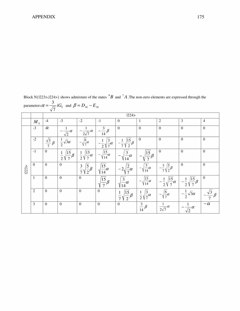
APPENDIX
175
Block N|223>,|224> shows admixture of the states B9 and A7 .The non-zero elements are expressed through the
parameters ||7
3iG=α and NiNi ED −=β
|224>
SM -4 -3 -2 -1 0 1 2 3 4
-3 α α
2
1− α
72
1− β
14
3− 0 0 0 0 0
-2 β
7
3 α32
1 α7
6−
α73
21
− β2
15
7
1−
0 0 0 0
-1 0 β
7
15
2
1 α
7
15
2
1 α14
15− α
14
3− β
7
15−
0 0 0
0 0 0 β
2
5
7
3 α
14
15 α
72
2− α145
− β2
5
7
3− 0 0
1 0 0 0 β
7
15 α
143
α1415
− α7
1521
− β7
15
2
1−
0
2 0 0 0 0 β
215
71
α7
3
2
1 α7
6− α3
2
1− β
7
3−
|223
>
3 0 0 0 0 0 β
14
3 α72
1 α2
1−
α−

APPENDIX
176
Block O1|224>, |123> shows admixture of the states B9 and E7 .The non-zero elements are expressed
through the parameters ( )⊥+−= GiG )1(14
3||1α , and ||2
72
3G
i=α
|224>
SM -4 -3 -2 -1 0 1 2 3 4
-3 1α 2α *
172
1α
0 0 0 0 0 0
-2 0 13
21
α 27
32 α
*17
3
2
1α
0 0 0 0 0
-1 0 0 17
1521
α 27
15α *
114
3α
0 0 0 0
0 0 0 0 114
15α 2
7
4α *
114
15α
0 0 0
1 0 0 0 0 114
3α
2715
α *17
1521
α 0 0
2 0 0 0 0 0 17
321
α 27
32 α *
132
1α
0
|123
>
3 0 0 0 0 0 0 1
72
1α 2α *
1α
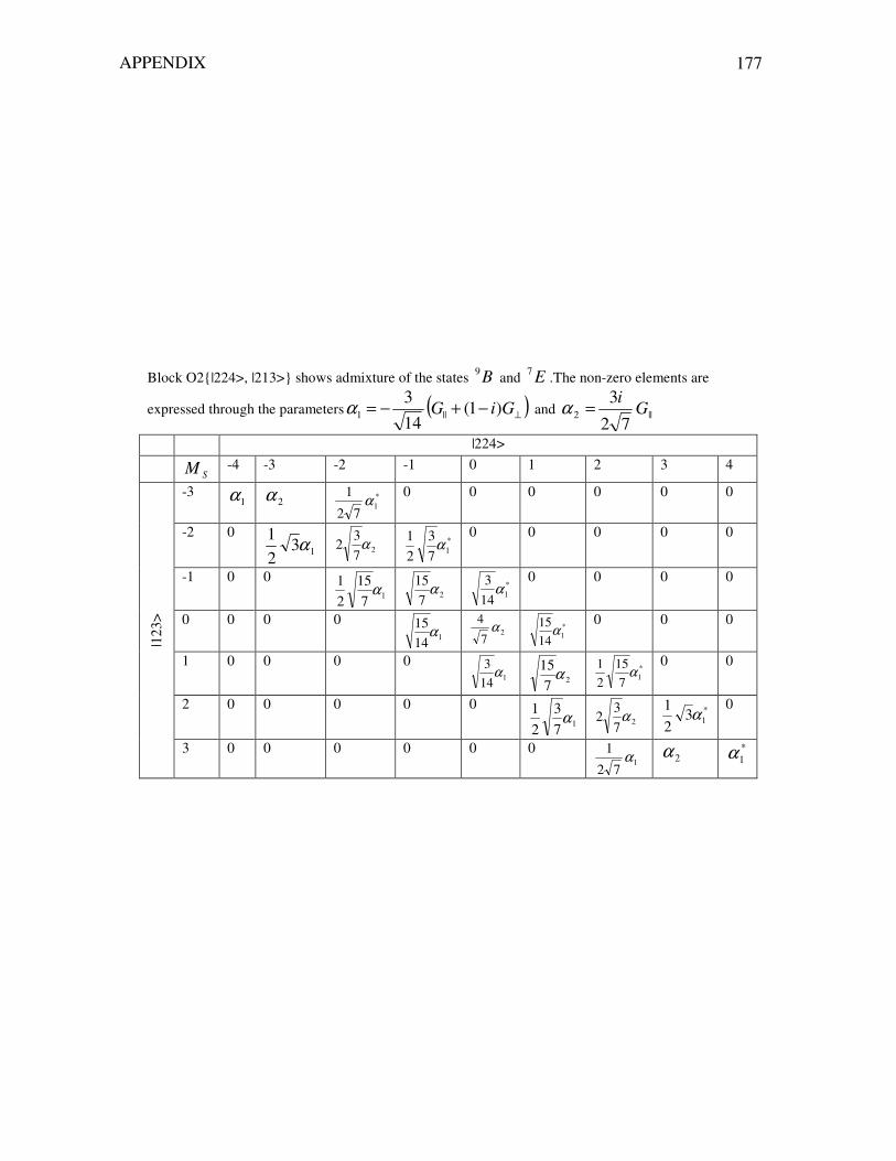
APPENDIX
177
Block O2|224>, |213> shows admixture of the states B9 and E7 .The non-zero elements are
expressed through the parameters ( )⊥−+−= GiG )1(14
3||1α and ||2
72
3G
i=α
|224>
SM -4 -3 -2 -1 0 1 2 3 4
-3 1α 2α *
172
1α 0 0 0 0 0 0
-2 0 13
21
α 27
32 α *
17
3
2
1α
0 0 0 0 0
-1 0 0 17
15
2
1α
2715
α *114
3α
0 0 0 0
0 0 0 0 114
15α 2
7
4α *
114
15α 0 0 0
1 0 0 0 0 114
3α
2715
α *17
15
2
1α 0 0
2 0 0 0 0 0 17
3
2
1α 27
32 α *
132
1α
0
|123
>
3 0 0 0 0 0 0 1
72
1α 2α *
1α

APPENDIX
178
Block P1|223>, |123> shows admixture of the states A7 and E7 .The non-zero elements are
expressed through the parameters ( )( )||1 162
1GGi ++−= ⊥α , , and ||6
Gi
=β
|223>
SM -3 -2 -1 0 1 2 3
-3 β3 *1α− 0 0 0 0 0
-2 1α β2
*13
5α−
0 0 0 0
-1 0
13
5α
β *12α− 0 0 0
0 0 0 12α 0 *
12α− 0 0
1 0 0 0 12α β−
*13
5α−
0
2 0 0 0 0
13
5α
β2− *1α−
|123
> 3 0 0 0 0 0
1α β3−

APPENDIX
179
Block P2|223>, |213> shows admixture of the states A7 and E7 .The non-zero elements are
expressed through the parameters ( )( )||1 162
1GGi +−−= ⊥α , , and ||6
Gi
=β
|223>
SM -3 -2 -1 0 1 2 3
-3 β3− *1α− 0 0 0 0 0
-2 1α β2−
*13
5α−
0 0 0 0
-1 0
13
5α
β− *12α− 0 0 0
0 0 0 12α 0 *
12α− 0 0
1 0 0 0 12α β
*13
5α−
0
2 0 0 0 0
13
5α
β2 *1α−
|123
> 3 0 0 0 0 0
1α β3
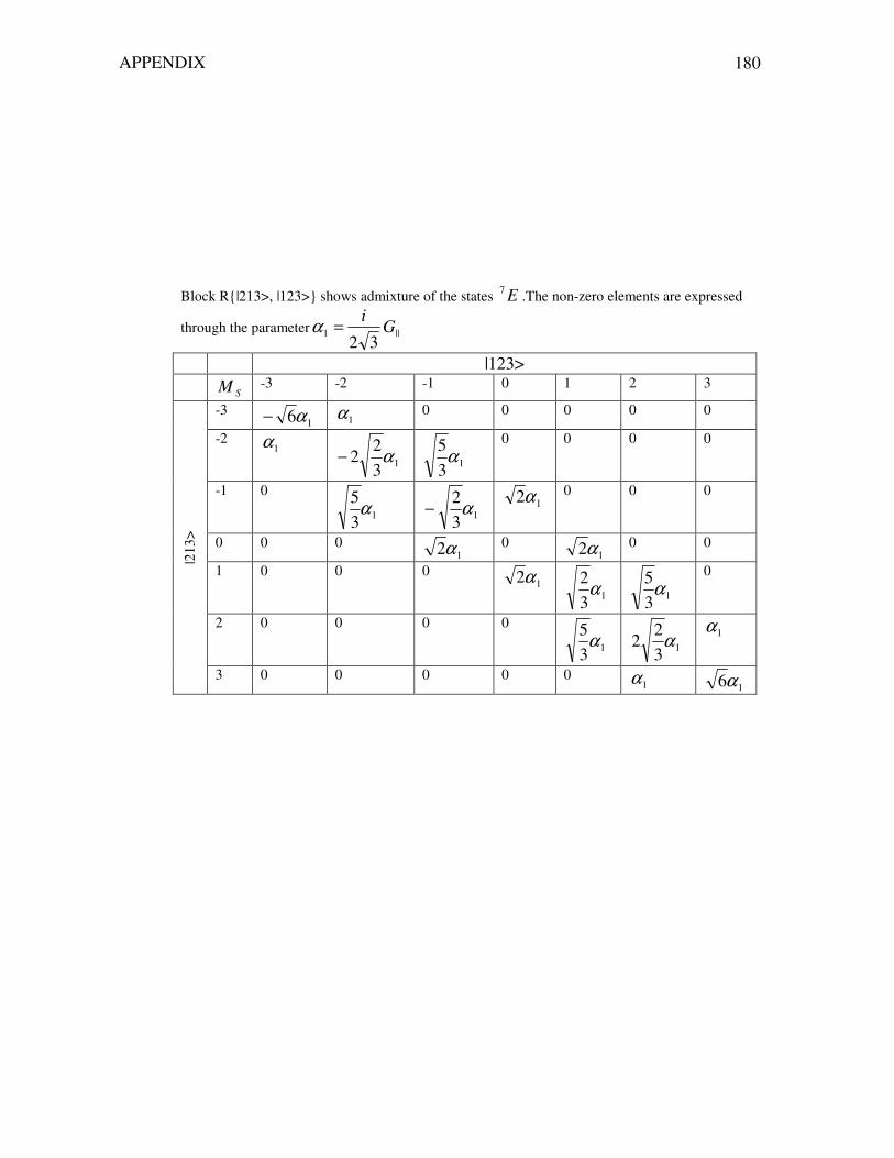
APPENDIX
180
Block R|213>, |123> shows admixture of the states E7 .The non-zero elements are expressed
through the parameter ||132
Gi
=α
|123>
SM -3 -2 -1 0 1 2 3
-3 16α− 1α 0 0 0 0 0
-2 1α
13
22 α− 13
5α
0 0 0 0
-1 0
13
5α 13
2α− 12α 0 0 0
0 0 0 12α 0
12α 0 0
1 0 0 0 12α
13
2α 13
5α
0
2 0 0 0 0
13
5α 13
22 α
1α
|213
> 3 0 0 0 0 0
1α 16α

Bibliography A [Abragam, 1970] Abragam, A., Bleaney, B., “Electron paramagnetic resonance of transition
ions”, Dover publications, Inc., New York (1970) [Alexiou, 2003] Alexiou, M., Zaleski, C. M., Dendrinou-Samara, C., Kampf, J., Kessissoglou, D. P., Pecoraro, V. L., "Trinuclear Mixed-Valent MnII/MnIV/MnII Complexes - Structure and
Magnetic Behavior", Zeitschrift f|r anorganische und allgemeine Chemie, 629(12-13), 2348-2355 (2003) [Aromi, 2003] Aromi, G, Roubeau, O., Helliwell, M., Teat, S., Winpenny, R.E. P., “Novel
topologies in NiII cluster chemistry: Incorporation of alkaline-earth metals in the new
[NiII
6MgII
2] and [NiII
8MII](M= Sr, Ba) cages”, Dalton Trans., 3436–3442 (2003)
[Aubin, 1999] Aubin, S., Sun, Z., Pardi, L., Krzystek, J., Folting, K., Brunel, L., Rheinhold, A., Christou, G., Hendrickson, D., “Reduced Anionic Mn12 Molecules with Half-Integer Ground
States as Single-Molecule Magnets”, Inorg. Chem. 38, 5329-5340 (1999) B [Barbara, 2001] Barbara, B., Gunter., L., “Magnets, Molecules and Quantum Mechanics”, Physics World, March, pp 35-39 (1999) [Barra, 1997] Barra, A.-L., Gatteschi, D., Sessoli, R., “High-frequency EPR spectra of a
molecular nanomagnet: Understanding quantum tunneling of the magnetization”, Phys. Rev. B 56, 8192–8198 (1997) [Basler, 2005] Basler, R., Sieber, A, Chaboussant, G, Güdel, H.U, Chakov, N.E., Soler, M, Christou, G., Desmedt, A., Lechner, A, “Inelastic Neutron Scattering Study of Electron
Reduction in Mn12 Derivatives”, Inorg. Chem. 44, 649-453 (2005) [Bencini, 1990] Bencini, A., Gatteschi, D. “Electron paramagnetic resonance of exchange
coupled systems”, Heidelberg: Springer (1990) [Bleaney, 1953] Bleaney, B., Stevens, K.W.H.,“Paramagnetic Resonance”, Rep. Progr. Phys., 16, 108 (1953) [Blügel, 2005] Blügel, S.,Brückel, Th.; Schneider, C. M. “Magnetism goes nano: electron
correlations, spin transport, molecular magnetism” ; lecture manuscripts of the 36th Spring School of the Institute of Solid State Research, Schriften des Forschungszentrum Jülich, Matter and Materials, 26, F1-F5, (2005)

BIBLIOGRAPHY
182
[Boca, 1999] Boca, R., “Theoretical Foundations of Molecular Magnetism”, Amsterdam: Elsevier (1999) [Boca, 2004] Boca, R., “Zero-field splitting in metal complexes”, Coordination Chemistry Reviews, 248, 757-815 (2004) [Borras-Almenar, 1999] Borras-Almenar, J.J., Clemente-Juan, J.M., Corondo, E., Tsukerblat, B.S., “High-Nuclearity Magnetic Clusters: Generalized Spin Hamiltonian and Its Use for the
Calculation of the Energy Levels, Bulk Magnetic Properties and Inelastic Neutron Scattering
Spectra”, Inorg. Chem., 38, 6081-6088 (1999) [Borrás-Almenar, 2001] J. J.Borrás-Almenar, J. M. Clemente-Juan, E. Coronado and B. S. Tsukerblat, “MAGPACK: a package to calculate the energy levels, bulk magnetic properties, and
inelastic neutron scattering spectra of high nuclearity spin clusters”, J. Comput. Chem., 22, 985 (2001) [Brechin, 2002] Brechin, E.K., Soler., M., Davidson, J., Hendrickson, D.N., Parsons, S., Christou, G., „A new class of single molecule magnet: [Mn9O7(OAc)11(thme)(py)3(H2O)2] with
an S=17/2 ground state”, Chem. Commun., 2252-2253 (2002) [Burns, 1977] Burns, G., “Introduction to group theory with applications”, Academic press, New York etc. (1977) [Butler, 1981] Butler, P.,H., “Point group symmetry applications”, Plenum Press, NewYork (1981) C [Carretta, 2003] Carretta, S., van Slageren,J., Guidi, T., Liviotti, E., Mondelli, C., Rovai, D., Cornia, A., Dearden, A. L., Carsughi, F., Affronte, M., Frost, C. D., Winpenny, R. E. P., Gatteschi, D., Amoretti, G., Caciuffo, R., “Microscopic spin Hamiltonian of a Cr8
antiferromagnetic ring from inelastic neutron scattering”, Phys. Rev. B 67, 094405 (2003) [Chatterjee, 2004] Chatterjee, S., “Heisenberg and Ferromagnetism”, Resonance, 8, 57 (2004) [Commins, 1996] Commins, E. D., Physics 221A, Quantum mechanics (lecture notes). Fall
1996, Notes 15, Irreducible tensor operators and the Wigner-Eckart theorem, University of California Physics Dept., Berkeley, CA, USA, http://www.physics.berkeley.edu/classes/phy221a (1996) D [del Barco, 2004] del Barco, E., Kent, A., Yang, E.-C., Hendrickson, D. N., "Quantum
Superposition of High Spin States in Single Molecule Magnet Ni4" , Physical Review Letters 93, 157202 (2004)

BIBLIOGRAPHY
183
[Dzialoshinski, 1958] Dzialoshinski,I., “A thermodynamic theory of "weak" ferromagnetism of
antiferromagnetics”, J.Phys.Chem. Solids, 4, 241 (1958) E [Edmonds, 1974] Edmonds, A., “Angular momentum in quantum mechanics”, Princeton University Press, Princeton, New Jersey (1974) [Edwards, 2003] Edwards, R.S., Maccagnano, S., Yang, E-C., Hill, S., Wernsdorfer, W., Hendrickson, D., Christou, G., “High frequency electron paramagnetic resonance investigations
of tetranuclear nickel-based single molecule magnets”, J. Appl. Phys. 93, 7807-7809 (2003). [Eppley, 1995] Eppley, H., Tsai, H.L., de Vries, N., Folting, K., Christou, G., Hendrickson, D.N., “High-Spin Molecules: Unusual Magnetic Susceptibility Relaxation Effects in
[Mn12O12(O2CEt)16(H2O)3] (S=9) and the One-Electron Reduction Product
(PPh4)[Mn12O12(O2CEt)16(H2O)4] (S=19/2)”, J. Am. Soc., 117, 301-317 (1995) [Esquinazi, 1998] Esquinazi, P., “Tunneling systems in amorphous and crystalline solids”, Springer-Verlag, (1998) F [Friedman, 2003] Friedman, J. R., “Resonant Magnetization Tunneling in Molecular Magnets”, in: Exploring the Quantum/Classical Frontier: Recent Advances in Macroscopic and Mesoscopic Quantum Phenomena, J. R. Friedman and S. Han, eds, (Nova Science, Huntington, NY, 2003). G [Garanin, 1997] Garanin, D.A., Chudnovsky, E.M., “Thermally activated resonant
magnetization tunneling in molecular magnets: Mn12Ac and others”, Phys. Rev. B, 56, 11102 (1997) [Gatteschi,1993-1] Gatteschi, D., Pardi, L., Magnetic Properties of High Nuclearity Spin
Clusters. A Fast and Efficient Procedure for the Calculation of the Energy Levels, Gazzetta
Chimica Italiana 123, 231-240 (1993) [Gatteschi,1993-2] Gatteschi, D., Pardi, L., Spin Levels of High Nuclearity Spin Clusters, in “Research frontiers in magnetochemistry”, ed. by Charles J. O'Connor, World Scientific Singapore [u.a.], 67-86 (1993) [Gatteschi, 1996] Gatteschi, D., Sessoli, R., Plass, W., Müller, A., Krickemeyer, E., Meyer, J., Sölter, D., Adler, P., Giant Clusters with Unusual Electronic and Magnetic structures Due to
Open Shell metal centers Embedded far Apart from Each Other: Spin Frustration and
Antisymmetric Exchange, Inorg. Chem., 35, 1926-1934 (1996)

BIBLIOGRAPHY
184
[Griffith, 1961] Griffith, “The theory of transition metal ions”, Cambridge University Press, (1961) [Griffith, 1962] Griffith, J. S., “The irreducible tensor method for molecular symmetry groups”, Englewood Cliffs, N.J.: Prentice-Hall (1962). [Guidi, 2004] Guidi, T., Carretta, S., Liviotti, E., Magnani, N., Mondelli, C., Waldmann, O., Thompson, L.K., Zhao, L., Frost, C.D., Amoretti, G., Caciuffo, R., “Inelastic neutron scattering
study of the molecular grid nanomagnet Mn-[3x3]”, Physical Review B,69, 104432 (2004) [Güven, 1999] Güven, M.H., Eryürek, M., “Dynamical and structural properties of the Ni4
cluster”, Phys. Stat. Sol. (b), 213, 283 (1999) H [Hamermesh, 1989] Hamermesh, M., “Group theory and its application to physical problems”, Dover Publications, Inc., New York (1989) [Harriman, 1978] Harriman, J.E., “Theoretical foundations of electron spin resonance”, Academic Press, London (1978) [Heine, 1960] Heine, V., “Group theory in quantum mechanics an introduction to its present usage”, Pergamon press, Oxford (1960) [Heitler, 1927] Heitler, W., London, F., „Wechselwirkung neutraler Atome und Homöopolare
Bindung nach der Quantenmechanik“ Z. Physik, 44, 455 (1927) [Herring, 1962] Herring, C., “Critique of the Heitler-London method of calculating spin
couplings at large distances”, Rev. Mod. Phys., 34, 631 (1962) [Hill, 1998] Hill, S., Perenboom, J. A. A. J, Dalal, N. S., Hathaway, T., Stalcup, T., Brooks, J. S., “High-Sensitivity Electron Paramagnetic Resonance of Mn12-Acetate”,Phys. Rev. Lett. 80, 2453–2456 (1998) [Hill, 2002] Hill, S., Maccagnano, S., Park, K., Achey, R.M., North, J.M., Dalal, N.S., “Detailed
Single-Crystal EPR Line Shape Measurements for Single-Molecule Magnets Fe8Br and Mn12-
Ac“, Phys. Rev. B, 65, 224410, (2002) [Howarth, 2003] Howarth, D.F., Weil, J.A., Zimpel, Z., “Generalization of the lineshape useful
in magnetic resonance spectroscopy”, J. Magn. Res., 161, 215-221 (2003) [Hund, 1927] Hund, F., „Symmetriecharaktere von Termen bei Systemen mit gleichenPartikeln
in der Quantenmechanik“, Z. Physik. 43, 788, 1927
BIBLIOGRAPHY
185
I [Inui, 1990] Inui, T., Tanabe, Y., Onodera, Y., “Group theory and its applications in physics”, Springer-Verlag, Berlin (1990) J [Johnson, 2002] Johnson, W.R., “Lectures on atomic physics”, Notre Dame, Indiana 46556, USA, http://www.nd.edu/~johnson/Publications/book.pdf (2002) [Jones, 1998] Jones, H.F., “Groups, representations and physics”, IOP Publishing Ltd (1998) K [Kahn, 1993] Kahn, O., “Molecular magnetism”, New York : VCH (1993) [Kammel, 2003] Kammel, M.,“Cofactors on the Donor Side of Photosystem II Investigated with
EPR Techniques”, PhD-thesis, Fakultät II-Mathematik und Naturwissenschaftender Technischen Universität Berlin (2003) [Karmakar, 2002] Karmakar TK, Chandra SK, Ribas J, Mostafa G, Lu TH, Ghosh BK., “Synthesis, structure and magnetism of a new dicubane-like ferromagnetic tetranuclear nickel
cluster containing versatile azido-only bridges and a bis(bidentate) Schiff base blocker”, Chem. Commun (Camb). Oct 21;(20), 2364-2365, (2002) [Kaupp, 2004] Kaupp, M., Bühl, M., Malkin, V., „Calculation of NMR and EPR parameters.
Theory and applications“, Wiley-VCH (2004) [Kirchner, 2005] Kirchner, N., van Slageren, J., Brechin, E.K., Dressel, M., „Frequency-domain
magnetic resonance spectroscopy on [Mn12]- and [Mn9]: Zero-field splitting and lineshape
analysis”, Polyhedron, 24, 2400 (2005) [Koch, 2003] Koch, R., Waldmann, O., Müller, P., Reimann, U., Saalfrank, R.W., “Ferromagnetic coupling and magnetic anisotropy in molecular Ni(II) squares“, Phys. Rev. B 67, 094407 (2003) [Koster, 1963] Koster, G.F., Dimmock, J.O., Wheeler, R.G., Statz, H., „Properties of the thirty-
two point groups”, MIT Press, Cambridge (1963) L [Landau, 2001] Landau, L. D., Lifshitz, E.M., “Theoretical physics: quantum mechanics”, FISMATLIT, Moscow (2001) in Russian

BIBLIOGRAPHY
186
[Lecren, 2005] Lecren L, Wernsdorfer W, Li YG, Roubeau O, Miyasaka H, Clerac R., “Quantum Tunneling and Quantum Phase Interference in a [Mn(II)(2)Mn(III)(2)] Single-
Molecule Magnet”, J Am Chem Soc. 127(32):11311-11317 (2005) [Leuenberger, 2000-1] Leuenberger, M.N., Loss, D., „Spin tunneling and phonon –assisted
relaxation in Mn12-acetate“, Phys. Rev. B, 61, 1286 (2000) [Leuenberger, 2000-2] Leuenberger, M., and Loss, D., “Incoherent Zener tunneling and its
application to molecular magnets”, Phys. Rev. B 61, 12200–12203 (2000) [Leuenberger, 2003] Leuenberger, M.N., Meier, F., Loss, D., “Quantum Spin Dynamics in
Molecular Magnets“, Monatshefte für Chemie, 134, 217-233 (2003) [Liviotti, 2002] Liviotti, E., Carretta, S., Amoretti, G., “S-mixing contributions to the high-order
anisotropy terms in the effective spin Hamiltonian for magnetic clusters”, J. Chem. Phys. 117, 3361 (2002) M [McWeeny, 2002] McWeeny, R., “Symmetry: an introduction to group theory and its
applications”, Dover Publications, INC, Mineola, New York (2002) [Messian, 1965] Messian, A., “Quantum mechanics”, (Volume 2), North-Holland Publishing Company, Amsterdam (1965) [Miller, 2000] Miller, J.S., Epstein, A.J., “Molecule-based magnets – an overview”, MRS Bulletin, 21-28, (2000) [Mirebeau, 1999] Mirebeau, M. Hennion, H. Casalta, H. Andres, H. U. Güdel, A. V. Irodova, and A. Caneschi, “Low-Energy Magnetic Excitations of the Mn12-Acetate Spin Cluster Observed
by Neutron Scattering”, Phys. Rev. Lett. 83, 628–631 (1999) [Misra, 1999] Misra, S.K., “Angular variation of electron paramagnetic resonance spectrum:
simulation of a polycrystalline EPR spectrum”, J. Magn. Reson., 137, 83-92 (1999) [Mlynarski, 1991] Mlynarski, P., Salahub, D. R., “Self-consistent implementation of nonlocal
exchange and correlation in a Gaussian density-functional method”, Phys. Rev. B 43, 1399–1410 (1991) [Moragues-Canovas, 2004] Moragues-Canovas, M., Helliwell, M., Ricard, L., Riviere, E., Wernsdorfer, W., Brechin, E., Mallah,T., “An Ni4 Single-Molecule Magnet: Synthesis, Structure
and Low-Temperature magnetic Behavior”, Eur. J. Inorg. Chem., 2219-2222 (2004) [Moryia, 1960] Moryia, T., “Anisotropic superexchange interaction and weak ferromagnetism”, Phys. Rev., 120, 91 (1960)

BIBLIOGRAPHY
187
[Mukhin, 1998] Mukhin, A. A., Travkin, V. D., Zvezdin, A. K., Lebedev, S. P., Caneschi, A.,Gatteschi, D., “Submillimeter spectroscopy of Mn12-Ac magnetic clusters”, Europhys. Lett., 44 (6), 778-782 (1998) [Mukhin, 2001] Mukhin,A.A., Gorshunov, B., Dressel, M., Sangregorio, C., Gatteschi, D. ”Optical Spectroscopy of the Crystal Field Transitions in the Molecular Magnet Fe8” Phys. Rev. B, 63, 214411 (2001) [Mukhin, 2002] Mukhin, A. A., Prokhorov, A.S., Gorshunov, B., Zvezdin, A.K., Travkin, V.D., Dressel M., “Submillimeter spectroscopy of electron transitions and the macroscopic quantum
tunneling of magnetization in molecular magnets” Physics-Uspekhi 45, 1186 - 1191 (2002) N [Nakano, 2002] Nakano, M., Matsubayashi, G.E., Muramatsu, T., Kobayashi, T.C., Amaya, K., Yoo, J., Christou, G., Hendrickson, D.N.,“Slow magnetization reversal in [Ni-
4(OMe)(4)(sal(4)(MeOH)(4)]”, Molecular Crystals & Liquid Crystals, 376, 405-410 (2002) O [Owen, 1972] Owen, J., Harris, E.A., “Pair spectra and exchange interactions”, Chapter 6, p. 427 in “Electron Paramagnetic Resonance”, ed. by S. Geschwind, Plenum Press, New York-London, 1972 P [Palii, 2004] Palli,A.V., Ostrovsky,S.M., Klokishner,S.I., Tsukerblat,B.S., Berlinguette,C.P., Dunbar, K. R., Galán-Mascarós, J.R., “Role of the Orbitally Degenerate Mn(III) Ions in the
Single-Molecule Magnet Behavior of the Cyanide Cluster [Mn II (tmphen) 2 ] 3 [Mn III (CN) 6
] 2 (tmphen = 3,4,7,8-tetramethyl-1,10-phenanthroline)”, J. Am. Chem. Soc., 126, 16860-16867 (2004). [Pilbrow, 1996] Pilbrow, J. R., “Principles of computer simulation of EPR spectra”, Appl. Magn. Reson., 10, 45-53 (1996) [Piligkos, 2005] S. Piligkos, G. Rajaraman, M. Soler, N. Kirchner, J. van Slageren, R. Bircher, J. Davidson, S. Parsons, H.-U. Güdel, J. Kortus, W. Wernsdorfer, G. Christou und E.K. Brechin, “Studies of an enneanuclear manganese single-molecule magnet”, J. Am. Chem. Soc. 127, 5572 - 5580 (2005) [Pohjola, 2000] Pohjola, T., Schoeller, H., “Spin dynamics of Mn12-acetate in the thermally
activated tunneling regime: ac susceptibility and magnetization relaxation”, Phys. Rev. B 62, 015026 (2000)
BIBLIOGRAPHY
188
[Postnikov, 2004] Postnikov, A., Kortus, J.,Pederson, M., “Density functional studies of
molecular magnets”, Ψk Newsletter, http://psi-k.dl.ac.uk/newsletters/News_61/Highlight_61.pdf (2004) [Price, 2002] Price, D.J., Batten, S.R., Moubaraki, B., Murray, K.S., “Synthesis, structure and
magnetism of a new manganese carboxylate cluster:
[Mn16O16(OMe)6(OAc)16(MeOH)3(H2O)3].6H2O”, Chem. Comm., 762-763 (2002). [Prokof’ev, 1998] Prokof’ev, N. V., Stamp, P.C. E., “Quantum relaxation of ensembles of
nanomagnets”, Journal of Low Temperature Physics, 113, 1147 (1998) [Prokof’ev, 2000] Prokof’ev, N. V., Stamp, P.C. E., “Theory of the spin bath”, Rep. Prog. Phys. 63, 669 (2000) R [Regnault, 2002] Regnault, N., Jolicœur, Th., Sessoli, R., Gatteschi, D., Verdaguer, M.,“Exchange coupling in the magnetic molecular cluster Mn12Ac”, Phys. Rev. B 66, 054409 (2002) [Rogez, 2005] G. Rogez, J.-N. Rebilly, A.-L. Barra, L. Sorace, N. Kirchner,M. Duran, J. van Slageren, S. Parsons, L. Ricard, A. Marvillers, T. Mallah, “Very Large Ising-Type Magnetic
Anisotropy in a Mononuclear NiII Complex”, Angew. Chem., Int. Ed., 117, 1910-1913 (2005)
[Rosen, 1995] Rosen, J., “Symmetry in science: an introduction to the general theory”, Springer (1995) S [Schnack, 2001] Schnack, J., Luban, M., Modler, R., “Quantum rotational band model for the
Heisenberg molecular magnet Mo72Fe30”, Europhys. Lett., 56 (6) , pp. 863-869 (2001) [Schnack, cond-mat/0509476] Schnack, J., Brüger,M., Luban, M., Kögerler,P., Morosan, E., Fuchs, R., Modler, R., Nojiri, H., Rai, R. C., Cao,J., Musfeldt, J. L., Wei, X., “Observation of
field-dependent magnetic parameters in the magnetic molecule Ni4Mo12”, cond-mat/0509476 [Scott, 2005] Scott, R. T. W., Parsons, S., Murugesu, M., Wernsdorfer, W., Christou, G., Brechin, E. K.,“Synthesis, structure and magnetic properties of a trinuclear
[MnIIIMnII2]single-molecule magnet”,Chem. Commun., 2083–2085, (2005) [Sessoli, 2003] Sessoli, R., Gatteschi, D., “Quantum tunneling of magnetization and related
phenomena in molecular magnets”, Angew. Chem.Int. Ed. 42, 268 (2003) [Sieber, 2005] Sieber, A., Boskovic, C., Bircher, R., Waldmann, O., Ochsenbein, S.T., Güdel, H.-U., Kirchner, N., van Slageren, J., Wernsdorfer, W., Neels, A., Stoeckli-Evans, H., Janssen, S., Juranyi, F., Mutka, H., “Synthesis and Spectroscopic Characterization of a New Family of
Ni4 Spin Clusters” Inorg. Chem. 44, 4315 - 4325 (2005)

BIBLIOGRAPHY
189
[Silver, 1976] Silver, B.,L.,“Irreducible tensor methods: an introduction for chemists”, New York : Acad. Pr. (1976) [Smith, 1994] Smith, S.A., Levante, T.O., Meier, B.H., Ernst, R. R., “Computer simulations in
magnetic resonance. An object-oriented programming approach”, J. Magn. Reson., Ser. A, 106, 75-105 (1994) [Soler, 2003] Soler, M.,Wernsdorfer, W., Abboud, K., Huffman, J., Davidson, E.R., Hendrickson, D.N., Christou, G., “Single-Molecule Magnets: Two-Electron Reduced Version of
a Mn12 Complex, and Environmental Influences on the Magnetization Relaxation of
(PPh4)2[Mn12O12(O2C-CHCl2)16(H2O)4]”, J. Am. Chem. Soc., 125, 3576-3588 (2003) [Sugano, 1970] Sugano, S.,Tanabe, Y., “Multiplets of transition-metal ions in crystals”, New York : Acad. Pr. (1970) T [Tinkham, 1964] Tinkham, M., “Group theory and quantum mechanics”, McGraw-Hill Book Company, New-York etc (1964) [Tsukerblat, 1983] Tsukerblat, B., Belinskii, M.I., “Magnetochemistry and radio-spectroscopy of
the exchange coupled clusters”, Kishinv: Stiinza (1983) in Russian
[Tsukerblat, 1987] Tsukerblat, B., Belinskii, M.I., Fainzilberg, V.E., “Magnetochemistry and
spectroscopy of transition metals exchange clusters”, Sov. Chem. Rev.B Chem, 9, 337-481 (1987) [Tsukerblat, 1994] Tsukerblat, B., “Group Theory in Chemistry and Spectroscopy. A Simple
Guide to Advanced Usage”, London: Academic Press (1994) [Tsukerblat, 2001] Tsukerblat, B. S., Palii, A. V.,Mirovitskii, V. Yu., Ostrovsky, S. M., Turta, K., Jovmir, T., Shova, S., Bartolome, J., Evangelisti, M., Filoti, G., “Non-Heisenberg magnetic
behavior of a triangular bridged heterometallic Fe2(III)Co(II) complex: Evidence of strong
orbital contributions”, J. Chem. Phys. 115, 9528 (2001) [Tupitsyn, 2002] Tupitsyn, I., Barbara, B., “Quantum tunneling of magnetization in molecular
complexes with large spins – effect of the environment”, p.109 in “Magnetism: molecules to materials. Nanosized magnetic materials”, Miller, J.S. and Drillon, M.,eds.,Willey-Vch (2002) V [van Vleck, 1932] van Vleck, J.H., “Theory of electric and magnetic susceptibilities”, Clarendon Press, Oxford, 1932

BIBLIOGRAPHY
190
[van Slageren, 2002] van Slageren, J., Sessoli, R., Gatteschi, D., Smith, A.A., Helliwell, M., Winpenny, R.E.P., Cornia, A., Barra, A.-L., Jansen, A.G.M., Rentschler, E., Timco, G.A., "Magnetic Anisotropy of the Antiferromagnetic Ring [Cr8F8Piv16]", Chem. Eur. J., 8, 277 – 285 (2002) [van Slageren, 2003] van Slageren, J., Vongtragool, S., Gorshunov, B., Mukhin, A. A., Karl, N., Krzystek, J., Telser, J., Müller, A., Sangregorio, C., Gatteschi, D., Dressel, M.,“Frequency-
domain magnetic resonance spectroscopy of molecular magnetic materials”, Phys. Chem. Chem. Phys. 5, 3837 - 3843 (2003) [Varshalovich, 1988] Varshalovich, D.A., Moskalev, A.N., Khersonsky, V.K., “Quantum theory
of angular momentum. Irreducible tensors, spherical harmonics, vector coupling coefficients, 3nj
symbols”, World Scientific, Singapore (1988) [Volkov, 1985] Volkov, A.A., Goncharov, Yu. G., Kozlov, G.V., Lebedev, S.P., Prokhorov, A.M., “Dielectric measurements in the submillimeter wavelength region”, Infrared Phys., 25(1/2), 369 (1985) [Vongtragool, 2003] Vongtragool, S., Gorshunov, B., Dressel, M., Krzystek, J., Eichhorn, D. M., Telser, J., “Direct Observation of Fine Structure Transitions in a Paramagnetic Nickel(II)
Complex Using Far-Infrared Magnetic Spectroscopy: A New Method for Studying High-Spin
Transition Metal Complexes”, Inorg. Chem., 42 (6), 1788 -1790, (2003) W [Waldmann, 1998] Waldmann, O., Hassmann, J., Müller, P., Volkmer, D., Schubert, U. S., Lehn, J.-M., “Magnetism of self-assembled mono- and tetranuclear supramolecular Ni
2+ complexes“,
Phys. Rev. B 58, 3277–3285 (1998) [Waldmann, 2000] Waldmann, O., “Symmetry and energy spectrum of high-nuclearity spin
clusters”, Phys. Rev. B., 61, 6138 (2000) [Waldmann, 2005] Waldmann, O., Güdel, H.U., “Many-spin effects in inelastic neutron
scattering and electron paramagnetic resonance of molecular nanomagnets”, Phys. Rev. B.,72, 094422 (2005) [Washimia, 1970] Washimia, S., Shinagawa, K., Sugano, S., “Effective Hamiltonian for Non-
Kramers Doublets”, Phys. Rev. B, 1, 2976 (1970) [Weil, 1999] Weil., J., “The simulation of EPR spectra: a mini-review”, Molecular Physics Reports, 26, 11-24 (1999) [Weiss, 1993] Weiss, U., “Quantum dissipative systems”, World Scientific (1993)
BIBLIOGRAPHY
191
[Wernsdorfer, 2001] Wernsdorfer, W., “Classical and Quantum Magnetization Reversal Studied
in Nanometer-Sized Particles and Clusters”, Adv. Chem. Phys., vol. 118, pp 99-190 (2001) [Wolfram, 1999] Wolfram, S., “The mathematica book”, - 4. ed.. - Champaign, Ill. : Wolfram Media, (1999) Y [Yang, 2003] Yang, E., Wernsdorfer, W, Hill, S.O., Edwards, R. S., Nakano, N., Maccagnano, S., Zakharov, L. N., Rheingold, A., L., Christou, G., Hendrickson, D.N., “Exchange bias in Ni4
single-molecule magnets”, Polyhedron, Volume 22, Issues 14-17, 15, 1727-1733 (2003). [Yang, 2005] Yang,E., Kirman,C, Lawrence,J, Zakharov,L,N, Rheingold,A.L., Hill,S., Hendrickson,D., “Single-Molecule Magnets: High-Field Electron Paramagnetic Resonance
Evaluation of the Single-Ion Zero-Field Interaction in a ZnII3NiII Complex”, Inorg. Chem., 44 (11), 3827 -3836 (2005) [Yoon, 2004] Yoon, J., Mirica, L. M., Stack, T. D. P., Solomon, E. I., “Spectroscopic
Demonstration of a Large Antisymmetric Exchange Contribution to the Spin-Frustrated Ground
State of a D3 Symmetric Hydroxy-Bridged Trinuclear Cu(II) Complex: Ground-to-Excited State
Superexchange Pathways”, J. Am. Chem. Soc. 126(39), 12586 (2004)
Zusammenfassung Das Forschungsgebiet des Magnetismus erlebt gegenwärtig eine Renaissance durch
die schnelle Entwicklung der Molekülchemie in den letzten Jahrzehnten. Das weltweite Interesse an molekularen Magneten hat sowohl wissenschaftliche also auch technologische Gründe. Diese Moleküle machen es möglich, die mit den herkömmlichen anorganischen Magneten verbundenen Eigenschaften zu erweitern, wie z.B. eine niedrige Dichte, optische Transparenz, elektrische Isolation, die Herstellung bei tiefen Temperaturen und die Kombination der magnetischen Ordnung mit anderen Eigenschaften, wie Photo-empfindlichkeit. Sie erlauben auch neue Möglichkeiten der Verarbeitungstechnologien, da diese Magnete auf Moleküle als Bausteine basieren. Über mehrere Klassen der molekularen Magnete wurde vor kurzem berichtet [ Miller, 2000 ], wobei eine Vielzahl neuer Phänomene beobachtet worden ist. Viele molekulare Magnete enthalten Metallionen; jedoch nehmen auch die organischen Bestandteile dieser Moleküle eine Schlüsselrolle zum Verständnis ihres magnetischen Verhaltens ein. Anders als herkömmliche anorganische Magnete, die seit dem 12. Jahrhundert verwendet werden, können die organischen Bestandteile der molekularen Magnete entweder selbst einen Spin tragen oder - falls sie spinlos sind – die Spins der metallischen Zentren in einzelne feste Fragmente (Clustern) koppeln. Folglich zeichnen sie sich durch eine breite Vielfalt der Bindung und der Struktur aus. Diese schließen lokalisierte Moleküle (null-dimensional, 0D), solche mit ausge-dehnten Bindungen entlang von Ketten (1D), innerhalb von Schichten (2D) und innerhalb von Netzstrukturen (3D) ein. Molekulare Magnete werden normalerweise in Familien gruppiert durch zwei Eigenschaften: entweder durch die Orbitale, in denen die Spins liegen, oder durch die chemische Bindung, die benachbarte Spins verbindet. Die weitere Klassifikation in Untergruppen wird entsprechend der festgestellten Art der magnetischen Ordnung durchgeführt. Zusätzlich zum ferri- und ferromagnetischem Verhalten können andere magnetische Phänomene in molekularen Magneten auftreten: Metamagnetismus, gekippter Antiferromagnetismus und Spinglasverhalten. Eine spezielle Kategorie der molekularen Magnete ist verbunden mit kleinen magnetischen Clustern, d.h. molekulare Nanomagnete, die keine weitreichende magnetische Ordnung besitzen. Es gibt Äquivalente zu dem Namen "molekularer Nanomagnet" wie z.B. "magnetisches Nanocluster"oder "Hoch-Spin-Cluster" aus Gründen, die im Kapitel 2 dargelegt werden. Einige von ihnen zeigen physikalische Effekte, die üblicherweise in herkömmlichen magnetischen Materialien nicht auftreten: Hysterese infolge eines reinen molekularen Ursprunges und der Quantentunneleffekt der Magnetisierung. Die Bezeichnung Einzelmolekülmagnete (Single Molecule Magnets, SMMs) bezieht sich auf diese Familie der magnetischen Nanoclustern. Sie sind im Fokus dieser Dissertation.
Magnetische Nano-Cluster sind Moleküle, die aus Metallionen bestehen, die durch organische Liganden verbunden werden. Das Energiespektrum der Ionen, die das Cluster formieren, wird durch die elektronische Konfiguration in dem umgebenden Ligandenfeld bestimmter Symmetrie festgelegt. Die Kopplung der Einzelionenspins verursacht ein Energiespektrum, das aus Multipletts mit definiertem Gesamtspin besteht. Ein nicht kompensierter Grundzustandspin ist typisch für molekulare Nanomagnete. Somit wird jede energetische Entartung verursacht von konkurrierenden Austauschwechselwirkungen in Multispinsystemen. Das energisch entartete Spin-Multiplett entsteht in Folge der isotropen

ZUSAMMENFASSUNG 193
Heisenberg Austauschwechselwirkung zwischen Spinzentren. Das Experiment zeigt jedoch, dass jedes Multiplett normalerweise bereits ohne äußeres Magnetfeld aufgespalten ist.
Die Nullfeldaufspaltung (Zero-Field Splitting, ZFS) des Multipletts vom Grund-zustand der Einzelmolekülmagnete kann mit einem Doppelmuldenpotenzial verglichen werden, die so hoch wie möglich sein muss, um diese Moleküle erfolgreich in dem Bereich der Speichermedien oder der Quantenberechnungen anwenden zu können. Die quantitative Charakterisierung der Nullfeldaufspaltung und das Verständnis der Natur der Nicht-Heisenberg-Wechselwirkungen, die die Entartung aufheben, sind von Bedeutung für die Synthese von neuen Einzelmolekülmagneten mit definierten Werten der Invertierungs-magnetisierungbarriere.
Trotz der Fortschritte der Dichtefunktionaltheorie (DFT) bleiben die Ab-Initio-Berechnungen der Nullfeldaufspaltung eine Herausforderung der Forschung [ Kaupp, 2004 ]. Die Hauptquelle der Informationen über die Nullfeldaufspaltungen bleibt das Experiment. Es gibt verschiedene experimentelle Techniken, die verwendet werden, um die Effekte der Nullfeldaufspaltung in vielkernigen Komplexen zu studieren. Dazu gehören die Methoden der magnetischen Suszeptibilität bei konstantem Magnetfeld, der Elektronen-Paramagnetischen-Resonanz-Spektroskopie (EPR), der unelastische gestreuten Neutronen (Inelastic Neutron Scattering, INS) sowie der Frequenz-Domain-Magnetresonanz-Spektroskopie (FDMRS), die in dieser Doktorarbeit präsentiert werden. Alle diese Techniken ermöglichen das Studium der magnetischen Anregungen innerhalb des aufgespalteten Grundzustandmultipletts in Abwesenheit des äußeren Magnetfeldes.
Im Gegensatz zur DFT, in der der vollständige molekulare Hamilton-Operator in der relativistischen Näherung konstruiert wird, wird ein Konzept des Spin-Hamilton-Operators zur Modellierung der experimentellen Daten verfolgt, d.h. zur Beschreibung der Energie-spektren und der Dynamik der molekularen Nanomagnete. Der Definition entsprechend muss er so entworfen werden, dass seine Diagonalisierung die Energieniveaus des Multiplett richtig reproduziert; d.h. eine adäquate Bewertung des messbaren magnetischen Parameters liefert (wie die Magnetisierung, die statische und dynamische magnetische Suszeptibilität und der INS Querschnitt) und eine korrekte Simulation der thermodyna-mischen Messungen oder der spektroskopischen Linien und deren Intensitäten ermöglicht.
Es werden drei Arten von Spin-Hamilton-Operatoren unterschieden in Abhängigkeit von der Methode ihrer Konstruktion und von dem mathematischen Formalismus zur Be-rechnung der Hamilton-Matrixelementen [ Tsukerblat, 1994 ]. Die Gruppentheorie dient als Grundlage für jeden von ihnen, da sich die Symmetrieeigenschaften der Moleküle in der Symmetrie des Hamilton-Operators widerspiegeln. Das vollständigste Spin-Hamilton-Modell verwendet das Wigner-Eckart-Theorem für finite Punktgruppen [ Washimia, 1970 ]. Es erlaubt die Vorhersage der Feinstruktur der Vielelektronterme und die a-priori Kenntnis der Auswahlregeln von spektroskopischen (elektrischen Dipol-, magnetischen Dipol-, elektrischen Quadrupol-) Übergängen sowie die Polarisationabhängigkeit der Intensität der erlaubten Übergänge. Dieses Modell gehört zum Gipfel der Hierarchie der Spin-Hamilton-Modelle und bleibt ein Werkzeug von Experten. Es wurde noch nie praktisch im Kontext der Einzelmolekülmagnete angewendet. Daher wird es in dieser Doktorarbeit nicht weiter verfolgt.
Der Definition entsprechend schließt der Spin-Hamilton-Operator die Drehimpuls-Operatoren sowie ihre gegenseitige Wechselwirkung ein (Bahn-Bahn-, Spin-Bahn- sowie

ZUSAMMENFASSUNG 194
Spin-Spin-Kopplung) und ihre Wechselwirkung mit einem externen magnetischen Feld ein. Die zweite Art der Spin-Hamilton-Operatoren (auch bezeichnet als Generalisierte
Effektive Spin-Hamiltonmodell, GESH) wendet das Wigner-Eckart-Theorem für die Rotationsgruppen an, da der Gesamtdrehimpuls-Operator Transformationen des quanten-mechanischen Systems durch unendlich kleine Drehungen erzeugt, die durch die irreduzible Darstellung der vollständigen Rotationsgruppe charakterisiert werden können. Die gruppentheoretische Betrachtung der Spin-Hamilton-Operatoren wurde bereits durch Bleaney und Stevens [ Bleaney, 1953 ] sowie Griffith [ Griffith, 1961, 1962 ] durchgeführt. Sie haben gezeigt, dass der Hamilton-Operator mit einer dem Operator äquivalenten Methode für finite Gruppen abgeleitet werden kann. Die von Stevens vorgeschlagene Methode zieht die Tatsache in Betracht, dass die Drehimpulsoperatoren dieselben Transformationseigenschaften haben, wie die entsprechenden Kugelflächenfunktionen, die zur Entwicklung der Kristallfeldpotenziale der zugehörigen Symmetrie erforderlich sind [ Abragam, 1970 ], [ Sugano, 1970 ]. Diese Methode erlaubt das quantenmechanische Äquivalent einer gegebenen Kugelflächenfunktion als explizite Funktion vom Gesamtdrehimpulsoperator J bezüglich eines ausgewählten J-Multipletts zu bestimmen, die auch als Stevens Operatoren genannt werden und z.B. in [ Abragam, 1970 ] tabelliert sind. Der dritte Typ der Spin-Hamilton-Operatoren wird durch den sogenannten effektiven Spin- Hamilton-Operator repräsentiert, der durch die Stevens Operatoren für jedes Spinmultiplett ausgedrückt werden kann. Die Auswahl des passenden Spin-Hamilton-Operator zur Modellierung der experimentellen Daten hängt von den spezifischen Eigenschaften des Energiespektrums des untersuchten Systems ab. Wenn die isotrope Heisenberg-Austauschwechselwirkung vorherrscht, spricht man vom sogenannten Grenzfall der starken Austauschwechselwirkung. In diesem Fall werden die Spinmultipletts in wohl separierten Gruppen eingeteilt, so dass die Wirkung der angeregten Zustände auf den Grundzustand in erster Näherung vernachlässigt werden kann. In der Mehrheit der berichteten Einzelmolekül-Magnete [ Sessoli, 2003] sind die angeregten Spinzustände bei niedrigen Temperaturen experimentell unzugänglich und können folglich vernachlässigt werden. Diese Tatsache öffnet den Weg zur spektroskopischen Simulationen durch Verwendung des effektiven Spin-Hamilton-Operators, der ausschließlich das Grundmultiplett einbezieht und als Einzel-Spin-Hamilton- oder Riesen-Spin-Hamilton-
Modell bezeichnet wird [ Waldmann, 2005 ]. Es stimmt mit dem Modell der Nullfeld-aufspaltung überein, die durch die Stevens Operatoren in Abwesenheit des äußeren magnetischen Feldes ausgedrückt werden.
Jeder Spin-Hamilton-Operator kann in zwei Teile getrennt werden. Das erste Teil hängt nur von der Symmetrie ab; das zweite hat seinen Ursprung in dem physikalischen Verhalten des Systems. Es kann als ein regulierbarer, semi-empirischer Parameter behandelt werden, der vom Experiment extrahiert werden kann. Durch die Anwendung des Einzelspin-Hamilton-Modells auf die experimentelle Datenanalyse der molekularen Nanomagnete wird ein Parametersatz der Nullfeldaufspaltung (ZFS) erhalten. Sie liefern einen Fingerabdruck, d.h. die relative Lage der Energieniveaus des Grundmultipletts. Das Generalisierte Effektive Spin-Hamilton-Modell wird benutzt, um die Natur der physikalischen Mechanismen zu analysieren, die für die Ausbildung der magnetischen Anisotropie des Clusters verantwortlich sind. Es schließt Parameter von einer isotropen Austauschwechselwirkung und von einer Nicht-Heisenberg-Wechselwirkungen ein. Ihre Größe weist auf die Rolle und auf das spezifischen Verhalten der entsprechenden Art der
ZUSAMMENFASSUNG 195
Intra-Cluster Wechselwirkung hin. Diese Informationen sind von Bedeutung für die Synthese von neuen Molekülen mit vorbestimmten Eigenschaften. Das Einzelspin- und das Generalisierte Effektive Spin-Hamilton-Modell sind komplementäre Werkzeuge für die Analyse der Energiespektren von ein und demselben molekularen Magnet. Das erste ermöglicht aufgrund seiner Einfachheit eine schnelle Antwort auf die Frage, wie das Energiespektrum des Moleküls beschaffen ist, während das zweite hauptsächlich von dem Problem handelt, warum das Energiespektrum die experimentell beobachtete Struktur hat.
Diese Doktorarbeit ist der Analyse der spektroskopischen Messdaten an molekularen Magneten gewidmet. Sie war motiviert durch den Bedarf, ein Computer Programm für die Simulation und die Interpretation der FDMR-Spektren zu entwickeln und den physikali-schen Urprung der Nullfeldaufpaltungsparameter zu verstehen. Daher folgt nach einer kurzer Einleitung in die Problemstellung (Kapitel 1) die Beschreibung der Haupteigen-schaften der molekularen Magnete im Kapitel 2. Die Grundvoraussetzungen für das einzel-molekulare magnetische Verhalten sind in Abschnitt 2.1 beschrieben. Da die molekularen Magnete zur Kategorie der Spintunnelsysteme gehören, werden die Gemeinsamkeiten und Unterschiede zwischen den Teilchen- und Spintunnelsystemen in Abschnitt 2.2 diskutiert. Der erster und am besten untersuchte Einzelmolekülmagnet ist Mn12Ac, der als ein illustratives Beispiel der SMM benutzt wird. Das Verhalten der Energieniveaus und der zugehörigen Wellenfunktionen vom Grundzustand der Mn12Ac Moleküle wurde unter dem Einfluss der Kristallfeldsymmetrie S4 und des äußeren Magnetfeld in Abschnitt 2.3 analysiert. Dort wurde gezeigt, dass die Kristallfeldsymmetrie die Hauptkraft gleich nach dem Magnetisierungstunnelmechanismus in dem Mn12Ac Molekül ist. Der Abschnitt 2.4 zeigt die Verbindung zwischen der Symmetrie eines quantenmechanischen Systems und dessen Energiespektrum. Rotations-, Punkt- und symmetrische Gruppen werden eingeführt, da die Energiespektren der molekularen Magnete durch die Eigenschaften dieser Gruppen analytisch und numerisch ermittelt werden können.
Die Quantentheorie des Drehimpulses ist ein oft verwendetes Werkzeug, um die Spinkopplung innerhalb des magnetischen Clusters und die Symmetrieeigenschaften des Energiespektrums zu beschreiben. Die wichtigsten Ergebnisse der Drehimpulstheorie sind im Kapitel 3 zusammengefasst. In Abschnitt 3.1 wird beschrieben, wie man die Wirkung der Transformationen einer Symmetriegruppe an einem quantenmechanischen System charakterisieren kann. Die Gesamt-, Bahn- und Spin-Drehimpulsoperatoren werden im Abschnitt 3.2 eingeführt. Dort werden die Regeln präsentiert, nach denen man die Matrixelemente von diesen Operatoren, ihre kartesischen Komponenten und die Erzeugungs- und Vernichtungsoperatoren berechnet. Für Berechnungen des molekularen Magnetismus ist insbesondere die Drehimpulskopplung von Bedeutung. Im Abschnitt 3.3 wird gezeigt, wie man den Gesamtdrehimpulszustand aus der Summe der Produkte der einzelnen Drehimpulszustände berechnet. Die Clebsch-Gordan Koeffizienten und die 3j-, 6j- und 9j-Symbole werden dort ebenfalls behandelt, weil man sie für die Berechnung der Matrizenelemente des zum magnetischen Cluster zugehörigen mikroskopischen Hamilton-Operator benuzt. Abschnitt 3.4 handelt von dem Konzept der Irreduziblen Tensor-Operatoren (ITO), das vollständig die Transformationseigenschaften der Drehimpuls-operatoren unter Rotation charakterisiert. Dort zeigen wir, dass jeder Operator, der aus Drehimpulsoperatoren zusammengesetzt ist, durch ITO-Komponenten beschrieben werden kann. Als Schlussfolgerung des Vorhergehenden wird in Abschnitt 3.4 das Wigner-Eckart-
ZUSAMMENFASSUNG 196
Theorem formuliert, das für die Berechnung der Matrixelemente einer jeden ITO-Komponente vom gegebenen Rang benötigt wird.
Da man die Spin-Hamilton-Modelle traditionell für die Beschreibung der Energie-spektren der molekularen Magnete benutzt, wird in Abschnitt 4.1 ein kurzer Überblick der bekannten Arten von Spin-Hamilton-Operatoren und die Anforderungen zur ihrer Beschaffenheit gegeben. Besondere Aufmerksamkeit wird dem Einzel-Spin- und dem Generalisierten Effektiven Spin-Hamilton-Operator (SSH bzw. GESH) beigemessen, da diese beiden zur Interpretation der experimentellen Ergebnissen in Rahmen dieser Doktor-arbeit benutzt werden. Am Ende des Abschnitts 4.1 werden die Vor- und Nachteile der praktischen Anwendung von SSH- und GESH-Modellen diskutiert. Wenn die Näherung der starker Austauschwechselwirkung gültig ist, dann werden durch den Einzelspin-Hamilton-Operator die relative Lage der energetischen Niveaus des Spingrundzustandes, die Position der experimentell beobachteten Spektrallinien, die durch die magnetischen Anregungen innerhalb des Grundzustand-Mutipletts verursacht sind, und deren Intensitäten gut reproduziert. Die Beschreibung moderner Trends in der Entwicklung des GESH-Models beschließt den Abschnitt 4.1, weil gerade das GESH-Modell für die Analyse der physikalischen Mechanismen angewandt wird, die zur Bildung der magnetischen Cluster-Anisotropie führt. Abschnitt 4.2 zeigt die Verbindung zwischen dem Kristallfeldpotential und dem Einzel-Spin- Hamilton-Operator, der durch Stevensoperatoren ausgedrückt wird. Der explizite Ausdruck für den Hamilton-Operator wurde - wie in der Elektron-Paramagnetische-Resonanz Spektroskopie üblich - abgeleitet. Abschnitt 4.3 stellt das Generalisierte Spin-Hamilton-Modell vor, d.h. den mikroskopischen Spin-Hamilton-Operator des magnetischen Moleküls ausgedrückt durch die Irreduziblen-Tensor-Operatoren. In diesem Abschnitt wird der Ursprung seiner möglichen Terme diskutiert: die isotrope Heisenberg-Austauschwechselwirkung zwischen den Spinzentren als auch die Nicht-Heisenberg-Terme, wie z.B. die Einzelion-kristallfelder und die antisymmetrische (Dzialozhinski-Moriya-) Austauschwechselwirkung. Schließlich wird das Wigner-Eckart-Theorem in einer Form umgeschrieben, die die Berechnung der Hamilton-Matrixelemente des Clusters mit einer beliebigen Anzahl von Spinzentren erlaubt.
Trotz neuester Fortschritte im Verständnis der magnetischen Eigenschaften der Multispin-Cluster, ist es immer noch eine Herausforderung, den zu Grunde liegenden mikroskopischen Spin-Hamilton-Operator zu deduzieren. Die Gruppentheorie erlaubt eine einfache Auswahl der dominanten Terme, wenn die Anzahl der Spinzentren pro Molekül und die Clusterpunktgruppe bekannt sind. In Abschnitt 5.1 wird ein kurzer Überblick über die Rolle der Gruppentheorie bei der Modellierung der spektroskopischen Dateien an molekularen Magneten gegeben. Die Aufspaltung und die Verschiebung der Energie-niveaus als auch die Mischung der entsprechenden Wellenfunktionen kann eindeutig in Rahmen der irreduziblen Darstellungen der Clusterpunktgruppe charakterisiert werden. Daher wird im Abschnitt 5.2 das Konzept der „Darstellung“ eingeführt. Abschnitt 5.3 ist der Formel der Reduktion von Darstellungen gewidmet, die die Klassifizierung der Aufspaltung der Energieniveaus durch die Störung erlaubt. Abschnitt 5.4 zeigt, wie man die Kopplung der Drehimpulse im Rahmen der Darstellungstheorie beschreibt. Im Abschnitt 5.5 werden die Projektionoperatoren erläutert, die es ermöglichen, die eins-zu-eins-Übereinstimmung zwischen den gekoppelten Spinzuständen und den irreduziblen Darstellungn der Clusterpunktgruppe zu finden. Die Methode für die gruppentheoretische

ZUSAMMENFASSUNG 197
Klassifikation der durch die Austauschwechselwirkung gekoppelten Multipletts der vielkernigen metallischen Komplexe wird in Abschnitt 5.6 vorgestellt.
Nach der Übersicht des theoretischen Formalismus (Kapitel 3-5), der für die Analyse der spektroskopischen Daten von magnetischen Molekülen notwendig ist, werden die Ergebnisse dieser Doktorabeit beschrieben. Das erste Ergebnis ist ein umfangreiches Computerprogramm, das für die Simulation der FDMR-Spektren an den molekularen Magneten im Rahmen des Einzelspin-Hamilton-Modells entwickelt wurde. Das Programm ermöglicht die automatische und hochgenaue Bestimmung der Parameter der Nullfeldaufspaltung von mono- und polykernigen metallischen Komplexen. Abschnitt 6.1 erklärt die allgemeine Logik der Simulation von Magnetresonanzspektren. Abschnitt 6.2 beschreibt das FDMRS Spektrometer und verdeutlicht die Entstehung eines FDMR-Spektrums. In Abschnitt 6.3 wird erstmalig der mathematische Formalismus vorgestellt, der in den Simulationen der FDMR-Spektren implementiert wurde. Schließlich zeigt der Abschnitt 6.4 den detailierten Datenfluss des entwickelten Programms, das aus drei Blöcken besteht. Innerhalb des ersten Blocks werden die Positionen der experimentell beobachteten Absorptionslinien und ihre Gesamtbreite beim halben Maximum mit Hilfe einer hochgradigen Polynomanpassung im Bereich der Resonanzen bestimmt. Der zweite Block erlaubt den Fit von Parametern des Einzelspin-Hamilton-Operators zu den Positionen der Absorptionslinien mit Hilfe der Gesamtgittersuche, bei dem das variable Intervall der Modellparameter als auch die Anzahl der Punkte vom Benutzer definiert werden kann. Die derzeitige Version des Programms ist in der Lage, zugleich bis zu fünf Parameter der Einzel-Spin-Hamilton-Operatoren zu fitten. Dabei ist jedoch zu beachten, dass die Genauigkeit der ZFS-Bestimmung sinkt und die Berechnungszeit mit der Zunahme des Gesamtspins vom Grundmultiplett ansteigt. Der dritter Block behandelt die Berechnung der Temperaturabhängigkeit der Intensität der induzierten magnetischen Dipol-Übergänge für den erhaltenen Satz der ZFS-Parameter als auch deren Vergleich mit den experimentell beobachteten Werten. Schließlich werden die Spektren der Transmission als Funktion der Frequenz unter Annahme einer Lorentz- und der Gauss-Linienform ausgerechnet. Die Anpassung der Intensitäten der spektoskopischen Linien und deren Linienbreiten zu den experimentellen Beobachtungen führt zu einer vollständigen Simulation der FDMR-Spektren. Das oben beschriebene Programm wurde erfolgreich zu ZFS-Studien an unterschiedlichen magnetischen Molekülen angewendet. Die Ergebnisse sind im Kapitel 7 zusammengefasst.
Studien am Mn12Ac Molekül haben die Suche nach neuen Einzelmolekülmagneten in der Gruppe der Mangankomplexe motiviert. Die Arbeit auf dem Gebiet der Mn12 Koordinationschemie hat zur Entwicklung von Methoden für die Modifikation der chemischen Umgebung der Mn12-Kerne geführt. Verschiedene PPh4
+ Derivate vom Mn12Ac Cluster wurden vor kurzem synthetisiert. Einer von ihnen ist der reduzierte Einelektron-Mn12-Komplex [Mn12]
-1=(PPh4)[Mn12O12(O2CEt)16(H2O)4] mit einem halb-zahligen Spingrundzustand. Die ZFS-Studien an diesem Komplex (s. Kapitel 7.1) sind deswegen interessant, weil die Spinparität den Quantentunneleffekt der Magnetisierung in den halbzahligen Spinkomplexen in Abwesenheit eines äußeren Magnetfeldes verbietet. Trotzdem wurde über Stufen in den Schleifen der Magnetisierungshysterese berichtet. Die Resultate der ZFS-Studie am [Mn12]
– mit Hilfe der FDMRS sind in guter Übereinstimmung zu den Ergebnissen der Studien mit anderen experimentellen Techniken wie der inelastischen Neutronen Streuung (INS), der Reduzierten Magnetisierung, der HFEPR und

ZUSAMMENFASSUNG 198
dc magnetischen Suszeptibilität. Die experimentellen Beobachtungen wurden in Rahmen des Einzelspin-Hamilton-Modells, bei dem nur die axialen Terme einbezogen wurden, gut reproduziert. Die erhaltenen ZFS-Parametern sind: D=-0.454±0.003 cm-1 and B4
0=(+1.01±0.25)x10-5 cm-1. Daher kann die Wirkung der Kristallfeldsymmetrie als mögliche Quelle des Tunnelmechanismus im [Mn12]
– -Komplex ausgeschlossen werden. Eine große Anzahl von Mnx-Komplexen mit den Eigenschaften der Einzelmolekül-
magnete und einem von 12 verschiedenen x wurde vor kurzem entdeckt. Einer von ihnen ist das Mn9-Molekül, d.h. der [Mn9O7(OAc)11(thme)(py)3(H2O)2]-Komplex. Die aus dem FDMRS-Experiment extrahierten ZFS-Parameter sind in exzellenter Übereinstimmung mit den anderen magnetischen Studien wie INS, Bulk- und Einzelkristallmessungen als auch mit Berechnungen der Dichte- Funktional-Theorie (Abschnitt 7.2). Sie sind: D = -0.247±0.005 cm-1 and B4
0 = (+4.6±0.1)×10-6 cm-1. In Abschnitt 7.3 wird die ZFS-Studie an einem mononuklearen Ni(II)-Komplex [Ni-
(HIM2-py)2NO3]NO3 präsentiert, der ein möglicher Grundbaustein der Einzelmolekül-magnete ist. Er hat den größten negativen axialen ZFS-Parameter, der über mononukleare Komplexe berichtet wurde: D=-10.0±0.01 cm-1 and E=0.3±0.01 cm-1.
In Abschnitt 7.4 wird das FDMRS-Experiment an einem tetramerischen Ni4-Komplex [Ni4(MeOH)4L4] untersucht. Er ist von großem Interesse, da die ganze Familie von ähnlichen Ni4-Verbindungen mit Ethyl- und Methyl-Gruppen als Liganden ein einzel-molekulares Verhalten gezeigt hat. Lediglich der Komplex [Ni4(MeOH)4L4] zeigt keine magnetische Hysterese bis zu einer Temperatur von 40mK. Der Einzelspin-Hamilton-Operator mit axialen und transversalen Termen vierter Ordnung ist für die Simulation der FDMRS- und INS-Experimente ausreichend: D=-0.93(2) cm-1, E=0.023(8) cm-1, B4
0=-4.3(16)*10-4 cm-1, B4
4=-2.1(4)*10-3 cm-1, jedoch ist er nicht in der Lage, die Feinstruktur des Niedrigfrequenzbereichs des INS-Spektrums zu erklären. Zudem vermag das Einzelspin-Hamilton-Modell nicht die Natur der physikalischen Prozessen zu erklären, die zu den nicht verschwindenden ZFS-Parametern der vierten Ordnung führen. Die lokalen Kristallfelder tragen zu den ZFS-Klusterparametern der zweiten Ordnung bei, d.h. zu D und E . Die nicht verschwindenden 0
4B und 44B deuten auf den Einfluss der angeregten
Zuständen auf das Grundzustand-Multiplett hin, d.h. auf Multispineffekte. Das wichtigsten Ergebnis dieser Doktorarbeit ist eine neue Entwicklung des
Generalisierten Effektiven Spin-Hamilton-Operators, die zur Untersuchung des Ursprungs der magnetischen Anisotropie in einem tetramerischen Ni(II)-Cluster angewandt wurde (Kapitel 8). Die kleinen magnetischen Moleküle wie [Ni4(MeOH)4L4] mit ihrer einfachen chemischen und magnetischen Struktur sind die besten Kandidaten, die Abhängigkeit der magnetischen Messgrößen von den Modellparametern zu untersuchen. Um den mikroskopischen Spin-Hamilton-Operator abzuleiten und zu begründen, wurde die gruppentheoretische Klassifizierung der austauschgekoppelten Multipletts im Rahmen der S4 Clusterpunktgruppe durchgeführt (Abschnitt 8.2). Die Studie zeigt, dass das erste angeregte Multiplett ein Orbitaldublett ist. Es weist auf eine ausgeprägte Rolle des nicht kompensierten orbitalen Drehimpulses im System hin. In Abschnitt 8.3 wird die gruppentheoretische Analyse der Spinbahnaufspaltung von Vielelektronentermen im Ni4-Cluster der S4-Gesamtsymmetrie vorgestellt. Unsere Analyse vermag die Aufspaltung der austauschgekoppelten Multipletts durch die Spinbahnwechselwirkung in der ersten und zweiten Ordnung der Streutheorie als auch die Mischung der angeregten Zustände in das Grundmultiplett durch die Spinbahnkopplung vorherzusagen. Daher wurden zwei Arten

ZUSAMMENFASSUNG 199
der Nicht-Heisenberg-Wechselwirkungen in den mikroskopischen Spin-Hamilton-Operator zusätzlich zum isotropen Heisenberg-Term eingefügt. Der erste beschreibt die anti-symmetrische (AS) Austauschwechselwirkung, die den innerhalb des orbitalen Dublett wirkenden Spinbahnkopplungsoperator modelliert. Der zweite Term bezeichnet die kollektive Wirkung des lokalen Kristallfeldes, das infolge des hohen Spinwerts des Grund-zustandmultipletts einen zur antisymmetrische Wechselwirkung vergleichbaren Beitrag liefert. Der Generalisierte Effektive Spin-Hamilton-Operator wurde im Abschnitt 8.4 konstruiert. Das vorgestellte Modell verwendet erstmalig nicht-kollineare Tensoren für die AS-Vektor-Parameter und für das lokale Kristallfeld. Die in dieser Doktorarbeit präsen-tierte Methodik wurde an einem konkreten Fall des [Ni4(MeOH)4L4]-Komplexes ange-wandt. Man kann sie jedoch auch erweitern und verallgemeinern. In den Abschnitten 8.5.1 –8.5.6 werden Argumente aufgeführt, die für die Richtigkeit des entwickelten Modells sprechen als auch die analytische Beschreibung des ausgerechneten Spektrums als Funktion der Modellparameter bestätigen. Die ersten Versuche, das INS-Spektrum – dem vorgestellten Modell ensprechend – auszurechnen (auch im vollständigen Hilbert-Raum), sind in den Abschnitten 8.5.6 und 8.5.7 gezeigt. Bisher wurde keine exakte Überein-stimmung zwischen dem berechneten und dem experimentell beobachteten INS-Spektrum erzielt. Die möglichen Ursachen dieser Diskrepanz werden im Abschnitt 8.5.8 diskutiert. Dennoch wirft die neue Entwicklung des Generalisierten Effektiven Spin-Hamilton-Modells ein neues Licht auf das Feld des molekularen Magnetismus.
Als eine mögliche Richtung der weiteren Arbeit wird die Erweiterung des GESH-Modells vorgeschlagen, z.B. die Einführung der biquadratischen Austauschwechsel-wirkung in dem mikroskopischen Spin-Hamilton-Operator. Es wäre auch interessant, das Modell zur Simulation der Temperaturabhängigkeit von der magnetischen Suszeptibilität zu implementieren, um die Konstanten der isotropen Austauschwechselwirkung zu überprüfen. Desweiteren können die Matrizen, die die Transformation der Koordinaten des lokalen Kristallfeldes zu dem Clusterkoordinatensystem beschreiben, in einer allgemei-neren Form durch die Euler-Winkel (s. Abschnitt 8.4.2A) entsprechend der lokalen Symmetrie ausgedrückt werden. Dies würde die Anwendung des Modells zur Analyse der Beiträge des lokalen Kristallfelds zur Clusteranisotropie auf ein beliebiges tetramerisches System ermöglichen. Schließlich soll auch der technische Aufwand der Computerberech-nungen erwähnt werden, denn die Laufzeiten sind nicht unerheblich. Der Algorithmus für die Berechnung der Matrixelemente nach dem Wigner-Eckart-Theorem kann nicht mehr wesentlich verbessert werden. Die gegenwärtige Version des Programms für die Berech-nung der Generalisierten Effektiven Hamilton-Matrixelementen ist in Mathematica ge-schrieben. Der schnellste am Institut verfügbare Computer rechnet an der Hamilton-Matrix für 36 ITOs des in dieser Doktorarbeit vorgestellten Modells im gesammten Hilbert-Raum über eine Stunde! Die Berechnung des INS Spektrums für ein Satz von Modellparametern dauert ca. 20 Sekunden und in Abhängigkeit von der Anzahl der erzeugten Linien sogar mehr. Dieser Rechenaufwand macht die Fit-Prozedur für eine Gesamtgittersuche sehr unflexibel. Mathematica ist bezüglich der zur Verfügung stehenden Funktionalität und der Rechenzeit für einen ersten Test des Modells durchaus ausreichend. Zur Optimierung der Rechenzeit würde sich z.B. C/C++ oder auch Visual Fortran für die Entwicklung eines allgemeinen Programms für die Simulation der Spektren molekularer Magnete im Rahmen des GESH-Modells eignen. Bezüglich des Einzel-Spin-Hamilton-Modells ist der Minimierungsfit-Algorithmus ausreichend für die gegenwärtige Auflösung der FDMRS

ZUSAMMENFASSUNG 200
Messdaten. Es wird empfohlen, ein breiteres Wahrscheinlichkeitsintervall einzuführen für die Simulation der Niedrigfrequenzlinien im Vergleich zu denen im Hochfrequenzbereich.

List of publications G. Dräger, Th. Kirchner, S. Bocharov, N. Kounakova, „The electronic structure of correlated 3d transition meal compounds investigated by linear dichroism in metal K-XANES“, X-99 Satellite Meeting “X-ray dichroism Workshop” at APS/ANL, Chicago 1999, paper and extended abstract. G. Dräger, S. Bocharov, Th. Kirchner, N. Kirchner, “Linear dichroism in 3d transition metal NEXAFS of correlated materials XAFS XI, Ako/Japan 2000: Poster and Proceed. R. Rogez, J-N. Rebilliy, A-L. Barra, L. Sorace, G. Blondin, N. Kirchner, M. Duran, J. van Slageren, S. Parsons, L. Ricaerd, A. Marvilliers, T. Mallah, Very Large Ising-Type Magnetic Anisotropy in a Mononuclear NiII Complex, Angewandte Chemie, Int. Ed. 117(12), 1910-1913, 2005 Piligkos, S; Rajaraman, G; Soler, M; Kirchner, N; van Slageren, J; Bircher, R; Parsons, S; Gudel, HU; Kortus, J; Wernsdorfer, W; Christou, G; Brechin, EK, “Studies of an enneanuclear manganese single-molecule magnet”, Journal of American Chemical Society: 127 (15): 5572-5580, 2005 A. Sieber, C. Boskovic, R. Bircher, O. Waldmann, S. T. Ochsenbein, H.U. Güdel, N. Kirchner, J. van Slageren, W. Wernsdorfer, A. Neels, H. Stoeckli-Evans, S. Janssen, F. Juranyi, H. Mutka , "Synthesis and Spectroscopic Characterization of a New Family of Ni4 Spin Clusters", Inorganic
Chemistry,44, 4315-4325, 2005 N. Kirchner, J. van Slageren, E.K. Brechin, M. Dressel, „Frequency domain magnetic resonance spectroscopy on [Mn12] and [Mn9]: zero-field splittings and line shape analysis“, Polyhedron, 24, 2400-2404 (2005)

Curriculum vitae
Name: Nadejda Kirchner, b. Kounakova Date and Place of Birth: Mai 7th, 1975 in Woronesh, Russia
Education: 1988-1992 College N1 at State University Woronesh, Department for Mathematics und
Physics, School leaving examination
Studies: 1992-1998 Physics at State University Woronesh, Final degree: Magister (Dipl. Phys.),
Magister Thesis in working group of Prof. Domaschewskaja, title: „Investigation of the crystal structure and micro twin phenomenon in the compound Cd6P7“
Experience: 1.9.98-31.5.01 -Martin-Luther-Universität Halle-Wittenberg
-Working group: Solid State Spectroscopy (Prof. Dr. Dräger) -Project: „X-ray-contrast imaging with novel position and energy sensitive X-
ray-CCD-Detectors"
1.6.01-30.11.02 Break for upbringing of my daughter
Since Dec.1st 02 -University Stuttgart -Working group: 1st Physical Institute (Prof. Dressel, Dr. J. van Slageren) -Project: „Molecular magnets“

ACKNOWLEDGEMENT 203
Acknowledgements
I would like to thank:
- Prof. Martin Dressel for giving me the opportunity to work on a theoretical PhD project in his experimental physics institute, for his financial support and for his comments about my work during these three years.
- Dr. Joris van Slageren for his patience, tolerance, cooperativeness and a very careful reading of the text of this thesis. He was an excellent supervisor: he has never suppressed my initiative, he was always open for discussions and he shared the up-to-date information related to the work on the project. All experiments presented in Chapter 7 were performed by Joris. My work together with him illustrates the well known fact that friendship is the best basis for a constructive and fruitful collaboration.
- Prof. Boris Tsukerblat, University of Negev, Israel for hours and days he spent with me during his visits to the Uni. Stuttgart for explanations and discussions about the theoretical description of exchange interactions in magnetic clusters. I admire his knowledge of group theory used for construction of the microscopic spin Hamiltonian, which makes the model consequent and elegant. It was his suggestion to use the Moriya rules to describe the pairwise antisymmetric exchange interactions that has given so nice numerical result.
- Prof. H. U. Güdel, University of Bern, Switzerland for invitation to Bern. There I had a pleasure to work with Dr. Oliver Waldmann and Dr. Andreas Sieber. I thank Olli for the intensive and well-founded criticisms, for the checking of the formulas describing the collective action of the local crystal fields in the tetrameric Ni(II) cluster, for the time he spent with me testing my program for calculation of the Hamiltonian matrix under a variety of conditions and for his help with the development of the computer code for simulation of the inelastic neutron scattering spectra. I thank Andreas for the very careful INS-measurements on the [Ni4(MeOH)4L4] complex and discussions during the simulation of both the INS and FDMRS experiments in terms of the single-spin Hamiltonian approach.
- Prof. Emil Roduner as the Chairman of the Graduate College “Modern Methods of Magnetic
Resonance in Materials Science” of the University of Stuttgart for the educational and financial support during this project.
- Dr. A. Mukhin, Institute of general physics of the Russian Academy of Sciences, Moscow, for help during the time I spent in Moscow at the beginning of this project and for consultations. He is the one who derived the original formulas (slightly modified in this thesis, see Chapter 6.3) for calculation of the FDMR-spectral line intensity.
- Prof. Jürgen Schnack, University of Osnabrück, who has tried to explain the steps in the low-temperature magnetization at irregular intervals of magnetic fields observed for another Ni4 complex of tetrahedral structure in terms of the microscopic spin Hamiltonian model
ACKNOWLEDGEMENT 204
including the biquadratic terms (without AS term) for exchange of information concerning the latest results.
- Dr. Jens Kortus, that time Max-Planck-Institute, Stuttgart for consultations related to the quantum theory of angular momentum at the preliminary stage of the work concerning the gesH-formalism.
- Prof. Martin Kaupp, University of Würzburg and his PhD-students for the search of the bridge between the density functional theory and the gesH-model.
- Dr. Dmitrij Garanin, University of Mainz, for explanations of the theoretical formalism describing the magnetization quantum tunneling in Mn12Ac molecule at the beginning of the work.
- Dr. Aswin Verhoeven, Max-Planck-Institute for Solid-State Research, Stuttgart, for interest in my work and many interesting questions.
- Dr. Reimar Finken, Roman Bedau and Peter Schust, II. Institute for theoretical Physics, University of Stuttgart, for consultations related to nuances of numerical calculations.
- The members of the molecular magnetism group, and the entire 1. Physikalisches Institut, especially Dr. A. Vongtragool, Dr. Marc Duran, Fadi El Hallak and Christoph Schlegel for their friendship and assistance.
- Matthias Fischer, PI1, Stuttgart, for his serene assistance with the solution of all kinds of computer and technical problems.
- Dr. Agnieszka Cienkowska-Schmidt, secretary of PI1, for her friendly help with the solution of the “bureaucratic” problems.
- Most of all my family: my mother Dr. med. Irina Kounakova, my husband Dr. Thomas Kirchner and my daughter Maria-Elisabeth Kirchner. This work would never have started and never have finished without their love and trust in me.


![3 Reaktionszentren [Kompatibilitätsmodus] · PDF fileD1 überträgt Elektron auf Phäophytin ... transport P700 P680 Excitations-energie- ... 3_Reaktionszentren_ [Kompatibilitätsmodus]](https://static.fdokument.com/doc/165x107/5a8f6ebb7f8b9a7f398d8f1a/3-reaktionszentren-kompatibilittsmodus-bertrgt-elektron-auf-phophytin-transport.jpg)