ANALYSIS OF THE ANOMALY OF

Journal of the Operations Research Society of Japan

Vol. 41, No. 3, September 1998

ANALYSIS OF THE ANOMALY OF ran10 GENERATOR IN MONTE CARLO PRICING OF FINANCIAL DERIVATIVES

Akira Tajima Syoiti Ninomiya Shu Tezuka IBM Research, Tokyo Research Laboratory

(Received March 6, 1997; Revised July 25, 1997)

Abstract Recently, Paskov reported that the use of a certain pseudo-random number generator, rani(), given in Numerical Recipes in C, First Edition makes Monte Carlo simulations for pricing financial derivatives converge to wrong values.

In this paper, we trace Paskov's experiment, investigate the characteristics and the generation algorithm of the pseudo-random number generator in question, and explain why the wrong convergences occur. We then present a method for avoiding such wrong convergences. A variance reduction procedure is applied, to- gether with a method for obtaining more precise values, and its correctness is examined. We also investigate whether statistical tests for pseudo-random numbers can detect the cause of wrong convergences.

1. Introduction Monte Carlo methods are effective for pricing some financial derivatives, especially when the price cannot be calculated analytically because it depends on the historical movement of the underlying variable or on multiple underlying variables [3]. For example, the payoffs of look-back options depend on the maximum or minimum prices of underlying assets during the lives of the options. The remaining annuities of Mortgage-Backed Securities depend on the interest rates of the past, as we will describe in Section 2. The prices of such options are therefore difficult to calculate analytically, but easy to estimate by using Monte Carlo simulation.

However, it is generally known that pseudo-random numbers can produce pathological results in Monte Carlo simulations. Further, this phenomenon is not restricted to poor or simple random number generators. In the Physics case reported by Ferrenberg [2], the use of a high-quality generator gave incorrect results, while a simple linear congruential generator gave correct results. In financial applications, Paskov reported that the use of a certain pseudo-random number generator, rani(), which is given in Numerical Recipes in C, First Edition [g], makes Monte Carlo pricing of derivatives converge to wrong values [ B ] . We will focus on this phenomenon in the present paper.

In recent years, low-discrepancy sequences have been investigated as substitutes for pseudo-random numbers in financial applications. Paskov investigated the effectiveness of low-discrepancy sequences in pricing a Collateralized Mortgage Obligation (CMO) [8]. Mo- rokoff pointed out that in high dimensions, low-discrepancy sequences are no more uniform than pseudo random numbers [5]. Although i t is known that low-discrepancy sequences improve the convergence speed, their applications are still restricted.

Consequently, there is no almighty sequence, and the Monte Carlo method with "pseudo- random" numbers is still effective. Further, it is important to know the cause of pathological results if they occur.

© 1998 The Operations Research Society of Japan

388 A. Tajima, S. Ninomiya & S. Tezuka

The objectives of this paper are to identify why the simulation converged to wrong values with ran1 () in Paskov7s experiment, and to investigate the anomaly so that it can be avoided in future. In section 2, we trace Paskov's experiment by using a pass-through Mortgage

acked Security (MBS), which is simpler than the CMO used by Paskov in the sense that it as no tranches. In section 3, we introduce the algorithm of the ran10 generator. In section

4, we analyze ran10 and show why Monte Carlo simulations converge to wrong values. We also present a method for avoiding the anomaly, and apply a variance reduction procedure to determine whether the results are precisely correct. In section 5, we investigate whether a statistical test for random numbers can detect the anomaly. Finally, we summarize our findings in section 6. This paper is a detailed and expanded version of Tajima, Ninomiya,

2. Pricing Mortgage-Backed Securities (MBS) In this section, we trace Paskov7s experiment [g], in which Monte Carlo simulations for estimating the present value of Collateralized Mortgage Obligation (CMO) converged to wrong values when the random number generator ran10 [g] was used. 2.1. MBS specification Paskov does not give the specification of the tranches of the CMO, so we simplify the problem into a pass-through MBS with no tranches. As we will show in Section 2.2, our simplification is sufficient for the same anomaly to be observed. The underlying pool of mortgages has a maturity of thirty years, and a cash flow occurs every month; in other words, there are 360 cash flows, and the dimension of the problem is also 360. Let C be the monthly payment on the underlying pool of mortgages.

For 1 < k < 360, r k - the appropriate interest rate; wk - the percentage of pre-payment;

a360-k+1 - the remaining annuity; uk - the discount factor.

Then, ak is given by n 1

where ro is the current monthly interest rate. C and ak are assumed to be constants. rk, wk, and U,+ are stochastic variables, defined

below. The interest rate follows the lognormal model, and the variable rk is computed as Â ¥ ri-, = K^~ ' ̂-̂-T~ ,

where &(l < k < 360) is an independent normal discount factor uk is given by

k-1 1

. -

The prepayment model wk is a function of r k , and is 1 + K2arctan(Ksrk + K^}

The cash flow in month k is Mk = C'(l - w1) - - (l - ~ k _ ~ ) ( l

Thus, the present value of the security all the months,

360

(2.2) random variable N(0 , l ) . Then, the

computed as

wk + wka360--k+l). P-5) is the sum of the present values of the cash flows in

Copyright © by ORSJ. Unauthorized reproduction of this article is prohibited.

Anomaly in Monte-Carlo Methods

l l l l l

'sobol" - ',-Jrand48"

'ranl-seedl" .---- A Iran1 -see&" .......... \.

100000 200000 300000 400000 500000 600000 700000 800000 900000 le+06 Number of simulations

Figure 1: Monte Carlo Simulations Using Sobol and ran10 with Three Seeds

In this experiment, we set the constants as follows: KO = 1/1.020201 ro = 0.075112 Ki = 0.24 (T = 0.02 K-> = 0.134 , C = 2000 Ks = -261.17 X 12 a0 = 0 KA = 12.72 W O = 0

To generate normal random variables N(0 , l ) from uniform random numbers [0,1), we used the inverse method given in RISK [14]. Obviously, 360 numbers are necessary for one path of Monte Carlo simulation. When we use pseudo-random generators such as rani(), we assign the numbers from one generator to 360 months sequentially. On the other hand, in the case with low-discrepancy sequences, we assign the i-th dimension of the sequence to the i-th month (1 < i < ̂ 360). Consequently, if we focus on the correlation problem among 360 variables, the serial correlations matter most with pseudo-random generators, whereas the independence among dimensions matters most with low-discrepancy sequences. 2.2. Pricing using ran1 () Figure 1 shows the result of Monte Carlo simulations. The simulation using Sobol sequences converges to the correct value. But simulations using ran10 converge to three different values, all incorrect. This result is consistent with Paskov's study. For comparison, a result using drand480, a system-supplied random number generator of IBM xlC, is also presented. For details of Sobol sequences, see Sobol [10].

3. ran10 in Numerical Recipes in C, First Edition In this section, we investigate the characteristics of ran10 in Press et al. [g].

The ran10 algorithm is based on three linear congruential generators. Linear congruential generators generate a sequence of integers between 0 and m - 1 by means of the


390 A. Tajima, S. Ninomiya & S. Tezuka

recurrence relation Ij+l = a I j + c (mod m). (3.1)

If m, a , and c are properly chosen, the period of the sequence will be equal t o m. In rani(), one generator ixl with m1 = 259200, a1 = 7141, and cl = 54773, and another

generator h with m2 = 134456, a2 = 8121, and 0 2 = 28411, are used to generate a fractional value x[0,1) as

1 1

The second generator,ix3, with m3 = 243000, a3 = 4561, and 03 = 51349, is for shuffling using 97 buckets. Shuffling is a popular method of avoiding serial correlations of the output, which have a negative effect on the results of the Monte Carlo method.

The ran10 algorithm is as follows: Initialization: Fill the 97 buckets with fractional values. Per Call:

1. Select a bucket by using the value generated by ixy 2. Return the value in the bucket as the output 3. Fill the bucket with the fractional value generated by 2x1 and 2x2

4. Analysis of the Anomaly In this section, we analyze the characteristics of ran10 and identify why the simulation converged t o wrong values, then try to avoid it. 4.1. Discrepancy of points generated by ran1 () We first measure the discrepancy of the points generated by rani(). The discrepancy can be viewed as a quantitative measure of the deviation from uniform distribution, and is related t o the error of the numerical integration [7]. For N points vo, v l , . . . , V N - ~ in [O, Ilk, k >, l, and a subinterval u = [O, u i ) X - X [O, uk), where 0 < U^ < 1 for 1 < h < k, we define the

- ~ ( ~ ) f d ~ ) l / z , (4.1)

where A(u; N ) is the number of values of n , 0 < n < N , with vn G U, and V(u) is the volume of U. The L2-discrepancy can be calculated in 0(N2) time.

Let xn be a 360-dimensional point whose z-th component is used for the i-th dimension of the n-th path of the simulation. We assign values as

xn "̂ (a360(n-l)+li a360(n-1)+2; - . - 7 a.360(n-1)+360), (4.2) where a, is the 2-th output of ranl ().

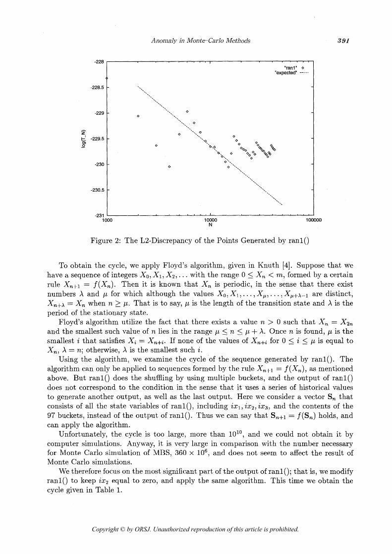
We calculate the L2-discrepancy of xn (Figure 2). If the points are really random, the estimated value of L2-discrepancy is known to be

and it decreases as the number of points increases, as shown by the straight line in Figure 2. However, the value never falls below 2 2 3 0 , which is reached after 4,000 points. The movement of the value has a pattern with a cycle of about 10,000 or 11,000 points. Consequently, xn has a cycle, and the accuracy of the integration does not improve after one cycle. 4.2. Cycle of ranl () 4.2.1. Floyd's Algorithm We have observed that the points generated from the output of ran10 seems to contain a cycle. In this section, we examine whether ran10 itself contains a short cycle.



' ' ' s a . a l . . . . . . . 'ranl" 0

"expected"

Figure 2: The L2-Discrepancy of the Points Generated by ran10

To obtain the cycle, we apply Floyd's algorithm, given in Knuth [4]. Suppose that we have a sequence of integers Xo, Xi, X2 , . . . with the range 0 < Xn < m, formed by a certain rule Xn+l = f{Xn). Then it is known that Xn is periodic, in the sense that there exist numbers A and p, for which although the values Xo, Xi, . . . , XÃˆ . . . , Xp+A_i are distinct,

- Xn when n > p. That is to say, p, is the length of the transition state and A is the Xn+A - period of the stationary state.

Floyd's algorithm utilize the fact that there exists a value n > 0 such that Xn = Xin and the smallest such value of n lies in the range p, < n < p, + A. Once n is found, p is the smallest i that satisfies Xi = Xn+i. If none of the values of Xn+i for 0 < i < p, is equal to Xn, A = n; otherwise, A is the smallest such i.

Using the algorithm, we examine the cycle of the sequence generated by rani(). The algorithm can only be applied to sequences formed by the rule Xn+1 = f (Xn)? as mentioned above. But ranl () does the shuffling by using multiple buckets, and the output of ranl () does not correspond to the condition in the sense that it uses a series of historical values to generate another output, as well as the last output. Here we consider a vector Sn that consists of all the state variables of rani(), including %, ix2? ixs, and the contents of the 97 buckets, instead of the output of rani(). Thus we can say that Sn+1 = f (Sn) holds, and can apply the algorithm.

Unfortunately, the cycle is too large, more than 101Â° and we could not obtain it by computer simulations. Anyway, it is very large in comparison with the number necessary for Monte Carlo simulation of MBS, 360 X 106, and does not seem to affect the result of Monte Carlo simulations.

We therefore focus on the most significant part of the output of rani(); that is, we modify ran10 to keep ix2 equal to zero, and apply the same algorithm. This time we obtain the cycle given in Table 1.


A. Tajima, S. Ninomiya & S. Tezuka

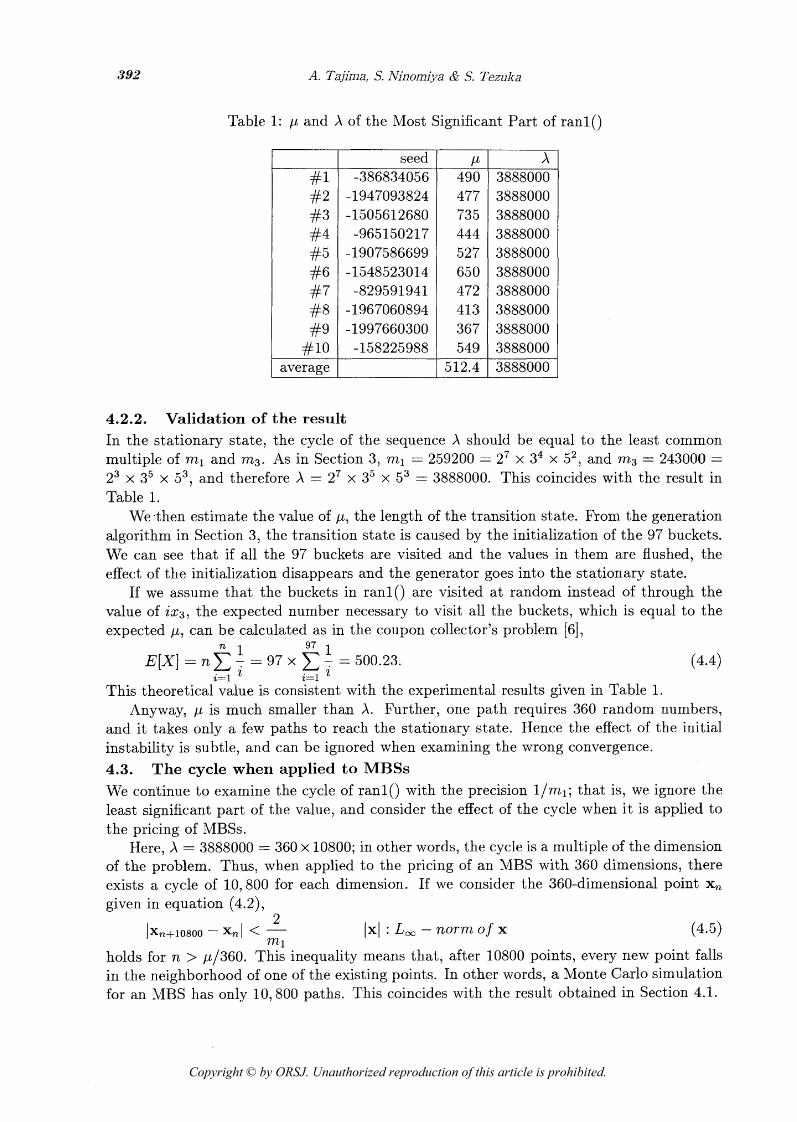
Table 1: p, and A of the Most Significant Part of ran10

- average

seed

4.2.2. Validation of the result In the stationary state, the cycle of the sequence A should be equal to the least common multiple of m1 and m3. As in Section 3, ml = 259200 = 27 X 34 X 52, and m3 = 243000 = z3 X 35 X 53, and therefore A = Z7 X 35 X 53 = 3888000. This coincides with the result in Table 1.

Wethen estimate the value of p, the length of the transition state. From the generation algorithm in Section 3, the transition state is caused by the initialization of the 97 buckets. We can see that if all the 97 buckets are visited and the values in them are flushed, the effect of the initialization disappears and the generator goes into the stationary state.

If we assume that the buckets in ran10 are visited at random instead of through the value of ix3, the expected number necessary to visit all the buckets, which is equal to the expected p, can be calculated as in the coupon collector's problem [6],

This theoretical value is consistent with the experimental results given in Table 1. Anyway, p, is much smaller than A. Further, one path requires 360 random numbers,

and it takes only a few paths to reach the stationary state. Hence the effect of the initial instability is subtle, and can be ignored when examining the wrong convergence.

4.3. The cycle when applied to MBSs We continue to examine the cycle of ran1 () with the precision l /ml ; that is, we ignore the least significant part of the value, and consider the effect of the cycle when it is applied to the pricing of MBSs.

Here, A = 3888000 = 360 X 10800; in other words, the cycle is a multiple of the dimension of the problem. Thus, when applied to the pricing of an MBS with 360 dimensions, there exists a cycle of 10,800 for each dimension. If we consider the 360-dimensional point xn given in equation (4.2),

2 lxn+10800 - xn l < 1x1 : L~~ - norm of X

m\ (4.5)

holds for n > f^/360. This inequality means that, after 10800 points, every new point falls in the neighborhood of one of the existing points. In other words, a Monte Carlo simulation for an MBS has only 10,800 paths. This coincides with the result obtained in Section 4.1.



l "truncated-seeds" -- -- -. l

100000 200000 300000 400000 500000 600000 700000 800000 900000 1e+06 Number of simulations

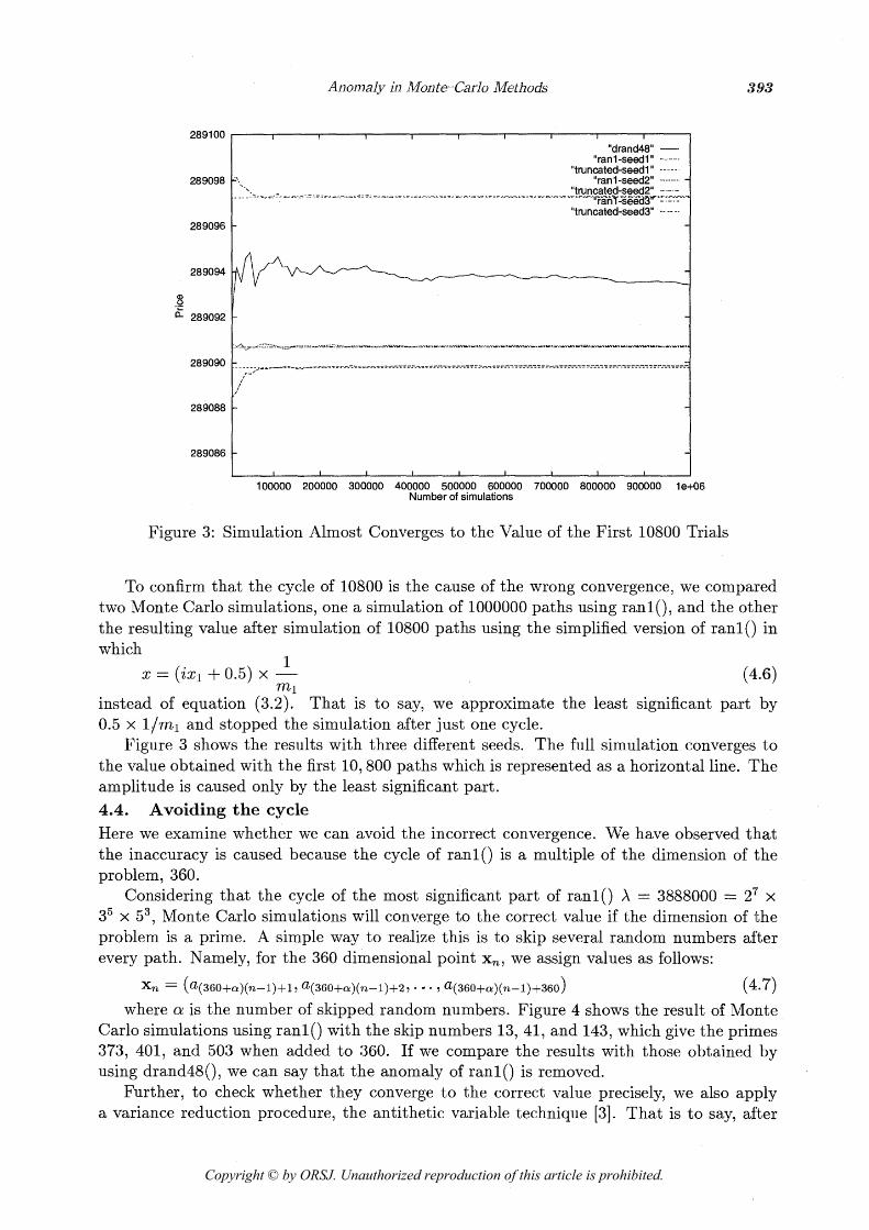
Figure 3: Simulation Almost Converges to the Value of the First 10800 Trials

To confirm that the cycle of 10800 is the cause of the wrong convergence, we compared two Monte Carlo simulations, one a simulation of 1000000 paths using rani(), and the other the resulting value after simulation of 10800 paths using the simplified version of ran10 in which

1 X = (ix1 + 0.5) X -

m1 (4.6)

instead of equation (3.2). That is to say, we approximate the least significant part by 0.5 X l /m l and stopped the simulation after just one cycle.

Figure 3 shows the results with three different seeds. The full simulation converges to the value obtained with the first 10,800 paths which is represented as a horizontal line. The amplitude is caused only by the least significant part. 4.4. Avoiding the cycle Here we examine whether we can avoid the incorrect convergence. We have observed that the inaccuracy is caused because the cycle of ran10 is a multiple of the dimension of the problem, 360.

Considering that the cycle of the most significant part of ran10 A = 3888000 = 27 X

35 X 53, Monte Carlo simulations will converge to the correct value if the dimension of the problem is a prime. A simple way to realize this is to skip several random numbers after every path. Namely, for the 360 dimensional point xn, we assign values as follows:

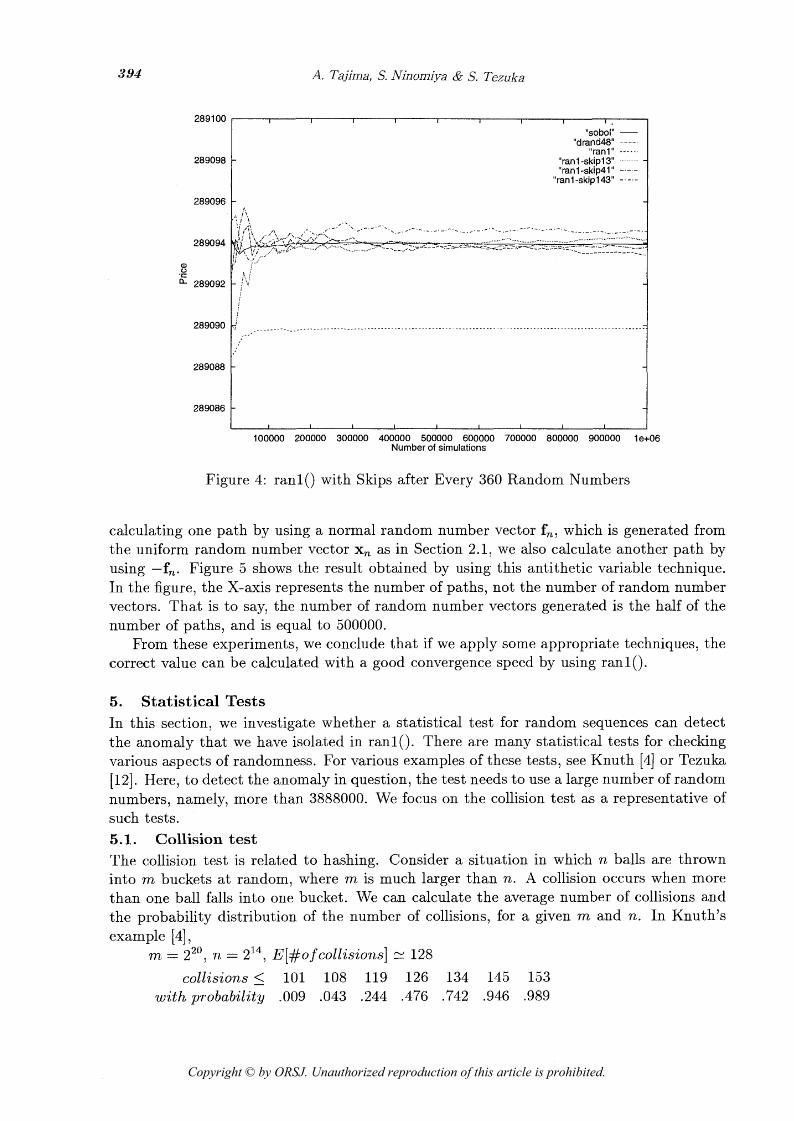
Xn = (0(360+a)(n-l)+l, a(360+et)(n-l)+2, m . 7 a(360+n)(n-l)+360) (4.7) where a is the number of skipped random numbers. Figure 4 shows the result of Monte

Carlo simulations using ran10 with the skip numbers 13, 41, and 143, which give the primes 373, 401, and 503 when added to 360. If we compare the results with those obtained by using drand48(), we can say that the anomaly of ran10 is removed.

Further, to check whether they converge to the correct value precisely, we also apply a variance reduction procedure, the antithetic variable technique [3]. That is to say, after


A. Tajima, S. Ninomiya & S. Tezuka


Figure 4: ran10 with Skips after Every 360 Random Numbers

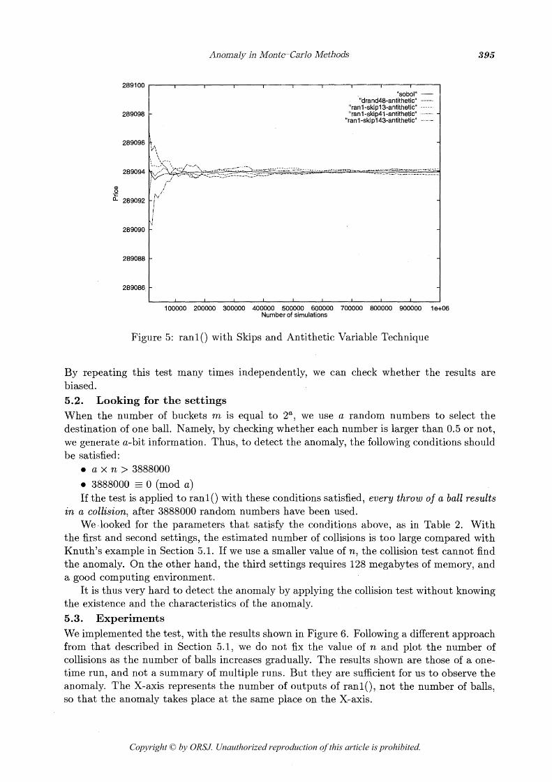
calculating one path by using a normal random number vector fn, which is generated from the uniform random number vector xn as in Section 2.1, we also calculate another path by using -fn. Figure 5 shows the result obtained by using this antithetic variable technique. In the figure, the X-axis represents the number of paths, not the number of random number vectors. That is to say, the number of random number vectors generated is the half of the number of paths, and is equal to 500000.

From these experiments, we conclude that if we apply some appropriate techniques, the correct value can be calculated with a good convergence speed by using rani().

5. Statistical Tests In this section, we investigate whether a statistical test for random sequences can detect the anomaly that we have isolated in rani(). There are many statistical tests for checking various aspects of randomness. For various examples of these tests, see Knuth [4] or Tezuka [12]. Here, t o detect the anomaly in question, the test needs to use a large number of random numbers, namely, more than 3888000. We focus on the collision test as a representative of such tests. 5.1. Collision test The collision test is related to hashing. Consider a situation in which n balls are thrown into m buckets a t random, where m is much larger than n. A collision occurs when more than one ball falls into one bucket. We can calculate the average number of collisions and the probability distribution of the number of collisions, for a given m and n. In Knuth's example [4],

m = 220, n = =l4, E[#o f collisions] = 128

collisions < 101 108 119 126 134 145 153 with probability .009 .043 .244 ,476 .742 .g46 ,989



'sobol" - "drand48-antithetic"

'ranl-skip13-antithetic" - m - . -

'ran1 -skip41 -antitheticu .-........ 'ran1 -skip1 43-antithetic''


Figure 5: ran10 with Skips and Antithetic Variable Technique

By repeating this test many times independently, we can check whether the results are biased. 5.2. Looking for the settings When the number of buckets m is equal to 2Â¡' we use a random numbers to select the destination of one ball. Namely, by checking whether each number is larger than 0.5 or not, we generate a-bit information. Thus, to detect the anomaly, the following conditions should be satisfied:

a X n > 3888000

3888000 0 (mod a) If the test is applied to ran10 with these conditions satisfied, every throw of a ball results

in a collision, after 3888000 random numbers have been used. We-looked for the parameters that satisfy the conditions above, as in Table 2. With

the first and second settings, the estimated number of collisions is too large compared with Knuth's example in Section 5.1. If we use a smaller value of n, the collision test cannot find the anomaly. On the other hand, the third settings requires 128 megabytes of memory, and a good computing environment.

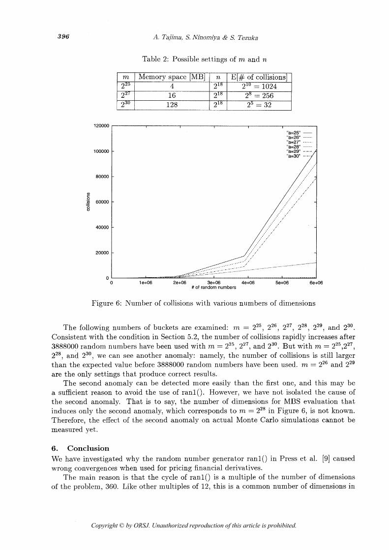
It is thus very hard to detect the anomaly by applying the collision test without knowing the existence and the characteristics of the anomaly. 5.3. Experiments We implemented the test, with the results shown in Figure 6. Following a different approach from that described in Section 5.1, we do not fix the value of n and plot the number of collisions as the number of balls increases gradually. The results shown are those of a one- time run, and not a summary of multiple runs. But they are sufficient for us to observe the anomaly. The X-axis represents the number of outputs of rani(), not the number of balls, so that the anomaly takes place at the same place on the X-axis.


A. Tajima, S. Mnomiya & S. Tezuka

Table 2: Possible settings of m and n

0 1 e+06 2e+06 3e+06 4e+06 5e+06 6e+06 # of random numbers

m >25

Figure 6: Number of collisions with various numbers of dimensions

The following numbers of buckets are examined: m = 225, 226, 227, 228, Z2', and 230. Consistent with the condition in Section 5.2, the number of collisions rapidly increases after 3888000 random numbers have been used with m = 225, 227, and 230. But with m = 225,227, 228, and z 3 O , we can see another anomaly: namely, the number of collisions is still larger than the expected value before 3888000 random numbers have been used. m = 226 and 229 are the only settings that produce correct results.

The second anomaly can be detected more easily than the first one, and this may be a sufficient reason to avoid the use of rani(). However, we have not isolated the cause of the second anomaly. That is to say, the number of dimensions for MBS evaluation that induces only the second anomaly, which corresponds t o m = 228 in Figure 6, is not known. Therefore, the effect of the second anomaly on actual Monte Carlo simulations cannot be measured yet.

Memory space [MB] 4

6. Conclusion We have investigated why the random number generator ran10 in Press et al. [g] caused wrong convergences when used for pricing financial derivatives.

The main reason is that the cycle of ran10 is a multiple of the number of dimensions of the problem, 360. Like other multiples of 12, this is a common number of dimensions in

n 218

E[# of collisions] 2'' = 1024


Anomaly in Monte-Carlo Methods 397

the financial domain, because a year has 12 months, and the same phenomenon will occur if the generator is used for pricing other derivative securities.

We have also presented a method for avoiding wrong convergences. Combined with the antithetic variable technique, ran10 can give the correct value with a good convergence speed. .

We have observed that statistical tests used to measure the randomness of pseudo- random numbers have difficulty in detecting the anomaly of rani(). The effect of another anomaly found in the experiment is not known.

References

M. Broadie, and P. Glasserman: Pricing American-style securities using simulation. Working paper, Columbia University, 1995. A. M. Ferrenberg, D. P. Landau and Y. J. Wong: Monte Carlo simulations: hidden errors from "good" random number generators. Physical Review Letters, 69 (23) (1992) 3382-3384. J. C. Hull: Options, Futures, and Other Derivative Securities, Second Edition (Prentice Hall International, 1993). D. E. Knuth: The Art of Computer Programming, Second Edition, Vol. 2, Semznumer- ical Algorithms (Addison-Wesley, 1981). W. J. Morokoff and R. E. Caflisch: Quasi-random sequences and their discrepancies. Journal on Scientific Computing, 15 (6) (1994) 1251-1280. R. Motwani and P. Raghavan: Randomized Algorithms (Cambridge University Press, 1995). H. Niederreiter: Random Number Generation and Quasi-Monte Carlo Methods, CBMS- NSF Regional Conference Series in Applied Math., No. 63, (SIAM, 1992). S. H. Paskov: Computing high dimensional integrals with applications to finance. Tech- nical Report CUCS-023-94, Columbia University, 1994. W. H. Press, S. Teukolsky, W. Vetterling and B. Flannery: Numerical Recipes in C, First Edition (Cambridge University Press, 1988). I. M. Sobol: The distribution of points in a cube and the approximate evaluation of integrals. USSR Computational Mathematics and Mathematical Physics, 7 (1967) 86-112. A. Tajima, S. Ninomiya and S. Tezuka: On the anomaly of rani() in Monte Carlo pricing of financial derivatives. 1996 Winter Simulation Conference Proceedings, (1996) 360-366. S. Tezuka: Uniform Random Numbers: Theory And Practice (Kluwer Academic Pub- lishers, 1995). J. A. Tilley: Valuing American options in a path simulation model. Transactions of the Society of Actuaries, 45 (1993) 499-519. B.,Moro: The full monte. RISK, 8 (2) (1995) 57-58.

Akira TAJIMA: tajimaQtrl.ibm.co. jp Syoiti NINOMIYA: ninomiya@trl. ibrn. CO. jp Shu TEZUKA: tezukaQtrl.ibm.co.jp IBM Research, Tokyo Research Laboratory 1623-14, Shimotsuruma, Yamato, Kanagawa 242-8502, Japan


ANALYSIS OF THE ANOMALY OF

Documents

Transcript of ANALYSIS OF THE ANOMALY OF