ANALYSIS OF THE RADIOMETRIC RESPONSE OF ORANGE TREE CROWN ...

ANALYSIS OF THE RADIOMETRIC RESPONSE OF ORANGE TREE CROWN IN

HYPERSPECTRAL UAV IMAGES

N. N. Imai1,2,*, E. A. S. Moriya1, E. Honkavaara3, G. T. Miyoshi2, M. V. A. de Moraes1, A. M. G. Tommaselli1,2, R. Näsi3

1 Dept. of Cartography, São Paulo State University (UNESP), Presidente Prudente-SP, Brazil - (nnimai, tomaseli)@fct.unesp.br,

(erikaasaito, antunesdemoraes)@gmail.com 2 Post Graduate Program in Cartographic Science, São Paulo State University (UNESP), Presidente Prudente-SP, Brazil -

[email protected] 3 Finnish Geospatial Research Institute FGI, Geodeetinrinne 2, P.O. Box 15, FI-02431 Masala, Finland - (eija.honkavaara,

roope.nasi)@nls.fi

KEY WORDS: radiometric calibration; hyperspectral image; bidirectional reflectance distribution function (BRDF); trend

analysis, UAV, high spectral and spatial resolution remote sensing.

Commission III, WG III/4

ABSTRACT:

High spatial resolution remote sensing images acquired by drones are highly relevant data source in many applications. However,

strong variations of radiometric values are difficult to correct in hyperspectral images. Honkavaara et al. (2013) presented a

radiometric block adjustment method in which hyperspectral images taken from remotely piloted aerial systems – RPAS were

processed both geometrically and radiometrically to produce a georeferenced mosaic in which the standard Reflectance Factor for

the nadir is represented. The plants crowns in permanent cultivation show complex variations since the density of shadows and the

irradiance of the surface vary due to the geometry of illumination and the geometry of the arrangement of branches and leaves. An

evaluation of the radiometric quality of the mosaic of an orange plantation produced using images captured by a hyperspectral

imager based on a tunable Fabry-Pérot interferometer and applying the radiometric block adjustment method, was performed. A

high-resolution UAV based hyperspectral survey was carried out in an orange-producing farm located in Santa Cruz do Rio Pardo,

state of São Paulo, Brazil. A set of 25 narrow spectral bands with 2.5 cm of GSD images were acquired. Trend analysis was

applied to the values of a sample of transects extracted from plants appearing in the mosaic. The results of these trend analysis on

the pixels distributed along transects on orange tree crown showed the reflectance factor presented a slightly trend, but the

coefficients of the polynomials are very small, so the quality of mosaic is good enough for many applications.

1. INTRODUCTION

Spatial and spectral high resolution remote sensing images

acquired from drones are a source of information of high

degree of relevance, but the variations of Digital Number - DN

introduced in these kind of images make their correction very

difficult.

Variations of radiometric measurements in remote sensing

images are caused by several factors related to the physical

environment. The anisotropy of the spectral response of targets

is a result of its Bidirectional Reflectance Distribution

Function - BRDF. The BRDF effects introduce variations in

radiance measured in different acquisition and lighting

geometries (Peltoniemi et al. 2007, Markelin et al. 2008,

Honkavaara et al. 2012). This anisotropy combined with the

variation of the irradiance of these targets produces variations

in the radiometric values, which are undesirable for many

applications. This type of problem has been addressed by

several researchers, which are interested in the plant cover

information (Li and Strahler 1986, Vermote et al. 2009, Bréon

and Vermote 2012). Alternatives to perform radiometric

correction of aerial images taken from piloted and remotely

piloted aerial systems (RPAS) have been more recently

developed (Pros et al. 2013).

Radiometric correction approaches of multispectral and

hyperspectral images taken from RPAS have been developed

mainly for applications in agriculture where the canopies are

frequently almost flat. In Brazil, mechanized annual crops

surfaces, as well as sugarcane cultivation have this kind of

geometry. However, some permanent crops, such as those for the

production of orange, lemon, mango, coffee, among others, have

a canopy in which the tops of the plants and the lines between

them form a mosaic that creates a 3D texture.

There is a great interest in the development of imaging systems

to monitor these crops, as this kind of system can produce

images which have great potential for detecting diseases as well

as nutritional plants deficiency. However, the radiometric and

geometric correction of images acquired at low altitude with

RPAS of this type of target remains a complex task, mainly due

to the effects of the micro relief generated by the trees canopies.

Images taken at low altitude, with ground sample distance

(GSD) around 10 cm or smaller have high frequency variations

both in geometry and radiometry.

Jakob et al. (2017) presented a solution for the geometric and

radiometric calibration of high spatial resolution images with a

GSD of 3.25 cm in rugged regions with low density of vegetation

cover, since mineral prospection was the subject of interest in

this job. The main problem faced in that work was the high

variation of the micro-relief. Honkavaara et al. (2013) presented

The International Archives of the Photogrammetry, Remote Sensing and Spatial Information Sciences, Volume XLII-3/W3, 2017 Frontiers in Spectral imaging and 3D Technologies for Geospatial Solutions, 25–27 October 2017, Jyväskylä, Finland

This contribution has been peer-reviewed. https://doi.org/10.5194/isprs-archives-XLII-3-W3-73-2017 | © Authors 2017. CC BY 4.0 License. 73

a solution in which hyperspectral images taken from RPAS

were processed both geometrically and radiometrically to

produce a georeferenced mosaic in which the standard

Reflectance Factor for the nadir is represented. A bundle block

adjustment was used to estimate orientation parameters

followed by digital surface model generation, which were the

start point of the proposed algorithm. Following, illumination

correction and a BRDF correction based on the model

developed by Walthall et al. (1985) were applied to correct the

anisotropy effects. Variations of the solar illumination and

other disturbances can be corrected by different approaches,

including measures of irradiance in a sensor placed over the

RPAS, or by a cosine sensor in the terrain. It is also feasible to

model factors causing radiometric differences between

overlapping images (illumination variations, BRDF, and other

effects) and to use a radiometric block adjustment to calculate

model parameters that minimize radiometric differences

between images.

The plant crowns in permanent cultivation show complex

variations since the density of shadows and the irradiance of

the surface vary due to the geometry of illumination and the

geometry of the arrangement of branches and leaves. The shape

of the plant crowns can be roughly modelled by a digital

surface model (DSM). The spectral reflectance factor can be

estimated for the nadir position based on this DSM and the

illumination geometry. In this sense, despite the solution

proposed by Honkavaara et al. (2013) had been optimized for

nearly flat canopy crop field, it can also be used for orange

production fields.

In this work, an evaluation of the radiometric quality of the

mosaic of an orange plantation produced using images captured

by a hyperspectral imager based on a tunable Fabry-Pérot

interferometer (FPI) and applying the method by Honkavaara et

al. (2013), is presented. Considering that a healthy plant

should present only random variations around its average

reflectance factor over its crown, a trend analysis was

performed based on observations extracted from a sample of

transects to check the hypothesis that the spatial distribution of

the values may show spatial tendency.

1.1 Study area

The study area is an orange production farm which belongs to

the AGROTERENAS which is a partner company in the

development of this work. It is located in Guacho farm, city of

Santa Cruz do Rio Pardo in the Sao Paulo State, Brazil. Figure

1 shows the location of this area. The coordinates of the study

area in the WGS84 system are 22°47'42.14"S and

49°23'46.28"W. The aerial and field surveys were carried out

on March 22, 2017.

Figure 1. Guacho farm in the city of Santa Cruz do Rio Pardo.

City of Santa Cruz do Rio Pardo in Sao Paulo State and in

Brazil.

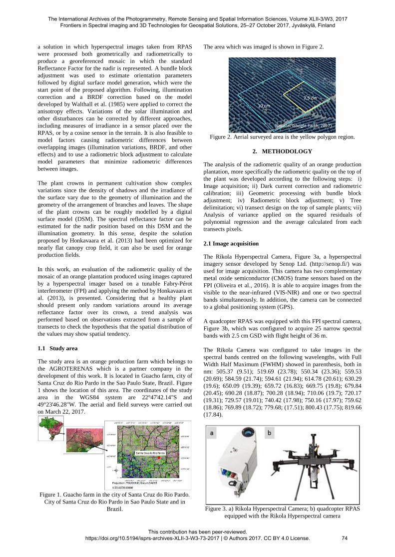
The area which was imaged is shown in Figure 2.

Figure 2. Aerial surveyed area is the yellow polygon region.

2. METHODOLOGY

The analysis of the radiometric quality of an orange production

plantation, more specifically the radiometric quality on the top of

the plant was developed according to the following steps: i)

Image acquisition; ii) Dark current correction and radiometric

calibration; iii) Geometric processing with bundle block

adjustment; iv) Radiometric block adjustment; v) Tree

delimitation; vi) transect design on the top of sample plants; vii)

Analysis of variance applied on the squared residuals of

polynomial regression and the average calculated from each

transects pixels.

2.1 Image acquisition

The Rikola Hyperspectral Camera, Figure 3a, a hyperspectral

imagery sensor developed by Senop Ltd. (http://senop.fi/) was

used for image acquisition. This camera has two complementary

metal oxide semiconductor (CMOS) frame sensors based on the

FPI (Oliveira et al., 2016). It is able to acquire images from the

visible to the near-infrared (VIS-NIR) and one or two spectral

bands simultaneously. In addition, the camera can be connected

to a global positioning system (GPS).

A quadcopter RPAS was equipped with this FPI spectral camera,

Figure 3b, which was configured to acquire 25 narrow spectral

bands with 2.5 cm GSD with flight height of 36 m.

The Rikola Camera was configured to take images in the

spectral bands centred on the following wavelengths, with Full

Width Half Maximum (FWHM) showed in parenthesis, both in

nm: 505.37 (9.51); 519.69 (23.78); 550.34 (23.36); 559.53

(20.69); 584.59 (21.74); 594.61 (21.94); 614.78 (20.61); 630.29

(19.6); 650.09 (19.39); 659.72 (16.83); 669.75 (19.8); 679.84

(20.45); 690.28 (18.87); 700.28 (18.94); 710.06 (19.7); 720.17

(19.31); 729.57 (19.01); 740.42 (17.98); 750.16 (17.97); 759.62

(18.86); 769.89 (18.72); 779.68; (17.51); 800.43 (17.75); 819.66

(17.84).

Figure 3. a) Rikola Hyperspectral Camera; b) quadcopter RPAS

equipped with the Rikola Hyperspectral camera



2.2 Image processing

Dark current correction was performed using a dark image

acquired before the flight, and the radiometric calibration using

a calibration file provided by the manufacturer both on the

images acquired. The Hyperspectral Imager software provided

by Senop Ltd was used for both procedures.

The Interior Orientation Parameters (IOP) were estimated

using the on-job calibration, performed with AgiSoft

PhotoScan in order to reconstruct the camera geometry. This

AgiSoft PhotoScan was used to refine the Exterior Orientation

Parameters (EOP) of three reference bands, for image

orientation. The reference bands were centred in 559.53 nm,

679.84 nm and 769.89 nm. The GNSS GPS sensor from the

camera was used to estimate the initial images position.

Then, a DSM of the area with 2.5 cm of GSD was produced by

dense matching method with AgiSoft PhotoScan as well. The

BRDF and illumination variation caused by differences in the

geometry of illumination and viewing during the imaging

acquisition were corrected by applying the method proposed

and presented by Honkavaara et al. (2013), Hakala et al.

(2013) and Näsi et al. (2016).

As the last step in the mosaic production process it is necessary

to transform DN to physical values in the images. In this sense,

the empirical line method (Smith and Milton, 1999) was

applied. Black, grey and white targets were placed in the study

area to be used as radiometric reference. Figure 4 shows

targets used in the hyperspectral image mosaic production: (A)

Targets for geometric correction, (b) Targets for radiometric

correction.

Figure 4. a) Targets for geometric correction, b) Targets for

radiometric correction.

2.3 Trend analysis

It was drawn lines at the top of the orange plant samples to

choose samples of pixels to be evaluated. These samples of

pixels were used to evaluate the radiometric variation of the

mosaic spectral reflectance of the pixels along these

trajectories. Therefore, it was drawn four directions on each

crown of orange plant in order to check the spectral reflectance

factor variation along all of these geometries. Figure 5 shows

all lines which were adopted to choose the pixels of the sample

transect. The wavelengths sampled were two in the visible and

two in the near-infrared since that each pair of bands are

acquired by different sensor in the camera. The bands centres

adopted to develop the analysis were: 550 nm and 660 nm in

the visible spectral region and 720 nm, 800 nm in the near-

infrared. Thus, images acquired by each sensor were

evaluated.

Trend analysis was applied to the values of a sample of transects

extracted from plants appearing in the mosaic. It is not expected

that there is a trend in the energy values reflected at any

wavelength of a healthy plant crown transect, but only random

variations around the mean. Considering the flat hemisphere

shape of the crown of an orange tree, it was decided to limit the

evaluations for linear and quadratic (parabolic) spatial trends.

This trend analysis is based on parameters presented in Table 1.

Source of

variation

Squared

sum D.F. Squared mean Fc

Polynomial

regression SQP m SQP/m = MQP

Residuals SQR n-m-1 SQR/(n-m-1) =

MQR

Total SQT n-1 SQT/(n-1) = MQT

Where: DF = Degrees of freedom, m = polynomial regression freedom

degree, n = sample number, H0 = spatial trend is accepted, H1 = trend is

not accepted. Residuals are independent among them, then: SQP = SQT

– SQR.

Table 1. Variance analysis table (ANOVA - ANalysis Of

VAriance).

3. RESULTS AND ANALYSIS

Figure 5 shows the transects on the crown of orange plants and

where are the pixels of the sample to be analysed.



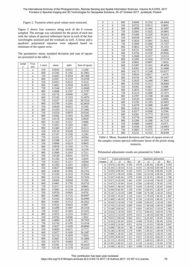
Figure 5. Transects where pixel values were extracted.

Figure 5 shows four transects along each of the 6 crowns

sampled. The average was calculated for the pixels of each one

with the values of spectral reflectance factor in each of the four

wavelengths analysed and the residuals as well. A linear and a

quadratic polynomial equation were adjusted based on

minimum of the square error.

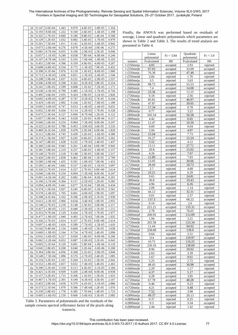
The parameters: mean, standard deviation and sum of square

are presented in the table 2.

sampl

e

Tran-

sect λ (nm) mean stdev Sum of square

1 a 550 0.0910 0.0521 1.5260

1 a 660 0.5342 0.1182 41.5963

1 a 720 0.4425 0.1054 28.7468

1 a 800 0.5957 0.1119 51.0538

1 b 550 0.0415 0.0522 0.3524

1 b 660 0.4061 0.2034 16.4653

1 b 720 0.3344 0.1637 11.0648

1 b 800 0.4948 0.1587 21.5797

1 c 550 0.0716 0.0440 1.2697

1 c 660 0.5182 0.1323 51.4670

1 c 720 0.4337 0.1226 36.5524

1 c 800 0.5769 0.1201 62.4819

1 d 550 0.0658 0.0321 0.5185

1 d 660 0.5193 0.1113 27.3481

1 d 720 0.4324 0.0970 19.0341

1 d 800 0.5942 0.1003 35.2095

2 a 550 0.0119 0.0256 0.0929

2 a 660 0.1345 0.1257 3.9486

2 a 720 0.1852 0.1303 5.9847

2 a 800 0.2460 0.1071 8.4113

2 b 550 0.0110 0.0246 0.0554

2 b 660 0.1547 0.1350 3.2282

2 b 720 0.2101 0.1375 4.8364

2 b 800 0.2588 0.1117 6.1059

2 c 550 0.0006 0.0219 0.0603

2 c 660 0.0878 0.1193 2.7741

2 c 720 0.1385 0.0106 4.2339

2 c 800 0.2069 0.1010 6.7211

2 d 550 0.0128 0.0241 0.0755

2 d 660 0.1342 0.1164 3.2055

2 d 720 0.1812 0.1211 4.8294

2 d 800 0.2393 0.1025 6.9023

3 a 550 0.0617 0.0494 0.7217

3 a 660 0.4630 0.1956 29.2701

3 a 720 0.3329 0.1533 15.5564

3 a 800 0.5154 0.1602 33.7626

3 b 550 0.0443 0.0344 0.2345

3 b 660 0.4401 0.1705 16.6753

3 b 720 0.3217 0.1233 8.8845

3 b 800 0.5065 0.1234 20.3632

3 c 550 0.0559 0.0426 0.6792

3 c 660 0.4403 0.1721 30.8097

3 c 720 0.3102 0.0122 16.0990

3 c 800 0.4901 0.1512 36.2822

3 d 550 0.0532 0.0425 0.5687

3 d 660 0.4499 0.1907 29.3318

3 d 720 0.3257 0.1425 15.5221

3 d 800 0.5076 0.1333 33.8617

4 a 550 0.0762 0.0566 1.3032

4 a 660 0.4894 0.1876 39.7929

4 a 720 0.2743 0.1295 13.3254

4 a 800 0.5637 0.1628 49.8840

4 b 550 0.0829 0.0375 0.7773

4 b 660 0.5077 0.1420 26.1087

4 b 720 0.2725 0.1010 7.9293

4 b 800 0.5661 0.1253 31.5800

4 c 550 0.0715 0.0465 1.1972

4 c 660 0.5591 0.1724 56.4419

4 c 720 0.3138 0.1178 18.5223

4 c 800 0.6060 0.1532 64.4404

4 d 550 0.0722 0.0512 0.9693

4 d 660 0.4898 0.1442 32.3087

4 d 720 0.2663 0.1025 10.0891

4 d 800 0.5496 0.1220 39.2812

5 a 550 0.0558 0.0471 0.6216

5 a 660 0.3824 0.1841 21.0425

5 a 720 0.3000 0.1660 13.7257

5 a 800 0.4853 0.1758 31.1351

5 b 550 0.0721 0.0505 0.6480

5 b 660 0.4756 0.1550 20.9945

5 b 720 0.3668 0.1257 12.6152

5 b 800 0.5495 0.1434 27.0718

5 c 550 0.0841 0.0497 1.5054

5 c 660 0.5407 0.1431 49.4094

5 c 720 0.4301 0.1245 31.6680

5 c 800 0.6172 0.1248 62.6377

5 d 550 0.0914 0.0617 1.4179

5 d 660 0.4756 0.1781 30.1457

5 d 720 0.3635 0.1448 17.8881

5 d 800 0.5559 0.1513 38.8084

6 a 550 0.0391 0.0427 0.3998

6 a 660 0.3874 0.1851 22.0897

6 a 720 0.3213 0.1680 15.7471

6 a 800 0.4787 0.1598 30.5406

6 b 550 0.0529 0.0260 0.2806

6 b 660 0.5190 0.1183 22.9403

6 b 720 0.4378 0.1088 16.4697

6 b 800 0.5814 0.1162 28.4580

6 c 550 0.0377 0.0368 0.3784

6 c 660 0.4361 0.1773 30.3235

6 c 720 0.3778 0.1694 23.4567

6 c 800 0.5289 0.1580 41.7135

6 d 550 0.0469 0.0450 0.4371

6 d 660 0.4594 0.1692 24.9003

6 d 720 0.3803 0.1575 17.5978

6 d 800 0.5231 0.1522 30.8399

Table 2. Mean, Standard deviation and Sum of square errors of

the samples crowns spectral reflectance factor of the pixels along

transects.

Polynomial adjustment results are presented in Table 3.

λ (nm)/

Sample

Linear polynomial Quadratic polynomial

a0 a1 Res. a0 a1 a2 Res.

1a 0.076 2.2E-04 0.364 0.078 1.4E-04 1.0E-06 0.363

1b 0.103 -1.5E-03 0.116 0.103 -1.5E-03 0.0E+00 0.116

1c 0.030 4.6E-04 0.243 0.052 -2.7E-04 4.0E-06 0.226

1d 0.075 -1.9E-04 0.096 0.082 -6.1E-04 4.0E-06 0.095

1a 0.567 4.6E-04 1.879 0.506 2.1E-03 -1.9E-05 1.780

1b 0.671 -6.5E-03 1.443 0.587 -4.1E-04 -7.6E-05 1.339

1c 0.472 5.1E-04 3.010 0.566 -2.6E-03 1.7E-05 2.705

1d 0.605 -1.8E-03 0.955 0.630 -3.3E-03 1.5E-05 0.944

1a 0.436 9.4E-05 1.530 0.391 2.0E-03 -1.4E-05 1.477

1b 0.541 -5.1E-03 1.008 0.480 -6.7E-04 -5.5E-05 0.954

1c 0.336 1.1E-03 2.120 0.421 -1.7E-03 1.6E-05 1.867

1d 0.499 -1.4E-03 0.763 0.528 -3.2E-03 1.8E-05 0.747

1a 0.610 -2.1E-04 1.718 0.560 2.0E-03 -1.5E-05 1.650

1b 0.703 -5.2E-03 0.860 0.643 -7.4E-04 -5.4E-05 0.806

1c 0.544 3.6E-04 2.521 0.603 1.6E-03 -1.1E-05 2.403

1d 0.654 -1.2E-03 0.855 0.712 4.8E-03 -3.6E-05 0.792

2a 0.013 -2.1E-05 0.076 0.013 -1.4E-05 0.0E+00 0.076

2b 0.023 -3.0E-04 0.043 0.011 6.2E-04 1.2E-05 0.041

2c -0.012 2.0E-04 0.054 -0.009 5.7E-05 1.0E-06 0.054

2d -0.003 3.1E-04 0.051 -0.016 1.1E-03 -7.0E-06 0.047

2a 0.088 7.9E-04 1.748 0.046 2.9E-03 -1.8E-05 1.708

2b 0.246 -2.3E-03 1.178 0.081 1.0E-02 -1.6E-04 0.792

2c 0.009 1.2E-03 1.539 -0.053 4.1E-03 -2.3E-05 1.445

2d 0.093 8.0E-04 1.313 0.012 5.5E-03 -4.6E-05 1.185

2a 0.113 -1.2E-03 1.772 0.071 3.4E-03 -1.8E-05 1.733

2b 0.302 2.4E-03 1.223 0.128 1.1E-02 1.7E-04 0.792

2c 0.049 1.4E-03 1.463 -0.009 4.1E-03 -2.1E-05 1.381



2d 0.147 6.6E-04 1.443 0.079 4.6E-03 -3.8E-05 1.354

2a 0.193 -9.0E-04 1.222 0.160 2.6E-03 -1.4E-05 1.198

2b 0.325 1.7E-03 0.840 0.186 8.8E-03 1.4E-04 0.568

2c 0.129 1.2E-03 1.032 0.082 3.4E-03 -1.7E-05 0.979

2d 0.201 7.5E-04 1.011 0.141 4.2E-03 -3.4E-05 0.942

3a 0.073 -2.0E-04 0.276 0.078 -4.5E-04 2.0E-06 0.275

3b 0.081 -9.7E-04 0.055 0.106 -2.9E-03 2.5E-05 0.046

3c 0.057 -1.1E-05 0.249 0.038 7.8E-04 -6.0E-06 0.240

3d 0.107 -8.7E-04 0.103 0.105 -7.6E-04 -1.0E-06 0.103

3a 0.451 2.0E-04 4.396 0.359 4.9E-03 -4.0E-05 4.207

3b 0.698 -6.8E-03 0.534 0.775 -1.3E-02 7.9E-05 0.452

3c 0.398 6.1E-04 3.976 0.118 1.3E-02 -8.6E-05 1.900

3d 0.713 -4.3E-03 1.636 0.651 -1.3E-03 -2.4E-05 1.546

3a 0.298 5.9E-04 2.657 0.231 4.0E-03 -2.9E-05 2.557

3b 0.506 -4.9E-03 0.298 0.562 -9.2E-03 5.8E-05 0.254

3c 0.241 1.0E-03 2.599 0.008 1.1E-02 -7.2E-05 1.171

3d 0.530 -3.3E-03 0.790 0.485 -1.1E-03 -1.7E-05 0.743

3a 0.495 3.6E-04 2.935 0.424 3.9E-03 -3.1E-05 2.826

3b 0.692 -4.9E-03 0.287 0.747 -9.2E-03 5.7E-05 0.244

3c 0.419 1.0E-03 2.902 0.164 1.2E-02 -7.8E-05 1.189

3d 0.695 -3.0E-03 0.747 0.633 -1.4E-05 -2.4E-05 0.655

4a 0.052 3.3E-04 0.434 0.114 -2.2E-03 1.7E-05 0.328

4b 0.072 2.3E-04 0.127 0.090 -8.7E-04 1.2E-05 0.122

4c 0.057 1.8E-04 0.343 0.028 1.2E-03 -6.0E-06 0.317

4d 0.046 1.6E-04 0.254 0.064 -7.3E-04 8.0E-06 0.247

4a 0.325 2.3E-03 3.786 0.453 -3.0E-03 3.6E-05 3.333

4b 0.469 8.1E-04 1.830 0.478 2.5E-04 6.0E-06 1.829

4c 0.511 5.8E-04 4.745 0.439 3.2E-03 -1.6E-05 4.580

4d 0.374 1.5E-04 3.927 0.245 6.6E-03 -5.5E-05 3.561

4a 0.147 1.8E-03 1.638 0.232 -1.7E-03 2.4E-05 1.437

4b 0.260 2.6E-04 0.943 0.261 2.4E-04 0.0E+00 0.943

4c 0.281 3.9E-04 2.219 0.237 2.0E-03 -1.0E-05 2.157

4d 0.140 2.7E-03 2.218 0.148 2.3E-03 3.0E-06 2.217

4a 0.420 2.0E-03 2.838 0.462 2.8E-04 1.2E-05 2.790

4b 0.580 -2.9E-04 1.455 0.591 -1.0E-03 7.0E-06 1.453

4c 0.595 1.4E-04 3.842 0.527 2.6E-03 -1.5E-05 3.697

4d 0.326 2.7E-03 2.614 0.327 2.7E-03 0.0E+00 2.614

5a 0.046 1.6E-04 0.254 0.064 -7.3E-04 8.0E-06 0.247

5b 0.091 -4.5E-04 0.202 0.082 2.0E-04 -8.0E-06 0.201

5c 0.106 -2.7E-04 0.364 0.157 -2.2E-03 1.2E-05 0.285

5d 0.094 -4.0E-05 0.441 0.077 8.1E-04 -7.0E-06 0.434

5a 0.374 1.5E-04 3.927 0.245 6.6E-03 -5.5E-05 3.561

5b 0.578 -2.4E-03 1.705 0.601 -4.0E-03 1.9E-05 1.697

5c 0.508 4.1E-04 3.162 0.596 -2.9E-03 2.1E-05 2.930

5d 0.612 -2.3E-03 2.966 0.634 -3.4E-03 1.0E-05 2.955

5a 0.140 2.7E-03 2.218 0.148 2.3E-03 3.0E-06 2.217

5b 0.427 -1.4E-03 1.215 0.440 -2.3E-03 1.1E-05 1.212

5c 0.353 9.7E-04 2.129 0.424 -1.7E-03 1.7E-05 1.977

5d 0.477 -1.9E-03 1.940 0.492 -2.7E-03 7.0E-06 1.935

5a 0.326 2.7E-03 2.614 0.327 2.7E-03 0.0E+00 2.614

5b 0.607 -1.4E-03 1.616 0.589 -7.7E-05 -1.5E-05 1.610

5c 0.542 9.4E-04 2.154 0.604 -1.4E-03 1.5E-05 2.038

5d 0.669 -1.9E-03 2.164 0.724 -4.7E-03 2.4E-05 2.096

6a 0.041 -3.6E-05 0.217 0.020 1.0E-03 -9.0E-06 0.206

6b 0.062 -2.2E-04 0.052 0.087 -2.0E-03 2.2E-05 0.043

6c 0.003 5.1E-04 0.129 0.001 5.9E-04 -1.0E-06 0.129

6d 0.045 2.8E-05 0.208 0.040 3.2E-04 -3.0E-06 0.208

6a 0.364 3.8E-04 4.056 0.268 5.1E-03 -3.9E-05 3.846

6b 0.549 -7.3E-04 1.096 0.576 -2.7E-03 2.4E-05 1.085

6c 0.216 3.2E-03 2.101 0.264 1.1E-03 1.5E-05 2.041

6d 0.552 -1.8E-03 2.657 0.652 -7.4E-03 5.4E-05 2.463

6a 0.290 5.2E-04 3.318 0.213 4.3E-03 -3.1E-05 3.184

6b 0.421 4.1E-04 0.939 0.430 -2.4E-04 8.0E-06 0.938

6c 0.157 3.2E-03 1.715 0.206 1.1E-03 1.5E-05 1.653

6d 0.467 -1.7E-03 2.301 0.549 -6.3E-03 4.5E-05 2.167

6a 0.455 3.9E-04 3.018 0.379 4.1E-03 -3.1E-05 2.886

6b 0.573 2.1E-04 1.079 0.586 -7.4E-04 1.2E-05 1.076

6c 0.339 2.8E-03 1.778 0.385 7.7E-04 1.4E-05 1.723

6d 0.605 -1.6E-03 2.159 0.666 -5.0E-03 3.3E-05 2.085

Table 3. Parameters of polynomials and the residuals of the

sample crowns spectral reflectance factor of the pixels along

transects.

Finally, the ANOVA was performed based on residuals of

average, Linear and quadratic polynomials which parameters are

shown in Table 2 and Table 3. The results of trend analysis are

presented in Table 4.

Linear

polynomial Fc = 3.84

Quadratic

polynomial Fc = 3.0

transect Fcalculated H0 Fcalculated H0

1 (550nm)a 4.05 accepted 2.03 rejected

1 (550nm)b 67.03 accepted 33.09 accepted

1 (550nm)c 76.38 accepted 47.48 accepted

1 (550nm)d 2.66 rejected 1.76 rejected

1 (660nm)a 3.5 rejected 5.63 accepted



1 (660nm)d 23.36 accepted 12.25 accepted

1 (720nm)a 0.18 rejected 2.56 rejected












2 (660nm)a 5.52 accepted 4.12 accepted







2 (720nm)d 2.7 rejected 4.68 accepted







3 (550nm)c 0.01 rejected 2.57 rejected




3 (660nm)c 2.78 rejected 76.65 accepted







3 (800nm)b 214 accepted 129.97 accepted




4 (550nm)b 2.63 rejected 3.39 accepted


4 (550nm)d 5.25 accepted 2.72 rejected


4 (660nm)b 2.29 rejected 1.17 rejected














5 (550nm)b 3.96 accepted 2.24 rejected












5 (800nm)b 4.63 accepted 2.45 rejected




6 (550nm)b 3.12 rejected 10.44 accepted















Table 4. Trend analysis results for 550 nm, 660 nm, 720 nm

and 800 nm: Fc is the critical value for the highest freedom

degree in the denominator and 1 or 2 for the numerator

according to the polynomial degree. Fcalculated for each

hypothesis test between the average against linear and

quadratic polynomials and H0 has the conclusion for each

hypothesis test. Fields filled by grey are accepted in a

Sequential Analysis of Variance.

The transect direction “a” was considered without linear trend

by the highest number of tests. It indicates this is a direction

that was better calibrated. But, the transect direction “c”

presented the highest number of linear and quadratic trend.

These differences can be related to the crown shape and solar

illumination angle at the aerial surveying.

The 550 nm wavelength presented the lower number of

accepted trend, it was 11 quadratic polynomials and 10 linear

which were rejected. Then, the algorithm performed better to

this wavelength than the others. The samples which represent

660 nm, 720 nm and 800 nm were accepted as presenting

quadratic trend as follows: 21, 21 and 19. Quadratic trend

could be a result related to the shape of crowns.

The analysis of variance accepted 65 linear polynomials as

trend and 74 quadratic ones as well. But another comparison

between Linear and quadratic polynomials accepted 20 linear

polynomials as trend while 41 quadratic ones. These accepted

polynomials as a trend were shown in the Table 3 with the cell

fulfilled in gray. The number of radiometric values along

transects presenting trend is higher than half of the transect

samples evaluated. The total amount of transect which do not

presented trend were 18. However, it is also noted the highest

absolute value of the linear polynomial angular coefficient was

0.00319 with -0.00024 as average value, which is almost zero.

The highest absolute value of the first order term quadratic

polynomial coefficient (a1) was 0.0126 and the second order

term (a2) was 0.000169, which denote low radiometric trend on

the plant crowns.

4. CONCLUSION

This study evaluated 96 transects considering 4 different

directions and 4 different wavelengths. There were spectral and

direction selectivity to the radiometric calibration. It was

concluded that more than half of radiometric samples had trend,

but the low values of coefficients showed that these trends are

too smooth which could not affect spectral analysis of plants in a

permanent kind of agricultural production.

Reason for these trends was that current model does not

compensate for the impacts of the sky view factor and the terrain

slope when the object topography is highly varying. In the future

the model will be enhanced in order to obtain accurate

calibration also in this type of environment.

5. ACKNOWLEDGEMENT

This research has been jointly funded by the São Paulo Research

Foundation (FAPESP – grant 2013/50426-4) and Academy of

Finland – decision number 273806) as well by the AGT-

Bravium-Fundunesp.

REFERENCES

Bréon, F. M., & Vermote, E., 2012. Correction of MODIS

surface reflectance time series for BRDF effects. Remote Sensing

of Environment, 125, pp. 1-9.

Hakala, T., Honkavaara, E., Saari, H., Mäkynen, J., Kaivosoja,

J., Pesonen, L., and Pölönen, I., 2013. Spectral imaging from

UAVs under varying illumination conditions. International

Archives of the Photogrammetry, Remote Sensing and Spatial

Information Sciences, 2013 UAV-g201, pp. 189-194.

Honkavaara. E., Markelin. L., Rosnell. T. and Nurminen. K.,

2012. Influence of solar elevation in radiometric and geometric

performance of multispectral photogrammetry. ISPRS Journal of

Photogrammetry and Remote Sensing, 67, pp. 13-26

Honkavaara. E., Saari. H., Kaivosoja. J., Pölönen. I., Hakala. T.,

Litkey. P., Mäkynen. J. and Pesonen. L., 2013. Processing and

Assessment of Spectrometric. Stereoscopic Imagery Collected

Using a Lightweight UAV Spectral Camera for Precision

Agriculture. Remote Sensing, 5(10), pp. 5006-5039

Jakob. S., Zimmermann. R. and Gloaguen. R., 2017. The Need

for Accurate Geometric and Radiometric Corrections of Drone-

Borne Hyperspectral Data for Mineral Exploration:

MEPHySTo—A Toolbox for Pre-Processing Drone-Borne

Hyperspectral Data. Remote Sensing, 9(1), pp. 1-17.

Li, X. and Strahler, A. H., 1986. Geometric-optical bidirectional

reflectance modeling of a conifer forest canopy. IEEE

Transactions on Geoscience and Remote Sensing, (6), pp. 906-

919.

Markelin, L., Honkavaara, E., Peltoniemi, J., Ahokas, E.,

Kuittinen, R., Hyyppä, J., Suomalainen, J. and Kukko, A., 2008.

Radiometric calibration and characterization of large-format

digital photogrammetric sensors in a test field. Photogrammetric

Engineering & Remote Sensing, 74(12), pp. 1487-1500.



Näsi, R., Honkavaara, E., Tuominen, S., Saari, H., Pölönen, I.,

Hakala, T., Viljanen N., Soukkamäki, J., Näkki, I., Ojanen, H.

and Reinikainen, J., 2016. UAS based tree species

identification using the novel FPI based hyperspectral cameras

in visible, NIR and SWIR spectral ranges. In: International

Archives of the Photogrammetry, Remote Sensing and Spatial

Information Sciences, 2016 ISPRS Congress, pp. 1143-1148.

Oliveira, R. A., Tommaselli, A. M., and Honkavaara, E., 2016.

Geometric Calibration of a Hyperspectral Frame Camera. The

Photogrammetric Record, 31 (155), pp. 325-347.

Peltoniemi, J. I., Piironen, J., Näränen, J., Suomalainen, J.,

Kuittinen, R., Markelin, L. and Honkavaara, E., 2007.

Bidirectional reflectance spectrometry of gravel at the Sjökulla

test field. ISPRS Journal of Photogrammetry and Remote

Sensing, 62(6), pp. 434-446.

Pros. A., Colomina. I., Navarro. J.A., Antequera. R. and

Andrinal. P., 2013. Radiometric block adjustment and digital

radiometric model generation. In: The International Archives of

the Photogrammetry. Remote Sensing and Spatial Information

Sciences. Hannover. Germany. Vol. XL-1/W1. pp. 21-24.

Smith, G. M. and Milton, E. J., 1999. The use of the empirical

line method to calibrate remotely sensed data to reflectance.

International Journal of Remote Sensing, v. 20, p. 2653-2662.

Vermote. E., Justice. C. O. and Bréon. F.-M., 2009. Towards a

Generalized Approach for Correction of the BRDF Effect in

MODIS Directional Reflectances. IEEE Transactions on

geoscience and remote sensing, 47(3), pp. 898-908.

Walthall. C.L., Norman. J.M., Welles. J.M., Campbell. G. and

Blad. B. L., 1985. Simple equation to approximate the

bidirectional reflectance from vegetative canopies and bare soil

surfaces. Appl. Opt, 24, pp. 383-387.



ANALYSIS OF THE RADIOMETRIC RESPONSE OF ORANGE TREE CROWN ...

Documents

Transcript of ANALYSIS OF THE RADIOMETRIC RESPONSE OF ORANGE TREE CROWN ...