AnhangA - link.springer.com978-3-658-21587-3/1.pdf · AnhangA A.1Grundlagenthemen Möchte man einen...
21
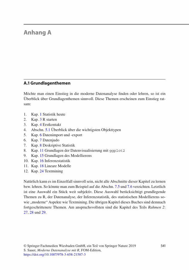
Anhang A A.1 Grundlagenthemen Möchte man einen Einstieg in die moderne Datenanalyse finden oder lehren, so ist ein Überblick über Grundlagenthemen sinnvoll. Diese Themen erscheinen zum Einstieg rat- sam: 1. Kap. 1 Statistik heute 2. Kap. 3 R starten 3. Kap. 4 Erstkontakt 4. Abschn. 5.1 Überblick über die wichtigsten Objekttypen 5. Kap. 6 Datenimport und -export 6. Kap. 7 Datenjudo 7. Kap. 8 Deskriptive Statistik 8. Kap. 11 Grundlagen der Datenvisualisierung mit ggplot2 9. Kap. 15 Grundlagen des Modellierens 10. Kap. 16 Inferenzstatistik 11. Kap. 18 Lineare Modelle 12. Kap. 24 Textmining Natürlich kann es im Einzelfall sinnvoll sein, nicht alle Abschnitte dieser Kapitel zu lernen bzw. lehren. So könnte man zum Beispiel auf die Abschn. 7.5 und 7.6 verzichten. Letztlich ist eine Auswahl ein Stück weit subjektiv. Diese Auswahl berücksichtigt grundlegende Themen zu R, der Datenanalyse, der Inferenzstatistik, des statistischen Modellierens so- wie „moderne“ Aspekte wie Textmining. Die übrigen Kapitel dieses Buches sind demnach fortgeschrittenere Themen. Am anspruchsvollsten sind die Kapitel des Teils Rahmen 2: 27, 28 und 29. 541 © Springer Fachmedien Wiesbaden GmbH, ein Teil von Springer Nature 2019 S. Sauer, Moderne Datenanalyse mit R, FOM-Edition, https://doi.org/10.1007/978-3-658-21587-3
Transcript of AnhangA - link.springer.com978-3-658-21587-3/1.pdf · AnhangA A.1Grundlagenthemen Möchte man einen...
Anhang A
A.1 Grundlagenthemen
Möchte man einen Einstieg in die moderne Datenanalyse finden oder lehren, so ist einÜberblick über Grundlagenthemen sinnvoll. Diese Themen erscheinen zum Einstieg rat-sam:
1. Kap. 1 Statistik heute2. Kap. 3 R starten3. Kap. 4 Erstkontakt4. Abschn. 5.1 Überblick über die wichtigsten Objekttypen5. Kap. 6 Datenimport und -export6. Kap. 7 Datenjudo7. Kap. 8 Deskriptive Statistik8. Kap. 11 Grundlagen der Datenvisualisierung mit ggplot29. Kap. 15 Grundlagen des Modellierens10. Kap. 16 Inferenzstatistik11. Kap. 18 Lineare Modelle12. Kap. 24 Textmining
Natürlich kann es im Einzelfall sinnvoll sein, nicht alle Abschnitte dieser Kapitel zu lernenbzw. lehren. So könnte man zumBeispiel auf die Abschn. 7.5 und 7.6 verzichten. Letztlichist eine Auswahl ein Stück weit subjektiv. Diese Auswahl berücksichtigt grundlegendeThemen zu R, der Datenanalyse, der Inferenzstatistik, des statistischen Modellierens so-wie „moderne“ Aspekte wie Textmining. Die übrigen Kapitel dieses Buches sind demnachfortgeschrittenere Themen. Am anspruchsvollsten sind die Kapitel des Teils Rahmen 2:27, 28 und 29.
541© Springer Fachmedien Wiesbaden GmbH, ein Teil von Springer Nature 2019S. Sauer, Moderne Datenanalyse mit R, FOM-Edition,https://doi.org/10.1007/978-3-658-21587-3
542 Anhang A
A.2 Übungsaufgaben
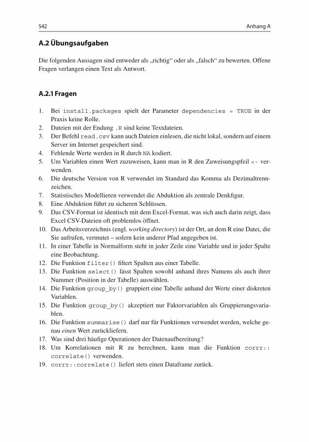
Die folgenden Aussagen sind entweder als „richtig“ oder als „falsch“ zu bewerten. OffeneFragen verlangen einen Text als Antwort.
A.2.1 Fragen
1. Bei install.packages spielt der Parameter dependencies = TRUE in derPraxis keine Rolle.
2. Dateien mit der Endung .R sind keine Textdateien.3. Der Befehl read.csv kann auch Dateien einlesen, die nicht lokal, sondern auf einem
Server im Internet gespeichert sind.4. Fehlende Werte werden in R durch NA kodiert.5. Um Variablen einen Wert zuzuweisen, kann man in R den Zuweisungspfeil <- ver-
wenden.6. Die deutsche Version von R verwendet im Standard das Komma als Dezimaltrenn-
zeichen.7. Statistisches Modellieren verwendet die Abduktion als zentrale Denkfigur.8. Eine Abduktion führt zu sicheren Schlüssen.9. Das CSV-Format ist identisch mit dem Excel-Format, was sich auch darin zeigt, dass
Excel CSV-Dateien oft problemlos öffnet.10. Das Arbeitsverzeichnis (engl. working directory) ist der Ort, an dem R eine Datei, die
Sie aufrufen, vermutet – sofern kein anderer Pfad angegeben ist.11. In einer Tabelle in Normalform steht in jeder Zeile eine Variable und in jeder Spalte
eine Beobachtung.12. Die Funktion filter() filtert Spalten aus einer Tabelle.13. Die Funktion select() lässt Spalten sowohl anhand ihres Namens als auch ihrer
Nummer (Position in der Tabelle) auswählen.14. Die Funktion group_by() gruppiert eine Tabelle anhand der Werte einer diskreten
Variablen.15. Die Funktion group_by() akzeptiert nur Faktorvariablen als Gruppierungsvaria-
blen.16. Die Funktion summarise() darf nur für Funktionen verwendet werden, welche ge-
nau einenWert zurückliefern.17. Was sind drei häufige Operationen der Datenaufbereitung?18. Um Korrelationen mit R zu berechnen, kann man die Funktion corrr::
correlate() verwenden.19. corrr::correlate() liefert stets einen Dataframe zurück.
Anhang A 543
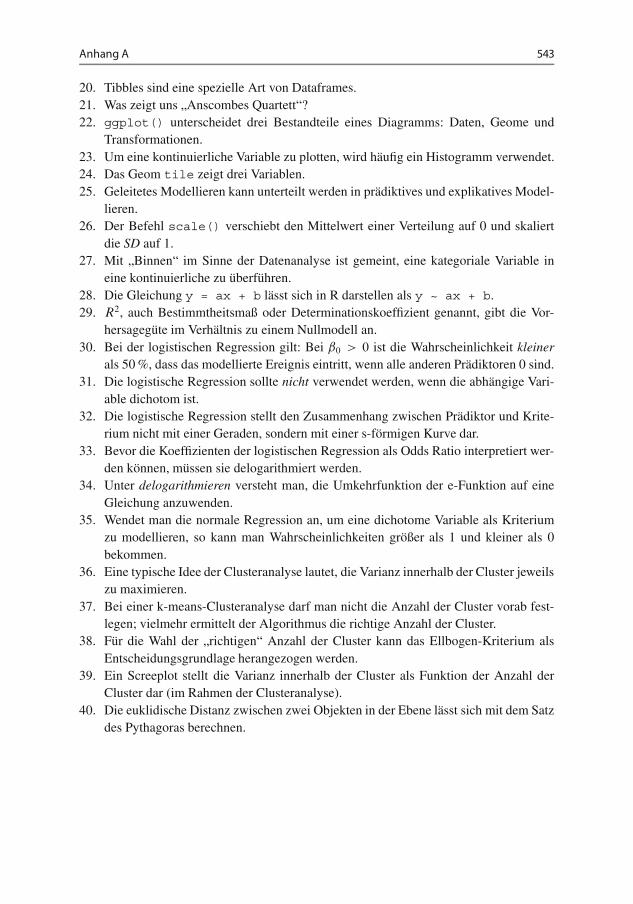
20. Tibbles sind eine spezielle Art von Dataframes.21. Was zeigt uns „Anscombes Quartett“?22. ggplot() unterscheidet drei Bestandteile eines Diagramms: Daten, Geome und
Transformationen.23. Um eine kontinuierliche Variable zu plotten, wird häufig ein Histogramm verwendet.24. Das Geom tile zeigt drei Variablen.25. Geleitetes Modellieren kann unterteilt werden in prädiktives und explikatives Model-
lieren.26. Der Befehl scale() verschiebt den Mittelwert einer Verteilung auf 0 und skaliert
die SD auf 1.27. Mit „Binnen“ im Sinne der Datenanalyse ist gemeint, eine kategoriale Variable in
eine kontinuierliche zu überführen.28. Die Gleichung y = ax + b lässt sich in R darstellen als y ~ ax + b.29. R2, auch Bestimmtheitsmaß oder Determinationskoeffizient genannt, gibt die Vor-
hersagegüte im Verhältnis zu einem Nullmodell an.30. Bei der logistischen Regression gilt: Bei ˇ0 > 0 ist die Wahrscheinlichkeit kleiner
als 50%, dass das modellierte Ereignis eintritt, wenn alle anderen Prädiktoren 0 sind.31. Die logistische Regression sollte nicht verwendet werden, wenn die abhängige Vari-
able dichotom ist.32. Die logistische Regression stellt den Zusammenhang zwischen Prädiktor und Krite-
rium nicht mit einer Geraden, sondern mit einer s-förmigen Kurve dar.33. Bevor die Koeffizienten der logistischen Regression als Odds Ratio interpretiert wer-
den können, müssen sie delogarithmiert werden.34. Unter delogarithmieren versteht man, die Umkehrfunktion der e-Funktion auf eine
Gleichung anzuwenden.35. Wendet man die normale Regression an, um eine dichotome Variable als Kriterium
zu modellieren, so kann man Wahrscheinlichkeiten größer als 1 und kleiner als 0bekommen.
36. Eine typische Idee der Clusteranalyse lautet, die Varianz innerhalb der Cluster jeweilszu maximieren.
37. Bei einer k-means-Clusteranalyse darf man nicht die Anzahl der Cluster vorab fest-legen; vielmehr ermittelt der Algorithmus die richtige Anzahl der Cluster.
38. Für die Wahl der „richtigen“ Anzahl der Cluster kann das Ellbogen-Kriterium alsEntscheidungsgrundlage herangezogen werden.
39. Ein Screeplot stellt die Varianz innerhalb der Cluster als Funktion der Anzahl derCluster dar (im Rahmen der Clusteranalyse).
40. Die euklidische Distanz zwischen zwei Objekten in der Ebene lässt sich mit dem Satzdes Pythagoras berechnen.
544 Anhang A
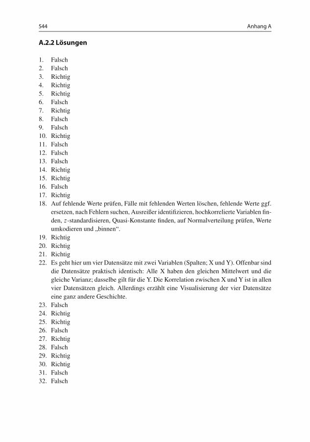
A.2.2 Lösungen
1. Falsch2. Falsch3. Richtig4. Richtig5. Richtig6. Falsch7. Richtig8. Falsch9. Falsch10. Richtig11. Falsch12. Falsch13. Falsch14. Richtig15. Richtig16. Falsch17. Richtig18. Auf fehlende Werte prüfen, Fälle mit fehlenden Werten löschen, fehlende Werte ggf.
ersetzen, nach Fehlern suchen, Ausreißer identifizieren, hochkorrelierte Variablen fin-den, z-standardisieren, Quasi-Konstante finden, auf Normalverteilung prüfen, Werteumkodieren und „binnen“.
19. Richtig20. Richtig21. Richtig22. Es geht hier um vier Datensätze mit zwei Variablen (Spalten; X und Y). Offenbar sind
die Datensätze praktisch identisch: Alle X haben den gleichen Mittelwert und diegleiche Varianz; dasselbe gilt für die Y. Die Korrelation zwischen X und Y ist in allenvier Datensätzen gleich. Allerdings erzählt eine Visualisierung der vier Datensätzeeine ganz andere Geschichte.
23. Falsch24. Richtig25. Richtig26. Falsch27. Richtig28. Falsch29. Richtig30. Richtig31. Falsch32. Falsch
Anhang A 545
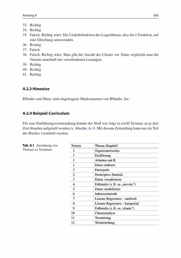
33. Richtig34. Richtig35. Falsch. Richtig wäre: Die Umkehrfunktion des Logarithmus, also die e-Funktion, auf
eine Gleichung anzuwenden.36. Richtig37. Falsch38. Falsch. Richtig wäre: Man gibt die Anzahl der Cluster vor. Dann vergleicht man die
Varianz innerhalb der verschiedenen Lösungen.39. Richtig40. Richtig41. Richtig
A.2.3 Hinweise
RStudio und Shiny sind eingetragene Markennamen von RStudio, Inc.
A.2.4 Beispiel-Curriculum
Für eine Einführungsveranstaltung könnte der Stoff wie folgt in zwölf Termine zu je dreiZeit-Stunden aufgeteilt werden (s. Abschn. A.1). Mit diesem Zeitumfang kann nur ein Teildes Buches vermittelt werden.
Tab. A.1 Zuordnung vonThemen zu Terminen
Termin Thema (Kapitel)
1 Organisatorisches
1 Einführung
1 Arbeiten mit R
1 Daten einlesen
2 Datenjudo
2 Deskriptive Statistik
3 Daten visualisieren
4 Fallstudie (z. B. zu „movies“)
5 Daten modellieren
6 Inferenzstatistik
7 Lineare Regression – metrisch
8 Lineare Regression – kategorial
9 Fallstudie (z. B. zu „titanic“)
10 Clusteranalyse
11 Textmining
12 Wiederholung
546 Anhang A
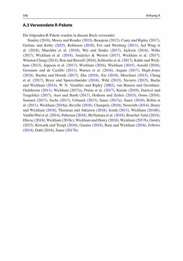
A.3 Verwendete R-Pakete
Die folgenden R-Pakete wurden in diesem Buch verwendet:Stanley (2018), Morey und Rouder (2015), Beaujean (2012), Canty und Ripley (2017),
Gerlanc und Kirby (2015), Robinson (2018), Fox und Weisberg (2011), Jed Wing etal. (2018), Maechler et al. (2018), Wei und Simko (2017), Jackson (2016), Wilke(2017), Wickham et al. (2018), Analytics & Weston (2017), Wickham et al. (2017),Winston Chang (2014), Ren und Russell (2016), Schloerke et al. (2017), Kahle undWick-ham (2013), Jeppson et al. (2017), Wickham (2016), Wickham (2015), Arnold (2018),Gesmann und de Castillo (2011), Warnes et al. (2016), Auguie (2017), Hugh-Jones(2018), Buchta und Hornik (2017), Zhu (2018), Xie (2018), Meschiari (2015), Chenget al. (2017), Bryer und Speerschneider (2016), Wild (2015), Navarro (2015), Bacheund Wickham (2014), W. N. Venables und Ripley (2002), van Buuren und Groothuis-Oudshoorn (2011), Wickham (2017a), Pruim et al. (2017), Raiche (2010), Daróczi undTsegelskyi (2017), Aust und Barth (2017), Hothorn und Zeileis (2015), Ooms (2018),Soetaert (2017), Sachs (2017), Urbanek (2013), Sauer (2017a), Sauer (2018), Robin etal. (2011), Wickham (2018a), Revelle (2018), Champely (2018), Neuwirth (2014), Henryund Wickham (2018), Therneau und Atkinson (2018), South (2011), Wickham (2018b),VanDerWal et al. (2014), Pebesma (2018),McNamara et al. (2018), Bouchet-Valat (2014),Hlavac (2018),Wickham (2018c),Wickham und Henry (2018),Wickham (2017b), Gentry(2015), Kowarik und Templ (2016), Garnier (2018), Ram und Wickham (2016), Fellows(2014), Dahl (2016), Sauer (2017b).
Literatur
AfD (2016). Party platform („Parteiprogramm“) of the AfD party („Alternative for Germany“) as of2016-05-01. Web page. https://www.afd.de/.
Agresti, A. (2013). Categorical data analysis. Hoboken, N.J: Wiley.American Psychological Association (2009). Publication Manual of the American Psychological
Association, 6th Edition. American Psychological Association (APA). https://www.amazon.com/Publication-Manual-American-Psychological-Association/dp/1433805618?SubscriptionId=0JYN1NVW651KCA56C102&tag=techkie-20&linkCode=xm2&camp=2025&creative=165953&creativeASIN=1433805618.
Analytics R., & Weston, S. (2017). doMC: Foreach Parallel Adaptor for ’parallel’. https://CRAN.R-project.org/package=doMC.
Anscombe, F. J. (1973). Graphs in Statistical Analysis. The American Statistician, 27(1), 17–21.https://doi.org/10.1080/00031305.1973.10478966.
Arnold, J. B. (2018). ggthemes: Extra Themes, Scales and Geoms for ’ggplot2’. https://CRAN.R-project.org/package=ggthemes.
Aronson, E., Akert, R.M., & Wilson, T.D. (2010). Sozialpsychologie. München: Pearson.Auguie, B. (2017). gridExtra: Miscellaneous Functions for „Grid“ Graphics. https://CRAN.R-
project.org/package=gridExtra.Aust, F., & Barth, M. (2017). papaja: Create APA manuscripts with R Markdown. https://github.
com/crsh/papaja.Azad, K. (2013).Math, Better Explained. Amazon.Bache, S.M., & Wickham, H. (2014). magrittr: A Forward-Pipe Operator for R. https://CRAN.R-
project.org/package=magrittr.Banerjee, M., Capozzoli, M., McSweeney, L., & Sinha, D. (1999). Beyond kappa: A review of
interrater agreement measures. Canadian Journal of Statistics, 27(1), 3–23. https://doi.org/10.2307/3315487.
Baron, R.M., & Kenny, D. A. (1986). The moderator-mediator variable distinction in social psycho-logical research: Conceptual, strategic, and statistical considerations. Journal of Personality andSocial Psychology, 51(6), 1173–1182.
Baumer, B., Kaplan, D. T., & Horton, N. J. (2017).Modern Data Science with R. Boca Raton, Flo-rida: Chapman; Hall/CRC.
Beaujean, A. A. (2012). BaylorEdPsych: R Package for Baylor University Educational PsychologyQuantitative Courses. https://CRAN.R-project.org/package=BaylorEdPsych.
Begley, C. G., & Ioannidis, J. P. (2015). Reproducibility in Science. Circulation Research, 116(1),116–126. https://doi.org/10.1161/CIRCRESAHA.114.303819.
547
548 Literatur
Benjamin, D. J., Berger, J., Johannesson, M., Nosek, B., Wagenmakers, E.-J., Berk, R., Johnson,V., et al. (2017). Redefine Statistical Significance. Nature Human Behaviour. https://doi.org/10.1038/s41562-017-0189-z.
Benjamin, D. J., Berger, J. O., Johannesson, M., Nosek, B. A., Wagenmakers, E.-J., Berk, R., et al.(2018). Redefine statistical significance. Nature Human Behaviour, 2(1), 6. https://doi.org/10.1038/s41562-017-0189-z.
Bishop, C.M. (2006). Pattern Recognition and Machine Learning. New York: Springer.Bogen, J., & Woodward, J. (1988). Saving the phenomena. The Philosophical Review, 97(3), 303–
352.Bortz, J. (2013). Statistik: Für Sozialwissenschaftler. Heidelberg: Springer.Bosco, F. A., Aguinis, H., Singh, K., Field, J. G., & Pierce, C.A. (2015). Correlational effect size
benchmarks. Journal of Applied Psychology, 100(2), 431–449. https://doi.org/10.1037/a0038047.Botsman, R. (2017, Oktober). Big data meets Big Brother as China moves to rate its citizens. http://
www.wired.co.uk/article/chinese-government-social-credit-score-privacy-invasion.Bouchet-Valat, M. (2014). SnowballC: Snowball stemmers based on the C libstemmer UTF-8 libra-
ry. https://CRAN.R-project.org/package=SnowballC.Breiman, L., Friedman, J., Stone, C. J., & Olshen, R.A. (1984). Classification and regression trees.
Boca Raton, Florida: CRC press.Brennan, R. L., & Prediger, D. J. (1981). Coefficient Kappa: Some Uses, Misuses, and Alterna-
tives. Educational and Psychological Measurement, 41(3), 687–699. https://doi.org/10.1177/001316448104100307.
Bresler, A. (2015, Januar). „Recreating Edward Tufte’s New York City Weather Visualization“.https://gist.github.com/abresler/46c36c1a88c849b94b07.
Briggs, W.M. (2008). Breaking the Law of Averages: Real-Life Probability and Statistics in PlainEnglish. Morrisville, NC: Lulu.com.
Briggs, W.M. (2016). Uncertainty: The Soul of Modeling, Probability & Statistics. New York:Springer.
Brown, J. D. (2015). Linear Models in Matrix Form: A Hands-On Approach for the BehavioralSciences. New York: Springer.
Brown, E.N., & Kass, R. E. (2009). What is statistics? The American Statistician, 63(2), 105–110.Bryer, J., & Speerschneider, K. (2016). likert: Analysis and Visualization Likert Items. https://
CRAN.R-project.org/package=likert.Brynjolfsson, E., & McAfee, A. (2016). The Second Machine Age: Work, Progress, and Prosperity
in a Time of Brilliant Technologies. New York, NY: W. W. Norton & Company. https://www.amazon.com/Second-Machine-Age-Prosperity-Technologies/dp/0393350649?SubscriptionId=0JYN1NVW651KCA56C102&tag=techkie-20&linkCode=xm2&camp=2025&creative=165953&creativeASIN=0393350649.
Buchta, C., & Hornik, K. (2017). ISOcodes: Selected ISO Codes. https://CRAN.R-project.org/package=ISOcodes.
Bundeswahlleiter (2017a). Strukturdaten für die Wahlkreise. https://www.bundeswahlleiter.de/dam/jcr/f7566722-a528-4b18-bea3-ea419371e300/btw17_strukturdaten.csv.
Bundeswahlleiter (2017b). Ergebnisse der Bundestagswahl 2017. https://www.bundeswahlleiter.de/bundestagswahlen/2017.html. Zugegriffen: 1. Okt. 2017.
Bureau of transportation statistics RITA (2013). nycflights13. http://www.transtats.bts.gov/DL_SelectFields.asp?Table_ID=236.
Burns, P. (2012). The R Inferno. Morrisville, NC: lulu.com.van Buuren, S. (2012). Flexible Imputation of Missing Data. Boca Raton, Fl: Chapman; Hall/CRC.van Buuren, S., & Groothuis-Oudshoorn, K. (2011). mice: Multivariate Imputation by Chained
Equations in R. Journal of Statistical Software, 45(3), 1–67. http://www.jstatsoft.org/v45/i03/.
https://www.bundeswahlleiter.de/dam/jcr/f7566722-a528-4b18-bea3-ea419371e300/btw17_strukturdaten.csv

Literatur 549
Bühner, M. (2011). Einführung in die Test- und Fragebogenkonstruktion. Hallbergmoos: Pearson.Canty, A., & Ripley, B. D. (2017). boot: Bootstrap R (S-Plus) Functions.Carsey, T.M., & Harden, J. J. (2013). Monte Carlo simulation and resampling methods for social
science. Los Angeles: SAGE.Chacon, S., & Straub, B. (2014). Pro Git. New York City, NY: Apress.Chambers, C. (2017). The Seven Deadly Sins of Psychology: A Manifesto for Reforming the Culture
of Scientific Practice. Princeton, CA: Princeton University Press.Champely, S. (2018). pwr: Basic Functions for Power Analysis. https://CRAN.R-project.org/
package=pwr.Cheng, J., Karambelkar, B., & Xie, Y. (2017). leaflet: Create Interactive Web Maps with the Java-
Script ’Leaflet’ Library. https://CRAN.R-project.org/package=leaflet.Chui, M., Manyika, J., Miremadi, M., Henke, N., Chung, R., Nel, P., & Malhotra, A. S. (2018).
Notes from the AI frontier. Report by McKinsey & Company. https://www.mckinsey.com/featured-insights/artificial-intelligence/notes-from-the-ai-frontier-applications-and-value-of-deep-learning.
Cleveland, W. S. (1993). Visualizing Data. Summit, NJ: Hobart Press.Clopper, C. J., & Pearson, E. S. (1934). The use of confidence or fiducial limits illustrated in the case
of the binomial. Biometrika, 26(4), 404–413.Cobb, G.W. (2007). The introductory statistics course: a Ptolemaic curriculum? Technology Inno-
vations in Statistics Education, 1(1).Cobb, G.W. (2015). Mere Renovation is Too Little Too Late: We Need to Rethink Our Undergra-
duate Curriculum from the Ground Up. The American Statistician, 69(4), 266–282. https://doi.org/10.1080/00031305.2015.1093029.
Cohen, J. (1988). Statistical Power Analysis for the Behavioral Sciences. Abingdon-on-Thames,UK: Routledge. https://doi.org/10.4324/9780203771587.
Cohen, J. (1992). A power primer. Psychological Bulletin, 112(1), 155–159.Cohen, J., Cohen, P., West, S. G., & Aiken, L. S. (2013). Applied multiple regression/correlation
analysis for the behavioral sciences. Boca Raton, Florida: Routledge.Dahl, D. B. (2016). xtable: Export Tables to LaTeX or HTML. https://CRAN.R-project.org/
package=xtable.Daróczi, G., & Tsegelskyi, R. (2017). pander: An R ’Pandoc’ Writer. https://CRAN.R-project.org/
package=pander.Deutsche Welle (2017). Liste von Twitter-Accounts deutscher Politiker. https://twitter.com/dw_
politics/lists/german-politicians/members?lang=en.Diez, D.M., Barr, C.D., & Cetinkaya-Rundel, M. (2014). Introductory Statistics with Randomizati-
on and Simulation. North Charleston, SC: CreateSpace.Diez, D.M., Barr, C. D., & Cetinkaya-Rundel, M. (2015).OpenIntro statistics. CreateSpace. https://
www.openintro.org/.Dodge, Y. (Hrsg.) (2006). The Oxford Dictionary of Statistical Terms. Oxford University Press.Durand, M. (2015). The OECD Better Life Initiative: How’s Life? and the Measurement of Well-
Being. Review of Income and Wealth, 61(1), 4–17. https://doi.org/10.1111/roiw.12156.Efron, B., & Tibshirani, R. (1994). An Introduction to the Bootstrap. Boca Raton, FL: Taylor &
Francis. https://books.google.de/books?id=gLlpIUxRntoC.Eid, M., Gollwitzer, M., & Schmitt, M. (2010). Statistik und Forschungsmethoden. Göttingen: Ho-
grefe.Fair, R. C. (1978). A theory of extramarital affairs. Journal of Political Economy, 86(1), 45–61.Farrell, H. (2012, Juli). Milton Friedman’s Thermostat. Blog Post. http://themonkeycage.org/2012/
07/milton-friedmans-thermostat/.Fellows, I. (2014). wordcloud: Word Clouds. https://CRAN.R-project.org/package=wordcloud.
550 Literatur
Fisher, R. A. (1955). Statistical methods and scientific induction. Journal of the Royal StatisticalSociety. Series B (Methodological), 17(1), 69–78.
Fisher, R. A. (2008). Photograph. http://www.swlearning.com/quant/kohler/stat/biographical_sketches/Fisher_3.jpeg.
Flach, P., & Hadjiantonis, A. (2013). Abduction and Induction: Essays on their Relation and Inte-gration. https://books.google.de/books?id=E7fnCAAAQBAJ.
Flick, U. (2007). Qualitative Sozialforschung: eine Einführung. Berlin: Rowohlt. http://books.google.de/books?id=zvISAQAAMAAJ.
Fonticons (2018). Icons ‘check-square-regular’, ‘laptop-solid’, and ‘bell-regular’ from Font Awe-some. https://fontawesome.com/license/free
Foucault, M. (1994).Überwachen und Strafen. Die Geburt des Gefängnisses. Frankfurt: Suhrkamp.Fox, J. (2005). The R Commander: A Basic Statistics Graphical User Interface to R. Journal of
Statistical Software, 14(9), 1–42. http://www.jstatsoft.org/v14/i09.Fox, J. (2016). Using the R Commander: A Point-and-Click Interface for R. Chapman & Hall/CRC
The R Series. Cambridge, MA: Chapman; Hall/CRC.Fox, J., & Weisberg, S. (2011). An R Companion to Applied Regression (Second.). Thousand Oaks
CA: SAGE. http://socserv.socsci.mcmaster.ca/jfox/Books/Companion.Franco, A., Malhotra, N., & Simonovits, G. (2014). Publication bias in the social sciences:
Unlocking the file drawer. Science, 345(6203), 1502–1505. https://doi.org/10.1126/science.1255484.
Freedman, D., Pisani, R., & Purves, R. (2007). Statistics (4. Aufl.). New York City, NY: W. W.Norton & Company.
Gansser, O. (2017). Data for Principal Component Analysis and Common Factor Analysis. Data set.Open Science Framework. osf.io/zg89r.
Garcia, J., & Quintana-Domeque, C. (2007). The evolution of adult height in Europe: a brief note.Economics and human biology, 5(2), 340–349.
Garnier, S. (2018). viridis: Default Color Maps from ’matplotlib’. https://CRAN.R-project.org/package=viridis.
Gelman, A. (2014). The Fallacy of Placing Confidence in Confidence Intervals. Blog Post. http://andrewgelman.com/2014/12/11/fallacy-placing-confidence-confidence-intervals/.
Gentry, J. (2015). twitteR: R Based Twitter Client. https://CRAN.R-project.org/package=twitteR.GeoBasis-DE, B.K. G. (2017). Verwaltungsgebiete 1 : 250 000. Web page. http://www.bkg.bund.
de.Gerlanc, D., & Kirby, K. (2015). bootES: Bootstrap Effect Sizes. https://CRAN.R-project.org/
package=bootES.Gesmann, M., & de Castillo, D. (2011). googleVis: Interface between R and the Google Visualisati-
on API. The R Journal, 3(2), 40–44. https://journal.r-project.org/archive/2011-2/RJournal_2011-2_Gesmann+de~Castillo.pdf.
Gigerenzer, G. (1980).Messung und Modellbildung in der Psychologie. Stuttgart: UTB.Gigerenzer, G. (2004).Mindless statistics. The Journal of Socio-Economics, 33(5), 587–606. https://
doi.org/10.1016/j.socec.2004.09.033.God (2016). I don’t care about you. Please share this with friends. TheTweetOfGod. Twitter Tweet.
https://twitter.com/TheTweetOfGod/status/688035049187454976.Gower, J. C. (1971). A general coefficient of similarity and some of its properties. Biometrics, 27(4),
857–871.Grolemund, G., & Wickham, H. (2014). A cognitive interpretation of data analysis. International
Statistical Review, 82(2), 184–204.Haig, B. D. (2014). Investigating the psychological world. Cambridge, MA: MIT Press.

Literatur 551
Han, J., Kamber, M., & Pei, J. (2011).DataMining: Concepts and Techniques (3. Aufl.). Burlington,Massachusetts: Morgan Kaufmann.
Hardin, J., Hoerl, R., Horton, N. J., Nolan, D., Baumer, B., Hall-Holt, O., et al. (2015). Data sciencein statistics curricula: Preparing students to ’Think with Data’. The American Statistician, 69(4),343–353.
Hastie, T., Tibshirani, R., & Friedman, J. (2013). The Elements of Statistical Learning: Data Mining,Inference, and Prediction. Bd. 1. New York City: Springer. https://doi.org/10.1007/b94608.
Hawkins, D.M., Basak, S. C., & Mills, D. (2003). Assessing model fit by cross-validation. Journalof chemical information and computer sciences, 43(2), 579–586.
Head, M. L., Holman, L., Lanfear, R., Kahn, A. T., & Jennions, M.D. (2015). The Extent and Con-sequences of P-Hacking in Science. PLOS Biology, 13(3), e1002106. https://doi.org/10.1371/journal.pbio.1002106.
Henrich, J., Heine, S. J., & Norenzayan, A. (2010). The Weirdest People in the World? Behavioraland Brain Sciences, 33(2-3), 61–83.
Henry, L., & Wickham, H. (2018). rlang: Functions for Base Types and Core R and ’Tidyverse’Features. https://CRAN.R-project.org/package=rlang.
Hlavac, M. (2018). stargazer: Well-Formatted Regression and Summary Statistics Tables. Bratisla-va, Slovakia: Central European Labour Studies Institute (CELSI). https://CRAN.R-project.org/package=stargazer.
Hothorn, T., & Zeileis, A. (2015). partykit: A Modular Toolkit for Recursive Partytioning in R.Journal of Machine Learning Research, 16, 3905–3909. http://jmlr.org/papers/v16/hothorn15a.html.
Hugh-Jones, D. (2018). huxtable: Easily Create and Style Tables for LaTeX, HTML and OtherFormats. https://CRAN.R-project.org/package=huxtable.
Hunt, A., & Thomas, D. (1999). The Pragmatic Programmer: From Journeyman to Master. Boston,MA: Addison-Wesley Professional.
Hyndman, R. J. (2014). To explain or predict? Blog Post. https://robjhyndman.com/hyndsight/to-explain-or-predict/.
Ihaka, R., & Gentleman, R. (1996). R: A Language for Data Analysis and Graphics. Journal ofComputational and Graphical Statistics, 5(3), 299–314. https://doi.org/10.1080/10618600.1996.10474713.
Jackson, S. (2016). corrr: Correlations in R. https://CRAN.R-project.org/package=corrr.James, G., Witten, D., Hastie, T., & Tibshirani, R. (2013). An Introduction to Statistical Learning.
Bd. 6. New York City, New York: Springer.Jaynes, E. T. (2003). Probability theory: The logic of science. Cambridge, MA: Cambridge Univer-
sity Press.from Jed Wing, M.K. C., Weston, S., Williams, A., Keefer, C., Engelhardt, A., Cooper, T., Hunt,
T., et al. (2018). caret: Classification and Regression Training. https://CRAN.R-project.org/package=caret.
Jeppson, H., Hofmann, H., & Cook, D. (2017). ggmosaic: Mosaic Plots in the ’ggplot2’ Framework.https://CRAN.R-project.org/package=ggmosaic.
Kahle, D., & Wickham, H. (2013). ggmap: Spatial Visualization with ggplot2. The R Journal, 5(1),144–161. http://journal.r-project.org/archive/2013-1/kahle-wickham.pdf.
Kashnitsky, I. (2017). Subplots in maps with ggplot2. Blog post. https://ikashnitsky.github.io/2017/subplots-in-maps/.
Kass, R. E., & Raftery, A. E. (1995). Bayes Factors. Journal of the American Statistical Association,90(430), 773–795. https://doi.org/10.1080/01621459.1995.10476572.
Kerby, D. S. (2014). The Simple Difference Formula: An Approach to Teaching NonparametricCorrelation. Comprehensive Psychology, 3(11.IT.3.1) https://doi.org/10.2466/11.IT.3.1.
552 Literatur
Kershaw, I. (2015). To Hell and Back: Europe, 1914–1949 (Alan Lane History). London: AllenLane.
Keynes, J.M. (2013). A treatise on probability. London: Courier Corporation.Kim, A.Y., & Escobedo-Land, A. (2015). OkCupid Data for Introductory Statistics and Data
Science Courses. Journal of Statistics Education, 23(2), n2.Kirby, K. N., & Gerlanc, D. (2013). BootES: An R package for bootstrap confidence intervals on
effect sizes. Behavior Research Methods, 45(4), 905–927. https://doi.org/10.3758/s13428-013-0330-5.
Kosinski, M., Stillwell, D., & Graepel, T. (2013). Private traits and attributes are predictable fromdigital records of human behavior. Proceedings of the National Academy of Sciences, 110(15),5802–5805.
Kowarik, A., & Templ, M. (2016). Imputation with the R Package VIM. Journal of Statistical Soft-ware, 74(7), 1–16. https://doi.org/10.18637/jss.v074.i07.
Krämer, W. (2011). Wie wir uns von falschen Theorien täuschen lassen. Berlin University Press.https://books.google.de/books?id=HWUKaAEACAAJ.
Krugman, P. (2013). The Excel Depression. The New York Times, A31.Kruschke, J. (2014). Doing Bayesian Data Analysis, Second Edition: A Tutorial with R, JAGS, and
Stan. Cambridge, MA: Academic Press.Kuhn, M., & Johnson, K. (2013). Applied predictive modeling. New York: Springer.Liaw, A., & Wiener, M. (2002). Classification and Regression by randomForest. R News, 2(3), 18–
22. http://CRAN.R-project.org/doc/Rnews/.Ligges, U. (2008). Programmieren mit R (Statistik und ihre Anwendungen) (German Edition). Ber-
lin: Springer.Little, R., & Rubin, D. B. (2002). Statistical Analysis with Missing Data. Wiley.Little, R., & Rubin, D. (2014). Statistical Analysis with Missing Data. New York City, NY: Wiley.
https://books.google.de/books?id=AyVeBAAAQBAJ.Lovett, M. C., & Greenhouse, J. B. (2000). Applying Cognitive Theory to Statistics Instruction. The
American Statistician, 54(3), 196–206. https://doi.org/10.1080/00031305.2000.10474545.Luhmann, M. (2015). R für Einsteiger. Beltz: Nordhausen.Maechler, M., Rousseeuw, P., Struyf, A., Hubert, M., & Hornik, K. (2018). cluster: Cluster Analysis
Basics and Extensions.Markgraf, N. (2018). typography.py. Software. https://github.com/NMarkgraf/typography.py.Matejka, J., & Fitzmaurice, G. (2017). Same stats, different graphs: Generating datasets with varied
appearance and identical statistics through simulated annealing. In Proceedings of the 2017 CHIConference on Human Factors in Computing Systems (S. 1290–1294). ACM.
McElreath, R. (2015). Statistical Rethinking: A Bayesian Course with Examples in R and Stan. BocaRaton, FL: Chapman; Hall/CRC.
McNamara, A., Arino de la Rubia, E., Zhu, H., Ellis, S., & Quinn, M. (2018). skimr: Compact andFlexible Summaries of Data. https://CRAN.R-project.org/package=skimr.
Meehl, P. E. (1978). Theoretical risks and tabular asterisks: Sir Karl, Sir Ronald, and the slow pro-gress of soft psychology. Journal of consulting and clinical Psychology, 46(4), 806.
Meschiari, S. (2015). latex2exp: Use LaTeX Expressions in Plots. https://CRAN.R-project.org/package=latex2exp.
Micceri, T. (1989). The unicorn, the normal curve, and other improbable creatures. PsychologicalBulletin, 105(1), 156–166. https://doi.org/10.1037/0033-2909.105.1.156.
Molinaro, A.M., Simon, R., & Pfeiffer, R.M. (2005). Prediction error estimation: a comparison ofresampling methods. Bioinformatics, 21(15), 3301–3307.
Mooney, C., Duval, R., & Duvall, R. (1993). Bootstrapping: A Nonparametric Approach to Statisti-cal Inference. SAGE. https://books.google.de/books?id=ZxaRC4I2z6sC.
Literatur 553
Moore, D. (1990). Uncertainty. In N. R. Council (Hrsg.), On the shoulders of giants: New approa-ches to numeracy (S. 95–137). Washington, DC: ERIC. https://doi.org/10.17226/1532.
Morey, R.D., & Rouder, J. N. (2015). BayesFactor: Computation of Bayes Factors for CommonDesigns. http://bayesfactorpcl.r-forge.r-project.org/.
Morey, R.D., Hoekstra, R., Rouder, J. N., Lee, M.D., & Wagenmakers, E.-J. (2016). The fallacyof placing confidence in confidence intervals. Psychonomic Bulletin & Review, 23(1), 103–123.https://doi.org/10.3758/s13423-015-0947-8.
Nakagawa, S., & Cuthill, I. C. (2007). Effect size, confidence interval and statistical significance:a practical guide for biologists. Biological Reviews, 82(4), 591–605. https://doi.org/10.1111/j.1469-185X.2007.00027.x.
Navarro, D. (2015). Learning statistics with R: A tutorial for psychology students and other begin-ners. (Version 0.5). Adelaide, Australia: University of Adelaide. http://ua.edu.au/ccs/teaching/lsr.
Neuwirth, E. (2014). RColorBrewer: ColorBrewer Palettes. https://CRAN.R-project.org/package=RColorBrewer.
Neyman, J. (1937). Outline of a Theory of Statistical Estimation Based on the Classical Theory ofProbability. Phil. Trans. R. Soc. Lond. A, 236(767), 333–380.
Neyman, J., & Pearson, E. S. (1933). On the problem of the most efficient tests of statistical hy-potheses. Philosophical Transactions of the Royal Society of London A: Mathematical, Physicaland Engineering Sciences, 231, 289–337. https://doi.org/10.1098/rsta.1933.0009.
OECD (2016). Data from the OECD Regional Wellbeing study (RWB_03112017172414431).https://www.oecdregionalwellbeing.org/ (Erstellt: 06.2016).
Ooms, J. (2018). pdftools: Text Extraction, Rendering and Converting of PDF Documents. https://CRAN.R-project.org/package=pdftools.
Open Science Collaboration (2015). Estimating the reproducibility of psychological science.Science, 349(6251) https://doi.org/10.1126/science.aac4716.
Orzetto (2010). Coefficient of Determination. https://en.wikipedia.org/wiki/Coefficient_of_determination#/media/File:Coefficient_of_Determination.svg Zugegriffen: 18.02.2017.
Pearl, J. (2009). Causality. Cambridge: Cambridge University Press.Pebesma, E. (2018). sf: Simple Features for R. https://CRAN.R-project.org/package=sf.Peng, R. (2014). R Programming for data science. Victoria: Canada: Leanpub.Popper, K. (1968). Logik der Forschung. Tübingen: Mohr.Popper, K. (1972). Die Offene Gesellschaft und ihre Feinde. Bern: Francke UTB.du Prel, J.-B., Roehrig, B., Hommel, G., & Blettner, M. (2010). Deutsches Aerzteblatt Online.
https://doi.org/10.3238/arztebl.2010.0343.Pruim, R., Kaplan, D. T., & Horton, N. J. (2017). The mosaic Package: Helping Students to ’Think
with Data’ Using R. The R Journal, 9(1), 77–102. https://journal.r-project.org/archive/2017/RJ-2017-024/index.html.
Quercia, D., Kosinski, M., Stillwell, D., & Crowcroft, J. (2011). Our twitter profiles, our selves:Predicting personality with twitter. In Privacy, Security, Risk and Trust (PASSAT) and 2011 IEEEThird InernationalConference on Social Computing (SocialCom), 2011 IEEE Third InternationalConference on (S. 180–185). IEEE.
R Core Team (2018). R language definition. Vienna, Austria: R foundation for statistical computing.Raiche, G. (2010). an R package for parallel analysis and non graphical solutions to the Cattell scree
test. http://CRAN.R-project.org/package=nFactors.Ram, K., & Wickham, H. (2016). wesanderson: A Wes Anderson Palette Generator. https://github.
com/karthik/wesanderson.Ranganathan, P., Pramesh, C., & Buyse, M. (2015). Common pitfalls in statistical analysis: „No
evidence of effect“ versus „evidence of no effect“. Perspectives in Clinical Research, 6(1), 62–63. https://doi.org/10.4103/2229-3485.148821.
554 Literatur
Remus, R., Quasthoff, U., & Heyer, G. (2010). SentiWS – a Publicly Available German-languageResource for Sentiment Analysis. In Proceedings of the 7th International Language Resourcesand Evaluation (LREC’10) (S. 1168–1171).
Ren, K., & Russell, K. (2016). formattable: Create ’Formattable’ Data Structures. https://CRAN.R-project.org/package=formattable.
Revelle, W. (2018). psych: Procedures for Psychological, Psychometric, and Personality Research.Evanston, Illinois: Northwestern University. https://CRAN.R-project.org/package=psych.
Rickert, J. (2017). 10,000 CRAN Packages. R-Views. https://rviews.rstudio.com/2017/01/06/10000-cran-packages/.
Robin, X., Turck, N., Hainard, A., Tiberti, N., Lisacek, F., Sanchez, J.-C., & Müller, M. (2011).pROC: an open-source package for R and S+ to analyze and compare ROC curves. BMC Bioin-formatics, 12, 77.
Robinson, D. (2017). What are the Most Disliked Programming Languages? Blog post. https://stackoverflow.blog/2017/10/31/disliked-programming-languages/.
Robinson, D. (2018). broom: Convert Statistical Analysis Objects into Tidy Data Frames. https://CRAN.R-project.org/package=broom.
Romeijn, J.-W. (2016). Philosophy of Statistics. In E.N. Zalta (Hrsg.), The Stanford Encyclopediaof Philosophy. http://plato.stanford.edu/archives/win2016/entries/statistics/.
RStudio (2018). RStudio Desktop. Software. https://www.rstudio.com/.Rucker, R. (2004). Infinity and the Mind. Princeton University Press.Rudis, B. (2014). ggcounty. https://github.com/hrbrmstr/ggcounty.Sachs, M.C. (2017). plotROC: A Tool for Plotting ROC Curves. Journal of Statistical Software,
Code Snippets, 79(2), 1–19. https://doi.org/10.18637/jss.v079.c02.Saint-Mont, U. (2011). Statistik im Forschungsprozess: eine Philosophie der Statistik als Baustein
einer integrativen Wissenschaftstheorie. Heidelberg: Springer.Salam, J. (2017). Quasi-Quotation By Analogy. Blog Post. http://blog.jalsalam.com/posts/2017/
quasi-quotation-as-meta-recipe/.Sauer, S. (2017a). prada: Data and R functions as a companion to my book „Statistik_21“.Sauer, S. (2017b). yart: A RMarkdown Template for writing PDF reports. https://github.com/
sebastiansauer/yart.Sauer, S. (2017c). Height, sex, and shoe size of some students. Data Set. https://doi.org/10.17605/
OSF.IO/JA9DW.Sauer, S. (2017d). Results from an exam in inferential statistics. Data Set. https://doi.org/10.17605/
OSF.IO/SJHUY.Sauer, S. (2017e). Results from a survey on extraversion. Data Set. https://doi.org/10.17605/OSF.
IO/4KGZH.Sauer, S. (2018). pradadata: Data Sets for Practical Data Analysis. https://github.com/sebastiansauer/
pradadata.Sauer, S., & Wolff, A. (2016). The effect of a status symbol on success in online dating: an ex-
perimental study (data paper). The Winnower. 3:e147241.13309. https://doi.org/10.15200/winn.147241.13309.
Sauer, S., Walach, H., & Kohls, N. (2010). Gray’s Behavioural Inhibition System as a mediator ofmindfulness towards well-being. Personality and Individual Differences, 50(4), 506–551. https://doi.org/10.1016/j.paid.2010.11.019.
Scherer, A. (2013). Neuronale Netze: Grundlagen und Anwendungen. Berlin: Springer.Schloerke, B., Crowley, J., Cook, D., Briatte, F., Marbach, M., Thoen, E., Larmarange, J., et al.
(2017). GGally: Extension to ’ggplot2’. https://CRAN.R-project.org/package=GGally.Schuler, H. (2015). Lehrbuch Organisationspsychologie. Bern: Huber Hans.

Literatur 555
Schwartz, S. H. (1999). A Theory of Cultural Values and Some Implications for Work. AppliedPsychology, 48(1), 23–47. https://doi.org/10.1111/j.1464-0597.1999.tb00047.x.
Shearer, C. (2000). The CRISP-DM model: the new blueprint for data mining. Journal of datawarehousing, 5(4), 13–22.
Shmueli, G. (2010). To Explain or to Predict? Statistical Science, 25(3), 289–310. https://doi.org/10.1214/10-STS330.
Sight, S. (2017). Data Science Crash-Course. Sharp Sight.Silge, J., & Robinson, D. (2016). tidytext: Text Mining and Analysis Using Tidy Data Principles in
R. The Journal of Open Source Software, 1(3) https://doi.org/10.21105/joss.00037.Silver, D., Hubert, T., Schrittwieser, J., Antonoglou, I., Lai, M., Guez, A., Hassabis, D., et al.
(2017a). Mastering Chess and Shogi by Self-Play with a General Reinforcement Learning Al-gorithm. CoRR, abs/1712.01815. http://arxiv.org/abs/1712.01815.
Silver, D., Schrittwieser, J., Simonyan, K., Antonoglou, I., Huang, A., Guez, A., Hassabis, D., etal. (2017b). Mastering the game of Go without human knowledge. Nature, 550(7676), 354–359.https://doi.org/10.1038/nature24270.
Silver, N. (2012). The signal and the noise: the art and science of prediction. London: Penguin UK.Simonsohn, U., Nelson, L.D., & Simmons, J. P. (2014). P-curve: a key to the file-drawer. Journal of
experimental psychology. General, 143(2), 534–547. https://doi.org/10.1037/a0033242.Soetaert, K. (2017). plot3D: PlottingMulti-Dimensional Data. https://CRAN.R-project.org/package
=plot3D.South, A. (2011). rworldmap: A New R package for Mapping Global Data. The R Journal, 3(1),
35–43. http://journal.r-project.org/archive/2011-1/RJournal_2011-1_South.pdf.Spurzem, L. (2017). VW 1303 von Wiking in 1:87. Photograph. https://de.wikipedia.org/wiki/
Modellautomobil#/media/File:Wiking-Modell_VW_1303_(um_1975).JPG.Stanley, D. (2018). apaTables: Create American Psychological Association (APA) Style Tables.
https://CRAN.R-project.org/package=apaTables.Stevenson, A. (2010). Oxford Dictionary of English. Oxford, UK: OUP. https://books.google.de/
books?id=anecAQAAQBAJ.Strauss, A., & Corbin, J.M. (1990). Basics of qualitative research: Grounded theory procedures and
techniques. Thousand Oaks, Ca: SAGE.Strobl, C., & Malley, J. (2009). An Introduction to Recursive Partitioning. Bagging and Random Fo-
rests: Rationale, Application and Characteristics. PsychologicalMethods, 14(4), 323–348. https://doi.org/10.1037/a0016973.
Suppes, P., & Zinnes, J. (1963). Basic Measurement Theory. In D. Luce (Hrsg.), Journal of SymbolicLogic (S. 1–1). John Wiley & Sons.
Tan, P.-N. (2013). Introduction to Data Mining. Boston, Ma: Addison-Wesley.Therneau, T., & Atkinson, B. (2018). rpart: Recursive Partitioning and Regression Trees. https://
CRAN.R-project.org/package=rpart.Trilling, B., & Fadel, C. (2012). 21st Century Skills: Learning for Life in Our Times. San Francisco,
CA: Jossey-Bass.Tufte, E. R. (1990). Envisioning Information. Ceshire, CO: Graphics Press.Tufte, E. R. (2001). The Visual Display of Quantitative Information. Ceshire, CO: Graphics Press.Tufte, E. R. (2006). Beautiful Evidence. Ceshire, CO: Graphics Press.Tukey, J.W. (1962). The future of data analysis. The annals of mathematical statistics, 33(1), 1–67.Unrau, S. (2017). No Title. Photograph. https://unsplash.com/photos/CoD2Q92UaEg.Urbanek, S. (2013). png: Read and write PNG images. https://CRAN.R-project.org/package=png.VanDerWal, J., Falconi, L., Januchowski, S., Shoo, L., & Storlie, C. (2014). SDMTools: Speci-
es Distribution Modelling Tools: Tools for processing data associated with species distributionmodelling exercises. https://CRAN.R-project.org/package=SDMTools.
556 Literatur
Venables, W.N., & Ripley, B.D. (2002). Modern Applied Statistics with S (Fourth.). New York:Springer. http://www.stats.ox.ac.uk/pub/MASS4.
Wagenmakers, E.-J. (2007). A practical solution to the pervasive problems of p values. PsychonomicBulletin & Review, 14(5), 779–804. https://doi.org/10.3758/bf03194105.
Wagenmakers, E.-J., Morey, R.D., & Lee, M.D. (2016). Bayesian benefits for the pragmatic rese-archer. Current Directions in Psychological Science, 25(3), 169–176.
Warnes, G. R., Bolker, B., Bonebakker, L., Gentleman, R., Liaw, W.H.A., Lumley, T., & . . . Vena-bles, B. (2016). gplots: Various R Programming Tools for Plotting Data. https://CRAN.R-project.org/package=gplots.
Wasserstein, R. L., & Lazar, N.A. (2016). The ASA’s Statement on p-Values: Context, Process,and Purpose. The American Statistician, 70(2), 129–133. https://doi.org/10.1080/00031305.2016.1154108.
Wei, T., & Simko, V. (2017). R package „corrplot“: Visualization of a Correlation Matrix. https://github.com/taiyun/corrplot.
Wicherts, J.M., Veldkamp, C. L. S., Augusteijn, H. E.M., Bakker, M., van Aert, R. C.M., & vanAssen, M.A. L.M. (2016). Degrees of Freedom in Planning, Running, Analyzing, and ReportingPsychological Studies: A Checklist to Avoid p-Hacking. Frontiers in Psychology, 7 https://doi.org/10.3389/fpsyg.2016.01832.
Wickham, H. (2014). Advanced R. Boca Raton, Florida: CRC Press.Wickham, H. (2015). ggplot2movies: Movies Data. https://CRAN.R-project.org/package=ggplot2
movies.Wickham, H. (2016). ggplot2: Elegant Graphics for Data Analysis (Use R!). New York: Springer.Wickham, H. (2017a). modelr: Modelling Functions that Work with the Pipe. https://CRAN.R-
project.org/package=modelr.Wickham, H. (2017b). tidyverse: Easily Install and Load the ’Tidyverse’. https://CRAN.R-project.
org/package=tidyverse.Wickham, H. (2018a). pryr: Tools for Computing on the Language. https://CRAN.R-project.org/
package=pryr.Wickham, H. (2018b). scales: Scale Functions for Visualization. https://github.com/hadley/scales.Wickham, H. (2018c). stringr: Simple, Consistent Wrappers for Common String Operations. https://
CRAN.R-project.org/package=stringr.Wickham, H., & Grolemund, G. (2016). R for Data Science: Visualize, Model, Transform, Tidy, and
Import Data. O’Reilly Media.Wickham, H., & Grolemund, G. (2017). R für Data Science. Sebastopol, CA: O’Reilly.Wickham, H., & Henry, L. (2018). tidyr: Easily Tidy Data with ’spread()’ and ’gather()’ Functions.
https://CRAN.R-project.org/package=tidyr.Wickham, H., Francois, R., Henry, L., & Müller, K. (2017). dplyr: A Grammar of Data Manipulati-
on. https://CRAN.R-project.org/package=dplyr.Wickham, H., Hester, J., & Chang, W. (2018). devtools: Tools to Make Developing R Packages
Easier. https://CRAN.R-project.org/package=devtools.Wikipedia (2017). Körpergröße — Wikipedia, Die freie Enzyklopädie. https://de.wikipedia.org/w/
index.php?title=K%C3%B6rpergr%C3%B6%C3%9Fe&oldid=165047921.Wild, C. J., & Pfannkuch, M. (1999). Statistical thinking in empirical enquiry. International Stati-
stical Review, 67(3), 223–248.Wild, F. (2015). lsa: Latent Semantic Analysis. https://CRAN.R-project.org/package=lsa.Wilke, C. O. (2017). cowplot: Streamlined Plot Theme and Plot Annotations for ’ggplot2’. https://
CRAN.R-project.org/package=cowplot.Wilkinson, L. (2006). The grammar of graphics. New York City, NY: Springer.

Literatur 557
Winston Chang (2014). extrafont: Tools for using fonts. https://CRAN.R-project.org/package=extrafont.
Wright, M.N., & Ziegler, A. (2017). ranger: A Fast Implementation of Random Forests for HighDimensional Data in C++ and R. Journal of Statistical Software, 77(1), 1–17. https://doi.org/10.18637/jss.v077.i01.
Xie, Y. (2015). Dynamic Documents with R and knitr (2. Aufl.). Boca Raton, Florida: Chapman;Hall/CRC. http://yihui.name/knitr/.
Xie, Y. (2018). knitr: A General-Purpose Package for Dynamic Report Generation in R. https://yihui.name/knitr/.
Youyou, W., Kosinski, M., & Stillwell, D. (2015). Computer-based personality judgments are moreaccurate than those made by humans. Proceedings of the National Academy of Sciences, 112(4),1036–1040.
Zhu, H. (2017). Create Awesome HTML Table with knitr::kable and kableExtra. https://cran.r-project.org/web/packages/kableExtra/vignettes/awesome_table_in_html.html.
Zhu, H. (2018). kableExtra: Construct Complex Table with ’kable’ and Pipe Syntax. https://CRAN.R-project.org/package=kableExtra.
Ziemann, M., Eren, Y., & El-Osta, A. (2016). Gene name errors are widespread in the scientificliterature. Genome Biology, 17(1), 177. https://doi.org/10.1186/s13059-016-1044-7.
Zuguang, G. (2017). Add legends to circlize plot. http://zuguang.de/blog/html/add_legend_to_circlize.html.
Zumel, N., Mount, J., & Porzak, J. (2014). Practical data science with R. Shelter Island, NY: Man-ning.
Sachverzeichnis
::, doppelter Doppelpunkt, 40
AAbduktion, 248Abweichungsbalken, 105Abweichungsstecken, Abweichungslinien, 324Achsenabschnitt, 322Achsenabschnitt, Intercept, 328agglomerative Clusteranalyse, 438Akaike Information Criterion, AIC, 353Algorithmus, 391Allgemeines Lineares Modell, Generalisiertes
Lineares Modell, 251Allgemeines Lineares Modells, Generalisiertes
Lineares Modell, General Linear Model,GLM, 347
Alpha-Wert, 168Alternativhypothese, H1, HA, 273angeleitetes Lernen, 253ANOVA, Varianzanalyse, AOV, 281Anscombe, 158Application Programming Interface, API, 466Arbeitsverzeichnis, 31Argument, 39Ästhetikum, 179, 210Attribute, 50, 55, 62AUC, Fläche unter der Kurve, Area Under
Curve, 358Ausdruck, Expression, Zitation, 529Ausprägungen, 8, 51Auszeichnungssprache, Markup Language, 479
BBagging, 377, 394baumbasierte Verfahren, Bäume, 377Befehl, 511
Befehl, Funktion, Anweisung, 39Befehle, Funktionen, 22Beobachtungseinheiten, Beobachtung, Fälle, 8Bereichsschätzer, Intervallschätzer, 286Bestimmtheitsmaß, 325Bias, 256Bibtex, 488Binnen, 136bivariat, multivariat, 104Bootstrap, Boostrapping, 308Bootstrapping, 394
CCART, Classification and Regression Trees,
378Chancen, 349Chi-Quadrat-Test, 278Choroplethenkarte, 233Closure, 531Clusteranalyse, Cluster, Typen, 437Codebuch, 61Codebuch, Code Book, 506Cohens d, 289Committen, Committing, 509Copy-Paste, 476Corpus, 450CRAN, 14, 23CSL-Stil, 489CSS-Datei, 479CSV, CSV-Datei, 65
DDataframes, 53, 59Daten, 8datengenerierende Maschine, 251Datenjudo, 76
559

560 Sachverzeichnis
Datensatz, 8Datenstrukturen, 48Deduktion, 249Delogarithmieren, 349, 350Determinationskoeffizient, 325deterministisch, 251Dichotomisieren, 331dimensionsreduzierendes Modellieren, 253Dokumentation, 506Dollar-Operator, 58dplyr::arrange, 82dplyr::count, 90dplyr::filter, 78dplyr::select, 81dplyr::summarise, 86DRY, 523Dublette, 125Dummy-Variablen, 407
EEffektstärke, 289, 426einfaches reproduzierbares Beispiel, 33Einflussgewicht, b, Beta, Regressionsgewicht,
327Einflussgewicht, Regressionsgewicht,
Regressionskoeffizient, 323Einflussgrößen, 250Elastic Net, 416Entschachteln, unnest, 451Entscheidungsbäume, 377Entwicklungsumgebung, Integrated
Development Environment, IDE, 21Environment, Umgebung, Arbeitsumgebung,
globale Umgebung, 22Erklären, 252euklidischer Abstand, 440Evaluation, 530Explikatives Modellieren, 252
FFaktoren, 51Faktorstufen, levels, 52fallreduzierendes Modellieren, 253Faltung, fold, 259Farbpalette divergierend, 188, 224Farbpalette kontrastierend, 188Farbpalette sequenziell, 188Fehlerterm, 251Fläche unter der Kurve, AUC, 430
Formelschreibweise, 107Funktionen, 511
GGegenstandsbereich, 246geleitetes Modellieren, 252Geome, 161, 166Git, 478, 509Github, 509Glättungslinie, 164Grundgesamtheit, Population, 301
HHashtag, Schlagwort, 467hierarchische Clusteranalyse, 438Homoskedastizität, 330
IImputieren, 122Indizieren, 55Induktion, 249Informationstheoretisches Maß, 353Innerhalb-Varianz, Varianz innerhalb, 439Interaktionseffekt, 335, 336Interaktionsterm, 336Interquartilsabstand, IQR, 106ISO 3166-1 alpha-3, 225Item-Labels, Labels, 208
JJSON, 467
KKausation, 252Klassifikation, 251, 353Kommentare, 37Komplexitätsparameter, 383Konfidenzintervalle, 286, 306Konfusionsmatrix, 354, 355Konsole, 22Kontingenztabelle, 110Korrelation, Zusammenhang, linearer
Zusammenhang, 112Kreuzvalidierung, 259Kriterium der Kleinsten Quadrate, 328
LLagemaße, 104LaTeX, TeX, 477
Sachverzeichnis 561
Lernen ohne Anleitung, unsupervised learning,254
Lieblingsstatistiken, 108Likelihood, 416lineare Modelle, 321, 327Linkfunktion, 348Listen, 53, 57Listenspalte, 217logistische Funktion, 347Logit, 349lokal gewichtete Polynomregression, LOESS,
430
MMakefile, 505Mapping, Zuordnung, 161Markdown, 479Markup-Format, Auszeichnungssprache, 481Masterbrain, 302Matrizen, 53Md, Median, 105Mean Descrease in Accuracy, 431Metadaten, 62Mitarbeiterbefragung, 464Mittelwert, arithmetisches Mittel, 104Mittlere Absolutabstand, MAA, MAD, 105Mittlerer Quadratfehler, Mean Squared Error,
MSE, 325Modell, 246Modellanpassung, 254Modellfit, Modellpassung, Modellgüte, 324Modellgüte, 254Modellgüte, Model Fit, 249Modus, 105Multikollinearität, 405multivariat, 334
NNHST, 269Non-standard Evaluation, NSE,
Non-Standard-Evaluation, 528Normalform eines Dataframes, 130Nullhypothese, 270Nullhypothese, H0, 273Nullhypothesen-Signifikanztesten, 269Nullmodel, No Information Rate, 389Nullmodell, 261, 409
OObjekte, 38, 48
Objekte, Variablen, 511Odds, 349Odds Ratio, OR, 427Ogive, 349OOB, Out-of-Bag-Beobachtungen, out of bag,
OOB-Sample, 394Ordinary Least Squares, 328Organisationsdiagnose, 464Overfitting, 255Overplotting, 168
PPakete, 14, 21, 23pandoc, 481Parameter, 39, 286Partionierung, 379partitionierende Clusteranalyse, 438Partitionierung, 136penalisierte Modelle, regularisierte Modelle,
penalized models, 416Pfadmodell, 250Pfeife, 91Population, Grundgesamtheit, 301Populationsparameter, 268Populismus, 495Portabilität, 507Power, 292prädiktives Modellieren, 16, 252Prädiktoren, 250Prädiktorenrelevanz, Prädiktorenwichtigkeit,
Wichtigkeit von Prädiktoren, 429Pruning, Zurückschneiden eines Baumastes,
392Punktschätzer, 286p-Wert, 269, 313
QQuantil, 106Quosure, 531
RRandom Forest, Random-Forest-Modell, 411Random Forests, 377, 394R-Befehl, Funktion, 40Reduzieren, 253Referenzstufe, 363Referenzstufe einer Faktorvariablen, 417Regression, 251, 321Regressionsgerade, Regressionslinie,
Trendgerade, 327
562 Sachverzeichnis
Regulärausdrücke, Regex, 453reiner Vektor, 49rekursives Partionieren, 391Relation, 248Relative Pfade, 506Repositorium, 504, 509Reproduzierbarkeit, 17, 504, 507Resampling, 259, 308Residuen, 329Residuum, Fehler, 324Richtigkeit, Korrektklassifikationsrate,
Accuracy, 388Ridge Regression, 416RMarkdown, 479robust, 257ROC-Kurve, ROC, 357R-Skript, 29
SSchätzer, 306Screeplot, 440, 446Sentiment, 464Sentimentanalyse, 465Sentimentlexikon, 460Shape-Daten, 217signal noise ratio, 289Signal, Phänomen, 9Signfifikanz, 271Signifikanz, 270Signifikanzniveau, 272Simulation, 305Skalenniveau, 104Skriptfenster, 22, 37SQLite-Datenbanken, 471Standardabweichung, SD, 105Standardfehler, 273, 304, 306Standardnormalverteilung, 133Standardwerte, Default Values, Voreinstellung,
40Steigung, 323Stichprobenverteilung, 272, 304, 305stochastisch, 251Stop-Kriterien, 391Strafterm, 416Streuungsmaße, 105Stufen, Faktorstufen, levels, 51Support Vector Machines, 414Syntax, Code, 13
TThemes, Themen, 195
Tibble, tbl-df, tbl, 68Tidy Data, Daten in Normalform, 3Tidytext-Dataframe, 450Token, Term, 450Transformieren, 94Trendgerade, Regressionsgerade, 322Trunkieren, Stemming, 457Tuningparameter, 384, 395, 414Twitter, 463
UÜberanpassung, 255Übergewissheit, Overcertainty, 426Umkodieren, 136Ungeleitetes Modellieren, 253univariat, 103Unquoting, Unzitieren, 533Unteranpassung, Underfitting, 255Urhorde, 496
VVariable, 38variable importance, 398Variablen, Merkmale, 8, 37Variablenrelevanz, 398Variablenwichtigkeit, variable importance, 426Varianz, Var, 105Vektor, 42, 48vektoriell, 42vektorielles Verarbeiten, vektorielles Rechnen,
42vektorisiert, 515Vorhersagefehler, 324, 325Vorhersagen, 252
WWert, 8
YYAML, Yaml, YAML-Header, 482Youden-Index, 355
ZZellen, Elemente, 8zentrieren, 337Zielgröße, Output-Variable, Kriterium,
Ausgabegröße, 250Zitieren, Quotation, Backen, 529Zufallszahlen, set.seed(), 409Zusammenfassungsfunktionen, 87