Aspects of - CORE · Wardrop’s traffic model has attracted a lot of interest and inspired a ......
106
Aspects of hallo W ardrop Equilibria Von der Fakultät für Mathematik, Informatik und Naturwissenschaften der RWTH Aachen University zur Erlangung des akademischen Grades eines Doktors der Naturwissenschaften genehmigte Dissertation vorgelegt von Diplom-Mathematiker Lars Olbrich aus Lünen in Westfalen Berichter: Universitätsprofessor Dr. Berthold Vöcking Universitätsprofessor Dr.-Ing. Ekkehard Wendler Tag der mündlichen Prüfung: 22. Februar 2010 Diese Dissertation ist auf den Internetseiten der Hochschulbibliothek online verfügbar.
Transcript of Aspects of - CORE · Wardrop’s traffic model has attracted a lot of interest and inspired a ......

Aspects of
hallo
Wardrop Equilibria
Von der Fakultät für Mathematik, Informatik und Naturwissenschaftender RWTH Aachen University zur Erlangung des akademischen Grades eines
Doktors der Naturwissenschaften genehmigte Dissertation
vorgelegt von
Diplom-Mathematiker
Lars Olbrich
aus Lünenin Westfalen
Berichter: Universitätsprofessor Dr. Berthold VöckingUniversitätsprofessor Dr.-Ing. Ekkehard Wendler
Tag der mündlichen Prüfung: 22. Februar 2010Diese Dissertation ist auf den Internetseiten der Hochschulbibliothek online verfügbar.

Aspects of Wardrop EquilibriaLars Olbrich
Aachen • November 2009
Abstract
Global communication networks like the Internet often lack a central authoritythat monitors and regulates network traffic. Mostly even cooperation amongnetwork users is not possible. Network users may behave selfishly accordingto their private interest without regard to the overall system performance.
Such highly complex environments prompted a paradigm shift in computerscience. Whereas traditional concepts are designed for stand-alone machinesand manageable networks, a profound understanding of large-scale commu-nication systems with strategic users requires to combine methods from the-oretical computer science with game-theoretic techniques. This motivates theanalysis of network traffic in the framework of non-cooperative game theory.The principal aspect of this theory is the notion of equilibrium that describesstable outcomes of a non-cooperative game.
In his seminal paper, Wardrop introduced a game-theoretic model in the1950s for describing resource sharing problems in the context of road trafficsystems. Wardrop’s traffic model has attracted a lot of interest and inspired agreat deal of research, especially after the emergence of huge non-cooperativesystems like the Internet. In this thesis, we follow this line of research andstudy equilibrium situations in Wardrop’s traffic model. In Wardrop’s modela rate of traffic between each pair of vertices of a network is modeled as net-work flow, i. e., traffic is allowed to split into arbitrary pieces. The resourcesare the network edges with latency functions quantifying the time needed totraverse an edge. The latency of an edge depends on the congestion. It in-creases the more flow traverses that edge. A common interpretation of theWardrop model is that flow is controlled by an infinite number of agents eachof which is responsible to route an infinitesimal amount of traffic between itsorigin and destination vertex. Each agent plays a pure strategy in choosing onepath from its origin to its destination, where the agent’s disutility is the sumof edge latencies on this path. Note that this game-theoretic model permitsextremely complex mutual dependencies among the agents’ disutilities pre-cluding application of standard optimization methods. A solution concept forthis network game is provided by the theory of Wardrop equilibria. A Wardropequilibrium denotes a strategy profile in which all used paths between a given

2
origin-destination pair have equal and minimal latency. Wardrop equilibriaare also Nash equilibria as no agent can decrease its experienced latency byunilaterally deviating to another path.
Wardrop equilibria are known to possess a number of desirable proper-ties. Foremost, they are optimal solutions to a related convex optimizationproblem which guarantees their existence and essential uniqueness. More-over, Wardrop equilibria can be computed efficiently using general purposealgorithms for convex programming. All of these positive results do not holdfor Nash equilibria in general games. In fact, in general games Nash equilib-ria are guaranteed to exist only in mixed strategies, there may exist multipleNash equilibria, and finding a Nash equilibrium is PPAD-complete. However,like Nash equilibria in general, Wardrop equilibria do not optimize any globalobjective per se. In particular, the total latency of all agents is not minimizedat Wardrop equilibrium. Addressing this issue, Roughgarden and Tardos gavetight bounds on the price of anarchy measuring the worst-possible inefficiencyof equilibria with respect to the incurred latency. Further, the famous Braess’sparadox states that adding edges to a network may in fact worsen the uniqueequilibrium.
The primary goal of this thesis is to provide a deeper understanding ofWardrop equilibria. We identify several problems whose solution captures theessence of Wardrop equilibria. All of the problems we analyze find their mo-tivation in the inefficiency of Wardrop equilibria or the counterintuitive phe-nomenon of Braess’s paradox. First, we study natural and innovative meansto reduce the price of anarchy. Secondly, we analyze the stability of equilibriaregarding modifications of the network environment. Finally, we propose adistributed algorithm for computing approximate equilibria.
The inefficiency of equilibria motivates our first line of research. We em-ploy the elegant theory of mechanism design that provides a large arsenal ofmethods for coping with selfish behavior and turn to the question of how toimprove the performance of equilibria. The goal of mechanism design is thedesign of protocols that interact with selfish actors following their individ-ual objective function and steer them to a socially desirable outcome. In thecontext of selfish routing most prominent protocols regulate the behavior ofagents by imposing taxes on the network edges. In Wardrop’s model, impos-ing marginal cost taxes on every edge completely eliminates the inefficiency ofselfish routing. However, in many networks there might be technical or le-gal restrictions that prevent an operator from imposing a tax on certain edges.Thus, we concentrate on optimal taxes for the crucial and more realistic case inwhich only a given subset of the edges can be taxed. We establish NP-hardnessof this optimization problem in general networks. On the positive side, we

3
provide a polynomial time algorithm for computing optimal taxes in parallellink networks with linear latency functions.
We also propose a novel approach to improve the performance of selfishflow in networks by additionally routing flow, called auxiliary flow. In oppo-sition to most well-established concepts designed to deal with negative effectsof selfish behavior, optimal utilization of auxiliary flow is neither detrimentalfrom an agents’ perspective nor does it assume partly control over the networkinfrastructure or the agents. Contrary to classical taxing for instance, optimallyassigning auxiliary flow does not increase the agents’ disutility. We focus onthe computational complexity for the optimal utilization of auxiliary flow andpresent strong inapproximability results. In particular, the minimal amountof auxiliary flow needed to induce an optimal flow as the outcome of selfishbehavior cannot be approximated by any subexponential factor.
Further, we study the sensitivity of Wardrop equilibria. Whereas the notionof Wardrop equilibrium captures stability in closed systems, traffic is typicallysubject to external influences. However, an equilibrium would be a rare eventif it were not sufficiently robust against environmental changes. Thus, fromboth the practical and the theoretical perspective it is a natural and intriguingquestion, how equilibria respond to slight modifications of either the networktopology or the traffic flow. We show positive and negative results on thestability of flow pattern and flow characteristics at equilibrium. Remarkablyis our finding, that an arbitrarily small environmental change may well causethe entire flow to redistribute. We also prove that the flow on every edge andthe unique path latency at equilibrium are stable.
As it is fundamental for the above studies that selfish behavior in networkrouting games yields an equilibrium, it is not clear how the set of agents canattain an equilibrium in the first place. Moreover, the definition of Wardropequilibrium requires agents to possess complete knowledge about the game. Inprevious work it was shown that an infinite set of selfish agents can approachWardrop equilibria quickly by following a simple round-based load-adaptivererouting policy relying on very mild assumptions only. We convert this pol-icy into an efficient, distributed algorithm for computing approximate Wardropequilibria for a slightly different setting in which the flow is controlled by afinite number of agents only each of which aims at balancing the entire flowof one commodity. We show that an approximate equilibrium in which onlya small fraction of the agents sustains latency significantly above average isreached in expected polynomial time.


Zusammenfassung
Weltweite Kommunikationsnetzwerke wie das Internet können nicht zentralgesteuert werden. Benutzer solcher Netzwerke handeln eigennützig, ohne dieGesamtleistung des Systems zubeachten. Solch komplexe Strukturen führtenzu einem Paradigmenshift in der Informatik. Während traditionelle Konzeptefür überschaubare Netzwerke konzipiert wurden, stellt die nicht-kooperativeSpieltheorie die benötigten Techniken zur Analyse von Verkehr in heutigenNetzwerken zur Verfügung.
Gegenstand dieser Arbeit sind Gleichgewichtszustände im von Wardropin den 1950er Jahren eingeführten Verkehrsmodell. In Wardrops Modell wirdVerkehr als Fluß zwischen Paaren von Knoten in einem Graphen modelliert.Latenzfunktionen beschreiben die flußabhängigen Latenz einer Kante. Eineweitverbreitete Interpretation des Modells ist, das unendlich viele Agentenjeweils einen infinitesimal kleinen Flußbetrag kontrollieren. Die Kosten jedesAgenten sind genau die Summe der Kantenlatenzen auf dem von ihm gewähltenPfad. Ein Wardrop Gleichgewicht ist einen Zustand, in dem jeder Agent einenlatenzminimalen Pfad zwischen seinem Start- und Zielknoten gewählt hat. Esist bekannt, dass die Netzwerklatenz in Wardrop Gleichgewichten nicht min-imiert wird. Darüberhinaus zeigt das Braess Paradox, dass das Hinzufügenvon Kapazität die Netzwerkleistung sogar verschlechtern kann.
In dieser Arbeit analysieren wir wichtige Probleme, die zum Verständnisder Wardrop Gleichgewichte beitragen. Es ist lange bekannt, dass wenn be-liebige Steuern auf jeder Kante erhoben werden können, ein bezüglich derGesamtlatenz optimaler Gleichgewichtsfluss erreicht werden kann. Wir unter-suchen den Fall, dass Steuern nur auf einigen Kanten erhoben werden kön-nen. Für beliebige Netzwerke zeigen wir dass optimale Steuern NP-schwer zuberechnen sind. Auf der anderen Seite präsentieren wir für einfache Netzw-erkstrukturen einen effizienten Algorithmus. Anschließend führen wir mitdem Konzept des Hilfsflusses einen alternativen Ansatz zur Verbesserungvon Gleichgewichten ein. Wir konzentrieren uns auf die Komplexität derwesentlichen damit verbundenen Optimierungsprobleme. In einem weiterenKapitel studieren wir die Sensitivität von Wardrop Gleichgewichten bezüglich

6
Änderungen entscheidender Netzwerkparameter und erhalten positive undnegative Ergebnisse zu allen wichtigen Gleichgewichtsmerkmalen. Abschließendanalysieren wir wie Agenten mit nur wenig Information ein Gleichgewichterreichen können. Basierend auf einer existierenden rundenbasierten Imita-tionsdynamik entwickeln wir einen verteilten Algorithmus, der in erwarteterpolynomieller Zeit zu einem approximativem Gleichgewicht konvergiert.
7
Acknowledgements
First and foremost I am grateful to my supervisor Berthold Vöcking for of-fering me the possibility to work in his group. I thank him for his constantsupport and guidance, but also for allowing me to work very independently onresearch topics I found interesting. I thank Ekkehard Wendler for his interest inthis work and for acting as a co-referee. Thanks to the DFG Research TrainingGroup “Algorithmic synthesis of reactive and discrete-continuous systems”for providing an inspiring research atmosphere and to the DFG for financialsupport.
This thesis would hardly exist without the support and input of my co-authors Matthias Englert, Simon Fischer, Thomas Franke, Martin Hoefer, Alexan-der Skopalik, and Berthold Vöcking. Thanks to all of you! I am further in-debted to Martin Hoefer for proofreading an earlier draft of this thesis.
Not least, I bow my thanks to the entire algorithms and complexity groupfor constantly providing hilarious material for the Liebling des Monats and tothe East Westphalian local reporter for referring to our community as chaoscalculators.

Contents
1 Introduction 131.1 Non-cooperative Game Theory in a Nutshell . . . . . . . . . . . . 161.2 Wardrop’s Traffic Model . . . . . . . . . . . . . . . . . . . . . . . . 17
1.2.1 Wardrop Equilibria . . . . . . . . . . . . . . . . . . . . . . . 191.3 The Price of Anarchy . . . . . . . . . . . . . . . . . . . . . . . . . . 221.4 Braess’s Paradox . . . . . . . . . . . . . . . . . . . . . . . . . . . . 251.5 Reducing the Price of Anarchy . . . . . . . . . . . . . . . . . . . . 26
1.5.1 Taxes . . . . . . . . . . . . . . . . . . . . . . . . . . . . . . . 271.5.2 Network Design . . . . . . . . . . . . . . . . . . . . . . . . 281.5.3 Stackelberg Routing . . . . . . . . . . . . . . . . . . . . . . 28
1.6 Extensions and Variations . . . . . . . . . . . . . . . . . . . . . . . 291.6.1 Nonatomic Routing Games . . . . . . . . . . . . . . . . . . 291.6.2 Congestion Games . . . . . . . . . . . . . . . . . . . . . . . 301.6.3 Splittable Flow . . . . . . . . . . . . . . . . . . . . . . . . . 311.6.4 General Latency Functions . . . . . . . . . . . . . . . . . . 321.6.5 Non-Increasing Latency Functions . . . . . . . . . . . . . . 331.6.6 Maximum Latency, Bottleneck and Elastic Demands . . . 331.6.7 Non-Selfish Agents . . . . . . . . . . . . . . . . . . . . . . . 341.6.8 Alternative Solution Concepts . . . . . . . . . . . . . . . . 35
1.7 Outline . . . . . . . . . . . . . . . . . . . . . . . . . . . . . . . . . . 35
2 Taxing Subnetworks 392.1 Our Results . . . . . . . . . . . . . . . . . . . . . . . . . . . . . . . 402.2 Preliminaries . . . . . . . . . . . . . . . . . . . . . . . . . . . . . . . 402.3 NP-Hardness for Multi-Commodity Networks . . . . . . . . . . . 412.4 Parallel Links with Linear Latency Functions . . . . . . . . . . . . 45
2.4.1 Candidate Supports Sets . . . . . . . . . . . . . . . . . . . . 462.4.2 Problem Parametrization . . . . . . . . . . . . . . . . . . . 472.4.3 A Polynomial-Time Algorithm for Computing Optimal
Taxes . . . . . . . . . . . . . . . . . . . . . . . . . . . . . . . 49
10 CONTENTS
3 Improving Equilibria with Auxiliary Flow 553.1 Our Results . . . . . . . . . . . . . . . . . . . . . . . . . . . . . . . 563.2 Preliminaries and Initial Results . . . . . . . . . . . . . . . . . . . 563.3 Computational Complexity of Optimal Additional Flows . . . . . 58
3.3.1 Complexity of Optimal-Flow . . . . . . . . . . . . . . . . 583.3.2 Complexity of Threshold-Flow . . . . . . . . . . . . . . . 623.3.3 Complexity of Worst-Flow . . . . . . . . . . . . . . . . . . 64
4 Sensitivity of Wardrop Equilibria 674.1 Our Results . . . . . . . . . . . . . . . . . . . . . . . . . . . . . . . 684.2 Sensitivity of Equilibrium Flows . . . . . . . . . . . . . . . . . . . 69
4.2.1 Instability of Equilibria: Every Agent Needs to Move . . . 694.2.2 Edge Flows are Locally Stable . . . . . . . . . . . . . . . . 71
4.3 Stability of the Path Latency . . . . . . . . . . . . . . . . . . . . . . 734.3.1 Increase of the Price of Anarchy . . . . . . . . . . . . . . . 75
4.4 Instability in Multi-Commodity Networks . . . . . . . . . . . . . 76
5 Distributed Approximation 775.1 Our results . . . . . . . . . . . . . . . . . . . . . . . . . . . . . . . . 785.2 Related Work . . . . . . . . . . . . . . . . . . . . . . . . . . . . . . 795.3 Preliminaries and Initial Results . . . . . . . . . . . . . . . . . . . 795.4 Elasticity of Latency Functions . . . . . . . . . . . . . . . . . . . . 805.5 Implicit Path Decomposition . . . . . . . . . . . . . . . . . . . . . 815.6 Distributed Computation Model . . . . . . . . . . . . . . . . . . . 825.7 A Pseudopolynomial Algorithm . . . . . . . . . . . . . . . . . . . 83
5.7.1 The Replication Policy . . . . . . . . . . . . . . . . . . . . . 835.7.2 Convergence Towards Equilibria . . . . . . . . . . . . . . . 845.7.3 Simulating the Replication Policy . . . . . . . . . . . . . . 85
5.8 The Polynomial Time Algorithm . . . . . . . . . . . . . . . . . . . 865.8.1 Useful Inequalities . . . . . . . . . . . . . . . . . . . . . . . 885.8.2 Randomized Decomposition . . . . . . . . . . . . . . . . . 895.8.3 Lower Bounding the Potential Gain . . . . . . . . . . . . . 915.8.4 From Expected Potential Gain to Expected Stopping Time 945.8.5 Convergence Time . . . . . . . . . . . . . . . . . . . . . . . 96
6 Concluding Thoughts 996.1 Reducing the Price of Anarchy . . . . . . . . . . . . . . . . . . . . 996.2 Sensitivity Analysis . . . . . . . . . . . . . . . . . . . . . . . . . . . 1016.3 Distributed Equilibrium Computation . . . . . . . . . . . . . . . . 1026.4 Dynamic Extensions . . . . . . . . . . . . . . . . . . . . . . . . . . 103
Bibliography 103
List of Figures
1.1 Bach and Stravinsky and Matching Pennies . . . . . . . . . . . . . 171.2 Wardrop equilibria and Nash equilibria . . . . . . . . . . . . . . . 211.3 The Prisoner’s Dilemma and Pigou’s example . . . . . . . . . . . 231.4 Braess’s paradox . . . . . . . . . . . . . . . . . . . . . . . . . . . . 25
2.1 Taxing one edge . . . . . . . . . . . . . . . . . . . . . . . . . . . . . 422.2 Hard instance for optimal taxing . . . . . . . . . . . . . . . . . . . 44
3.1 Auxiliary flow may help . . . . . . . . . . . . . . . . . . . . . . . . 573.2 Hardness of Optimal-Flow . . . . . . . . . . . . . . . . . . . . . . 593.3 Hardness of Optimal-Flow for little auxiliary flow . . . . . . . . 613.4 Hardness of Threshold-Flow . . . . . . . . . . . . . . . . . . . . 633.5 Hardness of Worst-Flow . . . . . . . . . . . . . . . . . . . . . . . 65
4.1 Equilibrium flows not monotone . . . . . . . . . . . . . . . . . . . 674.2 Braess graph B3 . . . . . . . . . . . . . . . . . . . . . . . . . . . . . 694.3 Multi-commodity equilibrium flows unstable . . . . . . . . . . . . 75


Chapter 1
Introduction
The Internet differs in many respects from classical networks studied in com-puter science. Whereas traditional network optimization proceeds under theassumption of a central authority that controls the entire network, here thecommunication infrastructure is built and governed by a huge number of eco-nomic entities that interact in an uncoordinated and distributed fashion fol-lowing their individual interest. The fact that globally optimal solutions areapparently not viable prompted a paradigmatic change in theoretical com-puter science. The field of algorithmic game theory resulted from the combina-tion of classical methods from traditional network optimization and conceptsprovided by the framework of game theory.
Following this line of research, we study the game-theoretic traffic modeldue to Wardrop [?]. Introduced in the 1950s in the context of road traffic, thismodel captures key features of resource sharing among many selfish agents.It has been utilized to analyze many problems in transportation and commu-nication networks. Suppose we are given a road network and a large numberof agents traveling through the network from their origin to their destination.Each agent aims to minimize its experiences travel time, which is the dura-tion needed to traverse every road segment on the selected route. Here, thetime it takes to traverse a road segment is dependent on both the road seg-ment’s characteristics and its congestion, i. e., the number of agents using it.Large-scale communication networks like the Internet provide another sce-nario of individuals sharing the same network, where congestion effects onedges generate interdependencies between the routing decisions. More pre-cisely, in Wardrop’s traffic model a network equipped with non-decreasinglatency functions mapping flow on edges to latencies is given. Between eachof several source-destination pairs a certain amount of flow demand has to berouted via a collection of paths.
The situation can be described as a non-cooperative game, in which in-finitely many selfish flow particles (agents) try to allocate a shortest path be-

14 Chapter 1. Introduction
tween their origin-destination vertices. In terms of the examples discussedabove, each agent could represent a vehicle in a highway system or one of theumpteen packets traversing the world wide web every minute. An importantsolution concept for this network game is provided by the theory of Wardropequilibria. A Wardrop equilibrium denotes a network flow that incurs equal andminimal latency on all used paths between a given origin-destination pair. As-suming that all agents select their strategies independently and rationally, sucha state is a Nash equilibrium [?] as no arbitrary small fraction of the traffic as-signed to some path can benefit from unilaterally deviating to another path. Itseems only natural to study Wardrop equilibria as they represent stable statesof the game.
Beckmann el al. [?] provided a rigorous mathematical formulation of War-drop equilibria. They formulated the network equilibrium problem as a con-vex optimization problem with a single objective function. In this optimizationproblem a potential function has to be minimized subject to natural flow con-straints. This formulation directly yields the existence, the essential unique-ness and the polynomial time computability of Wardrop equilibria.
Non-cooperative selfish behavior causes a potentially higher cost at equi-librium than in socially optimal solutions. Addressing this issue, Koutsoupiasand Papadimitriou [?] initiated investigations of the price of anarchy, whichmeasures the worst-possible inefficiency of equilibria with respect to a socialwelfare measure. In their seminal paper, Roughgarden and Tardos [?] studiedthe price of anarchy in the Wardrop model and gave tight bounds for severalclasses of networks.
A large fraction of the research on Wardrop’s traffic model is motivatedby the so-called Braess’s paradox. Braess [?] made the seminal observation thatadding extra capacity to a network may change a Wardrop equilibrium insuch a way that every agent experiences a higher latency. This counterintuitivephenomenon stems from the non-cooperative nature of the agents: every agentminimizes its individual path latency and does not care about the experiencedlatency of the others.
In this thesis, we analyze Wardrop equilibria in several respects. Through-out our studies, Braess’s original instance and natural extensions will serve asomnipresent benchmark networks. At first, we study two different ways to re-duce the price of anarchy. Certainly, the most well-studied approach is knownas taxing. The idea of taxing edges is to charge agents a fee for traversing anedge. The assumption is that tax and latency can be measured on the samescale. Agents strive to minimize their disutility, i. e., the experienced latencyplus the sum of the taxes on their chosen path. The classical result states thatimposing marginal cost taxes on every edge induces the social optimum [?]. Aserious drawback of marginal cost pricing is that it requires every edge of the

Introduction 15
network to be taxable, which may not possible for legal or technical reasons.Further, the process of collecting taxes may require an infrastructure that canbe costly or impossible to establish. We consider the more general case inwhich only a given subset of edges may be taxed striving at minimizing thenetwork wide performance. For this case, we give positive and negative resultson the computational complexity of finding optimal taxes for different classesof networks.
As mentioned above, the concept of taxing relies on the existence of directaccess to the edges and potentially costly infrastructure. Further, the agents’disutility is not minimized [?]. Alternative approaches to influence the behav-ior of selfish agents in networks as network design [?] or Stackelberg routing [?]require control over the network infrastructure or the agents, respectively.
We elaborate on the conceptually simple idea of influencing network per-formance by routing additional flow, which is more practicable in many sce-narios. We distinguish between auxiliary flow and adversarial flow, that may beutilized to influence the routing decisions of the set of selfish agents in sucha way that the induced equilibrium minimizes/maximizes the total latency ofthe selfish flow. Adversarial flow is loosely related to the concept of spam inthe Internet, while auxiliary flow would represent “useful spam”. As attractiveas this approach might seem, we prove several impossibility results for optimalroutings of these additional flows. Interestingly, several of our results on thecomputational complexity of taxing subnetworks and optimal auxiliary flowsharply contrast well-known results derived in the related field of Stackelbergrouting.
Most existing literature in the context of selfish routing based on Wardrop’smodel focuses on the static analysis of equilibria. In the majority of cases,however, uncoordinated networks are subject to traffic fluctuations. Entitiesconstantly enter and leave the system, they establish and remove connectionsamong each other. Braess’s paradox exemplifies that selfish behavior and theconsequences of such fluctuations are non-trivial to predict. Going one stepfurther, the notion of Wardrop equilibria serves only as a solution concept andit is not clear how an equilibrium state can be actually reached. For instance,Braess’s paradox shows that Wardrop equilibria are not computable by a naivealgorithm, that iteratively computes shortest paths for fractions of the flow androutes the flow accordingly.
We will address these issues in the second and third part of this thesis. Fol-lowing the line of research of stability and sensitivity analysis that has receiveda lot of attention especially after the discovery of Braess’s paradox and manysimilarly counterintuitive and counterproductive traffic behavior, we quantifythe changes of the crucial flow characteristics due to modification of the net-work environment.

16 Chapter 1. Introduction
Finally, we study how to approximate Wardrop equilibria in a distributedfashion. Motivated by the fact that in large networks agents may not havecomplete knowledge about the network environment, we show how agentsmay learn Wardrop equilibria in a repeated routing game under rather weakassumptions on the agents’ information about the game. Previous work [?]considers imitation dynamics in which agents are permitted to imitate eachother concurrently. Following a clever round-based protocol the infinite setof agents can approach Wardrop equilibria quickly. We transform this proto-col into a feasible distributed algorithm for computing approximate Wardropequilibria and focus on the time until a stable state is reached.
The remainder of this chapter is organized as follows. At first, we brieflydescribe fundamental game theoretic concepts. Then we formally introduceWardrop’s game-theoretic traffic model. We give an overview of classical re-sults surrounding Wardrop equilibria and discuss related work. Finally, weoutline the results presented in this dissertation.
1.1 Non-cooperative Game Theory in a Nutshell
The game theoretic concepts introduced in this section provide the necessarygame-theoretic knowledge for the remainder of this thesis.
A finite normal form game (or simply a game) is a tuple of three com-ponents (N , (Si), (ui)) where N = 1, . . . , n is the finite set of agents, andeach agent is equipped with a finite set of pure strategies Si and a cost functionui : ∏i∈N Si → R. Every agent i can either select a pure strategy or, moregenerally, a mixed strategy, i. e., it can choose a probability distribution overits strategy space Si. In a game, we assume that every agent is interested inminimizing the (expected) cost.
In his seminal dissertation, Nash [?] proposed a solution concept of non-cooperative equilibrium that later became known as Nash equilibrium. A gameis at Nash equilibrium if no agent can decrease its cost by unilaterally switch-ing to an alternative strategy. Using Brouwer’s fixed point theorem, Nashproves that such a stable state is guaranteed to exist for all finite non-cooperativegames if the agents are allowed to utilize mixed strategies. In fact, this ground-breaking result made Nash equilibria the most popular solution concept ingame theory.
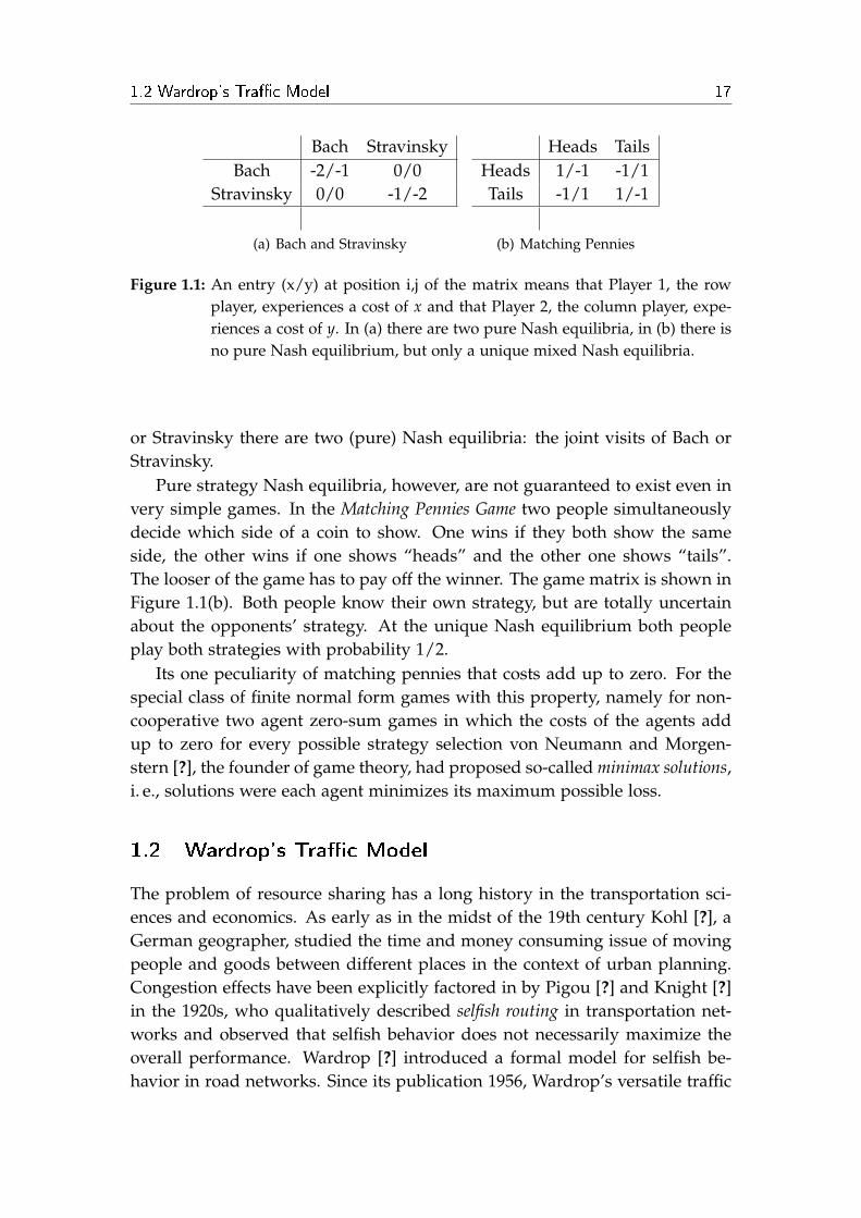
The Bach or Stravinsky game shows, that Nash equilibria do not need to beunique. Two opera lovers want to go to the classical concerto . One prefersa Bach concert, the other one favors Stravinsky. However, they both ratherlike to go to a concert together than on their own. Figure 1.1(a) depicts thecost matrix. (Negative costs can be considered as positive payoffs.) In Bach
1.2 Wardrop's Trac Model 17
Bach StravinskyBach -2/-1 0/0
Stravinsky 0/0 -1/-2
(a) Bach and Stravinsky
Heads TailsHeads 1/-1 -1/1Tails -1/1 1/-1
(b) Matching Pennies
Figure 1.1: An entry (x/y) at position i,j of the matrix means that Player 1, the rowplayer, experiences a cost of x and that Player 2, the column player, expe-riences a cost of y. In (a) there are two pure Nash equilibria, in (b) there isno pure Nash equilibrium, but only a unique mixed Nash equilibria.
or Stravinsky there are two (pure) Nash equilibria: the joint visits of Bach orStravinsky.
Pure strategy Nash equilibria, however, are not guaranteed to exist even invery simple games. In the Matching Pennies Game two people simultaneouslydecide which side of a coin to show. One wins if they both show the sameside, the other wins if one shows “heads” and the other one shows “tails”.The looser of the game has to pay off the winner. The game matrix is shown inFigure 1.1(b). Both people know their own strategy, but are totally uncertainabout the opponents’ strategy. At the unique Nash equilibrium both peopleplay both strategies with probability 1/2.
Its one peculiarity of matching pennies that costs add up to zero. For thespecial class of finite normal form games with this property, namely for non-cooperative two agent zero-sum games in which the costs of the agents addup to zero for every possible strategy selection von Neumann and Morgen-stern [?], the founder of game theory, had proposed so-called minimax solutions,i. e., solutions were each agent minimizes its maximum possible loss.
1.2 Wardrop's Trac Model
The problem of resource sharing has a long history in the transportation sci-ences and economics. As early as in the midst of the 19th century Kohl [?], aGerman geographer, studied the time and money consuming issue of movingpeople and goods between different places in the context of urban planning.Congestion effects have been explicitly factored in by Pigou [?] and Knight [?]in the 1920s, who qualitatively described selfish routing in transportation net-works and observed that selfish behavior does not necessarily maximize theoverall performance. Wardrop [?] introduced a formal model for selfish be-havior in road networks. Since its publication 1956, Wardrop’s versatile traffic

18 Chapter 1. Introduction
model became widely accepted within the transportation sciences. Over thelast decades, Wardrop’s traffic model has been reinvestigated by theoreticalcomputer scientists since it is also well-suited for the analysis of digital trafficin communication networks. Now we will describe Wardrop’s traffic modelformally.
An instance of the Wardrop routing game is given by a tuple (G, d). G =(V, E) denotes a directed multi-graph with latency functions ` = (`e)e∈E
`e : R≥0 → R≥0
attached to the edges. We assume the latency functions to be non-decreasing,differentiable and semi-convex, i. e., that x · `e(x) is convex. We explicitly men-tion if E is equipped with latency function different from `. Furthermore,we are given a set of commodities [k] = 1, . . . , k specified by source-sinkpairs (si, ti) ∈ V × V and flow demands di, where we can assume withoutloss of generality pairwise disjoint sets (si, ti) for i ∈ [k]. The total demand isd = ∑i∈[k] di. We call an instance single-commodity if k = 1 and multi-commodityif k > 1. Considering single-commodity instances, we drop the index i and setd = d1.
Let Pi denote the admissible acyclic paths of commodity i, i. e., all acyclicpaths connecting si and ti, and let P =
⋃i∈[k] Pi. For P ∈ P let fP denote the
volume of agents on path P. A path flow vector ( fP)P∈P induces an edge flowvector ( fe,i)e∈E,i∈[k] with fe,i = ∑P∈Pi :e∈P fP. The total flow on edge e is
fe = ∑i∈[k]
fe,i = ∑i∈[k]
∑P∈Pi :e∈P
fP = ∑P3e
fP .
The latency of an edge e ∈ E is given by `e( fe). The total latency of an edge e isgiven by `e( fe) · fe. Slightly abusing notation, we denote ( fP)P∈P , ( fe,i)e∈E,i∈[k]and ( fe)e∈E by f . A flow f is feasible either if fP ≥ 0 for P ∈ P and it satisfiesthe flow demands
∑P∈Pi
fP = di
for all i ∈ [k], or if it is induced by such a path flow. In this thesis, we onlyconsider the set of feasible flows denoted by F . The latency of a path P ∈ Pis given by the sum of the edge latencies
`P( f ) = ∑e∈P
`e( fe) .
Note that the path latency is not a function of the corresponding path flow,because it depends on the total flow on each of its edges.
Definition 1 (Total latency). The total latency of a flow f is defined as
C( f ) = ∑P∈P
`P( f ) fP . (1.1)

1.2 Wardrop's Trac Model 19
We drop the argument f whenever it is clear from the context.
Since the edge latency depends solely on the edge flow, the total latencycan also be expressed in terms of edge flows only:
C( f ) = ∑P∈P
(∑e∈P
`e( fe)
)fP = ∑
e∈E
(∑
P∈P :e∈PfP
)`e( fe) = ∑
e∈E`e( fe) fe .
1.2.1 Wardrop Equilibria
A natural goal for a central authority is to compute a routing f that minimizesthe total latency over all commodities. This min-cost flow problem can beformulated as the following non-linear program:
minf∈F
C( f ) ,
where the feasible set F can be expressed by a polynomial number of flowconservation and non-negativity constraints. Since the latency functions arecontinuous, F is a compact set and an optimal flow exists. Since `(x) · x isconvex, we can apply the concepts of convex programming and can use, e. g.,the ellipsoid method [?] to compute an optimal flow up to a small error term intime polynomial in the size of the instance and the number of bits of precision.This error term is unavoidable since the description of an optimal solution mayrequire irrational numbers even if the input contains only natural numbers.For solving the classical problem of efficiently computing a minimum costmulti-commodity flow, there are also several specific algorithms known. Foran overview see, e. g., [?] and [?]. Note that polynomial time computabilityrelies crucially on the semi-convexity of the latency function, as for the generalmulti-commodity case no fast algorithms are known.
Taking the game theoretic perspective, we envision the flow as composed ofan infinite number of agents each of which carries an infinitesimal amount offlow. Each agent plays a pure strategy in selecting one path from its origin to itsdestination, where the agent’s cost is the chosen path’s latency. Adjusting thedefinition of Nash equilibria to games with infinitely many agents we requirethat no arbitrarily small fraction of the agents can be shifted from their path toanother without increasing their latency.
Definition 2 (Nash equilibrium). A feasible flow f is at Nash equilibrium if forevery commodity i ∈ [k], all paths fP1, fP2 ∈ Pi with fP1 > 0, and every 0 ≤ ε ≤ fP1
it holds that`P1( f ) ≤ `P2( f ) ,
20 Chapter 1. Introduction
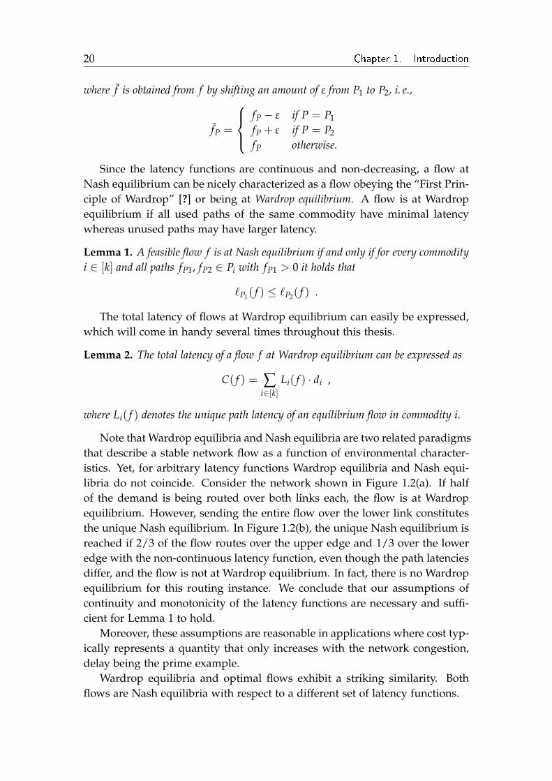
where f is obtained from f by shifting an amount of ε from P1 to P2, i. e.,
fP =
fP − ε if P = P1
fP + ε if P = P2
fP otherwise.
Since the latency functions are continuous and non-decreasing, a flow atNash equilibrium can be nicely characterized as a flow obeying the “First Prin-ciple of Wardrop” [?] or being at Wardrop equilibrium. A flow is at Wardropequilibrium if all used paths of the same commodity have minimal latencywhereas unused paths may have larger latency.
Lemma 1. A feasible flow f is at Nash equilibrium if and only if for every commodityi ∈ [k] and all paths fP1, fP2 ∈ Pi with fP1 > 0 it holds that
`P1( f ) ≤ `P2( f ) .
The total latency of flows at Wardrop equilibrium can easily be expressed,which will come in handy several times throughout this thesis.
Lemma 2. The total latency of a flow f at Wardrop equilibrium can be expressed as
C( f ) = ∑i∈[k]
Li( f ) · di ,
where Li( f ) denotes the unique path latency of an equilibrium flow in commodity i.
Note that Wardrop equilibria and Nash equilibria are two related paradigmsthat describe a stable network flow as a function of environmental character-istics. Yet, for arbitrary latency functions Wardrop equilibria and Nash equi-libria do not coincide. Consider the network shown in Figure 1.2(a). If halfof the demand is being routed over both links each, the flow is at Wardropequilibrium. However, sending the entire flow over the lower link constitutesthe unique Nash equilibrium. In Figure 1.2(b), the unique Nash equilibrium isreached if 2/3 of the flow routes over the upper edge and 1/3 over the loweredge with the non-continuous latency function, even though the path latenciesdiffer, and the flow is not at Wardrop equilibrium. In fact, there is no Wardropequilibrium for this routing instance. We conclude that our assumptions ofcontinuity and monotonicity of the latency functions are necessary and suffi-cient for Lemma 1 to hold.
Moreover, these assumptions are reasonable in applications where cost typ-ically represents a quantity that only increases with the network congestion,delay being the prime example.
Wardrop equilibria and optimal flows exhibit a striking similarity. Bothflows are Nash equilibria with respect to a different set of latency functions.

1.2 Wardrop's Trac Model 21
s t
1− x
1/2
(a)
s t
x
g(x)
(b)
Figure 1.2: A unit demand needs to be routed from s to t. The edges are labeled withtheir latency functions, where g(x) = x for x ≤ 1/3 and g(x) = 1 forx > 1/3. In (a) Wardrop equilibrium and Nash equilibrium differ. In (b)no Wardrop equilibrium exists.
Definition 3 (Marginal cost function). If ` is a differentiable function, then
`∗(x) =d
dx(x · `(x)) = `(x) + `′(x) x
denotes the corresponding marginal cost function.
Note that the marginal cost function of a latency function `e consists of twoterms `e(x) and `′e(x) x. The first captures the per-unit latency incurred byadditional flow whereas the second accounts for the per-unit increased latencyof the flow that is already using the edge.
Theorem 3. [?, ?] Let (G, d) be an instance with latency functions `e for all e ∈E. Then a flow f is optimal with respect to (`e)e∈E if and only if f is at Wardropequilibrium with respect to (`∗e )e∈E.
The idea of the proof of Theorem 3 is the following. For contradiction,assume that a minimal latency flow uses paths with suboptimal marginal costs.Hence, there are paths P1, P2 ∈ P with fP1 > 0 and `∗P1
( f ) > `∗P2( f ). Since the
marginal costs are continuous `∗P1( f − δ) > `∗P2
( f + δ) holds for a sufficientlysmall δ > 0. However, this flow shift changes the total latency by (−`P1( f ) +`P2( f )) · δ < 0.
Theorem 3 establishes not only a deep connection between optimal flowsand Wardrop equilibria but in fact yields an important existence and unique-ness result.
Theorem 4. [?] The set of Wardrop equilibria coincides with the set of solutions ofthe following convex program:
minf∈F ∑
e∈E
∫ fe
0`e(u) du .
22 Chapter 1. Introduction
Thus, every instance (G, d) admits a Wardrop equilibrium and every Wardrop equilib-rium induces the same edge latencies. Further, a Wardrop equilibrium can be computedin polynomial time.
This theorem holds even for latency function that are not semi-convex. Par-ticularly useful is the fact that the objective function Φ( f ) = ∑e∈E
∫ fe0 `e(u) du
serves as a potential function as it precisely absorbs progress: If an infinitesi-mal amount of flow du is shifted from path P1 to P2, thus improving its la-tency by `P1 − `P2 , the potential decreases by (`P1 − `P2)du. We will make useof this fact frequently. The existence of a potential function is sufficient toguarantee the existence of at least one Wardrop equilibrium. Let f be a flowminimizing the potential function Φ. If an infinitesimal amount of flow du isshifted from path P1 to path P2, transforming the flow f to f ′, it follows that`P2 − `P1 = Φ( f ′)− Φ( f ) ≥ 0. Hence, the fraction of deviating agents couldnot benefit from the migration move.
Since Wardrop equilibria are guaranteed to exist in pure strategies, theyconstitute the most appealing solution concept. However, there are routingscenarios that do not satisfy common game theoretic assumptions needed forthe motivation of Wardrop equilibria such as accurate knowledge of the net-work and its latency functions. Further, agents may incur some costs whenthey change their strategy. Thus, it is reasonable to assume that an agent onlyswitches its path for a significant latency gain. This assumption leads to thenotion of a popular, slightly weaker notion of Wardrop equilibria. A (1 + ε)-approximate Wardrop equilibrium is a state in which no arbitrary small fraction ofagents can reduce their latency by more than a multiplicative factor of (1 + ε)by unilaterally migrating to another path. We will comment on several alter-native solution concepts in Section 1.6.8.
1.3 The Price of Anarchy
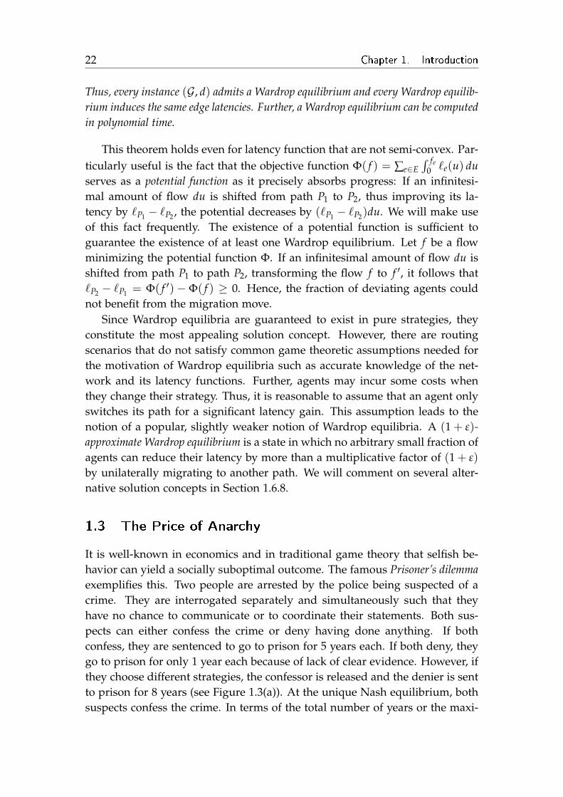
It is well-known in economics and in traditional game theory that selfish be-havior can yield a socially suboptimal outcome. The famous Prisoner’s dilemmaexemplifies this. Two people are arrested by the police being suspected of acrime. They are interrogated separately and simultaneously such that theyhave no chance to communicate or to coordinate their statements. Both sus-pects can either confess the crime or deny having done anything. If bothconfess, they are sentenced to go to prison for 5 years each. If both deny, theygo to prison for only 1 year each because of lack of clear evidence. However, ifthey choose different strategies, the confessor is released and the denier is sentto prison for 8 years (see Figure 1.3(a)). At the unique Nash equilibrium, bothsuspects confess the crime. In terms of the total number of years or the maxi-

1.3 The Price of Anarchy 23
Confess DenyConfess 5/5 8/0
Deny 0/8 1/1s t
x
1
Figure 1.3: (a) Nash equilibria in the Prisoner’s Dilemma can be arbitrarily bad. (b) Aunit demand needs to routed from s to t. The edges are labeled with theirlatency functions `1 and `2. At equilibrium the entire demand utilizes theupper edge. Socially desirable, however, is splitting traffic evenly amongboth paths
mum number of years spent in prison denying the crime is the socially optimal(from the suspects’ point of view) strategy for both suspects. The equilibriumsituation degrades arbitrarily by increasing the sentences in case of confession.
In the context of selfish routing the degradation of performance was al-ready observed by Pigou [?]. Braess [?] noticed that selfish behavior can in factbe worse for all agents. Interestingly, the natural problem of quantifying thisdegradation as not been addressed explicitly before the rise of the Internet. In1999, Koutsoupias and Papadimitriou [?] proposed to investigate the coordina-tion ratio which they defined as the worst case ratio between the social cost atNash equilibrium and the optimal social cost. Later, Papadimitriou [?] dubbedthis measure the price of anarchy.
Note that there are obvious structural similarities to other established con-cepts in theoretical computer science. In particular, the notion of the price ofanarchy is related to the approximation ratio measuring the performance lossdue to lack of computational power of approximation algorithms [?] and tothe competitive ratio measuring the performance loss due to lack of perfectinformation of online algorithms [?]. In the same spirit the price of anarchyquantifies the loss of performance due to lack of a central authority. A smallprice of anarchy indicates that every equilibrium is a good approximation of asocially optimal state.
Over the last ten years, equilibrium efficiency analyses have been con-ducted in a large variety of games, such as job scheduling, facility location andnetwork design (for an extensive overview see [?]). Arguably routing gamesare among the most successfully analyzed applications. In Wardrop routinggames the total latency L( f ) is the most common performance measure.
Definition 4 (Price of anarchy). [?,?] The price of anarchy for an instance (G, d)is defined as
ρ(G, d) =C( f ∗)C( f )
,

24 Chapter 1. Introduction
where f and f ∗ denote an optimal flow and an equilibrium flow, respectively. The priceof anarchy for a set of instances I is
ρ(I) = sup(G,d)∈I
ρ(G, d) .
Note that by Theorem 4 every Wardrop equilibrium incurs the same totallatency and the price of anarchy is well-defined.
Pigou’s example [?] (Figure 1.3(b)) exemplifies that selfish routing does notoptimize social welfare in general. Assume there is one unit of traffic routingitself from s to t. At the unique equilibrium every agent routes via the upperedge which incurs a total latency of 1. Following Theorem 3 the minimum costflow solves `∗1( f1) = `∗2(1− f1), which holds if the flow is split evenly. Whilethe agents on the upper edge experience a latency of 1/2, the agents on thelower edge incur a latency of 1. This minimum cost flow incurs a total latencyof 1/2 · 1/2 + 1/2 · 1 = 3/4. The minimum cost flow is not at equilibrium sincea small fraction of selfish agents currently using the lower edge experiences alatency of 1 and could improve their latency by switching to the upper edge.A switch would deteriorate the total latency since it would slightly increasethe latency of a large fraction of the selfish agents. Thus, the fact the agentsignore the latency increase their decisions imposes on the other agents is thereason why equilibria are inefficient in general. In Pigou’s example, the priceof anarchy is 1
3/4 = 4/3. The inefficiency can be amplified by changing thenon-constant latency function to `1(x) = xp for some large integer p > 0. Theequilibrium flow remains the same, but in the optimal flow almost all agentsare routed over the upper edge and the total latency vanishes for large p. Theprice of anarchy can be computed as roughly p/ log p.
In their ground-breaking work Roughgarden and Tardos [?] analyze theprice of anarchy in Wardrop’s model. In fact, they show that the price of an-archy equals 4/3 for linear latency functions and Θ(p/ log p) for polynomiallatency functions with non-negative coefficients of degree at most p. Later, im-proved bounds on the price of anarchy for special classes of polynomial latencyfunctions were given [?] . Whereas the set of latency functions were identifiedas the crucial parameter for the price of anarchy, the network topology is ir-relevant [?, ?]. In particular, Roughgarden [?] presents a simple procedure forcomputing the price of anarchy by proving that the worst-case ratio is alreadyachieved on parallel links (see also Correa et al. [?]). Observe that in thisregard Pigou’s example depicted in Figure 1.3(b) exhibits the worst possibleprice of anarchy among all networks with polynomial latency functions. Com-plementing the result that the inefficiency of equilibria cannot be bounded ingeneral, Roughgarden and Tardos [?] show that the total latency at Wardropequilibrium is upper bounded by the total latency of an optimal flow rout-
1.4 Braess's Paradox 25
s t
x
1
1
x
(a)
s t
x
1
1
x
0
(b)
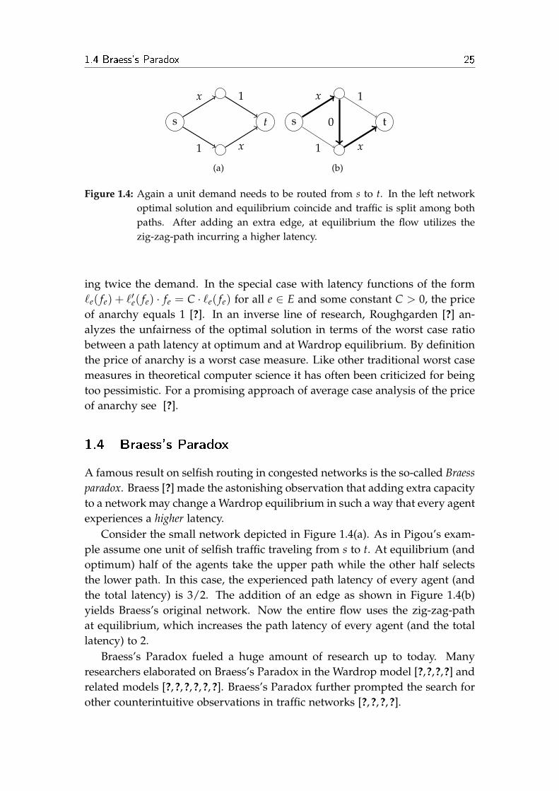
Figure 1.4: Again a unit demand needs to be routed from s to t. In the left networkoptimal solution and equilibrium coincide and traffic is split among bothpaths. After adding an extra edge, at equilibrium the flow utilizes thezig-zag-path incurring a higher latency.
ing twice the demand. In the special case with latency functions of the form`e( fe) + `′e( fe) · fe = C · `e( fe) for all e ∈ E and some constant C > 0, the priceof anarchy equals 1 [?]. In an inverse line of research, Roughgarden [?] an-alyzes the unfairness of the optimal solution in terms of the worst case ratiobetween a path latency at optimum and at Wardrop equilibrium. By definitionthe price of anarchy is a worst case measure. Like other traditional worst casemeasures in theoretical computer science it has often been criticized for beingtoo pessimistic. For a promising approach of average case analysis of the priceof anarchy see [?].
1.4 Braess's Paradox
A famous result on selfish routing in congested networks is the so-called Braessparadox. Braess [?] made the astonishing observation that adding extra capacityto a network may change a Wardrop equilibrium in such a way that every agentexperiences a higher latency.
Consider the small network depicted in Figure 1.4(a). As in Pigou’s exam-ple assume one unit of selfish traffic traveling from s to t. At equilibrium (andoptimum) half of the agents take the upper path while the other half selectsthe lower path. In this case, the experienced path latency of every agent (andthe total latency) is 3/2. The addition of an edge as shown in Figure 1.4(b)yields Braess’s original network. Now the entire flow uses the zig-zag-pathat equilibrium, which increases the path latency of every agent (and the totallatency) to 2.
Braess’s Paradox fueled a huge amount of research up to today. Manyresearchers elaborated on Braess’s Paradox in the Wardrop model [?,?,?,?] andrelated models [?, ?, ?, ?, ?, ?]. Braess’s Paradox further prompted the search forother counterintuitive observations in traffic networks [?, ?, ?, ?].

26 Chapter 1. Introduction
Roughgarden [?] gave results on the severeness of this phenomenon in theWardrop model. In networks with n vertices removing a set of edges maydecrease the total latency by a factor of bn/2c, which gives a tight bound.By removing at most k edges from a given network, the total latency can beimproved by at most a factor of k + 1. Yet, since for networks with linearlatency functions the price of anarchy equals 4/3 [?], Braess’s original fourvertex network exhibits the worst case manifestation of Braess’s paradox forthis class of networks. Even though Braess’s paradox is common in largerandom graphs [?, ?], it is hard to detect [?].
We want to emphasize that Braess’s paradox is far from being merely anacademic curiosity, as it has been observed many times in large road networks.For instance, the (temporal) closure of central roads in highly jammed trafficareas around the globe improved the total traffic flow notably [?, ?, ?]. In ananalytical approach, Youn et al. [?] estimated the price of anarchy with respectto the travel times in road networks of several major cities to be roughly 1.3and identified several roads, whose closure may improve traffic situation.
Remarkably, the occurrence of Braess’s Paradox is not confined to selfishbehavior. Similar effects have been observed in mechanical and electronic sys-tems [?], indicating that also physical equilibrium principles do not alwayspilot the network system to optimal states.
As another line of research stimulated by the paradoxical behavior of self-ish routing, stability and sensitivity analysis of equilibrium traffic character-istics have received a lot of attention. The outstanding result by Dafermosand Nagurney [?,?] states that equilibrium flow patterns depend continuouslyupon the demands and latency functions. In other words, small changes in thetravel demands or in the latency functions induce small changes in the edgeflows, path flows, and path latency at Wardrop equilibrium. In particular, forsingle-commodity networks the path latency at equilibrium is a monotone in-creasing function of the input demand. Further, they identified the structureof networks in which Braess’s paradox occurs.
1.5 Reducing the Price of Anarchy
A large portion of current research is dedicated to quantifying the price ofanarchy in Wardrop’s traffic model. While this work is vital, it is even morevaluable to design methods to reduce the inefficiency of selfish flow in scenar-ios with no central control. To this end, several approaches have been studied.Generally, the goal is to design a protocol that interacts with selfish agents fol-lowing their individual objective and steer their incentives to a socially desir-able outcome. In this section we will summarize known results about methods

1.5 Reducing the Price of Anarchy 27
to reduce the price of anarchy. We focus on introducing taxes [?, ?], designing“good” networks [?] and controlling a subset of the agents centrally [?].
1.5.1 Taxes
In the context of selfish routing most prominent protocols regulate the equilib-rium by the utilization of economic means in form of taxes. The idea of taxingis to charge agents a fee for traversing an edge. In other words, a tax τe ≥ 0on an edge e ∈ E raises the perceived disutility from `e( fe) to `e( fe) + τe.Subsequently, every agent selects a path minimizing its disutility, i. e., its expe-rienced latency plus the sum of the taxes on the chosen path. The effectivenessof such taxes has been observed by Pigou [?] and generalized by Beckmannet al. [?]. Theorem 3 yields the fundamental result that imposing marginal costtaxes τe = `′e( fe) · fe induces the social optimum [?], where f denotes an opti-mal flow. In other words, if each agent on the edge has to pay a tax equal tothe additional cost its presence causes for the other agents on the edge, oneentirely eradicates the inefficiency of selfish behavior. This classic result holdssince the agents are homogeneous with respect to their sensitivity to taxes. Ifwe generalize the model to the heterogeneous case in which every agent tradesoff money and time in an individual manner and minimizes a weighted sumof the edge latencies and the edge taxes, marginal cost taxing does not remainoptimal. Early work on taxes for heterogeneous agents considered unsatisfyingagent-specific taxes on the edges [?, ?, ?]. Later, Cole et al. [?] were the firstto consider the problem from the view of theoretical computer science. Theygive a non-constructive existence proof for taxes stabilizing the optimal flow insingle-commodity networks and upper bound the size of the maximal tax nec-essary. Fleischer [?] reduces the bounded on the required taxes to linear func-tions and gives an algorithm for computing optimal taxes for series-parallelnetworks. In following work, the existence of taxes was proved constructivelyfor multi-commodity networks [?,?,?]. Even more, Fleischer et al. [?] shows theexistence of taxes that induce optimal flows for several alternative objectives,such as minimum average weighted latency and minimum maximum latency.
The underlying assumption of the above mentioned work is that taxes canbe returned to the agents and therefore the network performance is deter-mined entirely by the total latency. However, there may arise situations, inwhich the refunding process could be costly or infeasible. In this case we needto consider non-refundable taxes, that minimize the total disutility (latency plustaxes) of the agents. Under this assumption, marginal cost pricing does notimprove the cost of Wardrop equilibria for linear latency functions [?] . Butalternative tax functions can still be beneficial as the Braess network exempli-fies. In networks with linear latency functions there are optimal taxes that are

28 Chapter 1. Introduction
either 0 or ∞ on each edge [?]. Still, optimal taxes are hard to approximate [?].Whereas for networks equipped with linear latency functions the trivial algo-rithm, i. e., imposing no taxes at all, yields a 4/3-approximation of the socialoptimum [?], it is NP-hard to approximate the social optimum within (4/3− ε)for every ε > 0.
1.5.2 Network Design
Braess’s paradox shows that removing edges from a network may improve equi-librium performance. More precisely, in networks with n vertices removing aset of edges may decrease the total latency by a factor of bn/2c [?]. How-ever, this approach is restricted since it does not even reduce the price ofanarchy on parallel links networks. Roughgarden [?] considered the com-putational complexity of detecting a subnetwork of a given network with nvertices exhibiting the best equilibrium and presented inapproximability re-sults and naive optimal approximation algorithms. In particular, whereas a(n/2 − ε)-approximation algorithm is NP-hard to compute, the trivial algo-rithm, i. e., choosing the entire network as the optimal subnetwork, is a n/2-approximation. Note that by imposing a sufficiently large tax on an edge onecan simulate the removal of that edge. Thus, the network design problem canbe seen as a special case of the taxing problem. As Roughgarden [?] points out,in selfish routing the difference between linear and nonlinear latency functionsis most often only quantitative, as bounds on the price of anarchy show. Yet,there is a qualitative gap in the relative power of taxes to the power of edgeremovals. When moving from linear to non-linear latency functions. While forlinear latency functions edge removal is as powerful as taxing [?], the benefit oftaxes exceeds the benefit through edge removal by O (n) for non-linear latencyfunctions.
1.5.3 Stackelberg Routing
Taxing and network design intend to reduce the price of anarchy by directlymodifying the network topology. Stackelberg routing [?] is an alternative ap-proach to mitigate the negative effects of selfish behavior in congested net-works. The idea of Stackelberg routing is to route a fraction of flow centrallysuch that the latency of all flow is optimized at equilibrium. In Stackelbergrouting, one assumes that an ε-fraction of the demand is controlled by a cen-tral authority, the Stackelberg leader, while the remaining (1− ε)-fraction iscontrolled by non-atomic selfish agents. In a first phase, the Stackelberg leaderfixes the routes for its fraction of the demand. In a second phase, the selfishagents enter the system and route their own flow on top of the leader demand.
1.6 Extensions and Variations 29
The objective of the leader is to minimize the resulting total cost of the total(both leader and selfish) flow, while the selfish agents solely aim to minimizetheir experienced path latency. One important application of Stackelberg rout-ing is the routing of Internet traffic within the domain of an Internet serviceprovider [?]. Here, the Internet service provider centrally controls a fraction ofthe overall traffic traversing its domain.
The problem of the computational complexity of an optimal leader strat-egy is essentially solved. An optimal leader strategy is NP-hard to computeeven for parallel links with linear latency functions [?] but the problem allowsan FPTAS [?]. There are polynomial time algorithms to compute the minimalportion of flow needed by the leader to induce optimum cost [?] and the min-imal value of the Stackelberg leader’s demand that can improve the price ofanarchy [?]. On the algorithmic side, Roughgarden [?] introduces an easy-to-implement Stackelberg strategy that reduces the price of anarchy for arbitrarylatency functions on parallel links to a constant factor of 1/ε. Thus, by con-trolling only a small amount of flow, the performance of equilibria can be dra-matically improved. This does not remain true in arbitrary single-commoditynetworks [?]. On the positive side, Swamy [?] presents latency-class specificbounds on the price of anarchy in arbitrary multi-commodity networks. Theobtained bounds yield a continuous trade-off between the amount of flow con-trolled and the price of anarchy (see also [?]).
1.6 Extensions and Variations
Wardrop’s traffic model was originally introduced in [?] to model selfish be-havior in road networks. Since it is also well-suited for the analyses of uncoor-dinated communication networks like the Internet, the model has attracted theinterest of theoretical computer scientists over the last 10 years. In this section,we review various ramifications and extensions of the model that have beenanalyzed and outline the results that have been obtained therein.
1.6.1 Nonatomic Routing Games
In Wardrop routing games the action of a every agent has essentially no ef-fect on the choices of the other agents. Games that possess this property arereferred to as nonatomic. General nonatomic non-cooperative games have beenintroduced by Schmeidler [?] in the early 1970s. A nonatomic game is definedas a game in which a continuum of agents is equipped with a nonatomic mea-sure. Strategies and cost functions can be defined similarly as for finite normalform games. However, in the case of infinitely many agents we do not need todifferentiate between pure and mixed strategies. Schmeidler [?] gave existence

30 Chapter 1. Introduction
proofs for equilibria, thereby greatly generalizing the results on the existenceof Wardrop equilibria [?] as stated in Theorem 4.
Whereas general nonatomic games are a very general concept, Wardrop’straffic model exhibits a much richer structure. Firstly, the strategy set of theagents is quite restricted as it contains only paths between the respectivesources and sinks. Secondly, and more importantly, the latency of an edgedoes not depend on the identities but only on the measure of agents choosingthis edge. The latter is indeed one of the main characteristics of congestionsensitive networks in general.
1.6.2 Congestion Games
Wardrop’s model assumes an infinite number of agents. In some real-worldapplications, however, there are a finite number of agents competing for sharedresources. To suitably model these situations Rosenthal [?] introduced conges-tion games in 1973. In a congestion game there are given a finite set of resourcesand a finite set of agents of non-negligible size. Each agents’ strategy consistsof a subset of the resources. The cost of a strategy is the sum of the latenciesof the chosen resources, and the cost for choosing a resource depends only onthe number of agents including this resource in their strategy sets. Congestiongames are a discrete version of Wardrop games.
Rosenthal [?] provided a potential function for congestion games provingthe existence of pure Nash equilibria. In fact, the class of congestion gamescoincides with the rich and broad class of potential games [?]. Rosenthal’s po-tential function resembles the potential function given by Beckmann et al. [?]for the Wardrop model, but the potential function yields a non-convex opti-mization problem that allows for multiple pure Nash solutions. Correspond-ingly, congestion games allow for multiple equilibria. Further, in congestiongames a Nash equilibrium can be achieved without incurring the same latencyto all agents, contrary to the “First principle of Wardrop”. On the positiveside, Rosenthal’s work implied that sequential best-response dynamics in con-gestion games converge to a pure Nash equilibrium.
While Wardrop equilibria can be computed efficiently, it is PLS-completeto compute a pure Nash equilibrium [?] in congestion games, i. e., there isno efficient algorithm for computing pure Nash equilibria unless PLS ⊆ P.This also holds for linear cost functions [?]. Skopalik and Vöcking [?] provethat even pure (1 + ε)-approximate Nash equilibria, i. e., states in which noagent can decrease its latency by more than a factor of (1 + ε) by unilaterallychanging its strategy, are PLS-complete to compute. On the other hand, ap-proximate equilibria in congestion games in which the strategy spaces of the
1.6 Extensions and Variations 31
agents coincide (symmetric congestion games) can be computed efficiently undermild smoothness conditions on the latency functions [?].
Most related to Wardrop routing games are network congestion games. Innetwork congestion games the strategy sets of the agents are presented im-plicitly as paths in a network. Fabrikant et al. [?] show that Nash equilibriaare efficiently computable for symmetric network congestion games using areduction to min-cost flow. However (1 + ε)-approximate Nash equilibria arestill PLS-complete to compute in general network congestion games [?]. Feld-mann et al. [?] identify properties that latency functions from natural classeshave to satisfy in order to guarantee that an approximate Nash equilibriumcan be computed in polynomial time.
As in the Wardrop model, in congestion games the degradation with re-spect to the total latency due to selfish behavior is well understood. The priceof anarchy for linear latency functions is 5/2 and pΘ(p) for polynomial latencyfunctions of degree p [?, ?]. Aland et al. [?] give the exact price of anarchyfor polynomial latency functions. Note that the price of anarchy in conges-tion games is much larger than in the Wardrop model. In both cases the setof allowed latency functions the crucial parameter and the price of anarchy isindependent of the network topology.
A wide range of results for special classes of congestion games and a varietyof social cost functions have been studied ( [?,?,?,?,?,?]). For instance, the priceof anarchy for parallel links with linear latency functions with respect to themaximum latency is Θ(log m/ log log m) [?].
As an alternative game-theoretic measure to the price of anarchy, Anshele-vich et al. [?] introduced the price of stability as a worst-case ratio, over allinstances, between the social cost of the best equilibrium (instead of the worst)and optimum social cost. The idea is that if a central authority is enabled toinitially set up a solution that selfish agents are free to adopt subsequently, thebest equilibrium is the prime selection. In other words, the price of stabilitymeasures the inevitable performance degradation due to the selfishness of theagents. First work shows, that for linear latency functions the price of stabilityis approximately 8/5 [?]. For results in related models see [?, ?, ?, ?].
Despite the considerable interest in optimal tax functions for congestiongames [?, ?, ?], it is - unlike in Wardrop’s model- still unknown whether thereexist optimal taxes for atomic congestion games.
1.6.3 Splittable Flow
In a natural generalization of Wardrop’s model, finitely many agents control anon-negligible fraction of the entire demand each. One interpretation of thissetting is that agents of a commodity form coalitions to reduce the expected

32 Chapter 1. Introduction
latency faced by the agents in the coalition, under the assumption that allagents within a coalition are randomly assigned to the different paths used bythe coalition. Motivating scenarios are route guidance systems recommendingoptimal routes to its users or freight companies dictating transportation routesto its truck fleet. Observe that the Wardrop model emerges as a special case inwhich infinitely many agents are allowed, each of them controlling a negligibleamount of flow. Orda et al. [?] introduced this model and showed that Nashequilibria exist under certain conditions. Uniqueness results were obtainedonly for some special cases [?, ?, ?]. In fact, this model allows for multipleequilibria in general [?] even for only two players.
In this model the price of anarchy is not well understood yet. Some finiteupper bounds on the price of anarchy for polynomial latency functions of lowdegrees are known [?, ?], but there is still a large gap between known upperand lower bounds for polynomial latency functions of arbitrary degree [?, ?].The price of anarchy in congestion games with splittable flow can be worsethan in the Wardrop game [?].
In light of the possibility of multiple equilibria [?], the situation with regardto taxing seems worse than in the Wardrop case. Nevertheless, there exists anoptimal tax function for multi-commodity networks even in the presence ofheterogeneous agents, in the sense that the optimal solution is realized as someequilibrium via taxes ( [?], see also [?, ?]). Hay et al. [?] consider collusiongames, a variant of splittable flow games in which agents traveling between asource-sink pair may form arbitrary coalitions and measure the degradationof performance due to this behavior.
1.6.4 General Latency Functions
Wardrop’s model has been extended over the years in various manners. Stick-ing to an infinite number of agents, one straightforward way is to allow moregeneral latency functions. Following this line, agent-specific latency functionsallow to model agents with different preferences. Gairing et al. . [?] concen-trate on existence results of equilibria and give bounds on the price of anar-chy. Agent-specific latency functions have also been considered in congestiongames [?, ?].
Most of the literature on Wardrop’s traffic model deals with the case ofseparable latency functions, i. e., the latency of an edge depends only on theamount of flow on this edge. It is, however, reasonable to assume that theamount of flow on other edges influences the latency of every edge to a certainextent. Non-separable latency functions account for this dependency as they arefunctions of the entire vector of edge latencies. Dafermos and Nagurney [?]prove existence of equilibria for this kind of latency functions (see also [?, ?]).
1.6 Extensions and Variations 33
For results on the price of anarchy for non-separable latency function s ee [?,?, ?].
A more accurate description of traffic flows can be obtained by introducingedge capacities [?, ?, ?, ?]. In this model multiple equilibria are possible and theprice of anarchy becomes unbounded even for linear latency functions. How-ever, the best equilibrium is still as efficient as in absence of edge capacities [?].
1.6.5 Non-Increasing Latency Functions
Throughout this work, we assume the latency functions on the edges to becontinuous and non-decreasing. The remark following Lemma 2 highlightsthat these assumptions are necessary (and in fact sufficient) for flows obeyingthe “First Principle of Wardrop” to be at Nash equilibrium. Further, these as-sumptions seem reasonable in real-world applications, because in congestiondependent networks the latency mostly represents delay. However, applica-tions such as multi-cast routing with multiple duplication of flow motivatethe analysis of selfish routing in the presence of strictly non-increasing latencyfunctions [?]. As it turns out, this model exhibits rather demotivating charac-teristics. Equilibria are not unique, and an optimal flow is not approximableby selfish behavior even for linear latency functions in a small network withonly six vertices.
1.6.6 Maximum Latency, Bottleneck and Elastic Demands
In the vast majority of the literature on the Wardrop model, the network per-formance is measured in total latency. As can be observed in Pigou’s exam-ple in Figure 1.3(b), a flow minimizing total latency may be unfair from theagents’ perspective [?]. In order to attain a system optimal routing, someagents may take costly detours that reduce the congestion encountered by theothers. This unfairness makes such a solution unattractive for the affectedagents. Arguably, the most intuitive way to establish a higher degree of fair-ness is to minimize the maximum latency incurred by a user. The price ofanarchy for the maximum path latency as social cost has been considered byseveral researchers [?,?,?,?]. For single-commodity networks the price of anar-chy is n− 1 [?], contrasting results for the total latency. For multi-commodityinstances the situation is worse as even the removal of a single edge may de-crease the maximum latency by a factor of 2O(n) [?].
An underlying assumption in Wardrop’s traffic model is that the agents’performance is determined by the sum of edge latencies. However, there aremany practical scenarios in which the agents follow bottleneck objectives [?],i. e., performance is determined by the worst component (highest edge la-

34 Chapter 1. Introduction
tency). Note that in Wardrop’s setting the bottleneck latency of a path corre-sponds to the ∞-norm of the vector of edge latencies whereas the total latencyequals the 1-norm. More generally, Cole et al. [?] focus on selfish routingnetworks under the p-norm for 1 < p ≤ ∞ and give several performance guar-antees of equilibria. In particular, for single-commodity the price of anarchyunder the p-norm for 1 < p < ∞ is bounded by the price of anarchy withrespect to the total latency (i. e., under the 1-norm), but for multi-commoditynetworks the price of anarchy under the p-norm for 1 < p ≤ ∞ can be arbi-trarily larger.
In many scenarios, the demand is not fixed a priori but is dependent onthe prevailing network congestion. Models allowing these so-called elasticdemands have been extensively studied in the transportation science litera-ture [?]. Recent work on elastic demands in Wardrop’s model focuses on theefficiency of equilibria [?, ?] and optimal taxes [?].
1.6.7 Non-Selsh Agents
Recent trends in the Internet like open source software development establishthat selfishness may be not as rampant as we might expect. Instead, peoplevoluntarily contribute to public goods projects without direct personal benefit.On the contrary, large uncoordinated systems often have to deal with spitefuladversaries who single-mindedly strive to degrade the network wide perfor-mance, Internet viruses being an infamous example. These examples exhibitcooperative behavior through the evolution of social norms or altruism andforms of spite as subjects aim to destruct systems. Thus, selfishness is not theonly challenge to optimize network performance.
In the Wardrop model altruistic and malicious behavior has been modeledin several ways [?, ?, ?, ?]. Babaioff et al. [?] introduce a model in which acertain fraction of agents act rationally and wish to minimize their individ-ual latency. The remaining fraction of flow consists of malicious agents thatwish to maximize the total latency of the rational agents. The authors studythe existence of equilibria for these games and demonstrate a counterintu-itive phenomenon which they coin “windfall of malice”: malicious agents canimprove the latency experienced by the selfish agents. Chen and Kempe [?] as-sume that agents trade off the benefit of themselves against the benefit of theothers and prove that Wardrop equilibria are guaranteed to exist. They furthershow that the price of anarchy for parallel link networks is merely a constantin the presence of a non-negligible amount of altruists, thereby generalizingthe Stackelberg routing result of Roughgarden [?].

1.7 Outline 35
The existence and computational complexity of equilibria in presence ofaltruistic or malicious agents has also been considered for discrete congestiongames [?, ?].
1.6.8 Alternative Solution Concepts
Wardrop equilibria are the most prevalent solution concept in non-atomic self-ish routing. But yet, some scenarios may require more general solution con-cepts.
For instance, agents often face the problem of uncertain latency estimates.The uncertainty may be caused by random effects, such as accidents, weather,or varying traffic conditions in road traffic as well as noise or signal degra-dation in the context of telecommunication networks [?]. Motivated by thisproblem, Ordonez and Stier-Moses [?] introduced robust Wardrop equilibria thataccount for the agents’ imperfect information. Robust Wardrop equilibria areappealing as they always exist and can be computed in polynomial time.
In a related approach, Fisk [?] generalizes Wardrop’s traffic model in thathe formalizes a network optimization problem whose solution is a probabilisticequilibrium that contains the original Wardrop equilibrium in a special case.
In congestion games several alternative solution concepts have been stud-ied. Closely related to robust Wardrop equilibria, the concept of Bayesian equi-libria has been applied to congestion games, in which agents possess onlyimperfect information about the game [?]. Correlated equilibria rely on a trustedauthority telling the agents how to play to minimize their cost. Correlatedequilibria can be computed efficiently [?] and exhibit a small price of anar-chy [?]. Strong equilibria [?] are strategy profiles in which no coalition of agentsmay improve the latency of each of its members by deviating from the currentstrategies. Their existence and their efficiency have also been studied [?]. Fi-nally, sink equilibria constitute an attractive solution concept, since they existeven in weighted congestion games. The price of sinking has been analyzedby Goemans et al. [?].
1.7 Outline
In this thesis we study a variety of algorithmic problems in Wardrop’s modelthat revolve around the price of anarchy and Braess’s paradox. In the first partwe study a general taxing problem and propose a novel approach to reducethe influence of selfish routing. Secondly, we analyze the stability of Wardropequilibria with respect to network parameter changes. Lastly, we provide adistributed approximation algorithm for Wardrop equilibria.
36 Chapter 1. Introduction
As a prerequisite for our results, we need to specify how to encode an in-stance (G, d). The network G can be represented using adjacency matrices oradjacency lists, and the demand vector d consisting of k rational entries can beencoded in a canonical way using binary representation. A natural represen-tation of polynomial latency functions is the coefficient representation whichlists the coefficients of all monomials. All our positive results that require theset of latency functions as input only hold for networks with linear or polyno-mial latency functions. The impossibility results hold even for linear latencyfunctions. Hence, it is sufficient to have efficient encodings for these sets oflatency functions.
Reducing the price of anarchy via taxes The most popular approachto reduce the inefficiency of Wardrop equilibria utilizes edge taxes. Marginalcost taxes are known to reduce the price of anarchy to 1 [?]. Since imposingtaxes on every network edge may be impossible or costly, we consider themore general problem of minimizing the network wide performance by settingtaxes for a given subset of edges only. While we prove that the problem is NP-complete in general networks, we provide a polynomial time algorithm solvingthis problem for single-commodity parallel link networks with linear latencyfunctions.
The results are presented in Chapter 2. In preliminary form these resultsalready appeared at the following conference:
• [?] Martin Hoefer, Lars Olbrich, and Alexander Skopalik. Taxing Sub-networks. In Proc. of the 4th Workshop Workshop on Internet and NetworkEconomics (WINE), pages 286-294, 2008.
Reducing the price of anarchy via auxiliary flow Taxing, Stackelbergrouting, and network design are the most prominent means to reduce the in-efficiency of selfish flow in scenarios without central control. Nevertheless,all of these approaches either require costly infrastructure or the possibilityof manipulating the network structure or the agents. We propose a novel ap-proach to reduce the price of anarchy that circumvents all of these problematicissues. We observe that routing an additional amount of flow, which we coinauxiliary flow, can actually improve the equilibrium situation for the selfishflow. We prove that the optimal auxiliary flow is NP-hard to approximate toless than a factor of 4/3 and the minimal amount of an optimal auxiliary flow isNP-hard to approximate within any subexponential factor. These results arecomplemented by proving that the worst adversarial flow, i. e., flow that aims tomaximize the total latency, is also NP-hard to compute. In fact, in all cases weobtain strong NP-hardness.
The results are presented in Chapter 3. In preliminary form these resultsalready appeared at the following conference:

1.7 Outline 37
• [?] Martin Hoefer, Lars Olbrich, and Alexander Skopalik. Doing Goodwith Spam is Hard. In Proc. of the 2nd Symposium on Algorithmic GameTheory (SAGT), pages 263-274, 2009.
Sensitivity of Wardrop Equilibria Braess’s paradox displays intriguingaspects of selfish behavior. In fact, it triggered the stability and sensitivityanalysis of Wardrop equilibria. While most existing literature concentrates onqualitative questions [?,?,?], we upper and lower bound the change of the mainflow parameters at the induced equilibrium due to an ε-change. An ε-change isdefined as a demand increase by a factor of (1 + ε) or the removal of an edgecarrying only an ε-fraction of flow. For single-commodity networks, we showhow an ε-change may force every agent to change its path in order to recoverequilibrium. Our proof employs a family of networks generalizing Braess’original graph. On the other hand, an ε-change in the demand increases thepath latency and the price of anarchy at most by a factor of (1 + ε)p for poly-nomial latency functions of degree at most p with nonnegative coefficients. Incontrast, the relative increase in the latency of an edge can be unbounded. Formulti-commodity networks neither the change in edge flows nor the increasein the path latency can be bounded.
The results are presented in Chapter 4. In preliminary form these resultsalready appeared at the following conference:
• [?] Matthias Englert, Thomas Franke, and Lars Olbrich. Sensitivity ofWardrop Equilibria. In Proc. of the 1st Symposium on Algorithmic GameTheory (SAGT), pages 158–169, 2008.
They also appeared as invited contribution to a special issue of Theory of Com-puting Systems with selected papers from SAGT 2008:
• [?] Matthias Englert, Thomas Franke, and Lars Olbrich. Sensitivity ofWardrop Equilibria. In Theory of Computing Systems, pages 263-274, 2009.
Distributed Approximation of Wardrop Equilibria The notion of War-drop equilibrium requires complete knowledge about the latency dependenceof the edges as well as unbounded reasoning capabilities of the agents. Further,most research on selfish routing focuses on the agents’ behavior at equilibriumand exclude the question how the set of agents may attain such a stable state.We study how approximate Wardrop equilibria can be computed efficientlyunder rather weak assumptions on the agents’ information about the game.Previous work [?] shows that the set of agents can approach Wardrop equilib-ria quickly by following a simple round-based rerouting policy. Following theso-called replication policy, in each round every agent concurrently samples an-other agent uniformly at random. If the sampled agent’s path latency is lower

38 Chapter 1. Introduction
than its current path latency, the agent switches to the other agent’s path witha probability increasing with the offered improvement. The policy avoids theproblem of oscillation due to its carefully chosen switching probability. Astate, in which only a small fraction of the agents sustains latency significantlyabove average is reached in a number of rounds that mainly depends on theapproximation parameters and the elasticity of the latency functions.
We consider a setting, in which the flow is controlled by a finite number ofagents only, each of which is responsible for the entire flow of one commodity.Each agent has a set of admissible paths among which it may distribute itsflow. Each agent aims to balance its own flow such that the jointly computedallocation will be at Wardrop equilibrium
Since the replication policy is designed for an infinite set of agents andpotentially exponentially many paths it does not directly yield a feasible dis-tributed algorithm. However, applying a randomized sampling technique weturn the replication policy into a distributed algorithm executable by finitelymany agents. The distributed algorithm achieves essentially the same con-vergence rates as in the setting with an infinite number of agents. Thus, anapproximate Wardrop equilibrium is reached in a number of rounds that isindependent of the size and the topology of the network and can be computedin expected polynomial time.
The results are presented in Chapter 5. In preliminary form these resultsalready appeared at the following conference:
• [?] Simon Fischer, Lars Olbrich, and Berthold Vöcking. Approximat-ing Wardrop Equilibria with Finitely Many Agents In Proc. of the 21stInternational Symposium on Distributed Computing (DISC), pages 238–252,2007.
They also appeared as invited contribution to a special issue of DistributedComputing with selected papers from DISC 2007:
• [?] Simon Fischer, Lars Olbrich, and Berthold Vöcking. ApproximatingWardrop Equilibria with Finitely Many Agents In Distributed Computing,21(2) pages 129–139, 2008.

Chapter 2
Taxing Subnetworks
We have already seen in the introduction of this dissertation that the set of War-drop equilibria embodies the set of stable states in Wardrop’s game theoretictraffic model. Such equilibria are solutions of related convex programs and canthus be found in polynomial time. In general a Wardrop equilibrium is not so-cially optimal, i. e., it does not minimize the total latency. The inefficiency ofselfish flows has been extensively studied in previous work [?, ?, ?, ?, ?, ?]. Infact, Roughgarden and Tardos [?] proved that even in parallel link networksthe price of anarchy may well be unbounded.
There are several approaches that have been proposed to address the in-efficiency of equilibria, most notably via taxing network edges. Agents areassumed to minimize the sum of their latencies and taxes. A fundamentalresult is that using marginal cost pricing to set a tax on every edge results inequilibrium flows that are optimal with respect to total latency [?]. Therein,the tax an agent has to pay on an edge equals the additional delay its presencecauses for other agents on this edge.
Marginal cost pricing is widely accepted as a benchmark solution. How-ever, the necessary underlying assumptions for marginal cost pricing will mostoften be an obstacle in real world applications. In this regard, a serious draw-back is that marginal cost pricing requires every edge of the network to betaxable. In many networks there might be technical or legal restrictions thatprevent an operator from imposing a tax on all edges. Even assuming di-rect access to the edges, the monitoring costs for many edges and the processof collecting taxes may be considered prohibitive. On many edges it furthermay generate only negligible benefits to social welfare. Therefore, we considerthe more realistic problem of computing taxes for a subset of taxable edges thatminimize the total latency of the resulting equilibrium. Nevertheless, we donot impose further restrictions on the taxes itself besides non-negativity andcomputability. This problem is certainly relevant in the context of road traffic,as an increasing number of urban areas are installing electronic road charg-
40 Chapter 2. Taxing Subnetworks
ing [?]. For example the optimal taxes for a toll-ring around a city center canbe the problem under consideration. This exemplifies that even if there are noimposed restrictions, a central authority may have a self interest in restrictingthe number or structure of taxed roads. In related work, Yang and Lam [?]give heuristics for the same problem in a queuing network, while Verhoef [?]presents analytically tractable solutions for small networks.
2.1 Our Results
Taxing subnetworks can be difficult and non-trivial. Consider the parallel linknetwork of two links and linear latency functions shown in Figure 2.1(a). Ifone can tax only one edge, the total latency is generally not monotone inthe imposed tax. Using this insight, we carefully construct networks withone taxable edge and several distinct optimal taxes. A combination of thesenetworks establishes NP-hardness of the problem for two commodities andlinear latency functions (Section 2.3). On the other hand, for parallel linknetworks with linear latency functions, we derive a precise structural analysisof optimally taxed equilibrium flows in Section 2.4. This allows to constructa polynomial time algorithm to find optimal taxes. The main ingredients areinsights on the set of links carrying flow, dependencies between total latencyand demand, and linearity of latency functions. Unlike a large part of relatedwork, we do not need to resort on convex programming.
2.2 Preliminaries
We have already formally introduced Wardrop’s model [?] in this thesis. Con-sidering the problem of taxing a subset of network edges, we slightly extendthe model and reformulate some classic results, which we will rely on through-out this chapter.
We are given a directed graph G = (V, E) with vertex set V and edge setE. Considering only parallel edges, we speak of parallel link networks anddenote the set of links by [n] = 1, . . . , n. We allow a set of non-negativetaxes τ = τee∈T to be imposed on a subset of edges T ⊂ E. We call edges inT taxable and edges in N = E \ T non-taxable. For simplicity, we set τe = 0 fore ∈ N. The disutility of an agent choosing a path P is defined as latency plustax, i. e., `P( f ) + ∑e∈P τe. Finally, we call the quadruple (V, T, N, d) an instance.
Bearing the definition of an agents’ disutility in mind, at Wardrop equilib-rium no fraction of the flow can improve its sustained latency plus taxes bymoving unilaterally to another path.

2.3 NP-Hardness for Multi-Commodity Networks 41
Definition 5 (Wardrop equilibrium with taxes). A flow vector f is at Wardropequilibrium if for every commodity i ∈ [k] and paths P1, P2 ∈ Pi with fP1 > 0 itholds that `P1( f ) + ∑e∈P1
τe ≤ `P2( f ) + ∑e∈P2τe.
Remember that without taxes at Wardrop equilibrium all used paths incommodity i have equal latency Li( f ) and the total latency can be expressedas ∑i∈[k] Li( f ) · di ( [?, ?], 2). In the presence of taxes, however, all agents incommodity i experience a unique disutility. A classical result on taxing selfishflow, called marginal cost pricing, is that with taxes τe = xe · `′e(xe) for all e ∈ Ethe resulting equilibrium flow minimizes the total latency. With `∗e (x) = (x ·`e(x))′ = `e(x) + x · `′e(x) denoting the marginal cost of increasing flow onedge e, Theorem 3 yields the following lemma.
Lemma 5. For an instance (V, E, ∅, d) a flow f minimizes the total latency withrespect to (`e)e∈E if and only if it is at Wardrop equilibrium with respect to (`∗e )e∈E.
In the restricted case with only a subset of edges being taxable such a resultis obviously out of reach as Pigou’s example (cf. Figure 2.1(a)) exemplifies. Ifonly the constant latency edge is taxable, no improvement is possible. Thisdirectly leads us to the following definition.
Definition 6 (Optimal taxes). Given an instance (V, T, N, d), a set of taxes τee∈T
is called optimal if there is an equilibrium flow fτ with respect to ` + τ with
C( fτ) ≤ C( fτ′)
for all equilibrium flows fτ′ with respect to ` + τ′ for any τ′ee∈T.
2.3 NP-Hardness for Multi-Commodity Networks
In this section we study the computational complexity of Subnetwork-Tax.In the decision problem Subnetwork-Tax we are given a multi-commodityselfish routing instance (V, T, N, d) and a threshold value C. The problem is todecide if there are taxes for the edges e ∈ T such that the induced equilibriumincurs total latency of at most C. Subnetwork-Tax turns out to be NP-hardeven for the two-commodity case with linear latency functions. We start withan observation that will allow us to discretize the problem.
Lemma 6. There is a family of instances (V, T, NA, dA)A∈N with parallel link net-works allowing for two distinct optimal tax values.
Proof. Consider the network shown in Figure 2.1(b). Two nodes s and t areconnected via three links, with latency functions `1(x) = x + A and `2(x) =`3(x) = x. Suppose we can only tax the third link.
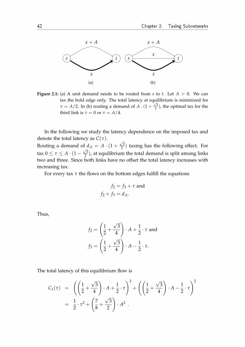
42 Chapter 2. Taxing Subnetworks
s t
x + A
x
(a)
s t
x + A
x
x
(b)
Figure 2.1: (a) A unit demand needs to be routed from s to t. Let A > 0. We cantax the bold edge only. The total latency at equilibrium is minimized forτ = A/2. In (b) routing a demand of A · (1 +
√3
2 ), the optimal tax for thethird link is τ = 0 or τ = A/4.
In the following we study the latency dependence on the imposed tax anddenote the total latency as C(τ).Routing a demand of dA = A · (1 +
√3
2 ) taxing has the following effect. For
tax 0 ≤ τ ≤ A · (1−√
32 ), at equilibrium the total demand is split among links
two and three. Since both links have no offset the total latency increases withincreasing tax.
For every tax τ the flows on the bottom edges fulfill the equations
f2 = f3 + τ and
f2 + f3 = dA.
Thus,
f2 =
(12
+√
34
)· A +
12· τ and
f3 =
(12
+√
34
)· A− 1
2· τ.
The total latency of this equilibrium flow is
C1(τ) =
((12
+√
34
)· A +
12· τ)2
+
((12
+√
34
)· A− 1
2· τ)2
=12· τ2 +
(78
+√
32
)· A2 .

2.3 NP-Hardness for Multi-Commodity Networks 43
C1(τ) is minimized for τ = 0.For A · (1−
√3
2 ) < τ < A · (1 +√
34 ) all links are used and the total latency is
not monotone as a function of the imposed tax. The corresponding flows andthe incurred latency can be calculated is a similar fashion as above. The linkflows satisfy
f1 + A = f2,
f2 = f3 + τ and
f1 + f2 + f3 = dA.
Thus,
f1 =13
(A ·(√
32− 1
)+ τ
),
f2 =13
(A ·(√
32
+ 2
)+ τ
)and
f3 =13
(A ·(√
32
+ 2
)− 2 · τ
).
induce a total latency of
C2(τ) =23· τ2 − 1
3· A · τ +
(1112
+√
32
)· A2
that is minimized for a tax of A/4.For τ ≥ A · (1 +
√3
4 ) the total latency at equilibrium is C2(A · (1 +√
34 )).
Hence, the total latency C is
C(τ) =
C1(τ) for 0 ≤ τ ≤ A · (1−
√3
2 )C2(τ) for A · (1−
√3
2 ) < τ ≤ A · (1 +√
34 )
C2(A · (1 +√
34 )) for τ > A · (1 +
√3
4 ) .
Since C(0) = C(A/4) the instance admits two optimal taxes 0 and A/4.
Having discretized the problem we are now able to prove the main resultof this section.
Theorem 7. Subnetwork-Tax is NP-hard, even for instances with only two com-modities and linear latency functions.
Proof. We reduce from the Partition problem: given k positive integers ai,is there a subset S ⊆ [k] satisfying ∑i∈S ai = 1
2 ∑ki=1 ai? We will show that
deciding the Partition problem reduces to deciding if a given 2-commodity

44 Chapter 2. Taxing Subnetworks
s1 v2 v3 vk t1
s2t2
x x x
x x x
D1 x + E1 D2 x + E2 D3 x + E3
x + ∑i ai
x x x
x
Figure 2.2: The network of an instance (Vai, Tai, Nai, (dai)). The edges are la-beled with the latency functions. Unlabeled edges have latency 0. Taxescan be imposed on the set of bold edges only.
instance (V, T, N, (di)) with latency functions admits taxes inducing a Wardropequilibrium with a given total latency.
Given an instance of Partition specified by non-negative integers a1, a2, . . . , akwe define an instance (Vai, Tai, Nai, (dai)) as depicted in Figure 2.2. Letthe set of taxable edges T consist of the bold edges.
Commodity one has a demand of A = ∏ki=1 ai to route between s1 = v1
and t1 = vk+1, the second commodity has to route a demand of ∑i ai betweens2 and t2. For i ∈ [k] define the following constants:
A−i =k
∏j 6=i
aj ,
Di =2− 4A−i + A2
−i4A−i − 2
and
Ei = 2ai(Di + 1) =AA−i
2A−i − 1.
Note that all values can be encoded by a number of bits that is polynomial inthe size of the instance of Partition.
We show that a1, . . . , ak is a Yes instance if and only if there are taxes forthe instance (Vai, Tai, Nai, (dai)) inducing a Wardrop equilibrium withtotal latency of at most C = k
2 A2 + 78(∑i ai)2. Since both commodities do not
share any latency incurring edge, the constructed network allows for a sepa-rated consideration of both commodities. The idea is that the minimal latencyis reached if and only if the tax between vi and vi+1 is 0 or ai and the sum ofall taxes is exactly ∑i ai/2.
First, consider the set of vertex disjoint paths between vi and vi+1 for somei ∈ [k]. A demand of A needs to be routed between those two nodes. The

2.4 Parallel Links with Linear Latency Functions 45
situation resembles the situation described in the proof of Lemma 6. The totallatency is
Ci(τ) =
A2
2 + τ2
2 for 0 ≤ τ ≤ 2Ei − A(Di+1)τ2−Eiτ+A(Di A+Ei)
2Di+1 for 2Ei − A < τ < Di A+EiDi+1
Ci(Di A+Ei
Di+1 ) for τ ≥ Di A+EiDi+1 .
One can easily check that for A−i > 1 there are two non-empty intervals for taxτ, in which the total latency as a function of the imposed tax τ is quadratic.The constants Di and Ei are chosen in such a way that the total latency isminimized for 0 and Ei
2·Di+2 = ai. Thus, both taxes 0 and ai are optimal for theset of parallel paths connecting vi with vi+1. The incurred total latency for theoptimal taxes is A2/2.
For the second commodity consider the sum g = ∑i τi of all taxes in thenetwork. At equilibrium a flow volume of ∑i ai − g
2 is routed via the pathincluding the taxable edges, and a flow of volume g
2 is routed via the loweredge. The total latency of C(g) = (∑i ai− g
2 )2 + g2 ( g
2 + ∑i ai) is then minimizedfor g = ∑i ai/2.
First, assume a1, . . . , ak is a Yes instance. We reach optimality for bothcommodities by choosing
τi =
ai for i ∈ S0 for i /∈ S .
The total latency sums up to
C = ∑i∈S
Ci(ai) + ∑i∈[k]\S
Ci(0) + C
(∑
iai/2
)
=k2
A2 +78
(∑
iai
)2
.
Now suppose a1, . . . , ak is a No instance. To obtain a total latency of k2 A2 for
commodity one, the tax on the taxable edge between vi and vi+1 needs to be 0or ai for every i. For the second commodity a total latency of 7
8(∑i ai)2 can beobtained only if the sum of the taxes adds up to ∑i ai/2. Obviously, in a No
instance both conditions can not be achieved at the same time. Thus, the totallatency is above the threshold composed of the two optima and the reductionis complete.
2.4 Parallel Links with Linear Latency Functions
The parallel link instances in the proof of Lemma 6 show that the total latencyis generally not monotone as a function of the imposed taxes. That holds even
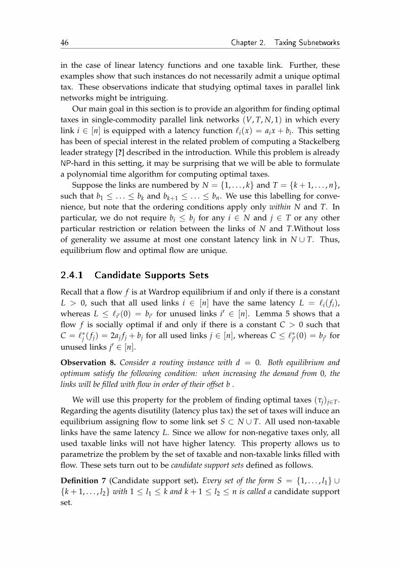
46 Chapter 2. Taxing Subnetworks
in the case of linear latency functions and one taxable link. Further, theseexamples show that such instances do not necessarily admit a unique optimaltax. These observations indicate that studying optimal taxes in parallel linknetworks might be intriguing.
Our main goal in this section is to provide an algorithm for finding optimaltaxes in single-commodity parallel link networks (V, T, N, 1) in which everylink i ∈ [n] is equipped with a latency function `i(x) = aix + bi. This settinghas been of special interest in the related problem of computing a Stackelbergleader strategy [?] described in the introduction. While this problem is alreadyNP-hard in this setting, it may be surprising that we will be able to formulatea polynomial time algorithm for computing optimal taxes.
Suppose the links are numbered by N = 1, . . . , k and T = k + 1, . . . , n,such that b1 ≤ . . . ≤ bk and bk+1 ≤ . . . ≤ bn. We use this labelling for conve-nience, but note that the ordering conditions apply only within N and T. Inparticular, we do not require bi ≤ bj for any i ∈ N and j ∈ T or any otherparticular restriction or relation between the links of N and T.Without lossof generality we assume at most one constant latency link in N ∪ T. Thus,equilibrium flow and optimal flow are unique.
2.4.1 Candidate Supports Sets
Recall that a flow f is at Wardrop equilibrium if and only if there is a constantL > 0, such that all used links i ∈ [n] have the same latency L = `i( fi),whereas L ≤ `i′(0) = bi′ for unused links i′ ∈ [n]. Lemma 5 shows that aflow f is socially optimal if and only if there is a constant C > 0 such thatC = `∗j ( f j) = 2aj f j + bj for all used links j ∈ [n], whereas C ≤ `∗j′(0) = bj′ forunused links j′ ∈ [n].
Observation 8. Consider a routing instance with d = 0. Both equilibrium andoptimum satisfy the following condition: when increasing the demand from 0, thelinks will be filled with flow in order of their offset b .
We will use this property for the problem of finding optimal taxes (τj)j∈T.Regarding the agents disutility (latency plus tax) the set of taxes will induce anequilibrium assigning flow to some link set S ⊂ N ∪ T. All used non-taxablelinks have the same latency L. Since we allow for non-negative taxes only, allused taxable links will not have higher latency. This property allows us toparametrize the problem by the set of taxable and non-taxable links filled withflow. These sets turn out to be candidate support sets defined as follows.
Definition 7 (Candidate support set). Every set of the form S = 1, . . . , l1 ∪k + 1, . . . , l2 with 1 ≤ l1 ≤ k and k + 1 ≤ l2 ≤ n is called a candidate supportset.

2.4 Parallel Links with Linear Latency Functions 47
Note that there are at most n2/4 candidate support sets for any instance.
Lemma 9. Let f denote a socially optimal flow for a parallel link network where everyedge is taxable. Then
`1( f1) ≤ `2( f2) ≤ . . . ≤ `n( fn) .
Proof. The set of used links is of the form 1, . . . , l for some l ≤ n. Sincef is a minimal latency flow, all links j ∈ 1, . . . , l have equal marginal cost,and there is a constant C > 0 with 2aj f j + bj = C. Thus, `j( f j) = aj f j + bj =C/2 + bj/2.
Let us first argue that the consideration of candidate support sets is indeedsufficient to find optimal taxes. Imagine two separate commodities, routingfixed demands dN and 1 − dN exclusively over N and T, resp. In such ascenario, it would be optimal to set marginal cost taxes on T. According toObservation 8 the set of used links form a candidate support set.
The difference to our setting is that demand can change between N and T,and thus we also need to ensure that latency and taxes create an equilibriumflow. In particular, latency plus tax of any used link in T must be equal to thecommon latency L of all used links in N. Furthermore, the offset plus tax ofany unused link in T must be higher than L.
If the optimal flow of all links in T yields latencies only smaller than L,then we can satisfy the latency constraint by setting appropriate non-negativetaxes. Otherwise, the latency restriction reduces the flow on some used links.Naturally, this can happen to all links j ∈ T with bj ≤ L. However, if theflow on a link is smaller than in the optimum due to the latency constraint,the marginal cost on this link is also smaller. Therefore, it is still optimal tofill the link with flow to the maximal possible extent, which we will provein Lemma 10. For all links not affected by the latency restriction, however, itis optimal to equalize the marginal costs, and the allocation of flow followsthe ordering of offsets. In conclusion, it can be observed that the set of linksallocated with flow remains a candidate support set. Thus, it is sufficient torestrict our attention to these sets.
2.4.2 Problem Parametrization
Fixing numbers nS and tS yields a candidate support set S = NS ∪ TS withNS = 1, . . . , nS and TS = k + 1, . . . , tS. For S denote by dNS and 1− dNS thedemand routed over NS and TS, respectively. CNS(dNS) is the total latency foran equilibrium flow ( fi)i∈NS of demand dNS . Denote by CTS(1− dNS) the totallatency for an optimal flow ( f j)j∈TS of demand 1− dNS additionally fulfilling

48 Chapter 2. Taxing Subnetworks
the latency constraint `j( f j) ≤ L(dNS) for all links j ∈ TS, where L(dNS) denotesthe unique latency of all used links in NS for a demand of dNS . Finally, let
C(dNS) = CNS(dNS) + CTS(1− dNS)
denote the total latency of the entire flow.We can further parametrize the problem of finding a set of optimal taxes
for a fixed set S by the demands routed over NS and TS. We formulate it in acompact way:
minimize C(dNS)
s.t. ( fi)i∈NS equilibrium for demand dNS
s.t. ( f j)j∈TS optimal for demand (1− dNS)
s.t. s.t. `j( f j) ≤ L(dNS) ∀j ∈ TS
s.t. 0 ≤ dNS ≤ 1 .
Note that we require the equilibrium and the optimum to hold for N and T(and not only for NS and TS). We will show that if this minimization problemhas a solution, the total latency C(dNS) is piecewise quadratic with at most nbreakpoints and the optimal demand distribution (d∗NS
, 1− d∗NS) for NS and TS
for a candidate support set S is efficiently computable. Iterating this for allpossible sets S enables us to find optimal taxes.
Definition 8 (Full and relaxed links). We call a link j ∈ T full with respect to someL > 0 if f j > 0 and its latency equals the constraint value, i. e., if `j( f j) = L or iff j = 0 and `j(0) = bj ≥ L. We call a link relaxed if f j > 0 and `j( f j) < L.
When shifting demand from N to T, the common latency L of used links inN decreases, while the demand on T increases. In the corresponding optimalflow on T respecting the constraint value, however, a full link never becomesrelaxed.
More formally, consider an instance (V, T, ∅, d) and let f denote the opti-mal flow respecting `i( fi) ≤ L for all i. With Lemma 9 we can assume the fulllinks to form a set p, . . . , n for some p ≥ 1. Furthermore, assume there areL′ ≤ L and d′ ≥ d such that there is a flow of demand d′ to T such that all usedlinks have latency at most L′. For all non-constant links, we define `−1
i (L) tobe the flow fi such that ai fi + bi = L if bi ≤ L, and 0 otherwise.
Lemma 10. The optimal flow f ′ respecting `i( f ′i ) ≤ L′ for all i assigns `−1i (L′) flow
to all non-constant links i ∈ p1, . . . , n for some uniquely defined p1 ≤ p.
Proof. Restricting the latencies to at most L′ removes flow from links p, . . . , nand distributes it among the remaining links. Therefore, more links mightbecome full with respect to L′. Let the newly affected links be p1, . . . , p − 1.

2.4 Parallel Links with Linear Latency Functions 49
Let f ′ denote the flow of volume d′ that assigns `−1j (L′) of flow to every non-
constant link j ∈ p1, . . . , n and that is optimal on links 1, . . . , p1 − 1. Thus,for all i ∈ 1, . . . , p1 − 1 and for all j ∈ p1, . . . , n
`∗j ( f ′j ) ≤ `∗i ( f ′i ) . (2.1)
For contradiction, assume that respecting L′ there is an optimal flow f with
f j0 < f ′j0 for some j0 ∈ p1, . . . , n . (2.2)
The latency `j0 is not constant since either j0 is full and, thus, f ′j0 = 0 or j0is relaxed and therefore it is not optimal to reduce the flow on j0. Since f isassumed to be optimal, for all links i ∈ 1, . . . , p1 − 1
`∗j0( f j0) ≥ `∗i ( fi) . (2.3)
Further, since p1, . . . , n loses flow there is a link i0 ∈ 1, . . . , p1 − 1 thatgains some flow, i. e.,
fi0 > f ′i0and therefore (even if `i0 is constant)
`∗i0( fi0) ≥ `∗i0( f ′i0) . (2.4)
Altogether,
`∗j0( f ′j0) >(2.2) `∗j0( f j0) ≥(2.3) `∗i0( fi0) ≥
(2.4) `∗i0( f ′i0) ≥(2.1) `∗j0( f ′j0) ,
which yields a contradiction.
2.4.3 A Polynomial-Time Algorithm for Computing Optimal
Taxes
Considering an optimal flow for an increasing demand, the links become usedin order of their offsets. Note that Lemma 9 and Lemma 10 show that thelinks become full with respect to some bound in reverse order. The fact thatwe know the order in which the links become both used and full and the lin-earity of the latency functions enable us to determine the lower and the upperbound dmin
NSand dmax
NSfor dNS such that the following holds. The equilibrium
flow of demand dNS on N exactly uses the set of links NS and there is a flowof demand 1− dNS on T respecting the bound L(dNS) exactly using the set oflinks TS, whose total latency can not be improved by using links in T \ TS.Given a candidate support set S we need to compute the optimal demanddistribution (dNS , 1 − dNS). If a distribution exists that fulfills the above re-quirements we call S feasible. We call the corresponding demand intervals[dmin
NS, dmax
NS] feasible demand intervals.

50 Chapter 2. Taxing Subnetworks
Lemma 11. The feasible demand intervals can be computed in polynomial time.
Proof. We will compute the feasible demand intervals by solving systems oflinear equations. As mentioned above, certain conditions on the flows on bothN and T must be met. Without loss of generality assume no constant latencylink.
Let us first consider N. We must ensure that at equilibrium there is someflow on all links of NS and no flow on N \ NS. Thus, for all i ∈ NS
`i( fi) = ai fi + bi = L(dNS) ≤ bnS+1
must hold. Thus, it is not possible to obtain an equilibrium flow for N usingexactly the set NS for a demand exceeding
d+NS
= ∑i∈NS
fi = ∑i∈NS
`−1i (bnS+1) .
Similarly we get a lower bound of
d−NS= ∑
i∈NS\nSfi = ∑
i∈NS\nS`−1
i (bnS) .
For NS = N, we set d+NS
= ∞. For NS = ∅, we set d−NS= d+
NS= 0.
Considering the set T, we must ensure that exactly the set TS = k +1, . . . , tS is filled with flow, such that the latency of no link exceeds the boundL and that shifting flow to links in T \ TS is not socially rewarding. Consider aflow f of demand 1− d′NS
such that
`j( f j) = L(d′NS) (2.5)
for all j ∈ TS. Note that both f and d′NSare unique.
If for the marginal costs`∗j ( f j) ≤ btS+1
holds for all j ∈ TS, the upper bound for the demand routed over TS is d+TS
=1− d′NS
. Here let btS+1 = ∞ for TS = T.Otherwise set for all j with `∗j ( f j) > btS+1
f ′j = (`∗j )−1(btS+1)
such that these links exhibit the same marginal cost values. Now, subtract∑`∗j ( f j)>btS+1
( f j− f ′j ) from the current demand 1− d′NSand iterate the procedure
beginning at Equation 2.5. The desired upper bound is
d+TS
= ∑`∗j ( f j)≤btS+1
f j + ∑`∗j ( f j)>btS+1
f j ,

2.4 Parallel Links with Linear Latency Functions 51
where f denotes the flow that has been obtained in the last iteration.The lower bound for 1− dNS , denoted by d−TS
, can be computed in an analogousfashion.Since we need to meet the conditions for the flows on both N and T at thesame time, we get demand bounds
dminNS
= max1− d+TS
, d−NS and
dmaxNS
= min1− d−TS, d+
NS .
Finally, the candidate support set S is feasible if and only if [dminNS
, dmaxNS
] isnon-empty.
Lemma 12. The common latency L of all used non-taxable links at equilibrium islinear as a function of dNS for dNS ∈ [dmin
NS, dmax
NS].
Proof. Suppose f is at equilibrium for demand dNS . Then L(dNS) fulfills
L(dNS) = ai fi + bi for every i and
∑NS
fi = dNS ,
which proves the claim.
Corollary 13. The total latency CNS(dNS) is quadratic for every feasible candidatesupport set S and dNS ∈ [dmin
NS, dmax
NS].
Proof. Suppose f is at equilibrium for demand dNS . Since L(dNS) is linear, thetotal latency CNS(dNS) = L(dNS) · dNS is quadratic for dNS ∈ [dmin
NS, dmax
NS].
Neglecting the constraints `j( f j) ≤ L(dNS), the total latency CTS of an opti-mal flow on TS of demand 1− dNS is a quadratic function for similar reasons.Respecting the constraints for increasing 1− dNS , we need to handle the fulllinks of decreasing latency. Due to the linearity of L, CTS turns out to bequadratic with at most n breakpoints.
Lemma 14. The breakpoints, i. e., the demand values for which the number of fulllinks increases, can be computed in polynomial time.
Proof. As in the proof of Lemma 11 solving systems of linear equations is thekey. Respecting the constraint for increasing 1− dNS , an increasing number oflinks in TS becomes affected by the bound L(dNS). This effect turns out to yielda piecewise quadratic total latency with at most n breakpoints. For readabilitylet TS = 1, . . . , tS for the remainder of the proof.
Computing an optimal flow respecting the bound LWe first efficiently compute an optimal flow x on TS of minimal demand, i. e.,of demand 1 − dmax
NS, respecting `j(xj) ≤ L(dmax
NS). We start with a socially

52 Chapter 2. Taxing Subnetworks
optimal flow ( f j)j∈TS , which can be computed in polynomial time. If `j( f j) ≤L(dmax
NS), we are done and x = f . Otherwise, due to Lemma 9 there is a j0 ∈ TS
such that
`j( f j) ≤ L(dmaxNS
) < `j′( f j′)
for 1 ≤ j < j0 ≤ j′ ≤ tS and ∑TSf j = 1 − dmax
NS. Lemma 10 shows that it
is optimal to set xj = `−1j (L(dmax
NS)) for the affected links j1, . . . , tS for some
j1 ≤ j0. In order to compute x, we first determine j1. We set f j′ = `−1j′ (L(dmax
NS))
for j′ = j0, . . . , tS. Computing the optimal flow for the links 1, . . . , j0 − 1 fora demand of (1− dmax
NS− ∑j0≤j′≤tS
`−1j′ (L(dmax
NS)) and proceeding as described
above until `j( f j) ≤ L(dmaxNS
) for all links completes the computation of j1. Thuswe can compute the desired optimal flow x, in which the links j1, . . . , tS are full.If j1 = 1, we are done. Otherwise, the imposed latency bound L(dNS) allowsfor a higher demand for the set TS. Nevertheless, the total latency becomesnon-differentiable and we need to compute the corresponding breakpoints.
Determine the breakpointsNow increasing the input demand 1− dNS , the latency bound of L(dNS) be-comes more restrictive. Determining the first breakpoint, i. e., the demandvalue dNS for which link j1 − 1 becomes full with respect to L(dNS), amountsto solving
`j1−1( f j1−1) = L(dNS) , (2.6)
where ( f j) denotes an optimal flow with respect to the additional constraintf j ≤ L(dNS) for all j. The equations
2a1 f1 + b1 = 2aj f j + bj for j = 2, . . . , j1 − 1 and
aj f j + bj = L(dNS) for j = j1 − 1, . . . , tS
uniquely define the link flows on TS. They can be written as
f j = αj(1− dNS) + β j
with αj and β j being rational functions in the coefficients of the latency func-tions. Solving
∑j∈TS
f j = ∑j∈TS
(αj(1− dNS) + β j) = 1− dNS
for dNS yields the first breakpoint.
Lemma 15. The total latency functions CTS(1 − dNS) and C(dNS) are piecewisequadratic for dNS ∈ [dmin
NS, dmax
NS] with at most n breakpoints for every feasible can-
didate support set S. The breakpoints can be computed in polynomial time.

2.4 Parallel Links with Linear Latency Functions 53
Algorithm 1 OptTax (V, T, N, 1)1: for every candidate support set S do2: if S feasible then3: compute the breakpoints dmin
NS= dNSk+1
, . . . , dNS1, dNS0
= dmaxNS
4: d∗NS← argmin0≤j≤k mindNS∈[dNS j
,dNS j+1] C(dNS)
5: end if6: end for7: γ(S) := C(d∗NS
)8: S∗ ← argminSγ(S)9: compute optimal flow on TS∗ respecting L(d∗NS∗
) with ∑TS∗f ∗j = 1− d∗NS∗
and set f ∗j := 0 for j ∈ T \ TS∗ .10: set taxes τj ← L(d∗NS∗
)− `j( f ∗j ) for j ∈ T
For dNS ∈ [dNS1, dmax
NS] the bound L(dNS) restricts exactly links j1, . . . , tS and
the total latency
CTS(1− dNS) = ∑j∈TS
`j( f j) f j = ∑j∈TS
`j(αj(1− dNS) + β j)(αj(1− dNS) + β j)
is quadratic. Further increasing 1 − dNS , we get a piecewise quadratic totallatency function CTS in [dmin
NS, dmax
NS] with at most n breakpoints.
Theorem 16. Given an instance (V, T, N, 1) with parallel links and linear latencyfunctions Algorithm OptTax(V,T,N,1) computes a set of optimal taxes (τj)j∈T in poly-nomial time.
Proof. Correctness We have already argued that restricting to candidate sup-port sets is sufficient for finding optimal taxes.
Runtime For each of at most n2/4 candidate support sets the total latencyand all breakpoints can be computed in polynomial time. Obviously, the min-imization steps can be carried out in polynomial time as well.


Chapter 3
Improving Equilibria with Auxiliary
Flow
Marginal cost pricing assumes a central authority that has direct access to ev-ery network edge and that agrees to build and maintain the possibly verycostly infrastructure necessary to collect taxes. We have seen in the previouschapter that the problem of computing optimal taxes for the more restrictedcase where only a given subset of edges is taxable becomes intractable fortwo-commodity networks. As another major drawback, marginal cost pricingcharges the agents higher taxes than necessary [?, ?]. Especially if the latencyfunctions on the edges have large derivatives, the marginal cost taxes can beextremely large. While minimal optimal taxes for single-commodity networkscan be computed in polynomial time [?], they are NP-hard to determine inmulti-commodity networks [?]. Addressing a quite related question, severalresearchers give worst-case bounds on the largest tax needed to induce an op-timal flow [?, ?, ?]. Moreover, a look at classical taxing procedures from anagents’ perspective reveals that, albeit taxes improve the latency of the net-works, they do not improve the disutility of agents for a large set of networks,e. g., for linear latency functions [?].Alternative approaches to reduce the price of anarchy as Stackelberg routingor network design directly manipulate the network or the agents both of whichare quite strong assumptions.
In this chapter, we study a means of reducing the inefficiency of selfishflow applicable in scenarios with no central control that circumvents all of theabove mentioned problems. Our approach is motivated by the observation,that routing some flow in addition to the given amount of selfish flow, mayin fact improve the performance of selfish flow. We introduce two sorts ofadditional flow, which we we call auxiliary and adversarial flow.
The goal is to route the additional flow in such a way that the inducedequilibrium minimizes/maximizes the total latency of the selfish flow. The

56 Chapter 3. Improving Equilibria with Auxiliary Flow
routed packets solely alter the latency of the used edges and have no intrinsicvalue. Therefore we assume that the latency of the additional flow does notcontribute to the total latency. Note that we equip an instance either with aux-iliary or with adversarial flow depending on our goal. The demand value ofthe additional flow is given independently in addition to the given selfish flowdemand. We want to remark that our approach has similarities to the con-cept of spam in the Internet. However, while in large uncoordinated networkslike the Internet spam does not accompany regular digital traffic, we route thegiven extra amount of flow within the same commodity in order to influenceits performance.
3.1 Our Results
We first present networks where auxiliary flow eradicates the inefficiency ofthe Wardrop equilibrium (Section 3.2). However, it turns out that both theoptimal auxiliary flow of given value and the minimal amount of an optimal aux-iliary flow are NP-hard to compute (Subsection 3.3.1 and 3.3.2). Further, weprove that for auxiliary flow there is no polynomial time approximation witha factor of less than 4
3 . The minimal amount of the optimal auxiliary flowneeded to induce the best possible equilibrium cannot be approximated evenby any subexponential factor. These results are complemented by proving NP-hardness for adversarial flow (Subsection 3.3.3).
3.2 Preliminaries and Initial Results
Again we rely on Wardrop’s model as described in the introduction, but wewill slightly extend the model and reformulate some of the classic results wewill rely on throughout this chapter.
We are given a directed graph G = (V, E), one commodity specified bya source-sink pair (s, t) ∈ V × V, and a unit flow demand. Additionally tothe given selfish flow, we introduce two kinds of flows - auxiliary flow andadversarial flow of demand δ > 0. The objective of the auxiliary/adversarialflow is to minimize/maximize the total latency of the induced equilibrium ofthe selfish flow. Given the routes of the additional flow and the selfish flow,the total latency equals
C( f , δ) = ∑e∈E
`e( fe + δe) fe .
If not specified further, we refer by flow to the selfish flow. Finally, we call thetuple Γ = (G, (s, t), δ) an instance. Since in this chapter we will confine our-selves to single-commodity networks the definition of a Wardrop equilibriumnow reads as follows.

3.2 Preliminaries and Initial Results 57
s t
x
1 + ε
1 + ε
x
ε x
2
2
(a)
Figure 3.1: In absence of additional flow, a unit demand of the selfish flow uses onlythe zig-zag-path at equilibrium. Routing auxiliary flow of demand 1/(2ε)over the dashed path increases the latency on the top down edge. Theselfish flow then splits half-half among the bold paths and reaches thesocial optimum.
Definition 9 (Wardrop equilibrium with additional flow). Given an instance Γand fixed routes for the additional flow δ, a flow vector f is at Wardrop equilibriumif and only if for paths P1, P2 ∈ P with fP1 > 0 it holds that `P1( f + δ) ≤ `P2( f + δ).
Note that the extra commodity δ is not composed of stabilizing selfishagents. Instead, the aim is to allocate this flow in a coordinated way to influ-ence the total latency of the Wardrop equilibrium. Our optimization problemis similar to Stackelberg routing [?]. In particular, it can be formulated as abilevel problem, where in a first phase the extra flow flow is allocated to theroutes. The additional flow naturally changes the latency on the used edges.In a second phase the selfish flow stabilizes at Wardrop equilibrium depend-ing on the allocation in the first phase. The resulting latency of the selfish flowis to be optimized by the allocation of auxiliary/adversarial flow in the firstplace.
Let us note two initial observations about auxiliary flow. Figure 3.1 yieldsour first observation.
Observation 17. There are networks in which auxiliary flow eradicates the ineffi-ciency of selfish routing.
One can easily modify the network in Figure 3.1, such that even an arbitrarysmall amount of auxiliary flow does the job.
Observation 18. Adding auxiliary flow to selfish flow increases the path latency inseries-parallel graphs. Since the total latency at equilibrium equals the path latency L,auxiliary flow of arbitrary value does not improve the total latency at equilibrium.

58 Chapter 3. Improving Equilibria with Auxiliary Flow
3.3 Computational Complexity of Optimal Additional Flows
In this section, we discuss the computational complexity of problems relatedto auxiliary and adversarial flow.
In the decision problem Optimal-Flow we are given a single-commodityselfish routing instance, some auxiliary flow, and a threshold value C. Theproblem is to decide if there is a routing of the auxiliary flow such that thetotal latency at equilibrium is at most C.
In the decision problem Threshold-Flow we are given a single-commodityselfish routing instance and auxiliary flow of amount δ. The problem is todecide if there is a routing of the auxiliary flow such that the total latency ofthe equilibrium is less or equal than the total latency at equilibrium inducedby any auxiliary flow δ′ > δ.
In the decision problem Worst-Flow a single-commodity selfish routinginstance is given, some adversarial flow, and a threshold value C. The problemis to decide if there is a routing of the adversarial flow such that the totallatency at equilibrium is at least C.
We will show NP-hardness of these decision problems and give strong inap-proximability results. Our results are based on extensions of Roughgarden’sproof of NP-hardness for the Network-Design problem [?]. Motivated byBraess’s paradox, the author formulates the problem as: Given an instance(G, `) of the routing problem, which subnetwork H ⊂ G allows a Wardropequilibrium with minimal total latency? Roughgarden shows that for linearlatency functions Network-Design is NP-hard to approximate with a factorless than 4/3. This negative result carries over to the case, in which taxes areto minimize the total user disutility (latency plus tax) at equilibrium [?]. Themain result of this section is the strong inapproximability of Threshold-Flow.This results sharply contrasts the work of Kaporis and Spirakis [?] on Stackel-berg routing, which stated that the minimal amount of flow that a Stackelbergleader needs to induce an optimal flow can be computed in polynomial time byvirtue of a surprisingly simple algorithm. They dubbed the minimal amountof flow needed “Price of Optimum”.
3.3.1 Complexity of Optimal-Flow
Observation 17 shows that auxiliary flow can improve the total latency at War-drop equilibrium. Here, we show that computing the optimal routing for agiven auxiliary flow is NP-hard.
Theorem 19. Optimal-Flow is NP-hard.
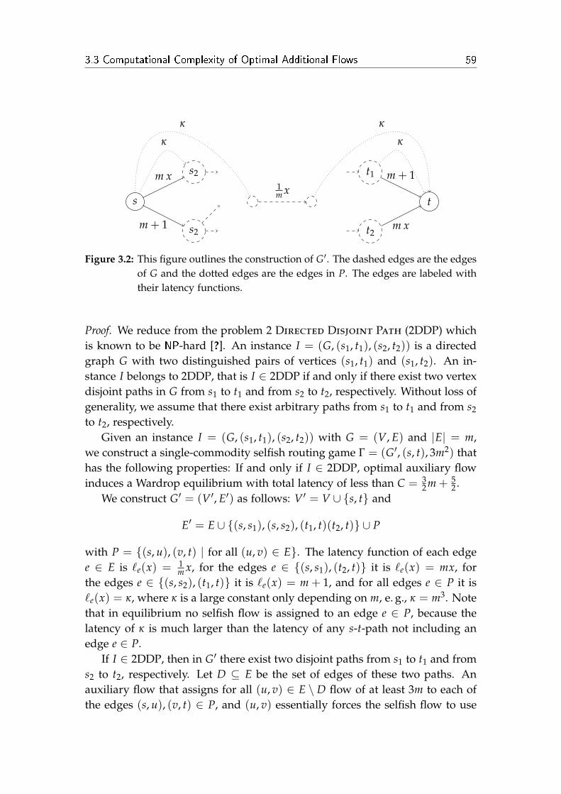
3.3 Computational Complexity of Optimal Additional Flows 59
s
s2
s2
t
t2
t11m x
m x
m + 1
m + 1
m x
κ
κ κ
κ
Figure 3.2: This figure outlines the construction of G′. The dashed edges are the edgesof G and the dotted edges are the edges in P. The edges are labeled withtheir latency functions.
Proof. We reduce from the problem 2 Directed Disjoint Path (2DDP) whichis known to be NP-hard [?]. An instance I = (G, (s1, t1), (s2, t2)) is a directedgraph G with two distinguished pairs of vertices (s1, t1) and (s1, t2). An in-stance I belongs to 2DDP, that is I ∈ 2DDP if and only if there exist two vertexdisjoint paths in G from s1 to t1 and from s2 to t2, respectively. Without loss ofgenerality, we assume that there exist arbitrary paths from s1 to t1 and from s2
to t2, respectively.Given an instance I = (G, (s1, t1), (s2, t2)) with G = (V, E) and |E| = m,
we construct a single-commodity selfish routing game Γ = (G′, (s, t), 3m2) thathas the following properties: If and only if I ∈ 2DDP, optimal auxiliary flowinduces a Wardrop equilibrium with total latency of less than C = 3
2 m + 52 .
We construct G′ = (V′, E′) as follows: V′ = V ∪ s, t and
E′ = E ∪ (s, s1), (s, s2), (t1, t)(t2, t) ∪ P
with P = (s, u), (v, t) | for all (u, v) ∈ E. The latency function of each edgee ∈ E is `e(x) = 1
m x, for the edges e ∈ (s, s1), (t2, t) it is `e(x) = mx, forthe edges e ∈ (s, s2), (t1, t) it is `e(x) = m + 1, and for all edges e ∈ P it is`e(x) = κ, where κ is a large constant only depending on m, e. g., κ = m3. Notethat in equilibrium no selfish flow is assigned to an edge e ∈ P, because thelatency of κ is much larger than the latency of any s-t-path not including anedge e ∈ P.
If I ∈ 2DDP, then in G′ there exist two disjoint paths from s1 to t1 and froms2 to t2, respectively. Let D ⊆ E be the set of edges of these two paths. Anauxiliary flow that assigns for all (u, v) ∈ E \ D flow of at least 3m to each ofthe edges (s, u), (v, t) ∈ P, and (u, v) essentially forces the selfish flow to use
60 Chapter 3. Improving Equilibria with Auxiliary Flow
the two disjoint paths only. The latency for flow demand d′ on such a path isat least md′ + m + 1 and at most md′ + m · 1
m + m + 1. Solving
md′ + m + 1 + α/m = m(1− d′) + m + 1 + β/m
with 0 ≤ α ≤ β ≤ m for d′ and 1− d′ shows that at equilibrium the maximalflow on each of the two paths is upper bounded by m+1
2m . Therefore, the latencyof a path at a resulting Wardrop equilibrium is at most 3
2 m + 52 and the total
latency is at most C. In particular, there is an optimal routing of the auxiliaryflow such that the total latency at equilibrium is at most C.
If I /∈ 2DDP, we show that there no auxiliary flow that induces an equilib-rium flow with total latency of less than 2m. We distinguish several cases bythe usage of the four edges incident to s and t. Since we have unit demandand all used paths have the same length at equilibrium, it suffices to show thatthere is a used path with latency of at least 2m.
1. If a flow uses a path starting with (s, s2) and ending with (t1, t), this pathhas total latency of at least 2m + 2.
2. If a flow uses only paths starting with (s, s1) and ending with (t2, t), ithas total latency of at least 2m.
3. If a flow uses only paths starting with (s, s1) and ending with (t2, t) or(t1, t), the latency from s1 to t must be the same on all paths. Thereforeevery path has latency of at least 2m + 1.
4. If a flow uses only paths starting with (s, s1) or (s, s2) and ending with(t2, t), the same argument holds.
5. If a flow uses at least one path starting with (s, s1) and ending with (t1, t)and at least one path starting with (s, s2) and ending with (t2, t), thereexists a vertex v∗ that is contained in both paths. Due to the equilibriumconstraint, all path segments from s to v∗ and from v∗ to t must have thesame latency. Thus, every path has latency of at least 2m + 2.
Thus, the optimal auxiliary flow induces an equilibrium with total latencyless or equal C in Γ if and only if I ∈ 2DDP.
Note that the decision in the previous instances is whether the total latencyof the selfish flow can be reduced to at most C = 3
2 m + 52 . If this is impossible,
for every flow the total latency is at least 2m. Now suppose there is a polyno-mial time approximation algorithm, which computes a
(43 − ε
)-approximation
for optimizing the total latency of selfish flow. Then, such an algorithm couldbe used to decide sufficiently large instances of 2DDP using the previouslyoutlined construction. We therefore get the following corollary.

3.3 Computational Complexity of Optimal Additional Flows 61
s∗
s′1 Γ1
s′2 Γ2
s′k Γk
t′1
t′2
t′k
t∗
0
0
0
0
0
0
κ′
κ′κ′ . . .
Figure 3.3: The network contains k = 3m2 · dε−1e copies of the network G′ of the proofof Theorem 19. Between s∗ and t∗ there is a demand of k.
Corollary 20. For every ε > 0 it is NP-hard to approximate Optimal-Flow oninstances with linear latency functions to a factor of 4
3 − ε.
In addition, note that in the NP-hardness reduction the auxiliary flow ismuch larger than the demand of selfish flow. However, we can show that theresult even holds if the auxiliary flow is only a (polynomially) small fractionof the selfish demand.
Theorem 21. Optimal-Flow is NP-hard to approximate to a factor of 43 − ε for
every constant ε > 0 on instances with linear latency functions and auxiliary flowδ ∈ O
(d
poly(m)
).
Proof. Again, we reduce from 2DDP. Given an instance I and an ε > 0, weconstruct a selfish routing game Γ as described in the proof of Theorem 19.We use k = 3m2 · dε−1e copies Γ1, . . . , Γk of this game to create a new gameΓ′ as follows. We add a source vertex s∗ and a target vertex t∗. The vertexs∗ is connected to each source vertex s′i of Γi (for all 1 ≤ i ≤ k) by an edge(s∗, si) with latency function `(s∗,si)(x) = 0. Likewise, there is an edge with`(t′i ,t
∗)(x) = 0 from each vertex t′i to t∗. Additionally, for every i ∈ 1, . . . , k− 1,there is an edge from t′i to s′i+1 with `(t′i ,si+1)(x) = κ′, where κ′ = k4. Thedemand of the selfish flow is d = k, and the auxiliary flow is limited to 3m2
and C = d · (32 m + 5
2).If I ∈ 2DDP, there is an auxiliary flow that yields an equilibrium flow with
total latency of at most d · (32 m + 5
2): We assign auxiliary flow of at most 3m2
62 Chapter 3. Improving Equilibria with Auxiliary Flow
between the vertices s′i and t′i in each copy Γi as described in the proof of Theo-rem 19. We assign the same amount of flow to the edges (s∗, s′1), (t′1, s′2), . . . , (t′k−1, s′k), (t′k, t∗)to obtain a flow of at most 3m2 from s∗ to t∗. At the resulting Wardrop equi-librium, there is a flow of 1 that is assigned to each copy Γi and the edges thatconnect it to s∗ and t∗. Each of these flows has latency of at most 3
2 m + 52 . Thus,
the total latency sums up to at most d · (32 m + 5
2).If I /∈ 2DDP, the total latency of the selfish flow is more than d · 2m. Note
that at equilibrium the selfish flow never chooses an edge that connects twoof the copies because it has latency of κ′, and there is always a s∗-t∗-path withlower latency. Therefore, there is at least one copy Γi in which flow of at least1 is routed from s′i to t′i. As shown in the proof of Theorem 19, the latency ofthe s′i-t
′i-paths is at least 2m. Since the flow is at Wardrop equilibrium, every
path between s′j and t′j for every 1 ≤ j ≤ k has latency of at least 2m. Thus, thetotal latency sums up to more than d · 2m.
Due to the known price of anarchy result [?], this hardness result can berestated in view of algorithm design as: For linear latency functions the trivialalgorithm, i. e., routing no auxiliary flow, is the optimal algorithm.
3.3.2 Complexity of Threshold-Flow
The previous result showed that it is computationally infeasible to computethe best possible auxiliary flow. In this section we show that even the minimalamount of auxiliary flow that is needed to achieve the best possible Wardropequilibrium is hard to approximate.
Note that this result strongly contrasts the corresponding result of Kaporisand Spirakis [?] for Stackelberg routing. In Stackelberg routing the minimalfraction of flow needed by the Stackelberg leader to induce optimal latencycan be computed in polynomial time for arbitrary multi-commodity networksusing a surprisingly simple algorithm.
Theorem 22. Threshold-Flow is NP-hard.
Proof. Again, we reduce from 2 Directed Disjoint Path (2DDP). Given aninstance I = (G, (s1, t1), (s2, t2)) with G = (V, E) and |E| = m, we con-struct a single-commodity selfish routing game that has an optimal auxil-iary flow of at most polynomial in m if and only if I ∈ 2DDP. ConstructΓ = (G′, (s, t), poly(m)) as described in the proof of Theorem 19 and modifyit as follows. Remove the edge (t2, t) and replace it with the following gad-get. Add the vertices u and v and the edges (t2, u), (u, v), (u, t), (t2, v), (v, t).Latency functions are `e(x) = (m
2 −1
2m+1 )x for the edges e ∈ (t2, u), (v, t)and `e(x) = m
2 + 12m+1 for the edges e ∈ (u, t), (t2, v) and `(u,v)(x) = 1
2m x. In

3.3 Computational Complexity of Optimal Additional Flows 63
s
s2
s1
m x
m + 1t
t2
t1
u
v
(m 2−
12m
+1)x
m2 + 1
2m+1
12m x
m2 + 1
2m+1
(m 2−
12m
+1)x
m + 1
κ
κ
κκ
κ
κ
Figure 3.4: This figure outlines the modified construction of G′ for the proof of Theo-rem 22.
addition, we add edges (s, u), (s, v), (u, t) and (v, t) with latency κ to the set P(cf. proof of Theorem 19).
Observe that for routing flow demand d′ ≤ m2m+1+23 m2m+1 from t2 to t, it is opti-
mal to leave all selfish flow on the zig-zag path, which generates path latencymd′ and also yields an equilibrium. Note that the optimum assignment of self-ish flow that is achievable by (marginal cost) taxing might split the flow alongall three possible paths from t2 to t. However, the resulting latency of such aflow is larger here, as the auxiliary flow, which can used to simulate taxes inour gadget, is accounted in the latency of selfish flow. For flow larger thanm2m+1+23 m2m+1 , splitting the flow and assigning d′
2 to the edges (t2, u), (t2, v), (u, t),and (v, t) yields a better latency. This flow and its improved latency can be in-duced using a sufficiently large auxiliary flow along edge (u, v). The auxiliaryflow needs only to be large enough to prevent the selfish flow from using theedge (u, v). Observe, that for large demand values in our gadget splitting theflow among (t2, u, t) and (t2, v, t) by blocking (u, v) yields also a better latencythan assigning an amount of flow to (u, v) that still allows some selfish flow touse this edge as well.
If I ∈ 2DDP, then in G′ there exist two disjoint paths from s1 to t1 andfrom s2 to t2, respectively. Again, let D ⊂ E be the set of edges of thesetwo paths. Then an auxiliary flow that assigns, for all (e, e′) ∈ E \ D, flow ofvolume 3m to each of the edges (s, e), (e, e′) and (e′, t) forces the selfish flowto use the two disjoint paths only. Thus, the flow becomes almost balancedbetween the two disjoint paths. The best possible Wardrop equilibrium can be

64 Chapter 3. Improving Equilibria with Auxiliary Flow
reached by sending additional auxiliary flow slightly unevenly over the edgesof both disjoint paths. Nevertheless, a polynomial amount of auxiliary flow issufficient to totally balance the selfish flow. To see this, assume some edge inD receives a super-polynomial amount of auxiliary flow. The resulting latencyof this edge would then surpass the path latency of the other disjoint path.Hence, an auxiliary flow of demand poly(m) is sufficient to obtain the bestpossible Wardrop equilibrium.
Note that selfish flow of demand close to 1/2, i. e., less than m2m+1+23 m2m+1 is
routed through the gadget from t2 to t. Therefore, it is not necessary to routeauxiliary flow over the edge (u, v).
If I /∈ 2DDP, then optimal auxiliary flow yields a Wardrop equilibrium inwhich the whole selfish demand is routed from s via s1 and t2 to t. Especially, aunit demand is being routed through the gadget between t2 and t. The optimalauxiliary flow thus must block edge (u, v). Hence, it needs to route auxiliaryflow of demand δ over (u, v), such that
12m δ +
(m2− 1
2m+1
)· 1
2≥ m
2+
12m+1 ,
i. e., δ ∈ Ω(2m).
Note that the latency functions in our gadget use exponentially large coeffi-cients. Nevertheless, the latency functions can be represented by a polynomialnumber of bits in the input size, assuming that the numbers in our instanceare represented in binary coding.
The proof shows that deciding 2DDPcan be reduced to the decision whethera polynomial auxiliary flow can be optimal in the previous instances or not.Thus, we have the following corollary.
Corollary 23. For any constant ε > 0, it is NP-hard to approximate Threshold-Flow by a factor of 2m(1−ε).
3.3.3 Complexity of Worst-Flow
We have seen that the optimal auxiliary flow is NP-hard to compute. We nowturn to the computational complexity of computing the optimal adversarialflow.
Theorem 24. Worst-Flow is NP-hard.
Proof. We reduce from the NP-hard problem Hamilton. A graph G ∈ Hamil-ton if and only if G contains a Hamiltonian path. Given a directed graphG = (V, E) with |V| = n and |E| = m and two vertices x, y ∈ V, we constructa selfish routing game Γ = (G′, (s, t), δ) with the property that the latency

3.3 Computational Complexity of Optimal Additional Flows 65
s
uv1
uv2
uv3
uvn
wv1
wv2
wv3
wvn
t
0
0
0
0
x
x
x
x
0
0
0
0
κ
κ
κ
Figure 3.5: This figure depicts the corresponding graph G′ for an instance G of theproblem Hamilton. The dashed edges correspond to vertices in G andthe dotted edges correspond to edges in G′.
maximizing adversarial flow induces total latency of at least C = 1n + δ if and
only if G ∈ Hamilton.We construct G′ = (V′, E′) as follows: For every vertex v in G there is a pair
of vertices uv, wv in G′ and, additionally we have a source and a sink vertexs and t. That is, V = s, t ∪ uv, wv | ∀v ∈ V. There are edges from s toall vertices uv, from each vertex uv to wv and from all vertices wv to t. Theselfish flow will use only these edges. Additionally, we have edges (with highlatency) that connect a vertex wv with a vertex uv′ if there is an edge from v tov′ in the graph G for v′ ∈ V − x. To summarize, E′ = S′ ∪U′ ∪W ′ with
S′ = (uv, wv) | ∀v ∈ V,U′ = (s, uv), (wv, t) | ∀v ∈ V, and
W ′ = (wv, uv′) | ∀(v, v′) ∈ E and v′ ∈ V − x.
For all edges e ∈ S′ we set `e(x) = x, for all edges e ∈ U′ we set `e(x) = 0,and for all edges e ∈ W ′ we set `e(x) = κ for a constant κ > 0. Note thatthe selfish flow never uses edges e ∈ W ′ and therefore assigns flow to the npaths s, uv, wv, t for all v ∈ V. Without adversarial flow, the equilibrium flowis equally distributed among these paths, and the total latency is n 1
n2 = 1n .
Assume G ∈ Hamilton and x = vi1 , . . . , vin = y is a Hamiltonian pathin the network G. Then it is possible to assign adversarial flow of amount δ
to all edges e ∈ S′ by choosing the path s, uvi1, wvi1
, uvi2, wvi2
, . . . , uvin, wvin ,, t.
Note, that the edges between the w and u vertices exist by construction. Alledges with non-constant latencies carry the maximal amount of adversarialflow. This maximizes the total latency and yields n( 1
n + δ) · 1n = 1
n + δ.

66 Chapter 3. Improving Equilibria with Auxiliary Flow
Consider a graph G /∈ Hamilton. Then there is no path in G′ from s tot that visits all vertices e ∈ U′. Therefore, the adversarial flow δ can not besent via all edges e ∈ S′, and there is at least one edge e ∈ S′ with adversarialflow less than δ. Thus, the equilibrium flow will balance accordingly amongall paths containing an edge e ∈ S′. The resulting path latency and thus thetotal latency at equilibrium is strictly less than 1
n + δ.

Chapter 4
Sensitivity of Wardrop Equilibria
In the preceding chapters we have tackled the problem of reducing the price ofanarchy for routing instances, where fixed amounts of flow need to be routedamong source-sink pairs through the network. In uncoordinated networks,however, neither the demands remain constant nor does the network topologyremain unchanged. In this regard, we study how equilibrium flows react toslight modification of the network environment.
To analyze this issue, we suppose we are given an equilibrium flow forunit demand and increase the demand by ε or remove an edge carrying onlyan ε-fraction of flow. How does the equilibrium responds to such an ε-changein terms of change in flow and latency?
The Braess network depicted in Figure 4.1 exhibits that, in general, neitherpath flows nor edge flows at equilibrium are monotone functions of the de-mand. This observation has already been made by Braess [?] and suggests thatstudying the effects of environmental changes might be intriguing. As one im-mediate implication Wardrop equilibria are not computable or approximable
s t
x
1
1
x
0
(a) Latency functions ...
s t
1
ε
ε
1
1− ε
(b) ... and flow.
Figure 4.1: (a) The links are labeled with the latency functions. At equilibrium theentire demand routes over the zig-zag-path. (b) The links are now labeledwith the unique equilibrium flow. Increasing the demand by 0 ≤ ε ≤ 1,the zig-zag-path loses an ε-fraction.
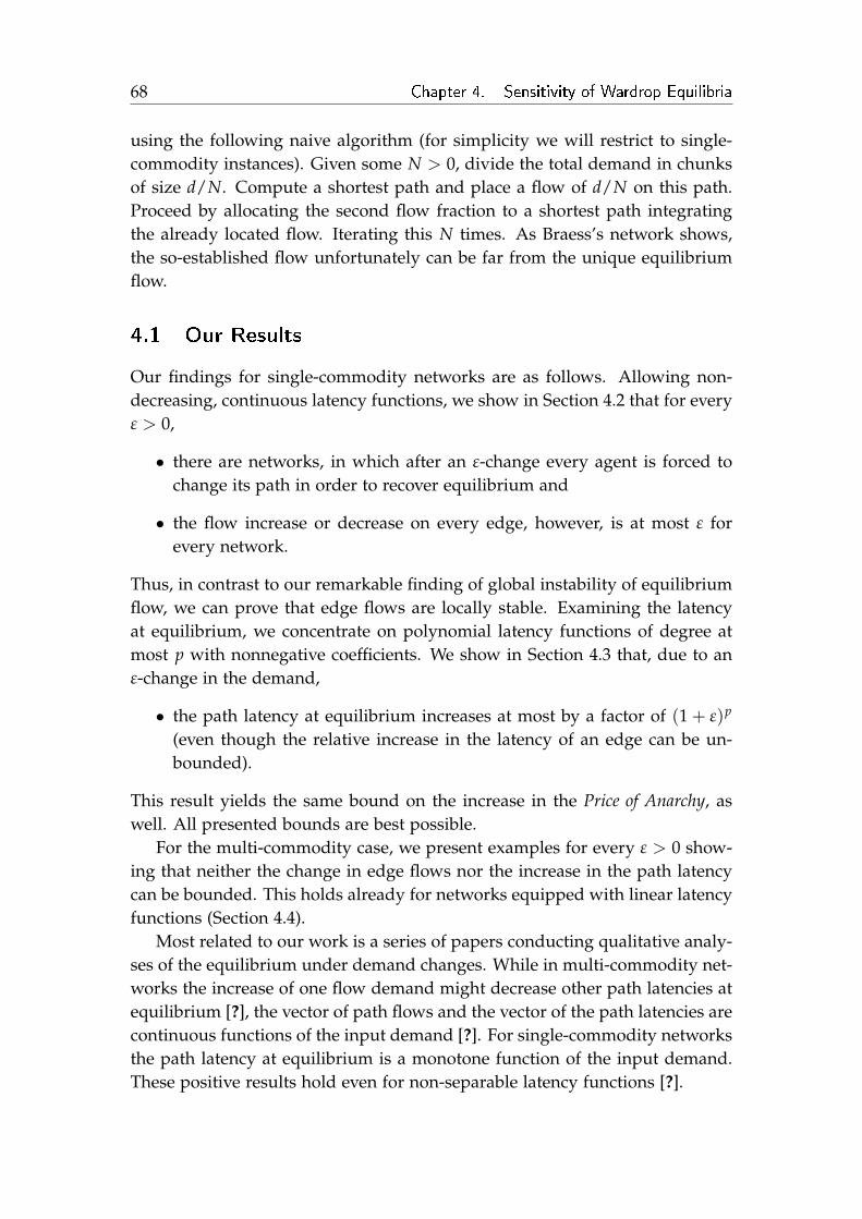
68 Chapter 4. Sensitivity of Wardrop Equilibria
using the following naive algorithm (for simplicity we will restrict to single-commodity instances). Given some N > 0, divide the total demand in chunksof size d/N. Compute a shortest path and place a flow of d/N on this path.Proceed by allocating the second flow fraction to a shortest path integratingthe already located flow. Iterating this N times. As Braess’s network shows,the so-established flow unfortunately can be far from the unique equilibriumflow.
4.1 Our Results
Our findings for single-commodity networks are as follows. Allowing non-decreasing, continuous latency functions, we show in Section 4.2 that for everyε > 0,
• there are networks, in which after an ε-change every agent is forced tochange its path in order to recover equilibrium and
• the flow increase or decrease on every edge, however, is at most ε forevery network.
Thus, in contrast to our remarkable finding of global instability of equilibriumflow, we can prove that edge flows are locally stable. Examining the latencyat equilibrium, we concentrate on polynomial latency functions of degree atmost p with nonnegative coefficients. We show in Section 4.3 that, due to anε-change in the demand,
• the path latency at equilibrium increases at most by a factor of (1 + ε)p
(even though the relative increase in the latency of an edge can be un-bounded).
This result yields the same bound on the increase in the Price of Anarchy, aswell. All presented bounds are best possible.
For the multi-commodity case, we present examples for every ε > 0 show-ing that neither the change in edge flows nor the increase in the path latencycan be bounded. This holds already for networks equipped with linear latencyfunctions (Section 4.4).
Most related to our work is a series of papers conducting qualitative analy-ses of the equilibrium under demand changes. While in multi-commodity net-works the increase of one flow demand might decrease other path latencies atequilibrium [?], the vector of path flows and the vector of the path latencies arecontinuous functions of the input demand [?]. For single-commodity networksthe path latency at equilibrium is a monotone function of the input demand.These positive results hold even for non-separable latency functions [?].

4.2 Sensitivity of Equilibrium Flows 69
s
w3
v3
v2
v1
w2
w1
t
1
3 x
6 x
9 x
0
1
0
1
0
9 x
6 x
3 x
1
(a) Latency functions ...
s
w3
v3
v2
v1
w2
w1
t
1/3
1/3
1/3
1/3
0
1/3
0
1/3
0
1/3
1/3
1/3
1/3
(b) ... and flow.
Figure 4.2: (a) Having unit demand, the solid paths in Bk=3 carry 1/3 of flow each,and the dashed edges carry zero flow. (b) After increasing the demandby (1 + ε) = (1 + 1/3), the solid paths lose all their flow, and the pathscontaining the dashed edges gain flow of (1 + ε)/(k + 1) = 1/3 each.
4.2 Sensitivity of Equilibrium Flows
For most of the section we concentrate on the single-commodity case. First, wepresent a network with linear latency functions for any given ε > 0, in whichevery agent needs to change its current path to recover equilibrium. Then weprove that due to ε-changes the flow on every edge does not change by morethan ε.
4.2.1 Instability of Equilibria: Every Agent Needs to Move
In [?] Roughgarden uses the generalized Braess graphs to show, that the pathlatency at equilibrium can arbitrarily decrease by removing several edges froma network. Our definition of Bk differs from the definition in [?] in the non-constant latency functions.
Definition 10 (Generalized Braess graph). For every k ∈ N, let Bk = (Vk, Ek) bethe graph with Vk = s, v1, . . . , vk, w1, . . . , wk, t and Ek = (s, vi), (vi, wi), (wi, t) :1 ≤ i ≤ k ∪ (vi, wi−1) : 2 ≤ i ≤ k ∪ (s, wk) ∪ (v1, t). Let Bk be equippedwith the following latency functions.
• `kvi,wi
(x) = 0 and `ks,vk−i+1
(x) = `kwi,t(x) = i · k · x for 1 ≤ i ≤ k,
• `kvi,wi−1
(x) = 1 for 2 ≤ i ≤ k and
• `ks,wk
(x) = `kv1,t(x) = 1.
Let Bk be called the kth Braess graph.

70 Chapter 4. Sensitivity of Wardrop Equilibria
Let ε > 0 and consider the instance (Bd1/εe, 1).Let (P1, . . . , P2k+1)T = (Ps,wk,t, Ps,vk,wk,t, Ps,vk,wk−1,t, Ps,vk−1,wk−1,t, . . . , Ps,v1,t)T denotethe corresponding path vector. The equilibrium flow is described by the vector( fPj) of path flows
fPj =
0 for j = 1, 3, . . . , 2k + 1
1/k for j = 2, 4, . . . , 2k
summing up to ∑P fP = ∑2k+1j=1 fPj = 1.
All paths have path length `P( f ) = k + 1, and since any unilateral devia-tion strictly increases the sustained latency, the edge flows at equilibrium areunique (Figure 4.2).
By increasing the demand by (1 + ε) the equilibrium flow vector becomes( f ′Pj
) with
f ′Pj=
(1 + ε)/(k + 1) for j = 1, 3, . . . , 2k + 1
0 for j = 2, 4, . . . , 2k
which sums up to ∑P f ′P = ∑2k+1j=1 f ′Pj
= 1 + ε. The path latency can easily be
computed to be 1 + k2(1+ε)k+1 .
Note that the path flow decomposition at equilibrium does not need to beunique. Nevertheless, we have uniqueness in Bk.
Definition 11 (ε-edge). An edge e ∈ E carrying flow of at most ε is called ε-edge.
Theorem 25. Let ε > 0 and consider (Bd 1ε e
, 1). Then increasing the flow by ε causesthe entire demand to be redistributed to recover a Wardrop equilibrium, i. e., everyagent is forced to change its path. Adding another edge to the network, one can achievethe same result for the removal of an ε-edge.
Proof. For the path flow vector ( fPj) and ( f ′Pj) it holds that fPj = 0 ⇔ f ′Pj
> 0.For the second assertion, simply simulate a demand increase in Bd 1
ε eby directly
connecting source s with sink t and choose the latency function such that (s, t)carries an ε-fraction of flow. Then remove this edge.
Let us remark that Theorem 25 can easily be transferred to optimal flows,i. e., flows minimizing the total cost. This is since for semi-convex latencyfunctions optimal flows are Wardrop equilibria with respect to the marginalcost functions. Thus, it is sufficient to change the linear latency functions inBd 1
ε e.

4.2 Sensitivity of Equilibrium Flows 71
4.2.2 Edge Flows are Locally Stable
Let f , f ′ ∈ F be feasible flows for demands d ≤ d′ and let ∆( f , f ′) denote thedifference of f ′ and f ,
∆e( f , f ′) = f ′e − fe , ∀e ∈ E .
An edge e is positive (with respect to f ′ and f ) if f ′e − fe > 0, and it is negativeif f ′e − fe < 0. A path is positive (or negative) if all its edges are positive(or negative). Let us remark that considering ∆( f , f ′) negative edges carry apositive amount of flow equal to fe − f ′e and have their directions reversed.Observe that the flow conservation property holds for the difference of twonetwork flows.
Definition 12 (Alternating flow cycle). A cycle consisting of flow carrying edges iscalled an alternating flow cycle.
Lemma 26. Let f denote an equilibrium flow for an instance (G, 1) with non-decreasing,continuous latency functions. Then there is an equilibrium flow f ′ for (G, 1 + ε), suchthat ∆( f , f ′) does not contain an alternating flow cycle.
Proof. Let f ′ denote an equilibrium flow for (G, 1 + ε). Assume there is analternating flow cycle C in ∆( f , f ′). Since we can assume both equilibriumflows to be cycle free, we can assume that the alternating flow cycle C containspositive and negative edges. C can thus be divided into positive and negativepath segments, C = p1n1p2 . . . nk, where pi denotes a sequence of positiveedges and ni denotes a sequence of negative edges. Let ui be the first node ofpi and denote the last node of ni by vi. Thus, there are two paths from u1 tovk in C. For u, v ∈ V, let `(u, v) denote the minimum path latency from u to vunder f . For u = s simply write `(v). For f ′ write `′(u, v) and `′(v).
There are two facts we will make consistently use of. Since at equilibriumthe flow routes only on shortest paths, we have
`(v) ≤ `(u) + `(u, v) for any u, v ∈ V , and (4.1)
`(v) = `(u) + `(u, v) (4.2)
if there is a flow carrying path between s and v containing u. We show thatassuming f and f ′ being at equilibrium yields `′(u1, vk) = `(u1, vk). On theone hand, since nk connects u1 with vk and there is more flow on every edgeof nk under f than under f ′, we have
`′(u1, vk) ≤ ∑e∈nk
`e( f ′e) ≤ ∑e∈nk
`e( fe) = `(u1, vk) .

72 Chapter 4. Sensitivity of Wardrop Equilibria
For the reverse direction we show `′(vk) ≥ `′(u1)+ `(u1, vk), since then `(u1, vk) ≤`′(vk)− `′(u1) ≤ `′(u1, vk). In the following, we repeatedly make use of Equa-tions (4.1) and (4.2).
`′(vk) = `′(uk) + `′(uk, vk) ≥ `′(vk−1)− `′(uk, vk−1) + `′(uk, vk)
= `′(uk−1) + `′(uk−1, vk−1)− `′(uk, vk−1) + `′(uk, vk)
≥ `′(u1) +k
∑i=1
`′(ui, vi)−k
∑i=2
`′(ui, vi−1)
≥ `′(u1) +k
∑i=1
`(ui, vi)−k
∑i=2
`(ui, vi−1)
≥ `′(u1) +k
∑i=1
(`(vi)− `(ui))−k
∑i=2
(`(vi−1)− `(ui))
= `′(u1)− `(u1) + `(vk) = `′(u1) + `(u1, vk) .
The third inequality is valid since f and f ′ route only on shortest paths. Ex-plicitly, `′(ui, vi) = ∑e∈pi
`e( f ′e) ≥ ∑e∈pi`e( fe) ≥ `(ui, vi) for each i ∈ [k] and
`′(ui, vi−1) ≤ ∑e∈ni`e( f ′e) ≤ ∑e∈ni
`e( fe) = `(ui, vi−1) for each i ∈ 2, . . . , k.Thus, `′(u1, vk) = `(u1, vk).
We deduce that the latency on every edge e ∈ nk does not change dueto the flow change. Since the same analysis can be conducted for any pathsegment pi and ni, the latency of both paths on C connecting two arbitrarynodes remains unchanged. Therefore, by removing the bottleneck edge flowin C no edge latency is affected and the alternating flow cycle is eliminated.We may remove the set of alternating flow cycles in any order. Adding f to thealtered difference, one gets the desired equilibrium flow for demand 1 + ε.
Thus, ∆( f , f ′) can be assumed a network flow of volume ε when edges areallowed to be traversed in both directions. We can now state the followingtheorem.
Theorem 27. Let f denote an equilibrium flow for an instance (G, 1) with non-decreasing, continuous latency functions `.
• Then there is an equilibrium flow f ′ for (G, 1 + ε), such that for all e ∈ E itholds that |∆e( f , f ′)| ≤ ε.
• Consider an ε-edge (u, v) in G. There is an equilibrium flow f ′ for (G′ =(V, E− (u, v)), 1) such that |∆e( f , f ′)| ≤ ε for all e ∈ E.
Proof. Since the difference of f and f ′ can be assumed alternating flow cyclefree, it constitutes a network flow of volume ε. To show the second asser-tion, let a single ε-edge (u, v) be removed. With the same argumentation as in

4.3 Stability of the Path Latency 73
Lemma 26, we can exclude alternating flow cycles in ∆( f , f ′) that do not in-clude (u, v). Due to the flow conservation property for every node u 6= w 6= v,∆( f , f ′) is a network flow from u to v of volume ε.
Note that since every edge gains or loses at most an ε amount of flow(Theorem 27), with respect to the number of paths Bd 1
ε eis a minimal example
exhibiting global instability.
4.3 Stability of the Path Latency
The latency increase at equilibrium due to a demand increase clearly dependson the latency functions. Considering polynomials with nonnegative coeffi-cients, the maximal degree is the critical parameter. Note that the results inthis section do not trivially result from Theorem 27, since the relative flowincrease on an edge might be unbounded.
Theorem 28. Let f and f ′ be equilibrium flows for instances (G, 1) and (G, 1 + ε)with polynomial latency functions ` of degree at most p with nonnegative coefficients.Let L and L′ denote the corresponding path latencies. Then L′ ≤ (1 + ε)p · L.
Proof. Due to a scaling argument it is sufficient to consider monic monomialsas latency functions. For equilibrium flows f and f ′ we have
L = ∑P∈P
fP`P( f ) = ∑e
fe`e( fe) and (1 + ε) · L′ = ∑e
f ′e`e( f ′e) ,
and we want to show that ∑e f ′pe+1e ≤ (1 + ε)p+1 ∑e f pe+1
e , where `e(x) = xpe .Since equilibrium flows f and f ′ minimize the potential function
Φ(x) = ∑e
∫ xe
0`e(u) du
over feasible flows x of volume 1 and (1 + ε), respectively, it holds that
Φ( f ) ≤ Φ(
f ′
1 + ε
)and Φ( f ′) ≤ Φ((1 + ε) · f )
More explicitly,
(1 + ε)p+1 ·Φ( f ) = (1 + ε)p+1 ·∑e
1pe + 1
f pe+1e ≤∑
e
(1 + ε)p−pe
pe + 1f ′pe+1
e , (A)
and similarly,
Φ( f ′) = ∑e
1pe + 1
f ′pe+1e ≤∑
e
(1 + ε)pe+1
pe + 1f pe+1e . (B)
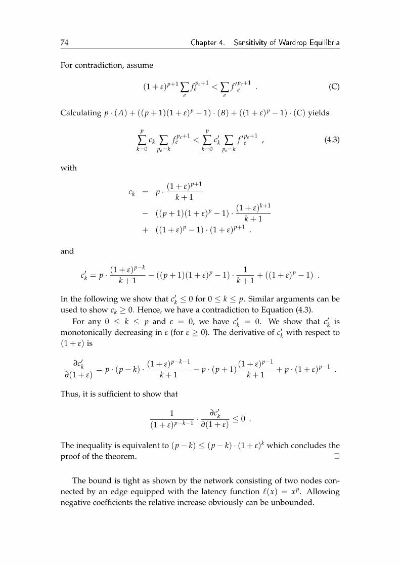
74 Chapter 4. Sensitivity of Wardrop Equilibria
For contradiction, assume
(1 + ε)p+1 ∑e
f pe+1e < ∑
ef ′pe+1
e . (C)
Calculating p · (A) + ((p + 1)(1 + ε)p − 1) · (B) + ((1 + ε)p − 1) · (C) yields
p
∑k=0
ck ∑pe=k
f pe+1e <
p
∑k=0
c′k ∑pe=k
f ′pe+1e , (4.3)
with
ck = p · (1 + ε)p+1
k + 1
− ((p + 1)(1 + ε)p − 1) · (1 + ε)k+1
k + 1+ ((1 + ε)p − 1) · (1 + ε)p+1 .
and
c′k = p · (1 + ε)p−k
k + 1− ((p + 1)(1 + ε)p − 1) · 1
k + 1+ ((1 + ε)p − 1) .
In the following we show that c′k ≤ 0 for 0 ≤ k ≤ p. Similar arguments can beused to show ck ≥ 0. Hence, we have a contradiction to Equation (4.3).
For any 0 ≤ k ≤ p and ε = 0, we have c′k = 0. We show that c′k ismonotonically decreasing in ε (for ε ≥ 0). The derivative of c′k with respect to(1 + ε) is
∂c′k∂(1 + ε)
= p · (p− k) · (1 + ε)p−k−1
k + 1− p · (p + 1)
(1 + ε)p−1
k + 1+ p · (1 + ε)p−1 .
Thus, it is sufficient to show that
1(1 + ε)p−k−1 ·
∂c′k∂(1 + ε)
≤ 0 .
The inequality is equivalent to (p− k) ≤ (p− k) · (1 + ε)k which concludes theproof of the theorem.
The bound is tight as shown by the network consisting of two nodes con-nected by an edge equipped with the latency function `(x) = xp. Allowingnegative coefficients the relative increase obviously can be unbounded.

4.3 Stability of the Path Latency 75
s1
s2
t1
t2
1
x1+ε
x1+ε
x1+ε
x1+ε
1 1 11
Figure 4.3: Unlabeled edges cause no latency. Assume there are 2 · d 1ε e − 1 many
edges on the unique path connecting s2 with t2. For d1 = d2 = 1, the flowdemand of commodity 1 is uniformly spread over all d1/εe paths usingone edge on the path connecting s2 and t2. After increasing d2 by ε, wehave f(s1,t1) = 1.
4.3.1 Increase of the Price of Anarchy
The price of anarchy quantifies the degradation of performance due to selfishbehavior. Recall that the price of anarchy for an instance (G, d) is defined asρ(G, d) = C( f ∗)
C( f ) , where f and f ∗ denote an optimal flow and an equilibriumflow, respectively. In [?] the price of anarchy is shown to be asymptoticallyΘ( p
ln p ) for polynomial latency functions of degree at most p with nonnegativecoefficients.
Corollary 29. Let ρ and ρ′ denote the price of anarchy for instances (G, 1) and (G, 1 +ε) with polynomial latency functions of degree at most p with nonnegative coefficients.Then ρ′ ≤ (1 + ε)p · ρ.
Proof. Let Ld denote the average path latency for an optimal flow in (G, d). LetC, C∗, C′ and C′∗ denote the costs of an optimal flow and an equilibrium flowfor demands 1 and 1 + ε, respectively. Then ρ = C∗/C and ρ′ = C′∗/C′. SinceC = 1 · L1 and C′ = (1 + ε) · L1+ε, we have
(1 + ε) · C = (1 + ε) · L1 ≤ (1 + ε) · L1+ε = C′ ,
since the average latency is clearly monotone in the demand. Thus, the in-crease of the price of anarchy can be bounded by
ρ′
ρ=
C′∗/C′
C∗/C=
L′ · (1 + ε) · CL · C′ ≤ L · (1 + ε)p · (1 + ε) · C
L · C · (1 + ε)= (1 + ε)p ,
where the inequality is due to Theorem 28.
This upper bound is tight in the following sense: There is a network family(G, d) with latency function `(p), such that limp
ρ′/ρ(1+ε)p = 1 for every ε > 0.
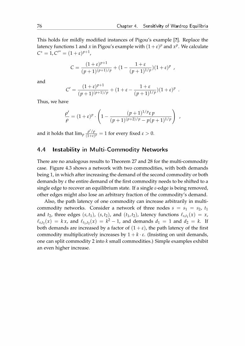
76 Chapter 4. Sensitivity of Wardrop Equilibria
This holds for mildly modified instances of Pigou’s example [?]. Replace thelatency functions 1 and x in Pigou’s example with (1 + ε)p and xp. We calculateC∗ = 1, C′∗ = (1 + ε)p+1,
C =(1 + ε)p+1
(p + 1)(p+1)/p+ (1− 1 + ε
(p + 1)1/p )(1 + ε)p ,
and
C′ =(1 + ε)p+1
(p + 1)(p+1)/p+ (1 + ε− 1 + ε
(p + 1)1/p )(1 + ε)p .
Thus, we have
ρ′
ρ= (1 + ε)p ·
(1− (p + 1)1/pε p
(p + 1)(p+2)/p − p(p + 1)1/p
),
and it holds that limpρ′/ρ
(1+ε)p = 1 for every fixed ε > 0.
4.4 Instability in Multi-Commodity Networks
There are no analogous results to Theorem 27 and 28 for the multi-commoditycase. Figure 4.3 shows a network with two commodities, with both demandsbeing 1, in which after increasing the demand of the second commodity or bothdemands by ε the entire demand of the first commodity needs to be shifted to asingle edge to recover an equilibrium state. If a single ε-edge is being removed,other edges might also lose an arbitrary fraction of the commodity’s demand.
Also, the path latency of one commodity can increase arbitrarily in multi-commodity networks. Consider a network of three nodes s = s1 = s2, t1
and t2, three edges (s, t1), (s, t2), and (t1, t2), latency functions `s,t1(x) = x,`s,t2(x) = k x, and `t1,t2(x) = k2 − 1, and demands d1 = 1 and d2 = k. Ifboth demands are increased by a factor of (1 + ε), the path latency of the firstcommodity multiplicatively increases by 1 + k · ε. (Insisting on unit demands,one can split commodity 2 into k small commodities.) Simple examples exhibitan even higher increase.

Chapter 5
Distributed Approximation
Given complete information about the game, Wardrop equilibria can be for-mulated as convex programs (under some mild assumptions on the latencyfunctions) and can thus be solved by centralized algorithms in polynomialtime. In particular, the convex programming formulation requires the exactlatency functions and the demand of every commodity. In this chapter, we re-frain from the complete information premise and study distributed algorithmsto compute Wardrop equilibria.
The common game-theoretic interpretation of the Wardrop model, whichwe heavily made use of in the previous chapters, assumes an infinite numberof agents, each of which carries an infinitesimal amount of flow. In [?] itwas shown that such a set of agents approaches Wardrop equilibria quickly byfollowing a simple round-based load-adaptive rerouting policy (for a thoroughtreatment cf. the dissertation of Fischer [?]). This policy, called the replicationpolicy, is executed by all agents in parallel and proceeds in the following way.Each agent samples another agent at random and, if this improves the latency,migrates to this agent’s path with a probability proportional to the latencygain.
For scenarios in which detailed information about the environment are rareand the consequences of a strategy change may be hard to assess, the replica-tion policy describes natural behavior: Imitation of successful agents. In thissetting, a natural goal is to reach approximate equilibria in the following bi-criterial sense. We say that a flow is at δ-ε-equilibrium if at most an ε-fractionof the flow utilizes paths whose latency exceeds the average latency of theircommodity by more than a δ-fraction of the overall average latency. Remark-ably, the number of rounds to reach an approximate equilibrium in this senseis independent of the size and the topology of the underlying network andchiefly depends on the approximation parameters and the elasticity of the la-tency functions.

78 Chapter 5. Distributed Approximation
We consider a different setting, in which the flow is controlled by a finitenumber of agents only, each of which is responsible for the entire flow of onecommodity. Each agent has a set of admissible paths among which it maydistribute its flow. To be able to represent exponentially large collections ofpaths we assume that these are represented by a DAG connecting the sourceand the sink of the agent. Each agent aims at balancing its own flow such thatthe jointly computed allocation will be at Wardrop equilibrium.
In each round each agent can observe the edge flows of its own commodityand the latency values of the paths it uses, but it does not know the latencyfunctions themselves or the other agents’ flow demands. Let us remark thatagents do not aim at minimizing the overall latency of their flow as in thesplittable demand model [?], but seek to minimize the maximum latency oftheir commodity.
5.1 Our results
Unfortunately, the replication policy does not yield a feasible distributed algo-rithm in this setting directly. Simulating an infinite number of agents each ofwhich chooses one out of the given collection of paths would require maintain-ing one variable for each path and computing a quadratic number of migrationrates between pairs of paths. As the number of paths may be exponential inthe size of the network this approach is rendered computationally infeasible.
We present two approaches to circumvent this problem. Our first approachexploits the fact that, for a simplified variant of the replication policy, theupdates of the edge flows can be expressed in a way that merely uses theedge flow variables themselves (rather than the path flow variables). Thus, theupdates can be computed in polynomial time. The convergence time of thisvariant is only pseudopolynomial in the latency functions since it depends onthe maximum slope of the latency functions.
Since the original replication policy cannot be expressed in this compactway, we consider a second approach to achieve convergence in a polynomialnumber of communication rounds. Consider a collection of paths for one ofthe commodities. In a first step, our algorithm samples a polynomial num-ber of paths with probability proportional to their flow. We thus obtain arandomized path decomposition. We consider paths in this decomposition withabove-average latency. From such paths, a fraction of the flow is removed andreallocated proportionally among all admissible paths. If this is done carefully,oscillations can be avoided, and a potential function argument ensures conver-gence towards Wardrop equilibria. Thus, we achieve essentially the same con-vergence rates as in the setting with an infinite number of agents and keep the

5.2 Related Work 79
computation time of one communication round polynomial. Altogether, wecan compute approximate Wardrop equilibria in expected polynomial time.
Let us comment on the inherent weakness of the underlying replicationpolicy. Because agents only imitate each other, they are not able to explorecurrently unused, possibly very cheap paths. Hence, convergence to the set ofWardrop equilibria can not be guaranteed. To this end, we assume a positiveamount of flow on each network edge, which ensures not only that we reachan δ-ε-equilibrium, but in fact convergence to a Wardrop equilibrium.
5.2 Related Work
The computation of Wardrop equilibria can be formulated as a min-cost flowproblem. For an overview of classical methods for finding a minimum costmulti-commodity flow see, e. g., [?] and [?]. Nevertheless, no fast algorithmsfor the multi-commodity case are known in general networks. Thus, mostwork analyzed confined and related problems.
In [?,?] an efficient distributed steepest-descent algorithm for solving multi-commodity flow problems with linear latency functions has been presentedrecently. Several authors (e. g.. [?,?]) consider dynamic routing from an online-learning perspective. Awerbuch and Kleinberg [?] present an algorithm for theonline shortest path problem in an end-to-end feedback model. Blum et al.[?] show that approximate Wardrop equilibria defined in a similar way canbe attained if the agents follow no-regret algorithms. Their bounds on theconvergence time depend polynomially on the regret bounds and networksize and depend pseudopolynomially on the maximum slope of the latencyfunctions.
The problem of load-balancing has also been studied in various discretesettings for networks of parallel links. For the case of identical links, both se-quential [?] and concurrent distributed algorithms were considered [?]. Even-Dar et al. [?] consider distributed algorithms for load balancing on links withspeeds using sampling rules which depend pseudopolynomially on the speedof the links. A variant of the replication policy [?] has also been applied incongestion games [?].
5.3 Preliminaries and Initial Results
In this chapter we consider arbitrary non-negative, non-decreasing and differ-entiable latency function. In particular, we do not require semi-convex latencyfunctions. We assume that the set of allowed paths Pi for commodity i isrepresented by a directed acyclic graph (DAG) and may assume that the setsPi are disjoint and define iP to be the unique commodity to which path P

80 Chapter 5. Distributed Approximation
belongs. We normalize the demand by ∑i∈[k] ∑P∈PifP = ∑i∈[k] di = 1. Further-
more, for v ∈ V and i ∈ [k], the total flow of commodity i through vertex vis fv,i = ∑(u,v)∈E f(u,v),i = ∑(v,w)∈E f(v,w),i for v /∈ si, ti and fsi,i = fti,i = di.Finally, while in previous chapters Li( f ) denoted the unique path latency atequilibrium in commodity i, now Li( f ) = ∑e∈E `e( f ) · ( fe,i/di) denotes theweighted average latency of commodity i ∈ [k]. Note that for unit demand thetotal latency C( f ) = ∑e∈E `e( f ) · fe is also the overall average latency.
Recall that Wardrop equilibria are exactly those allocations that minimizethe following potential function introduced in [?]:
Φ( f ) = ∑e∈E
∫ fe
0`e(u) du .
The minimum potential is denoted by Φ∗ = min f∈F Φ( f ). Every flowf with Φ( f ) = Φ∗ is then at Wardrop equilibrium. We assume that Φ∗ ispositive. The case that Φ∗ = 0 can be treated by adding virtual offsets to thelatency functions. For a detailed treatment see [?].
The algorithms presented in this paper will compute approximate equilib-ria in the following bicriterial sense.
Definition 13 (δ-ε-equilibrium). Consider a flow f of unit demand and let
P δi = P ∈ Pi | `P( f ) > Li( f ) + δ C( f )
denote the set of δ-expensive paths of commodity i ∈ [k]. A flow is at a δ-ε-equilibrium if
∑i∈[k]
∑P∈Pδ
i
fP ≤ ε.
This definition of approximate Wardrop equilibria requires that almost allflow utilizes paths with a latency that is close to the average of their owncommodity. A similar definition of approximate Nash equilibria is used, e. g.,in [?].
5.4 Elasticity of Latency Functions
Our algorithms take the steepness of the latency functions into account whendeciding how much flow to shift from one path to another. In [?] it was shownthat the critical parameter in this setting is not the slope but the elasticity.
Definition 14 (Elasticity). For any positive differentiable function` : R≥0 → R≥0, the elasticity of ` at x is r(x) = x·`′(x)
`(x) .
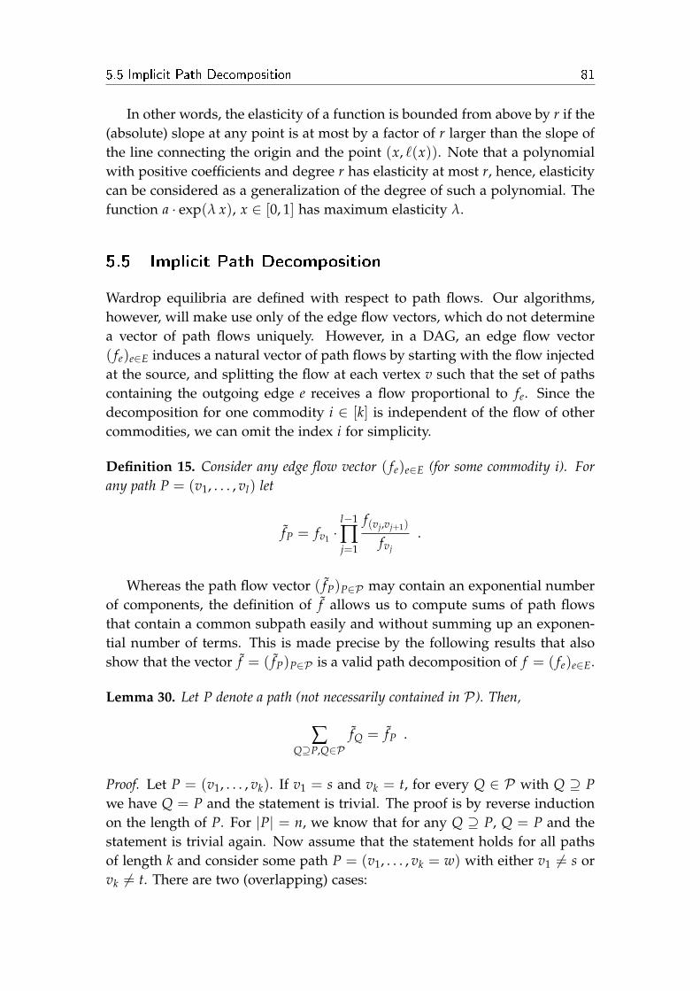
5.5 Implicit Path Decomposition 81
In other words, the elasticity of a function is bounded from above by r if the(absolute) slope at any point is at most by a factor of r larger than the slope ofthe line connecting the origin and the point (x, `(x)). Note that a polynomialwith positive coefficients and degree r has elasticity at most r, hence, elasticitycan be considered as a generalization of the degree of such a polynomial. Thefunction a · exp(λ x), x ∈ [0, 1] has maximum elasticity λ.
5.5 Implicit Path Decomposition
Wardrop equilibria are defined with respect to path flows. Our algorithms,however, will make use only of the edge flow vectors, which do not determinea vector of path flows uniquely. However, in a DAG, an edge flow vector( fe)e∈E induces a natural vector of path flows by starting with the flow injectedat the source, and splitting the flow at each vertex v such that the set of pathscontaining the outgoing edge e receives a flow proportional to fe. Since thedecomposition for one commodity i ∈ [k] is independent of the flow of othercommodities, we can omit the index i for simplicity.
Definition 15. Consider any edge flow vector ( fe)e∈E (for some commodity i). Forany path P = (v1, . . . , vl) let
fP = fv1 ·l−1
∏j=1
f(vj,vj+1)
fvj
.
Whereas the path flow vector ( fP)P∈P may contain an exponential numberof components, the definition of f allows us to compute sums of path flowsthat contain a common subpath easily and without summing up an exponen-tial number of terms. This is made precise by the following results that alsoshow that the vector f = ( fP)P∈P is a valid path decomposition of f = ( fe)e∈E.
Lemma 30. Let P denote a path (not necessarily contained in P). Then,
∑Q⊇P,Q∈P
fQ = fP .
Proof. Let P = (v1, . . . , vk). If v1 = s and vk = t, for every Q ∈ P with Q ⊇ Pwe have Q = P and the statement is trivial. The proof is by reverse inductionon the length of P. For |P| = n, we know that for any Q ⊇ P, Q = P and thestatement is trivial again. Now assume that the statement holds for all pathsof length k and consider some path P = (v1, . . . , vk = w) with either v1 6= s orvk 6= t. There are two (overlapping) cases:

82 Chapter 5. Distributed Approximation
1. vk 6= t. Then,
∑Q⊇P,Q∈P
fQ = ∑u∈Succ(vk)
∑Q⊇P·(vk,u),Q∈P
fQ
= ∑u∈Succ(vk)
fP·(vk,u)
= ∑u∈Succ(vk)
fP ·f(vk,u)
fvk
= fP .
The second equality is the induction hypothesis and the third is the def-inition of f .
2. v1 6= s. Analogous.
As a corollary, we see that the flow decomposition ( fP)P∈P is actually com-patible with the original path flows ( fe)e∈E. In addition, for every P ∈ P , fP isobviously non-negative.
Corollary 31. For any e ∈ E,fe = ∑
P3efP .
Proof. Consider an edge e = (v, w). Then,
fe = fv ·fe
fv= fe = ∑
P3e,P∈PfP ,
where the second inequality is the definition of fe and last equality is due toLemma 30.
5.6 Distributed Computation Model
Our algorithms operate in the following setting. Agents operate in a syn-chronous, round-based fashion. We assume that there is a billboard via whichthe agents are able to share information. On this billboard each agent canobserve the edge flows of its own commodity and the latency values of thepaths it uses. Agents know an upper bound r on the elasticity of the latencyfunctions, but they do not know the latency functions themselves. However,it is easily possible to extend our algorithm such that it does not rely on theknowledge of a bound on the elasticity.
In every round an agent can update the edge flows of its own commodityon the billboard. These updates become visible to all agents only in the next

5.7 A Pseudopolynomial Algorithm 83
round. All agents execute the same algorithm in parallel. Therefore, in thedescriptions of our algorithms, we may omit the index for the commodity, i. e.,fe refers to the flow fe,i of commodity i on edge e.
Let us remark that the billboard is a purely theoretical construction. Itmay model systems where this information is collected centrally and polledby or broadcast to the agents at intervals, but may also model scenarios inwhich agents concurrently perform measurements over finite intervals of timein order to obtain the necessary latency information.
5.7 A Pseudopolynomial Algorithm
Our first approach works by simulating the replication policy presented in [?].We will see that this can be done in polynomial time although this policyoperates on an exponential number of paths.
5.7.1 The Replication Policy
Let us start by introducing the replication policy formally. We consider aninfinite set of agents each of which controls an infinitesimal amount of flowwhich it assigns to a path. In each round agents may migrate their flow fromthe current path to another one. Consider an agent in commodity i ∈ [k]currently using path P ∈ Pi. Whenever activated it performs two steps.
1. Sampling. Sample another path Q where the probability to sample anypath Q′ equals fQ′/di.
2. Migration. There are two cases:
(a) `Q ≥ `P. In this case the agent stays with its old path.
(b) `Q < `P. The agent migrates to the sampled path Q with probabilityλ · (`P − `Q) for some constant λ > 0 to be determined later.
Altogether, we can characterize our policy by specifying the rate of agentsmigrating from one path P ∈ Pi to another path Q ∈ Pi with `Q( f ) < `P( f )within one round. This rate can be obtained by multiplying the probabilitiesspecified in steps (1) and (2) with the volume of agents using path P. For thisrate we obtain
ρPQ = λ · fP ·fQ
di· (`P − `Q)

84 Chapter 5. Distributed Approximation
if `Q < `P and ρPQ = 0 otherwise. Thus, we can compute a sequence of flowvectors ( fP(t))P∈P generated by this policy by summing over all paths Q:
fP(t + 1) = fP(t) + ∑Q∈Pi
ρQP − ∑Q∈Pi
ρPQ
= fP(t) + λ fP ∑Q∈Pi
fQ
di(`Q − `P)
= fP(t) + λ fP (Li − `P) . (5.1)
5.7.2 Convergence Towards Equilibria
For the time being assume that agents are migrating in a continuous fashionas described by the above rules. Then an infinitesimal amount of flow dx mi-grating from a path P to another path Q improving its latency from `P to `Q
causes the potential Φ to reduce by (`P − `Q) dx. Since we only accept migra-tions that improve the latency, this implies that the potential always decreaseswhich in turn implies convergence towards a Wardrop equilibrium if all pathsare used in the initial flow. However, in our concurrent round-based model,flow is not shifted continuously, but in finite chunks. Thus, if these chunksare chosen too large, overshooting and oscillation effects may occur. This issuecan be resolved by choosing the migration rate in step 2(b) of the replicationpolicy carefully. In [?] it was shown that if we choose λ = Θ(1/`′max) smallenough with
`′max = maxP∈P
maxf∈F ∑
e∈P`′e( f ) ,
convergence towards Wardrop equilibria can be guaranteed (provided that ini-tially all paths have non-zero flow and hence positive sampling probability).We may assume that `′max > 0 since otherwise all latency functions are con-stant, and our problem can be solved trivially by assigning the entire flow tothe path with lowest latency.
Theorem 32 ( [?, ?, ?]). If λ = Θ(1/`′max) sufficiently small, the replication policygiven by Equation (5.1) with initial flow f (0) = f 0 converges towards a Wardropequilibrium if f 0
P > 0 for all P ∈ P . Furthermore, the number of rounds in which theflow is not at a δ-ε-equilibrium is
O(
1ε2 δ2 ·
`′max`min
· log(
Φ( f 0)Φ∗
))where `min denotes a lower bound on the latency on any edge.
One may observe that the ratio between maximum slope and minimumlatency used in this theorem depends on the scale by which we measure flow.This scale, however, is fixed since we have normalized the total flow demandto be d = 1.

5.7 A Pseudopolynomial Algorithm 85
5.7.3 Simulating the Replication Policy
By a naive application of Theorem 32 we can compute a sequence of flowvectors ( f (t))t≥0 according to Equation (5.1) to obtain approximate Wardropequilibria. However, this approach is rendered computationally intractable bythe fact that there may be an exponential number of variables fP.
In the following, we describe an algorithm that computes the iterativechange rates of the edge flows according to the implicit flow decompositionf described in the preceding section. To that end, we show that the changerates of the edge flows fe can be expressed solely in terms of edge flows andedge latencies (i. e., without explicit reference to the fP variables). It suffices toknow the weighted average latencies of all paths containing e defined as
Le = ∑P3e
fP
fe· `P . (5.2)
Recall that we have fixed a commodity here, so we may drop the index i.
Lemma 33. Consider an edge flow vector ( fe(t))e∈E and its path decomposition f (t),and let f (t + 1) denote the flow generated by the replication policy in Equation (5.1)from f (t). Finally, let fe(t + 1) = ∑P3e fP(t + 1). Then,
fe(t + 1) = fe(t) + λ · fe(t) · (C− Le) .
Proof. Let f = f (t) and f ′ = f (t + 1). By definition of fe,
f ′e − fe = ∑P3e
( f ′P − fP)
= λ · ∑P3e
fP · (C− `P)
= λ · fe ·(
C− ∑P3e fP`P
fe
),
where the last term equals Le.
In order to obtain the value of Le, we implicitly compute the path decompo-sition f , i. e., for every edge e′ we compute the flow caused by paths containinge on edge e′. This is done by Algorithm SimulatedReplication e ∈ E. Sincethere are m edges, each iteration can be performed in time O
(m2).
Corollary 34. The sequence of flow vectors computed by Algorithm SimulatedRepli-cation converges towards the set of Wardrop equilibria. Furthermore, the number ofrounds in which the flow is not at a δ-ε-equilibrium with respect to f is bounded by
O(
1ε2 δ2 ·
`′max`min
· log(
Φ( f 0)Φ∗
)),
where f 0 is the initial flow vector. Each iteration takes time O(m2).

86 Chapter 5. Distributed Approximation
Algorithm 2 SimulatedReplication() (executed by all commodities in paral-lel; ( fe)e∈E denotes the edge flows vector of commodity i)
1: for all edges e ∈ E do2: sort all edges (v, w) in the subgraph reachable from e topologically3: compute total flow of all paths containing e and (v, w):
f (v,w)e = ∑(u,v)∈E f (u,v)
e · f(v,w)fv
4: reverse all edges and repeat steps 2 and 3 for edges between e and s
5: compute Le = ∑e′f e′efe
`e′
6: f ′e ← fe + λ · fe · (C− Le) with λ = 1/`′max7: end for8: replace ( fe)e∈E on the billboard with ( f ′e)e∈E
Proof. First note that for any edge e′ the value of f e′e computed in line 3 of the
algorithm equals the volume of all paths containing e and e′ with respect toour implicit decomposition f , i. e., f e′
e = ∑P⊇e,e′ fP. Thus, the value Le com-puted in line 5 equals the definition of Le in Equation (5.2). Hence, Lemma 33implies that the edge flow vector computed by our algorithm after one roundequals the edge flow vector obtained by applying the replication policy givenby Equation (5.1) to the path decomposition ( f )P∈P . Combining this with theupper bounds on the convergence time given in [?, ?], the claim follows.
5.8 The Polynomial Time Algorithm
The migration probability specified for step 2(b) of the replication policy canget very small since the latency difference `P− `Q may become small in relationto `′max if λ = 1/`′max is chosen constant. This causes the algorithm to achieveonly a pseudopolynomial convergence time depending on the maximum slopeof the latency functions. In this section we present an approach that avoids thisdependence.
To this end, we choose the amount of flow removed from a path propor-tional to its relative deviation (`P − LiP)/`P from the average and the recip-rocal of the elasticity r to obtain a polynomial number of communicationrounds. Whereas in the preceding section the amount of flow removed oradded to a path within one round could be expressed in a nice closed form asλ · fP · (C− `P) (Equation (5.1)), this is now no longer possible.
To compute flow updates in polynomial time we use a randomized flowdecomposition. First, we sample a path at random according to the implicitpath decomposition f , i. e., the probability to sample path P is fP/diP . Since thelength of a path is bounded by n, this is possible in time n log n by representingadjacent vertices and their flows in a binary tree. Now, the path is assigned a
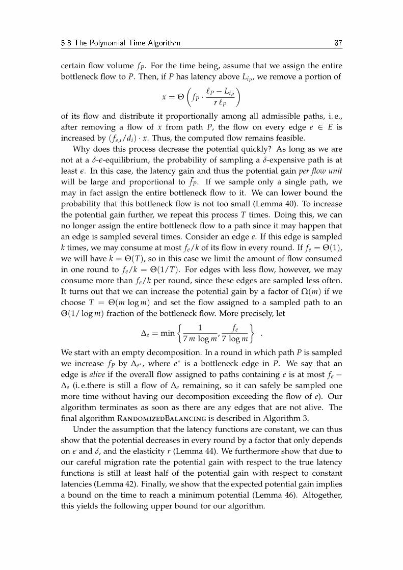
5.8 The Polynomial Time Algorithm 87
certain flow volume fP. For the time being, assume that we assign the entirebottleneck flow to P. Then, if P has latency above LiP , we remove a portion of
x = Θ(
fP ·`P − LiP
r `P
)of its flow and distribute it proportionally among all admissible paths, i. e.,after removing a flow of x from path P, the flow on every edge e ∈ E isincreased by ( fe,i/di) · x. Thus, the computed flow remains feasible.
Why does this process decrease the potential quickly? As long as we arenot at a δ-ε-equilibrium, the probability of sampling a δ-expensive path is atleast ε. In this case, the latency gain and thus the potential gain per flow unitwill be large and proportional to fP. If we sample only a single path, wemay in fact assign the entire bottleneck flow to it. We can lower bound theprobability that this bottleneck flow is not too small (Lemma 40). To increasethe potential gain further, we repeat this process T times. Doing this, we canno longer assign the entire bottleneck flow to a path since it may happen thatan edge is sampled several times. Consider an edge e. If this edge is sampledk times, we may consume at most fe/k of its flow in every round. If fe = Θ(1),we will have k = Θ(T), so in this case we limit the amount of flow consumedin one round to fe/k = Θ(1/T). For edges with less flow, however, we mayconsume more than fe/k per round, since these edges are sampled less often.It turns out that we can increase the potential gain by a factor of Ω(m) if wechoose T = Θ(m log m) and set the flow assigned to a sampled path to anΘ(1/ log m) fraction of the bottleneck flow. More precisely, let
∆e = min
17 m log m
,fe
7 log m
.
We start with an empty decomposition. In a round in which path P is sampledwe increase fP by ∆e∗ , where e∗ is a bottleneck edge in P. We say that anedge is alive if the overall flow assigned to paths containing e is at most fe −∆e (i. e.there is still a flow of ∆e remaining, so it can safely be sampled onemore time without having our decomposition exceeding the flow of e). Ouralgorithm terminates as soon as there are any edges that are not alive. Thefinal algorithm RandomizedBalancing is described in Algorithm 3.
Under the assumption that the latency functions are constant, we can thusshow that the potential decreases in every round by a factor that only dependson ε and δ, and the elasticity r (Lemma 44). We furthermore show that due toour careful migration rate the potential gain with respect to the true latencyfunctions is still at least half of the potential gain with respect to constantlatencies (Lemma 42). Finally, we show that the expected potential gain impliesa bound on the time to reach a minimum potential (Lemma 46). Altogether,this yields the following upper bound for our algorithm.

88 Chapter 5. Distributed Approximation
Theorem 35. Assume that for the initial flow vector f0 it holds that fe > 0 for alle ∈ E. Then, the sequence of flow vectors computed by Algorithm RandomizedBal-ancing converges towards the set of Wardrop equilibria. Furthermore, the expectednumber of rounds, in which the flow is not at a δ-ε-equilibrium with respect to f , isbounded by
O(
rε3 δ2 log
(Φ( f0)
Φ∗
)),
if r is an upper bound on the elasticity of the latency functions. The computation timeof each round is bounded by O (n log n ·m log m).
We present the proof after establishing the necessary lemmas.
Algorithm 3 RandomizedBalancing(r) (executed by all commodities in par-allel; ( fe)e∈E denotes the edge flows vector of commodity i)
1: F ← 02: for T = m log m times do
3: sample a path P where P [P] = fPdi
4: let e∗ denote the bottleneck edge of P; let fP = ∆e∗
5: if `P > Li then6: reduce the flow on all edges e ∈ P by ∆ fP = fP · `P−Li
4 r `P7: F ← F + ∆ fP
8: if for any e ∈ P, e is not alive then9: abort loop and continue in line 13
10: end if11: end if12: end for13: increase the flow on all edges e ∈ E proportionally by fe
di· F
Note that our algorithm can be easily modified for the case that the elastic-ity of the latency functions is not known to the algorithm in advance. In thatcase, we can find an upper bound r on the maximum elasticity by using anexponential search technique. We continue doubling the value of r until forthe first time it holds that for all edges relevant to the commodity, the elasticityof the latency functions is bounded by r within the interval defined by the oldand new flow values.
5.8.1 Useful Inequalities
To establish the necessary lemmas we make use of the following well knownfacts.

5.8 The Polynomial Time Algorithm 89
Lemma 36 (Chernoff Bound [?]). Let X be a real valued random variable that isthe sum of 0-1 random variables. Then
P [X ≥ q ·E [X]] ≤ 2−q·E[X]
for q ≥ 6.
Lemma 37 (Markov’s Inequality). Let X be a real valued random variable andh : R→ R monotone non-decreasing. If E [h(X)] is defined, then
P [X ≥ a] ≤ E [h(X)]h(a)
.
Lemma 38 (Jensen’s Inequality). Let X be real valued random variable and f : R→R a convex function. If E [X] and E [ f (X)] are defined, then
E [ f (X)] ≤ f (E [X]) .
Lemma 39 (Cauchy Schwarz Inequality). For two vectors (ai), (bi) ∈ Rn
(n
∑i=1
ai bi)2 ≤ (n
∑i=1
a2i )(
n
∑i=1
b2i ) .
5.8.2 Randomized Decomposition
Our algorithm generates a randomized flow decomposition using a samplingprocess based on f . In this section, we lower bound the probability that thebottleneck flows of the sampled paths are not too small. Furthermore, weshow that the total flow volume removed from every edge is at most fe withhigh probability.
For a unit flow f , let PP∼ f [X(P)] denote the probability that event X(P)occurs if the probability to draw a path P equals fP.
Lemma 40. Consider a flow f of unit demand and a set of paths Pε with ∑P∈PεfP =
ε. Then,
PP∼ f
[P ∈ Pε ∧min
e∈Pfe ≥
ε
2 m
]≥ ε
2.
Proof. We consider a scaled flow vector which supports only paths in Pε.
f ′P =
fPε P ∈ Pε
0 P /∈ Pε .
Observe that the total demand of f ′ is 1 again, hence
PP∼ f ′ [P = Q] = PP∼ f [P = Q | P ∈ Pε] .
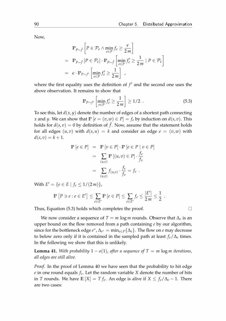
90 Chapter 5. Distributed Approximation
Now,
PP∼ f
[P ∈ Pε ∧min
e∈Pfe ≥
ε
2 m
]= PP∼ f [P ∈ Pε] ·PP∼ f
[mine∈P
f ′e ≥1
2 m| P ∈ Pε
]= ε ·PP∼ f ′
[mine∈P
f ′e ≥1
2 m
],
where the first equality uses the definition of f ′ and the second one uses theabove observation. It remains to show that
PP∼ f ′
[mine∈P
f ′e ≥1
2 m
]≥ 1/2 . (5.3)
To see this, let d(x, y) denote the number of edges of a shortest path connectingx and y. We can show that P [e = (v, w) ∈ P] = fe by induction on d(s, v). Thisholds for d(s, v) = 0 by definition of f . Now, assume that the statement holdsfor all edges (u, v) with d(s, u) = k and consider an edge e = (v, w) withd(s, v) = k + 1.
P [e ∈ P] = P [v ∈ P] ·P [e ∈ P | v ∈ P]
= ∑(u,v)
P [(u, v) ∈ P] · fe
fv
= ∑(u,v)
f(u,v) ·fe
fv= fe .
With E′ = e ∈ E | fe ≤ 1/(2 m),
P[P 3 e : e ∈ E′
]≤ ∑
e∈E′P [e ∈ P] ≤ ∑
e∈E′fe ≤
|E′|2 m≤ 1
2.
Thus, Equation (5.3) holds which completes the proof.
We now consider a sequence of T = m log m rounds. Observe that ∆e is anupper bound on the flow removed from a path containing e by our algorithm,since for the bottleneck edge e∗, ∆e∗ = mine∈P∆e. The flow on e may decreaseto below zero only if it is contained in the sampled path at least fe/∆e times.In the following we show that this is unlikely.
Lemma 41. With probability 1− o(1), after a sequence of T = m log m iterations,all edges are still alive.
Proof. In the proof of Lemma 40 we have seen that the probability to hit edgee in one round equals fe. Let the random variable X denote the number of hitsin T rounds. We have E [X] = T fe. An edge is alive if X ≤ fe/∆e − 1. Thereare two cases:

5.8 The Polynomial Time Algorithm 91
1. fe < 1m implying ∆e = fe/(7 log m). Then,
P
[X >
fe
∆e− 1]
= P
[X > E [X] ·
(7
fe m− 1
T fe
)]≤ P
[X > E [X] ·
(6
fe m
)]≤ 2−E[X]· 6
fe m = m−6 .
The first inequality is the definition of T and ∆e and uses our assump-tion that fe · m < 1, and the second inequality is Chernoff’s inequality(Lemma 36).
2. fe ≥ 1m implying ∆e = 1/(7 T). Then, with the same arguments,
P
[X >
fe
∆e− 1]
= P
[X > E [X] ·
(1
T ∆e− 1
T fe
)]≤ P
[X > E [X] ·
(7− 1
log(m)
)]≤ 2−6·E[X] ≤ 2−6·log m = m−6 .
This time the first inequality uses our assumption fe ≥ 1/m.
In both cases, the probability that edge e is not alive at the end of a sequenceof T iterations is bounded by m−6. Using a union bound, the probabilitythat at least one edge does not survive is at most m−5, and consequently theprobability that all edges survive the sequence is at least 1−m−5.
5.8.3 Lower Bounding the Potential Gain
We use a potential function argument to prove convergence. In order to showthat our algorithm avoids oscillations, we consider the potential gain achievedwithin one round. We show that this potential gain is at least half of the po-tential gain that would occur if latency values were fixed at the beginning of around. A second lemma shows that, in expectation, the potential decreases bya factor in every round, as long as we are not yet at an approximate equilib-rium.
Lemma 42. Let r denote an upper bound on the elasticity of the latency functions. Fora flow vector f consider a flow vector f ′ generated by Algorithm RandomizedBal-ancing(r) (Algorithm 3) with positive probability. For any P ∈ P let ∆ fP denotethe amount of flow removed from path P. Then,
Φ( f )−Φ( f ′) ≥ 12· ∑
P∈P(`P( f )− LiP) · ∆ fP .

92 Chapter 5. Distributed Approximation
To prove the lemma, we need the following fact about functions withbounded elasticity:
Fact 43 ( [?]). If the elasticity of a function ` is bounded from above by r, then for0 ≤ δ ≤ 1/(2 r), it holds that `((1 + δ) · x) ≤ (1 + 2 r δ) · `(x).
Proof (of Lemma 42). Throughout this proof, whenever we write `, Li and Cwithout an argument, we refer to `( f ), Li( f ) and C( f ). Let VP = (`P− LiP) ∆ fP
denote the virtual potential gain of any path P with `P ≥ Li. It can easily bechecked (see [?]) that
Φ( f )−Φ( f ′) = ∑P∈P
VP − ∑e∈E
∫ f ′e
fe(`e(u)− `e) du .
The true potential gain Φ( f )−Φ( f ′) would be achieved if the latency valuesdid not change due to the changing flow. The terms in the second sum canbe understood as error terms that reduce the potential gain to account for thisidealistic assumption. We show that the error terms are at most half of thevirtual potential gain. To that end, we attribute
VeP = VP ·
fe,iP · `e
2 · diP · C= (`P − LiP) · ∆ fP ·
fe,iP · `e
2 · diP · C
of the virtual potential gain made by path P to edge e. Note that summingover all edges e, this consumes precisely half of the virtual potential gain ofpath P, i. e., ∑e∈E Ve
P = VP/2. Thus, by a reordering of the terms,
Φ( f )−Φ( f ′) ≤ ∑P∈P
VP
2+ ∑
e∈E
(∑
P∈PVe
P −∫ f ′e
fe(`e(u)− `e) du
).
Hence, to prove the theorem it suffices to show that for any edge e ∈ E,∫ f ′e
fe(`e(u)− `e) du ≤ ∑
P∈PVe
P . (5.4)
Fix an edge e ∈ E and assume f ′e > fe. Edges with f ′e < fe can be treatedsymmetrically. We partition the integral over the interval [ fe, f ′e ] into segmentsof width ∆ f e
P, where ∆ f eP = ∆ fP · fe,iP /diP is the amount of flow moved from
P to paths containing e. We consider the sequence of paths Pj sampled by ouralgorithm in ascending order of (`P − LiP)/`P. In this sequence a path mayoccur more than once. Let f l
e = fe + ∑lj=1 ∆ f e
Pj. To conclude the proof, we
prove Equation (5.4) by showing that for l ≥ 0
∫ f le
fe(`e(u)− `e) du ≤
l
∑i=1
VePi

5.8 The Polynomial Time Algorithm 93
by induction on l. Then, the increase of flow of edge e caused by the first lpaths is
f le − fe ≤
l
∑j=1
∆ fPj ·fe,iPj
diPj
≤l
∑j=1
fPj ·`Pj − LiPj
4 r · `Pj
·fe,iPj
diPj
≤ 14 r·`Pl − LiPl
`Pl
·k
∑i=1
fe,i
≤ 14 r·`Pl − LiPl
`Pl
· fe .
The third inequality holds since we can separate the sum into sums over pathsfrom only one commodity. Then the fP in sum cancel out the di’s. Now, due tothe bounded elasticity of `e, we can apply Fact 43 to bound the total increaseof latency caused by this increase of flow by
∆`le = `e( f l
e)− `e ≤ 2 r · `e ·f le − fe
fe≤ `e ·
`Pl − LiPl
2 `Pl
.
Using the definition of ∆ f ePl
,
∆ f ePl· ∆`l
e ≤`e fe,iPl
2 `Pl diPl
· (`Pl − LiPl) · ∆ fPl ≤ Ve
Pl.
Using the induction hypothesis and the preceding inequality we have
∫ f le
fe(`e(u)− `e) du ≤
∫ f l−1e
fe(`e(u)− `e) du + ∆ f e
Pl· ∆`l
e ≤l
∑i=1
VePi
and the proof is complete.
Lemma 44. Assume that f is a flow that is not at δ-ε-equilibrium, and let the randomvariable f ′ denote a flow generated by our algorithm. Then
E[Φ( f ′)
]≤ Φ( f ) ·
(1−Ω
(ε3δ2
r
)).
Proof. For the time being, assume that the latency functions are constant. Ap-plying Markov’s inequality (Lemma 37) with X = Li, a = 2 L/ε and h = id,the total volume of flow in commodities with Li > 2 · C/ε is at most ε/2. Weconsider only commodities with Li ≤ 2 · C/ε. In total, at least a flow volumeof ε utilizes δ-expensive paths, and there is still at least a volume of ε/2 left in

94 Chapter 5. Distributed Approximation
the commodities we consider. Consider such a commodity i ∈ [k], and denotethe flow volume using δ-expensive paths in this commodity by εi.
Consider any iteration satisfying the precondition that all edges are alive.Let P denote the path sampled by the algorithm. Consider the event that`P ≥ Li + δ C and the minimum edge flow along P is at least εi/(2 m). ByLemma 40 the probability of this event is at least εi/(2 di) (we have to scale theflow of this commodity by a factor 1/di to make it a unit flow). The amountof flow removed from this path by our algorithm is
εi
2 m· 1
7 log m· `P − Li
4 r `P≥ εi ε δ
113 r m log m
where we have used that `P ≥ Li + δ C and Li ≤ 2 C/ε. The latency gain of thispath is then at least δ C. Since this event happens with probability εi/(2 di) theexpected virtual potential gain of such a path is then at least
ε2i ε δ2
226 r di m log mC .
By Lemma 41 the probability that in this iteration all edges are alive is 1− o(1),and the expected potential gain computed above is independent of this event.Summing up over all T = m log m iterations and all commodities, the totalexpected virtual potential gain of one round is at least
(1− o(1)) · ∑i∈[k]
ε2i ε δ2
226 r diC ≥ (1− o(1)) · ε3δ2
226 rC .
For the last inequality we have applied the Cauchy Schwarz Inequality (seeLemma 39) with ai = εi/
√di and bi =
√di. This implies the claim since C is
an upper bound on Φ and Lemma 42 ensures that the true potential gain withrespect to the real latency functions is at least half of the potential gain withrespect to the constant latency functions.
5.8.4 From Expected Potential Gain to Expected Stopping
Time
The preceding section has shown that in every round the potential decreases bya factor in expectation. Intuitively, this implies an expected running time thatis logarithmic in this factor and the initial values. This intuition is made preciseby the following two lemmas. Although it seems likely that similar lemmashave been proven elsewhere before, we are not aware of any formulation thatcan be used here.

5.8 The Polynomial Time Algorithm 95
Lemma 45. Let X0, X1, . . . denote a sequence of non-negative random variables. As-sume that for all i ≥ 0
E [Xi | Xi−1 = xi−1] ≤ xi−1 − 1
and let τ denote the first time t such that Xt = 0. Then,
E [τ | X0 = x0] ≤ x0 .
Proof. The proof is by induction on x0. Let
T(s) = E [τ | X0 = s] .
Clearly, T(0) = 0. For i ∈ [x0] let p(i) denote the probability that x0 − X1 = i.By our assumption and definition of p(i),
1 ≤ x0 −E [X1 | X0 = x0] =x0
∑i=0
p(i) · i .
By definition of T(j),
T(j) = 1 +j
∑i=0
p(i) · T(j− i)
≤ 1 + p(0) · T(j) +j
∑i=1
p(i) · (j− i)
= 1 + p(0) · T(j) + j · (1− p(0))−j
∑i=1
p(i) · i
≤ p(0) · T(j) + j · (1− p(0))
where the first inequality uses the induction hypothesis for 1 ≤ i < j. Hence,T(j) ≤ j, implying our claim.
Lemma 46. Let X0, X1, . . . denote a sequence of non-negative random variables. As-sume that for all i ≥ 0
E [Xi | Xi−1 = xi−1] ≤ xi−1 · α
for some constant α ∈ (0, 1). Furthermore, fix some constant x∗ ∈ (0, x0], and let τ
be the random variable that describes the smallest t such that Xt ≤ x∗. Then,
E [τ | X0 = x0] ≤2
log(1/α)· log
( x0
x∗)
.

96 Chapter 5. Distributed Approximation
Proof. In order to apply Lemma 45 we transform our random variable into anew sequence of random variables
Yi = 2 · log(Xi)− log(x∗)log(1/α)
.
Let xi = 2yi·log(1/α)/2+log x∗ . Then,
E [Yi | Yi−1 = yi−1] = E
[2 · log(Xi)− log x∗
log(1/α)| Xi−1 = xi−1
]= 2 · E [log(Xi) | Xi−1 = xi−1]− log(x∗)
log(1/α)
≤ 2 · log (E [Xi | Xi−1 = xi−1])− log(x∗)log(1/α)
≤ 2 · log(xi−1 · α)− log(x∗)log(1/α)
= yi−1 − 2
where the first inequality is Jensen’s inequality (Lemma 38) and the second isour assumption on the sequence Xi. Observe that Xi = x∗ if and only if Yi = 0and bYi + 1c = 0 implies that Xi ≤ x∗. Now,
E [bYic | bYi−1c = yi−1] ≤ E [Yi | bYi−1c = yi−1]
≤ maxz:byi−1c=z
E [Yi | Yi−1 = z]
≤ maxz:byi−1c=z
z− 2
≤ yi−1 − 1
implying that the sequence bYic satisfies the conditions of Lemma 45. Let τ
denote the smallest i such that bYi + 1c = 0, and observe that X0 = x0 impliesbY0 + 1c = b2 log(x0/x∗)/ log(1/α) + 1c. Hence,
E [τ | X0 = x0] ≤ E [τ | X0 = x0]
≤ E
[τ | bY0 + 1c =
⌊2 · log(x0/x∗)
log(1/α)+ 1⌋]
≤⌊
2 · log(x0/x∗)log(1/α)
+ 1⌋
,
our desired bound.
5.8.5 Convergence Time
Finally, we can prove our main result.

5.8 The Polynomial Time Algorithm 97
Proof of Theorem 35. Again, convergence follows from Lemma 42 as in [?]. Toobtain a bound on the convergence time, let f0, f1, . . . denote a sequence offlow
E [Φ( ft+1) | Φ( ft) = φ] ≤ φ ·(
1−Ω(
ε3 δ2
r
)).
Thus, the sequence (Φ( ft))t≥0 satisfies the conditions of Lemma 46 and theexpected time until Φ( ft) reaches its minimum Φ∗ implying that ft is a δ-ε-equilibrium is
2
log((
1−Ω(
ε3 δ2
r
))−1) log
(Φ( f0)
Φ∗
)= O
(r
ε3 δ2 log(
Φ( f0)Φ∗
)),
our desired bound.One path can be sampled in time O (n log n), the bottleneck edge can be
found in time O (n), and the flow update can be computed in time O (n).Altogether, at most T = m log m iterations have to be computed. Finally, theremoved flow can be reinserted in time O (m).

Chapter 6
Concluding Thoughts
In this thesis we have studied a variety of problems in Wardrop’s traffic modelthat revolve around the inefficiency of equilibria and their paradoxical behav-ior. We analyzed two different means to reduce the price of anarchy, studiedthe stability and sensitivity of equilibria, and designed a distributed algorithmto compute approximate equilibria. Throughout our research, structural sim-ple networks like parallel link networks or Braess’s original network served asbenchmark networks providing first insight, guiding our research, and finallyextending our understanding of Wardrop equilibria.
6.1 Reducing the Price of Anarchy
In the first part of this thesis, we draw connections between several establishedconcepts of reducing the price of anarchy. Generalizing marginal cost pricing,we first investigated optimal taxes if only a subnetwork can be taxed. Whilewe provided an efficient algorithm to compute taxes minimizing the networkwide performance in parallel link networks with linear latency functions, thisproblem turned out to be NP-hard in arbitrary networks with multiple com-modities. Our positive results may seem quite restricted, however, observethat in contrast the optimal leader strategy in Stackelberg routing is NP-hardto compute for the same class of simple networks [?].
Our results lead to a set of intriguing questions. The prime goal is an ap-proximation algorithm for multi-commodity networks. Unfortunately, we arenot aware of any non-trivial approximation algorithms incurring an approxi-mation ratio less than the price of anarchy. For single-commodity networks aninteresting question is whether one can close the “complexity gap” or not. Canone extend the NP-hardness results to more general classes of networks? Isthere a polynomial time algorithm for parallel link networks with polynomiallatency functions? Technically, the reasons that our proof fails for polynomial

100 Chapter 6. Concluding Thoughts
latency functions are that the total latency does not remain convex and thelatency threshold L(d) does not remain linear.
Also, the question of how to optimally set taxes for a finite set of edgesor even for a single edge remains open. Algorithms for this problem couldconstitute useful modules for approximation algorithms for the general case.Following this line of research, first (albeit negative) results have been obtainedrecently [?].
Towards another direction, one might want to abandon the strong homo-geneity assumption. Even for heterogeneous network users that minimizetheir own tax versus total latency, optimal taxes can be computed efficientlyfor arbitrary multi-commodity networks [?, ?, ?]. What can be said about thecomplexity of finding optimal taxes for a given subset of edges in this case?
As outlined we tackled the problem of computing optimal taxes for a givensubset of edges. But in the first place, one needs to decide, which set of links totax, given a choice. In light of the large number of possible sets and complexinteractions between taxes on different edges, this problem seems intriguing.Considering the related problem of computing optimal taxes, such that anadditional tax-dependent objective function, e.g., the number of taxed edges isoptimized, positive results have been obtained recently [?].
To dispense with direct taxing, we proposed a novel approach to reducethe price of anarchy by routing additional flow. Routing so-dubbed auxiliaryflow δ raises the edge latencies for the selfish flow and thus can be consideredas charging the selfish agents a non-refundable traffic dependent tax of `e( fe +δe)− `e( fe). There is also a strong connection to Stackelberg routing when theauxiliary flow is seen as the flow of a leader, who centrally routes its fraction offlow to improve the global performance. However, the critical difference is thatthe leader’s latency does account for the total latency, while the auxiliary flow’slatency does not. This is the reason why our results on auxiliary flow contrastthose obtained for Stackelberg routing. In particular, the minimal amount ofleader flow inducing the optimal flow can be computed in polynomial timein arbitrary multi-commodity networks [?]. For auxiliary flow this value isNP-hard to approximate even within subexponential factors. Alternatively,auxiliary flow can be interpreted as a separate altruistic commodity that triesto pilot the routing of the selfish players to a globally desirable state. In relatedwork it was shown that when all agents are assumed to be partly altruistic, theprice of anarchy can be bounded by a constant in parallel link networks [?].Yet, using (altruistic) auxiliary flow does not improve the network performancein this class of networks.
Our hardness result for optimal auxiliary flow is tight for networks withlinear latency functions, because the trivial algorithm, i. e., routing no spam,yields a 4/3 approximation [?]. For more general sets of latency functions, e. g.,

6.2 Sensitivity Analysis 101
for polynomials of bounded degree, the presented instances do not directlyyield tight inapproximability results. The question if the trivial algorithm isan optimal algorithm for nonlinear latency function is still open.
Reducing the price of anarchy by simply routing an additional amount offlow seems an appealing approach. But yet, our results show that importantproblems related to this approach are rendered computationally infeasible. Wehope that our hardness results inherently rely on the fact that we have confinedourself to extremal auxiliary flow. This would still allow efficient computationof flow that improves total latency by an arbitrary amount. Such algorithmsas well as the design of non-trivial approximation algorithms for the problemsconsidered here would certainly be of great interest.
6.2 Sensitivity Analysis
In his ground-breaking work, Braess [?] observed that adding capacity to a net-work might improve or deteriorate the total latency depending on the amountof input traffic. In other words, the occurrence of Braess’s paradox is demandsensitive. We employ a family of generalized Braess graphs to bring anotherremarkable facet of Wardrop equilibria into the open: Even the slightest in-crease in the demand may cause every agent to change its path.
However, our sensitivity analysis leaves open some obvious questions. Givena unit demand flow at Wardrop equilibrium, suppose an edge carrying onlyan ε-fraction of flow is removed. How does the path latency change after re-covering equilibrium? Considering a network with two parallel edges, onegets a lower bound of 1
(1−ε)p . Is this bound tight? Furthermore, we believe thatour bound on the increase of the path latency induced by a demand increaseof (1 + ε)p holds not only for polynomials of bounded degree but for latencyfunctions with bounded elasticity.
Less specifically, we believe that studying sensitivity of traffic equilibria isa natural and important task that is worthwhile also in related models, e. g.,in the presence of heterogeneous agents or in scenarios where finitely manyagents can split their non-negligible amount of flow. Further, while most ex-isting literature on sensitivity analysis concentrates on qualitative questions,we are convinced that quantitative studies are equally important and that bothkinds of results nicely complement one another. In this spirit, we have shownthat the vector of edge flows is not only continuously dependent on the trafficdemand [?], but in fact Lipschitz-continuous with constant one (Theorem 27).

102 Chapter 6. Concluding Thoughts
6.3 Distributed Equilibrium Computation
Braess’s original four vertex network demonstrates that naive algorithms forapproximating equilibria fail, even if a central authority has access to com-plete information about the game. But yet, in a dynamic round-based settingWardrop equilibria can be well approximated in a distributed way.
Our distributed algorithm works by redistributing flow of overloaded paths.To identify such paths we face the subproblem of finding a flow decomposi-tion that assigns much flow to paths with high latency (induced by the currentflow). In our algorithm we have used a randomized path decomposition toachieve this goal. It is a natural question whether this randomization can beavoided. In a greedy approach we could use a path decomposition that choosesa path with the largest latency, assigns to it a flow equivalent to the bottleneckflow of this path, and removes it from the network. In fact, a simple exampleshows that this approach does not necessarily maximize the unbalancednessof the decomposition. However, it has been shown in [?] that the problemof finding an unbalanced decomposition can be reduced to a Min-Cost-Flowproblem. At the cost of an increased running time this could be used as amodule in our algorithm derandomizing it.
In the long run, our algorithm converges towards the set of Wardrop equi-libria. A weakness of our notion of approximate equilibria, however, is thefact that the average latency may be arbitrarily far away from the minimumlatency. Furthermore, a δ-ε-equilibrium, allows some of the commodities to bevery out of balance.
There are two alternative, stronger definitions of approximate equilibria.First, one could require all but an ε-fraction to deviate from the average of theircommodity by at most δ Li rather than δ C. Second, one could also consider de-viations from the minimum latency rather than from the average latency. It isunclear whether convergence towards approximate equilibria in this sense canbe guaranteed in polynomial time. This seems questionable in light of corre-sponding results in the setting of discrete network congestion games. Thereinit has been proven that computing (1 + ε)-approximate Nash equilibria is PLS-complete. Hence most likely no polynomial time algorithms for this problemexists.
Finally, it would be desirable to design specialized (not necessarily dis-tributed) algorithms to compute (exact) Wardrop equilibria that improve uponthe standard solution via convex programming.
6.4 Dynamic Extensions 103
6.4 Dynamic Extensions
Not least we want to comment on an important extension of Wardrop’s model.Researchers almost exclusively concentrated on the classical static flow model.This seems a plausible assumption in networks, that are continuously usedby the same number of agents. In these situations, there is no need for theintroduction of a temporal component. However, in many natural networkapplications flow travels through a network over time and flow values on edgeschange over time. Already Beckmann et al. [?] stated:
The notion of a static equilibrium of flow in a network may bethought of as somewhat limited... An understanding of dynamicaspects of the traffic really depends on an understanding of de-mand substitution over time.
Only recently, Koch and Skutella [?] were the first to explore the avenue of self-ish flows over time. The authors show how flows over time can be thought ofas traditional network flows plus a scheduling component. They characterizedequilibria and gave first results on the price of anarchy for flows over time.Their work was followed by alternative approaches to incorporate the notionof time in selfish networks [?, ?, ?]. However, positive results are rare in exist-ing work. We believe that extending Wardrop’s traffic model (appropriately)by incorporating a temporal component embodies an important direction forfuture research.

Lebenslauf
Persönliche Daten
Lars OlbrichSüdstraße 4752064 Aachen
Geb. am 05. August 1979 in Lünendeutsch
Qualifikationen
2010 Promotion an der RWTH Aachen
2005 Diplom in Mathematik
2001–2002 Austauschstudium an der Arizona State UniversityTempe, Arizona, USA
1999–2005 Studium der Mathematik mit Nebenfach Informatikan der Ruprecht-Karls-Universität Heidelberg
1998 Abitur am Städtischen Gymnasium Selm
March 4, 2010


![Quantum Simulations of Out-of-Equilibrium Phenomena · Quantum Simulations of Out-of-Equilibrium Phenomena ... Systeme, z.B. die anisotrope XY Kette, ... explosion [Fey82] of the](https://static.fdokument.com/doc/165x107/5b9d375d09d3f253158bcf73/quantum-simulations-of-out-of-equilibrium-phenomena-quantum-simulations-of-out-of-equilibrium.jpg)