Aus dem Institut für Medizinische Psychologie der Ludwig ... · Aus dem Institut für Medizinische...
89
Aus dem Institut für Medizinische Psychologie der Ludwig-Maximilians-Universität München Vorstand: Prof. Dr. E. Pöppel The circadian surface of Neurospora crassa - From physiology to molecular mechanisms Dissertation zum Erwerb des Doktorgrads der Medizin an der Medizinischen Fakultät der Ludwig-Maximilians-Universität Vorgelegt von Jan Rémi Geboren in Krefeld 2007
Transcript of Aus dem Institut für Medizinische Psychologie der Ludwig ... · Aus dem Institut für Medizinische...

Aus dem Institut für Medizinische Psychologie der
Ludwig-Maximilians-Universität München
Vorstand: Prof. Dr. E. Pöppel
The circadian surface of Neurospora crassa -
From physiology to molecular mechanisms
Dissertation
zum Erwerb des Doktorgrads der Medizin
an der Medizinischen Fakultät
der Ludwig-Maximilians-Universität
Vorgelegt von Jan Rémi
Geboren in Krefeld
2007

2 - Dissertation Rémi
2
Mit Genehmigung der medizinischen Fakultät der Universität München
1. Berichterstatter: Prof. Dr. T. Roenneberg 2. Berichterstatter: Prof. Dr. B. Grothe Mitberichterstatter: Prof. Dr. M. Meyer Mitberichterstatter: Prof. Dr. Chr. Lauer
Mitbetreuung durch den promovierten Mitarbeiter: PD Dr. rer. nat. M. Merrow
Dekan: Prof. Dr. med. D. Reinhardt Tag der mündlichen Prüfung: 26.07.2007
Dissertation Rémi - 3 -
3
Inhaltsangabe – Table of contents 1. Introduction: ..................................................................... 4
1.1 Characteristics of circadian clocks .................................................................... 4 1.2. General properties of circadian clocks ............................................................ 7 1.3. Neurospora crassa – a molecular genetic model organism........................... 11 1.4. Neurospora crassa’s clock .................................................................................. 12 1.5. Aim of this study.............................................................................................. 17
2. Methods ................................................................... 19 2.1. Strains................................................................................................................. 19 2.2. Physiological methods..................................................................................... 19
2.2.1. Strain maintenance.................................................................................... 19 2.2.2. Race tubes ................................................................................................... 20 2.2.3. Light cycles:................................................................................................ 24
2.3. Molecular Methods: ......................................................................................... 27 2.3.1. RNA analysis ............................................................................................. 27 2.3.2. Protein analysis.......................................................................................... 32
3. Results ................................................................... 38 3.1. Physiological results ........................................................................................ 38
3.1.1. Skeleton photoperiods (SPP) ................................................................... 38 3.1.2. The circadian surface ................................................................................ 41
3.2. Molecular results .............................................................................................. 49 3.2.1. Choosing cycles for molecular analysis ................................................. 49 3.2.2. RT-PCR results........................................................................................... 50 3.2.3. Western blot results .................................................................................. 54
4. Discussion ................................................................... 57 4.1. Neurospora crassa’s behavior in light-dark cycles ......................................... 57
4.1.1. Entrainment to skeleton photo periods.................................................. 59 4.1.2. Entrainment on a circadian surface ........................................................ 62
4.2. Entrainment on the molecular level .............................................................. 66 4.3. Does Neurospora crassa have an M&E oscillator? ......................................... 68
5. Summary ................................................................... 71 6. Zusammenfassung ................................................................... 73 7. References ................................................................... 75 8. Appendix: ................................................................... 80
8.1. Abbreviations.................................................................................................... 80 8.2. Recipes ............................................................................................................... 82 8.3. List of Instruments ........................................................................................... 84 8.4. List of chemicals ............................................................................................... 85 8.5. List of Biochemicals.......................................................................................... 87
9. Acknowledgements – Danksagung ................................................................... 88 10. Lebenslauf – curriculum vitae ................................................................... 89

4 - Dissertation Rémi
4
1. Introduction:
1.1 Characteristics of circadian clocks
A dominant factor in the life of all organisms on earth is the alternation of day
and night. With the rotation of the earth, light, temperature, food and energy supply
change as well. These changes present a challenge to living systems, who could
adapt to this environment by responding randomly (chaos) or by allowing simple,
driven responses to occur. Rather, circadian clocks structure the biological temporal
organization in response to the daily changes in the physical world. Circadian clocks
confer an adaptive advantage (Johnson and Golden 1999; DeCoursey, Walker et al.
2000) and are found in all phyla, even unicellular organisms.
The alga Gonyaulax polyedra, as an example for single celled organisms, travels
each day from the ocean’s surface, where it gathers photosynthetic energy during the
day, to greater depths during the night for harvesting nutrients. This migration is
controlled by a circadian clock (Roenneberg and Morse 1993). Plant behavior and
physiology is coordinated in circadian cycles as seen in leaf movement (Darwin
1880), cell metabolism (Lüttge 2000) and gene regulation (Bognar, Adam et al. 1999).
In mammals, rest and activity (Pittendrigh and Daan 1976a), and its extensive
underlying physiological network, even circadian photoreception itself (Freedman,
Lucas et al. 1999) oscillate over 24 hours. This rhythm is conducted by the supra
chiasmatic nucleus (SCN), the central circadian pacemaker. Since the discovery of the
SCN’s function (Schwartz and Gainer 1977), the mammalian circadian system has

Dissertation Rémi - 5 -
5
been explored to great depths. Mutagenesis experiments yielded animals with
altered circadian properties. By now, the discovered clock genes have been put into
an intricate network, revealing the complexity of the mammalian system in
particular (Schwartz, Iglesia et al. 2001; Reppert and Weaver 2002) and circadian
systems in general.
In humans, the specific molecular mechanisms of our circadian rhythmicity
are just beginning to be explored (Hankins and Lucas 2002; Carpen, Archer et al.
2005), but the effects of the circadian clock on human physiology have been
extensively described. Jürgen Aschoff, a pioneer of circadian biology in general and
human circadian behavior in particular, had his subjects go through several weeks of
bunker experiments in Andechs, just outside of Munich, Germany, to explore
behavior without the “interference” of environmental cues (zeitgebers, German for
“time giver”) that reset the circadian clock (Aschoff 1985). Properties of the human
clock have been discovered and classified: a strictly consolidated sleep pattern
(Aschoff 1965), physiological oscillation of blood pressure levels (Covic and
Goldsmith 1999) and even gene expression (Ebisawa, Uchiyama et al. 2001), among
others, are under control of the circadian system.
The effects of the circadian clock for humans are exemplified in jet lag (Moore-
Ede 1986). Here, a desynchrony of external time cues and the timing of the body’s
physiology results in the known effects: disrupted sleep patterns, gastro-intestinal
afflictions, impairment of mental alertness. Now imagine being jet-lagged for most of
your life, as are shift workers (Roden, Koller et al. 1993). This part of the working

6 - Dissertation Rémi
6
population (about 20% in Germany) is challenged by the misalignment of
external and internal time, as the shifts rotate on a weekly or even daily basis. The
possible consequences are peptic ulcer (Reinberg, Andlauer et al. 1984), heart disease
(Kawachi, Colditz et al. 1995) and even an increased risk for cancer (Schernhammer,
Laden et al. 2001; Schernhammer, Laden et al. 2003). And not only workers with a
classic shift work schedule, but also the daytime work force can be stressed by the
misalignment of biological and social time. This effect was recently coined as “social
jet-lag” (Wittmann, Dinich et al. 2005). Here the time demands of modern work and
social life collide with the hard-wired biological timing of the human population.
Research incorporating circadian aspects is wide spread. But medical
treatment incorporating circadian knowledge is, so far, limited to few fields: Light
therapy is being applied to diseases such as seasonal affective disorders (Eastman,
Young et al. 1998), antepartum depressions (Oren, Wisner et al. 2002) and sleep
disorders (Terman, Lewy et al. 1995). Blind patients from certain subgroups receive
melatonin treatment to entrain them to a 24 hour day, otherwise they would be
freerunning (Sack, Lewy et al. 1991). Circadian timing in chemotherapy seems to be a
great opportunity for improving cancer therapy (Mormont and Levi 2003), although
it is yet rarely applied. Devising personalized solutions in chrono-pharmacology (for
example timing of medication) and chronoecology (for example tailoring shift
schedules to individual chronotypes) requires more knowledge of how to determine
a person’s chronotype and what its implications are (Roenneberg, Wirz-Justice et al.
2003).

Dissertation Rémi - 7 -
7
As there are many aspects of the circadian system discovered and several
applications of the knowledge at hand, there are still many open questions in
circadian research: the genes, proteins and interactions found so far are surely
important to the clock, but there remain more to be discovered. For those identified
already, their role within broad clock functions, from daily entrainment to
seasonality, remains to be described.
1.2. General properties of circadian clocks
Circadian systems have been described in many model organisms. By
analyzing their behavior, one can deduce properties of their clocks. Consolidating
these observations allows the definition of features that are shared and which can be
seen as descriptions and requirements of circadian clocks in general (Pittendrigh
1960; Roenneberg and Merrow 1998):
- Rhythmicity: An endogenous, self-sustained oscillation is observed. Examples
include: gene-protein feedback loops, nervous circuits, hormone feedback
mechanisms.
- Circadian range: The oscillation has a period in the circadian range. That
means that one full cycle should last around 24 hours (Latin: circa = about, diem = day).
Clock mutants though may have a shorter or longer period.
- Amplitude: The amplitude of the oscillation has to be large enough for
experimental manipulation; it must be robust.

8 - Dissertation Rémi
8
- Sustainability: In constant conditions (i.e. without zeitgebers) the rhythm
is self sustained. It has been shown that the circadian rhythmicity is self-sustained
even over years in some organisms. (Richter 1978; Gwinner 1986)
- Entrainability: Circadian systems must be synchronized to zeitgeber cycles.
This process is called entrainment (Roenneberg, Daan et al. 2003). The organism
entrains with a specific relation to the zeitgeber, called the phase angle. The cycles do
not have to be 24 hour cycles; in fact, it is a property of the circadian organism to be
able to entrain to cycles in a certain range, called the range of entrainment, defined by
the minimum and the maximum cycle length to which the system still entrains. As
an answer to very short or very long cycles, the organism can also show a frequency
demultiplication (for example in Neurospora: only one ‘event’ every two full 12 h
cycles; (Merrow, Brunner et al. 1999) or a frequency multiplication (two conidial bands
in every full cycle; Pittendrigh and Daan 1976). Another possibility of a biological
reaction to zeitgeber stimuli is driveness. It is a reaction to a zeitgeber stimulus that is
uniform in different zeitgeber conditions, and does not necessarily require a
circadian clock. Entrainment differs from driveness in being an active process where
the influence of timing information on the circadian clock depends on the state of the
circadian clock at the time of exposure.
- Temperature Compensation: Circadian Rhythms are highly temperature
compensated, i.e. the rhythm is unchanged when different (constant) temperatures in
a certain range are applied (Pittendrigh 1954). This extends to other parameters like

Dissertation Rémi - 9 -
9
nutrition, social interaction or cell pH. In general it could be considered as noise
compensation.
A conceptual approach to understanding the circadian clock is a dissection into
discrete domains as shown in figure 1.1. All circadian systems consist of at least (1) a
central oscillator or rhythm generator, (2) an input pathway to that oscillator and (3)
an output pathway to transduce the oscillatory signal to downstream targets.
Figure 1.1.: A basic flow-chart model of a circadian pathway, already incorporating the ideas of feedback within the input and output pathways as well as feedback from the central oscillator to the input pathway (zeitnehmer).
To further illustrate the basic three components of the circadian clock, an
example of each will be described shortly with an emphasis on the oscillator:
(1) Input pathway: The most important input to the circadian clock in most
organisms is light. Its receptor has requirements that make it special and different
from visual photoreception. Where photoreception for vision must be fast (high time
resolution) and accurate (high spatial resolution), circadian photoreception should
Output rhythm Rhythm generatorReceptor
Input signal transduction
Output signaltransduction Zeitgeber
Zeitnehmer

10 - Dissertation Rémi
10
only integrate amounts of light over the course of the day, just like a scintillation
counter (Roenneberg and Foster 1997; Roenneberg and Merrow 2000; Hattar, Liao et
al. 2002). After the receptor has been activated by the zeitgeber signal, the
information is then passed to the oscillator, for example by axonal conduction in
mammals from the retina to the supra chiasmatic nucleus - the central oscillator
(Berson, Dunn et al. 2002; Menaker 2003).
(2) Central oscillator: The SCN as the most prominent example for a circadian
oscillator, is made up of neurons that, when dissociated, display a circadian rhythm
in multi unit activity (Welsh, Logothetis et al. 1995). Thus, each of these cells,
receiving information about the state of the light environment, is a unit of the
circadian oscillator. One of the existing theories about the molecular mechanism of
circadian rhythm is that it consists of a single Transcriptional-Translational-
feedback-Loop (TTL). In Neurospora crassa for example, the negative element
FREQUENCY feeds back via the WHITE-COLLAR-COMPLEX (WCC) to an element
in the promoter region of the frequency gene itself (Denault, Loros et al. 2001). But
there are open questions: How does a single TTL slow down to a circa 24 hour
period? A gene-protein feedback loop can take less than 4 hours (Allada 2003).
Recent modeling shows that the circadian clock could consist of several short period
TTLs that, when forming a network, result in a freerunning period (FRP) of around
24 hours. That model has all the necessary properties mentioned above. It is also
conceptually attractive to model the evolution of circadian clocks as a connection of
already existing TTLs and not a newly evolved one (Roenneberg and Merrow 2002).

Dissertation Rémi - 11 -
11
(3) Output pathway: An example for the output pathway in mammals is the
induction of the VIP-gene (Silver, Sookhoo et al. 1999; Hurst, Mitchell et al. 2002).
VIP, as well as other neuropeptides (vasopressin, cholecystokinin and substance P),
has a regulating E-Box element in its promoter. These genes are used as readouts for
circadian activity and are represent an example of direct clock control. Next to VIP
and other neuropeptides, direct genetic clock control over more than a hundred
genes has already been shown (Oishi, Miyazaki et al. 2003), and the control of many
more is suspected.
1.3. Neurospora crassa – a molecular genetic model organism
When trying to understand different aspects of a system, the use of different
model organisms has proved to be a valuable tool. In this thesis, the pink bread
mould Neurospora crassa (see fig 1.2. for electron microscopy pictures) has been used
to investigate entrainment properties of the circadian system. Neurospora, which was
the tool to discover the “one gene - one enzyme” hypothesis, is an excellent research
tool for several reasons: tissue can be grown in a few days, sometimes even hours; it
has a haploid genome, making reverse and forward genetics easier than in diploid
organisms; it offers a wealth of well developed genetic and biochemical tools,
enabling widespread research.
Its genome is fully sequenced (Galagan, Calvo et al. 2003), making molecular
research even more systematic and mutagenesis experiments easily referenced.

12 - Dissertation Rémi
12
Neurospora is also very well suited for observing circadian physiology.
For its circadian output behavior, there is an obvious and convenient marker:
conidial banding. As part of its life cycle it produces asexual spores, called conidia,
and it does so with a distinct phase relationship to external time (Roenneberg and
Merrow 2001).
Figure 1.2.: Electron microscopy showing developmental forms of Neurospora crassa. (A) vegetative form with aerial hyphae. (The actual picture shows aconidiate-2, a mutant that doesn’t produce conidia.) (B) macroconidiophores or conidia after septation and some separation. Some regions of aerial hyphae are also visible. (pictures from Dr. Matt Springer, Fungal Genetic Stocks Center, www.fgsc.net)
1.4. Neurospora crassa’s clock
Neurospora crassa shows robust, self-sustained rhythmicity in constant
darkness (DD), but not in constant light (LL). Under that condition, the free-running
period (FRP) of the wild type is approximately 22 hours. The FRP can be altered by
mutations of the clock gene frequency (frq), which was discovered itself in a mutant
screen (Feldman and Hoyle 1973). Null mutants of the frequency gene are
arrhythmic, except when exposed to very special conditions (Loros and Feldman
A B
Dissertation Rémi - 13 -
13
1986; Aronson, Johnson et al. 1994; Roenneberg, Dragovic et al. 2005). The expression
levels and ratios of the long (l) and short (s) isoforms of the protein FREQUENCY
(FRQ) are, furthermore, crucial for the good temperature compensation of Neurospora
crassa. The ratio of l-FRQ versus s-FRQ is regulated by thermo-sensitive splicing of
intron 6 of frq, allowing adjustment of FRQ levels according to ambient temperature
(Liu, Garceau et al. 1997; Diernfellner, Schafmeier et al. 2005). The FRQ protein is the
central element of a negative feedback loop, with a negative feedback on its own
transcription, and furthermore inhibiting the promoting effect of the WHITE
COLLAR Complex (WCC) on frq transcription (Lee, Loros et al. 2000). On the other
hand, FRQ promotes the transcription of wc-1, thus enhancing the amount of WCC
(Schafmeier, Haase et al. 2005). The FRQ-WCC feedback loop is so far the only
oscillator with known components.
Next to the FRQ-WCC feedback loop, a multi-oscillator circadian system is
revealed by rhythmicity in frq knockout strains and the required components are
termed the “FRQ-Less-Oscillator” (FLO). It seems to be coupled to the FRQ/WCC
feedback loop. Its existence has been shown, yet specific components have not been
described so far (Loros and Feldman 1986; Merrow, Brunner et al. 1999).
As a circadian clock gene, frq is regulated under the influence of zeitgebers,
the most important being temperature and light, with the light input requiring
photoreceptive structures. In Neurospora crassa, WC-1 is a blue-light receptor that
mediates the induction of many light inducible genes (Lee, Dunlap et al. 2003). Along
with its partner WC-2, WC-1 is required for self-sustained rhythmicity in constant
14 - Dissertation Rémi
14
conditions (Crosthwaite, Dunlap et al. 1997). As mentioned above, the WCC
binds to the frq-promoter at two sites, enhancing transcription (Froehlich, Liu et al.
2002). Whereas WC-1 is a photoreceptor, WC-2 is an important mediator for protein
interaction (Loros and Dunlap 2001). Although WC-1 is so far thought to be the only
photoreceptor, it has been shown functionally that light responses involve other light
receptors (Dragovic, Tan et al. 2002), as also suggested by the genome sequence
(Galagan, Calvo et al. 2003).
Adding more complexity, Schwerdtfeger and Linden showed that the VIVID-
protein (VVD) is also a blue light photoreceptor, which gates light input to the
system, by interacting with other proteins via its PAS domain (Schwerdtfeger and
Linden 2003). vvd-null strains show robust rhythmicity (Heintzen, Loros et al. 2001).
Finally, a Neurospora opsin-like protein (NOP-1) was shown to have green light
photoreception by expressing it in the yeast Pichia pastoris (Bieszke, Spudich et al.
1999). This protein has no demonstrable function in Neurospora as yet.
Our group was able to show entrainment of Neurospora in temperature cycles
(22°C – 27°C T-cycles, where cycle length is varied to explore entrained phase
relationships). When light was used as a zeitgeber in symmetrical cycles of varying
lengths, Neurospora crassa seemed to be driven by full photoperiods, rather than
being entrained by them (Merrow, Brunner et al. 1999; see section 1.2 for further
explanation of entrainment and driveness). Subsequent entrainment experiments
with various photoperiods in the context of T = 24 h showed non-driven responses

Dissertation Rémi - 15 -
15
(Tan, Dragovic et al. 2004) leaving room for the experimental setup of this thesis (see
section 1.5).
OutputInputWC-1
WC-2WCCWCC
FRQFRQ
WCCWCC
WCCWCC
WCCWCC
WCCWCC
vvd
outputgenes
frq
FLOFLO
VVDVVD
Figure 1.2.: The levels of frequency (frq) RNA and FRQ protein depend on WHITE-COLLAR-1 (WC-1) and WC-2, which heterodimerize to form the White Collar Complex (WCC). WC-1 levels depend on FRQ. In constant darkness, expression of FRQ protein results in reduced frq RNA accumulation. The net effect is two interlinked regulatory loops. Light reaches the system through the WCC, which is essential for light responses in Neurospora. VVD gates the light input to the system by interaction with WC-1. ccgs are clock-controlled-genes, some of which are light induced. The FLO (frq-less-oscillator) has been shown to exist, but components have not yet described (Merrow, Brunner et al. 1999), (Loros and Feldman 1986). (Redrawn from (Heintzen, Loros et al. 2001)
Earlier, the acute induction of frq RNA by light, referenced to changes in the
phase angle in concomitant physiological experiments, led to a hypothesis for a
molecular entrainment mechanism: Resetting of frq mRNA, and with it FRQ protein

16 - Dissertation Rémi
16
levels, resets the circadian clock to the circadian time of day for which frq
expression is typical (Crosthwaite, Loros et al. 1995). Our group has shown, however,
that the peak in frq-RNA expression and the peak of FRQ-protein accumulation
under different photoperiods can be independent (Tan, Dragovic et al. 2004). Thus,
entrainment is obviously more complex than just a reset of the clock correlating with
the peak of mRNA expression.
A model of Neurospora crassa’s clock, as conceived so far, is shown in figure
1.2, summing up the above mentioned information.

Dissertation Rémi - 17 -
17
1.5. Aim of this study
Although circadian rhythms are extensively documented in free running
conditions at all levels – from genes to behavior – relatively few experiments applied
entrainment protocols, despite the fact that entraining conditions are the typical
environment for a functioning circadian clock. So, research on entrainment in an
excellent molecular model organism is the next step in understanding circadian
behavior after the successes in research of the free-running period.
Two different fundamental protocols were used in this study: Skeleton and
full photoperiods. Skeleton photoperiods are light-dark cycles, where two light
pulses are used to mimic dusk and dawn, i.e. a “skeleton” day.
We coined the term “circadian surface” to describe an extensive set of
experiments where three variables are changed systematically: (1) the length of
zeitgeber cycles (T; for example: light-dark cycles or cold-warm cycles), (2) the
proportion of the two phases (i.e. light or dark in photoperiod experiments) and (3)
the free-running period (FRP) of the studied strains. The latter were not changed as
part of the experiment, but rather were the strains selected for the experiments on the
base of their respective FRP.
Previous experiments applying surface-like experiments were mostly aimed at
revealing photoperiodic properties of the respective organisms. They showed highly
systematic responses to the different zeitgeber cycles. This study is the first time that
a complete circadian surface was compiled for any model organism.

18 - Dissertation Rémi
18
The questions that are addressed with this study are:
(1) What are the rules of entrainment by light for Neurospora?
(2) When the physiological behavior reveals entrainment, how does the critical
clock gene frq (frequency) behave in its molecular profiles?

Dissertation Rémi - 19 -
19
2. Methods
2.1. Strains
For circadian research Neurospora crassa strains with the band (bd) mutation
are commonly used. This mutation allows an analysis of conidial banding in race
tubes, which, in the wild type strain, is weak, presumably by a suppressive effect of
accumulating CO2 in the race tube (Sargent and Kaltenborn 1972).
For this study the following strains were used:
- bd a 30-7, the standard lab strain with only the bd mutation, showing a free
running period (FRP) of approximately 22h. (abbrev: frq+)
- bd frq1, a short period mutant (FRP ≈ 16h). (abbrev: frq1)
- bd frq7, a long period mutant (FRP ≈ 29h). (abbrev: frq7)
Both frq7 and the frq1 mutations are single point mutations (transition G to A) in the
frequency gene (Merrow and Dunlap 1994).
2.2. Physiological methods
2.2.1. Strain maintenance
The strains used for stocks were inoculated to reagent tubes with slanted
Vogel’s minimal agar medium (slants), then allowed to develop on the bench for 7
days, covered with parafilm and then frozen to -20°C.

20 - Dissertation Rémi
20
The strains for working stocks were kept at 4°C in the dark in minimal
medium slants, and discarded two months after inoculation.
The experimental conidia came from working cultures, about seven days old,
kept at room temperature in minimal medium slants.
To produce conidial suspensions for inoculation of liquid medium, 1000ml
Erlenmeyer flasks with 200ml of race tube medium were inoculated from stock and
allowed to grow for 14 days at room temperature. They were then rinsed with
approximately 100ml of sterile H2O, filtered through sterile gauze, filled to sterile
bottles and shaken to make a homogeneous suspension. The concentration was
determined by optical density at 420nm.
2.2.2. Race tubes
2.2.2.1. Race tube setup
For monitoring physiological responses to experimental conditions so called
race tubes were used. Race tubes are glass tubes about 30 cm long with a diameter of
1.3 cm, each end turned up by approximately 35° to allow filling (race tubes are
produced by companies Höhn, Munich and Schmitz, Munich). The single race tubes
were tied together to three-packs or six-packs to allow easier handling. The race
tubes were filled with 6 ml of hot, liquid race tube medium (see appendix for all
recipes). After autoclaving, the ends were sealed with sterile plugs to prevent
contamination. The cooled race tubes were inoculated with a loop of conidia from
working slants at one of the ends. They were allowed to germinate in constant light

Dissertation Rémi - 21 -
21
at room temperature for 24h. The growth front was then marked and they were
transferred into their respective experimental setup. During the experiment the
growth front in each tube was marked every other day to allow referencing
experimental time points to the presented phenotype. See fig 2.1. for an example of a
sixpack of racetubes.
Figure 2.1: Photograph of a sixpack of racetubes with the typical conidial banding pattern across the length of the racetube (b: single conidial band).
2.2.2.2. Race tube analysis
To allow easy analysis, the race tubes were scanned (AGFA Snapscan 1236,
settings: grayscale, 150 dpi). Then the optical density, changing with conidiation and
mycelial growth, was determined at every 10 minute time point with the image
analysis section of the Chrono program (Prof. T. Roenneberg, LMU). The resulting
series of optical densities was plotted as a function of time (fig. 2.2).
b
22 - Dissertation Rémi
22
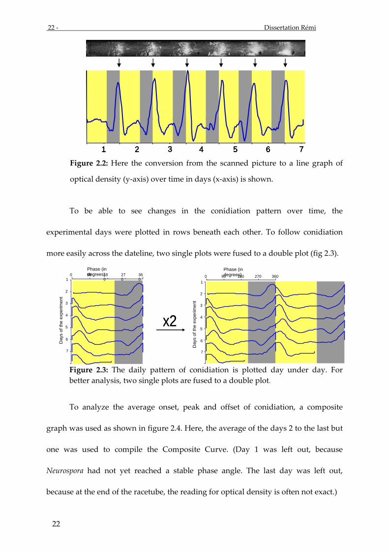
Figure 2.2: Here the conversion from the scanned picture to a line graph of
optical density (y-axis) over time in days (x-axis) is shown.
To be able to see changes in the conidiation pattern over time, the
experimental days were plotted in rows beneath each other. To follow conidiation
more easily across the dateline, two single plots were fused to a double plot (fig 2.3).
Figure 2.3: The daily pattern of conidiation is plotted day under day. For better analysis, two single plots are fused to a double plot.
To analyze the average onset, peak and offset of conidiation, a composite
graph was used as shown in figure 2.4. Here, the average of the days 2 to the last but
one was used to compile the Composite Curve. (Day 1 was left out, because
Neurospora had not yet reached a stable phase angle. The last day was left out,
because at the end of the racetube, the reading for optical density is often not exact.)
x2x2
Day
s of
the
expe
rimen
t
1
2
3
4
5
6
7
Phase (in degrees) 0 90 18
0 270 36
0
Day
s of
the
expe
rimen
t
1
2
3
4
5
6
7
Phase (in degrees) 0 90 180 270 360
1 2 3 4 5 6 7 1 2 3 4 5 6 7 1 2 3 4 5 6 7 1 2 3 4 5 6 7

Dissertation Rémi - 23 -
23
Figure 2.4: The Chrono program allows averaging curves over several days. By compiling the entrained days of the experiment to a Composite Curve, it is then easy to read out the peak of conidiation and the onset and offset of conidiation, both defined as the transition point through the daily average (blue horizontal line).
To analyze the average onset, peak and offset of conidiation, a composite
graph was used as shown in figure 2.4. Here, the average of the days 2 to the last but
one was used to compile the Composite Curve. (Day 1 was left out, because
Neurospora had not yet reached a stable phase angle. The last day was left out,
because at the end of the racetube, the reading for optical density is often not exact.)
From the composite curve, the times of onset, peak and offset - in relation to
the first lights on signal - were read into a spreadsheet to plot all light conditions for
one T-cycle onto one graph. The arithmetic mean for the Composite Curves of all the
race tubes (numbering six to fifteen racetubes per condition) for that one condition
was calculated. The data is expressed in degrees, whereby the 24 hour day is divided
into 360 degrees, to enable easier comparison of cycles that differ in length. See figure
2.5 (The results from the example race tube are encircled).
90
Phase (degree) 180 2700 360
offset
peak
onset + x
Day
s of
the
exp
erim
ent 1
2
3
4
5
6
7
Phase (in degrees) 0 90 180 270 36
0

24 - Dissertation Rémi
24
Figure 2.5: A double plotted depiction of the conidiation pattern (+ = onset, ∆ = peak, x = offset of conidiation) in a given T-cycle. Here, all 9 different photoperiods are plotted together in one graph, allowing analysis of the conidiation pattern. (The condition from the example in figs. 2.1., 2.2. and 2.3. is encircled.) As the 0 degree reference point, midnight was used. If lights on were chosen
as the 0 degrees reference point, the results would remain the same, but they are
easier to interpret with midnight as the reference. (See results figs. 3.4. - 3.21.) It is
also easier to follow, because it corresponds more readily to clock time, where
midnight is 0:00 h (Daan, Merrow et al. 2002)
2.2.3. Light cycles:
To perform the light-dark cycles experiments, light boxes had to be especially
designed and produced, to enable the very high amount of experimental conditions
in this thesis: 6 different cycle lengths with 9 different amounts of light-dark each for
3 different strains result 162 different conditions for the circadian surface physiology
alone. For the skeleton photo periods, another total of 66 conditions were added.
Considering the 3 - 4 repetitions that were done for each condition, this results in a
total of 700-800 experiments done (with 6-12 racetubes in each experiment), not yet
100
80
60
40
20
0
% o
f lig
ht
0 150 20 0 250 300 36050 100 150 200 25 0 300 36050 100
Phase in degrees

Dissertation Rémi - 25 -
25
considering the darkness-only controls - which were done in light tight aluminum
boxes - and the about 50 experiments for molecular results.
The lab’s facilities for light-dark racetube experiments were so far 3 separate
rooms, enabling 3 different setups at one time. Considering the average experiment
duration of 6-10 days, the experiments would have taken several years. Therefore, I
built 15 light-tight boxes (see figs. 2.6 and 2.7). The boxes had a fluorescent light
source (OSRAM Dulux L, 10W), producing 3.5 µE/m²/sec at the box’s floor level
(fluency was measured with an IL1400A Photometer, International Light). The light
in each box can be switched on and off with a computer interface independently
from other boxes, allowing up to 15 different experimental light conditions at a time.
The light within the boxes is homogenized by mirrors and a diffuser pane (Cinegel
#3026, Rosco), giving an even light distribution at the box’s floor. The boxes are set
up in a climatized room (25°C ± 0.5°C), with the temperature change being even less
within the boxes. The minimal amount of heat produced by the fluorescent bulbs
was fanned away with 10W computer fans (Philipps). The light cycles were
controlled with a computer program (Roenneberg, Munich) that allows graphical
control of On/Off cycles by transducing low voltage computer I/O signals via a
switch box into 220V current flow to the light sources.

26 - Dissertation Rémi
26
Figure 2.6: Photographs of the light boxes. A: Six of the 15 light boxes. Lighting was only turned on for the photograph. B: One of the light boxes with an open door. Italic letters denote: L light source, D diffusor pane, E experimental area (50x40cm) with even light distribution
Figure 2.7: Photograph of the control room with the computer interface to control cycles within the boxes. Italic letters: C Computer and screen with On/Off control program, S switch box, changing the computer’s I/O signals into electrical current I/O.
S
C
BL D
E
A

Dissertation Rémi - 27 -
27
2.3. Molecular Methods:
To produce tissue for molecular analysis, mycelial mats were grown in liquid
culture. For that purpose, sterile Petri dishes (60 mm diameter) containing 10 ml of
liquid Vogel’s medium were inoculated with approximately 106 conidia and
immediately transferred into their experimental condition. The mats were quickly
harvested by press-drying with paper towels, stored in 1.5 ml Eppendorf tubes and
deep frozen in liquid nitrogen. Samples were stored at -75°C for subsequent
processing.
2.3.1. RNA analysis
2.3.1.1. RNA extraction
1. Extraction
The frozen tissue was ground in a nitrogen cooled mortar with a pestle and
approximately 100 µl of sand, then immediately filled into a 1.5 ml Eppendorf tube,
containing 500 µl of Phenol and 600 µl of RNA extraction buffer. The tube was
vortexed and then shaken vigorously at room temperature for up to 30 minutes and
during that period vortexed three additional times. Centrifuging for 20 min at
14,000g, 4°C followed.
2. Cleaning
The clear supernatant was pipetted into a tube containing 500 µl Chloroform:
Isoamylic alcohol (24:1), being careful that none of the dividing layer was sucked into

28 - Dissertation Rémi
28
the pipette. The tube was vortexed 3 times, every 5 minutes, and then
centrifuged briefly.
3. Precipitation
The supernatant after centrifuging in step 2 was pipetted into a tube containing 1/10
Vol (of step 2 supernatant) of 3M Na-Acetate and 2 Vol (of step 2 supernatant) of ice
cold Ethanol (100%). The tube was shaken gently, put on ice for 10 minutes and
centrifuged for 10 minutes at 14 000 g, 4°C. The supernatant was poured off, the
remaining supernatant pipetted off and the cup left open to dry if necessary, to result
in a dry RNA pellet.
4. Resuspension
The precipitated RNA/DNA pellet was resuspended in 100 µl of RNA-Secure 1X and
shaken at 4°C for 10 minutes. When the RNA/DNA was fully resuspended, step 5
was carried out.
5. Aliquoting
The tube was centrifuged shortly, and divided into three: 55 µl in a stock tube, 20 µl
in an aliquot tube for measuring RNA concentration and 15 µl in a RT-tube for
eventual reverse transcription.
2.3.1.2. Quantification
The aliquots of the samples (see step 5 in “RNA extraction”) were diluted to
1:250. The RNA concentration was then determined by optical density (Ultrospec™
3100 pro, Biochrom) at a wave length of 260 nm. A solution containing 40 µg/ml
Dissertation Rémi - 29 -
29
RNA has an absorption of A = 1.0 at 260nm, when measured in a cuvette with a path
thickness of 10 mm. In addition to the measurement of the concentration with
260 nm UV-light, the quality of the RNA extraction was checked with a measurement
at 280 nm. The ratio of Absorption260nm/Absorption280nm is 2.0 for pure RNA. Another
measurement at 320 nm checked for protein contamination. If the OD320 was below
0.01, the sample was virtually protein free.
2.3.1.3. Reverse Transcription
For Real Time PCR, the RNA has to be reverse transcribed to cDNA. To
prevent false results from genomic DNA, the first step is to digest the contaminant
DNA. 10 µl of the RNA sample (0.2 µg/µl) were mixed with 10 µl of the DNAse
premix. The Premix contained 1X DNAse I buffer, 10 U/µl DNAse I enzyme
(amplification grade) and ddH2O for a total volume of 20 µl. The mixture was
incubated at 25°C for 10 minutes, followed by 10 minutes at 65°C. For reverse
transcription the resulting DNA-free sample was then mixed with the Reverse
Transcription (all reagents for reverse transcription from “TaqMan® RT Reagents”
and “AmpliTaq Gold® PCR Master Mix” kits, Applied Biosystems ) premix. The
premix contained:
- 1X TaqMan® RT buffer - 40 U RNAse inhibitor
- 500µM of each dNTP - 125 U Reverse Transcription enzyme
- 5.5mM MgCl - 2.5µM oligonucleotides (rN6/d(T)16/Spec.

30 - Dissertation Rémi
30
The reverse transcription then went through a three step incubation: 10
minutes at 25°C, 30 minutes at 42°C and 5 minutes at 95°C. After reverse
transcription, the samples were diluted 1:2 with RNAse free water.
2.3.1.4. Real Time PCR
Determining amounts of mRNA at distinct points of the circadian cycle is a
crucial tool to approach the kinetics of the molecular components of a circadian
clock. An excellent tool, allowing analysis in short time, is Real Time PCR. For
analysis in this study, the Applied Biosystems ABIPrism 7000 Sequence Detection
System was used.
As the reporter, SYBR Green PCR Master Mix (Applied Biosystems®) was used as
the fluorescent dye. The primers (from Metabion, Germany or from SigmaArk,
Germany®) and their sequences are listed in table 2.1. The final volume in each well
was 25 µl. The thermocycler was set to run a three stage program:
- Stage 1: 50°C for 2 minutes
- Stage 2: 95°C for 10 minutes
- Stage 3: 40 cycles of: 95°C for 15 seconds, followed by 60°C for 1 minute.
When the program was finished, the results section of the ABIPrism program was
checked to verify that the experiment was of high quality (smooth dissociation

Dissertation Rémi - 31 -
31
curves, clear sigmoid shape of the dissociation curve and comparison of the triple
repeats), and then saved to an export file to allow further analysis in Microsoft Excel.
Table 2.1: Sequences of the primers used in the RT-PCR
Product: Sequence of the primer:
Ribosomal 26s FO AGC GGA GGA AAA GAA ACC AAC
Ribosomal 26s RE CGC TTC ACT CGC CGT TAC TAG
frq-FO sy1 CGC CTT GCG CGA GAT ACT AG
frq-RE sy1 TCC CAG TGC GGA AGA TGA AG
wc-1 sy2 FO CCG ACT GGC ACA AAC AAT CC
wc-1 sy2 RE CGT CTG CGT TCT CAA AAA GC
vvd FO;sy1 GAC ACG TCA TGC GCT CTG AT
vvd RE;sy1 TGG CGT GTC TTT TTG CTT CA
32 - Dissertation Rémi
32
2.3.2. Protein analysis
2.3.2.1. Protein extraction
The frozen tissue was ground in a nitrogen cooled mortar with a pestle and
approximately 100 µl of sand, then immediately filled into a 1.5 ml Eppendorf tube,
containing 50 µl of Protein extraction buffer (PEB). The amount of the sample added
was about equal in volume to the buffer. To prevent proteolysis 10 µg/ml leupeptin,
10 µg/ml pepstatin and 1mM PMSF was added to the PEB just before the extraction.
The samples were kept on ice for 20 minutes and were vortexed 3 times during that
period to ensure a high yield. They were then centrifuged at 14,000 rpm, 4°C for 25
minutes. The clear supernatant was then carefully pipetted into another tube, making
sure that neither the solid layer underneath it, nor the thin lipid layer on top of it
were taken. The extract was then stored at -75°C until further analysis.
2.3.2.2. Quantification
For quantification 10 µl of a 1:10 dilution of the samples was mixed with 1ml
of the Bradford Assay Premix (Biorad) and referenced to a standard curve by optical
densimetry at 595nm (Ultrospec™ 3100 pro, Biochrom). The standard linear curve
was established with a best fit to the measurement of 5 concentration standards (3.5,
7, 10.5, 14, 21 µg/ml) of bovine IgG. The optical density is only accurate up to a
reading of 1.0. (i.e. where the standard curve remains linear.) In cases where the
Dissertation Rémi - 33 -
33
absorption exceeded 1.0, the samples were diluted and measured again to ensure
accurate results for the concentration of the proteins.
2.3.2.3. Dephosphorylation
One mechanism of posttranslational modification of the proteins involved in
the circadian rhythm is phosphorylation and dephosphorylation (Schafmeier, Haase
et al. 2005). In the circadian cycle, frq-RNA is translated into FRQ-protein and then
subsequently phosphorylated, which seems to be an important step before
degradation.
When performing gel electrophoresis and subsequent western blotting, this
mechanism poses the problem that there might be two or more bands for the same
protein – unphosphorylated and more or less phosphorylated protein. While two or
more species of the same protein may give interesting insight into clock mechanisms,
analysis of optical density of the total amount of protein is more accurate with single
bands. Therefore some of the experiments, where two bands were visible on the film,
were repeated after completely dephosporylating the protein to consolidate the
bands. These repeats with dephosphorylated protein were done as a proof of
concept. Each dephosphorylated run showed the same results for total density as the
previous phosphorylated run, assuring the accuracy of protein analysis. The data of
these test Western blots is not shown.
For dephosphorylation 200 mg of extracted protein was mixed with dephos-
phorylation buffer and 10 U/µl of alkaline phosphatase (CIP – New England

34 - Dissertation Rémi
34
BioLabs) to give a final volume of 50 µl. This was incubated for 1 hour at 37°C.
After incubation, gel electrophoresis, as described in 2.3.2.4, was performed.
2.3.2.4. Gel electrophoresis
I used SDS-polyacrylamide gel electrophoresis (SDS-PAGE). To prepare the
gels, first the resolving gel was poured between two glass plates, divided by two
spacers, creating a chamber (size: 9.5 cm x 14 cm x 0.2 cm). With a layer of
isopropanol on top of the resolving gel to achieve a level surface, the gel was
polymerized. 45 minutes later, the isopropanol was completely washed out, a
stacking gel (size: 2.5cm x 14cm x 0.2cm) was poured on top of the resolving gel and
a Teflon comb with 18 teeth introduced to create 18 wells for stacking. After placing
the gel in the electrophoresis apparatus (custom made, Helmut Klausner, IMP
workshop) and filling the anode and cathode chambers with running buffer, the
wells were carefully cleaned from any excess gel and flushed with buffer several
times.
Before loading the protein, 200 µg of Protein was mixed with 1X Laemmle
buffer and incubated at 95°C for denaturation. The protein was loaded onto the gel
as well as 10 µl of molecular weight standards (Precision Protein™ Standards,
BioRad) and a negative control, consisting of a mutant with a knockout of the target
gene chosen for that experiment. Electrophoresis was run at 80 V for about 90
minutes and changed to 125 V after the protein samples had reached the resolving

Dissertation Rémi - 35 -
35
gel. The gel was then run for about 3 hours (depending on the target protein’s size)
until the dye front had exited the gel.
2.3.2.5. Western Blotting
For antibody probing, we blotted onto a nitrocellulose membrane. For
electrophoretic transfer from the nitrocellulose membrane (PROTRAN®, Schleicher &
Schuell) it was first wetted with Blotting buffer. The gel and the membrane were
placed between two sheets of Whatman paper (GB 002 Gel-Blotting Paper, Schleicher
& Schuell), also soaked with Blotting buffer. After carefully rolling out possible air-
bubbles with a reagent tube, the sandwich was put into the blotting cassette between
two thin sponges and then put into the blotting chamber (TransBlot™
Electrophoretic Transfer Cell, BioRad®), filled with blotting buffer. The transfer was
run at 800 mA for two hours. After blotting, the membrane was rinsed with ddH2O
to remove the SDS and stained with Ponceau-S solution for 20 seconds to be able to
inspect the blot. The excess Ponceau-S was rinsed away with ddH2O and the
membrane then left to air-dry over night.
For proteins smaller than 80-90 kD, another blotting chamber was used. The
custom made (Helmut Klausner, IMP workshop) semi-dry blotting chamber
contained two graphite electrodes. The blotting was driven by a constant current of 2
mA/cm2 (of sandwich area). The transfer time was 90 minutes. After that the above
described Ponceau staining was performed. (Towbin, Staehelin et al. 1979)

36 - Dissertation Rémi
36
2.3.2.6. Probing for target proteins
The membrane was bathed and gently shaken in TBS Blotting buffer for 10
minutes to remove the Ponceau-S staining. To block the nitrocellulose membrane, it
was incubated with 50 ml of 5% milk (skim milk powder in TBS, filtered before use )
for one hour. The milk was poured of and 50 ml of milk with a 1:40 dilution of the
primary antibody was added. With gentle shaking at room temperature for two
hours the binding of antibody and protein was allowed. The primary antibody was
poured off and the membrane washed with TBS to remove excess antibodies. The
secondary antibody (in 5% milk, dilution 1:5000 for monoclonal primary antibody,
1:10 000 for polyclonal primary antibody), coupled to horse-radish-peroxidase, was
incubated with the membrane for 12-20 hours at 4°C with gentle shaking. The next
day the antibody-milk solution was poured off and the membrane washed with TBS
three times and shaken in TBS for 15 minutes to remove unbound secondary
antibodies.
Table 2.2: Antibodies used in this study
Antibody Antigen Origin
α-FRQ(3G11) MPB-FRQ(65-989 aa)
(Merrow, Franchi et al. 2001)
monoclonal,
mouse
α-VVD VVD-2 (13-29aa)
(Michael Brunner, personal communication)
polyclonal, rabbit

Dissertation Rémi - 37 -
37
2.3.2.7. Developing the membrane
The membrane was placed in a plastic envelope, and the excess TBS was
carefully wiped out off the envelope. 2ml of Luminol solution (Lumi-LightPlus ®,
Roche) was poured over the membrane. The excess Luminol was removed after 2
minutes. Then film (Medical X-ray film 100, Fuji) was exposed to the membrane for
different amounts of time to achieve different staining density and then developed.
(Airclean 200/35 plus - film developing machine, Protec, Germany)
2.3.2.8. Analysis of the developed film
All developed films were scanned (AGFA Snapscan 1236, settings: resolution
150 dpi, grayscale) and saved as .pict-files. The optical density of each band,
correlating with the amount of target protein, was determined with the Video analysis
1.8 program (Prof. T. Roenneberg, LMU Munich).
The density values for the different exposure times were transferred into the
Kaleidagraph 3.0.1. program. There, they were fitted to a sigmoidal curve:
(y=m1*(((x+m3)/m2)/(1+((x+m3)/m2)2)0.5)+m4), were y represents the pixel density and x
the exposure time. This process gives more accurate quantifications over a larger
dynamic range than using a single exposure.
38 - Dissertation Rémi
38
3. Results
3.1. Physiological results
3.1.1. Skeleton photoperiods (SPP)
The experimental setup (see section 1.5) and the graphical method for
evaluation (see section 2.2.2.2) of the skeleton photoperiods are described above. In
short, the three strains of Neurospora with three different free running periods (frq+,
frq1 and frq7) were exposed to 24 hour cycles with 2 light pulses of 2 hours length
each, separated by different lengths of time. The systematic setup also included one
cycle with a 4 hour light pulse (i.e. 2 light pulses with no dark pulse in between, i.e. 4
h light : 20 h dark) and also one cycle with only one 2 hour light pulse (2 light : 22
dark). Although all three strains were exposed to the same cycles, they yielded
different but systematic results. They illustrated in figures 3.1 – 3.3, with only the
onset of conidiation depicted in the respective graphs.
Skeleton photoperiods are an artificial approach to investigate circadian
properties by mimicking a full photo period with two separate light pulses. But those
two pulses can be seen as mimicking the non-parametric beginning and ending of a
single light period. Therefore, while describing and analyzing the results from
skeleton photoperiods, an assumption of which interval between light pulses is the
“day” and which is the “night” has to be made. So first, the results from the frq+
cycles will be described and the assumption of one of the intervals as the “day” will
be used when describing the results from the frq1 and frq7 cycles.

Dissertation Rémi - 39 -
39
1. In the frq+ strain (figure 3.1.), Neurospora assumes a stable phase angle at the
midpoint between the light pulses in each cycle. Because Neurospora crassa
starts to band around midnight in full photoperiods, it can be assumed that
the longer portion between the two skeleton photoperiods is interpreted as
night. So, as in full photoperiods of T = 24 h, Neurospora entrains to midnight
with its onset of conidiation (compare section 3.1.2 and previous experiments:
Tan, Merrow et al. 2004) and the onset of conidiation is around midnight. This
holds for all non-symmetrical cycles, where Neurospora shows only one
conidial band per 24 hour cycle. In the symmetrical and near symmetrical
cycles, N.c. shows two bands per 24 hour cycle and a distinction between a
subjective night and day can not be made.
Figure 3.1: Phase angles of onset of conidiation in the skeleton photo periods for the frq+ strain. Filled circles denote cycles with one band every 24 hours, open circles denote cycles with two bands per 24 hour cycle. The yellow bars represent the two hour light pulses and are correct in their relative size.
Thus, the results of the frq1 and frq7 cycles can be described with the assump-
tion that the longer interval is interpreted as the night in the skeleton photo-
periods.
frq+

40 - Dissertation Rémi
40
2. Unlike frq+, frq1 entrains coupled to the dawn lights-on, and again shows a
phase jump at around the symmetrical cycles. The onset of conidiation has a
phase angle of about 180° (12 hours) after the dawn lights-on.
3. As frq1, frq7 entrains coupled to the dawn lights-on signal in SPP cycles, again
with a phase jump at around the symmetrical cycles. Unlike in frq1, the onset
of conidiation in frq7 lags dawn by 22-23 hours.
.
Figure 3.2: Phase angles of onset of conidiation in the skeleton photo periods for the frq1 strain. Filled circles denote cycles with one band every 24 hours, open circles denote cycles with two bands per 24 hour cycle. The yellow bars represent the two hour light pulses and are correct in their relative size.
Figure 3.3: Phase angles of onset of conidiation in the skeleton photo periods for the frq7 strain. Filled circles denote cycles with one band every 24 hours, open circles denote cycles with two bands per 24 hour cycle. The yellow bars represent the two hour light pulses and are correct in their relative size.
One of the major questions of this thesis is, whether Neurospora is driven or
entrained by light cycles. As shown above, the coupling of the phase angle to
frq1
frq7

Dissertation Rémi - 41 -
41
midnight in the frq+ strain already shows entrainment, but also the phase jump
around the symmetrical cycles cannot be explained with driveness. When expecting
driveness, a strain should take a phase angle to one light pulse and not exhibit a
jump. Driveness would give a uniform reaction to a stimulus. And also in these
experiments, an irradiance effect does not explain the data, as the cycles all have a
total of 4 hours of light (with the 2 h light: 22 h dark as an exception). Thus,
Neurospora entrains to skeleton photo periods, rather than being driven by them.
3.1.2. The circadian surface
The only experiment that had used the term “circadian surface” previously
was a study, where the induction of diapause (resting state) of a beetle was
investigated under varying lengths of symmetrical light-dark cycles (Beck 1962). We
chose the term “circadian surface”, because it very well illustrates the experimental
approach. Three variables were changed in assembling the circadian surface: (1) the
length of the T-cycles, (2) the amount of light per T-cycle and (3) the free-running
period of the studied strains (see section 1.5 for more details). The T-cycles ranged
from 16 hours to 26 hours (16 h, 18 h, 20 h, 22 h, 24 h and 26 h), the light amounts
ranged from 16% to 84% (16%, 25%, 33%, 40%, 50%, 60%, 67%, 75% and 84%). This
results in 54 experimental conditions for each of the three strains (frq+, frq1 and frq7).
For each strain and condition 6-12 race tubes were used. To verify results, each
condition was repeated at least twice with 3-12 race tubes. The results are shown in
figures 3.4 through 3.21, sorted by strains and T-cycle length.

42 - Dissertation Rémi
42
100
80
60
40
20
0
% o
f lig
ht
0 150 200 250 300 36050 100 150 200 250 300 36050 100Phase in degrees
100
80
60
40
20
0
% o
f lig
ht
0 150 200 250 300 36050 100 150 200 250 300 36050 100Phase in degrees
100
80
60
40
20
0
% o
f lig
ht
100
80
60
40
20
0
% o
f lig
ht
0 150 200 250 300 36050 100 150 200 250 300 36050 100Phase in degrees
0 150 200 250 300 36050 1000 150 200 250 300 36050 100 150 200 250 300 36050 100 150 200 250 300 36050 100Phase in degrees
Figure 3.4.: conidiation (+ = onset, ∆ = peak, x = offset of conidiation) in the 16h T-cycle for the frq+ strain.
100
80
60
40
20
0
% o
f lig
ht
0 150 200 250 300 36050 100 150 200 250 300 36050 100
Phase in degrees
100
80
60
40
20
0
% o
f lig
ht
0 150 200 250 300 36050 100 150 200 250 300 36050 100
Phase in degrees
100
80
60
40
20
0
% o
f lig
ht
100
80
60
40
20
0
% o
f lig
ht
0 150 200 250 300 36050 100 150 200 250 300 36050 100
Phase in degrees0 150 200 250 300 36050 1000 150 200 250 300 36050 100 150 200 250 300 36050 100 150 200 250 300 36050 100
Phase in degrees Figure 3.5.: conidiation (+ = onset, ∆ = peak, x = offset of conidiation) in the 18h T-cycle for the frq+ strain
100
80
60
40
20
0
% o
f lig
ht
0 150 200 250 300 36050 100 150 200 250 300 36050 100Phase in degrees
100
80
60
40
20
0
% o
f lig
ht
0 150 200 250 300 36050 100 150 200 250 300 36050 100Phase in degrees
100
80
60
40
20
0
% o
f lig
ht
100
80
60
40
20
0
% o
f lig
ht
0 150 200 250 300 36050 100 150 200 250 300 36050 100Phase in degrees
0 150 200 250 300 36050 1000 150 200 250 300 36050 100 150 200 250 300 36050 100 150 200 250 300 36050 100Phase in degrees
Figure 3.6.: conidiation (+ = onset, ∆ = peak, x = offset of conidiation) in the 20h T-cycle for the frq+ strain

Dissertation Rémi - 43 -
43
100
80
60
40
20
0
% o
f lig
ht
0 150 200 250 300 36050 100 150 200 250 300 36050 100Phase in degrees
100
80
60
40
20
0
% o
f lig
ht
0 150 200 250 300 36050 100 150 200 250 300 36050 100Phase in degrees
100
80
60
40
20
0
% o
f lig
ht
100
80
60
40
20
0
% o
f lig
ht
0 150 200 250 300 36050 100 150 200 250 300 36050 100Phase in degrees
0 150 200 250 300 36050 1000 150 200 250 300 36050 100 150 200 250 300 36050 100 150 200 250 300 36050 100Phase in degrees
Figure 3.7.: conidiation (+ = onset, ∆ = peak, x = offset of conidiation) in the 22h T-cycle for the frq+ strain
100
80
60
40
20
0
% o
f lig
ht
0 150 200 250 300 36050 100 150 200 250 300 36050 100Phase in degrees
100
80
60
40
20
0
% o
f lig
ht
0 150 200 250 300 36050 100 150 200 250 300 36050 100Phase in degrees
100
80
60
40
20
0
% o
f lig
ht
100
80
60
40
20
0
% o
f lig
ht
0 150 200 250 300 36050 100 150 200 250 300 36050 100Phase in degrees
0 150 200 250 300 36050 1000 150 200 250 300 36050 100 150 200 250 300 36050 100 150 200 250 300 36050 100Phase in degrees
Figure 3.8: conidiation (+ = onset, ∆ = peak, x = offset of conidiation) in the 24h T-cycle for the frq+ strain
100
80
60
40
20
0
% o
f lig
ht
0 150 200 250 300 36050 100 150 200 250 300 36050 100Phase in degrees
100
80
60
40
20
0
% o
f lig
ht
0 150 200 250 300 36050 100 150 200 250 300 36050 100Phase in degrees
100
80
60
40
20
0
% o
f lig
ht
100
80
60
40
20
0
% o
f lig
ht
0 150 200 250 300 36050 100 150 200 250 300 36050 100Phase in degrees
0 150 200 250 300 36050 1000 150 200 250 300 36050 100 150 200 250 300 36050 100 150 200 250 300 36050 100Phase in degrees
Figure 3.9.: conidiation (+ = onset, ∆ = peak, x = offset of conidiation) in the 26h T-cycle for the frq+ strain

44 - Dissertation Rémi
44
100
80
60
40
20
0
% o
f lig
ht
0 150 200 250 300 36050 100 150 200 250 300 36050 100Phase in degrees
100
80
60
40
20
0
% o
f lig
ht
0 150 200 250 300 36050 100 150 200 250 300 36050 100Phase in degrees
100
80
60
40
20
0
% o
f lig
ht
100
80
60
40
20
0
% o
f lig
ht
0 150 200 250 300 36050 100 150 200 250 300 36050 100Phase in degrees
0 150 200 250 300 36050 1000 150 200 250 300 36050 100 150 200 250 300 36050 100 150 200 250 300 36050 100Phase in degrees
Figure 3.10.: conidiation (+ = onset, ∆ = peak, x = offset of conidiation) in the 16h T-cycle for the frq1 strain
100
80
60
40
20
0
% o
f lig
ht
0 150 200 250 300 36050 100 150 200 250 300 36050 100Phase in degrees
100
80
60
40
20
0
% o
f lig
ht
0 150 200 250 300 36050 100 150 200 250 300 36050 100Phase in degrees
100
80
60
40
20
0
% o
f lig
ht
100
80
60
40
20
0
% o
f lig
ht
0 150 200 250 300 36050 100 150 200 250 300 36050 100Phase in degrees
0 150 200 250 300 36050 1000 150 200 250 300 36050 100 150 200 250 300 36050 100 150 200 250 300 36050 100Phase in degrees
Figure 3.11.: conidiation (+ = onset, ∆ = peak, x = offset of conidiation) in the 18h T-cycle for the frq1 strain
100
80
60
40
20
0
% o
f lig
ht
0 150 200 250 300 36050 100 150 200 250 300 36050 100Phase in degrees
100
80
60
40
20
0
% o
f lig
ht
0 150 200 250 300 36050 100 150 200 250 300 36050 100Phase in degrees
100
80
60
40
20
0
% o
f lig
ht
100
80
60
40
20
0
% o
f lig
ht
0 150 200 250 300 36050 100 150 200 250 300 36050 100Phase in degrees
0 150 200 250 300 36050 1000 150 200 250 300 36050 100 150 200 250 300 36050 100 150 200 250 300 36050 100Phase in degrees
Figure 3.12.: conidiation (+ = onset, ∆ = peak, x = offset of conidiation) in the 20h T-cycle for the frq1 strain

Dissertation Rémi - 45 -
45
100
80
60
40
20
0
% o
f lig
ht
0 150 200 250 300 36050 100 150 200 250 300 36050 100
Phase in degrees
100
80
60
40
20
0
% o
f lig
ht
0 150 200 250 300 36050 100 150 200 250 300 36050 100
Phase in degrees
100
80
60
40
20
0
% o
f lig
ht
100
80
60
40
20
0
% o
f lig
ht
0 150 200 250 300 36050 100 150 200 250 300 36050 100
Phase in degrees0 150 200 250 300 36050 1000 150 200 250 300 36050 100 150 200 250 300 36050 100 150 200 250 300 36050 100
Phase in degrees Figure 3.13.: conidiation (+ = onset, ∆ = peak, x = offset of conidiation) in the 22h T-cycle for the frq1 strain
100
80
60
40
20
0
% o
f lig
ht
0 150 200 250 300 36050 100 150 200 250 300 36050 100Phase in degrees
100
80
60
40
20
0
% o
f lig
ht
0 150 200 250 300 36050 100 150 200 250 300 36050 100Phase in degrees
100
80
60
40
20
0
% o
f lig
ht
100
80
60
40
20
0
% o
f lig
ht
0 150 200 250 300 36050 100 150 200 250 300 36050 100Phase in degrees
0 150 200 250 300 36050 1000 150 200 250 300 36050 100 150 200 250 300 36050 100 150 200 250 300 36050 100Phase in degrees
Figure 3.14.: conidiation (+ = onset, ∆ = peak, x = offset of conidiation) in the 24h T-cycle for the frq1 strain
100
80
60
40
20
0
% o
f lig
ht
0 150 200 250 300 36050 100 150 200 250 300 36050 100
Phase in degrees
100
80
60
40
20
0
% o
f lig
ht
0 150 200 250 300 36050 100 150 200 250 300 36050 100
Phase in degrees
100
80
60
40
20
0
% o
f lig
ht
100
80
60
40
20
0
% o
f lig
ht
0 150 200 250 300 36050 100 150 200 250 300 36050 100
Phase in degrees0 150 200 250 300 36050 1000 150 200 250 300 36050 100 150 200 250 300 36050 100 150 200 250 300 36050 100
Phase in degrees Figure 3.15.: conidiation (+ = onset, ∆ = peak, x = offset of conidiation) in the 26h T-cycle for the frq1 strain

46 - Dissertation Rémi
46
100
80
60
40
20
0
% o
f lig
ht
0 150 200 250 300 36050 100 150 200 250 300 36050 100
Phase in degrees
100
80
60
40
20
0
% o
f lig
ht
0 150 200 250 300 36050 100 150 200 250 300 36050 100
Phase in degrees
100
80
60
40
20
0
% o
f lig
ht
100
80
60
40
20
0
% o
f lig
ht
0 150 200 250 300 36050 100 150 200 250 300 36050 100
Phase in degrees0 150 200 250 300 36050 1000 150 200 250 300 36050 100 150 200 250 300 36050 100 150 200 250 300 36050 100
Phase in degrees Figure 3.16.: conidiation (+ = onset, ∆ = peak, x = offset of conidiation) in the 16h T-cycle for the frq7 strain
100
80
60
40
20
0
% o
f lig
ht
0 150 200 250 300 36050 100 150 200 250 300 36050 100Phase in degrees
100
80
60
40
20
0
% o
f lig
ht
0 150 200 250 300 36050 100 150 200 250 300 36050 100Phase in degrees
100
80
60
40
20
0
% o
f lig
ht
100
80
60
40
20
0
% o
f lig
ht
0 150 200 250 300 36050 100 150 200 250 300 36050 100Phase in degrees
0 150 200 250 300 36050 1000 150 200 250 300 36050 100 150 200 250 300 36050 100 150 200 250 300 36050 100Phase in degrees
Figure 3.17.: conidiation (+ = onset, ∆ = peak, x = offset of conidiation) in the 18h T-cycle for the frq7 strain
100
80
60
40
20
0
% o
f lig
ht
0 150 200 250 300 36050 100 150 200 250 300 36050 100Phase in degrees
100
80
60
40
20
0
% o
f lig
ht
0 150 200 250 300 36050 100 150 200 250 300 36050 100Phase in degrees
100
80
60
40
20
0
% o
f lig
ht
100
80
60
40
20
0
% o
f lig
ht
0 150 200 250 300 36050 100 150 200 250 300 36050 100Phase in degrees
0 150 200 250 300 36050 1000 150 200 250 300 36050 100 150 200 250 300 36050 100 150 200 250 300 36050 100Phase in degrees
Figure 3.18.: conidiation (+ = onset, ∆ = peak, x = offset of conidiation) in the 20h T-cycle for the frq7 strain

Dissertation Rémi - 47 -
47
100
80
60
40
20
0
% o
f lig
ht
0 150 200 250 300 36050 100 150 200 250 300 36050 100
Phase in degrees
100
80
60
40
20
0
% o
f lig
ht
0 150 200 250 300 36050 100 150 200 250 300 36050 100
Phase in degrees
100
80
60
40
20
0
% o
f lig
ht
100
80
60
40
20
0
% o
f lig
ht
0 150 200 250 300 36050 100 150 200 250 300 36050 100
Phase in degrees0 150 200 250 300 36050 1000 150 200 250 300 36050 100 150 200 250 300 36050 100 150 200 250 300 36050 100
Phase in degrees Figure 3.19.: conidiation (+ = onset, ∆ = peak, x = offset of conidiation) in the 22h T-cycle for the frq7 strain
100
80
60
40
20
0
% o
f lig
ht
0 150 200 250 300 36050 100 150 200 250 300 36050 100Phase in degrees
100
80
60
40
20
0
% o
f lig
ht
0 150 200 250 300 36050 100 150 200 250 300 36050 100Phase in degrees
100
80
60
40
20
0
% o
f lig
ht
100
80
60
40
20
0
% o
f lig
ht
0 150 200 250 300 36050 100 150 200 250 300 36050 100Phase in degrees
0 150 200 250 300 36050 1000 150 200 250 300 36050 100 150 200 250 300 36050 100 150 200 250 300 36050 100Phase in degrees
Figure 3.20.: conidiation (+ = onset, ∆ = peak, x = offset of conidiation) in the 24h T-cycle for the frq7 strain
100
80
60
40
20
0
% o
f lig
ht
0 150 200 250 300 36050 100 150 200 250 300 36050 100Phase in degrees
100
80
60
40
20
0
% o
f lig
ht
0 150 200 250 300 36050 100 150 200 250 300 36050 100Phase in degrees
100
80
60
40
20
0
% o
f lig
ht
100
80
60
40
20
0
% o
f lig
ht
0 150 200 250 300 36050 100 150 200 250 300 36050 100Phase in degrees
0 150 200 250 300 36050 1000 150 200 250 300 36050 100 150 200 250 300 36050 100 150 200 250 300 36050 100Phase in degrees
Figure 3.21.: conidiation (+ = onset, ∆ = peak, x = offset of conidiation) in the 26h T-cycle for the frq7 strain

48 - Dissertation Rémi
48
The results add up to a highly systematic but simple set of rules for entrainment to
light cycles:
A. Long photoperiods (more than 50% of light per cycle):
1. Neurospora crassa entrains with coupling to midnight.
2. The longer T (cycle length) in relation to the τ (= FRP, free running
period), the more conidiation is delayed in relation to midnight.
B. Short photoperiods (less than 50% of light per cycle):
1. If T < τ, N.c. couples to dawn.
2. If T > τ, N.c. couples towards dusk.
3. If T = τ, N.c. couples to midnight.

Dissertation Rémi - 49 -
49
3.2. Molecular results
3.2.1. Choosing cycles for molecular analysis
Evaluation of the circadian surface revealed three ‘types’ of entrainment:
phase coupled (or “locked”) to dawn, to dusk or to midnight. Clock gene expression
was investigated in one case of each of these entrainment phenotypes.
Three cycles were chosen to be tested with the frq+-strain for molecular
analysis: T16 (LD 4:12), T22 (LD 4:18) and T26 (LD 4:22). Cycles with equal absolute
duration of the light phase were specifically chosen, so that irradiance effects could
be excluded. The frq+-strain has a free running period (τ) of about 22 h and therefore
with the three cycles, 3 different relationships of T and τ are tested for their
molecular profile:
1. In T = 16 (T < τ), the conidiation phase angles of Neurospora crassa are locked to
dawn, i.e. the phase angle in the shorter photoperiods (below 50% light) is
parallel to the dawn dark-light transition (fig. 3.22).
2. In T = 22 (T = τ), the conidiation phase angles of Neurospora crassa are locked to
midnight (fig. 3.22).
3. In T = 26 (T > τ), the conidiation phase angles of Neurospora crassa are locked to
dusk (fig. 3.22).

50 - Dissertation Rémi
50
Phase angle
T = 22
-90 90
T = 26
-90 90-90 90
T = 1650
% li
ght
„dawn lock“ „midnight lock“ „dusk lock“
Phase angle
T = 22
-90 90
T = 22
-90 90-90 90-90 90
T = 26
-90 90
T = 26
-90 90-90 90-90 90
T = 16
-90 90-90 90
T = 1650
% li
ght
„dawn lock“ „midnight lock“ „dusk lock“
Figure 3.22.: The three graphs for the T16, T22 and T26 cycles show the phase angles of the onset of conidiation in the frq+ strain of Neurospora crassa. For orientation, the slopes of the phase angles are fitted with lines. The cycles that were chosen for molecular analysis are pointed out with stars. (Compare with graphs in section 3.1.)
3.2.2. RT-PCR results
The results of the mRNA analysis using RT-PCR (figs. 3.23 – 3.27) reproduce
and extend previous results (Tan, Dragovic et al. 2004). frq-mRNA is rapidly
upregulated, reaching its highest level in each cycle at the 15 minute timepoint. This
is similar to the results of Crosthwaite (1995). The Crosthwaite study could also show
that frq-levels remained elevated when lights were kept on. With the longer light-
stimulus in this study (4 hours vs. a 2 minute light pulse in Crosthwaite’s study),
both elements are shown: the levels of frq-mRNA rise quickly after lights on, remain
elevated during the light and start decreasing right after lights-off. In our group’s
previous studies, we noted a non-systematic relationship between RNA and protein
(discussed below), but the results for mRNA were comparable despite the different

Dissertation Rémi - 51 -
51
structure of the cycles (Tan, Dragovic et al. 2004). The one difference in RNA results
between the different cycles with different length is, how long the levels of frq remain
elevated. Namely, the longer the cycle, the longer the levels are elevated above
baseline (level before lights on). Specifically, the frq-levels reach baseline after about
8.5 hours in T=16, after about 10 hours in T=22 and after about 13.5 hours in T=26.
(See figs. 3.23 – 3.25, sorted by strains)
The vvd-mRNA is also acutely induced by lights-on. Comparing the levels
before and 15 to 30 minute after lights on, the levels increase about 50 times in T=16
and T=26, and about 20 times in the T=22. The kinetics for up-regulation are similar
in all cycles, and the down-regulation starts in all cycles right after the early peak.
But, similar to frq-levels, the cycles differ in the duration of elevated levels of mRNA.
Specifically, the vvd-levels reach baseline (level before lights on) after about 8.5 hours
in T=16, after about 10 hours in T=22 and after about 13.5 hours in T=26 (See figs. 3.23
– 3.25, sorted by strains). Although we do not yet understand the mechanism, it is
worth noting that the regulation of the post-light induced levels of these two
different RNAs is highly similar.

52 - Dissertation Rémi
52
0
1
2
3
4
5
6
7
8
9
10
0
1
2
3
4
5
6
7
8
9
10
-100 0 100 200 300 400 500 600 700 800time in minutes
rel.
amou
ntof
frq
RN
A
T16 frq RNA
0
10
20
30
40
50
60
70
80
0
10
20
30
40
50
60
70
80
-100 0 100 200 300 400 500 600 700 800
time in minutes
rel.
amou
ntof
vvd
RN
A
T16 vvd RNA
Figure 3.23: The results of the RT-PCR for the T16 cycle are plotted with relative amount against time. The left graph showing frq RNA levels and the right graph showing the vvd RNA levels. The light cycle is plotted as the background of the graph, with yellow corresponding to the photoperiod and gray corresponding to the scotoperiod. The image above the graph represents the phase position of the conidial band. Figure 3.24: The results of the rtPCR for the T22 cycle are plotted with relative amount against time. The left graph showing frq RNA levels and the right graph showing the vvd RNA levels. See fig. 3.23 for further explanation.
0
10
20
30
40
50
60
-100 100 300 500 700 900 1100 1300time in minutes
rel.
amou
ntof
vvd
RN
A
T26 vvd RNA
Figure 3.25: The results of the rtPCR for the T26 cycle are plotted with relative amount against time. The left graph showing frq RNA levels and the right graph showing the vvd RNA levels. See fig. 3.23 for further explanation.
0
2
4
6
8
10
12
-100 100 300 500 700 900 1100 1300time in minutes
rel.
amou
ntof
frq
RN
A
T26 frq RNA
0
1
2
3
4
5
6
7
8
9
0
1
2
3
4
5
6
7
8
9
-100 100 300 500 700 900 1100time in minutes
rel.
amou
ntof
frq
RN
A
T22 frq RNA
0
5
10
15
20
25
0
5
10
15
20
25
-100 100 300 500 700 900 1100time in minutes
rel.
amou
ntof
vvd
RN
A
T22 vvd RNA

Dissertation Rémi - 53 -
53
wc-1 mRNA remains level at about 2 relative units throughout each cycle, but
is quickly up-regulated by light, reaching its highest amplitude in each cycle at the 15
minute time point. Comparing the three cycles, the difference is in the amplitude of
the acute RNA peak. It is highest in T=26 and lowest in T=22.
0
0,5
1
1,5
2
2,5
3
3,5
4
0
0,5
1
1,5
2
2,5
3
3,5
4
-100 0 100 200 300 400 500 600 700 800
time in minutes
rel.
amou
ntof
wc1
RN
A
T16 wc1 RNA
0
0,5
1
1,5
2
2,5
3
0
0,5
1
1,5
2
2,5
3
-100 100 300 500 700 900 1100time in minutes
rel.
amou
ntof
wc1
RN
A
T22 wc1 RNA
Figure 3.26: The results of the rtPCR for wc-1 RNA levels in the T=16h and T=22h cycles are plotted with relative amount against time. The left graph shows the T=16 cycle, the right graph the T=22 cycle. See fig. 3.23 for further explanation.
0
1
2
3
4
5
6
7
time in minutes
rel.
amou
ntof
wc1
RN
A
-100 100 300 500 700 900 1100 1300-100 100 300 500 700 900 1100 1300
T26 wc1 RNA
Figure 3.27: The results of the rtPCR for wc-1 RNA levels in the T=26 cycle. See fig. 3.23 for further explanation.

54 - Dissertation Rémi
54
3.2.3. Western blot results
Given our previous results, showing dissociation of frq RNA and protein in
entrained conditions, I investigated expression of FRQ and VVD protein (see section
1.4. for description of function and interaction). As to be expected, there is a lag
between the peak of RNA (see section 3.2.2) and protein levels (fig. 3.28). The
signature transition from unphosphorylated (early in the cycle) to phosphorylated
FRQ protein (later in the cycle) is also seen in all three T-cycles. Also similar to
previous results (Tan, Dragovic et al. 2004), the onset of conidiation occurs following
the peak of FRQ protein, although in this case conidiation occurs slightly earlier,
relative to the disappearance of FRQ. The peak of protein levels is approximately the
same in all cycles, about 8.5 hours after lights on. The cycles differ in the degradation
of FRQ, with the levels of FRQ staying elevated until shortly before the next lights-on
transition. Also note that in T = 16 h and T = 22 h there is an initial decrease of FRQ
levels following lights on. Previously, only increases in FRQ levels have been
invoked to explain entrainment. It may be that degradation is important for
entrainment also.

Dissertation Rémi - 55 -
55
Figure 3.28.: The graphs show the relative amount of FRQ-protein over the course of the respective cycle (T16 right, T22 middle, T26 left). The x-axis shows time in minutes, the y-axis shows relative amounts. The pictures above the graphs show the original developed x-ray film and a representation of the conidiation in the respective cycles. Please note that the gel-lanes are not aligned with the respective data points on the graph, as they more densely timed around lights-on.
I also probed Western blots for the VVD-protein. These blots represent the
first ever reported for VVD in a LD cycle. The blots show that production of VVD is
rapid in all cycles. Soon after lights on, VVD levels rise and reach their maximum at
lights off, 4 hours after lights on. The one marked difference in the three cycles and
their VVD-kinetics is the degradation. Where the peaks are alike in all cycles,
degradation changes systematically with the length of the cycle. In all cycles, the
degradation takes the whole scotoperiod to be complete. Namely 12 h in the T = 16 h,
18 h in the T = 22 h and 22 h in the T = 26 h cycle. The degradation of VVD is linear
from peak to baseline levels (the levels before lights on) and, therefore, fails to
correlate with either FRQ levels or with vvd-RNA. In up-regulation, protein
correlates with the RNA-kinetics (compare figs. 3.23 - 3.25 and 3.29).
0 500 1000
25
20
15
5
10
0
25
20
15
5
10
0 0 50 100
2
2
1
5
1
0
2
2
1
5
1
00 50 100 150
25
20
15
5
10
0

56 - Dissertation Rémi
56
Figure 3.29.: The graphs show the relative amount of VVD-protein over the course of the respective cycle (T=16h right, T=22h middle, T=26h left). The x-axis shows time in minutes, the y-axis shows relative amounts. The pictures above the graphs show the original stained x-ray film and a representation of the conidiation in the respective cycles. The arrows indicate the VVD-band on the gel. Please note, that the gel-lanes are not aligned with the respective data points on the graph, as they are more densely timed around lights-on.
0 200 400 600 800 1000 0
0.6
0.4
0.2
0.8
1.0
1.2
0 20 40 60 80 100 120100 1200
0.6
0.4
0.2
0.8
1.0
1.2
0
0.6
0.4
0.2
0.8
1.2
20 40 60 80 100 1200 140
1.0

Dissertation Rémi - 57 -
57
4. Discussion
As described above (see section 1.2.), a circadian system has several defining
properties: rhythmicity, a circadian range, a large enough amplitude and sustain-
ability of the output rhythm, noise compensation and entrainability. With this thesis
mainly one of the circadian properties of the model organism Neurospora crassa has
been investigated: entrainment on the physiological and on the molecular level.
The physiology and molecular biology of entrainment has been investigated in
many organisms (Bruce 1960; Crosthwaite et al. 1995; Merrow et al. 1999) and rules
for entrainment have been deducted (Roenneberg, Daan et al. 2003). Yet entrainment
has by far not been studied as systematically in such a wide spectrum of conditions
in a single organism as in this thesis.
4.1. Neurospora crassa’s behavior in light-dark cycles
In N. crassa, entrainment to temperature cycles and to a limited number of
light cycles has been demonstrated on the physiological level (Merrow, Brunner et al.
1999; Tan, Merrow et al. 2004). In other studies that adressed light responses
(Crosthwaite, Loros et al. 1995; Crosthwaite, Dunlap et al. 1997; Liu 2003), the
reaction to single light pulses was examined and showed a distinct phase change
(onset of conidiation in following cycle) with those light pulses. (The corresponding
molecular results will be addressed in section 4.2.)

58 - Dissertation Rémi
58
Figure 4.1: A) Phase angles of conidiation for N.crassa in different photo-periods within a 24 h cycle, showing photoperiodism. (Tan, Merrow et al. 2004) Note that the phase is coupled to midnight. B) Phase angles of conidiation for three different N. crassa mutants in symmetrical temperature cycles. The three mutants: frq+, frq1 and frq7 differ in their free running period (see graph). The lines are fitted curves (Merrow, Brunner et al. 1999).
These phase changes with one-time light exposure, or repeated zeitgeber
exposures in general, have also been demonstrated in other organisms. They showed
that entrainment is a dynamic process of synchronization that can take days to reach
a stable state and, therefore, experiments where the reaction to single light signal are
recorded will show how the clock reacts to that single light signal (mostly with a
discrete change of phase), but may fail to accurately capture the dynamic
mechanisms of entrainment. This thesis is the first to systematically show
entrainment to full photoperiods as well as skeleton photoperiods.
A B

Dissertation Rémi - 59 -
59
4.1.1. Entrainment to skeleton photo periods
The results from the skeleton photo periods are summarized in figure 4.2. As
described above (section 3.1.1), the two light portions seem to be computed as the
beginning and the end of a single light period. Under these conditions, Neurospora (as
other organisms) always chooses the longer interval as the night. The frq+ strain
entrains with the onset of conidiation coupled to midnight. The frq1 and the frq7
strains both entrain to dawn, but 180° out of phase from each other. The lag in the
time of conidiation for the frq1 and the frq7 strain is the same as in the full
photoperiods (about 11-12 hours), where frq1 conidiates during the night and frq7
during the day. So, the results from the skeleton photoperiods are compatible with
earlier studies, and the frq+ strain of Neurospora behaves as if the two pulses are
computed as the non-parametric beginning and end of a full photoperiod (compare
fig. 3.1 and fig. 3.8). This is also true for frq7 (compare figs. 3.3 and 3.20), where the
phase angle and its coupling to the dark-light transition is the same in skeleton
photoperiods (SPPs) as in full photoperiods.
Only frq1 does not show the same phase angle in SPPs as full photoperiods
(compare figs. 3.2 and 3.14). This might be because the free running period (FRP) of
frq1 (16 h) is much shorter than the cycle length (24 h), allowing a full circadian
oscillation in between the light periods. A coupling of the phase angle of the onset of
conidiation to dawn is observed in T-cycles where T < FRP (see fig 4.5). This allows to
conclude that the frq1 strain may not compute the two light periods per 24 hours as
60 - Dissertation Rémi
60
the beginning and end of a single light period, most likely due to the short
endogenous cycle compared to the longer dark period between two light signals.
With the short FRP, frq1 can form 2 conidial bands per full 24 hour cycle, and 2 bands
are actually observed in every strain around the symmetrical cycles (see figs 3.1 –
3.3), but the duration of the shorter of two dark periods is most likely not long
enough to allow an additional conidial band. The length is always less than 10 hours,
and only one band is seen when one of the dark periods is shorter than 9 hours. That
actual time between the two light periods in the non-symmetrical cycles is most
likely too short to allow an extra band, for example the 4 hours of darkness in a 2
hour light, 16 h dark, 2 h light and 4 h dark cycle.
Another explanation would be, that the mutation of the frequency gene in the
frq1 strain does not result only in a shortened free-running period, but also that the
mechanics of entrainment, namely the interaction with other proteins such as the
white-collar complex is altered. This is seen in the entrainment to long full
photoperiods (see fig. 4.7). If the mutation that results in a shortened free-running
period would result in a linear change of phase of entrainment, the phase angles of
entrainment in frq1 would extend the line that is drawn through the phase angles of
frq+ and frq7. frq1 does entrain with delays, as to be expected from a system with a
short FRP, but with less of a lead with respect to midnight than to be expected from a
linear change in entrainment behavior.

Dissertation Rémi - 61 -
61
Figure 4.2: A) phase angles of conidiation for N. crassa in the skeleton photoperiods. The three different strains (solid line: frq+, dashed line: frq1 and dotted line: frq7) are shown with their onset of conidiation only. The yellow bars represent the two hour light pulses and are correct in their relative size. B) Eclosion rhythm of Drosophila pseudoobscura in full (solid line) and skeleton photo periods (dashed line). For the full photoperiods, the yellow bars represent the beginning (left bar) and the end (right bar) of the respective photoperiod. For the skeleton photoperiods, the bars represent a 15 minute light pulse each (widened from actual size). In full photoperiods, the eclosion rhythm is coupled to midnight and starts around dawn. In the skeleton photoperiod cycles, the rhythm is also coupled to midnight, but “phase jumps” at the 13h light : 11h dark cycle experiment. (Adapted from: Pittendrigh 1960)
With theses results, the skeleton photo periods reveal complex mechanisms of
entrainment, but are similar to what is seen in other organisms, with clear
entrainment and a phase jump around the symmetrical skeleton photoperiods.
Classical examples are the experiments by Pittendrigh (1960), where the same
behavior (although 180° out of phase, with the activity period during the day, as
Drosophila is a day active insect) was shown. In figure 4.2B these results are depicted,
including the phase jump when the cycles become symmetrical. They show that
Neurospora plays by the basic rules of entrainment (Roenneberg, Daan et al. 2003),
and enables transfer of these results to other organisms, making the use of this model
organism even more useful.
62 - Dissertation Rémi
62
4.1.2. Entrainment on a circadian surface
The term “circadian surface” has been rarely used, as mentioned above
(section 1.5 and section 3.1.2). The one study explicitly using it, studied seasonal
behavior in insects (Beck 1962). Beck could show that insects adapt their diurnal
behavior to the change of the seasons, a behavior called photoperiodism. That study
and other studies showed that photoperiodism is not only observed in the context of
a 24 hour day, but that also non-24 hour cycles can induce the physiological changes
that characterize seasonal behavior, for example testis size in hamsters (Goldman
1999, Goldman 2001) or sporulation rhythm and carotenoid production in Neurospora
crassa (Tan, Merrow et al. 2004).
This thesis builds in part on the previous photoperiodism studies, because
photoperiodism and entrainment are closely linked by sharing circadian
mechanisms. This was illustrated by observing the effect of mutations on circadian
behavior that also changed photoperiodic behavior (Loudon, Ihara et al. 1998;
Somers, Devlin et al. 1998). Our group expanded that approach to Neurospora crassa
(Tan, Dragovic et al. 2004; Tan, Merrow et al. 2004).
To enhance these previous findings, this thesis systematically altered the
experimental conditions to yield a circadian surface; covering 'all' cycle lengths and
proportions of light. The results from the surface experiments lead to a systematic set
of rules, listed in section 3.1.2. These results are summed up in figures 4.5 and 4.6
(please see section 3.1.2 for further details) and analyzed graphically in figure 4.7.

Dissertation Rémi - 63 -
63
Figure 4.5: Results of the circadian surface for short photoperiods (< 50% of light per cycle). Shown are only the onsets of conidiation, being coupled to dawn, dusk or midnight. See section 3.1.2 for more details. The y-axis sorts the experiments by the proportion of light per cycle, the x-axis shows time in degrees (360° = one full cycle). (Graphs by Prof. Roenneberg)
In the long photoperiods (Fig. 4.7.A), where the phase angle is always coupled
to midnight, the phase angle is the more advanced, the longer the cycle is. In 4.7.B,
the results for short photoperiods show a change of the slope of the fitted lines.
When T is short enough compared to τ (= FRP, free-running period), the phase angle
of onset of conidiation is coupled to dawn. When T is long enough compared to τ,
the phase angle of onset of conidiation is coupled to dusk. When T is approximately
equal to τ, the phase angle is coupled to midnight.
frq+
τ=22.5
T = 16 T = 18 T = 20 T = 22 T = 24 T = 26 frq1
τ=16
frq7
τ=29
-90 90 -90 90 -90 90 -90 90 -90 90 -90 90
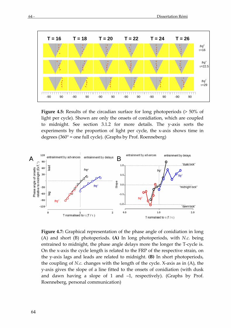
64 - Dissertation Rémi
64
Figure 4.5: Results of the circadian surface for long photoperiods (> 50% of light per cycle). Shown are only the onsets of conidiation, which are coupled to midnight. See section 3.1.2 for more details. The y-axis sorts the experiments by the proportion of light per cycle, the x-axis shows time in degrees (360° = one full cycle). (Graphs by Prof. Roenneberg)
Figure 4.7: Graphical representation of the phase angle of conidiation in long (A) and short (B) photoperiods. (A) In long photoperiods, with N.c. being entrained to midnight, the phase angle delays more the longer the T-cycle is. On the x-axis the cycle length is related to the FRP of the respective strain, on the y-axis lags and leads are related to midnight. (B) In short photoperiods, the coupling of N.c. changes with the length of the cycle. X-axis as in (A), the y-axis gives the slope of a line fitted to the onsets of conidiation (with dusk and dawn having a slope of 1 and –1, respectively). (Graphs by Prof. Roenneberg, personal communication)
frq+
τ=22.5
frq1
τ=16
frq7
τ=29
-90 90 -90 90 -90 90 -90 90 -90 90 -90 90
T = 16 T = 18 T = 20 T = 22 T = 24 T = 26
AA BB

Dissertation Rémi - 65 -
65
Summing up the physiological characteristics of entrainment in Neurospora
crassa, it is evident that Neurospora does entrain to light cycles. It does so in a highly
systematic fashion, and even in skeleton photoperiods. Furthermore, the coupling to
dusk, dawn and midnight is a behavior so far only shown in higher organisms.
Therefore, the results are comparable to entrainment in other organisms, underlining
the importance of Neurospora crassa as a model organism in circadian research.
Also, this study is the first to describe the phenotype of entrainment
comprehensively over so many conditions. Only in model organisms that offer the
experimental possibilities of Neurospora, is the compiling of so many conditions
possible. That allowed establishing rules of entrainment, which in turn allowed
choosing the best cycles for molecular experiments to investigate coupling to
midnight, dawn and dusk. The results from this thesis can now be used to test the
rules of entrainment - that were established for Neurospora - in other organisms with
fewer experiments. The rules of entrainment do not have to be investigated as
extensively as in this study but rather can the rules be tested in other organisms by
choosing cycles according to the relationship of the FRP and the cycle length.
Furthermore, designing molecular experiments will be more focused, when
considering the consequences of a cycle length longer, equal or shorter than the
endogenous cycle length of an organism.

66 - Dissertation Rémi
66
4.2. Entrainment on the molecular level
Neurospora entrains to light cycles and a set of simple and highly systematic
rules can be deducted. Taking those rules, this thesis then investigated the molecular
mechanisms of entrainment. In distinguishing driveness from entrainment, the
kinetics of protein and RNA and their relationship is especially important: In
driveness, uniform responses, irrespective of cycle length and zeitgeber strength, is
expected. In entrainment, a systematic change, indicating an active process of
synchronization is expected.
In addressing molecular responses to light in Neurospora, Crosthwaite and
colleagues (1995) have shown, that frq RNA is up-regulated within 5 minutes after
light reaches dark-grown Neurospora. In the concomitant physiological experiments,
they showed distinct phase advances in the banding pattern. The conclusion was that
the reset by the light stimulus is the molecular correlate of entrainment (Crosthwaite,
Loros et al. 1995; Crosthwaite, Dunlap et al. 1997). Our group has shown previously,
though, that the kinetics of RNA and protein dissociate in various entrainment
protocols and that the peak and trough of RNA levels do not correlate with the
changes in the entrained phase angle (Tan, Dragovic et al. 2004). That enhances the
notion that a one-time reaction of Neurospora as in Crosthwaite’s study does not
necessarily reflect the complex process of entrainment.
In this study, the sharp up-regulation of mRNA was replicated, not only for
frq-RNA but also for vvd-RNA. What was also replicated from our group’s previous
Dissertation Rémi - 67 -
67
work (Tan, Dragovic et al. 2004) was the dissociation of frq-RNA and FRQ-protein
kinetics. That, again, was enhanced by the findings for the VVD-protein in this thesis,
where a similar dissociation of RNA and protein could be shown.
Furthermore, degradation kinetics seem to play an important role for
entrainment. Up-regulation of FRQ is similar in all of the cycles, but the down-
regulation is markedly different, with a prolonged elevated level in longer cycles.
This is an important aspect for future research, because so far degradation has been
adressed in circadian research and it has been shown to be a crucial element in the
negative feedback loop (Ashmore and Sehgal 2003; He and Liu 2005), but it has so far
not been related to entrainment.
As a conclusion from this study of entrainment in Neurospora, protein kinetics
seem to be the key component in the mechanism, with the peak of protein levels and
the different degradation kinetics accounting for the differences in entrained phase
angles.
For future molecular research in general, the physiological experiments
should be chosen carefully to allow the studied organisms to fully entrain to
zeitgeber cycles. Also experimental conditions need to be chosen carefully to account
for the possibility of masking of results (Roenneberg, Dragovic et al. 2005), and to be
able to choose the correct cycles for molecular research. Lastly, when analyzing
molecular data, all aspects of molecular changes need to be adressed: up-regulation
as well as down-regulation.

68 - Dissertation Rémi
68
4.3. Does Neurospora crassa have an M&E oscillator?
As shown in this thesis, Neurospora is very well suited as a model organism in
circadian research. As described above (see section 1.2), the circadian oscillator is the
centerpiece of the circadian clock: in terms of mathematical description a sine-
oscillator, in terms of molecules a translational-transcriptional feedback loop (or
several of them).
This observation is important when evaluating whether Neurospora is
entrained (a systematic synchronization) instead of being driven (a fixed stimulus-
response pattern; Roenneberg, Dragovic et al. 2005). This study showed that
Neurospora crassa entrains to light cycles in a highly systematic fashion. The data
clearly show for the first time in Neurospora crassa that entrainment is not uniform in
respect to the light-dark transitions, but it rather changes the relationship, i.e. the
coupling, to the light-dark cycle, by being coupled to dawn, dusk or midnight. A
theory to explain morningness (M) and eveningness (E), i.e. the coupling of the phase
angle to dawn or dusk, is the M&E oscillator theory. It proposes the existence of two
distinct, non-redundant oscillators with a decisive difference in the way light signals
are computed (Pittendrigh and Daan 1976). The dawn (morningness) oscillator is
advanced by light and delayed by darkness, the dusk (eveningness) oscillator has
reciprocal properties (Daan, Albrecht et al. 2001).

Dissertation Rémi - 69 -
69
Next to the coupling of the phase angle to dawn and dusk, Neurospora crassa
fulfills other properties that the M&E model predicts. It changes the length of the
activity period α with a changing photo- and scotoperiod.
Two distinct oscillators can explain these different properties of the system.
When considering the M&E oscillators in a mammalian circadian system, one
question is left open, though: At what level of organization of the mammalian
circadian clock is the distinction between the M and the E component made? Is it at
the molecular level, with the per1, cry1 and the per2, cry2 complexes forming the two
parts (Daan, Albrecht et al. 2001)? Is it at the neuronal level, with different groups of
neurons generating multiple unit activities (MUA) at different times (Jagota, Iglesia
et al. 2000)? Or even at the anatomical level, with the distinction between different
layers or even the two suprachiasmatic nuclei (Jagota, Iglesia et al. 2000)?
The advantage of Neurospora crassa in investigating this question is its
organization as single cells, a syncitial organism at most. Anatomical distinctions are
obviously not possible. But even in the single cell, there are several possibilities for
the organization of an M and an E component.
The clear entrainment to dawn, dusk and to midnight could be the
physiological behaviour that is founded on M&E oscillators, which could be 2
distinct transcriptional-translational feedback loops (TTL). So far only one loop, the
frq-wc feedback-loop, is well described in Neurospora’s clock. A FRQ-less oscillator is
proposed, but its components remain elusive (Merrow and Roenneberg 2001). One
recent attempt to define a second TTL (Francois 2005), reports the less characterized

70 - Dissertation Rémi
70
enhancement of white-collar 1 (WC-1) protein synthesis by FRQ as the positive
second feedback loop.
The distinction of M&E could also be found in different light receptors, gating
light differently at different times of day (Dragovic, Tan et al. 2002), for example the
differential gating of light by WC-1 as well as by the VVD protein (Heintzen, Loros et
al. 2001). Furthermore, the VVD-protein showed similar kinetics in this study as the
FRQ-protein did in previous work (Tan, Dragovic et al. 2004). For both proteins,
degradation seems to be an important regulator for entrainment, with protein levels
remaining elevated for a longer time, the longer the cycle is chosen.
The M&E response could also be based on entirely different principles, for
example two distinct oscillations of redox-changes (Merrow and Roenneberg 2001).
The results from this study can be explained by an M&E oscillator, they fit its
criteria, but the generation of these two distinct oscillations remains only partly
understood, and opens many possibilities for future research.
A future goal of circadian research will be to assemble one complete model of
the molecular mechanisms of a circadian clock from input over central oscillations to
output. Neurospora could well be used to describe that first complete clock, because
despite its cellular-syncitial organization, this thesis shows for the first time a
circadian behavior as complex as in higher organisms with the extraordinary benefit
of an easily accessible research organism.

Dissertation Rémi - 71 -
71
5. Summary
Circadian rhythms influence almost every process in almost every organism.
Understanding circadian rhythmicity is a crucial tool to understand many other
biological processes. In this study Neurospora crassa, a filamentous fungus, was used
to investigate the synchronization of internal time and external light-dark cycles
(light entrainment).
For physiology experiments a circadian surface was done, taking light-dark
cycles of different lengths and varying the ratio of light to dark within each cycle. A
highly systematic response could be seen: In cycles shorter than the free running
period (FRP), conidiation in N. crassa entrains to dawn, in cycles with a length
around the FRP conidiation entrains to midnight, and in cycles longer than the FRP
conidiation entrains to dusk. This shows that N.c. entrains to light-dark cycles rather
than to be driven by them. Additionally, N.c. entrains even to skeleton photoperiods
with characteristics similar to other, higher, organisms. The results allowed to deduct
a set of simple and highly systematic rules for entrainment to light, which can now
be tested in higher organisms with less experimental effort.
After entrainment on the physiology level was shown, the next step in this
thesis was to investigate the mechanisms on the molecular level. Here a replication
and enhancement of previous results was shown: The quick up-regulation of RNA
after lights-on was repeated. Further repeating previous results, protein kinetics
were shown to not be uniformly coupled to RNA-kinetics. Enhancing previous
72 - Dissertation Rémi
72
results, protein degradation seems to play an important role in entrainment,
changing systematically with the varying entrainment protocols.
Circadian research has been focused on the free-running period. In the future,
entrainment - as an expression of the active process of zeitgeber computation by the
circadian clock - will be studied more closely to understand the clock wheels of the
circadian system. With this thesis it was shown that even a simple organism like
Neurospora crassa entrains to light cycles rather than to be merely driven, and it
entrains with characteristics that are comparable to higher organisms. This
underlines the usefulness of Neurospora crassa as a model organism in circadian
research, and lays the ground for entrainment research in higher organisms.
Dissertation Rémi - 73 -
73
6. Zusammenfassung
Circadiane Rhythmen beeinflussen fast jeden biologischen Prozess in fast
jedem Organismus. Das Verständnis von circadianen Rhythmen ist entscheidend um
viele andere biologische Prozesse zu verstehen. In dieser Doktorarbeit wurde der
Sprosspilz Neurospora crassa benutzt um die Synchronisation von innerer Uhr mit
Hell-Dunkel Zyklen zu untersuchen (Licht-„Entrainment“).
Durch physiologische Experimente wurde eine circadiane Oberfläche erstellt,
indem die Sporulation von Neurospora crassa in Licht-Dunkel-Zyklen verschiedener
Länge mit unterschiedlichen Licht-Dunkel-Verhältnissen innerhalb der einzelnen
Zyklen analysiert wurde. Das Verhalten von Neurospora war sehr systematisch: In
Lichtzyklen, die kürzer als der innere Tag waren, synchronisierte sich die
Sporulation bei N. crassa relativ zur Morgendämmerung (Licht an), in Zyklen die in
etwa der inneren Uhrlänge entsprachen synchronisierte sie sich zu Mitternacht, und
in Zyklen die länger waren zur Abenddämmerung (Licht aus). Dies zeigte, dass sich
N.c. aktiv mit Licht-Dunkel-Zyklen synchronisiert anstatt nur auf sie zu reagieren.
Zusätzlich konnte gezeigt werden, dass N.c. sich sogar mit skelettierten Licht-
Dunkel-Zyklen (Die Licht-an und die Licht-aus-Grenze wurden durch 2-stündige
Lichtpulse simuliert) aktiv synchronisiert, und zwar mit einer Systematik die in
höheren Organismen schon beschrieben wurde. Mit diesen Ergebnissen konnten
einfache aber sehr systematische Regeln für circadiane Lichtsynchronisation erstellt
werden. Diese könne nun wiederum benutzt werden, um Lichtsynchronisation in

74 - Dissertation Rémi
74
höheren Organismen zu untersuchen, bei denen die aufwendigen Experimente
dieser Doktorarbeit logistisch nicht möglich sind.
Nachdem die aktive Synchronisation von innerer Uhr und äußeren Zeitgebern
gezeigt wurde, wurden in dieser Doktorarbeit die molekularen Mechanismen der
Synchronisation von innerer und äußerer Zeit untersucht. Es konnten vorherige
Ergebnisse repliziert und erweitert werden: Die schnelle Hoch-Regulierung von
RNA durch das Lichtsignal wurde bestätigt, ebenso wie die vorherigen Ergebnisse
unserer Gruppe, dass RNA-Kinetik und Proteinkinetik nicht linear verbunden sind.
Die bekannten Mechanismen wurden erweitert, indem gezeigt wurde, dass
Proteinabbau eine wichtige Rolle in der aktiven Synchronisation von innerer und
äußerer Zeit spielt, da sie sich systematisch veränderte als die Lichtzyklen
systematisch verändert wurden.
Die circadiane Forschung hatte ihren Schwerpunkt bisher auf Versuchen in
konstanten Bedingungen. In der Zukunft wird „Entrainment“ (der aktive
Synchronisationsprozess von äußerer Zeitinformationen und Zustand der inneren
Uhr) in den Mittelpunkt der Forschung treten, um die Arbeit der Zahnräder der
inneren Uhr besser zu verstehen. Mit dieser Doktorarbeit konnte gezeigt werden,
dass ein einfacher Organismus wie Neurospora crassa sich aktiv mit Lichtzyklen
synchronisiert anstatt nur auf sie zu reagieren, und das mit Charakteristika, die dem
Verhalten von höheren Organismen entsprechen. Das zeigt den Nutzen von
Neurospora crassa als Modellorganismus in der circadianen Forschung und
ermöglicht systematischere “Entrainment”-Forschung in höheren Organismen.

Dissertation Rémi - 75 -
75
7. References 1. Allada, R. (2003). "Circadian clocks: a tale of two feedback loops." Cell 112(3):329-
41 2. Aronson, B. D., K. A. Johnson, et al. (1994). "The circadian clock locus frequency: a
single ORF defines period length and temperature compensation." Proc Natl Acad Sci USA 91: 7683-7687.
3. Aschoff, J. (1965). "Circadian rhythms in man." Science 148: 1427-1432. 4. Aschoff, J. (1985). "On the perception of time during prolonged isolation." Human
Neurobiol 4(time perception): 41-52. 5. Ashmore, L. and A. Sehgal (2003). "A fly's eye view of circadian entrainment." J
Biol Rhythms 18(3): 206-16. 6. Beck, S. D. (1962). "Photoperiodic induction of diapause in an insect." Biological
Bulletin 122(1): 1-12. 7. Berson, D. M., F. A. Dunn, et al. (2002). "Phototransduction by retinal ganglion
cells that set the circadian clock." Science 295(5557): 1070-3. 8. Bieszke, J., E. Spudich, et al. (1999). "A eukaryotic protein, NOP-1, binds retinal to
form an archaeal rhodopsin-like photochemically reactive pigment." Biochemistry 38(43): 14138-45.
9. Bognar, L. K., A. H. Adam, et al. (1999). "The circadian clock controls the expression pattern of the circadian input photoreceptor, phytochrome B." Proc Natl Acad Sci USA 96: 14652-14657.
10. Bruce, V. (1960). "Environmental Entrainment of Circadian Rhythms." Cold Spring Harbor Symp Quant Biol 25: 29-47.
11. Covic, A. and D. Goldsmith (1999). "Ambulatory blood pressure monitoring in nephrology: focus on BP variability." J Nephrol 12(4): 220-9.
12. Crosthwaite, S. K., J. C. Dunlap, et al. (1997). "Neurospora wc-1 and wc-2: Transcription, photoresponses, and the origin of circadian rhythmicity." Science 276: 763-769.
13. Crosthwaite, S. K., J. J. Loros, et al. (1995). "Light-induced resetting of a circadian clock is mediated by a rapid increase in frequency transcript." Cell 81: 1003-1012.
14. Daan, S., U. Albrecht, et al. (2001). "Assembling a clock for all seasons: are M and E oscillators in the genes?" J Biol Rhythms 16(2): 105-116.
15. Daan, S., M. Merrow, et al. (2002). "External time - internal time." J Biol Rhythms 17(2): 107-109.
16. Darwin, C. (1880). On the power of movement in plants. London, John Murray. 17. DeCoursey, P., J. Walker, et al. (2000). "A circadian pacemaker in free-living
chipmunks: essential for survival?" J Comp Physiol 186(2): 169-80. 18. Denault, D. L., J. J. Loros, et al. (2001). "WC-2 mediated WC-1-FRQ interaction within the PAS protein-linked circadian feedback loop of Neurospora." EMBO J 20: 109-117.

76 - Dissertation Rémi
76
19. Diernfellner, A., T. Schafmeier, et al. (2005). "Molecular mechanism of temperature sensing by the circadian clock of Neurospora crassa." Genes
Dev 19(17): 1968-73. 20. Dragovic, Z., Y. Tan, et al. (2002). "Light reception and circadian behavior in
'blind' and 'clock-less' mutants of Neurospora crassa." EMBO J 21: 3643-3651. 21. Eastman, C., M. Young, et al. (1998). "Bright light treatment of winter depression:
a placebo-controlled trial." Arch Gen Psychiatry 55(10): 883-9. 22. Ebisawa, T., M. Uchiyama, et al. (2001). "Association of structural polymorphisms
in the human period3 gene with delayed sleep phase syndrome." EMBO Rep 2(4): 342-6.
23. Feldman, J. F. and M. N. Hoyle (1973). "Isolation of circadian clock mutants of Neurospora crassa." Genetics 75: 605-613.
24. Francois, P. (2005). "A model for the Neurospora circadian clock." Biophys J 88(4): 2369-83.
25. Freedman, M. S., R. J. Lucas, et al. (1999). "Non-rod, non-cone ocular photoreceptors regulate the mammalian circadian behaviour." Science 284(5413): 502-504.
26. Froehlich, A. C., Y. Liu, et al. (2002). "White Collar-1, a circadian blue light photoreceptor, binding to the frequency promoter." Science 297: 815-819.
27. Galagan, J., S. Calvo, et al. (2003). "The genome sequence of the filamentous fungus Neurospora crassa." Nature 422(6934): 821-2.
28. Goldman, B. (1999). "The Siberian hamster as a model for study of the mammalian photoperiodic mechanism." Adv Exp Med Biol 460: 155-64.
29. Goldman, B. (2001). "Mammalian photoperiodic system: formal properties and neuroendocrine mechanisms of photoperiodic time measurement." J Biol Rhythms 16(4): 283-301.
30. Gwinner, E. (1986). Circannual rhythms. Berlin, Springer Verlag. 31. Hankins, M. W. and R. J. Lucas (2002). "A novel photopigment in the human
retina regulates the activity of primary visual pathways according to long-term light exposure." Curr Biol 12(3): 191-198.
32. Hattar, S., H. W. Liao, et al. (2002). "Melanopsin-containing retinal ganglion cells: architecture, projections, and intrinsic photosensitivity." Science 295: 1065-1070.
33. He, Q. and Y. Liu (2005). "Degradation of the Neurospora circadian clock protein FREQUENCY through the ubiquitin-proteasome pathway." Biochem Soc Trans 33: 953-6.
34. Heintzen, C., J. J. Loros, et al. (2001). "The PAS Protein VIVID Defines a Clock-Associated Feedback Loop that Represses Light Input, Modulates Gating, and Regulates Clock Resetting." Cell 104: 453-464.
35. Hurst, W., J. Mitchell, et al. (2002). "Synchronization and phase-resetting by glutamate of an immortalized SCN cell line." Biochem Biophys Res Commun 298(1): 133-43.
36. Jagota, A., H. d. l. Iglesia, et al. (2000). "Morning and evening circadian oscillations in the suprachiasmatic nucleus in vitro." Nat Neurosci 3(4): 372-6.

Dissertation Rémi - 77 -
77
37. Johnson, C. and S. Golden (1999). "Circadian programs in cyanobacteria: adaptiveness and mechanism." Annu Rev Microbiol 53: 389-409.
38. Kawachi, I., G. A. Colditz, et al. (1995). "Prospective study of shift work and risk of coronary heart disease in women." Circulation 92: 3178-3182.
39. Lee, K., J. C. Dunlap, et al. (2003). "Roles for WHITE COLLAR-1 in circadian and general photoreception in Neurospora crassa." Genetics 168: 103-114.
40. Lee, K., J. J. Loros, et al. (2000). "Interconnected feedback loops in the Neurospora circadian system." Science 289: 107-110.
41. Liu, Y. (2003). "Molecular mechanisms of entrainment in the Neurospora circadian clock." J Biol Rhythms 18(3): 195-205.
42. Liu, Y., N. Garceau, et al. (1997). "Thermally regulated translational control of FRQ mediates aspects of temperature responses in the neurospora circadian clock." Cell 89(3): 477-86.
43. Loros, J. and J. Feldman (1986). "Loss of temperature compensation of circadian period length in the frq-9 mutant of Neurospora crassa." J Biol Rhythms 1(3): 187-98.
44. Loros, J. J. and J. C. Dunlap (2001). "Genetic and molecular analysis of circadian rhythms in Neurospora." Annu Rev Physiol 63: 757-794.
45. Loros, J. J. and J. F. Feldman (1986). "Loss of temperature compensation of circadian period length in the frq-9 mutant of Neurospora crassa." J Biol Rhythms 1: 187-198.
46. Loudon, A. S., N. Ihara, et al. (1998). "Effects of a circadian mutation on seasonality in Syrian hamsters (Mesocricetus auratus)." Proc R Soc Lond B Biol Sci 265(1395): 517-521.
47. Lüttge, U. (2000). "The tonoplast functioning as the master switch for circadian regulation of crassulacean acid metabolism." Planta 211: 761-769.
48. Menaker, M. (2003). "Circadian rhythms. Circadian photoreception." Science 299(5604): 213-4.
49. Merrow, M., M. Brunner, et al. (1999). "Assignment of circadian function for the Neurospora clock gene frequency." Nature 399: 584-586.
50. Merrow, M., L. Franchi, et al. (2001). "Circadian regulation of the light input pathway in Neurospora crassa." EMBO J 20(3): 307-315.
51. Merrow, M. and T. Roenneberg (2001). "Circadian clocks: running on redox." Cell 106: 141-143.
52. Merrow, M. and T. Roenneberg (2001). "The circadian cycle: is the whole greater than the sum of its parts?" TIGS 17: 4-7.
53. Merrow, M. W. and J. C. Dunlap (1994). "Intergeneric complementation of a circadian rhythmicity defect: phylogenetic conservation of structure and function of the clock gene frequency." EMBO J 13: 2257-2266.
54. Moore-Ede, MC (1986) "Jet lag, shift work, and maladaption."NIPS 1:156-160. 55. Mormont, M. and F. Levi (2003). "Cancer chronotherapy: principles, applications,
and perspectives." Cancer 98(4): 881-2.

78 - Dissertation Rémi
78
56. Oishi, K., K. Miyazaki, et al. (2003). "Genome-wide expression analysis of mouse liver reveals CLOCK-regulated circadian output genes." J Biol Chem
278(42): 41519-27. 57. Oren, D., K. Wisner, et al. (2002). "An open trial of morning light therapy for
treatment of antepartum depression." Am J Psychiatry 159(4): 666-9. 58. Pittendrigh, C. S. (1954). "On temperature independence in the clock con-trolling
emergence time in Drosophila." Proc Natl Acad Sci USA 40: 1018-1029. 59. Pittendrigh, C. S. (1960). "Circadian rhythms and the circadian organization of
living systems." Cold Spring Harbor Symp Quant Biol 25: 159-184. 60. Pittendrigh, C. S. and S. Daan (1976). "A functional analysis of circadian
pacemakers in nocturnal rodents: V. Pacemaker structure: a clock for all seasons." J Comp Physiol A 106: 333-355.
61. Pittendrigh, C. S. and S. Daan (1976a). "A functional analysis of circadian pacemakers in noctural rodents: I. The stability and lability of circadian frequency." J Comp Physiol A 106: 223-252.
62. Reinberg, A., P. Andlauer, et al. (1984). "Desynchronization of the oral temperature circadian rhythm and intolerance to shift work." Nature 308: 272-274.
63. Reppert, S. M. and D. R. Weaver (2002). "Coordination of circadian timing in mammals." Nature 418: 935-941.
64. Richter, C. (1978). "Evidence for existence of a yearly clock in surgically and self-blinded chipmunks." Proc Natl Acad Sci USA 75(7): 3517-3521.
65. Roden, M., M. Koller, et al. (1993). "The circadian melatonin and cortisol secretion pattern in permanent shift workers." Am J Physiol 265: R261-R267.
66. Roenneberg, T., S. Daan, et al. (2003). "The art of entrainment." J Biol Rhythms 18(3): 183-194.
67. Roenneberg, T., Z. Dragovic, et al. (2005). "Demasking biological oscillators: Properties and principles of circadian entrainment exemplified by the Neurospora circadian clock." Proc Natl Acad Sci USA 102(21): 7742-7747.
68. Roenneberg, T. and R. Foster (1997). "Twilight times: light and the circadian system." Photochem Photobiol 66(5): 549-61.
69. Roenneberg, T. and M. Merrow (1998). "Molecular circadian oscillators - an alternative hypothesis." J Biol Rhythms 13: 167-179.
70. Roenneberg, T. and M. Merrow (2000). "Circadian light input: omnes viae Romam ducunt." Curr Biol 10: R742-R745.
71. Roenneberg, T. and M. Merrow (2001). "Seasonality and photoperiodism in fungi." J Biol Rhythms 16: 403-414.
72. Roenneberg, T. and M. Merrow (2002). "Life before the clock - modeling circadian evolution." J Biol Rhythms 17(6): 495-505.
73. Roenneberg, T. and D. Morse (1993). "Two circadian oscillators in one cell." Nature 362: 362-364.
74. Roenneberg, T., A. Wirz-Justice, et al. (2003). "Life between clocks - daily temporal patterns of human chronotypes." J Biol Rhythms 18(1): 80-90.

Dissertation Rémi - 79 -
79
75. Sack, R. L., A. J. Lewy, et al. (1991). "Melatonin administration to blind people: phase advances and entrainment." J Biol Rhythms 6: 249-262.
76. Sargent, M. L. and S. H. Kaltenborn (1972). "Effects of medium composition and corbon dioxide on circadian conidiation in Neurospora." Plant Physiol 50: 171-175.
77. Schafmeier, T., A. Haase, et al. (2005). "Transcriptional feedback of Neurospora circadian clock gene by phosphorylation-dependent inactivation of its transcription factor." Cell 122(2): 235-46.
78. Schernhammer, E., F. Laden, et al. (2001). "Rotating night shifts and risk of breast cancer in women participating in the nurses' health study." J Natl Cancer Inst 93(20): 1563-8.
79. Schernhammer, E., F. Laden, et al. (2003). "Night-shift work and risk of colorectal cancer in the nurses' health study." J Natl Cancer Inst 95:825-8.
80. Schwartz, W., H. d. l. Iglesia, et al. (2001). "Encoding le quattro stagioni within the mammalian brain: photoperiodic orchestration through the suprachiasmatic nucleus." J Biol Rhythms 16(4): 302-11.
81. Schwartz, W. J. and H. Gainer (1977). "Suprachiasmatic nucleus: use of C- labeld deoxyglucose uptake as a functional marker." 97: 89-109.
82. Schwerdtfeger, C. and H. Linden (2003). "VIVID is a flavoprotein and serves as a fungal blue light photoreceptor for photoadaptation." EMBO J 22(18): 4846-55.
83. Silver, R., A. Sookhoo, et al. (1999). "Multiple regulatory elements result in regional specificity in circadian rhythms of neuropeptide expression in mouse SCN." Neuroreport 10(15): 3165-74.
84. Somers, D. E., P. F. Devlin, et al. (1998). "Phytochromes and cryptochromes in the entrainment of the Arabidopsis circadian clock." Science 282: 1488-1490.
85. Tan, Y., Z. Dragovic, et al. (2004). "Entrainment dissociates transcription and translation of a circadian clock gene in neurospora." Curr Biol 14(5): 433-8.
86. Tan, Y., M. Merrow, et al. (2004). "Photoperiodism in Neurospora crassa." J Biol Rhythms 19(2): 135-143.
87. Terman, M., A. Lewy, et al. (1995). "Light treatment for sleep disorders: consensus report. IV. Sleep phase and duration disturbances." J Biol Rhythms 10(2): 135-47.
88. Towbin, H., T. Staehelin, et al. (1979). "Electrophoretic transfer of protein from polyacrylamid gels to nitrocellulose sheets: procedure and some applications." Proc Natl Acad Sci USA 79: 267-271. 89. Welsh, D. K., D. E. Logothetis, et al. (1995). "Individual neurons dissociated from
rat suprachiasmatic nucleus express independently phased circadian firing rhythms." Neuron 14: 697-706.

80 - Dissertation Rémi
80
8. Appendix:
8.1. Abbreviations
µ Micro (10-6)
A Ampere
aa amino-acid
bp base pairs
cDNA Complementary DNA
DD Constant darkness
DNA Deoxyribonucleic acid
dNTP Deoxynucleoside triphosphate
E (/sec/m2) Einstein, 1 mol photons (per second and m2)
FGSC also “fgsc”, Fungal Genetic Stock Centre
FRP Free running period = τ
frq frequency gene
FRQ frequency gene product (FRQ protein)
g Gram
h Hour
HEPES 4-(2-hydroxyethil)-1-piperazineethanesulfonic acid buffer
IgG Immunoglobulin G
k kilo (103)
LD Light-Dark
LL Constant light
M Molar
m milli (10-3)
min Minute
mRNA messenger ribonucleic acid
n nano (10-9)

Dissertation Rémi - 81 -
81
NTP Nucleoside triphosphate
OD optical density
PAGE Polyacrilamide gel electrophoresis
PCR Polymerase Chain Reaction
PMSF Phenyl-methyl-sulfonyl-fluoride
RNA Ribonucleic acid
RT-PCR Real Time Polymerase Chain Reaction
SCN supra chiasmatic nucleus
τ free running period, FRP
Taq Thermophilus aquaticus DNA polymerase
UTP Uridine-triphosphate
V Volt
vvd vivid gene
VVD vivid gene product (VVD protein)
V/V Volume per volume
w/V Weight per volume
wc-1 white collar-1gene
WC-1 white collar-1 gene product (WC-1 protein)
wc-2 white collar-2gene
WC-2 white collar-2 gene product (WC-2 protein)
wl wavelength
wt wild type

82 - Dissertation Rémi
82
8.2. Recipes
- Acrylamide solution Acrylamide 29.2 g N, N’-Methylene-bis-acrylamide 0.8 g ddH2O Up to 100 ml - Blotting buffer - Buffer for semi-dry blot TRIS 50mM Glycin 14.4 g Glycin 384mM Tris 3 g Methanol 20% (V/V) Methanol 200 ml ddH2O up to 1000ml - Electrophoresis buffer (SDS Page) 10X - PBS 10X Glycin 144.13 g NaCl 80 g TRIS 30.28 g KCl 2 g SDS 10 g Na2HPO4 x 7H2O 11.5 g ddH2O up to 1000ml K2HPO4 2 g ddH2O up to 1000ml - Laemmle Buffer - Ponceau solution TRIS/HCl pH6.8 60mM Ponceau 0.2% (w/V) SDS 2% (w/V) Trichloroacetic acid 3% (w/V) b-Mercaptoethanol 5% (w/V) Glycerol 10% (w/V) Bromophenol Blue 0.2% (w/V) - Protein dephosphorylation buffer 1X - Protein extraction buffer (PEB) HEPES/KOH pH 7.4 50 mM Hepes 1.2g NaCl 137 mM Glycerol 10ml Glyzerin 10% (v/v) NaCl (5M) 2.7ml EDTA 5 mM EDTA (0.5M, pH 8.0) 1ml PMSF 1 mM l H2O 90ml Leupeptin 1 µg/ml Pepstatin A 1 µg/ml - Race tube media - RNA extraction buffer Bacto-Agar 2% (w/V) EDTA (0.5M, pH 8.0) 2ml Arginine 0.5% (w/V) TRIS (1M, pH 8.0) 10ml Glucose 0.3% (w/V) SDS (10%) 40ml Vogel’s salts 1X NaCl (5M) 12ml Biotin 1ng/ml H2O 36ml
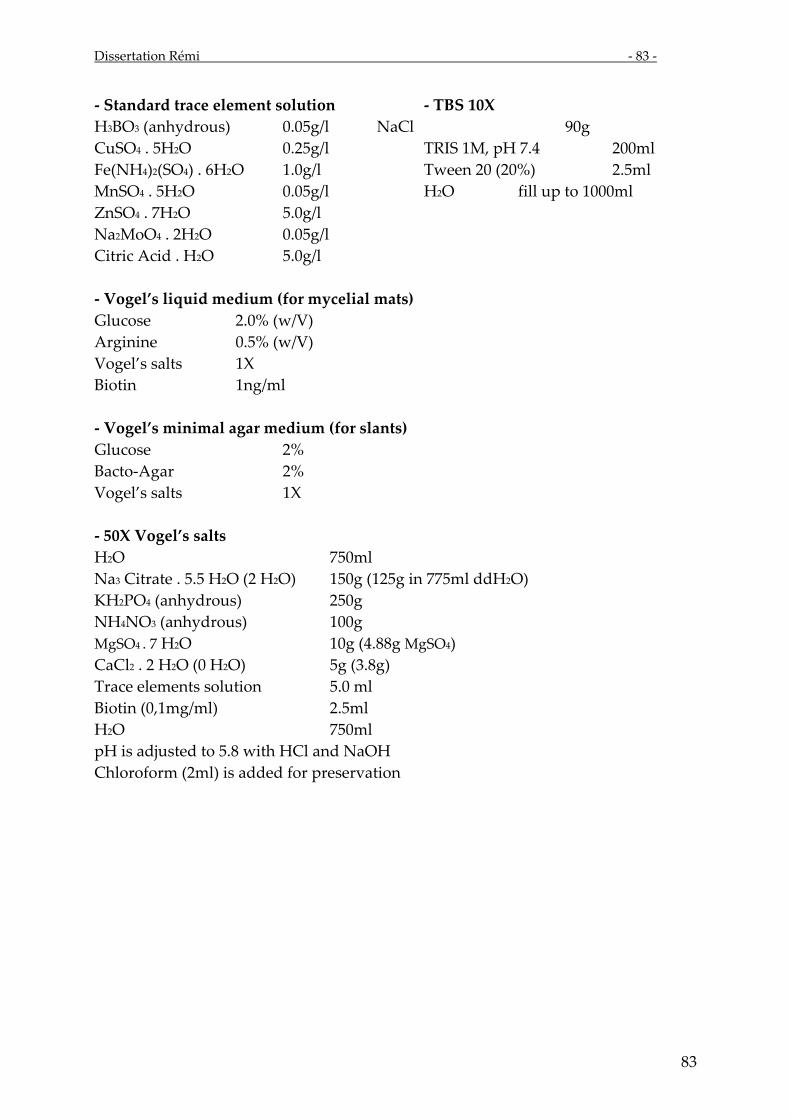
Dissertation Rémi - 83 -
83
- Standard trace element solution - TBS 10X H3BO3 (anhydrous) 0.05g/l NaCl 90g CuSO4 . 5H2O 0.25g/l TRIS 1M, pH 7.4 200ml Fe(NH4)2(SO4) . 6H2O 1.0g/l Tween 20 (20%) 2.5ml MnSO4 . 5H2O 0.05g/l H2O fill up to 1000ml ZnSO4 . 7H2O 5.0g/l Na2MoO4 . 2H2O 0.05g/l Citric Acid . H2O 5.0g/l - Vogel’s liquid medium (for mycelial mats) Glucose 2.0% (w/V) Arginine 0.5% (w/V) Vogel’s salts 1X Biotin 1ng/ml - Vogel’s minimal agar medium (for slants) Glucose 2% Bacto-Agar 2% Vogel’s salts 1X - 50X Vogel’s salts H2O 750ml Na3 Citrate . 5.5 H2O (2 H2O) 150g (125g in 775ml ddH2O) KH2PO4 (anhydrous) 250g NH4NO3 (anhydrous) 100g MgSO4 . 7 H2O 10g (4.88g MgSO4) CaCl2 . 2 H2O (0 H2O) 5g (3.8g) Trace elements solution 5.0 ml Biotin (0,1mg/ml) 2.5ml H2O 750ml pH is adjusted to 5.8 with HCl and NaOH Chloroform (2ml) is added for preservation
84 - Dissertation Rémi
84
8.3. List of Instruments
Autoclave, type 300, Varioklav
Blotting apparatus, Trans-Blot cell (with plate electrodes), BioRad
Blotting apparatus, custom made; Specification: Helmut Klausner, workshop of IMP, Goethestr.
31/U1, 80336 Munich, Germany
Centrifuge, 5415C, Eppendorf
Centrifuge, 5417R, Eppendorf
Centrifuge, Biofuge Primo-R, Heraeus
Electrophoresis apparati, vertical (gel size 120x140x0.75, 1.00 or 1.50mm) and horizontal (for
DNA and RNA, gel size 5x7.5, 9x7.5, 11x14 and 14x23 cm) all custom made; Specification:
Helmut Klausner, workshop of Inst. f. Med. Psych. Goethestr. 31/U1, 80336 Munich, Germany
Electrophoresis apparatus, Mini Protean II cell, BioRad
Electrophoresis apparatus, Protean II xi cell, BioRad
Freezer,-20°C, different models for household
Freezer,-80°C, Heraeus
Magnetic mixer, Ikamag, Junke&Kunkel-Ikawerk
Pipet, with positive displacement, Biomaster, Eppendorf
Pipets, Pipetman (10,20,100,200,1000µl), Gilson
Pipets, Reference (10,20,100,1000,2500µl), Eppendorf
Real Time PCR system, ABI PRISM 7000, Applied Biosystems
Racetubes, Glasbläserei Höhn, München & Glasbl. Schmitz, München
Scale, Handy H 110, Sartorius
Scale, L2200S Sartorius
Scale, Mettler, AE 50, Mettler,
Scintillation counter, LS 1801, Beckman
Shaker, KL2, Bachofer
Shaker, LS10, Gerhard
Spectrophotometer, DU64, Beckman
Spectrophotometer, Ultrospec 3000, Pharmacia
Speed-Vac, Bachofer
Thermal cycler, Primus, MWG Biotech
Thermomixer, 5436, Eppendorf
Thermomixer, comfort, Eppendorf
Dissertation Rémi - 85 -
85
Timers,WB-388 and TR-118, Oregon Scientific;
Vortex, k-550-GE, Bender&Hobein AG
8.4. List of chemicals
Substance Company Order No.
Acetic Acid SIGMA A-6283
Acetone ALDRICH 17,997-3
Acrylamide APPLICHEM A3705,0500
Acrylamide GERBU 1002
Agarose LOW EEO APPLICHEM A2114,0500
Agarose QA TM Q-BIOGEN AGR0050
Albumin Bovine SIGMA A-3350
Ammonium acetate SIGMA A-1542
Ammonium chloride SIGMA A-4514
Ammonium nitrate SIGMA A-1308
Ammonium peroxodisulfate (APS) ROTH 9592.3
Ammonium sulfate ALDRICH 22.125-2
Arginine hydrochlorid (L+) USB US 11500
Bacto Agar DIFCO 214010
Bis acrylamide SIGMA M-7279
Boric acid APPLICHEM A2940,1000
Boric acid APPLICHEM A3581,0500
Calcium chloride x 2H2O ROTH 5239.1
Chloroform SIGMA C-5312
Chloroform:isoamylalcohol SIGMA C-0549
Citric acid ALDRICH 24,062-1
Coomassie brilliant blue SIGMA B-0149
Ethanol ROTH 9065.2
Glucose monohydrate MERCK 1.04074
Glycerol APPLICHEM A2926,1000
Hepes SIGMA H-3375
Hexane ALDRICH 29,325.30

86 - Dissertation Rémi
86
Isoamyalcohol ROTH 8930.1
Leupeptin USB 18413
Magnesiumchlorid x 6H2O MERCK 1.05835.0500
Methanol ROTH 4627.1
Pepstatin A USB US20037
Phenol (DNA/RNA) ROTH A.156.1
Phenol (RNA) ROTH A.980.1
Phenylmethanesulfonyl fluoride (PMSF) FLUKA 78830
Polyethyleneglycol PEG 4000 ROTH 156.1
Ponceau S FLUKA 81460
Potassium chloride SIGMA P-3911
Sand SIGMA S-9887
SDS / Sodium Dodecyl Sulfate ROTH 2326.2
Sodium azide SIGMA S-2002
Sodium chloride MERCK 1.06404
Sodium chloride APPLICHEM A2942,1000
Sodium citrate ROTH 3580.1
Sodium dihydrogenphosphate MERCK 6346
Sodium hydroxid ROTH 6771.1
Sodium nitrate FLUKA 71755
Sodium nitrit ALDRICH 20,783-7
Temed SIGMA T-8133
Trichloracetic acid SIGMA T-4885
Tris APPLICHEM A1086,100
Tween 20 USB 20605

Dissertation Rémi - 87 -
87
8.5. List of Biochemicals
Name Company Cat No
Alkaline Phosphatase, Calf Intestinal (CIP) NEBL M 0290 L
α-Mouse polyvalent immunoglobulins SIGMA A-0412
Phophatase (CIP) ROCH 776785
dNTPmix AB N8080260
PCR system, Exp. Long Template ROCHE 1-681-842
Protein Assay (Bradford) BIORAD 500-0006
Protein Assay (gamma glob. standard) BIORAD 500-005
Protein Markers (pre-stained ladder) BIORAD 161-0373
Reverse Transcription reagents AB N8080234
Reverse Transcriptase AB 4311235
RNA polymerase PROMEGA P2075
RNA Secure AMBION 7005
RNAguard RNAse inhibitor AMERSHAM 27-0815-01
SYBR Green PCR master mix AB 4309155
Western Blotting sub. ECL ROCHE 2015196
88 - Dissertation Rémi
88
9. Acknowledgements – Danksagung
- I am indebted to my doctoral parents: Till Roenneberg and Martha
Merrow. I thank you from all of my heart for introducing me to science, for being an inspiration in curiosity without compromises and for allowing a medical student to linger around your habitat for a while. Thank you for your patience and your warm reception. You will always be my standard for true scientists.
- Ich danke Professor Ernst Pöppel für die wissenschaftliche Umgebung, die er in seinem Institut bereitet hat, in der Studenten ihre Forschung gestalten und als Wissenschaftler wachsen können.
- Ich danke den Laborassistentinnen des Roenneberg’schen Labors: Vera Schiewe, Elfie Henoch and Astrid Bauer für die konzentrierte und exakte Arbeit, die die Basis für unsere Erfolge ist.
- Helmut Klausner: Vielen Dank für die exzellente Arbeit beim Bau unserer Forschungsmittel.
- Allen Angestellten am Institut für Medizinische Psychologie: Danke für Eure Freundlichkeit und die schöne Atmosphäre.
- Zdravketina Dragovic: Hvala. I thank you for your introduction to and your teaching of molecular biology. Your exactness in experimental science will be hard to achieve for anyone. Also thank you for teaching me Serbian derogatory language and making bench work very entertaining.
- Kruno Sveric: Ohne Dich wäre ich verhungert und hätte verlernt auch mal wieder an Medizin zu denken.
- Conny Bösl: Never was grinding tissue more fun. Please uphold your spirit. Without you lab life is a lot quieter. I am grateful that I could spend time with you and our little orange friend.
- Ich danke meinen Eltern für ihre Geduld und liebevolle Zuwendung. Ohne sie hätte ich nicht einmal Medizin studiert.
- Ich danke Dir, Constanze, für die Unterstützung und Liebe in allen
Lebenslagen und für Deine liebevollen Zurechtweisungen.

Dissertation Rémi - 89 -
89
10. Lebenslauf – curriculum vitae Jan Rémi, geborener Ricken am 31.01.1977 in Krefeld Schulausbildung: 1987-97 Gymnasium Weilheim 1994/95 Austauschjahr an der Maroa-Forsyth Highschool in Illinois/USA Medizinische Ausbildung: 1997/98 Zivildienst (Individuelle Schwerstbehinderten-Betreuung) 1998 - 2005 Studium der Humanmedizin an der LMU München Praktisches Jahr (April 2004 –März 2005) 1. Tertial: Innere Medizin an der Harvard Medical School Stipendium der Munich-Harvard Educational Alliance 2. Tertial: Neurologie in der Neurologische Klinik Großhadern 3. Tertial: Chirurgie in der Chirurgische Klinik Innenstadt Seit Juni 2005: Assistenzarzt in der Neurologischen Klinik und Poliklinik der LMU München Wissenschaftliche Ausbildung:
- Seit Juni 2000 Mitarbeit als medizinischer Doktorand in der Arbeitsgruppe Prof. Dr. rer.nat. Roenneberg (Chronobiologie), LMU München
- August 2002 – Januar 2003: Aufenthalt bei Volkswagen in Wolfsburg zur Betreuung der Studie: „Einfluss von Licht auf die Innere Uhr von Schichtarbeitern“
- Seit Juni 2005: wissenschaftlicher Assistent an der Neurologischen Klinik und Poliklinik der LMU München (Forschungsgruppe Schlaf und Epilepsie unter Leitung von Prof. Dr. med. S. Noachtar)