Autism Waldman Nicholson Adilov
68
DOES TELEVISION CAUSE AUTISM? Michael Waldman Johnson Graduate School of Management Cornell University Sage Hall Ithaca, NY 14853 (607) 255-8631 Sean Nicholson Policy Analysis and Management Cornell University and NBER 133 Martha Van Rensselaer Hall Ithaca, NY 14853 (607) 254-6498 and Nodir Adilov Department of Economics Doermer School of Business and Management Sciences Indiana University-Purdue University Neff Hall Fort Wayne, IN 46805 (260) 481-6497 Revised December 2006 * We thank Artem Gulish, Gayatri Koolwal, Rebecc a Lee, Joe Podwol, an d Matthew White for excellent research assistance and Vrinda Kadiyali, Jonathan Skinner, and Ken Sokoloff for comments on earlier drafts and helpful discussions during the formulation of the paper.
-
Upload
phiynovitahusnanst -
Category
Documents
-
view
220 -
download
0
Transcript of Autism Waldman Nicholson Adilov
8/6/2019 Autism Waldman Nicholson Adilov
http://slidepdf.com/reader/full/autism-waldman-nicholson-adilov 1/68
DOES TELEVISION CAUSE AUTISM?
Michael WaldmanJohnson Graduate School of Management
Cornell UniversitySage Hall
Ithaca, NY 14853(607) 255-8631
Sean NicholsonPolicy Analysis and Management
Cornell University and NBER
133 Martha Van Rensselaer HallIthaca, NY 14853(607) 254-6498
and
Nodir AdilovDepartment of Economics
Doermer School of Business and Management SciencesIndiana University-Purdue University
Neff HallFort Wayne, IN 46805
(260) 481-6497
Revised December 2006
8/6/2019 Autism Waldman Nicholson Adilov
http://slidepdf.com/reader/full/autism-waldman-nicholson-adilov 2/68
ABSTRACT
Autism is currently estimated to affect approximately one in every 166 children, yet the
cause or causes of the condition are not well understood. One of the current theories concerning
the condition is that among a set of children vulnerable to developing the condition because of
their underlying genetics, the condition manifests itself when such a child is exposed to a
(currently unknown) environmental trigger. In this paper we empirically investigate the
hypothesis that early childhood television viewing serves as such a trigger. Using the Bureau of
Labor Statistics’ American Time Use Survey, we first establish that the amount of television a
young child watches is positively related to the amount of precipitation in the child’s
community. This suggests that, if television is a trigger for autism, then autism should be more
prevalent in communities that receive substantial precipitation. We then look at county-level
autism data for three states – California, Oregon, and Washington – characterized by high
precipitation variability. Employing a variety of tests, we show that in each of the three states
(and across all three states when pooled) there is substantial evidence that county autism rates
are indeed positively related to county-wide levels of precipitation. In our final set of tests we
use California and Pennsylvania data on children born between 1972 and 1989 to show, again
consistent with the television as trigger hypothesis, that county autism rates are also positively
related to the percentage of households that subscribe to cable television. Our precipitation tests
indicate that just under forty percent of autism diagnoses in the three states studied is the result
of television watching due to precipitation, while our cable tests indicate that approximately
seventeen percent of the growth in autism in California and Pennsylvania during the 1970s and
1980s is due to the growth of cable television. These findings are consistent with early
childhood television viewing being an important trigger for autism. We also discuss further tests
that can be conducted to explore the hypothesis more directly.
8/6/2019 Autism Waldman Nicholson Adilov
http://slidepdf.com/reader/full/autism-waldman-nicholson-adilov 3/68
I. INTRODUCTION
One of the major health care crises currently facing the United States is the exploding
incidence of autism diagnoses. Thirty years ago it was estimated that roughly one in 2500
children had autism while today it is estimated that approximately one in 166 is diagnosed with
the condition – more than a ten-fold increase. 1 In turn, due to the high costs of treating and
caring for a typical autistic individual over his or her lifetime, it is estimated that the annual cost
to society of autism is thirty-five billion dollars (Ganz 2006). Clearly, the highest priority needs
to be given to better understanding what is causing the dramatic increase in diagnoses and, if
possible, using that improved knowledge to reverse the trend.
Despite the recent rapid increase in diagnoses and the resulting increased attention the
condition has received both in the media and in the medical community, very little is known
about what causes the condition. Starting with the work of Rimland (1964), it is well understood
that genetics or biology plays an important role, but many in the medical community argue that
the increased incidence must be due to an environmental trigger that is becoming more common
over time (a few argue that the cause is a widening of the criteria used to diagnose the condition
and that the increased incidence is thus illusory). However, there seems to be little consensus
and little evidence concerning what the trigger or triggers might be. In this paper we empirically
investigate a possibility that has received almost no attention in the medical literature, i.e., that
early childhood television watching is an important trigger for the onset of autism. 2
Although there is very little hard evidence on the subject, many believe that, due to the
growth of cable television, VCRs, and DVDs, television watching by very young children has
grown dramatically over the last few decades (relevant discussions appear in Kaiser Family
Foundation (2003, 2006), Roberts and Foehr (2004), and Anderson and Pempek (2005)). It is
1 This increase is not confined to the US, but has rather been seen in many countries around the world. For example, in a recent paper Baird et al. (2006) find that in South Thames in the United Kingdom roughly one in
8/6/2019 Autism Waldman Nicholson Adilov
http://slidepdf.com/reader/full/autism-waldman-nicholson-adilov 4/68
2
also widely believed in the medical community that television watching is deleterious for very
young children. 3 While a few authors have speculated that the deleterious effects of earlychildhood television viewing might include autism, there has been no serious empirical
investigation of the issue. 4 We are interested in empirically investigating whether or not the
increase in autism diagnoses over time is being at least partly driven by an increase in early
childhood television watching.
Since there are few studies that directly measure television viewing for the age group we
are interested in, we start by identifying a variable that can be measured that is correlated with
television viewing by very young children. In particular, we use the Bureau of Labor Statistics’
American Time Use Survey (hereafter ATUS) to establish that young childhood television
watching is positively correlated with precipitation. This is not surprising. When it rains or
snows various outdoor activities such as going to a park become difficult, so it is not surprising
that when precipitation is high young children spend more time doing typical indoor activities
such as watching television.
After establishing this finding, we then test our hypothesis by using an instrumental
variable approach or natural experiment, similar to the method employed in important studies
such as Angrist and Krueger (1991), Levitt (1997), and Donohue and Levitt (2001). Basically, if
early childhood television watching is a trigger for autism, then our finding that young children
watch more television when it rains or snows means that autism rates should be higher in
communities that receive a lot of precipitation, and especially among age cohorts within those
communities that were exposed to a relatively large amount of precipitation. We test this by first
collecting and constructing county-level aggregate and age-specific autism rates and county-
3 The American Academy of Pediatricians recommends no television viewing for children below the age of two andno more than one to two hours per day for older children (see American Academy of Pediatrics Committee onPublic Education (2001)). Also, see Anderson and Pempek (2005) for a survey that discusses the effects of early
8/6/2019 Autism Waldman Nicholson Adilov
http://slidepdf.com/reader/full/autism-waldman-nicholson-adilov 5/68
3
level precipitation levels for three states that exhibit high precipitation variability – California,
Oregon, and Washington – and then conducting cross-sectional tests and time-series testsincluding with county fixed-effects. We find that in each of the three states and when all three
states are pooled, there is substantial evidence that autism rates are indeed positively correlated
with precipitation.
Although consistent with the hypothesis that early childhood television watching is an
important trigger for autism, our first main finding is also consistent with another possibility.
Specifically, since precipitation is likely correlated with young children spending more time
indoors generally, not just young children watching more television, our first main finding could
be due to any indoor toxin. Therefore, we also employ a second instrumental variable or natural
experiment, that is correlated with early childhood television watching but unlikely to be
substantially correlated with time spent indoors.
In our last test we examine whether county autism rates by cohort in California and
Pennsylvania for children born between 1972 and 1989 are related to the percentage of
households in the county who subscribe to cable television. 5 By offering more channels and
channels whose target audience is young children, cable should increase the amount of time
young children watch television. Over this time period both the percentage of California and
Pennsylvania households connected to cable television and autism rates grew dramatically. If
our hypothesis that early childhood television watching is a trigger for autism is correct, then one
of the factors increasing the autism rates in California and Pennsylvania during this time period
was likely the growth in cable television.
We find that, in each state and when the two states are pooled, the autism rate for a
cohort (e.g., children born in Alameda county in 1975) is indeed positively correlated with the
percentage of households who subscribed to cable television when the cohort was under the age
of three. Note that at some level this is not surprising because both autism and cable households
8/6/2019 Autism Waldman Nicholson Adilov
http://slidepdf.com/reader/full/autism-waldman-nicholson-adilov 6/68
8/6/2019 Autism Waldman Nicholson Adilov
http://slidepdf.com/reader/full/autism-waldman-nicholson-adilov 7/68
5
discusses our findings both in terms of interpretation and implications. Section VIII presents
concluding remarks.II. A BRIEF PRIMER ON AUTISM
In this section we provide a brief primer on various aspects of autism. We begin by
describing the nature of the condition. We then describe how the autism rate has varied over
time. Finally, we discuss the literature concerning what causes autism. For more in-depth
discussions see Baron-Cohen (1993), Wing (2003), and Volkmar et al. (2005).
A) What is Autism?
Autism is one of the conditions in the set of conditions referred to as the autism spectrum
(the other conditions are pervasive developmental disorder not otherwise specified (PDD-NOS),
Asperger syndrome, and the rare conditions Rett syndrome and childhood disintegrative
disorder). We will confine the discussion to autism although some of the discussion in both the
media and the medical literature concerning growth of autism is actually referring to the full
spectrum. 6
Autism is a disorder that is associated with deficiencies in three related domains. The
first is language and communication. To be classified as autistic there must be a delay during the
developmental period in the acquisition of language. If the individual exhibited no delay but
shows other deficiencies associated with autism, then the individual is typically classified as
having Asperger syndrome – especially when those other conditions are mild. A severely
autistic individual will never acquire language. Such individuals are typically not able to
function in society independently and eventually require institutionalization of one sort or
another. More mild autism is typically associated with eventual language acquisition, but
typically the individual shows clear deficiencies in the pragmatic or social use of language.
Back and forth conversation is difficult and the individual will frequently discuss one or two
8/6/2019 Autism Waldman Nicholson Adilov
http://slidepdf.com/reader/full/autism-waldman-nicholson-adilov 8/68
6
concerning various issues including that facial expressions and gestures frequently do not match
what is being said.The second related domain is social interaction. Not surprisingly, given the deficiencies
in pragmatic language skills, even high-functioning autistic individuals typically find social
interaction difficult. In addition, there are also a number of other aspects of the disorder that
make social interaction difficult. First, autistic individuals have difficulty making appropriate
eye contact during social interaction. Second, there is typically a deficiency in interpretingsubtle social cues such as smiles, winks, and grimaces. Third, autistic individuals frequently
exhibit what is referred to as mind blindness, i.e., they lack a conceptual understanding of what
other individuals are thinking. This last characteristic can lead an autistic individual to make
unintentional comments that the listener finds insulting (and the autistic speaker will sometimes
not understand the nature of the insult even after the fact).The final major way in which autistic individuals show deficiencies is in terms of
repetitive behaviors and obsessive interests. This set of deficiencies takes a number of different
forms. One specific way this deficiency manifests itself is in terms of odd repetitive motions
such as flapping arms or walking on toes. Another is in terms of a desire for consistency or
sameness of everyday routines. For example, an autistic child may demand that he or she leave
for school at exactly the same time every day and that exactly the same route be taken, where
any deviation concerning either of these dimensions can cause the child to become extremely
agitated. The last way this deficiency is manifested is in terms of obsessive interests. For
example, an autistic child may become obsessed with a narrow interest such as vacuum cleaners
or train schedules or wasps and want to learn everything he or she can about the topic. 7
There are a few additional aspects of the condition that will be helpful for thinking about
later results. First, autism is more common among males than among females. Specifically,
typical studies find approximately four males with the condition for every female. Second, the
8/6/2019 Autism Waldman Nicholson Adilov
http://slidepdf.com/reader/full/autism-waldman-nicholson-adilov 9/68
7
trigger where exposure occurs prior to the age of three. Third, there is a debate in the literature
concerning the fundamental deficit associated with the condition. That is, some argue that, of the various deficits associated with the condition, one serves as the cause of the condition while
the others are outcomes of the condition. Various possibilities have been suggested for the cause
including that it is what is called an executive function disorder, that mind blindness is the
central cause, and that the condition is a severe attention disorder. 8 As will be discussed in
detail in the next section, the idea that early childhood television viewing serves as a trigger for autism makes most sense if the condition is a type of attention disorder.
B) Prevalence
Autism was first identified as a condition in a paper by Leo Kanner in 1943. Kanner
described eleven young boys he had seen as patients who had significant and similar deficienciesincluding deficiencies concerning language development, social interaction, and repetitive
behaviors. Except for the related paper of Hans Asperger a year later in 1944, there were no
other contemporary descriptions of the condition. 9 So, although it is not necessarily the case, it
seems reasonable to think that prevalence of the condition was very low both during and prior to
this time period.
Over the next few decades the condition was thought to be quite rare and there was no
discussion of growth in prevalence. A typical estimate of prevalence say in the 1970s was that
autism affected roughly one in 2500 individuals. Most descriptions then point to the early 1990s
as the point in time at which prevalence started to grow. In 1991 federal legislation was passed
that required states to begin reporting to the US Department of Education the number of school-
age autistic individuals and the result was that between the 1992-1993 and 1999-2000 school
years – a mere seven years – the reported number of school-age children diagnosed with autism
increased by over 400 percent. Clearly, much of this increase was not real but was just due to
8/6/2019 Autism Waldman Nicholson Adilov
http://slidepdf.com/reader/full/autism-waldman-nicholson-adilov 10/68
8
school year while by 1999-2000 it reported 2435 autistic school-aged children, a growth of
48,600 percent. Much of this increase must have occurred because Illinois was notsystematically tracking the condition prior to the early 1990s. As a result of similar figures
across many states, how much of the reported growth at the national level represents real growth
in the underlying condition in the first few years after reporting was mandated is quite unclear.
One might have expected that within a few years after the implementation of the
reporting requirement autism rates would have leveled off. But this in fact has not occurred. If,for example, one compares the US Department of Education’s reported number of school-aged
children diagnosed with autism in 1999-2000 with the similar figure for 2003-2004, one sees that
over those four years the reported number has more than doubled. This is unlikely due solely to
a change in the reporting requirement. 10 Although many argue that at least part of the more
recent change represents a real change in the prevalence of the underlying condition, some arguethat this is not the case. Some argue that over time there has been a broadening of the criteria
used to diagnose the condition and that, in fact, none of the increase in diagnoses that has
occurred over time represents a real increase in prevalence (see, for example, Gernsbacher et al.
(2005) and Shattuck (2006)). The results we report later strongly suggest this is not the case.
C) Theories of the Causes of Autism
Early on there were two competing theories for the causes of autism. One theory put
forth by Bruno Bettelheim and his followers was the “refrigerator mother” theory (see
Bettelheim (1955,1967)). 11 In this theory autism is due to a mother who does not properly bond
with the child with the result that the child rejects the mother and winds up living in his or her
own world isolated from social interaction. The competing theory, first argued forcefully by
Bernard Rimland (1964), was that the condition is biological and thus genetic in nature. Over
time as numerous studies found evidence in favor of a genetic component such as the twin study
8/6/2019 Autism Waldman Nicholson Adilov
http://slidepdf.com/reader/full/autism-waldman-nicholson-adilov 11/68
9
most researchers pay no attention to the potential role that family environment can play in the
onset of autism. In fact, some authors claim that scientific findings clearly show that familyenvironment plays no role (see, for example, Powers (2000)). In our reading of the literature,
however, we have found no evidence that would support a broad claim that the family
environment plays no role whatsoever in the onset of autism.
More recently with the dramatic growth in diagnoses, two possibilities have been
discussed. The first is that there are one or more environmental toxins that have become more prevalent over time that serve as triggers for autism. One specific possibility that has been well
researched is that there are ingredients in vaccines, such as thermisol which is a mercury-based
preservative, that serve this role. But there are a variety of studies that have looked carefully at
this hypothesis and found no empirical support (see, for example, Hviid et al. (2003), Institute of
Medicine (2004), and Fombonne et al. (2006)). Although there is still some debate concerningthis issue, our reading of the literature is that most researchers in the field now believe that the
vaccine hypothesis represents a deadend.
A few very recent studies have investigated whether air pollution of various sorts serves
as a trigger. In particular, Palmer et al. (2006) and Windham et al. (Forthcoming) find results
that suggest that certain types of air pollution serve as important triggers for autism. Althoughthe results are intriguing, these tests to date have been cross-sectional, which leaves open the
possibility of a spurious correlation. For example, it is possible that what is driving these results
is that families that are more prone to have autistic children for other reasons tend to locate in
areas characterized by higher pollution levels. This possibility could be examined using time-
series data and a fixed-effects specification, but so far these researchers have not employed this
type of methodology. 12 Another drawback is that these studies may not measure the “relevant”
pollution level. Since as discussed earlier autism develops by the time a child turns three years
old, the most informative test would be to look for a correlation between autism rates and
8/6/2019 Autism Waldman Nicholson Adilov
http://slidepdf.com/reader/full/autism-waldman-nicholson-adilov 12/68
10
The other possibility discussed earlier is that there is no specific environmental trigger
because there has, in fact, according to this argument, not been an increase in the prevalence of the underlying condition. The standard argument here is that the increased rate of diagnoses is
due to a widening of the criteria used to judge whether or not someone has the condition. One
possibility, referred to as “diagnosis substitution,” is that over time individuals who in years past
would have received a different diagnosis such as mental retardation are now receiving an autism
diagnosis with a resulting increase in the reported prevalence of the condition. A number of authors have tried to look at the data to see whether this theory seems plausible, but these studies
are mixed in their conclusions. 13
III. FOUR REASONS TO SUSPECT TELEVISION
In this paper we empirically investigate a theory concerning what causes autism that isclosely related to the environmental toxin idea discussed in the previous section. That is, our
hypothesis is that a small segment of the population is vulnerable to developing autism because
of their underlying biology and that either too much or certain types of early childhood television
watching serves as a trigger for the condition. In other words, we are also focused on an
environmental trigger but one associated with the family environment rather than a pollutant of the natural environment.
In this section we discuss four reasons that lead us to believe that early childhood
television watching might serve this role. These are: i) the California data; ii) the evidence
concerning television and attention deficit hyperactivity disorder; iii) the behavior of “high risk”
infants; and iv) the Amish. We discuss each of these four reasons separately.
A) The California Data
One reason that looking for an environmental cause of autism is difficult is that the
8/6/2019 Autism Waldman Nicholson Adilov
http://slidepdf.com/reader/full/autism-waldman-nicholson-adilov 13/68
11
began. There are two other possibilities. First, the true date is either earlier or later and the early
1990s appears as the starting date because of the US Department of Education’s changedreporting requirements in the early 1990s. Second, there has been no change at all in the rate of
the underlying condition and the US Department of Education’s changed reporting requirements
simply created the appearance of a change in autism rates.
One can get around this problem by focusing on California autism rates rather than the
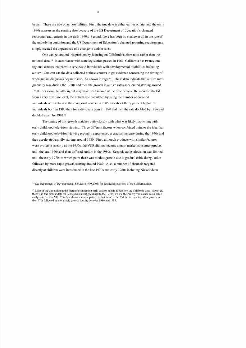
national data. 14 In accordance with state legislation passed in 1969, California has twenty-oneregional centers that provide services to individuals with developmental disabilities including
autism. One can use the data collected at these centers to get evidence concerning the timing of
when autism diagnoses began to rise. As shown in Figure 1, these data indicate that autism rates
gradually rose during the 1970s and then the growth in autism rates accelerated starting around
1980. For example, although it may have been missed at the time because the increase startedfrom a very low base level, the autism rate calculated by using the number of enrolled
individuals with autism at these regional centers in 2005 was about thirty percent higher for
individuals born in 1980 than for individuals born in 1970 and then the rate doubled by 1986 and
doubled again by 1992. 15
The timing of this growth matches quite closely with what was likely happening withearly childhood television viewing. Three different factors when combined point to the idea that
early childhood television viewing probably experienced a gradual increase during the 1970s and
then accelerated rapidly starting around 1980. First, although products with similar features
were available as early as the 1950s, the VCR did not become a mass market consumer product
until the late 1970s and then diffused rapidly in the 1980s. Second, cable television was limiteduntil the early 1970s at which point there was modest growth due to gradual cable deregulation
followed by more rapid growth starting around 1980. Also, a number of channels targeted
directly at children were introduced in the late 1970s and early 1980s including Nickelodeon
8/6/2019 Autism Waldman Nicholson Adilov
http://slidepdf.com/reader/full/autism-waldman-nicholson-adilov 14/68

8/6/2019 Autism Waldman Nicholson Adilov
http://slidepdf.com/reader/full/autism-waldman-nicholson-adilov 15/68
13
rather than early childhood television watching causing ADHD, it is at least possible that
children who are likely to develop the condition in the future are more drawn to television and asa result watch more of it. 18
Despite the drawback of the study discussed above, the results found in Christakis et al.
are certainly suggestive of the idea that early childhood television watching is a cause or trigger
for ADHD. The reason we feel this is of interest is that, as discussed briefly earlier, one of the
main hypotheses concerning the fundamental deficit in autism is that at its core it is an attentiondisorder and the other deficits associated with the condition are mostly outcomes of the problems
concerning attention. In turn, if this is the case, then the results found in Christakis et al. are
suggestive of the idea that early childhood television watching could also be a trigger for autism.
That is, if in the general population early childhood television watching serves as a trigger for
ADHD, it seems plausible that for a small segment of the population who are vulnerable becauseof their biology or genetics early childhood television watching may serve as a trigger for the
more severe attention disorder called autism.
C) The Behavior of “High Risk” Infants
Our hypothesis that early childhood television watching is a trigger for autism is more plausible if infants who are at “high risk” of becoming autistic exhibit behaviors consistent with
a high vulnerability to television viewing. For example, such a behavior might be that high risk
children have more difficulty disengaging from watching television once they begin watching.
A recent study by Zwaigenbaum et al. (2005) suggests that this may indeed be the case.
The idea that there is a clear genetic component to autism means that an infant with anolder sibling with autism has a higher probability of developing the condition than an infant with
no close relatives with autism. Zwaigenbaum et al. use this idea to identify differences in
behavior in the first years of life between those who are at high risk of developing autism, i.e.,
8/6/2019 Autism Waldman Nicholson Adilov
http://slidepdf.com/reader/full/autism-waldman-nicholson-adilov 16/68
14
group of high-risk infants and a group of low-risk infants, where risk is defined as above.
Further, one of the behaviors they focus on is what they refer to as “disengagement of visualattention,” i.e., how quickly does the child disengage from a screen showing “colorful dynamic
stimuli” when another similar visual stimulus is introduced into the environment. It seems
plausible that children who exhibit the type of slower disengagement found by Zwaigenbaum et
al. will also be slower to disengage from television viewing once viewing has begun and, as a
result, any negative effects of television viewing may manifest themselves in a more extremeway. In other words, if exposure to television during early childhood causes attention problems
as the work of Christakis et al. (2004) suggests, it is possible that those who exhibit slower
disengagement will on average have more severe attention problems as a result of early
childhood television exposure.
Zwaigenbaum et al. find that: i) at six months of age the high-risk group exhibits slower disengagement than the low-risk group; ii) the high-risk group shows less improvement on speed
of disengagement between six and twelve months of age than the low-risk group; and iii) within
the high-risk group the amount of improvement between six and twelve months of age is a
significant predictor of whether or not the child develops autism by the age of three. 19 Although
far from definitive, all three findings are consistent with the idea that television has a moresignificant effect on infants at high risk of autism than on others.
D) The Amish
The California data discussed above indicate that the longest time-series data on autism
rates is consistent with the hypothesis that early childhood television watching is a trigger for autism. A related issue is, does there exist similar cross-sectional evidence concerning autism
rates and, if there does, is it also consistent with our hypothesis? For example, is there a group
in the population whose young children watch significantly less television than the average and,
8/6/2019 Autism Waldman Nicholson Adilov
http://slidepdf.com/reader/full/autism-waldman-nicholson-adilov 17/68
15
For religious reasons the Amish do not use electricity and so young children in that
population watch no or at most very little television. Thus, our hypothesis that early childhoodtelevision watching is an important trigger for autism suggests that autism rates among the
Amish should be distinctly lower than in the rest of the population.
Interestingly, there has recently been an investigation of this issue. Dan Olmsted, a news
reporter for United Press International, recently conducted an informal investigation of this issue
(see Olmsted (2005a,b)). According to Olmsted, based on autism rates for the general population, there should be several hundred autistic individuals among the Amish. After
extensive investigation, however, Olmsted was able to identify fewer than ten. Also, his
interviews with individuals who should be in positions to know the general prevalence rate, such
as doctors, health care workers, and an Amish mother of an adopted autistic child, indicate that
the prevalence of autism among the Amish is indeed very low. 20
Of course, this is far from definitive evidence for our hypothesis. Olmsted’s
investigation was informal and possibly a more thorough investigation would turn up the
expected hundreds of autistic Amish. Or possibly, since the Amish lifestyle is quite different in
many ways – think about what your life would be like if you could not use electricity – there is
some other trigger for autism and the Amish lifestyle results in less exposure to this trigger thanthe typical lifestyle (see footnote 18 for a related discussion). Or, since the Amish represent a
relatively isolated gene pool, it is possible that the Amish have less autism because the genes that
cause the condition exist at a much lower frequency in that population. Nevertheless, even given
all these caveats, Olmsted’s findings do represent intriguing evidence consistent with our
hypothesis.
IV. EARLY CHILDHOOD TELEVISION WATCHING AND PRECIPITATION
In the previous section we discussed four reasons why we suspect early childhood
8/6/2019 Autism Waldman Nicholson Adilov
http://slidepdf.com/reader/full/autism-waldman-nicholson-adilov 18/68
16
Statistics’ American Time Use Survey, or ATUS, to investigate whether early childhood
television watching is positively correlated with precipitation. We show that indeed precipitation is an important determinant of television watching for young children. In the next
section we then use this finding to test whether early childhood television watching is a trigger
for autism.
A) DataThe test conducted in this section employs two types of data. The first is data taken from
the ATUS (see Hamermesh, Frazis, and Stewart (2005) for a detailed description of the ATUS).
The Bureau of Labor Statistics started conducting the ATUS in 2003 and we use the first wave of
the survey which took place in 2003. The survey asks individuals to record detailed information
concerning his or her activities during a specific day, including who else in the household is present during each activity.
We are interested in the cumulative amount of television watching for children under the
age of three, but the survey only contacts adults. Our approach, therefore, is to focus on
respondents for whom there is a child under three in the household, where our television viewing
variable is the total amount of time measured in minutes that the respondent watched televisionwith the child present during the survey day (if the household has more than one child under the
age of three, then each child is treated as a separate observation). Clearly, this technique cannot
be used to measure total television watching by the child. But it will allow us to look at whether
television watching is positively correlated with precipitation which is our focus. 21
We use two different definitions of what constitutes television watching, which we refer to as narrow and wide. The narrow definition includes all activities that involve looking at a
21 To be precise, we actually measure exposure to television rather than actual television watching since the ATUSdoes not tell us whether the child is actually watching the screen However since there should be a strong positive
8/6/2019 Autism Waldman Nicholson Adilov
http://slidepdf.com/reader/full/autism-waldman-nicholson-adilov 19/68
17
television screen. This includes watching television, watching DVD/video movies, and watching
home movies and home videos. In the wide definition we add in computer use for leisure andattending movies and films. 22
As indicated, our television watching variable is the respondent’s cumulative amount of
television watching in minutes when the child is present. For each survey respondent we also
record household characteristics including household income level, household type (a list of
household types appears in the Appendix), and race/ethnicity. We also record the MSA/PMSAof the respondent (we restrict our sample to respondents for whom there is an MSA/PMSA and it
is known) and the date of the survey. 23 As discussed next, by recording the location of the
respondent and the date of the survey we are able to construct measures of the weather at the
respondent’s location on the day of the survey, where our main focus is the amount of
precipitation.We use raw data taken from the National Climactic Data Center to construct our
precipitation variable. The National Climactic Data Center has daily weather data for over 8000
weather stations across the United States. Our precipitation variable is constructed as follows.
For each data point, i.e., each survey response, we first calculate the amount of precipitation that
fell on the day of the survey for each county in the MSA/PMSA of the respondent by averagingacross the amounts at all the weather stations in the county. We then calculate an average
precipitation level for the MSA/PMSA on the day of the survey by averaging the precipitation
levels for all of the counties weighted by the year 2003 county population of children under the
age of five as estimated by the US Census Bureau (the Census Bureau provides estimates by age
groups at the county level not by individual ages).
22 The ATUS does not allow us to exactly identify activities associated with watching a television-like screen
8/6/2019 Autism Waldman Nicholson Adilov
http://slidepdf.com/reader/full/autism-waldman-nicholson-adilov 20/68
18
Although not part of our analysis of autism rates in Section V, we employ a second
weather variable in our analysis of television watching in this section.24
Specifically, we allowfor the possibility that television watching by young children is correlated with the number of
hours of daylight on the day of the survey at the survey location. The logic here is that a young
child is more likely to be indoors when the sun is down and television watching is mostly an
indoor activity. So our hypothesis is that television watching should be negatively correlated
with hours of daylight. The reason we do not use this variable in next section’s analysis of autism rates is that the average number of daylight hours over a year does not vary in a
significant fashion across locations. We construct our daylight variable by using the formula in
Forsyth et al. (1995) which provides number of hours of daylight as a function of latitude of a
location and calendar day.
B) Tests and Results
In this subsection we investigate our hypothesis that early childhood television watching
is positively correlated with precipitation for children under the age of three. The reason we
focus on this age group is that, as discussed earlier, for a child to be considered autistic the
condition must develop before the child reaches three years of age. So, if early childhoodtelevision viewing is a trigger for autism, the relevant viewing should be that which occurs
before the age of three.
There is some evidence that television viewing for older children is positively correlated
with bad weather (see Zwaga (2000)). But because there is little systematic evidence concerning
the television viewing habits of very young children it is not surprising that whether bad weather or more specifically precipitation increases the television viewing of very young children has not
been established. Our analysis shows that indeed increased precipitation does result in increased
television viewing by children under three years of age.
8/6/2019 Autism Waldman Nicholson Adilov
http://slidepdf.com/reader/full/autism-waldman-nicholson-adilov 21/68
19
In our tests, in addition to including precipitation and hours of daylight, we include a
number of control variables that are likely to have an effect on the amount of television the childwatches. A number of our control variables come from results found in the recent study of
Roberts and Foehr (2004) which is probably the most comprehensive existing study of the use of
television and related media by children. First, since Roberts and Foehr find that television
exposure for their youngest age group is negatively related to family income, we include
household income as a control variable. Second, since Roberts and Foehr find that televisionexposure for their youngest age group is negatively related to the education level of the parents,
we include a dummy variable that captures whether the adult respondent has a college degree.
Third, since Roberts and Foehr find that television exposure for their youngest group is higher
for Blacks and Hispanics than for Whites, we include race and ethnicity dummies. Fourth, since
Roberts and Foehr find that for their youngest group television exposure is higher for males thanfemales, we also include a dummy variable that captures the gender of the child. 25
We also include a number of other control variables. First, we include a dummy variable
for whether or not the survey date was on a weekend, where our prediction is that the adult
respondent on average should be home more hours on a weekend day versus a weekday so
measured television viewing should be higher. Second, we include a dummy variable for whether or not the adult respondent is working the day of the survey, where similar to the logic
of the weekend dummy our prediction is that the respondent should be home less hours on a
workday so measured television viewing for the child should be lower. Third, we include a
gender dummy for the adult respondent where we conjecture that the proportion of time the
respondent spends with the child may be higher when the respondent is female, so measuredtelevision time may be higher when the respondent is female. Fourth, we control for household
type such as whether the household is a military family or a non-military family. Fifth, we
control for the MSA/PMSA of the respondent since television watching time may vary with
8/6/2019 Autism Waldman Nicholson Adilov
http://slidepdf.com/reader/full/autism-waldman-nicholson-adilov 22/68
20
number and quality of parks in the MSA/PMSA. 26 Because we include MSA/PMSA controls,
the coefficients on the precipitation variables are identified by variation in the amount of precipitation that occurred on the survey dates for surveys conducted within the same
metropolitan area. Table 1 reports sample statistics for this section’s analysis.
We consider the specification given in equation (1).
(1) TV i = β1 + β2PRCP i + β3PRCP i2 + β4X i + β5Z i + εi
TV i is measured television viewing time of the child, PRCP i is measured precipitation at therespondent’s location on the day of the survey, X i is a vector of individual and family control
variables, Z j is a vector of MSA/PMSA dummy variables, and ε i is an error term. Note that our
specification allows the incremental effect of precipitation on television viewing to change as
precipitation rises. This captures that once a child spends all day indoors because of
precipitation, a further increase in the number of inches of precipitation has no further effect onthe amount of television viewing. We run four regressions. First, as discussed above we
consider both narrow and wide definitions of television viewing time. Second, for each
definition of television viewing time, we consider both ordinary least squares and a Tobit
specification. The rationale for a Tobit regression is that television viewing time equals zero for
over fifty percent of the observations.The results for equation (1) are reported in Table 2. Consider first the control variables
(note that the table does not report the MSA/PMSA coefficients). Most of these coefficients
have the predicted signs and many are statistically significant at standard confidence levels.
First, the daylight coefficients, the work coefficients, and the education coefficients each have
the predicted sign in all four regressions and are statistically significant at the five percent levelin all four regressions (the work and education coefficient are in fact consistently statistically
significant at much higher confidence levels). Second, although not reported in the table, the
8/6/2019 Autism Waldman Nicholson Adilov
http://slidepdf.com/reader/full/autism-waldman-nicholson-adilov 23/68
21
coefficients on the fifteen income indicator variables are generally consistent with the prediction,
i.e., television viewing time decreases with household income. Third, the weekend coefficientconsistently has the predicted sign and is significant at the ten percent level in three of the four
regressions. Fourth, the signs of the Black and Hispanic coefficients are consistent with the
predictions, although each coefficient is only statistically significant at the ten percent
confidence level in one of the four regressions. Also, a result that was not predicted is that
indigenous groups (American Indian, Alaskan Native, and Hawaiian/Pacific Islander) have lower television watching and the coefficient is statistically significant at the five percent level in all
four regressions. Fifth, household type seems not to matter except that television viewing is
lower for military families, where this coefficient is statistically significant at the five percent
level in two of the regressions and statistically significant at the ten percent level in the other two
regressions.The remaining two control variables are the gender controls. Inconsistent with the
prediction, measured television viewing is sometimes higher and sometimes lower when the
adult respondent is female and the coefficient is never statistically significant at standard
confidence levels. On the other hand, consistent with the prediction, measured television
viewing is always higher when the child is male, where in two of the four regressions thecoefficient is significant at the five percent level, while in the other two it is not significant at
standard confidence levels. Further, the increase is also significant in an absolute sense. For
example, the OLS regressions indicate that being male increases television viewing by over ten
percent. Note that the finding that very young male children watch more television than very
young females is of particular interest given the higher incidence of autism in males relativefemales. In other words, if early childhood television watching is a trigger for autism (which is
what the results in the next section suggest), then the finding that very young males watch more
television could mean that one reason that autism is more common among males is exactly
8/6/2019 Autism Waldman Nicholson Adilov
http://slidepdf.com/reader/full/autism-waldman-nicholson-adilov 24/68
22
both precipitation and the precipitation-squared term have the predicted signs in all four
regressions, where the coefficients on the precipitation variable are statistically significant at theone percent level in all four regressions while those on the precipitation-squared variable are
statistically significant at the five percent level in all four regressions.
Further, the coefficients on the precipitation variables in these two tables are significant
in an absolute sense in addition to a statistical one. For example, in the Table 2 ordinary least
squares regression that uses the broad definition of television watching, the coefficients indicatethat a young child watches about twenty seven more minutes of television on a day when
precipitation equals one inch relative to a day with no precipitation (one inch of precipitation is
the equivalent of a heavy day of rain). Since average television viewing by children in our
sample is approximate sixty minutes, this result suggests that increasing precipitation from zero
to one inch represents a substantial proportional increase in television viewing due to precipitation. 27 In other words, the results in this section indicate that precipitation causes
increases in early childhood television watching both from statisical and absolute perspectives,
and thus, that precipitation should be a valid instrument for testing the effect that early childhood
television watching has on rates of autism. 28
V. AUTISM AND PRECIPITATION
In this section we employ the finding of the previous section that precipitation is
positively correlated with early childhood television watching to test the hypothesis that early
childhood television watching is a trigger for autism. That is, given that early childhood
television watching is higher when precipitation is higher, if such watching is indeed a trigger for autism then the autism rate itself should be positively correlated with precipitation.
To test the hypothesis we focus on three states that have a high level of precipitation
variability across counties – California, Oregon, and Washington. Because of the Cascade
8/6/2019 Autism Waldman Nicholson Adilov
http://slidepdf.com/reader/full/autism-waldman-nicholson-adilov 25/68
23
Mountains that run north to south across the middle of Oregon and Washington, each state is
characterized by vastly different precipitation patterns across the different regions of the state.Counties in each state that lie west of the mountains and on or near the coast are characterized by
heavy precipitation, while counties in the eastern part of each state that are east of the mountains
and far from the coast are dry (see Figures 3 and 4). In particular, for both Oregon and
Washington, the counties west of the Cascades have approximately 3.8 times more rain, on
average, than counties east of the mountains. We also include California in our analysis because precipitation variability in this state is also substantial (see Figure 5) and previous literature has
focused on this state. If our hypothesis that early childhood television watching is a trigger for
autism is correct, it is exactly in this type of state where precipitation variability across counties
is high that that the effect of precipitation on autism rates should be identifiable by a statistical
analysis. Note that the approach we are taking is an instrumental variables approach or, more
specifically, our approach is to employ what economists have come to call a natural experiment.
In other words, we employ the idea that early childhood television watching varies positively
with precipitation to test whether autism varies both cross sectionally and over time with changes
in precipitation in a fashion consistent with early childhood television watching serving as atrigger for autism. In this sense our study is similar to a number of recent studies in economics
that use a natural experiment to investigate various important empirical issues (see Rosenzweig
and Wolpin (2000) and Angrist and Krueger (2001) for surveys).
Many studies that use an instrumental variables approach do so because testing the theory
directly results in problems such as measurement error or omitted variables. In contrast, our main reason for using an instrumental variables approach is that there are not large enough
studies that directly measure both young children’s television watching and subsequent health
problems that could be used to study whether early childhood television watching is a trigger for
8/6/2019 Autism Waldman Nicholson Adilov
http://slidepdf.com/reader/full/autism-waldman-nicholson-adilov 26/68
24
But a finding that precipitation is positively correlated with autism is not subject to this criticism
– we can be quite certain that autism does not cause precipitation.A) Data
We employ two different types of data on autism. Our first set of tests employ autism
rates in 2005 by county in California, Oregon, and Washington for school-aged children, i.e.,
ages six to eighteen. To calculate these autism rates we took the autism counts for December
2005 provided to us by the state agencies and divided by the corresponding county-level totalschool-aged population taken from the 2000 census. We also investigate county-level age-
specific autism rates. Washington was unwilling to provide us with these data while California
and Oregon provided us with the figures, although for Oregon we were only provided figures
when the age-specific counts by county were at least ten. For Oregon we use age-specific counts
by county in 2005 and then construct autism rates by dividing by the corresponding county-levelage-specific population taken from the 2000 census. For the case of California we focus on
cohorts born between 1982 and 1997 (versus cohorts born between 1987 and 1999 for Oregon)
and use the county autism count in the year a birth cohort was eight years old and construct the
autism rate by dividing by that year’s corresponding county-level age-specific population also
derived from census data.29
For example, for children born in Los Angeles county in 1990 we use Los Angeles
county’s autism count of eight year olds in 1998. Our empirical methodology assumes that
autistic children spent their first three years of life in the same county where they reside when
they are recorded in our data set. Hence, using this type of data in the case of California rather
than counts from the 2005 survey reduces measurement error by reducing the number of autisticchildren who changed county of residence between the age of three and the age they are recorded
in our data set. We do not have this type of data for Oregon which is why in the case of Oregon
8/6/2019 Autism Waldman Nicholson Adilov
http://slidepdf.com/reader/full/autism-waldman-nicholson-adilov 27/68
25
we focus on the 2005 counts. Finally, we chose age eight for constructing the California data
because most children who are diagnosed with autism receive the diagnosis by the age of eight.30
Our precipitation variable is constructed in a fashion similar to the construction of the
precipitation variable in the previous section. To construct precipitation in a specific county in a
specific year we first calculate precipitation in that county on each day of the year by averaging
across all the weather stations in that county. We then add the resulting values across all the
days in the year to get the total year’s precipitation. We use two types of precipitation variables.First, we construct average annual precipitation by county between 1987 and 2001. Second, we
construct three-year intervals of average annual precipitation by county to match when a specific
age cohort was between the ages of zero and two. 31
We also employ a number of control variables. We include a county’s total population,
per capita income, the percent of Hispanics, Blacks, and indigenous groups for each county’sschool-aged population, and county-level age-specific percentages of Hispanics, Blacks, and
indigenous groups. To calculate these percentages we employ populations by group and age
range taken from census data and then use similar procedures to those described above used to
construct the analogous autism rates. 32 Statistics for the sample used in this section are reported
in Table 3.
B) Tests and Results
In our first set of tests the dependent variable is county autism rates for school-age
children in 2005. In this set of tests we consider a number of explanatory variables. First, our
main focus is on average annual precipitation by county over the time period 1987 to 2001,
30 In our tests using Oregon data we consider each age cohort that was between six and eighteen in 2005. In our tests using California data we drop the cohorts that were six and seven years old in 2005 because of our focus onautism rates calculated using the autism counts when the birth cohort was eight years old.
8/6/2019 Autism Waldman Nicholson Adilov
http://slidepdf.com/reader/full/autism-waldman-nicholson-adilov 28/68
26
which covers a time period in which at every date some subset of school-aged children in 2005
were between zero and two years of age (remember, given autism strikes by the age of three, anytrigger must be such that exposure occurs prior to the age of three). Our prediction is that there
should be a positive coefficient on this variable. Second, given the finding in Section IV that
early childhood television watching is higher for Hispanics and Blacks but lower for indigenous
groups, we include county population percentages in 2005 for Hispanics, Blacks, and indigenous
groups. Our prediction is that the coefficients on the Hispanic and Black variables should be positive since early childhood television watching is higher for Hispanics and Blacks, while the
coefficient on the indigenous group variable should be negative because these groups watch less
television. 33 Third, we include a county per capita income variable because in Section IV we
found that income is negatively related to early childhood television watching which suggests
autism rates should be negatively correlated with income.We also employ two other explanatory variables. For the regressions in which we pool
counties across the three states, we include dummy variables that control for which state the
county is in. We include this variable because the criteria used to classify an individual as
having the condition may vary across the three states. We also include a measure of the
population of the county in 2005. We include a population size variable because large countiesmay be better able to afford the infrastructure required to effectively diagnose the condition
which, in turn, suggests that autism rates might be higher in more populous counties. Table 3
reports characteristics of California, Oregon, and Washington counties for our sample period.
For the tests using the California counties, we also typically include a dummy variable
that captures whether the county was the home of one (or more) of the twenty-one regionalcenters that provides services to individuals with developmental disabilities including autism.
The California autism counts we rely on are counts of individuals who received services at one
of these regional centers. We would expect that, in counties with a regional center, a higher
27
8/6/2019 Autism Waldman Nicholson Adilov
http://slidepdf.com/reader/full/autism-waldman-nicholson-adilov 29/68
27
proportion of the individuals with autism would receive treatment at a regional center. Hence,
our prediction is that the coefficient on the regional center variable should be positive.The exact specifications we consider are given in equations (2) and (3).
(2) AUT k = β1 + β2PRCP k + εk
(3) AUT k = β1 + β2PRCP k +β3logPOP k + β4INC k + β5REG k + β6HISP k + β7BLK k + β8IND k + εk
In equations (2) and (3), AUT k denotes the 2005 autism rate among school-aged children in
county k, PRCP k is the average annual precipitation level in county k between 1987 and 2001,logPOP k is the logarithm of county k’s total population in 2000, INC k is county k’s per capita
GNP in 1999, HISP k is the percentage of school-aged children in county k who are Hispanics in
2000, BLK k is the percentage of school-aged children in county k who are Black in 2000, and
IND k is the percentage of school-aged children in county k who fall into one of the indigenous
group categories in 2000, and REG k equals 1 if California county k has a regional center and 0otherwise. We consider the specification in equation (2) for California counties only, Oregon
counties only, Washington counties only, and we also consider both equations (2) and (3) in a
pooled analysis of California, Oregon, and Washington counties.
Table 4 reports the results. Column 1 reports results for equation (2) for California
counties only, column 2 report results for equation (2) for Oregon counties only, and column 3reports results for equation (2) for Washington counties only. There is a positive relationship
between autism and precipitation in Oregon and Washington, but no in California. In particular,
the coefficient on the precipitation variable is positive and statistically significant at the one
percent level in both Oregon and Washington. So you can see visually what the table is
capturing concerning the relationship between precipitation and autism, in Figures 3 and 4 we present precipitation and autism maps for each state. Consistent with the results in the table, it is
clear from the maps that there is a very strong correlation in each state between precipitation and
autism.
28
8/6/2019 Autism Waldman Nicholson Adilov
http://slidepdf.com/reader/full/autism-waldman-nicholson-adilov 30/68
28
predicted sign and is significant at the one percent level. Second, the coefficients on the
population and income variables have the predicted sign in the relevant regression, where the
former is significant at the five percent level and the latter at the ten percent level. Third, the
coefficient on the indigenous group variable has the predicted sign and is significant at the one
percent level, while the two predictions that are not supported are the predictions concerning the
coefficients on the Black and Hispanic variables. This last result is not surprising given the
relatively weak evidence in the ATUS regarding whether young Black and Hispanic childrenwatch more television. Finally, given the very high autism rate in Oregon it is not surprising that
the coefficient on the Oregon dummy variable is positive and statistically significant at the one
percent level.
In our next set of tests, we define the dependent variable as the county autism rate for
each age cohort from six to eighteen. As discussed earlier, we only have such data for Californiaand for sixteen counties in Oregon because Washington was unwilling to share the data with us
and because Oregon only reported the county autism count when it was greater than or equal to
ten.
In this set of tests our precipitation variable is the average annual amount of precipitation
in the county over the years in which the age cohort was below the age of three. So, for example, when the observation is the autism rate for children in Multnomah county who were
born in 1995, our precipitation variable is the average precipitation in Multnomah county
between 1995 and 1997. As discussed earlier, since autism develops before the age of three, it is
only television watching and thus precipitation over those first three years that should matter.
The specification we consider for this set of tests is given in equation (4).(4) AUT k,b = β1 + β2PRCP k,b + β3TIME b + β4logPOP k + β5INC k + β6REG k + β7HISP k,b
+ β8BLK k,b + β9IND k,b + εk,b
In equation (4), AUT k,b denotes the autism rate in county k for birth cohort b, PRCP k,b is the
29
8/6/2019 Autism Waldman Nicholson Adilov
http://slidepdf.com/reader/full/autism-waldman-nicholson-adilov 31/68
29
are defined as before, while for California we use a county’s population and income when the
birth cohort was eight years of age (i.e., for the California tests better notation would be
logPOP k,b and INC k,b). The three race/ethnicity variables are calculated separately for each age
cohort using census data. Note that we include a time trend because California and Oregon, like
many other states, experienced rising autism rates over the time period covered.
Table 5 reports the results. 35 Column 1 reports the results for Oregon for equation (4).
The coefficient on precipitation has the predicted sign and is statistically significant at the five percent level. As for the control variables, consistent with the prediction, the coefficient on the
income variable is negative and statistically significant at the ten percent level. The other
control variables are all insignificant at standard confidence levels. Column 3 of Table 5 reports
the results for California for equation (4). Consistent with the predictions, the coefficient on the
population variable is positive and statistically significant at the ten percent level, the coefficienton the income variable is negative and statistically significant at the ten percent level, while the
coefficient on the time trend is positive and statistically significant at the one percent level.
Also, the coefficients on the other control variables are not significantly different from zero. But
most importantly, the California data continues to show no evidence of a positive correlation
between precipitation and autism.One possibility for why the California data does not exhibit a positive correlation
between precipitation and autism is that there is an omitted variables problem. That is, there
could be another important variable that is correlated with television watching and also
correlated with precipitation in the California data set in a manner that results in no significant
relationship between autism and precipitation in our test of equation (4) using California data.For example, suppose that urban density is positively correlated with early childhood television
watching. Then, because there are a number of counties in California such as Los Angeles,
Orange, and San Diego counties with both high urban density and low precipitation, it is possible
30
8/6/2019 Autism Waldman Nicholson Adilov
http://slidepdf.com/reader/full/autism-waldman-nicholson-adilov 32/68
30
In column 2 of Table 5 we employ a fixed-effects specification using age-specific county
autism rates in Oregon to investigate whether our finding of a positive correlation in Oregon
between precipitation and autism continues to hold even after we control for time-invariant
county characteristics. The coefficient on the precipitation variable in this test is determined
solely by how each county’s autism rate deviates from its average over time when the county’s
precipitation level deviates from its average. As depicted for Oregon in Figure 6, there is a
substantial amount of variation in precipitation from year to year, and this variation differs by
county. For children born in 1990, for example, Deschutes county received one percent less
precipitation between 1990 and 1992 relative to its average, whereas Yamhill and Polk counties
received twenty six percent and twenty two percent less than their averages, respectively. The
results continue to support a positive association in Oregon between autism and precipitation.
Specifically, the coefficient on the precipitation variable is positive and statistically significant atthe one percent level while the coefficient on the time trend is also positive and statistically
significant at the one percent level. As for the magnitude of this effect, a one-standard deviation
increase (21.3 inches per year) in the amount of precipitation a cohort was exposed to before
they were three would be predicted to increase the autism rate for that cohort by twelve percent.
In column 4 of Table 5 we employ a fixed-effects specification using age-specific countyautism rates in California. In contrast to earlier results concerning the California data, we now
find a positive correlation between autism and precipitation. Specifically, similar to what was
true for the Oregon test, the coefficient on the precipitation variable is positive and statistically
significant at the five percent level. Further, in this case a one-standard deviation increase (17.4
inches per year) in the amount of precipitation a cohort was exposed to before they were threewould be predicted to increase the autism rate for that cohort by twenty eight percent. 36
In columns 5 and 6 we pool the data across California and Oregon counties and consider
equation (4) and the fixed-effects specification. Column 5 shows that when we pool the data
31
8/6/2019 Autism Waldman Nicholson Adilov
http://slidepdf.com/reader/full/autism-waldman-nicholson-adilov 33/68
precipitation variable is positive and statistically significant at the five percent level. In terms of
the other variables, we only find statistical significance for the coefficient on the Hispanic
variable which, consistent with our prediction, is positive and statistically significant at the ten
percent level, and for the coefficient on the indicator variable that captures whether the county is
in Oregon which not surprisingly is positive and statistically significant at the one percent level.
Column 6 reports the results of the fixed effects specification when we pool the data. Here, as
was the case for the Oregon regression in column 2, the coefficient on the precipitation variable
is positive and statistically significant at the one percent level.
Overall, we believe that the results in this section strongly support the hypothesis that
early childhood television watching is a trigger for autism. That is, in each of the three states
that we consider there is evidence of a positive relationship between autism and precipitation as
predicted by the television as trigger hypothesis. In particular, in Oregon we find evidence for such a correlation using cross-sectional, time-series, and fixed-effects specifications. Further,
when we pool the data across either two or three states, we consistently find positive coefficients
on the precipitation variable that achieve high levels of statistical significance.
VI. AUTISM AND CABLE TELEVISIONIn the previous section we used county-level data in California, Oregon, and Washington
to investigate whether there is a positive correlation between autism and precipitation as
predicted by the hypothesis that early childhood television watching is a trigger for autism. In
this section we use county-level data from California and “intermediate unit” data from
Pennsylvania to investigate whether there is a positive correlation between autism and the percentage of households with cable television as predicted by the television as trigger
hypothesis. 37 The idea here is that, if early childhood television viewing is indeed a trigger for
autism, then the increased access to cable during the 1970s and 1980s was likely an important
32
8/6/2019 Autism Waldman Nicholson Adilov
http://slidepdf.com/reader/full/autism-waldman-nicholson-adilov 34/68
day in which at least one children’s show is being televised, children in households with cable to
watch a lot of television. With this in mind, in our tests we use cable subscription rates as an
instrumental variable for the amount of early childhood television watching.
A) Data
Using 1990 data, for each county in California and intermediate unit (IU) in Pennsylvania
we calculated an autism rate for each cohort of individuals born between 1972 and 1984. Using
autism rates for six-year olds in December 1991, 1992, 1993, 1994, and 1995, we then extended
this data set to include autism rates for each California county and Pennsylvania IU for each
cohort of individuals born between 1972 and 1989. We focus on this time period for two
reasons. First, during this time period there was substantial growth in California of both the
percentage of households with cable television and the percentage of children diagnosed with
autism. 38 Second, in the 1990s there was substantial growth in satellite television which serves
as a substitute for cable and, because of a lack of county-level and IU data concerning
households with satellite television, it is difficult in the 1990s to get an accurate picture at the
county level and IU level of the percentage of households with the expanded offerings typicallyassociated with cable and satellite television.
Our cable data are taken from the Services Volume of the Television Factbook . For each
cable company, this publication, which appears (almost) annually, reports the number of
subscribers, the primary community served, and the county or counties served. 39 For each year
between 1972 and 1991 we used these data to construct the number of households with a cablesubscription in each county. For the small number of years in which the data on cable
subscribers were not available – 1976, 1977, and 1980 – we used a linear interpolation to
estimate the number of cable households (e.g., the number of subscribers in a county in 1980 is
33
8/6/2019 Autism Waldman Nicholson Adilov
http://slidepdf.com/reader/full/autism-waldman-nicholson-adilov 35/68
assumed to the average of the numbers in 1979 and 1981). We then divided these numbers by
the total number of households in the county in the relevant year which we estimate using the
decennial census. Specifically, for 1971-1979 we linearly interpolate using the 1970 and 1980
censuses, while 1981-1989 values are estimated using a linear interpolation of the 1980 and 1990
censuses. For Pennsylvania we then used a population based weighting to construct our cable
subscription variable. 40
Our tests focus on a subset of California counties and Pennsylvania IUs. Some California
and Pennsylvania residents received poor over-the-air reception at the beginning of the time
period of our study, 1972. Many of the residents in these counties likely subscribed to cable in
order to watch the three major networks (ABC, CBS, and NBC), whereas in other counties the
main reason to subscribe to cable was to receive expanded channel offerings. As previously
indicated, in our tests we use cable subscription rates as an instrumental variable for the amount
of early childhood television watching. This use of the variable only makes sense for counties
and IUs with good over-the-air reception where cable was mostly employed for expanded
channel offerings. We thus dropped from our analysis California counties and Pennsylvania IUs
with poor over-the-air reception. Our specific procedure for dropping counties and IUs was as
follows. The Federal Communications Commission describes a television station as providing“Grade B” service when “the quality of picture (is) expected to be satisfactory to the median
observer at least 90% of the time for at least 50% of the receiving locations within the contour,
in the absence of interfering co-channel and adjacent-channel signals.” We dropped the
California counties and Pennsylvania IUs where in 1972 a majority of the county’s or IU’s area
lacked at least Grade B service. The result was that seven of California’s fity-seven counties andone of Pennsylvania’s twenty eight IUs were dropped from our cable analysis. 41
34
8/6/2019 Autism Waldman Nicholson Adilov
http://slidepdf.com/reader/full/autism-waldman-nicholson-adilov 36/68
In Figure 7 we plot the growth in cable households between 1972 and 1989 for some of
the California counties in our data set (the other California counties and Pennsylvania IUs
exhibit similar growth). As suggested by the figure, although cable grew substantially in
basically every California county and Pennsylvania IU during this time period, there was
substantial variation across counties both in the initial levels of cable subscriptions and rates of
growth.
We employ the same control variables in our cable analysis as in the precipitation
analysis, where values are taken from 1990. There is one small difference, however, which is
that the number of school-age Native Hawaiian and Pacific Islanders by county is not available
for 1990. Therefore, our indigenous group variable includes the percentage of school-age
children who are American Indian or Alaskan Native only, rather than combining this group with
Native Hawaiian and Pacific Islanders as we did in the precipitation cross section regressions.
The population, racial percentages, and income levels are 1990 measures because most of the
autism rates are calculated using 1990 data.
B) Tests and Results
The dependent variable is the county or IU autism rate for a specific age
cohort, while the main explanatory variable is the average percentage of county or IU
households with a cable subscription over the time period the cohort was less than three years of
age. Our prediction is that this cable percentage should be positively correlated with autism
rates. Note that the logic here for focusing on the average cable percentage when a cohort was
below three years of age is the same as the logic discussed earlier for the similar approach takenin our precipitation tests. That is, autism develops by the age of three, so if early childhood
television watching is serving as a trigger then autism should be correlated with television
watching that occurs prior to the age of three. Also, as indicated earlier, with one exception we
35
8/6/2019 Autism Waldman Nicholson Adilov
http://slidepdf.com/reader/full/autism-waldman-nicholson-adilov 37/68
autism rates. We control for this problem in two different ways. In our first set of tests we
include a time trend variable. Because of the seriousness of the concern, however, we also
report a second set of results where we omit the time trend variable but include dummy variables
for each age cohort.
The specifications we employ for our first test is given in equation (5).
(5) AUT k,b = β1 + β2CAB k,b + β3TIME b + β4logPOP k + β5INC k + β6REG k
+ β7HISP k + β8BLK k + β9IND k + εk,b
In equation (5), AUT k,b denotes the autism rate in county or IU k for age cohort b, CAB k,b is the
average percentage of households with cable in county or IU k over the years that cohort b was
below the age of three, TIME b is the value for a time trend variable, and the other variables are
defined as in equation (4) but are measured in 1990.
Column 1 of Table 6 reports the ordinary least squares estimate of equation (5) for
California, while column 3 reports the results for Pennsylvania. The first thing to note is that the
coefficient on the cable variable has the predicted sign and is significant at the five percent level
in the California test, while it is positive but insignificant in the Pennsylvania test. That is, in
California but not in Pennsylvania, even after including a time trend, autism rates are higher for
cohorts where a relatively large percentage of households subscribed to cable television during
the cohort’s first three years.
The results concerning the control variables are as follows. Not surprisingly, for both
states the coefficient on the time trend variable has the predicted sign and is strongly statistically
significant. The coefficients on the population and Black variables also have the predicted signin both states, where the coefficient on the population variable is significant at the one percent
level in the California test (but not in the Pennsylvania test) while the coefficient on the Black
variable is statistically significant at the ten percent level in both the California and Pennsylvania
36
8/6/2019 Autism Waldman Nicholson Adilov
http://slidepdf.com/reader/full/autism-waldman-nicholson-adilov 38/68
percent level in the California test but has the expected sign and is significant at the ten percent
level in the Pennsylvania test.
The final variable is income, where the coefficient has the opposite sign of the prediction
in both states and the coefficient is significant at the five percent level for California. We
conjecture that the effect of income on television viewing might be quite different in the time
period of this study than in that of the ATUS study. By 2003 VCR and DVD machines were
widely diffused and likely had little correlation with family income. In contrast, during the time
period of our cable study VCRs were just starting to diffuse and high-income households were
probably more likely to own them. This could explain the income coefficient in column 1 of
Table 6. That is, if having a VCR machine was strongly positively correlated with income, then
during this time period it is quite possible that, in contrast to what was true in the ATUS study,
income was positively rather than negatively correlated with early childhood television
watching.
In columns 2 and 4 of Table 6 we investigate the robustness of the findings in columns 1
and 3. As discussed, rather than including a time trend variable, we include dummy variables for
the various age cohorts. Any concerns about a spurious correlation between autism and cable
due to the rise in both during the period of the study should be eliminated with this more flexible
specification. We see that this alternative specification has no effect on the results. The
coefficients of interest are basically unchanged as are levels of statistical significance.
In columns 5 and 6 of Table 6 we pool data across the two states. The main result here is
that in both regressions the coefficient on the cable variable is positive and significant at the one
percent level.
Our final set of tests employ a fixed-effects specification in which we control for time
invariant county (California) or IU (Pennsylvania) effects. Columns 1 and 2 of Table 7 report
the results of this test for California, while columns 3 and 4 report the results for Pennsylvania.
37
8/6/2019 Autism Waldman Nicholson Adilov
http://slidepdf.com/reader/full/autism-waldman-nicholson-adilov 39/68
Pennsylvania test that employs a time trend and statistically significant at the five percent level
in the Pennsylvania tests that uses cohort indicator variables. In columns 5 and 6 of Table 7 we
report results for the fixed-effects specification where we pool the two states together. Here we
find that in both regressions the coefficient on the cable variable is positive and statistically
significant at the one percent level.
Overall, the results in this section strongly support our hypothesis that early childhood
television viewing is a trigger for autism. This hypothesis makes the prediction that, even after
controlling for the overall growth in cable in the time period studied, there should be a positive
correlation between household cable percentages and autism rates. In turn, there is substantial
evidence for exactly this type of positive relationship in the California data, in the Pennsylvania
data, and especially when we pool the data across the two states.
VII. INTERPRETATION AND IMPLICATIONS
As discussed briefly at the beginning of Section V, if we had a direct measure of early
childhood television watching and showed that children who developed autism had watched
more television before the age of three, we would have evidence consistent with the hypothesis
that early childhood television watching is a trigger for autism but there would be a question of
cause and effect. That is, especially given the findings of Zwaigenbaum et al. (2005) discussed
earlier, it is possible that such a correlation could be due not to early childhood television
watching causing autism but rather to children who are prone to developing autism being more
drawn to television and therefore watching more of it. Note that this is basically the same
drawback discussed earlier concerning the study of Christakis et al. (2004) concerning television
and ADHD.
But by using an instrumental variables or natural experiment methodology we avoid the
problem of cause and effect. Our first set of instrumental variables tests shows that in California,
38
8/6/2019 Autism Waldman Nicholson Adilov
http://slidepdf.com/reader/full/autism-waldman-nicholson-adilov 40/68
of precipitation. But this explanation for our results concerning precipitation is ruled out by our
finding that in California and Oregon precipitation is correlated with autism when a fixed-effects
specification is employed. That is, the fixed-effects specification controls for other unobserved
county variables, so the positive and statistically significant coefficients on the precipitation
variable in that specification indicate that, even after controlling for the composition of families
in a county and the diagnostic criteria being used, autism diagnoses in California and Oregon are
higher in years when precipitation is higher than average. We believe the most plausible
explanation for this finding is that there is a trigger for autism where exposure to this trigger is
positively related with the amount of precipitation in the child’s community prior to the age of
three.
Based on our findings using the ATUS, one plausible candidate for this trigger is early
childhood television watching. But this is not the only possibility. Given that it is also likely
that for young children indoor activities in general, not just television watching, are positively
correlated with precipitation, potentially any trigger for which indoor activities lead to more
exposure than outdoor activities could explain our precipitation findings. With this in mind, we
also investigated a second instrumental variable for television viewing. If early childhood
television watching is a trigger for autism, then one would expect the percentage of households
in a community or county with a susbscription to cable television to be correlated with the
autism rate in that community or county. We investigate this issue using autism and
corresponding cable rates broken down by geographic area in California and Pennsylvania for
children born between 1972 and 1989 and show that indeed cable subscription rates are
positively correlated with autism rates. Further, this is true even after one controls for the
general increase in autism rates during the time period of the analysis. That is, our finding of a
positive and statistically significant correlation between cable subscription rates and autism rates
is not due to the fact that both cable subscription rates and autism rates both grew during the time
39
8/6/2019 Autism Waldman Nicholson Adilov
http://slidepdf.com/reader/full/autism-waldman-nicholson-adilov 41/68
findings provide strong support for the hypothesis. Whereas there is a readily plausible
alternative explanation for why precipitation seems to be frequently positively correlated with
autism, we have more trouble finding a plausible alternative explanation for why precipitation
and cable subscriptions would both be positively correlated with autism. For example, it is
theoretically possible that autism is positively correlated with cable subscription rates because
young children in families with cable spend more time indoors and there is a toxin where
exposure is higher for indoor activities than outdoor activities. But, although theoretically
possible, we do not believe the effect of cable on time spent indoors by young children is likely
to be large enough to make the “time spent indoors” hypothesis a plausible explanation for our
cable findings.
Another possibility is that households predisposed to having autistic children may for one
reason or another find cable more desirable than the average household. But this possibility
neither explains our precipitation results, nor is it a particularly plausible explanation for our
cable results since the number of households predisposed to having autistic children is unlikely
to be sufficiently large to significantly affect county-wide cable subscription rates. So, although
as indicated we do not believe our tests provide definitive evidence for our hypothesis, we
believe the most likely explanation for our findings is that early childhood television watching is
indeed a trigger for autism.
A related issue is, if early childhood television watching is a trigger for autism, what
percentage of autism diagnoses is due to early childhood television viewing? In other words, if
all early childhood television watching was eliminated, how much would the autism rate fall?
We cannot use our results to estimate this decrease because, for example, even if we assume that
television watching is the sole factor driving our finding of a positive correlation between autism
and precipitation, we do not know how the autism rate would be affected by eliminating the
television watching that remains when precipitation equals zero.
40

8/6/2019 Autism Waldman Nicholson Adilov
http://slidepdf.com/reader/full/autism-waldman-nicholson-adilov 42/68
Using the results found in Table 3’s pooled cross-sectional analysis of California, Oregon, and
Washington’s county-level autism rates, we find that if early childhood television watching is the
sole trigger driving the positive correlation between autism and precipitation then thirty-eight
percent of autism diagnoses are due to the incremental television watching due to precipitation.
42
Similarly, we can use the results of our cable analysis to estimate the reduction in autism that
would occur if the incremental television watching due to cable were eliminated. For example,
using the cable coefficient found in column 5 of Table 7, we predict that approximately
seventeen percent of the increase in autism rates between the 1972 and 1989 birth cohorts in
California and Pennsylvania is due to the growth of cable households and the resulting increase
in early childhood television watching. 43 Hence, our results suggest that early childhood
television watching, or whatever is the trigger driving our finding of a positive correlation
between autism rates and precipitation and autism rates and cable, is an important factor in
autism diagnoses both from statistical and absolute standpoints.
VIII. CONCLUSION
One of the most important health care crises facing the United States currently is the
rising incidence of diagnoses of autism. In this paper we have investigated the possibility mostly
ignored by previous researchers in this area that early childhood television watching is an
important trigger for autism. Using the Bureau of Labor Statistics’ American Time Use Survey,
we first showed that early childhood television viewing is positively correlated with
precipitation. Given this finding, our hypothesis that early childhood television viewing is an
important trigger for autism translates into the prediction that autism rates should also be
42 To estimate the decrease in autism that would occur if all incremental television watching due to precipitation
41
8/6/2019 Autism Waldman Nicholson Adilov
http://slidepdf.com/reader/full/autism-waldman-nicholson-adilov 43/68
positively correlated with precipitation. With this in mind we then investigated how the rate of
autism diagnoses varies with precipitation. Looking at county autism rates in California,
Oregon, and Washington, we found support for such a positive correlation in all three states and
when we pool the three states together. We then used California and Pennsylvania data to look
at the correlation between autism rates and the percentage of households with cable television.
Again, we find the evidence supports our hypothesis that early childhood television watching is a
trigger for autism.
Although our findings are consistent with our hypothesis, we do not believe our findings
represent definitive evidence for our hypothesis. We believe the only way to establish
definitively whether or not early childhood television watching is a trigger for autism is to more
directly test the hypothesis. For example, one could monitor the viewing habits of a large
number of children from the ages of zero to three and see whether the children who are
eventually diagnosed with autism on average watched more television before the age of three.
The finding that those diagnosed with autism had indeed watched more television would be
subject to the criticism that maybe those prone to autism are more drawn to television viewing
(this is similar to the criticism of Christakis et al.’s (2004) study of television viewing and
ADHD). But if a condition of participation in the study was that parents were required to limit
television viewing, one could judge whether television viewing is important by looking at the
overall rate of autism in the sample.
The other way to extend our research would be to look more generally at the effects of
early childhood television viewing. There is a belief in the medical community that, particularly
before the age of two, television watching has negative health consequences. But because it is
difficult to measure early childhood television viewing, it has been difficult to establish firm
findings in this area. However, one can potentially use our findings of a positive correlation
between early childhood television viewing and precipitation and also the cable data to look at
8/6/2019 Autism Waldman Nicholson Adilov
http://slidepdf.com/reader/full/autism-waldman-nicholson-adilov 44/68
43
8/6/2019 Autism Waldman Nicholson Adilov
http://slidepdf.com/reader/full/autism-waldman-nicholson-adilov 45/68
Barkley, R.A., Taking Charge of ADHD , The Guilford Press: New York, 2000.
Baron-Cohen, S. and P. Bolton, Autism: The Facts , Oxford University Press: New York, 1993.
Bazar, K.A., A.J. Yun, P.Y. Lee, D.M. Stephanie, and J.D. Doux, “Obesity and ADHD mayRepresent Different Manifestations of a Common Environmental OversamplingSyndrome: A Model for Revealing Mechanistic Overlap Among Cognitive, Metabolic,and Inflammatory Disorders,” Medical Hypotheses , 66, 2006, pp. 263-269.
Bettelheim, B., “ Truants From Life: The Rehabilitation of Emotionally Disturbed Children ,”Free Press: Glencoe, IL, 1955.
Bettelheim, B., The Empty Fortress: Infantile Autism and the Birth of the Self , Free Press: NewYork, 1967.
Centers for Disease Control and Prevention, “Mental Health in the United States: Parental
Report of Diagnosed Autism in Children Aged 4-17 Years --- United States, 2003-2004, Morbidity and Mortality Weekly Report , 55, 2006, pp. 481-486.
Christakis, D.A., F.J. Zimmerman, D.L. DiGiuseppe, and C.A. McCarthy, “Early TelevisionExposure and Subsequent Attentional Problems in Children,” Pediatrics , 113, 2004, pp.708-713.
Department of Developmental Services, Changes in the Population of Persons with Autism and Pervasive Developmental Disorders in California’s Developmental Services System:1987 through 1998 , California Health and Human Services Agency: Sacramento, 1999.
Department of Developmental Services, Autism Spectrum Disorders, Changes in the CaliforniaCaseload, An Update: 1999 through 2002 , California Health and Human ServicesAgency: Sacramento, 2003.
Donohue III, J.J. and S.D. Levitt, “The Impact of Legalized Abortion on Crime,” Quarterly Journal of Economics , 116, 2001, pp. 379-420.
Easterbrook, G., “In Search of the Cause of Autism: How About Television?,” Slate Magazine ,September 5, 2006.
44
8/6/2019 Autism Waldman Nicholson Adilov
http://slidepdf.com/reader/full/autism-waldman-nicholson-adilov 46/68
Forsyth, W.C., E.J. Rykiel, R.S. Stahl, H. Wu, and R.M. Schoolfield, “A Model Comparison for Day Length as a Function of Latitude and Day of Year,” Ecological Modelling , 80, 1995,
pp. 87-95.
Ganz, M.L., “The Costs of Autism,” in Understanding Autism: From Basic Neuroscience toTreatment , S.O. Moldin and J.L.R. Rubenstein, eds., CRC Press, New York, 2006.
Gentzkow, M. and J.M. Shapiro, “Does Television Rot Your Brain: New Evidence from theColeman Study,” NBER Working Paper No. 12021, 2006.
Gernsbacher, M.A., M. Dawson, and H.H. Goldsmith, “Three Reasons Not to Believe in anAutism Epidemic,” Current Directions in Psychological Science , 14, 2005, pp. 55-58.
Gurney, J.G., M.S. Fritz, K.K. Ness, P. Sievers, C.J. Newschaffer, and E.G. Shapiro, “Analysisof Prevalence Trends of Autism Spectrum Disorder in Minnesota,” Archives of Pediatrics& Adolescent Medicine , 157, 2003, pp. 619-621.
Hamermesh, D.S., H. Frazis, and J. Stewart, “Data Watch: The American Time Use Survey,”
Journal of Economic Perspectives , 19, 2005, pp. 221-232.
Hviid, A., M. Stelfeld, J. Wohlfahrt, and M. Melbye, “Association Between Thimerosal-Containing Vaccine and Autism,” Journal of the American Medical Association , 290,2003, pp. 1763-1766.
Institute of Medicine, Immunization Safety Review: Vaccines and Autism , National AcademiesPress: Washington, DC, 2004.
Kaiser Family Foundation, Zero to Six: Electronic Media in the Lives of Infants, Toddlers, and Preschoolers , Kaiser Family Foundation: Menlo Park, CA, 2003
Kaiser Family Foundation, The Media Family: Electronic Media in the Lives of Infants,Toddlers, Preschoolers, and their Parents , Kaiser Family Foundation: Menlo Park, CA,2006.
Kanner, L., “Autistic Disturbances of Affective Contact,” Nervous Child , 2, 1943, pp. 217-250.
Kanner, L., “Early Infantile Autism,” Journal of Pediatrics , 25, 1944, pp. 211-217.
Kanner L “Problems of Nosology and Psychodynamics of Early Infantile Autism ” American
45
8/6/2019 Autism Waldman Nicholson Adilov
http://slidepdf.com/reader/full/autism-waldman-nicholson-adilov 47/68
Crime,” American Economic Review , 87, 1997, pp. 270-290.
McDowell, M., “Autism, Early Narcissistic Injury, and Self Organization: A Role for the Imageof the Mother’s Eyes?, Journal of Analytical Psychology , 49, 2004a, pp. 495-520.
McDowell, M., “Is Autism Statistically Linked to Early Non-Maternal Child Care?,” DynamicalPsychology , 2004b.
M.I.N.D. Institute, Report to the Legislature on the Principal Findings from the Epidemiology of Autism in California: A Comprehensive Pilot Study , University of California-Davis:Davis, CA, 2002.
Mullen, M., The Rise of Cable Programming in the United States , University of Texas Press:Austin, TX, 2003.
Nair, M.K.C., “President’s Page: Autism Spectrum Disorders,” Indian Pediatrics , 41, 2004, pp.541-543.
Newschaffer, C.J., M.D. Falb, and J.G. Gurney, “National Autism Prevalence Trends fromUnited States Special Education Data,” Pediatrics , 115, 2005, pp. e277-e282.
Olfman, S., “Asperger’s Disorder in Cultural Context,” Encounter , 15.
Olmsted, D., “The Age of Autism: The Amish Anomaly,” Washington Times , April 18, 2005a.
Olmsted, D., “The Age of Autism: Julia,” Washington Times , April 19, 2005b.
Palmer, R.F., S. Blanchard, Z. Stein, D. Mandell, and C. Miller, “Environmental MercuryRelease, Special Education Rates, and Autism Disorder: An Ecological Study of Texas,”
Health & Place , 12, 2006, pp. 203-205.
Powers, M.D., “What is Autism?,” in Children with Autism: A Parent’s Guide, 2 nd edition , M.D.Powers, ed., Woodbine House: Bethesda, MD, 2000.
Rimland, B., Infantile Autism: The Syndrome and its Implications for a Neural Theory of Behavior , Appleton-Century-Crofts: New York, 1964.
Roberts, D.F. and U.G. Foehr, Kids & Media in America , Cambridge University Press:Cambridge United Kingdom 2004
46
8/6/2019 Autism Waldman Nicholson Adilov
http://slidepdf.com/reader/full/autism-waldman-nicholson-adilov 48/68
Shattuck, P.T., “The Contribution of Diagnostic Substitution to the Growing AdministrativePrevalence of Autism in US Special Education,” Pediatrics , 117, 2006, pp. 1028-1037.
Shonkoff, J.P. and D.A. Phillips, editors, From Neurons to Neighborhoods: The Science of EarlyChildhood Development , National Academies Press, Washington, DC, 2000.
Stevens, T. and M. Mulsow, “There is no Meaningful Relationship Between TelevisionExposure and Symptoms of Attention-Deficit/Hyperactivity Disorder,” Pediatrics , 117,2006, pp. 665-672.
United States Census Bureau, Census 2000 Brief: The Hispanic Population , United StatesCensus Bureau, Washington, DC, 2001.
Volkmar, F.R., R. Paul, A. Klin, and D.J. Cohen, Handbook of Autism and Pervasive Developmental Disorders , Volumes 1 and 2, 3 rd edition , Wiley: New York, 2005.
Wender, P.H., ADHD: Attention-Deficit Hyperactivity Disorder in Children and Adults , Oxford
University Press, 2002.
Windham, G.C., L. Zhang, R. Gunier, L.A. Croen, and J.K. Grether, “Autism SpectrumDisorders in Relation to Distribution of Hazardous Air Pollutants in the San FranciscoBay Area,” Environmental Health Perspectives , Forthcoming.
Wing, L., The Autistic Spectrum: A Guide for Parents and Professionals , 2nd edition , ConstableRobinson: London, 2003.
Zwaga, W.E.R., “Researching Children’s Television Viewing Habits in the Context of the Free-To-Air Television Code Review,” mimeo, Broadcasting Standards Authority of NewZealand, 2000.
Zwaigenbaum, L., S. Bryson, J. Rogers, W. Roberts, J. Brian, and P. Szatmari, “BehavioralManifestations of Autism in the First Year of Life,” International Journal of
Developmental Neuroscience , 23, 2005, pp. 143-152.
47

8/6/2019 Autism Waldman Nicholson Adilov
http://slidepdf.com/reader/full/autism-waldman-nicholson-adilov 49/68
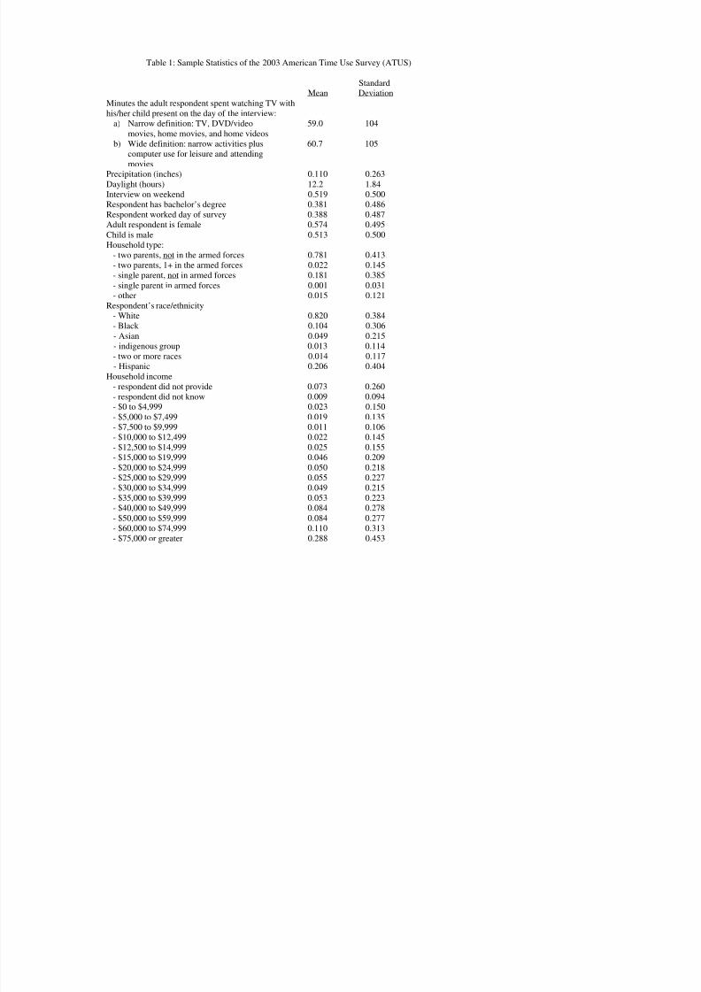
8/6/2019 Autism Waldman Nicholson Adilov
http://slidepdf.com/reader/full/autism-waldman-nicholson-adilov 50/68
Table 1: Sample Statistics of the 2003 American Time Use Survey (ATUS)
Standard
Mean DeviationMinutes the adult respondent spent watching TV withhis/her child present on the day of the interview:
a) Narrow definition: TV, DVD/video 59.0 104movies, home movies, and home videos
b) Wide definition: narrow activities plus 60.7 105computer use for leisure and attendingmovies
Precipitation (inches) 0.110 0.263Daylight (hours) 12.2 1.84Interview on weekend 0.519 0.500Respondent has bachelor’s degree 0.381 0.486Respondent worked day of survey 0.388 0.487Adult respondent is female 0.574 0.495Child is male 0.513 0.500Household type:
- two parents, not in the armed forces 0.781 0.413
- two parents, 1+ in the armed forces 0.022 0.145- single parent, not in armed forces 0.181 0.385- single parent in armed forces 0.001 0.031- other 0.015 0.121
Respondent’s race/ethnicity- White 0.820 0.384- Black 0.104 0.306- Asian 0.049 0.215- indigenous group 0.013 0.114- two or more races 0.014 0.117- Hispanic 0.206 0.404
Household income- respondent did not provide 0.073 0.260- respondent did not know 0.009 0.094- $0 to $4,999 0.023 0.150- $5,000 to $7,499 0.019 0.135- $7,500 to $9,999 0.011 0.106
- $10,000 to $12,499 0.022 0.145- $12,500 to $14,999 0.025 0.155- $15,000 to $19,999 0.046 0.209- $20,000 to $24,999 0.050 0.218- $25,000 to $29,999 0.055 0.227- $30 000 to $34 999 0 049 0 215
h l i l d 2 03 d l d h li i i h hild l h h

8/6/2019 Autism Waldman Nicholson Adilov
http://slidepdf.com/reader/full/autism-waldman-nicholson-adilov 51/68
Notes : the sample includes 2,035 adult respondents who were living with a child less than threeyears of age, and who live in a Metropolitan Statistical Area (MSA) or Primary MetropolitanStatistical Area (PMSA) that is recorded on the survey.
T bl 2 C ffi i t E ti t f Ti S t W t hi g T l i i
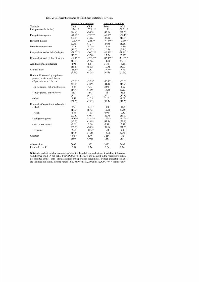
8/6/2019 Autism Waldman Nicholson Adilov
http://slidepdf.com/reader/full/autism-waldman-nicholson-adilov 52/68
Table 2: Coefficient Estimates of Time Spent Watching Television
Narrow TV Definition Wide TV Definition
Variable Tobit OLS Tobit OLSPrecipitation (in inches) 126*** 57.9*** 117*** 59.2***(44.4) (20.3) (43.5) (20.6)
Precipitation squared -76.2** -32.7** -65.8** -32.1**(34.4) (14.6) (33.1) (14.8)
Daylight (hours) -7.19*** -2.66** -7.43*** -2.65**(2.66) (1.27) (2.65) (1.28)
Interview on weekend 17.1 9.04* 18.3* 9.56*(10.7) (5.17) (10.7) (5.24)
Respondent has bachelor’s degree -39.7*** -20.7*** -40.5*** -21.9***(12.3) (5.78) (12.2) (5.87)
Respondent worked day of survey -82.1*** -37.5*** -82.9*** -38.8***(11.8) (5.56) (11.7) (5.63)
Adult respondent is female 4.94 -6.61 3.78 -6.18(10.6) (5.02) (10.5) (5.09)
Child is male 21.5** 7.37 19.5** 7.32(9.51) (4.54) (9.45) (4.61)
Household (omitted group is twoparents, not in armed forces)- 2 parents, armed forces -85.9** -32.5* -86.9** -33.3*
(41.4) (18.9) (41.4) (19.2)- single parent , not armed forces 2.33 4.33 2.08 4.59
(14.4) (7.10) (14.4) (7.20)- single parent, armed forces 112 49.1 113 46.6
(151) (81.7) (152) (82.8)- other 9.59 -1.25 7.17 -1.68
(38.7) (19.2) (38.7) (19.5)Respondent’s race (omitted = white)
- Black 25.0 14.3* 19.0 11.4(17.0) (8.43) (17.0) (8.55)
- Asian 2.54 -1.03 -0.98 -2.59(22.8) (10.8) (22.7) (10.9)
- indigenous group -106** -43.5** -107** -44.7**(43.3) (19.8) (43.3) (20.1)
- two or more races -7.01 2.66 -5.99 3.87(39.6) (20.3) (39.6) (20.6)- Hispanic 20.2 12.4* 16.0 9.48
(14.6) (7.20) (14.6) (7.31)Constant 340* 139 321* 140
(189) (102) (188) (104)
different from zero at a one percent confidence level; ** = significantly different from zero at a

8/6/2019 Autism Waldman Nicholson Adilov
http://slidepdf.com/reader/full/autism-waldman-nicholson-adilov 53/68
different from zero at a one-percent confidence level; ** = significantly different from zero at afive-percent confidence level; * = significantly different from zero at a 10-percent confidencelevel.
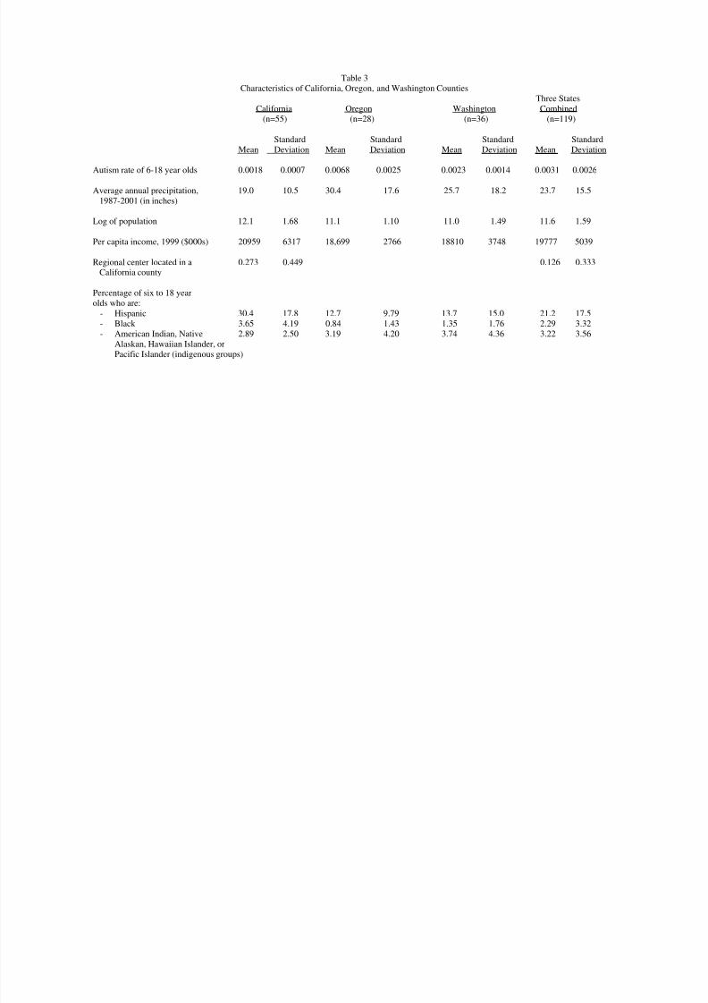
8/6/2019 Autism Waldman Nicholson Adilov
http://slidepdf.com/reader/full/autism-waldman-nicholson-adilov 54/68
Table 3Characteristics of California, Oregon, and Washington Counties
Three StatesCalifornia Oregon Washington Combined
(n=55) (n=28) (n=36) (n=119)
Standard Standard Standard StandardMean Deviation Mean Deviation Mean Deviation Mean Deviation
Autism rate of 6-18 year olds 0.0018 0.0007 0.0068 0.0025 0.0023 0.0014 0.0031 0.0026
Average annual precipitation, 19.0 10.5 30.4 17.6 25.7 18.2 23.7 15.51987-2001 (in inches)
Log of population 12.1 1.68 11.1 1.10 11.0 1.49 11.6 1.59
Per capita income, 1999 ($000s) 20959 6317 18,699 2766 18810 3748 19777 5039
Regional center located in a 0.273 0.449 0.126 0.333California county
Percentage of six to 18 yearolds who are:
- Hispanic 30.4 17.8 12.7 9.79 13.7 15.0 21.2 17.5- Black 3.65 4.19 0.84 1.43 1.35 1.76 2.29 3.32- American Indian, Native 2.89 2.50 3.19 4.20 3.74 4.36 3.22 3.56
Alaskan, Hawaiian Islander, orPacific Islander (indigenous groups)
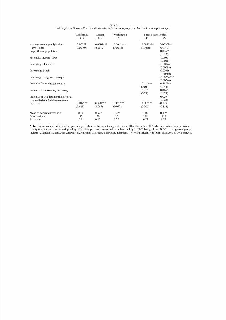
8/6/2019 Autism Waldman Nicholson Adilov
http://slidepdf.com/reader/full/autism-waldman-nicholson-adilov 55/68
Table 4Ordinary Least Squares Coefficient Estimates of 2005 County-specific Autism Rates (in percentages)
California Oregon Washington Three States Pooled(1) (2) (3) (4) (5)
Average annual precipitation, -0.00053 0.0098*** 0.0041*** 0.0049*** 0.0050***1987-2001 (0.00005) (0.0019) (0.0013) (0.0010) (0.0012)
Logarithm of population 0.026**(0.012)
Per capita income (000) -0.0038*(0.0020)
Percentage Hispanic -0.00044(0.00093)
Percentage Black 0.00059(0.00260)
Percentage indigenous groups -0.00774***(0.00244)
Indicator for an Oregon county 0.444*** 0.465***
(0.041) (0.044)Indicator for a Washington county 0.016 0.046*
(0.25) (0.025)Indicator of whether a regional center 0.029
is located in a California county (0.023)Constant 0.187*** 0.378*** 0.120*** 0.083*** -0.133
(0.019) (0.067) (0.037) (0.021) (0.118)
Mean of dependent variable 0.177 0.677 0.226 0.309 0.309Observations 55 28 36 119 119R-squared 0.01 0.47 0.27 0.73 0.77
Notes : the dependent variable is the percentage of children between the ages of six and 18 in December 2005 who have autism in a particularcounty (i.e., the autism rate multiplied by 100). Precipitation is measured in inches for July 1, 1987 through June 30, 2001. Indigenous groupsinclude American Indians, Alaskan Natives, Hawaiian Islanders, and Pacific Islanders. *** = significantly different from zero at a one-percent

8/6/2019 Autism Waldman Nicholson Adilov
http://slidepdf.com/reader/full/autism-waldman-nicholson-adilov 56/68
confidence level; ** = significantly different from zero at a five-percent confidence level; * = significantly different from zero at a 10-percentconfidence level.
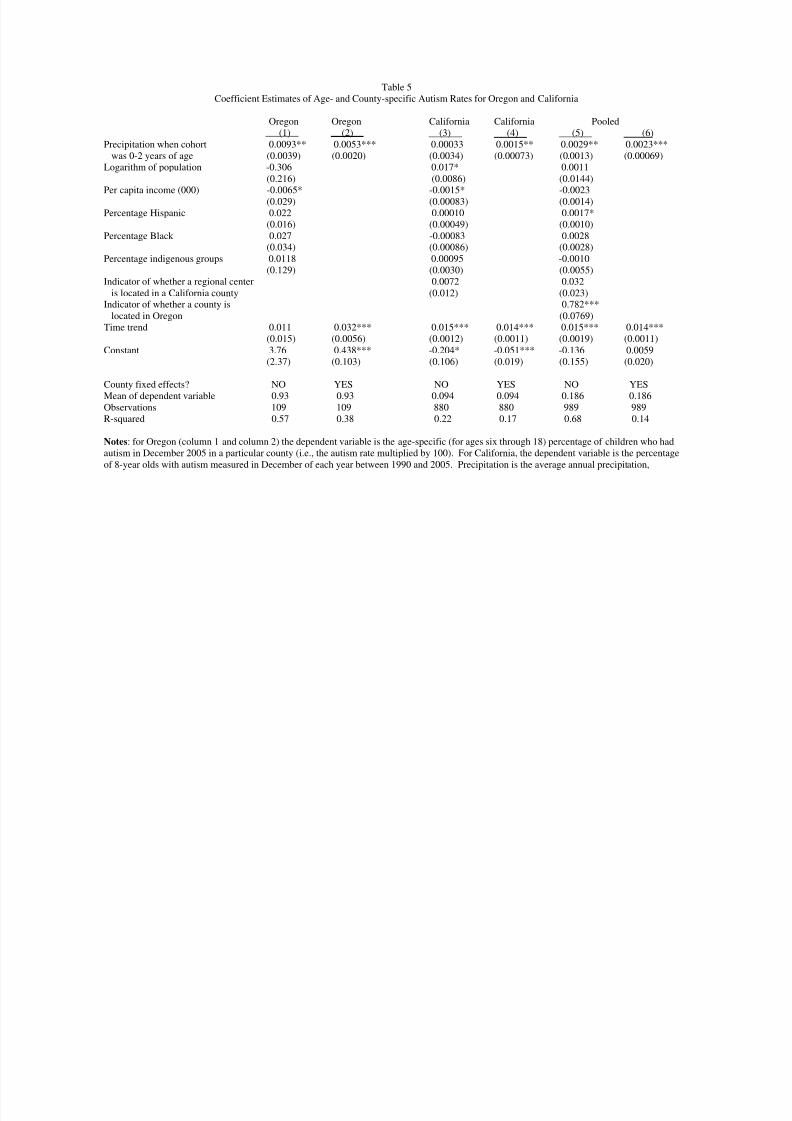
8/6/2019 Autism Waldman Nicholson Adilov
http://slidepdf.com/reader/full/autism-waldman-nicholson-adilov 57/68
Table 5Coefficient Estimates of Age- and County-specific Autism Rates for Oregon and California
Oregon Oregon California California Pooled(1) (2) (3) (4) (5) (6)
Precipitation when cohort 0.0093** 0.0053*** 0.00033 0.0015** 0.0029** 0.0023***was 0-2 years of age (0.0039) (0.0020) (0.0034) (0.00073) (0.0013) (0.00069)
Logarithm of population -0.306 0.017* 0.0011(0.216) (0.0086) (0.0144)
Per capita income (000) -0.0065* -0.0015* -0.0023(0.029) (0.00083) (0.0014)
Percentage Hispanic 0.022 0.00010 0.0017*(0.016) (0.00049) (0.0010)
Percentage Black 0.027 -0.00083 0.0028(0.034) (0.00086) (0.0028)
Percentage indigenous groups 0.0118 0.00095 -0.0010(0.129) (0.0030) (0.0055)
Indicator of whether a regional center 0.0072 0.032is located in a California county (0.012) (0.023)
Indicator of whether a county is 0.782***located in Oregon (0.0769)
Time trend 0.011 0.032*** 0.015*** 0.014*** 0.015*** 0.014***(0.015) (0.0056) (0.0012) (0.0011) (0.0019) (0.0011)
Constant 3.76 0.438*** -0.204* -0.051*** -0.136 0.0059(2.37) (0.103) (0.106) (0.019) (0.155) (0.020)
County fixed effects? NO YES NO YES NO YESMean of dependent variable 0.93 0.93 0.094 0.094 0.186 0.186Observations 109 109 880 880 989 989R-squared 0.57 0.38 0.22 0.17 0.68 0.14
Notes : for Oregon (column 1 and column 2) the dependent variable is the age-specific (for ages six through 18) percentage of children who hadautism in December 2005 in a particular county (i.e., the autism rate multiplied by 100). For California, the dependent variable is the percentageof 8-year olds with autism measured in December of each year between 1990 and 2005. Precipitation is the average annual precipitation,

8/6/2019 Autism Waldman Nicholson Adilov
http://slidepdf.com/reader/full/autism-waldman-nicholson-adilov 58/68
measured in inches, for the years when a cohort was under the age of three. Indigenous groups include American Indians, Alaskan Natives,Hawaiian Islanders, and Pacific Islanders. Standard errors are adjusted in column (1), column (3), and column (5) to allow for correlation of error
terms between age cohorts within a county. *** = significantly different from zero at a one-percent confidence level; ** = significantly differentfrom zero at a five-percent confidence level; * = significantly different from zero at a 10-percent confidence level.
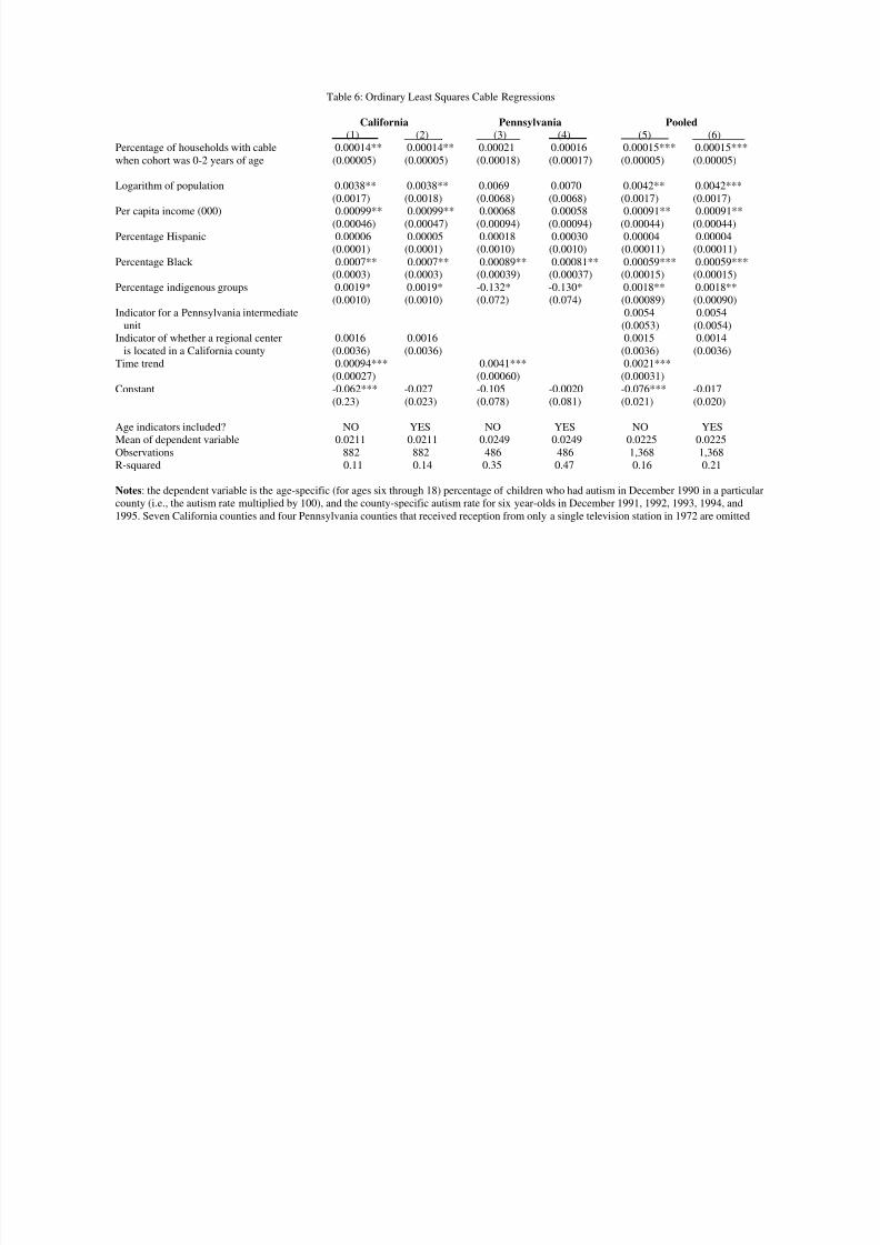
8/6/2019 Autism Waldman Nicholson Adilov
http://slidepdf.com/reader/full/autism-waldman-nicholson-adilov 59/68
Table 6: Ordinary Least Squares Cable Regressions
California Pennsylvania Pooled(1) (2) (3) (4) (5) (6)
Percentage of households with cable 0.00014** 0.00014** 0.00021 0.00016 0.00015*** 0.00015***when cohort was 0-2 years of age (0.00005) (0.00005) (0.00018) (0.00017) (0.00005) (0.00005)
Logarithm of population 0.0038** 0.0038** 0.0069 0.0070 0.0042** 0.0042***(0.0017) (0.0018) (0.0068) (0.0068) (0.0017) (0.0017)
Per capita income (000) 0.00099** 0.00099** 0.00068 0.00058 0.00091** 0.00091**(0.00046) (0.00047) (0.00094) (0.00094) (0.00044) (0.00044)
Percentage Hispanic 0.00006 0.00005 0.00018 0.00030 0.00004 0.00004(0.0001) (0.0001) (0.0010) (0.0010) (0.00011) (0.00011)
Percentage Black 0.0007** 0.0007** 0.00089** 0.00081** 0.00059*** 0.00059***(0.0003) (0.0003) (0.00039) (0.00037) (0.00015) (0.00015)
Percentage indigenous groups 0.0019* 0.0019* -0.132* -0.130* 0.0018** 0.0018**(0.0010) (0.0010) (0.072) (0.074) (0.00089) (0.00090)
Indicator for a Pennsylvania intermediate 0.0054 0.0054unit (0.0053) (0.0054)
Indicator of whether a regional center 0.0016 0.0016 0.0015 0.0014is located in a California county (0.0036) (0.0036) (0.0036) (0.0036)
Time trend 0.00094*** 0.0041*** 0.0021***(0.00027) (0.00060) (0.00031)
Constant -0.062*** -0.027 -0.105 -0.0020 -0.076*** -0.017(0.23) (0.023) (0.078) (0.081) (0.021) (0.020)
Age indicators included? NO YES NO YES NO YESMean of dependent variable 0.0211 0.0211 0.0249 0.0249 0.0225 0.0225Observations 882 882 486 486 1,368 1,368R-squared 0.11 0.14 0.35 0.47 0.16 0.21
Notes : the dependent variable is the age-specific (for ages six through 18) percentage of children who had autism in December 1990 in a particularcounty (i.e., the autism rate multiplied by 100), and the county-specific autism rate for six year-olds in December 1991, 1992, 1993, 1994, and1995. Seven California counties and four Pennsylvania counties that received reception from only a single television station in 1972 are omitted

8/6/2019 Autism Waldman Nicholson Adilov
http://slidepdf.com/reader/full/autism-waldman-nicholson-adilov 60/68
from the regressions. Indigenous groups include American Indian and Alaskan Natives. A set of indicator variables for each cohort are includedin the specifications in column (2), column (4), and column (6). *** = significantly different from zero at a one-percent confidence level; ** =
significantly different from zero at a five-percent confidence level; * = significantly different from zero at a 10-percent confidence level.
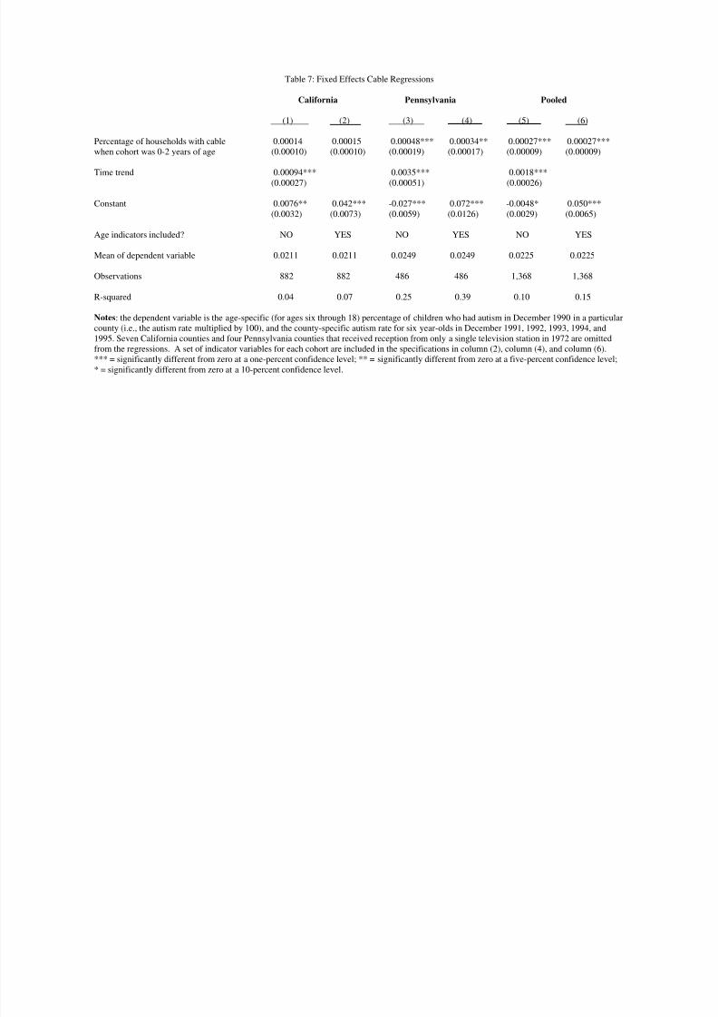
8/6/2019 Autism Waldman Nicholson Adilov
http://slidepdf.com/reader/full/autism-waldman-nicholson-adilov 61/68
Table 7: Fixed Effects Cable Regressions
California Pennsylvania Pooled
(1) (2) (3) (4) (5) (6)
Percentage of households with cable 0.00014 0.00015 0.00048*** 0.00034** 0.00027*** 0.00027***when cohort was 0-2 years of age (0.00010) (0.00010) (0.00019) (0.00017) (0.00009) (0.00009)
Time trend 0.00094*** 0.0035*** 0.0018***(0.00027) (0.00051) (0.00026)
Constant 0.0076** 0.042*** -0.027*** 0.072*** -0.0048* 0.050***(0.0032) (0.0073) (0.0059) (0.0126) (0.0029) (0.0065)
Age indicators included? NO YES NO YES NO YES
Mean of dependent variable 0.0211 0.0211 0.0249 0.0249 0.0225 0.0225
Observations 882 882 486 486 1,368 1,368
R-squared 0.04 0.07 0.25 0.39 0.10 0.15
Notes : the dependent variable is the age-specific (for ages six through 18) percentage of children who had autism in December 1990 in a particularcounty (i.e., the autism rate multiplied by 100), and the county-specific autism rate for six year-olds in December 1991, 1992, 1993, 1994, and1995. Seven California counties and four Pennsylvania counties that received reception from only a single television station in 1972 are omittedfrom the regressions. A set of indicator variables for each cohort are included in the specifications in column (2), column (4), and column (6).*** = significantly different from zero at a one-percent confidence level; ** = significantly different from zero at a five-percent confidence level;* = significantly different from zero at a 10-percent confidence level.
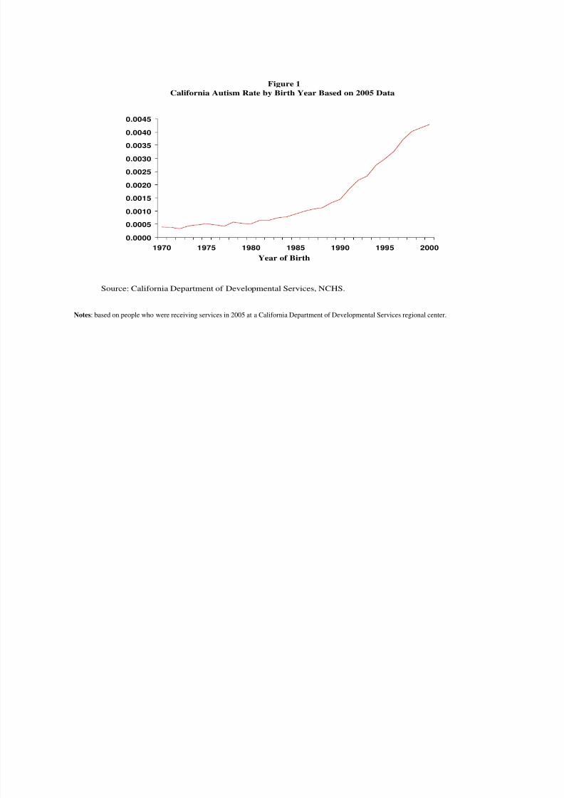
8/6/2019 Autism Waldman Nicholson Adilov
http://slidepdf.com/reader/full/autism-waldman-nicholson-adilov 62/68
0.0000
0.0005
0.0010
0.0015
0.0020
0.0025
0.0030
0.0035
0.0040
0.0045
1970 1975 1980 1985 1990 1995 2000
Figure 1California Autism Rate by Birth Year Based on 2005 Data
Year of Birth
Source: California Department of Developmental Services, NCHS.
Notes : based on people who were receiving services in 2005 at a California Department of Developmental Services regional center.
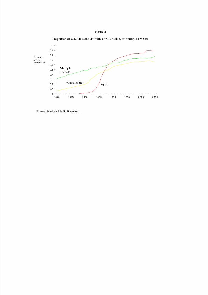
8/6/2019 Autism Waldman Nicholson Adilov
http://slidepdf.com/reader/full/autism-waldman-nicholson-adilov 63/68
0
0.1
0.20.3
0.4
0.5
0.6
0.7
0.8
0.9
1
1970 1975 1980 1985 1990 1995 2000 2005
Figure 2
Proportion of U.S. Households With a VCR, Cable, or Multiple TV Sets
Proportionof U.S.Households
VCRWired cable
MultipleTV sets
Source: Nielsen Media Research.
Figure 3Precipitation (1990-2001) and Autism Rates (2005) of Washington Counties
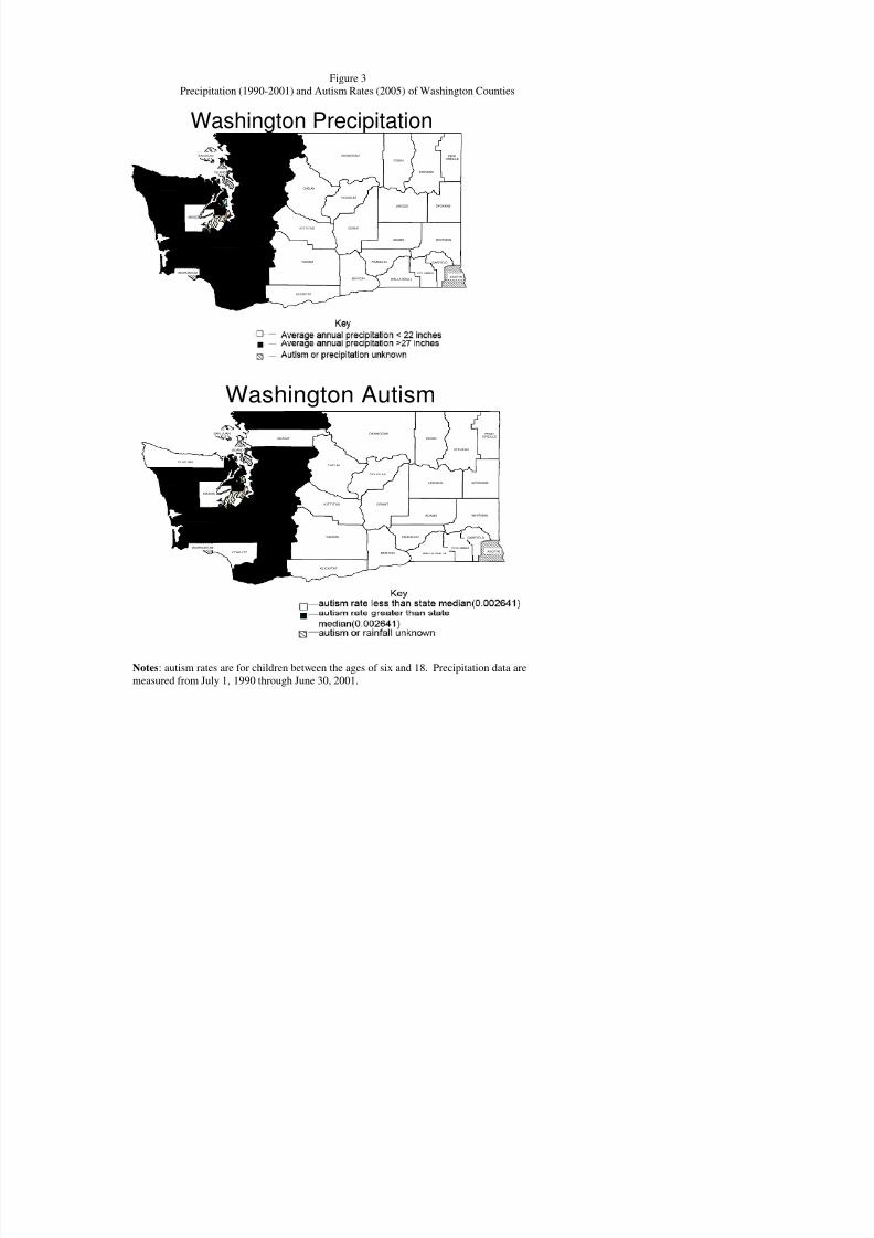
8/6/2019 Autism Waldman Nicholson Adilov
http://slidepdf.com/reader/full/autism-waldman-nicholson-adilov 64/68
p ( ) ( ) g
Washington Precipitation
ADAMS
ASOTINBENTON
CHELANCLALLAM
CLARK
COLUMBIA
COWLITZ
DOUGLAS
FERRY
FRANKLIN GARFIELD
GRANTGRAYSHARBOR
ISLAND
JEFFERSON
KINGKITSAP
KITTITAS
KLICKITAT
LEWIS
LINCOLN
MASON
OKANOGAN
PACIFIC
PENDOREILLE
PIERCE
SANJUAN
SKAGIT
SKAMANIA
SNOHOMISH
SPOKANE
STEVENS
THURSTON
WAHKIAKUM
WALLA WALLA
WHATCOM
WHITMAN
YAKIMA
Washington Autism
ADAMS
ASOTINBENTON
CHELAN
CLALLAM
CLARK
COLUMBIA
COWLITZ
DOUGLAS
FERRY
FRANKLIN GARFIELD
GRANTGRAYSHARBOR
ISLAND
JEFFERSON
KING
KITSAP
KITTITAS
KLICKITAT
LEWIS
LINCOLN
MASON
OKANOGAN
PACIFIC
PENDOREILLE
PIERCE
SAN JUAN
SKAGIT
SKAMANIA
SNOHOMISH
SPOKANE
STEVENS
THURSTON
WAHKIAKUM
WALLA WALLA
WHATCOM
WHITMAN
YAKIMA
Figure 4Precipitation (1990-2001) and Autism Rates (2005) of Oregon Counties
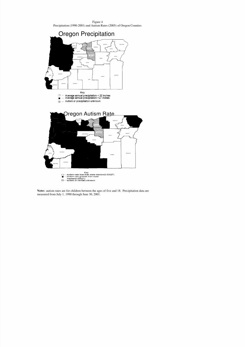
8/6/2019 Autism Waldman Nicholson Adilov
http://slidepdf.com/reader/full/autism-waldman-nicholson-adilov 65/68
p ( ) ( ) g
Oregon Precipitation
BAKER
BENTON
CLACKAMAS
CLATSOP
COOS
CROOK
CURRY
DESCHUTES
DOUGLAS
GILLIAM
GRANT
HARNEY
JACKSON
JEFFERSON
JOSEPHINE
KLAMATH
LAKE
LANE
LINCOLNLINN
MALHEUR
MORROW
MULTNOMAH
POLK
SHERMANTILLAMOOK
UMATILLA
UNION
WALLOWA
WASCO
WASHINGTON
WHEELER
YAMHILL
COLUMBIA
MARION
HOOD
RIVER
Oregon Autism Rate
BAKER
BENTON
CLACKAMAS
CLATSOP
COOS
CROOK
CURRY
DESCHUTES
DOUGLAS
GILLIAM
GRANT
HARNEY
JACKSON
JEFFERSON
JOSEPHINE
KLAMATH
LAKE
LANE
LINCOLNLINN
MALHEUR
MORROW
MULTNOMAH
POLK
SHERMAN
TILLAMOOK
UMATILLA
UNION
WALLOWA
WASCO
WASHINGTON
WHEELER
YAMHILL
COLUMBIA
MARION
HOOD
RIVER
Figure 5Precipitation (1990-2001) and Autism Rates (2005) of California Counties
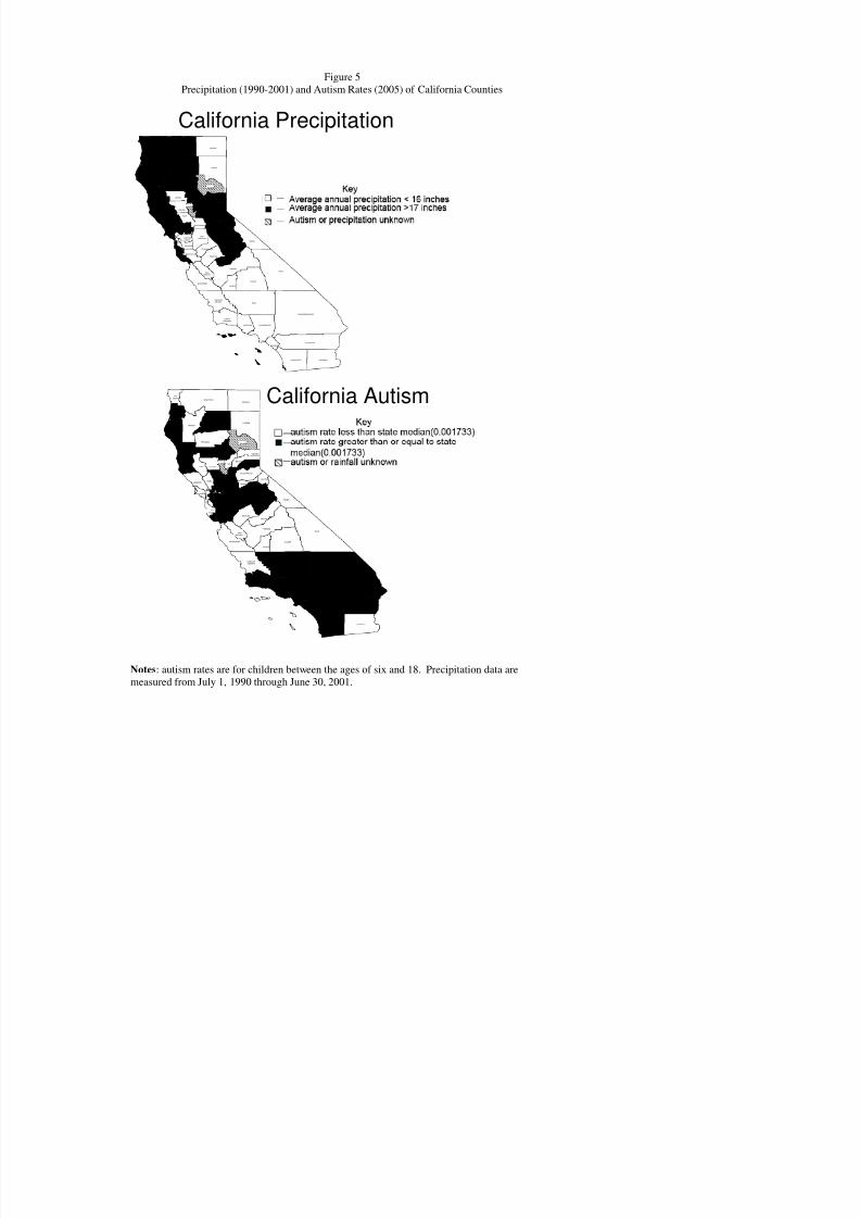
8/6/2019 Autism Waldman Nicholson Adilov
http://slidepdf.com/reader/full/autism-waldman-nicholson-adilov 66/68
California Precipitation
ALAMEDA
ALPINE
AMADOR
BUTTE
CALAVERAS
COLUSA
CONTRACOSTA
DELNORTE
ELDORADO
FRESNO
GLENN
HUMBOLDT
IMPERIAL
INYO
KERN
KINGS
LAKE
LASSEN
LOSANGELES
MADERA
MARIN
MARIPOSA
MENDOCINO
MERCED
MODOC
MONO
MONTEREY
NAPA
NEVADA
ORANGE
PLACER
PLUMAS
RIVERSIDE
SACRAMENTO
SANBENITO
SANBERNARDINO
SANDIEGO
SANLUISOBISPO
SANMATEO
SANTABARBARA
SANTACLARA
SANTACRUZ
SHASTA
SIERRA
SISKIYOU
SOLANO
SONOMA
STANISLAUS
SUTTER
TEHAMA
TRINITY
TULARE
TUOLUMNE
VENTURA
YOLO
Yuba
SANJOAQUIN
California Autism
ALAMEDA
ALPINE
AMADOR
BUTTE
CALAVERAS
COLUSA
CONTRACOSTA
DELNORTE
ELDORADO
FRESNO
GLENN
HUMBOLDT
INYO
KERN
KINGS
LAKE
LASSEN
LOSANGELES
MADERA
MARIN
MARIPOSA
MENDOCINO
MERCED
MODOC
MONO
MONTEREY
NAPA
NEVADA
PLACER
PLUMAS
SACRAMENTO
SANBENITO
SANBERNARDINO
SANLUISOBISPO
SANMATEO
SANTABARBARA
SANTACLARA
SANTACRUZ
SHASTA
SIERRA
SISKIYOU
SOLANO
SONOMA
STANISLAUS
SUTTER
TEHAMA
TRINITY
TULARE
TUOLUMNE
VENTURA
YOLO
Yuba
SANJOAQUIN
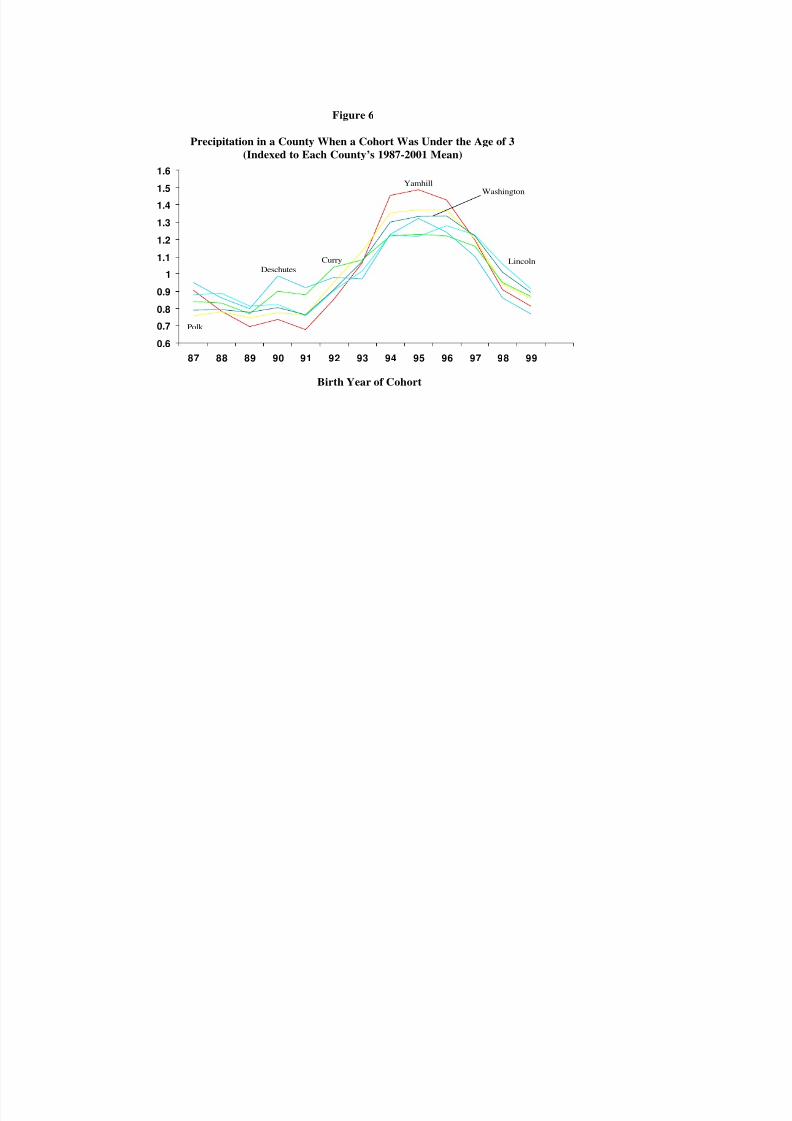
8/6/2019 Autism Waldman Nicholson Adilov
http://slidepdf.com/reader/full/autism-waldman-nicholson-adilov 67/68
0.6
0.7
0.8
0.9
1
1.1
1.2
1.3
1.4
1.5
1.6
87 88 89 90 91 92 93 94 95 96 97 98 99
Birth Year of Cohort
Figure 6
Precipitation in a County When a Cohort Was Under the Age of 3(Indexed to Each County’s 1987-2001 Mean)
Yamhill
Polk
LincolnDeschutes
Washington
Curry
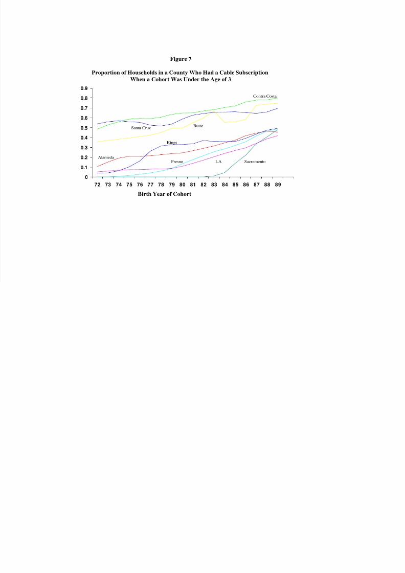
8/6/2019 Autism Waldman Nicholson Adilov
http://slidepdf.com/reader/full/autism-waldman-nicholson-adilov 68/68
0
0.1
0.2
0.3
0.4
0.5
0.6
0.7
0.8
0.9
72 73 74 75 76 77 78 79 80 81 82 83 84 85 86 87 88 89
Birth Year of Cohort
Figure 7
Proportion of Households in a County Who Had a Cable SubscriptionWhen a Cohort Was Under the Age of 3
Contra Costa
Butte
Kings
AlamedaSacramentoLAFresno
Santa Cruz