
Balancing water availability and water demand in the Blue...
172
Balancing water availability and water demand in the Blue Nile: A case study of Gumara watershed in Ethiopia Dissertation Zur Erlangung des Doktorgrades (Dr. rer. nat.) Der Mathematisch-Naturwissenschaftlichen Fakultät Der Rheinischen Friedrich-Wilhelms-Universität Bonn vorgelegt von Sisay Demeku Derib Aus Arsi-Sire, Ethiopia Bonn, Dezember 2013
Transcript of Balancing water availability and water demand in the Blue...
Balancing water availability and water demand in the Blue Nile: A case study of Gumara watershed in Ethiopia
Dissertation
Zur
Erlangung des Doktorgrades (Dr. rer. nat.)
Der
Mathematisch-Naturwissenschaftlichen Fakultät
Der
Rheinischen Friedrich-Wilhelms-Universität Bonn
vorgelegt von
Sisay Demeku Derib
Aus
Arsi-Sire, Ethiopia
Bonn, Dezember 2013

Angefertigt mit Genehmigung der Mathematisch-Naturwissenschaftlichen Fakultät der
Rheinischen Friedrich-Wilhelms-Universität Bonn
1. Gutachter: Prof. Dr. B. Diekkrüger
2. Gutachter: Prof. Dr. J. Bogardi Tag der Promotion: 31.03.2014 Erscheinungsjahr: 2014

DEDICATION
The well-being of the Nile basin society
The wise females that are always at my side: my wife (Hiwot Yirgu), my mother (Zewude Gashu) and my little daughters (Meklit and Etsubdink).
SUMMARY
Ethiopia suffers from economic water scarcity that makes its water utilization difficult. In-depth understanding of the hydrological processes is important for balancing availability and demand. As part of this basin-wide and national concern, this study examines the water balance and water availability on farm and watershed scales in different scenarios. The objectives of the study were (1) to evaluate water use and water productivity of a small-scale irrigation scheme, (2) to evaluate methods for filling gaps in climatic data, (3) to adopt the Soil and Water Assessment Tool (SWAT) hydrological model for modeling hydrological processes using different modeling setups, and (4) to simulate water demand and water stress status for a period up to 2050 using different land-use and demographic scenarios. The Gumara watershed (1520 km2), a tributary of Lake Tana and source of the Blue Nile in Ethiopia, was selected for this study. A case study at a small-scale irrigation scheme shows that there was high water loss during water conveyance and application. At the same time, water stress was observed during irrigation at the scheme level, as the applied water did not match the water needs of different crops. Environmental modeling requires complete climate data sets, which are rarely available. Therefore, different gap-filling methods were applied and tested. Considering data from neighboring climate stations, the methods arithmetic mean and coefficient of correlation weighting methods gave better daily rainfall estimation than the normal ratio and inverse distance weighting methods. Multiple linear regression methods performed well when filling daily air temperature gaps using data from neighboring stations. After seasonal categorization of daily data and optimization of parameters, procedures using maximum and minimum temperature for simulating solar radiation and relative humidity gave promising performances. For process analysis, SWAT was applied for the watershed with an acceptable performance when simulating river flow. The effect of data availability on model performance was analyzed using different numbers of climate stations. Using four and six stations resulted in better SWAT water flow modeling performance as compared to two stations. Penman-Monteith and Hargreaves procedures for potential evaporation calculation resulted in comparable river flow modeling in SWAT. Therefore, the Hargreaves method that needs only air temperature can be used for modeling when other climatic data are not available. Selected watershed management practices shift surface runoff to sub-surface and groundwater flows. An irrigation project planned in the watershed and the watershed management practices shift surface discharge to base flow and evapotranspiration. It will be hard to satisfy the basic human water requirements in 2050 if the existing water management and water productivity conditions pertain. Better green water management and non-consumptive water use options (e.g. hydro power, fishery) can minimize the blue water stress at the Nile basin level.

Zusammenfassung Äthiopien leidet unter ökonomischer Wasserknappheit, was die Wassernutzung erschwert. Dieses stellt sowohl für das untersuchte Wassereinzugsgebiet als auch für das Land ein großes Problem dar. Aus diesem Grund ist ein vertieftes Verständnis der hydrologischen Prozesse für die Abwägung der Wasserverfügbarkeit mit dem Wasserbedarf von hoher Bedeutung. Vor diesem Hintergrund untersucht diese Studie den Wasserhaushalt und die Wasserverfügbarkeit von der lokalen (Farm) bis zur Wassereinzugsskala unter Berücksichtigung verschiedener Szenarien mit folgenden Zielen: (1) Bewertung der Wassernutzung und -produktivität in einem kleinbäuerlichen Bewässerungssystem, (2) Bewertung von Methoden zur Ergänzung von Lücken in Klimadaten, (3) Anwendung des hydrologischen Soil and Water Assessment Tool (SWAT) für die Modellierung der hydrologischen Prozesse des Einzugsgebiets unter Berücksichtigung verschiedener Modellkonfigurationen und (4) Simulation von Wasserbedarf und Wasserstress für den Zeitraum bis 2050 mit verschiedenen Landnutzungs- und demographischen Szenarien. Das Gumara-Einzugsgebiet (1520 km2), ein Zufluss zum Tanasee und Ursprung des Blauen Nils in Äthiopien, wurde für diese Studie ausgewählt. Eine Fallstudie in einem kleinbäuerlichen Bewässerungssystem zeigt einen hohen Wasserverlust während des Wassertransports und der Wassernutzung. Gleichzeitig wurde Wasserstress während des Bewässerungszeitraums beobachtet, da die ausgebrachte Wassermenge dem Wasserbedarf der verschiedenen Anbaupflanzen nicht entsprach. Umweltmodellierung bedarf vollständiger Datensätze, die jedoch selten verfügbar sind. Daher wurden verschiedene Methoden angewandt und getestet mit denen die Datenlücken geschlossen werden können. Die Methoden arithmetisches Mittel sowie Korrelationskoeffizienten mit Gewichtung ergaben bessere tägliche Niederschlagsprognosen als die Methoden gewichtete Mittelwerte (normal ratio) und inverse Distanzgewichtung (inverse distance weighting). Lücken in Temperaturdaten können gut aus den Daten benachbarter Stationen mittels multipler linearer Regressionsmethoden geschlossen werden. Mit einer saisonalen Parametrisierung kann aus den Maximum- und Minimumtemperaturen die Solarstrahlung und die relativer Luftfeuchtigkeit abgeleitet werden. Für die Simulation der hydrologischen Prozesse und des Abflusses wurde SWAT erfolgreich eingesetzt. Die Auswirkung der Datenverfügbarkeit auf die Modellgüte wurde untersucht, indem unterschiedliche Anzahlen von Klimastationen berücksichtigt wurden. Vier bzw. sechs Stationen ergeben eine bessere Simulation des Abflusses verglichen mit zwei Stationen. Der Vergleich der Berechnung der potentiellen Verdunstung nach Penman-Monteith und nach Hargreaves resultiert in vergleichbaren Simulationen des Abflusses mit SWAT. Daher kann die Hargreaves Methode, die nur Lufttemperaturdaten benötigt, zur Modellierung eingesetzt werden wenn andere Klimadaten nicht verfügbar sind. Bestimmte Bewirtschaftungsverfahren im Einzugsgebiet verändern das Verhältnis des Oberflächen- zu unterirdischem und Grundwasserabfluss. Ein geplantes Bewässerungsprojekt sowie die vorhandenen Bewirtschaftungsverfahren verändern

den Oberflächenabfluss zu Basisabfluss und zur Verdunstung. Unter den derzeitigen Wasserbewirtschaftungsverfahren und der derzeitigen Wasserproduktivität wird es schwer sein, den Wasserbedarf der Bevölkerung im Jahre 2050 zu erfüllen. Ein besseres Management des grünen Wassers sowie Optionen für die nicht konsumtive Wassernutzung (Wasserenergie, Fischerei, etc.) können die Knappheit an blauem Wasser auf der Skala des Nileinzugsgebietes minimieren.
ማጠቃሇያ
ኢትዮጵያ ያሊትን የውኃ ሃብት በብቃት ሇመጠቀም እንዳትችሌ የኢኮኖሚ እና የቴክኖልጂ ክህልት ተግዳሮቶች ወስነዋታሌ። በአሁኑ ወቅት በተሻሇ መሌኩ የውኃ መሰረተ-ሌማት እየታየ ቢሆንም ዘሊቂነት ያሇው ሌማት ሇማከናወን በተሻሇ እውቀት ሊይ መመስረት አስፈሊጊ ነው። የውኃ ፍሰት ዑዯት ምጣኔን እና ሇመሰረታዊ ፍሊጎት ተዯራሽ የሆነን የውኃ አካሌ መጠን በጊዜ እና በቦታ ወሰን በጥሌቀት መረዳት የሚፈሇገውን ክህልት ያዳብራሌ፤ የሚሰሩ ሥራዎችን በመረጃ ይዯግፋሌ። ይህንን አጠቃሊይ አስፈሊጊነት መሰረት በማድረግ በእዚህ ጥናት የውኃ ፍሰት ዑዯትንና ሇጥቅም የሚውሌ የውኃ ሌክን በእርሻ መሬት፣ በተፋሰስና በተሇያዩ የመሬት አጠቃቀምና የመሰረታዊ የውኃ ፍሊጎት አማራጮች መሰረት የውኃ ምጣኔን ሇመተንተን ተሞክሯሌ። ጥናቱ ያተኮረባቸው አሊማዎች፤ (፩) የውኃ አጠቃቀምንና የውኃ ምርታማነትን በናሙና በተመረጠ አነስተኛ የመስኖ አውታር ሊይ መገምገም፣ (፪) የተጓዯለ የሚትሪዮልጂ መረጃዎችን ማምዋያ የተሇያዩ ቀመሮችን ማስሊት፣ (፫) የውኃ ዑዯትን መተንተን የሚያስችሌ ሞዴሌ ሇጥናቱ ቦታ እንዲያገሇግሌ መሰረታዊ መስፈርቶቹን ማስተካከሌ እና (፬) ሞዴለን በመጠቀም የውኃ ፍሰት ምጣኔ ድርሻና የፍሊጎት ጫናን በተሇያዩ አማራጮች ማስሊት ናቸው። በአባይ ወንዝ መነሻ በሆነው በጣና ሃይቅ ተፋሰስ ውስጥ የሚገኝ 1520 እስኩየር ኪል ሜትር ስፋት ያሇው የጉማራ ንዑስ ተፋሰስ ሇጥናቱ ቦታ ተመርጧሌ።
ጓንታ በተባሇ በተፋሰሱ ውስጥ በሚገኝ አነስተኛ የመስኖ አውታር (90 ሄክታር) ሊይ በተዯረገው ጥናት ውኃን
ከወንዝ ጠሌፎ ወዯተፈሇገው ማሳ በማጓጓዝና በማሳ ሊይ በሚዯረግ የውኃ አጠቃቀም ሂዯት ውኃ በብዛት እንዯሚባክን፣ ይህ የሚባክነው ውኃ ባሌተፈሇገ መሌኩ ማሳዎችን በማጥሇቅሇቅና በመስረግ የመስኖ ማሳዎችን ከጥቅም ውጪ ማድረጉ፣ የመስኖ ቦዮች ጥገና እና ፅዳት በወቅቱ ባሇመዯረጉ ውኃ በተፈሇገው ጊዜ፣ መጠንና ቦታ ማድረስ አሇመቻለና በታችኛው የመስኖ ማሳዎች የውኃ እጥረት መከሰቱ ዋና ዋና የሚታዩ ችግሮች ናቸው። በዚህና በተያያዥ ምክንያቶች የሰብልች የማሳና የውኃ ምርታማነት ከላልች ቦታዎች ጋር ሲወዳዯር ዝቅተኛ ነው። በመስኖ ቦዮችና ማሳዎች ዳርቻ ሊይ የሚገኝ የሳር ምርት በስርገት የሚባክንውን የተወሰነ ውኃ ሇከብቶች መኖ ምርት እንዲሰጥ በማድረጉ፣ የበጋ ወቅት የመኖ እጥረትን በመቅረፍና ጥምር የሰብሌና እንስሳት ግብርናን በመዯግፍ ተጨማሪ ጠቀሜታ አሇው፤ የመስኖ ውኃውንም ምርታማነት ከተሇመዯው የሰብሌ ምርታማነት ስላት የበሇጠ ያዯርገዋሌ። የምሽት ውኃ ማጠራቀሚያ ጊዜያዊ ኩሬዎች በተሇያዩ አመቺ ቦታዎች በመስራት ውኃን በሇሉት ሇመስኖ መጠቀምን ማስቀረት፣ ገበሬዎች መስኖውን እንዲቆጣጠሩ ማብቃት፣ ሇመስኖ ቦታዎች የተሻለ ምርታማ የሰብሌና የመኖ ዝርያዎችን ሇይቶ ማቅረብ፣ አዋጭ የሰብልችን የውኃ ፍሊጎት መወሰንና በገበሬዎች አቅም ውኃን የመሇኪያ ዘዴዎችን ማቅረብ የውኃ ብክነትን ሇመቀነስና ምርታማነትን ሇመጨመር ያስችሊሌ።
የተሟሊ የሚትሪዮልጂ መረጃ ሇውኃ አጠቃቀም ጥናትና ውሳኔ አሰጣጥ ወሳኝ ነው። በጥናቱ አካባቢ
በመሳሪያዎች አሇመሟሊትና ብሌሽት፣ በሰሇጠነ የሰው ሃይሌ እጦትና በመሳሰለት ምክንያቶች ከየሚትሪዮልጂ ጣቢያዎቹ ያሌተሟሊ መረጃ ማግኘት የተሇመዯ ነው። ዘሊቂ መፍትሄ የሚሰጡ ጥናቶችና የውኃ አጠቃቀም ሥራዎችን ሇማድረግ እነዚህን መረጃዎች ጥቅም እንዲሰጡ በማድረግ የመረጃ ክፍተትን መሙሊት ያስፈሌጋሌ። በዚህ ጥናት አምስተኛ ምእራፍ ሊይ የዝናብ፣ የአየር ሙቀት፣ የፀሐይ ሃይሌንና የአየር እርጥበት መረጃ ክፍተቶችን ሇመሙሊት የተሇያዩ አማራጭ ዘዴዎች ተገምግመው የተሻለት ዘዴዎች ተመርጠዋሌ። የአንድን መረጃ ማሰባሰቢያ ጣቢያ ክፍተት ከአጎራባች ጣቢያዎች መረጃ በመነሳት ሇመሙሊት የሚያስችለ ዘዴዎችን መጠቀሙ የተወሳሰበ ካሇመሆኑም በተጨማሪ በውሃ ፍሰት ትንታኔ ሊይ የተሻሇ ተአማኒ ትንታኔ ሇመስጠት አስችልዋሌ። የፀሐይ ሃይሌን እና የአየር እርጥበት መረጃን በቀሊለ መሇካት ከሚቻሌ የአየር ሙቀት መረጃ መቀመር በተወሰነ መጠን ተችልዋሌ። መሌክዓ ምድሩን መሰረት ያዯረገ ቀጣይ ጥናት የተሻሇ ግንዛቤ ሉያስገኝ ይችሊሌ።
በአሜሪካን ሃገር ተዋቅሮ በተሇታዩ የአሇማችን ተፋሰሶች ሇብዙ ጊዜ ሥራ ሊይ የዋሇ የውሃ ፍሰት ምጣኔ ሞዴሌ
(Soil and Water Assessment Tool-SWAT) ተመርጦ የሞዴለ የውስጥ መሰረታዊ መስፈርቶች ከአካባቢው መረጃ ጋር ተቀባይነት ባሇው መሌኩ እንዲሰራ ተዯርጓሌ። በጉማራ ተፋሰስ የተዯረጉ ጥናቶች በአብዛኛው የሚጠቀሙት የባህር ዳር ሚትሪዮልጂ መረጃ መመዝገቢያ ጣቢያን መረጃና ከሊይ በተገሇፀው ዘዴ የተሟሊን በተፋሰሱ አቅራቢያ የሚገኝን መረጃን በመጠቀም የሚገኘው የውሃ ፍሰት ምጣኔ ትንተና ከፍተኛ ሌዩነት አሇው። በአዲስ መሌክ መረጃዎችን አድራጅቶና አሟሌቶ መጠቀሙ የተሻሇ የትንተና ብቃትና ተአማኒነት አሇው። ወዯፊት ሇሚሰሩ የውኃ አጠቃቀም ጥናቶችና ሥራዎች በመሌክዓ ምድሩ ገፅታ ወካይነት መሰረት በማድረግ ተጨማሪ የመረጃ መሰብሰቢያ ጣቢያዎችን ማቋቋምና እስካሁን በአካባቢው ከተመዘገበው መረጃ ጋር በዚህ ጥናት የተገሇፀውን ስሌትና ላሊም በመጠቀም አንናቦ መተንተን የተሻሇ የውኃ ምጣኔ ግንዛቤ ሇማዳበር ይረዳሌ። እስከ ቀበላ ድረስ የተዋቀሩ የመጀመሪያ ዯረጃ ትምህርት ቤቶችን እና የጤና ኬሊዎችን ሇተጨማሪ የሚትሪዮልጂ መረጃ ማሰባሰቢያነት መጠቀሙ በትንሽ ወጪና በነበረ የተማረ የሰው ሃይሌ መረጃን በተሻሇ ዋስትና እና ጥራት ሇማሰባሰብ ያስችሊሌ።
የሃገሪትዋ የመሬት አጠቃቀም ፖሉሲ ተዯነገገው መሰረት እንዯ እርከን እና የዯን ሌማት ሥራዎችን በአማራጭነት በመጠቀም፣ መሰረታዊ የውኃ ፍሊጎትን በ2000ዎቹና በ2050ዎቹ የህዝብ ብዛት አንፃር በማስሊት የውኃ ምጣኔንና ጥቅም ሊይ ሉውሌ የሚችሌ የውኃ ድርሻን ሇመተንተን ተሞክርዋሌ። የእርከንና የዯን ሌማት የውኃ ፍሰት ምጣኔን የተወሰነውን ከጎርፍነት ወዯ ከርሰምድር ውኃ ፍስትና ሇተክልች እድገት ወዯሚውሌ ትነት መቀየር ያስችሊሌ። በታችኛው የተፋሰሱ ክፍሌ የሚከሰትን ዯራሽ ውኃ ከማማከለም በተጨማሪ የውኃውን ጠቃሚነት ይጨምራሌ። ጥናቱ የተጠናቀቀው የጉማራ መስኖ ፕሮጀክት ወዯ ጣና የሚፈሰውን ውኃ በብዙ ጥናቶች ከሚፈቀዯው ተፈጥሮአዊ የውኃ ፍሰትን ሳይገታ የጎርፍ ውኃን እና ያሇጥቅም ሲተን

የነበረን የበጋ ወቅት መጠነኛ የዝናብ ውኃን ተጨማሪ የመስኖ ምርት እንዲሰጥ ያስችሇዋሌ። አሁን ባሇው አነስተኛ ዝናብ ተኮር የግብርና ምርታማነትና የህዝብ ብዛት እድገት መሰረት በ2050ዎቹ የሚኖረውን መሰረታዊ የውኃ ፍሊጎት ማሟሊት እንዯማይቻሌ የጥናቱ ውጤት ያሳያሌ። ሁለንም የወንዝ ፍሰት ወዯ ግብርና ሥራ በመጥሇፍ የወዯፊት የውሃ ፍሊጎትን ማሟሊት ቢቻሌም ተፋሰሱ ከጣና ሐይቅ ጀምሮ እስከ ሜዴትራኒያን ባህር የናይሌ ጫፍ ድረስ ሊሇው አኗኗር መሰረት በመሆኑ የማይቻሌ ነገር ነው።የቤተሰብ ምጣኔን ማስተካከሌ፣ የውኃ ምርታማነትን ማሳዯግ እና ውኃ ፈጅ ያሌሆኑ የውኃ ጥቅሞችን (የአሳ ምርት፣ መጓጓዣ፣ መዝናኛና ቱሪዝንምን) ማስፋፋት፣ በግብርና ሊይ ብቻ ጥገኛ የሆነውን አኗኗር ማከፋፈሌ ወዯፊት የሚገጥመውን የውኃ እጥረት ማቃሇሌ ያስችሊሌ። የጉማራ ተፋሰስ ከሃገሪትዋም ሆነ ከክሌለ አማካይ የህዝብ እፍግታ (ከ200 ሰው በሊይ በካሬ ኪል ሜትር) በሊይ በመሸከሙና ውኃና የእርሻ መሬት የበሇጠ ያሊቸው የአባይ የታችኛው ተፋሰስ አካባቢዎች ዯግሞ በአንፃሩ እስከ 20 ሰው በካሬ ኪል ሜትር አነስተኛ የህዝብ ስብጠር አሊቸው። እነዚህን ቆሊማ ቦታዎች ሇኑሮና ሇሥራ ምቹ በማድረግ የህዝብ ስብጥርን በሃገር አቀፍ ዯረጃ እንዲመጣጠን ማድረጉም ላሊውና ወዯፊት ሉዯርስ የሚችሌ መሰረታዊ የውኃ እጥረትን ማቃሇያ ገፀ-በረከት ነው። አሁን ሃገሩቱዋ የጀመረችው ታሊቁ የህዳሤ ግድብ እንዯግብርና ውኃ ፈጅ ያሌሆኑ ኢኮኖሚያዊ ጥቅሞችን በመስጠት ወዯፊት ሉከሰት የሚችሇውን የውኃ እጥረት ሉያቃሌሌ ይችሊሌ። የሚያመነጨው የኤሇክትሪክ ሃይሌ ከናይሌ ተፋሰስ ውጪ ባለ ቦታዎች ሃገሪቱዋ ያሊትን የገፀ-ምድርና የከርሰ-ምድር ውኃ ከማሌማቱም በተጨማሪ ሇኑሮ ምቹ ያሌሆነውን የአባይ ሸሇቆን ሇመጓጓዣ፣ ሇአሳ ምርት፣ ሇመዝናኛ፣ ሇንግድና ሇቱሪዝም ምቹና ተመራጭ ቦታ በማድረግ የህዝቦችን አኗኗር የተሻሇ ያዯርጋሌ።
TABLE OF CONTENTS
1 GENERAL INTRODUCTION ................................................................................. 1
1.1 Problem definition ............................................................................................. 1
1.2 Research objectives ........................................................................................... 2
1.3 Outline of the dissertation ................................................................................ 3
2 STUDY AREA ....................................................................................................... 4
2.1 Location, topography and demography ............................................................ 4
2.2 Climate and soil ................................................................................................. 4
2.3 Land-use, agriculture and biodiversity .............................................................. 7
2.4 Water resources and development in Ethiopia ................................................ 7
3 WATER BALANCE AND MODEL STRUCTURE .................................................... 13
3.1 Hydrological processes and water balance ..................................................... 13
3.2 Hydrological models for data-scarce areas ..................................................... 15
3.3 Soil and Water Assessment Tool (SWAT) ........................................................ 15
3.4 Water balance and parameters in SWAT ........................................................ 17
4 WATER USE AND PRODUCTIVITY OF SMALL-SCALE IRRIGATION SCHEME ..... 28
4.1 Summary .......................................................................................................... 28
4.2 Introduction ..................................................................................................... 28
4.3 Materials and methods ................................................................................... 30
4.3.1 Study area ........................................................................................................ 30
4.3.2 Sampling and data collection .......................................................................... 34
4.3.3 Data preparation and analysis ......................................................................... 37
4.4 Results ............................................................................................................. 40
4.3.4 Water loss and grass production around canals and wetlands ...................... 40
4.3.5 Comparative performance .............................................................................. 41
4.3.6 Crop production and productivity ................................................................... 42
4.5 Discussion ........................................................................................................ 45
4.3.7 Irrigation water losses and shortage ............................................................... 45
4.3.8 Production and productivity ............................................................................ 47
4.3.9 Implications for livestock production .............................................................. 48
4.6 Recommendations ........................................................................................... 49

5 HANDLING MISSING METEOROLOGICAL DATA ............................................... 50
5.1 Summary .......................................................................................................... 50
5.2 Introduction ..................................................................................................... 50
5.3 Materials and methods ................................................................................... 52
5.3.1 Study area ........................................................................................................ 52
5.3.2 Database .......................................................................................................... 53
5.3.3 Spatial interpolation methods for rainfall data ............................................... 54
5.3.4 Regression models for temperature ............................................................... 57
5.3.5 Estimation of relative humidity using temperature data ................................ 58
5.3.6 Derivation of solar radiation............................................................................ 59
5.3.7 Comparison methods for estimates ................................................................ 63
5.4 Results ............................................................................................................. 64
5.4.1 Rainfall ............................................................................................................. 64
5.4.2 Maximum and minimum temperature ........................................................... 72
5.4.3 Relative humidity ............................................................................................. 77
5.4.4 Solar radiation ................................................................................................. 80
5.5 Discussion ........................................................................................................ 84
5.6 Conclusions ...................................................................................................... 86
6 EFFECT OF CLIMATE STATION DENSITY AND POTENTIAL EVAPOTRANSPIRATION CALCULATION METHODS ON WATER BALANCE MODELING ....................................................................................................... 87
6.1 Summary .......................................................................................................... 87
6.2 Introduction ..................................................................................................... 87
6.3 Objectives ........................................................................................................ 89
6.4 Materials and methods ................................................................................... 89
6.4.1 Description of the study area .......................................................................... 89
6.4.2 Database development ................................................................................... 90
6.4.3 Modeling setup ................................................................................................ 92
6.4.4 Model performance and uncertainty evaluation ............................................ 95
6.5 Results ............................................................................................................. 97
6.4.5 Time series and statistics ................................................................................. 98
6.4.6 Potential evapotranspiration calculation methods ....................................... 100
6.4.7 Meteorological station density ..................................................................... 101
6.4.8 Spatial patterns.............................................................................................. 103
6.4.9 Water balance ............................................................................................... 104
6.6 Discussion ...................................................................................................... 106
6.7 Conclusions .................................................................................................... 108
7 WATER BALANCE AND WATER AVAILABILITY UNDER LAND-USE AND LAND MANAGEMENT SCENARIOS ........................................................................... 111
7.1 Summary ........................................................................................................ 111
7.2 Introduction ................................................................................................... 111
7.3 Objectives ...................................................................................................... 113
7.4 Materials and methods ................................................................................. 113
7.4.1 Study area ...................................................................................................... 113
7.4.2 SWAT model development ............................................................................ 114
7.4.3 Land-use scenario development ................................................................... 114
7.4.4 Water stress indices development ................................................................ 118
7.4.5 Assumptions and limitations ......................................................................... 123
7.5 Results ........................................................................................................... 123
7.5.1 Water balance shift due to land-use changes ............................................... 123
7.5.2 Spatial patterns of water flow shifts ............................................................. 125
7.5.3 Water availability and scarcity ...................................................................... 127
7.6 Discussion ...................................................................................................... 129
7.6.1 Impact of watershed management interventions on water balance ........... 129
7.6.2 Water availability and demand ..................................................................... 130
7.6.3 Implications for the Nile Basin water ............................................................ 132
7.6.4 Uncertainties regarding water availability and demand quantification ....... 134
7.7 Conclusions .................................................................................................... 135
8 GENERAL SUMMARY AND PERSPECTIVES ..................................................... 138
9 REFERENCES ................................................................................................... 142
10 APPENDICES ................................................................................................... 155
10.1 Appendix 1 Initial runoff curve numbers (CN2) for cultivated and non-cultivated agricultural lands (SCS 1986) ........................................................ 155
10.2 Appendix 2. Watershed, irrigation and demographic maps. ........................ 156

LIST OF ACRONYMS
AET Actual evapotranspiration ALPHA_BF Baseflow alpha factor AM Arithmetic mean ARARI Amhara Region Agricultural Research Institute ARBIDMPP Abbay River Basin Integrated Development Master Plan Project ASTER Advanced Space borne Thermal Emission and Reflection
Radiometer AWC available soil water content BMZ German Federal Ministry for Economic Development
Cooperation (Bundesministerium Für Wirtschaftliche Zusammenarbeit)
CCW Coefficient of correlation weighting CSA Central Statistics Authority DEM Digital Elevation Model DM Dry matter EEPC Ethiopian Electric Power Corporation ENMA Ethiopian National Meteorological Agency EPLAUA Environmental Protection, Land Administration and Use
Authority ESCO Soil evaporation compensation factor EWNHS Ethiopian Wildlife and Natural History Society FAO Food and Agriculture Organization of the United Nations (UN) FC Field capacity GDEM Global Digital Elevation Model Ethiopian GERDP Grand Ethiopian Renaissance Dam Project GIP Gumara irrigation Project GIS Geographical Information System GPS Geographical Positioning System GW_DELAY Groundwater delay GW_REVAP Groundwater revap coefficient GWQMN Threshold water depth in the shallow aquifer for flow HRU Hydrologic response unit IDW Inverse distance weighting ILRI International Livestock Research Institute ITCZ Inter-tropical convergence zone IWMI International Water Management Research Institute LAI Leaf area index MEDaC Ministry of Economic Development and Co-operation MoFED Ministry of Finance and Economic Development MoWR Ministry of Water Resources NBI Nile Basin Initiative NMSA National Meteorological Services Agency NR Normal ratio
NSE Nash-Sutcliffe efficiency PBIAS Percent bias PET Potential evapotranspiration PW Permanent wilting RCHRG_DP Deep aquifer percolation fraction REVAPMN Threshold water depth in the shallow aquifer for revap RMSE Root mean square error RSR Ratio of root mean square error to observation standard
deviation SCS-CN Soil Conservations Service curve number SM soil moisture SMEC Snowy Mountains Engineering Corporation SPOT Satellite Pour l’Observation de la Terre SUFI Sequential Uncertainty Fitting SURLAG Surface runoff lag coefficient SWAT Soil and Water Assessment Tool TAW Total available water TLU Tropical livestock unit, (where 1 TLU is 250 kg live weight) USBR United States Bureau of Reclamation WAPCOS Water and Power Consultancy Service WCD World Commission on Dams WXGEN Weather generator
GENERAL INTRODUCTION
1
1 GENERAL INTRODUCTION
Water is vital for life. On a global scale, it is abundant in quantity, but spatial and
temporal availability of fresh water is a problem. Water scarcity is considered one of
the major challenges for livelihoods and the environment in sub-Saharan Africa (SSA;
Amede et al. 2011). After Nigeria, Ethiopia has the highest population in Africa with 80
million people (Awulachew et al. 2005). Although the country has abundant water
supplies and arable land, food insecurity due to the occurrence of frequent droughts
and famines is one of the main challenges (Ministry of Water Resources, MoWR 2007).
Water availability is erratic in space and time due to the seasonal variation in rainfall
and a lack of structures regulating water flow (Awulachew et al. 2005).
1.1 Problem definition
Effective water resources development is very important for the Ethiopian Nile in
particular and for the Nile Basin in general. It is widely recognized as being crucial for
sustainable economic growth and poverty reduction in developing countries (World
Bank 2004; Grey and Sadoff 2006). In 2007, MoWR (2007) concluded that promotion
and expansion of irrigation was urgent in order to increase food and raw materials
production for agro-industries, thus increasing employment opportunities and foreign
exchange earnings (MoWR 2007). However, according to Molden et al. (2007), Ethiopia
is grouped under the countries with economic and technological water scarcity. The
authors considered Ethiopia a country with a high water availability per capita, but this
availability may be different at finer space and time scales. It needs to be understood
when, where and how much water is available and how an intervention plan will be
suitable both now based on existing weather and land-use variables and in future with
the expected land-use and climate changes. Meteorological data are generally too
scarce for detailed analysis of the water balance at the local level where water
development is to be implemented. These information gaps need to be filled.
The study area is characterized by a mixed crop-livestock system (Haileslassie
et al. 2009a;b), and water is important for both crop and livestock components to
optimize productivity. Peden et al. (2007) proposed a concept of livestock water
productivity (LWP), a factor not considered previous productivity analyses. It is defined
GENERAL INTRODUCTION
2
as the ratio of the total net livestock products and services over the total water
depleted and degraded in the process of obtaining these products and services
(Descheemaeker et al. 2009). Crop-livestock water productivity is strongly affected by
the depleted water for each component. Understanding the spatial and temporal
distribution of the water balance is very important to control water depletion in order
to improve water productivity. Therefore, a joint project was proposed by the
International Livestock Research Institute (ILRI) and the International Water
Management Research Institute (IWMI): “Improving water productivity of crop-
livestock systems of sub-Saharan Africa”. The project was funded by the German
Federal Ministry for Economic Development Cooperation (Bundesministerium Für
Wirtschaftliche Zusammenarbeit-BMZ). Its overall objective was the development and
promotion of options for enhancing water productivity. Evaluating the water balance
of a pilot site and addressing the percentage of water lost as unproductive evaporation
and/or runoff and that of productive transpiration were two of the six specific
objectives. Potential improvement of water productivity will be driven based on the
vapor shifts for supporting decision making by local and regional development
planning officers. This research output of the project is the basis of this study, which
aims to fill information gaps existing for decision making in water development in the
area such as information on water use for small-scale irrigation schemes and methods
to improve database development, and to fill missing data. It also evaluates modeling
approaches and water balance and water availability in the study area.
1.2 Research objectives
The main research objective of this study was to evaluate the water balance and water
availability of the Gumara watershed, northwest Ethiopia, on spatial and temporal
scales. Although spatial and temporal scales can be refined into smaller units, data
availability at smaller scales is a problem in the area. For example, density of the
meteorological stations and land-use and soil data can determine the spatial scale of
the water balance modeling. Since the studied watershed is an agricultural area, rainy
and dry season time scales can provide meaningful water balance results to identify
GENERAL INTRODUCTION
3
gaps for development intervention. Therefore, the specific research objectives of the
research were:
1) To evaluate the water use and water productivity of a small-scale
irrigation scheme in the study area. This addresses the water use and
water productivity in the area in the dry seasons and at irrigation scheme
scales.
2) To evaluate different techniques for filling missing meteorological data so
that the existing database of the area can be exploited better for
improved hydrological modeling than in previous studies.
3) To assess the effect of meteorological station density, potential
evapotranspiration calculation methods and missing data on the
performance of the hydrological model Soil and Water Assessment Tool
(SWAT).
4) To assess the effect of land-use/water-use changes on the water balance
and water availability in the study area.
Each specific objective is presented in the following chapters of this
dissertation.
1.3 Outline of the dissertation
Chapter 1 comprises general introduction, problem definition and objectives of the
study. Chapter 2 highlights the study area and water resources of Ethiopia while
Chapter 3 introduces the theoretical background of water balance modeling and the
SWAT model. A case study on water balance and water productivity in a small-scale
irrigation scheme is presented in Chapter 4. Methods for filling spatial and temporal
missing data are presented in Chapter 5. Effects of meteorological station density and
potential evaporation methods on SWAT model performance are discussed in Chapter
6. Chapter 7 presents the results of the study on the effect of land-use and
demographic changes on water balance and water availability. Chapter 8 summarizes
the overall findings of the study.
STUDY AREA
4
2 STUDY AREA
2.1 Location, topography and demography
Ethiopia is classified into three physiographic regions: northwestern plateau,
southeastern plateau and the Rift Valley (Woldemariam 1972). The study area, the
Gumara watershed, is located on the northwestern plateau in the Lake Tana Basin
(Figure 2-1). This is considered as the source of Blue Nile River and is located on
10°57´-12°47´N latitude and 36°38´-38°14´E longitude (Tessema 2006). The basin
includes the Gojam-Gondor escarpment and the lower plains Dembiya, Fogera (part in
the study area) and Kunzila surrounding the lake, which are wetlands in the rainy
season. About 40 rivers drain into the lake (Kebede 2006). Lake Tana is the biggest
natural water body in Ethiopia. It obtains 93% of its water from four rivers: Gilgel-
Abbay, Reb, Gumara and Megetch (Kebede 2006); Gumera River is in the study area.
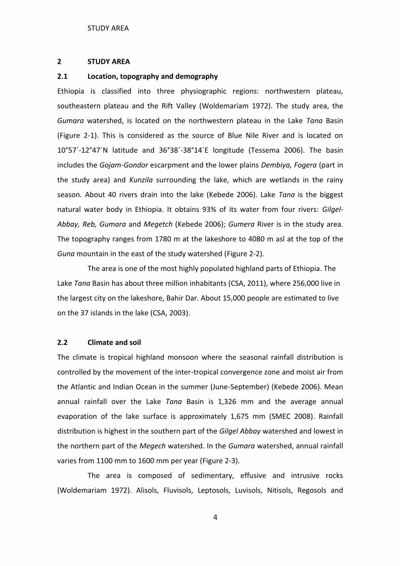
The topography ranges from 1780 m at the lakeshore to 4080 m asl at the top of the
Guna mountain in the east of the study watershed (Figure 2-2).
The area is one of the most highly populated highland parts of Ethiopia. The
Lake Tana Basin has about three million inhabitants (CSA, 2011), where 256,000 live in
the largest city on the lakeshore, Bahir Dar. About 15,000 people are estimated to live
on the 37 islands in the lake (CSA, 2003).
2.2 Climate and soil
The climate is tropical highland monsoon where the seasonal rainfall distribution is
controlled by the movement of the inter-tropical convergence zone and moist air from
the Atlantic and Indian Ocean in the summer (June-September) (Kebede 2006). Mean
annual rainfall over the Lake Tana Basin is 1,326 mm and the average annual
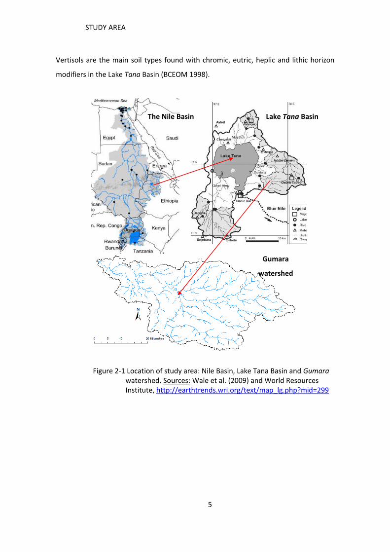
evaporation of the lake surface is approximately 1,675 mm (SMEC 2008). Rainfall
distribution is highest in the southern part of the Gilgel Abbay watershed and lowest in
the northern part of the Megech watershed. In the Gumara watershed, annual rainfall
varies from 1100 mm to 1600 mm per year (Figure 2-3).
The area is composed of sedimentary, effusive and intrusive rocks
(Woldemariam 1972). Alisols, Fluvisols, Leptosols, Luvisols, Nitisols, Regosols and
STUDY AREA
5
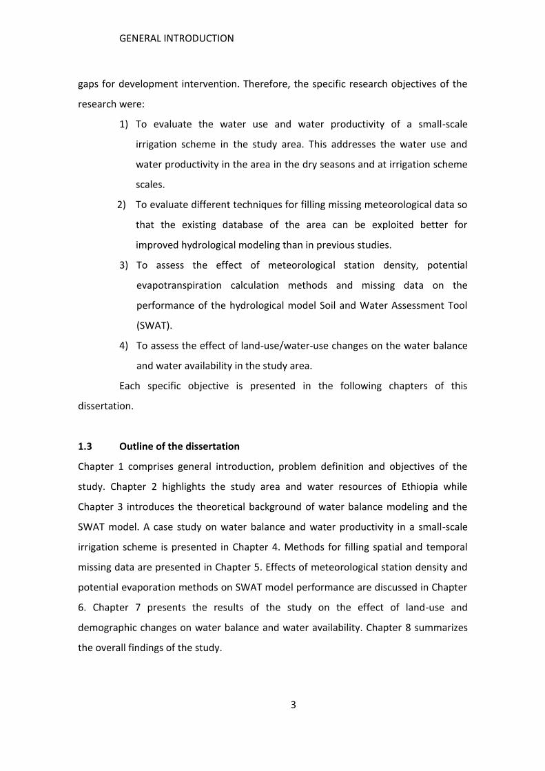
Vertisols are the main soil types found with chromic, eutric, heplic and lithic horizon
modifiers in the Lake Tana Basin (BCEOM 1998).
Figure 2-1 Location of study area: Nile Basin, Lake Tana Basin and Gumara watershed. Sources: Wale et al. (2009) and World Resources Institute, http://earthtrends.wri.org/text/map_lg.php?mid=299
The Nile Basin Lake Tana Basin
Gumara
watershed
STUDY AREA
6
Figure 2-2 Topography and hydrography of Lake Tana Basin Source: (Yilma and Awulachew 2009), where Gumera is synonomus to Gumara in the dissertation
Figure 2-3 Annual rainfall distribution in Lake Tana Basin Source: (Yilma and Awulachew 2009), where Gumera is synonomus to Gumara in the dissertation
a
STUDY AREA
7
2.3 Land-use, agriculture and biodiversity
About 10.1% of the country is covered by arable land, 0.65% by permanent crops and
1% is covered by water (MoWR 2002). Haileslassie et al. (2009a) classified the farming
system of the Gumara watershed into rice-based cash crops, maize-small cereals and
cereal-pulses. Rainfed mixed farming with a wide range of food crops like cereals,
pulses and vegetables is the main land-use of the study area, where livestock
production is also an important component of the livelihoods (Johnston and
McCartney, 2010). The area is characterized by low crop production (783 to 1234 kg
ha-1) with fragmented farmland holdings less than 1 ha per household (Erkossa et al.
2009).
The economic resources in the study area have great potential. It is the home
of the well-known Fogera cattle, which are used for milk production. Lake Tana has an
estimated fish production of 10,000 to 15,000 ton/year (IPMS, 2005). The lake and the
surrounding wetlands are endowed with rich biodiversity and cultural heritages. The
lake contains 18 species of barbus fish (Cyprinidae family) and the only large cyprinid
species flock in Africa (LakeNet 2004). At least 217 bird species are to be found in the
area, and the lake is estimated to hold a minimum of 20,000 water birds (EWNHS
1996). Twenty monasteries dating from the sixteenth and seventeenth century are
located on the lake islands with many cultural and natural assets. The Tis Issat Falls,
one of Africa’s largest waterfalls, is located on the Blue Nile approximately 35 km
downstream of the Lake Tana outflow. Around 30,000 domestic and foreign tourists
visit the area each year (EPLAUA 2006).
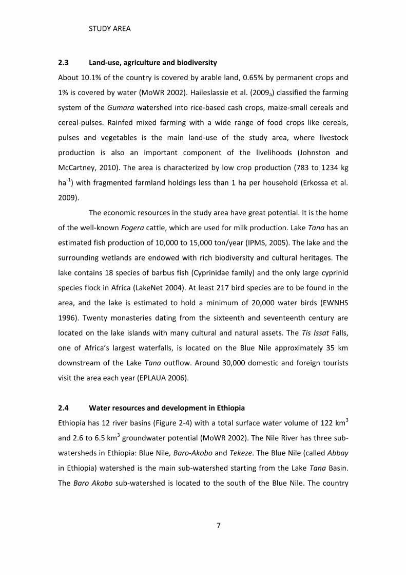
2.4 Water resources and development in Ethiopia
Ethiopia has 12 river basins (Figure 2-4) with a total surface water volume of 122 km3
and 2.6 to 6.5 km3 groundwater potential (MoWR 2002). The Nile River has three sub-
watersheds in Ethiopia: Blue Nile, Baro-Akobo and Tekeze. The Blue Nile (called Abbay
in Ethiopia) watershed is the main sub-watershed starting from the Lake Tana Basin.
The Baro Akobo sub-watershed is located to the south of the Blue Nile. The country
STUDY AREA
8
has abundant renewable water resources with 1300 and 2500 m3 per year per capita
at national and Blue Nile Basin levels, respectively (Johnston and McCartney 2010).
Figure 2-4 River basins of Ethiopia
Source: (Awulachew et al. 2007)
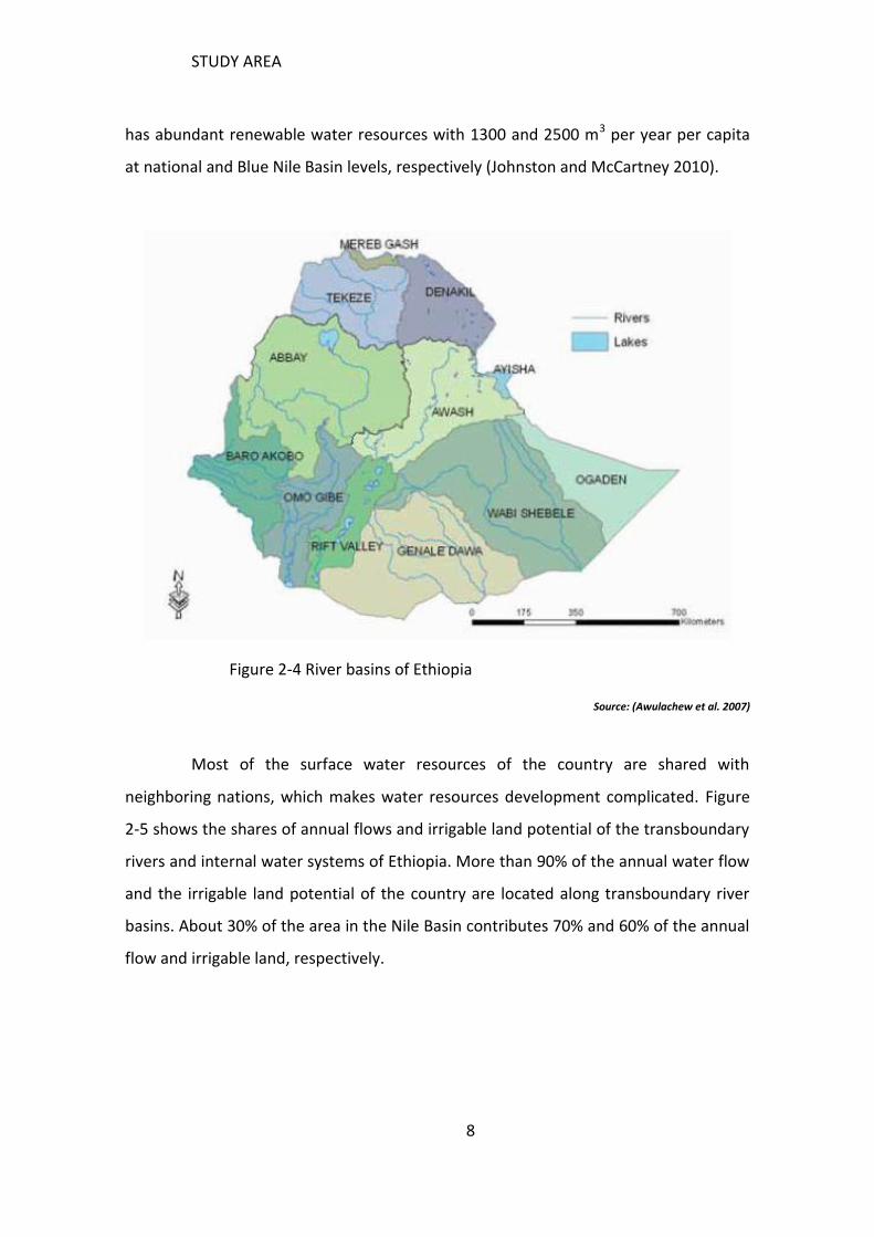
Most of the surface water resources of the country are shared with
neighboring nations, which makes water resources development complicated. Figure
2-5 shows the shares of annual flows and irrigable land potential of the transboundary
rivers and internal water systems of Ethiopia. More than 90% of the annual water flow
and the irrigable land potential of the country are located along transboundary river
basins. About 30% of the area in the Nile Basin contributes 70% and 60% of the annual
flow and irrigable land, respectively.
STUDY AREA
9
Figure 2-5 Relative potential of Nile Basin, total transboundary and internal watercourse systems with respect to whole Ethiopia
Source: secondary data taken from (Arsano 2007 )
Frequent and sever water shortages due to rainfall variability (CA 2007) are
one of the factors of the low land productivity in the country. The contribution of per
capita reservoir water has been very low (about 100 m3) as compared to that of South
Africa (750 m3) and North America (6150 m3) (World Bank 2006). The World Bank
(2006) recommended the development of water storage infrastructures as an
economic priority, since hydrological variability costs 30% of the country’s economic
development in GDP due to crop failure and livestock deaths. Hence, water shortage
and other related problems lead to food insecurity, so that 46% of the population was
undernourished in 2008 (von Grebmer et al. 2008). Rainfed agricultural production is
vulnerable to seasonal water shortage (Johnston and McCartney 2010), and 75-80% of
the rainfed production is consumed at the household level (World Bank 2006; Block et
al. 2007) even in good rainfall seasons and wet years with low surplus production for
the market. Moreover, the drinking water supply is very low (38% at country level and
26% in rural areas) (WHO-UNICEF 2010). People in rural areas travel more than a
kilometer to search for and to fetch drinking water (UN Water 2006).
There are indications that water development is one of the best entry points
to avert these problems. Smallholder irrigation can generate higher household
incomes (U$ 323 per ha) than rainfed systems (U$147 per ha) (Johnston and
0
10
20
30
40
50
60
70
80
90
100
Area (%) Average annualflow (%)
Potentialirrigable Land
(%)
Nile Basin
Transboundary system
Internal system
STUDY AREA
10
McCartney 2010). According to recommendations in studies and based on evidence,
water resources development has taken place throughout the country. The Ethiopian
government has been developing the water resources infrastructure since the 1980s.
About 5-6% of the 3.7 million ha potentially irrigable land of the country is covered by
irrigation. In 2005, this area covered only 30 m2 per capita. This is very low as
compared to the global level of 450 m2 (Awulachew et al. 2005).
Therefore, due to frequent droughts and extreme poverty, the Ethiopian
government is working to develop the water resources of the country to attain
economic growth and to reduce poverty through the construction of additional
infrastructure, particularly hydropower and irrigation schemes (MoFED 2006;
Awulachew et al. 2008; Block et al. 2007; McCartney et al. 2009).
Water resources assessment for hydroelectric power generation and
irrigation in 1964 by the U.S. Bureau of Reclamation (USBR) identified four main
hydropower dam sites along the main Blue Nile River in Ethiopia (USBR 1964). A
nationwide study in 1990 by the Water and Power Consultancy Service (WAPCOS
1990) identified 129 potential hydropower sites. The Abbay River Basin Integrated
Development Master Plan Project (ARBIDMPP) conducted by the MOWR of Ethiopia
proposed more than 20 projects for irrigation, hydropower, and multipurpose dams
(MOWR 1998) (Figure 2-6 ).
Lake Tana Basin is identified as a priority hydro-infrastructure development
area to attain the Millennium Development Goals (McCartney et al. 2010). In 2009, a
big multi-functional project was inaugurated that transfers Lake Tana water to the
nearby Beles catchment through a 12 km-long tunnel (7.1 m diameter) (Salini and Mid-
day 2006). This project generates 460 MW (2,310 GWh) electric power using 3 km3
water per annum (SMEC 2008). The tail water of this project is planned to be used for
irrigation. However, the social and environmental costs overweigh the benefits of
transferring water from one catchment to the other (WCD 2000; King and McCartney
2007). Two dams are under construction, and a feasibility study concerning another
three dams at the headwater of the lake for irrigation is in its final stage. Two
hydropower stations were functioning at the natural outlet of the lake at the time of
STUDY AREA
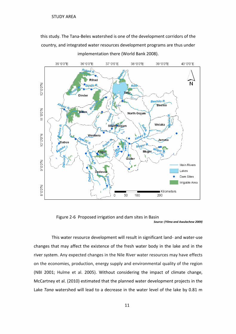
11
this study. The Tana-Beles watershed is one of the development corridors of the
country, and integrated water resources development programs are thus under
implementation there (World Bank 2008).
Figure 2-6 Proposed irrigation and dam sites in Basin Source: (Yilma and Awulachew 2009)
This water resource development will result in significant land- and water-use
changes that may affect the existence of the fresh water body in the lake and in the
river system. Any expected changes in the Nile River water resources may have effects
on the economies, production, energy supply and environmental quality of the region
(NBI 2001; Hulme et al. 2005). Without considering the impact of climate change,
McCartney et al. (2010) estimated that the planned water development projects in the
Lake Tana watershed will lead to a decrease in the water level of the lake by 0.81 m

STUDY AREA
12
(10% of the mean level), and in the lake area by 30-81 km2 (by ca. 1.9-3.6%). According
to the authors, the existing water resource development for hydropower generation at
Tis Issat at the outlet of Lake Tana has modified flows downstream of the lake,
reduced water levels of the lake, and significantly decreased the flow over the Tis Issat
waterfall.
WATER BALANCE AND MODEL STRUCTURE
13
3 WATER BALANCE AND MODEL STRUCTURE
3.1 Hydrological processes and water balance
Atmospheric, surface and subsurface/groundwater flows and storages are important
parts of the hydrological cycle. Water is found in solid, liquid and gaseous states in the
hydrological cycle. It can be transformed from one component to another either
naturally (runoff, precipitation, seepage, infiltration, evaporation, condensation, deep
percolation) or/and artificially (dam, irrigation, diversion, pumping).
The hydrological processes are too complex to illustrate them through exact
measurements everywhere and every time. The simplified representation of some of
the important hydrological processes can be done to conceptualize the hydrological
system in the form of a model (Anderson & Woessner 1992). A hydrological system
model approximates the actual system and transforms input variables to hydrological
output variables (Chow et al. 1988; Dooge 1968). It can be generally described as in
equation 3-1.
)()( tItQ (3–1)
where Q and I are output and input variables, respectively, as a function of time t, and
is a function transferring the input to the output. This function can be expressed by
an algebraic equation (algebraic operator) or differential equation (differential
operator). Parameters in a model are quantities that characterize some parts in the
system and attain constant values in time, space and condition.
Chow et al. (1988) classified hydrological models into three categories
according to the way they treat randomness, space and time. Stochastic models are
models whose variables are probabilistic in nature and random in distribution. If the
variables of the models are free from randomness, the models are said to be
deterministic. If we consider the spatial nature of models, we can group them as
lumped or distributed. Lumped models ignore the spatial variability of hydrological
processes, input variables or parameters, while distributed models try to address
spatial variability using more input data.
WATER BALANCE AND MODEL STRUCTURE
14
Models are also classified as conceptual/empirical and physical with respect
to how they equate the real processes within the hydrological system. Conceptual
models express the relationships of processes in the hydrological system based on
laboratory or field measurement data as done by using regression models, without
understanding the real physical process that is done behind. Physically based models,
on the other hand, try to equate and represent the processes based on some
understanding of their physics. Since physically based models have different
parameters related to one or more space coordinates, they can also be grouped under
distributed or semi-distributed models (Beven 1985).
Hydrological processes include canopy interception, infiltration, evaporation,
transpiration, overland flow, canal flow, unsaturated subsurface flow and saturated
subsurface flow. The processes are generally grouped into storages (surface,
subsurface and groundwater), inflows and outflows from the system. These processes
can be estimated using a series of empirical and hydraulic equations (Arnold et al.
1998) in the model. These equations have parameters that are dependent on
biophysical inputs, measured water outputs and management interventions. Model
parameters have to be optimized with respect to input-output data of the area. This is
known as parameter optimization (parameterization or calibration). Some parameters
influence the output of the model more than the others do. Identification of these
parameters will help to select very important parameters for model calibration
(Vandenberghe et al. 2002 cited in Alamirew 2006). The identification process is known
as sensitivity analysis. Verification is important by comparing the estimated output of
the calibrated model with measured data that are not used during the calibration
process. Models are calibrated and verified using standard statistical measures like
percent difference between measured and simulated values, coefficient of
determination (r2) to measure the trends of fitness of both measured and simulated
results, and Nash-Suttcliffe efficiency (Nash and Suttcliffe 1970) to compare how much
similar the average simulated result is to the average measured value within a given
period. Santhi et al. (2001) assumed an acceptable calibration for hydrology at percent

WATER BALANCE AND MODEL STRUCTURE
15
difference less than 15%, coefficient of determination greater than 0.6 and Nash-
Sutcliffe efficiency greater than 0.5.
3.2 Hydrological models for data-scarce areas
Model selection is determined by the availability of data, purpose of application and
the accuracy of the output needed. Physically based distributed models need more
data to calibrate a watershed. However, they are good for ungauged watersheds,
effectively saving time for measuring every parameter of the watershed once they are
calibrated. Studies advise to take care when using these models for data-scarce areas
(Legesse et al. 2003; Andersen et al. 2001). Lumped models are quite robust for these
areas although they result in less detailed output for climatic and land-use impacts.
Bormann and Diekkrueger (2003 and 2004) applied lumped hydrological models that
require less input data. However, they recommend applying detailed models to
address the effect of land-use and climate on the environment for relatively better
understanding.
3.3 Soil and Water Assessment Tool (SWAT)
SWAT is a continuation of about three decades of modeling efforts conducted by the
United States Department of Agriculture - Agricultural Research Service (USDA-ARS). It
has gained international acceptance as a robust interdisciplinary watershed-modeling
tool. More information is available from international SWAT conferences, hundreds of
SWAT-related papers presented at numerous scientific meetings, and dozens of
articles published in peer-reviewed journals (Gassman et al. 2007). SWAT is a basin-
scale, continuous-time model that operates on a daily time step. It is designed to
predict the impact of different watershed management on water, sediment, and
agricultural chemicals transportation for ungauged watersheds. It is physically based,
computationally efficient, and capable of continuous simulation over long periods.
Applications of SWAT have expanded worldwide over the past decade
(Gassman et al. 2007). Many of the applications have been driven by the needs of
various government agencies, particularly in the United States and the European
Union. These applications were done for assessments of anthropogenic, climate
change, and other influences on a wide range of water resources or exploratory
WATER BALANCE AND MODEL STRUCTURE
16
assessments of model capabilities for potential future applications. SWAT was selected
as an important tool for this study for the following reasons.
(1) It considers many components of the hydrologic balance like precipitation,
surface runoff, infiltration, evapotranspiration, lateral flow from the soil profile, and
return flow from shallow aquifers (Gassman et al. 2007).
(2) It considers sediment yield, crop biomass, crop rotations,
grassland/pasture systems, forest growth, planting, harvesting, tillage, nutrient
applications, pesticide applications, biomass removal and manure deposition of grazing
operations, continuous manure application options to confined animal feeding
operations, conservation and water management practices, and pollutants transport
(Gassman et al. 2007). These applications of SWAT can be used in the future once its
hydrological application to the area is verified.
(3) It has automated sensitivity, calibration, and uncertainty analysis
components, data generator and Geographic Information System (GIS) interface
(Gassman et al. 2007). The weather generator routine of SWAT considers the problem
of missing data for the area.
(4) It is physically based and can model ungauged watersheds that have no
monitoring data and can quantify the impact of changes in management practices
(Neitsch et al. 2011).
(5) It is computationally effective and can simulate processes in very large
basins or a variety of management strategies without excessive investment in time and
money (Neitsch et al. 2011).
(6) It enables users to study long-term impacts to address gradual impacts on
downstream water bodies (Neitsch et al. 2011).
In SWAT, a watershed is divided into multiple sub-watersheds and then into
hydrologic response units (HRUs) that consist of homogeneous land-use, management,
and soil characteristics (Gassman et al. 2007). The SWAT2009 version (Neitsch et al.
2011) under ArcSWAT2.5 in the ArcGIS interface of ArcGIS9.3 version is used for this
study. The Gumara River basin was partitioned in sub-watershed, and a refined stream
network layer was formed based on the threshold minimum drainage area required to
WATER BALANCE AND MODEL STRUCTURE
17
start a stream. These sub-watershed and stream network layers were done using the
digital elevation model (DEM). The smallest unit of spatial discretization was produced
based on a unique combination of land-use, slope and soil layers overlay. This spatial
unit is assumed to respond similarly for hydrological inputs in SWAT (Neitsch et al.
2011). It is called hydrologic response unit (HRU).
3.4 Water balance and parameters in SWAT
SWAT simulates the hydrologic cycle using the water balance equation 3-2:
)(1
gwseepasurf
t
i
tot QwEQRSWSW
(3–2)
where SWt is the final water content (mm H
2O), SW
0 is the initial water content in time
i (mm H2O), t is the time (in days, months, or years), R
t is the amount of rainfall in time
i (mm H2O), Q
surf is the amount of surface runoff in time i (mm H
2O), E
a is the amount of
evapotranspiration in time i (mm H2O), w
seep is the amount of water entering the
vadose zone from the soil profile in time i (mm H2O), and Q
gw is the amount of return
or baseflow in time i (mm H2O). The time scales depend on the concern of the analysis,
since SWAT can simulate at daily, monthly and annual scales. Each term of the water
balance equation has detailed physical processes that are interlinked in a harmony
related to the atmosphere-vegetation-soil consortium. The details of these processes
and physical phenomena are well presented in the SWAT input/output and theoretical
documentations and literature (http://swatmodel.tamu.edu/ Cited 27/06/2011). The
main terms in the water balance equation 3-2 are discussed below from these
documents.
1. Surface runoff: Also known as overland flow, the part of the rainfall flowing
along the slopes. SWAT uses the Soil Conservations Service (SCS) curve number
(CN) method to calculate surface runoff. Surface runoff is expressed using the
equation 3-3 (SCS, 1972):
WATER BALANCE AND MODEL STRUCTURE
18
SIR
IRQ
aday
aday
surf
2)( and SIa *2.0 (3–3)
where S is soil storage or retention, Rday is daily precipitation, and Ia initial surface
abstraction that includes surface storage, interception and infiltration to moist soil
surface up to runoff generation, all in mm water (mm H2O). Soil storage or retention
volume is expressed in terms of curve number CN as in equation 3-4:
10
10004.25
CNS (3–4)
By substituting Ia and S in equation 3-5, surface runoff is expressed as:
SR
SRQ
day
day
surf8.0
)2.0( 2
(3–5)
Surface runoff will occur when the amount of rainfall exceeds the initial abstraction
and infiltration to the root zone. Therefore, CN is a function of land-use, soil and
antecedent soil moisture content. These functional relationships and CN values are
provided in the SWAT manual and user guide (Neitsch et al. 2011).
The soil bulk density ( b ,) and saturated hydraulic conductivity ( satK ) of a soil play an
important role in the water movement through the soil profile, and also make water
accessible for surface runoff and evapotranspiration. The effects of b and satK are
explained with the relationships of soil-water constants. Field capacity (FC), available
soil water content (AWC) and permanent wilting point (WP) are the three constants of
soil-water content of a given soil that determine water fluxes in the soil profiles. They
are related in the expression given in equation 3-6:
WATER BALANCE AND MODEL STRUCTURE
19
lylyly AWCWPFC (3–6)
where FCly is the water content of a given soil layer at field capacity, WPly is the water
content of a given soil layer (ly) at permanent wilting point, and AWCly is the available
soil water content of the layer, all expressed as a fraction of the total soil volume.
SWAT estimates PW using equation 3-7:
100
**40.0 bc
ly
mPW
(3–7)
where mc is the percent clay content (%), and b is the bulk density of the soil layer
(Mg m-3). Actual water content of the given soil layer is the forcing input of
percolation. Water percolates to the next layer if the water content of the given layer
exceeds its field capacity by SWly,excess as expressed by equations 3-8 and 3-9:
lylyexcessly FCSWSW , if
lyly FCSW (3–8)
0, excesslySW if lyly FCSW (3–9)
where SWly,excess is the drainable volume of water in a given soil layer on a given day,
SWly is the soil layer water content on a given day, and FCly is the field capacity water
content of the soil layer on the same day, all in mm water (mm H2O). The amount of
water that moves from a given soil layer to its underlying layer is calculated using the
storage routing equation 3–10:
])exp[1(*,,
perc
excesslylypercTT
tSWw
(3–10)
where wperc,ly is the amount of water (mm H2O) that percolates from a given soil layer
on a given day, t is the length of the time steps (hrs) and TTperc is the travel time of
percolation in the soil layer (hrs).
WATER BALANCE AND MODEL STRUCTURE
20
The travel time of percolation (TTperc) is a function of the saturation water content
(SATly) in mm H2O, and saturated hydraulic conductivity (Ksat) in mm h-1 of the given
soil layer as in equation 3-11:
sat
lyly
percK
FCSATTT
(3–11)
Water that percolates in the underlying soil layer can flow to the nearby reach as a
subsurface flow and/or percolates to the next soil layer. Water that percolates from
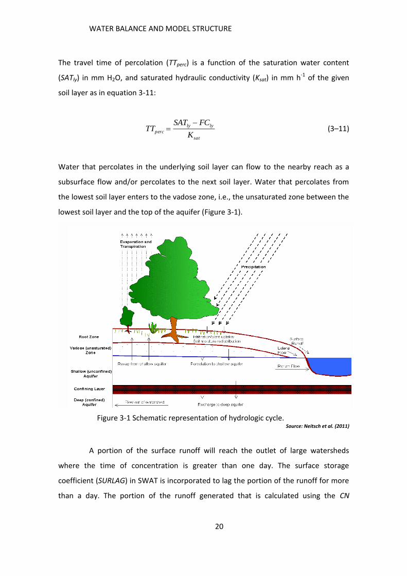
the lowest soil layer enters to the vadose zone, i.e., the unsaturated zone between the
lowest soil layer and the top of the aquifer (Figure 3-1).
Figure 3-1 Schematic representation of hydrologic cycle. Source: Neitsch et al. (2011)
A portion of the surface runoff will reach the outlet of large watersheds
where the time of concentration is greater than one day. The surface storage
coefficient (SURLAG) in SWAT is incorporated to lag the portion of the runoff for more
than a day. The portion of the runoff generated that is calculated using the CN
WATER BALANCE AND MODEL STRUCTURE
21
procedure and reached at the main channel on a given day is calculated in equation 3-
12:
conc
istorsurfsurft
surlagQQQ exp1).( 1,
' (3–12)
where surfQ is the runoff portion discharged to the main channel on a given day (mm
H2O), '
surfQ is the portion of runoff generated on that day (mm H2O), 1, istorQ is the
surface runoff lagged from the previous day (mm H2O), and tconc is time of
concentration of the sub-watershed (hrs). Time of concentration is the total time
needed for a drop of rain from the remotest point in the sub-watershed to the reach.
This parameter consists of time of overland flow-tov, i.e., the time needed to take the
water upstream to the outlet of the sub-watershed, and time of channel flow-tch, all in
hours. It is given by equation 3-13:
chovconc ttt (3–13)
2. Evapotranspiration: This is a term collectively used for the water in a given
watershed that is converted to water vapor. It is the interaction of water from soil-
vegetation surface and atmosphere. Evapotranspiration exceeds the runoff generated
at continental levels (Dingman 1994). Potential evapotranspiration, PET, is defined as
the amount of water transpired by a green 30-50 cm high alfalfa crop completely
shading the ground with unlimited soil water supply (Thornthwaite 1948; Jensen et al.
1990). This amount is the base to calculate actual evapotranspiration of any given day
for a given land-use and soil water supply. Two of the three methods used by SWAT
that are used in this study to calculate PET are the Penman-Monteith (Monteith 1965;
Allen 1986; Allen et al. 1989) and Hargreaves (Hargreaves et al. 1985) methods. The
Penman-Monteith method uses the parameters solar radiation, maximum and
minimum air temperature, relative humidity and wind speed to calculate potential
WATER BALANCE AND MODEL STRUCTURE
22
evapotranspiration, while the Hargreaves method requires only maximum and
minimum air temperature. The Hargreaves method can be used in a study area where
solar radiation, relative humidity and wind speed data are not available.
The Penman-Monteith method combines energy, aerodynamic and surface
resistance terms that account for water vapor removal to the atmosphere. It is given
by the equation 3-14:
)/1.(
/].[.).(
ac
az
o
zpairnet
rr
reecGHE
(3–14)
where E is the latent heat flux density in MJ m-2 d-1, E is potential evapotranspiration
(PET) rate in mm d-1, ( )(/)( Tded in kPa °C-1) is the slope of the saturation vapor
pressure-temperature curve, Hnet is the net radiation in MJ m-2 d-1, G is the heat flux
density to the ground in MJ m-2 d-1, air is the air density in kg m-3, pc is the specific
heat at constant pressure in MJ kg-1 1C , o
ze is the saturation vapor pressure of air at
height z in kPa, ez is the water vapor pressure of air at height z in kPa, is the
psychrometric constant in kPa 1C , rc is the plant canopy resistance in s m-1, and ra is
the diffusion resistance of the air layer or aerodynamic resistance in s m-1.
The Hargreaves method uses equation 3-15:
)8.17.().(.0023.0 5.0 avmnmxo TTTHE (3–15)
where is the latent heat of vaporization in MJ kg-1, E is potential evapotranspiration
(PET) rate in mm d-1, Ho is the extraterrestrial radiation in MJ m-2 d-1, Tmx is the
maximum air temperature in C , Tmn is the minimum air temperature in C , and avT is
the mean air temperature in C . Details and relationship of terms given in equations
3-14 and 3-15 are well described in Allen et al. (1998).
After PET is calculated, SWAT quantifies the actual evapotranspiration (AET) that is
composed of surface evaporation and transpiration through plant cells. SWAT first
WATER BALANCE AND MODEL STRUCTURE
23
calculates evaporation from the canopy and then evaporation from the soil surface
and sublimation from snow, if any, at hydrological response unit (HRU) level. All these
components of the actual evapotranspiration are calculated as a function of PET with
some additional parameters. For example, SWAT uses leaf area index (LAI) to calculate
transpiration and a soil evaporation compensation coefficient (ESCO) to adjust the
evaporative demand distribution through soil depth.
3. Lateral flow: This is the subsurface water flow for soils with high hydraulic
conductivity. The saturated soil zone is formed through water that ponds above a local
impermeable soil layer (perched water). This water is under atmospheric or less
pressure. SWAT uses the kinematic storage model developed by Sloan and Moore
(1984) to simulate subsurface flow in a two-dimensional section along a hillslope. The
saturated hydraulic conductivity of the soil plays a role in controlling the lateral flow as
indicated in the equation 3-16:
hilld
satexcessly
latL
slpKSWQ
.
...2.024.0
,
(3–16)
where Qlat is lateral flow discharged at a hillslope outlet on a given day (mm H2O),
SWly,excess is the volume of drainable water stored in a saturated soil layer for a given
day (mm H2O), Ksat is saturated hydraulic conductivity of the soil layer (mm h-1), slp is
slope of the soil layer given by )(tan hill , hill is hillslope segment angle to the
horizontal, d is the drainable porosity of the soil layer (mm/mm), and Lhill is the
hillslope length (m). The drainable volume of water stored in a saturated soil layer for a
given day is calculated as excess soil water from the field capacity as in equation 3-17:
lylyexcessly FCSWSW , if SWly>FCly ; SWly,excess=0 (3–17)
where SWly,excess is the stored portion of drainable water in a saturated soil layer (ly) for
a given day (mm H2O), SWly is soil moisture content of a soil layer at on a given day
WATER BALANCE AND MODEL STRUCTURE
24
(mm H2O), and FCly is the field capacity soil water content of the given soil layer (mm
H2O).
4. Groundwater: This is water in the saturated zone under a pressure higher than
atmospheric pressure (i.e., positive pressure). Water can join the groundwater system
by infiltration, percolation or/and seepage from the water bodies. It mainly leaves this
system by discharge into rivers or water bodies (return flow or baseflow). It can also
move upward to the unsaturated zone and then evapotranspires through the capillary
fringe.
Groundwater in SWAT is divided into two aquifer systems. The first is a
shallow, unconfined aquifer that contributes return flow to streams (groundwater flow
or baseflow). The second is a deep, confined aquifer that does not contribute return
flow to streams inside the watershed. Water is deep percolated into the confined
aquifer and is assumed lost from the given watershed.
The time needed to recharge the shallow aquifer through the vadose zone
through bypass flow or percolation is important to partition water as surface and
groundwater flow. The hydraulic properties of the geologic formation determine this
value. SWAT uses an exponential decay weighing function (Sangrey et al. 1984) to
quantify the time delay of the aquifer recharge. Water passing the soil layer and
recharging the two aquifers is given by equation 3-18:
1,, ]./1exp[])./1exp[1( irchrggwseepgwirchrg www (3–18)
where wrchg,i is the recharge amount entering the aquifers on i day (mm H2O), gw is
the groundwater delay time or drainage time of the overlaying geologic formation
(days), Wseep is amount of water existing at the bottom of the soil profile on day i (mm
H2O), and wrchrd,i-1 is the recharge amount entering the aquifers on i-1 day (mm H2O).
WATER BALANCE AND MODEL STRUCTURE
25
Part of the recharged water is routed to the deep aquifer as in equation 3-19:
rchrgdeepdeep ww . (3–19)
where wdeep is the water amount passing to the deep aquifer on a given day
(mm H2O), deep is the aquifer percolation constant, and wrchrg is the recharge amount
entering the aquifers on a given day (mm H2O). The groundwater delay time, gw , and
the aquifer percolation constant, deep , are important parameters (SWAT parameters
GW_DELAY and RCHRG_DP, respectively) and were used to adjust the water balance
during the calibration stage of this study. Groundwater delay time is varied with
respect to depth of the water table and the hydraulic properties of the soil and
geological structure. It is estimated indirectly by simulation of aquifer recharge of a
given watershed or optimizing simulation of the groundwater level with measured
values. Once the GW_DELAY value is calibrated for a given watershed, it can be used
for other watersheds within similar geomorphic areas (Sangrey et al. 1984).
GW_DELAY can shift the hydrograph limbs of simulation to adjust lagging curves.
The Hooghoudt (1940) steady-state ground water response to a given
recharge is used to quantify baseflow to a given reach (equation 3-20):
wtbl
gw
satgw h
L
KQ .
.80002
(3–20)
where Qgw is the baseflow into the given reach on a given day (mm H2O), Ksat is
saturated hydraulic conductivity of the shallow aquifer (mm day-1), Lgw is the distance
from the sub-watershed divide to the reach (m), and hwtbl is the water table height (m).
The groundwater discharge during no recharge time can be simplified as given by
equation 3-21:
].exp[., tQQ gwogwgw if aqsh>aqshthr,q otherwise Qgw=0 (3–21)
WATER BALANCE AND MODEL STRUCTURE
26
where Qgw,o is the baseflow into the given reach at the beginning of the recession curve
(mm H2O), gw is the baseflow recession constant (vary from 0 to 1) in days, aqsh is
amount of water stored in the shallow aquifer on a given day (mm H2O), and aqshthr,q is
the threshold water level in the shallow aquifer for which groundwater starts to
contribute baseflow (mm H2O). gw and aqshthr,q are important parameters in SWAT
(ALPHA_BF and GWQMN, respectively).
Baseflow alpha factor in days (ALPHA_BF) is the baseflow recession constant
of proportionality between groundwater flow and recharge changes to the aquifer
(Smedema and Rycroft 1983). ALPHA_BF varies from 0.1 to 0.3 for watersheds that
respond slowly to groundwater change and from 0.9 to 1.0 for fast response
watersheds. It can be estimated by analyzing the recession curve of the measured
discharge hydrograph of a watershed during the no-recharge period.
If the water table in the shallow aquifer exceeds GWQMN, baseflow to a
reach has occurred, otherwise there is no baseflow. Altering this value can control the
amount of water fluxes to baseflow directly, and to AET as “revap” flow indirectly. That
means that increasing GWQMN can decrease baseflow, and vice versa.
When the overlying soil surface is dry and the underlying layer is wet, water
will diffuse upward and evaporate. Water is also removed from the shallow aquifer by
deep-rooted plants. SWAT models this removal; the process is called “revap”. It occurs
only if the water content in the shallow aquifer exceeds a certain revap threshold level
during a dry period. The maximum amount of water that can pass through the revap
process is given by equation 3–22:
Ew revmxrevap ., (3–23)
where wrevap.mx is the maximum amount of water moving into the soil zone (mm H2O),
rev is the revap coefficient (GW_REVAP in SWAT), and E is the potential
evapotranspiration (PET) of the given day (mm H2O). The actual amount of revap is
then calculated as in equation 3–24:
WATER BALANCE AND MODEL STRUCTURE
27
rvpshthrmxrevaprevap aqww ,, if aqshthr,rvp>aqsh<(aqshthr,rvp+wrevap,mx)
wrevap=wrevap,mx if aqsh>(aqshthr,rvp+wrevap,mx)
Otherwise, wrevap = 0 (3–25)
where wrevap is the actual amount of water moving into the soil zone (mm H2O), aqsh is
the amount of water stored in the shallow aquifer for a given day (mm H2O), and
aqshthr,rvp (REVAPMN in SWAT) is the threshold water level in the shallow aquifer for a
revap to take place (mm H2O).
GW_REVAP is a coefficient that governs revap flow. There is no revap flow if
GW_REVAP is zero and revap is equal to PET when its value is 1.0. GW_REVAP varies
from 0.02 to 0.20.
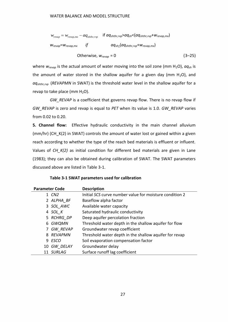
5. Channel flow: Effective hydraulic conductivity in the main channel alluvium
(mm/hr) (CH_K(2) in SWAT) controls the amount of water lost or gained within a given
reach according to whether the type of the reach bed materials is effluent or influent.
Values of CH_K(2) as initial condition for different bed materials are given in Lane
(1983); they can also be obtained during calibration of SWAT. The SWAT parameters
discussed above are listed in Table 3-1.
Table 3-1 SWAT parameters used for calibration
Parameter Code Description
1 CN2 Initial SCS curve number value for moisture condition 2 2 ALPHA_BF Baseflow alpha factor 3 SOL_AWC Available water capacity
4 SOL_K Saturated hydraulic conductivity 5 RCHRG_DP Deep aquifer percolation fraction 6 GWQMN Threshold water depth in the shallow aquifer for flow 7 GW_REVAP Groundwater revap coefficient 8 REVAPMN Threshold water depth in the shallow aquifer for revap 9 ESCO Soil evaporation compensation factor
10 GW_DELAY Groundwater delay 11 SURLAG Surface runoff lag coefficient
WATER USE AND PRODUCTIVITY OF SMALL-SCALE IRRIGATION SCHEME
28
4 WATER USE AND PRODUCTIVITY OF SMALL-SCALE IRRIGATION SCHEME
4.1 Summary
In Ethiopia, irrigation is mainly implemented in small-scale irrigation schemes, and
these are often characterized by low water productivity. This part of the study analyzes
the efficiency and productivity of a typical small-scale irrigation scheme in the
highlands of the Blue Nile, Ethiopia. Canal water flows and the volume of irrigation
water applied were measured at field level. Grain and crop residue biomass and grass
biomass production along the canals were also measured. To triangulate the
measurements, irrigation farm management, effects of water logging around irrigation
canals, farm water distribution mechanisms, effects of night irrigation, and water
losses due to soil cracking created by prolonged irrigation were closely observed. The
average canal water loss from the main, secondary and field canals was 2.58, 1.59 and
0.39 l s-1 100 m-1, representing 4.5, 4.0 and 26% of the total water flow, respectively.
About 0.05% of the loss was attributed to grass production for livestock, while the rest
was lost through evaporation and canal seepage. Grass production for livestock feed
had a land productivity of 6190.5 kg ha-1 and a water productivity of 0.82 kg m-3. Land
productivity for straw and grain was 2048 and 770 kg ha-1, respectively, for tef, and
1864 kg ha-1 and 758 kg ha-1, respectively, for wheat. Water productivity of the crops
varied from 0.2 to 1.63 kg m-3. A significant volume of water was lost from the small-
scale irrigation systems mainly because farmers’ water application did not match crop
needs. The high price incurred by pumped irrigation positively affected water
management by minimizing water losses, and forced farmers to use deficit irrigation.
Improving water productivity of small-scale irrigation requires integrated interventions
including night storage mechanisms, optimal irrigation scheduling, and empowerment
of farmers to maintain canals and to have proper irrigation schedules.
4.2 Introduction
Ethiopia, where recurrent drought affects agriculture, has 12 river basins and 19
natural lakes (see section 2.4). The mean annual surface water flow in Ethiopia is
estimated at 122 km3 (MCE 2001; MoWR 1999), and the potential irrigable land is
WATER USE AND PRODUCTIVITY OF SMALL-SCALE IRRIGATION SCHEME
29
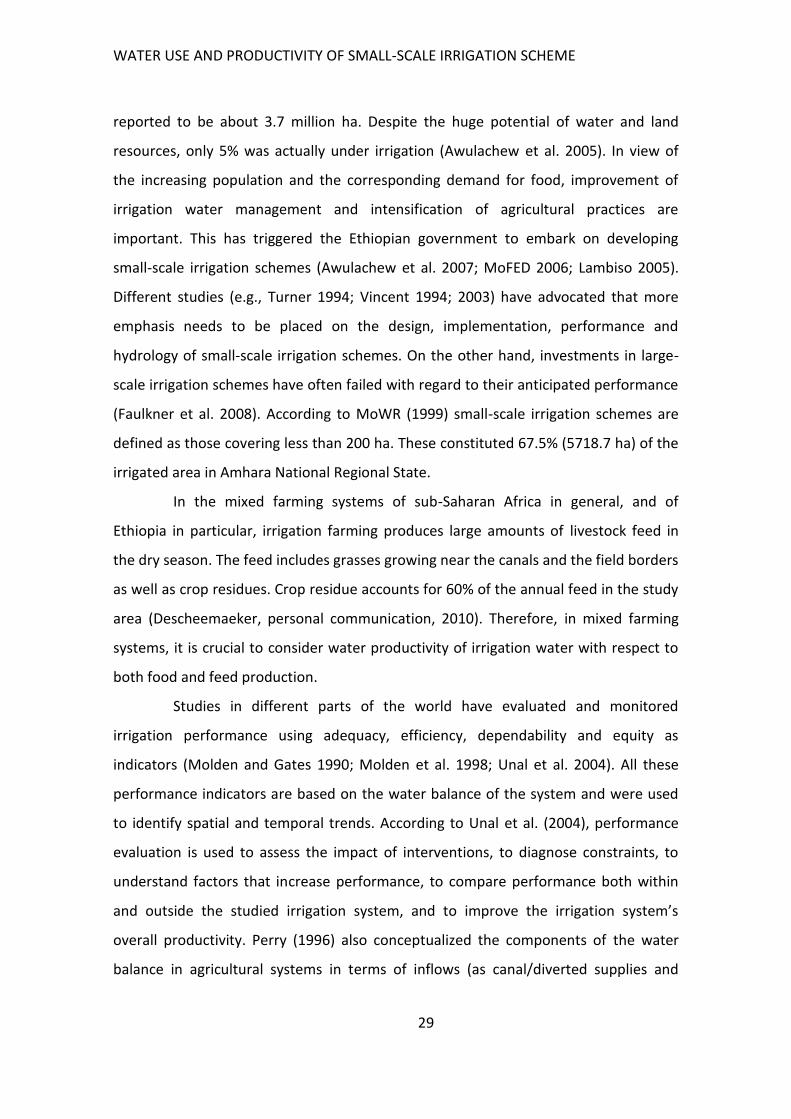
reported to be about 3.7 million ha. Despite the huge potential of water and land
resources, only 5% was actually under irrigation (Awulachew et al. 2005). In view of
the increasing population and the corresponding demand for food, improvement of
irrigation water management and intensification of agricultural practices are
important. This has triggered the Ethiopian government to embark on developing
small-scale irrigation schemes (Awulachew et al. 2007; MoFED 2006; Lambiso 2005).
Different studies (e.g., Turner 1994; Vincent 1994; 2003) have advocated that more
emphasis needs to be placed on the design, implementation, performance and
hydrology of small-scale irrigation schemes. On the other hand, investments in large-
scale irrigation schemes have often failed with regard to their anticipated performance
(Faulkner et al. 2008). According to MoWR (1999) small-scale irrigation schemes are
defined as those covering less than 200 ha. These constituted 67.5% (5718.7 ha) of the
irrigated area in Amhara National Regional State.
In the mixed farming systems of sub-Saharan Africa in general, and of
Ethiopia in particular, irrigation farming produces large amounts of livestock feed in
the dry season. The feed includes grasses growing near the canals and the field borders
as well as crop residues. Crop residue accounts for 60% of the annual feed in the study
area (Descheemaeker, personal communication, 2010). Therefore, in mixed farming
systems, it is crucial to consider water productivity of irrigation water with respect to
both food and feed production.
Studies in different parts of the world have evaluated and monitored
irrigation performance using adequacy, efficiency, dependability and equity as
indicators (Molden and Gates 1990; Molden et al. 1998; Unal et al. 2004). All these
performance indicators are based on the water balance of the system and were used
to identify spatial and temporal trends. According to Unal et al. (2004), performance
evaluation is used to assess the impact of interventions, to diagnose constraints, to
understand factors that increase performance, to compare performance both within
and outside the studied irrigation system, and to improve the irrigation system’s
overall productivity. Perry (1996) also conceptualized the components of the water
balance in agricultural systems in terms of inflows (as canal/diverted supplies and
WATER USE AND PRODUCTIVITY OF SMALL-SCALE IRRIGATION SCHEME
30
rainfall) and outflows (as crop transpiration, non-beneficial evaporation, drainage, and
net groundwater flow) and their interactions.
Data on the performance of small-scale irrigation schemes are scarce in
Ethiopia in particular (Awulachew et al. 2007) and in Africa in general (Faulkner et al.
2008). This study was designed to establish water depletion and food and feed water
productivity, and in order to assess which, where and when interventions could be
applied to improve the water productivity of such schemes. Therefore, the objectives
of this study were:
(i) To quantify irrigation water loss and water needed and used to produce
biomass,
(ii) To quantify feed and food water productivity, and
(iii) To identify opportunities for improving irrigation efficiency and
productivity.
4.3 Materials and methods
4.3.1 Study area
The study area, the Guanta small-scale irrigation scheme, is located in the
highlands of the Blue Nile basin 11◦50´N and 37◦39´E at 1797 m asl in Ethiopia (Figure
4-1; Figure 2-1). It was selected based on accessibility, representativeness of small-
scale irrigation in the study watershed, and availability of information. A stone
masonry diversion structure and a 1555 m main canal (conveying water from the
diversion) were constructed by the local government in 2001; 850 m of the main canal
and 1341 m of the secondary canal conveying water from the main canal were not yet
lined. The layout of field canals (conveying water from the secondary canals to the
individual fields) varied from time to time, and it was difficult to map them. Other land
units in the scheme were drainage basins and wetlands. Drainage basins were
enclosed gully-like natural flood basins during the main rain rainy season. Farmers
released excess irrigation water to these basins after irrigating their plots. On the other
hand, wetlands were irrigated lands in the first years of the scheme. These land units
were changed to wetlands due to the overflow of water from the secondary canals and
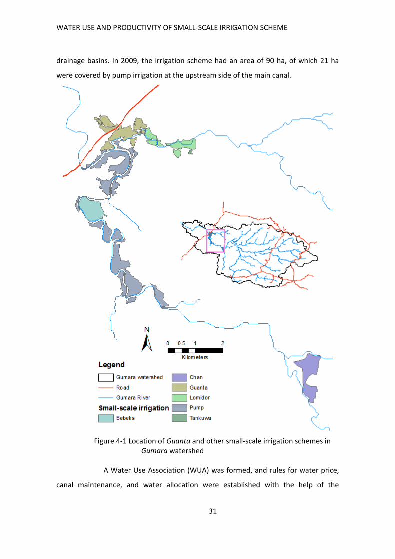
WATER USE AND PRODUCTIVITY OF SMALL-SCALE IRRIGATION SCHEME
31
drainage basins. In 2009, the irrigation scheme had an area of 90 ha, of which 21 ha
were covered by pump irrigation at the upstream side of the main canal.
Figure 4-1 Location of Guanta and other small-scale irrigation schemes in Gumara watershed
A Water Use Association (WUA) was formed, and rules for water price,
canal maintenance, and water allocation were established with the help of the
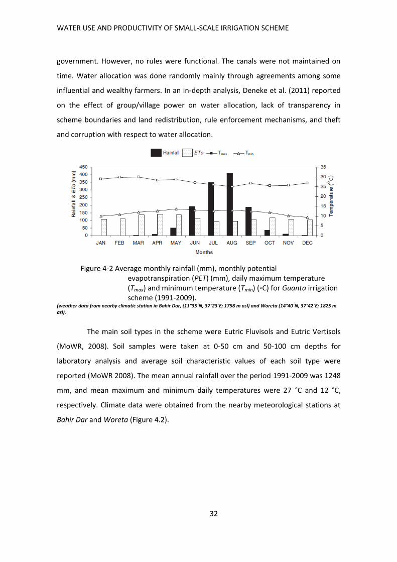
WATER USE AND PRODUCTIVITY OF SMALL-SCALE IRRIGATION SCHEME
32
government. However, no rules were functional. The canals were not maintained on
time. Water allocation was done randomly mainly through agreements among some
influential and wealthy farmers. In an in-depth analysis, Deneke et al. (2011) reported
on the effect of group/village power on water allocation, lack of transparency in
scheme boundaries and land redistribution, rule enforcement mechanisms, and theft
and corruption with respect to water allocation.
Figure 4-2 Average monthly rainfall (mm), monthly potential evapotranspiration (PET) (mm), daily maximum temperature (Tmax) and minimum temperature (Tmin) (◦C) for Guanta irrigation scheme (1991-2009).
(weather data from nearby climatic station in Bahir Dar, (11°35´N, 37°23´E; 1798 m asl) and Woreta (14°40´N, 37°42´E; 1825 m asl).
The main soil types in the scheme were Eutric Fluvisols and Eutric Vertisols
(MoWR, 2008). Soil samples were taken at 0-50 cm and 50-100 cm depths for
laboratory analysis and average soil characteristic values of each soil type were
reported (MoWR 2008). The mean annual rainfall over the period 1991-2009 was 1248
mm, and mean maximum and minimum daily temperatures were 27 °C and 12 °C,
respectively. Climate data were obtained from the nearby meteorological stations at
Bahir Dar and Woreta (Figure 4.2).
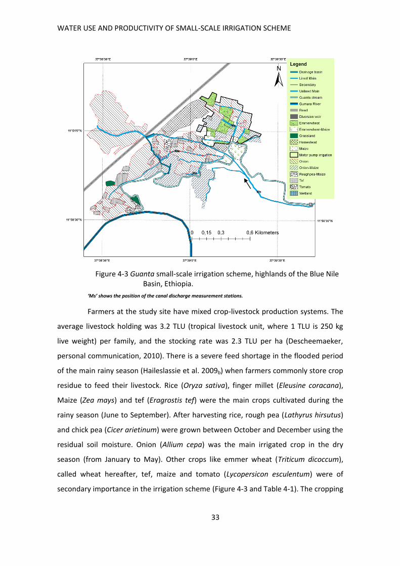
WATER USE AND PRODUCTIVITY OF SMALL-SCALE IRRIGATION SCHEME
33
Figure 4-3 Guanta small-scale irrigation scheme, highlands of the Blue Nile Basin, Ethiopia.
‘Ms’ shows the position of the canal discharge measurement stations.
Farmers at the study site have mixed crop-livestock production systems. The
average livestock holding was 3.2 TLU (tropical livestock unit, where 1 TLU is 250 kg
live weight) per family, and the stocking rate was 2.3 TLU per ha (Descheemaeker,
personal communication, 2010). There is a severe feed shortage in the flooded period
of the main rainy season (Haileslassie et al. 2009b) when farmers commonly store crop
residue to feed their livestock. Rice (Oryza sativa), finger millet (Eleusine coracana),
Maize (Zea mays) and tef (Eragrostis tef) were the main crops cultivated during the
rainy season (June to September). After harvesting rice, rough pea (Lathyrus hirsutus)
and chick pea (Cicer arietinum) were grown between October and December using the
residual soil moisture. Onion (Allium cepa) was the main irrigated crop in the dry
season (from January to May). Other crops like emmer wheat (Triticum dicoccum),
called wheat hereafter, tef, maize and tomato (Lycopersicon esculentum) were of
secondary importance in the irrigation scheme (Figure 4-3 and Table 4-1). The cropping
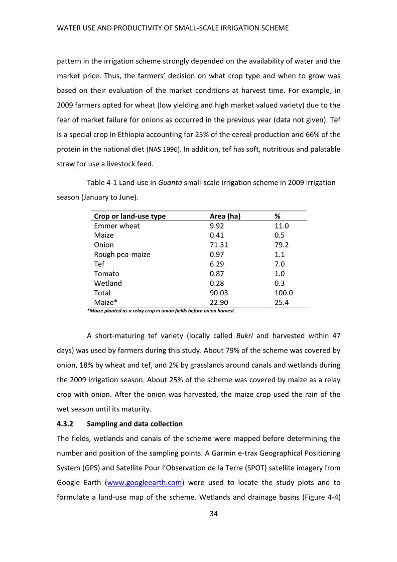
WATER USE AND PRODUCTIVITY OF SMALL-SCALE IRRIGATION SCHEME
34
pattern in the irrigation scheme strongly depended on the availability of water and the
market price. Thus, the farmers’ decision on what crop type and when to grow was
based on their evaluation of the market conditions at harvest time. For example, in
2009 farmers opted for wheat (low yielding and high market valued variety) due to the
fear of market failure for onions as occurred in the previous year (data not given). Tef
is a special crop in Ethiopia accounting for 25% of the cereal production and 66% of the
protein in the national diet (NAS 1996). In addition, tef has soft, nutritious and palatable
straw for use a livestock feed.
Table 4-1 Land-use in Guanta small-scale irrigation scheme in 2009 irrigation
season (January to June).
Crop or land-use type Area (ha) % Emmer wheat 9.92 11.0 Maize 0.41 0.5 Onion 71.31 79.2 Rough pea-maize 0.97 1.1 Tef 6.29 7.0 Tomato 0.87 1.0 Wetland 0.28 0.3 Total 90.03 100.0 Maize* 22.90 25.4
*Maize planted as a relay crop in onion fields before onion harvest
A short-maturing tef variety (locally called Bukri and harvested within 47
days) was used by farmers during this study. About 79% of the scheme was covered by
onion, 18% by wheat and tef, and 2% by grasslands around canals and wetlands during
the 2009 irrigation season. About 25% of the scheme was covered by maize as a relay
crop with onion. After the onion was harvested, the maize crop used the rain of the
wet season until its maturity.
4.3.2 Sampling and data collection
The fields, wetlands and canals of the scheme were mapped before determining the
number and position of the sampling points. A Garmin e-trax Geographical Positioning
System (GPS) and Satellite Pour l’Observation de la Terre (SPOT) satellite imagery from
Google Earth (www.googleearth.com) were used to locate the study plots and to
formulate a land-use map of the scheme. Wetlands and drainage basins (Figure 4-4)
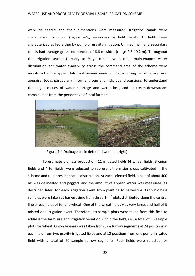
WATER USE AND PRODUCTIVITY OF SMALL-SCALE IRRIGATION SCHEME
35
were delineated and their dimensions were measured. Irrigation canals were
characterized as main (Figure 4-5), secondary or field canals. All fields were
characterized as fed either by pump or gravity irrigation. Unlined main and secondary
canals had average grassland borders of 6.6 m width (range 2.5-10.2 m). Throughout
the irrigation season (January to May), canal layout, canal maintenance, water
distribution and water availability across the command area of the scheme were
monitored and mapped. Informal surveys were conducted using participatory rural
appraisal tools, particularly informal group and individual discussions, to understand
the major causes of water shortage and water loss, and upstream-downstream
complexities from the perspective of local farmers.
Figure 4-4 Drainage basin (left) and wetland (right)
To estimate biomass production, 11 irrigated fields (4 wheat fields, 3 onion
fields and 4 tef fields) were selected to represent the major crops cultivated in the
scheme and to represent spatial distribution. At each selected field, a plot of about 400
m2 was delineated and pegged, and the amount of applied water was measured (as
described later) for each irrigation event from planting to harvesting. Crop biomass
samples were taken at harvest time from three 1-m2 plots distributed along the central
line of each plot of tef and wheat. One of the wheat fields was very large, and half of it
missed one irrigation event. Therefore, six sample plots were taken from this field to
address the farm size and irrigation variation within the field, i.e., a total of 15 sample
plots for wheat. Onion biomass was taken from 5-m furrow segments at 24 positions in
each field from two gravity-irrigated fields and at 12 positions from one pump-irrigated
field with a total of 60 sample furrow segments. Four fields were selected for
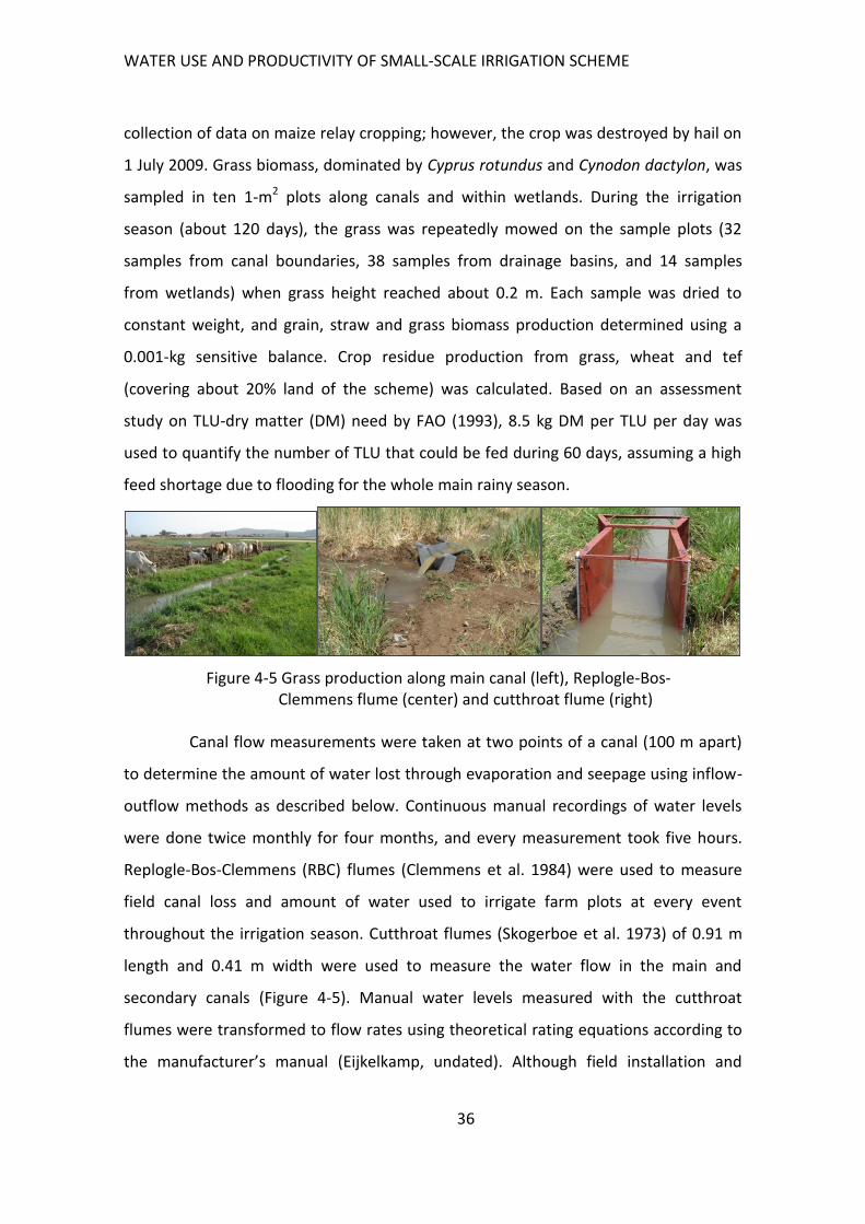
WATER USE AND PRODUCTIVITY OF SMALL-SCALE IRRIGATION SCHEME
36
collection of data on maize relay cropping; however, the crop was destroyed by hail on
1 July 2009. Grass biomass, dominated by Cyprus rotundus and Cynodon dactylon, was
sampled in ten 1-m2 plots along canals and within wetlands. During the irrigation
season (about 120 days), the grass was repeatedly mowed on the sample plots (32
samples from canal boundaries, 38 samples from drainage basins, and 14 samples
from wetlands) when grass height reached about 0.2 m. Each sample was dried to
constant weight, and grain, straw and grass biomass production determined using a
0.001-kg sensitive balance. Crop residue production from grass, wheat and tef
(covering about 20% land of the scheme) was calculated. Based on an assessment
study on TLU-dry matter (DM) need by FAO (1993), 8.5 kg DM per TLU per day was
used to quantify the number of TLU that could be fed during 60 days, assuming a high
feed shortage due to flooding for the whole main rainy season.
Figure 4-5 Grass production along main canal (left), Replogle-Bos-Clemmens flume (center) and cutthroat flume (right)
Canal flow measurements were taken at two points of a canal (100 m apart)
to determine the amount of water lost through evaporation and seepage using inflow-
outflow methods as described below. Continuous manual recordings of water levels
were done twice monthly for four months, and every measurement took five hours.
Replogle-Bos-Clemmens (RBC) flumes (Clemmens et al. 1984) were used to measure
field canal loss and amount of water used to irrigate farm plots at every event
throughout the irrigation season. Cutthroat flumes (Skogerboe et al. 1973) of 0.91 m
length and 0.41 m width were used to measure the water flow in the main and
secondary canals (Figure 4-5). Manual water levels measured with the cutthroat
flumes were transformed to flow rates using theoretical rating equations according to
the manufacturer’s manual (Eijkelkamp, undated). Although field installation and
WATER USE AND PRODUCTIVITY OF SMALL-SCALE IRRIGATION SCHEME
37
construction errors are always present, the flumes used for this study were selected
for their greater accuracy (Clemmens et al. 1984; Eijkelkamp, undated; Skogerboe et
al. 1973) compared to other methods, such as Parshall flumes or the ponding method.
4.3.3 Data preparation and analysis
Potential evapotranspiration (PET) and crop water requirements were calculated using
the Penman-Monteith and crop coefficient procedures described in Allen et al. (1998).
The database was formulated to use this procedure in order to minimize the
uncertainty of the Bahir Dar station data. Therefore, rainfall and temperature data
from Woreta and relative humidity, wind speed and sunshine hours from Bahir Dar
meteorological stations were used to calculate reference evapotranspiration.
The water balance of irrigated fields was calculated using the water balance
equation (4-1) for the growing season at field level.
( ) (4–1)
where ∆SM is the change in soil moisture content before the first irrigation
and after harvest, Peff is effective rainfall, I is total irrigation water applied, AET is
actual evapotranspiration, D is drainage loss, and Qr is capillary rise.
All quantities were defined within the same time domain (growing period)
and units (mm H2O). Total irrigation need was computed using climate, crop and soil
data with FAO CROPWAT version 8.0 (FAO, 2009). ∆SM was calculated as the
difference between soil moisture content before the first irrigation and soil moisture
content after harvest. Soil moisture data were determined using a gravimetric method
with dry bulk density data adopted from MoWR (2008). Peff was calculated using the
empirical formula of the United States Department of Agriculture’s Soil Conservation
Service. It was selected from the three options found in CROPWAT 8.0 software as it
was developed for long-term climatic and soil moisture data (FAO 1978). Actual
evapotranspiration (AET) was calculated by multiplying the crop coefficient, Kc, with
the water stress factor, Ks. Ks is a function of total available water, TAW, readily
WATER USE AND PRODUCTIVITY OF SMALL-SCALE IRRIGATION SCHEME
38
available water and root zone depletion. It was estimated from the daily water balance
computation (Allen et al. 1998). The crop parameters crop growth stages, allowable
depletion factor and rooting depth were adopted from Allen et al. (1998). Length of
cropping season was taken from the field data. Since tef is a local crop where these
important parameters are not given in the literature, grass values were adopted. Grass
Kc values are also almost similar to average values of cereal crops. The crop coefficient
for the grasslands around canals, drainage basins and wetlands was formulated using
the mean values of legumes and grasses previously reported (Haileslassie et al.
2009a;b). Drainage loss was calculated as the sum of irrigation water that was applied
above field capacity at every irrigation event. It should be noted that drainage loss
here is not the difference between irrigation water applied and irrigation water
required. Capillary rise was not considered, as the groundwater table was more than 2
m deep (Allen et al. 1998; MoWR 2008). Soil physical characteristics, such as bulk
density and TAW content, were adopted from MoWR (2008), as the data were
generated from the same scheme. Field capacity was calculated from TAW and root
depth.
Canal or conveyance loss (in l s-1 100 m-1 canal length) was calculated as
presented in equation 4-2 using the inflow-outflow method.
(4–2)
where Qin is water flow rate at the upper side of 100-m long canal segment
(measured), and Qout is water flow rate at the lower end of 100-m long canal segment
(measured).
Canal water loss was calculated as the percentage of conveyance loss to the
average of Qin and Qout within 100-m canal segments. From field observations, data on
total canal length and water loss per 100 m, an average of 30 l s-1 water was reached at
the end of the secondary canals and distributed to many field canals at the same time.
Therefore, measured canal loss was calculated based on this 30 l s-1 for comparison.
outin QQlossConveyance
WATER USE AND PRODUCTIVITY OF SMALL-SCALE IRRIGATION SCHEME
39
Water productivity along canals and in irrigated fields was calculated using
equations 4-3 and 4-4:
(4–3)
(4–4)
Irrigation and actual ET water productivity were calculated for both grain and
dry straw biomass using two approaches. The traditional approach considered all the
water supplied by irrigation and depleted by AET to compute grain or straw (but not
for both) biomass water productivity. A new approach (Haileslassie et al. 2009a;b) used
the water supplied by irrigation and depleted by AET for all biomass (both grain and
straw) production. Therefore, yield of the system at the numerator side of the water
productivity equations is larger than the traditional way of calculation. This can reflect
the real situation in the farming system that both straw and grain were produced using
the same AET water and that both were important for feed and food, respectively.
Both approaches, hereafter termed as “traditional” and “new” water productivity,
were used for comparison purposes.
Relative water supply (RWS), a performance indicator, was calculated using
equation 4-5 taken from Levine (1982). It is the ratio of total water supplied by
irrigation (I) and rainfall (P) to total water demanded by crop (i.e., actual crop
evapotranspiration, AET).
(4–5)
RWS was calculated for the growing season for selected crops for both gravity
and pump irrigation.
After the field data had been processed using the above procedures,
statistical analysis was conducted using descriptive statistics, one-way analysis of
WATER USE AND PRODUCTIVITY OF SMALL-SCALE IRRIGATION SCHEME
40
variance, which compares groups sample means with one factor at a time (SPSS Inc.
2007), for the 3 crop types, and t-test for gravity and pump irrigation types. Means
were compared using the least significant difference test at significance level p ≤ 0.05.
4.4 Results
4.4.1 Water loss and grass production around canals and wetlands
The highest water loss rate in l s-1 100 m-1 was from the main canal while the lowest
was from field canals (Table 4-2). The highest daily volume of water was lost from the
field canals when a 30 l s-1 flow rate was assumed for all canal types. Calculations of
the loss for the total flowing rate (30 l s-1) showed that about 26% of the water in the
field canals was lost. This loss was much lower for the main and secondary canals at
4.49% and 4.00%, respectively (Table 4-2).
Grasslands and wetlands were part of the irrigation scheme and
consumed irrigation water while producing biomass. The grasslands produced grass
biomass using seepage water from the canals. Wetlands were formed under the
influence of excess drainage water, and freely released water from the irrigated fields.
Wetlands and drainage basins were not observed in the motor pump irrigation area.
The ET water productivity of grassland varied with farm position from 0.4 to 1.2 kg m-3,
which was below the productivity of the rain-fed wetlands (Table 4-3). The grassland in
the drainage basin was the most productive, while the wetland showed the lowest
productivity. Land productivity was quite high, ranging from 3000 to 9000 kg ha-1
(Table 4-3). Although grass production can be considered as a productive use of the
water lost through canal seepage, only about 0.05% of the water lost from the canals
was actually used for grass production. The other part was lost through canal storage,
deep drainage, water surface evaporation and flow back to the river system.
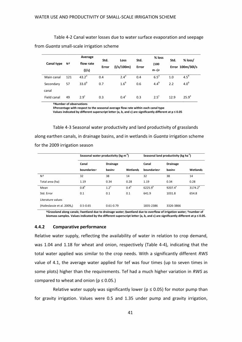
WATER USE AND PRODUCTIVITY OF SMALL-SCALE IRRIGATION SCHEME
41
Table 4-2 Canal water losses due to water surface evaporation and seepage
from Guanta small-scale irrigation scheme
Canal type N†
Average
flow rate
(l/s)
Std.
Error
Loss
(l/s/100m)
Std.
Error
% loss
(100
m−1)‡
Std.
Error
% loss/
100m/30l/s
Main canal 121 43.2a 0.4 2.4
a 0.4 6.5
a 1.0 4.5
b
Secondary
canal
57 33.0b 0.7 1.6
b 0.6 4.4
b 2.2 4.0
b
Field canal 49 2.9c 0.3 0.4
c 0.3 2.5
c 12.9 25.9
a
†Number of observations ‡Percentage with respect to the seasonal average flow rate within each canal type Values indicated by different superscript letter (a, b, and c) are significantly different at p ≤ 0.05
Table 4-3 Seasonal water productivity and land productivity of grasslands
along earthen canals, in drainage basins, and in wetlands in Guanta irrigation scheme
for the 2009 irrigation season
Seasonal water productivity (kg m-3)
Seasonal land productivity (kg ha-1)
Canal
boundaries†
Drainage
basin‡ Wetland§
Canal
boundaries†
Drainage
basin‡ Wetland§
N† 32 38 14 32 38 14
Total area (ha) 1.19 0.34 0.28 1.19 0.34 0.28
Mean 0.8b 1.2a 0.4b 6225.9b 9207.4a 3174.2b
Std. Error 0.1 0.1 0.1 641.9 1031.8 654.8
Literature values
(Haileslassie et al. 2009b) 0.5-0.65 0.61-0.79 1835-2386 3326-3866
†Grassland along canals; ‡wetland due to drainage water; •wetland due to overflow of irrigation water; †number of biomass samples. Values indicated by the different superscript letter (a, b, and c) are significantly different at p ≤ 0.05.
4.4.2 Comparative performance
Relative water supply, reflecting the availability of water in relation to crop demand,
was 1.04 and 1.18 for wheat and onion, respectively (Table 4-4), indicating that the
total water applied was similar to the crop needs. With a significantly different RWS
value of 4.1, the average water applied for tef was four times (up to seven times in
some plots) higher than the requirements. Tef had a much higher variation in RWS as
compared to wheat and onion (p ≤ 0.05.)
Relative water supply was significantly lower (p ≤ 0.05) for motor pump than
for gravity irrigation. Values were 0.5 and 1.35 under pump and gravity irrigation,
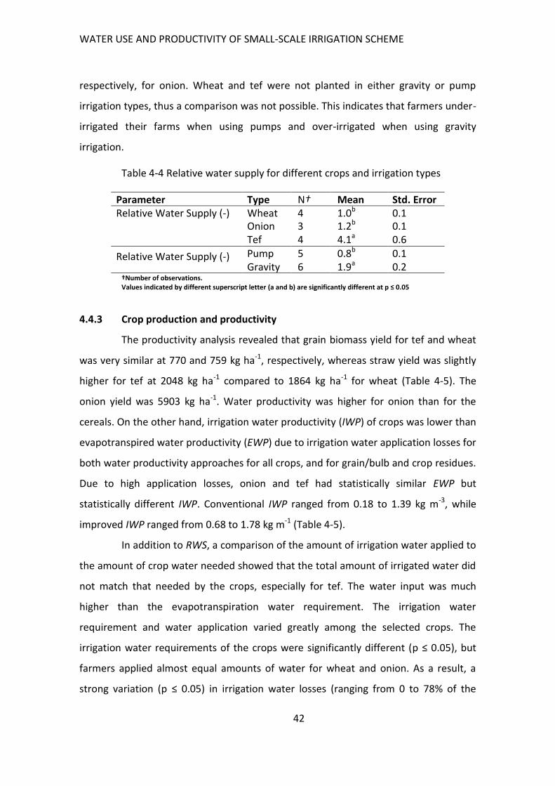
WATER USE AND PRODUCTIVITY OF SMALL-SCALE IRRIGATION SCHEME
42
respectively, for onion. Wheat and tef were not planted in either gravity or pump
irrigation types, thus a comparison was not possible. This indicates that farmers under-
irrigated their farms when using pumps and over-irrigated when using gravity
irrigation.
Table 4-4 Relative water supply for different crops and irrigation types
Parameter Type N† Mean Std. Error Relative Water Supply (-)
Wheat 4 1.0b 0.1 Onion 3 1.2b 0.1 Tef 4 4.1a 0.6
Relative Water Supply (-) Pump 5 0.8b 0.1 Gravity 6 1.9a 0.2
†Number of observations. Values indicated by different superscript letter (a and b) are significantly different at p ≤ 0.05
4.4.3 Crop production and productivity
The productivity analysis revealed that grain biomass yield for tef and wheat
was very similar at 770 and 759 kg ha-1, respectively, whereas straw yield was slightly
higher for tef at 2048 kg ha-1 compared to 1864 kg ha-1 for wheat (Table 4-5). The
onion yield was 5903 kg ha-1. Water productivity was higher for onion than for the
cereals. On the other hand, irrigation water productivity (IWP) of crops was lower than
evapotranspired water productivity (EWP) due to irrigation water application losses for
both water productivity approaches for all crops, and for grain/bulb and crop residues.
Due to high application losses, onion and tef had statistically similar EWP but
statistically different IWP. Conventional IWP ranged from 0.18 to 1.39 kg m-3, while
improved IWP ranged from 0.68 to 1.78 kg m-1 (Table 4-5).
In addition to RWS, a comparison of the amount of irrigation water applied to
the amount of crop water needed showed that the total amount of irrigated water did
not match that needed by the crops, especially for tef. The water input was much
higher than the evapotranspiration water requirement. The irrigation water
requirement and water application varied greatly among the selected crops. The
irrigation water requirements of the crops were significantly different (p ≤ 0.05), but
farmers applied almost equal amounts of water for wheat and onion. As a result, a
strong variation (p ≤ 0.05) in irrigation water losses (ranging from 0 to 78% of the
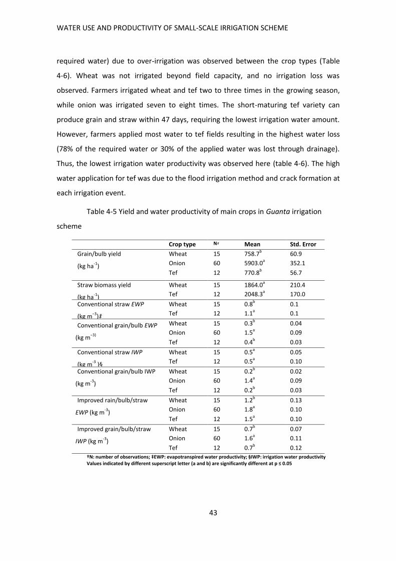
WATER USE AND PRODUCTIVITY OF SMALL-SCALE IRRIGATION SCHEME
43
required water) due to over-irrigation was observed between the crop types (Table
4-6). Wheat was not irrigated beyond field capacity, and no irrigation loss was
observed. Farmers irrigated wheat and tef two to three times in the growing season,
while onion was irrigated seven to eight times. The short-maturing tef variety can
produce grain and straw within 47 days, requiring the lowest irrigation water amount.
However, farmers applied most water to tef fields resulting in the highest water loss
(78% of the required water or 30% of the applied water was lost through drainage).
Thus, the lowest irrigation water productivity was observed here (table 4-6). The high
water application for tef was due to the flood irrigation method and crack formation at
each irrigation event.
Table 4-5 Yield and water productivity of main crops in Guanta irrigation
scheme
Crop type N† Mean Std. Error
Grain/bulb yield
(kg ha-1
)
Wheat 15 758.7b 60.9
Onion 60 5903.0a 352.1
Tef 12 770.8b 56.7
Straw biomass yield
(kg ha-1
)
Wheat 15 1864.0a 210.4
Tef 12 2048.3a 170.0
Conventional straw EWP
(kg m−3
)‡
Wheat 15 0.8b 0.1
Tef 12 1.1a 0.1
Conventional grain/bulb EWP
(kg m−3)
Wheat 15 0.3b 0.04
Onion 60 1.5a 0.09
Tef 12 0.4b 0.03
Conventional straw IWP
(kg m-3
)§
Wheat 15 0.5a 0.05
Tef 12 0.5a 0.10
Conventional grain/bulb IWP
(kg m-3
)
Wheat 15 0.2b 0.02
Onion 60 1.4a 0.09
Tef 12 0.2b 0.03
Improved rain/bulb/straw
EWP (kg m-3
)
Wheat 15 1.2b 0.13
Onion 60 1.8a 0.10
Tef 12 1.5a 0.10
Improved grain/bulb/straw
IWP (kg m-3
)
Wheat 15 0.7b 0.07
Onion 60 1.6a 0.11
Tef 12 0.7b 0.12
†N: number of observations; ‡EWP: evapotranspired water productivity; •IWP: irrigation water productivity Values indicated by different superscript letter (a and b) are significantly different at p ≤ 0.05
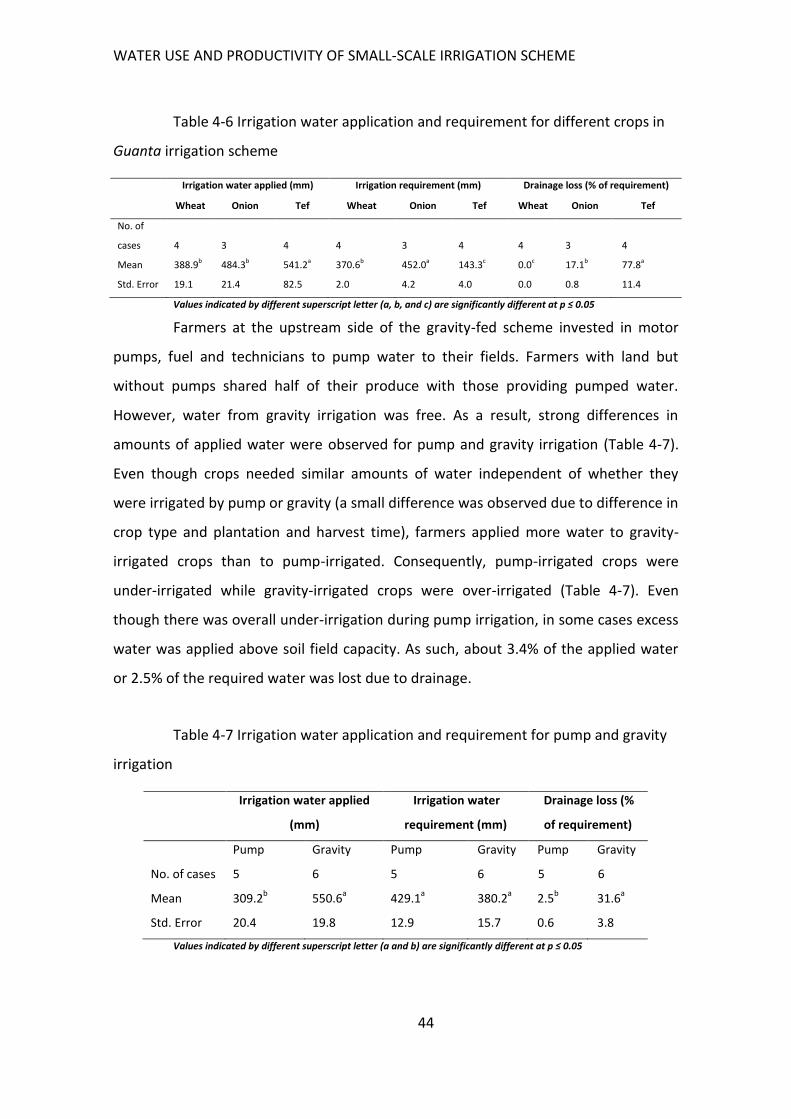
WATER USE AND PRODUCTIVITY OF SMALL-SCALE IRRIGATION SCHEME
44
Table 4-6 Irrigation water application and requirement for different crops in
Guanta irrigation scheme
Irrigation water applied (mm) Irrigation requirement (mm) Drainage loss (% of requirement)
Wheat Onion Tef Wheat Onion Tef Wheat Onion Tef
No. of
cases 4 3 4 4 3 4 4 3 4
Mean 388.9b 484.3b 541.2a 370.6b 452.0a 143.3c 0.0c 17.1b 77.8a
Std. Error 19.1 21.4 82.5 2.0 4.2 4.0 0.0 0.8 11.4
Values indicated by different superscript letter (a, b, and c) are significantly different at p ≤ 0.05
Farmers at the upstream side of the gravity-fed scheme invested in motor
pumps, fuel and technicians to pump water to their fields. Farmers with land but
without pumps shared half of their produce with those providing pumped water.
However, water from gravity irrigation was free. As a result, strong differences in
amounts of applied water were observed for pump and gravity irrigation (Table 4-7).
Even though crops needed similar amounts of water independent of whether they
were irrigated by pump or gravity (a small difference was observed due to difference in
crop type and plantation and harvest time), farmers applied more water to gravity-
irrigated crops than to pump-irrigated. Consequently, pump-irrigated crops were
under-irrigated while gravity-irrigated crops were over-irrigated (Table 4-7). Even
though there was overall under-irrigation during pump irrigation, in some cases excess
water was applied above soil field capacity. As such, about 3.4% of the applied water
or 2.5% of the required water was lost due to drainage.
Table 4-7 Irrigation water application and requirement for pump and gravity
irrigation
Irrigation water applied
(mm)
Irrigation water
requirement (mm)
Drainage loss (%
of requirement)
Pump Gravity Pump Gravity Pump Gravity
No. of cases 5 6 5 6 5 6
Mean 309.2b 550.6
a 429.1
a 380.2
a 2.5
b 31.6
a
Std. Error 20.4 19.8 12.9 15.7 0.6 3.8
Values indicated by different superscript letter (a and b) are significantly different at p ≤ 0.05
WATER USE AND PRODUCTIVITY OF SMALL-SCALE IRRIGATION SCHEME
45
Discussions with farmers revealed that there was an increasing irrigation
water demand (data not presented). The diversion and main canal capacity was
designed for 46 ha. However, about 20 ha of additional farmland were included by the
farmers at the tail end of the scheme. In addition, farmers in the upstream irrigated 21
ha of land using motor pipes, which was not originally part of the scheme. Increasing
water demand by both upstream and downstream communities aggravated the water
shortage leading to prolonged irrigation intervals. As a result, the soil was deeply
cracked in many locations, leading to high losses of irrigation water due to water
percolation through the cracks.
4.5 Discussion
The results of this study indicate that irrigation cost had implications for water
management decisions and variations in water productivity. Production costs
associated with pump irrigation forced farmers to save water and to maintain canals
frequently, which were evidenced by the absence of water draining away from the
fields. Farmers minimized water losses by using deficit irrigation and by transferring
water immediately to the next plot. On the other hand, over-irrigation and high water
losses were observed on fields irrigated by gravity-fed water. In this part of the
irrigation scheme, farmers were reluctant to maintain canals appropriately, and water
was released to the drainage basin in spite of the high water need at the tail. The
difference in water requirement for the same crop came from differences in planting
and maturity time in different fields.
4.5.1 Irrigation water losses and shortage
Higher small-scale irrigation canal water losses were observed in this study when
compared to the findings of Akkuzu et al. (2007), who reported an average loss from
lined field canals of about 9.3% and 1.1% loss from lined secondary canals in Turkey at
a similar flow capacity (30 l s-1). Bakry and Awad (1997) reported 0.17 to 0.70% losses
per 100 m canal in Egypt for a canal capacity of 2000 to 12 100 l s-1, which was also
lower than the findings in this study. Here the canal water loss was highest from the
WATER USE AND PRODUCTIVITY OF SMALL-SCALE IRRIGATION SCHEME
46
main canal due to its higher capacity (43.21 l s-1) and proximity to the riverbank as
compared to the other canal types. Expressed as percentage of the water flow capacity
of the canals, the canal loss was highest for the field canals, since these were
destroyed during tillage, so that the canal banks were not stabilized like the main and
secondary canals. The negative impact of seepage on production was more
pronounced in the case of field canals, as it led to more water logging than the
seepage from other canals.
In addition, the field canal network covered the largest area in the scheme.
Farmers preferred field canals because they allowed them to keep their plot sizes.
Apart from high seepage losses, field canals dried and cracked before the next
irrigation event. Field canals overtopping during night irrigation was common and
increased water logging and unmeasured canal water loss. These factors resulted in
high irrigation water loss, water logging and production losses. Therefore, large
farmlands within 8-15 m from the field canals were out of production. Although
farmers thought secondary canals occupied more land than field canals, in practice
field canals rendered more land unproductive and resulted in higher water losses than
secondary canals. The total volume of water lost from the 3077-m long canal system
(comprising all canal types) could have irrigated 9 ha of land at 50 mm irrigation depth
per day for the irrigation season.
The increasing water demand due to the extension of tail and pump irrigation
have made management of the irrigation water more complicated. The duration of the
irrigation intervals increased, which resulted in crop water stress and cracks in the
vertic soils. In addition, due to decreased canal flow capacity, the time needed for
sufficient irrigation increased, and farmers were forced to conduct nighttime irrigation,
resulting in large losses due to inefficiency and unpredicted canal flow rate during the
night.
Water was a more constraining factor than land around the scheme during
the irrigation season. Ample downstream plain land was out of production six months
a year (December to June). On the other hand, water from night stream flow, springs
and shallow groundwater was still not used properly. Night water storage will increase
WATER USE AND PRODUCTIVITY OF SMALL-SCALE IRRIGATION SCHEME
47
water use efficiency. It is possible to use the stream bank for this temporary storage. A
simple profile leveling survey of the Guanta stream bank showed great potential for
night water storage (up to 20 000 to 45 000 m3), which could be used during the day.
Farmers invested about 50% of their produce in kind for pump irrigation, with an
increasing trend of pumping activities.
However, because of higher production costs, pump irrigation typically
resulted in lower financial water productivity than downstream gravity irrigation. This
means that there is a greater possibility to improve water productivity in downstream
gravity irrigation than in upstream pump irrigation.
The variation in RWS indicates that more water was lost for tef and under
gravity irrigation. Values ranged from 0.8 to 4.0, where 0.8 indicates deficit irrigation
to maximize water productivity (Molden et al. 1998). In a public surface irrigation
scheme in Mexico, RWS was higher than 2.0 and showed differences with respect to
water access and water cost (Kloezen and Garcés-Restrepo 1998). Compared to the
above study that used RWS at scheme level, RWS for tef was extremely high.
4.5.2 Production and productivity
Area and water productivity of selected crops was comparable with findings of other
studies around the study area. Haileslassie et al. (2009b) reported yields of 892-972 kg
ha-1 for wheat and 981-1312 kg ha-1 for tef produced in rain-fed conditions in the same
watershed. The EWP values were 0.21-0.23 kg m-3 for wheat and 0.24- 0.33 kg m-3 for
tef in the study of Haileslassie et al. (2009b), which used the improved approach of
water productivity calculation. In this study, land productivity was relatively lower
while the water productivity was three times higher as compared to values in the study
of Haileslassie et al. (2009b). The difference observed between these rain-fed and
irrigation values arose from differences in crop varieties and water management
practices. On the one hand, short-maturing tef and wheat varieties with lower ETc
values than for rain-fed production were used for irrigation. On the other hand,
irrigation intervals were too long to create acceptable soil water stress conditions
whereby the water stress coefficient was reduced to 0.3 during some irrigation
WATER USE AND PRODUCTIVITY OF SMALL-SCALE IRRIGATION SCHEME
48
intervals. Bekele and Tilahun (2007), using experimental deficit irrigation at Sekota,
Ethiopia obtained onion yields of 5500-25000 kg ha-1 with 9-10 kg m-3 water, which is
about eight times higher than the observations in this study. This shows that
opportunities exist to increase onion production and productivity in the area. Flood
irrigation using a very low flow rate (less than 1 l s-1 during the night or day) and
irrigating deep cracks after prolonged irrigation intervals decreased the water
productivity of tef and wheat as compared to the field observations on water
application. For example, tef irrigation water was almost half as productive as ET water
compared to wheat and onion productivity due to higher drainage water losses.
The conventional way of quantifying water productivity underestimated
water productivity values, since the total water transpired was used to produce total
biomass while the estimation considered either grain or straw. This approach has more
a practical application in mixed crop-livestock systems where the straw biomass is a
very important livestock feed.
4.5.3 Implications for livestock production
As the importance of crop production for livestock is worth considering, it is also
important to stress the importance of crop residue as livestock feed during the
irrigation season. About 11428 kg grass, 18490 kg wheat straw and 12884 kg tef straw
(42884 kg DM in total) were produced from 18 ha (20%) land of the scheme during the
irrigation season. Based on 8.5 kg DM per day maintenance need for one TLU, 84 TLU
can be fed for 60 days. This can cover TLU from 26 households or TLUs on 37 ha
according to the livestock holding and stocking rate of the area studied determined by
Descheemaeker (personal communication, 2010). Dry matter production from the
relay maize cropping and other minor crops in the scheme was not considered in this
calculation, and the potential of the scheme to support livestock feed is expected to
exceed the above indicated figures. Therefore, increasing the biomass productivity of
each drop of irrigation water and on each plot of land within the scheme has strong
implications for livestock water productivity of the mixed crop-livestock systems.
WATER USE AND PRODUCTIVITY OF SMALL-SCALE IRRIGATION SCHEME
49
4.6 Recommendations
1. Based on the above findings, recommendations for improving water use
efficiency and productivity in the irrigation scheme include careful design and
construction of secondary canals and decreasing the use of field canals to minimize
canal water loss. Careful planning of the cropping pattern and irrigation scheduling
could result in more efficient water distribution. Given the fact that over-irrigation is
less common with pumped irrigation, allocating a water price to gravity-fed water
could positively influence water management. However, water pricing has to be based
on accurate water flow data as well as on equitable, adequate and reliable water
distribution rules governed by the water user associations. Water flow measurements
can be conducted using cement, wooden or iron sheet cutthroat flumes by trained
farmers.
2. Production of high-value crops (e.g., fruits) and/or high quality feeds along
canals and drained water could maximize water productivity for livestock, and there is
an opportunity to increase irrigation water productivity.
3. In order to improve water productivity of these system, farmers, water
users associations and development agents should receive training on canal water
management, crop water requirement, and equitable and efficient water distribution.
4. Different alternatives for improved water management, such as water
pricing and facilities for night water storage need to be considered in policy
development.
5. Considering the trade-offs between downstream gravity irrigation and
upstream pump irrigation needs further research for supporting policy articulations.
6. Shallow and frequent irrigation of tef using sprinkler or border irrigation
could minimize water loss and increase irrigation water productivity, but needs further
research on the applicability in the local context.
HANDLING MISSING METEOROLOGICAL DATA
50
5 HANDLING MISSING METEOROLOGICAL DATA
5.1 Summary
The Penman-Monteith equation is a commonly used method to estimate potential
evapotranspiration in most of the hydrological models and for water management
design. The equation is more input demanding compared to other approaches. Spatial
distribution of rainfall and temperature data is very important for hydrological
modeling. However, missing data is common in the measurements of meteorological
stations, e.g., solar radiation and relative humidity are not measured by most
meteorological stations in the study area. These problems are common in the Blue Nile
Basin in Ethiopia. Methods to fill rainfall and temperature data were developed and
compared in this study. Solar radiation and relative humidity data were derived from
temperature data. The estimation performance was done using statistical values. The
results of the estimation are promising for exploiting the existing database of the area
for better understanding and decision making.
5.2 Introduction
Meteorological variables, especially rainfall and temperature, are important for
hydrological modeling and for the design of water resources developments. Lack of
long-term and continuous data has been a challenge for water resources development
in Ethiopia. These data gaps have an impact on the value of environmental time series
(Presti et al. 2010) and hydrological modeling. Inconsistent and biased hydrologic
analysis and conclusions can affect water development planning (Kim and Ahn 2009).
Missing values have to be considered and filled before using the data for further
investigations. Temporal and spatial regression and interpolation methods were used
to fill the missing data of a selected station through values from the neighboring
stations.
Rainfall is an important factor in climate and agriculture studies (Ayoade
1983) that are conducted on problems related to floods, drought, and landslides, etc..
It has a strong influence on relative humidity, temperature and solar radiation (Neitsch
et al. 2011). An incomplete rainfall record (missing data) influences the consistency
HANDLING MISSING METEOROLOGICAL DATA
51
and continuity of the data (De Silva et al. 2007). Computational methods starting from
the simplest sample mean method to the complex multiple imputation method have
been used to fill missing data (Presti et al. 2010). Presti et al. (2010) used the strengths
of both simple and complex methodologies in Italy to achieve better estimations using
rainfall data of neighboring stations.
Different methods have been used to fill missing temperature data. Allen and
DeGaetano (2001) grouped these methods into within-station, between-station and
regression types. Average measured values prior to and following a missing date were
used to fill the missing values in the within-station method. This method is temporal
and depends only on data from one station, but is not suitable for stations with
consecutive days of missing data as observed in the study area. The between-station
method uses measured values of neighboring stations to fill the missing temperature
values of a given station. Regression models can be developed using one or more
neighboring stations to fill missing temperature data. Regression techniques such as
multiple regression and weighted regression (Eischeid et al. 1995) and optimized
regression (Allen and DeGaetano, 2001; Kotsiantis et al. 2006) have given more
accurate estimates of missing data as compared to the within-station and between-
station methods.
Relative humidity and solar radiation data are further inputs for Penman-
Monteith potential evapotranspiration calculation, but such values are scarce for the
study area. Data on sunshine hours have only been collected at sparsely distributed
class-one meteorological stations. In addition, the data are full of gaps due to failure of
the Campbell-Stokes recorder or/and lack of the treated card or/and lack of personnel.
Most of the stations in the area are of class-three or -four. For such stations, no
instruments are installed to measure relative humidity and sunshine hours. Allen
(1998) suggested that the missing data could be adopted from the nearby stations or
generated from daily temperature data.
Rainfall, maximum and minimum temperature, relative humidity, wind speed
and sunshine hour data are recorded in class-one stations. These stations have been
monitored more seriously and have better data availability than others. However, they
HANDLING MISSING METEOROLOGICAL DATA
52
only cover a limited area and show a considerable amount of missing data due to lack
of personnel for fixing the measuring instruments and due to political unrest in the
country. Most stations have only been equipped with rainfall and temperature
recording instruments (class-three stations) and some only for rainfall (class-four
stations).
The objective of this study is to identify and to evaluate methods to fill
missing rainfall, temperature, solar radiation and relative humidity data of
meteorological stations around Gumara watershed in the Blue Nile Basin of Ethiopia.
5.3 Materials and methods
5.3.1 Study area
The study area, the Gumara watershed, is located in the Lake Tana Basin of the Blue
Nile in Ethiopia. Lake Tana, covering about 3000 km2, is considered as the source of
the Blue Nile River. The lake basin contributes 7% of the Blue Nile water at the Sudan
boarder (Kebede et al. 2006). It has four main rivers that contribute 93% of the inflow
of the lake (Kebede et al. 2006). The climate of the area is tropical highland monsoon.
Seasonal rainfall distribution is controlled by the movement of the inter-tropical
convergence zone and moist air from the Atlantic and Indian Ocean in summer (June-
September) (Kebede et al. 2006). The four seasons in the country are winter (January-
March with some rain; called “bulg” in some parts of Ethiopia), spring (April–June, dry),
summer (July-September, main rainy season) and autumn (October–December, dry air)
(Latron et al. 2008). The rainfall in the study area is uni-modal with the main rainfall
occurring during June to September. There are nine meteorological stations within and
around the Gumara watershed: Debre Tabor (class-one), Wanzaye (class-three), Arb
Gebeya (class-four) and Luwaye (class-four) stations in the watershed, and Gassay
(class-three), Mekane Eyesus (class-three), Bahir Dar (class-one), Woreta (class-three)
and Amed Ber (class-three) around the watershed.
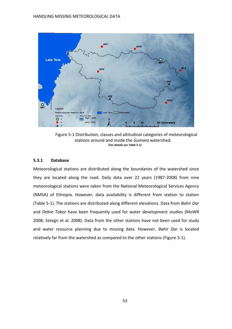
HANDLING MISSING METEOROLOGICAL DATA
53
Figure 5-1 Distribution, classes and altitudinal categories of meteorological stations around and inside the Gumara watershed.
(For details see Table 5-1)
5.3.1 Database
Meteorological stations are distributed along the boundaries of the watershed since
they are located along the road. Daily data over 22 years (1987-2008) from nine
meteorological stations were taken from the National Meteorological Services Agency
(NMSA) of Ethiopia. However, data availability is different from station to station
(Table 5-1). The stations are distributed along different elevations. Data from Bahir Dar
and Debre Tabor have been frequently used for water development studies (MoWR
2008; Setegn et al. 2008). Data from the other stations have not been used for study
and water resource planning due to missing data. However, Bahir Dar is located
relatively far from the watershed as compared to the other stations (Figure 5-1).
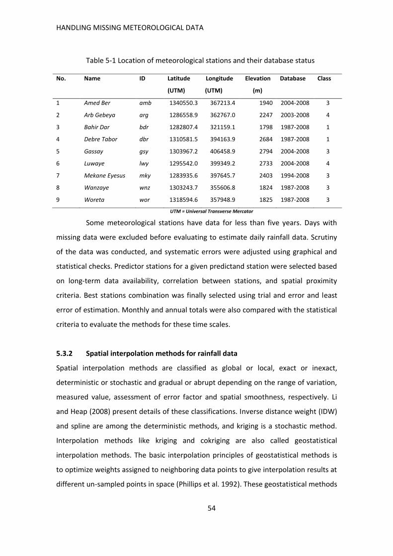
HANDLING MISSING METEOROLOGICAL DATA
54
Table 5-1 Location of meteorological stations and their database status
No. Name ID Latitude
(UTM)
Longitude
(UTM)
Elevation
(m)
Database Class
1 Amed Ber amb 1340550.3 367213.4 1940 2004-2008 3
2 Arb Gebeya arg 1286558.9 362767.0 2247 2003-2008 4
3 Bahir Dar bdr 1282807.4 321159.1 1798 1987-2008 1
4 Debre Tabor dbr 1310581.5 394163.9 2684 1987-2008 1
5 Gassay gsy 1303967.2 406458.9 2794 2004-2008 3
6 Luwaye lwy 1295542.0 399349.2 2733 2004-2008 4
7 Mekane Eyesus mky 1283935.6 397645.7 2403 1994-2008 3
8 Wanzaye wnz 1303243.7 355606.8 1824 1987-2008 3
9 Woreta wor 1318594.6 357948.9 1825 1987-2008 3
UTM = Universal Transverse Mercator
Some meteorological stations have data for less than five years. Days with
missing data were excluded before evaluating to estimate daily rainfall data. Scrutiny
of the data was conducted, and systematic errors were adjusted using graphical and
statistical checks. Predictor stations for a given predictand station were selected based
on long-term data availability, correlation between stations, and spatial proximity
criteria. Best stations combination was finally selected using trial and error and least
error of estimation. Monthly and annual totals were also compared with the statistical
criteria to evaluate the methods for these time scales.
5.3.2 Spatial interpolation methods for rainfall data
Spatial interpolation methods are classified as global or local, exact or inexact,
deterministic or stochastic and gradual or abrupt depending on the range of variation,
measured value, assessment of error factor and spatial smoothness, respectively. Li
and Heap (2008) present details of these classifications. Inverse distance weight (IDW)
and spline are among the deterministic methods, and kriging is a stochastic method.
Interpolation methods like kriging and cokriging are also called geostatistical
interpolation methods. The basic interpolation principles of geostatistical methods is
to optimize weights assigned to neighboring data points to give interpolation results at
different un-sampled points in space (Phillips et al. 1992). These geostatistical methods

HANDLING MISSING METEOROLOGICAL DATA
55
were found superior to the deterministic models for precipitation (Phillips et al. 1992).
They are best when correlation between precipitation and other topographic auxiliary
variables like elevation, relief and leeward direction are used to model the
interpolation at uniform grid levels of the area. Therefore, geostatistical methods of
interpolation of meteorological variables are very important for hydrological methods
that use uniform grids of the given watershed. Since SWAT uses hydrologic response
units (HRU) rather than uniform grid cells, the following four deterministic
interpolation methods were compared to fill the missing rainfall data of the Gumara
watershed for this study.
1) Arithmetic (local) mean (AM) method
The arithmetic mean can be used when the annual normal rainfall of the
neighboring stations varies within 10% of the rainfall of station to be modeled (Chow
et al. 1988; Tabios & Salas 1985). The method was used in this study for filling the
missing rainfall values of the selected station
2) Normal ratio (NR) method-
The normal ratio method is used when the variation of the normal annual
rainfall of the surrounding stations exceeds 10% of the values of the station under
consideration (De Silva et al. 2007). This method assigns weights of each surrounding
station (Sing 1994). The missing data of station n, , was calculated using equation 5-
1:
(5–1)
where is estimate of missing data for gauged station n, is measured
rainfall values of surrounding station i, is normal annual rainfall of station , is
normal annual rainfall of surrounding stations i, is the observed value at station i,
and r is number of surrounding stations.
n
r
ia
ni
i
a
nn
r 1
n ni
a
n n a
ni
i
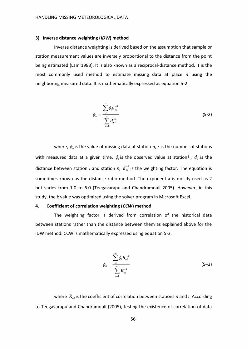
HANDLING MISSING METEOROLOGICAL DATA
56
3) Inverse distance weighting (IDW) method
Inverse distance weighting is derived based on the assumption that sample or
station measurement values are inversely proportional to the distance from the point
being estimated (Lam 1983). It is also known as a reciprocal-distance method. It is the
most commonly used method to estimate missing data at place n using the
neighboring measured data. It is mathematically expressed as equation 5-2:
(5-2)
where, is the value of missing data at station n, r is the number of stations
with measured data at a given time, is the observed value at station , is the
distance between station i and station n, is the weighting factor. The equation is
sometimes known as the distance ratio method. The exponent k is mostly used as 2
but varies from 1.0 to 6.0 (Teegavarapu and Chandramouli 2005). However, in this
study, the k value was optimized using the solver program in Microsoft Excel.
4. Coefficient of correlation weighting (CCW) method
The weighting factor is derived from correlation of the historical data
between stations rather than the distance between them as explained above for the
IDW method. CCW is mathematically expressed using equation 5-3.
(5–3)
where is the coefficient of correlation between stations n and i. According
to Teegavarapu and Chandramouli (2005), testing the existence of correlation of data
r
i
k
ni
r
i
k
nii
n
d
d
1
1
n
i inid
k
nid
m
i
k
ni
m
i
k
nii
n
R
R
1
1
niR
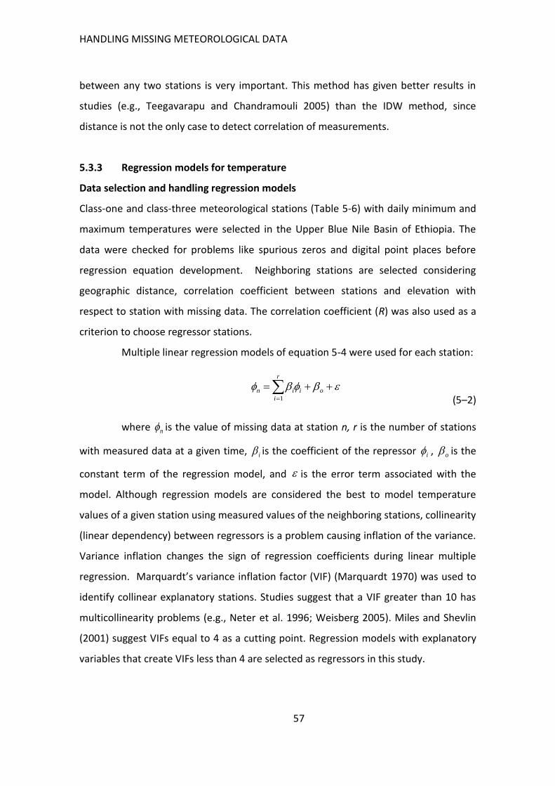
HANDLING MISSING METEOROLOGICAL DATA
57
between any two stations is very important. This method has given better results in
studies (e.g., Teegavarapu and Chandramouli 2005) than the IDW method, since
distance is not the only case to detect correlation of measurements.
5.3.3 Regression models for temperature
Data selection and handling regression models
Class-one and class-three meteorological stations (Table 5-6) with daily minimum and
maximum temperatures were selected in the Upper Blue Nile Basin of Ethiopia. The
data were checked for problems like spurious zeros and digital point places before
regression equation development. Neighboring stations are selected considering
geographic distance, correlation coefficient between stations and elevation with
respect to station with missing data. The correlation coefficient (R) was also used as a
criterion to choose regressor stations.
Multiple linear regression models of equation 5-4 were used for each station:
(5–2)
where is the value of missing data at station n, r is the number of stations
with measured data at a given time, is the coefficient of the repressor , is the
constant term of the regression model, and is the error term associated with the
model. Although regression models are considered the best to model temperature
values of a given station using measured values of the neighboring stations, collinearity
(linear dependency) between regressors is a problem causing inflation of the variance.
Variance inflation changes the sign of regression coefficients during linear multiple
regression. Marquardt’s variance inflation factor (VIF) (Marquardt 1970) was used to
identify collinear explanatory stations. Studies suggest that a VIF greater than 10 has
multicollinearity problems (e.g., Neter et al. 1996; Weisberg 2005). Miles and Shevlin
(2001) suggest VIFs equal to 4 as a cutting point. Regression models with explanatory
variables that create VIFs less than 4 are selected as regressors in this study.
o
r
i
iin
1
n
i i o
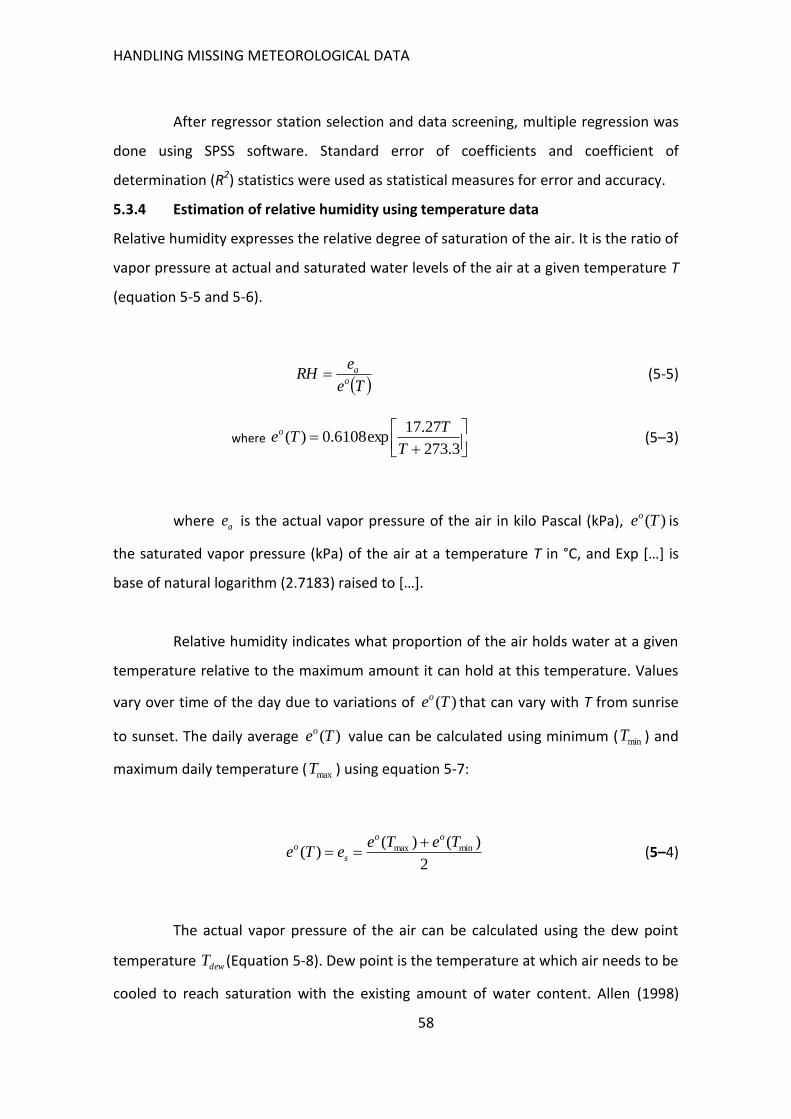
HANDLING MISSING METEOROLOGICAL DATA
58
After regressor station selection and data screening, multiple regression was
done using SPSS software. Standard error of coefficients and coefficient of
determination (R2) statistics were used as statistical measures for error and accuracy.
5.3.4 Estimation of relative humidity using temperature data
Relative humidity expresses the relative degree of saturation of the air. It is the ratio of
vapor pressure at actual and saturated water levels of the air at a given temperature T
(equation 5-5 and 5-6).
(5-5)
where (5–3)
where is the actual vapor pressure of the air in kilo Pascal (kPa), is
the saturated vapor pressure (kPa) of the air at a temperature T in °C, and Exp *…+ is
base of natural logarithm (2.7183) raised to *…+.
Relative humidity indicates what proportion of the air holds water at a given
temperature relative to the maximum amount it can hold at this temperature. Values
vary over time of the day due to variations of that can vary with T from sunrise
to sunset. The daily average value can be calculated using minimum ( ) and
maximum daily temperature ( ) using equation 5-7:
(5–4)
The actual vapor pressure of the air can be calculated using the dew point
temperature (Equation 5-8). Dew point is the temperature at which air needs to be
cooled to reach saturation with the existing amount of water content. Allen (1998)
Te
eRH
o
a
3.273
27.17exp6108.0)(
T
TTeo
ae )(Teo
)(Teo
)(Teo
minT
maxT
2
)()()( minmax TeTe
eTeoo
s
o
dewT
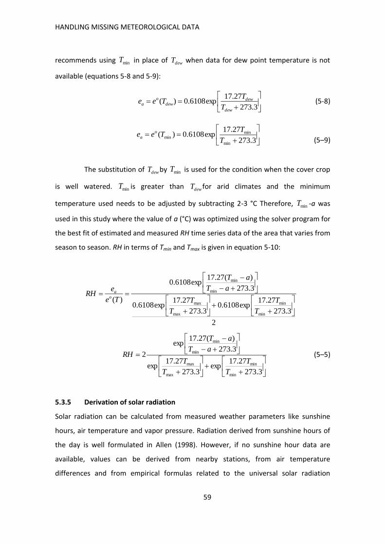
HANDLING MISSING METEOROLOGICAL DATA
59
recommends using in place of when data for dew point temperature is not
available (equations 5-8 and 5-9):
(5-8)
(5–9)
The substitution of by is used for the condition when the cover crop
is well watered. is greater than for arid climates and the minimum
temperature used needs to be adjusted by subtracting 2-3 °C Therefore, -a was
used in this study where the value of a (°C) was optimized using the solver program for
the best fit of estimated and measured RH time series data of the area that varies from
season to season. RH in terms of Tmin and Tmax is given in equation 5-10:
(5–5)
5.3.5 Derivation of solar radiation
Solar radiation can be calculated from measured weather parameters like sunshine
hours, air temperature and vapor pressure. Radiation derived from sunshine hours of
the day is well formulated in Allen (1998). However, if no sunshine hour data are
available, values can be derived from nearby stations, from air temperature
differences and from empirical formulas related to the universal solar radiation
minTdewT
3.273
27.17exp6108.0)(
dew
dewdew
o
aT
TTee
3.273
27.17exp6108.0)(
min
minmin
T
TTee o
a
dewT minT
minTdewT
minT
2
3.273
27.17exp6108.0
3.273
27.17exp6108.0
3.273
)(27.17exp6108.0
)(
min
min
max
max
min
min
T
T
T
T
aT
aT
Te
eRH
o
a
3.273
27.17exp
3.273
27.17exp
3.273
)(27.17exp
2
min
min
max
max
min
min
T
T
T
T
aT
aT
RH
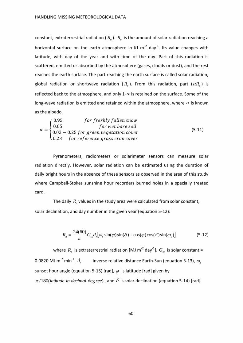
HANDLING MISSING METEOROLOGICAL DATA
60
constant, extraterrestrial radiation ( ). is the amount of solar radiation reaching a
horizontal surface on the earth atmosphere in KJ m-2 day-1. Its value changes with
latitude, with day of the year and with time of the day. Part of this radiation is
scattered, emitted or absorbed by the atmosphere (gases, clouds or dust), and the rest
reaches the earth surface. The part reaching the earth surface is called solar radiation,
global radiation or shortwave radiation ( ). From this radiation, part ( ) is
reflected back to the atmosphere, and only 1- is retained on the surface. Some of the
long-wave radiation is emitted and retained within the atmosphere, where is known
as the albedo.
{
(5-11)
Pyranometers, radiometers or solarimeter sensors can measure solar
radiation directly. However, solar radiation can be estimated using the duration of
daily bright hours in the absence of these sensors as observed in the area of this study
where Campbell-Stokes sunshine hour recorders burned holes in a specially treated
card.
The daily values in the study area were calculated from solar constant,
solar declination, and day number in the given year (equation 5-12):
(5-12)
where is extraterrestrial radiation [MJ m-2 day-1], is solar constant =
0.0820 MJ m-2 min-1, inverse relative distance Earth-Sun (equation 5-13),
sunset hour angle (equation 5-15) [rad], is latitude [rad] given by
, and is solar declination (equation 5-14) [rad].
aR aR
sR sR
aR
)sin()cos()cos()sin()sin()60(24
ssrsca dGR
aR scG
rds
)deg(180/ reedecimalinlatitude
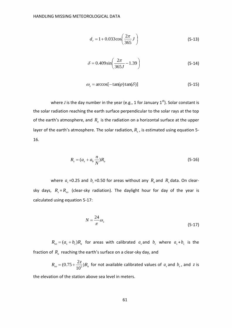
HANDLING MISSING METEOROLOGICAL DATA
61
(5-13)
(5-14)
(5-15)
where J is the day number in the year (e.g., 1 for January 1st). Solar constant is
the solar radiation reaching the earth surface perpendicular to the solar rays at the top
of the earth’s atmosphere, and is the radiation on a horizontal surface at the upper
layer of the earth’s atmosphere. The solar radiation, , is estimated using equation 5-
16.
(5-16)
where =0.25 and =0.50 for areas without any and data. On clear-
sky days, = (clear-sky radiation). The daylight hour for day of the year is
calculated using equation 5-17:
(5-17)
for areas with calibrated and where + is the
fraction of reaching the earth’s surface on a clear-sky day, and
for not available calibrated values of and , and is
the elevation of the station above sea level in meters.
Jdr
365
2cos033.01
39.1
365
2sin409.0
J
)]tan()tan(arccos[ s
aR
sR
abss RN
naaR )(
sa sb aR sR
sR soR
sN
24
assso RbaR )( sa sb sa sb
aR
aso Rz
R )10
275.0(
5 sa sb z
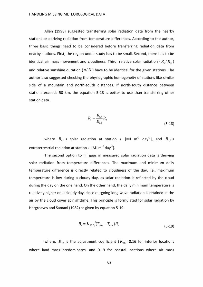
HANDLING MISSING METEOROLOGICAL DATA
62
Allen (1998) suggested transferring solar radiation data from the nearby
stations or deriving radiation from temperature differences. According to the author,
three basic things need to be considered before transferring radiation data from
nearby stations. First, the region under study has to be small. Second, there has to be
identical air mass movement and cloudiness. Third, relative solar radiation ( )
and relative sunshine duration ( ) have to be identical for the given stations. The
author also suggested checking the physiographic homogeneity of stations like similar
side of a mountain and north-south distances. If north-south distance between
stations exceeds 50 km, the equation 5-18 is better to use than transferring other
station data.
(5-18)
where is solar radiation at station [MJ m-2 day-1], and is
extraterrestrial radiation at station [MJ m-2 day-1].
The second option to fill gaps in measured solar radiation data is deriving
solar radiation from temperature differences. The maximum and minimum daily
temperature difference is directly related to cloudiness of the day, i.e., maximum
temperature is low during a cloudy day, as solar radiation is reflected by the cloud
during the day on the one hand. On the other hand, the daily minimum temperature is
relatively higher on a cloudy day, since outgoing long-wave radiation is retained in the
air by the cloud cover at nighttime. This principle is formulated for solar radiation by
Hargreaves and Samani (1982) as given by equation 5-19:
(5-19)
where, is the adjustment coefficient ( =0.16 for interior locations
where land mass predominates, and 0.19 for coastal locations where air mass
sos RR /
Nn /
a
ia
is
s RR
RR
,
,
isR , i iaR ,
i
aRSs RTTKR )( minmax
RSK RSK
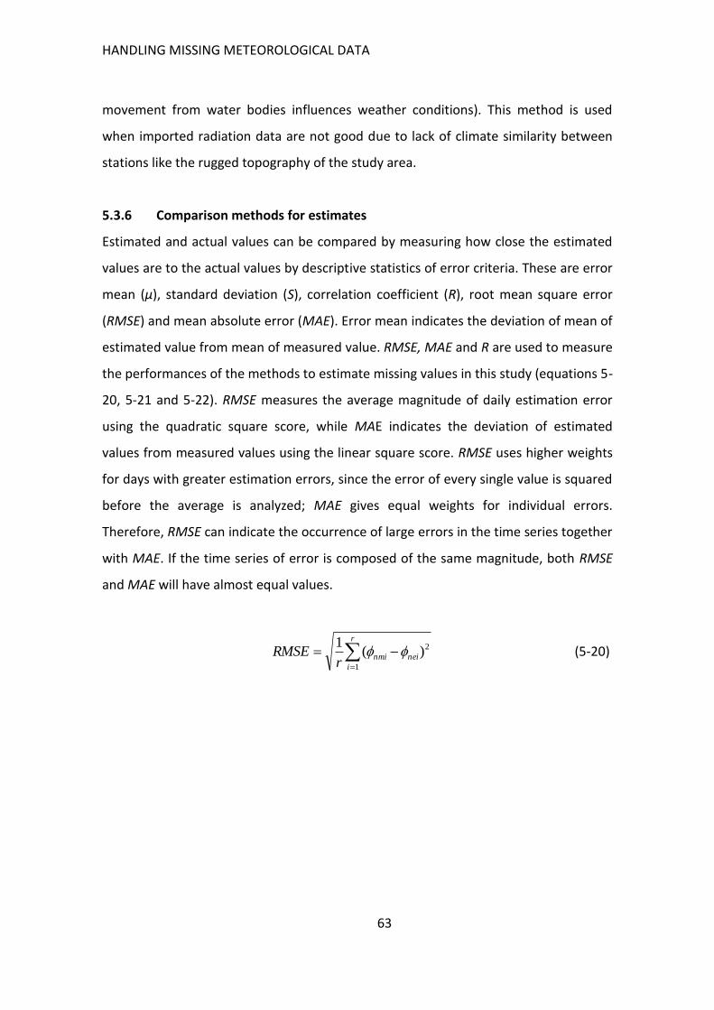
HANDLING MISSING METEOROLOGICAL DATA
63
movement from water bodies influences weather conditions). This method is used
when imported radiation data are not good due to lack of climate similarity between
stations like the rugged topography of the study area.
5.3.6 Comparison methods for estimates
Estimated and actual values can be compared by measuring how close the estimated
values are to the actual values by descriptive statistics of error criteria. These are error
mean (μ), standard deviation (S), correlation coefficient (R), root mean square error
(RMSE) and mean absolute error (MAE). Error mean indicates the deviation of mean of
estimated value from mean of measured value. RMSE, MAE and R are used to measure
the performances of the methods to estimate missing values in this study (equations 5-
20, 5-21 and 5-22). RMSE measures the average magnitude of daily estimation error
using the quadratic square score, while MAE indicates the deviation of estimated
values from measured values using the linear square score. RMSE uses higher weights
for days with greater estimation errors, since the error of every single value is squared
before the average is analyzed; MAE gives equal weights for individual errors.
Therefore, RMSE can indicate the occurrence of large errors in the time series together
with MAE. If the time series of error is composed of the same magnitude, both RMSE
and MAE will have almost equal values.
(5-20)
r
i
neinmir
RMSE1
2)(1
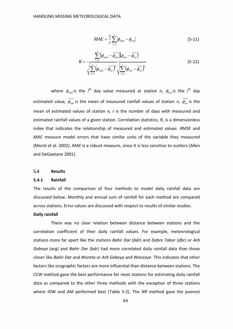
HANDLING MISSING METEOROLOGICAL DATA
64
(5-21)
(5-22)
where is the ith day value measured at station n, is the ith day
estimated value, is the mean of measured rainfall values of station n, is the
mean of estimated values of station n, r is the number of days with measured and
estimated rainfall values of a given station. Correlation statistics, R, is a dimensionless
index that indicates the relationship of measured and estimated values. RMSE and
MAE measure model errors that have similar units of the variable they measured
(Morid et al. 2002). MAE is a robust measure, since it is less sensitive to outliers (Allen
and DeGaetano 2001).
5.4 Results
5.4.1 Rainfall
The results of the comparison of four methods to model daily rainfall data are
discussed below. Monthly and annual sum of rainfall for each method are compared
across stations. Error values are discussed with respect to results of similar studies.
Daily rainfall
There was no clear relation between distance between stations and the
correlation coefficient of their daily rainfall values. For example, meteorological
stations more far apart like the stations Bahir Dar (bdr) and Debre Tabor (dbr) or Arb
Gebeya (arg) and Bahir Dar (bdr) had more correlated daily rainfall data than those
closer like Bahir Dar and Woreta or Arb Gebeya and Wanzaye. This indicates that other
factors like orographic factors are more influential than distance between stations. The
CCW method gave the best performance for most stations for estimating daily rainfall
data as compared to the other three methods with the exception of three stations
where IDW and AM performed best (Table 5-2). The NR method gave the poorest
r
i
neinmir
MAE1
1
r
i
nenei
r
i
nrnmi
r
i
neneinmnmi
R
1
2
1
2
1
nmi nei
nm ne
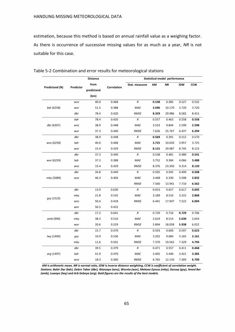
HANDLING MISSING METEOROLOGICAL DATA
65
estimation, because this method is based on annual rainfall value as a weighing factor.
As there is occurrence of successive missing values for as much as a year, NR is not
suitable for this case.
Table 5-2 Combination and error results for meteorological stations
Predictand (N) Predictor
Distance
from
predictand
(km)
Correlation
Statistical model performance
Stat. measures AM NR IDW CCW
bdr (6258)
wnz 40.0 0.468 R 0.538 0.385 0.527 0.532
wor 51.5 0.388 MAE 3.696 10.170 3.720 3.720
dbr 78.4 0.420 RMSE 8.359 29.986 8.582 8.415
dbr (6307)
bdr 78.4 0.420 R 0.557 0.463 0.558 0.558
wnz 38.9 0.448 MAE 3.533 9.844 2.599 2.598
wor 37.3 0.440 RMSE 7.626 25.767 6.437 6.294
wnz (6258)
dbr 38.9 0.448 R 0.569 0.391 0.512 0.570
bdr 40.0 0.468 MAE 3.725 10.020 3.957 3.725
wor 15.4 0.429 RMSE 8.131 29.987 8.745 8.123
wor (6259)
dbr 37.3 0.440 R 0.538 0.481 0.480 0.541
bdr 37.3 0.388 MAE 3.752 9.384 4.066 3.488
wnz 15.4 0.429 RMSE 8.376 23.350 9.314 8.120
mky (5089)
dbr 26.8 0.449 R 0.505 0.505 0.499 0.508
wnz 46.3 0.404 MAE 3.468 6.330 3.508 2.832
RMSE 7.560 13.941 7.710 6.562
gsy (1523)
dbr 13.9 0.630 R 0.653 0.657 0.617 0.692
mky 21.8 0.535 MAE 3.189 8.533 3.315 2.868
wnz 50.4 0.418 RMSE 6.441 17.947 7.522 6.004
wor 50.5 0.432
amb (990)
dbr 17.2 0.641 R 0.720 0.716 0.729 0.706
mky 38.3 0.510 MAE 2.619 8.514 2.630 2.654
wor 20.6 0.529 RMSE 5.894 18.058 5.938 6.022
lwy (1400)
dbr 15.7 0.470 R 0.593 0.600 0.597 0.623
gsy 10.9 0.536 MAE 3.202 9.684 3.165 2.161
mky 11.6 0.501 RMSE 7.370 19.562 7.329 4.794
arg (1497)
dbr 39.5 0.379 R 0.471 0.557 0.411 0.468
bdr 41.9 0.470 MAE 3.405 5.440 3.421 3.385
wnz 18.3 0.360 RMSE 6.765 12.133 7.369 6.709
AM is arithmetic mean, NR is normal ratio, IDW is inverse distance weighting, CCW is coefficient of correlation weight. Stations: Bahir Dar (bdr), Debre Tabor (dbr), Wanzaye (wnz), Woreta (wor), Mekane Eyesus (mky), Gassay (gsy), Amed Ber (amb), Luwaye (lwy) and Arb Gebeya (arg). Bold figures are the results of the best models.
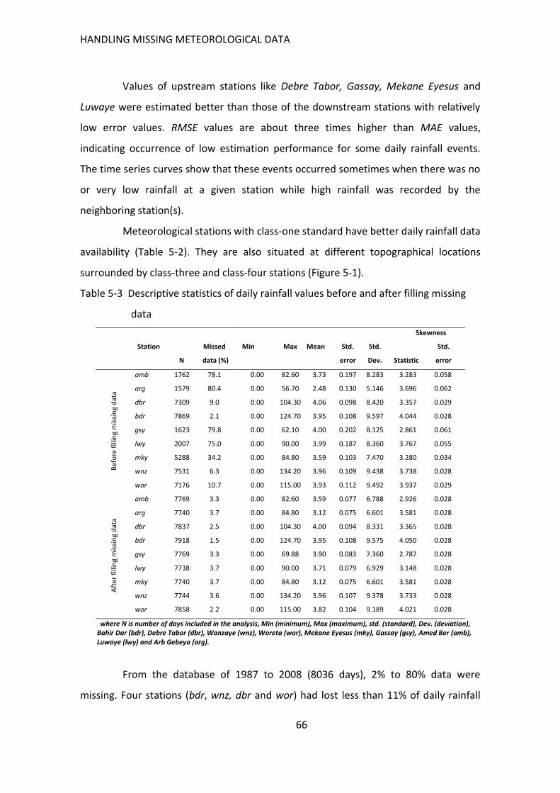
HANDLING MISSING METEOROLOGICAL DATA
66
Values of upstream stations like Debre Tabor, Gassay, Mekane Eyesus and
Luwaye were estimated better than those of the downstream stations with relatively
low error values. RMSE values are about three times higher than MAE values,
indicating occurrence of low estimation performance for some daily rainfall events.
The time series curves show that these events occurred sometimes when there was no
or very low rainfall at a given station while high rainfall was recorded by the
neighboring station(s).
Meteorological stations with class-one standard have better daily rainfall data
availability (Table 5-2). They are also situated at different topographical locations
surrounded by class-three and class-four stations (Figure 5-1).
Table 5-3 Descriptive statistics of daily rainfall values before and after filling missing
data
Station
N
Missed
data (%)
Min Max Mean Std.
error
Std.
Dev.
Skewness
Statistics
Std.
error
Bef
ore
fill
ing
mis
sin
g d
ata
amb 1762 78.1 0.00 82.60 3.73 0.197 8.283 3.283 0.058
arg 1579 80.4 0.00 56.70 2.48 0.130 5.146 3.696 0.062
dbr 7309 9.0 0.00 104.30 4.06 0.098 8.420 3.357 0.029
bdr 7869 2.1 0.00 124.70 3.95 0.108 9.597 4.044 0.028
gsy 1623 79.8 0.00 62.10 4.00 0.202 8.125 2.861 0.061
lwy 2007 75.0 0.00 90.00 3.99 0.187 8.360 3.767 0.055
mky 5288 34.2 0.00 84.80 3.59 0.103 7.470 3.280 0.034
wnz 7531 6.3 0.00 134.20 3.96 0.109 9.438 3.738 0.028
wor 7176 10.7 0.00 115.00 3.93 0.112 9.492 3.937 0.029
Aft
er f
illin
g m
issi
ng
dat
a
amb 7769 3.3 0.00 82.60 3.59 0.077 6.788 2.926 0.028
arg 7740 3.7 0.00 84.80 3.12 0.075 6.601 3.581 0.028
dbr 7837 2.5 0.00 104.30 4.00 0.094 8.331 3.365 0.028
bdr 7918 1.5 0.00 124.70 3.95 0.108 9.575 4.050 0.028
gsy 7769 3.3 0.00 69.88 3.90 0.083 7.360 2.787 0.028
lwy 7738 3.7 0.00 90.00 3.71 0.079 6.929 3.148 0.028
mky 7740 3.7 0.00 84.80 3.12 0.075 6.601 3.581 0.028
wnz 7744 3.6 0.00 134.20 3.96 0.107 9.378 3.733 0.028
wor 7858 2.2 0.00 115.00 3.82 0.104 9.189 4.021 0.028
where N is number of days included in the analysis, Min (minimum), Max (maximum), std. (standard), Dev. (deviation), Bahir Dar (bdr), Debre Tabor (dbr), Wanzaye (wnz), Woreta (wor), Mekane Eyesus (mky), Gassay (gsy), Amed Ber (amb), Luwaye (lwy) and Arb Gebeya (arg).
From the database of 1987 to 2008 (8036 days), 2% to 80% data were
missing. Four stations (bdr, wnz, dbr and wor) had lost less than 11% of daily rainfall
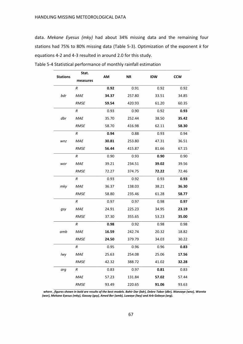
HANDLING MISSING METEOROLOGICAL DATA
67
data. Mekane Eyesus (mky) had about 34% missing data and the remaining four
stations had 75% to 80% missing data (Table 5-3). Optimization of the exponent k for
equations 4-2 and 4-3 resulted in around 2.0 for this study.
Table 5-4 Statistical performance of monthly rainfall estimation
Stations Stat.
measures AM NR IDW CCW
bdr
R 0.92 0.91 0.92 0.92
MAE 34.37 257.80 33.51 34.85
RMSE 59.54 420.93 61.20 60.35
dbr
R 0.93 0.90 0.92 0.93
MAE 35.70 252.44 38.50 35.42
RMSE 58.70 416.98 62.11 58.30
wnz
R 0.94 0.88 0.93 0.94
MAE 30.81 253.80 47.31 36.51
RMSE 56.44 415.87 81.66 67.15
wor
R 0.90 0.93 0.90 0.90
MAE 39.21 234.51 39.02 39.56
RMSE 72.27 374.75 72.22 72.46
mky
R 0.93 0.92 0.93 0.93
MAE 36.37 138.03 38.21 36.30
RMSE 58.80 235.46 61.28 58.77
gsy
R 0.97 0.97 0.98 0.97
MAE 24.91 225.23 34.95 23.19
RMSE 37.30 355.65 53.23 35.00
amb
R 0.98 0.92 0.98 0.98
MAE 16.59 242.74 20.32 18.82
RMSE 24.50 379.79 34.03 30.22
lwy
R 0.95 0.96 0.96 0.83
MAE 25.63 254.08 25.06 17.56
RMSE 42.32 388.72 41.02 32.28
arg R 0.83 0.97 0.81 0.83
MAE 57.23 131.84 57.02 57.44
RMSE 93.49 220.65 91.06 93.63
where , figures shown in bold are results of the best models. Bahir Dar (bdr), Debre Tabor (dbr), Wanzaye (wnz), Woreta (wor), Mekane Eyesus (mky), Gassay (gsy), Amed Ber (amb), Luwaye (lwy) and Arb Gebeya (arg).
HANDLING MISSING METEOROLOGICAL DATA
68
After filling the missing data with the best method for each station, the
percent of missing data decreased to less than 4%. Descriptive statistics before and
after filling missing daily rainfall values show that the structure of the database is not
altered, especially the mean and maximum daily rainfall values.
Monthly rainfall
Better correlation coefficients for monthly than daily rainfall data can be
observed for all meteorological stations. The AM and CCW methods showed
comparable performance with values of monthly estimated rainfall close to
corresponding measured values (Table 5-4). Monthly comparison of model
performance reveals the weakness of R to identify the best model. The value of R is the
same for most methods while RMSE and MAE values are different. For example, CCW
and AM provided comparable and better estimates for daily rainfall at wnz. However,
AM was the best for monthly rainfall estimation for wnz even if the value of R (R=0.94)
for both AM and CCW is the same. The higher R value was not the best as seen in the
case of gsy where IDW gave the best R value on a monthly time scale, while CCW
performed best for both RMSE and MAE values (Table 5-4). AM showed the best
estimation at both daily and monthly time scales at the downstream meteorological
stations and CCW the best at the upstream stations.
The time series of average monthly measured and estimated rainfall shows
how close the estimation is to the measures data (Figure 5-2). It makes clear the effect
of small statistical differences in MAE and RMSE as shown, for example, for wnz. NR
values are not included in Figure 5-2, since they are much more overestimated as
compared to the other methods.
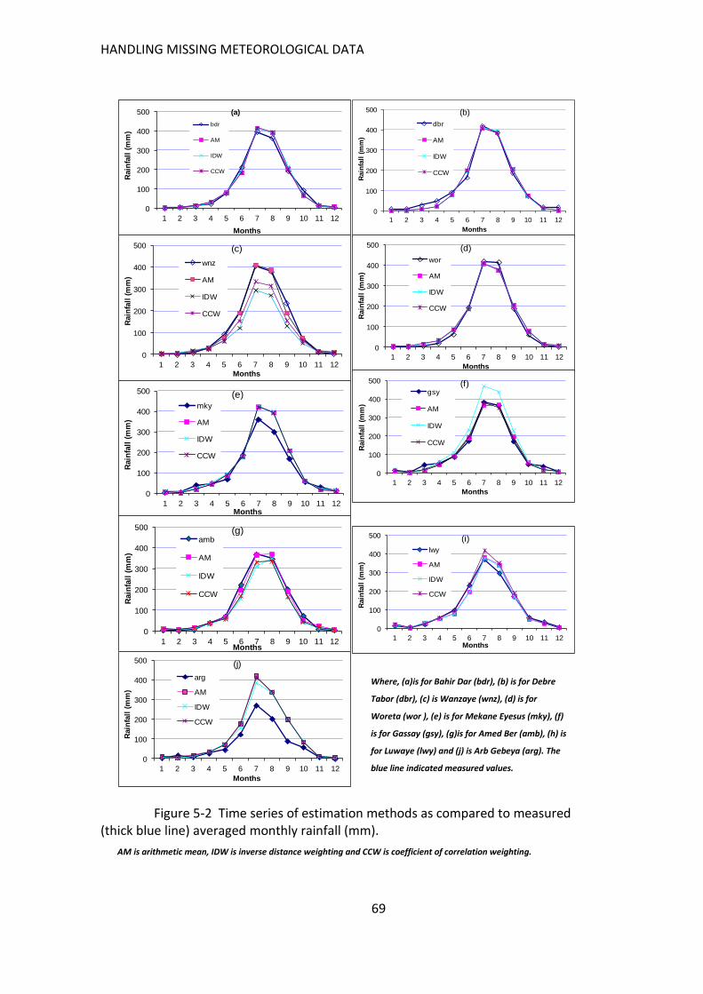
HANDLING MISSING METEOROLOGICAL DATA
69
Figure 5-2 Time series of estimation methods as compared to measured (thick blue line) averaged monthly rainfall (mm).
AM is arithmetic mean, IDW is inverse distance weighting and CCW is coefficient of correlation weighting.
0
100
200
300
400
500
1 2 3 4 5 6 7 8 9 10 11 12
Rain
fall
(m
m)
Months
(a)
bdr
AM
IDW
CCW
0
100
200
300
400
500
1 2 3 4 5 6 7 8 9 10 11 12
Rain
fall
(m
m)
Months
(b)
dbr
AM
IDW
CCW
0
100
200
300
400
500
1 2 3 4 5 6 7 8 9 10 11 12
Rain
fall
(m
m)
Months
(c)
wnz
AM
IDW
CCW
0
100
200
300
400
500
1 2 3 4 5 6 7 8 9 10 11 12R
ain
fall
(m
m)
Months
(d)
wor
AM
IDW
CCW
0
100
200
300
400
500
1 2 3 4 5 6 7 8 9 10 11 12
Rain
fall
(m
m)
Months
(e)mky
AM
IDW
CCW
0
100
200
300
400
500
1 2 3 4 5 6 7 8 9 10 11 12
Rain
fall
(m
m)
Months
(f)gsy
AM
IDW
CCW
0
100
200
300
400
500
1 2 3 4 5 6 7 8 9 10 11 12
Rain
fall
(m
m)
Months
(g)amb
AM
IDW
CCW
0
100
200
300
400
500
1 2 3 4 5 6 7 8 9 10 11 12
Rain
fall
(m
m)
Months
(i)
lwy
AM
IDW
CCW
0
100
200
300
400
500
1 2 3 4 5 6 7 8 9 10 11 12
Rain
fall
(m
m)
Months
(j)
arg
AM
IDW
CCW
Where, (a)is for Bahir Dar (bdr), (b) is for Debre
Tabor (dbr), (c) is Wanzaye (wnz), (d) is for
Woreta (wor ), (e) is for Mekane Eyesus (mky), (f)
is for Gassay (gsy), (g)is for Amed Ber (amb), (h) is
for Luwaye (lwy) and (j) is Arb Gebeya (arg). The
blue line indicated measured values.
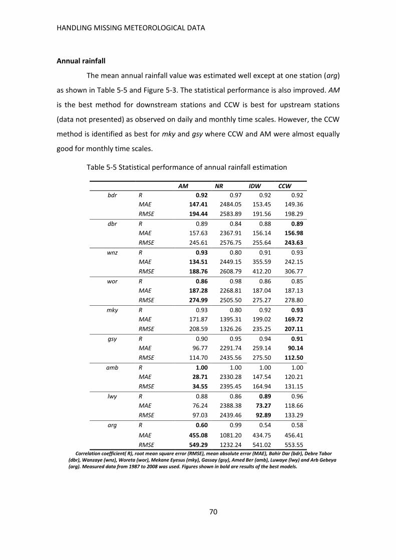
HANDLING MISSING METEOROLOGICAL DATA
70
Annual rainfall
The mean annual rainfall value was estimated well except at one station (arg)
as shown in Table 5-5 and Figure 5-3. The statistical performance is also improved. AM
is the best method for downstream stations and CCW is best for upstream stations
(data not presented) as observed on daily and monthly time scales. However, the CCW
method is identified as best for mky and gsy where CCW and AM were almost equally
good for monthly time scales.
Table 5-5 Statistical performance of annual rainfall estimation
AM NR IDW CCW
bdr R 0.92 0.97 0.92 0.92
MAE 147.41 2484.05 153.45 149.36
RMSE 194.44 2583.89 191.56 198.29
dbr R 0.89 0.84 0.88 0.89
MAE 157.63 2367.91 156.14 156.98
RMSE 245.61 2576.75 255.64 243.63
wnz R 0.93 0.80 0.91 0.93
MAE 134.51 2449.15 355.59 242.15
RMSE 188.76 2608.79 412.20 306.77
wor R 0.86 0.98 0.86 0.85
MAE 187.28 2268.81 187.04 187.13
RMSE 274.99 2505.50 275.27 278.80
mky R 0.93 0.80 0.92 0.93
MAE 171.87 1395.31 199.02 169.72
RMSE 208.59 1326.26 235.25 207.11
gsy R 0.90 0.95 0.94 0.91
MAE 96.77 2291.74 259.14 90.14
RMSE 114.70 2435.56 275.50 112.50
amb R 1.00 1.00 1.00 1.00
MAE 28.71 2330.28 147.54 120.21
RMSE 34.55 2395.45 164.94 131.15
lwy R 0.88 0.86 0.89 0.96
MAE 76.24 2388.38 73.27 118.66
RMSE 97.03 2439.46 92.89 133.29
arg R 0.60 0.99 0.54 0.58
MAE 455.08 1081.20 434.75 456.41
RMSE 549.29 1232.24 541.02 553.55 Correlation coefficient( R), root mean square error (RMSE), mean absolute error (MAE), Bahir Dar (bdr), Debre Tabor
(dbr), Wanzaye (wnz), Woreta (wor), Mekane Eyesus (mky), Gassay (gsy), Amed Ber (amb), Luwaye (lwy) and Arb Gebeya (arg). Measured data from 1987 to 2008 was used. Figures shown in bold are results of the best models.
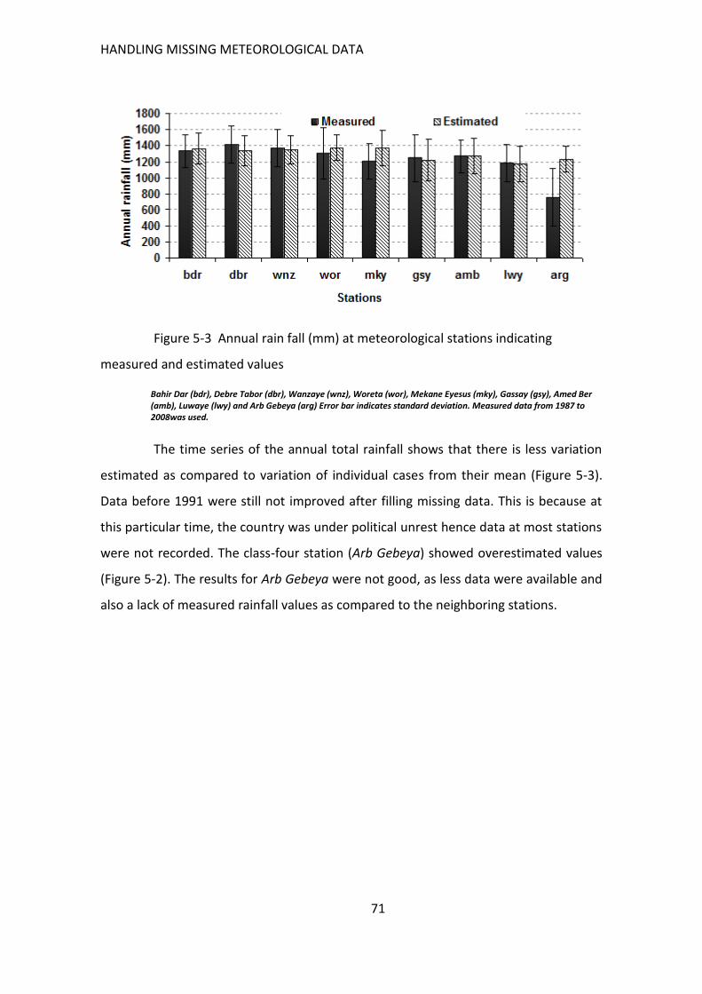
HANDLING MISSING METEOROLOGICAL DATA
71
Figure 5-3 Annual rain fall (mm) at meteorological stations indicating
measured and estimated values
Bahir Dar (bdr), Debre Tabor (dbr), Wanzaye (wnz), Woreta (wor), Mekane Eyesus (mky), Gassay (gsy), Amed Ber (amb), Luwaye (lwy) and Arb Gebeya (arg) Error bar indicates standard deviation. Measured data from 1987 to 2008was used.
The time series of the annual total rainfall shows that there is less variation
estimated as compared to variation of individual cases from their mean (Figure 5-3).
Data before 1991 were still not improved after filling missing data. This is because at
this particular time, the country was under political unrest hence data at most stations
were not recorded. The class-four station (Arb Gebeya) showed overestimated values
(Figure 5-2). The results for Arb Gebeya were not good, as less data were available and
also a lack of measured rainfall values as compared to the neighboring stations.
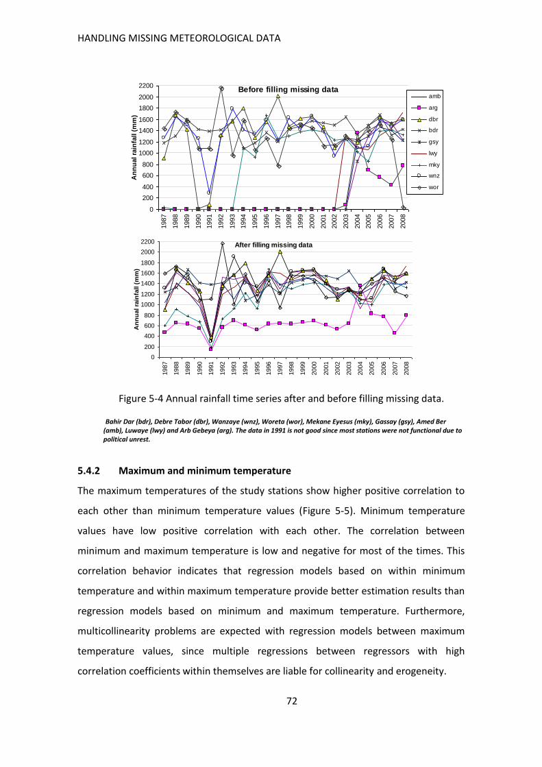
HANDLING MISSING METEOROLOGICAL DATA
72
Figure 5-4 Annual rainfall time series after and before filling missing data.
Bahir Dar (bdr), Debre Tabor (dbr), Wanzaye (wnz), Woreta (wor), Mekane Eyesus (mky), Gassay (gsy), Amed Ber (amb), Luwaye (lwy) and Arb Gebeya (arg). The data in 1991 is not good since most stations were not functional due to political unrest.
5.4.2 Maximum and minimum temperature
The maximum temperatures of the study stations show higher positive correlation to
each other than minimum temperature values (Figure 5-5). Minimum temperature
values have low positive correlation with each other. The correlation between
minimum and maximum temperature is low and negative for most of the times. This
correlation behavior indicates that regression models based on within minimum
temperature and within maximum temperature provide better estimation results than
regression models based on minimum and maximum temperature. Furthermore,
multicollinearity problems are expected with regression models between maximum
temperature values, since multiple regressions between regressors with high
correlation coefficients within themselves are liable for collinearity and erogeneity.
Before filling missing data
0
200
400
600
800
1000
1200
1400
1600
1800
2000
2200
1987
1988
1989
1990
1991
1992
1993
1994
1995
1996
1997
1998
1999
2000
2001
2002
2003
2004
2005
2006
2007
2008
An
nu
al ra
infa
ll (
mm
)
amb
arg
dbr
bdr
gsy
lwy
mky
wnz
wor
After filling missing data
0
200
400
600
800
1000
1200
1400
1600
1800
2000
2200
1987
1988
1989
1990
1991
1992
1993
1994
1995
1996
1997
1998
1999
2000
2001
2002
2003
2004
2005
2006
2007
2008
An
nu
al ra
infa
ll (
mm
)
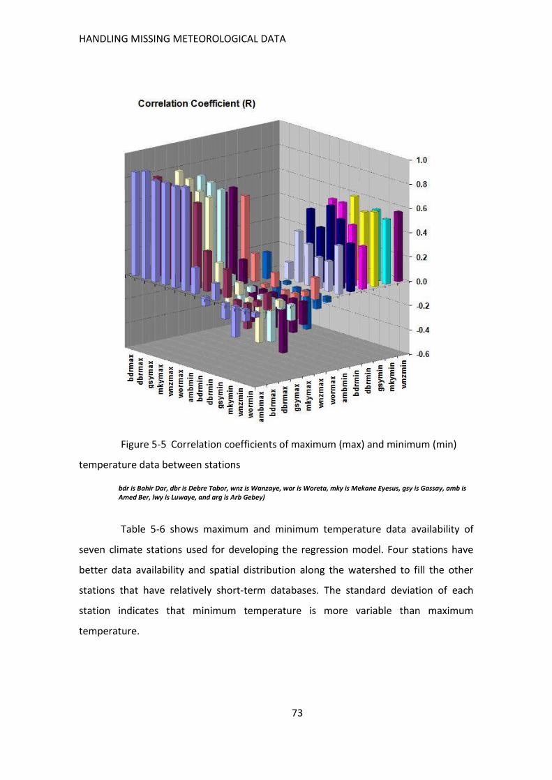
HANDLING MISSING METEOROLOGICAL DATA
73
Figure 5-5 Correlation coefficients of maximum (max) and minimum (min)
temperature data between stations
bdr is Bahir Dar, dbr is Debre Tabor, wnz is Wanzaye, wor is Woreta, mky is Mekane Eyesus, gsy is Gassay, amb is Amed Ber, lwy is Luwaye, and arg is Arb Gebey)
Table 5-6 shows maximum and minimum temperature data availability of
seven climate stations used for developing the regression model. Four stations have
better data availability and spatial distribution along the watershed to fill the other
stations that have relatively short-term databases. The standard deviation of each
station indicates that minimum temperature is more variable than maximum
temperature.
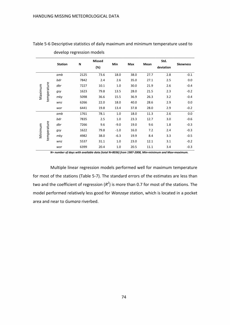
HANDLING MISSING METEOROLOGICAL DATA
74
Table 5-6 Descriptive statistics of daily maximum and minimum temperature used to
develop regression models
Station N Missed
(%) Min Max Mean
Std.
deviation Skewness
Max
imu
m
tem
per
atu
re
amb 2125 73.6 18.0 38.0 27.7 2.8 -0.1
bdr 7842 2.4 2.6 35.0 27.1 2.5 0.0
dbr 7227 10.1 1.0 30.0 21.9 2.6 -0.4
gsy 1623 79.8 13.5 28.0 21.5 2.3 -0.2
mky 5098 36.6 15.5 36.9 26.3 3.2 -0.4
wnz 6266 22.0 18.0 40.0 28.6 2.9 0.0
wor 6441 19.8 13.4 37.8 28.0 2.9 -0.2
Min
imu
m
tem
per
atu
re
amb 1761 78.1 1.0 18.0 11.3 2.6 0.0
bdr 7835 2.5 1.0 23.3 12.7 3.0 -0.6
dbr 7266 9.6 -9.0 19.0 9.6 1.8 -0.3
gsy 1622 79.8 -1.0 16.0 7.2 2.4 -0.3
mky 4982 38.0 -6.3 19.9 8.4 3.3 -0.5
wnz 5537 31.1 1.0 23.0 12.1 3.1 -0.2
wor 6399 20.4 1.0 20.5 11.1 3.4 -0.3
N= number of days with available data (total N=8036) from 1987-2008, Min=minimum and Max=maximum.
Multiple linear regression models performed well for maximum temperature
for most of the stations (Table 5-7). The standard errors of the estimates are less than
two and the coefficient of regression (R2) is more than 0.7 for most of the stations. The
model performed relatively less good for Wanzaye station, which is located in a pocket
area and near to Gumara riverbed.
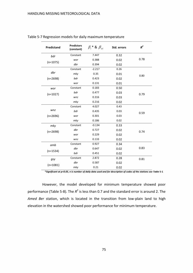
HANDLING MISSING METEOROLOGICAL DATA
75
Table 5-7 Regression models for daily maximum temperature
Predictand Predictors (constant)
* & Std. errors R2
bdr
(n=1075)
Constant 7.447 0.32 0.78 wor 0.388 0.02
dbr 0.394 0.02
dbr
(n=2698)
Constant -2.217 0.26
0.80 mky 0.35 0.01
bdr 0.423 0.02
wor 0.131 0.01
wor
(n=1027)
Constant 0.183 0.50
0.79 bdr 0.477 0.03
wnz 0.316 0.03
mky 0.216 0.02
wnz
(n=2696)
Constant 4.027 0.43
0.59 bdr 0.435 0.03
wor 0.301 0.03
mky 0.186 0.02
mky
(n=2698)
Constant -0.134 0.33
0.74 dbr 0.727 0.02
wor 0.229 0.02
wnz 0.133 0.02
amb
(n=1534)
Constant 0.927 0.34 0.83 dbr 0.647 0.02
bdr 0.451 0.02
gsy
(n=1081)
Constant 2.872 0.28
0.02
0.81
dbr 0.587 0.02
mky 0.21 0.02
*Significant at p<0.05, n is number of daily data used and for description of codes of the stations see Table 5-1
However, the model developed for minimum temperature showed poor
performance (Table 5-8). The R2 is less than 0.7 and the standard error is around 2. The
Amed Ber station, which is located in the transition from low-plain land to high
elevation in the watershed showed poor performance for minimum temperature.
i oi
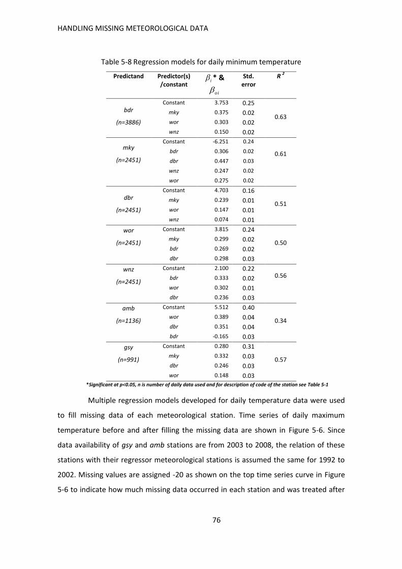
HANDLING MISSING METEOROLOGICAL DATA
76
Table 5-8 Regression models for daily minimum temperature
Predictand Predictor(s) /constant
* &
Std. error
R 2
bdr
(n=3886)
Constant 3.753 0.25
0.63
mky 0.375 0.02
wor 0.303 0.02
wnz 0.150 0.02
mky
(n=2451)
Constant -6.251 0.24
0.02 0.61
bdr 0.306 0.02
dbr 0.447 0.03
wnz 0.247 0.02
wor 0.275 0.02
dbr
(n=2451)
Constant 4.703 0.16
0.51 mky 0.239 0.01
wor 0.147 0.01
wnz 0.074 0.01
wor
(n=2451)
Constant 3.815 0.24
0.50 mky 0.299 0.02
bdr 0.269 0.02
dbr 0.298 0.03
wnz
(n=2451)
Constant 2.100 0.22 0.56
bdr 0.333 0.02
wor 0.302 0.01
dbr 0.236 0.03
amb
(n=1136)
Constant 5.512 0.40
0.34 wor 0.389 0.04
dbr 0.351 0.04
bdr -0.165 0.03
gsy
(n=991)
Constant 0.280 0.31
0.57 mky 0.332 0.03
dbr 0.246 0.03
wor 0.148 0.03
*Significant at p<0.05, n is number of daily data used and for description of code of the station see Table 5-1
Multiple regression models developed for daily temperature data were used
to fill missing data of each meteorological station. Time series of daily maximum
temperature before and after filling the missing data are shown in Figure 5-6. Since
data availability of gsy and amb stations are from 2003 to 2008, the relation of these
stations with their regressor meteorological stations is assumed the same for 1992 to
2002. Missing values are assigned -20 as shown on the top time series curve in Figure
5-6 to indicate how much missing data occurred in each station and was treated after
i
oi
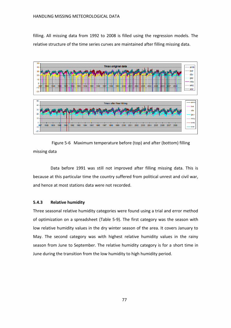
HANDLING MISSING METEOROLOGICAL DATA
77
filling. All missing data from 1992 to 2008 is filled using the regression models. The
relative structure of the time series curves are maintained after filling missing data.
Figure 5-6 Maximum temperature before (top) and after (bottom) filling
missing data
Data before 1991 was still not improved after filling missing data. This is
because at this particular time the country suffered from political unrest and civil war,
and hence at most stations data were not recorded.
5.4.3 Relative humidity
Three seasonal relative humidity categories were found using a trial and error method
of optimization on a spreadsheet (Table 5-9). The first category was the season with
low relative humidity values in the dry winter season of the area. It covers January to
May. The second category was with highest relative humidity values in the rainy
season from June to September. The relative humidity category is for a short time in
June during the transition from the low humidity to high humidity period.
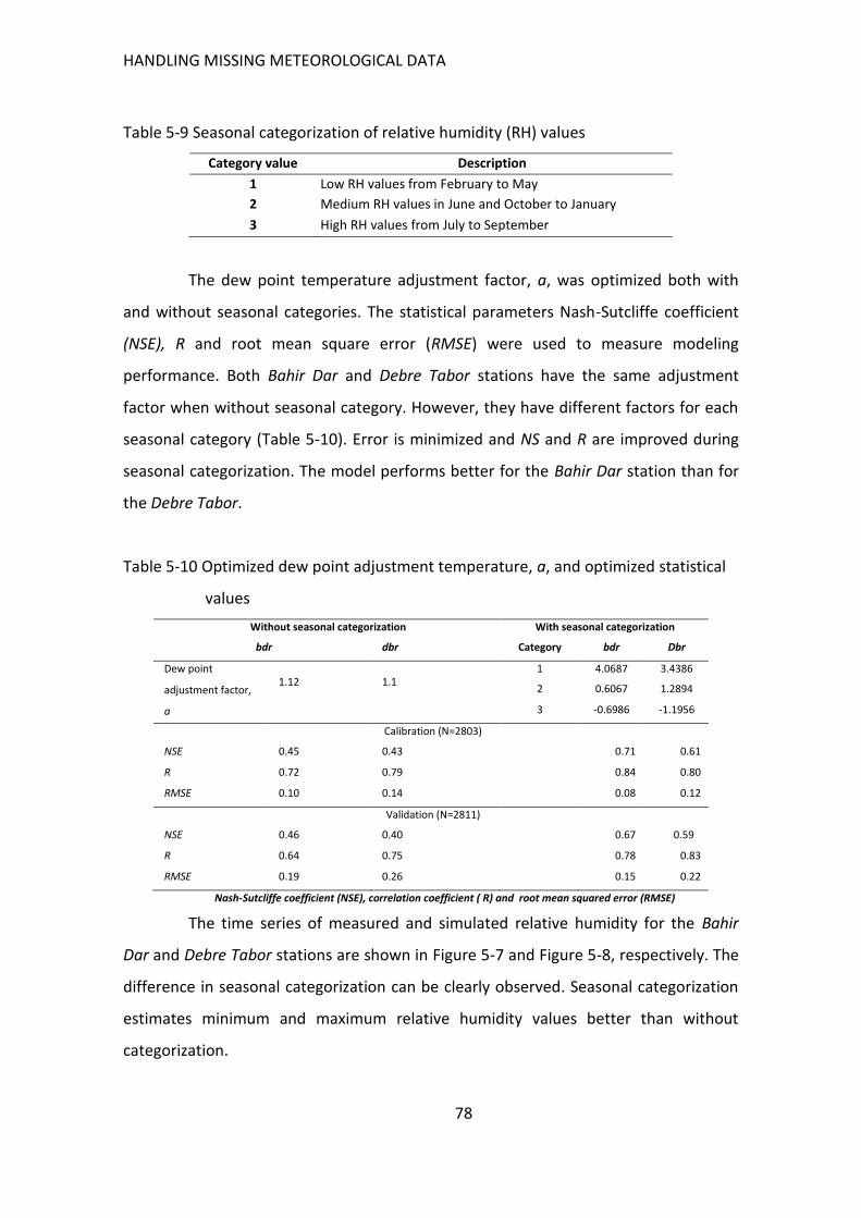
HANDLING MISSING METEOROLOGICAL DATA
78
Table 5-9 Seasonal categorization of relative humidity (RH) values
Category value Description
1 Low RH values from February to May
2 Medium RH values in June and October to January
3 High RH values from July to September
The dew point temperature adjustment factor, a, was optimized both with
and without seasonal categories. The statistical parameters Nash-Sutcliffe coefficient
(NSE), R and root mean square error (RMSE) were used to measure modeling
performance. Both Bahir Dar and Debre Tabor stations have the same adjustment
factor when without seasonal category. However, they have different factors for each
seasonal category (Table 5-10). Error is minimized and NS and R are improved during
seasonal categorization. The model performs better for the Bahir Dar station than for
the Debre Tabor.
Table 5-10 Optimized dew point adjustment temperature, a, and optimized statistical
values
Without seasonal categorization With seasonal categorization
bdr dbr Category bdr Dbr
Dew point
adjustment factor,
a
1.12 1.1 1 4.0687 3.4386
2 0.6067 1.2894
3 -0.6986 -1.1956
Calibration (N=2803)
NSE 0.45 0.43 0.71 0.61
R 0.72 0.79 0.84 0.80
RMSE 0.10 0.14 0.08 0.12
Validation (N=2811)
NSE 0.46 0.40 0.67 0.59
R 0.64 0.75 0.78 0.83
RMSE 0.19 0.26 0.15 0.22
Nash-Sutcliffe coefficient (NSE), correlation coefficient ( R) and root mean squared error (RMSE)
The time series of measured and simulated relative humidity for the Bahir
Dar and Debre Tabor stations are shown in Figure 5-7 and Figure 5-8, respectively. The
difference in seasonal categorization can be clearly observed. Seasonal categorization
estimates minimum and maximum relative humidity values better than without
categorization.
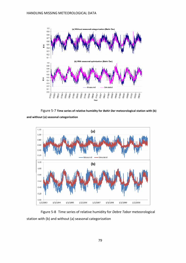
HANDLING MISSING METEOROLOGICAL DATA
79
Figure 5-7 Time series of relative humidity for Bahir Dar meteorological station with (b)
and without (a) seasonal categorization
Figure 5-8 Time series of relative humidity for Debre Tabor meteorological
station with (b) and without (a) seasonal categorization
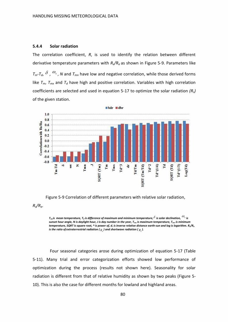
HANDLING MISSING METEOROLOGICAL DATA
80
5.4.4 Solar radiation
The correlation coefficient, R, is used to identify the relation between different
derivative temperature parameters with Rs/Ra as shown in Figure 5-9. Parameters like
Tm-Td, , , N and Tmn have low and negative correlation, while those derived forms
like Tm, Tmx and Td have high and positive correlation. Variables with high correlation
coefficients are selected and used in equation 5-17 to optimize the solar radiation (Rs)
of the given station.
Figure 5-9 Correlation of different parameters with relative solar radiation,
Rs/Ra.
Tm,is mean temperature, Td is difference of maximum and minimum temperature, is solar declination, is sunset hour angle, N is daylight hour, J is day number in the year, Tmx is maximum temperature, Tmn is minimum temperature, SQRT is square root, ^ is power of, dr is inverse relative distance earth-sun and log is logarithm. Rs/Ra
is the ratio of extraterrestrial radiation ( ) and shortwave radiation ( ).
Four seasonal categories arose during optimization of equation 5-17 (Table
5-11). Many trial and error categorization efforts showed low performance of
optimization during the process (results not shown here). Seasonality for solar
radiation is different from that of relative humidity as shown by two peaks (Figure 5-
10). This is also the case for different months for lowland and highland areas.
s
s
aR sR
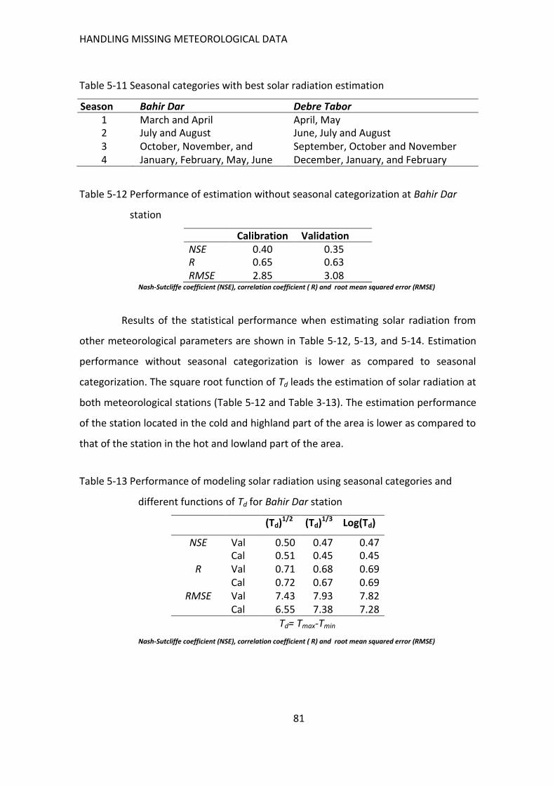
HANDLING MISSING METEOROLOGICAL DATA
81
Table 5-11 Seasonal categories with best solar radiation estimation
Season Bahir Dar Debre Tabor 1 March and April April, May 2 July and August June, July and August 3 October, November, and
December
September, October and November 4 January, February, May, June
and september
December, January, and February
Table 5-12 Performance of estimation without seasonal categorization at Bahir Dar
station
Calibration Validation NSE 0.40 0.35 R 0.65 0.63 RMSE 2.85 3.08
Nash-Sutcliffe coefficient (NSE), correlation coefficient ( R) and root mean squared error (RMSE)
Results of the statistical performance when estimating solar radiation from
other meteorological parameters are shown in Table 5-12, 5-13, and 5-14. Estimation
performance without seasonal categorization is lower as compared to seasonal
categorization. The square root function of Td leads the estimation of solar radiation at
both meteorological stations (Table 5-12 and Table 3-13). The estimation performance
of the station located in the cold and highland part of the area is lower as compared to
that of the station in the hot and lowland part of the area.
Table 5-13 Performance of modeling solar radiation using seasonal categories and
different functions of Td for Bahir Dar station
(Td)1/2 (Td)1/3 Log(Td)
NSE Val 0.50 0.47 0.47 Cal 0.51 0.45 0.45
R Val 0.71 0.68 0.69 Cal 0.72 0.67 0.69
RMSE Val 7.43 7.93 7.82 Cal 6.55 7.38 7.28
Td= Tmax-Tmin
Nash-Sutcliffe coefficient (NSE), correlation coefficient ( R) and root mean squared error (RMSE)
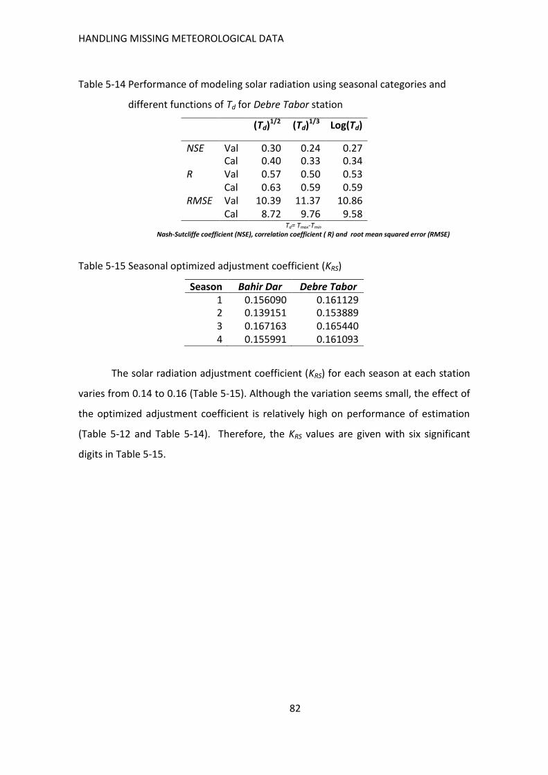
HANDLING MISSING METEOROLOGICAL DATA
82
Table 5-14 Performance of modeling solar radiation using seasonal categories and
different functions of Td for Debre Tabor station
(Td)1/2 (Td)1/3 Log(Td)
NSE Val 0.30 0.24 0.27 Cal 0.40 0.33 0.34
R Val 0.57 0.50 0.53 Cal 0.63 0.59 0.59
RMSE Val 10.39 11.37 10.86 Cal 8.72 9.76 9.58
Td= Tmax-Tmin Nash-Sutcliffe coefficient (NSE), correlation coefficient ( R) and root mean squared error (RMSE)
Table 5-15 Seasonal optimized adjustment coefficient (KRS)
Season Bahir Dar Debre Tabor 1 0.156090 0.161129 2 0.139151 0.153889 3 0.167163 0.165440 4 0.155991 0.161093
The solar radiation adjustment coefficient (KRS) for each season at each station
varies from 0.14 to 0.16 (Table 5-15). Although the variation seems small, the effect of
the optimized adjustment coefficient is relatively high on performance of estimation
(Table 5-12 and Table 5-14). Therefore, the KRS values are given with six significant
digits in Table 5-15.
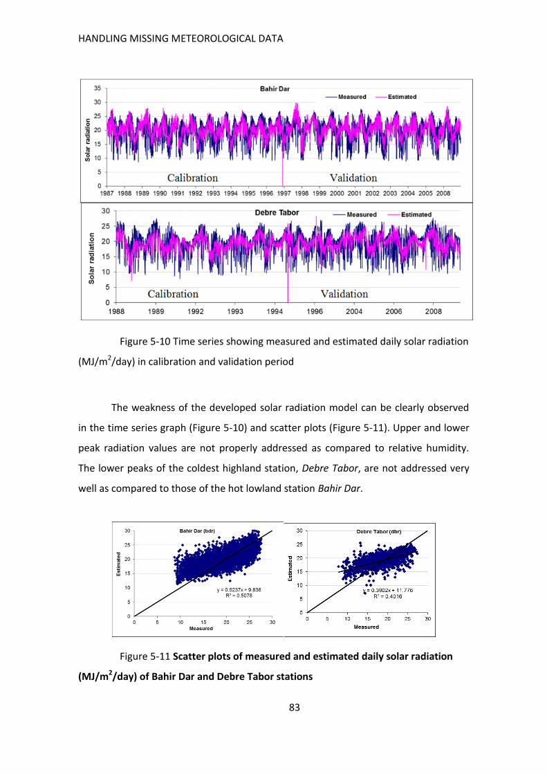
HANDLING MISSING METEOROLOGICAL DATA
83
Figure 5-10 Time series showing measured and estimated daily solar radiation
(MJ/m2/day) in calibration and validation period
The weakness of the developed solar radiation model can be clearly observed
in the time series graph (Figure 5-10) and scatter plots (Figure 5-11). Upper and lower
peak radiation values are not properly addressed as compared to relative humidity.
The lower peaks of the coldest highland station, Debre Tabor, are not addressed very
well as compared to those of the hot lowland station Bahir Dar.
Figure 5-11 Scatter plots of measured and estimated daily solar radiation
(MJ/m2/day) of Bahir Dar and Debre Tabor stations
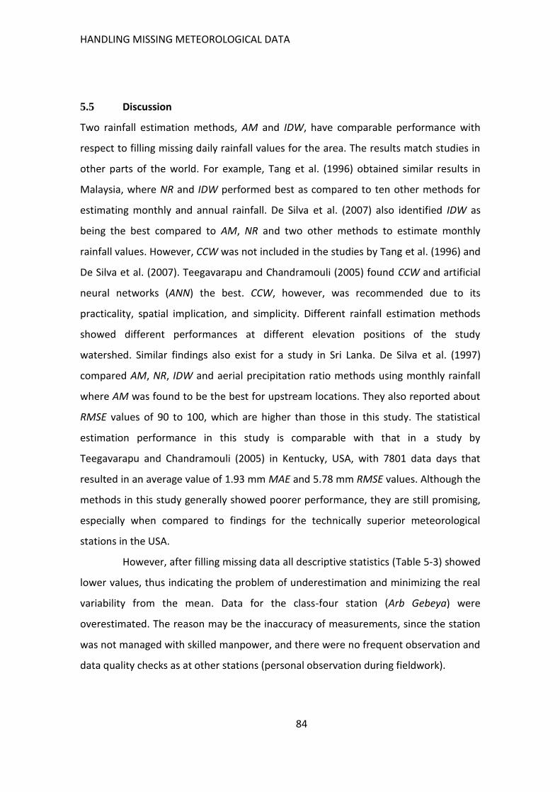
HANDLING MISSING METEOROLOGICAL DATA
84
5.5 Discussion
Two rainfall estimation methods, AM and IDW, have comparable performance with
respect to filling missing daily rainfall values for the area. The results match studies in
other parts of the world. For example, Tang et al. (1996) obtained similar results in
Malaysia, where NR and IDW performed best as compared to ten other methods for
estimating monthly and annual rainfall. De Silva et al. (2007) also identified IDW as
being the best compared to AM, NR and two other methods to estimate monthly
rainfall values. However, CCW was not included in the studies by Tang et al. (1996) and
De Silva et al. (2007). Teegavarapu and Chandramouli (2005) found CCW and artificial
neural networks (ANN) the best. CCW, however, was recommended due to its
practicality, spatial implication, and simplicity. Different rainfall estimation methods
showed different performances at different elevation positions of the study
watershed. Similar findings also exist for a study in Sri Lanka. De Silva et al. (1997)
compared AM, NR, IDW and aerial precipitation ratio methods using monthly rainfall
where AM was found to be the best for upstream locations. They also reported about
RMSE values of 90 to 100, which are higher than those in this study. The statistical
estimation performance in this study is comparable with that in a study by
Teegavarapu and Chandramouli (2005) in Kentucky, USA, with 7801 data days that
resulted in an average value of 1.93 mm MAE and 5.78 mm RMSE values. Although the
methods in this study generally showed poorer performance, they are still promising,
especially when compared to findings for the technically superior meteorological
stations in the USA.
However, after filling missing data all descriptive statistics (Table 5-3) showed
lower values, thus indicating the problem of underestimation and minimizing the real
variability from the mean. Data for the class-four station (Arb Gebeya) were
overestimated. The reason may be the inaccuracy of measurements, since the station
was not managed with skilled manpower, and there were no frequent observation and
data quality checks as at other stations (personal observation during fieldwork).
HANDLING MISSING METEOROLOGICAL DATA
85
The relationship between maximum and minimum temperature shows
negative and low correlation. That means that very hot days have very cold nights. This
extreme fluctuation has impacts on agricultural productivity, since plants need a
smooth shift from hot to cold temperature events (Zinn et al. 2010). The performance
when estimating daily minimum temperatures is poorer than that for daily maximum
temperatures. This is due to the fact that minimum temperatures are highly locally
variable, which resulted in low correlation with respect to neighboring station.
Kotsiantis et al. (2006) used temperature data of previous years of a given station to fill
missing data of a given year of the same station using the regression equation. The
correlation coefficient of 0.9 between estimated and measured air temperature is
comparable with the estimation of maximum daily air temperature in this study.
Maximum and minimum temperatures are used to estimate relative humidity
and solar radiation. Seasonal categorization improves estimation performance for
relative humidity better than for solar radiation. The dew-point temperature
adjustment coefficient varies greatly when compared to the adjustment coefficient for
solar radiation.
Measured solar radiation values vary for successive days especially at the lower
peak value days as compared to relative humidity. Therefore, the performance of the
temperature-based solar radiation estimation method is poorer than for relative
humidity. Low peak values occurred during the main rainy season where there is a high
cloud cover. This indicates that other variables like occurrence of cloud may be
important together with daily temperature values to estimate solar radiation. On the
other hand, higher peaks during the clear-sky dry seasons are underestimated.
Calibration using hourly time-scale measured data may improve addressing the peaks.
of a given day is better for the estimation of daily solar radiation than
other temperature derivatives as equated by Hargreaves and Samani (1982) for the
study area. However, these authors produce the same adjustment coefficient
throughout the year in the relationship between and / . Morid et al.
(2002) derived the adjustment coefficient using maximum and minimum temperature
minmax TT
minmax TT aR sR
HANDLING MISSING METEOROLOGICAL DATA
86
at an alpine catchment in Iran, and the resulting 0.16 is within the range of the value in
this study.
5.6 Conclusions
Different approaches and methods were used to estimate missing daily meteorological
variables, i.e., rainfall, maximum temperature, minimum temperature, relative
humidity and solar radiation. Data from nine stations that ranged from 5 to 22 years
coverage were used to compare spatial daily rainfall estimation methods at the
headwater of the Blue Nile basin in Ethiopia. The statistical performance of the
estimation methods showed results comparable with other similar studies done
elsewhere. The methods arithmetic mean (AM) and coefficient of correlation
weighting (CCW) provided better daily rainfall estimation than normal ratio (NR) and
inverse distance weighting (IDW) in most of the stations. Different estimation methods
performed best for different locations of the meteorological stations with respect to
elevation. AM performed best for stations at downstream locations, while CCW was
best at upstream locations.
It is very important to establish additional representative meteorological
stations so that interpolation and extrapolation of measured relative humidity and
solar radiation values are possible using the methods discussed above. The estimation
of relative humidity and solar radiation values using air temperature data from several
stations as in this study is promising when compared to estimations using data from
only two meteorological stations for local water management planning.
Further research is recommended that includes more stations and a larger
area cover for better water resources management. Altitude can be included as one
factor if more meteorological stations at different elevation are considered for better
performance with respect to filling missing data. This methodology will help to make
stations with low quality and quantity databases suitable for water resources
management of the area, as these stations have been excluded under the existing
water development. The importance of using every database in the area can be
evaluated further regarding efficiency of hydrological models.
EFFECT OF CLIMATE STATION DENSITY AND POTENTIAL EVAPOTRANSPIRATION
CALCULATION METHODS ON WATER BALANCE MODELING
87
6 EFFECT OF CLIMATE STATION DENSITY AND POTENTIAL
EVAPOTRANSPIRATION CALCULATION METHODS ON WATER BALANCE
MODELING
6.1 Summary
Water balance modeling increases our understanding to make decisions on using
water resources effectively and sustainably. However, hydrological modeling needs a
meteorological database with reliable time series. Obtaining reliable data for these
meteorological variables is difficult at spatial and temporal scales in developing
countries. Therefore, it is of utmost importance to study the effect of data availability
on hydrological modeling to be able to quantify uncertainty caused by boundary
conditions. Different modeling setups were used for the Soil and Water Assessment
Tool (SWAT) to quantify the performance of the water balance simulation. They
considered meteorological station density, different methods for calculating potential
evapotranspiration (PET) (Penman-Monteith and Hargreaves) and different
approaches for handling missing data. Penman-Monteith and Hargreaves PET
calculation methods gave comparable river flow modeling performance. Modeling
using six and four stations gave better performance concerning the water balance
patterns as compared to using two stations. It is important to have a minimum density
of meteorological stations in the mountainous highland parts of the Blue Nile to
manage the water resources at micro- and meso-watershed scales.
6.2 Introduction
Spatially distributed meteorological variables are highly important for hydrological
modeling and design of water resources projects. Rainfall is the major driving force for
runoff and solute transport as compared to the other meteorological variables (Cho et
al. 2009; Bormann et al. 1999). Gassman et al. (2007) reviewed previous SWAT
applications and identified inadequate representation of meteorological input
variables, especially rainfall. The representation can be inadequate due to lack of rain
gauges in the watershed or due to a sub-watershed configuration that is too coarse to

EFFECT OF CLIMATE STATION DENSITY AND POTENTIAL EVAPOTRANSPIRATION
CALCULATION METHODS ON WATER BALANCE MODELING
88
capture all spatially distributed stations. This inadequacy caused weak or incorrect
hydrological simulation results.
Some studies investigated the effects of spatial resolutions of input data on the
accuracy of hydrological modeling (Chaplot et al. 2005; Chaubey et al. 2005; Wang and
Melesse, 2006; Cho et al. 2009). Cho et al. (2009) performed a study on the effect of
spatially variable rainfall data on the uncertainty of SWAT output. SWAT takes climate
input data that is nearest to each sub-watershed centroid (Neitsch et al. 2002).
Therefore, the SWAT algorithm causes a sharp difference in rainfall and other water
balance components at the boundary of each sub-watershed.
River master plans, irrigation and hydropower projects have been developed
and implemented throughout Ethiopia to reduce poverty and to mitigate climatic
change effects. These water development projects need accurate hydrometeorological
analysis methodology and tools. In many countries, not only is the station density too
low and the period of measurements too short but data is also missing due to the
effect of device failure during the collection of climate data. The missing values affect
environmental time series (Presti et al. 2010) and hydrological modeling. Inconsistent
and biased hydrologic analysis and conclusions in water resources development
planning are the result of missing data (Kim and Ahn 2009). Missing values have to be
filled before using the data for further investigations.
Hydrological modeling is crucial for planning water development activities as
well as for controlling and implementing water use during and after implementation of
the projects. Previous studies in the study area used coarse databases, so that
evaluation of the results at the local scale, e.g., the Gumara watershed, is very difficult.
For example, Setegn et al. (2008) used only five stations for the 15,000 km2 Lake Tana
Basin; Gumara watershed is one of its sub-basins. This means that station density is
one station for an area of 3,000 km2. For planning irrigation water requirement and for
flood frequency analysis for the Gumara irrigation project (GIP), the MoWR (Ministry
of Water Resources of Ethiopia, 2008) use data from a station located 50 km away
(Bahir Dar). This may create discrepancies, since the physical status of the area of
interest (dam catchment of GIP) is different from that of the total catchment.
EFFECT OF CLIMATE STATION DENSITY AND POTENTIAL EVAPOTRANSPIRATION
CALCULATION METHODS ON WATER BALANCE MODELING
89
In this chapter, the effects of different setups in water balance modeling using SWAT
hydrological models are compared for the following objectives.
6.3 Objectives
The general objective is to calibrate the SWAT model for the Gumara watershed in the
Blue Nile Basin. This is guided by the following specific objectives:
1. To identify the effect of the meteorological station density on the water balance
modeling of the watershed.
2. To evaluate the effect of Penman-Monteith and Hargreaves potential
evapotranspiration methods on model performance.
3. To identify the effect of methods for filling missing spatial and temporal data on
SWAT modeling results.
6.4 Materials and methods
6.4.1 Description of the study area
The study was performed in the Gumara watershed in the Blue Nile Basin of Ethiopia.
It covers 1,360 km2, and is located between 37˚38' to 38˚ 11' E and 11˚ 35' to 11˚ 54' N
(Figure 2-1). Gumara River is one of the rivers draining to Lake Tana (Kebede, 2006),
which is one of the largest water bodies in Africa. The lake receives 93% of drained
water from four main rivers: Gilgel-Abbay, Reb, Gumara and Megetch (Kebede 2006;
Vijverberg et al. 2009). The climate is tropical highland monsoon where the seasonal
rain distribution is dominated by the movement of the inter-tropical convergence zone
(ITCZ) and by moist air from the Atlantic and Indian Ocean in the summer (June-
September) (Kebede 2006). The mean annual rainfall and mean temperature is 1400
mm and 20°C, respectively. The study area is characterized by a mixed crop-livestock
farming system with rice-based cash crops, maize, small cereals and cereal-pulse
(Haileslassie et al. 2009a).
EFFECT OF CLIMATE STATION DENSITY AND POTENTIAL EVAPOTRANSPIRATION
CALCULATION METHODS ON WATER BALANCE MODELING
90
6.4.2 Database development
SWAT needs spatially distributed data, i.e., digital elevation model (DEM), land-use,
soil and meteorological data (rainfall, temperature, relative humidity, solar radiation
and wind speed). These data were collected and checked for consistency before SWAT
modeling was applied.
The 30-m resolution Global Digital Elevation Model (GDEM) was downloaded
free from http://asterweb.jpl.nasa.gov/gdem.asp (Advanced Spaceborne Thermal
Emission and Reflection Radiometer (ASTER)). This DEM was used for watershed and
sub-watershed delineation, reach identification and slope-class categorization. The
land-use map and stream network data of the watershed were taken from the MoWR
database that was organized for the feasibility study of the Gumara irrigation project
(GIP). The data were checked using ground control points data that had been collected
during field observations in different seasons in 2009 and 2010.
Soil physical and chemical data at each soil unit and soil depth layer are
important spatial data for modeling hydrological balance components in SWAT. It was
difficult to obtain all soil data in Ethiopia, and different soil databases were used in this
study. The MoWR did a detailed soil survey study for the downstream side of Gumara
watershed (MoWR 2008) for the GIP feasibility study. This recent soil database was
used to fill most of soil physical and chemical properties in the watershed. Soil texture
and soil layer data were taken from the Abbay River Basin Integrated Development
Master Plan Project (ARBIDMPP) database of the MoWR, who had performed a semi-
detailed soil survey in the Blue Nile Basin (BCOM 1998). Figure 6-1 shows the DEM, soil
and land-use database maps.
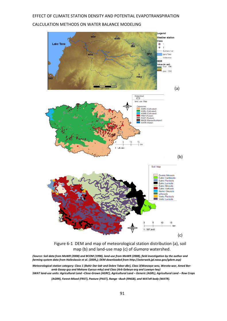
EFFECT OF CLIMATE STATION DENSITY AND POTENTIAL EVAPOTRANSPIRATION
CALCULATION METHODS ON WATER BALANCE MODELING
91
(a)
(b)
(c)
Figure 6-1 DEM and map of meteorological station distribution (a), soil map (b) and land-use map (c) of Gumara watershed.
(Source: Soil data from MoWR (2008) and BCOM (1998), land-use from MoWR (2008), field investigation by the author and farming system data from Haileslassie et al. (2009a); DEM downloaded from http://asterweb.jpl.nasa.gov/gdem.asp)
Meteorological station category: Class 1 (Bahir Dar-bdr and Debre Tabor-dbr), Class 3(Wanzaye-wnz, Werota-wor, Amed Ber-amb Gasay-gsy and Mekane Eyesus-mky) and Class (Arb Gebeya-arg and Luwaye-lwy)
SWAT land-use units: Agricultural Land –Close-Grown (AGRC), Agricultural Land – Generic (AGRL), Agricultural Land – Row Crops
(AGRR), Forest-Mixed (FRST), Pasture (PAST), Range –Bush (RNGB), and WATeR body (WATR).
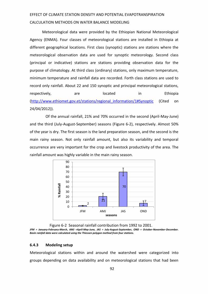
EFFECT OF CLIMATE STATION DENSITY AND POTENTIAL EVAPOTRANSPIRATION
CALCULATION METHODS ON WATER BALANCE MODELING
92
Meteorological data were provided by the Ethiopian National Meteorological
Agency (ENMA). Four classes of meteorological stations are installed in Ethiopia at
different geographical locations. First class (synoptic) stations are stations where the
meteorological observation data are used for synoptic meteorology. Second class
(principal or indicative) stations are stations providing observation data for the
purpose of climatology. At third class (ordinary) stations, only maximum temperature,
minimum temperature and rainfall data are recorded. Forth class stations are used to
record only rainfall. About 22 and 150 synoptic and principal meteorological stations,
respectively, are located in Ethiopia
(http://www.ethiomet.gov.et/stations/regional_information/1#Synoptic (Cited on
24/04/2012)).
Of the annual rainfall, 21% and 70% occurred in the second (April-May-June)
and the third (July-August-September) seasons (Figure 6-2), respectively. Almost 50%
of the year is dry. The first season is the land preparation season, and the second is the
main rainy season. Not only rainfall amount, but also its variability and temporal
occurrence are very important for the crop and livestock productivity of the area. The
rainfall amount was highly variable in the main rainy season.
Figure 6-2 Seasonal rainfall contribution from 1992 to 2001. JFM = January-February-March, AMJ =April-May-June, JAS = July-August-September, OND = October-November-December. Basin rainfall data were calculated using the Thiessen polygon method from four stations.
6.4.3 Modeling setup
Meteorological stations within and around the watershed were categorized into
groups depending on data availability and on meteorological stations that had been
2 21
70
7
0
10
20
30
40
50
60
70
80
90
JFM AMJ JAS OND
% R
ain
fall
seasons
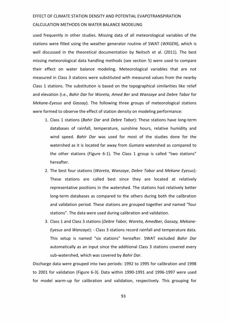
EFFECT OF CLIMATE STATION DENSITY AND POTENTIAL EVAPOTRANSPIRATION
CALCULATION METHODS ON WATER BALANCE MODELING
93
used frequently in other studies. Missing data of all meteorological variables of the
stations were filled using the weather generator routine of SWAT (WXGEN), which is
well discussed in the theoretical documentation by Neitsch et al. (2011). The best
missing meteorological data handling methods (see section 5) were used to compare
their effect on water balance modeling. Meteorological variables that are not
measured in Class 3 stations were substituted with measured values from the nearby
Class 1 stations. The substitution is based on the topographical similarities like relief
and elevation (i.e., Bahir Dar for Woreta, Amed Ber and Wanzaye and Debre Tabor for
Mekane-Eyesus and Gassay). The following three groups of meteorological stations
were formed to observe the effect of station density on modeling performance:
1. Class 1 stations (Bahir Dar and Debre Tabor): These stations have long-term
databases of rainfall, temperature, sunshine hours, relative humidity and
wind speed. Bahir Dar was used for most of the studies done for the
watershed as it is located far away from Gumara watershed as compared to
the other stations (Figure 6-1). The Class 1 group is called “two stations”
hereafter.
2. The best four stations (Woreta, Wanzaye, Debre Tabor and Mekane Eyesus):
These stations are called best since they are located at relatively
representative positions in the watershed. The stations had relatively better
long-term databases as compared to the others during both the calibration
and validation period. These stations are grouped together and named “four
stations”. The data were used during calibration and validation.
3. Class 1 and Class 3 stations (Debre Tabor, Woreta, Amedber, Gassay, Mekane-
Eyesus and Wanzaye): - Class 3 stations record rainfall and temperature data.
This setup is named “six stations” hereafter. SWAT excluded Bahir Dar
automatically as an input since the additional Class 3 stations covered every
sub-watershed, which was covered by Bahir Dar.
Discharge data were grouped into two periods: 1992 to 1995 for calibration and 1998
to 2001 for validation (Figure 6-3). Data within 1990-1991 and 1996-1997 were used
for model warm-up for calibration and validation, respectively. This grouping for
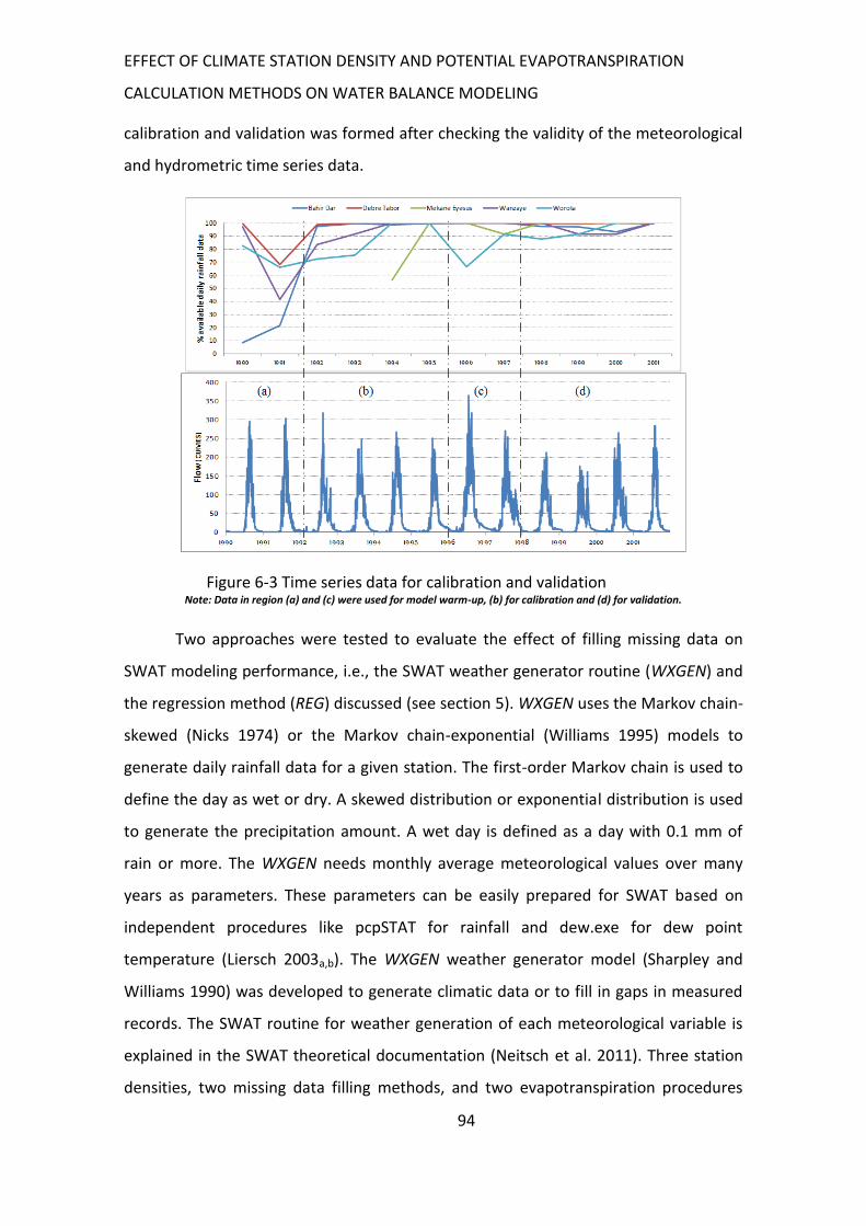
EFFECT OF CLIMATE STATION DENSITY AND POTENTIAL EVAPOTRANSPIRATION
CALCULATION METHODS ON WATER BALANCE MODELING
94
calibration and validation was formed after checking the validity of the meteorological
and hydrometric time series data.
Figure 6-3 Time series data for calibration and validation Note: Data in region (a) and (c) were used for model warm-up, (b) for calibration and (d) for validation.
Two approaches were tested to evaluate the effect of filling missing data on
SWAT modeling performance, i.e., the SWAT weather generator routine (WXGEN) and
the regression method (REG) discussed (see section 5). WXGEN uses the Markov chain-
skewed (Nicks 1974) or the Markov chain-exponential (Williams 1995) models to
generate daily rainfall data for a given station. The first-order Markov chain is used to
define the day as wet or dry. A skewed distribution or exponential distribution is used
to generate the precipitation amount. A wet day is defined as a day with 0.1 mm of
rain or more. The WXGEN needs monthly average meteorological values over many
years as parameters. These parameters can be easily prepared for SWAT based on
independent procedures like pcpSTAT for rainfall and dew.exe for dew point
temperature (Liersch 2003a,b). The WXGEN weather generator model (Sharpley and
Williams 1990) was developed to generate climatic data or to fill in gaps in measured
records. The SWAT routine for weather generation of each meteorological variable is
explained in the SWAT theoretical documentation (Neitsch et al. 2011). Three station
densities, two missing data filling methods, and two evapotranspiration procedures
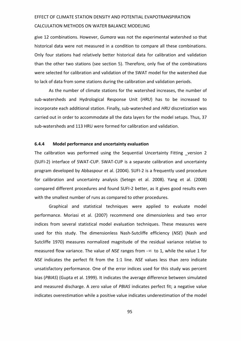
EFFECT OF CLIMATE STATION DENSITY AND POTENTIAL EVAPOTRANSPIRATION
CALCULATION METHODS ON WATER BALANCE MODELING
95
give 12 combinations. However, Gumara was not the experimental watershed so that
historical data were not measured in a condition to compare all these combinations.
Only four stations had relatively better historical data for calibration and validation
than the other two stations (see section 5). Therefore, only five of the combinations
were selected for calibration and validation of the SWAT model for the watershed due
to lack of data from some stations during the calibration and validation periods.
As the number of climate stations for the watershed increases, the number of
sub-watersheds and Hydrological Response Unit (HRU) has to be increased to
incorporate each additional station. Finally, sub-watershed and HRU discretization was
carried out in order to accommodate all the data layers for the model setups. Thus, 37
sub-watersheds and 113 HRU were formed for calibration and validation.
6.4.4 Model performance and uncertainty evaluation
The calibration was performed using the Sequential Uncertainty Fitting _version 2
(SUFI-2) interface of SWAT-CUP. SWAT-CUP is a separate calibration and uncertainty
program developed by Abbaspour et al. (2004). SUFI-2 is a frequently used procedure
for calibration and uncertainty analysis (Setegn et al. 2008). Yang et al. (2008)
compared different procedures and found SUFI-2 better, as it gives good results even
with the smallest number of runs as compared to other procedures.
Graphical and statistical techniques were applied to evaluate model
performance. Moriasi et al. (2007) recommend one dimensionless and two error
indices from several statistical model evaluation techniques. These measures were
used for this study. The dimensionless Nash-Sutcliffe efficiency (NSE) (Nash and
Sutcliffe 1970) measures normalized magnitude of the residual variance relative to
measured flow variance. The value of NSE ranges from - to 1, while the value 1 for
NSE indicates the perfect fit from the 1:1 line. NSE values less than zero indicate
unsatisfactory performance. One of the error indices used for this study was percent
bias (PBIAS) (Gupta et al. 1999). It indicates the average difference between simulated
and measured discharge. A zero value of PBIAS indicates perfect fit; a negative value
indicates overestimation while a positive value indicates underestimation of the model
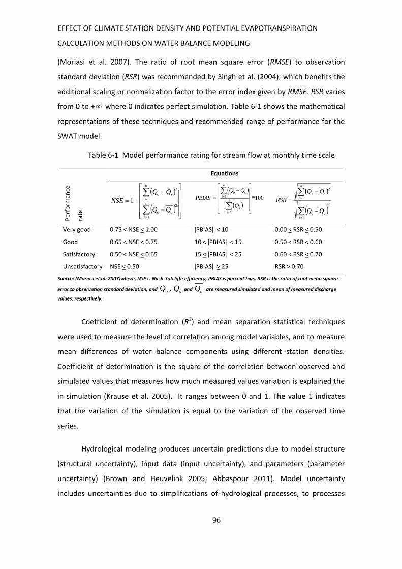
EFFECT OF CLIMATE STATION DENSITY AND POTENTIAL EVAPOTRANSPIRATION
CALCULATION METHODS ON WATER BALANCE MODELING
96
(Moriasi et al. 2007). The ratio of root mean square error (RMSE) to observation
standard deviation (RSR) was recommended by Singh et al. (2004), which benefits the
additional scaling or normalization factor to the error index given by RMSE. RSR varies
from 0 to + where 0 indicates perfect simulation. Table 6-1 shows the mathematical
representations of these techniques and recommended range of performance for the
SWAT model.
Table 6-1 Model performance rating for stream flow at monthly time scale
Per
form
ance
rate
Equations
Very good 0.75 < NSE < 1.00 ǀPBIASǀ < 10 0.00 < RSR < 0.50
Good 0.65 < NSE < 0.75 10 < ǀPBIASǀ < 15 0.50 < RSR < 0.60
Satisfactory 0.50 < NSE < 0.65 15 < ǀPBIASǀ < 25 0.60 < RSR < 0.70
Unsatisfactory NSE < 0.50 ǀPBIASǀ > 25 RSR > 0.70
Source: (Moriasi et al. 2007)where, NSE is Nash-Sutcliffe efficiency, PBIAS is percent bias, RSR is the ratio of root mean square
error to observation standard deviation, and , and are measured simulated and mean of measured discharge
values, respectively.
Coefficient of determination (R2) and mean separation statistical techniques
were used to measure the level of correlation among model variables, and to measure
mean differences of water balance components using different station densities.
Coefficient of determination is the square of the correlation between observed and
simulated values that measures how much measured values variation is explained the
in simulation (Krause et al. 2005). It ranges between 0 and 1. The value 1 indicates
that the variation of the simulation is equal to the variation of the observed time
series.
Hydrological modeling produces uncertain predictions due to model structure
(structural uncertainty), input data (input uncertainty), and parameters (parameter
uncertainty) (Brown and Heuvelink 2005; Abbaspour 2011). Model uncertainty
includes uncertainties due to simplifications of hydrological processes, to processes
n
i
oo
n
i
so
NSE
1
2
1
2
1
100*
1
1
n
i
o
n
i
so
Q
PBIAS
2
1
1
2
n
i
oo
n
i
so
RSR
oQ sQ oQ
EFFECT OF CLIMATE STATION DENSITY AND POTENTIAL EVAPOTRANSPIRATION
CALCULATION METHODS ON WATER BALANCE MODELING
97
occurring in the watershed but not included in the model, to processes that are
included in the model where their occurrences in the watershed are unknown to the
modeler, and to processes unknown to the modeler and not included in the model.
Input uncertainty is uncertainty due to errors in input data such as rainfall, like
extension of point data to large areas in distributed models. Parameter uncertainty is
uncertainty caused by inherent non-uniqueness of parameters in inverse modeling.
Due to the uncertainty that reflects in hydrological processes, parameters can
compensate each other giving many sets of parameters that produce the same output
signal. The occurrence of such sets of parameter non-uniqueness is known as
equifinality (Beven and Freer 2001). More details of these prediction uncertainty
sources are given by Abbaspour (2011).
SUFI-2 accounts for all the three sources of prediction uncertainties. Two
uncertainty measures, i.e., p-factor and r-factor, are used in SUFI-2 (Abbaspour 2011).
The p-factor measures the percentage of observations within 2.5% and 97.5%
percentiles, or 95% of prediction uncertainty (95PPU). The percentage of observation
captured (bracketed) by 95PPU measures the strength of the calibration. The higher
the percent of observations bracketed by 95PPU the more perfect is the model. The r-
factor measures the distance or the thickness of the 95PPU band divided by the
standard deviation of the measured data. The p-factor ranges from 0-100%, while the
r-factor ranges from 0 to . A p-factor of 1 or 100% and r-factor of 0 indicate a perfect
fit of simulation with the measured value. The objective of the uncertainty analysis is
to get a p-factor > 0.5 and r-factor <1.0 (Abbaspour, 2011).
6.5 Results
Data from four stations were used to calibrate SWAT for the PET calculation methods
and missing data filling methods. This is because these stations had better historical
data than the additional two stations in the calibration period. Penman-Monteith and
regression methods gave better discharge simulation than Hargreaves and WXGEN.
Finally, calibration of SWAT for two and six stations was done only using Penman-
Monteith and regression methods to minimize time cost and computer memory.
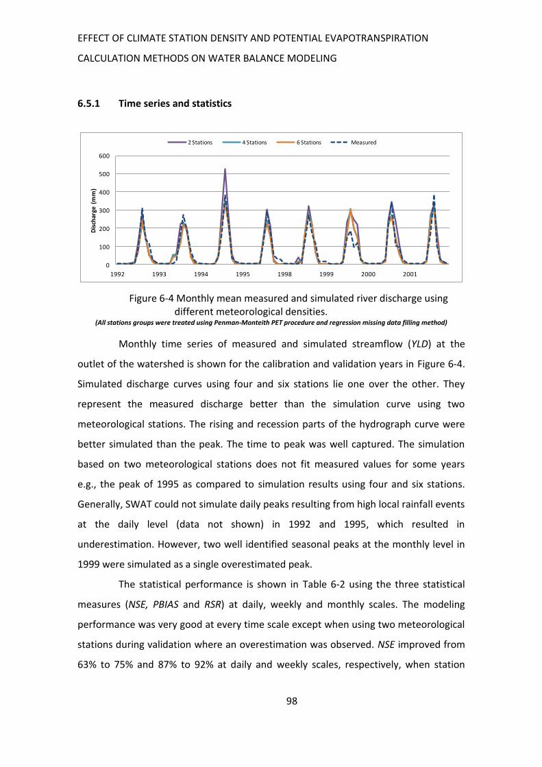
EFFECT OF CLIMATE STATION DENSITY AND POTENTIAL EVAPOTRANSPIRATION
CALCULATION METHODS ON WATER BALANCE MODELING
98
6.5.1 Time series and statistics
Figure 6-4 Monthly mean measured and simulated river discharge using different meteorological densities.
(All stations groups were treated using Penman-Monteith PET procedure and regression missing data filling method)
Monthly time series of measured and simulated streamflow (YLD) at the
outlet of the watershed is shown for the calibration and validation years in Figure 6-4.
Simulated discharge curves using four and six stations lie one over the other. They
represent the measured discharge better than the simulation curve using two
meteorological stations. The rising and recession parts of the hydrograph curve were
better simulated than the peak. The time to peak was well captured. The simulation
based on two meteorological stations does not fit measured values for some years
e.g., the peak of 1995 as compared to simulation results using four and six stations.
Generally, SWAT could not simulate daily peaks resulting from high local rainfall events
at the daily level (data not shown) in 1992 and 1995, which resulted in
underestimation. However, two well identified seasonal peaks at the monthly level in
1999 were simulated as a single overestimated peak.
The statistical performance is shown in Table 6-2 using the three statistical
measures (NSE, PBIAS and RSR) at daily, weekly and monthly scales. The modeling
performance was very good at every time scale except when using two meteorological
stations during validation where an overestimation was observed. NSE improved from
63% to 75% and 87% to 92% at daily and weekly scales, respectively, when station
0
100
200
300
400
500
600
1992 1993 1994 1995 1998 1999 2000 2001
Dis
char
ge (
mm
)
2 Stations 4 Stations 6 Stations Measured
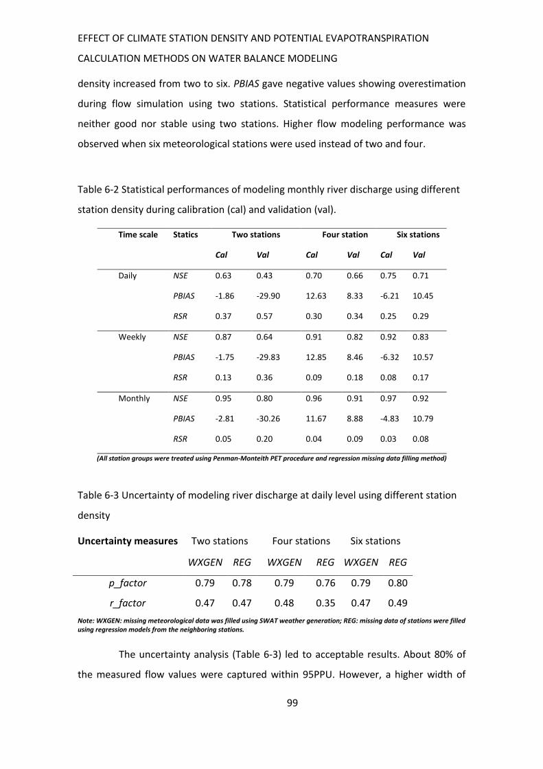
EFFECT OF CLIMATE STATION DENSITY AND POTENTIAL EVAPOTRANSPIRATION
CALCULATION METHODS ON WATER BALANCE MODELING
99
density increased from two to six. PBIAS gave negative values showing overestimation
during flow simulation using two stations. Statistical performance measures were
neither good nor stable using two stations. Higher flow modeling performance was
observed when six meteorological stations were used instead of two and four.
Table 6-2 Statistical performances of modeling monthly river discharge using different
station density during calibration (cal) and validation (val).
Time scale Statics Two stations Four station Six stations
Cal Val Cal Val Cal Val
Daily NSE 0.63 0.43 0.70 0.66 0.75 0.71
PBIAS -1.86 -29.90 12.63 8.33 -6.21 10.45
RSR 0.37 0.57 0.30 0.34 0.25 0.29
Weekly NSE 0.87 0.64 0.91 0.82 0.92 0.83
PBIAS -1.75 -29.83 12.85 8.46 -6.32 10.57
RSR 0.13 0.36 0.09 0.18 0.08 0.17
Monthly NSE 0.95 0.80 0.96 0.91 0.97 0.92
PBIAS -2.81 -30.26 11.67 8.88 -4.83 10.79
RSR 0.05 0.20 0.04 0.09 0.03 0.08
(All station groups were treated using Penman-Monteith PET procedure and regression missing data filling method)
Table 6-3 Uncertainty of modeling river discharge at daily level using different station
density
Uncertainty measures Two stations Four stations Six stations
WXGEN REG WXGEN REG WXGEN REG
p_factor 0.79 0.78 0.79 0.76 0.79 0.80
r_factor 0.47 0.47 0.48 0.35 0.47 0.49
Note: WXGEN: missing meteorological data was filled using SWAT weather generation; REG: missing data of stations were filled using regression models from the neighboring stations.
The uncertainty analysis (Table 6-3) led to acceptable results. About 80% of
the measured flow values were captured within 95PPU. However, a higher width of
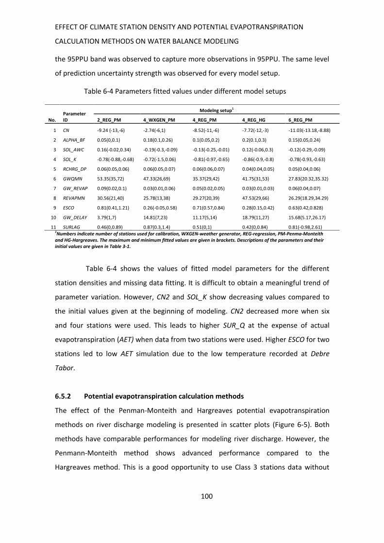
EFFECT OF CLIMATE STATION DENSITY AND POTENTIAL EVAPOTRANSPIRATION
CALCULATION METHODS ON WATER BALANCE MODELING
100
the 95PPU band was observed to capture more observations in 95PPU. The same level
of prediction uncertainty strength was observed for every model setup.
Table 6-4 Parameters fitted values under different model setups
No. Parameter ID
Modelng setup1
2_REG_PM 4_WXGEN_PM 4_REG_PM 4_REG_HG 6_REG_PM
1 CN -9.24 (-13,-6) -2.74(-6,1) -8.52(-11,-6) -7.72(-12,-3) -11.03(-13.18,-8.88)
2 ALPHA_BF 0.05(0,0.1) 0.18(0.1,0.26) 0.1(0.05,0.2) 0.2(0.1,0.3) 0.15(0.05,0.24)
3 SOL_AWC 0.16(-0.02,0.34) -0.19(-0.3,-0.09) -0.13(-0.25,-0.01) 0.12(-0.06,0.3) -0.12(-0.29,-0.09)
4 SOL_K -0.78(-0.88,-0.68) -0.72(-1.5,0.06) -0.81(-0.97,-0.65) -0.86(-0.9,-0.8) -0.78(-0.93,-0.63)
5 RCHRG_DP 0.06(0.05,0.06) 0.06(0.05,0.07) 0.06(0.06,0.07) 0.04(0.04,0.05) 0.05(0.04,0.06)
6 GWQMN 53.35(35,72) 47.33(26,69) 35.37(29,42) 41.75(31,53) 27.83(20.32,35.32)
7 GW_REVAP 0.09(0.02,0.1) 0.03(0.01,0.06) 0.05(0.02,0.05) 0.03(0.01,0.03) 0.06(0.04,0.07)
8 REVAPMN 30.56(21,40) 25.78(13,38) 29.27(20,39) 47.53(29,66) 26.29(18.29,34.29)
9 ESCO 0.81(0.41,1.21) 0.26(-0.05,0.58) 0.71(0.57,0.84) 0.28(0.15,0.42) 0.63(0.42,0.828)
10 GW_DELAY 3.79(1,7) 14.81(7,23) 11.17(5,14) 18.79(11,27) 15.68(5.17,26.17)
11 SURLAG 0.46(0,0.89) 0.87(0.3,1.4) 0.51(0,1) 0.42(0,0.84) 0.81(-0.98,2.61) 1Numbers indicate number of stations used for calibration, WXGEN-weather generator, REG-regression, PM-Penma-Monteith and HG-Hargreaves. The maximum and minimum fitted values are given in brackets. Descriptions of the parameters and their initial values are given in Table 3-1.
Table 6-4 shows the values of fitted model parameters for the different
station densities and missing data fitting. It is difficult to obtain a meaningful trend of
parameter variation. However, CN2 and SOL_K show decreasing values compared to
the initial values given at the beginning of modeling. CN2 decreased more when six
and four stations were used. This leads to higher SUR_Q at the expense of actual
evapotranspiration (AET) when data from two stations were used. Higher ESCO for two
stations led to low AET simulation due to the low temperature recorded at Debre
Tabor.
6.5.2 Potential evapotranspiration calculation methods
The effect of the Penman-Monteith and Hargreaves potential evapotranspiration
methods on river discharge modeling is presented in scatter plots (Figure 6-5). Both
methods have comparable performances for modeling river discharge. However, the
Penmann-Monteith method shows advanced performance compared to the
Hargreaves method. This is a good opportunity to use Class 3 stations data without
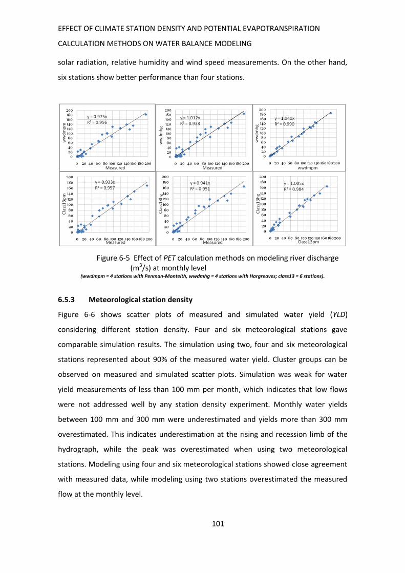
EFFECT OF CLIMATE STATION DENSITY AND POTENTIAL EVAPOTRANSPIRATION
CALCULATION METHODS ON WATER BALANCE MODELING
101
solar radiation, relative humidity and wind speed measurements. On the other hand,
six stations show better performance than four stations.
Figure 6-5 Effect of PET calculation methods on modeling river discharge (m3/s) at monthly level
(wwdmpm = 4 stations with Penman-Monteith, wwdmhg = 4 stations with Hargreaves; class13 = 6 stations).
6.5.3 Meteorological station density
Figure 6-6 shows scatter plots of measured and simulated water yield (YLD)
considering different station density. Four and six meteorological stations gave
comparable simulation results. The simulation using two, four and six meteorological
stations represented about 90% of the measured water yield. Cluster groups can be
observed on measured and simulated scatter plots. Simulation was weak for water
yield measurements of less than 100 mm per month, which indicates that low flows
were not addressed well by any station density experiment. Monthly water yields
between 100 mm and 300 mm were underestimated and yields more than 300 mm
overestimated. This indicates underestimation at the rising and recession limb of the
hydrograph, while the peak was overestimated when using two meteorological
stations. Modeling using four and six meteorological stations showed close agreement
with measured data, while modeling using two stations overestimated the measured
flow at the monthly level.
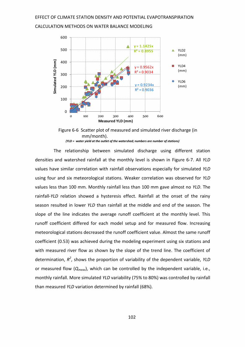
EFFECT OF CLIMATE STATION DENSITY AND POTENTIAL EVAPOTRANSPIRATION
CALCULATION METHODS ON WATER BALANCE MODELING
102
Figure 6-6 Scatter plot of measured and simulated river discharge (in mm/month).
(YLD = water yield at the outlet of the watershed; numbers are number of stations)
The relationship between simulated discharge using different station
densities and watershed rainfall at the monthly level is shown in Figure 6-7. All YLD
values have similar correlation with rainfall observations especially for simulated YLD
using four and six meteorological stations. Weaker correlation was observed for YLD
values less than 100 mm. Monthly rainfall less than 100 mm gave almost no YLD. The
rainfall-YLD relation showed a hysteresis effect. Rainfall at the onset of the rainy
season resulted in lower YLD than rainfall at the middle and end of the season. The
slope of the line indicates the average runoff coefficient at the monthly level. This
runoff coefficient differed for each model setup and for measured flow. Increasing
meteorological stations decreased the runoff coefficient value. Almost the same runoff
coefficient (0.53) was achieved during the modeling experiment using six stations and
with measured river flow as shown by the slope of the trend line. The coefficient of
determination, R2, shows the proportion of variability of the dependent variable, YLD
or measured flow (Qmeas), which can be controlled by the independent variable, i.e.,
monthly rainfall. More simulated YLD variability (75% to 80%) was controlled by rainfall
than measured YLD variation determined by rainfall (68%).
y = 1.1425xR² = 0.8955
y = 0.9562xR² = 0.9034
y = 0.9234xR² = 0.9036
0
100
200
300
400
500
600
0 100 200 300 400 500 600
Sim
ula
ted
YLD
(m
m)
Measured YLD (mm)
YLD2 (mm)
YLD4
(mm)
YLD6
(mm)
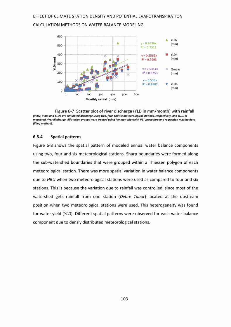
EFFECT OF CLIMATE STATION DENSITY AND POTENTIAL EVAPOTRANSPIRATION
CALCULATION METHODS ON WATER BALANCE MODELING
103
Figure 6-7 Scatter plot of river discharge (YLD in mm/month) with rainfall (YLD2, YLD4 and YLD6 are simulated discharge using two, four and six meteorological stations, respectively, and Qmeas is measured river discharge. All station groups were treated using Penman-Monteith PET procedure and regression missing data filling method).
6.5.4 Spatial patterns
Figure 6-8 shows the spatial pattern of modeled annual water balance components
using two, four and six meteorological stations. Sharp boundaries were formed along
the sub-watershed boundaries that were grouped within a Thiessen polygon of each
meteorological station. There was more spatial variation in water balance components
due to HRU when two meteorological stations were used as compared to four and six
stations. This is because the variation due to rainfall was controlled, since most of the
watershed gets rainfall from one station (Debre Tabor) located at the upstream
position when two meteorological stations were used. This heterogeneity was found
for water yield (YLD). Different spatial patterns were observed for each water balance
component due to densly distributed meteorological stations.
y = 0.6536xR² = 0.7512
y = 0.5565xR² = 0.7993
y = 0.5341xR² = 0.6753
y = 0.533xR² = 0.7802
0
100
200
300
400
500
600
0 100 200 300 400 500 600
YLD
(mm
)
Monthly rainfall (mm)
YLD2 (mm)
YLD4 (mm)
Qmeas (mm)
YLD6 (mm)
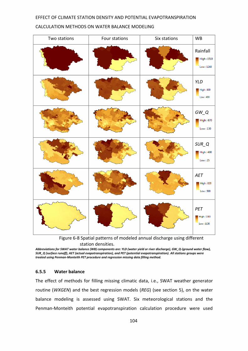
EFFECT OF CLIMATE STATION DENSITY AND POTENTIAL EVAPOTRANSPIRATION
CALCULATION METHODS ON WATER BALANCE MODELING
104
Two stations Four stations Six stations WB
Rainfall
YLD
GW_Q
SUR_Q
AET
PET
Figure 6-8 Spatial patterns of modeled annual discharge using different station densities.
Abbreviations for SWAT water balance (WB) components are: YLD (water yield or river discharge), GW_Q-(ground water flow), SUR_Q (surface runoff), AET (actual evapotranspiration), and PET (potential evapotranspiration). All stations groups were treated using Penman-Monteith PET procedure and regression missing data filling method.
6.5.5 Water balance
The effect of methods for filling missing climatic data, i.e., SWAT weather generator
routine (WXGEN) and the best regression models (REG) (see section 5), on the water
balance modeling is assessed using SWAT. Six meteorological stations and the
Penman-Monteith potential evapotranspiration calculation procedure were used
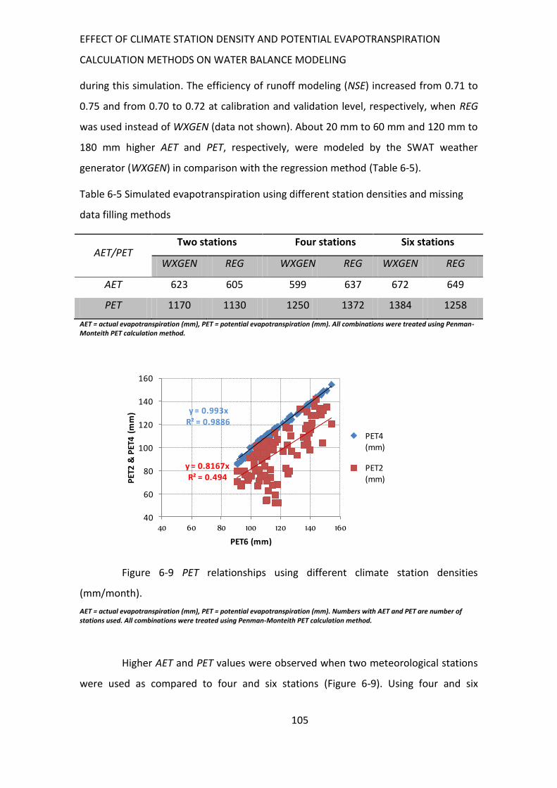
EFFECT OF CLIMATE STATION DENSITY AND POTENTIAL EVAPOTRANSPIRATION
CALCULATION METHODS ON WATER BALANCE MODELING
105
during this simulation. The efficiency of runoff modeling (NSE) increased from 0.71 to
0.75 and from 0.70 to 0.72 at calibration and validation level, respectively, when REG
was used instead of WXGEN (data not shown). About 20 mm to 60 mm and 120 mm to
180 mm higher AET and PET, respectively, were modeled by the SWAT weather
generator (WXGEN) in comparison with the regression method (Table 6-5).
Table 6-5 Simulated evapotranspiration using different station densities and missing
data filling methods
AET/PET Two stations Four stations Six stations
WXGEN REG WXGEN REG WXGEN REG
AET 623 605 599 637 672 649
PET 1170 1130 1250 1372 1384 1258
AET = actual evapotranspiration (mm), PET = potential evapotranspiration (mm). All combinations were treated using Penman-Monteith PET calculation method.
Figure 6-9 PET relationships using different climate station densities
(mm/month).
AET = actual evapotranspiration (mm), PET = potential evapotranspiration (mm). Numbers with AET and PET are number of stations used. All combinations were treated using Penman-Monteith PET calculation method.
Higher AET and PET values were observed when two meteorological stations
were used as compared to four and six stations (Figure 6-9). Using four and six
y = 0.993xR² = 0.9886
y = 0.8167xR² = 0.494
40
60
80
100
120
140
160
40 60 80 100 120 140 160
PET
2 &
PET
4 (
mm
)
PET6 (mm)
PET4 (mm)
PET2 (mm)
EFFECT OF CLIMATE STATION DENSITY AND POTENTIAL EVAPOTRANSPIRATION
CALCULATION METHODS ON WATER BALANCE MODELING
106
meteorological stations gave almost identical values for all months, while PET values
were low when only two meteorological stations were used.
Table 6-6 illustrates the annual water balance modeled using two, four and
six stations. It shows both the average quantity of the water balance components as
well as the statistical significant differences of simulated values at 95% level of
significance. A significant difference was observed for surface runoff (SUR_Q) and
potential evapotranspiration (PET) of the water balance components between
modeled results using two stations and the other station densities. Higher values were
observed for rainfall (RF), surface runoff (SUR_Q), groundwater discharge (GW_Q),
percolation to the soil layers (PERCO) and river discharge (YLD), while lower values
were observed for actual and potential evapotranspiration (AET and PET), respectively,
during simulation using two stations as compared to modeled values using four and six
meteorological stations.
Table 6-6 Annual water balance (mm) using different station densities
Rainfall SUR_Q LAT_Q GW_Q AET PET YLD
Two stations 1,549 326* 86 483 589 1,147
* 759
Four
stations 1,448 261 77 409 655 1,398 738
Six stations 1,433 209 86 419 670 1,408 707
Sig. 0.29 0.00 0.63 0.17 0.08 <0.01 0.85
* The mean difference is significant at the 0.05 level.
RF = rainfall, SUR_Q = surface runoff, LAT_Q = lateral flow, GW_Q = groundwater flow, AET = actual evapotranspiration, PET = potential evapotranspiration, YLD = water yield (all in mm). All combinations were treated using Penman-Monteith PET calculation method.
6.6 Discussion
This study gave better calibration results than other similar studies for the area.
Setegn et al. (2009a) achieved a p-factor of 0.79 and an r-factor of 0.77 for the
Gumara watershed. This indicates that the same percentage of observation in the
present study was captured at 95%PPU within a very wide 95%PPU band in the same
watershed. Setegn et al. (2009a) used only one meteorological station (Debre tabor)
with a coarse sub-watershed discretization, soil data, and 90-m resolution DEM.
Therefore, some prediction uncertainty might originate in uncertain input data. In an
earlier study, Setegn et al. (2008) concluded that the sub-watershed discretization
EFFECT OF CLIMATE STATION DENSITY AND POTENTIAL EVAPOTRANSPIRATION
CALCULATION METHODS ON WATER BALANCE MODELING
107
had a limited impact on flow prediction when only using data from one
meteorological station. However, it was impossible to capture additional
meteorological stations without further fine sub-watershed discretization. Schuol et
al. (2008) studied the water availability at the sub-watershed, country and continental
level for Africa and gained a p-factor from 0.41 to 0.60 and an r-factor from 0.64 to
0.80 for the Blue Nile of Ethiopia at the monthly level, which is a lower performance
than in this study. The reason for the better modeling performance in the present
study may be due to fine meteorological, soil and land-use data. In addition, careful
data screening was carried out on the base runoff-rainfall relation prior to calibration.
In addition to a lower uncertainty obtained in this study, the model efficiency
resulted in a performance level comparable with that of other studies. Setegn et al.
(2008), Asres and Awulachew (2010) and Easton et al. (2010) presented 0.62, 0.76 and
0.87 NSE values for the Gumara watershed, respectively, at the monthly level. All
studies used different approaches for SWAT modeling, which showed poorer
performance than the modeling in this study. In addition to coarse databases used in
the studies, the areas assigned for the watershed were different. Asres and
Awulachew (2010) and Easton et al. (2010) used 1464 km2 and 1286 km2, respectively,
while the area was 1369 km2 in this study. The difference in watershed area might be
from locating the watershed outlet in a different place. Ground control points were
taken to delineate the water divide at the outlet in this study to obtain more accurate
results than in the other studies.
There were two reasons for achieving better modeling performance by using
regression models (REG) rather than by using the SWAT weather generator (WXGEN)
for filling missing data. Firstly, WXGEN could not consider spatial attributes to fill the
missing data of a given station with data from its neighbor. It rather filled the missing
value at a given time from another time data of the same station. Secondly, data were
missing for months and years in the study area so the WXGEN approach could not be
used effectively. Therefore, better modeling performance confirmed the advantage of
using both spatial and temporal regression techniques to fill missing data.

EFFECT OF CLIMATE STATION DENSITY AND POTENTIAL EVAPOTRANSPIRATION
CALCULATION METHODS ON WATER BALANCE MODELING
108
Overestimated stream flow using two meteorological stations might be due to
the higher rainfall observed at the upstream of the watershed (Debre Tabor station)
than at the other stations. Cho et al. (2009) observed the same trend of increasing
simulated stream flow as the level of watershed delineation decreased.
Low modeling performance was observed during low flow situations. This is
because of the weakness of SWAT in addressing soil moisture (saturated excess flow)
for runoff formation. The curve number (CN) routine for calculating runoff only
addresses the infiltration excess runoff (Easton et al. 2010). However, a higher share of
the runoff is generated from the saturated excess rather than from the infiltration
excess in Ethiopian highland watersheds (Derib 2005; Lue et al. 2008; White et al.
2011; Easton et al. 2010). Therefore, most small rainfall events generated different
runoff amounts that varied from 0 to 50 mm.
Different spatial trends of water balance components (with small differences in
statistical modeling performances) were achieved when different station density was
used. Good statistical performance of stream flow modeling at the watershed outlet
using two stations was at the expense of the accuracy of the spatial distribution of the
water balance in the watershed. It is possible to use modeling results with low station
density for runoff management at the outlet of the watershed with relatively better
confidence than water resources management within the watershed. However,
Setegn et al. (2009b), Asres and Awulachew (2010) and Easton et al. (2010) used data
from less than three stations for the Gumara watershed for identifying hotspot areas
of severe soil erosion. Such studies for spatial details need fine spatial data with
distributed hydrological models (Bormann & Diekkrueger 2003). For a detailed
watershed management study, the use of six meteorological stations has shown
better practical significance than the statistical modeling performance presented in
this study.
6.7 Conclusions
In this study, calibration of SWAT with different model setups was performed. The
modeling setups were based on potential evapotranspiration (PET) calculation
EFFECT OF CLIMATE STATION DENSITY AND POTENTIAL EVAPOTRANSPIRATION
CALCULATION METHODS ON WATER BALANCE MODELING
109
methods (Penman-Monteith and Hargreaves), missing data filling methods (WXGEN
and spatial and temporal regression models), and three levels of meteorological
station density (two, four and six stations). Very good modeling performance was
observed with 65% (95%), +5 (+5) and 0.3 (0.06), at daily (monthly) levels for NSE,
PBIAS and RSR, respectively, using Penman-Monteith PET calculation methods and six
stations.
The Hargreaves PET calculation procedure uses only maximum and minimum
daily air temperature, which could be measured at most meteorological stations in the
area. However, the Penman-Monteith procedure also needs solar radiation, relative
humidity and wind speed data, which were hard to find at all climatic stations. The
Hargreaves procedure showed comparable SWAT modeling performance compared to
the Penman-Monteith. Therefore, Hargreaves method can be widely used for future
water resource management by increasing the climate stations that can measure air
temperature and rainfall. It is also possible to use climatic data from Class 3 stations
that have been excluded in past studies. As a recommendation, the Meteorological
Agency of Ethiopia can use elementary schools and health centers that have been
established in every small administration unit (Kebele) of the country to install Class 3
stations. Installation of automatic and manual recording stations can improve data
quality by minimizing personal errors as well as data missing due to failure of
automatic instrumentation.
Missing data handled by the SWAT weather generator (WXGEN) and
regression models using neighboring stations gave comparable modeling performance.
WXGEN gave values of 0.94, 2.5%, 0.07 and regression models 0.96, -5%, 0.05 for NSE,
PBIAS, RSR, respectively, at the monthly level. Regression models led to better
performance than WXGEN. In addition, regression models have a background that is
more practical, since the spatial correlation of climatic variables between stations is
not considered within WXGEN. For further SWAT applications, it is recommended to
incorporate the spatial regression routine.
Meteorological station density played a crucial role in the SWAT hydrological
modeling. Similar statistical modeling performance was observed using two, four and

EFFECT OF CLIMATE STATION DENSITY AND POTENTIAL EVAPOTRANSPIRATION
CALCULATION METHODS ON WATER BALANCE MODELING
110
six meteorological stations for the Gumara watershed in the Blue Nile Basin, Ethiopia.
However, the spatial distribution of the water balance components, which is very
important for water resources management, was very variable. Understanding of
spatial dynamics is very important for decision making regarding water resources in
addition to temporal flow modeling performance at the outlet of a watershed. This
study shows the influence of spatially distributed climatic data on SWAT. Considering
spatially distributed climatic data is crucial under the conditions of the monsoon
climate as in the study area.
WATER BALANCE AND WATER AVAILABILITY UNDER LAND-USE AND LAND
MANAGEMENT SCENARIOS
111
7 WATER BALANCE AND WATER AVAILABILITY UNDER LAND-USE AND LAND
MANAGEMENT SCENARIOS
7.1 Summary
Land-use scenarios were used to identify water flow shift and water availability in the
Gumara watershed, Ethiopia. Basic water requirements in 2001 and 2050 were used to
identify water scarcity at a seasonal level. Results show that watershed management
practices decrease the surface runoff and increase the groundwater flow without
significantly altering the average annual water yield at the outlet of the watershed. The
state of existing rainfed production system will not maintain the basic human and
ecosystem water demands in 2050.
7.2 Introduction
Sufficient quality and quantity of available water is fundamental for life (Jefferies et al.
2012). Accessibility of this resource is affected by the spatial and temporal distribution
of fresh water. About 30% of the world population suffers from lack of water
availability (IWMI 2007) and water scarcity has become one of the main challenges of
life. Population growth is among the expected factors that will increase the level of
water scarcity in the future (Jefferies et al. 2012). The Blue Nile Basin (known as Abbay
in Ethiopia) is the least managed sub-watershed with high and erratic rainfall of 800 to
2,200 mm per year with dry spells that reduce crop yields and sometimes lead to total
crop failure (Erkosa et al. 2009).
Agriculture is the backbone of the economy and the livelihoods of Ethiopia. It
supports about 85% of the population in terms of employment and livelihoods; 50% of
the country’s gross domestic product (GDP) generates about 88% of the export
earnings, and supplies around 73% of the raw material requirements of agriculture-
based domestic industries (MEDaC 1999). However, agriculture in this area is rainfed
and is highly vulnerable to droughts and dry spells, and rainfall productivity is low.
Based on the Agricultural Census Survey of Ethiopia, Diao and Pratt (2007) calculate
that 37% of the rural population lives in food-deficit areas. Water shortage that is
WATER BALANCE AND WATER AVAILABILITY UNDER LAND-USE AND LAND
MANAGEMENT SCENARIOS
112
related to the erratic seasonal rainfall is one of the main sources of this problem. Due
to the rainfall variability and other related factors, the country had to import 0.62
million tons of grain per year during 1995 to 2004 to feed 7 million people. It has made
the country the first food aid recipient in Sub-Saharan Africa (Walker and
Wandschneider 2005). The imported commercial and food aid accounts for 0.3
km3/year virtual water (Hoekstra and Hung 2002).
The government of Ethiopia is, therefore, trying to develop the water
resources, and the Blue Nile Basin is one of the development corridors of the country
(World Bank 2008; McCartney et al. 2010). The Gumara Irrigation Project (GIP) (MoWR
2008) is one of many development activities under feasibility evaluation. Outside the
Gumara watershed, many water resource development studies have been performed
along the Blue Nile Basin for irrigation and hydropower projects, the first one being in
1964 (USBR 1964; WAPCOS 1990; MoWR 1998; MoWR 2008).
Downstream countries have opposed water development in Ethiopia as it
may hamper their ‘historical’ right to use the Nile water. It is not the interest of Egypt
to share the Nile flow with upstream riparian countries especially Ethiopia, as they
assume that Ethiopia has ample green water from rainfall (Arsano 2007). However,
the net green water resource for Ethiopia could not been determined since this water
can be recycled and double counted again through evaporation and cooling process of
the hydrological cycle. In addition, the Ethiopian population is increasing, and drought
occurrence and climate change are becoming an increasing challenge for the existing
rainfed agriculture. Information on water availability and scarcity is limited in Africa
(Wallace and Gregory 2002) especially at meso- and micro-watershed levels and on
seasonal or monthly scales. As explained by Smakhtin et al. (2005) after comparison of
spatial patterns on maps, an increasing number of sub-watersheds show a higher
magnitude of water stress when considering ecosystem water requirements. Schoul et
al. (2008) recommend performing detailed spatially distributed studies for African
countries like Ethiopia.
WATER BALANCE AND WATER AVAILABILITY UNDER LAND-USE AND LAND
MANAGEMENT SCENARIOS
113
This study was carried out on the head water of the Blue Nile to identify the
water availability status in 2001 and 2050 considering the demographic and water
development options.
7.3 Objectives
The objectives of this study were:
1. To model the water balance components in different land-use and
land management scenarios, and
2. To identify the effect of land-use and demographic changes on the
water availability status at seasonal scales.
7.4 Materials and methods
7.4.1 Study area
The study was performed in the Gumara watershed in the Blue Nile Basin of Ethiopia,
which is located at 37˚38' to 38˚ 11' E longitude and 11˚ 35' to 11˚ 54' N latitude
(Figure 2-1). The study focuses on an area of 1520 km2 in the watershed after
calibration on the 1360 km2 gauged part. The watershed is tributary of Lake Tana,
which is considered the source of the Blue Nile. It is located in food-secure districts
(woredas; Fogera, Farta, Dera and Iste (see Section 10-2 or Appendix 2) in the south
Gondor administrative zone (FEWS NET 2008). The watershed is also a food balance
area where the production is similar to the average cereal equivalent production per
household at country level (Diao and Pratt 2007). The climate of the area is of a
tropical highland monsoon type with a single rainy season between June and
September (Alemayehu et al. 2009). The average annual rainfall 1992 to 2001 was
1444 mm. In the middle and upstream parts, the topography is highly rugged and
dissected, while the downstream part is flat with gentle slopes and plain topography.
About 87% of the watershed is intensively cultivated. Rice, tef, maize, wheat and
barley are the main crops grown. Overgrazed bush or shrubland, grassland, and
forest/wood land are other land-cover types (WWDSE 2007). Haplic luvisol, Chromic
luvisol, Lithic leptosol, Eutric vertisol, Eutric fluvisol and Chromic cambisol are the
WATER BALANCE AND WATER AVAILABILITY UNDER LAND-USE AND LAND
MANAGEMENT SCENARIOS
114
common soil types found in the watershed (FAO classification system; Asres and
Awulachew 2010).
7.4.2 SWAT model development
The SWAT model was applied to the Gumara watershed using 1992 to 1995 climate
and hydrometric data for calibration and 1998 to 2001 for validation (see section 6).
Sub-watersheds and hydrological response units (HRU) discretization was based on a
30-m resolution DEM as well as on land-use and soil data. During calibration, 37 sub-
watersheds with 113 HRUs were derived on the 1360 km2 gauged part of the Gumara
watershed. Daily meteorological data from six stations were used. Missing data were
filled using different methods as described (see section 5). The model was fitted very
well for the measured river discharge giving 0.75 Nash-Sutcliffe efficiency (NSE), 6
percent bias (PBIAS), and 0.3 root mean square error (RMSE) to observation standard
deviation (SRS) values (see section 6.5.1). After calibration, scenarios were computed
for the 1520 km2 watershed area using 328 sub-watersheds and 917 HRUs.
7.4.3 Land-use scenario development
Land-use scenario development was done using field survey data of the author in 2008
and 2009, scanned maps from the feasibility study of Gumara Irrigation Project (GIP)
from the library of the Ministry of Water Resources of Ethiopia (MoWR 2008), and
information from the land-use policy of the country. Two additional land-use scenarios
were developed: land-use up to 2008 and land-use planned by the government to be
implemented in the near future (explained further down). Five land-use types were
identified in the watershed, i.e., cultivated land (87% of the area), grazing bush-
rangelands (7%), pasture (4%), mixed forest woodlands (3%) and water (0.09%) (Figure
7-2). Cultivated lands were fine-tuned with respect to three farming systems identified
by Haileslassie et al. (2009a) for SWAT modeling. Small-scale irrigation covered 213.8
ha (0.14% of the watershed) in 2009. The farming systems have different tillage,
planting and harvesting schedules, which were identified during the field surveys in
2008 and 2009.
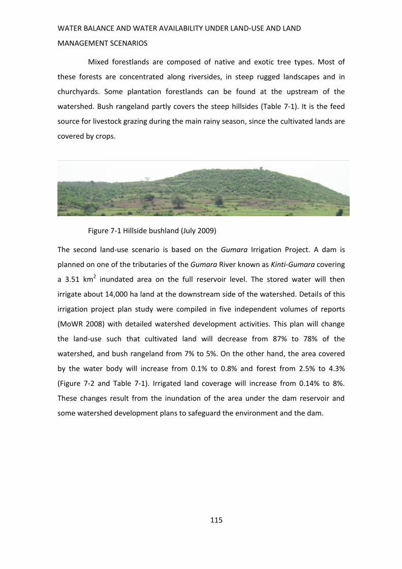
WATER BALANCE AND WATER AVAILABILITY UNDER LAND-USE AND LAND
MANAGEMENT SCENARIOS
115
Mixed forestlands are composed of native and exotic tree types. Most of
these forests are concentrated along riversides, in steep rugged landscapes and in
churchyards. Some plantation forestlands can be found at the upstream of the
watershed. Bush rangeland partly covers the steep hillsides (Table 7-1). It is the feed
source for livestock grazing during the main rainy season, since the cultivated lands are
covered by crops.
Figure 7-1 Hillside bushland (July 2009)
The second land-use scenario is based on the Gumara Irrigation Project. A dam is
planned on one of the tributaries of the Gumara River known as Kinti-Gumara covering
a 3.51 km2 inundated area on the full reservoir level. The stored water will then
irrigate about 14,000 ha land at the downstream side of the watershed. Details of this
irrigation project plan study were compiled in five independent volumes of reports
(MoWR 2008) with detailed watershed development activities. This plan will change
the land-use such that cultivated land will decrease from 87% to 78% of the
watershed, and bush rangeland from 7% to 5%. On the other hand, the area covered
by the water body will increase from 0.1% to 0.8% and forest from 2.5% to 4.3%
(Figure 7-2 and Table 7-1). Irrigated land coverage will increase from 0.14% to 8%.
These changes result from the inundation of the area under the dam reservoir and
some watershed development plans to safeguard the environment and the dam.
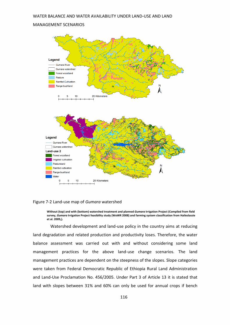
WATER BALANCE AND WATER AVAILABILITY UNDER LAND-USE AND LAND
MANAGEMENT SCENARIOS
116
Figure 7-2 Land-use map of Gumara watershed
Without (top) and with (bottom) watershed treatment and planned Gumara Irrigation Project (Compiled from field survey, Gumara Irrigation Project feasibility study (WoWR 2008) and farming system classification from Haileslassie et al. 2009a).
Watershed development and land-use policy in the country aims at reducing
land degradation and related production and productivity loses. Therefore, the water
balance assessment was carried out with and without considering some land
management practices for the above land-use change scenarios. The land
management practices are dependent on the steepness of the slopes. Slope categories
were taken from Federal Democratic Republic of Ethiopia Rural Land Administration
and Land-Use Proclamation No. 456/2005. Under Part 3 of Article 13 it is stated that
land with slopes between 31% and 60% can only be used for annual crops if bench
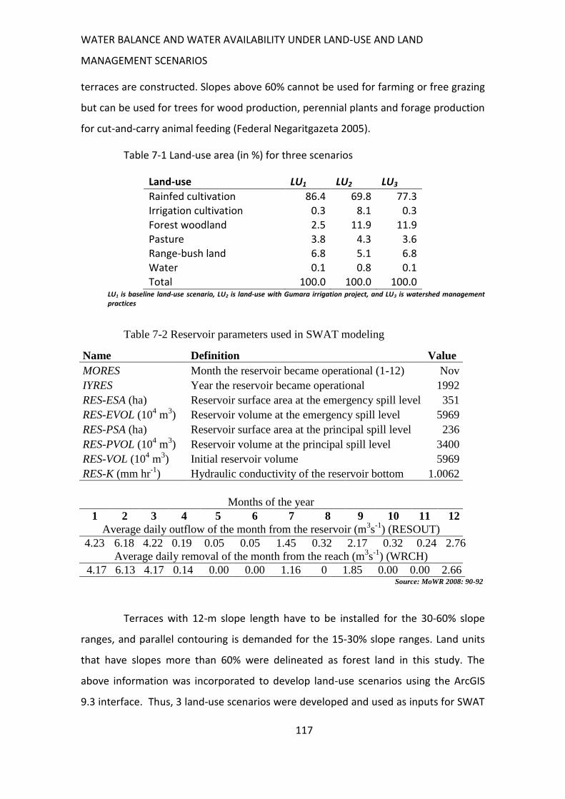
WATER BALANCE AND WATER AVAILABILITY UNDER LAND-USE AND LAND
MANAGEMENT SCENARIOS
117
terraces are constructed. Slopes above 60% cannot be used for farming or free grazing
but can be used for trees for wood production, perennial plants and forage production
for cut-and-carry animal feeding (Federal Negaritgazeta 2005).
Table 7-1 Land-use area (in %) for three scenarios
Land-use LU1 LU2 LU3
Rainfed cultivation 86.4 69.8 77.3 Irrigation cultivation 0.3 8.1 0.3
Forest woodland 2.5 11.9 11.9 Pasture 3.8 4.3 3.6 Range-bush land 6.8 5.1 6.8 Water 0.1 0.8 0.1 Total 100.0 100.0 100.0
LU1 is baseline land-use scenario, LU2 is land-use with Gumara irrigation project, and LU3 is watershed management practices
Table 7-2 Reservoir parameters used in SWAT modeling
Name Definition Value
MORES Month the reservoir became operational (1-12) Nov
IYRES Year the reservoir became operational 1992
RES-ESA (ha) Reservoir surface area at the emergency spill level 351
RES-EVOL (104 m
3) Reservoir volume at the emergency spill level 5969
RES-PSA (ha) Reservoir surface area at the principal spill level 236
RES-PVOL (104 m
3) Reservoir volume at the principal spill level 3400
RES-VOL (104 m
3) Initial reservoir volume 5969
RES-K (mm hr-1
) Hydraulic conductivity of the reservoir bottom 1.0062
Months of the year
1 2 3 4 5 6 7 8 9 10 11 12
Average daily outflow of the month from the reservoir (m3s
-1) (RESOUT)
4.23 6.18 4.22 0.19 0.05 0.05 1.45 0.32 2.17 0.32 0.24 2.76
Average daily removal of the month from the reach (m3s
-1) (WRCH)
4.17 6.13 4.17 0.14 0.00 0.00 1.16 0 1.85 0.00 0.00 2.66 Source: MoWR 2008: 90-92
Terraces with 12-m slope length have to be installed for the 30-60% slope
ranges, and parallel contouring is demanded for the 15-30% slope ranges. Land units
that have slopes more than 60% were delineated as forest land in this study. The
above information was incorporated to develop land-use scenarios using the ArcGIS
9.3 interface. Thus, 3 land-use scenarios were developed and used as inputs for SWAT
WATER BALANCE AND WATER AVAILABILITY UNDER LAND-USE AND LAND
MANAGEMENT SCENARIOS
118
to see their effect on the water balance of the watershed. The initial curve numbers of
the newly developed land-uses were selected from the corresponding hydrologic
conditions (see Appendix 10.1). Parameters calibrated for the existing land-use is
assumed to have the same effect on water flows as in the land-use scenarios.
7.4.4 Water stress indices development
Many indices have been developed to evaluate water availability and water stress in
the past decades. Most of them were calculated using the ratio of water demand and
water available (equation 7.1) based on human water requirements (Falkenmark 1989;
Gleick 1996), water withdrawal (Raskin et al. 1997), environmental water requirement
(EWR) (Smakhtin et al. 2005), and water footprint (Hoekstra et al. 2009; Hoekstra and
Mekonnen 2011). The International Water Management Institute (CA 2007) used
physical and economical water scarcity for countries with respect to the proportion of
water withdrawn from the total blue water and the infrastructure used for accessing
the water resources.
(7.1)
Different approaches using water stress indices (WSI; Equation 7.1) are based on
assumptions on the demand and the available water components. A recent study on
water stress index development using the water footprint (divided into green, blue,
grey water scarcity) considers the volume of fresh water used for the whole chain of
the given product (Hoekstra et al. 2009). These authors recommended correcting
errors in previous water stress indices development. One of these errors was caused
by ignoring return water. Another error is when total river discharge is considered as
available water, since a fraction of the runoff has to be used to maintain the
environment. The third error is when water stress indices are developed on an annual
level, since water availability is highly variable within the year. Falkenmark (1989)
recommends 1700 m3/capita per annum as a threshold for basic human water
requirements, while above this value there is no water stress.
WATER BALANCE AND WATER AVAILABILITY UNDER LAND-USE AND LAND
MANAGEMENT SCENARIOS
119
Water availability
Green water comprises most of the available water for the existing rainfed cultivation,
forest cover and grazing lands in the watershed. The blue water, which is mainly the
river discharge from the streams of the watershed, has not been accessible until now
except for about 0.03% of the watershed that uses springs, river diversions, and hand-
dug wells (see section 4 and Eguavoen et al. 2012). The inaccessibility is due to
technological limitations and the transboundary water barriers to borrow the
technology from elsewhere around the world.
FAO (1986) defines the green water (part of the rainfall that is available for
plant growth) as effective rainfall (mm per unit time day, month or growing season;
Equation 7.2):
(7-2)
It is the part that is stored in the root zone after a rainfall event and that is
ready for uptake by plant roots or stored as the soil moisture available for plant
growth. The amount of the effective rainfall is affected by the climate and the soil
factors like soil texture and structure, and the depth of the root zone.
The evaporation part represents water evaporated from stagnated water and
bare soil after rainfall events. The evaporation cannot be avoided since it occurs at the
pre-germination and early germination stage of cultivation activities (Rost et al. 2009).
It is difficult to separate this unproductive evaporation from the productive
transpiration in SWAT as seen in the water balance accounting (see section 3.4). Rost
et al. (2009) used a reduction factor of 0.85 to consider this unproductive rainfall
component of the actual evapotranspiration. Therefore, actual evapotranspiration
simulated using SWAT is used as available green water for the existing rainfed
production considering the reduction factor for the unproductive evaporation. This
factor is considered during categorization of the water stress index development. The
20% rule of a presumptive standard for environmental flow protection (Richter et al.
WATER BALANCE AND WATER AVAILABILITY UNDER LAND-USE AND LAND
MANAGEMENT SCENARIOS
120
2011) was used to establish the environmental flow requirement. This rule proposed
that 80% of the natural runoff be allocated for environmental flow with 20% as
available blue water.
Productive cultivated land, pasture and wood lands cover 99% and small-scale
irrigation 0.1% of the watershed (Figure 7-2 and Table 7-1), i.e., almost the whole of
the watershed is covered by productive land-use classes. The following water balance
components are defined as available water options in this study based on the land-use
scenarios developed (see section 7.4.3). Average actual evapotranspiration (AET) in
1992 to 2001 with factor of reduction as a green water, green water plus 20% river
flow and green water plus all river discharge were used as different options of
available water depending on the land-use scenarios.
Water demand
In this study, population data were used to quantify water demand for each water-
scarcity land unit (WSLU) in the dry and wet seasons using data as given in Table 7-3.
WSLU were formed by overlaying HRU and population density data on the smallest
administrative units (known as Kebele), which have an average size of 24 km2. Rainfed
agricultural activities starting from sowing to early harvesting occur in the period from
June to October. These months were considered as wet season and the rest of the year
as dry season. Most of the food and feed production of the year was in the wet season.
All agricultural water demands were distributed equally over these months. Domestic
and economic (industrial) water needs were also distributed equally over all months of
the year. Livestock drinking water demand was calculated from the water need for
different cattle types in different seasons and distributed over both seasons according
to the data. As observed during the field work in 2008 and 2009, the small rainfall
events during the dry season are very important to supplement livestock feed. These
rainfall events make the crop aftermath palatable and also make the grass- and
bushlands green for a short period of time. 30% of the animal feed production needs
were distributed equally over the dry months of the year.
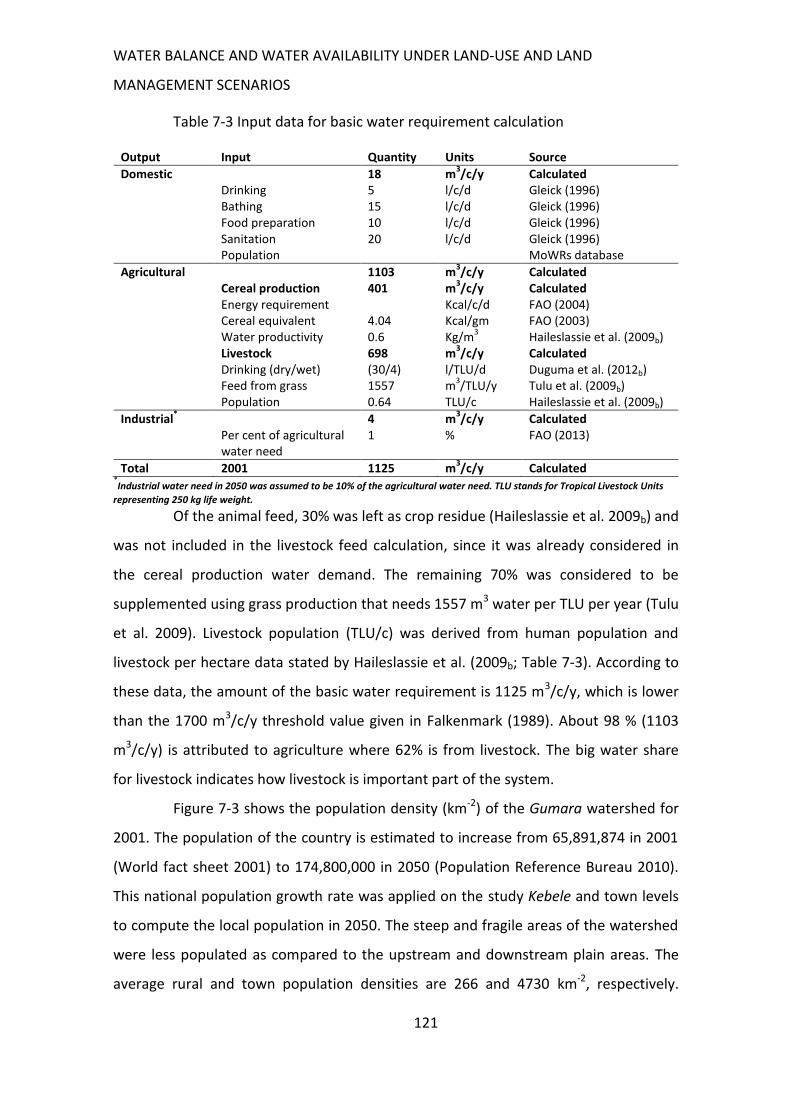
WATER BALANCE AND WATER AVAILABILITY UNDER LAND-USE AND LAND
MANAGEMENT SCENARIOS
121
Table 7-3 Input data for basic water requirement calculation
Output Input Quantity Units Source
Domestic 18 m3/c/y Calculated
Drinking 5 l/c/d Gleick (1996) Bathing 15 l/c/d Gleick (1996) Food preparation 10 l/c/d Gleick (1996) Sanitation 20 l/c/d Gleick (1996) Population MoWRs database
Agricultural 1103 m3/c/y Calculated
Cereal production 401 m3/c/y Calculated
Energy requirement Kcal/c/d FAO (2004) Cereal equivalent 4.04 Kcal/gm FAO (2003) Water productivity 0.6 Kg/m
3 Haileslassie et al. (2009b)
Livestock 698 m3/c/y Calculated
Drinking (dry/wet) (30/4) l/TLU/d Duguma et al. (2012b) Feed from grass 1557 m
3/TLU/y Tulu et al. (2009b)
Population 0.64 TLU/c Haileslassie et al. (2009b)
Industrial* 4 m
3/c/y Calculated
Per cent of agricultural water need
1 % FAO (2013)
Total 2001 1125 m3/c/y Calculated
*Industrial water need in 2050 was assumed to be 10% of the agricultural water need. TLU stands for Tropical Livestock Units
representing 250 kg life weight.
Of the animal feed, 30% was left as crop residue (Haileslassie et al. 2009b) and
was not included in the livestock feed calculation, since it was already considered in
the cereal production water demand. The remaining 70% was considered to be
supplemented using grass production that needs 1557 m3 water per TLU per year (Tulu
et al. 2009). Livestock population (TLU/c) was derived from human population and
livestock per hectare data stated by Haileslassie et al. (2009b; Table 7-3). According to
these data, the amount of the basic water requirement is 1125 m3/c/y, which is lower
than the 1700 m3/c/y threshold value given in Falkenmark (1989). About 98 % (1103
m3/c/y) is attributed to agriculture where 62% is from livestock. The big water share
for livestock indicates how livestock is important part of the system.
Figure 7-3 shows the population density (km-2) of the Gumara watershed for
2001. The population of the country is estimated to increase from 65,891,874 in 2001
(World fact sheet 2001) to 174,800,000 in 2050 (Population Reference Bureau 2010).
This national population growth rate was applied on the study Kebele and town levels
to compute the local population in 2050. The steep and fragile areas of the watershed
were less populated as compared to the upstream and downstream plain areas. The
average rural and town population densities are 266 and 4730 km-2, respectively.
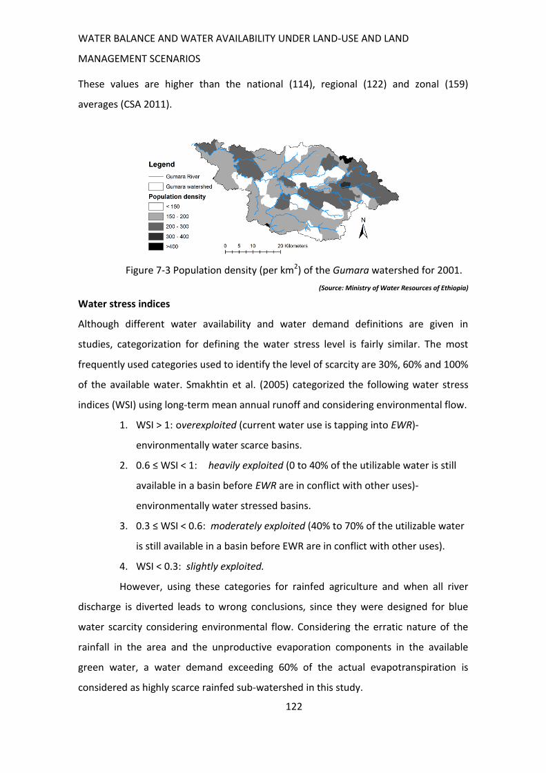
WATER BALANCE AND WATER AVAILABILITY UNDER LAND-USE AND LAND
MANAGEMENT SCENARIOS
122
These values are higher than the national (114), regional (122) and zonal (159)
averages (CSA 2011).
Figure 7-3 Population density (per km2) of the Gumara watershed for 2001.
(Source: Ministry of Water Resources of Ethiopia)
Water stress indices
Although different water availability and water demand definitions are given in
studies, categorization for defining the water stress level is fairly similar. The most
frequently used categories used to identify the level of scarcity are 30%, 60% and 100%
of the available water. Smakhtin et al. (2005) categorized the following water stress
indices (WSI) using long-term mean annual runoff and considering environmental flow.
1. WSI > 1: overexploited (current water use is tapping into EWR)-
environmentally water scarce basins.
2. 0.6 ≤ WSI < 1: heavily exploited (0 to 40% of the utilizable water is still
available in a basin before EWR are in conflict with other uses)-
environmentally water stressed basins.
3. 0.3 ≤ WSI < 0.6: moderately exploited (40% to 70% of the utilizable water
is still available in a basin before EWR are in conflict with other uses).
4. WSI < 0.3: slightly exploited.
However, using these categories for rainfed agriculture and when all river
discharge is diverted leads to wrong conclusions, since they were designed for blue
water scarcity considering environmental flow. Considering the erratic nature of the
rainfall in the area and the unproductive evaporation components in the available
green water, a water demand exceeding 60% of the actual evapotranspiration is
considered as highly scarce rainfed sub-watershed in this study.
WATER BALANCE AND WATER AVAILABILITY UNDER LAND-USE AND LAND
MANAGEMENT SCENARIOS
123
The different scenarios that were used to develop water stress indices are
listed in Table 7-4. Two land-uses and three water availability status were used for the
population of 2001 and 2050 to develop 8 water stress scenarios.
Table 7-4 Water stress indices scenarios
Scenario No. Code Scenario No. Code
1 LU1_ GN01 5 LU2_ GNEWR01 2 LU1_ GN50 6 LU2_ GNEWR50 3 LU2_ GN01 7 LU2_ GNYLD01 4 LU2_ GN50 8 LU2_ GNYLD50
LU1 is existing land-use practice, LU2 is land-use considering Gumara irrigation project (GIP). Water availability is GN (green water), GNYLD (green water plus water yield) and GNEWR (green water plus 20% of water yield that considers environmental water requirement-EWR). Total water needed was calculated based on the population in 2001 and 2050 indicated as 01 and 5o, respectively.
7.4.5 Assumptions and limitations
Computing land-use and demographic change scenarios was performed using the
following assumptions. Different HRU discretization used for model calibration and
scenario development results in the same water balance and water availability
modeling values. The basic water requirement for domestic and agriculture per capita
per year in 2001 was assumed to be the same in 2050, and industrial water demand
was assumed to be 1% and 10% of the agricultural demand in 2001 and 2050,
respectively. The availability of groundwater recharge was not considered. The effect
of climate change on water balance and water availability was not included in this
study.
7.5 Results
7.5.1 Water balance shift due to land-use changes
The annual water balance of the Gumara watershed using six meteorological stations
and the Penman-Monteith potential evapotranspiration methods for the 328 sub-
watersheds is shown in Figure 7-4 for the period 1992 to 2001 with and without the
Gumara Irrigation Project (GIP). About 95 % of the annual rainfall left the watershed
through river discharge or yield (YLD; 752 mm)) and AET (648 mm). The remaining 5%
was stored in the deep groundwater. This storage was about 61 mm (92 Mm3) per
annum. River discharge and AET accounted for 51% and 44% of the annual rainfall,
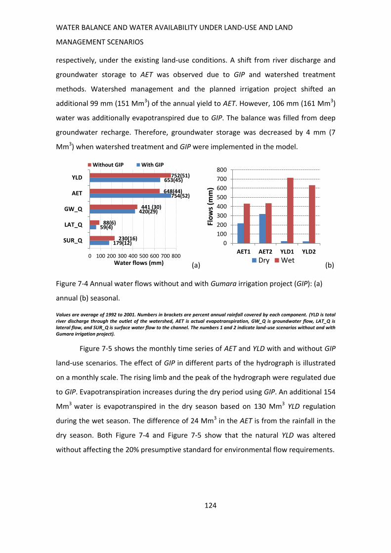
WATER BALANCE AND WATER AVAILABILITY UNDER LAND-USE AND LAND
MANAGEMENT SCENARIOS
124
respectively, under the existing land-use conditions. A shift from river discharge and
groundwater storage to AET was observed due to GIP and watershed treatment
methods. Watershed management and the planned irrigation project shifted an
additional 99 mm (151 Mm3) of the annual yield to AET. However, 106 mm (161 Mm3)
water was additionally evapotranspired due to GIP. The balance was filled from deep
groundwater recharge. Therefore, groundwater storage was decreased by 4 mm (7
Mm3) when watershed treatment and GIP were implemented in the model.
(a) (b)
Figure 7-4 Annual water flows without and with Gumara irrigation project (GIP): (a)
annual (b) seasonal.
Values are average of 1992 to 2001. Numbers in brackets are percent annual rainfall covered by each component. (YLD is total river discharge through the outlet of the watershed, AET is actual evapotranspiration, GW_Q is groundwater flow, LAT_Q is lateral flow, and SUR_Q is surface water flow to the channel. The numbers 1 and 2 indicate land-use scenarios without and with Gumara irrigation project).
Figure 7-5 shows the monthly time series of AET and YLD with and without GIP
land-use scenarios. The effect of GIP in different parts of the hydrograph is illustrated
on a monthly scale. The rising limb and the peak of the hydrograph were regulated due
to GIP. Evapotranspiration increases during the dry period using GIP. An additional 154
Mm3 water is evapotranspired in the dry season based on 130 Mm3 YLD regulation
during the wet season. The difference of 24 Mm3 in the AET is from the rainfall in the
dry season. Both Figure 7-4 and Figure 7-5 show that the natural YLD was altered
without affecting the 20% presumptive standard for environmental flow requirements.
179(12)
59(4)
420(29)
754(52)
653(45)
230(16)
88(6)
441 (30)
648(44)
752(51)
0 100 200 300 400 500 600 700 800
SUR_Q
LAT_Q
GW_Q
AET
YLD
Water flows (mm)
Without GIP With GIP
0
100
200
300
400
500
600
700
800
AET1 AET2 YLD1 YLD2
Flo
ws
(mm
)
Dry Wet
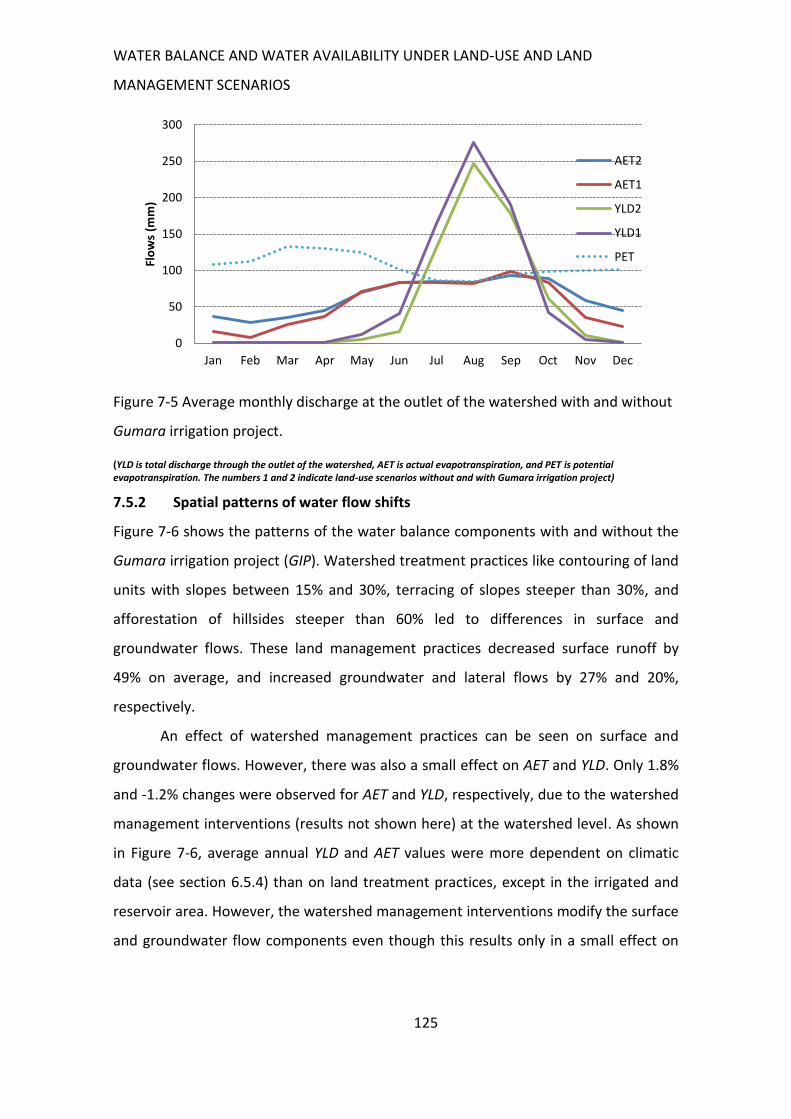
WATER BALANCE AND WATER AVAILABILITY UNDER LAND-USE AND LAND
MANAGEMENT SCENARIOS
125
Figure 7-5 Average monthly discharge at the outlet of the watershed with and without
Gumara irrigation project.
(YLD is total discharge through the outlet of the watershed, AET is actual evapotranspiration, and PET is potential evapotranspiration. The numbers 1 and 2 indicate land-use scenarios without and with Gumara irrigation project)
7.5.2 Spatial patterns of water flow shifts
Figure 7-6 shows the patterns of the water balance components with and without the
Gumara irrigation project (GIP). Watershed treatment practices like contouring of land
units with slopes between 15% and 30%, terracing of slopes steeper than 30%, and
afforestation of hillsides steeper than 60% led to differences in surface and
groundwater flows. These land management practices decreased surface runoff by
49% on average, and increased groundwater and lateral flows by 27% and 20%,
respectively.
An effect of watershed management practices can be seen on surface and
groundwater flows. However, there was also a small effect on AET and YLD. Only 1.8%
and -1.2% changes were observed for AET and YLD, respectively, due to the watershed
management interventions (results not shown here) at the watershed level. As shown
in Figure 7-6, average annual YLD and AET values were more dependent on climatic
data (see section 6.5.4) than on land treatment practices, except in the irrigated and
reservoir area. However, the watershed management interventions modify the surface
and groundwater flow components even though this results only in a small effect on
0
50
100
150
200
250
300
Jan Feb Mar Apr May Jun Jul Aug Sep Oct Nov Dec
Flo
ws
(mm
) AET2
AET1
YLD2
YLD1
PET
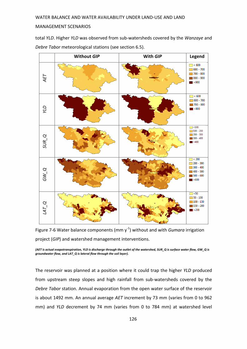
WATER BALANCE AND WATER AVAILABILITY UNDER LAND-USE AND LAND
MANAGEMENT SCENARIOS
126
total YLD. Higher YLD was observed from sub-watersheds covered by the Wanzaye and
Debre Tabor meteorological stations (see section 6.5).
Without GIP With GIP Legend
AET
YLD
SUR
_Q
GW
_Q
LAT_
Q
Figure 7-6 Water balance components (mm y-1) without and with Gumara irrigation
project (GIP) and watershed management interventions.
(AET is actual evapotranspiration, YLD is discharge through the outlet of the watershed, SUR_Q is surface water flow, GW_Q is groundwater flow, and LAT_Q is lateral flow through the soil layer).
The reservoir was planned at a position where it could trap the higher YLD produced
from upstream steep slopes and high rainfall from sub-watersheds covered by the
Debre Tabor station. Annual evaporation from the open water surface of the reservoir
is about 1492 mm. An annual average AET increment by 73 mm (varies from 0 to 962
mm) and YLD decrement by 74 mm (varies from 0 to 784 mm) at watershed level
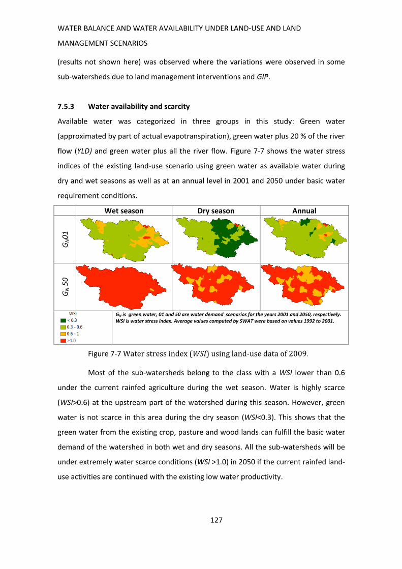
WATER BALANCE AND WATER AVAILABILITY UNDER LAND-USE AND LAND
MANAGEMENT SCENARIOS
127
(results not shown here) was observed where the variations were observed in some
sub-watersheds due to land management interventions and GIP.
7.5.3 Water availability and scarcity
Available water was categorized in three groups in this study: Green water
(approximated by part of actual evapotranspiration), green water plus 20 % of the river
flow (YLD) and green water plus all the river flow. Figure 7-7 shows the water stress
indices of the existing land-use scenario using green water as available water during
dry and wet seasons as well as at an annual level in 2001 and 2050 under basic water
requirement conditions.
Wet season Dry season Annual
GN0
1
GN 5
0
GN is green water; 01 and 50 are water demand scenarios for the years 2001 and 2050, respectively. WSI is water stress index. Average values computed by SWAT were based on values 1992 to 2001.
Figure 7-7 Water stress index (WSI) using land-use data of 2009.
Most of the sub-watersheds belong to the class with a WSI lower than 0.6
under the current rainfed agriculture during the wet season. Water is highly scarce
(WSI>0.6) at the upstream part of the watershed during this season. However, green
water is not scarce in this area during the dry season (WSI<0.3). This shows that the
green water from the existing crop, pasture and wood lands can fulfill the basic water
demand of the watershed in both wet and dry seasons. All the sub-watersheds will be
under extremely water scarce conditions (WSI >1.0) in 2050 if the current rainfed land-
use activities are continued with the existing low water productivity.
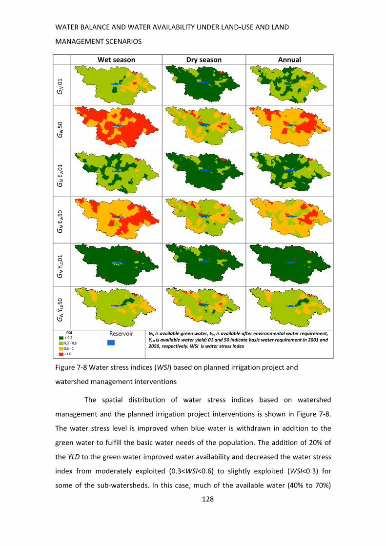
WATER BALANCE AND WATER AVAILABILITY UNDER LAND-USE AND LAND
MANAGEMENT SCENARIOS
128
Wet season Dry season Annual G
N 0
1
GN
50
GN
EW
01
GN
EW
50
GN
YLD
01
GN
YLD
50
GN is available green water, EW is available after environmental water requirement, YLD is available water yield; 01 and 50 indicate basic water requirement in 2001 and 2050, respectively. WSI is water stress index
Figure 7-8 Water stress indices (WSI) based on planned irrigation project and
watershed management interventions
The spatial distribution of water stress indices based on watershed
management and the planned irrigation project interventions is shown in Figure 7-8.
The water stress level is improved when blue water is withdrawn in addition to the
green water to fulfill the basic water needs of the population. The addition of 20% of
the YLD to the green water improved water availability and decreased the water stress
index from moderately exploited (0.3<WSI<0.6) to slightly exploited (WSI<0.3) for
some of the sub-watersheds. In this case, much of the available water (40% to 70%)
WATER BALANCE AND WATER AVAILABILITY UNDER LAND-USE AND LAND
MANAGEMENT SCENARIOS
129
was still there for other water needs beyond the basic water requirements in 2001.
However, most of the sub-watersheds will still be overexploited (WSI>1) in 2050 if only
green water is used. The watershed will be environmentally water scarce in 2050 and
the contribution of the watershed to downstream livelihoods will be limited.
7.6 Discussion
7.5.4 Impact of watershed management interventions on water balance
Slight differences in the watershed area and flow simulation results were simulated as
compared to the results of the GIP feasibility study carried out by MoWR (2008). The
total size of the sub-watersheds at the diversion and the dam were quantified as 1166
km2 and 385 km2 in the feasibility study, respectively, while the values were 1152 km2
and 381 km2 in this study. The annual water yield was 662 mm and 664 mm at the dam
and diversion sites, respectively, in the feasibility study and 710 mm and 827 mm in
this study. Potential evapotranspiration (PET) was 1391 mm for the Gumara irrigation
command area in the feasibility study and 1316 mm in this study. These differences
can be explained by the use of a different DEM, other meteorological data, and a
different model discretization in this study. This shows that meteorological data
refining (see section 5) plays a role in designing water resources. However,
measurement and interpolation errors and their propagation to the final model results
always exist. The amount of water evaporated from the water surface of the reservoir
was about 1492 mm per annum. This was lower than the evaporation from the surface
of Lake Tana that was estimated at about 1675 mm (SMEC 2008). A higher reservoir
evaporation value (1818 mm/year) (MoWR 2008) was simulated in the GIP feasibility
study as compared to the 1492 mm in this study. This PET difference were because the
meteorological data from the Bahir Dar station were used in the GIP feasibility study,
which is located in a relatively warm climate and far away from the watershed.
Water flow shift from one component of the water balance to another due to
watershed management intervention and the GIP was observed. This shift was not
only from water yield to AET, but also from deep groundwater recharge to AET. This
may be due to the lower seepage occurring on the lined irrigation canals compared to
WATER BALANCE AND WATER AVAILABILITY UNDER LAND-USE AND LAND
MANAGEMENT SCENARIOS
130
the natural river and the revap flow due to the well maintained vegetation covers
during the watershed management. Such vegetation together with afforestation of the
steep slopes increases actual evapotranspiration and decreases groundwater recharge.
Micro-basin water harvesting structures has shown good land-cover and increased
biomass production by minimizing discharge in the north-east Ethiopia (Derib et al.
2009). Shrubland was considered the best choice for minimizing runoff and soil erosion
in China as compared to alfalfa pastureland (Wei et al. 2007). The authors suggest
grassland and woodland for runoff and soil erosion management rather than large-
scale alfalfa plantations. Around the study area, legume trees, alfalfa, napier and
vetiver grasses were proposed and used (Gebreslassie et al. 2009). However, careful
selection of crops and trees has to be done with respect to environmental benefits and
water productivity optimization.
7.5.5 Water availability and demand
Green water is the only available water for the existing rainfed agricultural system in
the study area. Based on the experience of the author and field observations, the most
productive green water was that of the wet season. The AET during the dry season was
lost through unproductive evaporation, since the land is bare and there is almost no
production of food and feed during this season. This is for two reasons. The first and
most important reason is the small rainfall amount and duration and the resulting low
soil moisture (green water), which was not enough to supply the required AET for food
and feed production in the dry season. The second reason was that the farmers had no
additional technology such as irrigation infrastructure and low-water-demanding crops
in the dry season. However, the contribution of the existing small amount of available
blue water from rivers, springs and wells for domestic uses and livestock drinking was
not considered in the green water analysis.
Environmental water requirement was considered as the second option for
calculating water availability. Using the 20% rule of presumptive standard for
environmental flow protection (Richter et al. 2011), 20% of the YLD was added to the
green water, and this sum was considered as available water. However, in practice this
WATER BALANCE AND WATER AVAILABILITY UNDER LAND-USE AND LAND
MANAGEMENT SCENARIOS
131
presumptive standard is difficult to implement in the existing Nile hydropolitics. The
standard can minimize about 10.5 km3 of the water from Nile flow at Aswan if it is
implemented on the whole Ethiopian Blue Nile watershed. The sum of green water
and YLD was the other option used to calculate available water for each sub-
watershed.
Water availability and water stress status on seasonal scales resulted in
practical implications of how water and watershed management strategies can be
derived. Hoekstra and Mekonnen (2011) estimated blue water scarcity on monthly
levels. However, the results in their study showed similar monthly values within a
given season, so that seasonal scale can address most of the practical variability of the
water resources availability and water scarcity status. A monthly level water stress
analysis requires agricultural water demand data at a monthly level. This is only
possible with a detailed study of crop water requirements. This was done neither by
Hoekstra and Mekonnen (2011) nor in this study. However, seasonal analysis can
provide equivalent information to that based on a monthly scale saving modeling time
and resources. Nevertheless, a monthly scale analysis can address the impact of water
stress in the dry spells during the growing season.
The contribution of YLD to the water stress status was smaller during the dry
season as compared to the wet season in the watershed. This is due to the low YLD
occurring in this season. However, shifting 6% of the rainfall from annual YLD to the
productive evapotranspiration, GIP and associated watershed management
interventions made another 2% evaporated annual rainfall productive in the dry
season in the irrigation command area. It played a role in increasing water availability
for the community without compromising the environmental flow. This indicates that
water flow regulation structures are important to make water available so that the
unproductive green water in the dry season can be shifted to productive transpiration
using supplemental irrigation. Although the contribution of river YLD for available
water was low during the dry season, water stress level was seen to be better than in
the wet season. This is because the annual agricultural water need was assigned for
the productive wet season so that less water was needed during the dry season. Green
WATER BALANCE AND WATER AVAILABILITY UNDER LAND-USE AND LAND
MANAGEMENT SCENARIOS
132
water was shown to be enough to satisfy the basic water need in 2001 based on the
existing rainfed agricultural production conditions. However, observations and
informal discussions during the field study showed that the productivity of this green
water was not enough to sustain life due to rainfall variability and late entering and
early onset of the rainfall in the growing season.
After satisfying the environmental requirements, the available green and blue
water will not be sufficient to fulfill the basic water requirements of the area in 2050.
The results of this study show that it is possible to satisfy the basic needs using all the
environmental water in 2050. However, the watershed is situated in a position to
sustain downstream life from the nearby Lake Tana to the Mediterranean Sea.
Therefore, actions have to be taken at both local and basin levels. Some of the key
issues to increase green water productivity are to mitigate the problems associated
with intra-seasonal dry spells with supplemental irrigation, maximize infiltration,
minimize unproductive evaporation, increase soil-water holding capacity, maximize
root depth, and maximize the water-uptake of crops (Rockström et al. 2003). Selection
of short-maturing dry season food/feed materials can make evaporation water
beneficial for the livelihoods in the sub-watersheds.
7.5.6 Implications for the Nile Basin water
In addition to the physical water stress, Nile water is now in a more political tension
than ever. The Ethiopian highland contributes about 86 % of the Nile flow at the Aswan
High Dam while the country is using less than 5% of its total internal renewable water
(FAO AQUASTAT 2005) and 3% of the Blue Nile runoff (Mason 2004). The largest user
of this flow, Egypt, is dependent to 98% on the Nile water. However, it contributes
almost nothing, which means that the livelihoods of the Egyptians are totally
dependent on the blue water of the Nile that comes from the upstream countries.
Egypt and Sudan agreed to use the Nile flow in 1929 and 1959, but the agreements are
not binding for all the riparian countries in the Nile basin.
Ethiopia gains 936 km3 annual rainfall and discharges 122 km3 (14%) of this
rainfall, where 90% of this flow is transboundary (FAO AQUASTAT database;
WATER BALANCE AND WATER AVAILABILITY UNDER LAND-USE AND LAND
MANAGEMENT SCENARIOS
133
http://www.fao.org/nr/water/aquastat/countries_regions/ Cited 12/08/2013; see
section 2). Per capita, 14,200 (5,300) m3 and 1,800 (698) m3 rain and river flow water,
respectively, are calculated for 2001 (2050). The effective rainfall that accounts for a
total 814 km3 with 12,300 (4,600) m3 per capita in 2001 (2050) is a very large amount
as compared to Egypt’s total water availability of 68.3 km3 with 979 (504) m3 per capita
in 2001 (2050). However, as can be observed at the head water of the Blue Nile, about
53% of the annual rainfall is directed to river flow, and the green water is not enough
to support the basic water needs in the future if the existing rainfed water productivity
does not improve. This indicates that there are some sources and sinks of river flow in
the Blue Nile. For example, the study concerning the Lake Tana basin (15,096 km2)
showed that about 30% of the rainfall is discharged through the outlet (Setegn et al.
2008). Another modeling study carried out by Engida (2010) in the same basin using 8
sub-watersheds (area varies from 103 km2 to 15,120 km2) showed variation of
discharge contribution from 24% to 60% of the annual rainfall. Green and blue water
management has to be designed based on these difference. The rainfed agricultural
system is not productive enough to support future life due to the large discharge
contribution, low green water productivity and high population density.
The integral understanding of the global and the regional water balancing on
different time scales calls for another way of thinking to alleviate the consumptive
water scarcity and the existing hydro-political stress. Even watershed management and
blue water withdrawal can improve water availability in the area; it will not solve the
water stress in the society and the environment in the future. As recommended by
many studies (e.g., Waterbury and Whittington (1998); Whittington 2004; Mason
(2004); Arsano (2007); Martens (2011)), basin-wide integration and efficient water use
in the Nile Basin can benefit the local livelihoods and environment. Non-water-
consumptive uses like hydropower production, fishery and tourism can benefit the
local livelihoods while the environmental water is not negatively affected. An extensive
Blue Nile water development project in Ethiopia, the “Grand Ethiopian Millennium
Dam Project (GERDP)”, started in April 2011 on the Blue Nile River. It is designed to
generate 6000 MW electric power making 74 km3 in a reservoir covering 1680 km2
WATER BALANCE AND WATER AVAILABILITY UNDER LAND-USE AND LAND
MANAGEMENT SCENARIOS
134
(EEPC, Ethiopian Electric Power Corporation 2013). The project is non-water
consumptive, since it is designed only for power generation. As it is located in a
sparsely populated (19 persons km-2 (CSA 2011); (see Appendix 0; Figure 10-2)) and
inaccessible river valley area, it will attract human life after completion so that the
green water burden of the densely populated highland and cities will be alleviated to a
certain extent. Fish production, navigation and tourism and business activities related
to the stored water may be livelihood means for the community. There is also a chance
to use the generated power to develop the groundwater of the Ethiopian lowlands
outside the Nile basin for irrigation and drinking water infrastructure. Ethiopia has
ample potentials and diversity of non-water consumptive alternatives without
appreciably harming the water share of the downstream users.
The political will of the riparian countries to use diversified water
development corridors in different parts of the Nile Basin has been a challenge for
decades. An initiative, the ‘Nile Basin Initiative’, was formed in 1999 to smoothen the
political tensions so that the riparian countries can be benefited from cooperative
investments and equitable water sharing. The initiative has developed capacity,
regional institutions, and networks based on a shared vision and equitable utilization
of water resources. Promising advancement has been shown like signing of the
Cooperative Framework Agreement (CFA) by six out of the ten riparian countries
(Salman 2013; NBI http://www.nilebasin.org/newsite/).
7.5.7 Uncertainties regarding water availability and demand quantification
Reliability of calculations of water availability and water scarcity depends on the
quality of the underlining data (Hoekstra and Mekonnen 2011; Brown and Heuvelink
2005). Generally, model uncertainty is lower in physically based models like SWAT as
compared to empirical and conceptual models (Giertz et al. 2006). In this study, data
quality of the SWAT outputs for water availability was improved by using smaller
hydrological response units as compared to other studies of the area. Soil data were
improved by using a recent detailed study in the watershed (MoWR 2008). More data
from the climate stations were considered by using the best missing data filling
WATER BALANCE AND WATER AVAILABILITY UNDER LAND-USE AND LAND
MANAGEMENT SCENARIOS
135
methods among the selected approaches (see section 5). The recent 30-m resolution
DEM from ASTER and fine soil and climatic data used made it possible to use a fine
HRU delineation. The combined effect of the above data quality efforts results in
acceptable error measures of river discharge modeling: 0.49 r-factor and 0.8 p-factor
on a daily scale, and 65% (95%), +5 (+5) and 0.3 (0.06), on daily (monthly) levels for
NSE, PBIAS and RSR, respectively (see section 6.5). Errors in climatic variables
interpolation were discussed (see section 5). However, uncertainty sources from
inverse water balance modeling still exist. Sharp changes in water balance components
at the border of sub-watersheds are caused by the structure of the SWAT model.
Improving SWAT structures to spatial interpolation of point climate data needs further
research to improve water availability data quality with respect to the scale limit to
rugged topographical features affecting the local climate. Furthermore, water scarcity
information quality can be improved by decomposing water availability through
different crops with high green-water productivity and livestock management
activities, since about 98% of the basic water requirement is caused by agriculture.
Partitioning and averaging each component of human basic water needs for the
population of the smallest administrative units is the additional quality of this research
to increase our understanding at the local level. However, the effect of dry spells on
the rainfed agriculture within a growing season was not addressed but may receive
increasing importance due to climate change.
7.7 Conclusions
The water availability status with and without the Ethiopian government plan for the
Gumara watershed with an area of 1520 km2 was modeled at the head water of the
Blue Nile Basin. The hydrological model Soil and Water Assessment Tool (SWAT) was
applied at a very fine discretization. Livestock is not only the direct source of human
food but also a component of production and household assets. Therefore, the water
requirement of livestock was systematically included in the per capita basic water
requirement considering the local mixed crop-livestock agricultural production system.
Finally, the water scarcity status was identified on spatial and seasonal scales for 2001
WATER BALANCE AND WATER AVAILABILITY UNDER LAND-USE AND LAND
MANAGEMENT SCENARIOS
136
and 2050 population scenarios. The water availability was partitioned into three
options to consider rainfed and irrigation productions as well as environmental water
flows.
The watershed management interventions modified the hydrological balance,
especially the ratio of surface runoff to subsurface and groundwater flows. This can
increase the residence time of water in the watershed that favors the rainfed
agricultural production. The planned reservoir was designed to retain the discharge
from the highly contributing sub-watersheds. The dam and diversion structures were
modeled to minimize the natural flow of the main stream within acceptable ranges
that favor environmental flow. Both watershed management interventions and
proposed irrigation project increased water availability in the watershed. The
aggregated water availability per capita is 1125 m3 per annum: 98% is for agriculture
and 62% of this portion was used by livestock. High spatio-temporal variations of water
scarcity were simulated in the watershed. The green water of the rainfed production
supports the basic water requirement during the growing season using the existing
land-use and 2001 basic water requirement scenarios. This result could not address
the effect of dry spells of the growing season on the rainfed productivity that is
increasingly challenging the livelihoods in the area. Additional exploitation of the river
flow (blue water) improved the water stress status. However, the green water of the
existing land-use and climatic conditions will not support the basic water requirements
of the population in 2050 assuming the current population growth rate of the country
for the area in 2001. In 2050, water flow will be highly exploited to affect the
environment and the downstream uses.
The current land-use and rainfed production system will not withstand
demographic pressure. In addition, more and more intensive use of the blue water will
exploit the environmental flow in 2050 and affect the downstream life of this
transboundary water. In addition to family planning, improving green water
productivity by using supplemental irrigation and appropriate food and feed materials
and management systems, basin-wide cooperation of water use like hydropower
development, tourism and fish production can improve the local water stress shown in

WATER BALANCE AND WATER AVAILABILITY UNDER LAND-USE AND LAND
MANAGEMENT SCENARIOS
137
this study. As advised by many studies, these options may also improve the existing
physical and political water stress at the Nile Basin level.
GENERAL SUMMARY AND PERSPECTIVES
138
8 GENERAL SUMMARY AND PERSPECTIVES
Ethiopia suffers from economic and technological water scarcity that makes difficult to
increase the productivity of available water. In depth understanding of the water
balance and water availability at different scales and for different scenarios is
important for future intervention to alleviate the scarcity. As part of this basin-wide
and national concern, this study examines the water balance and water availability on
farm and watershed scales at different scenarios. Therefore, the study was carried out
to attain the following objectives: (1) to evaluate water use and water productivity of a
small-scale irrigation scheme, (2) to evaluate methods for filling gaps in climatic data,
(3) to adopt Soil and Water Assessment Tool (SWAT) hydrological model for modeling
river discharge using different modeling setups, and (4) to simulate water demand and
water stress status for a period up to 2050 using different land-use and demographic
scenarios. The Gumara watershed (1520 km2), a tributary of Lake Tana of the Blue Nile
in Ethiopia, was selected for this study.
A case study on small-scale irrigation scheme to investigate water balance
and water productivity.
After mapping small-scale irrigation schemes in the Gumara watershed, in-depth field
measurements (water flow through canals, water application on the field, and biomass
of grain, crop residue and grass) and close observation (effect of water logging and
water shortage) were taken on a 90 ha scheme during the irrigation season in 2009.
Farmlands, canal network, drainage basins and wetlands were mapped using
geographical information system (GIS), satellite images and field measurements.
Before selection and distribution of sampling plots in the scheme, classification of
irrigation system (as pumped and gravity), canals (as main, secondary and field) and
land-use (as cropland, drainage basin, wetland and grasslands) were performed. High
water loss was observed during water conveyance and water application while there
was water shortage to irrigation farms at the downstream side of the scheme. The
water loss and shortage varies along crop types, location of field in the scheme and
cost related to pumping. Some irrigation farmlands were out of production due to
GENERAL SUMMARY AND PERSPECTIVES
139
water logging resulted from canal overflow especially during night irrigation.
Therefore, water and land productivity was very low as compared to the results of
other studies. The water application of the farmers did not match the water
requirement of the crops. Night storage to solve problems associated with night
irrigation, proper irrigation scheduling and empowering farmers to manage irrigation
water are some of the recommendation to improve the diverted water productivity.
Compare and evaluate missing data filling methods to increase the
number of climate station for hydrological modeling.
Climatic variables, especially rainfall and temperature, are the forcing factors for
hydrological flows. Climatic data are very important particularly for data demanding
and most used Penman-Monteith evapotranspiration method in hydrological
modeling. However, gaps in climatic data are one of the constraints to have detailed
spatial water balance analysis in the Blue Nile basin. In this study, gaps climatic data
(rainfall, temperature, relative humidity and solar radiation) in a given station was
tried to fill using neighboring station data. This approach was used in SWAT water flow
modeling to compare its effect on model performance with SWAT weather generation
(WXGEN) routine. The WXGEN used only within a station relationship to fill missing
data that is not practical for stations with long and continuous gap in climatic data.
Four deterministic daily rainfall estimation methods were selected. The statistical
performance of estimation showed comparable results with similar studies done
elsewhere. Multiple regression models were developed to fill missing data of daily
minimum and maximum temperature data. These models perform well for maximum
temperature for most of the stations. However, the low performance was observed for
minimum air temperature. Relative humidity and solar radiation data of stations were
derived from minimum and maximum daily air temperature data. Some parameters
were optimized based on seasonal categorization of the area that resulted in better
results as compared to without seasonal categorization. It should be important to
derive additional relationship of climatic variables with some topographical features
like altitude. In this case, more stations data at a bigger spatial scale should be
GENERAL SUMMARY AND PERSPECTIVES
140
considered. As proposed by Oregon State University and Technical University of Delft
with a project called Trans-African Hydro-Meteorological Observatory (TAHMO) to
install weather stations every 30 km (available on http://tahmo.info/about-tahmo),
elementary schools and health centers can be used to install more climate stations.
The approach used in this study can be, then, used for the future to extrapolate the
newly installed stations in the watershed using long-term data of the existing stations.
Assess the effect of different modeling setups on SWAT modeling
performance.
Data availability and the way to develop the model setup could have significant effect
on the performance of a hydrological model. The study explores the effect of different
model setups on river flow modeling. Number of climate stations used varied (two,
three and six) according to their data availability and proximity to the watershed after
filling missing data using different methods. Two stations (one in the watershed and
the other outside) had frequently been used on academic and water resources
planning studies for the watershed. Different meteorological stations with varying
proximity to the study watershed were used to evaluate their relative performances
on hydrological modeling. Selection of representative climate stations and their
density affect the performance SWAT model adaptation. Four and six stations have
given better efficiency of water flow modeling than frequently used Bahir Dar and
Debre Tabor stations. The performance of stations density is explained not only
increasing modeling efficiency of estimating river discharge at the outlet of the
watershed from 60% to 70%, but also, each water balance component is differently
distributed in the watershed. Penman-Monteith and Hargreaves methods of
calculating potential evapotranspiration methods have given comparable modeling
performances. The approach to update and use local climate data has given better
hydrological modeling results. However, uncertainties from non-uniqueness of model
parameter, measurement error in class-three stations and errors propagated from
filling gaps in climate data are still there in the results. Further research should
consider effect of interpolation of climatic data for each sub-watershed delineated.
GENERAL SUMMARY AND PERSPECTIVES
141
The spatial interpolation can be based on the relation with relief and altitude
especially for rainfall and temperature data.
Assess the effect of different scenarios on water balance and availability.
Spatial and temporal water availability status can be used to derive development and
policy interventions. In this part of the study, land-use scenarios were developed to
evaluate water balance and water availability based on the results of the case study,
missing data handling and calibration of SWAT. Both green and blue water availability
options were considered to analyze the water stress status with respect to the basic
water requirement of the area in 2001 and 2050. Watershed treatment options
decreased surface runoff. This surface runoff was shifted to lateral flow, groundwater
flow and evapotranspiration increasing by 8%, 10% and 0.2%, respectively. Watershed
treatment and planned Gumara Irrigation Project (GIP) decreased surface runoff,
lateral flow and groundwater flow by 19%, 33% and 4%, respectively. Spatial basic
water requirement was quantified using literature values and the population
distribution. The aggregated basic water requirement per capita is 1125 m3 per annum
of which 98% is for agriculture. High variation of water scarcity was observed on spatial
and temporal distributions. Evapotranspired water from the existing rein fed
production is enough for the demand in 2001 while it will not support the basic water
requirement of the population in 2050. In 2050, water flow will be highly exploited to
affect the environment and the downstream uses. However, the existing low water
productivity wheat crop is used for this analysis. Increasing water productivity, non-
consumptive water uses development and green water management options may
improve the blue water stress on the Nile Basin level. Further modeling research that
address climatic change and different crop production is crucial.
REFERENCES
142
9 REFERENCES
Abbaspour, KC, CA Johnson, and MT van Genuchten (2004) Estimating Uncertain Flow
and Transport Parameters Using a Sequential Uncertainty Fitting Procedure. Vadose Zone J 3:1340-1352.
Abbaspour, KM (2011) SWAT-CUP4: SWAT Calibration and Uncertainty Programs - A User Manual. Swiss Federal Institute of Aquatic Science and Technology, (eawag).
Akkuzu, E, HB Unal and BS Karatafi (2007) Determination of water conveyance loss in the menemen open canal irrigation network. Turk J Agric 31:11-22
Alamirew, D (2006) Modelling of Hydrology and Soil Erosion of Upper Awash River Basin. PhD Dissertation, University of Bonn.
Alemayehu, T, M McCartney and S Kebede (2009) Simulation of water resource development and environmental flows in the Lake Tana Sub basin. In: Awulachew, SB, T Erkossa, V Smakhtin and A Fernando (Comps.) (2009) Improved water and land management in the Ethiopian highlands: its impact on downstream stakeholders dependent on the Blue Nile. Intermediate Results Dissemination Workshop held at the International Livestock Research Institute (ILRI), Addis Ababa, Ethiopia, 5-6 February 2009. Colombo, Sri Lanka.
Allen, RG (1986) A Penman for all seasons. J Irrig Drain E-ASCE 112(4): 348-368. Allen, RG, LS Pereira, D Reas and M Smith (1998) Crop evapotranspiration: guidelines
for computing crop water requirements, FAO irrigation and drainage paper 56. FAO- Food and Agriculture Organization of the United Nations, Rome.
Allen, RG, ME Jensen, JL Wright, and RD Burman (1989) Operational estimates of evapotranspiration. Agron J 81:650-662.
Allen, RJ and AT DeGaetano (2001) Estimating missing daily temperature extremes using an optimized regression approach. Int J Climatol 21:1305-1319.
Amede, T, S Tarawali and D Peden (2011) Improving water productivity in crop-livestock systems of drought-prone regions: Editorial comment. Exp Agr 47 (S1):1–5.
Andersen, J, J Refsgaard and K Jansen (2001) Distributed hydrological modeling of the Senegal River basin-model construction and validation. J Hydrol 247: 200-214.
Anderson, MP and WW Woessner (1992) Applied ground water modeling. Academic Press, Inc., San Diego.
Arnold, JG, R Srinivason, RR Muttiah and JR Williams (1998) Large Area Hydrologic Modeling and Assessment Part I: Model Development. J Am Wat Res 34(1): 73-89.
Arsano Y (2007) Ethiopia and the Nile Dilemmas of National and Regional Hydropolitics. PhD Dissertation. Swiss Federal Institute of Technology
Asres, MT and SB Awulachew (2010) SWAT based runoff and sediment yield modelling: A case study of the Gumera watershed in the Blue Nile basin. Ecohydrology and Hydrology 10(2-4):191-200.
Awulachew, SB, AD Yilma, M Loulseged,W Loiskandl, M Ayana, and T Alamirew (2007) Water Resources and Irrigation Development in Ethiopia. Colombo, Sri Lanka: International Water Management Institute. 78p. (Working Paper 123)

REFERENCES
143
Awulachew, SB, DJ Merrey, AB Kamara, B Van Koopen, De Vries, F Penning and E Boelle (2005) Experiences and opportunities for promoting small-scale/micro irrigation and rainwater harvesting for food security in Ethiopia. International Water Management Institute. (Working Paper 98)
Awulachew, SB, M McCartney and TS Steenhuis (2008) A review of hydrology, sediment and water resource use in the Blue Nile Basin. Colombo, Sri Lanka: International Water Management Institute. (Working Paper 131)
Ayoade, J. O. (1983). Introduction to Climatology for the Tropics. John Wiley and Sons, New York.
Bakry, MF and AM Awad (1997) Practical estimation of seepage losses along earthen canals in Egypt. Water Resour Manag 11: 197–206.
BCEOM (Egis Bceom International) (1998) Abbay river basin integrated development master plan. Ministry of Water Resources, Addis Ababa, Ethiopia.
Bekele S and K Tilahun (2007) Regulated deficit irrigation scheduling of onion in a semiarid region of Ethiopia. Agr water manage 89:148 – 1 52
Beven, K and J Freer (2001). Equifinality, data assimilation, and uncertainty estimation in mechanistic modelling of complex environmental systems using the GLUE methodology. J Hydrol 249(1-4): 11-29.
Beven, RL (1985) Distributed hydrological models, In: MG Anderson and TP Burt (Eds) Hydrological Forcasting, Wiley, Chichester, UK. 405-435.
Block, PJ, K Strzepek and B Rajagopalan (2007) Integrated Management of the Blue Nile Basin in Ethiopia: Hydropower and Irrigation Modeling. International food policy research institute, 2033 K Street, NW, Washington DC, USA. http://www.ifpri.org/sites/default/files/publications/ifpridp00700.pdf accessed on 23/5/2011 Cited 27 Jun 2010.
Bormann, H and B Diekkrueger (2003) Possibilities and limitations of regional hydrological models applied within an environmental change study in Benin (west Africa), Phys Chem Earth 28(33-36):1323-1332.
Bormann, H and B Diekkrueger (2004) A conceptual hydrological model for Benin (West Africa): validation, uncertainty assessment and assessment of applicability for environmental change analyses, Phys Chem Earth 29(11-12):759-768.
Bormann, H, B Diekkrüger and O. Richter (1999) Effects of spatial data resolution on the calculation of regional water balances. In: B Diekkrüger, MJ Kirkby and U Schröder (ed.) Regionalization in Hydrology: HAHS-AISH P 254:193-202.
Brown, J D and G B M Heuvelink (2005) Assessing uncertainty propagation through physically based models of soil water flow and solute transport, in: Encyclopedia of Hydrological Sciences, Andersen, M (ed.), John Wiley & Sons, Ltd.
CA (Comprehensive Assessment of Water Management in Agriculture) (2007) Water for Food, Water for Life: A Comprehensive Assessment of Water Management in Agriculture. London: Earthscan, and Colombo: International Water Management Institute.
REFERENCES
144
Chaplot, V, A Saleh and DB Jaynes (2005) Effect of the accuracy of spatial rainfall information on the modeling of water, sediment, and NO3–N loads at the watershed level. J Hydrol 312(1-4):223-234.
Chaubey, I, AS Cotter, TA Costello and TS Soerens (2005) Effect of DEM data resolution on SWAT output uncertainty. Hydrol Process 19:621–628.
Cho, J, D Bosch, R Lowrance, T Strickland and G Vellidis (2009) Effect of spatial distribution of rainfall on temporal and spatial uncertainty of SWAT output. ASABE 52(5):1545-1555.
Chow, VT, DR Maidment, and LW Mays (1988) Applied Hydrology. McGraw-Hill, New York.
Clemmens, AJ, MG Bos, and JA Replogle (1984) Portable RBC flumes for furrows and earthen channels. ASABE 27:1016–1021.
CSA (Central Statistics Authority) (2003) Ethiopian agricultural sample enumeration, 2001/2002 results for Amhara region, statistical reports on area and production of crops, part II B. Addis Ababa, Ethiopia.
CSA (Central Statistics Authority) (2011) Population Size by Sex, Area and Density by Region, Zone and Wereda, Addis Ababa, Ethiopia.
De Silva, RP, NDK Dayawansa and MD Ratnasiri (2007) A comparison of methods used in estimating missing rainfall data. J Agr Sci 3(2):101-108.
Deneke, TT (2011) Institutional implications of governance of local common pool resources on livestock water productivity in Ethiopia. Exp Agr 47(S1): 99-111.
Derib, SD (2005) Rainfall-runoff processes at a hill-slope watershed: case of simple models evaluation at Kori-Sheleko Catchments of Wollo, Ethiopia. M.Sc. Dissertation, Wageningen University.
Derib, SD, T Assefa, B Berhanu and G Zeleke (2009) Impacts of micro-basin water harvesting structures in improving vegetative cover in degraded hillslope areas of north-east Ethiopia. Rangeland J 31(2):259-265.
Descheemaeker, K, T Amede and A Haileslassie (2009) Livestock and water interactions in mixed crop-livestock farming systems of sub-Saharan Africa: Interventions for improved productivity. Colombo, Sri Lanka: International Water Management Institute. (Working Paper 133).
Diao, X and AN Pratt (2007) Growth Options and Poverty Reduction in Ethiopia – an economy-wide model analysis. Food Policy 32:205 -228.
Dingman, SL (1994) Physical hydrology. Prentice-Hall, Inc., Englewood Cliffs, NJ. Dooge, JCI (1968) The hydrologic cycle as a closed system. International Association of
Scientific Hydrology. Bulletin 13 (1):58-68. Duguma, B, A Tegegne and BP Hegde (2012) The effect of location and season on free
water intake of livestock under field condition in Ginchi watershed area, Ethiopia. World J Agr Sci 8 (1): 38-42.
Easton, ZM, DR Fuka, ED White, AS Collick, BB Ashagre, M McCartney, SB Awulachew, AA Ahmed and TS Steenhuis1 (2010) A multi basin SWAT model analysis of runoff and sedimentation in the Blue Nile, Ethiopia. Hydrol Earth Syst Sci 14:1827-1841.
EEPC (Ethiopian Electric Power Corporation) (2013) Grand Ethiopian Renaissance Project progress report
REFERENCES
145
http://www.hidasse.gov.et/c/document_library/get_file?p_l_id=11731&folderId=11740&name=DLFE-202.pdf Cited 23 Jun 2013.
Eguavoen, I, SD Derib, TT Deneke, M McCartney, BA Otto and SS Billa (2012) Digging, damming or diverting? Small-scale irrigation in the Blue Nile basin, Ethiopia. Water Alternatives 5(3): 678-699.
Eijkelkamp. Operating Instructions 13.17.02 RBC Flume. Hog Flume Software. http://www.eijkelkamp.com/Portals/2/Eijkelkamp/Files/Manuals/M2-131702e%20RBC-Flume.pdf Cited 22 Dec 2008.
Eischeid, JK, CB Baker, T Karl and HF Diaz (1995) The quality control of long-term climatological data using objective data analysis. Journal Appl Meteor 34:2787-2795.
Engida, A (2010) Hydrological and suspended sediment modeling in the Lake Tana Basin, Ethiopia. PhD Dissertation, Université de Grenoble.
EPLAUA (Environmental Protection, Land Administration and Use Authority) (2006) Ecological significances, threats and management options of Lake Tana-associated wetlands. Bahir Dar, Ethiopia.
Erkossa, T, AS Bekele, A Haileslassie, YA Denekew (2009) Impacts of improving water management of smallholder agriculture in the Upper Blue Nile Basin. In: AS Bekele, T Erkossa and SVF Ashra (Comps.). Improved water and land management in the Ethiopian highlands: its impact on downstream stakeholders dependent on the Blue Nile. Intermediate Results Dissemination Workshop held at the International Livestock Research Institute, Addis Ababa, Ethiopia.
EWNHS (Ethiopian Wildlife and Natural History Society) (1996) Important bird areas of Ethiopia, First inventory. Addis Ababa. www.worldlakes.org/lakedetails.asp?lakeid=8568 Cited 17 Feb 2008.
Falkenmark (1989) The massive water scarcity threatening Africa-why isn't it being addressed. Ambio 18(2): 112-118.
FAO (1978) Effective rainfall in irrigated agriculture. FAO Irrigation and Drainage Paper 25, Rome, Italy.
FAO (1986) Irrigation Water Management. Training manual No. 3 Food and Agriculture Organization of the United Nations, Via delle Terme di Caracalla, Rome, Italy.
FAO (2003) Food energy - methods of analysis and conversion factors. FAO Food and nutrition paper 77. Food and Agriculture Organization of the United Nations, Rome, Italy. http://www.fao.org/docrep/006/Y5022E/y5022e04.htm Cited 20 Feb 2013.
FAO (2004) Food and nutrition technical report series; human energy requirements, report of a joint FAO/WHO/UNU expert consultation: 17-24 October 2001. FAO, Rome.
FAO (2009) CROPWAT 8.0 for Windows. Rome, Italy. http://www.fao.org/nr/water/infores_databases_cropwat.html Cited 8 Feb 2009.
FAO (2013) Country Fact Sheet: Ethiopia. Aquastat, http://www.fao.org/nr/water/aquastat/data/factsheets/aquastat_fact_sheet_eth_en.pdf Cited 22 Feb 2013.

REFERENCES
146
FAO (Food and Agriculture Organization) (1993) Agro-ecological land resources assessment for agricultural development planning-a case study of Kenya resources data base and land productivity. Technical Annex 5, Rome, Italy. ftp://ftp.fao.org/agl/aglw/fwm/Manual3.pdf Cited 23 Feb 2013.
FAO AQUASTAT (2005) Irrigation in Africa in figures: Ethiopia – AQUASTAT Survey 2005 http://www.fao.org/nr/water/aquastat/countries_regions/ETH/CP_ETH.pdf Cited 18 Jul 2013.
Faulkner, JW, T Steenhuis, NV de Giesen, M Andreini and JR Liebe (2008) Water use and productivity of two small reservoir irrigation schemes in Ghana’s upper east region. Irrig drain 57: 151–163
Federal Negaritgazeta (2005) Federal Democratic Republic of Ethiopia rural land administration and land-use proclamation. Addis Ababa. P. 3134-3144.
FEWS NET (2008) ETHIOPIA Food Security Update. Famine Early Warning Systems Network and World Food Programme, FEWS NET Washington, DC. http://reliefweb.int/sites/reliefweb.int/files/resources/47D0640C5B43A3C08525740900651DEF-Full_Report.pdf Cited 24 Sep 2013.
Gassman, PW, MR Reyes, CH Green and JG Arnold (2007) The soil and water assessment tool: historical development, applications, and future research directions. ASABE 50(4):1211-1250.
Gebreselassie, Y, T Amdemariam, M Haile and C Yamoah (2009) Lessons from upstream soil conservation measures to mitigate soil erosion and its impact on upstream and downstream users of the Nile River. Upstream-Downstream Project in the Blue Nile Intermediate Results Dissemination Workshop held on 5-6 February 2009, International Water Management Institute (IWMI), Nile Basin and East Africa Office, Addis Ababa.
Giertz, S, B Diekkrueger, and G Steup (2006) Physically-based modeling of hydrological processes in a tropical headwater catchment (West Africa) - process representation and multi-criteria validation. Hydrol Earth Syst Sc 10:829–847.
Gleick, PH (1996) Basic water requirements for human activities: Meeting basic needs. Water Int 21: 83-92.
Grey, D and C Sadoff (2006) Water for growth and development. A theme document of the 4th World Water Forum. Mexico City, Mexico. 56 pp.
Gupta, HV, S Sorooshian, and PO Yapo (1999) Status of automatic calibration for hydrologic models: Comparison with multilevel expert calibration. J Hydrol Eng 4(2):135-143.
Haileslassie, A, D Peden, S Gebreselassie, T Amede and K Descheemaeker (2009b) Livestock water productivity in mixed crop–livestock farming systems of the Blue Nile basin: Assessing variability and prospects for improvement. Agr Syst 102: 33-40.
Haileslassie, A, D Peden, S Gebreselassie, T Amede, A Wagnew and A Taddesse (2009a) Livestock water productivity in the Blue Nile Basin: assessment of farm scale heterogeneity. Range J 31:213–222.
Hargreaves, GH and ZA Samani (1982) Estimating potential evapotranspiration, J Irrig Drain E-ASCE 108(3):25-230.
REFERENCES
147
Hargreaves, GH and ZA Samani (1985) Reference crop evapotranspiration from temperature. App Eng Agric 1:96-99.
Hoekstra, AY and MM Mekonnen (2011) Global water scarcity: monthly blue water footprint compared to blue water availability for the world’s major river basins, Value of Water Research Report Series No. 53, UNESCO-IHE, Delft, The Netherlands.
Hoekstra, AY and PQ Hung, PQ (2002) Virtual water trade: Quantification of virtual water flows between nations in relation to international crop trade. National Institute for Public Health and Environment. Research report No. 11. IHE Delft, the Netherlands.
Hoekstra, AY, AK Chapagain, MM Aldaya, and MM Mekonnen (2009) Water Footprint Manual. Enschede: The Water Footprint Network.
Hooghoudt, SB (1940) Bijdrage tot de kennis van enige natuurkundige grootheden van de grond. Versl. Landbouwkd Onderz 46: 515-707.
Hulme, M, R Doherty, T Ngara and M New (2005) Global warming and African climate change: a reassessment. Cambridge University Press, Cambridge, 338 pp.
IPMS (Improving productivity and market success) (2005) Fogera Woreda Pilot Learning Site Diagnosis and Program Design http://www.ipms-ethiopia.org/content/files/Documents/PLS-DPD/Fogera.pdf accessed on 2/12/2010. Cited 16 Feb 2007.
Jefferies, D, I Muñoz, J Hodges, VJ King, M Aldaya, AE Ercin, LM Canals and AY Hoekstra (2012) Water Footprint and Life Cycle Assessment as approaches to assess potential impacts of products on water consumption. Key learning points from pilot studies on tea and margarine. J Clean Prod 33: 155-166.
Jensen, ME, RD Burman and RG Allen (eds) (1990) Evapotranspiration and irrigation water requirements. ASCE Manuals and Reports on Engineering Practice No. 70, ASCE, N.Y. 332 pp.
Johnston, R and M McCartney (2010) Inventory of water storage types in the Blue Nile and Volta river basins. Colombo, Sri Lanka: International Water Management Institute. 48p. (IWMI Working Paper 140).
Kebede S, Y Travi, T Alemayehu, V Marc (2006) Water balance of Lake Tana and its sensitivity to fluctuations in rainfall, Blue Nile Basin, Ethiopia. J Hydrol 316(1–4): 233–247.
Kim, TW, and H Ahn (2009) Spatial rainfall model using a pattern classifier for estimating missing daily rainfall data. Stoch Env Res Risk A 23:367–376.
King, J and MP McCartney (2007) Dams, ecosystems and livelihoods. Int J Ser Prog Wat Res 5(3): 167-168.
Kloezen, WH and C Garcés-Restrepo (1998) Assessing irrigation performance with comparative indicators: The case of the Alto Rio Lerma Irrigation District, Mexico. International Water Management Institute. (Research Report 22), Colombo, Sri Lanka
Kotsaiantis, S, A Kostoulas, S Lykoudis, A Argiriou and K Menagias (2006) Filling temperature values in weather data banks. In: 2nd IEE International Conference on Intelligent Environments, 5-6 July, 2006, Athens, Greece. PP:327-334.
REFERENCES
148
Krause, P, DP Boyle and F Base (2005) Comparison of different efficiency criteria for hydrological model assessment. Adv Geosci 5:89–97
LakeNet (2004) Lake Tana Symposium. Bahir Dar University, Ethiopia. http://www.worldlakes.org/uploads/Lake_Tana_Symposium24Sep04_drb.pdf Cited 24 Feb 2007.
Lam, N.S., (1983). Spatial interpolation methods: a review. Am Cartographer 10(2): 129-139.
Lambiso, R (2005) Assessment of design practices and performance of small-scale irrigation structures in South Region, M.Sc. Dissertation, Arbaminch University.
Lane, LJ (1983) Transmission Losses (Chapter 4). p.19-1–19-21. In: Soil Conservation Service. National engineering handbook, section 4: hydrology. U.S. Government Printing Office, Washington, D.C.
Latron, J, M Soler, P Llorens and F Gallart (2008) Spatial and temporal variability of the hydrological response in a small Mediterranean research catchment. Hydrol Proces 22:775-787
Legesse, D, CV Coulomb and F Gasse (2003) Hydrological response of a chatchment to climate and land use change in Tropical Africa: case study South Central Ethiopia. Int J Hydrol 275:67-85.
Levine, G (1982) Relative water supply: An explanatory variable for irrigation systems. Technical Report 6. Ithaca, New York: Cornell University
Li, J and AD Heap (2008) A review of spatial interpolation methods for environmental scientists. Geoscience Australia, Record 2008/23, 137 pp.
Liersch, S (2003a) The program dew.exe and dew02.exe user’s manual. http://www.brc.tamus.edu/swat/manual_dew.pdf Cited 23 Apr 2010.
Liersch, S (2003b) The program pcpSTAT user’s manual. http://www.brc.tamus.edu/swat/manual_pcpSTAT.pdf Cited 23 Apr 2010.
Liu, BM, AS Collick, G Zeleke, E Adgo, ZM Easton and TS Steenhuis (2008) Rainfall-discharge relationships for a monsoonal climate in the Ethiopian highlands. Hydrol Process 22(7):1059–1067.
Marquardt, DW (1970) Generalized inverses, ridge regression and biased linear estimation. Technometrics 12:591–612.
Martens, AK (2011) Impacts of Global Change on the Nile Basin Options for Hydropolitical Reform in Egypt and Ethiopia, IFPRI Discussion Paper 01052, International Food Policy Research Institute (IFPRI).
Mason, S A (2004) From Conflict to Cooperation in the Nile Basin: Interaction Between Water Availability, Water Management in Egypt and Sudan, and International Relations in the Eastern Nile Basin, Conflict Sensitive Interviewing and Dialogue Workshop Methodology. PhD Dissertation, Swiss Federal Institute of Technology.
Matzarakis, A (1995). Human-biometeorological assessment of the climate of Greece. PhD Dissertation, University of Thessaloniki.
McCartney, M, T Alemayehu, A Shiferaw SB Awulachew (2010) Evaluation of current and future water resources development in the Lake Tana Basin, Ethiopia. Colombo, Sri Lanka: International Water Management Institute (IWMI) Research Report 134).
REFERENCES
149
McCartney, MP, Y Ibrahim, Y Seleshi and SB Awulachew (2009) Application of the Water Evaluation and Planning Model (WEAP) to simulate current and future water demand in the Blue Nile. In: Improved water and land management in the Ethiopian highlands: Its impact on downstream stakeholders dependent on the Blue Nile. Intermediate Results Dissemination Workshop 5-6 February, 2009, Awulachew, SB, Ergossa, T; Smakhtin, V; Fernando, A (eds.) Addis Ababa, Ethiopia: IWMI, pp. 78-88.
MCE (Metaferia Consulting Engineers) (2001) Assessment of experiences and opportunities on medium and large scale irrigation in Ethiopia. Addis Ababa, Ethiopia.
MEDaC (Ministry of Economic Development and Co-operation) (1999) Survey of the Ethiopian Economy: Review of Post-Reform Developments, 1992/93-1997/98, Addis Ababa, Ethiopia.
Miles, J and M Shevlin (2001) Applying Regression & Correlation. SAGE Publications, London.
MoFED (Ministry of Finance and Economic Development) (2006) A plan for accelerated and sustained development to end poverty (PASDEP), (2005/06-2009/10), volume I. Addis Ababa, Ethiopia.
Molden, D, K Frenken, R Barker, C de Fraiture, B Mati, M Svendsen, C Sadoff and CM Finlayson (2007) Trends in water and agricultural development. In: Water for food, Water for life: A Comprehensive Assessment of Water Management in Agriculture. Molden, D (Ed) Earthscan/IWMI, 2007, p.11
Molden, DJ and Gates, TK (1990) Performance measures for evaluation of irrigation water delivery systems. J Irrig Drain Engin 116 (6): 804–823.
Molden, DJ, R Sakthivadivel, CJ Perry, C de Fraiture, and WH Kloezen (1998) Indicators for comparing performance of irrigated agricultural systems. International Water Management Institute. (Research Report 20), Colombo, Sri Lanka
Monteith, JL (1965) Evaporation and the environment. In: The state and movement of water in living organisms, XIXth Symposium. Soc Exp Biol 205-234. Swansea, Cambridge University Press.
Moriasi, DN, JG Arnold, MW Van Liew, RL Bingner, RD Harmel and TL Veith (2007) Model evaluation guidelines for systematic quantification of accuracy in watershed simulations. Transactions of the ASABE 50(3): 885−900.
Morid, S, AK Gosain and AK Keshari (2002) Solar radiation estimation using temperature-based, stochastic and artificial neural networks approaches. Nord Hydrol 33(4): 291-304.
MoWR (Ministry of Water Resources) (1998) Abbay River Basin Integrated Development Mater Plan Project: Phase 2, vol. VI, Water Resources Development, Part 2, Large Irrigation and Hydropower Dams. Report, MOWR, Addis Ababa, Ethiopia.
MoWR (Ministry of Water Resources) (1999) Water Resource Management Policy (WRMP), Addis Ababa: Ethiopia. Ministry of Water Resources. 2002. Water Sector Development Program (WSDP), Addis Ababa, Ethiopia.
MoWR (Ministry of Water Resources) (2002) Water Sector Development Program (WSDP), Addis Ababa, Ethiopia.
REFERENCES
150
MoWR (Ministry of Water Resources) (2007) Lake Tana Sub-basin Four Dam Projects: Ribb dam project. Ministry of Water Resources of Ethiopia. Addis Ababa.
MoWR (Ministry of Water Resources) (2008) Gumara Irrigation Project Feasibility Study Report. Ministry of Water Resources, Addis Ababa, Ethiopia.
NAS (1996) Lost Crops of Africa: Volume I: Grains. National Academy Press, National Academy of Sciences, Washington, USA. ISBN: 0-309-58615-1, 408 pages.
Nash, JE and JV Sutcliffe (1970) River flow forecasting through conceptual models, Part I. A discussion of principles J Hydrol 10:282–290.
NBI (Nile Basin Initiative) (2001) Nile Basin Initiative Shared vision program 2001: report on Nile River Basin: transboundary environmental analysis. United Nations Development Programme World Bank and Global Environment Facility
Neitsch, SL, JG Arnold, JR Kiniry, JR Williams, and KW King (2002) Soil and Water Assessment Tool User's Manual, Version 2000. Temple, Tex.: USDA-ARS Grassland. Soil and Water Research Laboratory.
Neitsch, SL, JG Arnold, JRKiniry and JR Williams (2011) Soil and Water Assessment Tool theoretical documentation version 2009. Texas Water Resources Institute, Techinical Report No. 409. Texas A&M University.
Neter, J, W Wasserman and M Kutner (1996) Applied linear statistical models. Chicago, London: Irwin, 4th edition.
Nicks, AD (1974) Stochastic generation of the occurrence, pattern, and location of maximum amount of daily rainfall. In: Proc. Symp. Statistical Hydrology, 154-171, Aug-Sept 1971. Tucson, AZ. U.S. Dept. of Agriculture. Misc. Publ. No. 1275. US Gov. Print Office, Washington, DC.
Peden, D, G Tadesse and AK Misra (2007) Water and livestock for human development. In: ‘Water for Food, Water for Life: A Comprehensive Assessment of Water Management in Agriculture’. (Ed. D. Molden.) 485–514. International Water Management Institute: Colombo.
Perry, CJ (1996) The IIMI water balance framework: A model for project level analysis.. International Irrigation Management Institute (IIMI). (Research Report 5), Colombo, Sri Lanka
Phillips, DL, J Dolph and D Marks (1992) A comparison of geostatistical procedures for spatial analysis of precipitations in mountainous terrain. Agric Forest Meteor 58:119-141.
Population Reference Bureau (2010) World Population data sheet http://www.prb.org/Publications/Datasheets/2010/2010wpds.aspx Cited Aug 2013.
Presti, RL, B Emanuele and P Giuseppe (2010) A methodology for treating missing data applied to daily rainfall data in the Candelaro River Basin (Italy). Environ Monit Assess 160:1-22
Ramesh, SV and V Chandramouli (2005) Improved weighting methods, deterministic and stochastic data-driven models for estimation of missing precipitation records. J Hydrol 312:191–206
Raskin, P, P Gleick, P Kirshen, G Pontius, and K Strzepek (1997) Water futures: Assessment of long-range patterns and prospects. Stockholm, Sweden: Stockholm Environment Institute.
REFERENCES
151
Richter, BD, MM Davis, C Apse and C Konrad (2011) A presumptive standard for environmental flow protection. River Res Applic 28:1312–1321.
Rockström, J, J Barron and P Fox (2003) Water productivity in rain-fed agriculture: Challenges and opportunities for smallholder farmers in drought-prone tropical agroecosystems. CAB International. IN: Water Productivity in Agriculture: Limits and Opportunities for Improvement. (eds) JW Kijne, R Barker and D Molden http://www.iwmi.cgiar.org/publications/CABI_Publications/CA_CABI_Series/Water_Productivity/Unprotected/0851996698ch9.pdf 4/21/2013 Cited 13 Sep 2013.
Rost, S, D Gerten, H Hoff, W Lucht, M Falkenmark and J Rockström (2009) Global potential to increase crop production through water management in rainfed agriculture. Environ Res Lett 4 044002 (9pp)
Salini and Mid-day (2006) Environmental impact assessment for Beles multipurpose project. Addis Ababa, Ethiopia: Ethiopian Electric and Power Corporation.
Salman, MAS (2013) The Nile Basin Cooperative Framework Agreement: a peacefully unfolding African spring? Water Int 38(1):17-29
Sangrey, DA, KOH Williams, and JA Klaiber (1984) Predicting ground-water response to precipitation. ASCE J Geotech Eng 110(7): 957-975.
Santhi, C, JG Arnold, JR Williams, WA Dugas, R Srinivasan and LM Hauck (2001) Validation of the SWAT model on a large river basin with point and nonpoint sources. J Am Water Resour Assoc 37:1169–1188.
Schuol, J, KC Abbaspour, H Yang, R Srinivasan, and AJB Zehnder (2008) Modeling blue and green water availability in Africa. Water Resour Res 44(W07406):1-18.
SCS (Soil Conservation Service Engineering Division) (1986) Urban hydrology for small watersheds. U.S. Department of Agriculture, Technical Release 55.
SCS (Soil Conservation Service) (1972) National Engineering Handbook Section 4, Hydrology. USDA-SCS, Washington, DC, USA.
Setegn, SG, R Srinivasan and B Dargahi (2008) Hydrological modelling in the Lake Tana Basin, Ethiopia using SWAT model. Open Hydrology J 2: 49-62.
Setegn, SG, R Srinivasan, AM Melesse, and B Dargahi (2009a) SWAT model application and prediction uncertainty analysis in the Lake Tana Basin, Ethiopia. Hydrol Process 24(3): 357-367.
Setegn, SG, R Srinivasan, B Dargahi and AM Melesse (2009b) Spatial delineation of soil erosion vulnerability in the Lake Tana Basin, Ethiopia. Hydrol Proces 23:3738-3750.
Sharplay, AN and JR Williams (Eds) (1990) EPIC-Erosion Productivity Impact Calculator, 1. Model documentation. U.S. Department of Agricultural Research Service, Tech. Bull. 1768.
Sing, VP (1994) Elementary hydrology. Prentice Hall of India: New Delhi. Singh, J, HV Knapp and M Demissie (2004) Hydrologic modeling of the Iroquois River
watershed using HSPF and SWAT. ISWS CR 2004-08. Champaign, Ill.: Illinois State Water Survey. Available at: http://www.isws.illinois.edu/pubdoc/CR/ISWSCR2004-08.pdf Cited 8 Sep 2012.
REFERENCES
152
Skogerboe, GV, RS Bennett and WR Walker (1973) Selection and installation of cutthroat flumes for measuring irrigation and drainage water. Colorado State University Experimental Station, Fort Collins Technical Bulletin 120.
Sloan, PG and ID Moore (1984) Modeling subsurface stormflow on steeply sloping forested watersheds. Water Resour Res 20(12): 1815-1822.
Smakhtin, V, C Revanga, and P Doll (2005) Taking into account environmental water requirements in global-scale water resources assessments. IWMI The Global Podium. http://podium.iwmi.org/podium/Doc_Summary.asp Cited 23 Jun 2010.
SMEC (Snowy Mountains Engineering Corporation) (2008) Hydrological Study of the Tana-Beles sub-basins, main report. Addis Ababa, Ethiopia: Ministry of Water Resources.
Smedema, LK and DW Rycroft (1983) Land drainage-planning and design of agricultural drainage systems, Cornell University Press, Ithica, N.Y.
SPSS Inc. (2007) SPSS for Windows, Version 16.0. (Statistical Package for the Social Sciences Released 2007) Chicago, SPSS Inc.
Tabios, GQ and JD Salas (1985) A comparative analysis of techniques for spatial interpolation of precipitation. Water Resour Bull 21(3):365-380.
Tang, WY, AHM Kassim and SH Abubakar (1996) Comparative studies of various missing data treatment methods-Malaysian experience. Atmos Res 42:247-262.
Teegavarapu, RSV and V Chandramouli (2005) Improved weighting methods, deterministic and stochastic data-driven models for estimation of missing precipitation records. J Hydrol 312:191–206.
Tessema, SM (2006) Assessment of Temporal Hydrological Variations due to Land use Changes using Remote Sensing/GIS: A Case Study of Lake Tana Basin. http://www.lwr.kth.se/Publikationer/PDF_Files/LWR_EX_06_21.PDF Cited 3 Feb 2008.
Thornthwaite, CW (1948) An approach toward a rational classification of climate. Geogr Rev 38:55-94.
Tulu M, E Boelee, and G Taddesse (2009) Estimation of livestock, domestic use and crop water productivity of SG-2000 water harvesting pilot project in Ethiopia In: Proceedings of the CGIAR challenge program on water and food 2nd international forum, Addis Ababa, Ethiopia, November 10-14, 2008. Colombo.
Turner, B (1994) Small-scale irrigation in developing countries. Land Use Policy 11(4): 251–261.
UN Water (2006) Water: A shared responsibility. World Water Development Report 2. Case study: Ethiopia. www.unesco.org/water/wwap accessed on 21/2/2011 Cited 19 Mar 2011.
Unal, HB, S Asik, M Avci, S Yasar and E Akkuzu (2004) Performance of water delivery system at tertiary canal level: a case study of the Menemen Left Bank Irrigation System, Gediz Basin, Turkey. Agr Water Manage 65: 155–171.
USBR (United States Bureau of Reclamation) (1964) Land and Water Resources of the Blue Nile Basin. Main Report, United States Department of Interior Bureau of Reclamation, Washington, D.C.
REFERENCES
153
Vincent, L (1994) Lost chances and new futures: interventions and institutions in small-scale irrigation. Land Use Policy 11(4): 309–322.
Vincent, L (2003) Towards a smallholder hydrology for equitable and sustainable water management. Nat Resour Forum 27: 108–116.
von Grebmer, K, H Fritschel, B Nestorova, T Olofinbiyi, RP Lorch and Y Yohannes. (2008) Global Hunger Index: The Challenge of hunger. Bonn: Welthungerhilfe; Washington: IFPRI; Dublin: Concern Worldwide, 40p.
Wale, AT, HM Rientjes, ASM Gieske, and HA Getachew (2009) Ungauged catchment contributions to Lake Tana’s water Balance. Hydrol Process 23:3682-3693.
Walker, DJ and T Wandschneider (2005) Local Food Aid Procurement in Ethiopia: A case study report for EC-PREP (UK Department for International Development), Natural Resources Institute, University of Greenwich, Chatham Maritime , Kent ME4 4TB , UK.
Wallace, JS and PJ Gregory (2002) Water resources and their use in food production systems. Aquat Sci 64: 363–375.
Wang, X and AM Melesse (2006) Influences of potential evapotranspiration estimation methods on swat’s hydrologic simulation in a northwestern Minnesota watershed. ASABE 49(6):1755-1771.
WAPCOS (Water and Power Consultancy Service) (1990) Preliminary water resources development master plan for Ethiopia, vol. VII, Annex J: Hydropower, Ethiopia Valleys Development Studies Authority Report, WAPCOS, India.
Waterbury, J and D Whittington (1998) Playing chicken on the Nile? The implications of microdam development in the Ethiopian highlands and Egypt's New Valley Project. Nat Resour Forum 22(3):166-163.
WCD (World Commission on Dams) (2000) Dams and Development: a new framework for decision-making. The report of the World Commission on Dams. London, UK: Earthscan Publications, Thanet Press.
Wei, W, L Chen, B Fu, Z Huang, D Wu and L Gui (2007) The effect of land uses and rainfall regimes on runoff and soil erosion in the semi-arid loess hilly area, China. J Hydrol 335: 247-258.
Weisberg, S (2005). Applied Linear Regression, 3rd ed. John Wiley and Sons, Hoboken, New Jersey.
White, ED, ZM Easton, DR Fuka, AS Collick, E Adgo, M McCartney, SB Awulachew, Y Selassie and TS Steenhuis (2011) Development and application of a physically based landscape water balance in the SWAT model. Hydrol Process 25(6):915-925.
Whittington, W (2004) Visions of Nile basin development. Water policy 6:1-24. WHO-UNICEF (2010). Joint program for water supply and sanitation: Ethiopia 2008
estimates http://www.wssinfo.org/datamining/tables.html Cited 14 Jan 2012. Williams, JR (1995) The EPIC model. In: Computer Models of Watershed Hydrology,
909-1000. V P Singh (ed.) Highlands Ranch, Colo.: Water Resources Publications.
Woldemariam, M (1972) An introductory geography of Ethiopia. Berhanena Selam, H.S.I. Press, Addis Ababa.
REFERENCES
154
World Bank (2006) Ethiopia: Managing water resources to maximize sustainable growth: World Bank Agriculture and Rural Development Department, Washington, DC, USA.
World Bank (2008) Project appraisal document on a proposed credit in the amount of SDR 27.4 million (US$45 million equivalent) to the Federal Republic of Ethiopia for a Tana & Beles integrated water resources development project. Washington DC, USA.
World fact sheet (2001) https://www.cia.gov/library/publications/the-world-factbook/index.html Cited 15 June 2013.
WWDSE (Water Works Design and Supervision Enterprise) (2007) Catchment Development Plan, Gumara Irrigation Project. Ministry of water resources, Addis Ababa.
Yang, J, P Reichert, KC Abbaspour, J Xia and H Yang (2008) Comparing uncertainty analysis techniques for a SWAT application to the Chaohe basin in China. J Hydrol 358(1-2):1-23.
Yilma, AD and SB Awulachew (2009) Characterization and Atlas of the Blue Nile Basin and its Sub basins. In: Awulachew, SB; Erkossa, T; Smakhtin, V; Fernando, A (ed.) Improved water and land management in the Ethiopian highlands: its impact on downstream stakeholders dependent on the Blue Nile. Intermediate Results Dissemination Workshop held at the International Livestock Research Institute (ILRI), Addis Ababa, Ethiopia, 5-6 February 2009. Summary report, abstracts of papers with proceedings on CD-ROM. Colombo, Sri Lanka: International Water Management Institute (IWMI).
Zinn, KE, MT Zinn, M Ozdemir and JF Harper (2010) Temperature stress and plant sexual reproduction: uncovering the weakest links. J Exp Bot 61(7):1959–1968.

APPENDICES
155
10 APPENDICES
10.1 Appendix 1 Initial runoff curve numbers (CN2) for cultivated and non-
cultivated agricultural lands (SCS 1986)
Table 10-1 Runoff curve numbers for cultivated agricultural lands1
------------Cover description---------------------- Curve numbers for hydrologic soil group
Hydrologic Cover type Treatment
2 condition
3 A B C D
Fallow Bare soil — 77 86 91 94 Crop residue cover (CR) Poor 76 85 90 93 Good 74 83 88 90 Row crops Straight row (SR) Poor 72 81 88 91 Good 67 78 85 89 SR + CR Poor 71 80 87 90 Good 64 75 82 85 Contoured (C) Poor 70 79 84 88 Good 65 75 82 86 C + CR Poor 69 78 83 87 Good 64 74 81 85 Contoured & terraced (C&T) Poor 66 74 80 82 Good 62 71 78 81 C&T+ CR Poor 65 73 79 81 Good 61 70 77 80 Small grain SR Poor 65 76 84 88 Good 63 75 83 87 SR + CR Poor 64 75 83 86 Good 60 72 80 84 C Poor 63 74 82 85 Good 61 73 81 84 C + CR Poor 62 73 81 84 Good 60 72 80 83 C&T Poor 61 72 79 82 Good 59 70 78 81 C&T+ CR Poor 60 71 78 81 Good 58 69 77 80 Close-seeded SR Poor 66 77 85 89 or broadcast Good 58 72 81 85 legumes or C Poor 64 75 83 85 rotation Good 55 69 78 83 meadow C&T Poor 63 73 80 83 Good 51 67 76 80 1 Average runoff condition, and Ia=0.2S 2 Crop residue cover applies only if residue is on at least 5% of the surface throughout the year. 3 Hydraulic condition is based on combination factors that affect infiltration and runoff, including (a) density and canopy of
vegetative areas, (b) amount of year-round cover, (c) amount of grass or close-seeded legumes, (d) percent of residue cover on the land surface (good ≥ 20%), and (e) degree of surface roughness.
Poor: Factors impair infiltration and tend to increase runoff. Good: Factors encourage average and better than average infiltration and tend to decrease runoff.

APPENDICES
156
Table 10-2 Runoff curve numbers for other agricultural lands1
-------------- Cover description------------- Curve numbers for
hydrologic soil group
Hydrologic
Cover type condition A B C D
Pasture, grassland, or range—continuous Poor 68 79 86 89
forage for grazing2 Fair 49 69 79 84
Good 39 61 74 80
Meadow:-continuous grass, protected from grazing and generally mowed for hay. — 30 58 71 78
Brush:-brush-weed-grass mixture with Poor 48 67 77 83
brush the major element3 Fair 35 56 70 77
Good 30
4 48 65 73
Woods:-grass combination (orchard Poor 57 73 82 86
or tree farm)5 Fair 43 65 76 82
Good 32 58 72 79
Woods6 Poor 45 66 77 83
Fair 36 60 73 79
Good 30
4 55 70 77
Farmsteads:-buildings, lanes, driveways, — 59 74 82 86
and surrounding lots.
1 Average runoff condition, and Ia = 0.2S.
2 Poor: <50%) ground cover or heavily grazed with no mulch.
Fair: 50 to 75% ground cover and not heavily grazed. Good: > 75% ground cover and lightly or only occasionally grazed.
3 Poor: <50% ground cover.
Fair: 50 to 75% ground cover. Good: >75% ground cover.
4 Actual curve number is less than 30; use CN = 30 for runoff computations.
5 CN’s shown were computed for areas with 50% woods and 50% grass (pasture) cover. Other combinations of
conditions may be computed from the CN’s for woods and pasture. 6 Poor: Forest litter, small trees, and brush are destroyed by heavy grazing or regular burning.
Fair: Woods are grazed but not burned, and some forest litter covers the soil. Good: Woods are protected from grazing, and litter and brush adequately cover the soil.
Initial CN2 values for land-cover change and surface treatment scenarios model calibration were selected from this table (section 6.4.2). The hydrologic conditions of the cultivated agricultural and pasture lands were observed “poor”. However, the hydrologic conditions of bushlands (brush) and forestlands (woods) were fair.
10.2 Appendix 2. Watershed, irrigation and demographic maps.
Figure 10-1 Gumara watershed with planned irrigation infrastructures (dam,
canal network and command area).
Sources: Base map has downloaded from www.arcgis.com free database and the irrigation plan was taken from MoWR (2008).
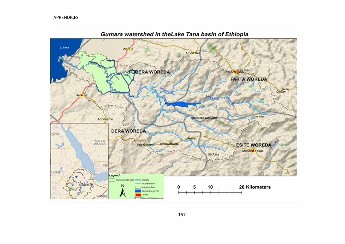
APPENDICES
157
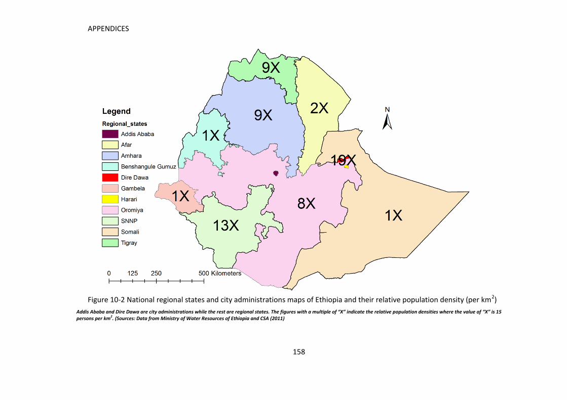
APPENDICES
158
Figure 10-2 National regional states and city administrations maps of Ethiopia and their relative population density (per km2)
Addis Ababa and Dire Dawa are city administrations while the rest are regional states. The figures with a multiple of “X” indicate the relative population densities where the value of “X” is 15 persons per km2. (Sources: Data from Ministry of Water Resources of Ethiopia and CSA (2011)
ACKNOWLEDGEMENT
“ስሇማይነገር ስጦታው እግዚአብሔር ይመስገን።”
2ኛ ቆሮ.9፥15
Glory to the Almighty!!! I am sincerely grateful to Prof. Dr. Bernd Diekkrüger, University of Bonn, Germany, for
his supervision. Without his scientific and unreserved assistance, it would have been very difficult to get this dissertation to the final stage. I am also very thankful to Prof. Dr. Paul Vlek and Dr. Bernhard Tischbein for their comments, encouragement and for giving me their precious time to shape my work at the starting stage of my study. Friendly coordination and support by Dr. Manfred Denich, Dr. Günther Manske, Ms. Rosemarie Zabel, Ms. Maike Retat-Amin, Ms. Sabine Aengenendt-Baer, and Ms. Doris Fuß (Center for Development Research, ZEF, Bonn University) were the most encouraging and feel-at-home ingredients of working at ZEF. I would like to thank Mss. Margaret Jend for language editing and fine tuning the first drafts of this dissertation. I thank the German Federal Ministry for Economic Development Cooperation (Bundesministerium für Wirtschaftliche Zusammenarbeit-BMZ) for the financial support, the International Water Management Institute (IWMI) and Amhara Region Agricultural Research Institute (ARARI) for providing me with materials and facilitating my field work. I would also like to acknowledge the National Meteorological Agency and Ministry of Water Resources of Ethiopia for providing secondary data. The Basic Educational Campaign Program of the Mengistu Haile-Mariam military regime is of special importance on my way to science. Without this program, it would have been completely impossible for me to start my education at all.
I would like to extend my sincere appreciation to Dr. Seleshi Awulachew, Dr. Tilahun Amede, Dr. Amare Hailesilassie, Dr. Girma Tadesse, Dr. Katrien Descheemaeker, Dr. Enyew Adgo, Dr. Yihenew Gebreselassie, Dr. Biru Yitaferu, Fisseha Werede, Asmare Wubet, Abebe Getu, Mesenbet Yibeltal, Mesfin Yibre, Kefelegn Nigussie, Ahmed Amedin, Hirut Yirgu, Besufekad Tadesse, Solomon Ewnetu, Habtamu Tensae, Aklilu Yirgu, and Ato Teferi, and to all others who facilitated field data collection and shared their experience.
Thank you all my friends Dr. Aymar Bossa, Dr. Lulseged Temam, Dr. Seid Nuru, Dr. Joe Hill, Dr. Sewmehon Demissie, Dr. Tilaye Teklewold, Dr. Dessie Salilew, Dr. Tigist Abebe, Dr. Adane Girma, Dr. Tilahun Derib, Dr. Asfaw Kebede, Adefirs Worku, Philipp Baumgartner, Jeroen Spauwen, Patrik, Tigist Araya, and all Ethiopian mates in Germany and The Netherlands. You made my life pleasant especially by your discussions about our countries and the world, which have given me extra-curricular knowledge for my life. Encouragement and paternal treatment by Dr. Moges Mekonnen and his family from Frankfurt played an indirect and important role in my study. Dr. Moges, Ambelye and Birhane, I remember your contribution at the start of my education under the big oak tree in my birth village.
Words can’t explain the respect and love I have for my lovely wife, Hiwot Yirgu Astemir for her treatment, comments and encouragement. My two lovely baby girls, Meklit and Etsubdink, thanks for coming - it is time for us to play together.
My mother, Zewdie Gashu Kinde, deserves all I have. Her paternal care both as a dad and as a mom alone in a rural and harsh poverty life in Ethiopia created my personality and education on a firm foundation. Mami, your long term-stock for me is now lucrative. Mam, live safe and long!