econstor www.econstor.eu

Der Open-Access-Publikationsserver der ZBW – Leibniz-Informationszentrum WirtschaftThe Open Access Publication Server of the ZBW – Leibniz Information Centre for Economics

Nutzungsbedingungen:Die ZBW räumt Ihnen als Nutzerin/Nutzer das unentgeltliche,räumlich unbeschränkte und zeitlich auf die Dauer des Schutzrechtsbeschränkte einfache Recht ein, das ausgewählte Werk im Rahmender unter→ http://www.econstor.eu/dspace/Nutzungsbedingungennachzulesenden vollständigen Nutzungsbedingungen zuvervielfältigen, mit denen die Nutzerin/der Nutzer sich durch dieerste Nutzung einverstanden erklärt.

Terms of use:The ZBW grants you, the user, the non-exclusive right to usethe selected work free of charge, territorially unrestricted andwithin the time limit of the term of the property rights accordingto the terms specified at→ http://www.econstor.eu/dspace/NutzungsbedingungenBy the first use of the selected work the user agrees anddeclares to comply with these terms of use.

zbw Leibniz-Informationszentrum WirtschaftLeibniz Information Centre for Economics

Bauer, Michal; Chytilová, Julie; Morduch, Jonathan

Working Paper

Behavioral foundations of microcredit: Experimentaland survey evidence from rural India

IES Working Paper, No. 28/2008

Provided in Cooperation with:Institute of Economic Studies (IES), Charles University

Suggested Citation: Bauer, Michal; Chytilová, Julie; Morduch, Jonathan (2008) : Behavioralfoundations of microcredit: Experimental and survey evidence from rural India, IES WorkingPaper, No. 28/2008

This Version is available at:http://hdl.handle.net/10419/83420

Institute of Economic Studies, Faculty of Social Sciences

Charles University in Prague

Behavioral Foundations of

Microcredit: Experimental and Survey

Evidence From Rural India

Michal Bauer Julie Chytilová

Jonathan Morduch

IES Working Paper: 28/2008

Institute of Economic Studies, Faculty of Social Sciences,

Charles University in Prague

[UK FSV – IES]

Opletalova 26 CZ-110 00, Prague

E-mail : ies@fsv.cuni.cz http://ies.fsv.cuni.cz

Institut ekonomických studií Fakulta sociá lních věd

Univerzita Karlova v Praze

Opletalova 26 110 00 Praha 1

E-mail : ies@fsv.cuni.cz

http://ies.fsv.cuni.cz

Disclaimer: The IES Working Papers is an online paper series for works by the faculty and students of the Institute of Economic Studies, Faculty of Social Sciences, Charles University in Prague, Czech Republic. The papers are peer reviewed, but they are not edited or formatted by the editors. The views expressed in documents served by this site do not reflect the views of the IES or any other Charles University Department. They are the sole property of the respective authors. Additional info at: ies@fsv.cuni.cz Copyright Notice: Although all documents published by the IES are provided without charge, they are licensed for personal, academic or educational use. All rights are reserved by the authors. Citations: All references to documents served by this site must be appropriately cited. Bibliographic information: Bauer, M., Chytilová , J., Morduch, J. (2008). “ Behavioral Foundations of Microcredit: Experimental and Survey Evidence From Rural India ” IES Working Paper 28/2008. IES FSV. Charles University. This paper can be downloaded at: http://ies.fsv.cuni.cz

Behavioral Foundations of Microcredit: Experimental and Survey Evidence

From Rural India

Michal Bauer* Julie Chytilová #

Jonathan Morduch°

* IES, Charles University Prague E-mail: bauerm@fsv.cuni.cz

# IES, Charles University Prague

E-mail: chytilova@fsv.cuni.cz

° NYU E-mail: jonathan.morduch@nyu.edu

November 2008

Abstract: This paper draws a link between self-control problems and the contractual mechanisms of microcredit. We use a series of “lab experiments in the field” which were designed to elicit measures of time discounting on a sample of 573 individuals in rural Karnataka, India. Evidence from the experiments were integrated with individual survey data on the economic and financial lives of villagers. One third of participants made choices consistent with hyperbolic preferences (more impatient now than in the future), and would be made better off if they could discipline their time inconsistent preferences. While hyperbolic preferences have been often associated with saving behavior, we describe links to borrowing as well. We find that “hyperbolic” women save a lower share of their savings at home and save less in total levels. Women with hyperbolic preferences are also more likely to borrow--and to do so through microcredit institutions specifically. The finding highlights the role of the fixed and frequent installment schedule ubiquitous in microcredit contracts. While microcredit contracts are celebrated for mitigating informational asymmetries, the evidence suggests that they also offer helpful structure for people with self-discipline problems who seek to accumulate capital but who lack suitable contractual saving devices.

Keywords: time preference, hyperbolic discounting, loan contracts, microfinance JEL: C93, D91, O12 Acknowledgements We thank BPKS and Caritas Prague for collaboration on the field work and J. Kabatová , D. Mascarenhas, S. Crasta and L. Perreira for excellent research assistance. We thank K.Basu, R. Filer, I. Gang, W. Greene, J. Hlavá č ek, D. Karlan, M. Mejstřík, D. Munich, A. Ortmann, D. Ray, A. Schotter and M. Skořepa for valuable comments in various stages of the project. We appreciate the financial support by a grant from the CERGE-EI Foundation under a program of the Global Development Network, the IES/Charles University research framework 2005-10 and the Fulbright Foundation. All opinions and errors are our own.

1

Introduction

The Nobel Peace Prize in 2006 celebrated the potential of microcredit to transform the lives of

small-scale entrepreneurs by providing access to small loans. Microcredit advocates argue

that such access to credit will unleash the productive potential of poor households (Yunus

2002). Microcredit providers are drawn together by shared commitments to offer small-scale

transactions, serve the under-served, and use innovative contracts to compensate for the fact

that most customers lack collateralizable assets that can be used to secure loans (Armendá riz

and Morduch, 2005).

The success of microcredit, though, poses a puzzle: if the untapped economic returns to

borrowing are so high, why don’t households save their way out of credit constraints? New

work in behavioral economics helps to answer that question by focusing on psychological

conflicts that undermine efforts to save. The focus has been on self-discipline problems that

persist in the absence of savings devices that foster regular deposits and that limit

withdrawals. One of the hidden challenges faced by the poor is posed by the lack of access to

such mechanisms.

These behavioral insights suggest a new view of microcredit, and they point to an often-

overlooked feature of contracts that, in principle, provides a mechanism that substitutes for

2

missing savings devices. This is the near-universal requirement that loans be repaid in

regular, frequent, fixed installments over time (Rutherford 2000, Armendá riz and Morduch

2000). An unusual feature of microcredit contracts is that borrowers must typically repay

loans in weekly or monthly installments beginning at the very start of the loan, well before

investments can be expected to bear fruit. Money to pay installments must, of necessity,

come at least in part from other income earned by households, such as from wage work. The

repayment process thus looks and feels much like the process of saving in regular increments

from earned income. To draw the link, Rutherford (2000) describes traditional saving

behavior as “saving up” and borrowing in this form as “saving down.” In a textbook loan

contract, by contrast, the principal and interest are paid in a single, large payment after profits

are reaped.1

In drawing the link between microcredit borrowing and saving, we focus on specific problems

that emerge when, intellectually, people value future consumption but they nonetheless give

in to the temptation to consume today. The internal tension is often depicted as a conflict

between a patient “future self” and an impatient “present self” (Schelling 1984, Strotz 1955,

Ainslie 1992), a tension captured parametrically by “hyperbolic” discount rates rather than

standard linear discounting (Laibson 1997). Our findings relate hyperbolic preferences to

microcredit borrowing.

We study villagers in India who are the target customers of microcredit providers. The

microcredit banks in the villages are run on a “self-help group” model promoted by the

Government of India and inspired by Grameen Bank of Bangladesh, the co-winner of the

2006 Nobel Peace Prize. We conducted a series of “lab experiments in the field” designed to

elicit measures of discounting and risk aversion for a random sample of 573 villagers spread

across eighteen villages in two regions of Karnataka, a coastal state in South India. (These

are “artefactual field experiments” in the classification scheme of Harrison and List, 2004.) 1 See Armendá riz and Morduch (2005) on the logic of microcredit repayment schedules, and Field and Pande (2007) for a field experiment from urban India.

3

The questions were not hypothetical: the experiments concerned choices over relatively large

stakes, as large as a week’s wage (as in Tanaka, et al 2006, and Binswanger 1980), and the

structure of the questions allow us to infer intervals for discount rates and evidence of time

inconsistency. We construct measures of hyperbolic discounting and relate the measures of

time discounting and risk aversion to survey data on the economic and financial lives of the

households, including participation in microcredit organizations.

The experiments identify roughly one third of the population as exhibiting choices consistent

with hyperbolic discounting. Those in this group discount the future more heavily when

asked a series of questions about the preference to consume now versus in three months,

relative to the degree of discounting implicit in how they answer similar questions about

consumption in twelve months versus fifteen months.

In our sample, women in the “hyperbolic” group tend to hold a smaller share of their overall

savings at home, a finding consistent with a desire to avoid the everyday temptation of

depleting cash on hand. Women in the hyperbolic group are also more likely than other

women to join local microcredit organizations, and more likely to borrow from them (after

controlling for their baseline degree of time discounting). While we find that women are

generally interested in opportunities to borrow, women with hyperbolic preferences are

especially likely to do so via microcredit. The results are robust to including a range of

observable individual characteristics, evidence on seasonal income patterns, and measures of

intra-family decision-making power.

The evidence is consistent with the notion that microcredit borrowing offers helpful structure

for people with self-discipline problems who seek to accumulate capital but who lack

convenient contractual saving devices. In a different world— one in which villagers weren’t

vulnerable to time-inconsistent behavior and/or had attractive contractual saving devices— the

households might only save (or at least would borrow less). But in an imperfect world, the

nature of microcredit contracts makes borrowing an alternative way to steadily transfer money

4

to a bank and end up with a “usefully large sum” (Rutherford 2000). In this sense, borrowing

and saving are drawn together as substitute mechanisms used toward similar ends.

The next section describes self-help groups. Section 3 describes the economics of self-

control. Section 4 describes the sample selection, experimental design for eliciting subjective

discount rates, and the survey data. Section 5 presents the empirical results on determinants of

patience and time inconsistencies. Section 6 discusses how the experimental choices correlate

with observed financial behavior and describes alternative hypotheses. Section 7 concludes.

2. Self-Help Groups and microcredit

Self-help groups (SHGs) are the main source of microcredit in India. SHGs are the major

providers of financial services in our sample, although moneylenders, banks, and postal

savings schemes also operate in the communities. SHGs are based on groups formed

endogenously in communities, sometimes facilitated by NGOs. The groups comprise 10-25

people, and groups gather regularly, typically every week, to pool their savings and lend from

their accumulated pot to members at an interest rate designed to cover costs (Seibel 2005).

SHG expansion has been driven by an initiative of the government’s National Bank for

Agriculture and Rural Development (NABARD) to encourage linkages between non-

governmental organizations and commercial banks. The SHGs are permitted as informal

entities to obtain bank loans and the whole group is responsible for the loan repayment. By

March 2007, 2.92 million SHGs were providing services to 41 million members (NABARD

2007).

SHGs predominantly attract women, although no bias is built into the program design. In our

sample, 76 percent of group members are women. The participation rate within our sample is

46 percent and this number is very similar in both regions we study. No village has fewer

than 20 percent of individuals participating in an SHG.

5

All SHG members must deposit regularly into compulsory savings accounts (deposits average

Rs. 40 per month2). These accounts have tight withdrawal restrictions: savings may only be

withdrawn when a member leaves a group or if there are exceptional circumstances. This kind

of forced saving aids the SHG by creating collateral that can be tapped in times of trouble, but

it is of limited immediate value as savings for customers.

Two thirds of SHG participants have a loan, with an average size of Rs. 6,708 (about $170).

The interest rate charged by banks to SHGs is about 20 percent annually; the interest rate for

individual loans is at the discretion of SHGs and varies. A recent survey of SHGs shows that

83 percent of loans were used for production or other purposes— notably agricultural

production, animal husbandry, and microenterprise--rather than consumption (Consultative

Group to Assist the Poor 2007).

3. Self-Control and Financial Behavior

The degree of time discounting is essential in making saving and investment decisions. The

behavioral economics literature has pushed further, based on experimental evidence that

discount rates often vary with the time frame (Frederick et al. 2002). In particular, people are

often more impatient for current trade-offs than for future tradeoffs (Strotz 1955, Ainslie

1992). This is captured parametrically by hyperbolic (or “quasi-hyperbolic”) time discount

functions (Laibson 1997). Hyperbolic preferences create a tension between future plans and

current actions. If individuals are “sophisticated” enough to realize it, they may demand a

commitment to “tie their hands” now. If they are “naïve” and do not address their

inconsistencies, individuals may later regret their decisions (O’Donoghue and Rabin 1999).

For sophisticated people with hyperbolic preferences, for example, savings rates should rise

when given the choice to opt into savings devices that incorporate commitments to save

regularly and that limit withdrawals. The cardinal feature of the devices is to keep present

2 At the time of our study the exchange rate was 40.6 Indian rupees per US dollar.

6

temptations at bay by contracting to deposit money in fixed increments at pre-specified times.

These kinds of devices take many forms. In richer countries, the most common is direct-

deposited pension accounts; in poorer communities, a range of informal devices share this

feature, including community-run savings clubs and rotating savings and credit associations

(Rutherford 2000).

Hyperbolic preferences have been invoked to explain a growing range of economic puzzles in

poor countries. Duflo, Kremer and Robinson (2005) observe patterns consistent with

sophisticated hyperbolic preferences in their field experiments on fertilizer adoption,

Mullainathan (2005) argues that time inconsistent preferences help explain erratic school

attendance. Gugerty (2007) similarly interprets the widespread use of informal rotating

savings and credit associations (ROSCAs) as a commitment device to overcome time

inconsistencies faced by savers. She observes that participants value public pressure to make

regular saving deposits; as some ROSCA participants put it, “you can’t save alone.” In

keeping with this, Armendá riz and Morduch (2005) highlight difficulties saving at home, and

they invoke savings difficulties as a rationale for why popular informal savings and borrowing

institutions such as ROSCAs do not fall apart. By keeping money at a distance or by

imposing rigidity to its access, spending may be much less tempting in the presence of

immediate pressures (Mullainathan 2005). Basu (2007) uses hyperbolic preferences as the

basis of a theoretical treatment that explains why individuals simultaneously save and borrow,

a pattern commonly observed by microcredit practitioners. He argues that the existence of

sanctions in the case of loan default provides incentives for discipline that make paying back a

loan easier for individuals with hyperbolic preferences than regularly building up savings

accounts. Self-control problems, although present around the world, may matter more in poor

countries where immediate pressures are greater and mechanisms to help with self-control

problems are more limited.

7

Ashraf et al. (2006) illustrate the link between time preference inconsistency and savings

rigidity. They offered savers of a rural bank in the Philippines the opportunity to save using a

new product that differed from the existing ones only by restricting access of savers to their

deposits until either given maturity or given amount was achieved. They find that 28 percent

of those being offered the commitment product accepted it. Women who demanded the

“commitment” product were more likely to have hyperbolic time preferences— and access to

such accounts notably increased their short-term saving.

We turn here to the link between hyperbolic preferences and borrowing decisions. As noted,

savings with commitment and paying credit in installments are very similar in terms of the

pressure to follow an intended course of action by taking regular steps. For example, Strotz

(1955) and more recently Laibson (1997) highlight this similarity. Borrowing, though, is a

roundabout way to save, and it is costly. While most people expect to earn interest on saving

deposits, evidence shows that people are willing to pay to save when options are limited. The

saving device tested in the Philippines, for example, was valued by the women although

costly to them in that the accounts offer no extra compensation for the associated illiquidity.

Similarly, in Ghana, local deposit collectors are a common part of the informal financial

sector, charging customers a substantial fee for a simple, secure, disciplined ways to save.

One calculation shows that in South India, a similar form of deposit collector who takes

savings from their customers each day, returning the accumulation after 220 days, charges

depositors a fee equivalent to 30 percent of deposits on an annualized basis.3 In parallel with

such devices, microcredit borrowing can be an effective next-best accumulation device.

An alternative reason why the poor may demand commitments like these stem from

household conflicts. In this case individuals do not seek to discipline their own preferences,

but try instead to “discipline” the preferences of other household members (often spouses).

Anderson and Baland (2002) show that the need to protect savings from their husbands

3 See Rutherford (2000) and the discussion in Armendá riz and Morduch (2005).

8

triggers women’s participation in ROSCAs in a Kenyan slum. They find a notable “inverted-

U” shaped pattern in their data: women who have little autonomy from their husbands are

unlikely to join ROSCAs, as are women with great autonomy (since they do not need the

protections that ROSCAs afford). Women in a middle range, though, are particularly likely to

be ROSCA participants. In the work below, we find that the effect of hyperbolic preferences

is robust to including measures of individual autonomy and power within households.

4. Experimental and survey design

Although much has been written about time discounting, experimental evidence is largely

limited to laboratory environments in developed countries. A significant contribution is

Harrison et al. (2002) and Andersen et al. (2008) who estimate the subjective discount rate

among a representative sample of the Danish population. Several innovative studies, typically

in low-income countries, employ experimental tasks to predict behavior outside of labs to

study motivations behind behavioral choices.4 In our study we are primarily interested in

whether people with time inconsistent preferences behave differently from those having

consistent preferences.

Sample selection

The survey design generated a varied sample of the rural population of Karnataka. Data were

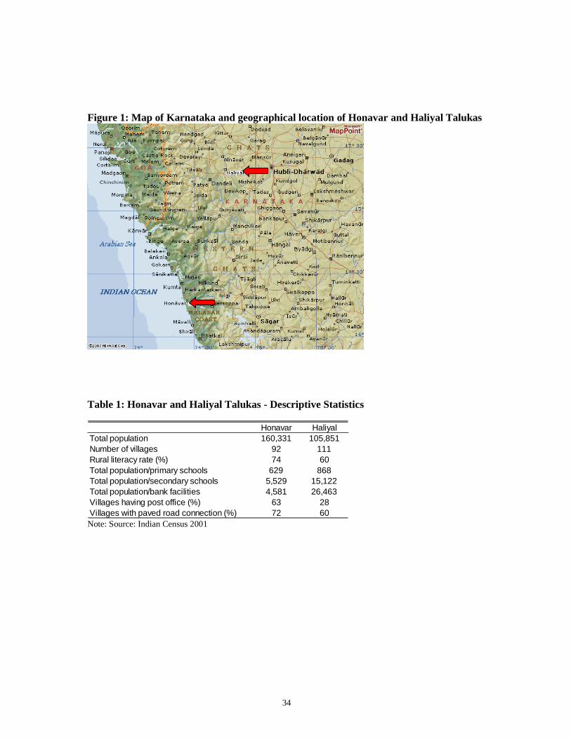
collected in June 2007 in cooperation with BPKS, an Indian NGO in Honavar and Haliyal

taluks (a taluk is an administrative unit akin to a county, part of a larger district within a

state). Honavar is a coastal region and, of the two, is more developed in terms of

infrastructure, market access and access to education and financial facilities. Figure 1

4 For example, Binswanger (1980) and Liu (2008) elicit individual attitudes to risk and observe correlations with agricultural behavior. Karlan (2005) uses the results of trust games to predict default among clients of FINCA. Tanaka et al (2007) take an approach similar to ours. Thomas and Hamoudi (2006) measure discounting, risk aversion, and altruism to study motivations behind inter-generational exchanges.

9

provides a map and Table 1 compares the two taluks on a range of variables. Nine villages

were selected from each taluk, and 35 people were selected in each village using a random

walk method. 5 Those identified were invited to participate in the study, and 90 percent did.

The total number of participants was 573, with no fewer than 25 participants per village.

We used village meeting halls, typically schools, as field labs. The very high response rate

stemmed in part from the support of village heads. Self-selection concerns are limited by the

high take-up rates.

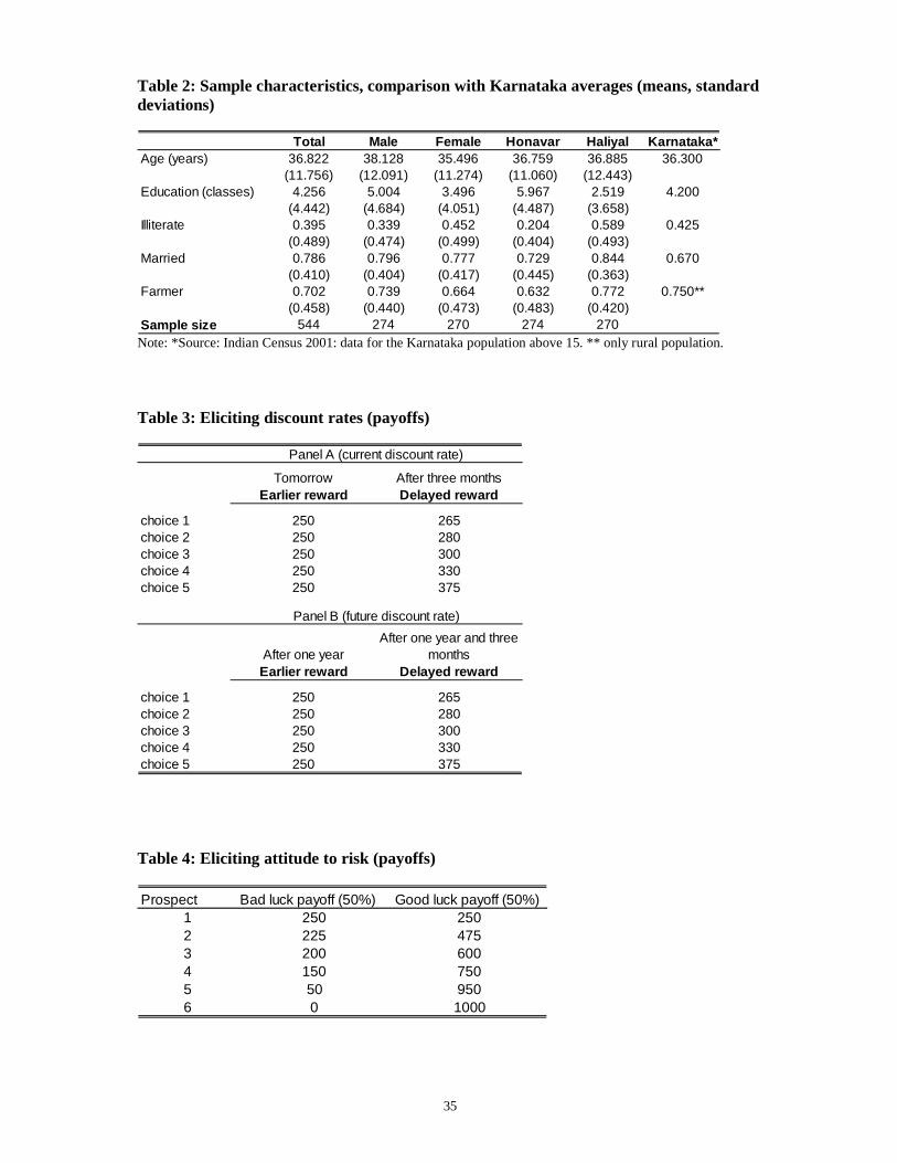
Table 2 compares the sample characteristics with Karnataka averages from 2001, restricted to

the population older than 15 years. The average age and education levels are not statistically

different, but we have a slightly lower proportion of illiterate respondents in our sample (40

percent compared with 43 percent in the entire state). This may reflect increases in

enrollment ratios in 1980s and 1990s. Age of marriage is typically higher in urban areas that

are included in the Karnataka average, while our respondents are villagers and therefore more

likely to be married. Although the selection strategy was not intended to generate a

representative sample of rural population of Karnataka, the sample captures its variety.

Measuring discount rates and risk aversion

We used a simple protocol to elicit discount rates, drawing on practices common in developed

and developing countries (e.g. Harrison et al. 2002; Tanaka et al. 2006).6 Respondents were

asked to choose between receiving smaller amount earlier in time or larger amounts with three

months delay. We start with: “Do you prefer Rs. 250 tomorrow or Rs. 265 three months

later?”

5 The villages were randomly selected based on the 2001 Indian Census database; however, in three villages in each taluk the BPKS did not have a good access and knowledge of a village head. These were replaced with other villages that were similar in size, distance to town and educational facilities to the ones originally selected. 6 In their surveying article Cardenas and Carpenter (2005) classify this methodology as the “choice task method.” For a discussion on relative advantages of using “choices task method” vs. alternative “matching-task method” see Frederick et al. (2002). Our decision was largely made on the basis of simplicity given the low education levels in the area.

10

We posed five such questions to each individual, with each question increasing the future

amount up to Rs. 375 while keeping the earlier amount constant. We thus made the choice to

delay increasingly more attractive in each subsequent binary choice (Table 3, Panel A gives

the choices). The point at which an individual switches from choosing the earlier reward to

the future reward gives an interval of her discount rate. In the analysis we use the arithmetic

means of these intervals to approximate individual discount rates (for specific values see

Table 5). Five percent of respondents switched more than once, and nothing could be inferred

about their discount rate. Such choices are uncorrelated with observable characteristics and

the respondents were excluded from the analysis, reducing our sample to 544.

The same set of binary choices was also offered at a future time frame (as in Ashraf, et al.

2006). Here, we started with: “Do you prefer to receive Rs. 250 in one year’s time or Rs. 265

in one year and three months?” (See Table 3, Panel B.) We denote the discount rate

calculated from the current tradeoffs as the “current discount rate,” and that calculated from

the future tradeoffs as the “future discount rate.” Inconsistencies provide evidence of

hyperbolic preferences, as discussed in the next section.

Several design features in the elicitation methodology allow us to identify time preference

reversals (differences between current and future discount rates) with greater confidence.

First, we shifted the time frame by exactly one year to reduce the effects of seasonality of

agricultural incomes and season-specific expenditures (e.g., annual celebrations).

Second, we introduced a short delay in the current income option in the earlier time frame.

This “front end delay” method should control for potential confounds due to lower credibility

and higher transaction costs associated with future payments (it is used, for example, by

Harrison et al. 2002; Pender 1996). If participants lack confidence that they will receive a

reward in the future, they may prefer a current reward irrespective of their actual discount

rate. Therefore no payments were made on the day of the experimental session. Instead,

11

participants were making choices between Rs. 250 delivered the next day and a higher amount

delivered after three months. The approach also reduces transaction costs differentials

between the options; since all payments are in the future, participants should assign the same

subjective transaction costs to both options.

Third, the set of binary choices in the future time period (with a one year delay) were asked

immediately after the set of choices offered in the earlier time frame. This sequencing should

lead to a conservative estimate of the likelihood of time preference reversals since it biases

toward consistency.

Individual attitudes to risk were also elicited in order to control for the curvature of utility

function. We have used a near replication of the simple protocol designed by Binswanger

(1980) in his study of villagers in South India and later used by Barr (2003) in Zimbabwe.

Each participant was asked to select one out of six different gambles. Every gamble yielded

either a high or a low payoff with a probability 0.5. In each subsequent gamble the expected

value increased jointly with the variance. The sizes of the prize were set at the level of time

discounting choices. The expected value of the least risky gamble was set at Rs. 250, and the

higher payoff in the most risky gamble was Rs. 1000. The prizes for all the gambles are in

Table 4.7

Much care has been devoted to ensuring a correct understanding of experimental choices

given the high proportion of illiterate respondents. Ten trained research assistants were on

hand to help illiterate respondents. Before the experimental choices were made, the

experimenter informed the participants that at the end of the session each of them would have

7 We used two sets of prizes to elicit risk aversion. The relative proportions in the gambles were exactly the same, but amounts for the second set of gambles were lower, with the expected value of Rs. 30 for the least risky gamble and with the maximum payoff of Rs. 120 for the most risky gamble. In the analysis we control for risk aversion inferred from gambles with higher amounts, which were set on a level comparable to time discounting choices.

12

a 20 percent chance of being paid according to one of their choices.8 He then explained the

principle of future payments and simulated the randomization procedure - tossing numbered

ping-pong balls from a bag – which would determine whether and according to which choice

a participant would be paid.9

At the end of a session, randomly selected respondents were rewarded. Payments relating to

risk aversion questions were disbursed immediately. For time discounting questions, winning

participants received a cash certificate signed by the chief of the NGO, a local leader and a

social worker familiar in the community. The prizes were deposited by the NGO and the

social worker was responsible to deliver the amount specified in the cash certificate at the

given date.10

Survey data

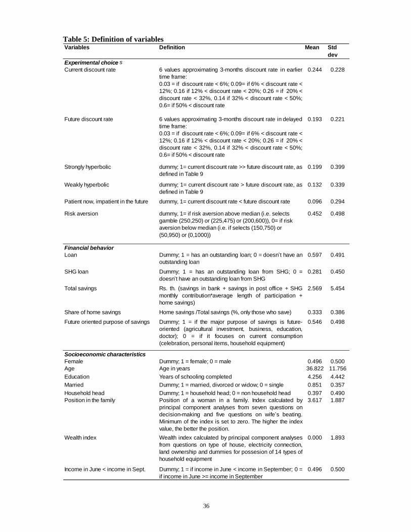
Table 5 describes definitions of variables used in the analysis. A wide range of information on

individual characteristics was collected such as age, education, family background (marital

status, household head, and woman’s position in the household), economic conditions and

financial behavior. We constructed an index approximating wealth using principal

components analysis based on information about items at home, characteristics of the house

and land possession. A set of questions on decision-making power and on attitudes about wife

beating was used to approximate women’s position within households (Jensen and Oster

2007). Again we used principle components to construct an index. Data on individual savings

in a bank, a post office, at home and participation in SHGs together with information on

borrowing indicate individual financial behavior.

8 A similar incentive technique was used, for example, by Botelho et al. (2006) in a lab experiment conducted among students in Timor-Leste. 9 In 12 villages, the experimenter was the director of the cooperating NGO, in six remaining villages the main instructor was the associate director who was also present at previous meetings as a research assistant. The results reported below do not change substantively after controlling for experimenter effect (not reported). 10 In addition, everyone was given a participation fee amounting Rs. 60 to compensate for opportunity costs (daily income). One session lasted on average four hours and these payments were made upon completion of the entire session.

13

5. Determinants of time discounting

We focus on four characteristics resulting from the experiments: current patience (based on

Table 3, Panel A), future patience (based on Table 3, Panel B), present-biased time

inconsistency (hyperbolic discounting) and future-biased time inconsistency (“patient now,

impatient in the future”). In this section we examine how observable characteristics (gender,

age, education, wealth, income fluctuations, family status) predict these traits. In Table 6 we

compare means for different subgroups. In the regression analysis we use OLS for discount

rates and probits for time preference reversals. Observations are clustered at the village

level.11

Determinants of discount rates

We observe two clear relationships with respect to levels of patience as approximated by the

level of discount rates. First, women make more patient choices than men.12 Table 6 shows

that the current three-months discount rate is 27.0 percent for men but only 21.8 percent for

women. For the future discount rate the averages are 22.6 percent and 15.9 percent

respectively. For both discount rates the differences are significant at the 1 percent level. The

results accord with evidence on behavior from developing countries showing that income in

the hands of women is more likely to be used for future-oriented activities like education and

health expenditures (Thomas 1990; Quisumbing and Maluccio 2003) rather than current

consumption. Similarly, the positive experience of microfinance institutions with women is

often attributed to women’s greater patience (Yunus, 2002). Thomas and Hamoudi (2006)

11 Using an ordered probit instead of OLS yields comparable results. The results also do not change substantively after controlling for village fixed effects (not reported). 12 During the experimental meetings the participants were given a lunch. We noticed that most women did not eat the meal, but waited until the end of the session and brought it home to share with their children. Men ate the lunch immediately.

14

also find greater patience in women relative to men in a recent experimental study in rural

Mexico.

Second, as in Kirby et al. (2002) and Bauer and Chytilová (2007), we find that more educated

individuals are more patient, an effect that is particularly strong for men (Table 6). The mean

of the current discount rate for men with above median education is 19.7 percent, while for

below median education it is 33.8 percent. For women, the effect is only marginally

significant, possibly due to the substantially lower variance in education of women (45

percent of women are illiterate in the sample).

In the first three columns of Table 7, the dependent variable is the current discount rate, and it

is the future discount rate in the next three columns. The regression specifications yield

similar conclusions as the table of means. Each additional year of schooling is associated

with a decrease in the current discount rate of 1.3 percentage points and a decrease in the

future rate of 1.5 percentage points. These are only associations, of course, since the

relationship is in part endogenous: education can reduce income constraints or enhance

planning skills and, all else the same, patient individuals are more likely to invest in

education.

Determinants of time-inconsistent preferences

We interpret the choices as “hyperbolic” if the inferred current discount rate is higher than the

future discount rate: an individual with hyperbolic preferences is more impatient now than in

the future. We further distinguish between individuals with weakly hyperbolic preferences

and strongly hyperbolic preferences. Weakly hyperbolic preferences reflect a difference

between current and future discount rates that is relatively small, resulting from choosing the

future reward only one binary choice earlier in future time frame (Table 3, Panel B) compared

to earlier time frame (Panel A). If the difference is larger, a person is regarded as having

strongly hyperbolic preferences.

15

Table 8 illustrates definitions of the time inconsistencies and describes their distribution. The

current discount rate is on the vertical axis and the future rate is on the horizontal axis. Cells

on the diagonal (where the current discount rate equals the future discount rate) represent

individuals with time consistent preferences. Below the diagonal, the current discount rate is

higher than the future discount rate. An individual is considered as “weakly hyperbolic” if she

made a combination of choices that are next to the diagonal and as “strongly hyperbolic” if

combinations lie further below the diagonal.13 Above the diagonal are individuals with future-

biased time inconsistency, in which individuals are more patient now than in the future.

Almost one third of individuals have hyperbolic time preferences (19.9 percent are strongly

hyperbolic and 13.2 percent are weakly hyperbolic), whereas fewer than 10 percent of

individuals are more patient now than in the future.

The first 6 columns of Table 9 show the determinants of hyperbolic preferences. Few

observable characteristics explain hyperbolic time inconsistency. Women who are married or

are household heads are more likely to have strongly hyperbolic preferences. The coefficients

have an opposite sign and are not statistically significant for women having weakly

hyperbolic preferences. None of the variables would predict time inconsistency of men with

statistical significance. These (non-) results are similar to estimates of Ashraf et al (2006) and

other psychological studies on impulsiveness that similarly find little association with

observable characteristics.

13 Note that the inferred discount rates are not linearly increasing (to limit censoring for a given number of binary choices). Hence, the definition of being “weakly hyperbolic” includes individuals with changes in discount rates between the two time frames that vary by different absolute amounts. As a robustness check, we redefined the dividing line between strongly and weakly hyperbolic preferences. In the first variant, we define “strongly hyperbolic” individuals as those whose preferences change by more than 0.09 from the range of discount rates associated with time consistent choices. This variant makes very little difference both in terms of the number of observations defined as strongly hyperbolic and, not surprisingly, in the results. In the second variant, we define “strongly hyperbolic” individuals as having a current discount rate higher than the future discount rate by more than 0.16 units. Doing so decreases the size of the group by 26 observations and reduces the differences in behavior between strongly and weakly hyperbolic described in Section 6, but the basic results hold.

16

There are two major concerns to consider before interpreting the observed reversals as

indications of hyperbolic preferences. First, the preference reversals may mirror cash flow

fluctuations between the earlier and the delayed time frame. Agricultural income is likely to

fluctuate between seasons within a particular year. Similarly, local celebrations are organized

on an annual basis with fixed dates. To address this concern, we deliberately shifted the time

frame by exactly one year. The remaining concern then reduces to the role of income or

expenditure fluctuations across years, such as those resulting from extremely adverse weather

conditions. If farmers experienced or expected relatively bad harvest this year compared to

their usual harvest, they could become more impatient now than in the future. According to

official standards and data from the Directorate of Economics and Statistics, Government of

Karnataka, the cumulated rainfall since the monsoon until the end of the survey was “normal”

in both Honavar and Haliyal Taluks, and when asked directly, most of local leaders indicated

that the present rainfall did not substantially differ from previous years. Moreover, being a

farmer does not predict a higher likelihood of having hyperbolic preferences. As a further

check, participants were asked to select the major unexpected shock during the last five years;

42 percent selected low harvest due to bad weather, but this characteristic also fails to predict

preference reversals.

Second, the reversals may reflect expected transaction costs and lower credibility of future

rewards resulting in a higher discount rate now and lower discounting in the future. As noted

earlier, we mitigate this concern by designing the binary choices so that there are no

immediate payments and by putting the responsibility for future payments into the hands of

respected individuals familiar to the participants. In order to test if the reversal is driven by

lack of trust we also included three questions from the General Social Survey (GSS) on

“trust”, “fairness” and “helping” into our survey. An index from these questions is

uncorrelated with both weakly and strongly hyperbolic preferences (p-value=0.39 and 0.34,

respectively) as are the elements taken separately. Similarly, individuals with no previous

17

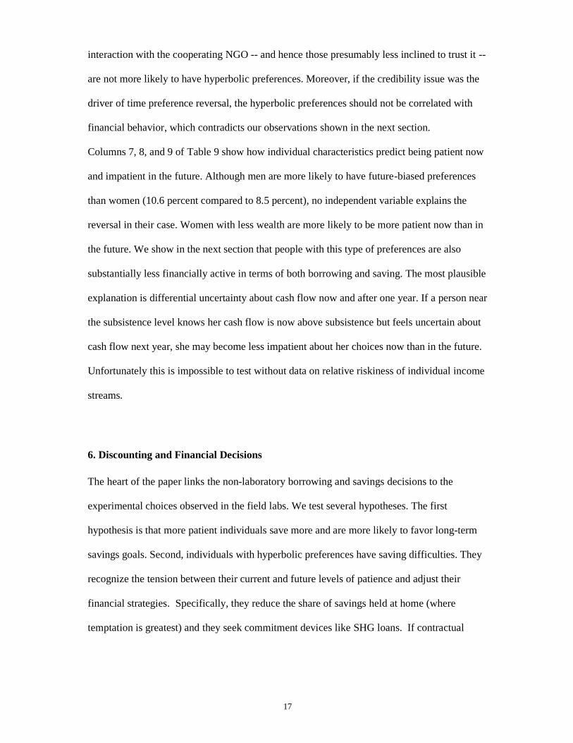
interaction with the cooperating NGO -- and hence those presumably less inclined to trust it --

are not more likely to have hyperbolic preferences. Moreover, if the credibility issue was the

driver of time preference reversal, the hyperbolic preferences should not be correlated with

financial behavior, which contradicts our observations shown in the next section.

Columns 7, 8, and 9 of Table 9 show how individual characteristics predict being patient now

and impatient in the future. Although men are more likely to have future-biased preferences

than women (10.6 percent compared to 8.5 percent), no independent variable explains the

reversal in their case. Women with less wealth are more likely to be more patient now than in

the future. We show in the next section that people with this type of preferences are also

substantially less financially active in terms of both borrowing and saving. The most plausible

explanation is differential uncertainty about cash flow now and after one year. If a person near

the subsistence level knows her cash flow is now above subsistence but feels uncertain about

cash flow next year, she may become less impatient about her choices now than in the future.

Unfortunately this is impossible to test without data on relative riskiness of individual income

streams.

6. Discounting and Financial Decisions

The heart of the paper links the non-laboratory borrowing and savings decisions to the

experimental choices observed in the field labs. We test several hypotheses. The first

hypothesis is that more patient individuals save more and are more likely to favor long-term

savings goals. Second, individuals with hyperbolic preferences have saving difficulties. They

recognize the tension between their current and future levels of patience and adjust their

financial strategies. Specifically, they reduce the share of savings held at home (where

temptation is greatest) and they seek commitment devices like SHG loans. If contractual

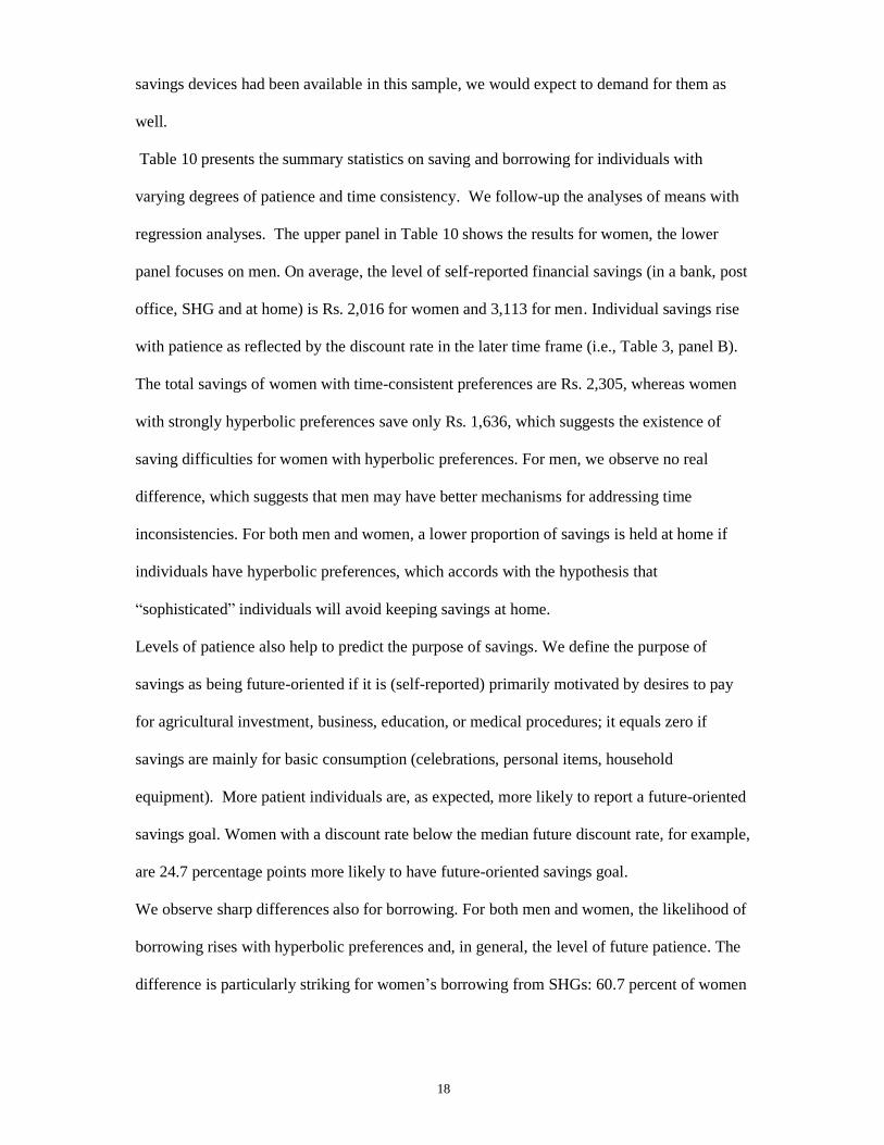
18

savings devices had been available in this sample, we would expect to demand for them as

well.

Table 10 presents the summary statistics on saving and borrowing for individuals with

varying degrees of patience and time consistency. We follow-up the analyses of means with

regression analyses. The upper panel in Table 10 shows the results for women, the lower

panel focuses on men. On average, the level of self-reported financial savings (in a bank, post

office, SHG and at home) is Rs. 2,016 for women and 3,113 for men. Individual savings rise

with patience as reflected by the discount rate in the later time frame (i.e., Table 3, panel B).

The total savings of women with time-consistent preferences are Rs. 2,305, whereas women

with strongly hyperbolic preferences save only Rs. 1,636, which suggests the existence of

saving difficulties for women with hyperbolic preferences. For men, we observe no real

difference, which suggests that men may have better mechanisms for addressing time

inconsistencies. For both men and women, a lower proportion of savings is held at home if

individuals have hyperbolic preferences, which accords with the hypothesis that

“sophisticated” individuals will avoid keeping savings at home.

Levels of patience also help to predict the purpose of savings. We define the purpose of

savings as being future-oriented if it is (self-reported) primarily motivated by desires to pay

for agricultural investment, business, education, or medical procedures; it equals zero if

savings are mainly for basic consumption (celebrations, personal items, household

equipment). More patient individuals are, as expected, more likely to report a future-oriented

savings goal. Women with a discount rate below the median future discount rate, for example,

are 24.7 percentage points more likely to have future-oriented savings goal.

We observe sharp differences also for borrowing. For both men and women, the likelihood of

borrowing rises with hyperbolic preferences and, in general, the level of future patience. The

difference is particularly striking for women’s borrowing from SHGs: 60.7 percent of women

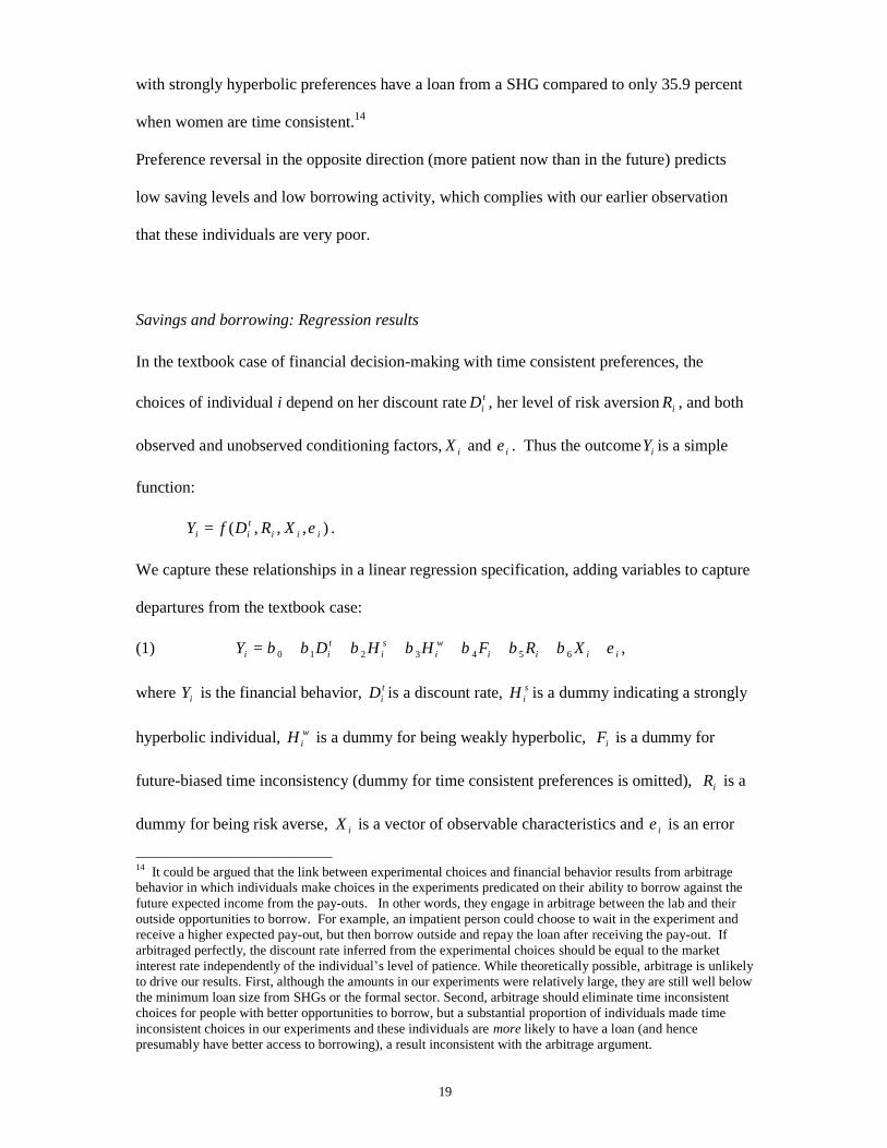
19

with strongly hyperbolic preferences have a loan from a SHG compared to only 35.9 percent

when women are time consistent.14

Preference reversal in the opposite direction (more patient now than in the future) predicts

low saving levels and low borrowing activity, which complies with our earlier observation

that these individuals are very poor.

Savings and borrowing: Regression results

In the textbook case of financial decision-making with time consistent preferences, the

choices of individual i depend on her discount rate tiD , her level of risk aversion iR , and both

observed and unobserved conditioning factors, iX and iε . Thus the outcome iY is a simple

function:

),,,( iiitii XRDfY ε= .

We capture these relationships in a linear regression specification, adding variables to capture

departures from the textbook case:

(1) iiiiwi

si

tii XRFHHDY εβββββββ +++++++= 6543210 ,

where iY is the financial behavior, tiD is a discount rate, s

iH is a dummy indicating a strongly

hyperbolic individual, wiH is a dummy for being weakly hyperbolic, iF is a dummy for

future-biased time inconsistency (dummy for time consistent preferences is omitted), iR is a

dummy for being risk averse, iX is a vector of observable characteristics and iε is an error

14 It could be argued that the link between experimental choices and financial behavior results from arbitrage behavior in which individuals make choices in the experiments predicated on their ability to borrow against the future expected income from the pay-outs. In other words, they engage in arbitrage between the lab and their outside opportunities to borrow. For example, an impatient person could choose to wait in the experiment and receive a higher expected pay-out, but then borrow outside and repay the loan after receiving the pay-out. If arbitraged perfectly, the discount rate inferred from the experimental choices should be equal to the market interest rate independently of the individual’s level of patience. While theoretically possible, arbitrage is unlikely to drive our results. First, although the amounts in our experiments were relatively large, they are still well below the minimum loan size from SHGs or the formal sector. Second, arbitrage should eliminate time inconsistent choices for people with better opportunities to borrow, but a substantial proportion of individuals made time inconsistent choices in our experiments and these individuals are more likely to have a loan (and hence presumably have better access to borrowing), a result inconsistent with the arbitrage argument.

20

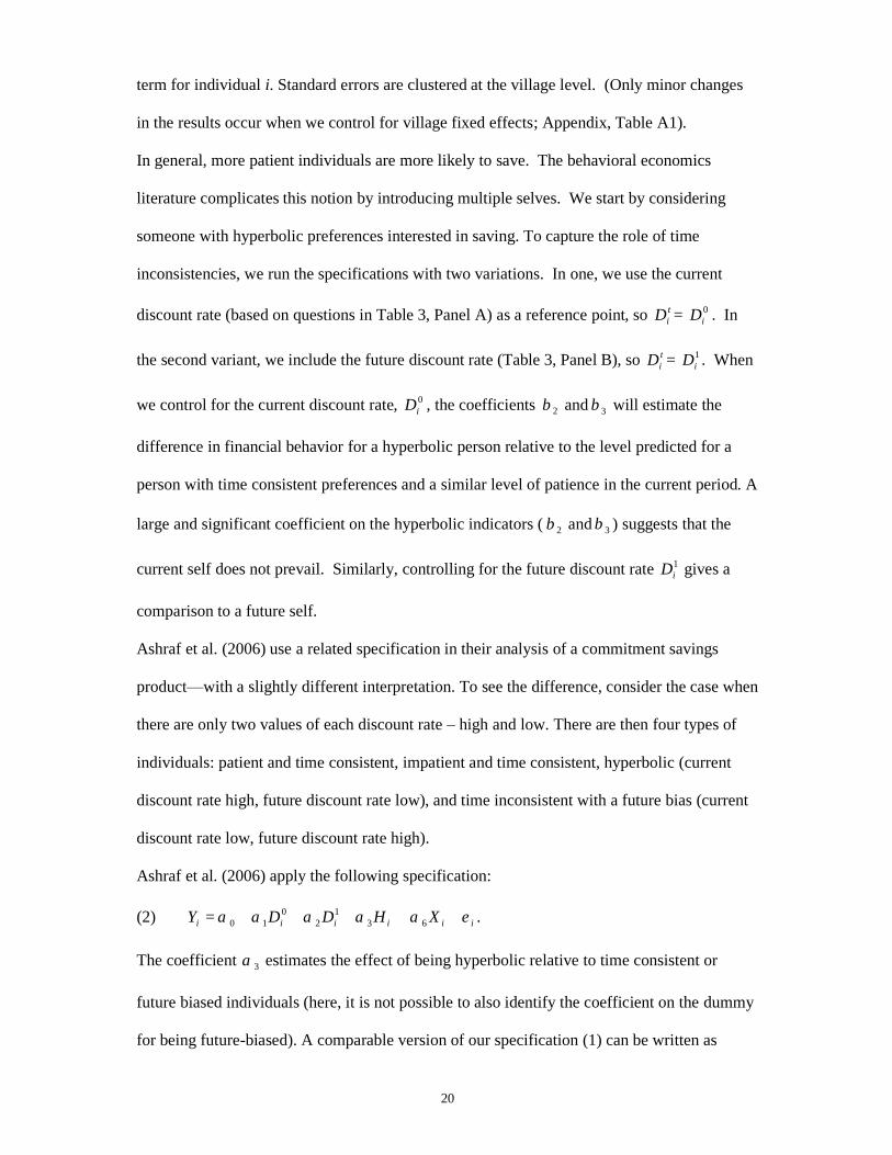
term for individual i. Standard errors are clustered at the village level. (Only minor changes

in the results occur when we control for village fixed effects; Appendix, Table A1).

In general, more patient individuals are more likely to save. The behavioral economics

literature complicates this notion by introducing multiple selves. We start by considering

someone with hyperbolic preferences interested in saving. To capture the role of time

inconsistencies, we run the specifications with two variations. In one, we use the current

discount rate (based on questions in Table 3, Panel A) as a reference point, so tiD = 0

iD . In

the second variant, we include the future discount rate (Table 3, Panel B), so tiD = 1

iD . When

we control for the current discount rate, 0iD , the coefficients 2β and 3β will estimate the

difference in financial behavior for a hyperbolic person relative to the level predicted for a

person with time consistent preferences and a similar level of patience in the current period. A

large and significant coefficient on the hyperbolic indicators ( 2β and 3β ) suggests that the

current self does not prevail. Similarly, controlling for the future discount rate 1iD gives a

comparison to a future self.

Ashraf et al. (2006) use a related specification in their analysis of a commitment savings

product— with a slightly different interpretation. To see the difference, consider the case when

there are only two values of each discount rate – high and low. There are then four types of

individuals: patient and time consistent, impatient and time consistent, hyperbolic (current

discount rate high, future discount rate low), and time inconsistent with a future bias (current

discount rate low, future discount rate high).

Ashraf et al. (2006) apply the following specification:

(2) iiiiii XHDDY εααααα +++++= 631

20

10 .

The coefficient 3α estimates the effect of being hyperbolic relative to time consistent or

future biased individuals (here, it is not possible to also identify the coefficient on the dummy

for being future-biased). A comparable version of our specification (1) can be written as

21

iiiitii XFHDY εβββββ +++++= ’

6’4

’3

’1

’0 , where t=0,1. The difference is that we include

only one of the discount rates and add the dummy for future biased individuals. When we

control for current patience, the coefficient ’3β indicates a difference in behavior between the

hyperbolic group and the time consistent impatient group, and it can be shown that

23’3 ααβ −= . In the second version, where we control for future patience, the behavior of

hyperbolic group is contrasted to the time consistent patient group and 13’3 ααβ += . Our

specification generalizes this simple set-up.

In the analysis we compare how the behavior of the hyperbolic individuals departs from that

of time consistent individuals, conditional on their level of patience. Two natural benchmarks

arise: the level of patience associated with current patience (current self) and the level

associated with future patience (future self). In equation (1) our two coefficients for

hyperbolic preferences directly capture these departures, whereas the coefficient in Ashraf et

al (2006) compares hyperbolic individuals to the average behavior of the group of time

consistent and future-biased individuals.15

If individuals completely give in to their immediate temptations— that is, they are “naïve”

hyperbolics— saving behavior should follow their current discount rate (i.e., 0iD ). The

indicator variable for being hyperbolic should not enter strongly in the regression (i.e.,

032 == ββ ), since saving behavior will be captured by the discount rate. But households are

unlikely to be completely naïve. If they are “sophisticated,” they appreciate the implications

of ,10ii DD ≠ and adjust their behavior to the extent they can given the available mechanisms.

In this case, commitment mechanisms might lead them to a situation in which a regression

that has the future discount rate in it (i.e., 1iD ), also yields that 032 == ββ . In this case,

temptations would be completely held at bay. The parallel regression with the current

15 See Appendix Table A2 for results from a specification in the spirit of Ashraf et al. (2006), in which both current and future discount rates are included instead of the dummy for future-biased preferences.

22

discount rate ( 0iD ) would yield that .032 >> ββ “Sophisticated” hyperbolics might also

over-compensate by applying commitment devices that lead to even higher levels of saving

than their future discount rates would suggest (a class of “sophisticated” behavior highlighted

by O’Donoghue and Rabin 1999); here, 032 >> ββ in the regression anchored by the future

discount rate 1iD .

An alternative situation, in which “sophisticated” individuals have no way to commit to

saving, could result in their giving up and saving even less than the level predicted by current

patience (i.e., 0, 32 <ββ when controlling for current patience). Here, individuals recognize

that in the future they will have to permanently fight not to over-spend so they choose not to

save so much in the first place (O’Donoghue and Rabin 1999).

The same patterns should hold for microcredit production loans, given the premise that they

are investments and, due to the structure of microcredit contracts, entail delayed gratification.

As with saving, people with hyperbolic preferences who do not recognize the tension with

their future selves (or who are powerless to act), will simply follow their current discount

rate 0iD . Sophisticated individuals, when armed with effective commitment devices, will

diverge from the pattern suggested by 0iD . In the villages we study, the structure of

microcredit loans can make them useful commitment devices for individuals seeking better

ways to accumulate. Using a similar argument as in the case of saving with commitment,

sophisticated hyperbolics would then be even more likely to borrow than predicted by the

preferences of their future selves (i.e., 032 >> ββ when controlling for 1iD ). The same

pattern could reflect, directly, the need by hyperbolic borrowers to compensate for their

saving difficulties. If this latter motivation drives behavior, then hyperbolic preferences

should increase the demand for all loans, rather than microcredit loans specifically, a result

we do not find for women.

23

Saving

Men and women who are more patient as predicted by the experiments save more. While for

men hyperbolic preferences make little difference to overall saving levels (columns 2 and 4 of

Table 11), they do for women. The evidence is consistent with men having better tools to

cope with time inconsistencies. Specifically, hyperbolic women save substantially less than

their future patience, as captured by 1iD , suggests (Table 11, columns 3), a result that holds

after controlling for observables. We see that via 02 <β . When controlling for current

patience 0iD , the coefficient for being hyperbolic is smaller and not statistically significant

(column 1). This suggests that women’s saving behavior follows their current patience level

more closely than their future patience level. The results are qualitatively similar for weakly

hyperbolic women, though measured with greater uncertainty. As expected, wealthier

individuals report higher saving levels and more educated men also report significantly higher

savings.

Preferences should also affect the purposes of saving. Table 12 turns to determinants of the

self-reported purpose of savings. Similarly to Table 7, more patient men and women have

more “future-oriented” savings goals, i.e. 01 <β . Having hyperbolic preferences matters

relatively less. For hyperbolic women, future patience is a better predictor of the purpose of

savings as indicated by positive significant coefficients on the hyperbolic indicators when

controlling for current patience (column 1) and negative and not significant coefficients when

controlling for future patience (columns 3). For hyperbolic men, current patience is a more

accurate predictor of savings goals (columns 2 and 4). In general household heads and

women are more likely to have future-oriented savings goals, as are married individuals and

people with more education.

24

Hyperbolic preferences should, though, affect how people save. In Table 13 we examine

home savings as a share of total savings. We hypothesize that people with self-discipline

problems are more likely to keep their money outside of the home.16 More impatient

individuals save a higher proportion of their savings at home and less outside of their

household (such as in a bank, a post office, or SHG), in part because more impatient people

save less overall (and saving less is associated with holding more at home). But the finding is

also consistent with a higher priority placed on spending which diminishes the value of

opening and using saving accounts.

Controlling for all of that, hyperbolic women adjust their savings practices to keep at home a

lower proportion of their financial savings than the level predicted by their current selves

(column 1). That is 02 <β . The future discount rate is a better predictor of their saving

practices (column 3).

In sum, the experimentally-derived discount rates yield plausible predictions about saving

behavior: patient people save more and have more “future-oriented” saving goals. Hyperbolic

women save less than their future level of patience suggests they should. They do, though

seem aware of the tension (and thus are not fully “naïve”). The clearest evidence thus far is

seen in their systematically saving less at home.

Borrowing

The role of hyperbolic preferences continues to mark financial decisions when we turn to

borrowing behavior. Hyperbolic people borrow more, a result consistent with both the greater

need for borrowing to compensate for low saving levels and for workable commitment

devices. As we show below, hyperbolic individuals have a particular demand for microcredit

16 There are 82 individuals who report not having any savings (see Table 10 for more details on their characteristics) and it is not clear how to treat the share of home saving among non-savers. In Table 13 they were excluded from the sample. In order to see the bounds of how important this exclusion is, we repeated the same analysis with non-savers treated as if (1) they saved 100% at home and (2) they saved nothing at home. In both cases the results are qualitatively similar to those observed in Table 13. In particular, strongly hyperbolic women save significantly less at home than predicted by their measured patience in the current period.

25

loans through SHGs, a finding that suggests the importance of commitment devices. As noted

in the introduction, SHG loans have the advantages (in terms of disciplining mechanisms) of

weekly loan installment schedules and public repayments within the villages.

In Table 14 we analyze the determinants of having a loan from any source: from a bank, a

SHG or a moneylender. Patient women borrow more, a result in keeping with the working

assumption that the loans are mainly taken for business investments and other forward-

looking investments.17 For women, being married, middle-aged, less educated, and having

recently experienced a shock at the harvest increases the likelihood of borrowing.

Strongly hyperbolic women are 20 percentage points more likely to have a loan compared to

the level predicted by the patience of their current self (column 1) and the coefficient on being

hyperbolic is positive though not statistically significant when controlling for the preferences

of the future self (column 3).

Although for men we also observe a positive correlation between being hyperbolic and having

a loan, we can push the analysis further on the sample of women. First, borrowing by men is

mainly restricted to banks, while there is substantial SHG borrowing activity among women

in our sample (42.6 percent have an SHG loan versus only 13.9 percent of men). In addition,

we didn’t find lower savings for time-inconsistent men as we did for women, which suggests

that they have other ways to cope with self-discipline problems not available to women.

We begin by studying how being hyperbolic affects the choice between different types of

loans. In Table 15 the dependent variable is equal to one if an individual has a loan from an

SHG. We can see that the results for women’s discounting and borrowing in Table14 were

largely driven by SHG loans. Strongly hyperbolic women are 36.4 percentage points more

likely to borrow from SHGs than predicted by their current level of patience (column 1).

17 Introductory economics tells us that patient individuals save more, and the impatient borrow more. That intuition fails, though, when we turn to the billions of people around the world, especially the poor, whose income derives largely from farming or small-scale business. As self-employed entrepreneurs, these households borrow often to support their farms and businesses.

26

In columns 5-8, we restrict the sample only to individuals who have a loan (independently of

its provider) and do the same analysis. This restriction thus conditions on the generic demand

for a loan and places the focus on loan type. Importantly, we still observe similar results for

hyperbolic discounting. Conditional on borrowing, strongly hyperbolic women are more

inclined to borrow from SHGs, which is consistent with the hypothesis that features specific

to SHG contracts and practices are desirable for individuals with hyperbolic preferences.

(SHG loans may have other advantages relative to alternative loans types, such as lower

interest rates, but our focus here is on features that are particularly appealing to hyperbolics.)

When future patience levels, 1iD , are included in the specification, strongly hyperbolic women

borrow at a rate even higher than those discount rates suggest. The result is explained by the

combination of the disciplining effect of SHG loans and the desire to compensate for lower

savings levels.

The interpretation above centers on self-control issues, and the results are robust to extending

the specifications to include a measure of women’s position within a household (to capture

“spousal control” issues). Spousal control can be another motivating factor for why women

seek commitment mechanisms; i.e., to keep money from husbands whose spending

preferences vary from those of their wives (Anderson and Baland 2002). Theory predicts that

women who have little autonomy from their husbands are unlikely to use a commitment

device, as are women with substantial autonomy (since they do not need the protection of

commitment).

As found by Anderson and Baland (2002), the action here comes from women with a mid-

level of autonomy. We find evidence supporting the spousal control motive for borrowing

behavior, but not for savings behavior. Women in the third quartile of our measure of

women’s position are the most likely to have a loan from SHGs (Table 15). The result

suggests that husbands or other family members respect women’s autonomy over resources

27

from SHG loans but less so for savings or other types of loans. The results on hyperbolics are

little changed by this extension.

7. Conclusions

The textbook model of optimal consumption choice abstracts from self-discipline problems

that households may face, limiting their ability to save. Behavioral economics has taken this

as a focus, centering on ways that various contracting mechanisms can generate greater

savings levels by promoting discipline. We draw a link between these kinds of disciplining

mechanisms and the propensity to borrow from microcredit institutions.

The study is based on results from a series of “lab experiments in the field” designed to elicit

measures of time discounting and risk aversion and survey data on financial behavior for a

random sample of over 500 individuals in rural India. We show that women’s choice to

borrow in general, and the propensity to do so through local microcredit institutions

specifically, is greater for women with hyperbolic preferences.

After controlling for the general preference for consuming today versus in the future, we find

that women with time preferences exhibiting “strong” hyperbolic discounting save lower

proportion of their savings at home (in keeping with self-discipline difficulties) and save less

in total levels.

Borrowing through microcredit institutions can provide a partial solution to these problems.

They provide a way to accumulate that is structured and regulated both by SHG loan officers

and by fellow villagers.

The finding that hyperbolic women favor borrowing from SHGs can be partly explained by

their difficulty saving, so they are less likely to be able to rely on their own resources for

capital. Hence, the hyperbolic group is more likely to need to borrow than otherwise similar

people undertaking comparable investments. Another explanation that has been a particular

28

focus above, is that the structure of microcredit loans provides a way to convert income flows

into large sums through a device that— for the hyperbolic group— is more effective than the

alternative of saving up. A third explanation is that the hyperbolic group is giving in to their

desire for current consumption, driving up loan demand. Our result, though, holds even after

controlling for the baseline degree of time discounting; the time preference variable should

capture aspects of loan demand associated with the desire for current consumption.

The analysis rests on the way that microcredit loans provide discipline and peer pressure

absent in the textbook lending contract. Microcredit contracts have been celebrated by

economic theorists for providing novel solutions to problems of moral hazard and adverse

selection. The evidence here suggests that a key to their success may rest as well with their

role in helping borrowers discipline their financial lives. The evidence helps to explain the

puzzling existence of the regular repayment schedules used in nearly all microfinance loan

contracts globally (Armendá riz and Morduch 2005). The evidence also helps to explain why

microfinance institutions that drop the joint liability element of group lending from their

contracts nonetheless have maintained regular repayment schedules and group meetings (Gine

and Karlan 2008).

29

References

Ainslie, George W. 1992. Picoeconomics. Cambridge, UK: Cambridge University Press.

Andersen, Steffen, Glenn W. Harrison, Morten I. Lau, and E. E. Rutströ m.

2008."Eliciting Risk and Time Preferences." Econometrica, 76(3): 583.

Anderson, C. L., Maya Dietz, Andrew Gordon, and Marieka Klawitter. 2004."Discount

Rates in Vietnam." Economic Development and Cultural Change, 52(4): 873-887.

Anderson, Siwan and Jean-Marie Baland. 2002."The Economics of Roscas and

Intrahousehold Resource Allocation." Quarterly Journal of Economics, 117(3): 963-995.

Armendáriz De Aghion, Beatriz and Jonathan Morduch. 2005. The economics of

microfinance. Cambridge, MA: MIT Press.

Ashraf, Nava, Dean Karlan, and Wesley Yin. 2006."Tying Odysseus to the Mast: Evidence

from a Commitment Savings Product in the Philippines." Quarterly Journal of Economics,

121(2): 635-672.

Barr, Abigail. 2003. "Risk Pooling, Commitment, and Information: An Experimental Test of

Two Fundamental Assumptions." Oxford University Centre for the Study of African

Economies Working Paper CSAE.

Basu, Karna. 2007. "A Behavioral Model of Simultaneous Borrowing and Saving."

http://www.cid.harvard.edu/neudc07/docs/neudc07_s3_p07_basu.pdf.

Bauer, Michal and Julie Chytilová. 2007. "The Impact of Education on Subjective Discount

Rate in Ugandan Villages." http://ies.fsv.cuni.cz/storage/publication/3293_uganda.pdf.

30

Binswanger, Hans B. 1980."Attitudes Toward Risk: Experimental Measurement in Rural

India." American Journal of Agricultural Economics, 62(3): 395-407.

Botelho, Anabela, Glenn W. Harrison, Pinto, Ligia M. Costa, E. E. Rutströ m and Paula

Veiga. 2006. "Discounting in Developing Countries: Experimental Evidence from Timor-

Leste."

http://www.econ.canterbury.ac.nz/downloads/discounting_in_developing_countries.pdf.

Cardenas, Juan C. and Jeffrey P. Carpenter. 2005. "Experiments and Economic

Development: Lessons from Field Labs in the Developing World." Middlebury College

Economics Discussion Paper No. 05-05.

Consultative Group to Assist the Poor [CGAP]. 2007. "Sustainability of Self-Help Groups

in India: Two Analyses." CGAP Occasional paper No. 12.

Daley-Harris, Sam. 2007. "State of the Microcredit Summit Campaign Report 2007."

http://www.microcreditsummit.org/pubs/reports/socr/EngSOCR2007.pdf.

Duflo, Esther, Michael Kremer and Jonathan Robinson. 2006. "Why Don’t Farmers use

Fertilizer: Evidence from Field Experiments in Western Kenya."

http://www.iies.su.se/seminars/papers/070308.pdf.

Field, Erica and Rohini Pande. 2007. "Repayment Frequency and Default in Micro-Finance:

Evidence from India." Forthcoming in Journal of European Economics Association Papers

and Proceedings.

Frederick, Shane, George Loewenstein, and Ted O’Donoghue. 2002."Time Discounting

and Time Preference: A Critical Review." Journal of Economic Literature, 40(2): 351-401.

31

Gine, Xavier and Dean Karlan. 2008. "Peer Monitoring and Enforcement: Long Term

Evidence from Microcredit Lending Groups with and without Group Liability."

http://research.yale.edu/karlan/downloads/bulak.pdf.

Gugerty, Mary K. 2007."You Can’t Save Alone: Commitment in Rotating Savings and

Credit Associations in Kenya." Economic Development and Cultural Change, 55: 251-282.

Harrison, Glenn W., Morten I. Lau, and Melonie B. Williams. 2002."Estimating

Individual Discount Rates in Denmark: A Field Experiment." American Economic Review,

92(5): 1606-1617.

Harrison, Glenn W. and John A. List. 2004."Field Experiments." Journal of Economic

Literature, 42(4): 1009-1055.

Jensen, Robert and Emily Oster. 2007. "The Power of TV: Cable Television and Women’s

Status in India." http://home.uchicago.edu/~eoster/tvwomen.pdf.

Karlan, Dean. 2005."Using Experimental Economics to Measure Social Capital and Predict

Financial Decisions." American Economic Review, 95(5): 1688-1699.

Kirby, Kris N., Ricardo Godoy, Victoria Reyes-García, Elizabeth Byron, Lilian Apaza,

William Leonard, Eddy Pérez, Vincent Vadez, and David Wilkie. 2002."Correlates of

Delay-Discount Rates: Evidence from Tsimane’ Amerindians of the Bolivian Rain Forest."

Journal of Economic Psychology, 23(3): 291-316.

Knack, Stephen and Philip Keefer. 1997."Does Social Capital have an Economic Payoff? A

Cross-Country Investigation." Quarterly Journal of Economics, 112(4): 1251-1288.

Laibson, David. 1997."Golden Eggs and Hyperbolic Discounting." Quarterly Journal of

Economics, 112(2): 443-477.

32

Lederman, Daniel, Norman V. Loayza, and Ana M. Menendez. 2002."

Violent Crime: Does Social Capital Matter?" Economic Development and Cultural Change,

50(3): 509-539.

Liu, Elaine. 2008. "Time to Change what to Sow: Risk Preferences and Technology

Adoption Decisions of Cotton Farmers in China." PhD diss. Princeton University.

Mullainathan, Sendhil. 2005. "Development economics through the lens of psychology." In

Annual wold bank conference in development economics 2005: Lessons from experience, ed.

Francois Bourguignon and Boris Pleskovic, Oxford, UK: Oxford University Press.

National Bank for Agriculture and Rural Development [NABARD]. 2007. "Snapshot of

SHG-Bank Linkage in India-March 2007." NABARD report.

O’Donoghue, Ted and Matthew Rabin. 1999."Doing it Now Or Doing it Later." American

Economic Review, 89(1): 103-124.

Pender, John L. 1996."Discount Rates and Credit Markets: Theory and Evidence from Rural

India." Journal of Development Economics, 50(2): 257-296.

Quisumbing, Agnes R. and John A. Maluccio. 2003."Resources at Marriage and

Intrahousehold Allocation: Evidence from Bangladesh, Ethiopia, Indonesia, and South

Africa." Oxford Bulletin of Economics and Statistics, 65(3): 283-328.

Rutherford, Stuart. 2000. The poor and their money. USA: Oxford University Press.

Schelling, Thomas C. 1984. Choice and consequence. Cambridge, MA: Harvard University

Press.

33

Seibel, Hans D. and Stefan Karduck. 2005. "Transaction costs of self-help groups: A study

of NABARD’s SHG banking programme in india." In Financial growth in india and china.

ed. Alagiri Dhandapani, Hyderabad: IFCAI Univ. Press.

Singh,Inderjit, Lyn Squire, and John Strauss. 1986. Agricultural household models:

Extensions, applications, and policy. Baltimore, MD: Johns Hopkins University Press.

Strotz, Robert H. 1955."Myopia and Inconsistency in Dynamic Utility Maximization." The

Review of Economic Studies, 23(3): 165-180.

Tanaka, Tomomi, Colin F. Camerer and Quang Nguyen. 2006. "Preferences, Poverty, and

Politics: Field Experiments and Survey Data from Vietnam."

http://www.hss.caltech.edu/~camerer/Vietnam.pdf.

Thomas, Duncan. 1990."Intra-Household Resource Allocation: An Inferential Approach."

Journal of Human Resources, 26(1): 635-664.

Thomas, Duncan and Amar Hamoudi. 2006. "Do You Care? Altruism and Inter-

Generational Exchanges in Mexico." California Center for Population Research Online

Working Paper No. 008-06.

Yunus, Muhammad. 2002. "Toward eliminating poverty from the world: Grameen bank

experience." In Making progress: Essays in progress and public policy, ed. C. Leigh

Anderson and Janet W. Looney, Lanham: MD: Lexington Books.

34

Figure 1: Map of Karnataka and geographical location of Honavar and Haliyal Talukas

Table 1: Honavar and Haliyal Talukas - Descriptive Statistics

Honavar HaliyalTotal population 160,331 105,851Number of villages 92 111Rural literacy rate (%) 74 60Total population/primary schools 629 868Total population/secondary schools 5,529 15,122Total population/bank facilities 4,581 26,463Villages having post office (%) 63 28Villages with paved road connection (%) 72 60 Note: Source: Indian Census 2001

35

Table 2: Sample characteristics, comparison with Karnataka averages (means, standard deviations)

Total Male Female Honavar Haliyal Karnataka*Age (years) 36.822 38.128 35.496 36.759 36.885 36.300

(11.756) (12.091) (11.274) (11.060) (12.443)Education (classes) 4.256 5.004 3.496 5.967 2.519 4.200

(4.442) (4.684) (4.051) (4.487) (3.658)Illiterate 0.395 0.339 0.452 0.204 0.589 0.425

(0.489) (0.474) (0.499) (0.404) (0.493)Married 0.786 0.796 0.777 0.729 0.844 0.670

(0.410) (0.404) (0.417) (0.445) (0.363)Farmer 0.702 0.739 0.664 0.632 0.772 0.750**

(0.458) (0.440) (0.473) (0.483) (0.420)Sample size 544 274 270 274 270 Note: *Source: Indian Census 2001: data for the Karnataka population above 15. ** only rural population. Table 3: Eliciting discount rates (payoffs)

Tomorrow After three monthsEarlier reward Delayed reward

choice 1 250 265choice 2 250 280choice 3 250 300choice 4 250 330choice 5 250 375

After one yearAfter one year and three

monthsEarlier reward Delayed reward

choice 1 250 265choice 2 250 280choice 3 250 300choice 4 250 330choice 5 250 375

Panel A (current discount rate)

Panel B (future discount rate)

Table 4: Eliciting attitude to risk (payoffs)

Prospect Bad luck payoff (50%) Good luck payoff (50%)1 250 2502 225 4753 200 6004 150 7505 50 9506 0 1000

36

Table 5: Definition of variables Variables Definition Mean Std

devExperimental choice s

6 values approximating 3-months discount rate in earliertime frame:0.03 = if discount rate < 6%; 0.09= if 6% < discount rate <12%; 0.16 if 12% < discount rate < 20%; 0.26 = if 20% <discount rate < 32%, 0.14 if 32% < discount rate < 50%;0.6= if 50% < discount rate

6 values approximating 3-months discount rate in delayedtime frame:0.03 = if discount rate < 6%; 0.09= if 6% < discount rate <12%; 0.16 if 12% < discount rate < 20%; 0.26 = if 20% <discount rate < 32%, 0.14 if 32% < discount rate < 50%;0.6= if 50% < discount rate

Strongly hyperbolic dummy; 1= current discount rate >> future discount rate, as defined in Table 9

0.199 0.399

Weakly hyperbolic dummy; 1= current discount rate > future discount rate, asdefined in Table 9

0.132 0.339

Patient now, impatient in the future dummy, 1= current discount rate < future discount rate 0.096 0.294

Risk aversion dummy, 1= if risk aversion above median (i.e. selects gamble (250,250) or (225,475) or (200,600)), 0= if risk aversion below median (i.e. if selects (150,750) or (50,950) or (0,1000))

0.452 0.498

Financial behaviorLoan Dummy; 1 = has an outstanding loan; 0 = doesn’t have an

outstanding loan0.597 0.491

SHG loan Dummy; 1 = has an outstanding loan from SHG; 0 =doesn’t have an outstanding loan from SHG

0.281 0.450

Total savings Rs. th. (savings in bank + savings in post office + SHGmonthly contribution*average length of participation +home savings)

2.569 5.454

Share of home savings Home savings /Total savings (%, only those who save) 0.333 0.386

Future oriented purpose of savings Dummy; 1 = if the major purpose of savings is future-oriented (agricultural investment, business, education,doctor); 0 = if it focuses on current consumption(celebration, personal items, household equipment)

0.546 0.498

Socioeconomic characteristicsFemale Dummy; 1 = female; 0 = male 0.496 0.500Age Age in years 36.822 11.756Education Years of schooling completed 4.256 4.442Married Dummy; 1 = married, divorced or widow; 0 = single 0.851 0.357Household head Dummy; 1 = household head; 0 = non household head 0.397 0.490Position in the family Position of a woman in a family. Index calculated by

principal component analyses from seven questions ondecision-making and five questions on wife’s beating.Minimum of the index is set to zero. The higher the indexvalue, the better the position.

3.617 1.887

Wealth index Wealth index calculated by principal component analysesfrom questions on type of house, electricity connection,land ownership and dummies for possesion of 14 types ofhousehold equipment

0.000 1.893

Income in June < income in Sept. Dummy; 1 = if income in June < income in September; 0 =if income in June >= income in September

0.496 0.500

Current discount rate 0.244 0.228

Future discount rate 0.193 0.221

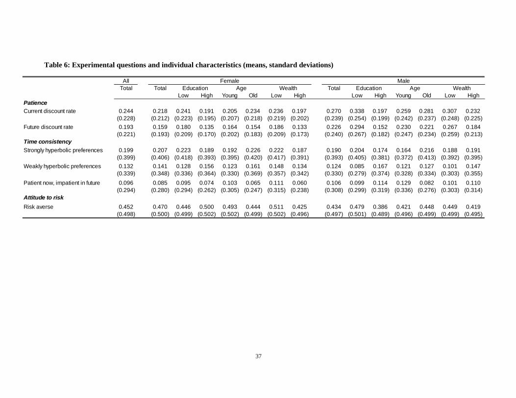
37

Table 6: Experimental questions and individual characteristics (means, standard deviations)

AllTotal Total Total

Low High Young Old Low High Low High Young Old Low HighPatienceCurrent discount rate 0.244 0.218 0.241 0.191 0.205 0.234 0.236 0.197 0.270 0.338 0.197 0.259 0.281 0.307 0.232

(0.228) (0.212) (0.223) (0.195) (0.207) (0.218) (0.219) (0.202) (0.239) (0.254) (0.199) (0.242) (0.237) (0.248) (0.225)Future discount rate 0.193 0.159 0.180 0.135 0.164 0.154 0.186 0.133 0.226 0.294 0.152 0.230 0.221 0.267 0.184

(0.221) (0.193) (0.209) (0.170) (0.202) (0.183) (0.209) (0.173) (0.240) (0.267) (0.182) (0.247) (0.234) (0.259) (0.213)Time consistencyStrongly hyperbolic preferences 0.199 0.207 0.223 0.189 0.192 0.226 0.222 0.187 0.190 0.204 0.174 0.164 0.216 0.188 0.191

(0.399) (0.406) (0.418) (0.393) (0.395) (0.420) (0.417) (0.391) (0.393) (0.405) (0.381) (0.372) (0.413) (0.392) (0.395)Weakly hyperbolic preferences 0.132 0.141 0.128 0.156 0.123 0.161 0.148 0.134 0.124 0.085 0.167 0.121 0.127 0.101 0.147

(0.339) (0.348) (0.336) (0.364) (0.330) (0.369) (0.357) (0.342) (0.330) (0.279) (0.374) (0.328) (0.334) (0.303) (0.355)Patient now, impatient in future 0.096 0.085 0.095 0.074 0.103 0.065 0.111 0.060 0.106 0.099 0.114 0.129 0.082 0.101 0.110

(0.294) (0.280) (0.294) (0.262) (0.305) (0.247) (0.315) (0.238) (0.308) (0.299) (0.319) (0.336) (0.276) (0.303) (0.314)Attitude to riskRisk averse 0.452 0.470 0.446 0.500 0.493 0.444 0.511 0.425 0.434 0.479 0.386 0.421 0.448 0.449 0.419

(0.498) (0.500) (0.499) (0.502) (0.502) (0.499) (0.502) (0.496) (0.497) (0.501) (0.489) (0.496) (0.499) (0.499) (0.495)

MaleFemaleEducation Age WealthEducation Age Wealth

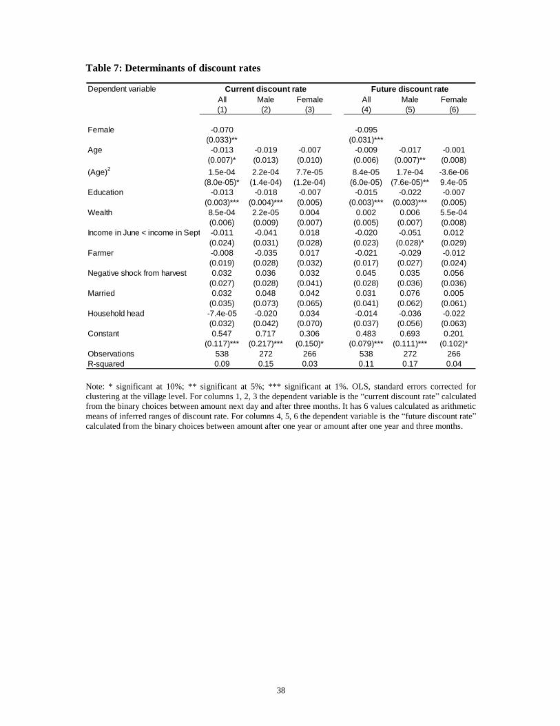
38

Table 7: Determinants of discount rates

Dependent variableAll Male Female All Male Female(1) (2) (3) (4) (5) (6)

Female -0.070 -0.095(0.033)** (0.031)***

Age -0.013 -0.019 -0.007 -0.009 -0.017 -0.001(0.007)* (0.013) (0.010) (0.006) (0.007)** (0.008)

(Age)2 1.5e-04 2.2e-04 7.7e-05 8.4e-05 1.7e-04 -3.6e-06(8.0e-05)* (1.4e-04) (1.2e-04) (6.0e-05) (7.6e-05)** 9.4e-05

Education -0.013 -0.018 -0.007 -0.015 -0.022 -0.007(0.003)*** (0.004)*** (0.005) (0.003)*** (0.003)*** (0.005)

Wealth 8.5e-04 2.2e-05 0.004 0.002 0.006 5.5e-04(0.006) (0.009) (0.007) (0.005) (0.007) (0.008)

Income in June < income in Sept. -0.011 -0.041 0.018 -0.020 -0.051 0.012(0.024) (0.031) (0.028) (0.023) (0.028)* (0.029)

Farmer -0.008 -0.035 0.017 -0.021 -0.029 -0.012(0.019) (0.028) (0.032) (0.017) (0.027) (0.024)

Negative shock from harvest 0.032 0.036 0.032 0.045 0.035 0.056(0.027) (0.028) (0.041) (0.028) (0.036) (0.036)

Married 0.032 0.048 0.042 0.031 0.076 0.005(0.035) (0.073) (0.065) (0.041) (0.062) (0.061)

Household head -7.4e-05 -0.020 0.034 -0.014 -0.036 -0.022(0.032) (0.042) (0.070) (0.037) (0.056) (0.063)

Constant 0.547 0.717 0.306 0.483 0.693 0.201(0.117)*** (0.217)*** (0.150)* (0.079)*** (0.111)*** (0.102)*

Observations 538 272 266 538 272 266R-squared 0.09 0.15 0.03 0.11 0.17 0.04

Current discount rate Future discount rate

Note: * significant at 10%; ** significant at 5%; *** significant at 1%. OLS, standard errors corrected for clustering at the village level. For columns 1, 2, 3 the dependent variable is the “current discount rate” calculated from the binary choices between amount next day and after three months. It has 6 values calculated as arithmetic means of inferred ranges of discount rate. For columns 4, 5, 6 the dependent variable is the “future discount rate” calculated from the binary choices between amount after one year or amount after one year and three months.

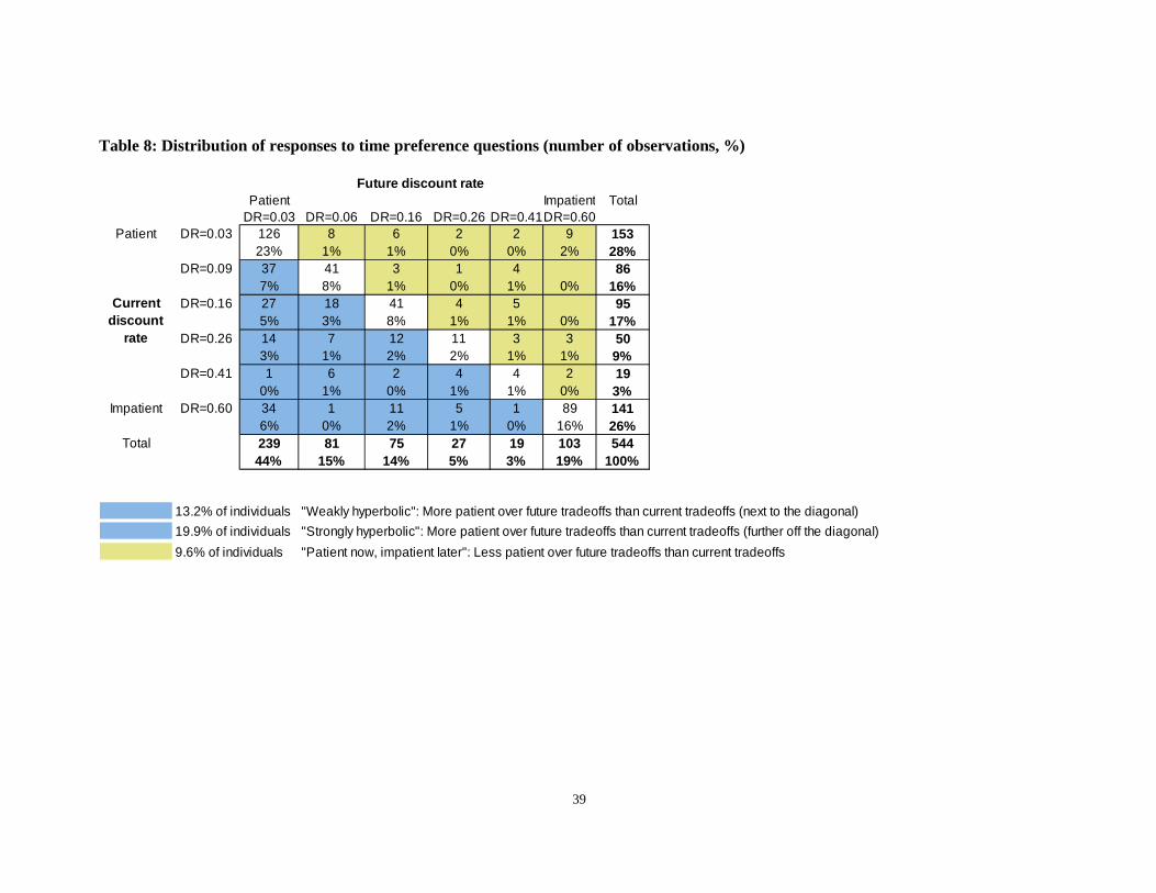
39

Table 8: Distribution of responses to time preference questions (number of observations, %)

Patient Impatient TotalDR=0.03 DR=0.06 DR=0.16 DR=0.26 DR=0.41DR=0.60

Patient DR=0.03 126 8 6 2 2 9 15323% 1% 1% 0% 0% 2% 28%

DR=0.09 37 41 3 1 4 867% 8% 1% 0% 1% 0% 16%

DR=0.16 27 18 41 4 5 955% 3% 8% 1% 1% 0% 17%

DR=0.26 14 7 12 11 3 3 503% 1% 2% 2% 1% 1% 9%

DR=0.41 1 6 2 4 4 2 190% 1% 0% 1% 1% 0% 3%

Impatient DR=0.60 34 1 11 5 1 89 1416% 0% 2% 1% 0% 16% 26%

Total 239 81 75 27 19 103 54444% 15% 14% 5% 3% 19% 100%

13.2% of individuals "Weakly hyperbolic": More patient over future tradeoffs than current tradeoffs (next to the diagonal)19.9% of individuals "Strongly hyperbolic": More patient over future tradeoffs than current tradeoffs (further off the diagonal)9.6% of individuals "Patient now, impatient later": Less patient over future tradeoffs than current tradeoffs

Current discount

rate

Future discount rate

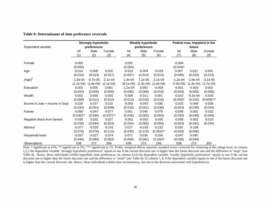
40

Table 9: Determinants of time preference reversals

Dependent variableAll Male Female All Male Female All Male Female(1) (2) (3) (4) (5) (6) (7) (8) (9)

Female 0.005 0.052 -0.058(0.050) (0.064) (0.034)*

Age 0.014 0.008 0.020 -0.010 -0.004 -0.019 0.007 0.011 0.001(0.010) (0.013) (0.017) (0.007) (0.013) (0.013) (0.006) (0.010) (0.013)

(Age)2 -1.3e-04 -6.7e-05 -2.1e-04 1.3e-04 7.1e-05 2.1e-04 -1.2e-04 -1.8e-04 -3.1e-05(1.1e-04) (1.4e-04) (2.1e-04) (8.1e-05) (1.3e-04) (1.4e-04) (7.6e-05) (1.3e-04) (1.7e-04)

Education 0.003 0.005 0.001 -1.2e-04 0.003 -0.003 -0.001 -0.003 0.002(0.004) (0.005) (0.006) (0.006) (0.008) (0.010) (0.004) (0.005) (0.008)

Wealth 0.002 0.005 -0.002 -0.006 -0.011 0.001 -0.010 -6.2e-04 -0.030(0.008) (0.011) (0.012) (0.013) (0.019) (0.016) (0.005)* (0.010) (0.009)***

Income in June < income in Sept. 0.026 0.037 0.015 -0.003 -0.043 0.036 -0.020 -0.049 -0.005(0.034) (0.051) (0.049) (0.033) (0.051) (0.038) (0.024) (0.039) (0.044)

Farmer -0.060 -0.047 -0.077 0.061 0.046 0.079 -0.006 0.005 -0.032(0.030)** (0.045) (0.037)** (0.046) (0.056) (0.064) (0.030) (0.049) (0.046)

Negative shock from harvest 0.030 0.033 0.027 -0.052 -0.052 -0.055 -0.008 -0.002 -0.023(0.038) (0.044) (0.053) (0.044) (0.065) (0.064) (0.024) (0.042) (0.034)

Married -0.077 -0.029 -0.141 0.027 -0.018 0.133 0.033 -0.109(0.070) (0.076) (0.112) (0.030) (0.119) (0.054)** (0.033) (0.096)

Household head -0.037 -0.027 -0.074 0.071 0.036 0.294 -0.047 0.040(0.046) (0.090) (0.052) (0.059) (0.081) (0.160)* (0.036) (0.044)

Observations 538 272 266 538 272 266 538 272 203

Weakly hyperbolic preferences

Strongly hyperbolic preferences

Patient now, impatient in the future

Note: * significant at 10%; ** significant at 5%; *** significant at 1%. Probit, marginal effects reported, standard errors corrected for clustering at the village level. In column 1,2,3 the dependent variable "strongly hyperbolic preferences" equals to one if the current discount rate is higher than the future discount rate and the difference is "large" (see Table 8). Hence, these individuals exhibit hyperbolic time preferences. In column 4,5,6 the dependent variable "weakly hyperbolic preferences" equals to one if the current discount rate is higher than the future discount rate and the difference is "small" (see Table 8). In column 7, 8, 9 the dependent variable equals to one if the future discount rate is higher than the current discount rate. Hence, these individuals exhibit time inconsistency, but not in the direction associated with hyperbolicity.

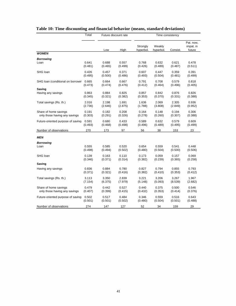
41

Table 10: Time discounting and financial behavior (means, standard deviations) Total

Low HighStrongly hyperbol.

Weakly hyperbol. Consist.

Pat. now, impat. in

futureWOMEN

BorrowingLoan 0.641 0.688 0.557 0.768 0.632 0.621 0.478

(0.481) (0.465) (0.499) (0.426) (0.489) (0.487) (0.511)

SHG loan 0.426 0.457 0.371 0.607 0.447 0.359 0.391(0.495) (0.500) (0.486) (0.493) (0.504) (0.481) (0.499)

SHG loan (conditional on borrowing)0.665 0.664 0.667 0.791 0.708 0.579 0.818(0.473) (0.474) (0.476) (0.412) (0.464) (0.496) (0.405)

SavingHaving any savings 0.863 0.884 0.825 0.857 0.842 0.876 0.826

(0.345) (0.321) (0.382) (0.353) (0.370) (0.331) (0.388)

Total savings (Rs. th.) 2.016 2.198 1.691 1.636 2.069 2.305 0.936(2.736) (2.646) (2.875) (1.788) (3.808) (2.849) (0.952)

Share of home savings 0.191 0.182 0.208 0.164 0.148 0.194 0.306 only those having any savings (0.303) (0.291) (0.326) (0.278) (0.260) (0.307) (0.388)

Future-oriented purpose of savings 0.591 0.680 0.433 0.589 0.632 0.579 0.609(0.493) (0.468) (0.498) (0.496) (0.489) (0.495) (0.499)

Number of observations 270 173 97 56 38 153 23

MEN

BorrowingLoan 0.555 0.585 0.520 0.654 0.559 0.541 0.448

(0.498) (0.494) (0.502) (0.480) (0.504) (0.500) (0.506)

SHG loan 0.139 0.163 0.110 0.173 0.059 0.157 0.069(0.346) (0.371) (0.314) (0.382) (0.239) (0.365) (0.258)

SavingHaving any savings 0.836 0.884 0.780 0.827 0.794 0.855 0.793

(0.371) (0.321) (0.416) (0.382) (0.410) (0.353) (0.412)

Total savings (Rs. th.) 3.113 3.350 2.839 3.221 3.206 3.267 1.967(7.154) (6.375) (7.979) (5.148) (5.093) (8.539) (2.682)

Share of home savings 0.479 0.442 0.527 0.440 0.375 0.500 0.546 only those having any savings (0.407) (0.399) (0.415) (0.432) (0.353) (0.414) (0.376)

Future-oriented purpose of savings 0.502 0.517 0.484 0.346 0.559 0.516 0.643(0.501) (0.501) (0.502) (0.480) (0.504) (0.501) (0.488)

Number of observations 274 147 127 52 34 159 29

Time consistencyFuture discount rate

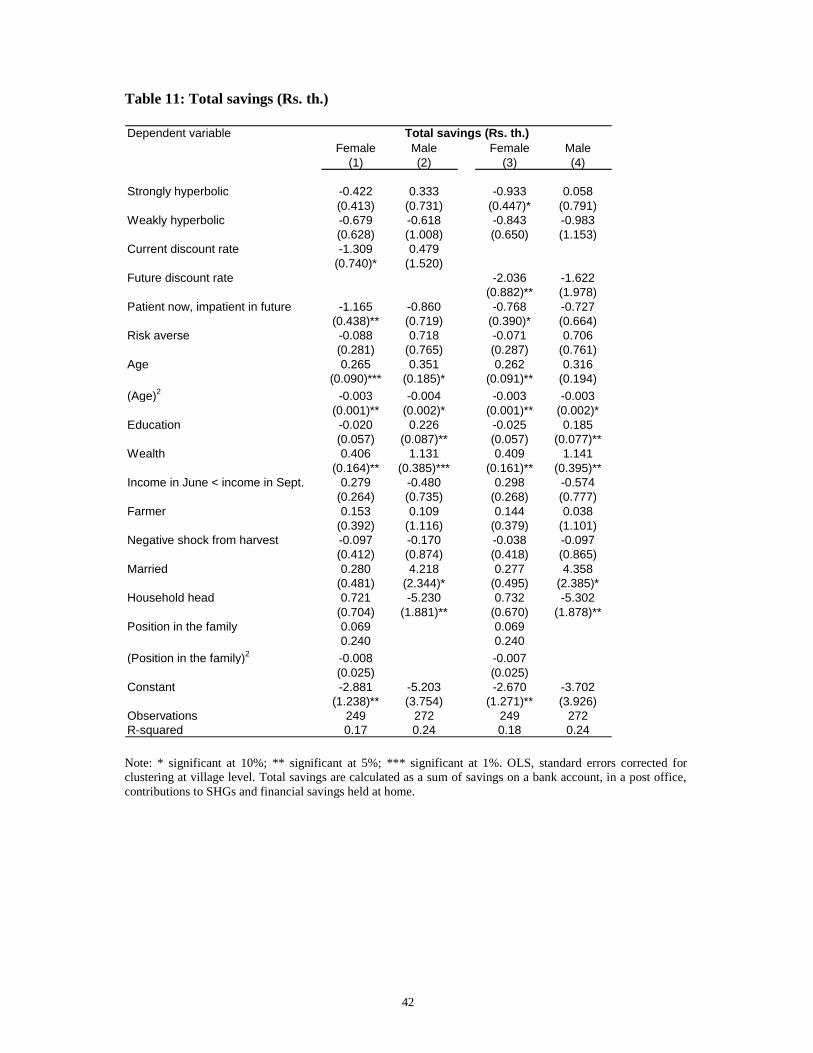
42

Table 11: Total savings (Rs. th.) Dependent variable

Female Male Female Male(1) (2) (3) (4)

Strongly hyperbolic -0.422 0.333 -0.933 0.058(0.413) (0.731) (0.447)* (0.791)

Weakly hyperbolic -0.679 -0.618 -0.843 -0.983(0.628) (1.008) (0.650) (1.153)

Current discount rate -1.309 0.479(0.740)* (1.520)

Future discount rate -2.036 -1.622(0.882)** (1.978)

Patient now, impatient in future -1.165 -0.860 -0.768 -0.727(0.438)** (0.719) (0.390)* (0.664)

Risk averse -0.088 0.718 -0.071 0.706(0.281) (0.765) (0.287) (0.761)

Age 0.265 0.351 0.262 0.316(0.090)*** (0.185)* (0.091)** (0.194)

(Age)2 -0.003 -0.004 -0.003 -0.003(0.001)** (0.002)* (0.001)** (0.002)*

Education -0.020 0.226 -0.025 0.185(0.057) (0.087)** (0.057) (0.077)**

Wealth 0.406 1.131 0.409 1.141(0.164)** (0.385)*** (0.161)** (0.395)**

Income in June < income in Sept. 0.279 -0.480 0.298 -0.574(0.264) (0.735) (0.268) (0.777)

Farmer 0.153 0.109 0.144 0.038(0.392) (1.116) (0.379) (1.101)

Negative shock from harvest -0.097 -0.170 -0.038 -0.097(0.412) (0.874) (0.418) (0.865)

Married 0.280 4.218 0.277 4.358(0.481) (2.344)* (0.495) (2.385)*

Household head 0.721 -5.230 0.732 -5.302(0.704) (1.881)** (0.670) (1.878)**

Position in the family 0.069 0.0690.240 0.240

(Position in the family)2 -0.008 -0.007(0.025) (0.025)

Constant -2.881 -5.203 -2.670 -3.702(1.238)** (3.754) (1.271)** (3.926)

Observations 249 272 249 272R-squared 0.17 0.24 0.18 0.24

Total savings (Rs. th.)

Note: * significant at 10%; ** significant at 5%; *** significant at 1%. OLS, standard errors corrected for clustering at village level. Total savings are calculated as a sum of savings on a bank account, in a post office, contributions to SHGs and financial savings held at home.

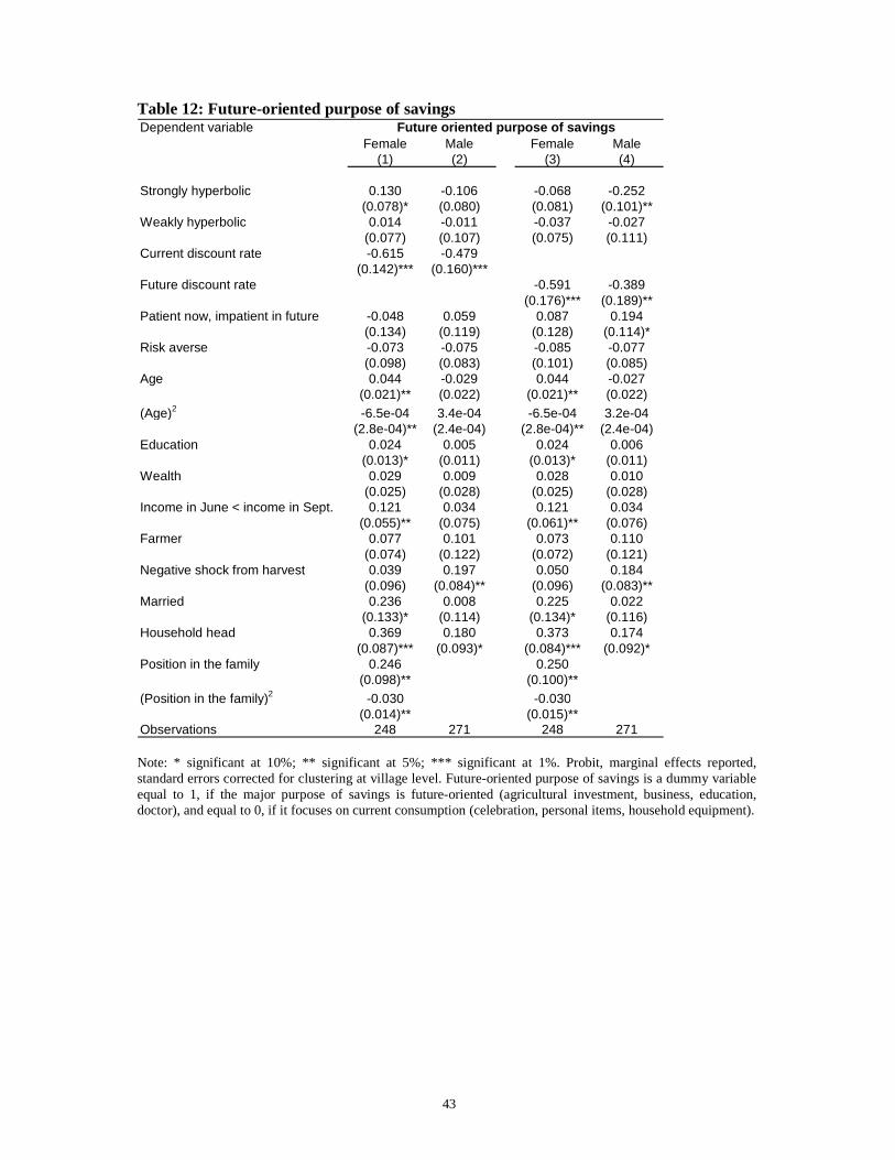
43

Table 12: Future-oriented purpose of savings Dependent variable

Female Male Female Male(1) (2) (3) (4)

Strongly hyperbolic 0.130 -0.106 -0.068 -0.252(0.078)* (0.080) (0.081) (0.101)**

Weakly hyperbolic 0.014 -0.011 -0.037 -0.027(0.077) (0.107) (0.075) (0.111)

Current discount rate -0.615 -0.479(0.142)*** (0.160)***

Future discount rate -0.591 -0.389(0.176)*** (0.189)**

Patient now, impatient in future -0.048 0.059 0.087 0.194(0.134) (0.119) (0.128) (0.114)*

Risk averse -0.073 -0.075 -0.085 -0.077(0.098) (0.083) (0.101) (0.085)

Age 0.044 -0.029 0.044 -0.027(0.021)** (0.022) (0.021)** (0.022)

(Age)2 -6.5e-04 3.4e-04 -6.5e-04 3.2e-04(2.8e-04)** (2.4e-04) (2.8e-04)** (2.4e-04)

Education 0.024 0.005 0.024 0.006(0.013)* (0.011) (0.013)* (0.011)

Wealth 0.029 0.009 0.028 0.010(0.025) (0.028) (0.025) (0.028)

Income in June < income in Sept. 0.121 0.034 0.121 0.034(0.055)** (0.075) (0.061)** (0.076)

Farmer 0.077 0.101 0.073 0.110(0.074) (0.122) (0.072) (0.121)

Negative shock from harvest 0.039 0.197 0.050 0.184(0.096) (0.084)** (0.096) (0.083)**

Married 0.236 0.008 0.225 0.022(0.133)* (0.114) (0.134)* (0.116)

Household head 0.369 0.180 0.373 0.174(0.087)*** (0.093)* (0.084)*** (0.092)*

Position in the family 0.246 0.250(0.098)** (0.100)**

(Position in the family)2 -0.030 -0.030(0.014)** (0.015)**

Observations 248 271 248 271

Future oriented purpose of savings

Note: * significant at 10%; ** significant at 5%; *** significant at 1%. Probit, marginal effects reported, standard errors corrected for clustering at village level. Future-oriented purpose of savings is a dummy variable equal to 1, if the major purpose of savings is future-oriented (agricultural investment, business, education, doctor), and equal to 0, if it focuses on current consumption (celebration, personal items, household equipment).

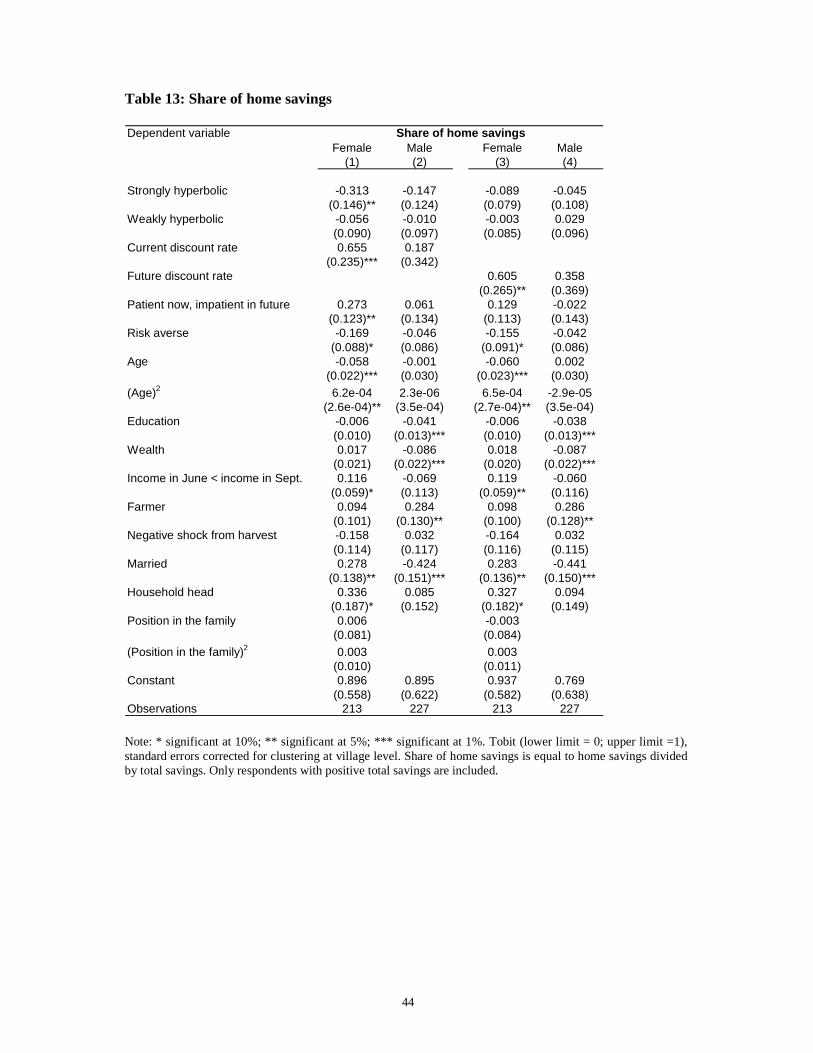
44

Table 13: Share of home savings Dependent variable

Female Male Female Male(1) (2) (3) (4)

Strongly hyperbolic -0.313 -0.147 -0.089 -0.045(0.146)** (0.124) (0.079) (0.108)

Weakly hyperbolic -0.056 -0.010 -0.003 0.029(0.090) (0.097) (0.085) (0.096)

Current discount rate 0.655 0.187(0.235)*** (0.342)

Future discount rate 0.605 0.358(0.265)** (0.369)

Patient now, impatient in future 0.273 0.061 0.129 -0.022(0.123)** (0.134) (0.113) (0.143)

Risk averse -0.169 -0.046 -0.155 -0.042(0.088)* (0.086) (0.091)* (0.086)

Age -0.058 -0.001 -0.060 0.002(0.022)*** (0.030) (0.023)*** (0.030)

(Age)2 6.2e-04 2.3e-06 6.5e-04 -2.9e-05(2.6e-04)** (3.5e-04) (2.7e-04)** (3.5e-04)

Education -0.006 -0.041 -0.006 -0.038(0.010) (0.013)*** (0.010) (0.013)***

Wealth 0.017 -0.086 0.018 -0.087(0.021) (0.022)*** (0.020) (0.022)***

Income in June < income in Sept. 0.116 -0.069 0.119 -0.060(0.059)* (0.113) (0.059)** (0.116)

Farmer 0.094 0.284 0.098 0.286(0.101) (0.130)** (0.100) (0.128)**

Negative shock from harvest -0.158 0.032 -0.164 0.032(0.114) (0.117) (0.116) (0.115)

Married 0.278 -0.424 0.283 -0.441(0.138)** (0.151)*** (0.136)** (0.150)***

Household head 0.336 0.085 0.327 0.094(0.187)* (0.152) (0.182)* (0.149)

Position in the family 0.006 -0.003(0.081) (0.084)

(Position in the family)2 0.003 0.003(0.010) (0.011)

Constant 0.896 0.895 0.937 0.769(0.558) (0.622) (0.582) (0.638)

Observations 213 227 213 227

Share of home savings

Note: * significant at 10%; ** significant at 5%; *** significant at 1%. Tobit (lower limit = 0; upper limit =1), standard errors corrected for clustering at village level. Share of home savings is equal to home savings divided by total savings. Only respondents with positive total savings are included.

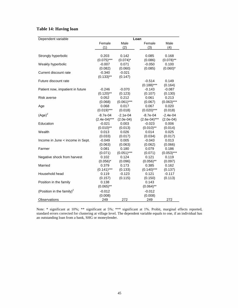
45

Table 14: Having loan

Dependent variableFemale Male Female Male

(1) (2) (3) (4)

Strongly hyperbolic 0.203 0.142 0.085 0.168(0.075)*** (0.074)* (0.086) (0.078)**

Weakly hyperbolic -0.007 0.071 -0.050 0.100(0.082) (0.060) (0.085) (0.060)*

Current discount rate -0.340 -0.021(0.133)** (0.147)

Future discount rate -0.514 0.149(0.188)*** (0.164)

Patient now, impatient in future -0.246 -0.070 -0.143 -0.087(0.120)** (0.123) (0.107) (0.130)

Risk averse 0.052 0.212 0.061 0.213(0.068) (0.061)*** (0.067) (0.063)***

Age 0.068 0.017 0.067 0.020(0.019)*** (0.018) (0.020)*** (0.018)

(Age)2 -8.7e-04 -2.1e-04 -8.7e-04 -2.4e-04(2.4e-04)*** (2.0e-04) (2.6e-04)*** (2.0e-04)

Education -0.021 0.003 -0.023 0.006(0.010)** (0.013) (0.010)** (0.014)

Wealth 0.013 0.026 0.014 0.025(0.033) (0.017) (0.034) (0.017)

Income in June < income in Sept. -0.049 0.005 -0.043 0.013(0.063) (0.063) (0.062) (0.066)

Farmer 0.081 0.180 0.079 0.186(0.071) (0.051)*** (0.071) (0.053)***

Negative shock from harvest 0.102 0.124 0.121 0.119(0.056)* (0.096) (0.056)** (0.097)

Married 0.379 0.173 0.385 0.162(0.141)*** (0.133) (0.140)*** (0.137)

Household head 0.119 -0.123 0.121 -0.117(0.157) (0.115) (0.150) (0.113)

Position in the family 0.138 0.143(0.065)** (0.064)**

(Position in the family)2 -0.012 -0.012(0.008) (0.008)

Observations 249 272 249 272

Loan

Note: * significant at 10%; ** significant at 5%; *** significant at 1%. Probit, marginal effects reported, standard errors corrected for clustering at village level. The dependent variable equals to one, if an individual has an outstanding loan from a bank, SHG or moneylender.

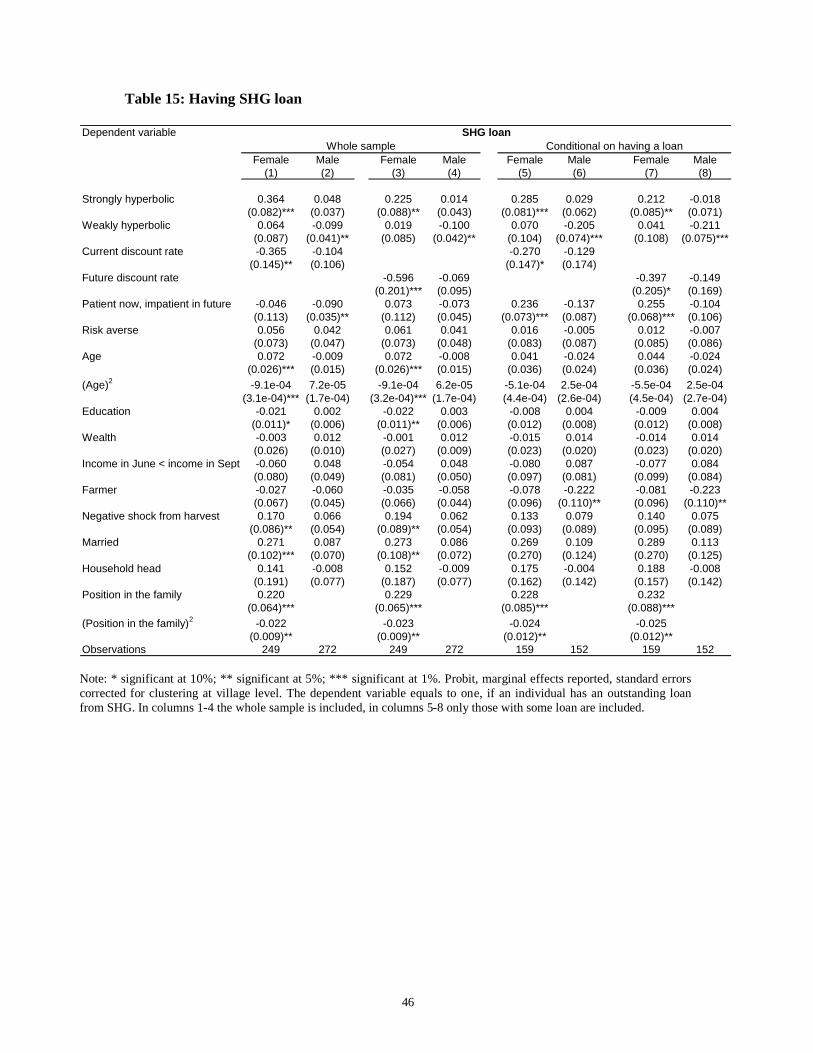
46

Table 15: Having SHG loan Dependent variable

Female Male Female Male Female Male Female Male(1) (2) (3) (4) (5) (6) (7) (8)

Strongly hyperbolic 0.364 0.048 0.225 0.014 0.285 0.029 0.212 -0.018(0.082)*** (0.037) (0.088)** (0.043) (0.081)*** (0.062) (0.085)** (0.071)

Weakly hyperbolic 0.064 -0.099 0.019 -0.100 0.070 -0.205 0.041 -0.211(0.087) (0.041)** (0.085) (0.042)** (0.104) (0.074)*** (0.108) (0.075)***

Current discount rate -0.365 -0.104 -0.270 -0.129(0.145)** (0.106) (0.147)* (0.174)

Future discount rate -0.596 -0.069 -0.397 -0.149(0.201)*** (0.095) (0.205)* (0.169)

Patient now, impatient in future -0.046 -0.090 0.073 -0.073 0.236 -0.137 0.255 -0.104(0.113) (0.035)** (0.112) (0.045) (0.073)*** (0.087) (0.068)*** (0.106)

Risk averse 0.056 0.042 0.061 0.041 0.016 -0.005 0.012 -0.007(0.073) (0.047) (0.073) (0.048) (0.083) (0.087) (0.085) (0.086)

Age 0.072 -0.009 0.072 -0.008 0.041 -0.024 0.044 -0.024(0.026)*** (0.015) (0.026)*** (0.015) (0.036) (0.024) (0.036) (0.024)

(Age)2 -9.1e-04 7.2e-05 -9.1e-04 6.2e-05 -5.1e-04 2.5e-04 -5.5e-04 2.5e-04(3.1e-04)*** (1.7e-04) (3.2e-04)*** (1.7e-04) (4.4e-04) (2.6e-04) (4.5e-04) (2.7e-04)

Education -0.021 0.002 -0.022 0.003 -0.008 0.004 -0.009 0.004(0.011)* (0.006) (0.011)** (0.006) (0.012) (0.008) (0.012) (0.008)

Wealth -0.003 0.012 -0.001 0.012 -0.015 0.014 -0.014 0.014(0.026) (0.010) (0.027) (0.009) (0.023) (0.020) (0.023) (0.020)

Income in June < income in Sept. -0.060 0.048 -0.054 0.048 -0.080 0.087 -0.077 0.084(0.080) (0.049) (0.081) (0.050) (0.097) (0.081) (0.099) (0.084)

Farmer -0.027 -0.060 -0.035 -0.058 -0.078 -0.222 -0.081 -0.223(0.067) (0.045) (0.066) (0.044) (0.096) (0.110)** (0.096) (0.110)**

Negative shock from harvest 0.170 0.066 0.194 0.062 0.133 0.079 0.140 0.075(0.086)** (0.054) (0.089)** (0.054) (0.093) (0.089) (0.095) (0.089)

Married 0.271 0.087 0.273 0.086 0.269 0.109 0.289 0.113(0.102)*** (0.070) (0.108)** (0.072) (0.270) (0.124) (0.270) (0.125)

Household head 0.141 -0.008 0.152 -0.009 0.175 -0.004 0.188 -0.008(0.191) (0.077) (0.187) (0.077) (0.162) (0.142) (0.157) (0.142)

Position in the family 0.220 0.229 0.228 0.232(0.064)*** (0.065)*** (0.085)*** (0.088)***

(Position in the family)2 -0.022 -0.023 -0.024 -0.025(0.009)** (0.009)** (0.012)** (0.012)**

Observations 249 272 249 272 159 152 159 152

SHG loanWhole sample Conditional on having a loan

Note: * significant at 10%; ** significant at 5%; *** significant at 1%. Probit, marginal effects reported, standard errors corrected for clustering at village level. The dependent variable equals to one, if an individual has an outstanding loan from SHG. In columns 1-4 the whole sample is included, in columns 5-8 only those with some loan are included.

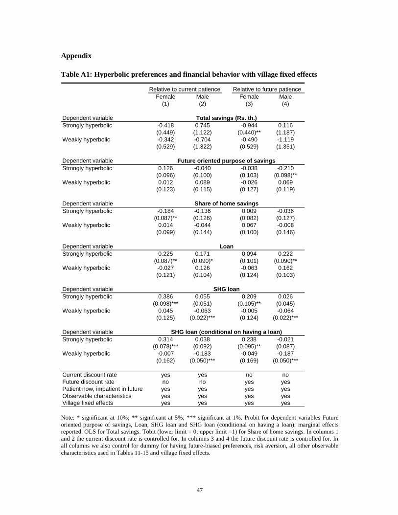
47

Appendix Table A1: Hyperbolic preferences and financial behavior with village fixed effects

Relative to current patience Relative to future patienceFemale Male Female Male

(1) (2) (3) (4)

Dependent variableStrongly hyperbolic -0.418 0.745 -0.944 0.116

(0.449) (1.122) (0.440)** (1.187)Weakly hyperbolic -0.342 -0.704 -0.490 -1.119

(0.529) (1.322) (0.529) (1.351)

Dependent variableStrongly hyperbolic 0.126 -0.040 -0.038 -0.210

(0.096) (0.100) (0.103) (0.098)**Weakly hyperbolic 0.012 0.089 -0.026 0.069

(0.123) (0.115) (0.127) (0.119)

Dependent variableStrongly hyperbolic -0.184 -0.136 0.009 -0.036

(0.087)** (0.126) (0.082) (0.127)Weakly hyperbolic 0.014 -0.044 0.067 -0.008

(0.099) (0.144) (0.100) (0.146)

Dependent variableStrongly hyperbolic 0.225 0.171 0.094 0.222

(0.087)** (0.090)* (0.101) (0.090)**Weakly hyperbolic -0.027 0.126 -0.063 0.162

(0.121) (0.104) (0.124) (0.103)

Dependent variableStrongly hyperbolic 0.386 0.055 0.209 0.026

(0.098)*** (0.051) (0.105)** (0.045)Weakly hyperbolic 0.045 -0.063 -0.005 -0.064

(0.125) (0.022)*** (0.124) (0.022)***

Dependent variableStrongly hyperbolic 0.314 0.038 0.238 -0.021

(0.078)*** (0.092) (0.095)** (0.087)Weakly hyperbolic -0.007 -0.183 -0.049 -0.187

(0.162) (0.050)*** (0.169) (0.050)***

Current discount rate yes yes no noFuture discount rate no no yes yesPatient now, impatient in future yes yes yes yesObservable characteristics yes yes yes yesVillage fixed effects yes yes yes yes

SHG loan

SHG loan (conditional on having a loan)

Total savings (Rs. th.)

Future oriented purpose of savings

Share of home savings

Loan

Note: * significant at 10%; ** significant at 5%; *** significant at 1%. Probit for dependent variables Future oriented purpose of savings, Loan, SHG loan and SHG loan (conditional on having a loan); marginal effects reported. OLS for Total savings. Tobit (lower limit = 0; upper limit =1) for Share of home savings. In columns 1 and 2 the current discount rate is controlled for. In columns 3 and 4 the future discount rate is controlled for. In all columns we also control for dummy for having future-biased preferences, risk aversion, all other observable characteristics used in Tables 11-15 and village fixed effects.

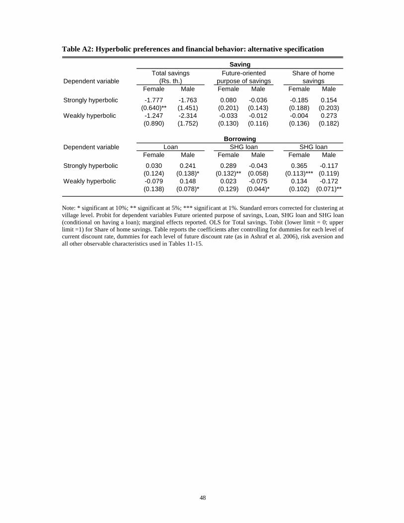
48

Table A2: Hyperbolic preferences and financial behavior: alternative specification

Dependent variableFemale Male Female Male Female Male

Strongly hyperbolic -1.777 -1.763 0.080 -0.036 -0.185 0.154(0.640)** (1.451) (0.201) (0.143) (0.188) (0.203)

Weakly hyperbolic -1.247 -2.314 -0.033 -0.012 -0.004 0.273(0.890) (1.752) (0.130) (0.116) (0.136) (0.182)

Dependent variableFemale Male Female Male Female Male

Strongly hyperbolic 0.030 0.241 0.289 -0.043 0.365 -0.117(0.124) (0.138)* (0.132)** (0.058) (0.113)*** (0.119)

Weakly hyperbolic -0.079 0.148 0.023 -0.075 0.134 -0.172(0.138) (0.078)* (0.129) (0.044)* (0.102) (0.071)**

SHG loan SHG loan

Saving

Borrowing

Total savings (Rs. th.)

Future-oriented purpose of savings

Share of home savings

Loan

Note: * significant at 10%; ** significant at 5%; *** significant at 1%. Standard errors corrected for clustering at village level. Probit for dependent variables Future oriented purpose of savings, Loan, SHG loan and SHG loan (conditional on having a loan); marginal effects reported. OLS for Total savings. Tobit (lower limit = 0; upper limit =1) for Share of home savings. Table reports the coefficients after controlling for dummies for each level of current discount rate, dummies for each level of future discount rate (as in Ashraf et al. 2006), risk aversion and all other observable characteristics used in Tables 11-15.

IES Working Paper Series

2008

1. Irena Jindrichovska, Pavel Kö rner : Determinants of corporate financing decisions: a

survey evidence from Czech firms 2. Petr Jakubík, Jaroslav Heřmánek : Stress testing of the Czech banking sector 3. Adam Geršl : Performance and financing of the corporate sector: the role of foreign direct

investment 4. Jiří Witzany : Valuation of Convexity Related Derivatives 5. Tomáš Richter : Použ ití (mikro)ekonomické metodologie při tvorbě a interpretaci

soukromého práva 6. František Turnovec : Duality of Power in the European Parliament 7. Natalie Svarciva, Petr Svarc : Technology adoption and herding behavior in complex social

networks 8. Tomáš Havránek, Zuzana Iršová : Intra-Industry Spillovers from Inward FDI: A Meta-

Regression Analysis 9. Libor Dušek, Juraj Kopecsni : Policy Risk in Action: Pension Reforms and Social Security

Wealth in Hungary, Czech Republic, and Slovakia 10. Alexandr Kuchynka : Volatility extraction using the Kalman filter 11. Petr Kadeřábek, Aleš Slabý , Josef Vodička : Stress Testing of Probability of Default of

Individuals 12. Karel Janda : Which Government Interventions Are Good in Alleviating Credit Market

Failures? 13. Pavel Štika : Mož nosti analytického uchopení reciprocity v sociálních interakcích 14. Michal Bauer, Julie Chytilová : A Model of Human Capital, Time Discounting and

Economic Growth 15. Milan Rippel, Petr Teplý : Operational Risk – Scenario Analysis 16. Martin Gregor : The Strategic Euro Laggards 17. Radovan Chalupka, Petr Teplý : Operational Risk Management and Implications for

Bank’s Economic Capital – a Case Study 18. Vít Bubák : Value-at-Risk on Central and Eastern European Stock Markets: An Empirical

Investigation Using GARCH Models 19. Petr Jakubík, Petr Teplý : The Prediction of Corporate Bankruptcy and Czech Economy’s

Financial Stability through Logit Analysis

20. Elisa Gaelotti : Do domestic firms benefit from geographic proximity with FDI? Evidence from the privatization of the Czech glass industry

21. Roman Horvá th, Marek Rusnák : How Important Are Foreign Shocks in Small Open Economy? The Case of Slovakia

22. Ondřej Schneider : Voting in the European Union - Central Europe’s lost voice 23. Fabricio Coricelli, Roman Horvá th : Price Setting and Market Structure: An Empirical

Analysis of Micro Data 24. Roman Horvá th, Kamila Koprnická : Inflation Differentials in EU New Member States:

An Empirical Evidence 25. Michal Franta, Branislav Saxa, Kateřina Šmídková : Inflation Persistence: Is It Similar in

the New EU Member States and the Euro Area Members? 26. Jakub Seidler : Implied Market Loss Given Default: structural-model approach 27. Radovan Chalupka, Juraj Kopecsni : Modelling Bank Loan LGD of Corporate and SME

Segments: A Case Study 28. Michal Bauer, Julie Chytilová , Jonathan Morduch: Behavioral Foundations of Microcredit:

Experimental and Survey Evidence From Rural India

All papers can be downloaded at: http://ies.fsv.cuni.cz•

Univerzita Karlova v Praze, Fakulta sociá lních věd Institut ekonomický ch studií [UK FSV – IES] Praha 1, Opletalova 26 E-mail : ies@fsv.cuni.cz http://ies.fsv.cuni.cz