Begleitung des Interkalibrierungsprozesses (O 4.09 ... · Abundanzklassen), Anzahl Taxa an EPTCBO...

Begleitung des Interkalibrierungsprozesses (O 4.09) - Teilprojekt komponentenübergreifende Arbeiten

und Makrozoobenthos der Seen

www.Interkalibrierung.de

Tätigkeitsbericht

Im Auftrag der Länderarbeitsgemeinschaft Wasser (LAWA)

Berichtszeitraum 01.04.2010 – 31.12.2010

Bearbeitung:

Jürgen Böhmer

Bioforum GmbH

Fachliche und Projektbetreuung:

LAWA-Expertenkreis Fliessgewässer

LAWA-Expertenkreis Seen

Begleitung des Interkalibrierungsprozesses – Makrozoobenthos der Seen. J. Böhmer / Bioforum GmbH

Inhalt

1. EINLEITUNG, AUFTRAG UND ZIELSETZUNG 1

2. TEILNAHME AN NATIONALEN UND INTERNATIONALEN TREFFEN 3

3. INTERNATIONALE ARBEITEN 3

3.1 SEENMAKROINVERTEBRATENINTERKALIBRIERUNG IM CB- UND AL-GIG, SOWIE

GIG-ÜBERGREIFEND ..................................................................................................................... 3

3.2 GROßE FLÜSSE ............................................................................................................................... 6

3.3 „GUIDANCE“ ZUR INTERKALIBRIERUNG ..................................................................................... 7

3.4 WISER-KOOPERATION .............................................................................................................. 14

4. ZUSAMMENSTELLUNG NATIONALER DATEN ZUR INTERKALIBRIERUNG 14

5. ÜBERARBEITUNG DER INTERNETPRÄSENZ ZUR INTERKALIBRIERUNG 14

6. ARBEITEN ZUR INTERKALIBRIERUNGSDATENBANK 14

7. LITERATUR 15

8. ANHANG 16

8.1 ERGEBNISPROTOKOLL DES SEEN-MAKROINVERTEBRATEN-CB-GIG-TREFFENS

IN TARTU (ORIGINALTEXT) ........................................................................................................ 16

8.2 ERGEBNISPROTOKOLL DES SEEN-MAKROINVERTEBRATEN-CB-GIG-TREFFENS

IN AALST (ORIGINALTEXT) ........................................................................................................ 22

8.3 ERGEBNISPROTOKOLL DES ZWEITEN XGIG-TREFFENS ZU GROßEN FLÜSSEN IN

KOBLENZ (ORIGINALTEXT OHNE ANHANG) ............................................................................. 27

8.4 ERGEBNISPROTOKOLL DES DRITTEN XGIG-TREFFENS ZU GROßEN FLÜSSEN IN

KOBLENZ (ORIGINALTEXT) ....................................................................................................... 30

8.5 ERGEBNISPROTOKOLL DES SEEN-MAKROINVERTEBRATEN-AL-GIG-TREFFENS

IN AIX EN PROVENCE (ORIGINALTEXT) .................................................................................... 35

8.6 DRITTER BERICHT DER CB-GIG-INVERTEBRATENGRUPPE AN ECOSTAT ........................... 38

Begleitung des Interkalibrierungsprozesses – Makrozoobenthos der Seen S. 1

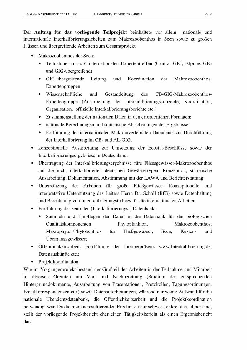
1. Einleitung, Auftrag und Zielsetzung

Die Interkalibrierung erwies sich als eine der schwierigsten Herausforderungen bei der

Umsetzung der Wasserrahmenrichtlinie. Sie soll die internationale Vergleichbarkeit der

Bewertungen nach Wasserrahmenrichtlinie gewährleisten, obwohl die Bewertungsverfahren

der einzelnen Mitgliedstaaten sehr unterschiedlich sein dürfen und daher auch sind. Letztlich

legt sie verbindliche Klassengrenzen für die fünf Bewertungsklassen fest.

Insbesondere die Klassengrenze "gut / mäßig" ist dabei von besonderer Bedeutung, weil für

mäßige Gewässer Maßnahmen zur Verbesserung des ökologischen Zustands getroffen werden

müssen, während für gute kein Handlungsbedarf besteht. Auch die Klassengrenze "sehr gut /

gut" ist wichtig, weil sehr gute Gewässer geschützt werden müssen.

Die Interkalibrierung fällt in den Aufgabenbereich der EU-Arbeitsgruppe ECOSTAT

(„Ecological Status“). Zur wissenschaftlichen Betreuung der Interkalibrierung wurde das

„European Centre for Ecological Water Quality and Intercalibration (EEWAI)“ des Joint

Research Centre (JRC) in Ispra, Italien eingerichtet.

In der gerade laufenden zweiten Phase werden die Bewertungsverfahren interkalibriert, die in

der ersten scheiterten oder noch nicht fertig entwickelt waren. Außerdem werden offene

Fragen und Probleme der ersten Phase aufgegriffen und bearbeitet.

Mittlerweile gibt es eine Vielzahl von Interkalibrierungs-Arbeitsgruppen, weil diese nach

Gewässerkategorie, Geographie („Geographical Intercalibration Groups“ = GIGs) und

Biokomponenten aufgeteilt sind.

Deutschland bringt sich mit einer Reihe von Experten intensiv in die Interkalibrierung ein, um

nach Möglichkeit die deutschen Bewertungsverfahren ohne nachträglichen Überarbeitungs-

bedarf erfolgreich zu interkalibrieren, und um darüber hinaus die deutschen Positionen

wirksam zu vertreten.

Daher übernahm Deutschland fürs Seen-Makrozoobenthos sowie für die großen

Fliessgewässer die internationale GIG-übergreifende Leitung und leitet die CB-GIG-

Expertengruppen fürs Seen-Makrozoobenthos sowie für die Fische der Seen. Ferner führt

Deutschland einen großen Teil der internationalen Analysen für die großen Fließgewässer, für

das Seen-Makrozoobenthos im Central/Baltic- und Alpinen GIG, für die

Fliessgewässermakrophyten im Central/Baltic-GIG, fürs Seenplankton im Central/Baltic-GIG

sowie für die Fische der Seen durch.

Das hier betrachtete Teilprojekt ist Teil eines LAWA-Gesamtprojekts zur Unterstützung aller

in 2010 anfallenden deutschen Interkalibrierungsaufgaben, die nicht anderweitig finanziert

werden konnten.

Für die einzelnen Projektpartner ges Gesamtprojekts wurden separate Verträge mit eigener

Berichtspflicht abgeschlossen, Daher wir bezüglich der Ergebnisse zu den anderen

Biokomponenten und Gewässerkategorien auf die entsprechenden separaten Berichte

verwiesen.

LAWA-Abschlußbericht O 1.08 J. Böhmer / Bioforum GmbH S. 2

Der Auftrag für das vorliegende Teilprojekt beinhaltete vor allem nationale und

internationale Interkalibrierungsarbeiten zum Makrozoobenthos in Seen sowie zu großen

Flüssen und übergreifende Arbeiten zum Gesamtprojekt.

• Makrozoobenthos der Seen:

• Teilnahme an ca. 6 internationalen Expertentreffen (Central GIG, Alpines GIG

und GIG-übergreifend)

• GIG-übergreifende Leitung und Koordination der Makrozoobenthos-

Expertengruppen

• Wissenschaftliche und Gesamtleitung des CB-GIG-Makrozoobenthos-

Expertengruppe (Ausarbeitung der Interkalibrierungskonzepte, Koordination,

Organisation, offizielle Interkalibrierungsberichte etc.)

• Zusammenstellung der nationalen Daten in den erforderlichen Formaten;

• nationale Berechnungen und statistische Absicherungen der Ergebnisse;

• Fortführung der internationalen Makroinvertebraten-Datenbank zur Durchführung

der Interkalibrierung im CB- und AL-GIG;

• konzeptionelle Ausarbeitung zur Umsetzung der Ecostat-Beschlüsse sowie der

Interkalibrierungsergebnisse in Deutschland;

• Übertragung der Interkalibrierungsergebnisse fürs Fliessgewässer-Makrozoobenthos

auf die nicht interkalibrierten deutschen Gewässertypen: Konzeption, statistische

Ausarbeitung, Dokumentation, Abstimmung mit der LAWA und Berichterstattung

• Unterstützung der Arbeiten für große Fließgewässer: Konzeptionelle und

interpretative Unterstützung des Leiters Herrn Dr. Schöll (BfG) sowie Datenhaltung

und Berechnung von Interkalibrierungsindices für die internationalen Arbeiten.

• Fortführung der zentralen (Interkalibrierungs-) Datenbank:

• Sammeln und Einpflegen der Daten in die Datenbank für die biologischen

Qualitätskomponenten Phytoplankton, Makrozoobenthos;

Makrophyten/Phytobenthos für Fließgewässer, Seen, Küsten- und

Übergangsgewässer;

• Öffentlichkeitsarbeit: Fortführung der Internetpräsenz www.Interkalibrierung.de,

Datenauskünfte etc.;

• Projektkoordination

Wie im Vorgängerprojekt bestand der Großteil der Arbeiten in der Teilnahme und Mitarbeit

in diversen Gremien mit Vor- und Nachbereitung (Studium der entsprechenden

Hintergrunddokumente, Ausarbeitung von Präsentationen, Protokollen, Tagungsordnungen,

Emailkorrespondenzen etc.) sowie Datenaufarbeitungen, während nur wenig Aufwand für die

nationale Übersichtsdatenbank, die Öffentlichkeitsarbeit und die Projektkoordination

notwendig war. Da die hieraus resultierenden Ergebnisse nur schwer konkret darstellbar sind,

stellt der vorliegende Projektbericht eher einen Tätigkeitsbericht als einen Ergebnisbericht

dar.


2. Teilnahme an nationalen und internationalen Treffen

Im Berichtszeitraum wurden 12 durchschnittlich 2-tägige Treffen besucht, davon 7 im

Ausland Tab. 1.

Die nationalen Treffen bei den betreuenden LAWA-Fliessgewässer- und -Seen-

Expertenkreisen dienten der Abstimmung der international einzubringenden deutschen

Interkalibrierungspositionen sowie der Berichterstattung über den Fortschritt der

Interkalibrierungsarbeiten.

Die internationalen Treffen dienten der Planung, Koordination und Durchführung der

eigentlichen Interkalibrierungsarbeiten, sowie der Beteiligung Deutschlands an

übergreifenden Problematiken (z.B. Interkalibrierungs-Leitfaden).

Tab. 1: Teilnahme an Expertentreffen

Datum Treffen Ort

8.-9.4.2010 Ecostat Brüssel / BE

14.-17.4.2010 AL-GIG Makrozoobenthos-IK Rom / IT

19.-20.4.2010 Interkalibrierung großer Flüsse Koblenz

26.-27.5.2010 LAWA-Seenexperten Steinhude

15.-18.6.2010 CB-GIG Makrozoobenthos-IK Tartu / EE

6.-8.7.2010 LAWA-Fliessgewässerexperten Hamburg

26.-27.8.2010 Comparability Criteria Ispra / IT

22.-23.9.2010 Interkalibrierung großer Flüsse Koblenz

20.-22.102010 CB-GIG Makrozoobenthos-IK Aalst / BE

3.-6.11.2010 Koordinatorentreffen Seen-IK Ispra / IT

6.-8.12.2010 CB-GIG Makrozoobenthos-IK Aix e.P. / FR

15.-16.12.2010 Koordination IK großer Flüsse Koblenz

3. Internationale Arbeiten

Die internationalen Aktivitäten umfassten hauptsächlich die Absprachen und Arbeiten zur

Interkalibrierung in den Seeninvertebratengruppen des CB- und AL-GIG, sowie in der

Gruppe zur Interkalibrierung großer Fliessgewässer. Darüber hinaus erfolgten Absprachen

und Berichterstattungen in übergeordneten Gruppen, wie der Seenkoordinatoren-Gruppe oder

ECOSTAT.

3.1 Seenmakroinvertebrateninterkalibrierung im CB- und AL-GIG, sowie GIG-übergreifend

In der Funktion des GIG-übergreifenden Leiters der Seeninvertebrateninterkalibrierung

vertrat ich die vier GIG-Gruppen in den übergeordneten und assoziierten Gremien und

koordinierte deren Arbeiten. Als koordinativer und wissenschaftlicher Leiter der CB-Gruppe

koordinierte ich außerdem die Arbeiten dieser Untergruppe. Dies bedeutete insgesamt einen

regen Emailaustausch mit einer Vielzahl von beteiligten Personen.


Im CB- und AL-GIG standen zunächst Korrekturen und Erweiterungen der Datenbank als

Voraussetzung für alle Arbeiten im Vordergrund. Die Datenaktualisierungen erfolgten in

heterogenen Formaten, die vereinheitlicht und in der gemeinsamen Datenbank

zusammengeführt werden mussten. Im Laufe der Zeit führte ich zunehmend auch

Datenauswertungen durch.

Im Folgenden wird ein Überblick über die Arbeiten gegeben. Weitergehende Details finden

sich in den Protokollen der Sitzungen (Anhänge 8.1 und 8.2 fürs CB-GIG, 0 fürs AL-GIG,

8.3 und 8.4 für die Großen Flüsse) sowie in den Berichten an ECOSTAT (Milestone-report;

Anhang 8.6 fürs CB-GIG).

CB-GIG

Der Datenbestand wurde auf 991 Proben von 873 Probestellen in 197 Seen aus 9 Ländern

erweitert.

Insgesamt befanden sich 1191 Taxa in der Datenbank. Die taxonomische Auflösung hängt

von der Makrozoobenthosgruppe ab: Überwiegend Familienniveau für Chironomiden und

Oligochaeten, gemischte Niveaus für Mollusken und überwiegend Artniveau für die weiteren

Gruppen.

Für die ersten Analysen wurden die Taxa mittels der operationellen Taxaliste Deutschlands

harmonisiert. Für die weiteren Analysen wurde diese Harmonisierungsliste an alle Länder

verteilt, um eine abgestimmte Liste zu erhalten. Diese Abstimmung wurde im Oktober beim

Treffen in Aalst vorgenommen. Dabei wurde der Filter mit folgende Änderungen

beschlossen: Familienlevel für Chironomidae; Ordnungslevel für Oligochaeta und Polychaeta.

Ein Großteil der Analysen zur Auswahl der sogenannten „Common Metrics“ wurde in

Zusammenarbeit mit dem EU-Projekt WISER vorgenommen und durch dieses finanziert.

Zur Auswahl der Kandidaten für die Interkalibrierungsmetrics wurden ca. 80 Metrics

berechnet und gegen nationale Bewertungsergebnisse (EQRs) und Belastungsfaktoren

korreliert.

Für die nationalen Bewertungsergebnisse der meisten Länder ergaben sich gute Korrelationen

mit der Taxazahl sowie mit sensitiven taxonomischen Gruppen (z.B. %ETO und Anzahl der

Taxa an ETO oder EPTCBO).

Die Korrelationen mit den Belastungsfaktoren variierten zwischen den Ländern,

wahrscheinlich aufgrund der Unterschiede in der Belastungssituation sowie der

Besammlungsmethodik. Insgesamt reagierten eine Reihe von Metrics jedoch

erwartungsgemäß auf die verschiedenen Belastungsfaktoren.

Als Kandidaten wurden daher vorläufig folgende Metrics ausgewählt:

% Odonata (bezogen auf Individuen), % ETO (bezogen auf Abundanzklassen), ASPT,

Taxazahl, % Indifferente (bezogen auf Abundanzklassen), % R/K Strategen (bezogen auf

Abundanzklassen), Anzahl Taxa an EPTCBO (oder ETO), % Crustacea (bezogen auf

Individuen) sowie % Lithalbewohner (bezogen auf Individuen).


Die endgültige Auswahl der Kandidatenmetrics wird beim ersten Treffen in 2011 mittels

GIG-Gruppen-Entscheidung erfolgen, hauptsächlich auf der Basis der Korrelationen mit den

nationalen Methoden.

Bezüglich der Durchführbarkeit der Interkalibrierung wurden die entsprechenden Fragen der

Interkalibrierungsleitlinie diskutiert:

1) Nach Einschätzung der GIG-Gruppe erfüllen die nationalen Methoden die

Anforderungen der WRRL. Dies muss jedoch noch im Detail belegt werden.

2) Die Interkalibrierung ist prinzipiell durchführbar, da alle außer zwei Methoden auf das

Eulitoral und hydromorphologische Belastungen fokussieren. Für die anderen

Methoden wird ein Vergleich zu Eulitoralproben angestrebt.

3) Die Ländermethoden sind unterschiedlich (= Ausschluß Interkalibrierungsoption 1).

4) Die Probenahmemethoden sind zu unterschiedlich für die Interkalibrierungsoption 3.

5) Die Entwicklung der Common Metrics ist auf einem guten Weg

6) Es gibt zu wenige Referenzseen für einen Referenzabgleich auf Ebene der

Gesamtgewässer; eventuell könnte es genügend Referenzen auf Probestellenebene

geben.

7) Das Setzen der Grenzen für die Bewertungsklassen der nationalen Methoden scheint

für alle Methoden die Anforderungen der WRRL zu erfüllen. Sollte die Detailprüfung

dies bestätigen so könnten die nationalen Klassengrenzen direkt auf der Common-

Metric-Skala verglichen werden.

AL-GIG

Trotz laufender Analysen wurde die internationale Datenbank ständig weiter aktualisiert.

Außerdem wurde begonnen Belastungsparameter auf Probestellenebene zu sammeln, um die

statistische Aussagekraft zu erhöhen.

Frankreich konstatierte, dass es bis zum Ende der aktuellen Interkalibrierungsrunde kein

Verfahren mehr entwickeln werde. Stattdessen werde es die Interkalibrierungsmetrics als

nationales Verfahren übernehmen, falls diese für die nationalen Typen anwendbar sein

würden. Auch Italien plante, die Interkalibrierungsmetrics zu übernehmen.

Es wurde beschlossen, die Interkalibrierung zweigleisig laufen zu lassen:

Auf der ersten Schiene werden die eulitoralen Verfahren von Slowenien und Deutschland

interkalibriert, die in diesen Ländern als offizielle Verfahren vorgesehen sind.

Auf der zweiten Schiene werden Interkalibrierungsmetrics fürs Sublitoral entwickelt. Da

hierfür nur das Bewertungsverfahren Deutschlands existierte, das derzeit nicht als offizielles

Bewertungsverfahren vorgesehen war, müssen die Klassengrenzen für die ökologischen

Zustandsklassen gemeinsam abgeleitet werden, und können dann mit den deutschen

Klassengrenzen abgeglichen werden.


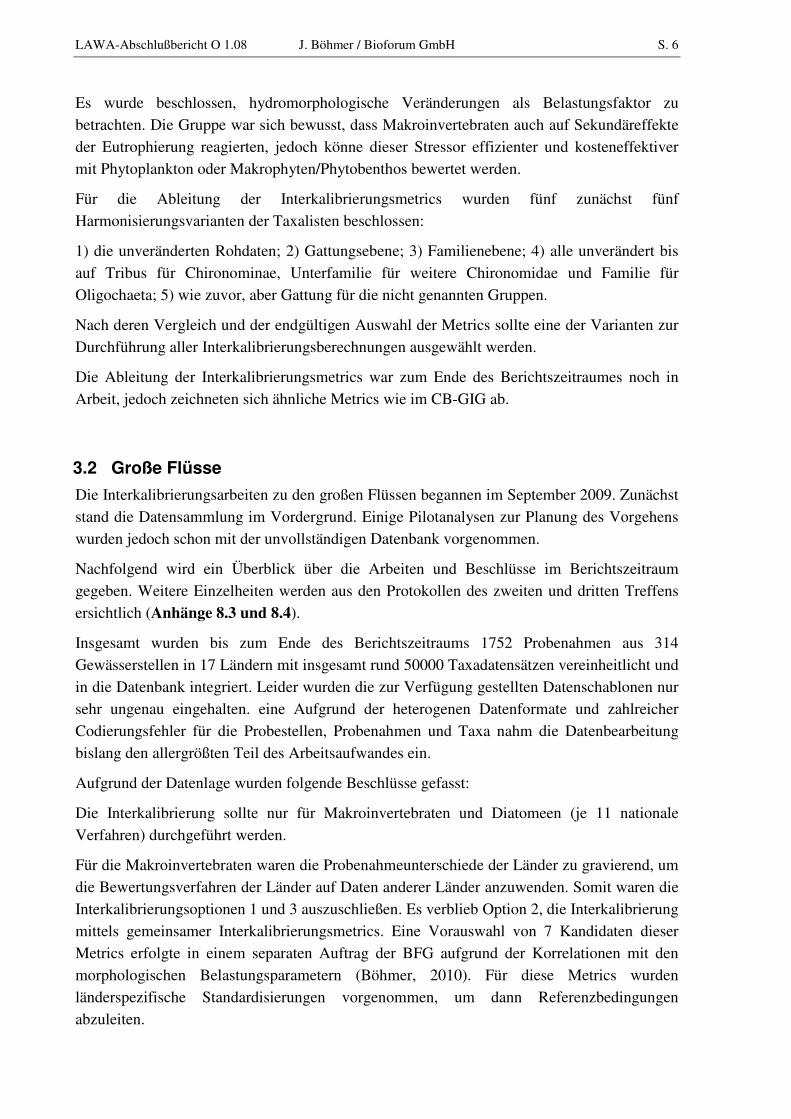
Es wurde beschlossen, hydromorphologische Veränderungen als Belastungsfaktor zu

betrachten. Die Gruppe war sich bewusst, dass Makroinvertebraten auch auf Sekundäreffekte

der Eutrophierung reagierten, jedoch könne dieser Stressor effizienter und kosteneffektiver

mit Phytoplankton oder Makrophyten/Phytobenthos bewertet werden.

Für die Ableitung der Interkalibrierungsmetrics wurden fünf zunächst fünf

Harmonisierungsvarianten der Taxalisten beschlossen:

1) die unveränderten Rohdaten; 2) Gattungsebene; 3) Familienebene; 4) alle unverändert bis

auf Tribus für Chironominae, Unterfamilie für weitere Chironomidae und Familie für

Oligochaeta; 5) wie zuvor, aber Gattung für die nicht genannten Gruppen.

Nach deren Vergleich und der endgültigen Auswahl der Metrics sollte eine der Varianten zur

Durchführung aller Interkalibrierungsberechnungen ausgewählt werden.

Die Ableitung der Interkalibrierungsmetrics war zum Ende des Berichtszeitraumes noch in

Arbeit, jedoch zeichneten sich ähnliche Metrics wie im CB-GIG ab.

3.2 Große Flüsse

Die Interkalibrierungsarbeiten zu den großen Flüssen begannen im September 2009. Zunächst

stand die Datensammlung im Vordergrund. Einige Pilotanalysen zur Planung des Vorgehens

wurden jedoch schon mit der unvollständigen Datenbank vorgenommen.

Nachfolgend wird ein Überblick über die Arbeiten und Beschlüsse im Berichtszeitraum

gegeben. Weitere Einzelheiten werden aus den Protokollen des zweiten und dritten Treffens

ersichtlich (Anhänge 8.3 und 8.4).

Insgesamt wurden bis zum Ende des Berichtszeitraums 1752 Probenahmen aus 314

Gewässerstellen in 17 Ländern mit insgesamt rund 50000 Taxadatensätzen vereinheitlicht und

in die Datenbank integriert. Leider wurden die zur Verfügung gestellten Datenschablonen nur

sehr ungenau eingehalten. eine Aufgrund der heterogenen Datenformate und zahlreicher

Codierungsfehler für die Probestellen, Probenahmen und Taxa nahm die Datenbearbeitung

bislang den allergrößten Teil des Arbeitsaufwandes ein.

Aufgrund der Datenlage wurden folgende Beschlüsse gefasst:

Die Interkalibrierung sollte nur für Makroinvertebraten und Diatomeen (je 11 nationale

Verfahren) durchgeführt werden.

Für die Makroinvertebraten waren die Probenahmeunterschiede der Länder zu gravierend, um

die Bewertungsverfahren der Länder auf Daten anderer Länder anzuwenden. Somit waren die

Interkalibrierungsoptionen 1 und 3 auszuschließen. Es verblieb Option 2, die Interkalibrierung

mittels gemeinsamer Interkalibrierungsmetrics. Eine Vorauswahl von 7 Kandidaten dieser

Metrics erfolgte in einem separaten Auftrag der BFG aufgrund der Korrelationen mit den

morphologischen Belastungsparametern (Böhmer, 2010). Für diese Metrics wurden

länderspezifische Standardisierungen vorgenommen, um dann Referenzbedingungen

abzuleiten.


Für die Diatomeen sind die Probenahmen einheitlicher, so dass die Durchführung der

Interkalibrierungsoption 3 angestrebt werden konnte. Allerdings war zum Ende des

Berichtszeitraumes noch nicht absehbar, ob es gelingen würde, hierfür die Gewässer nach

allen länderspezifischen Gewässertypisierungen einzustufen und alle nationalen

Verfahrensergebnisse für die Probenahmedaten zu berechnen. Andernfalls müssten auch für

die Diatomeen Interkalibrierungsmetrics gemäß Option 2 eingesetzt werden.

Sowohl bei den Makroinvertebraten als auch bei den Diatomeen stellt die Ableitung von

Referenzbedingungen eine große Herausforderung dar, weil fast alle Länder keine

Referenzgewässer besaßen. Auch das „Alternative Benchmarking“ scheiterte bislang am

Problem, dass die Länder jeweils nur einen kleinen Teil des Belastungsgradienten abdeckten .

Daher schlug ich vor, die Standardisierung der Interkalibrierungsmetrics nicht über

„Benchmarks“ sondern mittels der Gesamtdaten im Belastungsgradienten (sogenannte Dosis-

Wirkungsbeziehungen) vorzunehmen (vgl. Präsentation im nachfolgenden Kapitel 3.3).

Nach der Standardisierung mittels dieser Dosis-Wirkungsbeziehungen könnten die Daten aller

Länder zusammengefasst werden, um eine Normalisierung der Interkalibrierungsmetrics

mittels eines beliebigen Punktes auf der Dosis-Wirkungskurve (Benchmarking) oder mittels

abgeleiteter Referenzwerte vorzunehmen. Die Exaktheit der Referenz spielte in diesem Falle

keine Rolle, weil die Referenz für alle Länder dieselbe wäre (in Bezug auf die standardiserten

Metrics).

Sowohl für die Makroinvertebraten, als auch für die Diatomeen wurde die Standardisierung

der Interkalibrierungsmetric-Kandidaten sowie die Ableitung von Referenzbedingungen mit

einem vorläufigen Datenbestand vorgenommen (Böhmer, 2010). Falls die skizzierte

Vorgehensweise beim Treffen im Februar 2011 Zustimmung fände, müssten die

Berechnungen mit dem endgültigen Datenbestand wiederholt werden.

3.3 „Guidance“ zur Interkalibrierung

In meiner Funktion als Seenmakroinvertebratenkoordinator trug ich zur Gestaltung des

Interkalibrierungsleitfadens („Intercalibration Guidance“) bei. Diese Mitarbeit erfolgte über

Stellungnahmen zu den Entwurfsversionen, durch aktive Teilnahme beim Workshop zum

Anhang „Comparabilty Criteria“ sowie auch als Diskussionsbeiträge in der ECOSTAT-

Sitzung in Brüssel.

Beim Workshop zu den Comparability Criteria präsentierte ich den Vortrag „Approaches to

set Reference Conditions“, der nachfolgend in gekürzter Fassung wiedergegeben wird.

Hierbei wurden verschiedene Möglichkeiten zur Referenzfindung und zum „Benchmarking“

vorgestellt, welche zur Anwendung kommen könnten, wenn die in der Guidance beschriebene

Vorgehensweise aufgrund schwieriger Datenlage nicht anwendbar ist (z.B. bei großen

Fliessgewässern, die für jedes Land nur einen kleinen Teil des gesamten Belastungsgradienten

abdecken):


Reference Criteria: Example CB Lake Benthic Fauna

Problem: Few candidatereference lakes and incomplete data- only about 10-15 lakes remain

(10) no evidence for one of the following pressures:- Significant changes in the hydrological and sediment regime of the tributaries (larger than the range

between the natural mean low water level and the natural high water level)

- Fish farm activities or other fishing operations that negatively impact the structure, productivity,

function and diversity of the ecosystem

- Introduction of non-native fish species, unless their abundance and biomass is insignificant

- Sigificant changes in status parameters prior to major changes in industrialisation, urbanisation and

intensification of the agriculture

- Substances mentioned in Annex X and/or in annex VIII of the WFD in concentrations above the

limits of detection of the most advanced analytical techniques in general use or presence of possible

and important sources of pollutants.

- Measured values of other anthropogenic, synthetic substances above quality objectives and not

near natural background concentrations, except for those from atmospheric sources

(9) No actively invading (and reproducing) plant or animal species that may negatively impact the structure, productivity, function and diversity of the ecosystem

(8) No mass (or significant) recreation activities (camping, swimming, roing, coarse fish angling, put and take angling, releasing and feeding of ducks for hunting)

Other pressures

(7) Generally: No (or insignificant) deviation of the actual from the natural trophicstate

Trophic state

(6) ≤ 5 % artificial modification of the shore lineMorphology

(5) Impact of wastewater from scattered dwellings low (i.e. < 10 inhabitants km-2) within the whole catchment

(4) No direct inflow of treated or untreated waste water

(3) ≤ 5 % urbanisation and peri-urban areas in the near surroundings (i.e. within a zone of 200 m from the lake shore)

(2) No intensive crops (incl. vines) within in the near surroundings (i.e. within a zone of 200 m from the lake shore)

(1) Reference threshold > 85 % nature (i.e. "natural" forests, wetlands, moors, meadows, pasture); NOTE: Rejection threshold = 70 %

Catchmentcharacteristics

Criteria (1)

Criteria similar in AL-group; bothoriented at Plankton IC and Refcond

References Large Rivers

• only existent in few countries

• major problem for the derivation of reference conditions

and for the whole intercalibration exercise:

Most countries cover only a small part of the pressure

gradient


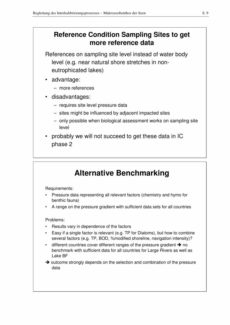
Reference Condition Sampling Sites to get more reference data

References on sampling site level instead of water body

level (e.g. near natural shore stretches in non-

eutrophicated lakes)

• advantage:

– more references

• disadvantages:

– requires site level pressure data

– sites might be influenced by adjacent impacted sites

– only possible when biological assessment works on sampling site

level

• probably we will not succeed to get these data in IC

phase 2

Alternative Benchmarking

Requirements:

• Pressure data representing all relevant factors (chemistry and hymo for

benthic fauna)

• A range on the pressure gradient with sufficient data sets for all countries

Problems:

• Results vary in dependence of the factors

• Easy if a single factor is relevant (e.g. TP for Diatoms), but how to combine

several factors (e.g. TP, BOD, %modified shoreline, navigation intensity)?

• different countries cover different ranges of the pressure gradient � no

benchmark with sufficient data for all countries for Large Rivers as well as

Lake BF

� outcome strongly depends on the selection and combination of the pressure

data


Other possibilities to derive reference

conditions

Extrapolation:

• the regression line between pressure factor and metric value is

extrapolated to the reference threshold

• requires good correlations, but often the pressure gradient is not

sufficiently covered;

• also somewhat dependent on the factor or factor combination

selected

Percentiles:

• for each metric the best 10% are seen as reference values;

• assumes that there are at least some sites in high biological status,

or at high status for the metric under consideration

0,00 0,05 0,10 0,15 0,20 0,25 0,30 0,35

T P_P_m g/l_avg

2,0

2,2

2,4

2,6

2,8

3,0

3,2

3,4

3,6

3,8

4,0

4,2

4,4

4,6

4,8

IPS

T P_P_m g/l_avg:IPS: r2 = 0,4125

extrapolation

References

90%ile

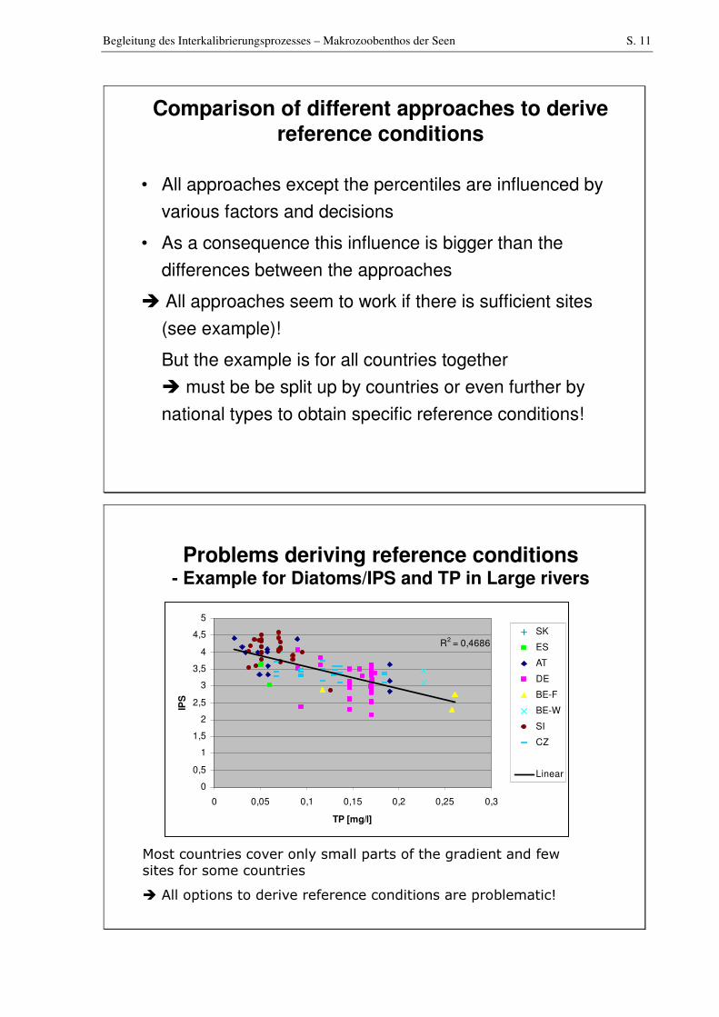
Comparison of different approaches to derive reference conditions

- Example for Diatoms/IPS and TP in Large rivers

range derivedfrom benchmarking

reference threshold used


Comparison of different approaches to derive

reference conditions

• All approaches except the percentiles are influenced by

various factors and decisions

• As a consequence this influence is bigger than the

differences between the approaches

� All approaches seem to work if there is sufficient sites

(see example)!

But the example is for all countries together

� must be be split up by countries or even further by

national types to obtain specific reference conditions!

Problems deriving reference conditions - Example for Diatoms/IPS and TP in Large rivers

Most countries cover only small parts of the gradient and fewsites for some countries

� All options to derive reference conditions are problematic!

R2 = 0,4686

0

0,5

1

1,5

2

2,5

3

3,5

4

4,5

5

0 0,05 0,1 0,15 0,2 0,25 0,3

TP [mg/l]

IPS

SK

ES

AT

DE

BE-F

BE-W

SI

CZ

Linear


Problems deriving reference conditions - Example for Diatoms/IPS and TP in Large rivers

R2 = 0,4686

0

0,5

1

1,5

2

2,5

3

3,5

4

4,5

5

0 0,05 0,1 0,15 0,2 0,25 0,3

TP [mg/l]

IPS

SK

ES

AT

DE

BE-F

BE-W

SI

CZ

Linear

Alignment of Regression Lines by Metric

Standardisation = “Multiple Benchmarking”- all Countries after Standardisation

R2 = 0,3541

0

0,5

1

1,5

2

2,5

3

3,5

4

4,5

5

0 0,05 0,1 0,15 0,2 0,25 0,3

TP [mg/l]

IPS

SK

ES

AT

DE

BE-F

BE-W

SI

CZ

Linear

1,0210,981,151,070,9451,21,1

ATSKSIESCZBE-WBE-FDEResultingfactors:


Metric Standardisation and Normalisation

• Multiplikation with country specific factor or addition of an

offset � standardised metric

• Derivation of Common Reference for standardised

common metric

• Division by common reference value � normalised

common metric, expressed as EQR from 0 to 1

(precision of common reference value does not influence the

comparison between countries, because it is the same factor for all)

• Several normalised Metrics can be averaged to a

common multimetric index (as EQR from 0 to 1)

Conclusions

• The derivation of a reference condition is very

problematic for large rivers as well as for lake

benthic invertebrates

• The percentile approach seems to be the best

and most robust reference approach for lake

benthic fauna

• Another option is the alignment of dose response

curves (“multiple benchmarking”), which seems

to be the only solution for the large rivers


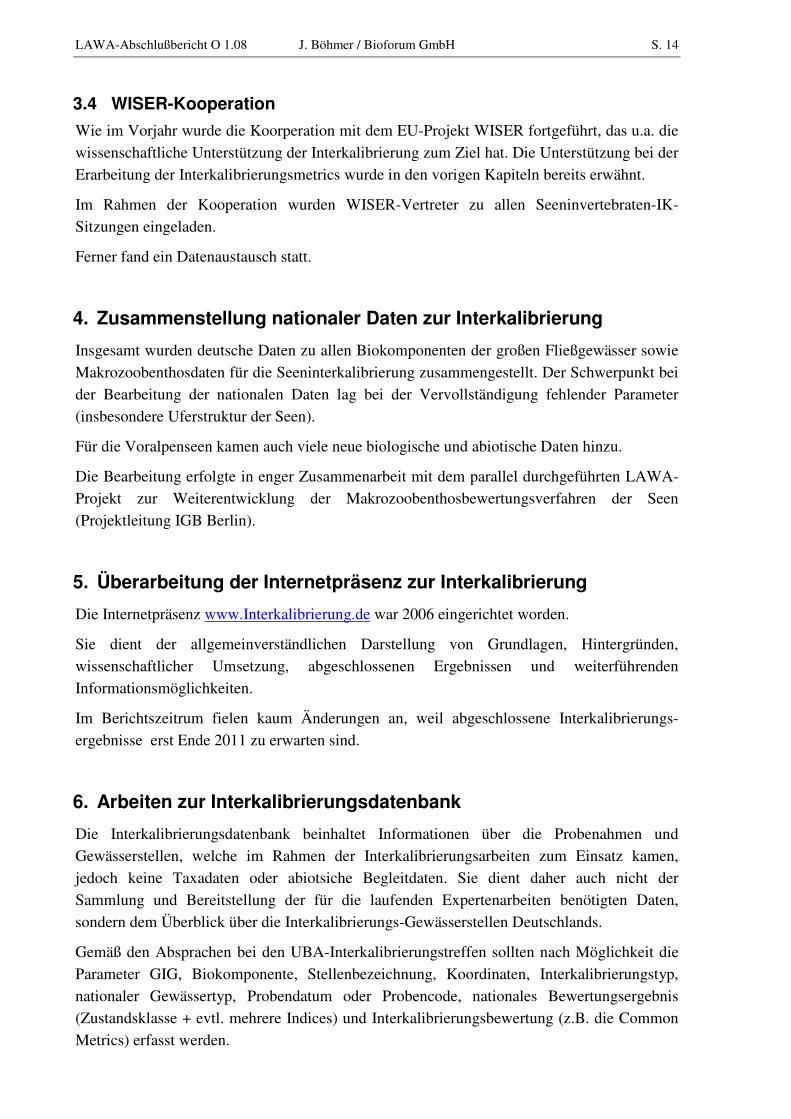
3.4 WISER-Kooperation

Wie im Vorjahr wurde die Koorperation mit dem EU-Projekt WISER fortgeführt, das u.a. die

wissenschaftliche Unterstützung der Interkalibrierung zum Ziel hat. Die Unterstützung bei der

Erarbeitung der Interkalibrierungsmetrics wurde in den vorigen Kapiteln bereits erwähnt.

Im Rahmen der Kooperation wurden WISER-Vertreter zu allen Seeninvertebraten-IK-

Sitzungen eingeladen.

Ferner fand ein Datenaustausch statt.

4. Zusammenstellung nationaler Daten zur Interkalibrierung

Insgesamt wurden deutsche Daten zu allen Biokomponenten der großen Fließgewässer sowie

Makrozoobenthosdaten für die Seeninterkalibrierung zusammengestellt. Der Schwerpunkt bei

der Bearbeitung der nationalen Daten lag bei der Vervollständigung fehlender Parameter

(insbesondere Uferstruktur der Seen).

Für die Voralpenseen kamen auch viele neue biologische und abiotische Daten hinzu.

Die Bearbeitung erfolgte in enger Zusammenarbeit mit dem parallel durchgeführten LAWA-

Projekt zur Weiterentwicklung der Makrozoobenthosbewertungsverfahren der Seen

(Projektleitung IGB Berlin).

5. Überarbeitung der Internetpräsenz zur Interkalibrierung

Die Internetpräsenz www.Interkalibrierung.de war 2006 eingerichtet worden.

Sie dient der allgemeinverständlichen Darstellung von Grundlagen, Hintergründen,

wissenschaftlicher Umsetzung, abgeschlossenen Ergebnissen und weiterführenden

Informationsmöglichkeiten.

Im Berichtszeitrum fielen kaum Änderungen an, weil abgeschlossene Interkalibrierungs-

ergebnisse erst Ende 2011 zu erwarten sind.

6. Arbeiten zur Interkalibrierungsdatenbank

Die Interkalibrierungsdatenbank beinhaltet Informationen über die Probenahmen und

Gewässerstellen, welche im Rahmen der Interkalibrierungsarbeiten zum Einsatz kamen,

jedoch keine Taxadaten oder abiotsiche Begleitdaten. Sie dient daher auch nicht der

Sammlung und Bereitstellung der für die laufenden Expertenarbeiten benötigten Daten,

sondern dem Überblick über die Interkalibrierungs-Gewässerstellen Deutschlands.

Gemäß den Absprachen bei den UBA-Interkalibrierungstreffen sollten nach Möglichkeit die

Parameter GIG, Biokomponente, Stellenbezeichnung, Koordinaten, Interkalibrierungstyp,

nationaler Gewässertyp, Probendatum oder Probencode, nationales Bewertungsergebnis

(Zustandsklasse + evtl. mehrere Indices) und Interkalibrierungsbewertung (z.B. die Common

Metrics) erfasst werden.


Da die Arbeiten der verschiedenen Interkalibrierungsgruppen Deutschlands in vollem Gange

waren, und niemand absehen konnte, welche Daten 2011 in der endgültigen Interkalibrierung

verwendet werden würden, fielen nur wenige Aktualisierungen an.

Ende 2011, nach Abschluß der Interkalibrierung, werden umfangreiche Aktualisierungs-

arbeiten anfallen.

7. Literatur

Birk, S., Bellack, E., Böhmer, J., Bunzel, K., Fischer, F., Kolbinger, A., Mischke, U.,

Schaumburg, J. & Schütz, C. (2009): Die Interkalibrierung nach EG-Wasserrahmenrichtlinie -

Ergebnisse der ersten Interkalibrierungsphase 2005-2007. Wasserwirtschaft 5: 20-25

Birk, S. & Böhmer, J. (2007): Die Interkalibrierung nach EG-Wasserrahmenrichtlinie -

Grundlagen und Verfahren. Wasserwirtschaft 9: 10-14

Böhmer, J. (2010): Derivation and Programming of „Common Metrics“ for the

Intercalibration of Large Rivers and Derivation of Reference Conditions by Extrapolation

and Percentiles - Short report. Berich an die BFG Koblenz; 3 pp.

Cardoso, A. C., A. G. Solimini, G. Premazzi, S. Birk, P. Hale, T. Rafael & M. L. Serrano,

2005. Report on Harmonisation of freshwater biological methods. EUR 21769 EN. European

Communities, Ispra.

CIS WG 2.A Ecological Status (ECOSTAT), 2004. Guidance on the intercalibration process.

Agreed version of WG 2.A Ecological Status meeting held 7-8 October 2004 in Ispra. Version

4.1. 14. October 2004.

CIS WG 2.A Ecological Status (ECOSTAT), 2004. Overview of common intercalibration

types. Final version for finalisation of the intercalibration network spring 2004. Version 5.1 -

23 April 2004. JRC EEWAI, Ispra.

Europäische Kommission, 2000. Richtlinie 2000/60/EG des Europäischen Parlaments und des

Rates vom 23. Oktober 2000 zur Schaffung eines Ordnungsrahmens für Maßnahmen der

Gemeinschaft im Bereich der Wasserpolitik.

Heiskanen, A.-S., W. van de Bund, A. C. Cardoso & P. Nõges, 2004. Towards good

ecological status of surface waters in Europe - interpretation and harmonisation of the

concept. Water Science and Technology 49: 169-177.


8. Anhang

8.1 Ergebnisprotokoll des Seen-Makroinvertebraten-CB-GIG-Treffens in Tartu (Originaltext)

Minutes CB-GIG lake macroinvertebrates meeting

Tartu (Estonia), June 16-17, 2010

Participants

Henn Timm (Estonia, host)

Kestas Arbaciauskas (Lithuania)

Juergen Boehmer (Germany; chairman)

Bart Reeze (Netherlands)

Wim Gabriels (Flanders, Belgium)

Absent

Malgorzata Golub (Poland), Peter Wiberg (DK), Andris Ceirans (LV) due to lack of funds.

Ben McFarland (UK) changed his job to a private company. Geoff Phillips (UK) provided the

name of a new delegate: Richard Hemsworth. Unfortunately Richard wasn’t able to attend

due to change of delegate and lack of funding.

Gwendolin Porst (WISER project), because another meeting in the USA.

Lionel Mazella (FR) without message.

Action list

Responsible Action By Juergen Send around format milestone report Asap All Fill in format milestone report for compliance of national methods

(chapter 4 of milestone report) August

All Check compliance of national methods with boundary setting protocol (see annex IV of IC guidance)

August

All Read IC guidance (step Q6, benchmarking annex III and comparability criteria annex V)

September

All Check data on questions about international typology (questions based on mean depth)

June

Kestas Revise submitted and add new data with emphasis on reference lakes

June

Wim Expand and revise data in dataset June Juergen Ask LV delegate to reconsider reference lakes and supply

information about reference criteria June

Juergen Send around list for harmonisation of taxonomic level June Juergen Ask Peter to contribute to first multivariate analysis June Bart/ Peter First rough (multivariate) analysis of data (if funds are sufficient) September Juergen Selection of metrics for the common metric July Juergen Give suggestions for common metric July Kestas Send around a list of invasive species (as a proposal) July


Agenda

1. Welcome

2. Status of national methods

3. Status of data collection

4. Compliance of methods

5. Intercalibration process (based on new IC guidance)

6. Discussion on boundary setting protocol (annex IV of IC guidance)

7. Results: towards a common metric

8. Other discussion points

9. Workplan and next meeting(s)

Wednesday, June 16, 2010

1. Welcome, overview

Henn Timm (EE) gives short overview of Estonian lakes. Contrary to most European

‘brown’lakes, some brown lakes in Estonia may be very well buffered.

The agenda is approved. The minutes of the Vilnius meeting are approved.

2. Status of national methods

Germany: the national method is under revision. Method is nationally accepted. Only class

boundaries have to be set. Descriptions only available in German. Assessment on site-level,

lake assessment based on weighted averaging.

Lithuania: still no national method. Method is still under construction. Main problem is lack

on representative data on lakes. Data are being collected.

Estonia: developed a national typology. For each type reference situations were found.

National method is official and accepted, further improvements are possible. Descriptions

only available in Estonian. Assessment on site-level (one site per lake).

Flanders (Belgium): method is official and published. Assessment on site-level, lake

assessment based on averaging.

Netherlands: the method is finished and at the moment it is not being further adjusted.

Assessment on site-level, lake assessment based on weighted averaging.

3. Status of data collection

Currently in the database:

Belgium: 12 lakes. Important missing data data will be added (mean depth, CB typology,

landuse, nutrients). For 6 lakes new samples on species level are available. Data to genus/

family level.


Germany: 138 lakes. Data of 53 lakes are consistent, only those lakes might be used for

analysis. Major problem is chemistry. Other data more or less complete. Landuse has to be

completed. All data to species level (53 lakes), except for chironomids and oligochaeta. Other

lakes mixed id-level. Probably the analysis should be limited to the set of 53 lakes.

Estonia: 20 lakes. Data are quite complete, no actions needed. Some extra data for shoreline

alteration will be added. Data to species level, except for chironomids, oligochaeta and

watermites.

Great-Britain: 35 lakes, about 20 lakes littoral and CPET data available. Data quite complete,

no action needed. Littoral data to species level, except for chironomids and oligochaeta.

Lithuania: 10 lakes. Some important data are missing (landuse, shoreline alteration (%)). New

data are available and will be sent within a month (including missing data).

Latvia: 23 lakes. Important missing data are landuse (surroundings (100-300m)) and shoreline

(15 m)) and shoreline alteration (%).

Netherland: 32 lakes. Missing data are mean depth (not available). All data to species level.

Poland: 6 lakes (WISER-data). Shoreline alteration (%) is missing.

Denmark: 17 lakes, stressor data incomplete;

Not in the database:

France: sent data for sublittoral and profundal. Parallel eulittoral samples will be needed for

intercalibration.

4. Compliance of methods

The milestone report provides a good format to check the compliance of national methods

(chapter 4). It was agreed that everybody fills in this format before the end of august (see

action list).

5. Intercalibration process (based on new IC guidance)

Q1: compliance of methods. See point 4 and action list.

Q2: Feasability check. Done in the beginning of the process: we focus on eulittoral and

hydromorphological pressure. Some methods are not similar (CPET and French method). For

those methods parallel data were collected (eulittoral and specific data for the methods).

Q3: All countries have different assessment methods so far.

Q4: The sampling is different in most countries. Furthermore the Dutch method is the only

method requiring identification to species level for chironimids and oligochaeta. The data of

other countries only provide family-data. Conclusion: option 2 is most favourable.

Nevertheless we will give option 3 a try.


Q5: First results show weak correlations between national methods and metrics possibly to be

included into the common metric. The Dutch method seems to perform well in correlations

with pressure data and possible metrics.

Q6: There might be enough sites for reference conditions if we agree to assess at a site level.

There are not enough reference lakes for intercalibration at a lake level. Description of

reference biological communities will probably be desribed at the level of values for the

(common) metrics at reference conditions.

Q7: Compliance of boundary setting of national methods. The boundary setting seems to be

WFD-compliant for all available methods, which would bring us to a direct comparison of

national classifications. Description of biological communities representing moderate

deviation from reference conditions will be desribed at the level of values for the (common)

metrics at the good-moderate boundary.

6. Discussion on boundary setting protocol (annex IV of IC guidance)

Estonia: Henn Timm explains boundary setting for the Estonia method. The boundary setting

is based on a practical view on possible scores for the sum of the five metrics.

Germany: all metrics were related to pressure data.

Belgium: the reference value for the method was set based on maximum scores (expert

judgement) for the individual metrics. Initially, the range of the method was devided into five

equal classes. Based on the river IC exercise the classes were upgraded a little bit.

Netherlands: boundaries are derived from a theoretical reference and deviding the range into

five equal classes. There has been no comparison with pressure data yet. The pressure data

from the current IC database provide a good basis for that.

7. Results: towards a common metric

The common metric will be based on a numer of ASTERICS metrics (and a number of

others). Correlations were carried to identify metrics for the common metric. The common

metric needs a good correlation with stressor parameters and national EQR’s. Correlations

were carried out between;

• Stressors x possible metrics • National EQR’s x possible metrics; • (Stressors x national EQR’s).

There are a numer of possible metrics which perform well for correlations with stressors and

national EQR’s:

• % Odonata (individuals) (composition/ tolerance); • % ETO (abundance classes) (composition/ tolerance); • Number of sensitive groups (diversity/ tolerance); • Numer of taxa (diversity);


• ASPT (tolerance); • % Indifferent species (abundance classes) (functional/ guild); • % R/K Strategists (abundance classes) (functional).

Discussion for further analysis:

• Level of comparison: site level or lake level. All available assessment systems are operating at site level. The WFD however requests a comparison at waterbody-level. The abiotic data are available at lake level too. Decision: use site level, show the results are valid for lake level as well;

• Building of common metric: how to proceed. Metric values might be biased between countries due to different ways of sampling and data processing. Normalisation (dividing metric values by reference values) will presumably level this bias out. So to enable the selection of the right metrics we need to select reference sites first. This seems to be difficult at this stage. Decision: normalisation will be carried out based on 90-percentile metric values for the whole dataset (and dataset per country which provides calculation factors);

• Still we need reference sites later on in the process. Due to the lack of reference data we will calibrate results of modelling with actual data from reference sites;

• After selection of possible metrics intercorrelation (covariation) between the possible metrics need to be checked. Then select metrics which describe the relation with stressors best.

Thursday, June 17, 2010

8. Other discussion points

Taxonomic level: some harmonisation on the taxonomic level is needed for metric calculation

and multivariate analysis. For example:

• Chironomids and dipterans on family level; • To be excluded: zoöplankton, fish, Acari, Ostracoda, meiofauna (nematods) Juergen will send around an existing list which for discussion.

Some basic data-analysis needs to be done to check coherence of the data, outliers, typology,

reference sites, etc. A good way to explore the data is a multivariate analysis (correspondal

analysis).

Juergen will ask Peter Wiberg to contribute in a first multivariate analysis.

There are no reasons to change the current typology so far (CB1 and CB2). There are not

enough data to include CB3. Maybe the multivariate analysis will provide new input for the

typology discussion.


Invasive species. We need a list of invasive species to set op a metric on biocontamination (as

a check for interference with metric scores). A list will be set up for catchment within Europe

(group Phil Boon), but this might take a couple of years.

Kestas will distribute a list of invasive species (as a proposal). This list needs to be extended/

checked by the rest of the group.

9. Workplan and next meeting(s)

Workplan

Next steps are:

• Finalisation of the dataset (new data, international typology); • Harmonisation of taxonomic level; • Reconsider reference lakes and supply information about reference criteria; • First rough (multivariate) analysis of data; • Selection of metrics for common metric; • Building common metric. See action list.

Next meetings

The next meeting will take place on October 20, 21 in Aalst (Flanders), hosted by Wim

Gabriels.

Action list NL (specific)

Wie Wat Wanneer

Bart Check correlaties maatlat NL x pressure data IC database

Bart Check internationale typologie (bijvoorbeeld M20 met geringe

diepte die tot CB1 worden gerekend)


8.2 Ergebnisprotokoll des Seen-Makroinvertebraten-CB-GIG-Treffens in Aalst (Originaltext)

Draft minutes CB-GIG lake macroinvertebrates meeting

Aalst (Belgium), October 20-21, 2010

Participants

Kestas Arbaciauskas (Lithuania)

Rachel Benstead (UK)

Jürgen Böhmer (Germany; GIG leader)

Wim Gabriels (Flanders-Belgium)

Gwendolin Porst (WISER)

Bart Reeze (the Netherlands)

Henn Timm (Estonia)

Denmark, Poland and Latvia cannot attend due to funding problems. We will of course keep

them informed of all developments.

Minutes

1. Welcome by Mr. Rudy Cautaerts, head of Department Water Monitoring

2. Approval of agenda; aims for the present meeting; approval of the minutes of the

previous meeting; election of meeting secretary (for the minutes)

Agenda is approved, with the addition of one item (WISER presentation).

Meeting secretary: Wim

Jürgen gives an overview of the minutes from the Estonia meeting (drafted by Bart):

Milestone report needs to be updated; later on everyone will have to answer all questions

regarding compliance check. Data from Kestas are not submitted yet. Wim has sent data. No

response from Latvia about reference lakes. List for harmonisation of taxonomic data was

distributed by Jürgen. The list of invasive species was distributed by Kestas. We will

intercalibrate at site level as most countries assess at site level.

The minutes are approved.

3. Feedback from ECOSTAT meeting: Milestone 3, deadline of second intercalibration

round, intercalibration guidance Annex V

Annex V was approved by ECOSTAT (and will probably be approved by the water directors

as well).

Deadline for the GIGs for the second intercalibration round is june 2011 (Milestone 5).


4. WISER presentation by Gwendolin

Final report on deliverable 3 (assessment of European lakes using benthic macroinvertebrates,

i.e. developing of common metrics using WISER data set as well as GIG data) is due 28

februari 2011. The final deadline for WISER is 29 march 2012.

5. WFD compliance of national methods

Situation for all countries is the same as during last meeting.

Milestone 3 report is used as template for milestone 4. The different questions of the

Milestone (points 1-4) are discussed and updated where necessary.

For question 3 (method compliance check):

-UK must write a response to question 3 and 8 (parameters included)

-all countries must list their national types and state whether they are compliant with Annex II

(provide a conversion table from national types to common types if possible)

6. Harmonisation of identification level (German taxa harmonisation filter)

The harmonisation filter is approved with a number of modifications:

-Chironomidae are set to family level;

-Oligochaeta are set to order level;

-Polychaeta remain at order level;

-all mites, copepods, ostracods, hydrozoans and bryozoans are ignored.

Jürgen will send the new database and the updated version of the harmonisation filter to

everyone by the end of october.

7. Database: available data, stressors, metrics (...)

Presentation by Jürgen about the database:

-9 countries

-197 lakes

-873 stations

-991 samples

In total 1191 taxa. Taxonomic resolution varies depending on group; they were harmonised

using an operational taxa list from Germany.

In order to select candidate metrics, metrics were correlated against national EQRs. Good

results are found for several metrics.


Stressor parameters were correlated against individual metrics. Which metrics give the

strongest correlations, depends on the dataset used (combined or for single countries). Some

metrics seem to respond differently in different countries:

-number of EPTCBO taxa (or ETO)

-ASPT

-% Odonata individuals

-% ETO (in relation to abundance classes)

-rk-index (ratio r-strategists vs. k-strategists)

-% habitat preference lithal individuals

-% indifferent individuals

(-% Crustacea individuals)

The final selection of metrics should depend on correlation of the metrics with national EQRs

and with pressures, and on acceptance by countries.

Kestas will try to update the Lithuanian data and send it to Jürgen ASAP.

8. Selection of common metrics, reference conditions/alternative benchmarking

In order to combine metrics, the metrics values need to be rescaled to the interval (0-1),

(“normalised”). For this purpose, we need reference (or benchmark) values for each metric.

This can be done by using a correlation of the metric against e.g. total P and convert the value

of P which is considered reference into the corresponding value of this metric. A similar

approach would be to use a “benchmark” value: e.g. a different P value which is assigned a

certain EQR value instead of the reference (e.g. 0.6 instead of 1). A different, but more robust,

approach is using the 90th percentile of a metric as reference value.

When different countries have a different correlation between pressures and metrics, multiple

benchmarking could be considered, which would mean shifting the correlation curve in such a

way that a similar pressure level (e.g. a certain total P-value) always corresponds to the same

metric value. This could be advantageous since taxa richness seems to be biased between

countries, presumably partly due to differences in sampling effort.

The agreed next steps are:

-harmonisation of taxa lists to produce the new data set

-normalising all metrics by dividing the values by the 90th percentile (e.g. metric value at the

90th percentile becomes 1)

-selection of different combinations of metrics (initially using a weighting factor of 1 for all

metrics)

-comparing the multimetric indices with the pressures and the national EQRs


Option 3 seems doesn’t seem to be very promising with our data (due to suspected differences

in sampling effort), and also it’s quite time-consuming. Therefore we decide to use option 2.

9. Boundary setting

We can either use the average of the boundaries or the median. The median will be affected

less by changing boundaries. The final decision on boundary setting methods can be taken at a

later stage (after finalising the common metric).

10. Compilation of alien species lists

Kestas has compiled and distributed a list of alien species. Several countries have indicated in

this list which ones are present in their country. However, some species are alien in one

member state (e.g. Astacus astacus in UK) but native in other member states.

Only species should be considered which are also in the taxa list used for calculating the

common index.

A number of indices assessing alien impact can be calculated:

ACI (Abundance Contamination Index) = number of individuals of aliens / total number of

individuals

RCIo (Richness Contamination Index at order rank) = number of alien orders present / total

number of orders identified

RCIf (Richness Contamination Index at family rank) = number of alien families present / total

number of families identified

Based on the list Kestas distributed earlier, we will compile a list of alien species with

indication of nativity (native or alien) for member states.

Jürgen will ask Jochen Vandekerkhove which (black)list(s) they use to assess impact of

aliens.

Kestas will check the national databases (from the ECOSTAT questionnaire report) in order

to update our list.

By december 2010 Kestas will distribute a draft list of all candidate alien species, each

country has to indicate which ones are native to their country.

Jürgen will check with Daniel Hering (WISER) about the availability of the data. He will send

Jochen Vandekerkhove the dataset with national EQRs and species lists wherever aliens

occur.


11. Summary of conclusions of the meeting and future tasks

Action points:

-Every country will eventually need to supply information on the compliance criteria for

national methods (template by Angelo Solimini will probably be updated in future).

-For Milestone 4, we will update Milestone 3. Jürgen will distribute the draft for Milestone 4

end of february for comments and additional information. For this, UK must write a response

to question 3 and 8 (parameters included) and all countries must list their national types and

state whether they are compliant with Annex II (provide a conversion table from national

types to common types if possible).

-Kestas will update the Lithuanian data and send it to Jürgen ASAP.

-Jürgen will send the new database and the updated version of the harmonisation filter to

everyone by the end of october.

-For Milestone 4, we will include information on common metrics and correlations with each

national EQR.

-Jürgen will ask Jochen Vandekerkhove which (black)list(s) they use to assess impact of

aliens next week.

-Kestas will check the national databases (from the ECOSTAT questionnaire report) in order

to update our list. By december 2010 Kestas will distribute a draft list of all candidate alien

species, each country has to indicate which ones are native to their country.

-Jürgen will check with Daniel Hering (WISER) about the availability of the data next week.

He will send Jochen Vandekerkhove the dataset with national EQRs and species lists

wherever aliens occur next week.

Next meeting:

Next ECOSTAT meetings are 30-31 March 2011 (Brussels) (Milestone 4) and 29-30 June

2011 (Ispra) (Milestone 5) and 24-25 October 2011 (Brussels).

We have a GIG meeting on 2-3 March 2011 in London (hosted by Rachel) to discuss the final

decisions on metric selection and completing Milestone 4 and discuss the boundary setting

procedure.

For the final decisions and completing Milestone 5, will have a meeting on 24-26 May 2011,

probably in Berlin (hosted by Gwen) (to be confirmed).


8.3 Ergebnisprotokoll des zweiten XGIG-Treffens zu großen Flüssen in Koblenz (Originaltext ohne Anhang)

Minutes

XGIG Large River Intercalibration - Second Workshop in Koblenz, April 19th, 2010

Franz Schöll

Participants: Sebastian Birk (DE), Jürgen Böhmer (DE), Roel Knoben (NL), Wim Gabriels (BE-FL),

Denisa Nemejcova (CZ), Franz Schöll (DE)

Low number of participants due to problems in air traffic (volcano-incidence)

1. National methods to assess the ecological status of very large rivers

12 Member States have reported on their assessment methods for the various BQE applied

to very large rivers prior to the meeting. The group discussed aspects of the methods’ WFD

compliance and intercalibration feasibility. The criteria given by the new intercalibration

guidance seem to be met in general (i.e. EQR, five class assessment etc.). However,

Member States will be asked to provide more detailed information or amend/correct the data

given (see Actions). A methods’ overview is annexed to this document.

General remarks on bioassessment of very large rivers

The intercalibration exercise of very large rivers is focusing on existing (and approved)

national methods. All these national methods acquire their biological data from the main river

channel and are mainly based on concepts similar to the assessment of smaller rivers. We

acknowledge that very large rivers feature more relevant habitat types than just the main

channel (e.g. secondary channels, floodplain pools, dead arms), suggesting an ecologically

more relevant assessment concept for very large rivers. We encourage to discuss this issue

at ECOSTAT, however we don’t consider this as a part of the current intercalibration exercise

for very large rivers.

2. Actual intercalibration feasibility as determined by the group

The group decided to enter the actual intercalibration analyses for selected BQE and national

methods, depending on the status of the methods and the availability of monitoring data. A

short documentation of relevant intercalibration aspects per BQE is given in the following.

Benthic invertebrates

11 countries hold assessment methods. The majority of countries does kick-sampling close

to the river banks, however the comparability of data gained from the whole sampling

designs is questionable. The level of taxonomic identification is different and ranges from

family- to species-level determination. Most countries apply multimetric assessment using


different sets of metrics. We suppose that the preferable method of intercalibration is Option

2 (use of common metrics). The pressure focus is general degradation (mixed pressures).

The common intercalibration database currently contains approx. 370 samples. Most data

were sampled at Central European rivers. The group considers the intercalibration feasible

for Central European rivers.

Phytobenthos (Benthic diatoms)

11 countries hold assessment methods. All countries assess the diatom flora, only two

countries additionally include other phytobenthos (DE, AT). Sampling techniques seem to be

sufficiently comparable to try to work with IC Option 3 (direct comparison). All methods focus

on similar pressures (mainly eutrophication), similar assessment metrics are used. The

common intercalibration database contains approx. 170 samples. Most samples originate

from Central European rivers. Intercalibration seems feasible. We will test IC Option 3 (direct

comparison) and additionally work with common metrics.

Fish fauna

9 MS hold assessment methods. All countries apply electrofishing, some countries perform

additional sampling by fyke nets or beam trawls. Multimetric assessment using different sets

of metrics is generally used. Both IC Options (2+3) seem feasible which is in accordance with

the experiences of the IC Fish Group. The pressure focus is general degradation (mixed

pressures). The common intercalibration database contains approx. 80 samples with the

majority of sites at Central European rivers. The group decided to further explore the

intercalibration feasibility with the existing data (if additional resources are provided – see

remarks below), and conclusions will be reported at the next XGIG Large Rivers meeting in

September 2010. Exchange with IC river fish expert group is foreseen.

Phytoplankton

Four countries hold assessment methods. The sampling method is similar, data assessment

is different. All methods focus on similar pressures (eutrophication), different assessment

metrics are used. The common intercalibration database currently holds approx. 17 site-

years (SK: 6, LT: 1, DE: 10). The group concludes that intercalibration is currently not

feasible due to lack of data.

Macrophytes

Four countries hold assessment methods. Macrophytes are sampled by different survey

techniques and different data assessment is applied. The common intercalibration database

includes approx. 100 surveys. Problems arising from different sampling and assessment in

combination with data scarcity are to be expected. The relevance of macrophytes for certain

very large river types/states of degradation seems to be narrowed (lack of species, low


abundances, large water depth). Currently, intercalibration seems less feasible for this

biocomponent. NL and FL consider a bilateral intercalibration exercise for macrophytes at

their common water bodies (Meuse river).

3. Analytical options for very large river intercalibration

The intercalibration of methods applied to very large rivers is challenged by the lack of

reference sites and the low availability of data from some countries (e.g. FL has only three

water bodies belonging to very large rivers). Jürgen Böhmer and Sebastian Birk outlined

possible approaches to overcome these issues in the data analyses. The exploration of

pressure-impact relationships in the available data allows for including country data with an

insufficient ecological gradient. These analyses support in selecting common intercalibration

metrics and help in modelling reference metric values. Defining common benchmarks similar

to the CBrivGIG Macrophyte exercise can set benchmark values for common metrics, but

requires common datasets assessed by all national methods. This approach allows for the

detection of typological differences between countries/regions. It is planned to present the

outcomes of these analytical options at the next XGIG Large River workshop in September

2010.

4. Outline of work plan / next steps

1 Completing info for WFD compliance checks based on Member States’ comments to

the methods’ overview

2 Finalising common database (filling of gaps, data quality checks)

3 Analysis of invertebrates and diatom data (step-wise approach)

a Selection of candidate common metrics using all available data

b Establishing pressure-impact relationship between common metrics and abiotic parameters/gradients

c Evaluation of typological differences using sites in Least Disturbed Conditions

d Application of common benchmarking/reference modelling

4 Analysis of fish data

The preliminary analysis for the intercalibration of fish assessment methods cannot

be done by the XGIG Large River IC steering group due to lack of resources. Member

States are asked to support the exercise providing adequate expertise and resources.

The River Fish IC group indicated no capacities to deal with the intercalibration of

very large rivers during the current intercalibration phase.

Anticipated work steps: see point 3.


5. Next XGIG Large River IC workshop in Koblenz

22. to 23. September 2010

6. List of actions

1 Sebastian Birk: Prepare WFD compliance check of national methods (beginning of

May 2010)

2 Member States’ delegates: Description of reference and boundary setting (if not

already provided specifically for very large rivers in the WISER-Questionnaires)

(middle of May 2010)

3 Jürgen Böhmer: Completion and validation of database quality (beginning of June

2010)

4 Jürgen Böhmer and Sebastian Birk: Intercalibration analyses according to work plan

(September 2010, next workshop)

5 Member States: provision of support regarding fish data and intercalibration (support

starting in May; results by September 2010, next workshop)

8.4 Ergebnisprotokoll des dritten XGIG-Treffens zu großen Flüssen in Koblenz (Originaltext)

Final Minutes XGIG Large River Intercalibration - Third Workshop in Koblenz, September 22nd- 23rd, 2010

Franz Schöll, Sebastian Birk

Participants: Ana Lara Romero (ES), Christine Keulen (BE-WL), Denisa Nemejcova (CZ),

Emilia Misikova Elexova (SK), Franz Schöll (DE), Franz Wagner (AT), Gorazd Urbanic (SI),

Jukka Aroviita (FI), Jürgen Böhmer (DE), Matus Haviar (SK), Nuno Caiola (ES), Rachel

Benstead (UK), Roel Knoben (NL), Sebastian Birk (DE), Simone Ciadamidaro (IT), Stina

Drakare (SE), Wim Gabriels (BE-FL), Wouter van de Bund (EC)

1. Update on IC comparability criteria The criteria for judging comparability of national class boundaries in the intercalibration

exercise were presented. Main criteria are

Method relatedness (i.e. coefficient resulting from Pearson correlation of national

assessment and (pseudo-) common metric): R ≥ 0.5

Boundary bias (i.e. deviation in the relative positioning of class boundaries, reflecting how

stringent Member States are in defining the good ecological status): ± quarter of a class


Class agreement (i.e. confidence that two or more national methods on average report the

same class for a given site): less than one class

Analytical options comprise either the regression of national assessment results against

common metrics (IC Option 2) or pseudo-common metrics (IC Option 3a), or the direct

comparison of assessment results per monitoring site (IC Option 3b). Member States are

currently asked to comment on the draft to allow for final adoption of the criteria at the

ECOSTAT meeting in October (i.e. Annex V of the Intercalibration Guidance).

2. Overview of national assessment methods for large rivers We presented an overview of national assessment methods. Three Member States

nominated new methods used in large river bioassessment: Italy (benthic invertebrates,

diatoms, fish fauna), Austria (macrophytes), Slovenia (macrophytes). In total, 46 national

methods are reported for the large river intercalibration exercise. We agreed to check their

WFD-compliance based on the data collected for the overview document1. Outcomes of this

check will be presented in the milestone 3 report. The compliance criteria are generally met,

but for certain methods more information is needed.

3. Relationship of the XGIG Large River work to the other GIGs The group concluded that all intercalibration work for very large rivers is completely carried

out in the cross-GIG Large River intercalibration exercise. This means that GIGs can hand

over the intercalibration work on very large rivers to the XGIG.

4. Database issues 12 Member States have delivered biological and environmental data for the common

intercalibration database of large rivers. A data overview for the benthic invertebrates (BI)

and diatoms (DI) was given. The data currently cover 42 (BI) / 26 (DI) rivers, 88 / 63

waterbodies, 137 / 77 stations, 367 / 378 samples and 945 / 649 taxa. Some implausible

data entries need to be clarified. France did not deliver any data yet and will be asked for

data submission to allow for full coverage of the geographical gradient in Europe.

The group stressed that the data will exclusively be used for the analyses required within this

intercalibration exercise. Any other use (incl. publications) will require the specific approval of

data owners.

5. First results of data analysis Definition of benchmarks – diatom case-study

Based on 80 water bodies for which biological, physico-chemical and stressor data were

available we performed a factor analysis to identify the main pressure gradients

characterising the dataset. The first two components resulting from the analysis were highly

related to either water quality variables or parameters of habitat quality (Figure 1). Most

national water bodies showed a clumped distribution, i.e. the water bodies at large rivers of a

region/country often show similar levels of disturbance instead of covering a broader gradient

of degradation. Factor 1 representing water quality was significantly correlated with the

potential common metrics for diatom intercalibration (IPS: r=-0.45, Trophic Index: r=0.37).


Figure 1: Position of national water bodies in „pressure space“ defined by factor analysis of

environmental data (Factor 1 related to concentrations of Orthophosphate, Nitrate, Chloride;

Factor 2 related to degree of channelization and impoundment)

Using the German standard for water quality, parameter thresholds were applied to the

physico-chemical data to define water bodies in good water quality status. The 75th

percentile value of Factor 1 scores at sites meeting this good status was chosen as the

threshold to differentiate between benchmark and non-benchmark water bodies. Most abiotic

parameters and the diatom metrics showed significant differences between these groups.

When mapping their geographical position we recognised that benchmarks are

predominantly located in north-eastern and eastern Europe, i.e. their geographical

distribution is highly skewed. Furthermore, the benchmark water bodies already cover a

relevant pressure gradient. These findings disclose that we need to develop an improved

concept of alternative benchmarking for the large river intercalibration exercise.

Metric selection and extrapolation of reference conditions

Based on the full dataset various biological metrics were related to selected stressor

parameters, i.e. stressor index (derived mainly from categorised morphology parameters),

catchment land use index and %near natural areas, national degradation class (3 countries

only), total phosphorus (TP) and minimum oxygen concentration. The invertebrate metrics

showed best correlations with the stressor index and somewhat weaker relations with land

use and TP. The national degradation class covered only parts of the gradient and had too

few data. Best metrics were: feeding type active filterer, current preference rheophilic as well

as indifferent, the “rheoindex”, habitat preferences akal as well as psammal, feeding type

gatherer, RTI, PTI, SI, zonation preference metapotamal and rhithral.

The diatom metrics revealed best correlations with TP that were much stronger than all

macroinvertebrate correlations (see Figure 2); the correlations were weaker with land use and

the stressor index. The best related metric was the IPS. The correlations of individual metrics with the

national EQRs provided with the biological data were generally weaker than correlations between

metrics and stressors. This was mainly caused by the differences among national assessment methods


emphasising different stressors. Improved concepts for alternative benchmarking were discussed. The

common data basis and strong dose-response relationships for the diatoms allow for an extrapolation

of reference conditions (Figure 2). This technique will be further investigated for diatoms and benthic

invertebrates in the next months.

Figure 2: Comparison of different approaches to derive reference conditions using the dose-

response relationship between TP and the diatom metric IPS (R2=0.41)

6. Checking the steps of the IC guideline The feasibility checks required by the IC guidance comprise intercalibration typology,

pressures addressed by the national classifications and assessment concepts. All aspects

were checked, and we concluded that intercalibration is feasible at least for the diatom and

invertebrate methods. More detailed replies to the questions on feasibility are given in the IC

milestone report 3.

The compilation of the common database is at an advance state (see above). We will ask for

more data from France, Hungary and Romania. Individual Member States that already

provided data will be addressed to clarify database issues, if necessary.

We agreed to test intercalibration option 3 (direct comparison) in the diatom exercise, since

national techniques of data acquisition for diatoms are sufficiently comparable. Thus, we will

ask the Member States to deliver information about the national diatom typology of large

rivers and specifications of the national diatom indices (indicator lists, metric algorithm and

combination etc.). The calculation of the national diatom assessments will be done centrally

using the common dataset. For invertebrates an intercalibration option 2 is envisaged.

However, the national datasets used in intercalibration mostly cover only a narrow quality

gradient and comprise few water bodies / monitoring sites. Therefore, we aim at merging

those national datasets that were acquired by similar techniques (e.g. comparable sampling

effort and level of identification). This should extent the data basis for the subsequent

regression analyses. We finally plan to compare the national class boundaries against a

common metric using these multi-national datasets of similar data characteristics.

The diatom exercise can operate on the basis of pseudo-common metrics (i.e. average of

national EQR excluding the country that is compared). The invertebrate exercise will refer to


true (biological) common metrics that will be selected on the basis of the outcomes of further

analyses (using the updated common database). The use of large river-subtypes reflecting

the biogeographical differences among European regions is also envisaged in the scope of

further data analysis.

7. Other topics Franz Wagner addressed the relevance of the XGIG Large River intercalibration work for the

ongoing development of bioassessment tools for very large rivers in Europe. In particular, a

possible contribution to the planning phase of the third Joint Danube Survey was mentioned.

The group concluded to participate in the discussion by providing a conceptual document

including an analysis of the state-of-the-art, shortcomings and perspectives of large river

bioassessment, and recommendations for future work.

8. List of actions 1 Franz Schöll will address France, Hungary and Romania for data delivery (end of

September 2010)

2 Jürgen Böhmer will clarify remaining database issues (e.g. missing data, implausibilities)

with the respective Member States (end of October 2010)

3 Jürgen Böhmer will collect specifications on the national diatom assessments to prepare IC

Option 3 (end of October 2010)

4 Simone Ciadamidaro will update information about the Italian assessment methods (incl.

delivery of the WISER questionnaire) (end of October 2010)

5 Sebastian Birk and Jürgen Böhmer will work on the intercalibration analyses during winter

2010/11 to report on the analytical outcomes by February 1st, 2011 (before the next meeting)

6 Sebastian Birk will draft a conceptual document on large river bioassessment to be

circulated to the group (before the next meeting)

9. Next XGIG Large River IC workshop in Koblenz February 10th and 11th, 2011


8.5 Ergebnisprotokoll des Seen-Makroinvertebraten-AL-GIG-Treffens in Aix en Provence (Originaltext)

Alpine Lake Invertebrate Meeting

Aix-en-Provence 06-07- Dec 2010

Participants:

Angelo Solimini (IT, Wiser)

Christine Argillier (Fr)

Cedrix Provost (Fr)

Muriel Gevrei (Fr)

Juergen Bohemer (DE)

Georg Wolfram (AT)

Gorazd Urbanic (SI)

Introduction and general statements

Developing pressure specific relationships should be preferred over general degradation type

relationships.

France will not develop a national method by the deadline of this IC round. However, France

will consider to adopt the common metric developed in the IC process as national method if

proved to be applicable to national types. Italy has not provided national boundaries for any

classification method to date. Suggestion of this group is to consider the adoption of the

common metric.

IC procedure in this GIG will be split among 2 exercises. The first will target established

classification methods in the eulittoral zone (DE and SI). The purpose of this exercise will be

to intercalibrate the 2 existing national metric and to provide to other member states a

standard (e.g. the common metric) that can be used in the future to validate newly developed

national methods. The second IC exercise, will establish a common metric and class

boundaries in the sublittoral zone (no national methods available, with the exception of DE

that will, however, not used in national monitoring). The purpose of this exercise will be to

provide a standard (the IC metric) to be used by member states to compare national methods

whenever available.

The pressure target in both IC exercises will be hydromorphological alterations. This group is

aware that benthic invertebrates respond to secondary effects of euthrophication but believe

that this pressure can be tracked more efficiently and in a more cost effective way with other

BQEs (e.g. phytoplankton).


Common database

The GIG established a common database. In addition to abundances of invertebrates per site,

the common database include information on morphologicl prameters and stressors at water

body (wjhole lake) and site levels.

Description of parameters of database

Water body level

MS

National type + IC lake type

Coordinates

Catchment, Altitude

Mean depth, Max depth

Surface area, Volume

Alkalinity, Conductivity

Ice cover

Stressors – whole lake

Obligatory

Land use 100-300 m; preferred: 200 m, 100 – 300 m is still ok

Forest

Intensive agriculture (corine codes 2.1, 2.2, 2.4.1, 2.4.2)

Grassland = non-intensive agriculture (corine codes 2.3.1, 2.4.3, 2.4.4)

Urban

Land use catchment

TP, TN, chl-a

Shoreline alteration %

Stressors – site level

Lake name

Sampling site

Naturalness national SI+GE

LHS sum of pressures (in table samples)

Land use


% forest

% grassland and agriculture

% urban (roads, houses, railway, camping, recreational, harbour …)

% near natural excl. forest (reed, shrubs, moor, rocks, …)

Shoreline alteration soft engineered p/a (e.g. beach, vegetation cut)

Shoreline alteration hard engineered p/a

Shoreline_classes

Taxa list

5 versions (all meiofauna and acari to be removed)

Raw (as provided)

All genus

All family

All raw, except chiro to subfamiliy (chironominae: tribe), oligochaetes to family

All genus, except chiro to subfamiliy (chironominae: tribe), oligochaetes to family

Not agreed !!

Action list

In 2011: 3 ecostat meetings (March, June, Oct)

Milestone 4 in Feb 2011: IC on eulittoral

Milestone 5 in May 2011 = final report

Next meeting 23-24 March 2011

Ljubljana (confirmed by Gorazd within next days)

- everybody sends missing data to Jürgen until mid Jan 2011

- Jürgen harmonizes tables and distributes again the final version (including the quieries)

- Jürgens sends final GE method

- check taxonomic levels (Georg), until March meeting

- option 3 with final SI and [soon] final GE method on eulittoral (Gorazd), until March

meeting

- metrics – correlation analysis (Jürgen)

- metrics by modelling approach/multivariate (Christine)

- ref cond (1. Lake level, 2. Site level)


8.6 Dritter Bericht der CB-GIG-Invertebratengruppe an ECOSTAT

EUROPEAN COMMISSION

DIRECTORATE GENERAL JRC

JOINT RESEARCH CENTRE

Institute of Environment and Sustainability

WFD Intercalibration Phase 2: Milestone 3 report

Water category/GIG/BQE/

horizontal activity:

Lake / Central Baltic / Benthic Fauna

Information provided by: Juergen Boehmer

1. Organisation

1.1. Responsibilities

Indicate how the work is organised, indicating the lead country/person and the list of involved

experts of every country:

Juergen Boehmer (DE; lead)

Kestas Arbaciauskas (LT)

Gwendolin Porst (WISER)

Bart Reeze (NL)

Andris Ceirans (LV),

Lionel Mazzella (FR)

Henn Timm (EE)

Wim Gabriels (BE/FL)

Malgorzata Golub (PL)

Peter Wiberg-Larsen (DK)

UK will determine a new expert soon

DE is responsible for the database. All countries are going to work on parts of the analysis

and the final reports.


1.2. Participation

Indicate which countries are participating in your group. Are there any difficulties with the

participation of specific Member States? If yes, please specify:

BE/FL, DE, DK, EE, FR, LT, LV, NL, PL, UK

Funding for Denmark and Poland is not sufficient for this year, limiting their participation;

UK is momentarily missing an expert

1.3. Meetings

List the meetings of the group:

PL (June 2008), DE (October 2008), NL (April 2009), LT (January 2010), EE (June 2010),

Belgium (planned Oktober 2010)

2. Overview of Methods to be intercalibrated

Identify for each MS the national classification method that will be intercalibrated and the status of the

method

1. finalized formally agreed national method,

2. intercalibratable finalized method,

3. method under development,

4. no method developed

Member State Method Status

BE/FL Multimetric

Macroinvertebrate Index

Flanders (MMIF)

1 - .finalized agreed national method

NL WFD-Metrics for Natural

Watertypes 1 - .finalized agreed national method

DE German

Macroinvertebrate Lake

Assessment

2 - intercalibratable finalized method

DK 3 – under development

EE Estimation of Freshwater

Quality Using

Macroinvertebrates


PL 3 – under development

LV 3 – under development

LT 3 – under development

UK Chironomid Pupal

Exuvial Technique

(CPET)



Make sure that the national method descriptions meet the level of detail required to fill in the table 1

at the end of this document !

3. Checking of compliance of national assessment methods with the WFD requirements (April

2010 + update in October 2010)

Do all national assessment methods meet the requirements of the Water Framework Directive?

(Question 1 in the IC guidance)

Do the good ecological status boundaries of the national methods comply with the WFD normative

definitions? (Question 7 in the IC guidance)

3 – not started; Compliance criteria were defined, but the methods have only been roughly

checked (results see below; detailed check will be on the Upcoming meeting in October;

List the WFD compliance criteria and describe the WFD compliance checking process and results (the

table below lists the criteria from the IC guidance, please add more criteria if needed)

Compliance criteria Compliance checking conclusions

1. Ecological status is classified by one of five classes (high, good, moderate, poor and bad).

Yes for all methods

2. High, good and moderate ecological status are set in line with the WFD’s normative definitions (Boundary setting procedure)

Yes for all methods

3. All relevant parameters indicative of the biological quality element are covered (see Table 1 in the IC Guidance). A combination rule to combine para-meter assessment into BQE assessment has to be defined. If parameters are missing, Member States need to demonstrate that the method is sufficiently indicative of the status of the QE as a whole.

To be discussed for UK and FR;

yes for the others

4. Assessment is adapted to intercalibration common types that are defined in line with the typological requirements of the WFD Annex II and approved by WG ECOSTAT

To be discussed

5. The water body is assessed against type-specific near-natural reference conditions

Yes for all

6. Assessment results are expressed as EQRs Not for EE; yes for others

7. Sampling procedure allows for represent-tative information about water body quality/ ecological status in space and time

Yes for all

8. All data relevant for assessing the biological parameters specified in the WFD’s normative definitions are covered by the sampling procedure

Yes dor all

9. Selected taxonomic level achieves adequate confidence and precision in classification

Yes for all

Clarify if there are still gaps in the national method descriptions information.

Summarise the conclusions of the compliance checking:

In conclusion, all methods should seem to be compliant, provided that the detailed checking will not

show otherwise


4. Methods’ intercalibration feasibility check

Do all national methods address the same common type(s) and pressure(s), and follow a similar

assessment concept? (Question 2 in the IC guidance)

4.1. Typology

Describe common intercalibration water body types and list the MS sharing each type

Common IC type Type characteristics MS sharing IC common type L-CB1 Lowland shallow stratified

calcareous BE – yes DE – yes DK – yes EE – yes UK – yes LT – yes LV – yes NL – yes PL – yes

L-CB2 Lowland very shallow stratified calcareous

BE – yes DE – yes DK – yes EE – yes UK – yes LT – yes LV – yes NL – yes PL – no

L-CB3 Lowland shallow stratified siliceous

BE – no DE – no DK – no EE – no UK – no LT – no LV – yes NL – no PL – no

What is the outcome of the feasibility evaluation in terms of typology? Are all assessment methods

appropriate for the intercalibration water body types, or subtypes?

Method Appropriate for IC types / subtypes Remarks

BE, DE, EE, UK, NL IC type 1

IC type 2

Conclusion Is the Intercalibration feasible in terms of typology ? Yes

4.2. Pressures

Describe the pressures addressed by the MS assessment methods


Method Pressure Remarks

BE, DE, EE, NL Multiple stressors (eutrophication

+ hydromorphology)

UK eutrophication

Conclusion

Is the Intercalibration feasible in terms of pressures addressed by the methods?

Yes, since both eutrophication and hydromorphology are analysed in the IC-exercise (together

and separately)

4.3. Assessment concept

Do all national methods follow a similar assessment concept?

Examples of assessment concept:

− Different community characteristics - structural, functional or physiological - can be used in assessment methods which can render their comparison problematic. For example, sensitive taxa proportion indices vs species composition indices.

− Assessment systems may focus on different lake zones - profundal, littoral or sublittoral - and subsequently may not be comparable.

− Additional important issues may be the assessed habitat type (soft-bottom sediments versus rocky sediments for benthic fauna assessment methods) or life forms (emergent macrophytes versus submersed macrophytes for lake aquatic flora assessment methods)

Method Assessment concept Remarks

BE, DE, EE, NL Eulittoral macroinvertebrates, sampled by handnet

UK Chironomid exuviae representing all lake zones Parallel eulittoral

samples were

collected for a

number of lakes

Conclusion

Is the Intercalibration feasible in terms of assessment concepts?

Yes for eulittoral methods; the UK method is not comparable due to differences in sampling design, but a linkage might

be possible via parallel eulittoral samples

5. Collection of IC dataset

Describe data collection within the GIG.

This description aims to safeguard that compiled data are generally similar, so that the IC options can

reasonably be applied to the data of the Member States.

Make the following table for each IC common type


Member State Number of lakes; () = incomplete

Biological data Physico- chemical data Pressure data

BE 10 lakes / 37 sites 10 0

DE 54 lakes / 410 sites 54 (54)

DK 17 lakes / 79 sites 17 (17)

EE 20 lakes / 20 sites 20 20

UK 26 lakes 26 sites 26 (26)

LT 8 lakes 8 sites 8 (8)

LV 23 lakes 23 sites 23 23

NL 32 lakes 113 sites 32 32

PL 6 lakes / 36 sites 6 6

List the data acceptance criteria used for the data quality control and describe the data acceptance

checking process and results

Since all taxonomic data could be assigned to the relevant taxonomic codes, and differences in

taxonomic precision could be largely minimised by applying a taxonomic harmonisation list, all data

were accepted for the analysis. All data fulfilled the requirements, but many the data are often

incomplete. Therefore, not all data could be included in each analysis.

6. Benchmarking: Reference conditions or alternative benchmarking

In section 2 of the method description of the national methods above, an overview has to be included on the derivation of reference conditions for the national methods. In section 6 the checking procedure and derivation of reference conditions or the alternative benchmark at the scale of the common IC type has to be explained to ensure the comparability within the GIG.

Clarify if you have defined - common reference conditions (Y/N) - or a common alternative benchmark for intercalibration (Y/N)

-

6.1. Reference conditions

Does the intercalibration dataset contain sites in near-natural conditions in a sufficient number to

make a statistically reliable estimate? (Question 6 in the IC guidance)

- Summarize the common approach for setting reference conditions (true reference sites or

indicative partial reference sites, see Annex III of the IC guidance):

Due to the scarcity of reference sites, different approaches for deriving the reference conditions

are being compared: The 90%ile of metrics values, modelling by extrapolation and

multibenchmarking. The final reference still to be set.

- Give a detailed description of reference criteria for screening of sites in near-natural conditions

(abiotic characterisation, pressure indicators):


Criteria (1) Notes (2) reference threshold

rejection threshold

Catchment characteristics

(1) Reference threshold > 85 % nature (i.e. "natural" forests, wetlands, moors, meadows, pasture); NOTE: Rejection threshold = 70 %

Land use is determined using CORINE categories, if more accurate national maps are not available. "Not natural" (opposite to "nature") are agricultural land and urban areas. Forest that are planted and fertilized (e.g. spruce cultures used as christmas trees etc.) are "not natural". They should be regarded as agricultural land. Pasture are extensively grazed grassland.

>=90 >=70

(2) No intensive crops (incl. vines) within in the near surroundings (i.e. within a zone of 200 m from the lake shore)

provide numerical value

(3) ≤ 5 % urbanisation and peri-urban areas in the near surroundings (i.e. within a zone of 200 m from the lake shore)

<=5 (not fixed yet)

<=5 (not fixed yet)

(4) No direct inflow of treated or untreated waste water

(5) Impact of wastewater from scattered dwellings low (i.e. < 10 inhabitants km

-2) within the whole

catchment

Inferred from national maps; number of houses multiplied by the national average of inhabitats per household; provide numerical value

<10 (not fixed yet)

<10 (not fixed yet)

Morphology (6) ≤ 5 % artificial modification of the shore line

provide numerical value <=5 (not fixed yet)

<=5 (not fixed yet)

Trophic state (7) Generally: No (or insignificant) deviation of the actual from the natural trophic state

Other pressures

(8) No mass (or significant) recreation activities (camping, swimming, roing, coarse fish angling, put and take angling, releasing and feeding of ducks for hunting)

(9) No actively invading (and reproducing) plant or animal species that may negatively impact the structure, productivity, function and diversity of the ecosystem

(10) no evidence for one of the following pressures: - Significant changes in the hydrological and sediment regime of the tributaries (larger than the range between the natural mean low water level and the natural high water level) - Fish farm activities or other fishing operations that negatively impact the structure, productivity, function and diversity of the ecosystem - Introduction of non-native fish species, unless their abundance and biomass is insignificant - Sigificant changes in status parameters prior to major changes in industrialisation, urbanisation and intensification of the agriculture - Substances mentioned in Annex X and/or in annex VIII of the WFD in concentrations above the limits of detection of the most advanced analytical techniques in general use or presence of possible and important sources of pollutants. - Measured values of other anthropogenic, synthetic substances above quality objectives and not near natural background concentrations, except for those from atmospheric sources


(1) The criteria are provided based on: /1/ CIRCA, Feb. 2008, "WFD Intercallibration technical report, Part 2 - lakes, section 3 - phytoplankton composition"; /2/ CIRCA, Feb. 2008, "WFD Intercallibration technical report, Part 2 - lakes, section 3 - macrophytes"; /3/ "CB GIG Rivers reference criteria"

(2) Some of the criteria are difficult to assess - due to the lack of data, and/or because there are qualitatively rather than quantitatively defined

- Identify the reference sites for each Member State in each common IC type. Is their number

sufficient to make a statistically reliable estimate?

No

- Explain how you have screened the biological data for impacts caused by pressures not regarded

in the reference criteria to make sure that true reference sites are selected:

Biological data were screened for alien species

- Give detailed description of setting reference conditions (summary statistics used)

Reference setting is stil in progress.

6.2. Alternative benchmarking (only if common dataset does not contain reference sites in a sufficient number)

- Summarize the common approach for setting alternative benchmark conditions (describe

argumentation of expert judgment, inclusion of modelling)

As stated above, different approaches of benchmarking/modelling are being compared. All

approaches a based on pressure-metric relationships (does response curves). Since no single

alternative benchmark can be found, which sufficiently covers all types for all countries, the whole

dose response relationship serves as kind of “multiple benchmark”. The adjustment is done by

selecting the reference value which adjusts all types/countries to the dose response regression for

all countries together. This procedure is also suitable (and probably the only way) to benchmark

types/countries with only few values.

- Give a detailed description of criteria for screening of alternative benchmark sites (abiotic

criteria/pressure indicators that represent a similar low level of impairment to screen for least

disturbed conditions)

Not applicable

- Identify the alternative benchmark sites for each Member State in each common IC type

Not applicable

- Describe how you validated the selection of the alternative benchmark with biological data

Not applicable


- Give detailed description how you identified the position of the alternative benchmark on the

gradient of impact and how the deviation of the alternative benchmark from reference conditions

has been derived

Not applicable

Describe the biological communities at reference sites or at the alternative benchmark, considering potential biogeographical differences: Not applicable for benchmarks, but a description of the characteristics of the reference conditions will

be given after their final derivation.

7. Design and application of the IC procedure

7.1. Please describe the choice of the appropriate intercalibration option.

Which IC option did you use?

- IC Option 1 - Same assessment method, same data acquisition, same numerical evaluation (Y/N)

No

- IC Option 2 - Different data acquisition and numerical evaluation (Y/N) Yes

- IC Options 3 - Similar data acquisition, but different numerical evaluation (BQE sampling and

data processing generally similar, so that all national assessment methods can reasonably be

applied to the data of other countries) � supported by the use of common metric(s) (Y/N)

- Other (specify) (Y/N) No

Explanation for the choice of the IC option:

The sampling and evaluation procedures of the methods are too different for option 1 and 3.

In case of IC Option 2, please explain the differences in data acquisition

The most important differences include differences in determination level of important taxonomic

groups, differences in sampling season and differences of habitats covered.

7.2. IC common metrics (When IC Options 2 or 3 are used)

Describe the IC Common metric:

Not finally determined

Are all methods reasonably related to the common metric(s)? (Question 5 in the IC guidance)


There might be weak correlations for some countries; work is still in progress;

Please provide the correlation coefficient (r) and the probability (p) for the correlation of each method

with the common metric (see Annex V of IC guidance).

Member State/Method r p

A

B

Explain if any method had to be excluded due to its low correlation with the common metric:

Preliminary results: Depending on the final selection of common metrics, there might be an exclusion

of a method. Which one this will be also depends on the final metric selection. In that case however

we will try to overcome this with a second multimetric index, which includes the excluded method and

excludes another country.

8. Boundary setting / comparison and harmonization in common IC type

Clarify if

- boundaries were set only at national level (Y/N) Yes - or if a common boundary setting procedure was worked out at the scale of the common IC type

(Y/N) No; yes only if will turn out to be necessary

In section 2 of the method description of the national methods above, an overview has to be included

on the boundary setting procedure for the national methods to check compliance with the WFD. In

section 8.1 the results of a common boundary setting procedure at the scale of the common IC type

should be explained where applicable.

8.1. Description of boundary setting procedure set for the common IC type

Summarize how boundaries were set following the framework of the BSP:

− Provide a description how you applied the full procedure (use of discontinuities, paired metrics, equidistant division of continuum)

− Provide pressure-response relationships (describe how the biological quality element changes as the impact of the pressure or pressures on supporting elements increases)


− Provide a comparison with WFD Annex V, normative definitions for each QE/ metrics and type

8.2. Description of IC type-specific biological communities representing the “borderline” conditions between good and moderate ecological status, considering possible biogeographical

differences (as much as possible based on the common dataset and common metrics).

Harmonised boundaries are not finally set yet

8.3. Boundary comparison and harmonisation

Describe comparison of national boundaries, using comparability criteria (see Annex V of IC

guidance).

Harmonised boundaries are not finally set yet

− Do all national methods comply with these criteria ? (Y/N) − If not, describe the adjustment process:

IK - Index ( „ Common

Index “ ) Option 3: Nationale

Methode = - Index

Begleitung des Interkalibrierungsprozesses (O 4.09 ... · Abundanzklassen), Anzahl Taxa an EPTCBO...

Documents

Transcript of Begleitung des Interkalibrierungsprozesses (O 4.09 ... · Abundanzklassen), Anzahl Taxa an EPTCBO...