
Bildverarbeitung mit Python - Der Arbeitsbereich Kognitive ...neumann/BV-WS-2010/... ·...
54
Bildverarbeitung mit Python Eine Einführung in Python, PIL und ein Ausblick auf NumPy / SciPy Zur Vorbereitung auf die Übungen zur Vorlesung Bildverarbeitung 1 im WiSe 2010/11 Benjamin Seppke 21.10.2010
Transcript of Bildverarbeitung mit Python - Der Arbeitsbereich Kognitive ...neumann/BV-WS-2010/... ·...
Bildverarbeitung mit Python
Eine Einführung in Python, PIL und ein Ausblick auf NumPy / SciPy
Zur Vorbereitung auf die Übungen zur Vorlesung Bildverarbeitung 1 im WiSe 2010/11
Benjamin Seppke 21.10.2010
Inhalt
● Einleitung
● Einführung in Python
● Einführung in die Python Imaging Library (PIL)
● Von PIL zu NumPy / SciPy
● Zusammenfassung
Inhalt
● Einleitung
● Einführung in Python
● Einführung in die Python Imaging Library (PIL)
● Von PIL zu NumPy / SciPy
● Zusammenfassung
Benötigte Software
● Python (hier: Version 2.X)
http://www.python.org
● Python Imaging Library PIL
http://www.pythonware.com/products/pil/
● Numpy/SciPy
http://www.scipy.org
Installationshinweise
● Linux
Alle hier beschriebenen Pakete sollten in den Paketmanagern der Distributionen enthalten sein.
● Mac OS X
Entweder Installation über Paket-System (wie unter Linux), z.B. mit den MacPorts (http://www.macports.org)
oder Binärdateien bzw. Installationsprogramme herunterladen und von Hand installieren.
● Windows
Binärdateien sowie zugehörige Installationsprogramme sind verfügbar!
Ziele
● Wecken des Interesses für eine weitere Programmiersprache: Python
● Schnellerer Einstieg in die praktische Bildverarbeitung mit Python und PIL
● Vermittlung einer interaktiven Arbeitsweise („Spielwiese“)
● Mehr Effizienz durch Benutzung bzw. Hinzunahme von NumPy / SciPy
Inhalt
● Einleitung
● Einführung in Python
● Einführung in die Python Imaging Library (PIL)
● Von PIL zu NumPy / SciPy
● Zusammenfassung
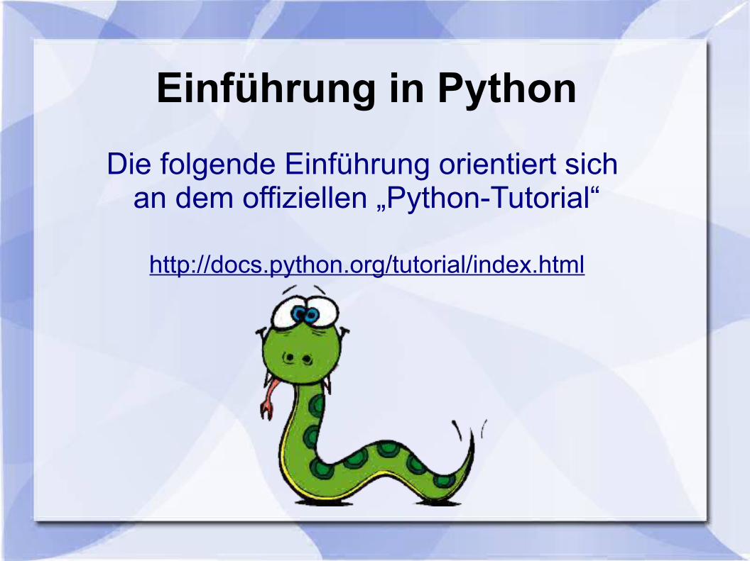
Einführung in Python
Die folgende Einführung orientiert sich an dem offiziellen „Python-Tutorial“
http://docs.python.org/tutorial/index.html
Python
„Python is an easy to learn, powerful programming language. It has efficient high-level data structures and a simple but effective approach to object-oriented programming. Python’s elegant syntax and dynamic typing, together with its interpreted nature, make it an ideal language for scripting and rapid application development in many areas on most platforms.“
„By the way, the language is named after the BBC show “Monty Python’s Flying Circus” and has nothing to do with reptiles.“
The Python Tutorial, Sep. 2010
Warum Python?
● Kein Schreib/Compile/Test-Zyklus!
● Vieles enthaltene Funktionalität vgl. mit traditionellen Skriptsprachen!
● Plattformunabhängig verfügbar!
● Frei erhältlich und gut dokumentiert!
● Unterstützt Kompaktheit und Lesbarkeit von Programmen
● In 10 Minuten erlernbar...
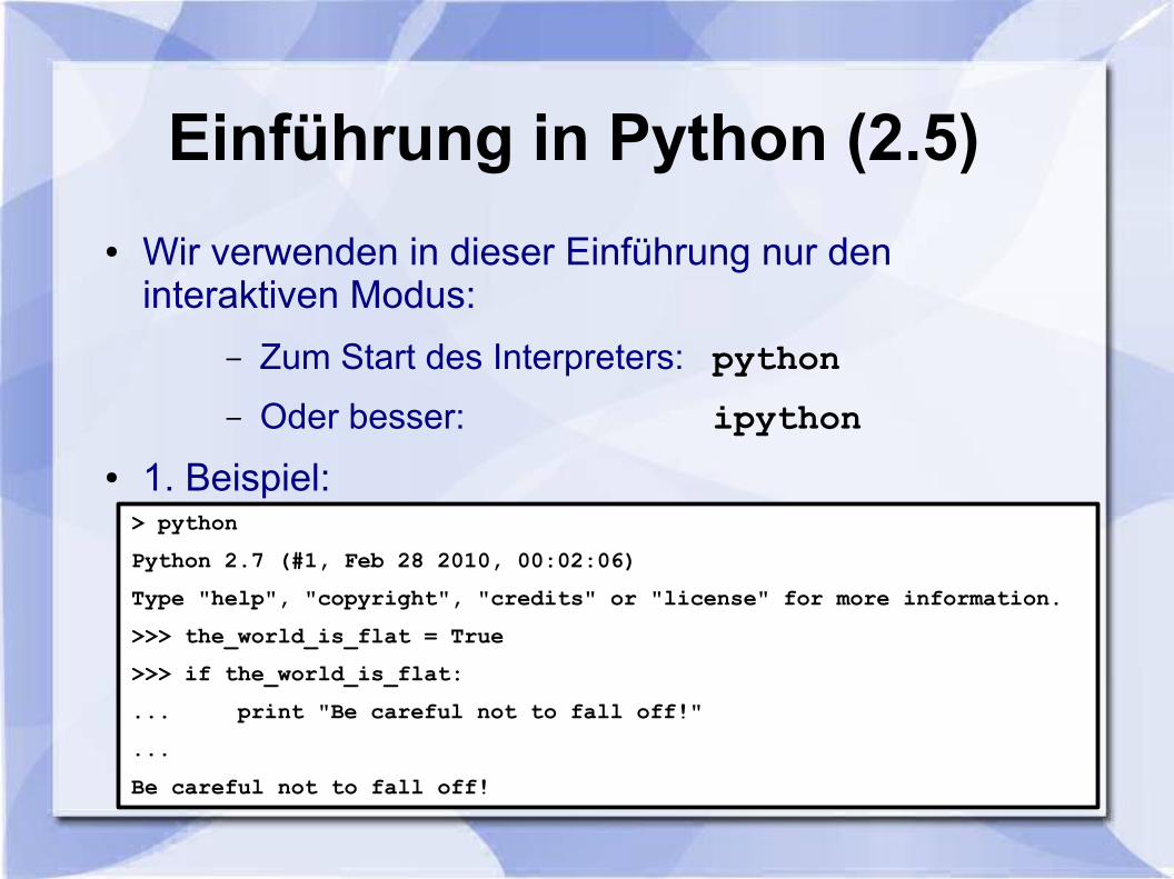
Einführung in Python (2.5)
● Wir verwenden in dieser Einführung nur den interaktiven Modus:
– Zum Start des Interpreters: python
– Oder besser: ipython
● 1. Beispiel:> python
Python 2.7 (#1, Feb 28 2010, 00:02:06)
Type "help", "copyright", "credits" or "license" for more information.
>>> the_world_is_flat = True
>>> if the_world_is_flat:
... print "Be careful not to fall off!"
...
Be careful not to fall off!
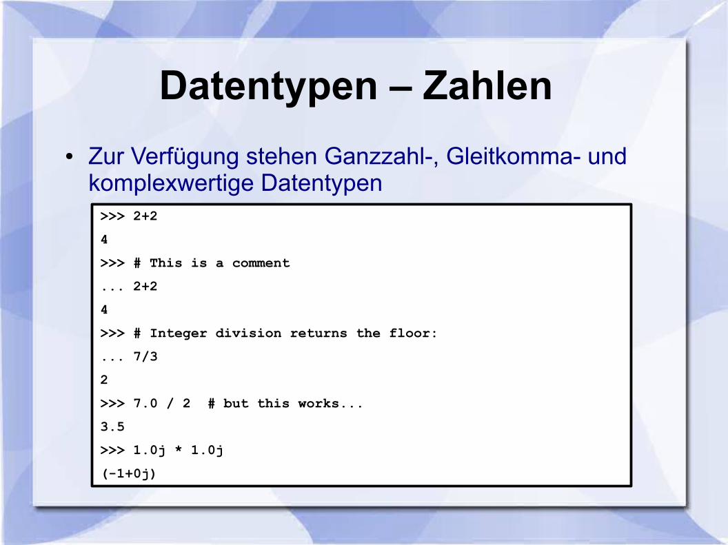
Datentypen – Zahlen
● Zur Verfügung stehen Ganzzahl-, Gleitkomma- und komplexwertige Datentypen>>> 2+2
4
>>> # This is a comment
... 2+2
4
>>> # Integer division returns the floor:
... 7/3
2
>>> 7.0 / 2 # but this works...
3.5
>>> 1.0j * 1.0j
(-1+0j)
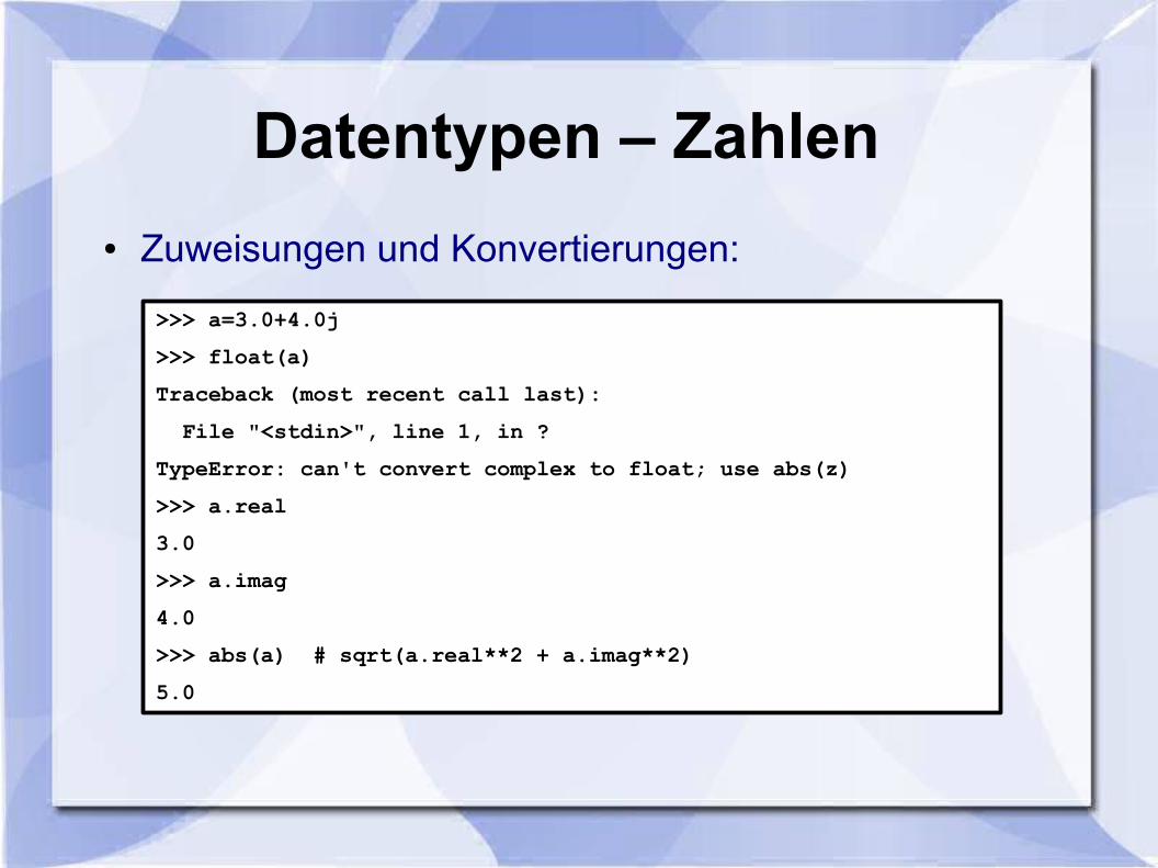
Datentypen – Zahlen
● Zuweisungen und Konvertierungen:
>>> a=3.0+4.0j
>>> float(a)
Traceback (most recent call last):
File "<stdin>", line 1, in ?
TypeError: can't convert complex to float; use abs(z)
>>> a.real
3.0
>>> a.imag
4.0
>>> abs(a) # sqrt(a.real**2 + a.imag**2)
5.0
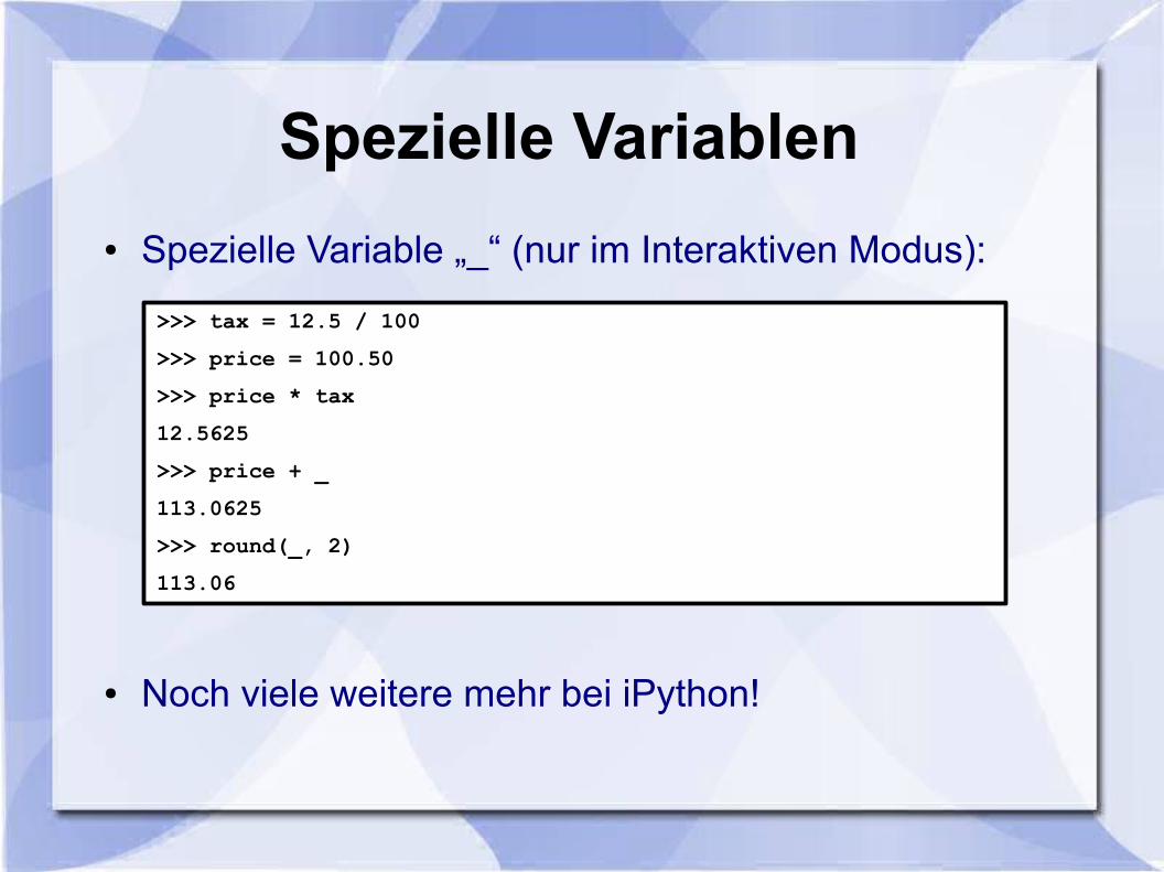
Spezielle Variablen
● Spezielle Variable „_“ (nur im Interaktiven Modus):
● Noch viele weitere mehr bei iPython!
>>> tax = 12.5 / 100
>>> price = 100.50
>>> price * tax
12.5625
>>> price + _
113.0625
>>> round(_, 2)
113.06
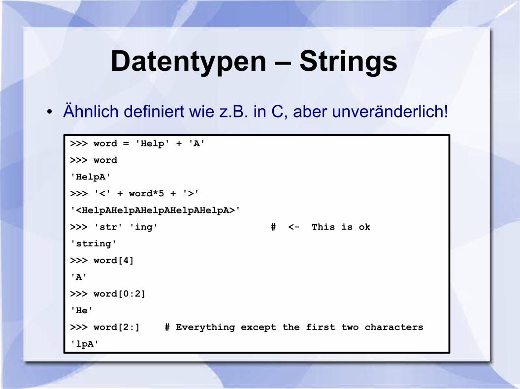
Datentypen – Strings
● Ähnlich definiert wie z.B. in C, aber unveränderlich!
>>> word = 'Help' + 'A'
>>> word
'HelpA'
>>> '<' + word*5 + '>'
'<HelpAHelpAHelpAHelpAHelpA>'
>>> 'str' 'ing' # <- This is ok
'string'
>>> word[4]
'A'
>>> word[0:2]
'He'
>>> word[2:] # Everything except the first two characters
'lpA'
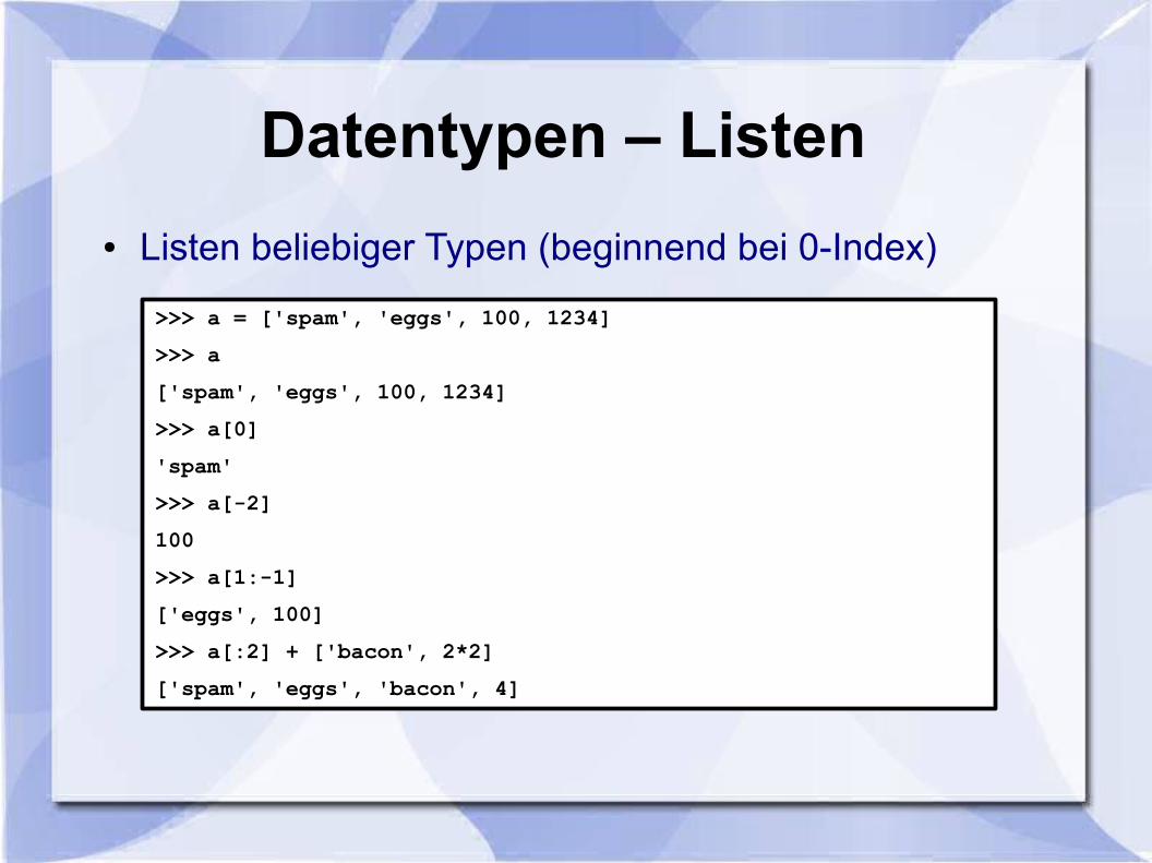
Datentypen – Listen
● Listen beliebiger Typen (beginnend bei 0-Index)
>>> a = ['spam', 'eggs', 100, 1234]
>>> a
['spam', 'eggs', 100, 1234]
>>> a[0]
'spam'
>>> a[-2]
100
>>> a[1:-1]
['eggs', 100]
>>> a[:2] + ['bacon', 2*2]
['spam', 'eggs', 'bacon', 4]
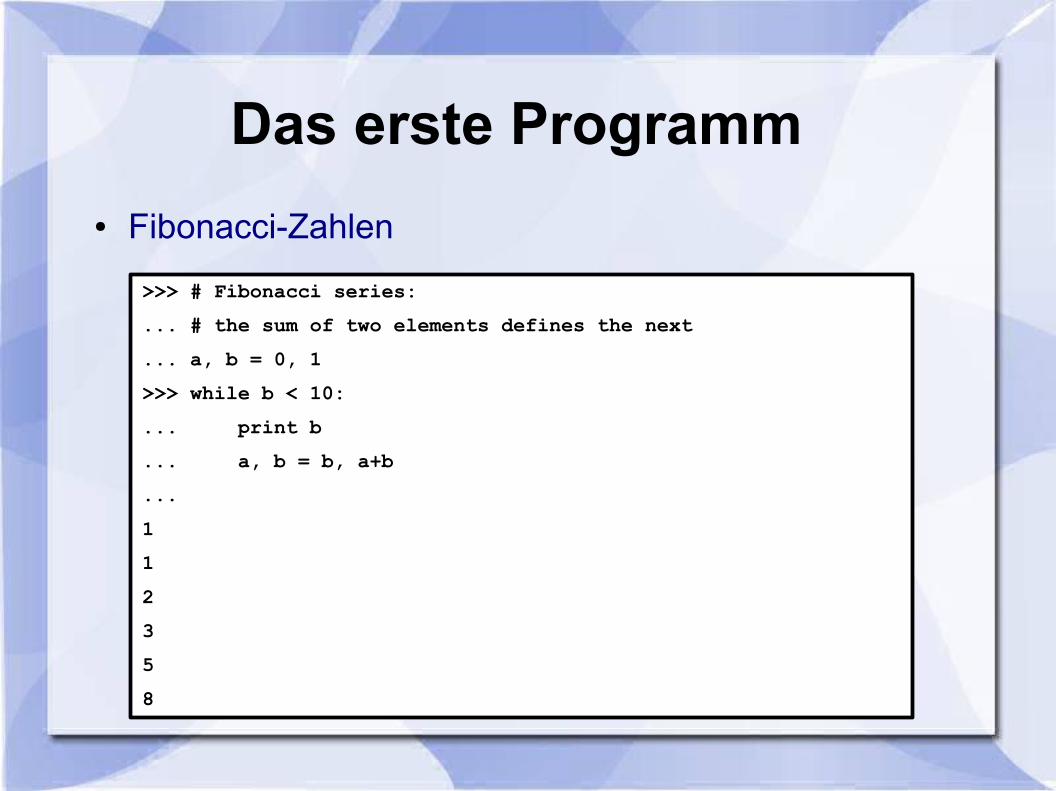
Das erste Programm
● Fibonacci-Zahlen
>>> # Fibonacci series:
... # the sum of two elements defines the next
... a, b = 0, 1
>>> while b < 10:
... print b
... a, b = b, a+b
...
1
1
2
3
5
8
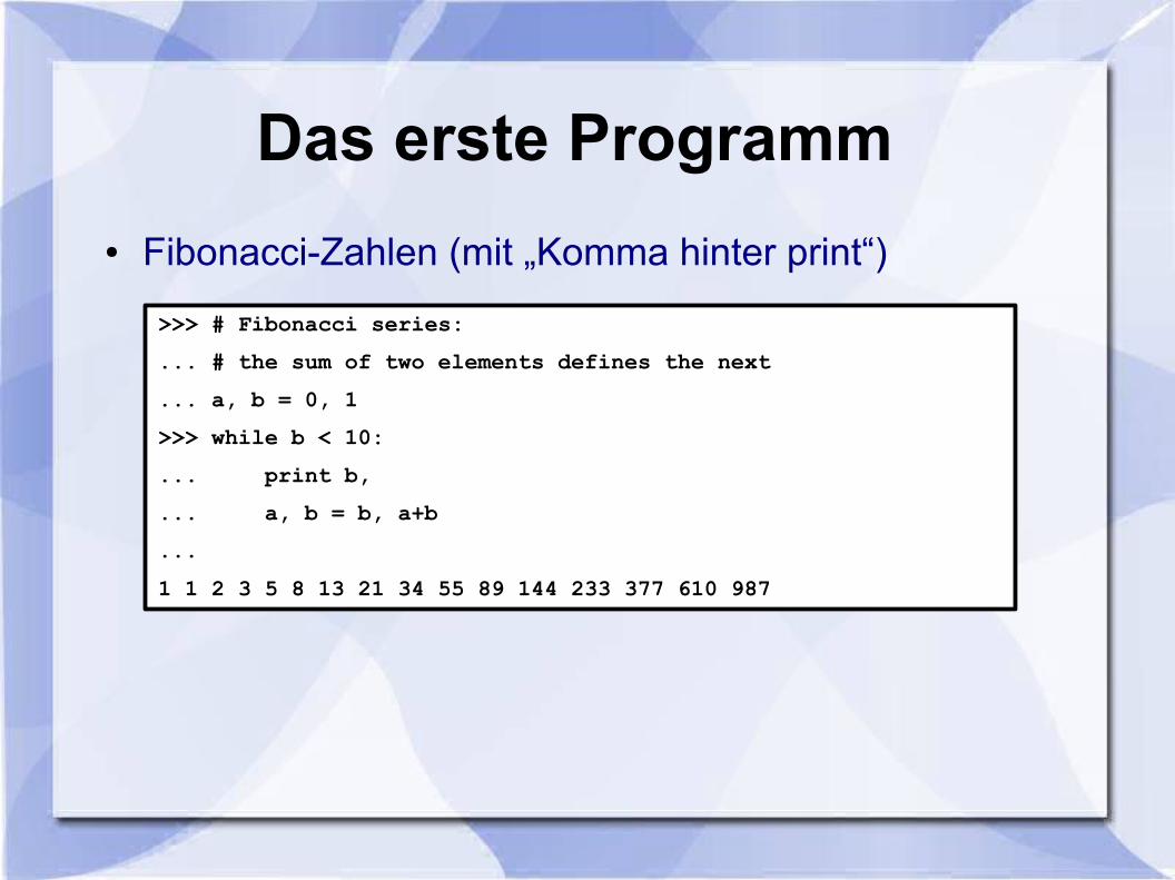
Das erste Programm
● Fibonacci-Zahlen (mit „Komma hinter print“)
>>> # Fibonacci series:
... # the sum of two elements defines the next
... a, b = 0, 1
>>> while b < 10:
... print b,
... a, b = b, a+b
...
1 1 2 3 5 8 13 21 34 55 89 144 233 377 610 987
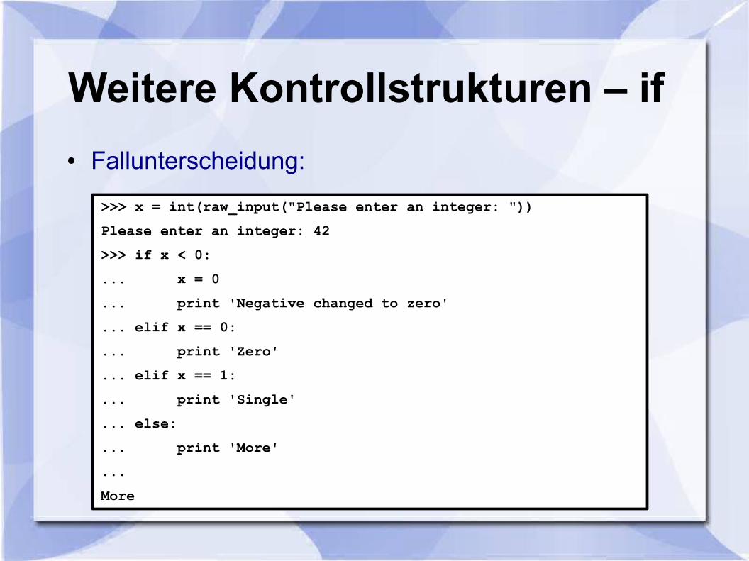
Weitere Kontrollstrukturen – if
● Fallunterscheidung:
>>> x = int(raw_input("Please enter an integer: "))
Please enter an integer: 42
>>> if x < 0:
... x = 0
... print 'Negative changed to zero'
... elif x == 0:
... print 'Zero'
... elif x == 1:
... print 'Single'
... else:
... print 'More'
...
More
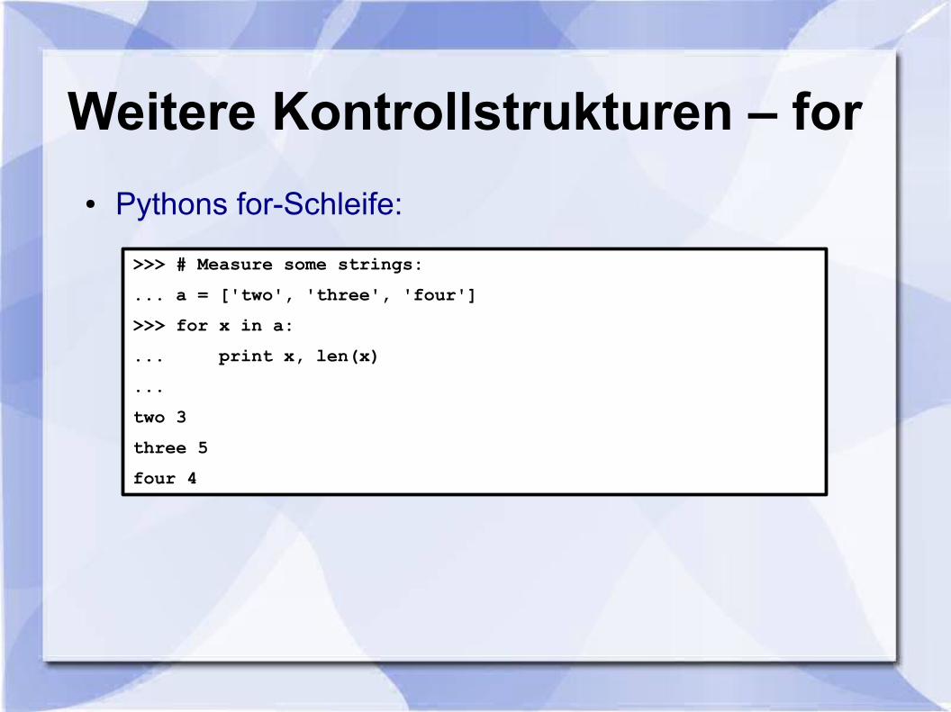
Weitere Kontrollstrukturen – for
● Pythons for-Schleife:
>>> # Measure some strings:
... a = ['two', 'three', 'four']
>>> for x in a:
... print x, len(x)
...
two 3
three 5
four 4
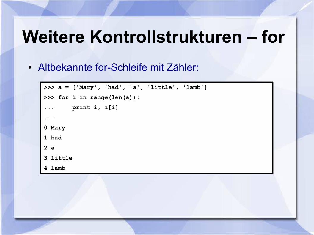
Weitere Kontrollstrukturen – for
● Altbekannte for-Schleife mit Zähler:
>>> a = ['Mary', 'had', 'a', 'little', 'lamb']
>>> for i in range(len(a)):
... print i, a[i]
...
0 Mary
1 had
2 a
3 little
4 lamb
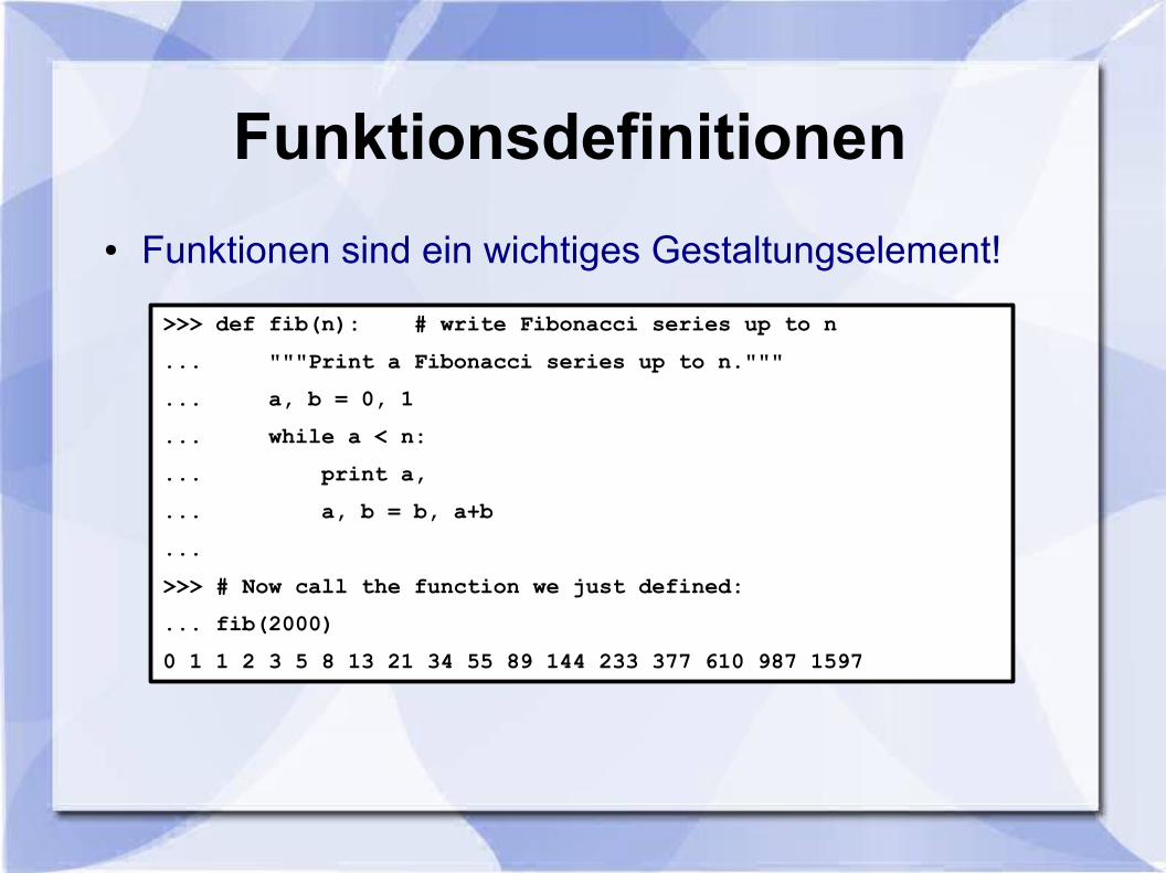
Funktionsdefinitionen
● Funktionen sind ein wichtiges Gestaltungselement!
>>> def fib(n): # write Fibonacci series up to n
... """Print a Fibonacci series up to n."""
... a, b = 0, 1
... while a < n:
... print a,
... a, b = b, a+b
...
>>> # Now call the function we just defined:
... fib(2000)
0 1 1 2 3 5 8 13 21 34 55 89 144 233 377 610 987 1597
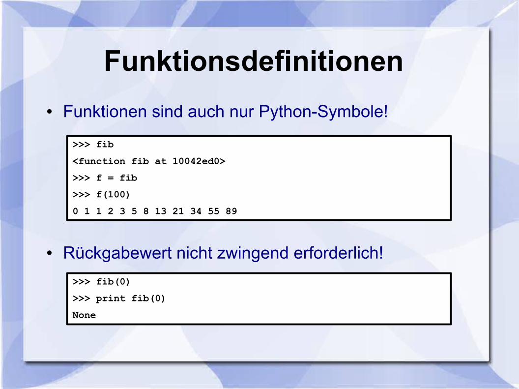
Funktionsdefinitionen
● Funktionen sind auch nur Python-Symbole!
● Rückgabewert nicht zwingend erforderlich!
>>> fib
<function fib at 10042ed0>
>>> f = fib
>>> f(100)
0 1 1 2 3 5 8 13 21 34 55 89
>>> fib(0)
>>> print fib(0)
None
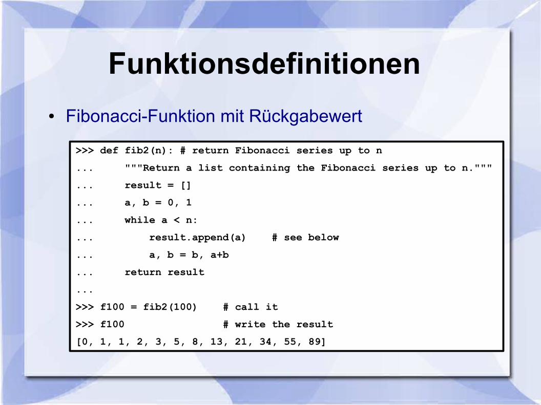
Funktionsdefinitionen
● Fibonacci-Funktion mit Rückgabewert
>>> def fib2(n): # return Fibonacci series up to n
... """Return a list containing the Fibonacci series up to n."""
... result = []
... a, b = 0, 1
... while a < n:
... result.append(a) # see below
... a, b = b, a+b
... return result
...
>>> f100 = fib2(100) # call it
>>> f100 # write the result
[0, 1, 1, 2, 3, 5, 8, 13, 21, 34, 55, 89]
Funktionsdefinitionen
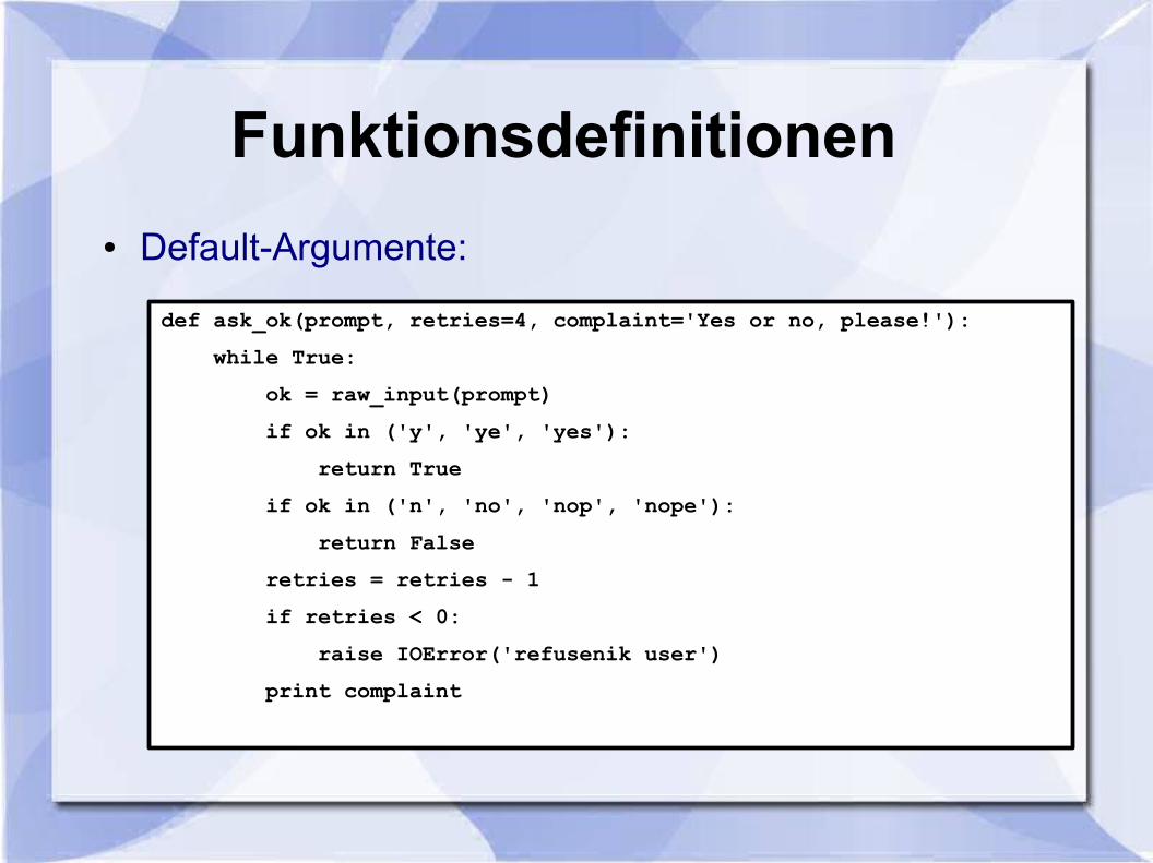
● Default-Argumente:
def ask_ok(prompt, retries=4, complaint='Yes or no, please!'):
while True:
ok = raw_input(prompt)
if ok in ('y', 'ye', 'yes'):
return True
if ok in ('n', 'no', 'nop', 'nope'):
return False
retries = retries - 1
if retries < 0:
raise IOError('refusenik user')
print complaint
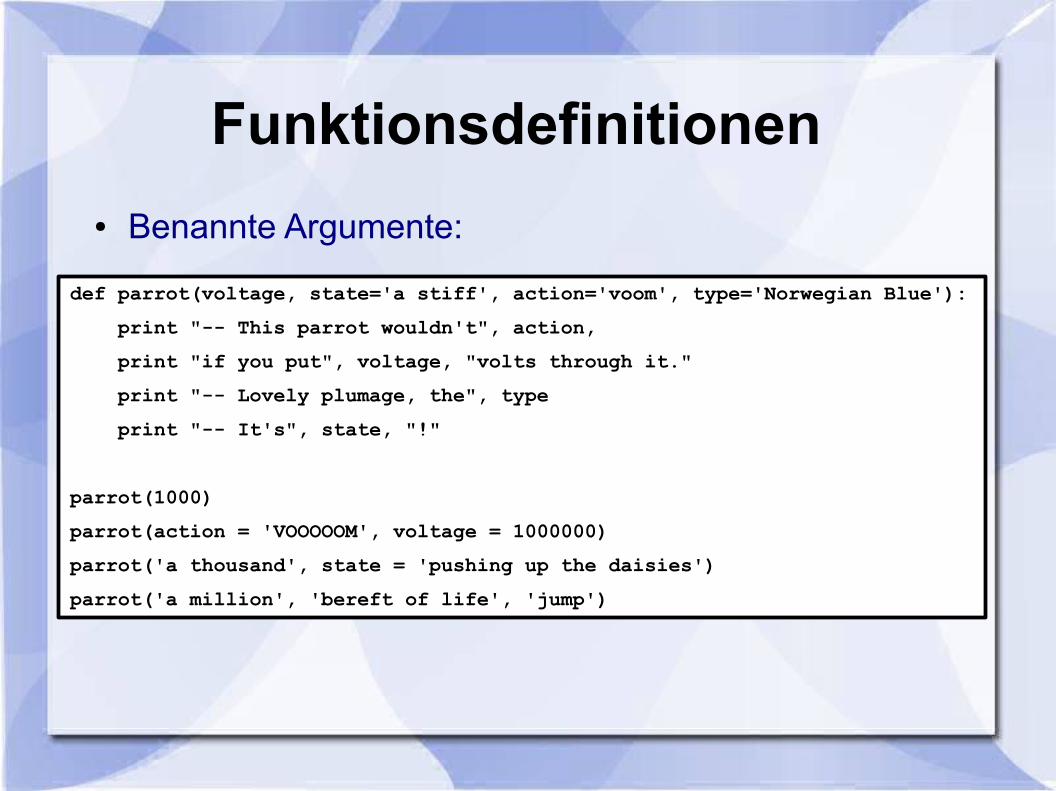
Funktionsdefinitionen
● Benannte Argumente:
def parrot(voltage, state='a stiff', action='voom', type='Norwegian Blue'):
print "-- This parrot wouldn't", action,
print "if you put", voltage, "volts through it."
print "-- Lovely plumage, the", type
print "-- It's", state, "!"
parrot(1000)
parrot(action = 'VOOOOOM', voltage = 1000000)
parrot('a thousand', state = 'pushing up the daisies')
parrot('a million', 'bereft of life', 'jump')
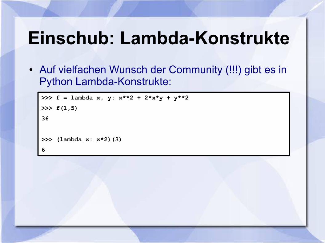
Einschub: Lambda-Konstrukte
● Auf vielfachen Wunsch der Community (!!!) gibt es in Python Lambda-Konstrukte:>>> f = lambda x, y: x**2 + 2*x*y + y**2
>>> f(1,5)
36
>>> (lambda x: x*2)(3)
6
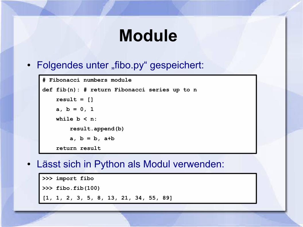
Module
● Folgendes unter „fibo.py“ gespeichert:
● Lässt sich in Python als Modul verwenden:
# Fibonacci numbers module
def fib(n): # return Fibonacci series up to n
result = []
a, b = 0, 1
while b < n:
result.append(b)
a, b = b, a+b
return result
>>> import fibo
>>> fibo.fib(100)
[1, 1, 2, 3, 5, 8, 13, 21, 34, 55, 89]
Python Resümee
● Python lernt man am besten:
… durch praktische Arbeit mit der Sprache!
… nicht durch Präsentationen!
● Viel, viel mehr, als hier heute vorgestellt!(z.B: Klassen, Fehler, IO, XML, GUI, Netzwerk …)
● Hoffentlich aus den Folien zu sehen:
– Schneller Einstieg
– Steile Lernkurve
– Frühe und wertvolle Erfolgserlebnisse!
● Daher: Zurzeit sehr populäre Sprache!
Inhalt
● Einleitung
● Einführung in Python
● Einführung in die Python Imaging Library (PIL)
● Von PIL zu NumPy / SciPy
● Zusammenfassung
Einführung in PIL
Die folgende Einführung orientiert sich andem offiziellen „PIL Handbook v1.1.5“.
http://www.pythonware.com/library/pil/handbook
Bildverarbeitung mit PIL
„The Python Imaging Library adds image processing capabilities to your Python interpreter.“
„The core image library is designed for fast access to data stored in a few basic pixel formats. It should provide a solid foundation for a general image processing tool.“
PIL Handbook 2010
● Einige Vorteile
– Unterstützt viele Bildformate für Im- und Export
– Effiziente interne Bildrepräsentation
– Grundlegende Bildverarbeitungs-Algorithmen sind bereits enthalten
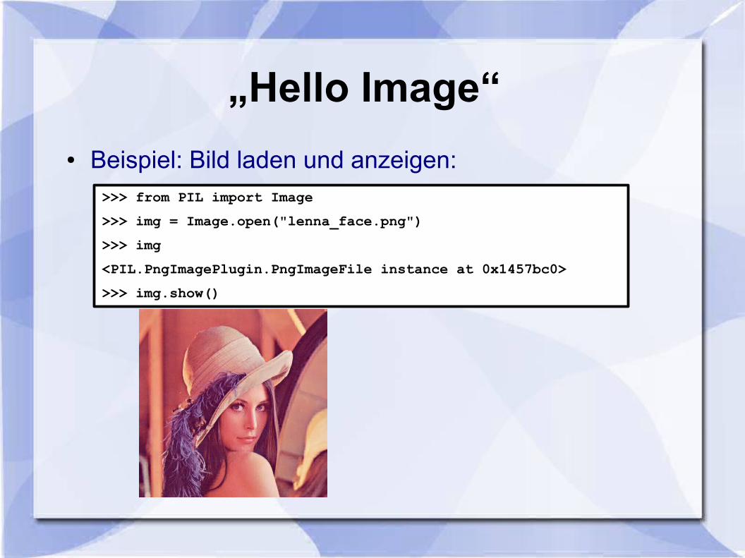
„Hello Image“
● Beispiel: Bild laden und anzeigen:>>> from PIL import Image
>>> img = Image.open("lenna_face.png")
>>> img
<PIL.PngImagePlugin.PngImageFile instance at 0x1457bc0>
>>> img.show()
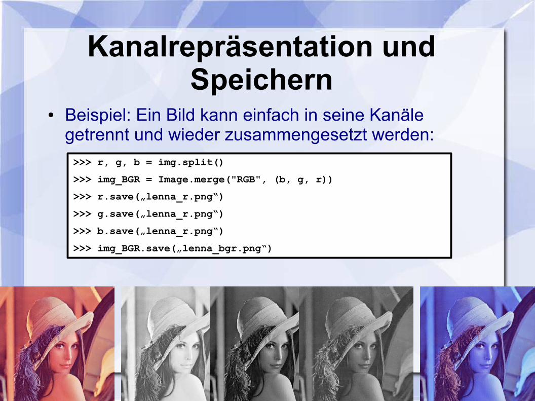
Kanalrepräsentation und Speichern
● Beispiel: Ein Bild kann einfach in seine Kanäle getrennt und wieder zusammengesetzt werden:
>>> r, g, b = img.split()
>>> img_BGR = Image.merge("RGB", (b, g, r))
>>> r.save(„lenna_r.png“)
>>> g.save(„lenna_r.png“)
>>> b.save(„lenna_r.png“)
>>> img_BGR.save(„lenna_bgr.png“)
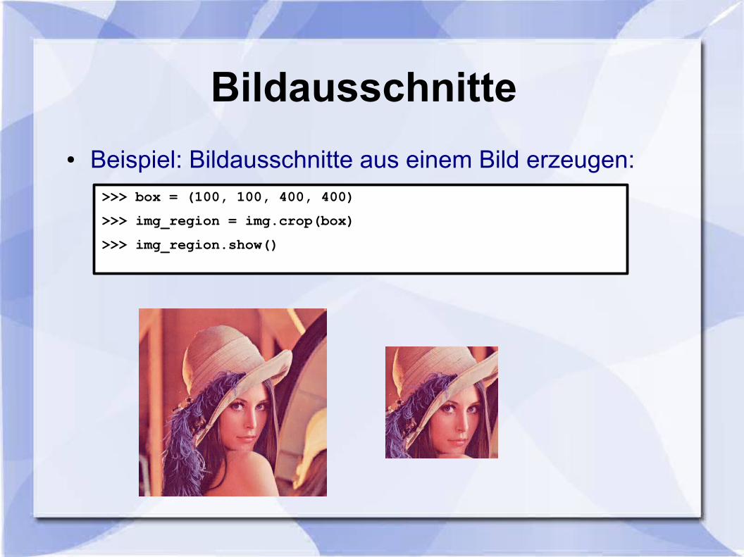
Bildausschnitte
● Beispiel: Bildausschnitte aus einem Bild erzeugen:>>> box = (100, 100, 400, 400)
>>> img_region = img.crop(box)
>>> img_region.show()
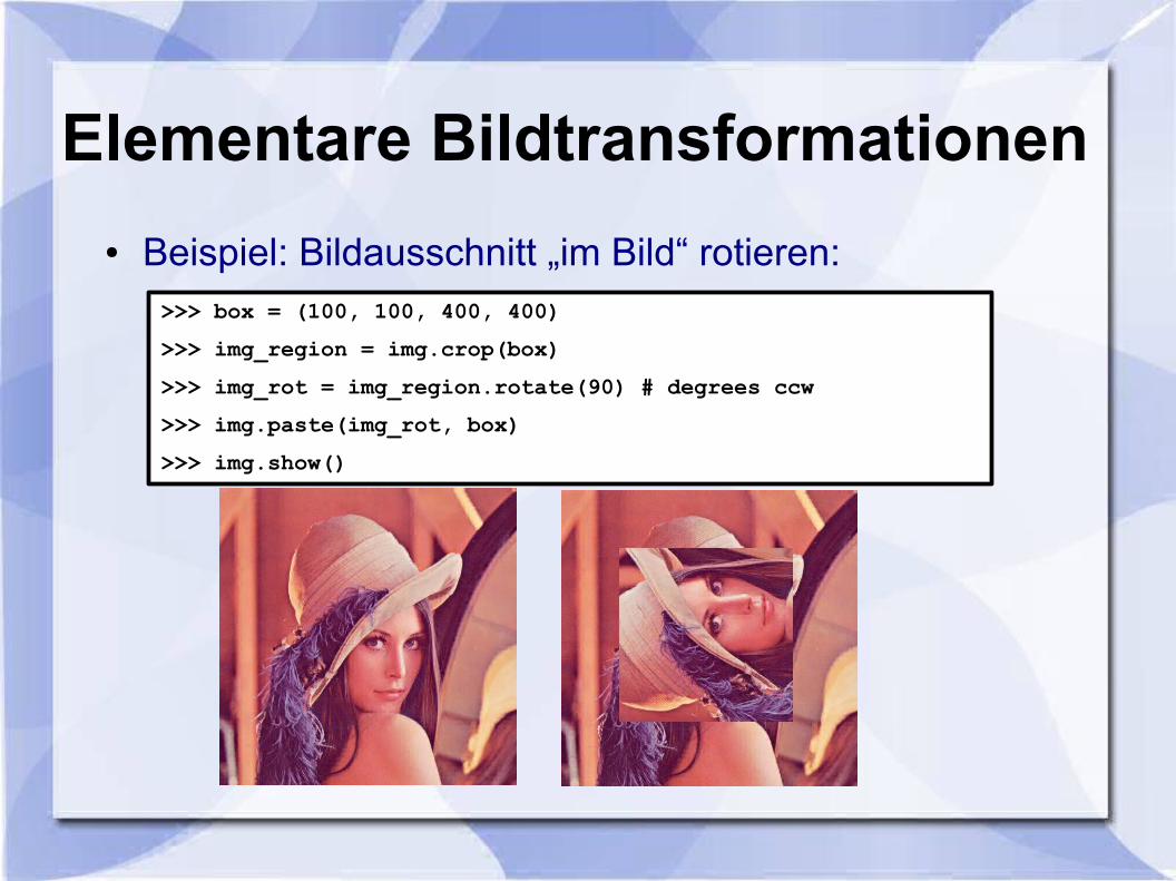
Elementare Bildtransformationen
● Beispiel: Bildausschnitt „im Bild“ rotieren:>>> box = (100, 100, 400, 400)
>>> img_region = img.crop(box)
>>> img_rot = img_region.rotate(90) # degrees ccw
>>> img.paste(img_rot, box)
>>> img.show()
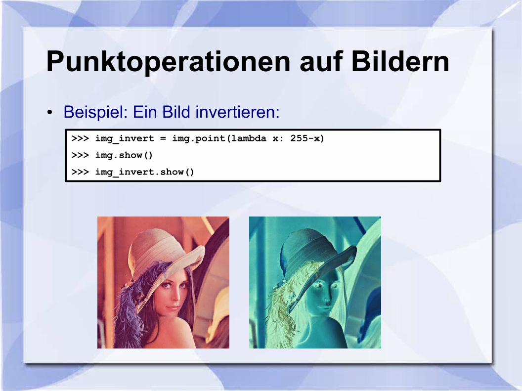
Punktoperationen auf Bildern
● Beispiel: Ein Bild invertieren:>>> img_invert = img.point(lambda x: 255-x)
>>> img.show()
>>> img_invert.show()
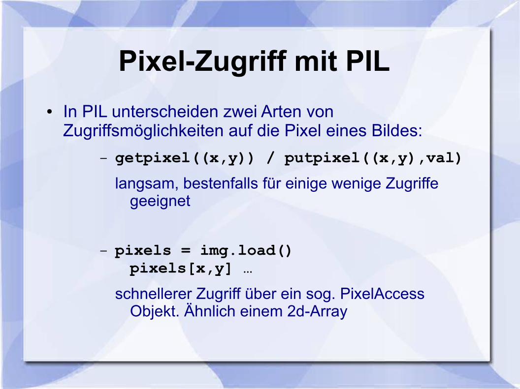
Pixel-Zugriff mit PIL
● In PIL unterscheiden zwei Arten von Zugriffsmöglichkeiten auf die Pixel eines Bildes:
– getpixel((x,y)) / putpixel((x,y),val)
langsam, bestenfalls für einige wenige Zugriffe geeignet
– pixels = img.load()pixels[x,y] …
schnellerer Zugriff über ein sog. PixelAccess Objekt. Ähnlich einem 2d-Array
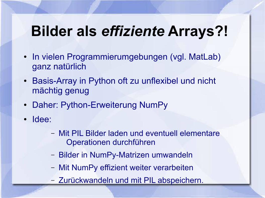
Bilder als effiziente Arrays?!
● In vielen Programmierumgebungen (vgl. MatLab) ganz natürlich
● Basis-Array in Python oft zu unflexibel und nicht mächtig genug
● Daher: Python-Erweiterung NumPy
● Idee:
– Mit PIL Bilder laden und eventuell elementare Operationen durchführen
– Bilder in NumPy-Matrizen umwandeln
– Mit NumPy effizient weiter verarbeiten
– Zurückwandeln und mit PIL abspeichern.
Inhalt
● Einleitung
● Einführung in Python
● Einführung in die Python Imaging Library (PIL)
● Von PIL zu NumPy / SciPy
● Zusammenfassung
Einführung in NumPy
Im Rahmen dieses Vortrags ist es leider nicht möglich, eine umfassende Einführung in NumPy zu geben.
Daher sei auf folgende Seiten verwiesen:
Homepage
http://numpy.scipy.org
Tutorial
http://www.scipy.org/Tentative_NumPy_Tutorial
NumPy kurz und knapp
„NumPy is the fundamental package needed for scientific computing with Python. It contains among other things:a powerful N-dimensional array object […]“
NumPy Homepage, 2010
● Bräuchte alleine schon mindestens eine Vorlesung!
● Wachsende Nutzergemeinschaft (SciPy/NumPy)
● Verlässliche Algorithmen
● Ähnlich schnelle Implementationen wie kommerzielle Software
Von PIL zu NumPy (und zurück)
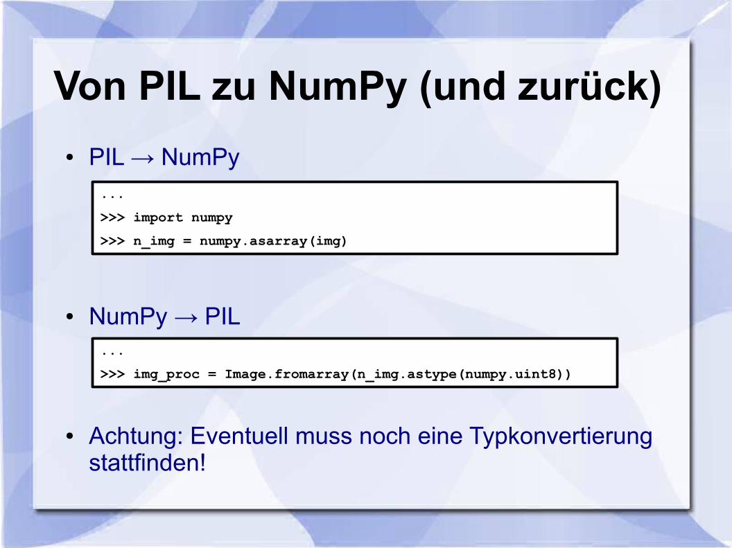
● PIL → NumPy
● NumPy → PIL
● Achtung: Eventuell muss noch eine Typkonvertierung stattfinden!
...
>>> import numpy
>>> n_img = numpy.asarray(img)
...
>>> img_proc = Image.fromarray(n_img.astype(numpy.uint8))
NumPy Bildrepräsentation
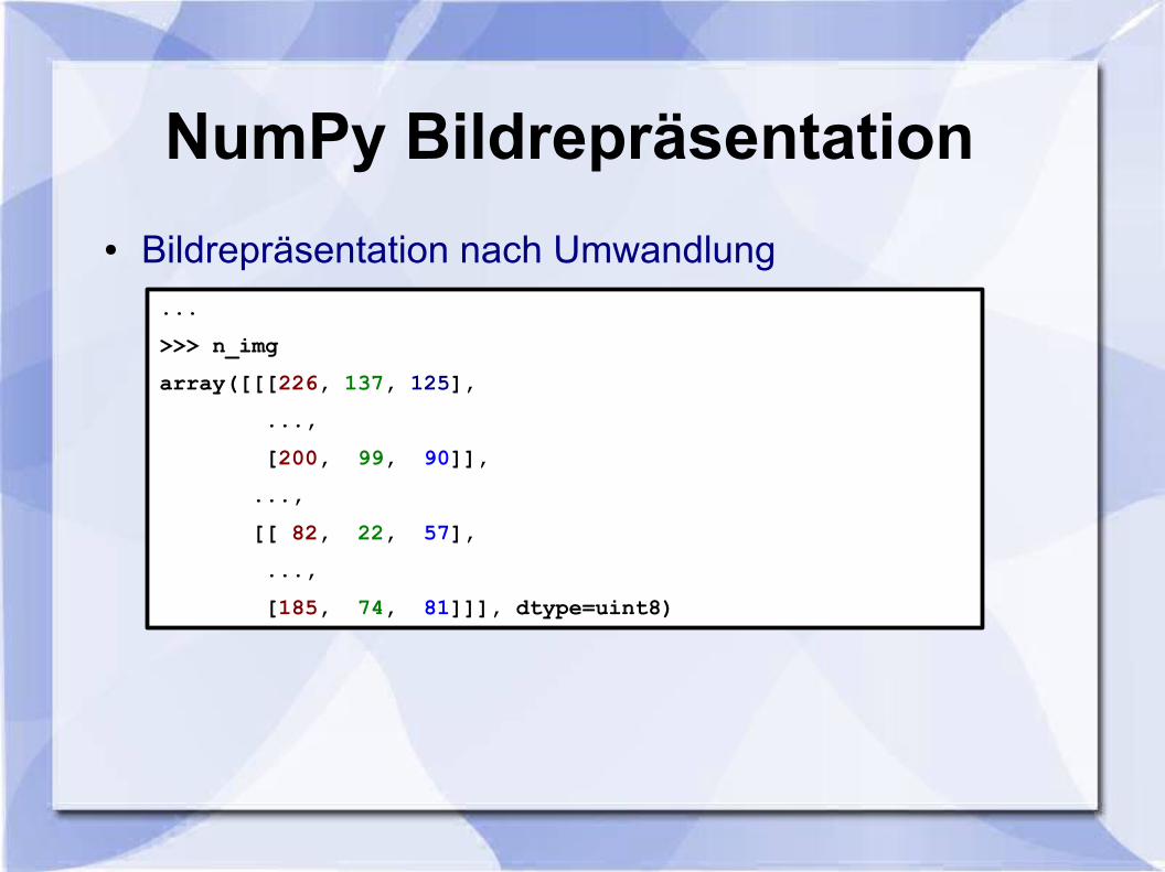
● Bildrepräsentation nach Umwandlung...
>>> n_img
array([[[226, 137, 125],
...,
[200, 99, 90]],
...,
[[ 82, 22, 57],
...,
[185, 74, 81]]], dtype=uint8)
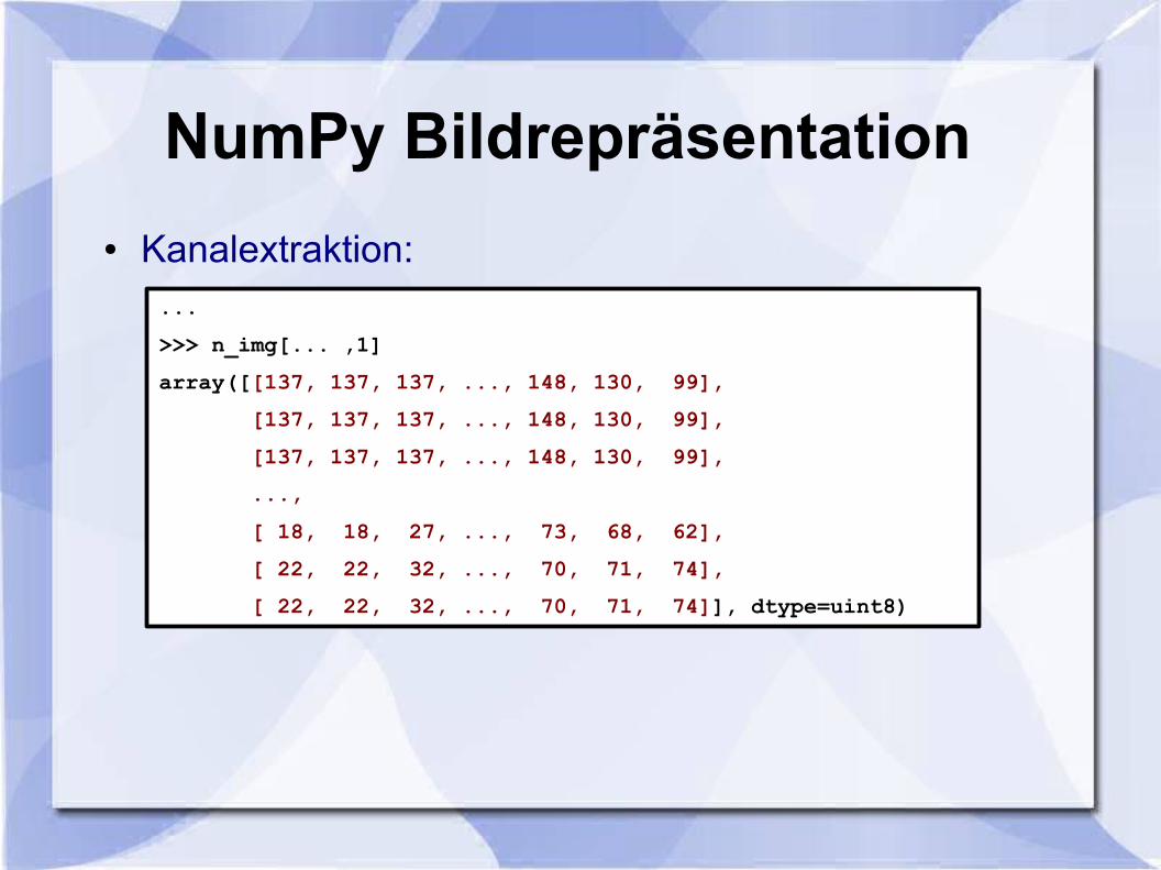
NumPy Bildrepräsentation
● Kanalextraktion:...
>>> n_img[... ,1]
array([[137, 137, 137, ..., 148, 130, 99],
[137, 137, 137, ..., 148, 130, 99],
[137, 137, 137, ..., 148, 130, 99],
...,
[ 18, 18, 27, ..., 73, 68, 62],
[ 22, 22, 32, ..., 70, 71, 74],
[ 22, 22, 32, ..., 70, 71, 74]], dtype=uint8)
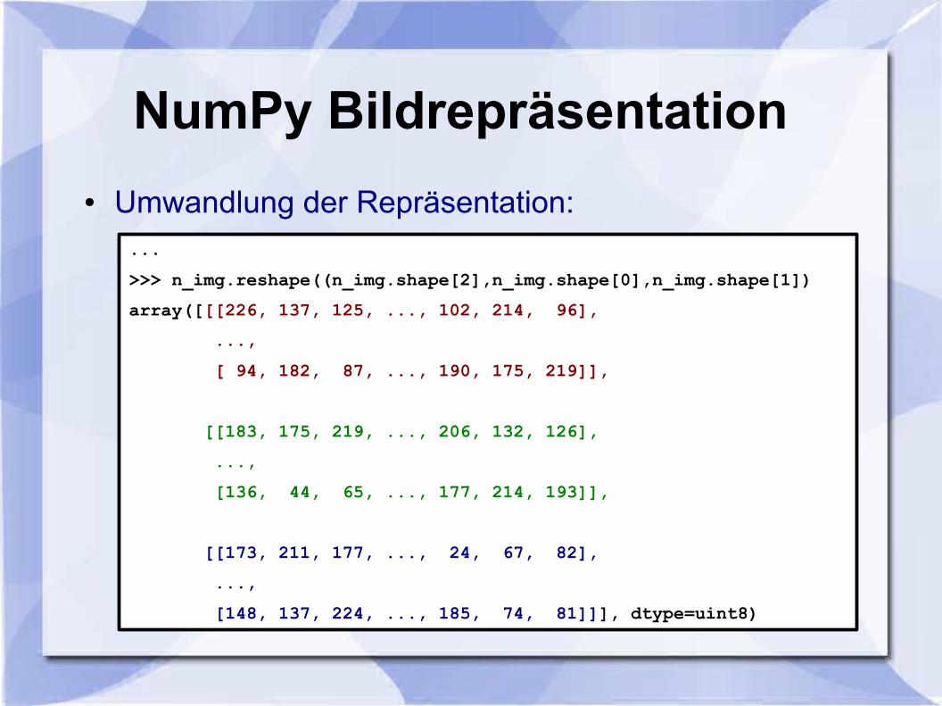
NumPy Bildrepräsentation
● Umwandlung der Repräsentation:...
>>> n_img.reshape((n_img.shape[2],n_img.shape[0],n_img.shape[1])
array([[[226, 137, 125, ..., 102, 214, 96],
...,
[ 94, 182, 87, ..., 190, 175, 219]],
[[183, 175, 219, ..., 206, 132, 126],
...,
[136, 44, 65, ..., 177, 214, 193]],
[[173, 211, 177, ..., 24, 67, 82],
...,
[148, 137, 224, ..., 185, 74, 81]]], dtype=uint8)
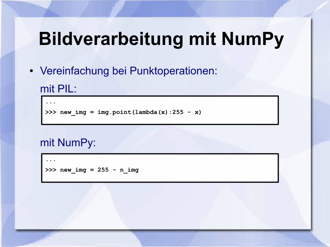
Bildverarbeitung mit NumPy
● Vereinfachung bei Punktoperationen:
mit PIL:
mit NumPy:
...
>>> new_img = img.point(lambda(x):255 - x)
...
>>> new_img = 255 - n_img
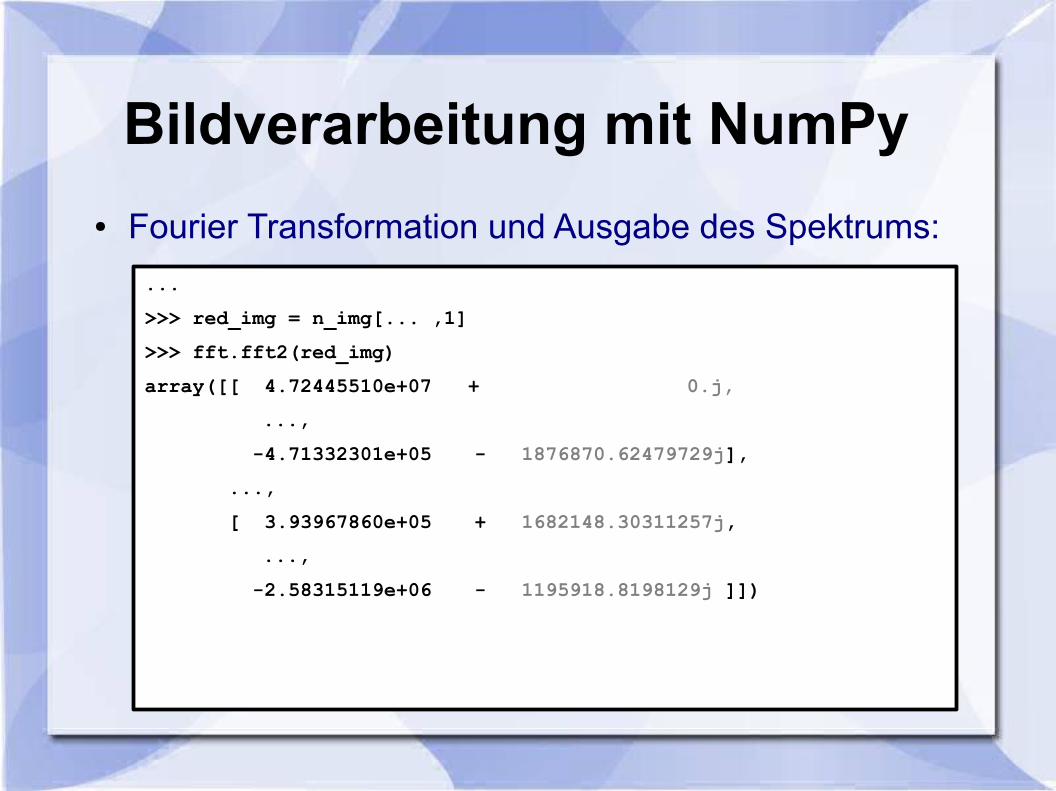
Bildverarbeitung mit NumPy
● Fourier Transformation und Ausgabe des Spektrums:
...
>>> red_img = n_img[... ,1]
>>> fft.fft2(red_img)
array([[ 4.72445510e+07 + 0.j,
...,
-4.71332301e+05 - 1876870.62479729j],
...,
[ 3.93967860e+05 + 1682148.30311257j,
...,
-2.58315119e+06 - 1195918.8198129j ]])
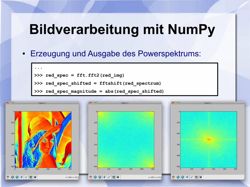
Bildverarbeitung mit NumPy
● Erzeugung und Ausgabe des Powerspektrums:
...
>>> red_spec = fft.fft2(red_img)
>>> red_spec_shifted = fftshift(red_spectrum)
>>> red_spec_magnitude = abs(red_spec_shifted)
Bildverarbeitung: SciPy/NumPy
● Viele vorgefertigte Funktionen, wie z.B. Filter und Fourier-Transformation
● Einfache Geschwindigkeitsoptimierung durch hervorragende C-Schnittstelle
● Auch für die Bildverarbeitung sinnvolle Features wie z.B. maskierte Arrays
● Nahezu alles, was man sich an numerischen Operationen wünschen kann...
● Zusätzliche Anbindung von Matplotlib zur Visualisierung leicht möglich (siehe FFT)
Inhalt
● Einleitung
● Einführung in Python
● Einführung in die Python Imaging Library (PIL)
● Von PIL zu NumPy / SciPy
● Zusammenfassung
Zusammenfassung I
● Python als Programmiersprache
– Verständliche Syntax
– Sehr mächtig
– Steile Lernkurve
– bestens geeignet für interaktives Arbeiten
– Einfach erweiterbar
– Große Community
Zusammenfassung II
● Python Imaging Library (PIL)
– Fügt elementare Bildverarbeitung hinzu
– Hier vor allem gezeigt: Import & Export
– Recht intuitiver Umgang mit Bildern
● NumPy/SciPy
– Effizientes Arbeiten mit Python
– Einfache Schnittstelle zur PIL
– Sehr mächtig
– Wird kontinuierlich erweitert

Vielen Dank für die Aufmerksamkeit!
Zeit für Fragen, Diskussion etc.


![Python - DESY · Python-Grundlagen moderne Hochsprache unterstützt Skripting (Prozeduren u. ... SciPy I - Statistik Modul In [1]: from scipy import * In [2]: f = stats.poisson ...](https://static.fdokument.com/doc/165x107/5ae89aba7f8b9acc26905b38/python-desy-moderne-hochsprache-untersttzt-skripting-prozeduren-u-scipy.jpg)