Bivariate Lorenz curves: a review of recent proposals
24
Bivariate Lorenz curves Bivariate Lorenz curves: a review of recent proposals Sarabia, Jos´ e Mar´ ıa ([email protected]) Departamento de Econom´ ıa, Universidad de Cantabria Avda. de los Castros s/n, 39005 Santander, Spain Jord´ a, Vanesa ([email protected]) Departamento de Econom´ ıa, Universidad de Cantabria Avda. de los Castros s/n, 39005 Santander, Spain RESUMEN La extensi´ on de la curva de Lorenz al caso bidimensional y a dimensiones superiores a dos no es un problema trivial. Existen en la literatura tres propuestas de curvas de Lorenz bidimensionales. La primera de estas definiciones fue propuesta por Taguchi (1972a,b). A continuaci´ on Arnold (1983) estableci´ o una segunda definici´on, que es una extensi´ on natural de la curva de concentraci´ on. Esta definici´ on no ha recibido mucha atenci´ on en la literatura econ´omica. Finalmente, Koshevoy y Mosler (1996) introdujeron la tercera de las definiciones, haciendo uso del concepto de zonoide. Recientemente, Sarabia y Jord´ a (2013, 2014) han propuesto varias clases param´ etricas de curvas de Lorenz bivariadas haciendo uso de la definici´on de Arnold. En el presente trabajo se revisan estas tres definiciones. Se estudia el origen de cada una de ellas, as´ ı como sus principales propiedades. Para el caso de la curva de Arnold, se presentan algunas formas param´ etricas propuestas para el caso bidimensional, con diferentes estructuras de dependencia y diferentes tipos de marginales. El trabajo termina comentando las extensiones de estas familias a dimensiones superiores a dos, y sus aplicaciones al estudio del bienestar considerando de forma conjunta varios atributos. XXII Jornadas de ASEPUMA y X Encuentro Internacional Anales de ASEPUMA n 22:1510 1
Transcript of Bivariate Lorenz curves: a review of recent proposals
Bivariate Lorenz curves
Bivariate Lorenz curves: a review of
recent proposals
Sarabia, Jose Marıa ([email protected])
Departamento de Economıa, Universidad de Cantabria
Avda. de los Castros s/n, 39005 Santander, Spain
Jorda, Vanesa ([email protected])
Departamento de Economıa, Universidad de Cantabria
Avda. de los Castros s/n, 39005 Santander, Spain
RESUMEN
La extension de la curva de Lorenz al caso bidimensional y a dimensiones superiores a
dos no es un problema trivial. Existen en la literatura tres propuestas de curvas de Lorenz
bidimensionales. La primera de estas definiciones fue propuesta por Taguchi (1972a,b).
A continuacion Arnold (1983) establecio una segunda definicion, que es una extension
natural de la curva de concentracion. Esta definicion no ha recibido mucha atencion en la
literatura economica. Finalmente, Koshevoy y Mosler (1996) introdujeron la tercera de las
definiciones, haciendo uso del concepto de zonoide. Recientemente, Sarabia y Jorda (2013,
2014) han propuesto varias clases parametricas de curvas de Lorenz bivariadas haciendo
uso de la definicion de Arnold.
En el presente trabajo se revisan estas tres definiciones. Se estudia el origen de
cada una de ellas, ası como sus principales propiedades. Para el caso de la curva de
Arnold, se presentan algunas formas parametricas propuestas para el caso bidimensional,
con diferentes estructuras de dependencia y diferentes tipos de marginales. El trabajo
termina comentando las extensiones de estas familias a dimensiones superiores a dos, y
sus aplicaciones al estudio del bienestar considerando de forma conjunta varios atributos.
XXII Jornadas de ASEPUMA y X Encuentro InternacionalAnales de ASEPUMA n 22:1510
1
Sarabia, Jose Marıa; Jorda, Vanesa
Palabras clave: curvas de Lorenz bivariadas, distribucion de Sarmanov-Lee, ındice de
Gini bivariado, dominacion estocastica, indicadores de bienestar.
Area tematica: Aspectos cuantitativos de problemas economicos y empresariales.
XXII Jornadas de ASEPUMA y X Encuentro InternacionalAnales de ASEPUMA n 22:1510
2
Bivariate Lorenz curves
ABSTRACT
The extension of the Lorenz curve to the bidimensional case and dimensions
higher than two is not trivial. Three different proposals can be found in the liter-
ature. The first definition was proposed by Taguchi (1972a,b). Thereafter, Arnold
(1983) developed a second definition which was a natural extension of the concentra-
tion curve. This proposal has not received much attention in the economic literature.
Finally, Koshevoy and Mosler (1996) introduced the third definition using the con-
cept of Lorenz Zonoid. Recently, Sarabia and Jorda (2013, 2014) proposed a number
of parametric classes of bivariate Lorenz curves based on the Arnold’s definition.
In this paper, the three existing definitions are revisited. We investigate their
origin as well as the main properties of each of them. In the case of the Arnold’s
definition, some parametric forms are presented for the bivariate case with different
dependence structures and different marginals. We finish this work by examining
briefly the extension of these families to dimensions higher than two and describing
their applications to well-being data when several attributes are jointly considered.
1 INTRODUCTION
In the last years, there is an increasing concern about the poor performance of
GDP per capita as an indicator of well-being. In this sense, quality of life is seen
as a multidimensional process which involves more than just economic aspects. The
discontent with the hegemony of income for measuring human well-being has led to
several attempts to develop a more comprehensive indicator using a multiattribute
framework (see Gadrey and Jany-Catrice (2006) for a review).
It is worth nothing that we should account for two types of inequality in a mul-
tidimensional context. On the one hand, disparities within each dimension have to
be assessed as in the unidimensional case. The second type of inequality is related
XXII Jornadas de ASEPUMA y X Encuentro InternacionalAnales de ASEPUMA n 22:1510
3
Sarabia, Jose Marıa; Jorda, Vanesa
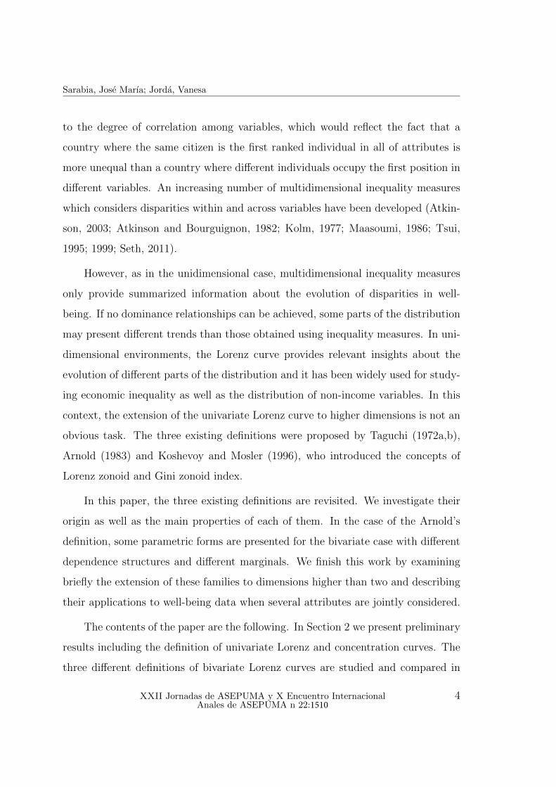
to the degree of correlation among variables, which would reflect the fact that a
country where the same citizen is the first ranked individual in all of attributes is
more unequal than a country where different individuals occupy the first position in
different variables. An increasing number of multidimensional inequality measures
which considers disparities within and across variables have been developed (Atkin-
son, 2003; Atkinson and Bourguignon, 1982; Kolm, 1977; Maasoumi, 1986; Tsui,
1995; 1999; Seth, 2011).
However, as in the unidimensional case, multidimensional inequality measures
only provide summarized information about the evolution of disparities in well-
being. If no dominance relationships can be achieved, some parts of the distribution
may present different trends than those obtained using inequality measures. In uni-
dimensional environments, the Lorenz curve provides relevant insights about the
evolution of different parts of the distribution and it has been widely used for study-
ing economic inequality as well as the distribution of non-income variables. In this
context, the extension of the univariate Lorenz curve to higher dimensions is not an
obvious task. The three existing definitions were proposed by Taguchi (1972a,b),
Arnold (1983) and Koshevoy and Mosler (1996), who introduced the concepts of
Lorenz zonoid and Gini zonoid index.
In this paper, the three existing definitions are revisited. We investigate their
origin as well as the main properties of each of them. In the case of the Arnold’s
definition, some parametric forms are presented for the bivariate case with different
dependence structures and different marginals. We finish this work by examining
briefly the extension of these families to dimensions higher than two and describing
their applications to well-being data when several attributes are jointly considered.
The contents of the paper are the following. In Section 2 we present preliminary
results including the definition of univariate Lorenz and concentration curves. The
three different definitions of bivariate Lorenz curves are studied and compared in
XXII Jornadas de ASEPUMA y X Encuentro Internacional Anales de ASEPUMA n 22:1510
4
Bivariate Lorenz curves
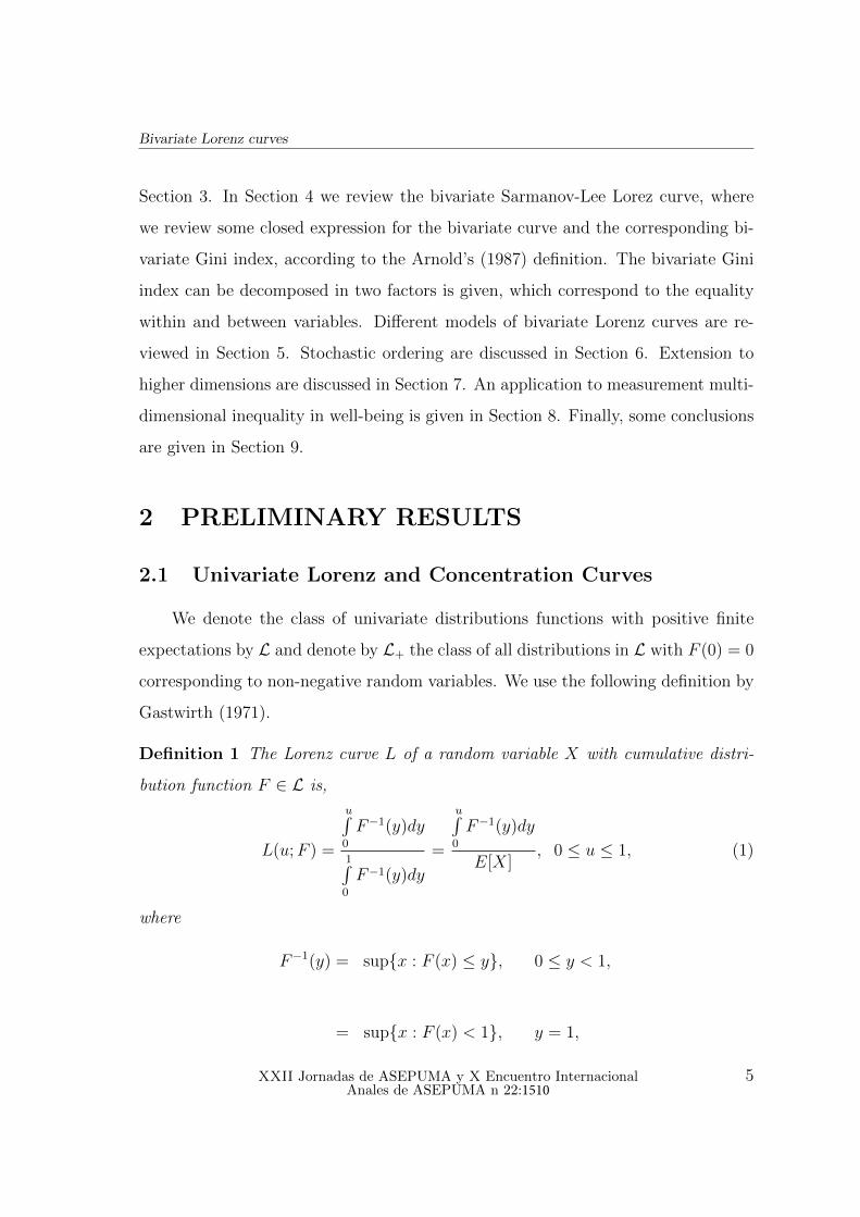
Section 3. In Section 4 we review the bivariate Sarmanov-Lee Lorez curve, where
we review some closed expression for the bivariate curve and the corresponding bi-
variate Gini index, according to the Arnold’s (1987) definition. The bivariate Gini
index can be decomposed in two factors is given, which correspond to the equality
within and between variables. Different models of bivariate Lorenz curves are re-
viewed in Section 5. Stochastic ordering are discussed in Section 6. Extension to
higher dimensions are discussed in Section 7. An application to measurement multi-
dimensional inequality in well-being is given in Section 8. Finally, some conclusions
are given in Section 9.
2 PRELIMINARY RESULTS
2.1 Univariate Lorenz and Concentration Curves
We denote the class of univariate distributions functions with positive finite
expectations by L and denote by L+ the class of all distributions in L with F (0) = 0
corresponding to non-negative random variables. We use the following definition by
Gastwirth (1971).
Definition 1 The Lorenz curve L of a random variable X with cumulative distri-
bution function F ∈ L is,
L(u;F ) =
u∫0
F−1(y)dy
1∫0
F−1(y)dy
=
u∫0
F−1(y)dy
E[X], 0 ≤ u ≤ 1, (1)
where
F−1(y) = supx : F (x) ≤ y, 0 ≤ y < 1,
= supx : F (x) < 1, y = 1,
XXII Jornadas de ASEPUMA y X Encuentro Internacional Anales de ASEPUMA n 22:1510
5
Sarabia, Jose Marıa; Jorda, Vanesa
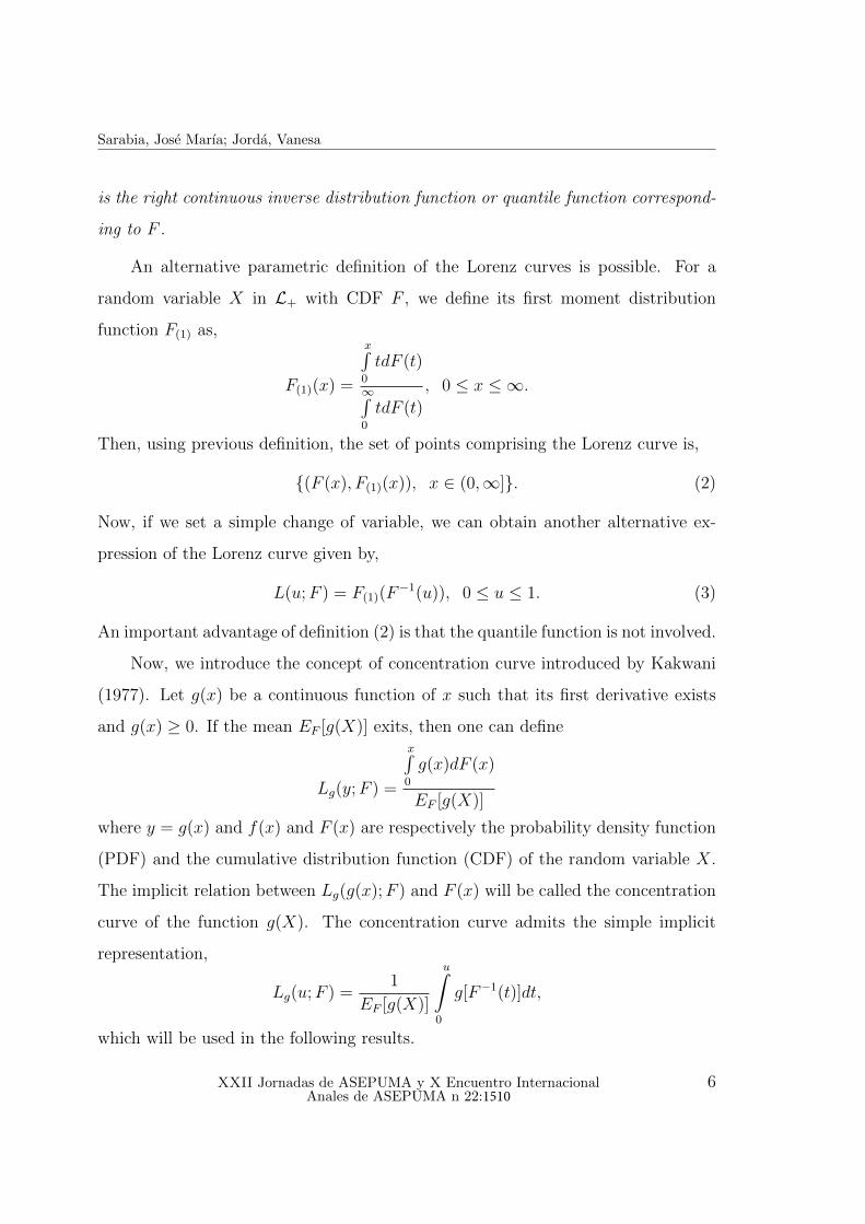
is the right continuous inverse distribution function or quantile function correspond-
ing to F .
An alternative parametric definition of the Lorenz curves is possible. For a
random variable X in L+ with CDF F , we define its first moment distribution
function F(1) as,
F(1)(x) =
x∫0
tdF (t)
∞∫0
tdF (t)
, 0 ≤ x ≤ ∞.
Then, using previous definition, the set of points comprising the Lorenz curve is,
(F (x), F(1)(x)), x ∈ (0,∞]. (2)
Now, if we set a simple change of variable, we can obtain another alternative ex-
pression of the Lorenz curve given by,
L(u;F ) = F(1)(F−1(u)), 0 ≤ u ≤ 1. (3)
An important advantage of definition (2) is that the quantile function is not involved.
Now, we introduce the concept of concentration curve introduced by Kakwani
(1977). Let g(x) be a continuous function of x such that its first derivative exists
and g(x) ≥ 0. If the mean EF [g(X)] exits, then one can define
Lg(y;F ) =
x∫0
g(x)dF (x)
EF [g(X)]
where y = g(x) and f(x) and F (x) are respectively the probability density function
(PDF) and the cumulative distribution function (CDF) of the random variable X.
The implicit relation between Lg(g(x);F ) and F (x) will be called the concentration
curve of the function g(X). The concentration curve admits the simple implicit
representation,
Lg(u;F ) =1
EF [g(X)]
u∫0
g[F−1(t)]dt,
which will be used in the following results.
XXII Jornadas de ASEPUMA y X Encuentro Internacional Anales de ASEPUMA n 22:1510
6
Bivariate Lorenz curves
3 THE THREE DIFFERENT DEFINITIONS OF
BIVARIATE LORENZ CURVES
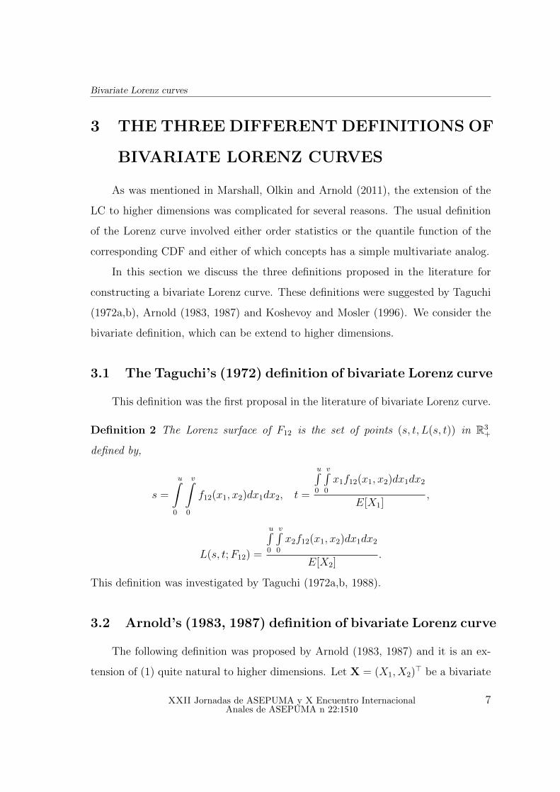
As was mentioned in Marshall, Olkin and Arnold (2011), the extension of the
LC to higher dimensions was complicated for several reasons. The usual definition
of the Lorenz curve involved either order statistics or the quantile function of the
corresponding CDF and either of which concepts has a simple multivariate analog.
In this section we discuss the three definitions proposed in the literature for
constructing a bivariate Lorenz curve. These definitions were suggested by Taguchi
(1972a,b), Arnold (1983, 1987) and Koshevoy and Mosler (1996). We consider the
bivariate definition, which can be extend to higher dimensions.
3.1 The Taguchi’s (1972) definition of bivariate Lorenz curve
This definition was the first proposal in the literature of bivariate Lorenz curve.
Definition 2 The Lorenz surface of F12 is the set of points (s, t, L(s, t)) in R3+
defined by,
s =
u∫0
v∫0
f12(x1, x2)dx1dx2, t =
u∫0
v∫0
x1f12(x1, x2)dx1dx2
E[X1],
L(s, t;F12) =
u∫0
v∫0
x2f12(x1, x2)dx1dx2
E[X2].
This definition was investigated by Taguchi (1972a,b, 1988).
3.2 Arnold’s (1983, 1987) definition of bivariate Lorenz curve
The following definition was proposed by Arnold (1983, 1987) and it is an ex-
tension of (1) quite natural to higher dimensions. Let X = (X1, X2)> be a bivariate
XXII Jornadas de ASEPUMA y X Encuentro Internacional Anales de ASEPUMA n 22:1510
7
Sarabia, Jose Marıa; Jorda, Vanesa
random variable with bivariate probability distribution function F12 on R2+ having
finite second and positive first moments. We denote by Fi, i = 1, 2 the marginal
CDF corresponding to Xi, i = 1, 2 respectively.
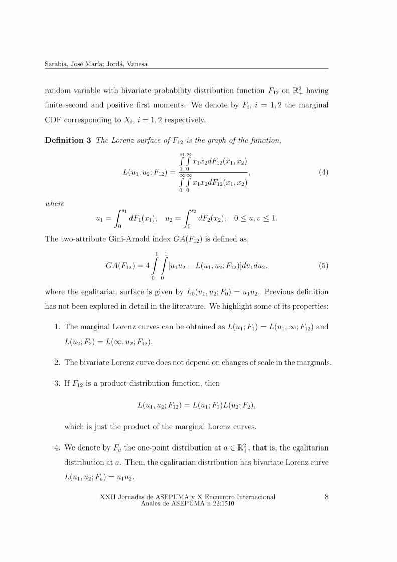
Definition 3 The Lorenz surface of F12 is the graph of the function,
L(u1, u2;F12) =
s1∫0
s2∫0
x1x2dF12(x1, x2)
∞∫0
∞∫0
x1x2dF12(x1, x2)
, (4)
where
u1 =
∫ s1
0
dF1(x1), u2 =
∫ s2
0
dF2(x2), 0 ≤ u, v ≤ 1.
The two-attribute Gini-Arnold index GA(F12) is defined as,
GA(F12) = 4
1∫0
1∫0
[u1u2 − L(u1, u2;F12)]du1du2, (5)
where the egalitarian surface is given by L0(u1, u2;F0) = u1u2. Previous definition
has not been explored in detail in the literature. We highlight some of its properties:
1. The marginal Lorenz curves can be obtained as L(u1;F1) = L(u1,∞;F12) and
L(u2;F2) = L(∞, u2;F12).
2. The bivariate Lorenz curve does not depend on changes of scale in the marginals.
3. If F12 is a product distribution function, then
L(u1, u2;F12) = L(u1;F1)L(u2;F2),
which is just the product of the marginal Lorenz curves.
4. We denote by Fa the one-point distribution at a ∈ R2+, that is, the egalitarian
distribution at a. Then, the egalitarian distribution has bivariate Lorenz curve
L(u1, u2;Fa) = u1u2.
XXII Jornadas de ASEPUMA y X Encuentro Internacional Anales de ASEPUMA n 22:1510
8
Bivariate Lorenz curves
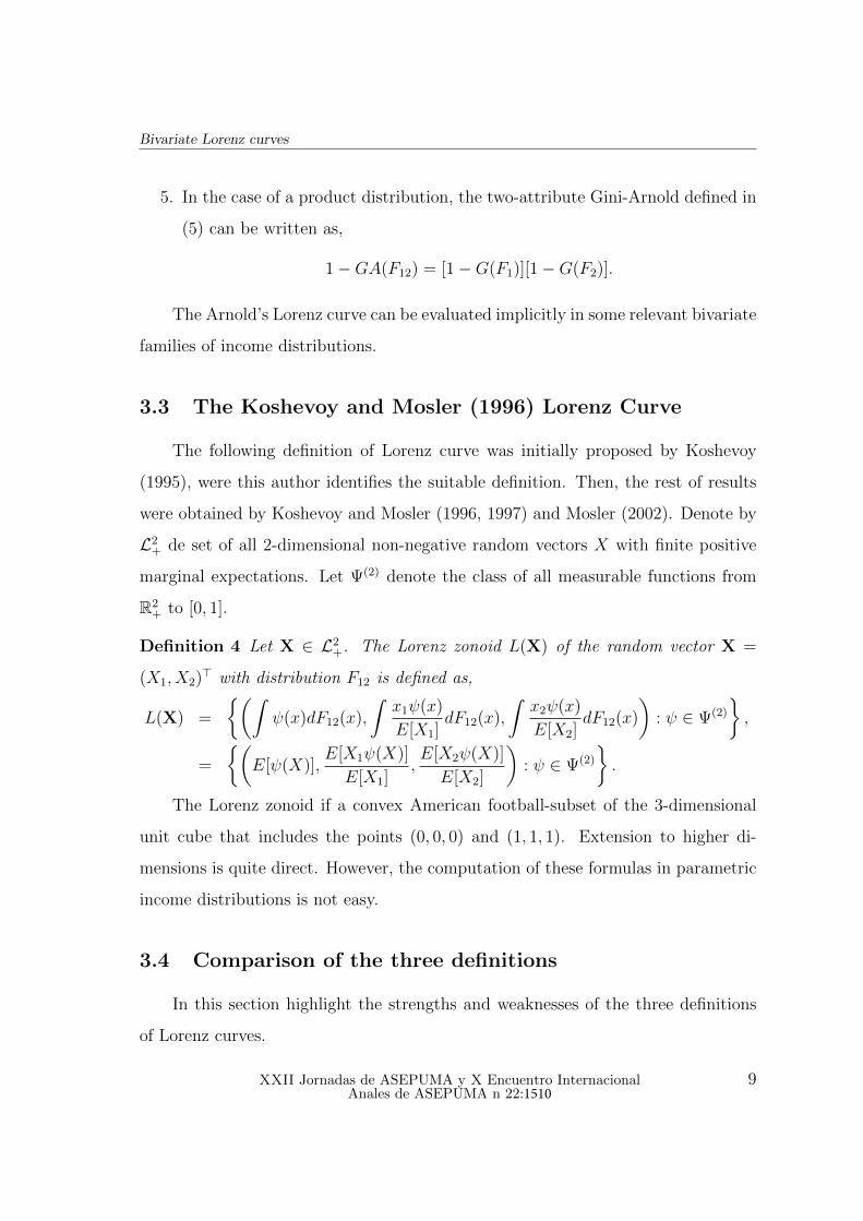
5. In the case of a product distribution, the two-attribute Gini-Arnold defined in
(5) can be written as,
1−GA(F12) = [1−G(F1)][1−G(F2)].
The Arnold’s Lorenz curve can be evaluated implicitly in some relevant bivariate
families of income distributions.
3.3 The Koshevoy and Mosler (1996) Lorenz Curve
The following definition of Lorenz curve was initially proposed by Koshevoy
(1995), were this author identifies the suitable definition. Then, the rest of results
were obtained by Koshevoy and Mosler (1996, 1997) and Mosler (2002). Denote by
L2+ de set of all 2-dimensional non-negative random vectors X with finite positive
marginal expectations. Let Ψ(2) denote the class of all measurable functions from
R2+ to [0, 1].
Definition 4 Let X ∈ L2+. The Lorenz zonoid L(X) of the random vector X =
(X1, X2)> with distribution F12 is defined as,
L(X) =
(∫ψ(x)dF12(x),
∫x1ψ(x)
E[X1]dF12(x),
∫x2ψ(x)
E[X2]dF12(x)
): ψ ∈ Ψ(2)
,
=
(E[ψ(X)],
E[X1ψ(X)]
E[X1],E[X2ψ(X)]
E[X2]
): ψ ∈ Ψ(2)
.
The Lorenz zonoid if a convex American football-subset of the 3-dimensional
unit cube that includes the points (0, 0, 0) and (1, 1, 1). Extension to higher di-
mensions is quite direct. However, the computation of these formulas in parametric
income distributions is not easy.
3.4 Comparison of the three definitions
In this section highlight the strengths and weaknesses of the three definitions
of Lorenz curves.
XXII Jornadas de ASEPUMA y X Encuentro Internacional Anales de ASEPUMA n 22:1510
9

Sarabia, Jose Marıa; Jorda, Vanesa
Taguchi’s definition
The strengths of this definition are the following
• It is easy to use in parametric families.
• It is related to some previous attempts by Lunetta (1972a,b).
On the other hand, the weakness of this definition are:
• The definition is not symmetric.
• Extension to higher dimensions does not look simple.
The Arnold’s definition
The strengths of this definition are the following
• It is easy to use in broad classes of parametric families in dimension two
(Sarabia and Jorda, 2014).
• It is related to some economic concepts in multidimensional utility theory
(Muller and Trannoy, 2011).
• Extensions to higher dimensions (greater than two) are direct.
• Inequality indices can be obtained in a simple way in dimension two.
On the other hand, the weakness are:
• The computation of inequality measures for dimensions higher than two are
difficult.
• The computation in dimensions higher than two for parametric families is
complicated.
The Koshevoy and Mosler’s definition
The strengths of this definition are:
XXII Jornadas de ASEPUMA y X Encuentro Internacional Anales de ASEPUMA n 22:1510
10
Bivariate Lorenz curves
• The extension to higher dimensions is direct.
• The economic interpretation is simple,
and the weakness are:
• The computation of the curve for dimensions two and higher than two are
complicated.
• The computation in parametric families is not simple.
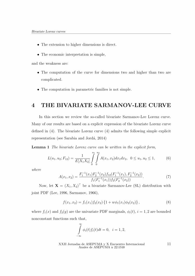
4 THE BIVARIATE SARMANOV-LEE CURVE
In this section we review the so-called bivariate Sarmanov-Lee Lorenz curve.
Many of our results are based on a explicit expression of the bivariate Lorenz curve
defined in (4). The bivariate Lorenz curve (4) admits the following simple explicit
representation (see Sarabia and Jorda, 2014)
Lemma 1 The bivariate Lorenz curve can be written in the explicit form,
L(u1, u2;F12) =1
E[X1X2]
u1∫0
u2∫0
A(x1, x2)dx1dx2, 0 ≤ u1, u2 ≤ 1, (6)
where
A(x1, x2) =F−1
1 (x1)F−12 (x2)f12(F−1
1 (x1), F−12 (x2))
f1(F−11 (x1))f2(F−1
2 (x2)). (7)
Now, let X = (X1, X2)> be a bivariate Sarmanov-Lee (SL) distribution with
joint PDF (Lee, 1996, Sarmanov, 1966),
f(x1, x2) = f1(x1)f2(x2) 1 + wφ1(x1)φ2(x2) , (8)
where f1(x) and f2(y) are the univariate PDF marginals, φi(t), i = 1, 2 are bounded
nonconstant functions such that,∞∫
−∞
φi(t)fi(t)dt = 0, i = 1, 2,
XXII Jornadas de ASEPUMA y X Encuentro Internacional Anales de ASEPUMA n 22:1510
11
Sarabia, Jose Marıa; Jorda, Vanesa
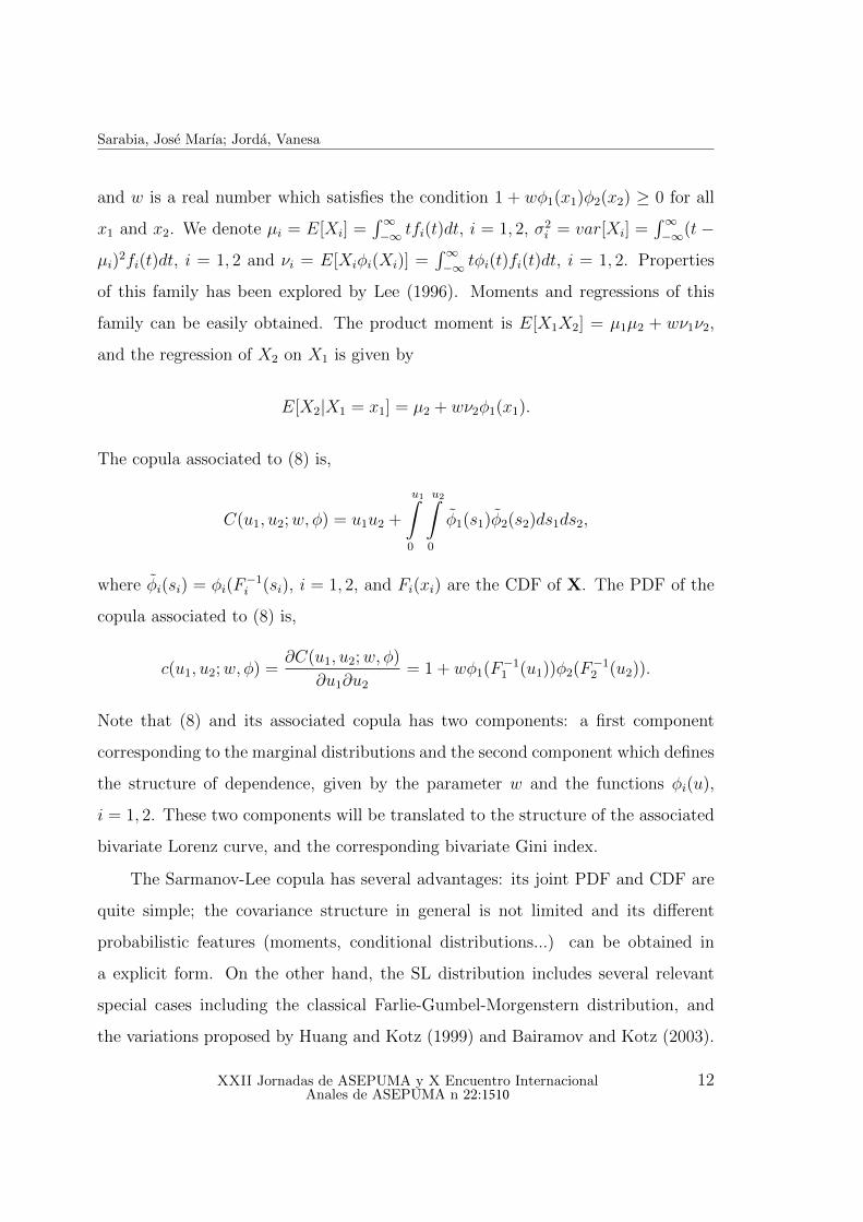
and w is a real number which satisfies the condition 1 + wφ1(x1)φ2(x2) ≥ 0 for all
x1 and x2. We denote µi = E[Xi] =∫∞−∞ tfi(t)dt, i = 1, 2, σ2
i = var[Xi] =∫∞−∞(t−
µi)2fi(t)dt, i = 1, 2 and νi = E[Xiφi(Xi)] =
∫∞−∞ tφi(t)fi(t)dt, i = 1, 2. Properties
of this family has been explored by Lee (1996). Moments and regressions of this
family can be easily obtained. The product moment is E[X1X2] = µ1µ2 + wν1ν2,
and the regression of X2 on X1 is given by
E[X2|X1 = x1] = µ2 + wν2φ1(x1).
The copula associated to (8) is,
C(u1, u2;w, φ) = u1u2 +
u1∫0
u2∫0
φ1(s1)φ2(s2)ds1ds2,
where φi(si) = φi(F−1i (si), i = 1, 2, and Fi(xi) are the CDF of X. The PDF of the
copula associated to (8) is,
c(u1, u2;w, φ) =∂C(u1, u2;w, φ)
∂u1∂u2
= 1 + wφ1(F−11 (u1))φ2(F−1
2 (u2)).
Note that (8) and its associated copula has two components: a first component
corresponding to the marginal distributions and the second component which defines
the structure of dependence, given by the parameter w and the functions φi(u),
i = 1, 2. These two components will be translated to the structure of the associated
bivariate Lorenz curve, and the corresponding bivariate Gini index.
The Sarmanov-Lee copula has several advantages: its joint PDF and CDF are
quite simple; the covariance structure in general is not limited and its different
probabilistic features (moments, conditional distributions...) can be obtained in
a explicit form. On the other hand, the SL distribution includes several relevant
special cases including the classical Farlie-Gumbel-Morgenstern distribution, and
the variations proposed by Huang and Kotz (1999) and Bairamov and Kotz (2003).
XXII Jornadas de ASEPUMA y X Encuentro Internacional Anales de ASEPUMA n 22:1510
12
Bivariate Lorenz curves
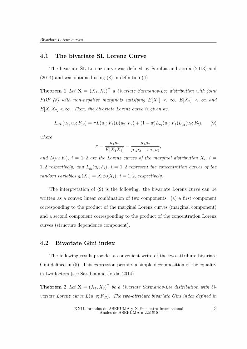
4.1 The bivariate SL Lorenz Curve
The bivariate SL Lorenz curve was defined by Sarabia and Jorda (2013) and
(2014) and was obtained using (8) in definition (4)
Theorem 1 Let X = (X1, X2)> a bivariate Sarmanov-Lee distribution with joint
PDF (8) with non-negative marginals satisfying E[X1] < ∞, E[X2] < ∞ and
E[X1X2] <∞. Then, the bivariate Lorenz curve is given by,
LSL(u1, u2;F12) = πL(u1;F1)L(u2;F2) + (1− π)Lg1(u1;F1)Lg2(u2;F2), (9)
where
π =µ1µ2
E[X1X2]=
µ1µ2
µ1µ2 + wν1ν2
,
and L(ui;Fi), i = 1, 2 are the Lorenz curves of the marginal distribution Xi, i =
1, 2 respectively, and Lgi(ui;Fi), i = 1, 2 represent the concentration curves of the
random variables gi(Xi) = Xiφi(Xi), i = 1, 2, respectively.
The interpretation of (9) is the following: the bivariate Lorenz curve can be
written as a convex linear combination of two components: (a) a first component
corresponding to the product of the marginal Lorenz curves (marginal component)
and a second component corresponding to the product of the concentration Lorenz
curves (structure dependence component).
4.2 Bivariate Gini index
The following result provides a convenient write of the two-attribute bivariate
Gini defined in (5). This expression permits a simple decomposition of the equality
in two factors (see Sarabia and Jorda, 2014).
Theorem 2 Let X = (X1, X2)> be a bivariate Sarmanov-Lee distribution with bi-
variate Lorenz curve L(u, v;F12). The two-attribute bivariate Gini index defined in
XXII Jornadas de ASEPUMA y X Encuentro Internacional Anales de ASEPUMA n 22:1510
13
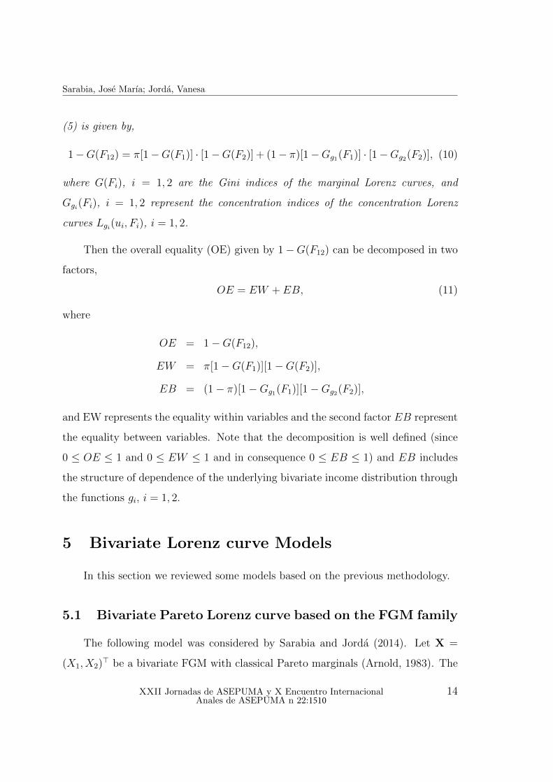
Sarabia, Jose Marıa; Jorda, Vanesa
(5) is given by,
1−G(F12) = π[1−G(F1)] · [1−G(F2)] + (1− π)[1−Gg1(F1)] · [1−Gg2(F2)], (10)
where G(Fi), i = 1, 2 are the Gini indices of the marginal Lorenz curves, and
Ggi(Fi), i = 1, 2 represent the concentration indices of the concentration Lorenz
curves Lgi(ui, Fi), i = 1, 2.
Then the overall equality (OE) given by 1−G(F12) can be decomposed in two
factors,
OE = EW + EB, (11)
where
OE = 1−G(F12),
EW = π[1−G(F1)][1−G(F2)],
EB = (1− π)[1−Gg1(F1)][1−Gg2(F2)],
and EW represents the equality within variables and the second factor EB represent
the equality between variables. Note that the decomposition is well defined (since
0 ≤ OE ≤ 1 and 0 ≤ EW ≤ 1 and in consequence 0 ≤ EB ≤ 1) and EB includes
the structure of dependence of the underlying bivariate income distribution through
the functions gi, i = 1, 2.
5 Bivariate Lorenz curve Models
In this section we reviewed some models based on the previous methodology.
5.1 Bivariate Pareto Lorenz curve based on the FGM family
The following model was considered by Sarabia and Jorda (2014). Let X =
(X1, X2)> be a bivariate FGM with classical Pareto marginals (Arnold, 1983). The
XXII Jornadas de ASEPUMA y X Encuentro Internacional Anales de ASEPUMA n 22:1510
14
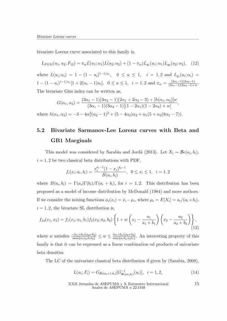
Bivariate Lorenz curves
bivariate Lorenz curve associated to this family is,
LFGM(u1, u2;F12) = πwL(u1;α1)L(u2;α2) + (1− πw)Lg1(u1;α1)Lg2(u2;α2), (12)
where L(ui;αi) = 1 − (1 − ui)1−1/αi , 0 ≤ u ≤ 1, i = 1, 2 and Lgi(ui;αi) =
1 − (1 − ui)1−1/αi [1 + 2(αi − 1)ui], 0 ≤ u ≤ 1, i = 1, 2 and πw = (2α1−1)(2α2−1)(2α1−1)(2α2−1)+w
.
The bivariate Gini index can be written as,
G(α1, α2) =(3α1 − 1)(3α2 − 1)(2α1 + 2α2 − 3) + [h(α1, α2)]w
(3α1 − 1)(3α2 − 1)[(1− 2α1)(1− 2α2) + w],
where h(α1, α2) = −3− 4α21(α2 − 1)2 + (5− 4α2)α2 + α1(5 + α2(8α2 − 7)).
5.2 Bivariate Sarmanov-Lee Lorenz curves with Beta and
GB1 Marginals
This model was considered by Sarabia and Jorda (2013). Let Xi ∼ Be(ai, bi),
i = 1, 2 be two classical beta distributions with PDF,
fi(xi; ai, bi) =xai−1i (1− xi)bi−1
B(ai, bi), 0 ≤ xi ≤ 1, i = 1, 2
where B(ai, bi) = Γ(ai)Γ(bi)/Γ(ai + bi), for i = 1, 2. This distribution has been
proposed as a model of income distribution by McDonald (1984) and more authors.
If we consider the mixing functions φi(xi) = xi−µi, where µi = E[Xi] = ai/(ai+bi),
i = 1, 2, the bivariate SL distribution is,
f12(x1, x2) = f1(x1; a1, b1)f2(x2; a2, b2)
1 + w
(x1 −
a1
a1 + b1
)(x2 −
a2
a2 + b2
),
(13)
where w satisfies −(a1+b1)(a2+b2)maxa1a2,b1b2 ≤ w ≤ (a1+b1)(a2+b2)
maxa1b2,a2b1 . An interesting property of this
family is that it can be expressed as a linear combination od products of univariate
beta densities.
The LC of the univariate classical beta distribution if given by (Sarabia, 2008),
L(ui;Fi) = GBe(ai+1,bi)[G−1Be(ai,bi)(ui)], i = 1, 2, (14)
XXII Jornadas de ASEPUMA y X Encuentro Internacional Anales de ASEPUMA n 22:1510
15
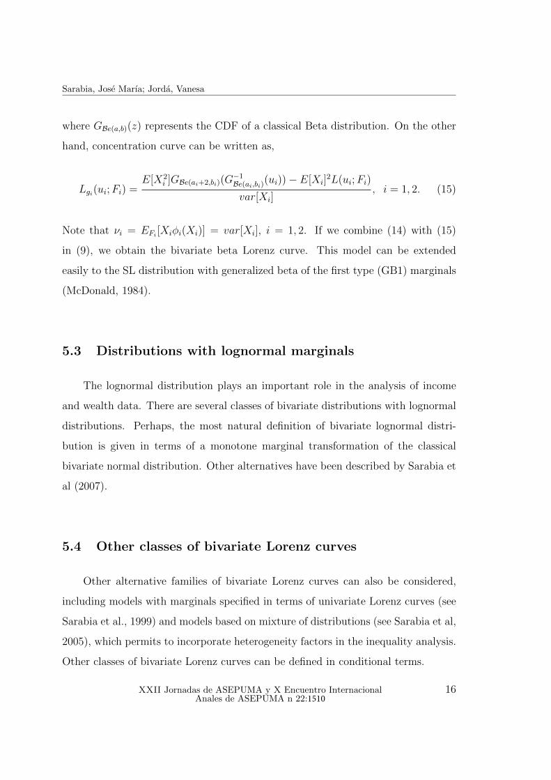
Sarabia, Jose Marıa; Jorda, Vanesa
where GBe(a,b)(z) represents the CDF of a classical Beta distribution. On the other
hand, concentration curve can be written as,
Lgi(ui;Fi) =E[X2
i ]GBe(ai+2,bi)(G−1Be(ai,bi)(ui))− E[Xi]
2L(ui;Fi)
var[Xi], i = 1, 2. (15)
Note that νi = EFi[Xiφi(Xi)] = var[Xi], i = 1, 2. If we combine (14) with (15)
in (9), we obtain the bivariate beta Lorenz curve. This model can be extended
easily to the SL distribution with generalized beta of the first type (GB1) marginals
(McDonald, 1984).
5.3 Distributions with lognormal marginals
The lognormal distribution plays an important role in the analysis of income
and wealth data. There are several classes of bivariate distributions with lognormal
distributions. Perhaps, the most natural definition of bivariate lognormal distri-
bution is given in terms of a monotone marginal transformation of the classical
bivariate normal distribution. Other alternatives have been described by Sarabia et
al (2007).
5.4 Other classes of bivariate Lorenz curves
Other alternative families of bivariate Lorenz curves can also be considered,
including models with marginals specified in terms of univariate Lorenz curves (see
Sarabia et al., 1999) and models based on mixture of distributions (see Sarabia et al,
2005), which permits to incorporate heterogeneity factors in the inequality analysis.
Other classes of bivariate Lorenz curves can be defined in conditional terms.
XXII Jornadas de ASEPUMA y X Encuentro Internacional Anales de ASEPUMA n 22:1510
16
Bivariate Lorenz curves
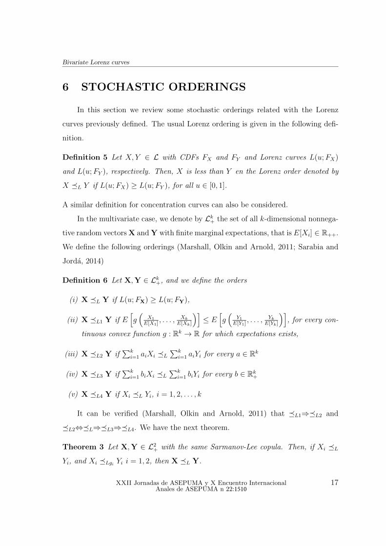
6 STOCHASTIC ORDERINGS
In this section we review some stochastic orderings related with the Lorenz
curves previously defined. The usual Lorenz ordering is given in the following defi-
nition.
Definition 5 Let X, Y ∈ L with CDFs FX and FY and Lorenz curves L(u;FX)
and L(u;FY ), respectively. Then, X is less than Y en the Lorenz order denoted by
X L Y if L(u;FX) ≥ L(u;FY ), for all u ∈ [0, 1].
A similar definition for concentration curves can also be considered.
In the multivariate case, we denote by Lk+ the set of all k-dimensional nonnega-
tive random vectors X and Y with finite marginal expectations, that is E[Xi] ∈ R++.
We define the following orderings (Marshall, Olkin and Arnold, 2011; Sarabia and
Jorda, 2014)
Definition 6 Let X,Y ∈ Lk+, and we define the orders
(i) X L Y if L(u;FX) ≥ L(u;FY),
(ii) X L1 Y if E[g(
X1
E[X1], . . . , Xk
E[Xk]
)]≤ E
[g(
Y1E[Y1]
, . . . , YkE[Yk]
)], for every con-
tinuous convex function g : Rk → R for which expectations exists,
(iii) X L2 Y if∑k
i=1 aiXi L∑k
i=1 aiYi for every a ∈ Rk
(iv) X L3 Y if∑k
i=1 biXi L∑k
i=1 biYi for every b ∈ Rk+
(v) X L4 Y if Xi L Yi, i = 1, 2, . . . , k
It can be verified (Marshall, Olkin and Arnold, 2011) that L1⇒L2 and
L2⇔L⇒L3⇒L4. We have the next theorem.
Theorem 3 Let X,Y ∈ L2+ with the same Sarmanov-Lee copula. Then, if Xi L
Yi, and Xi Lgi Yi i = 1, 2, then X L Y.
XXII Jornadas de ASEPUMA y X Encuentro Internacional Anales de ASEPUMA n 22:1510
17

Sarabia, Jose Marıa; Jorda, Vanesa
7 EXTENSIONS TO HIGHER DIMENSIONS
In this section we review extensions of the definitions to dimensions higher than
two. First, we consider the general definition of Lorenz curve (4).
7.1 The Arnold’s Lorenz Curve
Let X = (X1, . . . , Xm)> be a random vector in Lm+ with joint CDF F12...m(x1, . . . , xm).
The multivariate Arnold’s Lorenz curve can be defined as,
L(u;F12...m) =
s1∫0
. . .sm∫0
m∏i=1
xidF12...m(x1, . . . , xm)
E
[m∏i=1
Xi
] ,
where ui =si∫0
dFi(xi), i = 1, 2, . . . ,m and 0 ≤ u1, . . . , um ≤ 1.
The m-dimensional version of the Sarmanov-Lee distribution is defined as,
f(x1, . . . , xm) =
m∏i=1
fi(xi)
1 +Rφ1...φmΩm(x1, . . . , xm) , (16)
where
Rφ1...φmΩm(x1, . . . , xm)
=∑
1≤i1≤i2≤m
wi1i2φi1(xi1)φi2(xi2)
=∑
1≤i1≤i2≤i3≤m
wi1i2i3φi1(xi1)φi2(xi2)φi3(xi3)
+ . . .
+w12...m
m∏i=1
φi(xi),
and Ωm = wi1i2 , wi1i2i3 , . . . , w12...m, k ≥ 2 and m ≥ 3. The set of real numbers Ωm
is such that 1 +Rφ1...φmΩm(x1, . . . , xm) ≥ 0, ∀(x1, . . . , xm) ∈ Rm.
XXII Jornadas de ASEPUMA y X Encuentro Internacional Anales de ASEPUMA n 22:1510
18
Bivariate Lorenz curves
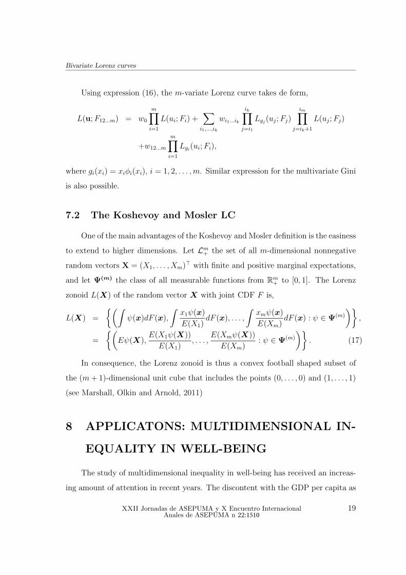
Using expression (16), the m-variate Lorenz curve takes de form,
L(u;F12...m) = w0
m∏i=1
L(ui;Fi) +∑i1,...,ik
wi1...ik
ik∏j=i1
Lgj(uj;Fj)im∏
j=ik+1
L(uj;Fj)
+w12...m
m∏i=1
Lgi(ui;Fi),
where gi(xi) = xiφi(xi), i = 1, 2, . . . ,m. Similar expression for the multivariate Gini
is also possible.
7.2 The Koshevoy and Mosler LC
One of the main advantages of the Koshevoy and Mosler definition is the easiness
to extend to higher dimensions. Let Lm+ the set of all m-dimensional nonnegative
random vectors X = (X1, . . . , Xm)> with finite and positive marginal expectations,
and let Ψ(m) the class of all measurable functions from Rm+ to [0, 1]. The Lorenz
zonoid L(X) of the random vector X with joint CDF F is,
L(X) =
(∫ψ(x)dF (x),
∫x1ψ(x)
E(X1)dF (x), . . . ,
∫xmψ(x)
E(Xm)dF (x) : ψ ∈ Ψ(m)
),
=
(Eψ(X),
E(X1ψ(X))
E(X1), . . . ,
E(Xmψ(X))
E(Xm): ψ ∈ Ψ(m)
). (17)
In consequence, the Lorenz zonoid is thus a convex football shaped subset of
the (m+ 1)-dimensional unit cube that includes the points (0, . . . , 0) and (1, . . . , 1)
(see Marshall, Olkin and Arnold, 2011)
8 APPLICATONS: MULTIDIMENSIONAL IN-
EQUALITY IN WELL-BEING
The study of multidimensional inequality in well-being has received an increas-
ing amount of attention in recent years. The discontent with the GDP per capita as
XXII Jornadas de ASEPUMA y X Encuentro Internacional Anales de ASEPUMA n 22:1510
19
Sarabia, Jose Marıa; Jorda, Vanesa
an indicator of well-being has lead to the consideration of other dimensions such as
health or education, which are considered as important as income in the assessment
of quality of life. The new conception of well-being requires the development of mul-
tivariate tools to measure inequality within the multi-attribute framework. In this
context, the multidimensional Lorenz curves are necessary to study distributional
dynamics of quality of life in different parts of the distribution.
In Sarabia and Jorda (2013), the Sarmanov-Lee Lorenz curve was applied to
study inequality in well-being, taking the Human Development Index as a theoretical
benchmark. Then, the beta distribution was considered a convenient model for the
marginals in this case given that it is ranged from 0 to 1. The results pointed out
that bidimensional inequality decreased during the last three decades. However,
inequality measures only offer summarized information of the evolution well-being
distribution and hence some internal dynamics can be masked. The estimation of
bivariate Lorenz curves showed a decrease in disparities in well-being for the whole
distribution except at the lower tail. The poorest, least educated and least healthy
countries presented a more unequal situation at the end of the study period. It
should be noted that the contrasting patterns at different parts of the distribution
cannot be concluded using inequality indices. As a result, the extension of the
Lorenz curves to higher dimensions stands as essential to assess the evolution of
disparities in well-being.
9 CONCLUSIONS
In this paper, the three existing definitions have been revisited. We have re-
viewed their origin as well as the main properties of each of them. For the Arnold’s
definition, some parametric forms are presented for the bivariate case with differ-
ent dependence structures and different marginals based on the Sarabia and Jorda
XXII Jornadas de ASEPUMA y X Encuentro Internacional Anales de ASEPUMA n 22:1510
20
Bivariate Lorenz curves
(2014) work. We have examinated briefly the extension of these families to dimen-
sions higher than two and describing their applications to well-being data when
several attributes are jointly considered.
10 REFERENCES
• Arnold, B. C. (1983). Pareto Distributions. International Co-operative Pub-
lishing House, Fairland, MD.
• Arnold, B.C. (1987). Majorization and the Lorenz Curve, Lecture Notes in
Statistics 43, Springer Verlag, New York.
• Atkinson, A.B. (2003). Multidimensional deprivation: contrasting social wel-
fare and counting approaches. Journal of Economic Inequality, 1, 51-65.
• Atkinson, A.B., Bourguignon, F. (1982). The comparison of multi-dimensioned
distributions of economic status. Review of Economics Studies, 49, 183-201.
• Bairamov, I., Kotz, S. (2003). On a new family of positive quadrant dependent
bivariate distributions. International Mathematical Journal, 3, 1247.1254.
• Gadrey J., Jany-Catrice, F. (2006). The new Indicators of Well-being and
Development. Macmillan, London.
• Gastwirth, J. L. (1971). A general definition of the Lorenz curve. Economet-
rica, 39, 1037-1039.
• Huang, J.S., Kotz, S. (1999). Modifications of the Farlie-Gumbel-Morgenstern
distributions. A tough hill to climb. Metrika, 49, 135-145.
• Kakwani, N.C. (1977). Applications of Lorenz Curves in Economic Analysis.
Econometrica, 45, 719-728.
XXII Jornadas de ASEPUMA y X Encuentro Internacional Anales de ASEPUMA n 22:1510
21
Sarabia, Jose Marıa; Jorda, Vanesa
• Kolm, S.C. (1977). Multidimensional Equalitarianisms. Quarterly Journal of
Economics, 91, 1-13.
• Koshevoy, G. (1995). Multivariate Lorenz majorization. Social Choice and
Welfare, 12, 93-102.
• Koshevoy, G., Mosler, K. (1996). The Lorenz zonoid of a multivariate distri-
bution. Journal of the American Statistical Association, 91, 873-882.
• Koshevoy, G., Mosler, K. (1997). Multivariate Gini indices. Journal of Multi-
variate Analysis, 60, 252-276.
• Lee, M-L.T. (1996). Properties of the Sarmanov Family of Bivariate Distribu-
tions, Communications in Statistics, Theory and Methods, 25, 1207-1222.
• G. Lunetta (1972). Sulla concentrazione delle distributione doppie, Societa
Italiana di Statistica, 27 (Riunione Scientifica, Palermo).
• G. Lunetta (1972). Di un indice di concentrazione per variabili statistische
doppie, Annah della Facolta di Economia e Commercio dell Universita di Cata-
nia A 18.
• Maasoumi, E. (1986). The measurement and decomposition of multi-dimensional
inequality. Econometrica, 54, 991-997.
• Marshall, A.W., Olkin, I., Arnold, B.C. (2011). Inequalities: Theory of Ma-
jorization and Its Applications. Second Edition. Springer, New York.
• McDonald, J.B. (1984). Some generalized functions for the size distribution
of income. Econometrica, 52, 647-663.
• Mosler, K. (2002). Multivariate Dispersion, Central Regions and Depth: The
Lift Zonoid Approach. Lecture Notes in Statistics 165, Springer, Berlin.
XXII Jornadas de ASEPUMA y X Encuentro Internacional Anales de ASEPUMA n 22:1510
22
Bivariate Lorenz curves
• Muller, C., Trannoy, A. (2011). A dominance approach to the appraisal of the
distribution of well-being across countries. Journal of Public Economics, 95,
239-246.
• Sarabia, J.M. (2008). Parametric Lorenz Curves: Models and Applications.
In: Modeling Income Distributions and Lorenz Curves. Series: Economic Stud-
ies in Inequality, Social Exclusion and Well-Being 4, Chotikapanich, D. (Ed.),
167-190, Springer-Verlag.
• Sarabia, J.M., Castillo, E., Pascual, M., Sarabia, M. (2005). Mixture Lorenz
Curves, Economics Letters, 89, 89-94.
• Sarabia, J.M., Castillo, E., Pascual, M., Sarabia, M. (2007). Bivariate Income
Distributions with Lognormal Conditionals. Journal of Economic Inequality,
5, 371-383.
• Sarabia, J.M., Castillo, E., Slottje, D. (1999). An Ordered Family of Lorenz
Curves. Journal of Econometrics, 91, 43-60.
• Sarabia, J.M., Jorda, V. (2013). Modeling Bivariate Lorenz Curves with Ap-
plications to Multidimensional Inequality in Well-Being. Fifth meeting of the
Society for the Study of Economic Inequality ECINEQ Bari, Italy.
• Sarabia, J.M., Jorda, V. (2014). Bivariate Lorenz Curves based on the Sarmanov-
Lee Distribution. IWS 2013 Book Proceedings, Springer (forthcoming).
• Sarmanov, O.V. (1966). Generalized Normal Correlation and Two-Dimensional
Frechet Classes, Doklady (Soviet Mathematics), 168, 596-599.
• Seth, S. (2011). A class of distribution and association sensitive multidimen-
sional welfare indices. Journal of Economic Inequality, DOI10.1007/ s10888-011-9210-3
XXII Jornadas de ASEPUMA y X Encuentro Internacional Anales de ASEPUMA n 22:1510
23
Sarabia, Jose Marıa; Jorda, Vanesa
• Taguchi, T. (1972a). On the two-dimensional concentration surface and exten-
sions of concentration coefficient and Pareto distribution to the two-dimensional
case-I. Annals of the Institute of Statistical Mathematics, 24, 355-382.
• Taguchi, T. (1972b). On the two-dimensional concentration surface and exten-
sions of concentration coefficient and Pareto distribution to the two-dimensional
case-II. Annals of the Institute of Statistical Mathematics, 24, 599-619.
• Taguchi, T. (1988). On the structure of multivariate concentration - some
relationships among the concentration surface and two variate mean difference
and regressions. Computational Statistics and Data Analysis, 6, 307-334.
• Tsui, K.Y. (1995). Multidimensional generalizations of the relative and ab-
solute inequality indices: the Atkinson-Kolm-Sen approach. Journal of Eco-
nomic Theory, 67, 251-265.
• Tsui, K.Y. (1999). Multidimensional inequality and multidimensional gener-
alized entropy measures: an axiomatic derivation. Social Choice and Welfare,
16, 145-157.
XXII Jornadas de ASEPUMA y X Encuentro Internacional Anales de ASEPUMA n 22:1510
24