Boolean Functions and Boolean Maps - uni-mainz.de€¦ · Boolean Functions and Boolean Maps Klaus...
27
Boolean Functions and Boolean Maps Klaus Pommerening Fachbereich Physik, Mathematik, Informatik der Johannes-Gutenberg-Universit¨ at Saarstraße 21 D-55099 Mainz February 2, 2003—English version August 30, 2003 last change February 21, 2015 1 Elementary Operations on Bits On the lowest software level computers process bits or groups of bits. Ex- amples of such groups are bytes that usually consist of 8 bits, or “words”, usually 32 or 64 bits, depending on the processor architecture. Bits have a logical interpretation as truth values “true” (T) or “false” (F). They also have an algebraic interpretation as values 0 (corresponding to F) or 1 (corresponding to T). As mathematical objects they are elements of the two element set {0, 1}, denoted by F 2 . This notation comes from the algebraic context: Consider the residue class ring of Z modulo 2. This ring has two elements and is a field since 2 is a prime number. Addition in this field is the same as the logical operation XOR, multiplication is the same as the logical operation AND, see Table 1. The algebraic structure as field is of fundamental importance in Cryp- tography. Therefore, as usual in Algebra, we use the notation F q for finite fields where q is the number of elements (often also written as GF(q) for “Galois Field”). In this context we also use the algebraic symbols + (for XOR), and · (for AND) for the operations, and often omit the multiplica- tion dot. Cryptographers sometimes like to use the symbols ⊕ and ⊗ that unfortunately have a quite different meaning in Mathematics (direct sum or tensor product of vector spaces). We use these circled symbols only in diagrams. 2 Description of Boolean Functions Let’s start with the naive definition: A Boolean function is a rule (or a formula or an algorithm) that takes a certain number of bits and produces 1
Transcript of Boolean Functions and Boolean Maps - uni-mainz.de€¦ · Boolean Functions and Boolean Maps Klaus...
Boolean Functions and Boolean Maps
Klaus PommereningFachbereich Physik, Mathematik, Informatik
der Johannes-Gutenberg-UniversitatSaarstraße 21
D-55099 Mainz
February 2, 2003—English version August 30, 2003last change February 21, 2015
1 Elementary Operations on Bits
On the lowest software level computers process bits or groups of bits. Ex-amples of such groups are bytes that usually consist of 8 bits, or “words”,usually 32 or 64 bits, depending on the processor architecture.
Bits have a logical interpretation as truth values “true” (T) or “false”(F). They also have an algebraic interpretation as values 0 (correspondingto F) or 1 (corresponding to T). As mathematical objects they are elementsof the two element set {0, 1}, denoted by F2. This notation comes from thealgebraic context:
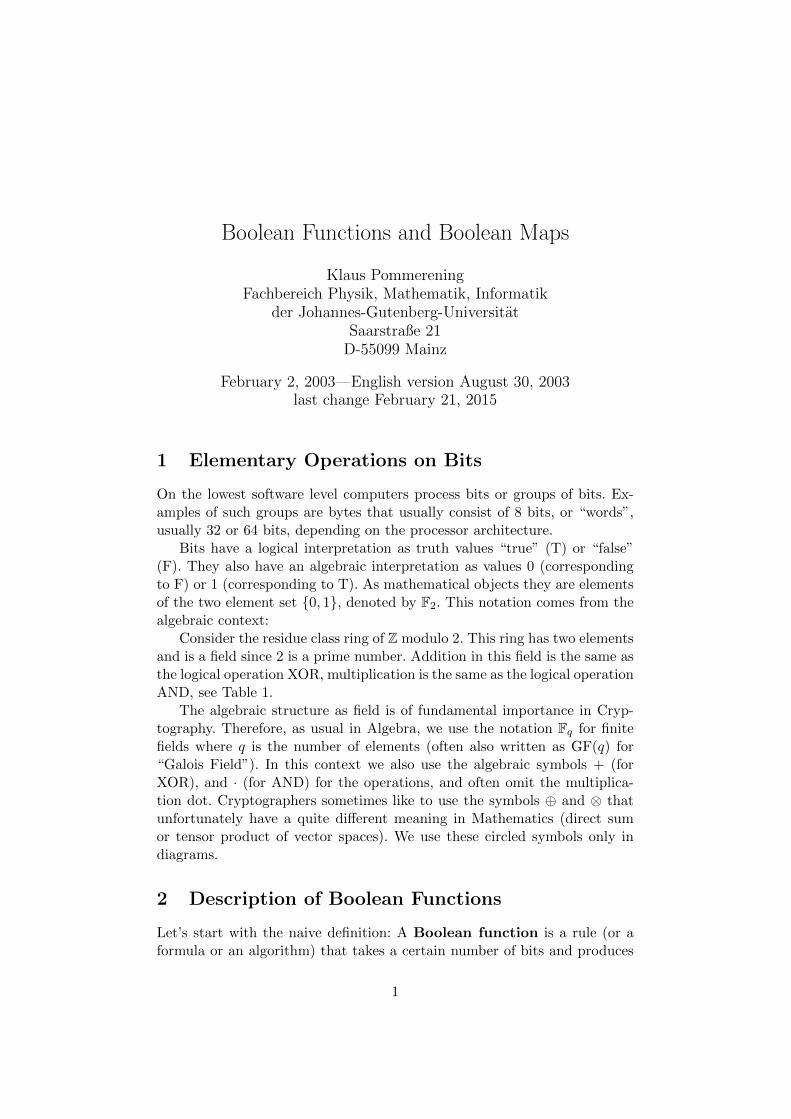
Consider the residue class ring of Z modulo 2. This ring has two elementsand is a field since 2 is a prime number. Addition in this field is the same asthe logical operation XOR, multiplication is the same as the logical operationAND, see Table 1.
The algebraic structure as field is of fundamental importance in Cryp-tography. Therefore, as usual in Algebra, we use the notation Fq for finitefields where q is the number of elements (often also written as GF(q) for“Galois Field”). In this context we also use the algebraic symbols + (forXOR), and · (for AND) for the operations, and often omit the multiplica-tion dot. Cryptographers sometimes like to use the symbols ⊕ and ⊗ thatunfortunately have a quite different meaning in Mathematics (direct sumor tensor product of vector spaces). We use these circled symbols only indiagrams.
2 Description of Boolean Functions
Let’s start with the naive definition: A Boolean function is a rule (or aformula or an algorithm) that takes a certain number of bits and produces
1
K. Pommerening, Boolean Functions and Boolean Maps 2
logical algebraic
bits operation bits operation
x y OR AND XOR x y + ·F F F F F 0 0 0 0F T T F T 0 1 1 0T F T F T 1 0 1 0T T T T F 1 1 0 1
Table 1: The elementary operations on bits
a new bit. Before making this definition mathematically precise we try todepict it in an appealing manner.
A first simple example is the function AND: It takes two bits and pro-duces a new bit by the logical operation AND, see Table 1.
For a slightly more complicated example we consider the function f0 thattakes three bits x1, x2 und x3 and produces the value
(1) f0(x1, x2, x3) = x1 AND (x2 OR x3).
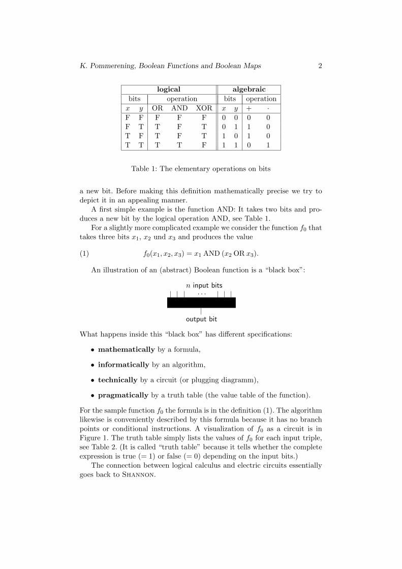
An illustration of an (abstract) Boolean function is a “black box”:
XgXXXXXXXXXX
. . .n input bits
output bit
What happens inside this “black box” has different specifications:
• mathematically by a formula,
• informatically by an algorithm,
• technically by a circuit (or plugging diagramm),
• pragmatically by a truth table (the value table of the function).
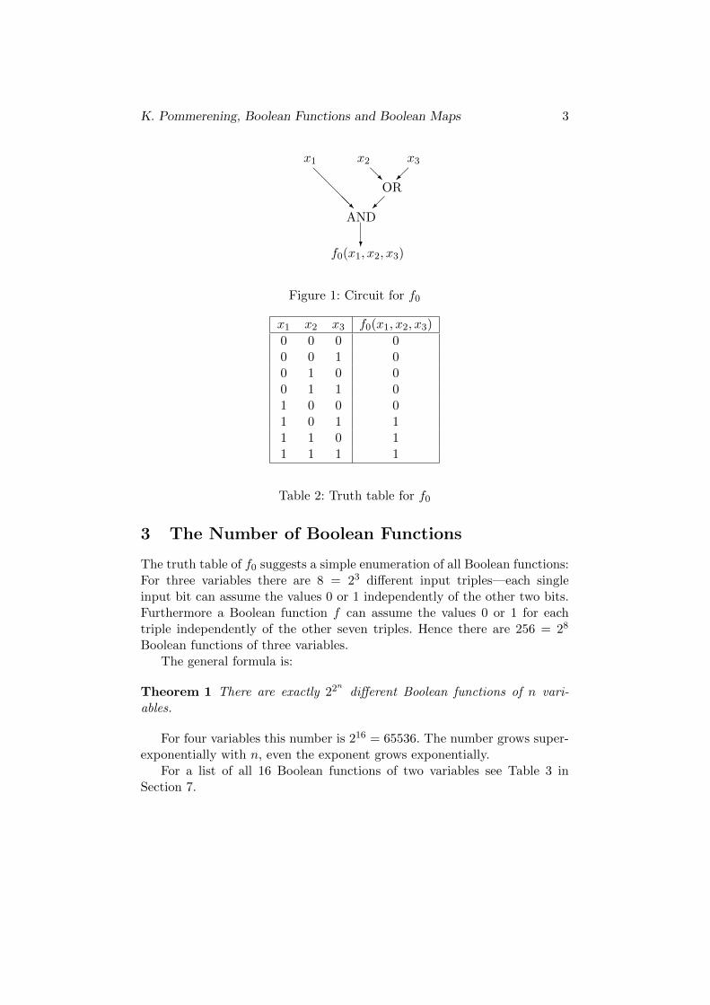
For the sample function f0 the formula is in the definition (1). The algorithmlikewise is conveniently described by this formula because it has no branchpoints or conditional instructions. A visualization of f0 as a circuit is inFigure 1. The truth table simply lists the values of f0 for each input triple,see Table 2. (It is called “truth table” because it tells whether the completeexpression is true (= 1) or false (= 0) depending on the input bits.)
The connection between logical calculus and electric circuits essentiallygoes back to Shannon.
K. Pommerening, Boolean Functions and Boolean Maps 3
AND
?f0(x1, x2, x3)
x1 x2 x3
OR
�
�@R@@@@R
Figure 1: Circuit for f0
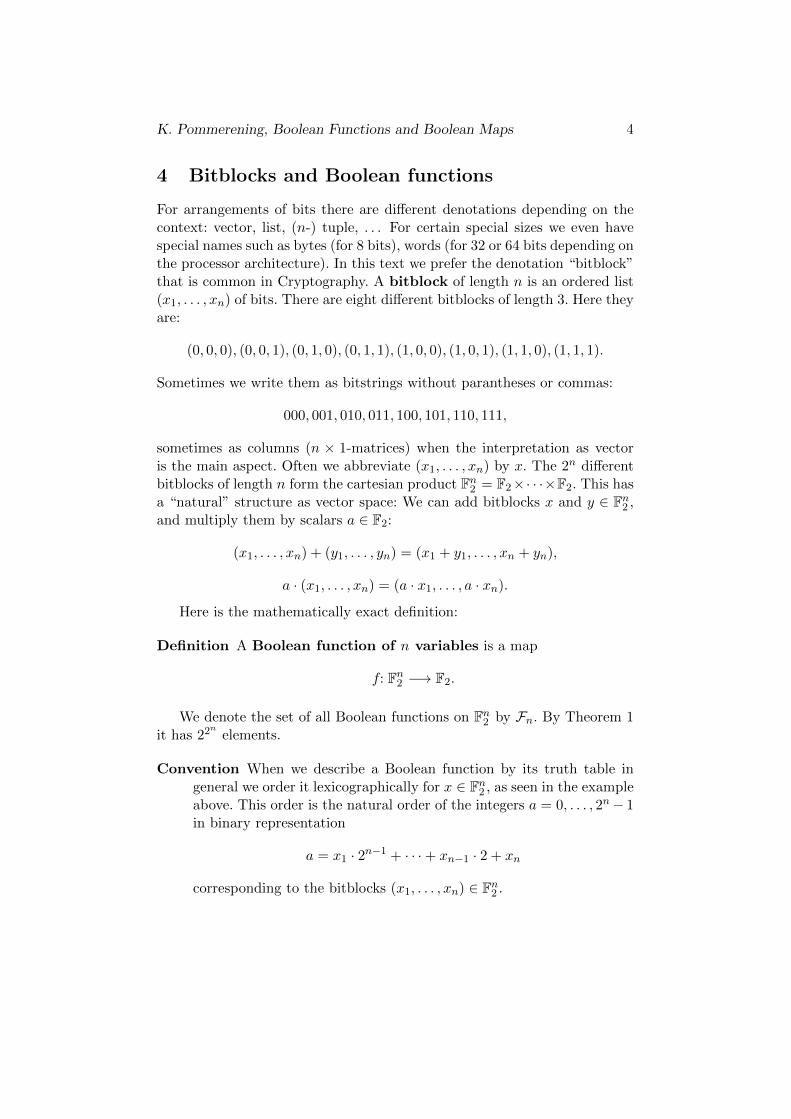
x1 x2 x3 f0(x1, x2, x3)
0 0 0 00 0 1 00 1 0 00 1 1 01 0 0 01 0 1 11 1 0 11 1 1 1
Table 2: Truth table for f0
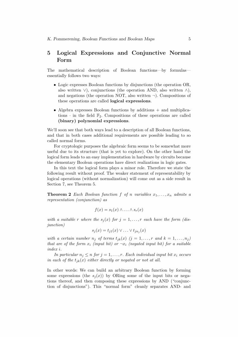
3 The Number of Boolean Functions
The truth table of f0 suggests a simple enumeration of all Boolean functions:For three variables there are 8 = 23 different input triples—each singleinput bit can assume the values 0 or 1 independently of the other two bits.Furthermore a Boolean function f can assume the values 0 or 1 for eachtriple independently of the other seven triples. Hence there are 256 = 28
Boolean functions of three variables.The general formula is:
Theorem 1 There are exactly 22n
different Boolean functions of n vari-ables.
For four variables this number is 216 = 65536. The number grows super-exponentially with n, even the exponent grows exponentially.
For a list of all 16 Boolean functions of two variables see Table 3 inSection 7.
K. Pommerening, Boolean Functions and Boolean Maps 4
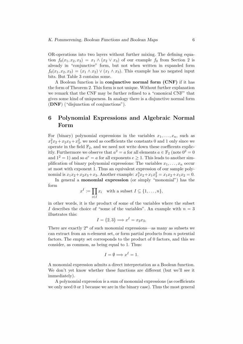
4 Bitblocks and Boolean functions
For arrangements of bits there are different denotations depending on thecontext: vector, list, (n-) tuple, . . . For certain special sizes we even havespecial names such as bytes (for 8 bits), words (for 32 or 64 bits depending onthe processor architecture). In this text we prefer the denotation “bitblock”that is common in Cryptography. A bitblock of length n is an ordered list(x1, . . . , xn) of bits. There are eight different bitblocks of length 3. Here theyare:
(0, 0, 0), (0, 0, 1), (0, 1, 0), (0, 1, 1), (1, 0, 0), (1, 0, 1), (1, 1, 0), (1, 1, 1).
Sometimes we write them as bitstrings without parantheses or commas:
000, 001, 010, 011, 100, 101, 110, 111,
sometimes as columns (n × 1-matrices) when the interpretation as vectoris the main aspect. Often we abbreviate (x1, . . . , xn) by x. The 2n differentbitblocks of length n form the cartesian product Fn
2 = F2×· · ·×F2. This hasa “natural” structure as vector space: We can add bitblocks x and y ∈ Fn
2 ,and multiply them by scalars a ∈ F2:
(x1, . . . , xn) + (y1, . . . , yn) = (x1 + y1, . . . , xn + yn),
a · (x1, . . . , xn) = (a · x1, . . . , a · xn).
Here is the mathematically exact definition:
Definition A Boolean function of n variables is a map
f: Fn2 −→ F2.
We denote the set of all Boolean functions on Fn2 by Fn. By Theorem 1
it has 22n
elements.
Convention When we describe a Boolean function by its truth table ingeneral we order it lexicographically for x ∈ Fn
2 , as seen in the exampleabove. This order is the natural order of the integers a = 0, . . . , 2n− 1in binary representation
a = x1 · 2n−1 + · · ·+ xn−1 · 2 + xn
corresponding to the bitblocks (x1, . . . , xn) ∈ Fn2 .
K. Pommerening, Boolean Functions and Boolean Maps 5
5 Logical Expressions and Conjunctive NormalForm
The mathematical description of Boolean functions—by formulas—essentially follows two ways:
• Logic expresses Boolean functions by disjunctions (the operation OR,also written ∨), conjunctions (the operation AND, also written ∧),and negations (the operation NOT, also written ¬). Compositions ofthese operations are called logical expressions.
• Algebra expresses Boolean functions by additions + and multiplica-tions · in the field F2. Compositions of these operations are called(binary) polynomial expressions.
We’ll soon see that both ways lead to a description of all Boolean functions,and that in both cases additional requirements are possible leading to socalled normal forms.
For cryptologic purposes the algebraic form seems to be somewhat moreuseful due to its structure (that is yet to explore). On the other hand thelogical form leads to an easy implementation in hardware by circuits becausethe elementary Boolean operations have direct realizations in logic gates.
In this text the logical form plays a minor role. Therefore we state thefollowing result without proof. The weaker statement of representability bylogical operations (without normalization) will come out as a side result inSection 7, see Theorem 5.
Theorem 2 Each Boolean function f of n variables x1, . . . , xn admits arepresentation (conjunction) as
f(x) = s1(x) ∧ . . . ∧ sr(x)
with a suitable r where the sj(x) for j = 1, . . . , r each have the form (dis-junction)
sj(x) = tj1(x) ∨ . . . ∨ tjnj (x)
with a certain number nj of terms tjk(x) (j = 1, . . . , r and k = 1, . . . , nj)that are of the form xi (input bit) or ¬xi (negated input bit) for a suitableindex i.
In particular nj ≤ n for j = 1, . . . , r. Each individual input bit xi occursin each of the tjk(x) either directly or negated or not at all.
In other words: We can build an arbitrary Boolean function by formingsome expressions (the sj(x)) by ORing some of the input bits or nega-tions thereof, and then composing these expressions by AND (“conjunc-tion of disjunctions”). This “normal form” cleanly separates AND- and
K. Pommerening, Boolean Functions and Boolean Maps 6
OR-operations into two layers without further mixing. The defining equa-tion f0(x1, x2, x3) = x1 ∧ (x2 ∨ x3) of our example f0 from Section 2 isalready in “conjunctive” form, but not when written in expanded formf0(x1, x2, x3) = (x1 ∧ x2) ∨ (x1 ∧ x3). This example has no negated inputbits. But Table 3 contains some.
A Boolean function is in conjunctive normal form (CNF) if it hasthe form of Theorem 2. This form is not unique. Without further explanationwe remark that the CNF may be further refined to a “canonical CNF” thatgives some kind of uniqueness. In analogy there is a disjunctive normal form(DNF) (“disjunction of conjunctions”).
6 Polynomial Expressions and Algebraic NormalForm
For (binary) polynomial expressions in the variables x1, . . . , xn, such asx21x2 +x2x3 +x23, we need as coefficients the constants 0 and 1 only since weoperate in the field F2, and we need not write down these coefficents explic-itly. Furthermore we observe that a2 = a for all elements a ∈ F2 (note 02 = 0and 12 = 1) and so ae = a for all exponents e ≥ 1. This leads to another sim-plification of binary polynomial expressions: The variables x1, . . . , xn occurat most with exponent 1. Thus an equivalent expression of our sample poly-nomial is x1x2+x2x3+x3. Another example: x31x2+x1x
22 = x1x2+x1x2 = 0.
In general a monomial expression (or simply “monomial”) has theform
xI :=∏i∈I
xi with a subset I ⊆ {1, . . . , n},
in other words, it is the product of some of the variables where the subsetI describes the choice of “some of the variables”. An example with n = 3illustrates this:
I = {2, 3} =⇒ xI = x2x3,
There are exactly 2n of such monomial expressions—as many as subsets wecan extract from an n-element set, or form partial products from n potentialfactors. The empty set corresponds to the product of 0 factors, and this weconsider, as common, as being equal to 1. Thus:
I = ∅ =⇒ xI = 1.
A monomial expression admits a direct interpretation as a Boolean function.We don’t yet know whether these functions are different (but we’ll see itimmediately).
A polynomial expression is a sum of monomial expressions (as coefficientswe only need 0 or 1 because we are in the binary case). Thus the most general
K. Pommerening, Boolean Functions and Boolean Maps 7
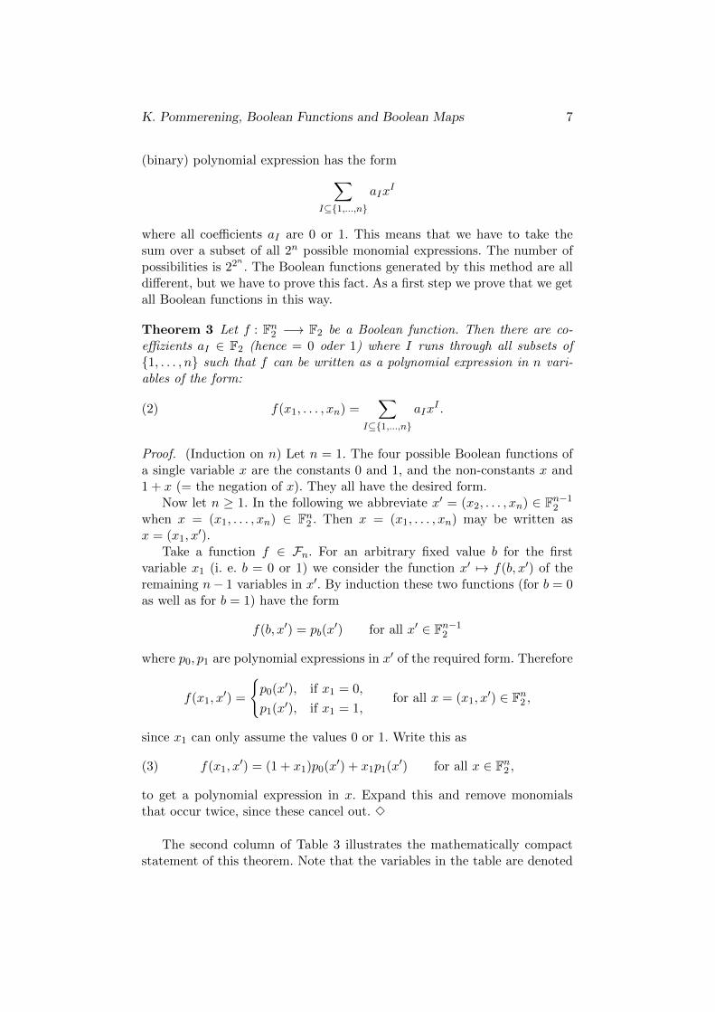
(binary) polynomial expression has the form∑I⊆{1,...,n}
aIxI
where all coefficients aI are 0 or 1. This means that we have to take thesum over a subset of all 2n possible monomial expressions. The number ofpossibilities is 22
n. The Boolean functions generated by this method are all
different, but we have to prove this fact. As a first step we prove that we getall Boolean functions in this way.
Theorem 3 Let f : Fn2 −→ F2 be a Boolean function. Then there are co-
effizients aI ∈ F2 (hence = 0 oder 1) where I runs through all subsets of{1, . . . , n} such that f can be written as a polynomial expression in n vari-ables of the form:
(2) f(x1, . . . , xn) =∑
I⊆{1,...,n}
aIxI .
Proof. (Induction on n) Let n = 1. The four possible Boolean functions ofa single variable x are the constants 0 and 1, and the non-constants x and1 + x (= the negation of x). They all have the desired form.
Now let n ≥ 1. In the following we abbreviate x′ = (x2, . . . , xn) ∈ Fn−12
when x = (x1, . . . , xn) ∈ Fn2 . Then x = (x1, . . . , xn) may be written as
x = (x1, x′).
Take a function f ∈ Fn. For an arbitrary fixed value b for the firstvariable x1 (i. e. b = 0 or 1) we consider the function x′ 7→ f(b, x′) of theremaining n− 1 variables in x′. By induction these two functions (for b = 0as well as for b = 1) have the form
f(b, x′) = pb(x′) for all x′ ∈ Fn−1
2
where p0, p1 are polynomial expressions in x′ of the required form. Therefore
f(x1, x′) =
{p0(x
′), if x1 = 0,
p1(x′), if x1 = 1,
for all x = (x1, x′) ∈ Fn
2 ,
since x1 can only assume the values 0 or 1. Write this as
(3) f(x1, x′) = (1 + x1)p0(x
′) + x1p1(x′) for all x ∈ Fn
2 ,
to get a polynomial expression in x. Expand this and remove monomialsthat occur twice, since these cancel out. 3
The second column of Table 3 illustrates the mathematically compactstatement of this theorem. Note that the variables in the table are denoted
K. Pommerening, Boolean Functions and Boolean Maps 8
by x and y instead of x1 and x2, and the coefficients by a, b, c, d instead ofa∅, a{1}, a{2}, a{1,2}. Each row of the table describes a Boolean function oftwo variables as sum of those terms 1, x, y, xy that have coefficient 1 in therepresentation of Equation (2), suppressing terms with coefficients 0.
The representation of a Boolean function as polynomial expression givenby Theorem 3 is called the algebraic normal form (ANF). Note that itis unique: Since there are 22
npolynomial expressions, and these represent
all the 22n
different Boolean functions, first all these polynomial expressionsmust be different as functions, secondly the representation of a Booleanfunction as a polynomial expression in ANF must be unique. We have shown:
Theorem 4 The representation of a Boolean function in algebraic normalform is unique.
Definition The degree of a Boolean function f ∈ Fn as polynomial expres-sion in algebraic normal form,
deg f = max{#I | aI 6= 0},
is called the (algebraic) degree of f . It is always ≤ n.
The degree is the maximum number of variables that occur in a monomialof the ANF.
Example The Boolean function given by x 7→ x1x2+x2x3+x3 has degree 2.
Remark A high degree of a Boolean function is not caused by high powersof variables but “only” by products of different variables. Each singlevariable occurs at most in the first power in each monomial of theANF. In other words all partial degrees—that are the degrees in thesingle variables xi without accounting for the remaining variablen—are≤ 1.
7 Boolean Functions of Two Variables
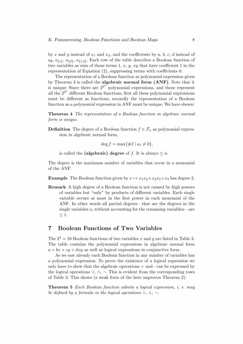
The 24 = 16 Boolean functions of two variables x and y are listed in Table 3.The table contains the polynomial expressions in algebraic normal forma+ bx+ cy + dxy as well as logical expressions in conjunctive form.
As we saw already each Boolean function in any number of variables hasa polynomial expression. To prove the existence of a logical expression weonly have to show that the algebraic operations + and · can be expressed bythe logical operations ∨, ∧, ¬. This is evident from the corresponding rowsof Table 3. This shows (a weak form of the here unproven Theorem 2):
Theorem 5 Each Boolean function admits a logical expression, i. e. maybe defined by a formula in the logical operations ∨, ∧, ¬.
K. Pommerening, Boolean Functions and Boolean Maps 9
a b c d ANF logical operation CNF
0 0 0 0 0 False constant x ∧ ¬x1 0 0 0 1 True constant x ∨ ¬x0 1 0 0 x x projection x
1 1 0 0 1 + x ¬x ¬x0 0 1 0 y y projection y
1 0 1 0 1 + y ¬y ¬y0 1 1 0 x+ y x XOR y XOR (x ∨ y) ∧ (¬x ∨ ¬y)
1 1 1 0 1 + x+ y x⇐⇒ y equivalence (x ∨ ¬y) ∧ (¬x ∨ y)
0 0 0 1 xy x ∧ y AND x ∧ y1 0 0 1 1 + xy ¬(x ∧ y) NAND (¬x) ∨ (¬y)
0 1 0 1 x+ xy x ∧ (¬y) x ∧ (¬y)
1 1 0 1 1 + x+ xy x =⇒ y implication (¬x) ∨ y0 0 1 1 y + xy (¬x) ∧ y (¬x) ∧ y1 0 1 1 1 + y + xy x⇐= y x ∨ (¬y)
0 1 1 1 x+ y + xy x ∨ y OR x ∨ y1 1 1 1 1 + x+ y + xy ¬(x ∨ y) NOR (¬x) ∧ (¬y)
Table 3: The 16 operations on two bits (= Boolean functions of 2 variables)
Hint The logical negation ¬ corresponds to the addition of 1 in the algebraicinterpretation.
Remark In analogy we may write the ANF of a Boolean function of threevariables x, y, z in the form
(x, y, z) 7→ a+ bx+ cy + dz + exy + fxz + gyz + hxyz.
This involves 8 coefficients a, . . . , h, and fits the observation that thereare 22
3= 28 = 256 such functions.
Example What does the ANF of the function f0 from Section 2 look like(here written as f0(x, y, z) = x ∧ (y ∨ z) using the variables x, y, z)?By Table 3 we have y ∨ z = y+ z+ yz, whereas the AND operation ∧simply is the product in the field F2. Hence
f0(x, y, z) = x · (y + z + yz) = xy + xz + xyz.
By the way this shows that f0 has degree 3.
8 Boolean Maps
Most cryptographic applications involve processes that produce several bitsat once, not only a single one. An abstract description uses the concept of
K. Pommerening, Boolean Functions and Boolean Maps 10
a Boolean map, that is a map
f : Fn2 −→ Fq
2
with natural numbers n and q, illustrated by the following figure
XgXXXXXXXXXX
. . .
. . .
n input bits
q output bits
Note that the conceptual differentiation between “function” and “map” issomewhat arbitrary. We follow a common usage in Mathematics for express-ing the property that the range is one- or multidimensional where “map” isthe superordinate concept.
The images of f are bitblocks of length q. If we decompose them intotheir components
f(x) = (f1(x), . . . , fq(x)) ∈ Fq2,
then we see that a Boolean map to Fq2 in a canonical way simply is a q-tuple
of Boolean functionsf1, . . . , fq : Fn
2 −→ F2.
Definition The (algebraic) degree of a Boolean map f: Fn2 −→ Fq
2 is themaximum of the algebraic degrees of its components,
deg f = max{deg fi | i = 1, . . . , q}.
Theorem 6 Each Boolean map f : Fn2 −→ Fq
2 has a unique representationin the form
f(x1, . . . , xn) =∑
I⊆{1,...,n}
xIaI
with aI ∈ Fq2 and monomials xI as in Theorem 3.
Like for functions this representation of a Boolean map is called algebraicnormal form. It arises by combining the algebraic normal forms of thecomponent functions f1, . . . , fq. Compared with Theorem 3 the xI and aIchanged their positions for by convention usually the “scalars” (the xI ∈ F2)precede the “vectors” (the aI ∈ Fq
2). The aI simply are the combinations ofthe corresponding coefficients of the component functions.
K. Pommerening, Boolean Functions and Boolean Maps 11
Example
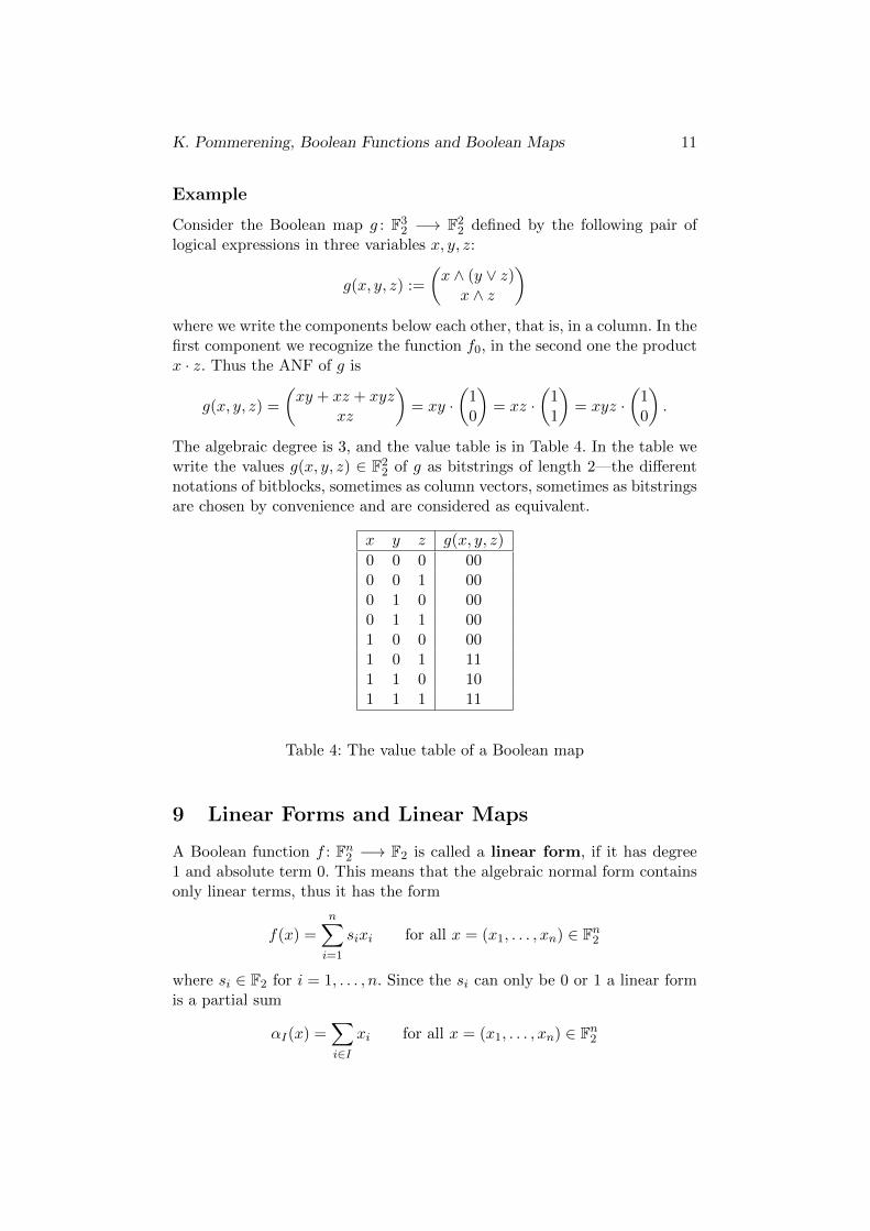
Consider the Boolean map g : F32 −→ F2
2 defined by the following pair oflogical expressions in three variables x, y, z:
g(x, y, z) :=
(x ∧ (y ∨ z)x ∧ z
)where we write the components below each other, that is, in a column. In thefirst component we recognize the function f0, in the second one the productx · z. Thus the ANF of g is
g(x, y, z) =
(xy + xz + xyz
xz
)= xy ·
(10
)= xz ·
(11
)= xyz ·
(10
).
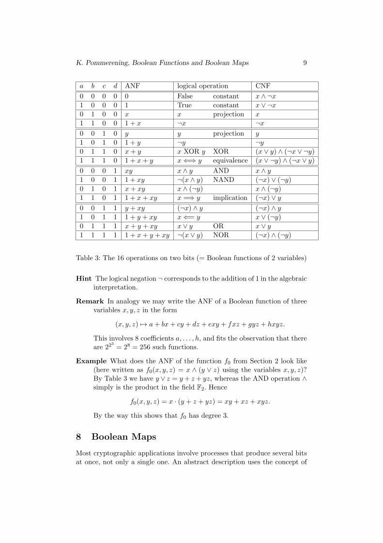
The algebraic degree is 3, and the value table is in Table 4. In the table wewrite the values g(x, y, z) ∈ F2
2 of g as bitstrings of length 2—the differentnotations of bitblocks, sometimes as column vectors, sometimes as bitstringsare chosen by convenience and are considered as equivalent.
x y z g(x, y, z)
0 0 0 000 0 1 000 1 0 000 1 1 001 0 0 001 0 1 111 1 0 101 1 1 11
Table 4: The value table of a Boolean map
9 Linear Forms and Linear Maps
A Boolean function f : Fn2 −→ F2 is called a linear form, if it has degree
1 and absolute term 0. This means that the algebraic normal form containsonly linear terms, thus it has the form
f(x) =n∑
i=1
sixi for all x = (x1, . . . , xn) ∈ Fn2
where si ∈ F2 for i = 1, . . . , n. Since the si can only be 0 or 1 a linear formis a partial sum
αI(x) =∑i∈I
xi for all x = (x1, . . . , xn) ∈ Fn2
K. Pommerening, Boolean Functions and Boolean Maps 12
over a subset I ⊆ {1, . . . , n} of the set of all indices, namely
I = {i | si = 1}.
We immediately conclude that there are exactly 2n Boolean linear forms inn variables, and they correspond to the power set P({1, . . . , n}) in a naturalway.
Other common notations are (for I = {i1, . . . , ir}):
αI(x) = x[I] = x[i1, . . . , ir] = xi1 + · · ·+ xir .
The following theorem connects linear forms with the usual notation ofLinear Algebra:
Theorem 7 A Boolean function f : Fn2 −→ F2 is a linear form if and only
if the following two conditions hold:(i) f(x+ y) = f(x) + f(y) for all x, y ∈ Fn
2 .(ii) f(ax) = af(x) for all a ∈ F2 and x ∈ Fn
2 .
Proof. For each linear form the conditions hold as immediately seen by therepresentation as partial sum.
For the reverse direction let f be a Boolean function that fulfills (i)and (ii). Let e1 = (1, 0, . . . , 0), . . . , en = (0, . . . , 1) be the “canonical unitvectors”. Then each x = (x1, . . . , xn) ∈ Fn
2 is a sum
x = x1e1 + · · ·+ xnen.
From this we get
f(x) = f(x1e1) + · · ·+ f(xnen) = x1f(e1) + · · ·+ xnf(en),
a partial sum of the xi for which the constant value f(ei) is not 0, hence 1.Thus f is a linear form in the sense of our definition. 3
A Boolean map f : Fn2 −→ Fq
2 is called linear if all of its componentfunctions f1, . . . , fq are linear forms. As in the case q = 1 we see:
Theorem 8 A Boolean map f : Fn2 −→ Fq
2 is linear if and only if the fol-lowing two conditions hold:
(i) f(x+ y) = f(x) + f(y) for all x, y ∈ Fn2 .
(ii) f(ax) = af(x) for all a ∈ F2 and x ∈ Fn2 .
Theorem 9 A Boolean map f: Fn2 −→ Fq
2 is linear if and only if it has theform
f(x) =n∑
i=1
xisi
with si ∈ Fq2.
K. Pommerening, Boolean Functions and Boolean Maps 13
A Boolean map is called affine if its algebraic degree is ≤ 1 or, equiva-lently, if it is the sum of a linear map and a constant.
In the case q = 1, for functions, the only constants are 0 and 1. Addingthe constant 1 is the same as the logical negation that “toggles” the bits.In other words: The affine Boolean functions are the linear forms and theirnegations.
10 Systems of Boolean Linear Equations
Algebra over the field F2 is quite easy. Many complications known fromother mathematical domains break down. This is the case for the solutionof systems of linear equations, systems of the form
a11x1 + · · · + a1nxn = b1...
......
am1x1 + · · · + amnxn = bm
where aij and bi ∈ F2 are given and the xj are the unknowns to be solvedfor. In matrix notation the equations become
Ax = b
where x and b are column vectors, that is (n× 1)- or (m× 1)-matrices.
Systems of Linear Equations in Sage
As a link with “ordinary” Linear Algebra we consider an example over therational numbers Q, the system
x1 + 2x2 + 3x3 = 03x1 + 2x2 + x3 = −4x1 + x2 + x3 = −1
This is treated by Sage Example 1. The single steps are:
1. Define the “coefficient matrix” A =
1 2 33 2 11 1 1
.
2. Define the “image vector” b = (0,−4, 1).
3. Let Sage find a “solution vector” x.—Having written the left-handside of the system as matrix product Ax we have to apply the methodsolve right().
K. Pommerening, Boolean Functions and Boolean Maps 14
4. The system could have other solutions. We find these by solving thecorresponding “homogeneous” system Az = 0. If z is a solution ofthe homogeneous system, then A · (x + z) = Ax + Az = b + 0 =b, hence x + z is another solution of the original (“inhomogeneous”)system. In this way we get all solutions: For if Ax = b and Ay = b,then A · (y − x) = 0, hence the difference y − x is a solution of thehomogeneous system. The Sage method right kernel() determinesall solutions of the homogeneous system.
5. The output of right kernel() is somewhat cryptic. It says that allsolutions of the homogeneous system are multiples of the vector z =(1,−2, 1). (Since all coefficients are integers Sage considers the systemas defined over Z (= Integer Ring).)
6. Finally we verify that y = x− 4z really is a solution, i. e. Ay = b.
In the general case (over an arbitrary field) the solution of a system oflinear equations is constructed by Gaussian elimination. The Sage methodsolve right() also uses this algorithm.
sage: A = Matrix([[1,2,3],[3,2,1],[1,1,1]])
sage: b = vector([0,-4,-1])
sage: x = A.solve_right(b); x
(-2, 1, 0)
sage: K = A.right_kernel(); K
Free module of degree 3 and rank 1 over Integer Ring
Echelon basis matrix:
[ 1 -2 1]
sage: y = x - 4*vector([1,-2,1]); y
(-6, 9, -4)
sage: A*y
(0, -4, -1)
Sage Example 1: Solution of a system of linear equations over Q
Systems of Linear Equations in the Boolean Case
In the Boolean case (over the field F2) the solution by Gaussian elimination isextremely simple since the only coefficients are 0 and 1, and multiplicationsor divisions are completely obsolete. There are no complicated coefficients(like fractions over Q) or inexact coefficients (like floating point numbers).So simple is the method that even for six unknowns the solution by “penciland paper” is faster then writing the corresponding program in Sage. Hereis an illustrative example.
K. Pommerening, Boolean Functions and Boolean Maps 15
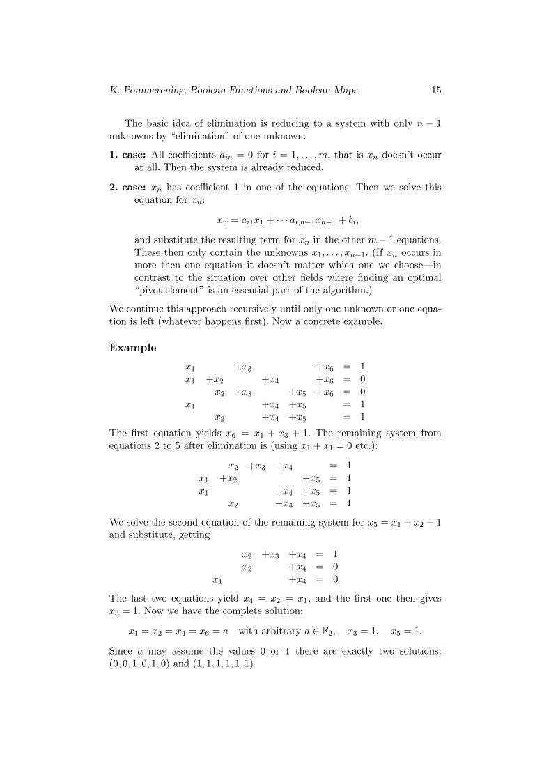
The basic idea of elimination is reducing to a system with only n − 1unknowns by “elimination” of one unknown.
1. case: All coefficients ain = 0 for i = 1, . . . ,m, that is xn doesn’t occurat all. Then the system is already reduced.
2. case: xn has coefficient 1 in one of the equations. Then we solve thisequation for xn:
xn = ai1x1 + · · · ai,n−1xn−1 + bi,
and substitute the resulting term for xn in the other m− 1 equations.These then only contain the unknowns x1, . . . , xn−1. (If xn occurs inmore then one equation it doesn’t matter which one we choose—incontrast to the situation over other fields where finding an optimal“pivot element” is an essential part of the algorithm.)
We continue this approach recursively until only one unknown or one equa-tion is left (whatever happens first). Now a concrete example.
Example
x1 +x3 +x6 = 1x1 +x2 +x4 +x6 = 0
x2 +x3 +x5 +x6 = 0x1 +x4 +x5 = 1
x2 +x4 +x5 = 1
The first equation yields x6 = x1 + x3 + 1. The remaining system fromequations 2 to 5 after elimination is (using x1 + x1 = 0 etc.):
x2 +x3 +x4 = 1x1 +x2 +x5 = 1x1 +x4 +x5 = 1
x2 +x4 +x5 = 1
We solve the second equation of the remaining system for x5 = x1 + x2 + 1and substitute, getting
x2 +x3 +x4 = 1x2 +x4 = 0
x1 +x4 = 0
The last two equations yield x4 = x2 = x1, and the first one then givesx3 = 1. Now we have the complete solution:
x1 = x2 = x4 = x6 = a with arbitrary a ∈ F2, x3 = 1, x5 = 1.
Since a may assume the values 0 or 1 there are exactly two solutions:(0, 0, 1, 0, 1, 0) and (1, 1, 1, 1, 1, 1).
K. Pommerening, Boolean Functions and Boolean Maps 16
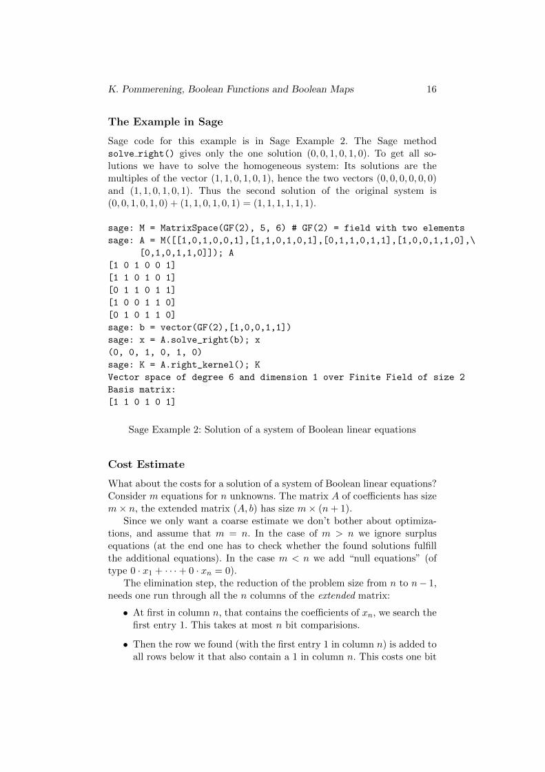
The Example in Sage
Sage code for this example is in Sage Example 2. The Sage methodsolve right() gives only the one solution (0, 0, 1, 0, 1, 0). To get all so-lutions we have to solve the homogeneous system: Its solutions are themultiples of the vector (1, 1, 0, 1, 0, 1), hence the two vectors (0, 0, 0, 0, 0, 0)and (1, 1, 0, 1, 0, 1). Thus the second solution of the original system is(0, 0, 1, 0, 1, 0) + (1, 1, 0, 1, 0, 1) = (1, 1, 1, 1, 1, 1).
sage: M = MatrixSpace(GF(2), 5, 6) # GF(2) = field with two elements
sage: A = M([[1,0,1,0,0,1],[1,1,0,1,0,1],[0,1,1,0,1,1],[1,0,0,1,1,0],\
[0,1,0,1,1,0]]); A
[1 0 1 0 0 1]
[1 1 0 1 0 1]
[0 1 1 0 1 1]
[1 0 0 1 1 0]
[0 1 0 1 1 0]
sage: b = vector(GF(2),[1,0,0,1,1])
sage: x = A.solve_right(b); x
(0, 0, 1, 0, 1, 0)
sage: K = A.right_kernel(); K
Vector space of degree 6 and dimension 1 over Finite Field of size 2
Basis matrix:
[1 1 0 1 0 1]
Sage Example 2: Solution of a system of Boolean linear equations
Cost Estimate
What about the costs for a solution of a system of Boolean linear equations?Consider m equations for n unknowns. The matrix A of coefficients has sizem× n, the extended matrix (A, b) has size m× (n+ 1).
Since we only want a coarse estimate we don’t bother about optimiza-tions, and assume that m = n. In the case of m > n we ignore surplusequations (at the end one has to check whether the found solutions fulfillthe additional equations). In the case m < n we add “null equations” (oftype 0 · x1 + · · ·+ 0 · xn = 0).
The elimination step, the reduction of the problem size from n to n− 1,needs one run through all the n columns of the extended matrix:
• At first in column n, that contains the coefficients of xn, we search thefirst entry 1. This takes at most n bit comparisions.
• Then the row we found (with the first entry 1 in column n) is added toall rows below it that also contain a 1 in column n. This costs one bit
K. Pommerening, Boolean Functions and Boolean Maps 17
comparision and at most n bit addition for each row—we may omitthe n-th entry because we know there will be a 0.
On the whole we need n bit comparisons and at most n·(n−1) bit additions,a total of at most n2 bit operations. Let us denote the number of needed bitoperations for the complete solution of the system by N(n). Then we havethe inequality:
N(n) ≤ n2 +N(n− 1) for all n ≥ 2.
Clearly N(1) = 1: We check the one coefficient of the one unknown whetherit is 0 or 1 and decide whether the equation has a unique solution (coefficient1), or whether it is fulfilled for no or for arbitrary values of the unknown(coefficient 0, right-hand side b = 1 or 0).
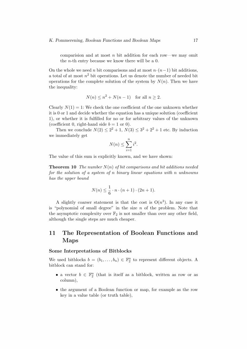
Then we conclude N(2) ≤ 22 + 1, N(3) ≤ 32 + 22 + 1 etc. By inductionwe immediately get
N(n) ≤n∑
i=1
i2.
The value of this sum is explicitly known, and we have shown:
Theorem 10 The number N(n) of bit comparisons and bit additions neededfor the solution of a system of n binary linear equations with n unknownshas the upper bound
N(n) ≤ 1
6· n · (n+ 1) · (2n+ 1).
A slightly coarser statement is that the cost is O(n3). In any case itis “polynomial of small degree” in the size n of the problem. Note thatthe asymptotic complexity over F2 is not smaller than over any other field,although the single steps are much cheaper.
11 The Representation of Boolean Functions andMaps
Some Interpretations of Bitblocks
We used bitblocks b = (b1, . . . , bn) ∈ Fn2 to represent different objects. A
bitblock can stand for:
• a vector b ∈ Fn2 (that is itself as a bitblock, written as row or as
column),
• the argument of a Boolean function or map, for example as the rowkey in a value table (or truth table),
K. Pommerening, Boolean Functions and Boolean Maps 18
• a bitstring of length n,
• a subset I ⊆ {1, . . . , n} that is defined by the indicator b via theequivalence i ∈ I ⇔ bi = 1,
• a linear form on Fn2 , expressed as sum of the variables xi for which
bi = 1,
• a monomial in n variables x1, . . . , xn with all partial degrees ≤ 1; herebi is the exponent 0 or 1 of the variable xi,
• an integer between 0 and 2n−1 in binary representation; the sequenceof the binary “digits” (= bits) is identical with the corresponding bit-string. Conversely the integer is the index (starting with 0) of thebitstring if the bitstrings are ordered alphabetically in increasing or-der.
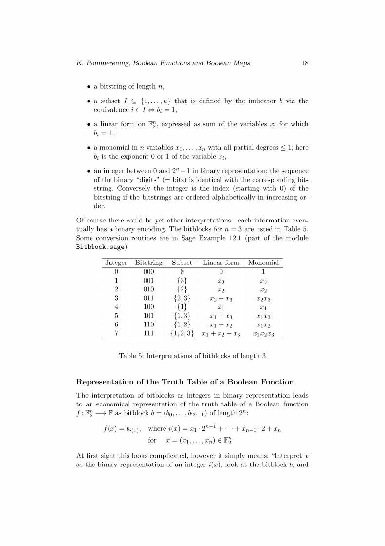
Of course there could be yet other interpretations—each information even-tually has a binary encoding. The bitblocks for n = 3 are listed in Table 5.Some conversion routines are in Sage Example 12.1 (part of the moduleBitblock.sage).
Integer Bitstring Subset Linear form Monomial
0 000 ∅ 0 11 001 {3} x3 x32 010 {2} x2 x23 011 {2, 3} x2 + x3 x2x34 100 {1} x1 x15 101 {1, 3} x1 + x3 x1x36 110 {1, 2} x1 + x2 x1x27 111 {1, 2, 3} x1 + x2 + x3 x1x2x3
Table 5: Interpretations of bitblocks of length 3
Representation of the Truth Table of a Boolean Function
The interpretation of bitblocks as integers in binary representation leadsto an economical representation of the truth table of a Boolean functionf : Fn
2 −→ F as bitblock b = (b0, . . . , b2n−1) of length 2n:
f(x) = bi(x), where i(x) = x1 · 2n−1 + · · ·+ xn−1 · 2 + xn
for x = (x1, . . . , xn) ∈ Fn2 .
At first sight this looks complicated, however it simply means: “Interpret xas the binary representation of an integer i(x), look at the bitblock b, and
K. Pommerening, Boolean Functions and Boolean Maps 19
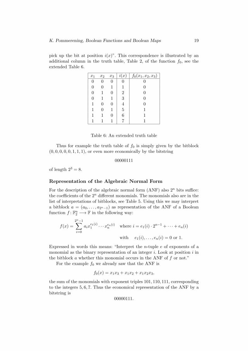
pick up the bit at position i(x)”. This correspondence is illustrated by anadditional column in the truth table, Table 2, of the function f0, see theextended Table 6.
x1 x2 x3 i(x) f0(x1, x2, x3)
0 0 0 0 00 0 1 1 00 1 0 2 00 1 1 3 01 0 0 4 01 0 1 5 11 1 0 6 11 1 1 7 1
Table 6: An extended truth table
Thus for example the truth table of f0 is simply given by the bitblock(0, 0, 0, 0, 0, 1, 1, 1), or even more economically by the bitstring
00000111
of length 23 = 8.
Representation of the Algebraic Normal Form
For the description of the algebraic normal form (ANF) also 2n bits suffice:the coefficients of the 2n different monomials. The monomials also are in thelist of interpretations of bitblocks, see Table 5. Using this we may interpreta bitblock a = (a0, . . . , a2n−1) as representation of the ANF of a Booleanfunction f : Fn
2 −→ F in the following way:
f(x) =2n−1∑i=0
aixe1(i)1 · · ·xen(i)n where i = e1(i) · 2n−1 + · · ·+ en(i)
with e1(i), . . . , en(i) = 0 or 1.
Expressed in words this means: “Interpret the n-tuple e of exponents of amonomial as the binary representation of an integer i. Look at position i inthe bitblock a whether this monomial occurs in the ANF of f or not.”
For the example f0 we already saw that the ANF is
f0(x) = x1x3 + x1x2 + x1x2x3,
the sum of the monomials with exponent triples 101, 110, 111, correspondingto the integers 5, 6, 7. Thus the economical representation of the ANF by abitstring is
00000111.
K. Pommerening, Boolean Functions and Boolean Maps 20
Caution! This is the same bitstring as for the truth table by accident—aspecial property of the function f0! The function f(x1, x2) = x1 hasthe truth table 0011 and the ANF 0010.
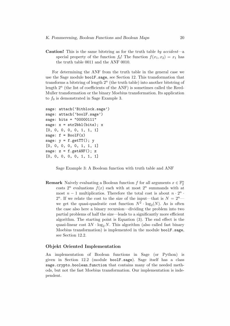
For determining the ANF from the truth table in the general case weuse the Sage module boolF.sage, see Section 12. This transformation thattransforms a bitstring of length 2n (the truth table) into another bitstring oflength 2n (the list of coefficients of the ANF) is sometimes called the Reed-Muller transformation or the binary Moebius transformation. Its applicationto f0 is demonstrated in Sage Example 3.
sage: attach(’Bitblock.sage’)
sage: attach(’boolF.sage’)
sage: bits = "00000111"
sage: x = str2bbl(bits); x
[0, 0, 0, 0, 0, 1, 1, 1]
sage: f = BoolF(x)
sage: y = f.getTT(); y
[0, 0, 0, 0, 0, 1, 1, 1]
sage: z = f.getANF(); z
[0, 0, 0, 0, 0, 1, 1, 1]
Sage Example 3: A Boolean function with truth table and ANF
Remark Naively evaluating a Boolean function f for all arguments x ∈ Fn2
costs 2n evaluations f(x) each with at most 2n summands with atmost n − 1 multiplicatios. Therefore the total cost is about n · 2n ·2n. If we relate the cost to the size of the input—that is N = 2n—we get the quasi-quadratic cost function N2 · log2(N). As is oftenthe case also here a binary recursion—dividing the problem into twopartial problems of half the size—leads to a significantly more efficientalgorithm. The starting point is Equation (3). The end effect is thequasi-linear cost 3N · log2N . This algorithm (also called fast binaryMoebius transformation) is implemented in the module boolF.sage,see Section 12.2.
Objekt Oriented Implementation
An implementation of Boolean functions in Sage (or Python) isgiven in Section 12.2 (module boolF.sage). Sage itself has a classsage.crypto.boolean function that contains many of the needed meth-ods, but not the fast Moebius transformation. Our implementation is inde-pendent.
K. Pommerening, Boolean Functions and Boolean Maps 21
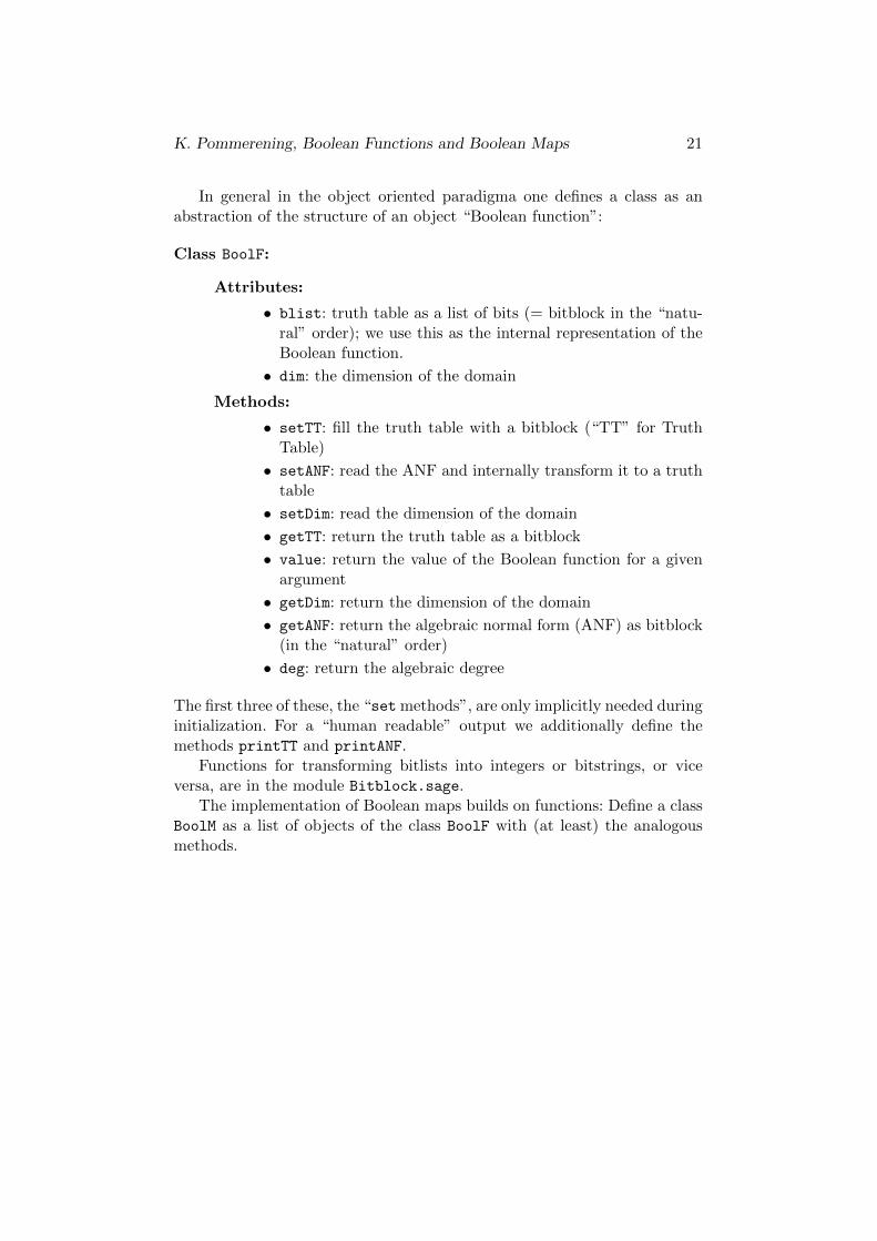
In general in the object oriented paradigma one defines a class as anabstraction of the structure of an object “Boolean function”:
Class BoolF:
Attributes:
• blist: truth table as a list of bits (= bitblock in the “natu-ral” order); we use this as the internal representation of theBoolean function.
• dim: the dimension of the domain
Methods:
• setTT: fill the truth table with a bitblock (“TT” for TruthTable)
• setANF: read the ANF and internally transform it to a truthtable
• setDim: read the dimension of the domain
• getTT: return the truth table as a bitblock
• value: return the value of the Boolean function for a givenargument
• getDim: return the dimension of the domain
• getANF: return the algebraic normal form (ANF) as bitblock(in the “natural” order)
• deg: return the algebraic degree
The first three of these, the “set methods”, are only implicitly needed duringinitialization. For a “human readable” output we additionally define themethods printTT and printANF.
Functions for transforming bitlists into integers or bitstrings, or viceversa, are in the module Bitblock.sage.
The implementation of Boolean maps builds on functions: Define a classBoolM as a list of objects of the class BoolF with (at least) the analogousmethods.
K. Pommerening, Boolean Functions and Boolean Maps 22
12 Appendix: Boolean Maps in Sage
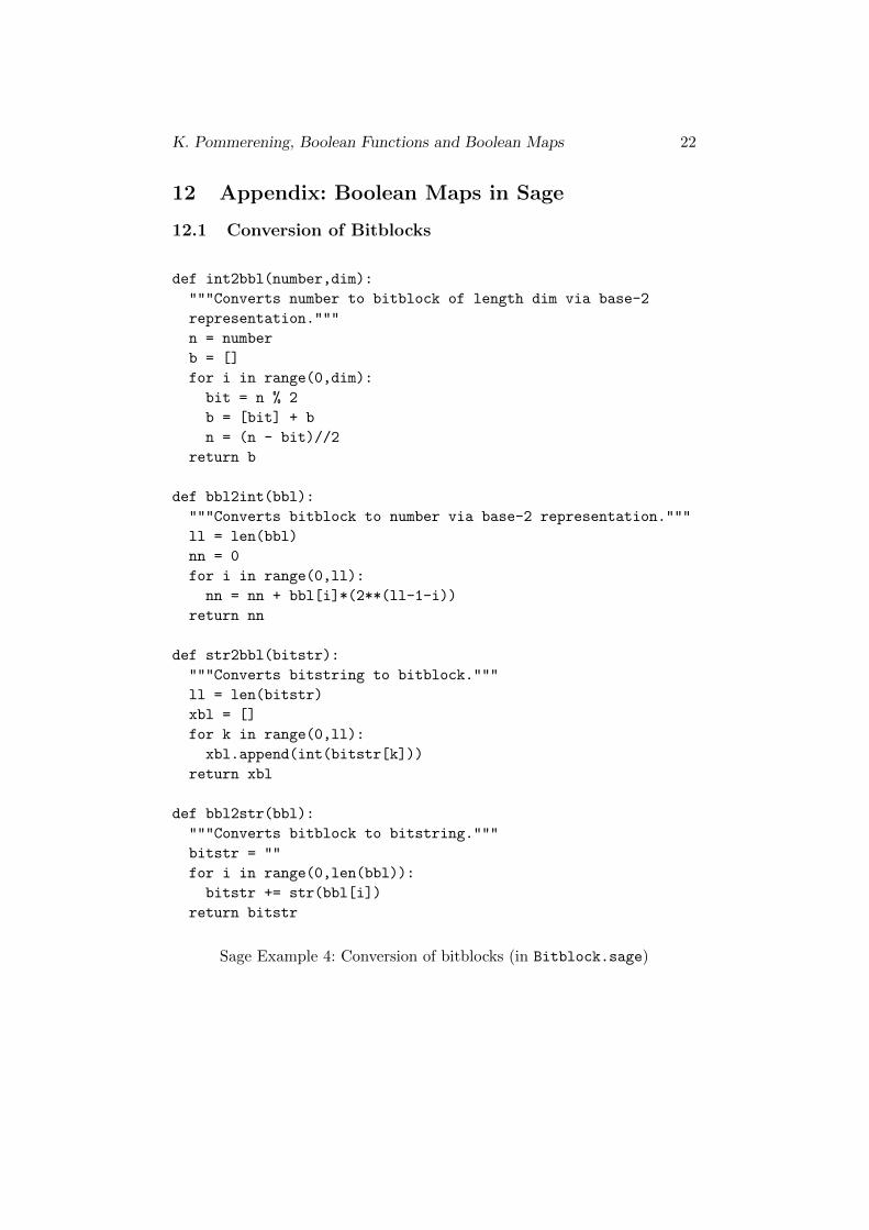
12.1 Conversion of Bitblocks
def int2bbl(number,dim):
"""Converts number to bitblock of length dim via base-2
representation."""
n = number
b = []
for i in range(0,dim):
bit = n % 2
b = [bit] + b
n = (n - bit)//2
return b
def bbl2int(bbl):
"""Converts bitblock to number via base-2 representation."""
ll = len(bbl)
nn = 0
for i in range(0,ll):
nn = nn + bbl[i]*(2**(ll-1-i))
return nn
def str2bbl(bitstr):
"""Converts bitstring to bitblock."""
ll = len(bitstr)
xbl = []
for k in range(0,ll):
xbl.append(int(bitstr[k]))
return xbl
def bbl2str(bbl):
"""Converts bitblock to bitstring."""
bitstr = ""
for i in range(0,len(bbl)):
bitstr += str(bbl[i])
return bitstr
Sage Example 4: Conversion of bitblocks (in Bitblock.sage)
K. Pommerening, Boolean Functions and Boolean Maps 23
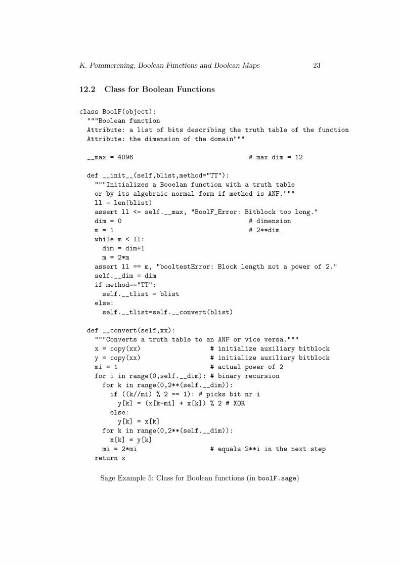
12.2 Class for Boolean Functions
class BoolF(object):
"""Boolean function
Attribute: a list of bits describing the truth table of the function
Attribute: the dimension of the domain"""
__max = 4096 # max dim = 12
def __init__(self,blist,method="TT"):
"""Initializes a Booelan function with a truth table
or by its algebraic normal form if method is ANF."""
ll = len(blist)
assert ll <= self.__max, "BoolF_Error: Bitblock too long."
dim = 0 # dimension
m = 1 # 2**dim
while m < ll:
dim = dim+1
m = 2*m
assert ll == m, "booltestError: Block length not a power of 2."
self.__dim = dim
if method=="TT":
self.__tlist = blist
else:
self.__tlist=self.__convert(blist)
def __convert(self,xx):
"""Converts a truth table to an ANF or vice versa."""
x = copy(xx) # initialize auxiliary bitblock
y = copy(xx) # initialize auxiliary bitblock
mi = 1 # actual power of 2
for i in range(0,self.__dim): # binary recursion
for k in range(0,2**(self.__dim)):
if ((k//mi) % 2 == 1): # picks bit nr i
y[k] = (x[k-mi] + x[k]) % 2 # XOR
else:
y[k] = x[k]
for k in range(0,2**(self.__dim)):
x[k] = y[k]
mi = 2*mi # equals 2**i in the next step
return x
Sage Example 5: Class for Boolean functions (in boolF.sage)
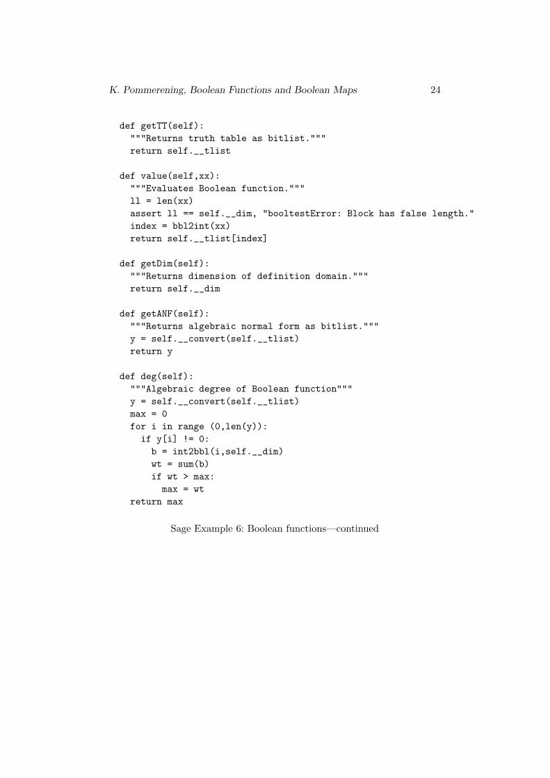
K. Pommerening, Boolean Functions and Boolean Maps 24
def getTT(self):
"""Returns truth table as bitlist."""
return self.__tlist
def value(self,xx):
"""Evaluates Boolean function."""
ll = len(xx)
assert ll == self.__dim, "booltestError: Block has false length."
index = bbl2int(xx)
return self.__tlist[index]
def getDim(self):
"""Returns dimension of definition domain."""
return self.__dim
def getANF(self):
"""Returns algebraic normal form as bitlist."""
y = self.__convert(self.__tlist)
return y
def deg(self):
"""Algebraic degree of Boolean function"""
y = self.__convert(self.__tlist)
max = 0
for i in range (0,len(y)):
if y[i] != 0:
b = int2bbl(i,self.__dim)
wt = sum(b)
if wt > max:
max = wt
return max
Sage Example 6: Boolean functions—continued
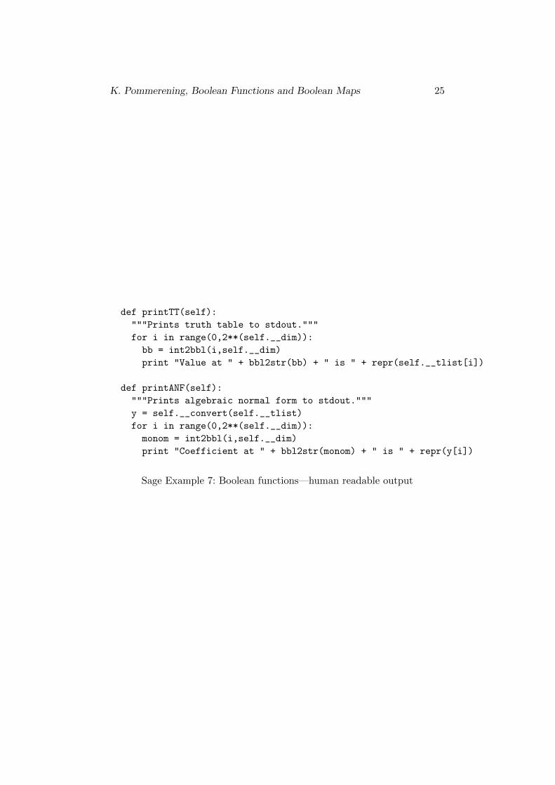
K. Pommerening, Boolean Functions and Boolean Maps 25
def printTT(self):
"""Prints truth table to stdout."""
for i in range(0,2**(self.__dim)):
bb = int2bbl(i,self.__dim)
print "Value at " + bbl2str(bb) + " is " + repr(self.__tlist[i])
def printANF(self):
"""Prints algebraic normal form to stdout."""
y = self.__convert(self.__tlist)
for i in range(0,2**(self.__dim)):
monom = int2bbl(i,self.__dim)
print "Coefficient at " + bbl2str(monom) + " is " + repr(y[i])
Sage Example 7: Boolean functions—human readable output
K. Pommerening, Boolean Functions and Boolean Maps 26
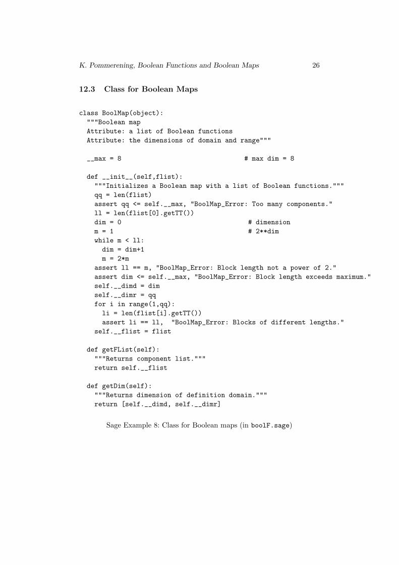
12.3 Class for Boolean Maps
class BoolMap(object):
"""Boolean map
Attribute: a list of Boolean functions
Attribute: the dimensions of domain and range"""
__max = 8 # max dim = 8
def __init__(self,flist):
"""Initializes a Boolean map with a list of Boolean functions."""
qq = len(flist)
assert qq <= self.__max, "BoolMap_Error: Too many components."
ll = len(flist[0].getTT())
dim = 0 # dimension
m = 1 # 2**dim
while m < ll:
dim = dim+1
m = 2*m
assert ll == m, "BoolMap_Error: Block length not a power of 2."
assert dim <= self.__max, "BoolMap_Error: Block length exceeds maximum."
self.__dimd = dim
self.__dimr = qq
for i in range(1,qq):
li = len(flist[i].getTT())
assert li == ll, "BoolMap_Error: Blocks of different lengths."
self.__flist = flist
def getFList(self):
"""Returns component list."""
return self.__flist
def getDim(self):
"""Returns dimension of definition domain."""
return [self.__dimd, self.__dimr]
Sage Example 8: Class for Boolean maps (in boolF.sage)
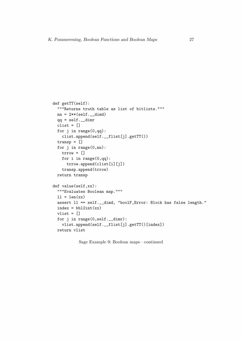
K. Pommerening, Boolean Functions and Boolean Maps 27
def getTT(self):
"""Returns truth table as list of bitlists."""
nn = 2**(self.__dimd)
qq = self.__dimr
clist = []
for j in range(0,qq):
clist.append(self.__flist[j].getTT())
transp = []
for j in range(0,nn):
trrow = []
for i in range(0,qq):
trrow.append(clist[i][j])
transp.append(trrow)
return transp
def value(self,xx):
"""Evaluates Boolean map."""
ll = len(xx)
assert ll == self.__dimd, "boolF_Error: Block has false length."
index = bbl2int(xx)
vlist = []
for j in range(0,self.__dimr):
vlist.append(self.__flist[j].getTT()[index])
return vlist
Sage Example 9: Boolean maps—continued