
Bose-Einstein condensation of erbium atoms for fractional ...
107
Bose-Einstein condensation of erbium atoms for fractional quantum Hall physics Dissertation zur Erlangung des Doktorgrades (Dr. rer. nat.) der Mathematisch-Naturwissenschaftlichen Fakult¨ at der Rheinischen Friedrich-Wilhelms-Universit¨ at Bonn vorgelegt von Daniel Frank Babik aus K¨ oln Bonn, November 2020
Transcript of Bose-Einstein condensation of erbium atoms for fractional ...
Bose-Einstein condensationof erbium atoms
for fractional quantum Hall physics
Dissertationzur
Erlangung des Doktorgrades (Dr. rer. nat.)
der
Mathematisch-Naturwissenschaftlichen Fakultat
der
Rheinischen Friedrich-Wilhelms-Universitat Bonn
vorgelegt von
Daniel Frank Babikaus
Koln
Bonn, November 2020

Angefertigt mit Genehmigung derMathematisch-Naturwissenschaftlichen Fakultat derRheinischen Friedrich-Wilhelms-Universitat Bonn
1. Gutachter: Prof. Dr. Martin Weitz2. Gutachter: Prof. Dr. Simon Stellmer
Tag der Promotion: 22.02.2021Erscheinungsjahr: 2021
Abstract
With the advent of ultracold atomic gases experimentally realized by laser cooling techniquesnearly 40 years ago, the doors to accessing novel physical behaviour have been opened wideand far. The possibility to prepare pure atomic samples of high coherence that can be preciselycontrolled and manipulated led to an abundance of opportunities for the study of fundamentalquantum physical laws. Highlights in this research domain include the realization of Bose-Einstein condensation in dilute gases, degenerate atomic Fermi gases and even novel molecularphysics. Experimentally, the investigation started with alkali atoms, proceeded with alkalineearth atoms, and only more recently laser cooling of atoms with higher complexity of theirspectrum, as e.g. the highly dipolar lanthanide atomic species erbium and dysprosium, wasrealized. Those elements possess a non-vanishing orbital angular momentum in the groundstate, leading to ample advantages for the manipulation with far-detuned laser light in phaseimprinting schemes, as losses due to spontaneous scattering can be suppressed radically incomparison to the case of alkali atomic species. This beneficial behaviour will be used in thefuture for the generation of synthetic magnetic fields for electrically neutral erbium atomsaimed at investigating fractional quantum Hall physics. It will also be interesting to studynovel interaction effects that due to the large dipole moment of the aforementioned lanthanideelements could arise in the context of artificial gauge fields.
This thesis describes in the first part the generation of an atomic erbium Bose-Einstein con-densate in a hybrid crossed optical dipole trap. The main purpose of this endeavor was anenhancement of absolute atom number of the degenerate ensemble and long-term stabilityof the experimental setup with respect to the use of a single beam dipole trap. Atoms areloaded from an atomic erbium beam originating from an oven located inside an ultra-highvacuum chamber with the help of a spin-flip Zeeman slower and a transversal cooling stage atthe transition wavelength near 400.91 nm wavelength into a narrow-line magneto-optical trapoperating near 582.84 nm wavelength. After spatially compressing this trap, the cold atomsare loaded into a hybrid crossed optical dipole trap realized with two far-detuned focusedlaser beams, a mid-infrared beam near 10.6µm wavelength emitted by a CO2 laser and atransverse beam near 1.064µm wavelength emitted by a Nd:YAG laser, and are subsequentlyevaporatively cooled until quantum degeneracy is reached. Starting from 5 · 107 atoms in thecompressed magneto-optical trap, 7 · 106 atoms are loaded into the optical dipole trap, andfinally a Bose-Einstein condensate with 3.5 · 104 atoms is realized. Here the critical temper-ature for the phase transition to a Bose-Einstein condensate was experimentally determinedto be around 170 nK. The condensate is spin-polarized, and has a lifetime of up to 12 s. Also,a comparison of the here achieved results with respect to those achieved in only a single CO2
laser beam dipole trap is presented.
In the second part of this thesis a theoretical evaluation of the generation of synthetic mag-netic fields for ultracold erbium atoms in prospect for experimental investigations of fractionalquantum Hall physics is given. One of the most promising techniques for the realization of
iii
strong synthetic magnetic fields is by phase imprinting via Raman manipulation. Here forthe theoretical calculation of such fields with erbium atoms a compared to earlier work onalkali atoms new modified optical Raman coupling scheme in a σ+ − σ− beam polarizationconfiguration is chosen. It is shown that sufficiently high field strengths with good spatialhomogeneity can be reached for experimentally viable parameters. Additionally, an estima-tion for the expected Laughlin gap in the proposed erbium atomic fractional quantum Hallsystem is given.
For the future, it will be important to experimentally realize the expected possible largesynthetic magnetic fields for a quantum gas of ultracold erbium atoms. Already at moderatesynthetic field strengths, the study of vortices in such a dipolar quantum gas is an interestingtopic. For larger field strengths the reaching of the fractional quantum Hall regime for theultracold atomic gas sample is expected. On the theoretical side, here work describing theform of the ground state in the presence of both the synthetic magnetic field and dipolarinteractions is of utmost importance.
Publication list
D. Babik, R. Roell, D. Helten, M. Fleischhauer, and M. Weitz, Synthetic magnetic fields forcold erbium atoms, Phys. Rev. A 101, 053603 (2020)
J. Ulitzsch, D. Babik, R. Roell, and M. Weitz, Bose-Einstein condensation of erbium atomsin a quasielectrostatic optical dipole trap, Phys. Rev. A 95, 043614 (2017)
iv


Contents
1 Introduction 1
2 Theoretical background: Ultracold atomic erbium quantum gases 52.1 Low-temperature behaviour of Bose gases . . . . . . . . . . . . . . . . . . . . 5
2.2 Some properties of the atomic erbium system . . . . . . . . . . . . . . . . . . 7
2.2.1 Energy level scheme and relevant transitions . . . . . . . . . . . . . . 8
2.3 Background on an experimental realization of a Bose-Einstein condensate . . 11
2.3.1 Laser cooling . . . . . . . . . . . . . . . . . . . . . . . . . . . . . . . . 12
2.3.2 Magneto-optical trap . . . . . . . . . . . . . . . . . . . . . . . . . . . . 14
2.3.3 Single and hybrid crossed optical dipole traps . . . . . . . . . . . . . . 17
2.3.4 Evaporative cooling . . . . . . . . . . . . . . . . . . . . . . . . . . . . 24
3 Experimental setup 293.1 Experimental overview . . . . . . . . . . . . . . . . . . . . . . . . . . . . . . . 29
3.2 Vacuum system . . . . . . . . . . . . . . . . . . . . . . . . . . . . . . . . . . . 30
3.3 Optical setup . . . . . . . . . . . . . . . . . . . . . . . . . . . . . . . . . . . . 33
3.3.1 Blue laser light setup . . . . . . . . . . . . . . . . . . . . . . . . . . . . 34
3.3.2 Yellow laser light setup . . . . . . . . . . . . . . . . . . . . . . . . . . 35
3.3.3 CO2 laser radiation setup . . . . . . . . . . . . . . . . . . . . . . . . . 37
3.3.4 Nd:YAG laser light setup . . . . . . . . . . . . . . . . . . . . . . . . . 39
3.4 Measurement methods . . . . . . . . . . . . . . . . . . . . . . . . . . . . . . . 41
3.4.1 Absorption imaging . . . . . . . . . . . . . . . . . . . . . . . . . . . . 41
3.4.2 Trap frequency measurements and phase space density determination 43
4 Characterization of the setup and experimental results 474.1 Magneto-optical trap . . . . . . . . . . . . . . . . . . . . . . . . . . . . . . . . 47
4.1.1 Loading of the magneto-optical trap . . . . . . . . . . . . . . . . . . . 47
4.1.2 Compressing process . . . . . . . . . . . . . . . . . . . . . . . . . . . . 48
4.2 Characterization of single and hybrid crossed dipole trap . . . . . . . . . . . . 51
4.2.1 Loading process . . . . . . . . . . . . . . . . . . . . . . . . . . . . . . 51
4.2.2 Trap frequencies . . . . . . . . . . . . . . . . . . . . . . . . . . . . . . 53
4.2.3 Holding time and temperature . . . . . . . . . . . . . . . . . . . . . . 54
4.2.4 Spin-polarization . . . . . . . . . . . . . . . . . . . . . . . . . . . . . . 55
4.3 Evaporative cooling of atoms . . . . . . . . . . . . . . . . . . . . . . . . . . . 57
4.3.1 Evaporation ramp . . . . . . . . . . . . . . . . . . . . . . . . . . . . . 58
4.3.2 Characterization of the atomic ensemble during evaporation . . . . . . 59
4.4 Bose-Einstein condensation of erbium atoms . . . . . . . . . . . . . . . . . . . 62
4.4.1 Bimodal density distribution . . . . . . . . . . . . . . . . . . . . . . . 62
4.4.2 Phase space density . . . . . . . . . . . . . . . . . . . . . . . . . . . . 62
4.4.3 Condensate holding time . . . . . . . . . . . . . . . . . . . . . . . . . 64
vii
Contents
4.4.4 Long-term stability . . . . . . . . . . . . . . . . . . . . . . . . . . . . . 65
5 Prospects for synthetic magnetic fields for ultracold erbium atoms 695.1 Introduction to synthetic gauge fields . . . . . . . . . . . . . . . . . . . . . . . 69
5.1.1 Review: Gauge fields for charged particles . . . . . . . . . . . . . . . . 705.2 Synthetic magnetic fields for three-level atoms . . . . . . . . . . . . . . . . . . 71
5.2.1 Hamiltonian and dispersion relation . . . . . . . . . . . . . . . . . . . 715.2.2 Vector potential and synthetic gauge field . . . . . . . . . . . . . . . . 74
5.3 Synthetic magnetic fields for erbium atoms . . . . . . . . . . . . . . . . . . . 745.3.1 Hamiltonian and dispersion relation . . . . . . . . . . . . . . . . . . . 755.3.2 Vector potential and synthetic gauge field . . . . . . . . . . . . . . . . 78
5.4 Laughlin-Gap . . . . . . . . . . . . . . . . . . . . . . . . . . . . . . . . . . . . 81
6 Conclusion and outlook 85
Appendix 87
Bibliography 89
viii
1 Introduction
The generation of ultracold atomic gases offers the possibility to study a wide range of quan-tum phenomena in a very pure and well controllable system, with vibrant research activitysince the mid 1980s. One of the highlights achieved with cold atoms is the demonstration ofBose-Einstein condensation, an effect theoretically discovered roughly 100 years ago. In 1924A. Einstein predicted a new state of matter in the wake of his work on quantum statisticsof massive bosonic particles, i.e. particles with integer spin: the Bose-Einstein condensate(BEC) [1–3]. Here single atoms are fully delocalized and the lowest energy state is macroscop-ically occupied, mathematically expressible by a single wavefunction describing the motionof the whole ensemble of particles, which is highly advantageous or often even absolutelyessential for the study of quantum mechanical phenomena.
To reach such a condensate in atomic systems, the ensemble has to be cooled to ultralowtemperatures typically in the nK regime, as the thermal de Broglie wavelength has to belarger than the average distance between the particles. The first experimental realization inthe gaseous phase was achieved in 1995 by the groups of C. E. Wieman and E. A. Cornell aswell as W. Ketterle [4,5]. From then on many fundamental experiments regarding the coher-ence of macroscopic quantum states, novel quantum phases in optical lattices and interactionaspects of ultracold bound states were conducted with the help of BECs [6–8]. Importantly,Bose-Einstein condensates can be used for simulations of physics of other domains. One ofthe most notable areas has to be solid-state physics with systems that are generally not asflexible and easily manipulated as in the quantum optics case, where e.g. periodic structurescan here be emulated by tunable optical lattices. A well-known example in this domain is thetransition from a superfluid to a Mott-insulator [9]. Notable other experiments involve thedetection of Bloch oscillations, and the study of topologically protected edge states [10, 11].Besides variations of trapping potentials and irradiation with light fields, one popular way ofmanipulating ultracold atomic ensembles is by modifying the inter-particle interaction, whichcan be attractive, vanishing, or repulsive, with the help of an external magnetic field, whereat distinct magnetic field strengths Feshbach resonances can occur [12–15].
Experimental simulations with BECs also come in handy when time dynamics of systemsbecome too complex to study numerically, as e.g. for out-of-equilibrium interacting quan-tum matter [16]. Further research areas of interest for such simulations include fundamentalconcepts of statistical physics [17], and possibly quantum chemistry as well as high-energyphysics [18]. Bose-Einstein condensation was also achieved for polaritons as well as pho-tons [19, 20], where condensation is achieved at higher temperatures [20, 21]. Besides Bose-Einstein condensates, also degenerate quantum gases with fermionic atoms and correspondingFermi-Dirac statistics could be realized experimentally [22–24], offering the possibility of aplethora of studies, as e.g. Fermi-Hubbard physics in optical lattices, aiding in the under-standing of high-temperature superconductivity [25].
1
1 Introduction
While in earlier works with cold atoms most of the Bose-Einstein condensates and degen-erate Fermi gases were generated with elements from the group of the alkali atoms, as e.g.rubidium [4], which exhibit a comparatively simple electronic level structure due to theirsingle valence electron, and later with elements from the group of the alkaline earth atoms,as e.g. strontium [26], which possess two valence electrons and feature a richer spectrum, afew years thereafter studies on spectrally very complex atomic species as e.g. the lanthanidesfrom the group of rare earth metals increased, leading to the Bose-Einstein condensation anddegenerate Fermi gas generation of several magnetic elements like dysprosium [27,28], ytter-bium [29], and erbium [30,31], or in the case of thulium and holmium to laser-cooled atomicensembles [32–34]. Additionally dipolar quantum mixtures of erbium and dysprosium havebeen realized [35]. Both dysprosium and erbium exhibit very rich spectra, and feature bosonicas well as fermionic isotopes with high relative occurrence, a non-vanishing electronic orbitalangular momentum in their electronic ground states, which amount to L = 6 and L = 5respectively, and high magnetic moments of 10 and 7 Bohr magnetons respectively. Reasonfor the complex energy spectra of lanthanides, with many transitions of various linewidthsranging from broad to ultra-narrow, are their incompletely filled 4f electron shells, leading toa so-called submerged shell structure, as the 4f shells are surrounded by the completely filledouter-lying 6s shell. For both dysprosium and erbium the d-wave collapse due to dipole-dipoleinteractions, as well as an abundance of Feshbach resonances, stemming from the lanthanidesintricate electronic energy level structures, could be observed and described by random ma-trix theory [36, 37]. Other research in conjunction with dipolar physics included Fermi sur-face deformations, Feshbach-induced erbium molecules, an extended Bose-Hubbard modelaccounting for dipole-dipole-interactions, anisotropic collisions, BEC crossovers to dipolarmacrodroplets, and studies of dipolar supersolids [38–43].
Ultracold atoms as a quantum simulator could also be used in the study of novel topologicalphases of matter that form in the sample when subjected to strong magnetic fields [44]. Inthis regard very interesting phenomena are expected for fractional quantum Hall states, assome of those could exhibit non-Abelian properties to possibly form topologically protectedqubits [45], a feature that is highly sought after as current implementations of quantum com-puters despite tremendous advances in the field still suffer from non-robustness for too highnumbers of qubits. As quantum Hall physics is normally only observable for charged particlessubject to strong magnetic fields, for the electrically neutral ultracold lanthanide atomic casestrong artificial magnetic fields via optical Raman manipulation have to be generated.
Prior experiments with the alkali atomic species rubidium were successful in creating syn-thetic magnetic fields, resulting in the observation of vortices in the rubidium BEC [46].However, the maximum strength of the synthetic magnetic field is in alkali atoms based im-plementations using a phase imprinting scheme limited by the maximum useable detuningof the Raman light field. Elements from the group of the alkali atoms exhibit a S-groundstate, i.e. possess an electronic orbital angular momentum of L = 0. The state-dependentmanipulation with laser light of these atoms requires a detuning of magnitude below thesize of the fine structure splitting of the electronically excited state [47]. Otherwise the en-ergy shifts of all ground state levels become identical and are not dependent of the magneticquantum number any more [48]. To prevent this behaviour the detuning of state-dependentoptical lattices for example has to be chosen smaller than the fine structure, leading to higherphoton scattering rates and therefore shorter coherence times of the BECs. Using erbium
2
or dysprosium atoms and their corresponding L 6= 0 ground state, such decoherence effectscan be avoided, allowing state-dependent lattices with higher detuning, leading to longer co-herence times [49]. Moreover, Raman manipulation between different ground state Zeemansublevels, as of interest for the synthetization of large magnetic fields by phase imprinting,should then be possible with large detuning and corresponding long coherence times. Forsufficiently strong synthetic magnetic fields studies of fractional quantum Hall physics withultracold quantum gases could become possible [50,51].
Specifically for the erbium system, the first realization of a magneto-optical trap (MOT),the latter being the standard tool to prepare a laser cooled ensemble as a first step in coldatom experiments, has despite the complex electronic structure of this lanthanide atomicspecies been achieved by McClelland and Hansen [52]. Further, evaporative cooling of theseatoms due to their high dipolar moments and associated interaction effects require the use oftraps being able to confine atoms in the lowest energetic Zeeman component of the electronicground state, as possible with optical dipole traps. In earlier work of our group an experimentwas built up which successfully prepared an ultracold atomic ensemble of erbium in a magneto-optical trap [53, 54], which was subsequently loaded into a quasi-electrostatic optical dipoletrap realized by a focused CO2 laser beam, where atoms were in a first step evaporativelycooled down to a few µK [55]. However due to the broad linewidth and the consequent highDoppler temperature of the 401 nm transition, together with the relatively high branchingratio of the transition, the losses during the cooling procedure were so high, that a BEC wasultimately not attainable. By using two cooling transitions, the 401 nm transition for slowingof the atomic beam on its way to the MOT chamber in a Zeeman slower, and the more nar-row 583 nm transition for the actual trapping process, the group around F. Ferlaino finallymanaged to generate an erbium BEC. There after loading atoms from the narrow-line MOTinto a crossed dipole trap formed by two laser beams at 1075 nm and 1064 nm wavelength,respectively, evaporative cooling was performed until quantum degeneracy was reached [30].Enthused by the narrow-line magneto-optical trap setup, our working group was successful increating an erbium BEC by evaporating atoms in a single beam CO2 laser dipole trap [56,57].
In the here presented thesis, a hybrid crossed dipole trap, consisting of a focused mid-infraredbeam of a CO2 laser operating near 10.6µm wavelength and a Nd:YAG laser beam near1064 nm wavelength, was realized. Erbium atoms loaded in such a trap were evaporativelycooled to Bose-Einstein condensation. Compared to the single beam CO2 laser dipole trappinggeometry, an increased atom number in the condensate and an improved long-term stabilitywere achieved. A comparison of results obtained in both the single beam CO2 laser dipoletrap and the new hybrid crossed dipole trapping geometry is presented.
In further work contained in this thesis, a proposal to realize strong synthetic magneticfields with cold erbium atoms is given based on phase imprinting by Raman manipulation.The unusual electronic structure of this rare earth multi-level atom is expected to allow forlarge synthetic magnetic fields. An estimate for the size of the Laughlin gap of the proposedtwo-dimensional system, devised for the future observation of the fractional quantum Halleffect, is given.
The work presented here consists of six chapters, with the introduction at hand being Chap. 1.In the following Chap. 2 properties of atomic erbium are described, and theoretical consider-
3
1 Introduction
ations regarding the various experimental steps for generating a Bose-Einstein condensate oferbium atoms are laid out. Chap. 3 shows the experimental setup and methods, including thevacuum apparatus and the employed light sources, as well as the controlling setup of the opti-cal dipole trap light. In the subsequent Chap. 4 a characterization of the experimental setupand the obtained experimental results are given. The theoretical derivation of a syntheticmagnetic field for ultracold erbium atoms is conducted in Chap. 5, followed by a look on theLaughlin gap of the described system. The thesis closes with a conclusion and an outlook onfuture prospects in Chap. 6. There further plans for the next theoretical and experimentalsteps are outlined.
4
2 Theoretical background: Ultracold atomicerbium quantum gases
The generation of Bose-Einstein condensates involves several experimental steps, here tai-lored for the erbium atomic case. Below theoretical considerations for the understanding ofthe experiment are presented, starting with the treatment of ultracold Bose gases in a har-monic trapping potential, followed by a review of important properties of atomic erbium, andproceeded with the theoretical discussion regarding the at this experiment employed stagesfor the realization of an erbium Bose-Einstein condensate.
2.1 Low-temperature behaviour of Bose gases
S. N. Bose first introduced the concept of an ideal Bose gas consisting of free, non-interactingparticles via Bose-statistics [3], which was extended to massive bosons by A. Einstein, whoalso predicted a phase transition of a thermal Bose gas to a Bose-Einstein condensate [2],where the particles occupy the ground state of the system macroscopically, leading to a singlewavefunction for the whole ensemble. It takes place for sufficiently high phase space densi-ties, that can be achieved by increasing the density and decreasing the temperature of theensemble below a critical non-vanishing temperature. This phase transition works only forbosonic particles with integer spin, which exhibit a symmetric multi-particle wavefunction,and therefore can be in the same quantum mechanical state simultaneously as the Pauli prin-ciple does not hold. In contrast for fermions with half-integer spin, the Pauli principle holdsand a quantum mechanial state cannot be occupied by two or more fermions with the sameset of quantum numbers [58].
The below mathematical treatment follows [6, 56, 59]. Consider N bosonic atoms trappedin an external harmonic potential, so that the particles act as N individual harmonic oscilla-tors, an approximation for the center of mass motion of the whole ensemble. The potentialfor each particle will take the form of
Vext(r) = 12m(ω2
xx2 + ω2
yy2 + ω2
zz2) (2.1)
with position space vector r = (x, y, z), mass m of the bosons, and trap frequencies ωx,y,z.For a dilute gas we can neglect the atom-atom interaction, and the system’s Hamiltonian canbe written as the sum of single-particle Hamiltonians with energy levels
ε(nx, ny, nz) =(nx + 1
2
)~ωx +
(ny + 1
2
)~ωy +
(nz + 1
2
)~ωz, (2.2)
where ~ = h/2π is the reduced Planck constant, and for the quantum numbers nx,y,z it holdsthat nx,y,z ∈ N. In the case of grand canonical ensembles the mean occupation number〈n(εnx,ny ,nz)〉 of state |nx, ny, nz〉 with energy ε(nx, ny, nz) is defined by
5
2 Theoretical background: Ultracold atomic erbium quantum gases
〈n(εnx,ny ,nz)〉 =1
e(εnx,ny,nz−µ)/kBT − 1, (2.3)
where all εnx,ny ,nz > µ, with µ being the chemical potential, kB the Boltzmann constant, andT the temperature. Here µ is fixed by the total particle number
N =∑
nx,ny ,nz
1
e(εnx,ny,nz−µ)/kBT − 1, (2.4)
but is still a function of the temperature T . To calculate the critical temperature one hasfirst to determine the density of states g(ε). By integrating Eq. 2.4 one obtains the numberof states G(ε) below energy ε (excluding the zero-point energy), and finally can calculate thedensity of states as g(ε) = dG/dε = ε2/(2~3ωxωyωz). As a next step the number of excitedstates for a vanishing chemical potential can be considered via
Nex =
∫ ∞0
dεg(ε)〈n(ε, µ = 0)〉. (2.5)
With this condition the critical temperature Tc is defined as the highest temperature at whicha macroscopical occupation of the lowest energy state appears, and the following holds:
N = Nex(Tc) =
∫ ∞0
dεg(ε)1
eε/kBTc − 1. (2.6)
Solving Eq. 2.6 leads to the critical temperature as
Tc =~kB
(ωxωyωzN
ζ(3)
)1/3
≈ 0,94 · ~ωkBN1/3. (2.7)
where ζ(α) is Riemann’s Zeta function, and ω = (ωxωyωz)1/3 is the geometric average of
the oscillator frequencies. As long as the temperature is below the critical temperature Tc,a macroscopically occupation of the lowest energy level is possible. With in this experimenttypical values for the mean trap frequency of about ω = 2π · 93 Hz, and for the atom numberof approximately 3.5 · 104, the phase transition from an ideal Bose gas to a Bose-Einsteincondensate should theoretically occur at a critical temperature of Tc = 136 nK. The fractionof atoms in the condensate for temperatures below Tc can be calculated via the relation
N0
N= 1−
(T
Tc
)3
, (2.8)
where N0 is the atom number in the ground state, N is the total atom number, and T < Tc
is the temperature of the ensemble. For a temperature of T = 0 the gas would theoreticallycondensate completely.
6
2.2 Some properties of the atomic erbium system
Bosons can be considered as quantum mechanical objects that appear in the form of wavepack-ets with size in the order of the de-Broglie wavelength λdB =
√2π~2/(mkBT ). Near the
critical temperature interparticle distances become comparable to λdB, and the wavepacketsstart to overlap. The phase space density ρ is an important marker in determing the currentphase the ensemble exhibits. It is defined as the number of particles in a cube of edge lengthequal to the thermal de Broglie wavelength λdB:
ρ = nλ3dB = n
(2π~2
mkBT
)3/2
. (2.9)
When the critical phase space density ρc is reached, the transition to quantum degeneracyoccurs. The resulting macroscopical wavefunction from the overlapping wavepackets canbe interpreted as the Bose-Einstein condensate. Assuming a uniform Bose gas in a three-dimensional box with volume V the critical temperature can be calculated as
Tc =2π
kB[ζ(3/2)]3/2~2n3/2
m≈ 3.31 · ~
2n3/2
m, (2.10)
where n = N/V is the particle number density. Using Eq. 2.9 and Eq. 2.10 one obtains thecritical phase space density as
ρc ≈ 2.612. (2.11)
Thus for the preparation of a Bose-Einstein condensate the atoms must be prepared as denseand cool as possible. On the other hand measurements of the phase space density can providea neat way to experimentally verify if Bose-Einstein condensation occured.
2.2 Some properties of the atomic erbium system
Erbium is one of the chemical elements in the lanthanide series with atomic number of Z = 68and atomic mass of 167.26 amu, with 1 amu = 1.6605402 · 10−27 kg [60], discovered in a mix-ture of rare earth metal elements, which show similar geochemical characteristics, in 1843,and first successfully isolated in 1934 [61–63]. Naturally, erbium occurs mostly in chemicalcompounds as e.g. monazites, a brown phosphate ore mineral. Pure solid erbium appearsas a soft, silvery-white metal if kept away from air, as it would otherwise oxidize slowly tothe tarnished erbium(III) oxide. It possesses a melting point of 1802 K and a boiling point of3136 K [64].
Besides the many qualities of ionic erbium Er3+ as a doping agent for crystals in technical andscientific applications ranging from telecommunications to quantum storage and even medicaltherapies [65–69], another outstanding feature is found for atomic erbium with its high mag-netic moment of 7µB, where µB is the Bohr magneton [70], which belongs to the strongestmagnetic moments in the periodic table, leading to interesting dipolar effects observable inthe ultracold regime. In comparison alkali metals only possess a magnetic moment of 1µB. Innature there exist six different stable isotopes of erbium, five bosonic and one fermionic, with
7
2 Theoretical background: Ultracold atomic erbium quantum gases
Isotope Abundance [%] Nuclear spin I[~]
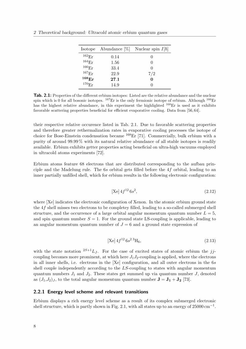
162Er 0.14 0164Er 1.56 0166Er 33.4 0167Er 22.9 7/2168Er 27.1 0170Er 14.9 0
Tab. 2.1: Properties of the different erbium isotopes: Listed are the relative abundance and the nuclearspin which is 0 for all bosonic isotopes. 167Er is the only fermionic isotope of erbium. Although 166Erhas the highest relative abundance, in this experiment the highlighted 168Er is used as it exhibitsfavorable scattering properties beneficial for efficient evaporative cooling. Data from [56,64].
their respective relative occurence listed in Tab. 2.1. Due to favorable scattering propertiesand therefore greater rethermalization rates in evaporative cooling processes the isotope ofchoice for Bose-Einstein condensation became 168Er [71]. Commercially, bulk erbium with apurity of around 99.99 % with its natural relative abundance of all stable isotopes is readilyavailable. Erbium exhibits getter properties acting beneficial on ultra-high vacuums employedin ultracold atoms experiments [72].
Erbium atoms feature 68 electrons that are distributed corresponding to the aufbau prin-ciple and the Madelung rule. The 6s orbital gets filled before the 4f orbital, leading to aninner partially unfilled shell, which for erbium results in the following electronic configuration:
[Xe] 4f12 6s2, (2.12)
where [Xe] indicates the electronic configuration of Xenon. In the atomic erbium ground statethe 4f shell misses two electrons to be completey filled, leading to a so-called submerged shellstructure, and the occurrence of a large orbital angular momentum quantum number L = 5,and spin quantum number S = 1. For the ground state LS-coupling is applicable, leading toan angular momentum quantum number of J = 6 and a ground state expression of
[Xe] 4f12 6s2 3H6, (2.13)
with the state notation 2S+1LJ . For the case of excited states of atomic erbium the jj-coupling becomes more prominent, at which here J1J2-coupling is applied, where the electronsin all inner shells, i.e. electrons in the [Xe] configuration, and all outer electrons in the 6sshell couple independently according to the LS-coupling to states with angular momentumquantum numbers J1 and J2. These states get summed up via quantum number J , denotedas (J1,J2)J , to the total angular momentum quantum number J = J1 + J2 [73].
2.2.1 Energy level scheme and relevant transitions
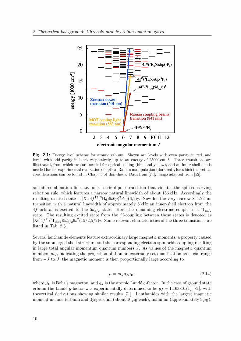
Erbium displays a rich energy level scheme as a result of its complex submerged electronicshell structure, which is partly shown in Fig. 2.1, with all states up to an energy of 25000 cm−1.
8
2.2 Some properties of the atomic erbium system
Wavelength [nm] Energy[cm−1
]Natural linewidth
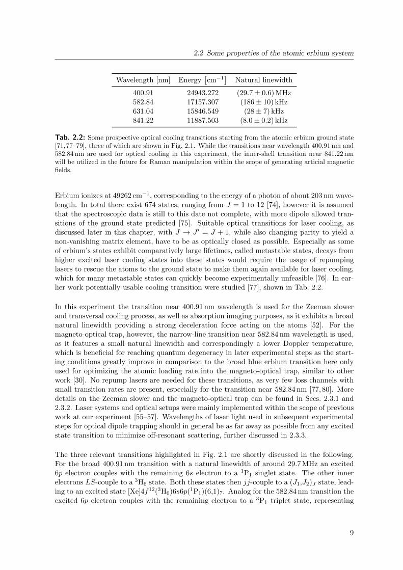
400.91 24943.272 (29.7± 0.6) MHz582.84 17157.307 (186± 10) kHz631.04 15846.549 (28± 7) kHz841.22 11887.503 (8.0± 0.2) kHz
Tab. 2.2: Some prospective optical cooling transitions starting from the atomic erbium ground state[71,77–79], three of which are shown in Fig. 2.1. While the transitions near wavelength 400.91 nm and582.84 nm are used for optical cooling in this experiment, the inner-shell transition near 841.22 nmwill be utilized in the future for Raman manipulation within the scope of generating articial magneticfields.
Erbium ionizes at 49262 cm−1, corresponding to the energy of a photon of about 203 nm wave-length. In total there exist 674 states, ranging from J = 1 to 12 [74], however it is assumedthat the spectroscopic data is still to this date not complete, with more dipole allowed tran-sitions of the ground state predicted [75]. Suitable optical transitions for laser cooling, asdiscussed later in this chapter, with J → J ′ = J + 1, while also changing parity to yield anon-vanishing matrix element, have to be as optically closed as possible. Especially as someof erbium’s states exhibit comparatively large lifetimes, called metastable states, decays fromhigher excited laser cooling states into these states would require the usage of repumpinglasers to rescue the atoms to the ground state to make them again available for laser cooling,which for many metastable states can quickly become experimentally unfeasible [76]. In ear-lier work potentially usable cooling transition were studied [77], shown in Tab. 2.2.
In this experiment the transition near 400.91 nm wavelength is used for the Zeeman slowerand transversal cooling process, as well as absorption imaging purposes, as it exhibits a broadnatural linewidth providing a strong deceleration force acting on the atoms [52]. For themagneto-optical trap, however, the narrow-line transition near 582.84 nm wavelength is used,as it features a small natural linewidth and correspondingly a lower Doppler temperature,which is beneficial for reaching quantum degeneracy in later experimental steps as the start-ing conditions greatly improve in comparison to the broad blue erbium transition here onlyused for optimizing the atomic loading rate into the magneto-optical trap, similar to otherwork [30]. No repump lasers are needed for these transitions, as very few loss channels withsmall transition rates are present, especially for the transition near 582.84 nm [77, 80]. Moredetails on the Zeeman slower and the magneto-optical trap can be found in Secs. 2.3.1 and2.3.2. Laser systems and optical setups were mainly implemented within the scope of previouswork at our experiment [55–57]. Wavelengths of laser light used in subsequent experimentalsteps for optical dipole trapping should in general be as far away as possible from any excitedstate transition to minimize off-resonant scattering, further discussed in 2.3.3.
The three relevant transitions highlighted in Fig. 2.1 are shortly discussed in the following.For the broad 400.91 nm transition with a natural linewidth of around 29.7 MHz an excited6p electron couples with the remaining 6s electron to a 1P1 singlet state. The other innerelectrons LS-couple to a 3H6 state. Both these states then jj-couple to a (J1,J2)J state, lead-ing to an excited state [Xe]4f12(3H6)6s6p(1P1)(6,1)7. Analog for the 582.84 nm transition theexcited 6p electron couples with the remaining electron to a 3P1 triplet state, representing
9
2 Theoretical background: Ultracold atomic erbium quantum gases
5
Fig. 2.1: Energy level scheme for atomic erbium. Shown are levels with even parity in red, andlevels with odd parity in black respectively, up to an energy of 25000 cm−1. Three transitions areillustrated, from which two are needed for optical cooling (blue and yellow), and an inner-shell one isneeded for the experimental realization of optical Raman manipulation (dark red), for which theoreticalconsiderations can be found in Chap. 5 of this thesis. Data from [74], image adapted from [52].
an intercombination line, i.e. an electric dipole transition that violates the spin-conservingselection rule, which features a narrow natural linewidth of about 186 kHz. Accordingly theresulting excited state is [Xe]4f12(3H6)6s6p(3P1)(6,1)7. Now for the very narrow 841.22 nmtransition with a natural linewidth of approximately 8 kHz an inner-shell electron from the4f orbital is excited to the 5d5/2 state. Here the remaining electrons couple to a 4I15/2
state. The resulting excited state from the jj-coupling between those states is denoted as[Xe]4f11(4I15/2)5d5/26s2(15/2,5/2)7. Some relevant characteristics of the three transitions arelisted in Tab. 2.3.
Several lanthanide elements feature extraordinary large magnetic moments, a property causedby the submerged shell structure and the corresponding electron spin-orbit coupling resultingin large total angular momentum quantum numbers J . As values of the magnetic quantumnumbers mJ , indicating the projection of J on an externally set quantization axis, can rangefrom −J to J , the magnetic moment is then proportionally large according to
µ = mJgJµB, (2.14)
where µB is Bohr’s magneton, and gJ is the atomic Lande g-factor. In the case of ground stateerbium the Lande g-factor was experimentally determined to be gJ = 1.163801(1) [81], withtheoretical derivations showing similar results [71]. Lanthanides with the largest magneticmoment include terbium and dysprosium (about 10µB each), holmium (approximately 9µB),
10
2.3 Background on an experimental realization of a Bose-Einstein condensate
Wavelength λ [nm] 400.91 582.84 841.22
Transition rate Γ[s−1]
1.9 · 108 1.2 · 106 5.0 · 104
Natural linewidth ∆ν [MHz] 29.7 0.186 0.008Saturation intensity IS [mW/cm2] 60.3 0.13 0.002Doppler temperature TD [µK] 714 4.6 0.2Recoil temperature TR [nK] 717 339 81
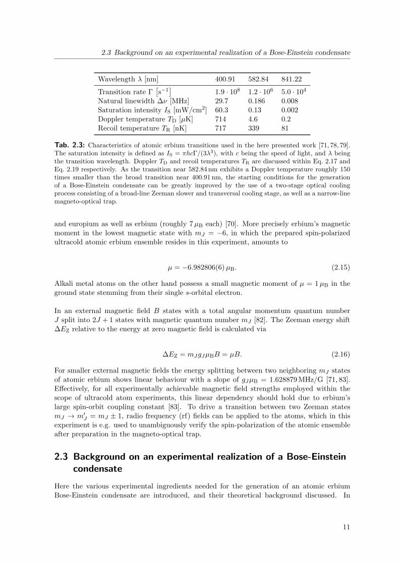
Tab. 2.3: Characteristics of atomic erbium transitions used in the here presented work [71, 78, 79].The saturation intensity is defined as IS = πhcΓ/(3λ3), with c being the speed of light, and λ beingthe transition wavelength. Doppler TD and recoil temperatures TR are discussed within Eq. 2.17 andEq. 2.19 respectively. As the transition near 582.84 nm exhibits a Doppler temperature roughly 150times smaller than the broad transition near 400.91 nm, the starting conditions for the generationof a Bose-Einstein condensate can be greatly improved by the use of a two-stage optical coolingprocess consisting of a broad-line Zeeman slower and transversal cooling stage, as well as a narrow-linemagneto-optical trap.
and europium as well as erbium (roughly 7µB each) [70]. More precisely erbium’s magneticmoment in the lowest magnetic state with mJ = −6, in which the prepared spin-polarizedultracold atomic erbium ensemble resides in this experiment, amounts to
µ = −6.982806(6)µB. (2.15)
Alkali metal atoms on the other hand possess a small magnetic moment of µ = 1µB in theground state stemming from their single s-orbital electron.
In an external magnetic field B states with a total angular momentum quantum numberJ split into 2J + 1 states with magnetic quantum number mJ [82]. The Zeeman energy shift∆EZ relative to the energy at zero magnetic field is calculated via
∆EZ = mJgJµBB = µB. (2.16)
For smaller external magnetic fields the energy splitting between two neighboring mJ statesof atomic erbium shows linear behaviour with a slope of gJµB = 1.628879 MHz/G [71, 83].Effectively, for all experimentally achievable magnetic field strengths employed within thescope of ultracold atom experiments, this linear dependency should hold due to erbium’slarge spin-orbit coupling constant [83]. To drive a transition between two Zeeman statesmJ → m′J = mJ ± 1, radio frequency (rf) fields can be applied to the atoms, which in thisexperiment is e.g. used to unambiguously verify the spin-polarization of the atomic ensembleafter preparation in the magneto-optical trap.
2.3 Background on an experimental realization of a Bose-Einsteincondensate
Here the various experimental ingredients needed for the generation of an atomic erbiumBose-Einstein condensate are introduced, and their theoretical background discussed. In
11
2 Theoretical background: Ultracold atomic erbium quantum gases
short the steps include first stage laser cooling of an atomic erbium beam via broad-lineZeeman slower and transversal cooling, second stage laser cooling via narrow-line magneto-optical trap, loading into single or hybrid optical dipole traps, and subsequent evaporativecooling until quantum degeneracy is reached. The ensemble is prepared inside an ultra-highvacuum chamber to minimize perturbations by the environment.
2.3.1 Laser cooling
Laser cooling is an experimental method to decelerate atoms, and thus for an equilibriumdistribution to reduce the mean velocity of atoms, by the use of light, as in the following de-scribed via [84]. The mean kinetic energy of all particles of an ideal gas is proportional to itsmean squared velocity v2 and temperature T , respectively [85], so that the temperature canbe expressed via T = mv2/(3kB). The velocity of each atom inside the gas can be decreasedby momentum transfer from photons with appropriate momentum of |p| = ~ |k| per photon,with k being the wavevector of the absorbed photon. After absorption the atom occupies anenergetically excited state for a mean duration of the spontaneous lifetime, from which it canthen relaxate into a lower state by stimulated or spontaneous emission of a photon. Whilefor the case of stimulated emissions no net momentum transfer takes place, for spontaneousemissions a net momentum transfer occurs after many absorption and emission cycles as thesum of all momenta from emitted photons averages to zero over time, but the sum of allmomenta from absorbed photons does not, leading to a so-called spontaneous force, whichfor the case of a magneto-optical trap in one dimension is shown in Eq. 2.21. Thus we canchange the velocity v = p/m of atoms by directed illumination with resonant photons frome.g. a laser beam. The spontaneous force can be mathematically derived from the descriptionof a two-level system using the Bloch equations [84]. For atoms moving in opposite directionto the laser light propagation direction, the Doppler shift ∆ω = ±ω0v/c = kv, where ∆ω isthe frequency shift away from the atomic resonance frequency ω0 [86], has to be counteredby red-detuning the light frequency.
For optical cooling of an atomic ensemble in a fixed position in space, three pairs of counter-propagating laser beams are necessary. The atomic ensemble, then also called optical mo-lasses, only experiences a reduction of the mean velocity, but not a restoring force in positionspace, so that they can spatially diffuse out of the molasses [87]. The in Sec. 2.3.2 discussedupgrade, named magneto-optical trap, adds such a restoring force by applying a linear mag-netic field gradient in each spatial dimension to make trapping of atoms without diffusionpossible. In the idealized system of a two-level atom with the choice of a red-detuning ofδ = −Γ/2, where Γ = 1/τ , and τ being the lifetime of the excited state, one obtains theso-called Doppler temperature, which acts as a lower limit for the standard optical coolingprocess, as
TD =~Γ
2kB. (2.17)
Other cooling techniques like polarization gradient cooling can reach even lower temperatures[88]. The fundamental limit stemming from the discrete momentum transfer of a single photonis represented by the recoil temperature [89]
12
2.3 Background on an experimental realization of a Bose-Einstein condensate
TR =~2Γ2
mkB. (2.18)
It should be noted that also techniques for subrecoil laser cooling have been demonstrated [90].
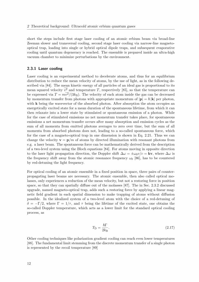
In the present experiment, erbium atoms are loaded from an atomic beam into the magneto-optical trap for the preparation of an ultracold atomic ensemble. As erbium exists as a solid atroom temperature, it has to be heated greatly in a crucible, embedded in a two-stage effusioncell including apertures for collimation, as seen in a sketch in Fig. 2.2, and in a technical draw-ing in Fig. 3.2. The emerging atomic beam from the effusion cell can be further collimated bymeans of transversal cooling techniques [71,91], which reduces the mean transversal velocity ofthe atoms and therefore the divergence angle of the atomic beam [92,93]. Transversal coolingutilizes laser cooling in one dimension using two counter-propagating resonant laser beamsperpendicular to the atomic beam. This is typically applied in both dimensions orthogonal tothe atomic beam axis, so that in total two beam pairs (four beams) irradiate the atoms. Ide-ally elliptically shaped beam profiles are used to maximize the interaction area and thereforeinteraction time of the light with the passing atoms, leading to a stronger collimation effect.Ultimately the atomic flux is increased, as indicated in Fig. 2.2. It is however limited by theaperture with diameter dct of the next connecting tube in the vacuum system that leads tothe Zeeman slower.
v
dct
transversalcooling beams
Zeemanslower beam
Fig. 2.2: Outline of the transversal cooling and Zeeman slower light setup. With two counter-propagating resonant laser beams in one dimension perpendicular to the atomic beam axis the lattercan be collimated, i.e. the divergence angle can be reduced (here shown from cyan to lavender), leadingto a higher atomic flux at the aperture with diameter dct of the connecting tube between effusion cellchamber and main vacuum chamber. The here used laser beams exhibit an elliptic beam profile tomaximize the interaction area with the atomic beam. The Zeeman slower laser beam (shown in darkpurple, with some part of the Zeeman slower coil profile here being indicated as coppery geometry)travels along the tube axis and counter-propagates the atomic beam. A portion of the collimatedbeam scatters light from the Zeeman slower beam and is continuously decelerated on the way to themain vacuum chamber inside the Zeeman slower. A complete view of the setup can be seen in Fig. 3.1.Transversal cooling sketch adapted from [56].
The transversal cooling stage only collimates the atomic beam, but does not slow the atomsin longitudinal direction. Due to a much higher mean velocity than the capture velocity ofthe magneto-optical trap, as briefly discussed in Sec. 3.2, such a longitudinal deceleration isneeded and here provided by a so-called Zeeman slower [94]. A counter-propagating laserbeam reduces the velocity of the atoms via optical cooling as sketched in Fig. 2.2. Because asomewhat slowed down atom soon would not be resonant with the laser beam of frequency ωanymore due to the Doppler effect, the resonance condition
13
2 Theoretical background: Ultracold atomic erbium quantum gases
ω0 − kv(z) +µ
~B(z) = ω (2.19)
has to be continuously met with the help of a spatially varying magnetic field B(z) alongthe Zeeman slower axis in z-direction, which changes the energy levels of the atoms via theZeeman effect at each position appropriately. µ = µB(geme− ggmg) is the difference betweenmagnetic moments of excited and ground state. Here a long-standing spin-flip Zeeman slowerwith a maximum capture velocity of vZS
max ≈ 600 m/s and an arbitrarily low minimum capturevelocity, respectively, is used [55].
2.3.2 Magneto-optical trap
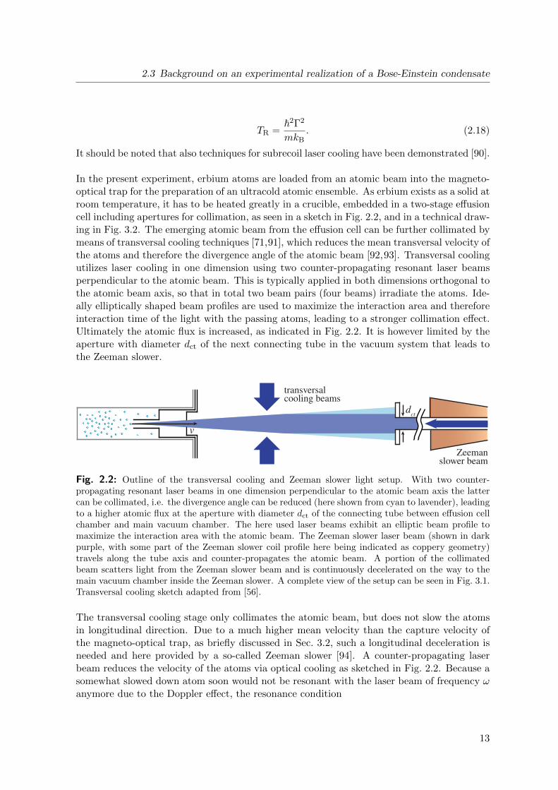
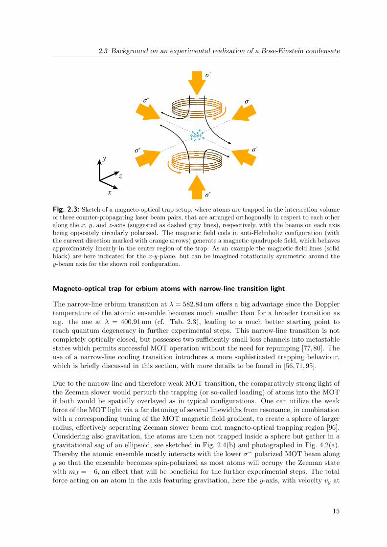
In addition to the laser cooling effect possible in the optical molasses discussed in Sec. 2.3.1 tocover also a restoring force in position space and actually trap atoms spatially without the riskof diffusion, one can apply a magnetic quadrupole field resulting in a so-called magneto-opticaltrap (MOT) [76], where the theoretical description below follows [84]. The MOT consists ofthree pairs of red-detuned, counter-propagating and circularly polarized laser beams, with onepair along each spatial direction, and two magnetic field coils in anti-Helmholtz configuration,shown as a sketch in Fig. 2.3. The coils produce the magnetic quadrupole field with its pointof origin lying at the intersection point of the laser beams, which exhibits an approximatelylinear behaviour in each spatial axis around the origin. For simplicity we consider only onespatial dimension and a two level system with a J = 1 excited state in the following. Theinhomogeneous magnetic field of form B(z) = bz, with slope b and B(0) = 0, splits the threeZeeman levels mJ = 0,±1 of the excited state energetically in respect to position z, whilethe single Zeeman level of the ground state with J = 0 and mJ = 0 is unaffected, as seen inFig. 2.4(a).
If the two counter-propagating beams in direction of the magnetic field gradient are right (σ+)and left circularly (σ−) polarized respectively, due to the selection rules for electric dipoletransitions they preferably excite the mJ = +1 and mJ = −1 transition respectively. If σ+
polarized light is irradiated from the side with the mJ = +1 state being energetically lowerand therefore closer to resonance with the laser light (z < 0), atoms further away from thecenter will experience an increased spontaneous force pushing them back to the center of theMOT. For the same considerations of the other side (z > 0) now with σ− polarized light, oneascertains that the atoms will here also experience a spontaneous force directed to the MOTcenter region. Thus for a pair of counter-propagating beams along each of the three spatialaxes the atoms can be trapped position-dependently in space. The spontaneous force alongone axis, e.g. the z-axis, can be written as
FMOTz =
~kΓ
2
(s
1 + s+ 4(δ−kvz+µ∂zBz/~)2
Γ2
− s
1 + s+ 4(δ+kvz−µ∂zBz/~)2
Γ2
), (2.20)
where s = I/IS is the saturation parameter with I being the light intensity, and IS being thesaturation intensity respectively.
14
2.3 Background on an experimental realization of a Bose-Einstein condensate
y
z
x
σ+
σ+
σ
σ-
σ-
σ+
-
Fig. 2.3: Sketch of a magneto-optical trap setup, where atoms are trapped in the intersection volumeof three counter-propagating laser beam pairs, that are arranged orthogonally in respect to each otheralong the x, y, and z-axis (suggested as dashed gray lines), respectively, with the beams on each axisbeing oppositely circularly polarized. The magnetic field coils in anti-Helmholtz configuration (withthe current direction marked with orange arrows) generate a magnetic quadrupole field, which behavesapproximately linearly in the center region of the trap. As an example the magnetic field lines (solidblack) are here indicated for the x-y-plane, but can be imagined rotationally symmetric around they-beam axis for the shown coil configuration.
Magneto-optical trap for erbium atoms with narrow-line transition light
The narrow-line erbium transition at λ = 582.84 nm offers a big advantage since the Dopplertemperature of the atomic ensemble becomes much smaller than for a broader transition ase.g. the one at λ = 400.91 nm (cf. Tab. 2.3), leading to a much better starting point toreach quantum degeneracy in further experimental steps. This narrow-line transition is notcompletely optically closed, but possesses two sufficiently small loss channels into metastablestates which permits successful MOT operation without the need for repumping [77,80]. Theuse of a narrow-line cooling transition introduces a more sophisticated trapping behaviour,which is briefly discussed in this section, with more details to be found in [56,71,95].
Due to the narrow-line and therefore weak MOT transition, the comparatively strong light ofthe Zeeman slower would perturb the trapping (or so-called loading) of atoms into the MOTif both would be spatially overlayed as in typical configurations. One can utilize the weakforce of the MOT light via a far detuning of several linewidths from resonance, in combinationwith a corresponding tuning of the MOT magnetic field gradient, to create a sphere of largerradius, effectively seperating Zeeman slower beam and magneto-optical trapping region [96].Considering also gravitation, the atoms are then not trapped inside a sphere but gather in agravitational sag of an ellipsoid, see sketched in Fig. 2.4(b) and photographed in Fig. 4.2(a).Thereby the atomic ensemble mostly interacts with the lower σ− polarized MOT beam alongy so that the ensemble becomes spin-polarized as most atoms will occupy the Zeeman statewith mJ = −6, an effect that will be beneficial for the further experimental steps. The totalforce acting on an atom in the axis featuring gravitation, here the y-axis, with velocity vy at
15
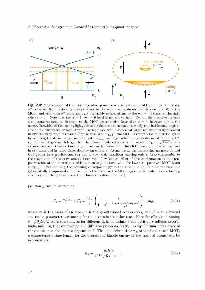
2 Theoretical background: Ultracold atomic erbium quantum gases
z
energy
ωcomp
σ+ σ-
J = 0
mJJ = 1
0
+1
-1
0
σ+
σ-
y
z
g δ ≈ Γpb
δ ≫ Γpb
(a) (b)
ωload
loading
compressing
Fig. 2.4: Magneto-optical trap. (a) Operation principle of a magneto-optical trap in one dimension.σ+ polarized light preferably excites atoms to the mJ = +1 state on the left side (z < 0) of theMOT, and vice versa σ− polarized light preferably excites atoms to the mJ = −1 state on the rightside (z > 0). Note that the J = 1, mJ = 0 level is not shown here. Overall the atoms experiencea spontaneous force in direction to the MOT center region located at z = 0, however due to thenarrow linewidth of the cooling light, this is for the one-dimensional case only true inside small regionsaround the illustrated arrows. After a loading phase with a somewhat larger red-detuned light severallinewidths away from resonance (orange level with ωload), the MOT is compressed in position spaceby reducing the detuning (yellow level with ωcomp) amongst other things as discussed in Sec. 4.1.2.(b) For detunings δ much larger than the power broadened transition linewidth Γpb = Γ
√1 + s atoms
experience a spontaneous force only in regions far away from the MOT center, similar to the casein (a), described in three dimensions by an ellipsoid. Atoms inside the narrow-line magneto-opticaltrap gather in a gravitational sag due to the weak transition exerting only a force comparable tothe magnitude of the gravitational force mg. A welcomed effect of this configuration is the spin-polarization of the atomic ensemble as it mostly interacts with the lower σ− polarized MOT beamalong y. After reducing the detuning correspondingly to the scheme in (a), the atomic ensemblegets spatially compressed and lifted up to the center of the MOT region, which enhances the loadingefficiency into the optical dipole trap. Images modified from [71].
position y can be written as
Fy = FMOTy + Fg =
~kΓ
2
s
1 + s′ +4(δ+kvy−µ∂yBy/~)2
Γ2
−mg, (2.21)
where m is the mass of an atom, g is the gravitational acceleration, and s′ is an adjustedsaturation parameter accounting for the beams in the other axes. Here the effective detuningδ − µ∂yBy/~ stays constant, as for different light detunings δ the position y adjusts accord-ingly, meaning that dampening and diffusion processes, as well as equilibrium parameters ofthe atomic ensemble do not depend on δ. The equilibrium time τeq of the far-detuned MOT,a characteristic time length for the decrease of kinetic energy of the trapped atoms, can beexpressed as
τeq =mR2s
4~k2√Rs− s− 1
(2.22)
16
2.3 Background on an experimental realization of a Bose-Einstein condensate
and the equilibrium temperature of the far-detuned loading MOT can be defined as
Teq =~Γ√s
2kB
R
2√R− 2/s
, (2.23)
where R = ~kΓ/(2mg), so that experimentally τeq and Teq are only dependent on the satu-ration parameter s. For typical experimental parameters of the loading MOT, Teq,load shouldlie in the region of 17µK, while τeq,load should amount to approximately 110 ms. After com-pressing, the values change for the equilibrium temperature to a few µK, concordantly withthe Doppler temperature of 4.6µK of the narrow-line transition, and for the equilibrium timeto approximately 15 ms respectively, as the intensity of the MOT light is ramped down sig-nificantly during the compression phase (cf. Fig. 4.1). The maximum capture velocity of thefar-detuned MOT can also be estimated via
vMOTcap =
d
τeq, (2.24)
where d is the diameter of the MOT light beams. With d = 36 mm one arrives at vMOTcap =
3.3 m/s, illustrating the need of a well-adjusted Zeeman slower. After loading atoms from theZeeman slowed atomic beam into the far-detuned MOT, the MOT is subsequently compressedvia changes of detuning δ and the magnetic field gradient ∂yB to achieve a much betteroverlapping with – and therefore increased loading into – the optical dipole trap used in thenext experimental step. Details about the experimental MOT compression process can befound in Sec. 4.1.2.
2.3.3 Single and hybrid crossed optical dipole traps
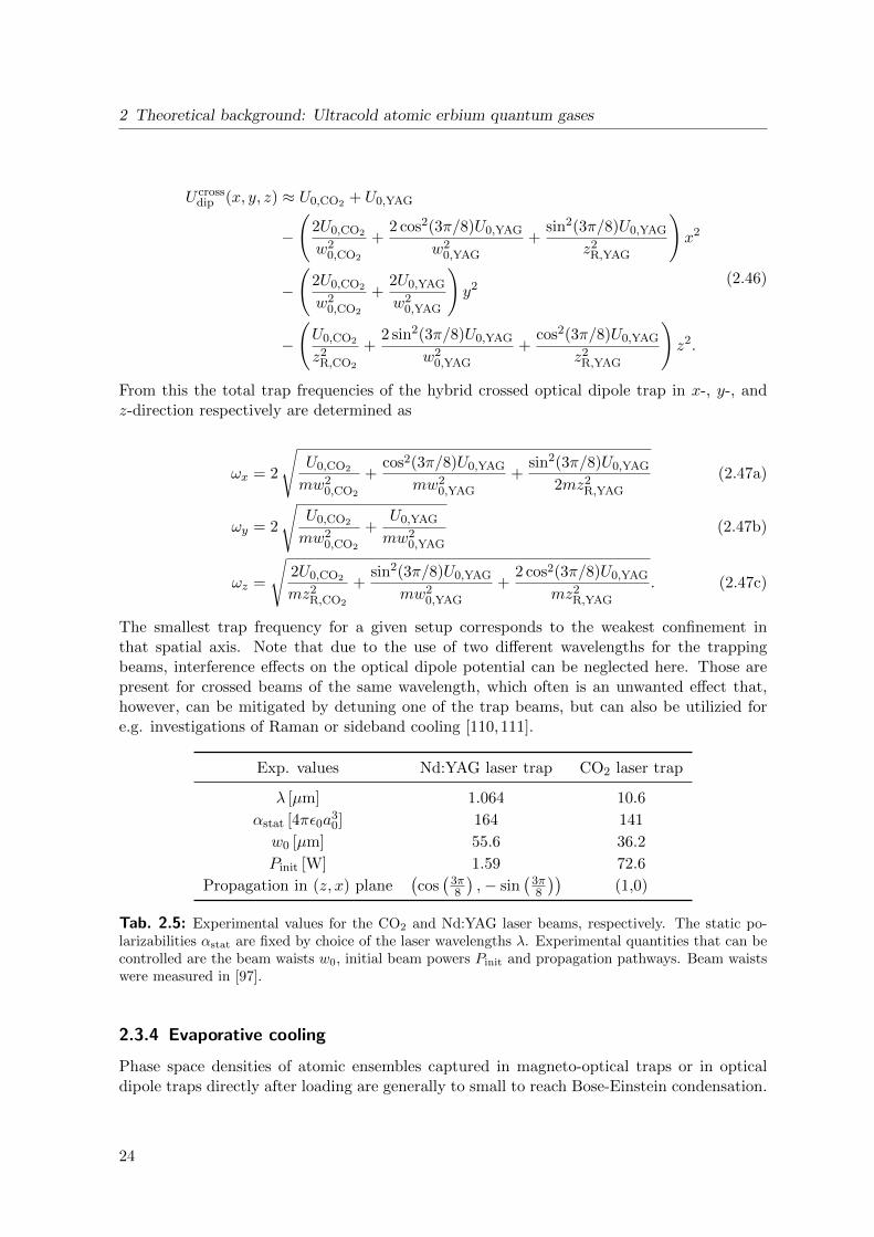
To circumvent temperature and density limits of atom traps based on optical cooling tech-niques and ultimately reach quantum degeneracy, the atomic ensemble has to be transferred(or loaded) into other types of traps with high coherence times capable of performing evap-orative cooling. Two of those types are magnetic traps and optical dipole traps, from whichthe latter is employed in this experiment and theoretically discussed in this section. Anoptical dipole trap is generally a laser field configuration with at least one point of stableequilibrium for the atomic motion, so that a mean restoring force is exterted on the atoms ifthey should be displaced from that point of stability. As this thesis describes the transitionfrom a single optical dipole trap (SODT) to a hybrid crossed optical dipole trap (HCODT),both geometries, including trap depths and trap frequencies, are here studied and in Sec. 4.2experimentally compared, respectively. The theoretical description follows [48,97].
Dipole trap potential and scattering rate
Far-detuned light can induce an electric dipole moment in particles that then in turn interactswith the light field, leading to a so-called dipole force acting upon the particles. In the presenceof an ac electric field E(r, t) = eE(r)e−iωt of amplitude E(r) and frequency ω according tothe oscillator model the dipole moment dg,e(r, t) = edg,e(r)e−iωt is induced on an atom, withe being the unit polarization vector, and g and e denoting the ground state and excited stateof the atom, respectively. Electric field amplitude and dipole moment are related via
17
2 Theoretical background: Ultracold atomic erbium quantum gases
dg,e(r) = α(ω)E(r), (2.25)
where α(ω) is the frequency-dependent complex polarizability. The interaction or dipolepotential can be expressed with the field intensity I(r) = 2ε0c|E(r)|2 as
Udip(r, ω) = −1
2〈dg,e(r, ω)E(r, ω)〉 = − 1
2ε0cRe[α(ω)]I(r). (2.26)
As the potential is proportional to the light intensity, e.g. a red-detuned focused laser beamcan be used for trapping cold atoms. The photon scattering rate is given by
Γdip(r, ω) =〈dg,e(r, ω)E(r, ω)〉
~ω=
1
~ε0cIm[α(ω)]I(r). (2.27)
Here the imaginary part of the complex polarizability Im[α(ω)] relates to the number ofphase-shifted dipole oscillations. As scattering events, i.e. absorption and emission cycles,and therefore heating processes take place, the atoms inside an optical dipole trap have afinite lifetime, which for a given atomic species is dependent on intensity and frequency ofthe light. The damping rate Γd, that describes to the spontaneous decay rate of the excitedlevel |e〉 into the ground state |g〉, can be calculated by looking at the corresponding dipolematrix element µ via
Γd =ω3
0
3πε0~c3|〈e|µ|g〉|2. (2.28)
Optical dipole trapping of erbium atoms
The above discussion of the dipole trap potential implied an atomic two-level system consistingof a ground state and an excited state. In reality atoms possess multi-level structures, whichfor e.g. the erbium case can be highly complex, so that this idealization does not necessarilyhold anymore as in general the dipole potential can depend on the substate of the atom,which e.g. can lead to laser light polarization dependencies. We first discuss a multi-levelatom without degeneracy, after which the multi-level case with degeneracy follows. Theeffect of off-resonant laser light acting on atomic levels can be described using second-orderperturbation theory. In a dressed states approach, the energy shift ∆Ei of state i stemmingfrom a perturbation Hamiltonian Hint = −µ ·E, with eletric dipole operator µ, can be writtenas [98]
∆Ei =∑j 6=i
|〈j|Hint|i〉|2
Ei − Ej. (2.29)
A dressing of the states with unperturbed energies Ei of the i-th state is applied by consideringthe overall system consisting of atom plus laser light field. Here Ei = n~ω is the ground stateenergy that is fully provided by the laser field’s energy as the internal ground state energy
18
2.3 Background on an experimental realization of a Bose-Einstein condensate
amounts to zero. Photon absorption leads to an internal energy of ~ωj of the excited atomand a field energy of (n − 1)~ω, respectively. This results in the energy difference of statesbeing ~∆ij = Ei − Ej = ~(ω − ωj), and with Eq. 2.28 one arrives for a two-level system atthe simplified expression
∆E = ±|〈e|µ|g〉|2
∆eg|E|2 = ±3πc2
2ω30
Γd
∆egI(r), (2.30)
which is known as the ac Stark shift, where the ± signs relate to the ground and excited state,respectively [99, 100]. Here ∆eg = ω − ω0 is the light detuning from the atomic resonancefrequency ω0 of the two-level system. For low light saturation intensities the atoms mostlyoccupy the ground state, so that the ac Stark shifted ground state becomes the relevant dipolepotential for the movement of the atoms.
When an electronic substructure is considered, one has to sum over all possible excited states|ej〉 for a given ground state |gi〉. For this the dipole matrix elements µij = 〈ej |µ|gi〉 of thecorresponding transitions have to be calculated, with specific transition elements
µij = cij ||µ||, (2.31)
where ||µ|| is the reduced dipole matrix element which is dependent on the electronic orbitalwavefunctions and can be expressed via Eq. 2.28. Here cij are the real transition coefficients,which define the coupling strength between sublevels i and j, and are dependent on thepolarization of the trapping light as well as on the electronic and nuclear angular momenta,respectively. Considering Eq. 2.28, Eq. 2.29 and Eq. 2.31, the dipole potential for a groundstate i in the case of large detunings and negligible saturation results as
Udip,i(r, ω) = −∑j
3πc2
2ω3j
(c2ijΓj
ωj − ω+
c2ijΓj
ωj + ω
)I(r), (2.32)
where ωj is the resonance frequency, and Γj the damping rate respectively, for a transitionfrom |gi〉 to |ej〉. For absolute values of detunings much smaller than the resonance frequency,i.e. |∆ij | ωj , the second so-called counter-rotating term inside the parentheses can beneglected within the scope of the rotating wave approximation. Importantly, for blue-detunedlight with ω > ωj the potential is positive, and for red-detuned light with ω < ωj negative,respectively. With red-detuned light a dipole force in direction of maximum intensity iscreated, which presents a viable setting for a focused laser beam trap. For blue-detuned lightthe dipole force pushes particles out of regions with high intensity. The scattering rate isgiven by
Γdip,i(r, ω) =∑j
3πc2
2~ω3j
(ω
ωj
)3(c2ijΓj
ωj − ω+
c2ijΓj
ωj + ω
)2
I(r), (2.33)
where again the rotating wave approximation can be applied for |∆ij | ωj , eliminating thesecond counter-rotating term inside the parentheses.
19
2 Theoretical background: Ultracold atomic erbium quantum gases
Quasi-electrostatic optical dipole trapping
For the special case of very far-detuned laser light with ω ω0, as it is the case for CO2
laser light at 10.6µm wavelength used in this experiment as the beam of the SODT and themain beam of the HCODT respectively, the light field oscillates very slowly in respect tothe atomic eigenfrequency. In this limit the induced dipole moment can follow the electricfield essentially without a phase shift, i.e. statically. The rotating wave approximation asmentioned above is in this case not valid, however as now for e.g. the two-level case theapproximation ω0 − ω ≈ ω0 + ω ≈ ω0 holds, a quasi-electrostatic expression can be found fora simplified dipole potential according to
Uquestdip (r) = −3πc2
ω30
Γdω0I(r), (2.34)
that is independent of ω. In general for the quasi-electrostatic approximation in the limit ofω → 0 the potential can also be expressed with the static polarizability αstat → α(0) as
Uquestdip (r) = −αstat
I(r)
2ε0c. (2.35)
In contrast to the treatment before the shifted potential for excited states is now also attrac-tive. One advantage of such potentials is that even different atomic species and moleculescould be simultaneously trapped independent of their internal state [101, 102], as the trapdepth in Eq. 2.35 does not reference any specific transition frequency. Another advantageis the very small scattering rate obtainable due to the very large detuning from any atomicresonance. It can be calculated from its relation to the dipole potential as
Γquestdip (r, ω) = 2
(ω
ω0
)3 Γd~ω0
Uquestdip (r). (2.36)
Typical scattering rates lie in the order of 10−3 s−1 [103] with recoil energies of approximatelykB ·1 nK, so that a conservative trap with negligible decoherence effects by photon absorptioncan be realized. For such low scattering rates, the lifetime of the atoms will almost exlusivelyresult from collisions with the background gas in the ultra-high vacuum chamber.
Atomic polarizabilities
As erbium is a multi-level atom with a rich electronic spectrum, Eq. 2.32 has to be applied.One can, however, express the dipole trap potential for an atom in a state with J andmJ by inserting the transition coefficients into that equation so that the atomic transitionproperties are captured in the atomic scalar αscal, vector αvect, and tensor polarizability αtens,respectively, and parameters of the light field polarization are explicitely set via
Udip(r, ω,A, θk, θp) =I(r)
2ε0c
(Re [αscal(ω)] +A cos(θk)
mJ
2JRe [αvect(ω)]
+3m2
J − J(J + 1)
J(2J − 1)· 3 cos2(θp)− 1
2Re [αtens(ω)]
),
(2.37)
20
2.3 Background on an experimental realization of a Bose-Einstein condensate
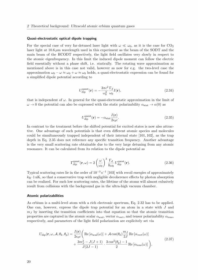
where A is the ellipticity parameter describing the polarization state of the light [75]. Hereθk is the angle between quantization axis z and wavevector k, and θp is chosen so that|e · ez| = cos2(θp), where e is the unit polarization vector. The scattering rate can be ob-tained by replacing all instances of Re [αi(ω)] in Eq. 2.37 with Im [αi(ω)]. The values of theground state erbium polarizabilities for both the CO2 laser light main dipole trap beam atλ = 10.6µm (equaling 943.4 cm−1) as well as the Nd:YAG laser light cross dipole trap beamat λ = 1064 nm (corresponding to 9398.5 cm−1) are given in Tab. 2.4.
ω [cm−1]
Polarizability [a.u.] 0 943.40 9398.50
Re [αscal] 141 141 164
Re [αvect] 0 -0.084 -0.943
Re [αtens] -2.52 -2.53 -3.93
Im [αscal] /10−6 1.51 1.52 2.34
Im [αvect] /10−6 0 −0.129 −1.74
Im [αtens] /10−6 −0.421 0.421 −0.69
Tab. 2.4: Theoretical polarizability values of ground state erbium atoms at different light frequenciesin atomic units of 4πε0a
30 [55, 75], which especially for the scalar polarizability were experimentally
verified to good agreement in [104]. Here values for the CO2 laser light at ω = 943.40 cm−1 andthe Nd:YAG laser light at ω = 9398.50 cm−1 are shown. The electrostatic case is depicted in thecolumn with ω = 0 cm−1. The values for the imaginary part of the polarizability for the case ofω = 9398.50 cm−1 have to be taken with a pinch of salt, since due to the (ω/ω0)3 scaling of thephase-space factor, which possibly has not been taken into account, smaller values for the scatteringrate are expected here.
For the case of the CO2 laser light the frequency lies far below all atomic transition frequencies,as seen in Fig. 2.1 where the lowest excited state is located at energies of about 5000 cm−1,so that static and scalar polarizability are almost equal, with Re [αstat] ≈ Re [αscal(0)] =Re[αscal(943.4 cm−1)
]= 141, whereat this isotropic behaviour of the polarizability in the
ground state seems to be a result of the completely filled 6s shell [75]. As the value forthe scalar polarizability is much greater than all other contributions, the dipole potential inEq. 2.35 can be well approximated by setting Re [αstat] = Re [αscal,CO2 ]. It should be notedthat vector and tensor polarizabilities can reach values comparable to αstat for wavelengthsassociated with transitions of the incompletely filled submerged shell.
In comparison for the case of Nd:YAG laser light near λ = 1.064µm wavelength the po-larizability values differ from the static case, although here Re [αscal] also is the dominantquantity, so that the Nd:YAG light contribution to the overall dipole potential of the crossedtrap hardly depends on the light polarization or atomic quantization axis, too, so that in goodapproximation Eq. 2.35 can be written with the replacement Re [αstat] → Re [αscal,YAG]. Onthe other hand the imaginary parts of scalar, vector, and tensor polarizability respectively es-pecially for the laser light near λ = 1.064µm wavelength are of the same order of magnitudeso that the light polarization and atomic quantization axis have a strong influence on thescattering rate. A linear polarization of the dipole trapping beams seems to achieve longer
21
2 Theoretical background: Ultracold atomic erbium quantum gases
trap lifetimes [75].
Single optical dipole trap geometry
There are various dipole trap geometries feasible for capturing neutral atoms, with classicsetups for red-detuned light being single focused Gaussian beam traps, crossed Gaussian beamtraps, and standing wave traps [105–107]. From those mentioned the first two configurationsare employed in this experiment and compared within this thesis. Starting with the simplestsingle Gaussian beam configuration, the intensity profile of such a beam propagating along zcan be described as
I(r, z) =2P
πw2(z)exp
(2
r2
w2(z)
), (2.38)
where P is the beam power, and the radial coordinate r =√x2 + y2 is the distance from the
z axis, with y being the direction of gravity. The 1/e2 beam radius along z is given as
w(z) = w0
√1 +
(z
zR
)2
, (2.39)
where√
2w0 is the beam radius at which the Rayleigh length zR = πω20/λ is reached [108],
which results for typical dipole trapping light wavelengths in the spatial confinement beingin radial direction much stronger than in the axial direction. With Eq. 2.35 one obtains thedipole trap potential in the quasi-electrostatic case for the CO2 laser beam as
Uquestdip (r, z) = −αstat
2ε0c
2P
πw2(z)e−2r2/w2(z), (2.40)
and the maximum trap potential depth as
U0 = −Uquestdip (r = 0, z = 0) =
αstat
2ε0c
2P
πw20
=αstat
2ε0cI0, (2.41)
where I0 = I(r = 0, z = 0) is the maximum intensity at the center of the Gaussian beamwaist. For thermal energies kBT of the atomic ensemble much smaller than the trap potentialdepth U0, the spatial extent of the ensemble in radial direction is small compared to the beamwaist, and in axial direction small compared to the Rayleigh range, respectively, so that thetrap potential can be approximated as a cylindrically symmetric harmonic oscillator potentialby means of a Taylor expansion around z = 0 and r = 0 up to second order, leading to
Uquestdip (r, z) ≈ −U0
(1− 2
(r
w0
)2
−(z
zR
)2)
(2.42a)
= −U0 +1
2mω2
rr2 +
1
2mω2
zz2. (2.42b)
22
2.3 Background on an experimental realization of a Bose-Einstein condensate
The corresponding oscillator (or trap) frequencies, with which the atoms move inside thesingle beam optical dipole potential, are then found in the radial case as
ωr =
√4U0
mw20
= ωz
√2πw0
λ, (2.43)
and in the axial (or longitudinal) case as
ωz =
√2U0λ2
mπ2w40
=
√2U0
mz2R
. (2.44)
As seen in Sec. 3.4.2, measurements of the trap frequencies are crucial for the calculation ofthe phase space density inside the trap. Be it that an elliptic beam profile is prevalent onehas to consider two different beam waists w0,h in horizontal and w0,v in vertical directionrespectively, and their corresponding radial trap frequencies, as well as a modified axial trapfrequency via an effective Rayleigh length [109]. For a not too large ellipticity, the beam waistcan be approximated by w0 =
√w0,hw0,v.
Hybrid crossed optical dipole trap geometry
In this section properties of a hybrid crossed optical trap are discussed. The general idea isto increase the spatial confinement in each direction as single beam trapping can suffer fromweak confinement in axial direction. The hybrid trap here consists of a Gaussian main dipoletrap beam provided by a CO2 laser with wavelength λ = 10.6µm, aligned in z-direction,and a Gaussian secondary dipole trap beam provided by a Nd:YAG laser with wavelengthλ = 1064 nm, which crosses the main trap beam at an angle of 67.5 and is adjusted in a way sothat the central regions of both the respective beam waists overlap, s. Fig. 2.5. For maximumconfinement a crossing angle of 90 would be optimal, however this was in the present worktechnically not possible due to the available vacuum chamber setup. Characteristic propertiesof the two trapping beams are listed in Tab. 2.5 and 2.6. As the two individual potentials areadditive, the complete spatial profile of the hybrid crossed optical dipole trap potential canbe described as
U crossdip (x, y, z) = UYAG(x, y, z) + UCO2(x, y, z)
=U0,YAGw
20,YAG
w2YAG(x, z)
exp
(−2
(x cos(3π/8) + z sin(3π/8))2 + y2
w2YAG(x, z)
)+U0,CO2w
20,CO2
w2CO2
(z)exp
(−2
x2 + y2
w2CO2
(z)
).
(2.45)
For a perfect overlap of the beam waists of both beams, the maximum trap depth can beobtained by just adding the individual maximum trap depths of the beams, as U cross
0,dip =U0,YAG + U0,CO2 . A Taylor expansion of Eq. 2.45 for the potential near the trap bottom, i.e.around x = y = z = 0, leads to
23
2 Theoretical background: Ultracold atomic erbium quantum gases
U crossdip (x, y, z) ≈ U0,CO2 + U0,YAG
−
(2U0,CO2
w20,CO2
+2 cos2(3π/8)U0,YAG
w20,YAG
+sin2(3π/8)U0,YAG
z2R,YAG
)x2
−
(2U0,CO2
w20,CO2
+2U0,YAG
w20,YAG
)y2
−
(U0,CO2
z2R,CO2
+2 sin2(3π/8)U0,YAG
w20,YAG
+cos2(3π/8)U0,YAG
z2R,YAG
)z2.
(2.46)
From this the total trap frequencies of the hybrid crossed optical dipole trap in x-, y-, andz-direction respectively are determined as
ωx = 2
√U0,CO2
mw20,CO2
+cos2(3π/8)U0,YAG
mw20,YAG
+sin2(3π/8)U0,YAG
2mz2R,YAG
(2.47a)
ωy = 2
√U0,CO2
mw20,CO2
+U0,YAG
mw20,YAG
(2.47b)
ωz =
√2U0,CO2
mz2R,CO2
+sin2(3π/8)U0,YAG
mw20,YAG
+2 cos2(3π/8)U0,YAG
mz2R,YAG
. (2.47c)
The smallest trap frequency for a given setup corresponds to the weakest confinement inthat spatial axis. Note that due to the use of two different wavelengths for the trappingbeams, interference effects on the optical dipole potential can be neglected here. Those arepresent for crossed beams of the same wavelength, which often is an unwanted effect that,however, can be mitigated by detuning one of the trap beams, but can also be utilizied fore.g. investigations of Raman or sideband cooling [110,111].
Exp. values Nd:YAG laser trap CO2 laser trap
λ [µm] 1.064 10.6
αstat [4πε0a30] 164 141
w0 [µm] 55.6 36.2
Pinit [W] 1.59 72.6
Propagation in (z, x) plane(cos(
3π8
),− sin
(3π8
))(1,0)
Tab. 2.5: Experimental values for the CO2 and Nd:YAG laser beams, respectively. The static po-larizabilities αstat are fixed by choice of the laser wavelengths λ. Experimental quantities that can becontrolled are the beam waists w0, initial beam powers Pinit and propagation pathways. Beam waistswere measured in [97].
2.3.4 Evaporative cooling
Phase space densities of atomic ensembles captured in magneto-optical traps or in opticaldipole traps directly after loading are generally to small to reach Bose-Einstein condensation.
24
2.3 Background on an experimental realization of a Bose-Einstein condensate
(a) (b)
y
z
x
Nd:YAG lasercross beam
CO laser2
beamCO laser
2
main beam67.5 °
w0,CO2
w0,YAG
gravity
Fig. 2.5: (a) Sketch of the single (SODT) and (b) hybrid crossed optical dipole trap (HCODT)geometry, respectively. For the HCODT the Gaussian secondary Nd:YAG laser beam crosses theGaussian CO2 laser main beam at an angle of 67.5 . Here gravity points into the drawing plane.Characteristic values of the two trapping beams can be found in Tab. 2.5 and 2.6.
Theo. geometry Nd:YAG laser trap CO2 laser trap
Beam waist w0,YAG
√1 +
(z cos 3π
8−x sin 3π
8zR,YAG
)2
w0,CO2
√1 +
(z
zR,CO2
)2
U(x, y, z)U0,YAGw
20,YAG
w2YAG(x,z)
exp(−2
(x cos 3π8
+z sin 3π8
)2+y2
w2YAG(x,z)
)U0,CO2
w20,CO2
w2CO2
(z)exp
(−2 x2+y2
w2CO2
(z)
)Tab. 2.6: Theoretical geometry, i.e. calculated beam waists and dipole trap potentials, for twoGaussian trapping beams with different wavelength and propagation pathways chosen as in Tab. 2.5and shown in Fig. 2.5.
To reduce the temperature of an ensemble further, the evaporative cooling technique can beemployed [112]. For this the Maxwell-Boltzmann distribution gets truncated by removingatoms in the high-energy tail of the thermal distribution from the trap, followed by rether-malization of the remaining atoms via elastic collisions, leading to a velocity distribution ofnow smaller temperature, i.e. a colder atomic ensemble, as sketched in Fig. 2.6 [105]. That istypically achieved by lowering the optical dipole potential more and more until a satisfactoryphase space density is reached. Theoretical considerations in this section follow [113].
For efficient evaporative cooling the optical dipole trap potential depth has to be loweredquickly enough so that the process does not stagnate, as a drop of temperature also reducesthe rethermalization rate drastically, but slow enough so that the atoms have the chance torethermalize at all. The efficiency of evaporative cooling is characterized by the cut-off pa-rameter η = U/(kBT ). For very cold atoms in comparison to the potential depth, kBT < U ,the number of colliding pairs of atoms with high enough energy for one atom to leave thetrap is proportional to e−η. After loading atoms into the optical dipole trap, a short period
25
2 Theoretical background: Ultracold atomic erbium quantum gases
of so-called natural evaporation in the order of seconds takes place, and latest when thiseffect tapers off the potential U has to be continuously lowered, if one wants to avoid a rapiddecrease of the rethermalization rate. For optimal results, the lowering process should runadiabatically, and η should be kept constant. For this so-called induced evaporation one thenyields a temporal evolution of the atom number as
N(t)
Ninit=
(U(t)
Uinit
)3/[2(η′−3)]
, (2.48)
where η′ = η+ (η− 5)/(η− 4) can be used in the case of an approximate harmonic potential[114]. For a constant η the temperature should change proportionally with the potentialdepth. Most interesting is the temporal evolution of the phase space density ρ, which can beexpressed via
ρ(t)
ρinit=
(Uinit
U(t)
)3(η′−4)/[2(η′−3)]
. (2.49)
The for the experimental implementation important temporal evolution of the trap depth canbe written with help of the time constant τevap for evaporation as
U(t)
Uinit=
(1 +
t
τevap
)−2(η′−3)/η′
, (2.50)
where 1/τevap = 2η′(η − 4) exp(−η)γinit/3 is then the rethermalization rate, and γinit is theinitial collision rate between atoms. As one has also to consider atom losses from the trapdue to collisions with the residual background gas of the ultra-high vacuum, the replacementt→ 1− exp(t · Γloss)/Γloss, with the collision loss rate Γloss, has to be applied in Eq. 2.50.
Additionally the gravitation has to be considered, which becomes relevant for small trapdepths near the end of the evaporative cooling process. The total potential acting on theatomic ensemble is then for a HCODT via Eq. 2.45 given by
U totdip(x,y,z) = U cross
dip (x,y,z)−mgy, (2.51)
with g as the gravitational acceleration. Thus gravity introduces modifications to the po-tential, which lead to a reduced effective trap depth, as one side of the potential well getslowered, resulting in a faster evaporation process at low trap potential depths in the order ofthe gravitational potential, as indicated in Fig. 2.7(b). This effect, however, can be increasedby an applied magnetic field gradient adjusted so that the Stern-Gerlach force acts in the samedirection as the gravitational force, which then results in an even faster evaporation processthat can be tuned experimentally [115], and was first implemented in our experiment withinthe scope of a previous thesis [56]. The total acceleration amounts then to atot = aSG + g,where aSG = mJgJµB∂yBy/m is the Stern-Gerlach acceleration in y-direction [116], whichmodifies Eq. 2.51 via g → atot. The advantage here is that for the same effective potentialdepth the spatial occlusion is stronger, leading to higher phase space densities, as indicated in
26
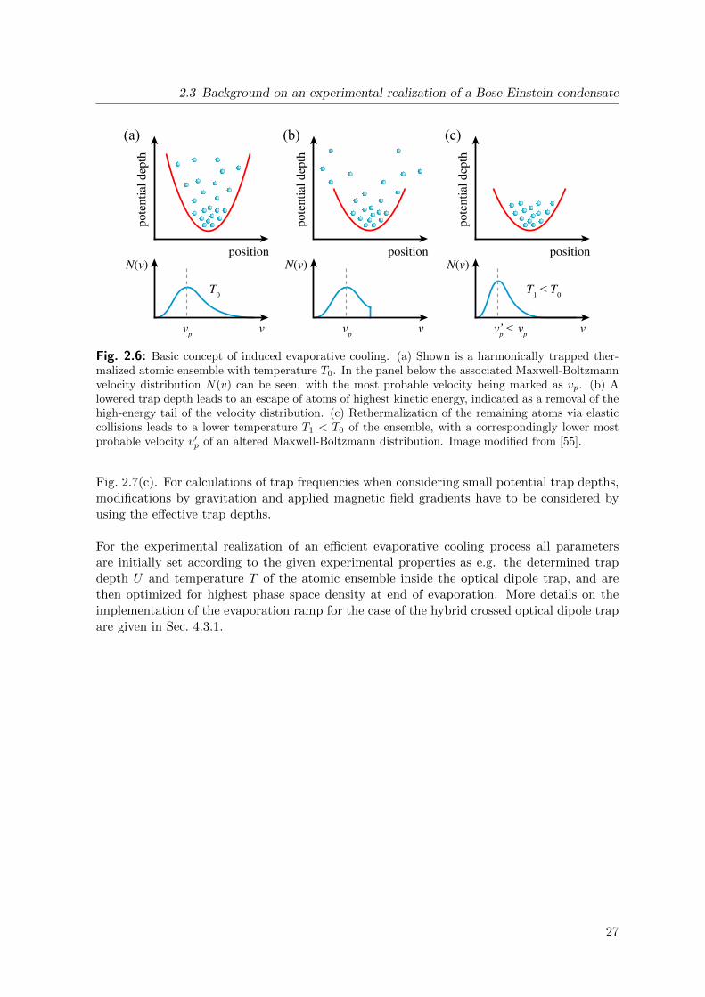
2.3 Background on an experimental realization of a Bose-Einstein condensate
position
pote
ntia
l dep
th
N(v)
v
T0
T1 < T
0
(a)
position
pote
ntia
l dep
th
N(v)
v
(b)
position
pote
ntia
l dep
th
N(v)
v
(c)
vp
vp
vp < v
p’
Fig. 2.6: Basic concept of induced evaporative cooling. (a) Shown is a harmonically trapped ther-malized atomic ensemble with temperature T0. In the panel below the associated Maxwell-Boltzmannvelocity distribution N(v) can be seen, with the most probable velocity being marked as vp. (b) Alowered trap depth leads to an escape of atoms of highest kinetic energy, indicated as a removal of thehigh-energy tail of the velocity distribution. (c) Rethermalization of the remaining atoms via elasticcollisions leads to a lower temperature T1 < T0 of the ensemble, with a correspondingly lower mostprobable velocity v′p of an altered Maxwell-Boltzmann distribution. Image modified from [55].
Fig. 2.7(c). For calculations of trap frequencies when considering small potential trap depths,modifications by gravitation and applied magnetic field gradients have to be considered byusing the effective trap depths.
For the experimental realization of an efficient evaporative cooling process all parametersare initially set according to the given experimental properties as e.g. the determined trapdepth U and temperature T of the atomic ensemble inside the optical dipole trap, and arethen optimized for highest phase space density at end of evaporation. More details on theimplementation of the evaporation ramp for the case of the hybrid crossed optical dipole trapare given in Sec. 4.3.1.
27
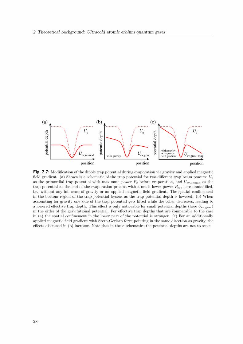
2 Theoretical background: Ultracold atomic erbium quantum gases
pote
ntia
dep
th
position
pote
ntia
l dep
th
position
U0
Uev,gravUev,unmod
U0
pote
ntia
l dep
th
position
U0
Uev,grav+mag
(a) (b) (c)
with gravity
with gravity+ magnetic
field gradient
Fig. 2.7: Modification of the dipole trap potential during evaporation via gravity and applied magneticfield gradient. (a) Shown is a schematic of the trap potential for two different trap beam powers: U0
as the primordial trap potential with maximum power P0 before evaporation, and Uev,unmod as thetrap potential at the end of the evaporation process with a much lower power Pev, here unmodified,i.e. without any influence of gravity or an applied magnetic field gradient. The spatial confinementin the bottom region of the trap potential lessens as the trap potential depth is lowered. (b) Whenaccounting for gravity one side of the trap potential gets lifted while the other decreases, leading toa lowered effective trap depth. This effect is only noticeable for small potential depths (here Uev,grav)in the order of the gravitational potential. For effective trap depths that are comparable to the casein (a) the spatial confinement in the lower part of the potential is stronger. (c) For an additionallyapplied magnetic field gradient with Stern-Gerlach force pointing in the same direction as gravity, theeffects discussed in (b) increase. Note that in these schematics the potential depths are not to scale.
28
3 Experimental setup
Here the experimental apparatus and used techniques for the generation as well as character-ization of an atomic erbium Bose-Einstein condensate (BEC) are presented. The core setupconsisting of the vacuum chamber including the effusion cell and Zeeman slower, as well asthe blue and yellow laser light setups for optical cooling were constructed within the scopeof previous works [56, 117–119], so that these topics are discussed only briefly, while moreattention is paid to the updated setup of the single (SODT) and hybrid crossed optical dipoletraps (HCODT), respectively.
3.1 Experimental overview
Initially erbium atoms in the metallic state are heated in an atomic beam oven to form aneffusive atomic beam. A transversal cooling stage reduces its transverse velocity spread, whilea Zeeman slower decelerates a portion of the atoms to sufficiently low velocities so that theycan get captured by the narrow-line MOT. Once trapped inside the MOT, the trap is spa-tially compressed (cMOT) to achieve a higher atom transfer efficiency into the next stage: theoptical dipole trap (either in SODT or HCODT configuration). After successful loading intothe optical dipole trap, evaporative cooling is performed until Bose-Einstein condensation isaccomplished. The whole setup described is set into an ultra-high vacuum chamber with apressure of order of 10−10 mbar, leading to a lifetime in the optical dipole trap that shouldonly be limited by collisions with residual background particles [120]. Fig. 3.4 indicates theoverall setup including sketches of the laser pathways, where all components are placed ontothree optical tables (with the two larger ones featuring pneumatically damped bed-plates tosuppress mechanical vibrations). The light for laser cooling purposes is connected to the maintable with the main vacuum chamber via optical fibers, which ensures an uncoupling of theoptical setup on the main table from maintenance adjustments of the laser systems on othertables.
In this experiment the process of trapping atoms and cooling them down to quantum de-generacy followed by a measurement is performed periodically, as a) measurements are typ-ically invasive so that the atoms are heated or even lost during that process, and b) oftenone experimental parameter is varied from measurement to measurement. The experimen-tal cycle is controlled by an electronic real-time controller (ADwin Pro II, manufactured byJager Messtechnik) with a temporal resolution of 1µs by delivering trigger signals and ana-log control signals to many experimental components as e.g. rf electronics and mechanicalshutters. The experimental cycle can be customized via a graphical interface1 on PC, whichis connected by ethernet to the controller. Many measurements are done via optical imagingwith the help of a camera that sends the recorded images to the PC for further analysis.
1Programmed by C. Geckeler in python for an ADwin Pro system.
29
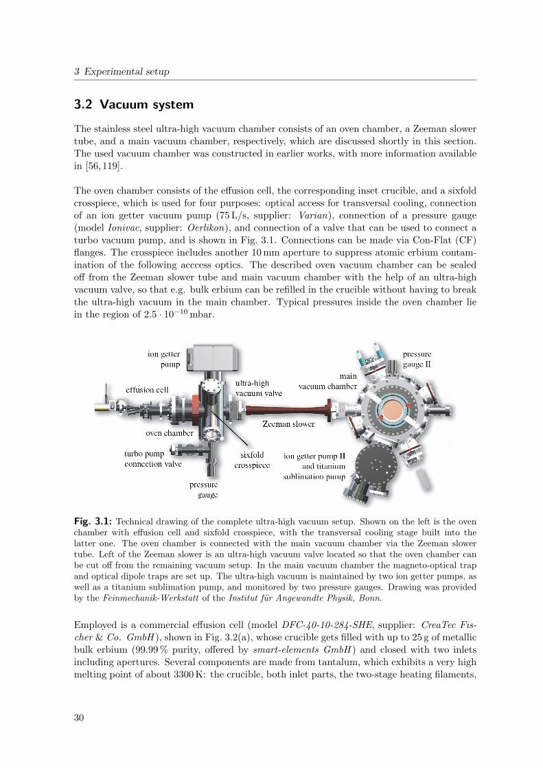
3 Experimental setup
3.2 Vacuum system
The stainless steel ultra-high vacuum chamber consists of an oven chamber, a Zeeman slowertube, and a main vacuum chamber, respectively, which are discussed shortly in this section.The used vacuum chamber was constructed in earlier works, with more information availablein [56,119].
The oven chamber consists of the effusion cell, the corresponding inset crucible, and a sixfoldcrosspiece, which is used for four purposes: optical access for transversal cooling, connectionof an ion getter vacuum pump (75 L/s, supplier: Varian), connection of a pressure gauge(model Ionivac, supplier: Oerlikon), and connection of a valve that can be used to connect aturbo vacuum pump, and is shown in Fig. 3.1. Connections can be made via Con-Flat (CF)flanges. The crosspiece includes another 10 mm aperture to suppress atomic erbium contam-ination of the following acccess optics. The described oven vacuum chamber can be sealedoff from the Zeeman slower tube and main vacuum chamber with the help of an ultra-highvacuum valve, so that e.g. bulk erbium can be refilled in the crucible without having to breakthe ultra-high vacuum in the main chamber. Typical pressures inside the oven chamber liein the region of 2.5 · 10−10 mbar.
Fig. 3.1: Technical drawing of the complete ultra-high vacuum setup. Shown on the left is the ovenchamber with effusion cell and sixfold crosspiece, with the transversal cooling stage built into thelatter one. The oven chamber is connected with the main vacuum chamber via the Zeeman slowertube. Left of the Zeeman slower is an ultra-high vacuum valve located so that the oven chamber canbe cut off from the remaining vacuum setup. In the main vacuum chamber the magneto-optical trapand optical dipole traps are set up. The ultra-high vacuum is maintained by two ion getter pumps, aswell as a titanium sublimation pump, and monitored by two pressure gauges. Drawing was providedby the Feinmechanik-Werkstatt of the Institut fur Angewandte Physik, Bonn.
Employed is a commercial effusion cell (model DFC-40-10-284-SHE, supplier: CreaTec Fis-cher & Co. GmbH ), shown in Fig. 3.2(a), whose crucible gets filled with up to 25 g of metallicbulk erbium (99.99 % purity, offered by smart-elements GmbH ) and closed with two inletsincluding apertures. Several components are made from tantalum, which exhibits a very highmelting point of about 3300 K: the crucible, both inlet parts, the two-stage heating filaments,
30
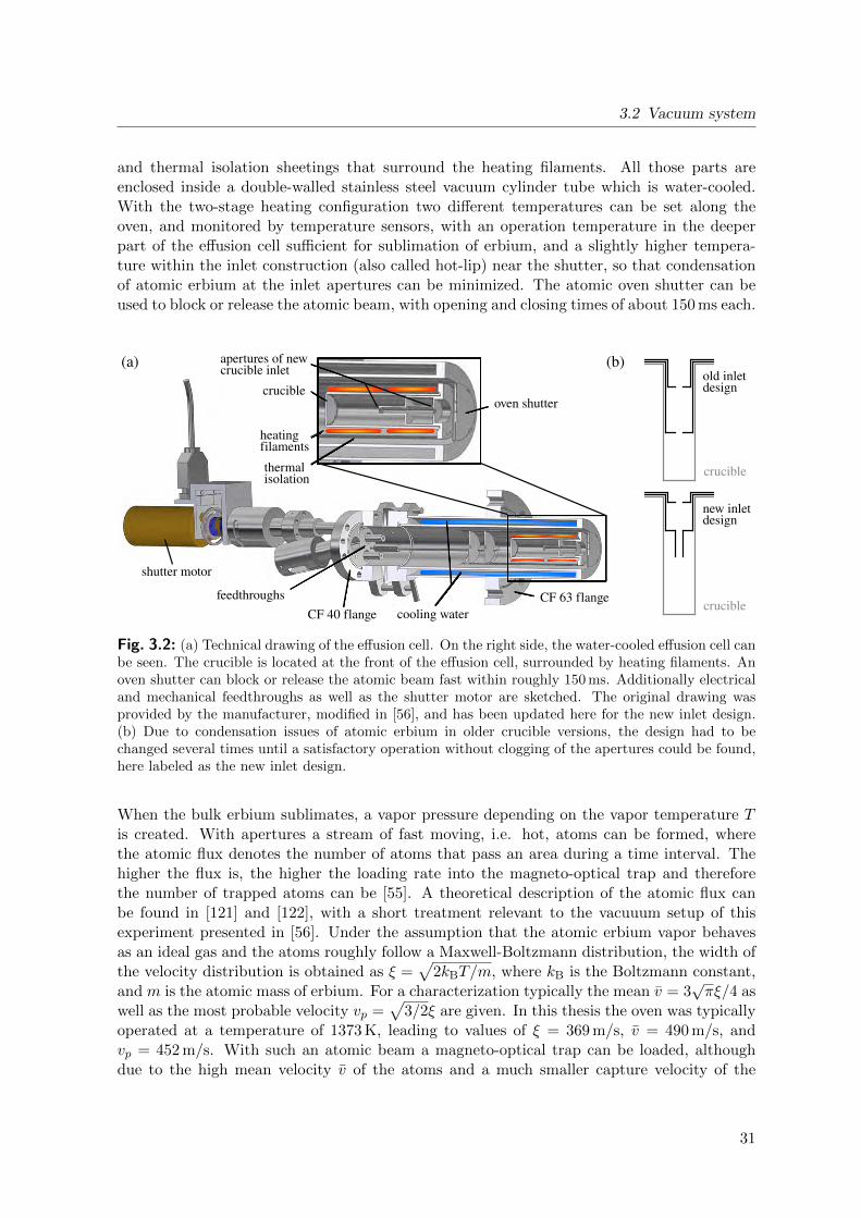
3.2 Vacuum system
and thermal isolation sheetings that surround the heating filaments. All those parts areenclosed inside a double-walled stainless steel vacuum cylinder tube which is water-cooled.With the two-stage heating configuration two different temperatures can be set along theoven, and monitored by temperature sensors, with an operation temperature in the deeperpart of the effusion cell sufficient for sublimation of erbium, and a slightly higher tempera-ture within the inlet construction (also called hot-lip) near the shutter, so that condensationof atomic erbium at the inlet apertures can be minimized. The atomic oven shutter can beused to block or release the atomic beam, with opening and closing times of about 150 ms each.
apertures of newcrucible inlet
crucible
heatingfilaments
thermalisolation
oven shutter
CF 40 flange cooling water
feedthroughs CF 63 flange
(a) (b)
crucible
old inletdesign
crucible
new inletdesign
shutter motor
Fig. 3.2: (a) Technical drawing of the effusion cell. On the right side, the water-cooled effusion cell canbe seen. The crucible is located at the front of the effusion cell, surrounded by heating filaments. Anoven shutter can block or release the atomic beam fast within roughly 150 ms. Additionally electricaland mechanical feedthroughs as well as the shutter motor are sketched. The original drawing wasprovided by the manufacturer, modified in [56], and has been updated here for the new inlet design.(b) Due to condensation issues of atomic erbium in older crucible versions, the design had to bechanged several times until a satisfactory operation without clogging of the apertures could be found,here labeled as the new inlet design.
When the bulk erbium sublimates, a vapor pressure depending on the vapor temperature Tis created. With apertures a stream of fast moving, i.e. hot, atoms can be formed, wherethe atomic flux denotes the number of atoms that pass an area during a time interval. Thehigher the flux is, the higher the loading rate into the magneto-optical trap and thereforethe number of trapped atoms can be [55]. A theoretical description of the atomic flux canbe found in [121] and [122], with a short treatment relevant to the vacuuum setup of thisexperiment presented in [56]. Under the assumption that the atomic erbium vapor behavesas an ideal gas and the atoms roughly follow a Maxwell-Boltzmann distribution, the width ofthe velocity distribution is obtained as ξ =
√2kBT/m, where kB is the Boltzmann constant,
and m is the atomic mass of erbium. For a characterization typically the mean v = 3√πξ/4 as
well as the most probable velocity vp =√
3/2ξ are given. In this thesis the oven was typicallyoperated at a temperature of 1373 K, leading to values of ξ = 369 m/s, v = 490 m/s, andvp = 452 m/s. With such an atomic beam a magneto-optical trap can be loaded, althoughdue to the high mean velocity v of the atoms and a much smaller capture velocity of the
31
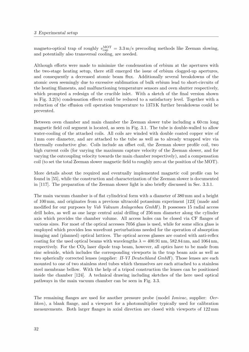
3 Experimental setup
magneto-optical trap of roughly vMOTcap = 3.3 m/s precooling methods like Zeeman slowing,
and potentially also transversal cooling, are needed.
Although efforts were made to minimize the condensation of erbium at the apertures withthe two-stage heating setup, there still emerged the issue of erbium clogged-up apertures,and consequently a decreased atomic beam flux. Additionally several breakdowns of theatomic oven seemingly due to excessive sublimation of bulk erbium lead to short-circuits ofthe heating filaments, and malfunctioning temperature sensors and oven shutter respectively,which prompted a redesign of the crucible inlet. With a sketch of the final version shownin Fig. 3.2(b) condensation effects could be reduced to a satisfactory level. Together with areduction of the effusion cell operation temperature to 1373 K further breakdowns could beprevented.
Between oven chamber and main chamber the Zeeman slower tube including a 60 cm longmagnetic field coil segment is located, as seen in Fig. 3.1. The tube is double-walled to allowwater-cooling of the attached coils. All coils are winded with double coated copper wire of1 mm core diameter, and are attached to the tube as well as to already wrapped wire viathermally conductive glue. Coils include an offset coil, the Zeeman slower profile coil, twohigh current coils (for varying the maximum capture velocity of the Zeeman slower, and forvarying the outcoupling velocity towards the main chamber respectively), and a compensationcoil (to set the total Zeeman slower magnetic field to roughly zero at the position of the MOT).
More details about the required and eventually implemented magnetic coil profile can befound in [55], while the construction and characterization of the Zeeman slower is documentedin [117]. The preparation of the Zeeman slower light is also briefly discussed in Sec. 3.3.1.
The main vacuum chamber is of flat cylindrical form with a diameter of 380 mm and a heightof 100 mm, and originates from a previous ultracold potassium experiment [123] (made andmodified for our purposes by Vab Vakuum Anlagenbau GmbH ). It possesses 15 radial accessdrill holes, as well as one large central axial drilling of 256 mm diameter along the cylinderaxis which provides the chamber volume. All access holes can be closed via CF flanges ofvarious sizes. For most of the optical accesses 7056 glass is used, while for some silica glass isemployed which provides less wavefront perturbations needed for the operation of absorptionimaging and (planned) optical lattices. The optical access glasses are coated with anti-reflexcoating for the used optical beams with wavelengths λ = 400.91 nm, 582.84 nm, and 1064 nm,respectively. For the CO2 laser dipole trap beam, however, all optics have to be made fromzinc selenide, which includes the corresponding viewports in the trap beam axis as well astwo spherically corrected lenses (supplier: II-VI Deutschland GmbH ). Those lenses are eachmounted to one of two stainless steel tubes which themselves are each attached to a stainlesssteel membrane bellow. With the help of a tripod construction the lenses can be positionedinside the chamber [124]. A technical drawing including sketches of the here used opticalpathways in the main vacuum chamber can be seen in Fig. 3.3.
The remaining flanges are used for another pressure probe (model Ionivac, supplier: Oer-likon), a blank flange, and a viewport for a photomultiplier typically used for calibrationmeasurements. Both larger flanges in axial direction are closed with viewports of 122 mm
32
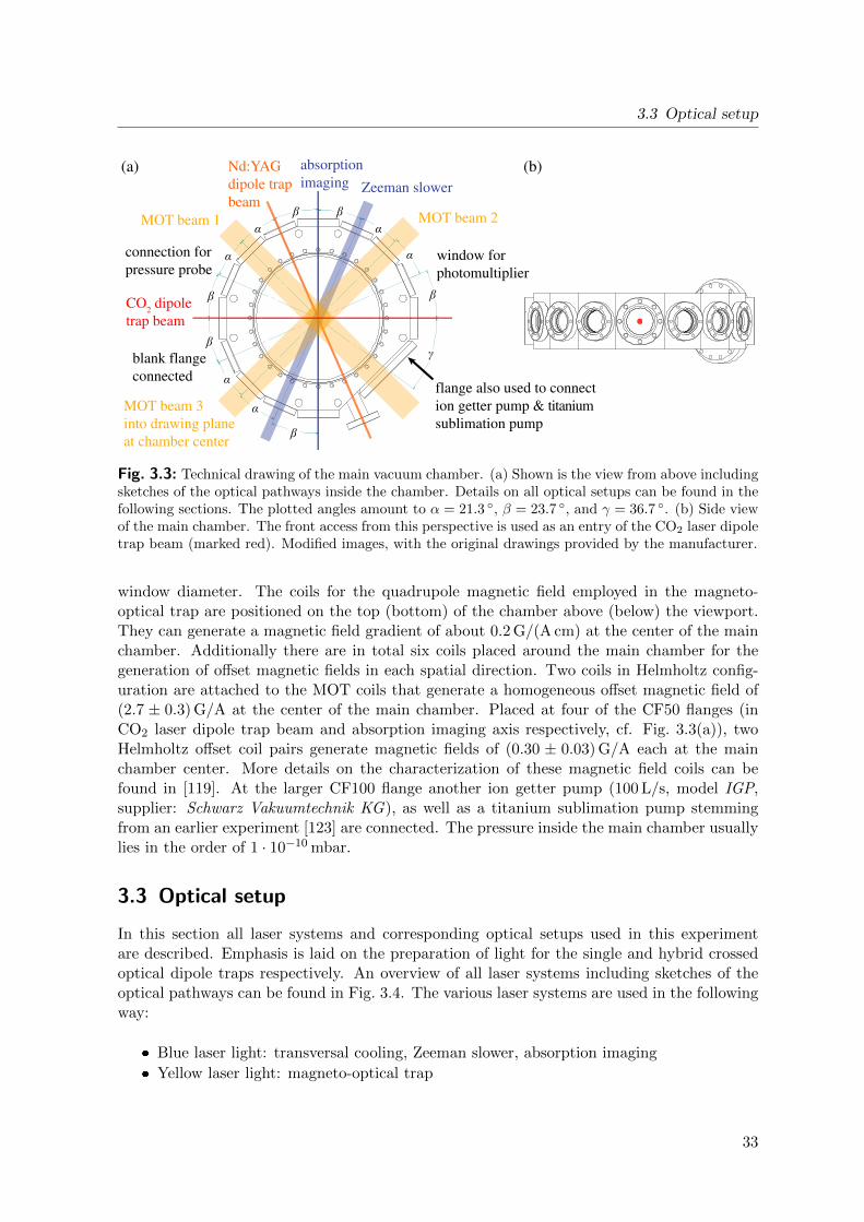
3.3 Optical setup
γ
α
α α
α
α
α
β
β
β
β β
β
(b)(a) absorption imaging Zeeman slower
Nd:YAGdipole trapbeam
MOT beam 1 MOT beam 2
CO2 dipole
trap beam
window forphotomultiplier
connection forpressure probe
MOT beam 3into drawing planeat chamber center
blank flangeconnected
flange also used to connection getter pump & titaniumsublimation pump
Fig. 3.3: Technical drawing of the main vacuum chamber. (a) Shown is the view from above includingsketches of the optical pathways inside the chamber. Details on all optical setups can be found in thefollowing sections. The plotted angles amount to α = 21.3 , β = 23.7 , and γ = 36.7 . (b) Side viewof the main chamber. The front access from this perspective is used as an entry of the CO2 laser dipoletrap beam (marked red). Modified images, with the original drawings provided by the manufacturer.
window diameter. The coils for the quadrupole magnetic field employed in the magneto-optical trap are positioned on the top (bottom) of the chamber above (below) the viewport.They can generate a magnetic field gradient of about 0.2 G/(A cm) at the center of the mainchamber. Additionally there are in total six coils placed around the main chamber for thegeneration of offset magnetic fields in each spatial direction. Two coils in Helmholtz config-uration are attached to the MOT coils that generate a homogeneous offset magnetic field of(2.7 ± 0.3) G/A at the center of the main chamber. Placed at four of the CF50 flanges (inCO2 laser dipole trap beam and absorption imaging axis respectively, cf. Fig. 3.3(a)), twoHelmholtz offset coil pairs generate magnetic fields of (0.30 ± 0.03) G/A each at the mainchamber center. More details on the characterization of these magnetic field coils can befound in [119]. At the larger CF100 flange another ion getter pump (100 L/s, model IGP,supplier: Schwarz Vakuumtechnik KG), as well as a titanium sublimation pump stemmingfrom an earlier experiment [123] are connected. The pressure inside the main chamber usuallylies in the order of 1 · 10−10 mbar.
3.3 Optical setup
In this section all laser systems and corresponding optical setups used in this experimentare described. Emphasis is laid on the preparation of light for the single and hybrid crossedoptical dipole traps respectively. An overview of all laser systems including sketches of theoptical pathways can be found in Fig. 3.4. The various laser systems are used in the followingway:
Blue laser light: transversal cooling, Zeeman slower, absorption imaging
Yellow laser light: magneto-optical trap
33
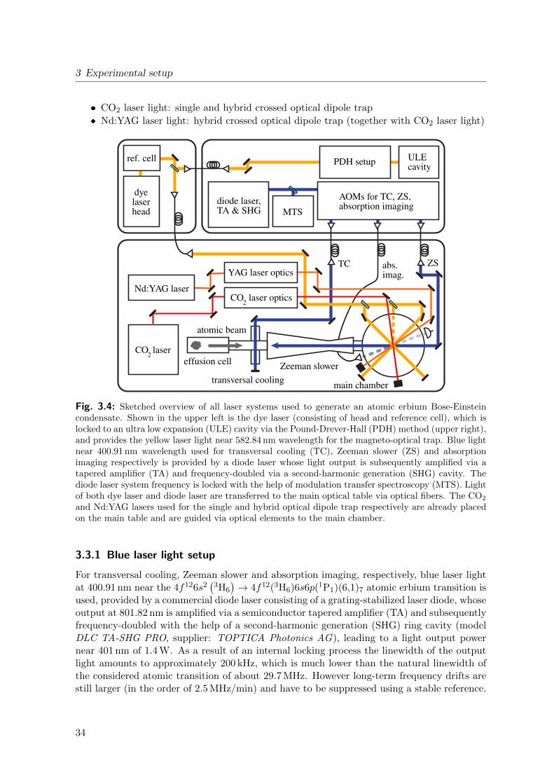
3 Experimental setup
CO2 laser light: single and hybrid crossed optical dipole trap
Nd:YAG laser light: hybrid crossed optical dipole trap (together with CO2 laser light)
dyelaserhead
ref. cell ULEcavityPDH setup
ZS
effusion cell Zeeman slower
main chamber
TC abs.imag.
atomic beam
transversal cooling
MTS
CO2 laser optics
YAG laser optics
Nd:YAG laser
CO2 laser
AOMs for TC, ZS,absorption imagingdiode laser,
TA & SHG
Fig. 3.4: Sketched overview of all laser systems used to generate an atomic erbium Bose-Einsteincondensate. Shown in the upper left is the dye laser (consisting of head and reference cell), which islocked to an ultra low expansion (ULE) cavity via the Pound-Drever-Hall (PDH) method (upper right),and provides the yellow laser light near 582.84 nm wavelength for the magneto-optical trap. Blue lightnear 400.91 nm wavelength used for transversal cooling (TC), Zeeman slower (ZS) and absorptionimaging respectively is provided by a diode laser whose light output is subsequently amplified via atapered amplifier (TA) and frequency-doubled via a second-harmonic generation (SHG) cavity. Thediode laser system frequency is locked with the help of modulation transfer spectroscopy (MTS). Lightof both dye laser and diode laser are transferred to the main optical table via optical fibers. The CO2
and Nd:YAG lasers used for the single and hybrid optical dipole trap respectively are already placedon the main table and are guided via optical elements to the main chamber.
3.3.1 Blue laser light setup
For transversal cooling, Zeeman slower and absorption imaging, respectively, blue laser lightat 400.91 nm near the 4f126s2
(3H6
)→ 4f12(3H6)6s6p(1P1)(6,1)7 atomic erbium transition is
used, provided by a commercial diode laser consisting of a grating-stabilized laser diode, whoseoutput at 801.82 nm is amplified via a semiconductor tapered amplifier (TA) and subsequentlyfrequency-doubled with the help of a second-harmonic generation (SHG) ring cavity (modelDLC TA-SHG PRO, supplier: TOPTICA Photonics AG), leading to a light output powernear 401 nm of 1.4 W. As a result of an internal locking process the linewidth of the outputlight amounts to approximately 200 kHz, which is much lower than the natural linewidth ofthe considered atomic transition of about 29.7 MHz. However long-term frequency drifts arestill larger (in the order of 2.5 MHz/min) and have to be suppressed using a stable reference.
34
3.3 Optical setup
Here the laser frequency is shifted by an acousto-optic modulator (AOM) (model 3200-125,supplier: Gooch & Housego PLC ) and locked to an atomic resonance of 168Er by means ofmodulation transfer spectroscopy (MTS) [125,126] on an erbium hollow cathode lamp (model3QQAYEr, supplier: Heraeus Noblelight GmbH ). The error signal stemming from the spec-troscopy can be fed directly into the diode laser electronics, which then stabilizes the laserfrequency against long-term drifts via the Pound-Drever-Hall technique [127]. Details on thecharacterization of the diode laser and the locking procedure via MTS can be found in [128].
The light for absorption imaging, Zeeman slower, and transversal cooling respectively hasto be prepared before it is sent via optical fibers to the main optical table (as sketched inFig. 3.4 in the upper right corner). For this each optical pathway includes another AOM usedto appropriately shift the light frequency. As the laser light frequency is locked by MTS to avalue shifted from atomic resonance by an AOM (see above), another AOM (model 3307-121,supplier: Gooch & Housego PLC ) employed for absorption imaging light preparation has tocancel this shift to make the probing light again approximately resonant with the atomic en-semble. After transferring the absorption imaging light to the main table via an optical fiberit propagates through the main vacuum chamber and is subsequently guided onto a camerasensor (model 5.5 sCMOS, supplier: Andor Technology Ltd.) to image the shadow of theatomic cloud, as discussed in Sec. 3.4.1.
Preparation of the Zeeman slower light is done with the help of an AOM (model 3220-120,supplier: Crystal Technology, Inc.) by red-shifting the light about 600 MHz (≈ 20 naturallinewidths) away from the atomic erbium resonance near 400.91 nm wavelength. Afterwardsthe shifted light is coupled into a high power optical fiber (model aeroGUIDE-10-PM-APC,supplier: NKT Photonics GmbH ) and delivered to the main optical table, where the outputbeam with a typical power of 300 mW is widened with a telescope to a beam radius of ap-proximately 4 mm and guided into the main chamber to counterpropagate the atomic beamaxis.
Light for the transversal cooling stage is prepared with an AOM (model 3307-121, supplier:Gooch & Housego PLC ), red-shifting the frequency roughly 20 MHz (equaling 0.7 naturallinewidths) away from atomic resonance. After transfer of the light to the main optical tablevia optical fiber, its transversal beam profile is transformed from a circular to an ellipticalshape via a telescope consisting of cylindrical lenses to increase the interaction length of thelight with the atomic beam. The beam with a power of about 80 mW is then lead into thesixfold crosspiece of the oven vacuum chamber in a way so that two counterpropagating laserbeam pairs orthogonal to each other each illuminate the atomic beam transversally. Moredetails on the light preparation and the particular transversal cooling setup can be foundin [56].
3.3.2 Yellow laser light setup
Laser light near 582.84 nm wavelength is employed for the magneto-optical trap, while utiliz-ing the 4f126s2
(3H6
)→ 4f12(3H6)6s6p(3P1)(6,1)7 atomic erbium transition, provided by a
commercial dye laser system (model Matisse DX, supplier: Sirah Lasertechnik GmbH ). Herethe active dye medium is Rhodamin 6G (type Rhodamin 590 Chlorid, supplier: Exciton, Inc.)solved in ethylene glycole with a mass concentration of 0.75 g/L, which is optically pumped
35
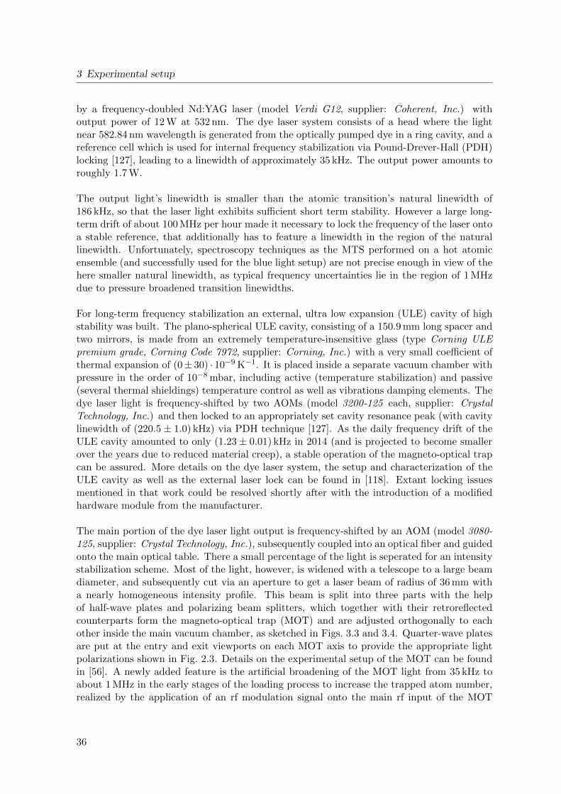
3 Experimental setup
by a frequency-doubled Nd:YAG laser (model Verdi G12, supplier: Coherent, Inc.) withoutput power of 12 W at 532 nm. The dye laser system consists of a head where the lightnear 582.84 nm wavelength is generated from the optically pumped dye in a ring cavity, and areference cell which is used for internal frequency stabilization via Pound-Drever-Hall (PDH)locking [127], leading to a linewidth of approximately 35 kHz. The output power amounts toroughly 1.7 W.
The output light’s linewidth is smaller than the atomic transition’s natural linewidth of186 kHz, so that the laser light exhibits sufficient short term stability. However a large long-term drift of about 100 MHz per hour made it necessary to lock the frequency of the laser ontoa stable reference, that additionally has to feature a linewidth in the region of the naturallinewidth. Unfortunately, spectroscopy techniques as the MTS performed on a hot atomicensemble (and successfully used for the blue light setup) are not precise enough in view of thehere smaller natural linewidth, as typical frequency uncertainties lie in the region of 1 MHzdue to pressure broadened transition linewidths.
For long-term frequency stabilization an external, ultra low expansion (ULE) cavity of highstability was built. The plano-spherical ULE cavity, consisting of a 150.9 mm long spacer andtwo mirrors, is made from an extremely temperature-insensitive glass (type Corning ULEpremium grade, Corning Code 7972, supplier: Corning, Inc.) with a very small coefficient ofthermal expansion of (0± 30) · 10−9 K−1. It is placed inside a separate vacuum chamber withpressure in the order of 10−8 mbar, including active (temperature stabilization) and passive(several thermal shieldings) temperature control as well as vibrations damping elements. Thedye laser light is frequency-shifted by two AOMs (model 3200-125 each, supplier: CrystalTechnology, Inc.) and then locked to an appropriately set cavity resonance peak (with cavitylinewidth of (220.5 ± 1.0) kHz) via PDH technique [127]. As the daily frequency drift of theULE cavity amounted to only (1.23± 0.01) kHz in 2014 (and is projected to become smallerover the years due to reduced material creep), a stable operation of the magneto-optical trapcan be assured. More details on the dye laser system, the setup and characterization of theULE cavity as well as the external laser lock can be found in [118]. Extant locking issuesmentioned in that work could be resolved shortly after with the introduction of a modifiedhardware module from the manufacturer.
The main portion of the dye laser light output is frequency-shifted by an AOM (model 3080-125, supplier: Crystal Technology, Inc.), subsequently coupled into an optical fiber and guidedonto the main optical table. There a small percentage of the light is seperated for an intensitystabilization scheme. Most of the light, however, is widened with a telescope to a large beamdiameter, and subsequently cut via an aperture to get a laser beam of radius of 36 mm witha nearly homogeneous intensity profile. This beam is split into three parts with the helpof half-wave plates and polarizing beam splitters, which together with their retroreflectedcounterparts form the magneto-optical trap (MOT) and are adjusted orthogonally to eachother inside the main vacuum chamber, as sketched in Figs. 3.3 and 3.4. Quarter-wave platesare put at the entry and exit viewports on each MOT axis to provide the appropriate lightpolarizations shown in Fig. 2.3. Details on the experimental setup of the MOT can be foundin [56]. A newly added feature is the artificial broadening of the MOT light from 35 kHz toabout 1 MHz in the early stages of the loading process to increase the trapped atom number,realized by the application of an rf modulation signal onto the main rf input of the MOT
36
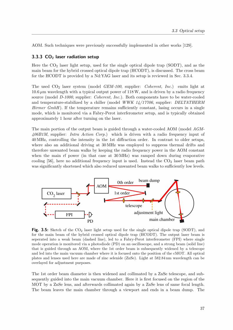
3.3 Optical setup
AOM. Such techniques were previously successfully implemented in other works [129].
3.3.3 CO2 laser radiation setup
Here the CO2 laser light setup, used for the single optical dipole trap (SODT), and as themain beam for the hybrid crossed optical dipole trap (HCODT), is discussed. The cross beamfor the HCODT is provided by a Nd:YAG laser and its setup is reviewed in Sec. 3.3.4.
The used CO2 laser system (model GEM-100, supplier: Coherent, Inc.) emits light at10.6µm wavelength with a typical output power of 118 W, and is driven by a radio frequencysource (model D-1000, supplier: Coherent, Inc.). Both components have to be water-cooledand temperature-stabilized by a chiller (model WWK 14/17706, supplier: DELTATHERMHirmer GmbH ). If the temperature remains sufficiently constant, lasing occurs in a singlemode, which is monitored via a Fabry-Perot interferometer setup, and is typically obtainedapproximately 1 hour after turning on the laser.
The main portion of the output beam is guided through a water-cooled AOM (model AGM-406B1M, supplier: Intra Action Corp.) which is driven with a radio frequency input of40 MHz, controlling the intensity in the 1st diffraction order. In contrast to older setups,where also an additional driving at 30 MHz was employed to suppress thermal drifts andtherefore unwanted beam walks by keeping the radio frequency power in the AOM constantwhen the main rf power (in that case at 30 MHz) was ramped down during evaporativecooling [56], here no additional frequency input is used. Instead the CO2 laser beam pathwas significantly shortened which also reduced unwanted beam walks to sufficiently low levels.
CO2 laser
FPI
PD
beam dumpAOM
0th order
1st order
telescope
main chamber
adjustment light
Fig. 3.5: Sketch of the CO2 laser light setup used for the single optical dipole trap (SODT), andfor the main beam of the hybrid crossed optical dipole trap (HCODT). The output laser beam isseperated into a weak beam (dashed line), led to a Fabry-Perot interferometer (FPI) where singlemode operation is monitored via a photodiode (PD) on an oscilloscope, and a strong beam (solid line)that is guided through an AOM, where the 1st order beam is subsequently widened by a telescopeand led into the main vacuum chamber where it is focused onto the position of the cMOT. All opticalplates and lenses used here are made of zinc selenide (ZnSe). Light at 582.84 nm wavelength can beoverlayed for adjustment purposes.
The 1st order beam diameter is then widened and collimated by a ZnSe telescope, and sub-sequently guided into the main vacuum chamber. Here it is first focused on the region of theMOT by a ZnSe lens, and afterwards collimated again by a ZnSe lens of same focal length.The beam leaves the main chamber through a viewport and ends in a beam dump. The
37
3 Experimental setup
maximum power directly before the main chamber amounts to approximately 73 W. For ad-justment purposes light at 582.84 nm can be overlayed with the CO2 beam. The completesetup is sketched in Fig. 3.5.
The beam waist w0 of the CO2 laser light was determined by a razor-edge measurementoutside the vacuum chamber with a proxy setup identical to the setup inside the main cham-ber, accessible via a flip mirror [97]. For this the collimated beam radius w at the lensposition is measured, from which the beam waist at the trapping site can be estimated viaw0 = λf/(πw), where λ is the wavelength of the light, and f = 63.5 mm is the focal lengthof the lens [130]. To check for an eventual ellipticity of the transversal beam profile, hori-zontal w0,h as well as vertical beam waists w0,v were measured. A slightly elliptically-shapedGaussian beam can be approximated by an ideal Gaussian beam via w0 =
√w0,hw0,v. This
approximation avoids to overcomplexify especially the already dense formulas describing thetrapping potential and trapping frequencies of the HCODT (cf. Eqs. 2.46 and 2.47). TheCO2 laser light beam waists showed indeed a flattening of (w0,h − w0,v)/w0,v ≈ 0.67, wherethe effective beam waist was obtained as w0 ≈ 36µm. This value (together with that of theeffective beam waist of the Nd:YAG trap beam) is later used for the theoretical determinationof trap frequencies of the SODT and HCODT, as well as the phase space density of the atomicensemble inside the trap. Experimental determination of those quantities is done via differentmeasurement methods described in Sec. 3.4.
Intensity control
The intensity of the 1st diffracted order beam can be controlled via the AOM radio frequency(rf) power input, which is proportional to the diffraction efficiency, up to a saturation regime.High rf powers lead to a heating of the germanium crystal inside the AOM, causing a changeof the refractive index and subsequently a beam walk in the order of several mm for a lengthof 2 m. Therefore in earlier iterations of the experiment an additional driving frequency hadto be implemented to keep the temperature of the germanium crystal stable while changingthe main driving rf power at in that case 30 MHz [56]. Here the path length of the CO2 laserbeam was significantly reduced so that the influence of thermal drifts of the non-stabilizedAOM on the spatial beam stability became negligible for the operation of an optical dipoletrap.
The intensity control setup for the CO2 laser light is shown in Fig. 3.6, with the rf path(indicated with yellow arrows) that leads to the AOM for continuous operation consistingof the following parts in the installed order (if not stated otherwise the rf components aresupplied by Mini-Circuits, Inc.):
Signal generator (model SMY 01, supplier: Rohde & Schwarz GmbH & Co. KG) witha 40 MHz rf output
Switch (model ZYSWA-2-50DR)
Amplifier (model LZY-1+)
Voltage variable attenuator (VVA, custom model from the Elektronikwerkstatt Physikalis-ches Institut Tubingen)
Mixer (model ZSC-2-1 )
Switch (same switch model as before)
38
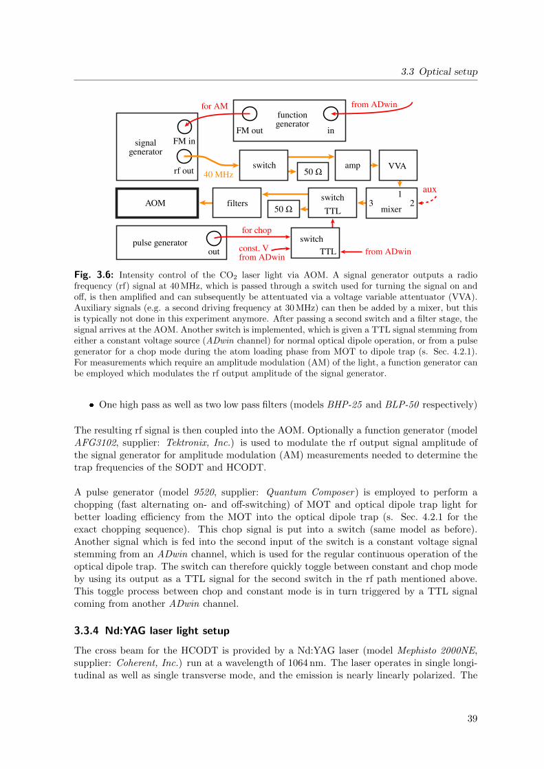
3.3 Optical setup
signalgenerator
FM in
functiongenerator
FM out
for AM from ADwin
rf out 40 MHz 50 Ω
in
switch amp VVA
aux
mixer
123AOM filters
50 Ωswitch
pulse generatorconst. Vfrom ADwin
out
TTL
switchTTL from ADwin
for chop
Fig. 3.6: Intensity control of the CO2 laser light via AOM. A signal generator outputs a radiofrequency (rf) signal at 40 MHz, which is passed through a switch used for turning the signal on andoff, is then amplified and can subsequently be attentuated via a voltage variable attentuator (VVA).Auxiliary signals (e.g. a second driving frequency at 30 MHz) can then be added by a mixer, but thisis typically not done in this experiment anymore. After passing a second switch and a filter stage, thesignal arrives at the AOM. Another switch is implemented, which is given a TTL signal stemming fromeither a constant voltage source (ADwin channel) for normal optical dipole operation, or from a pulsegenerator for a chop mode during the atom loading phase from MOT to dipole trap (s. Sec. 4.2.1).For measurements which require an amplitude modulation (AM) of the light, a function generator canbe employed which modulates the rf output amplitude of the signal generator.
One high pass as well as two low pass filters (models BHP-25 and BLP-50 respectively)
The resulting rf signal is then coupled into the AOM. Optionally a function generator (modelAFG3102, supplier: Tektronix, Inc.) is used to modulate the rf output signal amplitude ofthe signal generator for amplitude modulation (AM) measurements needed to determine thetrap frequencies of the SODT and HCODT.
A pulse generator (model 9520, supplier: Quantum Composer) is employed to perform achopping (fast alternating on- and off-switching) of MOT and optical dipole trap light forbetter loading efficiency from the MOT into the optical dipole trap (s. Sec. 4.2.1 for theexact chopping sequence). This chop signal is put into a switch (same model as before).Another signal which is fed into the second input of the switch is a constant voltage signalstemming from an ADwin channel, which is used for the regular continuous operation of theoptical dipole trap. The switch can therefore quickly toggle between constant and chop modeby using its output as a TTL signal for the second switch in the rf path mentioned above.This toggle process between chop and constant mode is in turn triggered by a TTL signalcoming from another ADwin channel.
3.3.4 Nd:YAG laser light setup
The cross beam for the HCODT is provided by a Nd:YAG laser (model Mephisto 2000NE,supplier: Coherent, Inc.) run at a wavelength of 1064 nm. The laser operates in single longi-tudinal as well as single transverse mode, and the emission is nearly linearly polarized. The
39
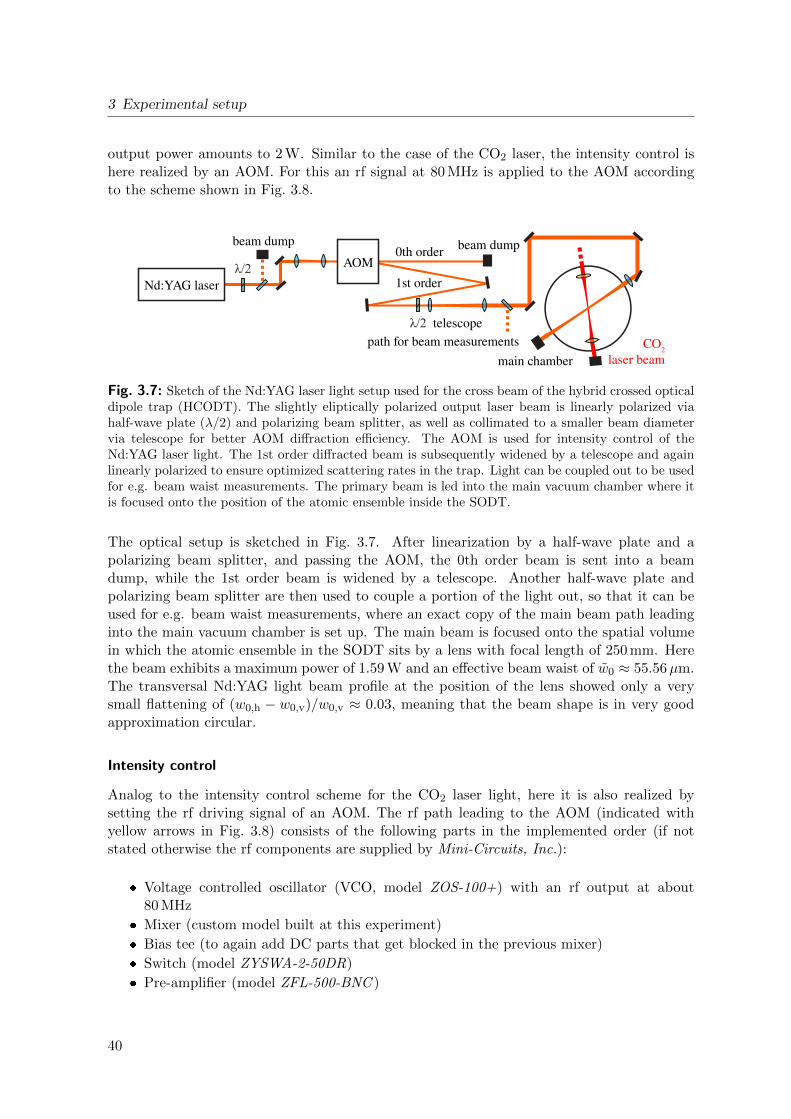
3 Experimental setup
output power amounts to 2 W. Similar to the case of the CO2 laser, the intensity control ishere realized by an AOM. For this an rf signal at 80 MHz is applied to the AOM accordingto the scheme shown in Fig. 3.8.
beam dumpAOM
0th order
1st order
telescope
main chamber
Nd:YAG laserλ/2
λ/2
beam dump
path for beam measurements CO2
laser beam
Fig. 3.7: Sketch of the Nd:YAG laser light setup used for the cross beam of the hybrid crossed opticaldipole trap (HCODT). The slightly eliptically polarized output laser beam is linearly polarized viahalf-wave plate (λ/2) and polarizing beam splitter, as well as collimated to a smaller beam diametervia telescope for better AOM diffraction efficiency. The AOM is used for intensity control of theNd:YAG laser light. The 1st order diffracted beam is subsequently widened by a telescope and againlinearly polarized to ensure optimized scattering rates in the trap. Light can be coupled out to be usedfor e.g. beam waist measurements. The primary beam is led into the main vacuum chamber where itis focused onto the position of the atomic ensemble inside the SODT.
The optical setup is sketched in Fig. 3.7. After linearization by a half-wave plate and apolarizing beam splitter, and passing the AOM, the 0th order beam is sent into a beamdump, while the 1st order beam is widened by a telescope. Another half-wave plate andpolarizing beam splitter are then used to couple a portion of the light out, so that it can beused for e.g. beam waist measurements, where an exact copy of the main beam path leadinginto the main vacuum chamber is set up. The main beam is focused onto the spatial volumein which the atomic ensemble in the SODT sits by a lens with focal length of 250 mm. Herethe beam exhibits a maximum power of 1.59 W and an effective beam waist of w0 ≈ 55.56µm.The transversal Nd:YAG light beam profile at the position of the lens showed only a verysmall flattening of (w0,h − w0,v)/w0,v ≈ 0.03, meaning that the beam shape is in very goodapproximation circular.
Intensity control
Analog to the intensity control scheme for the CO2 laser light, here it is also realized bysetting the rf driving signal of an AOM. The rf path leading to the AOM (indicated withyellow arrows in Fig. 3.8) consists of the following parts in the implemented order (if notstated otherwise the rf components are supplied by Mini-Circuits, Inc.):
Voltage controlled oscillator (VCO, model ZOS-100+) with an rf output at about80 MHz
Mixer (custom model built at this experiment)
Bias tee (to again add DC parts that get blocked in the previous mixer)
Switch (model ZYSWA-2-50DR)
Pre-amplifier (model ZFL-500-BNC )
40
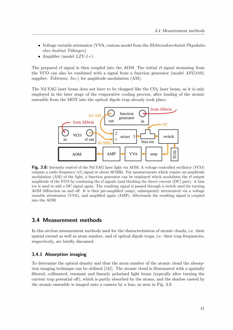
3.4 Measurement methods
Voltage variable attenuator (VVA, custom model from the Elektronikwerkstatt Physikalis-ches Institut Tubingen)
Amplifier (model LZY-1+)
The prepared rf signal is then coupled into the AOM. The initial rf signal stemming fromthe VCO can also be combined with a signal from a function generator (model AFG3102,supplier: Tektronix, Inc.) for amplitude modulation (AM).
The Nd:YAG laser beam does not have to be chopped like the CO2 laser beam, as it is onlyemployed in the later stage of the evaporative cooling process, after loading of the atomicensemble from the MOT into the optical dipole trap already took place.
VCOin
functiongenerator
outfor AM
from ADwin
rf out80 MHz
50 Ω
in
switch
AOM AMP
from ADwin
VVA amp
bias teemixer
1
23
DC
Fig. 3.8: Intensity control of the Nd:YAG laser light via AOM. A voltage controlled oscillator (VCO)outputs a radio frequency (rf) signal at about 80 MHz. For measurements which require an amplitudemodulation (AM) of the light, a function generator can be employed which modulates the rf outputamplitude of the VCO by combining the rf signals (and blocking the direct current (DC) part). A biastee is used to add a DC signal again. The resulting signal is passed through a switch used for turningAOM diffraction on and off. It is then pre-amplified (amp), subsequently attentuated via a voltagevariable attentuator (VVA), and amplified again (AMP). Afterwards the resulting signal is coupledinto the AOM.
3.4 Measurement methods
In this section measurement methods used for the characterization of atomic clouds, i.e. theirspatial extend as well as atom number, and of optical dipole traps, i.e. their trap frequencies,respectively, are briefly discussed.
3.4.1 Absorption imaging
To determine the optical density and thus the atom number of the atomic cloud the absorp-tion imaging technique can be utilized [131]. The atomic cloud is illuminated with a spatiallyfiltered, collimated, resonant and linearly polarized light beam (typically after turning thecurrent trap potential off), which is partly absorbed by the atoms, and the shadow casted bythe atomic ensemble is imaged onto a camera by a lens, as seen in Fig. 3.9.
41
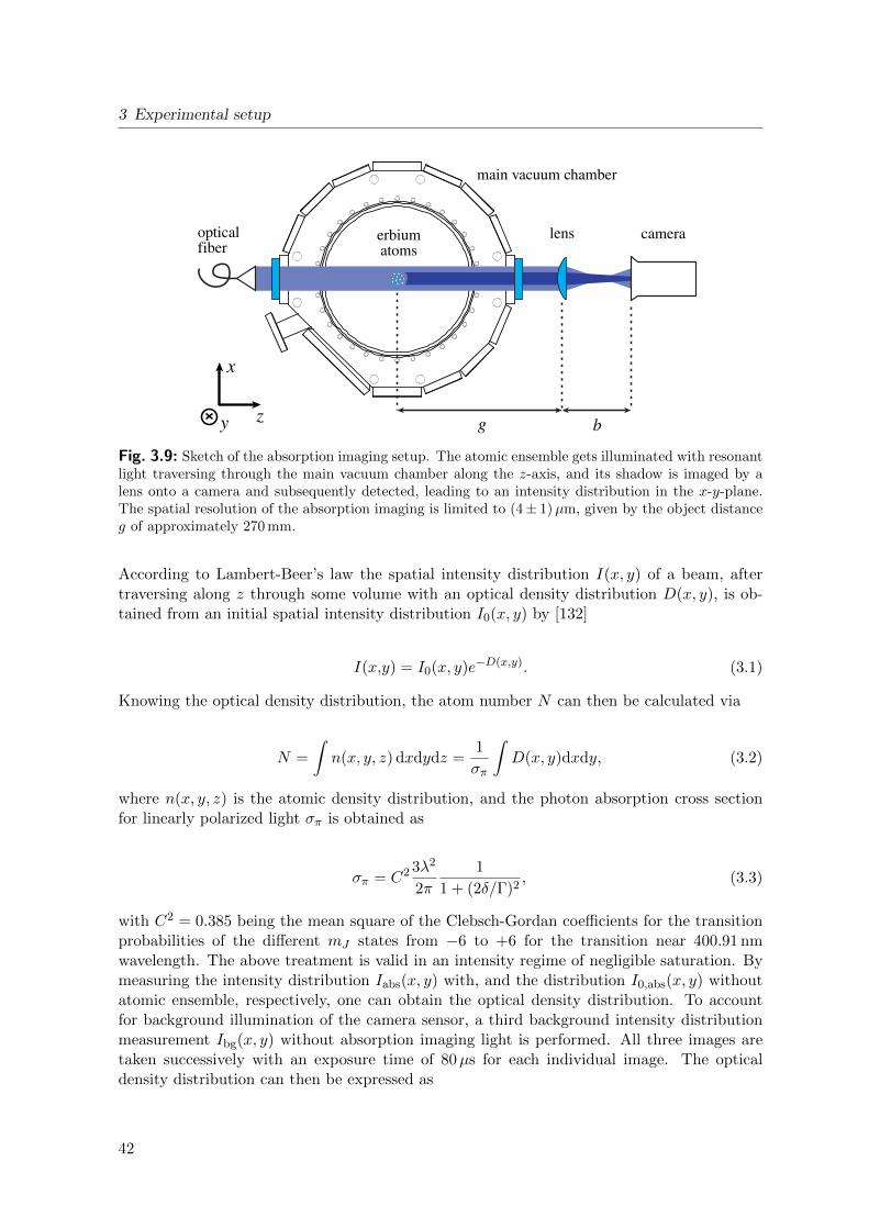
3 Experimental setup
erbiumatoms
cameralens
x
y z
opticalfiber
g b
main vacuum chamber
Fig. 3.9: Sketch of the absorption imaging setup. The atomic ensemble gets illuminated with resonantlight traversing through the main vacuum chamber along the z-axis, and its shadow is imaged by alens onto a camera and subsequently detected, leading to an intensity distribution in the x-y-plane.The spatial resolution of the absorption imaging is limited to (4± 1)µm, given by the object distanceg of approximately 270 mm.
According to Lambert-Beer’s law the spatial intensity distribution I(x, y) of a beam, aftertraversing along z through some volume with an optical density distribution D(x, y), is ob-tained from an initial spatial intensity distribution I0(x, y) by [132]
I(x,y) = I0(x, y)e−D(x,y). (3.1)
Knowing the optical density distribution, the atom number N can then be calculated via
N =
∫n(x, y, z) dxdydz =
1
σπ
∫D(x, y)dxdy, (3.2)
where n(x, y, z) is the atomic density distribution, and the photon absorption cross sectionfor linearly polarized light σπ is obtained as
σπ = C2 3λ2
2π
1
1 + (2δ/Γ)2, (3.3)
with C2 = 0.385 being the mean square of the Clebsch-Gordan coefficients for the transitionprobabilities of the different mJ states from −6 to +6 for the transition near 400.91 nmwavelength. The above treatment is valid in an intensity regime of negligible saturation. Bymeasuring the intensity distribution Iabs(x, y) with, and the distribution I0,abs(x, y) withoutatomic ensemble, respectively, one can obtain the optical density distribution. To accountfor background illumination of the camera sensor, a third background intensity distributionmeasurement Ibg(x, y) without absorption imaging light is performed. All three images aretaken successively with an exposure time of 80µs for each individual image. The opticaldensity distribution can then be expressed as
42
3.4 Measurement methods
D(x,y) = − ln
(I(x, y)
I0(x, y)
)= − ln
(Iabs(x, y)− Ibg(x, y)
I0,abs(x, y)− Ibg(x, y)
). (3.4)
The spatial resolution of the absorption imaging amounts to (4±1)µm. By taking absorptionimages at different points in time (while for each image a new experimental cycle has to beconducted as the method is destructive), the temporal evolution of e.g. expanding clouds aftertrap release can be documented (called time of flight measurement), which for this examplecan be used to determine the temperature of the atomic ensemble, as further discussed inSec. 4.1.2.
3.4.2 Trap frequency measurements and phase space density determination
The atomic density has to be known for the determination of the phase space density, andcan be calculated from the trap frequencies [48]. We here assume a Gaussian atomic densitydistribution according to
n(x, y, z) = n0 exp
(− x2
2σ2x
− y2
2σ2y
− z2
2σ2z
), (3.5)
where σi is the 1/e2 atomic cloud radius in direction along i, with i = x, y, z, and n0 =N/((2π)3/2σxσyσz) is the central atomic density. The total atom number N is obtained viaEq. 3.2. The cloud radii can be calculated by means of the virial theorem, which connectsthe temporal mean of potential and kinetic energy, respectively, the latter here provided bythe thermal motion of the atoms in the considered spatial direction i [133]. For a harmonicpotential and a Gaussian density distribution it follows that
σi =
√kBT
mω2i
. (3.6)
With Eq. 2.9 and the central atomic density n0, the phase space density is obtained as
ρ =~3N
k3BT
3ω2rωz, (3.7)
where ωx = ωy = ωr is assumed. The trap frequencies can be measured by means of para-metric excitations of the trap. Two methods are used in this thesis and discussed below.Together with the temperature T , the phase space density can therefore be calculated frommeasurable quantities in the experiment.
Amplitude modulation
Here the amplitude of the optical dipole trap potential is sinusoidally modulated to find thetrap frequencies νtrap = ωtrap/(2π) of the optical dipole trap. For this the atomic ensemble isfirst loaded from the MOT into the dipole trap, then evaporatively cooled up to a set point
43
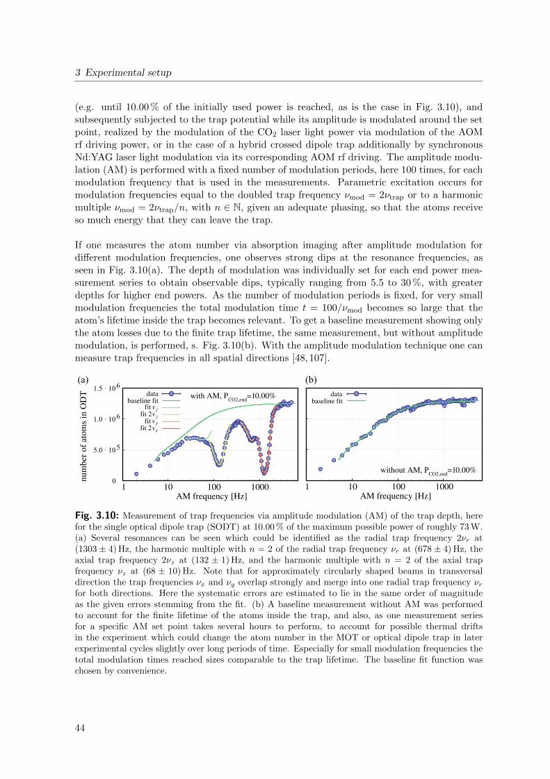
3 Experimental setup
(e.g. until 10.00 % of the initially used power is reached, as is the case in Fig. 3.10), andsubsequently subjected to the trap potential while its amplitude is modulated around the setpoint, realized by the modulation of the CO2 laser light power via modulation of the AOMrf driving power, or in the case of a hybrid crossed dipole trap additionally by synchronousNd:YAG laser light modulation via its corresponding AOM rf driving. The amplitude modu-lation (AM) is performed with a fixed number of modulation periods, here 100 times, for eachmodulation frequency that is used in the measurements. Parametric excitation occurs formodulation frequencies equal to the doubled trap frequency νmod = 2νtrap or to a harmonicmultiple νmod = 2νtrap/n, with n ∈ N, given an adequate phasing, so that the atoms receiveso much energy that they can leave the trap.
If one measures the atom number via absorption imaging after amplitude modulation fordifferent modulation frequencies, one observes strong dips at the resonance frequencies, asseen in Fig. 3.10(a). The depth of modulation was individually set for each end power mea-surement series to obtain observable dips, typically ranging from 5.5 to 30 %, with greaterdepths for higher end powers. As the number of modulation periods is fixed, for very smallmodulation frequencies the total modulation time t = 100/νmod becomes so large that theatom’s lifetime inside the trap becomes relevant. To get a baseline measurement showing onlythe atom losses due to the finite trap lifetime, the same measurement, but without amplitudemodulation, is performed, s. Fig. 3.10(b). With the amplitude modulation technique one canmeasure trap frequencies in all spatial directions [48,107].
0
5.0 · 105
1.0 · 106
1.5 · 106
1 10 100 1000
num
ber
of a
tom
s in
OD
T
AM frequency [Hz]
databaseline fit
fit νzfit 2νz
fit νrfit 2νr
1 10 100 1000AM frequency [Hz]
databaseline fit
(a) (b)
without AM, PCO2,end
=10.00%
with AM, PCO2,end
=10.00%
Fig. 3.10: Measurement of trap frequencies via amplitude modulation (AM) of the trap depth, herefor the single optical dipole trap (SODT) at 10.00 % of the maximum possible power of roughly 73 W.(a) Several resonances can be seen which could be identified as the radial trap frequency 2νr at(1303 ± 4) Hz, the harmonic multiple with n = 2 of the radial trap frequency νr at (678 ± 4) Hz, theaxial trap frequency 2νz at (132 ± 1) Hz, and the harmonic multiple with n = 2 of the axial trapfrequency νz at (68 ± 10) Hz. Note that for approximately circularly shaped beams in transversaldirection the trap frequencies νx and νy overlap strongly and merge into one radial trap frequency νrfor both directions. Here the systematic errors are estimated to lie in the same order of magnitudeas the given errors stemming from the fit. (b) A baseline measurement without AM was performedto account for the finite lifetime of the atoms inside the trap, and also, as one measurement seriesfor a specific AM set point takes several hours to perform, to account for possible thermal driftsin the experiment which could change the atom number in the MOT or optical dipole trap in laterexperimental cycles slightly over long periods of time. Especially for small modulation frequencies thetotal modulation times reached sizes comparable to the trap lifetime. The baseline fit function waschosen by convenience.
44
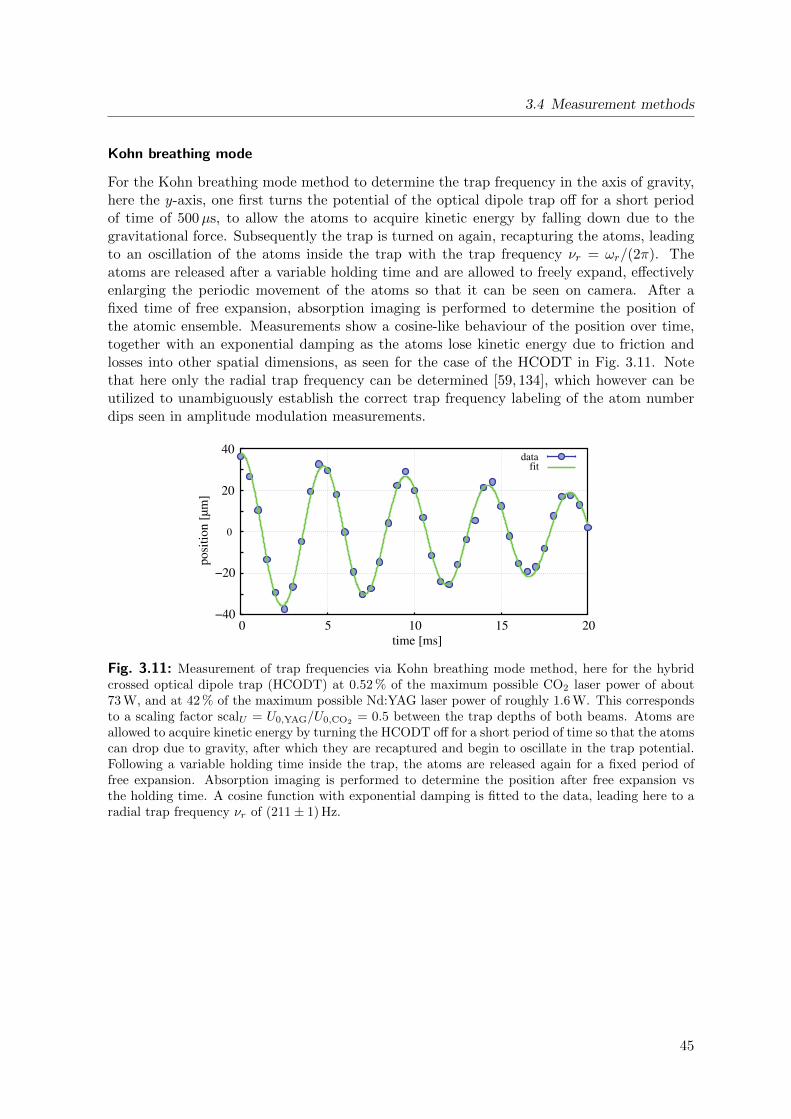
3.4 Measurement methods
Kohn breathing mode
For the Kohn breathing mode method to determine the trap frequency in the axis of gravity,here the y-axis, one first turns the potential of the optical dipole trap off for a short periodof time of 500µs, to allow the atoms to acquire kinetic energy by falling down due to thegravitational force. Subsequently the trap is turned on again, recapturing the atoms, leadingto an oscillation of the atoms inside the trap with the trap frequency νr = ωr/(2π). Theatoms are released after a variable holding time and are allowed to freely expand, effectivelyenlarging the periodic movement of the atoms so that it can be seen on camera. After afixed time of free expansion, absorption imaging is performed to determine the position ofthe atomic ensemble. Measurements show a cosine-like behaviour of the position over time,together with an exponential damping as the atoms lose kinetic energy due to friction andlosses into other spatial dimensions, as seen for the case of the HCODT in Fig. 3.11. Notethat here only the radial trap frequency can be determined [59, 134], which however can beutilized to unambiguously establish the correct trap frequency labeling of the atom numberdips seen in amplitude modulation measurements.
−40
−20
0
20
40
0 5 10 15 20
posi
tion
[µm
]
time [ms]
datafit
Fig. 3.11: Measurement of trap frequencies via Kohn breathing mode method, here for the hybridcrossed optical dipole trap (HCODT) at 0.52 % of the maximum possible CO2 laser power of about73 W, and at 42 % of the maximum possible Nd:YAG laser power of roughly 1.6 W. This correspondsto a scaling factor scalU = U0,YAG/U0,CO2
= 0.5 between the trap depths of both beams. Atoms areallowed to acquire kinetic energy by turning the HCODT off for a short period of time so that the atomscan drop due to gravity, after which they are recaptured and begin to oscillate in the trap potential.Following a variable holding time inside the trap, the atoms are released again for a fixed period offree expansion. Absorption imaging is performed to determine the position after free expansion vsthe holding time. A cosine function with exponential damping is fitted to the data, leading here to aradial trap frequency νr of (211± 1) Hz.
45

4 Characterization of the setup andexperimental results
In this chapter results regarding the characterization of the experimental setup for the gen-eration of an atomic erbium Bose-Einstein condensate (BEC) in a hybrid crossed dipole trapare presented. Starting with the narrow-line magneto-optical trap (MOT), properties as thetemperature of the atomic ensemble and the total atom number, as well as the compressingprocess are shown. Next the atom loading procedure from the compressed MOT into theoptical dipole trap is described. Following this, many properties of the trap, as e.g. the trapfrequencies, in single optical dipole trap (SODT) configuration and in hybrid crossed opticaldipole trap (HCODT) configuration, respectively, are discussed and compared. Here the sec-ond (cross) beam for the hybrid crossed optical dipole trap is only used in the later stages ofthe experimental cycle after the evaporative cooling process has already started. This evapo-ration process is then as well compared for both possible setups (SODT/HCODT). Emphasisis also put on the spin-polarization of the atomic ensemble inside the optical dipole trap, mea-sured via an Stern-Gerlach type experiment. In the end proof of Bose-Einstein condensation,including a determination of the phase space density and the lifetime in the different trapconfigurations, is presented.
4.1 Magneto-optical trap
Atoms decelerated by the Zeeman slower are captured in the magneto-optical trap. A char-acterization of the atomic beam including the efficiency of the Zeeman slower can be foundin [56] and is not repeated here as the corresponding part of the setup remained mainlyunchanged. The atoms leave the atomic oven with a mean velocity of 490 m/s. Here theoperation temperature of the effusion cell was reduced by 100 K to 1373 K in comparison toolder iterations of the experiment to preserve the atomic oven against further breakdownsmentioned in Sec. 3.2. Due to the capture velocity of the MOT of vMOT
cap = 3.3 m/s a portionof the atoms in the atomic beam has to be slowed down considerably. For this the Zeemanslower beam operated at about 400.91 nm wavelength is roughly aligned by maximizing itsdecelarating influence on the atomic beam observable via velocity-sensitive fluorescence imag-ing [56]. After that, fine-tuning of the Zeeman slower takes place by maximizing the loadingrate of the MOT and therefore the maximal number of trapped atoms after a fixed loadingperiod. The transversal cooling stage efficiency is optimized in the same manner. The in thisway pre-cooled atoms are then loaded into the MOT which is roughly located at the centerof the main vacuum chamber.
4.1.1 Loading of the magneto-optical trap
More precisely, there exist two MOT phases: a loading phase where atoms from the decel-erated atomic beam are captured, operated with light of large detuning from resonance near
47
4 Characterization of the setup and experimental results
582.84 nm wavelength, resulting in a large spherical trapping volume (called MOT in thefollowing), and a compressing phase where the detuning and intensity of the MOT light isdecreased, leading to a spatial shrinking of the MOT volume (called cMOT in the following),utilized to maximize the efficiency of the following step, a transfer process into the opticaldipole trap. The temporal evolution of the corresponding experimental parameters can beseen in Fig. 4.1, and in situ images of the atomic fluorescence during the different MOT phasesare shown in Fig. 4.2. In this section measurements for the characterization of the loadingprocess of the magneto-optical trap are presented.
Atom numbers in the loading MOT during this thesis amount up to 5 · 107 after a loadingtime of 10 s. Here the use of a transversal cooling stage increased the final atom number inthe MOT roughly by a factor 2, comparable to earlier works [56]. The loading MOT light isoperated at a detuning of −44 natural linewidths away from resonance. The magnetic fieldgradient is set to 3.8 G/cm. The light intensity per axis amounts to roughly 8 mW/cm2. Dueto the large detuning the atoms gather in a gravitational sag below the Zeeman slower beam.
Then the number of atoms could be increased by another factor of 1.5 compared to ear-lier work [56] by modulating the MOT light at the beginning of the loading phase, leading toa very broad linewidth of the light of approximately 3.2 MHz. This is done by applying an rfmodulation signal onto the AOM originally used for intensity control of the MOT light. Dueto the increased linewidth, MOT light scattering and therefore optical cooling takes place fora broader velocity class of atoms from the atomic beam. The broadening is ramped downlinearly in time and vanishes during the loading phase.
The qualitative loading behaviour is discussed in [56] and is not further examined here forbrevity. The holding time in the MOT after turning off the Zeeman slower light also hasnot changed significantly from earlier setups and lies in the region of a few minutes, which ismore than sufficient for trapping and subsequent loading into the optical dipole trap. Typicalequilibrium temperatures lie theoretically in the region of 20µK, but are in practice difficultto determine, as the trapping volume has to be estimated. A more interesting quantity is thetemperature in the cMOT after the compression phase ended, which is discussed in the nextsection.
4.1.2 Compressing process
For a good spatial overlap of the atomic cloud inside the MOT and the comparatively smallbeam volume of the optical dipole trap, the MOT is compressed by changing the light fre-quency and intensity, as well as the magnetic field gradient linearly over time. This alsochanges the absolute position of the atomic ensemble inside the MOT, which is in the loadingprocess below the center height of the main vacuum chamber and therefore the optical dipoletrapping laser beams, but after the compressing phase on the correct height. The detuning ofthe MOT light frequency is ramped to approximately −3 natural linewidths, while the lightintensity per axis is lowered to 0.13 mW/cm2, both within a time interval of 400 ms, which ismuch bigger than the equilibrium time of 15 ms, as discussed in Sec. 2.3.2, and thus shouldnot cause any additional heating of the atoms. For an overview of all parameters changedduring the compressing phase, see Fig. 4.1. The cMOT encompasses about 5 · 107 atomswith a radius of approximately 160µm in both horizontal axes, and 60µm in the vertical
48
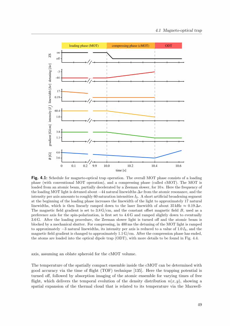
4.1 Magneto-optical trap
inte
nsity
[I S]
detu
ning
[∆ν]
B [
G]
off
onZ
S
-44
-3
grad
ient
[G
/cm
]
3.8
1.1
0 10.69.90.1 0.2 10.0 10.2 10.4
4.6
60.4
1.0
loading phase (MOT) compressing phase (cMOT) ODT
time [s]
linew
idth
[∆ν]
17
0.19
3.6
Fig. 4.1: Schedule for magneto-optical trap operation. The overall MOT phase consists of a loadingphase (with conventional MOT operation), and a compressing phase (called cMOT). The MOT isloaded from an atomic beam, partially decelerated by a Zeeman slower, for 10 s. Here the frequency ofthe loading MOT light is detuned about −44 natural linewidths ∆ν from the atomic resonance, and theintensity per axis amounts to roughly 60 saturation intensities IS. A short artificial broadening segmentat the beginning of the loading phase increases the linewidth of the light to approximately 17 naturallinewidths, which is then linearly ramped down to the laser linewidth of about 35 kHz ≈ 0.19 ∆ν.The magnetic field gradient is set to 3.8 G/cm, and the constant offset magnetic field B, used as apreference axis for the spin-polarization, is first set to 4.6 G and ramped slightly down to eventually3.6 G. After the loading procedure, the Zeeman slower light is turned off and the atomic beam isblocked by a mechanical shutter. For compressing, in 400 ms the detuning of the MOT light is rampedto approximately −3 natural linewidths, its intensity per axis is reduced to a value of 1.0 IS, and themagnetic field gradient is changed to approximately 1.1 G/cm. After the compression phase has ended,the atoms are loaded into the optical dipole trap (ODT), with more details to be found in Fig. 4.4.
axis, assuming an oblate spheroid for the cMOT volume.
The temperature of the spatially compact ensemble inside the cMOT can be determined withgood accuracy via the time of flight (TOF) technique [135]. Here the trapping potential isturned off, followed by absorption imaging of the atomic ensemble for varying times of freeflight, which delivers the temporal evolution of the density distribution n(x, y), showing aspatial expansion of the thermal cloud that is related to its temperature via the Maxwell-
49
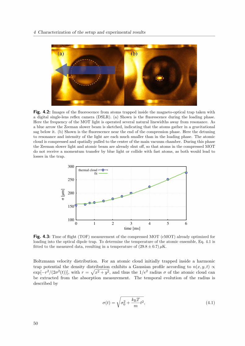
4 Characterization of the setup and experimental results
Fig. 4.2: Images of the fluorescence from atoms trapped inside the magneto-optical trap taken witha digital single-lens reflex camera (DSLR). (a) Shown is the fluorescence during the loading phase.Here the frequency of the MOT light is operated several natural linewidths away from resonance. Asa blue arrow the Zeeman slower beam is sketched, indicating that the atoms gather in a gravitationalsag below it. (b) Shown is the fluorescence near the end of the compression phase. Here the detuningto resonance and intensity of the light are each much smaller than in the loading phase. The atomiccloud is compressed and spatially pulled to the center of the main vacuum chamber. During this phasethe Zeeman slower light and atomic beam are already shut off, so that atoms in the compressed MOTdo not receive a momentum transfer by blue light or collide with fast atoms, as both would lead tolosses in the trap.
100
150
200
250
300
0 1 2 3 4 5 6
σ [µ
m]
time [ms]
thermal cloudfit
Fig. 4.3: Time of flight (TOF) measurement of the compressed MOT (cMOT) already optimized forloading into the optical dipole trap. To determine the temperature of the atomic ensemble, Eq. 4.1 isfitted to the measured data, resulting in a temperature of (29.8± 0.7)µK.
Boltzmann velocity distribution. For an atomic cloud initially trapped inside a harmonictrap potential the density distribution exhibits a Gaussian profile according to n(x, y, t) ∝exp[−r2/(2σ2(t))], with r =
√x2 + y2, and thus the 1/e2 radius σ of the atomic cloud can
be extracted from the absorption measurement. The temporal evolution of the radius isdescribed by
σ(t) =
√σ2
0 +kBT
mt2, (4.1)
50
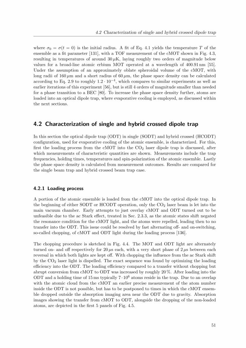
4.2 Characterization of single and hybrid crossed dipole trap
where σ0 = σ(t = 0) is the initial radius. A fit of Eq. 4.1 yields the temperature T of theensemble as a fit parameter [131], with a TOF measurement of the cMOT shown in Fig. 4.3,resulting in temperatures of around 30µK, laying roughly two orders of magnitude belowvalues for a broad-line atomic erbium MOT operated at a wavelength of 400.91 nm [55].Under the assumption of an approximately oblate spheroidal volume of the cMOT, withlong radii of 160µm and a short radius of 60µm, the phase space density can be calculatedaccording to Eq. 2.9 to roughly 1.2 · 10−4, which compares to similar experiments as well asearlier iterations of this experiment [56], but is still 4 orders of magnitude smaller than neededfor a phase transition to a BEC [80]. To increase the phase space density further, atoms areloaded into an optical dipole trap, where evaporative cooling is employed, as discussed withinthe next sections.
4.2 Characterization of single and hybrid crossed dipole trap
In this section the optical dipole trap (ODT) in single (SODT) and hybrid crossed (HCODT)configuration, used for evaporative cooling of the atomic ensemble, is characterized. For this,first the loading process from the cMOT into the CO2 laser dipole trap is discussed, afterwhich measurements of characteristic quantities are shown. Measurements include the trapfrequencies, holding times, temperatures and spin-polarization of the atomic ensemble. Lastlythe phase space density is calculated from measurement outcomes. Results are compared forthe single beam trap and hybrid crossed beam trap case.
4.2.1 Loading process
A portion of the atomic ensemble is loaded from the cMOT into the optical dipole trap. Inthe beginning of either SODT or HCODT operation, only the CO2 laser beam is let into themain vacuum chamber. Early attempts to just overlay cMOT and ODT turned out to beunfeasible due to the ac Stark effect, treated in Sec. 2.3.3, as the atomic states shift negatedthe resonance condition for the cMOT light, and the atoms were repelled, leading then to notransfer into the ODT. This issue could be resolved by fast alternating off- and on-switching,so-called chopping, of cMOT and ODT light during the loading process [136].
The chopping procedure is sketched in Fig. 4.4. The MOT and ODT light are alternatelyturned on- and off respectively for 20µs each, with a very short phase of 2µs between eachreversal in which both lights are kept off. With chopping the influence from the ac Stark shiftby the CO2 laser light is dispelled. The exact sequence was found by optimizing the loadingefficiency into the ODT. The loading efficiency compared to a transfer without chopping butabrupt conversion from cMOT to ODT was increased by roughly 20 %. After loading into theODT and a holding time of 15 ms typically 7 ·106 atoms reside in the trap. Due to an overlapwith the atomic cloud from the cMOT an earlier precise measurement of the atom numberinside the ODT is not possible, but has to be postponed to times in which the cMOT ensem-ble dropped outside the absorption imaging area near the ODT due to gravity. Absorptionimages showing the transfer from cMOT to ODT, alongside the dropping of the non-loadedatoms, are depicted in the first 5 panels of Fig. 4.5.
51
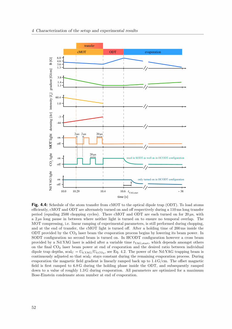
4 Characterization of the setup and experimental results
grad
ient
[G
/cm
]B
[G
]C
O2 l
ight
detu
ning
[∆ν]
1.0
60.4
MO
T lig
ht
on
off
on
off
-3
-44
time [s]
evaporationcMOT ODT
1.1
3.8
4.6
inte
nsity
[I S]
20µs
20 µs2µs2µs
transferN
d:Y
AG
ligh
t
10.6 ~ 3810.4
on
off
10.0
only turned on in HCODT configuration
used in SODT as well as in HCODT configuration
tYAG,start10.29
1.4
3.61.3
6.8
Fig. 4.4: Schedule of the atom transfer from cMOT to the optical dipole trap (ODT). To load atomsefficiently, cMOT and ODT are alternately turned on and off respectively during a 110 ms long transferperiod (equaling 2500 chopping cycles). There cMOT and ODT are each turned on for 20µs, witha 2µs long pause in between where neither light is turned on to ensure no temporal overlap. TheMOT compressing, i.e. linear ramping of experimental parameters, is still performed during chopping,and at the end of transfer, the cMOT light is turned off. After a holding time of 200 ms inside theODT provided by the CO2 laser beam the evaporation process begins by lowering its beam power. InSODT configuration no second beam is turned on. In HCODT configuration however a cross beamprovided by a Nd:YAG laser is added after a variable time tYAG,start, which depends amongst otherson the final CO2 laser beam power at end of evaporation and the desired ratio between individualdipole trap depths, scalU = U0,YAG/U0,CO2
, see Eq. 4.2. The power of the Nd:YAG trapping beam iscontinuously adjusted so that scalU stays constant during the remaining evaporation process. Duringevaporation the magnetic field gradient is linearly ramped back up to 1.4 G/cm. The offset magneticfield is first ramped to 6.8 G during the holding phase inside the ODT, and subsequently rampeddown to a value of roughly 1.3 G during evaporation. All parameters are optimized for a maximumBose-Einstein condensate atom number at end of evaporation.
52
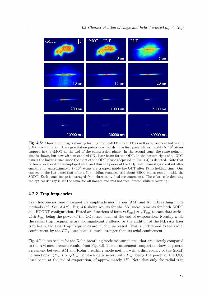
4.2 Characterization of single and hybrid crossed dipole trap
Fig. 4.5: Absorption images showing loading from cMOT into ODT as well as subsequent holding inSODT configuration. Here gravitation points downwards. The first panel shows roughly 5 · 107 atomstrapped in the cMOT at the end of the compression phase. In the second panel the same point intime is shown, but now with an enabled CO2 laser beam for the ODT. In the bottom right of all ODTpanels the holding time since the start of the ODT phase (depicted in Fig. 4.4) is denoted. Note thatno forced evaporation is employed here, and thus the power of the CO2 laser beam stays constant afterenabling it. Approximately 7 · 106 atoms are trapped inside the ODT after 15 ms holding time. Onecan see in the last panel that after a 60 s holding sequence still about 35000 atoms remain inside theSODT. Each panel image is averaged from three individual measurements. The color scale denotingthe optical density is set the same for all images and was not recalibrated while measuring.
4.2.2 Trap frequencies
Trap frequencies were measured via amplitude modulation (AM) and Kohn breathing modemethods (cf. Sec. 3.4.2). Fig. 4.6 shows results for the AM measurements for both SODTand HCODT configuration. Fitted are functions of form ν(Pend) ∝
√Pend to each data series,
with Pend being the power of the CO2 laser beam at the end of evaporation. Notably whilethe radial trap frequencies are not significantly altered by the addition of the Nd:YAG lasertrap beam, the axial trap frequencies are muchly increased. This is understood as the radialconfinement by the CO2 laser beam is much stronger than its axial confinement.
Fig. 4.7 shows results for the Kohn breathing mode measurements, that are directly comparedto the AM measurement results from Fig. 4.6. The measurement comparison shows a generalagreement between AM and Kohn breathing mode method with a discrepancy of the (solid)fit functions ν(Pend) ∝
√Pend for each data series, with Pend being the power of the CO2
laser beam at the end of evaporation, of approximately 7 %. Note that only the radial trap
53
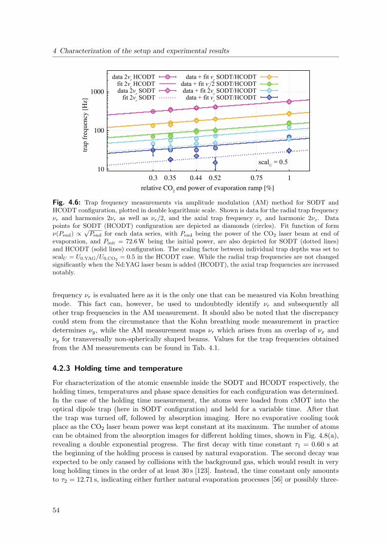
4 Characterization of the setup and experimental results
10
100
1000
0.3 0.35 0.44 0.52 0.75 1
trap
fre
quen
cy [
Hz]
relative CO2 end power of evaporation ramp [%]
scalU = 0.5
data 2νr HCODTfit 2νr HCODTdata 2νr SODT
fit 2νr SODT
data + fit νr SODT/HCODTdata + fit νr/2 SODT/HCODTdata + fit 2νz SODT/HCODTdata + fit νz SODT/HCODT
Fig. 4.6: Trap frequency measurements via amplitude modulation (AM) method for SODT andHCODT configuration, plotted in double logarithmic scale. Shown is data for the radial trap frequencyνr and harmonics 2νr as well as νr/2, and the axial trap frequency νz and harmonic 2νz. Datapoints for SODT (HCODT) configuration are depicted as diamonds (circles). Fit function of formν(Pend) ∝
√Pend for each data series, with Pend being the power of the CO2 laser beam at end of
evaporation, and Pinit = 72.6 W being the initial power, are also depicted for SODT (dotted lines)and HCODT (solid lines) configuration. The scaling factor between individual trap depths was set toscalU = U0,YAG/U0,CO2
= 0.5 in the HCODT case. While the radial trap frequencies are not changedsignificantly when the Nd:YAG laser beam is added (HCODT), the axial trap frequencies are increasednotably.
frequency νr is evaluated here as it is the only one that can be measured via Kohn breathingmode. This fact can, however, be used to undoubtedly identify νr and subsequently allother trap frequencies in the AM measurement. It should also be noted that the discrepancycould stem from the circumstance that the Kohn breathing mode measurement in practicedetermines νy, while the AM measurement maps νr which arises from an overlap of νx andνy for transversally non-spherically shaped beams. Values for the trap frequencies obtainedfrom the AM measurements can be found in Tab. 4.1.
4.2.3 Holding time and temperature
For characterization of the atomic ensemble inside the SODT and HCODT respectively, theholding times, temperatures and phase space densities for each configuration was determined.In the case of the holding time measurement, the atoms were loaded from cMOT into theoptical dipole trap (here in SODT configuration) and held for a variable time. After thatthe trap was turned off, followed by absorption imaging. Here no evaporative cooling tookplace as the CO2 laser beam power was kept constant at its maximum. The number of atomscan be obtained from the absorption images for different holding times, shown in Fig. 4.8(a),revealing a double exponential progress. The first decay with time constant τ1 = 0.60 s atthe beginning of the holding process is caused by natural evaporation. The second decay wasexpected to be only caused by collisions with the background gas, which would result in verylong holding times in the order of at least 30 s [123]. Instead, the time constant only amountsto τ2 = 12.71 s, indicating either further natural evaporation processes [56] or possibly three-
54
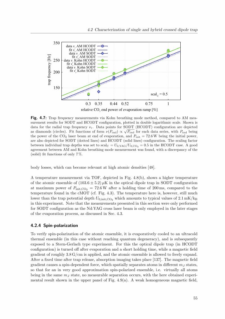
4.2 Characterization of single and hybrid crossed dipole trap
150
200
250
350
0.3 0.35 0.44 0.52 0.75 1
trap
freq
uenc
y [H
z]
relative CO2 end power of evaporation ramp [%]
data νr AM HCODTfit νr AM HCODTdata νr AM SODT
fit νr AM SODTdata νr Kohn HCODT
fit νr Kohn HCODTdata νr Kohn SODT
fit νr Kohn SODT
scalU = 0.5
Fig. 4.7: Trap frequency measurements via Kohn breathing mode method, compared to AM mea-surement results for SODT and HCODT configuration, plotted in double logarithmic scale. Shown isdata for the radial trap frequency νr. Data points for SODT (HCODT) configuration are depictedas diamonds (circles). Fit functions of form ν(Pend) ∝
√Pend for each data series, with Pend being
the power of the CO2 laser beam at end of evaporation, and Pinit = 72.6 W being the initial power,are also depicted for SODT (dotted lines) and HCODT (solid lines) configuration. The scaling factorbetween individual trap depths was set to scalU = U0,YAG/U0,CO2
= 0.5 in the HCODT case. A goodagreement between AM and Kohn breathing mode measurement was found, with a discrepancy of the(solid) fit functions of only 7 %.
body losses, which can become relevant at high atomic densities [48].
A temperature measurement via TOF, depicted in Fig. 4.8(b), shows a higher temperatureof the atomic ensemble of (103.6± 5.2)µK in the optical dipole trap in SODT configurationat maximum power of Pinit,CO2 = 72.6 W after a holding time of 200 ms, compared to thetemperature found in the cMOT (cf. Fig. 4.3). The temperature here is, however, still muchlower than the trap potential depth U0,init,CO2 which amounts to typical values of 2.1 mK/kB
in this experiment. Note that the measurements presented in this section were only performedfor SODT configuration as the Nd:YAG cross laser beam is only employed in the later stagesof the evaporation process, as discussed in Sec. 4.3.
4.2.4 Spin-polarization
To verify spin-polarization of the atomic ensemble, it is evaporatively cooled to an ultracoldthermal ensemble (in this case without reaching quantum degeneracy), and is subsequentlyexposed to a Stern-Gerlach type experiment. For this the optical dipole trap (in HCODTconfiguration) is turned off after evaporation and a short holding time, while a magnetic fieldgradient of roughly 3.8 G/cm is applied, and the atomic ensemble is allowed to freely expand.After a fixed time after trap release, absorption imaging takes place [137]. The magnetic fieldgradient causes a spin-dependent force, which spatially separates atoms in different mJ states,so that for an in very good approximation spin-polarized ensemble, i.e. virtually all atomsbeing in the same mJ state, no measurable separation occurs, with the here obtained experi-mental result shown in the upper panel of Fig. 4.9(a). A weak homogeneous magnetic field,
55
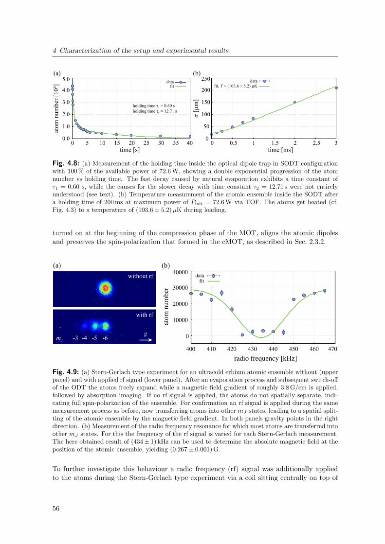
4 Characterization of the setup and experimental results
0.0
1.0
2.0
3.0
4.0
5.0
0 5 10 15 20 25 30 35 40
atom
num
ber [
106 ]
time [s]
holding time τ1 = 0.60 sholding time τ2 = 12.71 s
datafit
0
50
100
150
200
250
0 0.5 1 1.5 2 2.5 3
σ [µ
m]
time [ms]
datafit, T = (103.6 ± 5.2) µK
(a) (b)
Fig. 4.8: (a) Measurement of the holding time inside the optical dipole trap in SODT configurationwith 100 % of the available power of 72.6 W, showing a double exponential progression of the atomnumber vs holding time. The fast decay caused by natural evaporation exhibits a time constant ofτ1 = 0.60 s, while the causes for the slower decay with time constant τ2 = 12.71 s were not entirelyunderstood (see text). (b) Temperature measurement of the atomic ensemble inside the SODT aftera holding time of 200 ms at maximum power of Pinit = 72.6 W via TOF. The atoms get heated (cf.Fig. 4.3) to a temperature of (103.6± 5.2)µK during loading.
turned on at the beginning of the compression phase of the MOT, aligns the atomic dipolesand preserves the spin-polarization that formed in the cMOT, as described in Sec. 2.3.2.
0
10000
20000
30000
40000
400 410 420 430 440 450 460 470
atom
num
ber
radio frequency [kHz]
datafit
(b)(a)without rf
with rf
mJ -6-5-4-3g
Fig. 4.9: (a) Stern-Gerlach type experiment for an ultracold erbium atomic ensemble without (upperpanel) and with applied rf signal (lower panel). After an evaporation process and subsequent switch-offof the ODT the atoms freely expand while a magnetic field gradient of roughly 3.8 G/cm is applied,followed by absorption imaging. If no rf signal is applied, the atoms do not spatially separate, indi-cating full spin-polarization of the ensemble. For confirmation an rf signal is applied during the samemeasurement process as before, now transferring atoms into other mJ states, leading to a spatial split-ting of the atomic ensemble by the magnetic field gradient. In both panels gravity points in the rightdirection. (b) Measurement of the radio frequency resonance for which most atoms are transferred intoother mJ states. For this the frequency of the rf signal is varied for each Stern-Gerlach measurement.The here obtained result of (434± 1) kHz can be used to determine the absolute magnetic field at theposition of the atomic ensemble, yielding (0.267± 0.001) G.
To further investigate this behaviour a radio frequency (rf) signal was additionally appliedto the atoms during the Stern-Gerlach type experiment via a coil sitting centrally on top of
56
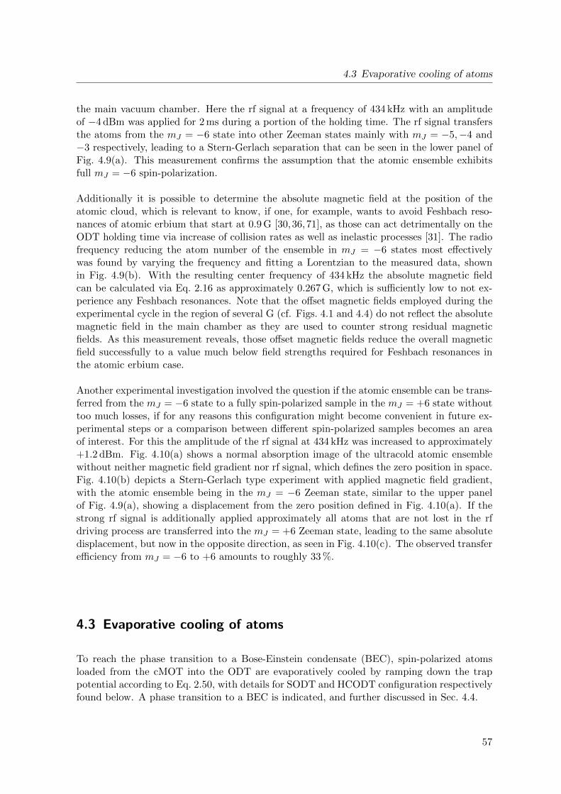
4.3 Evaporative cooling of atoms
the main vacuum chamber. Here the rf signal at a frequency of 434 kHz with an amplitudeof −4 dBm was applied for 2 ms during a portion of the holding time. The rf signal transfersthe atoms from the mJ = −6 state into other Zeeman states mainly with mJ = −5,−4 and−3 respectively, leading to a Stern-Gerlach separation that can be seen in the lower panel ofFig. 4.9(a). This measurement confirms the assumption that the atomic ensemble exhibitsfull mJ = −6 spin-polarization.
Additionally it is possible to determine the absolute magnetic field at the position of theatomic cloud, which is relevant to know, if one, for example, wants to avoid Feshbach reso-nances of atomic erbium that start at 0.9 G [30,36,71], as those can act detrimentally on theODT holding time via increase of collision rates as well as inelastic processes [31]. The radiofrequency reducing the atom number of the ensemble in mJ = −6 states most effectivelywas found by varying the frequency and fitting a Lorentzian to the measured data, shownin Fig. 4.9(b). With the resulting center frequency of 434 kHz the absolute magnetic fieldcan be calculated via Eq. 2.16 as approximately 0.267 G, which is sufficiently low to not ex-perience any Feshbach resonances. Note that the offset magnetic fields employed during theexperimental cycle in the region of several G (cf. Figs. 4.1 and 4.4) do not reflect the absolutemagnetic field in the main chamber as they are used to counter strong residual magneticfields. As this measurement reveals, those offset magnetic fields reduce the overall magneticfield successfully to a value much below field strengths required for Feshbach resonances inthe atomic erbium case.
Another experimental investigation involved the question if the atomic ensemble can be trans-ferred from the mJ = −6 state to a fully spin-polarized sample in the mJ = +6 state withouttoo much losses, if for any reasons this configuration might become convenient in future ex-perimental steps or a comparison between different spin-polarized samples becomes an areaof interest. For this the amplitude of the rf signal at 434 kHz was increased to approximately+1.2 dBm. Fig. 4.10(a) shows a normal absorption image of the ultracold atomic ensemblewithout neither magnetic field gradient nor rf signal, which defines the zero position in space.Fig. 4.10(b) depicts a Stern-Gerlach type experiment with applied magnetic field gradient,with the atomic ensemble being in the mJ = −6 Zeeman state, similar to the upper panelof Fig. 4.9(a), showing a displacement from the zero position defined in Fig. 4.10(a). If thestrong rf signal is additionally applied approximately all atoms that are not lost in the rfdriving process are transferred into the mJ = +6 Zeeman state, leading to the same absolutedisplacement, but now in the opposite direction, as seen in Fig. 4.10(c). The observed transferefficiency from mJ = −6 to +6 amounts to roughly 33 %.
4.3 Evaporative cooling of atoms
To reach the phase transition to a Bose-Einstein condensate (BEC), spin-polarized atomsloaded from the cMOT into the ODT are evaporatively cooled by ramping down the trappotential according to Eq. 2.50, with details for SODT and HCODT configuration respectivelyfound below. A phase transition to a BEC is indicated, and further discussed in Sec. 4.4.
57
4 Characterization of the setup and experimental results
without B gradientwithout rf
atoms inmJ = - 6
with B gradientwithout rf
atoms inmJ = - 6
with B gradientwith rf
atoms inmJ = + 6
g(a)
(b)
(c)
Fig. 4.10: (a) Absorption image of an atomic ensemble after evaporation without added magnetic fieldgradient or rf signal, defining a zero point in space. Atoms are spin-polarized in the mJ = −6 Zeemanstate. (b) Stern-Gerlach type experiment similar to the case depicted in the upper panel of Fig. 4.9(a),showing a displacement from the zero point. As no rf signal is applied here, the atoms remain in themJ = −6 state. (c) Stern-Gerlach type experiment with added strong rf signal, transferring a portionof approximately 33 % of the atoms into the mJ = +6 Zeeman state. This is confirmed by the positionof the atomic ensemble, which exhibits the same absolute displacement from the zero point, but nowin the opposite direction, while considering the influence of gravity. In all panels gravity points in theright direction.
4.3.1 Evaporation ramp
The used temporal evolution of the CO2 laser beam trapping potential is given by Eq. 2.50and therefore dependent on the cut-off parameter η, the collision rate γ, the initial trap depthU0, and the end trap depth U(tend). The cut-off parameter should stay constant during thecomplete evaporation process, as discussed in Sec. 2.3.4. As the maximal trap depth providedby the CO2 laser beam amounts to approximately U0,init,CO2 = 2.1 mK/kB, and the tempera-ture of the atomic ensemble in the SODT right after loading from the cMOT lies in the regionof 100µK (cf. Fig. 4.8), initial optimization started with η = 21, and was finally set to 7.25.Due to the addition of the Nd:YAG beam in HCODT configuration and therefore an relativeincrease of the total potential depth in the later stages of the evaporation cycle, and the factthat collisions with the residual background gas modify the temporal evolution, it is imper-ative to optimize η experimentally. The order of magnitude for the starting parameter of γis known from previous work [56] and gets also experimentally optimized to a final value of 325.
In HCODT configuration the Nd:YAG laser beam joins the evaporation process at a vari-able time tYAG,start after the evaporation process via lowering of the CO2 laser beam powerhas started (cf. Fig. 4.4), calculated by
tYAG,start = −(
U0,init,YAG
scalUU0,init,CO2
)−1/β ( U0,init,YAG
scalUU0,init,CO2
)1/β−1
τevap, (4.2)
where β = 2(η′ − 3)/η′, and scalU = U0,YAG/U0,CO2 which (if not stated otherwise) is set to0.5. The full temporal evolution of the trap potential depth provided by the Nd:YAG laserbeam is chosen as
U0,YAG(t) =
U0,init,YAG, t < tYAG,start
scalUU0,CO2(t), t ≥ tYAG,start. (4.3)
58
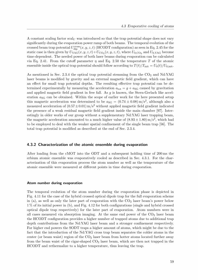
4.3 Evaporative cooling of atoms
A constant scaling factor scalU was introduced so that the trap potential shape does not varysignificantly during the evaporation power ramp of both beams. The temporal evolution of thecrossed beam trap potential U cross
dip (x, y, z, t) (HCODT configuration) as seen in Eq. 2.45 for thestatic case is then given by UYAG(x, y, z, t)+UCO2(x, y, z, t), where U0,CO2 and U0,YAG becometime-dependent. The needed power of both laser beams during evaporation can be calculatedvia Eq. 2.41. From the cutoff parameter η and Eq. 2.50 the temperature T of the atomicensemble inside the optical trap potential should follow according to T (t)/Tinit = U0(t)/U0,init.
As mentioned in Sec. 2.3.4 the optical trap potential stemming from the CO2 and Nd:YAGlaser beams is modified by gravity and an external magnetic field gradient, which can havean effect for small trap potential depths. The resulting effective trap potential can be de-termined experimentally by measuring the acceleration atot = g + aSG caused by gravitationand applied magnetic field gradient in free fall. As g is known, the Stern-Gerlach like accel-eration aSG can be obtained. Within the scope of earlier work for the here presented setupthis magnetic acceleration was determined to be aSG = (0.74 ± 0.08) m/s2, although also ameasured acceleration of (0.57±0.01) m/s2 without applied magnetic field gradient indicatedthe presence of a weak residual magnetic field gradient inside the main chamber [97]. Inter-estingly in older works of our group without a supplementary Nd:YAG laser trapping beam,the magnetic acceleration amounted to a much higher value of (8.93± 1.80) m/s2, which hadto be employed to deal with the weaker spatial confinement of the single beam trap [56]. Thetotal trap potential is modified as described at the end of Sec. 2.3.4.
4.3.2 Characterization of the atomic ensemble during evaporation
After loading from the cMOT into the ODT and a subsequent holding time of 200 ms theerbium atomic ensemble was evaporatively cooled as described in Sec. 4.3.1. For the char-acterization of this evaporation process the atom number as well as the temperature of theatomic ensemble were measured at different points in time during evaporation.
Atom number during evaporation
The temporal evolution of the atom number during the evaporation phase is depicted inFig. 4.11 for the case of the hybrid crossed optical dipole trap for the full evaporation schemein (a), as well as only the later part of evaporation with the CO2 laser beam’s power below1 % of its initial power in (b), and Fig. 4.12 for both configurations (single and hybrid crossedoptical dipole trap respectively) for the later part of evaporation. Atom numbers were inall cases measured via absorption imaging. At the same end power of the CO2 laser beamthe HCODT configuration provides a higher number of trapped atoms due to additional trapdepth contributions from the Nd:YAG laser beam and a stronger confinement respectively.For higher end powers the SODT traps a higher amount of atoms, which might be due to thefact that the introduction of the Nd:YAG cross trap beam separates the colder atoms in thecenter (or beam waist) region of the CO2 laser beam from hotter atoms located further awayfrom the beam waist of the cigar-shaped CO2 laser beam, which are then not trapped in theHCODT and rethermalize to a higher temperature, thus leaving the trap.
59
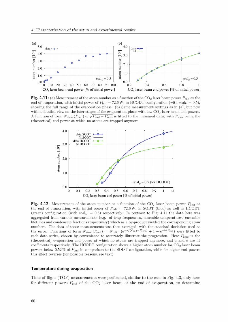
4 Characterization of the setup and experimental results
0.0
1.0
2.0
3.0
4.0
0.2 0.4 0.6 0.8 1CO
2 laser beam end power [% of initial power]
datafit
1.0
2.0
3.0
4.0
5.0
0 10 20 30 40 50 60 70 80 90 100CO
2 laser beam end power [% of initial power]
data
atom
num
ber [
106 ]
atom
num
ber [
105 ]
0.0
(a) (b)
scalU = 0.5 scal
U = 0.5
Fig. 4.11: (a) Measurement of the atom number as a function of the CO2 laser beam power Pend at theend of evaporation, with initial power of Pinit = 72.6 W, in HCODT configuration (with scalU = 0.5),showing the full range of the evaporation phase. (b) Same measurement settings as in (a), but nowwith a detailed view on the later stages of the evaporation phase with low CO2 laser beam end powers.A function of form Natom(Pend) ∝
√Pend − Pzero is fitted to the measured data, with Pzero being the
(theoretical) end power at which no atoms are trapped anymore.
1.0
2.0
3.0
4.0
0 0.1 0.2 0.3 0.4 0.5 0.6 0.7 0.8 0.9 1 1.1
atom
num
ber
[105 ]
CO2 laser beam end power [% of initial power]
data SODTfit SODT
data HCODTfit HCODT
0.0scal
U = 0.5 (for HCODT)
Fig. 4.12: Measurement of the atom number as a function of the CO2 laser beam power Pend atthe end of evaporation, with initial power of Pinit = 72.6 W, in SODT (blue) as well as HCODT(green) configuration (with scalU = 0.5) respectively. In contrast to Fig. 4.11 the data here wasaggregated from various measurements (e.g. of trap frequencies, ensemble temperatures, ensemblelifetimes and condensate fractions respectively) which as a by-product yielded the corresponding atomnumbers. The data of those measurements was then averaged, with the standard deviation used asthe error. Functions of form Natom(Pend) = Ninit · (e−a/(Pend−Pzero) + 1 − e−b/Pend) were fitted toeach data series, chosen by convenience to accurately illustrate the progression. Here Pzero is the(theoretical) evaporation end power at which no atoms are trapped anymore, and a and b are fitcoefficients respectively. The HCODT configuration shows a higher atom number for CO2 laser beampowers below 0.52 % of Pend in comparison to the SODT configuration, while for higher end powersthis effect reverses (for possible reasons, see text).
Temperature during evaporation
Time-of-flight (TOF) measurements were performed, similar to the case in Fig. 4.3, only herefor different powers Pend of the CO2 laser beam at the end of evaporation, to determine
60
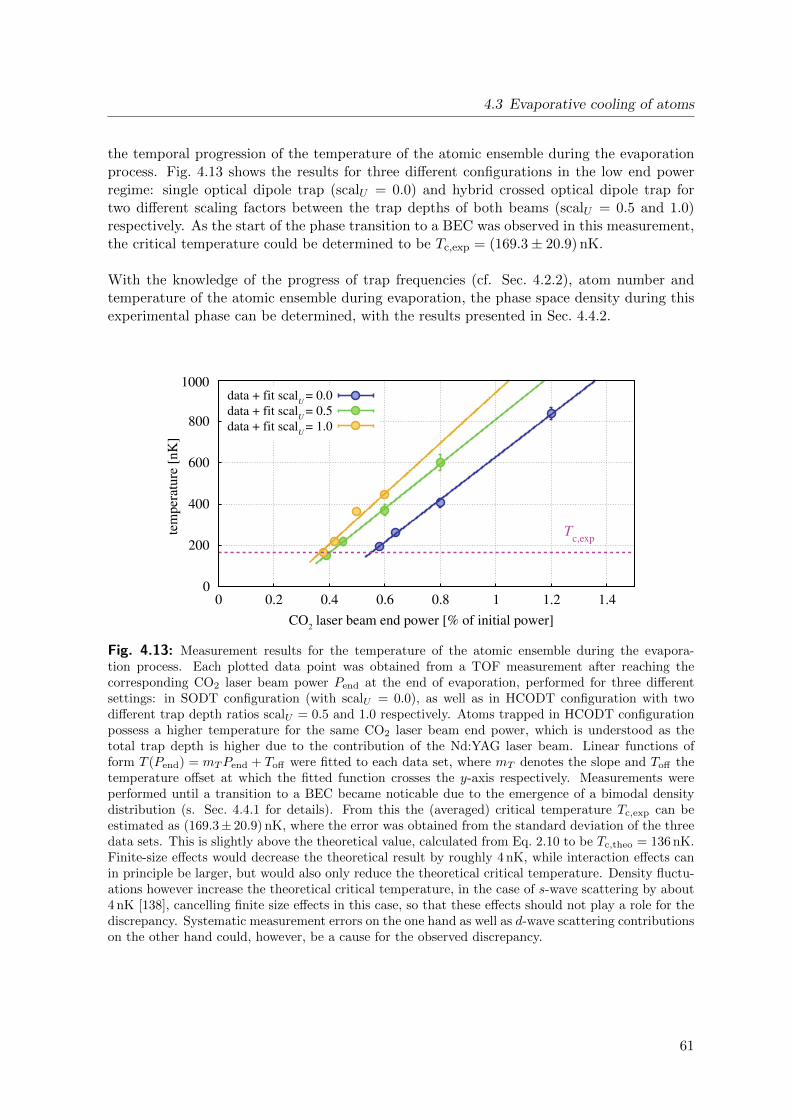
4.3 Evaporative cooling of atoms
the temporal progression of the temperature of the atomic ensemble during the evaporationprocess. Fig. 4.13 shows the results for three different configurations in the low end powerregime: single optical dipole trap (scalU = 0.0) and hybrid crossed optical dipole trap fortwo different scaling factors between the trap depths of both beams (scalU = 0.5 and 1.0)respectively. As the start of the phase transition to a BEC was observed in this measurement,the critical temperature could be determined to be Tc,exp = (169.3± 20.9) nK.
With the knowledge of the progress of trap frequencies (cf. Sec. 4.2.2), atom number andtemperature of the atomic ensemble during evaporation, the phase space density during thisexperimental phase can be determined, with the results presented in Sec. 4.4.2.
0
200
400
600
800
1000
0 0.2 0.4 0.6 0.8 1 1.2 1.4
tem
pera
ture
[nK
]
CO2 laser beam end power [% of initial power]
data + fit scalU
= 0.0data + fit scal
U = 0.5
data + fit scalU
= 1.0
Tc,exp
Fig. 4.13: Measurement results for the temperature of the atomic ensemble during the evapora-tion process. Each plotted data point was obtained from a TOF measurement after reaching thecorresponding CO2 laser beam power Pend at the end of evaporation, performed for three differentsettings: in SODT configuration (with scalU = 0.0), as well as in HCODT configuration with twodifferent trap depth ratios scalU = 0.5 and 1.0 respectively. Atoms trapped in HCODT configurationpossess a higher temperature for the same CO2 laser beam end power, which is understood as thetotal trap depth is higher due to the contribution of the Nd:YAG laser beam. Linear functions ofform T (Pend) = mTPend + Toff were fitted to each data set, where mT denotes the slope and Toff thetemperature offset at which the fitted function crosses the y-axis respectively. Measurements wereperformed until a transition to a BEC became noticable due to the emergence of a bimodal densitydistribution (s. Sec. 4.4.1 for details). From this the (averaged) critical temperature Tc,exp can beestimated as (169.3± 20.9) nK, where the error was obtained from the standard deviation of the threedata sets. This is slightly above the theoretical value, calculated from Eq. 2.10 to be Tc,theo = 136 nK.Finite-size effects would decrease the theoretical result by roughly 4 nK, while interaction effects canin principle be larger, but would also only reduce the theoretical critical temperature. Density fluctu-ations however increase the theoretical critical temperature, in the case of s-wave scattering by about4 nK [138], cancelling finite size effects in this case, so that these effects should not play a role for thediscrepancy. Systematic measurement errors on the one hand as well as d-wave scattering contributionson the other hand could, however, be a cause for the observed discrepancy.
61
4 Characterization of the setup and experimental results
4.4 Bose-Einstein condensation of erbium atoms
By means of the evaporation process characterized in the previous section, the transition toquantum degeneracy was successful, leading to the generation of an erbium atomic Bose-Einstein condensate (BEC) in an optical dipole trap either consisting of a single CO2 laserbeam (SODT configuration), or of a hybrid crossed beam setup provided by the CO2 laserbeam and an additional Nd:YAG laser beam (HCODT configuration). Atom numbers in thepure condensate usually amount up to 3.5 · 104. This section presents work to search forsignatures of the phase transition to a BEC, namely by bimodal density distribution mea-surements as well as phase space density calculations from measurement data. Subsequentlythe lifetime of the ultracold atomic ensemble is characterized, and a brief note regarding thelong-term stability of the experiment is given.
4.4.1 Bimodal density distribution
To verify the successful generation of a BEC, the spatial density distribution can be measuredfor different times during the evaporation process. If a transition to quantum degeneracy oc-curs, the density distribution should change from a Maxwell-Boltzmann distribution to abimodal distribution, which should then revert back to a monomodal distribution when alltrapped atoms reach quantum degeneracy during evaporation [6]. Fig. 4.14 shows four suchmeasurements during evaporation, i.e. for different end powers of the trapping beams, inHCODT configuration. One clearly observes the emergence of bimodality in panels (b) and(c), while for further evaporation shown in (d) the density distribution reverts back to amonomodal distribution, indicating a macroscopic occupation of the ground state. The formof the density distribution for a BEC is determined by the trap potential shape [6]. As herethe harmonic trap potential exhibits a nearly parabolic shape for cold atoms sitting in thebottom region of the potential, the resulting density distribution is of inverted parabolic form(yellow curves).
If one plots the condensate fractions obtained via measurement methods discussed in Fig. 4.14for various trap depth ratios scalU = U0,YAG/U0,CO2 , one obtains the results depicted inFig. 4.15.
4.4.2 Phase space density
The phase space density can be determined via several experimentally accessible parametersaccording to Eq. 3.7. As shown in Fig. 4.16, it exceeds the critical phase space density of2.612 during evaporation with a sudden increase, and reaches values of up to 61±55 in SODTconfiguration, and 9.8± 6.5 in HCODT configuration respectively, confirming the generationof an atomic erbium Bose-Einstein condensate, which was observed in situ in Fig. 4.14. Cor-responding measured experimental quantities are listed in Tab. 4.1.
A third method to detect the generation of a BEC, the observation of a radius inversion afterfree expansion of the condensate due to a repulsive interaction between the atoms [40, 59],could for the here used crossed dipole trapping geometry not be reliably observed, other thanin earlier measurements with a single CO2 laser beam dipole trap [56]. In the hybrid crossedoptical dipole trap setup the spatial distribution of atoms is more spherically symmetric, while
62
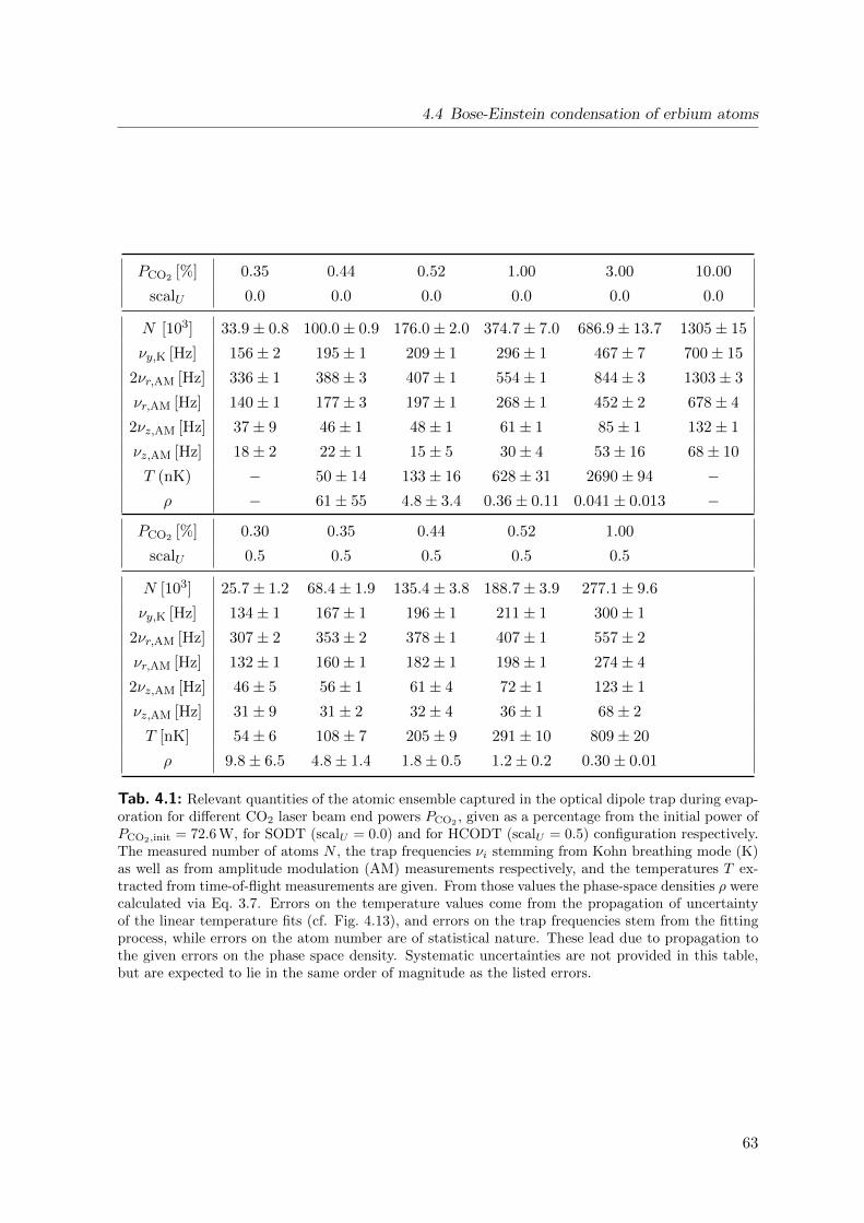
4.4 Bose-Einstein condensation of erbium atoms
PCO2 [%] 0.35 0.44 0.52 1.00 3.00 10.00
scalU 0.0 0.0 0.0 0.0 0.0 0.0
N [103] 33.9± 0.8 100.0± 0.9 176.0± 2.0 374.7± 7.0 686.9± 13.7 1305± 15
νy,K [Hz] 156± 2 195± 1 209± 1 296± 1 467± 7 700± 15
2νr,AM [Hz] 336± 1 388± 3 407± 1 554± 1 844± 3 1303± 3
νr,AM [Hz] 140± 1 177± 3 197± 1 268± 1 452± 2 678± 4
2νz,AM [Hz] 37± 9 46± 1 48± 1 61± 1 85± 1 132± 1
νz,AM [Hz] 18± 2 22± 1 15± 5 30± 4 53± 16 68± 10
T (nK) − 50± 14 133± 16 628± 31 2690± 94 −ρ − 61± 55 4.8± 3.4 0.36± 0.11 0.041± 0.013 −
PCO2 [%] 0.30 0.35 0.44 0.52 1.00
scalU 0.5 0.5 0.5 0.5 0.5
N [103] 25.7± 1.2 68.4± 1.9 135.4± 3.8 188.7± 3.9 277.1± 9.6
νy,K [Hz] 134± 1 167± 1 196± 1 211± 1 300± 1
2νr,AM [Hz] 307± 2 353± 2 378± 1 407± 1 557± 2
νr,AM [Hz] 132± 1 160± 1 182± 1 198± 1 274± 4
2νz,AM [Hz] 46± 5 56± 1 61± 4 72± 1 123± 1
νz,AM [Hz] 31± 9 31± 2 32± 4 36± 1 68± 2
T [nK] 54± 6 108± 7 205± 9 291± 10 809± 20
ρ 9.8± 6.5 4.8± 1.4 1.8± 0.5 1.2± 0.2 0.30± 0.01
Tab. 4.1: Relevant quantities of the atomic ensemble captured in the optical dipole trap during evap-oration for different CO2 laser beam end powers PCO2
, given as a percentage from the initial power ofPCO2,init = 72.6 W, for SODT (scalU = 0.0) and for HCODT (scalU = 0.5) configuration respectively.The measured number of atoms N , the trap frequencies νi stemming from Kohn breathing mode (K)as well as from amplitude modulation (AM) measurements respectively, and the temperatures T ex-tracted from time-of-flight measurements are given. From those values the phase-space densities ρ werecalculated via Eq. 3.7. Errors on the temperature values come from the propagation of uncertaintyof the linear temperature fits (cf. Fig. 4.13), and errors on the trap frequencies stem from the fittingprocess, while errors on the atom number are of statistical nature. These lead due to propagation tothe given errors on the phase space density. Systematic uncertainties are not provided in this table,but are expected to lie in the same order of magnitude as the listed errors.
63
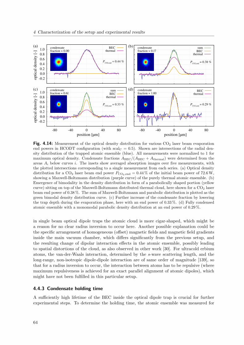
4 Characterization of the setup and experimental results
-0.2 0.0 0.2 0.4 0.6 0.8 1.0
optic
al d
ensi
ty [
-]
BECthermal
-0.2 0.0 0.2 0.4 0.6 0.8 1.0
-80 -40 0 40 80
optic
al d
ensi
ty [
-]
position [µm]-80 -40 0 40 80
position [µm]
sumBEC
thermal
sumBEC
thermal
BECthermal
(a) (b)
(c) (d)
condensatefraction ≈ 0.00
condensatefraction ≈ 0.17
condensatefraction ≈ 0.61
condensatefraction ≈ 1.00
PCO2,end = 0.44 % P
CO2,end = 0.38 %
PCO2,end
= 0.33 % PCO2,end
= 0.29 %
Fig. 4.14: Measurement of the optical density distribution for various CO2 laser beam evaporationend powers in HCODT configuration (with scalU = 0.5). Shown are intersections of the radial den-sity distribution of the trapped atomic ensemble (blue). All measurements were normalized to 1 formaximum optical density. Condensate fractions ABEC/(ABEC + Athermal) were determined from theareas Ai below curves i. The insets show averaged absorption images over five measurements, withthe plotted intersections corresponding to a single measurement from each series. (a) Optical densitydistribution for a CO2 laser beam end power PCO2,end = 0.44 % of the initial beam power of 72.6 W,showing a Maxwell-Boltzmann distribution (purple curve) of the purely thermal atomic ensemble. (b)Emergence of bimodality in the density distribution in form of a parabolically shaped portion (yellowcurve) sitting on top of the Maxwell-Boltzmann distributed thermal cloud, here shown for a CO2 laserbeam end power of 0.38 %. The sum of Maxwell-Boltzmann and parabolic distribution is plotted as thegreen bimodal density distribution curve. (c) Further increase of the condensate fraction by loweringthe trap depth during the evaporation phase, here with an end power of 0.33 %. (d) Fully condensedatomic ensemble with a monomodal parabolic density distribution at an end power of 0.29 %.
in single beam optical dipole traps the atomic cloud is more cigar-shaped, which might bea reason for no clear radius inversion to occur here. Another possible explanation could bethe specific arrangement of homogeneous (offset) magnetic fields and magnetic field gradientsinside the main vacuum chamber, which differs significantly from the previous setup, andthe resulting change of dipolar interaction effects in the atomic ensemble, possibly leadingto spatial distortions of the cloud, as also observed in other work [30]. For ultracold erbiumatoms, the van-der-Waals interaction, determined by the s-wave scattering length, and thelong-range, non-isotropic dipole-dipole interaction are of same order of magnitude [139], sothat for a radius inversion to occur, the interaction between atoms has to be repulsive (wheremaximum repulsiveness is achieved for an exact parallel alignment of atomic dipoles), whichmight have not been fulfilled in this particular setup.
4.4.3 Condensate holding time
A sufficiently high lifetime of the BEC inside the optical dipole trap is crucial for furtherexperimental steps. To determine the holding time, the atomic ensemble was measured for
64
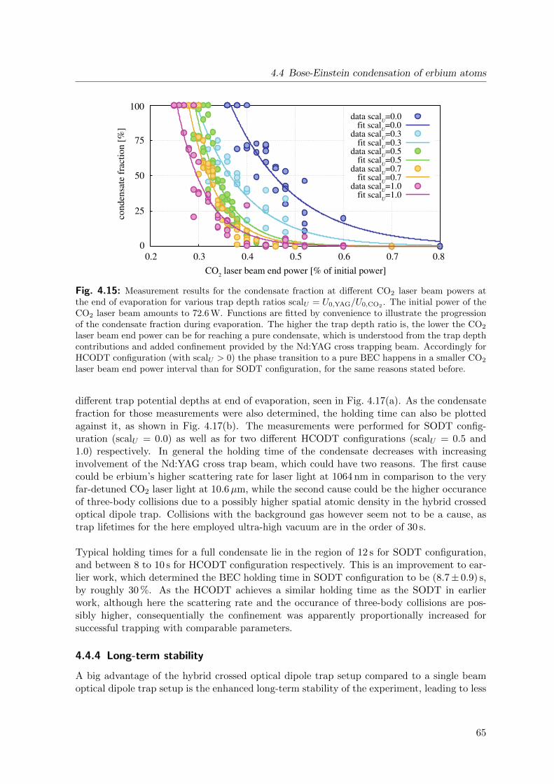
4.4 Bose-Einstein condensation of erbium atoms
0
25
50
75
100
0.2 0.3 0.4 0.5 0.6 0.7 0.8
cond
ensa
te f
ract
ion
[%]
CO2 laser beam end power [% of initial power]
data scalU=0.0
fit scalU=0.0
data scalU=0.3
fit scalU=0.3
data scalU=0.5
fit scalU=0.5
data scalU=0.7
fit scalU=0.7
data scalU=1.0
fit scalU=1.0
Fig. 4.15: Measurement results for the condensate fraction at different CO2 laser beam powers atthe end of evaporation for various trap depth ratios scalU = U0,YAG/U0,CO2
. The initial power of theCO2 laser beam amounts to 72.6 W. Functions are fitted by convenience to illustrate the progressionof the condensate fraction during evaporation. The higher the trap depth ratio is, the lower the CO2
laser beam end power can be for reaching a pure condensate, which is understood from the trap depthcontributions and added confinement provided by the Nd:YAG cross trapping beam. Accordingly forHCODT configuration (with scalU > 0) the phase transition to a pure BEC happens in a smaller CO2
laser beam end power interval than for SODT configuration, for the same reasons stated before.
different trap potential depths at end of evaporation, seen in Fig. 4.17(a). As the condensatefraction for those measurements were also determined, the holding time can also be plottedagainst it, as shown in Fig. 4.17(b). The measurements were performed for SODT config-uration (scalU = 0.0) as well as for two different HCODT configurations (scalU = 0.5 and1.0) respectively. In general the holding time of the condensate decreases with increasinginvolvement of the Nd:YAG cross trap beam, which could have two reasons. The first causecould be erbium’s higher scattering rate for laser light at 1064 nm in comparison to the veryfar-detuned CO2 laser light at 10.6µm, while the second cause could be the higher occuranceof three-body collisions due to a possibly higher spatial atomic density in the hybrid crossedoptical dipole trap. Collisions with the background gas however seem not to be a cause, astrap lifetimes for the here employed ultra-high vacuum are in the order of 30 s.
Typical holding times for a full condensate lie in the region of 12 s for SODT configuration,and between 8 to 10 s for HCODT configuration respectively. This is an improvement to ear-lier work, which determined the BEC holding time in SODT configuration to be (8.7± 0.9) s,by roughly 30 %. As the HCODT achieves a similar holding time as the SODT in earlierwork, although here the scattering rate and the occurance of three-body collisions are pos-sibly higher, consequentially the confinement was apparently proportionally increased forsuccessful trapping with comparable parameters.
4.4.4 Long-term stability
A big advantage of the hybrid crossed optical dipole trap setup compared to a single beamoptical dipole trap setup is the enhanced long-term stability of the experiment, leading to less
65
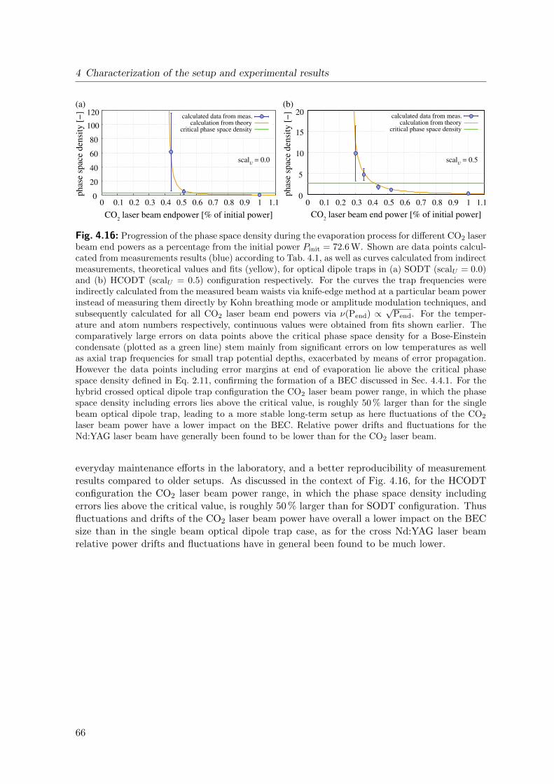
4 Characterization of the setup and experimental results
0
20
40
60
80
100
120
0 0.1 0.2 0.3 0.4 0.5 0.6 0.7 0.8 0.9 1 1.1
phas
e sp
ace
dens
ity [
−]
CO2 laser beam endpower [% of initial power]
calculated data from meas.calculation from theory
critical phase space density
0
5
10
15
20
0 0.1 0.2 0.3 0.4 0.5 0.6 0.7 0.8 0.9 1 1.1
phas
e sp
ace
dens
ity [
−]
CO2 laser beam end power [% of initial power]
scalU = 0.0 scal
U = 0.5
calculated data from meas.calculation from theory
critical phase space density
(a) (b)
Fig. 4.16: Progression of the phase space density during the evaporation process for different CO2 laserbeam end powers as a percentage from the initial power Pinit = 72.6 W. Shown are data points calcul-cated from measurements results (blue) according to Tab. 4.1, as well as curves calculated from indirectmeasurements, theoretical values and fits (yellow), for optical dipole traps in (a) SODT (scalU = 0.0)and (b) HCODT (scalU = 0.5) configuration respectively. For the curves the trap frequencies wereindirectly calculated from the measured beam waists via knife-edge method at a particular beam powerinstead of measuring them directly by Kohn breathing mode or amplitude modulation techniques, andsubsequently calculated for all CO2 laser beam end powers via ν(Pend) ∝
√Pend. For the temper-
ature and atom numbers respectively, continuous values were obtained from fits shown earlier. Thecomparatively large errors on data points above the critical phase space density for a Bose-Einsteincondensate (plotted as a green line) stem mainly from significant errors on low temperatures as wellas axial trap frequencies for small trap potential depths, exacerbated by means of error propagation.However the data points including error margins at end of evaporation lie above the critical phasespace density defined in Eq. 2.11, confirming the formation of a BEC discussed in Sec. 4.4.1. For thehybrid crossed optical dipole trap configuration the CO2 laser beam power range, in which the phasespace density including errors lies above the critical value, is roughly 50 % larger than for the singlebeam optical dipole trap, leading to a more stable long-term setup as here fluctuations of the CO2
laser beam power have a lower impact on the BEC. Relative power drifts and fluctuations for theNd:YAG laser beam have generally been found to be lower than for the CO2 laser beam.
everyday maintenance efforts in the laboratory, and a better reproducibility of measurementresults compared to older setups. As discussed in the context of Fig. 4.16, for the HCODTconfiguration the CO2 laser beam power range, in which the phase space density includingerrors lies above the critical value, is roughly 50 % larger than for SODT configuration. Thusfluctuations and drifts of the CO2 laser beam power have overall a lower impact on the BECsize than in the single beam optical dipole trap case, as for the cross Nd:YAG laser beamrelative power drifts and fluctuations have in general been found to be much lower.
66
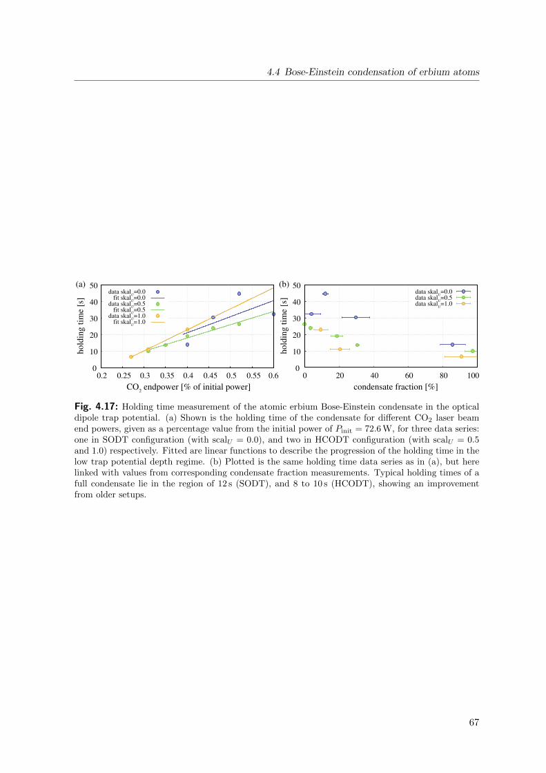
4.4 Bose-Einstein condensation of erbium atoms
0
10
20
30
40
50
0.2 0.25 0.3 0.35 0.4 0.45 0.5 0.55 0.6
hold
ing
time
[s]
CO2 endpower [% of initial power]
data skalU=0.0
fit skalU=0.0
data skalU=0.5
fit skalU=0.5
data skalU=1.0
fit skalU=1.0
0
10
20
30
40
50
0 20 40 60 80 100
hold
ing
time
[s]
condensate fraction [%]
data skalU=0.0
data skalU=0.5
data skalU=1.0
(a) (b)
Fig. 4.17: Holding time measurement of the atomic erbium Bose-Einstein condensate in the opticaldipole trap potential. (a) Shown is the holding time of the condensate for different CO2 laser beamend powers, given as a percentage value from the initial power of Pinit = 72.6 W, for three data series:one in SODT configuration (with scalU = 0.0), and two in HCODT configuration (with scalU = 0.5and 1.0) respectively. Fitted are linear functions to describe the progression of the holding time in thelow trap potential depth regime. (b) Plotted is the same holding time data series as in (a), but herelinked with values from corresponding condensate fraction measurements. Typical holding times of afull condensate lie in the region of 12 s (SODT), and 8 to 10 s (HCODT), showing an improvementfrom older setups.
67

5 Prospects for synthetic magnetic fields forultracold erbium atoms
In this part of the thesis a theoretical treatment of synthetic magnetic fields for electricallyneutral bosonic erbium atoms, strong enough to reach the fractional quantum Hall regime,is presented. After an introduction of the general concept and a review of the better knowncase of gauge fields for charged particles, firstly the simpler three-level atomic system will bediscussed, after which the more complex atomic erbium case is treated. Here a parameterregime is given, for which strong synthetic magnetic fields with good spatial homogeneity arepredicted. Finally an estimation of the Laughlin gap, the energetic gap between the lowestand the other remaining Landau levels of a two-dimensional atomic erbium microcloud in thesynthetic magnetic field, expected from the s-wave contribution of the interaction is presented.The main findings in this chapter were also published in [50].
5.1 Introduction to synthetic gauge fields
Ultracold atomic clouds are extremely well-suited systems to study matter behaviour, as thosesystems are pure and controllable to a high degree. Atoms are electrically neutral, which isusually an advantage for many experimental studies. For the study of some currently veryinteresting phenomena as the fractional and integer quantum Hall effect [140], the spin Halleffect [141, 142] and topological insulators [143] an analogon of the Lorentz force is needed,which is present for electrically charged electrons in a magnetic field. To overcome thislimitation artificial gauge fields can be constructed, imitating a circular motion of particlessubject to the synthetic gauge field leading to the introduction of a Berry phase (analogousto the Aharonov-Bohm phase), and thus creating a Lorentz force equivalent [144,145]. Tech-niques include trap rotation [146, 147], lattice shaking [148], or phase imprinting via photonrecoil [46, 149–154]. Since trap rotation and lattice shaking techniques historically producedonly comparably weak synthetic magnetic fields, in this thesis the possibility of the genera-tion of strong artificial gauge fields for neutral lanthanide erbium atoms with a non-vanishingangular orbital momentum L in their ground state by phase imprinting via Raman manipu-lation beams is theoretically investigated.
Current implementations of such synthetic magnetic fields (for e.g. alkali atoms with theirL = 0 S-electronic ground state) are not strong enough for fractional quantum Hall statesto form, mainly because of limitations of the achievable coherence time, caused by the im-possibility to detune the Raman light field further away from resonance than the electronicfine structure splitting of the excited states. However, another readily available Bose-Einsteincondensated lanthanide atomic species is dysprosium, for which a similar, yet different schemefor artificial magnetic fields was proposed [49], which recently was utilized for theoretical in-vestigations of dysprosium topological quantum Hall systems [51]. Further atomic specieswith a suitable P -electronic ground state as the oxygen atom are difficult to laser cool due to
69
5 Prospects for synthetic magnetic fields for ultracold erbium atoms
technical inconvenient UV electronic transition wavelengths and a large number of requiredrepumping lasers.
Instead of looking at atoms circulating in a lattice and accumulating a Peierls phase [155], oursystem is composed of a bulk gas whose atoms are adiabatically transferred to dressed statesby altering the bandstructure. While the here presented system as well as earlier publishedwork construct Abelian gauge fields [46], (synthetic) gauge fields can also be extended to thenon-Abelian case [156], e.g. to study spin-orbit coupling [157, 158] leading to the spin Halleffect [159].
5.1.1 Review: Gauge fields for charged particles
To establish the basic concept the case of gauge fields in classical electrodynamics is discussed.The electric and magnetic (gauge) fields, E and B, can be described by the vector and scalarpotentials, A and φ:
E = −∇φ− ∂A
∂t, B = −∇×A. (5.1)
Here A and φ are only defined up to a gauge, meaning that certain constraints can be specifiedfor them, leaving the resulting interaction of the particles in the gauge field unchanged –or invariant to the gauge. In a magnetic field B particles with mass m, charge q, andvelocity v then experience the Lorentz force F = qv×B, which can also be expressed as theHamiltonian [160]
H =(p− qA)2
2m+ qφ, (5.2)
where p is the canonical momentum operator, originating from the replacement for a freeparticle p → p − qA, in which an additional term −qA is introduced into the dispersionrelation of the particle. As we are especially interested in the strength of the (synthetic)magnetic field, the cyclotron frequency is an important quantity. For e.g. a uniform magneticfield B = Bez along the z-axis, the cyclotron frequency of the circular motion a particle withcharge q experiences in the x− y-plane can be defined as
ωc =|q|Bm
. (5.3)
The minimal cyclotron orbit size, called magnetic length, is then [161]
`mag =
√~
mωc, (5.4)
which serves as a characteristic length scale for e.g. the determination of the vortex density ina given system. To later reach experimentally interesting regimes for the study of fractionalquantum Hall states, the vortex density has to be higher than the atomic density in thesystem.
70
5.2 Synthetic magnetic fields for three-level atoms
5.2 Synthetic magnetic fields for three-level atoms
To keep the discussion simple, the treatment is started by considering the generation of asynthetic magnetic field for a three-level atom with two stable ground state levels and anexcited state in a Λ-configuration. This setup has similarities with the rubidium alkali casein [47], however here we assume a different polarization configuration of the Raman beams,and consider Raman transitions with a Zeeman quantum number difference of ∆mF = 2.
5.2.1 Hamiltonian and dispersion relation
To begin with, a three-level atom with two stable ground state levels |g+1〉 and |g−1〉 and onespontaneously decaying excited state level |e0〉 is considered, as shown in Fig. 5.1(b). The in-dex denotes the corresponding Zeeman quantum number. The here suggested implementationfollows the work of I. Spielman [47] developed for alkali atoms, however our approach choosesthe atoms to be driven by two far-detuned counter-propagating laser beams in a σ+ − σ−polarization configuration, which results in Raman coupling between ground state sublevels|g+1〉 and |g−1〉 with ∆mF = 2. For comparison the scheme for rubidium alkali atoms used aπ − σ polarization configuration with ∆mF = 1 coupling between sublevels.
The basic idea is to construct a Hamiltonian offering an atomic dispersion that mimics thatof a charged particle in the presence of a position-dependent vector potential A∗, so that asynthetic magnetic field B∗ = ∇×A∗ emerges. Considering A∗ = (A∗x, A
∗y, A
∗z), the compo-
nents A∗i with i = x, y, z themselves can be of scalar, vectorial or matrix-valued nature. Hereonly the case for A∗x 6= 0 is regarded, so that A∗ = (A∗x, 0, 0) (Landau gauge). Note that thesuperscript ∗ denotes synthetic quantities to distinguish them from real ones, e.g. syntheticand real magnetic fields.
From Eq. 5.1 one can see that for a time-varying synthetic vector potential a synthetic electricfield, and for the case of a spatially varying synthetic vector potential a synthetic magneticfield can be constructed. The latter can be achieved with a transversal gradient of the (real)magnetic field, which leads to a two-photon detuning δ = ω+ − ω− − ωZ, where ω+ andω− denote the laser frequencies with corresponding polarizations, and ~ωZ is the energeticdifference between |g+1〉 and |g−1〉 that is position-dependent. Both the magnetic field B =Bxex and the counter-propagating laser beams are assumed to be oriented along the x-axis,and a magnetic field gradient along the y-axis, as seen in Fig. 5.1(c). This results in Bx(y) =B0,x + y∂Bx/∂y, which realizes a position-dependent Raman detuning
δ(y) = ∆mFgµB∂Bx∂y
y, (5.5)
where g is the atomic Lande g-factor and µB the Bohr magneton.
As the next step an experimentally tunable energy momentum dispersion relation (p −qA∗)2/(2m∗), with m∗ as an effective mass for the motion along the x-direction, account-ing for the differently shaped dispersion, has to be created. The momentum of the atoms inx-direction is identified as p = ~k = ~kxex, where k is the atomic wave vector, and kx is theabsolute value of the wave vector along ex. Here the dynamics of a free particle in y-directionand a strong confinement in z-direction are assumed, and hereinafter only the Hamiltonian
71
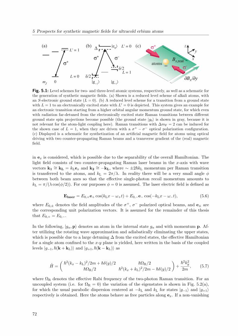
5 Prospects for synthetic magnetic fields for ultracold erbium atoms
Δ
δ/2
δ/2 |g-1⟩
σ+ σ-
(c) σ+
σ-Bx,realatoms
∂Bx/∂y
x
yz(b)(a)
0
σ+
mJ |g+1⟩
|e0⟩L’ = 1
L = 0
L’ = 0
L = 1
Fig. 5.1: Level schemes for two- and three-level atomic systems, respectively, as well as a schematic forthe generation of synthetic magnetic fields. (a) Shown is a reduced level scheme of alkali atoms, withan S-electronic ground state (L = 0). (b) A reduced level scheme for a transition from a ground statewith L = 1 to an electronically excited state with L′ = 0 is depicted. This system gives an example foran electronic transition starting from a higher orbital angular momentum ground state, for which evenwith radiation far-detuned from the electronically excited state Raman transitions between differentground state spin projections become possible (the ground state |g0〉 is shown in gray, because it isnot relevant for the atom-light coupling here). Raman transitions with ∆mF = 2 can be induced forthe shown case of L = 1, when they are driven with a σ+ − σ− optical polarization configuration.(c) Displayed is a schematic for synthetization of an artificial magnetic field for atoms using opticaldriving with two counter-propagating Raman beams and a transverse gradient of the (real) magneticfield.
in ex is considered, which is possible due to the separability of the overall Hamiltonian. Thelight field consists of two counter-propagating Raman laser beams in the x-axis with wavevectors k1
∼= kL = kLex and k2∼= −kL, where ∼ ±2~kL momentum per Raman transition
is transferred to the atoms, and kL = 2π/λ. In reality there will be a very small angle φbetween both beam axes so that the effective single-photon recoil momentum amounts tokL = π/(λ cos(φ/2)). For our purposes φ = 0 is assumed. The laser electric field is defined as
Elaser = E0,+e+ cos(kLx− ω+t) + E0,−e− cos(−kLx− ω−t), (5.6)
where E0,± denotes the field amplitudes of the σ+, σ− polarized optical beams, and e± arethe corresponding unit polarization vectors. It is assumed for the remainder of this thesisthat E0,+ = E0,−.
In the following, |gα,p〉 denotes an atom in the internal state gα and with momentum p. Af-ter utilizing the rotating wave approximation and adiabatically eliminating the upper states,which is possible due to a large detuning ∆ from the excited states, the effective Hamiltonianfor a single atom confined to the x-y plane is yielded, here written in the basis of the coupledlevels |g−1, ~(k + kL)〉 and |g+1, ~(k− kL)〉 as
H =
(~2(kx − kL)2/2m+ ~δ(y)/2 ~ΩR/2
~ΩR/2 ~2(kx + kL)2/2m− ~δ(y)/2
)+
~2k2y
2m, (5.7)
where ΩR denotes the effective Rabi frequency of the two-photon Raman transition. For anuncoupled system (i.e. for ΩR = 0) the variation of the eigenstates is shown in Fig. 5.2(a),for which the usual parabolic dispersion centered at −kL and kL for states |g−1〉 and |g+1〉respectively is obtained. Here the atoms behave as free particles along ex. If a non-vanishing
72
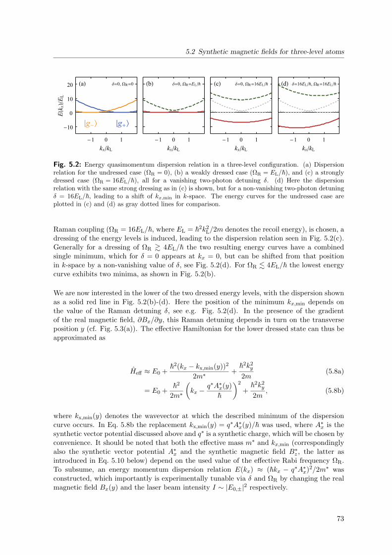
5.2 Synthetic magnetic fields for three-level atoms
δ=0, ΩR=0
|g-⟩ |g+⟩
(a)
-10
0
10
20
E(kx)/EL
-1 0 1
kx/kL
δ=0, ΩR=EL/ℏ(b)
-1 0 1
kx/kL
δ=0, ΩR=16EL/ℏ(c)
-1 0 1
kx/kL
δ=16EL/ℏ, ΩR=16EL/ℏ(d)
-1 0 1
kx/kL
Fig. 5.2: Energy quasimomentum dispersion relation in a three-level configuration. (a) Dispersionrelation for the undressed case (ΩR = 0), (b) a weakly dressed case (ΩR = EL/~), and (c) a stronglydressed case (ΩR = 16EL/~), all for a vanishing two-photon detuning δ. (d) Here the dispersionrelation with the same strong dressing as in (c) is shown, but for a non-vanishing two-photon detuningδ = 16EL/~, leading to a shift of kx,min in k-space. The energy curves for the undressed case areplotted in (c) and (d) as gray dotted lines for comparison.
Raman coupling (ΩR = 16EL/~, where EL = ~2k2L/2m denotes the recoil energy), is chosen, a
dressing of the energy levels is induced, leading to the dispersion relation seen in Fig. 5.2(c).Generally for a dressing of ΩR & 4EL/~ the two resulting energy curves have a combinedsingle minimum, which for δ = 0 appears at kx = 0, but can be shifted from that positionin k-space by a non-vanishing value of δ, see Fig. 5.2(d). For ΩR . 4EL/~ the lowest energycurve exhibits two minima, as shown in Fig. 5.2(b).
We are now interested in the lower of the two dressed energy levels, with the dispersion shownas a solid red line in Fig. 5.2(b)-(d). Here the position of the minimum kx,min depends onthe value of the Raman detuning δ, see e.g. Fig. 5.2(d). In the presence of the gradientof the real magnetic field, ∂Bx/∂y, this Raman detuning depends in turn on the transverseposition y (cf. Fig. 5.3(a)). The effective Hamiltonian for the lower dressed state can thus beapproximated as
Heff ≈ E0 +~2(kx − kx,min(y))2
2m∗+
~2k2y
2m(5.8a)
= E0 +~2
2m∗
(kx −
q∗A∗x(y)
~
)2
+~2k2
y
2m, (5.8b)
where kx,min(y) denotes the wavevector at which the described minimum of the dispersioncurve occurs. In Eq. 5.8b the replacement kx,min(y) = q∗A∗x(y)/~ was used, where A∗x is thesynthetic vector potential discussed above and q∗ is a synthetic charge, which will be chosen byconvenience. It should be noted that both the effective mass m∗ and kx,min (correspondinglyalso the synthetic vector potential A∗x and the synthetic magnetic field B∗z , the latter asintroduced in Eq. 5.10 below) depend on the used value of the effective Rabi frequency ΩR.To subsume, an energy momentum dispersion relation E(kx) ≈ (~kx − q∗A∗x)2/2m∗ wasconstructed, which importantly is experimentally tunable via δ and ΩR by changing the realmagnetic field Bx(y) and the laser beam intensity I ∼ |E0,±|2 respectively.
73
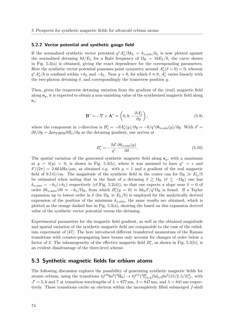
5 Prospects for synthetic magnetic fields for ultracold erbium atoms
5.2.2 Vector potential and synthetic gauge field
If the normalized synthetic vector potential q∗A∗x/~kL = kx,min/kL is now plotted againstthe normalized detuning ~δ/EL for a Rabi frequency of ΩR = 16EL/~, the curve shownin Fig. 5.3(a) is obtained, giving the exact dependence for the corresponding parameters.Here the synthetic vector potential possesses point symmetry around A∗x(δ = 0) = 0, whereatq∗A∗x/~ is confined within +kL and −kL. Near y = 0, for which δ ≈ 0, A∗x varies linearly withthe two-photon detuning δ, and correspondingly the transverse position y.
Then, given the transverse detuning variation from the gradient of the (real) magnetic fieldalong ey, it is expected to obtain a non-vanishing value of the synthesized magnetic field alongez:
B∗ = −∇×A∗ =
(0, 0,−∂A
∗x
∂y
), (5.9)
where the component in z-direction is B∗z = −∂A∗x(y)/∂y = −~/q∗∂kx,min(y)/∂y. With δ′ =∂δ/∂y = ∆mFgµB∂Bx/∂y as the detuning gradient, one arrives at
B∗z = −~δ′
q∗∂kx,min(y)
∂δ. (5.10)
The spatial variation of the generated synthetic magnetic field along ey, with a maximumat y = δ(y) = 0, is shown in Fig. 5.3(b), where it was assumed to have q∗ = e andδ′/(2π) = 2.66 kHz/µm, as obtained e.g. with g = 1 and a gradient of the real magneticfield of 9.5 G/cm. The magnitude of the synthetic field in the center can for ΩR EL/~be estimated when noting that in the limit of a detuning δ & ΩR (δ . −ΩR) one haskx,min = −kL(+kL) respectively (cf Fig. 5.2(d)), so that one expects a slope near δ = 0 oforder ∂kx,min/∂δ ≈ −kL/ΩR, from which B∗z (y = 0) ≈ ~kLδ
′/q∗ΩR is found. If a Taylorexpansion up to lowest order in δ (for ΩR EL/~) is employed for the analytically derivedexpression of the position of the minimum kx,min, the same results are obtained, which isplotted as the orange dashed line in Fig. 5.3(a), showing the based on this expansion derivedvalue of the synthetic vector potential versus the detuning.
Experimental parameters for the magnetic field gradient, as well as the obtained magnitudeand spatial variation of the synthetic magnetic field are comparable to the case of the rubid-ium experiment of [47]. The here introduced different transferred momentum of the Ramantransitions with counter-propagating laser beams only account for changes of order below afactor of 2. The inhomogeneity of the effective magnetic field B∗z , as shown in Fig. 5.3(b), isan evident disadvantage of the three-level scheme.
5.3 Synthetic magnetic fields for erbium atoms
The following discussion explores the possibility of generating synthetic magnetic fields foratomic erbium, using the transitions 4f126s2(3H6)→ 4f11(4I0
15/2)5d5/26s2(15/2, 5/2)0J ′ , with
J ′ = 5, 6 and 7 at transition wavelengths of λ = 877 nm, λ = 847 nm, and λ = 841 nm respec-tively. These transitions excite an electron within the incompletely filled submerged f -shell
74
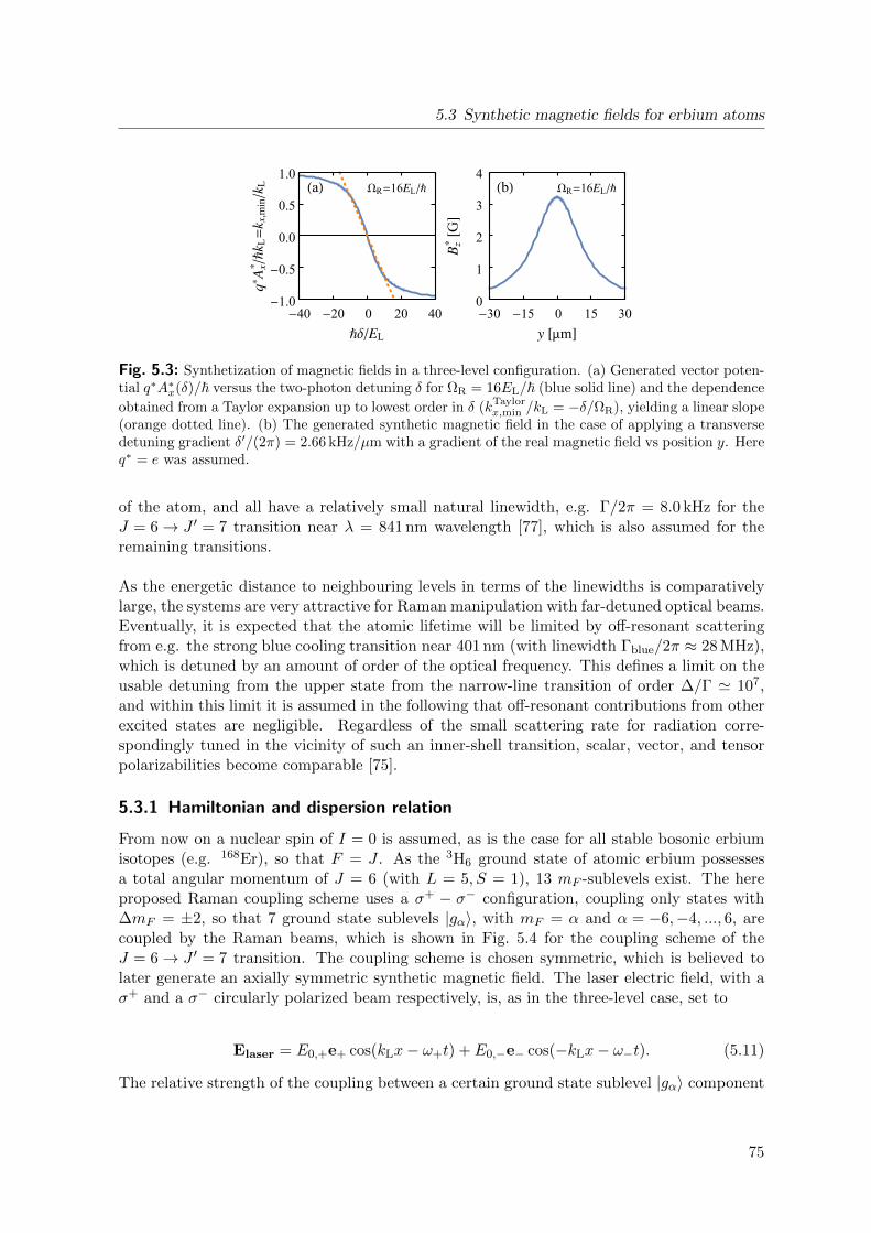
5.3 Synthetic magnetic fields for erbium atoms
ΩR=16EL/ℏ(a)
-1.0
-0.5
0.0
0.5
1.0
q*A
x* /ℏk
L= k
x,m
in/k
L
-40 -20 0 20 40ℏδ/EL
ΩR=16EL/ℏ(b)
0
1
2
3
4
Bz*[G]
-30 -15 0 15 30y [µm]
Fig. 5.3: Synthetization of magnetic fields in a three-level configuration. (a) Generated vector poten-tial q∗A∗x(δ)/~ versus the two-photon detuning δ for ΩR = 16EL/~ (blue solid line) and the dependence
obtained from a Taylor expansion up to lowest order in δ (kTaylorx,min /kL = −δ/ΩR), yielding a linear slope
(orange dotted line). (b) The generated synthetic magnetic field in the case of applying a transversedetuning gradient δ′/(2π) = 2.66 kHz/µm with a gradient of the real magnetic field vs position y. Hereq∗ = e was assumed.
of the atom, and all have a relatively small natural linewidth, e.g. Γ/2π = 8.0 kHz for theJ = 6→ J ′ = 7 transition near λ = 841 nm wavelength [77], which is also assumed for theremaining transitions.
As the energetic distance to neighbouring levels in terms of the linewidths is comparativelylarge, the systems are very attractive for Raman manipulation with far-detuned optical beams.Eventually, it is expected that the atomic lifetime will be limited by off-resonant scatteringfrom e.g. the strong blue cooling transition near 401 nm (with linewidth Γblue/2π ≈ 28 MHz),which is detuned by an amount of order of the optical frequency. This defines a limit on theusable detuning from the upper state from the narrow-line transition of order ∆/Γ ' 107,and within this limit it is assumed in the following that off-resonant contributions from otherexcited states are negligible. Regardless of the small scattering rate for radiation corre-spondingly tuned in the vicinity of such an inner-shell transition, scalar, vector, and tensorpolarizabilities become comparable [75].
5.3.1 Hamiltonian and dispersion relation
From now on a nuclear spin of I = 0 is assumed, as is the case for all stable bosonic erbiumisotopes (e.g. 168Er), so that F = J . As the 3H6 ground state of atomic erbium possessesa total angular momentum of J = 6 (with L = 5, S = 1), 13 mF -sublevels exist. The hereproposed Raman coupling scheme uses a σ+ − σ− configuration, coupling only states with∆mF = ±2, so that 7 ground state sublevels |gα〉, with mF = α and α = −6,−4, ..., 6, arecoupled by the Raman beams, which is shown in Fig. 5.4 for the coupling scheme of theJ = 6→ J ′ = 7 transition. The coupling scheme is chosen symmetric, which is believed tolater generate an axially symmetric synthetic magnetic field. The laser electric field, with aσ+ and a σ− circularly polarized beam respectively, is, as in the three-level case, set to
Elaser = E0,+e+ cos(kLx− ω+t) + E0,−e− cos(−kLx− ω−t). (5.11)
The relative strength of the coupling between a certain ground state sublevel |gα〉 component
75
5 Prospects for synthetic magnetic fields for ultracold erbium atoms
Δ
3δ2δ
δ
-3δ-2δ
-δ
σ
-
ωz
mJ -6 -4 -2 0 2 4 6
J = 6
J’ = 7
σ +
Fig. 5.4: Relevant atomic erbium levels for the J = 6→ J ′ = 7 transition driven by Raman beams in aσ+−σ− optical polarization configuration. The Raman beams are irradiated in a counter-propagatinggeometry.
and an excited state component |en〉 with α = n ± 1 is characterized by the correspondingClebsch-Gordan coefficient cα,n.1 The laser coupling between levels can be written in theform
Ω±cα,α±1 =〈eα±1|e±d|gα〉E0,±
~, (5.12)
where d denotes the dipole operator, and Ω+,Ω− the Rabi frequencies for the σ+,σ− polarizedwaves, respectively, for a transition with a Clebsch-Gordan coefficient of unity. The upperstates can again be adiabatically eliminated for a large detuning ∆ from the excited levels,resulting in an effective interaction Hamiltonian for the coupling to the laser fields
H ′eff =p2
2m+
6∑α=−6α/2∈Z
~[ωAC,α −
α
2δ]|gα〉〈gα|
+
4∑α=−6α/2∈Z
~ΩR,α,α+2
2|gα〉〈gα+2|e−i2kLx
+6∑
α=−4α/2∈Z
~ΩR,α,α−2
2|gα〉〈gα−2|ei2kLx,
(5.13)
where
ΩR,α,α±2 =cα,α±1cα±2,α±1Ω±Ω∓
2∆(5.14)
denotes effective two-photon Rabi frequencies between ground state sublevels and
1A list of relevant Clebsch-Gordan coefficients for the three erbium transitions mentioned above can be foundin the appendix.
76
5.3 Synthetic magnetic fields for erbium atoms
δ=0, ΩR=0
|kx+6ℏkL⟩ |kx-6ℏkL⟩
(a)
-20
0
20
40
60
E(kx)/EL
-6 0 6
kx/kL
δ=0, ΩR=8EL/ℏ
(b)
-20
0
20
40
60
E(kx)/EL
-6 0 6
kx/kL
δ=0, ΩR=8EL/ℏ
(c)
0.0
2.5
5.0
7.5
10.0
E(kx)/EL
-6 0 6
kx/kL
δ=0, ΩR=64EL/ℏ
(d)
-20
0
20
40
60
80
100
E(kx)/EL
-6 0 6
kx/kL
Fig. 5.5: Energy quasimomentum dispersion relation for the multi-level erbium case. (a) Dispersionrelation E(kx) of the seven undressed (with ΩR = 0) states for δ = 0. (b) Dispersion of the dressedstate system with moderate Raman coupling (ΩR = 8EL/~, for which ΩR < m2
F,maxEL/~) and δ = 0.(c) Zoom into the lower energy regions of (b) to reveal the well structure of the lowest energy band.(d) Dispersion for a larger value of the Raman coupling (ΩR = 64EL/~, for which ΩR > m2
F,maxEL/~,with mF,max = 6), for which the lowest energetic dressed state level has a near parabolic shape, againhere for δ = 0.
ωAC,α =c2α,α+1Ω2
+ + c2α,α−1Ω2
−2∆
(5.15)
is the ac Stark shift of the ground state sublevels. Any excited-state shifts δn can be neglected,as here a large detuning ∆ was chosen. In the basis of eigenstates |gα,p + α~kL〉 withα = −6,−4, ..., 6, where p = ~k, Eq. 5.13 can be written more explicitely using the matrixform
Heff =
H−6,−6 Ω−6,−4 0 0 0 0 0
Ω−4,−6 H−4,−4 Ω−4,−2 0 0 0 0
0 Ω−2,−4 H−2,−2 Ω−2,0 0 0 0
0 0 Ω0,−2 H0,0 Ω0,2 0 0
0 0 0 Ω2,0 H2,2 Ω2,4 0
0 0 0 0 Ω4,2 H4,4 Ω4,6
0 0 0 0 0 Ω6,4 H6,6
, (5.16)
where Hα,α = ~(ωAC,α − αδ/2) + ~2((kx + αkL)2 + k2y)/2m and Ωα,α±2 = ~ΩR,α,α±2/2. To
find the eigenenergies of the multi-level system, the eigensystem 5.16 was solved numerically.
Fig. 5.5(a) shows the seven energy dispersion curves for δ = 0 of the uncoupled system(ΩR = 0), and Figs. 5.5(b)-(d) for different values of ΩR = 8EL/~ and 64EL/~ respectively,where ΩR = Ω±Ω∓/(2∆) denotes the effective two-photon Rabi frequency for Clebsch-Gordancoefficients of unity.
As in future experiments the atoms are planned to be adiabatically loaded from a BEC intothe ground state of the dressed system, we are here only interested in the dispersion of thelowest energetic eigenstate. Whereas for lower values of the two-photon Rabi coupling, as seen
77
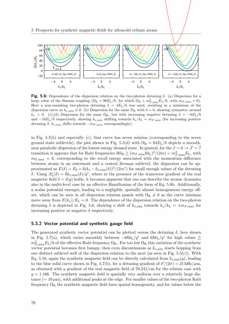
5 Prospects for synthetic magnetic fields for ultracold erbium atoms
δ=4EL/ℏ, ΩR=96EL/ℏ
(a)
-200
20406080
100
E( k
x)/E
L
-6 0 6kx/kL
δ=0, ΩR=96EL/ℏ
(b)
-6 0 6kx/kL
δ=-8EL/ℏ, ΩR=96EL/ℏ
(c)
-6 0 6kx/kL
δ=-16EL/ℏ, ΩR=96EL/ℏ
(d)
-6 0 6kx/kL
kx,min
Fig. 5.6: Dependence of the dispersion relation on the two-photon detuning δ. (a) Dispersion for alarge value of the Raman coupling (ΩR = 96EL/~, for which ΩR > m2
F,maxEL/~, with mF,max = 6).Here a non-vanishing two-photon detuning δ = 4EL/~ was used, resulting in a minimum of thedispersion curve at kx,min 6= 0. (b) Dispersion for the same ΩR with δ = 0, showing symmetry aroundkx = 0. (c),(d) Dispersion for the same ΩR, but with increasing negative detuning δ = −8EL/~and −16EL/~ respectively, showing kx,min shifting towards kx/kL = mF,max (for increasing positivedetuning δ, kx,min shifts towards −mF,max correspondingly).
in Fig. 5.5(b) and especially (c), that curve has seven minima (corresponding to the sevenground state sublevels), the plot shown in Fig. 5.5(d) with ΩR = 64EL/~ depicts a smooth,near parabolic dispersion of the lowest energy dressed state. In general, for the J = 6→ J ′ = 7transition it appears that for Rabi frequencies ~ΩR & (mF ,max~kL)2/(2m) = m2
F ,maxEL, withmF ,max = 6, corresponding to the recoil energy associated with the momentum differencebetween atoms in an outermost and a central Zeeman sublevel, the dispersion can be ap-proximated as E(δ) = E0 + ~(kx− kx,min(δ))2/(2m∗) for small enough values of the detuningδ. Using A∗x(δ) = ~kx,min(δ)/q∗, where in the presence of the transverse gradient of the realmagnetic field δ = δ(y) holds, it becomes apparent that one can describe the atomic dynamicsalso in the multi-level case by an effective Hamiltonian of the form of Eq. 5.8b. Additionally,a scalar potential emerges, leading to a negligible, spatially almost homogeneous energy off-set, which can be seen in all dispersion relation panels with ΩR 6= 0 as the curve minimasmove away from E(kx)/EL = 0. The dependence of the dispersion relation on the two-photondetuning δ is depicted in Fig. 5.6, showing a shift of kx,min towards kx/kL = ±mF ,max forincreasing positive or negative δ respectively.
5.3.2 Vector potential and synthetic gauge field
The generated synthetic vector potential can be plotted versus the detuning δ, here shownin Fig. 5.7(a), which varies smoothly between −6~kL/q
∗ and 6~kL/q∗ for high values &
m2F ,maxEL/~ of the effective Rabi frequency ΩR. For too low ΩR this variation of the synthetic
vector potential becomes first bumpy, then even discontinuous as kx,min starts hopping fromone distinct sublevel well of the dispersion relation to the next (as seen in Fig. 5.5(c)). WithEq. 5.10, again the synthetic magnetic field can be directly calculated from kx,min(y), leadingto the blue solid curve shown in Fig. 5.7(b), for a detuning gradient of δ′/(2π) = 21 kHz/µm,as obtained with a gradient of the real magnetic field of 70.3 G/cm for the erbium case withg = 1.166. The synthetic magnetic field is spatially very uniform over a relatively large dis-tance (∼ 10µm), with additional peaks at the edge. For smaller values of the two-photon Rabifrequency ΩR the synthetic magnetic field loses spatial homogeneity, and for values below the
78
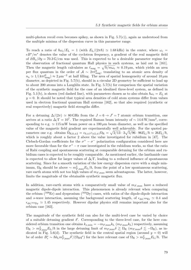
5.3 Synthetic magnetic fields for erbium atoms
multi-photon recoil even becomes spikey, as shown in Fig. 5.7(c)), again as understood fromthe multiple minima of the dispersion curve in this parameter range.
To reach a ratio of ~ωc/EL = 1 (with EL/(2π~) ' 1.68 kHz) in the center, where ωc =eB∗/m∗ denotes the value of the cyclotron frequency, a gradient of the real magnetic fieldof ∂Bx/∂y = 70.3 G/cm was used. This is expected to be a desirable parameter regime forthe observation of fractional quantum Hall physics in such systems, as laid out in [161].Then the magnetic length calculates as `mag =
√~/mωc ≈ 0.19µm, which yields an area
per flux quantum in the order of A ∼ 2π`2mag, translating to an atomic area density ofna ' 1/(4π`2mag) ≈ 2µm−2 at half filling. The area of spatial homogeneity of around 10µmdiameter, as depicted in Fig. 5.7(b), should in a circular 2D geometry be sufficient to load upto about 200 atoms into a Laughlin state. In Fig. 5.7(b) for comparison the spatial variationof the synthetic magnetic field for the case of an idealized three-level system, as defined inFig. 5.1(b), is shown (red dashed line), with parameters chosen as to also obtain ~ωc = EL aty = 0. It should be noted that typical area densities of cold atom systems differ from valuesused in electron fractional quantum Hall systems [162], so that also required (synthetic orreal respectively) magnetic field strengths differ.
For a detuning ∆/(2π) ' 80 GHz from the J = 6→ J ′ = 7 atomic erbium transition, onearrives at a ratio ∆/Γ = 107. The required Raman beam intensity of ∼ 14.6 W/mm2, corre-sponding to e.g. ' 115 mW beam power on a 100µm beam diameter, as well as the specifiedvalue of the magnetic field gradient are experimentally well achievable. For the quoted pa-rameters one e.g. obtains ΩR,0,±2 = c0,±1c±2,±1ΩR =
√2/13 · 3
√5/96 · 96EL/~ ' 26EL/~,
which is roughly about a factor 2 above the value investigated for rubidium in [47]. TheClebsch-Gordan coefficients for the σ+ − σ− polarization configuration considered here aremore favorable than for the σ+−π case investigated in the rubidium works, so that the ratioof Rabi coupling and spontaneous scattering at comparable detuning for the erbium and ru-bidium cases is expected to be roughly comparable. As mentioned earlier, the lanthanide caseis expected to allow for larger values of ∆/Γ, leading to a reduced influence of spontaneousscattering. Since for a smooth variation of the low energy dispersion curve with a single min-imum, ΩR should be above ∼ m2
F ,maxEL/~, from the point of a low spontaneous scattering,rare earth atoms with not too high values of mF ,max seem advantageous. The latter, however,limits the magnitude of the obtainable synthetic magnetic flux.
In addition, rare-earth atoms with a comparatively small value of mF ,max have a reducedmagnetic dipole-dipole interaction. This phenomenon is already relevant when comparingthe erbium (168Er) and dysprosium (164Dy) cases, with ratios of the dipole-dipole interactionand s-wave interaction, assuming the background scattering length, of εdd,168Er ' 0.4 andεdd,164Dy ' 1.45 respectively. However dipolar physics still remains important also for theerbium case [163].
The magnitude of the synthetic field can also for the multi-level case be varied by choiceof a suitable detuning gradient δ′. Corresponding to the three-level case, for the here con-sidered erbium transition one obtains kx,min = −mF,maxkL (mF,maxkL) respectively, assumingΩR > m2
F,maxEL/~ in the large detuning limit of mF,maxδ & ΩR (mF,maxδ . −ΩR), as in-dicated in Fig. 5.6(d). The synthetic field in the central spatial region (around y = 0) willbe of order B∗z ∼ ~kLm
2F,maxδ
′/(ΩRq∗) for the here relevant case of ΩR > m2
F,maxEL/~. The
79
5 Prospects for synthetic magnetic fields for ultracold erbium atoms
ΩR=16EL/ℏ
ΩR=32EL/ℏ
ΩR=64EL/ℏ
ΩR=96EL/ℏ
(a)
-6
-3
0
3
6
q*Ax*/ℏk L
-20 0 20
ℏδ/EL
ΩR=96EL/ℏ
Er
3-level
(b)
0
250
500
750
1000
Bz*[G
]
-10 -5 0 5 10
y [µm]
ΩR=16EL/ℏ(c)
0
5
10
15
Bz*/1000[G
]
-2 -1 0 1 2
y [µm]
Fig. 5.7: Synthetization of magnetic fields for the multi-level erbium case. (a) Variation of thesynthetic vector potential A∗x versus the two-photon detuning δ for different values of the effective two-photon Rabi frequency ΩR. For smaller values of ΩR (roughly below m2
F,maxEL/~, with mF,max = 6),no continuous variation is observed. Level scheme as in Fig. 5.4. (b) Corresponding synthetic magneticfield (blue solid line) versus position along the y-axis for a transverse gradient of the real magneticfield of ∂Bx/∂y = 70.3 G/cm. For ΩR = 96EL/~ a over a relatively large spatial region good spatialhomogeneity is reached. For comparison, also the spatial variation of the synthetic magnetic fieldobtained for a pure three-level system as shown in Fig. 5.1(b) is depicted here (red dashed line), wherea two-photon Rabi frequency ΩR = 16EL/~, g = 1, and a magnetic field gradient of 595 G/cm wasassumed, for which the desired value of ~ωc = EL in the center (at y = 0) is achieved. (c) Whereasthe synthetic magnetic field is homogeneous in the center region for large values of ΩR, it becomesspikey for the case of small values of e.g. ΩR = 16EL/~ < m2
F,maxEL/~. Additionally the extend ofthe synthetic field in real space reduces for smaller ΩR, if the condition ~ωc = EL is kept unchanged.
synthetic field is dependent on the effective Rabi frequency ΩR, which is understood from theinfluence of the coupling on the dressed system dispersion relation, as depicted in Fig. 5.5.Since the dispersion curve requires a smooth progression, ΩR is not truly a free parameter, butpreferably has to be choosen as a few times m2
F,maxEL/~. Accordingly, the dependence of thesynthetic field on the maximum Zeeman quantum number mF,max effectively cancels, in viewof the for large values of mF,max required increased Rabi coupling. However, for large valuesof mF,max the possible maximum momentum transfer mF,max~kL increases, which leads to alarger spatial area over which the synthetic magnetic field is imprinted, and correspondinglyto a higher synthetic flux.
Besides the above considered transition, two other, namely the J = 6 → J ′ = 5 and J ′ = 6components of the 4f126s2(3H6)→ 4f11(4I0
15/2)5d5/26s2(15/2, 5/2)0J ′ erbium transition, were
investigated regarding their use for synthetic magnetic fields. A comparison can be found inthe top panel of Fig. 5.8, where dispersion curves for the J = 6→ J ′ = 5, 6, 7 transitions aregiven for δ = 4EL/~ and ΩR = 96EL/~. The middle and lower panels depict the detuning de-pendence of the synthetic vector potential and the spatial variation of the synthetic magneticfield respectively. For the J = 6→ J ′ = 5 component it is also expected to reach a spatiallyquite uniform synthetic magnetic field and obtain ~ωc = EL in the center, with comparableparameters for the transverse magnetic field gradient. However for the J = 6→ J ′ = 6 casethe synthetic field essentially reduces to a single divergent spike in the center, which is un-derstood from the less favorable variation of Clebsch-Gordan coefficients with the Zeemanquantum number, with relatively small couplings near the center of the Zeeman diagram(|mF | ≈ 0). Therefore, the lowest energetic dispersion curve has two, rather than a single
80
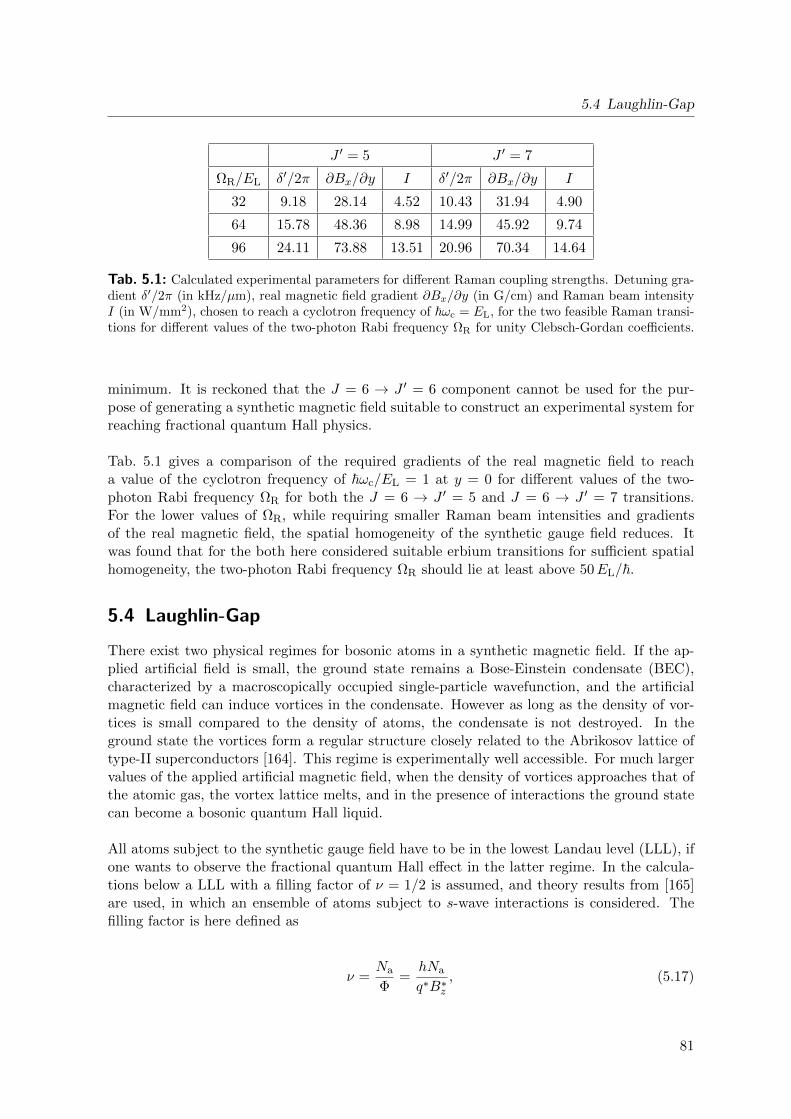
5.4 Laughlin-Gap
J ′ = 5 J ′ = 7
ΩR/EL δ′/2π ∂Bx/∂y I δ′/2π ∂Bx/∂y I
32 9.18 28.14 4.52 10.43 31.94 4.90
64 15.78 48.36 8.98 14.99 45.92 9.74
96 24.11 73.88 13.51 20.96 70.34 14.64
Tab. 5.1: Calculated experimental parameters for different Raman coupling strengths. Detuning gra-dient δ′/2π (in kHz/µm), real magnetic field gradient ∂Bx/∂y (in G/cm) and Raman beam intensityI (in W/mm2), chosen to reach a cyclotron frequency of ~ωc = EL, for the two feasible Raman transi-tions for different values of the two-photon Rabi frequency ΩR for unity Clebsch-Gordan coefficients.
minimum. It is reckoned that the J = 6 → J ′ = 6 component cannot be used for the pur-pose of generating a synthetic magnetic field suitable to construct an experimental system forreaching fractional quantum Hall physics.
Tab. 5.1 gives a comparison of the required gradients of the real magnetic field to reacha value of the cyclotron frequency of ~ωc/EL = 1 at y = 0 for different values of the two-photon Rabi frequency ΩR for both the J = 6 → J ′ = 5 and J = 6 → J ′ = 7 transitions.For the lower values of ΩR, while requiring smaller Raman beam intensities and gradientsof the real magnetic field, the spatial homogeneity of the synthetic gauge field reduces. Itwas found that for the both here considered suitable erbium transitions for sufficient spatialhomogeneity, the two-photon Rabi frequency ΩR should lie at least above 50EL/~.
5.4 Laughlin-Gap
There exist two physical regimes for bosonic atoms in a synthetic magnetic field. If the ap-plied artificial field is small, the ground state remains a Bose-Einstein condensate (BEC),characterized by a macroscopically occupied single-particle wavefunction, and the artificialmagnetic field can induce vortices in the condensate. However as long as the density of vor-tices is small compared to the density of atoms, the condensate is not destroyed. In theground state the vortices form a regular structure closely related to the Abrikosov lattice oftype-II superconductors [164]. This regime is experimentally well accessible. For much largervalues of the applied artificial magnetic field, when the density of vortices approaches that ofthe atomic gas, the vortex lattice melts, and in the presence of interactions the ground statecan become a bosonic quantum Hall liquid.
All atoms subject to the synthetic gauge field have to be in the lowest Landau level (LLL), ifone wants to observe the fractional quantum Hall effect in the latter regime. In the calcula-tions below a LLL with a filling factor of ν = 1/2 is assumed, and theory results from [165]are used, in which an ensemble of atoms subject to s-wave interactions is considered. Thefilling factor is here defined as
ν =Na
Φ=
hNa
q∗B∗z, (5.17)
81
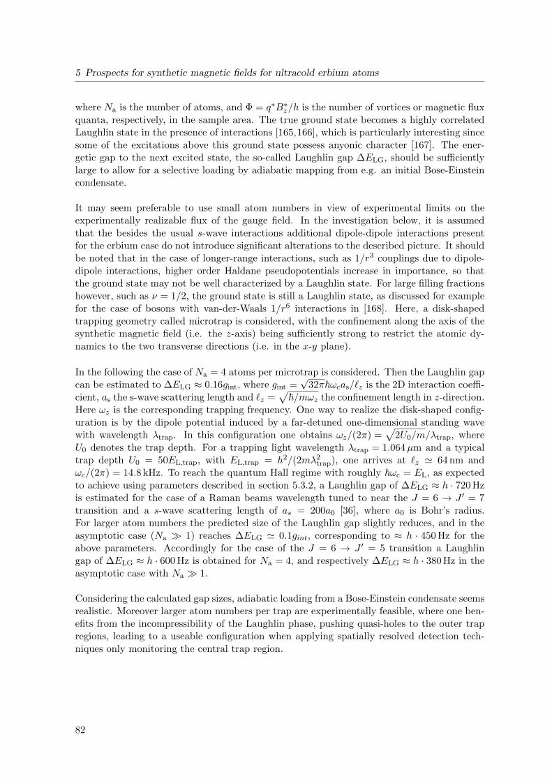
5 Prospects for synthetic magnetic fields for ultracold erbium atoms
where Na is the number of atoms, and Φ = q∗B∗z/h is the number of vortices or magnetic fluxquanta, respectively, in the sample area. The true ground state becomes a highly correlatedLaughlin state in the presence of interactions [165,166], which is particularly interesting sincesome of the excitations above this ground state possess anyonic character [167]. The ener-getic gap to the next excited state, the so-called Laughlin gap ∆ELG, should be sufficientlylarge to allow for a selective loading by adiabatic mapping from e.g. an initial Bose-Einsteincondensate.
It may seem preferable to use small atom numbers in view of experimental limits on theexperimentally realizable flux of the gauge field. In the investigation below, it is assumedthat the besides the usual s-wave interactions additional dipole-dipole interactions presentfor the erbium case do not introduce significant alterations to the described picture. It shouldbe noted that in the case of longer-range interactions, such as 1/r3 couplings due to dipole-dipole interactions, higher order Haldane pseudopotentials increase in importance, so thatthe ground state may not be well characterized by a Laughlin state. For large filling fractionshowever, such as ν = 1/2, the ground state is still a Laughlin state, as discussed for examplefor the case of bosons with van-der-Waals 1/r6 interactions in [168]. Here, a disk-shapedtrapping geometry called microtrap is considered, with the confinement along the axis of thesynthetic magnetic field (i.e. the z-axis) being sufficiently strong to restrict the atomic dy-namics to the two transverse directions (i.e. in the x-y plane).
In the following the case of Na = 4 atoms per microtrap is considered. Then the Laughlin gapcan be estimated to ∆ELG ≈ 0.16gint, where gint =
√32π~ωcas/`z is the 2D interaction coeffi-
cient, as the s-wave scattering length and `z =√
~/mωz the confinement length in z-direction.Here ωz is the corresponding trapping frequency. One way to realize the disk-shaped config-uration is by the dipole potential induced by a far-detuned one-dimensional standing wavewith wavelength λtrap. In this configuration one obtains ωz/(2π) =
√2U0/m/λtrap, where
U0 denotes the trap depth. For a trapping light wavelength λtrap = 1.064µm and a typicaltrap depth U0 = 50EL,trap, with EL,trap = h2/(2mλ2
trap), one arrives at `z ' 64 nm andωc/(2π) = 14.8 kHz. To reach the quantum Hall regime with roughly ~ωc = EL, as expectedto achieve using parameters described in section 5.3.2, a Laughlin gap of ∆ELG ≈ h · 720 Hzis estimated for the case of a Raman beams wavelength tuned to near the J = 6 → J ′ = 7transition and a s-wave scattering length of as = 200a0 [36], where a0 is Bohr’s radius.For larger atom numbers the predicted size of the Laughlin gap slightly reduces, and in theasymptotic case (Na 1) reaches ∆ELG ' 0.1gint, corresponding to ≈ h · 450 Hz for theabove parameters. Accordingly for the case of the J = 6 → J ′ = 5 transition a Laughlingap of ∆ELG ≈ h · 600 Hz is obtained for Na = 4, and respectively ∆ELG ≈ h · 380 Hz in theasymptotic case with Na 1.
Considering the calculated gap sizes, adiabatic loading from a Bose-Einstein condensate seemsrealistic. Moreover larger atom numbers per trap are experimentally feasible, where one ben-efits from the incompressibility of the Laughlin phase, pushing quasi-holes to the outer trapregions, leading to a useable configuration when applying spatially resolved detection tech-niques only monitoring the central trap region.
82
5.4 Laughlin-Gap
δ=4EL/ℏ, ΩR=96EL/ℏ
(a)
-200
20406080
100E(
k x)/E
L
-6 0 6kx/kL
δ=4EL/ℏ, ΩR=96EL/ℏ
-6 0 6kx/kL
δ=4EL/ℏ, ΩR=96EL/ℏ
-6 0 6kx/kL
ΩR=96EL/ℏ(b)
-6
-3
0
3
6
q*A x* /ℏk
L
-20-10 0 10 20ℏδ/EL
ΩR=96EL/ℏ
-20-10 0 10 20ℏδ/EL
ΩR=96EL/ℏ
-20-10 0 10 20ℏδ/EL
ΩR=96EL/ℏ(c)
0
250
500
750
1000
B z*[G]
-10 -5 0 5 10y [µm]
ΩR=96EL/ℏ
-10 -5 0 5 10y [µm]
ΩR=96EL/ℏ
-10 -5 0 5 10y [µm]
ΩR=96EL/ℏ
-10 -5 0 5 10
J ' = 5 J ' = 6 J ' = 7
Fig. 5.8: Comparison of results for the different narrow-line transition components J = 6→ J ′ = 5, 6,and 7 (left, middle, and right panels respectively) of the erbium transition, where ΩR = 96EL/~ isassumed in all cases. (a) Energy wavevector dispersion E(kx) for a two-photon detuning δ = 4EL/~.(b) Synthetic vector potential A∗x versus the two-photon detuning δ, and (c) the synthetic magneticfield versus position y for a transverse gradient of the (real) magnetic field of 73.9 G/cm in the caseof J ′ = 5 and of 70.3 G/cm in the case of J ′ = 7, for which in both cases ~ωc = EL is reached in thecenter. Then for both the J = 6→ J ′ = 5 and J ′ = 7 transitions the lowest energetic dispersion curvehas only a single minimum, enabling the synthetization of a – within the central region – spatiallyrelatively homogeneous synthetic magnetic field. In the case of the J = 6→ J ′ = 6 transition thelowest energy dispersion curve for the same value of the Raman coupling has two minima, with theabsolute minimum alternating from kx,min < 0 to kx,min > 0 for δ > 0 and δ < 0 respectively, sothat the synthetic vector potential exhibits a step-like behaviour. The resulting expected syntheticmagnetic field (shown here for a transverse gradient of the real magnetic field of 70.3 G/cm) exhibitsa divergence at y = 0, as understood from the here discontinuous variation of the vector potentialversus δ. The synthetic magnetic field in the latter case is estimated to not be usable for the purposeof constructing an experimental system capable of reaching fractional quantum Hall physics.
83

6 Conclusion and outlook
Quantum degenerate atomic rare earth gases are attractive systems for both studies of noveldipolar gas effects as well as for the physics of atoms in strong gauge fields. This thesisreports of an experiment where an atomic erbium Bose-Einstein condensate was generated ina hybrid crossed optical dipole trap realized with a focused mid-infrared beam near 10.6µmwavelength generated by a CO2 laser and a beam near 1.064µm wavelength generated by aNd:YAG laser. In further work of this thesis, a proposal for the generation of strong syntheticmagnetic fields based on ultracold erbium atoms is given.
In the first experimental part of the thesis, ultracold erbium atoms were generated by initiallydecelerating an erbium atomic beam with a Zeeman slower, as to load a magneto-optical trapoperated on a narrow-line transition. After spatially compressing the trapped atomic ensem-ble, it is loaded into an optical dipole trap potential provided by a CO2 laser beam near10.6µm wavelength, which then is supplemented by an additional crossing beam stemmingfrom a Nd:YAG laser operated near 1064 nm wavelength during evaporation. Here it waspossible to increase the phase space density above the critical value of 2.612, and observe theformation of a Bose-Einstein condensate consisting of up to 3.5 · 104 erbium atoms, showingan improvement of more than 15 % compared to earlier iterations of the experiment with asingle beam optical dipole trap setup. The BEC exhibits a condensate lifetime of up to 12 s,increased by 30 % in comparison to former single beam optical dipole trap setups. Further-more the general long-term stability of the experimental setup was improved significantly,leading to much less maintenance efforts and downtimes of the experiment, which arguablywas the main challenge of the old setup.
As an experimental outlook it should be mentioned that also other optical dipole trap con-figurations are tested in setups succeeding this thesis, especially a crossed optical dipole trapconsisting of a CO2 laser beam and an erbium fiber laser beam operated at 1550 nm to po-tentially further optimize condensate lifetimes due to lower scattering rates with the crossbeam in comparison to Nd:YAG laser light. In parallel the experimental realization of syn-thetic magnetic fields by phase imprinting via Raman manipulation in prospect of fractionalquantum Hall physics has begun at this experiment, with theoretical work carried out withinthe scope of this thesis to determine critical future experimental parameters.
For the latter the laser-induced synthetization of gauge fields in the atomic erbium lan-thanide system with a ground state orbital angular momentum L > 0 was investigated here.A configuration with two counter-propagating oppositely circularly polarized Raman beamswas shown to be an attractive approach for both on J = 6→ J ′ = 5 and J ′ = 7 narrow-lineatomic erbium transitions. In the presence of a transverse gradient of the real magnetic field,sufficiently strong synthetic magnetic fields with good spatial homogeneity are predicted to bepossible, with estimated photon scattering rates roughly two orders of magnitude lower thanin implementations with alkali atomic systems. Moreover the size of the expected Laughlin
85
6 Conclusion and outlook
gap arising from s-wave interactions for typical experimental parameters was estimated, show-ing that rare earth atomic systems are attractive candidates for experimental investigationsof fractional quantum Hall physics.
For the future, it will be important to experimentally realize synthetic magnetic fields inan erbium atomic system. Attractive areas of research interest then include the investigationof vortices in such a dipolar quantum gas, as well as the generation and detection of frac-tional quantum Hall states. Here theoretical work describing the form of the ground statein the presence of both the synthetic magnetic field and dipolar interactions will be cru-cial [169,170]. A far future outlook would be the achievement of fundamental understandingsof fractional quantum Hall states and their topology-induced robustness as well as their non-Abelian dynamics, possibly supporting the realization of a fault-tolerant topological quantumcomputer [145].
86
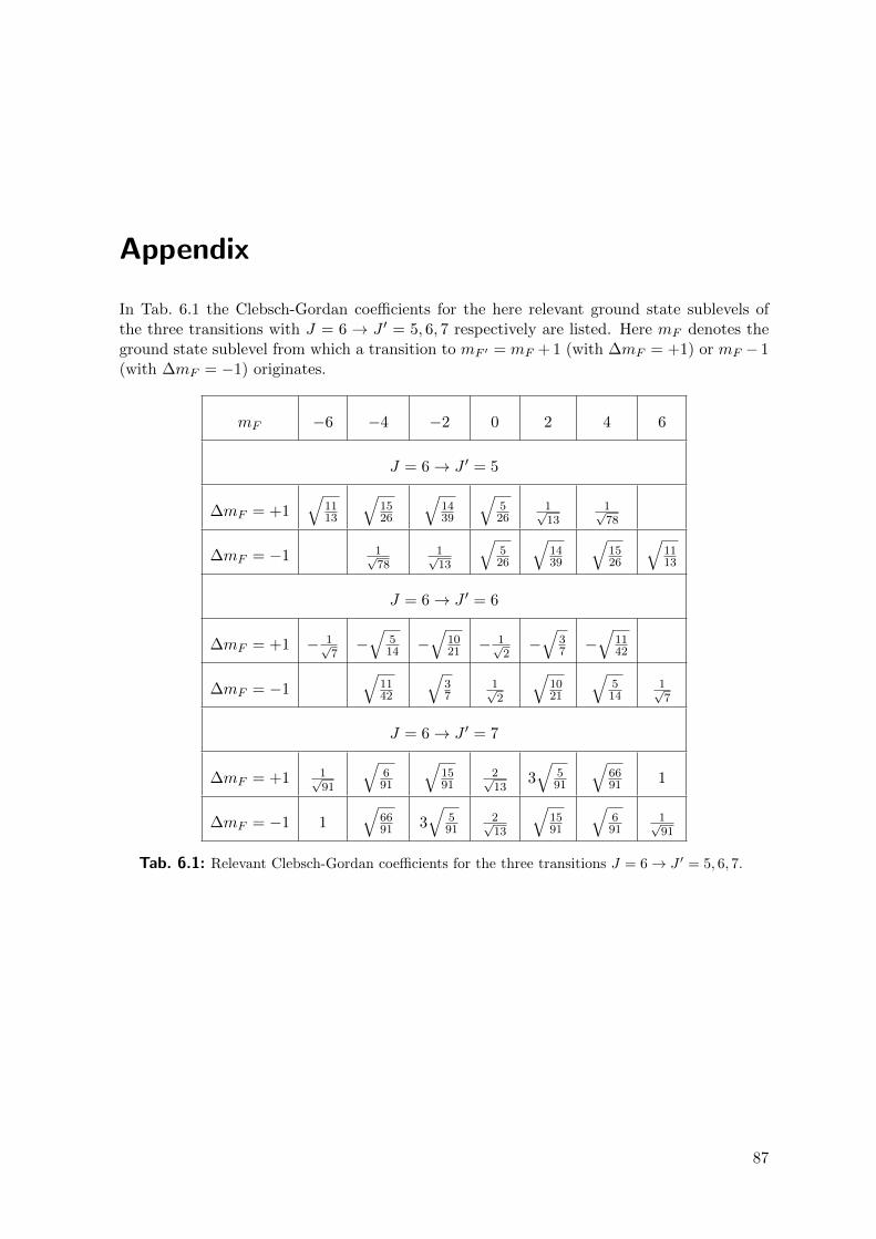
Appendix
In Tab. 6.1 the Clebsch-Gordan coefficients for the here relevant ground state sublevels ofthe three transitions with J = 6 → J ′ = 5, 6, 7 respectively are listed. Here mF denotes theground state sublevel from which a transition to mF ′ = mF + 1 (with ∆mF = +1) or mF − 1(with ∆mF = −1) originates.
mF −6 −4 −2 0 2 4 6
J = 6→ J ′ = 5
∆mF = +1√
1113
√1526
√1439
√526
1√13
1√78
∆mF = −1 1√78
1√13
√526
√1439
√1526
√1113
J = 6→ J ′ = 6
∆mF = +1 − 1√7−√
514 −
√1021 − 1√
2−√
37 −
√1142
∆mF = −1√
1142
√37
1√2
√1021
√514
1√7
J = 6→ J ′ = 7
∆mF = +1 1√91
√691
√1591
2√13
3√
591
√6691 1
∆mF = −1 1√
6691 3
√591
2√13
√1591
√691
1√91
Tab. 6.1: Relevant Clebsch-Gordan coefficients for the three transitions J = 6→ J ′ = 5, 6, 7.
87

Bibliography
[1] A. Einstein, Quantentheorie des einatomigen idealen Gases, Sitzber. Kgl. Preuß. Akad.Wiss., 261–267 (1924).
[2] A. Einstein, Quantentheorie des einatomigen idealen Gases. Zweite Abhandlung,Sitzber. Kgl. Preuß. Akad. Wiss., 3–14 (1925).
[3] S. N. Bose, Plancks Gesetz und Lichtquantenhypothese, Z. Phys. 26, 178–181 (1924).
[4] M. H. Anderson, J. R. Ensher, M. R. Matthews, and E. A. Wieman, C. E. und Cornell,Observation of Bose-Einstein Condensation in a Dilute Atomic Vapor, Science 269, 198(1995).
[5] K. B. Davis, M. O. Mewes, M. R. Andrews, N. J. Van Druten, D. S. Durfee, D. M.Kurn, and W. Ketterle, Bose-Einstein Condensation in a Gas of Sodium Atoms, Phys.Rev. Lett. 75, 3969–3973 (1995).
[6] F. Dalfovo, S. Giorgini, L. P. Pitaevskii, and S. Stringari, Theory of Bose-Einsteincondensation in trapped gases, Rev. Mod. Phys. 71, 463 (1999).
[7] M. R. Andrews, Observation of Interference Between Two Bose Condensates, Science275, 637–641 (1997).
[8] M. R. Matthews, B. P. Anderson, P. C. Haljan, D. S. Hall, C. E. Wieman, and E. A.Cornell, Vortices in a Bose-Einstein Condensate, Phys. Rev. Lett. 83, 2498–2501 (1999).
[9] M. Greiner, O. Mandel, T. Esslinger, T. W. Hansch, and I. Bloch, Quantum phasetransition from a superfluid to a Mott insulator in a gas of ultracold atoms, Nature415, 39–44 (2002).
[10] M. B. Dahan, E. P., J. R., Y. C., and C. Salomon, Bloch Oscillations of Atoms in anOptical Potential, Physical Review Letters 76, 4508–4511 (1996).
[11] M. Leder, C. Grossert, L. Sitta, M. Genske, A. Rosch, and M. Weitz, Real-space imag-ing of a topologically protected edge state with ultracold atoms in an amplitude-chirpedoptical lattice, Nat. Commun. 7, 13112 (2016).
[12] U. Fano, Sullo spettro di assorbimento dei gas nobili presso il limite dello spettro d’arco,Nuovo Cim. 12, 154–161 (1935).
[13] H. Feshbach, Unified theory of nuclear reactions, Ann. Phys. 5, 357–390 (1958).
[14] S. L. Cornish, N. R. Claussen, J. L. Roberts, E. A. Cornell, and C. E. Wieman, Stable85Rb Bose-Einstein Condensates with Widely Tunable Interactions, Phys. Rev. Lett.85, 1795–1798 (2000).
[15] C. Chin, R. Grimm, P. Julienne, and E. Tiesinga, Feshbach resonances in ultracoldgases, Rev. Mod. Phys. 82, 1225–1286 (2010).
[16] A. Polkovnikov, K. Sengupta, A. Silva, and M. Vengalattore, Colloquium: Nonequilib-rium dynamics of closed interacting quantum systems, Rev. Mod. Phys. 83, 863–883(2011).
[17] A. M. Kaufman, M. E. Tai, A. Lukin, M. Rispoli, R. Schittko, P. M. Preiss, andM. Greiner, Quantum thermalization through entanglement in an isolated many-bodysystem, Science 353, 794–800 (2016), no. 6301.
89
BIBLIOGRAPHY
[18] I. M. M. Georgescu, S. Ashhab, and F. Nori, Quantum simulation, Rev Mod Phys 86,153–185 (2014).
[19] R. Balili, V. Hartwell, D. Snoke, L. Pfeiffer, and K. West, Bose-Einstein Condensationof Microcavity Polaritons in a Trap, Science 316, 1007–1010 (2007).
[20] J. Klaers, J. Schmitt, F. Vewinger, and M. Weitz, Bose-Einstein condensation of photonsin an optical microcavity, Nature 468, 545–548 (2010).
[21] S. Christopoulos, G. Baldassarri, H. von Hogersthal, A. J. D. Grundy, P. G. Lagoudakis,A. V. Kavokin, J. J. Baumberg, G. Christmann, R. Butte, E. Feltin, J.-F. Carlin, andN. Grandjean, Room-Temperature Polariton Lasing in Semiconductor Microcavities,Phys. Rev. Lett. 98, 126405 (2007).
[22] B. DeMarco, Onset of Fermi Degeneracy in a Trapped Atomic Gas, Science 285, 1703–1706 (1999).
[23] E. Fermi, Zur Quantelung des idealen einatomigen Gases, Z. Phys. 36, 902–912 (1926).
[24] P. A. M. Dirac, On the Theory of Quantum Mechanics, Proc. R. Soc. Lond. Series A112, 661–677 (1926).
[25] T. Esslinger, Fermi-Hubbard Physics with Atoms in an Optical Lattice, Ann. Rev. Cond.Matt. Phys. 1, 129–152 (2010).
[26] S. Stellmer, M. K. Tey, B. Huang, R. Grimm, and F. Schreck, Bose-Einstein Conden-sation of Strontium, Phys. Rev. Lett. 103, 200401 (2009).
[27] M. Lu, N. Q. Burdick, S.-H. Youn, and B. L. Lev, Strongly Dipolar Bose-EinsteinCondensate of Dysprosium, Phys. Rev. Lett. 107, 190401 (2011).
[28] M. Lu, N. Q. Burdick, and B. L. Lev, Quantum Degenerate Dipolar Fermi Gas, Phys.Rev. Lett. 108, 1–5 (2012).
[29] Y. Takasu, K. Maki, K. Komori, T. Takano, K. Honda, M. Kumakura, T. Yabuzaki,and Y. Takahashi, Spin-Singlet Bose-Einstein Condensation of Two-Electron Atoms,Phys. Rev. Lett. 91, 040404 (2003).
[30] K. Aikawa, A. Frisch, M. Mark, S. Baier, A. Rietzler, R. Grimm, and F. Ferlaino,Bose-Einstein Condensation of Erbium, Phys. Rev. Lett. 108, 210401 (2012).
[31] K. Aikawa, A. Frisch, M. Mark, S. Baier, R. Grimm, and F. Ferlaino, Reaching FermiDegeneracy via Universal Dipolar Scattering, Phys. Rev. Lett. 112, 010404 (2014).
[32] D. Sukachev, A. Sokolov, K. Chebakov, A. Akimov, S. Kanorsky, N. Kolachevsky, andV. Sorokin, Magneto-optical trap for thulium atoms, Phys. Rev. A 82, 011405(R) (2010).
[33] E. Kalganova, G. Vishnyakova, A. Golovisin, D. Tregubov, D. Sukachev, S. Fedorov,K. Khabarova, A. Akimov, N. Kolachevsky, and V. Sorokin, Laser cooling and trappingof thulium atoms for further investigation of collisional properties, J. Phys.: Conf. Ser.635, 092117 (2015).
[34] J. Miao, J. Hostetter, G. Stratis, and M. Saffman, Magneto-optical trapping of holmiumatoms, Phys. Rev. A 89, 041401(R) (2014).
[35] A. Trautmann, P. Ilzhofer, G. Durastante, C. Politi, M. Sohmen, M. J. Mark, andF. Ferlaino, Dipolar Quantum Mixtures of Erbium and Dysprosium Atoms, Phys. Rev.Lett. 121, 213601 (2018).
[36] A. Frisch, M. Mark, K. Aikawa, F. Ferlaino, J. L. Bohn, C. Makrides, A. Petrov,and S. Kotochigova, Quantum chaos in ultracold collisions of gas-phase erbium atoms,Nature 507, 475–9 (2014).
90
BIBLIOGRAPHY
[37] K. Baumann, N. Q. Burdick, M. Lu, and B. L. Lev, Observation of low-field Fano-Feshbach resonances in ultracold gases of dysprosium, Phys. Rev. A 89, 020701(R)(2014).
[38] K. Aikawa, S. Baier, A. Frisch, M. Mark, C. Ravensbergen, and F. Ferlaino, Observationof Fermi surface deformation in a dipolar quantum gas, Science 345, 1484 (2014).
[39] A. Frisch, M. Mark, K. Aikawa, S. Baier, R. Grimm, A. Petrov, S. Kotochigova,G. Quemener, M. Lepers, O. Dulieu, and F. Ferlaino, Ultracold Dipolar Molecules Com-posed of Strongly Magnetic Atoms, Phys. Rev. Lett. 115, 203201 (2015).
[40] S. Baier, M. J. Mark, D. Petter, K. Aikawa, L. Chomaz, Z. Cai, M. Baranov, P. Zoller,and F. Ferlaino, Extended Bose-Hubbard Models with Ultracold Magnetic Atoms, Science352, 6282 (2016).
[41] N. Q. Burdick, A. G. Sykes, Y. Tang, and B. Lev, Anisotropic collisions of dipo-lar Bose–Einstein condensates in the universal regime, New. J. Phys. 18, (2016),no. 111004.
[42] L Chomaz, S Baier, D Petter, M. J. Mark, F Wachtler, L Santos, and F Ferlaino,Quantum-Fluctuation-Driven Crossover from a Dilute Bose-Einstein Condensate to aMacrodroplet in a Dipolar Quantum Fluid, Physical Review X 6, (2016), no. 4.
[43] D. Petter, A. Patschneider, G. Natale, M. J. Mark, M. A. Baranov, R. v. Bijnen, S. M.Roccuzzo, A. Recati, B. Blakie, D. Baillie, L. Chomaz, and F. Ferlaino, High-energyBragg scattering measurements of a dipolar supersolid, , arXiv:2005.02213 (2016).
[44] X.-L. Qi and S.-C. Zhang, Topological insulators and superconductors, Rev. Mod. Phys.83, 1057–1110 (2011).
[45] S. Das Sarma, M. Freedman, and C. Nayak, Topologically Protected Qubits from a Pos-sible Non-Abelian Fractional Quantum Hall State, Phys. Rev. Lett. 94, 166802 (2005).
[46] Y.-J. Lin, R. L. Compton, K. Jimenez-Garcıa, J. V. Porto, and I. B. Spielman, Syntheticmagnetic fields for ultracold neutral atoms, Nature 462, 628–632 (2009).
[47] I. B. Spielman, Raman processes and effective gauge potentials, Phys. Rev. A 79, 063613(2009).
[48] R. Grimm, M. Weidemuller, and Y. B. Ovchinnikov, Optical Dipole Traps for NeutralAtoms, Adv. At. Mol. Opt. Phys. 42, 95–170 (2000).
[49] X. Cui, B. Lian, T. L. Ho, B. L. Lev, and H. Zhai, Synthetic gauge field with highlymagnetic lanthanide atoms, Phys. Rev. A 88, 011601 (2013).
[50] D. Babik, R. Roell, D. Helten, M. Fleischhauer, and M. Weitz, Synthetic magnetic fieldsfor cold erbium atoms, Phys. Rev. A 101, 053603 (2020).
[51] T. Chalopin, T. Satoor, A. Evrard, V. Makhalov, J. Dalibard, R. Lopes, and S. Nascim-bene, Probing chiral edge dynamics and bulk topology of a synthetic Hall system, Nat.Phys. (2020). https://doi.org/10.1038/s41567-020-0942-5.
[52] J. J. McClelland and J. L. Hanssen, Laser cooling without repumping: A magneto-opticaltrap for erbium atoms, Phys. Rev. Lett. 96, 143005 (2006).
[53] H. Brammer, Aufbau eines frequenzstabilisierten Lasersystems zur optischen Kuhlungvon Erbiumatomen, Diplomarbeit, Rheinische Friedrich-Wilhelms-Universitat Bonn(2010).
[54] J. Ulitzsch, Magnetooptische Falle fur Erbiumatome, Diplomarbeit, RheinischeFriedrich-Wilhelms-Universitat Bonn (2011).
[55] H. Brammer, Ultrakalte Erbiumatome in einer CO2 -Laser Dipolfalle, Dissertation,Rheinische Friedrich-Wilhelms-Universitat Bonn (2016).
91
BIBLIOGRAPHY
[56] J. Ulitzsch, Erzeugung eines Bose-Einstein-Kondensats aus Erbiumatomen ineiner quasi-elektrostatischen Dipolfalle, Dissertation, Rheinische Friedrich-Wilhelms-Universitat Bonn (2016).
[57] J. Ulitzsch, D. Babik, R. Roell, and M. Weitz, Bose-einstein condensation of erbiumatoms in a quasielectrostatic optical dipole trap, Phys. Rev. A 95, 043614 (2017).
[58] W. Pauli, Uber den Zusammenhang des Abschlusses der Elektronengruppen im Atommit der Komplexstruktur der Spektren, Z. Phys. 31, 765–783 (1925).
[59] C. J. Pethick and H. Smith, Bose-Einstein condensation in Dilute Gases, 1. Ed., Cam-bridge: Cambridge University Press, 2002.
[60] C. Patrignani, Review of particle physics, Chin. Phys. C 40, 100001 (2016).
[61] C. G. Mosander, On the new metals, lanthanium and didymium, which are associatedwith cerium; and on erbium and terbium, new metals associated with yttria, Philos.Mag. [3] 23, 241–254 (1843).
[62] A. F. Holleman and N. Wiberg, Lehrbuch der Anorganischen Chemie, 102. Ed., Berlin:de Gruyter, 2007.
[63] J. Emsley, Nature’s building blocks - An A-Z Guide to the Elements, 1. Ed., Oxford:Oxford University Press, 2001.
[64] J. Emsley, The Elements, 1. Ed., Oxford: Oxford University Press, 1989.
[65] T. Daniyarov, Metallische magnetische Kalorimeter zum hochauflosenden Nachweisvon Rontgenquanten und hochenergetischen Molekulen, Dissertation, Ruprecht-Karls-Universitat Heidelberg (2005).
[66] G. Teikemeier and D. J. Goldberg, Skin Resurfacing with the Erbium: YAG Laser,Dermatologic Surgery 23, 685–687 (1997).
[67] E. Bornstein, Proper use of Er:YAG lasers and contact sapphire tips when cutting teethand bone: scientific principles and clinical application, Dentistry Today 23, 84 (2004).
[68] E. Saglamyurek, J. Jin, V. B. Verma, M. D. Shaw, F. Marsili, S. W. Nam, D. Oblak,and W. Tittel, Quantum storage of entangled telecom-wavelength photons in an erbium-doped optical fibre, Nature Phot. 9, 83–87 (2015).
[69] X. Cheng, Y. Pan, Z. Yuan, X. Wang, W. Su, L. Yin, X. Xie, and L. Huang, Er3+
Sensitized Photon Upconversion Nanocrystals, Adv. Funct. Mater. 28, 1800208 (2018).
[70] W. C. Martin, R. Zalubas, and L. Hagan, Atomic energy levels - The rare-Earth el-ements, Washington: National Bureau of Standards, U.S. Department of Commerce,1978.
[71] A. Frisch, Dipolar Quantum Gases of Erbium, Dissertation, Universitat Innsbruck(2014).
[72] J. Muller, B. Singh, and N. A. Surplice, The gettering action of evaporated films oftitanium and erbium, Jour. Phys. D 5, 6 (1972).
[73] B. G. Wybourne and L. Smentek, Optical Spectroscopy of Lanthanides: Magnetic andHyperfine Interactions, Boca Raton: CRC Press, 2007.
[74] A. Kramida, Y. Ralchenko, J. Reader, and NIST ASD Team, NIST Atomic SpectraDatabase (version 5.7.1), Gaithersburg, MD, 2019 [visited on 15.09.2020].
[75] M. Lepers, J.-F. Wyart, and O. Dulieu, Anisotropic optical trapping of ultracold erbiumatoms, Phys. Rev. A 89, 022505 (2014).
[76] E. Raab, M. Prentiss, A. Cable, S. Chu, and D. Pritchard, Trapping of Neutral SodiumAtoms with Radiation Pressure, Phys. Rev. Lett. 59, 2631 (1987).
92
BIBLIOGRAPHY
[77] H. Ban, M. Jacka, J. Hanssen, J. Reader, and J. McClelland, Laser cooling transitionsin atomic erbium, Opt. Express 13, 3185–3195 (2005).
[78] E. A. Den Hartog, J. P. Chisholm, and J. E. Lawler, Radiative lifetimes of neutralerbium, Jour. Phys. B 43, 155004 (2010).
[79] J. E. Lawler, J.-F. Wyart, and E. A. Den Hartog, Atomic transition probabilities of ErI, Jour. Phys. B 43, 235001 (2010).
[80] A. Frisch, K. Aikawa, M. Mark, A. Rietzler, J. Schindler, E. Zupanic, R. Grimm, andF. Ferlaino, Narrow-line magneto-optical trap for erbium, Phys. Rev. A 85, 051401(2012).
[81] J. G. Conway and B. G. Wybourne, Low-Lying Energy Levels of Lanthanide Atoms andIntermediate Coupling, Phys. Rev. 130, 2325 (1963).
[82] P. Zeeman, The Effect of Magnetisation on the Nature of Light Emitted by a Substance,Nature 55, 347–347 (1897).
[83] B. R. Judd and I. Lindgren, Theory of Zeeman Effect in the Ground Multiplets of Rare-Earth Atoms, Phys. Rev. 122, 1802–1812 (1961).
[84] H. Metcalf and P. van der Straten, Laser Cooling and Trapping, New York: Springer,1999.
[85] W. Demtroder, Experimentalphysik 1, Berlin: Springer, 2008.
[86] C. A. Doppler, Ueber das farbige Licht der Doppelsterne und einiger anderer Gestirnedes Himmels, Abhandlung der Koniglich Bohmischen Gesellschaft der Wissenschaften5, 3 (1842).
[87] S. Chu, L. Hollberg, J. E. Bjorkholm, A. Cable, and A. Ashkin, Three-dimensionalviscous confinement and cooling of atoms by resonance radiation pressure, Phys. Rev.Lett. 55, 48–51 (1985).
[88] J. Dalibard and C. Cohen-Tannoudji, Laser cooling below the Doppler limit by polariza-tion gradients: simple theoretical models, J. Opt. Soc. Am. B 6, 2023–2045 (1989).
[89] C. S. Adams and E. Riis, Laser cooling and trapping of neutral atoms, Prog. Quant.Electr. 21, 1–79 (1997).
[90] F. Bardou, J. P. Bouchaud, O. Emile, A. Aspect, and C. Cohen-Tannoudji, Subrecoillaser cooling and Levy flights, Phys. Rev. Lett. 72, 203–206 (1994).
[91] F. M. Peixoto, Enhanced Loading of a Lithium 7 Magneto Optical Trap using TransverseCooling and Frequency Spread Light, Dissertation, Yale University (2002).
[92] M. A. Joffe, W. Ketterle, A. Martin, and D. E. Pritchard, Transverse cooling anddeflection of an atomic beam inside a Zeeman slower, J. Opt. Soc. Am. B 10, 2257(1993).
[93] N. Leefer, A. Cingoz, B. Gerber-Siff, A. Sharma, J. R. Torgerson, and D. Budker,Transverse laser cooling of a thermal atomic beam of dysprosium, Phys. Rev. A 81,043427 (2010).
[94] W. D. Phillips and H. Metcalf, Laser Deceleration of an Atomic Beam, Phys. Rev. Lett.48, 596–599 (1982).
[95] T. H. Loftus, T. Ido, M. M. Boyd, A. D. Ludlow, and J. Ye, Narrow line cooling andmomentum-space crystals, Phys. Rev. A 70, 063413 (2004).
[96] H. Katori, T. Ido, Y. Isoya, and M. Kuwata-Gonokami, Magneto-Optical Trapping andCooling of Strontium Atoms down to the Photon Recoil Temperature, Phys. Rev. Lett.82, 1116–1119 (1999).
93
BIBLIOGRAPHY
[97] C. V. Harnik, A hybrid crossed optical dipole trap for Bose-Einstein condensation ofatomic erbium, Masterarbeit, Rheinische Friedrich-Wilhelms-Universitat Bonn (2019).
[98] P. W. Langhoff, S. T. Epstein, and M. Karplus, Aspects of Time-Dependent PerturbationTheory, Rev. Mod. Phys. 44, 602–644 (1972).
[99] J. Stark, Beobachtungen uber den Effekt des elektrischen Feldes auf Spektrallinien. I.Quereffekt, Ann. d. Phys. 348, 965–982 (1914).
[100] J. Stark and G. Wendt, Beobachtungen uber den Effekt des elektrischen Feldes aufSpektrallinien. II. Langseffekt, Ann. d. Phys. 348, 983–990 (1914).
[101] A. Mosk, S. Kraft, M. Mudrich, K. Singer, W. Wohlleben, R. Grimm, and M. Wei-demuller, Mixture of ultracold lithium and cesium atoms in an optical dipole trap, App.Phy. B 73, 791–799 (2001).
[102] A. N. Nikolov, E. E. Eyler, X. T. Wang, J. Li, H. Wang, W. C. Stwalley, and P. L.Gould, Observation of Ultracold Ground-State Potassium Molecules, Phys. Rev. Lett.82, 703–706 (1999).
[103] T. Takekoshi, J. R. Yeh, and R. J. Knize, Quasi-electrostatic trap for neutral atoms,Opt. Commun. 114, 421–424 (1995).
[104] J. H. Becher, S. Baier, K. Aikawa, M. Lepers, J.-F. Wyart, O. Dulieu, and F. Ferlaino,Anisotropic polarizability of erbium atoms, Phys. Rev. A 97, 012509 (2018).
[105] C. S. Adams, H. J. Lee, N. Davidson, M. Kasevich, and S. Chu, Evaporative cooling ina crossed dipole trap, Phys. Rev. Lett. 74, 3577–3580 (1995).
[106] T. Takekoshi and R. J. Knize, CO2 laser trap for cesium atoms, Opt. Lett. 21, 77(1996).
[107] M. Weitz, S. Friebel, R. Scheunemann, J. Walz, and T. W. Hansch, A CO2 laseroptical lattice with cold rubidium atoms, in Int. Quant. Electr. Conf., P. Corkum andN. Peyghambarian (eds.), 7, OSA Technical Digest (1998).
[108] E. Hecht, Optics, 4. Ed., San Francisco: Addison Wesley, 2001.
[109] S. Baier, An optical dipole trap for Erbium with tunable geometry, Masterthesis, Uni-versity of Innsbruck (2012).
[110] A. Kuhn, H. Perrin, W. Hansel, and C. Salomon, Three Dimensional Raman Coolingusing Velocity Selective Rapid Adiabatic Passage, in OSA TOPS on Ultracold Atomsand BEC, K. Burnett (eds.), Opt. Soc. Am. 7, 58; arXiv:1109.5237 (1996).
[111] H. Perrin, A. Kuhn, I. Bouchoule, and C. Salomon, Sideband cooling of neutral atomsin a far-detuned optical lattice, EPL 42, 395–400 (1998).
[112] H. F. Hess, Evaporative cooling of magnetically trapped and compressed spin-polarizedhydrogen, Phys. Rev. B 34, 3476–3479 (1986).
[113] W. Ketterle and N. J. van Struten, Evaporative Cooling of Trapped Atoms, AdvancesIn Atomic, Molecular, and Optical Physics, Bd. 37, 181–236 (1999).
[114] K. M. O’Hara, M. E. Gehm, S. R. Granade, and J. E. Thomas, Scaling laws for evapo-rative cooling in time-dependent optical traps, Phys. Rev. A 64, 051403(R) (2001).
[115] C.-L. Hung, X. Zhang, N. Gemelke, and C. Chin, Accelerating evaporative cooling ofatoms into Bose-Einstein condensation in optical traps, Phys. Rev. A 78, 011604(R)(2008).
[116] D. Meschede, Gerthsen Physik, 23. Ed., Berlin Heidelberg New York: Springer, 2006.
[117] M. Rehberger, Ultracold Erbium Atoms in Far-Detuned Optical Traps - Constructionof a Zeeman-Slower, Masterarbeit, Rheinische Friedrich-Wilhelms-Universitat Bonn(2013).
94
BIBLIOGRAPHY
[118] D. Babik, Frequency stabilization of a dye laser for narrow-line laser cooling of erbiumatoms, Masterarbeit, Rheinische-Friedrich-Wilhelms-Universitat Bonn (2014).
[119] A. Harder, Setup and testing of an apparatus for cooling and trapping erbium atoms,Masterarbeit, Rheinische Friedrich-Wilhelms-Universitat Bonn (2014).
[120] M. Prentiss, E. L. Raab, D. E. Pritchard, A. Cable, J. E. Bjorkholm, and S. Chu,Atomic-density-dependent losses in an optical trap, Opt. Lett. 13, 452 (1988).
[121] N. F. Ramsey, Molecular Beams, Oxford: Oxford University Press, 1963.
[122] G. Scoles, Atomic and Molecular Beam Methods Volume I, Oxford: Oxford UniversityPress, 1988.
[123] C. Bolkart, Erzeugung eines ultrakalten Gases fermionischer Kaliumatome im op-tischen Dipolfallenpotential, Dissertation, Rheinische Friedrich-Wilhelms-UniversitatBonn (2011).
[124] A. Gatto, Trapping fermionic potassium atoms in a quasi-electrostatic optical dipolepotential, Dissertation, Rheinische Friedrich-Wilhelms-Universitat Bonn (2011).
[125] D. J. McCarron, S. A. King, and S. L. Cornish, Modulation transfer spectroscopy inatomic rubidium, Meas. Sci. Technol. 19, 105601 (2008).
[126] V. Negnevitsky and L. D. Turner, Wideband laser locking to an atomic reference withmodulation transfer spectroscopy, Opt. Express 21, 3103 (2013).
[127] R. W. P. Drever, J. L. Hall, F. V. Kowalski, J. Hough, G. M. Ford, A. J. Munley,and H. Ward, Laser phase and frequency stabilization using an optical resonator, Appl.Phys. B 31, 97–105 (1983).
[128] M. Hohn, Frequenzstabilisierung eines Diodenlasers mittels Doppler-freier Spektroskopiean einer Erbium-Hohlkathodenlampe, Bachelorarbeit, Rheinische Friedrich-Wilhelms-Universitat Bonn (2017).
[129] D. Dreon, L. A. Sidorenkov, C. Bouazza, W. Maineult, J. Dalibard, and S. Nascimbene,Optical cooling and trapping of highly magnetic atoms: the benefits of a spontaneous spinpolarization, J. Phys. B: At. Mol. Opt. Phys. 50, 065005 (2017).
[130] D. Meschede, Optik, Licht und Laser, 2. Ed., Wiesbaden: Vieweg+Teubner, 2005.
[131] W. Ketterle and M. W. Zwierlein, Making, probing and understanding ultracold Fermigases, Proceedings of the International School of Physics “Enrico Fermi” on UltracoldFermi Gases, Course CLXIV, M. Inguscio, W. Ketterle, and C. Salomon (eds.); Ams-terdam: IOS Press, 2008.
[132] L. Bergmann and C. Schaefer, Lehrbuch der Experimentalphysik, Band 3, Optik, 10.Ed., Berlin, New York: Walter de Gruyter, 2004.
[133] L. D. Landau and E. M. Lifschitz, Lehrbuch der Theoretischen Physik, Band 1,Mechanik, 14. Ed., Frankfurt am Main: Harri Deutsch, 2004.
[134] F. Chevy, V. Bretin, P. Rosenbusch, K. W. Madison, and J. Dalibard, TransverseBreathing Mode of an Elongated Bose-Einstein Condensate, Phys. Rev. Lett. 88, 250402(2002).
[135] P. D. Lett, R. N. Watts, C. I. Westbrook, W. D. Phillips, P. L. Gould, and H. J.Metcalf, Observation of Atoms Laser Cooled below the Doppler Limit, Phys. Rev. Lett.61, 169–172 (1988).
[136] J. D. Miller, R. A. Cline, and D. J. Heinzen, Far-off-resonance optical trapping of atoms,Phys. Rev. A 47, R4567(R) (1993).
[137] W. Gerlach and O. Stern, Der experimentelle Nachweis der Richtungsquantelung imMagnetfeld, Z. Phys. 9, 349–352 (1922).
95
BIBLIOGRAPHY
[138] F. Gerbier, J. H. Thywissen, S. Richard, M. Hugbart, P. Bouyer, and A. Aspect, CriticalTemperature of a Trapped, Weakly Interacting Bose Gas, Phys. Rev. Lett. 92, 030405(2004).
[139] K. Aikawa, A. Frisch, M. Mark, S. Baier, R. Grimm, J. L. Bohn, D. S. Jin, G. M. Bruun,and F. Ferlaino, Anisotropic Relaxation Dynamics in a Dipolar Fermi Gas Driven Outof Equilibrium, Physical Review Letters 113, 263201 (2014).
[140] K. v. Klitzing, G. Dorda, and M. Pepper, New Method for High-Accuracy Determinationof the Fine-Structure Constant Based on Quantized Hall Resistance, Phys. Rev. Lett.45, 494–497 (1980).
[141] M. I. D’Yakonov and V. I. Perel’, Possibility of Orienting Electron Spins with Current,Sov. Phys. JETP 13, 467 (1971).
[142] J. Sinova, D. Culcer, Q. Niu, N. A. Sinitsyn, T. Jungwirth, and A. H. MacDonald,Universal intrinsic spin hall effect, Phys. Rev. Lett. 92, 126603 (2004).
[143] C. L. Kane and E. J. Mele, Z2 Topological Order and the Quantum Spin Hall Effect,Phys. Rev. Lett. 95, 146802 (2005).
[144] J. Dalibard, F. Gerbier, G. Juzeliunas, and P. Ohberg, Colloquium: Artificial gaugepotentials for neutral atoms, Rev. Mod. Phys. 83, 1523–1543 (2011).
[145] N. Goldman, G. Juzeliunas, P. Ohberg, and I. B. Spielman, Light-induced gauge fieldsfor ultracold atoms, Rep. Prog. Phys. 77, 126401 (2014).
[146] V. Bretin, S. Stock, Y. Seurin, and J. Dalibard, Fast Rotation of a Bose-Einstein Con-densate, Phys. Rev. Lett. 92, 050403 (2004).
[147] V. Schweikhard, I. Coddington, P. Engels, V. P. Mogendorff, and E. A. Cornell, RapidlyRotating Bose-Einstein Condensates in and near the Lowest Landau Level, Phys. Rev.Lett. 92, 040404 (2004).
[148] P. Hauke, O. Tieleman, A. Celi, C. Olschlager, J. Simonet, J. Struck, M. Weinberg,P. Windpassinger, K. Sengstock, M. Lewenstein, and A. Eckardt, Non-Abelian GaugeFields and Topological Insulators in Shaken Optical Lattices, Phys. Rev. Lett. 109,145301 (2012).
[149] J. Ruseckas, G. Juzeliunas, P. Ohberg, and M. Fleischhauer, Non-Abelian Gauge Po-tentials for Ultracold Atoms with Degenerate Dark States, Phys. Rev. Lett. 95, 010404(2005).
[150] G. Juzeliunas, J. Ruseckas, P. Ohberg, and M. Fleischhauer, Light-induced effective mag-netic fields for ultracold atoms in planar geometries, Phys. Rev. A 73, 025602 (2006).
[151] Shi-Liang Zhu, Hao Fu, C.-J. Wu, S.-C. Zhang, and L.-M. Duan, Spin hall effects forcold atoms in a light-induced gauge potential, Phys. Rev. Lett. 97, 240401 (2006).
[152] K. Jimenez-Garcıa, Artificial Gauge Fields for Ultracold Neutral Atoms, Dissertation,NIST, and the University of Maryland (2012).
[153] M. Aidelsburger, M. Atala, M. Lohse, J. T. Barreiro, B. Paredes, and I. Bloch, Real-ization of the Hofstadter Hamiltonian with Ultracold Atoms in Optical Lattices, Phys.Rev. Lett. 111, 185301 (2013).
[154] C. J. Kennedy, G. A. Siviloglou, H. Miyake, W. C. Burton, and W. Ketterle, Spin-OrbitCoupling and Quantum Spin Hall Effect for Neutral Atoms without Spin Flips, Phys.Rev. Lett. 111, 225301 (2013).
[155] M. Aidelsburger, M. Atala, S. Nascimbene, S. Trotzky, Y.-A. Chen, and I. Bloch, Ex-perimental Realization of Strong Effective Magnetic Fields in an Optical Lattice, Phys.Rev. Lett. 107, 255301 (2011).
96
BIBLIOGRAPHY
[156] F. Wilczek and A. Zee, Appearance of Gauge Structure in Simple Dynamical Systems,Phys. Rev. Lett. 52, 2111–2114 (1984).
[157] Y.-J. Lin, K. Jimenez-Garcıa, and I. B. Spielman, Spin–orbit-coupled Bose–Einsteincondensates, Nature 471, 83–86 (2011).
[158] P. Wang, Z.-Q. Yu, Z. Fu, J. Miao, L. Huang, S. Chai, H. Zhai, and J. Zhang, Spin-OrbitCoupled Degenerate Fermi Gases, Phys. Rev. Lett. 109, 095301 (2012).
[159] M. C. Beeler, R. A. Williams, K. Jimenez-Garcıa, L. J. LeBlanc, A. R. Perry, and I. B.Spielman, The spin Hall effect in a quantum gas, Nature 498, 201–204 (2013).
[160] J. D. Jackson, Classical Electrodynamics, 2. Ed., New York: Wiley, 1987.
[161] J. Dalibard, Introduction to the physics of artificial gauge fields, Proceedings of theInternational School of Physics “Enrico Fermi” on Quantum Matter at Ultralow Tem-peratures, M. Inguscio, W. Ketterle, S. Stringari, and G. Roati (eds.); arXiv:1504.05520(2016).
[162] D. Yoshioka, The Quantum Hall Effect, Berlin: Springer-Verlag, 2002.
[163] A. M. Martin, N. G. Marchant, D. H. J. O’Dell, and N. G. Parker, Vortices and vortexlattices in quantum ferrofluids, J. Phys.: Condens. Matter 29, 103004 (2017).
[164] A. A. Abrikosov, The magnetic properties of superconducting alloys, J. Phys. Chem.Solids 2, 199–208 (1957).
[165] N. Regnault and Th. Jolicoeur, Quantum Hall Fractions in Rotating Bose-EinsteinCondensates, Phys. Rev. Lett. 91, 030402 (2003).
[166] N. R. Cooper, N. K. Wilkin, and J. M. F. Gunn, Quantum Phases of Vortices in RotatingBose-Einstein Condensates, Phys. Rev. Lett. 87, 120405 (2001).
[167] B. Paredes, P. Fedichev, J. I. Cirac, and P. Zoller, 12 -Anyons in Small Atomic Bose-
Einstein Condensates, Phys. Rev. Lett. 87, 010402 (2001).
[168] F. Grusdt and M. Fleischhauer, Fractional quantum Hall physics with ultracold Rydberggases in artificial gauge fields, Phys. Rev. A 87, 043628 (2013).
[169] T. Lahaye, T. Koch, B. Frohlich, M. Fattori, J. Metz, A. Griesmaier, S. Giovanazzi, andT. Pfau, Strong dipolar effects in a quantum ferrofluid, Nature 448, 672–675 (2007).
[170] L. Chomaz, D. Petter, P. Ilzhofer, G. Natale, A. Trautmann, C. Politi, G. Durastante,R. M. W. van Bijnen, A. Patscheider, M. Sohmen, M. J. Mark, and F. Ferlaino, Long-Lived and Transient Supersolid Behaviors in Dipolar Quantum Gases, Phys. Rev. X 9,021012 (2019).
97

Danksagung
Bedanken mochte ich mich an dieser Stelle bei einer Vielzahl von Personen, allen voran beiHerrn Prof. Dr. Martin Weitz, der mir in seiner Arbeitsgruppe die Moglichkeit gegeben hat,im Rahmen meiner Dissertation an einem spannenden Forschungsprojekt mitzuwirken. SeineBetreuung und Ideen halfen mir im Laboralltag bei der Losung zahlreicher Probleme weiter,und trugen sehr zu meinem physikalischen Verstandnis bei. Außerdem mochte ich Herrn Prof.Dr. Simon Stellmer fur die freundliche Ubernahme des Koreferats recht herzlich danken.
Desweiteren danke ich meinen Arbeitskollegen, die mich wahrend der Dissertation im La-bor tatkraftig unterstutzt haben. Das war vor allem Roberto Roll, mit dem das Forschennie langweilig wurde, und mit dem man, falls es doch mal schwierige Herausforderungenim Labor gab, nie den Humor verloren hat. Auch mochte ich meinen Betreuern aus altenTagen zu Beginn der Promotion danken: Henning Brammer und Jens Ulitzsch. Von ihnenkonnte ich viel physikalisches und technisches Know-How erlangen, und den Grundstein furdiese Dissertation legen. Weiterhin danke ich allen Bachelor- und Masterstudenten, die unserTeam uber die Jahre am Erbium-Experiment verstarkt haben. Spezieller Dank gilt auch denKollegen vom Rubidium-Nachbarexperiment, die uns bei der ein oder anderen technischenHurde gerne unter die Arme gegriffen haben, zu nennen seien hier u.a. Martin Leder undJohannes Koch. Danke auch an die ganze Arbeitsgruppe, die immer sehr hilfsbereit, und furdas ein oder andere Spaßchen zu haben war. Ferner mochte ich noch der Verwaltung und denWerkstatten des IAPs danken. Zudem danke ich Herrn Prof. Dr. Michael Fleischhauer furdie produktive Zusammenarbeit an unserem Paper.
Außerdem mochte ich mich noch bei meiner Familie, und insbesondere bei meinen Elternbedanken, die immer eine gute Unterstutzung wahrend des Studiums gewesen sind. Zuletztdanke ich auch allen meinen Freunden, die in der ganzen Zeit ein willkommener Gegenpolzum Arbeitsalltag waren, und mich stets motiviert haben. Vielen Dank!
99


![Quantization and Scattering in the Presence of Singular Attractive Potential Tails … · 2013-05-06 · Bose-Einstein condensation [16, 17] to atom lasers [18, 19], quantum simulators](https://static.fdokument.com/doc/165x107/5f0395ad7e708231d409c659/quantization-and-scattering-in-the-presence-of-singular-attractive-potential-tails.jpg)