
CFD Simulation of Moving Geometries Using Cartesian Grids · PDF fileTechnische...
102
Technische Universität München Fakultät für Informatik Diplomarbeit in Informatik CFD Simulation of Moving Geometries Using Cartesian Grids Kristof Unterweger
Transcript of CFD Simulation of Moving Geometries Using Cartesian Grids · PDF fileTechnische...
Technische Universität MünchenFakultät für Informatik
Diplomarbeit in Informatik
CFD Simulation of Moving GeometriesUsing Cartesian Grids
Kristof Unterweger

Technische Universität MünchenFakultät für Informatik
Diplomarbeit in Informatik
CFD-Simulation bewegter Geometrien aufkartesischen Gittern
CFD Simulation of Moving GeometriesUsing Cartesian Grids
Author: Kristof UnterwegerSupervisor: Univ.-Prof. Dr. Hans-Joachim BungartzAdvisor: Dipl.-Tech. Math. Tobias NeckelSubmission Date: 31.7.2009


Ich versichere, dass ich diese Diplomarbeit selbständig verfasst und nur die angegebe-nen Quellen und Hilfsmittel verwendet habe.
I assure the single handed composition of this diploma thesis only supported bydeclared resources.
31.7.2009Datum Kristof Unterweger

Contents
1 Introduction 9
2 Computational Fluid Dynamics 112.1 Navier-Stokes Equations . . . . . . . . . . . . . . . . . . . . . . . . . . . . . . 11
2.1.1 Physical Fundamentals . . . . . . . . . . . . . . . . . . . . . . . . . . . 112.1.2 Derivation . . . . . . . . . . . . . . . . . . . . . . . . . . . . . . . . . . 132.1.3 Discretization . . . . . . . . . . . . . . . . . . . . . . . . . . . . . . . . 142.1.4 Cartesian-Discrete Navier-Stokes Equations . . . . . . . . . . . . . . . 182.1.5 Basic Algorithm . . . . . . . . . . . . . . . . . . . . . . . . . . . . . . 18
2.2 The PDE-Framework Peano . . . . . . . . . . . . . . . . . . . . . . . . . . . . 192.2.1 Architecture . . . . . . . . . . . . . . . . . . . . . . . . . . . . . . . . 202.2.2 Adapter Concept . . . . . . . . . . . . . . . . . . . . . . . . . . . . . . 212.2.3 Fluid Component . . . . . . . . . . . . . . . . . . . . . . . . . . . . . . 22
3 Moving Geometry 253.1 Grid Representation of Geometry . . . . . . . . . . . . . . . . . . . . . . . . . 25
3.1.1 Continuous Representation . . . . . . . . . . . . . . . . . . . . . . . . 263.1.2 Mapping to Grid . . . . . . . . . . . . . . . . . . . . . . . . . . . . . . 263.1.3 Boundary Conditions . . . . . . . . . . . . . . . . . . . . . . . . . . . 28
3.2 Approaches for Moving Boundaries . . . . . . . . . . . . . . . . . . . . . . . . 303.2.1 Arbitrary Lagrangian-Eulerian . . . . . . . . . . . . . . . . . . . . . . 303.2.2 Immersed Boundaries . . . . . . . . . . . . . . . . . . . . . . . . . . . 30
3.3 Handling of Time-Dependent Geometry . . . . . . . . . . . . . . . . . . . . . 313.3.1 Discretized Geometry Movement . . . . . . . . . . . . . . . . . . . . . 313.3.2 Basic Algorithm . . . . . . . . . . . . . . . . . . . . . . . . . . . . . . 323.3.3 Grid Update . . . . . . . . . . . . . . . . . . . . . . . . . . . . . . . . 32
3.4 Divergence Correction . . . . . . . . . . . . . . . . . . . . . . . . . . . . . . . 373.4.1 Pseudo-Pressure Approach . . . . . . . . . . . . . . . . . . . . . . . . 383.4.2 Algorithm with Divergence Correction . . . . . . . . . . . . . . . . . . 39
3.5 Fluid-Structure Interaction . . . . . . . . . . . . . . . . . . . . . . . . . . . . 393.5.1 Force Feedback . . . . . . . . . . . . . . . . . . . . . . . . . . . . . . . 403.5.2 preCICE . . . . . . . . . . . . . . . . . . . . . . . . . . . . . . . . . . . 40
3.6 Performance . . . . . . . . . . . . . . . . . . . . . . . . . . . . . . . . . . . . . 413.6.1 Staged Processing . . . . . . . . . . . . . . . . . . . . . . . . . . . . . 413.6.2 Adapter Merging . . . . . . . . . . . . . . . . . . . . . . . . . . . . . . 43
4 Implementation 454.1 Geometry . . . . . . . . . . . . . . . . . . . . . . . . . . . . . . . . . . . . . . 45
4.1.1 Geometry Interface . . . . . . . . . . . . . . . . . . . . . . . . . . . . . 454.1.2 Geometry Speed . . . . . . . . . . . . . . . . . . . . . . . . . . . . . . 47
7
Contents
4.1.3 Hexahedron Queries . . . . . . . . . . . . . . . . . . . . . . . . . . . . 474.2 Trivialgrid . . . . . . . . . . . . . . . . . . . . . . . . . . . . . . . . . . . . . . 48
4.2.1 Basics . . . . . . . . . . . . . . . . . . . . . . . . . . . . . . . . . . . . 504.2.2 Updating Grid . . . . . . . . . . . . . . . . . . . . . . . . . . . . . . . 504.2.3 Creating New Solver . . . . . . . . . . . . . . . . . . . . . . . . . . . . 514.2.4 FluidStructureInteractionAdapter . . . . . . . . . . . . . . . . . . . . . 524.2.5 Divergence Correction . . . . . . . . . . . . . . . . . . . . . . . . . . . 52
4.3 Adaptive Grid . . . . . . . . . . . . . . . . . . . . . . . . . . . . . . . . . . . . 524.3.1 Basics . . . . . . . . . . . . . . . . . . . . . . . . . . . . . . . . . . . . 524.3.2 Updating grid . . . . . . . . . . . . . . . . . . . . . . . . . . . . . . . . 554.3.3 Post-Processing Steps . . . . . . . . . . . . . . . . . . . . . . . . . . . 61
5 Results 635.1 Test Scenario . . . . . . . . . . . . . . . . . . . . . . . . . . . . . . . . . . . . 635.2 Trivialgrid Evaluation . . . . . . . . . . . . . . . . . . . . . . . . . . . . . . . 65
5.2.1 Velocity Error . . . . . . . . . . . . . . . . . . . . . . . . . . . . . . . . 655.2.2 Flow Resistance . . . . . . . . . . . . . . . . . . . . . . . . . . . . . . 685.2.3 Simulation in 3D . . . . . . . . . . . . . . . . . . . . . . . . . . . . . . 795.2.4 Runtime Performance . . . . . . . . . . . . . . . . . . . . . . . . . . . 79
5.3 Adaptive Grid Evaluation . . . . . . . . . . . . . . . . . . . . . . . . . . . . . 835.3.1 Flow resistance . . . . . . . . . . . . . . . . . . . . . . . . . . . . . . . 845.3.2 Runtime Performance . . . . . . . . . . . . . . . . . . . . . . . . . . . 88
6 Conclusion 93
A Adapter Interfaces 95A.1 Trivialgrid . . . . . . . . . . . . . . . . . . . . . . . . . . . . . . . . . . . . . . 95A.2 Adaptive Grid . . . . . . . . . . . . . . . . . . . . . . . . . . . . . . . . . . . . 96
8
1 Chapter 1
Introduction
Research in most scientific fields is based on experiments to prove or falsify hypotheses.However, carrying out real experiments is often an expensive task in terms of resources andtime. Especially in fluid mechanics it is often very difficult or virtually impossible to retrievearbitrary data from an experiment setup, like the flow velocity or the pressure within thefluid. Thus, already more than a century ago the Navier-Stokes equations have been derivedto describe the flow of fluids by mathematical methods. By this the analytical solution ofthese equations for a specific scenario provided the possibility to compute the properties ofthe fluid.However, due to their complexity the Navier-Stokes equations can only be solved analyt-
ically for very simple scenarios. Hence, it was not possible to compute arbitrary scenariosuntil the development of computers since the middle of the 20th century and the introductionof numerical solutions for Partial Differential Equations (PDE) like the Navier-Stokes equa-tions. After the appearance of these techniques the Computational Fluid Dynamics (CFD)were born and advanced to an interdisciplinary field of research, touching physics, engineeringand computer science.
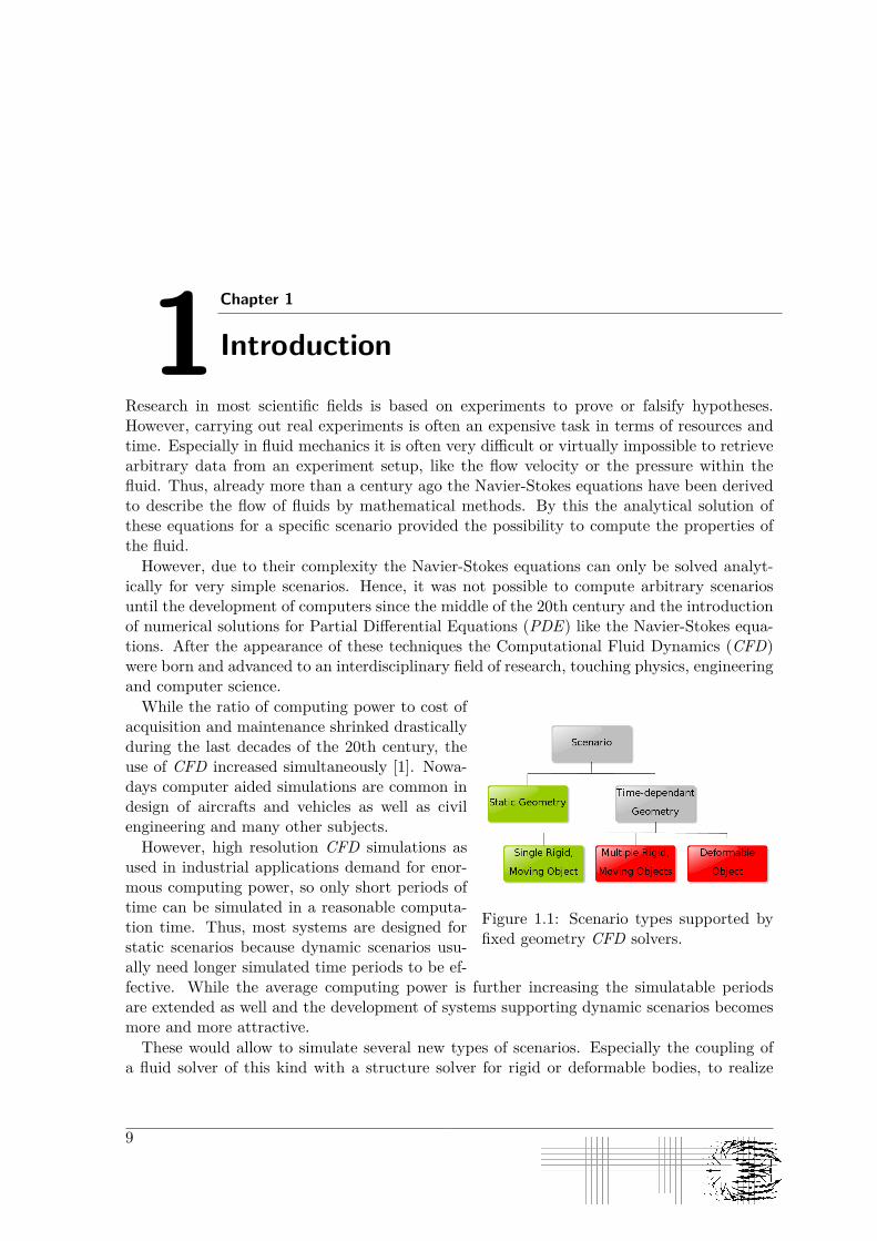
Figure 1.1: Scenario types supported byfixed geometry CFD solvers.
While the ratio of computing power to cost ofacquisition and maintenance shrinked drasticallyduring the last decades of the 20th century, theuse of CFD increased simultaneously [1]. Nowa-days computer aided simulations are common indesign of aircrafts and vehicles as well as civilengineering and many other subjects.However, high resolution CFD simulations as
used in industrial applications demand for enor-mous computing power, so only short periods oftime can be simulated in a reasonable computa-tion time. Thus, most systems are designed forstatic scenarios because dynamic scenarios usu-ally need longer simulated time periods to be ef-fective. While the average computing power is further increasing the simulatable periodsare extended as well and the development of systems supporting dynamic scenarios becomesmore and more attractive.These would allow to simulate several new types of scenarios. Especially the coupling of
a fluid solver of this kind with a structure solver for rigid or deformable bodies, to realize
9
1 Introduction
Fluid-Structure Interaction (FSI), offers a lot of new possibilities for simulation, like the flowof fuel and exhaust in combustion engines or the blood flow in the heart, for example. Thetopic of FSI is not a part of this thesis, but due to the close relation between the two fieldsit is sketched later on.Figure 1.1 shows the possible scenario types that can be computed with a CFD solver
supporting only fixed geometry. Actually it is possible to simulate one constantly movingrigid body with such a solver by fixing the coordinate system of the object to the referencecoordinate system. However, having forces applied to the rigid body, external body forces likegravity or forces applied by the fluid like pressure or friction, makes this approach much moredifficult. And, finally, simulations with several objects moving relatively to each other, oreven deformable bodies, where the shape of the geometry itself can change, cannot be handledby fixed geometries and, therefore, can not be simulated by such systems. To simulate thesetypes of scenarios CFD solvers are needed that support time-dependent geometry.In the year 2005 the development of the PDE framework Peano was started at the chair
for Scientific Computing at the Technische Universität München (TUM). This framework isdesigned for providing a relatively simple possibilty to implement PDE solvers with up-to-date technology like adaptive grids and a memory efficient implementation. A fluid solver isavailable that is implemented on this framework.Initially Peano only supported static grids. The grid was built once during the setup
phase of the simulation and could not be changed afterwards. Thus there was no supportof time-dependent geometries like moving or deformable objects, but was desired because,amongst others, a new geometry interface is under development that contains a coupling toolfor FSI solvers. So during this thesis an extension for moving geometry was implementedand evaluated as described in the following.The thesis is structured as follows:Chapter 2 gives an overview over CFD in general and Peano in special, while Chapter 3
introduces an algorithm to support moving geometry and gives a short introduction intofluid-structure interaction.Chapter 4 shows how this algorithm has been implemented in the fluid solver for the
regular (Section 4.2) and the adaptive grid (Section 4.3). To ensure the physical correctnessof the implementation an evaluation has been made, of which the results are presented anddiscussed in Chapter 5.Finally, Chapter 6 summarizes the thesis and gives a short outlook on the future projects,
using the moving boundary implementation in Peano.
10
2 Chapter 2
Computational Fluid Dynamics
Simulation of fluids is a field that closely links computer science with physics and mathemat-ics. Therefore, Section 2.1 offers a short introduction into the theoretical background, themathematical modelling of the physical behaviour of fluids. Thereby, the general approachis depicted as well as the specific techniques used in this thesis.The practical background for this thesis is given in Section 2.2, in form of an overview on
the CFD framework Peano, which is the basis of the implementation that has been done inthis thesis.
2.1 Navier-Stokes Equations
The common approach to the numerical simulation of fluids are the so-called Navier-Stokesequations. These PDE are derived from the physical model of a fluid as a homogeneousmedium. That means that the fluid is seen from a macroscopic point of view from which thefluid particles, such as atoms, molecules or even larger chunks of material, are not resolvable.Thus, the ratio of the scale of the observed volume to the size of a fluid particle must belarge enough that the particles can be assumed to be infinitely small and hence provides ahomogeneous distribution of the physical properties throughout the considered domain.
2.1.1 Physical Fundamentals
The first question arising when dealing with fluids is, what fluids actually are. The distinctionis hereby made between fluids and solids, where a solid is a substance which is difficult to bedeformed by applying shear forces. On a microscopic scale this can be traced back to strongbonds, usually covalent or ionic bonds, between the solid particles.For fluids the central point is that they do not have these strong bonds but the particles
in the fluid can move more or less freely within the fluid domain. As stated above thederivation of the Navier-Stokes equations does not care about particles in the fluid but itassumes a homogenous substance, so why does this distinction affect these equations? Ofcourse the microscopic behaviour of the fluid particles appears in some way in the macroscopicbehaviour of the fluid even though it can be approximated by the homogenous model. So thefollowing paragraphs will show the influence of the particles on the macroscopic observablebehaviour and the used modelling of this influence.
11
2 Computational Fluid Dynamics
a b c
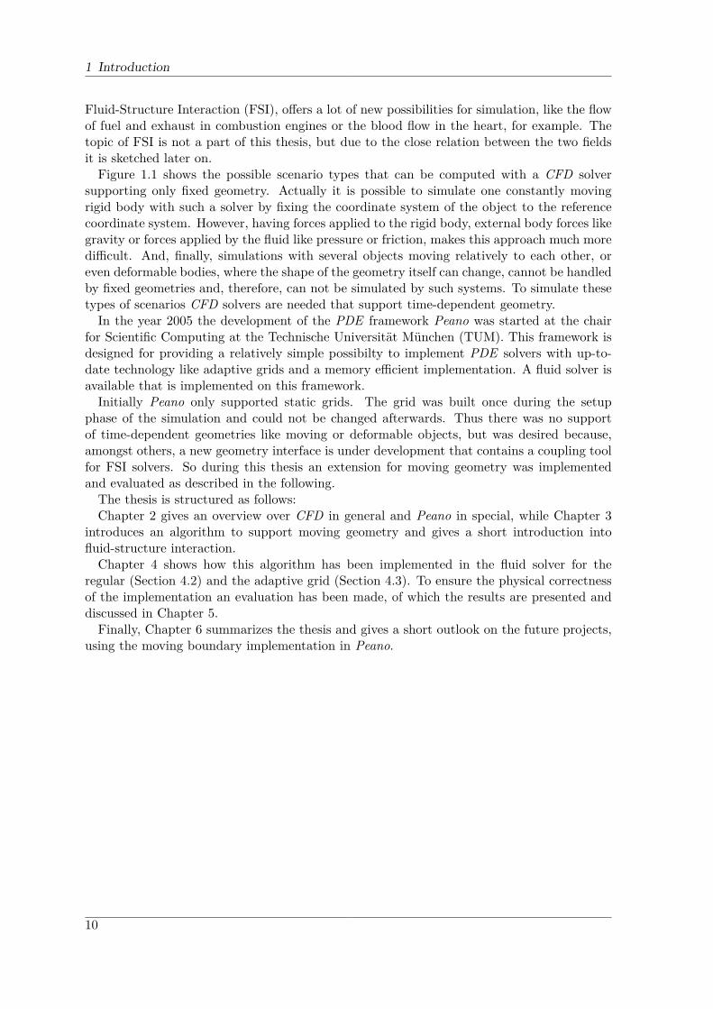
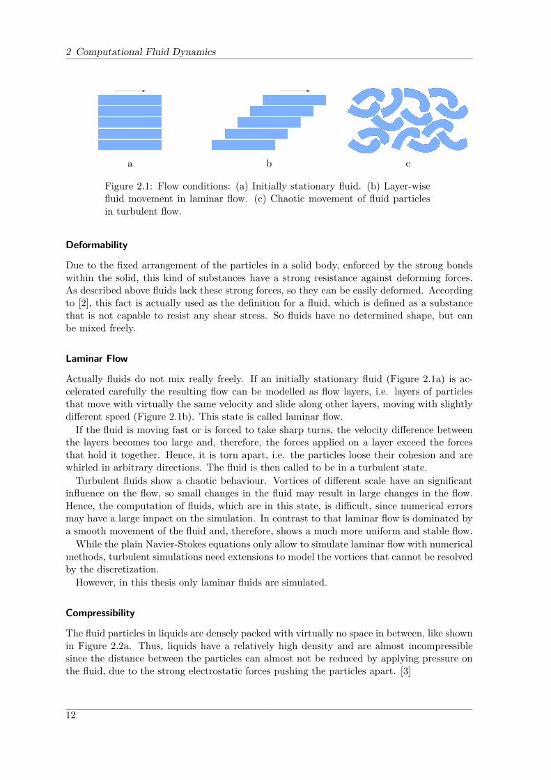
Figure 2.1: Flow conditions: (a) Initially stationary fluid. (b) Layer-wisefluid movement in laminar flow. (c) Chaotic movement of fluid particlesin turbulent flow.
Deformability
Due to the fixed arrangement of the particles in a solid body, enforced by the strong bondswithin the solid, this kind of substances have a strong resistance against deforming forces.As described above fluids lack these strong forces, so they can be easily deformed. Accordingto [2], this fact is actually used as the definition for a fluid, which is defined as a substancethat is not capable to resist any shear stress. So fluids have no determined shape, but canbe mixed freely.
Laminar Flow
Actually fluids do not mix really freely. If an initially stationary fluid (Figure 2.1a) is ac-celerated carefully the resulting flow can be modelled as flow layers, i.e. layers of particlesthat move with virtually the same velocity and slide along other layers, moving with slightlydifferent speed (Figure 2.1b). This state is called laminar flow.If the fluid is moving fast or is forced to take sharp turns, the velocity difference between
the layers becomes too large and, therefore, the forces applied on a layer exceed the forcesthat hold it together. Hence, it is torn apart, i.e. the particles loose their cohesion and arewhirled in arbitrary directions. The fluid is then called to be in a turbulent state.Turbulent fluids show a chaotic behaviour. Vortices of different scale have an significant
influence on the flow, so small changes in the fluid may result in large changes in the flow.Hence, the computation of fluids, which are in this state, is difficult, since numerical errorsmay have a large impact on the simulation. In contrast to that laminar flow is dominated bya smooth movement of the fluid and, therefore, shows a much more uniform and stable flow.While the plain Navier-Stokes equations only allow to simulate laminar flow with numerical
methods, turbulent simulations need extensions to model the vortices that cannot be resolvedby the discretization.However, in this thesis only laminar fluids are simulated.
Compressibility
The fluid particles in liquids are densely packed with virtually no space in between, like shownin Figure 2.2a. Thus, liquids have a relatively high density and are almost incompressiblesince the distance between the particles can almost not be reduced by applying pressure onthe fluid, due to the strong electrostatic forces pushing the particles apart. [3]
12
2.1 Navier-Stokes Equations
a b
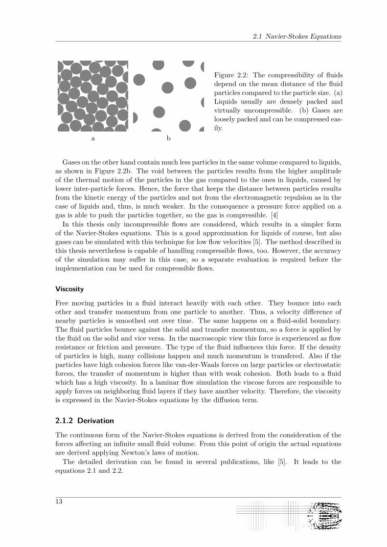
Figure 2.2: The compressibility of fluidsdepend on the mean distance of the fluidparticles compared to the particle size. (a)Liquids usually are densely packed andvirtually uncompressible. (b) Gases areloosely packed and can be compressed eas-ily.
Gases on the other hand contain much less particles in the same volume compared to liquids,as shown in Figure 2.2b. The void between the particles results from the higher amplitudeof the thermal motion of the particles in the gas compared to the ones in liquids, caused bylower inter-particle forces. Hence, the force that keeps the distance between particles resultsfrom the kinetic energy of the particles and not from the electromagnetic repulsion as in thecase of liquids and, thus, is much weaker. In the consequence a pressure force applied on agas is able to push the particles together, so the gas is compressible. [4]In this thesis only incompressible flows are considered, which results in a simpler form
of the Navier-Stokes equations. This is a good approximation for liquids of course, but alsogases can be simulated with this technique for low flow velocities [5]. The method described inthis thesis nevertheless is capable of handling compressible flows, too. However, the accuracyof the simulation may suffer in this case, so a separate evaluation is required before theimplementation can be used for compressible flows.
Viscosity
Free moving particles in a fluid interact heavily with each other. They bounce into eachother and transfer momentum from one particle to another. Thus, a velocity difference ofnearby particles is smoothed out over time. The same happens on a fluid-solid boundary.The fluid particles bounce against the solid and transfer momentum, so a force is applied bythe fluid on the solid and vice versa. In the macroscopic view this force is experienced as flowresistance or friction and pressure. The type of the fluid influences this force. If the densityof particles is high, many collisions happen and much momentum is transfered. Also if theparticles have high cohesion forces like van-der-Waals forces on large particles or electrostaticforces, the transfer of momentum is higher than with weak cohesion. Both leads to a fluidwhich has a high viscosity. In a laminar flow simulation the viscose forces are responsible toapply forces on neighboring fluid layers if they have another velocity. Therefore, the viscosityis expressed in the Navier-Stokes equations by the diffusion term.
2.1.2 Derivation
The continuous form of the Navier-Stokes equations is derived from the consideration of theforces affecting an infinite small fluid volume. From this point of origin the actual equationsare derived applying Newton’s laws of motion.The detailed derivation can be found in several publications, like [5]. It leads to the
equations 2.1 and 2.2.
13
2 Computational Fluid Dynamics
∂u
∂t+ (u · ∇)u = −∇p+ ν∆u+ f (2.1)
∇u = 0 (2.2)
These PDE describe the behavior of a continuous incompressible fluid specified by thekinematic viscosity ν. The momentum equation 2.1, represents actually Newton’s secondlaw of motion in the momentum-wise formulation F = ∂I
∂t . So this equation describes themomentum change over time, caused by the inner forces of the fluid and possible outer forceslike gravity, which actually are often neglected.While the outer forces are summed up in f the inner forces are dissected into three parts.
While the cohesion force caused by the viscosity appears in ν∆u, the transport of impulsby the fluid motion is represented by the term (u · ∇)u. Finally ∇p represents the pressureforce within the fluid. All these values refer to an infinitesimal small fluid volume, so theyare valid at any point within the fluid.The continuity equation 2.2 describes the conservation of mass, which matches the conser-
vation of volume in the incompressible case. Visually speaking it says that the same amountof fluid that goes into a volume of the fluid domain has to go out again for every volume ofthe domain and any time.
2.1.3 Discretization
Since the Navier-Stokes equations cannot be solved analytically in general, a discretizationof the spacetime is needed in order to solve the equations numerically for a given scenario.So the continuous form (Equations 2.1 and 2.2) has to be discretized in space and time. Forthis central topic of numerical simulation several different approaches have been developed.The next paragraphs give a very decent overview about these approaches. Here the emphasisis put on the grids that can be used as a basis for the spatial discretization, since this is anessential point for the development of a method supporting moving geometries.
Space Discretization
In contrast to the one-dimensional temporal discretization the spatial discretization is two-or even three-dimensional in common scenarios and, thus, is more complex. This multidi-mensional space is usually partitioned into a grid consisting of cells and vertices, a processthat reduces the infinite-dimensional problem to a finite-dimensional one.There are several ways to partition a domain into a grid. Most flexibility is granted by
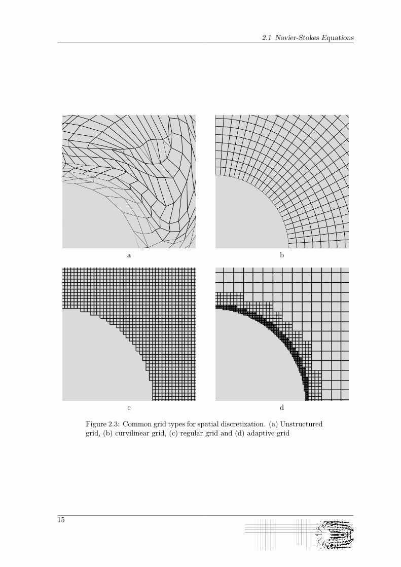
so-called unstructured grids (Figure 2.3a). In this type of grid the cell sizes and forms arechosen according to the local needs. Thus, there is neither a restriction to the size of thecells nor to the number of sides, respectively faces, of one cell, which allows to adapt to thegiven geometry as well as to the local resolution needs. So this type of grids provide anexcellent control about the local discretization error. But the creation of these grids needssophisticated algorithms, which often need support by the user [1] and the solution of PDEis very complex due to the non-uniform grid cells [6]. Therefore, unstructured grids are onlyapplicable for specific problems but inept for a general solver.Object-aligned grids like the one shown in Figure 2.3b provide highest accuracy for objects
that can be described in closed analytical form. They work very good on primitive shapes likespheres or cylinders. However this type of grids is not applicable for arbitrary geometries and
14
2.1 Navier-Stokes Equations
a b
c d
Figure 2.3: Common grid types for spatial discretization. (a) Unstructuredgrid, (b) curvilinear grid, (c) regular grid and (d) adaptive grid
15
2 Computational Fluid Dynamics
even finding a good partitioning automatically for appropriate geometries is still a challengingtask [6]. Thus, also these grids are limited to special cases of PDE solvers.The demand for generally usable grids with a simple discretization of the solved PDE lead
to Cartesian grids. These grids consist of rectangular cells which are aligned to the axes ofthe coordinate system. Therefore regular grids, like shown in Figure 2.3c, result in the samediscretization for all grid cells, which eases the handling of the PDE in the software.Additionally there exists an universally valid mapping from the given geometry to the
final grid for Cartesian grids. Since the position and the shape of the cells are determinedindependently from the computational domain only the state of the cells and vertices have tobe set. So basically all grid cells completely inside the computation domain are taken for thecomputation of the PDE, while cells completely outside of the domain are discarded. Sincethe grid lines do not match the geometry’s boundaries in general there occur cells that are cutby boundaries and, therefore, cover parts of both areas, inside and outside. The actual statedepends on the used mapping. For vertices a similar mapping has to be applied. Section 3.1treats with the details of the mapping used in this thesis.So Cartesian grids allow a simple and flexible grid generation, an easy discretization of the
solved PDE and also a fairly simple way to realize adaptivity. Therefore, Peano uses thistype of grids for doing the spatial discretization.However, due to the discretization all smooth boundaries that are not aligned with the
grid result in a stepped grid boundary which of course results in an error in the PDE ’ssolution. This error can be reduced by using a higher resolution of the grid, with which thereal boundary is approximated more precisely. Hereby, a grid spacing of h on a grid domainof size ∆x0 by ∆x1 leads to a total number of ∆x0
h ·∆x1h grid cells though. That means the
number of grid cells grows with the power of two for finer resolutions [6].Normal numerical PDE solutions do not have a homogenous error on the whole domain.
Thus, there are areas with higher numerical error and areas with smaller numerical errorwhich is suboptimal since the quality of the solution depends usually on the maximum errorthat occurs. So it is desirable to spend more computation time for the areas with high errorwhile it is sufficient to do less work on the areas with smaller error. A grid-based possibilityto achieve this goal is the use of adaptive grids, which are Cartesian grids that may havedifferent resolutions within the computation domain as shown in Figure 2.3d. So the cellsmay vary in size, but the size of one cell must always be an integer multiple of its surroundingcells, so that the final grid can be constructed by recursively subdividing or refining a rootcell containing the whole computation domain, depending on a subdivision or refinementcriterion. Figure 2.4 shows this process where the spatial situation of a cell is used as therefinement criterion, which means that a cell is refined if it is intersected by a boundary ofthe computation domain. To avoid an infinite refinement usually a lower threshold for thecell width or a maximum refinement level is set.Hence, adaptive grids use the grid refinement to influence the discretization error, so the
refinement criterion should be choosen in a way that it triggers a refinement of the grid inplaces where high discretization errors are to be expected. Common criterions are, therefore,the spatial situation as mentioned before or an estimator-based criterion depending on thecurrent interim solution of the PDE. Former is the one used in the fluid solver which is thebasis for this thesis and, hence, is discussed in more detail in Subsection 4.3.2.Handling these grids is quite more complex than regular grids, since there is no unique
topology of the cells. In regular grids each cell has 2 ·D neighbours, where D is the dimensionof the computation domain, while an adaptive grid can have up to 2D · 2D neighbour cells
16
2.1 Navier-Stokes Equations
a b c d
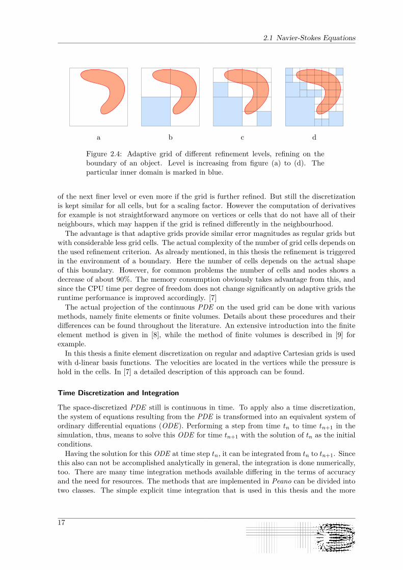
Figure 2.4: Adaptive grid of different refinement levels, refining on theboundary of an object. Level is increasing from figure (a) to (d). Theparticular inner domain is marked in blue.
of the next finer level or even more if the grid is further refined. But still the discretizationis kept similar for all cells, but for a scaling factor. However the computation of derivativesfor example is not straightforward anymore on vertices or cells that do not have all of theirneighbours, which may happen if the grid is refined differently in the neighbourhood.The advantage is that adaptive grids provide similar error magnitudes as regular grids but
with considerable less grid cells. The actual complexity of the number of grid cells depends onthe used refinement criterion. As already mentioned, in this thesis the refinement is triggeredin the environment of a boundary. Here the number of cells depends on the actual shapeof this boundary. However, for common problems the number of cells and nodes shows adecrease of about 90%. The memory consumption obviously takes advantage from this, andsince the CPU time per degree of freedom does not change significantly on adaptive grids theruntime performance is improved accordingly. [7]The actual projection of the continuous PDE on the used grid can be done with various
methods, namely finite elements or finite volumes. Details about these procedures and theirdifferences can be found throughout the literature. An extensive introduction into the finiteelement method is given in [8], while the method of finite volumes is described in [9] forexample.In this thesis a finite element discretization on regular and adaptive Cartesian grids is used
with d-linear basis functions. The velocities are located in the vertices while the pressure ishold in the cells. In [7] a detailed description of this approach can be found.
Time Discretization and Integration
The space-discretized PDE still is continuous in time. To apply also a time discretization,the system of equations resulting from the PDE is transformed into an equivalent system ofordinary differential equations (ODE). Performing a step from time tn to time tn+1 in thesimulation, thus, means to solve this ODE for time tn+1 with the solution of tn as the initialconditions.Having the solution for this ODE at time step tn, it can be integrated from tn to tn+1. Since
this also can not be accomplished analytically in general, the integration is done numerically,too. There are many time integration methods available differing in the terms of accuracyand the need for resources. The methods that are implemented in Peano can be divided intotwo classes. The simple explicit time integration that is used in this thesis and the more
17

2 Computational Fluid Dynamics
accurate and more complex implicit time integration.When former is used in CFD, it results in a linear system of equations that is relatively
cheap to solve. Latter leads to a non-linear system of equations which requires much moreeffort to be computed. So performing one time step with an implicit method is more expensivebut due to the higher order of this integration, it allows also larger time step sizes.
2.1.4 Cartesian-Discrete Navier-Stokes EquationsFor this thesis the following solver setup is used. The time discretization uses a constant timestep size and an explicit Euler time integration. Space is discretized using a finite elementmethod on regular and adaptive Cartesian grids [7].With this discretization scheme the continuous Navier-Stokes equations, as shown in equa-
tions 2.1 and 2.2, are transformed into the discretized form
Au+ C(u)u+D(u) +MT p = 0 ∈ RN (2.3)
Mu = 0 ∈ RZ . (2.4)
These equations are not valid in every point of the computation domain like the continuousform, but only in discrete points defined by the spatial discretization. Hence, they are vec-torial equations, whereas Equation 2.3 is a N-dimensional and Equation 2.4 a Z-dimensionalvector equation, where N = D · n is the dimension times the number of fluid nodes holdinga real degree of freedom, and Z is the number of fluid cells.A,C,D and M are matrices that depend on the actual used grid and on the actual used dis-
cretization method. These matrices are global matrices; thus, Equation 2.3 and Equation 2.4describe the fluid over the whole grid. Having these matrices the Navier-Stokes equationsare, finally, given in a discrete form in which the state of a fluid can be simulated.To do the time integration by the explicit Euler method, the equations have to be trans-
formed. By assigning the velocity and pressure values to specific time steps and by applyingthe discrete derivative of the continuity equation, Mu = 0, the so-called Pressure PoissonEquation (PPE) is created in its discretized form:
(MA−1MT )pt+1 = MA−1(−C(ut)ut −Dut)
To perform a time step, this system of linear equations has to be solved to compute thepressure pt+1, which can thereafter be used to calculate the next time step’s velocities. Moredetailed information on this can be found in [5] and [7] .
2.1.5 Basic AlgorithmGiven the discretized Navier-Stokes equations for the used discretization scheme and timeintegration method, the fluid solver, finally, sums up to a basic algorithm for computing afluid simulation over a certain time period. The first step to be done is always the generationof the grid and the setup of the boundary conditions. On this grid the starting conditionsare imposed to get the initial state of the system.From this point the simulation starts and the time step-wise solving of the PDE is done in
a loop. Here a time integration step is run on the current solution to get the next time step’ssolution, which afterwards can be visualized, saved to disc or sent to another process. Thenthe loop iterates again for the next time step. This process is repeated until the end of thesimulation period is reached.
18
2.2 The PDE-Framework Peano
After the simulation nothing has to be done in this abstract view of the algorithm, if theintermediate solutions are already used during the time step iterations. Otherwise the finalsolution can be processed further at this point.
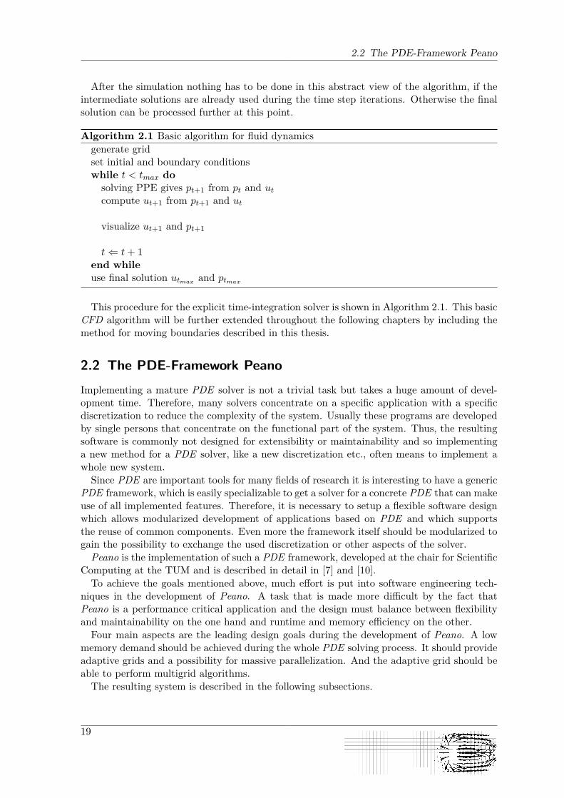
Algorithm 2.1 Basic algorithm for fluid dynamicsgenerate gridset initial and boundary conditionswhile t < tmax dosolving PPE gives pt+1 from pt and utcompute ut+1 from pt+1 and ut
visualize ut+1 and pt+1
t⇐ t+ 1end whileuse final solution utmax and ptmax
This procedure for the explicit time-integration solver is shown in Algorithm 2.1. This basicCFD algorithm will be further extended throughout the following chapters by including themethod for moving boundaries described in this thesis.
2.2 The PDE-Framework PeanoImplementing a mature PDE solver is not a trivial task but takes a huge amount of devel-opment time. Therefore, many solvers concentrate on a specific application with a specificdiscretization to reduce the complexity of the system. Usually these programs are developedby single persons that concentrate on the functional part of the system. Thus, the resultingsoftware is commonly not designed for extensibility or maintainability and so implementinga new method for a PDE solver, like a new discretization etc., often means to implement awhole new system.Since PDE are important tools for many fields of research it is interesting to have a generic
PDE framework, which is easily specializable to get a solver for a concrete PDE that can makeuse of all implemented features. Therefore, it is necessary to setup a flexible software designwhich allows modularized development of applications based on PDE and which supportsthe reuse of common components. Even more the framework itself should be modularized togain the possibility to exchange the used discretization or other aspects of the solver.Peano is the implementation of such a PDE framework, developed at the chair for Scientific
Computing at the TUM and is described in detail in [7] and [10].To achieve the goals mentioned above, much effort is put into software engineering tech-
niques in the development of Peano. A task that is made more difficult by the fact thatPeano is a performance critical application and the design must balance between flexibilityand maintainability on the one hand and runtime and memory efficiency on the other.Four main aspects are the leading design goals during the development of Peano. A low
memory demand should be achieved during the whole PDE solving process. It should provideadaptive grids and a possibility for massive parallelization. And the adaptive grid should beable to perform multigrid algorithms.The resulting system is described in the following subsections.
19
2 Computational Fluid Dynamics
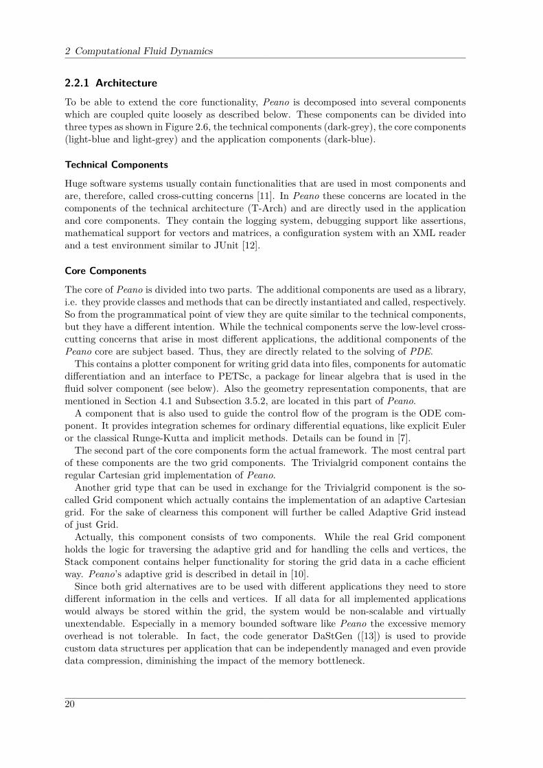
2.2.1 ArchitectureTo be able to extend the core functionality, Peano is decomposed into several componentswhich are coupled quite loosely as described below. These components can be divided intothree types as shown in Figure 2.6, the technical components (dark-grey), the core components(light-blue and light-grey) and the application components (dark-blue).
Technical Components
Huge software systems usually contain functionalities that are used in most components andare, therefore, called cross-cutting concerns [11]. In Peano these concerns are located in thecomponents of the technical architecture (T-Arch) and are directly used in the applicationand core components. They contain the logging system, debugging support like assertions,mathematical support for vectors and matrices, a configuration system with an XML readerand a test environment similar to JUnit [12].
Core Components
The core of Peano is divided into two parts. The additional components are used as a library,i.e. they provide classes and methods that can be directly instantiated and called, respectively.So from the programmatical point of view they are quite similar to the technical components,but they have a different intention. While the technical components serve the low-level cross-cutting concerns that arise in most different applications, the additional components of thePeano core are subject based. Thus, they are directly related to the solving of PDE.This contains a plotter component for writing grid data into files, components for automatic
differentiation and an interface to PETSc, a package for linear algebra that is used in thefluid solver component (see below). Also the geometry representation components, that arementioned in Section 4.1 and Subsection 3.5.2, are located in this part of Peano.A component that is also used to guide the control flow of the program is the ODE com-
ponent. It provides integration schemes for ordinary differential equations, like explicit Euleror the classical Runge-Kutta and implicit methods. Details can be found in [7].The second part of the core components form the actual framework. The most central part
of these components are the two grid components. The Trivialgrid component contains theregular Cartesian grid implementation of Peano.Another grid type that can be used in exchange for the Trivialgrid component is the so-
called Grid component which actually contains the implementation of an adaptive Cartesiangrid. For the sake of clearness this component will further be called Adaptive Grid insteadof just Grid.Actually, this component consists of two components. While the real Grid component
holds the logic for traversing the adaptive grid and for handling the cells and vertices, theStack component contains helper functionality for storing the grid data in a cache efficientway. Peano’s adaptive grid is described in detail in [10].Since both grid alternatives are to be used with different applications they need to store
different information in the cells and vertices. If all data for all implemented applicationswould always be stored within the grid, the system would be non-scalable and virtuallyunextendable. Especially in a memory bounded software like Peano the excessive memoryoverhead is not tolerable. In fact, the code generator DaStGen ([13]) is used to providecustom data structures per application that can be independently managed and even providedata compression, diminishing the impact of the memory bottleneck.
20

2.2 The PDE-Framework Peano
Application Components
Peano is a high performance application, so during the development of the framework virtualmethod calls where avoided as far as possible. Especially the adapters, described in Subsec-tion 2.2.2, rely on inheritance and would cause a lot of these calls, which are said to have alarge impact on the runtime performance [14].Hence, the adapters are not realized with dynamic polymorphism, but with template poly-
morphism, which results in static binding between the adapted components. So Peano doesnot provide a dynamically linkable library, but a monolithic design was chosen. That meansthat the framework and the applications built on it are compiled into the same executablefile. Therefore, the different applications appear as normal Peano components, the so-calledapplication components.By now there are four applications implemented, which use the Peano framework, as shown
in Figure 2.6. This thesis is based on the Fluid component; therefore, this component isdescribed in Subsection 2.2.3.
2.2.2 Adapter Concept
Since many problems in CFD have no generally optimal solution and are still subject of re-search, a CFD solver is destined to be a heavily changing system. Several different approachesare to be made, like time integration schemes or solvers for linear systems of equations, ofwhich most are coupled to each other in any way. Software systems of this type are likely tobecome bulky and unmanagable due to their more and more complex design.
Figure 2.5: Exemplary adapter for Peano.
To encounter this fact, Peano implements theseapproaches in separate components and decou-ples them by introducing linking structures thatare built in a combined observer/template pat-tern. These structures provide a specific interfacefor the component in which they are defined andcan be used by other components, resembling anevent-handling system, like used in many mod-ern software designs [15]. Said in the context offramework design the component that providesthis interface is part of the framework, while thecomponent that uses it is part of an application.With this design the used grid component is
responsible for the control flow of the applicationand provides an interface class that can be usedby the application component to inject code intothis control flow. Since this class enables other
components to adapt their behaviour to the used framework component, it is called adapter,and represents a central concept within the Peano framework.Figure 2.5 illustrates this concept. Here the AbstractAdapter interface provides a couple of
abstract methods. This interface can be implemented by a class in an application componentto create a ConcreteAdapter that can be injected into the grid, which is actually done bytemplatizing the grid, to allow static binding. This ConcreteAdapter then has access to theinternals of the application component and is able to manipulate them, according to theneeds of the application, but is controlled by the framework.
21

2 Computational Fluid Dynamics
When an adapter is run, the grid component traverses the whole grid, calling the adaptermethods for each cell and vertex in the grid. There is no guarantee about the order in whichthe grid is traversed, so adapters always have to work locally on a single vertex or a cellwith its adjacent vertices. Hence, this adapter concept is appropriate for complex traversionschemes like the Peano curve, which is used to traverse the adaptive grid in Peano, or evendistributed traversion schemes, used in parallel computing. The application component isdecoupled from this scheme and can use the grid component transparently.Since the adapter concept is the key for the use of the Peano framework, the implementation
of this thesis is based on it as it is shown in Section 4.2 and Section 4.3. The interfaces ofthe used Trivialgrid and Adaptive Grid components are listed in Appendix A.
2.2.3 Fluid ComponentAmongst the application components the Fluid component is the most interesting one forthis thesis. It is built on the framework, so several adapters are implemented for linking thiscomponent to the Trivialgrid and the Adaptive Grid.The process of computing a fluid simulation is controlled in this component by triggering
adapter traversals over the currently used grid, to form Algorithm 2.1.While the intrinsic properties of the fluid, in particular viscosity and density, are directly
used within this component, the geometry—that describes the computation domain—is holdin the Geometry component. To make this information accessible for the used grid, the Fluid-Scenario component is used. Within this closely related component additional adapters areimplemented that fulfill an interface that allows to query all needed information from thegeometry.Here also the mapping is done from the mere abstract spatial information to specific flow
related settings like inflow, outflow or wall boundary conditions.A significant fraction of the time, needed for the computation of a time step, is used for
solving the PPE. Due to the discretization this is actually a linear system of equations, soit is advantageous to use an optimized third-party tool to minimize the time needed for thisstep.In the Fluid component for this task the Portable, Extensible Toolkit for Scientific Compu-
tation (PETSc) [16] is used. This library supports different iterative solvers for linear systemsof equations, also with sparse matrices. Since the matrices used in CFD describe local de-pendencies within the flow field, these matrices are very sparse; so, the use of appropriatenumerical algorithms is indispensable in the terms of memory and time performance.
22
2.2 The PDE-Framework Peano
T−
Arc
h
low
mem
stacks
vtk
tecplot
ADOL−C
cppAD
equation
conti−
equation
heat−
grid
trivialgrid
para
llel
plotter
ODE
preCICE
AD
PETSc
fluid poisson
geometry
Figure 2.6: The architecture of Peano. Application components (blue) usecore components (light-blue) and additional components (light-grey). Thedark-grey technical components are available in all other components andprovide basic functionality. (taken from [7], p. 18)
23

2 Computational Fluid Dynamics
24
3 Chapter 3
Moving Geometry
Moving boundaries in fluid simulation are still not a trivial problem, since no general bestpractice has been developed by now. Several approaches have been presented for differentdiscretization types and different application domains. Two of them are mentioned in Sec-tion 3.2.The approach that is taken in this thesis is the most straightforward way by directly
imposing the changed geometry on the discretized boundary domain. The advantage of thismethod is that it fits nicely into the complete picture of the Peano framework, by integratinginto the abstract level of the grid and not interfering with details of the solver implementation.So, this approach minimizes the necessary changes on existing code, and it can be easilyadapted to various solvers or may even work with them instantly.Thus, the method presented in this chapter provides a simple, robust and flexible tool
for simulating moving boundaries in fluid dynamics, which is able to work with arbitrarygeometry.As a prerequisite the general handling of geometry in Peano is explained in Section 3.1,
while Section 3.3 then discusses the extension for time-dependent geometries. A possibilityto improve the solution of this method is covered in Section 3.4, while Section 3.5 offers anintroduction into fluid-structure interaction. In the end of this chapter Section 3.6 addressesthe question how to optimize the performance of the algorithm.
3.1 Grid Representation of Geometry
Due to the fact that it is not possible to solve the PDE of interest analytically, and that theyneed to be discretized for the numerical solution, the used geometry needs to be mapped tothe discretized grid. This section will give an introduction how the geometry of the simulatedscenario is handled in Peano.Throughout this thesis some phrases are used frequently with quite related but nevertheless
different meaning. So their usage within the next chapters is defined as follows.An object is a physical obstacle in a theoretical physical scenario. For example a sphere in
a liquid or an airplane in a wind channel. In chapters 4 and 5 the term object is also used forthe instance of a class of course, as it is common in the field of object-oriented programming.The particular meaning is derivable from the context.A geometry, in contrast to this, is the mathematical representation of an object. The
geometries contained in Peano are of course precise only up to the precision of the underlying
25

3 Moving Geometry
hardware, i.e. up to the precision of the floating point numbers used for the representation.These give an sufficient range of values to neglect the influence of this limitation.A larger error is introduced by the fact that more complex geometries cannot be described
analytically and, therefore, the representation of a physical object is not precise but approxi-mated. Since this always depends on the simulated scenario that fact was not paid attentionto in this thesis.The mere surface of the geometry is what is here called boundary. So this is the set of
points separating the inside of the geometry from its outside. The border of the clippingdomain, which is described below, is also called boundary in the following.While a geometry only contains the spatial information of an object’s surface, the struc-
ture contains the spatial information as well as the physical properties of an object. Thus,the geometry of an object is sufficient for the consideration of the object’s movement in thefluid dynamics, but the structure is needed if the object’s dynamics is to be computed, too.This thesis only concerns about geometries, but for Section 3.5. There structures are
needed for the fluid-structure interaction.
3.1.1 Continuous Representation
The spatial information of a simulation scenario is taken from a specified geometry. Thisgeometry basically is a hypersurface that divides the considered space into two volumes.One of these volumes, the set of points ΩGeometry, is taken to be inside the geometry. Thecomplement ΩGeometry, therefore, is taken to be outside.Due to the lack of infinite computing power and memory the theoretically infinite domain
of interest Ω has to be clipped to a finite scenario domain ΩScenario. The computation domainΩFluid then is the intersection of the clipped scenario domain and the part of space that isnot covered by a geometry ΩScenario ∩ ΩGeometry.
ΩFluid is an open domain due to the needs of the PDE solver. In contrast to that a closeddomain is needed for the correct mapping of a geometry to a grid as shown in the nextsubsection. There Ω′Fluid = Γ(ΩFluid)∪ΩFluid is used, with Γ(ΩFluid) being the boundary ofthe fluid domain.In the following the meaning of the terms inner and outer are exchanged. So, inner is seen
as inside the computation domain and, thus, inside the fluid and not inside the geometry.
3.1.2 Mapping to Grid
Resulting from the space division, caused by the geometry, the discretization of Peano pro-vides two types of cells, inner and outer, and three types of vertices, inner, outer andboundary. To decide the type of a cell or a vertex the so-called h-environments are required.Based on the mesh width of the grid each vertex v regards to a certain region, called h(v)(Figure 3.1a), which basically resembles its support. Each cell c analogously covers a regionh(c) (Figure 3.1b) which corresponds to its spatial area. Both of these sets of points are opensets, i.e. they do not contain the boundary points. In the following the term h-environmentwill denote both of these region-types.Cartesian grids usually are set up in the whole clipping domain ΩScenario. So grid cells
and vertices are created throughout this space. In order to map a given geometry to a givengrid, each cell has to be set to either inner or outer while each vertex has to be set to eitherinner, outer or boundary. This mapping is accomplished in the following manner.
26

3.1 Grid Representation of Geometry
v
h(v)
a
c
h(c)
b
Figure 3.1: Concerned environments for (a) vertices and (b) cells.
Cell-Mapping
In the used discretization scheme a cell is inside of the discrete computation domain if it iscompletely contained by the continuous domain. If it is completely outside of the continuousdomain it is taken as outside of the discrete domain as well as a cell that contains a do-main boundary and, thus, covers points outside and inside the continuous domain. Formallyspeaken a cell c is marked as an Inside-Cell if and only if the following condition holds:
h(c) ⊆ ΩFluidThis procedure leads to the phenomenon that objects tend to grow by the discretization
while the fluid domain shrinks. However, this effect can be neglected for a sufficient smallmesh width.Figure 3.3b shows the two possibilities for the cell state.
Vertex-Mapping
The mapping of the geometry on the vertices of a grid has to match the conditions for thecell-mapping. Thereby, an inner cell must only have inner or boundary vertices as adjacentvertices, while an outer cell is only allowed to have adjacent boundary or outer vertices. Thisensures that inner vertices always have valid neighbors, either inner or boundary vertices.Outer vertices do not hold a valid solution for the PDE and, therefore, cannot be used tocompute the solution of another vertex.This leads to the constraint that the geometry’s boundary has to consist of a single closed
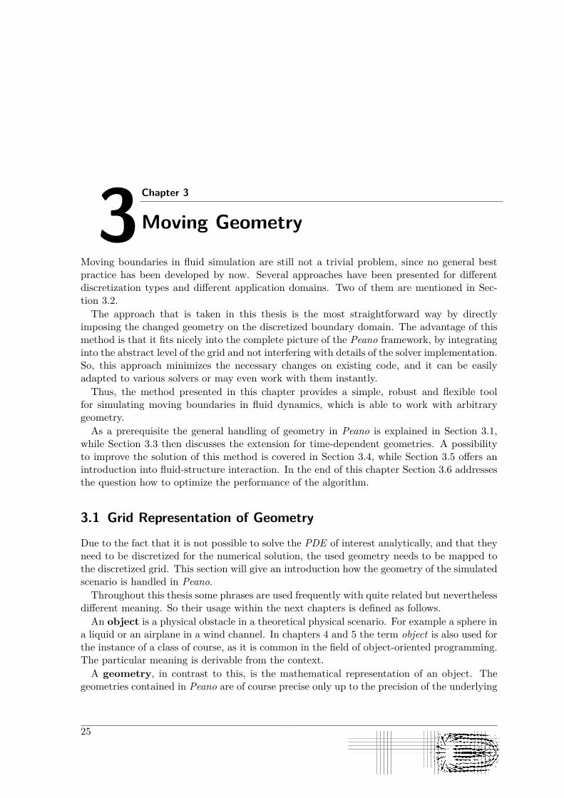
line of boundary vertices. Thus, all boundary vertices must be adjacent to at least twoother boundary vertices and there must not be two or more consecutive boundary verticesperpendicular to the actual boundary. Figure 3.2 shows some illegal boundary vertices.From this the following mapping is derived. A vertex v is marked as an inner vertex if the
condition
27
3 Moving Geometry
A
B
Figure 3.2: Illegal vertex states.
h(v) ⊆ ΩFluid
holds. Otherwise v is marked as a boundary vertex if
h(v) ∩ ΩFluid 6= ∅
and
x(v) ∈ Ω′Fluid
holds, where x(v) is the spatial d-dimensional position of the vertex. Here the closeddomain Ω′Fluid and not the open ΩFluid (see Subsection 3.1.1) is needed. Otherwise a vertexlocated exactly on the boundary would be set incorrectly and, thus, generate an illegal settingof vertices as shown in Figure 3.2.If none of the above conditions holds, the vertex is marked as an outer vertex which
effectively denotes the condition
x(v) 6∈ Ω′Fluid
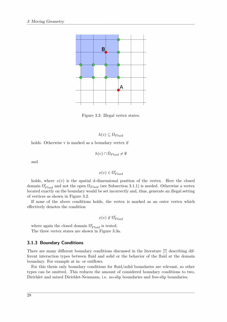
where again the closed domain Ω′Fluid is tested.The three vertex states are shown in Figure 3.3a.
3.1.3 Boundary Conditions
There are many different boundary conditions discussed in the literature [7] describing dif-ferent interaction types between fluid and solid or the behavior of the fluid at the domainboundary. For example at in- or outflows.For this thesis only boundary conditions for fluid/solid boundaries are relevant, so other
types can be omitted. This reduces the amount of considered boundary conditions to two,Dirichlet and mixed Dirichlet-Neumann, i.e. no-slip boundaries and free-slip boundaries.
28
3.1 Grid Representation of Geometry
Ω
a
Ω
b
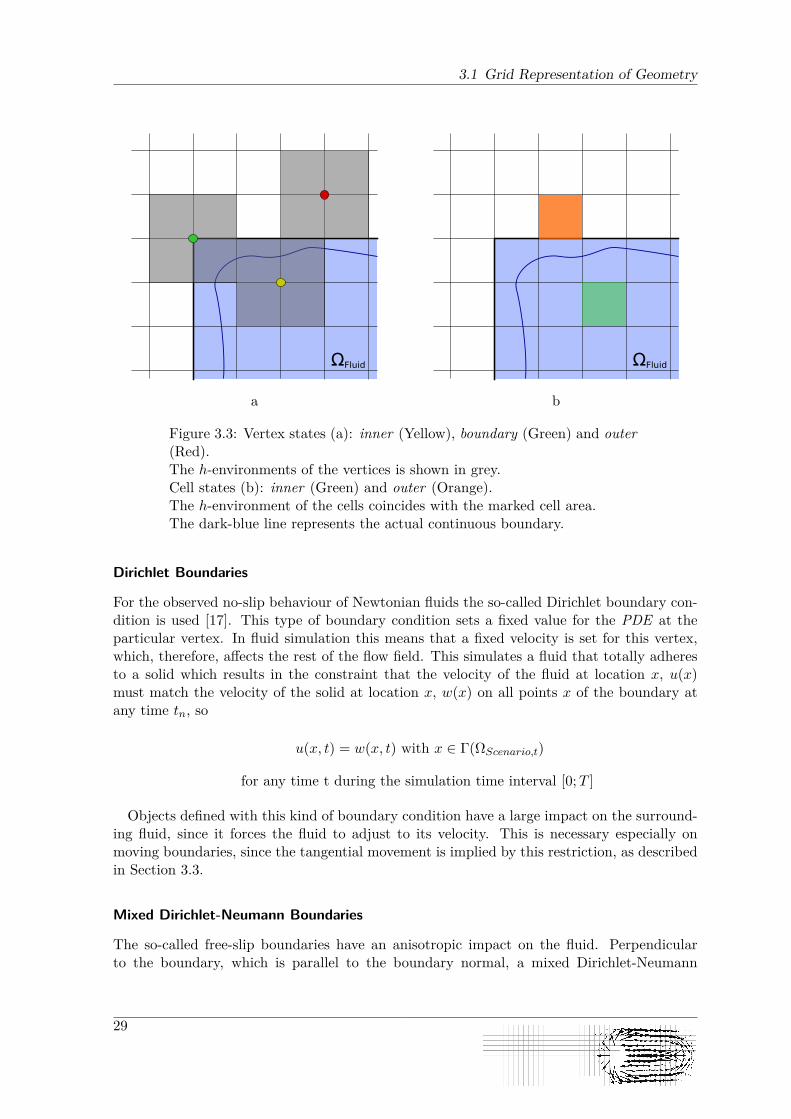
Figure 3.3: Vertex states (a): inner (Yellow), boundary (Green) and outer(Red).The h-environments of the vertices is shown in grey.Cell states (b): inner (Green) and outer (Orange).The h-environment of the cells coincides with the marked cell area.The dark-blue line represents the actual continuous boundary.
Dirichlet Boundaries
For the observed no-slip behaviour of Newtonian fluids the so-called Dirichlet boundary con-dition is used [17]. This type of boundary condition sets a fixed value for the PDE at theparticular vertex. In fluid simulation this means that a fixed velocity is set for this vertex,which, therefore, affects the rest of the flow field. This simulates a fluid that totally adheresto a solid which results in the constraint that the velocity of the fluid at location x, u(x)must match the velocity of the solid at location x, w(x) on all points x of the boundary atany time tn, so
u(x, t) = w(x, t) with x ∈ Γ(ΩScenario,t)
for any time t during the simulation time interval [0;T ]
Objects defined with this kind of boundary condition have a large impact on the surround-ing fluid, since it forces the fluid to adjust to its velocity. This is necessary especially onmoving boundaries, since the tangential movement is implied by this restriction, as describedin Section 3.3.
Mixed Dirichlet-Neumann Boundaries
The so-called free-slip boundaries have an anisotropic impact on the fluid. Perpendicularto the boundary, which is parallel to the boundary normal, a mixed Dirichlet-Neumann
29
3 Moving Geometry
boundary behaves like a Dirichlet boundary, i.e. the fluid velocity parallel to the boundarynormal has to match the boundary’s speed parallel to the boundary normal.Tangential to the boundary it behaves like a Neumann boundary. Thus, it gives an addi-
tional degree of freedom for the fluid computation, because the fluid velocity tangential tothe boundary is not constraint to the boundary’s velocity [17].Physically this boundary condition simulates a totally frictionless surface of an object.
Since most real objects apply a lot of friction forces on the surrounding fluid, this conditionmatches the physical reality quite rarely. It is more often used to decrease the error introducedby the domain clipping mentioned in Subsection 3.1.1. Therefore, mixed Dirichlet-Neumannboundaries are not considered as moving boundaries further on, but show up in the testscenario in Section 5.1.
3.2 Approaches for Moving Boundaries
The method presented later in this thesis is not the only possibility to realize time-dependentgeometry. Especially on different grid types different methods are to be applied, but also onCartesian grids other concepts have been suggested. In the following two examples of differentapproaches for moving boundaries are given. The actually used approach is described in detailin the next section.
3.2.1 Arbitrary Lagrangian-Eulerian
This type of grid provides the most freedom. So the grid vertices do not have fixed locationsdetermined by a global variable, like the mesh width in regular Cartesian grids, but they maybe placed arbitrarily. This does not only apply in the beginning, when the grid is initiallycreated, but may also be done during the simulation if an appropriate mapping is used totransfer the solution from the grid before the change to the grid after. By this, the grid canfollow the boundary movement and, therefore, provide a Lagrangian view of the geometry,while the fluid is still seen in an Eulerian manner. Hence, this approach is known as ArbitraryLagrangian-Eulerian (ALE) approach [18].This method performs well for small grid changes where the vertices are moved only slightly.
However, if the grid receives heavy changes by large movements or by rotations of the object,this method is likely to produce a distorted grid that leads to an unstable system [9]. Toavoid this problem the grid may be recreated in such cases, which is a very expensive taskfor unstructured grids and, therefore, has a large impact on the runtime performance [6].Hence, in scenarios that are appropriate for unstructured grids and that only contain
small movements, this approach provides a highly accurate method for moving boundaries.However, it lacks the ability to simulate arbitrary scenarios with arbitrary motion.
3.2.2 Immersed Boundaries
While most approaches on Cartesian grids use an Eulerian view on the fluid, due to the Eule-rian nature of the grid, the methodology of Immersed Boundaries is based on an Lagrangianapproach. Here the obstacles in the fluid are not mapped to the grid but all grid cells withinthe clipping domain ΩScenario are considered as “inner” cells. So the Navier-Stokes equationsare solved on this grid, while the boundary conditions are regarded by a modification of theseequations.
30
3.3 Handling of Time-Dependent Geometry
The common method for imposing the effect of the boundary on the fluid is an additionalforce term in the momentum equation, that simulates the resistance force of the obstacle.Here the central point is how to calculate this force from the given geometry. Often this isdone by some kind of triangulated mesh describing the geometry, from which the impact onthe grid can be interpolated. However, several different flavours for Immersed Boundariesexist, too many to be listed here. An introduction into this part of fluid simulation can befound in [6].
3.3 Handling of Time-Dependent GeometryCompared to fixed geometries a moving geometry represents a physical body that changesits shape or position continuously. Thus, the geometry is time-dependent. In the formalrepresentation of the geometry used above, this results in the fact that
Γ(ΩGeometry)∂t
6= 0.
Therefore, a fluid simulation with moving geometry needs additional information comparedto a fixed-geometry simulation. At a specific time t, the current position ΩGeometry,t of thegeometry and the current velocity ∂Γ(ΩGeometry,t)
∂t of the geometry’s boundary are required tospecify the flow simulation.Hence, this movement has to be handled in the discretized system. Since the grid is based
on the geometry that describes the computation domain, the initial setup of the grid, asused in fixed-geometry simulations, is not sufficient anymore. Additionally the boundaryconditions along a moving boundary have to be set differently than for a fixed boundary.This handling is decomposed into a theoretical and a technical part. Former defines the
abstract algorithm for moving boundaries and is discussed in this chapter. Latter is basedon the particular implementation of the used fluid solver. In Chapter 4 this part is presentedfor the implementation within the Peano framework.
3.3.1 Discretized Geometry Movement
The fluid simulation is performed in discrete time steps. Hence, it is convenient to discretizethe geometry movement in the same manner, which leads to a particular geometry ΩGeometry,nand the corresponding velocity ∂ΩGeometry,n∂t for time step n. This state can then be used forapplying the moving geometry on the fluid simulation.Imposing the boundary velocity on the grid vertices is a straightforward task. As mentioned
before the regarded boundaries have no-slip boundary conditions that are achieved by aDirichlet vertex type. In simulations with fixed geometry the boundary velocity is implicitlytaken to be zero and is imposed as that on the boundary vertices. The same can be done forvertices located on moving boundaries. Of course here the particular boundary velocity hasto be used.Hence, the fluid solver does not need to be changed as long as it supports Dirichlet type
vertices.However, the actual change of the geometry requires more effort. Since the grid, used for
the fluid simulation, depends on the current position of the geometry, the grid may changeduring the simulation, if the geometry moves. That means the grid may have to be adaptedto the current ΩGeometry,n in each time step n within the simulation period.
31
3 Moving Geometry
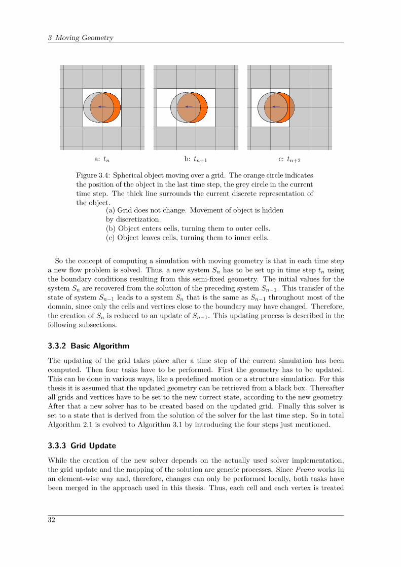
a: tn b: tn+1 c: tn+2
Figure 3.4: Spherical object moving over a grid. The orange circle indicatesthe position of the object in the last time step, the grey circle in the currenttime step. The thick line surrounds the current discrete representation ofthe object.
(a) Grid does not change. Movement of object is hiddenby discretization.(b) Object enters cells, turning them to outer cells.(c) Object leaves cells, turning them to inner cells.
So the concept of computing a simulation with moving geometry is that in each time stepa new flow problem is solved. Thus, a new system Sn has to be set up in time step tn usingthe boundary conditions resulting from this semi-fixed geometry. The initial values for thesystem Sn are recovered from the solution of the preceding system Sn−1. This transfer of thestate of system Sn−1 leads to a system Sn that is the same as Sn−1 throughout most of thedomain, since only the cells and vertices close to the boundary may have changed. Therefore,the creation of Sn is reduced to an update of Sn−1. This updating process is described in thefollowing subsections.
3.3.2 Basic Algorithm
The updating of the grid takes place after a time step of the current simulation has beencomputed. Then four tasks have to be performed. First the geometry has to be updated.This can be done in various ways, like a predefined motion or a structure simulation. For thisthesis it is assumed that the updated geometry can be retrieved from a black box. Thereafterall grids and vertices have to be set to the new correct state, according to the new geometry.After that a new solver has to be created based on the updated grid. Finally this solver isset to a state that is derived from the solution of the solver for the last time step. So in totalAlgorithm 2.1 is evolved to Algorithm 3.1 by introducing the four steps just mentioned.
3.3.3 Grid Update
While the creation of the new solver depends on the actually used solver implementation,the grid update and the mapping of the solution are generic processes. Since Peano works inan element-wise way and, therefore, changes can only be performed locally, both tasks havebeen merged in the approach used in this thesis. Thus, each cell and each vertex is treated
32
3.3 Handling of Time-Dependent Geometry
Algorithm 3.1 Handling of moving geometrygenerate gridset initial and boundary conditionswhile t < tmax dosolving PPE gives pt+1 from pt and utcompute ut+1 from pt+1 and ut
visualize ut+1 and pt+1
update geometryupdate gridcreate new solvermap solution to new solver
t⇐ t+ 1end whileuse final solution utmax and ptmax
only once per time step and has its new valid state afterwards.
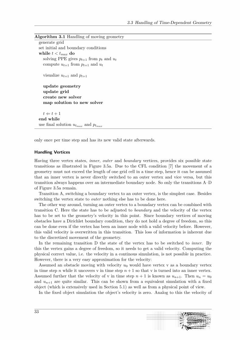
Handling Vertices
Having three vertex states, inner, outer and boundary vertices, provides six possible statetransitions as illustrated in Figure 3.5a. Due to the CFL condition [7] the movement of ageometry must not exceed the length of one grid cell in a time step, hence it can be assumedthat an inner vertex is never directly switched to an outer vertex and vice versa, but thistransition always happens over an intermediate boundary node. So only the transitions A–Dof Figure 3.5a remain.Transition A, switching a boundary vertex to an outer vertex, is the simplest case. Besides
switching the vertex state to outer nothing else has to be done here.The other way around, turning an outer vertex to a boundary vertex can be combined with
transition C. Here the state has to be adjusted to boundary and the velocity of the vertexhas to be set to the geometry’s velocity in this point. Since boundary vertices of movingobstacles have a Dirichlet boundary condition, they do not hold a degree of freedom, so thiscan be done even if the vertex has been an inner node with a valid velocity before. However,this valid velocity is overwritten in this transition. This loss of information is inherent dueto the discretized movement of the geometry.In the remaining transition D the state of the vertex has to be switched to inner. By
this the vertex gains a degree of freedom, so it needs to get a valid velocity. Computing thephysical correct value, i.e. the velocity in a continous simulation, is not possible in practice.However, there is a very easy approximation for the velocity:Assumed an obstacle moving with velocity u0 would have vertex v as a boundary vertex
in time step n while it uncovers v in time step n+ 1 so that v is turned into an inner vertex.Assumed further that the velocity of v in time step n + 1 is known as un+1. Then un = u0and un+1 are quite similar. This can be shown from a equivalent simulation with a fixedobject (which is extensively used in Section 5.1) as well as from a physical point of view.In the fixed object simulation the object’s velocity is zero. Analog to this the velocity of
33
3 Moving Geometry
a b
Figure 3.5: (a): Vertex state transitions. The transitions E and F do notappear due to the velocity constraint resulting from the CFL condition.(b): Cell state transitions.
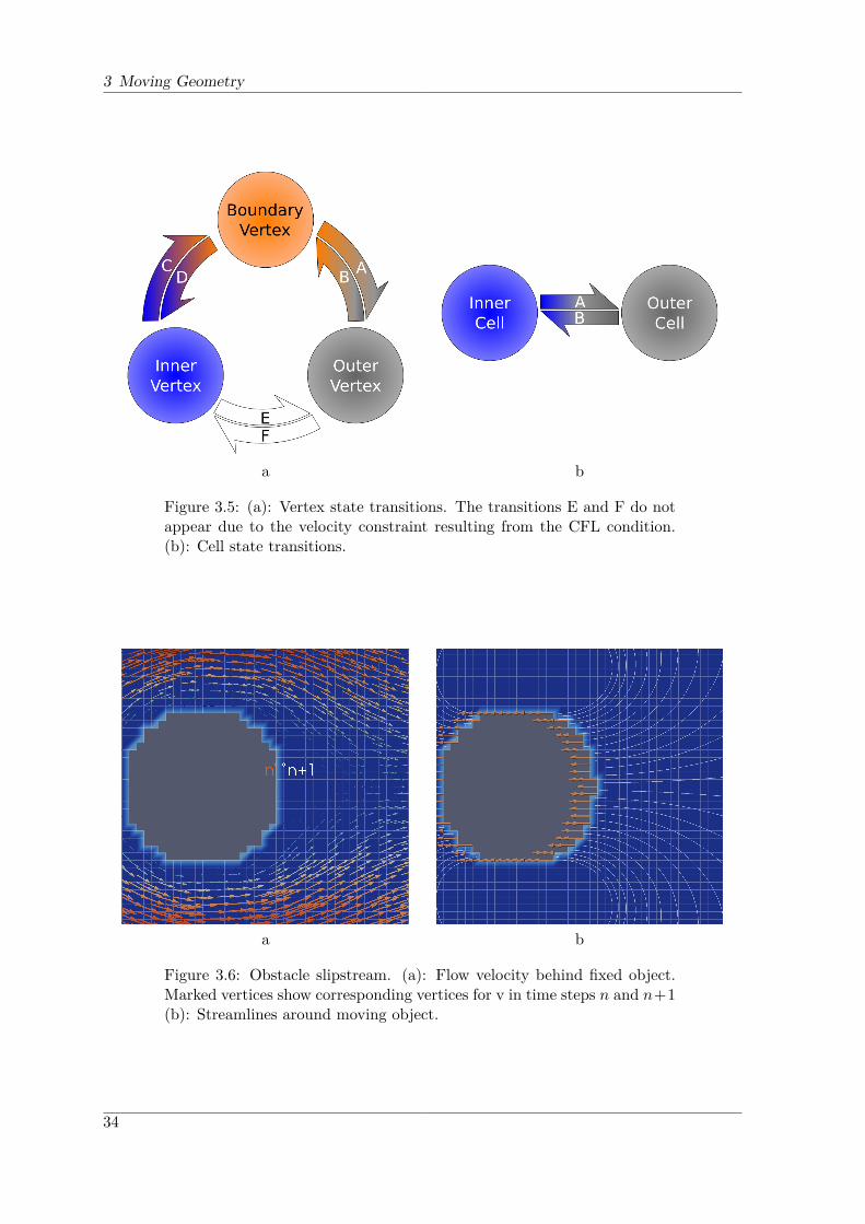
a b
Figure 3.6: Obstacle slipstream. (a): Flow velocity behind fixed object.Marked vertices show corresponding vertices for v in time steps n and n+1(b): Streamlines around moving object.
34

3.3 Handling of Time-Dependent Geometry
the moving object is u0. Then v in time step n corresponds to a boundary vertex in the fixedobject simulation and in time step n+ 1 it corresponds to a vertex that is one cell width offthe boundary, as shown in Figure 3.6a. There it is obvious that the velocity of the verticesdirectly “behind” the obstacle is close to zero, so it can initially be approximated by zero.With smaller cells this similarity becomes even larger, so a finer grid leads to an even smallererror induced by this approximation.The physical intuition is based on the laminar flow behaviour of the fluid. While the
fluid particles at the boundary move with the same velocity as the boundary, they drag theparticles, that are a little bit farther, with them. This effect propagates further through thefluid, while the impact decreases with increasing distance to the boundary. Due to this, thevelocities of the fluid change slowly and a smooth flow field is obtained. This can be seen onthe stream lines in Figure 3.6b, which are parallel to the velocity vector of the object on theboundary. They follow a trajectory that does not yield abrupt changes of the flow direction,but shows the mentioned smoothness.
Handling Cells
The cell update is easier, since cells only have two states, inner and outer, which also leavestwo cell state transitions (Figure 3.5b).Transition A, changing an inner cell to an outer one, is straightforward. Only the cell state
actually has to be changed. Since an outer cell is not taken into account by the CFD solver,the pressure that is held such a cell does not matter.The other way around, Transition B, is more complicated in this sense. Since outer cells
do not have a valid pressure this value needs to be derived. As with the velocities for newinner vertices, the task is to get a good approximation of the actual value. This can be doneby an extrapolation of the surrounding pressure values, for example.
Conservation of Volume
Setting the velocities of boundary vertices to the boundary velocity obviously gives the correctresult for the fluid velocity along the boundary within the scope of the discretization. Thereby,only the boundary velocity is regarded but not the actual change of the position, that leadsto a change in the grid. Since the movement of the geometry is discretized by the grid, theconservation of mass is not hold implicitly anymore as it is done in a continuous movement.Hence, the process described above is responsible to conserve the mass, at least within theresolution of the discretization. In the following it is shown that this is true for incompressibleflows in 2D, as they are simulated in this thesis. Here the conservation of mass is the sameas the conservation of volume.The mesh width of the grid is assumed to be fine enough, so that each boundary can be
approximated linearly within the environment of a particular cell. In the following a cell c isobserved that is passed by a moving boundary, as shown in Figure 3.7. Again the mesh widthhas to be fine enough to allow a linear approximation of the boundary movement. Underthese preconditions the observed time can be divided into four intervals.In the beginning c is a normal fluid cell with at least one boundary vertex v0. During this
period c holds a constant amount of fluid, which is enforced by the continuity equation.When the boundary crosses vertex v0 at time t0, the second period starts. During this
phase all vertices of c, besides v0 that is already an outer vertices, have fixed velocity values,determined by the boundary velocity.
35

3 Moving Geometry
hx
hy
v0 v1
v2 v3
t0 t1 t2
wt
bx
by
α
c
x
y
Figure 3.7: A boundary (dark-blue) crossing cell c (grey shaded).
When vertex v2 is crossed by the boundary at time t1, border by of c is turned into a borderthat is completely outside of the computation domain. Thus, no fluid can cross this borderafterwards and border bx of c is the only remaining connection to the fluid domain.With time t2, when vertex v1 is passed, also this bx is turned to an completely outside
border and c is then surrounded by outer cells.So the fluid that is initially contained in c has to be pressed out to the rest of the compu-
tation domain in the time interval [t0, t1] while it can leave c by bx during the whole intervalbut only during the sub-interval [t0, t1] it can pass by. Note that the axis x and y always canbe chosen in a way that t1 ≤ t2 holds.In general, c does not have to be quadratic, so it is assumed to have the side lengths hx
and hy. So if the angle between the boundary and the y-axis is α, the boundary has to coverthe distances
a1 = sin(α) · hy
until time t1, and
a2 = cos(α) · hx
until time t2. The boundary has velocity wt at time t with the components wt,x = wt ·cos(α)and wt,y = wt · sin(α). This velocity must hold∫ t1
t0wt dt = a1
and ∫ t2t0wt dt = a2,
thus
36
3.4 Divergence Correction
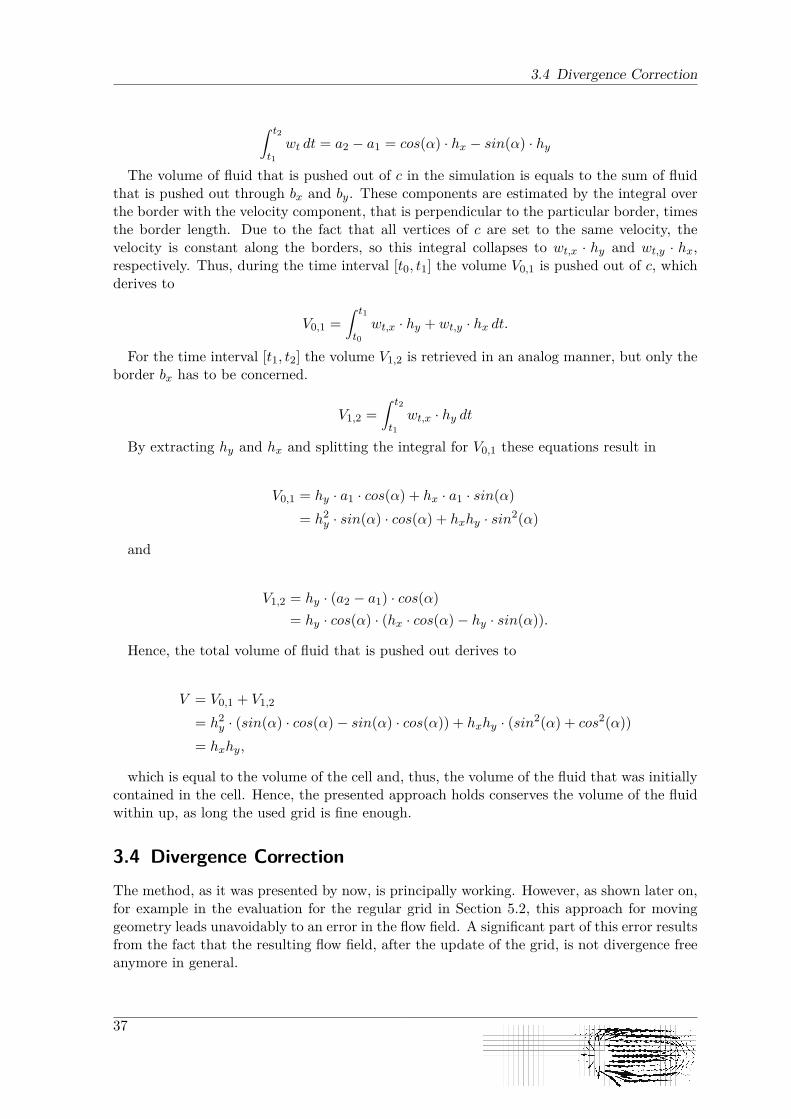
∫ t2t1wt dt = a2 − a1 = cos(α) · hx − sin(α) · hy
The volume of fluid that is pushed out of c in the simulation is equals to the sum of fluidthat is pushed out through bx and by. These components are estimated by the integral overthe border with the velocity component, that is perpendicular to the particular border, timesthe border length. Due to the fact that all vertices of c are set to the same velocity, thevelocity is constant along the borders, so this integral collapses to wt,x · hy and wt,y · hx,respectively. Thus, during the time interval [t0, t1] the volume V0,1 is pushed out of c, whichderives to
V0,1 =∫ t1t0wt,x · hy + wt,y · hx dt.
For the time interval [t1, t2] the volume V1,2 is retrieved in an analog manner, but only theborder bx has to be concerned.
V1,2 =∫ t2t1wt,x · hy dt
By extracting hy and hx and splitting the integral for V0,1 these equations result in
V0,1 = hy · a1 · cos(α) + hx · a1 · sin(α)= h2y · sin(α) · cos(α) + hxhy · sin2(α)
and
V1,2 = hy · (a2 − a1) · cos(α)= hy · cos(α) · (hx · cos(α)− hy · sin(α)).
Hence, the total volume of fluid that is pushed out derives to
V = V0,1 + V1,2
= h2y · (sin(α) · cos(α)− sin(α) · cos(α)) + hxhy · (sin2(α) + cos2(α))
= hxhy,
which is equal to the volume of the cell and, thus, the volume of the fluid that was initiallycontained in the cell. Hence, the presented approach holds conserves the volume of the fluidwithin up, as long the used grid is fine enough.
3.4 Divergence CorrectionThe method, as it was presented by now, is principally working. However, as shown later on,for example in the evaluation for the regular grid in Section 5.2, this approach for movinggeometry leads unavoidably to an error in the flow field. A significant part of this error resultsfrom the fact that the resulting flow field, after the update of the grid, is not divergence freeanymore in general.
37
3 Moving Geometry
a b
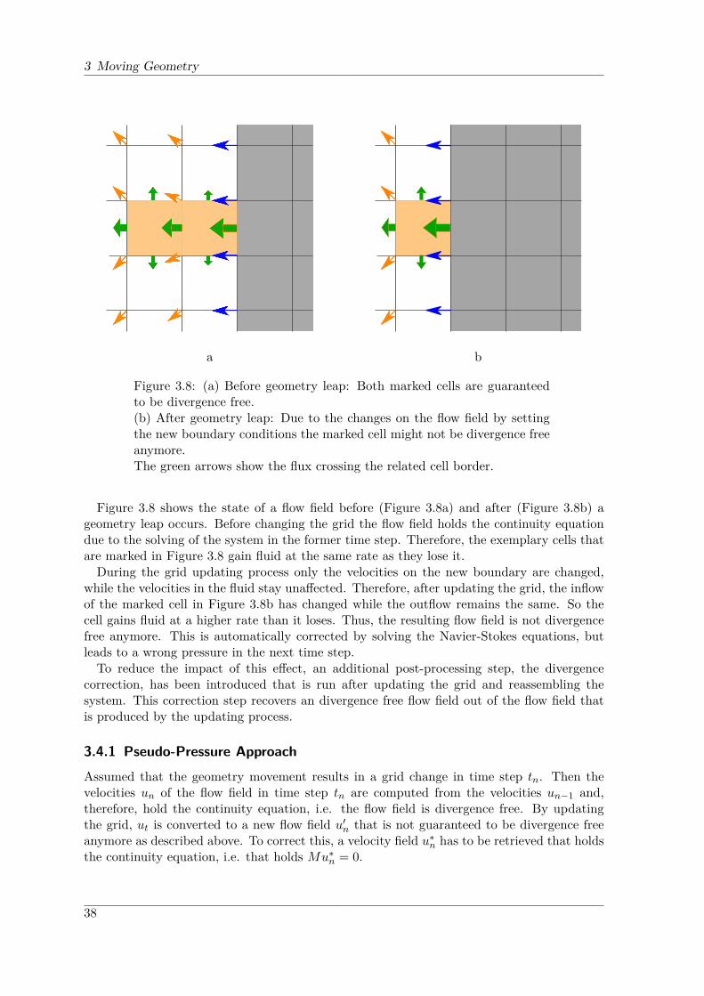
Figure 3.8: (a) Before geometry leap: Both marked cells are guaranteedto be divergence free.(b) After geometry leap: Due to the changes on the flow field by settingthe new boundary conditions the marked cell might not be divergence freeanymore.The green arrows show the flux crossing the related cell border.
Figure 3.8 shows the state of a flow field before (Figure 3.8a) and after (Figure 3.8b) ageometry leap occurs. Before changing the grid the flow field holds the continuity equationdue to the solving of the system in the former time step. Therefore, the exemplary cells thatare marked in Figure 3.8 gain fluid at the same rate as they lose it.During the grid updating process only the velocities on the new boundary are changed,
while the velocities in the fluid stay unaffected. Therefore, after updating the grid, the inflowof the marked cell in Figure 3.8b has changed while the outflow remains the same. So thecell gains fluid at a higher rate than it loses. Thus, the resulting flow field is not divergencefree anymore. This is automatically corrected by solving the Navier-Stokes equations, butleads to a wrong pressure in the next time step.To reduce the impact of this effect, an additional post-processing step, the divergence
correction, has been introduced that is run after updating the grid and reassembling thesystem. This correction step recovers an divergence free flow field out of the flow field thatis produced by the updating process.
3.4.1 Pseudo-Pressure Approach
Assumed that the geometry movement results in a grid change in time step tn. Then thevelocities un of the flow field in time step tn are computed from the velocities un−1 and,therefore, hold the continuity equation, i.e. the flow field is divergence free. By updatingthe grid, ut is converted to a new flow field u′n that is not guaranteed to be divergence freeanymore as described above. To correct this, a velocity field u∗n has to be retrieved that holdsthe continuity equation, i.e. that holds Mu∗n = 0.
38

3.5 Fluid-Structure Interaction
To achieve this field, a pseudo time step is computed where a pseudo pressure q is usedto affect the fluid velocity in the same way as does the real pressure in a normal time step.With this approach the equation
u∗t = u′t −MT qt
can be derived from the discretized momentum equation 2.3. The gradient of the pseudopressure q is used to correct the flow field. Multiplying this equation with M from the leftresults in
Mu∗t = Mu′t −MMT qt
where the left-hand side is zero, due to the precondition that u∗t is divergence free. Solvingthis for Mu′t finally provides the divergence correction equation
MMT qt = Mu′t.
So to compute u∗t a linear system of equations has to be solved just like during a real fluidtime step, but with a matrix MMT and a different right-hand side [19].
3.4.2 Algorithm with Divergence Correction
Due to this system of equations the divergence correction is a quite expensive post-processingstep. However, it can be computed by means of the same techniques that are used in thenormal CFD solver runs, so it benefits from any optimizations done for the normal CFDsolver.Within the computation of a time step the divergence correction of course needs to be done
after updating the grid and before computing the solution of the next time step. Since ituses a similar technique like the actual solver, the divergence correction takes place also afterthe creation of the new solver and the mapping of the old solution to this solver. Hence, thesolver for the divergence correction can be derived from the actual fluid solver. Algorithm3.1, therefore, is extended by the steps for creating the divergence correction solver out ofthe fluid solver, for solving the system of equations for the divergence correction and, finally,by updating the velocities to retrieve the divergence free flow field. The resulting process isshown in Algorithm 3.2.Due to the effort that is necessary to perform the divergence correction, it is interesting
what the benefit is. During the evaluation of the regular grid the effect of the divergencecorrection has been tested. The results can be found in Subsection 5.2.2.
3.5 Fluid-Structure Interaction
Supporting moving geometry in fluid simulation is actually only one side of a larger coin.While moving boundaries affect the fluid, the other way around happens, too. By pressureand adhesion the fluid also affects the structure represented by the movable geometry. Sinceboth sides, the fluid and the structure, act on each other, this process is called Fluid-StructureInteraction (FSI).
39
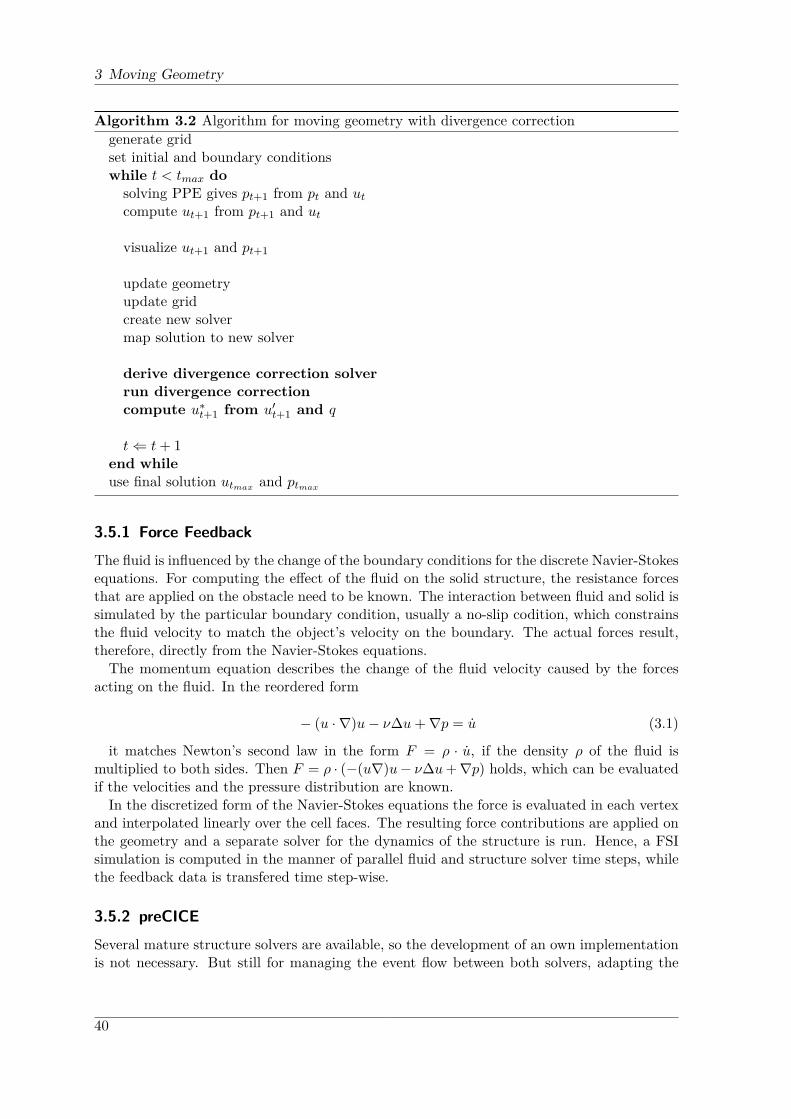
3 Moving Geometry
Algorithm 3.2 Algorithm for moving geometry with divergence correctiongenerate gridset initial and boundary conditionswhile t < tmax dosolving PPE gives pt+1 from pt and utcompute ut+1 from pt+1 and ut
visualize ut+1 and pt+1
update geometryupdate gridcreate new solvermap solution to new solver
derive divergence correction solverrun divergence correctioncompute u∗t+1 from u′t+1 and q
t⇐ t+ 1end whileuse final solution utmax and ptmax
3.5.1 Force Feedback
The fluid is influenced by the change of the boundary conditions for the discrete Navier-Stokesequations. For computing the effect of the fluid on the solid structure, the resistance forcesthat are applied on the obstacle need to be known. The interaction between fluid and solid issimulated by the particular boundary condition, usually a no-slip codition, which constrainsthe fluid velocity to match the object’s velocity on the boundary. The actual forces result,therefore, directly from the Navier-Stokes equations.The momentum equation describes the change of the fluid velocity caused by the forces
acting on the fluid. In the reordered form
− (u · ∇)u− ν∆u+∇p = u (3.1)
it matches Newton’s second law in the form F = ρ · u, if the density ρ of the fluid ismultiplied to both sides. Then F = ρ · (−(u∇)u− ν∆u+∇p) holds, which can be evaluatedif the velocities and the pressure distribution are known.In the discretized form of the Navier-Stokes equations the force is evaluated in each vertex
and interpolated linearly over the cell faces. The resulting force contributions are applied onthe geometry and a separate solver for the dynamics of the structure is run. Hence, a FSIsimulation is computed in the manner of parallel fluid and structure solver time steps, whilethe feedback data is transfered time step-wise.
3.5.2 preCICE
Several mature structure solvers are available, so the development of an own implementationis not necessary. But still for managing the event flow between both solvers, adapting the
40
3.6 Performance
interfaces and coping with a distributed layout of the system, a sophisticated coupling toolis required.At the chair for scientific computing at the TUM such a tool is under development, called
preCICE [7]. This module also contains a geometry representation that can handle triangu-lated geometry and, thus, in contrast to the basic Geometry component of Peano, supportsarbitrarily shaped objects.The usage of the new geometry is almost analog to the Geometry component of Peano,
since they virtually have the same interface. preCICE also supports the geometry queriespresented in Subsection 4.1.1, taking the current form of the structure, as computed by thestructure solver, into account. So the extension for moving geometry can use preCICE almosttransparently.
3.6 PerformancePeano is an application from the field of high performance computation; thus, some attentionhas to be paid to the optimization of the runtime performance. The modifications that havebeen done to improve the performance of the implementation are described in the following.
3.6.1 Staged Processing
Reducing unnecessary operations is one central task in runtime optimization. In this imple-mentation this reduction can be achieved in several places.
Semi-Static Geometry
If a classical simulation, without moving objects, is computed, the whole updating processfor the grid is needless. For this cases the whole implementation for moving boundaries canbe skipped by means of a flag.However, even in a simulation that uses moving objects it may happen that there are time
steps in that no object moves. An example for this are initially fixed objects that are releasedafter the flow has stabilized in a temporary steady state. In these cases it is unnecessary toupdate the grid and setup a new solver, so it is possible to check if the continuous geometryhas changed before triggering the grid update.
Hidden Movement
In the numerical solution of PDE the CFL condition is a central aspect for the stability ofthe computation [7]. In CFD this condition demands a time step size that shrinks with thepower of two with the decrease of the grid mesh width. Thus, the time step size often is verysmall compared to the mesh width. So, in many time steps the motion of the geometry ishidden by the spatial discretization as shown in Figure 3.4a.Hence, the creation of a new solver and especially the divergence correction run is not
necessary during these steps. To avoid this overhead the adapter for updating the grid has tocheck whether the grid has actually changed. Otherwise the subsequent steps for adjustingthe fluid solver can be omitted.Together with the check for semi-static geometries this leads to Algorithm 3.3 that is
derived from Algorithm 3.2. Here the processing of moving boundaries is divided into threestages, where one can trigger the next one or skip it.
41
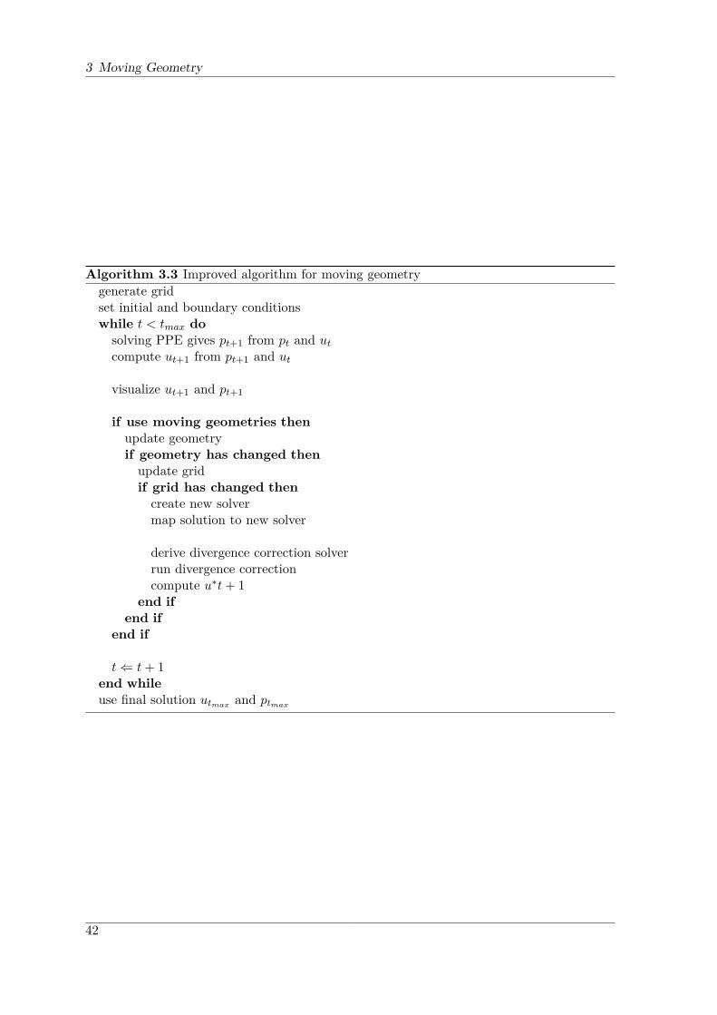
3 Moving Geometry
Algorithm 3.3 Improved algorithm for moving geometrygenerate gridset initial and boundary conditionswhile t < tmax dosolving PPE gives pt+1 from pt and utcompute ut+1 from pt+1 and ut
visualize ut+1 and pt+1
if use moving geometries thenupdate geometryif geometry has changed thenupdate gridif grid has changed thencreate new solvermap solution to new solver
derive divergence correction solverrun divergence correctioncompute u∗t+ 1
end ifend if
end if
t⇐ t+ 1end whileuse final solution utmax and ptmax
42
3.6 Performance
Since the divergence correction actually demands for the solution of the linear system ofequations, just with slightly different vector entries, it is virtually as expensive as a normaltime step. So avoiding unnecessary divergence correction runs usually has a drastic impacton the overall runtime performance. The results for the performance tests with the im-plementations for the regular and the adaptive grid can be found in Subsection 5.2.4 andSubsection 5.3.2, respectively.
3.6.2 Adapter MergingHigh resolution simulations for serious scientific projects suffer from an enormous need formemory. During the development of Peano this aspect has been paid attention to by thereduction of data per degree of freedom and the use of cache efficient algorithms [10], [13].But still the main memory’s access time has a major impact on the overall performance.During an adapter iteration all vertex and cell data for the whole grid has to be read from
the main memory, or even the hard disk drive in large simulations, and written back again.Thus, such an iteration needs a lot of memory accesses and, therefore, may suffer from largeaccess times. In fine granular adapters, i.e. adapters which are responsible only for one singletask, not much work has to be done for a single vertex or cell. Therefore, the memory accessmay become the performance bottleneck in adapters of this kind since the time for readingand writing exceeds the time for the mere processing of the data.To avoid this bottleneck it would be optimal to have few, large adapters performing all
necessary work in a minimum number of grid iterations. However this contradicts the en-capsulation principle of object-oriented programming, so a balance has to be found betweenperformance and maintainability.In the implementation of this thesis some tasks have been merged into other adapters to
improve the runtime performance of the system. Since this is based on the actual implemen-tation these mergencies are mentioned in the corresponding Section 4.2 and Section 4.3.
43

3 Moving Geometry
44
4 Chapter 4
Implementation
To put the method, described in Chapter 3, into practice, several changes needed to be madewithin Peano. This chapter depicts these changes, ordered by the component in which theyhave been implemented. Section 4.1 shows the extensions for the interface of the Geometrycomponent, which are necessary for the subsequent implementations in the Fluid component.Since the interfaces for the regular and the adaptive grid differ in various details, separateimplementations are needed for both components. Section 4.2 and Section 4.3 explain theseimplementations for the particular grid type.
4.1 Geometry
While the grid components only hold the discretized spatial information, the Geometry com-ponent of Peano holds the real geometry information for the simulated scenario. This com-ponent represents the used geometry as a collection of primitive objects. Each object dividesthe viewed domain into two subdomains ΩObject and ΩObject, i.e. the inside and outside ofthe object, while each object can be inverted, which basically swaps ΩObject and ΩObject.The computation domain ΩFluid is, finally, assembled as the intersection of all domains
outside an object: ΩFluid =⋂ni=0 ΩiObject.
The design of this component resembles a composite pattern [15] as shown in Figure 4.1.This offers the possibility to build a deep geometry tree, which, however, is not used in Peanoso far.
4.1.1 Geometry Interface
For defining a basic CFD scenario the Geometry component only provides data about thegeometry in just three ways. The whole interface for the Geometry component is voxel andpoint oriented. Thus, it does not provide direct access to the defined geometry but affordsqueries for voxels and single points. From the point of view of this interface, a voxel, a“volume element”, is a d-dimensional cuboid whose set of points is seen as an open set, i.e.the boundary points are not part of the cuboid. For this reason a single point is not justa voxel of size zero, since this would result in an empty set of points. For simplicity theinterface methods assume a zero voxel as a single point in most cases. But for some cases thisassumption does not give the right results. So, for these queries there are separate methodsfor voxels and points.
45

4 Implementation
Figure 4.1: Architecture of the Geometry component
For defining a basic CFD scenario the Geometry component provides data accessible withthe following queries.
Domain Queries
The primary information provided by the geometry of a simulation is the spatial situationor state of a voxel or a single point. That is that a point can be either inside or outside ofthe defined geometry, while a voxel can be either inside, outside or on a boundary. Threemethods are offered by the Geometry component for these domain queries:
bool i sComplete lyOuts ide ( Voxel )bool i sComp l e t e l y In s ide ( Voxel )bool isOutsideClosedDomain ( Point )
Due to the decoupling of the Fluid and the Geometry component the voxel state is notdirectly returned. But it can be derived from the return values of the first two methods asdenoted in Table 4.1.
CompletelyInside
CompletelyOutside
State
false true Outsidetrue false Insidefalse false On Boundary
Table 4.1: Return values for the domainquery methods.
Since points have two states only (inner andouter), one method is sufficient to retrieve thestate for a given point. Voxel queries checkagainst open domains since voxels are open setsas stated above. Therefore, the method isOut-sideClosedDomain is needed to check a singlepoint against the closed geometry domain. Oth-erwise queries for points contained in the do-main boundary would give incorrect results ifthey would be queried by the method isComplete-lyInside with a zero-sized voxel.
Boundary Queries
The second type of information, which the Geometry component offers, is boundary informa-tion. This can be retrieved by boundary queries which always work on a given voxel, i.e. only
46

4.1 Geometry
the boundaries intersecting the given voxel are taken into account. Thus, the main methodfor boundary queries returns the number of boundaries intersecting a given voxel.
i n t getNumberOfBoundariesIntersected ( Voxel )
All boundary queries for specific boundaries rely on the boundary id which identifies aboundary amongst all boundaries intersecting the given voxel. Having this id the actual datafor a specific boundary can be retrieved; for example the boundary number, a number thatcan be used later on by the used scenario to map this boundary to a specific boundary type .
i n t getBoundaryNumber ( Voxel , ID )
4.1.2 Geometry Speed
Before moving boundaries were introduced, the Geometry component did not need to knowabout any more information for the geometry. The speed of a boundary could be implicitlyresolved to zero since all objects were fixed by definition. Other velocities like inflow or lidflows for channel or driven cavity simulations [7] are defined in the scenario globally for thewhole simulation.As shown in Chapter 3 the boundary speed of an object has to be known to set the boundary
conditions of the CFD solver correctly. For this, two changes on the Geometry componenthave been necessary to be carried out.First each Geometry object has to hold its own velocity. Since the Geometry component
does neither support deformations on the geometry nor any transformation other than trans-lations, only translational and rotational velocities have been implemented. Examples canbe seen in Figure 4.2.Since the Geometry component is not able to really apply rotations on the objects, rota-
tion velocity can only be simulated on objects with rotational invariant shape, like spheres.Hence, real moving boundaries can currently be simulated only with translations, which isindeed sufficient as a basis for the development of an Implementation for moving geometries.However, the implementation of rotational velocity shows that the used approach is capa-ble of handling arbitrary movement. Thus, it can be easily adapted for more sophisticatedgeometry representations like the FSI coupling tool preCICE noted in Subsection 3.5.2.The second change is the introduction of a boundary speed query into the Geometry
interface. This query is analog to the boundary number query, see Subsection 4.1.1; thus, itspecifies an object by the id of its boundary within a given voxel. The signature of this queryis
Vector getBoundaryVelocity ( Voxel , ID )
and returns the velocity value of the object to that the boundary belongs. The velocityis actually evaluated in the center of the voxel and, therefore, does not generally match theactual boundary velocity. This approximation has to be done to provide a general interfacethat does not make great demands on the geometry representation. However, if the grid ischosen fine enough, this difference can be neglected anyway.
4.1.3 Hexahedron Queries
Usually hexahedrons are uncommon obstacles for fluid simulation, because more often smoothobstacles, like spheres, are used. However, for moving geometries they have the advantage
47
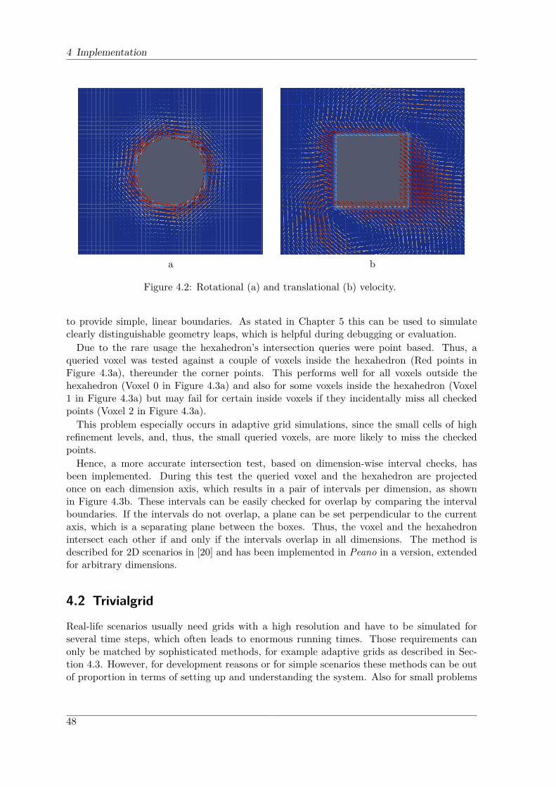
4 Implementation
a b
Figure 4.2: Rotational (a) and translational (b) velocity.
to provide simple, linear boundaries. As stated in Chapter 5 this can be used to simulateclearly distinguishable geometry leaps, which is helpful during debugging or evaluation.Due to the rare usage the hexahedron’s intersection queries were point based. Thus, a
queried voxel was tested against a couple of voxels inside the hexahedron (Red points inFigure 4.3a), thereunder the corner points. This performs well for all voxels outside thehexahedron (Voxel 0 in Figure 4.3a) and also for some voxels inside the hexahedron (Voxel1 in Figure 4.3a) but may fail for certain inside voxels if they incidentally miss all checkedpoints (Voxel 2 in Figure 4.3a).This problem especially occurs in adaptive grid simulations, since the small cells of high
refinement levels, and, thus, the small queried voxels, are more likely to miss the checkedpoints.Hence, a more accurate intersection test, based on dimension-wise interval checks, has
been implemented. During this test the queried voxel and the hexahedron are projectedonce on each dimension axis, which results in a pair of intervals per dimension, as shownin Figure 4.3b. These intervals can be easily checked for overlap by comparing the intervalboundaries. If the intervals do not overlap, a plane can be set perpendicular to the currentaxis, which is a separating plane between the boxes. Thus, the voxel and the hexahedronintersect each other if and only if the intervals overlap in all dimensions. The method isdescribed for 2D scenarios in [20] and has been implemented in Peano in a version, extendedfor arbitrary dimensions.
4.2 Trivialgrid
Real-life scenarios usually need grids with a high resolution and have to be simulated forseveral time steps, which often leads to enormous running times. Those requirements canonly be matched by sophisticated methods, for example adaptive grids as described in Sec-tion 4.3. However, for development reasons or for simple scenarios these methods can be outof proportion in terms of setting up and understanding the system. Also for small problems
48

4.2 Trivialgrid
Voxel 0 Voxel 1
Voxel 2
a b
Figure 4.3: Hexahedron intersection tests.(a) Point based intersection test: Red spots mark checked points insidethe hexahedron (blue).
Voxel 0 is considered outside correctly.Voxel 1 is considered inside correctly.Voxel 2 is considered outside falsely.
(b) Intersection test by interval overlap. Blue and Red boxes are projectedto the x0 and x1 axes. Overlap occurs on axis x0.
49

4 Implementation
the computational overhead for these methods can exceed the benefit. Additionally thesemethods may cause side effects that are not as obvious as they would be with simpler meth-ods. Therefore, Peano contains a component for regular grids as a simplified alternative forthe adaptive grid. It offers a simple-to-use fundament for other components, and, therefore,allows easier development and testing and higher performance in uncomplex scenarios.
4.2.1 Basics
The Trivialgrid component of Peano offers a regular Cartesian grid space discretization witharbitrary resolution in each dimension. Logically this grid is described as a d-dimensionalarray of cells and vertices, holding the information for the PDE solver. However, as mentionedin Subsection 2.2.2, the fluid simulation is actually decoupled from the physical representationof the grid by the use of adapters. So physically the grid can be hold by Peano in an arbitrarymanner, which allows to develop the fluid solver without regarding the implementation detailsof the Trivialgrid component.The lifecycle of a regular grid is fairly simple. That means that the cells and vertices are
created before the simulation throughout the whole clipping domain ΩScenario and are set totheir appropriate state. Afterwards the set of cells and vertices cannot be changed during thesimulation, until the grid is destroyed as a whole, after the simulation. So it is not possibleto add or remove cells or vertices after the initial creation. Thus an adapter is needed toupdate the grid during the simulation.For introducing moving geometries into the regular grid component, the method of Chap-
ter 3 can almost be used directly. This chapter describes the details of the implementationof this method on the regular grid.Subsection 4.2.2 presents the UpdateGridAdapter that is the central element of the algo-
rithm. Here all the work for setting the cells and vertices to a correct state is done.In Subsection 4.2.3 the necessary steps for setting up a new solver are described.Subsection 4.2.4 introduces the FluidStructureInteractionAdapter which is a stump for
integrating a potential FSI solver and performs the geometry time steps.
4.2.2 Updating Grid
The connection to the Trivialgrid framework component is done by dependency injectionvia an event handling mechanism as described in Subsection 2.2.2. An adapter template is,therefore, provided by this component that consists of a couple of events. Appendix A showsa complete listing of the adapter’s interface.For the UpdateGridAdapter two methods of the Trivialgrid adapter have been implemented.
While the event touchVertexFirstTime handles the vertices of the grid, the handleElementevent takes care of the cells.
Handling Vertices
This first task is basically done in the way as it is described in Subsection 3.3.3. The state andthe velocity of the particular vertex is set, based on two geometry queries. One is performedon isCompletelyInside( Voxel ) for the h-environment of the current vertex, the other one onisOutsideClosedDomain( Point ) for the particular location of the current vertex.Additionally it is tracked whether a vertex has changed its state or not, to avoid unnecessary
subsequent steps, as described in Subsection 3.6.1. Mere velocity changes do not change the
50
4.2 Trivialgrid
used solver, so they don’t have to be tracked here.
Handling Cells
As with the vertices, the cell handling also follows directly the approach from Subsection 3.3.3.So the cell state is adjusted, based on the current geometry. And also here the updating istracked for a real change of a cell to trigger the recreation of the solver and a possibledivergence correction. However, one difference exists.As described in the theoretical approach the pressure of a new inner cell has to be set to
an approximated value that should be close to the real value. In the used discretization thepressure is determined by the current velocity field of the flow over the PPE and any changesin the pressure vector do not have an effect, as long as the solver for the PPE can makeenough iterations to converge to the real solution.According to that, tests have shown that the influence of the choice for the pressure value
is negligible small. Also the overhead for the slight increase of used iterations for solving thePPE was found to be rather small. Thus, the initial pressure for a new inner cell is set tozero.
Counting Degrees of Freedom
After the grid has been updated, a new solver has to be created, as described in the following.To achieve that, it has to be known, how many inner cells and vertices exist in the current grid,since an appropriate amount of memory has to be allocated, as mentioned below. For thistask the InnerCellCountingAdapter is available, which is anyway used for the initial solvercreation. Subsection 3.6.2 stated that it is desirable to minimize the number of adapter runsfor the sake of runtime performance. And, since it is known for every cell and vertex inthe UpdateGridAdapter whether it holds a degree of freedom or not, this counting can bedone together with the updating process. Therefore, this functionality is implemented in theUpdateGridAdapter, too, and the unnecessary run of the InnerCellCountingAdapter can beomitted.
4.2.3 Creating New Solver
The matrices A,C,D and M from the discretized Navier-Stokes equations (Equation 2.3 andEquation 2.4) basically are global matrices. However, they are never assembled in total inPeano, but are only evaluated locally, directly on the grid. Thus, a possible grid change isimplicitly imposed on these matrices.In contrast to that the matrix Q = MA−1MT , also a global matrix, is actually hold within
PETSc for solving the PPE (see Subsection 2.2.3). Therefore, this matrix and the vectorsfor the pressure and the right hand side of the PPE have to be reassembled everytime thegrid changes. Hence, an appropriate amount of memory has to be allocated by PETSc andthe matrix entries have to be set. The entries of the right hand side are anyway set with thecurrent values during the normal time step computation, so nothing has to be done for them.However, the pressure vector, which is the solution vector for the discretized PPE, has to beset, too. In normal time steps, without a grid change, the solution vector, still held in PETSc,is used as a starting point for the iterative solver. To achieve the same result, the currentpressure values, saved in the cells, have to be transfered to the newly allocated solution vector
51
4 Implementation
within PETSc. This task is done within the adapter that assembles the matrix Q to avoidan additional adapter run.
4.2.4 FluidStructureInteractionAdapter
For simulating moving geometry, the actual change of the position and the velocity has to becomputed. Usually this is done by a FSI solver or a predefined trajectory for the geometry. Fortriggering this updating process the FluidStructureInteractionAdapter has been implemented.This thesis uses a very simple model for the movement. The geometry is set to a constantvelocity, while the time integration is done by an explicit Euler approach. This is inadequatefor complex scenarios but provides a sufficient environment for testing the implementation ofthis thesis.
4.2.5 Divergence Correction
A method for computing a divergence free flow field was already implemented in Peano, sothis task did not need to be accomplished within this thesis. This procedure contains twoadapter runs for setting up the matrix MMT and the right hand side vector. Afterwardsthe linear system of equations is solved and another adapter run is performed to update thevelocities and thereby retrieve the corrected flow field.
4.3 Adaptive GridCompared to the regular grid, the Adaptive Grid component is the much more sophisticatedgrid representation. This also means that the implementation of moving geometry becomesmore complex. However, having the implementation working on this grid type is essential.While the regular grid is mostly used during development and for simple simulations, mostserious simulations need too high resolutions in space and time and too long simulationperiods to be computed using this component in reasonable time. In this case the use ofadaptive grids is compulsory. So if the implementation of moving boundaries would only beworking on regular grids, it would lose a wide field of application.
4.3.1 Basics
As already mentioned in Subsection 2.1.3 adaptive grids are a common approach for Cartesiangrids to reduce the number of cells, while keeping the discretization error low. The price forthis benefit is the substantial higher implementation effort. While the data storage and thegrid traversing is straightforward in regular grids, since they can be mapped to a simpled-dimensional array, adaptive grids demand for more sophisticated algorithms to gain fulleffectivity.
Grid Traversing
Due to the performance gap between processor and main memory, as it is given in today’scomputers, it is also a matter of performance to traverse the used grid in a cache-efficientway, to fully exploit the benefits of the memory hierarchy [10]. Subsection 2.1.3 alreadymentioned the recursive nature of adaptive grids. Building on this, a common method forgaining efficient traversal schemes is the use of space-filling curves. These curves can be
52
4.3 Adaptive Grid
constructed directly from the subdivision pattern of the grid, since their self-similarity leadsalso to a recursive structure. And due to their spatial locality, they provide a cache convenientmemory access pattern. In Peano a cell is trisected in each refinement step along each axis,so it allows the use of the namegiving Peano curve. Figure 4.4a shows an exemplary grid in2D with a maximum refinement level of 3.
Spacetree
As with the space-filling curves, the refinement pattern of a grid can also be mapped directlyto a tree, the so-called spacetree. The root of this tree represents the initial root cell thatcontains the whole computation domain and which, therefore, is the starting point of therecursive grid construction. Each inner node matches a further refined grid cell, while theleaf nodes of the spacetree finally form the actual grid, since they represent the cells of thegrid that are not further refined.Figure 4.5 shows the spacetree resulting from the grid shown in Figure 4.4a. Note that each
refined node has 3D children (9 in this two-dimensional example), matching the 3D subcellsof the corresponding cell.This consideration of the grid structure gives a simple representation of the grid as a graph
that can be traversed with common algorithms. For the traversal of the spacetree a depth-first search is used [10], whereas the order of the child nodes in the traversal is determinedby the Peano curve.So this is actually the way that Peano uses to store the grid. Each cell and each vertex is
taken as a node in the spacetree and the whole tree is stored in a couple of stacks [7], but forthe exception of hanging vertices, which are described later in this section. This means thateach vertex that exists on level l0 also exists on all sub-levels li down to the finest level towhich at least one of the adjacent cells is refined, and is also stored separately for each level.The same applies for the cells. Even a cell that is further refined, and, therefore, does notshow up in the actual grid, exists in memory and is traversed by the adapters.This design is inherently appropriate for multigrid and multiscale algorithms and is still
transparent for simulations running on normal, static grids, since the cells and vertices thatdo not show up in the grid can simply be ignored by an application. However, if the grid isnot static anymore, it may happen that a hidden vertex or cell becomes part of the actualgrid, for example by coarsening the considered cell. These cells and vertices also have to betaken into account by the implementation to gain correct results.
Dynamic Grids
From the geometrical point of view a refinement takes place in a cell that is hereby subdividedinto several subcells. So in this view the refinement information is stored in the cells. InPeano, however, this is not the case. Here the refinement information is rather stored inthe vertices. Of course a vertex itself cannot be refined, since it does not cover an area ofthe computation domain. But if the refinement for a vertex is triggered, all adjacent cells ofthis vertex are actually subdivided, so the whole area of the support of a vertex is actuallyinfluenced by its refinement setting. This procedure allows an easy determination of hangingvertices, which are described below, and an easier management of the grid [10].In Peano the refinement of the grid is basically triggered by the boundary of the computa-
tion domain. I.e. if the h-environment of a vertex is intersected by the boundary, it is refined,as long as a lower threshold for the mesh width is not under-run. So, if the computation
53
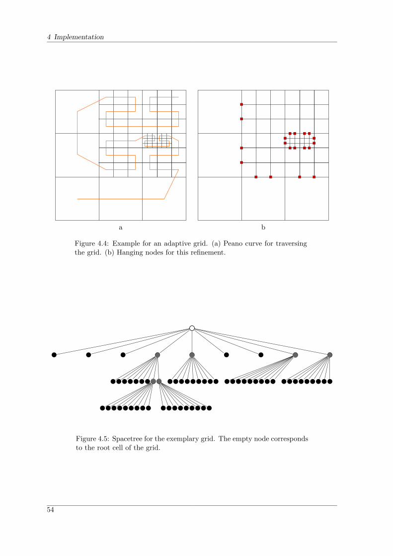
4 Implementation
a b
Figure 4.4: Example for an adaptive grid. (a) Peano curve for traversingthe grid. (b) Hanging nodes for this refinement.
Figure 4.5: Spacetree for the exemplary grid. The empty node correspondsto the root cell of the grid.
54

4.3 Adaptive Grid
domain changes over time, due to a time-dependent geometry, the grid has to readapt. Againthe recursive nature of the subdivision method gives a benefit:Like refining corresponds to adding child nodes to a leaf in the spacetree, coarsening corre-
sponds to removing a subtree from the coarsed node. So readapting a grid can be performedlocally, affecting only a subtree of the spacetree, without changing other subtrees and, there-fore, other parts of the grid. This is essential for moving boundaries, since a wide gridrestructuring during the simulation would be quite expensive [21]. With the spacetree ap-proach, only the paths from the cells in the environment of the moving object to the root maybe affected. This gives an O(n · s) limit for the number of changed cells if n is the numberof cells adjacent to the moving boundary and s is the height of the spacetree. For commonscenarios with smooth boundaries the number of cells along the boundary grows similarlywith the finest mesh width in the grid. Hence, this threshold resembles to O(n · log(n)).
Hanging Vertices
For the computation of a discretized gradient in a vertex, i.e. a velocity gradient in CFD, thevelocities of the neighbor vertices have to be known. In a regular grid the neighborhood ofan inner vertex is always well defined, since all 2D neighbor vertices exist. For adaptive gridsthis is not the case on the border between differently refined areas of the grid. Figure 4.4bshows the vertices in the formerly introduced grid, that do not have all neighbors due to thecurrent grid refinement. Since it is not possible to solve the PDE for them, these verticesdo not hold a degree of freedom for the computation of the discrete Navier-Stokes equationsand are called hanging vertices or hanging nodes. Thus, no velocity is computed for thesevertices during a time step, but they are only used for the computation of a valid solution intheir neighbors. Therefore, the velocity that they hold during the computation is not a realfluid velocity but is retrieved by a d-linear interpolation of the velocities from the vertices inthe next higher level.Hanging vertices are not directly affected by the implementation for moving boundaries,
since the boundary conditions are imposed implicitly by the super-level vertices. But theymay have to be switched to vertices holding a real degree of freedom due to the geometrymovement and, therefore, have to be taken into account.
4.3.2 Updating gridFor changing the adaptive grid, more effort is necessary compared to the regular grid, whichcan already be seen from the amount of events defined in the adapter of the Adaptive Gridcomponent (Appendix A). In principle the implementation is also based on the methoddescribed in Section 3.3, so the handling for vertices and cells is analog to the one done inthe regular grid, but the state of vertices and cells is defined by more variables than just bythe current spatial situation. These variables are
• the passive mode for outer cells and vertices,
• the refinement state for vertices
• and an additional flag to prune subtrees off the spacetree that don’t have to be traversedby the updating process.
This leads to some differences and some extensions, compared to the regular grid imple-mentation, which are discussed in the following.
55

4 Implementation
Passive Cells and Vertices
The boundary refinement criterion leads to the situation that also outside of the computationdomain it is likely that there are many cells and vertices which are not required for thecomputation, at all. This fact is even intensified by the tri-section used in Peano since therecan be up to 3D−1 not required cells and up to 4D−2D unused vertices per refined cell thatis intersected by a boundary, as shown below.To reduce the impact of these cells and vertices, Peano offers the possibiliby to set them
to passive. In this mode they are traversed as usual, but the event handlers are not called.Thus, the time for running these handlers unnecessarily is saved.However, if the computation domain is not static anymore, as in the case of moving geom-
etry, the mode of the grid cells and vertices has to be adapted, too. To get the mapping ofthe grid to the current mode, it is important to understand when a vertex and a cell is setto passive.The basic idea for this is that every event call has to work on valid, thus active, cells and
vertices. Additionally cells are only allowed to be passive if they are completely outside of thecomputation domain. The cell-vertex interaction in the event handler, therefore, determinesthe passive vertices. In the adapter for the Adaptive Grid component (Appendix A) it canbe found that only the enterElement and leaveElement events have access to both, the celland its adjacent vertices. The events touchVertexFirstTime and touchVertexLastTime onlywork on the particular vertex, but do not grant access to the adjacent cells. This enforces allvertices that are adjacent to an active cell to be active. Otherwise the event call for this cellwould provide access to a passive vertex which should not be the case. This does not holdthe other way around. An active vertex may have passive adjacent cells, which anyway arenot accessible through the events for this vertex.Thus, the following mapping can be applied:
• A cell is passive if and only if it is completely outside the (continuous)computation domain.
• A vertex is passive if and only if its h-environment is completelyoutside the (continuous) computation domain.
Each cell that is intersected by a boundary, has at least one subcell that is also intersected.All other cells can be completely outside of the computational domain and, thus, they can bepassive, as shown in Figure 4.6b. This leads to the mentioned maximum number of 3D − 1not required subcells and 4D − 2D not required vertices.An additional fact is that a passive cell can only have passive children, since they are,
trivially, also completely outside the computation domain if the supercell is.For the implementation of the UpdateGridAdapter two things need to be done. The map-
ping has to be performed and all direct subcells and -vertices of an active cell have to be setto active, before the grid traversal descends to their level. Otherwise passive cells or verticeswould never be set to active, since their event handles are not called. If a cell or vertex is setto active by this procedure, which should be passive according to the described mapping, itis anyway set to passive again when the adapter updates its state. So during the descendingto the sublevel no further effort has to be put into the question which subcell or vertex of aparticular cell really has to be set to active.Therefore, the mapping is implemented as described but with one exception. If the cells
are set as described in the list, a geometry query is performed on a larger h-environment as
56
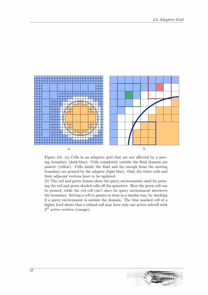
4.3 Adaptive Grid
a b
Figure 4.6: (a) Cells in an adaptive grid that are not affected by a mov-ing boundary (dark-blue). Cells completely outside the fluid domain arepassive (yellow). Cells inside the fluid and far enough from the movingboundary are pruned by the adapter (light-blue). Only the white cells andtheir adjacent vertices have to be updated.(b) The red and green frames show the query environments used for prun-ing the red and green shaded cells off the spacetree. Here the green cell canbe pruned, while the red cell can’t since its query environment intersectsthe boundary. Setting a cell to passive is done in a similar way, by checkingif a query environment is outside the domain. The blue marked cell of ahigher level shows that a refined cell may have only one active subcell with2D active vertices (orange).
57

4 Implementation
shown in Figure 4.6b. However this is an unnecessary effort since the passive mode can bedirectly derived from the adjacent vertex modes. This is because the given rules allow thestatement that a vertex is only passive if all of its adjacent cells are passive, since only thenthe h-environment of the vertex is completely outside the computation domain. So in theopposite direction this leads to the fact that a cell is passive exactly if it has at least onepassive, adjacent vertex.Hence, the updating of the cell is implemented in a way that all adjacent vertices are
checked and if at least one is passive, the cell can be switched to passive, too.
Spacetree Pruning
By the passive mode it is possible to exclude subtrees from being traversed. As describedabove, this does not affect the cells and vertices inside the computation domain, because inmost cases an adapter needs to traverse the whole domain.Updating the grid, however, is inherently constrained to the near environment around the
moving boundary. Thus, many subtrees that contain only parts of the grid which are nottoo close to the moving boundary can be omitted. Figure 4.6a shows an example, where theblue shaded cells and the adjacent vertices do not have to be updated. Note that cells, whichare adjacent to a non-moving boundary, i.e. at the border of Figure 4.6a, and their adjacentvertices, can also be omitted.Technically this optimization can be achieved by passing a flag down the tree that is initially
set to false on the whole grid and is switched to true, for the parts of the grid that have tobe traversed, successively during the grid traversal. So in the beginning the flag is set to trueonly for the root cell and its adjacent vertices. Then the pruning is done by passing the flagdown the tree during the traversal. The rule for this passing is simple. The subcells and-vertices of a particular cell c have to be processed only if c contains a moving boundary inthe current time step, or has contained one in the last time step. Only in these cases thestates of the cells or vertices may have to be changed due to a movement of the boundary.The CFL condition leads to the fact that the boundary has moved for at most one cell in thelast time step. So the flags in the subcells and -vertices have to be switched to true if c or oneof its 3D− 1 neighbor cells currently contain a moving boundary. This can be determined bya single geometry query on the combined h-environment of c and its adjacent cells, as shownin Figure 4.6b.
Refining and Coarsening
The built-in refinement of the grid in Peano is triggered by the boundary of the computationdomain. To achieve the same refinement pattern on dynamic grids, the UpdateGridAdapterhas to imitate this funcionality, which is located in the Adaptive Grid component of theframework.The criterion is defined as follows:
A non-refined vertex v has to refine if
• v is inside the closed computation domain Ω′Fluid, the h-environmentof v is intersected by the boundary of the computation domain andh is larger than the lower threshold hmin for the mesh width or
• h is larger than the upper threshold hmax for the mesh width.
58
4.3 Adaptive Grid
On the other hand, if v is refined it has to coarse if none of the upper conditions hold. Soit is possible to determine the current target state of a vertex with two geometry queries.One for determining if h(v) is completely inside the computation domain and, if this is nottrue, another one to check if at least v is inside the closed domain.More effort is necessary during refinements or coarsenings from the point of view of the
fluid simulation. A coarsening, thereby, results in the deletion of vertices that hold validinformation about the flow field. This loss is inherent, but the impact of it has to be min-imized. For this the flow field should be changed as few as possible. For this it has to benoted that, if a cell is coarsed, its adjacent vertices also appear on the sublevel and hold validdata. Hence, the information of the vertices on the sublevel can be transfered to the samevertices in the current level, since they are held in memory separated due to the spacetreeaproach. This leads to a flow field that is the same as before but, of course, with a coarserresolution.In the implementation this is done by copying the velocity of each leaf vertex to its pendant
in the next higher level, no matter if the supervertex will be coarsed or not. By this thevelocity is saved if a coarsening is triggered.In contrast, a refinement is more complex. Again the adjacent vertices of a cell, that is
refined, have matching vertices in the sublevel to which they can copy their velocity. However,the subvertices that have no matching vertex in the current level are not regarded by this.For them an interpolation is needed to approximate the actual value.Currently a d-linear interpolation is used to estimate the velocities. However this method
has a serious drawback. Even if the refined cell is divergence free, this kind of interpolationdoes not guarantee the new created subcells to be divergence free as well. The results of thisfact can be found later on in Subsection 5.3.1.An alternative interpolation could be derived from the divergence free elements, described
in [7]. This has not been done in this thesis and is left as a future task to further improvethe implementation.
Spatial Vertex and Cell State
This part of the algorithm can be implemented in a similar way like in the regular grid. Hence,setting the vertices to inner, outer or boundary and the cells to inner or outer, respectively,is based on the same conditions, but with two differences. The h-environment defined inSubsection 3.1.1 is based on a unique h for all cells and vertices in the regular grid, but inthe adaptive grid h depends on the currently processed level of refinement. This has to betaken into account for the geometry queries.The second difference are the hanging vertices that become real fluid nodes. Since hanging
vertices do not hold a real degree of freedom, no valid data is set on them. However, since thiscase can only happen during a refinement, the same technique, that is used when creatingnew subvertices of a refining cell, can be applied. Thus, they are set to an interpolated state,derived from the superlevel vertices.
Order of Processing
In the regular grid implementation, the updating of the state of a particular cell or vertex isindependent from the rest of the grid, so the code also is not constrained to a certain order.In contrast to this, the states in the adaptive grid actually interact, between cells and
vertices as well as the separate variables of a single state. Here the passive flag is the central
59

4 Implementation
Figure 4.7: Dependency graph for updating an adaptive grid.
element since it influences the adjustment of all other variables, because they cannot be setif the according cell or vertex is passive. That means, a passive cell or vertex always has tobe switched to active to be updated to the current geometry.Additionally another constraint is set for optimizing the performance. Cells completely
outside of the continuous computation domain would be set to passive in the first traversal.If the cell is a refined cell, the subcells could, therefore, not be removed by coarsening the gridand, hence, would cause a performance penalty. So the UpdateGridAdapter has to ensure,that only leaf nodes are set to passive.Setting cells to passive leads to another dependency. As mentioned above, cells are switched
to passive according to the passive mode of their adjacent vertices, to avoid an unnecessarygeometry query. Hence, this mode of the vertices has to be set correctly before the particularcell can be updated.These dependencies result in the graph shown in Figure 4.7. In this graph two levels of
the spacetree are regarded. The cross-level arrows show the dependencies between a cell andits subcells and -vertices. As can be seen, the prune flag of a cell triggers the activation ofthe subcells and -vertices. So here this flag is actually used for two things. First it is usedto set the flag on the sublevel, but second it is also used for activating cells and vertices onthe sublevel if necessary. This can be done, since cells that can be set to passive are anyway
60

4.3 Adaptive Grid
outside the grid and, therefore, do not apply for being pruned by the prune flag. The sameapplies for vertices.It is also mentionable that triggering a refinement or coarsening on a vertex does not imply
additional dependencies. This results from the fact that the actual change of the grid is notperformed instantly but in the next grid traversal [10]. This has the disadvantage that theUpdateGridAdapter may have to run another time after a refinement has been triggered, toset the new subcells and -vertices to their correct state. On the other hand a coarsening canbe triggered by this on any vertex, without influencing the rest of the current grid traversalor any refinement or coarsening that is triggered on another vertex during this traversal.
Event Handlers
The dependencies of the states have to be regarded, when implementing the UpdateGrid-Adapter. Since the adapter interface of the Adaptive Grid component (see Appendix A)provides events that are called in a specified order, the tasks for setting the states have tobe mapped carefully to these events. Table 4.2 denotes the order of the events. In the leftcolumn all events are listed that are called during the traversal of a specific cell or element.Due to the recursive traversal of the grid the events are also called in a recursive mannerwhich is denoted by the recursive descent, where the events for the subcells are called. Alsoduring the handling of a single cell and its vertices all data for the subcells and -vertices hasto be loaded. This leads to an interlaced order of the events of two grid levels. The indentedentries in the table refer to events of the sublevel.The right column lists the tasks mapped to the according event. So this table actually
illustrates the implementation of the UpdateGridAdapter for the adaptive grid.
4.3.3 Post-Processing StepsIn the section about the Trivialgrid component the details of the FluidStructureInteraction-Adapter, the divergence correction and the creation of a new fluid solver have been described.These tasks are very similar in the case of the Adaptive Grid component. Therefore, thedescription given in Section 4.2 can be taken for the adaptive grid as well. The same appliesto the integration of the inner-cell counting into the UpdateGridAdapter, which is again doneto save the time for the additional grid traversal.
61

4 Implementation
Grid Event Update Action
enterElement Set cell to passive if necessary, set cell to inneror outer, adjust prune flag
createTemporaryVertex
createPersistentVertex Interpolate velocities
touchVertexFirstTime
loadSubElement
startStepsDown Activate subcells, set prune flag of subcells and-vertices, set passive flag of vertices if appro-priate
recursive descent
startStepsUp
storeSubElement
touchVertexLastTime Set vertex to inner, boundary or outer, triggerrefinement or coarsening
destroyPersistentVertex
destroyTemporaryVertex
finishedStepsUp Restrict velocities
leave Element
Table 4.2: Mapping of the events, provided by the adaptive grid, to thetasks needed during the grid update.
62
5 Chapter 5
ResultsThe main function of the fluid solver of Peano is to compute high accurate simulations of flowfields; thus, every change to Peano must be checked for its impact on the physical accuracy.This is important especially if further components will be built upon a new implementedfeature, which is the case for the moving boundary simulation that is used by the FSI toolpreCICE (see Subsection 3.5.2).Due to the leaps of the geometry, the simulation is an inherent physical incorrect repre-
sentation of the simulated scenario. So errors occur in the result of the simulation comparedto the physical reality, induced by the discretized movement of the geometry.In this chapter the setup and the results of the tests, done during this thesis, are discussed.
The intention of these tests were to show how far the leaps of the geometry influence thenumerical solution.The evaluation of the implementation is mainly based on a test scenario, described in
Section 5.1, that is run with different obstacles, settings and resolutions for both, the regulargrid (Section 5.2) and the adaptive grid (Section 5.3). As mentioned before, the pressure inthe CFD simulation does not resemble the real physical pressure, but is used as an Lagrangemultiplier. Hence, there are two values left that define the simulation: The fluid velocityand the force, applied on the obstacle, resulting from its flow resistance. These are used asindicators to measure the quality of the simulation.Throughout this chapter all values for lengths, velocities, time, volumes and viscosities are
given in SI units.
5.1 Test ScenarioMost test simulations are performed in 2D to examine the behaviour of the implementationin a scenario that is as simple as possible. However, one examination in 3D is describedbelow.Evaluating 2D scenarios for moving objects causes the problem that there are no standard-
ized benchmark scenarios available. Aditionally a 2D scenario does not resemble a three-dimensional physical scenario which could provide an analytical reference solution. Therefore,another approach has to be taken.The used test scenario simulates a unit square channel that is filled with an initially non-
moving fluid and contains an obstacle moving in negative x0 direction. This scenario iscomputed twice with different reference coordinate systems. Once the frame of reference isfixed to the channel, which results in a scenario with the stationary fluid (see Figure 5.1a),
63
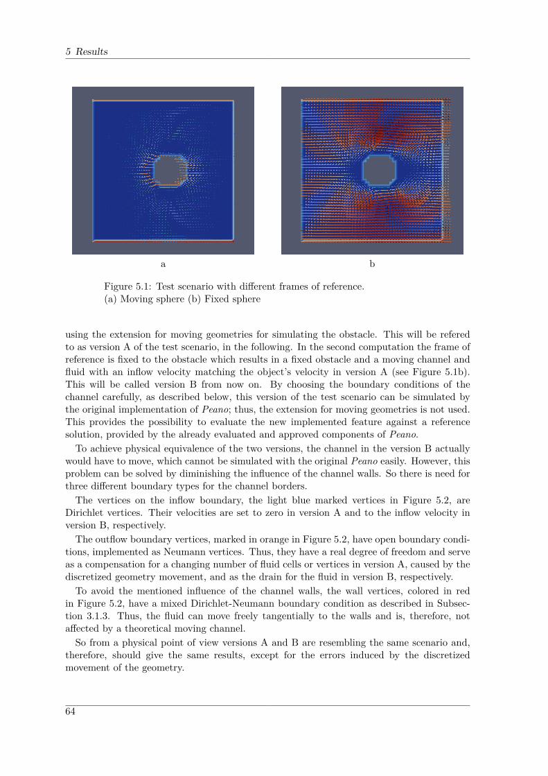
5 Results
a b
Figure 5.1: Test scenario with different frames of reference.(a) Moving sphere (b) Fixed sphere
using the extension for moving geometries for simulating the obstacle. This will be referedto as version A of the test scenario, in the following. In the second computation the frame ofreference is fixed to the obstacle which results in a fixed obstacle and a moving channel andfluid with an inflow velocity matching the object’s velocity in version A (see Figure 5.1b).This will be called version B from now on. By choosing the boundary conditions of thechannel carefully, as described below, this version of the test scenario can be simulated bythe original implementation of Peano; thus, the extension for moving geometries is not used.This provides the possibility to evaluate the new implemented feature against a referencesolution, provided by the already evaluated and approved components of Peano.To achieve physical equivalence of the two versions, the channel in the version B actually
would have to move, which cannot be simulated with the original Peano easily. However, thisproblem can be solved by diminishing the influence of the channel walls. So there is need forthree different boundary types for the channel borders.The vertices on the inflow boundary, the light blue marked vertices in Figure 5.2, are
Dirichlet vertices. Their velocities are set to zero in version A and to the inflow velocity inversion B, respectively.The outflow boundary vertices, marked in orange in Figure 5.2, have open boundary condi-
tions, implemented as Neumann vertices. Thus, they have a real degree of freedom and serveas a compensation for a changing number of fluid cells or vertices in version A, caused by thediscretized geometry movement, and as the drain for the fluid in version B, respectively.To avoid the mentioned influence of the channel walls, the wall vertices, colored in red
in Figure 5.2, have a mixed Dirichlet-Neumann boundary condition as described in Subsec-tion 3.1.3. Thus, the fluid can move freely tangentially to the walls and is, therefore, notaffected by a theoretical moving channel.So from a physical point of view versions A and B are resembling the same scenario and,
therefore, should give the same results, except for the errors induced by the discretizedmovement of the geometry.
64
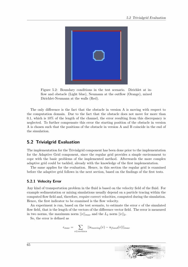
5.2 Trivialgrid Evaluation
Figure 5.2: Boundary conditions in the test scenario. Dirichlet at in-flow and obstacle (Light blue), Neumann at the outflow (Orange), mixedDirichlet-Neumann at the walls (Red).
The only difference is the fact that the obstacle in version A is moving with respect tothe computation domain. Due to the fact that the obstacle does not move for more than0.1, which is 10% of the length of the channel, the error resulting from this discrepancy isneglected. To further compensate this error the starting position of the obstacle in versionA is chosen such that the positions of the obstacle in version A and B coincide in the end ofthe simulation.
5.2 Trivialgrid EvaluationThe implementation for the Trivialgrid component has been done prior to the implementationfor the Adaptive Grid component, since the regular grid provides a simple environment tocope with the basic problems of the implemented method. Afterwards the more complexadaptive grid could be tackled, already with the knowledge of the first implementation.The same applies for the evaluation. Hence, in this section the regular grid is examined
before the adaptive grid follows in the next section, based on the findings of the first tests.
5.2.1 Velocity Error
Any kind of transportation problem in the fluid is based on the velocity field of the fluid. Forexample sedimentation or mixing simulations usually depend on a particle tracing within thecomputed flow field and, therefore, require correct velocities, computed during the simulation.Hence, the first indicator to be examined is the flow velocity.An experiment is run, based on the test scenario, to estimate the error e of the simulated
flow field, that is the length of the vectors of the difference vector field. The error is measuredin two norms, the maximum norm ||e||max and the L2 norm ||e||2.So, the error is defined as
εmax =∑
v∈vertices||umoving(v)− ufixed(v)||max
65
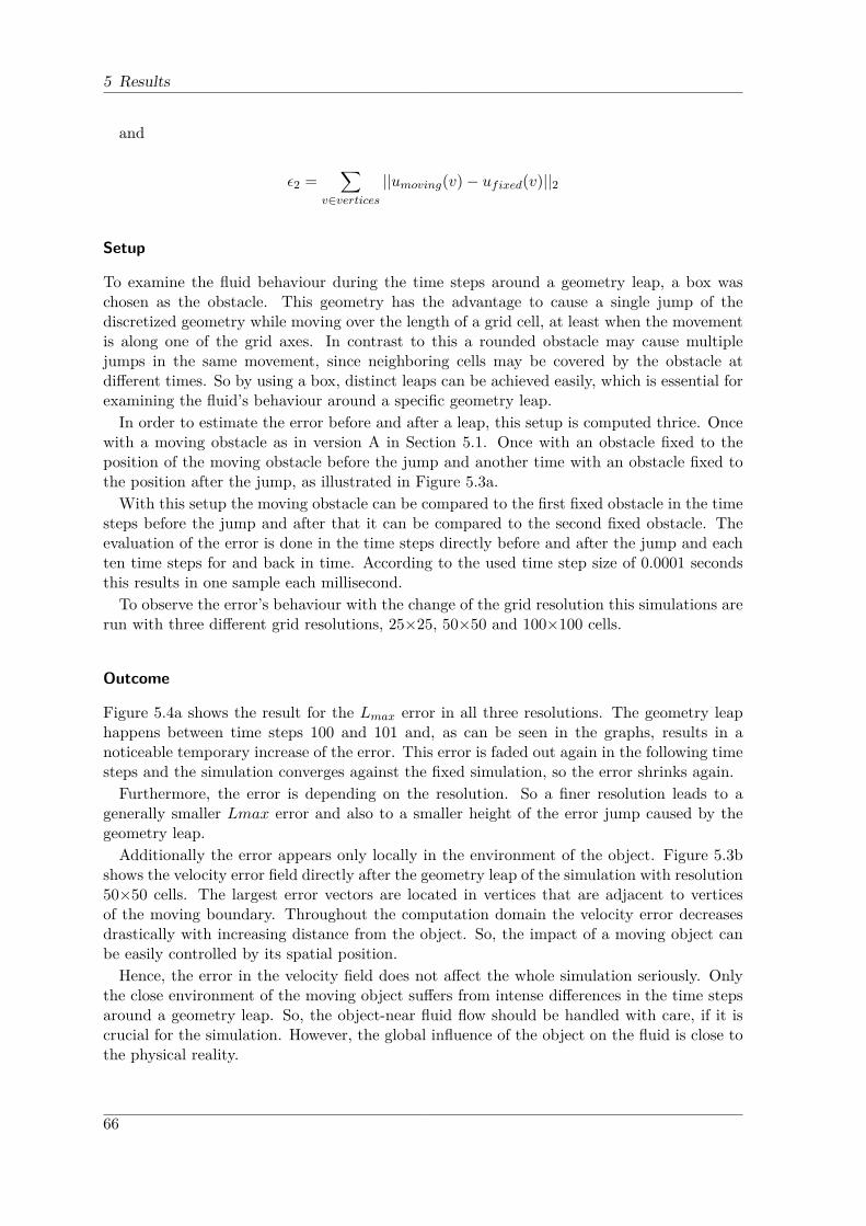
5 Results
and
ε2 =∑
v∈vertices||umoving(v)− ufixed(v)||2
Setup
To examine the fluid behaviour during the time steps around a geometry leap, a box waschosen as the obstacle. This geometry has the advantage to cause a single jump of thediscretized geometry while moving over the length of a grid cell, at least when the movementis along one of the grid axes. In contrast to this a rounded obstacle may cause multiplejumps in the same movement, since neighboring cells may be covered by the obstacle atdifferent times. So by using a box, distinct leaps can be achieved easily, which is essential forexamining the fluid’s behaviour around a specific geometry leap.In order to estimate the error before and after a leap, this setup is computed thrice. Once
with a moving obstacle as in version A in Section 5.1. Once with an obstacle fixed to theposition of the moving obstacle before the jump and another time with an obstacle fixed tothe position after the jump, as illustrated in Figure 5.3a.With this setup the moving obstacle can be compared to the first fixed obstacle in the time
steps before the jump and after that it can be compared to the second fixed obstacle. Theevaluation of the error is done in the time steps directly before and after the jump and eachten time steps for and back in time. According to the used time step size of 0.0001 secondsthis results in one sample each millisecond.To observe the error’s behaviour with the change of the grid resolution this simulations are
run with three different grid resolutions, 25×25, 50×50 and 100×100 cells.
Outcome
Figure 5.4a shows the result for the Lmax error in all three resolutions. The geometry leaphappens between time steps 100 and 101 and, as can be seen in the graphs, results in anoticeable temporary increase of the error. This error is faded out again in the following timesteps and the simulation converges against the fixed simulation, so the error shrinks again.Furthermore, the error is depending on the resolution. So a finer resolution leads to a
generally smaller Lmax error and also to a smaller height of the error jump caused by thegeometry leap.Additionally the error appears only locally in the environment of the object. Figure 5.3b
shows the velocity error field directly after the geometry leap of the simulation with resolution50×50 cells. The largest error vectors are located in vertices that are adjacent to verticesof the moving boundary. Throughout the computation domain the velocity error decreasesdrastically with increasing distance from the object. So, the impact of a moving object canbe easily controlled by its spatial position.Hence, the error in the velocity field does not affect the whole simulation seriously. Only
the close environment of the moving object suffers from intense differences in the time stepsaround a geometry leap. So, the object-near fluid flow should be handled with care, if it iscrucial for the simulation. However, the global influence of the object on the fluid is close tothe physical reality.
66
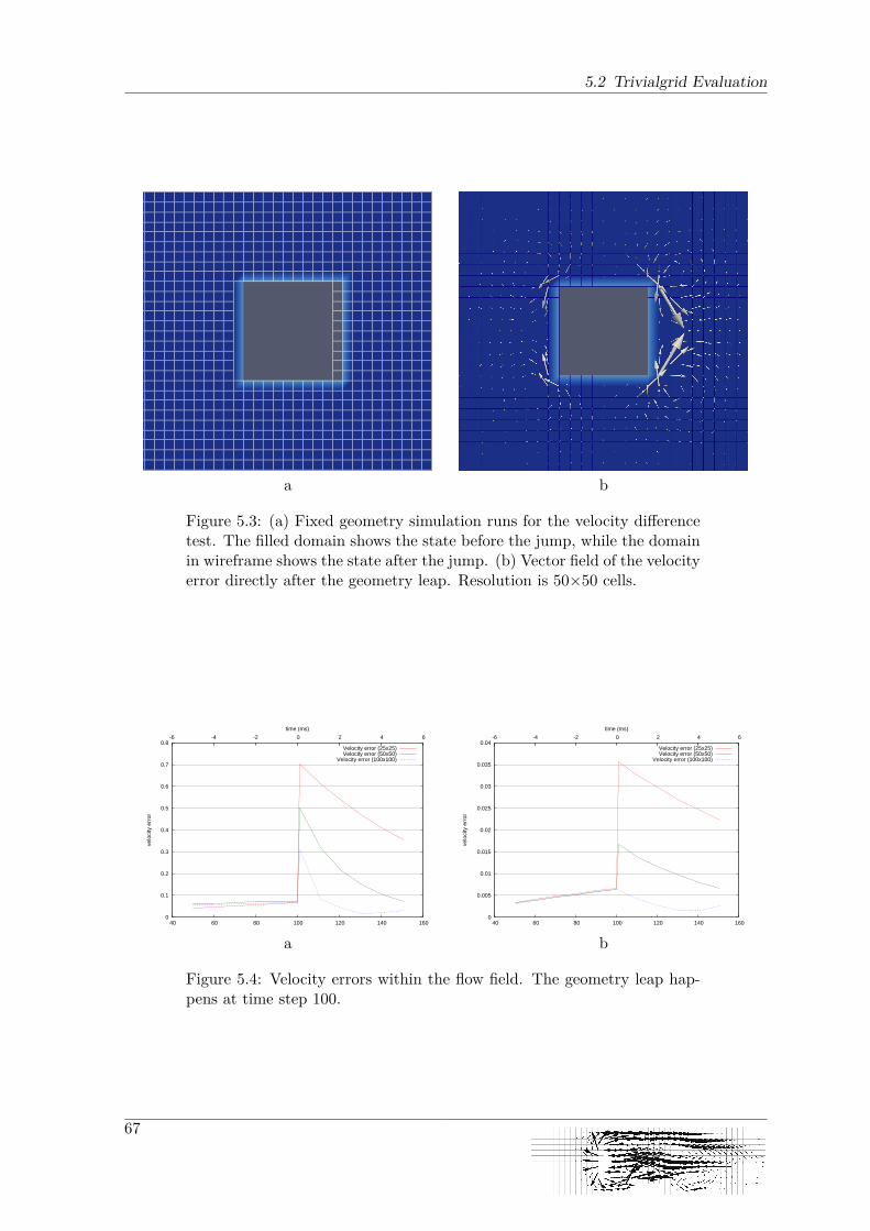
5.2 Trivialgrid Evaluation
a b
Figure 5.3: (a) Fixed geometry simulation runs for the velocity differencetest. The filled domain shows the state before the jump, while the domainin wireframe shows the state after the jump. (b) Vector field of the velocityerror directly after the geometry leap. Resolution is 50×50 cells.
0
0.1
0.2
0.3
0.4
0.5
0.6
0.7
0.8
40 60 80 100 120 140 160
-6 -4 -2 0 2 4 6
velo
city
err
or
time (ms)
Velocity error (25x25)Velocity error (50x50)
Velocity error (100x100)
a
0
0.005
0.01
0.015
0.02
0.025
0.03
0.035
0.04
40 60 80 100 120 140 160
-6 -4 -2 0 2 4 6
velo
city
err
or
time (ms)
Velocity error (25x25)Velocity error (50x50)
Velocity error (100x100)
b
Figure 5.4: Velocity errors within the flow field. The geometry leap hap-pens at time step 100.
67
5 Results
5.2.2 Flow Resistance
Since the error of the discretized movement only shows up close to the moving object, theimpact of it on the object has to be examined further. Especially with regard to a possibleFSI coupling, the force applied on the object by the flow resistance of the fluid is importantfor the simulation. Large errors in this value could make it virtually impossible to performaccurate FSI simulations. Hence, in the following the flow resistance of the moving object ischosen as the indicator for the quality of the simulation. More effort has been put into theseexaminations than into the previous tests for the fluid’s velocity field. The reason for thisdiscrepancy is that FSI simulations will probably be the main field of application for movingboundaries.In the tests in this subsection again a linear movement is used that is aligned to the x0
axis and the obstacle is centered in the channel in x1 direction. Thus, the drag force, i.e. theforce component in x0 direction is dominant over the lift component in x1 direction, so onlythe drag component is used as the indicator.To be precise the error of the drag component is the actual indicator which is computed as
the difference between the drag force resulting from the moving obstacle simulation f(t)movingand the force of the fixed one f(t)fixed, i.e. ε(t) = f(t)moving − f(t)fixed.
Box in fluid
As in the test scenario for the flow field, a box was chosen for the test of the flow resistance.The advantage hereby again is the simplicity of the geometry and, therefore, the simplicity ofthe resulting forces. The scenario is virtually identical with the scenario used in the resistancetest but it is computed only twice, once with the moving obstacle, once with the fixed one.To get a simulation as simple as possible, the box was adjusted to the grid; thus, it keeps thesame size throughout all used resolutions and over the whole simulation time that reachesover 50 milliseconds, simulated in 2000 time steps. Hence, there are no separated leaps forthe front and the back side of the box as it would happen if the box was not adjusted to thegrid size. So the elongation and the shortening of the box, caused by the discretization ofthe geometry, happen in the same time step.Figure 5.5 shows the resulting forces. In these plots the geometry leaps can be found as
discontinuities in the drag force. Since the boxes are moving with the same speed in allresolutions, more leaps happen in simulations with a finer resolution, due to the smallermesh width. Hence, in a given interval of time step 321 to time step 1221 (excluded) oneleap happens in the coarsest resolution (Figure 5.5a), while with each bisection of the meshwidth the number of leaps is doubled (Figure 5.5b and following).In the time steps following a geometry leap the induced force error is damped out. Thus, in
the time between two leaps, the simulation, using a moving obstacle, approaches quite closeto the fixed obstacle simulation regarding the drag force. So the geometry leaps do not causea permanent error in the system but an error that vanishes rapidly after the leap, if there isenough time until the next change of the grid. This will be further discussed later on, wherespheres lead to more frequent geometry leaps.Another finding is, that the discontinuities in Figure 5.5d can hardly be seen, so a depen-
dency of the force error on the grid resolution seems to be obvious. To confirm this theory therelative integrated force error is to be examined. That means the force error of one resolutionis integrated over time, beginning with the first leap in Figure 5.5a, that happens at timestep 321, until the end of the simulation period. This results in the impulse error that is
68
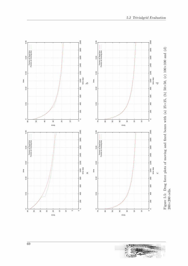
5.2 Trivialgrid Evaluation
0 5 10
15
20
25
30
35
40
0 2
00 4
00 6
00 8
00 1
000
120
0 1
400
160
0 1
800
200
0
0 0
.01
0.0
2 0
.03
0.0
4 0
.05
force
time
step
time
For
ces
on fi
xed
box
For
ces
on m
ovin
g bo
x
a
0 10
20
30
40
50
60
0 2
00 4
00 6
00 8
00 1
000
120
0 1
400
160
0 1
800
200
0
0 0
.01
0.0
2 0
.03
0.0
4 0
.05
force
time
step
time
For
ces
on fi
xed
box
For
ces
on m
ovin
g bo
x
b
0 10
20
30
40
50
60
70
0 2
00 4
00 6
00 8
00 1
000
120
0 1
400
160
0 1
800
200
0
0 0
.01
0.0
2 0
.03
0.0
4 0
.05
force
time
step
time
For
ces
on fi
xed
box
For
ces
on m
ovin
g bo
x
c
0 10
20
30
40
50
60
70
0 2
00 4
00 6
00 8
00 1
000
120
0 1
400
160
0 1
800
200
0
0 0
.01
0.0
2 0
.03
0.0
4 0
.05
force
time
step
time
For
ces
on fi
xed
box
For
ces
on m
ovin
g bo
x
d
Figu
re5.5:
Dragforceplotsof
movingan
dfix
edbo
xeswith
(a)25×25
,(b)50×50
,(c)10
0×10
0an
d(d)
200×
200cells.
69
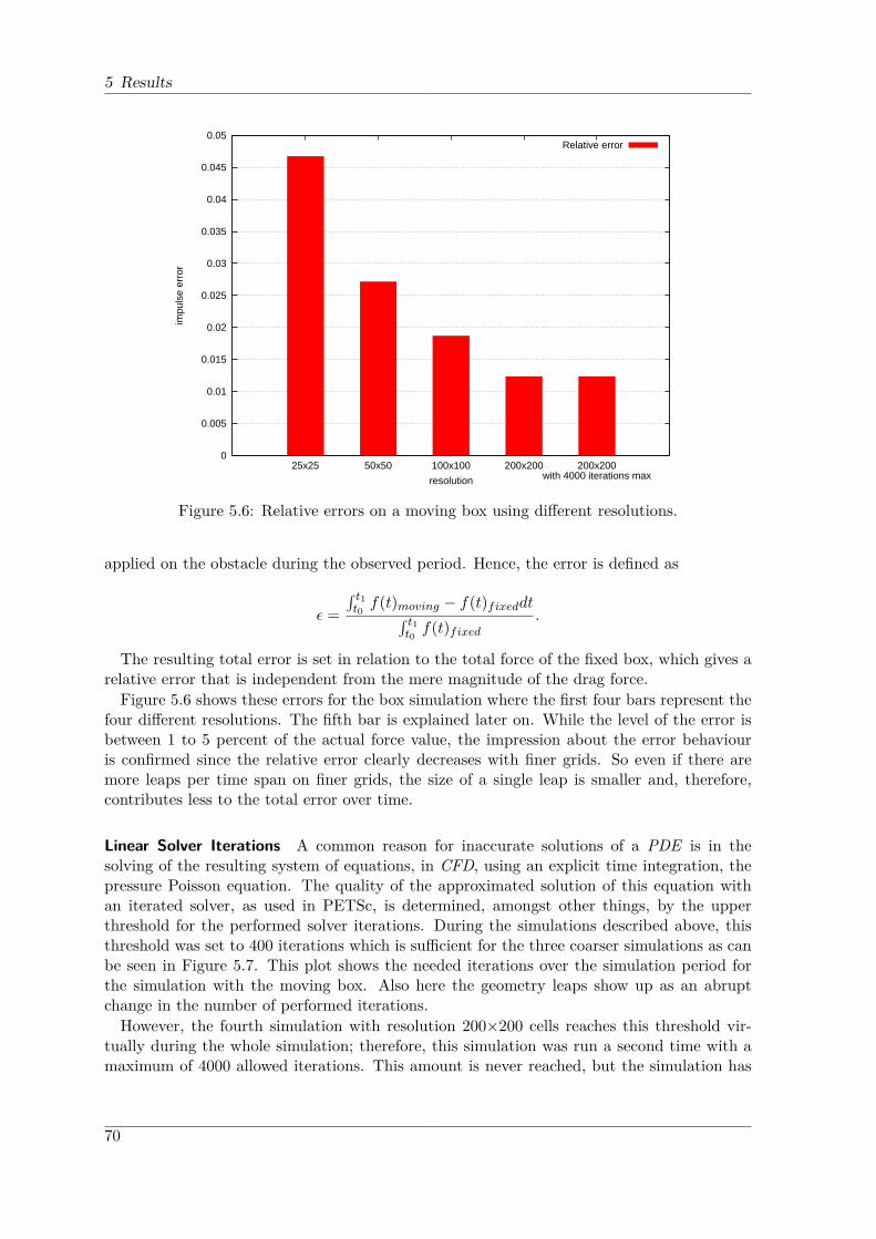
5 Results
0
0.005
0.01
0.015
0.02
0.025
0.03
0.035
0.04
0.045
0.05
25x25 50x50 100x100 200x200 200x200with 4000 iterations max
impu
lse
erro
r
resolution
Relative error
Figure 5.6: Relative errors on a moving box using different resolutions.
applied on the obstacle during the observed period. Hence, the error is defined as
ε =∫ t1t0f(t)moving − f(t)fixeddt∫ t1
t0f(t)fixed
.
The resulting total error is set in relation to the total force of the fixed box, which gives arelative error that is independent from the mere magnitude of the drag force.Figure 5.6 shows these errors for the box simulation where the first four bars represent the
four different resolutions. The fifth bar is explained later on. While the level of the error isbetween 1 to 5 percent of the actual force value, the impression about the error behaviouris confirmed since the relative error clearly decreases with finer grids. So even if there aremore leaps per time span on finer grids, the size of a single leap is smaller and, therefore,contributes less to the total error over time.
Linear Solver Iterations A common reason for inaccurate solutions of a PDE is in thesolving of the resulting system of equations, in CFD, using an explicit time integration, thepressure Poisson equation. The quality of the approximated solution of this equation withan iterated solver, as used in PETSc, is determined, amongst other things, by the upperthreshold for the performed solver iterations. During the simulations described above, thisthreshold was set to 400 iterations which is sufficient for the three coarser simulations as canbe seen in Figure 5.7. This plot shows the needed iterations over the simulation period forthe simulation with the moving box. Also here the geometry leaps show up as an abruptchange in the number of performed iterations.However, the fourth simulation with resolution 200×200 cells reaches this threshold vir-
tually during the whole simulation; therefore, this simulation was run a second time with amaximum of 4000 allowed iterations. This amount is never reached, but the simulation has
70
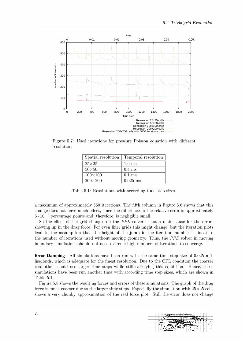
5.2 Trivialgrid Evaluation
0
100
200
300
400
500
600
0 200 400 600 800 1000 1200 1400 1600 1800 2000
0 0.01 0.02 0.03 0.04 0.05
num
ber
of it
erat
ions
time step
time
Resolution 25x25 cellsResolution 50x50 cells
Resolution 100x100 cellsResolution 200x200 cells
Resolution 200x200 cells with 4000 iterations max
Figure 5.7: Used iterations for pressure Poisson equation with differentresolutions.
Spatial resolution Temporal resolution25×25 1.6 ms50×50 0.4 ms100×100 0.1 ms200×200 0.025 ms
Table 5.1: Resolutions with according time step sizes.
a maximum of approximately 560 iterations. The fifth column in Figure 5.6 shows that thischange does not have much effect, since the difference in the relative error is approximately6 · 10−7 percentage points and, therefore, is negligible small.So the effect of the grid changes on the PPE solver is not a main cause for the errors
showing up in the drag force. For even finer grids this might change, but the iteration plotslead to the assumption that the height of the jump in the iteration number is linear tothe number of iterations used without moving geometry. Thus, the PPE solver in movingboundary simulations should not need extreme high numbers of iterations to converge.
Error Damping All simulations have been run with the same time step size of 0.025 mil-liseconds, which is adequate for the finest resolution. Due to the CFL condition the coarserresolutions could use larger time steps while still satisfying this condition. Hence, thesesimulations have been run another time with according time step sizes, which are shown inTable 5.1.Figure 5.8 shows the resulting forces and errors of these simulations. The graph of the drag
force is much coarser due to the larger time steps. Especially the simulation with 25×25 cellsshows a very chunky approximation of the real force plot. Still the error does not change
71
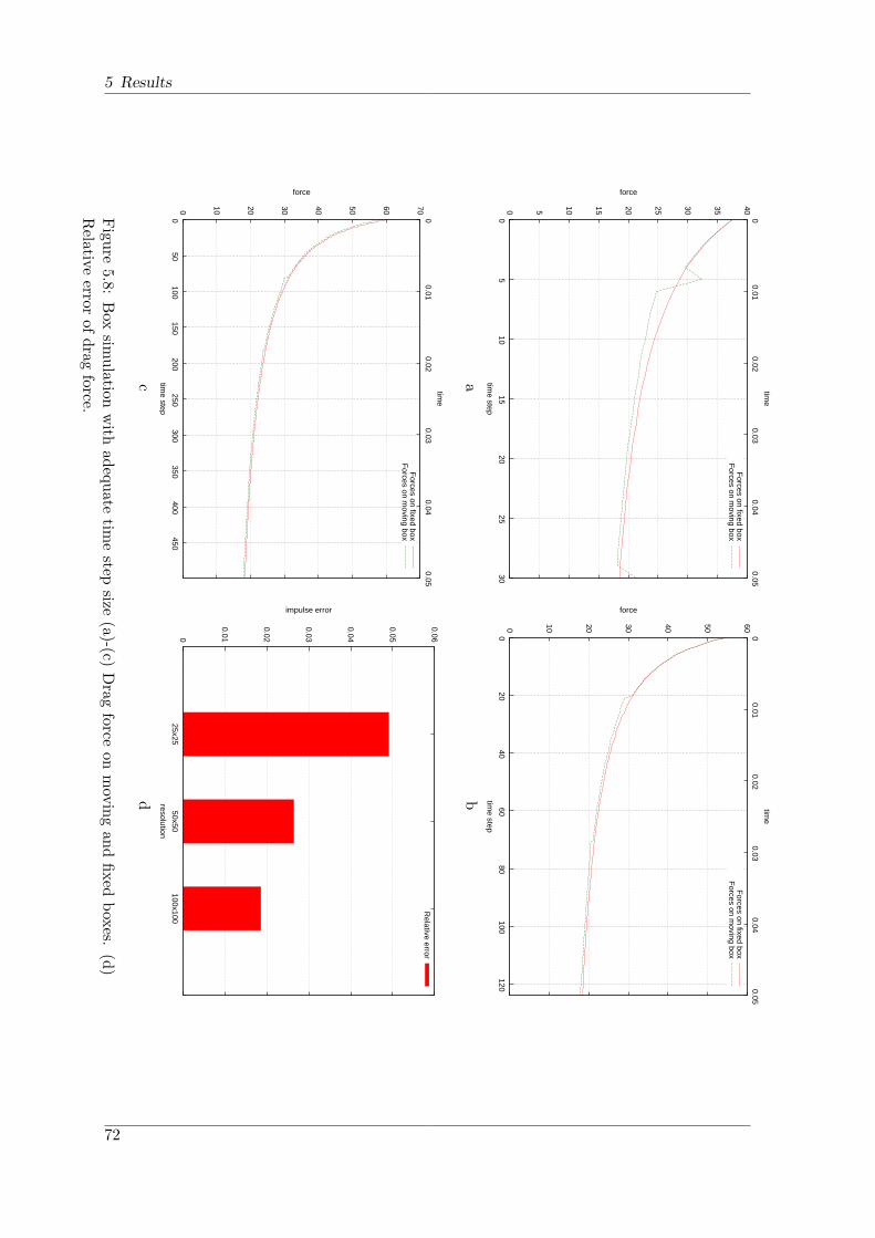
5 Results
0 5
10
15
20
25
30
35
40
0 5
10 15
20 25
30
0 0.01
0.02 0.03
0.04 0.05
force
time step
time
Forces on fixed box
Forces on m
oving box
a
0
10
20
30
40
50
60
0 20
40 60
80 100
120
0 0.01
0.02 0.03
0.04 0.05
force
time step
time
Forces on fixed box
Forces on m
oving box
b
0
10
20
30
40
50
60
70
0 50
100 150
200 250
300 350
400 450
0 0.01
0.02 0.03
0.04 0.05
force
time step
time
Forces on fixed box
Forces on m
oving box
c
0
0.01
0.02
0.03
0.04
0.05
0.06
25x2550x50
100x100
impulse error
resolution
Relative error
d
Figure5.8:
Box
simulation
with
adequatetim
estep
size(a)-(c)
Drag
forceon
moving
andfixed
boxes.(d)
Relative
errorofdrag
force.
72
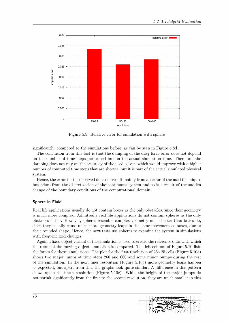
5.2 Trivialgrid Evaluation
0
0.005
0.01
0.015
0.02
0.025
0.03
0.035
0.04
25x25 50x50 100x100
impu
lse
erro
r
resolution
Relative error
Figure 5.9: Relative error for simulation with sphere
significantly, compared to the simulations before, as can be seen in Figure 5.8d.The conclusion from this fact is that the damping of the drag force error does not depend
on the number of time steps performed but on the actual simulation time. Therefore, thedamping does not rely on the accuracy of the used solver, which would improve with a highernumber of computed time steps that are shorter, but it is part of the actual simulated physicalsystem.Hence, the error that is observed does not result mainly from an error of the used techniques
but arises from the discretization of the continuous system and so is a result of the suddenchange of the boundary conditions of the computational domain.
Sphere in Fluid
Real life applications usually do not contain boxes as the only obstacles, since their geometryis much more complex. Admittedly real life applications do not contain spheres as the onlyobstacles either. However, spheres resemble complex geometry much better than boxes do,since they usually cause much more geometry leaps in the same movement as boxes, due totheir rounded shape. Hence, the next tests use spheres to examine the system in simulationswith frequent grid changes.Again a fixed object variant of the simulation is used to create the reference data with which
the result of the moving object simulation is compared. The left column of Figure 5.10 liststhe forces for these simulations. The plot for the first resolution of 25×25 cells (Figure 5.10a)shows two major jumps at time steps 260 and 660 and some minor bumps during the restof the simulation. In the next finer resolution (Figure 5.10c) more geometry leaps happenas expected, but apart from that the graphs look quite similar. A difference in this patternshows up in the finest resolution (Figure 5.10e). While the height of the major jumps donot shrink significantly from the first to the second resolution, they are much smaller in this
73
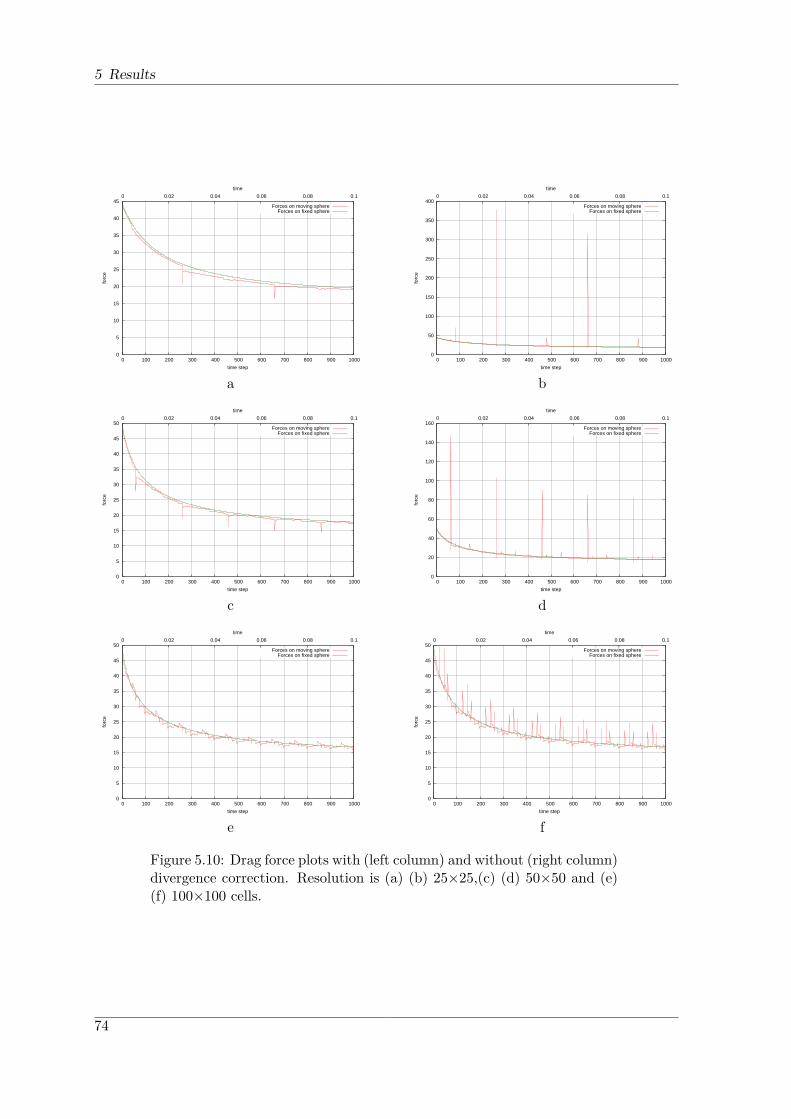
5 Results
0
5
10
15
20
25
30
35
40
45
0 100 200 300 400 500 600 700 800 900 1000
0 0.02 0.04 0.06 0.08 0.1
forc
e
time step
time
Forces on moving sphereForces on fixed sphere
a
0
50
100
150
200
250
300
350
400
0 100 200 300 400 500 600 700 800 900 1000
0 0.02 0.04 0.06 0.08 0.1
forc
e
time step
time
Forces on moving sphereForces on fixed sphere
b
0
5
10
15
20
25
30
35
40
45
50
0 100 200 300 400 500 600 700 800 900 1000
0 0.02 0.04 0.06 0.08 0.1
forc
e
time step
time
Forces on moving sphereForces on fixed sphere
c
0
20
40
60
80
100
120
140
160
0 100 200 300 400 500 600 700 800 900 1000
0 0.02 0.04 0.06 0.08 0.1fo
rce
time step
time
Forces on moving sphereForces on fixed sphere
d
0
5
10
15
20
25
30
35
40
45
50
0 100 200 300 400 500 600 700 800 900 1000
0 0.02 0.04 0.06 0.08 0.1
forc
e
time step
time
Forces on moving sphereForces on fixed sphere
e
0
5
10
15
20
25
30
35
40
45
50
0 100 200 300 400 500 600 700 800 900 1000
0 0.02 0.04 0.06 0.08 0.1
forc
e
time step
time
Forces on moving sphereForces on fixed sphere
f
Figure 5.10: Drag force plots with (left column) and without (right column)divergence correction. Resolution is (a) (b) 25×25,(c) (d) 50×50 and (e)(f) 100×100 cells.
74

5.2 Trivialgrid Evaluation
third one. Instead of that the minor jumps increase in size, which yields a very unsteadygraph. Apparently the reason for this is that the geometry leaps happen very frequently,so the errors induced into the system interfere with each other. Thus, the decay periods ofseveral jumps overlap and produce an even larger deviance from the reference solution.In Figure 5.9 this fact also appears. While the error decreases from the first to the second
simulation, it even increases again in the third. So in the second simulation the smaller errorinduced by a single geometry leap leads to a smaller overall error. But in the third simulationthe errors accumulate, since one is not totally damped out when the next occurs. This effectexceeds the benefit of the again smaller single errors and leads to a larger relative error,compared to the second simulation.This is a problematic finding since it may be a serious issue in simulations with very frequent
geometry changes, so simulations with very high resolutions or fast moving objects. Furtherexaminations are done later on. Fine resolved simulations are performed in Section 5.3 whilehighspeed simulations are shown below in this subsection. Before this, another aspect of thesystem is evaluated.
Divergence Correction Section 3.4 presented a way to reduce the impact of the discretizedmovement of the geometry. The effect of this correction is tested with a scenario, simulatedagain in different resolutions but this time with a deactivated divergence correction in contrastto virtually all other tests run in this thesis.Figure 5.10 opposes the results of the simulations done with divergence correction to the
ones done without. The improved results in the left column show much lower jumps of theforce graph than the results computed without the divergence correction shown in the rightcolumn. However, these large force errors are cut down, to the level which they have withthe divergence correction, within one time step. This is due to the continuity equation thathas to be fulfilled after a fluid time step has been performed. So a geometry leap causes asingle large burst of the flow resistance force but the long time effect is much smaller.The question is, how eminent the benefit of the divergence correction actually is. For once
this burst in the drag force may have a negative impact on a coupled structure solver. Astrong acceleration may be applied to the structure. This acceleration lasts only for a shorttime, but it might cause a break of bonds in a fragile structure or may induce oscillationswithin the body, if such bursts happen quite frequently.Additionally, even if the force is cut down very fast, it still has a significant impact, at
least in coarse grid simulations, as shown in Figure 5.11. In the simulation with 25×25 cellsthe error is almost cut in half by the use of the divergence correction. However, this ratiodecreases with increasing grid resolution. In the finest simulation, with 100×100 cells, thebenefit is only around 20% relative to the error without divergence correction.Due to the computational overhead of the divergence correction it needs to be checked in
a simulation with fine resolved grids, whether this step should be used or not. Reducing theaccuracy by omitting the divergence correction can bring a benefit in performance and viceversa.
Viscosity By now the level of the reference force has remained about the same in all tests.Several aspects affect the force magnitude like the velocity of the flow and the shape or thesize of the obstacle. Another variable is the viscosity of the fluid. Since CFD simulations areperformed with very different settings for this variable, a test series has been set up to gatherinformation about the relative error in different cases.
75

5 Results
0
0.01
0.02
0.03
0.04
0.05
0.06
0.07
25x25 25x25w/o div corr
100x100 50x50w/o div corr
400x400 100x100w/o div corr
impu
lse
erro
r
resolution
Relative error
Figure 5.11: Relative error without divergence correction
0
0.005
0.01
0.015
0.02
0.025
0.03
1 5 11 16
impu
lse
erro
r
viscosity
Relative error
Figure 5.12: Relative error with different viscosities.
76

5.2 Trivialgrid Evaluation
0 5 10
15
20
25
30
35
40
45
50
0 1
00 2
00 3
00 4
00 5
00 6
00 7
00 8
00 9
00 1
000
0 0
.02
0.0
4 0
.06
0.0
8 0
.1
force
time
step
time
For
ces
on m
ovin
g sp
here
For
ces
on fi
xed
sphe
re
a
0 20
40
60
80
100
120
140
160
0 1
00 2
00 3
00 4
00 5
00 6
00 7
00 8
00 9
00 1
000
0 0
.02
0.0
4 0
.06
0.0
8 0
.1
force
time
step
time
For
ces
on m
ovin
g sp
here
For
ces
on fi
xed
sphe
re
b
0 50
100
150
200
250
0 1
00 2
00 3
00 4
00 5
00 6
00 7
00 8
00 9
00 1
000
0 0
.02
0.0
4 0
.06
0.0
8 0
.1
force
time
step
time
For
ces
on m
ovin
g sp
here
For
ces
on fi
xed
sphe
re
c
0 50
100
150
200
250
300
350
0 1
00 2
00 3
00 4
00 5
00 6
00 7
00 8
00 9
00 1
000
0 0
.02
0.0
4 0
.06
0.0
8 0
.1
force
time
step
time
For
ces
on m
ovin
g sp
here
For
ces
on fi
xed
sphe
re
d
Figu
re5.13
:Sp
here
influ
idwith
viscosity
(a)1,
(b)6,
(c)11
and(d)16
.
77
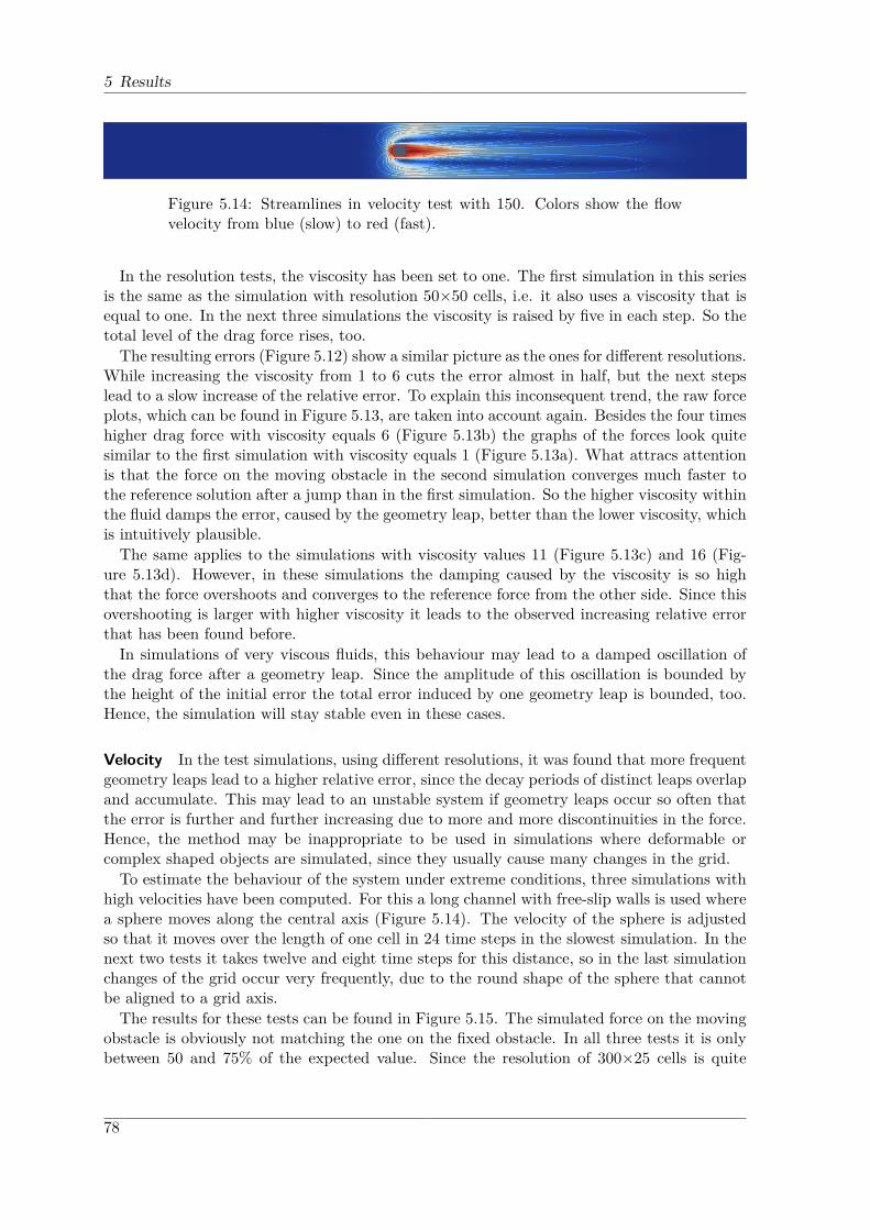
5 Results
Figure 5.14: Streamlines in velocity test with 150. Colors show the flowvelocity from blue (slow) to red (fast).
In the resolution tests, the viscosity has been set to one. The first simulation in this seriesis the same as the simulation with resolution 50×50 cells, i.e. it also uses a viscosity that isequal to one. In the next three simulations the viscosity is raised by five in each step. So thetotal level of the drag force rises, too.The resulting errors (Figure 5.12) show a similar picture as the ones for different resolutions.
While increasing the viscosity from 1 to 6 cuts the error almost in half, but the next stepslead to a slow increase of the relative error. To explain this inconsequent trend, the raw forceplots, which can be found in Figure 5.13, are taken into account again. Besides the four timeshigher drag force with viscosity equals 6 (Figure 5.13b) the graphs of the forces look quitesimilar to the first simulation with viscosity equals 1 (Figure 5.13a). What attracs attentionis that the force on the moving obstacle in the second simulation converges much faster tothe reference solution after a jump than in the first simulation. So the higher viscosity withinthe fluid damps the error, caused by the geometry leap, better than the lower viscosity, whichis intuitively plausible.The same applies to the simulations with viscosity values 11 (Figure 5.13c) and 16 (Fig-
ure 5.13d). However, in these simulations the damping caused by the viscosity is so highthat the force overshoots and converges to the reference force from the other side. Since thisovershooting is larger with higher viscosity it leads to the observed increasing relative errorthat has been found before.In simulations of very viscous fluids, this behaviour may lead to a damped oscillation of
the drag force after a geometry leap. Since the amplitude of this oscillation is bounded bythe height of the initial error the total error induced by one geometry leap is bounded, too.Hence, the simulation will stay stable even in these cases.
Velocity In the test simulations, using different resolutions, it was found that more frequentgeometry leaps lead to a higher relative error, since the decay periods of distinct leaps overlapand accumulate. This may lead to an unstable system if geometry leaps occur so often thatthe error is further and further increasing due to more and more discontinuities in the force.Hence, the method may be inappropriate to be used in simulations where deformable orcomplex shaped objects are simulated, since they usually cause many changes in the grid.To estimate the behaviour of the system under extreme conditions, three simulations with
high velocities have been computed. For this a long channel with free-slip walls is used wherea sphere moves along the central axis (Figure 5.14). The velocity of the sphere is adjustedso that it moves over the length of one cell in 24 time steps in the slowest simulation. In thenext two tests it takes twelve and eight time steps for this distance, so in the last simulationchanges of the grid occur very frequently, due to the round shape of the sphere that cannotbe aligned to a grid axis.The results for these tests can be found in Figure 5.15. The simulated force on the moving
obstacle is obviously not matching the one on the fixed obstacle. In all three tests it is onlybetween 50 and 75% of the expected value. Since the resolution of 300×25 cells is quite
78

5.2 Trivialgrid Evaluation
coarse, the first and the second simulation have been repeated with a resolution of 600×50cells. So now the sphere moves over one cell in twelve and six time steps, respectively. Theforce plots in Figure 5.16 show that the large error in the first runs results from the coarsegrid, since in these simulations the error is much smaller. However, the forces oscillate heavilyeven on the fine resolved grid. This is due to the very frequent grid changes. The assumption,made above, that the errors would accumulate and the system would become unstable arenot true, as can be easily seen in the plots.
5.2.3 Simulation in 3D
Conceptually the used approach is not limited to 2D simulations, but the implementation hasnot been tested in detail for 3D. However, one test has been run, simulating a sphere movingin a cubic channel. The scenario is shown in Figure 5.17, while the resulting forces for thefixed and the moving obstacle are plotted in Figure 5.18. Here a significant discrepancy canbe seen between the reference solution and the force on the moving sphere. This probablyresults from the coarse grid that is used.No further effort has been put into evaluating the behaviour of the system in three-
dimensional simulations. However, the made simulation shows that the method is actuallyworking in 3D.
5.2.4 Runtime Performance
As mentioned already, fluid simulation is time critical. Hence, a test has been made toestimate the impact of moving boundaries on the runtime performance. The test focuses ontwo aspects. First it examines the performance with respect to the frequency of grid changes,which is actually the main aspect. Additionally to that, the benefit of the staged processing,that is described in Subsection 3.6.1, is tested.All simulations during these test use a box as the obstacle, in a channel with a resolution
of 100×100 cells. Two sets of simulations are run, once with a speed of 25, the other timewith a speed of 10. This leads to a geometry leap every fourth time step in the first caseand every tenth time step in the second. In each set the scenario is simulated four times.The first time is used as a reference simulation. So it uses a fixed geometry and performs noadditional steps that are only necessary for moving geometries. Here the speed value is usedas the inflow velocity of the channel and no geometry leaps happen at all.The second run is performed with a naive implementation, where in every time step all
stages are performed: Grid update, solver creation and initialization and divergence correc-tion.This is also done in the third run, but here the divergence correction is omitted.Finally the fourth run performs the actual implementation, i.e. staged processing and
enabled divergence correction.The running times for 150 time steps in each simulation are shown in Figure 5.19. As ex-
pected, the flow velocity does not influence the performance of the fixed-geometry simulation.The naive implementation takes about twice the time, which results from the additional
adapter runs and the solving of the system of equations for the divergence correction. It isinteresting to see that these simulations actually depend on the frequency of the geometryleaps, even though they perform all steps in any case. The reason for this is the number ofused iterations for the divergence correction solver. While it converges very fast, when theflow field is divergence free already, it takes longer, if this is not the case.
79
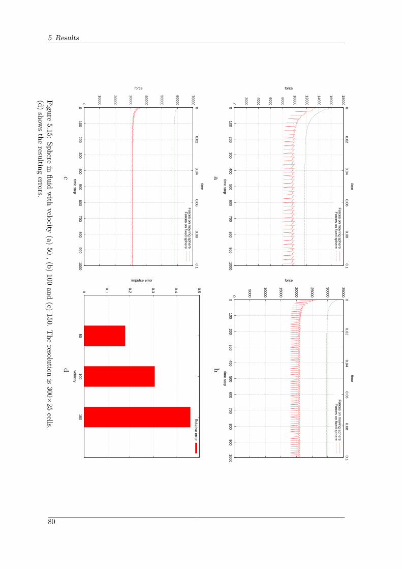
5 Results
0
2000
4000
6000
8000
10000
12000
14000
16000
18000
0 100
200 300
400 500
600 700
800 900
1000
0 0.02
0.04 0.06
0.08 0.1
force
time step
time
Forces on m
oving sphereF
orces on fixed sphere
a
0
5000
10000
15000
20000
25000
30000
35000
0 100
200 300
400 500
600 700
800 900
1000
0 0.02
0.04 0.06
0.08 0.1
force
time step
time
Forces on m
oving sphereF
orces on fixed sphere
b
0
10000
20000
30000
40000
50000
60000
70000
0 100
200 300
400 500
600 700
800 900
1000
0 0.02
0.04 0.06
0.08 0.1
force
time step
time
Forces on m
oving sphereF
orces on fixed sphere
c
0
0.1
0.2
0.3
0.4
0.5
50100
150
impulse error
velocity
Relative error
d
Figure5.15:
Spherein
fluidwith
velocity(a)
50,(b)
100and
(c)150.
The
resolutionis
300×25
cells.(d)
showsthe
resultingerrors.
80

5.2 Trivialgrid Evaluation
0
200
0
400
0
600
0
800
0
100
00
120
00
140
00
160
00
0 1
00 2
00 3
00 4
00 5
00 6
00 7
00 8
00 9
00 1
000
0 0
.02
0.0
4 0
.06
0.0
8 0
.1
force
time
step
time
For
ces
on m
ovin
g sp
here
For
ces
on fi
xed
sphe
re
a
0
500
0
100
00
150
00
200
00
250
00
300
00
350
00
0 1
00 2
00 3
00 4
00 5
00 6
00 7
00 8
00 9
00 1
000
0 0
.02
0.0
4 0
.06
0.0
8 0
.1
force
time
step
time
For
ces
on m
ovin
g sp
here
For
ces
on fi
xed
sphe
re
b
0
0.1
0.2
0.3
0.4
0.5
5010
0
impulse error
velo
city
Rel
ativ
e er
ror
c
Figu
re5.16
:Sp
here
influ
idwith
velocity
(a)50
and(b)10
0,usingaresolutio
nof
600×
50cells.
(c)show
stheresulting
errors.
81
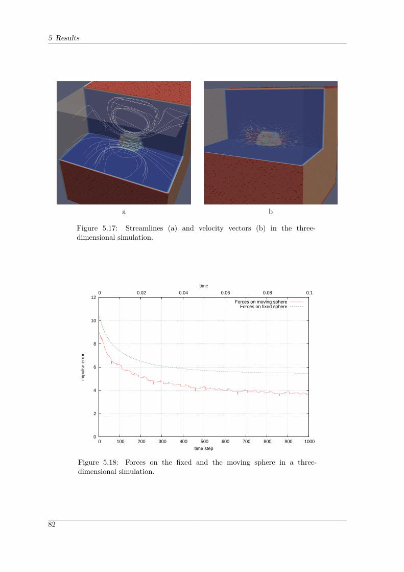
5 Results
a b
Figure 5.17: Streamlines (a) and velocity vectors (b) in the three-dimensional simulation.
0
2
4
6
8
10
12
0 100 200 300 400 500 600 700 800 900 1000
0 0.02 0.04 0.06 0.08 0.1
impu
lse
erro
r
time step
time
Forces on moving sphereForces on fixed sphere
Figure 5.18: Forces on the fixed and the moving sphere in a three-dimensional simulation.
82
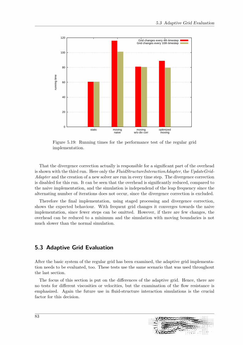
5.3 Adaptive Grid Evaluation
0
20
40
60
80
100
120
static movingnaive
movingw/o div corr
optimizedmoving
runn
ing
time
Grid changes every 4th timestepGrid changes every 10th timestep
Figure 5.19: Running times for the performance test of the regular gridimplementation.
That the divergence correction actually is responsible for a significant part of the overheadis shown with the third run. Here only the FluidStructureInteractionAdapter, the UpdateGrid-Adapter and the creation of a new solver are run in every time step. The divergence correctionis disabled for this run. It can be seen that the overhead is significantly reduced, compared tothe naive implementation, and the simulation is independend of the leap frequency since thealternating number of iterations does not occur, since the divergence correction is excluded.Therefore the final implementation, using staged processing and divergence correction,
shows the expected behaviour. With frequent grid changes it converges towards the naiveimplementation, since fewer steps can be omitted. However, if there are few changes, theoverhead can be reduced to a minimum and the simulation with moving boundaries is notmuch slower than the normal simulation.
5.3 Adaptive Grid Evaluation
After the basic system of the regular grid has been examined, the adaptive grid implementa-tion needs to be evaluated, too. These tests use the same scenario that was used throughoutthe last section.The focus of this section is put on the differences of the adaptive grid. Hence, there are
no tests for different viscosities or velocities, but the examination of the flow resistance isemphasized. Again the future use in fluid-structure interaction simulations is the crucialfactor for this decision.
83
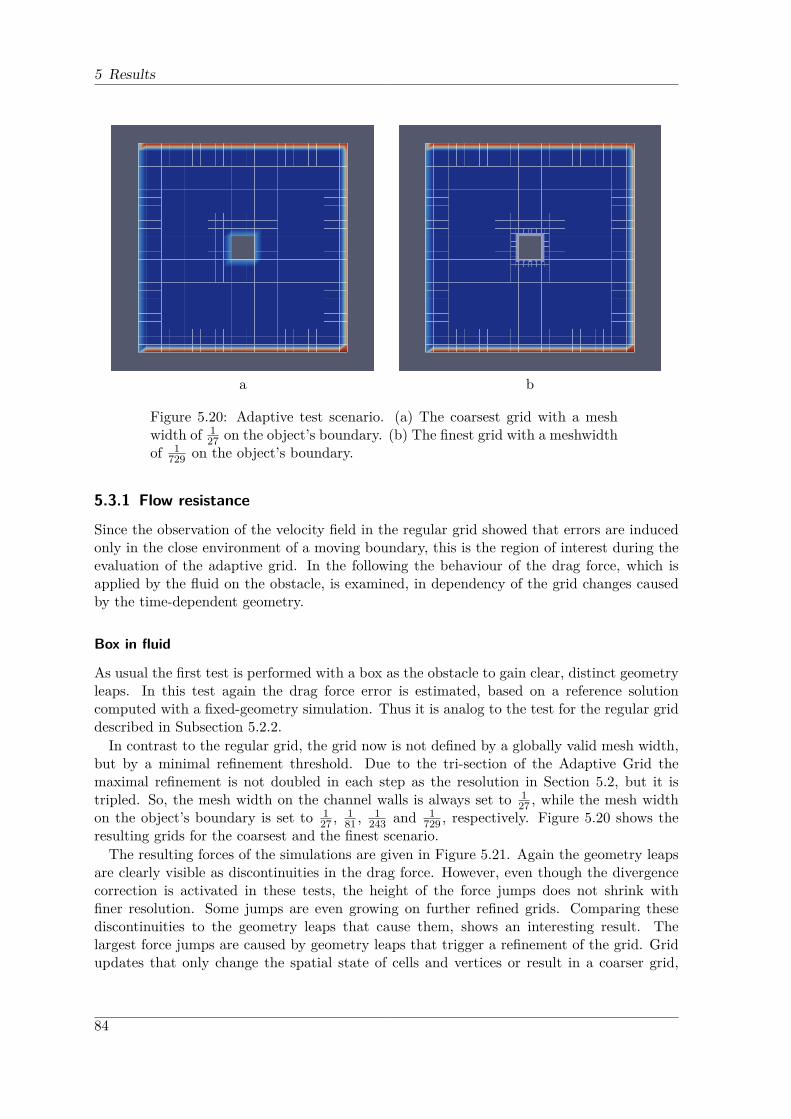
5 Results
a b
Figure 5.20: Adaptive test scenario. (a) The coarsest grid with a meshwidth of 1
27 on the object’s boundary. (b) The finest grid with a meshwidthof 1
729 on the object’s boundary.
5.3.1 Flow resistance
Since the observation of the velocity field in the regular grid showed that errors are inducedonly in the close environment of a moving boundary, this is the region of interest during theevaluation of the adaptive grid. In the following the behaviour of the drag force, which isapplied by the fluid on the obstacle, is examined, in dependency of the grid changes causedby the time-dependent geometry.
Box in fluid
As usual the first test is performed with a box as the obstacle to gain clear, distinct geometryleaps. In this test again the drag force error is estimated, based on a reference solutioncomputed with a fixed-geometry simulation. Thus it is analog to the test for the regular griddescribed in Subsection 5.2.2.In contrast to the regular grid, the grid now is not defined by a globally valid mesh width,
but by a minimal refinement threshold. Due to the tri-section of the Adaptive Grid themaximal refinement is not doubled in each step as the resolution in Section 5.2, but it istripled. So, the mesh width on the channel walls is always set to 1
27 , while the mesh widthon the object’s boundary is set to 1
27 ,181 ,
1243 and 1
729 , respectively. Figure 5.20 shows theresulting grids for the coarsest and the finest scenario.The resulting forces of the simulations are given in Figure 5.21. Again the geometry leaps
are clearly visible as discontinuities in the drag force. However, even though the divergencecorrection is activated in these tests, the height of the force jumps does not shrink withfiner resolution. Some jumps are even growing on further refined grids. Comparing thesediscontinuities to the geometry leaps that cause them, shows an interesting result. Thelargest force jumps are caused by geometry leaps that trigger a refinement of the grid. Gridupdates that only change the spatial state of cells and vertices or result in a coarser grid,
84
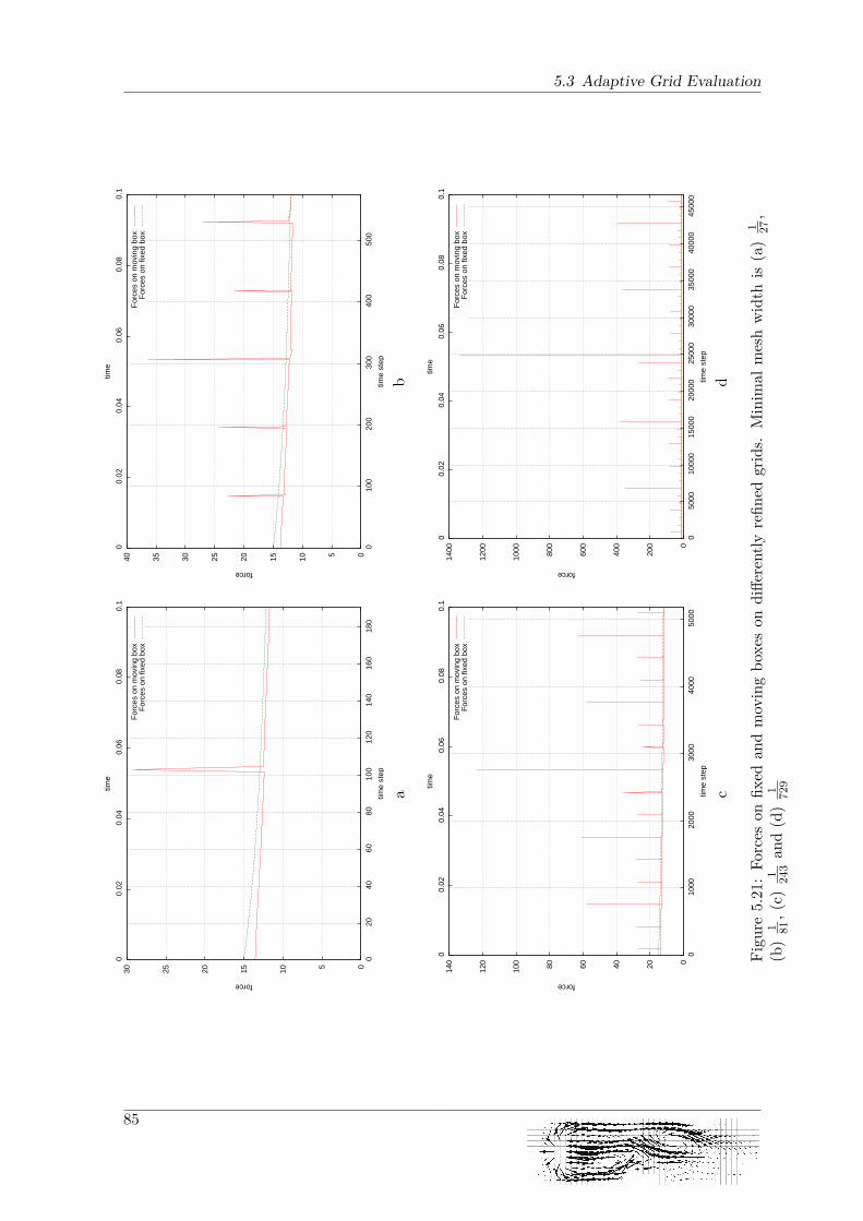
5.3 Adaptive Grid Evaluation
0 5 10
15
20
25
30
0 2
0 4
0 6
0 8
0 1
00 1
20 1
40 1
60 1
80
0 0
.02
0.0
4 0
.06
0.0
8 0
.1
force
time
step
time
For
ces
on m
ovin
g bo
xF
orce
s on
fixe
d bo
x
a
0 5 10
15
20
25
30
35
40
0 1
00 2
00 3
00 4
00 5
00
0 0
.02
0.0
4 0
.06
0.0
8 0
.1
force
time
step
time
For
ces
on m
ovin
g bo
xF
orce
s on
fixe
d bo
x
b
0 20
40
60
80
100
120
140
0 1
000
200
0 3
000
400
0 5
000
0 0
.02
0.0
4 0
.06
0.0
8 0
.1
force
time
step
time
For
ces
on m
ovin
g bo
xF
orce
s on
fixe
d bo
x
c
0
200
400
600
800
100
0
120
0
140
0
0 5
000
100
00 1
5000
200
00 2
5000
300
00 3
5000
400
00 4
5000
0 0
.02
0.0
4 0
.06
0.0
8 0
.1
force
time
step
time
For
ces
on m
ovin
g bo
xF
orce
s on
fixe
d bo
x
d
Figu
re5.21
:Fo
rces
onfix
edan
dmovingbo
xeson
diffe
rently
refin
edgrids.
Minim
almeshwidth
is(a)
1 27,
(b)
1 81,(c)
1 243an
d(d)
1 729
85
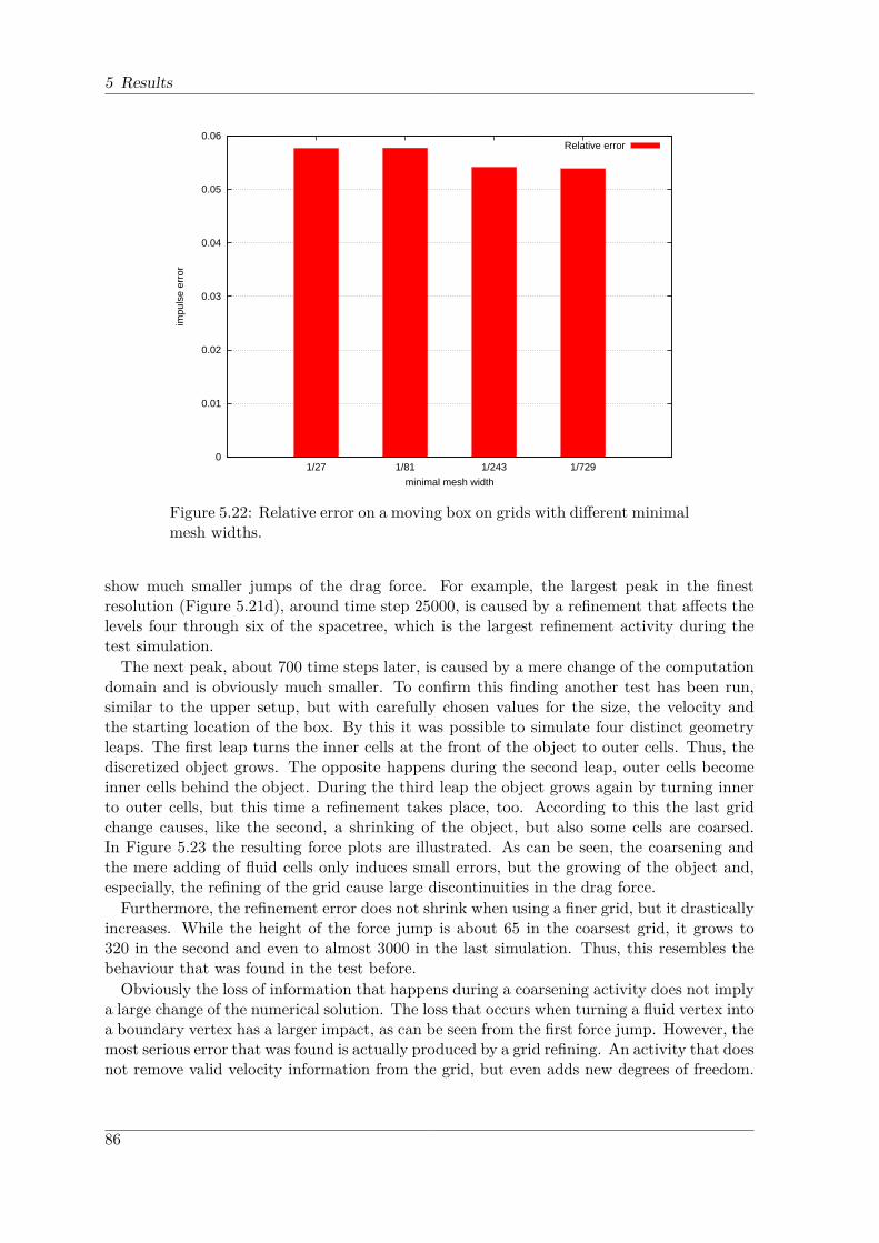
5 Results
0
0.01
0.02
0.03
0.04
0.05
0.06
1/27 1/81 1/243 1/729
impu
lse
erro
r
minimal mesh width
Relative error
Figure 5.22: Relative error on a moving box on grids with different minimalmesh widths.
show much smaller jumps of the drag force. For example, the largest peak in the finestresolution (Figure 5.21d), around time step 25000, is caused by a refinement that affects thelevels four through six of the spacetree, which is the largest refinement activity during thetest simulation.The next peak, about 700 time steps later, is caused by a mere change of the computation
domain and is obviously much smaller. To confirm this finding another test has been run,similar to the upper setup, but with carefully chosen values for the size, the velocity andthe starting location of the box. By this it was possible to simulate four distinct geometryleaps. The first leap turns the inner cells at the front of the object to outer cells. Thus, thediscretized object grows. The opposite happens during the second leap, outer cells becomeinner cells behind the object. During the third leap the object grows again by turning innerto outer cells, but this time a refinement takes place, too. According to this the last gridchange causes, like the second, a shrinking of the object, but also some cells are coarsed.In Figure 5.23 the resulting force plots are illustrated. As can be seen, the coarsening andthe mere adding of fluid cells only induces small errors, but the growing of the object and,especially, the refining of the grid cause large discontinuities in the drag force.Furthermore, the refinement error does not shrink when using a finer grid, but it drastically
increases. While the height of the force jump is about 65 in the coarsest grid, it grows to320 in the second and even to almost 3000 in the last simulation. Thus, this resembles thebehaviour that was found in the test before.Obviously the loss of information that happens during a coarsening activity does not imply
a large change of the numerical solution. The loss that occurs when turning a fluid vertex intoa boundary vertex has a larger impact, as can be seen from the first force jump. However, themost serious error that was found is actually produced by a grid refining. An activity that doesnot remove valid velocity information from the grid, but even adds new degrees of freedom.
86
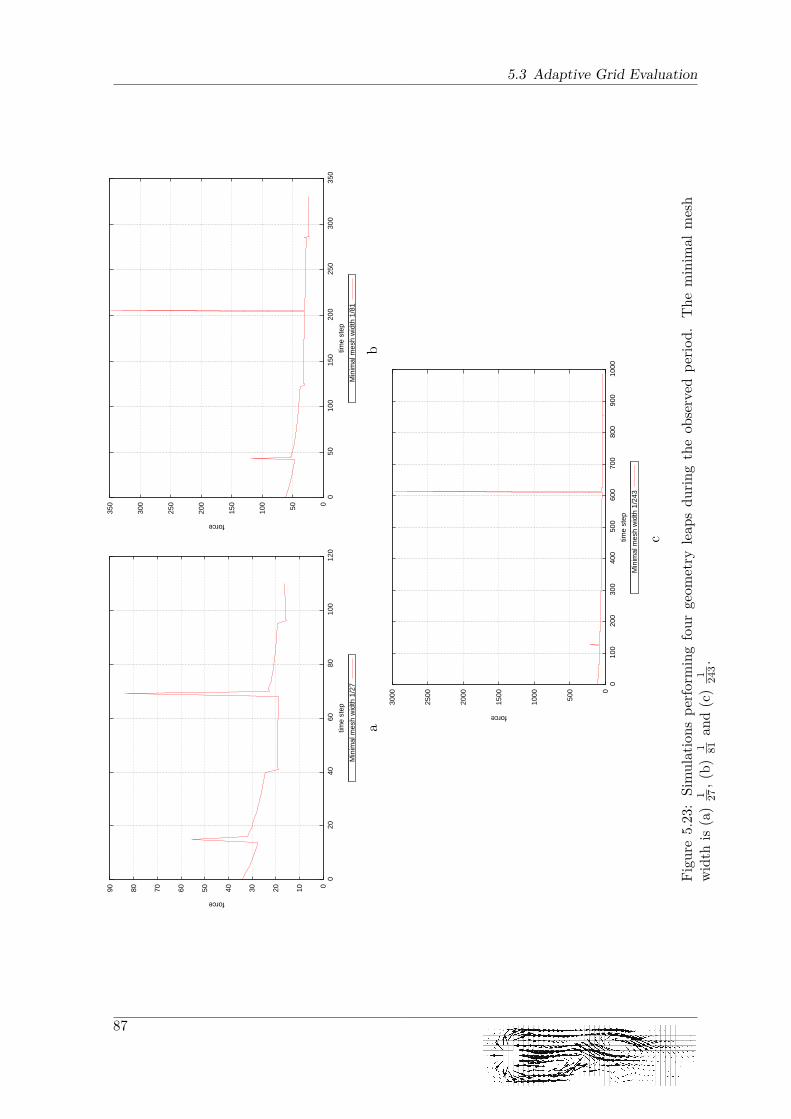
5.3 Adaptive Grid Evaluation
0 10
20
30
40
50
60
70
80
90
0 2
0 4
0 6
0 8
0 1
00 1
20
force
time
step
Min
imal
mes
h w
idth
1/2
7
a
0 50
100
150
200
250
300
350
0 5
0 1
00 1
50 2
00 2
50 3
00 3
50
force
time
step
Min
imal
mes
h w
idth
1/8
1
b
0
500
100
0
150
0
200
0
250
0
300
0
0 1
00 2
00 3
00 4
00 5
00 6
00 7
00 8
00 9
00 1
000
force
time
step
Min
imal
mes
h w
idth
1/2
43
c
Figu
re5.23
:Simulations
performingfour
geom
etry
leap
sdu
ringtheob
served
perio
d.The
minim
almesh
width
is(a)
1 27,(b)
1 81an
d(c)
1 243.
87
5 Results
However, these degrees of freedom have to be initialized. The reason for the large error canassumably be found in this initialization. As mentioned in Subsection 4.3.2 the initial valuesfor these vertices are interpolated from the supervertices. The used interpolation, however,does not guarantee the newly created cells to be divergence free. The resulting incorrectsolution of the Navier-Stokes equations is supposed to be the reason for the large impact of arefinement on the drag force. So this is actually a cause that can be reduced. Subsection 4.3.2also mentions that a divergence free interpolation can be obtained. This would assumablyreduce the error induced by a refinement.In total the results are still acceptable. Figure 5.22 shows the force errors integrated
over time, as described in Subsection 5.2.2. In contrast to the results for the regular grid therelative error does not decrease significantly on finer grids. However, it also does not increase,so in total a constant level of accuracy can be provided. Hence, with a better interpolationscheme the error will assumably show a similar behaviour as for the regular grid.
Sphere in fluid
Also for the adaptive grid the test scenario is simulated with a sphere as the obstacle, toexamine the system with non-aligned geometry. The layout of the test is analog to the testof the box, but only three different minimal mesh widths are simulated.As in the regular grid the simulations with the moving obstacle are run twice, once with
and once without the divergence correction. The results are illustrated in Figure 5.24 in thetwo-column layout as used in the regular grid section before.The left column contains the force plots of the simulations with activated divergence cor-
rection, while the right column shows the one without divergence correction. On the coarsestgrid (Figure 5.24a and Figure 5.24b) the height of the force discontinuities is considerablyreduced, i.e. the jumps are only half to two-thirds in size. Also in the second resolution abenefit of around 10–20% of the jump height is found.However, the same effect that was shown in the regular grid appears here also: The error
does not necessarily decrease with increasingly finer grids. In Figure 5.25 the integratederrors are shown, and here it is obvious that the first refinement results in a lower error,while the second causes an even slighlty higher error. This applies for both test series, withand without divergence correction.However, the errors do not tend to accumulate increasingly, hence it is unlikely that further
refinement will lead to an unbounded error and, thus, to an unstable system. Furthermore,the extreme jumps, caused by the refinement and coarsening activities, that have been foundin the box simulations before, are also found here. So assumably the error behaviour willalso improve with the divergence free interpolation scheme.
5.3.2 Runtime Performance
The implementation for the adaptive grid varies in several aspects from the one for the regulargrid. While the UpdateGridAdapter in the regular grid is only run once per time step, it maybe run more often in the adaptive grid, to finish all refinement or coarsening activities. Inaddition, this adapter contains more functionality due to the more complex state of the cellsand vertices in the adaptive grid. Hence, it takes more time to traverse the grid and, thus,may have a larger effect on the performance of the simulation.To examine the impact of moving boundaries on the runtime performance of the adaptive
grid, a similar test is used as for the regular grid in Subsection 5.2.4. Again there are four
88

5.3 Adaptive Grid Evaluation
0
5
10
15
20
25
30
35
40
45
50
0 20 40 60 80 100 120 140 160 180
0 0.02 0.04 0.06 0.08 0.1
forc
e
time step
time
Forces on moving sphereForces on fixed sphere
a
0
20
40
60
80
100
120
0 50 100 150 200 250
0 0.02 0.04 0.06 0.08 0.1
forc
e
time step
time
Forces on moving sphereForces on fixed sphere
b
0
10
20
30
40
50
60
0 100 200 300 400 500
0 0.02 0.04 0.06 0.08 0.1
forc
e
time step
time
Forces on moving sphereForces on fixed sphere
c
0
10
20
30
40
50
60
70
0 100 200 300 400 500
0 0.02 0.04 0.06 0.08 0.1
forc
e
time step
time
Forces on moving sphereForces on fixed sphere
d
0
50
100
150
200
250
300
350
400
450
0 1000 2000 3000 4000 5000
0 0.02 0.04 0.06 0.08 0.1
forc
e
time step
time
Forces on moving sphereForces on fixed sphere
e
0
50
100
150
200
250
300
350
400
450
500
0 1000 2000 3000 4000 5000
0 0.02 0.04 0.06 0.08 0.1
forc
e
time step
time
Forces on moving sphereForces on fixed sphere
f
Figure 5.24: Drag force plots with (left column) and without (right column)divergence correction. Minimal mesh width is (a) (b) 1
27 , (c) (d) 181 and
(e) (f) 1243 .
89

5 Results
0
0.01
0.02
0.03
0.04
0.05
0.06
0.07
0.08
0.09
1/27 1/27w/o div corr
1/243 1/81w/o div corr
1/2187 1/243w/o div corr
impu
lse
erro
r
resolution
Relative error
Figure 5.25: Relative error on a moving sphere on grids with differentminimal mesh widths. Always two bars represent the results for one meshwidth, but once with and once without divergence correction.
different layouts of the algorithm:
• Without any moving boundary and thus no grid changes,
• with a naive implementation doing all work in every time step,
• the naive implementation without the divergence correction and, finally,
• the actual implementation with the techniques for improving the performance.
These layouts are computed twice with different speeds of the object, or inflow velocitiesfor the channel in the run with static geometry. In the first pass the speed is set such thata geometry leap happens every fourth time step, while in the second pass a geometry leaphappens only every tenth time step. During the static-geometry simulations no geometryleaps occur, of course.Since the adaptive grid is more efficient for the same minimal mesh width, compared to the
regular grid, a different setup for the simulation was used. Still 150 time steps are simulated,but the minimal mesh width is 1
243 and not 1100 , while also the minimal mesh width along the
channel walls was reduced to 181 . The resulting running times are shown in Figure 5.26.
The most obvious fact is that the difference between the static geometry simulation andthe naive implementation is rather large. While the running time has been almost doubled inthe regular grid implementation, it grows almost to five times the running time of the staticsimulation in the adaptive grid.While comparing this to the third run it can be found that the divergence correction is
responsible for almost half of this amount. So this step and the adapter runs for updating
90
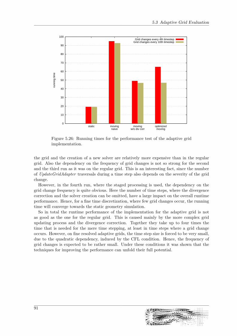
5.3 Adaptive Grid Evaluation
0
10
20
30
40
50
60
70
80
90
100
static movingnaive
movingw/o div corr
optimizedmoving
runn
ing
time
Grid changes every 4th timestepGrid changes every 10th timestep
Figure 5.26: Running times for the performance test of the adaptive gridimplementation.
the grid and the creation of a new solver are relatively more expensive than in the regulargrid. Also the dependency on the frequency of grid changes is not so strong for the secondand the third run as it was on the regular grid. This is an interesting fact, since the numberof UpdateGridAdapter traversals during a time step also depends on the severity of the gridchange.However, in the fourth run, where the staged processing is used, the dependency on the
grid change frequency is quite obvious. Here the number of time steps, where the divergencecorrection and the solver creation can be omitted, have a large impact on the overall runtimeperformance. Hence, for a fine time discretization, where few grid changes occur, the runningtime will converge towards the static geometry simulation.So in total the runtime performance of the implementation for the adaptive grid is not
as good as the one for the regular grid. This is caused mainly by the more complex gridupdating process and the divergence correction. Together they take up to four times thetime that is needed for the mere time stepping, at least in time steps where a grid changeoccurs. However, on fine resolved adaptive grids, the time step size is forced to be very small,due to the quadratic dependency, induced by the CFL condition. Hence, the frequency ofgrid changes is expected to be rather small. Under these conditions it was shown that thetechniques for improving the performance can unfold their full potential.
91

5 Results
92

6 Chapter 6
Conclusion
In this thesis, the Peano framework has been extended by the support for moving boundarieswithin the fluid solver. An approach was taken that fits best into this framework, i.e. that isbased on a Cartesian grid simulation and can be integrated easily into the existing design ofadapter interfaces and the used geometry representation. After theoretically developing thisapproach it was implemented for both grid types that are provided by Peano, regular andadaptive grids.This implementation now provides the possibility to produce nice-looking pictures of mov-
ing objects. Even more impressive are movies, showing multiple objects moving over thescreen, especially if this is coupled with a structure solver, allowing deformable bodies toswirl and swing in the flow.However, Peano is not a tool for making computer animated cartoons, which have become
more and more famous during the last decade. For them nice pictures are the declared goal.But Peano is a framework for scientific simulations and these have significantly differentdemands than cartoons. The numerical simulation of a scientific experiment has to reflectthe physical reality as well as possible.To ensure the correctness of the implemented algorithm, several tests have been run. These
tests have generally shown the expected results. For the few divergencies from the expecta-tions, namely the increased errors on finer grids in some simulations, the reasons could befound and they do not harm the usability of the implementation. However, all of the testsimprove the empirical and theoretical understanding of the system’s behaviour in variousscenarios. Also simulations with extreme velocities have been tested, to explore the limits ofthe system. So the implemented method can be interpreted as a general approach for variousscenarios. It supports arbitrary movements and complex geometry and is numerically stable,even under extreme conditions.Additionally it is available for the regular and the adaptive grid implementation in Peano.
And due to its solver independent approach, it can be easily adapted to different discretizationschemes or solver types. Hence, it provides a flexible and stable basis for further projects inthe field of time-dependent fluid simulation and FSI.So, what will be the future of this work? Currently two projects are under development
that are based upon the results of this thesis.The first project, the FSI coupling tool preCICE, has already been mentioned. It currently
uses the regular grid implementation and several benchmarks are evaluated. In future thiswill be extended to run also on adaptive grids, to make use of their advantages.The second project allows direct control about the movement of objects in the scenario.
93
6 Conclusion
This tool is further described in [22]. It allows interactive steering of a fluid simulation bya graphical user interface that serves as a front-end for the flow solver of Peano. It alsosupports a parallel computation of the simulation and a parallelization of the visualization,to provide a scalable system. This is a step towards real-time fluid simulation with extensivepossibilities for manipulating the scenario interactively, a field that is of increasing importancedue to increasingly faster algorithms and hardware systems. For this a robust fundament isnecessary to allow the development of a functional and usable system, which are able tosimulate large scenarios with up-to-date techniques.How much further the approach, described in this thesis, is used, remains to be seen.
But at least various fields of application for it exist. So, it would be desirable that theimplementation will be the basis for future projects.
94
A Appendix A
Adapter Interfaces
This chapter lists the signatures of the interface methods for the grid adapters. The fol-lowing code is taken from the Peano header files, but shown in a pseudo code manner. Itcontains comments in doxys syntax [23], which is actually a derivative of the known auto-documentation system Doxygen [24]. The comments for the parameters have been removedfor the sake of brevity. However, the meaning of the particular arguments should be deriveablefrom their names.
A.1 Trivialgrid
The first adapter that is shown, is the adapter for the Trivialgrid component. The followingmethods are called during a grid iteration once for each vertex or cell, respectively. Just thebeginIteration and endIteration methods are called only once per grid iteration.
/∗∗∗ I s c a l l e d f o r any element that i s entered on a t r i v i a l g r i d with∗ c e l l degree s o f freedom .∗/
void handleElement (ad jacentVer t i c e s ,c e l l ,h ,p o s i t i o n )
/∗∗∗ Cal led when the ver tex i s loaded from the input stream .∗/
void touchVertexFirstTime (vertex ,p o s i t i o n )
/∗∗∗ Cal led be f o r e the ver tex i s s to r ed to the input stream .∗/
void touchVertexLastTime (
95

A Adapter Interfaces
vertex ,p o s i t i o n )
/∗∗∗ I s c a l l e d once be f o r e an i t e r a t i o n .∗/
void b e g i n I t e r a t i o n ( )
/∗∗∗ I s c a l l e d once a f t e r an i t e r a t i o n .∗/
void end I t e r a t i on ( )
A.2 Adaptive Grid
The following listing shows the adapter interface for the Adaptive Grid component. Asmentioned before, the grid traversal follows the Peano curve, which is implemented by anautomaton based on a grammar that describes this curve. Furthermore, the terms cell andelement are used virtually synonymously in the following. The order of the calls of thefollowing methods is listed in Subsection 4.3.2.
/∗∗∗ I s c a l l e d f o r every element , once per i t e r a t i o n as soon as the∗ t r a v e r s a l automaton en t e r s the element .∗/
void enterElement (ad jacentVer t i c e s ,c e l l ,h ,po s i t i on ,l e v e l )
/∗∗∗ I s c a l l e d f o r every element , once per i t e r a t i o n as soon as the∗ t r a v e r s a l automaton l e av e s the element , i . e . a l l a c t i on s f o r∗ the element have terminated .∗/
void leaveElement (ad jacentVer t i c e s ,c e l l ,h ,po s i t i on ,l e v e l )
/∗∗∗ I s c a l l e d as soon as a sub element has been loaded .∗/
96
A.2 Adaptive Grid
void loadSubElement (f a the rCe l lL eve l ,f a t h e rCe l lVe r t i c e s ,f a th e rCe l l ,fatherCe l lH ,f a t h e rCe l lPo s i t i o n ,ad jacentVer t i c e s ,ch i l dCe l l ,h ,p o s i t i o n )
/∗∗∗ I s c a l l e d be f o r e a sublement i s saved on the output stream .∗ Thus , i s i t c a l l e d a f t e r the l eave . . . ope ra t i on on the∗ subelement , but be f o r e the leaveElement ( ) opera t i on on the∗ f a t h e r c e l l .∗/
void storeSubElement (f a the rCe l lL eve l ,f a t h e rCe l lVe r t i c e s ,f a th e rCe l l ,fatherCe l lH ,f a t h e rCe l lPo s i t i o n ,ad jacentVer t i c e s ,ch i l dCe l l ,h ,p o s i t i o n )
/∗∗∗ I s c a l l e d by the RefinedEvent as soon as a l l the subelements∗ and t h e i r v e r t i c e s are loaded , but be f o r e the a lgor i thm∗ descends .∗/
void startStepsDown (ad jacentVer t i c e s ,c e l l ,h ,po s i t i on ,subVert i ces ,subCel l s ,subLevel )
/∗∗∗ I s c a l l e d f o r a r e f i n e d element , as soon as a l l the a c t i on s f o r∗ each sub element have terminated , but be f o r e the sub elements∗ are wr i t t en to the output streams .∗/
97
A Adapter Interfaces
void startStepsUp (ad jacentVer t i c e s ,c e l l ,h ,po s i t i on ,subVert i ces ,subCel l ,subLevel )
/∗∗∗ I s c a l l e d f o r each r e f i n e d element as soon as a l l s t o r e∗ a c t i v i t i e s f o r subelements have terminated .∗/
void f in i shedStepsUp (ad jacentVer t i c e s ,c e l l ,h ,po s i t i on ,subVert i ces ,subCel l ,subLevel )
/∗∗∗ I s c a l l e d whenever a ver tex i s loaded from the input stream .∗ Note that t h i s opera t i on i s not c a l l e d f o r hanging nodes . The∗ opera t ion i s c a l l e d during the loadSubElement ( ) sequence . Thus ,∗ i n t e r p o l a t i o n or such s t u f f should not be done with in t h i s∗ opera t ion ( i t i s an i n i t i a l i z e r only ) , but with in the∗ startStepsDown ( ) opera t i on that i s c a l l e d as soon as a l l∗ e lements are loaded , a l l v e r t i c e s are loaded and a l l hanging∗ po in t s have been crea ted .∗/
void touchVertexFirstTime (i n t vertex ,po s i t i on ,l e v e l ,h ,superLeve lVer t i c e s ,d i s c r e t eP o s i t i o n )
/∗∗∗ This opera t i on i s c a l l e d f o r every p e r s i s t e n t ver tex once .∗ Before , the ver tex i s handed over to the geometry/ s c ena r i o and∗ i t s r e f inement s are s e t . Thus , the opera t i on∗ c r e a t ePe r s i s t en tVe r t ex ( ) i s passed a complete ly i n i t i a l i s e d∗ ver tex .∗/
98
A.2 Adaptive Grid
void c r e a t ePe r s i s t en tVe r t ex (vertex ,po s i t i on ,l e v e l ,h ,superLeve lVer t i c e s ,d i s c r e t eP o s i t i o n )
/∗∗∗ Cal led f o r every p e r s i s t e n t ver tex once at the end o f i t s∗ l i f e c y c l e .∗/
void de s t r oyPe r s i s t en tVe r t ex (i n t vertex ,po s i t i on ,l e v e l ,h ,i n t superLeve lVer t i c e s ,i n t d i s c r e t eP o s i t i o n )
/∗∗∗ I s c a l l e d be f o r e a p e r s i s t e n t ver tex i s wr i t t en to the output∗ stream .∗/
void touchVertexLastTime (vertex ,po s i t i on ,l e v e l ,h ,superLeve lVer t i c e s ,d i s c r e t eP o s i t i o n )
/∗∗∗ This opera t i on i s c a l l e d immediatly a f t e r a hanging po int has∗ been crea ted . So the opera t i on can be cons ide red as equ iva l en t∗ compared to touchVertexFirstTime ( ) . The opera t ion i s c a l l e d∗ during the loadSubElement ( ) sequence . Thus , i n t e r p o l a t i o n or∗ such s t u f f should not be done with in t h i s operat i on ( i t i s an∗ i n i t i a l i z e r only ) , but with in the startStepsDown ( ) operat i on∗ that i s c a l l e d as soon as a l l e lements are loaded , a l l v e r t i c e s∗ are loaded and a l l hanging po in t s have been crea ted .∗/
void createTemporaryVertex (i n t vertex ,po s i t i on ,l e v e l ,superLeve lVer t i c e s ,
99
A Adapter Interfaces
d i s c r e t eP o s i t i o n )
/∗∗∗ This opera t i on i s c a l l e d f o r every hanging ver tex . I t i s∗ something l i k e to counterpart to touchVertexLastTime ( )∗/
void destroyTemporaryVertex (vertex ,
po s i t i on ,l e v e l ,superLeve lVer t i c e s ,d i s c r e t eP o s i t i o n )
/∗∗∗ I s c a l l e d be f o r e the t r a v e r s a l beg ins . In the p a r a l l e l∗ implementation , the opera t i on might be passed the do not∗ cont inue to i t e r a t e f l a g . This means , that t h i s i s the l a s t∗ i t e r a t i o n on t h i s t r e e . In the s e r i a l implementation , the∗ argument i s always t rue ( d e f au l t ) .∗/
void beg inTraver sa l ( )
/∗∗∗ I s c a l l e d immediatly a f t e r the t r a v e r s a l has f i n i s h e d .∗∗ The gr id c a l l s endTraversa l ( ) a f t e r the v e r t i c e s and c e l l s are∗ sent to the master node .∗/
void endTraversa l ( )
100
Bibliography
[1] Bernhard E. Schönung. Numerische Strömungsmechanik. Springer Berlin, 1990.
[2] Kolumban Hutter. Fluid- und Thermodynamik : eine Einführung. Springer, 2nd edition,2003.
[3] Gerd Wedler. Lehrbuch der Physikalischen Chemie. Wiley-VCH, 5th edition, 2004.
[4] Ludwig Bergmann, Clemens Schaefer, and Karl Kleinermanns. Lehrbuch der Experi-mentalphysik: Gase, Nanosysteme, Flüssigkeiten. Walter de Gruyter, 2nd edition, 2005.
[5] M. Griebel, T. Dornseifer, and T. Neunhoeffer. Numerical Simulation in Fluid Dynamics,a Practical Introduction. SIAM, Philadelphia, 1998.
[6] Rajat Mittal and Gianluca Iaccarino. Immersed boundary methods. Annual Reviews ofFluid Mechanics, 2005.
[7] Tobias Neckel. The PDE Framework Peano: An Environment for Efficient Flow Simu-lations. Dissertation, Institut für Informatik,Technische Universität München, 2009.
[8] Philip M. Gresho and Robert L. Sani. Incompressible Flow and the Finite ElementMethod. Wiley-VCH Verlag, Weinheim, Deutschland, 3rd edition, 2000.
[9] Joel H. Ferziger and Milovan Peric. Computational Methods for Fluid Dynamics.Springer Verlag, 2nd edition, 1999.
[10] Tobias Weinzierl. A Framework for Parallel PDE Solvers on Multiscale Adaptive Carte-sian Grids. Dissertation, Institut für Informatik,Technische Universität München, 2009.
[11] Ian Sommerville. Software Engineering. Pearson Education Limited, 8th edition, 2007.
[12] Junit. www.junit.org.
[13] Hans-Joachim Bungartz, Miriam Mehl, Tobias Weinzierl, and Wolfgang Eckhardt. Dast-gen - a data structure generator for parallel c++ hpc software. In ICCS 2008: AdvancingScience through Computation, Part III, volume 5103 of Lecture Notes in Computer Sci-ence, pages 213–222. Springer-Verlag, Heidelberg, Berlin, June 2008.
[14] Karel Driesen and Urs Hölzle. The direct cost of virtual function calls in c++. SIGPLANNot., 31(10):306–323, 1996.
[15] Bernd Brügge and Allen H. Dutoit. Object–Oriented Software Engineering: Using UML,Patterns and Java. Pearson Education Inc as Prentice Hall, 2nd edition, 2004.
[16] S. Balay, K. Buschelman, V. Eijkhout, W. Gropp, D. Kaushik, M. Knepley, L. CurfmanMcInnes, B. Smith, and H. Zhang. PETSc Users Manual. Mathematics and ComputerScience Division, Argonne National Laboratory, 3.0.0 edition, 2008.
101
Bibliography
[17] Joseph H. Spurk and Nuri Aksel. Fluid Mechanics. Springer, 1st edition, 1997.
[18] Jean Donea and Antonio Huerta. Finite Element Methods for Flow Problems. JohnWiley & Sons Inc., 2003.
[19] M. Brenk, H.-J. Bungartz, M. Mehl, I. L. Muntean, T. Neckel, and T. Weinzierl. Nu-merical simulation of particle transport in a drift ratchet. SIAM Journal of ScientificComputing, 30(6):2777–2798, 2008.
[20] Mark Szymczk. MAC Game Programming. Premier Press, 2002.
[21] Gengsheng Wei. a Fixed-Mesh Method for General Moving Objects in Fluid Flow.Modern Physics Letters B, 19:1719–1722, 2005.
[22] Atanas Atanasov. Design and implementation for a computational steering frameworkfor cfd simulations. Diploma thesis, Institut für Informatik, 2009.
[23] Martin Harring and Martin Lutken. Doxys. www.doxys.dk, 2007.
[24] Dimitri van Heesch. Doxygen. www.stack.nl, 2009.
102