Chapter 5. Matter Waves

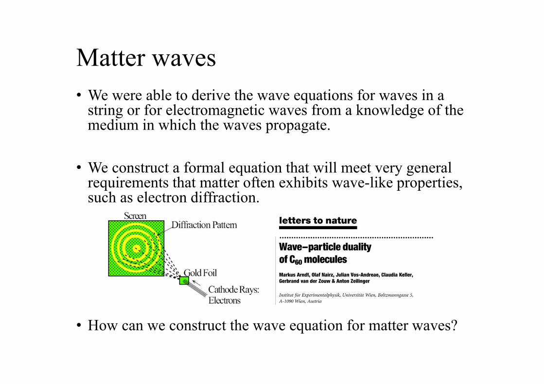
Matter waves• We were able to derive the wave equations for waves in a

string or for electromagnetic waves from a knowledge of the medium in which the waves propagate.

• We construct a formal equation that will meet very general requirements that matter often exhibits wave-like properties, such as electron diffraction.

• How can we construct the wave equation for matter waves?

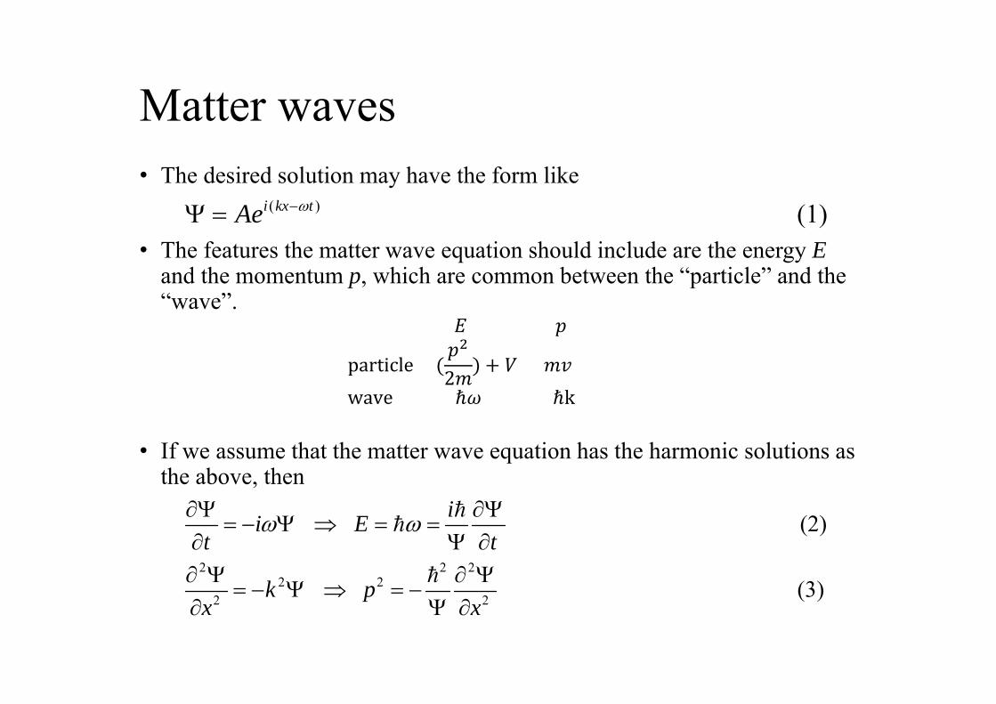
Matter waves• The desired solution may have the form like

• The features the matter wave equation should include are the energy Eand the momentum p, which are common between the “particle” and the “wave”.

• If we assume that the matter wave equation has the harmonic solutions as the above, then

( ) (1)i kx tAe

𝐸 𝑝

particle 𝑝2𝑚 𝑉 𝑚𝑣

wave ℏ𝜔 ℏk

2 2 22 2

2 2

(2)

(3)

ii Et t

k px x

Schrödinger time dependent wave equation

• Since the energy of a particle is given by

• The above equation is the Schrödinger time-dependent wave equation.

• The equation must be used if we want to describe processes related to dynamic transition, such as in optical absorption and carrier relaxation.

2

2 2

2

22

( 2 ) ,a reasonable choice of a wave equation is

1 2

. . (4)2

E p m V

i Vt m x

i e i Vt m

Schrödinger time-independent wave equation

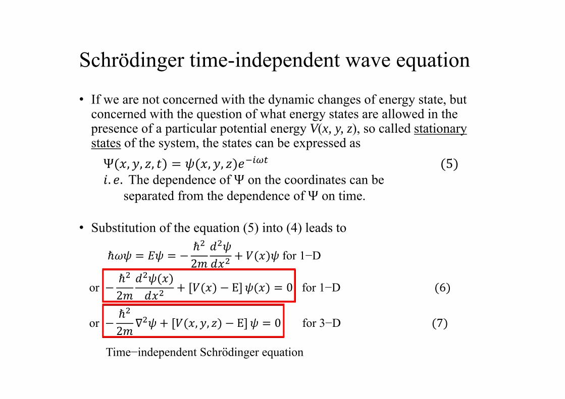
• If we are not concerned with the dynamic changes of energy state, but concerned with the question of what energy states are allowed in the presence of a particular potential energy V(x, y, z), so called stationary states of the system, the states can be expressed as

• Substitution of the equation (5) into (4) leads to

Ψ 𝑥, 𝑦, 𝑧, 𝑡 𝜓 𝑥, 𝑦, 𝑧 𝑒 5𝑖. 𝑒. The dependence of Ψ on the coordinates can be separated from the dependence of Ψ on time.

ℏ𝜔𝜓 𝐸𝜓ℏ2𝑚

𝑑 𝜓𝑑𝑥 𝑉 𝑥 𝜓 for 1−D

or ℏ2𝑚

𝑑 𝜓 𝑥𝑑𝑥 𝑉 𝑥 E 𝜓 𝑥 0 for 1−D 6

or ℏ2𝑚 ∇ 𝜓 𝑉 𝑥, 𝑦, 𝑧 E 𝜓 0 for 3−D 7

Time−independent Schrodinger equation

Schrödinger time-independent wave equation

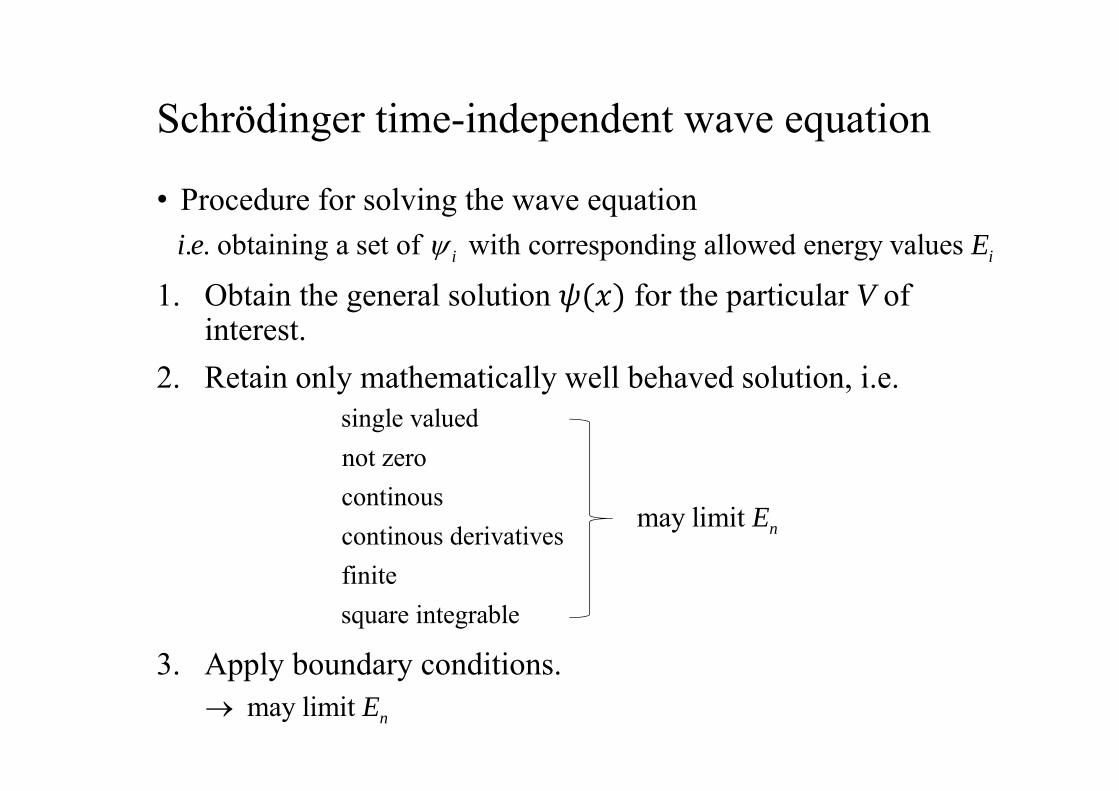
• Procedure for solving the wave equation

1. Obtain the general solution 𝜓 𝑥 for the particular V of interest.

2. Retain only mathematically well behaved solution, i.e.

3. Apply boundary conditions.

. . obtaining a set of with corresponding allowed energy values i ii e E

single valuednot zerocontinouscontinous derivativesfinitesquare integrable

may limit nE

may limit nE

• What is 𝑥 ?• Physical significance of 𝑥 can be associated at least with

the real quantity .• Suppose that a plot of vs x representing a

“particle” has the dependence on x shown in the below figure.

2*

2

x0x

*

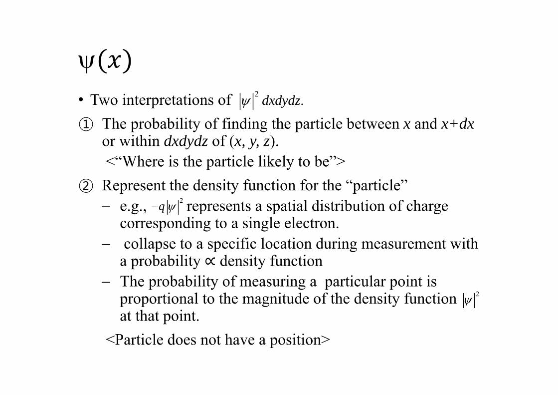
• Two interpretations of① The probability of finding the particle between x and x+dx

or within dxdydz of (x, y, z).<“Where is the particle likely to be”>

② Represent the density function for the “particle” e.g., represents a spatial distribution of charge

corresponding to a single electron. collapse to a specific location during measurement with

a probability ∝ density function The probability of measuring a particular point is

proportional to the magnitude of the density function at that point.

<Particle does not have a position>

2 .dxdydz

2q

2

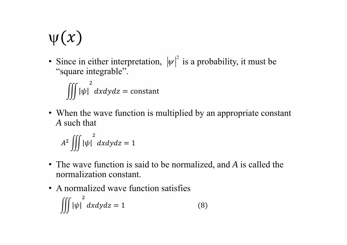
• Since in either interpretation, is a probability, it must be

“square integrable”.

• When the wave function is multiplied by an appropriate constant A such that

• The wave function is said to be normalized, and A is called the normalization constant.

• A normalized wave function satisfies

2

𝐴 𝜓 𝑑𝑥𝑑𝑦𝑑𝑧 1

𝜓 𝑑𝑥𝑑𝑦𝑑𝑧 constant

𝜓 𝑑𝑥𝑑𝑦𝑑𝑧 1 8

• To be used as a probability, the wave function must be normalized.

• In spherical coordinates

• Three important systems allow exact solutions.

① A free electron model of a confined electron

② Linear harmonic oscillator (F=-gx)

③

𝑒. 𝑔. 𝑞 𝜓 𝑑𝑥 𝑞 9

𝜓 𝑟, 𝜃, 𝜙 𝑟 sin 𝜃 𝑑𝑟𝑑𝜃𝑑𝜙 1 10

𝑉12 𝑔𝑥 ,

𝑉𝑍𝑞

4𝜋𝜀 𝜀 𝑟 , Hydrogenic atom 𝑍 1, hydrogen

0 for 0 ,V x L

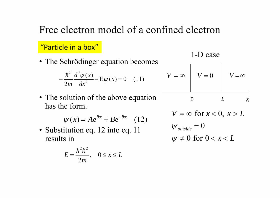
Free electron model of a confined electron

• The Schrödinger equation becomes

• The solution of the above equation has the form.

• Substitution eq. 12 into eq. 11 results in

2 2

2

( ) E ( ) 0 (11)2

d x xm dx

( ) (12)ikx ikxx Ae Be

2 2

, 02

kE x Lm

0 L

0V V V

for 0, 0

0 for 0outside

V x x L

x L

1-D case“Particle in a box”

x

Free electron model of a confined electron

• B.C’s①

②

, 2

sinn n

n nk LL

n xCL

1/2*

0

1/2

22 2 2 2

2

21

2 sin

2 2

L

n

n

n

dx CL

n xL L

n nEm L mL

0 at 0 and x L

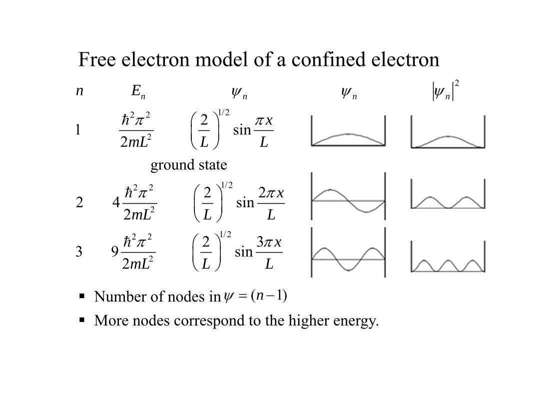
Free electron model of a confined electron

Number of nodes in More nodes correspond to the higher energy.

2

1/22 2

2

1/22 2

2

21 sin2

ground state

2 22 4 sin2

n n n nn E

xmL L L

xmL L

1/22 2

2

2 33 9 sin2

L

xmL L L

( 1)n

Free electron model of a confined electron

For large n2

n

Classical① Equal probability of

finding particle anywhere (for any E) = 1/L

② Continuous E 0 allowed

WaveProbability is function of x and varies with E

Discrete En allowed

③ As wave picture reduces to classical picture.“correspondence principle”

,n

15 21 3.8 10 eVE L (L in centimeters)

Linear harmonic oscillator

- solution :

𝐹 𝑔𝑥

𝑉 𝐹𝑑𝑥12 𝑔𝑥

ℏ2𝑚

𝑑 𝜓𝑑𝑥

12 𝑔𝑥 𝐸 𝜓 0

𝜓 𝑥 𝑓 𝑥 𝑒 when 𝛾𝑚𝑔ℏ

𝑓 𝑥 : p olynomial that terminate after a finite number of terms to keep 𝜓 𝑥 finite and normalizable

𝜓 𝐻 𝛾𝑥 𝑒

𝐻 𝑦 1 𝑒𝑑

𝑑𝑦 𝑒

:Consists of a particle moving under a restoring force proportional to the displacement.

From termination condition :

• Applications

𝐸 𝑛12 ℏ𝜔 𝜔 2𝜋

𝑔𝑚

phononphonon

k

Linear harmonic oscillator

① Vibration of atoms in a crystal can be represented by a collection of oscillators representing lattice waves. →

② Collection of charge oscillators generates electromagneticradiation →

Linear harmonic oscillator

photonphoton

𝑛 𝜓 𝐸 𝜓 𝜓

0 𝐴 𝑒 12 ℏ𝜔

1 𝐴 𝛾 𝑥𝑒 32 ℏ𝜔

2 𝐴 2𝛾𝑥 1 𝑒 52 ℏ𝜔

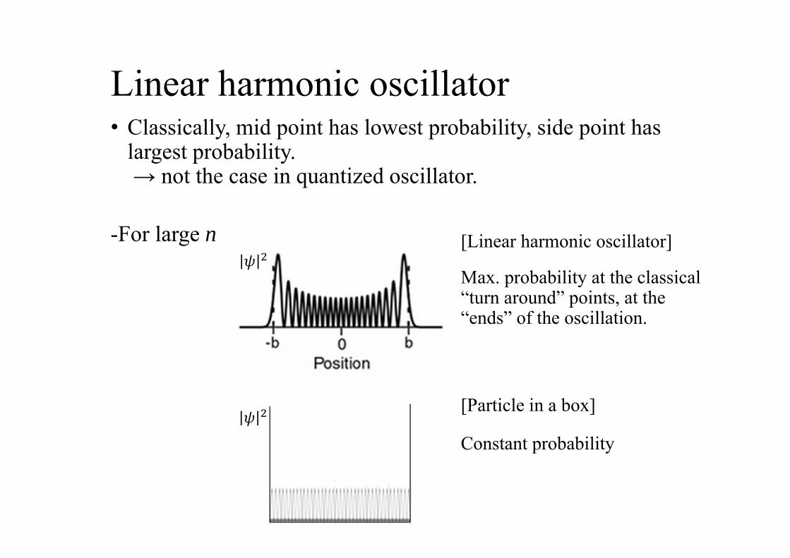
• Classically, mid point has lowest probability, side point has largest probability.→ not the case in quantized oscillator.

-For large n

Linear harmonic oscillator

𝜓

𝜓Max. probability at the classical “turn around” points, at the “ends” of the oscillation.

Constant probability

[Particle in a box]

[Linear harmonic oscillator]