Geodätisch-geophysikalische Arbeiten in der Schweiz (Fortsetzung der Publikationsreihe «Astronomisch-geodätische Arbeiten in der Schweiz»)

herausgegeben von der

Schweizerischen Geodätischen Kommission (Organ der Akademie der Naturwissenschaften Schweiz)

Siebzigster Band The Swiss Trolley – A Modular Volume 70 System for Track Surveying

Ralph Glaus 2006

Adresse der Schweizerischen Geodätischen Kommission: Institut für Geodäsie und Photogrammetrie Eidg. Technische Hochschule Zürich ETH Hönggerberg CH-8093 Zürich, Switzerland Internet: http://www.sgc.ethz.ch ISBN 3-908440-13-0 Redaktion des 70. Bandes: Dr. R. Glaus, Dr. M. Troller Druck: Print-Atelier E. Zingg, Zürich

VORWORT

Die präzise und schnelle Absteckung und Überwachung von Verkehrssystemen, wie Hoch-geschwindigkeits-Eisenbahnen, ist zunehmend zu einer Herausforderung für die Geodätische Messtechnik geworden. Dabei sind vor allem die Weiterentwicklungen in der Eisenbahn-Bautechnik, insbesondere die so genannte „Feste Fahrbahn“ zu berücksichtigen, die Ge-schwindigkeiten von mehr als 300 km/h ermöglichen. Zur Erfüllung der vielfältigen stati-schen und kinematischen Messaufgaben bei Schienenwegen haben sich leichte und portable Gleismesswagen bewährt, die neben den Positionierungstechnologien, GPS und Tachymetrie, mit einer Vielzahl von weiteren Sensoren ausgerüstet werden können.

Der in der vorliegenden Arbeit entwickelte Gleismesswagen ist aus einer Zusammenarbeit des Instituts für Geodäsie und Photogrammetrie der ETH Zürich mit der Firma terra vermessun-gen AG, Zürich, der FH Burgdorf und der Firma Grunder Ingenieure AG, Hasle-Rüegsau, entstanden und wurde von der Kommission für Technologie und Innovation (KTI) des Bun-desamts für Berufsbildung und Technologie (BBT) gefördert. Zur Erfüllung der verschiede-nen Funktionen wurden Algorithmen entwickelt, die die räumlich-geometrische Zuordnung der einzelnen Sensoren modellieren. Für den kinematischen Messmodus mussten zusätzlich die dynamischen Eigenschaften der verschiedenen Sensoren analysiert und modelliert werden und vor allem Synchronisationsprobleme gelöst werden. Dazu gehören auch Ansätze aus be-nachbarten Disziplinen wie der Regelungstechnik oder der Dynamik.

Herr Glaus hat die Funktionalität des Gleismesswagens durch zusätzliche bildgebende Senso-ren wie Scanner und Präzisions-Digitalkamera erweitert. Dabei wurde eine neue Methode entwickelt, um aus Kamerabildern die Gleisgeometrie abzuleiten. Umfangreiche Untersu-chungen der Scannerkonfiguration, insbesondere der dualen Scanneranordnung im kinemati-schen Modus, führten zu Kalibrierungen und Algorithmen, die sich in der Praxis in mehreren Projekten bewährt haben. Inzwischen wird die neu entwickelte Technik auch auf anderen Plattformen, wie nicht schienengebundenen Landfahrzeugen zusammen mit Laserradar er-folgreich eingesetzt.

Die Schweizerische Geodätische Kommission (SGK) gratuliert Herrn Glaus zu dieser erfolg-reich abgeschlossenen Arbeit. Eines der Ziele der SGK ist es, neuste und zukunftsträchtige Entwicklungen im Bereich der Geodäsie zu erkennen und diese zu konkretisieren. Herrn Glaus ist es in bemerkenswerter Weise gelungen, aus geodätischen und mathematischen The-orien, praxisorientierte Lösungsansätze zu entwickeln und umzusetzen. Die SGK bedankt sich bei der Akademie der Naturwissenschaften Schweiz (SCNAT) für die Übernahme der Druck-kosten.

Prof. Dr. H. Ingensand Prof. Dr. A. Geiger Institut für Geodäsie und Photogrammetrie ETH Zürich ETH Zürich Präsident der SGK

PREFACE

La surveillance et le traçage rapide des systèmes de circulation, comme par exemple les trains à grandes vitesses, sont devenus des défis pour la métrologie géodésique. Les futurs dévelop-pements des techniques de construction des chemins de fer dénommés “voie ferrée fixe” qui permettront des vitesses supérieures à 300 km/h sont à prendre tout particulièrement en compte. Pour atteindre les multiples buts statiques et cinématiques fixés par les tâches des mesures des lignes de trains, les véhicules de mesures légers et portables ont fait leurs preu-ves. Ceux-ci à côté des technologies de positionnement, GPS et tachymètres, peuvent être en plus équipés de multiples autres senseurs.

Le véhicule de mesure des voies de chemin de fer présenté dans ce travail a été développé à l’institut de Géodésie et Photogrammétrie de l’EPF de Zürich en collaboration avec les firmes terra vermessungen SA de Zürich, Grunder Ingenieurs SA de Hasle-Rüegsau, et la haute école spécialisée de Burgdorf et supporté par l’agence pour la promotion de l’innovation de l’office fédéral de la formation professionnelle et de la technologie. Afin de satisfaire les diverses fonctions assignées à ce véhicule, des algorithmes ont été développés pour la modélisation de la distribution spatiale de chaque senseur. Pour le mode en mesures cinématiques, les caracté-ristiques dynamiques des différents senseurs on dû être analysées et modélisées et en particu-lier les problèmes de synchronisation ont dû être résolus. Ceci a nécessité des approches dans des disciplines adjacentes telles que les techniques de régulation ou de dynamique.

Monsieur Glaus a amélioré la fonctionnalité du chariot de mesures des voies par l’adjonction de senseurs d’images tels que scanners et cameras de précisions. Dans ce cadre une nouvelle méthode a été développée pour déterminer la géométrie des voies à partir des images obtenues par ces senseurs. Des études extensives des configurations du scanner, particulièrement la mise en place de scanner double en mode dynamique, ont conduit au développement d’algorithmes et de calibrations qui ont passés avec succès de nombreux tests pratiques. Dans le même temps la technique nouvellement développée – aussi sur d’autres plateformes telles que celles non liées au rail – a été appliquée avec succès conjointement avec un radar à laser.

La commission géodésique suisse (CGS) exprime à Monsieur Glaus sa gratitude pour l’achèvement, couronné de succès, de ce project. C’est un des buts de la CGS de reconnaître et de concrétiser de nouveaux projets en géodésie. Monsieur Glaus a réussi d’une manière remarquable le développement d’approches pratiques à partir de théories géodésiques et ma-thématiques. La commission géodésique suisse est reconnaissante à l ‘Académie Suisse des Sciences Naturelles pour son aide financière couvrant les coûts d’impression de ce fascicule.

Prof. Dr. H. Ingensand Prof. Dr. A.Geiger Institut de Géodésie et Photogrammetrie ETH Zürich ETH Zürich Président de la CGS

FOREWORD

Precise and fast staking out and monitoring of traffic systems such as high-speed railways have become a challenge to geodetic metrology. Further developments in the railway con-struction technique, mainly the so called slab tracks have to be taken into consideration which allow for speeds of more than 300 km/h. In order to compete with the numerous static and kinematic measuring tasks for railways lines, light and portable track trolleys stood the test. Besides the positioning technologies GPS and tacheometry, these trolleys can integrate a large number of further sensors.

The track trolley (multi-sensor platform) described in the present work was developed at the Institute of Geodesy and Photogrammetry of ETH Zürich in collaboration with terra vermes-sungen AG, Zürich, Grunder Ingenieure AG, Hasle-Rüegsau, the Berne University of Applied Sciences, Burgdorf, supported by The Innovation Promotion Agency (CTI) of the Swiss Fed-eral Office for Professional Education and Technology (OPET). In order to fulfil the various functions, algorithms have been developed for the modelling of the spatial geometric alloca-tion of the individual sensors. For the kinematic measuring mode the dynamic features of the various sensors had to be analysed and modelled and above all the synchronisation problems had to be solved. This included approaches from adjacent disciplines such as control tech-nique or dynamics.

Ralph Glaus has extended the functionality of the multi-sensor platform by additional imaging sensors like scanners and a high-precision digital camera. Thereby, a new method was devel-oped to determine the track geometry from the camera image. Extensive research of the scan-ner configuration, mainly of the dual scanner set up in the kinematic mode resulted in calibra-tions and algorithms which were approved in several projects in the practice. In the meantime the newly developed technique – also on other kinematic platforms such as cars – is success-fully applied together with laser radar.

The Swiss Geodetic Commission (SGC) expresses its gratitude to Ralph Glaus for the suc-cessful completion of this project. One of SGC’s goals is to anticipate and concretize newest developments in the area of Geodesy. Ralph Glaus has been remarkably successful in trans-ferring geodetic and mathematic theories into practice. The SGC is grateful to the Swiss Academy of Sciences (SCNAT) for covering the printing costs of this volume.

Prof. Dr. H. Ingensand Prof. Dr. A. Geiger Institute of Geodesy and Photogrammetry ETH Zürich ETH Zürich President of SGC

VII

Abstract Modern railway infrastructure requires accurate, absolute referenced spatial data for project planning, construction and maintenance. On the one hand, passenger safety and travel comfort depend to a large extent on accurate tracks. On the other hand, absolute referenced coordi-nates of railway assets facilitate data exchange between railway operators and third parties. In addition, time slots for maintenance are short, due to the high volumes of traffic on major railway lines. Thus, flexible surveying systems are required yielding accurate data within a short time. The multi-sensor platform Swiss Trolley, which offers such a flexible system, copes with absolute referenced spatial data. The platform is mounted on a track vehicle. This allows for a complete description of the track environment in kinematic mode with a mini-mum of interference time with regular traffic.

The Swiss Trolley features a modular design. A basic module for assessing track key parame-ters such as chainage, cant, twist, gradients and track gauge covers monitoring tasks on con-struction sites. A positioning module integrating GPS or total stations allows for the determi-nation of the track axis. A further scan module can be used to generate absolute referenced point clouds in the track environment.

This work compiles the development steps of the Swiss Trolley. Relevant side conditions re-garding track surveying, coming from track geometry and the railway operators are summa-rised and state-of-the-art systems are reviewed. Based on these premises, a niche for Swiss Trolley applications is defined. Sensors providing geometric data in the track environment are evaluated in regard to their suitability and error behaviour.

The key problem of the trolley positioning consists in determining the six degrees of freedom of the multi-sensor platform at any point in time. The chosen kinematic approach asks for a careful treatment of time constraints. Each data string coming from a specific sensor must own an accurate time tag. Kinematic surveys at walking speed with subcentimetric accuracy require time tags with millisecond accuracy.

The incorporated sensors were investigated regarding their error behaviour. Calibration issues are addressed and approaches for the bias determination are presented. Models for correcting collimation errors and nuisance accelearations are given for the pendulum inclination sensors used. Moreover, emphasis was placed on biases emerging at kinematic surveys for the par-ticular optical total station used. Reduction models for the laser scanner data are proposed and calibration procedures providing intrinsic orientation and latency parameters are given.

A kinematic model for Swiss Trolley surveys based on the Frenet base system and its canoni-cal representation was developed. Explicit formulae are given for runs on geometric elements dominating in the railway track environment. For the mutual data processing, a loosely cou-pled filter concept is proposed consisting of data pre-processing, synchronisation and filtering steps. The core of data processing is a Kalman filter, estimating vehicle and track states in an absolute or a relative reference frame. By means of the filter approach, the observations of the involved sensors can be integrated in a spatial model. Individual filter runs can be assembled by an additional merge step. Merged runs in up and down direction allow for a quality as-sessment and also allow for the monitoring of eventually remaining biases such as a boresight misalignment or inclination sensor zero point offsets.

Positioning accuracies for the static and kinematic case were assessed on the one hand by the comparison of up and down runs. On the other hand, comparisons were carried out with inde-pendently measured reference data. The static error behaviour of the Swiss Trolley could be

evaluated by using a slab track alignment. Submillimetric positioning accuracies were ob-tained in combination with high-precision total stations. Kinematic positioning accuracy mainly depends on the positioning sensor used. Optical total stations providing synchronised angle and distance data allow for subcentimetric positioning. High-precision DGPS position-ing yields subcentimetric accuracy for the horizontal component. The typical vertical accu-racy is better than two centimetres. The integrated longitudinally mounted inclination sensor slightly augments the mere GPS solution. The attitude determination of the platform is a re-sult of the combined data treatment. For GPS surveys, the typical pitch angle accuracy is two mrad. Yaw angles essentially correspond to the derivation of the trajectory with respect to the covered path and are determined with one mrad accuracy. Roll angle accuracy is domi-nated by the inclination sensor measurements across the track. The typical accuracy is 0.3 mrad. For the scan module, laser dots in the absolute reference frame are degraded by the uncertainty of the trajectory and the platform attitude amplified by a geometry-depending lever. The absolute accuracy of such a dot is three centimetres using a time-of-flight laser scanner. Relative accuracy between two adjacent dots amounts to five millimetres.

The Swiss Trolley was successfully applied on numerous assignments. Adaptations for the multi-sensor platform exist for tunnel site locomotives and road-vehicles.

IX

Zusammenfassung Eine moderne Bahninfrastruktur erfordert für Projektierung, Bau und Unterhalt genaue, abso-lut referenzierte Geodaten. Einerseits hängen Sicherheit und Reisekomfort in hohem Masse von genauen Gleisen ab. Andererseits erleichtern absolut georeferenzierte Daten über feste Anlagen den Datenaustausch zwischen Netz-Betreibern und Dritten. Zusätzlich ist wegen des hohen Verkehrsaufkommens auf Hauptstrecken nur noch mit kurzen Zeitfenstern, die für den Unterhalt zur Verfügung stehen, zu rechnen. Es sind also flexible Vermessungssysteme ge-sucht, die innerhalb kurzer Zeit genaue und zuverlässige Daten liefern. Ein solch flexibles System, welches in der Lage ist, Geodaten in einem absoluten Referenzrahmen zu liefern, ist die Multisensor-Plattform Swiss Trolley. Die Plattform ist auf einem Gleiswagen montiert und ermöglicht die komplette, dreidimensional-geometrische Beschreibung der Gleisumgebung im kinematischen Betrieb mit minimaler Beeinträchtigung des regulären Verkehrs.

Der Gleismesswagen Swiss Trolley ist modular aufgebaut. Ein Basis-Modul für die Erfassung von Gleisparametern wie Kilometrierung, Überhöhung, Verwindung, Gradient und Spurweite deckt Überwachungsaufgaben auf Bahn-Baustellen ab. Ein integrierbares Positionierungsmo-dul, welches die Verwendung von GPS-Sensoren oder Tachymetern zulässt, kann für Gleis-achsbestimmungen eingesetzt werden. Ein weiteres Scan-Modul kann verwendet werden, um absolut referenzierte Punktwolken der Gleisumgebung zu generieren.

Diese Arbeit stellt die Entwicklungsschritte des Swiss Trolley zusammen. Für die Gleisver-messung relevante Randbedingungen, gegeben durch die Gleisgeometrie und die Eisenbahn-netzbetreiber, werden zusammengefasst. Der Stand der Technik der Bahnvermessung wird aufgearbeitet. Ausgehend von diesen Grundlagen wird eine Nische für Swiss Trolley-Anwendungen definiert. Sensoren, welche geometrische Daten in der Gleisumgebung liefern, werden hinsichtlich Eignung und Fehlerverhalten evaluiert.

Das zentrale Problem der Fahrzeug-Positionierung besteht im Bestimmen der sechs Freiheits-grade der Multi-Sensor Plattform für jeden beliebigen Zeitpunkt. Der gewählte kinematische Ansatz erfordert eine sorgfältige Behandlung von zeitlichen Randbedingungen. Jeder, von einem spezifischen Sensor erfasste Datenstring muss über einen genauen Zeitstempel verfü-gen. Kinematische Aufnahmen im Schritttempo mit Subzentimeter-Genauigkeit erfordern Synchronisationsgenauigkeiten von einigen wenigen Millisekunden.

Die involvierten Sensoren wurden in Bezug auf ihr Fehlerverhalten untersucht. Aspekte zur Kalibrierung werden erörtert und Methoden zur Bestimmung der systematischen Abweichun-gen werden präsentiert. Modelle zur Elimination von Kreuzungsfehlern und zur Reduktion von Störbeschleunigungen werden für die verwendeten Pendelneigungssensoren angegeben. Des Weiteren wurde das Augenmerk auf die Untersuchung systematischer Abweichungen beim kinematischen Vermessen mit Tachymetern gerichtet. Reduktionsmodelle für Laser-scanner sowie Kalibrierungsmodelle, die intrinsische Orientierungsparameter und Latenzzei-ten der Scanner liefern, werden aufgeführt.

Ein kinematisches Modell für den Swiss Trolley, das auf dem Frenet-Basis-System und dessen kanonischer Darstellung aufbaut, wurde entwickelt. Explizite Formeln für Messfahrten auf im Gleisbau vorherrschenden geometrischen Elementen sind angegeben. Für die gemeinsame Datenverarbeitung wird ein schwach gekoppeltes Filter-Konzept, welches aus einem Daten-vorverarbeitungs-, einem Synchronisations- und einem Filterschritt besteht, vorgeschlagen. Kernpunkt der Datenverarbeitung ist ein Kalman-Filter, welches die Fahrzeug- und Gleiszu-stände wahlweise in einem absoluten oder in einem relativen Referenzrahmen schätzt. Mit Hilfe des Filter-Ansatzes können alle Beobachtungen in einem räumlichen Modell integriert werden. Einzelne Filter-Durchläufe können in einem zusätzlichen Merge-Schritt zusammen-

geführt werden. Solche zusammengefügten Messfahren ermöglichen eine Qualitätskontrolle und eine Überwachung allfälliger verbleibender systematischer Abweichungen wie zum Bei-spiel fehlerhaften Koordinaten des Prismas im Wagenrahmen oder Nullpunktfehler der Nei-gungsmesser.

Positionierungsgenauigkeiten für den statischen und kinematischen Fall wurden einerseits durch den Vergleich von Hin- und Rückfahrten und andererseits durch den Vergleich mit Re-ferenzdatensätzen unabhängiger Messsysteme abgeleitet. Das statische Übertragungsverhalten des Swiss Trolley konnte anlässlich einer Absteckung der Festen Fahrbahn evaluiert werden. Genauigkeiten im Submillimeter-Bereich konnten bei Verwendung eines Präzisionstachyme-ters nachgewiesen werden. Die kinematische Positionierungsgenauigkeit hängt hauptsächlich vom verwendeten Positionierungssensor ab. Tachymeter mit synchronisierten Richtungs- und Distanzmessungen ermöglichen Positionierungen im Subzentimeter-Bereich. Hochpräzises DGPS liefert Subzentimetergenauigkeit für die horizontale Komponente. Die typische Verti-kalgenauigkeit ist besser als zwei Zentimeter. Der longitudinal montierte Neigungsmesser verbessert dabei die reine GPS-Höhenlösung geringfügig. Die Bestimmung der Orientie-rungswinkel der Plattform resultiert aus der gemeinsamen Datenverarbeitung. Für GPS-Aufnahmen ist die typische Nickwinkelgenauigkeit 2 mrad. Die Gierwinkel der Plattform entsprechen im Wesentlichen der Ableitung der Trajektorie bezüglich des zurückgelegten Weges. Diese können auf 1 mrad genau bestimmt werden. Die Rollwinkelgenauigkeit wird bestimmt durch die Neigungsmessung quer zum Gleis. Typische Genauigkeiten betragen 0.3 mrad. Die Genauigkeitsangabe für das Scan-Modul setzt sich zusammen aus der Unsi-cherheit der Trajektorien- und Orientierungswinkelbestimmung verstärkt durch geometrieab-hängige Hebel. Die Genauigkeit bezogen auf einen übergeordneten Referenzrahmen eines Laserpunktes beträgt 3 cm beim Einsatz eines Pulslaufzeit-Scanners. Die Relativgenauigkeit zwischen zwei benachbarten Pixeln beträgt 5 mm.

Der Swiss Trolley wurde in zahlreichen Aufträgen erfolgreich eingesetzt. Anpassungen der Multisensor-Plattform für die Verwendung auf weiteren Fahrzeugtypen existieren für Tunnel-baustellen-Lokomotiven und Strassenfahrzeuge.

XI

Contents

1 Introduction 1

2 Track Geometry 3

2.1 Nominal Geometries ................................................................................................. 3 2.1.1 Introduction ..................................................................................................... 3 2.1.2 Horizontal Layout............................................................................................ 3 2.1.3 Vertical Layout................................................................................................ 6

2.2 Rules and Standards of Different Countries ............................................................. 7 2.2.1 Horizontal Layout............................................................................................ 7 2.2.2 Vertical Layout................................................................................................ 8 2.2.3 Cant ................................................................................................................. 8

2.3 Kinematic Model of Motion ..................................................................................... 9 2.3.1 Kinematics in the Frenet System..................................................................... 9 2.3.2 Canonical Representation of the Most Common Track Curves.................... 11

2.4 Remarks on Track Accuracy................................................................................... 14 2.4.1 General Remarks ........................................................................................... 14 2.4.2 Relative and Absolute Accuracy of a Track.................................................. 15

2.5 Methods for Track Surveying ................................................................................. 15 2.5.1 Overview ....................................................................................................... 15 2.5.2 Relative Track Surveying.............................................................................. 17 2.5.3 Absolute Track Surveying............................................................................. 19 2.5.4 Selected Track-Surveying Systems ............................................................... 20 2.5.5 The Swiss Trolley – Finding the Niche ......................................................... 24

3 Potentials and Limitations of a Kinematic Track-Surveying System 25

3.1 Kinematic Surveying .............................................................................................. 25

3.2 Absolute Position Fixing ........................................................................................ 27 3.2.1 GNSS............................................................................................................. 27 3.2.2 Tracking Total Stations ................................................................................. 29

3.3 Dead Reckoning...................................................................................................... 30 3.3.1 Inertial Navigation Systems (INS) ................................................................ 30 3.3.2 Yaw Rates by Chord Techniques .................................................................. 30 3.3.3 Odometers ..................................................................................................... 36 3.3.4 Height Determination by an Inclination Sensor ............................................ 39

3.4 Attitude Determination ........................................................................................... 40

3.5 Kinematic Surveys of the Railway Inventory......................................................... 40 3.5.1 Track Gauge Measuring Systems.................................................................. 41 3.5.2 Laser Scanners............................................................................................... 42 3.5.3 3D Cameras ................................................................................................... 44 3.5.4 Ground Penetration Radar (GPR) ................................................................. 45

3.6 Synchronisation ...................................................................................................... 45

3.7 Modelling................................................................................................................ 47

3.8 Transformation........................................................................................................ 47

4 The Track-Surveying Trolley 51

4.1 Introduction............................................................................................................. 51 4.1.1 Development ................................................................................................. 51 4.1.2 Concept.......................................................................................................... 51

4.2 Data Acquisition ..................................................................................................... 55 4.2.1 Electronic Box............................................................................................... 55 4.2.2 A/D Conversion............................................................................................. 55 4.2.3 Data Synchronisation .................................................................................... 57

4.3 Reconstruction ........................................................................................................ 60

4.4 Inclination Sensors.................................................................................................. 61 4.4.1 Sensor Characteristics ................................................................................... 61 4.4.2 Calibration of Characteristic Curve............................................................... 61 4.4.3 Temperature Influences................................................................................. 62 4.4.4 Corrections for Non-Orthogonalities (Collimation Error) ............................ 62 4.4.5 Dynamic Behaviour of the Inclination Sensor .............................................. 66 4.4.6 Transformation of the Inclination Angles into the Body-System ................. 73

4.5 Track Gauge Measuring System............................................................................. 73 4.5.1 Characteristics and Measuring Principle of the Track Gauge Measuring

System ........................................................................................................... 73 4.5.2 Calibration..................................................................................................... 76

4.6 Odometers............................................................................................................... 76 4.6.1 Characteristics and Calibration ..................................................................... 76

4.7 Integration of Tracking Total Stations.................................................................... 77 4.7.1 Characteristics ............................................................................................... 77 4.7.2 Common Total Station Biases....................................................................... 79 4.7.3 Deflections of the Vertical ............................................................................ 81 4.7.4 Surveys in Canted Sections ........................................................................... 82 4.7.5 Synchronisation of Distances and Angles ..................................................... 83 4.7.6 Internal Tacheometer and Radio Latencies ................................................... 90

4.8 Integration of GPS .................................................................................................. 90 4.8.1 Characteristics ............................................................................................... 90 4.8.2 NMEA Data ................................................................................................... 90

4.9 Boresight Calibration of Prism and Antenna Phase Centre.................................... 91

4.10 Laser Scanners ........................................................................................................ 93 4.10.1 Characteristics .......................................................................................... 93 4.10.2 Model ....................................................................................................... 94 4.10.3 Yaw Angle Correction ............................................................................. 96 4.10.4 Evaluation of the Laser Scanner Precision............................................... 97 4.10.5 Variance Propagation for a Given Scanner Arrangement ........................ 99 4.10.6 Kinematic Calibration of mbR , mbx and the Latency.............................. 102

5 Data Processing 107

5.1 Introduction........................................................................................................... 107

XIII

5.2 Post-Processing Software Concept ....................................................................... 109

5.3 Data Preprocessing ............................................................................................... 110 5.3.1 Blunder Labelling........................................................................................ 110 5.3.2 Reduction, Model ........................................................................................ 112 5.3.3 Linear Filters ............................................................................................... 114 5.3.4 Synchronisation........................................................................................... 116 5.3.5 Reduction to the Centre Line of the Track .................................................. 116

5.4 Trajectory Smoothing by a Kalman Filter ............................................................ 117 5.4.1 Discrete Kalman Filter ................................................................................ 117 5.4.2 Backward Filter and Smoother.................................................................... 120 5.4.3 Absolute Model ........................................................................................... 121 5.4.4 Relative Model ............................................................................................ 127

5.5 Smoothing Splines ................................................................................................ 131 5.5.1 Smoothing Splines with First Derivatives................................................... 131 5.5.2 Comparison between Kalman Filter and Smoothing Splines...................... 133

5.6 Merging Trajectories............................................................................................. 134 5.6.1 Strategies for Merging................................................................................. 134 5.6.2 Chaining the Pieces ..................................................................................... 134 5.6.3 Merging ....................................................................................................... 136 5.6.4 Linking Scans to Merged Trajectories ........................................................ 140

6 Applications 141

6.1 Slab Track Alignment........................................................................................... 141

6.2 Kinematic Track Axis Surveys ............................................................................. 145 6.2.1 Comparison between Forward Filter, Backward Filter and Smoother........ 145 6.2.2 Filter Tuning................................................................................................ 146 6.2.3 Comparison between Absolute and Relative Model ................................... 149 6.2.4 The Influence of Inclinometer Measurement on GPS Heights ................... 149 6.2.5 The Smoother in Action – GPS Example.................................................... 150 6.2.6 The Smoother in Action – Total Station Example ...................................... 153

6.3 Kinematic Scanning.............................................................................................. 155

7 Conclusions 163

List of Figures 167

List of Tables 171

References 173

A Appendix 181

A.1 Transformation of Inclinations into Euler Angles ................................................ 181

A.2 Minimum Distance from the Track Axis.............................................................. 182

1 Introduction 1

1 Introduction The fast growth of individual motorcar traffic during the second half of the last century in-duced a vast expansion of national road networks. While the passenger car traffic increased continuously, the rail traffic lost its initial importance. During the seventies of the last cen-tury, traffic management authorities tried raise public awareness of sustainable rail traffic. The fuel shortage and, consequently, the increase in energy prices demanded a long-term transport policy in favour of railways. Throughout Europe, major railway projects were initi-ated. The two Swiss projects AlpTransit [ZBINDEN, 2000] and Rail 2000 [KRÄUCHI, 2005] can be considered two ambitious exponents of this railway renaissance.

The realisation of projects of such dimensions requires meticulous research in regard to plan-ning and implementation. At every stage, geodetic surveys play an important role providing base data for decision-making and the execution of projects. Railway key parameters such as safety and passenger comfort depend to a high degree on accurate surveys. However, tradi-tional survey concepts have to be reconsidered in order to satisfy the demands of the railway operators. The increasing rail traffic shortens the track’s availability for maintenance, asking for fast and flexible survey systems. Further, survey concepts have to be adapted to new re-quirements concerning accuracy and work efficiency evoked by novel railway construction techniques. As an example, on new high-speed railway lines ballast tracks have been partly replaced by slab tracks [e.g. DARR, 1997].

Railways and surveying are closely connected at all times. Efforts assessing the track’s posi-tion horizontally and vertically date back to the nineteenth century. Up to the 1980’s, chord surveys [e.g. HÖHNE et al., 1981] dominated the applications reproducing the relative ge-ometry of tracks. In the late 1980’s, the Swiss Federal Railways began with the establishment of an absolute reference frame [EISENEGGER, 1990]. This milestone in railway surveying resulted in a significant improvement in work efficiency. Constructors were able to connect tamping machines for track alignments to this reference frame. Apart from an increase in work efficiency, an accuracy gain could be demonstrated. Long periodic track position errors could be significantly reduced by such absolute surveys. Nowadays, efforts are made by the International Union of Railways (UIC) to unify national reference frames to the European Terrestrial Reference Frame ETRF89 aiming at cross-national homogeneous geodetic net-works [ENGEL et al., 2003].

The progress of GPS data processing strategies in the 1990’s [e.g. HATCH, 1990] and recent improvements in synchronisation issues for tracking total stations [e.g. STEMPFHUBER et al., 2004] has opened the field for kinematic absolute surveys on tracks. As an example, [FRITZENSMEIER et al., 1997] developed a flexible track-surveying trolley providing abso-lute geometry data using differential GPS. As a matter of fact, a stand-alone GPS based sur-vey suffers a loss of satellite signals in obstructed areas. Kinematic total station surveys fill the gap here. However, leapfrog strategies for connecting individual stations result in an inter-rupted workflow and cannot compete with GPS surveys in terms of work-efficiency.

The kinematic assessment of relative track parameters has a long tradition. Operational track recording vehicles were first used in the 1920’s [SCHRAMM, 1962]. These vehicles found their successors in track recording coaches, which are used nowadays for quality control of tracks [PRESLE, 2001]. Recent developments allow an accurate absolute positioning of these coaches by means of global navigation satellite systems, inertial navigation systems and bal-ises. Such expensive systems only can be maintained by major network operators. Further, these coaches cannot be applied cost-effectively on short sections or on construction sites.

2 1 Introduction

Recently, the emergence of laser scanners has asked for innovations in the domain of railway surveys. Laser scanners on vehicles allow for the acquisition of geometric data in a corridor of several dozens of metres. Such data are of great use for track maintenance. Missing track bal-last evaluation, clearance inspection, track gauge determination or the update of a fixed assets database is just an incomplete catalogue of potential applications. In contrast, occasionally used photogrammetric approaches for such tasks [e.g. BLONDEAU et al., 1999] become less important due to method-inherent geometrical accuracy constraints. However, combinations of laser scanner and photogrammetric approaches are prospective unifying accurate geometric data of laser scanners and comprehensive texture contents of images.

This thesis presents methods for modern track surveying. It especially features surveys by means of a portable track-surveying trolley. Emphasis is given to absolute surveys with a con-nection to global reference frames. GPS and total stations are proposed as absolute position-ing sensors. The combination of these sensors with a track gauge measuring system and laser scanners allows for an absolute and kinematic three-dimensional description of the track in-ventory. The presented track-surveying vehicle Swiss Trolley was part of a joint venture pro-ject initiated by the surveying company terra vermessungen AG of Zürich, Switzerland. Hard-ware and data acquisition software were developed at the Institute for Mechatronics of the University of Applied Sciences Burgdorf. The Institute for Geodesy and Photogrammetry of the Swiss Federal Institute of Technology of Zürich joined the project in 2002 and developed algorithms for data processing. New key algorithms are presented in this work. Thanks to the close collaboration between the project partners and the operational use of the Swiss Trolley in real assignments, immediate feedback from the users on new introduced algorithms was guaranteed during the whole project phase.

The report builds on a general overview of available systems and focuses then on the devel-opment of calibration procedures and algorithms for Swiss Trolley surveys. In Chapter 2, as a theoretical background, basic terms in the context of track geometry are reviewed. A kine-matic model for the trolley motion on the track is developed. An overview of state-of-the-art track-surveying systems is presented. Processes and requirements are analysed. The chapter concludes in defining a niche for the Swiss Trolley. Chapter 3 compiles potential sensors for a track-surveying system. Variance propagation is studied for selected dead reckoning sensors. The problem of time constraints is addressed and consequences for the sensor selection, the data acquisition and the post processing software are drawn. Chapter 4 focuses on the Swiss Trolley and the used sensors. Sensor models are given for the different trolley configurations. Systematic biases are studied and calibration procedures are proposed. In Chapter 5, data post-processing is treated. The loosely coupled concept contains several prefilter steps. The core is a least squares smoother basing on the kinematic model derived in Chapter 2. Further, a model for trajectory merges is proposed. In Chapter 6, results of several applications are presented. Examples of stop-and-go slab track surveys, kinematic track axis surveys and ki-nematic laser scanning surveys are given. The results are compared to reference data. Accura-cies for different Swiss Trolley modes are indicated. Chapter 7 draws conclusions from the research.

2 Track Geometry 3

2 Track Geometry

2.1 Nominal Geometries

2.1.1 Introduction With regard to the design of a track-surveying trolley, it is important to study the possible track geometry layouts. For one thing, the maximal cant has an immediate impact on the choice of an adequate inclination sensor. Further, the clearance towards the track bed deter-mines the design of a track gauge measuring system. The knowledge of the track layout is also a basis for kinematic modelling of a track-surveying vehicle. Hence, the most common rules for track layouts are to be given in the subsequent sections. The remarks base on [BÖSCH, 1991], [ESVELD, 1989] and [MÜLLER et al., 2000].

The railway track layout is determined by alignment elements. In the plan view, there are three types of these elements: the straight line, the circular arc and as a connecting element the transition curve. The transition curve type is country-specific, whereas the clothoid is the most widespread. For the vertical section, straight lines for constant slopes and fillets between changes of slopes are common. The change of an alignment element always leads to track discontinuities. Consequently, vibrations with a decay time of about 1.5 to 2 seconds are gen-erated. The layout of the track has to be designed in such a way that coach vibrations are not superposed by various track discontinuities.

The kinematics of the track layout is given by the trains in transit. The layout should take into account for inertial forces acting on the vehicles. Project engineers also have to regard the centrifugal force acting on a vehicle in curved sections. In contrast, the coriolis force evoked by the earth’s rotation amounts values which not even for high-speed trains circulating in north-south direction are relevant for the track layout. The physical impacts are described by simple functional rules and formulae which consider the safety, the riding comfort and a rea-sonable cost-value ratio. Mostly, operating speed wants to be maximised. For existing lines, this is restricted due to reasons of safety, comfort and maintenance. For new railway lines, the designed operating speed influences minimal radii and maximal slopes. Apart from topogra-phy, these are key elements for construction costs and land use. Further, train type and train frequency essentially affect the track layout.

2.1.2 Horizontal Layout Straight Lines

The straight line is the simplest element concerning construction and operation. Apart from the layout accuracies, the element length and the element slope, the maximum speed on the straight line is only limited by parameters which are independent from the layout design. Such parameters are the vehicle type, the train lengths, friction for braking and operating restric-tions.

Circular Arcs

A vehicle passing a curve is affected by a centrifugal force. In a first approximation, the vehi-cle is considered as a mass point. The centrifugal force is induced by the centrifugal accelera-tion za .

Apart from the centrifugal force, further horizontal lateral forces are present which are trans-ferred from the wheel on the rail. On the one hand, these are forces which are necessary to

4 2 Track Geometry

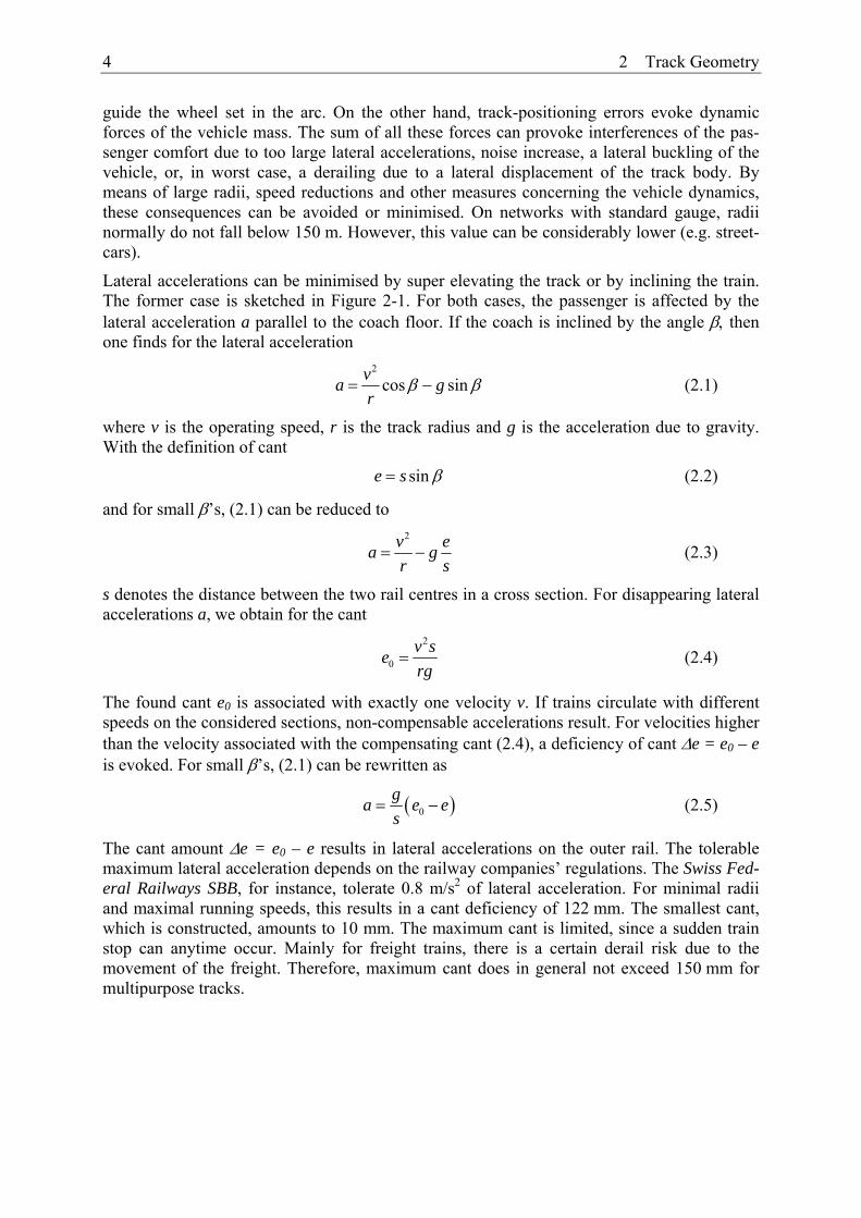
guide the wheel set in the arc. On the other hand, track-positioning errors evoke dynamic forces of the vehicle mass. The sum of all these forces can provoke interferences of the pas-senger comfort due to too large lateral accelerations, noise increase, a lateral buckling of the vehicle, or, in worst case, a derailing due to a lateral displacement of the track body. By means of large radii, speed reductions and other measures concerning the vehicle dynamics, these consequences can be avoided or minimised. On networks with standard gauge, radii normally do not fall below 150 m. However, this value can be considerably lower (e.g. street-cars).

Lateral accelerations can be minimised by super elevating the track or by inclining the train. The former case is sketched in Figure 2-1. For both cases, the passenger is affected by the lateral acceleration a parallel to the coach floor. If the coach is inclined by the angle β, then one finds for the lateral acceleration

2

cos sinva gr

β β= − (2.1)

where v is the operating speed, r is the track radius and g is the acceleration due to gravity. With the definition of cant

sine s β= (2.2)

and for small β’s, (2.1) can be reduced to

2v ea g

r s= − (2.3)

s denotes the distance between the two rail centres in a cross section. For disappearing lateral accelerations a, we obtain for the cant

2

0v serg

= (2.4)

The found cant e0 is associated with exactly one velocity v. If trains circulate with different speeds on the considered sections, non-compensable accelerations result. For velocities higher than the velocity associated with the compensating cant (2.4), a deficiency of cant Δe = e0 – e is evoked. For small β’s, (2.1) can be rewritten as

( )0ga e es

= − (2.5)

The cant amount Δe = e0 – e results in lateral accelerations on the outer rail. The tolerable maximum lateral acceleration depends on the railway companies’ regulations. The Swiss Fed-eral Railways SBB, for instance, tolerate 0.8 m/s2 of lateral acceleration. For minimal radii and maximal running speeds, this results in a cant deficiency of 122 mm. The smallest cant, which is constructed, amounts to 10 mm. The maximum cant is limited, since a sudden train stop can anytime occur. Mainly for freight trains, there is a certain derail risk due to the movement of the freight. Therefore, maximum cant does in general not exceed 150 mm for multipurpose tracks.

2 Track Geometry 5

Figure 2-1 Vehicle in a canted curve (adapted from [MÜLLER et al., 2000])

The actual measurable lateral accelerations are larger than shown before, because the coach’s centre of gravity lies above the track plane. An additional momentum is raised in curves, since the body of the coach is inclined with respect to the wheel kit.

The track gauge in the circular arc has to be widened if small radii are encountered. Too nar-row gauges prevent a restraint free run of the coaches. For SBB tracks with a nominal gauge of 1435 mm, the track gauge is widened for radii smaller than 275 m. Track gauges larger than 1470 mm must not occur. In contrast, the smallest tolerable gauge amounts to 1430 mm.

Transition Curves

The transition between curves represents always a discontinuity. If a circular curve follows a straight line, curvature, non-compensable lateral acceleration and cant have to change from zero to a certain amount. This results in a theoretically infinite jerk (derivative of the accelera-tion with respect to time). If a transition curve is laid between the straight line and the circular arc, the jerk can be held in finite limits.

For a constant lateral acceleration rate, the curve must hold a constant curvature change. The curve that fulfils this requirement is the clothoid. However, due to the constant lateral accel-eration rate, there are lateral jerk discontinuities at the beginning and at the end of this transi-tion curve. Curves with a smoother transition of lateral accelerations are the Bloss curve and the sinusoid. The Bloss curve was proposed by [BLOSS, 1936] and is used for high-speed tracks. The sinusoid [KLEIN, 1937] even shows a smoother jerk transitions than a Bloss curve. Sinusoids are used for layouts of e.g. Transrapid tracks. However, Swiss railway com-panies exclusively use clothoids for curve transitions.

β

za

g

se

β

a

6 2 Track Geometry

Figure 2-2 shows the jerk as a function of the chainage. Discontinuities at the beginning and the end of the transition can be minimised by the Bloss curve. They disappear for the sinu-soid.

Figure 2-2 Jerks for a clothoid, a Bloss curve and a sinusoid (according to [HENNECKE et al., 1993])

The Austrian Federal Railways (ÖBB) extensively studied lateral acceleration rates on transi-tion curves. Theoretical findings lead to the stipulation of the so-called Vienna arc [PRESLE, 2005]. The classical track layout is designed for the centre of gravity on the track axis. Thus, considerable forces act on the vehicle entering a transition curve. The Vienna arc regards the actual engine’s centre of gravity. This leads to an overshooting transition curve.

For a linear increase of the lateral acceleration on a clothoid, not only the curvature must in-crease linearly but also the cant. If the cant increases linearly, the lateral acceleration rate (jerk) and the curvature rate remain constant. This renders a quiet ride.

A critical issue in transition curves is the twist. The twist n is defined as cant change Δe per length unit Δl.

enl

Δ=

Δ (2.6)

During a transition ride, the four wheels of a two-axle coach are not in the same plane. In or-der to avoid derails, the amount of twist has to be held in certain limits. The twist should not be larger than two per mil. The time dependent cant rate is defined as lift velocity and has to be considered for higher operating speeds.

Finally, the minimal length of a transition curve mainly depends on the operating speed. Thresholds for twist, jerk and lift velocities have to be fulfilled.

2.1.3 Vertical Layout The maximal inclination of a railway line is influenced by various factors such as the topo-graphy, the adhesion between the wheel and the rail, the availability of locomotives or the operating method. For instance, the San Gottardo railway line in the Swiss Alps has a maxi-

Chainage

Jerk

Je

rk

Jerk

2 Track Geometry 7

mal inclination of twenty-eight per mil. In contrast, the new flat San Gottardo tunnel, which is under construction, will have a maximal inclination of eight per mil.

Changes of inclinations are realised by means of vertical circular arcs without additional tran-sition curves. The radii depend on different parameters. Thus, the wheel-rail contact must be maintained. Further, the vertical acceleration should not exceed 0.5 m/s2 for comfort motives. Due to reasons of derailing, curve peaks have larger radii than curve dips. Inclination changes in switches and cant ramps do generally not occur.

2.2 Rules and Standards of Different Countries It is essential to use reproducible rail reference marks for surveys and alignments of tracks. The definitions vary for different network operators. Especially, the Swiss railway companies use definitions, which slightly deviate from elsewhere. This section summarises definitions that are relevant for track surveying. For the Swiss Federal Railways SBB, directives are de-fined in the regulation R220.46 [SBB, 1989]. The German Railways DB has published defini-tions for the projection of the horizontal and vertical layout in regulation DB883.9002 [DB, 1999].

2.2.1 Horizontal Layout The horizontal layout represents the plan view of a track. It is a sequence of various, admitted geometric elements. The reference rail for the horizontal layout is always the outer rail in curves. For straight lines, the reference is the centre line of both rails. The track axis is de-fined as the parallel line to the reference rail, with an offset of the half nominal track gauge (Figure 2-3). This parallel line lies in the plane defined by the two rail surfaces. For various railway companies, the definitions differ from the above mentioned with regard to straight lines. The reference rail can also be defined as the identical rail regarding the subsequent ref-erence rail of the curve towards the increasing chainage.

Figure 2-3 Definition of track axis and track gauge

The track gauge is defined as the smallest distance between the rails measured 0 – 14 mm below the rail top edge. Standard gauge tracks have a nominal measure of 1.435 m (4’ 8”). For high-speed railway lines the nominal gauge can be increased by one millimetre, in order to enable smoother riding qualities.

By means of the track axis, the horizontal layout can be staked out, reconstructed or con-trolled. From a mathematical point of view, parallels of transition curves lose their geometric properties. Thus, a parallel to a clothoid is no longer a clothoid. However, these inconsisten-cies are not relevant to the track layout.

Track gauge

717.5 mm

0 - 14 mm

Track axis

8 2 Track Geometry

Displacements of the measured control point with respect to the nominal track axis are called slew values. Control points right of the nominal track towards an increasing chainage have a positive sign.

2.2.2 Vertical Layout For Swiss railway companies, the vertical layout is defined by the track centre line. Aber-rantly, the vertical layout in many countries is referred to the lower rail in curves. Displace-ments of the measured control point with regard to the reference are called lift parameters. Measured control points below the nominal axis obtain a positive sign.

2.2.3 Cant The cant is the amount by which one rail, usually the outside rail of a curved track, rises above the lower rail on the same piece of track. The cant is referred to a nominal base, which corresponds to the distance between the points of contact of the mean wheel circles with the rails (e.g. 1.500 m).

Figure 2-4 Definition of cant

In Switzerland, a designed cant is realised by rotating the track plane around the track axis. The outer and inner rails are super and under elevated, respectively, by half of the total cant amount (Figure 2-5). Thus, the coach’s centre of gravity does not change its height level dur-ing the curve ride. However, the underground has to be partly adapted for keeping the ballast layer thickness. Therefore, in other countries mostly the outer rail is raised by the total cant amount (Figure 2-6).

Figure 2-5 Realisation of the cant by rising the outer rail and lowering the inner rail

2e

inner rail

outer rail

2e

1500 mm

Cant

Centre line

2 Track Geometry 9

Figure 2-6 Realisation of the cant by rising the outer rail

2.3 Kinematic Model of Motion

2.3.1 Kinematics in the Frenet System In the foregoing section, evidence was given for the use of straight lines, circular arcs and transition curves for track design. With regard to the later treatment of kinematic methods for track surveying (section 3) and data filtering (section 5), a kinematic model for the movement of a mass point along a trajectory containing the mentioned track geometry elements is given here. The derivation rests on the Frenet base system and its canonical representation [e.g. BÄSCHLIN, 1947].

Figure 2-7 Frenet system for a trajectory with non-vanishing curvature

The differential geometry of curves traditionally starts with the vector ( )R R t= that describes a curve as a function of t. The independent parameter t represents the time. As an intermediate parameter, the arc length l is introduced. In the context of railway surveying, the expression chainage is used synonymously. In some extent, l(t) represents the schedule of the mass point on its trajectory. For the further considerations, the vector ( )R t must be at least thrice differ-

entiable. Then, the tangent vector ( )te t is well defined at every point and two additional or-thogonal vectors in the plane perpendicular can be chosen to form a complete local orientation system. Provided the curvature of ( )R R t= vanishes nowhere, this local coordinate system is chosen to be the Frenet system (also known as the Frenet-Serret system) consisting of the

outer rail

inner rail

e

0l l=

x

l(t)

m

( )R t

( )ne t

y

z

( )te t

( )be t

10 2 Track Geometry

unity vector along the tangent te , the unity vector along the binormal be and the unity vector along the principal normal ne which are given in terms of the curve itself by these expres-sions:

( ) ( )( )

t

R te t

R t= (2.7)

( ) ( ) ( )( ) ( )

b

R t R te t

R t R t

×=

× (2.8)

( ) ( ) ( )n b te t e t e t= × (2.9)

Differentiating the Frenet system yields the classical Frenet equations

( )( )( )

( )( )( )( )

0 00

0 0

t t

n n

b b

e t e te t v t e te t e t

κκ τ

τ

⎛ ⎞ ⎛ ⎞⎛ ⎞⎜ ⎟ ⎜ ⎟⎜ ⎟= ⋅ − ⋅⎜ ⎟ ⎜ ⎟⎜ ⎟

⎜ ⎟ ⎜ ⎟⎜ ⎟ −⎝ ⎠ ⎝ ⎠⎝ ⎠

(2.10)

Here, ( ) ( )v t R t= is the velocity and acts as a scalar magnitude of the curve derivative. The

intrinsic geometry of the curve is given by the curvature κ and the torsion υ. Both parameters can be written in terms of the curve itself:

( )( ) ( )

( )3

R t R tt

R tκ

×= (2.11)

( )( ) ( )( ) ( )

( ) ( )3

R t R t R tt

R t R tυ

× ⋅=

× (2.12)

Note that for straight lines neither the normal nor the binormal unity vector can be assessed unambiguously. Note also that the curvature κ(t) is always positive. Two curves with opposite curvatures in an identical plane obtain binormal unity vectors of the same magnitude but of opposite signs.

As explained in section 2.1, track geometry classically is divided into a horizontal and a verti-cal layout. Torsions of the track axis are not considered. However, relative torsions between the two rails are accounted for by separately looking at the track twist. This partition in a hori-zontal and vertical component allows for a reduction of the Frenet system to two dimensions. For the horizontal component, curves are defined in a projection system. The vertical compo-nent commonly is treated in a plane which is perpendicular to the local horizon and which contains the tangential unity vector. Thus, it holds for the planimetry

( )( ) ( ) ( )

( )0

0

hhh tt

hhh nn

e te tv t

e te tκ

κ⎛ ⎞ ⎛ ⎞⎛ ⎞

= ⋅ ⋅⎜ ⎟ ⎜ ⎟⎜ ⎟ ⎜ ⎟⎜ ⎟ −⎝ ⎠ ⎝ ⎠⎝ ⎠ (2.13)

and for the altimetry

2 Track Geometry 11

( )( ) ( ) ( )

( )0

0

vvv tt

vvv nn

e te tv t

e te tκ

κ⎛ ⎞ ⎛ ⎞⎛ ⎞

= ⋅ ⋅⎜ ⎟ ⎜ ⎟⎜ ⎟ ⎜ ⎟⎜ ⎟ −⎝ ⎠ ⎝ ⎠⎝ ⎠ (2.14)

Since the third component was dropped, the curvature orientation can no longer be assessed unambiguously. Therefore, for the horizontal and vertical layout right curves and curve peaks, respectively, obtain a positive sign.

2.3.2 Canonical Representation of the Most Common Track Curves Within this project, the canonical representations of the most common track curves were writ-ten down. For this, consider the trajectory in the environment of ( )R t . The Taylor series ex-pansion of ( )R t is

)(

!31

!21)()( 43

3

32

2

2

tOttRt

tRt

tRtRttR Δ+Δ

∂∂

+Δ∂∂

+Δ∂∂

+=Δ+ (2.15)

Subsequently, terms of the order 4( )O tΔ are omitted. The Frenet equations (2.10) provide for a curve with vanishing torsion

( ) ( ) ( )( )2 2 3 2 3 31 1( ) ( ) 32 6t t n t nR t t R t v e t a e v e t v j e va v c e tκ κ κ+ Δ ≅ + Δ + + Δ + − + + + Δ (2.16)

with the following abbreviations

( )l t arc length

( ) ( )v t l t= velocity

( ) ( )a t l t= algebraic acceleration

( ) ( )j t l t= algebraic jerk

clκ∂

=∂

curvature rate

Further, the following terms are summarised

ta a= tangential acceleration 2

na v κ= normal acceleration 3 2

tj v jκ= − + tangential jerk 33nj va v cκ= + normal jerk

Thus, (2.16) can also be written as

( ) ( )2 31 1( ) ( )2 6t t t n n t t n nR t t R t v e t a e a e t j e j e t+ Δ ≅ + Δ + + Δ + + Δ (2.17)

The form (2.16) is known as the canonical representation of a curve by means of the Frenet basic system. This representation reveals that the curve walks as a first approximation in the direction of its tangent. The curvature appears as a coefficient of the second order term and represents the deviation of the curve from the tangent.

For a kinematic survey, a uniform motion is aimed for (a = 0, j = 0). For a uniform motion, (2.16) decays to

12 2 Track Geometry

( ) ( )2 2 3 2 3 31 1( ) ( )2 6t n t nR t t R t v e t v e t v e v c e tκ κ+ Δ ≅ + Δ + Δ + − + Δ (2.18)

Further, for small sampling intervals Δt, a disregard of third order terms is acceptable:

( )2 21( ) ( )2t nR t t R t v e t v e tκ+ Δ ≅ + Δ + Δ (2.19)

In the following, the canonical representations of the most common curves for railway tracks are given. Clothoids, circle and straight lines are considered. Higher order curves like sinu-soids, Bloss curves or Vienna arcs are not discussed.

Clothoid

The parametric representation of a clothoid is provided by the Fresnel integrals. A clothoid in a global reference frame is given by

( )( ) ( )

( ) ( )

0

0

20 0 0

20 0 0

1sin21cos2

i

i

l

l

Gl

l

Y l t cl t dlR t

X l t cl t dl

τ κ

τ κ

⎛ ⎞⎛ ⎞+ + +⎜ ⎟⎜ ⎟⎝ ⎠⎜ ⎟=⎜ ⎟⎛ ⎞+ + +⎜ ⎟⎜ ⎟

⎝ ⎠⎝ ⎠

∫

∫ (2.20)

where

Y0: easting at time t=0 X0: northing at time t=0 τ0: azimuth of tangential unity vector at time t=0 κ0: curvature at time t=0 l0: arc length at time t=0

li: arc length at time t=ti

Often, instead of the curvature rate c, the clothoid parameter A is used. A can be obtained by

2

1cA

= (2.21)

A has the geometric meaning of a similarity parameter. Thus, any clothoid is similar to the unity clothoid with A. However, within this work the use of the parameter A is avoided. The use of c allows for a more flexible formulation of left and right curves.

In (2.20), the starting azimuth 0τ can be separated from the integrand. Thus, the curve in the global reference frame can be obtained by a similarity transformation of the Fresnel integrals given in a local frame with the translation ( )0 0

TY X and the rotation around the Z-axis by the angle 0τ :

( ) ( )0 0 0

0 0 0

cos sinsin cosG L

YR t R t

Xτ ττ τ

⎛ ⎞ ⎛ ⎞= + ⋅⎜ ⎟ ⎜ ⎟−⎝ ⎠ ⎝ ⎠

(2.22)

where

2 Track Geometry 13

0

0

20

20

1sin ( ) ( )2

( )1cos ( ) ( )2

i

i

l

l

Ll

l

l t cl t dlR t

l t cl t dl

κ

κ

⎛ ⎞⎛ ⎞+⎜ ⎟⎜ ⎟⎝ ⎠⎜ ⎟=⎜ ⎟⎛ ⎞+⎜ ⎟⎜ ⎟

⎝ ⎠⎝ ⎠

∫

∫ (2.23)

For the canonical representation, the Frenet base vectors have to be indicated. The tangent unity vector is

( )( )

sin( )

cost

te t

tττ

⎛ ⎞= ⎜ ⎟

⎝ ⎠ (2.24)

with

( ) ( )( ) ( ) ( )20 0

12

t l t l t cl tτ τ τ κ= = + + , (2.25)

For convenience, the upper integration limit ( )i il t is set to ( )l t here.

The normal unity vector is

( )( )

cos( )

sinn

te t

tττ

⎛ ⎞= ⎜ ⎟−⎝ ⎠

. (2.26)

In conclusion, the canonical representation of a clothoid is

( ) ( )

2 2

3 2 3 3

sin sin cos1( ) ( )cos cos sin2

sin cos1 3cos sin6

R t t R t v t a v t

v j va v c t

τ τ τκ

τ τ τ

τ τκ κ

τ τ

⎛ ⎞⎛ ⎞ ⎛ ⎞ ⎛ ⎞+ Δ ≅ + Δ + + Δ⎜ ⎟⎜ ⎟ ⎜ ⎟ ⎜ ⎟−⎝ ⎠ ⎝ ⎠ ⎝ ⎠⎝ ⎠⎛ ⎞⎛ ⎞ ⎛ ⎞

+ − + + + Δ⎜ ⎟⎜ ⎟ ⎜ ⎟−⎝ ⎠ ⎝ ⎠⎝ ⎠

(2.27)

Circle A circle can be represented as a clothoid with a vanishing curvature rate c. Thus, (2.25) re-duces to

( ) ( )0 0t l tτ τ κ= + (2.28)

and (2.20) to

( )( )( ) ( )

( )( ) ( )

0 0 0 0 0 00 0

0 0 0 0 0 00 0

1 1cos cos

1 1sin sinG

Y l t lR t

X l t l

τ κ τ κκ κ

τ κ τ κκ κ

⎛ ⎞− + + +⎜ ⎟⎜ ⎟=⎜ ⎟

+ + − +⎜ ⎟⎝ ⎠

(2.29)

Having regard to the vanishing curvature rate c, equations (2.24) to (2.27) also holds for a circle.

Straight Line

Accordingly, a straight line is a circle with a disappearing curvature. Thus, the azimuth ( )tτ remains constant over time:

14 2 Track Geometry

( ) 0tτ τ= (2.30)

The trajectory is given by

( )( )( )( )( )

0 0 0

0 0 0

sin

cosG

Y l t lR t

X l t l

τ

τ

⎛ ⎞+ ⋅ −= ⎜ ⎟

⎜ ⎟+ ⋅ −⎝ ⎠ (2.31)

0

0

sin( )

coste tττ

⎛ ⎞= ⎜ ⎟

⎝ ⎠ (2.32)

with the canonical representation:

0

0

sin( ) ( )

cosR t t R t v t

ττ

⎛ ⎞+ Δ = + Δ ⎜ ⎟

⎝ ⎠ (2.33)

The canonical representation of the circle and the straight line can also be used for the altimet-ric description of a curve. However, the parameters from (2.28) to (2.33) have a slightly dif-ferent meaning. With the common conventions for rail track surveys 0τ becomes

0 :2πτ α= − (2.34)

and κ0 has to be replaced by

0 : vκ κ= − (2.35)

where α is the longitudinal inclination of the track axis and κv the vertical curvature.

The found canonical representations of the basic track geometry elements will be of use for the formulation of the state transition of the trolley (section 5.4).

2.4 Remarks on Track Accuracy

2.4.1 General Remarks Within this work, for quantifying errors, it is distinguished between accuracy and precision (e.g. [DEAKIN ET AL., 1999]). Accuracy refers to the closeness of the observations to the true value. Precision refers to the closeness of repeated observations to the sample mean. A measure to express the accuracy is the root mean square error which is defined as

( )2

1

1 n

i ii

RMS x an =

= −∑ (2.36)

where ai is a set of accepted values. If the accepted value in any sample is a (a constant) and the sample mean is x , then (2.36) becomes

( ) ( ) ( )2 2 2

1

1 n

ii

RMS x x x an =

⎧ ⎫= − + −⎨ ⎬

⎩ ⎭∑ (2.37)

or in words

( ) ( )2 2RMS estimateof variance estimateof bias= + (2.38)

2 Track Geometry 15

In contrast, the standard deviation σ is used to quantify the precision of a normally distributed sample:

( )2

1

11

n

ii

xn

σ μ=

= −− ∑ (2.39)

1

n

ii

x

nμ ==

∑ (2.40)

where μ is the mean.

Further, within this work, accuracy is used in a more general way, if it is not obvious whether a sample is biased by systematic effects or not.

2.4.2 Relative and Absolute Accuracy of a Track There are different accuracy requirements concerning the track course smoothness and the absolute position of the track in the reference frame. The former is quantified by the relative or inner accuracy, the latter by the absolute or outer accuracy.

Inner accuracy has to be guaranteed since track inhomogeneities cause lateral accelerations and jerks. Apart of the nominal lateral acceleration given by the track radius and the operating speed, these additional accelerations have to be taken into account. For instance, values up to 2.5 m/s2 are acceptable for the DB. Furthermore, there is a relevant safety aspect. Activating frequencies as a result of track undulations have to be avoided. There are several types of fre-quencies which can be dangerous for trains and infrastructure. Short wave effects can affect coaches and bridges. Due to long wave effects, the whole train composition could be affected. In the literature, wavelengths of 150 – 300 m are mentioned [MÖHLENBRINK et al., 2002].

The inner accuracy can be verified by the measurements of versines along a chord. Two groups of baseline lengths are common. For detecting dominant singular displacements, 20 – 30 m baselines are chosen. Long periodic patterns are checked by up to 300 m long base-lines.

Independently of the dynamic requirements on the track course, there are outer constraints like bridges, tunnels, level crossings or railway station platforms which ask for clearance ful-filment. Typically, absolute accuracies in the centimetre range with respect to a reference frame must be guaranteed.

2.5 Methods for Track Surveying

2.5.1 Overview A perfect system for track surveying should cost-effectively provide optimum relative and absolute accuracy without interfering regular train traffic. Historically, relative methods were commonly used for track surveys. Due to the unfavourable variance propagation of these methods, tracks suffered from undesirable cyclic patterns. Absolute track surveying was in-troduced by the Swiss Federal Railways in the late 1980’s establishing a reference frame, which is based on the official Swiss grid. This change of working method resulted in a sig-nificant increase of track quality. Thanks to the Global Positioning System GPS, homogenous and accurate global networks became possible. Recently, GPS has been introduced even for track axis surveying [e.g. FRITZENSMEIER et al., 1997].

16 2 Track Geometry

Figure 2-8 gives an overview of some selected methods for railway track surveying. The indi-cated methods are classified by the properties relativity of accuracy and operating speed. A slow, rather static system providing mainly good relative accuracies is placed on the lower, left part of the chart. A fast, rather kinematic system providing primarily good absolute accu-racies is placed on the upper right part. Axes are not to be scaled linearly. Systems, which can be combined with tamping machines or with alignment devices for staking out the slab track, are outlined. If the systems are used for track alignment tasks, the work progress is rather stop-and-go than kinematic. There are three different classes of working speeds. First, the classical chord methods as well as the tacheometric point-by-point approach are the slowest techniques. Then, there is a second class with operating speeds of up to one to three kilome-tres per hour, containing track-surveying trolleys, alignment systems and tamping machines. Finally, track-recording coaches (TRC) can be attached to regular trains. TRC’s can be oper-ated at speeds of up to 250 kilometres per hour.

2 Track Geometry 17

rather good relative accuracies(chord techniques)

rather good absolute accuracies(GPS)

track must be closed for surveys

System can be used in combination with a tamping machine

chord techniquesrail gauge and total station tying it up to a

reference network („free station“)

laser alignment

track surveying trolleySurver Geo++

track surveying trolleyRhomberg

track surveying trolleyLEICA / Amberg

track surveying trolleySwiss Trolley

EM-SAT with GPS

PALAS

track recording coach

rath

er k

inem

atic

rath

er st

atic

System can be used in combination with a correction device for slab track alignment

0.1

km/h

250

km/h

0.5

–5

km/h

Figure 2-8 Overview of different track-surveying methods

2.5.2 Relative Track Surveying Relative methods are based on the idea that the track curvature can be determined by the versine of a chord. Up until the introduction of the track reference system at the Swiss Federal

18 2 Track Geometry

Railways SBB, such methods were common practice for track surveys and track alignments [EISENEGGER, 1990]. The SBB used the so-called Hallade (or Nalenz-Höfer) system and referenced their tracks by rail stubs placed along the railway line.

For a Hallade survey, chords of 20 m length are defined along the railway line. Versines are measured and transformed to tangent angle rates dτi from

4 j

j

vd

cτ = (2.41)

where c is the chord length and dτi a small angle (Figure 2-9).

Figure 2-9 Versine and differential tangent angle

The actual tangent angle τi is obtained from

01

4 n

i jj

vc

τ τ=

= +∑ (2.42)

τ0 is an arbitrarily chosen starting angle. For the nominal tangent angle at point n results

0 00

1

4 n

n jj

vc

τ τ=

= +∑ . (2.43)

Thus, the residual tangent angle becomes

0

1

4 n

i i i jj

vc

τ τ τ=

Δ = − = Δ∑ (2.44)

where Δvj is the residual versine. Finally, the searched slew dn is obtained by numerical inte-gration of (2.44)

01 1

4n i

n ji j

dld v dc = =

= Δ +∑∑ . (2.45)

dl is the sampling interval and is supposed to be constant. The initial slew d0 can be set to zero for convenience.

For the variance propagation of (2.45) with disappearing covariances, the following expres-sion is found

2 2 23

2 2 2 243

n ndn dl c v

d d n dldl c c

σ σ σ σ Δ⎛ ⎞ ⎛ ⎞ ⎛ ⎞= + + ⎜ ⎟⎜ ⎟ ⎜ ⎟

⎝ ⎠⎝ ⎠ ⎝ ⎠ (2.46)

The resulting variance is mainly influenced by the last term of (2.46). The variance of the slew due to the variance of the versine measurement is progressively increasing with the

Pj

2jdτ

c

c vj

vj+1

dτj Pj-1 Pj+1

2 Track Geometry 19

number n of versine measurements. A long chord c has a favourable effect on the final slew accuracy.

If no nominal geometry is defined, the existing track is improved by a fitting curve in the path-tangent angle chart. This procedure uses the path-tangent angle chart for finding a new optimum trajectory graphically by minimizing the deviations from the fitting curve.

The described ancient chord methods provided excellent results for continuity and relative accuracies for operating speeds up to 120 km/h. However, the unfavourable variance propaga-tion was a serious drawback for surveys of high-speed train tracks.

Nowadays, chord methods are mainly used for correcting existing tracks by means of tamping machines. Three point chord methods are applied for tracks with a known layout; four point chord methods are utilised if no nominal layout is available. A disadvantage of both align-ment methods is the unfavourable transfer function of the wandering chord. Short wave pat-terns lead to multiple artefacts in the corrected track, but with abating amplitudes. Long wave patterns cannot be detected and are blurred at the edges [ECKERLE, 1999]. Modern align-ment systems use further sensors like inertial measuring systems (IMS) to control these dis-continuities. In addition, if the alignments are linked to a reference frame (if available), peri-odic patterns can be detected reliably.

2.5.3 Absolute Track Surveying As mentioned before, the Swiss Federal Railways established in the late 1980’s an absolute track reference frame [EISENEGGER, 1990]. Apart from the listed deficiencies concerning absolute accuracy, the chord methods could no longer be used effectively for track renewals. Track surveying became the slowest part in the process chain due to the progress of the track construction equipment. Therefore, mainly track construction companies urged for an abso-lute way of surveying which led to the definition of the absolute track reference system. The chosen reference system was realised by studs in stanchions. Depending on the arc radii, these studs were installed every 40 – 70 meters. Coordinates of these studs were determined by traverse-like geodetic networks. By incorporating reference points of the official Swiss grid, a good adaptation to the official cadastre was obtained. Hence, tampers have been directly ref-erenced to the studs. Besides, nominal axes could be defined in the track reference system and directly recovered in-situ by tying it up to stanchion studs. This was realised first by laser chords which were established between two studs. The measurement of the chainage and the versine allowed for the reconstruction of the track axis. Later, the Swiss Federal Railways introduced the concept of the free station allowing for a more flexible workflow. The official SBB field programme package CORAIL features a free station module marking blunders by robustification [ENGEL et al., 2002]. For instance, deformations of stanchions can be de-tected effectively by a sufficiently redundant positioning. By the late 1990’s, the old relative reference frame had been completely replaced by the new absolute reference frame. Apart from an increase in work efficiency, it could also be shown that the track quality significantly increased by the introduction of the new absolute system [MARON et al., 2004]. This resulted not only in an improvement in passenger comfort but also in a reduction of track maintenance. In the meantime, several European railway companies own an absolute track reference sys-tem.

The linking of a track reference frame to primary networks of limited accuracy results in local distortions. These distortions frequently occur at borders of federal states or countries where the primary networks independently emerged. This was one reason for the International Railway Union (UIC) to stipulate a cross-national railway reference system based on the ETRF89 (project GEORAIL [ENGEL et al., 2003]). Such a system would be free of distor-

20 2 Track Geometry

tions. The German Railways DB [LAHR, 2004] already is introducing a consistent, homoge-nous reference system, named DB-REF, which can be adapted to the mentioned European rail reference system. However, the introduction of a new reference system provokes numerous problems. Thus, transformation between the old frame and the new reference frame must be defined. The DB [WÜBBENA et al., 2004] developed a one-to-one transformation which counts for uniformity, homogeneity, consistency and the preservation of neighbour accuracy. Since no similarity transformation can fulfil these requirements, curvature parameters of the track geometry will not be maintained. This asks for new definitions of track geometries in the new reference frame.

2.5.4 Selected Track-Surveying Systems

2.5.4.1 Laser Alignment A laser alignment system with an active target was developed by intermetric GmbH of Stutt-gart, Germany, and Sinning Vermessungsbedarf GmbH of Wiesentheid, Germany [MATTIVI et al., 1994]. This system is primarily used for high precision tasks like the staking out of the slab track. The active target can detect the receiving laser beam with an accuracy of 0.5 mm. Special software allows for connecting adjacent chords, for the evaluation of coordinates in the primary reference frame and for slew indications. The laser beams are connected by an overlapping design and tied to the reference frame by a geodetic coordinate determination every 30 meters. [MATTIVI et al., 1994] explains the system for surveys of slab track sleep-ers for the Züblin slab track system. The system was developed further allowing for the semi-automatic alignment of the slab track [MATTIVI et al., 1999].

2.5.4.2 EM-SAT 120 with GPS The EM-SAT 120 system by Plasser&Theurer of Linz, Austria, can be applied, if the nominal geometry is given in the reference system. For the use without GPS, nominal offsets between studs and the track axis must be known. The measuring principle is based on so-called long chord measurements combined with absolute referencing. The ends of such long chords are defined by the intersections between the connecting lines of opposite studs and the track axis. A chord is physically realised by a beam emitted by a laser source. This source is placed on a satellite bogie. The laser beam is received by the main engine and detected on a photosensi-tive unit. Along the chord, versines are measured and transformed to the slew and lift parame-ters with regard to the nominal track. The absolute position of the track can be assessed by measurements of the track reference frame by total stations or by a special device called Fest-punktmessgerät. Since 2000, the EM-SAT can be combined with GPS for absolute referenc-ing.

The measuring procedure without GPS is as follows [HOLLINGER et al., 1995]:

2 Track Geometry 21

• Positioning of the main engine at a reference point. The receiving unit is posi-tioned at the chainage of the track reference point.

• The satellite bogie proceeds to the next track reference point and is placed 5 – 10 metres beyond the corresponding chainage.

• The main engine advances with its receiving unit and records every 20 cm the fol-lowing parameters:

o cant

o track gauge

o horizontal and vertical versines

• The main engine stops at the chainage of the second reference point, measures the versines in the local system defined by the starting point and the direction of the chord towards the satellite. The local system with the versine measurements can now be transformed into the primary reference frame.

• The satellite advances to the next stanchion. The procedure is repeated.

The accuracy of the update points is specified as 2 – 3 mm. The accuracy of the versine meas-urement along the chord is better than 1 mm [LICHTBERGER, 2002]. Applying terrestrial updates, the chord length is given by the reference point interval of about seventy metres. The mean working performance amounts to 2.5 km/h.

Figure 2-10 Measurement principle of EM-SAT without GPS (according to [HOLLINGER et al., 1995])

The described procedure has the disadvantage of a separate work step carried out by a sur-veyor for the reference point transfer to the rail. Moreover, the main engine has to be posi-tioned exactly at the marked reference point. Furthermore, the chord length is limited to the

1 2 3

1 2 3

1 2 3

EM-SAT

EM-SAT

EM-SAT

satellite

satellite

satellitedirection of survey

direction of survey

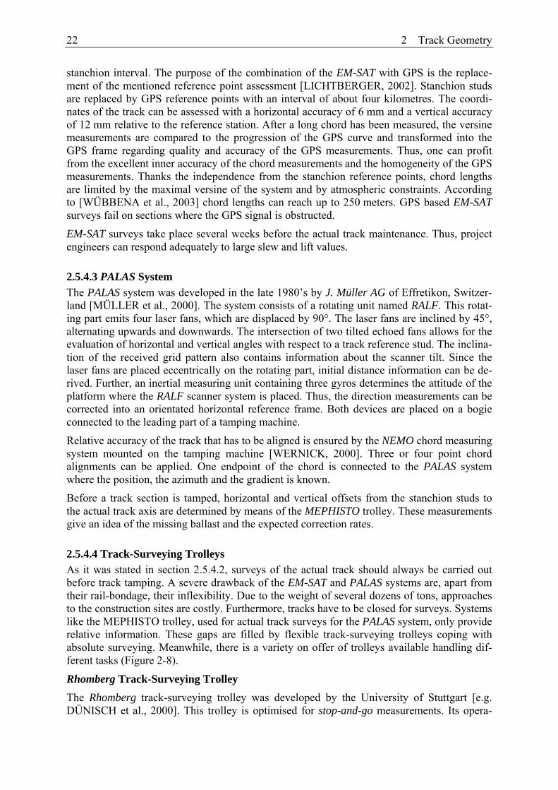
22 2 Track Geometry

stanchion interval. The purpose of the combination of the EM-SAT with GPS is the replace-ment of the mentioned reference point assessment [LICHTBERGER, 2002]. Stanchion studs are replaced by GPS reference points with an interval of about four kilometres. The coordi-nates of the track can be assessed with a horizontal accuracy of 6 mm and a vertical accuracy of 12 mm relative to the reference station. After a long chord has been measured, the versine measurements are compared to the progression of the GPS curve and transformed into the GPS frame regarding quality and accuracy of the GPS measurements. Thus, one can profit from the excellent inner accuracy of the chord measurements and the homogeneity of the GPS measurements. Thanks the independence from the stanchion reference points, chord lengths are limited by the maximal versine of the system and by atmospheric constraints. According to [WÜBBENA et al., 2003] chord lengths can reach up to 250 meters. GPS based EM-SAT surveys fail on sections where the GPS signal is obstructed.

EM-SAT surveys take place several weeks before the actual track maintenance. Thus, project engineers can respond adequately to large slew and lift values.

2.5.4.3 PALAS System The PALAS system was developed in the late 1980’s by J. Müller AG of Effretikon, Switzer-land [MÜLLER et al., 2000]. The system consists of a rotating unit named RALF. This rotat-ing part emits four laser fans, which are displaced by 90°. The laser fans are inclined by 45°, alternating upwards and downwards. The intersection of two tilted echoed fans allows for the evaluation of horizontal and vertical angles with respect to a track reference stud. The inclina-tion of the received grid pattern also contains information about the scanner tilt. Since the laser fans are placed eccentrically on the rotating part, initial distance information can be de-rived. Further, an inertial measuring unit containing three gyros determines the attitude of the platform where the RALF scanner system is placed. Thus, the direction measurements can be corrected into an orientated horizontal reference frame. Both devices are placed on a bogie connected to the leading part of a tamping machine.

Relative accuracy of the track that has to be aligned is ensured by the NEMO chord measuring system mounted on the tamping machine [WERNICK, 2000]. Three or four point chord alignments can be applied. One endpoint of the chord is connected to the PALAS system where the position, the azimuth and the gradient is known.

Before a track section is tamped, horizontal and vertical offsets from the stanchion studs to the actual track axis are determined by means of the MEPHISTO trolley. These measurements give an idea of the missing ballast and the expected correction rates.

2.5.4.4 Track-Surveying Trolleys As it was stated in section 2.5.4.2, surveys of the actual track should always be carried out before track tamping. A severe drawback of the EM-SAT and PALAS systems are, apart from their rail-bondage, their inflexibility. Due to the weight of several dozens of tons, approaches to the construction sites are costly. Furthermore, tracks have to be closed for surveys. Systems like the MEPHISTO trolley, used for actual track surveys for the PALAS system, only provide relative information. These gaps are filled by flexible track-surveying trolleys coping with absolute surveying. Meanwhile, there is a variety on offer of trolleys available handling dif-ferent tasks (Figure 2-8).

Rhomberg Track-Surveying Trolley The Rhomberg track-surveying trolley was developed by the University of Stuttgart [e.g. DÜNISCH et al., 2000]. This trolley is optimised for stop-and-go measurements. Its opera-

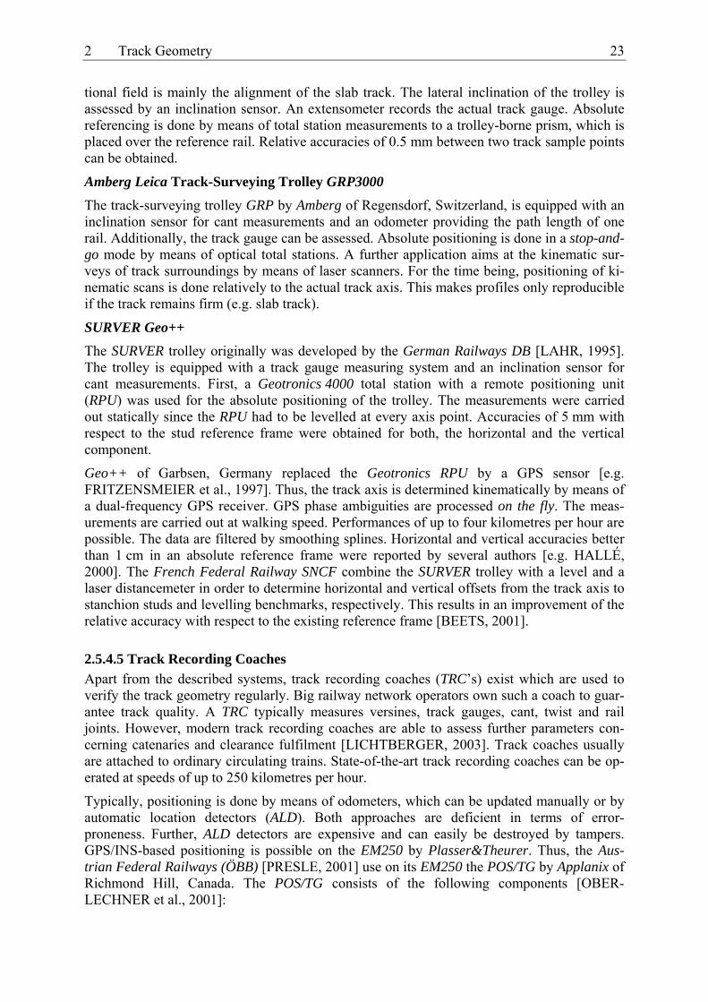
2 Track Geometry 23

tional field is mainly the alignment of the slab track. The lateral inclination of the trolley is assessed by an inclination sensor. An extensometer records the actual track gauge. Absolute referencing is done by means of total station measurements to a trolley-borne prism, which is placed over the reference rail. Relative accuracies of 0.5 mm between two track sample points can be obtained.

Amberg Leica Track-Surveying Trolley GRP3000 The track-surveying trolley GRP by Amberg of Regensdorf, Switzerland, is equipped with an inclination sensor for cant measurements and an odometer providing the path length of one rail. Additionally, the track gauge can be assessed. Absolute positioning is done in a stop-and-go mode by means of optical total stations. A further application aims at the kinematic sur-veys of track surroundings by means of laser scanners. For the time being, positioning of ki-nematic scans is done relatively to the actual track axis. This makes profiles only reproducible if the track remains firm (e.g. slab track).

SURVER Geo++ The SURVER trolley originally was developed by the German Railways DB [LAHR, 1995]. The trolley is equipped with a track gauge measuring system and an inclination sensor for cant measurements. First, a Geotronics 4000 total station with a remote positioning unit (RPU) was used for the absolute positioning of the trolley. The measurements were carried out statically since the RPU had to be levelled at every axis point. Accuracies of 5 mm with respect to the stud reference frame were obtained for both, the horizontal and the vertical component.

Geo++ of Garbsen, Germany replaced the Geotronics RPU by a GPS sensor [e.g. FRITZENSMEIER et al., 1997]. Thus, the track axis is determined kinematically by means of a dual-frequency GPS receiver. GPS phase ambiguities are processed on the fly. The meas-urements are carried out at walking speed. Performances of up to four kilometres per hour are possible. The data are filtered by smoothing splines. Horizontal and vertical accuracies better than 1 cm in an absolute reference frame were reported by several authors [e.g. HALLÉ, 2000]. The French Federal Railway SNCF combine the SURVER trolley with a level and a laser distancemeter in order to determine horizontal and vertical offsets from the track axis to stanchion studs and levelling benchmarks, respectively. This results in an improvement of the relative accuracy with respect to the existing reference frame [BEETS, 2001].

2.5.4.5 Track Recording Coaches Apart from the described systems, track recording coaches (TRC’s) exist which are used to verify the track geometry regularly. Big railway network operators own such a coach to guar-antee track quality. A TRC typically measures versines, track gauges, cant, twist and rail joints. However, modern track recording coaches are able to assess further parameters con-cerning catenaries and clearance fulfilment [LICHTBERGER, 2003]. Track coaches usually are attached to ordinary circulating trains. State-of-the-art track recording coaches can be op-erated at speeds of up to 250 kilometres per hour.

Typically, positioning is done by means of odometers, which can be updated manually or by automatic location detectors (ALD). Both approaches are deficient in terms of error-proneness. Further, ALD detectors are expensive and can easily be destroyed by tampers. GPS/INS-based positioning is possible on the EM250 by Plasser&Theurer. Thus, the Aus-trian Federal Railways (ÖBB) [PRESLE, 2001] use on its EM250 the POS/TG by Applanix of Richmond Hill, Canada. The POS/TG consists of the following components [OBER-LECHNER et al., 2001]:

24 2 Track Geometry

• The POS inertial measuring unit (IMU). It represents the core of the measuring system and contains three optical gyros and three accelerometers

• A GPS receiver which allows for differential measurements

• A distance-measuring indicator DMI which is basically an odometer. The DMI is used for improving navigation data, especially during GPS outages

• An optical track gauge measuring system OGMS

Thanks to the combined navigation solution, POS/TG provides 200 Hz geometry data. This corresponds to a sampling interval of 0.11 m at an operation speed of 80 kilometres per hour.

By means of TRC’s surveys, tracks of railway network are classified by quality numbers [ESVELD, 1989], which are archived and compared to earlier records. Thus, it could be dem-onstrated that track quality increased progressively on the network of the Swiss Federal Rail-ways by the introduction of the track reference system.

TRC’s provide − unlike track-surveying trolleys − track geometry parameters under dynamic stress. However, due to the limited numbers of TRC’s, their disposability is restricted. Typi-cally, each railway line is checked by a TRC once every half year. For high-speed tracks, this interval can be shorter. Further, the use of TRC’s on short sections is not cost-effective. Fi-nally, absolute track geometry derived from TRC records does not fulfil the accuracy re-quirement for track renewals.

2.5.5 The Swiss Trolley – Finding the Niche In the previous section, a selection of track-surveying systems was given featuring the sys-tems’ properties with regard to relative and absolute accuracy as well as work performance. Most of these systems were developed in terms of a special application. Below, justification is given for the development of the Swiss Trolley. In contrast to the EM-SAT and PALAS system, the design of the Swiss Trolley focuses on a lightweight construction. Two operators can carry out a survey without the need of track blocking. The system works kinematically. Absolute track geometry can be assessed by GPS. As it can be concluded from the previous section, GPS-based flexible systems are not widespread so far. Contrary to a common opinion that relative accuracies in the millimetre range have to be reached for an actual track survey of a ballast track, GPS-based systems, providing sub-centimetre accuracy, fulfil most accuracy requirements. Actual track surveys only have to provide information about the missing ballast and the expected slew and lift values in the absolute reference frame. Further, GPS-based data can be a basis for a nominal track regression. However, inner accuracy of the track is re-established by the chord alignment systems of the tamping machines. In contrast to the de-scribed systems, the trolley can cope with GPS outages incorporating kinematic total station measurements for absolute positioning. Apart from the assessment of track geometry parame-ters, the trolley is dimensioned for the adaptation of further sensors like laser scanners or ground penetrating radars. Then, an operational system does not only ask for rugged hardware but also for adequate data processing techniques. The Swiss Trolley software package includes data filtering of a single survey, processing techniques for merging the filtered single surveys, algorithms for slab track alignment and the integration of laser scan surveys. These features will be deepened in the subsequent chapters.

3 Potentials and Limitations of a Kinematic Track-Surveying System 25

3 Potentials and Limitations of a Kinematic Track-Surveying System

3.1 Kinematic Surveying This chapter outlines potentials and limitations of kinematic track surveying in terms of posi-tioning and object assessment. Several methods are analysed with respect to their suitability for kinematic surveying. Time crucial aspects are brought up in a further section. The problem of transformation between the body frame and global frame is addressed. The findings of this chapter flowed in during the development of the Swiss Trolley.

For surveys in motion, it can be profited by the fact that motions follow physical laws [e.g. KUHLMANN, 2004]. Motions are always caused by specific forces. Due to inertia, heading, velocity or accelerations cannot change arbitrarily fast. However, acting forces are not always known or are not of interest. Such kinematic models deal with geometrically possible motions of a body or a system of bodies without the consideration of the cause-effect-chain. Kinematic models represent good mappings for reality if no sudden jumps with respect to the used sam-pling interval occur. A kinematic model is used in this work for characterising the motion of the track-surveying trolley in chapter 5.

However, a multi-sensor platform cannot be modelled completely independently from the forces acting on it. For instance, inclination sensors obeying the earth’s gravitational field are not able to record sudden inclination jumps but react with a certain delay. Dynamic models are introduced for treating cause and effect of such a sensor. Thus, the response time of the inclination sensor have to be known. A dynamic model for the inclination sensors on the track-surveying platform is introduced in section 4.4.5.

The kinematic track-surveying parameters to be considered are functions of time. Modelling leads to an ordinary differential equation system with respect to time t. In practice, modelling deals with concrete parameters. The equations of motion are discretised with respect to the independent parameter t. Difference equation systems take the place of differential equation systems.

Kinematic surveying can contain both, surveys of moved objects by means of static systems, and vehicle-borne surveys. The survey of moved objects is typically realised by global navi-gation satellite systems (GNSS), tracking total stations or laser trackers. Autonomous track vehicle based determinations of trajectories can be carried out by inertial navigation systems, chord-measuring systems paired with odometers and others. The exclusive trajectory determi-nation of the moved objects can be an aim of a survey. However, for track surveying this is in general not of interest. Kinematic track surveying rather implies the assessment of static ob-jects along the railway stretches. Thus, for a kinematic survey of the track axis the vector between the trajectory and the reference rail has to be known in the resulting reference frame at any time of the run. Additional sensors are necessary to determine this vector. These are on the one hand sensors providing the attitude of the trolley like INS gyros, inclination sensors or high-speed cameras imaging control points. On the other hand, the trolley has to be held con-stant with respect to the reference rail, or a sensor is needed which measures the trolley wob-bling between the two rails. Further, kinematic surveying also comprises surveys of static objects in the track surroundings. This can include inspections of clearances, the track bed or the rail state. Optical sensors like laser scanners or high-speed cameras can be used for the determination of nearby railway infrastructure. Ground penetrating radar allows for the in-spection of the track underground and for the detection of layer discontinuities. Ultrasonic

26 3 Potentials and Limitations of a Kinematic Track-Surveying System

sensors can be used to scan cross-sections of rails. All tasks have in common that the six de-grees of freedom of the kinematic surveying platform have to be known at every time. Figure 3-1 gives an overview of potential sensors and tasks of kinematic track surveying classified by sensor placement and tasks.

GNSS sensorsINSinclination sensorsodometerschord lasershigh-speed cameras (CCD, CMOS)prisms (subsidiary to optical total stations)optical total stations...

GNSS satellitespseudolitesoptical total stationsprisms (subsidiary to optical total stations)laser trackersactive targets on satellite bogies (subsidiary to chord lasers)...

trolley position and attitude as intermediate result

kinematic surveys oftrack axis (track geometry inspection)track inventory (inspection of clearances)track underground (track bed inspection)rail crosssections (rail inspection)

trolley-borne sensors external sensors / actuators

trolley-borne sensorstrack gauge measuring systemlaser scannersground penetrating radar (GPR)ultrasonic sensorshigh-speed cameras (CCD, CMOS)3D cameras...

Figure 3-1: Potential sensors and tasks of a track-surveying trolley

Kinematic surveys are characterised by a permanent movement of the survey platform. How-ever, kinematic sensors do not sample the data continuously, but are time and value-discrete. Therefore, the sampling frequency has to be related to the speed of the survey platform. Par-ticularly, Nyquist’s sampling theorem has to be followed. This states that the sampling fre-quency has to be at least twice as high as the maximal signal frequency, or symbolically:

122Max Sampling Max

Sampling

f f or ft

≤ ≤Δ

(3.1)

3 Potentials and Limitations of a Kinematic Track-Surveying System 27

In contrast to time series, track surveying mainly considers series as a function of l describing the covered chainage. In analogy to (3.1), it results

2Min

Samplingl λΔ ≤ (3.2)

or for a kinematic survey with a constant velocity v

2Min

Samplingtv

λΔ ≤ (3.3)

where λmin is the minimal wavelength. For instance, wave patterns in the track axis with a period of five metres can only be detected by a kinematic survey with a velocity of 2 m/s, if at least every 1.25 seconds a data point is sampled.

Additionally, one has to consider that a particular measurement takes a certain time. The dura-tion of a particular measurement has to be very short with respect to the velocity of the sensor platform.

3.2 Absolute Position Fixing Position fixing directly determines the absolute coordinates of the trolley by measurements to or from reference points (section 2.5.3). Directions, ranges, pseudoranges, range rates base as measuring quantities. Two absolute position-fixing methods are considered here: GNSS and tracking total stations.

3.2.1 GNSS GNSS is used to refer to global navigation satellite systems. The American Global Positioning System (GPS) and the Russian Global Navigation Satellite System (GLONASS) are the two most prominent representatives. Both systems were designed as military navigation systems with poor accuracy but permanent operational availability. In 1994, the European Commis-sion (EC) identified the need for an own civil satellite system leading to the Galileo program. According to the mission program [EC, 2005], Galileo will be operational from 2008 on-wards. Further general GNSS information can be found in textbooks [e.g. LEICK, 1995; HOFMANN-WELLENHOF et al., 2001]. Although combined GPS/GLONASS receivers are available, this work is focused on the use of GPS receivers due to the insecure further devel-opment of GLONASS.

Geodetic applications make use of the carrier phase signals providing pseudo ranges to the satellites. By using differential techniques, many systematic influences can be eliminated by forming differences of corresponding observations. Kinematic differential GPS (GPS-RTK) for determining the trajectory of a moving receiver is a widely used method [SEEBER, 1993]. A key of processing GPS data is the integer phase ambiguity resolution. Several approaches to determine the integer ambiguities on-the-fly have been proposed and successfully imple-mented [e.g. HATCH, 1990; TEUNISSEN, 1994; COCARD, 1995]. On-the-fly integer ambi-guity resolution requires signal reception of at least five satellites. State-of-the-art ambiguity resolution techniques resolve integer ambiguities within a few seconds on-the-fly [e.g. LARGE et al., 2001]. Further, the success and the duration of the ambiguity resolution depend on the baseline length due to ionospheric disturbances that increase with the baseline length.

Multi station approaches guarantee short baselines by interpolating data for a nearby virtual reference station (VRS). Systematic influences can be considerably reduced by using VRS data. There exist nationwide commercial networks providing VRS data for any point with

28 3 Potentials and Limitations of a Kinematic Track-Surveying System

GPS and correction signal reception. In Switzerland, networks are operated by e.g. the na-tional agency for topography swisstopo of Berne.

A kinematic sensor system must be able to recuperate the integer ambiguity after an interrup-tion of the satellite signal. Additional sensors like INS help to regain the ambiguity resolution [SKALOUD, 1998]. These additional sensors must detect cycle slips quickly and provide sufficiently accurate initial values for a reliable ambiguity resolution after a longer GPS out-age.

A critical issue concerning GPS in a track environment are obstructions. Catenary masts can cause losses of lock, which affects the GPS solutions negatively. In mountainous regions, obstructions due to the local horizon have to be considered. The satellite visibility is an a pri-ori property and can be calculated for a specified railway stretch if satellite ephemerides are known and a digital terrain model is present. Figure 3-2 shows the percentage of the satellites over the actual horizon with respect to all satellites with an elevation larger than 15° within a time span of two identical constellations (23h 56m) for the main Swiss north-south railway connection. Twenty-eight satellites were considered. Apart from tunnel sections, topography does not affect GPS measurements in the Swiss midlands and the Jura mountains (chainage 0 - 130 km). However, on more than 50 % of the stretch, GPS reception is limited or impossi-ble. For curved sections, the reception can be even worse than shown in Figure 3-2 due to the inclined antenna. Taking into account that other obstructions like forests and buildings can affect GPS measurements negatively, it is obvious that alternative sensors have to be involved on a track-surveying platform for positioning.

0 50000 100000 150000 200000 250000 3000000

1000

2000

3000

Chainage [m]

Hei

ght a

bove

sea

leve

l [m

]

Basel Luzern

San Gottardo tunnel

Chiasso

longitudinal section (topography)longitudinal section (track)

0 50000 100000 150000 200000 250000 300000

0

20

40

60

80

100

Chainage [m]Topo

grap

hy in

duce

d G

PS o

bstru

ctio

ns [%

]

Figure 3-2: GPS obstructions due to topography along the principal north-south connection of the Swiss Federal Railways

3 Potentials and Limitations of a Kinematic Track-Surveying System 29

The issue of satellite visibility is closely related to multipath effects. Multipath originates from reflection of the signal in the surroundings of the antenna. It is perceived as an apparent prolongation of the signal path. Metallic or wet surfaces near the GPS antenna are critical. For a moving antenna, the effect of multipath changes rapidly due to the changing geometry be-tween the antenna and the surrounding reflective objects. Multipath is more probable at low satellite elevation angles where reflections show small incident angles. Thus, the reflected signal is hardly attenuated. Railway track surroundings are bad multipath environments, since there are many potential reflectors like catenary masts, stationary trains and others. Therefore, satellites at low elevation angles (< 15°) should not be tracked. Further, antennas with ground planes should be used. Ground planes can reduce multipath considerably, mainly at low eleva-tion angles. GPS antennas commonly use two types of ground planes: the conventional flat metal ground plane or the choke ring. Newer developments like those that are realised in the Trimble “Stealth” ground plane use the electrical resistance of the ground plane to weaken multipath signals. The electrical resistance within the ground plane increases exponentially along any line radiating out from the antenna centre. This electric field resistance burns up multipath as heat. Multipath resistance is comparable to that of quality-milled, expensive choke ring ground planes [KRANTZ et al., 2001].

It is known that the antenna phase centre is not stable with respect to varying azimuth, eleva-tion or frequency [WÜBBENA et al., 2000]. However, modern antennae show submillimetre variations [KRANTZ et al., 2001]. Within the domain of the track surveying, these magni-tudes should not cause concern.

The expectable accuracies mainly depend on the current satellite constellation. For kinematic surveys with geodetic receivers, accuracy is indicated by the manufacturers as 1 cm + 1 ppm for the horizontal component. The vertical component is deteriorated by a factor of two due to the rather unfavourable satellite geometry concerning height determination and due to errors in modelling tropospheric delays. If GPS heights have to be transformed in an orthometric height system, one has to account for the uncertainty of geoid undulations.

3.2.2 Tracking Total Stations Tracking total stations represent a valuable alternative for kinematic absolute position fixing. On the one hand, stretches with GPS gaps can be filled by linking the total station data to the reference frame. On the other hand, the combined use of GPS and total stations result in an improvement of accuracy and reliability linking the total station data to the GPS trajectory.

A total station for kinematic surveys is typically placed near the track and tied up to the refer-ence frame. A prism is placed on the survey platform and tracked by the tracking total station. Coarse location of the prism is automatically carried out in a predefined search window. An auxiliary laser fan can be used to accelerate the coarse location process. Automated target recognition (ATR) contains the fine positioning with respect to the collimation axis. This can be realised by digital image processing or further scan techniques [INGENSAND et al., 1997]. After target recognition, the prism is locked and tracked by the total station. In case of signal loss, locks can be regained by means of extrapolation algorithms and search procedures which are included in most total stations. For a 3D position fix, the horizontal and vertical angle encoders, the electronic distance meter and the two-axis compensator have to be read out synchronically. These processes have varying time spans. Direction encoding is the fastest process; a complete range measurement lasts longer than the determination of range rates. Further, distance measurements, ATR and the compensator readout depend on exterior influ-ences which can result in lags [HENNES, 1999]. The determination of a 3D position depends

30 3 Potentials and Limitations of a Kinematic Track-Surveying System

on the slowest single process. Consequences of this effect on positioning are discussed in de-tail in [STEMPFHUBER, 2004] and further in this work.

The work progress is restricted to the maximum line of sight. The maximum line of sight mainly depends on atmospheric conditions. Lines of sight longer than 200 metres should be avoided due to unknown refraction and scintillation. These effects can reach considerable amounts over ballast on sunny days. As the case may be, lines of sight have to be reduced.

Accuracy mainly depends on synchronisation errors. If we consider this fact and count for the azimuthal dependency of time synchronisation errors, accuracies in the range of 5 mm (both planimetric and altimetric) can be obtained at velocities of up to 2 m/s.

3.3 Dead Reckoning Dead reckoning (DR) for position determination starts from a known initial position and con-tinuously adds relative vectors. Three different possibilities of dead reckoning are described subsequently. In contrast to absolute position fixing, the variance propagation is not homoge-nous, but increases progressively. Therefore, this section also focuses on variance propagation of the proposed systems. A DR system can only be used in combination with a primary abso-lute system. A DR system can help to pass by GPS or total station gaps. Locally, it can im-prove relative accuracy.

3.3.1 Inertial Navigation Systems (INS) In case of inertial navigation, adjacent fixes are determined by a double integration of the ac-celerations along three axes of a reference frame. Either the reference frame is gimballed by gyroscopes or its attitude with respect to an initial orientation is determined by gyroscopes. Latter implementation is also known as strap-down mechanisation. A comprehensive over-view of inertial navigation systems is given by [JEKELI, 2001].

A limitation of a stand-alone INS is its unfavourable error propagation. Path errors, which are obtained by double integration of accelerometer errors, quadratically increase with time. Gyro drifts cause position errors which increase by the third power of time. Furthermore, due to a rather poor signal-to-noise ratio of the gyros, random walk has to be taken into account for the error budget. Random walk is due to the integration of the white-noise-contaminated gyro signal. This integration does not yield a normally distributed noise, but a bias which randomly walks away. Errors can be controlled by zero velocity updates (ZUPT). If fixed reference points are available, coordinate updates (CUPT) can be carried out for error control. Thus, integrated GNSS/INS systems perform high frequent CUPT’s. The available integrated sys-tems differ in the degree of coupling. Uncoupled systems reset INS errors whenever a GNSS solution is available. Coupled integration uses the data of both systems for simultaneous error compensation and navigation solution within a Kalman filter.

Inertial navigation systems in the required accuracy range are expensive. Further, the filter algorithms of available INS are tuned for the specific task. The unfavourable error propaga-tion for stand-alone INS prevented them from being integrated on the trolley.

3.3.2 Yaw Rates by Chord Techniques In analogy to chord techniques for correcting tracks (section 2.5.2), wandering chords can also be used for dead reckoning. Measurands are the chainage and the deflection angle be-tween two adjacent chords. Note that by means of two chords defining three points the trajec-tory is locally adapted by a circle. On transition curves, the measured deflection angle lags behind a certain amount as a function of the curvature variation. Several approaches are con-

3 Potentials and Limitations of a Kinematic Track-Surveying System 31

ceivable for assessing these two parameters. Chord techniques can be used for horizontal and vertical positioning. Subsequently, variance propagation is studied for the planimetric compo-nent. The derivation for the vertical component can be found analogously.

Δτi

Δτi

Δli

Pi-1

Pi+1

Pi

Q2,i

Q1,i

Y

X

c

c

Figure 3-3 Dead reckoning by means of wandering chords

The horizontal components of the position relative to an initial value can be found by

10

0

1

sin

cos

n

i iiin

ii i

i

lY YX X

l

τ

τ

=

=

⎛ ⎞Δ⎜ ⎟⎛ ⎞ ⎛ ⎞ ⎜ ⎟= +⎜ ⎟ ⎜ ⎟ ⎜ ⎟⎝ ⎠ ⎝ ⎠ Δ⎜ ⎟

⎝ ⎠

∑

∑ (3.4)

with

01

i

i j jj

lτ τ κ=

= + Δ∑ (3.5)

For a ride on a circle, it is

0 01 1

2 1sin2

i ij

i j j jj j

l lc c

ττ τ τ τ

= =

Δ= + Δ ≅ + Δ Δ∑ ∑ (3.6)

where κj is the curvature, Δτj is the deflection angle of two adjacent chords or the yaw rate, τi is the azimuth or the yaw angle, c the length of the chord and Δlj is the sampling interval ex-

32 3 Potentials and Limitations of a Kinematic Track-Surveying System

pressed in length units (Figure 3-3). The current chainage of the track-surveying system can be assessed by odometers, for instance. Note that c is a constant.

For estimating errors, a survey on a straight line towards east ( ,0 2 0jπτ τΔ= = ) with a constant

sampling interval Δl is assumed. Then, the derivative of (3.4) with respect to Δl and Δτ be-comes

1 1 1

1 1 1

sin cos

cos sin

n n n

i i i i ii i in n n

i i i i ii i i

d l l d d ldYdX

d l l d l d

τ τ τ

τ τ τ τ

= = =

= = =

⎛ ⎞ ⎛ ⎞Δ + Δ Δ⎜ ⎟ ⎜ ⎟⎛ ⎞ ⎜ ⎟ ⎜ ⎟= =⎜ ⎟ ⎜ ⎟ ⎜ ⎟⎝ ⎠ Δ + Δ Δ⎜ ⎟ ⎜ ⎟

⎝ ⎠ ⎝ ⎠

∑ ∑ ∑

∑ ∑ ∑ (3.7)

0 21 1 1

1i i i

i j j j jj j j

l ld d dc d l dc c c

τ τ τ τ τ= = =

Δ Δ= − Δ + Δ Δ +∑ ∑ ∑ (3.8)

For an error free initial azimuth τ0 and a ride on a straight line, the differential of (3.8) reduces to

1

i

i jj

ld dc

τ τ=

Δ= ∑ (3.9)

and (3.7) becomes

12

1 1

n

ii

n i

ji j

d ldYdX l d

cτ

=

= =

⎛ ⎞Δ⎜ ⎟⎛ ⎞ ⎜ ⎟=⎜ ⎟ ⎜ ⎟Δ⎝ ⎠ Δ⎜ ⎟

⎝ ⎠

∑

∑∑ (3.10)

For constant errors dΔl and dΔτ and for disappearing covariances, the standard deviation along and across the trajectory can be found

along lnσ σ Δ= (3.11)

3

3acrossl l

c τσ σ ΔΔ

≅ (3.12)

where l is the chainage. Note that if the sampling rate is equal to the chord length, (3.12) cor-responds to the cross error of a free stretched traverse. (3.12) can be used for estimating the maximal cross error if the primary system samples out. Figure 3-4 shows the influence of the chord length of the resulting cross error as a function of the chainage l. By means of a ten metre chord and a system, providing yaw rate precisions better than 10 mgon, GPS gaps of 100 metres can be bypassed with a precision better than 1 cm across the trajectory. In prac-tice, cross errors with the indicated precisions are likely higher since correlations between adjacent measurements were not considered here.

3 Potentials and Limitations of a Kinematic Track-Surveying System 33

0.0 10.0 20.0 30.0 40.0 50.0 60.0 70.0 80.0 90.0 100.00.0

2.0

4.0

6.0

8.0

10.0

12.0

14.0

16.0

18.0

20.0

Chainage [m]

Late

ral e

rror

[mm

]chord: 5 mchord: 10 mchord: 20 m

Figure 3-4 Cross error as a function of the chainage for a sampling interval of 1 m and an a priori yaw rates standard deviation of 10 mgon.

The chords are typically realised mechanically or by laser beams with active targets. Horizon-tal and vertical deflection angles can be obtained. For instance, a total station is placed on the trolley continuously tracking a target on an additional front bogie (“Mini EM-SAT”). Chord lengths and deflection angles are measured by the total station. Since prevailing cants and gradients exceed the range of built-in inclinometers, the total station compensators have to be switched off. Pitch and roll information for reducing the measured angles to a horizontal and a vertical plane has to be acquired by independent inclination sensors.

An additional, photogrammetric approach for deducing horizontal deflection angles by a trol-ley-borne system is conceivable, if one keeps in mind that the projection of the track gauge provides an accurate scale in an image. Such an approach would considerably benefit yaw rate determination since it could work autonomously. No satellite bogies would be necessary for chord supports. Subsequently, a proposal is developed for photogrammetric yaw rate determi-nation. This approach capitalises on this inherent scale.

A camera is mounted over the track axis on the survey platform. The image plane has to be approximately perpendicular to the track axis. If a linear array image of a track is taken along the track axis, the offsets of the displayed rail edges from the image principal point in the pixel row are a function of the track curvature and the trolley wobble. If a second image pointing in the opposite direction is considered, then the trolley wobble can be compensated. Both offsets yield the yaw rate Δτ as it will be shown below. For deriving azimuths at a par-ticular chainage i, the chord length c has to be known (equation (3.5)). The chord length c can be obtained by the use of the inherent scale provided by the projection of the track gauge.

Figure 3-5 shows the principle of yaw rate determination using two linear array cameras. By means of the running edges Eb1, Eb2 and Ef1, Ef2 the offsets eb, ef from the principal points Hb, Hf can be determined in the images. Although projective geometry does not hold proportional-ity, the offsets eb and ef can be found as the average between the edges E as a first approxima-tion. The effect of small deviations from a central projection with parallel image and object planes is given in [KRAUS, 1994]. For the deflection angle of the forward image, one obtains

34 3 Potentials and Limitations of a Kinematic Track-Surveying System

ff

ec

α ≅ (3.13)

and analogously for the backward image

bb

ec

α ≅ (3.14)

The sum of (3.13) and (3.14) yields

1

2 2i i

b fτ τ α α+Δ Δ

+ = + (3.15)

For similar chord lengths and curvatures, Δτi and Δτi+1 are identical. Thus, (3.15) degrades to

( )1i b f b fe e

cτ α αΔ = + = + (3.16)

Δτi

αf

αb

eb

Eb1

Ef1

Eb2

Ef2

Hb

Hfef

Δτi+1

Figure 3-5 Yaw rate measurements by means of two cameras

In Figure 3-6, the relation between the offset in the image plane and the offset in the object plane can be seen:

cos cos

e c eefτ τ

′= =

Δ Δ (3.17)

3 Potentials and Limitations of a Kinematic Track-Surveying System 35

where e’ is the projection of the offset in the object space plane, e the offset in the image plane and f the focal length of the camera. e’ deviates from the true offset e as a function of the track radius. With (3.16) the yaw rate can be found by iterating

( )1cosi b f

i

e ef

ττ

Δ = +Δ

. (3.18)

Figure 3-6 Determination of the chord length c and the offset e in the linear array

For the azimuth determination according to (3.5), the chord c has to be known in order to normalise the yaw rate regarding the corresponding sampling rate Δl. The chord length c can be read out from Figure 3-6

g gc f fg g′

= ≅ (3.19)

The precision of the azimuth mainly depends on the precision of the yaw rate determination. Therefore, the approximation made in (3.19) is acceptable. In turn, yaw rate precision mainly depends on the precision of the offset determination in the image. For a straight section, it results

2efτσ σΔ = (3.20)

where eσ is the precision of the offset determination in the image. (3.20) reveals that a long focal length affects the yaw rate ΔτI positively. Focal length precision, in turn, has no influ-ence on yaw rate determination. This does not hold for curved sections where a weak correla-tion is present. A more critical parameter of the inner camera orientation is the position of the principal point within the pixel array. A systematic bias of this parameter has an immediate impact upon the yaw rate determination. Therefore, the principal points of both pixel arrays have to be calibrated in advance or they have to be modelled as random constants. Preferably, this is done on a straight track section.

The determination of the measurands be and fe in (3.18) can be realised by edge detection. In contrast to the classical 2D-edge detection [e.g. CANNY, 1986], the image gradients just have to be evaluated across the direction of motion.

e

E1

f c

e’ eE2

H

Δτ

g

36 3 Potentials and Limitations of a Kinematic Track-Surveying System

Using high-speed cameras with micrometre precision for edge detection and objectives with focal lengths of 10 mm, standard deviations of the sought yaw rate around ten mgon are ob-tained. Referring to Figure 3-4, these precisions would suffice to bypass GPS gaps of several tens of metres. In practice, edge detection of rails in the CCD array has to be investigated. This could be a limiting issue since the contrast between the rail and the ballast could be too small. Figure 3-7 gives an idea of the quality of edge detection. Edge detection by means of a Canny filter was performed on an image taken by a commercial digital camera with an effec-tive focal length of 10.5 mm and a pixel size of 3 μm.

Figure 3-7 Edge detection of rails by a Canny filter

If this concept is applied in kinematic applications, adequate exposure times have to be cho-sen in order to avoid blurred images. Further, the images or the derived yaw rates have to be time tagged.

Precision can be improved by evaluating several lines of the digital image. If yaw rates are averaged, the samples have to be weighted in concordance with the corresponding chord length c.

The proposed method implies that the track-surveying platform is guided along a rail. Alter-natively, bounces from the guiding rail can be assessed by a scanning system, correcting the raw yaw rates for the corresponding amounts.

Within the Swiss Trolley project, [HOHL, 2005] applied the proposed approach on images acquired by an industrial camera with a 6.5 μm pixel size and an objective with a focal length of 16 mm. The main difficulty was the reliable edge detection. Depending on the illumination, the rail edge could vary in several pixels. Further, the used algorithms are very time-consuming. For an effective use, specialised routines have to be developed.

3.3.3 Odometers An odometer counts the number of wheel revolutions of a vehicle, which is proportional to the distance travelled. If two odometers are placed in two opposite wheels, the average of both readings provides the path length l of the track centre line. The difference contains bearing information (Figure 3-8).

3 Potentials and Limitations of a Kinematic Track-Surveying System 37

Δτ

R

s

l1

ll2

Figure 3-8 Path and yaw rate measurements by odometers

With l1 and l2 denoting both odometers, the average distance l and the yaw rate are given by

1 2

2l ll +

= (3.21)

1 2l ls

τ −Δ = (3.22)

or

1 2

2N Nl C +

= (3.23)

1 2N NCs

τ −Δ = (3.24)

where s is the distance between the points of contacts of both wheels, C the circumference of the wheels and N1 and N2 the numbers of revolutions of the left and right wheel, respectively. The variance of (3.24) can be computed as

( ) 22 21 22 2 2 21 2

22C N s

C N NN N Cs s sτσ σ σ σΔ

⎛ ⎞−−⎛ ⎞ ⎛ ⎞= + + ⎜ ⎟⎜ ⎟⎜ ⎟⎝ ⎠⎝ ⎠ ⎝ ⎠

(3.25)

In analogy, the variance for the chainage results in

( )22 2 2 21 2

1 12 4l N CC N Nσ σ σ= + + . (3.26)

Figure 3-9 represents the precision of the yaw rates and the distances as a function of the chainage for different wheel diameters and track radii. The a priori standard deviations for the wheel diameter, the revolution counter and the offset s were set to 0.1 mm, 0.0005 and 1 mm, respectively. The distance error essentially increases proportionally with the covered path for curved sections and does not correlate with the track radius. Large diameters influence the error propagation positively. On the other hand, yaw rate precision depends on the track ra-dius but does not correlate with the covered path on straight sections. According to (3.25), only the revolution counter precision contributes to the yaw rate error for straight lines since the counter difference N1-N2 disappears. For differential odometry, small wheel diameters have a favourable effect on error propagation, since the influence of the revolution count pre-cision dominates the error propagation mainly on short sections.

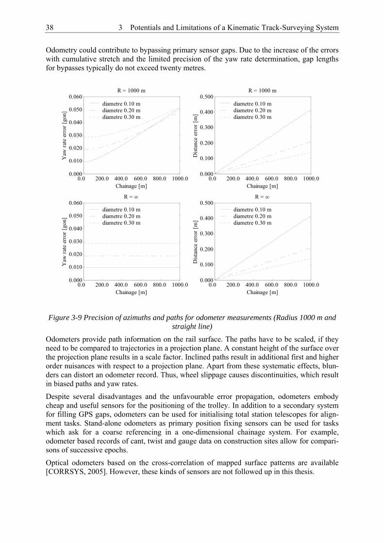
38 3 Potentials and Limitations of a Kinematic Track-Surveying System

Odometry could contribute to bypassing primary sensor gaps. Due to the increase of the errors with cumulative stretch and the limited precision of the yaw rate determination, gap lengths for bypasses typically do not exceed twenty metres.

0.0 200.0 400.0 600.0 800.0 1000.00.000

0.010

0.020

0.030

0.040

0.050

0.060R = 1000 m

Chainage [m]

Yaw

rate

err

or [g

on]

diametre 0.10 mdiametre 0.20 mdiametre 0.30 m

0.0 200.0 400.0 600.0 800.0 1000.00.000

0.100

0.200

0.300

0.400

0.500R = 1000 m

Chainage [m]D

istan

ce e

rror

[m]

diametre 0.10 mdiametre 0.20 mdiametre 0.30 m

0.0 200.0 400.0 600.0 800.0 1000.00.000

0.010

0.020

0.030

0.040

0.050

0.060R = ∞

Chainage [m]

Yaw

rate

err

or [g

on]

diametre 0.10 mdiametre 0.20 mdiametre 0.30 m

0.0 200.0 400.0 600.0 800.0 1000.00.000

0.100

0.200

0.300

0.400

0.500R = ∞

Chainage [m]

Dist

ance

err

or [m

]

diametre 0.10 mdiametre 0.20 mdiametre 0.30 m

Figure 3-9 Precision of azimuths and paths for odometer measurements (Radius 1000 m and straight line)

Odometers provide path information on the rail surface. The paths have to be scaled, if they need to be compared to trajectories in a projection plane. A constant height of the surface over the projection plane results in a scale factor. Inclined paths result in additional first and higher order nuisances with respect to a projection plane. Apart from these systematic effects, blun-ders can distort an odometer record. Thus, wheel slippage causes discontinuities, which result in biased paths and yaw rates.

Despite several disadvantages and the unfavourable error propagation, odometers embody cheap and useful sensors for the positioning of the trolley. In addition to a secondary system for filling GPS gaps, odometers can be used for initialising total station telescopes for align-ment tasks. Stand-alone odometers as primary position fixing sensors can be used for tasks which ask for a coarse referencing in a one-dimensional chainage system. For example, odometer based records of cant, twist and gauge data on construction sites allow for compari-sons of successive epochs.

Optical odometers based on the cross-correlation of mapped surface patterns are available [CORRSYS, 2005]. However, these kinds of sensors are not followed up in this thesis.

3 Potentials and Limitations of a Kinematic Track-Surveying System 39

3.3.4 Height Determination by an Inclination Sensor Height differences of a particular rail by means of an inclination sensor and the true path length can be found by the integration of the rail inclinations along the covered path. For small sampling intervals, it holds

01

sinn

n i ii

H H l α=

= + Δ∑ (3.27)

where α is the longitudinal inclination of the rail with respect to the local horizon and Δli is the sampling interval expressed in length units on the true path. The true path can be assessed by odometers or by an absolute-position fixing device. The standard deviation of Hn for a non-curved, little inclined stretch and a constant sampling interval corresponds to

H l l ασ σ= Δ ⋅ (3.28)

where l is the covered path. Figure 3-10 shows the height error as function of the chainage. For the a priori precision of the inclinations, 5 mrad was chosen. The behaviour of the dis-played curves corresponds to the error propagation of azimuth traverses for planimetric posi-tioning or levelling for altimetric positioning and grows with the square root of the covered chainage for a constant sampling rate. A small sampling rate has a positive effect on error propagation. For kinematic applications, the main drawback of the inclinometer based height determination is the sensitivity of inclination sensors to accelerations. Accelerations have to be assessed during the survey and removed from the raw inclinometer readings. Further, sys-tematic errors affect the height determination. An inclination sensor bias results in an apparent tilt of the track. An inadequate gain factor ends up with errors which grow quadratically to the covered path.

0.0 10.0 20.0 30.0 40.0 50.0 60.0 70.0 80.0 90.0 100.00.0

20.0

40.0

60.0

80.0

100.0

120.0

140.0

160.0

Chainage [m]

Hei

ght e

rror

[mm

]

sampling interval: 1 msampling interval: 5 msampling interval: 10 m

Figure 3-10 Height error as a function of the chainage (σα = 0.005 rad) for a stretched survey

The height of the centre line and the opposite rail is given by

40 3 Potentials and Limitations of a Kinematic Track-Surveying System

sin

2sin

an n n

on n n

sH H

H H s

β

β

= +

= + (3.29)

where s denotes the offset between the point of wheel contacts and β the inclination across the track axis.

Due to the non-homogenous error propagation along a covered stretch, height determination by means of an inclination sensor can only serve as a secondary system for positioning. How-ever, accurate inclinations help to bypass GPS gaps. If accelerations can be properly separated from inclinations, they can even improve GPS based height accuracy.

3.4 Attitude Determination The attitude defines the relative orientation between the global frame (g-frame) and the trolley frame (body or b-frame). It is described by the three Euler angles roll, pitch and yaw typically denoted by ω, ϕ, κ. In contrast, τ is used here for the yaw angle, since the symbol κ is already reserved for the track curvature. Alternatively, attitude is occasionally described by quater-nions [e.g. JEKELI, 2001]. Quaternions outmatch the Euler angle approach concerning com-putational speed. The evaluation of trigonometric functions is not required. In contrary to the Euler angle approach, singularities for special configurations for attitude angle determinations do not occur [KRAUS, 1994]. In spite of these benefits, the classical, geometrically more in-tuitive Euler angle approach is used to assess attitude in this work. The knowledge of the atti-tude is essential for reducing GPS, total station or laser scanner data from the b-frame to the g-frame. Further, the pitch and roll angles of a track-surveying vehicle are highly correlated with the two track key parameters gradient and cant, respectively. Attitude can be measured directly or it can be determined by using vectors given in the b-frame and in the g-frame [e.g. FAVEY, 2000]. For the latter approach, at least two vectors have to be known in both frames.

Direct attitude determination by strap-down inertial navigation systems provides all three atti-tude angles where gimballed INS remain constant with respect to the local frame. Direct atti-tude data can also be partially obtained by inclination sensors. Two non-collinear inclination sensors provide roll and pitch information. Inclination sensors refer to the local astronomical horizon. The measured inclinations have to be transformed in proper roll and pitch values. The disadvantage of kinematic attitude determination by inclination sensors is, as stated be-fore, their sensitivity to accelerations. Inclinations can only be obtained, if the accelerations acting on the inclinometers are known. Conversely, inclination sensors act as accelerometers if the inclination is known.

In the special case of track-based surveying, vehicles without suspension, roll, pitch and yaw angles are highly correlated with the track geometry. Initial attitude information can be ob-tained if nominal geometry data are available. Further, advantage can be taken of the covered trajectory which contains inherent yaw and pitch information.

3.5 Kinematic Surveys of the Railway Inventory In general, trajectory surveys and attitude determination are intermediate results of kinematic track surveying. A main objective of kinematic track surveying is the determination of the actual track axis. Kinematic surveys of the track environment are gradually widening applica-tion fields. Figure 3-11 shows a typical cross section containing selected railway assets that are of interest for a railway inventory. What all applications have in common is that the addi-tional data describing the track axis or the track environment have to be correlated chrono-

3 Potentials and Limitations of a Kinematic Track-Surveying System 41

logically and spatially with the primary geo-referencing sensors. This means that the addi-tional sensor information has to be time-tagged. Further, the sensor origin and its alignment have to be known in the b-frame.

Subsequently, most demanding applications with regard to the design of a track-surveying trolley are mentioned.

Figure 3-11 Cross section of double track railway alignment showing names of principal parts of construction [NETWORK RAIL, 2003]

3.5.1 Track Gauge Measuring Systems For track axis surveying, the current position offset of the track-surveying vehicle with re-spect to the datum rail has to be assessed or maintained constantly. A number of systems press the vehicle against the reference rail. Due to friction, this method only works for low velocities. Further, problems emerge at switch crossings due to clearance violation. Another approach aims at the determination of trolley wobble rates with respect to both rails. This can be realised by laser systems or mechanically, pressing levers by springs or magnets to the running rail edges. The deflections of the levers are measured by angular transducers. Me-chanical systems must count for the track clearance for switch crossings. As an additional approach, laser systems working according to the time-of-flight principle or laser diodes using the optical triangulation principle [SCHLEMMER, 1996] can be applied. Latter system works since distance rates for assessing the trolley wobble do not exceed 4 cm. Further, reflection properties of the running rail edge are constant.

Another key parameter in terms of track surveying is the track gauge. If the vehicle wobble is assessed by one of the described systems, track gauge is obtained by the sum of both dis-tances to the running rail edges plus the offset between the two distance sensors. A realisation of a laser gauge track measuring system is given in Figure 3-12. If the vehicle is guided along a reference rail, rope extensometers are conceivable for track gauge determination.

Fence

Topsoil

Cable through Drain Drain

Cable through Cess

Embankment

Topsoil

Ditch

Fence

Sleepers Ballast

Ditch Batter Slope

Catenary Mast

Overhead Line

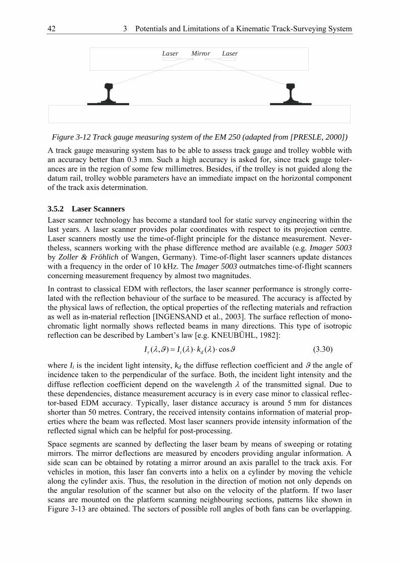
42 3 Potentials and Limitations of a Kinematic Track-Surveying System

Laser Mirror Laser

Figure 3-12 Track gauge measuring system of the EM 250 (adapted from [PRESLE, 2000])

A track gauge measuring system has to be able to assess track gauge and trolley wobble with an accuracy better than 0.3 mm. Such a high accuracy is asked for, since track gauge toler-ances are in the region of some few millimetres. Besides, if the trolley is not guided along the datum rail, trolley wobble parameters have an immediate impact on the horizontal component of the track axis determination.

3.5.2 Laser Scanners Laser scanner technology has become a standard tool for static survey engineering within the last years. A laser scanner provides polar coordinates with respect to its projection centre. Laser scanners mostly use the time-of-flight principle for the distance measurement. Never-theless, scanners working with the phase difference method are available (e.g. Imager 5003 by Zoller & Fröhlich of Wangen, Germany). Time-of-flight laser scanners update distances with a frequency in the order of 10 kHz. The Imager 5003 outmatches time-of-flight scanners concerning measurement frequency by almost two magnitudes.

In contrast to classical EDM with reflectors, the laser scanner performance is strongly corre-lated with the reflection behaviour of the surface to be measured. The accuracy is affected by the physical laws of reflection, the optical properties of the reflecting materials and refraction as well as in-material reflection [INGENSAND et al., 2003]. The surface reflection of mono-chromatic light normally shows reflected beams in many directions. This type of isotropic reflection can be described by Lambert’s law [e.g. KNEUBÜHL, 1982]:

( , ) ( ) ( ) cosr i dI I kλ ϑ λ λ ϑ= ⋅ ⋅ (3.30)

where Ii is the incident light intensity, kd the diffuse reflection coefficient and ϑ the angle of incidence taken to the perpendicular of the surface. Both, the incident light intensity and the diffuse reflection coefficient depend on the wavelength λ of the transmitted signal. Due to these dependencies, distance measurement accuracy is in every case minor to classical reflec-tor-based EDM accuracy. Typically, laser distance accuracy is around 5 mm for distances shorter than 50 metres. Contrary, the received intensity contains information of material prop-erties where the beam was reflected. Most laser scanners provide intensity information of the reflected signal which can be helpful for post-processing.

Space segments are scanned by deflecting the laser beam by means of sweeping or rotating mirrors. The mirror deflections are measured by encoders providing angular information. A side scan can be obtained by rotating a mirror around an axis parallel to the track axis. For vehicles in motion, this laser fan converts into a helix on a cylinder by moving the vehicle along the cylinder axis. Thus, the resolution in the direction of motion not only depends on the angular resolution of the scanner but also on the velocity of the platform. If two laser scans are mounted on the platform scanning neighbouring sections, patterns like shown in Figure 3-13 are obtained. The sectors of possible roll angles of both fans can be overlapping.

3 Potentials and Limitations of a Kinematic Track-Surveying System 43

Thus, depending on the phase shift in chainage direction and the velocity of the vehicle reso-lution can be improved.

For laser profilers only rotating around one axis, the scanner attitude on the trolley has to be defined depending on the task. Clearance inspections preferably are carried out with a laser fan scanning perpendicular to the track axis. This results in optimal accuracies for clearance critical elements since incidence angles of interesting structures are optimal. On the other hand, a pitched laser fan is able to gather information of structures facing in track direction. Figure 3-13 shows apart of a non-inclined laser fan, scans of two scanners which are pitched by 45° and rolled by 45° and -45°, respectively.

-5 0 5-5

0

5ω = 0°, φ = 0°

y [m]

z [m

]

-5 0 50

5

10

15

20

y [m]

x (d

irect

ion

of m

otio

n) [m

]

010

20

-50

5-4-2024

x [m]y [m]

z [m

]

-5 0 5-5

0

5ω = 45°, φ = 45°

y [m]

z [m

]

-5 0 50

5

10

15

20

y [m]

x (d

irect

ion

of m

otio

n) [m

]

010

20

-50

5-4-2024

x [m]y [m]

z [m

]

Figure 3-13 Traces on a cylinder surface recorded by two laser scanners placed on the cylin-der axis.

Figure 3-13 reveals different resolutions with respect to the cardinal axis of the vehicle sys-tem. This dependence has to be considered for mission planning. Pitch and roll layout of the

44 3 Potentials and Limitations of a Kinematic Track-Surveying System

scanners must be adapted to the requirements of the survey task. Further, the top views of Figure 3-13 shed light on the use of skewed scans. By means of non-pitched laser scanners, structures facing in the direction of motion are cut by flat incident angles. Reversely, the pitched scans cut lines with constant x-coordinates with significantly less flat incident angles improving accuracy in the direction of motion. In either case, kinematic scanning outmatches static polar scans for linear objects like railway lines or tunnels. Kinematic scans benefit from more homogeneous incident angles along the track. Further, kinematic scanning faces less obstructing zones.

Attention has to be paid to the data amounts accumulating during a kinematic survey. For example, a laser scanner with a sampling frequency of 13.5 kHz (13500 points per seconds) produces for a one-kilometre survey carried out at a velocity of 1 m/s about 27 MB of data. Per data point, a 16-bit integer type has to be used for an unambiguous representation of dis-tances with millimetre resolution up to 64 metres. Data amounts can be reduced by adapting the scan resolution, the vehicle velocity and the scan window with regard to the specific ap-plication. Thus, scans for clearance determination require a much smaller resolution than scans for the positioning of the overhead line. On the other hand, the scan window for the latter application can be constricted. Laser scanning is an effective method for both mentioned applications, since a high degree of automation can be reached by comparisons between nominal profiles or line tracing for overhead line determination. However, if arbitrary railway assets have to be extracted from the data, the objects mostly have to be modelled semi-automatically. These operations are in general very time-consuming. As a rule of thumb, the modelling work exceeds the fieldwork by a factor of ten [SCHULZ et al., 2004].

3.5.3 3D Cameras 3D solid-state cameras represent a valuable alternative to laser scanners for clearance inspec-tion. Most 3D cameras operate on a CCD/CMOS basis and unify the advantages of both tech-nologies [BLANC, 2001]. CCD arrays (charge-coupled device) provide low-noise data with good sensitivity, whereas CMOS (complementary metal oxide semiconductor) offers signifi-cant advantages in term of low consumption, low voltage, monolithic integration and on-chip functionality even at the pixel level.

The Swiss Center for Electronics and Microtechnology, Inc. (CSEM) of Neuchâtel, Switzer-land developed a range camera which offers 3D image data in real-time [OGGIER et al., 2004]. The 3D camera SwissRanger SR-2 EDM bases on the phase-difference principle and works with a modulated infrared light source. The emitted light is reflected by the objects in a scene and travels back to the camera, where the phase lags of the modulated signal are meas-ured locally in “smart” pixels. Only one light emitter faces a 124 · 160 pixel array of light receivers. In contrast to conventional cameras, the SR-2 range camera not only determines the local brightness in the scene, but also the complete distance map, i.e. the 3D model of its envi-ronment. According to the technical specifications, up to thirty frames per second can be ac-quired. Unambiguous ranges of the SR-2 are limited to 7.5 metres. This fits most requirements for clearance inspections. However, double track tunnels with a circular profile exceed in general this limit. Distance accuracy is indicated as 5 mm [KAHLMANN, 2005]. The re-marks of section 3.5.2 concerning Lambert’s law of reflection also holds for 3D cameras. In spite of several deficiencies with regard to kinematic track surveying, this promising technol-ogy has to be kept in view for future applications.

3 Potentials and Limitations of a Kinematic Track-Surveying System 45

Figure 3-14 3D camera SwissRanger SR2

3.5.4 Ground Penetration Radar (GPR) For a complete description of the track environment, also the track bed underground is of in-terest. The first step of track renewal planning is in general a geotechnical study. Inspection is focused on the thickness of the ballast, on subsoil material penetrating upwards into the bal-last and on geotechnical properties of subgrade and subsoil materials [HELLMANN et al., 1994]. Ground penetration radar (GPR) [e.g. LECKEBUSCH, 2001] allows for non-destructive underground exploring. GPR measures time-of-flight of electromagnetic impulses penetrating into the underground which are partly or totally reflected on layer discontinuities. The used frequencies are in the UHF band of the electromagnetic spectrum (e.g. 900 MHz). In order to determine layer depths, the knowledge of the propagation velocity within the ballast has to be known. [HUGENSCHMIDT, 2000] indicates a signal velocity of 1.4 · 108 m/s. The reflections caused by sleepers and rails have to be eliminated from radargrams by appropriate filter techniques. [HUGENSCHMIDT, 2000] compared GPR results with layer depths ac-quired in trenches and reported an accuracy of 4 cm for the layer detection.

3.6 Synchronisation Kinematic multisensor systems ask for a careful time treatment. The faster the survey plat-form moves the more accurate time information has to be handled. Positioning errors lδ due to synchronisation errors tδ proportionally grow with velocity v:

l v tδ δ= ⋅ (3.31)

Figure 3-15 quantifies this effect for several velocities. For example, a synchronisation error of 1 ms causes an uncertainty of 1 mm for a velocity of 1 m/s.

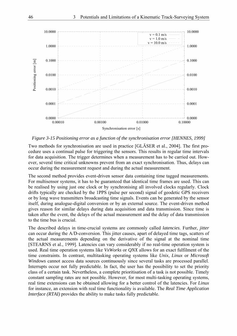
46 3 Potentials and Limitations of a Kinematic Track-Surveying System

0.0000

0.0001

0.0010

0.0100

0.1000

1.0000

10.0000

0.00010 0.00100 0.01000 0.100000.0000

0.0001

0.0010

0.0100

0.1000

1.0000

10.0000Po

sitio

ning

err

or [m

]

Synchronisation error [s]

v = 0.1 m/sv = 1.0 m/s

v = 10.0 m/s

Figure 3-15 Positioning error as a function of the synchronisation error [HENNES, 1999]

Two methods for synchronisation are used in practice [GLÄSER et al., 2004]. The first pro-cedure uses a continual pulse for triggering the sensors. This results in regular time intervals for data acquisition. The trigger determines when a measurement has to be carried out. How-ever, several time critical unknowns prevent from an exact synchronisation. Thus, delays can occur during the measurement request and during the actual measurement.

The second method provides event-driven sensor data containing time tagged measurements. For multisensor systems, it has to be guaranteed that identical time frames are used. This can be realised by using just one clock or by synchronising all involved clocks regularly. Clock drifts typically are checked by the 1PPS (pulse per second) signal of geodetic GPS receivers or by long wave transmitters broadcasting time signals. Events can be generated by the sensor itself, during analogue-digital conversion or by an external source. The event-driven method gives reason for similar delays during data acquisition and data transmission. Since time is taken after the event, the delays of the actual measurement and the delay of data transmission to the time bus is crucial.

The described delays in time-crucial systems are commonly called latencies. Further, jitter can occur during the A/D-conversion. This jitter causes, apart of delayed time tags, scatters of the actual measurements depending on the derivative of the signal at the nominal time [STEARNS et al., 1999]. Latencies can vary considerably if no real-time operation system is used. Real time operation systems like VxWorks or QNX allows for an exact fulfilment of the time constraints. In contrast, multitasking operating systems like Unix, Linux or Microsoft Windows cannot access data sources continuously since several tasks are processed parallel. Interrupts occur not fully predictable. In fact, the user has the possibility to set the priority class of a certain task. Nevertheless, a complete prioritisation of a task is not possible. Timely constant sampling rates are not possible. However, for most multi-tasking operating systems, real time extensions can be obtained allowing for a better control of the latencies. For Linux for instance, an extension with real time functionality is available. The Real Time Application Interface (RTAI) provides the ability to make tasks fully predictable.

3 Potentials and Limitations of a Kinematic Track-Surveying System 47

3.7 Modelling Apart of the synchronisation of the data, an accurate geometric assignment of the sensors has to be guaranteed. For a combined data processing, all sensors have to be referenced with re-spect to the body frame (b-frame).

The lowest level represents the measuring process itself and its reconstruction (Figure 3-16, [RUHM, 2002]). The process ( )y t is mapped by the sensor system and provides carrier sig-nals ( )sy t . The reconstruction system transforms the carrier signals back to the sought meas-urands ( )my t . The reconstruction system inverts the mapping of the original process ( )y t .

( )y t is a vector and can contain arbitrary elements like coordinates or attitude angles. In gen-eral, reconstruction is done by calibration functions or look-up tables. Since the sensor system and the reconstruction system are not error free, the observed parameter ( )my t deviates from the original process parameter ( )y t by ( )ye t .

sensor system reconstructionsystem

( )y t ( )y t

( )y t ( )my t( )sy t

processinstrumentation

measuring system

∑

+

( )ye t-

Figure 3-16 Measuring process [RUHM, 2002]

For example, in Figure 3-16 the cant of a track can be thought as a function of chainage. The chainage, in turn, is a function of time for a kinematic track survey. The cant ( )y t is meas-ured within a measuring system by an inclination sensor placed on a track-surveying platform. The inclination sensor provides voltages as a function of the timely varying cant. The recon-struction system transforms these voltages to cants by means of a characteristic curve. The characteristic curve has to be found by calibrating the measuring system. Typically, the char-acteristic curve is defined by a zero-point offset and a gain factor. Both, the mapped cant

( )sy t and the characteristic curve are exposed to errors and bias the reconstructed cant ( )my t by ( )ye t .

Above-mentioned model covers the steady state of a general dynamic process. Mapping and reconstruction can be represented as a serial connection. The solution for the general dynamic case is realised by combining a parallel connection with error correction in a closed-loop [e.g. GEERING, 2001]. For deterministic processes, this is realised by a Luenberger observer. The Kalman-Bucy filter covers the stochastic time-continuous case, the Kalman filter the stochas-tic time-discrete case. Section 5.4 deals with a kinematic model for stochastic data of a track-surveying trolley.

3.8 Transformation For a common data treatment of positioning data, positioning sensors have to be referenced with respect to the vehicle’s origin. This leads to the definition of the body system (b-system). Within this work, the axes of the b-system are defined along the forward, left and the “through-the-roof” directions (see Figure 3-17). The origin of the b-system is the intersection of the plane formed by the contact surface of the three wheels, the plane perpendicular to the

48 3 Potentials and Limitations of a Kinematic Track-Surveying System

contact surface containing both points of contact of the track gauge measuring system and the plane perpendicular to both previously mentioned planes containing the centre of the front axle.

Figure 3-17 Definition of the body system of a track-surveying vehicle In general, a spatial similarity transformation is applied to transform coordinates from the measuring system to the body system:

( ) ( )b mb mb mx t x R x t= + ⋅ (3.32)

( )mx t corresponds to ( )my t in Figure 3-16, but is restricted to Cartesian coordinates. The origin of the measuring coordinate system expressed in the body system mbx as well as the rotation matrix mbR is found by calibration procedures. The translation vector as well as the rotation matrix can be supposed to be constant for a kinematic survey. This assumption re-quires a stable mounting on the platform and negligible vibrations during operation. The measuring coordinate system is taken to be orthogonal. Non-orthogonalities have to be deter-mined with special calibration procedures depending on the sensors.

Next, ( )bx t is transformed into a superior global system. For example, this global system can be a reference system of a railway company. Locally, this can be done again by a spatial simi-larity transformation

( ) ( ) ( ) ( )g bg bg bx t x t R t x t= + ⋅ (3.33)

(3.33) implies that the product ( ) ( )bg bR t x t⋅ provides a vector in a local Cartesian system. For small vectors ( ) ( )bg bR t x t⋅ , above notation is also allowable for combined planimetric and altimetric systems like they commonly occur for track surveying. Strictly speaking, the plani-metric components of ( ) ( )bg bR t x t⋅ have to be reduced to a reference height. Then, reductions

yg

xg

zg

xb

yb

zb

P

3 Potentials and Limitations of a Kinematic Track-Surveying System 49

due to a projection system have to be applied. For mixed systems, a further correction for earth curvature has to be applied to the height component of ( ) ( )bg bR t x t⋅ .

In (3.33), the translation ( )bgx t and ( )bgR t containing vehicles attitude vary with time and have to be updated continuously. Further, ( )bgR t is a function of the Euler angles. It can be split into three elementary rotations around the coordinate axes:

( )( ) ( ) ( )2( ) ( ) ( ) ( )bg bg bg bgz y xR t R t R t R tπ τ ϕ ω−= − − − (3.34)

where

( )1 0 0

( ) 0 cos ( ) sin ( )0 sin ( ) cos ( )

bgxR t t t

t tω ω ω

ω ω

⎛ ⎞⎜ ⎟− = −⎜ ⎟⎜ ⎟⎝ ⎠

(3.35)

( )cos ( ) 0 sin ( )

( ) 0 1 0sin ( ) 0 cos ( )

bgy

t tR t

t t

ϕ ϕϕ

ϕ ϕ

⎛ ⎞⎜ ⎟− = ⎜ ⎟⎜ ⎟−⎝ ⎠

(3.36)

( )( )( ) ( )( ) ( )

2 2

2 2 2

cos ( ) sin ( ) 0

( ) sin ( ) cos ( ) 0

0 0 1

bgz

t t

R t t t

π π

π π π

τ τ

τ τ τ

− −

− −

⎛ ⎞−⎜ ⎟⎜ ⎟− − =⎜ ⎟⎜ ⎟⎝ ⎠

(3.37)

The matrices of equations (3.35) to (3.37) describe a clockwise rotation as viewed from the origin to the corresponding positive rotation axis around the negative Euler angle since the used Euler angles ω(t) and ϕ(t) describe rotations from the global into the body system. This stipulation means that right curves and declines obtain positive roll and pitch angles. Note that the angle of rotation in (3.37) implicitly changes the orientation. In this spirit, the yaw angle τ(t) corresponds to the current azimuth of the vehicle. Thus, the vector ( )gx t contains the components easting, northing and upwards.

In general, ( )bgx t cannot be directly determined. However, if a particular point P is known in the b- and g-frame, then, ( )bgx t can be obtained by rearranging (3.33):

( ) ( ) ( )bg g bg bP Px t x t R t x= − ⋅ (3.38)

Thus, for an arbitrary point Q in the g-frame, (3.33) can be written with (3.38) as

( )( ) ( ) ( ) ( )g g bg b bQ P Q Px t x t R t x t x= + ⋅ − (3.39)

where ( )bQx t is the obtained vector by the additional sensor (e.g. laser scanner or track gauge

measuring system).

The update of the rotation matrix ( )bgR t can be obtained by a continuous sampling of the roll and pitch angles derived from inclination measurements, for example. Note that, in general, inclinations do not correspond to Euler angles and have to be transformed first. Nominal yaw angles can be derived from the covered trajectory. The difference between the heading of the platform and the bearing of the trajectory has to be taken into account.

50 3 Potentials and Limitations of a Kinematic Track-Surveying System

Both, (3.32) and (3.33) can be exposed to different scales in the original and transformed sys-tem. The scales can be absorbed by introducing a scalar in (3.32) and (3.33).

A second approach to the explained exterior orientation problem deals with the indirect de-termination of the six degrees of freedom for a particular sensor if a sufficient number of known control points is available in the global frame. This approach is followed up for cali-bration tasks (see section 4.10.6).

The effect of small errors of the vehicle position, the vehicle attitude and the measured vector in the body frame on the sought vector in the global frame can be studied by forming the total differential of (3.39).

( ) ( )( ) ( ) ( ) ( ) ( ) ( )g g bg b b bg b bQ P Q P Q Pdx t dx t dR t x t x R t dx t dx= + − + − (3.40)

( )b bQ Px t x− acts as a lever on attitude errors which are compiled in the matrix ( )bgdR t . There-

fore, the conclusion has to be drawn that the positioning sensor and the track measuring sys-tem should to be placed as close as possible. For laser scanning, attitude has to be determined the more accurately the longer distances are measured.

For completeness, the covariance matrix of ( )gQx t is given:

( ) ( )g gQ Q

Tbg bg bg bgxxx x

E K R R E K R RΣ = − Σ − (3.41)

The covariance matrix xxΣ contains the variances of the positioning, the attitude, the position-ing sensor determination in the b-frame and the ( )b

Qx t determination:

0 0 0

0 0 0

0 0 0

0 0 0

g gP P

bg bg

b bP P

b bQ Q

x x

xxx x

x x

ϑ ϑ

Σ⎛ ⎞⎜ ⎟

Σ⎜ ⎟Σ = ⎜ ⎟

Σ⎜ ⎟⎜ ⎟Σ⎜ ⎟⎝ ⎠

(3.42)

For the auxiliary, skew-symmetric matrix K, it holds

( ) ( )( ) ( )( ) ( )

3 2

3 1

2 1

0 ( ) ( )

( ) 0 ( )

( ) ( ) 0

b b b bQ P Q P

b b b bQ P Q P

b b b bQ P Q P

x t x x t x

K x t x x t x

x t x x t x

⎛ ⎞− − −⎜ ⎟⎜ ⎟= − − −⎜ ⎟⎜ ⎟− − −⎝ ⎠

(3.43)

where ( )( )b bQ P i

x t x− are the components of the vector. The derivation of the product bg bg

K ϑ ϑ⋅Σ

is shown in [FAVEY, 2001].

4 The Track-Surveying Trolley 51

4 The Track-Surveying Trolley

4.1 Introduction

4.1.1 Development The idea of constructing a track-surveying trolley in Switzerland dates back to 1995. There, the surveying company Wild Ingenieure AG of Küssnacht a.R. developed a prototype based on DGPS. Due to the lack of suitability for daily use, the project was not continued. Thus, switches and traverses could not be passed. Further, track gauge and inclinations were not measured. The antenna was held over the track axis by closed loop control counting for track gauge and cant rates. In 1998, the surveying company terra vermessungen AG of Zürich to-gether with the University of Applied Sciences of Burgdorf started a new project aiming at the construction of a new track-surveying trolley with significant improvements compared to the first prototype. An enhanced successor was built in the context of a diploma thesis [WILDI, 1998; WILDI, 1999]. This trolley provided apart of the track axis, cant, gradient and track gauge information. Financial support was given by the Swiss Commission for Technology and Innovation. In 2002, the Institute of Geodesy and Photogrammetry of the Swiss Federal Insti-tute of Technology Zurich and Grunder Ingenieure AG of Hasle-Rüegsau joined the project. Up to the end of 2005, the track-surveying trolley Swiss Trolley has been used in various pro-jects. Thus, terra vermessungen AG carried out for the British company Network Rail several hundred kilometres of track surveys during 2003 and 2004 in the context of the British West Coast route modernisation programme [PEELS et al., 2004; GLAUS et al., 2004]. Another major project aimed at the alignment of the slab track. Grunder Ingenieure AG used the Swiss Trolley for 18 km slab track alignment in the Zürich-Thalwil tunnel of the Swiss Federal Railways [GLAUS et al., 2003]. Further, the Swiss Trolley is regularly used for kinematic track inventory scans.

4.1.2 Concept The Swiss Trolley (Figure 4-1) is designed as lightweight construction (operation weight: 45 kg). It can easily be handled by two operators and stored in an estate car. During the de-velopment, attention was turned to the fulfilment of the clearance towards the track bed. For instance, rail grooves along switches and traverses are 40 mm wide and constrict the choice of possible methods for track gauge measuring. A bond bridge can be exchanged for correspond-ing track gauges. Up to the completion of this work, there exist standard gauge and metre gauge implementations. Power supply is realised by 12 V DC batteries. The trolley is con-ceived for surveys at walking speed. A motorisation is available, but no effort for admission on commercial tracks has been undertaken so far. A handbrake prevents from unintentional manoeuvres when the trolley is at rest.

As shown in Figure 4-1, the two front wheels come without flanges. This is necessary for the track gauge measuring system asking for a constrain free ride. The guidance of the trolley is realised by two track rolls at the front axle and by a double track roll at the axle of the back wheel. This double flange track roll allows for switch passes (Figure 4-2). The track gauge measuring system itself consists of two levers which are guided by springs along the running edges of the rails. The lever deflections are measured by angular transducers. Both front wheels are equipped with odometers providing the covered path. Inclination sensors are placed in an insulated box in order to minimise temperature influences on the inclination read-ings. For temperature control, a PT100 sensor is used. A further temperature sensor measures the ambient temperature. The bond bridge allows for attaching an optical station prism and/or

52 4 The Track-Surveying Trolley

a GPS antenna. Antenna extensions can be used for reducing GPS signal obstructions and multipath. However, extensions in general amplify attitude errors which can affect data reduc-tion for track axis determination for example.

Figure 4-1 Track-surveying vehicle “Swiss Trolley” with a Trimble Zephyr antenna and a Trimble ATS600 active prism (P configuration)

Figure 4-2 Back wheel with mechanism for passing switches

The Swiss Trolley features a modular design (Figure 4-3). Depending on the specific task, the platform can be flexibly adapted with corresponding sensors. Three configurations can be set up [WILDI et al., 2002]:

4 The Track-Surveying Trolley 53

• Basic configuration B

• Positioning configuration P

• Scanning configuration S

The B configuration contains the two mentioned inclination sensors, the track gauge measur-ing system and two odometers placed in both front wheels. These sensors enable the assess-ment of the parameters cant, gradient, track gauge and chainage. The key parameter twist is obtained by the derivative of the low-pass filtered cant with respect to the chainage. Software packages are available, which provide charts showing the mentioned parameters as a function of the covered chainage in quasi real-time. Such stand-alone surveys represent a quick method for track monitoring during construction.

The P configuration allows for absolute position fixing. GPS-RTK and optical total stations can be used for the determination of the actual trajectory. As stated in section 3.3.3, differen-tial odometry could be used for extracting yaw rate information. However, due to restrictions of the electronic signal pre-processing, only the centreline chainage, represented by the aver-age of both wheel readings, can be recorded. The odometer chainage supports the positioning by the GPS-RTK or by the total stations.

The S configuration aims at the scanning of the track environment. Two laser scanners can be placed on the platform. Side scans generate a dense point cloud along the covered track. For documentation, a high-speed camera is available. The camera can be triggered by a pulse. Corresponding time tags can be stored for referencing the images.

Figure 4-3 outlines a hierarchical structure of the possible configurations. Theoretically, a survey run combining laser scans without positioning by GPS or total stations is possible. Doing so, laser scans can be referenced with respect to the track axis by means of the odome-ters. If nominal track geometry data are available, a full 3D point map based on nominal track data can be drawn. However, since tracks are induced to displacements, such a survey is not reproducible with time. Therefore, this approach is not followed up.

Sensors providing analogue signals are acquired by a data acquisition (DAQ) card with ana-logue-digital conversion (ADC). Communication to sensor-sided digitised data of total sta-tions, GPS receivers and laser scanners is handled by the serial ports of the host computer.

All data are centrally acquired on a rugged host computer. Each data record owns a time tag allowing for synchronisation. Data processing primarily takes place after a survey run. The main reason for post processing is to make use of correlations of vicinal data points. The trol-ley trajectory is constrained to physical laws and the track geometry. Bearing, velocity and accelerations cannot change randomly. Therefore, the trajectory accuracy can be improved if correlations of vicinal “past” and “future” points are considered. However, software modules were written for applications which ask for a quasi real-time processing. Further, there exists software for slab-track alignment and in-situ construction site monitoring.

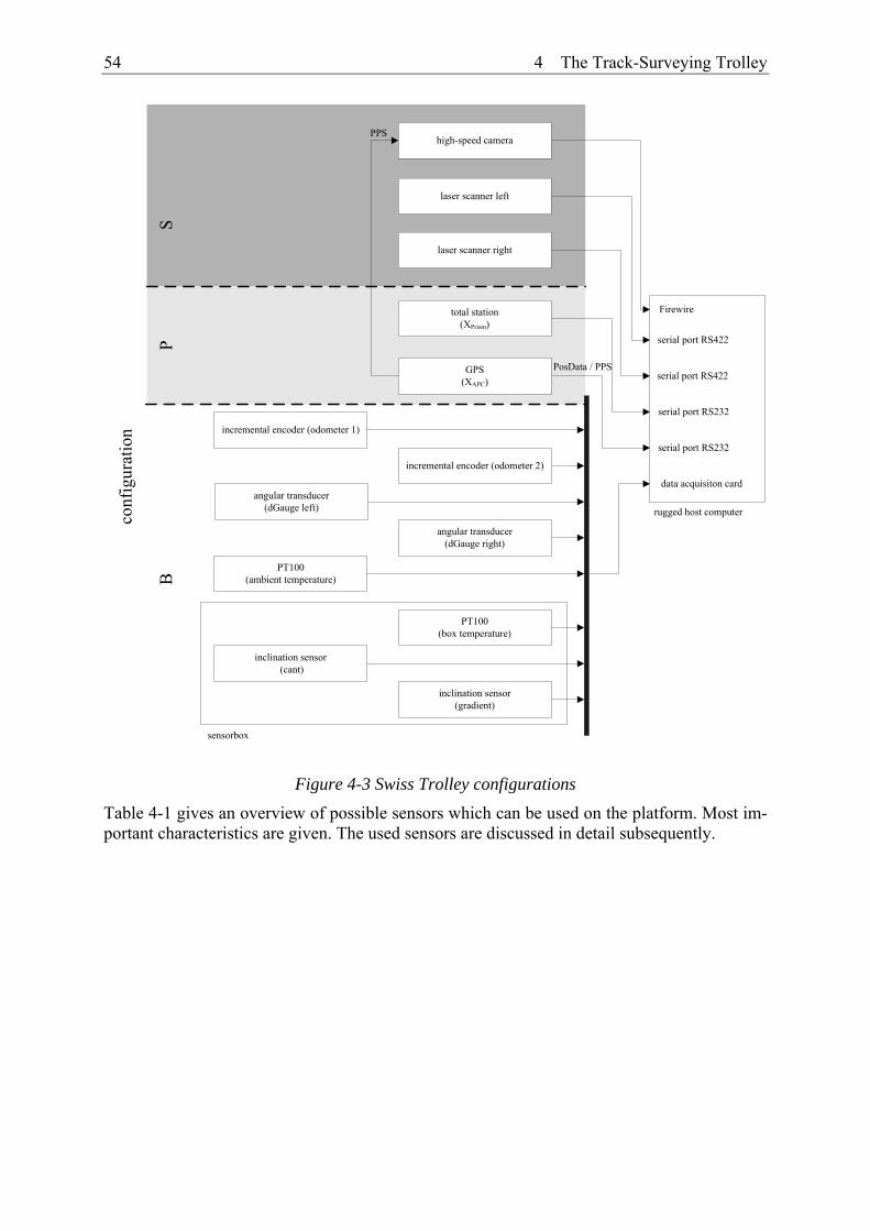
54 4 The Track-Surveying Trolley

incremental encoder (odometer 1)

GPS(XAPC)

incremental encoder (odometer 2)

angular transducer(dGauge left)

angular transducer(dGauge right)

PT100(ambient temperature)

PT100(box temperature)

inclination sensor (cant)

inclination sensor(gradient)

sensorbox

total station(XPrism)

PosData / PPS

serial port RS232

data acquisiton card

serial port RS422

rugged host computer

laser scanner right

laser scanner left

serial port RS422

serial port RS232

BP

S

conf

igur

atio

nhigh-speed camera

Firewire

PPS

Figure 4-3 Swiss Trolley configurations

Table 4-1 gives an overview of possible sensors which can be used on the platform. Most im-portant characteristics are given. The used sensors are discussed in detail subsequently.

4 The Track-Surveying Trolley 55

Category Sensor type Manufacturer / sensor name

Range Resolution

chainage incremental en-coder

Baumer electric BHL 16.24K2000

- 0.08 mm

cant, gradient

inclination sensor Midori PMP-S15TA-V1

± 15° 0.01°

track gauge angular transducer Contelec GL60 0° − 45° 0.03°

B

temperature resistance ther-mometer

PT100 -30°C − 80°C 0.1° C

P positioning GPS various, e.g. Trimble 5700

- 1 mm

positioning optical total station various, e.g. Trimble ATS600

- 1 mm

S side scans laser scanner SICK LMS200-300106

180° / 32 m 180° / 80 m

0.25° / 1 mm0.25° / 10 mm

digital im-ages

high-speed camera Basler A102f - 1392 · 1040 pixel 6.45 μm2 pixel size 15 frames/s

Table 4-1 Overview of Swiss Trolley sensors

4.2 Data Acquisition

4.2.1 Electronic Box All signals of the B-configuration sensors (Figure 4-3) are channelled within the electronic assembly and supplied to the analogue-digital (A/D) conversion. No signal conditioning is carried out. Thus, non-linearities of active elements like amplifiers are not matter of concern. In turn, the maximum voltage range of the A/D conversion cannot be used. However, as it will be shown subsequently, the A/D resolution exceeds the sensor resolution in most cases by at least one magnitude. Therefore, the abandonment of signal conditioning prevails over a resolution gain.

The electronic assembly is placed together with the inclination sensors in an insulated box. The box temperature is directly controlled on a constant level by a PT100 sensor. The main reason for heating the box is the attenuation of temperature influences on the inclination sen-sors.

Within the electronic box, an accurate, constant reference voltage of 4.8 V is generated. The reference voltage and the ground voltage are supplied as additional channels to the A/D con-version. This allows for an assessment of electronic fluctuations and jumps. A reference volt-age is also available on the A/D conversion card outside the box. However, the reference volt-age generated in the heated box is more representative since drifts are supposed to be similar for the reference and the sensor signal.

4.2.2 A/D Conversion The A/D converter samples continuous voltage signals with a constant time interval and maps it to a sequence of coded numbers [STEARNS et al., 1999]. For the track-surveying trolley, a National Instruments NI-DaqCard 5-16 with eight analogue channels, 16-bit resolution and 50 kHz sampling rate is used. Thus, a time span of 20 μs is required for one analogue-digital conversion. Within this time span, the signal is sampled and held on a constant voltage. A

56 4 The Track-Surveying Trolley

complete scan of all eight analogue channels by multiplexing in a round-robin sequence lasts 160 μs.

After sampling, the time-discrete signal is quantified by dividing it to a uniformly spaced grid. The number of the grid levels or the resolution is determined by the word length of the result-ing digital value. For a voltage range of ±5 V and the 16-bit word, the resolution amounts to 152 μV. This voltage skip corresponds to a change of the least-significant bit (LSB) of the digital value. During sampling, the input voltage must not change more than one LSB. Oth-erwise, the conversion provides nonsensical results. In our case, the signal rate of a particular sensor must not exceed 152 μV / 20 μs.

The difference between the effective analogue value and the digitised value provides a unique distribution from the point of view of the ADC. From the point of view of ADC output with-out knowledge of the input signal, this difference is random. In an error model, the random quantisation error can be considered as a noise source with a unique distribution within the quantisation level. The random error of the quantisation error corresponds to the standard de-viation of the unique distribution or to 1/ 12 of the LSB width [e.g. WEICHERT et al., 2000]. For the used A/D converter, 44 μV are found. However, other error sources exceed this quantisation error. Thus, thermal effects of the A/D converter have to be considered. Typi-cally, thermal effects are perceived as long-term drifts. Crosstalk effects evoked by incom-plete condenser discharge of vicinal data channels are a further error source. According to the manufacturer, the accuracy of the A/D converter is limited to four LSB which corresponds to 608 μV.

A critical issue concerning accuracy of analogue sensor data is the electromagnetic compati-bility (EMC) of the sensor system. ADC should be lined up to the sensors as closely as possi-ble, since cables and connectors give reasons for electromagnetic interferences. In turn, short connections with adequate shielding improve EMC and reduce errors from unknown noise sources.

The A/D converter accuracy can be verified by sampling a reference voltage during a certain time span. Another approach is to sample data of a sensor in rest position. Apart of the ADC accuracy, such data are degraded by sensor noise and electromagnetic interfering signals. Figure 4-4 reveals the behaviour of the mapped signal of an angular transducer during five minutes. The maximal sampling rate of the A/D converter was used, but only five values per second were saved. Almost stationary noise can be perceived. The standard deviation in the considered window of 273 μV falls below the indicated accuracy. Figure 4-4 does not allow for drawing conclusions considering long-term effects since the time series is too short. Con-versely, it can be concluded that electromagnetic compatibility is given and that the specified accuracy can be held, at least for a short term.

4 The Track-Surveying Trolley 57

0.0 50.0 100.0 150.0 200.0 250.0 300.0-2.0

-1.0

0.0

1.0

2.0 Angular Transducer (σ = 273 μV)

Time [s]

Vol

tage

[mV

]

Figure 4-4 A/D conversion of angular transducer in rest with NI DAQCard

The A/D resolution has to be compared in relation to the resolution of the particular sensor. Whenever possible, A/D resolution should not affect the sensor resolution. As shown before, a 16-bit A/D converter guarantees for accuracies on the 0.6 mV level taking into account the quantisation error and outside influences. Table 4-2 maps the sensor resolution on correspond-ing voltages. Note that, for our case, sensors cannot take advantage of the maximum allow-able voltage range of the A/D converter since they are not amplified (see chapter 4.2.1). Nev-ertheless, the 16-bit A/D converter resolves the input signals for each sensor better than re-quired.

Sensor Voltage range [V] Sensor range Sensor resolution

Corresponding voltage resolution [mV]

Inclination sensor 4 ±15° 0.01° 1.33

Angular transducer 4.8 0° – 45° 0.03° 3.20

PT100 4.8 -30° – 80°C 0.1°C 4.36

Table 4-2 Required voltage resolution of utilised sensors

4.2.3 Data Synchronisation Referring to 3.6, kinematic surveying asks for a careful treatment of time constraints. The track-surveying trolley is commonly used at walking speed (1 m/s). Therefore, synchronisa-tion uncertainties of 1 ms produce assignment uncertainties of 1 mm. Since in general, track surveys do not have to be referenced to primary time frames, used clocks may be biased and drift. However, within a period of comparison of two involved clocks, short-term stability should be guaranteed. If GPS is present, it can be profited by the use of the 1PPS event (pulse per second) of the GPS receiver providing time tags in the GPS system time. For this reason, not only the mandatory requirement of short-term stability is fulfilled. As a further benefit, kinematic data can be assigned with absolute accurate time tags. The Trimble 5700 receiver outputs the 1PPS pulse associated with an ASCII time tag output [TRIMBLE, 2001a]. The leading edge of the pulse corresponds with the beginning of each UTC second, as shown in Figure 4-5. The pulse is driven by an RS-422 driver between nominal levels of 0 V and 4 V. The leading edge is positive, rising from 0 V to 4 V. The pulse is approximately 8 μs wide, with rise and fall times of about 100 ns.

58 4 The Track-Surveying Trolley

35126.999990 35127.000000 35127.000010 35127.000020-1.0

0.0

1.0

2.0

3.0

4.0

5.0

GPS time [seconds of day]

Vol

tage

[V]

Figure 4-5 1PPS event of the Trimble 5700 receiver according to [TRIMBLE, 2001a]

The time tag is derived from the C/A-code based single point position solution and has an accuracy of approximately 40 ns [e.g. DANUSER, 1992]. Several external factors limit accu-racy to approximately 1 μs. Thus, each metre of position error results in 3 ns of error in the 1PPS pulse. Further, each metre of cable adds a delay of about 2 ns to satellite signals and a corresponding delay in the 1PPS pulse. These magnitudes are far from any concern with re-spect to a regular time synchronisation on a 1 ms-level. The 1PPS pulse provided by the Trimble 5700 receiver completely fulfils the synchronisation requirements for the track-surveying trolley only asking for short-term stability. On the track-surveying trolley, the 1PPS pulse is used for updating the internal clock of the DAQ card. The DAQ clock is synchronised once per second.

Figure 4-6 shows the principle of time synchronisation by a 1PPS pulse. The UTC timeline not only contains the 1PPS pulse but also the GPS position strings. In the example, the posi-tion is updated once per second. GPS positions come with a time tag being consistent with the 1PPS pulse. A delayed arrival of the GPS data strings on the computer interface is therefore not relevant for post-mission applications. The ADC data on the drifting tDAQ timeline are synchronised once per second with the GPS positions. The data on the tDAQ timeline originate from a ring-buffer with a predefined frequency. In the above example, this is nominally 5 Hz. The clock-pulse is generated by the DAQ card timer or by PC-clocks. PC-clock timers typi-cally drift up to 0.1 ms per second, whereas the used processor and the operating system are actuating parameters [STEMPFHUBER, 2004]. DAQ card timers show a similar behaviour. One single A/D conversion of the round-robin sequence is not broke down into an individual time tag, but is referred to a mean time tag of one cycle. This results in a maximal error of 160 μs (see section 4.2.2).

Figure 4-6 Time synchronisation by the 1PPS pulse

Table 4-3 shows an excerpt of a trolley data file for clarification. Each line is headed by a time tag. Time tags are given in seconds past 01.01.2000 0:00:00 UTC. Then, the actual data string contains odometer, inclination sensor, angular transducer and temperature readings. Furthermore, the data string can include a GPS-RTK string being composed of coordinates and quality information. GPS-RTK records refer to the heading time tag within the GPS posi-

tDAQ

tUTC

tUTC

4 The Track-Surveying Trolley 59

tion jitter, the remaining data within the mentioned 0.1 ms jitter. The drift of the ADC timer is considered. The ADC sampling rate and the GPS sampling rate do not necessarily coincide. Typically, GPS data is logged with 1 Hz. Complete ADC records can be sampled with up to 6.25 kHz (section 4.2.2). A sampling rate of 5 – 20 Hz fulfils in every case Nyquist’s theorem applied to track surveys (see 3.1) and produces reasonable data amounts. For the shown ex-ample, GPS data is sampled with 1 Hz, the remaining sensor data with 5 Hz. 142825968.000,10014.871,17.62944,1.31196,0.11003,0.11318,60.1,14.6,606836.073,164455.545,43.336000,3.300,5,3

142825968.200,10015.147,18.34480,-2.32269,0.11115,0.11116,59.9,14.6

142825968.401,10015.421,17.90206,2.60764,0.10973,0.11066,60.0,14.3

142825968.601,10015.698,18.55998,2.76252,0.10935,0.11105,60.2,14.7

142825968.801,10015.974,18.91224,4.70748,0.11013,0.11138,60.0,14.4

142825969.000,10016.251,19.11701,9.35967,0.10865,0.11352,60.1,14.7,606835.438,164456.768,43.314000,3.300,5,3

142825969.201,10016.534,18.68665,2.89242,0.10996,0.11441,60.1,14.7

142825969.401,10016.814,19.63030,2.14972,0.10995,0.11443,60.0,14.4

142825969.601,10017.093,19.30514,-1.72689,0.10930,0.11553,60.1,14.7

142825969.802,10017.368,19.44969,-5.76418,0.11139,0.11548,60.1,14.6

142825970.000,10017.635,20.27607,-3.73948,0.10998,0.11246,60.2,14.8,606834.787,164458.001,43.336000,3.300,5,3

Table 4-3 Data records with time tag

One possible trolley configuration combines GPS measurements with cant, gradient, chainage and track gauge measurements (configuration P of Figure 4-3). As an example, a synchronisa-tion jitter of 10 ms results in small biases of cant, gradient, chainage and track gauge assign-ment. For instance, if the track is twisted by a maximal value of 2 per mil and the operation speed is limited to 1 m/s, the associated cant is biased by marginal 0.02 mm. However, time synchronisation becomes more critical if laser scanners are used. The same 10 ms synchroni-sation jitter produces uncertainties for laser scanner dots in the direction of motion of 10 mil-limetres.

A modified concept for synchronisation has to be applied if a total station is used as primary positioning sensor and no 1PPS pulse is available. ADC data are no longer triggered by a primary pulse generator, but time tags of the PC clock and the ADC timer are stored. Conse-quently, total station epochs and DAQ card epochs do not coincide. Synchronisation must be effected at post-processing. Figure 4-7 elucidates this fact. Total station measurements are time tagged on the PC timeline. They are pointed out by diamonds. The corresponding time tags are taken on the arrival of the total station string on the interface of the data acquisition computer. Latencies due to the radio link are considered within the data acquisition pro-gramme resulting in a timeline with unbiased total station tags. The calibration of these laten-cies will be subject of section 4.7.6. ADC data refer to the DAQ timeline. The ADC timer drift is assessed by regular comparisons of the ADC cycle and the PC clock. Subsequently, ADC data can be reduced to the PC time scale. Further, Figure 4-7 points out that PC clocks may drift with respect to a time normal (e.g. UTC).

60 4 The Track-Surveying Trolley

Figure 4-7 Time synchronisation without 1PPS pulse

As a further important point, the operating system has to guarantee that within the predefined sampling rate, the measurements can be carried out and passed to the data bus. Overflows must not occur. In order to enable continuous data streams, the data acquisition has to be pri-oritised on multi-task operating systems. Other processes running on the computer must not charge the operating system. The current version of the data acquisition software running on Windows NT, 2000 or XP uses specialised drivers which privilege a specific task. The used Kithara timer toolkit [KITHARA, 2005] allows for the adjustment of the corresponding thread priority. CPU time can be reserved almost exclusively for a specific task. Applications being intensive on data or asking for a more restrictive fulfilment of time constraints (e.g. the Swiss Trolley laser scanning configuration) cannot be handled by the mentioned data acquisi-tion software. A data acquisition tool running under Linux with the RTAI extension (section 3.6) was written for such applications [HEINZELMANN, 2004]. This DAQ software pro-vides individual time tags for each measurement record. Further, clocks can be synchronised by the 1PPS pulse or by a master clock.

4.3 Reconstruction As explained in section 3.7, a sensor maps a continuous process to carrier signals by model-ling. The original process can be obtained by inverting the model of the mapping process within a reconstruction step. Reconstruction in this section is limited to the static sensor be-haviour. For the inclination sensors and the angular transducers, the process signals are analo-gously mapped as voltages. The odometers map the covered path digitally by revolution counts. The sought signals are reconstructed here by linear functions. For one particular sen-sor, this leads to

0sy y yγ= + (4.1)

where y is the reconstructed signal, ys the carrier signal, γ the gain and y0 the zero-point offset. For the analogue inclination sensors and the angular transducers, not the voltages are meas-ured but the ratio of differential voltages of the sensor signal and a reference source with re-spect to the ground voltage. Thus, voltage drifts or an increase of the voltage level can be as-sessed and compensated. ys can be expressed as

y gnds

ref gnd

U Uy

U U−

=−

(4.2)

where Uy is the voltage of the particular sensor, Ugnd the ground voltage and Uref the voltage of the reference source. The nominal value for Ugnd and Uref are 0 V and 4.8 V, respectively. Note that ys is dimensionless. Thus, the gain γ obtains the dimension unit of the sought sensor signal y. The gain γ and the offset y0 have to be found by calibration. In general, both vari-

tDAQ

tPC

tPC

tUTC

tPC

4 The Track-Surveying Trolley 61

ables ys and y have to be considered as erroneous leading to an orthogonal regression [e.g. WOLF, 1994].

4.4 Inclination Sensors

4.4.1 Sensor Characteristics Two fluid damped Midori PMP-S15TA-V1 pendulum sensors with capacitive read out are used on the trolley. They are placed crosswise in the sensor box. Nominally, the sensor axes coincide with the track axis and its perpendicular. Thus, the inclination sensors provide gradi-ent and cant information. In the above-mentioned Table 4-1, the characteristics of the used sensors are listed. Table 4-4 allows for the conversion between common angle units for incli-nation sensors. The range of ±15° permits to cover most prevailing cant and gradient ranges. For regular tracks, the cant range does not exceed 200 mm (scaled to normal gauge). This corresponds to an angular amplitude of 7.7° or 134 mrad. The resolution of 0.01° allows for detecting cant changes of 0.3 mm scaled to normal gauge.

Degrees Arc seconds Radians Cant (1.5 m base) Remarks

15° 54000” 261.8 mrad 388.2 mm Sensor range

1° 3600” 17.4 mrad 26.1 mm

0.0573° 206” 1.0 mrad 1.5 mm

0.01° 36” 0.2 mrad 0.3 mm resolution

0.0003° 1” 0.005 mrad 0.008 mm

Table 4-4 Conversion table for inclination measuring units

Figure 4-8 Inclination sensor Midori PMP-S15TA-V1

4.4.2 Calibration of Characteristic Curve The output voltage shows a nearly linear input in the small angle range. According to the manufacturer, gain precision is given as 0.5 %. For a cant of 200 mm, this results in a shortly tolerable 1 mm error. Therefore, the provided gain factor was verified and improved by an adequate calibration procedure. A Wyler Clino 2000 digital inclinometer was used to verify gain precision of the Midori sensor. Inclination accuracy of the Wyler sensor is specified as 5”. This suffices to verify easily the characteristic curves of the used Midori sensors with the 36” resolution. An orthogonal regression was applied to the acquired data along the cant range

62 4 The Track-Surveying Trolley

of -200 mm to 200 mm. An orthogonal regression provided a standard deviation of the gain of 0.3 %. Compared to the manufacturer’s specification, gain precision can be improved by the calibration procedure by almost a factor of two resulting in errors of 0.6 mm at maximal incli-nations.

The zero point offset of the mounted inclination sensors can easily be verified in situ by two faces measurements. The difference between both readings provides the double zero point offset. However, it has to be guaranteed that the trolley is set up over the identical reference plane in both faces. Further, the reference plane has to be as horizontal as possible. Otherwise, the found zero point offset is biased by misalignment effects of the inclination sensors. Sec-tion 4.4.4 gives explicit formulae for correcting such errors. Ideally, the zero point offset is verified before and after a trolley survey. In such way, trolley frame deformations and further residual error contributions can be monitored.

4.4.3 Temperature Influences A further error source of inclination sensors are temperature influences. Reasons for tempera-ture dependencies are evoked by mechanical geometrical variations of the sensor and by a change of the electrical behaviour of converters and amplifiers [INGENSAND, 1985]. Incli-nation changes of up to 1.25 mV / °C or 0.2 mrad / °C are specified by the manufacturer for the used sensor. Since the temperature range during a track survey can vary considerably, temperature drifts of the sensor have to be taken into account. Two kinds of methods are con-ceivable for controlling temperature drifts. Firstly, temperature drifts can be corrected by means of characteristic curves. Secondly, the sensor temperature during the survey can be held constant. The first approach asks for a calibration providing inclination rates as a func-tion of temperature. Characteristic curves have to be known over a range of several 10° C in order to be able to correct summer and winter measurements. As a drawback, hysteresis ef-fects cannot be excluded. Within the track-surveying trolley project, the second approach was followed. The box containing both inclination sensors is heated and controlled by closed-loop control on a constant temperature of 60°C. This temperature is obviously higher than the am-bient temperature. Thus, the measuring system is protected against ambient temperature varia-tions. No knowledge about the temperature behaviour of the inclination sensors is required. In contrast, energy is needed to heat up the box on 60°C. A 12 V voltage source requires 4 A to reach the required temperature. The accomplishment of the operation temperature depends on the ambient temperature. In general, five minutes are enough for heating up the electronic box. Then, for the closed-loop control, about 0.5 A suffices to regulate the constant tempera-ture.

4.4.4 Corrections for Non-Orthogonalities (Collimation Error) The mounted pair of inclination sensors on the trolley cannot be aligned perfectly along the sought parameters cant and gradient. The longitudinal as well as the cross inclination sensor are slewed by different amounts with respect to the trolley b-frame. Such collimation errors have to be taken into account if submillimetric accuracies are sought. For instance, such high accuracies are required for slab track surveys. [KAHLMANN, 2003] gives a structural model for the correction of collimation errors. This work uses the proposed approach and adapts it to the requirements of the track-surveying trolley.

Two angles are needed to describe the pivoting of both sensors. The magnitude of these mis-alignment angles is perceivable if cants or gradients are measured at different gradient or cant amounts, respectively. If the trolley is pitched but remained constant with respect to its roll axis, different cants are measured for a misaligned inclination sensor. Analogously, varying

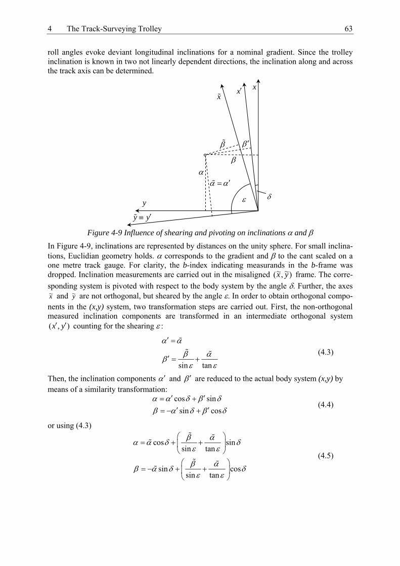
4 The Track-Surveying Trolley 63

roll angles evoke deviant longitudinal inclinations for a nominal gradient. Since the trolley inclination is known in two not linearly dependent directions, the inclination along and across the track axis can be determined.

Figure 4-9 Influence of shearing and pivoting on inclinations α and β

In Figure 4-9, inclinations are represented by distances on the unity sphere. For small inclina-tions, Euclidian geometry holds. α corresponds to the gradient and β to the cant scaled on a one metre track gauge. For clarity, the b-index indicating measurands in the b-frame was dropped. Inclination measurements are carried out in the misaligned )~,~( yx frame. The corre-sponding system is pivoted with respect to the body system by the angle δ. Further, the axes x~ and y~ are not orthogonal, but sheared by the angle ε. In order to obtain orthogonal compo-nents in the (x,y) system, two transformation steps are carried out. First, the non-orthogonal measured inclination components are transformed in an intermediate orthogonal system ( , )x y′ ′ counting for the shearing ε :

sin tan

α α

β αβε ε

′ =

′ = + (4.3)

Then, the inclination components α′ and β ′ are reduced to the actual body system (x,y) by means of a similarity transformation:

cos sin

sin cosα α δ β δβ α δ β δ

′ ′= +′ ′= − +

(4.4)

or using (4.3)

cos sin

sin tan

sin cossin tan

β αα α δ δε ε

β αβ α δ δε ε

⎛ ⎞= + +⎜ ⎟

⎝ ⎠⎛ ⎞

= − + +⎜ ⎟⎝ ⎠

(4.5)

x

α α′=

x′

β

βα

x

ε δ

y y′≡

y

β ′

64 4 The Track-Surveying Trolley

(4.5) can be used to transform inclination components from the pivoted and sheared system to the body system. Pivoting and shearing errors on inclination components can be estimated by forming the total differential of (4.5).

2 2

2 2

cossin cos sinsin tan sin sin

coscos sin cossin tan sin sin

d d d d

d d d d

β α β ε αα α δ δ δ δ δ εε ε ε ε

β α β ε αβ α δ δ δ δ δ εε ε ε ε

⎛ ⎞ ⎛ ⎞= − + + + − −⎜ ⎟ ⎜ ⎟

⎝ ⎠ ⎝ ⎠⎛ ⎞ ⎛ ⎞

= − − + + − −⎜ ⎟ ⎜ ⎟⎝ ⎠ ⎝ ⎠

(4.6)

or for a small shearing angle ϕ and a pivoting angle 2ε π≈

d dd d dα β δβ α δ α ε

== − +

(4.7)

(4.7) reveals that for non-canted, horizontal stretches neither gradients nor cants are biased. For a 25 per mil slope with 130 mm of cant and inclination sensors alignment errors of 1° each, gradients are biased by 1.5 mm. Cant errors, scaled on normal gauge, are biased by 1.3 mm (as a maximal error). It can be concluded that for very accurate applications, the knowledge of the pivoting and shearing is required.

For calibration, pivoting and shearing can be obtained by measuring longitudinal and trans-versal inclinations for several trolley attitudes. Ideally, the whole range of prevailing gradients and cants is utilised. For adhesive tracks, this covers cants up to 200 mm and gradients up to 50 per mil. Each pair of inclinations provides two condition equations:

1

2

cos sinsin tan

sin cossin tan

i ii i

i ii i

c

c

β αα α δ δε ε

β αβ α δ δε ε

⎛ ⎞− − + =⎜ ⎟

⎝ ⎠⎛ ⎞

+ − + =⎜ ⎟⎝ ⎠

(4.8)

If (4.8) is linearised with respect to the unknowns αi, βi, ϕ, ε and the observations ,i iα β , an equation system in the form

TAx B v w+ = (4.9)

can be written. The least-squares estimate x is based on the minimisation of the function vTPv. A solution is obtained by introducing a vector of Lagrange multipliers, k, and by minimising the function

( )( , , ) 2T T Tv k x v Pv k Ax B v wΦ = − + + (4.10)

This corresponds to a mixed adjustment (Gauss-Helmert) model [SCHMID, 1977] with the solution

( ) 1T Tx A PA A PA−

= (4.11)

and

( ) 1TP B CB−

= (4.12)

where C is the covariance matrix of the observables.

4 The Track-Surveying Trolley 65

The vector x of the shortened parameter

( )1 1... ...Tp qx d d d d d dα α β β ε δ= (4.13)

contains p nominal gradients, q nominal cants, the pivoting and the shearing. The observa-tions are organised in two p q⋅ -matrices with the elements ijα and ijβ , respectively. Each line of the α -matrix lists q gradient measurements for one particular cant. Each column of the β -matrix lists p cant measurements for one particular gradient. This convention leads to the building of the system matrices:

11 11 11 11112 2

11 11 11 11112 2

12 122 2

cos cos cos1 0 ... 0 0 0 ... 0 sin sinsin sin sin tan

cos sin sin0 0 ... 0 1 0 ... 0 cos cossin sin sin tan

cos0 1 ... 0 0 0 ... 0sin sin

A

β ε α β δ α δδ α δε ε ε ε

β ε α β δ α δδ α δε ε ε ε

β ε αε ε

⎛ ⎞+ − −⎜ ⎟

⎝ ⎠⎛ ⎞

+ + +⎜ ⎟⎝ ⎠⎛ ⎞

+⎜⎝ ⎠

=

12 212

12 12 12 12122 2

2 2

cos cossin sinsin tan

cos sin sin0 0 ... 0 0 1 ... 0 cos cossin sin sin tan

cos cos0 0 ... 1 0 0 ... 0 sin sin

sin sin sinpq pq pq pq

pq

β δ α δδ α δε ε

β ε α β δ α δδ α δε ε ε ε

β ε α β δ αδ α δ

ε ε ε

− −⎟

⎛ ⎞+ + +⎜ ⎟

⎝ ⎠

⎛ ⎞+ − −⎜ ⎟⎜ ⎟

⎝ ⎠

2 2

costan

cos sin sin0 0 ... 0 0 0 ... 1 cos cos

sin sin sin tanpq pq pq pq

pq

δε

β ε α β δ α δδ α δ

ε ε ε ε

⎛ ⎞⎜ ⎟⎜ ⎟⎜ ⎟⎜ ⎟⎜ ⎟⎜ ⎟⎜ ⎟⎜ ⎟⎜ ⎟⎜ ⎟⎜ ⎟⎜ ⎟⎜ ⎟⎜ ⎟⎜ ⎟⎜ ⎟⎜ ⎟⎜ ⎟⎜ ⎟⎛ ⎞

+ + +⎜ ⎟⎜ ⎟⎜ ⎟⎜ ⎟⎝ ⎠⎝ ⎠ (4.14)

sin sincos 0 0 0 0tan sin

cos cossin 0 0 0 0tan sin

sin sin0 0 cos 0 0tan sin

cos cos0 0 sin 0 0tan sin

sin sin0 0 0 0 costan sin

cos cos0 0 0 0 sintan sin

TB

δ δδε ε

δ δδε ε

δ δδε ε

δ δδε ε

δ δδε ε

δ δδε ε

⎛ ⎞− − −⎜ ⎟⎜ ⎟⎜ ⎟− −⎜ ⎟⎜⎜ − − −⎜⎜= ⎜ − −⎜⎜⎜⎜ − − −⎜⎜⎜ − −⎜⎝ ⎠

…

…

…

…

…

…

⎟⎟⎟⎟⎟⎟⎟⎟⎟⎟⎟⎟⎟

(4.15)

66 4 The Track-Surveying Trolley

1 11 11 11

1 11 11 11

sin sincossin tancos cossinsin tan

sin sincossin tan

cos cossinsin tan

p pq pq pq

q pq pq pq

w

δ δα α δ β αε εδ δβ α δ β αε ε

δ δα α δ β αε εδ δβ α δ β αε ε

⎛ ⎞⎛ ⎞− − − −⎜ ⎟⎜ ⎟⎝ ⎠⎜ ⎟

⎜ ⎟⎛ ⎞− − − −⎜ ⎟⎜ ⎟⎝ ⎠⎜ ⎟

⎜=⎜

⎛ ⎞⎜ − − − −⎜ ⎟⎜ ⎝ ⎠⎜⎛ ⎞⎜ − − − −⎜ ⎟⎜ ⎝ ⎠⎝ ⎠

⎟⎟⎟⎟⎟⎟⎟

(4.16)

For p = 5 nominal gradients and q = 4 nominal cants taken over the described measurement range by the two Midori sensors, the mixed adjustment yields pivoting and shearing preci-sions of 0.1° and inclination precisions of 0.2 mrad. The found pivoting and shearing values typically amount to 1°. This corresponds to a misalignment of the sensor enclosure of 1 mm taken on the enclosure base.

4.4.5 Dynamic Behaviour of the Inclination Sensor Due to their physical measuring principle, inclination sensors respond to the accelerations of gravity as well as to other translatory or rotatory accelerations. If inclinations are sought, nui-sance accelerations have to be separated from the actual gravity induced accelerations. For kinematic applications, non-gravitational accelerations have to be provided by independent sensors. Further, the dynamic behaviour of the sensor has to be known in order to model the influence of nuisance accelerations. The dynamic behaviour of oscillating systems is de-scribed by the transfer function and the step response which are evaluated by the solution of the inhomogeneous and homogeneous equations of motion. The transfer function describes the ratio of the output and input signal while the system is periodically activated. The step response shows the temporal transient behaviour [EICHHOLZ et al., 1982].

Dynamical modelling of pendulum sensors typically starts with the formulation of the equa-tions of motion of a mathematical pendulum (Figure 4-10). If a horizontally levelled inclina-tion sensor is assumed and the pendulum axis is perpendicular to the ground plane, the fol-lowing second-order differential equation can be put up [SCHWARZ, 1995]:

0rr

Xm X d X m gl

⋅ + ⋅ + ⋅ ⋅ = (4.17)

where X is the pendulum motion, d the damping, Xr the relative motion of the pendulum with respect to the sensor enclosure, m the pendulum mass, g the acceleration of gravity and l the pendulum length. For small pendulum deflection angles α, it holds

rX l α= ⋅ (4.18)

4 The Track-Surveying Trolley 67

Figure 4-10 Principle of pendulum inclination sensor

(adapted from [EICHHOLZ et al., 1982])

Further, the pendulum motion is split into a relative motion and a motion of the sensor enclo-sure

r eX X X= + (4.19)

Thus, (4.17) is rewritten as

em l d l m g m Xα α α⋅ ⋅ + ⋅ ⋅ + ⋅ ⋅ = − ⋅ (4.20)

(4.20) represents an inhomogeneous differential equation with the disturbance term em X− ⋅ . For the enclosure motion, a uniform motion with a superposed periodic oscillation is set up:

0 0 0cosE EX X t v t Xω= ⋅ + + . (4.21)

XE0 is the amplitude of the enclosure oscillation, ω is the angular frequency of the disturbance term, v0 is the initial speed and X0 the initial position. For the general solution, a particular function for α is chosen:

( )cosnV tα ω ϕ= − (4.22)

The amplitude gain Vn and the phase shift ϕn between the periodic enclosure motion XE and the pendulum motion can be found by inserting (4.22) into (4.20) and by comparing the coef-ficients:

( )

20

22 2 20 1 4

rn

E

XVX D

Ω= =

− Ω + ⋅ ⋅Ω. (4.23)

α

l

d/2 d/2

m

g

X

XE

68 4 The Track-Surveying Trolley

2

2tan1n

Dϕ ⋅ ⋅Ω=

− Ω (4.24)

Xr0 is the amplitude of the pendulum taken with respect to the enclosure. Ω denotes the stan-dardised angular frequency and is obtained by

0

ωω

Ω = (4.25)

where

0 00

2 2 gfT lπω π= = ⋅ = (4.26)

is the eigenfrequency of the pendulum and

02

dDm ω

=⋅ ⋅

(4.27)

the standardised damping. The graphical representation of (4.23) and (4.24) is the so-called Bode diagram.

If Xr0 in (4.23) is substituted by (4.18) for maximal elongation, the pendulum deflection αn due to nuisance acceleration aE0 can be found:

( )

022 2 2

1

1 4

En

ag D

α⎛ ⎞⎜ ⎟= − ⎜ ⎟⎜ ⎟− Ω + ⋅ ⋅Ω⎝ ⎠

(4.28)

The nuisance acceleration aE0 is obtained by means of (4.21):

20 0E Ea Xω= − ⋅ (4.29)

For small Ω, that means small nuisance frequencies ω with respect to the eigenfrequency ω0, (4.24) disappears and (4.28) tends to

0En

ag

α = − (4.30)

The pendulum eigenfrequency of the used Midori sensor is approximately 20 Hz. In general, no significant frequency contributions greater than 0.1 Hz have to be worried about for a sur-vey run at walking speed. Thus, the undisturbed inclination v can be found by

00

Eag

ν ν= − (4.31)

Note that positive accelerations pretend an apparent decline of the stretch (Figure 4-11).

4 The Track-Surveying Trolley 69

Figure 4-11 Apparent inclination due to an acceleration aE0

Hence, (4.30) permits to estimate inclination magnitudes evoked by nuisance accelerations. Cant readings are mainly influenced by centripetal accelerations, whereas gradient readings are affected by translatory accelerations. For walking speed (1.5 m/s) and exceptionally small track radii of 200 m, centripetal accelerations up to 0.01 m/s2 occur providing apparent maxi-mal inclinations of 1 mrad. On straight stretches, translatory accelerations exceed rotatory accelerations considerably. For surveys at walking speed, permanent translatory accelerations in the order of magnitude of the mentioned maximal centripetal acceleration (0.01 m/s2) have to be taken into account. For the trolley activation, accelerations up to 0.2 m/s2 have to be considered. As an illustrative example, Figure 4-12 shows gradients contaminated by nui-sance accelerations. The data were acquired at 5 Hz on a horizontal stretch. Thus, data should scatter around 0 mrad. However, at the survey start a significant offset of 10 mrad from the nominal gradient can be perceived. This offset can be attributed to the activation of the trol-ley. The apparent inclination decays within the first ten second. Significant energy portions stemming from frequencies up to 1.2 Hz can be perceived in the spectrum. Predominant fre-quencies around 1 Hz most likely can be attributed to the operator’s step frequency. Higher frequencies almost do not contribute to the spectrum. A statement concerning higher frequen-cies is not possible, since the sampling frequency of 5 Hz allows, according to Nyquist theo-rem, just for the assessment of frequencies up to 2.5 Hz. Due to the aspired uniform trolley motion, high nuisance frequencies are less probable. Thus, formula (4.31) can be used for correcting raw inclination measurements.

αn

0Ea

*0Ea

g

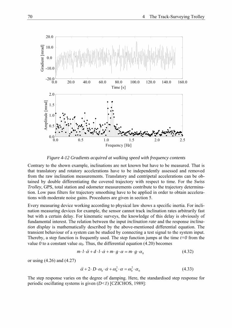
70 4 The Track-Surveying Trolley

0.0 20.0 40.0 60.0 80.0 100.0 120.0 140.0 160.0-20.0

-10.0

0.0

10.0

20.0

Time [s]

Gra

dien

t [m

rad]

0.0 0.5 1.0 1.5 2.0 2.50.0

0.5

1.0

1.5

2.0

Frequency [Hz]

Am

plitu

de [m

rad]

Figure 4-12 Gradients acquired at walking speed with frequency contents

Contrary to the shown example, inclinations are not known but have to be measured. That is that translatory and rotatory accelerations have to be independently assessed and removed from the raw inclination measurements. Translatory and centripetal accelerations can be ob-tained by double differentiating the covered trajectory with respect to time. For the Swiss Trolley, GPS, total station and odometer measurements contribute to the trajectory determina-tion. Low pass filters for trajectory smoothing have to be applied in order to obtain accelera-tions with moderate noise gains. Procedures are given in section 5.

Every measuring device working according to physical law shows a specific inertia. For incli-nation measuring devices for example, the sensor cannot track inclination rates arbitrarily fast but with a certain delay. For kinematic surveys, the knowledge of this delay is obviously of fundamental interest. The relation between the input inclination rate and the response inclina-tion display is mathematically described by the above-mentioned differential equation. The transient behaviour of a system can be studied by connecting a test signal to the system input. Thereby, a step function is frequently used. The step function jumps at the time t=0 from the value 0 to a constant value α0. Thus, the differential equation (4.20) becomes

0m l d l m g m gα α α α⋅ ⋅ + ⋅ ⋅ + ⋅ ⋅ = ⋅ ⋅ (4.32)

or using (4.26) and (4.27)

2 20 0 0 02 Dα ω α ω α ω α+ ⋅ ⋅ ⋅ + ⋅ = ⋅ (4.33)

The step response varies on the degree of damping. Here, the standardised step response for periodic oscillating systems is given (D<1) [CZICHOS, 1989]:

4 The Track-Surveying Trolley 71

( )00

0

1 cosD tD D

D

e tωωα ω ϕα ω

−= − ⋅ ⋅ − (4.34)

with

20 1D Dω ω= − and

2tan

1D

DD

ϕ =−

(4.35)

ωD and ϕD describe the angular frequency and the phase shift of the damped system. Step re-sponses for a pendulum sensor with an eigenfrequency of 0ω = 20 Hz are charted in Figure 4-13 for different dampings.

0.0 0.2 0.4 0.6 0.8 1.0 1.2 1.4 1.6 1.8 2.00.0

0.2

0.4

0.6

0.8

1.0

1.2

1.4

1.6

Time [s]

Stan

dard

ised

step

resp

onse

[]

D = 0D = 0.5D = 0.7D = 2.0

Figure 4-13 Sensor response of step function for different dampings

For oscillating systems, the step response overshoots the value α0 and level off depending on the damping D. For the marginal case D=1, no overshoot takes place, but the value α0 is reached at the time , 1 01R DT ω= = . For non-periodic settings (D>1), the value α0 is not accom-plished. For an ideally damped 20 Hz sensor with D=0.7, the pendulum levels off after a de-lay of TR = 0.3 s. The transient behaviour of a sensor with a damping of D=0.7 is almost lin-ear. Thus, (4.34) can be linearised at the time t=τ. The undelayed inclination at time t=τ is obtained by (PD-filter):

( ) ( )undelayed delayed Rd Tdtαα τ α τ= + ⋅ (4.36)

with the response time TR = 0.3 s for the used sensor.

For the Swiss Trolley inclination sensors, the response time TR was verified by a forward and a backward trolley run on the same stretch. Cants of both runs were compared since in con-

72 4 The Track-Surveying Trolley

trast to kinematically assessed gradients, measured cants are almost free from translatory ac-celerations. A clothoid with a nominal linear cant ramp was chosen as a test stretch. This al-lows for an accurate estimation of the sought response time TR since cant ramps significantly differ from zero. Zero point offset and gain were calibrated in advance.

Figure 4-14 Verification of response time

Figure 4-14 shows the cant as a function of the chainage l for both, the forward and the back-ward run. Both curves are geo-referenced by means of GPS and matched to a nominal chain-age axis. Equidistant data sets were produced by smoothing spline interpolation. The cut-out outlines that both curves are shifted by an offset Δl or a delay 0dt l v= Δ , respectively where v0 is the absolute, constant trolley speed. The delay dt is twice the sought response time TR. It must hold (Figure 4-14)

( ) ( )f bl l lβ β+ Δ = (4.37)

or for small offsets Δl

( )

( ) ( ) 0ff b

d ll l l

dlβ

β β+ ⋅Δ − = (4.38)

For erroneous data and for 02 Rl v TΔ = ⋅ ⋅ , (4.38) can be written as

0

( )( ) 2 ( )f i

f i R b i i

d ll v T l v

dlβ

β β+ ⋅ ⋅ ⋅ − = (4.39)

Since for flat ramps the response time cannot be determined, the data were weighted counting for the current derivative. For the weight evaluation, (4.39) is solved for TR and the total dif-ferential is formed. With the classical weight definition 2 2

0ii ip σ σ= , the weight of a particu-lar response time observation equation is

2( )f

ii

d lp

dlβ⎛ ⎞

⎜ ⎟⎝ ⎠∼ (4.40)

60.0 65.0 70.0 75.0 80.014.0

15.0

16.0

17.0

18.0

19.0

20.0

21.0

22.0

23.0Cut-Out

Chainage [m]

Cant

[mra

d]

forwardbackward

0.0 50.0 100.0 150.0 200.0-5.0

0.0

5.0

10.0

15.0

20.0

25.0

30.0

35.0

40.0Cant along a Clothoid Ramp

Chainage [m]

Cant

[mra

d]

forwardbackward

Δl

βf(l+Δl)

βf(l)

βb(l)

4 The Track-Surveying Trolley 73

The residuals vi of (4.39) are minimised according to the least-squares principle. The cant rates can be obtained easily by deriving the spline curve for the forward run with respect to the chainage. The least-squares adjustment provided for the data set of Figure 4-14 a response time TR = 0.29 s with a standard deviation of σTR = 0.01 s. This result confirms the above-mentioned theoretical findings.

4.4.6 Transformation of the Inclination Angles into the Body-System The angles in formulae 3.8 for the transformation of sensor measurements from the b-system into the g-system are referred to Euler orientation angles. For the track-surveying trolley, Euler angles are not directly measured. Instead, the trolley inclination with respect to a local horizontal system is determined. This requires a transformation from the inclination angles to the attitude angles. The dependency of the Euler angles of the order of the rotation has to be considered. It holds for the evaluation of the pitch and roll angle by longitudinal and transver-sal inclinations

2 2

sintan1 sin sin

βωα β

=− −

(4.41)

ϕ α= − (4.42)

where ω is the roll angle, ϕ is the pitch angle, α the longitudinal inclination and β the trans-versal inclination. A derivation of (4.41) and (4.42) is given in the appendix A.1. The differ-ence between the roll angle and the transversal inclination amounts to 1 mrad for a 200 mm cant curve and a 50 per mil slope.

4.5 Track Gauge Measuring System

4.5.1 Characteristics and Measuring Principle of the Track Gauge Measuring System As mentioned above, the track gauge measuring system consists of two angular transducers measuring the deflection of two levers (Figure 4-15). Both levers are pressed by springs to the running edges of both rails. Two angular transducers Contelec GL60 are used (Table 4-1). The measuring range from 0° − 45° allows for covering all possible deflections. The 0.03° resolution corresponds to a deflection of 0.08 mm for the 15 cm long lever. The mechanical adaptation of the levers allows for a rail edge scanning 14 mm below the upper edge of the rails (see 2.2.3). Further, the track gauge levers and the prism (or the APC) form a plane being perpendicular to the track axis.

74 4 The Track-Surveying Trolley

Figure 4-15 Angular transducer with shaft and blocking pole in enclosure

The measuring principle is drafted in Figure 4-16. The track gauge is obtained by the sum of both lever deflection determinations and the base between the two stop positions of the levers. For the determination of the horizontal component of the track axis or the centre line, the trol-ley wobble with respect to the rails can be assessed by means of the lever deflections. The running edge of the left rail in the body frame is obtained by

0l l lr p p= + (4.43)

where 0lp is the position vector of the left lever stop position and lp is the lever deflection.

The lever deflection can be found by

sinl l yp s eς= ⋅ ⋅ . (4.44)

ζl is the angular deflection of the lever, s the lever length and ye the unity vector in y-direction in the b-frame. Analogously, the running edge of the right rail renders

0r r rr p p= + (4.45)

with the corresponding vector position vector 0rp and the lever deflection

sinr r yp s eς= ⋅ ⋅ . (4.46)

Note that ζr is negative. If the origin of the body system is the mid point between the two stop positions, the x-components of lp and rp vanish. If a skew of the trolley is excluded then the centre line of the track in the body system is found by

( ) ( )0 01 12 2l r l l r rc r r p p p p= + = + + + (4.47)

With the above-made stipulation of the body system origin, it holds further

0 0l rp p= − (4.48)

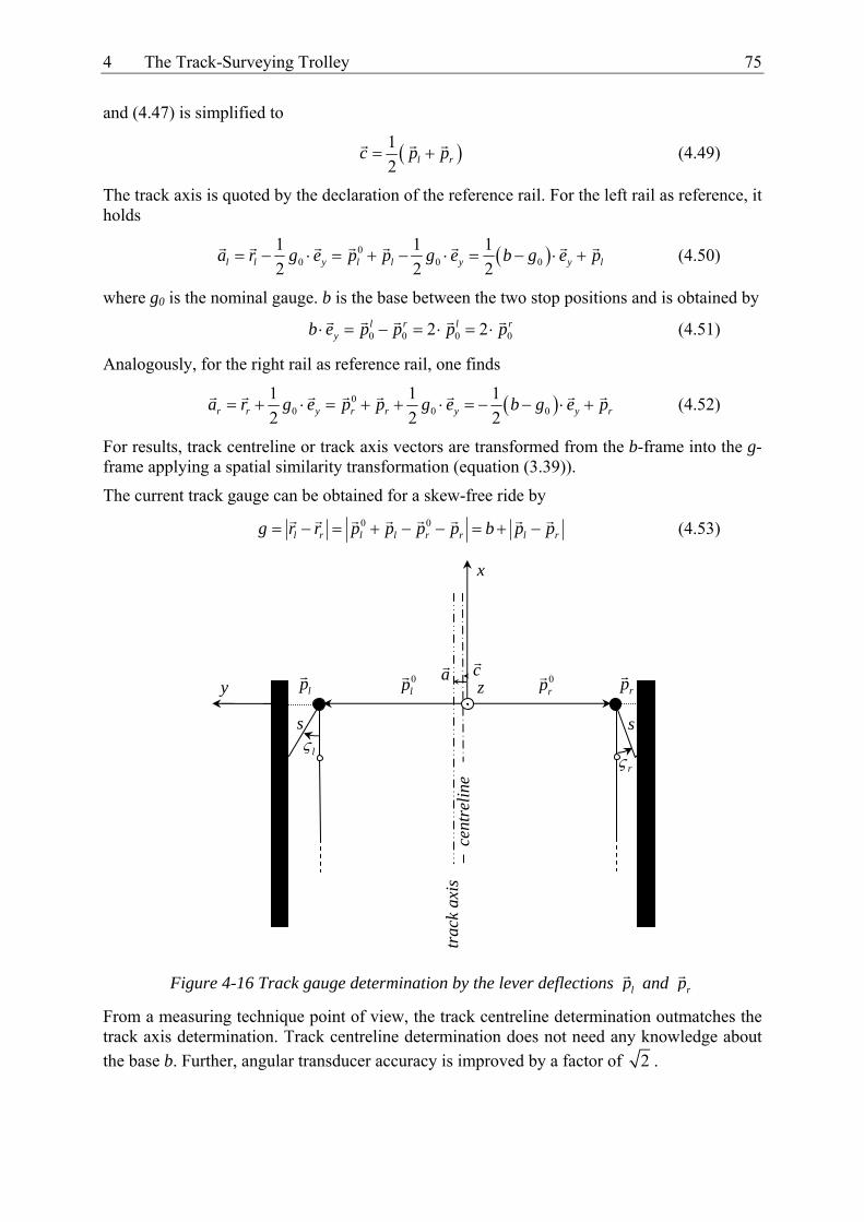
4 The Track-Surveying Trolley 75

and (4.47) is simplified to

( )12 l rc p p= + (4.49)

The track axis is quoted by the declaration of the reference rail. For the left rail as reference, it holds

( )00 0 0

1 1 12 2 2l l y l l y y la r g e p p g e b g e p= − ⋅ = + − ⋅ = − ⋅ + (4.50)

where g0 is the nominal gauge. b is the base between the two stop positions and is obtained by

0 0 0 02 2l r l ryb e p p p p⋅ = − = ⋅ = ⋅ (4.51)

Analogously, for the right rail as reference rail, one finds

( )00 0 0

1 1 12 2 2r r y r r y y ra r g e p p g e b g e p= + ⋅ = + + ⋅ = − − ⋅ + (4.52)

For results, track centreline or track axis vectors are transformed from the b-frame into the g-frame applying a spatial similarity transformation (equation (3.39)).

The current track gauge can be obtained for a skew-free ride by

0 0l r l l r r l rg r r p p p p b p p= − = + − − = + − (4.53)

Figure 4-16 Track gauge determination by the lever deflections lp and rp

From a measuring technique point of view, the track centreline determination outmatches the track axis determination. Track centreline determination does not need any knowledge about the base b. Further, angular transducer accuracy is improved by a factor of 2 .

0lp

x

y z 0rp lp rp

lς rς

s s

cent

relin

e tr

ack

axis

c a

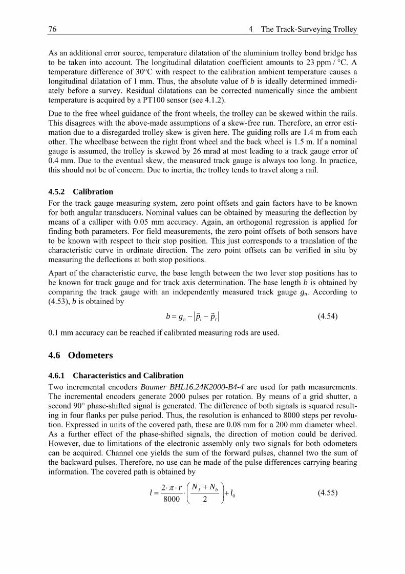
76 4 The Track-Surveying Trolley

As an additional error source, temperature dilatation of the aluminium trolley bond bridge has to be taken into account. The longitudinal dilatation coefficient amounts to 23 ppm / °C. A temperature difference of 30°C with respect to the calibration ambient temperature causes a longitudinal dilatation of 1 mm. Thus, the absolute value of b is ideally determined immedi-ately before a survey. Residual dilatations can be corrected numerically since the ambient temperature is acquired by a PT100 sensor (see 4.1.2).

Due to the free wheel guidance of the front wheels, the trolley can be skewed within the rails. This disagrees with the above-made assumptions of a skew-free run. Therefore, an error esti-mation due to a disregarded trolley skew is given here. The guiding rolls are 1.4 m from each other. The wheelbase between the right front wheel and the back wheel is 1.5 m. If a nominal gauge is assumed, the trolley is skewed by 26 mrad at most leading to a track gauge error of 0.4 mm. Due to the eventual skew, the measured track gauge is always too long. In practice, this should not be of concern. Due to inertia, the trolley tends to travel along a rail.

4.5.2 Calibration For the track gauge measuring system, zero point offsets and gain factors have to be known for both angular transducers. Nominal values can be obtained by measuring the deflection by means of a calliper with 0.05 mm accuracy. Again, an orthogonal regression is applied for finding both parameters. For field measurements, the zero point offsets of both sensors have to be known with respect to their stop position. This just corresponds to a translation of the characteristic curve in ordinate direction. The zero point offsets can be verified in situ by measuring the deflections at both stop positions.

Apart of the characteristic curve, the base length between the two lever stop positions has to be known for track gauge and for track axis determination. The base length b is obtained by comparing the track gauge with an independently measured track gauge gn. According to (4.53), b is obtained by

n l rb g p p= − − (4.54)

0.1 mm accuracy can be reached if calibrated measuring rods are used.

4.6 Odometers

4.6.1 Characteristics and Calibration Two incremental encoders Baumer BHL16.24K2000-B4-4 are used for path measurements. The incremental encoders generate 2000 pulses per rotation. By means of a grid shutter, a second 90° phase-shifted signal is generated. The difference of both signals is squared result-ing in four flanks per pulse period. Thus, the resolution is enhanced to 8000 steps per revolu-tion. Expressed in units of the covered path, these are 0.08 mm for a 200 mm diameter wheel. As a further effect of the phase-shifted signals, the direction of motion could be derived. However, due to limitations of the electronic assembly only two signals for both odometers can be acquired. Channel one yields the sum of the forward pulses, channel two the sum of the backward pulses. Therefore, no use can be made of the pulse differences carrying bearing information. The covered path is obtained by

028000 2

f bN Nrl lπ +⎛ ⎞⋅ ⋅= ⋅ +⎜ ⎟

⎝ ⎠ (4.55)

4 The Track-Surveying Trolley 77

where r is the wheel radius, Nf the sum of the forward pulses of both odometers and Nb the sum of the backward pulses. The obtained chainage l is referred to the centreline of the track, since both odometer readings are averaged. The start chainage l0 can be chosen arbitrary. A radius error acts as scale factor in the path measurement. An error for the radius determination of 0.05 mm results in a scale factor of 250 ppm or 25 cm per kilometre. A more accurate es-timation of the radius can be obtained by comparing the odometer path with the path derived from GPS or total station measurements. Section 5.4 deals with a model where the odometer scale is introduced as an adaptive parameter into a Kalman filter.

Further error sources are collected dirt on the wheel or wheel slippage. The first error source always leads to an apparent shortening of the covered path. The latter error source acts as blunder. Slippage can be perceived in the time-path chart as jumps with an equivalent behav-iour as GPS phase cycle slips. Odometer cycle slips can be repaired by studying the progres-sion of the time-path chart or by comparing it with GPS or total station derived path informa-tion. Well-defined “milestones” of balises help to monitor the odometer scale and the odome-ter slippage.

4.7 Integration of Tracking Total Stations

4.7.1 Characteristics For the trolley kinematic mode, a Trimble ATS600 optical tracking total station is used. Apart, there exist interfaces for the Leica-Geocom protocol [LEICA, 2000] for the stop-and-go mode. For stop-and-go surveys with submillimetric accuracies, a Leica TCA2003 or similar total stations can be used. The reason for the choice on the ATS600 optical station is its fa-vourable properties with respect to kinematic surveying. The latency between angle and dis-tance measurement of the Trimble ATS600 can be held in small limits. This is affected by means of internal interpolation algorithms. However, remaining latencies still can influence the positioning. The consequence of residual latencies for coordinate evaluation is given sub-sequently.

The ATS600 is equipped with a tracking unit. The tracker controls the servomotors of the total station as a function of the received infrared light generated by an active prism. The infrared light is emitted by ten annularly arranged diodes and deflected by a conically shaped mirror (Figure 4-17). Offsets from a nominal telescope alignment can be obtained by evaluating the received signal on a four-quadrant semi-conductor cell sensor (position sensitive detector). Thereby, the intensity differences between diametric quadrants serve as a measure for the misalignment [INGENSAND et al., 1997]. Signals of the active prism are coded. In contrast to passive systems where the light for track control is emitted by the tacheometer, the ATS600 only accepts signals emitted by the infrared diodes on the active prism. Therefore, the instru-ment cannot be locked on retro-reflective targets like those that passive systems occasionally do. Further, different servo modes are available. Servo modes for fast tracking improve prism locking by extrapolating the telescope orientation. The instrument can switch between two different servo modes depending on the angular velocity of the telescope.

78 4 The Track-Surveying Trolley

Figure 4-17 Trimble ATS600 and miniprism RMT

For electronic distance measurements, seven singular reflectors are arranged concentrically above the active unit. EDM and tracking unit are not coaxial. Thus, measurements in the op-posite face are not possible.

By means of the telemetry unit, the instrument can be controlled from the trolley. A detailed command set allows for the programming of the ATS600. General ATS600 information made by the manufacturer is listed in Table 4-5 [TRIMBLE, 2001b]. The indicated accuracies are referred to an object moving with constant speed. During acceleration or retarding, the accu-racy will decrease.

Category Parameter Value Maximum acceleration of target Radial acceleration 10 gon/s2 Maximum velocity of target Radial speed 25 gon/s Axial speed 6 m/s Timing of data Rate 1-6 Hz Latency 183 ms (incl. radio modem) Synchronised

measurement data < 5 ms

Accuracy (standard deviation) of constant speed 1 m/s at 300 m

Horizontal 2 mm + 14 ppm

Vertical 2 mm + 14 ppm

Table 4-5 Technical specifications Trimble ATS600 according to manufacturer [TRIM-BLE, 2001b]

Rigorous strategies for testing tacheometers are specified by ISO regulations [RÜEGER et al., 2001]. However, an investigation of all possible systematic error sources is neither meaning-ful nor economical because not all biases affect kinematic track surveys. Therefore, an in-complete catalogue is given here focussing on most significant error budget portions with regard to kinematic track surveying. The error treatment is separated into stationary and non-stationary errors. Non-stationary errors are limited to time synchronisation aspects.

4 The Track-Surveying Trolley 79

4.7.2 Common Total Station Biases Since only one-face measurements are carried out, the common instrument errors of the tacheometer has to be calibrated. A critical parameter is the index error resulting from a zero point offset of the vertical angle encoder. An index error pretends jigsaw patterns of the verti-cal component with the period of instrument set-ups and the amplitude of the index error scaled by the maximum measured distance. Figure 4-18 shows the difference induced by an index error of 1 mgon from a nominal profile. Instrument positions are each 200 metres start-ing at chainage 100 m. As a remedy, the index error is checked and calibrated by a two-face measurement to a reference marker before a track survey.

0.0 100.0 200.0 300.0 400.0 500.0 600.0 700.0 800.0 900.0 1000.0-5.0

0.0

5.0

Chainage [m]

Diff

eren

ce [m

m]

Figure 4-18 Difference from a nominal vertical layout due to a disregarded index error of 1 mgon

Further components affecting the vertical layout are zero point offsets of the two-axis com-pensator. Disregarded zero point offsets pretend an inclined horizon. Figure 4-19 shows the difference from a nominal layout induced by the along-track component of a zero point offset error. At the transitions at 200 m and their multiples, discontinuities of 3 mm are caused by a 1 mgon error. Again, two face measurements at the survey begin have to be carried out for calibration.

0.0 100.0 200.0 300.0 400.0 500.0 600.0 700.0 800.0 900.0 1000.0-5.0

0.0

5.0

Chainage [m]

Diff

eren

ce [m

m]

Figure 4-19 Difference from a nominal vertical layout due to a disregarded compensator zero

point offset error of 1 mgon

For high-accurate applications, the total station is set up on the track axis. Surveys or align-ments are carried out with similar azimuths. Thus, systematic EDM errors do not affect the relevant component across to the track axis. However, in practice, set-ups on the track axis are not desired due to a derogated workflow. By set-ups on the track axis, work efficiency is di-minished by a factor of almost two. As a consequence, an EDM-based determination of the cross component becomes dominant for passings. Thus, additive EDM constants can be per-ceived with the frequency of the setting-ups affecting the horizontal component across the track axis. Maximal deviations are pretended to the base point of the plumb-line from the in-strument position to the track axis. Figure 4-21 shows the influence of an ignored additive EDM constant of 2 mm. The network layout is identical to the above-mentioned index error example. Again, apparent periodic patterns with the frequency of the set-ups are pretended.

80 4 The Track-Surveying Trolley

However, maximum differences occur at the total station position. The decay of the peaks depends on the offset of the instrument position from the track axis. In this example, the in-strument was placed 3.5 m next to the track axis.

0.0 100.0 200.0 300.0 400.0 500.0 600.0 700.0 800.0 900.0 1000.0-1.0

0.0

1.0

2.0

3.0

Chainage [m]

Diff

eren

ce [m

m]

Figure 4-20 Difference from a nominal horizontal layout due to a disregarded additive con-stant of 2 mm

It is obvious that periodic track errors coming from surveys must be avoided. Such patterns can activate circulating trains with corresponding travel speed and eigenfrequencies evoking undesired side effects as accelerated rail wastage.

Less critical are horizontal collimation errors, trunnion axis errors and horizontal zero point offsets of the tracking device. These types of errors are compensated by the orientation deter-mination by means of reference points. Since horizontal lines of sight are predominant, the influences of collimation and trunnion axis errors are equal and do not affect the angle meas-urements.

As a further error source, the changing prism orientation with respect to total station telescope has to be considered. Target eccentricities cause errors of different magnitudes depending on the prism orientation [FAVRE et al., 2000]. Again, these errors carry weight if trolley pass-ings are admitted. [GROSSE-HÜNDFELD et al., 2004] studied the influence of different prism orientations on positioning. For that purpose, the RMT prism was mounted on a theodolite. The nominal directional orientation of the prism was determined by the theodolite angle reading. Figure 4-21 shows the differences from a mean prism position for the horizon-tal directions, the vertical angles and the horizontal distances and their corresponding spectra for a ten metre base line. Directional effects can be studied best at short distances due to the narrow light bundle. The found amplitudes in the order of 0.5 mm do not cause concern for kinematic applications. The seven singular EDM reflectors cause the 57 gon period in the distance chart. This is implied by two aliasing frequencies in the corresponding distance spec-trum. Predominant frequencies in the horizontal angle spectrum can be found at 200 gon and at 100 gon. The 200 gon period can most likely be attributed to a residual central bubble graduation of the prism. No further effort was undertaken to trace back the 100 gon period. Then, no predominant frequencies can be found for the vertical component.

4 The Track-Surveying Trolley 81

0.0 100.0 200.0 300.0 400.0-1.0

0.0

1.0 Difference from mean horizontal direction

Prism orientation [gon]

Diff

eren

ce [m

m]

0.0 100.0 200.0 300.0 400.0-1.0

0.0

1.0 Difference from mean vertical angle

Prism orientation [gon]

Diff

eren

ce [m

m]

0.0 100.0 200.0 300.0 400.0-1.0

0.0

1.0 Difference from mean distance

Prism orientation [gon]

Diff

eren

ce [m

m]

0.0 50.0 100.0 150.0 200.00.0

0.5

1.0Amplitude spectrum of directions

Period [gon]

Am

plitu

de [m

m]

0.0 50.0 100.0 150.0 200.00.0

0.5

1.0Amplitude spectrum of vertical angles

Period [gon]

Am

plitu

de [m

m]

0.0 50.0 100.0 150.0 200.00.0

0.5

1.0Amplitude spectrum of distances

Period [gon]

Am

plitu

de [m

m]

Figure 4-21 Differences from mean Trimble RMT prism position for horizontal direction, vertical angle and horizontal distance as a function of the prism orientation with correspond-

ing frequency contents.

4.7.3 Deflections of the Vertical In mountainous regions, the deflections of the vertical mainly affect vertical angle readings. Horizontal directions are almost not influenced since horizontal lines of sight particularly oc-cur for railway surveying tasks. In Figure 4-22, the effect of a disregarded deflection of the vertical on a vertical layout is shown. A deflection of the vertical of 1 mgon for the along-track component is assumed. The set-up corresponds to the set-up chosen for the index error, the compensator zero point offset error and the additive constant scenarios. The resulting pe-riodic patterns matches the compensator zero point offset error plot of Figure 4-19. From this, it follows that deflections of the vertical have to be considered for high-accurate surveys in mountainous regions.

82 4 The Track-Surveying Trolley

0.0 100.0 200.0 300.0 400.0 500.0 600.0 700.0 800.0 900.0 1000.0-5.0

0.0

5.0

Chainage [m]

Diff

eren

ce [m

m]

Figure 4-22 Difference from a nominal vertical layout due to disregarded deflections of verti-cal of 1 mgon

4.7.4 Surveys in Canted Sections Due to the non-coaxial layout of the EDM and the tracking subsystem, geometrical eccentrici-ties between both systems have to be considered. Eccentricities concerning the vertical angu-lar readings are considered by the manufacturer. However, in canted track sections with in-clined prisms, these eccentricities also affect horizontal angular readings [GLAUS, 2003]. An observer using the telescope perceives a horizontal offset of the reticule from the EDM prism rosette (Figure 4-23). This means that the horizontal angular reading does not correspond with the prism reference point. Biases from the nominal position of up to 5 mm can be observed mainly depending on the prism inclination.

Figure 4-23 Tracking of ATS600 prism in canted section. The EDM rosette and the diode ring

offset are separated by the offset b.

For the evaluation of this bias, the angle ray SR is projected to the distance ray SD (Figure 4-24). Then, the azimuthal correction ΔτSR with respect to the angular ray can be expressed as

sin hcSR

SR

bd

τΔ ≅ (4.56)

with

( )sinhc h Tr SR bb b τ τ ϑ= ⋅ − + (4.57)

2 2hb b α β≅ ⋅ + (4.58)

b

4 The Track-Surveying Trolley 83

tan bβϑα

≅ (4.59)

bh is the projection of the offset b between the prism and diode ring onto a horizontal plane. b amounts to 4.7 cm for the ATS600. bhc represents the component of bh across to the distance ray. ϑb is the orientation angle of bh in the body system. τSR corresponds to the measured ori-entation angle from the station S to the diode ring R. τTr is the current azimuth of the track axis. α and β are the longitudinal and transversal inclinations, respectively. Here, the inclina-tions are positive for left curves and declines. Since α and β are small, Euclidian geometry can be applied. Note also that ϑb is taken counter-clockwise.

Figure 4-24 Reduction due to inclined prism in canted section

Longitudinal inclinations differing form zero just contribute for corrections along the track and become dominant for trolley pass-bys. Due to maximal track gradients of 50 per mil, the longitudinal component contributes 2.5 mm at most to the azimuthal correction. However, if the alignment principle is followed, longitudinal inclinations do not affect the angular read-ings. Therefore, for the sake of simplicity, ϑb is set to 2

π and (4.56) becomes

( )cossin SR Tr

SRSR

bd

β τ ττ

⋅ ⋅ −Δ ≅ (4.60)

Easting and northing of the EDM reflector rosette in the global system are obtained by

( )

( )cos cos

cos sinD R SR Tr Tr

D R SR Tr Tr

Y Y b

X X b

β τ τ τ

β τ τ τ

≅ − ⋅ ⋅ − ⋅

≅ + ⋅ ⋅ − ⋅ (4.61)

4.7.5 Synchronisation of Distances and Angles For kinematic positioning, the components of a tacheometer have to provide synchronised or time-tagged data. Non-considered latencies between angle and distance measurements lead to systematic coordinate errors [KUHLMANN, 1999]. A model for correcting 3D-positions due to such latencies gives [STEMPFHUBER et al., 2000]. Here, a derivation for the two-dimensional case is given. The two-dimensional approach covers the demands for track sur-veying. It will be shown subsequently that the trolley velocity is an acting parameter evaluat-ing the magnitudes of latency-induced coordinate offsets. For trolley surveys, the vertical component of the velocity vector is small compared to the horizontal component. Its impact on height determination is not followed up.

R

b α⋅ b β⋅

xb

yb ϑb D

τSR

S

R τTr

ΔτSR

D

xb

yb bhc

bh

84 4 The Track-Surveying Trolley

Latencies between the different subsystems of a tacheometer are caused by their different op-eration principles. In general, it is not possible to trigger angle and distance measurements at one common epoch. The angle encoders can be read out and corrected for calibration parame-ters (e.g. axis anomalies) within a few milliseconds; similar but not equal time spans are re-quired for electronic distance measurements. Latest generation tacheometers yield 60 Hz sampling rates for angular encoders and 80 Hz readouts for EDM components [STEMPFHUBER et al., 2004]. The used ATS600 probably updates angles and distances with similar frequencies. For the user, 6 Hz data at most are available at the interface (Table 4-5). The EDM subsystem of the ATS600 works according to the phase difference measurement principle. In contrary to the static case, not a signal-to-noise ratio has to be kept within a pre-defined threshold. In doing so, this would result in varying time intervals not allowing for the assignment of accurate time tags. In fact, the total time of distance measurement is held con-stantly. Modern EDM components acquire a distance within 0.1 ms but distances are inte-grated during a certain minimal time span to ensure a certain quality. Typically, 10 ms (corre-sponding approximately to the above-mentioned 80 Hz) are required for a representative dis-tance measurement. The assigned time tag has to be attributed to any point in time of the cor-responding interval. By means of a further subsystem, the compensator components for cor-rections due to an inclined vertical axis of the total station are measured. The read out of the fluid compensators in motion is a delicate task. In place of raw compensator measurements, which are adulterated by the accelerated fluid surface, an adequate inclination model with occasional measurement updates provides in general results that are more reliable.

Figure 4-25 gives more information about the total latency and its portions. Apart of the men-tioned EDM latency, the delay from the deliverance of the data package to the arrival at the data acquisition unit has to be known, unless the tacheometer provides individual time tags in a known time system for each data record. The knowledge of ATS internal, radio and inter-face latencies is essential, since total station data are correlated on the trolley with secondary sensors like track gauge angular transducers or laser scanners. Interface latencies on the data acquisition computer have to be minimised by using a real-time extension for the correspond-ing operating system in order to control interrupts. Subsequently, the influence of the EDM delay is discussed on positioning.

Figure 4-25 Latency portions of a tracking tacheometer (partly from [TRIMBLE, 2001b])

Now, the question is raised of how latencies between angle and distance measurements (EDM latency) act on coordinate evaluation. First, the progression of the polar elements as a function of time is studied. Therefore, a run on a straight line is considered. The polar measuring ele-ments slope distance D, direction r and zenith angle z are expressed as a function of time. Let

Time taken to measure distanceCoarse Fine

Time taken to measure direction

t

EDM latency

Internal latency

Radio latency

Total latency

Interface latency

4 The Track-Surveying Trolley 85

the trolley run on a constant level H. The tacheometer is to be placed at chainage l0. Its offset from the track is a0. Its transverse axis is at the elevation H0. Then, the polar elements and their time derivatives are given by (4.62) to (4.67).

( ) ( ) ( )2 220 0 0D t v t l a H H= ⋅ − + + − (4.62)

0v t ldD vdt D

⋅ −= ⋅ (4.63)

( ) 0

0

tan v t lr ta

⋅ −= (4.64)

( )

022

0 0

a vdrdt a v t l

⋅=

+ ⋅ − (4.65)

( ) ( )0cos H Hz t

D t−

= (4.66)

02 sin

H Hdz dDdt D z dt

−= ⋅

⋅ (4.67)

Figure 4-26 shows the corresponding plots. In the example, the total station was set up at chainage l0 = 100 m, 2.5 m and 10 m next to the track axis. The transverse axis is 1.6 metres above the track axis. The trolley is moved with a constant speed of 1 m/s. The resulting angu-lar variations (horizontal component) show that even for a moderate speed and typical set-ups for track surveying, limits are reached for prism locking (25 gon/s according to manufacturer). For surveys at walking speed, distance variations are not of concern. Similarly, zenith angle variations are not critical with regard to prism locking for track surveys.

Formulae (4.62) to (4.67) shed light on the impact of a latency on the polar elements. Thus, at chainage l0 a distance lagged by dt does not have any consequence on a combined treatment of distance and angular measurements. In contrast, if r(t) is delayed by dt at t=0, then a maximal positioning error in the direction of motion results.

Further, variations of measuring elements have certain relevance if coordinates have to be interpolated for the assignment of cants and track gauges, for instance. If the trolley speed is not constant or the nominal track is not a straight line, the functional relations between time and the polar measuring elements do not hold any longer. Instead, dependencies that are more complex take place. If the polar measuring elements are transformed to Cartesian coordinates linear relations are obtained for the three components x, y, z for a straight line and a constant velocity. Variations from a constant speed and a straight line just give rise for minor devia-tions from these linear functions. The interpolation of these curves remains good-natured. Low-order polynomials suffice for interpolation.

86 4 The Track-Surveying Trolley

Figure 4-26 Angle and distance variations for a trolley passing. Adapted from [HEN-

NES, 1999]

The previous considerations revealed directional dependencies for kinematic coordinate evaluation. Now, the effect of a latency on positioning is studied. The distances are to be lagged by dt with respect to the directions. In order to estimate the components along and across a track, again a trolley run on a straight, horizontal line is considered again. For con-venience, the zenith angle variation is supposed to be zero. Figure 4-27 elucidates that a par-ticular direction r is measured at the time tr. A distance measurement is available at the time td. However, the total station stores both elements at an arbitrary time with the time tag tr. During the time span Δt = tD – tr, the trolley covers the distance r DP P . For a constant velocity and a constant latency, it holds

r DP P v t= ⋅ Δ (4.68)

0.0 50.0 100.0 150.0 200.00.0

50.0

100.0D

istan

ce [m

]

-1.0

-0.5

0.0

0.5

1.0

Dist

ance

rate

[m/s]D, a0 = 2.5 m

dD/dt, a0 = 2.5 m

D, a0 = 10 m

dD/dt, a0 = 10 m

0.0 50.0 100.0 150.0 200.0-100.0

-50.0

0.0

50.0

100.0

Dire

ctio

n [g

on]

-10.0

0.0

10.0

20.0

30.0

40.0

Dire

ctio

n ra

te [g

on/s]

r, a0 = 2.5 m

dr/dt, a0 = 2.5 m

r, a0 = 10 m

dr/dt, a0 = 10 m

0.0 50.0 100.0 150.0 200.0100.0

110.0

120.0

130.0

140.0

Chainage [m]

Zeni

th A

ngle

[gon

]

-5.0

0.0

5.0

Zeni

th a

ngle

rate

[gon

/s]

z, a0 = 2.5 m

dz/dt, a0 = 2.5 m

z, a0 = 10 m

dz/dt, a0 = 10 m

S

a0 = 2.5 m Trolley motion

4 The Track-Surveying Trolley 87

Figure 4-27 Influence of latency on horizontal component

Then, the law of cosine in the triangle ( )r dSP P renders

( ) ( )22 222 cosD r rd d v t d v t rπ= + Δ − ⋅ ⋅ Δ ⋅ + . (4.69)

A solution of (4.69) is

( )22 2cos sinr Dd d v t r v t r= − Δ − Δ ⋅ . (4.70)

The second solution is not of interest here. In general, it is ( )22 2cosDd t v rΔ ⋅ . Thus, it fol-lows

( )sinr Dd d v t r≅ − Δ ⋅ (4.71)

The displacements of the nominal trajectory can now be evaluated by

( ) sinD rdY d d r≅ − ⋅ (4.72)

and

( ) cosD rdX d d r≅ − ⋅ (4.73)

Using (4.71), one finds

2sindY v t r≅ Δ ⋅ (4.74)

and

1 sin 22

dX v t r≅ ⋅ Δ ⋅ (4.75)

(4.74) and (4.75) give the relation between a constant latency Δt between angle and distance measurements and the influence of Cartesian coordinate evaluation. Conceptually, the find-ings correspond to the model given by [STEMPFHUBER et al., 2000] linearised and reduced to the two-dimensional case. (4.74) and (4.75) are independent from the offset a0 of the total station from the track and therefore also from the angular velocity of the total station tele-scope. (4.74) has its maximum at 2r π= ± , (4.75) at 4r π= ± . Both components vanish at 0r = (Figure 4-28). The absolute value of the components dY and dX tends to v tΔ for 2r π→ ± .

S

'rP

Pr PD

dX

r a0

X

Y 2rπ

+

dD

dr

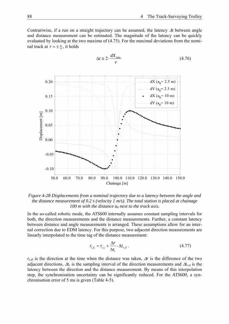
88 4 The Track-Surveying Trolley

Contrariwise, if a run on a straight trajectory can be assumed, the latency Δt between angle and distance measurement can be estimated. The magnitude of the latency can be quickly evaluated by looking at the two maxima of (4.75). For the maximal deviations from the nomi-nal track at 4r π= ± , it holds

max2 dXtv

Δ ≅ ⋅ (4.76)

50.0 60.0 70.0 80.0 90.0 100.0 110.0 120.0 130.0 140.0 150.0

-0.10

-0.05

0.00

0.05

0.10

0.15

0.20

Chainage [m]

Disp

lace

men

t [m

]

dX (a0= 2.5 m)

dY (a0= 2.5 m)

dX (a0= 10 m)

dY (a0= 10 m)

Figure 4-28 Displacements from a nominal trajectory due to a latency between the angle and the distance measurement of 0.2 s (velocity 1 m/s). The total station is placed at chainage

100 m with the distance a0 next to the track axis.

In the so-called robotic mode, the ATS600 internally assumes constant sampling intervals for both, the direction measurements and the distance measurements. Further, a constant latency between distance and angle measurements is arranged. These assumptions allow for an inter-nal correction due to EDM latency. For this purpose, two adjacent direction measurements are linearly interpolated to the time tag of the distance measurement:

, , ,i it d t r r dr

rr r tt

Δ= + ⋅Δ

Δ. (4.77)

rt,di is the direction at the time when the distance was taken, Δr is the difference of the two adjacent directions, Δtr is the sampling interval of the direction measurements and Δtr,d is the latency between the direction and the distance measurement. By means of this interpolation step, the synchronisation uncertainty can be significantly reduced. For the ATS600, a syn-chronisation error of 5 ms is given (Table 4-5).

4 The Track-Surveying Trolley 89

Figure 4-29 Principle of direction and distance synchronisation carried out by the robotic mode of the ATS600 (from [TRIMBLE, 2001b])

On the calibration track of the Institute of Geodesy and Photogrammetry of the Swiss Federal Institute of Technology of Zürich, measurements particularly with regard to the verification of the latency between direction and distance measurements were carried out. A Trimble RMT mini prism mounted on a moving platform was tracked by the ATS600. The tacheometer was placed on a pillar at station 20 m 2.25 metres next to the calibration track. Runs with different platform velocities, servo modes and prism orientation were carried out. Comprehensive re-sults are compiled in [GROSSE-HÜNDFELD et al., 2004]. Here, only a representative plot is given illustrating the findings of this section.

0.0 5.0 10.0 15.0 20.0 25.0 30.0-0.010

-0.005

0.000

0.005

0.010

Chainage [m]

Disp

lace

men

t [m

]

forward nominalforwardbackward nominalbackward

Figure 4-30 Forward and backward run on a calibration track carried out at a velocity of 0.45 m/s

Figure 4-30 shows a forward and a backward run carried out at a velocity of 0.45 m/s. Dis-placements from the nominal straight line of up to 8 millimetres occurred in the regions of

4r π= ± . According to (4.76), a latency of 35 ms has to be taken into account. A more reliable model fits (4.75) to the pattern of the forward run and the backward run, respectively. This

Interpolated direction at time td,i Measurement of current direction at time tr,i+1

Last direction measured at time tr,i

Distance measurement at time td,i

S

Trolley movement

90 4 The Track-Surveying Trolley

approach yields a latency of 20 ms. Nominal curves for this latency are given for the forward and the backward run in Figure 4-30. Residual errors between the actual and nominal curves can be attributed to the changing prism alignment and deviations from a constant latency. The specified 5 ms synchronisation error could not be confirmed for the used instrument.

Both runs were contaminated by outliers. Outliers in the order of magnitude of several centi-metres occurred at the 57 gon direction interval whenever the laser beam hit the interspace between two singular prisms.

4.7.6 Internal Tacheometer and Radio Latencies ATS600 data are sent to the Swiss Trolley laptop by a radio link. To accelerate data transmis-sion, BCD (binary coded decimal) coding is used. Thus, only 15 bytes are used for a complete tacheometer data record. For a 9600 baud rate, data transmission can be realised within 16 ms. However, internal delays of the tacheometer and the radio exceed data transmission latency by one magnitude and have to be considered if the ATS600 positioning is combined with other data. A latency of 183 ms is specified by the manufacturer.

In general, not the absolute latency is of interest but the relative latency between two sensors. Latency is not critical for almost steady parameters such as the track gauge or the cant. How-ever, latency becomes important for laser scanners acquiring data with a high dynamic range. A calibration approach for the determination of the latency between a laser scanner and a po-sitioning sensor is given in section 4.10.6.

4.8 Integration of GPS

4.8.1 Characteristics In addition to total stations, GPS-RTK can be applied for absolute positioning. Preferably, a Trimble 5700 two frequency receiver with 1PPS output is used [TRIMBLE, 2001a]. The Trimble 5700 receiver resolves the carrier phase ambiguities on-the-fly (OTF) typically within 10 seconds whereby base line length, multipath and prevailing atmospheric conditions are acting parameters. 10 Hz position updates are available. However, the more accurate synchro-nised mode only supports 1 Hz position fixes. The synchronised RTK solution yields the highest position accuracy and suits the Swiss Trolley application. With the synchronised op-tion, the trolley receiver waits until the reference station measurements are received before computing a baseline vector. Specified accuracies given by the manufacturer are for the hori-zontal component 1 cm + 1 ppm and for the vertical component 2 cm + 2 ppm. The rover re-ceiver handles different GPS data output formats. The Swiss Trolley data acquisition software makes use of the NMEA protocol.

4.8.2 NMEA Data Geodetic GPS receivers provide a data string on the serial interface. The most common format of these data is the NMEA-1083 format, proposed by the U.S. National Marine Electronics Association. The NMEA format is an eight-bit ASCII format. NMEA data are sent in the form of strings denoted as sentences starting with the dollar sign delimiter and with a maximal length of 82 characters. The sentences are subdivided into several fields including an address field (two characters identifying one of around 40 approved talkers and three characters iden-tifying one of about 60 approved sentence types), a variable number of data field and a check-sum field, followed by a carriage return and line feed terminator.

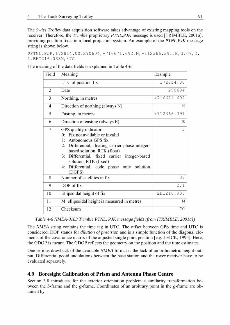
4 The Track-Surveying Trolley 91

The Swiss Trolley data acquisition software takes advantage of existing mapping tools on the receiver. Therefore, the Trimble proprietary PTNL,PJK message is used [TRIMBLE, 2001a], providing position fixes in a local projection system. An example of the PTNL,PJK message string is shown below. $PTNL,PJK,172814.00,290604,+716671.692,N,+112366.391,E,3,07,2.1,EHT216.033M,*7C

The meaning of the data fields is explained in Table 4-6.

Field Meaning Example

1 UTC of position fix 172814.00

2 Date 290604

3 Northing, in metres +716671.692

4 Direction of northing (always N) N

5 Easting, in metres +112366.391

6 Direction of easting (always E) E

7 GPS quality indicator: 0: Fix not available or invalid 1: Autonomous GPS fix 2: Differential, floating carrier phase integer-

based solution, RTK (float) 3: Differential, fixed carrier integer-based

solution, RTK (fixed) 4: Differential, code phase only solution

(DGPS)

3

8 Number of satellites in fix 07

9 DOP of fix 2.1

10 Ellipsoidal height of fix EHT216.033

11 M: ellipsoidal height is measured in metres M

12 Checksum 7C

Table 4-6 NMEA-0183 Trimble PTNL, PJK message fields (from [TRIMBLE, 2001a])

The NMEA string contains the time tag in UTC. The offset between GPS time and UTC is considered. DOP stands for dilution of precision and is a simple function of the diagonal ele-ments of the covariance matrix of the adjusted single point position [e.g. LEICK, 1995]. Here, the GDOP is meant. The GDOP reflects the geometry on the position and the time estimates.

One serious drawback of the available NMEA format is the lack of an orthometric height out-put. Differential geoid undulations between the base station and the rover receiver have to be evaluated separately.

4.9 Boresight Calibration of Prism and Antenna Phase Centre Section 3.8 introduces for the exterior orientation problem a similarity transformation be-tween the b-frame and the g-frame. Coordinates of an arbitrary point in the g-frame are ob-tained by

92 4 The Track-Surveying Trolley

( )g g bg b bQ R Q Rx x R x x= + − (4.78)

where gRx and b

Rx are the position vectors of the antenna phase centre or the active prism in the g-frame and the b-frame, respectively. The rotational matrix is given by the current trolley attitude. The position vector b

Qx provides the position of the surveyed object in the b-frame. bQx is determined by the track gauge measuring system or by a laser scanner, for instance. For

an unambiguous transformation from the b-frame into the g-frame the components of the po-sition vector b

Rx have to be known. The determination of this vector is commonly called bore-sight calibration [e.g. EL-SHEIMY et al., 2002]. This section explains the boresight calibra-tion of the position vector b

Rx by means of a forward and a backward trolley run. Identical points are measured in forward and backward direction by means of the stop-and-go method. Thus, accelerations affecting the inclination sensors do not occur. This procedure does not allow for the determination of the vertical component of the b

Rx vector. However, the vertical component can be easily obtained by levelling the height difference between the top edges of both rails and the prism centre or the antenna phase centre, respectively.

For the calibration of the horizontal components of the bRx vector, the centreline of a track is

established by

( )f f f

g g bg b bC R f C Rx x R x x= + − (4.79)

where f

bCx is the track centreline forward run fixing in the body frame realised by the two

track gauge levers (section 4.5.1). Correspondingly, we find for the backward run centreline fixing

( )b b b

g g bg b bC R b C Rx x R x x= + − (4.80)

For an identical point on the track, it holds

f b

g gC Cx x= (4.81)

or

( )b f b f

bg bg b g g bg b bg bb f R R R b c f cR R x x x R x R x− ⋅ = − + − (4.82)

If a non-skewed trolley in forward and backward position is assumed, then it yields further

bgf

bg T Tb

R R R R

R R R R R R Rτ ϕ ω

τ π ϕ ω τ π ϕ ω+ − − +

=

= = (4.83)

Pitch and roll angles are derived from the inclination sensor measurements. The yaw angle has to be derived from a nominal azimuth. For the difference bg bg

b fR R− , we find for small pitch and roll angles

cos sin 0

2 sin cos 00

bg bgb fR R

τ ττ τ

ϕ ω

−⎛ ⎞⎜ ⎟− = ⋅ − −⎜ ⎟⎜ ⎟−⎝ ⎠

(4.84)

4 The Track-Surveying Trolley 93

whereas second order terms containing small angles were dropped. (4.84) is singular and does not allow for the determination of all components of the vector b

Rx . Like stated before, the z-component of the vector b

Rx cannot be obtained by this set-up. Therefore, the third component of (4.82) is cancelled for the benefit of the evaluation of the planimetric components. Then, (4.82) can be solved for b

Rx ′ :

( ) ( )1

b f b f

b bg bg g g bg b bg bR b f R R b c f cx R R x x R x R x

−′⎛ ⎞′′ = − − + −⎜ ⎟

⎝ ⎠ (4.85)

The apostrophe ( ′ ) indicates the reduced two-dimensional vectors and the reduced two-by-two difference matrix, respectively.

From an economical point of view, this procedure outmatches a direct tacheometric determi-nation of the vector b

Rx . A tacheometric determination of bRx with respect to the lever zero

positions is in general more time-consuming than the proposed procedure. Metrologically speaking, a direct tacheometric determination is more accurate since the trolley attitude does not have to be known. However, (4.85) provides for most applications a sufficiently accurate vector b

Rx , since the relative accuracy of track surveys is not affected by the accuracy of bRx .

4.10 Laser Scanners

4.10.1 Characteristics The S configuration of the Swiss Trolley (Figure 4-3) allows for the adaptation of laser scan-ners. SICK LMS200-30106 laser scanners are used (Figure 4-31). SICK laser scanners are widespread within the mobile robotics community [e.g. ARRAS et al., 2003; JENSEN et al., 2005; REIMER et al., 2005]. The competitive price of the SICK LMS200, its weight (5 kg) and its integration flexibility compared to geodetic scanners make it also applicable for the Swiss Trolley.

Figure 4-31 SICK Laser scanner LMS200-30106

The SICK LMS200 bases on the time-of-flight principle. A rotating mirror deflects the laser beam in a regular interval between 0° and 180° within a plane. The frequency of the rotating mirror is 75 Hz. 13500 distance measurements per second are carried out. Thus, the angular resolution in the 180° interval is 1°. Angular step width can be improved by interlacing the

94 4 The Track-Surveying Trolley

laser fan by steps of 0.25°. Four consecutive scans provide a complete profile with an angular resolution of 0.25° or 4.5 mrad. Two distance resolution modes are available. The nominal range of the 1 centimetre mode is 80 metres. For the 1 millimetre mode, the range is limited to the 15-bit width of the distance coding (32 metres). This mode is mainly used for Swiss Trol-ley applications. Due to beam widening, the spot diameter increases as a function of the dis-tance. The spot diameter at 30 metres amounts to 15 centimetres. Figure 4-32 gives and idea of the angular resolution and reveals that even a five-millimetre overhead line wire separated about five metres from the moving laser scanner can be recognized. Here, laser beams per-pendicularly hit the wire with the used arrangement of the scanners. The velocity in the ex-ample was approximately 1 m/s resulting in a resolution in the direction of motion of 1.3 centimetres. The stripe close to the right rail originates from a denser resolution induced by the overlapping sector of two scanners.

Figure 4-32 Kinematic scan of an overhead line. The overhead wire has a diameter of about 6 mm and is 5.7 m above the track axis.

Further, the SICK scanner supports a synchronised mode. This means for two parallel operat-ing scanners, that they do not interfere. Laser beams emitted by the first scanner are not re-ceived by the second scanner. This is realised by timely shifted scans.

Time tags are given by the data acquisition software. Due to large data load on the interface and the requirements concerning time resolution, the Linux data acquisition software (section 4.2.3) with the adapted Linux real time application interface is used.

4.10.2 Model The polar measurands provided by the laser scanners are expressed as Cartesian coordinates in the measuring frame of the scanner. The origin of the measuring system is defined by the projection centre of the scanner. The y-z-plane is spanned by the laser fan. The y-axis corre-sponds with a measurement carried out at 0°. The x-axis is perpendicular to the y-z-plane in such way that a right-handed system is formed (Figure 4-33). If the measuring system is de-fined in such a manner, roll angles from the measuring system to the body system around 90° can be excluded for most reasonable scanner mounts. Like stated in section 3.4, roll angles of 90° would lead to singularities for the calibration of the attitude angles.

4 The Track-Surveying Trolley 95

Figure 4-33 Definition of the laser scanner measuring system

According to the measuring principle of the SICK scanner, the following sequence is scanned in the interlaced mode:

0.0 … 6.7 ms 0.00° 1.00° 2.00° … 180.00° (181 distances) 13.3 … 20.0 ms 0.25° 1.25° 2.25° … 179.25° (180 distances) 26.6… 33.3 ms 0.50° 1.50° 2.50° … 179.50° (180 distances) 40.0 … 46.7 ms 0.75° 1.75° 2.75° … 179.75° (180 distances) 53.3 … 60.0 ms 0.00° 1.00° 2.00° … 180.00° (181 distances) …

The time tag ti of the k-th beam of a particular scan j is

( ) [ ] [ ]( )11, 2, 3, 4 ; 1, 2, 3...180 |181

75 360i j

kt t j k

−= + ∈ ∈

⋅ (4.86)

where tj is the time tag of the first beam within a particular scan. The corresponding angle is

( ) [ ] [ ]( )1 1, 2, 3, 4 ; 1, 2, 3...180 |181i j k j kα α α= + − ⋅Δ ∈ ∈ (4.87)

with ( )( )0.25 1 mod 4j jα = °⋅ − and 1αΔ = ° . The mirror of the scanner rotates in the counter clock sense viewed from the origin to the positive x-axis.

Hence, a pixel in the Cartesian measuring frame is obtained by

0

cossin

m i i

i i

x dd

αα

⎛ ⎞⎜ ⎟= ⎜ ⎟⎜ ⎟⎝ ⎠

(4.88)

where d is the distance measured by the laser scanner and α the angle obtained by (4.87). The same pixel in the g-frame is expressed by

( ) ( ) ( ) ( )( )P Pg bg bg mb mb mx t x t R t x R x t= + + ⋅ (4.89)

mbR and mbx have to be determined by means of a calibration. Since bgx cannot directly be determined, it has to make use of an additional vector known in the b- and the g-frame. By means of (3.39), (4.89) can be written as

mx

my

mz

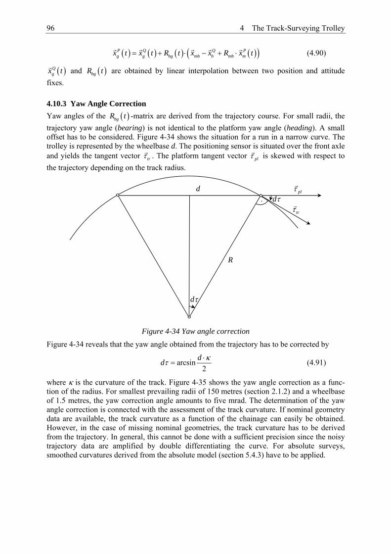
96 4 The Track-Surveying Trolley

( ) ( ) ( ) ( )( )P Q Q Pg g bg mb b mb mx t x t R t x x R x t= + ⋅ − + ⋅ (4.90)

( )Qgx t and ( )bgR t are obtained by linear interpolation between two position and attitude

fixes.

4.10.3 Yaw Angle Correction Yaw angles of the ( )bgR t -matrix are derived from the trajectory course. For small radii, the trajectory yaw angle (bearing) is not identical to the platform yaw angle (heading). A small offset has to be considered. Figure 4-34 shows the situation for a run in a narrow curve. The trolley is represented by the wheelbase d. The positioning sensor is situated over the front axle and yields the tangent vector trτ . The platform tangent vector plτ is skewed with respect to the trajectory depending on the track radius.

Figure 4-34 Yaw angle correction

Figure 4-34 reveals that the yaw angle obtained from the trajectory has to be corrected by

arcsin2

dd κτ ⋅= (4.91)

where κ is the curvature of the track. Figure 4-35 shows the yaw angle correction as a func-tion of the radius. For smallest prevailing radii of 150 metres (section 2.1.2) and a wheelbase of 1.5 metres, the yaw correction angle amounts to five mrad. The determination of the yaw angle correction is connected with the assessment of the track curvature. If nominal geometry data are available, the track curvature as a function of the chainage can easily be obtained. However, in the case of missing nominal geometries, the track curvature has to be derived from the trajectory. In general, this cannot be done with a sufficient precision since the noisy trajectory data are amplified by double differentiating the curve. For absolute surveys, smoothed curvatures derived from the absolute model (section 5.4.3) have to be applied.

· dτ trτ

R

d plτ

dτ

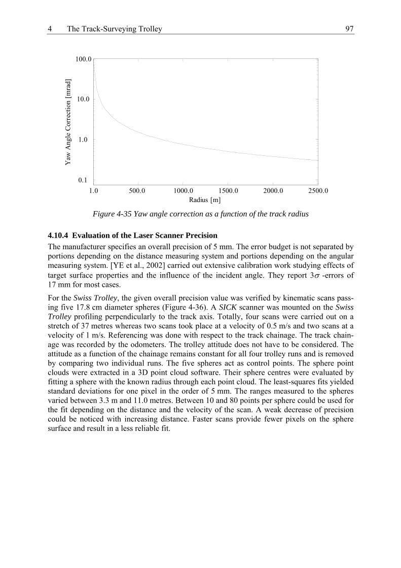
4 The Track-Surveying Trolley 97

1.0 500.0 1000.0 1500.0 2000.0 2500.00.1

1.0

10.0

100.0

Radius [m]

Yaw

Ang

le C

orre

ctio

n [m

rad]

Figure 4-35 Yaw angle correction as a function of the track radius

4.10.4 Evaluation of the Laser Scanner Precision The manufacturer specifies an overall precision of 5 mm. The error budget is not separated by portions depending on the distance measuring system and portions depending on the angular measuring system. [YE et al., 2002] carried out extensive calibration work studying effects of target surface properties and the influence of the incident angle. They report 3σ -errors of 17 mm for most cases.

For the Swiss Trolley, the given overall precision value was verified by kinematic scans pass-ing five 17.8 cm diameter spheres (Figure 4-36). A SICK scanner was mounted on the Swiss Trolley profiling perpendicularly to the track axis. Totally, four scans were carried out on a stretch of 37 metres whereas two scans took place at a velocity of 0.5 m/s and two scans at a velocity of 1 m/s. Referencing was done with respect to the track chainage. The track chain-age was recorded by the odometers. The trolley attitude does not have to be considered. The attitude as a function of the chainage remains constant for all four trolley runs and is removed by comparing two individual runs. The five spheres act as control points. The sphere point clouds were extracted in a 3D point cloud software. Their sphere centres were evaluated by fitting a sphere with the known radius through each point cloud. The least-squares fits yielded standard deviations for one pixel in the order of 5 mm. The ranges measured to the spheres varied between 3.3 m and 11.0 metres. Between 10 and 80 points per sphere could be used for the fit depending on the distance and the velocity of the scan. A weak decrease of precision could be noticed with increasing distance. Faster scans provide fewer pixels on the sphere surface and result in a less reliable fit.

98 4 The Track-Surveying Trolley

Figure 4-36 Swiss Trolley scanning five spheres for precision evaluation of the SICK laser scanner

For the evaluation of the laser scanner precision, the component in the direction of motion is not of interest. The precision of this component is dominated by the odometer precision. Therefore, only two-dimensional Helmert transformations in the plane perpendicular to the track axis were carried out. The standard deviation of one transformed coordinate amounts again to 5 mm. Distance precision and angular precision can be evaluated by analysing the orientation of the residuals with respect to the scanner projection centre (Figure 4-37). Radial residual patterns were found for any run indicating an inferior distance precision compared to the angular component. The angular component is dominated by the constancy of the rotating frequency of the mirror and the time tag of a particular beam. In the investigated range up to 12 m, uncertainties of both acting parameters cause marginal radial errors. It can be concluded that the angular precision must be better than 0.2 mrad.

4 The Track-Surveying Trolley 99

2.0 4.0 6.0 8.0 10.0 12.0

-1.0

0.0

1.0

2.0

3.0

4.0

5.0

6.0

7.0

Horizontal distance to scanner centre [m]

Ver

tical

dist

ance

to sc

anne

r cen

tre [m

]

5 mm

1

2

34

5

Figure 4-37 Residuals of Helmert transformation between scanned spheres and total station

sphere centre coordinates

4.10.5 Variance Propagation for a Given Scanner Arrangement A frequently used Swiss Trolley set-up uses two scanners whose fans are yawed by ±45° with respect to the track axis (Figure 4-38). This allows for gathering information of structures facing towards the direction of motion (see section 3.5.2). The variance propagation for this particular set-up is expanded in the following starting from the individual variance contribu-tions of the involved subsystems making use of the findings of section 3.8. A tunnel survey situation is simulated by beams hitting a cylindrical surface. The trolley is supposed to pro-gress on the cylinder axis. The scanner precision for both, the radial and the angular compo-nent, were verified in the previous section. A mapping function counting for the resulting in-cident angles on the cylinder is considered. The Lambertian behaviour leads to

( ) 1cos

m ϑϑ

= (4.92)

for distance precision attenuation where ϑ is the incident angle taken to the perpendicular of the cylinder surface. Figure 4-39 shows the incident angle and the resulting distance precision as a function of the beam number. For the beams #0 and #180, optimal hits occur. For the beam #90, distance precision is diminished by a factor of 1.4.

100 4 The Track-Surveying Trolley

Figure 4-38 Scanner arrangement on the Swiss Trolley

0 50 100 1500.0

10.0

20.0

30.0

40.0

50.0

Beam number []

Inci

dent

ang

le [°

]

0 50 100 1505.0

5.5

6.0

6.5

7.0

7.5

Beam number []

Dist

ance

pre

cisio

n [m

m]

Figure 4-39 Incident angle and distance precision on a cylinder for a 45° yawed laser scan-ner. The cylinder axis is parallel to the track axis.

The resulting variances for coordinates in the superordinated reference frame are obtained expanding the covariance matrix (3.41) by the influence of the similarity transformation from the scanner system to the body system.

( )

( )g gQ Q

b bg bg bg m bg mb mxxx x

Tb bg bg bg m bg mb m

E K R R R K R R L

E K R R R K R R L

Σ = − ⋅ ⋅ ⋅ ⋅Σ ⋅

− ⋅ ⋅ ⋅ (4.93)

Rmb·Lm propagates the variances of the scanner distances and angles into the body system. Lm contains the partial derivatives with respect to the scan elements d and α:

0 0

cos sinsin cos

mL dd

α αα α

⎛ ⎞⎜ ⎟= −⎜ ⎟⎜ ⎟⎝ ⎠

(4.94)

The covariance matrix of d and α is

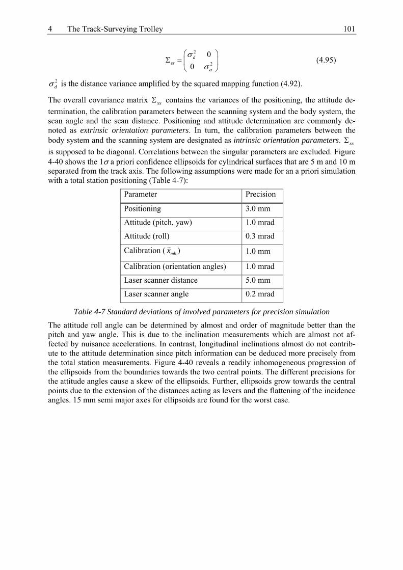
4 The Track-Surveying Trolley 101

2

2

00

dss

α

σσ

⎛ ⎞Σ = ⎜ ⎟

⎝ ⎠ (4.95)

2dσ is the distance variance amplified by the squared mapping function (4.92).

The overall covariance matrix xxΣ contains the variances of the positioning, the attitude de-termination, the calibration parameters between the scanning system and the body system, the scan angle and the scan distance. Positioning and attitude determination are commonly de-noted as extrinsic orientation parameters. In turn, the calibration parameters between the body system and the scanning system are designated as intrinsic orientation parameters. xxΣ is supposed to be diagonal. Correlations between the singular parameters are excluded. Figure 4-40 shows the 1σ a priori confidence ellipsoids for cylindrical surfaces that are 5 m and 10 m separated from the track axis. The following assumptions were made for an a priori simulation with a total station positioning (Table 4-7):

Parameter Precision

Positioning 3.0 mm

Attitude (pitch, yaw) 1.0 mrad

Attitude (roll) 0.3 mrad

Calibration ( mbx ) 1.0 mm

Calibration (orientation angles) 1.0 mrad

Laser scanner distance 5.0 mm

Laser scanner angle 0.2 mrad

Table 4-7 Standard deviations of involved parameters for precision simulation

The attitude roll angle can be determined by almost and order of magnitude better than the pitch and yaw angle. This is due to the inclination measurements which are almost not af-fected by nuisance accelerations. In contrast, longitudinal inclinations almost do not contrib-ute to the attitude determination since pitch information can be deduced more precisely from the total station measurements. Figure 4-40 reveals a readily inhomogeneous progression of the ellipsoids from the boundaries towards the two central points. The different precisions for the attitude angles cause a skew of the ellipsoids. Further, ellipsoids grow towards the central points due to the extension of the distances acting as levers and the flattening of the incidence angles. 15 mm semi major axes for ellipsoids are found for the worst case.

102 4 The Track-Surveying Trolley

-1.00.0

1.0 2.0

3.0 4.0

5.0 6.0 -2.0

0.0

2.0

4.0

6.0

-20.0

-10.0

0.0

10.0

y [m]

1σ confidence ellipsoidlength of semi axes: 0.01 m

x [m]

z [m

]

Figure 4-40 Variance propagation for a 45° yawed scanner on cylindrical surfaces which are 5 m and 10 m away from the scanner projection centre.

4.10.6 Kinematic Calibration of mbR , mbx and the Latency

A static calibration of the six degrees of freedom requires a visualisation of the laser fan. La-ser detectors of rotation construction levels can be used. However, tests yielded that a repre-sentative mapping of the fan is hard to realise. Further, the body frame has to be represented by discrete points on the trolley that have to be linked with the laser fan. These issues pre-vented from a static calibration. Therefore, a simultaneous calibration of mbR , mbx and the latency between the scanner and the positioning sensor is aimed for. As a drawback, the cali-bration parameters are degenerated by the current uncertainty of the trolley position and the attitude. This is accepted in favour of better pixel recognition and more effectiveness. In con-trast to the track axis determination, the latency assessment becomes here relevant due to the high dynamics of laser scans. A simultaneous calibration scenario of all acting parameters includes kinematic scans of control points in a global frame. A scanned control point in the global reference frame is expressed as

( ) ( ) ( ) ( )( )0 0 1 0 2 0g bg bg mb mb mx t x t t R t t x R x t= + Δ + + Δ ⋅ + ⋅ (4.96)

where Δt1 is the latency between the positioning system and the scanner. Δt2 is the latency between the attitude angles and the scanner. A linearisation around t0 yields

4 The Track-Surveying Trolley 103

( ) ( ) ( ) ( )( )0 0 1 0 2 00 0

bg bgg bg bg mb mb m

x Rx t x t t R t t x R x t

t t⎛ ⎞∂ ∂

= + ⋅Δ + + ⋅Δ ⋅ + ⋅⎜ ⎟⎜ ⎟∂ ∂⎝ ⎠ (4.97)

In general, bgR shows a smooth progression with moderate rates. Therefore, a determination of Δt2 is not considered here. Further, a calibration run on a straight line is to be carried out where the derivative of bgR nominally disappears.

A simultaneous calibration of the six degrees of freedom and the latency will not work in practice since counteracting demands with respect to a precise estimation of the sought pa-rameters are inherent to (4.97). A precise determination of Δt1 asks for fast calibration runs. On the other, a fast run generates badly resolved scans regarding the direction of motion. Tar-get point recognition becomes less reliable. Therefore, an accurate determination of mbx and

mbR requires a slow run. Due to these conflictive stipulations, a two-step calibration proce-dure is proposed here.

Calibration of mbR and mbx

A slow run minimises the influence of the latency on the calibration of mbR and mbx . La-tency depending terms in (4.97) are dropped. The calibration is realised by control point measurements in the global frame and comparisons with laser scanner measurements in the measuring frame. For the evaluation of the rotational matrix mbR and the translation vec-tor mbx , the position ( )bgx t and the attitude ( )bgR t have to be known at every epoch t. Linear interpolation between position fixes for calibration runs on a straight line are acceptable. Then, control points in the global frame are transformed into the body frame and compared with the actual scanner coordinates by means of a redundant similarity transformation:

( ) ( )( ) ( )1 0bg g bg b mb mb m mR t x x t v x R x v− ⋅ − + = + ⋅ + (4.98)

0gx represents the nominal global coordinates of the control points. Coordinate residuals bv

and mv are admitted in the b- and in the m-frame. (4.98) corresponds to a general least-squares model (Gauss-Helmert model, see also section 4.4.4).

The manufacturer delivers the projection centre coordinates of the scanner with respect to the enclosure. Thus, a direct determination of the vector mbx with millimetre accuracy in the body frame can be carried out a priori. Hence, the three attitude angles in (4.98) remain unknown.

The main difficulty of the proposed calibration approach is the selection of identical control points in the g-frame and the m-frame. White rectangular targets were used as control points. The coordinates in the g-frame are determined by total station measurements. The trolley run is referenced to the same frame by means of connecting ATS600 measurements. As a next step, the closest pixel to the target centre has to be identified in the preliminary referenced point cloud. The time tag of the identified pixel allows for the evaluation of the trolley posi-tion and attitude. Linear interpolation between adjacent waypoints is acceptable if the calibra-tion stretch is a straight line. Pixel identification is occasionally cumbersome. For a target 10 m separated from the scanner, a maximal error of 2 cm for point identification has to be taken into account if the correct pixel was chosen. Further, attention has to be paid to the con-trol point configuration. Since the control points are transformed into the laser plane, a good distribution also concerning the height component has to be aimed for. Control points laying

104 4 The Track-Surveying Trolley

in a plane perpendicular to the laser fan in the g-frame are projected onto a line in the b-frame. This would result in a bad conditioned normal equation matrix.

A calibration was carried out using the described procedure. A good control point distribution could be realised by incorporating additional points as well-defined structures on overhead line stanchions. The attitude determination provided a standard deviation for one coordinate of 8 mm. Attitude angle precision was in the order of 1 mrad.

A more flexible concept provides for a dense, statically acquired scan of the calibration area. The control point selection is not only restricted to well-defined targets. Every recognisable object in both scans can serve as a control point.

Latency Calibration

For latency calibration, a well detectable structure is scanned in forward and backward direc-tion. In order to reduce the influence of attitude errors, the structure has to be as close as pos-sible to the scanner. Sleepers in general provide too bad contrast for element extraction and are not suitable. Good recognisable structures are catenary yokes (Figure 4-41). Here, pitch errors affect the latency calibration. Pitch angles have to be carefully assessed.

Figure 4-41 Top view of catenary yoke scanned by a forward run (light) and a backward run (dark)

Figure 4-41 shows a small systematic offset between both scans in chainage direction. This offset Δl is attributed to a non-considered latency Δt. Figure 4-42 clarifies the latency impact of one particular edge recognized in a forward and a backward run.

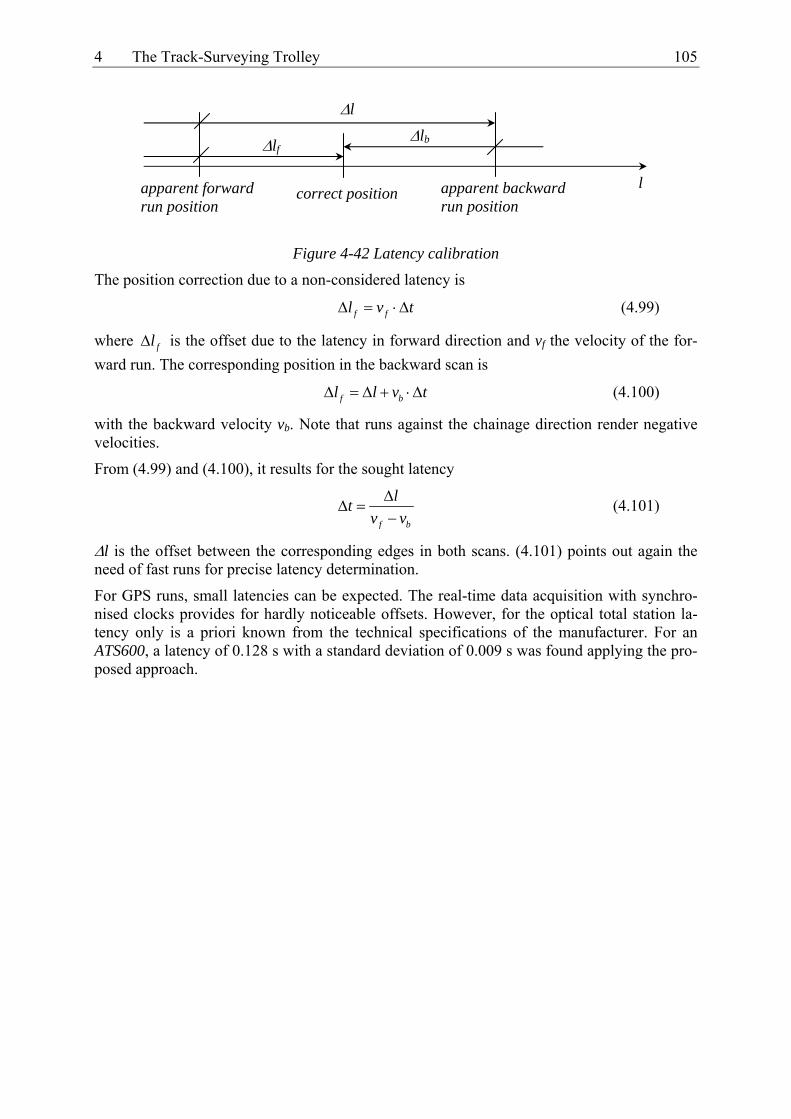
4 The Track-Surveying Trolley 105

Figure 4-42 Latency calibration

The position correction due to a non-considered latency is

f fl v tΔ = ⋅Δ (4.99)

where flΔ is the offset due to the latency in forward direction and vf the velocity of the for-ward run. The corresponding position in the backward scan is

f bl l v tΔ = Δ + ⋅Δ (4.100)

with the backward velocity vb. Note that runs against the chainage direction render negative velocities.

From (4.99) and (4.100), it results for the sought latency

f b

ltv v

ΔΔ =

− (4.101)

Δl is the offset between the corresponding edges in both scans. (4.101) points out again the need of fast runs for precise latency determination.

For GPS runs, small latencies can be expected. The real-time data acquisition with synchro-nised clocks provides for hardly noticeable offsets. However, for the optical total station la-tency only is a priori known from the technical specifications of the manufacturer. For an ATS600, a latency of 0.128 s with a standard deviation of 0.009 s was found applying the pro-posed approach.

l apparent forward run position

apparent backward run position

correct position

Δl

Δlf Δlb

5 Data Processing 107

5 Data Processing

5.1 Introduction This chapter deals with the mutual data treatment of all available information. The geometri-cal reduction of the sensor data to a common body frame was partly matter of the previous chapter. In the sequel, a model is given dealing with the reduction of positioning data to the track centre line. The track centre line acts then as a basis for trajectory filtering, smoothing, merging and linking laser scan vectors.

For stop-and-go applications such as the alignment of the slab track, data are not submitted to trajectory filtering modules presented subsequently. Consequently, no assumptions about the filter behaviour have to be made. In general, the stop-and-go mode provides results that are more accurate since motion model uncertainties are not introduced. However, work efficiency is affected dramatically.

Primarily, data processing includes integrity checks and blunder detection for each data chan-nel. Since not all channels are referred to an identical time tag, synchronisation has to be car-ried out in a second step. Synchronisation to common epochs is not a stringent condition for the subsequent filtering algorithms. However, data processing becomes less cumbersome. Great importance is attached to data filtering and smoothing. A kinematic model is introduced allowing for the functional and stochastic description of the trolley motion. Thus, the inherent low redundancy of single point trajectory determination can be increased significantly. This results in a considerable accuracy gain. In order to benefit from the past and future correla-tions of adjacent measurements, data are post-mission processed by means of a Kalman Filter working in forward and backward direction. A final smoother step provides an optimal solu-tion incorporating all available information. A scheme of the filter data processing is given in Figure 5-1.

Figure 5-1 reveals that the chosen model uses a cascading or a loosely coupled filter concept. In contrast to a tightly coupled filter, kinematic data are pre-processed for each channel sepa-rately. This allows for a more flexible and modular treatment. On the other hand, a tightly coupled or centralised filter just uses one error state model and would lead to an optimal solu-tion. However, filter formulation becomes more complex. Large size of error state models result. For a detailed discussion about the degree of coupling, see [SKALOUD, 1999].

As an alternative to Kalman filtering, a smoothing splines approach is presented here. In con-trary to common smoothing splines [e.g. DE BOOR, 2001], the proposed approach allows for the introduction of first derivatives as additional observations.

The typical workflow of a kinematic track survey contains several track runs with overlapping sections. To improve accuracy, a track is normally surveyed in both directions. A further post-processing step allows for merging data from all runs and takes into consideration the even-tual remaining biases. The merge process accounts for the covariance matrix of the single filtered solutions. Sections with poor GPS receptions or with GPS outages (tunnels, bridges) are supplemented by total station measurements in combination with the trolley. The total station data are tied up to the GPS reference frame. If laser scans were carried out, the trans-formed vectors are attached to the merged trajectory (Figure 5-2).

108 5 Data Processing

Figure 5-1 Post-processing concept [GLAUS, 2004]

Figure 5-2 Merging several filter runs

Inclination sensor (gradient)

Odometers (centerline path)

Transducer left

GPS/RTK and/or track-ing total stations

Inclination sensor (cant)

Transducer right

Corrected gradients

Track gauge

Sync

hron

isat

ion,

redu

ctio

n to

refe

renc

e ra

il an

d co

mpa

rison

with

nom

inal

geo

met

ry

Dat

a pr

epro

cess

ing

(Int

egrit

y te

sts a

nd b

lund

er d

etec

tion)

Forw

ard

/ bac

kwar

d fil

ter a

nd sm

ooth

er

Res

ults

(Ste

erin

g fil

e fo

r tam

ping

mac

hine

s, ch

arts

, 3D

-poi

nt c

loud

s and

so fo

rth)

Attach laser scan vectors

…

• R

esul

ts

• Li

nkin

g la

ser s

can

vect

ors

Mer

ged

traje

ctor

y

Attach laser scan vectors

5 Data Processing 109

5.2 Post-Processing Software Concept All modules are written in the Delphi programming language for the Windows operating sys-tem. For matrix and vector operations, the MtxVec library is used. MtxVec makes extensive use of Lapack. Lapack is short for Linear Algebra Package. Lapack is today de-facto standard for linear algebra and is free.

rmpAnalysis unifies the introductorily mentioned filter and merging strategies in one pro-gramme. The acronym rmp stands for real-time multisensor platform and elucidates the fact that not only Swiss Trolley data but also data acquired by the platform mounted on any vehi-cle can be processed. Data filtering for several runs and the final merging step can be realised by batch processing (Figure 5-4). Results of each filter and the final merge step can be visual-ised by floating charts (Figure 5-3). Each filter or merge step is divided into several so-called subsystems. Each subsystem owns an input and an output interface. Input and output can be a single data channel represented by a vector or multiple data channels represented by an array of vectors or a matrix. Some algorithms were developed and tested by Matlab and Simulink-procedures before implementing them in the Delphi environment.

Figure 5-3 Graphical user interface of the post-processing software rmpAnalysis

110 5 Data Processing

Figure 5-4 Batch-processing with rmpAnalysis

5.3 Data Preprocessing

5.3.1 Blunder Labelling We consider a signal ( )ix t that is corrupted by additive Gaussian noise ( )in t and impulsive noise ( )ii t

( ) ( ) ( ) ( )i i i ix t s t n t i t= + + (5.1)

The impulsive noise is assumed to take a large value relative to the other components in (5.1). For the track-surveying trolley, such high-frequent spikes can be noticed for the angular trans-ducers if welding seams are passed or for accelerations affecting the gradient inclination sen-sor. Further, the total station ATS600 occasionally provides wrong phase ambiguities which results in 10 m errors. The signal of interest ( )is t here is found by two steps. Firstly, the im-pulsive noise is labelled as an outlier in the observed signal ( )ix t . The applied strategy is stated below. Secondly, the remaining Gaussian noise is reduced by low-pass filters.

Extremely high or low values within a data series can be removed by the classical median filter [e.g. TUKEY, 1977]. The median filter removes high frequent dither spikes from data supposed to proceed constantly within a data window whose size has to be defined. The me-dian filter has the property of not affecting step functions or ramp functions. Pulse functions whose periods are less than one-half the window width, are suppressed. However, the peak of the triangle is flattened. Due to the awkward property of flattening peaks, a modified filter is used for outlier detection. A robust estimate of the scale of the input data window is obtained by calculating the median absolute deviation from the median (MAD) [e.g. SACHS, 1984] of the data window

{ }{ }i j jmad median x median x= − (5.2)

Then,

5 Data Processing 111

{ },

ˆ,

i i i

ij i i

x d k madx

median x d k mad

≤ ⋅⎧⎪= ⎨ > ⋅⎪⎩ (5.3)

where

{ }i i jd x median x= − (5.4)

k is an arbitrary chosen factor.

Figure 5-5 charts the differences between the MAD and the median filter. The data stem from one angular transducer of the track gauge measuring system of a trolley survey. The sampling rate is 20 Hz. The window width is 21. The factor k was set to 4. The MAD filter leaves sig-nals as they are. Spikes are labelled. In contrast, the median filter acts as low-pass filter and flattens the signal.

0.0 100.0 200.0 300.0 400.0 500.0 600.0 700.0 800.0120.0

125.0

130.0

135.0MAD Filter

Chainage [m]

Def

lect

ion

[mra

d] RawMAD Filter

0.0 100.0 200.0 300.0 400.0 500.0 600.0 700.0 800.0120.0

125.0

130.0

135.0Median Filter

Chainage [m]

Def

lect

ion

[mra

d] RawMedian

0.0 100.0 200.0 300.0 400.0 500.0 600.0 700.0 800.0-2.0

0.0

2.0

4.0 Difference between MAD and Median Filter

Chainage [m]

Diff

eren

ce [m

rad]

Figure 5-5 Comparison of MAD and median filter

112 5 Data Processing

MAD filtering is applied to the track gauge, the transversal inclination and the longitudinal inclination channels. In general, these data channels provide slow-changing values. Locally, a constant can be used to describe the data representatively.

5.3.2 Reduction, Model Figure 5-6 outlines data preprocessing after blunder labelling. The data preprocessing is com-piled in a module called PrePreFilter. Six channels from the data acquisition card are proc-essed here. Each channel provides a vector of the length n where n is the number of epochs. Thus, a 30 minutes run with a sampling rate of 20 Hz provides 36000 samples for each chan-nel. An additional vector contains the time tags.

The heading of the run is assessed by comparing the first and the last odometer record:

0 1

0 1

::

n

n

l l run in chainage directionl l run against chainage direction

−

−

<>

As a next step, the borders of the run are clipped by a user-defined amount. In this manner, data at the run borders potentially affected by nuisance accelerations are not considered.

The clipped odometer readings are used as a first input for the next data processing module. Further, odometer readings have to be derived with respect to time for velocity and accelera-tion evaluation. This is done by means of a local polynomial approximation acting as a FIR low-pass filters. More information is given in the next section. Cross inclinations, gradients and the readings of both angular transducers for the track measuring system are low-pass fil-tered first. Again, polynomials are used. Cross inclinations and gradients are corrected for the response time TR. Translatory accelerations affecting the gradients are corrected for using equation (4.36). Centripetal accelerations affecting the cross inclinations are not considered. Their magnitudes are marginal (see section 4.4.5 for an estimation). The angular transducer readings are scaled by means of the lever length and processed further according to equation (4.49) for the track centreline determination. The track gauge evaluation is carried out accord-ing to equation (4.53). As it is indicated in Figure 5-6, the longitudinal temperature dilation is considered using the corresponding dilation coefficient and calibration temperature.

As Figure 5-6 outlines, total station data and GPS data are treated completely independently from the remaining data channels on this stage of processing. For total station data, EDM la-tency can be applied (equation (4.77)). Total station data are reduced into the projection plane. As a result, the coordinates of the prism centre in the reference frame are obtained.

GPS-NMEA strings directly provide coordinates in the reference frame. However, the used Trimble receivers do not yield orthometric heights but ellipsoidal heights. NMEA strings can-not be connected to a geoid model. Therefore, at this stage of data evaluation, the geoid undu-lation is evaluated by the post-processing software. Control points with known ellipsoidal and orthometric heights along the railway track define a geoid model. If nominal geometry data are available, these control points are mapped to the corresponding chainage axis. For tracks without nominal geometries, a traverse is defined by chaining the geoid control points. For the trolley trajectory, the corresponding trajectory points are then mapped to the chainage axis. The geoid undulations are linearly interpolated. Operators have to be sure to utilise ellipsoidal heights on GPS base stations. If they do not so, differential geoid undulations between the base station and the current trolley position have to be applied.

5 Data Processing 113

Assess Headingddt

ddt

1g −−

ddt

-TR

ddt

-TR

LPF

LPF

sin s

bTCalib

-1

-1

LPF

LPF

Al x

lin

in

in

plin

prin

Tambin

lout

out

out

cout

gout

v a

0.5

in ddt

tr,d

in ddt

tr,dReduction to

projection system

din

0,stationX Hz

Yout

Xout

Hout

Evaluate chainage

Evaluate geoid undulationNi

Yout

Xout

Hout

Yin

Xin

hin

-1

DAQ Card

ATS Total Station

GPS

sin s

Figure 5-6 Block diagram of data pre-processing

114 5 Data Processing

5.3.3 Linear Filters This section describes the design of a low pass filter which is most suitable for the preprocess-ing of A/D converted raw data. A low pass filter is selected which reduces the short-term noise in the A/D output while not altering the underlying signal. The filter should attenuate all frequency components which are not due to track induced signals. Digital filters are classified into to major subclasses: recursive, Infinite Impulse Response (IIR) filters, and non-recursive, Finite Impulse Response (FIR) filters. The main difference is that the coefficients of the FIR filters operate only on the input data while the IIR filters feed also back their own output. Since post-mission processing is applied here, a symmetric FIR filter can be applied. A gen-eral form of such an FIR filter is

q

i k i kk p

y xα −=−

= ∑ (5.5)

where αk are the filter coefficient. A symmetric FIR filter is characterised by p q= and 1ka =∑ . Further, (5.5) implies that data are equidistant. For p > 0, the filter is non-causal.

This means that x-values of the future are needed to evaluate the filtered value at epoch i. On the other hand, the output of the symmetric filter leaves the phase of the original data un-changed. An ideal filter response in the frequency domain has a maximum magnitude re-sponse in the pass band and zero elsewhere. By means of a finite number of filter coefficients, the mentioned criterion is not realisable. Due to the Gibbs phenomenon, overshoots at the cut-off frequency take place. The corresponding coefficients in the time domain can be found by means of a Fourier transform. For more details, see the extensive literature on this topic [e.g. OPPENHEIM et al., 1999]. Here, a least-squares approach in the time domain is followed [CASPARY, 2000]. As an example, a third order polynomial can be adapted to the time series at five equidistant base points:

2 30 1 2 3k kx v b b k b k b k+ = + + + k = -2, -1, 0, 1, 2 (5.6)

k determines the number of time intervals

i k it tk

t+ −

=Δ (5.7)

Figure 5-7 Smoothing by adjusting a polynomial at five equidistant base points

The adjusted coefficients are just needed for k = 0. Thus, one finds for the filtered value yi:

t

x

t

t+Δt t+2Δt

t-Δt t-2Δt

5 Data Processing 115

0/i iy b= (5.8)

The least squares solution yields the required coefficient b0

( )0 2 1 0 1 21 3 12 17 12 335

b x x x x x− −= − + + + − (5.9)

The frequency characteristics can be obtained by applying a digital Fourier transform on the filter coefficients.

The precision of the filtered values can be estimated by studying their variance propagation. If a single value x owns the variance σx, then the variance for the filtered value is

2

2 2 2

20.49y x k x

kσ σ α σ

=−

= ⋅ = ⋅∑ (5.10)

For the correction of the inclination measurements, the first and second derivatives with re-spect to time of (5.6) are needed. The filtered velocity and acceleration can be obtained by

11x kv b

k t t∂ ∂

= ⋅ = ⋅∂ ∂ Δ

(5.11)

and

2 2

12x ka bt k t t

∂ ∂ ∂⎛ ⎞= ⋅ = ⋅⎜ ⎟∂ ∂ ∂ Δ⎝ ⎠ (5.12)

with the least squares solutions

( )1 2 1 1 21 8 8

12b x x x x− −= − + − (5.13)

and

( )2 2 1 0 1 21 2 2 2

14b x x x x x− −= − − − + (5.14)

The corresponding noise gains are

2 22

22 2

20.90vx x

v kkt t

σ σσ α=−

= ⋅ = ⋅Δ Δ∑ (5.15)

2 22

24 4

20.29ax x

a kkt t

σ σσ α=−

= ⋅ = ⋅Δ Δ∑ (5.16)

In comparison with an unfiltered series, noise can be significantly reduced. The unfiltered series of the actual value, its first and second derivative owns noise gains of 1, 2 and 6.

The complete filtered series can be obtained by means of a convolution of the raw values with the filter coefficients

y xα= ∗ (5.17)

For a symmetric filter, values of the epochs [0..p-1] and [n-1-p..n-1] cannot be convolved. The PrePreFilter module discards these values after convolution.

116 5 Data Processing

5.3.4 Synchronisation As explained in section 4.2.3, two concepts of synchronisation have to be applied. Firstly, the DAQ card is triggered by the 1PPS pulse. Secondly, if no 1PPS pulse is available, each sensor stores data with a time tag given in a unique time frame.

In the first case, data are normalised to an equidistant one-dimensional grid defined by the GPS sampling interval. This is realised again by means of a convolution using a symmetric smoothing filter

z yα= ∗ (5.18)

Thus, the sampling interval of the synchronised data corresponds to the GPS sampling inter-val.

In the second case, the positioning sensor epochs do not coincide with the DAQ card epochs. For synchronisation, smoothing polynomials are used. In contrary to the FIR filter approach, all coefficients of the polynomial have to be known, since k in (5.6) does not vanish for the sought epoch. In general, k will be a floating-point number. The polynomial fit leads to a Vandermonde system. Vandermonde systems tend to be ill conditioned. Solving for the coef-ficients asks for specialised routines (e.g. [PRESS et. al., 1994]).

Third order polynomials are used for time synchronisation. Due to the smooth progression of all involved parameters, third order polynomials accurately interpolate unsynchronised data. This does not hold for the acquired polar elements of tacheometric runs passing by the total station. As it can be seen in Figure 4-26, rates are maximal, if the trolley passes the total sta-tion. In order to rid these pseudo-accelerations of the total station measurements, the polar elements are transformed to Cartesian coordinates. If the trolley runs are straight lines and the motion is uniform, then the Cartesian coordinates are linear functions of the covered path. The local Cartesian coordinates are rotated against a primary reference frame by the unknown ori-entation of the graduated circle.

5.3.5 Reduction to the Centre Line of the Track For track survey smoothing, two approaches are conceivable. If the track axis is not of inter-est, trajectory smoothing is applied. However, if the track axis is sought, the centre line track axis vector can be attached at every epoch to the actual trajectory. The points of these arrows tend to form a curve to be smooth. For smoothing of the centre line, the track centre line measurements have to be transformed first into the global reference frame by

( )( ) ( ) ( ) ( )g g bg b bc P c Px t x t R t x t x= + ⋅ − (5.19)

bPx is the vector of the positioning sensor within the body frame. Its coordinates are found by

a calibration. ( )bcx t is the measured track centre line in the body system ( )g

Px t is the vector given by the positioning sensor and ( )bgR t the rotation matrix between the two frames.

( )bgR t contains the Euler angles. The roll and pitch angles can be obtained by the inclination measurements by means of equations (4.41) and (4.42). One difficulty consists in the azimuth of the track centre line which is not known at this state of data processing. Here, two ap-proaches are applied:

If a nominal geometry is available, nominal azimuths can be easily obtained as a function of the chainage.

5 Data Processing 117

In case of missing geometric base data, initial azimuths have to be computed. Initial azimuth can be obtained by

tan YX

τ = (5.20)

Y and X denotes easting and northing, respectively. With regard to the extended Kalman filter formulation, initial values for the curvature are evaluated in the same step

( )

32 2 2

YX YX

Y Xκ −

=+

(5.21)

using again polynomials for low pass filtering, (5.20) and (5.21) become

1

1

tan ba

τ = (5.22)

( )

1 2 2 13

2 2 21 1

2 2a b a b

a bκ −

=+

(5.21)

5.4 Trajectory Smoothing by a Kalman Filter

5.4.1 Discrete Kalman Filter The preprocessed data are for optimal trajectory estimation processed by a discrete Kalman filter. This algorithm estimates the state of a system at the time tk based on observations at this time as well as all prior information that is captured in the state at time tk-1. Then, an estima-tion at a subsequent time tk+1 is obtained recursively using the estimate at time tk and new in-formation up to the new time. Theoretical background of the algorithm can be found in many textbooks (e.g. [GELB, 1974]).

The nature of the Kalman filter is the combination of measurement and system dynamics equations for an optimal estimate of the current system state by means of the minimisation of the error variances. Optimal also means that all available deterministic and stochastic infor-mation is incorporated into the filter. The system equations can be put up by the use of a pri-ori knowledge about railway tracks and the mass point kinematics derived in section 2.3. The expansion of the filter equations leads to a representation which can be considered as a least-squares adjustment problem [HEUNECKE, 1995].

The adaptation to the real situation, the parameter identification, is realised by the observa-tions. System identification on the other hand denotes the mathematical description between the transfer behaviour of input and output parameters. The incompatibility between theory and the real situation is expressed in the filter innovation.

In contrast to the symmetric smoothing filter of section 5.3.3, the Kalman filter is a recursive filter or an IIR filter. The filter uses filtered values dating back. There is no need to store past measurements for computing present estimates. This makes the Kalman filter especially suit-able for real-time applications. A self-contained processing would require too many computa-tion time and memory.

The set-up of the Kalman filter algorithm starts with the state-space notation of a dynamic system. The state-space notation allows for the computation of the state of any epoch if the

118 5 Data Processing

state vector at a particular time and a description of the system forcing and control behaviour are given:

( ) ( ) ( ) ( ) ( ) ( ) ( )x t F t x t G t w t L t u t= ⋅ + ⋅ + ⋅ (5.23)

x(t) is the state vector, F, G and L are well defined matrices and are in general time dependent. The non-homogenous, forcing part of the equation consists of a deterministic component u(t) and a stochastic component w(t). u(t) can be used to model a deterministic forcing part.

The discrete, stationary solution of (5.23) neglecting deterministic forcing parts is described by the vector difference equation (ahead propagation of the state):

1 1 1 1 1 1, , ,p q p p p qk k k k k k k k kx x w x w × ×

− − − − − −= Φ ⋅ + Γ ⋅ ∈ℜ ∈ℜ Φ ∈ℜ Γ ∈ℜ (5.24)

Φk-1 is the transition matrix for p state parameters to be taken between the epoch tk-1 and tk. Γk-1 is the disturbance input matrix for p state parameters and q process noise parameters wk.

Measurements are taken at every epoch k and are incorporated as linear functions of the state. An additive noise contribution vk is admitted

, ,r r pk k k k k k kz H x v z v H ×= + ∈ℜ ∈ℜ (5.25)

In contrast to the classical geodetic observation model, the residual vk is introduced here with opposite sign. This does not have any consequences for the further considerations.

Assumptions about the behaviour of the stochastic components have to be made. wk consists of a Gaussian, zero-mean, white noise process

( )

( )0,

cov , 0= ∀ ≠

∼k k

k l

w N Q

w w k l (5.26)

Similar assumptions are made for vk:

( )0,k kv N R∼ (5.27)

Qk and Rk are the covariance matrices of the process noise and the measurement noise. Fur-thermore, the initial state ξ is a random vector with the stochastic property

( )0 0,N x Pξ ∼ (5.28)

x0 is the expectation value. P0 is the initial covariance of the process. Assumptions about x0 and P0 have to be made in order to initiate the filter. Further, it is assumed that the random variables xk, wk, vk are mutually independent. These presumptions about the stochastic behav-iour are not mandatory. Even for coloured noise between the stochastic parameters, almost optimal states can be obtained. However, this results in a more complex filter formulation [SCHRICK, 1977].

All findings given yet are valid for a discrete-time controlled process that is governed by lin-ear stochastic difference equations. The more general case of a non-linear process or meas-urement relationships leads to the formulation of the so-called extended Kalman filter (EKF) [JAZWINSKI, 1970]. The EKF expands the non-linear process and measurement relations in Taylor series around initial state vectors 0

kx that are close to kx . Transition, disturbance input and measurement matrices are replaced by Jacobian matrices of partial derivatives with re-spect to the state and the process noise, respectively. The estimates ˆkx are then repeatedly improved, each time linearising around the most recent estimate. The non-linearities of the

5 Data Processing 119

EKF appear in the state propagation and in the measurement update. The truncation of higher order terms result in propagation errors and in biased estimates [JULIER et al., 2004]. The kinematic model of the Swiss Trolley makes use of non-linear process and measurement de-pendencies. Due to the good-natured, almost linear state propagation along railway tracks of all involved parameters, convergence emerges rapidly.

Figure 5-8 shows the filter loops. The equations of the Kalman filter can be assigned to two groups. The prediction equations propagate the current state and its covariance forward in time. In Figure 5-8, a (-) is used to denote a state and its covariance just prior to the inclusion of a measurement zk. The measurement update equations incorporate new information. By the Kalman gain matrix K, this new information is weighted in relation to the expected values. This difference ˆ( )−k kz h x is the before mentioned filter innovation. It is up to the filter user how much of the innovation should be added to the a priori estimate. If the measurements are not precise, i.e. Rk is large, the Kalman gain will be small and the filter “relies” on the proc-ess. Note that in Figure 5-8 non-linear functions have taken the place of the linear state propa-gation (5.24) and linear measurement update (5.25).

Figure 5-8 Extended Kalman filter loops (adapted from [WELCH, 1997])

The form of

( ) ( )T Tk k k k k k k k kP I K H P I K H K R K−= − − + (5.29)

ensures the symmetry and positive definiteness of the computed matrices. However, it is pru-dent to replace the computed covariance matrices by [JEKELI, 2001]

( )( )1:2

T

k k kP P P− − −= + (5.30)

Time-Update Measurement-Update

(1) Ahead propagation of state

1ˆ ˆ( )k kx f x−−=

(2) Ahead propagation of error co-variance

Tkkk

Tkkkk QPP 111111 −−−−−−

− ΓΓ+ΦΦ=

(1) Computation of the Kalman gain

( ) 1

k

T Tk k k k k kK P H H P H R

−− −= +

(2) State update with measurement zk

( )ˆ ˆ ˆ( )k k k k kx x K z h x− −= + −

(3) Update of error covariance matrix

( ) ( )T Tk k k k k k k k kP I K H P I K H K R K−= − − +

Initial estimates for 1ˆkx − and 1kP −

k:= k+1

120 5 Data Processing

( )1:2

Tk k kP P P= + (5.31)

5.4.2 Backward Filter and Smoother A forward filtered solution for an epoch k is obtained by operating on all the data before the epoch k. For post-mission data, a filtered state for epoch k can also be obtained by processing all the data after the epoch k. The combination of this backward and forward filtered solution provides an optimal smoother. All available information is used by the two filters. The lags inherent to a causal filter can be minimised. In literature, different types of smoothing can be found [JEKELI, 2001]. For post-mission trolley data, a so-called fixed-interval smoother can be applied. Fixed-interval smoothing means that the initial and the final time are fixed and the estimate is sought, where the time varies from the initial to the final time. There exist several versions of the fixed-interval smoothing algorithm. Here, a combination of a forward-in-time and a backward-in-time filter is given [FRASER, 1967]. The forward-in-time filter corre-sponds to the Kalman filter already discussed in 5.4.1. The backward-in-time filter can be derived from the forward filter by careful implementation of time indices. The advantage of such a derivation is the re-use of the scheme exposed in Figure 5-8. According to this, the state transition matrix and the disturbance input matrix are adapted. We set

:k kt T t= − (5.32)

and

1 1:k k k kt t− −Δ = −Δ (5.33)

where T is the time tag of the last epoch n. Then, the transition matrix Φ and the disturbance input matrix Γ becomes

1: −Φ = Φ (5.34)

1: −Γ = −Φ ⋅Γ (5.35)

The state transition backward in time corresponds to an inversion of the non-linear forward transition in Figure 5-8. For this, consider the time axis with an intermediate time index j used for the backward filter. j increases backward in time.

Figure 5-9 Forward and backward propagation of the state

The ahead propagation of the state in backward-direction is described by

( )1

1ˆ ˆj jb bx f x

−

− −= (5.36)

where f are the governing equations of the forward transition. In general, the solution of the non-linear equation system (5.36) can only be obtained by iterative methods. Instead, almost linearity is assumed yielding similar state variations Δxb for adjacent epochs underlying iden-tical time intervals. Therefore, the forward-in-time-propagation of

1ˆ

jbx−

is considered

... ...

2k − 1k − k

j 1j − 2j −

... ...forward

backward

t

5 Data Processing 121

( )2 1ˆ ˆ

j jb bx f x− −

− = (5.37)

or

2 1 1 2

ˆ ˆj j j jb b bx x x− − − −

− = + Δ (5.38)

Then, the backward propagation derived from the forward propagation can be approximated by

2 1 2

ˆ ˆ 2j j j jb b bx x x

− − −

− −≅ − ⋅Δ (5.39)

or

2 1

ˆ ˆ ˆ2j j jb b bx x x

− −

− −≅ − + ⋅ (5.40)

Here, the assumption is made that the state rate Δx remains constant for two adjacent epochs. This is acceptable if time intervals are small and the state progression is almost linear. This notation outmatches a complete derivation of the backward filter equations since the non-linear state transition can be derived from the forward-filter formulation.

The backward filter provides for each time tag a state vector with a corresponding covariance matrix. A smoothed state vector is obtained by combining the forward and the backward fil-tered solution [FRASER, 1967]:

( )1 1/ /ˆ ˆ ˆk N k N k k bk bkx P P x P x− −= + (5.41)

( ) 11 1/k N k bkP P P

−− −= + (5.42)

where /ˆk Nx and /k NP are the smoothed mean vector and the corresponding covariance matrix. ˆkx and ˆbkx are the a posteriori forward and backward mean vectors, respectively. Pk, Pbk de-

nominate the corresponding covariance matrices. The subscript N notifies that all information up to epoch N is used for the final estimate. (5.41) and (5.42) represent the general weighted mean of the two vectors x and xb.

5.4.3 Absolute Model The scheme of Figure 5-8 can be used to set up process models for the Swiss Trolley. Two models were developed. The model presented in the sequel describes the trolley motion in an absolute Cartesian reference frame. This model is denoted as the absolute model. Frequently, nominal geometry data of axes are a priori known and can be used for data processing. The corresponding model refers the data to a chainage axis. It is denominated as the relative model. The relative model is explained in section 5.4.4.

For the description of the trolley trajectory, it can be reverted to a priori knowledge of track axes even if no nominal track data are available. The trolley motion is split up into a horizon-tal and a vertical component. Generally, for the horizontal track layouts straight lines, circles and transition curves are used. For vertical geometries, only straight lines and circles are common. This information can be applied while formulating the state equations. For the hori-zontal description, a circular motion is supposed. A circle model for vehicle tracking is com-mon in navigation applications. For example, [BAGNASCHI, 1993], [STERNBERG, 2000] or [RAMM et al., 2004] use circle models in order to describe trajectories of road vehicles. Deviations from circular trajectories not only in transition curves but also due to track errors are compensated by stochastic disturbance terms. For vertical modelling, a uniform motion on

122 5 Data Processing

a straight line which is inclined by an angle α against the horizontal plane is assumed. Com-pared to the horizontal component, small radii almost do not occur. Therefore, a linear model is acceptable.

For the trolley case, equidistant data are available. Typical update rates are 1 Hz or 5 Hz. A thirteen state model is set up describing the trolley motion on a track. The state model in-cludes the modelling of the trajectory, the cant and the gauge. All states to be estimated are compiled in the state vector:

( )0Tx Y X l v n s Hτ κ β μ α α′= (5.43)

Y, X: easting and northing of track centre line l: track chainage v: tangential velocity of trolley τ: azimuth of track centre line κ: curvature of track centre line β: transversal inclination n': change of transversal inclination μ: odometer scale s: track gauge H: height of track centre line α: gradient of track centre line α0: gradient zero point offset

For the state transition, it can be reverted to the findings of chapter 2.3.2. Starting from the canonical representation of a circle with vanishing tangential accelerations and radial jerks, one finds

2 2sin cos1( ) ( )cos sin2

R t t R t v t v tτ τ

κτ τ

⎛ ⎞ ⎛ ⎞+ Δ = + Δ + Δ⎜ ⎟ ⎜ ⎟−⎝ ⎠ ⎝ ⎠

(5.44)

or explicitly

( ) ( )221 1 1 1 1 1 1 1

1sin cos2k k k k k k k k k k kY Y v t t v t tτ κ τ− − − − − − − −= + − + − (5.45)

( ) ( )221 1 1 1 1 1 1 1

1cos sin2k k k k k k k k k k kX X v t t v t tτ κ τ− − − − − − − −= + − − − (5.46)

Deviations from this model can be described by disturbance terms, as it will be shown below. For a uniform circular motion, it holds further

( )1 1 1k k k k kl l v t t− − −= + − (5.47)

1k kv v −= (5.48)

( )1 1 1 1k k k k k kv t tτ τ κ− − − −= + − (5.49)

1k kκ κ −= (5.50)

( )1 1 1 1k k k k k kn v t tβ β − − − −′= + − (5.51)

1k kn n −′ ′= (5.52)

1k kμ μ −= (5.53)

5 Data Processing 123

1k ks s −= (5.54)

( )1 1 1 1sink k k k k kH H v t tα− − − −= + − (5.55)

1k kα α −= (5.56)

0/ 0 / 1k kα α −= (5.57)

Cant and twist can easily be obtained by scaling (5.51) and (5.52) to the nominal rail offset. A correlation between the cant and the curvature is not considered here (equation (2.4)). Due to the limited accuracy of the inclination sensor, a corresponding state equation only contributes in much canted sections. Further, an additional parameter is required for describing this de-pendency resulting in a less reliable model.

Odometry is subject to systematic errors caused by factors such as unequal wheel-diameters, imprecisely measured wheel diameters, or an uneven tread. This is compensated by the intro-duction of an odometer scale factor μk. The odometer scale contains also contributions due to the height above the reference plane and due to the projection system. This parameter tends to vary slowly if the stretch ascends or descends. As a further parameter, the zero point offset of the gradient inclination sensor is introduced as a random constant. For sections with no GPS coverage, a poor calibrated inclination sensor would cause height drifts. This effect can be absorbed by estimating a bias for the inclination sensor. The user can hold the adaptive pa-rameters μk and α0 constant in consecutive filter runs. This results in a reliability gain.

The transition matrix results from the linearisation of the state equations (5.45) to (5.56) with respect to the parameters of the state vector (5.43):

1,14 1,15 1,16

1,24 1,25 1,26

1 1

1 1 1

1 0 0 0 0 0 0 0 0 00 1 0 0 0 0 0 0 0 00 0 1 0 0 0 0 0 0 0 0 00 0 0 1 0 0 0 0 0 0 0 0 00 0 0 1 0 0 0 0 0 0 00 0 0 0 0 1 0 0 0 0 0 0 00 0 0 0 0 1 0 0 0 0 00 0 0 0 0 0 0 1 0 0 0 0 00 0 0 0 0 0 0 0 1 0 0 0 00 0 0 0 0 0 0 0 0 1 0 0 00 0 0 sin

k k k

k k k

k k

k k k

t

t v t

n t v t

κ

α

− − −

− − −

− −

− − −

Φ Φ ΦΦ Φ Φ

Δ

Δ Δ

′Φ = Δ Δ

1 1 10 0 0 0 0 0 1 cos 00 0 0 0 0 0 0 0 0 0 0 1 00 0 0 0 0 0 0 0 0 0 0 0 1

k k kt v tα− − −

⎛ ⎞⎜ ⎟⎜ ⎟⎜ ⎟⎜ ⎟⎜ ⎟⎜ ⎟⎜ ⎟⎜ ⎟⎜ ⎟⎜ ⎟⎜ ⎟⎜ ⎟⎜ ⎟⎜ ⎟⎜ ⎟Δ Δ⎜ ⎟⎜ ⎟⎜ ⎟⎝ ⎠

(5.58)

21,14 1 1 1 1sin cosk k k k kt v tτ κ τ− − − − −Φ = Δ + Δ (5.59)

2 21,15 1 1 1 1 1

1cos sin2k k k k k kv t v tτ κ τ− − − − − −Φ = Δ − Δ (5.60)

2 21,16 1 1

1 cos2k k kv tτ− − −Φ = Δ (5.61)

124 5 Data Processing

21,24 1 1 1 1cos sink k k k kt v tτ κ τ− − − − −Φ = Δ − Δ (5.62)

2 21,25 1 1 1 1 1

1sin cos2k k k k k kv t v tτ κ τ− − − − − −Φ = − Δ − Δ (5.63)

2 21,26 1 1

1 sin2k k kv tτ− − −Φ = − Δ (5.64)

For the measurement update, position vector, transversal inclination, gradient, gauge and odometer chainage observations are available. Except for the odometer chainages and the gra-dients, all observations are contained in the state vector and are directly observable. The rela-tion between the odometer chainage and the actual track chainage is not linear in terms of the state parameters. The following observation equations are obtained:

/ /Pos k k Y kY Y v= + (5.65)

/ /Pos k k X kX X v= + (5.66)

/ 0 0 /( )Odometer k k k l kl l l l vμ= + − + (5.67)

/ /Inclinometer k k kvββ β= + (5.68)

/ /Gauge k k s ks s v= + (5.69)

/ /Pos k k H kH H v= + (5.70)

/ 0/ /Inclino k k k kvαα α α= − + (5.71)

The observation matrix results from the linearisation of the observation equations with respect to the parameters of the state vector:

0

1 0 0 0 0 0 0 0 0 0 0 0 00 1 0 0 0 0 0 0 0 0 0 0 00 0 0 0 0 0 0 0 0 0 00 0 0 0 0 0 1 0 0 0 0 0 00 0 0 0 0 0 0 0 0 1 0 0 00 0 0 0 0 0 0 0 0 0 1 0 00 0 0 0 0 0 0 0 0 0 0 1 1

k

k

l lH

μ

⎛ ⎞⎜ ⎟⎜ ⎟⎜ ⎟−⎜ ⎟

= ⎜ ⎟⎜ ⎟⎜ ⎟⎜ ⎟⎜ ⎟−⎝ ⎠

(5.72)

with the observation vector

( )TGPS GPS Odometer Inclinometer Gauge GPS Inclinometerz Y X l s Hβ α= (5.73)

and its covariance matrix

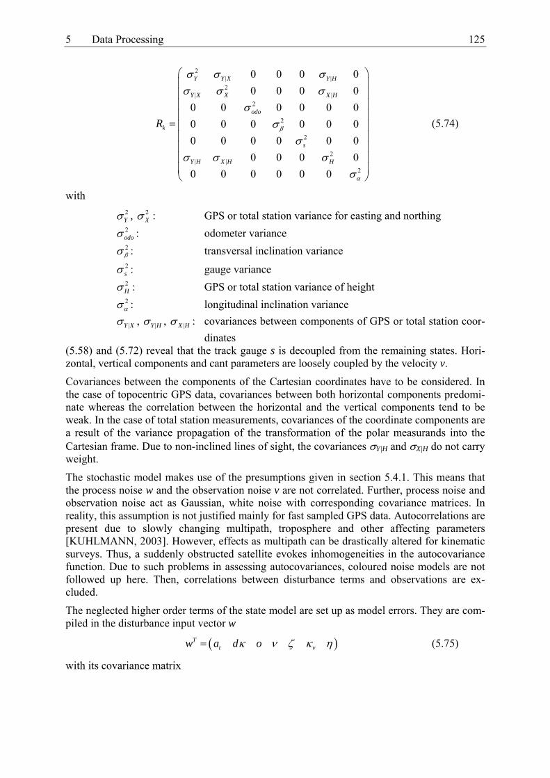
5 Data Processing 125

2| |2

| |2

2

2

2| |

2

0 0 0 00 0 0 0

0 0 0 0 0 00 0 0 0 0 00 0 0 0 0 0

0 0 0 00 0 0 0 0 0

Y Y X Y H

Y X X X H

odo

k

s

Y H X H H

R β

α

σ σ σσ σ σ

σσ

σσ σ σ

σ

⎛ ⎞⎜ ⎟⎜ ⎟⎜ ⎟⎜ ⎟

= ⎜ ⎟⎜ ⎟⎜ ⎟⎜ ⎟⎜ ⎟⎝ ⎠

(5.74)

with 2Yσ , 2

Xσ : GPS or total station variance for easting and northing 2odoσ : odometer variance 2βσ : transversal inclination variance 2sσ : gauge variance 2Hσ : GPS or total station variance of height 2ασ : longitudinal inclination variance

|Y Xσ , |Y Hσ , |X Hσ : covariances between components of GPS or total station coor-dinates

(5.58) and (5.72) reveal that the track gauge s is decoupled from the remaining states. Hori-zontal, vertical components and cant parameters are loosely coupled by the velocity v.

Covariances between the components of the Cartesian coordinates have to be considered. In the case of topocentric GPS data, covariances between both horizontal components predomi-nate whereas the correlation between the horizontal and the vertical components tend to be weak. In the case of total station measurements, covariances of the coordinate components are a result of the variance propagation of the transformation of the polar measurands into the Cartesian frame. Due to non-inclined lines of sight, the covariances σY|H and σX|H do not carry weight.

The stochastic model makes use of the presumptions given in section 5.4.1. This means that the process noise w and the observation noise v are not correlated. Further, process noise and observation noise act as Gaussian, white noise with corresponding covariance matrices. In reality, this assumption is not justified mainly for fast sampled GPS data. Autocorrelations are present due to slowly changing multipath, troposphere and other affecting parameters [KUHLMANN, 2003]. However, effects as multipath can be drastically altered for kinematic surveys. Thus, a suddenly obstructed satellite evokes inhomogeneities in the autocovariance function. Due to such problems in assessing autocovariances, coloured noise models are not followed up here. Then, correlations between disturbance terms and observations are ex-cluded.

The neglected higher order terms of the state model are set up as model errors. They are com-piled in the disturbance input vector w

( )Tt vw a d oκ ν ζ κ η= (5.75)

with its covariance matrix

126 5 Data Processing

2

2

2

2

2

2

2

0 0 0 0 0 00 0 0 0 0 00 0 0 0 0 00 0 0 0 0 00 0 0 0 0 00 0 0 0 0 00 0 0 0 0 0

at

d

k

v

Q

κ

ο

ν

ζ

κ

η

σσ

σσ

σσ

σ

⎛ ⎞⎜ ⎟⎜ ⎟⎜ ⎟⎜ ⎟

= ⎜ ⎟⎜ ⎟⎜ ⎟⎜ ⎟⎜ ⎟⎝ ⎠

(5.76)

with

at: tangential acceleration dκ: normal modified jerk ο: twist rate ν: rate of odometer scale ζ: gauge rate κv: curvature in vertical section η: gradient zero point offset rate

The disturbance input vector compiles deviations from the nominal circular motion with con-stant velocity.

Parameters depending on the track condition are dκ, o, ζ and κv. dκ counts for transition curves and for horizontal track errors. o counts for second derivatives of the cant with respect to the chainage. ζ compensates deviations from the nominal constant track gauge. κv counts for fillets in the vertical section. Deviations from the uniformity of motion are described by at. ν and η model deviations from the trolley model.

In order to emphasise the geometric impact of the normal jerk jn, a modified jerk parameter dκ is used in the w vector:

3njd

vκ = (5.77)

where jn is the normal jerk of section 2.3.2. In the case of a uniform motion, the modified normal jerk corresponds to the curvature rate c in equation (2.16). The factor 3

1v is compen-

sated in the disturbance input matrix Γ.

In contrast to the observation covariance matrix, the magnitudes of the Qk elements are not known a priori. The assessment of the standard deviations has to be done by a tuning step. In the case of track surveying, the trajectory can be reproduced. Filter runs with varying parame-ters of two independent surveys carried out in up and down direction can be compared. An example for filter tuning can be found in section 6.2.2.

The disturbance vector is amplified by the disturbance input matrix. Its elements are obtained by expanding the states to higher order terms.

5 Data Processing 127

2 3 31 1 1

2 3 31 1 1

2

2 2 21 1

11

2 21

1

1

1

21

1 1sin cos 0 0 0 0 02 61 1cos sin 0 0 0 0 02 6

1 0 0 0 0 0 02

0 0 0 0 0 01 1 0 0 0 0 02 2

0 0 0 0 0 010 0 0 0 0 02

0 0 0 0 0 00 0 0 0 0 00 0 0 0 0 0

1 1sin 0 0 0 02 2

k k k

k k k

k k

kk

k

k

k

k

k

t v t

t v t

t

t

t v t

v t

v t

v tv t

v t

t v

τ τ

τ τ

κ

α

− − −

− − −

− −

−−

−

−

−

−

−

Δ Δ

Δ − Δ

Δ

Δ

Δ Δ

ΔΓ =

Δ

ΔΔ

Δ

Δ 2 21 1

1

1

cos 0

0 0 0 0 0 00 0 0 0 0 0

k k

k

k

t

v tv t

α− −

−

−

⎛ ⎞⎜ ⎟⎜ ⎟⎜ ⎟⎜ ⎟⎜ ⎟⎜ ⎟⎜ ⎟⎜ ⎟⎜ ⎟⎜ ⎟⎜ ⎟⎜ ⎟⎜ ⎟⎜ ⎟⎜ ⎟⎜ ⎟⎜ ⎟⎜ ⎟⎜ ⎟⎜ ⎟⎜ ⎟⎜ ⎟Δ⎜ ⎟⎜ ⎟Δ⎜ ⎟⎜ ⎟Δ⎝ ⎠

(5.78)

The absolute model is applied in forward and backward-in-time direction. States and covari-ance matrices have to be stored for each time batch. Then, a smoothed solution can be found by (5.41) resulting in a smoothed state vector and a corresponding covariance matrix for each batch.

The presented matrices own a relatively small number of matrix elements which are nonzero. Sparse matrix operations can be applied to save computational time and memory. Both issues are not very critical since time and memory proportionally increase to the number of time batches. The rmpAnalysis programme does not make use of sparse matrix operations.

5.4.4 Relative Model In many cases, a nominal geometry of the stretch to be surveyed is available. For that case, an additional relative filter model was developed. Instead of the estimation of the absolute posi-tion and the trolley attitude, offsets with respect to a nominal trajectory are estimated. Thus, known systematic portions can be removed previously. Consequently, only displacements from the nominal geometry are filtered. After filtering, the previously removed systematic portions are added to the filtered values. The Remove-Restore method has the advantage of filtering a smoother progression. A more accurate motion model can be set up. Thus, transi-tion curves no longer are compensated by the disturbance terms. For the horizontal compo-nent, azimuthal rates are admitted. This counts for drifting horizontal track errors. Thanks to the introduction of yaw rates in the state vector, the model can be easily expanded in the pres-ence of yaw rate measurements coming from e.g. differential odometry. Due to the removal of the systematic geometric contributions, filter equations become simpler.

128 5 Data Processing

For the evaluation of slew and lift parameters of the most common curves see e.g. [KRASZNAI, 1989]. An algorithm for the slew evaluation for arbitrary curves is given in the appendix A.2.

In the relative model, eleven states are introduced. The state vector is

( )0Tx dh l v d d dn s dv dτ β μ α α′= (5.79)

dh: horizontal displacement from nominal geometry (slew) l: track chainage v: tangential velocity of trolley dτ: residual azimuth of track centre line κ: curvature of track centre line dβ: residual transversal inclination dn′ : residual rate of transversal inclination μ: odometer scale s: track gauge dv: vertical displacement from nominal geometry (lift) dα: residual gradient α0: zero point offset of gradient inclination sensor

For the state propagation, it holds

( )1 1 1 1k k k k k kdh dh d v t tτ− − − −= + − (5.80)

( )1 1 1k k k k kl l v t t− − −= + − (5.81)

1k kv v −= (5.82)

1k kd dτ τ −= (5.83)

( )1 1 1 1k k k k k kd d dn v t tβ β − − − −′= + − (5.84)

1k kdn dn −′ ′= (5.85)

1k kμ μ −= (5.86)

1k ks s −= (5.87)

( )1 1 1 1k k k k k kdv dv d v t tα− − − −= + − (5.88)

1k kd dα α −= (5.89)

0/ 0 / 1k kα α −= (5.90)

The linearisation of the state equations yields the transition matrix:

5 Data Processing 129

1 1

1 1

1

1 1

1 0 0 0 0 0 0 0 00 1 0 0 0 0 0 0 0 00 0 1 0 0 0 0 0 0 0 00 0 0 1 0 0 0 0 0 0 00 0 0 1 0 0 0 0 00 0 0 0 0 1 0 0 0 0 00 0 0 0 0 0 1 0 0 0 00 0 0 0 0 0 0 1 0 0 00 0 0 0 0 0 0 1 00 0 0 0 0 0 0 0 0 1 00 0 0 0 0 0 0 0 0 0 1

k k

k k

k

k k

d t v tt

dn t v t

d t v t

τ

α

− −

− −

−

− −

Δ Δ⎛ ⎞⎜ ⎟Δ⎜ ⎟⎜ ⎟⎜ ⎟⎜ ⎟⎜ ⎟′ Δ Δ⎜ ⎟

Φ = ⎜ ⎟⎜ ⎟⎜ ⎟⎜ ⎟⎜ ⎟Δ Δ⎜ ⎟⎜ ⎟⎜ ⎟⎝ ⎠

(5.91)

The observations are compiled in the observation vector

( )TPos Pos Odometer Inclinometer Gauge Pos Inclinometerz dh l l s dvβ α= (5.92)

Except for the odometers and the gradients, the observations correspond to the filter states. For the odometers, the following non-linear relation holds

( )/ 0 0 /odo k k k odo kl l l l vμ= + − + (5.93)

Gradient observations with an additional bias yield

/ 0/ /Inclinometer k k k kd d vαα α α= − + (5.94)

The observation matrix results from the linearisation of the observation equations with respect to the parameters of the state vector:

0

1 0 0 0 0 0 0 0 0 0 00 1 0 0 0 0 0 0 0 0 00 0 0 0 0 0 0 0 00 0 0 0 1 0 0 0 0 0 00 0 0 0 0 0 0 1 0 0 00 0 0 0 0 0 0 0 1 0 10 0 0 0 0 0 0 0 0 1 1

k k

k

l lH

μ

⎛ ⎞⎜ ⎟⎜ ⎟⎜ ⎟−⎜ ⎟

= ⎜ ⎟⎜ ⎟⎜ ⎟⎜ ⎟⎜ ⎟−⎝ ⎠

(5.95)

The measurement covariance matrix is

2| |

2| |

2

2

2

2| |

2

0 0 0 0

0 0 0 0

0 0 0 0 0 00 0 0 0 0 00 0 0 0 0 0

0 0 0 0

0 0 0 0 0 0

Pos Pos Pos Pos Pos

Pos Pos Pos Pos Pos

Pos Pos Pos Pos Pos

dh dh l dh dv

dh l l l dv

odo

k

s

dh dv l dv dv

Rβ

α

σ σ σ

σ σ σ

σσ

σσ σ σ

σ

⎛ ⎞⎜ ⎟⎜ ⎟⎜ ⎟⎜ ⎟⎜ ⎟=⎜ ⎟⎜ ⎟⎜ ⎟⎜ ⎟⎜ ⎟⎝ ⎠

(5.96)

130 5 Data Processing

2Posdhσ , 2

Poslσ and 2Posdvσ correspond to the GPS or the optical total station precision for the hori-

zontal and the vertical component, respectively. Between the components, covariances ac-cording to (5.74) are introduced. The remarks considering the covariance information of the absolute model also hold for the relative model. In addition, if the alignment principle is fol-lowed for total station measurements, dhPos and lPos are almost decorrelated. The remaining variances in (5.96) are in accordance with the measurement covariance matrix (5.74).

Concerning the stochastic properties of the relative model, the stipulation of section 5.4.1 can be adapted. Equivalent to the absolute model a disturbance vector is set up:

( )Tt vw a d o dκ ν ζ κ η= (5.97)

Its covariance matrix is

2

2

2

2

2

2

2

0 0 0 0 0 00 0 0 0 0 00 0 0 0 0 00 0 0 0 0 00 0 0 0 0 00 0 0 0 0 00 0 0 0 0 0

at

d

k

d v

Q

κ

ο

ν

ζ

κ

η

σσ

σσ

σσ

σ

⎛ ⎞⎜ ⎟⎜ ⎟⎜ ⎟⎜ ⎟

= ⎜ ⎟⎜ ⎟⎜ ⎟⎜ ⎟⎜ ⎟⎝ ⎠

(5.98)

with

at: tangential acceleration dκ: curvature rate ο: second derivative of differential cant ν: rate of odometer scale ζ: gauge rate dκv: curvature rate in vertical section η: gradient zero point offset rate

and the disturbance input matrix

5 Data Processing 131

2 2 21 1

21

1

2 21

1

1

1

1

2 2 21 1

1

1

1 1 0 0 0 0 02 21 0 0 0 0 0 02

0 0 0 0 0 00 0 0 0 0 0

10 0 0 0 0 02

0 0 0 0 0 00 0 0 0 0 00 0 0 0 0 0

1 10 0 0 0 02 2

0 0 0 0 0 00 0 0 0 0 0

k k

k

k

kk

k

k

k

k k

k

k

d t v t

d t

tv t

v t

v tv t

v t

d t v t

v tv t

τ

τ

α

− −

−

−

−−

−

−

−

− −

−

−

⎛ ⎞Δ Δ⎜ ⎟⎜ ⎟⎜ ⎟Δ⎜ ⎟⎜ ⎟Δ⎜ ⎟⎜ ⎟Δ⎜ ⎟⎜ ⎟Δ⎜Γ =⎜ Δ⎜⎜ Δ⎜ Δ⎜⎜

Δ Δ⎜⎜

Δ⎜⎜ Δ⎝ ⎠

⎟⎟⎟⎟⎟⎟⎟⎟⎟⎟⎟

(5.99)

In contrast to the absolute model, eleven state parameters suffice for an adequate description of the trolley motion. This results in a reliability gain. Further, almost linear state transition and observation equations are obtained. In general, the relative model should converge more rapidly than the absolute model. Thus, whenever a nominal geometry of a track is available, the relative model is to be applied for trajectory smoothing.

5.5 Smoothing Splines

5.5.1 Smoothing Splines with First Derivatives An interesting alternative to trajectory smoothing by means of a Kalman filter, represents the use of smoothing cubic splines. Cubic splines have the property, that curvatures along the whole trajectory are minimised which is equivalent to a minimisation of the deformation en-ergy. In turn, this roughly corresponds to the rail situation. In contrary to the classical interpo-lation splines [e.g. GEIGER, 2004], which exactly contain the base points, smoothing splines, admit residuals [REINSCH, 1967; DE BOOR, 2001]. Thus, they are appropriate for the ap-proximation of a trajectory by uncertain measurements.

Here, a variety is presented where derivatives of the trajectory can be incorporated as meas-urements. For n base points with corresponding first derivatives, n-1 cubic parabolas are con-sidered:

( ) ( ) ( )3 2k k k k k k k ky A x x B x x C x x D= − + − + − + (5.100)

If a fixed interval [xk, xk+1] is regarded, we find for the function, its first and second derivative in the edge points

132 5 Data Processing

3 21

21

1

3 2

26 2

k k

k k k k k k k k

k k

k k k k k k

k k

k k k k k

y D

y A x B x C x D

y C

y A x B x C

y By A x B x

+

+

+

=

= Δ + Δ + Δ +

′ =

′ = Δ + Δ +

′′ =′′ = Δ + Δ (5.101)

For the sought coefficients as a function of y and y′ , we obtain

( ) ( )

( ) ( )

1 12 3

1 12

1 2

1 32

k k k k kk k

k k k k kk k

k k

k k

A y y y yx x

B y y y yx x

C yD y

+ +

+ +

′ ′= + − +Δ Δ

′ ′= − + −Δ Δ′=

= (5.102)

The stipulation on continuity of the second derivative

1( ) ( ) ( 2, , 1)k k k ky x y x k n−′′ ′′= = −… (5.103)

renders the coupling condition

1 1 1 16 2 2k k k k kA x B x B− − − −Δ + Δ = (5.104)

Inserting (5.102) in (5.104) yields

1 1 1 12 2 2 21 1 1 1

3 3 3 3 1 4 2 1 0k k k k k kk k k k k k k k

y y y y y yx x x x x x x x− + − +

− − − −

⎛ ⎞ ⎛ ⎞′ ′ ′+ − + − + + + − =⎜ ⎟ ⎜ ⎟Δ Δ Δ Δ Δ Δ Δ Δ⎝ ⎠ ⎝ ⎠

(5.105)

These are n-2 condition equations for the observations 1 1 1 1, , , , ,k k k k k ky y y y y y− + − +′ ′ ′ . (5.105) is a linear system of the form

0Ay = (5.106)

with

2 2 2 2

1 1 1 1

3 3 3 3 1 4 2 1

k k k k k k k k

Ax x x x x x x x− − − −

= + +Δ Δ Δ Δ Δ Δ Δ Δ

⎛ ⎞⎜ ⎟⎜ ⎟− − −⎜ ⎟⎜ ⎟⎜ ⎟⎝ ⎠

… … … … … … … …

… … …

… … … … … … … …

(5.107)

( )1 1 1 1T

k k k k k ky y y y y y y− + − +′ ′ ′= … … … (5.108)

For noisy base points and derivatives, y is set to y:= y + v in (5.106). It results

Ay w− = (5.109)

with

5 Data Processing 133

w Av= (5.110)

The vector v under consideration of the side condition (5.109) has to be minimised in the least-squares sense. For the Lagrangeian vector k, one finds [SCHMID, 1977]

( ) 11 Tllk AP A w

−−= (5.111)

An (n-2)·(n-2) matrix has to be inverted. This corresponds to the number of knots incorpo-rated into the adjustment. The residual vector is

1 Tllv P A k−= (5.112)

llP denominates the weight matrix of the observations ,k ky y′ .

By means of the residuals and the observations, the adjusted observations can be computed straightforward. The spline coefficients are obtained by (5.102).

5.5.2 Comparison between Kalman Filter and Smoothing Splines Kalman filtering outmatches smoothing splines in terms of computational efficiency. The complexity of a Kalman filter including backward filtering and smoothing is proportional to the number of time batches. The smoothing splines approach leads to a least-squares problem with a (n-2)·(n-2) normal matrix. The involved matrix multiplications and the matrix inver-sion leads to a complexity of O(k·n3) where k is about 3 using conventional Gauss elimination for matrix inversion. A comparable Kalman filter using a state and its derivative as model parameters and observations requires O(l·n) operations where l is about 176. A comparison concerning computational complexity for this example can be found in Figure 5-10. It is evi-dent that the smoothing splines approach is inferior in terms of computational complexity even for less than 10 time batches.

Similar deficiencies can be perceived for the memory usage of smoothing splines. The mem-ory needed quadratically increases with the number of time batches. Except of the observation variance matrix all matrices are fully populated. In contrast to the Kalman filter approach, sparse techniques cannot be applied.

On the other hand, the proposed smoothing spline algorithm is easy to implement. Thank to its descriptive characteristics, no assumptions regarding the kinematic model have to be made. The stochastic model just incorporates the weighting of the observations and their derivatives. If only observations are present, then the smoothing splines have to be tuned by a smoothing parameter λ.

In conclusion, smoothing splines can be an alternative for short stretches as they can occur for deformation networks on construction sites.

134 5 Data Processing

0 10 20 30 40 50 60 70 80 90 10010

0

102

104

106

108

Batches []

Com

plex

ity []

Kalman Filter / SmootherSplines with Derivatives

Figure 5-10 Computational complexity of Kalman filter / smoother and splines with deriva-tives

5.6 Merging Trajectories

5.6.1 Strategies for Merging The typical workflow of a kinematic track survey contains several track runs with overlapping sections. For accuracy reasons, a stretch is often surveyed in forward and backward direction. Due to random errors, incomplete models and remaining systematic biases, the smoothed tra-jectories do not coincide in the overlapping zones. Subsequently, an algorithm is given for adjusting such inconsistencies. The proposed algorithm can be applied to data acquired just in one direction or to forward and backward runs. In the former case, a smooth as possible pro-gression is aimed for. In the latter case, remaining systematic biases are estimated and a weighted mean between the involved trajectories is evaluated. The merge step requires state vectors and corresponding variances of the filter/smoother step. Thus, sections with GPS am-biguity fix losses can be improved by incorporating the corresponding run in the opposite direction. Gap completion of a GPS run by Swiss Trolley total station measurements is an-other frequent merge strategy.

5.6.2 Chaining the Pieces If data of several runs are to be merged, they have to be linked first to a common chainage axis. The relative model already provides smoothed data runs that can be compared by the chainage. In contrast, the chainage provided by the absolute smoother model is arbitrary and is not consistent for different runs. Subsequently, an algorithm is presented which allows for chaining all incorporated runs of an absolute model survey. Figure 5-11 outlines a typical situation encountered for absolute surveys. A certain number of runs are carried out. Each run is referenced to its own chainage frame lk. The individual chainages have to be shifted with respect to an arbitrary selected run in order to obtain a unique chainage frame where the dif-ferences between the parameters of interest can be compared.

5 Data Processing 135

Figure 5-11 Chaining the smoothed series

Consider now n runs to be chained. An arbitrary run is selected and assigned to a still empty list of chained series. This arbitrary run defines the chainage axis. The remaining n-1 runs are linked to the chained series as follows:

By means of the tangent vectors 00,t i

e and 00, 1t i

e+

, the criterion (A.13) of the appendix A.2 can

be applied to decide whether a data point , k

kh i

R of a neighbouring series lays within the sector

spanned by the perpendiculars to 00,t i

e and 00, 1t i

e+

. , k

kh i

R is the horizontal component of the posi-

tion vector of the ki -th data point of the kth run. The criterion (A.13) only holds for continuous curves. In the present case, continuity is given within the filter uncertainty of the azimuth state transition. The tangent vectors

0

0

ite and

0 1

0

ite

+ can be easily obtained by

0

0

0

00

0,

sincos

it i

i

eττ

⎛ ⎞= ⎜ ⎟⎜ ⎟

⎝ ⎠ (5.113)

and

0

0

0

00 1

0, 11

sincos

it i

i

eττ

++

+

⎛ ⎞= ⎜ ⎟⎜ ⎟

⎝ ⎠ (5.114)

where 00i

τ and 00

1iτ

+ are the adjacent azimuths of the first arbitrary selected filtered run.

As a further criterion, the length of the plumb line to the chord of two adjacent points is checked. The length of the plumb line has to coincide within the measurement uncertainty. An additional criterion checks the special case for helical tunnels. Height differences between a possible candidate and the base series may not exceed a certain amount. If all three criteria are fulfilled, the selected series is shifted by the chainage difference.

The strategy of how to link an arbitrary series with a list of chained series is sketched in detail in Figure 5-12.

( )00 0,h i

R l

( ), kk kh i

R l

( )11 1

, kk kh i

R l++ +

136 5 Data Processing

Select first point of series to chain; repeat Select first chained series; repeat Select first two tangents of selected chained series; repeat PointFound:= ((condition (A.13) = true) and (slew < MAX_SLEW)) and (DH < MAX_DH); Select next two tangents of chained series; until PointFound or (no potential tangents left) ; Select next chained series; until PointFound or (Maximum number of chained series reached) select next point of series to chain; until PointFound or (no potential points left);

Figure 5-12 Algorithm for chaining trajectories of different runs

In order to accelerate the algorithm, binary search strategies are used for the selection of the base series tangents and to select candidates

, kkh i

R . Typical thresholds for MAX_SLEW and MAX_DH for a GPS survey are 2.5 cm and 7.5 cm, respectively.

If a series can be assigned by the above algorithm, then the chainage of the assigned series is shifted by

( )0:k k kF Fl l l l= + − (5.115)

0Fl and k

Fl are the chainages of the base point of the found candidate expressed in the final chainage frame and the individual chainage frame, respectively. As a next step, the corrected series is added to the list of chained series. This procedure is repeated until all series are chained with respect to the initial run. It can occur that no connection is possible between two individual series due to survey gaps. In that case, a new chainage frame is defined for the re-spective series and its eventual successors.

5.6.3 Merging Once all data are referenced to a coherent chainage frame, parameters can be averaged and accuracies can be evaluated. For measurements carried out only in forward direction, as smooth as possible transitions between subsequent runs are sought. Linear interpolation of the differences between both curves fulfils this requirement as a first approximation. For meas-urements in forward and backward direction, remaining systematic biases can be eliminated by averaging. Instead of an interpolation, a weighted mean between both curves provides re-sults that are more representative.

For the merge process, track parameters are considered as a function of the chainage. The chainage is supposed to be free of errors. Then, the software accounts for overlapping sections and evaluates the averaged track parameters. A particular parameter i

ly of the state vector ilx

of the i-th trajectory at chainage l is compared with an interpolated track parameter jly of an

adjacent trajectory j (Figure 5-13). State transition here is assumed to be linear. Thus, the merge step does not need any deterministic information from the filter/smoother step.

5 Data Processing 137

Figure 5-13 Merging of two curves: linear interpolation in overlapping section

For a linear interpolation of the track parameter jly , a linear decay within the overlapping

section and a weighted mean between two parameters at chainage l, it holds

mly W L D y= ⋅ ⋅ ⋅ (5.116)

1

ilj

kj

k

yy y

y−

⎛ ⎞⎜ ⎟

= ⎜ ⎟⎜ ⎟⎝ ⎠

(5.117)

1

1 1

1 0 0

0 k k

k k k k

D l l l ll l l l

−

− −

⎛ ⎞⎜ ⎟= − −⎜ ⎟⎜ ⎟− −⎝ ⎠

(5.118)

, ,

,

,

,

0

0

i j i jl

i j

i jli j

dl dldlL

dldl

⎛ ⎞−⎜ ⎟⎜ ⎟=⎜ ⎟⎜ ⎟⎝ ⎠

(5.119)

2 2

2 2 2 2

j il l

i j i jl ll l

y y

y yy y

Wσ σ

σ σ σ σ

⎛ ⎞⎜ ⎟=⎜ ⎟+ +⎝ ⎠

(5.120)

with the variance

m m

T T Ty y yyC W L D C D L W= ⋅ ⋅ ⋅ ⋅ ⋅ ⋅ (5.121)

where

1 1

1

2

2

2

0 0

0

0

il

j j jk k k

j j jk k k

y

yy y y y

y y y

C

σ

σ σ

σ σ− −

−

⎛ ⎞⎜ ⎟⎜ ⎟=⎜ ⎟⎜ ⎟⎝ ⎠

(5.122)

0.0 10.0 20.0 30.0 40.0 50.0 60.0 70.0 80.0 90.0 100.00.0360

0.0370

0.0380

0.0390

0.0400

0.0410

Chainage [m]

Cant

[m]

ily

jly

1j

ky −

jky

mly

,i jdl

,i jldl

138 5 Data Processing

mly is the averaged track parameter of the merged series (easting, northing, slew, cant, twist,

etc.) at chainage l. As input data, the track parameters ily , j

ky and 1j

ky − with their correspond-ing covariance information are required. The interpolation matrix D yields the interpolated track parameter j

ly . Then, L distributes the inconsistencies between the trajectories i and j proportionally to the progression ,i j

ldl within the overlapping section ,i jdl . Finally, the weight matrix W counts for the variances coming from the individual smoother solutions.

A difficulty consists in the evaluation of the variance 2j

lyσ for the trajectory j at chainage l

since the two track parameters 1j

ky − and jky are highly correlated. Here, the covariance propa-

gation between two adjacent smoother states is evaluated. For this, consider

1 1

1 1 1

0k k

k k k k

x E xx w

− −

− − −

⎛ ⎞ ⎛ ⎞ ⎛ ⎞= ⋅⎜ ⎟ ⎜ ⎟ ⎜ ⎟Φ Γ⎝ ⎠ ⎝ ⎠ ⎝ ⎠

(5.123)

with the associated covariance matrix

11

1

00k

kk

PC

Q−

−−

⎛ ⎞= ⎜ ⎟

⎝ ⎠ (5.124)

Then, the variance propagation of (5.123) yields

1 1 11|

1 1 1 1 1 1 1 1

Tk k k

k k T Tk k k k k k k k

P PC

P P Q− − −

−− − − − − − − −

⎛ ⎞⋅Φ= ⎜ ⎟

Φ ⋅ Φ ⋅ ⋅Φ + Γ ⋅ ⋅Γ⎝ ⎠ (5.125)

Ck-1|k contains the covariance matrices of the epochs k and k-1. The covariance matrices are in correspondence with the Kalman filter scheme given in Figure 5-8. In addition, (5.125) con-tains covariance information between the two epochs k and k-1. In order to study the decay of correlation between two adjacent states, correlation coefficients derived from (5.125) for a particular run were studied. The survey features a run on a straight line towards north with a velocity of 1 m/s. Figure 5-14 shows correlation coefficients for selected track parameters as a function of the covered chainage. Apart of the time (or chainage) dependency, there is an in-fluence of the dynamics of the individual parameters. If more stochastic uncertainty is admit-ted, the correlation decays faster. Here, this is the case for the northing component mainly depending on the uncertainty of the translatory acceleration for this specific run. Further, the correlation of higher order modelled parameters decays faster.

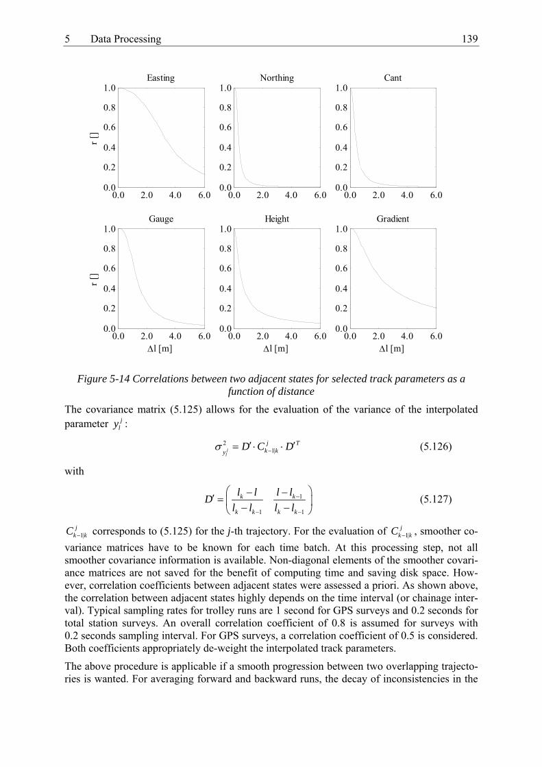
5 Data Processing 139

0.0 2.0 4.0 6.00.0

0.2

0.4

0.6

0.8

1.0Easting

r []

0.0 2.0 4.0 6.00.0

0.2

0.4

0.6

0.8

1.0Northing

0.0 2.0 4.0 6.00.0

0.2

0.4

0.6

0.8

1.0Cant

0.0 2.0 4.0 6.00.0

0.2

0.4

0.6

0.8

1.0Gauge

Δl [m]

r []

0.0 2.0 4.0 6.00.0

0.2

0.4

0.6

0.8

1.0Height

Δl [m]0.0 2.0 4.0 6.0

0.0

0.2

0.4

0.6

0.8

1.0Gradient

Δl [m]

Figure 5-14 Correlations between two adjacent states for selected track parameters as a function of distance

The covariance matrix (5.125) allows for the evaluation of the variance of the interpolated parameter j

ly :

21|j

l

j Tk ky

D C Dσ −′ ′= ⋅ ⋅ (5.126)

with

1

1 1

k k

k k k k

l l l lDl l l l

−

− −

⎛ ⎞− −′ = ⎜ ⎟− −⎝ ⎠ (5.127)

1|j

k kC − corresponds to (5.125) for the j-th trajectory. For the evaluation of 1|j

k kC − , smoother co-variance matrices have to be known for each time batch. At this processing step, not all smoother covariance information is available. Non-diagonal elements of the smoother covari-ance matrices are not saved for the benefit of computing time and saving disk space. How-ever, correlation coefficients between adjacent states were assessed a priori. As shown above, the correlation between adjacent states highly depends on the time interval (or chainage inter-val). Typical sampling rates for trolley runs are 1 second for GPS surveys and 0.2 seconds for total station surveys. An overall correlation coefficient of 0.8 is assumed for surveys with 0.2 seconds sampling interval. For GPS surveys, a correlation coefficient of 0.5 is considered. Both coefficients appropriately de-weight the interpolated track parameters.

The above procedure is applicable if a smooth progression between two overlapping trajecto-ries is wanted. For averaging forward and backward runs, the decay of inconsistencies in the

140 5 Data Processing

overlapping section is not required (Figure 5-15). Thus, the linear propagator L in (5.116) can be dropped:

mly W D y= ⋅ ⋅ (5.128)

Figure 5-15 Merging of two curves: weighted average

A special treatment requires sections with only one run for the forward-backward case since a remaining bias is not known a priori. In this case, the biases for each data channel are evalu-ated first. In a subsequent step, a mean bias is applied to sections surveyed in only one direc-tion. At transitions from double runs to single runs, inconsistencies can emerge. However, for questions of reliability, a complete coverage in forward and backward direction is aimed for.

5.6.4 Linking Scans to Merged Trajectories Like stated in 4.10.2, laser scanner vectors are linked to the trajectory by correlating time tags. However, time tags become useless for merged series. Consequently, they are dropped. In order to link laser scan vectors associated with a particular run of a merged series, chainages are evaluated for each laser pixel in the consistent chainage frame after the chaining step. Thus, laser scan vectors can be linked to the improved merged series by the use of the chain-age information after the merge step.

0.0 10.0 20.0 30.0 40.0 50.0 60.0 70.0 80.0 90.0 100.00.0360

0.0370

0.0380

0.0390

0.0400

0.0410

Chainage [m]

Cant

[m]

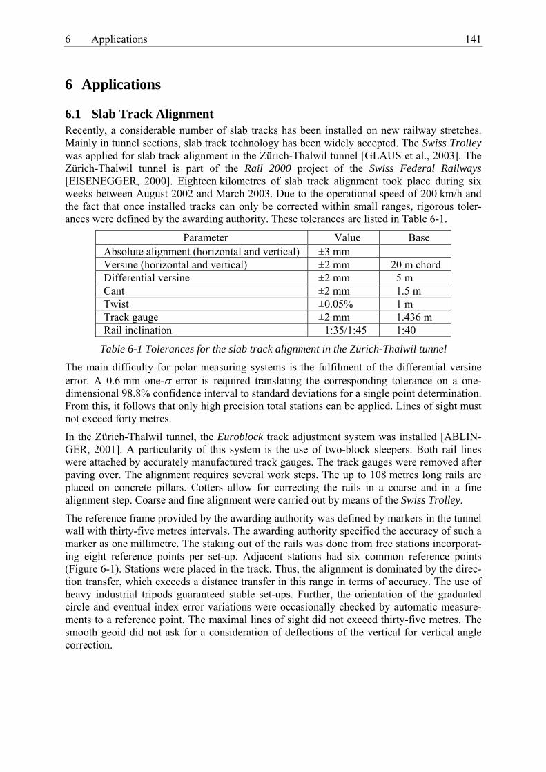
6 Applications 141

6 Applications

6.1 Slab Track Alignment Recently, a considerable number of slab tracks has been installed on new railway stretches. Mainly in tunnel sections, slab track technology has been widely accepted. The Swiss Trolley was applied for slab track alignment in the Zürich-Thalwil tunnel [GLAUS et al., 2003]. The Zürich-Thalwil tunnel is part of the Rail 2000 project of the Swiss Federal Railways [EISENEGGER, 2000]. Eighteen kilometres of slab track alignment took place during six weeks between August 2002 and March 2003. Due to the operational speed of 200 km/h and the fact that once installed tracks can only be corrected within small ranges, rigorous toler-ances were defined by the awarding authority. These tolerances are listed in Table 6-1.

Parameter Value Base Absolute alignment (horizontal and vertical) ±3 mm Versine (horizontal and vertical) ±2 mm 20 m chord Differential versine ±2 mm 5 m Cant ±2 mm 1.5 m Twist ±0.05% 1 m Track gauge ±2 mm 1.436 m Rail inclination 1:35/1:45 1:40

Table 6-1 Tolerances for the slab track alignment in the Zürich-Thalwil tunnel

The main difficulty for polar measuring systems is the fulfilment of the differential versine error. A 0.6 mm one-σ error is required translating the corresponding tolerance on a one-dimensional 98.8% confidence interval to standard deviations for a single point determination. From this, it follows that only high precision total stations can be applied. Lines of sight must not exceed forty metres.

In the Zürich-Thalwil tunnel, the Euroblock track adjustment system was installed [ABLIN-GER, 2001]. A particularity of this system is the use of two-block sleepers. Both rail lines were attached by accurately manufactured track gauges. The track gauges were removed after paving over. The alignment requires several work steps. The up to 108 metres long rails are placed on concrete pillars. Cotters allow for correcting the rails in a coarse and in a fine alignment step. Coarse and fine alignment were carried out by means of the Swiss Trolley.

The reference frame provided by the awarding authority was defined by markers in the tunnel wall with thirty-five metres intervals. The awarding authority specified the accuracy of such a marker as one millimetre. The staking out of the rails was done from free stations incorporat-ing eight reference points per set-up. Adjacent stations had six common reference points (Figure 6-1). Stations were placed in the track. Thus, the alignment is dominated by the direc-tion transfer, which exceeds a distance transfer in this range in terms of accuracy. The use of heavy industrial tripods guaranteed stable set-ups. Further, the orientation of the graduated circle and eventual index error variations were occasionally checked by automatic measure-ments to a reference point. The maximal lines of sight did not exceed thirty-five metres. The smooth geoid did not ask for a consideration of deflections of the vertical for vertical angle correction.

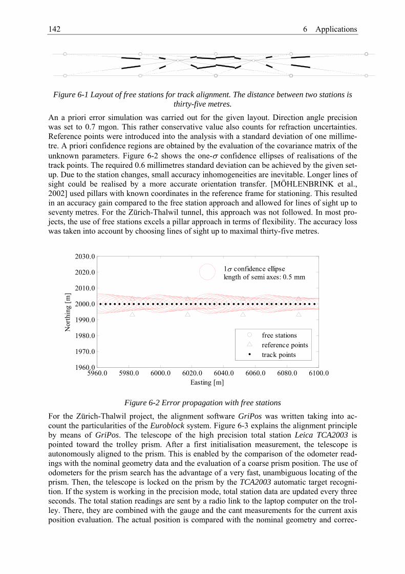
142 6 Applications

Figure 6-1 Layout of free stations for track alignment. The distance between two stations is thirty-five metres.

An a priori error simulation was carried out for the given layout. Direction angle precision was set to 0.7 mgon. This rather conservative value also counts for refraction uncertainties. Reference points were introduced into the analysis with a standard deviation of one millime-tre. A priori confidence regions are obtained by the evaluation of the covariance matrix of the unknown parameters. Figure 6-2 shows the one-σ confidence ellipses of realisations of the track points. The required 0.6 millimetres standard deviation can be achieved by the given set-up. Due to the station changes, small accuracy inhomogeneities are inevitable. Longer lines of sight could be realised by a more accurate orientation transfer. [MÖHLENBRINK et al., 2002] used pillars with known coordinates in the reference frame for stationing. This resulted in an accuracy gain compared to the free station approach and allowed for lines of sight up to seventy metres. For the Zürich-Thalwil tunnel, this approach was not followed. In most pro-jects, the use of free stations excels a pillar approach in terms of flexibility. The accuracy loss was taken into account by choosing lines of sight up to maximal thirty-five metres.

5960.0 5980.0 6000.0 6020.0 6040.0 6060.0 6080.0 6100.01960.0

1970.0

1980.0

1990.0

2000.0

2010.0

2020.0

2030.0

1σ confidence ellipselength of semi axes: 0.5 mm

Easting [m]

Nor

thin

g [m

]

free stationsreference pointstrack points

Figure 6-2 Error propagation with free stations

For the Zürich-Thalwil project, the alignment software GriPos was written taking into ac-count the particularities of the Euroblock system. Figure 6-3 explains the alignment principle by means of GriPos. The telescope of the high precision total station Leica TCA2003 is pointed toward the trolley prism. After a first initialisation measurement, the telescope is autonomously aligned to the prism. This is enabled by the comparison of the odometer read-ings with the nominal geometry data and the evaluation of a coarse prism position. The use of odometers for the prism search has the advantage of a very fast, unambiguous locating of the prism. Then, the telescope is locked on the prism by the TCA2003 automatic target recogni-tion. If the system is working in the precision mode, total station data are updated every three seconds. The total station readings are sent by a radio link to the laptop computer on the trol-ley. There, they are combined with the gauge and the cant measurements for the current axis position evaluation. The actual position is compared with the nominal geometry and correc-

6 Applications 143

tion parameters are derived. The displacements are shown on the laptop display and can be used for the rail correction. For the Euroblock system, the nominal rail inclination has to be adjusted. The alignment software evaluates inclinations for both rails as a function of the cant. The rail inclinations are adjusted by electronic spirit levels.

Figure 6-3 Principle of the track alignment

Figure 6-4 gives an impression of the alignment. A Leica TCRA1101 total station was used for the coarse alignment. Two operators aligned the rails according to the displacement given by the Swiss Trolley. A surveyor was responsible for the establishment of the free stations.

Figure 6-4 TCRA1101 on an industrial tripod used for the coarse alignment in interaction

with the Swiss Trolley

Alignment software GriPos

Nominal geometry

Calibration data

Trolley

TCA2003

Odometer Gauge, cant

τ0, z0

τ, z, d, 2003TCAX

144 6 Applications

After paving over, a Swiss Trolley run for quality control took place. Every five metres, a static measurement was carried out. Histograms of the residuals of a three kilometres long stretch are shown in Figure 6-5 for the relative slew, the relative lift, the cant and the gauge component. Nine hundred samples are considered here. Non-biased normal distributed histo-grams are found for the horizontal and the vertical component. The root mean square errors for both components are 0.8 mm and 0.6 mm, respectively. An explanation for the better ver-tical accuracy gives [DÜNISCH et al., 2001]. Track stability in the vertical direction is higher than for the horizontal component. Extraneous impacts on the construction sites mainly affect the horizontal component. The cant component shows a slightly biased distribution. This can most likely be attributed to an alternating zero point offset. For completeness, the track gauge histogram is given here. The alignment process had no influence on the track gauge quality due to the predefined constant distance between both rails. It will be shown subsequently that typical Swiss Trolley precisions for track gauge determination are better than 0.5 mm. The obtained accuracies by the Swiss Trolley fulfil the given tolerances. Notice that for the slew and lift components relative displacements are given. [DÜNISCH et al., 2001] report slightly better accuracies for the slab track alignment on the Frankfurt-Cologne stretch. There, the specialised Hergie slab track trolley (section 2.5.4.4) was used for the alignment.

-5.0 0.0 5.0 0.0

10.0

20.0

30.0

40.0

Differential slewσ = 0.8 mm, rms = 0.8 mm

Displacement [mm]

Freq

uenc

y [%

]

-5.0 0.0 5.0 0.0

10.0

20.0

30.0

40.0

Differential liftσ = 0.6 mm, rms = 0.6 mm

Displacement [mm]

Freq

uenc

y [%

]

-5.0 0.0 5.0 0.0

10.0

20.0

30.0

Cantσ = 0.7 mm, rms = 0.9 mm

Displacement [mm]

Freq

uenc

y [%

]

-5.0 0.0 5.0 0.0

10.0

20.0

30.0

Gaugeσ = 0.9 mm, rms = 0.9 mm

Displacement [mm]

Freq

uenc

y [%

]

Figure 6-5 Histograms of differential slew, differential lift, cant error and gauge error after

paving over

As an additional quality control measure, the Swiss Federal Railways carried out several track recording coach runs. The track recording coach runs allow for the verification of relative track geometry parameters. A qualitative record is given in Figure 6-6. The transition between ballast track and slab track is clearly seen at chainage 850 m. Noisy curves of the recorded parameters level off to a smooth progression after the transition to the slab track.

6 Applications 145

Figure 6-6 Qualitative record of track recording coach run [SBB, 2003]

Slab track alignment requires a perfect team play with the other contractors on the site. The workflow must not be interrupted by delays coming from the alignment. On the other hand, the alignment has to take place directly before paving over with concrete. Otherwise, the probability of rail displacements due to exterior impacts increases. The given shift perform-ance of 250 metres of coarse and fine alignment could easily be fulfilled by the surveyors.

6.2 Kinematic Track Axis Surveys Section 5.4 introduces Kalman filtering and smoothing for kinematically acquired data. This subsection gives reasons for the use of the presented non-causal smoother by means of several examples. In order to emphasise the generality of the developed smoother, GPS and total sta-tion data acquired on track of different grades of quality are discussed.

6.2.1 Comparison between Forward Filter, Backward Filter and Smoother For post-mission data, a non-causal filtering of data is possible (section 5.4.2). In Figure 6-7, the cant and the twist estimated by the forward filter, the backward filter and the smoother are compared on a section containing a clothoid and consequently a cant ramp with inherent twist values differing from zero. Clearly, the causality of the forward filter introduces a shift in chainage direction. This shift appears in the opposite direction by the backward filter. The smoother eliminates these lags because this procedure uses all measurements in order to com-pute the estimated state at each time.

Track gauge

Curvature

Cant

Evenness of contact area

Twist

Vertical curvature

left rail

left rail

right rail

right rail

Ballast Slab track

0 500 1000 1500 Chainage [m]

146 6 Applications

0.0 50.0 100.0 150.0 200.0 250.0 300.0 350.0 400.0 450.0 500.0

0.0

20.0

40.0

60.0

Chainage [m]

Cant

[mm

]nominalforwardbackwardsmoothed

0.0 50.0 100.0 150.0 200.0 250.0 300.0 350.0 400.0 450.0 500.0-2.0

-1.0

0.0

1.0

2.0

Chainage [m]

Twist

[mm

/m]

forwardbackwardsmoothed

Figure 6-7 Forward filtered, backward filtered and smoothed cant and twist

6.2.2 Filter Tuning For the assessment of the Rk-1 matrix, the precisions of the involved sensors have to be known a priori. The orders of magnitudes are known from the manufacturers’ specifications. In addi-tion, the static error behaviour of the involved sensor was partly shown in section 6.1. The values of the sensors used on the trolley are listed in Table 6-2.

Parameter σ Unit Remark σY, σX 8.0 mm GPS horizontal component, fixed ambiguities σY, σX 5.0 m GPS horizontal component, floating ambiguities σY, σX 30.0 m GPS horizontal component, single point solution σY, σX 5.0 mm Optical total station, horizontal component σodo 10.0 mm Odometer σβ 1.0 mrad Cant σs 0.5 mm Track gauge σH 20.0 mm GPS vertical component, fixed ambiguities σH 15.0 m GPS vertical component, floating ambiguities σH 150.0 m GPS vertical component, fixed ambiguities σH 5.0 mm Optical total station, vertical component σα 5.0 mrad Gradients

Table 6-2 Used values for weighting observations

6 Applications 147

For GPS observations, the GDOP value is not considered for refining the weighting. How-ever, GPS observations exceeding a DOP value of eight are de-weighted.

The definition of the covariance matrix Qk-1 describing the uncertainty of the disturbance in-put terms is more delicate. In general, the process noise has to be set up very carefully. For questions of track axis determination, the track errors deviating from a nominal track design are of interest and must not be filtered. In other words, the filter dynamics has to be fast; the reality must not be adapted to the model. The process noise for the absolute model (section 5.4.3) depends on the track condition, the uniformity of motion and the accordance of the trol-ley model. Applicable values for the matrix Qk-1 were found by comparing the filter dynamics of different realisations varying the Qk-1 covariance matrix. Different filter realisations also were compared with statically acquired measurements. The following standard deviations (Table 6-3) guarantee a conservative filtering with high filter dynamics.

Parameter Value Unit Remark σat 0.01 m/s2 Tangential acceleration σdκ 0.001 1/m2 Modified normal jerk, curvature rate σο 0.0001 rad/m2 Second derivative of cant σν 0.001 1/m Rate of odometer scale σζ 0.001 m/m Gauge rate σκv 0.001 1/m Curvature in vertical section ση 0.0001 rad/m Gradient zero point offset

Table 6-3 Used values for kinematic model

Figure 6-8 shows a comparison between the slew values estimated by different realisations of the absolute filter. Absolute positioning was done here by GPS-RTK. The 1 Hz sampling in-terval and the velocity of 1.5 m/s provided every 1.5 metres a data point on the chainage axis. The curvature plot contains two clothoids in the considered section. Clothoids represent an alteration from the nominal circular motion. Additionally, the available track features excep-tionally great slew values and is appropriate for filter fine-tuning. A significantly smoother progression compared to the unfiltered solution is obtained by σdκ = 10-3 1/m2. By reducing the σdκ -value the filter assumes slower dynamics, and therefore the estimated slews are more damped. Wanted signals in the track are smoothed. Such a realisation represents the σdκ = 10-5 1/m2-solution. Between chainages 400 m and 450 m occasionally only four satel-lites were tracked. The resulting GDOP value exceeded the threshold for de-weighting. The low-dynamics filter apparently provides more realistic results. However, standard deviations of the smoothed slew values considerably increase in the corresponding section. Such a gap has to be filled with a backward GPS run or with a total station run.

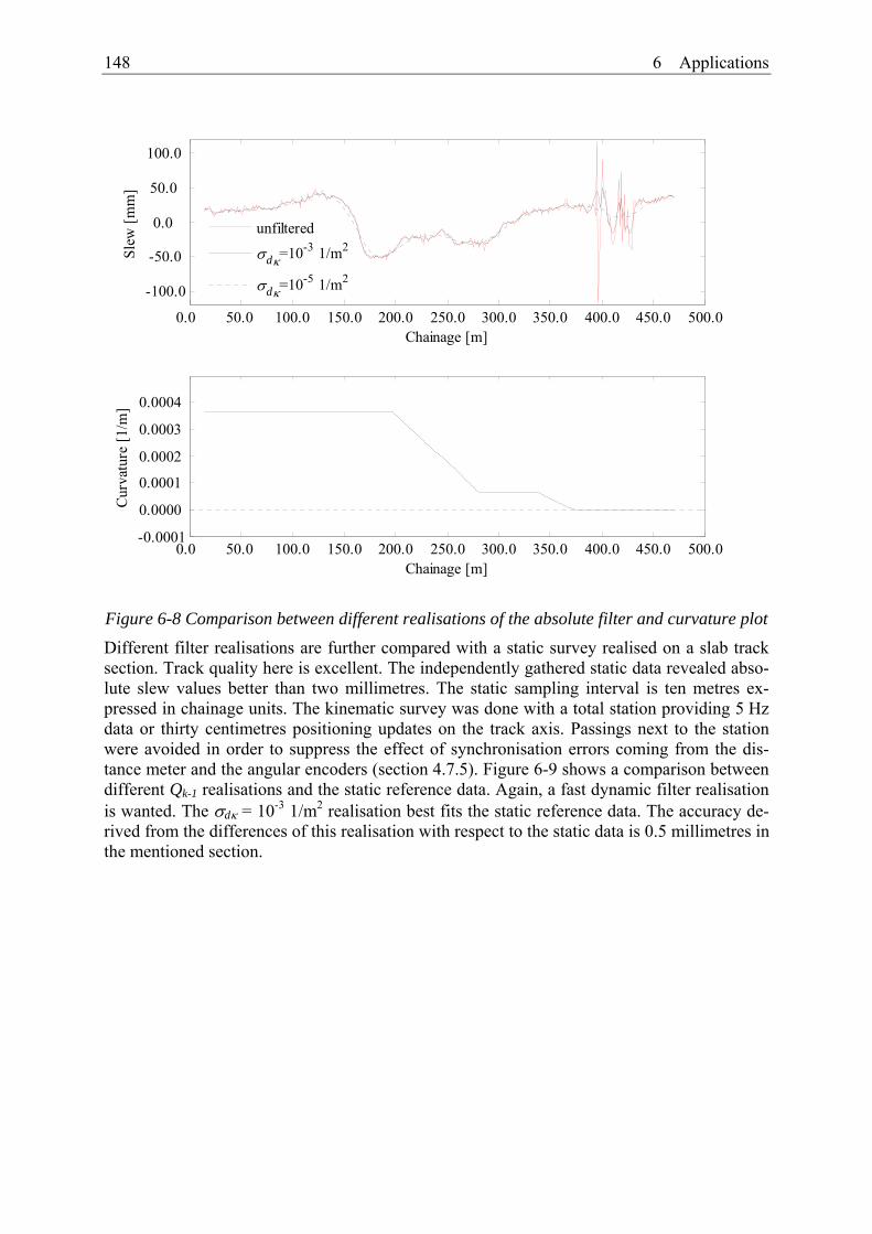
148 6 Applications

0.0 50.0 100.0 150.0 200.0 250.0 300.0 350.0 400.0 450.0 500.0

-100.0

-50.0

0.0

50.0

100.0

Chainage [m]

Slew

[mm

]

unfiltered

σdκ=10-3 1/m2

σdκ=10-5 1/m2

0.0 50.0 100.0 150.0 200.0 250.0 300.0 350.0 400.0 450.0 500.0-0.0001

0.0000

0.0001

0.0002

0.0003

0.0004

Chainage [m]

Curv

atur

e [1

/m]

Figure 6-8 Comparison between different realisations of the absolute filter and curvature plot

Different filter realisations are further compared with a static survey realised on a slab track section. Track quality here is excellent. The independently gathered static data revealed abso-lute slew values better than two millimetres. The static sampling interval is ten metres ex-pressed in chainage units. The kinematic survey was done with a total station providing 5 Hz data or thirty centimetres positioning updates on the track axis. Passings next to the station were avoided in order to suppress the effect of synchronisation errors coming from the dis-tance meter and the angular encoders (section 4.7.5). Figure 6-9 shows a comparison between different Qk-1 realisations and the static reference data. Again, a fast dynamic filter realisation is wanted. The σdκ = 10-3 1/m2 realisation best fits the static reference data. The accuracy de-rived from the differences of this realisation with respect to the static data is 0.5 millimetres in the mentioned section.

6 Applications 149

0.0 20.0 40.0 60.0 80.0 100.0 120.0 140.0 160.0 180.0 200.0-3.0

-2.0

-1.0

0.0

1.0

2.0

3.0

Chainage [m]

Slew

[mm

]static

σdκ=10-3 1/m2

σdκ=10-5 1/m2

Figure 6-9 Comparison between different realisations of the relative filter

6.2.3 Comparison between Absolute and Relative Model The relative model represents the covered trajectory more accurately since transition curves and track errors are part of the model. In the absolute model, these parameters appear as in-consistencies. In fact, the differences between both models are small. Figure 6-10 reveals these differences. The data from the filter-tuning step were used here. The acting σdκ -parameter was set to σdκ = 10-3 1/m2. A comparison with the backward run for each model yields a slightly better accuracy for the relative model. This is in accordance with the level of detail of the corresponding models.

0.0 50.0 100.0 150.0 200.0 250.0 300.0 350.0 400.0 450.0 500.0

-50.0

0.0

50.0

Chainage [m]

Slew

[mm

]

absoluterelative

Figure 6-10 Comparison between absolute and relative model

6.2.4 The Influence of Inclinometer Measurement on GPS Heights Inclinations integrated along the track locally provide more precise heights than GPS (see 3.3.4). A mandatory condition for the use of longitudinal inclinations is the separation of translatory accelerations from the raw data (section 4.4.5). Translatory accelerations are ob-tained from the odometer measurements by a low pass filter (section 5.3.3). Figure 6-11 shows the raw and the from accelerations freed gradient data. The nominal gradient in the considered section is -3 mrad.

150 6 Applications

Figure 6-12 reveals the influence of the gradient measurements on the GPS heights. Inclina-tion measurements smooth a pure GPS solution with a consequent improvement in accuracy by a factor of up to 1.5 compared to the GPS-only solution (Table 6-4). Accuracy was as-sessed by means of the merge tool of section 5.6. 220 differences between both runs were available. In the given example, an a priori standard deviation of twenty millimetres was cho-sen for the GPS heights, while the gradient a priori standard deviation was set to five mrad. However, gradients have to be weighed carefully, since residual nuisance accelerations can result in local trajectory tilts.

0.0 50.0 100.0 150.0 200.0 250.0 300.0 350.0 400.0-10.0

-5.0

0.0

5.0

10.0

Chainage [m]

Gra

dien

t [m

rad]

unfilteredprefiltered

Figure 6-11 Gradients removed from translatory accelerations

0.0 50.0 100.0 150.0 200.0 250.0 300.0 350.0 400.0

40.0

60.0

80.0

100.0

Chainage [m]

Lift

[mm

]

GPSGPS and inclination sensor

Figure 6-12 Influence of the inclination sensor on the lift parameter

Mean [mm] σ [mm] Minimum [mm] Maximum [mm]GPS and inclinations 0.4 7.7 -18.5 17.3 GPS only 0.4 11.0 -27.0 27.1

Table 6-4 The mean, standard deviation, minimum and maximum in lift parameters between the forward and the backward run.

6.2.5 The Smoother in Action – GPS Example The performance of the Swiss Trolley in GPS mode was evaluated by comparing a forward and a backward run on a 250-metre-long track section. Trimble 5700 GPS receivers were used

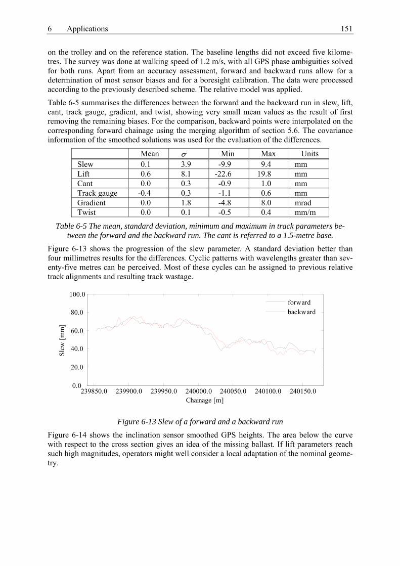
6 Applications 151

on the trolley and on the reference station. The baseline lengths did not exceed five kilome-tres. The survey was done at walking speed of 1.2 m/s, with all GPS phase ambiguities solved for both runs. Apart from an accuracy assessment, forward and backward runs allow for a determination of most sensor biases and for a boresight calibration. The data were processed according to the previously described scheme. The relative model was applied.

Table 6-5 summarises the differences between the forward and the backward run in slew, lift, cant, track gauge, gradient, and twist, showing very small mean values as the result of first removing the remaining biases. For the comparison, backward points were interpolated on the corresponding forward chainage using the merging algorithm of section 5.6. The covariance information of the smoothed solutions was used for the evaluation of the differences.

Mean σ Min Max Units Slew 0.1 3.9 -9.9 9.4 mm Lift 0.6 8.1 -22.6 19.8 mm Cant 0.0 0.3 -0.9 1.0 mm Track gauge -0.4 0.3 -1.1 0.6 mm Gradient 0.0 1.8 -4.8 8.0 mrad Twist 0.0 0.1 -0.5 0.4 mm/m

Table 6-5 The mean, standard deviation, minimum and maximum in track parameters be-tween the forward and the backward run. The cant is referred to a 1.5-metre base.

Figure 6-13 shows the progression of the slew parameter. A standard deviation better than four millimetres results for the differences. Cyclic patterns with wavelengths greater than sev-enty-five metres can be perceived. Most of these cycles can be assigned to previous relative track alignments and resulting track wastage.

239850.0 239900.0 239950.0 240000.0 240050.0 240100.0 240150.00.0

20.0

40.0

60.0

80.0

100.0

Chainage [m]

Slew

[mm

]

forwardbackward

Figure 6-13 Slew of a forward and a backward run

Figure 6-14 shows the inclination sensor smoothed GPS heights. The area below the curve with respect to the cross section gives an idea of the missing ballast. If lift parameters reach such high magnitudes, operators might well consider a local adaptation of the nominal geome-try.

152 6 Applications

239850.0 239900.0 239950.0 240000.0 240050.0 240100.0 240150.00.0

20.0

40.0

60.0

80.0

100.0

Chainage [m]

Lift

[mm

]forwardbackward

Figure 6-14 Lift of a forward and a backward run

Further, the Swiss Trolley provides cant, twist and track gauge charts (Figure 6-15 – Figure 6-17). Typical accuracies are in the sub-millimetre range. In the given example, the compari-son of the forward and the backward run yielded standard deviations of 0.3 mm for the cant taken on a 1.5-metre base. The twist parameter is only observed within the Kalman filter as the derivative of the cant. The noise gain can be considerable due to the derivation of the (noisy) cant measurements. By means of the Kalman filter, smooth estimates for the twist are obtained as seen in Figure 6-16. Figure 6-17 shows the track gauge. It reveals a typical preci-sion of 0.3 mm. Further, a slightly significant offset of 0.4 mm can be observed between the forward and backward run. Gain errors of the angular transducers are one possible explana-tion for this bias. For a run in one direction, the trolley tends to travel along one rail due to inertia. This results in almost constant readings for both gauge levers. Therefore, gain errors of the gauge levers act as a remaining bias. For a forward and a backward run, this bias is dif-ferent due to aberrant lever deflections.

The accuracies demonstrated here fulfil most track alignment requirements. Long periodic track position errors, such as the ones induced by relative chord techniques, do not occur us-ing a GPS reference frame. Thanks to the GPS-based approach, homogenous accuracies are obtained along a railway track.

239850.0 239900.0 239950.0 240000.0 240050.0 240100.0 240150.0-10.0

-8.0

-6.0

-4.0

-2.0

0.0

Chainage [m]

Cant

[mm

]

forwardbackward

Figure 6-15 Cant of a forward and a backward run

6 Applications 153

239850.0 239900.0 239950.0 240000.0 240050.0 240100.0 240150.0-2.0

-1.0

0.0

1.0

2.0

Chainage [m]

Twist

[mm

/m]

forwardbackward

Figure 6-16 Twist of a forward and a backward run

239850.0 239900.0 239950.0 240000.0 240050.0 240100.0 240150.01.4300

1.4320

1.4340

1.4360

1.4380

1.4400

Chainage [m]

Gau

ge [m

]

forwardbackward

Figure 6-17 Gauge of a forward and a backward run

6.2.6 The Smoother in Action – Total Station Example In the sequel, a total station example is given. In contrast to the above-mentioned GPS ap-proach, accuracies in the millimetre range are obtained here. However, this goes on the ex-pense of work efficiency. The survey, presented here, was carried out on a curved slab track section in a tunnel. The cant on the considered stretch nominally was 68 mm taken on a 1.5-metre base. A total station Trimble ATS600 was set-up next to the track axis. Lines of sight up to 200 metres were observed. Trolley passings next to the total station were admitted. A ve-locity of 1.8 m/s was chosen in order to study the behaviour of the synchronisation offset be-tween distance and angle measurements of the ATS600 (section 4.7.5). The relative model was used for filtering.

Table 6-6 compiles the statistics of the comparison between the forward and the backward survey. For all observed parameters, precisions in the millimetre range were obtained. Slew and lift are bias-free indicating an adequate boresight calibration. Likewise, no significant bias was found for the cant parameter. Track gauges are slightly biased. Reasons are most likely remaining gain errors (see above).

154 6 Applications

Mean σ Min Max Units Slew 0.5 1.3 -3.2 8.2 mm Lift 0.5 0.5 -1.2 1.9 mm Cant -0.6 0.5 -1.8 0.3 mm Track gauge -0.3 0.1 -0.6 -0.1 mm Gradient 0.0 0.3 -1.4 0.9 mrad Twist 0.0 0.2 -0.3 0.3 mm/m

Table 6-6 The mean, standard deviation, minimum and maximum in track parameters be-tween the forward and the backward run. The cant is referred to a 1.5-metre base.

Figure 6-18 shows the slew component as a function of the chainage. The pattern known from section 4.7.5 can be identified. Local maxima and minima for the forward and backward curve are around the direction angles ±50 gon taken from the total station with respect to the perpendicular to the trajectory. Figure 6-18 also contains the slew progression of the reference data. A small remaining bias between the kinematic data and the static data can be found on the left side of the peaks. Due to the canted stretch, the correction of section 4.7.4 affects hori-zontal angle measurements and consequently the slew component. Residual errors of the boresight calibration and the calibration of the offset b between the prism and the diode ring explain this bias.

53450.0 53500.0 53550.0 53600.0 53650.0 53700.0 53750.0 53800.0 53850.0 53900.0

-5.0

0.0

5.0

Chainage [m]

Slew

[mra

d]

forwardbackwardstatic

Figure 6-18 Slew of a forward run, a backward run and a static survey

As revealed by Figure 6-19, the ATS600 synchronisation error affects the lift parameter far less. This is due to the negligible vertical component of the trolley velocity vector. With re-spect to the static reference data, forward and backward run seem to be slightly distorted. The edge of the roof shaped curve being symmetric to the total station chainage indicates a resid-ual index error smaller than 0.5 mgon.

6 Applications 155

53450.0 53500.0 53550.0 53600.0 53650.0 53700.0 53750.0 53800.0 53850.0 53900.0

-5.0

0.0

5.0

Chainage [m]

Lift

[mm

]forwardbackwardstatic

Figure 6-19 Lift of a forward run, a backward run and a static survey

For both runs, accuracy can be assessed with respect to the static reference data. Table 6-7 and Table 6-8 compile statistics for the forward run and the backward run, respectively. As it can be seen from both tables, the root mean square errors remain in the millimetre range. Evi-dently, trolley calibration procedures explained in section 4, are appropriate. This does not hold for the cant parameter. A slightly significant bias with respect to the static data was found. A zero point offset can be excluded since the comparison between the forward and backward run did not yield a systematic contribution. The offset can be attributed to an inap-propriate gain factor affecting inclination measurements on canted tracks.

Mean RMS Min Max Units Slew 0.7 0.9 -1.1 2.9 mm Lift -1.7 1.3 -4.0 0.9 mm Cant 1.1 0.4 0.4 1.8 mm Track gauge -0.1 0.2 -0.4 0.5 mm

Table 6-7 The mean, root mean square error, minimum and maximum in track parameters between the forward run and the reference data. The cant is referred to a 1.5-metre base.

Mean RMS Min Max Units Slew 0.3 1.3 -2.9 3.3 mm Lift -2.1 1.2 -3.8 0.3 mm Cant 1.7 0.5 0.6 1.6 mm Track gauge -0.2 0.2 -0.8 0.2 mm

Table 6-8 The mean, root mean square error, minimum and maximum in track parameters between the backward run and the reference data. The cant is referred to a 1.5-metre base.

6.3 Kinematic Scanning The Swiss Trolley S-option allows for kinematic scans. Here, an example is given of an as-signment carried out for the Siemens CargoMover division. The CargoMover [HERBST et al., 2002] is an autonomous train designed for freight shipping on e.g. harbour terminals. The guideless train asks for several safety measures. As an example, laser scanners are used to monitor the environment for obstacle recognition. The generated three dimensional point clouds are compared with accurate vectorised nominal sceneries. If differences between both models exceed thresholds, the CargoMover slows down. Base data for the vectorised nominal

156 6 Applications

sceneries for the Siemens Wegberg-Wildenrath test centre in Germany were acquired by the Swiss Trolley in kinematic laser scanning mode (Figure 6-20). GPS was used for positioning. All data were referenced to the DB-REF reference frame.

Figure 6-20 CargoMover on the way. Nominal scenery used for obstacle recognition

The CargoMover obstacle recognition software requires track data and the track environment data in a node-section model. Nodes are defined by switches and buffers. A first prototype model contains five kilometres of tracks (Figure 6-21).

1

2

3

4

5 6

7

8

9

10

11

12

13 14 15 16

17

18

19

1

2 3

4

5

6

7

8

9

10 11 12

13 14

15

16 17

Figure 6-21 Node-section model for CargoMover. The mapped model contains five kilometres of railway lines.

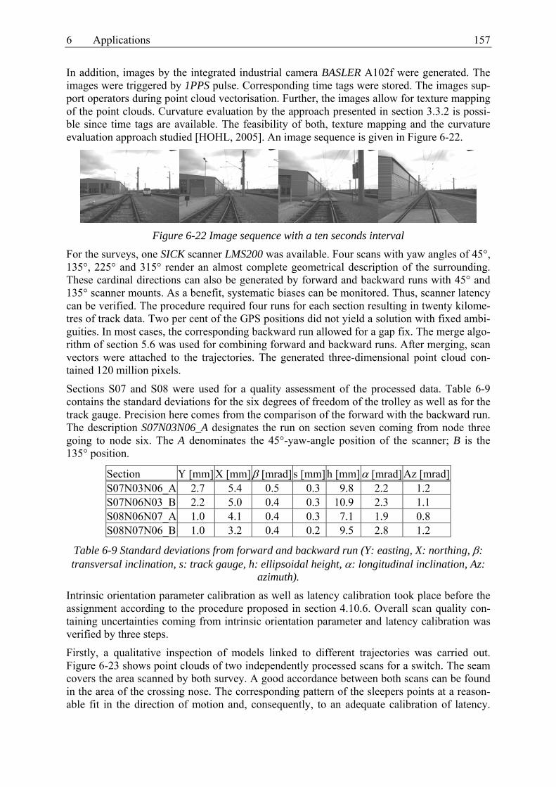
6 Applications 157

In addition, images by the integrated industrial camera BASLER A102f were generated. The images were triggered by 1PPS pulse. Corresponding time tags were stored. The images sup-port operators during point cloud vectorisation. Further, the images allow for texture mapping of the point clouds. Curvature evaluation by the approach presented in section 3.3.2 is possi-ble since time tags are available. The feasibility of both, texture mapping and the curvature evaluation approach studied [HOHL, 2005]. An image sequence is given in Figure 6-22.

Figure 6-22 Image sequence with a ten seconds interval

For the surveys, one SICK scanner LMS200 was available. Four scans with yaw angles of 45°, 135°, 225° and 315° render an almost complete geometrical description of the surrounding. These cardinal directions can also be generated by forward and backward runs with 45° and 135° scanner mounts. As a benefit, systematic biases can be monitored. Thus, scanner latency can be verified. The procedure required four runs for each section resulting in twenty kilome-tres of track data. Two per cent of the GPS positions did not yield a solution with fixed ambi-guities. In most cases, the corresponding backward run allowed for a gap fix. The merge algo-rithm of section 5.6 was used for combining forward and backward runs. After merging, scan vectors were attached to the trajectories. The generated three-dimensional point cloud con-tained 120 million pixels.

Sections S07 and S08 were used for a quality assessment of the processed data. Table 6-9 contains the standard deviations for the six degrees of freedom of the trolley as well as for the track gauge. Precision here comes from the comparison of the forward with the backward run. The description S07N03N06_A designates the run on section seven coming from node three going to node six. The A denominates the 45°-yaw-angle position of the scanner; B is the 135° position.

Section Y [mm] X [mm] β [mrad] s [mm] h [mm] α [mrad] Az [mrad] S07N03N06_A 2.7 5.4 0.5 0.3 9.8 2.2 1.2 S07N06N03_B 2.2 5.0 0.4 0.3 10.9 2.3 1.1 S08N06N07_A 1.0 4.1 0.4 0.3 7.1 1.9 0.8 S08N07N06_B 1.0 3.2 0.4 0.2 9.5 2.8 1.2

Table 6-9 Standard deviations from forward and backward run (Y: easting, X: northing, β: transversal inclination, s: track gauge, h: ellipsoidal height, α: longitudinal inclination, Az:

azimuth).

Intrinsic orientation parameter calibration as well as latency calibration took place before the assignment according to the procedure proposed in section 4.10.6. Overall scan quality con-taining uncertainties coming from intrinsic orientation parameter and latency calibration was verified by three steps.

Firstly, a qualitative inspection of models linked to different trajectories was carried out. Figure 6-23 shows point clouds of two independently processed scans for a switch. The seam covers the area scanned by both survey. A good accordance between both scans can be found in the area of the crossing nose. The corresponding pattern of the sleepers points at a reason-able fit in the direction of motion and, consequently, to an adequate calibration of latency.

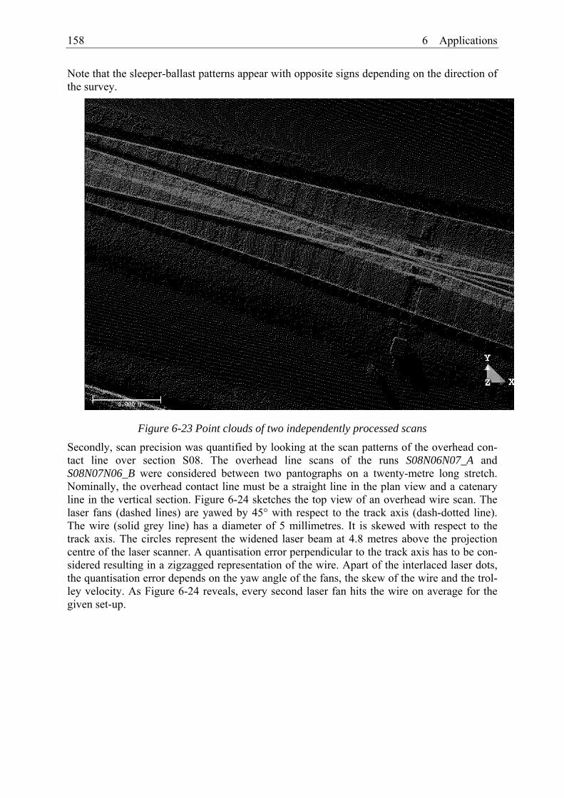
158 6 Applications

Note that the sleeper-ballast patterns appear with opposite signs depending on the direction of the survey.

Figure 6-23 Point clouds of two independently processed scans

Secondly, scan precision was quantified by looking at the scan patterns of the overhead con-tact line over section S08. The overhead line scans of the runs S08N06N07_A and S08N07N06_B were considered between two pantographs on a twenty-metre long stretch. Nominally, the overhead contact line must be a straight line in the plan view and a catenary line in the vertical section. Figure 6-24 sketches the top view of an overhead wire scan. The laser fans (dashed lines) are yawed by 45° with respect to the track axis (dash-dotted line). The wire (solid grey line) has a diameter of 5 millimetres. It is skewed with respect to the track axis. The circles represent the widened laser beam at 4.8 metres above the projection centre of the laser scanner. A quantisation error perpendicular to the track axis has to be con-sidered resulting in a zigzagged representation of the wire. Apart of the interlaced laser dots, the quantisation error depends on the yaw angle of the fans, the skew of the wire and the trol-ley velocity. As Figure 6-24 reveals, every second laser fan hits the wire on average for the given set-up.

6 Applications 159

Figure 6-24 LMS200 scan of overhead line For the horizontal component, orthogonal regressions were computed. For the sake of sim-plicity, this was also done for the vertical component taking into account deviations from the theoretically correct catenary line. The residuals are shown in Figure 6-25. The left column plots are attributed to the horizontal component. The jigsaw pattern of Figure 6-24 reappears. The slope of the saw tooth depends on the mutual skew between the scan grid and the over-head wire. The thickness of the pattern corresponds to the given resolution perpendicular to the overhead wire. Slow varying trends superposed by the quantisation noise can be perceived for both runs indicating positioning and attitude angle errors. Systematic portions in the DOF elements can be obtained by looking at the residuals of the backward run with respect to the forward regression line (lower left plot of Figure 6-25). A root mean square error of seventeen millimetres was found for the horizontal component. Main acting parameters for this bias are slew errors and roll angle errors.

The right column plots of Figure 6-25 show the residuals for the vertical component. Here, the found standard deviation mainly contains uncertainty portions of the LMS200 EDM and the height component. Quantisation errors are smaller than the measurement noise. Compared to the root mean square error of the horizontal component, the vertical root mean square error of 14.8 millimetres insignificantly exceeds the vertical precision. This indicates that the height components are almost bias-free (lower right plot Figure 6-25). Acting levers amplifying atti-tude errors are much smaller than for the horizontal component.

0 10 20 cm

160 6 Applications

0.0 5.0 10.0 15.0 20.0-50.0

0.0

50.0

S08N06N07_A (horizontal)σ = 7.5 mm

Resid

uals

[mm

]

0.0 5.0 10.0 15.0 20.0

-50.0

0.0

50.0

S08N07N06_B (horizontal)σ = 7.6 mm

Resid

uals

[mm

]

0.0 5.0 10.0 15.0 20.0

-50.0

0.0

50.0

S08N07N06_B to S08N06N07_A (hor)rms = 16.9 mm

Chainage [m]

Resid

uals

[mm

]

0.0 5.0 10.0 15.0 20.0-50.0

0.0

50.0

S08N06N07_A (vertical)σ = 10.7 mm

0.0 5.0 10.0 15.0 20.0

-50.0

0.0

50.0

S08N07N06_B (vertical)σ = 10.3 mm

0.0 5.0 10.0 15.0 20.0

-50.0

0.0

50.0

S08N07N06_B to S08N06N07_A (ver)rms = 14.8 mm

Chainage [m]

Figure 6-25 Overhead line: residuals from the orthogonal regression

Thirdly, scan accuracy was verified on a test field established next to the sections S07 and S08 (Figure 6-21). Checkpoint coordinates were determined by a total station and attached to the DB-REF reference frame. The distribution of totally five checkpoints can be seen in Figure 6-26. Points 2001 – 2003 are target marks on tripods. Scan distances up to fifteen me-tres occurred. The targets were aligned with respect to the track axis in such way that optimal incident angles for the laser beam resulted. In addition, two accidentally chosen points on a catenary mast were incorporated. The checkpoint 2004 is nine meters above the track axis. Scans from the merged runs S07N03N06, S07N06N03, S08N06N07 and S08N0706 were considered for the accuracy assessment.

6 Applications 161

Figure 6-26 Checkpoints for quality control

Table 6-10 shows the checkpoint residuals. The residuals contain uncertainties coming from the intrinsic orientation, the extrinsic orientation and the scanner (see 4.10.5). In addition, the assignment of a pixel to a checkpoint is limited due to the limited angular resolution of the scanner and the limited resolution in the direction of motion depending on the velocity. A maximal quantisation error of 2.3 centimetres in roll direction has to be taken into account for a checkpoint ten metres away. In the direction of motion, this error amounts to about five mil-limetres. Hence, the obtained root mean square error of thirty-three millimetres is rather pes-simistic since quantisation noise is superposed.

Id dY [mm] dX [mm] dH [mm] Run 2001 13 -68 1 S07N03N06_A 2002 -17 -15 -4 S07N03N06_A 2003 -24 -27 21 S07N03N06_B 2001 -4 -2 -1 S07N06N03_B 2002 -48 2 13 S07N06N03_A 2003 -48 27 2 S07N06N03_A 2001 -6 -12 58 S08N06N07_B 2002 -30 23 50 S08N06N07_B 2003 -3 35 5 S08N06N07_B 2004 -6 -18 -96 S08N06N07_B 2005 2 18 -6 S08N06N07_B 2005 -73 14 7 S08N07N06_A 2004 -29 9 -70 S08N07N06_A

Table 6-10 Checkpoint residuals

2001 2002

2003

2004

2005

7 Conclusions 163

7 Conclusions The track-surveying vehicle Swiss Trolley features absolute, kinematic track inventory sur-veys. This work compiles behaviour, calibration and fusion of the involved sensors and points out applications for absolute railway surveys by means of examples.

For the realisation of the data acquisition and data-processing components, importance was attached to a modular design. Depending on the task, configurations with different levels of sensor assemblies can be used. The integration of additional sensors should not cause any concern. Likewise, data-processing components can be expanded by additional sensor models.

A stringent condition for reliable kinematic surveys is an accurate spatial and timely mapping of all involved sensors. Timely correlation was solved for the Swiss Trolley project by the University of Applied Sciences of Burgdorf. For high dynamics applications like kinematic laser scanning, accurate time-tags are provided by a data acquisition programme running un-der Linux with the real time application interface (RTAI-Linux). Time-tags for the involved sensors with jitters better than one millisecond are obtained.

Trolley yaw rates are determined by the trajectory course. Roll and pitch angles are obtained from inclination sensors. The given inclination sensor model counts for nuisance accelerations affecting inclinations and considers the transient behaviour. Accuracies in the range of 0.5 mrad for the transversal inclinations and in the range of 5 mrad for the longitudinal incli-nations were found for kinematic surveys at walking speed. In the case of total station sur-veys, pitch angles derived from the trajectory yield more accurate information for the attitude determination. Calibration procedures for inclinometers are given, counting for cross-collimation biases. Such biases can be of certain relevance for high-accuracy surveys.

For absolute positioning, total stations or GPS are used. The suitability of Trimble ATS600 for kinematic track surveys was evaluated. Biases coming from the special network layout along railway tracks were assessed. A bias coming from the inclined prism in curved sections was pointed out. Errors up to five millimetres for the slew component occur if this offset is not considered. The synchronisation error between angle and distance measurements of the used Trimble ATS600 is acceptable for kinematic track surveying. The influence on the slew com-ponent can be minimised for trolley passings next to the total station by slowing down. For higher accuracy requirements, a procedure is given which allows for the calibration of the latency between angle and distance measurements.

The integration of GPS-RTK is based on time-tagged NMEA strings. NMEA strings come by default with ellipsoidal heights. Geoid undulations can be submitted in a post-processing step.

A mechanical track gauge measuring system allows for the assessment of the track gauge and the trolley wobble by levers dragging along the running edges of the rails. This simple but reliable realisation provides submillimetre accuracies.

For track inventory surveys, SICK LMS200 laser scanners are used. The given angular resolu-tion yields reasonable data amounts, which can be handled by state-of-the-art post-processing software. Sufficiently dense information is acquired for 3D modelling in a corridor of up to ten metres, next to the track axis. The presented calibration procedure allows for the determi-nation of the attitude angles in the b-frame in the order of 1 mrad. For scanner latency calibra-tion, scans of identical structures in a forward and backward run are used. Then, scanner la-tency is a function of the shift in the direction of the trolley motion and the trolley velocity.

A cascading, loosely coupled post-processing strategy is introduced. Here, post-processing is preferred, owing to the ability to formulate non-causal filters, which in turn results in an accu-

164 7 Conclusions

racy gain. The post-processing strategy contains a pre-processing, a synchronisation and a smoother step. Two filter models are given. The absolute model prevails if no nominal track axis data are available. The relative model determines displacements from the nominal axis. The use of the relative model is preferable, since it models the trajectory more accurately. The smoother model renders accuracies for total station surveys better than five millimetres. Sub-centimetre accuracy is obtained for the horizontal GPS components. Vertical GPS heights can be slightly improved by incorporating longitudinal inclination measurements. However, sub-centimetre accuracy is difficult to achieve.

For Swiss Trolley surveys with required centimetre accuracy, the following working method has become accepted. GPS surveys are carried out in the up and down direction. Then, GPS outage gap filling is completed by total station runs with overlapping zones. Inconsistencies in the overlapping zones are adjusted by the presented merge technique. In addition to a smooth progression of the surveyed track, the proposed merge tool represents an efficient way to as-sess measurement quality.

The Swiss Trolley has proven its operational readiness in various assignments. Eighteen kilo-metres of slab track surveys have been carried out offering an optimal integration in the work-flow on the sites. The sensor layout on the trolley is not optimised for slab track alignment. Nevertheless, the given tolerances were fulfilled. Besides, the odometer-aided prism search favoured an uninterrupted workflow on construction sites with obstructed lines of sight.

In the meantime, kinematic track geometry surveys have taken place for through alignments for more than five hundred kilometres. The dense and accurate track information, captured on the runs, enabled engineers to guarantee a precise description of the actual physical track. Data evaluated by the absolute model can serve as a basis for a regression analysis of the track axis. By means of the relative model, slew and lift parameters can be generated directly which are used by tamping machines for rail corrections. A kinematic track axis survey outmatches a traditional static approach mainly for two reasons: Firstly, the much denser track information of kinematic surveys holds in every case Nyquist theorem applied to track element regression. By contrast, static surveys with a five-metre sampling rate can fail for short elements. Sec-ondly, mainly for GPS surveys, work efficiency can be significantly increased. The typical survey performance is four kilometres per hour.

Operational readiness was also proven for the Swiss Trolley with the scanning extension. Pixel accuracies of three centimetres were demonstrated for kinematic scans. The relative precision between two pixels is better than 1.5 centimetres. As an example, a survey provid-ing ground truth data for a scanning obstacle recognition system was presented. Further appli-cations are manifold. Overhead line inspection can easily be performed with no need to inter-rupt the traction current. This is still the case for traditional inspections. Another application points at the determination of ballast deficiencies. The generated 3D point cloud allows for the generation of high-resolution digital terrain models. Furthermore, Swiss Trolley scans serve as a basis for clearance inspections. Scans can also serve for contact-free track gauge determinations with inferior accuracy. Tests with least squares matching of known rail pro-files into the acquired point clouds yielded accuracies in the range of three millimetres.

The above-mentioned modularity of the Swiss Trolley allows for various extensions. Thus, the integration of differential odometry is foreseen. Differential odometry helps to bypass GPS outages. As a consequence, gap completion by total station trolley runs could be avoided. Then, the integration of ground penetration radar (GPR) completes a comprehensive descrip-tion of the track surroundings with regard to track bed inspection. Conceptually, a GPR mod-ule can be included. Moreover, the scanners and positioning sensors are not rail-bound. Prom-ising trials are being carried out with the platform installed on a road-vehicle.

7 Conclusions 165

The Swiss Trolley is the result of a joint venture project of the partners terra vermessungen AG of Zürich, Grunder Ingenieure AG of Hasle-Rüegsau, the University of Applied Sciences of Burgdorf and the Institute for Geodesy and Photogrammetry at ETH Zürich. The project was supported by the Commission for Technology and Innovation of the Swiss Office for Pro-fessional Education and Technology.

List of Figures 167

List of Figures Figure 2-1 Vehicle in a canted curve (adapted from [MÜLLER et al., 2000]).......................... 5 Figure 2-2 Jerks for a clothoid, a Bloss curve and a sinusoid (according to

[HENNECKE et al., 1993]).................................................................................... 6 Figure 2-3 Definition of track axis and track gauge................................................................... 7 Figure 2-4 Definition of cant...................................................................................................... 8 Figure 2-5 Realisation of the cant by rising the outer rail and lowering the inner rail .............. 8 Figure 2-6 Realisation of the cant by rising the outer rail.......................................................... 9 Figure 2-7 Frenet system for a trajectory with non-vanishing curvature................................... 9 Figure 2-8 Overview of different track-surveying methods..................................................... 17 Figure 2-9 Versine and differential tangent angle.................................................................... 18 Figure 2-10 Measurement principle of EM-SAT without GPS (according to [HOLLINGER et

al., 1995]) ............................................................................................................. 21 Figure 3-1: Potential sensors and tasks of a track-surveying trolley........................................ 26 Figure 3-2: GPS obstructions due to topography along the principal north-south connection of

the Swiss Federal Railways.................................................................................. 28 Figure 3-3 Dead reckoning by means of wandering chords..................................................... 31 Figure 3-4 Cross error as a function of the chainage for a sampling interval of 1 m and an

a priori yaw rates standard deviation of 10 mgon. ............................................... 33 Figure 3-5 Yaw rate measurements by means of two cameras ................................................ 34 Figure 3-6 Determination of the chord length c and the offset e in the linear array ................ 35 Figure 3-7 Edge detection of rails by a Canny filter ................................................................ 36 Figure 3-8 Path and yaw rate measurements by odometers ..................................................... 37 Figure 3-9 Precision of azimuths and paths for odometer measurements (Radius 1000 m and

straight line).......................................................................................................... 38 Figure 3-10 Height error as a function of the chainage (σα = 0.005 rad) for a stretched survey

.............................................................................................................................. 39 Figure 3-11 Cross section of double track railway alignment showing names of principal parts

of construction [NETWORK RAIL, 2003].......................................................... 41 Figure 3-12 Track gauge measuring system of the EM 250 (adapted from [PRESLE, 2000])42 Figure 3-13 Traces on a cylinder surface recorded by two laser scanners placed on the

cylinder axis. ........................................................................................................ 43 Figure 3-14 3D camera SwissRanger SR2............................................................................... 45 Figure 3-15 Positioning error as a function of the synchronisation error [HENNES, 1999]... 46 Figure 3-16 Measuring process [RUHM, 2002] ...................................................................... 47 Figure 3-17 Definition of the body system of a track-surveying vehicle................................. 48 Figure 4-1 Track-surveying vehicle “Swiss Trolley” with a Trimble Zephyr antenna and a

Trimble ATS600 active prism (P configuration) ................................................. 52 Figure 4-2 Back wheel with mechanism for passing switches................................................. 52 Figure 4-3 Swiss Trolley configurations.................................................................................. 54 Figure 4-4 A/D conversion of angular transducer in rest with NI DAQCard .......................... 57 Figure 4-5 1PPS event of the Trimble 5700 receiver according to [TRIMBLE, 2001a] ......... 58 Figure 4-6 Time synchronisation by the 1PPS pulse ............................................................... 58 Figure 4-7 Time synchronisation without 1PPS pulse ............................................................. 60 Figure 4-8 Inclination sensor Midori PMP-S15TA-V1 ........................................................... 61 Figure 4-9 Influence of shearing and pivoting on inclinations α and β ................................... 63 Figure 4-10 Principle of pendulum inclination sensor (adapted from [EICHHOLZ et al.,

1982]) ................................................................................................................... 67 Figure 4-11 Apparent inclination due to an acceleration aE0 ................................................... 69

168 List of Figures

Figure 4-12 Gradients acquired at walking speed with frequency contents ............................ 70 Figure 4-13 Sensor response of step function for different dampings ..................................... 71 Figure 4-14 Verification of response time ............................................................................... 72 Figure 4-15 Angular transducer with shaft and blocking pole in enclosure ............................ 74 Figure 4-16 Track gauge determination by the lever deflections lp and rp .......................... 75 Figure 4-17 Trimble ATS600 and miniprism RMT................................................................. 78 Figure 4-18 Difference from a nominal vertical layout due to a disregarded index error of

1 mgon.................................................................................................................. 79 Figure 4-19 Difference from a nominal vertical layout due to a disregarded compensator zero

point offset error of 1 mgon ................................................................................. 79 Figure 4-20 Difference from a nominal horizontal layout due to a disregarded additive

constant of 2 mm.................................................................................................. 80 Figure 4-21 Differences from mean Trimble RMT prism position for horizontal direction,

vertical angle and horizontal distance as a function of the prism orientation with corresponding frequency contents........................................................................ 81

Figure 4-22 Difference from a nominal vertical layout due to disregarded deflections of vertical of 1 mgon ................................................................................................ 82

Figure 4-23 Tracking of ATS600 prism in canted section. The EDM rosette and the diode ring offset are separated by the offset b....................................................................... 82

Figure 4-24 Reduction due to inclined prism in canted section............................................... 83 Figure 4-25 Latency portions of a tracking tacheometer (partly from [TRIMBLE, 2001b]) .. 84 Figure 4-26 Angle and distance variations for a trolley passing. Adapted from

[HENNES, 1999] ................................................................................................. 86 Figure 4-27 Influence of latency on horizontal component ..................................................... 87 Figure 4-28 Displacements from a nominal trajectory due to a latency between the angle and

the distance measurement of 0.2 s (velocity 1 m/s). The total station is placed at chainage 100 m with the distance a0 next to the track axis. ................................. 88

Figure 4-29 Principle of direction and distance synchronisation carried out by the robotic mode of the ATS600 (from [TRIMBLE, 2001b])................................................ 89

Figure 4-30 Forward and backward run on a calibration track carried out at a velocity of 0.45 m/s ................................................................................................................ 89

Figure 4-31 SICK Laser scanner LMS200-30106 ................................................................... 93 Figure 4-32 Kinematic scan of an overhead line. The overhead wire has a diameter of about

6 mm and is 5.7 m above the track axis. .............................................................. 94 Figure 4-33 Definition of the laser scanner measuring system................................................ 95 Figure 4-34 Yaw angle correction............................................................................................ 96 Figure 4-35 Yaw angle correction as a function of the track radius ........................................ 97 Figure 4-36 Swiss Trolley scanning five spheres for precision evaluation of the SICK laser

scanner.................................................................................................................. 98 Figure 4-37 Residuals of Helmert transformation between scanned spheres and total station

sphere centre coordinates ..................................................................................... 99 Figure 4-38 Scanner arrangement on the Swiss Trolley ........................................................ 100 Figure 4-39 Incident angle and distance precision on a cylinder for a 45° yawed laser scanner.

The cylinder axis is parallel to the track axis. .................................................... 100 Figure 4-40 Variance propagation for a 45° yawed scanner on cylindrical surfaces which are

5 m and 10 m away from the scanner projection centre..................................... 102 Figure 4-41 Top view of catenary yoke scanned by a forward run (light) and a backward run

(dark) .................................................................................................................. 104 Figure 4-42 Latency calibration ............................................................................................. 105 Figure 5-1 Post-processing concept [GLAUS, 2004] ............................................................ 108

List of Figures 169

Figure 5-2 Merging several filter runs ................................................................................... 108 Figure 5-3 Graphical user interface of the post-processing software rmpAnalysis ............... 109 Figure 5-4 Batch-processing with rmpAnalysis..................................................................... 110 Figure 5-5 Comparison of MAD and median filter................................................................ 111 Figure 5-6 Block diagram of data pre-processing.................................................................. 113 Figure 5-7 Smoothing by adjusting a polynomial at five equidistant base points ................. 114 Figure 5-8 Extended Kalman filter loops (adapted from [WELCH, 1997]) .......................... 119 Figure 5-9 Forward and backward propagation of the state................................................... 120 Figure 5-10 Computational complexity of Kalman filter / smoother and splines with

derivatives .......................................................................................................... 134 Figure 5-11 Chaining the smoothed series............................................................................. 135 Figure 5-12 Algorithm for chaining trajectories of different runs ......................................... 136 Figure 5-13 Merging of two curves: linear interpolation in overlapping section .................. 137 Figure 5-14 Correlations between two adjacent states for selected track parameters as a

function of distance ............................................................................................ 139 Figure 5-15 Merging of two curves: weighted average ......................................................... 140 Figure 6-1 Layout of free stations for track alignment. The distance between two stations is

thirty-five metres. ............................................................................................... 142 Figure 6-2 Error propagation with free stations ..................................................................... 142 Figure 6-3 Principle of the track alignment ........................................................................... 143 Figure 6-4 TCRA1101 on an industrial tripod used for the coarse alignment in interaction

with the Swiss Trolley........................................................................................ 143 Figure 6-5 Histograms of differential slew, differential lift, cant error and gauge error after

paving over......................................................................................................... 144 Figure 6-6 Qualitative record of track recording coach run [SBB, 2003].............................. 145 Figure 6-7 Forward filtered, backward filtered and smoothed cant and twist ....................... 146 Figure 6-8 Comparison between different realisations of the absolute filter and curvature plot

............................................................................................................................ 148 Figure 6-9 Comparison between different realisations of the relative filter .......................... 149 Figure 6-10 Comparison between absolute and relative model ............................................. 149 Figure 6-11 Gradients removed from translatory accelerations............................................. 150 Figure 6-12 Influence of the inclination sensor on the lift parameter .................................... 150 Figure 6-13 Slew of a forward and a backward run............................................................... 151 Figure 6-14 Lift of a forward and a backward run................................................................. 152 Figure 6-15 Cant of a forward and a backward run ............................................................... 152 Figure 6-16 Twist of a forward and a backward run.............................................................. 153 Figure 6-17 Gauge of a forward and a backward run ............................................................ 153 Figure 6-18 Slew of a forward run, a backward run and a static survey................................ 154 Figure 6-19 Lift of a forward run, a backward run and a static survey.................................. 155 Figure 6-20 CargoMover on the way. Nominal scenery used for obstacle recognition......... 156 Figure 6-21 Node-section model for CargoMover. The mapped model contains five

kilometres of railway lines. ................................................................................ 156 Figure 6-22 Image sequence with a ten seconds interval....................................................... 157 Figure 6-23 Point clouds of two independently processed scans........................................... 158 Figure 6-24 LMS200 scan of overhead line........................................................................... 159 Figure 6-25 Overhead line: residuals from the orthogonal regression................................... 160 Figure 6-26 Checkpoints for quality control .......................................................................... 161 Figure A-1 Transformation from inclination angles to Euler angles ..................................... 181 Figure A-2 Minimum distance from the track axis ................................................................ 183

List of Tables 171

List of Tables Table 4-1 Overview of Swiss Trolley sensors ......................................................................... 55 Table 4-2 Required voltage resolution of utilised sensors ....................................................... 57 Table 4-3 Data records with time tag ....................................................................................... 59 Table 4-4 Conversion table for inclination measuring units .................................................... 61 Table 4-5 Technical specifications Trimble ATS600 according to manufacturer

[TRIMBLE, 2001b].............................................................................................. 78 Table 4-6 NMEA-0183 Trimble PTNL, PJK message fields (from [TRIMBLE, 2001a]) ...... 91 Table 4-7 Standard deviations of involved parameters for precision simulation................... 101 Table 6-1 Tolerances for the slab track alignment in the Zürich-Thalwil tunnel .................. 141 Table 6-2 Used values for weighting observations ................................................................ 146 Table 6-3 Used values for kinematic model........................................................................... 147 Table 6-4 The mean, standard deviation, minimum and maximum in lift parameters between

the forward and the backward run...................................................................... 150 Table 6-5 The mean, standard deviation, minimum and maximum in track parameters

between the forward and the backward run. The cant is referred to a 1.5-metre base..................................................................................................................... 151

Table 6-6 The mean, standard deviation, minimum and maximum in track parameters between the forward and the backward run. The cant is referred to a 1.5-metre base..................................................................................................................... 154

Table 6-7 The mean, root mean square error, minimum and maximum in track parameters between the forward run and the reference data. The cant is referred to a 1.5-metre base........................................................................................................... 155

Table 6-8 The mean, root mean square error, minimum and maximum in track parameters between the backward run and the reference data. The cant is referred to a 1.5-metre base........................................................................................................... 155

Table 6-9 Standard deviations from forward and backward run (Y: easting, X: northing, β: transversal inclination, s: track gauge, h: ellipsoidal height, α: longitudinal inclination, Az: azimuth).................................................................................... 157

Table 6-10 Checkpoint residuals............................................................................................ 161

References 173

References ABLINGER, P. [2001]: Vermessen und Einrichten von Festen Fahrbahnen − Systemkonzept.

EI – Eisenbahningenieur (52) 09/2001. Tetzlaff, Hamburg.

ARRAS, O.K., R. PHILIPPSEN, N. TOMATIS, M. DE BATTISTA, M. SCHILT, R. SIEGWART [2003]: A Navigation Framework for Multiple Mobile Robots and its Application at the Expo-02 Exhibition. Proceedings of the 2003 IEEE International Conference on Robotics and Automation, Taipei, Taiwan, 14-19 September, 2003.

BAGNASCHI, L. [1993]: Application of an Adaptive Kalman Filter for the Estimation of Position, Velocity and Acceleration of a Moving Body from GPS Measurements. Institut für Geodäsie und Photogrammetrie, Report 226. ETH Zürich.

BÄSCHLIN, C.F. [1947]: Einführung in die Kurven- und Flächentheorie. Orell Füssli, Zürich.

BEETS, S. [2001]: Bilan d’un levé de ligne à grande vitesse par profilomètre ferroviaire – Adaption au TGV Méditerranée. XYZ No 88.

BLANC, N. [2001]: CCD versus CMOS − Has CCD Imaging Come to an End? Photogrammetric Week, 01. D. Fritsch and R. Spiller, Eds. Wichmann, Heidelberg.

BLONDEAU, J., F. STEINFORT [1999]: LIMEZ II - Der Lichtraummesszug der Deutschen Bahn. EI − Eisenbahningenieur (50) 02/1999. Tetzlaff, Hamburg.

BLOSS, A. [1936]: Der Übergangsbogen mit geschwungener Überhöhungsrampe. Organ für die Fortschritte des Eisenbahnwesens 91 15. pp. 319-320.

BÖSCH, D. [1991]: Projektierung von Bahnanlagen, Linienführung. Lecture notes „Grundlagen des öffentlichen Verkehrs, Block Infrastruktur“. Institut für Verkehrsplanung, Transporttechnik, Strassen und Eisenbahnbau, ETH Zürich.

CANNY, J. F. [1986]: A Computational Approach to Edge Detection. IEEE Transactions on Pattern Analysis and Machine Intelligence, 8 (6). pp. 679-698.

CASPARY, W. [2000]: Zur Analyse geodätischer Zeitreihen. In: 25 Jahre Institut für Geodäsie. Teil 1: Wissenschaftliche Beiträge und Berichte. Schriftenreihe des Studiengangs Geodäsie und Geoinformation der Universität der Bundeswehr München.

COCARD, M. [1995]: High Precision GPS Processing in Kinematic Mode. Geodätisch-geophysikalische Arbeiten in der Schweiz. Volume 52. Schweizerische Geodätische Kommission.

CORRSYS [2005]: Datasheet of Correvit-Rail sensor (online). Last update 01-03-2005. Available in the Internet at http://www.corrsys-datron.com/c3d_rail_sensors.htm (Last visited: 13-12-2005).

CZISCHOS, H. [1989]: Hütte − Die Grundlagen der Ingenieurwissenschaften. Springer, Berlin.

DANUSER, G. [1992]: Zeitübertragung und Synchronisation mit GPS: Anwendung in der Überwachung verteilter Systeme. Institut für Geodäsie und Photogrammetrie, Report 196. ETH Zürich.

DARR, E. [1997]: Qualität und Beständigkeit der Gleislage von Festen Fahrbahnen. EI – Eisenbahningenieur (48) 01/1997. Tetzlaff, Hamburg.

174 References

DB [1999]: Richtlinie 883.9002. Gleis- und Bauvermessung. Definitionen zur Abbildung der Trasse, der Gradiente und der Überhöhung im Gleis.

DE BOOR, C.A. [2001]: A Practical Guide to Splines. Rev. Ed., Vol. 27, 2001, Springer, New York.

DEAKIN, R.E., D.G. KILDEA [1999]: A Note on Standard Deviation and RMS. The Australian Surveyor. Vol. 44, No 1.

DÜNISCH, M., H. KUHLMANN [2001]: Investigation on Accuracy of Tracking Motorized Tacheometers. Proceedings of the Optical 3D Measurement Techniques V Congress. Vienna, 2001. pp. 218 - 225.

DÜNISCH, M., H. KUHLMANN, W. MÖHLENBRINK [2000]: Baubegleitendes Festpunktfeld bei der Einrichtung und Kontrolle der Festen Fahrbahn. AVN 10/2000. Wichmann, Heidelberg.

EC [2005]: European Commision. Galileo, European Satellite Navigation System (online). Last update 13-09-2005. Available in the Internet at http://europa.eu.int/comm/dgs/energy_transport/galileo/index_en.htm (Last visited: 06-10-2005).

ECKERLE, M. [1999]: Innovation durch digitale Signalentzerrung in klassischer Gleisgeometriemesstechnik. EI – Eisenbahningenieur (50) 01/1999. Tetzlaff, Hamburg.

EICHHOLZ, K., R. SCHÄFLER [1982]: Zur Dynamik elektronischer Neigungsmesser (Teil 1). AVN 01/1982. Wichmann, Heidelberg.

EISENEGGER, S. [1990]: Das neue Gleisversicherungssystem der SBB. Vermessung, Photogrammetrie, Kulturtechnik 12/1990.

EISENEGGER, S. [2000]: Vielfältige Vermessungsarbeiten für den Bahn2000-Tunnel Zürich-Thalwil. Vermessung, Photogrammetrie, Kulturtechnik 12/2000.

EL-SHEIMY, N., C. ELLUM [2002]: Boresight Calibration of Mobile Multisensor Systems. 2nd Symposium on Geodesy for Geotechnical and Structural Engineering, 21-24 May, 2002, Berlin.

ENGEL, T., D. SCHNEIDER [2002]: Track Maintenance on the Basis of Absolute Co-ordinates. 2nd Symposium on Geodesy for Geotechnical and Structural Engineering, 21-24 May, 2002, Berlin.

ENGEL, T., G. BARBU, H.-R. GNÄGI, P. WINTER [2003]: GEORAIL. Abstract for slide presentation to the NAVSAT 2003. Geneva.

ESVELD, C. [1989]: Modern Railway Track. MRT Productions. Duisburg.

FAVEY, E. [2001]: Investigation and Improvement of Airborne Laser Scanning Technique for Monitoring Surface Elevation Changes of Glaciers. Institut für Geodäsie und Photogrammetrie, Mitteilung Nr. 72. ETH Zürich.

FAVRE, C., M. HENNES. [2000]: Zum Einfluss der geometrischen Ausrichtung von 360°-Reflektoren bei Messungen mit automatischer Zielerfassung. Vermessung, Photogrammetire, Kulturtechnik 02/2000.

FRASER, D. [1967]: A New Technique for the Optimal Smoothing of Data. Report No. T-474, M.I.T. Instrumentation Lab, Cambridge, Massachusetts.

References 175

FRITZENSMEIER, K., K. LUDWIG, C. SEIFERT [1997]: GPS-gestützte Gleisvermessung. EI − Eisenbahningenieur (48) 09/1997. Tetzlaff, Hamburg.

GEERING, H.P. [2001]: Regelungstechnik : mathematische Grundlagen, Entwurfsmethoden, Beispiele. Springer, Berlin.

GEIGER, A. [2004]: Geoprocessing. Lecture Notes. Institut für Geodäsie und Photogrammetrie, ETH Zürich.

GELB. A. [1974]: Applied Optimal Estimation. Written by the Analytic Sciences Corpora-tion. The MIT Press. Cambridge, Massachusetts and London.

GLÄSER, A., R. SCHOLLMEYER [2004]: Messwerteerfassung und -synchronisation in Multisensorsystemen. Kinematische Messmethoden “Vermessung in Bewegung”. Beiträge zum 58. DVW-Seminar. Band 45. 2004. Wissner, Augsburg.

GLAUS R., M. BAUMELER [2003]: Absteckung der Festen Fahrbahn im SBB-Tunnel Zürich-Thalwil. Vermessung, Photogrammetrie, Kulturtechnik 03/2003.

GLAUS, R. [2003]: Kinematic Track Surveying by Means of a Track-Surveying Vehicle. Proceedings of the 11th IAIN World Congress, 21-24 October, 2003 Berlin.

GLAUS, R., U. MÜLLER, G. PEELS, A. GEIGER. [2004]: Precise Rail Track Surveying. GPS World, May 2004.

GROSSE HÜNDFELD, A., M. HABERECHT, R. GLAUS. [2004]: Test des Trimble Geodimeter ATS600 – Testmessungen im Messkeller des Instituts für Geodäsie und Photogrammetrie der ETH Zürich. Institut für Geodäsie und Photogrammetrie, ETH Zürich. Unpublished.

HALLÉ, P. [2000]: Analyse qualitative d’une voie ferrée par levé dynamique GPS. XYZ No 85.

HATCH, R. [1990]: Kinematic Systems in Geodesy, Surveying and Remote Sensing. Chapter Instataneous Ambiguity Resolution pp. 299 – 308. K.P. Schwarz and G. Lachapelle (eds.). Springer, New York, Berlin, Heidelberg.

HEINZELMANN, E. [2004]: Les mesures améliorent le confort. Swiss Engineering 11/04. Künzler-Bachmann Medien AG, St. Gallen.

HELLMANN, R., C. GÖBEL, H. PETZOLD, G. STACCONE [1994]: Anwendung des Georadar. Inspektionsverfahren für das Tragsystem von Eisenbahnstrecken. EI – Eisenbahningenieur (45) 09/1994. Tetzlaff, Hamburg.

HENNECKE, F., G. MÜLLER, H. WERNER [1993]: Handbuch Ingenieurvermessung – Band 5 Verkehrsbau, Eisenbahnbau. Ergänzungsband Deutsche Bundesbahn. Wichmann, Karlsruhe.

HENNES, M. [1999]: Grundlegende Aspekte zur Bestimmung der Leistungsfähigkeit von Robottachymetern. AVN 11-12/1999, Wichmann, Heidelberg. pp. 374-385.

HERBST, U., F. MAIRHOFER [2002]: Cargomover – ein autonom fahrender Güterwagen. Gesamtverkehrsforum 2002, VDI, Düsseldorf. pp. 92-108.

HEUNECKE, O: [1995]: Zur Identifikation und Verifikation von Deformationsprozessen mittels adaptiver KALMAN-Filterung (Hannoversches Filter). Wissenschaftliche Arbeiten der Fachrichtung Vermessungswesen der Universität Hannover, Nr. 208.

176 References

HOFMANN-WELLENHOF, B., H. LICHTENEGGER, J. COLLINS [2001]: GPS – Theory and Practice. 5th edition. Springer, Wien.

HOHL, S. [2005]: Kinematische Bahnvermessung mit Einbindung der Industriekamera A102f und der Laserprofiler SICK LMS200. Diploma thesis. Institut für Geodäsie und Photogrammetrie, ETH Zürich. Unpublished.

HÖHNE, D., W. ALBRECHT, O. ENGLER, E. GUHL, U. HAUPTMANN, W. KRAATZ, W. KRÜGER, W. MÜLLER, M. PIEHL, G. RICHTER, A. SCHMIDT, A. ZIEGLER [1981]: Eisenbahnvermessung. Transpress. VEB Verlag für Verkehrswesen, Berlin.

HOLLINGER, W., B. LICHTBERGER, R. BESSEL [1995]: Einsatzerfahrungen mit dem Gleisvormesswagen EM-SAT. EI − Eisenbahingenieur (46) 05/1995.

HUGENSCHMIDT, J. [2000]: Railway track inspection using GPR. Journal of Applied Geophysics 43/2000. Elsevier.

INGENSAND, H. [1985]: Ein Beitrag zur Entwicklung und Untersuchung hochgenauer elektronischer Neigungsmesssysteme für kontinuierliche Messungen. DGK Series C Dissertations, München 1985.

INGENSAND, H., A. RYF., T. SCHULZ [2003]: Performances and Experiences in Terrestrial Laserscanning. In: Proceedings of the 6th Conference on Optical 3D Measurement Techniques. Grün, A., Kahmen, H. (Eds.), Zürich.

INGENSAND, H., B. BÖCKEM [1997]: Automatic Location and Pointing Techniques in Local Positioning Systems. In: Proceedings of the 4th Conference on Optical 3D Measurement Techniques. Grün, A., Kahmen, H. (Eds.), Zürich.

JAZWINSKI, A. H. [1970]: Stochastic Processes and Filtering Theory. Academic Press, New York.

JEKELI, Ch. [2001]: Inertial Navigation Systems with Geodetic Applications. De Gruyter, Berlin, New York.

JENSEN, B., J. WEINGARTEN, S. KOLSKI, R. SIEGWART [2005]: Laser Range Imaging using Mobile Robots: From Pose Estimation to 3d-Models. Proceedings of the 1st Range Imaging Day. 8/9 September 2005, Zürich.

JULIER, S. J., J. K. UHLMANN [2004]: Unscented Filtering and Nonlinear Estimation. Proceedings of IEEE, Vol. 92, No. 3, March 2004.

KAHLMANN, T. [2003]: Untersuchungen zur hochpräzisen Neigungsmessung mit elektronischen Pendelsystemen. Diploma Thesis. Institut für Erdmessung, Universität Hannover. Unpublished.

KAHLMANN, T., H. INGENSAND. [2005]: Calibration and Improvements of the High-Resolution Range-Imaging Camera SwissRanger. Conference on Videometrics VIII, Part of the IS&T/SPIE Symposium on Electronic Imaging 2005, 16-20 January 2005. San José, CA, USA.

KITHARA [2005]: Homepage of Kithara Software (online). Last update 08-04-2005. Available in the Internet at http://www.kithara.de. (Last visited 06-10-2005)

KLEIN, R. [1937]: Beitrag zur Gestaltung der Übergangsbogen. Gleistechnik und Fahrbahn. pp. 101 et seqq.

KNEUBÜHL, F. [1982]: Repetitorium der Physik. Zweite, überarbeitete und erweiterte Auflage. Teubner, Stuttgart.

References 177

KRANTZ, E., S. RILEY, P. LARGE [2001]: GPS Antenna Design and Performance Advancements: The Trimble Zephyr. White Paper (online). Available in the Internet at http://trl.trimble.com/docushare/dsweb/Get/Document-86094/5700WPZephyrE.pdf (Last visited 07-10-2005).

KRASZNAI, A.P. [1989]: Die Klotoide in der horizontalen Trassierungslinie. Mitteilung Nr. 45. Insitut für Geodäsie und Photogrammetrie. ETH Zürich.

KRÄUCHI, CH. [2004]: Bahn 2000 – Nach 20 Jahren am Ziel. Swiss Engineering 11/04. Künzler-Bachmann Medien AG. St. Gallen.

KRAUS, K. [1994]: Photogrammetrie – Grundlagen und Standardverfahren. Ferdinand Dümmler, Bonn.

KUHLMANN, H. [1999]: Sensorik zielverfolgender Tachymeter. DVW-Mitteilungen, Heft 2 10/99, pp. 79-97.

KUHLMANN, H. [2003]: Kalman-Filtering with Coloured Measurement Noise for Deformation Analysis. Proceedings of the 11th FIG Symposium on Deformation Measurements, Santorini.

KUHLMANN, H. [2004]: Mathematische Modellbildung zu kinematischen Prozessen. In: Schwieger, V., K. Foppe (Eds.): Kinematische Messmethoden „Vermessung in Bewegung“. Beiträge zum 58. DVW-Seminar, 17/18 Feburary, 2004, Stuttgart.

LAHR, B. [1995]: Neue Möglichkeiten der Erfassung, Absteckung und Kontrolle von Gleisen. Der Vermessungsingenieur. 3 – 1995.

LAHR, B. [2004]: Umsetzung und Realisierung der Richtlinienforderung ETRF89 bei der DB Netz AG. EI – Eisenbahningenieur (55) 02/2004.

LARGE, P., D. GODDARD, H. LANDAU [2001]: eRTK: A New Generation of Solutions for Centimeter-Accurate Wide-Area Real-Time Positioning. White Paper (online). Available in the Internet at http://trl.trimble.com/docushare/dsweb/Get/Document-6785/5700WPertkE.pdf. (Last visited 07-10-2005).

LECKEBUSCH, J. [2001]: Die Anwendung des Bodenradars (GPR) in der archäologischen Prospektion. 3-D Visualisierung und Interpretation. Verlag Marie Leidorf GmbH. Rahden, Westfalen.

LEICA [2000]: GeoCOM, Reference Manual. TPS1100 – Version 1.05. Leica Geosystems AG, Heerbrugg.

LEICK, A. [1995]: GPS Satellite Surveying. Wiley, New York.

LICHTBERGER, B. [2002]: Mechanisierung der Gleisvormessung mittels EM-SAT kombiniert mit Differential-GPS. 2nd Symposium on Geodesy for Geotechnical and Structural Engineering. Berlin, Germany, 21-24 May, 2002.

LICHTBERGER, B. [2003]: Die neue Generation von Multifunktionsmessfahrzeugen. EI – Eisenbahningenieur (54) 03/2003. Tetzlaff, Hamburg.

MARON, M., R. BEDA [2004]: Das absolute Gleisversicherungssystem der Schweiz. Geomatik Schweiz 12/2004.

MATTIVI, N., M. MÜLLER, U. VÖLTER [1994]: Feste Fahrbahn. Eine Herausforderung für den Vermessungsingenieur. EI – Eisenbahningenieur (45) 08/1994. Tetzlaff, Hamburg.

178 References

MATTIVI, N., M. MÜLLER [1999]: Vermessung Feste Fahrbahn. EI – Eisenbahningenieur (50) 05/1999. Tetzlaff, Hamburg.

MÖHLENBRINK, W., H. KUHLMANN, M. DÜNISCH [2002]: Vermessung „Feste Fahrbahn“. Verfahren für die Vermessung Bauart „Feste Fahrbahn“. EIK – Eisenbahningenieurkalender 2002. Tetzlaff, Hamburg.

MÜLLER, G., H.-J. DACH, T. ENGEL, F. GIELSDORF, R. KRETZSCHMAR, A. LIEBERUM, P. MALZ, N. MATIVI, U. VÖLTER [2000]: Handbuch Ingenieurgeodäsie – Eisenbahnbau. Wichmann, Heidelberg.

NETWORK RAIL [2003]: Introduction to the Permanent Way Infrastructure. Heron Press, Kings Norton, Birmingham.

OBERLECHNER G., J. ZYWIEL [2001]: POS/TG – Innovation auf dem Gebiet der Gleisgeometriemessungen. EI – Eisenbahningenieur (52) 09/2001.

OGGIER, T., R. KAUFMANN, M. LEHMANN, P. METZLER, G. LANG, M. SCHWEIZER, M. RICHTER, B. BÜTTGEN, N. BLANC, K. GRIESBACH, B. UHLMANN, K.-H. STEGEMANN, C. ELLMERS [2004]: 3D-Imaging in Real-Time with Miniaturized Optical Range Camera. Proceedings of the Opto Conference, Nürnberg.

OPPENHEIM, A., R. SCHAFER [1999]: Zeitdiskrete Signalverarbeitung. R. Oldenbourg, München, Wien.

PEELS, G., S. DALE [2004]: A „Simple” Approach for Track Renewals and Maintenance from a Surveying Point of View. Permanent Way Institution. Journal and Report of Proceedings. June 2004.

PRESLE, G. [2000]: The EM250 high-speed track recording coach and the EM-SAT 120 track survey car, as networked track diagnosis and therapy system. Rail Engineering International. 03/2000.

PRESLE, G. [2001]: Ein GPS gestütztes Intertialsystem als Grundlage der Gleiszustandsmessung. XI. Internationale geodätische Woche, Obergurgl. Universität Innsbruck, Institut für Geodäsie, Fachvorträge, Band 19.

PRESLE, G. [2005]: Der kräftearme Wiener Übergangsbogen. Internationale geodätische Woche Obergurgl, 2005. Chesi, Weinold (Editors). Wichmann, Heidelberg.

PRESS, W.H., B.P. FLANNERY, S.A. TEUKOLSKY, W.T. VETTERLING [1994]: Numerical Recipes in Pascal. Cambridge University Press.

RAMM, K., V. SCHWIEGER [2004]: Multisensorortung für Kraftfahrzeuge. In: Kinematische Messmethoden „Vermessung in Bewegung”. Contributions to 58th DVW seminar. 17/18 February 2004, Stuttgart.

REIMER, M., O. WULF, B. WAGNER [2005]: Continous 360 degree real-time 3D laser scanner. Proceedings of the 1st Range Imaging Day. Zürich, Switzerland. 8/9 September, 2005.

REINSCH, CH. [1967]: Smoothing by Spline Functions. Numerische Mathematik 10, 1967, pp. 177 - 183.

RÜEGER, J.M., R. GOTTWALD [2001]: Field Tests and Checks for Electronic Tacheometers. Trans Tasman Surveyor, No. 4.

RUHM, K. [2002]: Sensorprinzipien. Lecture Notes. Measurement and Control Laboratory, ETH Zürich.

References 179

SACHS, L. [1984]: Angewandte Statistik. Springer, Berlin, Heidelberg, New York, Tokyo.

SBB [1989]: R220.46. Geometrische Gestaltung der Fahrbahn für Normalspur. Schweizerische Bundesbahnen, Bern.

SBB [2003]: Track Recording Coach Records of 17 May 2003 by the Swiss Federal Railways on Line 722. Schweizerische Bundesbahnen, Bern.

SCHLEMMER, H. [1996]: Grundlagen der Sensorik: Eine Instrumentenkunde für Vermessungsingenieure. Verlag Wichmann, Heidelberg.

SCHMID, H.H. [1977]: Ein allgemeiner Ausgleichungs-Algorithmus für die numerische Auswertung in der Photogrammetrie. Mitteilung Nr. 22. Institut für Geodäsie und Photogrammetrie, ETH Zürich.

SCHRAMM, G. [1962]: Der Gleisbogen. Seine geometrische und bauliche Gestalt. Otto Elsener Verlagsgesellschaft. Darmstadt.

SCHRICK, K. W. [1977]: Anwendungen der Kalman-Filter-Technik. R. Oldenbourg, München, Wien.

SCHULZ, T., H. INGENSAND [2004]: Influencing Variables, Precision and Accuracy of Terrestrial Laser Scanners. In: Proceedings of Ingeo 2004, Bratislava.

SCHWARZ, W. [1995]: Vermessungsverfahren im Maschinen- und Anlagenbau. Konrad Wittwer, Stuttgart.

SKALOUD, J. [1998]: Reducing The GPS Ambiguity Search Space by Including Inertial Data. ION-GPS 98, 15-18 September 1998. Nashville, Tennessee. pp. 2073-2080.

SKALOUD, J. [1999]: Optimizing Georeferencing of Airborne Survey Systems by INS/DGPS. PhD thesis. Department of Geomatics Engineering, University of Calgary.

STEARNS, S.D., D.R. HUSH [1999]: Digitale Verarbeitung analoger Signale. R. Oldenbourg, München, Wien.

STEMPFHUBER, W. [2004]: Ein integritätswahrendes Messsystem für kinematische Anwendungen. PhD thesis. Institut für Geodäsie und Landmanagement. Technische Universität München.

STEMPFHUBER, W., K. SCHNÄDELBACH, W. MAURER [2000]: Genaue Positionierung von bewegten Objekten mit zielverfolgenden Tachymetern. In: Schnädelbach, K., M. Schilcher: Ingenieurvermessung 2000. Wittwer, Stuttgart. pp. 144-154.

STEMPFHUBER, W., T. WUNDERLICH [2004]: LEICA System 1200: Auf dem Weg zur Sensorsynchronisation von GPS und TPS für kinematische Messaufgaben. AVN 05/2004. Wichmann, Heidelberg.

STERNBERG, H. [2000]: Zur Bestimmung der Trajektorie von Landfahrzeugen mit einem hybriden Messsystem. Schriftenreihe der Universität der Bundeswehr München, Studiengang Geodäsie und Geoinformation, Neubiberg.

TEUNISSEN, P.J.G. [1994]: A New Method for Fast Carrier Phase Ambiguity Estimation. In: Proceedings of IEEE PLANS. 11-15 April 1994. Las Vegas. pp. 562 - 573.

TRIMBLE [2001a]: 5700 GPS Receiver. User Guide. Trimble Navigation Limited. Sunnyvale, CA.

180 References

TRIMBLE [2001b]: Trimble 600 ATS. Product sheet. Trimble Navigation Limited. Sunnyvale, CA.

TUKEY, J. W. [1977]: Exploratory Data Analysis. Addison-Wesley, Reading, Masachusetts.

WEICHERT, N., M. WÜLKER [2000]: Messtechnik und Messdatenerfassung. Oldenbourg, München, Wien.

WELCH, G., G. BISHOP [1997]: An Introduction to the Kalman Filter (online). Last update 13-08-2004. Department of Computer Sciences, University of North Carolina at Chapel Hill. Available in the Internet at http://www.cs.unc.edu/~welch/media/pdf/kalman_intro.pdf (Last visitited 07-10-2005).

WERNICK, F. [2000]: Das integrale Konzept der Universal-Stopf-Maschine MATISA B66U. EI – Eisenbahningenieur (51) 09/2000. Tetzlaff, Hamburg.

WILDI, T. [1998]: DGPS-Gleismesswagen. Entwicklung eines Leichtbau-Gleismesswagens mit Differential Global Positioning System. Semester thesis. Institute for Mechatronics. University of Applied Sciences, Burgdorf. Unpublished.

WILDI, T. [1999]: Entwicklung eines Gleismesswagens für die kontinuierliche Gleisvermessung mit Hilfe von DGPS. Diploma thesis. Institute for Mechatronics. University of Applied Sciences, Burgdorf. Unpublished.

WILDI, T., R. GLAUS [2002]: A Multisensor Platform for Kinematic Track Surveying. 2nd Symposium on Geodesy for Geotechnical and Structural Engineering, 21-24 May 2002, Berlin.

WOLF, H. [1994]: Ausgleichungsrechnung I. Ferd. Dümmler, Bonn.

WÜBBENA, G., B. LAHR, L. MARX, B. LICHTBERGER [2003]: Laserlangsehnen-vermessung und Ermittlung von GPS-Absolutkoordinaten. EI – Eisenbahningenieur (54) 5/2003. Tetzlaff, Hamburg.

WÜBBENA, G., M. BACHMANN, M. SCHMITZ [2004]: Koordinatentransformation: Modellbildung und Eigenschaften. EI – Eisenbahningenieur (55) 02/2004. Tetzlaff, Hamburg.

WÜBBENA, G., M. SCHMITZ, F. MENGE, V. BÖDER, G. SEEBER [2000]: Automated Absolute Field Calibration of GPS Antennas in Real-Time. ION-GPS 2000, 19-22 September 2000. Salt Lake City.

YE, C., J. BORENSTEIN [2002]: Characterization of a 2-D Laser Scanner for Mobile Robot Obstacle Negotiation. Proceedings of the 2002 IEEE International Conference on Robotics and Automation. Washington DC.

ZBINDEN, P. [2000]: Der Gotthard-Basistunnel – Die besonderen Herausforderungen. EI – Eisenbahningenieur (51) 03/2000. Tetzlaff, Hamburg.

A Appendix 181

A Appendix

A.1 Transformation of Inclinations into Euler Angles

x1

x2

y1

y2

z2 z1

ϕ

ω α

β

Figure A-1 Transformation from inclination angles to Euler angles

Let 1 be a coordinate frame whose z-axis points towards local zenith. The orientation of the x-axis may be arbitrary. The body frame is defined by the 2 coordinate frame. Two inclination sensors in the body frame are installed corresponding with the x2-axis and the y2-axis, respec-tively. The alignment of both sensors can be described by the corresponding unity vectors:

2

100

xe⎛ ⎞⎜ ⎟= ⎜ ⎟⎜ ⎟⎝ ⎠

(A.1)

and

2

010

ye⎛ ⎞⎜ ⎟= ⎜ ⎟⎜ ⎟⎝ ⎠

(A.2)

The unity vectors expressed in the global 1 frame can be obtained by two elementary rotations around the x2 and y2 axis (Figure A-1):

( ) ( )1 2x y x xe R R eϕ ω= ⋅ ⋅ (A.3)

and

182 A Appendix

( ) ( )1 2y y x ye R R eϕ ω= ⋅ ⋅ . (A.4)

With

1 0 00 cos sin0 sin cos

xR ω ωω ω

⎛ ⎞⎜ ⎟= ⎜ ⎟⎜ ⎟−⎝ ⎠

(A.5)

and

cos 0 sin

0 1 0sin 0 cos

yRϕ ϕ

ϕ ϕ

−⎛ ⎞⎜ ⎟= ⎜ ⎟⎜ ⎟⎝ ⎠

(A.6)

the unity vectors become

1

cos0

sinxe

ϕ

ϕ

⎛ ⎞⎜ ⎟= ⎜ ⎟⎜ ⎟⎝ ⎠

(A.7)

and

1

sin sincos

sin cosye

ω ϕω

ω ϕ

⎛ ⎞⎜ ⎟= ⎜ ⎟⎜ ⎟−⎝ ⎠

(A.8)

Now, the Euler angle of the secondary rotation can be found by

sintancos

ϕαϕ

= − (A.9)

or

ϕ α= − (A.10)

The inclination across the direction of motion can be obtained by evaluating the angle be-tween the y2 axis and the projection of the unity vector into the x1y1-plane

2 2 2

sin costansin sin cos

ω ϕβω ϕ ω

=+

(A.11)

By rearranging (A.11) and making use of (A.10), one finds

2 2

sinarctan1 sin sin

βωα β

=− −

(A.12)

A.2 Minimum Distance from the Track Axis Consider a sequence of curves given by their parametric representation ( )kr l and a point P

where 2( ),kr l P ∈ℜ . The minimum distance from P to the sequence of curves is sought.

A Appendix 183

Figure A-2 Minimum distance from the track axis

First, possible candidates for the minimum problem have to be selected. If a particular curve element is monotonic, then the elements which fulfil the criterion

( )( ) ( ) ( )( ) ( )0 0k B k B k E k EP r l l P r l lτ τ− ⋅ > ∧ − ⋅ < (A.13)

are possible candidates.

( ) ( )kk

r ll

lτ

∂=

∂ (A.14)

is the tangent vector.

Geometrically speaking, (A.13) selects the sector spanned by the normals in ( )k Br l and ( )k Er l . Note that singular points as circle centres are not contained in the sectors. Within these

candidates, the element yielding the minimum distance to the curve is the sought-one. For the base point of the plump line to one curve element, it holds

( ) ( )( ) 0k F k Fl P r lτ ⋅ − = (A.15)

or

( ) ( )( ) 0k Fk F

r lP r l

l∂

⋅ − =∂

(A.16)

The chainage of the base point of the plumb line is obtained by solving (A.16) for lF. In gen-eral, there is no elementary solution for (A.16). If Newton’s method is used for solving the zeros of the function

( )k Fr l

( )1kr l− ( )k Br l P

( )k Er l

( )k Flτ

B

E

184 A Appendix

( ) ( ) ( )( )k FF k F

r lf l P r l

l∂

= ⋅ −∂

(A.17)

then Fl is found by iteration:

( ) ( )( )( ) ( )( ) ( )1 2

2

2

i

i

i i

i i

i

k Fk F

F F

k F k Fk F

r lP r l

ll lr l r l

P r ll l

+

∂⋅ −

∂= +⎛ ⎞∂ ∂⎜ ⎟⋅ − −⎜ ⎟∂ ∂⎝ ⎠

(A.18)

A starting value can be obtained for example by calculating the plumb line base point from P

to the chord ____

BE . The minimum distance is found by inserting Fl in

( )k Fd P r l= − . (A.19)

“Geodätisch-geophysikalische Arbeiten in der Schweiz”

(Fortsetzung der Publikationsreihe ”Astronomisch-geodätische Arbeiten in der Schweiz”) der Schweizerischen Geodätischen Kommission (ab Bd. 48):

48 1994 Ionosphere and Geodetic Satellite Systems: Permanent GPS Tracking Data for Model-

ling and Monitoring: Urs Wild, 155 Seiten. 49 1994 Optical Astrometry of Fast Moving Objects using CCD Detectors: Thomas Schildknecht,

200 Seiten. 50 1995 Geodätische Alpentraverse Gotthard: A. Elmiger, R. Köchle, A. Ryf und F. Chaperon.

214 Seiten. 51 1995 Dreidimensionales Testnetz Turtmann 1985-1993, Teil II (GPS-Netz). F. Jeanrichard (Hrsg.) Autoren: G. Beutler, A. Geiger, M. Rothacher, Stefan Schaer, D.

Schneider, A. Wiget, 173 Seiten. 52 1995 High Precision GPS Processing in Kinematic Mode: M. Cocard. 139 Seiten. 53 1995 Ambiguity Resolution Techniques in Geodetic and Geodynamic Applications of the

Global Positioning System. L. Mervart. 155 Seiten. 54 1997 SG 95: Das neue Schweregrundnetz der Schweiz: F. Arnet und E. Klingelé. 37 Seiten. 55 1997 Combination of Solutions for Geodetic and Geodynamic Applications of the Global Po-

sitioning System (GPS). Elmar Brockmann, 211 Seiten. 56 1997 Geoid der Schweiz 1997. Urs Marti, 140 Seiten. 57 1998 Astrometry and Satellite Orbits: Theoretical Considerations and Typical Applications.

Urs Hugentobler, 209 Seiten. 58 1998 Systematic Investigations of Error- and System-Modelling of Satellite Based Flight Ap-

proaches and Landings in Switzerland. Maurizio Scaramuzza, 165 Seiten. 59 1999 Mapping and Predicting the Earth’s Ionosphere Using the Global Positioning System.

Stefan Schaer, 205 Seiten. 60 2000 Modeling and Validating Orbits and Clocks Using the Global Positioning System. Timon Anton Springer, 154 Seiten. 61 2001 Spatial and Temporal Distribution of Atmospheric Water Vapor using Space Geodetic

Techniques. Lars Peter Kruse, 128 Seiten. 62 2001 Solar Spectrometry for Determination of Tropospheric Water Vapor. Bernd Sierk, 212

Seiten. 63 2001 Analysis of refraction influences in geodesy using image processing and turbulence

models. Philipp Flach, 175 Seiten. 64 2003 INS/GPS Integration for Pedestrian Navigation. V. Gabaglio, 161 Seiten. 65 2003 Efficient Methods for Determining Precise Orbits of Low Earth Orbiters Using the

Global Positioning System. Heike Bock, 214 Seiten. 66 2003 Capteurs et Algorithmes pour la Localisation Autonome en Mode Pédestre. Quentin

Ladetto, 121 Seiten. 67 2004 GPS based Determination of the Integrated and Spatially Distributed Water Vapor in the

Troposphere. Marc Troller, 172 Seiten. 68 2005 Geodetic Mobile Solar Spectrometer. Alexander Somieski, 205 Seiten. 69 2005 Absolute Airborne Gravimetry. Henri Baumann, 142 Seiten. 70 2006 The Swiss Trolley – A Modular System for Track Surveying. Ralph Glaus, 184 Seiten.