
Contributions to Modeling Extreme Events on Financial and ... · Contributions to Modeling Extreme...
130
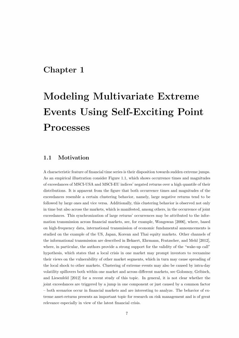
Contributions to Modeling Extreme Events on Financial and Electricity Markets Inauguraldissertation zur Erlangung des Doktorgrades der Wirtschafts- und Sozialwissenschaftlichen Fakult¨at der Universit¨ at zu K¨ oln 2013 vorgelegt von M.Sc. Volodymyr Korniichuk aus Kuznetsovsk (Ukraine)
Transcript of Contributions to Modeling Extreme Events on Financial and ... · Contributions to Modeling Extreme...
Contributions to Modeling Extreme Events onFinancial and Electricity Markets
Inauguraldissertation
zur
Erlangung des Doktorgrades
der
Wirtschafts- und Sozialwissenschaftlichen Fakultat
der
Universitat zu Koln
2013
vorgelegt
von
M.Sc. Volodymyr Korniichuk
aus
Kuznetsovsk (Ukraine)

Referent: Jun.-Prof. Dr. Hans Manner
Korreferent: Prof. Dr. Karl Mosler
Tag der Promotion: 21.01.2014

Acknowledgements
I carried out the research underlying the material of this thesis at the University of Cologne
under the supervision of Dr. Hans Manner and Dr. Oliver Grothe. I am sincerely grateful
to my supervisors for their constant support in my professional and personal development, for
their critical advice that has so often shown me the right direction, and for their patience during
our countless discussions. This dissertation would have never been accomplished without a wise
assistance of my supervisors. I would also like to thank Prof. Dr. Karl Mosler, who kindly
agreed to be my external examiner.
The financial and research support through the Cologne Graduate School is gratefully acknowl-
edged. CGS has been a constant source of encouragement where I have experienced an excellent
academic environment and a very friendly atmosphere. Many thanks go to my colleagues from
CGS and to Dr. Dagmar Weiler.
Finally, I would like to thank my parents Ludmila and Volodymyr Korniichuk, my brother
Andriy, and Olena Pobochiienko for their unconditional support.
i

Contents
Acknowledgements i
List of Figures iv
List of Tables vii
Introduction 1
1 Modeling Multivariate Extreme Events Using Self-Exciting Point Processes 7
1.1 Motivation . . . . . . . . . . . . . . . . . . . . . . . . . . . . . . . . . . . . . . . 7
1.2 Model . . . . . . . . . . . . . . . . . . . . . . . . . . . . . . . . . . . . . . . . . . 10
1.2.1 Univariate model . . . . . . . . . . . . . . . . . . . . . . . . . . . . . . . . 11
1.2.1.1 Self-exciting POT model . . . . . . . . . . . . . . . . . . . . . . 11
1.2.1.2 Decay and impact functions . . . . . . . . . . . . . . . . . . . . 13
1.2.1.3 Stationarity condition and properties of the SE-POT model . . . 14
1.2.1.4 Relationship of SE-POT and EVT . . . . . . . . . . . . . . . . . 18
1.2.2 Multivariate Model . . . . . . . . . . . . . . . . . . . . . . . . . . . . . . . 19
1.2.2.1 Model Construction . . . . . . . . . . . . . . . . . . . . . . . . . 19
1.2.2.2 A closer look at the model implied dependence . . . . . . . . . . 24
1.2.3 Properties of the multivariate model . . . . . . . . . . . . . . . . . . . . . 26
1.2.3.1 Joint conditional distribution of the marks . . . . . . . . . . . . 26
1.2.3.2 Probabilities of exceedances in a remote region . . . . . . . . . . 27
1.2.3.3 Contagion mechanism . . . . . . . . . . . . . . . . . . . . . . . . 27
1.2.3.4 Risk Management implications . . . . . . . . . . . . . . . . . . . 29
1.3 Estimation, Goodness-of-Fit and Simulation . . . . . . . . . . . . . . . . . . . . . 31
1.3.1 Univariate model estimation . . . . . . . . . . . . . . . . . . . . . . . . . . 31
1.3.2 Multivariate model estimation . . . . . . . . . . . . . . . . . . . . . . . . 32
1.3.3 Goodness-of-fit . . . . . . . . . . . . . . . . . . . . . . . . . . . . . . . . . 33
1.3.4 Simulation . . . . . . . . . . . . . . . . . . . . . . . . . . . . . . . . . . . 34
1.4 Application to Financial Data . . . . . . . . . . . . . . . . . . . . . . . . . . . . . 35
1.4.1 Data and Preliminary Analysis . . . . . . . . . . . . . . . . . . . . . . . . 36
1.4.2 Copula Choice . . . . . . . . . . . . . . . . . . . . . . . . . . . . . . . . . 36
1.4.3 Applying the Model . . . . . . . . . . . . . . . . . . . . . . . . . . . . . . 37
1.4.3.1 Two-dimensional Model . . . . . . . . . . . . . . . . . . . . . . . 37
1.4.3.2 Four-dimensional Model . . . . . . . . . . . . . . . . . . . . . . . 41
1.5 Conclusion . . . . . . . . . . . . . . . . . . . . . . . . . . . . . . . . . . . . . . . 45
Appendices 47
A Method of Moments 48
B Extreme value condition and the initial threshold 50
ii

Contents iii
C Marginal goodness-of-fit tests 53
D Goodness-of-fit for the bivariate model with the MM estimates 55
E Goodness-of-fit for the sub-models of the four-dimensional model 57
2 Forecasting extreme electricity spot prices 59
2.1 Motivation . . . . . . . . . . . . . . . . . . . . . . . . . . . . . . . . . . . . . . . 59
2.2 Defining a price spike . . . . . . . . . . . . . . . . . . . . . . . . . . . . . . . . . 60
2.3 Modeling magnitudes of the spikes . . . . . . . . . . . . . . . . . . . . . . . . . . 63
2.3.1 Description of the model . . . . . . . . . . . . . . . . . . . . . . . . . . . . 63
2.3.1.1 Modeling long tails in magnitudes of the spikes . . . . . . . . . . 63
2.3.1.2 Modeling dependence in magnitudes of the spikes . . . . . . . . 65
2.3.1.3 Estimation . . . . . . . . . . . . . . . . . . . . . . . . . . . . . . 68
2.3.1.4 Simulation and Goodness-of-fit . . . . . . . . . . . . . . . . . . . 68
2.3.2 Accounting for the price ceiling in magnitudes of the spikes . . . . . . . . 69
2.3.3 Estimation results . . . . . . . . . . . . . . . . . . . . . . . . . . . . . . . 70
2.4 Modeling durations between spike occurrences . . . . . . . . . . . . . . . . . . . . 73
2.4.1 Spike durations . . . . . . . . . . . . . . . . . . . . . . . . . . . . . . . . . 74
2.4.2 Models for the spike durations . . . . . . . . . . . . . . . . . . . . . . . . 74
2.4.3 Negative binomial duration model . . . . . . . . . . . . . . . . . . . . . . 75
2.4.3.1 Model description . . . . . . . . . . . . . . . . . . . . . . . . . . 76
2.4.3.2 Estimation . . . . . . . . . . . . . . . . . . . . . . . . . . . . . . 77
2.4.3.3 Simulation and Goodness-of-fit . . . . . . . . . . . . . . . . . . . 77
2.4.4 Estimation results . . . . . . . . . . . . . . . . . . . . . . . . . . . . . . . 78
2.5 Forecasting extreme electricity prices . . . . . . . . . . . . . . . . . . . . . . . . . 80
2.5.1 Forecasting approach . . . . . . . . . . . . . . . . . . . . . . . . . . . . . . 80
2.5.2 Out-of-sample forecasting performance . . . . . . . . . . . . . . . . . . . . 81
2.6 Conclusion . . . . . . . . . . . . . . . . . . . . . . . . . . . . . . . . . . . . . . . 84
3 Estimating tails in top-coded data 85
3.1 Motivation . . . . . . . . . . . . . . . . . . . . . . . . . . . . . . . . . . . . . . . 85
3.2 Preliminaries . . . . . . . . . . . . . . . . . . . . . . . . . . . . . . . . . . . . . . 86
3.2.1 Tail index . . . . . . . . . . . . . . . . . . . . . . . . . . . . . . . . . . . . 86
3.2.2 Top-coding . . . . . . . . . . . . . . . . . . . . . . . . . . . . . . . . . . . 87
3.2.3 Regularly varying tails . . . . . . . . . . . . . . . . . . . . . . . . . . . . . 88
3.2.4 Distribution of Exceedances . . . . . . . . . . . . . . . . . . . . . . . . . . 90
3.3 GPD-based estimator on top-coded data . . . . . . . . . . . . . . . . . . . . . . . 90
3.3.1 GPD and extreme value distributions . . . . . . . . . . . . . . . . . . . . 91
3.3.2 Estimation of GPD on excesses under top-coding . . . . . . . . . . . . . . 92
3.3.3 Properties of cGPD estimator: X ∼ GPD . . . . . . . . . . . . . . . . . . 94
3.3.4 Properties of cGPD estimator: X ∼ EVD . . . . . . . . . . . . . . . . . . 97
3.4 Hill estimator on top-coded data . . . . . . . . . . . . . . . . . . . . . . . . . . . 100
3.5 Comparison of cGPD and cHill . . . . . . . . . . . . . . . . . . . . . . . . . . . . 103
3.6 Applications . . . . . . . . . . . . . . . . . . . . . . . . . . . . . . . . . . . . . . . 106
3.6.1 Simulation study . . . . . . . . . . . . . . . . . . . . . . . . . . . . . . . . 106
3.6.2 Application to electricity prices . . . . . . . . . . . . . . . . . . . . . . . . 110
3.7 Conclusion . . . . . . . . . . . . . . . . . . . . . . . . . . . . . . . . . . . . . . . 112
Conclusion 114
Bibliography 116
List of Figures
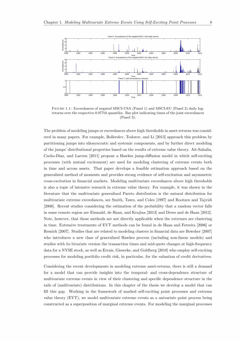
1.1 Exceedances of negated MSCI-USA (Panel 1) and MSCI-EU (Panel 2) daily log-returns over the respective 0.977th quantiles. Bar plot indicating times of thejoint exceedances (Panel 3). . . . . . . . . . . . . . . . . . . . . . . . . . . . . . . 8
1.2 Probability of a joint extreme event at time point t conditioned on the eventthat at least one of the margins jumps at t. . . . . . . . . . . . . . . . . . . 28
1.3 π2 (t, t+): instantaneous average number of second margin exceedances in the unitinterval triggered by the increase of ∆t,t+τ1(s, u1) (x-axis) in the first margin’sconditional rate. . . . . . . . . . . . . . . . . . . . . . . . . . . . . . . . . . . . . 28
1.4 π (t, t+): increase in the rate of the joint exceedances triggered by a joint ex-ceedance at time t. . . . . . . . . . . . . . . . . . . . . . . . . . . . . . . . . . . . 29
1.5 Estimated conditional rate of the marginal exceedances over the initial thresholdfor MSCI-USA and MSCI-EU. MLE estimates from Table 1.2. . . . . . . . . . . . 39
1.6 The estimated time-varying dependence parameter (left-hand panel) and the con-ditional probability of multivariate events when at least one margins exceed theinitial threshold (right-hand panel) in the two dimensional model. The tick marksat the bottom of the right panel denote times of multivariate events. . . . . . . . 40
1.7 Effects of different values of MSCI-EU and MSCI-US negated returns, that couldhave happened on 01.03.2009 (left panel) and 15.02.2010 (right panel), on the nextday’s conditional rate of joint exceedances. . . . . . . . . . . . . . . . . . . . . . . 40
1.8 Exponential QQ-plot of the residual inter-exceedance intervals (left-hand panel)in the bivariate model. The sample autocorrelation function of those (squared)intervals (right-hand panel). . . . . . . . . . . . . . . . . . . . . . . . . . . . . . . 41
1.9 The estimated conditional rates of the marginal exceedances over the initial thresh-old in the SE-POT model for negated log-returns of DB, HSBC, RBS, and UBSstocks. . . . . . . . . . . . . . . . . . . . . . . . . . . . . . . . . . . . . . . . . . . 42
1.10 The estimated time-varying dependence parameter (left-hand panel) and the con-ditional probability of multivariate events when at least one margins exceed theinitial threshold (right-hand panel) in the four-dimensional model. The tick marksat the bottom of the right panel denote times of multivariate events. . . . . . . . 44
1.11 Exponential QQ-plot of the residual inter-exceedances intervals in the four-dimensionalmodel (left-hand panel). The sample autocorrelation function of those (squared)intervals (right-hand panel). . . . . . . . . . . . . . . . . . . . . . . . . . . . . . . 44
B.1 Sample mean excess plots of negated daily log-returns of the MSCI-USA, MSCI-EU, DB, HSBC, RBS, and UBS. Solid red vertical lines indicate the initial thresh-old chosen for the model estimation. . . . . . . . . . . . . . . . . . . . . . . . . . 50
B.2 Estimated Q-curves on negated returns of MSCI-USA and MSCI-EU: k de-notes the number of upper order statistics used for estimation. . . . . . . . 51
B.3 Exponential QQ-plots of time intervals, measured in days, between consecutivemarginal exceeances above the initial threshold. . . . . . . . . . . . . . . . . . . . 51
B.4 Estimated Q-curves on negated log-returns of DB, HSBC, RBS, and UBS. . . . . 52
C.1 Exponential QQ-plot of the residual marginal inter-exceedances intervals. . . . . 53
C.2 Exponential QQ-plot of the residual marks. . . . . . . . . . . . . . . . . . . . . . 53
iv
List of Figures v
D.1 Estimated conditional rate of the marginal exceedances over the initial thresholdfor MSCI-USA and MSCI-EU. MM estimates from Table 1.2. . . . . . . . . . . . 55
D.2 The estimated time-varying dependence parameter (left-hand panel) and the con-ditional probability of multivariate events when at least one margins exceed theinitial threshold (right-hand panel) in the two dimensional model. The tick marksat the bottom of the right panel denote times of multivariate events. MM estimates. 55
D.3 Exponential QQ-plot of the residual inter-exceedance intervals (left-hand panel)in the bivariate model. The sample autocorrelation function of those (squared)intervals (right-hand panel). MM estimates. . . . . . . . . . . . . . . . . . . . . 56
E.1 Exponential QQ-plot for the residual inter-exceedance intervals of the bivariatesub-models of the four-dimensional model. . . . . . . . . . . . . . . . . . . . . . . 57
E.2 Exponential QQ-plot for the residual inter-exceedance intervals of the trivariatesub-models of the four-dimensional model. . . . . . . . . . . . . . . . . . . . . . . 58
2.1 Electricity prices in NSW region of Australia’s electricity market over the periodJan 1, 2002–Dec 31, 2011. . . . . . . . . . . . . . . . . . . . . . . . . . . . . . . . 60
2.2 Mean and standard deviation of the electricity prices pooled by 30-min period ofthe day. . . . . . . . . . . . . . . . . . . . . . . . . . . . . . . . . . . . . . . . . . 61
2.3 Diurnal threshold. Note: solid vertical lines illustrate parts of the day whereparameter ξ of the GPD can be assumed to be the same, details in Section 2.3.1.1. 62
2.4 Monthly proportions of the spikes. Note: the period of atypically high proportionof spikes in 2007 will be removed in modeling occurrences times of the spikes. . . 62
2.5 Sequential sample second moments of the electricity prices on the NSW region.The second moments were calculated on the electricity prices from the 1st Jan2002 to the time point denoted on x-axis. . . . . . . . . . . . . . . . . . . . . . . 63
2.6 Mean excess functions calculated for the NSW electricity prices pooled by 1st,14th, 19th, 36th, 45th, and 48th half-hour period of the day. . . . . . . . . . . . . 64
2.7 Spearman’s rank correlation between the lagged spike magnitudes. . . . . . . . . 65
2.8 Histogram of the electricity prices exceeding 400AUD/MWh. . . . . . . . . . . . 65
2.9 Autocorrelation of the residuals. Solid vertical lines show 99% confidence intervals. 72
2.10 QQ-plot of the transformed residuals. Green points show expected deviations ofthe residuals. . . . . . . . . . . . . . . . . . . . . . . . . . . . . . . . . . . . . . . 72
2.11 QQ-plot of the standardized durations (transformed by the theoretically implieddistribution to the standard exponential) of the estimated ACD models and theresidual inter-arrivals times of the estimated Hawkes process. The models wereestimated on NSW spike durations occurred in the period over January 1, 2008–December 31, 2010. . . . . . . . . . . . . . . . . . . . . . . . . . . . . . . . . . . . 75
2.12 Density function of the negative binomial distribution. . . . . . . . . . . . . . . . 76
2.13 QQ-plot of a typical sample of the estimated transformed generators. Comparethis figure with Figure 2.11. . . . . . . . . . . . . . . . . . . . . . . . . . . . . . . 79
2.14 The conditional probability of a spike occurrence on the four regions of Australia’selectricity market. The probability was estimated according to (2.18) with param-eters values from Table 2.6. pi was set on its max achievable value: pi = 0.0016for NSW; pi = 0.0017 for QLD; pi = 0.0232 for SA; pi = 0.0335 for VIC. . . . . . 81
3.1 Influence function. . . . . . . . . . . . . . . . . . . . . . . . . . . . . . . . . . . . 88
3.2 Mean (left panel) and standard deviation (right panel) of the asymptotic distri-bution of the cGPD estimators. For this illustration the parameters are set asfollows: ξ = 1/2, µ = 1/3, ρ = −1/5. . . . . . . . . . . . . . . . . . . . . . . . . . 100
3.3 Mean (left panel) and standard deviation (right panel) of the asymptotic distribu-tion of the cHill estimator. For this illustration the parameters are set as follows:ξ = 1/2, µ = 1/3, ρ = −1/5. . . . . . . . . . . . . . . . . . . . . . . . . . . . . . . 103

List of Figures vi
3.4 RMSE(ξ, ρ, λ∗) for various sets of the parameters ξ, ρ, λ∗. Note: instead of λ∗we report on the figure λ
−1/ξ∗ , which shows what proportion of the exceedances is
top-coded. . . . . . . . . . . . . . . . . . . . . . . . . . . . . . . . . . . . . . . . . 106
3.5 Estimates of ξ by the cGPD and the cHill estimators for the Parameter-set 1.Panel 1 and 3 correspond to the cGPD estimates. Panel 2 and 4 correspond tothe cHill estimates. . . . . . . . . . . . . . . . . . . . . . . . . . . . . . . . . . . 108
3.6 Estimates of ξ by the cGPD and the cHill estimators for the Parameter-set 2.Panel 1 and 3 correspond to the cGPD estimates. Panel 2 and 4 correspond tothe cHill estimates. . . . . . . . . . . . . . . . . . . . . . . . . . . . . . . . . . . 108
3.7 Estimates of ξ by the cGPD and the cHill estimators for the Parameter-set 3.Panel 1 and 3 correspond to the cGPD estimates. Panel 2 and 4 correspond tothe cHill estimates. . . . . . . . . . . . . . . . . . . . . . . . . . . . . . . . . . . 109
3.8 Estimates of ξ by the cGPD and the cHill estimators for the Parameter-set 4.Panel 1 and 3 correspond to the cGPD estimates. Panel 2 and 4 correspond tothe cHill estimates. . . . . . . . . . . . . . . . . . . . . . . . . . . . . . . . . . . 109
3.9 Daily maximum of SA electricity spot prices (since the data is very volatile, rang-ing from 15AUD/MWh to 12500AUD/MWh, it is plotted on the log-scale) . . . 111
3.10 Sample mean excess plots of daily maximum of SA electricity spot prices. A solidred vertical line indicates the threshold u1,N chosen for the estimation of ξ. . . . 111
3.11 Excess distribution functions implied by the cGPD and the cHill estimators com-pared to the empirical excess distribution function of the exceedances of dailymaxima of SA electricity prices. . . . . . . . . . . . . . . . . . . . . . . . . . . . . 112
List of Tables
1.1 Summary statistics . . . . . . . . . . . . . . . . . . . . . . . . . . . . . . . . . . . 36
1.2 Parameter estimates of the SE-POT model by the MLE and the MM. An inverseHessian of the likelihood function is used to obtain the standard errors reportedin parentheses right to the MLE estimates. . . . . . . . . . . . . . . . . . . . . . 38
1.3 Parameter estimates of the dependence parameter. An inverse Hessian of thelikelihood function is used to obtain the standard errors reported in parenthesesright to the MLE estimates. . . . . . . . . . . . . . . . . . . . . . . . . . . . . . . 39
1.4 MLE parameter estimates of the SE-POT model. An inverse Hessian of the likeli-hood function is used to obtain the standard errors reported in parentheses rightto the estimates. . . . . . . . . . . . . . . . . . . . . . . . . . . . . . . . . . . . . 41
1.5 p-values of the likelihood tests testing hypothesis that the bivariate dependencestructure in the four-dimensional model is symmetric. . . . . . . . . . . . . . . . 42
1.6 Parameter estimates of the four-dimensional model of exceedances. An inverseHessian of the likelihood function is used to obtain the standard errors reportedin parentheses right to the estimates. . . . . . . . . . . . . . . . . . . . . . . . . . 43
1.7 p-values the Kolmogorov-Smirnov (KS) and Ljung-Box (LB) with 15 lags tests forresidual inter-exceedances intervals for the two- and three-dimensional sub-modelsof the four-dimensional model. . . . . . . . . . . . . . . . . . . . . . . . . . . . . 44
C.1 p-values of Kolmogorov-Smirnov (KS) and Ljung-Box (LB) tests checking thehypothesis of exponentially distributed and uncorrelated residual inter-exceedanceintervals and marks of the marginal processes of exceedances. . . . . . . . . . . . 54
2.1 Descriptive statistics for half-hourly electricity spot prices (AUD/MWh) from thefour regions of Australia’s electricity market in the period over January 1, 2002–December 31, 2011. . . . . . . . . . . . . . . . . . . . . . . . . . . . . . . . . . . . 61
2.2 Parameter estimates of the model for spike magnitudes. . . . . . . . . . . . . . . 71
2.3 Estimated mean, standard deviation (std), mean relative bias (MRB), and meansquared error (MSE) of estimated parameters for the ceiling adjusted model from500 simulated paths. . . . . . . . . . . . . . . . . . . . . . . . . . . . . . . . . . . 72
2.4 Descriptive statistics of the actual and simulated prices (500 simulations). . . . . 73
2.5 Descriptive statistics for the spikes durations. . . . . . . . . . . . . . . . . . . . . 74
2.6 Parameter estimates of the negative binomial duration model estimated on thespike durations. . . . . . . . . . . . . . . . . . . . . . . . . . . . . . . . . . . . . 78
2.7 Goodness-of-fit test: non-rejection rates (in %) of the Kolmogorov-Smirnov andLjung-Box (10 lags) tests with a significance level of 1% conducted on 1000 randomsamples of the estimated generators. . . . . . . . . . . . . . . . . . . . . . . . . . 78
2.8 Descriptive statistics of the actual and simulated durations (500 simulations). . . 79
2.9 Out-of-sample performance of the models in forecasting electricity prices exceeding300AUD/MWh. . . . . . . . . . . . . . . . . . . . . . . . . . . . . . . . . . . . . . 82
2.10 Out-of-sample performance of our model in forecasting electricity prices exceeding500AUD/MWh, 1000AUD/MWh, 2000AUD/MWh, and 5000AUD/MWh levels. 83
3.1 Estimated bias, standard deviation, and mean squared error (MSE) of estimatesof ξ by the cGPD and cHill estimators (1000 simulations). . . . . . . . . . . . . . 110
vii
Introduction
Words like extremes, extremal events, worst case scenarios have long become an integral part
in the vocabulary of financial researches and practitioners. This is not without reason. In view
of the extreme and highly correlated financial turbulences in the last decades, the introduction
of new (ill-understood) derivative products, and growing computerization of financial trading
systems, it becomes evident that events that were believed to occur once in one hundred or
even one thousand years (based on the standard financial models) tend to occur much more
frequently than expected leading to severe unexpected losses on financial markets. Modeling
and forecasting those extreme events is a topic of vivid interest and great importance in the
current research of quantitative risk management and is exactly the topic of the thesis at hand.
In this thesis, we consider the problem of modeling very large (in absolute terms) returns on
financial markets and focus on describing their distributional properties. Our aim is to design
an approach that can accommodate the characteristic features of those returns, namely, heavy
tails, contagion effects, tail dependence, and clustering in both magnitudes and times of occur-
rences. Additionally, the thesis contributes to the literature on forecasting extreme electricity
spot prices. The challenge of this problem is determined, first, by the difficulty of modeling the
price directories in high-frequency settings, and, second, by the distinctive feature of electricity,
namely, its limited storability. Furthermore, in this thesis, we investigate a problem of estimat-
ing probability distributions whose tails decrease very slowly (heavy-tailed distributions). In
particular, we study the properties of two popular estimators of those distributions in the case
when the underlying data is top-coded, i.e., unknown above a certain threshold.
To cope with the task of describing extreme events, both an accurate quantitative analysis –
a focus of this thesis – as well as a sound qualitative judgement are required. Considering the
latter, for example, it is astonishing to see how many early warnings of the subprime crisis
2007 both in the press (see Danielsson [2013]) and in the academics (see Das, Embrechts, and
Fasen [2013] and Chavez-Demoulin and Embrechts [2011] for an overview) were ignored by the
regulators and practitioners. Examples of blunders with the quantitative analysis include, among
others, an extensive reliance on correlation based risk measures, which are known to be often
misleading, see Embrechts, McNeil, and Straumann [2002], and an often unjustified use of the
Gaussian copula in the standard pricing formulas for tranches of collateralized debt obligations.
It is known from Sibuya [1959] that this copula underestimates the probability of joint extremal
events, because it does not exhibit tail dependence, see Chavez-Demoulin and Embrechts [2011].
Whatever the reason of that misuse of quantitative methods in practice, the statistical modeling
1

Introduction 2
of extreme events, as a crucial component in understanding heavy-tailed phenomena, needs to
be further developed from a scientific point of view.
Currently there is general agreement that daily financial data is well described by (multivari-
ate) distributions whose tails are much heavier than the ones of the normal distribution and
whose dependence structure can accommodate clustering of extremes. Popular models that can
partly fulfil the above requirements are generalized autoregressive conditional heteroskedastic-
ity (GARCH) [Bollerslev, 1986] and stochastic volatility, see Shephard [1996] for an overview.
The popularity of those models is founded by their computational simplicity and ability to cap-
ture volatility clustering and heavy-tailed phenomena. Furthermore, a GARCH process can
also account for clustering of extremes [Davis and Mikosch, 2009a]. In particular, large values
of a GARCH process always occur in clusters, as opposed to a stochastic volatility process,
whose large values behave similarly to extremes of the corresponding serially independent pro-
cess [Davis and Mikosch, 2009b]. These findings imply that a GARCH model performs better
than a stochastic volatility model in describing the timing of extreme events in financial data.
Although displaying very useful features, there are limitations for using GARCH processes. In
particular, those processes do not seem to accurately capture the size of extremes in financial time
series [Mikosch and Starica, 2000]. Furthermore, the stationarity condition of GARCH processes
restricts their applications to situations with finite variance. As it will be highlighted in Section
2 of the thesis, the assumptions of finite variance is inappropriate for modeling electricity spot
prices. From a statistical point of view, extreme observations may also have strong deleterious
effects on the parameter estimates and tests of a GARCH model [van Dijk, Franses, and Lucas,
1999].
Overall, extreme observations have its own unique features which differ substantially from the
rest of the sample and hence cannot always be accommodated by models that are intended to
describe the whole structure of the data. To capture those unique features, there is increased
interest in approaches that use mainly extreme observations for inferences. This requirement
calls for applications of extreme value theory. In this thesis, we will introduce models developed
in the framework of that theory and consider specific problems of modeling extreme events on
financial as well as electricity markets that have attracted much attention in the literature in
recent years.
Extreme Value Theory (EVT) studies phenomena related to very high or very low values in
sequences of random variables and in stochastic processes. EVT provides fundamental theo-
retical results and a multitude of probabilistic approaches to modeling heavy tails and extreme
multivariate dependences. A basic result of the univariate EVT is the Fisher-Tippet-Gnedenko
theorem, see de Haan and Ferreira [2006] (Theorem 1.1.3), which allows for modeling the maxima
of a set of contiguous blocks of stationary data using the generalized extreme value distribution
(up to changes of location and scale) Hξ(x) = exp(−(1 + ξx)
−1/ξ+
). In particular, if for inde-
pendent random variables X1, X2, . . . with the same probability distribution function F , there
exist sequences an > 0, bn ∈ R, such that
limn→∞
P
(max (X1, X2, . . . , Xn)− bn
an≤ x
)= limn→∞
Fn (anx+ bn)→ H(x)
Introduction 3
where H(x) is a non-generate distribution function, then the only possible non-generate dis-
tribution H(x) is of the form Hξ(ax + b). Another model for extremes is provided by the
Pickands-Balkema-de Haan theorem (see Pickands [1975], Balkema and de Haan [1974]), which
is inherently connected to the previous model through a common basis of Karamata’s theory
of regular variation. According to that theorem the distribution of excesses of a heavy-tailed
random variable over a sufficiently high threshold is necessarily the generalized Pareto distri-
bution (GPD) G(x; ξ, β) = 1 − (1 + ξx/β)−1/ξ+ . The choice of that high threshold is however
complicated in practice as it depends on the second order properties of the distribution function,
see Chavez-Demoulin and Embrechts [2011]. Along with the GPD choice for the magnitudes of
the excesses, the occurrence of those excesses follows a Poisson process, see Leadbetter [1991].
The results of the univariate EVT allow for the statistical modeling of common risk measures
like Value-at-Risk (used more in banking) and expected shortfall (used more in insurance). Note
however that application of the GPD and the generalized extreme value distribution is often
confronted with a problem of interpretation of the parameters from a practitioner’s point of view
(in contrast to mean and standard deviation of the normal distribution). A fundamental work
considering the univariate EVT and applications of those models to financial data is Embrechts,
Kluppelberg, and Mikosch [1997], see also McNeil and Frey [2000] for estimation of tail related
risk measures. Extensions of the univariate EVT to stationary time series which show a certain
short-range dependence can be found in Leadbetter, Lindgren, and Rootzen [1983].
Multivariate extensions of the (classical) univariate EVT play also an important role in describ-
ing extreme events, especially considering their dependence structure. The basic result of the
multivariate EVT concerns the limit multivariate distribution of the componentwise block max-
ima. In particular, if for independent and identically distributed random vectors (X1,i, . . . , Xd,i),
i = 1, 2, . . . there exist sequences ak,n > 0, bk,n ∈ R, k = 1, . . . , d such that
limn→∞
P
(max (Xk,1, , . . . , Xk,n)− bk,n
ak,n≤ xk, k = 1, . . . , d
)→ H (x1, ..., xd)
where H (x1, ..., xd) is a distribution function with non-degenerate marginals, then H (x1, ..., xd)
is a multivariate extreme value distribution. This distribution is characterized by the margins,
which have the generalized extreme value distributions Hξk(x) = exp(−(1 + ξkx)
−1/ξk+
), k =
1, . . . , d, and by copula C, referred to as extreme value copula, for which it holds
∀a > 0,∀(u1, . . . , ud) ∈ [0, 1]d : C (u1, ..., ud) = C1/a (ua1 , ..., uad) .
A specific dependence structure (not unique) implied by the above property provides useful
copulas, for example Gumbel and Galambos copulas, for capturing the joint tail behavior of risk
factors that show tail dependence. Applications and discussions of multivariate extreme value
distributions can be found in de Haan and de Ronde [1998], Embrechts, de Haan, and Huang
[2000], Tawn [1990], Haug, Kluppelberg, and Peng [2011] and Mikosch [2005]. An extensive
textbook treatment of EVT can be found in de Haan and Ferreira [2006] and Resnick [2007].
The solid theoretical background behind EVT makes its application for modeling extreme events
natural and consequent. As it is noted in Chavez-Demoulin and Embrechts [2010], a careful use
of EVT models is preferred above the casual guessing of some parametric models that may fit
Introduction 4
currently available data over a restricted range, where only a few (if any) extreme observations are
available. Due to the strict underlying assumptions and the non-dynamic character, however, the
methods of EVT are not always directly applicable in situations where the extremes are serially
dependent, as it is the case in almost all financial time series. This problem was discussed, among
others, in Leadbetter, Lindgren, and Rootzen [1983], Chavez-Demoulin, Davison, and McNeil
[2005], Chavez-Demoulin and McGill [2012], Davison and Smith [1990], Coles [2001] (Chapter
5), and see also Chavez-Demoulin and Davison [2012] for an overview.
In this thesis we will attempt to contribute to the literature by proposing models which extend
the current results of EVT and offer new insight with modeling extreme events in serially de-
pendent time series. In particular, we will review theoretical and practical questions that arise
in the process of modeling extreme events on financial and electricity markets in daily and high-
frequency settings. Under extreme events we understand situations when a financial parameter
(e.g., equity return, electricity spot price) exceeds a characteristic high threshold (e.g., 99.9%th
quantile). The questions of conditional modeling occurrence times and magnitudes (heavy tails)
of those events as well as their complex dependence structure will be addressed.
Outline and summary
Chapter 1 deals with the problem of modeling multivariate extreme events observed in finan-
cial time series. The major challenge coping with that problem is to provide insights into the
temporal- and cross-dependence structure of those extreme events in view of their clustering,
which is observed both in their sizes and occurrence times, and specific dependence structure
in the tails of multivariate distributions. Furthermore, those events demonstrate a certain syn-
chronization in occurrences across markets and assets (e.g., contagion effects), which motivates
the application of multivariate methods. To capture those characteristic features, we develop a
multivariate approach based on self-exciting point processes and EVT. We show that the con-
ditional rate of the point process of multivariate extreme events (constructed as a superposition
of the univariate processes) is functionally related to the multivariate extreme value distribution
that governs the magnitudes of the observations. This extreme value distribution combines the
univariate rates of the point processes of extreme events into the multivariate one. Extensive
references to the point process approach to EVT can be found in Resnick [1987]. Due to its point
process representation, the model of Chapter 1 provides an integrated approach to describing two
inherently connected characteristics: occurrence times and sizes of multivariate extreme events.
A separate contribution of this chapter is a derivation of the stationarity conditions for the self-
exciting peaks-over-threshold model with predictable marks (this model was first presented in
McNeil, Frey, and Embrechts [2005], Section 7.4.4). We discuss the properties of the model, treat
its estimation (maximum likelihood and method of moments), deal with testing goodness-of-fit,
and develop a simulation algorithm. We also consider an application of that model to return
data of two stock markets (MSCI-EU, MSCI-USA) and four major European banks (Deutsche
Bank, HSBC, UBS, and RBS).
Along with financial time series, electricity spot prices are also strongly exposed to sudden
extreme jumps. Contrary to financial markets, where the reasons of turmoil are often explained
by behavioral aspects of the market participants, in electricity markets the occurrence of extreme
prices is attributed to an inelastic demand for electricity and very high marginal production
Introduction 5
costs in the case of unforeseen supply shortfalls or rises in the demand for electricity. Due to
the lack of practical ways to store electricity, those inelasticities and high marginal costs may
manifest themselves in electricity prices that exceed the average level a hundred times. This
type of price behavior presents an important topic for risk management research and is of great
relevance for electricity market participants, for example, retailers, who buy electricity at spot
prices but redistribute it at fixed prices to consumers. In Chapter 2 of this thesis we present a
model for forecasting the occurrence of extreme electricity spot prices. The unique feature of
this model is its ability to forecast electricity price exceedances over very high thresholds (e.g.
99.99%th quantile), where only a few (if any) observations are available. The model can also be
applied for simulating times of occurrence and magnitudes of the extreme prices. We employ a
copula with a changing dependence parameter for capturing serial dependence in the extreme
prices and the censored GPD (to account for possible price ceilings on the market) for modeling
their marginal distributions. For modeling times of the extreme price occurrences we propose a
duration model based on a negative binomial distribution, which can reproduce large variation, a
strong clustering pattern and the discrete nature of the time intervals between the occurrences of
extreme prices. This duration model outperforms the common approaches to duration modeling:
the autoregressive duration models (Engle and Russell [1998]) and the Hawkes processes (Hawkes
[1971]), see Bauwens and Hautsch [2009] for an overview. Once being estimated, our forecasting
model can be applied (without re-estimation) for forecasting occurrences of price exceedances
over any sufficiently high threshold. This unique feature is provided by a special construction
of the model in which price exceedances over very high thresholds may be triggered by the
price exceedances over a comparatively smaller threshold. Our forecasting model is applied to
electricity spot prices from Australia’s national electricity market.
Another research question addressed in this thesis is the estimation of heavy-tailed distribu-
tions on top-coded observations, i.e., observations, whose values are unknown above a certain
threshold. Not knowing the exact values of the upper-order statistics in the data, the top-coding
(right-censoring) may have a strong effect on estimation of the main characteristic of the heavy-
tailed distributions – the tail index, the decay rate of the power function that describes the
distribution’s tail. This problem occurs, for example, in the insurance industry where, due to
the policy limits on insurance products, the amount by how much the insurance claims (typically
heavy-tailed) exceed those limits is not available. The tail index plays a crucial role in determin-
ing common risk measures (e.g., Value-at-Risk, expected shortfall) and is therefore required to
be estimated accurately. In Chapter 3 we examine how two popular estimators of the tail index
can be extended to the settings of top-coding. We consider the maximum likelihood estimator of
the generalized Pareto distribution and the Hill estimator. Working in the framework of Smith
[1987], we establish the asymptotic properties of those estimators and show their relationship to
various levels of top-coding. For high levels of top-coding and small values of the tail index, our
findings suggest a superior performance of the Hill estimator over the GPD approach. This result
contradicts the broad conclusion about the performance of those estimators in the uncensored
case as it was established in Smith [1987].
The main chapters of the thesis are based on academic papers. Chapter 1 is in line with Grothe,
Korniichuk, and Manner [2012], which is a joint work of Oliver Grothe, Volodymyr Korniichuk,
and Hans Manner, all of whom have contributed substantially to the paper. Korniichuk [2012]

Introduction 6
underlies Chapter 2. Finally, Chapter 3 is based on Korniichuk [2013]. Since the papers under-
lying the chapters of the thesis are independent of each other, those chapters can be read in any
order. Each of the chapters has a detailed introduction (motivation) and a conclusion. The final
chapter of the thesis shortly summarizes the major contributions.
Chapter 1
Modeling Multivariate Extreme
Events Using Self-Exciting Point
Processes
1.1 Motivation
A characteristic feature of financial time series is their disposition towards sudden extreme jumps.
As an empirical illustration consider Figure 1.1, which shows occurrence times and magnitudes
of exceedances of MSCI-USA and MSCI-EU indices’ negated returns over a high quantile of their
distributions. It is apparent from the figure that both occurrence times and magnitudes of the
exceedances resemble a certain clustering behavior, namely, large negative returns tend to be
followed by large ones and vice versa. Additionally, this clustering behavior is observed not only
in time but also across the markets, which is manifested, among others, in the occurrence of joint
exceedances. This synchronization of large returns’ occurrences may be attributed to the infor-
mation transmission across financial markets, see, for example, Wongswan [2006], where, based
on high-frequency data, international transmission of economic fundamental announcements is
studied on the example of the US, Japan, Korean and Thai equity markets. Other channels of
the informational transmission are described in Bekaert, Ehrmann, Fratzscher, and Mehl [2012],
where, in particular, the authors provide a strong support for the validity of the “wake-up call”
hypothesis, which states that a local crisis in one market may prompt investors to reexamine
their views on the vulnerability of other market segments, which in turn may cause spreading of
the local shock to other markets. Clustering of extreme events may also be caused by intra-day
volatility spillovers both within one market and across different markets, see Golosnoy, Gribisch,
and Liesenfeld [2012] for a recent study of this topic. In general, it is not clear whether the
joint exceedances are triggered by a jump in one component or just caused by a common factor
– both scenarios occur in financial markets and are interesting to analyze. The behavior of ex-
treme asset-returns presents an important topic for research on risk management and is of great
relevance especially in view of the latest financial crisis.
7
Chapter 1. Modeling Multivariate Extreme Events Using Self-Exciting Point Processes 8
1990 1992 1994 1996 1998 2000 2002 2004 2006 2008 2010 20120
2
4
6
8Panel 1: Exceedances of the negated MSCI−USA daily returns
Time
Exc
eeda
nces
1990 1992 1994 1996 1998 2000 2002 2004 2006 2008 2010 20120
2
4
6
8Panel 2: Exceedances of the negated MSCI−EU daily returns
Time
Exc
eeda
nces
1990 1992 1994 1996 1998 2000 2002 2004 2006 2008 2010 20120
0.5
1Panel 3: Joint Exceedances Indicator
Time
Figure 1.1: Exceedances of negated MSCI-USA (Panel 1) and MSCI-EU (Panel 2) daily log-returns over the respective 0.977th quantiles. Bar plot indicating times of the joint exceedances
(Panel 3).
The problem of modeling jumps or exceedances above high thresholds in asset-returns was consid-
ered in many papers. For example, Bollerslev, Todorov, and Li [2013] approach this problem by
partitioning jumps into idiosyncratic and systemic components, and by further direct modeling
of the jumps’ distributional properties based on the results of extreme value theory. Aıt-Sahalia,
Cacho-Diaz, and Laeven [2011] propose a Hawkes jump-diffusion model in which self-exciting
processes (with mutual excitement) are used for modeling clustering of extreme events both
in time and across assets. That paper develops a feasible estimation approach based on the
generalized method of moments and provides strong evidence of self-excitation and asymmetric
cross-excitation in financial markets. Modeling multivariate exceedances above high thresholds
is also a topic of intensive research in extreme value theory. For example, it was shown in the
literature that the multivariate generalized Pareto distribution is the natural distribution for
multivariate extreme exceedances, see Smith, Tawn, and Coles [1997] and Rootzen and Tajvidi
[2006]. Recent studies considering the estimation of the probability that a random vector falls
in some remote region are Einmahl, de Haan, and Krajina [2013] and Drees and de Haan [2012].
Note, however, that those methods are not directly applicable when the extremes are clustering
in time. Extensive treatments of EVT methods can be found in de Haan and Ferreira [2006] or
Resnick [2007]. Studies that are related to modeling clusters in financial data are Bowsher [2007]
who introduces a new class of generalized Hawkes process (including non-linear models) and
studies with its bivariate version the transaction times and mid-quote changes at high-frequency
data for a NYSE stock, as well as Errais, Giesecke, and Goldberg [2010] who employ self-exciting
processes for modeling portfolio credit risk, in particular, for the valuation of credit derivatives.
Considering the recent developments in modeling extreme asset-returns, there is still a demand
for a model that can provide insights into the temporal- and cross-dependence structure of
multivariate extreme events in view of their clustering and specific dependence structure in the
tails of (multivariate) distributions. In this chapter of the thesis we develop a model that can
fill this gap. Working in the framework of marked self-exciting point processes and extreme
value theory (EVT), we model multivariate extreme events as a univariate point process being
constructed as a superposition of marginal extreme events. For modeling the marginal processes

Chapter 1. Modeling Multivariate Extreme Events Using Self-Exciting Point Processes 9
of exceedances we revise the existing specification of the univariate self-exciting peaks-over-
threshold model of Chavez-Demoulin, Embrechts, and Neslehova [2006] and McNeil, Frey, and
Embrechts [2005], which is able to cope with the clustering of extremes (in both times and
magnitudes) in the univariate case. After this revision, we are able to formulate stationarity
conditions, not discussed in the literature before, and to analyze the distributional properties of
the model. This constitutes a separate contribution of this chapter of the thesis.
We show that the only way how the marginal rates can be coupled into the multivariate rate
of the superposed process is through the exponent measure of an extreme value copula. The
copula used for the construction of the multivariate rate follows naturally from EVT arguments,
and is the same extreme value copula that governs the (conditional) multivariate distribution
of the marginal exceedances at the same point of time. This result provides an integrated ap-
proach to modeling occurrence times and sizes of multivariate extreme events, because those two
characteristics are inherently connected. Furthermore, the results provide insight into the depen-
dence between point processes that are jointly subject to EVT. This is in contrast to alternative
approaches in the literature, where the dependence between marginal point processes is incor-
porated through an affine mutual excitement, see, for example, Aıt-Sahalia, Cacho-Diaz, and
Laeven [2011], Embrechts, Liniger, and Lin [2011], and magnitudes of the jumps (if considered)
are modelled in a separate way.
Concerning the advantages of our method, it is worth noting that we use the data explicitly only
above a high threshold. This allows us to leave the time series model for the non-extreme parts
of the data unspecified. We consider the dependence structure of multivariate exceedances only
in regions where the results from multivariate extreme value theory (MEVT) are valid. Further-
more, the MEVT enables us to extrapolate exceedance probabilities far into remote regions of
the tail where hardly any data is available. With such a model we are able to extract the prob-
abilities of arbitrary combinations of the dimensions in any sufficiently remote region. Since the
model captures clustering behavior in (multivariate) exceedances, and accounts for the fact that
not only times but also sizes of exceedances may trigger subsequent extreme events, the model
provides asymmetric influences of marginal exceedances so that spill-over and contagion effects
in financial market may be analyzed. This model may be of great interest for risk management
purposes. For example, we can estimate the probabilities that from a portfolio of, say, d assets,
a certain subset falls in a remote (extreme) set conditioned on the event that some other assets
(or at least one of them) from that portfolio take extreme values at the same point of time. We
shortly discuss other possible risk management applications of the model and provide real data
examples.
To estimate our proposed model, we derive the closed form likelihood function and describe the
goodness-of-fit and simulation procedures. As noted earlier, our model treats a multivariate
extreme exceedance as a realization of a univariate point process. This property is advantageous
for the estimation, because, as it is mentioned in Bowsher [2007], there are currently no results
concerning the properties of the maximum likelihood estimation (MLE) for multivariate point
processes. For the univariate case, on the other hand, it is shown in Ogata [1978], that under
some regularity conditions, the MLE for a stationary, simple point process is consistent and
asymptotically normal. Inspired by Aıt-Sahalia, Cacho-Diaz, and Laeven [2011], we consider
Chapter 1. Modeling Multivariate Extreme Events Using Self-Exciting Point Processes 10
also the model estimation based on method of moments, which, however, seems to underperform
the MLE in the case of our model. The reason for this may lie in both the choice of moment
conditions and in the fact that all moment conditions are based on the goodness-of-fit statistics,
which cannot be directly calculated from the sample independently from the unknown parameters
of the models.
In the empirical part of the chapter, we apply our model to study extreme negative returns
on the financial markets (USA, Europe) and in the European banking sector (Deutsche Bank,
RBS, HSBC, and UBS). The results of goodness-of-fit tests demonstrate a reasonable fit of
the model and suggest an empirical importance of the self-exciting feature for modeling both
occurrence times, magnitudes, and interdependencies of the extreme returns. We find that
conditional multivariate distributions of the returns are close to symmetric with the strength
of dependence strongly responding to individual jumps. Despite the symmetrical structure of
the distribution, there are still asymmetric effects coming from the self-exciting structure of the
conditional marginal distributions of the exceedances’ magnitudes. This self-exciting structure
provides also a natural way how to model time-varying volatility of the magnitudes and, hence,
their heavy tails.
The rest of the chapter is structured as follows. The model and its properties are derived in
Section 1.2. In Section 1.3 we describe estimation of the model, along with the goodness-of-fit
and simulation procedures. Section 1.4 presents applications of the model to financial data and
Section 1.5 concludes. Finally, some of the goodness-of-fit graphs and intermediary calculations
are relegated to the Appendix.
1.2 Model
The major challenges in constructing the model presented in this section are twofold. First, the
model should capture the distinctive features of multivariate extreme events typically observed
in financial markets, namely, clustering and spillover effects. Second, the model should be able to
account for the specific distributional properties of magnitudes of extreme observations (i.e., for
the distributions over the threshold). For both reasons, our model is developed in the framework
of extreme value theory and marked point processes.
Throughout the text we use the following notation. Consider a random vector Xt = (X1,t, . . . , Xd,t)
which may, e.g., represent daily (negated) log-returns of d equities at time t. By u = (u1, . . . , ud),
the initial threshold, we denote a vector with components relating to sufficiently high quantiles
of the marginal distributions of Xt. We focus on the occurrence times as well as the magni-
tudes of multivariate extreme observations, which we define as situations when Xt exceeds u
in at least one component. Under an i-th marginal extreme event we understand the situation
when Xi,t > ui. We refer to such extreme events as marginal exceedances and characterise
them by occurrence times Ti,1, Ti,2, . . . and magnitudes (the marks) of realizations Xi,1, Xi,2, . . .,
i.e., Xi,k = Xi,Ti,k . The history that includes both the times and magnitudes of exceedances of
(Xi,s)s<t above ui will be denoted as Hi,t and the combined history over all marginal exceedances
is denoted as Ht =⋃di=1 Hi,t.
Chapter 1. Modeling Multivariate Extreme Events Using Self-Exciting Point Processes 11
This section is structured as follows. Section 1.2.1 deals with the univariate self-exciting peaks-
over-threshold model, which is the basis for our multivariate model developed in Section 1.2.2.
Section 1.2.3 provides some properties of the multivariate model.
1.2.1 Univariate model
This section deals with the univariate self-exciting peaks-over-threshold model. After a short
review of this model, we reconsider some parts of its construction to enrich it with some new
useful properties. In particular, we suggest a new specification for the impact function which,
contrary to its existing specification, provides an intuitively reasonable mechanism how past
exceedances trigger the future ones (Section 1.2.1.2), allows us to set a stationarity condition
and to develop some distributional properties of the univariate model (Section 1.2.1.3). Finally,
in Section 1.2.1.4 we consider the relationship of the univariate self-exciting peaks-over-threshold
model to the general framework of the extreme value theory.
1.2.1.1 Self-exciting POT model
The basic setup to model univariate exceedances is to assume independent and identically dis-
tributed (iid) data and to use a peaks-over-threshold (POT) model developed in Davison and
Smith [1990] and Leadbetter [1991]. In the framework of EVT, the POT model is based on
the asymptotic behavior of the threshold exceedances for iid or stationary data if these are in
the maximum domain of attraction of some extreme value distribution. If the threshold is high
enough, then the exceedances occur in time according to a homogeneous Poisson process and
the mark sizes are independently and identically distributed according to the generalized Pareto
distribution (GPD).
The self-exciting POT model presented in Chavez-Demoulin, Davison, and McNeil [2005] ex-
tends the standard set-up of the POT model by allowing for temporal dependence between
extreme events. This temporal dependence is introduced into the model by modeling the rate of
occurrences in the standard POT method with self-exciting processes, see Hawkes [1971].
Definition 1.1. (Self-exciting point process) A point process N(t), representing the cumulative
number of events up to time t, is called a (linear) self-exciting process with the conditional rate
τ(t), if
P (N(t+ ∆)−N(t) = 1 | Ht) = τ(t)∆ + o(∆), P (N(t+ ∆)−N(t) > 1 | Ht) = o(∆)
with
τ(t) = τ + ψ
∫ t
−∞c(Xs
)g (t− s) dN(s), τ > 0, ψ ≥ 0,
where Xs indicates the event’s mark at time s. The impact function c(·) determines the contri-
bution of events to the conditional rate and the decay function g(·) determines the rate how an
influence of events decays in time. When no mark is associated with the event c(Xs
)≡ 1.
Chapter 1. Modeling Multivariate Extreme Events Using Self-Exciting Point Processes 12
Choices of impact and decay functions are discussed in Section 1.2.1.2. The self-exciting POT
is further extended in McNeil, Frey, and Embrechts 2005, where the temporal dependence is
incorporated also into the conditional distribution of the marks, i.e., also the distribution of the
marks depends on past information. We refer to this model as the self-exciting POT model with
predictable marks (SE-POT). For convenience and consistency of notation we present the model
using subindizes i = 1 . . . d which will later refer to the dimensions of our multivariate model.
In the SE-POT model, the rate of crossing the initial threshold ui is modelled by a self exciting
point process where the rate is parametrized as
τi(t, ui) = τi + ψiv∗i (t), τi > 0, ψi ≥ 0, (1.1)
with
v∗i (t) =
∫ t
−∞ci (Xi,s) gi (t− s) dNi(s), (1.2)
where again ci(·) and gi(·) denote, respectively, the impact and decay functions, and Ni(s) is a
counting measure of i-th margin exceedances.
Additionally, the excesses over the threshold ui are now assumed to follow the GPD with shape
parameter ξi and time varying scale parameter βi + αiv∗(t). In particular, for xi > ui,
P (Xi,t ≤ xi | Xi,t > ui,Hi,t) = 1−(
1 + ξixi − ui
βi + αiv∗i (t)
)−1/ξi
=: Fi,t (xi) , βi > 0, αi ≥ 0.
(1.3)
This distribution covers the cases of Weibull (ξi < 0), Gumbel (ξi = 0) and Frechet (ξi > 0) tails,
corresponding to distributions with finite endpoints, light tails, and heavy tails, respectively. For
ξi = 0, the distribution function in (1.3) should be interpreted as Fi,t (xi) = 1 − e−xi . Finally,
due to the GPD as the conditional distribution of the marks, the conditional rate of exceeding
a higher threshold xi ≥ ui scales in the following way
τi(t, xi) = τi(t, ui)
(1 + ξi
xi − uiβi + αiv∗i (t)
)−1/ξi
, xi ≥ ui, (1.4)
where τi(t, ui) is the rate of crossing the initial threshold ui given by Equation (1.1). The
conditional rate τi(t, xi) explicitly describes the conditional distribution of times of exceedances
above any threshold xi ≥ ui in the following way.
P(Ti,k+1 (xi) ≤ t | Hi,Ti,k(xi)
)= 1− exp
(−∫ t
Ti,k(xi)
τi(s, xi)ds
), t ≥ Ti,k (xi) , (1.5)
where Ti,k (xi) denotes (random) time of the k-th exceedance of (Xi,s)s∈R above xi. The above
relationship is a direct consequence of the definition of the conditional intensity as the combina-
tion of hazard rates of the time intervals between exceedances, see Daley and Vere-Jones [2005],
p. 231. There is a small abuse of notation in the equation above, as, to make the notation easy,
we interchange the use of a hazard rate, a deterministic function, with the conditional intensity,
a piecewise determined amalgam of hazard rates.
Note that the self-exciting component v∗i (t) enters both τi(t, ui) in (1.1) and Fi,t in (1.3) and thus
provides a specific “clustering mechanism” into the conditional distribution of both times and
Chapter 1. Modeling Multivariate Extreme Events Using Self-Exciting Point Processes 13
marks of exceedances. After an exceedance occurs at time t0 with mark x0, the function v∗i (·)jumps by ci (x0) and increases the instantaneous probability of the exceedance’s occurrence and
the marks’ volatility (through time-varying scale parameter βi(t)). In absence of exceedances
v∗i (·) tends towards zero through function gi (·). Being a transmitter of information of past
exceedances to the future ones, the function v∗i (·) may be interpreted as a kind of volatility
measure of extreme exceedances. This interpretation may be found also in Bowsher [2007], where
the estimated mid-quote intensity is used as approximation to the stock price’s instantaneous
volatility.
The clustering mechanism of the SE-POT model, how past exceedances may trigger the oc-
currence of future exceedances, can quite accurately describe the cluster behavior of extreme
exceedances observed on financial markets, see Chavez-Demoulin and McGill [2012]. That is
why the SE-POT model is chosen as a cornerstone for our multivariate model developed in
Section 1.2.2.
Because of the overall importance of the SE-POT model for our multivariate model, in the next
sections we develop some of its distributional properties, including a stationarity condition, and
reconsider the existing specifications for the decay and impact functions.
1.2.1.2 Decay and impact functions
Considering functional specification of the decay and impact functions in (1.2) there are advan-
tages in some specific forms. The decay function chosen in this thesis is g(s) = e−γs, γ > 0
(the subindex “i” is dropped), which is a popular specification suggested in Hawkes [1971]. This
specification makes the self-exciting process a Markov process [Oakes, 1975] and leads to a simple
formula for the covariance density (derived in Proposition 1.3). This choice is also motivated in
view of Boltzman’s theory of elastic after-effects, see Ogata [1988], p.11. An alternative is the
function g(s) = (s+ γ)−(1+ρ)
, with γ, ρ > 0. This specification originally comes from seismology,
where is known as Omori law, see Helmstetter and Sornette [2002]. Due to the substantial ad-
vantages in deriving the analytical formulas, we will stick to g(s) = e−γs throughout this chapter
of the thesis.
The aim of the impact function c(·) is to capture the effect of the marks of exceedances onto the
conditional rate of future exceedances. A popular choice is c(x) = eδx, see for example Chavez-
Demoulin and McGill [2012] or McNeil, Frey, and Embrechts [2005] (Section 7.4.3). However, an
important point to consider when specifying that function is to ensure its ability to accurately
extract information from the marks. Provided the conditional distribution of the marks is time-
varying (as it is indeed the case with the SE-POT model, see (1.3)), one expects c(·) to account
not only for the magnitudes of the marks but also for the conditional distribution from which they
were drawn. To put it differently, not the size of the mark but its quantile in the corresponding
conditional distribution is decisive in determining the effect of the mark onto the conditional
rate. Thus, instead of specifying c(·) as a fixed function, we suggest the following specification
c(xt) = c∗ (Ft(xt)) ,

Chapter 1. Modeling Multivariate Extreme Events Using Self-Exciting Point Processes 14
where Ft is the marks’ conditional distribution (1.3) and c∗(·) is an increasing function [0, 1]→[1,∞]. This specification can properly capture the time-varying impact of an exceedance on the
conditional rate. An easy way to construct c∗(·) is as c∗(·) = 1 + G←(·), where G←(·) is the
inverse of a distribution function G of some continuous positive random variable with finite mean
δ. With such c∗(·) the impact function takes the form
c(xt) = 1 +G← (Ft(xt)) . (1.6)
We will use the above specification for the impact function throughout the text. In the empirical
part of this chapter, we will use G← of an exponential distribution, which yields c∗(u) = 1 −δ log(1− u).
Besides the appropriate extraction of information from the marks, the choice (1.6) for the impact
function is advantageous over c(x) = eδx, because (1.6) allows us to set the stationarity condition
for the SE-POT model and to develop its distributional properties. In the next section we discuss
those properties.
1.2.1.3 Stationarity condition and properties of the SE-POT model
As it was noted in Chavez-Demoulin, Davison, and McNeil [2005], the SE-POT model relates to
the class of general self-exciting Hawkes processes and constitutes by its construction a branching
process. A comprehensible explanation of the Hawkes process’ representation as a branching
process can be found in Møller and Rasmussen [2005] or Hawkes and Oakes [1974].
According to the branching process representation, there are two types of exceedances above the
initial threshold in the SE-POT model: immigrants, that arrive as a homogeneous Poisson process
with a constant rate τ , and descendants (triggered events), that follow a finite Poisson process
with decaying rate determined by function v∗(·), see Daley and Vere-Jones [2005] (see Example
6.3(c)). Since both immigrants and descendants can trigger further descendants, for setting
stationarity conditions it is necessary to consider the average number of the first-generation
descendants trigged by one exceedance (whether by an immigrant or descendant).
That average number of triggered descendants is known as a branching coefficient and we denote
it as ν. It is usual to consider ν = 1 as a certain level of stability of the exceedance process:
if ν ≥ 1 the development of the process could explode, i.e., the number of events in finite time
interval tends to infinity. Clearly, in that case the process is non-stationary. In the seismological
literature, see Helmstetter and Sornette [2002], the situation of ν > 1 is called super-critical
regime.
For practical application the case ν < 1 is the most important because then the process of
exceedances becomes stationary, provided the process of immigrants is stationary as well (which
is the case in the SE-POT model). In the SE-POT model with ν < 1, exceedances occur in finite
clusters of length (1 − ν)−1, where exceedances within the cluster are temporally dependent
but the clusters themselves are independent. In Proposition 1.2 we provide a formula for the
branching coefficient and the stationarity condition of the SE-POT model.
Chapter 1. Modeling Multivariate Extreme Events Using Self-Exciting Point Processes 15
Proposition 1.2. The process of exceedances with the conditional intensity τ(t, u) of the SE-
POT model, where τ(t, u) is as in (1.1)-(1.2) (dropping the subindex i), with decay function
g(s) = e−γs, and the impact function as in (1.6), has the branching coefficient ν = ψ(1+δ)γ and
is stationary if ν < 1 with an average rate τ := E[τ(t, u)] = τ1−ν .
Proof. Due the branching process’s representation of the SE=POT model, the sufficient condition
for stationarity of the SE-POT with conditional intensity τ(t) requires Eτ(t) = τ ∈ (0,∞), see
Daley and Vere-Jones [2005], Ex.6.3(c). From (1.1) τ can be expressed as
τ = τ + ψE
∫ t
−∞c(Xs
)g (t− s) dN(s). (1.7)
Note, that from the interpretation of the branching coefficient in Hawkes and Oakes [1974] and
Daley and Vere-Jones [2005] (Example 6.3(c)) it follows that ν = ψE∫ t−∞ c
(Xs
)g (t− s) dN(s).
Since the integral on the right-hand side of the above equation is just a sum of random variables,
we can write
E
∫ t
−∞c(Xs
)g (t− s) dN(s) =
∫ t
−∞g (t− s) E
[c(Xs
)dN(s)
]. (1.8)
From construction of the SE-POT model, see (1.1) and (1.3), it immediately follows that random
variables Xs and dN(s) are dependent in general but conditional v∗(s) (or even Hs) they are
independent. Hence it follows,
E{c(Xs
)dN(s)
}= E
{E[c(Xs
)dN(s)
∣∣∣Hs]} = E{
E[c(Xs
)∣∣∣Hs] E [dN(s)|Hs]}, (1.9)
where E [dN(s) | Hs] = τ(s)ds and, considering the conditional distribution of Xs in (1.3),
E[c(Xs
)∣∣∣Hs] =
∫ ∞0
c(x)fs(x)dx,
where fs(x) = dFs(x)dx = 1
β+αv∗(s)
(1 + ξ x
β+αv∗(s)
)−1/ξ−1
is the conditional distribution density
function of Xs.
Note that the integral in the above equation tends to infinity in all cases when the order of c(x)
exceeds 1/ξ. In particular, the integral tends to infinity with c(x) = eδx, which is a commonly
used specification for c(x) in the literature Chavez-Demoulin, Davison, and McNeil [2005] and
McNeil, Frey, and Embrechts [2005]. With the specification (1.6), however, we get
E[c(Xs
)∣∣∣Hs] =
∫ ∞0
c∗ (Fs(x)) fs(x)dx =
∫ 1
0
c∗ (u) du.
In Section 1.2.1.2 it was suggested to construct c∗(·) as c∗(·) = 1 + G←(·), where G←(·) is an
inverse of the distribution function G of some continuous positive random variable with mean δ.
Using this construction to calculate integral in the above equation we get
E[c(Xs
)∣∣∣Hs] = 1 + δ. (1.10)

Chapter 1. Modeling Multivariate Extreme Events Using Self-Exciting Point Processes 16
Substituting this result and E [dN(s) | Hs] = τ(s)ds into (1.9) we get
E[c(Xs
)dN(s)
]= τ(1 + δ)ds,
which with (1.8) provides a formula for the expected value
E
∫ t
−∞c(Xs
)g (t− s) dN(s) = τ(1 + δ)
∫ ∞0
g (s) ds.
Substituting the above equation into (1.7), finally yields
τ =τ
1− ψ(1 + δ)∫∞
0g (s) ds
. (1.11)
and
ν = ψ(1 + δ)
∫ ∞0
g (s) ds.
Thus, under the assumption of stationarity, we must have
ν = ψ (1 + δ)
∫ ∞0
g (s) ds < 1.
With, g(s) = e−γs, the above condition takes the form
ψ (1 + δ)
γ< 1.
Under the stationarity condition of Proposition 1.2, the moments of the counting measure N(t, t+
s) of marginal exceedances above the initial threshold in time interval (t, t+ s) can be expressed
as follows
E [N(t, t+ s)] = sτ , s > 0,
Var [N(t, t+ s)] = sτ + 2
∫ s
0
(s− z)µ(z)dz, s > 0,
Cov [N(t1, t2), N(t3, t4)] =
∫ t2
t1
∫ t4
t3
µ (z1 − z2) dz1dz2, t1 < t2 < t3 < t4,
where µ(u) is the process’ covariance density defined as
µ(z) =E [dN(t+ z)dN(t)]
(dt)2− τ2, z > 0.
A reference for the above formulas can be found in, e.g, Vere-Jones and Davies [1966], p.253.
Proposition 1.3. Setting the decay function as g(s) = e−γs and the impact function as in (1.6)
the covariance density of the SE-POT model takes the form
µ(z) = Ae−bz, z > 0, (1.12)
Chapter 1. Modeling Multivariate Extreme Events Using Self-Exciting Point Processes 17
where
b = γ − ψ(1 + δ), A =τψ(1 + δ) (2γ − ψ(1 + δ))
2 (γ − ψ(1 + δ)).
Proof. The covariance density µ(z) of the SE-POT process of exceedances above the initial
threshold is defined for z > 0 as
µ(z) =E [dN(t+ z)dN(t)]
(dt)2− τ2, z > 0,
and for z < 0 the covariance density reads µ(z) = µ(−z).
Note that for the case z = 0 , the situation is slightly different, because E[(dN(t))
2]
=
E [dN(t)] = τ ds, i.e., the covariance density for z = 0 equals τ . The complete covariance
density µ(c)(z) (we use the same notation as in Hawkes [1971]) takes the form
µ(c)(z) = τ Iz=0 + µ(z), (1.13)
where IA denotes an indicator of event A.
To obtain an explicit formula for the covariance density µ(z), we follow the procedure described
in Hawkes [1971]. For z > 0 we write
µ(z) = E
{E
[dN(t)
dt
dN(t+ z)
dt
∣∣∣∣Ht+z]}− τ2 = E
{dN(t)
dtE
[dN(t+ z)
dt
∣∣∣∣Ht+z]}− τ2 =
E
{dN(t)
dt
[τ + ψ
∫ t+z
−∞c(Xs
)g (t+ z − s) dN(s)
]}− τ2 =
τ τ − τ2 + ψ
∫ t+z
−∞g (t+ z − s) E
[c(Xs
) dN(t)
dt
dN(s)
ds
]ds. (1.14)
Recalling (1.9) and (1.10) we can write
E
[c(Xs
) dN(t)
dt
dN(s)
ds
]= E
{E[c(Xs
)∣∣∣Hs] E
[dN(t)
dt
dN(s)
ds
∣∣∣∣Hs]} =
(1 + δ)E
[dN(t)
dt
dN(s)
ds
]= (1 + δ)
(µ(c)(s− t) + τ2
),
which substituted in (1.14) yields
µ(z) = τ τ − τ2 + ψ(1 + δ)
∫ t+z
−∞g (t+ z − s)
(µ(c)(s− t) + τ2
)ds =
τ τ − τ2 + ψ(1 + δ)
∫ z
−∞g (z − v)
(µ(c)(v) + τ2
)dv =
τ τ − τ2
(1− ψ(1 + δ)
∫ ∞0
g (z − v) dv
)+ ψ(1 + δ)
∫ z
−∞g (z − v)µ(c)(v)dv.
Together with (1.11) and (1.13), the above equation transforms
µ(z) = ψ(1 + δ)
(g(z)τ +
∫ z
−∞g (z − v)µ(v)dv
), (1.15)
Chapter 1. Modeling Multivariate Extreme Events Using Self-Exciting Point Processes 18
or, exploiting the symmetry of µ(z),
µ(z) = ψ(1 + δ)
(g(z)τ +
∫ ∞0
g (z + v)µ(v)dv +
∫ z
0
g (z − v)µ(v)dv
). (1.16)
As it was noted in Hawkes [1971], the above equation is difficult to solve analytically in general.
But for the case when g(·) decays exponentially the analytical solution may be obtained. Setting
g(v) = e−γv and taking the Laplace transform (denote it as µ∗) of (1.16), we get
µ∗(y) =τψ(1 + δ) (2γ − ψ(1 + δ))
2(γ − ψ(1 + δ))
1
y + γ − ψ(1 + δ).
Recalling that the Laplace transform f∗(y) of f(z) = eaz equals f∗(y) = 1y−a , it is easy to see
from the above equation that
µ(z) =τψ(1 + δ) (2γ − ψ(1 + δ))
2(γ − ψ(1 + δ))e−(γ−ψ(1+δ))z.
With (1.12) the above formulas for second moments of the counting process N take the forms
Var [N(t, t+ s)] = sτ +2A
b2(bs+ e−bs − 1
)and
Cov [N(t1, t2), N(t3, t4)] =A
b2
(e−b(t3−t2) − e−b(t3−t1) − e−b(t4−t2) + e−b(t4−t1)
), (1.17)
for t1 < t2 < t3 < t4.
From this one can conclude, first, that the variance of N(t, t + s) grows for large s linearly
with s – a feature similar to Brownian motion. Second, the covariance between N(t1, t2) and
N(t3, t4) reduces exponentially to zero as t3 − t2 → ∞. This property corresponds with the
earlier statement that exceedances occurring within one cluster are serially dependent but those
lying in different clusters are uncorrelated.
In this section we analysed the SE-POT model from the perspective of self-exciting point-
processes. In the next section we discuss the relationship of the SE-POT model to EVT models.
1.2.1.4 Relationship of SE-POT and EVT
As it was noted in Section 1.2.1.3, the SE-POT model relates to the class of general self-exciting
Hawkes processes. On the other hand, by setting α = ψ = 0 the SE-POT transforms to the
standard POT model for iid exceedances. Hence, one can expect that the SE-POT can be
regarded as a special representation of point process of non-independent extremes.
According to the extremal index’ theory (see Section 4 in Leadbetter, 1983), the extremal clusters
of exceedances of a stochastic processes with an extremal index θ < 1 (e.g., GARCH) have an
average cluster size θ−1 and occur in time according to a homogeneous Poisson process, i.e.,

Chapter 1. Modeling Multivariate Extreme Events Using Self-Exciting Point Processes 19
individual exceedances follow a Poisson cluster process. The parallels to the SE-POT model
are that there individual exceedances occur also according to a Poisson cluster process with an
average cluster size (1− ν)−1 and cluster arrival rate τ , see Hawkes and Oakes [1974].
To set the relationship between the properties of SE-POT model and the extremal index, note
that the latter is an asymptotic concept and the former model is rather a finite sample empirical
representation of the possible asymptotic dependence. This difference precludes the formalization
of that relationship, but still note that the SE-POT model meets all the assumptions required
for the extremal index. Those assumptions include stationarity of the process, heavy-tailedness
of the marks, and a mixing condition D(wn) that restricts the “long range” dependence in the
process, for details consult Leadbetter [1988], Section 2. While the first two conditions are
discussed earlier in the text, we refer to Daley and Vere-Jones [1988], Proposition 10.3.IX, for
the general proof of the last condition. That proposition states that a cluster process is mixing
if the process of cluster-centers is mixing itself. Indeed, this is the case for the SE-POT model
where the the process of cluster-centers is a homogeneous Poisson process with rate τ .
1.2.2 Multivariate Model
In this section we introduce our approach to model the process of multivariate exceedances of
Xt = (X1,t, . . . , Xd,t), t ∈ R above any x ≥ u, where u = (u1, . . . , ud) is the initial threshold,
conditioned on the history of the past realizations. The model is subject to multivariate extreme
value theory (MEVT), accounting for the specific multivariate dependence structure between
exceedances, and to the SE-POT model, accounting for the clustering in times of occurrence and
marks of marginal extreme events.
Under a multivariate exceedance at time t we understand a situation when Xt exceeds x in at
least one component. Our model provides an instantaneous conditional rate that Xt exceeds
any x ≥ u in at least one component. Each of the univariate components is modeled as a
SE-POT process as described in Section 1.2.1. This conditional multivariate rate and the rates
of the univariate processes can then be used to extract the probabilies of all combinations of
exceedances, e.g., that Xt exceeds x ≥ u in all components simultaneously.
1.2.2.1 Model Construction
Assuming that the point process of marginal exceedances of Xt = (X1,t, . . . , Xd,t) above x ≥ u is
governed by the conditional rates τi(t, xi), i = 1, . . . , d of the SE-POT model, the ultimate aim of
the multivariate model is to provide an instantaneous conditional rate of at least one exceedance
of Xt above x. We denote this rate as τ(t,x). From the interpretation of the conditional rate as
a combination of hazard rates, see Daley and Vere-Jones [2005], Section 7.2, it should hold for
τ(t,x) that
P (Tk(x) > t | Ht0) = exp
(−∫ t
t0
τ(s,x)ds
), t ≥ t0 ≥ Tk−1(x), (1.18)
Chapter 1. Modeling Multivariate Extreme Events Using Self-Exciting Point Processes 20
where Tk−1(x) is the time of the last event, when (Xs)s≤t0 exceeds x in at least one component.
The following proposition shows the relationship of the joint rate τ(t,x) and the marginal rates
τi(t, xi), i = 1, . . . , d.
Proposition 1.4. If the marginal point processes of exceedances of Xt = (X1,t, . . . , Xd,t), t ∈R above threshold x = (x1, . . . , xd), that lies above the initial threshold u = (u1, . . . , ud), are
governed by conditional rates τi(t, xi), i = 1, . . . , d of the SE-POT model, then the conditional
rate of the event that Xt exceeds x in at least one component is of the form
τ(t,x) = Vt
(1
τ1(t, x1), . . . ,
1
τd(t, xd)
), (1.19)
where Vt is the exponent measure of extreme value copula C∗t , i.e.,
Vt (y1, . . . , yd) = − logC∗t
(e−1/y1 , . . . , e−1/yd
). (1.20)
Proof. For the ease of presentation, we employ the following notation. N(t,x) denotes a counting
measure of events when (Xs)s≤t exceeds x in at least one component. T1(x), T2(x), . . . stand for
the consecutive times of those multivariate events. The corresponding notation for the marginal
processes of exceedances are denoted as, respectively, Ni(t, xi) and Ti,1(xi), Ti,2(xi), . . .
Provided there is no exceedance at time t, the conditional distribution of TN(t0,x)+1(x) given
Ht0 can be expressed in terms of marginal times of exceedances in the following way
P(TN(t0,x)+1 (x) > t | Ht0
)= P
(T1,N1(t0,x1)+1 (x1) > t, . . . , Td,Nd(t0,xd)+1 (xd) > t | Ht0
).
(1.21)
Recall that Ht0 =⋃di=1 Hi,t0 , where Hi,t0 is a history of point process of exceedances of (Xi,s)s≤t0
above the initial threshold ui.
The conditional set Ht0 contains information both on the conditional distribution of the mar-
gins (i.e., distribution of Ti,Ni(t0,xi)+1(xi) > t0 given Hi,t0) and on their joint distribution (i.e.,
distribution of Ti,Ni(t0,xi)+1(xi) > t0 given Ht0). Since we know from (1.5) that
P(Ti,Ni(t0,xi)+1 (xi) ≥ t | Hi,t0
)= exp
(−∫ t
t0
τi(s, xi)ds
), t ≥ t0,
we decompose the right-hand side of (1.21) into the conditional distribution of the margins
given their own histories and joint distribution of those conditional distributions (with help of a
copula1):
P(T1,N1(t0,x1)+1(x1) > t, . . . , Td,Nd(t0,xd)+1(xd) > t | Ht0
)=
P(U1,N1(t0,x1)+1 ≤ e
−∫ tt0τ1(s,x1)ds
, . . . , Ud,Nd(t0,xd)+1 ≤ e−∫ tt0τd(s,xd)ds
)=: Ct0
(e−∫ tt0τ1(s,x1)ds
, . . . , e−∫ tt0τd(s,xd)ds
), (1.22)
1In continuous case, a copula is a multivariate distribution function with uniformly on [0, 1] distributedmarginal distributions. A detailed introduction to copulas can be found in Nelsen [2006]. For an excellentreview of copula based models for econometric time series see Patton [2012].
Chapter 1. Modeling Multivariate Extreme Events Using Self-Exciting Point Processes 21
where Ui,Ni(t0,xi)+1 := exp(−∫ Ti,Ni(t0,xi)+1(xi)|Hi,t0t0
τi(s, xi)ds)
, with Ti,Ni(t0,xi)+1(xi) | Hi,t0 de-
noting a random variable Ti,Ni(t0,xi)+1(xi) conditioned on Hi,t0 ; Ct0 is a copula function condi-
tioned on the information set Ht0 . The use of copula function is justified because Ui,Ni(t0,xi)+1 ∼Unif[0, 1].
Comparing (1.22) and (1.18), the condition on the intensity τ(t, x1, . . . , xd) reads
exp
(−∫ t
t0
τ(s, x1, . . . , xd)ds
)= Ct0
(e−∫ tt0τ1(s,x1)ds
, . . . , e−∫ tt0τd(s,xd)ds
). (1.23)
To solve the above equation, note that for t0 ↑ t the following holds∫ t
t0
τ(s, x1, . . . , xd)ds ≈ (t−t0)τ(t0, x1, . . . , xd) and
∫ t
t0
τi(s, ui)ds ≈ (t−t0)τi(t0, ui), i = 1, . . . d,
which, in turn, allows us to write
τ(t, x1, . . . , xd) = − limt0↑t
logCt0(e−(t−t0)τ1(t0,x1), . . . , e−(t−t0)τd(t0,xd)
)t− t0
.
Denoting s = 1/(t− t0) and setting t0 = t in the subscript of copula and in τi(t0, ui), we obtain
τ(t, x1, . . . , xd) = − log lims→∞
Ct
(e−
τ1(t,x1)s , . . . , e−
τd(t,xd)
s
)s. (1.24)
With the following intuitive boundaries on τ(t, x1, . . . , xd)
0 < max{τ1(t, x1), . . . , τd(t, xd)} ≤ τ(t, x1, . . . , xd) ≤d∑i=1
τi(t, ui) <∞,
we conclude that a non-trivial limit in (1.24) exists for all 0 < τi(t, ui) <∞, i = 1, . . . , d, namely,
there exists a function C∗t (w1, . . . , wd) ∈ [0, 1] defined on (w1, . . . , wd) ∈ [0, 1]d, such that
lims→∞
Ct
(e−
τ1(t,x1)s , . . . , e−
τd(t,xd)
s
)s= C∗t
(e−τ1(t,x1), . . . , e−τd(t,xd)
)∈ (0, 1). (1.25)
From the results of multivariate extreme value theory, see for example Gudendorf and Segers
[2010], it is well known that if there exists a copula C(w1, . . . , wd) such that
lims→∞
C(w
1/s1 , . . . , w
1/sd
)s= C∗ (w1, . . . , wd) , ∀ (w1, . . . , wd) ∈ [0, 1]d, (1.26)
then C∗ is an extreme value copula and C is said to be in the domain of attraction of C∗. Surely,
this definition applies to (1.25) with wi = e−τi(t,ui). Hence, we conclude that C∗t is an extreme
value copula.
Note that for any extreme value copula C∗ there exists a measure V , the exponent measure,
such that
C∗ (w1, . . . , wd) = exp
(−V
(1
− logw1, . . . ,
1
− logwd
)), (1.27)
where for the exponent measure, we have the homogeneity property
V (ay1, . . . , ayd) =1
aV (y1, . . . , yd) ∀a > 0. (1.28)

Chapter 1. Modeling Multivariate Extreme Events Using Self-Exciting Point Processes 22
Denoting the exponent measure of C∗t as Vt, the final conditional rate of at least one exceedance
above (x1, . . . , xd) takes the form
τ(t, x1, . . . , xd) = Vt
(1
τ1(t, x1), . . . ,
1
τd(t, xd)
).
Note that since Ct in (1.25) is conditioned on the information set Ht we allow the copula C∗t ,
and hence Vt, to evolve with time.
Remark 1.5. The presence of the extreme-value copula in rate (1.19) is quite surprising, as the
derivation considers only the conditional time intervals between exceedances, not their magni-
tudes. Furthermore, if τi(t, xi) and the dependence parameters of Vt do not evolve with time,
we obtain a standard EVT model. Note, that extreme value copulas include a broad spectrum
of dependence structures, including the independence case. Popular extreme value copulas are
Gumbel, Galambos, Husler-Reiss, and t-EV copulas, see Gudendorf and Segers [2010].
The extreme value copula in Proposition 1.4 has a direct relationship to the copula that governs
the sizes of exceedances of Xt above u. The following proposition formulates that relationship.
Proposition 1.6. The extreme value copula that governs the multivariate conditional rate (1.19)
from Proposition 1.4 is the same copula that governs the limiting distribution of the normalized
magnitudes of Xt, i.e., for every fixed t there exist sequences at(n) = (a1,t(n), . . . , ad,t(n)) ∈ Rd+and bt(n) = (b1,t(n), . . . , bd,t(n)) ∈ Rd, such that
limn→∞
nP
(X1,t − b1,t(n)
a1,t(n)> y1 ∪ . . . ∪
Xd,t − bd,t(n)
ad,t(n)> yd
)= Wt
(1
y1, . . . ,
1
yd
), (1.29)
with Wt
(1y1, . . . , 1
yd
)being equal to Vt
(1y1, . . . , 1
yd
)from Proposition 1.4.
Proof. Since the point process of exceedances of (Xs)s∈R above a sufficiently high threshold is
assumed to follow the SE-POT model, the magnitudes of exceedances of Xt have the generalized
Pareto distribution (1.3). Clearly, the GPD belongs to the maximum domain of attraction of
the extreme value distribution, which reassures the existence of the normalized constants at(n)
and bt(n) such that (1.29) holds.
It remains to be shown that Wt = Vt, or, in terms of copulas, C◦t = C∗t , where C◦t is an
extreme value copula associated with exponent measure Wt, see (1.20). It suffices to prove that
relationship for the case when Xi,s, i = 1, . . . , d, does not depend on its own history, because
C∗t models the (limiting) conditional survival distributions of time intervals between marginal
exceedances, see (1.22) and (1.25). Although the marginal exceedances of (Xi,s)s∈R, i = 1, . . . , d
are serially dependent, due to conditioning of those survival distributions with the SE-POT
model, which captures that serial dependence, the functional form of C∗t is the same as if the
marginal exceedances were serially independent.
Consider iid random vectors Yj = (Y1,j , . . . , Yd,j), j = 1, 2, . . . that have the same dependence
structure as Xt. We assume that the margins of Yj are unit Frechet distributed, P (Yi,j ≤ y) =
e−1/y, i = 1, . . . , d. This assumption does not deprive of the proof’s generality, because the
marginal tail distribution of Xt is known and the relationship Wt = Vt defines the equivalence

Chapter 1. Modeling Multivariate Extreme Events Using Self-Exciting Point Processes 23
only in the corresponding dependence structures of Xt and of the one suggested by exponent
measure Vt. Relationship (1.29) for Yj reads
limn→∞
nP
(Y1,j
n> y1 ∪ . . . ∪
Y1,j
n> yd
)= Wt
(1
y1, . . . ,
1
yd
).
It is a well known result from the EVT that for A ∈ [0, 1] and B = Rd+ \ [(0, y1)× . . .× (0, yd)]
the point process
Nn(S = A×B) =
n∑j=1
I{(j/n,Yj/n)∈S}, as n→∞, (1.30)
of events when (Yj/n) exceeds threshold y = (y1, . . . , yd) in at least one component converges
in distribution to a Poisson point process with rate λ (A)×Wt
(1y1, . . . , 1
yd
), where λ (A) is the
Lebesgue measure of A ∈ [0, 1] and Wt is the exponent measure of the set B. For details consult
Coles and Tawn [1991] and Theorem 6.1.11 in de Haan and Ferreira [2006].
Using the same notation for counting measures and times of exceedances of (Yj/n) above thresh-
old (y1, . . . , yd) as in the proof of Proposition 1.4 and recalling that intervals between homoge-
neous Poisson events are exponentially distributed (with the mean equal to the inverse rate), the
conditional distribution of TN(t0,y)+1(y) given Ht0 takes the form
P(TN(t0,y)+1(y) > t | Ht0
)= exp
[−(t− t0)Wt
(1
y1, . . . ,
1
yd
)]. (1.31)
On the other hand, from straightforward arguments one can conclude that marginal processes
of exceedances of (Yi,j/n) above yi also converges to the homogeneous Poisson process on [0, 1]
with rate limn→∞ nP (Yi,j/n > yi) = limn→∞ n(1− e−1/(yin)
)= 1/yi, i.e.,
P(Ti,Ni(t0,yi)+1(yi) ≥ t | Hi,t0
)= exp
(− t− t0
yi
), t ≥ t0.
The above distribution allows us to express the right-hand side of marginal decomposition (1.21)
as
P(T1,N1(t0,y1)+1(y1) > t, . . . , Td,Nd(t0,yd)+1(yd) > t | Ht0
)=
P(U1,N1(t0,y1)+1 ≤ e−
t−t0y1 , . . . , Ud,Nd(t0,yd)+1 ≤ e
− t−t0yd
)=: C◦t0
(e−
t−t0y1 , . . . , e
− t−t0yd
), (1.32)
where Ui,Ni(t0)+1 = exp(−Ti,Ni(t0,yi)+1(yi)|Hi,t0−t0
yi
)with Ti,Ni(t0,yi)+1(yi) | Hi,t0 denoting a ran-
dom variable Ti,Ni(t0,yi)+1(yi) conditioned on Hi,t0 , and C◦t0 is a copula function.
Equating (1.32) to (1.31) we obtain the following condition on the copula C◦t0 :
C◦t0(e−z1 , . . . , e−zd
)= exp
[−aWt
(a
z1, . . . ,
a
zd
)], a > 0,∀t0 < t (1.33)
where we denote zi = (t− t0)/yi and a = t− t0. Existence of the unique copula C◦t0 is guaranteed
only in the case when the right-hand side of (1.33) does not change with a. Since this condition
is nothing else than the homogeneity property of the exponent measure: aWt
(az1, . . . , azd
)=
Chapter 1. Modeling Multivariate Extreme Events Using Self-Exciting Point Processes 24
Wt
(1z1, . . . , 1
zd
), ∀a > 0, – we conclude that C◦t0 exists and it can be expressed as
C◦t0 (w1, . . . , wd) = exp
[−Wt
(1
− logw1, . . . ,
1
− logwd
)], (1.34)
where wi denotes e−zi from (1.33). From decomposition (1.27) it follows that C◦t0 is an extreme
value copula. Note that C◦t0 is independent of the conditional set Ht0 .
Due to the characteristic property (see Theorem 7.44 in McNeil, Frey, and Embrechts [2005]) of
extreme value copulas:
C◦t0 (us1, . . . , usd) = C◦t0 (u1, . . . , ud)
s, s > 0. (1.35)
the limit copula in (1.25) with Ct := C◦t yields the same limiting copula C∗t = C◦t . Hence, we
conclude that exponent measure Vt of C∗t equals exponent measure Wt of C◦t .
The above proposition presents an interesting result, because it relates the multivariate rate
(1.19) to the extreme value copula of the properly normalized magnitudes of Xt∗ . This relation-
ship may be regarded as an extension of the EVT result (1.30) for multivariate exceedances in
the independence case to the special case of dependence provided by the SE-POT model and the
(possible) time-variation of the exponent measure Vt.
1.2.2.2 A closer look at the model implied dependence
Proposition 1.4 develops a natural way how dynamics of marginal exceedances can be incor-
porated through extreme value copula C∗t into the construction of the multivariate rate (1.19).
Combining the point processes of marginal exceedances, the copula C∗t provides a specific type
of dependence between them. In this section we attempt to clarify the concept of dependence be-
tween the point processes provided by our multivariate model and we suggest a way of modeling
that dependence.
Consider a specific form of rate (1.19) with exponent measure Vt(y1, y2) =(y−θ1 + y−θ2
)1/θof the
two-dimensional symmetric Gumbel copula. Rate (1.19) takes the form
τ(t, x1, x2) =[τ1(t, x1)θ + τ2(t, x2)θ
]1/θ,
where θ is the dependence parameter of the Gumbel copula. In the limit this copula approaches
the two-dimensional comonotonicity copula as θ →∞ and the independence copula as θ = 1. It
is easy to verify that for τ(t, x1, x2) it holds
τ(t, x1, x2)|θ>1 =[τ1(t, x1)θ + τ2(t, x2)θ
]1/θ< τ1(t, x1) + τ2(t, x2) = τ(t, x1, x2)|θ=1 . (1.36)
The above inequality illustrates the concept of the point processes’ dependence suggested by
our model: if the marginal processes of exceedances are “dependent” (θ > 1), then the (instan-
taneous) expected number of events at which at least one of the margin exceeds the threshold
is always smaller than the expected number of the events in the “independence” case (θ = 1).

Chapter 1. Modeling Multivariate Extreme Events Using Self-Exciting Point Processes 25
Thus, if the two marginal processes of exceedances are dependent, then the probability that the
margins exceed any threshold (x1, x2) simultaneously is strictly larger than in the independent
case, i.e., strictly larger than zero. Note that by holding for any threshold (x1, x2), this describes
dependence not only of the times of the exceedances, but also of their marks.
Note further that the feature of simultaneous marginal exceedances is a direct consequence of the
point process interpretation of the extreme value theory as it described in Propositions 1.4 and
1.6 and that it presents a characteristic property of our model. It provides a specific definition
of the dependence between point processes which are subject to EVT.
From a practical point of view, the concept of dependence between point processes of exceedances
may be particularly useful in modeling moderately aggregated data, where simultaneous extreme
events are observable, such as daily data. That concept may also be applicable for high-frequency
data. This, however, may require a specific definition of simultaneous exceedances, e.g, those
exceedances that occur in time interval of, say, 10 seconds can be regarded as simultaneous.
Nevertheless, in recent studies, see Bollerslev, Todorov, and Li [2013] for an overview, it was
argued that in high-frequency data the occurrence of common jumps across different assets may
be induced by strong dependencies in the “extreme”.
Returning to the modeling aspects, note that due to the conditioning on Ht, the exponent
measure Vt, and hence copula C∗t , in the specification of conditional rate (1.19) may evolve
through time. There are three possible ways for this time-evolution: first, C∗t remains the same
through time; second, the functional form of C∗t remains the same but its parameters vary
through time; finally, both the functional form and the parameters vary through time. In this
thesis we focus on the second option and fix the functional form of C∗t (this choice is supported
by Proposition 1.6) leaving its dependence parameter to change over time. The time-variation
of the dependence parameter is a useful property, which can be justified from the financial point
of view by contagion, frailty, and clustering of marginal exceedances which cause the strength of
dependence described by C∗t to change.
From the interpretation of the dependence between the point process, it is plausible to pa-
rameterize the time-varying dependence parameter θ(t) as a finite function of the number of
simultaneous exceedances of (Xs)s<t above the initial threshold. The relationship between the
dependence and the number of simultaneous exceedances is also encountered in the literature,
see, e.g., Bae, Karolyi, and Stulz [2003]. On the other hand, it is reasonable to allow for changes
in the dependence parameter when at least one of the margins jumps. This accounts for the fact
that contagion between markets may occur in response to losses from only one of the markets.
Finally, the dependence parameter may include (exogenous) information of some risk factors zt
such as the CBOE Volatility Index (VIX), which are believed to influence or forecast the strength
of dependence between the margins. One way to construct the time varying dependence param-
eter θ(t) ≥ 0 (assuming that its size is proportional to the strength of dependence) is given by
the multivariate Hawkes process
θ(t) = θm +
d∑i=1
ψm,i
∫ t
−∞gm,i(t− s)dNi(s) + Υ
′zt, θm ≥ 0,Υ ≥ 0, ψm,i ≥ 0,∀i, (1.37)

Chapter 1. Modeling Multivariate Extreme Events Using Self-Exciting Point Processes 26
where Ni(s) is a counting measure of ith marginal exceedances, gm,i(·) is the decay function, e.g.,
gm,i(t) = e−γm,it, and Υ is a vector of coefficients. This parametrization is not derived from any
theoretical arguments, but is simply one possible parametrization of many others that could be
thought of. However, we believe (1.37) is one of the easiest and most practical ways to account
for time-varying changes in the degree of the extreme dependence described by C∗. Estimating
the model with dependence parameter (1.37), one can carry out statistical tests to identify the
most influential factors for dependence modeling and place restrictions on the parameters. Note
that the multivariate model discussed in this chapter of the thesis captures the dependence in
two aspects: marginally, through the self-exciting structure of the conditional intensities, and
cross-sectionally, through θ(t). This allows for a certain “decoupling” of the dependence and
hence contributes to its more effective modeling. Note that the precise functional forms of θ(t)
chosen for our applications are discussed in later sections.
1.2.3 Properties of the multivariate model
Using the multivariate model of exceedances, in this section we infer the joint conditional dis-
tribution of the marks (Section 1.2.3.1) and develop an approach to estimate probabilities to
fall into any sufficiently remote region (Section 1.2.3.2). In Section 1.2.3.3 we investigate the
mechanism how single marginal exceedances may trigger the other margins to exceed the initial
threshold. Finally, Section 1.2.3.4 outlines useful implications of the model for risk management.
1.2.3.1 Joint conditional distribution of the marks
Proposition 1.6 intuitively suggests that from the conditional multivariate rate τ(t, x1, . . . , xd)
one should be able to infer the conditional joint distribution of the sizes of exceedances. Indeed,
from the interpretation of τ(t, x1, . . . , xd) as an instantaneous (i.e., as the time interval tends to
zero) conditionally expected number of events when (Xs)s∈(t,t+1) exceeds (x1, . . . , xd) in at least
one marginal component per unit time, it follows
P
(d⋃i=1
Xi,t > xi
∣∣∣∣∣d⋃i=1
Xi,t > ui,
)=τ(t, x1, . . . , xd)
τ(t, u1, . . . , ud), xi ≥ ui, i = 1, . . . , d
and hence
P
(X1,t ≤ x1, . . . Xd,t ≤ xd
∣∣∣∣∣d⋃i=1
Xi,t > ui,
)= 1− τ(t, x1, . . . , xd)
τ(t, u1, . . . , ud). (1.38)
This conditional distribution of the marks incorporates the dynamics of marginal exceedances
and of the dependence shifts. Equation (1.38) may be useful for estimation of the conditional
marginal expected shortfall, see Section 1.2.3.4.
A characteristic property of distribution (1.38) is that it provides a positive coefficient χU of
upper tail dependence between the all marginal pairs of the distribution. Considering the two-
dimensional version of (1.38), the coefficient of upper tail dependence χU may be expressed
Chapter 1. Modeling Multivariate Extreme Events Using Self-Exciting Point Processes 27
as
χU = limq→1−
2− 2q − τ (t, (1− q)τ (t, u1, u2) , (1− q)τ (t, u1, u2)) /τ (t, u1, u2)
1− q= 2− τ(t, 1, 1).
(1.39)
For example, with the Gumbel symmetric dependence structure, χU = 2− 21/θ(t). Note that χU
is time-varying. This feature enables to approach the modeling of extreme dependencies with
more flexibility. Furthermore, the upper tail dependence allows us to model clustering of the
exceedances’ sizes, which we observe in real data.
1.2.3.2 Probabilities of exceedances in a remote region
Proposition 1.4 provides a conditional multivariate rate of an event that Xt exceeds x in at least
one component. Equation (1.19) can also be used to construct the conditional rate that Xt falls
in any “remote” set A ∈ Rd+ \ [(0, u1)× . . .× (0, ud)]. We denote this rate as τ (t,A). This can
be achieved by calculating the model’s conditional intensity λ (t, x1, . . . , xd) which is defined as
follows ∫ ∞x1
. . .
∫ ∞xd
λ (t, s1, . . . , sd) dsd . . . ds1 = τ (t, x1, . . . , xd) ,
where τ (t, x1, . . . , xd) is the multivariate rate (1.19). With this intensity, the conditional rate
τ (t,A) takes the form
τ (t,A) =
∫x∈A
λ (t, x1, . . . , xd) dxd . . . dx1. (1.40)
Formulation (1.40) is very useful for practical applications, because with only one rate (1.19) we
can infer the extremal behavior of (Xt)t∈R in any remote region without a need of re-estimating
the model.
1.2.3.3 Contagion mechanism
Clustering of (multivariate) extreme events in both times and magnitudes is a ubiquitous feature
of financial time-series. The sources for that clustering may be attributed to financial contagion
and/or exposure to (unobservable) common risk factors that determine the extreme behavior of
the returns. Without distinguishing the reason for the clustering, our model, being deliberately
a reduced-form one, provides a specific clustering mechanism in occurrence of multivariate ex-
treme events. This mechanism is propagated in three channels. First, making the dependence
parameter depend on the history of past exceedances allows an adjustment of the strength of
that dependence, which in turn may accelerate occurrence of joint extreme events. Second, our
model provides upper tail dependence in distribution of the marks of exceedances, see Section
1.2.3.1. Due to this feature our model reproduces clustering in the magnitudes of exceedances.
Finally, the sheer possibility of joint extreme events, implied by our model, induces the univariate
extremes to occur jointly, which consequently triggers further joint exceedances.

Chapter 1. Modeling Multivariate Extreme Events Using Self-Exciting Point Processes 28
0.1
0.2
0.3
0.4
0.5
0.1
0.2
0.3
0.4
0.50
0.05
0.1
0.15
0.2
0.25
0.3
0.35
0.4
0.45
τ1 (t, u
1)τ
2 (t, u
2)
Figure 1.2: Probability of a joint ex-treme event at time point t condi-tioned on the event that at least one of
the margins jumps at t.
0 0.05 0.1 0.15 0.2 0.25 0.3 0.35 0.4 0.450
0.002
0.004
0.006
0.008
0.01
0.012
0.014
0.016
0.018
0.02
∆t,t
+ τ1 (s,u
1)
π 2 (t,t
+)
Figure 1.3: π2
(t, t+
): instantaneous
average number of second margin ex-ceedances in the unit interval triggered bythe increase of ∆t,t+τ1(s, u1) (x-axis) in
the first margin’s conditional rate.
To highlight the last point on a two-dimensional version of our model, consider an event that at
least one univariate exceedance happens at time t. Conditioned on this event, there is a non-
negligible probability that both margins of the model jumps jointly. Figure 1.2 illustrates the
level of this conditional probability for different values of marginal rates τ1 (t, u1) and τ2 (t, u2).
For the calculations, the two-dimensional model with the Gumbel symmetric exponent mea-
sure and θ(t) = 2 is used. The conditional probability is calculated as (τ1 (t, u1) + τ2 (t, u2) −
τ (t, u1, u2))/τ (t, u1, u2), where τ (t, u1, u2) =(τ1 (t, u1)
θ(t)+ τ2 (t, u2)
θ(t))1/θ(t)
. The occur-
rence of a joint exceedance increases the conditional intensities of both margins, which, in turn,
increases the conditional probability of a next co-exceedance. This interplay leads to the clus-
tering in occurrence of simultaneous extreme events.
Figure 1.2 may also serve to describe the contagion mechanism implied by our model. For
example, consider a single exceedance by the first margin at time t. This event instantaneously
increases the conditional rate of the first margin, i.e., τ1(t+, u1) > τ1(t, u1), and hence the
multivariate rate, i.e., τ(t+, u1, u2) > τ(t, u1, u2), where we denote t+ = t + ∆ for very small
∆ > 0. Investigating the contagion, it is of interest to note that the first margin’s exceedance
does not affect the conditional rate of the second margin exceedances but affects indirectly the
time of their occurrences. This indirect contagion mechanism can be described as follows: an
increase τ(t, u1, u2)→ τ(t+, u1, u2) triggers the occurrence of multivariate (when at least one of
the margins jumps) exceedances, which, in turn, may trigger, with the conditional probabilities
in Figure 1.2, the occurrence of simultaneous exceedances, i.e., the exceedance when both the
margins jump, which through the self-exciting structure of the processes trigger future jumps.
To quantify this contagion impact, we suggest to consider the difference, π2 (t, t+), between the
increments of the conditional rates. π2 (t, t+) is defined as follows
π2
(t, t+
):= ∆t,t+τ1(s, u1)−∆t,t+τ(s, u1, u2) (1.41)
with ∆t1,t2τ(s) := τ(t2) − τ(t1), t is the time when the first margin jumps, and t+ = t + ∆ for
very small ∆ > 0. From the interpretation of a conditional rate as an instantaneous (i.e.,
as the time interval tends to zero) conditionally expected number of events in a unit time
interval, it follows that ∆t,t+τ1(s, u1) and ∆t,t+τ(s, u1, u2) express the instantaneous expected

Chapter 1. Modeling Multivariate Extreme Events Using Self-Exciting Point Processes 29
0.1
0.2
0.3
0.4
0.5
0.1
0.2
0.3
0.4
0.50
0.05
0.1
0.15
0.2
0.25
0.3
0.35
∆t,t
+ τ1 (s,u
1)∆
t,t+ τ
2 (s,u
2)
Figure 1.4: π(t, t+
): increase in the rate of the joint exceedances triggered by a joint ex-
ceedance at time t.
number of, respectively, the first margin’s or multivariate (when at least one of the margins
jumps) exceedances triggered by the first margin’s jump at time t. Hence, π2 (t, t+) describes the
instantaneous expected (incremental) number of exceedances by the second margin, triggered
by the first margin’s event at time t. It is straightforward to show that π2 (t, t+) ≥ 0, with
π2 (t, t+) = 0 in case when the margins are independent. Note that π2 (t, t+) is defined only for
those t’s when the first margin’s exceendances occur. Figure 1.3 illustrates π2 (t, t+) for different
values of ∆t,t+τ1(s, u1). For the calculations we used the symmetric Gumbel exponent measure
with θ(t) = 2, τ1(t, u1) = τ2(t, u1) = 0.05. Similarly to π2 (t, t+) one can straightforwardly
construct π1 (t, t+). To quantify the effect of the joint exceedances, we suggest to consider
π (t, t+) := ∆t,t+τ1(s, u1) + ∆t,t+τ2(s, u2) − ∆t,t+τ(s, u1, u2), which determines the increase in
the rate of the joint exceedances triggered by a joint exceedance at time t. With the settings
used for construction of the previous figure, Figure 1.4 illustrates π (t, t+) for different values of
∆t,t+τ1(s, u1) and ∆t,t+τ2(s, u2).
The contagion mechanism provided by our model differs from the one discussed in the literature,
e.g., Aıt-Sahalia, Cacho-Diaz, and Laeven [2011], where a jump in one margin directly increases
the conditional intensity of the other margins. In our model, this relationship is not automatic
but stochastically determined based on the initial level of the intensities, see Figure 1.2.
1.2.3.4 Risk Management implications
Conditional marginal expected shortfall The ability of our model to capture tail co-
movements and effects of spreading distress caused by a single marginal exceedance can well
be exploited in measuring systemic risk of a financial system. Acharya, Pedersen, Philippon,
and Richardson [2010] introduce marginal expected shortfall (MES) as an important factor in
constructing those systemic risk measures. The MES of a firm is defined as the expected shortfall
of the firm X in a crisis. Defining a crisis as the occurrence of an extreme loss Y of the aggregate
return on the market, the MES of the firms can be expressed as
MES = E (X | Y > y∗)
where X and Y are the loss of the firm and the entire market, respectively, and y∗ denotes the
loss threshold above that the market is assumed to be in a critical state. By considering the
Chapter 1. Modeling Multivariate Extreme Events Using Self-Exciting Point Processes 30
conditional distributions in the above formula, one can obtain the conditional MES (notation
MESt) of the firm
MESt = E (Xt | Yt > y∗) ,
with Xt and Yt denoting the conditional up to time t loss distribution of the returns. MESt
can be estimated in the framework of the multivariate model by using conditional distribution
(1.38) of the marks. Indeed, express MESt as
MESt = E (Xt | Xt > u, Yt > y∗)+E (Xt | Xt < −u, Yt > y∗)+E (Xt | Xt ∈ [−u, u], Yt > y∗) ,
where u (−u) corresponds to the high (low) quantile of the right (left) tail of Xt. Estimating
the bivariate model for point processes of exceedances of Xt > u (Xt < −u) and Yt > y∗,
and exploiting the conditional distribution (1.3) of the marks, the first two expectations in the
above equation can easily be found. For estimation of E (Xt | Xt ∈ [−u, u], Yt > y∗) , i.e., the
non-extreme body of the distribution, one can employ conventional methods.
Portfolio risk management Consider d financial assets with the corresponding, say, daily
negated returns (R1,j , . . . , Rd,j)j=1,2,.... The daily negated return RPj of the portfolio constructed
from those assets takes the form RPj = w1R1,j + . . . + wdRd,j , where (w1, . . . , wd) are weights
of the assets in the portfolio. A typical problem that risk managers face is to estimate the
probability
P(RPj > b | Hj−1
)(1.42)
for some high level of the portfolio loss b, where Hj−1 denotes a history including informa-
tion about past returns (R1,k, . . . , Rd,k)k=1,...,j−1. Using (1.40) one can estimate a lower bound
for P (Rj > b | Hj−1). Indeed, assume that the multivariate model with rate (1.19) is applica-
ble for the point process of exceedances of (R1,j , . . . , Rd,j)j=1,2,... above some initial threshold
(u1, . . . , ud). Setting b such that b > w1u1 + . . .+ wdud, there exists the conditional rate
τP (t, b) =
∫x∈{s1,...,sd|s1w1+...sdwd>b}
λ (t, x1, . . . , xd) dx1 . . . dxd =
∫ b−w2u2−...wdudw1
u1
. . .
∫ b−∑k−1l=1
wlxl−∑dl=k+1 wlul
wk
uk
. . .
∫ ∞b−∑d−1l=1
wlxlwd
λ (t, x1, . . . , xd) dxd . . . dx1,
which is derived from (1.40). Here, τP (t, b) is the conditional rate of the point process NP (t, b)
that counts the number of exceedances of level b by RPj = w1R1,j + . . .+ wdRd,j , j = 1, . . . , [t],
for Ri,j ≥ 0, i = 1, . . . , d. Note that NP (t, b) is a continuous process, but we observe Rj only at
discrete times j = 1, 2, . . .. Taking this discreteness into account, we can approximate the lower
bound for the conditional probability that RPj crosses the level b as the probability of at least
one exceedance of NP (t, b) in period (j, j + 1]. Formally,
P(RPj > b | Hj−1
)≥ 1− P (NP (j, b)−NP (j − 1, b) = 0 | Hj−1) = 1− exp
(−∫ j
j−1
τP (t, b)dt
).

Chapter 1. Modeling Multivariate Extreme Events Using Self-Exciting Point Processes 31
1.3 Estimation, Goodness-of-Fit and Simulation
Maximum likelihood (ML) method is the most obvious and convenient approach for the esti-
mation of intensity-based models, see Daley and Vere-Jones [2005], Section 7. Statistical fitting
with ML of the multivariate model of exceedances presented in Section 1.2.2 can proceed through
multi-stage ML or construction of the full likelihood function. In the multi-stage ML the pa-
rameters of the marginal point processes of exceedances (τi(t, xi), for i = 1, . . . , d) are estimated
via univariate ML, and then the remaining parameters of τ(t, x1, . . . , xd) are estimated condi-
tional on the estimated parameters for τi(t, xi), for i = 1, . . . , d. Similarly as for copula-based
models, see Patton [2012], the multi-stage ML is computationally tractable, but it suffers from
the loss of efficiency compared to the estimation via the full likelihood function. Besides MLE,
one may consider estimation with the generalized method of moments (GMM), see Aıt-Sahalia,
Cacho-Diaz, and Laeven [2011]. We relegate the details of the GMM estimation procedure to
Appendix A and discuss it in more detail in the empirical part of this chapter.
We consider the univariate ML estimation in Section 1.3.1. Construction of the full likelihood
function is described in Section 1.3.2. The goodness-of-fit and the simulation algorithm are
presented, respectively, in Section 1.3.3 and Section 1.3.4.
Recall the notation: (X1,j , . . . , Xd,j), j = 1, 2, . . . , T ∗ are the observations, u = (u1, . . . , ud) is
the initial threshold, i.e., ui is a sufficiently high quantile of (Xi,j)j=1,2,...,T∗ ; Ti,k and Xi,k, with
k = 1, . . . , Nui , stand for the times and marks of the marginal exceedances over ui. By Tk,
k = 1, . . . , Nu, we denote the times when Xt exceeds u in at least one component.
1.3.1 Univariate model estimation
The likelihood function, denote it as Li, of the SE-POT model for the marginal rate of ex-
ceedances τi(t, xi) is of the form, see McNeil, Frey, and Embrechts [2005],
Li = exp
(−T ∗τi − ψi
∫ T∗
0
v∗i (s)ds
)Nui∏j=1
λi
(Ti,j , Xi,j
), (1.43)
where Nui is the number of the marginal exceedances above ui, and
λi(t, xi) =τi + ψiv
∗i (t)
βi + αiv∗i (t)
(1 + ξi
xiβi + αiv∗i (t)
)−1/ξi−1
is the conditional intensity of the self-exciting POT model with predictable marks. The intensity
λi(t, xi) is derived from the equation∫ ∞xi
λi(t, s)ds = τi(t, xi).
Chapter 1. Modeling Multivariate Extreme Events Using Self-Exciting Point Processes 32
With function v∗i as in (1.2), gi(s) = e−γis, and c(x) as in (1.6), the integral in (1.43) takes the
form
∫ T∗
0
v∗i (s)ds =
∫ n
0
∑j:0<Ti,j<s
e−γi(s−Ti,j)(
1 +G←(Fi,j
(Xi,j
)))ds =
1
γi
Nui∑k=1
(e−γiTi,k − e−γiTi,k+1) k∑j=1
eγiTi,j(
1 +G←(Fi,j
(Xi,j
))) ,where Fi,j(·) is the conditional distribution function of the marks defined in (1.3) and G←(·) is an
inverse of the distribution function G of some continuous positive random variable (compare to
Section 1.2.1.2). In the above equation Ti,Nui+1 should be interpreted as T ∗. For the theoretical
background behind the likelihood function (1.43) consult Daley and Vere-Jones [2005], Proposi-
tion 7.2.III. Consistency and asymptotic normality of the MLE estimator are shortly discussed
at the end of the next section.
1.3.2 Multivariate model estimation
As the first step before expressing the complete likelihood function for the multivariate model
of exceedances, we consider the procedure of constructing the densities of the observed events.
Consider an event that the k-th multivariate exceedance occurs at time Tk = t with, for exam-
ple, only the first and second (out of d > 2) margins exceeding the initial threshold with the
corresponding marks X1,1 > u1 and X2,1 > u2. Conditioning on the fact that the previous event
occurred at time Tk−1, the density of the event at time Tk reads
p(Tk = t | HTk−1
)p(X1,t = X1,1, X2,t = X2,1, X3,t ≤ u3, . . . , Xd,t ≤ ud | Tk = t
), (1.44)
where p(A) denotes the density of A.
The first part of the above density can easily be obtained from (1.18) in the following form
p(Tk = t | HTk−1
)= τ(t, u1, . . . , ud) exp
(−∫ t
Tk−1
τ(s, u1, . . . , ud)ds
)
and, due to (1.38), the second term of (1.44) reads
p(X1,t = X1,1, X2,t = X2,1, X3,t ≤ u3, . . . , Xd,t ≤ ud | Tk = t
)=
− ∂2τ(t, x1, x2, u3 . . . , ud)
∂x1∂x2
∣∣∣∣x1=X1,1,x2=X2,1
1
τ(t, u1, . . . , ud).
Finally, (1.44) takes the form
− ∂2τ(t, x1, x2, u3 . . . , ud)
∂x1∂x2
∣∣∣∣x1=X1,1,x2=X2,1
exp
(−∫ t
Tk−1
τ(s, u1, . . . , ud)ds
).
The form of the above density is typical for all multivariate exceedances. To write down the
complete likelihood function of the whole sample observed multivariate exceedances occurred in

Chapter 1. Modeling Multivariate Extreme Events Using Self-Exciting Point Processes 33
time interval [0, T ∗] at times T1, T2, . . . , TNu , we adopt the following notation. Let
ind(t) ={i1, . . . , ip : Xi1,t > ui1 , . . . , Xip,t > uip
}∈ (1, 2, . . . , d)
be the set of indices of the margins which exceed the initial margin at time t. We use ind(t) to
define the following sets: xind(t) =(xi1 , . . . , xip
), x−ind(t) = x \ xind(t), where x = (x1, . . . , xd).
With those sets, the final likelihood function takes the form
exp
(−∫ T∗
0
τ (s, u1, . . . , ud) ds
)Nu∏j=1
− ∂τ(t, x1, . . . , xd)
∂xind(Tj)
∣∣∣∣xind(Tj)
=Xind(Tj),x−ind(Tj)
=u−ind(Tj)
,(1.45)
where ∂τ(t,x1,x2,...,xd)∂xind(Tj)
is a multiple partial derivative of τ(t, x1, x2, . . . , xd) by all xi with i ∈ind (Tj). The integral in (1.45) cannot be solved explicitly. Hence, in practice, this integral is
approximated by a sum over all observations.
Considering the properties of the MLE estimators, note that the multivariate model of ex-
ceedances treats the data as a realization of a univariate point process on (0, T ∗]. This property
is advantageous for estimation, because, as it is mentioned in Bowsher [2007], there are currently
no results concerning the properties of the MLE for multivariate point processes. For the uni-
variate case, it is shown in Ogata [1978], that under some regularity conditions, the MLE for a
stationary, simple2 point process is consistent and asymptotically normal as T ∗ →∞. Concern-
ing these conditions, note that our multivariate model is stationary if both the marginal processes
of exceedances (Section 1.2.1.3) and the dependence parameter (namely risk factors zt) in (1.37)
are stationary. Employing the results from Ogata [1978], there is a subtle point considering the
conditional set used for the intensity evaluation in the likelihood, namely, whether the complete
information set from (−∞, T ∗) or rather incomplete (practically available) information set from
(0, T ∗) is used. Nevertheless, it was noted in the paper that the likelihood evaluated on (0, T ∗)
for the Hawkes self-exciting process with the exponential decay function satisfies the required
regularity conditions. It should also hold for our model, because exactly the exponential decay
function is suggested for both the SE-POT model and the dependence parameter. Another result
from Ogata [1978], which we will intensively use in the empirical part of the chapter, is that
under the null hypothesis the likelihood ratio test statistics satisfies asymptotically the standard
χ2 distribution.
1.3.3 Goodness-of-fit
Applying the models of marginal and joint exceedances in practice, where true probabilities are
unknown, it is vital to perform a goodness-of-fit procedure to check the performance of the model.
Our approach to the goodness-of-fit test is based on the probability integral transformation
[Diebold, Gunther, and Tay, 1998] of the sample of times of marginal exceedances Ti,1, . . . , Ti,Nuiwith the estimated conditional intensity τi (t, ui). Recalling that for a continuous random variable
X with distribution function F , F (X) is uniformly distributed on the unit interval, we obtain
2A point process is simple, if no two events occur at the same time.
Chapter 1. Modeling Multivariate Extreme Events Using Self-Exciting Point Processes 34
from (1.5) that residuals χi,j , j = 1, . . . , Nui − 1 defined as
χi,j =
∫ Ti,j+1
Ti,j
τi(s, ui)ds, j = 1, 2, . . . , Nui − 1, i = 1, . . . , d,
are independent realizations from the standard exponential distribution. Since the goodness-
of-fit looks for evidence that the model is misspecified, the test of the estimated model can be
limited to checking a hypothesis that the residuals are independent realizations from the standard
exponential distribution.
With the analogous consideration as for the times of marginal exceedances, due to (1.18) we
obtain a similar result for the times of multivariate exceedances. For T1, . . . , TNu the residuals
defined as
χj =
∫ Tj+1
Tj
τ(s, u1, . . . , ud)ds, j = 1, 2, . . . , Nu − 1, (1.46)
are also independent realizations from the standard exponential distribution. We will refer to the
sample of χi,j or χj as residual (marginal) inter-exceedance intervals. Note that the goodness-
of-fit test based the standardized (marginal) inter-exceedance times directly corresponds to the
random time transformation of point processes, for details, see Section 7.4 in Daley and Vere-
Jones [2005].
To test the fit of the model in describing the marks of exceedances, we employ the concept of the
probability integral transformation as well. With the conditional distribution (1.3), the residual
marks defined as
mi,j = − 1
ξilog
(1 +
Xi,Ti,j − uiβi + αiv∗i (Ti,j)
), j = 1, 2, . . . , Nui , i = 1, . . . , d,
should be independent realizations from the standard exponential distribution, if the estimated
model is suitable. The goodness-of-fit can be checked either graphically using QQplots, or using
a formal goodness-of-fit test such as the Kolmogorov-Smirnov or Anderson-Darling tests to test
whether the estimates of χj (or χi,j or mi,j) follow the standard exponential distribution. As
part of a goodness-of-fit procedure one can also analyze the ability of random data simulated
from the model to reproduce certain characteristics of the data. The simulation procedure is
described in the next section.
Note that the residual inter-exceedance intervals and marks are not only useful for measuring
the model’s fit, but they also form the basis for the moment estimator discussed in Appendix A.
1.3.4 Simulation
To simulate from the multivariate model of exceedances, we need to obtain both times and
marks of those exceedances. Equation (1.46) offers an easy simulation procedure for the times of
multivariate exceedances. It follows that conditioned on Tj , a realization of Tj+1 can be found
solving ∫ Tj+1
Tj
τ(s, u1, . . . , ud)ds = E, j = 1, 2, . . . ,

Chapter 1. Modeling Multivariate Extreme Events Using Self-Exciting Point Processes 35
where E is the standard exponential random variable. To find T1, we set T0 = 0 in the above
equation. The above simulation method is known in the literature as the inverse method, see
Daley and Vere-Jones [2005] (Algorithm 7.4.III). Alternatively, in order to omit calculation of
the integral in the equation above, one can simulate the times of exceedances by the thinning
algorithm, see Ogata [1981]. It is a simple and efficient method that requires the specification of
the conditional intensity only (without a need of solving any integrals).
To simulate the marks at times of multivariate exceedance, first, it should be identified which
margin exceeds the initial threshold, and then the marks should be simulated from the appro-
priate conditional distribution. In the two-dimensional model, for example, the marks should be
simulated as follows:
i) with probability P (X1,t > u1, X2,t ≤ u2 | Tj+1 = t) = 1 − τ2(t,u2)τ(t,u1,u2) , only the first mar-
gin exceeds the initial threshold. The mark X1,t should be simulated from the following
distribution
P (X1,t ≤ x1 | Tj+1 = t,X2,t ≤ u2) =τ (t, u1, u2)− τ (t, x1, u2)
τ (t, u1, u2)− τ2 (t, u2), x1 > u1.
ii) with probability P (X1,t ≤ u1, X2,t > u2 | Tj+1 = t) = 1 − τ1(t,u1)τ(t,u1,u2) , only the second mar-
gin exceeds the initial threshold. The mark X2,t should be simulated from the following
distribution
P (X2,t ≤ x2 | Tj+1 = t,X1,t ≤ u1) =τ (t, u1, u2)− τ (t, u1, x2)
τ (t, u1, u2)− τ1 (t, u1), x2 > u2.
iii) with probability P (X1,t > u1, X2,t > u2 | Tj+1 = t) = τ1(t,u1)+τ2(t,u2)−τ(t,u1,u2)τ(t,u1,u2) , both the
first and the second margin exceed the initial threshold. The mark (X1,t, X2,t) should be
simulated from the following distribution
P (X1,t ≤ x1, X2,t ≤ x2 | Tj+1 = t,X1,t > u1, X2,t > u2) =
τ (t, x1, u2) + τ (t, u1, x2)− τ (t, x1, x2)− τ (t, u1, u2)
τ1 (t, u1) + τ2 (t, u2)− τ (t, u1, u2),
for x1 > u1 and x2 > u2.
The above cases for marginal exceedances are a direct consequence of the conditional distributions
of marks in (1.38) and hence can be extended for multivariate cases with any d > 2.
1.4 Application to Financial Data
In this section we illustrate an application of the model of multivariate exceedances to financial
data. For illustration we consider a two- and four-dimensional application of the model, and
focus on describing the behavior of extreme negative returns in financial markets worldwide and
in the European banking sector. The choice of the data for and dimension of the models is
motivated by illustrative reasons only.
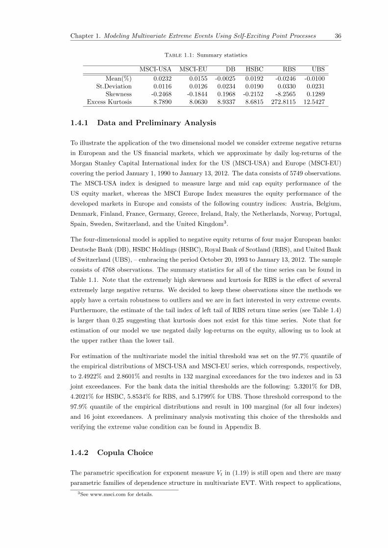
Chapter 1. Modeling Multivariate Extreme Events Using Self-Exciting Point Processes 36
Table 1.1: Summary statistics
MSCI-USA MSCI-EU DB HSBC RBS UBS
Mean(%) 0.0232 0.0155 -0.0025 0.0192 -0.0246 -0.0100St.Deviation 0.0116 0.0126 0.0234 0.0190 0.0330 0.0231
Skewness -0.2468 -0.1844 0.1968 -0.2152 -8.2565 0.1289Excess Kurtosis 8.7890 8.0630 8.9337 8.6815 272.8115 12.5427
1.4.1 Data and Preliminary Analysis
To illustrate the application of the two dimensional model we consider extreme negative returns
in European and the US financial markets, which we approximate by daily log-returns of the
Morgan Stanley Capital International index for the US (MSCI-USA) and Europe (MSCI-EU)
covering the period January 1, 1990 to January 13, 2012. The data consists of 5749 observations.
The MSCI-USA index is designed to measure large and mid cap equity performance of the
US equity market, whereas the MSCI Europe Index measures the equity performance of the
developed markets in Europe and consists of the following country indices: Austria, Belgium,
Denmark, Finland, France, Germany, Greece, Ireland, Italy, the Netherlands, Norway, Portugal,
Spain, Sweden, Switzerland, and the United Kingdom3.
The four-dimensional model is applied to negative equity returns of four major European banks:
Deutsche Bank (DB), HSBC Holdings (HSBC), Royal Bank of Scotland (RBS), and United Bank
of Switzerland (UBS), – embracing the period October 20, 1993 to January 13, 2012. The sample
consists of 4768 observations. The summary statistics for all of the time series can be found in
Table 1.1. Note that the extremely high skewness and kurtosis for RBS is the effect of several
extremely large negative returns. We decided to keep these observations since the methods we
apply have a certain robustness to outliers and we are in fact interested in very extreme events.
Furthermore, the estimate of the tail index of left tail of RBS return time series (see Table 1.4)
is larger than 0.25 suggesting that kurtosis does not exist for this time series. Note that for
estimation of our model we use negated daily log-returns on the equity, allowing us to look at
the upper rather than the lower tail.
For estimation of the multivariate model the initial threshold was set on the 97.7% quantile of
the empirical distributions of MSCI-USA and MSCI-EU series, which corresponds, respectively,
to 2.4922% and 2.8601% and results in 132 marginal exceedances for the two indexes and in 53
joint exceedances. For the bank data the initial thresholds are the following: 5.3201% for DB,
4.2021% for HSBC, 5.8534% for RBS, and 5.1799% for UBS. Those threshold correspond to the
97.9% quantile of the empirical distributions and result in 100 marginal (for all four indexes)
and 16 joint exceedances. A preliminary analysis motivating this choice of the thresholds and
verifying the extreme value condition can be found in Appendix B.
1.4.2 Copula Choice
The parametric specification for exponent measure Vt in (1.19) is still open and there are many
parametric families of dependence structure in multivariate EVT. With respect to applications,
3See www.msci.com for details.

Chapter 1. Modeling Multivariate Extreme Events Using Self-Exciting Point Processes 37
the dependence structure should both be as flexible as possible and be able to capture an asym-
metric dependence structure, in the sense that Vt(y1, y2) 6= Vt(y2, y1). This allows for asymmetric
responses of the probability of joint exceedances to exceedances of the individual variables im-
plying interesting economic interpretations. For example, the stock market of a small country
may react strongly to shocks to the US stock market, but not vice versa. We suggest to use the
exponent measure of the Gumbel copula4. It has a simple structure with only one parameter
θ ≥ 1, which makes it easy to add the time-dependent part and to extend it to an asymmetric
form. It also can be extended to dimensions beyond two, which is advantageous for the multi-
variate application in Section 1.4.3.2. Furthermore, its dependence function in the tail is almost
identical to the one of the t-copula for any choice of the parameters of the t-copula and is thus
very flexible, see Demarta and McNeil [2005] for details.
The non-exchangeable Gumbel copula, see Tawn [1990], has the following exponent measure
V (y1, . . . , yd) =∑s∈S
(∑i∈s
wi,s/yi
)θs1/θs
, (1.47)
where S is the set of all non-empty subsets of {1, . . . , d} and the parameters are constrained
by θs ≥ 1 for all s ∈ S, wi,s = 0 if i /∈ s, wi,s ≥ 0 (asymmetry parameters), i = 1, . . . , d
and∑s∈S wi,s = 1 see also Coles and Tawn [1991]. V in (1.47) is overparameterized for most
applications, as it contains 2d−1(d+2)−(2d+1) parameters. The task of estimating such a model
is very similar to the estimation of high-dimensional copula-based models, for which pair copula
construction is an effective solution to overcome a proliferation of parameters, while maintaining
the flexible dependence structure of the model, see, for example, Aas, Czado, Frigessi, and
Bakken [2009], Okhrin, Okhrin, and Schmid [2013]. The idea of pair copula construction may
also be transferred to construction of multivariate point processes with intensity (1.19). The
only condition to preserve is that the exponent measure associated with the final rate must be
one of an extreme value copula. We leave this estimation topic for future research as it is beyond
the scope of this thesis.
1.4.3 Applying the Model
1.4.3.1 Two-dimensional Model
In this section, we focus on extreme negative log-returns of MSCI-USA and MSCI-EU indexes
and estimate the multivariate model of exceedances with the two-dimensional version of (1.47):
Vt(y1, y2) =(1− w1)
y1+
(1− w2)
y2+
((w1
y1
)θ(t)+
(w2
y2
)θ(t))1/θ(t)
, (1.48)
where w1 and w2 denote the asymmetry parameters in the dependence structure. Setting w1 =
w2 = 1, the symmetric version of (1.48) is obtained. Based on the discussion in Section 1.2.2.2, we
parametrize dependence parameter θ(t) in the equation above as the Hawkes process of different
4We initially also considered the Galambos copula, but its fit was inferior for all applications we considered.
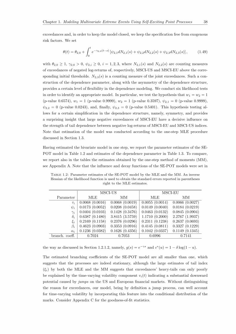
Chapter 1. Modeling Multivariate Extreme Events Using Self-Exciting Point Processes 38
exceedances and, in order to keep the model closed, we keep the specification free from exogenous
risk factors. We set
θ(t) = θ2,0 +
∫ t
0
e−γ2,0(t−s) [ψ2,1dN2,1(s) + ψ2,2dN2,2(s) + ψ2,3dN2,3(s)] , (1.49)
with θ2,0 ≥ 1, γ2,0 > 0, ψ2,i ≥ 0, i = 1, 2, 3, where N2,1(s) and N2,2(s) are counting measures
of exceedances of negated log-returns of, respectively, MSCI-US and MSCI-EU above the corre-
sponding initial thresholds. N2,3(s) is a counting measure of the joint exceedances. Such a con-
struction of the dependence parameter, along with the asymmetry of the dependence structure,
provides a certain level of flexibility in the dependence modeling. We conduct six likelihood tests
in order to identify an appropriate model. In particular, we test the hypothesis that w1 = w2 = 1
(p-value 0.6574), w1 = 1 (p-value 0.9999), w2 = 1 (p-value 0.3597), ψ2,1 = 0 (p-value 0.9999),
ψ2,2 = 0 (p-value 0.0243), and, finally, ψ2,3 = 0 (p-value 0.5401). This hypothesis testing al-
lows for a certain simplification in the dependence structure, namely, symmetry, and provides
a surprising insight that large negative exceedances of MSCI-EU have a decisive influence on
the strength of tail dependence between negative log-returns of MSCI-EU and MSCI-US indices.
Note that estimation of the model was conducted according to the one-step MLE procedure
discussed in Section 1.3.
Having estimated the bivariate model in one step, we report the parameter estimates of the SE-
POT model in Table 1.2 and estimates of the dependence parameter in Table 1.3. To compare,
we report also in the tables the estimates obtained by the one-step method of moments (MM),
see Appendix A. Note that the influence and decay functions of the SE-POT models were set in
Table 1.2: Parameter estimates of the SE-POT model by the MLE and the MM. An inverseHessian of the likelihood function is used to obtain the standard errors reported in parentheses
right to the MLE estimates.
MSCI-US MSCI-EUParameter MLE MM MLE MM
τi 0.0068 (0.0016) 0.0068 (0.0019) 0.0055 (0.0014) 0.0066 (0.0027)ψi 0.0173 (0.0052) 0.0208 (0.0458) 0.0149 (0.0040) 0.0184 (0.0219)γi 0.0404 (0.0103) 0.1428 (0.3476) 0.0463 (0.0132) 0.0845 (0.0904)δi 0.6387 (0.1480) 3.8415 (3.5759) 1.1710 (0.2000) 2.2767 (1.9937)ξi 0.2169 (0.1158) 0.2376 (0.0296) 0.2311 (0.1238) 0.2637 (0.0693)βi 0.4623 (0.0903) 0.3353 (0.0916) 0.4145 (0.0811) 0.3327 (0.1229)αi 0.1236 (0.0382) 0.1626 (0.4356) 0.1042 (0.0337) 0.1149 (0.1345)
branch. coeff. 0.7024 0.7053 0.6996 0.7141
the way as discussed in Section 1.2.1.2, namely, g(s) = e−γs and c∗(u) = 1− δ log(1− u).
The estimated branching coefficients of the SE-POT model are all smaller than one, which
suggests that the processes are indeed stationary, although the large estimates of tail index
(ξi) by both the MLE and the MM suggests that exceedances’ heavy-tails can only poorly
be explained by the time-varying volatility component vi(t) indicating a substantial downward
potential caused by jumps on the US and European financial markets. Without distinguishing
the reason for exceedances, our model, being by definition a jump process, can well account
for time-varying volatility by incorporating this feature into the conditional distribution of the
marks. Consider Appendix C for the goodness-of-fit statistics.
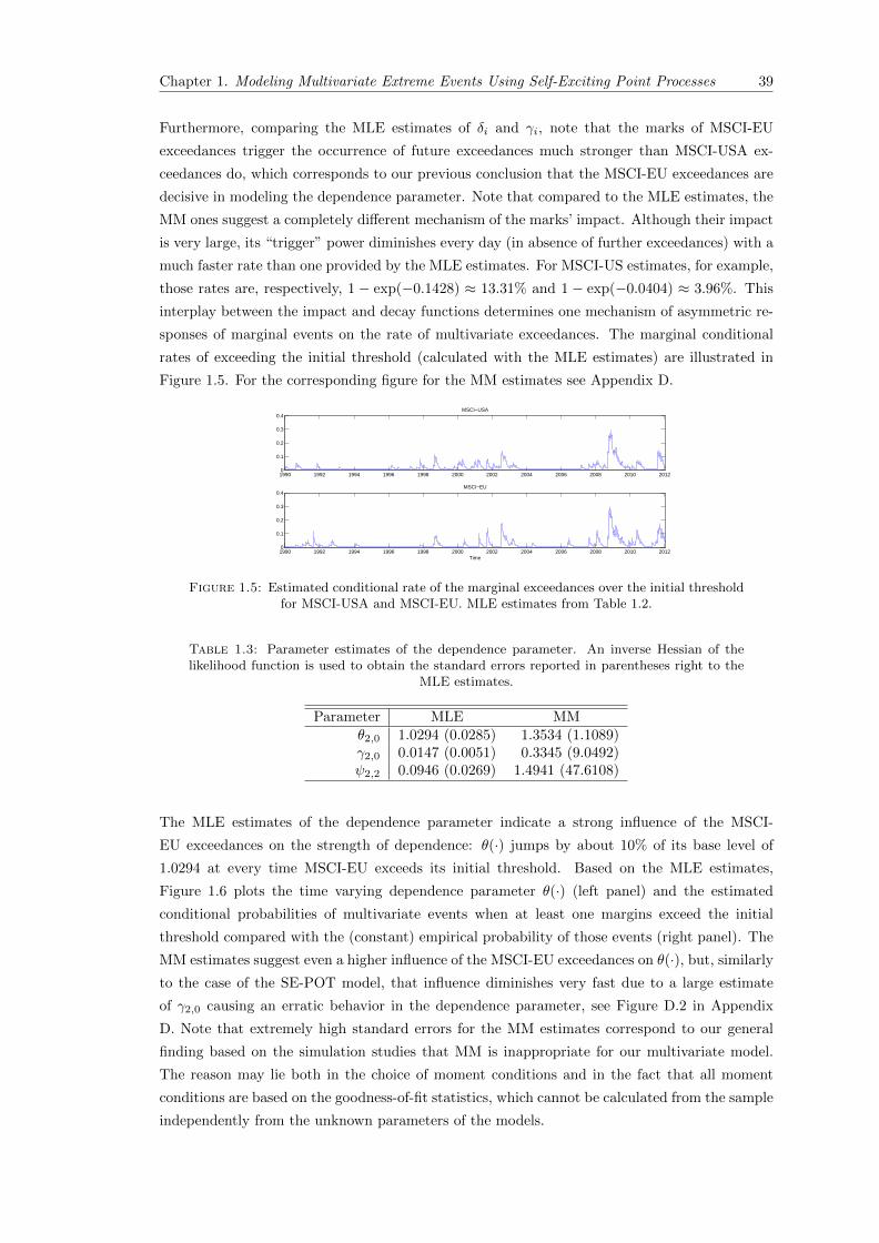
Chapter 1. Modeling Multivariate Extreme Events Using Self-Exciting Point Processes 39
Furthermore, comparing the MLE estimates of δi and γi, note that the marks of MSCI-EU
exceedances trigger the occurrence of future exceedances much stronger than MSCI-USA ex-
ceedances do, which corresponds to our previous conclusion that the MSCI-EU exceedances are
decisive in modeling the dependence parameter. Note that compared to the MLE estimates, the
MM ones suggest a completely different mechanism of the marks’ impact. Although their impact
is very large, its “trigger” power diminishes every day (in absence of further exceedances) with a
much faster rate than one provided by the MLE estimates. For MSCI-US estimates, for example,
those rates are, respectively, 1 − exp(−0.1428) ≈ 13.31% and 1 − exp(−0.0404) ≈ 3.96%. This
interplay between the impact and decay functions determines one mechanism of asymmetric re-
sponses of marginal events on the rate of multivariate exceedances. The marginal conditional
rates of exceeding the initial threshold (calculated with the MLE estimates) are illustrated in
Figure 1.5. For the corresponding figure for the MM estimates see Appendix D.
1990 1992 1994 1996 1998 2000 2002 2004 2006 2008 2010 20120
0.1
0.2
0.3
0.4MSCI−USA
1990 1992 1994 1996 1998 2000 2002 2004 2006 2008 2010 20120
0.1
0.2
0.3
0.4
Time
MSCI−EU
Figure 1.5: Estimated conditional rate of the marginal exceedances over the initial thresholdfor MSCI-USA and MSCI-EU. MLE estimates from Table 1.2.
Table 1.3: Parameter estimates of the dependence parameter. An inverse Hessian of thelikelihood function is used to obtain the standard errors reported in parentheses right to the
MLE estimates.
Parameter MLE MMθ2,0 1.0294 (0.0285) 1.3534 (1.1089)γ2,0 0.0147 (0.0051) 0.3345 (9.0492)ψ2,2 0.0946 (0.0269) 1.4941 (47.6108)
The MLE estimates of the dependence parameter indicate a strong influence of the MSCI-
EU exceedances on the strength of dependence: θ(·) jumps by about 10% of its base level of
1.0294 at every time MSCI-EU exceeds its initial threshold. Based on the MLE estimates,
Figure 1.6 plots the time varying dependence parameter θ(·) (left panel) and the estimated
conditional probabilities of multivariate events when at least one margins exceed the initial
threshold compared with the (constant) empirical probability of those events (right panel). The
MM estimates suggest even a higher influence of the MSCI-EU exceedances on θ(·), but, similarly
to the case of the SE-POT model, that influence diminishes very fast due to a large estimate
of γ2,0 causing an erratic behavior in the dependence parameter, see Figure D.2 in Appendix
D. Note that extremely high standard errors for the MM estimates correspond to our general
finding based on the simulation studies that MM is inappropriate for our multivariate model.
The reason may lie both in the choice of moment conditions and in the fact that all moment
conditions are based on the goodness-of-fit statistics, which cannot be calculated from the sample
independently from the unknown parameters of the models.
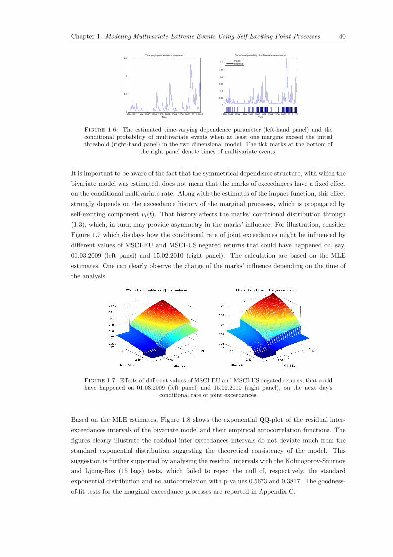
Chapter 1. Modeling Multivariate Extreme Events Using Self-Exciting Point Processes 40
1990 1992 1994 1996 1998 2000 2002 2004 2006 2008 2010 20121
1.5
2
2.5Time varying dependence parameter
Time
0
0.05
0.1
0.15
0.2
0.25
0.3
Conditional probabilty of multivariate exceedances
modelempirical
1990 1992 1994 1996 1998 2000 2002 2004 2006 2008 2010 2012Time
Figure 1.6: The estimated time-varying dependence parameter (left-hand panel) and theconditional probability of multivariate events when at least one margins exceed the initialthreshold (right-hand panel) in the two dimensional model. The tick marks at the bottom of
the right panel denote times of multivariate events.
It is important to be aware of the fact that the symmetrical dependence structure, with which the
bivariate model was estimated, does not mean that the marks of exceedances have a fixed effect
on the conditional multivariate rate. Along with the estimates of the impact function, this effect
strongly depends on the exceedance history of the marginal processes, which is propagated by
self-exciting component vi(t). That history affects the marks’ conditional distribution through
(1.3), which, in turn, may provide asymmetry in the marks’ influence. For illustration, consider
Figure 1.7 which displays how the conditional rate of joint exceedances might be influenced by
different values of MSCI-EU and MSCI-US negated returns that could have happened on, say,
01.03.2009 (left panel) and 15.02.2010 (right panel). The calculation are based on the MLE
estimates. One can clearly observe the change of the marks’ influence depending on the time of
the analysis.
Figure 1.7: Effects of different values of MSCI-EU and MSCI-US negated returns, that couldhave happened on 01.03.2009 (left panel) and 15.02.2010 (right panel), on the next day’s
conditional rate of joint exceedances.
Based on the MLE estimates, Figure 1.8 shows the exponential QQ-plot of the residual inter-
exceedances intervals of the bivariate model and their empirical autocorrelation functions. The
figures clearly illustrate the residual inter-exceedances intervals do not deviate much from the
standard exponential distribution suggesting the theoretical consistency of the model. This
suggestion is further supported by analysing the residual intervals with the Kolmogorov-Smirnov
and Ljung-Box (15 lags) tests, which failed to reject the null of, respectively, the standard
exponential distribution and no autocorrelation with p-values 0.5673 and 0.3817. The goodness-
of-fit tests for the marginal exceedance processes are reported in Appendix C.
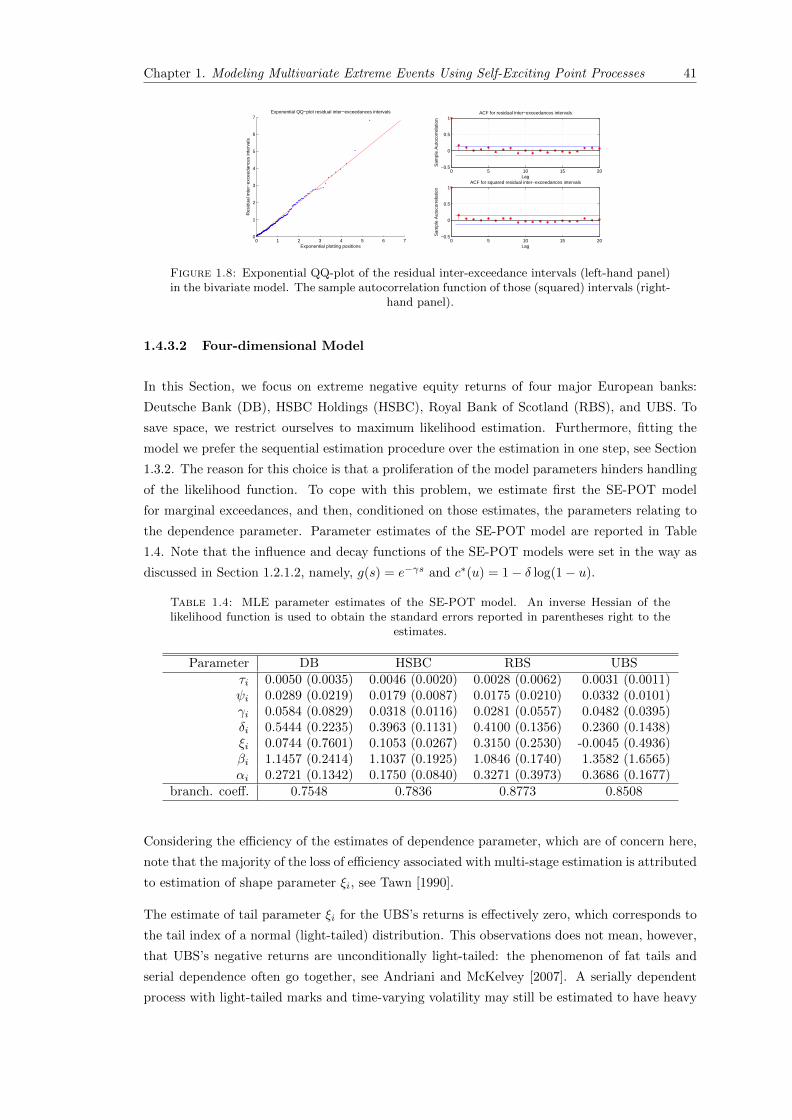
Chapter 1. Modeling Multivariate Extreme Events Using Self-Exciting Point Processes 41
0 1 2 3 4 5 6 70
1
2
3
4
5
6
7
Exponential plotting positionsR
esid
ual i
nter
−ex
ceed
ance
s in
terv
als
Exponential QQ−plot residual inter−exceedances intervals
0 5 10 15 20−0.5
0
0.5
1
Lag
Sam
ple
Aut
ocor
rela
tion
ACF for residual inter−exceedances intervals
0 5 10 15 20−0.5
0
0.5
1
Lag
Sam
ple
Aut
ocor
rela
tion
ACF for squared residual inter−exceedances intervals
Figure 1.8: Exponential QQ-plot of the residual inter-exceedance intervals (left-hand panel)in the bivariate model. The sample autocorrelation function of those (squared) intervals (right-
hand panel).
1.4.3.2 Four-dimensional Model
In this Section, we focus on extreme negative equity returns of four major European banks:
Deutsche Bank (DB), HSBC Holdings (HSBC), Royal Bank of Scotland (RBS), and UBS. To
save space, we restrict ourselves to maximum likelihood estimation. Furthermore, fitting the
model we prefer the sequential estimation procedure over the estimation in one step, see Section
1.3.2. The reason for this choice is that a proliferation of the model parameters hinders handling
of the likelihood function. To cope with this problem, we estimate first the SE-POT model
for marginal exceedances, and then, conditioned on those estimates, the parameters relating to
the dependence parameter. Parameter estimates of the SE-POT model are reported in Table
1.4. Note that the influence and decay functions of the SE-POT models were set in the way as
discussed in Section 1.2.1.2, namely, g(s) = e−γs and c∗(u) = 1− δ log(1− u).
Table 1.4: MLE parameter estimates of the SE-POT model. An inverse Hessian of thelikelihood function is used to obtain the standard errors reported in parentheses right to the
estimates.
Parameter DB HSBC RBS UBSτi 0.0050 (0.0035) 0.0046 (0.0020) 0.0028 (0.0062) 0.0031 (0.0011)ψi 0.0289 (0.0219) 0.0179 (0.0087) 0.0175 (0.0210) 0.0332 (0.0101)γi 0.0584 (0.0829) 0.0318 (0.0116) 0.0281 (0.0557) 0.0482 (0.0395)δi 0.5444 (0.2235) 0.3963 (0.1131) 0.4100 (0.1356) 0.2360 (0.1438)ξi 0.0744 (0.7601) 0.1053 (0.0267) 0.3150 (0.2530) -0.0045 (0.4936)βi 1.1457 (0.2414) 1.1037 (0.1925) 1.0846 (0.1740) 1.3582 (1.6565)αi 0.2721 (0.1342) 0.1750 (0.0840) 0.3271 (0.3973) 0.3686 (0.1677)
branch. coeff. 0.7548 0.7836 0.8773 0.8508
Considering the efficiency of the estimates of dependence parameter, which are of concern here,
note that the majority of the loss of efficiency associated with multi-stage estimation is attributed
to estimation of shape parameter ξi, see Tawn [1990].
The estimate of tail parameter ξi for the UBS’s returns is effectively zero, which corresponds to
the tail index of a normal (light-tailed) distribution. This observations does not mean, however,
that UBS’s negative returns are unconditionally light-tailed: the phenomenon of fat tails and
serial dependence often go together, see Andriani and McKelvey [2007]. A serially dependent
process with light-tailed marks and time-varying volatility may still be estimated to have heavy

Chapter 1. Modeling Multivariate Extreme Events Using Self-Exciting Point Processes 42
tails, if treated as an i.i.d sample. For example, an unconditional estimate of the UBS’s tail
parameter is ξ = 0.1145(0.1249). Along with the time-varying volatility, heavy tails may result
from jumps in the underlying process [Bollerslev, Todorov, and Li, 2013], which, in our model, are
accounted for by the tail index estimate. For the UBS’s returns, it seems like the marks’ heavy
tails are well captured through incorporating the self-exciting component vi(t) into the marks’
conditional distribution. The large tail parameter estimate of the RBS’s returns suggests however
that vi(t) cannot explain all variation in the tails, hence (assuming the model is correct) there is
a significant (unexpected) jump component with tail parameter ξ = 0.3150(0.2530) determining
the distribution of the marks. Note that an unconditional estimate of the RBS’s tail parameter
is ξ = 0.5452(0.1513). The conditional rates of exceeding the initial threshold are reported in
Figure 1.9.
1994 1996 1998 2000 2002 2004 2006 2008 2010 20120
0.1
0.2
0.3
DB
1994 1996 1998 2000 2002 2004 2006 2008 2010 20120
0.1
0.2
0.3
HSBC
1994 1996 1998 2000 2002 2004 2006 2008 2010 20120
0.1
0.2
0.3
RBS
1994 1996 1998 2000 2002 2004 2006 2008 2010 20120
0.1
0.2
0.3
Time
UBS
Figure 1.9: The estimated conditional rates of the marginal exceedances over the initialthreshold in the SE-POT model for negated log-returns of DB, HSBC, RBS, and UBS stocks.
To estimate dependence structure of our model, we employ the Gumbel exponent measure (1.47)
in the four-dimensional case, which provides 39 parameters responsible for the dependence struc-
ture. Clearly, this model is overparameterized for most applications and therefore some prelim-
inary analysis must be conducted to simplify that dependence structure. To do that, we first
analyse the bivariate dependencies for asymmetry. The procedure is the following: we fit the
bivariate model of excedances with the dependence parameter as in (1.49) for all pairs of the
four-dimensional data and then conduct a likelihood test on the hypothesis that the dependence
structure is symmetric. Table 1.5 reports p-values of those likelihood tests.
Table 1.5: p-values of the likelihood tests testing hypothesis that the bivariate dependencestructure in the four-dimensional model is symmetric.
Pair pValue Pair pValue
DB and HSBC 0.9219 HSBC and RBS 0.9343DB and RBS 0.9999 HSBC and UBS 0.8160DB and UBS 0.9974 RBS and HSBC 0.9999
It is clear from the table, the bivariate models display no evidence against symmetric dependen-
cies. Extrapolating this observation also to the trivariate models and assuming the dependence
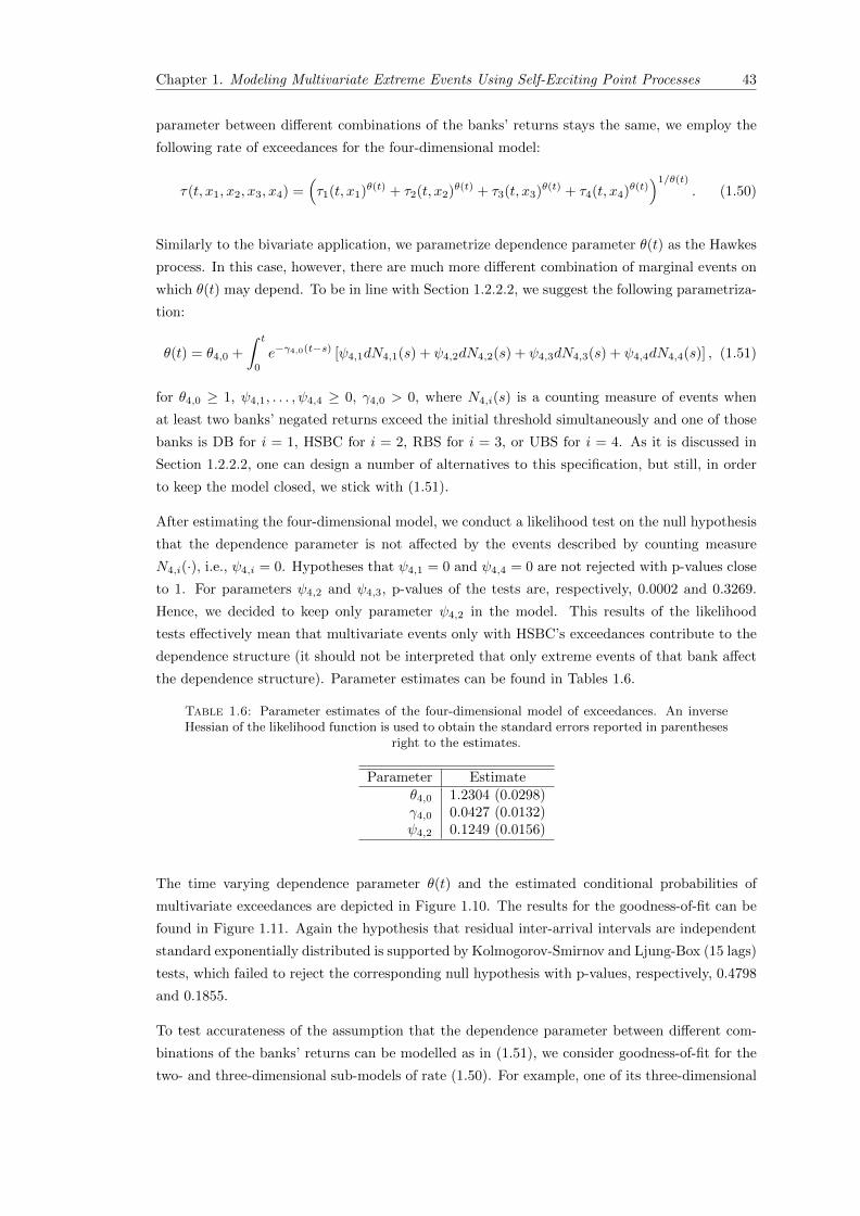
Chapter 1. Modeling Multivariate Extreme Events Using Self-Exciting Point Processes 43
parameter between different combinations of the banks’ returns stays the same, we employ the
following rate of exceedances for the four-dimensional model:
τ(t, x1, x2, x3, x4) =(τ1(t, x1)θ(t) + τ2(t, x2)θ(t) + τ3(t, x3)θ(t) + τ4(t, x4)θ(t)
)1/θ(t)
. (1.50)
Similarly to the bivariate application, we parametrize dependence parameter θ(t) as the Hawkes
process. In this case, however, there are much more different combination of marginal events on
which θ(t) may depend. To be in line with Section 1.2.2.2, we suggest the following parametriza-
tion:
θ(t) = θ4,0 +
∫ t
0
e−γ4,0(t−s) [ψ4,1dN4,1(s) + ψ4,2dN4,2(s) + ψ4,3dN4,3(s) + ψ4,4dN4,4(s)] , (1.51)
for θ4,0 ≥ 1, ψ4,1, . . . , ψ4,4 ≥ 0, γ4,0 > 0, where N4,i(s) is a counting measure of events when
at least two banks’ negated returns exceed the initial threshold simultaneously and one of those
banks is DB for i = 1, HSBC for i = 2, RBS for i = 3, or UBS for i = 4. As it is discussed in
Section 1.2.2.2, one can design a number of alternatives to this specification, but still, in order
to keep the model closed, we stick with (1.51).
After estimating the four-dimensional model, we conduct a likelihood test on the null hypothesis
that the dependence parameter is not affected by the events described by counting measure
N4,i(·), i.e., ψ4,i = 0. Hypotheses that ψ4,1 = 0 and ψ4,4 = 0 are not rejected with p-values close
to 1. For parameters ψ4,2 and ψ4,3, p-values of the tests are, respectively, 0.0002 and 0.3269.
Hence, we decided to keep only parameter ψ4,2 in the model. This results of the likelihood
tests effectively mean that multivariate events only with HSBC’s exceedances contribute to the
dependence structure (it should not be interpreted that only extreme events of that bank affect
the dependence structure). Parameter estimates can be found in Tables 1.6.
Table 1.6: Parameter estimates of the four-dimensional model of exceedances. An inverseHessian of the likelihood function is used to obtain the standard errors reported in parentheses
right to the estimates.
Parameter Estimateθ4,0 1.2304 (0.0298)γ4,0 0.0427 (0.0132)ψ4,2 0.1249 (0.0156)
The time varying dependence parameter θ(t) and the estimated conditional probabilities of
multivariate exceedances are depicted in Figure 1.10. The results for the goodness-of-fit can be
found in Figure 1.11. Again the hypothesis that residual inter-arrival intervals are independent
standard exponentially distributed is supported by Kolmogorov-Smirnov and Ljung-Box (15 lags)
tests, which failed to reject the corresponding null hypothesis with p-values, respectively, 0.4798
and 0.1855.
To test accurateness of the assumption that the dependence parameter between different com-
binations of the banks’ returns can be modelled as in (1.51), we consider goodness-of-fit for the
two- and three-dimensional sub-models of rate (1.50). For example, one of its three-dimensional

Chapter 1. Modeling Multivariate Extreme Events Using Self-Exciting Point Processes 44
1994 1996 1998 2000 2002 2004 2006 2008 2010 20121
1.1
1.2
1.3
1.4
1.5
1.6
1.7
1.8
Time varying dependence parameter
Time
0
0.05
0.1
0.15
0.2
0.25
0.3
0.35
0.4
Conditional probabilty of multivariate exceedances
modelempirical
1994 1996 1998 2000 2002 2004 2006 2008 2010 2012Time
Figure 1.10: The estimated time-varying dependence parameter (left-hand panel) and theconditional probability of multivariate events when at least one margins exceed the initialthreshold (right-hand panel) in the four-dimensional model. The tick marks at the bottom of
the right panel denote times of multivariate events.
0 1 2 3 4 5 6 7 8 90
1
2
3
4
5
6
7
8
9
Exponential plotting positions
Res
idua
l int
er−
exce
edan
ces
inte
rval
s
Exponential QQ−plot residual inter−exceedances intervals
0 5 10 15 20−0.5
0
0.5
1
Lag
Sam
ple
Aut
ocor
rela
tion
ACF for residual inter−exceedances intervals
0 5 10 15 20−0.5
0
0.5
1
Lag
Sam
ple
Aut
ocor
rela
tion
ACF for squared residual inter−exceedances intervals
Figure 1.11: Exponential QQ-plot of the residual inter-exceedances intervals in the four-dimensional model (left-hand panel). The sample autocorrelation function of those (squared)
intervals (right-hand panel).
rates is of the form
τ(t, x1, x2, x3) =(τ1(t, x1)θ(t) + τ2(t, x2)θ(t) + τ3(t, x3)θ(t)
)1/θ(t)
. (1.52)
Treating those lower dimensional versions of (1.50) as the rates of the corresponding sum of
marginal point process, we employ the same goodness-of-fit procedure as for the main model.
Table 1.7 reports the p-values of the Kolmogorov-Smirnov and Ljung-Box (15 lags) tests for
residual inter-exceedances intervals for different combinations of the considered banks. The
corresponding exponential QQ-plots can be found in Appendix E. It is evident from the table
that all sub-models describe the data well supporting by this our suggestion that the extreme
dependence between the banks can be described by relationship (1.51). In case the number of
considered banks (firms) is large, one can consider the extreme dynamics of the market index to
construct the dependence parameter between those banks.
Table 1.7: p-values the Kolmogorov-Smirnov (KS) and Ljung-Box (LB) with 15 lags testsfor residual inter-exceedances intervals for the two- and three-dimensional sub-models of the
four-dimensional model.
Combination KS LB Combination KS LBDB and HSBC 0.3311 0.7799 RBS and HSBC 0.5676 0.9322
DB and RBS 0.1835 0.8049 DB and HSBC and RBS 0.3231 0.4384DB and UBS 0.5641 0.8803 DB and HSBC and UBS 0.6107 0.5896
HSBC and RBS 0.3108 0.7943 DB and RBS and UBS 0.4333 0.5212HSBC and UBS 0.2807 0.6523 HSBC and RBS and UBS 0.4024 0.7976

Chapter 1. Modeling Multivariate Extreme Events Using Self-Exciting Point Processes 45
The fit of the model of joint exceedances in the two and four-dimensional cases suggest that
the model provides an efficient way to quantify the effects that cause the clustering of extreme
financial returns. Among others, these effects are the reaction of markets to common economic
factors and interplay between markets through time-varying linkages. Note that while being able
to quantify the effects, our model cannot explain the source of clustering and contagion, because
our model is decidedly reduced-form. To show when and where exactly the shock occurs, a pure
qualitative analysis is required.
1.5 Conclusion
In this chapter of the thesis, we develop a multivariate approach to model extreme asset returns
considering the conditional distributional properties of both their magnitudes and occurrence
times. The approach is developed in the framework of self-exciting point processes and mul-
tivariate extreme value theory, and follows naturally from treating the multivariate process of
extreme events as a univariate process constructed as a superposition of individual extreme
events. This is an intensity-based model which incorporates a feasible possibility to get updated
in continuous time and lends itself to likelihood inference.
The major statistical contribution of the chapter is that it shows that, provided the marginal
processes of extreme events follow the self-exciting peaks-over-threshold model, the functional
form of the multivariate rate of extreme exceedances should follow the exponent measure of an
extreme value copula. This exponent measure combines the marginal rates into the multivari-
ate one. Due to its construction, the model can capture typical features of the financial time
series, namely, heavy tails, extreme dependences, and clustering of extreme events in both time
and across the assets (markets). A separate contribution of this chapter is a derivation of the
stationarity conditions for the self-exciting peaks-over-threshold model with predictable marks
(the marginal process of exceedances).
To estimate the proposed model, we derive the closed form likelihood function and describe the
goodness-of-fit and simulation procedures. Additionally, we consider the model estimation based
on method of moments, which, however, turned out to be inferior to the MLE. The reason lies in
the fact that the moment conditions cannot be directly calculated from the sample independently
from the unknown parameters of the models.
We implemented the estimation procedure on extreme negative returns, studying MSCI-EU and
MSCI-USA indexes, and equity of Deutsche Bank, RBS, HSBC, and UBS. The goodness-of-fit
procedure demonstrates a reasonable fit of the model and suggests an empirical importance of
the self-exciting feature for modeling both occurrence times, magnitudes, and interdependencies
of the extreme returns. While the dependence structure of the model can account for asymmetry
relationships, we find that conditional multivariate distributions of the returns are close to sym-
metric. Nevertheless, there are still asymmetric effects coming from the self-exciting structure
of the conditional marginal distributions of the magnitudes of the exceedances. In the bivariate
application with MSCI-EU and MSCI-USA indexes, we find that the extreme return exceedances
of MSCI-EU are decisive (statistically) for modeling strength of the dependence between the two

Chapter 1. Modeling Multivariate Extreme Events Using Self-Exciting Point Processes 46
indexes. For the banking data, the multivariate exceedances with HSBC equity are the most
important for modeling the dependence.
In the future research, it would be interesting to consider high-dimensional applications of the
model for, e.g., risk management purposes, and to compare its performance to existing alter-
natives. This comparison would be particularly interesting if the application to high frequency
data is considered. In order to overcome the problem of parameters’ proliferation and to provide
a flexible estimation approach, we plan also to apply the principle of pair copula construction to
our multivariate point-process model.

Appendices
47
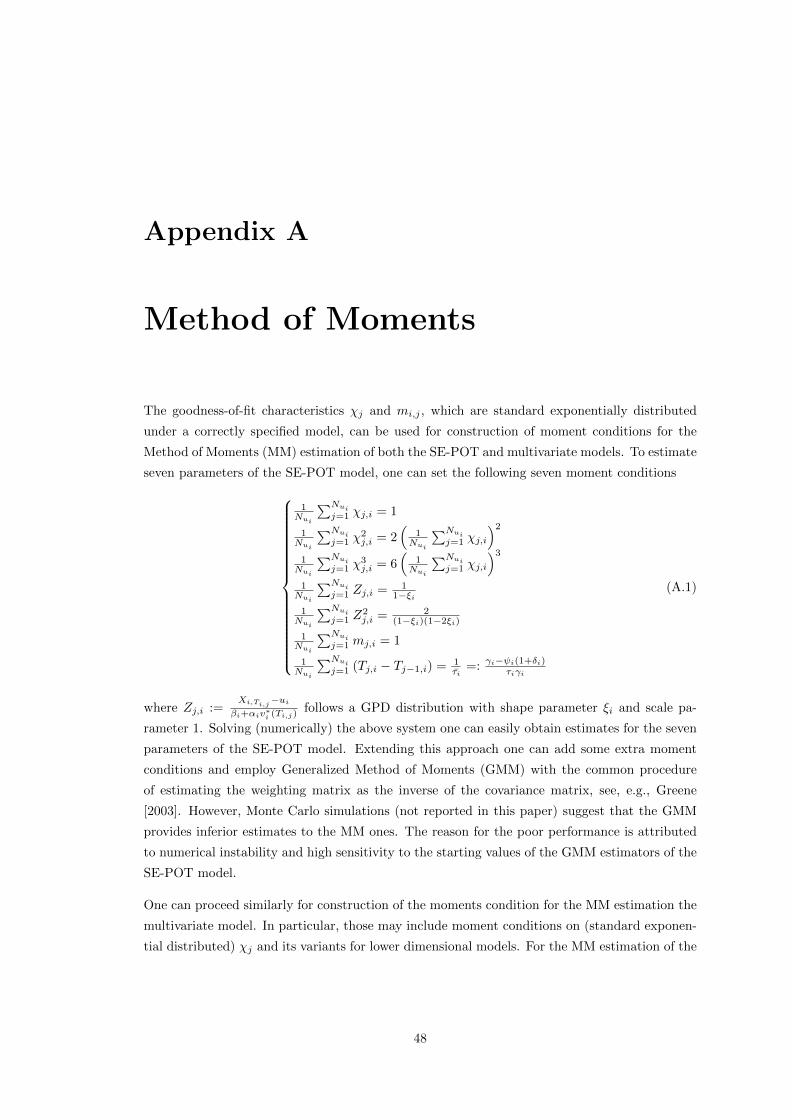
Appendix A
Method of Moments
The goodness-of-fit characteristics χj and mi,j , which are standard exponentially distributed
under a correctly specified model, can be used for construction of moment conditions for the
Method of Moments (MM) estimation of both the SE-POT and multivariate models. To estimate
seven parameters of the SE-POT model, one can set the following seven moment conditions
1Nui
∑Nuij=1 χj,i = 1
1Nui
∑Nuij=1 χ
2j,i = 2
(1Nui
∑Nuij=1 χj,i
)2
1Nui
∑Nuij=1 χ
3j,i = 6
(1Nui
∑Nuij=1 χj,i
)3
1Nui
∑Nuij=1 Zj,i = 1
1−ξi1Nui
∑Nuij=1 Z
2j,i = 2
(1−ξi)(1−2ξi)
1Nui
∑Nuij=1 mj,i = 1
1Nui
∑Nuij=1 (Tj,i − Tj−1,i) = 1
τi=: γi−ψi(1+δi)
τiγi
(A.1)
where Zj,i :=Xi,Ti,j−ui
βi+αiv∗i (Ti,j)follows a GPD distribution with shape parameter ξi and scale pa-
rameter 1. Solving (numerically) the above system one can easily obtain estimates for the seven
parameters of the SE-POT model. Extending this approach one can add some extra moment
conditions and employ Generalized Method of Moments (GMM) with the common procedure
of estimating the weighting matrix as the inverse of the covariance matrix, see, e.g., Greene
[2003]. However, Monte Carlo simulations (not reported in this paper) suggest that the GMM
provides inferior estimates to the MM ones. The reason for the poor performance is attributed
to numerical instability and high sensitivity to the starting values of the GMM estimators of the
SE-POT model.
One can proceed similarly for construction of the moments condition for the MM estimation the
multivariate model. In particular, those may include moment conditions on (standard exponen-
tial distributed) χj and its variants for lower dimensional models. For the MM estimation of the
48
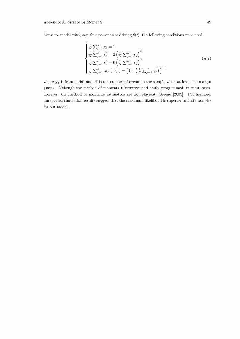
Appendix A. Method of Moments 49
bivariate model with, say, four parameters driving θ(t), the following conditions were used
1N
∑Nj=1 χj = 1
1N
∑Nj=1 χ
2j = 2
(1N
∑Nj=1 χj
)2
1N
∑Nj=1 χ
3j = 6
(1N
∑Nj=1 χj
)3
1N
∑Nj=1 exp (−χj) =
(1 +
(1N
∑Nj=1 χj
))−1
(A.2)
where χj is from (1.46) and N is the number of events in the sample when at least one margin
jumps. Although the method of moments is intuitive and easily programmed, in most cases,
however, the method of moments estimators are not efficient, Greene [2003]. Furthermore,
unreported simulation results suggest that the maximum likelihood is superior in finite samples
for our model.
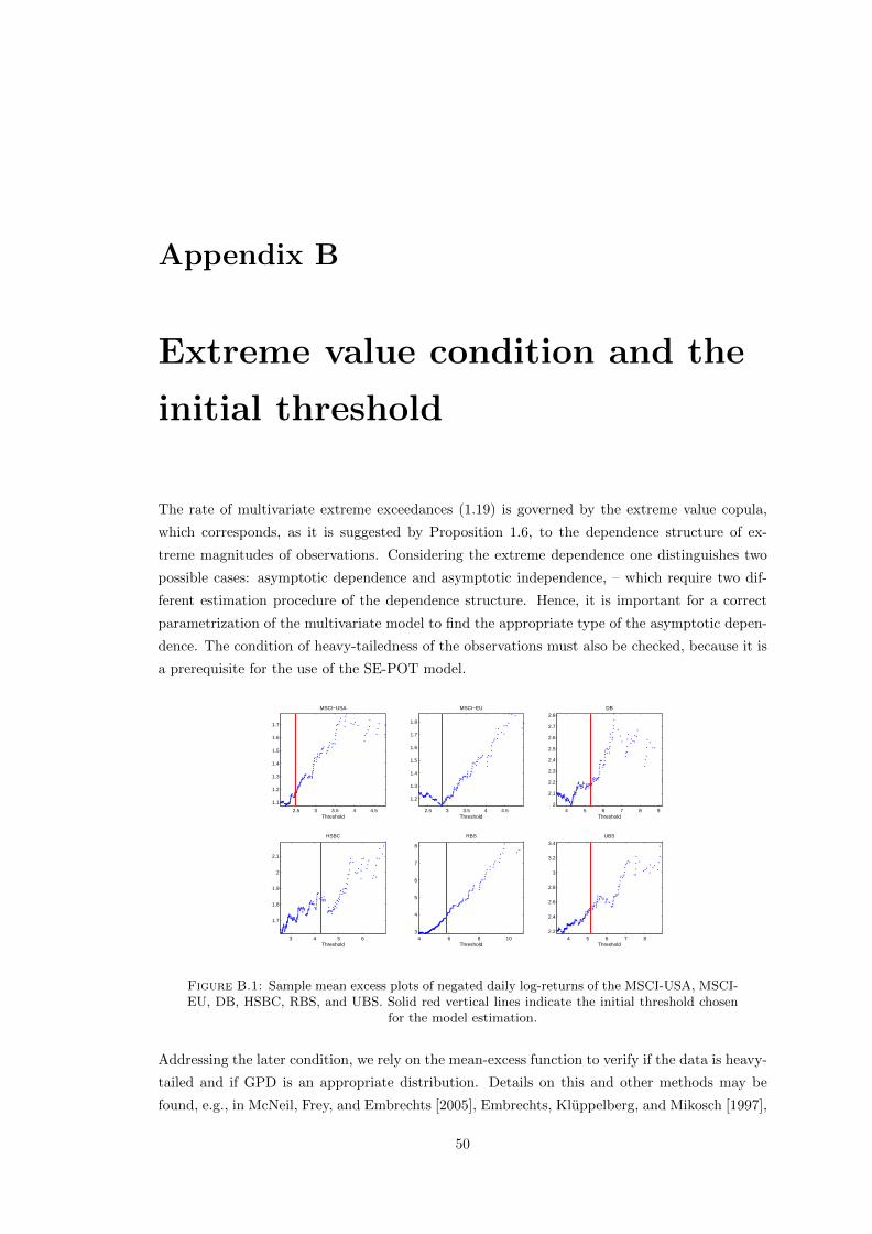
Appendix B
Extreme value condition and the
initial threshold
The rate of multivariate extreme exceedances (1.19) is governed by the extreme value copula,
which corresponds, as it is suggested by Proposition 1.6, to the dependence structure of ex-
treme magnitudes of observations. Considering the extreme dependence one distinguishes two
possible cases: asymptotic dependence and asymptotic independence, – which require two dif-
ferent estimation procedure of the dependence structure. Hence, it is important for a correct
parametrization of the multivariate model to find the appropriate type of the asymptotic depen-
dence. The condition of heavy-tailedness of the observations must also be checked, because it is
a prerequisite for the use of the SE-POT model.
2.5 3 3.5 4 4.5
1.1
1.2
1.3
1.4
1.5
1.6
1.7
MSCI−USA
Threshold2.5 3 3.5 4 4.5
1.2
1.3
1.4
1.5
1.6
1.7
1.8
MSCI−EU
Threshold4 5 6 7 8 9
2
2.1
2.2
2.3
2.4
2.5
2.6
2.7
2.8DB
Threshold
3 4 5 6
1.7
1.8
1.9
2
2.1
HSBC
Threshold4 6 8 10
3
4
5
6
7
8
RBS
Threshold4 5 6 7 8
2.2
2.4
2.6
2.8
3
3.2
3.4UBS
Threshold
Figure B.1: Sample mean excess plots of negated daily log-returns of the MSCI-USA, MSCI-EU, DB, HSBC, RBS, and UBS. Solid red vertical lines indicate the initial threshold chosen
for the model estimation.
Addressing the later condition, we rely on the mean-excess function to verify if the data is heavy-
tailed and if GPD is an appropriate distribution. Details on this and other methods may be
found, e.g., in McNeil, Frey, and Embrechts [2005], Embrechts, Kluppelberg, and Mikosch [1997],
50
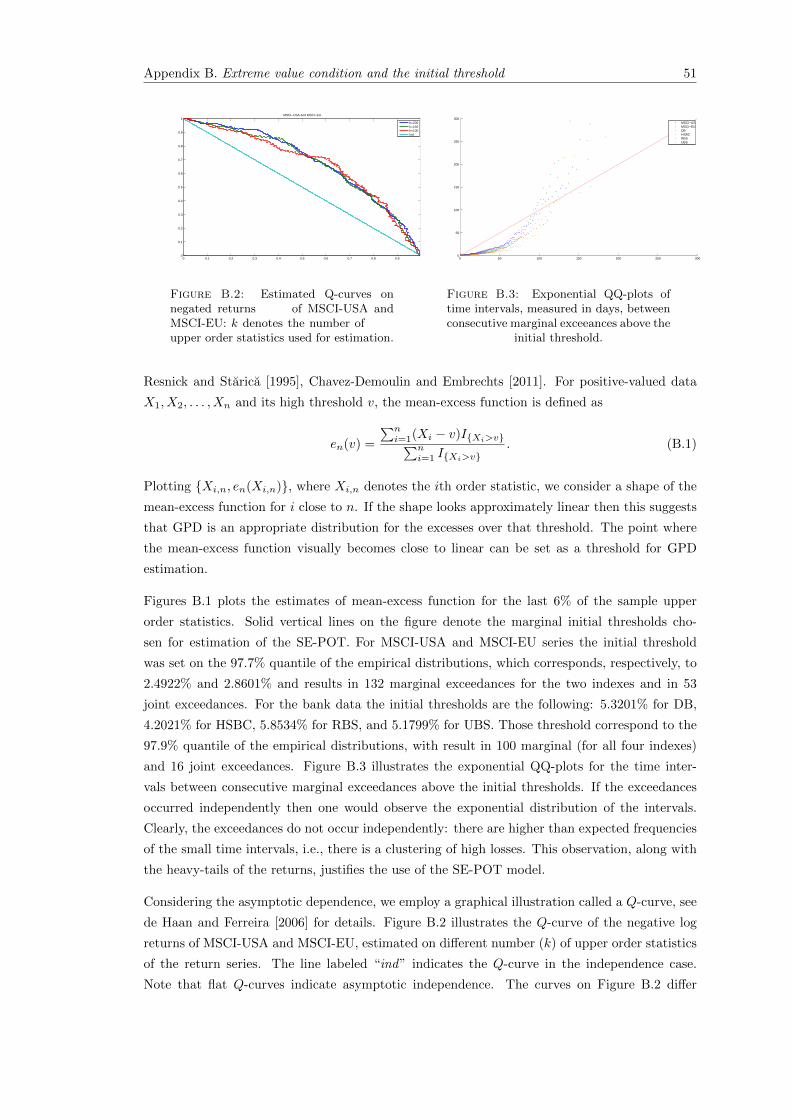
Appendix B. Extreme value condition and the initial threshold 51
0 0.1 0.2 0.3 0.4 0.5 0.6 0.7 0.8 0.9 10
0.1
0.2
0.3
0.4
0.5
0.6
0.7
0.8
0.9
1MSCI−USA and MSCI−EU
k=200k=150k=100ind
Figure B.2: Estimated Q-curves onnegated returns of MSCI-USA andMSCI-EU: k denotes the number ofupper order statistics used for estimation.
0 50 100 150 200 250 3000
50
100
150
200
250
300
MSCI−USMSCI−EUDBHSBCRBSUBS
Figure B.3: Exponential QQ-plots oftime intervals, measured in days, betweenconsecutive marginal exceeances above the
initial threshold.
Resnick and Starica [1995], Chavez-Demoulin and Embrechts [2011]. For positive-valued data
X1, X2, . . . , Xn and its high threshold v, the mean-excess function is defined as
en(v) =
∑ni=1(Xi − v)I{Xi>v}∑n
i=1 I{Xi>v}. (B.1)
Plotting {Xi,n, en(Xi,n)}, where Xi,n denotes the ith order statistic, we consider a shape of the
mean-excess function for i close to n. If the shape looks approximately linear then this suggests
that GPD is an appropriate distribution for the excesses over that threshold. The point where
the mean-excess function visually becomes close to linear can be set as a threshold for GPD
estimation.
Figures B.1 plots the estimates of mean-excess function for the last 6% of the sample upper
order statistics. Solid vertical lines on the figure denote the marginal initial thresholds cho-
sen for estimation of the SE-POT. For MSCI-USA and MSCI-EU series the initial threshold
was set on the 97.7% quantile of the empirical distributions, which corresponds, respectively, to
2.4922% and 2.8601% and results in 132 marginal exceedances for the two indexes and in 53
joint exceedances. For the bank data the initial thresholds are the following: 5.3201% for DB,
4.2021% for HSBC, 5.8534% for RBS, and 5.1799% for UBS. Those threshold correspond to the
97.9% quantile of the empirical distributions, with result in 100 marginal (for all four indexes)
and 16 joint exceedances. Figure B.3 illustrates the exponential QQ-plots for the time inter-
vals between consecutive marginal exceedances above the initial thresholds. If the exceedances
occurred independently then one would observe the exponential distribution of the intervals.
Clearly, the exceedances do not occur independently: there are higher than expected frequencies
of the small time intervals, i.e., there is a clustering of high losses. This observation, along with
the heavy-tails of the returns, justifies the use of the SE-POT model.
Considering the asymptotic dependence, we employ a graphical illustration called a Q-curve, see
de Haan and Ferreira [2006] for details. Figure B.2 illustrates the Q-curve of the negative log
returns of MSCI-USA and MSCI-EU, estimated on different number (k) of upper order statistics
of the return series. The line labeled “ind” indicates the Q-curve in the independence case.
Note that flat Q-curves indicate asymptotic independence. The curves on Figure B.2 differ
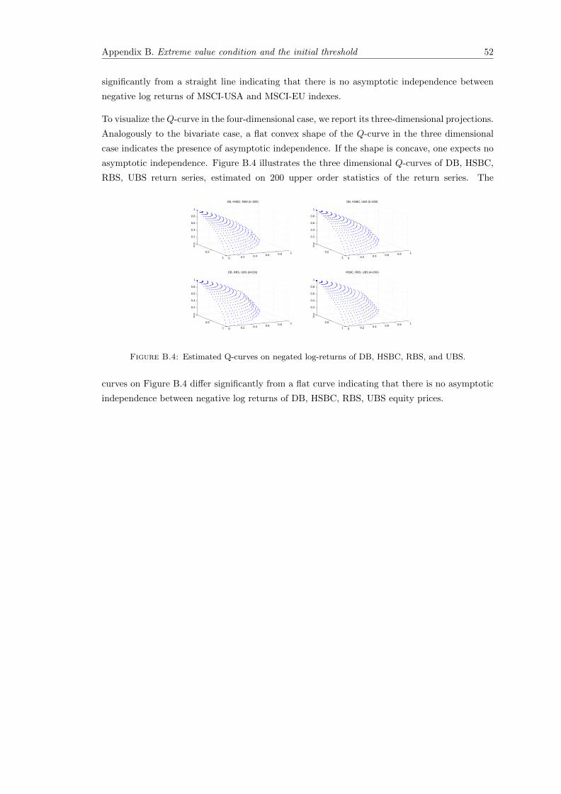
Appendix B. Extreme value condition and the initial threshold 52
significantly from a straight line indicating that there is no asymptotic independence between
negative log returns of MSCI-USA and MSCI-EU indexes.
To visualize theQ-curve in the four-dimensional case, we report its three-dimensional projections.
Analogously to the bivariate case, a flat convex shape of the Q-curve in the three dimensional
case indicates the presence of asymptotic independence. If the shape is concave, one expects no
asymptotic independence. Figure B.4 illustrates the three dimensional Q-curves of DB, HSBC,
RBS, UBS return series, estimated on 200 upper order statistics of the return series. The
0
0.5
1 0 0.2 0.4 0.6 0.8 1
0
0.2
0.4
0.6
0.8
1
DB, HSBC, RBS (k=200)
0
0.5
1 0 0.2 0.4 0.6 0.8 1
0
0.2
0.4
0.6
0.8
1
DB, HSBC, UBS (k=200)
0
0.5
1 0 0.2 0.4 0.6 0.8 1
0
0.2
0.4
0.6
0.8
1
DB, RBS, UBS (k=200)
0
0.5
1 0 0.2 0.4 0.6 0.8 1
0
0.2
0.4
0.6
0.8
1
HSBC, RBS, UBS (k=200)
Figure B.4: Estimated Q-curves on negated log-returns of DB, HSBC, RBS, and UBS.
curves on Figure B.4 differ significantly from a flat curve indicating that there is no asymptotic
independence between negative log returns of DB, HSBC, RBS, UBS equity prices.
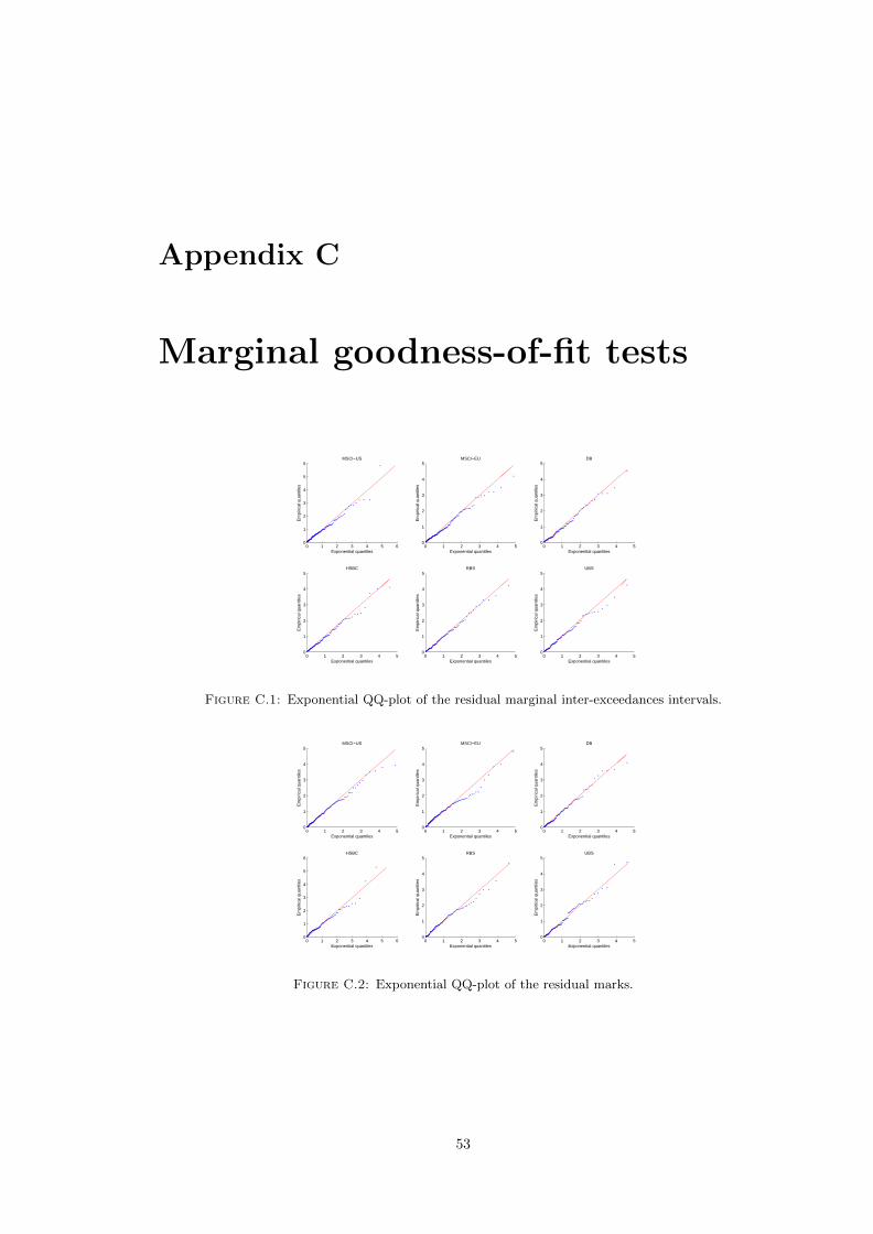
Appendix C
Marginal goodness-of-fit tests
0 1 2 3 4 5 60
1
2
3
4
5
6
Exponential quantiles
Em
piric
al q
uant
iles
MSCI−US
0 1 2 3 4 50
1
2
3
4
5
Exponential quantiles
Em
piric
al q
uant
iles
MSCI−EU
0 1 2 3 4 50
1
2
3
4
5
Exponential quantiles
Em
piric
al q
uant
iles
DB
0 1 2 3 4 50
1
2
3
4
5
Exponential quantiles
Em
piric
al q
uant
iles
HSBC
0 1 2 3 4 50
1
2
3
4
5
Exponential quantiles
Em
piric
al q
uant
iles
RBS
0 1 2 3 4 50
1
2
3
4
5
Exponential quantiles
Em
piric
al q
uant
iles
UBS
Figure C.1: Exponential QQ-plot of the residual marginal inter-exceedances intervals.
0 1 2 3 4 50
1
2
3
4
5
Exponential quantiles
Em
piric
al q
uant
iles
MSCI−US
0 1 2 3 4 50
1
2
3
4
5
Exponential quantiles
Em
piric
al q
uant
iles
MSCI−EU
0 1 2 3 4 50
1
2
3
4
5
Exponential quantiles
Em
piric
al q
uant
iles
DB
0 1 2 3 4 5 60
1
2
3
4
5
6
Exponential quantiles
Em
piric
al q
uant
iles
HSBC
0 1 2 3 4 50
1
2
3
4
5
Exponential quantiles
Em
piric
al q
uant
iles
RBS
0 1 2 3 4 50
1
2
3
4
5
Exponential quantiles
Em
piric
al q
uant
iles
UBS
Figure C.2: Exponential QQ-plot of the residual marks.
53

Appendix C. Marginal goodness-of-fit tests 54
Table C.1: p-values of Kolmogorov-Smirnov (KS) and Ljung-Box (LB) tests checking thehypothesis of exponentially distributed and uncorrelated residual inter-exceedance intervals
and marks of the marginal processes of exceedances.
residual intervals residual marksData KS LB KS LB
MSCI-US 0.5498 0.9185 0.9558 0.9869MSCI-EU 0.2566 0.4211 0.2358 0.9862
DB 0.3788 0.5971 0.4439 0.4809HSBC 0.8852 0.2812 0.6144 0.6251
RBS 0.9349 0.7653 0.7534 0.3143UBS 0.9237 0.6603 0.9563 0.0314
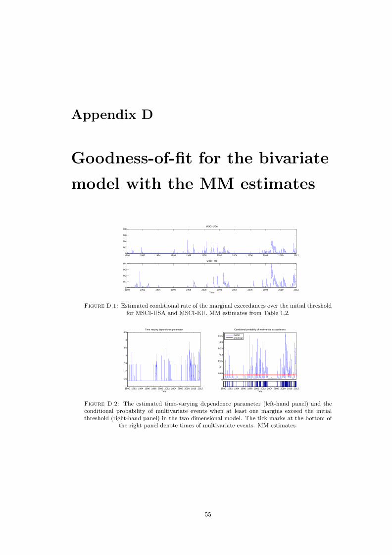
Appendix D
Goodness-of-fit for the bivariate
model with the MM estimates
1990 1992 1994 1996 1998 2000 2002 2004 2006 2008 2010 20120
0.2
0.4
0.6
0.8MSCI−USA
1990 1992 1994 1996 1998 2000 2002 2004 2006 2008 2010 20120
0.1
0.2
0.3
0.4
Time
MSCI−EU
Figure D.1: Estimated conditional rate of the marginal exceedances over the initial thresholdfor MSCI-USA and MSCI-EU. MM estimates from Table 1.2.
1990 1992 1994 1996 1998 2000 2002 2004 2006 2008 2010 20121
1.5
2
2.5
3
3.5
4
4.5Time varying dependence parameter
Time
0
0.05
0.1
0.15
0.2
0.25
0.3
0.35
Conditional probabilty of multivariate exceedances
modelempirical
1990 1992 1994 1996 1998 2000 2002 2004 2006 2008 2010 2012Time
Figure D.2: The estimated time-varying dependence parameter (left-hand panel) and theconditional probability of multivariate events when at least one margins exceed the initialthreshold (right-hand panel) in the two dimensional model. The tick marks at the bottom of
the right panel denote times of multivariate events. MM estimates.
55
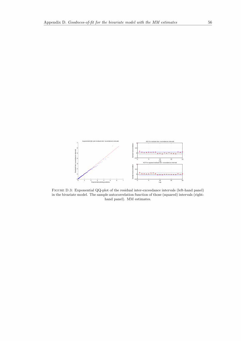
Appendix D. Goodness-of-fit for the bivariate model with the MM estimates 56
0 1 2 3 4 5 6 70
1
2
3
4
5
6
7
Exponential plotting positions
Res
idua
l int
er−
exce
edan
ces
inte
rval
s
Exponential QQ−plot residual inter−exceedances intervals
0 5 10 15 20−0.5
0
0.5
1
Lag
Sam
ple
Aut
ocor
rela
tion
ACF for residual inter−exceedances intervals
0 5 10 15 20−0.5
0
0.5
1
Lag
Sam
ple
Aut
ocor
rela
tion
ACF for squared residual inter−exceedances intervals
Figure D.3: Exponential QQ-plot of the residual inter-exceedance intervals (left-hand panel)in the bivariate model. The sample autocorrelation function of those (squared) intervals (right-
hand panel). MM estimates.

Appendix E
Goodness-of-fit for the
sub-models of the
four-dimensional model
0 2 4 6 80
1
2
3
4
5
6
7
Exponential plotting positions
Sta
ndar
dize
d in
ter−
arriv
al ti
mes
QQ−plot for DB and HSBC
0 2 4 6 80
1
2
3
4
5
6
7
Exponential plotting positions
Sta
ndar
dize
d in
ter−
arriv
al ti
mes
QQ−plot for DB and RBS
0 1 2 3 4 5 60
1
2
3
4
5
6
Exponential plotting positions
Sta
ndar
dize
d in
ter−
arriv
al ti
mes
QQ−plot for DB and UBS
0 1 2 3 4 5 60
1
2
3
4
5
6
Exponential plotting positions
Sta
ndar
dize
d in
ter−
arriv
al ti
mes
QQ−plot for HSBC and RBS
0 1 2 3 4 5 60
1
2
3
4
5
6
Exponential plotting positions
Sta
ndar
dize
d in
ter−
arriv
al ti
mes
QQ−plot for HSBC and UBS
0 1 2 3 4 5 60
1
2
3
4
5
6
Exponential plotting positions
Sta
ndar
dize
d in
ter−
arriv
al ti
mes
QQ−plot for RBS and UBS
Figure E.1: Exponential QQ-plot for the residual inter-exceedance intervals of the bivariatesub-models of the four-dimensional model.
57
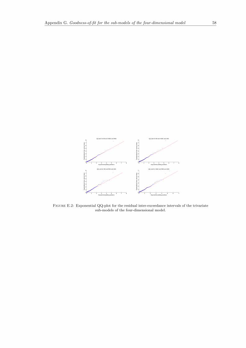
Appendix G. Goodness-of-fit for the sub-models of the four-dimensional model 58
0 1 2 3 4 5 6 7 80
1
2
3
4
5
6
7
8
Exponential plotting positions
Sta
ndar
dize
d in
ter−
arriv
al ti
mes
QQ−plot for DB and HSBC and RBS
0 1 2 3 4 5 6 7 80
1
2
3
4
5
6
7
8
Exponential plotting positions
Sta
ndar
dize
d in
ter−
arriv
al ti
mes
QQ−plot for DB and HSBC and UBS
0 1 2 3 4 5 6 7 80
1
2
3
4
5
6
7
8
Exponential plotting positions
Sta
ndar
dize
d in
ter−
arriv
al ti
mes
QQ−plot for DB and RBS and UBS
0 1 2 3 4 5 6 70
1
2
3
4
5
6
7
Exponential plotting positions
Sta
ndar
dize
d in
ter−
arriv
al ti
mes
QQ−plot for HSBC and RBS and UBS
Figure E.2: Exponential QQ-plot for the residual inter-exceedance intervals of the trivariatesub-models of the four-dimensional model.
Chapter 2
Forecasting extreme electricity
spot prices
2.1 Motivation
Electricity spot prices are typically characterized by their disposition towards sudden extreme
jumps. This phenomenon stems from the lack of practical ways to store electricity and is at-
tributed to an inelastic demand for electricity and very high marginal production costs in case of
unforeseen shortfalls in electricity supply or unexpected rises in the demand. Although lasting
for rather short time intervals, the magnitudes of those jumps may take extreme proportions
hundred times exceeding the average electricity prices. This type of price behavior presents an
important topic for the risk management research and is of great relevance for electricity market
participants, for example, retailers, who buy electricity at market prices but redistribute it at
fixed prices to consumers. Estimating the probabilities of electricity prices to exceed some high
thresholds is of paramount importance for the retailers, because even a few hours of extreme
prices on the market may cause significant losses in their portfolios.
The problem of modeling extreme electricity prices was considered in many papers, e.g., Eichler,
Grothe, Manner, and Tuerk [2012], Christensen, Hurn, and Lindsay [2012], which concentrate
on modeling times of extreme price occurrences in Australia’s national electricity market, and
Kluppelberg, Meyer-Brandis, and Schmidt [2010] for the electricity spot price model applied to
daily data of the EEX Phelix Base electricity price index. Considering the recent developments
in modeling extreme electricity prices, there is still a lack of an approach for a combined modeling
of times of occurrence and magnitudes of extreme electricity prices in real time (high frequency)
settings. To fill that gap, we develop in this chapter of the thesis a model for a complete
description of extreme electricity spot prices. The model consists of two components (sub-
models): one for modeling the magnitudes of extreme electricity prices and the other for modeling
occurrence times of extreme electricity prices. Once being estimated, our model can be applied
(without re-estimation) for forecasting the price exceedances over any sufficiently high threshold.
59

Chapter 2. Forecasting extreme electricity spot prices 60
Figure 2.1: Electricity prices in NSW region of Australia’s electricity market over the periodJan 1, 2002–Dec 31, 2011.
This unique feature is provided by a special construction of the model in which price exceedances
over a comparatively small threshold may trigger the exceedances over much larger levels.
Common distributions used in the literature for modeling electricity prices are Gaussian, expo-
nential, and generalized beta (Geman and Roncoroni [2010], Becker, Hurn, and Pavlov [2007]).
Since those distributions cannot account for heavy tails of the magnitudes of extreme electric-
ity spot prices, we suggest, first, to use a generalized Pareto distribution (GPD) for capturing
the heavy tails and, second, to employ a copula (survival Clayton) with a changing dependence
parameter for capturing the serial dependence between the magnitudes. We account also for
possible ceilings in the electricity prices by applying the censored GPD approach.
For modeling occurrence times of extreme electricity prices, we propose a duration model based
on a negative binomial distribution with a time-varying parameter. That model can capture the
main features of time intervals between the extreme price occurrences, namely, the high variabil-
ity, the strong persistence, and the discreteness. We compare the performance of the proposed
model to the performance of other suitable approaches, like the autoregressive conditional dura-
tion model [Engle and Russell, 1998] and the Hawkes process [Hawkes, 1971].
The model of this chapter of the thesis is developed on and applied to the dataset of half-hourly
electricity spot prices from the four regions of Australia’s electricity market: New South Wales
(NSW), Queensland (QLD), South Australia (SA), and Victoria (VIC). The dataset consists of
175296 observations, embracing the period over January 1, 2002–December 31, 2011.
The rest of the chapter is organized as follows. In Section 2.2 we define a price spike, a building
block of our approach, and provide then a short data-analysis of the prices. In Sections 2.3
and 2.4 we present our models for, respectively, magnitudes and times of the spikes. Section
2.5 combines those models into one model for forecasting extreme electricity prices. Section 2.6
concludes.
2.2 Defining a price spike
In intra-day electricity spot prices, one frequently observes a feature which is common for most
electricity markets, namely sudden extreme prices. In Australia’s electricity market, for example,
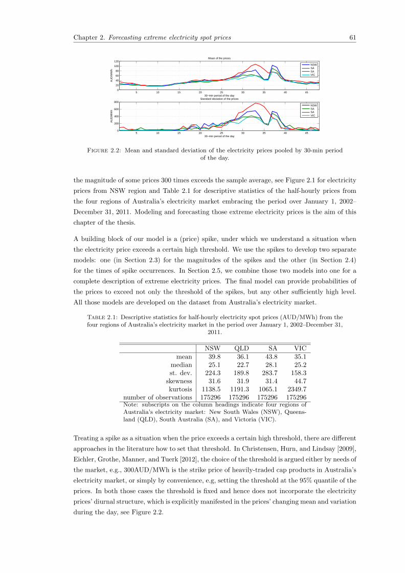
Chapter 2. Forecasting extreme electricity spot prices 61
5 10 15 20 25 30 35 40 450
20
40
60
80
100
120
30−min period of the day
AU
D/M
Wh
Mean of the prices
NSWSASAVIC
5 10 15 20 25 30 35 40 450
200
400
600
800
30−min period of the day
AU
D/M
Wh
Standard deviation of the prices
NSWSASAVIC
Figure 2.2: Mean and standard deviation of the electricity prices pooled by 30-min periodof the day.
the magnitude of some prices 300 times exceeds the sample average, see Figure 2.1 for electricity
prices from NSW region and Table 2.1 for descriptive statistics of the half-hourly prices from
the four regions of Australia’s electricity market embracing the period over January 1, 2002–
December 31, 2011. Modeling and forecasting those extreme electricity prices is the aim of this
chapter of the thesis.
A building block of our model is a (price) spike, under which we understand a situation when
the electricity price exceeds a certain high threshold. We use the spikes to develop two separate
models: one (in Section 2.3) for the magnitudes of the spikes and the other (in Section 2.4)
for the times of spike occurrences. In Section 2.5, we combine those two models into one for a
complete description of extreme electricity prices. The final model can provide probabilities of
the prices to exceed not only the threshold of the spikes, but any other sufficiently high level.
All those models are developed on the dataset from Australia’s electricity market.
Table 2.1: Descriptive statistics for half-hourly electricity spot prices (AUD/MWh) from thefour regions of Australia’s electricity market in the period over January 1, 2002–December 31,
2011.
NSW QLD SA VICmean 39.8 36.1 43.8 35.1
median 25.1 22.7 28.1 25.2st. dev. 224.3 189.8 283.7 158.3
skewness 31.6 31.9 31.4 44.7kurtosis 1138.5 1191.3 1065.1 2349.7
number of observations 175296 175296 175296 175296Note: subscripts on the column headings indicate four regions ofAustralia’s electricity market: New South Wales (NSW), Queens-land (QLD), South Australia (SA), and Victoria (VIC).
Treating a spike as a situation when the price exceeds a certain high threshold, there are different
approaches in the literature how to set that threshold. In Christensen, Hurn, and Lindsay [2009],
Eichler, Grothe, Manner, and Tuerk [2012], the choice of the threshold is argued either by needs of
the market, e.g., 300AUD/MWh is the strike price of heavily-traded cap products in Australia’s
electricity market, or simply by convenience, e.g, setting the threshold at the 95% quantile of the
prices. In both those cases the threshold is fixed and hence does not incorporate the electricity
prices’ diurnal structure, which is explicitly manifested in the prices’ changing mean and variation
during the day, see Figure 2.2.

Chapter 2. Forecasting extreme electricity spot prices 62
0 5 10 15 20 25 30 35 40 45
50
100
150
200
250
300Diurnal threshold
30−min period of the day
AU
D/M
Wh
NSWQLDSAVIC
Figure 2.3: Diurnal threshold. Note:solid vertical lines illustrate parts of theday where parameter ξ of the GPD can beassumed to be the same, details in Section
2.3.1.1.
2002 2003 2004 2005 2006 2007 2008 2009 2010 2011 20120
10
20
30
40
50
60Monthly proportion of spikes (%) in NSW
2002 2003 2004 2005 2006 2007 2008 2009 2010 2011 20120
10
20
30
40
50
60
70Monthly proportion of spikes (%) in QLD
2002 2003 2004 2005 2006 2007 2008 2009 2010 2011 20120
10
20
30
40
50
60
70Monthly proportion of spikes (%) in SA
2002 2003 2004 2005 2006 2007 2008 2009 2010 2011 20120
10
20
30
40
50
60
70Monthly proportion of spikes (%) in VIC
Figure 2.4: Monthly proportions of thespikes. Note: the period of atypically highproportion of spikes in 2007 will be re-moved in modeling occurrences times of
the spikes.
This diurnal structure has a strong impact on the retailers’ expectations of the prices. For
instance, a retailer operating on Australia’s electricity market at 6am may expect an average
price for electricity of approximately 20AUD/MWh, but at 12am the retailer’s expectation are
completely different: the average price is doubled and the standard deviation is at least tripled.
Due to these varying expectations, the price level of 155AUD/MWh at 12am can be regarded
as extreme because it exceeds the 99% quantile of the expected prices at 12am, but at 6am the
price should exceed the level of only 50AUD/MWh in order to be considered as extreme in the
same sense. Those comparatively small extreme prices carry information about the state of the
market (indicating, for example, a rise in the demand for electricity or a shortfall in the supply)
and they should therefore be accounted for in forecasting electricity prices to exceed some higher
(e.g. > 300AUD/MWh) thresholds.
Considering the diurnal distribution of the prices as a representation of the retailers’ price expec-
tations, we suggest to define a spike as a situation when the price exceeds a certain high quantile
of those expectations. For this reason we set the diurnal threshold – the threshold which consists
of 48 values corresponding to the 97% quantile of the prices happened at each of 48 half-hour
periods of the day. The choice of the 97% quantile is motivated by the intention to consider high
prices, on one hand, and to have enough data for statistical inferences, on the other hand. The
spikes defined with help of the diurnal threshold will be used in Section 2.5 for construction of
the model that can forecast the prices to exceed not only the diurnal threshold, but any other
sufficiently high levels.
Figure 2.3 and 2.4 plot, respectively, the diurnal threshold and monthly proportions of the spikes
provided by that diurnal threshold in the four regions of Australia’s electricity market in the
period over January 1, 2002–December 31, 2011. Note that an atypically high proportion of the
spikes in the year 2007 is unrepresentative for the whole dataset and can severely distort the
modeling of times of spike occurrences. We will address that issue in Section 2.4.
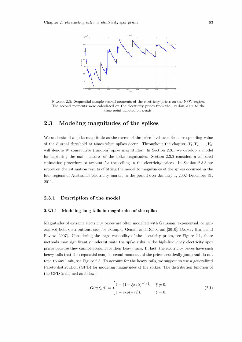
Chapter 2. Forecasting extreme electricity spot prices 63
2003 2004 2005 2006 2007 2008 2009 2010 2011 20122.5
3
3.5
4
4.5
5
5.5
6x 10
4 NSW
Year
(AU
D/M
Wh)
2
Figure 2.5: Sequential sample second moments of the electricity prices on the NSW region.The second moments were calculated on the electricity prices from the 1st Jan 2002 to the
time point denoted on x-axis.
2.3 Modeling magnitudes of the spikes
We understand a spike magnitude as the excess of the price level over the corresponding value
of the diurnal threshold at times when spikes occur. Throughout the chapter, Y1, Y2, . . . , YN
will denote N consecutive (random) spike magnitudes. In Section 2.3.1 we develop a model
for capturing the main features of the spike magnitudes. Section 2.3.2 considers a censored
estimation procedure to account for the ceiling in the electricity prices. In Section 2.3.3 we
report on the estimation results of fitting the model to magnitudes of the spikes occurred in the
four regions of Australia’s electricity market in the period over January 1, 2002–December 31,
2011.
2.3.1 Description of the model
2.3.1.1 Modeling long tails in magnitudes of the spikes
Magnitudes of extreme electricity prices are often modelled with Gaussian, exponential, or gen-
eralized beta distributions, see, for example, Geman and Roncoroni [2010], Becker, Hurn, and
Pavlov [2007]. Considering the large variability of the electricity prices, see Figure 2.1, those
methods may significantly underestimate the spike risks in the high-frequency electricity spot
prices because they cannot account for their heavy tails. In fact, the electricity prices have such
heavy tails that the sequential sample second moments of the prices erratically jump and do not
tend to any limit, see Figure 2.5. To account for the heavy tails, we suggest to use a generalized
Pareto distribution (GPD) for modeling magnitudes of the spikes. The distribution function of
the GPD is defined as follows
G(x; ξ, β) =
1− (1 + ξx/β)−1/ξ, ξ 6= 0,
1− exp(−xβ), ξ = 0,(2.1)
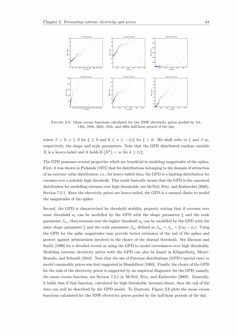
Chapter 2. Forecasting extreme electricity spot prices 64
60 80 100 120 140 160 180 200 22010
20
30
40
50
60
70
80
Threshold
Mea
n ex
cess
1st half−hour period
60 80 100 120 140 1605
10
15
20
25
30
35
40
Threshold
Mea
n ex
cess
14th half−hour period
100 150 200 250 3000
1000
2000
3000
4000
5000
6000
Threshold
Mea
n ex
cess
19th half−hour period
500 1000 1500 2000 2500 3000 3500 4000 45000
500
1000
1500
2000
2500
Threshold
Mea
n ex
cess
36th half−hour period
50 100 150 200 250 3000
20
40
60
80
100
120
140
ThresholdM
ean
exce
ss
45th half−hour period
100 150 200 250 30030
40
50
60
70
80
90
100
110
120
Threshold
Mea
n ex
cess
48th half−hour period
Figure 2.6: Mean excess functions calculated for the NSW electricity prices pooled by 1st,14th, 19th, 36th, 45th, and 48th half-hour period of the day.
where β > 0, x ≥ 0 for ξ ≥ 0 and 0 ≤ x ≤ −β/ξ for ξ < 0. We shall refer to ξ and β as,
respectively, the shape and scale parameters. Note that the GPD distributed random variable
X is a heavy-tailed and it holds E(Xk)
=∞ for k ≥ 1/ξ.
The GPD possesses several properties which are beneficial in modeling magnitudes of the spikes.
First, it was shown in Pickands [1975] that for distributions belonging to the domain of attraction
of an extreme value distribution, i.e., for heavy-tailed data, the GPD is a limiting distribution for
excesses over a suitably high threshold. This result basically means that the GPD is the canonical
distribution for modelling excesses over high thresholds, see McNeil, Frey, and Embrechts [2005],
Section 7.2.1. Since the electricity prices are heavy-tailed, the GPD is a natural choice to model
the magnitudes of the spikes.
Second, the GPD is characterized by threshold stability property stating that if excesses over
some threshold u1 can be modelled by the GPD with the shape parameter ξ and the scale
parameter βu1, then excesses over the higher threshold u2 can be modelled by the GPD with the
same shape parameter ξ and the scale parameter βu2defined as βu2
= βu1+ ξ(u2 − u1). Using
the GPD for the spike magnitudes may provide better estimates of the tail of the spikes and
protect against arbitrariness involved in the choice of the diurnal threshold. See Davison and
Smith [1990] for a detailed record on using the GPD to model exceedances over high thresholds.
Modeling extreme electricity prices with the GPD can also be found in Kluppelberg, Meyer-
Brandis, and Schmidt [2010]. Note that the use of Paretian distributions (GPD’s special case) to
model commodity prices was first suggested in Mandelbrot [1963]. Finally, the choice of the GPD
for the tails of the electricity prices is supported by an empirical diagnostic for the GPD, namely,
the mean excess function, see Section 7.2.1 in McNeil, Frey, and Embrechts [2005]. Generally,
it holds that if that function, calculated for high thresholds, becomes linear, then the tail of the
data can well be described by the GPD model. To illustrate, Figure 2.6 plots the mean excess
functions calculated for the NSW electricity prices pooled by the half-hour periods of the day.

Chapter 2. Forecasting extreme electricity spot prices 65
1 2 3 4 5 6 7 8 9 100
0.2
0.4
0.6
0.8
1NSW
lag1 2 3 4 5 6 7 8 9 10
0
0.2
0.4
0.6
0.8
1QLD
lag
1 2 3 4 5 6 7 8 9 100
0.2
0.4
0.6
0.8
1SA
lag1 2 3 4 5 6 7 8 9 10
0
0.2
0.4
0.6
0.8
1VIC
lag
Figure 2.7: Spearman’s rank correlationbetween the lagged spike magnitudes.
2000 4000 6000 8000 10000 120000
10
20
30
40
50
60
70
80Histrogam of the prices exceeding 400AUD/MWh in NSW
prices
freq
uenc
y
2000 4000 6000 8000 10000 120000
10
20
30
40
50
60Histrogam of the prices exceeding 400AUD/MWh in QLD
prices
freq
uenc
y
2000 4000 6000 8000 10000 120000
10
20
30
40
50
60
70
80Histrogam of the prices exceeding 400AUD/MWh in SA
prices
freq
uenc
y
2000 4000 6000 8000 10000 120000
5
10
15
20
25
30
35
40Histrogam of the prices exceeding 400AUD/MWh in VIC
prices
freq
uenc
y
Figure 2.8: Histogram of the electricityprices exceeding 400AUD/MWh.
Applying the GPD for description of the spike magnitudes is not straightforward, because the
diurnal structure of the prices implies that the spikes across the day have different characteristics
and hence they cannot be modelled by the same GPD. We suggest to model the spike magnitudes
belonging to each of 48 half-hour periods of the day by a separate GPD. In order to reduce the
number of the shape parameters (ξ) to be estimated, which, in turn, simplifies our model and
leads to more accurate estimates, we distinguish parts of the day when the shape parameters
of the prices can be assumed to be the same (but not the scale parameters). Based on the
individual estimates of ξ (not reported here) for the electricity prices pooled by each of the
half-hour periods of the day, a possible division of the day for estimation of ξ can be as follows:
12am–2am; 2.30am–7.30am; 8am–13.30pm; 14pm–7pm; 7.30pm–11.30pm. Solid vertical lines
on Figure 2.3 illustrate that division. Further in the text, we will denote by m(i) a function
that identifies to which part of the day (where the shape parameters are assumed equal) the i-th
observation belongs, and by n(i) a function that identifies to which out of 48 half-hour periods of
the day the i-th observation belongs. The corresponding parameters of the GPD will be denoted
by ξm(i) and βn(i).
2.3.1.2 Modeling dependence in magnitudes of the spikes
In addition to the distributional choice for spike magnitudes Y1, Y2, . . . , YN , there is a need
of modeling a dependence between them. Figure 2.7 plots the estimated rank autocorrelation
of the spike magnitudes calculated as Spearman’s rank correlation between k-lagged samples
Y1, Y2, . . . , YN−k and Yk+1, Yk+2, . . . , YN . Although the autocorrelations on Figure 2.7 cannot
be directly interpreted, because time intervals between the spike occurrences ranges from 30
minutes to 5 months, they still clearly indicate a strong positive dependence between the spike
magnitudes. In addition to the strong dependence, extreme electricity prices display a peculiar
clustering behavior around the level of 10000AUD/MWh, see Figure 2.8, which is attributed to
price ceiling on the market. We will address modeling this price ceiling in Section 2.3.2.
Quantifying the dependence between the lagged magnitudes we withstand from using the Pearson
linear correlation as the measure of dependence, because, first, high variability of the spikes may
imply its infinite variance which rules out the existence of the linear correlation; second, the
linear correlation ρ between two generalized Pareto distributed random variables with shape
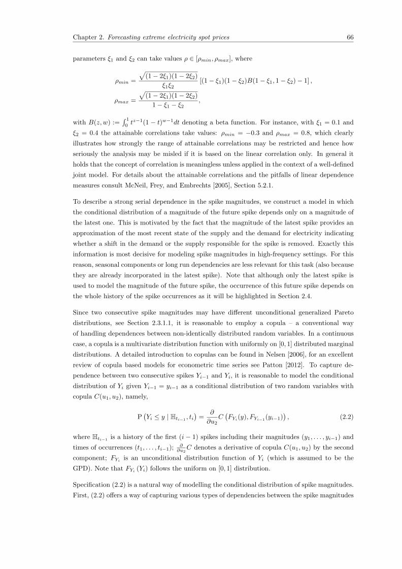
Chapter 2. Forecasting extreme electricity spot prices 66
parameters ξ1 and ξ2 can take values ρ ∈ [ρmin, ρmax], where
ρmin =
√(1− 2ξ1)(1− 2ξ2)
ξ1ξ2[(1− ξ1)(1− ξ2)B(1− ξ1, 1− ξ2)− 1] ,
ρmax =
√(1− 2ξ1)(1− 2ξ2)
1− ξ1 − ξ2,
with B(z, w) :=∫ 1
0tz−1(1 − t)w−1dt denoting a beta function. For instance, with ξ1 = 0.1 and
ξ2 = 0.4 the attainable correlations take values: ρmin = −0.3 and ρmax = 0.8, which clearly
illustrates how strongly the range of attainable correlations may be restricted and hence how
seriously the analysis may be misled if it is based on the linear correlation only. In general it
holds that the concept of correlation is meaningless unless applied in the context of a well-defined
joint model. For details about the attainable correlations and the pitfalls of linear dependence
measures consult McNeil, Frey, and Embrechts [2005], Section 5.2.1.
To describe a strong serial dependence in the spike magnitudes, we construct a model in which
the conditional distribution of a magnitude of the future spike depends only on a magnitude of
the latest one. This is motivated by the fact that the magnitude of the latest spike provides an
approximation of the most recent state of the supply and the demand for electricity indicating
whether a shift in the demand or the supply responsible for the spike is removed. Exactly this
information is most decisive for modeling spike magnitudes in high-frequency settings. For this
reason, seasonal components or long run dependencies are less relevant for this task (also because
they are already incorporated in the latest spike). Note that although only the latest spike is
used to model the magnitude of the future spike, the occurrence of this future spike depends on
the whole history of the spike occurrences as it will be highlighted in Section 2.4.
Since two consecutive spike magnitudes may have different unconditional generalized Pareto
distributions, see Section 2.3.1.1, it is reasonable to employ a copula – a conventional way
of handling dependences between non-identically distributed random variables. In a continuous
case, a copula is a multivariate distribution function with uniformly on [0, 1] distributed marginal
distributions. A detailed introduction to copulas can be found in Nelsen [2006], for an excellent
review of copula based models for econometric time series see Patton [2012]. To capture de-
pendence between two consecutive spikes Yi−1 and Yi, it is reasonable to model the conditional
distribution of Yi given Yi−1 = yi−1 as a conditional distribution of two random variables with
copula C(u1, u2), namely,
P(Yi ≤ y | Hti−1 , ti
)=
∂
∂u2C(FYi(y), FYi−1
(yi−1)), (2.2)
where Hti−1is a history of the first (i− 1) spikes including their magnitudes (y1, . . . , yi−1) and
times of occurrences (t1, . . . , ti−1); ∂∂u2
C denotes a derivative of copula C(u1, u2) by the second
component; FYi is an unconditional distribution function of Yi (which is assumed to be the
GPD). Note that FYi (Yi) follows the uniform on [0, 1] distribution.
Specification (2.2) is a natural way of modelling the conditional distribution of spike magnitudes.
First, (2.2) offers a way of capturing various types of dependencies between the spike magnitudes
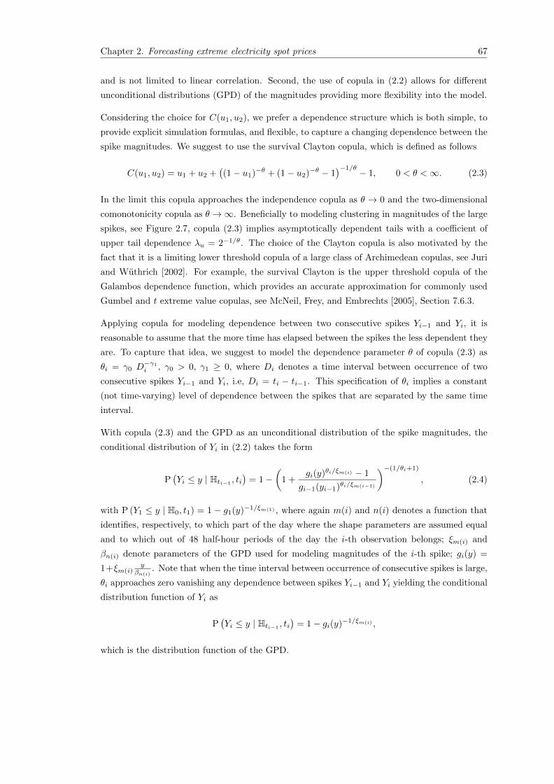
Chapter 2. Forecasting extreme electricity spot prices 67
and is not limited to linear correlation. Second, the use of copula in (2.2) allows for different
unconditional distributions (GPD) of the magnitudes providing more flexibility into the model.
Considering the choice for C(u1, u2), we prefer a dependence structure which is both simple, to
provide explicit simulation formulas, and flexible, to capture a changing dependence between the
spike magnitudes. We suggest to use the survival Clayton copula, which is defined as follows
C(u1, u2) = u1 + u2 +((1− u1)−θ + (1− u2)−θ − 1
)−1/θ − 1, 0 < θ <∞. (2.3)
In the limit this copula approaches the independence copula as θ → 0 and the two-dimensional
comonotonicity copula as θ →∞. Beneficially to modeling clustering in magnitudes of the large
spikes, see Figure 2.7, copula (2.3) implies asymptotically dependent tails with a coefficient of
upper tail dependence λu = 2−1/θ. The choice of the Clayton copula is also motivated by the
fact that it is a limiting lower threshold copula of a large class of Archimedean copulas, see Juri
and Wuthrich [2002]. For example, the survival Clayton is the upper threshold copula of the
Galambos dependence function, which provides an accurate approximation for commonly used
Gumbel and t extreme value copulas, see McNeil, Frey, and Embrechts [2005], Section 7.6.3.
Applying copula for modeling dependence between two consecutive spikes Yi−1 and Yi, it is
reasonable to assume that the more time has elapsed between the spikes the less dependent they
are. To capture that idea, we suggest to model the dependence parameter θ of copula (2.3) as
θi = γ0 D−γ1i , γ0 > 0, γ1 ≥ 0, where Di denotes a time interval between occurrence of two
consecutive spikes Yi−1 and Yi, i.e, Di = ti − ti−1. This specification of θi implies a constant
(not time-varying) level of dependence between the spikes that are separated by the same time
interval.
With copula (2.3) and the GPD as an unconditional distribution of the spike magnitudes, the
conditional distribution of Yi in (2.2) takes the form
P(Yi ≤ y | Hti−1
, ti)
= 1−(
1 +gi(y)θi/ξm(i) − 1
gi−1(yi−1)θi/ξm(i−1)
)−(1/θi+1)
, (2.4)
with P (Y1 ≤ y | H0, t1) = 1 − g1(y)−1/ξm(1) , where again m(i) and n(i) denotes a function that
identifies, respectively, to which part of the day where the shape parameters are assumed equal
and to which out of 48 half-hour periods of the day the i-th observation belongs; ξm(i) and
βn(i) denote parameters of the GPD used for modeling magnitudes of the i-th spike; gi(y) =
1+ξm(i)y
βn(i). Note that when the time interval between occurrence of consecutive spikes is large,
θi approaches zero vanishing any dependence between spikes Yi−1 and Yi yielding the conditional
distribution function of Yi as
P(Yi ≤ y | Hti−1
, ti)
= 1− gi(y)−1/ξm(i) ,
which is the distribution function of the GPD.

Chapter 2. Forecasting extreme electricity spot prices 68
2.3.1.3 Estimation
For fully parametric copula-based time series models the most efficient estimation method is
maximum likelihood, see Patton [2012]. Assuming that the conditional distributions of the
spikes are independent, the (quasi-)likelihood of N realization y1, y2, . . . , yN of spike magnitudes
from model (2.4) takes the form
L =
N∏i=1
∂P(Yi ≤ y | Hti−1
, ti)
∂y
∣∣∣∣∣y=yi
, (2.5)
where
∂P(Yi ≤ y | Hti−1
, ti)
∂y
∣∣∣∣∣y=yi
=(θi + 1)
βn(i)
(1 +
gi(yi)θi/ξm(i) − 1
gi−1(yi−1)θi/ξm(i−1)
)−(2+1/θi)gi(yi)
θi/ξm(i)−1
gi−1(yi−1)θi/ξm(i−1),
(2.6)
with ∂P(Y1≤y|H0,t1)∂y
∣∣∣y=y1
= 1βn(1)
g1(y1)−1/ξm(1)−1.
Computing standard errors of the estimated parameters we will consider robust standard errors,
which are calculated as the maximum likelihood analogue of White’s consistent standard errors,
see Section 17.9 in Greene [2003], and simulation-based standard errors, which are computed on
parameter estimates of the model fitted on many simulated samples from the originally estimated
model. The former approach is less sensitive to a possible misspecification of the model and the
latter approach, provided the correct model specification, yields correct finite-sample standard
errors when a number of simulations is sufficient, see Patton [2012].
2.3.1.4 Simulation and Goodness-of-fit
Applying the above model in practice, where true distributions are unknown, it is vital to
conduct a goodness-of-fit test and a simulation study to check the fit of the estimated model.
Our approach to the goodness-of-fit test is based on the probability integral transformation
[Diebold, Gunther, and Tay, 1998] of the sample of spike magnitudes y1, y2, . . . , yN with the
estimated conditional density forecast (2.4). Recalling that for a continuous random variable X
with distribution function F , F (X) is uniformly distributed on the unit interval, we obtain from
(2.4) that residuals defined as
ui = 1−(
1 +gi(yi)
θi/ξm(i) − 1
gi−1(yi−1)θi/ξm(i−1)
)−(1/θi+1)
, i = 2, . . . , N, (2.7)
with u1 = 1 − g1(y1)−1/ξm(1) , are supposed to be N independent realizations from the uniform
on [0, 1] distribution, if the estimated model is correct (suitable). Since the goodness-of-fit looks
for evidence that the model is misspecified, the test of the estimated model can be limited to
checking a hypothesis that the residuals are independent realizations from the standard uniform
distribution.
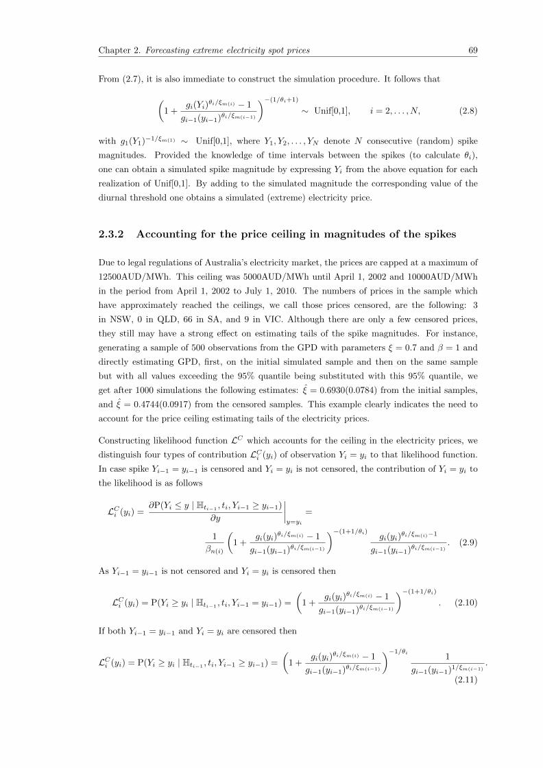
Chapter 2. Forecasting extreme electricity spot prices 69
From (2.7), it is also immediate to construct the simulation procedure. It follows that
(1 +
gi(Yi)θi/ξm(i) − 1
gi−1(yi−1)θi/ξm(i−1)
)−(1/θi+1)
∼ Unif[0,1], i = 2, . . . , N, (2.8)
with g1(Y1)−1/ξm(1) ∼ Unif[0,1], where Y1, Y2, . . . , YN denote N consecutive (random) spike
magnitudes. Provided the knowledge of time intervals between the spikes (to calculate θi),
one can obtain a simulated spike magnitude by expressing Yi from the above equation for each
realization of Unif[0,1]. By adding to the simulated magnitude the corresponding value of the
diurnal threshold one obtains a simulated (extreme) electricity price.
2.3.2 Accounting for the price ceiling in magnitudes of the spikes
Due to legal regulations of Australia’s electricity market, the prices are capped at a maximum of
12500AUD/MWh. This ceiling was 5000AUD/MWh until April 1, 2002 and 10000AUD/MWh
in the period from April 1, 2002 to July 1, 2010. The numbers of prices in the sample which
have approximately reached the ceilings, we call those prices censored, are the following: 3
in NSW, 0 in QLD, 66 in SA, and 9 in VIC. Although there are only a few censored prices,
they still may have a strong effect on estimating tails of the spike magnitudes. For instance,
generating a sample of 500 observations from the GPD with parameters ξ = 0.7 and β = 1 and
directly estimating GPD, first, on the initial simulated sample and then on the same sample
but with all values exceeding the 95% quantile being substituted with this 95% quantile, we
get after 1000 simulations the following estimates: ξ = 0.6930(0.0784) from the initial samples,
and ξ = 0.4744(0.0917) from the censored samples. This example clearly indicates the need to
account for the price ceiling estimating tails of the electricity prices.
Constructing likelihood function LC which accounts for the ceiling in the electricity prices, we
distinguish four types of contribution LCi (yi) of observation Yi = yi to that likelihood function.
In case spike Yi−1 = yi−1 is censored and Yi = yi is not censored, the contribution of Yi = yi to
the likelihood is as follows
LCi (yi) =∂P(Yi ≤ y | Hti−1 , ti, Yi−1 ≥ yi−1)
∂y
∣∣∣∣y=yi
=
1
βn(i)
(1 +
gi(yi)θi/ξm(i) − 1
gi−1(yi−1)θi/ξm(i−1)
)−(1+1/θi)gi(yi)
θi/ξm(i)−1
gi−1(yi−1)θi/ξm(i−1). (2.9)
As Yi−1 = yi−1 is not censored and Yi = yi is censored then
LCi (yi) = P(Yi ≥ yi | Hti−1, ti, Yi−1 = yi−1) =
(1 +
gi(yi)θi/ξm(i) − 1
gi−1(yi−1)θi/ξm(i−1)
)−(1+1/θi)
. (2.10)
If both Yi−1 = yi−1 and Yi = yi are censored then
LCi (yi) = P(Yi ≥ yi | Hti−1, ti, Yi−1 ≥ yi−1) =
(1 +
gi(yi)θi/ξm(i) − 1
gi−1(yi−1)θi/ξm(i−1)
)−1/θi1
gi−1(yi−1)1/ξm(i−1).
(2.11)
Chapter 2. Forecasting extreme electricity spot prices 70
In the case of Yi−1 = yi−1 and Yi = yi being not censored, the contribution of Yi = yi is as in
(2.6).
The final likelihood function LC is a product of contributions LCi (yi) across all spikes, where
LCi (yi) takes one form of (2.6),(2.9)-(2.11).
2.3.3 Estimation results
In this section we report on the estimation results of fitting the model of Section 2.3.1 to the
magnitudes of the spikes occurred in the four regions of Australia’s electricity market over the
period January 1, 2002–December 31, 2011. Note that the model estimation is not adversely
affected by the atypically high proportion of spikes in the year 2007, see Figure (2.4), because
the conditional distribution (2.4) of the spike magnitudes depends only on the information of the
previous spike and time of the current spike occurrence, not on the whole history of the spikes.
Estimating the model, we define spikes that occurred by April 1, 2002 as censored if the associated
prices are higher than 4995AUD. Spikes happened in the period over April 1, 2002–July 1, 2010
are set as censored if the associated prices exceed the level of 9995AUD, and the spikes occurred
after July 1, 2010 are considered to be censored if the associated prices reach 12495AUD. Note
that, since the prices tend to cluster up to the ceiling, we allow for 5AUD deviation in identifying
the censored data. The numbers of observations in the sample which were set as censored are
the following: 3 in NSW, 0 in QLD, 66 in SA, and 9 in VIC. The total number of the spikes in
the samples is as follows: 5241 in NSW, 5279 in QLD, 5271 in SA, and 5278 in VIC.
Table 2.2 presents parameter estimates of model (2.4) obtained by maximizing the ceiling ad-
justed likelihood LC (column “censored”) and the unadjusted likelihood function L in (2.5)
(column “uncensored”). For estimation of the model we distinguish five parts of the day: 12am–
2am; 2.30am–7.30am; 8am–13.30pm; 14pm–7pm; 7.30pm–11.30pm, – and model magnitudes of
the spikes within the part with the GPD which has the same shape parameter ξ but different
scale parameters β corresponding to every half-hour period of the day. Note that improving the
fit of the model for spike magnitudes in VIC region, we use another partition of the day where
the shape parameters are assumed equal. The partition is as follows: 12am–8am; 8.30am–12pm;
12.30pm–14.30pm; 15pm–5.30pm; 6pm–8pm, 8.30pm–11.30pm. In the table, we report only the
estimates of the shape parameter (ξ) of the GPD and of the dependence parameters (γ0, γ1).
To save space, estimates of the scale parameter are not displayed in the table.
Accounting for the price censoring has insignificant effects on the estimates of the shape param-
eter for NSW spikes, which have a few censored observations, but on the estimates for VIC and
SA spikes that effect is strong leading to a significant upward adjustment of the uncensored esti-
mates. Without that upward adjustment of the shape parameter estimates, the risk of extreme
prices would be underestimated.
Provided by the asymptotic distributional properties of the maximum likelihood estimators,
calculation of the robust standard errors for the parameter estimates in Table 2.2 is based on
the score vector and the inverse Hessian of the likelihood function. Since the use of asymptotic
arguments in finite-size samples may yield inaccurate results, we conduct a further analysis of

Chapter 2. Forecasting extreme electricity spot prices 71
Table 2.2: Parameter estimates of the model for spike magnitudes.
uncensored censored uncensored censoredNSW QLD
ξ1 0.4822 (0.0052) 0.4855 (0.0054) 0.5709 (0.0195) 0.5709 (0.0195)
ξ2 0.5125 (0.0022) 0.5161 (0.0029) 0.5298 (0.0022) 0.5298 (0.0022)
ξ3 1.1917 (0.0057) 1.1995 (0.0061) 1.2812 (0.0376) 1.2812 (0.0376)
ξ4 1.7956 (0.0113) 1.8161 (0.0123) 1.8200 (0.0260) 1.8200 (0.0260)
ξ5 0.8911 (0.0087) 0.8972 (0.0086) 1.2042 (0.0420) 1.2042 (0.0420)γ0 2.8289 (0.1713) 2.8487 (0.1691) 2.7253 (0.7202) 2.7253 (0.7202)γ1 0.3677 (0.0898) 0.3636 (0.0870) 1.4367 (1.7991) 1.4367 (1.7991)
SA VIC
ξ1 1.0049 (0.0095) 1.1463 (0.0092) 0.4693 (0.0029) 0.4841 (0.0030)
ξ2 0.7680 (0.0101) 0.8913 (0.0108) 0.8732 (0.0053) 0.9076 (0.0052)
ξ3 1.1501 (0.0303) 1.3036 (0.0325) 1.2580 (0.0163) 1.3031 (0.0164)
ξ4 1.7370 (0.0313) 2.3066 (0.0565) 1.6176 (0.0109) 1.6668 (0.0112)
ξ5 1.1263 (0.0372) 1.2982 (0.0408) 1.6290 (0.0146) 1.7265 (0.0149)
ξ6 – – 0.5561 (0.0082) 0.5735 (0.0083)γ0 2.6284 (0.9160) 3.0280 (0.9684) 2.4701 (0.3261) 2.5457 (0.3256)γ1 1.5777 (2.4453) 1.4117 (2.0451) 0.6722 (0.4040) 0.6400 (0.3559)Note: This table presents estimates of the shape (ξ) and dependence (γ0, γ1) pa-rameters of the model for spike magnitudes. For estimation of ξ in NSW, QLD,and SA, five parts of the day were distinguished: 12am–2am; 2.30am–7.30am;8am–13.30pm; 14pm–7pm; 7.30pm–11.30pm. For VIC region the following par-tition was used: 12am–8am; 8.30am–12pm; 12.30pm–14.30pm; 15pm–5.30pm;6pm–8pm, 8.30pm–11.30pm. The so-called “Huber sandwich estimator” is usedto obtain the robust standard errors reported in parentheses right to the estimates.
the estimators based on the ceiling adjusted maximum likelihood LC . We simulated 500 paths
of (censored) spike magnitudes with the parameter values of Table 2.2 (column “censored”) and
estimated the ceiling adjusted model on every simulated path. The mean, the standard deviation,
the mean relative bias, and the mean squared error of the estimated parameters are summarized
in Table 2.3. Non-surprisingly, the estimators show a large variation and tend to overestimate
the parameters. This large variation of the estimates is a typical feature of all extreme value
statistics, especially of those based on threshold data, see Kluppelberg, Meyer-Brandis, and
Schmidt [2010].
As a goodness-of-fit test of the estimated ceiling adjusted model, Figure 2.9 plots the autocorre-
lation of the residuals (u1, . . . , uN ) computed according to (2.7). The estimated autocorrelations
lie mainly within the confidence bounds indicating no evidence against an assumption of zero
autocorrelations. This suggestion is supported by the Ljung-Box test (15 lags) which failed to
reject the null of no autocorrelation with p-values 61.82% for NSW, 91.44% for QLD, 16.58%
for SA, and 7.39% for VIC. The hypothesis of no autocorrelation was also supported by investi-
gating the squares of the residuals (p-values: 59.48% for NSW, 84.97% for QLD, 12.89% for SA,
28.06% for VIC). The absence of significant autocorrelation in the estimated residual indicates
the ability of our model to capture the serial dependence between the spike magnitudes.
Considering the distributional properties of (u1, . . . , uN ), Figure 2.10 illustrates the plot of the
quantiles of transformed residuals (− log (u1) , . . . ,− log (uN )) versus the corresponding quantiles
of the standard exponential distribution. We have also added to the figure the QQ-plots of 100

Chapter 2. Forecasting extreme electricity spot prices 72
Table 2.3: Estimated mean, standard deviation (std), mean relative bias (MRB), and meansquared error (MSE) of estimated parameters for the ceiling adjusted model from 500 simulated
paths.
true value mean std MRB MSE true value mean std MRB MSENSW QLD
ξ1 0.4855 0.64 0.09 0.31 0.03 0.5709 0.67 0.09 0.17 0.02
ξ2 0.5161 0.68 0.08 0.32 0.03 0.5298 0.62 0.07 0.17 0.01
ξ3 1.1995 1.58 0.19 0.32 0.18 1.2812 1.51 0.15 0.18 0.08
ξ4 1.8161 2.48 0.28 0.37 0.53 1.8200 2.25 0.23 0.24 0.24
ξ5 0.8972 1.18 0.14 0.32 0.10 1.2042 1.41 0.14 0.17 0.06γ0 2.8487 3.79 0.42 0.33 1.06 2.7253 3.23 0.27 0.19 0.33γ1 0.3636 0.34 0.03 -0.07 0.00 1.4367 1.36 0.15 -0.05 0.03
SA VIC
ξ1 1.1463 1.36 0.13 0.19 0.06 0.4841 0.55 0.07 0.13 0.01
ξ2 0.8913 1.05 0.10 0.18 0.04 0.9076 1.03 0.12 0.13 0.03
ξ3 1.3036 1.56 0.14 0.19 0.08 1.3031 1.50 0.18 0.15 0.07
ξ4 2.3066 2.92 0.26 0.27 0.44 1.6668 1.95 0.22 0.17 0.13
ξ5 1.2982 1.55 0.15 0.20 0.09 1.7265 1.99 0.21 0.16 0.12
ξ6 – – – – – 0.5735 0.64 0.08 0.12 0.01γ0 3.0280 3.64 0.28 0.20 0.46 2.5457 2.90 0.27 0.14 0.20γ1 1.4117 1.35 0.13 -0.04 0.02 0.6400 0.62 0.05 -0.04 0.00Note: This table presents characteristics for estimates of the shape (ξ) and dependence (γ0, γ1)parameters of the ceiling adjusted model for the spike magnitudes estimated on 500 simulationsfrom that model with parameter values of Table 2.2 column “censored”.
2 4 6 8 10 12 14 16 18 20−0.1
−0.05
0
0.05
0.1
Lag
Sam
ple
Aut
ocor
rela
tion
NSW
2 4 6 8 10 12 14 16 18 20−0.1
−0.05
0
0.05
0.1
Lag
Sam
ple
Aut
ocor
rela
tion
QLD
2 4 6 8 10 12 14 16 18 20−0.1
−0.05
0
0.05
0.1
Lag
Sam
ple
Aut
ocor
rela
tion
SA
2 4 6 8 10 12 14 16 18 20−0.1
−0.05
0
0.05
0.1
Lag
Sam
ple
Aut
ocor
rela
tion
VIC
Figure 2.9: Autocorrelation of the resid-uals. Solid vertical lines show 99% confi-
dence intervals.
Figure 2.10: QQ-plot of the transformedresiduals. Green points show expected de-
viations of the residuals.
realizations of the standard exponential random variable (in green color), to illustrate what type
of deviations one can expect. In case of a good fit of the estimated model, the transformed
residuals are supposed to be standard exponentially distributed, implying the uniform on [0, 1]
distribution of the estimated residuals. After an inspection of the plot, it becomes apparent that
the transformed residuals seem indeed be consistent with the standard exponential distribution,
although comparatively few of them deviate from the expected boundaries. Those few deviations
may be attributed, among others, to an inevitable estimation error of the model (55 estimated
parameters), the price ceiling, and a peculiar clustering behavior of the prices (especially in
QLD) around the level of 1700AUD/MWh, see Figure 2.8.
For a further analysis of the estimated ceiling adjusted model, we investigate its properties
in a small simulation study. Using the original time intervals between the spike occurrences
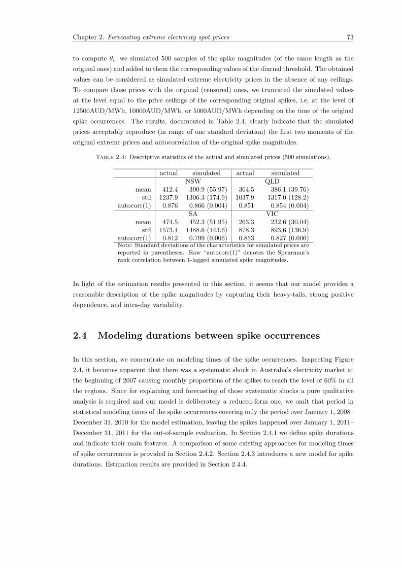
Chapter 2. Forecasting extreme electricity spot prices 73
to compute θi, we simulated 500 samples of the spike magnitudes (of the same length as the
original ones) and added to them the corresponding values of the diurnal threshold. The obtained
values can be considered as simulated extreme electricity prices in the absence of any ceilings.
To compare those prices with the original (censored) ones, we truncated the simulated values
at the level equal to the price ceilings of the corresponding original spikes, i.e, at the level of
12500AUD/MWh, 10000AUD/MWh, or 5000AUD/MWh depending on the time of the original
spike occurrences. The results, documented in Table 2.4, clearly indicate that the simulated
prices acceptably reproduce (in range of one standard deviation) the first two moments of the
original extreme prices and autocorrelation of the original spike magnitudes.
Table 2.4: Descriptive statistics of the actual and simulated prices (500 simulations).
actual simulated actual simulatedNSW QLD
mean 412.4 390.9 (55.97) 364.5 386.1 (39.76)std 1237.9 1306.3 (174.9) 1037.9 1317.0 (128.2)
autocorr(1) 0.876 0.866 (0.004) 0.851 0.854 (0.004)SA VIC
mean 474.5 452.3 (51.95) 263.3 232.6 (30.04)std 1573.1 1488.6 (143.6) 878.3 893.6 (136.9)
autocorr(1) 0.812 0.799 (0.006) 0.853 0.827 (0.006)Note: Standard deviations of the characteristics for simulated prices arereported in parentheses. Row “autocorr(1)” denotes the Spearman’srank correlation between 1-lagged simulated spike magnitudes.
In light of the estimation results presented in this section, it seems that our model provides a
reasonable description of the spike magnitudes by capturing their heavy-tails, strong positive
dependence, and intra-day variability.
2.4 Modeling durations between spike occurrences
In this section, we concentrate on modeling times of the spike occurrences. Inspecting Figure
2.4, it becomes apparent that there was a systematic shock in Australia’s electricity market at
the beginning of 2007 causing monthly proportions of the spikes to reach the level of 60% in all
the regions. Since for explaining and forecasting of those systematic shocks a pure qualitative
analysis is required and our model is deliberately a reduced-form one, we omit that period in
statistical modeling times of the spike occurrences covering only the period over January 1, 2008–
December 31, 2010 for the model estimation, leaving the spikes happened over January 1, 2011–
December 31, 2011 for the out-of-sample evaluation. In Section 2.4.1 we define spike durations
and indicate their main features. A comparison of some existing approaches for modeling times
of spike occurrences is provided in Section 2.4.2. Section 2.4.3 introduces a new model for spike
durations. Estimation results are provided in Section 2.4.4.

Chapter 2. Forecasting extreme electricity spot prices 74
2.4.1 Spike durations
Under a spike duration, or simply duration, we understand a time interval between occurrences
of two consecutive spike. In Australia’s electricity market, the smallest duration constitutes
30 minutes, – we shall refer to that duration as a unit duration and assign a value of one to
it. Note that the unit duration denotes the smallest time interval between occurrences of two
consecutive spikes. Time intervals of 60 minutes correspond to durations of two, intervals of 90
minutes correspond to durations of three, and so on. Throughout the chapter D1, D2, . . . , DN
will denote a sample of N consecutive (random) spike durations.
A major challenge of modeling spike durations in Australia’s electricity market lies in their large
variation and high proportion of unit durations (at least 62%), see Table 2.5, indicating a strong
persistence of the spike occurrences and a distinctive integer character of the durations. There
are many models in the literature which may capture those distinctive features of the spike
durations. In the next section, we compare the performance of some of those models.
Table 2.5: Descriptive statistics for the spikes durations.
NSW QLD SA VICmean 64.72 95.57 52.46 43.76
std 284.09 438.83 226.78 213.59proportion of unit durations 0.68 0.62 0.69 0.67
number of observations 760 539 969 1168Note: spike durations are measured in units of 30 minutes.
2.4.2 Models for the spike durations
A well-known model for durations is the autoregressive conditional duration (ACD) suggested
by Engle and Russell [1998], see Bauwens and Hautsch [2009] for an overview of extensions and
applications of this model. Another suitable approach for duration (actual time) modeling is the
Hawkes process [Hawkes, 1971]. Applications of the Hawkes process to modeling financial time
series can be found in Embrechts, Liniger, and Lin [2011], Aıt-Sahalia, Cacho-Diaz, and Laeven
[2011], Chavez-Demoulin, Davison, and McNeil [2005], Bowsher [2007].
To demonstrate the performance of the those approaches, we estimated four models on NSW
spike durations from the period over January 1, 2008–December 31, 2010: Exponential ACD(1,1),
Weibull ACD(1,1), Burr ACD(1,1) [Grammig and Maurer, 2000], and the univariate Hawkes
process with an exponential response function. As a measure of goodness-of-fit of the estimated
models, Figure 2.11 illustrates a plot of empirical quantiles of the standardized durations (trans-
formed by theoretically implied distribution into standard exponential) of the estimated ACD
models and the residual inter-arrivals times, see Embrechts, Liniger, and Lin [2011] for a defini-
tion, of the estimated Hawkes process versus corresponding quantiles of the standard exponential
distribution.
For a reasonable fit of the models one expects the standardized durations and the residual inter-
arrivals times to follow the standard exponential distribution. The QQ-plots indicate a strong
deviation from the standard exponential distribution suggesting that the estimated ACD models
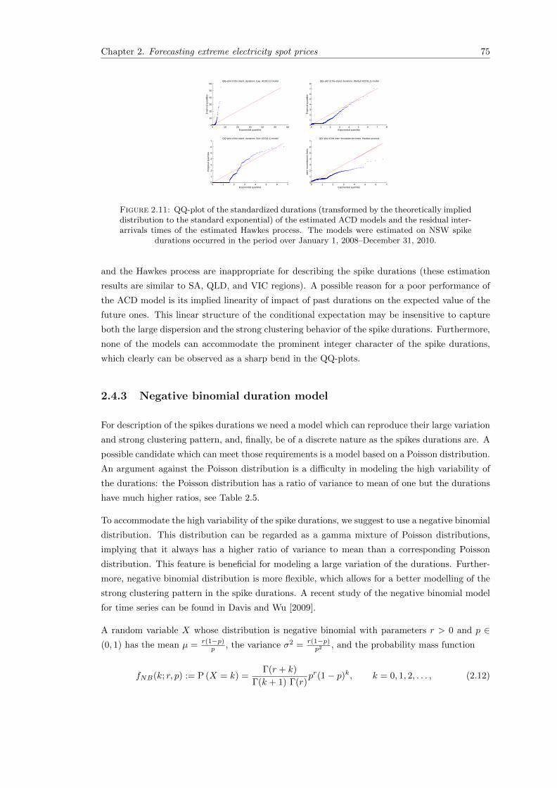
Chapter 2. Forecasting extreme electricity spot prices 75
0 10 20 30 40 50 600
10
20
30
40
50
60
Exponential quantiles
Em
piric
al q
uant
iles
QQ−plot of the stand. durations. Exp. ACD(1,1) model
0 1 2 3 4 5 6 7 80
1
2
3
4
5
6
7
8
Exponential quantiles
Em
piric
al q
uant
iles
QQ−plot of the stand. durations. Weibull ACD(1,1) model
0 1 2 3 4 5 6 70
1
2
3
4
5
6
7
Exponential quantiles
Em
piric
al q
uant
iles
QQ−plot of the stand. durations. Burr ACD(1,1) model
0 1 2 3 4 5 6 70
1
2
3
4
5
6
7
Exponential quantiles
inte
r−ex
ceed
ance
s tim
es
QQ−plot of the inter−exceedances times. Hawkes process
Figure 2.11: QQ-plot of the standardized durations (transformed by the theoretically implieddistribution to the standard exponential) of the estimated ACD models and the residual inter-arrivals times of the estimated Hawkes process. The models were estimated on NSW spike
durations occurred in the period over January 1, 2008–December 31, 2010.
and the Hawkes process are inappropriate for describing the spike durations (these estimation
results are similar to SA, QLD, and VIC regions). A possible reason for a poor performance of
the ACD model is its implied linearity of impact of past durations on the expected value of the
future ones. This linear structure of the conditional expectation may be insensitive to capture
both the large dispersion and the strong clustering behavior of the spike durations. Furthermore,
none of the models can accommodate the prominent integer character of the spike durations,
which clearly can be observed as a sharp bend in the QQ-plots.
2.4.3 Negative binomial duration model
For description of the spikes durations we need a model which can reproduce their large variation
and strong clustering pattern, and, finally, be of a discrete nature as the spikes durations are. A
possible candidate which can meet those requirements is a model based on a Poisson distribution.
An argument against the Poisson distribution is a difficulty in modeling the high variability of
the durations: the Poisson distribution has a ratio of variance to mean of one but the durations
have much higher ratios, see Table 2.5.
To accommodate the high variability of the spike durations, we suggest to use a negative binomial
distribution. This distribution can be regarded as a gamma mixture of Poisson distributions,
implying that it always has a higher ratio of variance to mean than a corresponding Poisson
distribution. This feature is beneficial for modeling a large variation of the durations. Further-
more, negative binomial distribution is more flexible, which allows for a better modelling of the
strong clustering pattern in the spike durations. A recent study of the negative binomial model
for time series can be found in Davis and Wu [2009].
A random variable X whose distribution is negative binomial with parameters r > 0 and p ∈(0, 1) has the mean µ = r(1−p)
p , the variance σ2 = r(1−p)p2 , and the probability mass function
fNB(k; r, p) := P (X = k) =Γ(r + k)
Γ(k + 1) Γ(r)pr(1− p)k, k = 0, 1, 2, . . . , (2.12)

Chapter 2. Forecasting extreme electricity spot prices 76
0 2 4 6 8 10 12 14 16 18 200
0.1
0.2
0.3
0.4
0.5
0.6
0.7
0.8Density function of the Negative Binomial distribution
r=3, p=.2r=3, p=.5r=3, p=.9
Figure 2.12: Density function of the negative binomial distribution.
where Γ(·) is the gamma function: Γ(k) =∫∞
0xk−1e−xdx. Note for a positive integer k, the
gamma function is related to the factorial by Γ(k) = (k − 1)!. Figure 2.12 illustrates density
function fNB(k; r, p) for various sets of parameters.
2.4.3.1 Model description
For modeling durations we consider the following approach. Let D1, D2, . . . , DN , be a se-
ries of (spike) durations. We assume that the conditional distribution of Di depends only on
D1, . . . , Di−1 and it can be expressed in the following way
P(Di = k | Hti−1
)= fNB(k − 1; r, pi), k = 1, 2, . . . (2.13)
where fNB(·; r, p) is a probability mass function of the negative binomial distribution, see (2.12),
and pi is a function of (D1, . . . , Di−2, Di−1). Recall that Hti−1 is a history of the first (i−1) spikes
including their magnitudes (y1, . . . , yi−1) and times of occurrences (t1, . . . , ti−1). To account for
the strong persistence of the spike occurrences, we suggest the following parametrization for pi:
pi = ω + αDi−1pi−1, α ∈ (0, 1). (2.14)
This parametrization comes from a simple AR(1) process and is constructed to accommodate
an empirical evidence that spikes in the electricity prices tend to cluster. Dependence between
parameters pi and pi−1 provides an intuitive link between durations of consecutive spikes as the
dependence between them is adjusted to time span Di−1 between their occurrences: when Di−1
is small then parameter pi of Di becomes strongly influenced by pi−1 leading to an increased
probability that time interval Di will be small; in case Di−1 is large, αDi−1 ≈ 0 implying that
pi−1 has a small contribution to pi. Similarly to modeling spike magnitudes, we restrain from
incorporating seasonal components or long run dependencies into the durations modeling. This
is motivated by the fact that in high-frequently settings spikes are mainly caused by unexpected
supply shortfalls, rather than by well-known seasonal fluctuations.

Chapter 2. Forecasting extreme electricity spot prices 77
2.4.3.2 Estimation
Estimation of model (2.13) is easily performed by the (quasi-)maximum likelihood method. With
conditional distribution (2.13) and probability mass function (2.12), the log-likelihood function
of durations D1, . . . , DN takes the form
L(D1, . . . , DN ; r, ω, α) =
N∑i=1
(log Γ(r +Di − 1)− log Γ(r) + r log pi + (Di − 1) log(1− pi)) .
(2.15)
Maximizing the likelihood we set a condition that a sample mean of durations D1, . . . , DN
should be equal to the expected value of their conditional distributions implied by the model,
namely, 1N
∑Ni=1Di = 1
N
∑Ni=1
(1 + r 1−pi
pi
). This condition is quite useful as it allows to express
r =∑Ni=1(Di−1)∑Ni=1
1−pipi
and by this to reduce the number of parameters to be estimated from three
parameters to two: ω ans α. For the overall stability of the estimated model, it is necessary that
the condition pi ∈ (0, 1) (implied by definition (2.12)) holds. Expressing pi from (2.14) as
pi = ω(1 + αDi−1 + αDi−1+Di−2 + αDi−1+Di−2+Di−3 + . . .
),
it is easy to see that pi achieves its minimum of ω as Di−1 → ∞ and its maximum of ω1−α as
Di−k = 1, for all k = 1, . . . , (i − 1). Since pi should lie within the unit interval, the following
two conditions on the parameter estimates should hold: ω > 0 and ω1−α < 1.
2.4.3.3 Simulation and Goodness-of-fit
In this section we consider a simulation procedure and a goodness-of-fit test for the proposed
duration model. By considering the inverse of the negative binomial distribution function, it is
straightforward to simulate duration Di that follows model (2.13) in the following way
Di ∼ 1 + min [k : Ui ≤ FNB(k; r, pi)] , (2.16)
where Ui ∼ Unif[0, 1] and FNB(·; r, p) is a distribution function of the negative binomial dis-
tribution with parameters r and p. Note that min [k : u ≤ FNB(k; r, p)] denotes an inverse of
FNB(·; r, p) in point u. To construct a sample of simulated durations, function pi+1 should be
updated according to (2.14) after each realization of Di, and then the realization of Di+1 can be
found from (2.16).
Our approach to the goodness-of-fit test is based on the adaptation of the probability integral
transformation, discussed in the continuous case in Diebold, Gunther, and Tay [1998], to the
discrete case. Considering (2.16) in the way that Di (sample duration) and pi are known and
Ui is unknown one can can reproduce Di from Ui, but vice versa it is not true, because the
distribution function of Di is discrete. The only information on series U1, U2, . . . , UN which can
be extracted from the sample data D1, D2, . . . , DN is that Ui satisfies
Ui ∼ Unif [FNB (Di − 2; r, pi) , FNB (Di − 1; r, pi)] , i = 1, 2, . . . , N. (2.17)
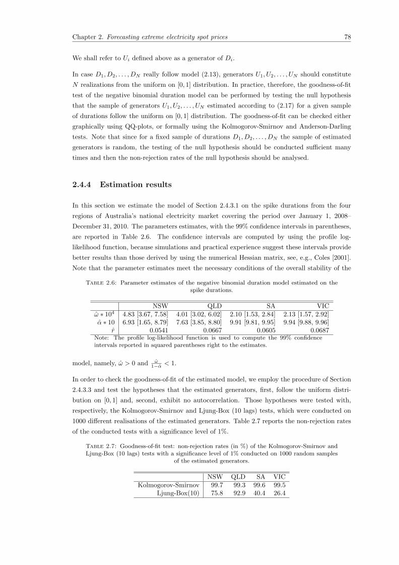
Chapter 2. Forecasting extreme electricity spot prices 78
We shall refer to Ui defined above as a generator of Di.
In case D1, D2, . . . , DN really follow model (2.13), generators U1, U2, . . . , UN should constitute
N realizations from the uniform on [0, 1] distribution. In practice, therefore, the goodness-of-fit
test of the negative binomial duration model can be performed by testing the null hypothesis
that the sample of generators U1, U2, . . . , UN estimated according to (2.17) for a given sample
of durations follow the uniform on [0, 1] distribution. The goodness-of-fit can be checked either
graphically using QQ-plots, or formally using the Kolmogorov-Smirnov and Anderson-Darling
tests. Note that since for a fixed sample of durations D1, D2, . . . , DN the sample of estimated
generators is random, the testing of the null hypothesis should be conducted sufficient many
times and then the non-rejection rates of the null hypothesis should be analysed.
2.4.4 Estimation results
In this section we estimate the model of Section 2.4.3.1 on the spike durations from the four
regions of Australia’s national electricity market covering the period over January 1, 2008–
December 31, 2010. The parameters estimates, with the 99% confidence intervals in parentheses,
are reported in Table 2.6. The confidence intervals are computed by using the profile log-
likelihood function, because simulations and practical experience suggest these intervals provide
better results than those derived by using the numerical Hessian matrix, see, e.g., Coles [2001].
Note that the parameter estimates meet the necessary conditions of the overall stability of the
Table 2.6: Parameter estimates of the negative binomial duration model estimated on thespike durations.
NSW QLD SA VICω ∗ 104 4.83 [3.67, 7.58] 4.01 [3.02, 6.02] 2.10 [1.53, 2.84] 2.13 [1.57, 2.92]α ∗ 10 6.93 [1.65, 8.79] 7.63 [3.85, 8.80] 9.91 [9.81, 9.95] 9.94 [9.88, 9.96]
r 0.0541 0.0667 0.0605 0.0687Note: The profile log-likelihood function is used to compute the 99% confidenceintervals reported in squared parentheses right to the estimates.
model, namely, ω > 0 and ω1−α < 1.
In order to check the goodness-of-fit of the estimated model, we employ the procedure of Section
2.4.3.3 and test the hypotheses that the estimated generators, first, follow the uniform distri-
bution on [0, 1] and, second, exhibit no autocorrelation. Those hypotheses were tested with,
respectively, the Kolmogorov-Smirnov and Ljung-Box (10 lags) tests, which were conducted on
1000 different realisations of the estimated generators. Table 2.7 reports the non-rejection rates
of the conducted tests with a significance level of 1%.
Table 2.7: Goodness-of-fit test: non-rejection rates (in %) of the Kolmogorov-Smirnov andLjung-Box (10 lags) tests with a significance level of 1% conducted on 1000 random samples
of the estimated generators.
NSW QLD SA VICKolmogorov-Smirnov 99.7 99.3 99.6 99.5
Ljung-Box(10) 75.8 92.9 40.4 26.4
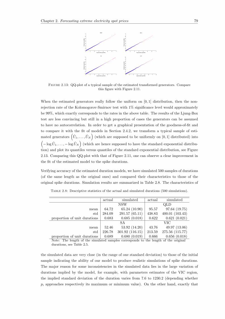
Chapter 2. Forecasting extreme electricity spot prices 79
0 1 2 3 4 5 6 70
1
2
3
4
5
6
7
Exponential quantiles
Em
piric
al q
uant
iles
NSW
0 1 2 3 4 5 6 70
1
2
3
4
5
6
7
Exponential quantiles
Em
piric
al q
uant
iles
QLD
0 1 2 3 4 5 6 70
1
2
3
4
5
6
7
Exponential quantiles
Em
piric
al q
uant
iles
SA
0 1 2 3 4 5 6 7 80
1
2
3
4
5
6
7
8
Exponential quantiles
Em
piric
al q
uant
iles
VIC
Figure 2.13: QQ-plot of a typical sample of the estimated transformed generators. Comparethis figure with Figure 2.11.
When the estimated generators really follow the uniform on [0, 1] distribution, then the non-
rejection rate of the Kolomogorov-Smirnov test with 1% significance level would approximately
be 99%, which exactly corresponds to the rates in the above table. The results of the Ljung-Box
test are less convincing but still in a high proportion of cases the generators can be assumed
to have no autocorrelation. In order to get a graphical presentation of the goodness-of-fit and
to compare it with the fit of models in Section 2.4.2, we transform a typical sample of esti-
mated generators(U1, . . . , UN
)(which are supposed to be uniformly on [0, 1] distributed) into(
− log U1, . . . ,− log UN
)(which are hence supposed to have the standard exponential distribu-
tion) and plot its quantiles versus quantiles of the standard exponential distribution, see Figure
2.13. Comparing this QQ-plot with that of Figure 2.11, one can observe a clear improvement in
the fit of the estimated model to the spike durations.
Verifying accuracy of the estimated duration models, we have simulated 500 samples of durations
(of the same length as the original ones) and compared their characteristics to those of the
original spike durations. Simulation results are summarized in Table 2.8. The characteristics of
Table 2.8: Descriptive statistics of the actual and simulated durations (500 simulations).
actual simulated actual simulatedNSW QLD
mean 64.72 65.24 (10.90) 95.57 97.64 (19.75)std 284.09 291.57 (65.11) 438.83 400.01 (103.43)
proportion of unit durations 0.683 0.685 (0.018) 0.622 0.621 (0.021)SA VIC
mean 52.46 53.92 (14.20) 43.76 49.97 (13.06)std 226.78 301.92 (116.15) 213.59 275.56 (115.77)
proportion of unit durations 0.689 0.680 (0.019) 0.666 0.656 (0.018)Note: The length of the simulated samples corresponds to the length of the originaldurations, see Table 2.5.
the simulated data are very close (in the range of one standard deviation) to those of the initial
sample indicating the ability of our model to produce realistic simulations of spike durations.
The major reason for some inconsistencies in the simulated data lies in the large variation of
durations implied by the model, for example, with parameters estimates of the VIC region,
the implied standard deviation of the duration varies from 7.6 to 1230.2 (depending whether
pi approaches respectively its maximum or minimum value). On the other hand, exactly that

Chapter 2. Forecasting extreme electricity spot prices 80
feature in combination with the dynamic structure of the model is necessary in reproducing the
high variation of the spike durations.
2.5 Forecasting extreme electricity prices
For good risk management in electricity markets it is essential to accurately forecast extreme
electricity prices in order to prevent unexpected losses. In this section we combine the results from
Section 2.3, modeling magnitudes of the spikes, and Section 2.4, modeling the spike durations,
into one model for forecasting extreme electricity prices.
2.5.1 Forecasting approach
The duration model estimated in Section 2.4.4 readily lends itself for estimating the probability
of price spikes conditional on their past. The probability that a spike occurs at time t conditional
the last spike with duration Di−1 happened at time ti−1 can be expressed as
P(spike occurs at time t | Ht−1) =P(Di = t− ti−1 | Ht−1)
P(Di > t− ti−1 − 1 | Ht−1),
where Di follows model (2.13), Ht−1 is an information set consisting of times (t1, . . . , ti−1) and
magnitudes (y1, . . . , yi−1) of the spikes up to time (t − 1). In terms of model (2.13) the above
probability takes the form
P(spike occurs at time t | Ht−1) =fNB (t− ti−1 − 1; r, pi)
1− FNB (t− ti−1 − 2; r, pi), (2.18)
where FNB(·; r, p) is a distribution function of the negative binomial distribution with parameters
r and p; fNB(·; r, p) is the corresponding probability mass function. Figure 2.14 illustrates
the above conditional probability calculated with the parameters estimates of Table 2.6. Note
that for the calculation of the conditional probabilities on the plot, we set parameter pi on its
maximum achievable value in order to get the maximum achievable conditional probabilities of
spike occurrences.
Equation (2.18) provides a conditional probability that a spike occurs, i.e., that electricity price
exceeds the diurnal threshold defined in Section 2.2. Surely, the electricity market participants
may be interested in probabilities that the prices exceed other thresholds: a common example
is a price level of 300AUD/MWh which is the strike price of heavily-traded cap products in
Australia’s electricity market. Designing an approach to estimate those probabilities, one can
informally express the probability of the price to exceed some threshold y (provided it is higher
than the diurnal threshold) in the following way
P(price at time t exceeds y | Ht−1) =
P(spike occurs at time t | Ht−1)P(price at time t exceeds y | spike occurs at time t,Ht−1).
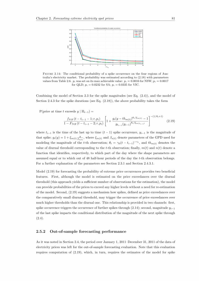
Chapter 2. Forecasting extreme electricity spot prices 81
1 2 3 4 5 6 7 8 9 100
0.1
0.2
0.3
0.4
0.5
0.6
0.7
0.8
0.9
t−ti−1
prob
Conditional probability of a spike occurrence
NSWQLDSAVIC
Figure 2.14: The conditional probability of a spike occurrence on the four regions of Aus-tralia’s electricity market. The probability was estimated according to (2.18) with parametersvalues from Table 2.6. pi was set on its max achievable value: pi = 0.0016 for NSW; pi = 0.0017
for QLD; pi = 0.0232 for SA; pi = 0.0335 for VIC.
Combining the model of Section 2.3 for the spike magnitudes (see Eq. (2.4)), and the model of
Section 2.4.3 for the spike durations (see Eq. (2.18)), the above probability takes the form
P(price at time t exceeds y | Ht−1) =
fNB (t− ti−1 − 1; r, pi)
1− FNB (t− ti−1 − 2; r, pi)
[1 +
gt(y − thm(t))θt/ξm(t) − 1
gti−1(yi−1)θt/ξm(ti−1)
]−(1/θt+1)
(2.19)
where ti−1 is the time of the last up to time (t − 1) spike occurrence, yi−1 is the magnitude of
that spike; gt(y) = 1 + ξm(t)y
βn(t), where ξm(t) and βn(t) denote parameters of the GPD used for
modeling the magnitude of the t-th observation; θt = γ0(t − ti−1)−γ1 , and thm(t) denotes the
value of diurnal threshold corresponding to the t-th observation; finally, m(t) and n(t) denote a
function that identifies, respectively, to which part of the day where the shape parameters are
assumed equal or to which out of 48 half-hour periods of the day the t-th observation belongs.
For a further explanation of the parameters see Section 2.3.1 and Section 2.4.3.1.
Model (2.19) for forecasting the probability of extreme price occurrences provides two beneficial
features. First, although the model is estimated on the price exceedances over the diurnal
threshold (this approach yields a sufficient number of observations for the estimation), the model
can provide probabilities of the prices to exceed any higher levels without a need for re-estimation
of the model. Second, (2.19) suggests a mechanism how spikes, defined as price exceedances over
the comparatively small diurnal threshold, may trigger the occurrence of price exceedances over
much higher thresholds than the diurnal one. This relationship is provided in two channels: first,
spike occurrence triggers the occurrence of further spikes through (2.14); second, magnitude yi−1
of the last spike impacts the conditional distribution of the magnitude of the next spike through
(2.4).
2.5.2 Out-of-sample forecasting performance
As it was noted in Section 2.4, the period over January 1, 2011–December 31, 2011 of the data of
electricity prices was left for the out-of-sample forecasting evaluation. Note that this evaluation
requires computation of (2.19), which, in turn, requires the estimates of the model for spike
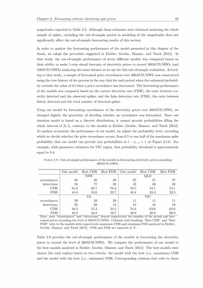
Chapter 2. Forecasting extreme electricity spot prices 82
magnitudes reported in Table 2.2. Although those estimates were obtained analysing the whole
sample of spikes, excluding the out-of-sample period in modeling of the magnitudes does not
significantly affect the out-of-sample forecasting results of this section.
In order to analyse the forecasting performance of the model presented in this chapter of the
thesis, we adopt the procedure suggested in Eichler, Grothe, Manner, and Tuerk [2012]. In
that study, the out-of-sample performance of seven different models was compared based on
their ability to make 1-step ahead forecasts of electricity prices to exceed 300AUD/MWh (and
100AUD/MWh) analysing the same dataset as we use for this out-of-sample evaluation. Accord-
ing to that study, a sample of forecasted price exceedances over 300AUD/MWh was constructed
using the true history of the process in the way that for each period when the estimated probabil-
ity exceeds the value of 0.5 then a price exceedance was forecasted. The forecasting performance
of the models was compared based on the correct detection rate (CDR), the ratio between cor-
rectly detected and the observed spikes, and the false detection rate (FDR), the ratio between
falsely detected and the total number of detected spikes.
Using our model for forecasting exceedances of the electricity prices over 300AUD/MWh, we
changed slightly the procedure of deciding whether an exceedance was forecasted. Since our
duration model is based on a discrete distribution, it cannot provide probabilities filling the
whole interval of [0, 1], contrary to the models in Eichler, Grothe, Manner, and Tuerk [2012].
To analyse accurately the performance of our model, we adjust the probability level, exceeding
which we decide whether the price exceedance occurs, from 0.5 to one half of the maximum spike
probability that our model can provide (see probabilities at t − ti−1 = 1 on Figure 2.14). For
example, with parameter estimates for VIC region, that probability threshold is approximately
equal to 0.4.
Table 2.9: Out-of-sample performance of the models in forecasting electricity prices exceeding300AUD/MWh.
Our model Best CDR Best FDR Our model Best CDR Best FDRNSW QLD
exceedances 38 38 38 37 37 37detections 58 77 38 43 30 30
CDR 84.2 94.7 76.3 59.5 54.1 54.1FDR 44.8 53.6 23.7 48.8 33.3 33.3
SA VICexceedances 29 29 29 11 11 11
detections 25 29 12 10 10 10CDR 48.3 55.2 34.5 54.6 63.6 63.6FDR 44.0 44.8 16.7 40.0 30.0 30.0
Note: rows “exceedances” and “detections” denote respectively the number of the actual and fore-casted prices exceeding the level of 300AUD/MWh. Columns with headings “Best CDR” and “BestFDR” refer to the models with respectively maximum CDR and minimum FDR analysed in Eichler,Grothe, Manner, and Tuerk [2012]. CDR and FDR are reported in %.
Table 2.9 provides the out-of-sample performance of the models in forecasting the electricity
prices to exceed the level of 300AUD/MWh. We compare the performance of our model to
the best models analysed in Eichler, Grothe, Manner, and Tuerk [2012]. The best models were
chosen (for each region) based on two criteria: the model with the best (i.e., maximum) CDR
and the model with the best (i.e., minimum) FDR. Corresponding columns that refer to those

Chapter 2. Forecasting extreme electricity spot prices 83
models are denoted as “Best CDR” and “Best FDR”. Note that those models are not the same
for each of the regions.
An ideal model for spike forecasting provides CDR= 100% and FDR= 0%. In practice, however,
there is often a trade-off between the high CDR and the low FDR. From Table 2.9 it is apparent
that the performance of our model is always somewhere in the middle compared to performance
of the other models analysed in the table: our model provides either a higher CDR or a smaller
FDR. The only exception constitutes the performance of our model for the VIC region.
Table 2.9 provides only a limited assessment of the forecasting performance of our model, because
it is suited to estimate probabilities of the prices to exceed any sufficiently high level, not just
the level for which the model was estimated. As a demonstration of that feature, we estimated 1-
step ahead probabilities of the electricity prices to exceed different price levels: 500AUD/MWh,
1000AUD/MWh, 2000AUD/MWh, and 5000AUD/MWh, – and, applying the same procedure as
used for construction of Table 2.9, we evaluated the out-of-sample forecasting performance of our
model. Table 2.10 provides the evaluation results. Unexpectedly, the forecasting performance of
the model for higher price threshold was only slightly decreased compared to the results in Table
2.9. Moreover, for some regions the duration model showed even better results, for example, for
SA region, eight from nine spikes over 5000AUD/MWh were correctly forecasted (in the sense
that the probability exceeds some level).
This ability to forecast the electricity price exceedances over high thresholds is a unique and
valuable feature of our model. Other approaches for modeling extreme electricity prices can
experience estimation problems because very few data may be available fitting the model to the
prices that exceed very high thresholds. For example, in Australia’s electricity market, in the
period over January 1, 2002–December 31, 2010, there were only a few out of 157728 observations
when the electricity prices exceed the level of 5000AUD/MWh: 99 in NSW, 72 in QLD, 135 in
SA, and 45 in VIC.
Table 2.10: Out-of-sample performance of our model in forecasting electricity prices exceeding500AUD/MWh, 1000AUD/MWh, 2000AUD/MWh, and 5000AUD/MWh levels.
NSW QLD SA VIC NSW QLD SA VIC500AUD/MWh 1000AUD/MWh
exceedances 30 28 24 8 30 23 22 8detections 34 29 23 8 28 24 22 7
CDR 70.0 50.0 54.2 62.5 63.3 56.5 50.0 50.0FDR 38.2 51.7 43.5 37.5 32.1 45.8 50.0 42.9
2000AUD/MWh 5000AUD/MWhexceedances 22 19 19 5 13 8 9 3
detections 22 17 13 5 11 5 9 2CDR 63.6 63.2 42.1 40.0 61.5 62.5 88.9 33.3FDR 36.4 29.4 38.5 60.0 27.3 0 11.1 50.0
Note: rows “exceedances” and “detections” denote respectively the numberof the actual and forecasted price exceedances. CDR and FDR are in %.

Chapter 2. Forecasting extreme electricity spot prices 84
2.6 Conclusion
This study presents a model for forecasting extreme electricity prices in real-time (high fre-
quency) settings. The model consists of two components (sub-models) which deal separately
with times of occurrence and magnitudes of extreme electricity prices. We employ a copula with
a changing dependence parameter for capturing serial dependence in the magnitudes of extreme
electricity prices and the censored GPD distribution for modeling their heavy tails. For modeling
times of the extreme price occurrences, we propose an approach based on the negative binomial
distribution. For both of the sub-models, the simulation procedure and the goodness-of-fit test
are presented.
The model is applied to half-hourly electricity prices from the four regions of Australia’s national
electricity market embracing the period over January 1, 2002–December 31, 2011. The simulation
studies and the goodness-of-fit tests indicate an ability of our model in capturing the main
characteristics of extreme electricity prices. In particular, our approach to times of the extreme
price occurrences outperforms the ACD models and the Hawkes process. The out-of-sample
evaluation also indicates a convincing performance of our model in forecasting the prices to
exceed very high thresholds.
In future research, it would be interesting to consider a multivariate approach for modeling
extreme electricity spot prices. That suggestion is motivated by the fact that in interconnected
regional markets, spikes in one region tend to trigger the occurrence of spikes in the other regions.
Multivariate approaches can capture those interdependencies and describe the contagion effects
of extreme electricity prices.
Chapter 3
Estimating tails in top-coded data
3.1 Motivation
Many practical phenomena are well described by heavy-tailed distributions. This is especially
the case in financial applications, where those distributions have already become a standard
approach for modelling financial time-series. In practice, it is may be required to estimate
heavy-tailed distributions on data that contains top-coded observations, i.e., observations that
are measured only below a certain threshold, while observations that exceed that threshold are
not measured or are simply regarded as uninformative. An example of top-coding can be found in
electricity spot prices on the markets that have a regulatory ceiling on the prices, e.g, Australia’s
national electricity market. Another example relates to insurance companies: due to policy limits
on insurance products, the amount by how much the insurance claims (typically heavy-tailed)
exceed those limits is not recorded. It is clear that the estimation of the distribution’s tail strongly
relies on the quality of the upper-order statistics of the data. Therefore, the top-coding may
have a strong effect on the estimates of the main characteristic of the heavy-tailed distributions
– the tail index, the decay rate of the power function that describes the distribution’s tail.
The problem of estimating the tail index on top-coded data has obtained much attention in the
literature. An adaptation of the Hill estimator to top-coded data is discussed in Beirlant and
Guillou [2001]. The estimation of the tail index under random-censoring assuming that both
censored and censoring distributions are in the maximum domain of attraction of the extreme
value distribution is treated in Beirlant, Guillou, Dierckx, and Fils-Villetard [2007]. Davison and
Smith [1990] shortly consider the effects of top-coding on the asymptotic loss of efficiency for
the GPD-based estimator.
Considering the recent developments in extending the results of extreme value analysis to the
top-coded case, there is still a need for an investigation how exactly different levels of top-coding
may affect the bias and the standard deviation of the most popular estimators of the tail index:
the GPD-based estimator and the Hill estimator. In this chapter of the thesis we try to fill
that gap. Working mainly in the framework of Smith [1987], we extend the maximum likelihood
estimator of the generalized Pareto distribution (GPD) and the Hill estimator to the situations
85
Chapter 3. Estimating tails in top-coded data 86
when the data is top-coded. Our approach differs from the mentioned literature in that we
analyse the estimators jointly and employ the same procedure in determining observations for
estimation. This brings about an opportunity to compare their performance based on mean
squared errors (MSE) depending on the second order properties of the underlying distribution
function of the observations. In contrast to Beirlant, Guillou, Dierckx, and Fils-Villetard [2007],
we treat only the top-coding case without making any assumption about the distribution above
the censoring level and consider a more in-depth analysis of the effects of top-coding on the
estimators. Furthermore, establishing the asymptotic normality of the estimators, we provide a
detailed analysis how both the parameters of the underlying distribution and various levels of
top-coding influence the characteristics of the estimators.
We show that for situations when the proportion of the top-coded observations is large, the Hill
estimator provides a superior performance (based on MSE) over the GPD approach in estimating
tail indexes. Providing a detailed analysis of this performance, we show that it depends on a
number of factors including the size of the tail index and the second-order properties of the
underlying distribution. Note that this finding about the Hill estimator contradicts the broad
conclusion about the performance of that estimator in the uncensored case, where the GPD-
based estimator is often considered as superior, see Smith [1987]. We demonstrate our findings
in a small simulation study and apply the estimators to electricity spot prices of the Australia’s
national electricity market.
The chapter is organized as follows. In Section 3.2 we present shortly some definitions and
preliminary results concerning heavy-tailed distributions. The censored GPD (cGPD) estimator
is described in Section 3.3, the censored Hill (cHill) – in Section 3.4. Comparison of those
estimators is provided in Section 3.5. In Section 3.6 we demonstrate the performance of the
estimators in a small simulation study and a practical application to electricity data. Section
3.7 concludes.
3.2 Preliminaries
In this section we shortly present some definitions and preliminary results concerning heavy-
tailed distributions. Based on the assumptions about the underlying heavy-tailed distribution
presented in this section, we will derive the properties of the GPD-based and Hill estimators
further in the text.
3.2.1 Tail index
Suppose the distribution function F of a random variable X is in the maximum domain of
attraction of the extreme value distribution Hξ(x) = exp(−(1 + ξx)−1/ξ
)for ξ > 0 (Frechet
case), i.e., there exists a sequence of constants an > 0 and bn ∈ R such that
Fn (anx+ bn)→ exp(−(1 + ξx)−1/ξ
)ξ > 0, as n→∞. (3.1)
Denote this relationship as F ∈ MDA (Hξ).
Chapter 3. Estimating tails in top-coded data 87
A characteristic feature of random variables with F ∈ MDA (Hξ), ξ > 0 is that their tails decay
as a power function with rate 1/ξ, which is often referred to as the tail index of the distribution.
The parameter ξ determines heavy-tailedness of the distribution and is of great importance for
financial models. For example, daily log-returns on traded equities or commodity prices are
usually heavy-tailed, see Mandelbrot [1963] for an early study of this topic. Furthermore, the
parameter ξ determines the order of finite moments for random variable X with distribution
function F ∈ MDA (Hξ), ξ > 0, in that it holds E(Xk)
=∞ for k > 1/ξ. While the estimation
of ξ is already a difficult task, as the estimation is based on “extreme” observations only, the
problem becomes even more challenging if the data is incomplete in the sense that there is
top-coding in the data. We discuss exactly this issue in the study at hand.
There are many estimators of ξ presented in the literature: the Hill estimator [Hill, 1975], the
maximum likelihood estimator based on the generalized Pareto distribution [Smith, 1987], the
Pickands estimator [Pickands, 1975], and many others, see de Haan and Ferreira [2006] for an
overview. In this study, we consider the asymptotic properties of the Hill and the GPD-based
estimators, the two most popular ones, for the case of top-coding in the data at some high level.
In particular, we shall consider how different levels of the top-coding may affect the asymptotic
bias and variance of those estimators. In the next section we define exactly what we mean by
top-coding.
3.2.2 Top-coding
Definition 3.1. A random variable X is said to be top-coded at level u with respect to a
random variable X, if X = X when X < u, and X = u + η when X ≥ u, where η is a non-
negative random variable.
Notation: X ∼ Cens(X,u).
Note that we do not make any assumption on η and consider this random variable as an error
term which distorts those realisations of X that exceed u. In practice, η is often set to be zero.
Top-coding at high levels of heavy-tailed distribution removes the largest observations from
the data and influences by this the performance of various estimators of ξ. To illustrate the
importance of the largest observations for the GPD and the Hill estimators, we use a standard
tool in robust statistics – the influence function (IF). This function describes the infinitesimal
effect of a single observation on the estimator, standardized by the value of that observation.
Consult Hampel, Ronchetti, Rousseeuw, and Stahel [1986], Section 2.1b for a formal definition
of the IF, and Section 2.3a for the IF of the maximum likelihood estimator. In general, the
IF of a maximum likelihood estimator of parameter vector θ of distribution function F can be
expressed as
ICθ,F (y) = J (F )−1 ∂l(y; θ)
∂θ, (3.2)
where J (F ) is the Fisher information matrix computed under underlying distribution function
F ; l(y; θ) is the log-likelihood contribution of observation with value y.
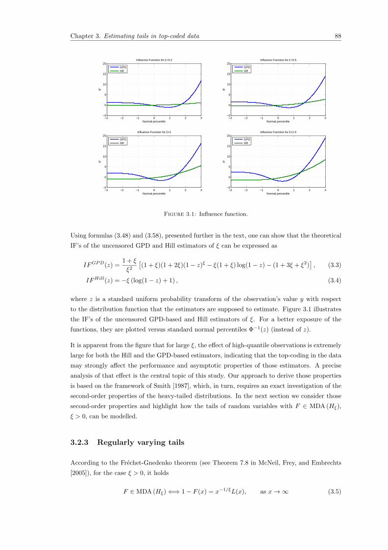
Chapter 3. Estimating tails in top-coded data 88
−3 −2 −1 0 1 2 3−5
0
5
10
15
20Influence Function for ξ=0.2
Normal percentile
IF
GPDHill
−3 −2 −1 0 1 2 3−5
0
5
10
15
20Influence Function for ξ=0.5
Normal percentile
IF
GPDHill
−3 −2 −1 0 1 2 3−5
0
5
10
15
20Influence Function for ξ=1.5
Normal percentile
IF
GPDHill
−3 −2 −1 0 1 2 3−5
0
5
10
15
20Influence Function for ξ=1
Normal percentile
IF
GPDHill
Figure 3.1: Influence function.
Using formulas (3.48) and (3.58), presented further in the text, one can show that the theoretical
IF’s of the uncensored GPD and Hill estimators of ξ can be expressed as
IFGPD(z) =1 + ξ
ξ2
[(1 + ξ)(1 + 2ξ)(1− z)ξ − ξ(1 + ξ) log(1− z)− (1 + 3ξ + ξ2)
], (3.3)
IFHill(z) = −ξ (log(1− z) + 1) , (3.4)
where z is a standard uniform probability transform of the observation’s value y with respect
to the distribution function that the estimators are supposed to estimate. Figure 3.1 illustrates
the IF’s of the uncensored GPD-based and Hill estimators of ξ. For a better exposure of the
functions, they are plotted versus standard normal percentiles Φ−1(z) (instead of z).
It is apparent from the figure that for large ξ, the effect of high-quantile observations is extremely
large for both the Hill and the GPD-based estimators, indicating that the top-coding in the data
may strongly affect the performance and asymptotic properties of those estimators. A precise
analysis of that effect is the central topic of this study. Our approach to derive those properties
is based on the framework of Smith [1987], which, in turn, requires an exact investigation of the
second-order properties of the heavy-tailed distributions. In the next section we consider those
second-order properties and highlight how the tails of random variables with F ∈ MDA (Hξ),
ξ > 0, can be modelled.
3.2.3 Regularly varying tails
According to the Frechet-Gnedenko theorem (see Theorem 7.8 in McNeil, Frey, and Embrechts
[2005]), for the case ξ > 0, it holds
F ∈ MDA (Hξ)⇐⇒ 1− F (x) = x−1/ξL(x), as x→∞ (3.5)
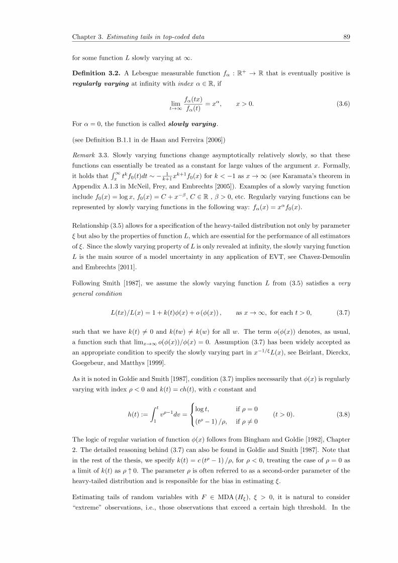
Chapter 3. Estimating tails in top-coded data 89
for some function L slowly varying at ∞.
Definition 3.2. A Lebesgue measurable function fα : R+ → R that is eventually positive is
regularly varying at infinity with index α ∈ R, if
limt→∞
fα(tx)
fα(t)= xα, x > 0. (3.6)
For α = 0, the function is called slowly varying .
(see Definition B.1.1 in de Haan and Ferreira [2006])
Remark 3.3. Slowly varying functions change asymptotically relatively slowly, so that these
functions can essentially be treated as a constant for large values of the argument x. Formally,
it holds that∫∞xtkf0(t)dt ∼ − 1
k+1xk+1f0(x) for k < −1 as x→∞ (see Karamata’s theorem in
Appendix A.1.3 in McNeil, Frey, and Embrechts [2005]). Examples of a slowly varying function
include f0(x) = log x, f0(x) = C + x−β , C ∈ R , β > 0, etc. Regularly varying functions can be
represented by slowly varying functions in the following way: fα(x) = xαf0(x).
Relationship (3.5) allows for a specification of the heavy-tailed distribution not only by parameter
ξ but also by the properties of function L, which are essential for the performance of all estimators
of ξ. Since the slowly varying property of L is only revealed at infinity, the slowly varying function
L is the main source of a model uncertainty in any application of EVT, see Chavez-Demoulin
and Embrechts [2011].
Following Smith [1987], we assume the slowly varying function L from (3.5) satisfies a very
general condition
L(tx)/L(x) = 1 + k(t)φ(x) + o (φ(x)) , as x→∞, for each t > 0, (3.7)
such that we have k(t) 6= 0 and k(tw) 6= k(w) for all w. The term o(φ(x)) denotes, as usual,
a function such that limx→∞ o(φ(x))/φ(x) = 0. Assumption (3.7) has been widely accepted as
an appropriate condition to specify the slowly varying part in x−1/ξL(x), see Beirlant, Dierckx,
Goegebeur, and Matthys [1999].
As it is noted in Goldie and Smith [1987], condition (3.7) implies necessarily that φ(x) is regularly
varying with index ρ < 0 and k(t) = ch(t), with c constant and
h(t) :=
∫ t
1
vρ−1dv =
log t, if ρ = 0
(tρ − 1) /ρ, if ρ 6= 0(t > 0). (3.8)
The logic of regular variation of function φ(x) follows from Bingham and Goldie [1982], Chapter
2. The detailed reasoning behind (3.7) can also be found in Goldie and Smith [1987]. Note that
in the rest of the thesis, we specify k(t) = c (tρ − 1) /ρ, for ρ < 0, treating the case of ρ = 0 as
a limit of k(t) as ρ ↑ 0. The parameter ρ is often referred to as a second-order parameter of the
heavy-tailed distribution and is responsible for the bias in estimating ξ.
Estimating tails of random variables with F ∈ MDA (Hξ), ξ > 0, it is natural to consider
“extreme” observations, i.e., those observations that exceed a certain high threshold. In the
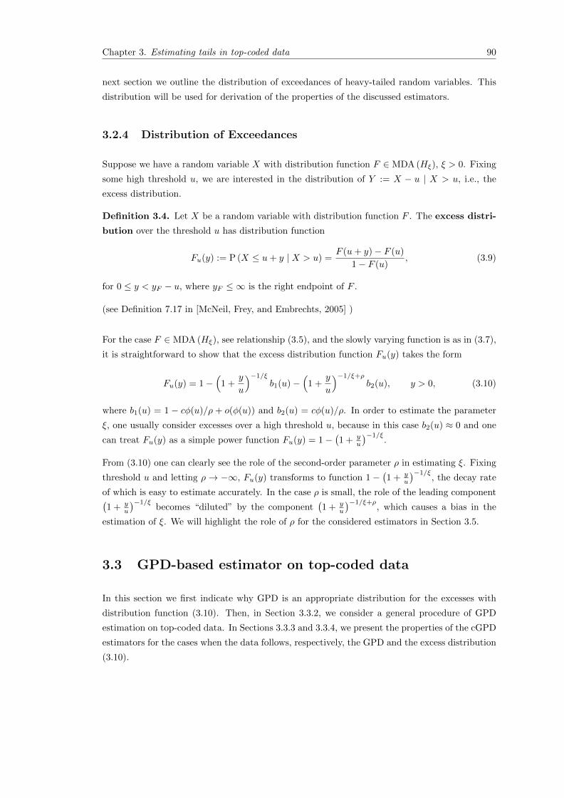
Chapter 3. Estimating tails in top-coded data 90
next section we outline the distribution of exceedances of heavy-tailed random variables. This
distribution will be used for derivation of the properties of the discussed estimators.
3.2.4 Distribution of Exceedances
Suppose we have a random variable X with distribution function F ∈ MDA (Hξ), ξ > 0. Fixing
some high threshold u, we are interested in the distribution of Y := X − u | X > u, i.e., the
excess distribution.
Definition 3.4. Let X be a random variable with distribution function F . The excess distri-
bution over the threshold u has distribution function
Fu(y) := P (X ≤ u+ y | X > u) =F (u+ y)− F (u)
1− F (u), (3.9)
for 0 ≤ y < yF − u, where yF ≤ ∞ is the right endpoint of F .
(see Definition 7.17 in [McNeil, Frey, and Embrechts, 2005] )
For the case F ∈ MDA (Hξ), see relationship (3.5), and the slowly varying function is as in (3.7),
it is straightforward to show that the excess distribution function Fu(y) takes the form
Fu(y) = 1−(
1 +y
u
)−1/ξ
b1(u)−(
1 +y
u
)−1/ξ+ρ
b2(u), y > 0, (3.10)
where b1(u) = 1 − cφ(u)/ρ + o(φ(u)) and b2(u) = cφ(u)/ρ. In order to estimate the parameter
ξ, one usually consider excesses over a high threshold u, because in this case b2(u) ≈ 0 and one
can treat Fu(y) as a simple power function Fu(y) = 1−(1 + y
u
)−1/ξ.
From (3.10) one can clearly see the role of the second-order parameter ρ in estimating ξ. Fixing
threshold u and letting ρ→ −∞, Fu(y) transforms to function 1−(1 + y
u
)−1/ξ, the decay rate
of which is easy to estimate accurately. In the case ρ is small, the role of the leading component(1 + y
u
)−1/ξbecomes “diluted” by the component
(1 + y
u
)−1/ξ+ρ, which causes a bias in the
estimation of ξ. We will highlight the role of ρ for the considered estimators in Section 3.5.
3.3 GPD-based estimator on top-coded data
In this section we first indicate why GPD is an appropriate distribution for the excesses with
distribution function (3.10). Then, in Section 3.3.2, we consider a general procedure of GPD
estimation on top-coded data. In Sections 3.3.3 and 3.3.4, we present the properties of the cGPD
estimators for the cases when the data follows, respectively, the GPD and the excess distribution
(3.10).
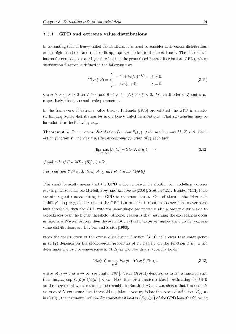
Chapter 3. Estimating tails in top-coded data 91
3.3.1 GPD and extreme value distributions
In estimating tails of heavy-tailed distributions, it is usual to consider their excess distributions
over a high threshold, and then to fit appropriate models to the exceedances. The main distri-
bution for exceedances over high thresholds is the generalised Pareto distribution (GPD), whose
distribution function is defined in the following way
G(x; ξ, β) =
1− (1 + ξx/β)−1/ξ, ξ 6= 0,
1− exp(−xβ), ξ = 0,(3.11)
where β > 0, x ≥ 0 for ξ ≥ 0 and 0 ≤ x ≤ −β/ξ for ξ < 0. We shall refer to ξ and β as,
respectively, the shape and scale parameters.
In the framework of extreme value theory, Pickands [1975] proved that the GPD is a natu-
ral limiting excess distribution for many heavy-tailed distributions. That relationship may be
formulated in the following way.
Theorem 3.5. For an excess distribution function Fu(y) of the random variable X with distri-
bution function F , there is a positive-measurable function β(u) such that
limu→∞
supy>0|Fu(y)−G(x; ξ, β(u))| = 0, (3.12)
if and only if F ∈ MDA (Hξ), ξ ∈ R.
(see Theorem 7.20 in McNeil, Frey, and Embrechts [2005])
This result basically means that the GPD is the canonical distribution for modelling excesses
over high thresholds, see McNeil, Frey, and Embrechts [2005], Section 7.2.1. Besides (3.12) there
are other good reasons fitting the GPD to the exceedances. One of them is the “threshold
stability” property, stating that if the GPD is a proper distribution to exceedances over some
high threshold, then the GPD with the same shape parameter is also a proper distribution to
exceednaces over the higher threshold. Another reason is that assuming the exccedances occur
in time as a Poisson process then the assumption of GPD excesses implies the classical extreme
value distributions, see Davison and Smith [1990].
From the construction of the excess distribution function (3.10), it is clear that convergence
in (3.12) depends on the second-order properties of F , namely on the function φ(u), which
determines the rate of convergence in (3.12) in the way that it typically holds
O(φ(u)) = supy>0|Fu(y)−G(x; ξ, β(u))|, (3.13)
where φ(u) → 0 as u → ∞, see Smith [1987]. Term O(φ(u)) denotes, as usual, a function such
that limu→∞ sup |O(φ(u))/φ(u) | < ∞. Note that φ(u) creates a bias in estimating the GPD
on the excesses of X over the high threshold. In Smith [1987], it was shown that based on N
excesses of X over some high threshold uN (those excesses follow the excess distribution FuN as
in (3.10)), the maximum likelihood parameter estimates(βN , ξN
)of the GPD have the following

Chapter 3. Estimating tails in top-coded data 92
property
N1/2
[βN/βN − 1
ξN − ξ
]→d N
([µ(1+ξ)(1−2ξρ)
1+ξ−ρξµξ(1+ξ)(1+ρ)
1+ξ−ρξ
],
[2(1 + ξ) −(1 + ξ)
−(1 + ξ) (1 + ξ)2
]), (3.14)
as N →∞, uN →∞ such that N1/2cξφ (uN ) /(1− ξρ)→ µ ∈ R. In the next sections we intend
to extend this result to the case when the data is top-coded at some high level.
3.3.2 Estimation of GPD on excesses under top-coding
Suppose(X1, X2, . . . , Xn
)denotes a vector of n independent realisations of random variable
X ∼ Cens(X,u2,N ), where X is a heavy-tailed random variable with distribution function
F ∈ MDA (Hξ), ξ > 0, and u2,N is a threshold corresponding to a very high quantile of X.
Setting another high threshold u1,N , such that u1,N < u2,N , we consider excesses (Y1, . . . , YN )
of(X1, . . . , Xn
)over u1,N , namely, if Xi > u1,N then Yk = Xi − u1,N , where N denotes the
number of exceedances of(X1, . . . , Xn
)over u1,N . To estimate efficiently the tail index ξ by
fitting the GPD to (Y1, . . . , YN ), it is natural to use a censored GPD (cGPD) approach. The
idea behind the approach is simple and lies, first, in determining the region (u1,N , u2,N ), where
observations follow the GPD, and, second, in constructing the likelihood function that captures
properly the censoring in the observations. Setting the thresholds u1,N in practice, there is
always a certain trade-off between the bias and the standard deviations of the GPD’s parameter
estimates: the higher the threshold u1,N the more accurate the approximation of the tail with
the GPD (smaller bias) but smaller the number of the observations (larger variance). There
is no agreed way to choose the “optimal” threshold u1,N in the GPD estimation, see Chavez-
Demoulin and Embrechts [2011], because the choice of u1,N depends crucially on the second-order
properties of the underlying distribution function of the observations.
The likelihood function of cGPD estimator is of the form
LN (ξ, βN ; Y) =
(∏i∈S1
g (Yi; ξ, βN )
)(∏k∈S2
(1−G(wN ; ξ, βN ))
), (3.15)
where wN = u2,N − u1,N , g(y; ξ, βN ) = (∂/∂y)G(y; ξ, βN ), with function G defined in (3.11),
S1 = {k : Yk < wN} and S2 = {k : Yk ≥ wN}. Using notation δk = I(Yk ≥ wN ), the
log-likelihood function takes the form
logLN (ξ, βN ; Y) =
N∑k=1
Lk,N (Yk), (3.16)
where
Lk,N (Yk) = (1− δk) log g(Yk; ξ, βN ) + δk log (1−G (wN ; ξ, βN )) . (3.17)
Note that since the true parameter βN depends on u1,N , as it is explicitly stated in (3.12), we
emphasize this link through the subscript N in βN .

Chapter 3. Estimating tails in top-coded data 93
Following the standard procedure in the analysis of the maximum likelihood estimators, see, for
example, Cox and Hinkley [1974], Chapter 9, we define the score statistic
UN (βN , ξ) =
N∑k=1
Uk,N (βN , ξ),where Uk,N (βN , ξ) =
[βN∂Lk,N/∂βN
∂Lk,N/∂ξ
]
and the observed information matrix
IN =
N∑k=1
Ik,N ,where Ik,N =
[β2N∂
2Lk,N/∂β2N βN∂
2Lk,N/∂βN∂ξ
βN∂2Lk,N/∂βN∂ξ ∂2Lk,N/∂ξ
2
].
To simplify the computations, we follow Smith [1987] and multiply by βN the derivatives with
respect to βN in both UN and IN .
Letting N →∞ and u1,N →∞, we consider the convergence of the following score statistics
N1/2E(Uk,N (βN , ξ))→ b, (3.18)
E[Uk,N (βN , ξ)U
Tk,N (βN , ξ)
]− E(Uk,N (βN , ξ)) (E(Uk,N (βN , ξ)))
T → H, (3.19)
N−1IN →M. (3.20)
Those limit values determine the parameters of the asymptotic distribution of the cGPD esti-
mators βN and ξN (see Greene [2003], Chapter 17 and Smith [1987]) in the following way
N1/2
[βN/βN − 1
ξN − ξ
]→d N
(−M−1b,M−1H
(M−1
)T), (3.21)
whereN (a, b) denotes a normally distributed random variable with mean a and covariance matrix
b. Note that by convergence (3.18)-(3.21) is meant for N → ∞ and u1,N → ∞ simultaneously.
We discuss this relationship and the behaviour of u2,N in Section 3.3.4.
The asymptotic normality of the estimators stated in (3.21) follows from the limit fluctuation
of the normalized vector UN (βN , ξ). In particular, since the MLE estimators βN , ξN maximise
(3.16), it should hold that UN (βN , ξN ) = 0. Expressing UN (βN , ξN ) by the first order Taylor
expansion
UN (βN , ξN ) = UN (β, ξ) + IN
[βN/β − 1
ξN − ξ
]+ o(1) (3.22)
and setting UN (βN , ξN ) = 0, one can obtain the following relationship[βN/βN − 1
ξN − ξ
]=(−N−1IN
)−1 (N−1UN (ξ, β)
)(1 + o(1)). (3.23)
Provided the first two moments of Uk,N (ξ, β) exist, the Lindberg-Levy CLT suggests that
N−1/2UN (ξ, β)→d N (b, H), from which the result in (3.21) follows.
Considering the asymptotic properties of the maximum likelihood estimates, we have omitted
the analysis of the first three moments of Uk,N (ξ, β) (the regularity conditions, see Greene [2003],
p. 474) required to establish (3.22), (3.23) and ultimately (3.21). In the absence of censoring

Chapter 3. Estimating tails in top-coded data 94
these conditions, under the assumption of underlying generalized Pareto and extreme value
distributions, were studied in Smith [1987] and Goldie and Smith [1987]. In the case of top-
coding these conditions automatically hold because top-coding can only decrease the variability
in the moments.
In the following two sections we study the properties of the cGPD estimators under various
assumption on the underlying distribution X.
3.3.3 Properties of cGPD estimator: X ∼ GPD
Suppose that a random variable X is such that its exceedances over some high threshold u1,N
have an exact GPD distribution with ξ > 0. The easiest example is X ∼ GPD. As usual let
u1,N and u2,N be thresholds corresponding to high quantiles of X and set such that u1,N < u2,N ,(X1, . . . , Xn
)be a vector of n independent realizations of Cens (X,u2,N ), and (Y1, . . . , YN ) be
a vector of N excesses of(X1, . . . , Xn
)over the threshold u1,N , namely, for Xi > u1,N it is set
Yk = Xi − u1,N . Conditionally on N , the excesses (Y1, . . . , YN ) are independent and identically
distributed. It is clear that fitting the censored GPD to the excesses is a “correct” model. In
order to find the asymptotic characteristics of the parameter estimates fitting cGPD, in the
following lemma we outline some results for the score statistics in (3.18)-(3.20).
Lemma 3.6. Fitting the cGPD to the excesses (Y1, . . . , YN ) of the independent realizations of
Cens (X,u2,N ), X ∼ GPD, over the threshold u1,N , it holds for the score statistics (3.18)-(3.20)
of the maximum likelihood function (3.15):
E(Uk,N (βN , ξ)) = 0 and M = −H. (3.24)
Proof. Suppose f(x; θ) be a continuous density function with parameter θ of some continuous
random variable Z, and F (x; θ) – its cumulative distribution function. Define K(x; θ) := (1 −δ) log f(x; θ) + δ log F (w; θ), where δ = I(x > w). The expectation of ∂K(Z; θ)/∂θ with respect
to the density f(x; θ) takes the form:
Ef (∂K(Z; θ)/∂θ) =
∫ w
−∞
(∂ log f(x; θ)
∂θ
)f(x; θ)dx+
(∂ log F (w; θ)
∂θ
)F (w; θ) =
=
∫ w
−∞
∂f(x; θ)
∂θdx+
∂F (w; θ)
∂θ= 0, (3.25)
because∂F (w; θ)
∂θ=
∂
∂θ
(1−
∫ w
−∞f(x; θ)dx
)= −
∫ w
−∞
∂f(x; θ)
∂θdx, (3.26)
where we use the notation Ef (h (Z)) =∫h(x)f(x)dx. Since components of the vector Uk,N has
exactly the same form as ∂K(Z; θ)/∂θ, it follows that for the expectation of Uk,N calculated
with respect to density g(x;β, ξ), used for construction of Uk,N , it holds Eg [Uk,N ] = 0.
Chapter 3. Estimating tails in top-coded data 95
To prove that M = −H, we must show H := Ef
[(∂K(Z;θ)
∂θ
)2]
= −Ef
[∂2K(Z;θ)
∂θ2
]=: −M . It
follows
Ef
[(∂K(Z; θ)
∂θ
)2]
= Ef
[(1− δ)2
(∂ log f(Z; θ)
∂θ
)2]
+ Ef
[δ2
(∂ log F (w; θ)
∂θ
)2]
+ 2Ef
[δ(1− δ)∂ log f(Z; θ)
∂θ
∂ log F (w; θ)
∂θ
]Evaluating each component separately we get:
Ef
[(1− δ)2
(∂ log f(Z; θ)
∂θ
)2]
=
∫ w
−∞
(∂ log f(x; θ)
∂θ
)2
f(x; θ)dx
=
∫ w
−∞
(∂ log f(x; θ)
∂θ
)∂f(x; θ)
∂θdx;
Ef
[δ2
(∂ log F (w; θ)
∂θ
)2]
=
(∂ log F (w; θ)
∂θ
)2
F (w; θ) =
(∂ log F (w; θ)
∂θ
)∂F (w; θ)
∂θ;
2Ef
[δ(1− δ)∂ log f(Z; θ)
∂θ
∂ log F (w; θ)
∂θ
]= 0.
Finally,
Ef
[(∂K(Z; θ)
∂θ
)2]
=
∫ w
−∞
(∂ log f(x; θ)
∂θ
)∂f(x; θ)
∂θdx+
(∂ log F (w; θ)
∂θ
)∂F (w; θ)
∂θ. (3.27)
To obtain Ef
[∂2K(Z;θ)
∂θ2
]we differentiate expression
∫ w
−∞
(∂ log f(x; θ)
∂θ
)f(x; θ)dx+
(∂ log F (w; θ)
∂θ
)F (w; θ) = 0 (3.28)
see (3.25), from the both sides by θ obtaining
∫ w
−∞
[(∂2 log f(x; θ)
∂θ2
)f(x; θ) +
(∂ log f(x; θ)
∂θ
)∂f(x; θ)
∂θ
]dx
+
(∂2 log F (w; θ)
∂θ2
)F (w; θ) +
(∂ log F (w; θ)
∂θ
)∂F (w; θ)
∂θ= 0. (3.29)
Rearranging the terms in (3.29) and comparing with (3.27) one immediately obtains M = −H.
Since components of the vector Uk,N has exactly the same form as ∂K(Z; θ)/∂θ, the statement
of the proposition M = −H follows immediately from the above calculations.
The asymptotic properties of the cGPD estimators on data generated by the Cens(X,u2,N ),
with X ∼ GPD, can be summarized in the following proposition.
Proposition 3.7. Let (Y1, . . . , YN ) be N independent realisations of excesses of Cens(X,u2,N ),
with X ∼ GPD(ξ, β), over the high the threshold u1,N (u1,N < u2,N ). As N →∞, the maximum

Chapter 3. Estimating tails in top-coded data 96
likelihood cGPD estimators of the parameters ξ and βN = β + ξu1,N of the excess distribution
satisfy
N1/2
[βN/βN − 1
ξN − ξ
]→d N
([0
0
], H(λ)−1
), (3.30)
where
H(λ)−1 =(1 + ξ)(1 + 2ξ)
(1 + 2ξ + ψ3(λ)(1 + ξ) + ψ1(λ)(2 + ψ3(λ))− ψ2(λ)(2 + ψ2(λ)))×[
2 + ψ3(λ) −(1 + ψ2(λ))
−(1 + ψ2(λ)) 1 + ξ + ψ1(λ)
](3.31)
with
λ = 1 + ξu2,N − u1,N
βN; ψ2(λ) =
λ−1/ξ−2
ξ(1 + ξ − λ(1 + 2ξ)) ; (3.32)
ψ1(λ) = −λ−1/ξ−2(1 + ξ); ψ3(λ) =λ−1/ξ−2
ξ2
(−λ2(1 + ξ)(1 + 2ξ) + 2λ(1 + 2ξ)− (1 + ξ)
).
(3.33)
Proof. The statement of this proposition is based on the previous results in (3.21). Since the
components of that asymptotic result are partially determined in (3.24), the only element left to
find for completion of (3.21) is the matrix M of the expected value of the second-order derivatives
of the score vector UN , see (3.20). As the first step in calculating that matrix, we list below
some formulas required for the construction of M . With Lk,N as in (3.17) we have
βN∂Lk,N (y)
∂βN= −(1− δ)
[(1 +
1
ξ
)λ(y)−1
]− δ 1
ξ
[λ(wN )−1
]+
1
ξ, (3.34)
∂Lk,N (y)
∂ξ=
1− δξ2
[log λ(y) + (1 + ξ)λ(y)−1
]+
δ
ξ2
[log λ(wN ) + λ(wN )−1 + ξ
]− 1 + ξ
ξ2,
(3.35)
β2N
∂2Lk,N (y)
∂β2N
= (1− δ)(
1 +1
ξ
)λ(y)−2 +
δ
ξλ(wN )−2 − 1
ξ, (3.36)
βN∂2Lk,N (y)
∂βN∂ξ= (1− δ)
[2 + ξ
ξ2λ(y)−1 − 1 + ξ
ξ2λ(y)−2
]+
δ
ξ2
[2λ(wN )−1 − λ(wN )−2
]− 1
ξ2,
(3.37)
and
∂2Lk,N (y)
∂ξ2= (1− δ)
[− 2
ξ3log λ(y) +
3 + ξ
ξ3− 2(2 + ξ)
ξ3λ(y)−1 +
1 + ξ
ξ3λ(y)−2
]+
δ
ξ3
[3− 2 log λ(wN )− 4λ(wN )−1 + λ(wN )−2
], (3.38)
where λ(y) = 1 + ξy/βN , wN = u2,N − u1,N and δ = I(y > wN ). For the ease of exposition, we
shall also use λ := λ(wN ).
Chapter 3. Estimating tails in top-coded data 97
With respect to the GPD density g (y; ξ, βN ) = 1βN
(1 + ξ y
βN
)−1/ξ−1
, one can easily calculate
the elements of matrix M , the expected value of the Hessian matrix, with the following formulas∫ w
0
log λ(y)g (y; ξ, βN ) dy = ξ − ξλ(w)−1/ξ − λ(w)−1/ξ log λ(w);∫ w
0
λ(y)−rg (y; ξ, βN ) dy =1
1 + rξ− λ(w)−1/ξ−r
1 + rξ.
Calculating the Hessian matrix M with the above formulas and employing the results from
Lemma 3.6 H(λ) = −M , one can show, omitting some intermediary calculations, that matrix
H(λ) takes the form
H(λ) =1
(1 + ξ)(1 + 2ξ)
[1 + ξ + ψ1(λ) 1 + ψ2(λ)
1 + ψ2(λ) 2 + ψ3(λ)
], (3.39)
with functions ψ1(·), ψ2(·), ψ3(·) defined in the statement of the proposition.
Remark 3.8. Note, that the above asymptotic result holds as N → ∞ and we do not require
u1,N → ∞. This will be completely changed for the case when the underlying distribution is
only approximately GPD, see Section 3.3.4.
The size of λ can be treated as the level of top-coding in the data: the larger λ (provided every-
thing stays unchanged) the lower the level of top-coding in the observations used for estimation.
To consider how λ influences the asymptotic variance of the cGPD estimators, note that for the
elements that constitute covariance matrix H(λ)−1 in (3.31) the following holds
1 + ξ + ψ1(λ) ≥ 0, 1 + ψ2(λ) ≥ 0, 2 + ψ3(λ) ≥ 0, for all λ ≥ 1 and ξ > 0.
Furthermore, the functions ψ1(λ), ψ2(λ), ψ3(λ), and ψ3(λ)(1+ξ)+ψ1(λ)(2+ψ3)−ψ2(λ)(2+ψ2)
are all non-positive and increasing in λ with 0 upper bounds, and the corresponding lower bounds:
−(1+ξ), −1, −2, and −(1+2ξ). Those bounds guarantee that covariance matrix (3.31) is positive
semi-definite. The upper bounds are achieved as λ→∞ – the case when there is no top-coding;
the lower bounds are achieved as λ → 1 – the case when effectively all data is censored away.
Due to the properties of the above functions, it is easy to see, as it was expected, that the
variance of the cGPD estimators increases with the level of top-coding in the data. Figure 3.2
(right-panel) illustrates how the standard deviation of the cGPD estimator of ξ depends on the
level of top-coding λ.
3.3.4 Properties of cGPD estimator: X ∼ EVD
Suppose that the random variable X has distribution function F that belongs to the MDA of
the EVD with ξ > 0. Similarly to the settings of the previous section, let(X1, . . . , Xn
)be a
vector of n independent realizations of X ∼ Cens(X,u2,N ), and (Y1, . . . , YN ) be a vector of N
excesses of(X1, . . . , Xn
)over the threshold u1,N , such that u1,N < u2,N . Conditionally on N ,
the excesses (Y1, . . . , YN ) are independent and identically distributed with distribution function

Chapter 3. Estimating tails in top-coded data 98
Fu1,Nas in (3.10). In the sense of the relationship (3.12), it is clear that fitting the censored GPD
to the excesses is a correct model only asymptotically resulting in bias and increased variance
of the cGPD estimators, compared to the case of X ∼ GPD. In the following proposition, we
summarize those properties.
Proposition 3.9. Suppose X is a heavy-tailed distibution with the excess distribution as in
(3.10). Let (Y1, . . . , YN ) be N independent realisations of Cens(X,u2,N )’s excesses over the high
threshold u1,N set such that u1,N < u2,N and as N →∞,
N1/2cξφ(u1,N )
1− ρξ→ µ ∈ R, (3.40)
u2,N
u1,N→ λ∗ > 1. (3.41)
Then there exist a local maximum(βN , ξN
)of the cGPD likelihood function evaluated on
(Y1, . . . , YN ), such that
N1/2
[βN/βN − 1
ξN − ξ
]→d N
(H (λ∗)
−1b, H (λ∗)
−1), (3.42)
where
b (λ∗) =
µ(1−ρξ)1+ξ−ρξ
(1− λ−1/ξ+ρ−1
∗
)µ
ξ(1+ξ−ρξ)
(ξ + (1− ρξ)λ−1/ξ+ρ−1
∗ − (1 + ξ − ρξ)λ−1/ξ+ρ∗
) , (3.43)
and H (λ∗) as defined in (3.39).
Proof. As it is noted in Section 3.3, the limit of N1/2E (Uk,N (βN , ξ)), as N → ∞ and u1,N →∞ simultaneously, determines the asymptotic bias of the maximum likelihood estimators in
the sense of relationship (3.21), where the expected value E (Uk,N (βN , ξ)) is evaluated with
respect to the distribution function Fu1,N(y) as in (3.10). Note that the parameter βN , which we
wish to estimate, depends on the threshold u1,N (which in turn depends on the number of the
observations) through the threshold stability property of the GPD, namely, βN = ξu1,N . With
this parametrization for βN in the excess distribution function Fu(y), we have the following
relationships
∫ w
0
log λ(y)dFu(y) = ξ +ξ2cφ(u)
1− ρξ− ξb1(u)λ(w)−1/ξ − ξb2(u)
1− ρξλ(w)−1/ξ+ρ−(
λ(w)−1/ξb1(u) + λ(w)−1/ξ+ρb2(u))
log λ(w), (3.44)
∫ w
0
λ(y)−rdFu(y) =1
1 + rξ− ξ2crφ(u)
(1 + rξ)(1 + rξ − ρξ)− b1(u)
1 + rξλ(w)−1/ξ−r−
b2(u)(1− ρξ)1 + rξ − ρξ
λ(w)−1/ξ−r+ρ, (3.45)
where λ(y) = 1 + ξy/βN , b1(u) = 1− cφ(u)/ρ+ o(φ(u)) and b2(u) = cφ(u)/ρ.
Using these formulas, it is easy to show that the expected value E (Uk,N (βN , ξ)) of the com-
ponents (3.34)-(3.35) of the score vector Uk,N (βN , ξ) with respect to the distribution function
Chapter 3. Estimating tails in top-coded data 99
Fu1,N(y) take the form
ξcφ(u1,N )1+ξ−ρξ
(1−
(u2,N
u1,N
)−1/ξ+ρ−1)
+ o(φ(u1,N ))
cφ(u1,N )(1−ρξ)(1+ξ−ρξ)
(ξ + (1− ρξ)
(u2,N
u1,N
)−1/ξ+ρ−1
− (1 + ξ − ρξ)(u2,N
u1,N
)−1/ξ+ρ)
+ o(φ(u1,N ))
.Due to (3.40) and (3.41), we obtain
b (λ∗) := limN→∞
N1/2E (Uk,N (βN , ξ)) = µ(1−ρξ)1+ξ−ρξ
(1− λ−1/ξ+ρ−1
∗
)µ
ξ(1+ξ−ρξ)
(ξ + (1− ρξ)λ−1/ξ+ρ−1
∗ − (1 + ξ − ρξ)λ−1/ξ+ρ∗
) . (3.46)
Considering the covariance matrix in (3.42), note that its functional form is the same as in
the asymptotic distribution (3.30). This is supported by the fact that the result H = −M of
Lemma 3.6 for the case when the excesses follow exactly the GPD, holds asymptotically also
in the case with distribution function Fu1,N, because E (Uk,N (βN , ξ)) → 0, as N → ∞ (this is
because φ(u1,N )→ 0). Furthermore, by direct calculation of elements of M (employing formulas
(3.36)-(3.38) and (3.44)-(3.45)), one can show that the elements of matrix M calculated with
distribution function Fu1,Ndeviate by O(φ(u1,N )) from the corresponding components of this
matrix calculated with distribution function of the corresponding GPD. Therefore as N →∞ it
makes no difference whether M is calculated with respect to Fu1,Nor the corresponding GPD.
As a result, the covariance matrix H−1(λ∗) in (3.42) has the same form as H−1 in (3.31). The
only difference is that λ is replaced by λ∗.
Remark 3.10. Considering λ∗ := limN→∞ λN = limN→∞ u2,N/u1,N , it is clear that there are
three possible cases:
a) λ∗ ∈ [0, 1]; this case leads to degenerate results since it effectively implies that all observa-
tions (excesses) for estimation are censored away.
b) λ∗ →∞; this case effectively implies that there is no censoring. Properties of the estimators
are derived in Smith [1987].
c) λ∗ ∈ (1,∞); this case is the most important for our study as it suggests effective top-coding
in the data. For λ∗ ∈ (1,∞), threshold u2,N should increase with N in the same rate as
u1,N does.
From the assumptions (3.40) and (3.41), it is clear that the thresholds u1,N and u2,N increase
at a certain rate with N (the number of exceedances above u1,N ) and consequently with n
(the number of observations from which exceedances are observed). That relationship can be
derived by considering the second-order properties of the underlying distribution function. As
it is noted in definition (3.7), the function φ(u) is regularly varying with some index ρ < 0, i.e.
φ(u) ∼ uρL(u) , for large u, where L(u) is a slowly varying function. Due to regular variation of
φ(u) and assumption (3.40) one can conclude that
u1,N ∼ O(N−
12ρ
). (3.47)
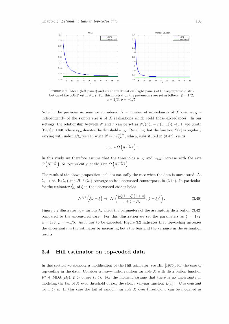
Chapter 3. Estimating tails in top-coded data 100
5 10 15 20 25 30 35 40 45 500.124
0.126
0.128
0.13
0.132
0.134
0.136
0.138
0.14
λ*
Mean
cGPDuncensored
5 10 15 20 25 30 35 40 45 501.4
1.6
1.8
2
2.2
2.4
2.6
2.8
3
3.2
3.4
λ*
Standard Deviation
cGPDuncensored
Figure 3.2: Mean (left panel) and standard deviation (right panel) of the asymptotic distri-bution of the cGPD estimators. For this illustration the parameters are set as follows: ξ = 1/2,
µ = 1/3, ρ = −1/5.
Note in the previous sections we considered N – number of exceedances of X over u1,N –
independently of the sample size n of X realisations which yield those exceedances. In our
settings, the relationship between N and n can be set as N/(n(1 − F (v1,n))) →p 1, see Smith
[1987] p.1180, where v1,n denotes the threshold u1,N . Recalling that the function F (x) is regularly
varying with index 1/ξ, we can write N ∼ nv−1/ξ1,n , which, substituted in (3.47), yields
v1,n ∼ O(n
ξ1−2ρξ
).
In this study we therefore assume that the thresholds u1,N and u2,N increase with the rate
O(N−
12ρ
), or, equivalently, at the rate O
(n
ξ1−2ρξ
).
The result of the above proposition includes naturally the case when the data is uncensored. As
λ∗ → ∞, b (λ∗) and H−1 (λ∗) converge to its uncensored counterparts in (3.14). In particular,
for the estimator ξN of ξ in the uncensored case it holds
N1/2(ξN − ξ
)→d N
(µξ(1 + ξ)(1 + ρ)
1 + ξ − ρξ, (1 + ξ)2
). (3.48)
Figure 3.2 illustrates how various λ∗ affect the parameters of the asymptotic distribution (3.42)
compared to the uncensored case. For this illustration we set the parameters as ξ = 1/2,
µ = 1/3, ρ = −1/5. As it was to be expected, Figure 3.2 indicates that top-coding increases
the uncertainty in the estimates by increasing both the bias and the variance in the estimation
results.
3.4 Hill estimator on top-coded data
In this section we consider a modification of the Hill estimator, see Hill [1975], for the case of
top-coding in the data. Consider a heavy-tailed random variable X with distribution function
F ∗ ∈ MDA (Hξ), ξ > 0, see (3.5). For the moment assume that there is no uncertainty in
modeling the tail of X over threshold u, i.e., the slowly varying function L(x) = C is constant
for x > u. In this case the tail of random variable X over threshold u can be modelled as

Chapter 3. Estimating tails in top-coded data 101
F ∗(x) = 1 − Cx−1/ξ, C > 0. It is natural to consider upper-order statistics that exceed some
threshold u1,N > u from n independent realizations of X and then to estimate ξ and C by the
maximum likelihood estimators ξ and C in the following way
ξ =1
N
N∑j=1
log (1 + Yj,n/u1,N ) , C =N
nu
1/ξ1,N , (3.49)
where N is the number of the upper-order statistics Xn,n > Xn−1,n > . . . > Xn−N+1,n that
exceed u1,N and Yj,n = Xn−j+1,n − u1,N , see Smith [1987].
In the case when the data is top-coded the estimators (3.49) are slightly changed. Consider N
i.i.d excesses (Y1, . . . , YN ) of the random variable X ∼ Cens (X,u2,N ) over the threshold u1,N
set such that u2,N > u1,N , where the tail of X above u1,N follows the distribution function
F ∗(x) = 1 − Cx−1/ξ, x ≥ u1,N . Recall that the random variable of excesses is defined as
Y := X − u1,N | X > u1,N . The likelihood of the excesses can be expressed as
LN (ξ; Y) =
N∏k=1
(f∗u1,N
(Yk; ξ))1−δk (
1− F ∗u1,N(wN ; ξ)
)δk, (3.50)
where F ∗u1,N(y; ξ) = 1 −
(1 + y
u1,N
)−1/ξ
is a distribution function of excesses of X over the
threshold u1,N ; f∗u1,N(y;α) = (∂/∂y)F ∗u1,N
(y; ξ), wN = u2,N − u1,N , and δk = I (Yk ≥ wN ).
One can easily show that function (3.50) is maximised at point ξN set as
ξN =1∑N
i=1 (1− δi)
N∑k=1
[(1− δk) log
(1 +
Yku1,N
)+ δk log
(1 +
wNu1,N
)]. (3.51)
The corresponding estimator of the scale parameter C is identical to (3.49), namely CN =Nn u
1/ξN1,N . Note that without censoring, i.e. as wN → ∞, and setting u1,N as the nearest
upper-order statistic of (X1, . . . , Xn), the above estimator (3.51) transforms to the standard Hill
estimator. As it is noted in Smith [1987], the uncensored version of ξN differs from the Hill’s
estimator, in that deriving ξN N is random and u1,N is fixed while for the standard version of
that estimator N is predetermined and u1,N is set as (N + 1)’st order statistic. Smith [1987]
points out that, in practical terms, there is little difference between those two approaches.
The estimator (3.51) is a natural choice for estimation of ξ also in the case when the tail of X
can only approximately be modelled by the distribution function F ∗(x) = 1−Cx−1/ξ, x ≥ l. In
the following proposition, we summarize the properties of the estimator (3.51) for the case when
data comes from a heavy-tailed distribution with the excess distribution function as in (3.10).
Proposition 3.11. Suppose X is a heavy-tailed distibution with excess distribution as in (3.10).
From n independent realizations of Cens(X,u2,N ), let (Y1, . . . , YN ) denote N excesses over the
Chapter 3. Estimating tails in top-coded data 102
high the threshold u1,N set such that u1,N < u2,N and as N →∞,
N1/2cξφ(u1,N )
1− ρξ→ µ ∈ R, (3.52)
u2,N
u1,N→ λ∗ > 1, (3.53)
N (log u1,N )−2 →∞. (3.54)
Then for the maximum likelihood estimators ξN as in (3.51) and CN = Nn u
1/ξN1,N of the model
P (X > x) = Cx−1/ξ, x ≥ u1,N , the following holds
N1/2
[ξN − ξ
CN−L(u1,N )L(u1,N ) log u1,N
]→d N
(µξ
1− λ−1/ξ+ρ∗
1− λ−1/ξ∗
[1
1
],
ξ2
1− λ−1/ξ∗
[1 1
1 1
]). (3.55)
Proof. Proceeding similarly as in Section 3.3, we denote Uk,N = ∂Lk,N/∂ξ and
IN =∑Nk=1 ∂
2Lk,N/∂ξ2, where
Lk,N = (1− δk)
[−(
1 +1
ξ
)log
(1 +
Yku1,N
)− log ξ − log u1,N
]− δk
1
ξlog
(1 +
wNu1,N
)is a contribution of one observation (excess) to the logarithm of the likelihood function (3.50).
Equations (3.18)-(3.20) determine the parameters of the asymptotic distribution of N1/2(ξN −ξ)in the same way as in (3.21).
Using formulas (3.44)-(3.45) from the proof of the proposition 3.9, it is straightforward to show
E Uk,N =cφ(u1,N )
1− ρξ
(1− λ−1/ξ+ρ
N
), Var Uk,N =
1− λ−1/ξN
ξ2+O (φ (u1,N )) , and
N−1IN → −(
1−λ−1/ξN
)ξ2 , where λN = u2,N/u1,N . Due to the relationships
N1/2cξφ(u1,N )1−ρξ → µ in
(3.52) and λN → λ∗ in (3.53), the asymptotic relation (3.21) in this case takes the form
N1/2(ξN − ξ
)→d N
(µξ
1− λ−1/ξ+ρ∗
1− λ−1/ξ∗
,ξ2
1− λ−1/ξ∗
), N →∞. (3.56)
For the proof the asymptotic properties of CN , we refer to Theorem 4.3.1 in Goldie and Smith
[1987], where, in particular, it is shown that
√N
log u1,N
(uξN−ξ1,N − 1
)∼√N(ξN − ξ
)(3.57)
from which the statement of the proposition can easily be proved.
The results of Proposition 3.11 also hold for the case when the data is uncensored, i.e. letting
λ∗ →∞ in (3.56). In particular, for the estimator of ξ, it holds
N1/2(ξN − ξ
)→d N
(µξ, ξ2
). (3.58)
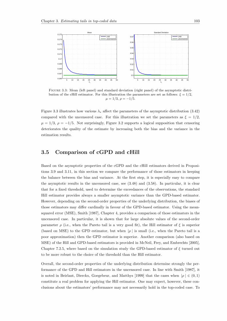
Chapter 3. Estimating tails in top-coded data 103
5 10 15 20 25 30 35 40 45 500.166
0.167
0.168
0.169
0.17
0.171
0.172
0.173
0.174
0.175
λ*
Mean
cHilluncensored
5 10 15 20 25 30 35 40 45 50
0.5
0.51
0.52
0.53
0.54
0.55
0.56
0.57
λ*
Standard Deviation
cHilluncensored
Figure 3.3: Mean (left panel) and standard deviation (right panel) of the asymptotic distri-bution of the cHill estimator. For this illustration the parameters are set as follows: ξ = 1/2,
µ = 1/3, ρ = −1/5.
Figure 3.3 illustrates how various λ∗ affect the parameters of the asymptotic distribution (3.42)
compared with the uncensored case. For this illustration we set the parameters as ξ = 1/2,
µ = 1/3, ρ = −1/5. Not surprisingly, Figure 3.2 supports a logical supposition that censoring
deteriorates the quality of the estimate by increasing both the bias and the variance in the
estimation results.
3.5 Comparison of cGPD and cHill
Based on the asymptotic properties of the cGPD and the cHill estimators derived in Proposi-
tions 3.9 and 3.11, in this section we compare the performance of those estimators in keeping
the balance between the bias and variance. At the first step, it is especially easy to compare
the asymptotic results in the uncensored case, see (3.48) and (3.58). In particular, it is clear
that for a fixed threshold, used to determine the exceedances of the observations, the standard
Hill estimator provides always a smaller asymptotic variance than the GPD-based estimator.
However, depending on the second-order properties of the underlying distribution, the biases of
those estimators may differ cardinally in favour of the GPD-based estimator. Using the mean-
squared error (MSE), Smith [1987], Chapter 4, provides a comparison of those estimators in the
uncensored case. In particular, it is shown that for large absolute values of the second-order
parameter ρ (i.e., when the Pareto tail is a very good fit), the Hill estimator of ξ is superior
(based on MSE) to the GPD estimator, but when |ρ | is small (i.e., when the Pareto tail is a
poor approximation) then the GPD estimator is superior. Another comparison (also based on
MSE) of the Hill and GPD-based estimators is provided in McNeil, Frey, and Embrechts [2005],
Chapter 7.2.5, where based on the simulation study the GPD-based estimator of ξ turned out
to be more robust to the choice of the threshold than the Hill estimator.
Overall, the second-order properties of the underlying distribution determine strongly the per-
formance of the GPD and Hill estimators in the uncensored case. In line with Smith [1987], it
is noted in Beirlant, Dierckx, Goegebeur, and Matthys [1999] that the cases when |ρ | ∈ (0, 1)
constitute a real problem for applying the Hill estimator. One may expect, however, these con-
clusions about the estimators’ performance may not necessarily hold in the top-coded case. To
Chapter 3. Estimating tails in top-coded data 104
investigate this issue in more detail, we employ the procedure described in Smith [1987], Chapter
4, and consider
RMSE (ξ, ρ, λ∗) := limN→∞
minµ MSE for cGPD
minµ MSE for cHill(3.59)
– a ratio of minimised (separately) with respect to µ mean squared errors of cGPD and cHill
estimators of ξ. Minimizing with respect to µ is motivated by the fact that the optimal (in
the sense of minimizing the MSE) threshold u1,N may be set differently for the considered
estimators. In the following proposition we formulate an analytical expression for RMSE based
on the estimators’ properties derived earlier in the text.
Proposition 3.12. With the cGPD estimator as in Proposition 3.9 and the cHill estimator
considered in Proposition 3.11, relationship RMSE defined in (3.59) takes the following form
RMSE(ξ, ρ, λ∗) =d1
d2
(e1d2
e2d1
) 11−2ρξ
,
where d1 = q(1 + ξ + ψ1 (λ∗)),
e1 =q2
(1 + ξ − ρξ)2
[−(1 + ψ2 (λ∗))(1− ρξ)
(1− λ−1/ξ+ρ−1
∗
)+
(1 + ξ + ψ1 (λ∗))
ξ
(ξ + (1− ρξ)λ−1/ξ+ρ−1
∗ − (1 + ξ − ρξ)λ−1/ξ+ρ∗
)]2
,
q =(1 + ξ)(1 + 2ξ)
1 + 2ξ + ψ3 (λ∗) (1 + ξ) + ψ1 (λ∗) (2 + ψ3 (λ∗))− ψ2 (λ∗) (2 + ψ2 (λ∗))
and
d2 =ξ2
1− λ−1/ξ∗
, e2 = ξ2
(1− λ−1/ξ+ρ
∗
1− λ−1/ξ∗
)2
. (3.60)
with functions ψ1(·), ψ2(·), ψ3(·) as defined in (3.32)-(3.33).
Proof. Recalling that the MSE may be decomposed into squared bias plus variance, we obtain
from (3.42) that the asymptotic MSE of the cGPD estimator may be expressed as
MSE(cGPD) ≈(e1µ
2 + d1
)/N, (3.61)
with e1 and d1 defined in the statement of the proposition.
Similarly, one can express the asymptotic MSE of the cHill using (3.56) in the following way
MSE(cHill) ≈(e2µ
2 + d2
)/N, (3.62)
where e2 and d2 are from the proposition above.
Minimizing those MSE’s with respect to µ note that N and µ in both (3.61) and (3.62) are
interrelated through the relationship (3.40), namely,
N1/2cξφ(u1,N )
1− ρξ→ µ. (3.63)

Chapter 3. Estimating tails in top-coded data 105
To make a more in-depth analysis of this relationship, note that for N (the number of ex-
ceedances) and n (the sample size) it holds N ≈ n (1− F (v1,n)), where v1,n denotes the threshold
u1,N . Since F (·) is assumed to be a regularly varying function with index 1/ξ, the relationship
between n and N reads N ≈ nv−1/ξ1,n LF (v1,n), where LF is a slowly varying function. Recalling
that function φ(·) is also regularly varying with index ρ < 0, the relationship (3.63) can finally
be transformed as
nv1(n)−1−2ρξξ L∗(v1(n))→ µ2(1− ρξ)2
c2ξ2, (3.64)
where is L∗ is a slowly varying function. From the above equation we conclude that v1,n is
proportional to µ−2ξ
1−2ρξ , and hence N is proportional to µ2
1−2ρξ . Transferring this result to the
analysis of the asymptotic MSE’s we obtain
MSE(cGPD) ∝(e1µ
2 + d1
)µ−
21−2ρξ MSE(cHill) ∝
(e2µ
2 + d2
)µ−
21−2ρξ . (3.65)
Following Smith [1987] we minimize separately the right-hand sides of the above expressions and
compute RMSE(ξ, ρ, λ) – a ratio of those minimized values (cGPD’s value in numerator). To
find those minimized values note that function g(µ) = (eµ2 + d)µ−k, k > 0 reaches its minimum
value of 2d2−k
(kd
e(2−k)
)−k/2at point µ∗ =
√kd
e(2−k) if g′′ (µ∗) = 2e(2− k) > 0. Since expressions
in (3.65) are of the form as g(µ) and it holds 2e1(2− k) > 0 and 2e2(2− k) > 0 with k = 21−2ρξ ,
it follows that
RMSE(ξ, ρ, λ∗) =d1
d2
(e1d2
e2d1
) 11−2ρξ
. (3.66)
Note that without censoring RMSE(ξ, ρ, λ∗) converges to its uncensored version:
RMSE(ξ, ρ, λ∗)→(1 + ξ)2
ξ2
(ξ(1 + ρ)
1 + ξ − ρξ
) 21−2ρξ
, as λ∗ →∞.
Depending on ρ, RMSE(ξ, ρ, λ∗) takes the following values:
RMSE(ξ, ρ, λ∗)→q(1 + ξ)(1− λ−1/ξ−2
∗ )(1− λ−1/ξ∗ )
ξ2, as ρ→ −∞, (3.67)
RMSE(ξ, ρ, λ∗)→ 1, as ρ→ 0, (3.68)
RMSE(ξ, ρ, λ∗)→ 0, as ρ = −1. (3.69)
Figure 3.4 illustrates RMSE(ξ, ρ, λ∗) for various sets of the parameters ξ, ρ, λ−1/ξ∗ . Note, that
instead of λ∗ we report on the figure λ−1/ξ∗ , which, due to its construction, shows approximately
what proportion of the exceedances is top-coded.
Figure 3.4 clearly illustrates that, in contrast to the uncensored case, the performance of cGPD
estimator depends not only on ρ but also on λ−1/ξ∗ (the proportion of top-coded observations)
and ξ. So cGPD estimator is always superior to cHill in region of small ρ when λ−1/ξ∗ is small.
But when λ−1/ξ∗ is large, i.e., a large proportion of the exceedances is top-coded, the performance
of cGPD estimator depends strongly on ξ: the larger the parameter ξ the smaller the region of
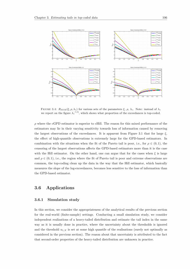
Chapter 3. Estimating tails in top-coded data 106
−2 −1.8 −1.6 −1.4 −1.2 −1 −0.8 −0.6 −0.4 −0.2 00
1
2
3
4
5
6
7
8
ρ
RM
SE
Ratio of minimised MSEs; ξ=0.2
λ*−1/ξ=0.005
λ*−1/ξ=0.01
λ*−1/ξ=0.02
λ*−1/ξ=0.05
λ*−1/ξ=0.1
λ*−1/ξ=0.2
−2 −1.8 −1.6 −1.4 −1.2 −1 −0.8 −0.6 −0.4 −0.2 00
1
2
3
4
5
6
7
8
ρ
RM
SE
Ratio of minimised MSEs; ξ=0.5
λ*−1/ξ=0.005
λ*−1/ξ=0.01
λ*−1/ξ=0.02
λ*−1/ξ=0.05
λ*−1/ξ=0.1
λ*−1/ξ=0.2
−2 −1.8 −1.6 −1.4 −1.2 −1 −0.8 −0.6 −0.4 −0.2 00
0.5
1
1.5
2
2.5
3
3.5
4
4.5
5
ρ
RM
SE
Ratio of minimised MSEs; ξ=1
λ*−1/ξ=0.005
λ*−1/ξ=0.01
λ*−1/ξ=0.02
λ*−1/ξ=0.05
λ*−1/ξ=0.1
λ*−1/ξ=0.2
−2 −1.8 −1.6 −1.4 −1.2 −1 −0.8 −0.6 −0.4 −0.2 00
0.5
1
1.5
2
2.5
3
3.5
4
4.5
5
ρ
RM
SE
Ratio of minimised MSEs; ξ=1.5
λ*−1/ξ=0.005
λ*−1/ξ=0.01
λ*−1/ξ=0.02
λ*−1/ξ=0.05
λ*−1/ξ=0.1
λ*−1/ξ=0.2
Figure 3.4: RMSE(ξ, ρ, λ∗) for various sets of the parameters ξ, ρ, λ∗. Note: instead of λ∗
we report on the figure λ−1/ξ∗ , which shows what proportion of the exceedances is top-coded.
ρ where the cGPD estimator is superior to cHill. The reason for this mixed performance of the
estimators may lie in their varying sensitivity towards loss of information caused by removing
the largest observations of the exceedances. It is apparent from Figure 3.1 that for large ξ,
the effect of high-quantile observations is extremely large for the GPD-based estimators. In
combination with the situations when the fit of the Pareto tail is poor, i.e., for ρ ∈ (0, 1), the
censoring of the largest observations affects the GPD-based estimators more than it is the case
with the Hill estimator. On the other hand, one can argue that for the cases when ξ is large
and ρ ∈ (0, 1), i.e., the region where the fit of Pareto tail is poor and extreme observations are
common, the top-coding clean up the data in the way that the Hill estimator, which basically
measures the slope of the log-exceedances, becomes less sensitive to the loss of information than
the GPD-based estimator.
3.6 Applications
3.6.1 Simulation study
In this section, we consider the appropriateness of the analytical results of the previous section
for the real-world (finite-sample) settings. Conducting a small simulation study, we consider
independent realizations of a heavy-tailed distribution and estimate the tail index in the same
way as it is usually done in practice, where the uncertainty about the thresholds is ignored
and the threshold u1,N is set at some high quantile of the realisations (surely not optimally as
considered in the previous section). The reason about that uncertainty is attributed to the fact
that second-order properties of the heavy-tailed distribution are unknown in practice.

Chapter 3. Estimating tails in top-coded data 107
Without aiming to reach a complete generality, we consider the following hypothetical case for
the simulations: there are daily returns of some stock embracing the period of ten years (ap-
proximately 2500 observations); setting threshold u1,N at the 96%th quantile of the observations
(yielding approximately 100 exceedances), we estimate the tail index on those exceedances under
different levels of top-coding. The threshold set at the 96%th quantile cannot be considered as
an optimal choice in terms of minimizing a MSE of the estimates: this threshold is simply one
possible choice which could have been made in practice, where the second-order properties of the
distribution are unknown. Setting the threshold set at the 96%th quantile, we fix the number
of exceedances N = 100 with respect to the total sample size n = 2500. Alternatively, one can
fix the threshold and consider the number of exceedances as random. In practice, there is little
difference between those two approaches.
In order to capture the cases plotted in Figure 3.4, in the simulation study we consider the
following sets of parameters (ξ, ρ) for the underlying distribution and the level of top-coding
λ−1/ξ∗ :
Parameter-set 1: small ρ, small ξ, and
a) large λ−1/ξ∗ – cGPD should be superior according to our findings in Section 3.5;
b) small λ−1/ξ∗ – cGPD should be superior.
Parameter-set 2: small ρ, large ξ, and
a) large λ−1/ξ∗ – cHill should be superior;
b) small λ−1/ξ∗ – cGPD should be superior.
Parameter-set 3: large ρ, small ξ and
a) large λ−1/ξ∗ – cHill should be superior;
b) small λ−1/ξ∗ – cHill should be superior.
Parameter-set 4: large ρ, large ξ and
a) large λ−1/ξ∗ – cHill should be superior;
b) small λ−1/ξ∗ – cHill should be superior.
Recall: λ−1/ξ∗ shows what proportion of the exceedances is top-coded.
To simulate datasets corresponding to the above cases we use the Burr distribution. Its dis-
tribution function FB(x) = 1 −(
ββ+xτ
)θallows for a direct specification of the second-order
properties. In particular, FB(x) is regularly varying with ξ = 1/(τθ) and ρ = −1/θ, see Beirlant
and Guillou [2001]. Setting the parameters of Burr distribution correspondingly to the above sets
of parameters, we simulate 1000 samples with 100 exceedances over the 96% quantile (threshold
u1,N ) of the underlying distribution. Then setting the censoring threshold u2,N such that a par-
ticular proportion (denoted as λ−1/ξ∗ ) of the exceedances is censored, we estimate ξ parameter on
those exceedances by cGPD and cHill estimators for various levels of censoring λ−1/ξ∗ . Figures
3.5-3.8 illustrate the estimates from the simulation study. As it is expected, the cGPD estimates
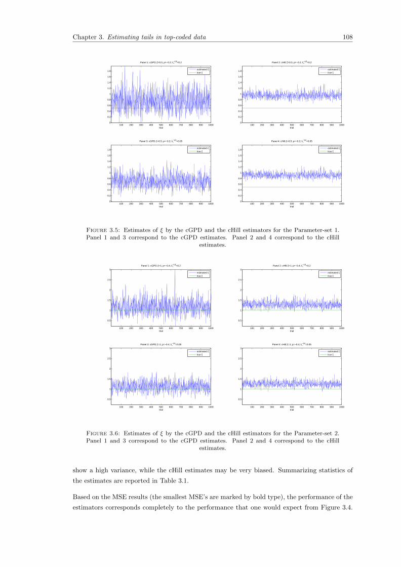
Chapter 3. Estimating tails in top-coded data 108
100 200 300 400 500 600 700 800 900 10000
0.2
0.4
0.6
0.8
1
1.2
1.4
1.6
1.8
Panel 1: cGPD; ξ=0.5; ρ=−0.2; λ*−1/ξ=0.2
trial
estimated ξtrue ξ
100 200 300 400 500 600 700 800 900 10000
0.2
0.4
0.6
0.8
1
1.2
1.4
1.6
1.8
Panel 2: cHill; ξ=0.5; ρ=−0.2; λ*−1/ξ=0.2
trial
estimated ξtrue ξ
100 200 300 400 500 600 700 800 900 10000
0.2
0.4
0.6
0.8
1
1.2
1.4
1.6
1.8
Panel 3: cGPD; ξ=0.5; ρ=−0.2; λ*−1/ξ=0.05
trial
estimated ξtrue ξ
100 200 300 400 500 600 700 800 900 10000
0.2
0.4
0.6
0.8
1
1.2
1.4
1.6
1.8
Panel 4: cHill; ξ=0.5; ρ=−0.2; λ*−1/ξ=0.05
trial
estimated ξtrue ξ
Figure 3.5: Estimates of ξ by the cGPD and the cHill estimators for the Parameter-set 1.Panel 1 and 3 correspond to the cGPD estimates. Panel 2 and 4 correspond to the cHill
estimates.
100 200 300 400 500 600 700 800 900 1000
0.5
1
1.5
2
2.5
3
Panel 1: cGPD; ξ=1; ρ=−0.4; λ*−1/ξ=0.2
trial
estimated ξtrue ξ
100 200 300 400 500 600 700 800 900 1000
0.5
1
1.5
2
2.5
3
Panel 2: cHill; ξ=1; ρ=−0.4; λ*−1/ξ=0.2
trial
estimated ξtrue ξ
100 200 300 400 500 600 700 800 900 1000
0.5
1
1.5
2
2.5
3
Panel 3: cGPD; ξ=1; ρ=−0.4; λ*−1/ξ=0.05
trial
estimated ξtrue ξ
100 200 300 400 500 600 700 800 900 1000
0.5
1
1.5
2
2.5
3
Panel 4: cHill; ξ=1; ρ=−0.4; λ*−1/ξ=0.05
trial
estimated ξtrue ξ
Figure 3.6: Estimates of ξ by the cGPD and the cHill estimators for the Parameter-set 2.Panel 1 and 3 correspond to the cGPD estimates. Panel 2 and 4 correspond to the cHill
estimates.
show a high variance, while the cHill estimates may be very biased. Summarizing statistics of
the estimates are reported in Table 3.1.
Based on the MSE results (the smallest MSE’s are marked by bold type), the performance of the
estimators corresponds completely to the performance that one would expect from Figure 3.4.

Chapter 3. Estimating tails in top-coded data 109
100 200 300 400 500 600 700 800 900 1000−0.2
0
0.2
0.4
0.6
0.8
1
1.2
1.4
Panel 1: cGPD; ξ=0.5; ρ=−3; λ*−1/ξ=0.2
trial
estimated ξtrue ξ
100 200 300 400 500 600 700 800 900 1000−0.2
0
0.2
0.4
0.6
0.8
1
1.2
1.4
Panel 2: cHill; ξ=0.5; ρ=−3; λ*−1/ξ=0.2
trial
estimated ξtrue ξ
100 200 300 400 500 600 700 800 900 1000−0.2
0
0.2
0.4
0.6
0.8
1
1.2
1.4
Panel 3: cGPD; ξ=0.5; ρ=−3; λ*−1/ξ=0.05
trial
estimated ξtrue ξ
100 200 300 400 500 600 700 800 900 1000−0.2
0
0.2
0.4
0.6
0.8
1
1.2
1.4
Panel 4: cHill; ξ=0.5; ρ=−3; λ*−1/ξ=0.05
trial
estimated ξtrue ξ
Figure 3.7: Estimates of ξ by the cGPD and the cHill estimators for the Parameter-set 3.Panel 1 and 3 correspond to the cGPD estimates. Panel 2 and 4 correspond to the cHill
estimates.
100 200 300 400 500 600 700 800 900 10000.2
0.4
0.6
0.8
1
1.2
1.4
1.6
1.8
2
Panel 1: cGPD; ξ=1; ρ=−3; λ*−1/ξ=0.2
trial
estimated ξtrue ξ
100 200 300 400 500 600 700 800 900 10000.2
0.4
0.6
0.8
1
1.2
1.4
1.6
1.8
2
Panel 2: cHill; ξ=1; ρ=−3; λ*−1/ξ=0.2
trial
estimated ξtrue ξ
100 200 300 400 500 600 700 800 900 10000.2
0.4
0.6
0.8
1
1.2
1.4
1.6
1.8
2
Panel 3: cGPD; ξ=1; ρ=−3; λ*−1/ξ=0.05
trial
estimated ξtrue ξ
100 200 300 400 500 600 700 800 900 10000.2
0.4
0.6
0.8
1
1.2
1.4
1.6
1.8
2
Panel 4: cHill; ξ=1; ρ=−3; λ*−1/ξ=0.05
trial
estimated ξtrue ξ
Figure 3.8: Estimates of ξ by the cGPD and the cHill estimators for the Parameter-set 4.Panel 1 and 3 correspond to the cGPD estimates. Panel 2 and 4 correspond to the cHill
estimates.
In particular, the simulation results for the “Parameter-Set 2” are encouraging, as they indicate
a specific for top-coding shift in the performance of the cGPD and cHill parameters depending
on the level of top-coding. Although this simulation study serves rather demonstrative purposes,
the consistency of the theoretical and the simulated behaviour of the estimators indicates their
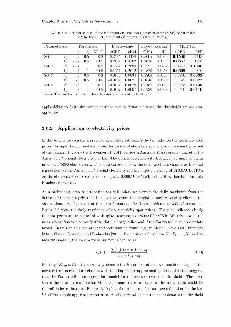
Chapter 3. Estimating tails in top-coded data 110
Table 3.1: Estimated bias, standard deviation, and mean squared error (MSE) of estimatesof ξ by the cGPD and cHill estimators (1000 simulations).
Parameter-set Parameters Bias average St.dev. average MSE*100
ρ ξ λ−1/ξ∗ cGPD cHill cGPD cHill cGPD cHill
Set 1 a) -0.2 0.5 0.2 0.2535 0.4484 0.3005 0.1014 0.1546 0.2113b) -0.2 0.5 0.05 0.2109 0.4162 0.2030 0.0858 0.0857 0.1806
Set 2 a) -0.4 1 0.2 0.1567 0.2880 0.3221 0.1452 0.1283 0.1040b) -0.4 1 0.05 0.1251 0.2612 0.2320 0.1258 0.0695 0.0840
Set 3 a) -3 0.5 0.2 -0.0172 0.0034 0.2806 0.0563 0.0790 0.0032b) -3 0.5 0.05 -0.0109 0.0021 0.1846 0.0518 0.0342 0.0027
Set 4 a) -3 1 0.2 -0.0112 0.0028 0.3157 0.1159 0.0998 0.0135b) -3 1 0.05 -0.0107 0.0007 0.2230 0.1048 0.0499 0.0110
Note: The smallest MSE’s of the estimates are marked by bold type.
applicability to finite-size-sample settings and to situations when the thresholds are set non-
optimally.
3.6.2 Application to electricity prices
In this section we consider a practical example of estimating the tail index on the electricity spot
prices. As input for our analysis serves the dataset of electricity spot prices embracing the period
of the January 1, 2002 - the December 31, 2011, on South Australia (SA) regional market of the
Australia’s National electricity market. The data is recorded with frequency 30 minutes which
provides 175296 observations. This data corresponds to the settings of this chapter as the legal
regulations on the Australia’s National electricity market impose a ceiling of 12500AUD/MWh
on the electricity spot prices (this ceiling was 10000AUD/MWh until 2010), therefore our data
is indeed top-coded.
As a preliminary step to estimating the tail index, we extract the daily maximum from the
dataset of the 30min prices. This is done to reduce the correlation and seasonality effect in the
observations. As the result of this transformation, the dataset reduces to 3651 observations.
Figure 3.9 plots the daily maximum of SA electricity spot prices. The plot indicates clearly
that the prices are heavy-tailed with spikes reaching to 12500AUD/MWh. We rely also on the
mean-excess function to verify if the data is heavy-tailed and if the Pareto tail is an appropriate
model. Details on this and other methods may be found, e.g., in McNeil, Frey, and Embrechts
[2005], Chavez-Demoulin and Embrechts [2011]. For positive-valued data X1, X2, . . . , Xn and its
high threshold u, the mean-excess function is defined as
en(u) =
∑ni=1(Xi − u)I{Xi>u}∑n
i=1 I{Xi>u}. (3.70)
Plotting {Xi,n, en(Xi,n)}, where Xi,n denotes the ith order statistic, we consider a shape of the
mean-excess function for i close to n. If the shape looks approximately linear then this suggests
that the Pareto tail is an appropriate model for the excesses over that threshold. The point
where the mean-excess function visually becomes close to linear can be set as a threshold for
the tail index estimation. Figures 3.10 plots the estimates of mean-excess function for the last
5% of the sample upper order statistics. A solid vertical line on the figure denotes the threshold
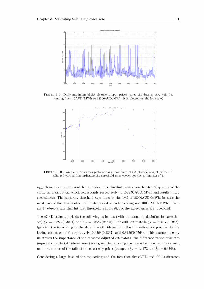
Chapter 3. Estimating tails in top-coded data 111
2002 2003 2004 2005 2006 2007 2008 2009 2010 2011 201210
1
102
103
104
105
Daily max of SA electricity spot ptices
Year
AU
D/M
Wh
(log−
scal
e)
Figure 3.9: Daily maximum of SA electricity spot prices (since the data is very volatile,ranging from 15AUD/MWh to 12500AUD/MWh, it is plotted on the log-scale)
1000 2000 3000 4000 5000 6000 7000 8000 90001000
1500
2000
2500
3000
3500
4000
Mean−excess function for SA max daily electricity prices
Threshold
AU
D/M
Wh
Figure 3.10: Sample mean excess plots of daily maximum of SA electricity spot prices. Asolid red vertical line indicates the threshold u1,N chosen for the estimation of ξ.
u1,N chosen for estimation of the tail index. The threshold was set on the 96.85% quantile of the
empirical distribution, which corresponds, respectively, to 1589.33AUD/MWh and results in 115
exceedances. The censoring threshold u2,N is set at the level of 10000AUD/MWh, because the
most part of the data is observed in the period when the ceiling was 10000AUD/MWh. There
are 17 observations that hit that threshold, i.e., 14.78% of the exceedances are top-coded.
The cGPD estimator yields the following estimates (with the standard deviation in parenthe-
ses) ξN = 1.4272(0.3811) and βN = 1068.7(247.2). The cHill estimate is ξN = 0.9547(0.0963).
Ignoring the top-coding in the data, the GPD-based and the Hill estimators provide the fol-
lowing estimates of ξ, respectively, 0.3268(0.1237) and 0.8236(0.0768). This example clearly
illustrates the importance of the censored-adjusted estimators: the difference in the estimates
(especially for the GPD-based ones) is so great that ignoring the top-coding may lead to a strong
underestimation of the tails of the electricity prices (compare ξN = 1.4272 and ξN = 0.3268).
Considering a large level of the top-coding and the fact that the cGPD and cHill estimators

Chapter 3. Estimating tails in top-coded data 112
0 2000 4000 6000 8000 10000 120000
0.1
0.2
0.3
0.4
0.5
0.6
0.7
0.8
0.9
1Distribution function of the excedances
empirical cdfstandard GPDstandard Hillcensored GPDcensored Hill
Figure 3.11: Excess distribution functions implied by the cGPD and the cHill estimatorscompared to the empirical excess distribution function of the exceedances of daily maxima of
SA electricity prices.
provide a large estimate of ξ (much higher than the usual estimates in the financial literature),
one may expect, based on the analysis in Figure 3.4, that the cHill estimator provides a better
(less biased, less volatile) estimate of ξ and hence a better a fit to the data. On the other
hand, since the excess distribution function F ∗u1,N(y; ξ) = 1−
(1 + y
u1,N
)−1/ξ
implied by the Hill
estimator lacks the scale parameter (which is available in the GPD), one would expect that the
fit the cHill estimator is inferior to the cGPD’s one, see McNeil, Frey, and Embrechts [2005],
Section 7.2.4. Figure 3.11 plots the excess distribution functions implied by the cGPD and
the cHill estimators compared to the empirical excess distribution function. The figure clearly
illustrates that the excess distribution function of the cHill estimator fits the data convincingly
well, supporting the the major finding of this chapter that the cHill estimator provides reasonable
estimates of ξ in situations when both the parameter ξ and the level of top-coding are large.
3.7 Conclusion
Practitioners often encounter problems estimating extreme value distributions on data where the
values of observations above a certain threshold are unknown. In this chapter we examine how
two popular estimators of the extreme value distribution can be adjusted to those settings. In
particular, we consider the maximum likelihood estimation of the generalized Pareto distribution
(GPD) and the Hill estimator. Working in the framework of Smith [1987], we establish the
asymptotic normality of those estimators and provide a detailed analysis of how various levels
of top-coding influence the asymptotic bias and variance of the estimators depending on the
second order properties of the underlying distribution. For high levels of top-coding, our findings
suggest a superior performance of the Hill estimator over the GPD approach in estimating large
extreme value indexes. In particular, the Hill estimator may provide a smaller MSE than the
GPD approach. This result contradicts the broad conclusion about the performance of those
estimators in the uncensored case. Our findings are supported by a small simulation study and
an application to electricity spot prices of Australia’s national electricity market.

Chapter 3. Estimating tails in top-coded data 113
Since the performance of the cGPD and cHill estimators depends strongly on the second order
properties (mostly parameter ρ) of the underlying distribution, in future research it would be
interesting to integrate the methods of ρ estimation, see, for example Fraga Alves, Gomes, and
de Haan [2003], with the estimation of the tail index on the top-coded data.
Conclusion
In view of the recent financial crisis and growing reciprocal distrust of financial institutions,
there is a strong demand for risk management models that can describe the occurrence and the
main characteristics of (multivariate) extreme events. In this thesis, we make an attempt to
develop some quantitative aspects of those models focusing mainly on applications of extreme
value theory.
Chapter 1 presents a model that can capture the typical features of multivariate extreme events
observed in financial time series, namely, clustering behavior in magnitudes and arrival times
of multivariate extreme events, and time-varying dependence. The model is developed in the
framework of the peaks-over-threshold approach in extreme value theory and relies on a Poisson
process with self-exciting intensity. We discuss the properties of the model, treat its estimation,
deal with testing goodness-of-fit, develop a simulation algorithm. The model is applied to return
data of two stock markets and four major European banks. The empirical results demonstrate
a reasonable fit of the model and support an empirical importance of the self-exciting feature
for modeling both occurrence times, magnitudes, and interdependencies of the extreme returns.
A major advantage of the proposed model is its combined approach for modeling time and
magnitudes of the multivariate extreme events in dependent time series.
The model of Chapter 1 provides also a number of suggestions for future research. In particular,
high-dimensional applications of the model are worth consideration. The problem of parameters’
proliferation, which is inevitable in this case, may be resolved by applying the principle of pair
copula construction to our multivariate point-process model (this is possible due to the repre-
sentation form in Proposition 1.4). This construction principle will provide a flexible estimation
approach and equip the model with a feasible ability to get estimated on multivariate data, say,
with 50 or larger number of dimensions.
Chapter 2 introduces a forecasting model to extreme electricity prices in high frequency settings.
The model is suited for forecasting electricity price exceedances over very high thresholds, where
no or only a few observations are available. Employing a copula with a changing dependence
parameter, the model captures explicitly the time-adjusted dependence in the extreme prices.
Magnitudes of extreme prices are modelled by the censored GPD, which allows for a price ceiling
in the electricity spot prices. For modelling occurrence times of the extreme prices, a duration
approach based on a negative binomial distribution is proposed. An eminent advantage of this
approach is that it captures the main characteristics of the occurrence times and outperforms
common duration models like the ACD models and the Hawkes processes. The forecasting model
114
Conclusion 115
is successfully applied to electricity spot prices from Australia’s national electricity market. A
promising direction for a future research is to consider a multivariate approach for modeling
extreme electricity spot prices. Multivariate approaches can capture strong interdependences
between regional electricity markets and describe the contagion effects between them.
The aim of Chapter 3 is to examine how two popular estimators of the extreme value distributions
can be extended to the settings of top-coding, i.e., to situations when the values of observations
above a certain threshold are unknown. In particular, the maximum likelihood estimator of the
GPD and the Hill estimator are considered and their asymptotic properties under top-coding
are established. The major finding of the chapter is that the Hill estimator preforms superiorly
over the GPD-based approach in estimating small (< 1) tail indexes under high levels of top-
coding. This finding contradicts the broad conclusion about the performance of those estimators
in the uncensored case. In all cases, however, the performance of the considered estimators
depends strongly on the second order properties of the underlying distribution of observations.
In future research it would be interesting to integrate the estimation methods of the second-order
properties with the estimation of the tail index on the top-coded data. It would ensure use of
the best estimator for a particular case of the second order properties.

Bibliography
Aas, K., C. Czado, A. Frigessi, and H. Bakken (2009): “Pair-copula constructions of
multiple dependence,” Insurance: Mathematics and Economics, 44(2), 182–198.
Acharya, V., L. Pedersen, T. Philippon, and M. Richardson (2010): “Measuring Sys-
tematic Risk,” Working paper.
Aıt-Sahalia, Y., J. Cacho-Diaz, and R. J. Laeven (2011): “Modeling Financial Contagion
Using Mutually Exciting Jump Processes,” NBER Working Paper No. w15850.
Andriani, P., and B. McKelvey (2007): “A negative binomial model for time series of
counts,” Journal of International business Studies, 38, 1212–1230.
Bae, K.-H., G. A. Karolyi, and R. M. Stulz (2003): “A New Approach to Measuring
Financial Contagion,” The Review of Financial Studies, 16(3), 717–763.
Balkema, A. A., and L. de Haan (1974): “Residual life time at great age,” The Annals of
Probability, 2(5), 792–804.
Bauwens, L., and N. Hautsch (2009): “Modelling financial high frequency data with point
processes,” in Handbook of Financial Time Series, ed. by T. G. Andersen, R. A. Davis, J.-P.
Kreiss, and T. Mikosch. Springer Verlag.
Becker, R., S. Hurn, and V. Pavlov (2007): “Modeling Spike in Electricity Prices,” The
Economic Record, 83(263), 371–382.
Beirlant, J., G. Dierckx, Y. Goegebeur, and G. Matthys (1999): “Tail Index Estimation
and an Exponential Regression Model,” Extremes, 2:2, 177–200.
Beirlant, J., and A. Guillou (2001): “Pareto Index Estimation Under Moderate Right
Censoring,” Scandinavian Actuarial Journal, 2, 111–125.
Beirlant, J., A. Guillou, G. Dierckx, and A. Fils-Villetard (2007): “Estimation of the
extreme value index and extreme quantiles under random censoring,” Extremes, 10, 151–174.
Bekaert, G., M. Ehrmann, M. Fratzscher, and A. Mehl (2012): “Global crisis and
equity market contagion,” Working Paper.
Bingham, N. H., and C. M. Goldie (1982): “Extension of regular variation, I: uniformity
and quantifiers,” Proc. London Math. Soc., 44, 473–496.
116
Bibliography 117
Bollerslev, T. (1986): “Generalized autoregressive conditional heteroskedasticity,” Journal
of Econometrics, 31, 307–327.
Bollerslev, T., V. Todorov, and S. Z. Li (2013): “Jump tails, extreme dependencies, and
the distribution of stock returns,” Journal of Econometrics, 172, 307–324.
Bowsher, C. G. (2007): “Modelling security market events in continuous time: Intensity based,
multivariate point process models,” Journal of Econometrics, 141, 876–912.
Chavez-Demoulin, V., and A. C. Davison (2012): “Modelling time series extremes,” REV-
STAT – Statistical Journal, 10(1), 109–133.
Chavez-Demoulin, V., A. C. Davison, and A. J. McNeil (2005): “Estimating Value-at-
Risk: A point process approach,” Quantitative Finance, 5(2), 227–234.
Chavez-Demoulin, V., and P. Embrechts (2010): “Revisiting the edge, ten years on,”
Communications in Statistics - Theory and Methods, 39, 1674–1688.
(2011): “An EVT primer for credit risk,” The Oxford Handbook of Credit Derivatives,
73(1), 500–532.
Chavez-Demoulin, V., P. Embrechts, and J. G. Neslehova (2006): “Quantitative models
for operational risk: Extremes, dependence and aggregation,” Journal of Banking & Finance,
30, 2635–2658.
Chavez-Demoulin, V., and J. A. McGill (2012): “High-frequency financial data modeling
using Hawkes processes,” Journal of Banking & Finance, 36, 3415–3426.
Christensen, T. M., S. Hurn, and K. A. Lindsay (2009): “It never rains but it pours:
modelling the persistence of spikes in electricity prices,” The Energy Journal, 30, 25–48.
(2012): “Forecasting spikes in electricity prices,” International Journal of Forecasting,
28(2), 400–411.
Coles, S. G. (2001): An Introduction to Statistical Modeling of Extreme Values. Springer.
Coles, S. G., and J. A. Tawn (1991): “Modelling extreme multivariate events,” Journal of
Royal Statistical Society B, 53(2), 377–392.
Cox, D. R., and D. V. Hinkley (1974): Theoretical Statistics. Chapman and Hall, London.
Daley, D. J., and D. Vere-Jones (1988): An Introduction to the Theory of Point Processes.
New York: Springer.
(2005): An Introduction to the Theory of Point Processes. Volume 1. Elementary Theory
and Methods. Springer.
Danielsson, J. (2013): “Does Risk Forecasting Help Macroprudential Pol-
icy Makers?,” Working Paper, http://www.riskresearch.org/files/
Does-Risk-Forecasting-Help-Macroprudential-Policy-Makers.pdf.
Das, B., P. Embrechts, and V. Fasen (2013): “Four Theorems and a Financial Crisis,”
International Journal of Approximate Reasoning, 54(6), 701–716.
Bibliography 118
Davis, R. A., and T. Mikosch (2009a): “Extreme Value Theory for GARCH Processes,” in
Handbook of Financial Time Series, ed. by T. G. Andersen, R. A. Davis, J.-P. Kreiss, and
T. Mikosch, pp. 355–364. Springer Verlag.
(2009b): “Extreme Value Theory for GARCH Processes,” in Handbook of Financial
Time Series, ed. by T. G. Andersen, R. A. Davis, J.-P. Kreiss, and T. Mikosch, pp. 187–200.
Springer Verlag.
Davis, R. A., and R. Wu (2009): “A negative binomial model for time series of counts,”
Biometrika, 96(3), 735–749.
Davison, A. C., and R. L. Smith (1990): “Models for Exceedances over High Thresholds,”
Journal of the Royal Statistical Society B, 52, 393–442.
de Haan, L., and J. de Ronde (1998): “Sea and Wind: Multivariate Extremes at Work,”
Extremes, 1(1), 7–45.
de Haan, L., and A. Ferreira (2006): Extreme Value Theory: An Introduction. New York:
Springer.
Demarta, S., and A. J. McNeil (2005): “The t copula and related copulas,” International
Statistical Review, 73(1), 111–129.
Diebold, F. X., T. A. Gunther, and A. S. Tay (1998): “Evaluating Density Forecasts with
Applications to Financial Risk Management,” International Economic Review, 39(4), 863–883.
Drees, H., and L. de Haan (2012): “Estimating Failure Probabilities,” Working Paper.
Eichler, M., O. Grothe, H. Manner, and D. Tuerk (2012): “Modeling spike occurrences
in electricity spot prices for forecasting,” METEOR Research Memoranda.
Einmahl, J. H. J., L. de Haan, and A. Krajina (2013): “Estimating extreme bivariate
quantile regions,” Extremes, 16, 121–145.
Embrechts, P., L. de Haan, and X. Huang (2000): “Modelling multivariate extremes,”
Extremes and Integrated Risk Management, pp. 59–67, RISK Books.
Embrechts, P., C. Kluppelberg, and T. Mikosch (1997): Modelling Extremal Events for
Insurance and Finance. Springer.
Embrechts, P., T. Liniger, and L. Lin (2011): “Multivariate Hawkes Processes: an Appli-
cation to Financial Data,” Journal of Applied Probability, 48(A), 367–378.
Embrechts, P., A. J. McNeil, and D. Straumann (2002): “Correlation and Dependency in
Risk Management: Properties and Pitfalls,” in Risk Management: Value at Risk and Beyond,
ed. by M. Dempster, pp. 176–223. Cambridge University Press.
Engle, R. F., and J. R. Russell (1998): “Autoregressive Conditional Duration: A New
Model for Irregularly Spaced Transaction Data,” Econometrica, 66(5), 1127–62.
Errais, E., K. Giesecke, and L. R. Goldberg (2010): “Affine Point Processes and Portfolio
Credit Risk,” SIAM Journal of Financial Mathematics, 1, 642–665.
Bibliography 119
Fraga Alves, M. I., M. I. Gomes, and L. de Haan (2003): “A new class of semi-parametric
estimators of the second-order parameter,” Portugalia Mathematica, 60, 193–213.
Geman, H., and A. Roncoroni (2010): “Understanding the fine structure of electricity prices,”
Journal of Business, 79, 1225–1261.
Goldie, C. M., and R. L. Smith (1987): “Slow variation with remainder: a survey of the
theory and its applications,” Quarterly Journal Of Mathematics, 38(2), 45–71.
Golosnoy, V., B. Gribisch, and R. Liesenfeld (2012): “Intra-Daily Volatility Spillovers
between the US and German Stock Markets,” Working Paper.
Grammig, J., and K.-O. Maurer (2000): “Non-monotonic hazard functions and the autore-
gressive conditional duration model,” Econometrics Journal, 3, 16–38.
Greene, W. H. (2003): Econometric Analysis. Prentice Hall.
Grothe, O., V. Korniichuk, and H. Manner (2012): “Modeling Multivariate Extreme
Events Using Self-Exciting Point Processes,” CGS Working Papers.
Gudendorf, G., and J. Segers (2010): “Extreme-Value Copulas,” in Copula Theory and Its
Applications, ed. by P. Jaworski, F. Durante, W. K. Hardle, and T. Rychlik, pp. 127–145.
Hampel, F. R., E. M. Ronchetti, P. J. Rousseeuw, and W. A. Stahel (1986): Robust
Statistics: The Approach Based on Infleunce Functions. New York, Willey.
Haug, S., C. Kluppelberg, and L. Peng (2011): “Statistical models and methods for de-
pendence in insurance data,” Journal of the Korean Statistical Society, 40, 125–139.
Hawkes, A. G. (1971): “Point Spectra of Some Mutually Exciting Point Processes,” Journal
of the Royal Statistical Society B, 33(3), 438–443.
Hawkes, A. G., and D. Oakes (1974): “A cluster process representation of a self-exciting
process,” Journal of Applied Probability, 11, 493–503.
Helmstetter, A., and D. Sornette (2002): “Sub-critical and Super-critical Regimes in
Epidemic Models of Earthquake Aftershocks,” Journal of Geophysical Research, 107(10), 1–
21.
Hill, B. M. (1975): “A Simple General Approach to Inference About the Tail of a Distribution,”
The Annals of Statistics, 3(5), 1163–1174.
Juri, A., and M. V. Wuthrich (2002): “Copula convergence theorems for tail events,” In-
surance: Mathematics and Economics, 30, 405–420.
Kluppelberg, C., T. Meyer-Brandis, and A. Schmidt (2010): “Electricity spot price
modelling with a view towards extreme spike risk,” Quantitative Finance, 10:9, 963–974.
Korniichuk, V. (2012): “Forecasting extreme electricity spot prices,” CGS Working Papers.
(2013): “Estimating tails in right-censored data,” CGS Working Papers.

Bibliography 120
Leadbetter, M. R. (1983): “Extremes and local dependence in stationary sequences,”
Zeitschrift fur Wahrscheinlichkeitstheorie und verwandte Gebiete, 65, 291–306.
(1988): “Extremal theory for stochastic processes,” The Annals of Probability, 16(2),
431–478.
(1991): “On a basis for ”Peaks over Threshold” modeling,” Statistics and Probability
Letters, 12, 357–362.
Leadbetter, M. R., G. Lindgren, and H. Rootzen (1983): Extremes and related properties
of random sequences and processes. Springer-Verlag.
Mandelbrot, B. B. (1963): “The variation of certain speculative prices,” The Journal of
Business of the University of Chicago, 36, 394–419.
McNeil, A. J., and R. Frey (2000): “Estimation of tail-related risk measures for heteroscedas-
tic financial time series: an extreme value approach,” Journal of Empirical Finance, 7, 271–
300.
McNeil, A. J., R. Frey, and P. Embrechts (2005): Quantitative Risk Management: Con-
cepts, Techniques, Tools. Princeton University Press.
Mikosch, T. (2005): “How to model multivariate extremes if one must,” Statistica Neerlandica,
59(3), 324–338.
Mikosch, T., and C. Starica (2000): “Limit Theory for the Sample Autocorrelations and
Extremes of a GARCH (1, 1) process,” The Annals of Statistics, 28(5), 1427–1451.
Møller, J., and J. G. Rasmussen (2005): “Perfect simulation of Hawkes processes,” Advances
in Applied Probability, 37, 629–646.
Nelsen, R. B. (2006): An Introduction to Copulas. Springer.
Oakes, D. (1975): “A Markovian self-exciting process,” Journal of Applied Probability, 12,
69–77.
Ogata, Y. (1978): “The asymptotic behaviour of maximum likelihood estimators for stationary
point processes,” Annals of the Institute of Statistical Mathematics, 30(A), 223–261.
(1981): “On Lewis’ Simulation Method for Point Processes,” IEEE Transactions on
Information Theory, 27(1), 23–31.
(1988): “Statistical Models for Earthquake Occurrences and Residual Analysis for Point
Processes,” Journal of the American Statistical Association, 83(401), 9–27.
Okhrin, O., Y. Okhrin, and W. Schmid (2013): “On the structure and estimation of hier-
archical Archimedean copulas,” Journal of Econometrics, 173, 189–204.
Patton, A. J. (2012): “A review of copula models for econometric time series,” Journal of
Multivariate Analysis, 110, 4–18.
Pickands, J. (1975): “Statistical inference using extreme order statistics,” The Annals of Statis-
tics, 3, 119–131.

Bibliography 121
Resnick, S. I. (1987): Extreme Values, Point Processes, and Regular Variation. Springer-
Verlag.
(2007): Extreme Values, Regular Variation, and Point Processes. Springer.
Resnick, S. I., and C. Starica (1995): “Consistency of Hill’s estimator for dependent data,”
Journal of Applied Probability, 32, 139–167.
Rootzen, H., and N. Tajvidi (2006): “Multivariate generalized Pareto distributions,”
Bernoulli, 12, 917–930.
Shephard, N. (1996): “Statistical aspects of ARCH and stochastic volatility,” in Time Series
Models: In econometrics, finance and other fields, ed. by D. R. Cox, D. V. Hinkley, and O. E.
Barndorff-Nielsen, pp. 1–67. Chapman and Hall, London.
Sibuya, M. (1959): “Bivariate extreme statistics,” Annals of the Institute of Statistical Mathe-
matics, 11, 195–210.
Smith, R. L. (1987): “Estimating tails of probability distributions,” The Annals of Statistics,
18(3), 1174–1207.
Smith, R. L., J. A. Tawn, and S. G. Coles (1997): “Markov chain models for threshold
exceedances,” Biometrika, 84(2), 249–268.
Tawn, J. A. (1990): “Modelling multivariate extreme value distributions,” Biometrika, 77,2,
245–253.
van Dijk, D., P. H. Franses, and A. Lucas (1999): “Testing for ARCH in the Presence of
Additive Outliers,” Journal of Applied Econometrics, 14, 539–562.
Vere-Jones, D., and R. B. Davies (1966): “A statistical survey of earthquakes in the main
seismic region of New Zealand,” New Zealand Journal of Geology and Geophysics, 9(3), 251–
284.
Wongswan, J. (2006): “Transmission of information across international equity markets,”
Review of Financial Studies, 19, 1157–1189.