econstor www.econstor.eu

Der Open-Access-Publikationsserver der ZBW – Leibniz-Informationszentrum WirtschaftThe Open Access Publication Server of the ZBW – Leibniz Information Centre for Economics

Standard-Nutzungsbedingungen:

Die Dokumente auf EconStor dürfen zu eigenen wissenschaftlichenZwecken und zum Privatgebrauch gespeichert und kopiert werden.

Sie dürfen die Dokumente nicht für öffentliche oder kommerzielleZwecke vervielfältigen, öffentlich ausstellen, öffentlich zugänglichmachen, vertreiben oder anderweitig nutzen.

Sofern die Verfasser die Dokumente unter Open-Content-Lizenzen(insbesondere CC-Lizenzen) zur Verfügung gestellt haben sollten,gelten abweichend von diesen Nutzungsbedingungen die in der dortgenannten Lizenz gewährten Nutzungsrechte.

Terms of use:

Documents in EconStor may be saved and copied for yourpersonal and scholarly purposes.

You are not to copy documents for public or commercialpurposes, to exhibit the documents publicly, to make thempublicly available on the internet, or to distribute or otherwiseuse the documents in public.

If the documents have been made available under an OpenContent Licence (especially Creative Commons Licences), youmay exercise further usage rights as specified in the indicatedlicence.

zbw Leibniz-Informationszentrum WirtschaftLeibniz Information Centre for Economics

Arroyo Miranda, Juan; Gómez Cram, Roberto; Lever Guzmán, Carlos

Working Paper

Can matching frictions explain the increase inMexican unemployment after 2008?

Working Papers, Banco de México, No. 2014-08

Provided in Cooperation with:Bank of Mexico, Mexico City

Suggested Citation: Arroyo Miranda, Juan; Gómez Cram, Roberto; Lever Guzmán, Carlos(2014) : Can matching frictions explain the increase in Mexican unemployment after 2008?,Working Papers, Banco de México, No. 2014-08

This Version is available at:http://hdl.handle.net/10419/100119

Banco de Mexico

Documentos de Investigacion

Banco de Mexico

Working Papers

N◦ 2014-08

Can Matching Frictions Explain the Increase inMexican Unemployment After 2008?

Juan Arroyo Miranda Roberto Gomez CramBanco de Mexico Banco de Mexico

Carlos Lever GuzmanBanco de Mexico

April 2014

La serie de Documentos de Investigacion del Banco de Mexico divulga resultados preliminares de

trabajos de investigacion economica realizados en el Banco de Mexico con la finalidad de propiciar

el intercambio y debate de ideas. El contenido de los Documentos de Investigacion, ası como las

conclusiones que de ellos se derivan, son responsabilidad exclusiva de los autores y no reflejan

necesariamente las del Banco de Mexico.

The Working Papers series of Banco de Mexico disseminates preliminary results of economic

research conducted at Banco de Mexico in order to promote the exchange and debate of ideas. The

views and conclusions presented in the Working Papers are exclusively of the authors and do not

necessarily reflect those of Banco de Mexico.

Documento de Investigacion Working Paper2014-08 2014-08

Can Matching Frictions Explain the Increase inMexican Unemployment After 2008?*

Juan Arroyo Miranda† Roberto Gomez Cram†

Banco de Mexico Banco de Mexico

Carlos Lever Guzman†

Banco de Mexico

Abstract: We use a novel data set on firm vacancies and job seekers from a Mexicangovernment job placement service to analyze whether changes in matching frictions canexplain the large and persistent increase in Mexican unemployment after the 2008 globalfinancial crisis. We find evidence of a statistically significant reduction in the efficiency ofthe matching function during the crisis. The estimated effect explains about 70 basis points ofthe 233 basis points observed increase in the unemployment rate. Hence, these results suggestthat changes in matching frictions cannot explain most of the increase in unemployment.Keywords: Matching function estimation; Unemployment; Vacancies.JEL Classification: J63; J64; E24.

Resumen: Este trabajo utiliza una nueva fuente de datos sobre vacantes de empleopublicadas por empresas y de solicitantes de empleo proveniente de un servicio de vinculacionlaboral del gobierno mexicano para analizar si los cambios en las fricciones de contratacionpueden explicar el importante y persistente incremento del desempleo en Mexico despues dela crisis financiera mundial de 2008. Se encuentra evidencia de una reduccion estadısticamentesignificativa en la eficiencia de la funcion de matching durante la crisis. El efecto estimadoexplica alrededor de 70pb del aumento de 233pb observado en la tasa de desempleo. Ası,este resultado sugiere que los cambios en las fricciones de contratacion no pueden explicarla mayor parte del aumento en el desempleo.Palabras Clave: Estimacion de la funcion de matching; Desempleo; Vacantes.

*We would like to thank Alberto Torres, Ana Marıa Aguilar, Laura Juarez, Santiago Garcıa-Verdu andthe seminar and conference participants at Banco de Mexico, the CEMLA Research Network meetings, theLabor Economics Summer School at Barcelona Graduate School of Economics and the LACEA-LAMESmeetings in Mexico City for their comments and support. Daniel Casarın and Mario Oliva were very helpfulin providing research assistance at early stages of the project. We are especially indebted to Marcelo Delajara,Jose Antonio Murillo and Jaime Rogerio Giron for their role in getting access to the data. All remainingerrors are our own.

† Direccion General de Investigacion Economica. Email of corresponding author: clever@banxico.org.mx.

1 Introduction

During the global �nancial crisis, unemployment levels in Mexico showed an increase

not seen since the 1994 Tequila crisis. Although output recovered fairly quickly in both

crises, after 2008 the response of the Mexican labor market has been sluggish and by

2013, unemployment had still not returned to pre-crisis levels.

Similar persistent increases in unemployment in developed countries have led to a

research agenda that explores the possibility of structural changes in the labor market.

For example, Daly et al. (2013) analyze the relationship between unemployment, GDP

growth, total employment, hours worked and productivity in several developed coun-

tries1 before and after the global �nancial crises. Concerns about structural changes

in unemployment levels in the US have focused on the role of geographic and skill mis-

matches and the role of extended unemployment bene�ts in explaining recent jobless

recoveries.2

In this context it is surprising that Mexico su¤ered from a similar atypical beha-

vior in its unemployment rate, albeit of a lower magnitude and starting from a lower

level, since the most common theories to explain structural unemployment shifts in

the U.S. do not translate to the Mexican labor market. For example, the absence of

any form of unemployment insurance precludes the role of government programs in

explaining Mexican unemployment, and Mexico did not su¤er from a housing boom,

so geographical mobility has not been impeded by the �house-lock�conjecture. Given

that Mexico operates at di¤erent segments of the value chain than the U.S., concerns

about a long-term decline of manufacturing due to outsourcing cannot be invoked to

explain Mexican unemployment.

Therefore, alternative theories must be invoked if one wishes to justify shifts in

the Mexican labor market. Some potential candidates exist: the shock experienced

in the U.S., Mexico�s main trading partner, might have forced a shift from manufac-

1Germany, United Kingdom and United States.2Although the question is not settled, several papers have found evidence against these hypothesis.

In an in�uential paper, Lazear & Spletzer (2012) conclude that �Neither industrial nor demographicshifts nor a mismatch of skills with job vacancies is behind the increased rates of unemployment.�Barnichon & Figura (2011) �nd that neither dispersion in market tightness nor extended unemploy-ment bene�ts can explain movements in the aggregate matching e¢ ciency.

1

turing to services which could potentially have generated a skill mismatch. According

to INEGI, employed personnel in manufacturing decreased approximately by 11.2%,

between january 2007 and july 2009, although from july 2009 to october 2013 grew by

13.6%.3

A related but di¤erent concern is that the crisis signi�cantly impacted migration

�ows from Mexico to the U.S. due to the contraction in the construction sector, tra-

ditionally an important source of employment for Mexican migrant workers. The net

�ow of migration reduced to almost zero since 2008.4 If returning migrants have a

skill mismatch with respect to those demanded domestically, this supply shock could

have potentially ampli�ed matching fractions after 2008, but such a mismatch would

be hard to justify if the reduction in net �ows came mainly from potential migrants

choosing to stay given the conditions abroad.

An important reference to order the discussion above is the job search literature

(Blanchard & Diamond, 1989; Mortensen & Pissarides, 1999; Rogerson & Shimer,

2004) which has highlighted the importance of matching frictions in the hiring process

to explain unemployment. Matching frictions are those factors that prevent �rms that

are actively seeking to �ll job vacancies from hiring workers that are actively seeking

a job at market clearing wages. Among the di¤erent frictions that may hinder the

matching technology, we highlight the following: 1) Di¤erences between the job skills

of workers and the skills demanded by employers, as mentioned above, and, 2) Labor

regulations a¤ecting the hiring process, either because of legal obstacles to the entry of

new workers or high �ring costs that make employers averse to hiring employees which

they are not sure are adequate to �ll out their available job positions.

Despite recent legal reforms which aim to modernize the Mexican labor market, the

di¢ culty to lay o¤ workers is a relevant factor that a¤ects the hiring process of �rms,

especially in the formal sector of the economy. According to the Doing Business report

of 2013, prepared by the World Bank, the severance pay for redundancy dismissal in

Mexico ranges from 14.6 to 30.0 times the weekly salary for a person who worked

3Instituto Nacional de Estadística y Geografía, the national statistics agency. In july 2009 employedpersonnel in manufacturing was at its lowest point.

4Pew Research Hispanic Trends Project.

2

for a year to ten years, respectively. The average severance payment for some Latin

American countries (Brazil, Chile, Colombia and Peru) ranges from 3.0 to 20.1 times.

In this context, this paper analyzes if changes in matching frictions can explain the

increase in Mexican unemployment after 2008. Although our data will not allow us to

distinguish which of the theories above might be the source of the changes in frictions,

we will contribute to the debate by quantifying the magnitude of the change and seeing

if it can potentially explain the size of the shift in the unemployment level.

To measure the level of frictions, we analyze a novel data set from a government

job placement service in Mexico administered by the Ministry of Labor.5 This data

set is the only source we are aware of that contains information on job vacancies in

Mexico. It also contains information on job seekers and placements executed through

the system. By observing the demand and supply of labor separately, the data allows

us to assess whether changes in matching frictions are responsible for the sustained

increase in unemployment after 2008.

Using this data set, we estimate the matching function, the reduced-form relation

between unemployment, vacancies, and new hires. Our parameter estimates are con-

sistent with those reported in the literature for developed economies: the matching

function exhibits constant returns to scale and a relative coe¢ cient of about one half

for vacancies with respect to unemployment (Blanchard & Diamond (1989) and Pet-

rongolo & Pissarides (2001)).

We also �nd evidence of a reduction in the e¢ ciency of the matching function

during the 2008 crisis. The estimated e¤ect explains 70bp of the 233bp increase in

the unemployment rate, so we conclude that an alternative explanation is required to

explain most of the movement in unemployment.

Our work is related to Barnichon & Figura (2011) who decompose the cyclical

movements in the aggregate e¢ ciency of the matching function into changes due to

composition and dispersion e¤ects. Composition e¤ects occur because workers with

lower idiosyncratic matching e¢ ciencies increase their share of the unemployed during

recessions. For example, typically during recession there is an increase in the share

5Secretaría de Trabajo y Previsión Social (STPS).

3

of long-term unemployed which also have lower matching e¢ ciency. Dispersion occurs

because of variance in the market tightness between separate labor markets that shows

up as a loss of e¢ ciency in the aggregate data. Such dispersion would be consistent

with concerns of mismatch. From their empirical estimations, the authors conclude

that dispersion explains relatively little of the cyclical movements compared to the

composition e¤ects. In a related work, Sahin et al. (2012) �nd that �mismatch across

industries and occupations explains at most one-third of the total observed increase in

the unemployment rate�while �geographical mismatch plays no apparent role�.

In spite of the fact that throughout the paper we focus on real frictions and do

not analyze the response of wages, it is necessary to note that an important concern

from a central bank�s perspective is the role of nominal wage rigidities in introducing

frictions in the labor market. This is particularly relevant in the new macroeconomic

environment of the Mexican economy, where the double digit in�ation observed in the

1990s gave way to a very di¤erent behavior since the 2000s. For example, although

GDP in 2009 dropped 4.7% at an annual rate, core in�ation decreased only 1.3 p.p.

(from 5.5% to 4.2%). This contrasts with the experience of 1995 during the Tequila

crisis, where GDP declined 5.8%, while core in�ation spiked from 7.7% in 1994 to 50.6%

at the end of 1995.

The rest of this paper is organized as follows. Section 2 reviews the main character-

istics of the data we use. In section 3 we present our measure of labor market tightness

in Mexico and relate it to some important macroeconomic variables through the cycle.

Section 4 introduces our speci�cation for the matching function and provides our es-

timation results. In section 5 we analyze if changes in matching frictions can explain

the increase in Mexican unemployment after 2008. Section 6 concludes.

4

2 The Data

Since we employ a novel data set, it is worth reviewing its main characteristics in

detail. One important hindrance to develop empirical studies of matching frictions in

developing countries is the lack of data on job vacancies. In this work, we analyze

a new data set that comes from Bolsa de Trabajo (BT) which is a government-run

free employment service under the supervision of the Ministry of Labor. The data set

includes monthly observations for vacancies, job applications and hirings through the

system from January 1993 to April 2013 for each of Mexico�s 31 federal states and its

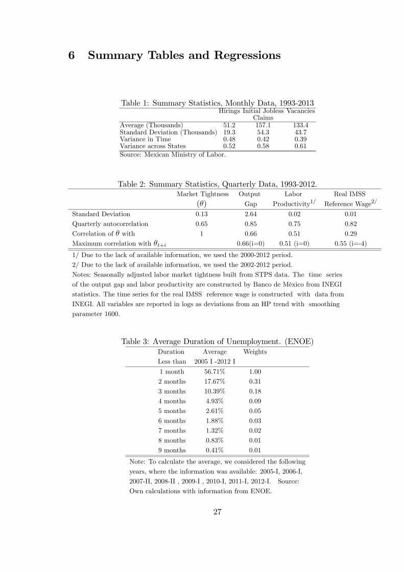
Federal District (Table 1 reports some summary statistics). This source of information

allows us to analyze the job matching process in a well-de�ned segment of the Mexican

labor market.

The Bolsa handles large volumes of job seekers and vacancies in about 160 branches

throughout Mexico. The main aim of BT is to link job seekers with job openings that

are appropriate to their pro�le. A job seeker is a person who has registered with BT

during a month to apply for a job. Although job seekers are not necessarily unemployed

we will treat them as such.

The system is run by state-level authorities and the information is collected by the

federal government. The service works under quite speci�c terms. Job seekers have

to �ll out in person a detailed form with their quali�cations and interests. If they are

still looking for a job after one year they have to begin the process again. BT o¤ers

job seekers guidance and feedback on the availability of current vacancies to �nd an

appropriate �t.

On the other side of the market, �rms post vacancies and are also required to �ll out

a detailed form when registering them, including the exact number of vacancies and

type of employee wanted. Every two weeks �rms report if their vacancies are still open.

Firms are not required to register their vacancies in person: BT o¤ers the option to

register it through a BT agent. These procedures render vacancies a speci�c meaning

with a well-de�ned lifespan.

At the �nal stage of the process, BT sends job seekers to interview with employers

5

which decide to hire them or not. No fees are charged for any of these services, but

�rms are required to disclose whether a hiring was successful.

BT has strict criteria to ensure there is no redundancy in their administrative

records. They have procedures to prevent a worker from registering more than once in

the system and require that �rms post a separate vacancy for each unique employment

position. If a �rm is recruiting several workers for the same position it registers a

separate vacancy for each of them in the system.

A concern on the scope of our data is that all BT branches are located in the main

urban areas of each state. A casual inspection of the posted vacancies shows that the

majority of them are urban jobs, for example, secretaries, plant managers, electricians

or plumbers. Given the transient nature of many rural jobs, it is hard to imagine

that a rural employer would use job postings to �ll out its vacancies. Because of this

we interpret our data set as representative of urban jobs and will hereafter mostly

compare our predictions with the urban series from the national employment surveys.

In particular, we use the Encuesta Nacional de Empleo Urbano (ENEU) from 1993

to 2004 and the urban series of its successor, the Encuesta Nacional de Ocupación y

Empleo (ENOE) from 2005 to 2012. This is somewhat convenient because the urban

employment series are the longest available for the Mexican labor market. For the

period in which the ENOE becomes available, 2005-2013, urban workers represent,

on average, 80% of all employed workers, while the urban unemployed represent, on

average, 88% of the unemployed population.

Another concern with our data is that it might be skewed towards the formal sector,

since �rms are asked that the vacancies they post comply with all labor regulations.

This could in principle alter the representativeness of the data, since informality is

especially prevalent in the Mexican labor market, accounting for approximately 60%

of the employed population,6 yet it is unclear how the BT can guarantee that �rms

comply. Because of this, currently we have decided not to analyze the relationship of

6INEGI has two di¤erent measures for informality the Tasa de ocupación en el sector informal,which is around 28%, and the Tasa de Informalidad Laboral, which is around 59%. The �rst measureincludes workers in informal �rms as well as the self-employed, while the second measure includes allthose workers in the informal sector as well as the workers in the formal sector who do not receive thebene�ts required by law.

6

our data with the (unobserved) formality status of its job placements.

It is important to understand that the BT is not in itself a major player in the Mex-

ican labor market. For example, when we compare the hirings from the system with

the gross �ows from unemployment to employment reported in the national employ-

ment surveys we �nd that hirings through the Bolsa are on average 6.4 times smaller

than the total gross �ows.7 Instead, we take our data to be a good proxy for the gen-

eral conditions of the Mexican labor market through the cycle subject to the caveats

previously mentioned: it is biased towards urban and formal employment.

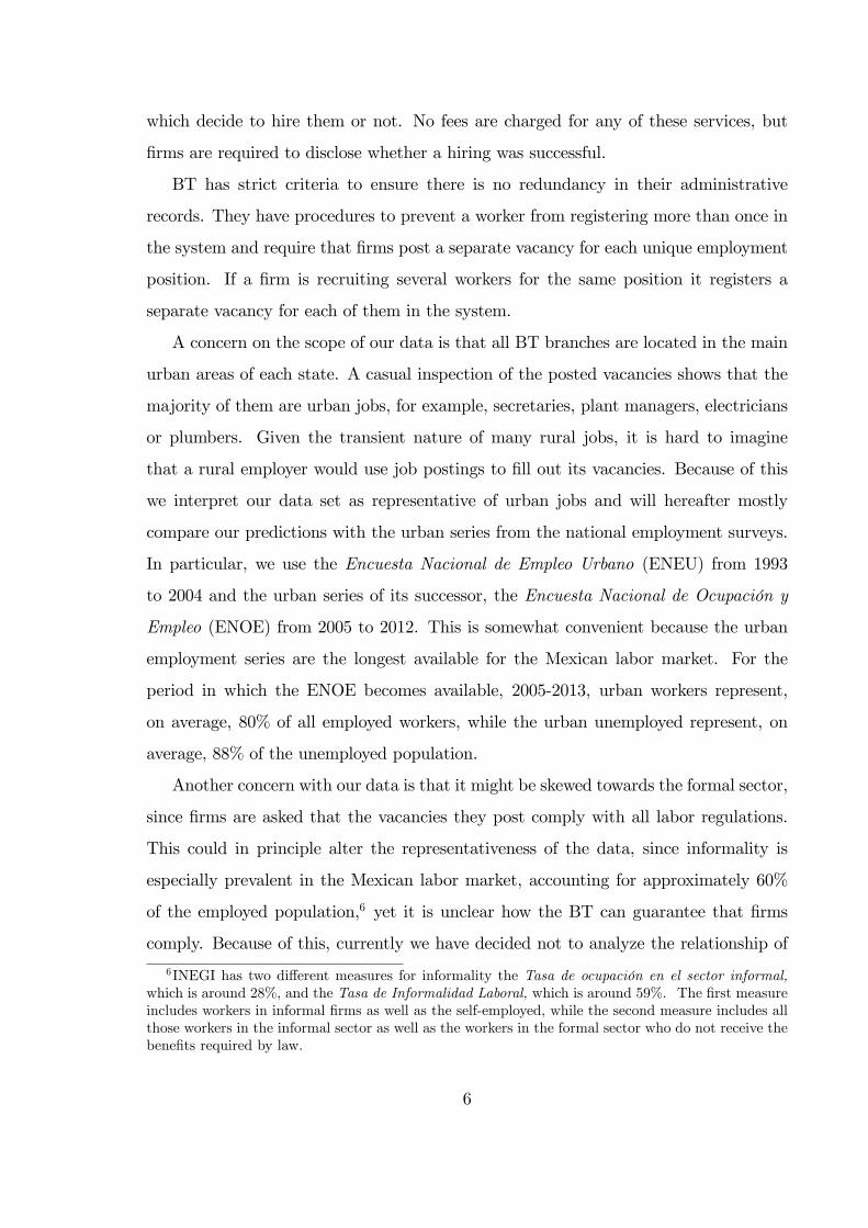
Finally, it is worth mentioning that the Ministry of Labor o¤ers an independent

parallel employment service called �Portal de Empleo� that forms matches between

workers and jobs through an online site. This service is relatively new, starting in

March 2002. Because of this, we observe an exponential growth in the data as it

became more popular, which stabilized in recent years (Figure 1b).

Figure 1a: Employment series Figure 1b: Employment seriesin "Bolsa de Trabajo" in "Portal de Empleo"

(Thousands, s.a.) (Thousands)

Source: Mexican Ministry of Labor.

A disadvantage of the data from Portal is that there is no easy way to evaluate

the quality of the data, since there are no controls to prevent a job seeker or a �rm

from �lling more than one posting. The experience in other countries, especially in

7Because the ENEU/ENOE data su¤er from a downward bias due to time-aggregation, this numberoverstates the relative size of BT.

7

developed ones, shows that the online vacancy publishing services have tended to dis-

place traditional services. So far it is not clear that this has happened in Mexico and

so we decided not include this information in our analysis.

3 Some macroeconomic facts of labor market tight-

ness in Mexico.

The fact that we have data available for both the supply and demand side of the labor

market allows us to study for the �rst time the relationship between some labor indic-

ators commonly used in the job search literature and other macroeconomic variables in

Mexico. The purpose of this section is twofold: �rst we present some macroeconomic

facts of the Mexican labor market tightness and then we relate them with the literature

(Shimer (2005), Rogerson & Shimer (2010)). We are especially interested in describing

the behavior of labor market tightness during economic downturns, its correlation with

the output gap, productivity and wages.

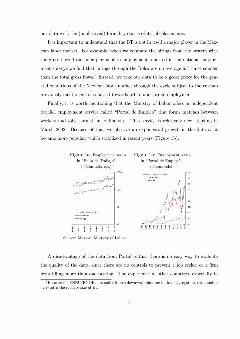
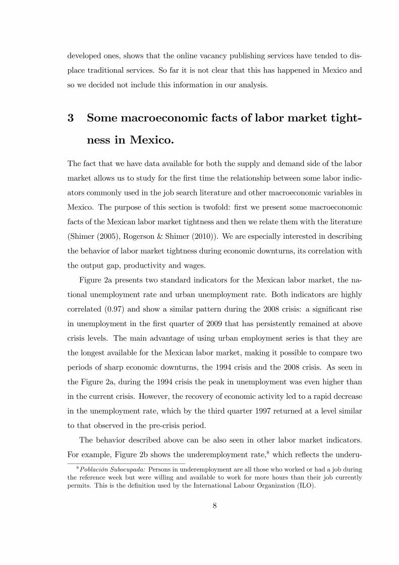
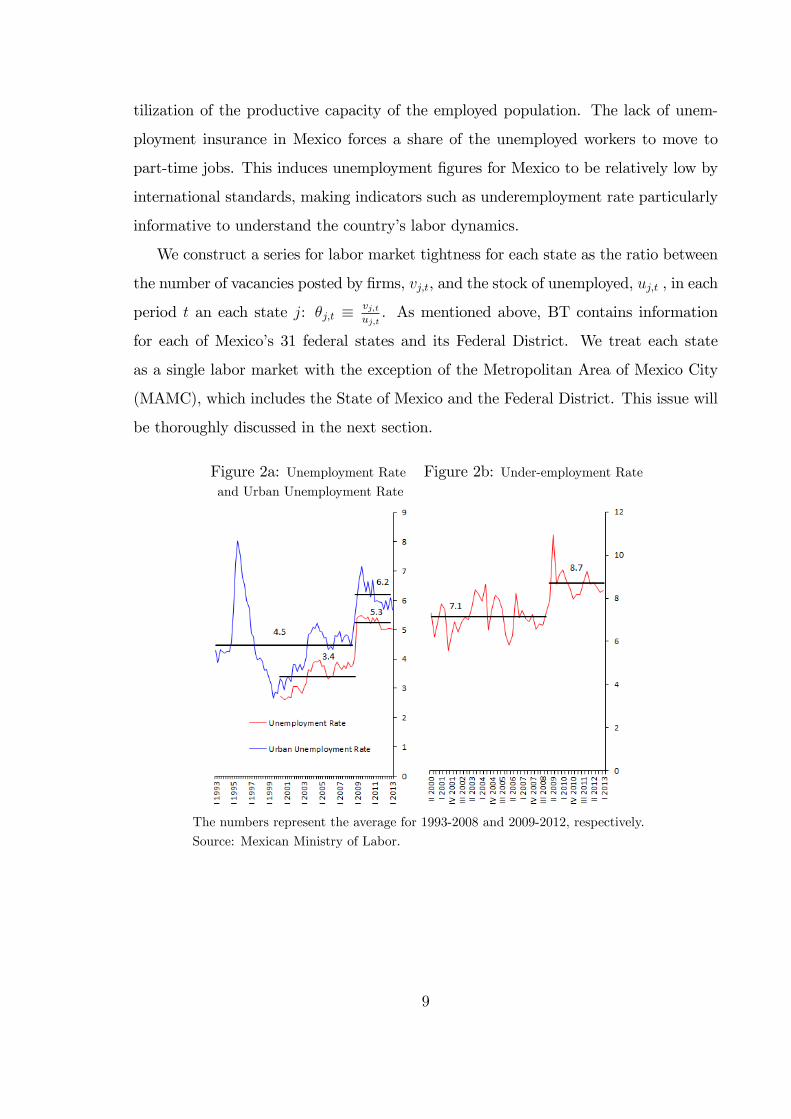
Figure 2a presents two standard indicators for the Mexican labor market, the na-

tional unemployment rate and urban unemployment rate. Both indicators are highly

correlated (0.97) and show a similar pattern during the 2008 crisis: a signi�cant rise

in unemployment in the �rst quarter of 2009 that has persistently remained at above

crisis levels. The main advantage of using urban employment series is that they are

the longest available for the Mexican labor market, making it possible to compare two

periods of sharp economic downturns, the 1994 crisis and the 2008 crisis. As seen in

the Figure 2a, during the 1994 crisis the peak in unemployment was even higher than

in the current crisis. However, the recovery of economic activity led to a rapid decrease

in the unemployment rate, which by the third quarter 1997 returned at a level similar

to that observed in the pre-crisis period.

The behavior described above can be also seen in other labor market indicators.

For example, Figure 2b shows the underemployment rate,8 which re�ects the underu-

8Población Subocupada: Persons in underemployment are all those who worked or had a job duringthe reference week but were willing and available to work for more hours than their job currentlypermits. This is the de�nition used by the International Labour Organization (ILO).

8

tilization of the productive capacity of the employed population. The lack of unem-

ployment insurance in Mexico forces a share of the unemployed workers to move to

part-time jobs. This induces unemployment �gures for Mexico to be relatively low by

international standards, making indicators such as underemployment rate particularly

informative to understand the country�s labor dynamics.

We construct a series for labor market tightness for each state as the ratio between

the number of vacancies posted by �rms, vj;t, and the stock of unemployed, uj;t , in each

period t an each state j: �j;t � vj;tuj;t. As mentioned above, BT contains information

for each of Mexico�s 31 federal states and its Federal District. We treat each state

as a single labor market with the exception of the Metropolitan Area of Mexico City

(MAMC), which includes the State of Mexico and the Federal District. This issue will

be thoroughly discussed in the next section.

Figure 2a: Unemployment Rate Figure 2b: Under-employment Rateand Urban Unemployment Rate

The numbers represent the average for 1993-2008 and 2009-2012, respectively.

Source: Mexican Ministry of Labor.

9

We de�ne the aggregate labor market tightness as the weighted average of the

market tightness in each state using the size of its labor force, LFj;t, as weights. Thus,

our measure of market tightness is

�t =Xj

LFj;tPk

LFk;t�j;t

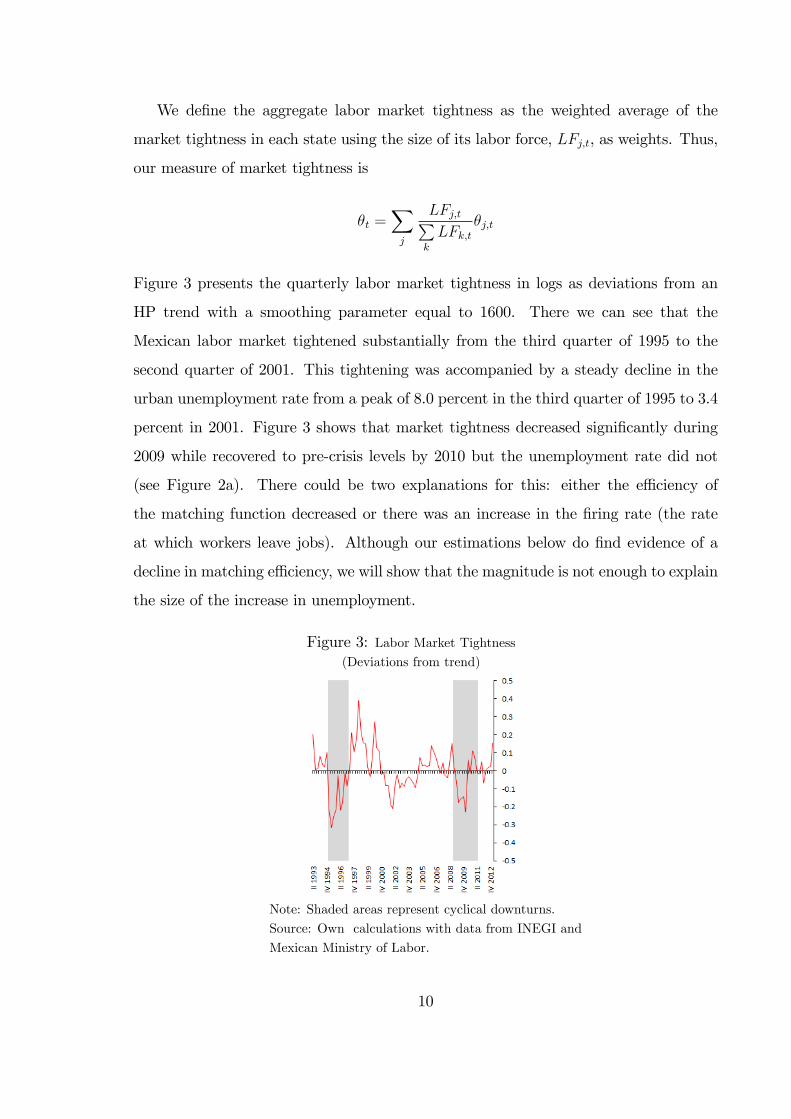
Figure 3 presents the quarterly labor market tightness in logs as deviations from an

HP trend with a smoothing parameter equal to 1600. There we can see that the

Mexican labor market tightened substantially from the third quarter of 1995 to the

second quarter of 2001. This tightening was accompanied by a steady decline in the

urban unemployment rate from a peak of 8.0 percent in the third quarter of 1995 to 3.4

percent in 2001. Figure 3 shows that market tightness decreased signi�cantly during

2009 while recovered to pre-crisis levels by 2010 but the unemployment rate did not

(see Figure 2a). There could be two explanations for this: either the e¢ ciency of

the matching function decreased or there was an increase in the �ring rate (the rate

at which workers leave jobs). Although our estimations below do �nd evidence of a

decline in matching e¢ ciency, we will show that the magnitude is not enough to explain

the size of the increase in unemployment.

Figure 3: Labor Market Tightness(Deviations from trend)

Note: Shaded areas represent cyclical downturns.

Source: Own calculations with data from INEGI and

Mexican Ministry of Labor.

10

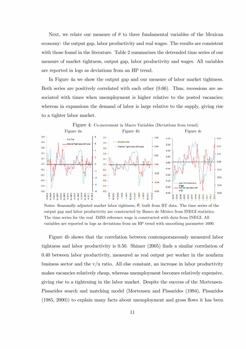
Next, we relate our measure of � to three fundamental variables of the Mexican

economy: the output gap, labor productivity and real wages. The results are consistent

with those found in the literature. Table 2 summarizes the detrended time series of our

measure of market tightness, output gap, labor productivity and wages. All variables

are reported in logs as deviations from an HP trend.

In Figure 4a we show the output gap and our measure of labor market tightness.

Both series are positively correlated with each other (0.66). Thus, recessions are as-

sociated with times when unemployment is higher relative to the posted vacancies;

whereas in expansions the demand of labor is large relative to the supply, giving rise

to a tighter labor market.

Figure 4: Co-movement in Macro Variables (Deviations from trend)

Figure 4a Figure 4b Figure 4c

Notes: Seasonally adjusted market labor tightness, �, built from BT data. The time series of the

output gap and labor productivity are constructed by Banco de México from INEGI statistics.

The time series for the real IMSS reference wage is constructed with data from INEGI. All

variables are reported in logs as deviations from an HP trend with smoothing parameter 1600.

Figure 4b shows that the correlation between contemporaneously measured labor

tightness and labor productivity is 0.50. Shimer (2005) �nds a similar correlation of

0.40 between labor productivity, measured as real output per worker in the nonfarm

business sector and the v/u ratio. All else constant, an increase in labor productivity

makes vacancies relatively cheap, whereas unemployment becomes relatively expensive,

giving rise to a tightening in the labor market. Despite the success of the Mortensen-

Pissarides search and matching model (Mortensen and Pissarides (1994), Pissarides

(1985, 2000)) to explain many facts about unemployment and gross �ows it has been

11

argued (Shimer (2005)) that the model cannot explain the cyclical behavior of labor

market variables (e.g. vacancies and unemployment) in response to measured pro-

ductivity shocks consistent with the data. The correlation between contemporaneously

measured labor market tightness and productivity is closed to 1 in those models. For

instance Shimer (2005) and Hagedorn and Manovskii (2008) use di¤erent versions of

the standard search and matching models and found a correlation of 0.999 and 0.967,

respectively. This is much larger than what we observe in our data.

Finally, Figure 4c shows the co-movement between � and the IMSS reference wage

in in�ation-adjusted pesos. The contemporaneous correlation between these two vari-

ables is 0.29, while the four lag correlation between them rises to 0.55; the latter

suggests that � is a good predictor of real wage growth. Hence, a tightening of the

labor market is associated with an increase in real wages paid to the employees four

quarters ahead. If the number of vacancies increases relative to the number of unem-

ployed, a job seeker may expect to �nd a vacant relatively more quickly than a �rm

may expect to �nd an unemployed worker. Thus, the �rm may o¤er higher wages, with

a lag, in order to improve its hiring probability.

3.1 The empirical speci�cations and some preliminary ana-

lysis

As is standard in the literature, we model the total number of new hires as a Cobb-

Douglas function of vacancies and unemployment:

Uj;tHj;t = Aj;tV�vj;t U

�uj;t (1)

Where j=1,. . . ,N denotes the state-level cross-sectional dimension and t=1,. . . ,T

the time series dimension; Hj;t denotes the monthly hiring probability, the percentage

of unemployed workers that �nd a job during period t, Uj;t times Hj;t denotes the

number of hires during period t, while Vj;t and Uj;t denote the number of vacancies and

unemployed, respectively. As in Kano and Ohta (2005), Aj;t denotes region-speci�c

12

and time-varying matching e¢ ciency, which we model in the following way:

Aj;t = e�+�j+�t+"j;t (2)

Where �j denotes time-invariant regional attribute for j, � stands for a state-

invariant time attribute for t, and "j;t is a random shock for state j at period t. We

consider each state to be a separate labor market with one exception: since most of

the BT o¢ ces in the State of Mexico are in municipalities of the Metropolitan Area

of Mexico City (MAMC), we integrate the data with the series for the Federal Dis-

trict into a single labor market. This criterion is consistent with the de�nition for

the main metropolitan areas used in national labor surveys, which includes only those

municipalities that belong to the same state, with the exception of the MAMC.

At this point, it is worth mentioning that there are some peculiarities with the data

coming from MAMC. As shown in Figure 5b, all series, the �ow of initial jobless claims,

vacancies and hirings, show a signi�cant drop during the �rst quarter of 2010. This

suggests the presence of a methodological change rather than a fundamental change

in the market activity. Since the MAMC represents a large share of the labor market,

this decline is re�ected at the national level. Figure 5a shows that the discrete drop is

observed in all of our series although Figure 5b shows it occurred in an approximately

proportional matter. Nevertheless, this measurement problem may be biasing our

results towards �nding losses in the e¢ ciency of the matching process; therefore, as a

robustness check, we will repeat our analysis excluding the MAMC. As shown in Figure

5c, once we eliminate the MAMC from our data we can no longer observe the decline

in the �rst quarter of 2010.

13

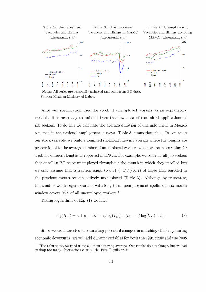
Figure 5a: Unemployment, Figure 5b: Unemployment, Figure 5c: Unemployment,

Vacancies and Hirings Vacancies and Hirings in MAMC Vacancies and Hirings excluding

(Thousands, s.a.) (Thousands, s.a.) MAMC (Thousands, s.a.)

Notes: All series are seasonally adjusted and built from BT data.

Source: Mexican Ministry of Labor.

Since our speci�cation uses the stock of unemployed workers as an explanatory

variable, it is necessary to build it from the �ow data of the initial applications of

job seekers. To do this we calculate the average duration of unemployment in Mexico

reported in the national employment surveys. Table 3 summarizes this. To construct

our stock variable, we build a weighted six-month moving average where the weights are

proportional to the average number of unemployed workers who have been searching for

a job for di¤erent lengths as reported in ENOE. For example, we consider all job seekers

that enroll in BT to be unemployed throughout the month in which they enrolled but

we only assume that a fraction equal to 0.31 (=17.7/56.7) of those that enrolled in

the previous month remain actively unemployed (Table 3). Although by truncating

the window we disregard workers with long term unemployment spells, our six-month

window covers 95% of all unemployed workers.9

Taking logarithms of Eq. (1) we have:

log(Hj;t) = a+ �j + �t+ �v log(Vj;t) + (�u � 1) log(Uj;t) + "j;t (3)

Since we are interested in estimating potential changes in matching e¢ ciency during

economic downturns, we will add dummy variables for both the 1994 crisis and the 2008

9For robustness, we tried using a 9 month moving average. Our results do not change, but we hadto drop too many observations close to the 1994 Tequila crisis.

14

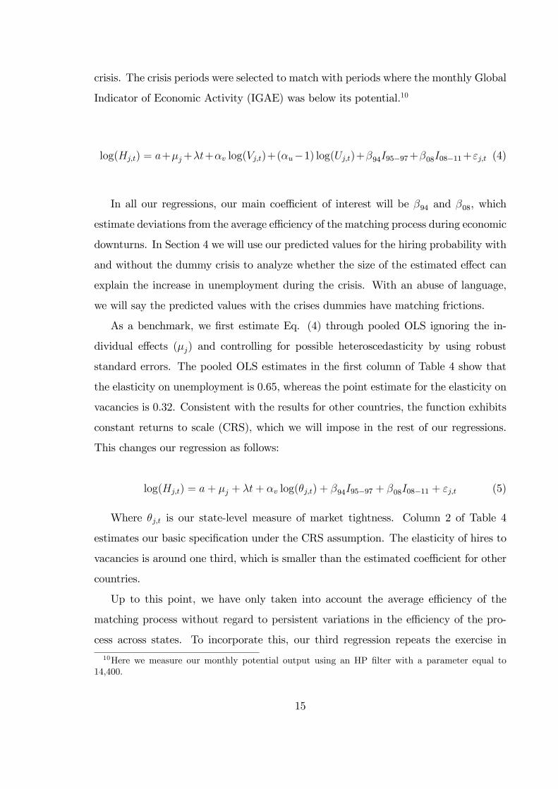
crisis. The crisis periods were selected to match with periods where the monthly Global

Indicator of Economic Activity (IGAE) was below its potential.10

log(Hj;t) = a+�j+�t+�v log(Vj;t)+(�u�1) log(Uj;t)+�94I95�97+�08I08�11+"j;t (4)

In all our regressions, our main coe¢ cient of interest will be �94 and �08, which

estimate deviations from the average e¢ ciency of the matching process during economic

downturns. In Section 4 we will use our predicted values for the hiring probability with

and without the dummy crisis to analyze whether the size of the estimated e¤ect can

explain the increase in unemployment during the crisis. With an abuse of language,

we will say the predicted values with the crises dummies have matching frictions.

As a benchmark, we �rst estimate Eq. (4) through pooled OLS ignoring the in-

dividual e¤ects (�j) and controlling for possible heteroscedasticity by using robust

standard errors. The pooled OLS estimates in the �rst column of Table 4 show that

the elasticity on unemployment is 0.65, whereas the point estimate for the elasticity on

vacancies is 0.32. Consistent with the results for other countries, the function exhibits

constant returns to scale (CRS), which we will impose in the rest of our regressions.

This changes our regression as follows:

log(Hj;t) = a+ �j + �t+ �v log(�j;t) + �94I95�97 + �08I08�11 + "j;t (5)

Where �j;t is our state-level measure of market tightness. Column 2 of Table 4

estimates our basic speci�cation under the CRS assumption. The elasticity of hires to

vacancies is around one third, which is smaller than the estimated coe¢ cient for other

countries.

Up to this point, we have only taken into account the average e¢ ciency of the

matching process without regard to persistent variations in the e¢ ciency of the pro-

cess across states. To incorporate this, our third regression repeats the exercise in

10Here we measure our monthly potential output using an HP �lter with a parameter equal to14,400.

15

column 2 including state �xed e¤ects. The main di¤erence between this regression

and the one in the second column is the rise in the elasticity of vacancies from 0.32 to

0.46. This coe¢ cient is closer to what has typically been found in the literature. We

can reject the null hypothesis that the state �xed e¤ects (�j) are jointly equal to zero

(p-value<0.0001). Hence, there is evidence to reject the null hypothesis. Thus, it is

important to consider in our estimation biases due to unobservable regional heterogen-

eity.

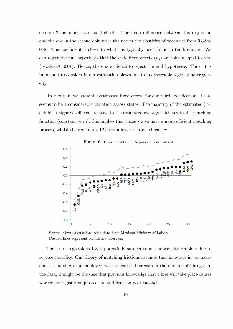
In Figure 6, we show the estimated �xed e¤ects for our third speci�cation. There

seems to be a considerable variation across states. The majority of the estimates (19)

exhibit a higher coe¢ cient relative to the estimated average e¢ ciency in the matching

function (constant term), this implies that those states have a more e¢ cient matching

process, whilst the remaining 12 show a lower relative e¢ ciency.

Figure 6: Fixed E¤ects for Regression 3 in Table 4

Source: Own calculations with data from Mexican Ministry of Labor.

Dashed lines represent con�dence intervals.

The set of regressions 1-3 is potentially subject to an endogeneity problem due to

reverse causality. Our theory of matching frictions assumes that increases in vacancies

and the number of unemployed workers causes increases in the number of hirings. In

the data, it might be the case that previous knowledge that a hire will take place causes

workers to register as job seekers and �rms to post vacancies.

16

To try and solve this problem, our next regression estimates (5) using instrumental

variables, assuming CRS and maintaining the state �xed e¤ects. As Blanchard and

Diamond (1989), we use three lags for both vacancies and unemployment as instru-

ments11. Our hope is that lagged values of unemployment and vacancies are correlated

with the current value of labor market tightness and not directly correlated with the

current value of the hiring rate.

Borowczyk-Martins, Jolivet and Postel (2013) use an alternative speci�cation that

models matching productivity as an ARMA process. They then propose a systematic

procedure to identify which lags should be used as instruments. Since using a �exible

reduced-form estimation to model cyclicality might bias our estimation against �nding

level changes during economic crises, we prefer to maintain our simpler speci�cation

while performing robustness checks on the lag selection for our instruments.

The equation for our �rst-stage of this regression12 can be expressed as follows:

log(�j;t) = a+�j+�t+�94I95�97+�08I08�11+3Xi=1

�iLi log(Uj;t)+

3Xi=1

�iLi log(Vj;t)+�j;t

(6)

Where �i and �i represent the coe¢ cients for lags 1-3 for unemployment and va-

cancies, respectively and �j;t the error term. The value of the F statistic is 235.4, which

is above the heuristic value of 10, indicates that we do not have a weak-instruments

problem. We also conducted the Anderson-Rubin and Stock-Wright tests and, in both

cases, we rejected the null that the instruments are weak. Finally, we performed

Hansen�s J test, testing overidentifying restrictions, and we did not reject the null that

the instruments are valid at a 5% con�dence level. (The p-value is about 9%, see Table

7).

The results for the second-stage of this regression show an increase in the elasticity

of vacancies with respect to the estimates in the third column, which is consistent with

11To analyze whether there is a systematic di¤erence, we estimate our instrumental variables re-gression varying the number of lags on both variables, from 1 to 6 lags, without �nding a signi�cantdi¤erence. As robustness check, we also estimate our regression using lagged values of market tightnessas instruments and our results do not change.12The results for the �rst-stage regression can be seen in Table 6.

17

the results found by Blanchard and Diamond (1989) once they use instruments. In our

case, the coe¢ cient changes from 0.46 to 0.50.

Although the coe¢ cient for the linear time trend is not statistically signi�cant in

most speci�cations, it gives us additional information about the evolution of the match-

ing process. Averaging the coe¢ cient for the linear time trend across the speci�cations

in Table 4, our estimation suggests that the e¢ ciency of the matching process in Mexico

increased 6.2% in ten years.13

Focusing on our main coe¢ cients of interest, the dummy variables during the two

crises, we consistently �nd in all regressions a statistically signi�cant decrease in the

e¢ ciency of the matching process during both economic crises. For 1994, the estimated

loss in the e¢ ciency of the matching function is between 0.18 and 0.21 log points, while

the e¢ ciency loss during the 2008 crisis is between 0.11 and 0.13 pp. For each of our

speci�cations we tested the null hypothesis that �94=�08, and for all our regressions

we fail to reject the di¤erence between both crises (see Table 4). Since our reduced-

form estimation �nds no di¤erence in matching e¢ cienty during 1994 relative to 2008

and the point estimate is larger for 1994, it is unlikely that this estimated loss in itself

could be the explanation for the persistent increase in unemployment observed in latter

crises, but not in the �rst.

Finally, we perform two di¤erent robustness checks for our estimations. First, we

complement the analysis by allowing a more �exible functional form by estimating a

constant elasticity of substitution function (CES) instead of a Cobb-Douglas speci�c-

ation. We estimated the CES function through nonlinear least squares. This changes

our speci�cation in the following way:

log(Hj;t) = a+ �j + �t+1

�log� + (1� )��j;t

�+ �94I95�97 + �08I08�11 + "j;t (7)

Where � represents the elasticity of substitution between vacancies and unemploy-

ment and the share parameter. The results for the regression are presented in Column

5 of Table 4. This estimated value of � = �1:53 suggests that the relationship between13We performed this calculation as follows: e(��4t) � 1, where �� is the average of the coe¢ cient of

linear time trend across speci�cations and 4t = 120 or twelve months times ten years.

18

vacancies and unemployment is more complementary than the one implied by a Cobb-

Douglas matching function. Despite this di¤erence, our estimates for the changes in

the matching e¢ ciency during the crises periods (1994 and 2008) are practically the

same as those obtained in previous speci�cations.

We were also concerned that the methodological change in the MAMC data could

be biasing our results. To address this problem, we repeat all our regressions excluding

the MAMC. The point estimates, shown in Table 5, are consistent with those found in

exercises involving all states. This suggests that the large movement in the MAMC is

not guiding our results.

4 Can matching frictions explain the change in un-

employment after 2008?

To evaluate the implications of our estimations for the unemployment rate, we use the

following well-known steady-state formula that relates unemployment rate with �ow

rates. Assume the size of the labor force remains constant. Let �t denote the �ring

rate: the rate at which employed workers become unemployed during period t which

corresponds to a continuous time Poisson switching model. Likewise let ht denote the

hiring rate. If �t and ht remain constant for a su¢ cient period, the system will converge

to the following steady state unemployment rate:

ut =�t

�t+ht

As is common in the literature, we assume the system converges to the steady

state fast enough so that gross �ows give an accurate approximation to the actual

unemployment rate. This formula will form our basis to evaluate whether changes in

our estimated hiring rate can explain changes in the unemployment rate. Our functional

form allows us to do counterfactual analysis on what the hiring rate should be in the

absence of changes in matching frictions (changes in At) or under alternative paths for

the observed market tightness (changes in �t).

19

But �rst we need an estimate of the �ring rate �t. We build one using the urban

series of the national employment surveys (ENEU and ENOE). From this data we can

identify workers who were employed in period t-1, which happened to be unemployed in

the next period. Thus, we de�ned the �ring probability DLS;t as the number of people

who changed their employment status from employed to unemployed between periods t

-1 and t divided by the number of employed in t-1. The corresponding continuous time

�ring rate is given by �LS;t � � log(1 � DLS;t): Analogously, we construct the hiring

rates and probabilities consistent with the gross �ow of workers from unemployment

to employment: hLS;t and HLS;t respectively.

A usual concern when working with discrete time data is the loss of labor transitions

within periods, which can cause a signi�cant bias in the transition probabilities. As

argued by Shimer (2012), this time aggregation bias can be more severe for the �ring

rate than for the hiring rate, since a worker who loses his job is more likely to �nd a

new one without experiencing a measured spell of unemployment. This is especially

true for Mexico given the long sampling window in ENOE (3 months) and the relatively

short unemployment spells (85% of respondents have a duration of unemployment of

less than 3 months, see Table 3).

To address this issue, we use the methodology proposed by Shimer (2012) to correct

for time aggregation bias in the �ring rate. Our adjusted �ring rate, �SH , is estimated

numerically by solving the following formula:

ut+1 = (1� e�hLS;t��SH;t) �SH;t�SH;t+hLS;t

+ e�hLS;t��SH;tut

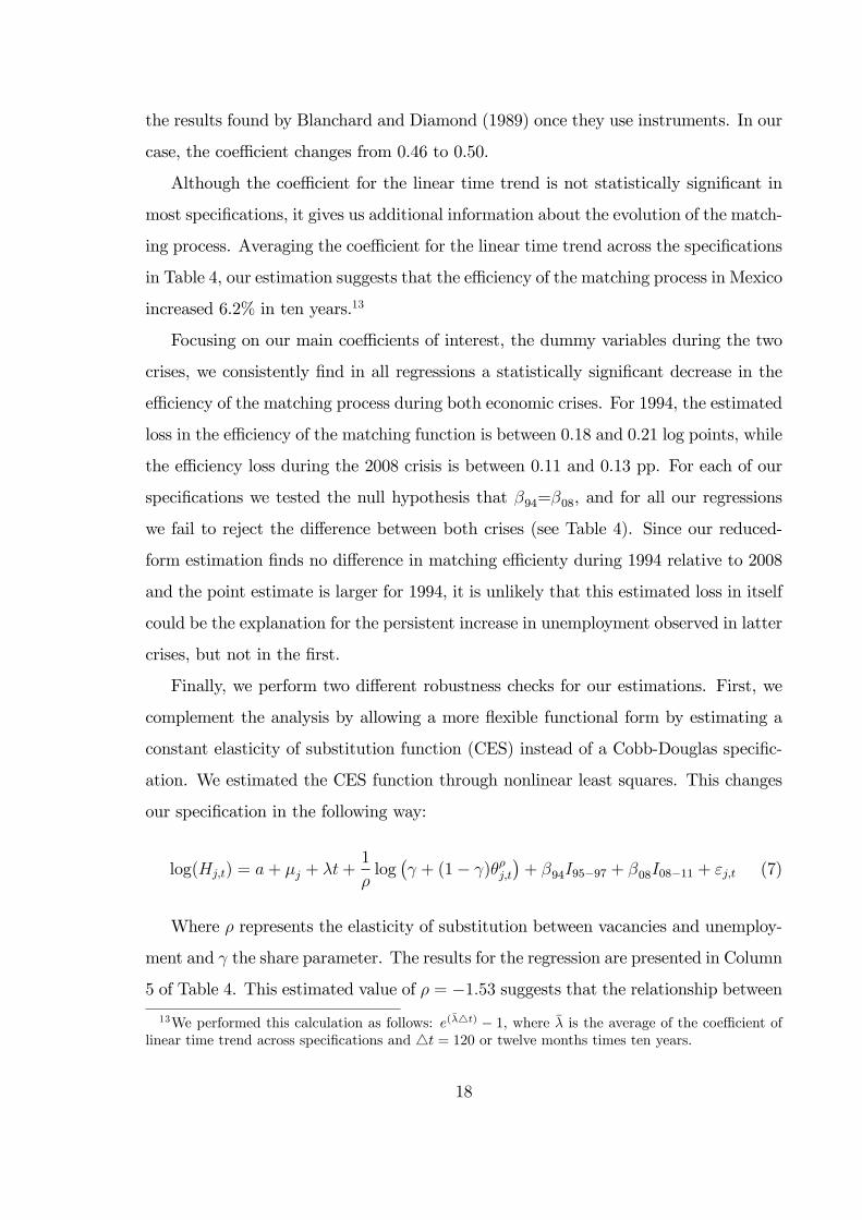
Figure 7a shows the comparison between the �ring rate estimated from the data

available in the national labor surveys �LS and the �ring rate we obtain using Shi-

mer�s methodology �SH .The �rst lesson we get from Figure 7a unless we correct for

time aggregation bias, �LS signi�cantly underestimates the �ring rate in economy, as

expected. Second, we observe that �SH is much more volatile than �LS. The latter

becomes relevant at the end of the period where we see a high variation in the �ring

rate. Therefore, to construct the implied unemployment rate, we decided to smooth

the continuous exit rate with a four quarter moving average.

20

Figure 7a: Firing Rate from ENEU/ENOE Figure 7b: Hiring Rate from ENEU/ENOE

Source: Own calculations with data from INEGI.

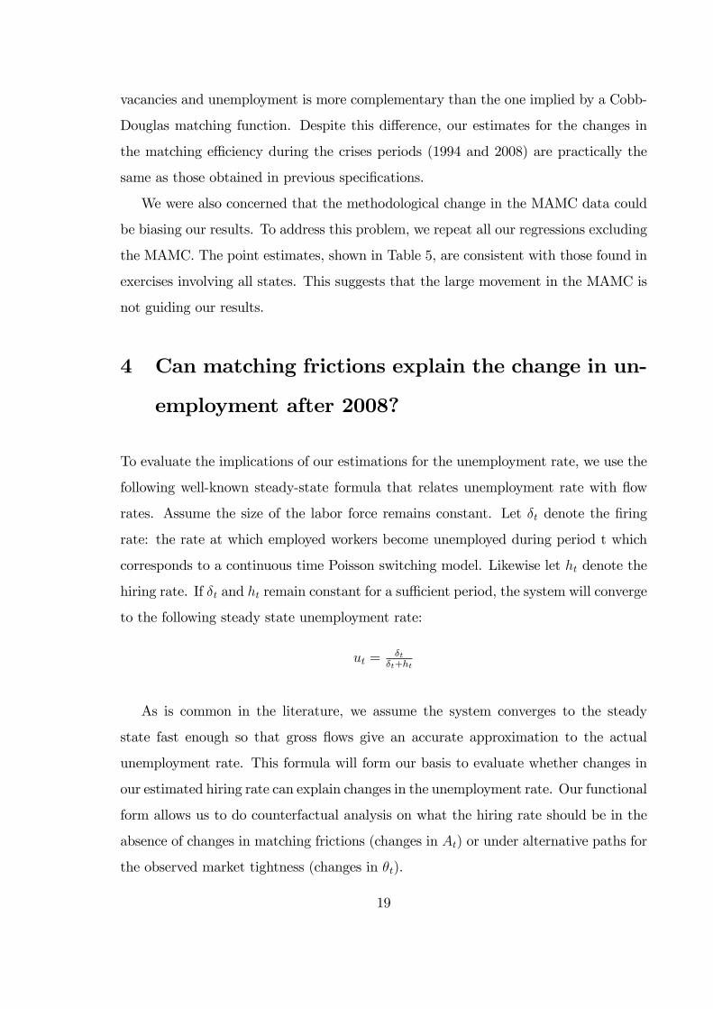
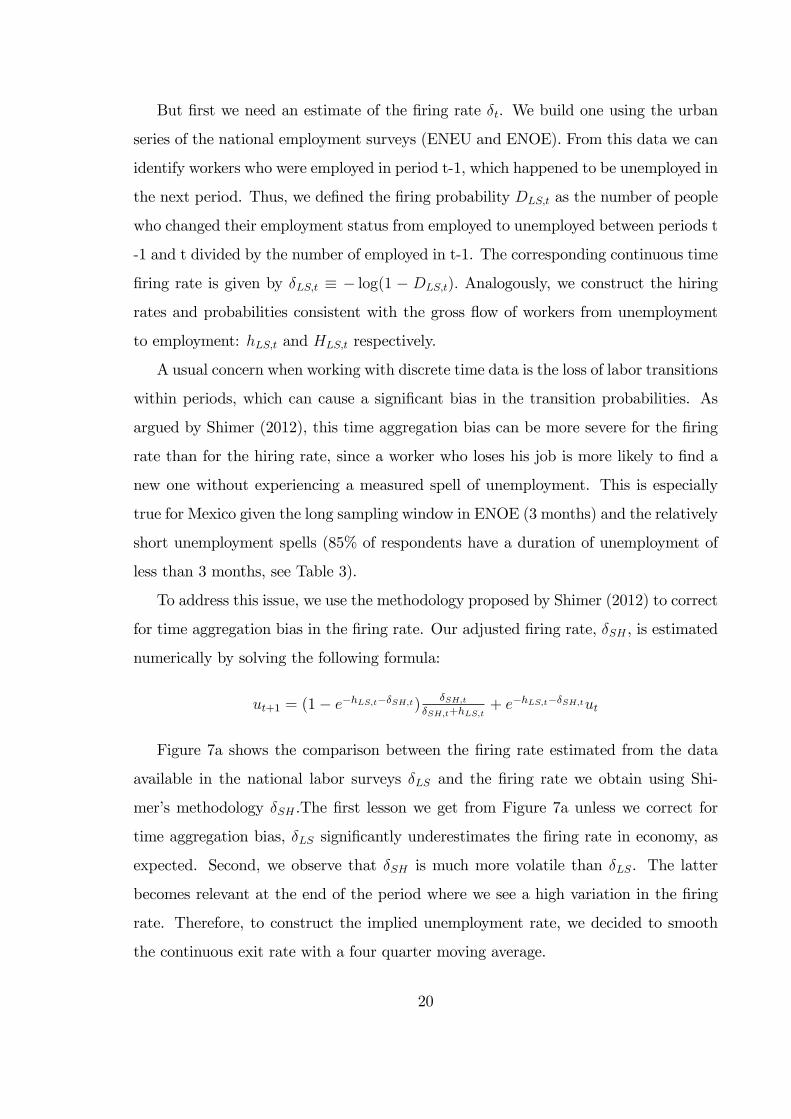
Figure 8 shows the urban unemployment rate from the national labor surveys

(ENEU and ENOE) and uses the gross �ows from the same survey to calculate an

implied unemployment rate. The correlation between the series is quite high (0.98)

and the implied unemployment rate captures the big movements of the series during

the booms and busts.

Figure 8: Urban Unemployment Rate vs. Implied Gross-FlowsUnemployment Rate

Source: Own calculations with data from INEGI.

To analyze the implications of our estimated matching frictions on the unemploy-

ment rate we replace the ENOE hiring probability with the predicted hiring probabil-

ity of our estimations with and without crisis dummies. We will base all our analysis

on the IV regression with state-level �xed e¤ects reported in column 4 of Table 4.14

14Our regression is based on a state-level panel, so we need to aggregate the data to compare themwith the national urban unemployment numbers. To do so we weigh the predicted hiring rate for eachstate by the size of its labor force as follows: ht =

Pj

LFj;tPk

LFk;thj;t:

21

Before proceeding, we must make the following clari�cation. Our estimates for the

hiring probability (with and without) matching frictions are based on monthly obser-

vations. Therefore, it is necessary to perform a slight transformation to the data in

order to make our predictions comparable with the national labor survey�s quarterly

data. Once again, Shimer�s methodology provides a reasonable framework to perform

this task. According to Shimer (2012) the hiring probability Ht is related to the con-

tinuous hiring rate ht in the following way ht � � log(1 � Ht). From our predictions

we construct a monthly hiring rate, which we average in order to obtain quarterly ob-

servations. The quarterly hiring probability is related to the quarterly hiring rate as

follows: HQ;t � 1 � e�ht4t, where 4t represents the change in frequency in monthly

terms.

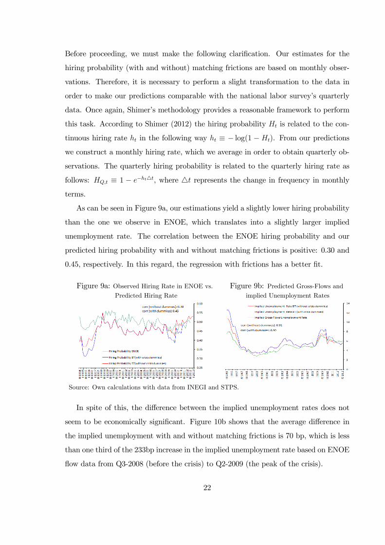
As can be seen in Figure 9a, our estimations yield a slightly lower hiring probability

than the one we observe in ENOE, which translates into a slightly larger implied

unemployment rate. The correlation between the ENOE hiring probability and our

predicted hiring probability with and without matching frictions is positive: 0.30 and

0.45, respectively. In this regard, the regression with frictions has a better �t.

Figure 9a: Observed Hiring Rate in ENOE vs. Figure 9b: Predicted Gross-Flows andPredicted Hiring Rate implied Unemployment Rates

Source: Own calculations with data from INEGI and STPS.

In spite of this, the di¤erence between the implied unemployment rates does not

seem to be economically signi�cant. Figure 10b shows that the average di¤erence in

the implied unemployment with and without matching frictions is 70 bp, which is less

than one third of the 233bp increase in the implied unemployment rate based on ENOE

�ow data from Q3-2008 (before the crisis) to Q2-2009 (the peak of the crisis).

22

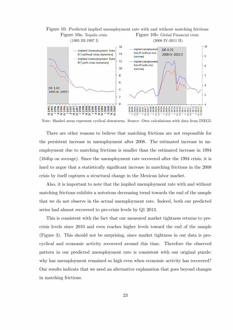
Figure 10: Predicted implied unemployment rate with and without matching frictionsFigure 10a: Tequila crisis Figure 10b: Global Financial crisis

(1995 III-1997 I) (2008 IV-2011 II)

Note: Shaded areas represent cyclical downturns. Source: Own calculations with data from INEGI.

There are other reasons to believe that matching frictions are not responsible for

the persistent increase in unemployment after 2008. The estimated increase in un-

employment due to matching frictions is smaller than the estimated increase in 1994

(164bp on average). Since the unemployment rate recovered after the 1994 crisis, it is

hard to argue that a statistically signi�cant increase in matching frictions in the 2008

crisis by itself captures a structural change in the Mexican labor market.

Also, it is important to note that the implied unemployment rate with and without

matching frictions exhibits a notorious decreasing trend towards the end of the sample

that we do not observe in the actual unemployment rate. Indeed, both our predicted

series had almost recovered to pre-crisis levels by Q1 2013.

This is consistent with the fact that our measured market tightness returns to pre-

crisis levels since 2010 and even reaches higher levels toward the end of the sample

(Figure 3). This should not be surprising, since market tightness in our data is pro-

cyclical and economic activity recovered around this time. Therefore the observed

pattern in our predicted unemployment rate is consistent with our original puzzle:

why has unemployment remained so high even when economic activity has recovered?

Our results indicate that we need an alternative explanation that goes beyond changes

in matching frictions.

23

5 Conclusion

In this paper we study the role played by matching frictions in explaining the behavior

in unemployment in Mexico after 2008. To do so, we estimate the potential loss of

e¢ ciency of the matching function during two similar crises that involved large drops

in GDP: the 1994 Tequila crisis and the 2008 Global Financial crisis.

We are able to measure matching frictions for the �rst time in Mexico because we

had access to a novel data on job vacancies and hirings through a government job

placement service: Bolsa de Trabajo, which is under the supervision of the Ministry of

Labor. These data are more concentrated on urban jobs so we compare our results to

the urban series in the national employment surveys. In principle the data should also

be a subset of the formal sector in the economy, but we cannot observe this directly.

By observing the demand and supply of labor separately, the data allows us to assess

whether changes in matching frictions are responsible for the sustained increase in

unemployment after 2008.

We �nd evidence of a statistically signi�cant reduction in the e¢ ciency of the match-

ing function after 2008. The estimated e¤ect explains about 70bp of the 233bp observed

increase in the urban unemployment rate from 4.85 in the third quarter of 2008 to 7.17

in the third quarter of 2009. We also �nd that the estimated loss in the matching e¢ -

ciency during 1994 is higher than in 2008, so increases in matching frictions might be

a recurring occurrence during large crises in Mexico. Our results suggest that changes

in matching frictions cannot explain most of the increase in unemployment after 2008.

24

References

Barnichon, R. and A. Figura (2011). "What Drives Matching E¢ ciency? A Tale

of Composition and Dispersion," Finance and Economics Discussion Series 2011-10,

Board of Governors of the Federal Reserve System (U.S.).

Blanchard, O.J. and P. Diamond (1989). "The Beveridge Curve," Brookings Papers on

Economic Activity, Economic Studies Program, The Brookings Institution, vol. 20(1),

pages 1-76.

Borowczyk-Martins, D., G. Jolivet, and F. Postel-Vinay (2013). "Accounting For En-

dogeneity in Matching Function Estimation," Review of Economic Dynamics, Elsevier

for the Society for Economic Dynamics, vol. 16(3), pages 440-451.

Cheron, A. and F. Langot (2000). "The Phillips and Beveridge Curves Revisited,"

Economics Letters, Elsevier, vol. 69(3), pages 371-376.

Daly, M. C., J. Fernald, O. Jorda, and F. Nechio (2013). "Labor Markets in the Global

Financial Crisis," FRBSF Economic Letter, Federal Reserve Bank of San Francisco.

Hagedorn, M., and I. Manovskii (2008). "The Cyclical Behavior of Equilibrium Unem-

ployment and Vacancies Revistied," American Economic Review, 98(4), 1692-1076.

Hall, R. (2011). "The Long Slump," American Economic Review, American Economic

Association, vol. 101(2), pages 431-69.

Kano, S. andM. Ohta (2005). "Estimating a Matching Function and Regional Matching

E¢ ciencies: Japanese Panel Data for 1973-1999," Japan and the World Economy 17,

25-41.

Kennes, J. (2006). "Underemployment, on-the-job Search, and the Beveridge Curve,"

Economics Letters, Elsevier, vol. 91(2), pages 167-172.

Lazear, E. and J. Spletzer (2012). "The United States Labor Market: Status Quo or A

New Normal?," NBERWorking Papers 18386, National Bureau of Economic Research,

Inc.

25

Lilien, D. and R. Hall (1987). "Cyclical �uctuations in the Labor Market," O. Ashen-

felter and R. Layard (ed.), Handbook of Labor Economics, Elsevier, edition 1, volume

2, chapter 17, pages 1001-1035.

Mortensen, D. and C. Pissarides (1994). "Job Creation and Job Destruction in the

Thepry of Unemployment," Review of Economic Studies, 61(3), 397-415.

Mortensen, D. and C. Pissarides (1999). "New Developments in Models of Search in

the Labor Market," Handbook of Labor Economics 3, Chapter 3, 2567-2627.

Passel, S. Je¤rey, D�Vera Cohn and A. Gonzalez (2012). "Net Migration from Mexico

Falls to Zero-and Perhaps Less," Pew Research Hispanic Trends Project.

Petrongolo, B. and C. Pissarides (2001). "Looking into the Black Box: A Survey of the

Matching Function," Journal of Economic Literature, American Economic Association,

vol. 39(2), pages 390-431, June.

Pissarides, C. (1985). "Short-Run Equilibrium Dynamics of Unemployment, Vacancies,

and Real Wages," Amercian Economic Review, 75(4), 676-690.

Pissarides, C. (1985). "Equilibirum Unemployment Theory," MIT Press, Cambridge,

MA, second ed.

Rogerson, R. and T. Shimer (2011). "Search in Macroeconomic Models of the Labor

Market," Handbook of Labor Economics, Elsevier.

Sahin, A., J. Song, G. Topa and G.Violante (2012). "Mismatch Unemployment," Sta¤

Reports 566, Federal Reserve Bank of New York.

Scha¤er, M.E. (2010). xtivreg2: Stata module to perform extended IV/2SLS, GMM

and AC/HAC, LIML and k-class regression for panel data models.

Shimer, R. (2005). "The Cyclical Behavior of Equilibrium Unemployment and Vacan-

cies," American Economic Review, 95(1), 25-49.

Shimer, R. (2012). "Reassessing the ins and outs of Unemployment," Review of Eco-

nomic Dynamics 15, 187-148.

26

6 Summary Tables and Regressions

Table 1: Summary Statistics, Monthly Data, 1993-2013Hirings Initial Jobless Vacancies

ClaimsAverage (Thousands) 51.2 157.1 133.4Standard Deviation (Thousands) 19.3 54.3 43.7Variance in Time 0.48 0.42 0.39Variance across States 0.52 0.58 0.61Source: Mexican Ministry of Labor.

Table 2: Summary Statistics, Quarterly Data, 1993-2012.Market Tightness Output Labor Real IMSS

(�) Gap Productivity1= Reference Wage2=

Standard Deviation 0.13 2.64 0.02 0.01

Quarterly autocorrelation 0.65 0.85 0.75 0.82

Correlation of � with 1 0.66 0.51 0.29

Maximum correlation with �t+i 0.66(i=0) 0.51 (i=0) 0.55 (i=-4)

1/ Due to the lack of available information, we used the 2000-2012 period.

2/ Due to the lack of available information, we used the 2002-2012 period.

Notes: Seasonally adjusted labor market tightness built from STPS data. The time series

of the output gap and labor productivity are constructed by Banco de México from INEGI

statistics. The time series for the real IMSS reference wage is constructed with data from

INEGI. All variables are reported in logs as deviations from an HP trend with smoothing

parameter 1600.

Table 3: Average Duration of Unemployment. (ENOE)Duration Average Weights

Less than 2005 I -2012 I

1 month 56.71% 1.00

2 months 17.67% 0.31

3 months 10.39% 0.18

4 months 4.93% 0.09

5 months 2.61% 0.05

6 months 1.88% 0.03

7 months 1.32% 0.02

8 months 0.83% 0.01

9 months 0.41% 0.01

Note: To calculate the average, we considered the following

years, where the information was available: 2005-I, 2006-I,

2007-II, 2008-II , 2009-I , 2010-I, 2011-I, 2012-I. Source:

Own calculations with information from ENOE.

27

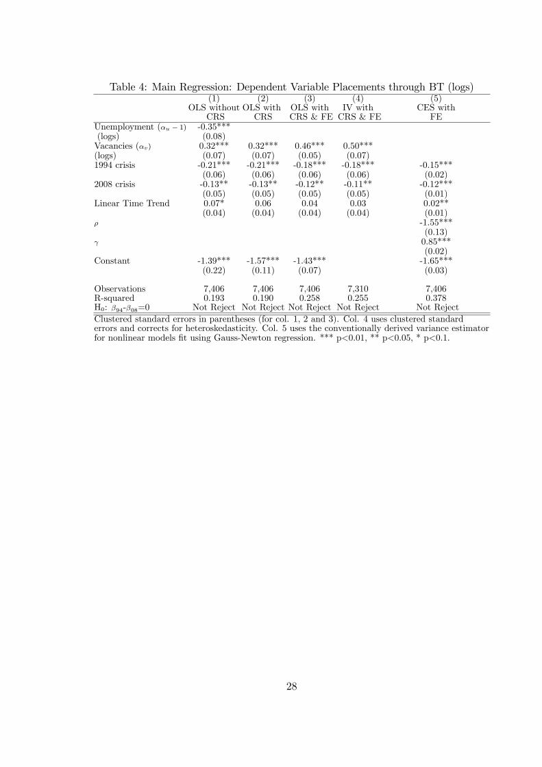
Table 4: Main Regression: Dependent Variable Placements through BT (logs)(1) (2) (3) (4) (5)

OLS without OLS with OLS with IV with CES withCRS CRS CRS & FE CRS & FE FE

Unemployment (�u � 1) -0.35***(logs) (0.08)Vacancies (�v) 0.32*** 0.32*** 0.46*** 0.50***(logs) (0.07) (0.07) (0.05) (0.07)1994 crisis -0.21*** -0.21*** -0.18*** -0.18*** -0.15***

(0.06) (0.06) (0.06) (0.06) (0.02)2008 crisis -0.13** -0.13** -0.12** -0.11** -0.12***

(0.05) (0.05) (0.05) (0.05) (0.01)Linear Time Trend 0.07* 0.06 0.04 0.03 0.02**

(0.04) (0.04) (0.04) (0.04) (0.01)� -1.55***

(0.13) 0.85***

(0.02)Constant -1.39*** -1.57*** -1.43*** -1.65***

(0.22) (0.11) (0.07) (0.03)

Observations 7,406 7,406 7,406 7,310 7,406R-squared 0.193 0.190 0.258 0.255 0.378H0: �94-�08=0 Not Reject Not Reject Not Reject Not Reject Not RejectClustered standard errors in parentheses (for col. 1, 2 and 3). Col. 4 uses clustered standarderrors and corrects for heteroskedasticity. Col. 5 uses the conventionally derived variance estimatorfor nonlinear models �t using Gauss-Newton regression. *** p<0.01, ** p<0.05, * p<0.1.

28

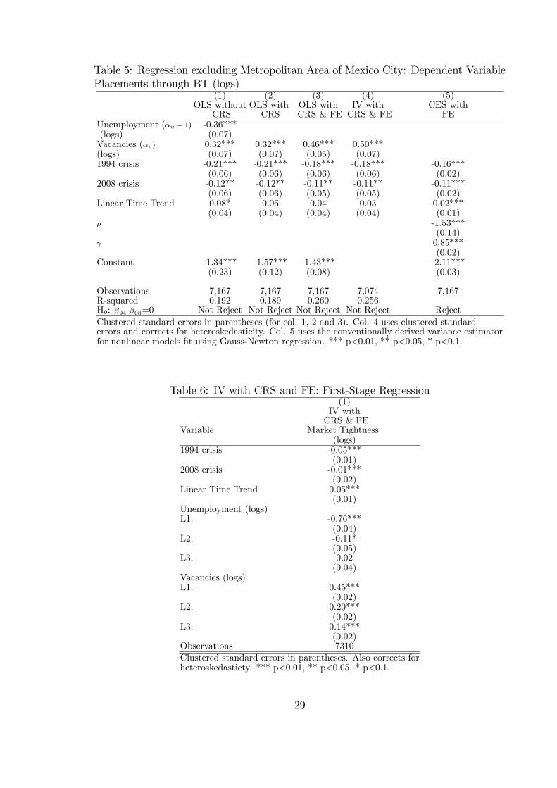
Table 5: Regression excluding Metropolitan Area of Mexico City: Dependent VariablePlacements through BT (logs)

(1) (2) (3) (4) (5)OLS without OLS with OLS with IV with CES with

CRS CRS CRS & FE CRS & FE FEUnemployment (�u � 1) -0.36***(logs) (0.07)Vacancies (�v) 0.32*** 0.32*** 0.46*** 0.50***(logs) (0.07) (0.07) (0.05) (0.07)1994 crisis -0.21*** -0.21*** -0.18*** -0.18*** -0.16***

(0.06) (0.06) (0.06) (0.06) (0.02)2008 crisis -0.12** -0.12** -0.11** -0.11** -0.11***

(0.06) (0.06) (0.05) (0.05) (0.02)Linear Time Trend 0.08* 0.06 0.04 0.03 0.02***

(0.04) (0.04) (0.04) (0.04) (0.01)� -1.53***

(0.14) 0.85***

(0.02)Constant -1.34*** -1.57*** -1.43*** -2.11***

(0.23) (0.12) (0.08) (0.03)

Observations 7,167 7,167 7,167 7,074 7,167R-squared 0.192 0.189 0.260 0.256H0: �94-�08=0 Not Reject Not Reject Not Reject Not Reject RejectClustered standard errors in parentheses (for col. 1, 2 and 3). Col. 4 uses clustered standarderrors and corrects for heteroskedasticity. Col. 5 uses the conventionally derived variance estimatorfor nonlinear models �t using Gauss-Newton regression. *** p<0.01, ** p<0.05, * p<0.1.

Table 6: IV with CRS and FE: First-Stage Regression(1)

IV withCRS & FE

Variable Market Tightness(logs)

1994 crisis -0.05***(0.01)

2008 crisis -0.01***(0.02)

Linear Time Trend 0.05***(0.01)

Unemployment (logs)L1. -0.76***

(0.04)L2. -0.11*

(0.05)L3. 0.02

(0.04)Vacancies (logs)L1. 0.45***

(0.02)L2. 0.20***

(0.02)L3. 0.14***

(0.02)Observations 7310Clustered standard errors in parentheses. Also corrects forheteroskedasticty. *** p<0.01, ** p<0.05, * p<0.1.

29

Table 7: Weak Instruments and Overidenti�cation Tests

Global Signi�cance in First-Stage RegressionStatistic Value p-value H0 ResultF 235.4 0.000 All �i = 0 Reject

Weak-Instrument Tests

Anderson-Rubin F 20.03 0.000 RejectAnderson-Rubin 124.50 0.000 The coe¢ cients of the endogenous RejectChi-squared regressors in the structuralStock-Wright 24.73 0.000 equation are jointly equal to zero RejectS statistic

Overidenti�cation Test

Hansen J Instruments are uncorrelated withChi-squared 9.44 0.09 the error term, and excluded Fail to Reject

instruments are correctly exludedNote: All tests were computed by the xtivreg2 command in Stata.

30