Coupling and numerical integration of the Landau Lifshitz ...

D I S S E R T A T I O N

Coupling and numerical integration

of the Landau–Lifshitz–Gilbert equation(Kopplung und numerische Integration der Landau–Lifshitz–Gilbert-Gleichung)

ausgeführt zum Zwecke der Erlangung des akademischen Gradeseines Doktors der technischen Wissenschaften unter der Leitung von

Prof. Dr. Dirk PraetoriusE101 – Institut für Analysis und Scientific Computing – TU Wien

eingereicht an der Technischen Universität WienFakultät für Mathematik und Geoinformation

von

Dott.mag. Michele RuggeriMatrikelnummer: 1328691

Oswaldgasse 118/5/10, 1120 Wien

Diese Dissertation haben begutachtet:

1. Prof. Dr. Sören BartelsAbteilung für Angewandte Mathematik, Albert-Ludwigs-Universität Freiburg

2. Prof. Dr. Ansgar JüngelInstitut für Analysis und Scientific Computing, TU Wien

3. Prof. Dr. Dirk PraetoriusInstitut für Analysis und Scientific Computing, TU Wien

Wien, am 25. Oktober 2016

Abstract

The understanding of the magnetization dynamics plays an essential role in the design of manytechnological applications, e.g., magnetic sensors, actuators, storage devices, electric motors, andgenerators. The availability of reliable numerical tools to perform large-scale micromagnetic simula-tions of magnetic systems is therefore of fundamental importance. Time-dependent micromagneticphenomena are usually described by the Landau–Lifshitz–Gilbert (LLG) equation. The numericalintegration of the LLG equation poses several challenges: strong nonlinearities, a nonconvex point-wise constraint, an intrinsic energy law, which combines conservative and dissipative effects, as wellas the presence of nonlocal field contributions, which prescribes the coupling with other partial dif-ferential equations (PDEs). This dissertation is concerned with the numerical analysis of a tangentplane integrator for the LLG equation. The method is based on an equivalent reformulation of theequation in the tangent space, which is discretized by first-order finite elements and requires onlythe solution of one linear system per time-step. The pointwise constraint is enforced at the discretelevel by applying the nodal projection mapping to the computed solution at each time-step. Inthis work, we provide a unified abstract analysis of the tangent plane scheme, which includes theeffective discretization of the field contributions. We prove that the sequence of discrete approx-imations converges towards a weak solution of the problem. Under appropriate assumptions, theconvergence is unconditional, i.e., the numerical analysis does not require to impose any CFL-typecondition on the time-step size and the spatial mesh size. Moreover, we show that a fully linearprojection-free variant of the method preserves the (unconditional) convergence result. One par-ticular focus of this work is on the efficient treatment of coupled systems, for which we show thatan approach based on the decoupling of the time integration of the LLG equation and the coupledPDE is very attractive in terms of computational cost and still leads to time-marching algorithmsthat are unconditionally convergent. As an application of the abstract theory, we analyze severalextensions of the micromagnetic model for the simulation of spintronic devices. These range fromextended forms of the LLG equation to more involved coupled systems, in which, e.g., the nonlinearcoupling with a diffusion equation, which describes the evolution of the spin accumulation in thepresence of spin-polarized currents, is considered. Numerical experiments support our theoreticalfindings and demonstrate the applicability of the method for the simulation of practically relevantproblem sizes.

iii

Kurzfassung

Das Verständnis des dynamischen Verhaltens der Magnetisierung spielt beim Design vieler tech-nologischer Anwendungen – z.B. magnetischer Sensoren, Aktoren, Datenspeicher, Elektromoto-ren und elektrischer Generatoren – eine essentielle Rolle. Die Verfügbarkeit zuverlässiger nume-rischer Methoden für die umfassende Simulation von magnetischen Systemen ist dazu sehr wich-tig, um die kosten- und zeitintensive Produktion von Prototypen zu vermeiden. Zeitabhängigemikromagnetische Phänomene werden üblicherweise durch die Landau-Lifshitz-Gilbert-Gleichung(LLG-Gleichung) beschrieben. Die numerische Integration der LLG-Gleichung führt auf einige ma-thematische Herausforderungen: Nichtlinearitäten, eine nichtkonvexe punktweise Nebenbedingung,ein Energieerhaltungsgesetz und nichtlokale Effekte, die die Kopplung mit anderen partiellen Dif-ferentialgleichungen notwendig machen. Diese Arbeit befasst sich mit der numerischen Analyse dessogenannten Tangent-Plane-Verfahrens für die LLG-Gleichung. Diese Methode basiert auf der äqui-valenten Formulierung der Gleichung im Tangentialraum, die durch ein Finite-Elemente-Verfahrenerster Ordnung diskretisiert wird. Pro Zeitschritt muss bei diesem Verfahren ein lineares Glei-chungssystem gelöst werden. Die punktweise Nebenbedingung der diskreten Lösung wird durchdie knotenweise Projektion auf die Einheitssphäre sichergestellt. In dieser Arbeit erweitern wir dieAnalysis des Tangent-Plane-Verfahrens. Wir beweisen, dass die Folge der Näherungslösungen gegeneine schwache Lösung der LLG-Gleichung konvergiert. Unter gewissen Voraussetzungen konvergiertdas Verfahren unbedingt, d.h. in der numerischen Analysis muss keine CFL-Bedingung zwischender Zeitschrittweite und Ortsgitterweite gefordert werden. Außerdem zeigen wir, dass das Verfahrenohne nodale Projektion ebenfalls unbedingt konvergiert. Ein zentrales Thema dieser Arbeit ist dieBehandlung einiger gekoppelter Systeme. Wir erweitern die Diskretisierung der LLG-Gleichung aufdiese Kopplungen. Das resultierende, unbedingt konvergente Verfahren entkoppelt die Zeitintegra-tion der LLG-Gleichung und der gekoppelten Gleichung, was zu einem günstigeren Rechenaufwandführt. Als Anwendung analysieren wir einige Erweiterungen des mikromagnetischen Modells in derSpintronik. Wir betrachten erweiterte Formen der LLG-Gleichung sowie (nichtlineare) Kopplungender LLG-Gleichung mit einer Diffusionsgleichung für die Spin-Akkumulation. Numerische Expe-rimente bestätigen die theoretischen Resultate und damit die Anwendbarkeit der entwickeltenAlgorithmen auf die Simulation praktisch relevanter Problemgrößen.

v

Riassunto

La comprensione dei fenomeni di evoluzione nei corpi ferromagnetici riveste un ruolo fondamentaleper la progettazione di numerose applicazioni tecnologiche: sensori magnetici, attuatori, supportidi memoria, motori elettrici e generatori. La disponibilità di metodi affidabili per eseguire simu-lazioni numeriche di sistemi magnetici su larga scala è pertanto di vitale importanza. I fenomenimicromagnetici di tipo evolutivo sono normalmente descritti dall’equazione di Landau–Lifshitz–Gilbert, la cui approssimazione numerica pone diverse difficoltà: non-linearità, un vincolo puntualee non-convesso, una legge di conservazione dell’energia (che combina effetti conservativi e dissipa-tivi) e la presenza di contributi non-locali, che richiedono lo studio di sistemi in cui l’equazionedi Landau–Lifshitz–Gilbert è accoppiata ad altre equazioni alle derivate parziali. Questa tesi sioccupa dell’analisi numerica di un metodo di tipo ‘tangent plane’ per l’equazione di Landau–Lifshitz–Gilbert. Il metodo si fonda su una formulazione variazionale del problema basata sullospazio tangente, che viene discretizzata mediante elementi finiti di primo ordine, in modo da ri-chiedere soltanto la soluzione di un sistema lineare sparso per ogni time-step. La validità delvincolo puntuale a livello discreto viene assicurata attraverso la proiezione nodale della soluzionecalcolata. In questa tesi, si propone un’analisi astratta del metodo ‘tangent plane’. In particolare,si dimostra che la successione delle approssimazioni discrete converge verso una soluzione deboledel problema. Assumendo la validità di ipotesi appropriate, la convergenza è incondizionata, ossiarisulta valida senza che sia necessario imporre alcuna condizione CFL tra i parametri associati alladiscretizzazione temporale e a quella spaziale. Inoltre, si mostra che l’omissione della proiezione,pur determinando la violazione del vincolo, non intacca il risultato di convergenza (incondizionata).Nel lavoro, si evidenzia come il disaccoppiamento della discretizzazione temporale dell’equazione diLandau–Lifshitz–Gilbert da quella dell’equazione a essa accoppiata costituisca una valida strategiaper lo studio di sistemi. Tale approccio non solo risulta essere molto interessante dal punto divista del costo computazionale, ma conduce anche ad algoritmi incondizionatamente convergen-ti. Come applicazione della teoria presentata, si analizzano alcune tra le più comuni estensionidel modello micromagnetico utilizzate per la simulazione di dispositivi spintronici. Esse spazianoda forme generalizzate dell’equazione di Landau–Lifshitz–Gilbert a sistemi complessi di equazioninon-lineari, in cui, per esempio, l’equazione di evoluzione per la magnetizzazione viene accoppiataa un’equazione di diffusione per lo spin, che incorpora nel modello la presenza di correnti elettrichepolarizzate. Alcuni esperimenti numerici supportano i risultati teorici e dimostrano l’efficacia deimetodi proposti anche per la risoluzione di problemi derivanti da applicazioni concrete.

vii

Acknowledgments

This thesis would not have been possible without the support of many people and institutions.First and foremost, I would like to express my gratitude to my supervisor, Prof. Dirk Praetorius,

for his guidance over the past three and a half years. His patience, knowledge, and invaluableassistance have been fundamental for my growth both as an individual and as a mathematician.One could not wish for a better supervisor.

I would like to thank Prof. Sören Bartels and Prof. Ansgar Jüngel for their reports on thisthesis and their interest in my work.

I wish to thank all the colleagues of the working group I had the opportunity to meet duringmy doctoral studies for the fabulous work atmosphere and for all the fun we have had together:Michael Feischl, Thomas Führer, Gregor Gantner, Alexander Haberl, Josef Kemetmüller, MarcusPage, Carl-Martin Pfeiler, and Stefan Schimanko, as well as the foster members (at least for therecreational activities) Markus Faustmann and Alexander Rieder. A special mention is deserved bymy office mate Bernhard Stiftner for his fundamental help during the preparation of the numericalexperiments of this thesis.

I would like to extend my appreciation to Claas Abert, Florian Bruckner, Gino Hrkac, ThomasSchrefl, Dieter Suess, and Christoph Vogler. The interdisciplinary collaboration with them hasbeen very important to broaden my horizons. Mathematicians sometimes forget the practicalimplications of their work.

I am very grateful to Ms Ursula Schweigler for her precious support during my countless battlesagainst the Austrian bureaucracy and for her help during the organization of workshops.

I would like to thank the colleagues and friends of the doctoral program in Dissipation anddispersion in nonlinear PDEs for many interesting discussions.

Moreover, I would like to acknowledge the support of TU Wien through the Innovative Projekteinitiative, the Austrian Science Fund (FWF) under grant W1245, and the Vienna Science andTechnology Fund (WWTF) under grant MA14-44.

Deepest gratitude is also due to my family for their constant support throughout my studies.Finally, I wish to thank my beloved wife Nicole for her encouragement, understanding, and

patience, even during hard times. This thesis is dedicated to her and to who is growing inside her.

Vienna, October 25, 2016 Michele Ruggeri

ix

Contents

1 Introduction 11.1 Motivation . . . . . . . . . . . . . . . . . . . . . . . . . . . . . . . . . . . . . . . . 11.2 State of the art . . . . . . . . . . . . . . . . . . . . . . . . . . . . . . . . . . . . . . 41.3 Contributions and general outline of the dissertation . . . . . . . . . . . . . . . . . 6

2 Mathematical modeling 92.1 Maxwell’s equations . . . . . . . . . . . . . . . . . . . . . . . . . . . . . . . . . . . 92.2 Classical micromagnetic theory . . . . . . . . . . . . . . . . . . . . . . . . . . . . . 112.3 Metal spintronics . . . . . . . . . . . . . . . . . . . . . . . . . . . . . . . . . . . . . 21

3 Preliminaries 313.1 Nondimensionalization . . . . . . . . . . . . . . . . . . . . . . . . . . . . . . . . . . 313.2 Notation for Lebesgue/Sobolev/Bochner spaces . . . . . . . . . . . . . . . . . . . . 363.3 Time discretization . . . . . . . . . . . . . . . . . . . . . . . . . . . . . . . . . . . . 383.4 Finite element discretization . . . . . . . . . . . . . . . . . . . . . . . . . . . . . . . 38

4 Tangent plane integrators 474.1 Model problem . . . . . . . . . . . . . . . . . . . . . . . . . . . . . . . . . . . . . . 474.2 Numerical algorithm . . . . . . . . . . . . . . . . . . . . . . . . . . . . . . . . . . . 494.3 Convergence analysis . . . . . . . . . . . . . . . . . . . . . . . . . . . . . . . . . . . 52

5 Application to metal spintronics 775.1 Spin diffusion model . . . . . . . . . . . . . . . . . . . . . . . . . . . . . . . . . . . 775.2 Spintronic extensions of the LLG equation . . . . . . . . . . . . . . . . . . . . . . . 91

6 Numerical results 1016.1 Solution of the system . . . . . . . . . . . . . . . . . . . . . . . . . . . . . . . . . . 1016.2 Numerical experiments . . . . . . . . . . . . . . . . . . . . . . . . . . . . . . . . . . 106

7 Perspectives and future work 115

A Physical quantities, constants and units 119A.1 Physical quantities . . . . . . . . . . . . . . . . . . . . . . . . . . . . . . . . . . . . 119A.2 Physical constants . . . . . . . . . . . . . . . . . . . . . . . . . . . . . . . . . . . . 120

B Auxiliary results 121B.1 Linear algebra . . . . . . . . . . . . . . . . . . . . . . . . . . . . . . . . . . . . . . . 121B.2 Useful (in)equalities . . . . . . . . . . . . . . . . . . . . . . . . . . . . . . . . . . . 122B.3 Vector calculus . . . . . . . . . . . . . . . . . . . . . . . . . . . . . . . . . . . . . . 123

References 125

Curriculum Vitae 137

xi

Chapter 1

Introduction

1.1 MotivationThe understanding of the magnetization dynamics plays an important role in the design of manytechnological applications, e.g., magnetic sensors, actuators, storage devices, electric motors, andgenerators. In magnetic recording devices, e.g., in hard disk drives (HDDs), the magnetization offerromagnetic materials is used for the storage of data. The information is stored as tiny areas ofeither positive or negative magnetization on the surfaces of the disks. Each tiny area correspondsto a bit of information and the total storage capacity depends directly on how small the area neededto represent one bit of information can be made: The smaller the bits are, the greater becomes thecapacity.

(a) Longitudinal magnetic recording

(b) Perpendicular magnetic recording

Figure 1.1: Different technologies for data recording in HDDs [1]: Longitudinal magneticrecording (a) vs. perpendicular magnetic recording (b).

Figure 1.1(a) shows the operating principle of an HDD based on the so-called longitudinalmagnetic recording (LMR). This technique has been used for nearly 50 years in the industry and hasnowadays been replaced by a more effective method, the perpendicular magnetic recording (PMR);

1

see Figure 1.1(b). In LMR-based HDDs, the magnetization of each bit is aligned horizontally withrespect to the spinning platter of the drive. The areas which correspond to two adjacent bits withopposing magnetizations must be separated by a sufficiently wide transition region, in order toprevent the random magnetization flipping due to the superparamagnetic effect. In PMR-basedHDDs, the perpendicular geometry allows the recording head field to penetrate the medium moreefficiently, which substantially increases the number of magnetic elements that can be stored in agiven area of the platter [172, 209].

(a) Low resistance state (b) High resistance state

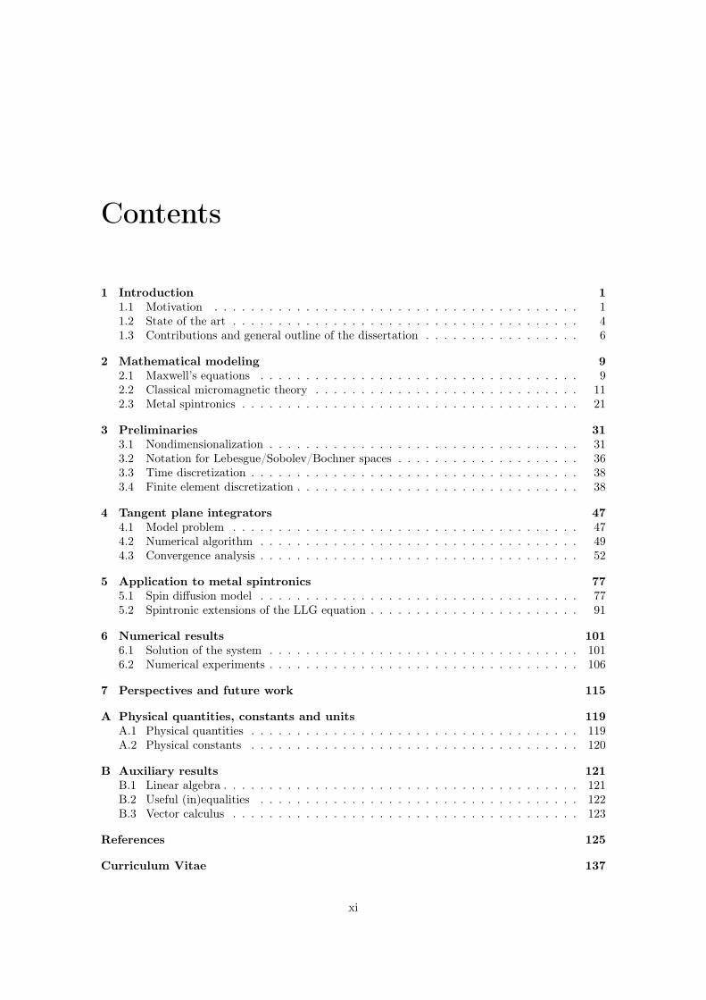
Figure 1.2: Giant magnetoresistance effect. The electrical resistance of a magnetic multi-layer depends on whether the magnetization configurations of consecutive ferromagneticsublayers are in parallel alignment (a) or in antiparallel alignment (b).

The discovery of the giant magnetoresistance effect (GMR) in 1988 [19, 49], for which A. Fertand P. Grünberg were awarded the Nobel Prize in physics in 2007, determined a breakthroughin magnetic HDD storage capacity. This effect occurs in magnetic multilayers (systems constitutedby alternating ferromagnetic and nonmagnetic sublayers) and consists in the dependence of theelectrical resistance on the relative orientation of the magnetization in the ferromagnetic layers.The electrical resistance changes from low for a parallel alignment to high for an antiparallelalignment; see Figure 1.2.

substrate

lower contact

ferromagnet

insulator

ferromagnet

upper contact

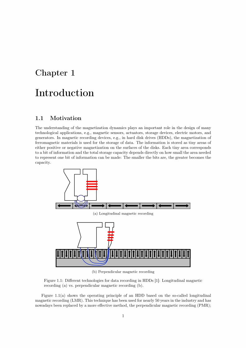
Figure 1.3: Schematic of a magnetic tunnel junction.

2

The GMR effect is the fundamental ingredient to understand the operating principle of amagnetic (or magnetoresistive) random access memory (MRAM) [80]. Unlike conventional solid-state RAMs, in MRAMs the information is stored neither as electric charge in a capacitor nor aselectric current in an electronic circuit, but rather by magnetic storage elements. Every cell of aMRAM contains a magnetic tunnel junction (MTJ), such as the one depicted in Figure 1.3, whichconsists of a magnetic trilayer with two ferromagnetic sublayers separated by a thin nonmagneticsublayer. One of the ferromagnetic layers (the so-called pinned or fixed layer) is a permanentmagnet set with a fixed orientation of the magnetization. The information is stored in the relativeorientation of the two ferromagnetic sublayers. Both the writing and the reading processes areperformed by applying an electric current which flows perpendicularly with respect to the planeof the layers. On the one hand, in the writing process, the orientation of the magnetization of thefree layer is switched by the resulting Oersted field. On the other hand, the reading process isbased on the GMR effect and consists in measuring the electrical resistance of the structure.

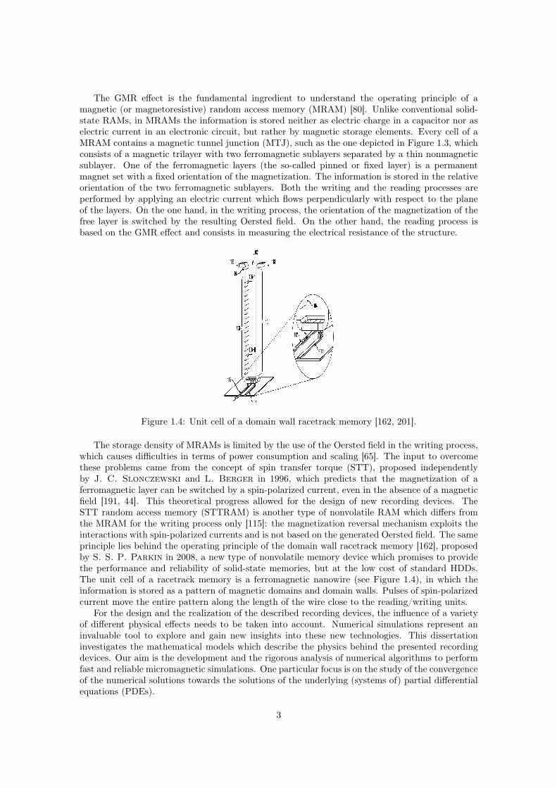
Figure 1.4: Unit cell of a domain wall racetrack memory [162, 201].

The storage density of MRAMs is limited by the use of the Oersted field in the writing process,which causes difficulties in terms of power consumption and scaling [65]. The input to overcomethese problems came from the concept of spin transfer torque (STT), proposed independentlyby J. C. Slonczewski and L. Berger in 1996, which predicts that the magnetization of aferromagnetic layer can be switched by a spin-polarized current, even in the absence of a magneticfield [191, 44]. This theoretical progress allowed for the design of new recording devices. TheSTT random access memory (STTRAM) is another type of nonvolatile RAM which differs fromthe MRAM for the writing process only [115]: the magnetization reversal mechanism exploits theinteractions with spin-polarized currents and is not based on the generated Oersted field. The sameprinciple lies behind the operating principle of the domain wall racetrack memory [162], proposedby S. S. P. Parkin in 2008, a new type of nonvolatile memory device which promises to providethe performance and reliability of solid-state memories, but at the low cost of standard HDDs.The unit cell of a racetrack memory is a ferromagnetic nanowire (see Figure 1.4), in which theinformation is stored as a pattern of magnetic domains and domain walls. Pulses of spin-polarizedcurrent move the entire pattern along the length of the wire close to the reading/writing units.

For the design and the realization of the described recording devices, the influence of a varietyof different physical effects needs to be taken into account. Numerical simulations represent aninvaluable tool to explore and gain new insights into these new technologies. This dissertationinvestigates the mathematical models which describe the physics behind the presented recordingdevices. Our aim is the development and the rigorous analysis of numerical algorithms to performfast and reliable micromagnetic simulations. One particular focus is on the study of the convergenceof the numerical solutions towards the solutions of the underlying (systems of) partial differentialequations (PDEs).

3

1.2 State of the artMicromagnetism, or micromagnetics1, is the study of magnetic processes on a submicrometerlength scale. Started with pioneering works by P.-E. Weiss, F. Bloch, L. D. Landau, andE. M. Lifshitz, the theory was developed in the 1940s by W. F. Brown, Jr, who gave thefirst extended treatment of the topic in his 1963 book [54]. For several years, the micromagnetictheory essentially consisted of applications of, on the one hand, standard variational techniquesto the so-called static micromagnetic problem, i.e., a constrained minimization problem for themicromagnetic energy [139], and, on the other hand, classical nucleation theory to model differentmagnetization reversal mechanisms [134, 135]. In the 1980s, with the simultaneous development ofnew magnetic materials (used, e.g., for permanent magnets, media and heads in recording devices,or magnetic sensors) and the widespread availability of large scale computational resources, one ofthe main focuses of the micromagnetic theory became the development of fast and reliable toolsto perform large-scale simulations of magnetic systems.

Applications to magnetic recording, in which the external field can change fast so that thehysteresis properties are not accurately described by a static approach, encouraged the studyof numerical methods to deal with the the so-called dynamic micromagnetic problem, i.e., thesolution of the Landau–Lifshitz–Gilbert (LLG) equation which governs the time evolution of themagnetization [139, 107, 108]. In this framework, one of the main issues concerns the computationof the nonlocal magnetostatic interactions, which turns out to be, in many situations, the mosttime-consuming part of micromagnetic simulations [188, 177, 159].

Most of the micromagnetic codes (both commercial and open-source) are based on either thefinite difference method (FDM) or the finite element method (FEM); see, e.g., [152, 185]. Infinite-difference-based codes, the computation of the magnetostatic interactions is usually basedon the fast Fourier transform (FFT). As an example, we mention the widely used Object-OrientedMicroMagnetic Framework (OOMMF) software [4, 82], a FDM-FFT micromagnetic code devel-oped at the National Institute of Standards and Technologies (NIST) of Gaithersburg (USA). Theapplication of the FEM in micromagnetics, more suitable to capture possible irregular shapes andgrain structures of the magnets, was proposed by D. R. Fredkin and T. R. Koehler [98, 125].The efficiency of finite-element-based micromagnetic simulations was improved by the work of thegroups of J. Fidler, T. Schrefl, and D. Suess at TU Wien [181, 182, 97, 194, 180]. Themagnetostatic interaction is formulated in terms of a scalar potential and discretized by combiningthe FEM with the boundary element method (BEM).

Nowadays, important lines of research in micromagnetics, from both the modeling and thecomputational point of view, concern the spintronic extensions of micromagnetics, e.g., with theconcepts of spin transfer torque [202, 191, 212] or spin-orbit coupling [85, 197, 91], the study ofenucleation processes, stability, and dynamics of magnetic skyrmions [157, 173, 175, 200, 127], andthe incorporation of thermal effects [55, 100, 105, 90].

For a long time, the investigation of micromagnetic phenomena has been a prerogative ofphysicists and engineers. However, in the last three decades, the growing need of fast and reliablenumerical simulations encouraged several mathematical studies, from both the analytical and thenumerical point of view.

The first existence result for weak solutions to the LLG equation can be traced back to [203],where the coupling of the LLG equation with the Maxwell equations and with a balance law for thelinear momentum to model the magnetoelastic interaction was considered. Since then, existenceand regularity questions for the LLG equation have been the subject of intense research. Theso-called small particle limit of the LLG equation, in which the effective field comprises only theexchange contribution, was studied, almost simultaneously, in [17, 114]. In particular, [17] adaptedthe proof of the analogous result for the harmonic maps heat flow [78, 48] and established globalexistence and nonuniqueness of weak solutions of the LLG equation. If the initial condition issufficiently regular, strong solutions of the LLG equation exist locally in time and are unique [63].

1Throughout the literature, these terms are usually used as synonyms of each other. To specify the preciseacceptation of each of these words, we might say that micromagnetism refers to the underlying science, whilemicromagnetics is more concerned with the application of that science.

4

These two notions of solutions are connected by a weak-strong uniqueness principle, in the sensethat if a strong solution exists up to some time T > 0, then any global weak solution coincides withit up to time T [84]. Extended versions and coupled problems have also been considered; see, e.g.,an extended LLG equation with an additional spin transfer torque term [151], the coupling of theLLG equation with the full Maxwell equations [62], with a conservation law for the linear momen-tum [61], with a spin diffusion equation [103], with a system of drift-diffusion equations [210, 211]to model the magnetization dynamics in semiconductors. Further analytical results for (coupledproblems for) the LLG equation can be found, e.g., in the papers [148, 154, 73, 74, 77, 149], in themonograph [113], in the recent preprint [94], as well as in the references therein. Recently, to includethermal effects, also the stochastic LLG equation has been investigated; see, e.g., [126, 59, 160, 60].

In parallel, the numerical integration of the LLG equation has also been the subject of manymathematical studies. The main challenges concern the strong nonlinearity of the equation, thenonconvex pointwise constraint satisfied by the solutions, an intrinsic energy law, which combinesconservative and dissipative effects and has to be preserved by the numerical scheme, as well asthe presence of nonlocal field contributions, which prescribes the (possibly nonlinear) couplingwith other PDEs; see the review articles [21, 137, 101, 75], the papers [20, 71, 22, 72], and themonographs [169, 26]. One important aspect of the research is related to the development ofunconditionally convergent (stable) methods, for which the numerical analysis does not requireto impose any CFL-type condition on the spatial and temporal discretization parameters. For anumerical integrator of the LLG equation, such a property is highly desirable, since the applicationof standard ‘off-the-shelf’ explicit schemes usually enforces severe constraints on the time-step sizewhich are sometimes unfeasible in practice or lead to unnecessary long computational time. Asan example for numerical schemes based on the finite difference method, we mention the uncondi-tionally stable Gauss–Seidel projection method [87, 207] and the scheme introduced in [79] basedon the midpoint rule in time.

The works [40, 12] proposed numerical integrators, based on lowest-order finite elements inspace, that are proven to be (unconditionally) convergent towards a weak solution of the smallparticle limit of the LLG equation. Both approaches were successfully applied to similar geometri-cally constrained evolution equations, such as the harmonic maps heat flow or the wave maps heatflow [41, 38, 35, 37], and extended to the case of the stochastic LLG equation [27, 25, 26, 13, 112].

On the one hand, the implicit midpoint scheme [40], proposed by S. Bartels and A. Prohl in2006, is formally of 2nd order in time and inherently preserves some of the fundamental propertiesof the LLG equation, such as the pointwise constraint (at the nodes of the mesh) and the energylaw, but requires the solution of a nonlinear system of equations per time-step. To deal withit, the authors proposed a linear fixed-point iteration, which is still constraint-preserving, butrequires the condition k = O(h2) for the time-step size k and the mesh size h in order to bestable. The analysis of the algorithm was extended allowing the inexact solution of the nonlinearsystem in [34, 76]. In the recent preprint [167], we extended the analysis of the algorithm to the fulleffective field and proposed an implicit-explicit treatment of the field contributions, attractive fromthe computational point of view, which formally preserves the convergence of 2nd order in time.Extensions of the scheme for the coupling of the LLG equation with the Maxwell equations [24]and for an extended LLG equation which models the dynamics of the magnetization when thetemperature is not constant were also considered [30, 31].

On the other hand, the θ-method [12], proposed by F. Alouges, is based on an equivalentreformulation of the LLG equation in the tangent space and requires only the solution of one linearsystem per time-step. Moreover, it is (unconditionally) convergent and formally of 1st order intime. The pointwise constraint, which characterizes the solutions of the LLG equation, is enforcedat a discrete level by applying the nodal projection mapping to the computed solution at eachtime step. The stability of the scheme requires restrictive conditions either on the discretizationparameters or on the underlying mesh. The method improves the explicit scheme introducedin [14] and analyzed in [39], where also the finite time blow-up of the solutions, motivated bythe analogous result for the harmonic maps heat flow, was numerically investigated. An implicit-explicit approach for the full effective field was introduced and analyzed in [109, 16] and [56],

5

where the discretization of the field contributions and the coupling with a nonlinear material lawwere also considered. Strategies to improve the convergence order in time of the method wereproposed in [16, 15]. Extensions of the tangent plane scheme for the discretization of the couplingof the LLG equation with the full Maxwell equations, the eddy current equation, a balance law forthe linear momentum (magnetostriction), and a spin diffusion equation for the spin accumulationwere considered in [142, 161, 29, 141, 28, 6]. In [161, 29, 141, 28, 6] one particular focus is onthe decoupling of the time integration of the LLG equation and the coupled PDE, which is veryattractive in terms of computational cost and leads to algorithms that are still unconditionallyconvergent. Inspired by [37], the projection-free version of the tangent plane scheme, which avoidsthe use of the nodal projection mapping, was introduced and analyzed in [6]. The violation of theconstraint at the nodes of the triangulation occurring in this case is controlled by the time-stepsize, independently of the number of iterations. The projection-free tangent plane scheme wascombined with a FEM-BEM coupling method for the discretization of the coupling of the LLGequation with the magnetoquasistatic Maxwell equations in full space in [92, 93]. There, assumingthe existence of a unique sufficiently regular solution, the authors proved also convergence rates ofthe method.

1.3 Contributions and general outline of the dissertationIn the present dissertation, we contribute to the study of reliable and effective numerical methodsfor the LLG equation. Our algorithm is an extension of the tangent plane scheme [12]. We transferideas from [37] and propose a projection-free variant of the scheme. Moreover, we investigate itsapplicability for the efficient discretization of coupled systems of PDEs, in which the LLG equationis coupled with another equation that describes a particular nonlocal effective field contribution.One of the main focuses is on the development of unconditionally convergent finite element methodsfor the numerical approximation of LLG-based models for metal spintronic devices.

The thesis is the continuation of a successful cooperation between the Institute of Solid StatePhysics (group of D. Suess) and the Institute for Analysis and Scientific Computing (group ofD. Praetorius) of TU Wien [111, 110, 58, 57, 56, 6, 7, 174, 205, 204, 8].

The remainder of this work is organized as follows:

• In Chapter 2, we describe the physical background which is behind the mathematical modelsconsidered in the dissertation. We start with a concise and micromagnetics-oriented pre-sentation of the Maxwell equations (Section 2.1), the fundamental system of PDEs for themodeling of electromagnetic phenomena. In Section 2.2, we give a brief introduction on theclassical theory of micromagnetics, with a careful description of the involved energy and fieldcontributions as well as a formal derivation of the LLG equation. We conclude the chapterwith an organic presentation of the, in our opinion, most relevant spintronic extensions ofthe LLG equation (Section 2.3).

• In Chapter 3, as a preparation for the following analysis, we collect some auxiliary results.To start with, we analyze the rigorous nondimensionalization of the problems introduced inChapter 2 (Section 3.1). Then, we briefly describe the notation used for Lebesgue, Sobolev,and Bochner spaces (Section 3.2). Finally, we discuss some preliminary results about thetime discretization (Section 3.3) and the spatial discretization (Section 3.4), which is basedon 1st order finite elements.

• In Chapter 4, we propose a unified analysis of the tangent plane scheme for a generalizedform of the LLG equation, which improves and extends those of [12, 16, 56, 6]. The pro-posed framework considers both the standard tangent plane scheme and its projection-freevariant (Algorithm 4.2.1). We introduce a set of general assumptions (on the discretizationparameters, on the field contributions as well as on their numerical approximations) whichguarantee the (unconditional) convergence of the sequence of discrete solutions towards aweak solution of the problem (Theorem 4.3.2). The abstract framework covers most of theclassical contributions that are usually included into the effective field.

6

• Chapter 5 is devoted to the numerical approximation of the extensions of the LLG equation,which are currently used for the micromagnetic modeling of spintronic devices. These models,which take the effects of the interaction between the magnetization and spin-polarized electriccurrents into account, can be classified into two main categories. On the one hand, thereare extended forms of the LLG equation, in which the classical energy-based effective field isaugmented by (local or nonlocal) additional terms which include the effect of the spin transfertorque [191, 213, 174, 8]. In this case, we show that the resulting extended forms of the LLGequation are covered by the abstract framework of Chapter 4, which ensures the convergenceof the numerical scheme. On the other hand, the LLG equation is nonlinearly coupledwith a diffusion equation for the spin accumulation [212, 103]. We show that the approachof [29, 141, 28], introduced to deal with the coupling of the LLG equation with the Maxwellequations (both the full system and the eddy current approximation) and the conservationof momentum (magnetostriction) and based on the decoupling of the time integration of theLLG equation and the coupled PDE, can be successfully applied. Here, differently from thosecases, the magnetization affects not only the right-hand side of the coupled equation, but alsothe main part of the involved differential operator, which leads to a slightly more involvedanalysis.

• In Chapter 6, we propose some effective strategies for the solution of the constrained linearsystem which arises when the LLG equation is discretized by the tangent plane scheme(Section 6.1). In Section 6.2, to support our theoretical findings, we present some numericalresults, which investigate both the general performance of our methods as well as theirapplicability for the simulation of practically relevant problem sizes.

• For most of the results and the methods of the present dissertation, there are a numberof possible extensions and related open questions, which are, in our opinion, worth to beinvestigated. In Chapter 7, we give a short outlook on some of them.

• For the convenience of the reader, we conclude this work with two appendices. In Appendix A,we summarize the physical quantities and the physical constants considered throughout thethesis. In Appendix B, we collect some useful linear algebra definitions, vector identities, andwell-known product rules of classical vector calculus.

Some of the presented results have been partially published in our papers [56, 6, 7, 174, 8]. How-ever, in the present work, we propose an extended treatment of the topic with several additionalcomments. In particular, some results are more general or slightly sharper and some proofs haveeven been improved.

7

Chapter 2

Mathematical modeling

In this chapter, we introduce the partial differential equations that are considered throughout thethesis. When we refer to physical quantities, we use physical units in the International System ofUnits (SI). For an overview of the considered physical quantities/constants and the correspondingunits, we refer the reader to Appendix A.

2.1 Maxwell’s equationsThe Maxwell system is a set of four fundamental equations in the theory of electromagnetism [145].A classical reference for the physics of electromagnetism is, e.g., the book [119]. Here, we considerthe macroscopic Maxwell equations, namely

∇ ·D = ρ, (2.1a)∇ ·B = 0, (2.1b)∇×E = −∂tB, (2.1c)∇×H = Je + ∂tD. (2.1d)

The physical quantities which appear in (2.1) are the magnetic flux density B (in T), the electricdisplacement field D (in C/m2), the electric field E (in V/m), the magnetic field H (in A/m),and the electric current density Je (in A/m2), which are three-dimensional vector fields, and thescalar-valued electric charge density ρ (in C/m3). For the orientation of the electric field and theelectric current density, we adopt the standard convention: The direction of the electric field ischosen to be the direction of the force exerted on a positive test charge; consistently, the directionof electric current is arbitrarily defined as the direction of a flow of positive charges. The Maxwellsystem comprises the Gauss law (2.1a), the Gauss law for magnetism (2.1b), the Faraday law ofinduction (2.1c), and the Maxwell–Ampère circuital law (2.1d). The above equations are posed onthe full space R3. However, the charge density ρ and the electric current density Je are supportedon a limited region of space, which we assume to be a bounded domain Ω ⊂ R3, which representsthe volume occupied by a conducting body. We assume R3 \ Ω to be vacuum.

Formally, the summation of the time derivative of (2.1a) with the divergence of (2.1d) yields aconservation law for the electric charge on the conducting domain Ω, i.e., the continuity equation

∂tρ+∇ · Je = 0.

Moreover, if the initial condition for B satisfies (2.1b), the equation will be satisfied for all time.This follows by taking the divergence of (2.1c) and noting that the divergence of the curl is zero.

In the case of linear materials, one usually assumes the constitutive laws

D = εE, (2.2a)B = µH, (2.2b)

9

where the electric permittivity ε (in F/m) and the magnetic permeability µ (in N/A2) are sym-metric and uniformly positive definite matrices in R3×3. In particular, in vacuum, e.g., in R3 \ Ω,it holds that ε = ε0I3×3 as well as µ = µ0I3×3, where the positive constants ε0 and µ0 are thevacuum permittivity (in F/m) and the vacuum permeability (in N/A2), respectively. Under thisassumption, the Maxwell system (2.1) can be rewritten as

∇ · (εE) = χΩρ, (2.3a)∇ · (µH) = 0, (2.3b)∇×E = −µ∂tH, (2.3c)∇×H = χΩJe + ε∂tE. (2.3d)

The characteristic function χΩ is a reminder that the charge density and the electric currentdensity vanish in R3 \ Ω. The electromagnetic energy (in J) is the sum of the electric energy andthe magnetic energy

E(E,H) =1

2

∫R3

εE ·E dx+1

2

∫R3

µH ·H dx. (2.4)

Using the product rule

∇ · (E ×H) = (∇×E) ·H − (∇×H) ·E, (2.5)

together with the equations (2.3c)–(2.3d), we obtain

d

dtE(E,H) =

∫R3

δEδE· ∂tE dx+

∫R3

δEδH· ∂tH dx

(2.4)=

∫R3

ε∂tE ·E dx+

∫R3

µ∂tH ·H dx

(2.3)=

∫R3

(∇×H) ·E dx−∫

Ω

Je ·E dx−∫R3

(∇×E) ·H dx

(2.5)= −

∫R3

∇ · (E ×H) dx−∫

Ω

Je ·E dx.

We conclude the energy law

d

dtE(E,H) +

∫R3

∇ · (E ×H) dx = −∫

Ω

Je ·E dx.

The vector S = E×H, usually referred to as Poynting vector (in W/m2), plays the role of energyflux density, while the term on the right-hand side refers to the so-called Joule heating, i.e., theenergy which is converted into heat when an electric current flows through a resistance.

Associated with the Maxwell equations, one usually considers a constitutive law for conductionthat relates the fields to the sources. The usual choice for a conducting material is the Ohm law,i.e.,

Je = σE, (2.6)

where σ ∈ R3×3, a symmetric and uniformly positive definite matrix, is the conductivity (inA/(m V)). Under this assumption, the Faraday law of induction (2.3c) and the Maxwell–Ampèrecircuital law (2.3d), namely

µ∂tH +∇×E = 0,

ε∂tE −∇×H + χΩσE = 0,

are sufficient to determine the electromagnetic fields, and the charge density ρ becomes a ‘leftoverquantity’, which can be obtained from (2.3a) once the electric field is known. Moreover, in thiscase the energy law becomes

d

dtE(E,H) +

∫R3

∇ · (E ×H) dx = −∫

Ω

σE ·E dx < 0.

10

The negative right-hand side reveals the dissipative nature of the Joule heating.In many practical situations, since wave phenomena usually occur on a very short time scale,

for an appropriate description of the electromagnetic fields it is sufficient to consider truncatedversions of the Maxwell equations, where the time derivative of either the magnetic field or theelectric field (quasistatic approximation) or both of them (static approximation) are omitted. Inthese cases, the electromagnetic waves, which result from the coupling of the magnetic field andthe displacement current, are neglected.

The magnetoquasistatic Maxwell equations can be considered whenever |ε∂tE| |∇ ×H| +|σE|, e.g., when µmaxεmaxL

2T−2 1 and εmaxσ−1minT

−1 1, where εmax and µmax (resp. σmin)denote the maximal (resp. minimal) eigenvalues of ε and µ (resp. σ), while L > 0 and T > 0denote some typical length (in m) and typical time (in s) of the problem; see [10, Section 1.2]. Fora material which satisfies the Ohm law (2.6), the resulting system is given by

∇ · (εE) = χΩρ, (2.7a)∇ · (µH) = 0, (2.7b)∇×E = −µ∂tH, (2.7c)∇×H = χΩσE. (2.7d)

Replacing the electric field E in (2.7c) by the expression that can be derived from (2.7d), which isadmissible in the conducting region Ω, we obtain the so-called eddy current equation

µ∂tH = −∇× (σ−1∇×H).

In the static case, the equations for the electric field and the magnetic field can be decoupled.The resulting systems are the electrostatic Maxwell equations

∇ · (εE) = χΩρ,

∇×E = 0,

and the magnetostatic Maxwell equations

∇ · (µH) = 0,

∇×H = χΩJe.

2.2 Classical micromagnetic theoryIn this section, we briefly introduce the classical theory of micromagnetism. For further details,we refer the interested reader to the monographs [9, 118, 47, 136] and the review articles [97, 96,183, 184].

Micromagnetics can be defined as the study of magnetic processes at submicrometer lengthscales. The considered length scale, which ranges from few nanometers to micrometers, is largeenough to average the atomic structure of the material, which allows to replace the individualatomistic magnetic moments by a continuous function in space (the so-called continuous mediumapproximation). At the same time, the length scale is small enough to resolve magnetic structuressuch as domain walls or vortices. The magnetic condition of a ferromagnetic body is described bya physical quantity called magnetization. It is defined as the quantity of magnetic moment perunit volume and it is measured in A/m. Mathematically, the magnetization is represented by athree-dimensional vector field M , defined on a bounded domain Ω ⊂ R3, which represents thevolume occupied by the ferromagnetic body, with boundary denoted by Γ := ∂Ω.

If the temperature is constant and far below the so-called Curie temperature of the ferromag-netic material (in K), the modulus of the magnetization is assumed to be constant, i.e.,

|M | = Ms. (2.8)

11

The constant Ms > 0 is called saturation magnetization and is a measure of the maximal amountof field that can be generated by a material (in A/m). We define the normalized magnetizationby m := M/Ms, for which the modulus constraint (2.8) becomes |m| = 1, i.e., the normalizedmagnetization assumes values on the unit sphere

S2 =x ∈ R3 : |x| = 1

.

In the case of linear ferromagnetic materials, the constitutive law (2.2b) takes the form

B = µ0(H +MsχΩm). (2.9a)

Moreover, for the sake of simplicity, we restrict ourselves to the case of scalar-valued electricpermittivity ε > 0 and conductivity σ > 0, i.e., we consider the constitutive laws

D = εE, (2.9b)Je = σE, (2.9c)

instead of (2.2a) and (2.6).

2.2.1 Total magnetic Gibbs’ free energyIn micromagnetism, the study of magnetic processes is characterized by an energy-based approach.The key quantity is the total magnetic Gibbs free energy of the ferromagnetic body (in J), whichdepends on the magnetization and on possible applied external fields. The total magnetic Gibbsfree energy comprises several energy contributions.

2.2.1.1 Exchange energy

The exchange energy contribution stems from the exchange interactions between the spins theorizedby W. K. Heisenberg. According to this quantum mechanical effect, neighboring magneticmoments tend to be parallel to each other. This is reflected by an energy contribution whichpenalizes disuniformities of the magnetization, i.e.,

Eex(m) = A

∫Ω

|∇m|2 dx,

where A > 0 is the so-called exchange stiffness constant. Its value for standard ferromagneticmaterials is usually of the order of 10−11 J/m.

2.2.1.2 Magnetocrystalline anisotropy energy

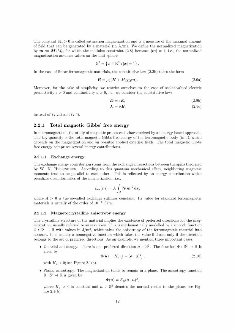
The crystalline structure of the material implies the existence of preferred directions for the mag-netization, usually referred to as easy axes. This is mathematically modelled by a smooth functionΦ : S2 → R with values in J/m3, which takes the anisotropy of the ferromagnetic material intoaccount. It is usually a nonnegative function which takes the value 0 if and only if the directionbelongs to the set of preferred directions. As an example, we mention three important cases:

• Uniaxial anisotropy: There is one preferred direction a ∈ S2. The function Φ : S2 → R isgiven by

Φ(u) = Ku

[1− (a · u)2

], (2.10)

with Ku > 0; see Figure 2.1(a).

• Planar anisotropy: The magnetization tends to remain in a plane. The anisotropy functionΦ : S2 → R is given by

Φ(u) = Kp(a · u)2,

where Kp > 0 is constant and a ∈ S2 denotes the normal vector to the plane; see Fig-ure 2.1(b).

12

• Cubic anisotropy: There are three mutually orthogonal easy directions ai ∈ S2, 1 ≤ i ≤ 3.A possible expression for the function Φ : S2 → R is given by

Φ(u) = Kc1

[(a1 · u)2(a2 · u)2 + (a1 · u)2(a3 · u)2 + (a2 · u)2(a3 · u)2

]+Kc2(a1 · u)2(a2 · u)2(a3 · u)2,

with Kc1,Kc2 ∈ R; see Figure 2.1(c).

−1−0.5

00.5

1

−1

−0.5

0

0.5

1−0.4

−0.2

0

0.2

0.4

(a) Uniaxial anisotropy−0.4

−0.20

0.20.4

−0.4

−0.2

0

0.2

0.4−1

−0.5

0

0.5

1

(b) Planar anisotropy−0.5

0

0.5

−0.5

0

0.5−0.5

0

0.5

(c) Cubic anisotropy

Figure 2.1: Anisotropy functions. (a) Plot of the uniaxial anisotropy function withKu = 1 and a = e3. (b) Plot of the planar anisotropy function with Kp = 1 and a = e3.(c) Plot of the cubic anisotropy function with Kc1 = 2, Kc2 = 0 and ai = ei for all1 ≤ i ≤ 3.

The above constants Ku,Kp,Kc1,Kc2 are material parameters and are measured in J/m3.Throughout this work, we consider a general anisotropy function of the form Φ = Kφ, where

K > 0 is a general anisotropy constant in J/m3, while φ : S2 → R is a (nondimensional) smoothfunction. Clearly, the three aforementioned examples can be recasted into this framework. Themagnetocrystalline anisotropy energy is given by

Eani(m) = K

∫Ω

φ(m) dx

and can be defined as the work required to rotate the magnetization out of the easy axes.

2.2.1.3 Zeeman’s energy

In the presence of an external field, the magnetization tends to align itself to it. The Zeemanenergy, named after P. Zeeman, is an energy contribution which penalizes any deviation of themagnetization from this field inside the body. The corresponding term is

Eext(m,Hext) = −µ0Ms

∫Ω

Hext ·m dx,

where Hext denotes the applied external field (in A/m).

2.2.1.4 Antisymmetric exchange energy

Chiral magnets are characterized by an atomic structure which lacks inversion symmetry. The asso-ciated interaction is called antisymmetric exchange interaction, also referred to as Dzyaloshinskii–Moriya (DM) interaction. It is a short-range effect which tries to twist the magnetization (neighbor-ing magnetic moments tend to be perpendicular to each other) and it is thus in direct competitionwith the exchange interaction which favors uniform magnetization configurations. It was foundthat the mechanism behind this effect is based on spin-orbit coupling [86, 156]. The correspondingenergy contribution takes the form

EDM(m) = D

∫Ω

(∇×m) ·m dx,

13

where D ∈ R is the DM constant (in J/m2). The Dzyaloshinskii–Moriya interaction turns out tobe one of the main ingredient for the formation of magnetic skyrmions [95, 157, 175, 127].

2.2.1.5 Magnetostatic energy

Taking the constitutive law (2.9a) for ferromagnetic materials into account, it turns out thatthe magnetization ‘generates’ a magnetic field, which is described by the Maxwell equations; seeSection 2.1. Since the electromagnetic wavelength is much larger than the standard dimensions ofa ferromagnet, an appropriate description of this magnetic field usually employs the magnetostaticMaxwell equations, which for a ferromagnet are given by

∇ ·H = −Ms∇ · (χΩm), (2.11a)∇×H = χΩJe. (2.11b)

We decompose the magnetic field into two components, i.e., H = Hs + Hc. Here, Hs is theso-called stray field (or demagnetizing field, since it acts on the magnetization so as to reduce thetotal magnetic moment), ‘generated’ by the magnetization m, while Hc is usually referred to asOersted field, ‘generated’ by the electric current density Je. From the superposition principle, itfollows that Hs and Hc satisfy

∇ ·Hs = −Ms∇ · (χΩm), (2.12a)∇×Hs = 0, (2.12b)

and

∇ ·Hc = 0, (2.13a)∇×Hc = χΩJe, (2.13b)

respectively. Note that the stray field and the Oersted field are nothing but the gradient part andthe curl part of the Helmholtz decomposition of H, respectively. From (2.12b), it turns out thatthe stray fieldHs is an irrotational field in a simply connected domain (the full space), from whichit follows that it can be understood as the gradient of a scalar potential. It holds that Hs = −∇u,where u denote the magnetostatic potential (in A). With the usual transmission conditions (thenormal component of the magnetic flux density must be continuous at the interface) and a suitableradiation condition at infinity, from (2.12) it follows that the magnetostatic potential solves thescalar full-space transmission problem

−∆uint = −Ms∇ ·m in Ω, (2.14a)

−∆uext = 0 in R3 \ Ω, (2.14b)

uext − uint = 0 on Γ, (2.14c)

(∇uext −∇uint) · n = −Msm · n on Γ, (2.14d)u(x) = O(1/ |x|) as |x| → ∞. (2.14e)

Here, the superscripts ‘int’ and ‘ext’ denote the restriction of the magnetostatic potential to Ωand its complement. This interpretation explains why, in analogy with the electrostatic case, thequantities −Ms∇·m and −Msm·n are usually referred to as magnetic volume charge and magneticsurface charge, respectively. As for the Oersted field, using the vector identity

∇× (∇×Hc) = ∇(∇ ·Hc)−∆Hc, (2.15)

we obtain that

∇× (χΩJe)(2.13b)

= ∇× (∇×Hc)(2.15)

= ∇(∇ ·Hc)−∆Hc(2.13a)

= −∆Hc.

14

With the usual transmission conditions (the tangential component of the magnetic field must becontinuous at the interface) and a suitable radiation condition at infinity, we deduce that theOersted field solves the vector full-space transmission problem

−∆H intc = ∇× Je in Ω, (2.16a)

−∆Hextc = 0 in R3 \ Ω, (2.16b)

Hextc −H int

c = 0 on Γ, (2.16c)

(∇Hextc −∇H int

c )n = n× Je on Γ, (2.16d)Hc(x) = O(1/ |x|) as |x| → ∞. (2.16e)

The decomposition of the magnetic field into stray field and Oersted field is reflected by a decom-position of the magnetic energy

E(H) =µ0

2

∫R3

|H|2 dx =µ0

2

∫R3

|Hs|2 dx+µ0

2

∫R3

|Hc|2 dx.

In micromagnetics, the (magnetization-dependent) magnetic energy of the stray field is usuallyreferred to as magnetostatic energy. It can be understood as the energy of the magnetizationassociated with the interactions with its own demagnetizing field

Estray(m) =µ0

2

∫R3

|Hs|2 dx = −µ0Ms

2

∫Ω

Hs ·m dx.

The classical theory of micromagnetism usually models the behavior of ferromagnetic materials inthe absence of electric currents, i.e., without Oersted field. However, for conducting materials andcertain geometries, e.g., in the case of ferromagnetic nanowires, the effect of the electric currentand the associated Oersted field cannot be ignored.

2.2.1.6 Magnetoelastic energy

Ferromagnetic bodies are also sensible to mechanical stresses and deformations: Changes in themagnetization cause strains in the crystal lattice. Conversely, if an applied force produces a strainin a ferromagnetic material, this stress affects the magnetization. This bidirectional couplingbetween magnetic and elastic properties is usually referred to as magnetostriction.

According to the second Newton law, the displacement u ∈ R3, i.e., the distance of the deformedconfiguration from the reference configuration (in m), satisfies

κ∂ttu = ∇ · σ + f , (2.17)

where κ > 0 is the density of the medium (in kg/m3), σ ∈ R3×3 is the stress tensor (in Pa), andf ∈ R3 represents an applied body force (in N/m3). Let ε(u) ∈ R3×3 denote the (nondimensional)strain tensor. In linear elasticity, the displacement-strain relation is given by the symmetrizedJacobian

ε(u) =1

2

(∇u+ ∇u>

);

see, e.g., [69, Section 6.3]. We assume that the strain tensor can be decomposed into two com-ponents, i.e., ε = εel + εm, where εel denotes the elastic strain tensor, whereas εm denotes themagnetostrain tensor. In a linear elastic material, the elastic strain tensor εel is related to thestress tensor by the Hooke law

σ = Cεel,

where C is a symmetric and positive definite 4th order tensor, usually referred to as stiffness tensor(in Pa)1. As for the magnetostrain tensor, several expressions can be found in the literature; see,

1In the case of homogeneous and isotropic materials, e.g., it holds that σ = λ tr(εel)I + 2µεel, with λ ∈ R andµ > 0 being the so-called Lamé constants (both in Pa); see, e.g., [69, Section 3.8]. The corresponding stiffness tensoris given by Cijkl = λδijδkl + µ(δikδjl + δilδjk).

15

e.g., [118, Section 3.2.6] or [136, Section 2.2.4]. Here, we restrict ourselves to the form

εm(m) = λ(m⊗m− I3×3/3),

with λ also being a symmetric and positive definite 4th order tensor (nondimensional). Withinthis framework, the conservation of momentum (2.17) can be rewritten as

κ∂ttu = ∇ · [Cεel(u,m)] + f , (2.18)

where εel(u,m) = ε(u)−εm(m). This equation is usually supplemented with the mixed boundaryconditions

u = 0 on ΓD,

σn = t on ΓN ,

for a given partition of the boundary Γ = ΓD ∪ ΓN into relatively open parts ΓD,ΓN ⊂ Γ suchthat ΓD ∩ ΓN = ∅ and |ΓD| > 0. The homogeneous Dirichlet condition imposes that the body isclamped on ΓD, whereas the Neumann condition allows the possible effect of a contact force t ∈ R3

(traction, in N/m2). The expression of the elastic energy is given by

Eel(m,u) =1

2

∫Ω

κ |∂tu|2 dx+1

2

∫Ω

εel(u,m) : [Cεel(u,m)] dx−∫

Ω

f ·udx−∫

ΓN

t ·udS. (2.19)

It comprises four terms: the kinetic energy, the elastic energy, and the work done by the bodyforce and the contact force, respectively. In many practical situations, the deformation of theferromagnetic body can be considered at equilibrium, see, e.g., [190]. It is thus sufficient toconsider the stationary case of (2.18)

∇ · [Cεel(u,m)] + f = 0.

In this case, the kinetic energy is not taken into account.

2.2.2 The Landau–Lifshitz–Gilbert equationAccording to the theory of micromagnetism, the admissible configurations of the magnetizationare those which minimize the total Gibbs free energy of the ferromagnetic body, i.e., we are led toconsider the minimization problem

min|m|=1

E(m). (2.20)

The qualitative structure of the stable configurations are the result of the balance between thedifferent energy contributions [118, Section 3.3]. Minimizing the exchange energy is achieved by auniform magnetization configuration, which is however characterized by a significant magnetostaticenergy. As a compromise, the magnetization in ferromagnetic materials exhibits intricate domainstructures, which consist of areas where the magnetization is almost uniform or varies slowly (mag-netic domains), separated by sharp transition layers, where the orientation of the magnetizationrotates coherently from the direction in one domain to that in the next domain on a much shorterlengthscale (domain walls). The presence of an applied external field has an influence on the size ofthe domains, while the anisotropy of the material tends to favor the easy directions. The domainwall width is a compromise between the tendency of the exchange energy to enlarge the layers,since minimizing the exchange energy implies that the magnetization changes slowly as functionof position, and that of the anisotropy energy to reduce their thickness, in order to reduce theregion in which the magnetization deviates from a preferred direction. The interplay between theexchange interaction and the Dzyaloshinskii–Moriya interaction is the fundamental ingredient forthe stabilization of magnetic skyrmions [175].

Important quantitative parameters in micromagnetics, which are usually considered for thecomparison of ferromagnetic materials, are

16

• the magnetostatic energy density (in J/m3)

Ks =µ0M

2s

2, (2.21)

• the exchange length (in m)

λex =

√A

Ks, (2.22)

that is the length below which the exchange interaction dominates typical magnetostaticfields,

• the Bloch parameter (in m)

δ0 =

√A

K,

that is the length below which the exchange interaction dominates anisotropy effects and isproportional to the Bloch wall width δ = πδ0 (in m),

• the magnetic hardness parameter (nondimensional)

q =λex

δ0=

√K

Ks, (2.23)

whose value is used to classify the ferromagnetic materials into hard magnetic materials(q 1) and soft magnetic materials (q 1).

A key quantity of the micromagnetic theory is the effective field. It is defined, up to constants,as the negative functional derivative of the Gibbs free energy with respect to m, i.e.,

µ0MsHeff = − δEδm

. (2.24)

It has the physical dimensions of a magnetic field (A/m) and can be understood as the localfield affected by the magnetization. The effective field appears in the Euler–Lagrange equationsassociated with the minimization problem (2.20). Indeed, any solution of (2.20) is a weak solutionof the boundary value problem

m×Heff = 0 in Ω, (2.25a)δE

δ(∇mi)· n = 0 on Γ, for all 1 ≤ i ≤ 3. (2.25b)

The equation (2.25a) states that the magnetization is parallel to the effective field at a minimizer or,equivalently, that the local torque exerted on a minimizing magnetization is zero. If the only termof the energy involving derivatives of m is the exchange energy, the boundary conditions (2.25b)turn out to be homogeneous Neumann boundary conditions

∂nm = 0. (2.26)

In this case, the Euler–Lagrange equations (2.25) are usually referred to as Brown’s equations.If the energy comprises both the exchange and the Dzyaloshinskii–Moriya interaction, then theresulting boundary condition is

2A∂nm+Dm× n = 0.

Under these assumptions, for each energy contribution considered in Section 2.2.1, a direct com-putation of the functional derivative in (2.24) yields an explicit expression of the corresponding

17

effective field:

Eex(m) = A

∫Ω

|∇m|2 dx =⇒ Heff,ex =2A

µ0Ms∆m,

Eani(m) = K

∫Ω

φ(m) dx =⇒ Heff,ani = − K

µ0Ms∇φ(m),

Eext(m,Hext) = −µ0Ms

∫Ω

Hext ·mdx =⇒ Heff,ext = Hext,

EDM(m) = D

∫Ω

(∇×m) ·m dx =⇒ Heff,DM = − 2D

µ0Ms∇×m,

Estray(m) =µ0

2

∫R3

|Hs|2 dx =⇒ Heff,stray = Hs,

Eel(m,u) =1

2

∫Ω

εel(u,m) : [Cεel(u,m)] dx+ . . . =⇒ Heff,el =2

µ0Ms(λσ)m.

In concrete applications of the micromagnetic model, the energy comprises the terms that arerelevant for the process which is considered. The choice usually depends on the material andthe geometry of the sample. The most common contributions are exchange energy, anisotropyenergy, Zeeman energy, and magnetostatic energy, which already allow to describe a large varietyof phenomena. In this case, the effective field takes the form

Heff =2A

µ0Ms∆m+

2K

µ0Ms(a ·m)a+Hext +Hs.

So far, we have discussed the equilibrium configurations for a magnetized body, but we have notdescribed how the magnetization, starting from an unstable configuration, reaches the equilibrium.Following [108], we formally derive the equation of motion for the magnetization dynamics. Themagnetic moment of a particle, e.g., of an electron, is defined as the vector which relates the torqueon the particle when it is subjected to a magnetic field to the magnetic field itself. The relation is

τ = µ×B

where τ is the torque (in J) and µ is the magnetic moment (in J/T). The equation for therotational motion of a rigid body is

τ = ∂tL,

where L is the angular momentum of the particle (in J s). The magnetic moment of an electron isrelated to the angular momentum by

µ = γL,

where γ < 0 is the gyromagnetic ratio of the electron (in rad/(s T)). Altogether, we thus obtain

∂tµ = γµ×B.

This equation of motion is satisfied by each discrete magnetic moment in the ferromagnetic sample.In micromagnetism, we replace this set of differential equations (one for each magnetic moment)with a single differential equation for the continuous magnetization. The role of the magneticinduction (the origin of the torque) is played by the effective field Heff . Moreover, we define therescaled gyromagnetic ratio by γ0 = −γµ0 (in m/(A s)). We obtain the equation

∂tm = −γ0m×Heff . (2.27)

Equation (2.27) describes the precession of the magnetization around the effective field; see Fig-ure 2.2(a).

It is clear from experiments that the magnetization dynamics is a dissipative process. Themicroscopic nature of the dissipation is still not clear, and it is probably too complex to be explicitly

18

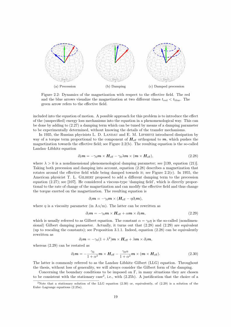
(a) Precession (b) Damping (c) Damped precession

Figure 2.2: Dynamics of the magnetization with respect to the effective field. The redand the blue arrows visualize the magnetization at two different times tred < tblue. Thegreen arrow refers to the effective field.

included into the equation of motion. A possible approach for this problem is to introduce the effectof the (unspecified) energy loss mechanisms into the equation in a phenomenological way. This canbe done by adding to (2.27) a damping term which can be tuned by means of a damping parameterto be experimentally determined, without knowing the details of the transfer mechanisms.

In 1935, the Russian phycisists L. D. Landau and E. M. Lifshitz introduced dissipation byway of a torque term proportional to the component of Heff orthogonal to m, which pushes themagnetization towards the effective field; see Figure 2.2(b). The resulting equation is the so-calledLandau–Lifshitz equation

∂tm = −γ0m×Heff − γ0λm× (m×Heff), (2.28)

where λ > 0 is a nondimensional phenomenological damping parameter; see [139, equation (21)].Taking both precession and damping into account, equation (2.28) describes a magnetization thatrotates around the effective field while being damped towards it; see Figure 2.2(c). In 1955, theAmerican physicist T. L. Gilbert proposed to add a different damping term to the precessionequation (2.27); see [107]. He considered a viscous-type ‘damping field’, which is directly propor-tional to the rate of change of the magnetization and can modify the effective field and thus changethe torque exerted on the magnetization. The resulting equation is

∂tm = −γ0m× (Heff − η∂tm),

where η is a viscosity parameter (in A s/m). The latter can be rewritten as

∂tm = −γ0m×Heff + αm× ∂tm, (2.29)

which is usually referred to as Gilbert equation. The constant α = γ0η is the so-called (nondimen-sional) Gilbert damping parameter. Actually, it turns out that (2.28) and (2.29) are equivalent(up to rescaling the constants); see Proposition 3.1.1. Indeed, equation (2.28) can be equivalentlyrewritten as

∂tm = −γ0(1 + λ2)m×Heff + λm× ∂tm,

whereas (2.29) can be restated as

∂tm = − γ0

1 + α2m×Heff −

γ0α

1 + α2m× (m×Heff). (2.30)

The latter is commonly referred to as the Landau–Lifshitz–Gilbert (LLG) equation. Throughoutthe thesis, without loss of generality, we will always consider the Gilbert form of the damping.

Concerning the boundary conditions to be imposed on Γ, in many situations they are chosento be consistent with the stationary case2, i.e., with (2.25b). A justification that the choice of a

2Note that a stationary solution of the LLG equation (2.30) or, equivalently, of (2.29) is a solution of theEuler–Lagrange equations (2.25a).

19

homogeneous Neumann boundary condition (2.26), in the pure exchange case and in the absenceof surface effects, is physically meaningful also in the dynamic case can be found in [171].

Taking the scalar product of (2.29) with m, we deduce the orthogonality condition

m · ∂tm = 0. (2.31)

In particular, since∂t |m|2 = 2m · ∂tm = 0,

it follows that the modulus constraint |m| = 1 is always satisfied, provided it is satisfied by theinitial condition.

We now aim at studying the evolution of the energy during the dynamics. Taking the vectorproduct of (2.29) with m, we obtain

m× ∂tm = −γ0m× (m×Heff) + αm× (m× ∂tm).

Taking (2.31) and the constraint |m| = 1 into account, the vector triple product expansion formula

a× (b× c) = (a · c)b− (a · b)c for all a,b, c ∈ R3,

yields the equalitym× ∂tm = −γ0(m ·Heff)m+ γ0Heff − α∂tm.

Taking the scalar product of the latter with ∂tm and exploiting the orthogonality (2.31), we obtainthe relation

γ0Heff · ∂tm = α |∂tm|2 . (2.32)

A formal application of the chain rule yields the energy law

d

dtE(m) =

∫Ω

δEδm· ∂tm dx+

∫Ω

δEδHext

· ∂tHext dx

(2.24)= −µ0Ms

∫Ω

Heff · ∂tmdx− µ0Ms

∫Ω

∂tHext ·m dx

(2.32)= −µ0Msα

γ0

∫Ω

|∂tm|2 dx− µ0Ms

∫Ω

∂tHext ·m dx.

If the applied field Hext is constant in time, the energy law reduces to

d

dtE(m) = −µ0Msα

γ0

∫Ω

|∂tm|2 dx ≤ 0,

which reveals the dissipative behavior of the model and the Lyapunov structure of the LLG equa-tion [164].

In several practical situations, the effect of eddy currents must be taken into account [46, 117,196]. Taking the constitutive laws (2.9) for ferromagnetic materials into account, the magnetoqua-sistatic Maxwell equations (2.7) take the form

∇ · (εE) = χΩρ, (2.33a)∇ ·H = −Ms∇ · (χΩm), (2.33b)∇×E = −µ0∂tH − µ0MsχΩ∂tm, (2.33c)∇×H = χΩσE. (2.33d)

In the mathematical literature, see, e.g., [203, 62, 155, 24, 28], also the coupling of the LLG equationwith the full Maxwell system

µ0∂tH +∇×E = −µ0MsχΩ∂tm, (2.34a)ε∂tE −∇×H + χΩσE = 0, (2.34b)

20

is studied, but, due to the short time scales of wave phenomena, this is essentially of no practicalconcern. In both cases, the magnetic field H then interacts with the magnetization during thedynamics as an additional field contribution to be added to the energy-based effective field, i.e.,

∂tm = −γ0m× (Heff +H) + αm× ∂tm.

The identity (2.32) in this case turns out to be

γ0(Heff +H) · ∂tm = α |∂tm|2 . (2.35)

In the case of the full Maxwell system (2.34), the evolution of the energy, defined as the sum ofthe electromagnetic energy (2.4) and the micromagnetic Gibbs free energy, follows the law

d

dtE(E,H,m)

=

∫R3

δEδE· ∂tE dx+

∫R3

δEδH· ∂tH dx+

∫Ω

δEδm· ∂tm dx

=

∫R3

εE · ∂tE dx+ µ0

∫R3

H · ∂tH dx− µ0Ms

∫Ω

Heff · ∂tm dx

(2.35)=

∫R3

εE · ∂tE dx+ µ0

∫R3

H · ∂tH dx+ µ0Ms

∫Ω

H · ∂tmdx− µ0Msα

γ0

∫Ω

|∂tm|2 dx

(2.34)=

∫R3

(∇×H) ·E dx−∫

Ω

σ |E|2 dx−∫R3

(∇×E) ·H dx− µ0Msα

γ0

∫Ω

|∂tm|2 dx

(2.5)= −

∫R3

∇ · (E ×H) dx−∫

Ω

σ |E|2 dx− µ0Msα

γ0

∫Ω

|∂tm|2 dx.

We conclude the section by formally computing the energy law for the Gibbs free energy, assumedto include the elastic energy (2.19), when its evolution is driven by the coupling of the LLG equationand the conservation of momentum law (2.18). It holds that

d

dtE(m,u)

=

∫Ω

δEδm· ∂tm dx+

∫Ω

δEδu· ∂tudx+

∫Ω

δEδ(∂tu)

· ∂ttudx−∫

Ω

∂tf · udx−∫

ΓN

∂tt · udS

= −µ0Ms

∫Ω

Heff · ∂tm dx+

∫Ω

[Cεel(u,m)] : ε(∂tu) dx−∫

Ω

f · ∂tudx−∫

ΓN

t · ∂tudS

+

∫Ω

κ∂ttu · ∂tudx−∫

Ω

∂tf · udx−∫

ΓN

∂tt · udS

= −αµ0Ms

γ0

∫Ω

|∂tm|2 dx+

∫Ω

σ : ε(∂tu) dx−∫

Ω

f · ∂tudx−∫

ΓN

t · ∂tudS

+

∫Ω

κ∂ttu · ∂tudx−∫

Ω

∂tf · udx−∫

ΓN

∂tt · udS

(2.18)= −αµ0Ms

γ0

∫Ω

|∂tm|2 dx−∫

Ω

∂tf · udx−∫

ΓN

∂tt · udS.

2.3 Metal spintronicsSpintronics, a portmanteau for spin electronics, is a recent field of research, which can be definedas the study of active control and manipulation of the spin degree of freedom in solid-state sys-tems [206]. Its roots can be traced back to the discoveries on the influence of the spin on theelectrical conduction in ferromagnetic metals obtained during the 1980s, e.g., the observation ofspin-polarized electron injection from a ferromagnetic metal to a normal metal [120] or the discov-ery of the giant magnetoresistance (GMR) effect, independently carried out by the groups of A.Fert [19] and P. Grünberg [49] in 1988.

21

The GMR effect consists in a relevant change in the electrical resistance observed in magneticmultilayers composed of alternating ferromagnetic and nonmagnetic sublayers. The resistanceturns out to depend on whether the magnetization configurations of consecutive ferromagneticsublayers are in a parallel alignment (lower resistance) or in an antiparallel alignment (higherresistance), which shows that the magnetic state of a material has an influence on its conductionproperties.

Conversely, the magnetization can be manipulated by spin-polarized currents, even withoutapplying any external magnetic field. The fundamental physics underlying this phenomenon isunderstood as a mutual transfer of spin angular momentum between the conduction electrons andthe magnetization. The concept of spin transfer was proposed independently by J. C. Slon-czewski and L. Berger in 1996 [191, 44]. The key mechanism was named spin transfer torque(STT) and involves the so-called s-d exchange interaction between the nonequilibrium itinerant4s conduction electrons and the localized 3d magnetic electrons. The original ballistic model formultilayer structures proposed in [191] was then extended in [212, 189] by including the effects ofthe spin diffusion and the electric conduction in the bulk of the layer. The derivation of the modeldoes not follow the typical energy-based approach of micromagnetics.

In this section, we present some of the most used extensions of the classical micromagneticmodel in metal spintronics.

N1

F1

N2

F2

N3

Je

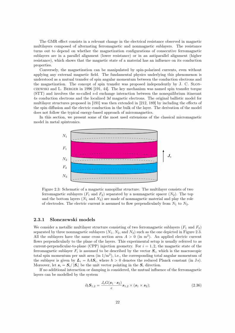
Figure 2.3: Schematic of a magnetic nanopillar structure. The multilayer consists of twoferromagnetic sublayers (F1 and F2) separated by a nonmagnetic spacer (N2). The topand the bottom layers (N1 and N3) are made of nonmagnetic material and play the roleof electrodes. The electric current is assumed to flow perpendicularly from N1 to N3.

2.3.1 Slonczewski modelsWe consider a metallic multilayer structure consisting of two ferromagnetic sublayers (F1 and F2)separated by three nonmagnetic sublayers (N1, N2, and N3) such as the one depicted in Figure 2.3.All the sublayers have the same cross section area A > 0 (in m2). An applied electric currentflows perpendicularly to the plane of the layers. This experimental setup is usually referred to ascurrent-perpendicular-to-plane (CPP) injection geometry. For i = 1, 2, the magnetic state of theferromagnetic sublayer Fi is assumed to be described by the vector Si, which is the macroscopictotal spin momentum per unit area (in 1/m2), i.e., the corresponding total angular momentum ofthe sublayer is given by Li = ~ASi, where ~ > 0 denotes the reduced Planck constant (in J s).Moreover, let si = Si/ |Si| be the unit vector pointing in the Si direction.

If no additional interaction or damping is considered, the mutual influence of the ferromagneticlayers can be modelled by the system

∂tS1,2 =JeG(s1 · s2)

es1,2 × (s1 × s2); (2.36)

22

−1 −0.8 −0.6 −0.4 −0.2 0 0.2 0.4 0.6 0.8 1

0

1

2

3

4

5P = 0.3P = 0.5P = 0.7

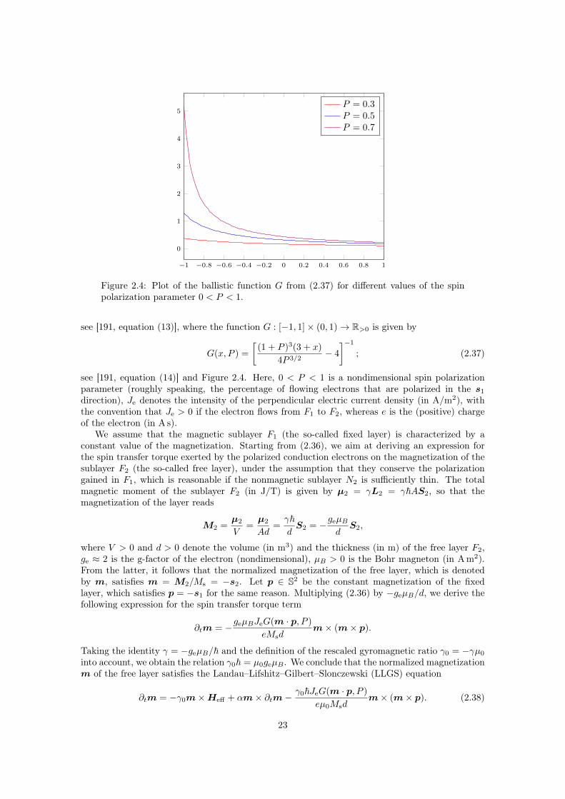
Figure 2.4: Plot of the ballistic function G from (2.37) for different values of the spinpolarization parameter 0 < P < 1.

see [191, equation (13)], where the function G : [−1, 1]× (0, 1)→ R>0 is given by

G(x, P ) =

[(1 + P )3(3 + x)

4P 3/2− 4

]−1

; (2.37)

see [191, equation (14)] and Figure 2.4. Here, 0 < P < 1 is a nondimensional spin polarizationparameter (roughly speaking, the percentage of flowing electrons that are polarized in the s1

direction), Je denotes the intensity of the perpendicular electric current density (in A/m2), withthe convention that Je > 0 if the electron flows from F1 to F2, whereas e is the (positive) chargeof the electron (in A s).

We assume that the magnetic sublayer F1 (the so-called fixed layer) is characterized by aconstant value of the magnetization. Starting from (2.36), we aim at deriving an expression forthe spin transfer torque exerted by the polarized conduction electrons on the magnetization of thesublayer F2 (the so-called free layer), under the assumption that they conserve the polarizationgained in F1, which is reasonable if the nonmagnetic sublayer N2 is sufficiently thin. The totalmagnetic moment of the sublayer F2 (in J/T) is given by µ2 = γL2 = γ~AS2, so that themagnetization of the layer reads

M2 =µ2

V=µ2

Ad=γ~dS2 = −geµB

dS2,

where V > 0 and d > 0 denote the volume (in m3) and the thickness (in m) of the free layer F2,ge ≈ 2 is the g-factor of the electron (nondimensional), µB > 0 is the Bohr magneton (in A m2).From the latter, it follows that the normalized magnetization of the free layer, which is denotedby m, satisfies m = M2/Ms = −s2. Let p ∈ S2 be the constant magnetization of the fixedlayer, which satisfies p = −s1 for the same reason. Multiplying (2.36) by −geµB/d, we derive thefollowing expression for the spin transfer torque term

∂tm = −geµBJeG(m · p, P )

eMsdm× (m× p).

Taking the identity γ = −geµB/~ and the definition of the rescaled gyromagnetic ratio γ0 = −γµ0

into account, we obtain the relation γ0~ = µ0geµB . We conclude that the normalized magnetizationm of the free layer satisfies the Landau–Lifshitz–Gilbert–Slonczewski (LLGS) equation

∂tm = −γ0m×Heff + αm× ∂tm−γ0~JeG(m · p, P )

eµ0Msdm× (m× p). (2.38)

23

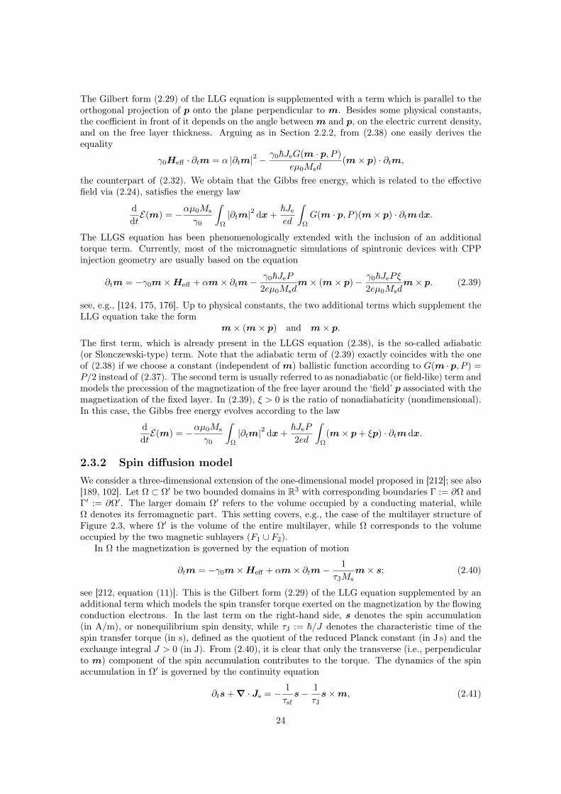
The Gilbert form (2.29) of the LLG equation is supplemented with a term which is parallel to theorthogonal projection of p onto the plane perpendicular to m. Besides some physical constants,the coefficient in front of it depends on the angle betweenm and p, on the electric current density,and on the free layer thickness. Arguing as in Section 2.2.2, from (2.38) one easily derives theequality

γ0Heff · ∂tm = α |∂tm|2 −γ0~JeG(m · p, P )

eµ0Msd(m× p) · ∂tm,

the counterpart of (2.32). We obtain that the Gibbs free energy, which is related to the effectivefield via (2.24), satisfies the energy law

d

dtE(m) = −αµ0Ms

γ0

∫Ω

|∂tm|2 dx+~Je

ed

∫Ω

G(m · p, P )(m× p) · ∂tm dx.

The LLGS equation has been phenomenologically extended with the inclusion of an additionaltorque term. Currently, most of the micromagnetic simulations of spintronic devices with CPPinjection geometry are usually based on the equation

∂tm = −γ0m×Heff + αm× ∂tm−γ0~JeP

2eµ0Msdm× (m× p)− γ0~JePξ

2eµ0Msdm× p. (2.39)

see, e.g., [124, 175, 176]. Up to physical constants, the two additional terms which supplement theLLG equation take the form

m× (m× p) and m× p.The first term, which is already present in the LLGS equation (2.38), is the so-called adiabatic(or Slonczewski-type) term. Note that the adiabatic term of (2.39) exactly coincides with the oneof (2.38) if we choose a constant (independent of m) ballistic function according to G(m · p, P ) =P/2 instead of (2.37). The second term is usually referred to as nonadiabatic (or field-like) term andmodels the precession of the magnetization of the free layer around the ‘field’ p associated with themagnetization of the fixed layer. In (2.39), ξ > 0 is the ratio of nonadiabaticity (nondimensional).In this case, the Gibbs free energy evolves according to the law

d

dtE(m) = −αµ0Ms

γ0

∫Ω

|∂tm|2 dx+~JeP

2ed

∫Ω

(m× p+ ξp) · ∂tm dx.

2.3.2 Spin diffusion modelWe consider a three-dimensional extension of the one-dimensional model proposed in [212]; see also[189, 102]. Let Ω ⊂ Ω′ be two bounded domains in R3 with corresponding boundaries Γ := ∂Ω andΓ′ := ∂Ω′. The larger domain Ω′ refers to the volume occupied by a conducting material, whileΩ denotes its ferromagnetic part. This setting covers, e.g., the case of the multilayer structure ofFigure 2.3, where Ω′ is the volume of the entire multilayer, while Ω corresponds to the volumeoccupied by the two magnetic sublayers (F1 ∪ F2).

In Ω the magnetization is governed by the equation of motion

∂tm = −γ0m×Heff + αm× ∂tm−1

τJMsm× s; (2.40)

see [212, equation (11)]. This is the Gilbert form (2.29) of the LLG equation supplemented by anadditional term which models the spin transfer torque exerted on the magnetization by the flowingconduction electrons. In the last term on the right-hand side, s denotes the spin accumulation(in A/m), or nonequilibrium spin density, while τJ := ~/J denotes the characteristic time of thespin transfer torque (in s), defined as the quotient of the reduced Planck constant (in J s) and theexchange integral J > 0 (in J). From (2.40), it is clear that only the transverse (i.e., perpendicularto m) component of the spin accumulation contributes to the torque. The dynamics of the spinaccumulation in Ω′ is governed by the continuity equation

∂ts+ ∇ · Js = − 1

τsfs− 1

τJs×m, (2.41)

24

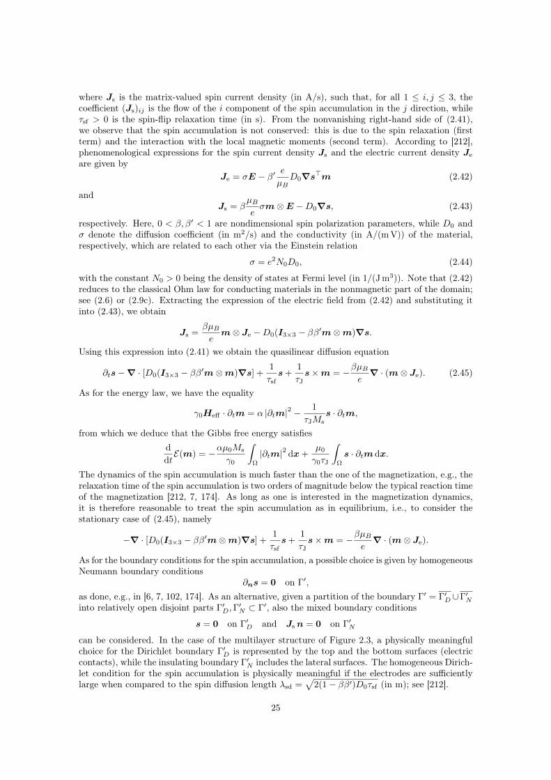
where Js is the matrix-valued spin current density (in A/s), such that, for all 1 ≤ i, j ≤ 3, thecoefficient (Js)ij is the flow of the i component of the spin accumulation in the j direction, whileτsf > 0 is the spin-flip relaxation time (in s). From the nonvanishing right-hand side of (2.41),we observe that the spin accumulation is not conserved: this is due to the spin relaxation (firstterm) and the interaction with the local magnetic moments (second term). According to [212],phenomenological expressions for the spin current density Js and the electric current density Je

are given byJe = σE − β′ e

µBD0∇s>m (2.42)

andJs = β

µBeσm⊗E −D0∇s, (2.43)

respectively. Here, 0 < β, β′ < 1 are nondimensional spin polarization parameters, while D0 andσ denote the diffusion coefficient (in m2/s) and the conductivity (in A/(m V)) of the material,respectively, which are related to each other via the Einstein relation

σ = e2N0D0, (2.44)

with the constant N0 > 0 being the density of states at Fermi level (in 1/(J m3)). Note that (2.42)reduces to the classical Ohm law for conducting materials in the nonmagnetic part of the domain;see (2.6) or (2.9c). Extracting the expression of the electric field from (2.42) and substituting itinto (2.43), we obtain

Js =βµBem⊗ Je −D0(I3×3 − ββ′m⊗m)∇s.

Using this expression into (2.41) we obtain the quasilinear diffusion equation

∂ts−∇ · [D0(I3×3 − ββ′m⊗m)∇s] +1

τsfs+

1

τJs×m = −βµB

e∇ · (m⊗ Je). (2.45)

As for the energy law, we have the equality

γ0Heff · ∂tm = α |∂tm|2 −1

τJMss · ∂tm,

from which we deduce that the Gibbs free energy satisfiesd

dtE(m) = −αµ0Ms

γ0

∫Ω

|∂tm|2 dx+µ0

γ0τJ

∫Ω

s · ∂tm dx.

The dynamics of the spin accumulation is much faster than the one of the magnetization, e.g., therelaxation time of the spin accumulation is two orders of magnitude below the typical reaction timeof the magnetization [212, 7, 174]. As long as one is interested in the magnetization dynamics,it is therefore reasonable to treat the spin accumulation as in equilibrium, i.e., to consider thestationary case of (2.45), namely

−∇ · [D0(I3×3 − ββ′m⊗m)∇s] +1

τsfs+

1

τJs×m = −βµB

e∇ · (m⊗ Je).

As for the boundary conditions for the spin accumulation, a possible choice is given by homogeneousNeumann boundary conditions

∂ns = 0 on Γ′,

as done, e.g., in [6, 7, 102, 174]. As an alternative, given a partition of the boundary Γ′ = Γ′D ∪Γ′Ninto relatively open disjoint parts Γ′D,Γ

′N ⊂ Γ′, also the mixed boundary conditions

s = 0 on Γ′D and Js n = 0 on Γ′N

can be considered. In the case of the multilayer structure of Figure 2.3, a physically meaningfulchoice for the Dirichlet boundary Γ′D is represented by the top and the bottom surfaces (electriccontacts), while the insulating boundary Γ′N includes the lateral surfaces. The homogeneous Dirich-let condition for the spin accumulation is physically meaningful if the electrodes are sufficientlylarge when compared to the spin diffusion length λsd =

√2(1− ββ′)D0τsf (in m); see [212].

25

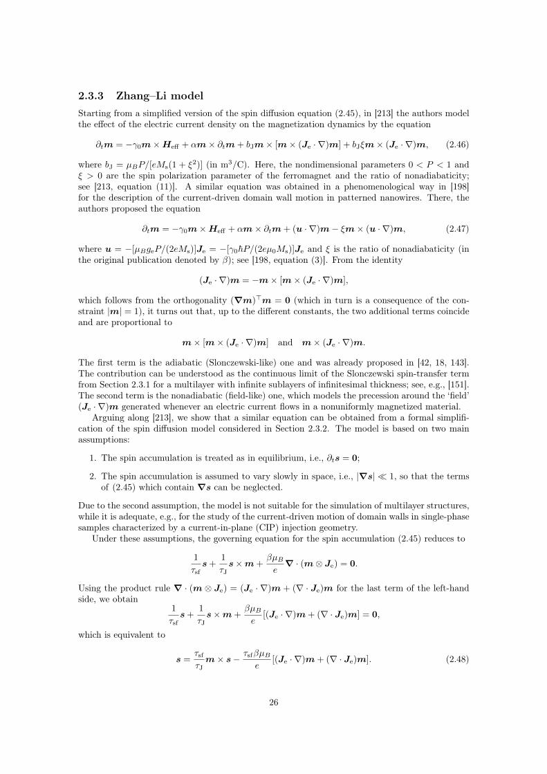
2.3.3 Zhang–Li modelStarting from a simplified version of the spin diffusion equation (2.45), in [213] the authors modelthe effect of the electric current density on the magnetization dynamics by the equation

∂tm = −γ0m×Heff + αm× ∂tm+ bJm× [m× (Je · ∇)m] + bJξm× (Je · ∇)m, (2.46)

where bJ = µBP/[eMs(1 + ξ2)] (in m3/C). Here, the nondimensional parameters 0 < P < 1 andξ > 0 are the spin polarization parameter of the ferromagnet and the ratio of nonadiabaticity;see [213, equation (11)]. A similar equation was obtained in a phenomenological way in [198]for the description of the current-driven domain wall motion in patterned nanowires. There, theauthors proposed the equation

∂tm = −γ0m×Heff + αm× ∂tm+ (u · ∇)m− ξm× (u · ∇)m, (2.47)

where u = −[µBgeP/(2eMs)]Je = −[γ0~P/(2eµ0Ms)]Je and ξ is the ratio of nonadiabaticity (inthe original publication denoted by β); see [198, equation (3)]. From the identity

(Je · ∇)m = −m× [m× (Je · ∇)m],

which follows from the orthogonality (∇m)>m = 0 (which in turn is a consequence of the con-straint |m| = 1), it turns out that, up to the different constants, the two additional terms coincideand are proportional to

m× [m× (Je · ∇)m] and m× (Je · ∇)m.

The first term is the adiabatic (Slonczewski-like) one and was already proposed in [42, 18, 143].The contribution can be understood as the continuous limit of the Slonczewski spin-transfer termfrom Section 2.3.1 for a multilayer with infinite sublayers of infinitesimal thickness; see, e.g., [151].The second term is the nonadiabatic (field-like) one, which models the precession around the ‘field’(Je · ∇)m generated whenever an electric current flows in a nonuniformly magnetized material.

Arguing along [213], we show that a similar equation can be obtained from a formal simplifi-cation of the spin diffusion model considered in Section 2.3.2. The model is based on two mainassumptions:

1. The spin accumulation is treated as in equilibrium, i.e., ∂ts = 0;

2. The spin accumulation is assumed to vary slowly in space, i.e., |∇s| 1, so that the termsof (2.45) which contain ∇s can be neglected.

Due to the second assumption, the model is not suitable for the simulation of multilayer structures,while it is adequate, e.g., for the study of the current-driven motion of domain walls in single-phasesamples characterized by a current-in-plane (CIP) injection geometry.

Under these assumptions, the governing equation for the spin accumulation (2.45) reduces to

1

τsfs+

1

τJs×m+

βµBe

∇ · (m⊗ Je) = 0.

Using the product rule ∇ · (m ⊗ Je) = (Je · ∇)m + (∇ · Je)m for the last term of the left-handside, we obtain

1

τsfs+

1

τJs×m+

βµBe

[(Je · ∇)m+ (∇ · Je)m] = 0,

which is equivalent to

s =τsfτJm× s− τsfβµB

e[(Je · ∇)m+ (∇ · Je)m]. (2.48)

26

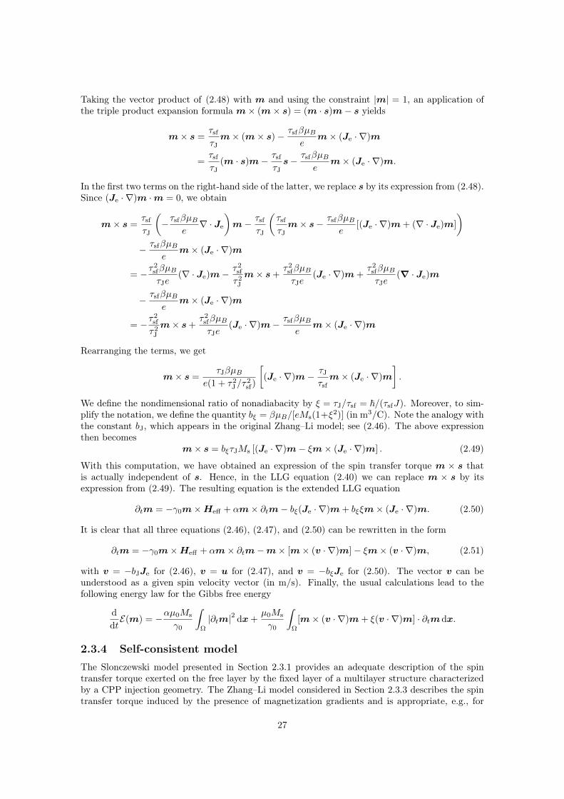
Taking the vector product of (2.48) with m and using the constraint |m| = 1, an application ofthe triple product expansion formula m× (m× s) = (m · s)m− s yields

m× s =τsfτJm× (m× s)− τsfβµB

em× (Je · ∇)m

=τsfτJ

(m · s)m− τsfτJs− τsfβµB

em× (Je · ∇)m.

In the first two terms on the right-hand side of the latter, we replace s by its expression from (2.48).Since (Je · ∇)m ·m = 0, we obtain

m× s =τsfτJ

(−τsfβµB

e∇ · Je

)m− τsf

τJ

(τsfτJm× s− τsfβµB

e[(Je · ∇)m+ (∇ · Je)m]

)− τsfβµB

em× (Je · ∇)m

= −τ2sfβµBτJe

(∇ · Je)m− τ2sf

τ2J

m× s+τ2sfβµBτJe

(Je · ∇)m+τ2sfβµBτJe

(∇ · Je)m

− τsfβµBe

m× (Je · ∇)m

= −τ2sf

τ2J

m× s+τ2sfβµBτJe

(Je · ∇)m− τsfβµBe

m× (Je · ∇)m

Rearranging the terms, we get

m× s =τJβµB

e(1 + τ2J /τ

2sf)

[(Je · ∇)m− τJ

τsfm× (Je · ∇)m

].

We define the nondimensional ratio of nonadiabacity by ξ = τJ/τsf = ~/(τsfJ). Moreover, to sim-plify the notation, we define the quantity bξ = βµB/[eMs(1+ξ2)] (in m3/C). Note the analogy withthe constant bJ, which appears in the original Zhang–Li model; see (2.46). The above expressionthen becomes

m× s = bξτJMs [(Je · ∇)m− ξm× (Je · ∇)m] . (2.49)

With this computation, we have obtained an expression of the spin transfer torque m × s thatis actually independent of s. Hence, in the LLG equation (2.40) we can replace m × s by itsexpression from (2.49). The resulting equation is the extended LLG equation

∂tm = −γ0m×Heff + αm× ∂tm− bξ(Je · ∇)m+ bξξm× (Je · ∇)m. (2.50)

It is clear that all three equations (2.46), (2.47), and (2.50) can be rewritten in the form

∂tm = −γ0m×Heff + αm× ∂tm−m× [m× (v · ∇)m]− ξm× (v · ∇)m, (2.51)

with v = −bJJe for (2.46), v = u for (2.47), and v = −bξJe for (2.50). The vector v can beunderstood as a given spin velocity vector (in m/s). Finally, the usual calculations lead to thefollowing energy law for the Gibbs free energy

d

dtE(m) = −αµ0Ms

γ0

∫Ω

|∂tm|2 dx+µ0Ms

γ0

∫Ω

[m× (v · ∇)m+ ξ(v · ∇)m] · ∂tm dx.

2.3.4 Self-consistent modelThe Slonczewski model presented in Section 2.3.1 provides an adequate description of the spintransfer torque exerted on the free layer by the fixed layer of a multilayer structure characterizedby a CPP injection geometry. The Zhang–Li model considered in Section 2.3.3 describes the spintransfer torque induced by the presence of magnetization gradients and is appropriate, e.g., for

27

the description of current-driven domain wall motion in structures with a CIP injection geometry.Both the situations can be described by the spin diffusion model considered in Section 2.3.2,which provides a generalization based on the interaction of the local magnetization with the spinaccumulation. However, in all three approaches, the effects of the magnetic state of the system onthe electronic transport are neglected. Indeed, the electric current density is always assumed tobe known and the models can be used only to investigate how the electronic transport affects themagnetization dynamics, but not vice versa.

In this section, we introduce a model, which includes a bidirectional coupling of the magneti-zation to the electric current, for the self-consistent computation of magnetization dynamics andspin-polarized currents. The model has been applied to a magnetic nanowire geometry for theprediction of current-driven motion of domain walls [193] and for investigating the magnetization-dependent resistivity related to the GMR effect in composite multilayer structures [8].

The three basic ingredients of the model are the LLG equation (2.40) with spin transfer torquefor the magnetization dynamics, the continuity equation (2.41) for the spin accumulation, and theMaxwell equations for the electromagnetic fields discussed in Section 2.1. As in Section 2.3.2, weconsider two bounded domains Ω ⊂ Ω′ in R3 which represent the volume occupied by a conductingbody and its ferromagnetic part, respectively. We assume that Ω′ is a simply connected domainand denote by Γ := ∂Ω and Γ′ := ∂Ω′ the respective boundaries.

To obtain a self-consistent and well-defined system of equations, we introduce some appropriateassumptions. Since the dynamics of both the spin accumulation and the electromagnetic fields isindeed much faster than the one of the magnetization, we treat the spin accumulation and theelectromagnetic fields as in equilibrium and thus consider the stationary cases of the correspondinggoverning equations.

The magnetostatic Maxwell equations, namely

∇ ·H = −Ms∇ · (χΩm), (2.52a)∇×H = χΩ′Je, (2.52b)

can be treated as in Section 2.2.1 and give rise to the stray field Hs and the Oersted field Hc;see page 14. Moreover, from the static Maxwell–Ampére law (2.52b), we deduce that the electriccurrent density is divergence-free. Together with the stationary case of (2.41), we thus obtain thefollowing conservation laws for the electric current and the spin accumulation

∇ · Je = 0,

∇ · Js = − 1

τsfs− 1

τJs×m.

The electrostatic Maxwell equations are given by

∇ · (εE) = χΩ′ρ, (2.53a)∇×E = 0. (2.53b)

The static Faraday law (2.53b) shows that the electric field E is irrotational. Since Ω′ is simplyconnected, it is also conservative, i.e., E = −∇V , with V being the electric potential (in V). Letc := eN0µB , so that the Einstein relation (2.44) can be rewritten as σ = c(e/µB)D0. Under theseassumptions, the phenomenological expressions (2.42)–(2.43) for the electric current density andthe spin current density take the form

Je = −c eµB

D0∇V − β′e

µBD0∇s>m,

Js = −βcD0m⊗∇V −D0∇s.

We conclude that the magnetization, the spin accumulation and the electric potential solve the

28

system

∂tm = −γ0m× (Heff +Hc) + αm× ∂tm−1

τJMsm× s (2.54a)

− c∇ · (D0∇V )− β′∇ · (D0∇s>m) = 0, (2.54b)

− βc∇ · (D0m⊗∇V )−∇ · (D0∇s) = − 1

τsfs− 1

τJs×m. (2.54c)

In (2.54a) the energy-based effective field, besides the stray field, comprises the contributions thatare relevant for the specific model under consideration.

To complete the setting, we need to impose appropriate boundary conditions. To this end, weconsider a partition of the boundary Γ′ = Γ′D ∪ Γ′N into relatively open parts Γ′D,Γ

′N ⊂ Γ′ such

that Γ′D ∩Γ′N = ∅. On Γ′D, we impose Dirichlet boundary conditions for both the electric potentialand the spin accumulation, i.e.,

V = VD and s = 0 on Γ′D

for some given electric potential VD. On Γ′N , we prescribe no flux conditions, i.e.,

Je · n = 0 and Js n = 0 on Γ′N .

The appropriate boundary condition for the magnetization on Γ depends on the contributions thatare included in the effective field.

29

Chapter 3

Preliminaries

In this chapter, in view of the forthcoming analysis, we collect some auxiliary results. We start withthe rigorous nondimensionalization of the problems considered in Chapter 2. Then, we introducethe notation and discuss some preliminary results about the discretization methods considered inthe following chapters.

3.1 NondimensionalizationLet Ω ⊂ R3 be a bounded domain representing the volume occupied by a ferromagnetic body andlet T > 0 be some finite time. The magnetization is mathematically represented by a vector fieldm : Ω× (0, T )→ S2, where

S2 =x ∈ R3 : |x| = 1

denotes the unit sphere.

We start by rescaling the time variable: We perform the substitution t∗ = γ0Mst with t∗ beingthe so-called reduced time. Recall that the physical units of the rescaled gyromagnetic ratio γ0

and the saturation magnetization Ms are m/(A s) and A/m, respectively, from which it followsthat the reduced time is nondimensional. Consistently, we define T ∗ := γ0MsT .

We rescale the effective field and the Gibbs free energy by heff = Heff/Ms and E∗ = E/(2Ks),where Ks = µ0M

2s /2 is the magnetostatic energy density introduced in (2.21). Moreover, we

rescale the quantities which appear in the expression of the elastic energy (2.19) as κ∗ = κγ20/Ms,

C∗ = C/Ks, f∗ = f/Ks, and t∗ = t/Ks, and define σ∗ := C∗εel, so that the expression of theenergy with the rescaled constants remains the same. Indeed, it holds that

E∗el(m,u) =Eel(m,u)

2Ks

=γ2

0

2µ0

∫Ω

κ |∂tu|2 dx+1

2µ0M2s

∫Ω

εel(u,m) : [Cεel(u,m)] dx

− 1

µ0M2s

∫Ω

f · u dx− 1

µ0M2s

∫ΓN

t · u dS

=1

2

∫Ω

κ∗ |∂tu|2 dx+1

2

∫Ω

εel(u,m) : [C∗εel(u,m)] dx−∫

Ω

f∗ · udx−∫

ΓN

t∗ · udS.

As a consequence, the rescaled effective field is related to the rescaled energy via the relation

heff = −δE∗

δm.

31

In particular, for each of the energy contributions introduced in Section 2.2.1, it holds that

E∗ex(m) =λ2

ex

2

∫Ω

|∇m|2 dx =⇒ heff,ex = λ2ex∆m,

E∗ani(m) =q2

2

∫Ω

φ(m) dx =⇒ heff,ani = −q2

2∇φ(m),

E∗ext(m,hext) = −∫

Ω

hext ·m dx =⇒ heff,ext = hext,

E∗DM(m) =λDM

2

∫Ω

(∇×m) ·m dx =⇒ heff,DM = −λDM∇×m,

E∗stray(m) =1

2

∫R3

|hs|2 dx =⇒ heff,stray = hs,

E∗el(m,u) =1

2

∫Ω

εel(u,m) : [C∗εel(u,m)] dx+ . . . =⇒ heff,el = 2(λσ∗)m.

Here, λex is the exchange length from (2.22), q is the magnetic hardness parameter from (2.23),hext = Hext/Ms is the rescaled applied field, λDM = D/Ks is a length scale associated with theDzyaloshinskii–Moriya interaction (in m), hs solves a rescaled version of the magnetostatic Maxwellequations (2.12), namely

∇ · hs = −∇ · (χΩm) in R3,

∇× hs = 0 in R3.

Similarly, the nondimensional Oersted field hc solves a rescaled version of (2.13), namely

∇ · hc = 0 in R3,

∇× hc = χΩje in R3,

where je = Je/Ms. Correspondingly, we obtain the transmission problem

−∆uint = −∇ ·m in Ω, (3.1a)

−∆uext = 0 in R3 \ Ω, (3.1b)

uext − uint = 0 on Γ, (3.1c)

(∇uext −∇uint) · n = −m · n on Γ, (3.1d)u(x) = O(1/ |x|) as |x| → ∞ (3.1e)

for the rescaled magnetostatic potential and the transmission problem

−∆hintc = ∇× je in Ω, (3.2a)

−∆hextc = 0 in R3 \ Ω, (3.2b)

hextc − hint

c = 0 on Γ, (3.2c)

(∇hextc −∇hint

c )n = n× je on Γ, (3.2d)hc(x) = O(1/ |x|) as |x| → ∞ (3.2e)

for the rescaled Oersted field; see (2.14) and (2.16). However, to simplify the notation, we willalways omit the ∗-superscripts from the equations, e.g., we denote the reduced time also by t.

With these substitutions, the nondimensional form of the LLG equation (2.30) becomes

∂tm = − 1

1 + α2m× heff −

α

1 + α2m× (m× heff) in Ω.

The homogeneous Neumann boundary conditions

∂nm = 0 on Γ := ∂Ω

32

associated with the exchange interaction becomes

2λ2ex∂nm+ λDMm× n = 0 on Γ

in the presence of the Dzyaloshinskii–Moriya interaction. The same formal computation performedin Section 2.2.2 yields the energy law

d

dtE(m,hext) = −α

∫Ω

|∂tm|2 dx−∫

Ω

∂thext ·m dx, (3.3)

which reveals the dissipative behavior of the model, when hext is constant in time.In the following proposition, we establish the equivalence of three different reformulations of

the LLG equation.

Proposition 3.1.1. Under the constraint |m| = 1, the following three reformulations of the LLGequation are equivalent:

• the Landau–Lifshitz form

∂tm = − 1

1 + α2m× heff −

α

1 + α2m× (m× heff)

• the Gilbert form∂tm = −m× heff + αm× ∂tm (3.4)

• the so-called ‘alternative form’

α∂tm+m× ∂tm = heff − (heff ·m)m. (3.5)

Proof. The proof follows from straightforward algebraic manipulations. It exploits the triple prod-uct expansion formula

a× (b× c) = (a · c)b− (a · b)c for all a,b, c ∈ R3

from Proposition B.2.1(vi), in combination with the modulus constraint |m| = 1 and the resultingorthogonality property ∂tm ·m = 0. For the complete argument, we refer the reader to [109,Lemma 1.2.1].

3.1.1 Coupling with the Maxwell equations and magnetostrictionIn this section, we denote the micromagnetic Gibbs free energy by EGibbs in order to distinguish itfrom the energy of the system, which can also depend on quantities associated with the equation(s)coupled to the LLG equation.

For the nondimensionalization of the coupling of the LLG equation with the full Maxwellsystem (2.34), we consider the substitutions µ∗0 = γ0Msµ0, ε∗ = γ0Msε, e = E/Ms, and h =H/Ms. We obtain the system

∂tm = −m× (heff + h) + αm× ∂tm in Ω, (3.6a)

µ0∂th = −∇× e− µ0χΩ∂tm in R3, (3.6b)

ε∂te = ∇× h− χΩσe in R3. (3.6c)

For the sake of simplicity, we assume the Maxwell equations (3.6b)–(3.6c) to be posed on a boundedcavity Ω′ ⊂ R3 with perfectly conducting boundary in which the ferromagnet is embedded, i.e.,Ω b Ω′; see [24, 28]. Moreover, we assume Ω′ \ Ω to be vacuum. The resulting system, i.e.,

∂tm = −m× (heff + h) + αm× ∂tm in Ω,

µ0∂th = −∇× e− µ0χΩ∂tm in Ω′,

ε∂te = ∇× h− χΩσe in Ω′,

33

is supplemented with the appropriate boundary conditions on Γ for the LLG equation (whichdepend on the contributions included into heff) as well as the following boundary conditions forthe electric field

e× n = 0 on Γ′ = ∂Ω′.

The energy of the system, defined as the sum of the micromagnetic Gibbs free energy and theelectromagnetic energy, i.e.,

E(e,h,m) = EGibbs(m) +1

2µ0

∫Ω′ε |e|2 dx+

1

2

∫Ω′|h|2 dx,

satisfies the energy law

d

dtE(e,h,m) = −α

∫Ω

|∂tm|2 dx−∫

Ω

∂thext ·m dx− µ−10

∫Ω

σ |e|2 dx.

For the nondimensionalization of the coupling of the LLG equation with the magnetoquasistaticMaxwell equations (2.33), we perform the same substitutions used for the full Maxwell equations.We obtain the system


∇ · (εe) = γ0χΩρ in R3,

∇ · h = −∇ · (χΩm) in R3,

∇× e = −µ0∂th− µ0χΩ∂tm in R3,

∇× h = χΩσe in R3.

Moreover, for the sake of simplicity, we consider the system only on the ferromagnetic domain Ω,which we assume to be a perfectly conducting body; see [142, 141]. Eliminating the electric fieldyields the system


µ0∂th = −∇× (σ−1∇× h)− µ0∂tm in Ω,

where the LLG equation is coupled with the eddy current equation. The adequate boundaryconditions for the magnetization are supplemented with the following boundary conditions for themagnetic field

(∇× h)× n = 0 on Γ.

The energy, defined in this case as the sum of the micromagnetic Gibbs free energy and the magneticenergy, i.e.,

E(h,m) = EGibbs(m) +1

2

∫Ω

|h|2 dx,

is driven by the energy law

d

dtE(h,m) = −α

∫Ω

|∂tm|2 dx−∫

Ω

∂thext ·m dx− µ−10

∫Ω

σ−1 |∇ × h|2 dx.

With the substitutions previously introduced to rescale the elastic energy, the coupling of the LLGequation with the conservation of momentum law takes the form

∂tm = −m× heff + αm× ∂tm in Ω,

κ∂ttu = ∇ · σ + f in Ω,

where σ = C[ε(u) − εm(m)] and the effective field, among others, comprises the magnetoelasticcontribution heff,el = 2(λσ)m. The appropriate boundary conditions for the magnetization aresupplemented with the following mixed boundary conditions for the displacement

u = 0 on ΓD,

σn = t on ΓN ,

34

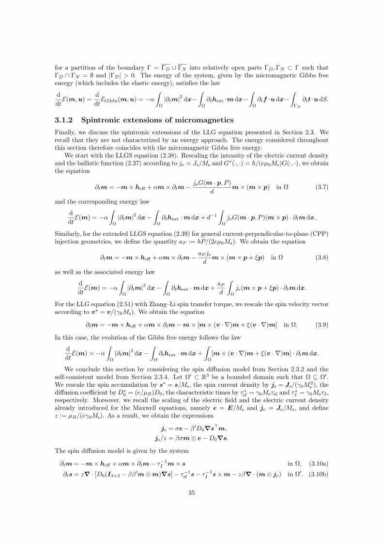
for a partition of the boundary Γ = ΓD ∪ ΓN into relatively open parts ΓD,ΓN ⊂ Γ such thatΓD ∩ ΓN = ∅ and |ΓD| > 0. The energy of the system, given by the micromagnetic Gibbs freeenergy (which includes the elastic energy), satisfies the law

d

dtE(m,u) =

d

dtEGibbs(m,u) = −α

∫Ω

|∂tm|2 dx−∫

Ω

∂thext ·m dx−∫

Ω

∂tf ·udx−∫

ΓN

∂tt ·udS.

3.1.2 Spintronic extensions of micromagneticsFinally, we discuss the spintronic extensions of the LLG equation presented in Section 2.3. Werecall that they are not characterized by an energy approach. The energy considered throughoutthis section therefore coincides with the micromagnetic Gibbs free energy.

We start with the LLGS equation (2.38). Rescaling the intensity of the electric current densityand the ballistic function (2.37) according to je = Je/Ms and G∗(·, ·) = ~/(eµ0Ms)G(·, ·), we obtainthe equation

∂tm = −m× heff + αm× ∂tm−jeG(m · p, P )

dm× (m× p) in Ω (3.7)

and the corresponding energy law

d

dtE(m) = −α

∫Ω

|∂tm|2 dx−∫

Ω

∂thext ·m dx+ d−1

∫Ω

jeG(m · p, P )(m× p) · ∂tm dx.

Similarly, for the extended LLGS equation (2.39) for general current-perpendicular-to-plane (CPP)injection geometries, we define the quantity aP := ~P/(2eµ0Ms). We obtain the equation

∂tm = −m× heff + αm× ∂tm−aP jedm× (m× p+ ξp) in Ω (3.8)

as well as the associated energy law

d

dtE(m) = −α

∫Ω

|∂tm|2 dx−∫

Ω

∂thext ·m dx+aPd

∫Ω

je(m× p+ ξp) · ∂tm dx.

For the LLG equation (2.51) with Zhang–Li spin transfer torque, we rescale the spin velocity vectoraccording to v∗ = v/(γ0Ms). We obtain the equation

∂tm = −m× heff + αm× ∂tm−m× [m× (v · ∇)m+ ξ(v · ∇)m] in Ω. (3.9)

In this case, the evolution of the Gibbs free energy follows the law

d

dtE(m) = −α

∫Ω

|∂tm|2 dx−∫

Ω

∂thext ·mdx+

∫Ω

[m× (v · ∇)m+ ξ(v · ∇)m] · ∂tm dx.

We conclude this section by considering the spin diffusion model from Section 2.3.2 and theself-consistent model from Section 2.3.4. Let Ω′ ⊂ R3 be a bounded domain such that Ω ⊆ Ω′.We rescale the spin accumulation by s∗ = s/Ms, the spin current density by js = Js/(γ0M

2s ), the

diffusion coefficient byD∗0 = (e/µB)D0, the characteristic times by τ∗sf = γ0Msτsf and τ∗J = γ0MsτJ,respectively. Moreover, we recall the scaling of the electric field and the electric current densityalready introduced for the Maxwell equations, namely e = E/Ms and je = Je/Ms, and definez := µB/(eγ0Ms). As a result, we obtain the expressions

je = σe− β′D0∇s>m,

js/z = βσm⊗ e−D0∇s.

The spin diffusion model is given by the system

∂tm = −m× heff + αm× ∂tm− τ−1J m× s in Ω, (3.10a)

∂ts = z∇ · [D0(I3×3 − ββ′m⊗m)∇s]− τ−1sf s− τ

−1J s×m− zβ∇ · (m⊗ je) in Ω′. (3.10b)

35

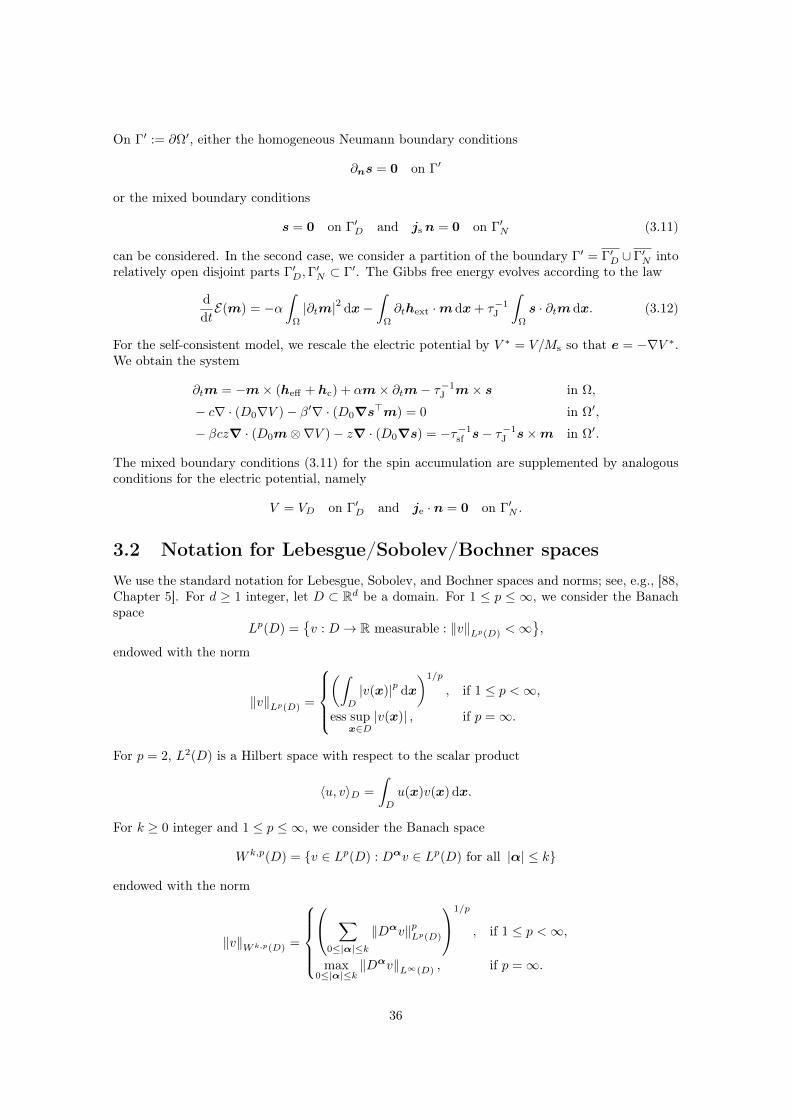
On Γ′ := ∂Ω′, either the homogeneous Neumann boundary conditions

∂ns = 0 on Γ′

or the mixed boundary conditions

s = 0 on Γ′D and js n = 0 on Γ′N (3.11)

can be considered. In the second case, we consider a partition of the boundary Γ′ = Γ′D ∪ Γ′N intorelatively open disjoint parts Γ′D,Γ

′N ⊂ Γ′. The Gibbs free energy evolves according to the law

d

dtE(m) = −α

∫Ω

|∂tm|2 dx−∫

Ω

∂thext ·mdx+ τ−1J

∫Ω

s · ∂tm dx. (3.12)

For the self-consistent model, we rescale the electric potential by V ∗ = V/Ms so that e = −∇V ∗.We obtain the system

∂tm = −m× (heff + hc) + αm× ∂tm− τ−1J m× s in Ω,

− c∇ · (D0∇V )− β′∇ · (D0∇s>m) = 0 in Ω′,

− βcz∇ · (D0m⊗∇V )− z∇ · (D0∇s) = −τ−1sf s− τ

−1J s×m in Ω′.

The mixed boundary conditions (3.11) for the spin accumulation are supplemented by analogousconditions for the electric potential, namely

V = VD on Γ′D and je · n = 0 on Γ′N .

3.2 Notation for Lebesgue/Sobolev/Bochner spacesWe use the standard notation for Lebesgue, Sobolev, and Bochner spaces and norms; see, e.g., [88,Chapter 5]. For d ≥ 1 integer, let D ⊂ Rd be a domain. For 1 ≤ p ≤ ∞, we consider the Banachspace

Lp(D) =v : D → R measurable : ‖v‖Lp(D) <∞

,

endowed with the norm

‖v‖Lp(D) =

(∫

D

|v(x)|p dx

)1/p

, if 1 ≤ p <∞,

ess supx∈D|v(x)| , if p =∞.

For p = 2, L2(D) is a Hilbert space with respect to the scalar product

〈u, v〉D =

∫D

u(x)v(x) dx.

For k ≥ 0 integer and 1 ≤ p ≤ ∞, we consider the Banach space

W k,p(D) = v ∈ Lp(D) : Dαv ∈ Lp(D) for all |α| ≤ k


‖v‖Wk,p(D) =

∑

0≤|α|≤k

‖Dαv‖pLp(D)

1/p

, if 1 ≤ p <∞,

max0≤|α|≤k

‖Dαv‖L∞(D) , if p =∞.

36

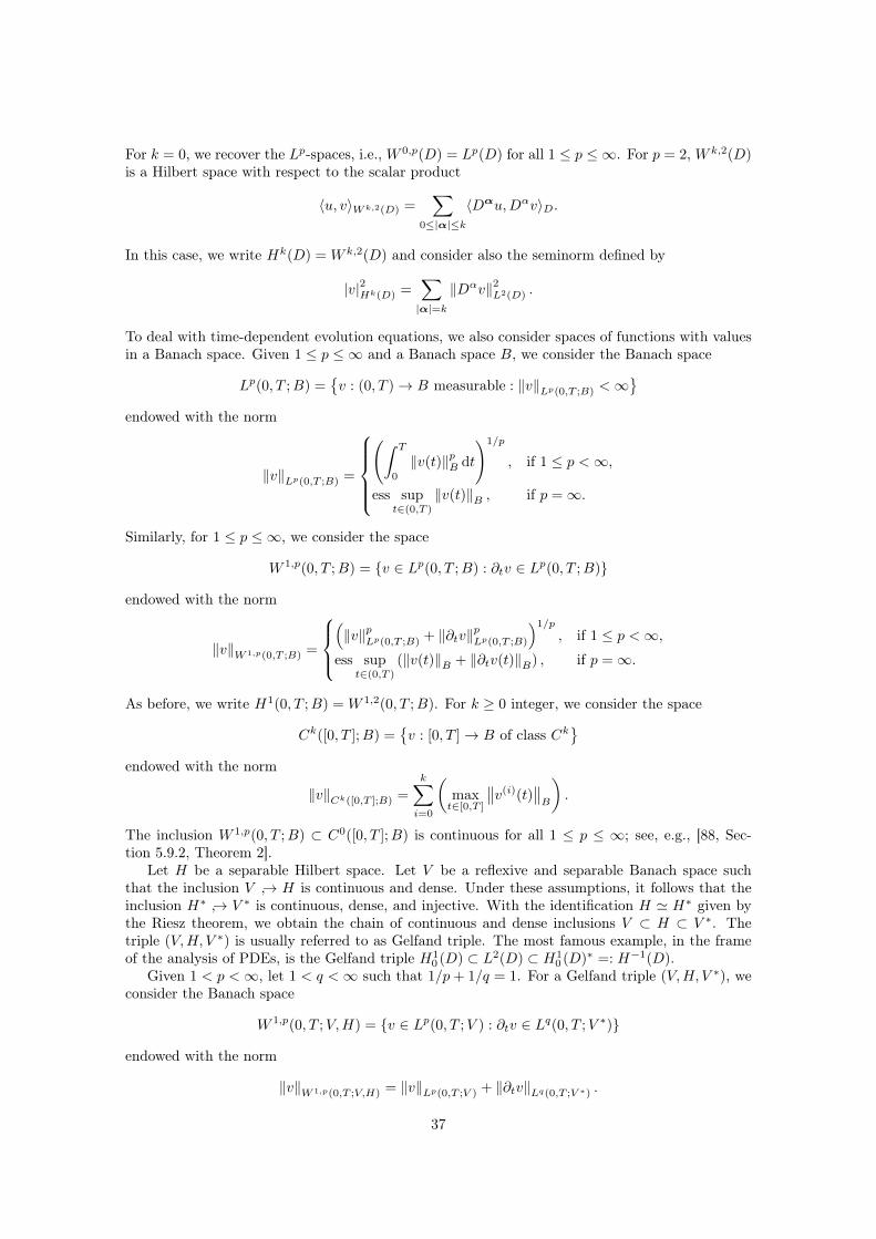
For k = 0, we recover the Lp-spaces, i.e., W 0,p(D) = Lp(D) for all 1 ≤ p ≤ ∞. For p = 2, W k,2(D)is a Hilbert space with respect to the scalar product

〈u, v〉Wk,2(D) =∑

0≤|α|≤k

〈Dαu,Dαv〉D.

In this case, we write Hk(D) = W k,2(D) and consider also the seminorm defined by

|v|2Hk(D) =∑|α|=k

‖Dαv‖2L2(D) .

To deal with time-dependent evolution equations, we also consider spaces of functions with valuesin a Banach space. Given 1 ≤ p ≤ ∞ and a Banach space B, we consider the Banach space

Lp(0, T ;B) =v : (0, T )→ B measurable : ‖v‖Lp(0,T ;B) <∞


‖v‖Lp(0,T ;B) =

(∫ T

0

‖v(t)‖pB dt

)1/p

, if 1 ≤ p <∞,

ess supt∈(0,T )

‖v(t)‖B , if p =∞.

Similarly, for 1 ≤ p ≤ ∞, we consider the space

W 1,p(0, T ;B) = v ∈ Lp(0, T ;B) : ∂tv ∈ Lp(0, T ;B)


‖v‖W 1,p(0,T ;B) =

(‖v‖pLp(0,T ;B) + ‖∂tv‖pLp(0,T ;B)

)1/p

, if 1 ≤ p <∞,ess sup

t∈(0,T )

(‖v(t)‖B + ‖∂tv(t)‖B) , if p =∞.

As before, we write H1(0, T ;B) = W 1,2(0, T ;B). For k ≥ 0 integer, we consider the space

Ck([0, T ];B) =v : [0, T ]→ B of class Ck


‖v‖Ck([0,T ];B) =

k∑i=0

(maxt∈[0,T ]

∥∥v(i)(t)∥∥B

).

The inclusion W 1,p(0, T ;B) ⊂ C0([0, T ];B) is continuous for all 1 ≤ p ≤ ∞; see, e.g., [88, Sec-tion 5.9.2, Theorem 2].

Let H be a separable Hilbert space. Let V be a reflexive and separable Banach space suchthat the inclusion V → H is continuous and dense. Under these assumptions, it follows that theinclusion H∗ → V ∗ is continuous, dense, and injective. With the identification H ' H∗ given bythe Riesz theorem, we obtain the chain of continuous and dense inclusions V ⊂ H ⊂ V ∗. Thetriple (V,H, V ∗) is usually referred to as Gelfand triple. The most famous example, in the frameof the analysis of PDEs, is the Gelfand triple H1

0 (D) ⊂ L2(D) ⊂ H10 (D)∗ =: H−1(D).

Given 1 < p <∞, let 1 < q <∞ such that 1/p+ 1/q = 1. For a Gelfand triple (V,H, V ∗), weconsider the Banach space

W 1,p(0, T ;V,H) = v ∈ Lp(0, T ;V ) : ∂tv ∈ Lq(0, T ;V ∗)


‖v‖W 1,p(0,T ;V,H) = ‖v‖Lp(0,T ;V ) + ‖∂tv‖Lq(0,T ;V ∗) .

37

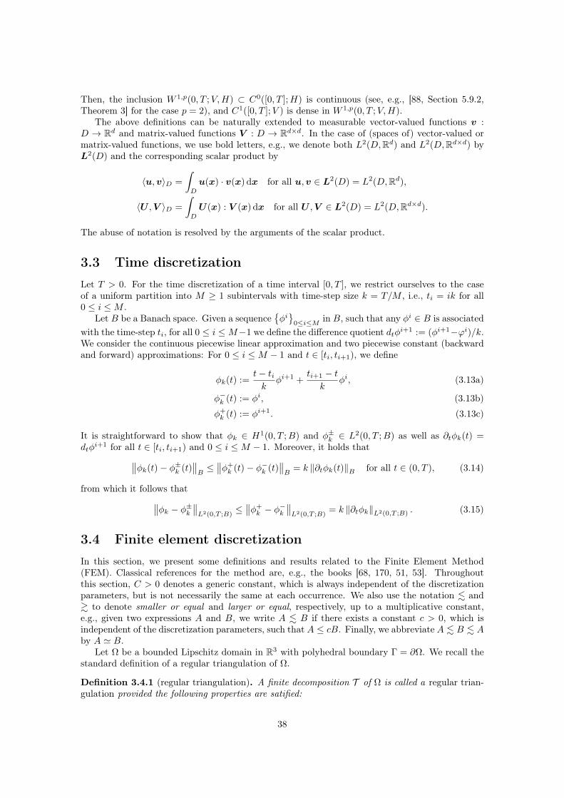
Then, the inclusion W 1,p(0, T ;V,H) ⊂ C0([0, T ];H) is continuous (see, e.g., [88, Section 5.9.2,Theorem 3] for the case p = 2), and C1([0, T ];V ) is dense in W 1,p(0, T ;V,H).

The above definitions can be naturally extended to measurable vector-valued functions v :D → Rd and matrix-valued functions V : D → Rd×d. In the case of (spaces of) vector-valued ormatrix-valued functions, we use bold letters, e.g., we denote both L2(D,Rd) and L2(D,Rd×d) byL2(D) and the corresponding scalar product by

〈u,v〉D =

∫D

u(x) · v(x) dx for all u,v ∈ L2(D) = L2(D,Rd),

〈U ,V 〉D =

∫D

U(x) : V (x) dx for all U ,V ∈ L2(D) = L2(D,Rd×d).

The abuse of notation is resolved by the arguments of the scalar product.

3.3 Time discretizationLet T > 0. For the time discretization of a time interval [0, T ], we restrict ourselves to the caseof a uniform partition into M ≥ 1 subintervals with time-step size k = T/M , i.e., ti = ik for all0 ≤ i ≤M .

Let B be a Banach space. Given a sequenceφi

0≤i≤M in B, such that any φi ∈ B is associatedwith the time-step ti, for all 0 ≤ i ≤M−1 we define the difference quotient dtφi+1 := (φi+1−ϕi)/k.We consider the continuous piecewise linear approximation and two piecewise constant (backwardand forward) approximations: For 0 ≤ i ≤M − 1 and t ∈ [ti, ti+1), we define

φk(t) :=t− tik

φi+1 +ti+1 − t

kφi, (3.13a)

φ−k (t) := φi, (3.13b)

φ+k (t) := φi+1. (3.13c)

It is straightforward to show that φk ∈ H1(0, T ;B) and φ±k ∈ L2(0, T ;B) as well as ∂tφk(t) =dtφ

i+1 for all t ∈ [ti, ti+1) and 0 ≤ i ≤M − 1. Moreover, it holds that∥∥φk(t)− φ±k (t)∥∥B≤∥∥φ+

k (t)− φ−k (t)∥∥B

= k ‖∂tφk(t)‖B for all t ∈ (0, T ), (3.14)

from which it follows that∥∥φk − φ±k ∥∥L2(0,T ;B)≤∥∥φ+

k − φ−k

∥∥L2(0,T ;B)

= k ‖∂tφk‖L2(0,T ;B) . (3.15)

3.4 Finite element discretizationIn this section, we present some definitions and results related to the Finite Element Method(FEM). Classical references for the method are, e.g., the books [68, 170, 51, 53]. Throughoutthis section, C > 0 denotes a generic constant, which is always independent of the discretizationparameters, but is not necessarily the same at each occurrence. We also use the notation . and& to denote smaller or equal and larger or equal, respectively, up to a multiplicative constant,e.g., given two expressions A and B, we write A . B if there exists a constant c > 0, which isindependent of the discretization parameters, such that A ≤ cB. Finally, we abbreviate A . B . Aby A ' B.

Let Ω be a bounded Lipschitz domain in R3 with polyhedral boundary Γ = ∂Ω. We recall thestandard definition of a regular triangulation of Ω.

Definition 3.4.1 (regular triangulation). A finite decomposition T of Ω is called a regular trian-gulation provided the following properties are satified:

38

• Ω =⋃K∈T K,

• each K ∈ T is a polyhedron with int(K) 6= ∅,

• if F = K1 ∩K2 6= ∅ for some distinct elements K1,K2 ∈ T , then F is either a common face,or a common edge, or a common vertex of K1 and K2.

The adjective ‘regular’, sometimes replaced by ‘conforming’, refers to the last property, whichexcludes the presence of hanging nodes. For a regular triangulation T , we denote by N = N (T )the set of all of its vertices and by E = E(T ) the set of all of its faces. The same notation is alsoused for subsets, e.g., we denote by N (K) the set of the vertices of an element K ∈ T .

We restrict ourselves to the case in which any element K ∈ T can be obtained as the image ofa fixed reference element K under an invertible affine mapping TK , i.e., for all K ∈ T , there existsTK : K → K such that K = TK(K). In particular, it holds that TK(x) = BK x+bK for all x ∈ K,for some nonsingular matrix BK ∈ R3×3 and a vector bK ∈ R3. We assume that the referenceelement is the unit 3-simplex, i.e., K = conv ei0≤i≤3, where e0 = 0 ∈ R3 and ei1≤i≤3 denotesthe standard basis of R3. As a consequence, any element K = TK(K) of T is a tetrahedron.

Given a tetrahedron K ∈ T , we consider the quantities

hK = diam(K) and ρK = sup diam(B) : B is a ball contained in K ,

which satisfyπρ3

K

6≤ |K| ≤ h3

K .

We define the shape-regularity parameter by

σ(T ) = maxK∈T

hKρK≥ 1.

Let γ > 0. A triangulation T is called γ-shape-regular if σ(T ) ≤ γ. For γ-shape-regular triangula-tions, the cardinality of the set of neighboring nodes of a given node z ∈ N is uniformly bounded,i.e., there exists a positive constant C > 0, which depends only on γ, such that

# y ∈ N : ∃ K ∈ T such that z,y ∈ N (K) ≤ C.

Moreover, for every element K ∈ T of a γ-shape-regular triangulation T , it holds that |K| ' h3K .

We define as dihedral angle each of the six angles between any pair of the four faces of atetrahedron. Let F1 and F2 be two faces of a tetrahedron with outward unit normal vectors n1

and n2, respectively. The dihedral angle ∠(F1, F2) between F1 and F2 is given by ∠(F1, F2) = π−∠(n1,n2), where ∠(n1,n2) denotes the angle between the normals n1 and n2. It is straightforwardto show that ∠(F1, F2) ≤ π/2 if and only if n1 · n2 ≤ 0. A tetrahedron is called weakly acute (orof acute type or nonobtuse) if the measure of any of its dihedral angles is less than or equal toπ/2. A triangulation is called weakly acute if all its tetrahedra are weakly acute. The constructionof a weakly acute tetrahedral triangulation and the generation of weakly acute (global or local)refinements of a given weakly acute triangulation are not trivial tasks. For a deeper discussion ofthese issues, we refer the interested reader to [128, 129, 130, 131, 132].

Let T be a regular triangulation. For all K ∈ T , we denote by P1(K) the space of linearpolynomials on K. We consider the space of piecewise linear and globally continuous functionsfrom Ω to R

S1(T ) =vh ∈ C0(Ω) : vh|K ∈ P1(K) for all K ∈ T

.

A classical basis for this finite-dimensional linear space is given by the set of the nodal shapefunctions ϕzz∈N , usually referred to as hat functions, which satisfy ϕz(y) = δzy for all z,y ∈ N .With our assumptions, for all K ∈ T and z ∈ N (K), it holds that ϕz|K TK = ϕi for some0 ≤ i ≤ 3, where ϕi0≤i≤3 is the set of the hat functions on the reference element, i.e,

ϕ0(x) = 1−3∑i=1

xi, ϕi(x) = xi (1 ≤ i ≤ 3) for all x = (x1, x2, x3) ∈ K.

39

The weak acuteness of a triangulation can be characterized in terms of the hat functions. In orderto show this, let K ∈ T and z ∈ N (K). The key observation is that the gradient of the hatfunction ϕz is antiparallel to the normal of the face opposite to z. In particular, a tetrahedron Kis weakly acute if and only if ∇ϕz|K ·∇ϕy|K ≤ 0 for all z 6= y ∈ N (K). It follows that, for weaklyacute triangulations, it holds that

〈∇ϕz,∇ϕy〉Ω ≤ 0 for all distinct nodes z,y ∈ N , (3.16)

i.e., if and only if the off-diagonal entries of the so-called stiffness matrix are nonpositive.For a family of triangulations Thh>0 parametrized by the mesh size h = maxK∈Th hK , we

use the shorthand notation Nh = N (Th) and Nh = #Nh. In the following definition, we state twouseful properties that are usually required for families of triangulations in the analysis of finiteelement methods.

Definition 3.4.2 (shape-regularity & quasi-uniformity). Let Thh>0 be a family of regular tri-angulations.

• Thh>0 is called shape-regular if there exists γ > 0, independent of h, such that Th isγ-shape-regular for all h > 0.

• Thh>0 is called quasi-uniform if there exists γ > 0, independent of h, such that h ≤γminK∈Th ρK for all h > 0.

We will refer to the above properties as γ-shape-regularity and γ-quasi-uniformity when wewant to specify the constants which realize the definitions. Note that a γ-quasi-uniform family ofregular triangulations is also γ-shape-regular.

We consider the nodal interpolant Ih : C0(Ω) → S1(Th) such that Ih[v](z) = v(z) for allz ∈ Nh and v ∈ C0(Ω), i.e.,

Ih[v] =∑z∈Nh

v(z)ϕz.

It is well known that the nodal interpolant satisfies the following approximation estimate; see, e.g.,[53, Theorem 4.4.4 and Theorem 4.4.20].

Proposition 3.4.3 (approximation estimate). Let Thh>0 be a γ-shape-regular family of regulartriangulations of Ω. Let 3/2 < p ≤ ∞ so that W 2,p(Ω) ⊂ C0(Ω) with continuous inclusion. Forall integers 0 ≤ m ≤ 2, it holds that

|v − Ih[v]|Wm,p(Ω) ≤ Ch2−m |v|W 2,p(Ω) for all v ∈W 2,p(Ω).

The constant C > 0 depends only on γ and p.

Inverse estimates are typically needed for the analysis of finite element methods when it isrequired to have estimates for a stronger norm of a discrete function in terms of a weaker norm.The following classical inverse estimate requires the quasi-uniformity of the underlying family oftriangulations; see, e.g., [68, Theorem 3.2.6].

Proposition 3.4.4 (inverse estimate). Let Thh>0 be a γ-quasi-uniform family of regular trian-gulations of Ω and let 1 ≤ p ≤ ∞. Then, it holds that

‖∇vh‖Lp(Ω) ≤ Ch−1 ‖vh‖Lp(Ω) for all vh ∈ S1(Th). (3.17)


The following result follows from standard scaling arguments. It states that for discrete func-tions the Lp-norm is equivalent to a weighted `p-norm of the vector of the nodal values.

40

Proposition 3.4.5. Let Thh>0 be a γ-quasi-uniform family of regular triangulations of Ω. Givenp ∈ [1,∞), it holds that

C−1 ‖vh‖pLp(Ω) ≤ h3∑z∈Nh

|vh(z)|p ≤ C ‖vh‖pLp(Ω) for all vh ∈ S1(Th). (3.18)


We denote by Ph : L2(Ω)→ S1(Th) the L2-orthogonal projection, defined by

〈Phv, vh〉Ω = 〈v, vh〉Ω for all vh ∈ S1(Th).

Clearly, considered as a mapping of L2(Ω) onto S1(Th) endowed with the L2-norm, Ph is a boundedoperator with norm 1, i.e.,

‖Phv‖L2(Ω) ≤ ‖v‖L2(Ω) for all v ∈ L2(Ω).

Moreover, in the case of a γ-quasi-uniform family of triangulations, it is well known that Ph isH1-stable, i.e., it holds that

‖Phv‖H1(Ω) ≤ C ‖v‖H1(Ω) for all v ∈ H1(Ω), (3.19)

where C > 0 depends only on γ. We refer to [52, 123, 32] for more results on the H1-stability ofthe L2-projection on locally refined meshes.

For the approximation of vector-valued functions, such as the unknown of the LLG equation, weapproximate each component by piecewise linear and globally continuous functions, i.e., we considerthe space S1(Th)3. We consider the corresponding nodal interpolant Ih : C0(Ω) → S1(Th)3 suchthat Ih[φ](z) = φ(z) for all z ∈ Nh and φ ∈ C0(Ω). It is clear that any function φh ∈ S1(Th)3

takes the formφh =

∑z∈Nh

ϕzφh(z).

Similarly, we denote by Ph : L2(Ω) → S1(Th)3 the L2-projection for vector-valued functions.Moreover, the inequalities from Proposition 3.4.3, Proposition 3.4.4 and Proposition 3.4.5 clearlytransfer to the vector-valued case (up to some generic multiplicative factor in the involved con-stants).

The solution of the LLG equation is characterized by the nonconvex pointwise constraint |m| =1. Since any discrete function of S1(Th)3 which satisfies the pointwise constraint everywhere in Ω isconstant, it appears necessary to weaken the constraint. A fair compromise is obtained by requiringthe discrete solution to realize the pointwise constraint only at the nodes of the triangulation. Tothis end, we therefore introduce the set

Mh :=φh ∈ S1(Th)3 : |φh(z)| = 1 for all z ∈ Nh

. (3.20)

The following lemma follows from the fact that piecewise linear functions attain their L∞-norm inone of the vertices.

Lemma 3.4.6. For all φh ∈Mh, it holds that ‖φh‖L∞(Ω) = 1.

Proof. Let x ∈ Ω. There exists zi0≤i≤3 ⊂ Nh such that x ∈ K = conv zi0≤i≤3 ∈ Th. On thesimplex K, we can consider the barycentric coordinate system and write x =

∑3i=0 λizi for some

coefficients λi ≥ 0 such that∑3i=0 λi = 1. Since φh|K is an affine function, for all y ∈ K we have

φh(y) = Ay + b for some matrix A ∈ R3×3 and some vector b ∈ R3. It holds that

φh(x) = Ax+ b = A

(3∑i=0

λizi

)+ b =

3∑i=0

λi (Azi + b) =

3∑i=0

λiφh(zi).

41

Since |φh(zi)| = 1 for all 0 ≤ i ≤ 3, it follows that

|φh(x)| =

∣∣∣∣∣3∑i=0

λiφh(zi)

∣∣∣∣∣ ≤3∑i=0

λi |φh(zi)| =3∑i=0

λi = 1,

which concludes the proof.

The following proposition shows that satisfying the constraint at the nodes of the triangulationis sufficient to guarantee that the limit of a convergent sequence of elements of Mh satisfies theconstraint almost everywhere; see [36, Proposition 7.1].

Proposition 3.4.7. Let Thh>0 be a γ-quasi-uniform family of regular triangulations of Ω. Letφhh>0 be a sequence in Mh such that

• φhh>0 is uniformly bounded in H1(Ω),

• there exists φ ∈ L2(Ω) such that φh → φ in L2(Ω) as h→ 0.

Then, it holds that |φ| = 1 a.e. in Ω.

Proof. Since φh ∈ Mh it follows that Ih[|φh|2

]= 1. Let K ∈ Th. Due to the approximation

properties of the nodal interpolant (Proposition 3.4.3), it holds that∥∥|φh|2 − 1∥∥L2(K)

=∥∥|φh|2 − Ih[ |φh|2 ]∥∥L2(K)

. h2K

∣∣|φh|2∣∣H2(K).

Since ∇φh|K is constant, we obtain that∣∣|φh|2∣∣2H2(K)=

∑1≤i≤j≤3

∥∥∂i∂j |φh|2∥∥2

L2(K)= 4

∑1≤i≤j≤3

‖∂iφh · ∂jφh‖2L2(K) ≤ 4 ‖∇φh‖4L4(K)

= 4 |K| |∇φh|K |4 = 4 ‖∇φh‖2L∞(K) ‖∇φh‖2L2(K) .

Using an inverse estimate and ‖φh‖L∞(Ω) = 1 (see Lemma 3.4.6), we deduce that∥∥|φh|2 − 1∥∥L2(K)

. h2K ‖∇φh‖L∞(K) ‖∇φh‖L2(K)

(3.17). hK ‖φh‖L∞(K) ‖∇φh‖L2(K)

= hK ‖∇φh‖L2(K) .

Summing over all elements K ∈ Th, we thus obtain∥∥|φh|2 − 1∥∥L2(Ω)

. h ‖∇φh‖L2(Ω) .

Since the sequence is uniformly bounded in H1(Ω), we deduce that |φh|2 → 1 in L2(Ω) as h→ 0.In particular, upon extraction of a subsequence (not relabeled), it holds that |φh| → 1 a.e. in Ω.Moreover, since φh → φ in L2(Ω) by assumption, it follows that |φh| → |φ| in L2(Ω) and thus,upon extraction of a further subsequence (also not relabeled), it holds that |φh| → |φ| a.e. in Ω.We conclude that |φ| = 1 a.e. in Ω.

In the following proposition, which generalizes the previous one, we show that the result remainsvalid even if the nodewise constraint is satisfied by the sequence of discrete functions only in anapproximate way; see [36, Lemma 7.2].

Proposition 3.4.8. Let Thh>0 be a γ-shape-regular family of regular triangulations of Ω. Letφhh>0 be a sequence in S1(Th)3 such that

•∥∥Ih[ |φh|2 ]− 1

∥∥L1(Ω)

→ 0 as h→ 0,

42

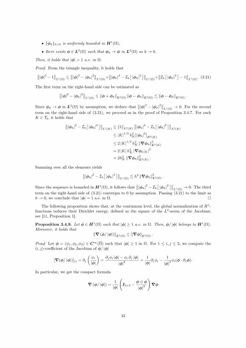
• φhh>0 is uniformly bounded in H1(Ω),

• there exists φ ∈ L2(Ω) such that φh → φ in L2(Ω) as h→ 0.

Then, it holds that |φ| = 1 a.e. in Ω.

Proof. From the triangle inequality, it holds that∥∥|φ|2 − 1∥∥L1(Ω)

≤∥∥|φ|2 − |φh|2∥∥L1(Ω)

+∥∥|φh|2 − Ih[ |φh|2 ]∥∥L1(Ω)

+∥∥Ih[ |φh|2 ]− 1

∥∥L1(Ω)

. (3.21)

The first term on the right-hand side can be estimated as∥∥|φ|2 − |φh|2∥∥L1(Ω)≤ ‖φ+ φh‖L2(Ω) ‖φ− φh‖L2(Ω) . ‖φ− φh‖L2(Ω) .

Since φh → φ in L2(Ω) by assumption, we deduce that∥∥|φ|2 − |φh|2∥∥L1(Ω)

→ 0. For the secondterm on the right-hand side of (3.21), we proceed as in the proof of Proposition 3.4.7. For eachK ∈ Th, it holds that∥∥|φh|2 − Ih[ |φh|2 ]∥∥L1(K)

≤ ‖1‖L2(K)

∥∥|φh|2 − Ih[ |φh|2 ]∥∥L2(K)

≤ |K|1/2 h2K

∣∣|φh|2∣∣H2(K)

≤ 2 |K|1/2 h2K ‖∇φh‖

2L4(K)

= 2 |K|h2K |∇φh|K |

2

= 2h2K ‖∇φh‖

2L2(K) .

Summing over all the elements yields∥∥|φh|2 − Ih[ |φh|2 ]∥∥L1(Ω). h2 ‖∇φh‖2L2(Ω) .

Since the sequence is bounded in H1(Ω), it follows that∥∥|φh|2 − Ih[ |φh|2 ]∥∥L1(Ω)

→ 0. The thirdterm on the right-hand side of (3.21) converges to 0 by assumption. Passing (3.21) to the limit ash→ 0, we conclude that |φ| = 1 a.e. in Ω.

The following proposition shows that, at the continuous level, the global normalization of H1-functions reduces their Dirichlet energy, defined as the square of the L2-norm of the Jacobian;see [11, Proposition 1].

Proposition 3.4.9. Let φ ∈H1(Ω) such that |φ| ≥ 1 a.e. in Ω. Then, φ/ |φ| belongs to H1(Ω).Moreover, it holds that

‖∇ (φ/ |φ|)‖L2(Ω) ≤ ‖∇φ‖L2(Ω) .

Proof. Let φ = (φ1, φ2, φ3) ∈ C∞(Ω) such that |φ| ≥ 1 in Ω. For 1 ≤ i, j ≤ 3, we compute the(i, j)-coefficient of the Jacobian of φ/ |φ|

[∇(φ/ |φ|)]ij = ∂j

(φi|φ|

)=∂jφi |φ| − φi ∂j |φ|

|φ|2=

1

|φ|∂jφi −

1

|φ|3φi(φ · ∂jφ).

In particular, we get the compact formula

∇ (φ/ |φ|) =1

|φ|

(I3×3 −

φ⊗ φ|φ|2

)∇φ

43

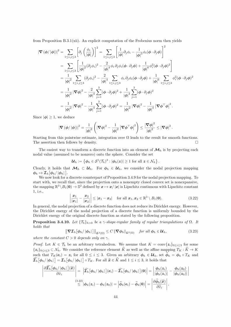
from Proposition B.3.1(xii). An explicit computation of the Frobenius norm then yields

|∇ (φ/ |φ|)|2 =∑

1≤i,j≤3

[∂j

(φi|φ|

)]2

=∑

1≤i,j≤3

[1

|φ|∂jφi −

1

|φ|3φi(φ · ∂jφ)

]2

=∑

1≤i,j≤3

[1

|φ|2(∂jφi)

2 − 2

|φ|4φi ∂jφi(φ · ∂jφ) +

1

|φ|6φ2i (φ · ∂jφ)2

]

=1

|φ|2∑

1≤i,j≤3

(∂jφi)2 − 2

|φ|4∑

1≤i,j≤3

φi ∂jφi(φ · ∂jφ) +1

|φ|6∑

1≤i,j≤3

φ2i (φ · ∂jφ)2

=1

|φ|2|∇φ|2 − 2

|φ|43∑j=1

(φ · ∂jφ)2 +1

|φ|43∑j=1

(φ · ∂jφ)2

=1

|φ|2|∇φ|2 − 1

|φ|43∑j=1

(φ · ∂jφ)2 =1

|φ|2|∇φ|2 − 1

|φ|4∣∣∇φ>φ∣∣2 .

Since |φ| ≥ 1, we deduce

|∇ (φ/ |φ|)|2 =1

|φ|2

(|∇φ|2 − 1

|φ|2∣∣∇φ>φ∣∣2) ≤ |∇φ|2

|φ|2≤ |∇φ|2 .

Starting from this pointwise estimate, integration over Ω leads to the result for smooth functions.The assertion then follows by density.

The easiest way to transform a discrete function into an element of Mh is by projecting eachnodal value (assumed to be nonzero) onto the sphere. Consider the set

Uh :=φh ∈ S1(Th)3 : |φh(z)| ≥ 1 for all z ∈ Nh

.

Clearly, it holds that Mh ⊂ Uh. For φh ∈ Uh, we consider the nodal projection mappingφh 7→ Ih

[φh/ |φh|

].

We now look for a discrete counterpart of Proposition 3.4.9 for the nodal projection mapping. Tostart with, we recall that, since the projection onto a nonempty closed convex set is nonexpansive,the mapping R3\B1(0)→ S2 defined by x 7→ x/ |x| is Lipschitz continuous with Lipschitz constant1, i.e., ∣∣∣∣ x1

|x1|− x2

|x2|

∣∣∣∣ ≤ |x1 − x2| for all x1,x2 ∈ R3 \B1(0). (3.22)

In general, the nodal projection of a discrete function does not reduce its Dirichlet energy. However,the Dirichlet energy of the nodal projection of a discrete function is uniformly bounded by theDirichlet energy of the original discrete function as stated by the following proposition.

Proposition 3.4.10. Let Thh>0 be a γ-shape-regular family of regular triangulations of Ω. Itholds that ∥∥∇Ih

[φh/ |φh|

]∥∥L2(Ω)

≤ C ‖∇φh‖L2(Ω) for all φh ∈ Uh, (3.23)

where the constant C > 0 depends only on γ.

Proof. Let K ∈ Th be an arbitrary tetrahedron. We assume that K = convzi0≤i≤3 for somezi0≤i≤3 ⊂ Nh. We consider the reference element K as well as the affine mapping TK : K → K

such that TK(ei) = zi for all 0 ≤ i ≤ 3. Given an arbitrary φh ∈ Uh, set φh = φh TK andIh[φh/ |φh|

]= Ih

[φh/ |φh|

] TK . For all x ∈ K and 1 ≤ i ≤ 3, it holds that∣∣∣∣∣∂Ih

[φh/ |φh|

](x)

∂xi

∣∣∣∣∣ =∣∣∣Ih[φh/ |φh| ](ei)− Ih

[φh/ |φh|

](0)∣∣∣ =

∣∣∣∣ φh(zi)

|φh(zi)|− φh(z0)

|φh(z0)|

∣∣∣∣(3.22)≤ |φh(zi)− φh(z0)| =

∣∣∣φh(ei)− φh(0)∣∣∣ =

∣∣∣∣∣∂φh(x)

∂xi

∣∣∣∣∣ ,44

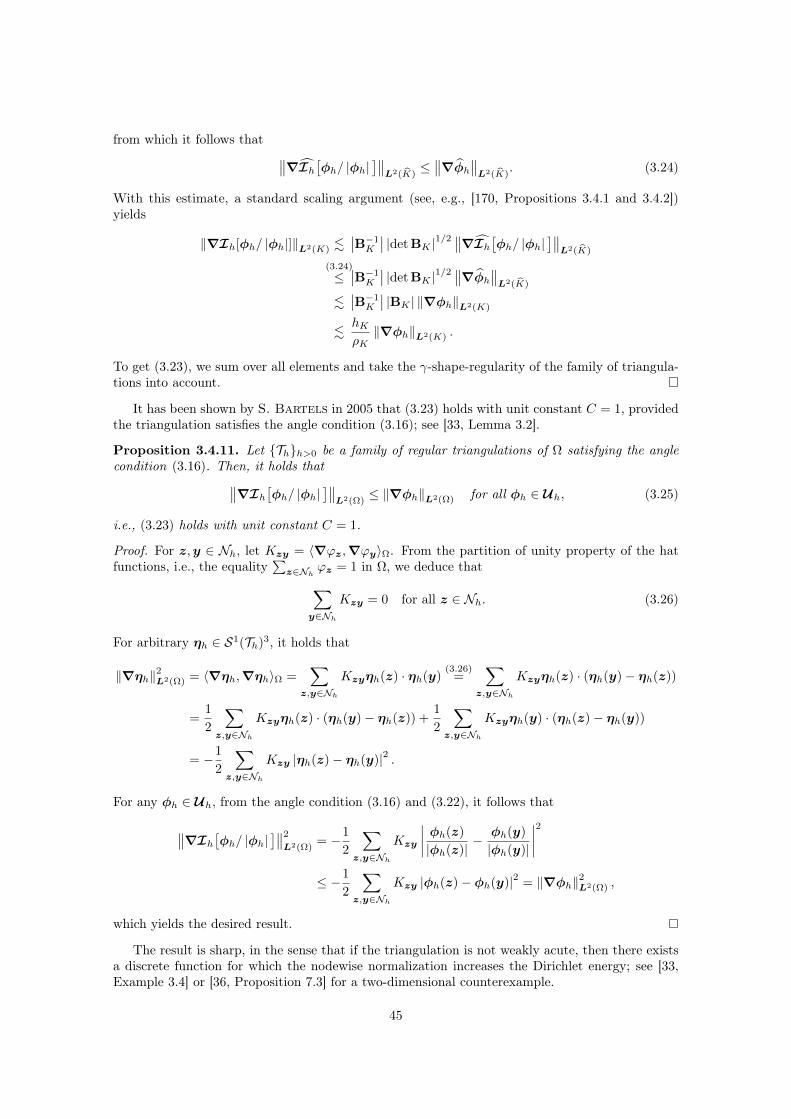
from which it follows that ∥∥∇Ih[φh/ |φh|

]∥∥L2(K)

≤∥∥∇φh∥∥L2(K)

. (3.24)

With this estimate, a standard scaling argument (see, e.g., [170, Propositions 3.4.1 and 3.4.2])yields

‖∇Ih[φh/ |φh|]‖L2(K) .∣∣B−1

K

∣∣ |det BK |1/2∥∥∇Ih

[φh/ |φh|

]∥∥L2(K)

(3.24)≤∣∣B−1

K

∣∣ |det BK |1/2∥∥∇φh∥∥L2(K)

.∣∣B−1

K

∣∣ |BK | ‖∇φh‖L2(K)

.hKρK‖∇φh‖L2(K) .

To get (3.23), we sum over all elements and take the γ-shape-regularity of the family of triangula-tions into account.

It has been shown by S. Bartels in 2005 that (3.23) holds with unit constant C = 1, providedthe triangulation satisfies the angle condition (3.16); see [33, Lemma 3.2].

Proposition 3.4.11. Let Thh>0 be a family of regular triangulations of Ω satisfying the anglecondition (3.16). Then, it holds that∥∥∇Ih

[φh/ |φh|

]∥∥L2(Ω)

≤ ‖∇φh‖L2(Ω) for all φh ∈ Uh, (3.25)

i.e., (3.23) holds with unit constant C = 1.

Proof. For z,y ∈ Nh, let Kzy = 〈∇ϕz,∇ϕy〉Ω. From the partition of unity property of the hatfunctions, i.e., the equality

∑z∈Nh

ϕz = 1 in Ω, we deduce that∑y∈Nh

Kzy = 0 for all z ∈ Nh. (3.26)

For arbitrary ηh ∈ S1(Th)3, it holds that

‖∇ηh‖2L2(Ω) = 〈∇ηh,∇ηh〉Ω =∑

z,y∈Nh

Kzyηh(z) · ηh(y)(3.26)

=∑

z,y∈Nh

Kzyηh(z) · (ηh(y)− ηh(z))

=1

2

∑z,y∈Nh

Kzyηh(z) · (ηh(y)− ηh(z)) +1

2

∑z,y∈Nh

Kzyηh(y) · (ηh(z)− ηh(y))

= −1

2

∑z,y∈Nh

Kzy |ηh(z)− ηh(y)|2 .

For any φh ∈ Uh, from the angle condition (3.16) and (3.22), it follows that

∥∥∇Ih[φh/ |φh|

]∥∥2

L2(Ω)= −1

2

∑z,y∈Nh

Kzy

∣∣∣∣ φh(z)

|φh(z)|− φh(y)

|φh(y)|

∣∣∣∣2≤ −1

2

∑z,y∈Nh

Kzy |φh(z)− φh(y)|2 = ‖∇φh‖2L2(Ω) ,

which yields the desired result.

The result is sharp, in the sense that if the triangulation is not weakly acute, then there existsa discrete function for which the nodewise normalization increases the Dirichlet energy; see [33,Example 3.4] or [36, Proposition 7.3] for a two-dimensional counterexample.

45

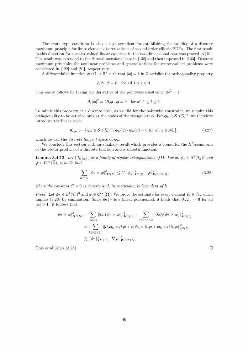
The acute type condition is also a key ingredient for establishing the validity of a discretemaximum principle for finite element discretizations of second order elliptic PDEs. The first resultin this direction for a scalar-valued linear equation in the two-dimensional case was proved in [70].The result was extended to the three-dimensional case in [138] and then improved in [133]. Discretemaximum principles for nonlinear problems and generalizations for vector-valued problems wereconsidered in [122] and [81], respectively.

A differentiable function φ : Ω→ R3 such that |φ| = 1 in Ω satisfies the orthogonality property

∂iφ · φ = 0 for all 1 ≤ i ≤ 3.

This easily follows by taking the derivative of the pointwise constraint |φ|2 = 1

∂i |φ|2 = 2∂iφ · φ = 0 for all 1 ≤ i ≤ 3.

To mimic this property at a discrete level, as we did for the pointwise constraint, we require thisorthogonality to be satisfied only at the nodes of the triangulation. For φh ∈ S1(Th)3, we thereforeintroduce the linear space

Kφh:=ψh ∈ S1(Th)3 : φh(z) ·ψh(z) = 0 for all z ∈ Nh

, (3.27)

which we call the discrete tangent space of φh.We conclude this section with an auxiliary result which provides a bound for the H2-seminorm

of the vector product of a discrete function and a smooth function.

Lemma 3.4.12. Let Thh>0 be a family of regular triangulations of Ω. For all φh ∈ S1(Th)3 andϕ ∈ C∞(Ω), it holds that∑

K∈Th

|φh ×ϕ|2H2(K) ≤ C ‖φh‖2H1(Ω) ‖ϕ‖

2W 2,∞(Ω) , (3.28)

where the constant C > 0 is generic and, in particular, independent of h.

Proof. Let φh ∈ S1(Th)3 and ϕ ∈ C∞(Ω). We prove the estimate for every element K ∈ Th, whichimplies (3.28) by summation. Since φh|K is a linear polynomial, it holds that ∂αφh = 0 for all|α| > 1. It follows that

|φh ×ϕ|2H2(K) =∑|α|=2

‖∂α(φh ×ϕ)‖2L2(K) =∑

1≤i≤j≤3

‖∂i∂j(φh ×ϕ)‖2L2(K)

=∑

1≤i≤j≤3

‖∂jφh × ∂iϕ+ ∂iφh × ∂jϕ+ φh × ∂i∂jϕ‖2L2(K)

. ‖φh‖2H1(K) ‖∇ϕ‖2W 1,∞(K) .

This establishes (3.28).

46

Chapter 4

Tangent plane integrators

In this chapter, we introduce and analyze two variants of the tangent plane scheme for the numericalapproximation of the LLG equation. We show that the methods are (unconditionally) convergenttowards a weak solution of the problem. Throughout this chapter, we use the standard notationfor Lebesgue/Sobolev/Bochner spaces and norms; see Section 3.2.

4.1 Model problemLet Ω ⊂ R3 be a bounded Lipschitz domain with polyhedral boundary Γ := ∂Ω. Let T > 0 be somefinite time. We denote the space-time cylinder by ΩT := Ω × (0, T ) and define ΓT := Γ × (0, T ).Moreover, we use the notation 〈·, ·〉 := 〈·, ·〉Ω to denote the scalar product in L2(Ω) (resp. L2(Ω)).This does not lead to ambiguities, since Ω is the unique domain considered throughout the chapter.

We consider the initial boundary value problem

∂tm = −m× [heff(m,f) + Π(m)] + αm× ∂tm in ΩT , (4.1a)∂nm = 0 on ΓT , (4.1b)

m(0) = m0 in Ω. (4.1c)

In (4.1a), which is the Gilbert form (3.4) of the nondimensional LLG equation, α > 0 is constantand the effective field takes the form

heff(m,f) = λ2ex∆m+ π(m) + f , (4.2)

where λex > 0 is constant, while π(m) and f denote the generalm-dependent andm-independenteffective field contributions, respectively. We assume that π : L2(Ω) → L2(Ω) is a bounded,linear, and self-adjoint operator, while f belongs to H1(0, T ;L2(Ω)). Under these assumptions,the effective field satisfies

heff(m,f) = −δE(m,f)

δm

for the energy functional

E(m,f) =λ2

ex

2‖∇m‖2L2(Ω) −

1

2〈π(m),m〉 − 〈f ,m〉. (4.3)

We assume Π :m ∈H1(Ω) : |m| = 1 a.e. in Ω

→ L2(Ω) to be a bounded operator. For the

initial condition in (4.1c), we assume that m0 ∈ H1(Ω) satisfies∣∣m0

∣∣ = 1 a.e. in Ω. In thefollowing definition, we introduce the notion of a weak solution of (4.1).

Definition 4.1.1 (weak solution). A function m : ΩT → R3 is called a weak solution of (4.1) ifthe following properties (i)–(iv) are satisfied:

47

(i) m ∈ L∞(0, T ;H1(Ω)) ∩H1(0, T ;L2(Ω)) and |m| = 1 a.e. in ΩT ,

(ii) m(0) = m0 in the sense of traces,

(iii) for all ϕ ∈H1(ΩT ), it holds that∫ T

0

〈∂tm(t),ϕ(t)〉 dt− α∫ T

0

〈m(t)× ∂tm(t),ϕ(t)〉 dt

= λ2ex

∫ T

0

〈m(t)×∇m(t),∇ϕ(t)〉 dt−∫ T

0

〈m(t)× π(m(t)),ϕ(t)〉 dt

−∫ T

0

〈m(t)× f(t),ϕ(t)〉 dt−∫ T

0

〈m(t)×Π(m(t)),ϕ(t)〉 dt,

(4.4)

(iv) m satisfies the energy inequality

E(m(τ),f(τ)) + α

∫ τ

0

‖∂tm(t)‖2L2(Ω) dt+

∫ τ

0

〈∂tf(t),m(t)〉 dt

≤ E(m0,f(0)) +

∫ τ

0

〈Π(m(t)), ∂tm(t)〉 dt

(4.5)

for a.e. τ ∈ (0, T ).

Definition 4.1.1 extends [17, Definition 1.2], introduced by F. Alouges and A. Soyeur todefine the notion of a weak solution for the case in which the effective field comprises only theexchange contribution. After possibly being redefined on a set of measure zero, any solution min the sense of Definition 4.1.1 belongs to C0([0, T ];L2(Ω)); see [88, Section 5.9.2, Theorem 2].For functions in H1(ΩT ), the time evaluation can be defined by density as the limit of the timeevaluation for smooth functions. In this sense, for all t ∈ [0, T ], it holds that m(t) ∈ H1/2(Ω).This concept is implied behind the expression ‘in the sense of traces’ in part (ii) of Definition 4.1.1.The variational formulation (4.4) comes from a weak formulation of (4.1a) in the space-time do-main. The boundary conditions (4.1b) are enforced in the variational formulation (4.4) as naturalboundary conditions. In particular, using (4.1b), the boundary term, which arises from integratingby parts the exchange contribution, vanishes. The energy inequality (4.5) is a weak counterpart ofthe energy law (3.3) for (4.1). In (4.4)–(4.5), by π(m) and Π(m) we mean the functions definedby t 7→ π(m(t)) and t 7→ Π(m(t)) for all t ∈ (0, T ). From the regularity of m required by thedefinition and the stability of π and Π, it follows that both π(m) and Π(m) belong to L2(ΩT ),so that all the integrals involving these functions in (4.4)–(4.5) are well defined.

This abstract framework covers most of the physics introduced in Chapter 2. The first termof the effective field (4.2), which corresponds to the first term of the energy (4.3), clearly refers tothe exchange contribution. If the general m-dependent field contribution comprises, e.g., uniaxialanisotropy and stray field, the corresponding operator takes the form

π(m) = q2(a ·m)a+ hs(m),

where q > 0 is constant, a ∈ S2 denotes the easy axis, and hs is the stray field. In this case, πis a linear, bounded and self-adjoint operator L2(Ω)→ L2(Ω). The m-independent effective fieldcontribution f includes the applied external field hext and the Oersted field hc generated by agiven electric current density. Only the Dzyaloshinskii–Moriya interaction and the magnetoelasticcontribution cannot be included into this setting; see Remark 4.1.2. The operator Π takes thepossible presence of nonenergetic (i.e., not belonging to the effective field) torque terms into ac-count. This is the case, for instance, for the spintronic extensions of the LLG equation presentedin Section 2.3, for which the application of the present framework will be discussed in details inChapter 5.

48

Remark 4.1.2. The magnetoelastic contribution of the effective field takes the form

heff,el = 2(λσ)m,

where λ ∈ L∞(Ω) is a 4th order tensor, while σ ∈ L2(Ω) is the weak solution of the boundaryvalue problem

∇ · σ + f = 0 in Ω,

C[ε(u)− εm(m)] = σ in Ω,

u = 0 on ΓD,

σn = t on ΓN ;

see page 16 for the definition of all involved quantities. Clearly, the mapping π : m 7→ 2(λσ)m isnot a linear, bounded, and self-adjoint operator L2(Ω) → L2(Ω). In particular, π(m) belongs toL2(Ω) only if m ∈ L∞(Ω).

In the presence of the Dzyaloshinskii–Moriya interaction, i.e., when the effective field alsocomprises the term

heff,DM = −λDM∇×m,

the homogeneous Neumann boundary conditions (4.1b), which are appropriate whenever the uniquecomponent of the effective field involving magnetization derivatives is the exchange contribution,must be replaced by

2λ2ex∂nm+ λDMm× n = 0.

This clearly affects the variational formulation (4.4). The analysis of the algorithm introduced inthe next section for this situation is currently being investigated, and we refer the interested readerto a forthcoming publication [116].

4.2 Numerical algorithmIn this section, we introduce a numerical method for the approximation of the abstract problemdiscussed in Section 4.1. The starting point is the alternative form of the LLG equation (3.5),which in this case takes the form

α∂tm+m× ∂tm = heff(m,f) + Π(m)− [heff(m,f) ·m+ Π(m) ·m]m. (4.6)

We recall that, under the constraint |m| = 1, this formulation is equivalent to the Landau–Lifshitzform and to the Gilbert form; see Proposition 3.1.1.

Since (4.6) is linear with respect to the time derivative ∂tm, we introduce the free variablev = ∂tm

αv +m× v = heff(m,f) + Π(m)− [heff(m,f) ·m+ Π(m) ·m]m. (4.7)

From the equality |m|2 = 1, we deduce the orthogonality m · v = 0. Hence, for each t ∈ (0, T ),v(t) ∈ R3 belongs to the tangent space of the sphere at m(t). Taking this orthogonality aswell as the expression (4.2) of the effective field into account, we obtain the following variationalformulation of (4.7): Find v(t) ∈ L2(Ω) with m(t) · v(t) = 0 a.e. in Ω such that

α〈v(t),φ〉 + 〈m(t)× v(t),φ〉 = −λ2ex〈∇m(t),∇φ〉 + 〈π(m(t)),φ〉 + 〈f ,φ〉 + 〈Π(m(t)),φ〉

(4.8)

for all φ ∈ H1(Ω) satisfying m(t) · φ = 0 a.e. in Ω. Note that in (4.8) the boundary integralwhich arises from integrating by parts the exchange contribution vanishes thanks to the boundaryconditions (4.1b). Moreover, since the test function φ belongs to the tangent space of the sphere atm(t), in (4.8) the term corresponding to the last (strongly nonlinear inm) term on the right-handside of (4.7) also vanishes.

49

For the time discretization, given an integer M > 0, we consider a uniform partition of thetime interval (0, T ) with time-step size k = T/M , i.e., ti = ik for all 0 ≤ i ≤ M ; see Section 3.3.For the spatial discretization, we consider a γ-quasi-uniform family Thh>0 of regular tetrahedraltriangulations of Ω; see Section 3.4.

For each time-step 0 ≤ i ≤ M − 1, the structure of the numerical scheme is the following:First of all, given an approximation mi

h ∈ S1(Th)3 of m(ti), we compute vih ≈ v(ti) from a finiteelement discretization of (4.8) based on the discrete tangent space introduced in (3.27), i.e.,

Kmih

:=ψh ∈ S1(Th)3 : mi

h(z) ·ψh(z) = 0 for all z ∈ Nh.

We obtain the following variational problem: Find vih ∈ Kmihsuch that

α〈vih,φh〉 + 〈mih × vih,φh〉 + λ2

exθk〈∇vih,∇φh〉= −λ2

ex〈∇mih,∇φh〉 + 〈πh(mi

h),φh〉 + 〈f ih,φh〉 + 〈Πh(mih),φh〉

for all φh ∈ Kmih. Here, the operators πh : S1(Th)3 → L2(Ω) and Πh : S1(Th)3 → L2(Ω) denote

discretized versions of π and Π, respectively, while, for all 0 ≤ i ≤ M − 1, f ih ∈ L2(Ω) denotesan approximation of f(ti). The parameter 0 ≤ θ ≤ 1 modulates the ‘degree of implicitness’ of themethod in the treatment of the leading-order term of the effective field (which is the second-orderexchange contribution).

The computed vih ∈ Kmihis then used to update the current magnetizationmi

h ≈m(ti) to thenew value mi+1

h ≈m(ti+1) via a 1st order time-stepping. A simple choice is given by the classicallinear time-stepping

mi+1h = mi

h + kvih.

In this case, the pointwise constraint |m| = 1 which characterizes the solution of the LLG equationis ignored by the numerical scheme. To have a numerical realization of it, the nodal projectionmapping φh 7→ Ih(φh/ |φh|) can be applied. The resulting time-stepping is then given by

mi+1h = Ih

[mih + kvih∣∣mih + kvih

∣∣].

With this choice, for every 0 ≤ i ≤ M − 1, mi+1h belongs to the set Mh of the discrete functions

which satisfy the pointwise constraint at the nodes of the triangulation introduced in (3.20), i.e.,

Mh :=φh ∈ S1(Th)3 : |φh(z)| = 1 for all z ∈ Nh

.

We refer to the method which includes the nodal projection as standard tangent plane scheme(TPS). We refer to the method in which the nodal projection is omitted as projection-free tangentplane scheme (PFTPS).

We recall the definition of the set

Uh :=φh ∈ S1(Th)3 : |φh(z)| ≥ 1 for all z ∈ Nh

⊃Mh,

which is the domain of the nodal projection mapping, and summarize the proposed numericalschemes in the following algorithm.

Algorithm 4.2.1 (tangent plane scheme). Input: Eitherm0h ∈Mh (TPS) orm0

h ∈ Uh (PFTPS).Loop: For all 0 ≤ i ≤M − 1, iterate:

(i) Compute πh(mih) ∈ L2(Ω) and Πh(mi

h) ∈ L2(Ω),

(ii) Compute vih ∈ Kmihsuch that

α〈vih,φh〉 + 〈mih × vih,φh〉 + λ2

exθk〈∇vih,∇φh〉= −λ2



(4.9)

for all φh ∈ Kmih,

50

(iii) Either define mi+1h ∈ Uh by

mi+1h = mi

h + kvih (PFTPS) (4.10a)

or define mi+1h ∈Mh by

mi+1h = Ih


∣∣]

(TPS). (4.10b)

Output: Sequence of discrete functions

(vih,mi+1h )

0≤i≤M−1

.

In Algorithm 4.2.1, in the same spirit as [56] and unlike [16], the numerical approximation ofthe lower-order effective field contributions and the additional torque term is considered. Indeed,step (i) can include the solution of a nonlocal problem, e.g., the computation of the stray fieldfor a given configuration of the magnetization. In the case of the standard tangent plane scheme,omitting both the lower-order effective field terms and the additional nonenergetic torque term,and choosing θ = 0, we recover the explicit method of [14]. The idea of removing the nodalprojection from the tangent plane scheme goes back to [6] for the LLG equation and has beeninspired by [37], where the same principle is applied to a certain class of geometrically constrainedpartial differential equations, e.g., the harmonic map heat flow.

In Algorithm 4.2.1, the approach for the treatment of the leading-order effective field contri-bution, introduced in [12], is similar to the classical θ-method for the heat equation: The choiceθ = 0 produces an explicit version of the scheme, the choice θ = 1/2 yields a Crank-Nicolson-typescheme, while for θ = 1 we obtain a kind of fully implicit version of the scheme. In analogywith the corresponding result for the heat equation, one may conjecture that the method is un-conditionally stable for θ > 1/2, but requires a stability condition, usually referred to as CFLcondition (Courant–Friedrichs–Lewy condition, named after the mathematicians R. Courant,K. Friedrichs, and H. Lewy), for θ < 1/2. We will indeed prove a result of that kind in thenext section; see Theorem 4.3.2. Note that this approach concerns only the exchange contributionof the effective field, but does not affect the other terms, which are treated explicitly.

Both versions of the scheme are formally 1st order methods in time. In order to show this, fora sufficiently smooth solution and 0 ≤ i ≤ M − 1, let mi = m(ti) and vi = v(ti) = ∂tm(ti). Inthe case of the projection-free version of the method, the Taylor theorem directly shows∣∣mi+1 −mi − kvi

∣∣ = O(k2) as k → 0. (4.11)

In the case of the standard version of the method, it holds that

mi+1 − mi + kvi

|mi + kvi|= mi + kvi +O(k2)− mi + kvi

|mi + kvi|= (mi + kvi)

(1− 1

|mi + kvi|

)+O(k2).

Since∣∣mi

∣∣ = 1 and mi · vi = 0, we deduce that∣∣mi + kvi∣∣2 =

∣∣mi∣∣2 + 2mi · vi + k2

∣∣vi∣∣2 = 1 + k2∣∣vi∣∣2 .

The Taylor expansion1√

1 + x= 1− x

2+O(x2) as x→ 0

then reveals1

|mi + kvi|= 1− 1

2k2∣∣vi∣∣2 +O(k4) as k → 0.

Altogether, we thus obtain∣∣∣∣mi+1 − mi + kvi

|mi + kvi|

∣∣∣∣ =

∣∣∣∣(mi + kvi)

(k2

2

∣∣vi∣∣2 +O(k4)

)+O(k2)

∣∣∣∣ = O(k2) as k → 0. (4.12)

Strategies to improve the convergence order in time of the standard tangent plane scheme are basedon similar Taylor expansions and have been proposed in [16, 15].

The following proposition states that Algorithm 4.2.1 is well posed.

51

Proposition 4.2.2. For all 0 ≤ i ≤ M − 1, there exists a unique solution vih ∈ Kmihof (4.9).

Moreover, the time-stepping (4.10) is well defined.

Proof. Let 0 ≤ i ≤ N − 1. Consider the bilinear form a(mih; ·, ·) : S1(Th)3 × S1(Th)3 → R defined

bya(mi

h;ηh,φh) := α〈ηh,φh〉 + 〈mih × ηh,φh〉 + λ2

exθk〈∇ηh,∇φh〉for all ηh,φh ∈ S1(Th)3, and the linear functional F (mi

h; ·) : S1(Th)3 → R defined by

F (mih;φh) := −λ2



for all φh ∈ S1(Th)3. Then, we can rewrite step (ii) of the algorithm as: Find vih ∈ Kmihsuch that

a(mih;vih,φh) = F (mi

h;φh) for all φh ∈ Kmih.

Since it holds that

a(mih;φh,φh) = α ‖φh‖2L2(Ω) + λ2

exθk ‖∇φh‖2L2(Ω) for all φh ∈ S1(Th)3,

the bilinear form is elliptic (even in the full space S1(Th)3). Existence and uniqueness of thesolution vih ∈ Kmi

hto (4.9) thus follows from the Lax–Milgram theorem. It remains to show that

the time-stepping (4.10) is always well defined. This is straightforward for the projection-free timestepping (4.10a). If the algorithm includes the nodal projection, it holds that mi

h ∈Mh. Sincevh ∈ Kmi

h, it follows that∣∣mi

h(z) + kvih(z)∣∣2 =

∣∣mih(z)

∣∣2 + k2∣∣vih(z)

∣∣2 = 1 + k2∣∣vih(z)

∣∣2 ≥ 1,

i.e., mih + kvih ∈ Uh. The projection step (4.10b) is therefore also well defined.

4.3 Convergence analysisFrom Algorithm 4.2.1 we obtain two sequences of discrete functions mi

h0≤i≤M and vih0≤i≤M−1,which can be used to define the piecewise linear and piecewise constant time reconstructionsfrom (3.13). In particular, we consider the functions defined, for all t ∈ [ti, ti+1) and 0 ≤ i ≤M−1,by

mhk(t) :=t− tik

mi+1h +

ti+1 − tk

mih, m−hk(t) := mi

h, m+hk(t) := mi+1

h , and v−hk(t) := vih.

(4.13)Similarly, we define the functions π−hk,Π

−hk : [0, T )→ L2(Ω) by

π−hk(t) := πh(mih), and Π−hk(t) := Πh(mi

h), (4.14)

for all t ∈ [ti, ti+1) and 0 ≤ i ≤M − 1.In the following assumption, we collect some of the requirements on the approximation of the

initial condition m0h, on the discrete operators πh and Πh, and on the sequence f ih0≤i≤M−1.

Assumption 4.3.1. The discrete initial condition m0h belongs to Uh and satisfies the convergence

propertym0h m0 in H1(Ω) as h→ 0. (4.15)

For the standard tangent plane scheme, we additionally assume that m0h ∈ Mh. The discrete

operators πh : Uh → L2(Ω) and Πh : Uh → L2(Ω) are stable, in the sense that there exist twopositive constants, Cπ and CΠ, independent of h, such that

‖πh(φh)‖L2(Ω) ≤ Cπ(

1 + ‖φh‖H1(Ω)

)for all φh ∈ Uh, (4.16a)

‖Πh(φh)‖L2(Ω) ≤ CΠ

(1 + ‖φh‖H1(Ω)

)for all φh ∈ Uh. (4.16b)

52

For the sequence f ih0≤i≤M−1 in L2(Ω), we define the piecewise constant time reconstruction f−hkby f−hk(t) := f ih for all t ∈ [ti, ti+1) and 0 ≤ i ≤M −1, and assume that it satisfies the convergenceproperty

f−hk f in L2(ΩT ) as k, h→ 0. (4.17)

Moreover, for the sake of simplicity, we assume that f ∈ C1([0, T ],L2(Ω)). In particular, theexpressions f(t) and ∂tf(t) are meaningful for all t ∈ [0, T ].

The following theorem, which is the main result of this chapter, states that the time reconstruc-tions from (4.13) converge in an appropriate sense towards a weak solution of (4.1) as k, h→ 0.

Theorem 4.3.2. Let Thh>0 be a γ-quasi-uniform family of regular tetrahedral triangulations ofΩ.(a) Suppose that Assumption 4.3.1 is satisfied. For the standard tangent plane scheme, assumethat

• either 1/2 < θ ≤ 1 and any triangulation Th satisfies the angle condition (3.16),

• or θ = 1/2, any triangulation Th satisfies the angle condition (3.16), and k = o(h) ask, h→ 0,

• or k = o(h2) as k, h→ 0.

For the projection-free tangent plane scheme, assume that

• either 1/2 < θ ≤ 1,

• or θ = 1/2 and k = o(h) as k, h→ 0,

• or k = o(h2) as k, h→ 0.

Then, the sequences of discrete functions mhk and m±hk, constructed from the output of Al-gorithm 4.2.1 according to (4.13), admit subsequences (not relabeled) which converge towards afunction m satisfying the requirements (i)–(ii) of Definition 4.1.1. More precisely, it holds thatmhk m in H1(ΩT ) and mhk,m

±hk∗m in L∞(0, T ;H1(Ω)) as k, h→ 0.

(b) Under the assumptions of part (a), suppose that the discrete operators πh and Πh are consistent,in the sense that, given the convergent subsequences of part (a), the corresponding subsequences ofdiscrete functions (4.14) satisfy

π−hk π(m) in L2(ΩT ) as k, h→ 0, (4.18a)

Π−hk Π(m) in L2(ΩT ) as k, h→ 0. (4.18b)

Then, the limit function m of part (a) satisfies also the requirement (iii) of Definition 4.1.1.(c) Under the assumption of part (b), assume that (4.15), (4.17) and (4.18) hold with strongconvergence. In the case of the standard tangent plane scheme, assume the following additionalL4-regularity on f and π

f ∈ C0([0, T ],L4(Ω)) and ‖π(φ)‖L4(Ω) ≤ C ‖φ‖L4(Ω) for all φ ∈ L4(Ω), (4.19)

where C > 0 is constant. Then, the limit functionm from part (b) satisfies also the requirement (iv)of Definition 4.1.1. In particular, m is a weak solution of (4.1) .

For both versions of the method, for 1/2 < θ ≤ 1, the convergence is unconditional. Theproof of Theorem 4.3.2 is constructive, in the sense that it also establishes the existence of a weaksolution of (4.1). The proof will follow the usual energy method for proving existence of solutionsof linear second-order parabolic problems; see, e.g., [88, Section 7.1.2]. The main difference isthat the construction of approximate solutions is not obtained by applying the Galerkin methodbased on a set of appropriately normalized eigenfunctions of the Laplacian, but rather by usingthe discrete solutions of Algorithm 4.2.1.

53

Remark 4.3.3. For the applicability of Theorem 4.3.2 to effective discretizations of the lower-order effective field terms, we refer the reader to [56, Section 4]. There, it is shown that ifthe discrete operator πh is a continuous function of the magnetization (which is the case, e.g.,for anisotropy contributions) or the approximate stray field computed with the hybrid FEM-BEMmethod of D. R. Fredkin and T. R. Koehler [99], then the stability (4.16a) and the consistencyassumption (4.18a) are satisfied. In Chapter 5, we will discuss the applicability of Theorem 4.3.2to the analysis of the tangent plane scheme for the spintronic extensions of the LLG equationpresented in Section 2.3, which will provide concrete examples for the discrete operator Πh.

For the sake of clarity, we divide the proof of Theorem 4.3.2 into several lemmata and proposi-tions. We start with the observation that, for the standard tangent plane scheme, from Lemma 3.4.6it follows that

∥∥mih

∥∥L∞(Ω)

= 1 for all 0 ≤ i ≤ M . The following lemma concerns two geometricestimates satisfied by the iterates of Algorithm 4.2.1 in this case.

Lemma 4.3.4. For all 0 ≤ i ≤ M − 1 and z ∈ Nh, the iterates of the standard tangent planescheme satisfy ∣∣mi+1

h (z)−mih(z)− kvih(z)

∣∣ ≤ 1

2k2∣∣vih(z)

∣∣2 (4.20)

and ∣∣mi+1h (z)−mi

h(z)∣∣ ≤ k ∣∣vih(z)

∣∣ . (4.21)

Proof. Let 0 ≤ i ≤ M − 1. For z ∈ Nh, using the expression (4.10b) of the time-stepping, weobtain that∣∣mi+1

h (z)−mih(z)− kvih(z)

∣∣=

∣∣∣∣∣ mih(z) + kvih(z)∣∣mih(z) + kvih(z)

∣∣ −mih(z)− kvih(z)

∣∣∣∣∣ =∣∣mi

h(z) + kvih(z)∣∣ ∣∣∣∣∣ 1∣∣mi

h(z) + kvih(z)∣∣ − 1

∣∣∣∣∣=∣∣mi

h(z) + kvih(z)∣∣(1− 1∣∣mi

h(z) + kvih(z)∣∣)

=∣∣mi

h(z) + kvih(z)∣∣− 1.

To estimate the right-hand side, we compute

0 ≤(∣∣mi

h(z) + kvih(z)∣∣− 1

)2=∣∣mi

h(z) + kvih(z)∣∣2 − 2

∣∣mih(z) + kvih(z)

∣∣+ 1

=∣∣mi

h(z)∣∣2 + k2

∣∣vih(z)∣∣2 − 2


∣∣+ 1 = 2 + k2∣∣vih(z)

∣∣2 − 2∣∣mi

h(z) + kvih(z)∣∣ .

Rearranging the terms, we deduce that∣∣mih(z) + kvih(z)

∣∣− 1 ≤ 1

2k2∣∣vih(z)

∣∣2 .As a result, we obtain (4.20).

For z ∈ Nh, a simple computation reveals∣∣mi+1h (z)−mi

h(z)∣∣2 =

∣∣mi+1h (z)

∣∣2 − 2mi+1h (z) ·mi

h(z) +∣∣mi

h(z)∣∣2 = 2

(1−mi+1

h (z) ·mih(z)

)= 2

(1− mi

h(z) + kvih(z)∣∣mih(z) + kvih(z)

∣∣ ·mih(z)

)= 2

(1− 1∣∣mi

h(z) + kvih(z)∣∣)

= 2


∣∣− 1∣∣mih(z) + kvih(z)

∣∣ = 2


∣∣− ∣∣mi+1h (z)

∣∣∣∣mih(z) + kvih(z)

∣∣ .

Due to the Lipschitz continuity (with unit constant) of the Euclidean norm, we can estimate thenumerator by


∣∣− ∣∣mi+1h (z)

∣∣ ≤ ∣∣mih(z) + kvih(z)−mi+1

h (z)∣∣ (4.20)≤ 1

2k2∣∣vih(z)

∣∣2 .54

For the denominator, it holds that∣∣mi

h(z) + kvih(z)∣∣ ≥ 1. We deduce

∣∣mi+1h (z)−mi

h(z)∣∣2 ≤ 2


∣∣− ∣∣mi+1h (z)

∣∣∣∣mih(z) + kvih(z)

∣∣ ≤ k2∣∣vih(z)

∣∣2 .This yields (4.21).

We recall the norm equivalence

‖φh‖pLp(Ω) ' h3∑z∈Nh

|φh(z)|p for all φh ∈ S1(Th)3 and p ∈ [1,∞) (4.22)

from Proposition 3.4.5, which holds with an equivalence constant that depends only on the meshregularity parameter γ. The combination of (4.22) with the geometric estimates from Lemma 4.3.4leads to the following result.

Corollary 4.3.5. For all 0 ≤ i ≤M − 1, the iterates of the standard tangent plane scheme satisfy

∥∥mi+1h −mi

h

∥∥L2(Ω)

≤ Ck∥∥vih∥∥L2(Ω)

, (4.23a)∥∥mi+1h −mi

h − kvih∥∥L1(Ω)

≤ Ck2∥∥vih∥∥2

L2(Ω), (4.23b)∥∥mi+1

h −mih − kvih

∥∥L4/3(Ω)

≤ Ck2∥∥vih∥∥2

L8/3(Ω), (4.23c)

where the constant C > 0 depends only on γ.

Proof. The estimate (4.23a) follows from (4.21) and a double application of (4.22) (p = 2). Theestimate (4.23b) follows from (4.20) and a double application of (4.22) (first p = 1, then p = 2).The estimate (4.23c) follows from (4.20) and a double application of (4.22) (first p = 4/3, thenp = 8/3).

If the nodal projection mapping is omitted in Algorithm 4.2.1, thanks to (4.10a), the esti-mates from Lemma 4.3.4 and Corollary 4.3.5 become trivial. However, in this case, the equality‖mi

h‖L∞(Ω) = 1 for all 0 ≤ i ≤ M is not satisfied. In the following lemma, we prove an easyrecursive relation.

Lemma 4.3.6. For all 1 ≤ j ≤M , the iterates of the projection-free tangent plane scheme satisfy

|mjh(z)|2 =

∣∣m0h(z)

∣∣2 + k2

j−1∑i=0

∣∣vih(z)∣∣2 for all z ∈ Nh. (4.24)

Proof. Let 1 ≤ j ≤M . For all 0 ≤ i ≤ j − 1 and z ∈ Nh, since vih belongs to Kmih, it holds that∣∣mi+1

h (z)∣∣2 (4.10a)

=∣∣mi

h(z) + kvih(z)∣∣2 =

∣∣mih(z)

∣∣2 + k2∣∣vih(z)

∣∣2 .Summation over 0 ≤ i ≤ j − 1 yields (4.24).

In the following lemma, we start with the study of the evolution of the discrete energy.

Lemma 4.3.7. Let 0 ≤ i ≤M − 1. For the standard tangent plane scheme, it holds that

λ2ex

2kdt

∥∥∇mi+1h

∥∥2

L2(Ω)+ [α− c(k, h)]k

∥∥vih∥∥2

L2(Ω)+ λ2

ex

(θ − 1

2

)k2∥∥∇vih∥∥2

L2(Ω)

≤ k〈πh(mih),vih〉 + k〈f ih,vih〉 + k〈Πh(mi

h),vih〉,(4.25)

with

c(k, h) =

0 if the triangulation Th satisfies the angle condition (3.16),Ckh−2 else.

55

The constant C > 0 depends only on γ and λex. In particular, it is independent of k and h. Forthe projection-free tangent plane scheme, it holds that

λ2ex

2kdt

∥∥∇mi+1h

∥∥2

L2(Ω)+ αk

∥∥vih∥∥2

L2(Ω)+ λ2

ex

(θ − 1

2

)k2∥∥∇vih∥∥2

L2(Ω)

= k〈πh(mih),vih〉 + k〈f ih,vih〉 + k〈Πh(mi

h),vih〉.(4.26)

Proof. Let 0 ≤ i ≤M − 1. We test (4.9) with φh = vih ∈ Kmihand multiply the resulting equation

by k:

αk∥∥vih∥∥2

L2(Ω)+ k

= 0︷︸︸︷〈mi

h × vih,vih〉+λ2exθk

2∥∥∇vih∥∥2

L2(Ω)

= −λ2exk〈∇mi

h,∇vih〉 + k〈πh(mih),vih〉 + k〈f ih,vih〉 + k〈Πh(mi

h),vih〉.(4.27)

We apply the vector identity

|a|2 − |b|2 = |a− b|2 + 2(a− b) · b for all a,b ∈ R9

with the choices a = ∇mi+1h and b = ∇mi

h, and multiply the resulting equation by λ2ex/2. We

obtain

λ2ex

2

∥∥∇mi+1h

∥∥2

L2(Ω)− λ2

ex

2

∥∥∇mih

∥∥2

L2(Ω)

=λ2

ex

2

∥∥∇mi+1h −∇mi

h

∥∥2

L2(Ω)+ λ2

ex〈∇mi+1h −∇mi

h,∇mih〉.

Summation of the latter with (4.27) yields

λ2ex

2

∥∥∇mi+1h

∥∥2

L2(Ω)− λ2

ex

2

∥∥∇mih

∥∥2

L2(Ω)+ αk

∥∥vih∥∥2

L2(Ω)+ λ2

exθk2∥∥∇vih∥∥2

L2(Ω)

=λ2

ex

2

∥∥∇mi+1h −∇mi

h

∥∥2

L2(Ω)+ λ2


h − k∇vih,∇mih〉

+ k〈πh(mih),vih〉 + k〈f ih,vih〉 + k〈Πh(mi

h),vih〉.

(4.28)

We first discuss the case of the standard tangent plane scheme. If the triangulation satisfies theangle condition (3.16), we subtract the quantity λ2

exk2∥∥∇vih∥∥2

L2(Ω)/2 from both sides of (4.28).

We obtain

λ2ex

2

∥∥∇mi+1h

∥∥2

L2(Ω)− λ2

ex

2

∥∥∇mih

∥∥2

L2(Ω)+ αk

∥∥vih∥∥2

L2(Ω)+ λ2

ex

(θ − 1

2

)k2∥∥∇vih∥∥2

L2(Ω)

=λ2

ex

2

∥∥∇mi+1h −∇mi

h

∥∥2

L2(Ω)+ λ2


h − k∇vih,∇mih〉 −

λ2ex

2k2∥∥∇vih∥∥2

L2(Ω)

+ k〈πh(mih),vih〉 + k〈f ih,vih〉 + k〈Πh(mi

h),vih〉.

An explicit computation of the first three terms on the right-hand side, together with Proposi-tion 3.4.11, then reveals

λ2ex

2

∥∥∇mi+1h −∇mi

h

∥∥2

L2(Ω)+ λ2


h − k∇vih,∇mih〉 −

λ2ex

2k2∥∥∇vih∥∥2

L2(Ω)

=λ2

ex

2

∥∥∇mi+1h

∥∥2

L2(Ω)− λ2

ex

2

∥∥∇(mih + kvih)

∥∥2

L2(Ω)

(3.25)≤ 0.

We conclude that

λ2ex

2

∥∥∇mi+1h

∥∥2

L2(Ω)+ αk

∥∥vih∥∥2

L2(Ω)+ λ2

ex

(θ − 1

2

)k2∥∥∇vih∥∥2

L2(Ω)

≤ λ2ex

2

∥∥∇mih

∥∥2

L2(Ω)+ k〈πh(mi

h),vih〉 + k〈f ih,vih〉 + k〈Πh(mih),vih〉,

56

which is (4.25) with c(k, h) = 0.If the triangulation does not satisfy the angle condition (3.16), we proceed with the direct

estimate of the first two terms on the right-hand side of (4.28). Using an inverse estimate andCorollary 4.3.5, we can estimate the first term as∥∥∇mi+1

h −∇mih

∥∥2

L2(Ω)

(3.17). h−2

∥∥mi+1h −mi

h

∥∥2

L2(Ω)

(4.23a). k2h−2

∥∥vih∥∥2

L2(Ω).

Using the Hölder inequality, an inverse estimate, the equality∥∥mi

h

∥∥L∞(Ω)

= 1 and Corollary 4.3.5,we can similarly obtain an estimate for the second term on the right-hand side∣∣〈∇mi+1

h −∇mih − k∇vih,∇mi

h〉∣∣ ≤ ∥∥∇mi+1

h −∇mih − k∇vih

∥∥L1(Ω)

∥∥∇mih

∥∥L∞(Ω)

(3.17). h−2

∥∥mi+1h −mi

h − kvih∥∥L1(Ω)

∥∥mih

∥∥L∞(Ω)

(4.23b). k2h−2

∥∥vih∥∥2

L2(Ω).

We thus obtain

λ2ex

2

∥∥∇mi+1h

∥∥2

L2(Ω)+ [α− Ckh−2]k

∥∥vih∥∥2

L2(Ω)+ λ2

ex

(θ − 1

2

)k2∥∥∇vih∥∥2

L2(Ω)

≤ λ2ex

2

∥∥∇mih

∥∥2

L2(Ω)+ k〈πh(mi


where C > 0 depends only on γ and λex. This establishes (4.25) and concludes the proof for thestandard tangent plane scheme.

In the case of the projection-free method, thanks to the linear time-stepping (4.10a), (4.28)simplifies to

λ2ex

2

∥∥∇mi+1h

∥∥2

L2(Ω)− λ2

ex

2

∥∥∇mih

∥∥2

L2(Ω)+ αk

∥∥vih∥∥2

L2(Ω)+ λ2

exθk2∥∥∇vih∥∥2

L2(Ω)

=λ2

ex

2k2∥∥∇vih∥∥2

L2(Ω)+ k〈πh(mi


which is (4.26).

In the following lemma, we establish an energy estimate for the iterates of Algorithm 4.2.1.

Lemma 4.3.8. Let Assumption 4.3.1 be satisfied.(a) Let 1/2 < θ ≤ 1. For the standard tangent plane scheme, suppose additionally that either anytriangulation Th satisfies the angle condition (3.16) or k = o(h2) as k, h → 0. If k is sufficientlysmall, then, for all 1 ≤ j ≤M , it holds that

∥∥mjh

∥∥2

H1(Ω)+ k

j−1∑i=0

∥∥vih∥∥2

L2(Ω)+ k2

j−1∑i=0

∥∥∇vih∥∥2

L2(Ω)≤ C. (4.29)

(b) Let 0 ≤ θ < 1/2. Suppose that

• either θ = 1/2 and, additionally for the standard tangent plane scheme, that any triangulationTh satisfies the angle condition (3.16),

• or k = o(h2) as k, h→ 0.

If k is sufficiently small, then, for all 1 ≤ j ≤M , it holds that

∥∥mjh

∥∥2

H1(Ω)+ k

j−1∑i=0

∥∥vih∥∥2

L2(Ω)≤ C. (4.30)

In both cases, the constant C > 0 depends only on the problem data (α, Cπ, CΠ, f , λex, m0, |Ω|,T ) and on the discretization parameters γ and θ. In particular, it is independent of k and h.

57

Proof. To start with, we recall that, since m0h m0 in H1(Ω) by assumption (4.15), there exists

a positive constant C = C(m0) > 0 such that∥∥m0

h

∥∥H1(Ω)

≤ C.Let 1 ≤ j ≤M . For the standard tangent plane scheme, since ‖mj

h‖2L∞(Ω) = 1, it holds that

‖mjh‖

2L2(Ω) ≤ |Ω| .

For the projection-free tangent plane scheme, from the combination of Lemma 4.3.6 and the normequivalence (4.22), we deduce that

‖mjh‖

2L2(Ω) ≤ C

(∥∥m0h

∥∥2

L2(Ω)+ k2

j−1∑i=0

∥∥vih∥∥2

L2(Ω)

),

for a positive constant C = C(γ) > 0. We can summarize the preceding estimates by means of theinequality

‖mjh‖

2L2(Ω) ≤ C1 + C2k

2

j−1∑i=0

∥∥vih∥∥2

L2(Ω), (4.31)

with C1 = C1(γ,m0, |Ω|) > 0 and C2 = C2(γ) > 0 being constants.We now apply Lemma 4.3.7. For all 0 ≤ i ≤ M − 1 and both versions of the tangent plane

scheme, it holds that

λ2ex

2kdt

∥∥∇mi+1h

∥∥2

L2(Ω)+ (α− C3kh

−2)k∥∥vih∥∥2

L2(Ω)+ λ2

ex

(θ − 1

2

)k2∥∥∇vih∥∥2

L2(Ω)

≤ k〈πh(mih),vih〉 + k〈f ih,vih〉 + k〈Πh(mi

h),vih〉.

Note that, for the projection-free tangent plane scheme and for the standard tangent plane schemeif any triangulation of the family satisfies the angle condition (3.16), the estimate holds withC3 = 0. Otherwise, it holds that C3 = C3(γ, λex) > 0; see (4.25)–(4.26). Summation over all0 ≤ i ≤ j − 1 then yields

λ2ex

2

∥∥∇mjh

∥∥2

L2(Ω)+ (α− C3kh

−2)k

j−1∑i=0

∥∥vih∥∥2

L2(Ω)+ λ2

ex

(θ − 1

2

)k2

j−1∑i=0

∥∥∇vih∥∥2

L2(Ω)

≤ λ2ex

2

∥∥∇m0h

∥∥2

L2(Ω)+ k

j−1∑i=0

(〈πh(mi

h),vih〉 + 〈f ih,vih〉 + 〈Πh(mih),vih〉

).

(4.32)

The first term on the right-hand side is uniformly bounded by assumption (4.15). For the secondterm, we use the Cauchy–Schwarz inequality as well as the weighted Young inequality. Let δ > 0be arbitrary (we will choose it later in a convenient way). It holds that

k

j−1∑i=0

(〈πh(mi

h),vih〉 + 〈f ih,vih〉 + 〈Πh(mih),vih〉

)≤ k

j−1∑i=0

(∥∥πh(mih)∥∥L2(Ω)

+∥∥f ih∥∥L2(Ω)

+∥∥Πh(mi

h)∥∥L2(Ω)

)∥∥vih∥∥L2(Ω)

≤ 3δ

2k

j−1∑i=0

∥∥vih∥∥2

L2(Ω)+

1

2δk

j−1∑i=0

(∥∥πh(mih)∥∥2

L2(Ω)+∥∥f ih∥∥2

L2(Ω)+∥∥Πh(mi

h)∥∥2

L2(Ω)

).

The first term on the right-hand side can be absorbed into the corresponding term on the left-handside of (4.32). For the term associated with the m-dependent effective field contribution, it holdsthat

k

j−1∑i=0

∥∥πh(mih)∥∥2

L2(Ω)

(4.16a)≤ C2

πk

j−1∑i=0

(1 +

∥∥mih

∥∥H1(Ω)

)2

≤ 2C2π

(T + k

j−1∑i=0

∥∥mih

∥∥2

H1(Ω)

).

58

The same holds true for the term associated with the nonenergetic torque term. We obtain

k

j−1∑i=0

∥∥Πh(mih)∥∥2

L2(Ω)

(4.16b)≤ 2C2

Π

(T + k

j−1∑i=0

∥∥mih

∥∥2

H1(Ω)

).

Moreover, since f−hk f in L2(ΩT ) by assumption (4.17), it follows that

k

j−1∑i=0

∥∥f ih∥∥2

L2(Ω)≤ k

M−1∑i=0

∥∥f ih∥∥2

L2(Ω)=∥∥f−hk∥∥2

L2(Ω)≤ C,

with C = C(f) > 0 being constant. Altogether, we thus obtain that

∥∥∇mjh

∥∥2

L2(Ω)+

2

λ2ex

(α− 3δ

2− C3kh

−2

)k

j−1∑i=0

∥∥vih∥∥2

L2(Ω)+ (2θ − 1)k2

j−1∑i=0

∥∥∇vih∥∥2

L2(Ω)

≤ C4 + C5k

j−1∑i=0

∥∥mih

∥∥2

H1(Ω),

(4.33)

where C4 = C4(Cπ, CΠ, δ,f , λex,m0, T ) > 0 and C5 = C5(Cπ, CΠ, δ, λex) > 0 are constants. The

summation of (4.31) and (4.33) then yields

∥∥mjh

∥∥2

H1(Ω)+

2

λ2ex

(α− 3δ

2− C2λ

2ex

2k − C3kh

−2

)k

j−1∑i=0

∥∥vih∥∥2

L2(Ω)+ (2θ − 1)k2

j−1∑i=0

∥∥∇vih∥∥2

L2(Ω)

≤ C1 + C4 + C5k

j−1∑i=0

∥∥mih

∥∥2

H1(Ω).

(4.34)

Under the assumptions of part (a), since 1/2 < θ ≤ 1, the third term on the left-hand sideis nonnegative. We choose δ = α/3. For the projection-free tangent plane scheme, or for thestandard tangent plane scheme if any triangulation satisfies the angle condition (3.16), it holdsthat C3 = 0. Otherwise, for a sufficiently small k it holds that kh−2 < α/(4C3). In both cases, ifk < α/(2C2λ

2ex), also the second term on the left-hand side of (4.34) is nonnegative. In particular,

for a sufficiently small time-step size k, we thus obtain the estimate

∥∥mjh

∥∥2

H1(Ω)+ k

j−1∑i=0

∥∥vih∥∥2

L2(Ω)+ k2

j−1∑i=0

∥∥∇vih∥∥2

L2(Ω)≤ C ′1 + C ′2k

j−1∑i=0

∥∥mih

∥∥2

H1(Ω),

where the constants C ′1, C ′2 > 0 depend only on the problem data (α, Cπ, Cπ, f , λex, m0, |Ω|, T )and on the discretization parameters γ and θ, but are independent of time-step size k and meshsize h. An application of the discrete Gronwall lemma (see Lemma B.2.4) then yields (4.29) andconcludes the proof of part (a).

Under the assumptions of part (b), if θ = 1/2 the third term on the left-hand side of (4.34)vanishes. If 0 ≤ θ < 1/2, it can be estimated by means of an inverse estimate as

0 ≤ (1− 2θ)k2

j−1∑i=0

∥∥∇vih∥∥2

L2(Ω)

(3.17)≤ C(1− 2θ)k2h−2

j−1∑i=0

∥∥vih∥∥2

L2(Ω),

where C = C(γ) > 0. In both cases, we obtain the estimate

∥∥mjh

∥∥2

H1(Ω)+

2

λ2ex

[α− 3δ

2− C2λ

2ex

2k − (C3 + C6)kh−2

]k

j−1∑i=0

∥∥vih∥∥2

L2(Ω)

≤ C1 + C4 + C5k

j−1∑i=0

∥∥mih

∥∥2

H1(Ω),

59

where C6 = C6(γ, λex, θ) > 0 is constant.We choose δ = α/3. If kh−2 < α/[4(C3 +C6)] (which is true, by assumption, if k is sufficiently

small) and k < α/(2C2λ2ex), all the terms on the left-hand side are nonnegative. Under our

assumptions, for a sufficiently small time-step size k, it thus holds that

∥∥mjh

∥∥2

H1(Ω)+ k

j−1∑i=0

∥∥vih∥∥2

L2(Ω)≤ C ′′1 + C ′′2 k

j−1∑i=0

∥∥mih

∥∥2

H1(Ω),

where the constants C ′′1 , C ′′2 > 0 depend only on the problem data (α, Cπ, CΠ, f , λex, m0, |Ω|,T ) and on the discretization parameters γ and θ, but are independent of the time-step size k andthe mesh size h. As before, an application of the discrete Gronwall lemma then yields (4.30). Thisestablishes part (b) of the lemma and concludes the proof.

Exploiting Lemma 4.3.8, we are now able to prove that the discrete functions in (4.13) areuniformly bounded.

Proposition 4.3.9. Suppose that the assumptions of Lemma 4.3.8 are satisfied. Then, if k issufficiently small, the sequences mhk, m±hk and v

−hk are uniformly bounded in the sense that

‖m∗hk‖L∞(0,T ;H1(Ω)) + ‖∂tmhk‖L2(ΩT ) +∥∥v−hk∥∥L2(ΩT )

≤ C, (4.35)

for m∗hk ∈ mhk,m±hk. The constant C > 0 depends only on the problem data (α, Cπ, CΠ, f ,

λex, m0, |Ω|, T ) and on the discretization parameters γ and θ. In particular, it is independent ofk and h.

Proof. We apply Lemma 4.3.8. Since (4.29) is stronger than (4.30), the latter is always satisfiedprovided the time-step size k is sufficiently small.

For any t ∈ (0, T ), let 0 ≤ i ≤M − 1 such that t ∈ [ti, ti+1). It holds that

‖mhk(t)‖H1(Ω) =

∥∥∥∥ t− tikmi+1h +

ti+1 − tk

mih

∥∥∥∥H1(Ω)

≤ t− tik

∥∥mi+1h

∥∥H1(Ω)

+ti+1 − t

k

∥∥mih

∥∥H1(Ω)

≤∥∥mi+1

h

∥∥H1(Ω)

+∥∥mi

h

∥∥H1(Ω)

(4.30)≤ C.

This shows that ‖mhk‖L∞(0,T ;H1(Ω)) ≤ C. The same proof holds also for m±hk.For the time derivative, it holds that

‖∂tmhk‖2L2(ΩT ) =

∫ T

0

‖∂tmhk(t)‖2L2(Ω) dt = k

M−1∑i=0

∥∥dtmi+1h

∥∥2

L2(Ω).

For the standard tangent plane scheme, it follows from Corollary 4.3.5 that

∥∥dtmi+1h

∥∥L2(Ω)

(4.23a).

∥∥vih∥∥L2(Ω).

For the projection-free tangent plane scheme, it holds that∥∥dtmi+1h

∥∥L2(Ω)

(4.10a)=

∥∥vih∥∥L2(Ω).

In both cases, we thus obtain the estimate

‖∂tmhk‖2L2(ΩT ) . k

M−1∑i=0

∥∥vih∥∥2

L2(Ω)

(4.30)≤ C.

60

Finally, it holds that

∥∥v−hk∥∥2

L2(ΩT )=

∫ T

0

∥∥v−hk(t)∥∥2

L2(Ω)dt = k

M−1∑i=0

∥∥vih∥∥2

L2(Ω)

(4.30)≤ C,

which establishes (4.35) and concludes the proof.

In general, the sequencev−hkis not uniformly bounded in L2(0, T ;H1(Ω)). Nevertheless, in

the following lemma, we show that, under assumptions that are similar to those of Proposition 4.3.9(slightly stronger only for the case θ = 1/2), the norm

∥∥∇v−hk∥∥L2(ΩT )can be somehow controlled.

Lemma 4.3.10. Suppose that Assumption 4.3.1 is satisfied. For the standard tangent planescheme, assume that



• or k = o(h2) as k, h→ 0.


• either 1/2 < θ ≤ 1,

• or θ = 1/2 and k = o(h) as k, h→ 0,

• or k = o(h2) as k, h→ 0.

Then, it holds thatlimk,h→0

k∥∥∇v−hk∥∥L2(ΩT )

= 0. (4.36)

Proof. For 1/2 < θ ≤ 1, we can apply Lemma 4.3.8(a). It follows that, if k is sufficiently small, itholds that

k2∥∥∇v−hk∥∥2

L2(ΩT )= k3

M−1∑i=0

∥∥∇vih∥∥2

L2(Ω)

(4.29)≤ Ck,

where C > 0 is independent of k and h. This concludes the proof of (4.36) for 1/2 < θ ≤ 1.For 0 ≤ θ ≤ 1/2, using an inverse estimate, we obtain that

k2∥∥∇v−hk∥∥2

L2(ΩT )= k3

M−1∑i=0

∥∥∇vih∥∥2

L2(Ω)

(3.17). k3h−2

M−1∑i=0

∥∥vih∥∥2

L2(Ω)= k2h−2

∥∥v−hk∥∥2

L2(ΩT ).

We now apply Proposition 4.3.9, which ensures that the sequence v−hk is uniformly bounded inL2(Ω) if k is sufficiently small. Since at least k = o(h), it follows that

k2∥∥∇v−hk∥∥2

L2(ΩT ). k2h−2

∥∥v−hk∥∥2

L2(ΩT )

(4.35). k2h−2 → 0.

This concludes (4.36).

Thanks to the boundedness established in Proposition 4.3.9, we are able to derive the existenceof convergent subsequences.

61

Proposition 4.3.11. Suppose that the assumptions of part (a) of Theorem 4.3.2 are satisfied.Then, there existsm ∈ L∞(0, T ;H1(Ω))∩H1(0, T ;L2(Ω)), which satisfies |m| = 1 andm ·∂tm =0 a.e. in ΩT , such that, upon extraction of a subsequence, it holds that

mhk m in H1(ΩT ), (4.37a)mhk →m in Hs(ΩT ) for all 0 < s < 1, (4.37b)

mhk →m in L2(0, T ;Hs(Ω)) for all 0 < s < 1, (4.37c)

mhk,m±hk m in L2(0, T ;H1(Ω)), (4.37d)

mhk,m±hk →m in L2(ΩT ), (4.37e)

mhk,m±hk →m pointwise a.e. in ΩT , (4.37f)

mhk,m±hk∗m in L∞(0, T ;H1(Ω)), (4.37g)

v−hk ∂tm in L2(ΩT ), (4.37h)

as k, h → 0. In particular, all the limits are attained simultaneously for at least one particularsubsequence.

Proof. For the sake of clarity, we divide the proof into three steps.

• Step 1: Proof of the convergence results (4.37a)–(4.37g).

The uniform boundedness (4.35) from Proposition 4.3.9 allows us to apply the Eberlein–Šmuliantheorem to extract weakly convergent subsequences (not relabeled) of mhk,

m±hk

, with possible

different limits, andv−hkin H1(ΩT ), L2(0, T ;H1(Ω)), and L2(ΩT ), respectively.

Let m ∈H1(ΩT ) be such that mhk m in H1(ΩT ). The continuous inclusions

H1(ΩT ) ⊂ L2(0, T ;H1(Ω)) ⊂ L2(ΩT ) (4.38)

and the compact embedding H1(ΩT ) b L2(ΩT ) from the Rellich–Kondrashov theorem show thatmhk m in L2(0, T ;H1(Ω)) and mhk → m in L2(ΩT ). Moreover, the strong convergence inL2(ΩT ) guarantees that, upon extraction of a further subsequence, mhk → m pointwise a.e. inΩT .

Let 0 < s < 1. From the compact embedding H1(ΩT ) b L2(ΩT ) and the well-known in-terpolation result [L2(ΩT ),H1(ΩT )]s = Hs(ΩT ) (see, e.g., [45, Theorem 6.4.5]), we obtain thecompact embedding H1(ΩT ) b Hs(ΩT ); see, e.g., [45, Theorem 3.8.1]. From the continuousinclusions (4.38) and the interpolation result [L2(ΩT ), L2(0, T ;H1(Ω))]s = L2(0, T ;Hs(Ω)) (see,e.g., [45, Theorem 5.1.2]), we deduce that the inclusion Hs(ΩT ) ⊂ L2(0, T ;Hs(Ω)) is continuous.To sum up, it holds that

H1(ΩT ) bHs(ΩT ) ⊂ L2(0, T ;Hs(Ω)),

from which it follows thatmhk →m inHs(ΩT ) and in L2(0, T ;Hs(Ω)). This concludes the proofof the convergence results (4.37a)–(4.37f) for the sequence mhk.

From (3.15), it follows that

∥∥mhk −m±hk∥∥L2(ΩT )

≤ k ‖∂tmhk‖L2(ΩT )

(4.35). k.

In particular, it follows that m±hk m in L2(0, T ;H1(Ω)) as well as m±hk → m in L2(ΩT ) andpointwise a.e. in ΩT .

Since the sequences mhk andm±hk

are uniformly bounded in L∞(0, T ;H1(Ω)), from the

Banach–Alaoglu theorem, we can extract further weakly-star convergent subsequences (also notrelabeled). From the continuous inclusion L∞(0, T ;H1(Ω)) ⊂ L2(0, T ;H1(Ω)), it follows thatthe limits coincide with the weak limits in L2(0, T ;H1(Ω)), i.e., it holds that mhk,m

±hk∗ m in

L∞(0, T ;H1(Ω)).

62

• Step 2: Proof of (4.37h)

Let v ∈ L2(ΩT ) such that v−hk v in L2(ΩT ). We show that v = ∂tm a.e. in ΩT . For thestandard tangent plane scheme, for all t ∈ (0, T ), let 0 ≤ i ≤ M − 1 such that t ∈ [ti, ti+1). FromCorollary 4.3.5, it follows that

∥∥∂tmhk(t)− v−hk(t)∥∥L1(Ω)

=∥∥dtmi+1

h − vih∥∥L1(Ω)

(4.23b). k

∥∥vih∥∥2

L2(Ω)= k

∥∥v−hk(t)∥∥2

L2(Ω).

Integrating over time, we obtain that

∥∥∂tmhk − v−hk∥∥L1(ΩT )

. k∥∥v−hk∥∥2

L2(ΩT )

(4.35). k.

Exploiting the sequential weak lower semicontinuity of the L1-norm, we deduce that

‖∂tm− v‖L1(ΩT ) ≤ lim infk,h→0

∥∥∂tmhk − v−hk∥∥L1(ΩT )

= 0,

which leads to the desired result. For the projection-free tangent plane scheme, the result directlyfollows from (4.10a), which leads to the equality dtmi+1

h = vih for all 0 ≤ i ≤M − 1.

• Step 3: The limit function m satisfies |m| = 1 and m · ∂tm = 0 a.e. in ΩT .

Since m−hk → m in L2(ΩT ) by (4.37e) and v−hk ∂tm in L2(ΩT ) by (4.37h), we obtain theconvergence m−hk · v

−hk m · ∂tm in L1(ΩT ). From the sequential weak lower semicontinuity of

the L1-norm and the fact that vih ∈ Kmihfor all 0 ≤ i ≤M − 1, it follows that

‖m · ∂tm‖L1(ΩT )

≤ lim infk,h→0

∥∥m−hk · v−hk∥∥L1(ΩT )= lim inf

k,h→0

∫ T

0

∥∥m−hk(t) · v−hk(t)∥∥L1(Ω)

dt

= lim infk,h→0

M−1∑i=0

∫ ti+1

ti

∥∥m−hk(t) · v−hk(t)∥∥L1(Ω)

dt = lim infk,h→0

(k

M−1∑i=0

∥∥mih · vih

∥∥L1(Ω)

)= 0.

This shows that m · ∂tm = 0 a.e. in ΩT .It remains to show that |m| = 1 a.e. in ΩT . For the standard tangent plane scheme, we argue

as in the proof of Proposition 3.4.7. With the same argument, one can prove that∥∥∣∣m−hk(t)∣∣2 − 1

∥∥L2(Ω)

. h∥∥∇m−hk(t)

∥∥L2(Ω)

for all t ∈ (0, T ).

Integrating over time, it follows that

∥∥∣∣m−hk∣∣2 − 1∥∥L2(ΩT )

. h∥∥∇m−hk∥∥L2(ΩT )

(4.35). h,

which yields the convergence∣∣m−hk∣∣2 → 1 in L2(ΩT ). Since m−hk → m pointwise a.e. in ΩT

by (4.37f), we deduce that |m| = 1 a.e. in ΩT .For the projection-free tangent plane scheme, we argue as in the proof of Proposition 3.4.8.

From the triangle inequality, it follows that∥∥|m|2 − 1∥∥L1(ΩT )

≤∥∥|m|2 − ∣∣m+

hk

∣∣2∥∥L1(ΩT )

+∥∥∣∣m+

hk

∣∣2 − Ih[ ∣∣m+hk

∣∣2 ]∥∥L1(ΩT )

+∥∥Ih[ ∣∣m+

hk

∣∣2 ]− 1∥∥L1(ΩT )

Since ∥∥|m|2 − ∣∣m+hk

∣∣2∥∥L1(ΩT )

≤∥∥m+m+

hk

∥∥L2(ΩT )

∥∥m−m+hk

∥∥L2(ΩT )

.∥∥m−m+

hk

∥∥L2(ΩT )

63

and m+hk → m in L2(ΩT ) by (4.37e), the first term on the right-hand side converges to 0. An

argument similar to the one used in the proof of Proposition 3.4.8 shows that∥∥∣∣m+hk

∣∣2 − Ih[ ∣∣m+hk

∣∣2 ]∥∥L1(ΩT )

. h2∥∥∇m+

hk

∥∥2

L2(ΩT )

(4.35). h2.

The second term on the right-hand side thus also converges to 0. It remains to show that∥∥Ih[ ∣∣m+hk

∣∣2 ]− 1∥∥L1(ΩT )

→ 0. (4.39)

For all t ∈ (0, T ), let 0 ≤ i ≤M − 1 such that t ∈ [ti, ti+1). From the triangle inequality, it followsthat∥∥Ih[ ∣∣m+

hk(t)∣∣2 ]− 1

∥∥L1(Ω)

=∥∥Ih[ ∣∣mi+1

h

∣∣2 ]− 1∥∥L1(Ω)

≤∥∥Ih[ ∣∣mi+1

h

∣∣2 ]− Ih[ ∣∣m0h

∣∣2 ]∥∥L1(Ω)

+∥∥Ih[ ∣∣m0

h

∣∣2 ]− ∣∣m0h

∣∣2∥∥L1(Ω)

+∥∥∣∣m0

h

∣∣2 − 1∥∥L1(Ω)

.

Using the norm equivalence (4.22) and applying Lemma 4.3.6, it follows that∥∥Ih[ ∣∣mi+1h

∣∣2 ]− Ih[ ∣∣m0h

∣∣2 ]∥∥L1(Ω)

' h3∑z∈Nh

∣∣∣∣∣mi+1h (z)

∣∣2 − ∣∣m0h(z)

∣∣2∣∣∣(4.24)

= h3∑z∈Nh

k2i∑

`=0

∣∣v`h(z)∣∣2

' k2i∑

`=0

∥∥v`h∥∥2

L2(Ω). k

∥∥v−hk∥∥2

L2(ΩT )

(4.35). k.

For all K ∈ Th, using the approximation properties of the nodal interpolant (see Proposition 3.4.3),we deduce that∥∥Ih[ ∣∣m0

h

∣∣2 ]− ∣∣m0h

∣∣2∥∥L1(K)

≤ |K|1/2∥∥Ih[ ∣∣m0

h

∣∣2 ]− ∣∣m0h

∣∣2∥∥L2(K)

. |K|1/2 h2K

∣∣∣∣m0h

∣∣2∣∣H2(K)

≤ 2 |K|1/2 h2K

∥∥∇m0h

∥∥2

L4(K)= 2 |K|h2

K

∣∣∇m0h|K∣∣2

= 2h2K

∥∥∇m0h

∥∥2

L2(K).

It follows that ∥∥Ih[ ∣∣m0h

∣∣2 ]− ∣∣m0h

∣∣2∥∥L1(Ω)

. h2∥∥∇m0

h

∥∥2

L2(Ω). h2.

Finally, since∣∣m0

∣∣ = 1 a.e. in Ω, it holds that∥∥∣∣m0h

∣∣2 − 1∥∥L1(Ω)

=∥∥∣∣m0

h

∣∣2 − ∣∣m0∣∣2∥∥

L1(Ω)≤∥∥m0

h +m0∥∥L2(Ω)

∥∥m0h −m0

∥∥L2(Ω)

.∥∥m0

h −m0∥∥L2(Ω)

,

which, thanks to (4.15), yields the convergence∣∣m0

h

∣∣2 → 1 in L1(Ω). This shows (4.39). Weconclude that, also for the limit of the output obtained from the projection-free tangent planescheme, it holds that |m| = 1 a.e. in ΩT .

We aim to discuss the convergence of the sequences in L∞(ΩT ). To that end, we define the‘normalized iterate’ by

mih := Ih

[mih/∣∣mi

h

∣∣ ] for all 0 ≤ i ≤M, (4.40)

and consider the corresponding time reconstructions from (3.13), i.e., the functions defined, for all0 ≤ i ≤M − 1 and t ∈ [ti, ti+1), by

mhk(t) :=t− tik

mi+1h +

ti+1 − tk


h, and m+hk(t) := mi+1

h . (4.41)

64

Note that, in the case of the standard tangent plane scheme, which already includes the nodalprojection mapping in the time-stepping, we have the equality mi

h = mih for all 0 ≤ i ≤ M ,

from which it follows that mhk = mhk and m±hk = m±hk. In the following proposition, we discussthe convergence properties, also in L∞(ΩT ), of the functions (4.41). This result will be useful inChapter 5.

Proposition 4.3.12. Suppose that the assumptions of part (a) of Theorem 4.3.2 are satisfied.For the subsequences which satisfy the convergence properties (4.37) of Proposition 4.3.11, uponextraction of a further subsequence, it holds that

mhk, m±hk m in L2(0, T ;H1(Ω)), (4.42a)

mhk, m±hk →m in L2(ΩT ), (4.42b)

mhk, m±hk →m pointwise a.e. in ΩT , (4.42c)

mhk, m±hk∗m in L∞(0, T ;H1(Ω)), (4.42d)

mhk, m±hk∗m in L∞(ΩT ) (4.42e)

as k, h → 0. In particular, there exists a subsequence for which the convergence properties (4.37)and (4.42) are simultaneously valid.

Proof. For the standard tangent plane scheme, since mhk = mhk and m±hk = m±hk, the con-vergence results (4.42a)–(4.42d) already follow from Proposition 4.3.11. To show (4.42e), since‖mhk‖L∞(ΩT ) = 1, thanks to the Banach–Alaoglu theorem, we can extract a weakly-star con-vergent subsequence (not relabeled) which converges towards some m in L∞(ΩT ). In particular,mhk m in Lp(ΩT ) for all 1 ≤ p < ∞. Since we already know that mhk → m in L2(ΩT )by (4.42b), it follows that m = m. The same result holds for the sequences

m±hk

, which leads

to (4.42e) and concludes the proof of (4.42).For the projection-free tangent plane scheme, we start with the observation that, for all x ∈ R3

such that |x| ≥ 1, it holds that∣∣∣∣x− x

|x|

∣∣∣∣ = |x| − 1 =|x|2 − 1

|x|+ 1≤ 1

2

(|x|2 − 1

). (4.43)

It follows that ∣∣m0h(z)− m0

h(z)∣∣ (4.43)≤ 1

2

(∣∣m0h(z)

∣∣2 − 1)

as well as, for 1 ≤ j ≤M ,

∣∣mjh(z)− mj

h(z)∣∣(4.43)≤ 1

2

(∣∣mjh(z)

∣∣2 − 1)

=1

2

(∣∣mjh(z)

∣∣2 − ∣∣m0h(z)

∣∣2)+1

2

(∣∣m0h(z)

∣∣2 − 1)

(4.24)≤ 1

2k2

j−1∑i=0

∣∣vih(z)∣∣2 +

1

2

(∣∣m0h(z)

∣∣2 − 1),

where in the second inequality we have used Lemma 4.3.6. Exploiting the norm equivalence (4.22),we deduce that

∥∥mjh − m

jh

∥∥L1(Ω)

. k2

j−1∑i=0

∥∥vih∥∥2

L2(Ω)+∥∥Ih[ ∣∣m0

h

∣∣2 ]− 1∥∥L1(Ω)

for all 0 ≤ j ≤M,

where the sum on the right-hand side vanishes if j = 0. Since∥∥Ih[ ∣∣m0h

∣∣2 ]− 1∥∥L1(Ω)

. h2 +∥∥m0

h −m0∥∥L2(Ω)

65

(see the last part of Step 3 of the proof of Proposition 4.3.11 on page 64), it follows that∥∥mhk − mhk

∥∥L1(ΩT )

+∥∥m±hk − m±hk∥∥L1(ΩT )

. k∥∥v−hk∥∥2

L2(ΩT )+ h2 +

∥∥m0h −m0

∥∥L2(Ω)

.

Sincemhk,m±hk →m in L2(ΩT ) by (4.37e), and thus also in L1(ΩT ), we infer that mhk, m

±hk →m

in L1(ΩT ).Since ‖mhk‖L∞(ΩT ) =

∥∥m±hk∥∥L∞(ΩT )= 1, we can extract weakly-star convergent subsequences

in L∞(ΩT ) and identify their limits withm. This yields (4.42e). The convergence results (4.42a)–(4.42d) can be proved with the same argument based on the Eberlein–Šmulian theorem and theBanach–Alaoglu theorem of Proposition 4.3.11. The uniform boundedness of the norms, necessaryto extract weakly(-star) convergent subsequences, follows from the identity

∥∥mih

∥∥L∞(Ω)

= 1 andthe estimate ∥∥∇mi

h

∥∥L2(Ω)

(3.23).

∥∥∇mih

∥∥L2(Ω)

(4.30)≤ C,

which hold for all 0 ≤ i ≤M .

Remark 4.3.13. In Assumption 4.3.1, for the projection-free tangent plane scheme, we assumedthe approximate initial condition m0

h to belong to Uh only to guarantee that the ‘normalized iter-ate’ (4.40) is always well defined.

In the following lemma, we establish two convergence results that will be exploited in the proofof Theorem 4.3.2.

Lemma 4.3.14. Suppose that the assumptions of Proposition 4.3.11 are satisfied. For the standardtangent plane scheme, it holds that

m−hk × v−hk m× ∂tm in L2(ΩT ) (4.44)

as k, h→ 0. For the projection-free tangent plane scheme, it holds that

m±hk →m in L2(0, T ;Hs(Ω)) for all 0 < s < 1 (4.45)

as k, h→ 0.

Proof. We start with the proof of (4.44). Since m−hk →m in L2(ΩT ) by (4.37e) and v−hk ∂tmin L2(ΩT ) by (4.37h), it follows that

m−hk × v−hk m× ∂tm in L1(ΩT ).

For the standard tangent plane scheme, since∥∥m−hk∥∥L∞(ΩT )

= 1, the sequencem−hk × v

−hk

is

uniformly bounded in L2(ΩT ) and we can extract a weakly convergent subsequence. From thecontinuous inclusion L2(ΩT ) ⊂ L1(ΩT ), it follows that the limit in L2(ΩT ) coincides with thelimit in L1(ΩT ).

In order to prove (4.45) for the projection-free tangent plane scheme, we show that, for all0 < s < 1, it holds that ∥∥mhk −m±hk

∥∥L2(0,T ;Hs(Ω))

→ 0 as k, h→ 0.

Since mhk →m in L2(0, T ;Hs(Ω)) by (4.37c), this leads to the desired result. Let 0 < s < 1. Itholds that∥∥mhk −m±hk

∥∥2

L2(0,T ;Hs(Ω))=

∫ T

0

∥∥mhk(t)−m±hk(t)∥∥2

Hs(Ω)dt

(3.14)≤ k2

∫ T

0

‖∂tmhk(t)‖2Hs(Ω) dt

= k2M−1∑i=0

∫ ti+1

ti

‖∂tmhk(t)‖2Hs(Ω) dt = k3M−1∑i=0

∥∥dtmi+1h

∥∥2

Hs(Ω)

(4.10a)= k3

M−1∑i=0

∥∥vih∥∥2

Hs(Ω). k3

M−1∑i=0

∥∥vih∥∥2

H1(Ω)

= k2∥∥v−hk∥∥2

L2(ΩT )+ k2

∥∥∇v−hk∥∥2

L2(ΩT ).

66

The result follows from Proposition 4.3.11 and Lemma 4.3.10.

We are ready for the proof of Theorem 4.3.2.

Proof of Theorem 4.3.2. For the sake of clarity, we divide the proof into five steps.

• Step 1: Proof of part (a) of the theorem.

Proposition 4.3.11 yields the desired convergences towards a function m ∈ L∞(0, T ;H1(Ω)) ∩H1(0, T ;L2(Ω)) such that |m| = 1 a.e. in ΩT . Sincemhk m in H1(ΩT ), we also have the weakconvergence of the traces, i.e., mhk(0) m(0) in H1/2(Ω). By assumption (4.15), it holds thatmhk(0) = m0

h m0 in H1(Ω). It follows that m(0) = m0 in the sense of traces, which verifiesDefinition 4.1.1(ii) and thus concludes the proof.

• Step 2: Set up and auxiliary results for the verification of Definition 4.1.1(iii).

Let ϕ ∈ C∞(ΩT ) be an arbitrary test function. Let ζh : [0, T ]→ S1(Th)3 be defined by

ζh(t) = Ih[m−hk(t)×ϕ(t)] for all t ∈ [0, T ].

Let 0 ≤ i ≤M − 1. For all t ∈ [ti, ti+1) and z ∈ Nh, it holds that

ζh(t)(z) ·mih(z) = Ih[m−hk(t)×ϕ(t)](z) ·mi

h(z)

= Ih[mih ×ϕ(t)](z) ·mi

h(z)

= [mih(z)×ϕ(z, t)] ·mi

h(z) = 0.

This shows that, for all 0 ≤ i ≤M −1 and t ∈ [ti, ti+1), ζh(t) belongs to Kmih. Therefore, for each

0 ≤ i ≤ M − 1, in (4.9) we can choose the test function φh = ζh(t) ∈ Kmihfor all t ∈ (ti, ti+1).

Then, integrating over time, we obtain the identity

α

∫ T

0

〈v−hk(t), ζh(t)〉 dt+

∫ T

0

〈m−hk(t)× v−hk(t), ζh(t)〉 dt+ λ2exθk

∫ T

0

〈∇v−hk(t),∇ζh(t)〉 dt

= −λ2ex

∫ T

0

〈∇m−hk(t),∇ζh(t)〉 dt+

∫ T

0

〈π−hk(t) + f−hk(t) + Π−hk(t), ζh(t)〉 dt.

(4.46)

Since m−hk →m in L2(ΩT ) by (4.37e), it is straightforward to show that

m−hk ×ϕ→m×ϕ in L2(ΩT ), (4.47a)

m−hk ×∇ϕ→m×∇ϕ in L2(ΩT ). (4.47b)

From the approximation properties of the nodal interpolant (Proposition 3.4.3) and Lemma 3.4.12,we deduce that, for all t ∈ (0, T ), it holds that∥∥(Id− Ih)[m−hk(t)×ϕ(t)]

∥∥2

H1(Ω)=

∑K∈Th

∥∥(Id− Ih)[m−hk(t)×ϕ(t)]∥∥2

H1(K)

. h2∑K∈Th

∣∣m−hk(t)×ϕ(t)∣∣2H2(K)

(3.28). h2

∥∥m−hk(t)∥∥2

H1(Ω)‖ϕ(t)‖2W 2,∞(Ω) .

In particular, it follows that∥∥(Id− Ih)[m−hk ×ϕ]∥∥L∞(0,T ;H1(Ω))

. h∥∥m−hk∥∥L∞(0,T ;H1(Ω))

‖ϕ‖W 2,∞(ΩT ) . h. (4.48)

Finally, we recall the convergence results

π−hk π(m) in L2(ΩT ),

f−hk f in L2(ΩT ),

Π−hk Π(m) in L2(ΩT ),

which hold thanks to assumptions (4.17)–(4.18).

67

• Step 3: We show that

α

∫ T

0

〈v−hk(t),m−hk(t)×ϕ(t)〉 dt+

∫ T

0

〈m−hk(t)× v−hk(t),m−hk(t)×ϕ(t)〉 dt

+ λ2ex

∫ T

0

〈∇m−hk(t),∇(m−hk(t)×ϕ(t))〉 dt+ λ2exθk

∫ T

0

〈∇v−hk(t),∇(m−hk(t)×ϕ(t))〉 dt

−∫ T

0

〈π−hk(t) + f−hk(t) + Π−hk(t),m−hk(t)×ϕ(t)〉 dt = O(h) as k, h→ 0.

(4.49)

First, comparing (4.46) to (4.49), we note that (4.49) is equivalent to the identity

α

∫ T

0

〈v−hk(t), (Ih − Id)[m−hk(t)×ϕ(t)]〉 dt+

∫ T

0

〈m−hk(t)× v−hk(t), (Ih − Id)[m−hk(t)×ϕ(t)]〉 dt

+ λ2ex

∫ T

0

〈∇m−hk(t),∇(Ih − Id)[m−hk(t)×ϕ(t)]〉 dt

+ λ2exθk

∫ T

0

〈∇v−hk(t),∇(Ih − Id)[m−hk(t)×ϕ(t)]〉 dt

−∫ T

0

〈π−hk(t) + f−hk(t) + Π−hk(t), (Ih − Id)[m−hk(t)×ϕ(t)]〉 dt = O(h) as k, h→ 0.

(4.50)

To show (4.50), we prove that each term which appears on the left-hand side is essentially boundedby the mesh size h. For the first term and the third term, we deduce from Proposition 4.3.9 that∣∣∣∣∣

∫ T

0

〈v−hk(t), (Ih − Id)[m−hk(t)×ϕ(t)]〉 dt

∣∣∣∣∣ ≤ ∥∥v−hk∥∥L2(ΩT )

∥∥(Ih − Id)[m−hk ×ϕ]∥∥L2(ΩT )

(4.35).∥∥(Ih − Id)[m−hk ×ϕ]

∥∥L2(ΩT )

(4.48). h

and ∣∣∣∣∣∫ T

0

〈∇m−hk(t),∇(Ih − Id)[m−hk(t)×ϕ(t)]〉 dt

∣∣∣∣∣≤∥∥∇m−hk∥∥L2(ΩT )

∥∥∇(Ih − Id)[m−hk ×ϕ]∥∥L2(ΩT )

(4.35).∥∥∇(Ih − Id)[m−hk ×ϕ]

∥∥L2(ΩT )

(4.48). h,

respectively. For the second term, we apply the generalized Hölder inequality and Proposition 4.3.9,and we exploit the Sobolev embedding H1(Ω) ⊂ L4(Ω); see, e.g., [106, Theorem 7.26]. It followsthat ∣∣∣∣∣

∫ T

0

〈m−hk(t)× v−hk(t), (Ih − Id)[m−hk(t)×ϕ(t)]〉 dt

∣∣∣∣∣≤∫ T

0

∥∥m−hk(t)∥∥L4(Ω)

∥∥v−hk(t)∥∥L2(Ω)

∥∥(Ih − Id)[m−hk(t)×ϕ(t)]∥∥L4(Ω)

dt

.∫ T

0

∥∥m−hk(t)∥∥H1(Ω)

∥∥v−hk(t)∥∥L2(Ω)

∥∥(Ih − Id)[m−hk(t)×ϕ(t)]∥∥H1(Ω)

dt

≤∥∥m−hk∥∥L∞(0,T ;H1(Ω))

∥∥v−hk∥∥L2(ΩT )

∥∥(Ih − Id)[m−hk ×ϕ]∥∥L2(0,T ;H1(Ω))

(4.35).∥∥(Ih − Id)[m−hk ×ϕ]

∥∥L2(0,T ;H1(Ω))

(4.48). h.

68

For the fourth term, since k∥∥∇v−hk∥∥L2(ΩT )

→ 0 by Lemma 4.3.10, we obtain

k

∣∣∣∣∣∫ T

0

〈∇v−hk(t),∇(Ih − Id)[m−hk(t)×ϕ(t)]〉 dt

∣∣∣∣∣≤ k

∥∥∇v−hk∥∥L2(ΩT )

∥∥∇(Ih − Id)[m−hk ×ϕ]∥∥L2(ΩT )

(4.36).∥∥∇(Ih − Id)[m−hk ×ϕ]

∥∥L2(ΩT )

(4.48). h.

For the last term on the left-hand side of (4.50), we proceed in a similar way and obtain theestimate∣∣∣∣∣

∫ T

0

〈π−hk(t) + f−hk(t) + Π−hk(t), (Ih − Id)[m−hk(t)×ϕ(t)]〉 dt

∣∣∣∣∣≤(∥∥π−hk∥∥L2(ΩT )

+∥∥f−hk∥∥L2(ΩT )

+∥∥Π−hk∥∥L2(ΩT )

)∥∥(Ih − Id)[m−hk ×ϕ]∥∥L2(ΩT )

.∥∥(Ih − Id)[m−hk ×ϕ]

∥∥L2(ΩT )

(4.48). h.

This concludes the proof of (4.50) and thus yields (4.49).

• Step 4: We consider each of the five terms on the left-hand side of (4.49) and show that, ask, h → 0, the fourth integral vanishes, while the remaining four terms converge towards thecorresponding terms in the variational formulation (4.4).

We will repeatedly use the fact that, in a Hilbert space, the sequence of scalar products of a weaklyand a strongly convergent sequence converges towards the scalar product of the limits of both thesequences.

For the first term on the left-hand side of (4.49), thanks to (4.47a) and the weak convergencevhk ∂tm in L2(ΩT ) by (4.37h), we obtain that∫ T

0

〈v−hk(t),m−hk(t)×ϕ(t)〉 dt→∫ T

0

〈∂tm(t),m(t)×ϕ(t)〉 dt = −∫ T

0

〈m(t)× ∂tm(t),ϕ(t)〉 dt.

To treat the second term on the left-hand side of (4.49), we first recall the so-called Lagrangeidentity

(a× b) · (c× d) = (a · c)(b · d)− (a · d)(b · c) for all a,b, c,d ∈ R3; (4.51)

see Proposition B.2.1(vii). On the one hand, in the case of the standard tangent plane scheme,from Lemma 4.3.14, we obtain the weak convergence

m−hk × v−hk m× ∂tm in L2(ΩT ).

Using (4.47a), it follows that∫ T

0

〈m−hk(t)× v−hk(t),m−hk(t)×ϕ(t)〉 dt→∫ T

0

〈m(t)× ∂tm(t),m(t)×ϕ(t)〉 dt

=

∫ T

0

〈∂tm(t),ϕ(t)〉 dt.

The latter equality follows from (4.51), together with |m| = 1 andm · ∂tm = 0, which hold a.e. inΩT . On the other hand, to show the convergence of the integral in the case of the projection-freetangent plane scheme, we first recall the continuous embedding Hs(Ω) ⊂ L4(Ω), which holds forall s ≥ 3/4, and note that, thanks to Lemma 4.3.14, we have the strong convergence

m−hk →m in L2(0, T ;Hs(Ω)) for all 0 < s < 1.

69

Choosing an arbitrary 3/4 ≤ s < 1, we obtain the estimate∥∥∣∣m−hk∣∣2 − 1∥∥2

L2(ΩT )=∥∥∣∣m−hk∣∣2 − |m|2∥∥2

L2(ΩT )

=

∫ T

0

∥∥∣∣m−hk(t)∣∣2 − |m(t)|2

∥∥2

L2(Ω)dt

=

∫ T

0

∥∥[m−hk(t) +m(t)] · [m−hk(t)−m(t)]∥∥2

L2(Ω)dt

≤∫ T

0

∥∥m−hk(t) +m(t)∥∥2

L4(Ω)

∥∥m−hk(t)−m(t)∥∥2

L4(Ω)dt

≤∫ T

0

∥∥m−hk(t) +m(t)∥∥2

H1(Ω)

∥∥m−hk(t)−m(t)∥∥2

Hs(Ω)dt

≤∥∥m−hk +m

∥∥2

L∞(0,T ;H1(Ω))

∥∥m−hk −m∥∥2

L2(0,T ;Hs(Ω))

.∥∥m−hk −m∥∥2

L2(0,T ;Hs(Ω))→ 0,

i.e., it holds that∣∣m−hk∣∣2 → 1 in L2(ΩT ). Together with the weak convergence v−hk · ϕ ∂tm · ϕ

in L2(ΩT ), it follows that∫ T

0

〈m−hk(t)× v−hk(t),m−hk(t)×ϕ(t)〉 dt

(4.51)=

∫ T

0

〈∣∣m−hk(t)

∣∣2 ,v−hk(t) ·ϕ(t)〉 dt→∫ T

0

〈∂tm(t),ϕ(t)〉 dt,

which is the desired result.For the third term on the left-hand side of (4.49), from the weak convergence ∇m−hk ∇m

in L2(ΩT ) and (4.47b), we deduce that∫ T

0

〈∇m−hk(t),∇[m−hk(t)×ϕ(t)]〉 dt =

∫ T

0

〈∇m−hk(t),m−hk(t)×∇ϕ(t)〉 dt

→∫ T

0

〈∇m(t),m(t)×∇ϕ(t)〉 dt = −∫ T

0

〈m(t)×∇m(t),∇ϕ(t)〉 dt.

Similarly, for the last term on the left-hand side of (4.49), thanks to (4.17)–(4.18) and (4.47a), itfollows that∫ T

0

〈π−hk(t),m−hk(t)×ϕ(t)〉 dt→∫ T

0

〈π(m(t)),m(t)×ϕ(t)〉 dt = −∫ T

0

〈m(t)×π(m(t)),ϕ(t)〉 dt,

∫ T

0

〈f−hk(t),m−hk(t)×ϕ(t)〉 dt→∫ T

0

〈f(t),m(t)×ϕ(t)〉 dt = −∫ T

0

〈m(t)× f(t),ϕ(t)〉 dt,

and∫ T

0

〈Π−hk(t),m−hk(t)×ϕ(t)〉 dt→∫ T

0

〈Π(m(t)),m(t)×ϕ(t)〉 dt = −∫ T

0

〈m(t)×Π(m(t)),ϕ(t)〉 dt.

We conclude this step of the proof by considering the fourth term on the left-hand side of (4.49).It holds that

k

∣∣∣∣∣∫ T

0

〈∇v−hk(t),∇(m−hk(t)×ϕ(t))〉 dt

∣∣∣∣∣ ≤ k ∥∥∇v−hk∥∥L2(ΩT )

∥∥∇m−hk∥∥L2(ΩT )‖ϕ‖W 1,∞(ΩT )

. k∥∥∇v−hk∥∥L2(ΩT )

.

70

From the convergence k∥∥∇v−hk∥∥L2(ΩT )

→ 0 ensured by Lemma 4.3.10, it follows that

k

∫ T

0

〈∇v−hk(t),∇(m−hk(t)×ϕ(t))〉 dt→ 0.

This shows that m satisfies the variational formulation (4.4) for all ϕ ∈ C∞(ΩT ). By density, theresult also holds for all ϕ ∈H1(ΩT ), which verifies Definition 4.1.1(iii) and concludes the proof ofpart (b) of the theorem.

• Step 5: Proof of part (c) of the theorem.

We aim to verify Definition 4.1.1(iv), i.e., to show that m satisfies the energy inequality (4.5).For all 0 ≤ i ≤M , we use the notation f i := f(ti). We recall that, in the case of the standard

tangent plane scheme, by assumption (4.19) it holds that f i ∈ L4(Ω) for all 0 ≤ i ≤M . Moreover,we consider the continuous piecewise linear time-approximation fk and the two piecewise constanttime-approximations f−k and f+

k from (3.13), defined by

fk(t) :=t− tik

f i+1 +ti+1 − t

kf i, f−k (t) := f i, and f+

k (t) := f i+1

for all t ∈ [ti, ti+1) and 0 ≤ i ≤ M − 1. Note that, since f ∈ C1([0, T ],L2(Ω)), it holds thatfk,f

±k → f in L2(ΩT ) and ∂tfk → ∂tf in L2(ΩT ) as k → 0.

Given an arbitrary time τ ∈ [0, T ), let 1 ≤ j ≤ M such that τ ∈ [tj−1, tj). Let 0 ≤ i ≤ j − 1.From Lemma 4.3.7, we deduce that

E(mi+1h ,f i+1)− E(mi

h,fi)

=λ2

ex

2kdt

∥∥∇mi+1h

∥∥2

L2(Ω)− 1

2〈π(mi+1

h ),mi+1h 〉 +

1

2〈π(mi

h),mih〉 − 〈f i+1,mi+1

h 〉 + 〈f i,mih〉

≤ −[α− c(k, h)]k∥∥vih∥∥2

L2(Ω)− λ2

ex

(θ − 1

2

)k2∥∥∇vih∥∥2

L2(Ω)

−〈f i+1,mi+1h 〉 + 〈f i,mi

h〉 + k〈f ih,vih〉︸︷︷︸Tf :=

−1

2〈π(mi+1

h ),mi+1h 〉 +

1

2〈π(mi

h),mih〉 + k〈πh(mi

h),vih〉︸︷︷︸Tπ :=

+k〈Πh(mih),vih〉.

On the one hand, for the standard tangent plane scheme, it holds that c(k, h) = 0 if the triangu-lation Th satisfies the angle condition (3.16) and c(k, h) = Ckh−2 otherwise, with C > 0 being aconstant which depends only on γ and λex; see (4.25). On the other hand, for the projection-freetangent plane scheme, it holds that c(k, h) = 0 and the inequality actually turns out to be anequality; see (4.26). In Tπ and Tf , we have collected the terms related to π and f , respectively.

We now perform some algebraic manipulations. We can rewrite Tπ as

Tπ = −1

2〈π(mi+1

h ),mi+1h 〉 +

1

2〈π(mi

h),mih〉 + k〈πh(mi

h),vih〉

= −k〈π(mih)− πh(mi

h),vih〉 + k〈π(mih),vih〉 −

1

2〈π(mi+1

h ),mi+1h 〉 +

1

2〈π(mi

h),mih〉

= −k〈π(mih)− πh(mi

h),vih〉 −k

2〈π(mi+1

h )− π(mih),vih〉 +

k

2〈π(mi+1

h ) + π(mih),vih〉

− 1

2〈π(mi+1

h ),mi+1h 〉 +

1

2〈π(mi

h),mih〉,

where in the second equality we have just added and subtracted the quantity k〈π(mih),vih〉, while

in the third equality we have just added and subtracted the quantity k2 〈π(mi+1

h ),vih〉. Since π isself-adjoint, it holds that

〈π(mi+1h ),mi+1

h 〉 − 〈π(mih),mi

h〉 = 〈π(mi+1h ) + π(mi

h),mi+1h −mi

h〉.

71

Finally, using the linearity of π, it follows that

Tπ = −k〈π(mih)−πh(mi

h),vih〉 −k

2〈π(mi+1

h −mih),vih〉 −

1

2〈π(mi+1

h +mih),mi+1

h −mih − kvih〉.

For Tf , we proceed similarly. Rearranging the terms, we can rewrite Tf as

Tf = −〈f i+1,mi+1h 〉 + 〈f i,mi

h〉 + k〈f ih,vih〉= −〈f i+1 − f i,mi+1

h 〉 − 〈fi,mi+1

h −mih〉 + k〈f ih,vih〉

= −k〈dtf i+1,mi+1h 〉 − 〈f

i,mi+1h −mi

h − kvih〉 − k〈f i − f ih,vih〉,

where in the second equality we have just added and subtracted the quantity 〈f i,mi+1h 〉, while in

the third equality we have just added and subtracted the quantity k〈f i,vih〉.Altogether, after these algebraic manipulations, we have thus obtained the inequality


h,fi) + [α− c(k, h)]k

∥∥vih∥∥2

L2(Ω)+ k〈dtf i+1,mi+1

h 〉 − k〈Πh(mih),vih〉

+ λ2ex

(θ − 1

2

)k2∥∥∇vih∥∥2

L2(Ω)+ k〈π(mi

h)− πh(mih),vih〉 + k〈f i − f ih,vih〉

≤ −k2〈π(mi+1

h −mih),vih〉 −

1

2〈π(mi+1

h +mih),mi+1

h −mih − kvih〉

− 〈f i,mi+1h −mi

h − kvih〉.(4.52)

We now analyze the three terms which constitute the right-hand side. We start with the caseof the standard tangent plane scheme. First of all, using the well-known interpolation resultL8/3(Ω) = [L2(Ω),L4(Ω)]1/2 (see, e.g., [45, Theorem 5.1.1]) together with the Sobolev embeddingH1(Ω) ⊂ L4(Ω), we obtain the inequality∥∥vih∥∥2

L8/3(Ω)≤∥∥vih∥∥L2(Ω)

∥∥vih∥∥L4(Ω).∥∥vih∥∥L2(Ω)

∥∥vih∥∥H1(Ω). (4.53)

For the first term on the right-hand side of (4.52), we apply the Cauchy–Schwarz inequality andexploit the boundedness of π in L2(Ω) as well as Corollary 4.3.5. We obtain that

k

2

∣∣〈π(mi+1h −mi

h),vih〉∣∣ ≤ k

2

∥∥π(mi+1h −mi

h)∥∥L2(Ω)

∥∥vih∥∥L2(Ω)

. k∥∥mi+1

h −mih

∥∥L2(Ω)


(4.23a). k2

∥∥vih∥∥2

L2(Ω).

Using the Hölder inequality, the boundedness of π in L4(Ω) by assumption (4.19), the identity∥∥mih

∥∥L∞(Ω)

= 1 for all 0 ≤ i ≤M , and Corollary 4.3.5, we can estimate the second term by

1

2

∣∣〈π(mi+1h +mi

h),mi+1h −mi

h − kvih〉∣∣ ≤ 1

2

∥∥π(mi+1h +mi

h)∥∥L4(Ω)

∥∥mi+1h −mi

h − kvih∥∥L4/3(Ω)

.∥∥mi+1

h +mih

∥∥L4(Ω)

∥∥mi+1h −mi


(4.23c). k2

∥∥vih∥∥2

L8/3(Ω)

(4.53). k2


∥∥vih∥∥H1(Ω).

As for the third term, using the Hölder inequality, the uniform boundedness of∥∥f i∥∥

L4(Ω)by

72

assumption (4.19), and Corollary 4.3.5, we obtain the estimate∣∣〈f i,mi+1h −mi

h − kvih〉∣∣ ≤ ∥∥f i∥∥

L4(Ω)

∥∥mi+1h −mi


(4.23c). k2

∥∥vih∥∥2

L8/3(Ω)

(4.53). k2


∥∥vih∥∥H1(Ω).

In the case of the projection-free tangent plane scheme, we estimate the first term on the right-handside of (4.52) in the same way and observe that, thanks to (4.10a), the second term and the thirdterm vanish. In both cases, we thus obtain the following inequality


h,fi) + [α− c(k, h)]k

∥∥vih∥∥2

L2(Ω)+ k〈dtf i+1,mi+1

h 〉 − k〈Πh(mih),vih〉

+ λ2ex

(θ − 1

2

)k2∥∥∇vih∥∥2

L2(Ω)+ k〈π(mi

h)− πh(mih),vih〉 + k〈f i − f ih,vih〉

. k2(∥∥vih∥∥2

L2(Ω)+∥∥vih∥∥L2(Ω)

∥∥∇vih∥∥L2(Ω)

).

If 1/2 ≤ θ ≤ 1, the sixth term on the left-hand side is nonnegative. If 0 ≤ θ < 1/2, we can argueas in the proof of Lemma 4.3.8 and use an inverse estimate to absorb it into the third term. Inboth cases, summing over 0 ≤ i ≤ j − 1, we obtain that

E(mjh,f

j)− E(m0h,f

0) + [α− C(k, h, θ)]k

j−1∑i=0

∥∥vih∥∥2

L2(Ω)+ k

j−1∑i=0

〈dtf i+1,mi+1h 〉

− kj−1∑i=0

〈Πh(mih),vih〉 + k

j−1∑i=0

〈π(mih)− πh(mi

h),vih〉 + k

j−1∑i=0

〈f i − f ih,vih〉

. k2

j−1∑i=0

(∥∥vih∥∥2

L2(Ω)+∥∥vih∥∥L2(Ω)

∥∥∇vih∥∥L2(Ω)

),

which can be equivalently rewritten as

E(m+hk(τ),f+

k (τ))− E(m−hk(0),f(0)) + [α− C(k, h, θ)]

∫ tj

0

∥∥v−hk(t)∥∥2

L2(Ω)dt

+

∫ tj

0

〈∂tfk(t),m+hk(t)〉 dt−

∫ tj

0

〈Π−hk(t),v−hk(t)〉 dt+

∫ tj

0

〈π(m−hk(t))− π−hk(t),v−hk(t)〉 dt

+

∫ tj

0

〈f−k (t)− f−hk(t),v−hk(t)〉 dt

. k(∥∥v−hk∥∥2

L2(Ω×(0,tj))+∥∥v−hk∥∥L2(Ω×(0,tj))

∥∥∇v−hk∥∥L2(Ω×(0,tj))

).

With our assumptions, for all 0 ≤ θ ≤ 1, it holds that C(k, h, θ)→ 0 as k, h→ 0. In particular, itfollows that

E(m+hk(τ),f+

k (τ))− E(m−hk(0),f(0)) + [α− C(k, h, θ)]

∫ τ

0

∥∥v−hk(t)∥∥2

L2(Ω)dt

+

∫ τ

0


∫ τ

0

〈Π−hk(t),v−hk(t)〉 dt

+

∫ tj

τ


∫ tj

τ

〈Π−hk(t),v−hk(t)〉 dt

+

∫ tj

0

〈π(m−hk(t))− π−hk(t),v−hk(t)〉 dt+

∫ tj

0


. k(∥∥v−hk∥∥2

L2(Ω×(0,tj))+∥∥v−hk∥∥L2(Ω×(0,tj))

∥∥∇v−hk∥∥L2(Ω×(0,tj))

).

(4.54)

73

We now consider the limit as k, h→ 0 for each term of (4.54). Sincem+hk m in L2(0, T ;H1(Ω))

by (4.37d) and f+k → f in L2(ΩT ), it holds that

E(m(τ),f(τ)) ≤ lim infk,h→0

E(m+hk(τ),f+

k (τ)).

Since m0h →m0 in H1(Ω) by assumption (4.15) (with strong convergence), it holds that

lim infk,h→0

E(m−hk(0),f(0)) = limk,h→0

E(m−hk(0),f(0)) = E(m0,f(0)).

From the convergence v−hk ∂tm in L2(ΩT ) by (4.37h), it follows that∫ τ

0

‖∂tm(t)‖2L2(Ω) dt ≤ lim infk,h→0

∫ τ

0

∥∥v−hk(t)∥∥2

L2(Ω)dt.

Since ∂tfk → ∂tf in L2(ΩT ) and m+hk →m in L2(ΩT ) by (4.37e), it holds that∫ τ

0

〈∂tfk(t),m+hk(t)〉 dt→

∫ τ

0

〈∂tf(t),m(t)〉 dt.

Similarly, since Π−hk → Π(m) in L2(ΩT ) by (4.18b) (with strong convergence) and v−hk ∂tm inL2(ΩT ) by (4.37h), it holds that∫ τ

0

〈Π−hk(t),v−hk(t)〉 dt→∫ τ

0

〈Π(m(t)), ∂tm(t)〉 dt.

By no-concentration of Lebesgue functions (note that τ ≤ tj ≤ τ + k), the sixth and the seventhterms on the left-hand side of (4.54) vanish, i.e., it holds that∫ tj

τ

〈∂tfk(t),m+hk(t)〉 dt→ 0

and ∫ tj

τ

〈Π−hk(t),v−hk(t)〉 dt→ 0.

From the fact that π : L2(Ω) → L2(Ω) is a linear and bounded operator, together with theconvergence m−hk → m in L2(ΩT ) given by (4.37e), we obtain the strong convergence in L2(ΩT )of the function π(mhk), defined by t 7→ π(mhk(t)) for all t ∈ (0, T ), towards π(m) ∈ L2(ΩT ).Since π−hk → π(m) in L2(ΩT ) by assumption (4.18a) (with strong convergence), it follows that∫ tj

0

〈π(m−hk(t))− π−hk(t),v−hk(t)〉 dt→ 0.

Similarly, since f−k ,f−hk → f in L2(ΩT ), we obtain∫ tj

0

〈f−k (t)− f−hk(t),v−hk(t)〉 dt→ 0.

From the uniform boundedness of the sequencev−hk

in L2(ΩT ) by Proposition 4.3.9 and theconvergence of Lemma 4.3.10, it follows that the right-hand side of (4.54) vanishes as k, h → 0.

74

Hence, for every measurable set I ⊆ [0, T ], it holds that∫I

[E(m(τ),f(τ)) +

∫ τ

0

‖∂tm(t)‖2L2(Ω) dt

]dτ

≤ lim infk,h→0

∫I

[E(m+

hk(τ),f+k (τ)) +

∫ τ

0

∥∥v−hk(t)∥∥2

L2(Ω)dt

]dτ

(4.54)≤ lim inf

k,h→0

∫I

[E(m−hk(0),f(0)) + C(k, h, θ)

∫ τ

0

∥∥v−hk(t)∥∥2

L2(Ω)dt

−∫ τ

0

〈∂tfk(t),m+hk(t)〉 dt+

∫ τ

0

〈Π−hk(t),v−hk(t)〉 dt−∫ tj

τ

〈∂tfk(t),m+hk(t)〉 dt

+

∫ tj

τ

〈Π−hk(t),v−hk(t)〉 dt−∫ tj

0

〈π(m−hk(t))− π−hk(t),v−hk(t)〉 dt

−∫ tj

0


+ Ck(∥∥v−hk∥∥2

L2(Ω×(0,tj))+∥∥v−hk∥∥L2(Ω×(0,tj))

∥∥∇v−hk∥∥L2(Ω×(0,tj))

)]dτ

=

∫I

[E(m0,f(0))−

∫ τ

0

〈∂tf(t),m(t)〉 dt+

∫ τ

0


]dτ.

Since I ⊆ [0, T ] was an arbitrary measurable subset, we deduce that the integrand satisfies theinequality a.e. in (0, T ), i.e., it holds that

E(m(τ),f(τ)) + α

∫ τ

0

‖∂tm(t)‖2L2(Ω) dt+

∫ τ

0

〈∂tf(t),m(t)〉 dt

≤ E(m0,f(0)) +

∫ τ

0


for a.e. τ ∈ (0, T ), which is (4.5). This verifies the validity of the energy inequality of Defini-tion 4.1.1(iv) and thus concludes the proof.

Remark 4.3.15. Retracing the proof of Theorem 4.3.2, it comes to light that many assumptionscan be weakened if one gives up the proof of the energy inequality (4.5). In Definition 4.1.1(iv), ifone settles for the inequality

‖∇m(τ)‖2L2(Ω) +

∫ τ

0

‖∂tm(t)‖2L2(Ω) dt ≤ C for a.e. τ ∈ (0, T ),

where C > 0 is a constant which depends only on the problem data, the assumptions of part (b) ofTheorem 4.3.2 are sufficient; see, e.g., [56]. In particular, the strong convergence in (4.15), (4.17),and (4.18) is not needed. Moreover, the linearity and self-adjointness of π as well as assumingthat f ∈ C1([0, T ],L2(Ω)) can be avoided.

75

Chapter 5

Application to metal spintronics

In this chapter, we discuss the numerical approximation of the spintronic models introduced inSection 2.3. The discretization of the LLG equation is based on the tangent plane scheme analyzedin Chapter 4.

5.1 Spin diffusion modelIn this section, we introduce an algorithm for the discretization of the spin diffusion model intro-duced in Section 2.3.2 and rescaled in nondimensional form in (3.10). For ease of presentation,we assume that the micromagnetic energy comprises only the exchange contribution. Lower-orderterms can be included into the analysis using the approach discussed in Chapter 4.

5.1.1 SettingLet Ω and Ω′ be two bounded Lipschitz domains in R3 with polyhedral boundaries Γ := ∂Ω andΓ′ := ∂Ω′, such that Ω ⊆ Ω′. Given T > 0, we denote the space-time cylinders by ΩT := Ω× (0, T )and Ω′T := Ω′× (0, T ). We define ΓT := Γ× (0, T ) and Γ′T := Γ′× (0, T ). We consider the couplingof the LLG equation for the normalized magnetization m with a diffusion equation for the spinaccumulation s, i.e.,

∂tm = −m× heff + αm× ∂tm− τ−1J m× s in ΩT , (5.1a)

∂ts = z∇ · [D0(I3×3 − ββ′m⊗m)∇s]− τ−1sf s− τ

−1J s×m− βz∇ · (m⊗ j) in Ω′T . (5.1b)

In (5.1a), the effective field is given by heff = λ2ex∆m, while α, λex, and τJ are positive constants.

In (5.1b) the quantities z > 0, τsf > 0, and 0 < β, β′ < 1 are constant, the function1 j belongsto C0([0, T ];H1(Ω′)) ∩L∞(Ω′), while D0 ∈ L∞(Ω′) is positive and bounded away from zero, i.e.,there exists a constant D∗ > 0 such that D0 ≥ D∗ a.e. in Ω′. The system is supplemented withhomogeneous Neumann boundary conditions

∂nm = 0 on ΓT and ∂ns = 0 on Γ′T (5.1c)

and initial conditionsm = m0 in Ω and s = s0 in Ω′, (5.1d)

where m0 ∈ H1(Ω) satisfies |m| = 1 a.e. in Ω, and s0 ∈ H1(Ω′). The energy of the system isgiven by the functional

E(m) =λ2

ex

2‖∇m‖2L2(Ω) .

1Here, to simplify the notation, we denote the rescaled electric current density by j. In (3.10) it was denoted byje.

77

The system is a nonlinearly coupled system of the nonlinear LLG equation (5.1a) and a lineardiffusion equation (5.1b). As it happens for the Maxwell equations (both the full system and theeddy current approximation) and the conservation of momentum (magnetostriction), the quantitygoverned by the coupled equation (in this case, the spin accumulation) affects the LLG equation asan additional source of torque added to the effective field. However, differently from those cases,here the magnetization affects not only the right-hand side of the coupled equation, but also themain part of the involved differential operator.

Form ∈ L∞(Ω) satisfying |m| = 1 a.e. in Ω, we consider the bilinear form a(m; ·, ·) : H1(Ω′)×H1(Ω′)→ R defined, for all ζ1, ζ2 ∈H1(Ω′), by

a(m; ζ1, ζ2) = z〈D0∇ζ1,∇ζ2〉Ω′−zββ′〈D0(m⊗m)∇ζ1,∇ζ2〉Ω′+τ−1sf 〈ζ1, ζ2〉Ω′+τ−1

J 〈ζ1×m, ζ2〉Ω.(5.2)

In the following lemma we show that the bilinear form (5.2) is elliptic. This highlights the parabolicnature of (5.1b).

Lemma 5.1.1. For any m ∈ L∞(Ω) satisfying |m| = 1 a.e. in Ω, the bilinear form a(m; ·, ·) iscontinuous and elliptic.

Proof. For all ζ1, ζ2 ∈H1(Ω′), it holds that

a(m; ζ1, ζ2) ≤ z(1+ββ′) ‖D0‖L∞(Ω′) ‖∇ζ1‖L2(Ω′) ‖∇ζ2‖L2(Ω′)+(τ−1sf +τ−1

J ) ‖ζ1‖L2(Ω′) ‖ζ2‖L2(Ω′) .

This shows that the bilinear form is continuous. As for the positive definiteness, it holds that

a(m; ζ, ζ) = z〈D0∇ζ,∇ζ〉Ω′ − zββ′〈D0(m⊗m)∇ζ,∇ζ〉Ω′ + τ−1sf ‖ζ‖

2L2(Ω′)

≥ z(1− ββ′)D∗ ‖∇ζ‖2L2(Ω′) + τ−1sf ‖ζ‖

2L2(Ω′)

for all ζ ∈H1(Ω′).

Let us denote by H−1(Ω′) = H1(Ω′)∗ the dual space of H1(Ω′). Let 〈·, ·〉H−1↔H1 be thecorresponding duality pairing, to be understood in the sense of the Gelfand triple H1(Ω′) ⊂L2(Ω′) ⊂ H−1(Ω′). In the following definition, we introduce the notion of a weak solution of (5.1),which is similar to those considered in [103, 6].

Definition 5.1.2. The pair (m, s), withm : ΩT → R3 and s : Ω′T → R3, is called a weak solutionof (5.1) if the following properties (i)–(v) are satisfied:

(i) m belongs to L∞(0, T ;H1(Ω))∩H1(0, T ;L2(Ω)) and satisfies |m| = 1 a.e. in ΩT , s belongsto L2(0, T ;H1(Ω′),L2(Ω′)) ∩ L∞(0, T ;L2(Ω′)),

(ii) m(0) = m0 in the sense of traces and s(0) = s0 in L2(Ω′),

(iii) For all ϕ ∈H1(ΩT ), it holds that∫ T

0

〈∂tm(t),ϕ(t)〉Ω dt− α∫ T

0

〈m(t)× ∂tm(t),ϕ(t)〉Ω dt

= λ2ex

∫ T

0

〈m(t)×∇m(t),∇ϕ(t)〉Ω dt− τ−1J

∫ T

0

〈m(t)× s(t),ϕ(t)〉Ω dt,

(5.3)

(iv) For a.e. t ∈ (0, T ) and all ζ ∈H1(Ω′), it holds that

〈∂ts(t), ζ〉H−1↔H1 +a(m(t); s(t), ζ) = zβ〈m(t)⊗j(t),∇ζ〉Ω−zβ〈j(t)·n,m(t)·ζ〉Γ′∩Γ, (5.4)

(v) (m, s) satisfies the energy inequality

E(m(τ)) + α

∫ τ

0

‖∂tm(t)‖2L2(Ω) dt ≤ E(m0) + τ−1J

∫ τ

0

〈s(t), ∂tm(t)〉Ω dt (5.5)

for a.e. τ ∈ (0, T ).

78

Definition 5.1.2 extends Definition 4.1.1 to the present situation. The variational formula-tion (5.4) of (5.1b) considered in part (iv) follows the classical approach for linear second-orderparabolic problems; see, e.g., [88, Section 7.1.1]. In particular, since s ∈ C0([0, T ];L2(Ω′)) by [88,Section 5.9.2, Theorem 3], the equality s(0) = s0 in L2(Ω′) of part (ii) is meaningful. The energyinequality (5.5) is a weak counterpart of the energy law (3.12).

Remark 5.1.3. In [103], the boundary integral of (5.4), which arises from integrating by partsthe last term on the right-hand side of (5.1b) and using the homogeneous Neumann boundaryconditions for the spin accumulation, was wrongly omitted. This mistake was noticed and correctedin [6] so that the overall existence result of [103] remains valid; see [104].

5.1.2 Decoupled algorithmFor the time discretization, we consider a uniform partition of the time interval (0, T ) into M > 0subintervals, i.e., ti = ik for all 0 ≤ i ≤ M , where k = T/M denotes the time-step size; seeSection 3.3. For the spatial discretization, we consider a γ-quasi-uniform family T ′hh>0 of regulartetrahedral triangulations of Ω′; see Section 3.4. We assume that Ω is resolved, i.e., the restrictionTh := T ′h|Ω provides a regular triangulation of Ω. We recall the definitions of the sets Mh and Uh,i.e.,

Mh =φh ∈ S1(Th)3 : |φh(z)| = 1 for all z ∈ Nh

and

Uh =φh ∈ S1(Th)3 : |φh(z)| ≥ 1 for all z ∈ Nh

as well as the one of the discrete tangent space, i.e.,

Kφh:=ψh ∈ S1(Th)3 : φh(z) ·ψh(z) = 0 for all z ∈ Nh

for all φh ∈ S1(Th)3.

For all 0 ≤ i ≤ M , we consider the approximations mih ≈ m(ti), vih ≈ ∂tm(ti), sih ≈ s(ti),

and abbreviate ji = j(ti). For the discretization of (5.1), we propose the following decoupledalgorithm.

Algorithm 5.1.4. Input: Either m0h ∈Mh (TPS) or m0

h ∈ Uh (PFTPS), s0h ∈ S1(T ′h)3.

Loop: For all 0 ≤ i ≤M − 1, iterate:

(i) Compute vih ∈ Kmihsuch that

α〈vih,φh〉Ω + 〈mih × vih,φh〉Ω + λ2

exθk〈∇vih,∇φh〉Ω = −λ2ex〈∇mi

h,∇φh〉Ω + τ−1J 〈s

ih,φh〉Ω

(5.6)for all φh ∈ Kmi

h.

(ii) Either define mi+1h ∈ Uh by

mi+1h = mi

h + kvih (PFTPS) (5.7a)

or define mi+1h ∈Mh by

mi+1h = Ih


∣∣]

(TPS). (5.7b)

(iii) Compute si+1h ∈ S1(T ′h)3 such that

〈dtsi+1h , ζh〉Ω′+a(mi+1

h ; si+1h , ζh) = zβ〈mi+1

h ⊗ji+1,∇ζh〉Ω−zβ〈ji+1·n, mi+1

h ·ζh〉Γ′∩Γ (5.8)

for all ζh ∈ S1(T ′h)3.

Output: Sequence of discrete functions

(vih,mi+1h , si+1

h )

0≤i≤M−1.

79

Steps (i)–(ii) contain the tangent plane scheme for the discretization of the extended LLG equa-tion (5.1a). The additional torque term given by the spin accumulation is treated explicitly, i.e., itonly contributes to the right-hand side of (5.6). Step (iii), in which we discretize (5.1b), consistsof a Galerkin approximation of the variational formulation (5.4). For the time discretization, weemploy the implicit Euler method. To approximate the magnetization m, which enters both thebilinear form and the right-hand side of (5.4), we exploit the approximate magnetization mi+1

h

available from step (ii). More precisely, we use the ‘normalized iterate’ introduced in (4.40), namely

mih := Ih

[mih/∣∣mi

h

∣∣ ] for all 0 ≤ i ≤M.

Clearly, for the standard tangent plane scheme, it holds that mih = mi

h for all 0 ≤ i ≤ M .Although (5.1) is a nonlinearly coupled system of the nonlinear LLG equation and a linear diffusionequation, Algorithm 5.1.4 only requires the solution of two linear systems per time-step.

The following proposition establishes the well-posedness of Algorithm 5.1.4.

Proposition 5.1.5. For all 0 ≤ i ≤ M − 1, there exist unique solutions vih ∈ Kmihof (5.6) and

si+1h ∈ S1(T ′h)3 of (5.8). The time-stepping (5.7) is well defined.

Proof. The well-posedness of the tangent plane scheme of steps (i)–(ii) follows from Proposi-tion 4.2.2, as the presence of the spin accumulation contributes only to the right-hand side of (5.6)and, in particular, does not affect the ellipticity of the bilinear form. Since mi+1

h ∈ Mh for all0 ≤ i ≤ M − 1, from Lemma 5.1.1 we deduce that a(mi+1

h ; ·, ·) is elliptic. It follows that thebilinear form of the discrete variational problem (5.8), i.e., a(mi+1

h ; ·, ·) + 〈·, ·〉Ω′ , is also elliptic.Unique solvability thus follows from linearity and finite space dimension.

5.1.3 Convergence resultThe output of Algorithm 5.1.4 is used to define the piecewise linear and piecewise constant timereconstructions (3.13). In particular, we consider the functions defined, for all 0 ≤ i ≤M − 1 andt ∈ [ti, ti+1), by

mhk(t) :=t− tik

mi+1h +

ti+1 − tk


h, m+hk(t) := mi+1

h , v−hk(t) := vih,

(5.9a)

mhk(t) :=t− tik

mi+1h +

ti+1 − tk


h, m+hk(t) := mi+1

h , (5.9b)

shk(t) :=t− tik

si+1h +

ti+1 − tk

sih, s−hk(t) := sih, s+hk(t) := si+1

h , (5.9c)

Similarly, we define the piecewise constant time approximation j+k defined by j+

k (t) := ji+1 for all0 ≤ i ≤M − 1 and t ∈ [ti, ti+1). Since j belongs to C0([0, T ];H1(Ω′)), it holds that

j+k → j in L2(0, T ;H1(Ω′)) as k → 0. (5.10)

The following theorem extends Theorem 4.3.2 to the present situation.

Theorem 5.1.6. Let T ′hh>0 be a γ-quasi-uniform family of regular tetrahedral triangulationsof Ω′ which resolve Ω. Let the discrete initial conditions m0

h ∈ Uh and s0h ∈ S1(T ′h)3 satisfy the

convergence properties

m0h →m0 in H1(Ω) as h→ 0, (5.11a)

s0h s0 in H1(Ω′) as h→ 0. (5.11b)

For the standard tangent plane scheme, assume that m0h ∈Mh and that


80


• or k = o(h2) as k, h→ 0.


• either 1/2 < θ ≤ 1,

• or θ = 1/2 and k = o(h) as k, h→ 0,

• or k = o(h2) as k, h→ 0.

Then, there exist m ∈ L∞(0, T ;H1(Ω)) ∩ H1(0, T ;L2(Ω)) and s ∈ L2(0, T ;H1(Ω′),L2(Ω′)) ∩L∞(0, T ;L2(Ω′)) such that, for the discrete functions (5.9) constructed using the output of Algo-rithm 5.1.4, up to extraction of a subsequence, it holds that mhk m in H1(ΩT ) and shk sin L2(0, T ;H1(Ω′),L2(Ω′)) as k, h → 0. In particular, (m, s) is a weak solution of (5.1) in thesense of Definition 5.1.2.

With the following lemma, we start with the proof of Theorem 5.1.6. The proof is identical tothe one of Lemma 4.3.7, therefore we omit it.

Lemma 5.1.7. Let 0 ≤ i ≤M − 1. For the standard tangent plane scheme, it holds that

λ2ex

2kdt

∥∥∇mi+1h

∥∥2

L2(Ω)+ [α− c(k, h)]k

∥∥vih∥∥2

L2(Ω)+ λ2

ex

(θ − 1

2

)k2∥∥∇vih∥∥2

L2(Ω)≤ τ−1

J k〈sih,vih〉Ω,

(5.12)with

c(k, h) =

0 if the triangulation Th satisfies the angle condition (3.16),Ckh−2 else.

The constant C > 0 depends only on γ and λex. In particular, it is independent of k and h. Forthe projection-free tangent plane scheme, it holds that

λ2ex

2kdt

∥∥∇mi+1h

∥∥2

L2(Ω)+ αk

∥∥vih∥∥2

L2(Ω)+ λ2

ex

(θ − 1

2

)k2∥∥∇vih∥∥2

L2(Ω)= τ−1

J k〈sih,vih〉Ω. (5.13)

In the following two lemmata, we establish two energy estimates for the iterates of Algo-rithm 5.1.4.

Lemma 5.1.8. For all 1 ≤ j ≤M , it holds that

∥∥sjh∥∥2

L2(Ω′)+

j−1∑i=0

∥∥si+1h − sih

∥∥2

L2(Ω′)+ k

j−1∑i=0

∥∥si+1h

∥∥2

H1(Ω′)≤ C. (5.14)

The constant C > 0 depends only on the problem data (β, β′, D∗, j, Ω, s0, τsf , z). In particular,it is independent of the discretization parameters k and h.

Proof. In (5.8), we choose the test function ζh = si+1h to obtain

〈dtsi+1h , si+1

h 〉Ω′ + a(mi+1h ; si+1

h , si+1h ) = zβ〈mi+1

h ⊗ ji+1,∇si+1h 〉Ω − zβ〈j

i+1 ·n,mi+1h · si+1

h 〉Γ′∩Γ.

Using the ellipticity of the bilinear form (see the proof of Lemma 5.1.1) and multiplying theresulting equation by the time-step size k yields the inequality

〈si+1h − sih, si+1

h 〉Ω′ + zD∗(1− ββ′)k∥∥∇si+1

h

∥∥2

L2(Ω′)+ τ−1

sf k∥∥si+1

h

∥∥2

L2(Ω′)

≤ zβk〈mi+1h ⊗ ji+1,∇si+1

h 〉Ω − zβk〈ji+1 · n,mi+1

h · si+1h 〉Γ′∩Γ.

81

Summing over 0 ≤ i ≤ j − 1 and using the identity

j−1∑i=0

〈si+1h − sih, si+1

h 〉Ω′ =1

2

∥∥sjh∥∥2

L2(Ω′)− 1

2

∥∥s0h

∥∥2

L2(Ω′)+

1

2

j−1∑i=0

∥∥si+1h − sih

∥∥2

L2(Ω′)

(Abel’s summation by parts, see Lemma B.2.3), we obtain

1

2

∥∥sjh∥∥2

L2(Ω′)+

1

2

j−1∑i=0

∥∥si+1h − sih

∥∥2

L2(Ω′)+ zD∗(1− ββ′)k

j−1∑i=0

∥∥∇si+1h

∥∥2

L2(Ω′)

+ τ−1sf k

j−1∑i=0

∥∥si+1h

∥∥2

L2(Ω′)

≤ 1

2

∥∥s0h

∥∥2

L2(Ω′)+ zβk

j−1∑i=0

(〈mi+1

h ⊗ ji+1,∇si+1h 〉Ω − 〈j

i+1 · n, mi+1h · si+1

h 〉Γ′∩Γ

).

Let δ > 0 be arbitrary. Since∥∥mi+1

h

∥∥L∞(Ω)

= 1, for the last term on the right-hand side, it holdsthat

j−1∑i=0

〈mi+1h ⊗ ji+1,∇si+1

h 〉Ω −j−1∑i=0

〈ji+1 · n,mi+1h · si+1

h 〉Γ′∩Γ

≤j−1∑i=0

(∥∥ji+1∥∥L2(Ω′)

∥∥∇si+1h

∥∥L2(Ω′)

+∥∥ji+1

∥∥L2(Γ′)

∥∥si+1h

∥∥L2(Γ′)

)≤ (1 + C1)

j−1∑i=0

∥∥ji+1∥∥H1(Ω′)

∥∥si+1h

∥∥H1(Ω′)

≤ 1 + C1

2δ

j−1∑i=0

∥∥ji+1∥∥2

H1(Ω′)+δ(1 + C1)

2

j−1∑i=0

∥∥si+1h

∥∥2

H1(Ω′),

where C1 = C1(Ω′) is the continuity constant of the trace operator. It follows that

∥∥sjh∥∥2

L2(Ω′)+

j−1∑i=0

∥∥si+1h − sih

∥∥2

L2(Ω′)+ [2C2 − δzβ(1 + C1)] k

j−1∑i=0

∥∥si+1h

∥∥2

H1(Ω′)

≤∥∥s0

h

∥∥2

L2(Ω′)+zβ(1 + C1)

δk

j−1∑i=0

∥∥ji+1∥∥2

H1(Ω′),

where C2 = minzD∗(1− ββ′), τ−1

sf

. We choose δ < 2C2/(zβ(1 + C1)) so that all the terms on

the left-hand side are nonnegative. Thanks to the convergences (5.10) and (5.11b) the right-handside is uniformly bounded. This leads to (5.14). The involved constant C > 0 depends on β, C1,C2, j, s0, and z. In particular, it is independent of k and h.

Lemma 5.1.9. (a) Let 1/2 < θ ≤ 1. For the standard tangent plane scheme, suppose that eitherany triangulation Th satisfies the angle condition (3.16) or k = o(h2) as k, h→ 0. If k is sufficientlysmall, then, for all 1 ≤ j ≤M , it holds that

∥∥mjh

∥∥2

H1(Ω)+ k

j−1∑i=0

∥∥vih∥∥2

L2(Ω)+ k2

j−1∑i=0

∥∥∇vih∥∥2

L2(Ω)≤ C. (5.15)

(b) Let 0 ≤ θ ≤ 1/2. Suppose that

• either θ = 1/2 and, only for the standard tangent plane scheme, that any triangulation Thsatisfies the angle condition (3.16),

82

• or k = o(h2) as k, h→ 0.

If k is sufficiently small, then, for all 1 ≤ j ≤M , it holds that

∥∥mjh

∥∥2

H1(Ω)+ k

j−1∑i=0

∥∥vih∥∥2

L2(Ω)≤ C. (5.16)

In both cases, the constant C > 0 depends only on the problem data (α, β, β′, D∗, j, λex, m0, Ω,s0, τsf , τJ, z) and on the discretization parameters γ and θ. In particular, it is independent of kand h.

Proof. The proof follows the lines of the one of Lemma 4.3.8, therefore we only sketch it. Let1 ≤ j ≤M . First of all, note that (4.31), namely

∥∥mjh

∥∥2

L2(Ω)≤ C1 + C2k

2

j−1∑i=0

∥∥vih∥∥2

L2(Ω),

with C1 = C1(γ,m0, |Ω|) > 0 and C2 = C2(γ) > 0 being constants, remains valid also for thepresent situation.

We now apply Lemma 5.1.7. Owing to (5.12)–(5.13) and taking the sum over 0 ≤ i ≤ j − 1, itfollows that

λ2ex

2

∥∥∇mjh

∥∥2

L2(Ω)+ [α− C3kh

−2]k

j−1∑i=0

∥∥vih∥∥2

L2(Ω)+ λ2

ex

(θ − 1

2

)k2

j−1∑i=0

∥∥∇vih∥∥2

L2(Ω)

≤ λ2ex

2

∥∥∇m0h

∥∥2

L2(Ω)+ τ−1

J k

j−1∑i=0

〈sih,vih〉Ω,

(5.17)

where, for the projection-free tangent plane scheme and for the standard tangent plane scheme ifany triangulation of the family satisfies the angle condition (3.16), the estimate holds with C3 = 0.Otherwise, it holds that C3 = C3(γ, λex, |Ω|) > 0. The first term on the right-hand side is uniformlybounded by assumption (5.11a). For the second term, we use the Cauchy–Schwarz inequality aswell as the weighted Young inequality:

j−1∑i=0

〈sih,vih〉Ω ≤j−1∑i=0

∥∥sih∥∥L2(Ω)

∥∥vih∥∥L2(Ω)≤ δ

2

j−1∑i=0

∥∥vih∥∥2

L2(Ω)+

1

2δ

j−1∑i=0

∥∥sih∥∥2

L2(Ω),

where δ > 0 is arbitrary. The first term on the right-hand side can be absorbed into the correspond-ing term on the left-hand side of (5.17). The second term is uniformly bounded by Lemma 5.1.8;see (5.14). Altogether, we thus obtain that

∥∥mjh

∥∥2

H1(Ω)+

2

λ2ex

(α− δ

2τJ− C2λ

2ex

2k − C3kh

−2

)k

j−1∑i=0

∥∥vih∥∥2

L2(Ω)

+ (2θ − 1)k2

j−1∑i=0

∥∥∇vih∥∥2

L2(Ω)≤ C4,

where C4 = C4(C, δ, γ, λex,m0,Ω) > 0 with C > 0 being the constant in (5.14). With this estimate,

both the inequalities (5.15)–(5.16) easily follow by choosing a sufficiently small δ, e.g., δ = ατJ, anda sufficiently small time-step size k (in the case of (5.16) also an inverse estimate is needed).

Using the energy estimates proved in Lemma 5.1.9, the result of Lemma 4.3.10, i.e., the con-vergence

k∥∥∇v−hk∥∥L2(ΩT )

→ 0 as k, h→ 0, (5.18)

remains valid under the same assumptions on the discretization parameters k, h, and θ. In thefollowing proposition, we establish the uniform boundedness of the discrete functions (5.9).

83

Proposition 5.1.10. Suppose that the assumptions of Theorem 5.1.6 are satisfied. Then, if k issufficiently small, the sequences mhk,

m±hk

, mhk,

m±hk

,v−hk, shk, and

s±hkare

uniformly bounded in the sense that

‖m∗hk‖L∞(0,T ;H1(Ω)) + ‖∂tmhk‖L2(ΩT ) +∥∥v−hk∥∥L2(ΩT )

≤ C, (5.19a)

‖m∗hk‖L∞(0,T ;H1(Ω)) + ‖m∗hk‖L∞(ΩT ) ≤ C, (5.19b)

‖shk‖L2(0,T ;H1(Ω′),L2(Ω′)) + ‖s∗hk‖L∞(0,T ;L2(Ω′)) +∥∥s±hk∥∥L2(0,T ;H1(Ω′))

≤ C, (5.19c)

for m∗hk = mhk,m±hk, m

∗hk = mhk, m

±hk, and s

∗hk = shk, s

±hk. The constant C > 0 depends only

on the problem data (α, β, β′, D∗, j λex, m0, Ω, s0, τJ, τsf , and z) and on the discretizationparameters γ and θ. In particular, it is independent of k and h.

Proof. The estimates (5.19a)–(5.19b) for the magnetization-related functions can be obtained withthe same argument of Proposition 4.3.9 and Proposition 4.3.12. For the sake of clarity, we dividethe proof of (5.19c) into two steps.

• Step 1 Proof of the boundedness ‖s∗hk‖L∞(0,T ;L2(Ω′)) + ‖s∗hk‖L2(0,T ;H1(Ω′)) ≤ C for s∗hk =

shk, s±hk.

We apply Lemma 5.1.8. For any t ∈ (0, T ), let 0 ≤ i ≤M − 1 such that t ∈ [ti, ti+1). It holds that

‖shk(t)‖L2(Ω′) =

∥∥∥∥ t− tiksi+1h +

ti+1 − tk

sih

∥∥∥∥L2(Ω′)

≤ t− tik

∥∥si+1h

∥∥L2(Ω′)

+ti+1 − t

k

∥∥sih∥∥L2(Ω′)

≤∥∥si+1

h

∥∥L2(Ω′)

+∥∥sih∥∥L2(Ω′)

(5.14)≤ C,

which shows that ‖shk‖L∞(0,T ;L2(Ω′)) ≤ C. Similarly, it holds that

‖shk‖2L2(0,T ;H1(Ω′)) =

∫ T

0

‖shk(t)‖2H1(Ω′) dt

=

M−1∑i=0

∫ ti+1

ti

∥∥∥∥ t− tiksi+1h +

ti+1 − tk

sih

∥∥∥∥2

H1(Ω′)

dt

≤ 2

M−1∑i=0

∫ ti+1

ti

(t− ti)2

k2

∥∥si+1h

∥∥2

H1(Ω′)+

(ti+1 − t)2

k2

∥∥sih∥∥2

H1(Ω′)dt

=2

3k

M−1∑i=0

(∥∥si+1h

∥∥2

H1(Ω′)+∥∥sih∥∥2

H1(Ω′)

) (5.14)≤ C,

which shows that ‖shk‖L2(0,T ;H1(Ω′)) ≤ C. The same proof holds also for s±hk.

• Step 2 Proof of the boundedness ‖shk‖L2(0,T ;H1(Ω′),L2(Ω′)) ≤ C.

It remains to show that ‖∂tshk‖L2(0,T ;H−1(Ω))≤ C. To that end, let Ph : L2(Ω′) → S1(T ′h)3 be

the L2-orthogonal projection. Recall that, since we are dealing with a γ-quasi-uniform family ofregular triangulations, Ph is H1-stable; see (3.19). Let ζ ∈ H1(Ω′) \ 0 and 0 ≤ i ≤ M − 1 be

84

arbitrary. For all t ∈ [ti, ti+1), it holds that

〈∂tshk(t), ζ〉H−1↔H1

= 〈∂tshk(t), ζ〉Ω′ = 〈dtsi+1h , ζ〉Ω′ = 〈dtsi+1

h ,Phζ〉Ω′= zβ〈mi+1

h ⊗ ji+1,∇Phζ〉Ω − zβ〈ji+1 · n, mi+1h ·Phζ〉Γ′∩Γ − a(mi+1

h ; si+1h ,Phζ)

≤ zβ∥∥ji+1

∥∥L2(Ω′)

‖∇Phζ‖L2(Ω′) + zβ∥∥ji+1

∥∥L2(Γ′)

‖Phζ‖L2(Γ′) + C∥∥si+1

h

∥∥H1(Ω′)

‖Phζ‖H1(Ω′)

.(∥∥ji+1

∥∥H1(Ω′)

+∥∥si+1

h

∥∥H1(Ω′)

)‖Phζ‖H1(Ω′)

.(∥∥ji+1

∥∥H1(Ω′)

+∥∥si+1

h

∥∥H1(Ω′)

)‖ζ‖H1(Ω′) .

Here, we have used the continuity of both the bilinear form a(mi+1h ; ·, ·) and the trace operator

H1(Ω′) → L2(Γ′) as well as the H1-stability of the L2-projection. Dividing by ‖ζ‖H1(Ω′) andtaking the supremum with respect to ζ ∈H1(Ω′) \ 0, it follows that

‖∂tshk(t)‖H−1(Ω′)

.∥∥ji+1

∥∥H1(Ω′)

+∥∥si+1

h

∥∥H1(Ω′)

.

Integrating in time over (0, T ), we obtain

‖∂tshk‖L2(0,T ;H−1(Ω′)).∥∥j+k

∥∥L2(0,T ;H1(Ω′))

+∥∥s+

hk

∥∥L2(0,T ;H1(Ω′))

.

Thanks to step 1 and (5.10), the right-hand side is uniformly bounded, which concludes the proof.

In the following proposition, we proceed with the extraction of weakly convergent subsequences.

Proposition 5.1.11. Suppose that the assumptions of Theorem 5.1.6 are satisfied. Then, thereexistm ∈ L∞(0, T ;H1(Ω))∩H1(0, T ;L2(Ω)), which satisfies |m| = 1 andm ·∂tm = 0 a.e. in ΩT ,and s ∈ L2(0, T ;H1(Ω′),L2(Ω′)) ∩ L∞(0, T ;L2(Ω′)) such that, upon extraction of a subsequence,it holds that

mhk m in H1(ΩT ), (5.20a)

mhk,m±hk, mhk, m

±hk m in L2(0, T ;H1(Ω)), (5.20b)

mhk →m in Hs(ΩT ) for all 0 < s < 1, (5.20c)

mhk →m in L2(0, T ;Hs(Ω)) for all 0 < s < 1, (5.20d)

mhk,m±hk, mhk, m

±hk →m in L2(ΩT ), (5.20e)

mhk,m±hk, mhk, m

±hk →m pointwise a.e. in ΩT , (5.20f)

mhk,m±hk, mhk, m

±hk∗m in L∞(0, T ;H1(Ω)), (5.20g)

mhk, m±hk∗m in L∞(ΩT ) (5.20h)

v−hk ∂tm in L2(ΩT ), (5.20i)

shk s in L2(0, T ;H1(Ω′),L2(Ω′)), (5.20j)

s±hk s in L2(0, T ;H1(Ω′)), (5.20k)

shk, s±hk → s in L2(Ω′T ), (5.20l)

shk, s±hk → s pointwise a.e. in Ω′T , (5.20m)

shk, s±hk∗ s in L∞(0, T ;L2(Ω′)) (5.20n)

as k, h → 0. In particular, all the limits are attained simultaneously for at least one particularsubsequence.

85

Proof. We omit the proof of the results for the magnetization-related discrete functions, as it followsthe lines of those of Proposition 4.3.11 and Proposition 4.3.12. It remains to show the existence ofs ∈ L2(0, T ;H1(Ω′),L2(Ω′)) ∩ L∞(0, T ;L2(Ω′)) such that the convergence results (5.20j)–(5.20n)hold. Thanks to the uniform boundedness (5.19c) established in Proposition 5.1.10, we can ap-ply the Eberlein–Šmulian theorem and extract weakly convergent subsequences (not relabeled)of shk,

s±hk, with possible different limits, in L2(0, T ;H1(Ω′),L2(Ω′)) and L2(0, T ;H1(Ω′)),

respectively. Let s ∈ L2(0, T ;H1(Ω′),L2(Ω′)) such that shk s in L2(0, T ;H1(Ω′),L2(Ω′)).From the compact embedding L2(0, T ;H1(Ω′),L2(Ω′)) b L2(Ω′T ) guaranteed by the Aubin–Lionslemma, it follows that shk → s in L2(Ω′T ). Upon extraction of a further subsequence, it also holdsthat shk → s pointwise a.e. in Ω′T . From Lemma 5.1.8, it follows that

∥∥shk − s±hk∥∥2

L2(Ω′T )

(3.15)≤

∥∥s+hk − s

−hk

∥∥2

L2(Ω′T )= k

M−1∑i=0

∥∥si+1h − sih

∥∥2

L2(Ω′)

(5.14). k.

In particular, it follows that s±hk s in L2(0, T ;H1(Ω′)) as well as s±hk → s in L2(Ω′T ) andpointwise a.e. in Ω′T .

Finally, since the sequences shk ands±hkare uniformly bounded in L∞(0, T ;L2(Ω′)), ap-

plying the Banach–Alaoglu theorem, we can extract further weakly-star convergent subsequences(also not relabeled). From the continuous inclusion L∞(0, T ;L2(Ω′)) ⊂ L2(Ω′T ), it follows thatthe weak-star limits coincide with the strong limits in L2(Ω′T ), i.e., it holds that shk, s±hk

∗ s in

L∞(0, T ;L2(Ω′)).

In the following lemma, we establish two convergence results that are preparatory for the proofof Theorem 5.1.6.

Lemma 5.1.12. Suppose that the assumptions of Theorem 5.1.6 are satisfied. Then, it holds that

m+hk ⊗ j

+k →m⊗ j in L2(ΩT ), (5.21a)

m+hk ⊗ m

+hk →m⊗m in L2(ΩT ) (5.21b)

as k, h→ 0.

Proof. An application of the triangle inequality yields the estimate∥∥m+hk ⊗ j

+k −m⊗ j

∥∥L2(ΩT )

≤∥∥m+

hk ⊗ (j+k − j)

∥∥L2(ΩT )

+∥∥(m+

hk −m)⊗ j∥∥L2(ΩT )

≤∥∥j+k − j

∥∥L2(ΩT )

+ ‖j‖L∞(ΩT )

∥∥m+hk −m

∥∥L2(ΩT )

.

The convergence (5.21a) then follows from (5.10) and (5.20e). The same proof also leads to (5.21b).

We are ready for the proof of Theorem 5.1.6.

Proof of Theorem 5.1.6. From Proposition 5.1.11, we obtain the desired convergence propertiestowards some functionsm ∈ L∞(0, T ;H1(Ω))∩H1(0, T ;L2(Ω)), satisfying |m| = 1 a.e. in Ω, ands ∈ L2(0, T ;H1(Ω′),L2(Ω′))∩L∞(0, T ;L2(Ω′)). It remains to show that (m, s) is a weak solutionof (5.1) in the sense of Definition 5.1.2. For the sake of clarity, we divide the proof into four steps.

• Step 1: Verification of Definition 4.1.1(iii).

The proof of (5.3) coincides with the one of (4.4), therefore we only sketch it; see steps 2–4 of theproof of Theorem 4.3.2.

Let ϕ ∈ C∞(ΩT ) be an arbitrary test function. For all 0 ≤ i ≤M −1 and t ∈ (ti, ti+1), we canchoose the test function φh = Ih[m−hk(t) × ϕ(t)] ∈ Kmi

hin (5.6). Integrating in time over (0, T )

86

yields the identity

α

∫ T

0

〈v−hk(t),Ih[m−hk(t)×ϕ(t)]〉Ω dt+

∫ T

0

〈m−hk(t)× v−hk(t),Ih[m−hk(t)×ϕ(t)]〉Ω dt

+ λ2exθk

∫ T

0

〈∇v−hk(t),∇Ih[m−hk(t)×ϕ(t)]〉Ω dt

= −λ2ex

∫ T

0

〈∇m−hk(t),∇Ih[m−hk(t)×ϕ(t)]〉Ω dt+

∫ T

0

〈s−hk(t),Ih[m−hk(t)×ϕ(t)]〉Ω dt.

With the same argument employed in step 3 of the proof of Theorem 4.3.2, we deduce that

α

∫ T

0

〈v−hk(t),m−hk(t)×ϕ(t)〉Ω dt+

∫ T

0

〈m−hk(t)× v−hk(t),m−hk(t)×ϕ(t)〉Ω dt

+ λ2ex

∫ T

0

〈∇m−hk(t),∇(m−hk(t)×ϕ(t))〉Ω dt+ λ2exθk

∫ T

0

〈∇v−hk(t),∇(m−hk(t)×ϕ(t))〉Ω dt

−∫ T

0

〈s−hk(t),m−hk(t)×ϕ(t)〉Ω dt = O(h) as k, h→ 0.

Passing to the limit as k, h → 0, we obtain (5.3). The fact that each of the first three terms onthe left-hand side converge towards the corresponding one of (5.3) and that the fourth one, thanksto (5.18), vanishes as k, h→ 0 was already shown in step 4 of the proof of Theorem 4.3.2. As forthe fifth one, since s−hk → s in L2(ΩT ) ⊆ L2(Ω′T ) by (5.20l) and m−hk × ϕ → m × ϕ in L2(ΩT )by (4.47a), it holds that∫ T

0

〈s−hk(t),m−hk(t)×ϕ(t)〉Ω dt→∫ T

0

〈s(t),m(t)×ϕ(t)〉Ω dt = −∫ T

0

〈m(t)× s(t),ϕ(t)〉Ω dt,

which concludes the verification of Definition 4.1.1(iii).

• Step 2: Verification of Definition 4.1.1(iv).

Let η ∈ C1([0, T ];C∞(Ω′)). Let ηh : [0, T ] → S1(T ′h)3 be defined by ηh(t) = Ih[η(t)] for allt ∈ [0, T ]. Owing to the approximation properties of the nodal interpolant (see Proposition 3.4.3),we infer that

ηh → η in L∞(0, T ;W 1,p(Ω′)) for all 3/2 < p <∞. (5.22)

For all 0 ≤ i ≤ M − 1 and t ∈ (ti, ti+1), we can choose the test function ζh = ηh(t) ∈ S1(T ′h)3

in (5.8). Integrating in time over (0, T ), we obtain∫ T

0

〈∂tshk(t),ηh(t)〉Ω′ dt+

∫ T

0

a(m+hk(t); s+

hk(t),ηh(t)) dt

= zβ

∫ T

0

〈m+hk(t)⊗ j+

k (t),∇ηh(t)〉Ω dt− zβ∫ T

0

〈j+k (t) · n, m+

hk(t) · ηh(t)〉Γ′∩Γ dt.

(5.23)

We now study the limit of (5.23) as k, h → 0. For the first term on the left-hand side, since∂tshk ∂ts in L2(0, T ; H−1(Ω′)) by (5.20j) and ηh → η in L2(0, T ;H1(Ω′)) by (5.22), it holdsthat∫ T

0

〈∂tshk(t),ηh(t)〉Ω′ dt =

∫ T

0

〈∂tshk(t),ηh(t)〉H−1↔H1 dt→∫ T

0

〈∂ts(t),η(t)〉H−1↔H1 dt.

For the first term on the right-hand side of (5.23), thanks to the convergence (5.21a), which followsfrom Lemma 5.1.12, and (5.22), we obtain that∫ T

0

〈m+hk(t)⊗ j+

k (t),∇ηh(t)〉Ω dt→∫ T

0

〈m(t)⊗ j(t),∇η(t)〉Ω dt.

87

For the second term on the right-hand side of (5.23), since j+k → j in L2(0, T ;H1(Ω′)) by (5.10),

m+hk m in L2(0, T ;H1(Ω)) by (5.20b), and ηh → η in L2(0, T ;H1(Ω′)) by (5.22) (together

with the resulting convergence of the corresponding traces), it holds that∫ T

0

〈j+k (t) · n, m+

hk(t) · ηh(t)〉Γ′∩Γ dt→∫ T

0

〈j(t) · n,m(t) · η(t)〉Γ′∩Γ dt.

We now analyze the second term on the left-hand side of (5.23). From the convergences s+hk s

in L2(0, T ;H1(Ω′)) by (5.20k) and (5.22), we deduce that∫ T

0

〈D0∇s+hk(t),∇ηh(t)〉Ω′ dt→

∫ T

0

〈D0∇s(t),∇η(t)〉Ω′ dt.

Thanks to (5.20k) and the convergence (m+hk ⊗ m

+hk)∇η>h → (m⊗m)∇η> in L2(ΩT ), which in

turn follows from (5.21b) and (5.22), we obtain that∫ T

0

〈D0[m+hk(t)⊗ m+

hk(t)]∇s+hk(t),∇ηh(t)〉Ω′ dt

=

∫ T

0

〈D0∇s+hk(t), [m+

hk(t)⊗ m+hk(t)]∇η>h (t)〉Ω′ dt

→∫ T

0

〈D0∇s(t), [m(t)⊗m(t)]∇η>(t)〉Ω′ dt =

∫ T

0

〈D0[m(t)⊗m(t)]∇s(t),∇η(t)〉Ω′ dt.

Since s+hk → s in L2(Ω′T ) by (5.20l) and (5.22), it follows that∫ T

0

〈s+hk(t),ηh(t)〉Ω′ dt→

∫ T

0

〈s(t),η(t)〉Ω′ dt.

Finally, thanks to (5.20l), (5.20e) and (5.22), we obtain that∫ T

0

〈s+hk(t)× m+

hk(t),ηh(t)〉Ω dt→∫ T

0

〈s(t)×m(t),η(t)〉Ω dt.

We conclude that ∫ T

0

a(m+hk(t); s+

hk(t),ηh(t)) dt→∫ T

0

a(m(t); s(t),η(t)) dt.

Altogether, passing (5.23) to the limit as k, h→ 0, we obtain∫ T

0

〈∂ts(t),η(t)〉H−1↔H1 dt+

∫ T

0

a(m(t); s(t),η(t)) dt

= zβ

∫ T

0

〈m(t)⊗ j(t),∇η(t)〉Ω dt− zβ∫ T

0

〈j(t) · n,m(t) · η(t)〉Γ′∩Γ dt

(5.24)

for all η ∈ C1([0, T ];C∞(Ω′)). By density, the equality then holds for all η ∈ L2(0, T ;H1(Ω′)). Inparticular, for a.e. t ∈ (0, T ) and ζ ∈H1(Ω′) it holds that

〈∂ts(t), ζ〉H−1↔H1 + a(m(t); s(t), ζ) = zβ〈m(t)⊗ j(t),∇ζ〉Ω − zβ〈j(t) · n,m(t) · ζ〉Γ′∩Γ,

which is (5.4).

• Step 3: Verification of Definition 5.1.2(ii).

88

With the same argument used in Step 1 of the proof of Theorem 4.3.2, one can show that m(0) =m0 in the sense of traces. In order to prove that s(0) = s0 in L2(Ω′), we start by integrating byparts in time (5.24). We deduce that

−∫ T

0

〈∂tη(t), s(t)〉H−1↔H1 dt+

∫ T

0


= 〈s(0),η(0)〉Ω′ + zβ

∫ T

0


0

〈j(t) · n,m(t) · η(t)〉Γ′∩Γ dt

(5.25)

for all η ∈ C1([0, T ];H1(Ω′)) with η(T ) = 0. Similarly, from (5.23) we deduce that

−∫ T

0

〈∂tηh(t), shk(t)〉H−1↔H1 dt+

∫ T

0

a(m+hk(t); s+

hk(t),ηh(t)) dt

= 〈shk(0),ηh(0)〉Ω′ + zβ

∫ T

0

〈m+hk(t)⊗ j+

k (t),∇ηh(t)〉Ω dt

− zβ∫ T

0

〈j+k (t) · n, m+

hk(t) · ηh(t)〉Γ′∩Γ dt

= 〈s0h,ηh(0)〉Ω′ + zβ

∫ T

0

〈m+hk(t)⊗ j+

k (t),∇ηh(t)〉Ω dt

− zβ∫ T

0

〈j+k (t) · n, m+

hk(t) · ηh(t)〉Γ′∩Γ dt.

With the same argument used in Step 2 of the proof, we can pass this equality to the limit ask, h→ 0. As s0

h → s0 in L2(Ω′) by (5.11b), it follows that

−∫ T

0

〈∂tη(t), s(t)〉H−1↔H1 dt+

∫ T

0


= 〈s0,η(0)〉Ω′ + zβ

∫ T

0


0

〈j(t) · n,m(t) · η(t)〉Γ′∩Γ dt

(5.26)

for all η ∈ C1([0, T ];H1(Ω′)) with η(T ) = 0. Comparing (5.25) and (5.26), it follows that

〈s(0),η(0)〉Ω′ = 〈s0,η(0)〉Ω′ .

Since the function η ∈ C1([0, T ];H1(Ω′)) satisfying η(T ) = 0 is arbitrary, we deduce that s(0) = s0

in L2(Ω′), which concludes the verification of Definition 5.1.2(ii).

• Step 4: Verification of Definition 5.1.2(v).

For the proof of (5.5), we follows the lines of the one of (4.5) developed in step 5 of the proof ofTheorem 4.3.2. Given τ ∈ [0, T ), let 1 ≤ j ≤ M such that τ ∈ [tj−1, tj). Let 0 ≤ i ≤ j − 1. FromLemma 5.1.7, we deduce that

E(mi+1h ) + [α− c(k, h)]k

∥∥vih∥∥2

L2(Ω)+ λ2

ex

(θ − 1

2

)k2∥∥∇vih∥∥2

L2(Ω)≤ E(mi

h) + τ−1J k〈sih,vih〉Ω,

where, for the standard tangent plane scheme, it holds that c(k, h) = 0 if the triangulation Thsatisfies the angle condition (3.16) and c(k, h) = Ckh−2 otherwise (with C > 0 being a constantwhich depends only on γ and λex), while, for the projection-free tangent plane scheme, it holds thatc(k, h) = 0; see (5.12)–(5.13). If 1/2 ≤ θ ≤ 1, the third term on the left-hand side is nonnegativeand the inequality remains valid even if we omit it. If 0 ≤ θ < 1/2, we can exploit an inverseestimate to absorb it into the second term. In both cases, summing over 0 ≤ i ≤ j − 1, we obtainthat

E(m+hk(τ)) + [α− C(k, h, θ)]

∫ τ

0

∥∥v−hk(t)∥∥2

L2(Ω)dt ≤ E(m−hk(0)) + τ−1

J

∫ tj

0

〈s−hk(t),v−hk(t)〉 dt,

89

where, for all 0 ≤ θ ≤ 1, it holds that C(k, h, θ) → 0 as k, h → 0. The latter is equivalent to theinequality

E(m+hk(τ))− E(m−hk(0)) + [α− C(k, h, θ)]

∫ τ

0

∥∥v−hk(t)∥∥2

L2(Ω)dt− τ−1

J

∫ τ

0

〈s−hk(t),v−hk(t)〉 dt

≤ τ−1J

∫ tj

τ

〈s−hk(t),v−hk(t)〉 dt,

for which we now consider the limit as k, h → 0. Since m+hk m in L2(0, T ;H1(Ω)) by (5.20b),

it holds thatE(m(τ)) ≤ lim inf

k,h→0E(m+

hk(τ)).

Since m0h →m0 in H1(Ω) by assumption (5.11a), it holds that

limk,h→0

E(m−hk(0)) = E(m0).

From the convergence v−hk ∂tm in L2(ΩT ) by (5.20i), it follows that∫ τ

0

‖∂tm(t)‖2L2(Ω) dt ≤ lim infk,h→0

∫ τ

0

∥∥v−hk(t)∥∥2

L2(Ω)dt.

Since s−hk → s in L2(Ω′T ) by (5.20l) and v−hk ∂tm in L2(ΩT ) by (5.20i), it holds that∫ τ

0

〈s−hk(t),v−hk(t)〉 dt→∫ τ

0

〈s(t), ∂tm(t)〉 dt.

Finally, since τ ≤ tj ≤ τ + k, it holds that∫ tj

τ

〈s−hk(t),v−hk(t)〉 dt→ 0.

Hence, for every measurable set I ⊆ [0, T ], it holds that∫I

(E(m(τ)) +

∫ τ

0

‖∂tm(t)‖2L2(Ω) dt

)dτ

≤ lim infk,h→0

∫I

(E(m+

hk(τ)) +

∫ τ

0

∥∥v−hk(t)∥∥2

L2(Ω)dt

)dτ

≤ lim infk,h→0

∫I

[E(m−hk(0)) + C(k, h, θ)

∫ τ

0

∥∥v−hk(t)∥∥2

L2(Ω)dt

+ τ−1J

∫ τ

0

〈s−hk(t),v−hk(t)〉 dt+ τ−1J

∫ tj

τ

〈s−hk(t),v−hk(t)〉 dt

]dτ

=

∫I

(E(m0) + τ−1

J

∫ τ

0

〈s(t), ∂tm(t)〉 dt

)dτ.

As I ⊆ [0, T ] is arbitrary, the integrand satisfies the inequality a.e. in (0, T ), i.e., it holds that

E(m(τ)) + α

∫ τ

0

‖∂tm(t)‖2L2(Ω) dt ≤ E(m0) + τ−1J

∫ τ

0

〈s(t), ∂tm(t)〉 dt

for a.e. τ ∈ (0, T ), which is (5.5). This establishes the energy inequality from Definition 5.1.2(v)and thus concludes the proof of the theorem.

90

5.2 Spintronic extensions of the LLG equationIn this section, we consider the models introduced in Section 2.3, in which the LLG equation issupplemented with (possibly nonlocal) additional spin transfer torque terms. Throughout thissection, we denote by Ω ⊂ R3 a bounded Lipschitz domain with polyhedral boundary Γ := ∂Ω, inwhich we aim at solving the extended LLG equation

∂tm = −m× [heff + Π(m)] + αm× ∂tm (5.27)

introduced in Section 4.1. For the analysis, we apply the framework of Theorem 4.3.2.

5.2.1 Slonczewski modelsWe discuss the extensions of the LLG equation for current-perpendicular-to-plane (CPP) injec-tion geometries. We start with the LLGS equation, introduced in Section 2.3.1 and rescaled innondimensional form in (3.7), namely

∂tm = −m× heff + αm× ∂tm−jeG(m · p, P )

dm× (m× p),

where d > 0, 0 < P < 1, and p ∈ S2 are constant, while je ∈ L∞(Ω) and G(·, P ) ∈ C1[−1, 1] forall 0 < P < 1. If we define the operator Π : L∞(Ω)→ L2(Ω) by

Π(m) =jeG(m · p, P )

dm× p for all m ∈ L∞(Ω),

we recover (5.27). To approximate Π, we consider the discrete operator defined by

Πh(mh) =jeG

(Ih[mh/ |mh|

]· p, P

)d

Ih[mh/ |mh|

]× p for all mh ∈ Uh.

The inclusion of the nodal projection mapping mh 7→ Ih[mh/ |mh|

]in the definition of the

discrete operator ensures that the product Ih[mh/ |mh|

]· p belongs to [−1, 1], which is the

domain of the ballistic function G. For all mh ∈ Uh, it holds that

‖Πh(mh)‖L2(Ω) ≤‖je‖L∞(Ω) ‖G(·, P )‖L∞[−1,1] |Ω|

1/2

d,

which shows that the stability requirement (4.16b) is satisfied. It remains to verify that Πh fulfillsalso the consistency assumption (4.18b). Let m−hk be the piecewise constant time reconstruc-tion (4.41) obtained from the output of Algorithm 4.2.1 using the ‘normalized iterate’ (4.40). LetΠ−hk be defined by (4.14). It holds that∥∥Π−hk −Π(m)

∥∥L2(ΩT )

=∥∥[jeG(m−hk · p, P )/d](m−hk × p)−

[jeG

(m · p, P

)/d](m× p)

∥∥L2(ΩT )

≤‖je‖L∞(Ω)

d

∥∥G(m−hk · p, P )(m−hk × p)−G(m · p, P

)(m× p)

∥∥L2(ΩT )

≤‖je‖L∞(Ω)

d

(∥∥[G(m−hk · p, P )−G(m · p, P )](m−hk × p)∥∥L2(ΩT )

+∥∥G(m · p, P )(m−hk −m)× p

∥∥L2(ΩT )

)≤‖je‖L∞(Ω)

d

(L∥∥m−hk −m∥∥L2(ΩT )

+ ‖G(·, P )‖L∞[−1,1]

∥∥m−hk −m∥∥L2(ΩT )

),

where L > 0 denotes the Lipschitz continuity constant of G. Since m−hk →m in L2(ΩT ) by (4.42b),we obtain (4.18b) with strong convergence. The framework of part (c) of Theorem 4.3.2 is therefore

91

satisfied, which guarantees the convergence of the approximate solutions towards a weak solutionof the LLGS equation.

Next, we consider the extended LLGS equation (3.8)

∂tm = −m× heff + αm× ∂tm−aP jedm× (m× p+ ξp),

where aP > 0, d > 0, ξ > 0, and p ∈ S2 are constant, whereas the scalar function je belongs toL∞(Ω). In order to see that also this model fits into the setting of the general LLG equation (5.27),we define the operator Π : L2(Ω)→ L2(Ω) by

Π(m) =aP jed

(m× p+ ξp) for all m ∈ L2(Ω).

Correspondingly, we consider the discrete operator Πh defined by

Πh(mh) =aP jed

(mh × p+ ξp) for all mh ∈ S1(Th)3.

Since, for all mh ∈ S1(Th)3, it holds that

‖Πh(φh)‖L2(Ω) ≤aP ‖je‖L∞(Ω)

d

(ξ |Ω|1/2 + ‖mh‖L2(Ω)

),

the stability condition (4.16b) is satisfied. It is straightforward to verify that, since m−hk →m inL2(ΩT ) by (4.37e), also the consistency condition (4.18b) with strong convergence is satisfied. Itfollows that the framework of part (c) of Theorem 4.3.2 fully applies also in this case.

5.2.2 Zhang–Li modelIn this section, we discuss the numerical approximation of the Zhang–Li model presented in Sec-tion 2.3.3 and nondimensionalized in (3.9). We consider the extended LLG equation

∂tm = −m× heff + αm× ∂tm−m× [m× (v · ∇)m+ ξ(v · ∇)m],

where ξ > 0 is constant and v belongs to L∞(Ω). To recover (5.27), we consider the operatorΠ : H1(Ω) ∩L∞(Ω)→ L2(Ω) defined by

Π(m) = m× (v · ∇)m+ ξ(v · ∇)m for all m ∈H1(Ω) ∩L∞(Ω).

To approximate Π we introduce the discrete operator Πh defined by

Πh(mh) = Ih[mh/ |mh|

]× (v · ∇)mh + ξ(v · ∇)mh for all mh ∈ Uh.

For all mh ∈ Uh, it holds that

‖Πh(mh)‖L2(Ω) =∥∥Ih[mh/ |mh|

]× (v · ∇)mh + ξ(v · ∇)mh

∥∥L2(Ω)

≤ (1 + ξ) ‖v‖L∞(Ω) ‖∇mh‖L2(Ω) .

In particular, the stability condition (4.16b) is satisfied. As for the consistency condition (4.18b),let ϕ ∈ L2(ΩT ) be arbitrary. Let m−hk and m−hk be the piecewise constant time approximationsconstructed from the output of Algorithm 4.2.1 and let Π−hk be defined by (4.14). Note thatm−hk m in L2(0, T ;H1(Ω)) by (4.37d) and m−hk → m in L2(ΩT ) by (4.42b), from which it

92

follows that (v · ∇)m−hk (v · ∇)m and m−hk ×ϕ→m×ϕ in L2(ΩT ). It holds that∫ T

0

〈Π−hk(t),ϕ(t)〉Ω dt

=

∫ T

0

〈m−hk(t)× (v · ∇)m−hk(t) + ξ(v · ∇)m−hk(t),ϕ(t)〉Ω dt

= −∫ T

0

〈(v · ∇)m−hk(t), m−hk(t)×ϕ(t)〉Ω dt+ ξ

∫ T

0

〈(v · ∇)m−hk(t),ϕ(t)〉Ω dt

→ −∫ T

0

〈(v · ∇)m,m(t)×ϕ(t)〉Ω dt+ ξ

∫ T

0

〈(v · ∇)m,ϕ(t)〉Ω dt

=

∫ T

0

〈m(t)× (v · ∇)m(t) + ξ(v · ∇)m(t),ϕ(t)〉Ω dt =

∫ T

0

〈Π(m(t)),ϕ(t)〉Ω dt,

which shows that Π−hk Π(m) in L2(ΩT ), i.e., the consistency requirement (4.18b) is fulfilled.Therefore, we can apply part (b) of Theorem 4.3.2 and deduce the existence of a function m ∈L∞(0, T ;H1(Ω)) ∩ H1(0, T ;L2(Ω)) which satisfies the requirements (i)–(iii) of Definition 4.1.1.Because of the lack of strong convergence in (4.18b), the framework of part (c) of Theorem 4.3.2does not apply and we are not able to establish the energy inequality (4.5) of Definition 4.1.1 (iv).

5.2.3 Stationary spin diffusion modelLet Ω′ ⊂ R3 be a bounded Lipschitz domain with polyhedral boundaries Γ′ := ∂Ω′ such thatΩ ⊆ Ω′. In Ω, we consider the extended LLG equation

∂tm = −m× heff + αm× ∂tm− τ−1J m× s

where τJ > 0 is constant, while s : Ω′ → R3 solves the boundary value problem

z∇ · [D0(I3×3 − ββ′m⊗m)∇s]− τ−1sf s− τ

−1J s×m = βz∇ · (m⊗ j) in Ω′,

∂ns = 0 on Γ′.

Here, the quantities z > 0, τsf > 0, and 0 < β, β′ < 1 are constant, j belongs to H1(Ω′) ∩L∞(Ω′), while D0 ∈ L∞(Ω′) is positive and bounded away from zero, i.e., there exists a con-stant D∗ > 0 such that D0 ≥ D∗ a.e. in Ω′. To recover (5.27), we define the operator Π :m ∈ L∞(Ω) : |m| = 1 a.e. in Ω → L2(Ω) as the mapping m 7→ τ−1

J s|Ω, where s ∈ H1(Ω′) isthe solution of the following variational problem: Find s ∈H1(Ω′) such that

a(m; s, ζ) = F (m; ζ) for all ζ ∈H1(Ω′).

Here, for m ∈ L∞(Ω) satisfying |m| = 1 a.e. in Ω, a(m; ·, ·) is the bilinear form (5.2), whileF (m; ·) ∈H1(Ω′)∗ is defined by

F (m; ζ) = zβ〈m⊗ j,∇ζ〉Ω − zβ〈j · n,m · ζ〉Γ′∩Γ for all H1(Ω′).

Since the bilinear form is continuous and elliptic by Lemma 5.1.1, the variational problem is wellposed. In particular, the operator Π is well defined.

Let T ′hh>0 be a γ-quasi-uniform family of regular tetrahedral triangulations of Ω′ whichresolve Ω, i.e., the restriction Th := T ′h|Ω provides a regular triangulation of Ω. To discretizeΠ, we define the discrete operator Πh : Uh → S1(Th)3 as the mapping mh 7→ τ−1

J sh|Ω, wheresh ∈ S1(T ′h)3 is the solution of the following discrete variational problem: Find sh ∈ S1(T ′h)3 suchthat

a[Ih[mh/ |mh|]

](sh, ζh) = F

[Ih[mh/ |mh|]

](ζh) for all ζh ∈ S1(T ′h)3.

93

The application of the nodal projectionmh 7→ Ih[mh/ |mh|] guarantees that a[Ih[mh/ |mh|]

](·, ·)

is elliptic; see Lemma 5.1.1. In particular, the Lax–Milgram theorem ensures that also the discretevariational problem is well posed and that its unique solution sh ∈ S1(T ′h)3 satisfies

‖sh‖H1(Ω′) ≤‖F‖H1(Ω′)∗

C≤zβ ‖j‖H1(Ω′)

C, (5.28)

where C = minz(1 − ββ′)D∗, τ−1

sf

. In particular, the discrete operator Πh is well defined and

fulfills

‖Πh(mh)‖L2(Ω) =‖sh‖L2(Ω)

τJ≤‖sh‖H1(Ω′)

τJ≤zβ ‖j‖H1(Ω′)

CτJfor all mh ∈ Uh,

which shows that the stability condition (4.16b) is satisfied. Differently from the previous cases,here the operator Π is a nonlocal operator. Indeed, here the computation of Πh(mi

h) included instep (i) of Algorithm 4.2.1 requires the approximate solution of a boundary value problem.

As for the consistency condition (4.18b), m−hk be the piecewise constant time reconstructiondefined by (4.41) and letm ∈ L∞(0, T ;H1(Ω))∩H1(0, T ;L2(Ω)) with |m| = 1 a.e. in Ω such thatthe convergence results (4.42) are satisfied. Moreover, let s ∈ L∞(0, T ;H1(Ω′)) be defined by

a(m(t); s(t), ζ) = F (m(t); ζ) for all ζ ∈H1(Ω′) and a.e. t ∈ (0, T ).

Similarly, let s−hk : [0, T ) → S1(T ′h)3 be defined by s−hk(t) := sih for all 0 ≤ i ≤ M − 1 such thatt ∈ [ti, ti+1), where sih ∈ S1(T ′h)3 satisfies

a(mih; sih, ζh) = F (mi

h; ζh) for all ζh ∈ S1(T ′h)3 and 0 ≤ i ≤M − 1. (5.29)

We aim to show that s−hk s in L2(0, T ;H1(Ω′)). Since, with the notation of Theorem 4.3.2, itholds that Π−hk = τ−1

J s−hk and Π(m) = τ−1J s, this implies (4.18b).

From (5.28) it follows that s−hk is uniformly bounded in L2(0, T ;H1(Ω′)). We can applythe Eberlein–Šmulian theorem and extract a weakly convergent subsequence (not relabeled) whichconverges towards some function s ∈ L2(0, T ;H1(Ω′)). Now we follow the argument of Step 2of the proof of Theorem 5.1.6. Let η ∈ C1([0, T ];C∞(Ω′)) and define ηh : [0, T ] → S1(T ′h)3 byηh(t) = Ih[η(t)] for all t ∈ [0, T ]. From (5.29), we deduce that, for every measurable set I ⊆ [0, T ],it holds that ∫

I

a(m−hk(t); s−hk(t),ηh(t)) dt =

∫I

F (m−hk(t);ηh(t)) dt.

Passing this identity to the limit as k, h→ 0, thanks to the available convergence results, we obtainthat ∫

I

a(m(t); s(t),η(t)) dt =

∫I

F (m(t);η(t)) dt

(for more details, see Step 2 of the proof of Theorem 5.1.6 on page 87). By density, since I ⊆ [0, T ]is arbitrary, it follows that

a(m(t); s(t), ζ) = F (m(t); ζ) for all ζ ∈H1(Ω′) and a.e. t ∈ (0, T ).

This shows that s = s, so that the convergence s−hk s in L2(0, T ;H1(Ω′)) is established.We conclude that the consistency condition (4.18b) is satisfied and the framework of part (b) ofTheorem 4.3.2 therefore applies.

5.2.4 Self-consistent modelWe conclude this chapter by discussing the numerical discretization of the self-consistent modelintroduced in Section 2.3.4.

94

5.2.4.1 Setting

Let Ω′ ⊂ R3 be a bounded Lipschitz domain with polyhedral boundaries Γ′ := ∂Ω′ such thatΩ ⊆ Ω′. Let Γ′ = Γ′D ∪ Γ′N be a partition of the boundary into relatively open parts Γ′D,Γ

′N ⊂ Γ′

such that Γ′D ∩ Γ′N = ∅. In Ω, we consider the extended LLG equation

∂tm = −m× (heff + hc) + αm× ∂tm− τ−1J m× s,

where τJ > 0 is constant, the Oersted field hc : R3 → R3 solves the transmission problem (3.2),i.e.,

−∆hintc = ∇× je in Ω′, (5.30a)

−∆hextc = 0 in R3 \ Ω′, (5.30b)

hextc − hint

c = 0 on Γ′, (5.30c)

(∇hextc −∇hint

c )n = n× je on Γ′, (5.30d)hc(x) = O(1/ |x|) as |x| → ∞, (5.30e)

while s : Ω′ → R3, together with V : Ω′ → R, is a solution of the system

∇ · je = 0 in Ω′, (5.31a)

∇ · js = −τ−1sf s− τ

−1J s×m in Ω′, (5.31b)

V = VD on Γ′D, (5.31c)s = 0 on Γ′D, (5.31d)

je · n = 0 on Γ′N , (5.31e)js n = 0 on Γ′N , (5.31f)

where

je = −cD0∇V − β′D0∇s>m, (5.31g)js/z = −βcD0m⊗∇V −D0∇s. (5.31h)

Here, 0 < β, β′ < 1 and c, τsf , z > 0 are constant, VD ∈ H1/2(Γ′D), while D0 ∈ L∞(Ω′) is positiveand bounded away from zero, i.e., there exists a constant D∗ > 0 such that D0 ≥ D∗ a.e. in Ω′.

5.2.4.2 Analysis of the system

In view of the application of Theorem 4.3.2, we discuss the system (5.30)–(5.31) for the spinaccumulation s, the electric potential V , and the Oersted field hc, for a given time-independentmagnetization m.

Given m ∈ L∞(Ω) satisfying |m| = 1 a.e. in Ω, the variational formulation of (5.31) reads asfollows: Find s ∈H1

D(Ω′) and V ∈ H1(Ω′) with V = VD on Γ′D such that, for all ψ ∈ H1D(Ω′) and

ζ ∈H1D(Ω′), it holds that

c〈D0∇V,∇ψ〉Ω′ + β′〈D0∇s>m,∇ψ〉Ω′ = 0

βcz〈D0m⊗∇V,∇ζ〉Ω′ + z〈D0∇s,∇ζ〉Ω′ + τ−1sf 〈s, ζ〉Ω′ + τ−1

J 〈s×m, ζ〉Ω′ = 0.

For all (ζ1, ψ1), (ζ2, ψ2) ∈H1(Ω′)×H1(Ω′), we define the bilinear form b(m; ·, ·) by

b(m; (ζ1, ψ1), (ζ2, ψ2)) = z〈D0∇s,∇ζ〉Ω′ + c2z〈D0∇V,∇ψ〉Ω′ + βcz〈D0m⊗∇V,∇ζ〉Ω′+ β′cz〈D0∇s>m,∇ψ〉Ω′ + τ−1

sf 〈s, ζ〉Ω′ + τ−1J 〈s×m, ζ〉Ω′ .

With this definition, the above variational problem can be rewritten in a more compact form: Finds ∈H1

D(Ω′) and V ∈ H1(Ω′) with V = VD on Γ′D such that

b(m; (s, V ), (ζ, ψ)) = 0 for all (ζ, ψ) ∈H1D(Ω′)×H1

D(Ω′) (5.32)

The well-posedness of (5.32) is established in the following proposition.

95

Proposition 5.2.1. For any m ∈ L∞(Ω) satisfying |m| = 1 a.e. in Ω, there exist unique s ∈H1D(Ω′) and V ∈ H1(Ω′) with V = VD on Γ′D which satisfy the variational problem (5.32).

Moreover, there exists a constant C > 0 such that

‖s‖H1(Ω′) + ‖V ‖H1(Ω′) ≤ C. (5.33)

The constant C depends only on the problem data (β, β′, c, D0, τsf , VD, z).

Proof. Consider the Hilbert space X := H1D(Ω′)×H1

D(Ω′) endowed with the norm

‖(ζ, ψ)‖2X = z∥∥D1/2

0 ∇ζ∥∥2

L2(Ω′)+ c2z

∥∥D1/20 ∇ψ

∥∥2

L2(Ω′)+ τ−1

sf ‖ζ‖2L2(Ω′) for all (ζ, ψ) ∈ X .

We show that the bilinear form b(m; ·, ·) : X × X → R is elliptic. To that end, we consider anarbitrary (ζ, ψ) ∈ X and note the pointwise identity (m ⊗ ∇ψ) : ∇ζ = (∇ζ>m) · ∇ψ. Since‖m‖L∞(Ω′) = 1 and 0 < β, β′ < 1, it holds that

b(m; (ζ, ψ), (ζ, ψ)) = z∥∥D1/2

0 ∇ζ∥∥2

L2(Ω′)+ c2z

∥∥D1/20 ∇ψ

∥∥2

L2(Ω′)+ τ−1

sf ‖ζ‖2L2(Ω)

+ cz(β + β′)〈D0m⊗∇ψ,∇ζ〉Ω′

≥ z∥∥D1/2

0 ∇ζ∥∥2

L2(Ω′)+ c2z

∥∥D1/20 ∇ψ

∥∥2

L2(Ω′)+ τ−1

sf ‖ζ‖2L2(Ω)

− cz(β + β′)∥∥D1/2

0 ∇ζ∥∥L2(Ω′)

∥∥D1/20 ∇ψ

∥∥L2(Ω′)

≥ z(

1− β + β′

2

)∥∥D1/20 ∇ζ

∥∥2

L2(Ω′)+ c2z

(1− β + β′

2

)∥∥D1/20 ∇ψ

∥∥2

L2(Ω′)

+ τ−1sf ‖ζ‖

2L2(Ω)

≥ z(

1− β + β′

2

)‖(ζ, ψ)‖2X .

The result then follows from the Lax–Milgram theorem.

As for the Oersted field, we first introduce the Beppo Levi space

BL1(R3) =φ ∈ H1

loc(R3) : ∇φ ∈ L2(R3)/R,

endowed with the norm defined by ‖φ‖BL1(R3) = ‖∇φ‖L2(R3) for all φ ∈ BL1(R3). Given je ∈L2(Ω′), the variational formulation of (5.30) reads as follows: Find hc ∈ BL1(R3)3 such that

〈∇hc,∇φ〉R3 = 〈je,∇× φ〉Ω′ for all φ ∈ BL1(R3)3. (5.34)

From the Riesz representation theorem, it follows that (5.34) admits a unique solution hc ∈BL1(R3)3 such that ‖hc‖BL1(R3)3 ≤ ‖je‖L2(Ω′). Moreover, since the inclusion H1(R3) → BL1(R3)

is continuous and injective, the problem has at most one solution inH1(R3). Indeed, for the three-dimensional case, it can be proved that the solution hc ∈ BL1(R3)3 belongs to H1(R3) and thesolution operator je 7→ hc is a bounded operator L2(Ω′)→H1(R3). For more details, we refer thereader to [166], where the theory is developed for the analysis of the transmission problem (3.1) forthe magnetostatic potential. Note that (3.1) and (3.2) have the same structure so that the resultsof [166] transfer to the present situation. We conclude that hc ∈ H1(R3) satisfies the stabilityestimate

‖hc‖H1(R3) ≤ C ‖je‖L2(Ω′) , (5.35)

where C = C(|Ω′|) is constant. For m ∈ L∞(Ω′) satisfying ‖m‖L∞(Ω′) ≤ 1, applying Proposi-tion 5.2.1 and taking the expression (5.31g) of the electric current into account, we obtain that

‖hc‖H1(R3)

(5.35). ‖je‖L2(Ω′)

(5.31g). ‖∇s‖L2(Ω′) + ‖∇V ‖L2(Ω′)

(5.33)≤ C.

96

To recover (5.27), we define the operator Π : m ∈ L∞(Ω) : |m| = 1 a.e. in Ω → L2(Ω) as themapping m 7→ hc|Ω + τ−1

J s|Ω. From the above discussion, it follows that

‖Π(m)‖L2(Ω) ≤ C for all m ∈ L∞(Ω) such that |m| = 1 a.e. in Ω,

where the constant C > 0 depends only on the data of the problem.

5.2.4.3 Numerical discretization

To define the discrete operator Πh which approximates Π and apply the framework of Theo-rem 4.3.2, we need two effective numerical methods to discretize (5.30) and (5.31). To that end, letT ′h be a γ-quasi-uniform regular tetrahedral triangulation of Ω′. Let E ′h := T ′h|Γ′ . We assume that Ωand the partition of Γ′ into Γ′D and Γ′N are resolved, i.e., the restrictions Th := T ′h|Ω′ , E ′D,h := T ′h|Γ′Dand E ′N,h := T ′h|Γ′N provide regular triangulations of Ω, ΓD, and ΓN , respectively. Let H1

∗ (Ω′) =

φ ∈ H1(Ω′) :∫

Ω′φ(x) dx = 0. We consider the discrete spaces S1

∗(T ′h) = S1(T ′h) ∩ H1∗ (Ω

′),S1D(T ′h) = S1(T ′h) ∩H1

D(Ω′), S10 (T ′h) = S1(T ′h) ∩H1

0 (Ω′), and S1(E ′D,h) = vh|ΓD: vh ∈ S1

D(T ′h).To approximate (5.31), we consider a finite element discretization of (5.32). Let mh ∈ Uh

be the approximate magnetization. Let VD,h = PhVD be a discretization of the Dirichlet dataobtained by applying the L2-orthogonal projection Ph : L2(Γ′D) → S1(E ′D,h). Since Ph is H1-stable, it is also H1/2-stable by standard interpolation results. We consider the following discretevariational formulation: Find sh ∈ S1

D(T ′h)3 and Vh ∈ S1(T ′h), with Vh = VD,h on Γ′D, such that

b(Ih[mh/ |mh|]; (sh, Vh), (ζh, ψh)) = 0 for all (ζh, ψh) ∈ S1D(T ′h)3 × S1

D(T ′h). (5.36)

Since ‖Ih[mh/ |mh|]‖L∞(Ω) = 1, the bilinear form b(Ih[mh/ |mh|]; ·, ·) is uniformly elliptic onS1D(T ′h)3×S1

D(T ′h). Taking the H1/2-stability of Ph into account, it follows from Proposition 5.2.1that (5.36) is well posed. Moreover, the unique solutions sh ∈ S1

D(T ′h)3 and Vh ∈ S1(T ′h) satisfy

‖sh‖H1(Ω′) + ‖Vh‖H1(Ω′) ≤ C, (5.37)

where the constant C > 0 depends on the problem data and on γ, but it is independent of themesh size h.

To approximate (5.30), we apply the hybrid FEM-BEM method for stray field computationsof [99]; see also [56, Section 4.4.1] and [109, Section 4.3]. The starting point is the decompositionhc|Ω′ = h1 + h2, where h1 ∈ H1

∗ (Ω′) and h2 ∈ H1(Ω′) are the unique weak solutions of the

boundary value problems

−∆h1 = ∇× je in Ω′, (5.38a)∂nh1 = −n× je on Γ′, (5.38b)

and

−∆h2 = 0 in Ω′, (5.38c)h2 = (K− 1/2)[h1|Γ′ ] on Γ′, (5.38d)

respectively. In (5.38d), we denote by K : H1/2(Γ′) → H1/2(Γ′) the (vector-valued) double layerintegral operator associated with the Laplace problem, which is formally defined by

K[φ](x) =1

4π

∫Γ′

(x− y) · n(y)

|x− y|3φ(y)dS(y) for all φ ∈H1/2(Γ′);

see, e.g., [186, Section 3.1] or [147, Chapter 7]. Let je,h ∈ S1(T ′h)3 denote a given approximation ofje ∈ L2(Ω′). Taking the characterization (5.38) into account, an effective approximation of hc|Ω′can be obtained by means of the following algorithm.

Algorithm 5.2.2 (Hybrid FEM-BEM method for Oersted field computations). Input: je,h ∈S1(T ′h)3.

97

(i) Compute h1,h ∈ S1∗(T ′h)3 such that

〈∇h1,h,∇φh〉Ω′ = 〈je,h,∇× φh〉Ω′ for all φh ∈ S1∗(T ′h)3.

(ii) Define gh := Ph(K− 1/2)[h1,h|Γ′ ] ∈ S1(E ′h)3, i.e, it holds that

〈gh,φh〉Γ′ = 〈(K− 1/2)[h1,h|Γ′ ],φh〉Γ′ for all φh ∈ S1(E ′h)3.

(iii) Compute h2,h ∈ S1(T ′h)3 such that h2,h|Γ′ = gh and

〈∇h1,h,∇φh〉Ω′ = 0 for all φh ∈ S10 (T ′h)3.

(iv) Define hc,h := h1,h + h2,h ∈ S1(T ′h)3.

Output: hc,h ∈ S1(T ′h)3.

We have collected all ingredients to define the discrete operator Πh : Uh → L2(Ω). For anymh ∈ Uh, we first compute the unique solutions sh ∈ S1

D(T ′h)3 and Vh ∈ S1(T ′h) of (5.36). Then,motivated by (5.31g), we define je,h = −cD0∇Vh − β′D0∇s>h Ih[mh/ |mh|] ∈ S1(T ′h)3. Finally,this function is used as input for the computation of hc,h ∈ S1(T ′h)3 by Algorithm 5.2.2. Thediscrete operator Πh is then defined as the mapping mh 7→ hc,h|Ω + τ−1

J sh|Ω.In the remainder of this section, we prove that Πh satisfies the assumptions (4.16b) and (4.18b)

of Theorem 4.3.2. Owing to (5.37), it holds that ‖sh‖L2(Ω′) ≤ C. As for the Oersted fieldpart, stability and consistency follow from [56, Lemma 4.1 and Proposition 4.2]; see also [109,Section 4.3]. It remains to show that the spin accumulation contribution to Πh satisfies theconsistency condition (4.18b). The proof follows the lines of the analogous result for the stationaryspin diffusion model considered in the previous section.

Let m−hk be the piecewise constant time reconstruction defined by (4.41) using the ‘normalizediterate’ (4.40). We denote by m ∈ L∞(0, T ;H1(Ω)) ∩H1(0, T ;L2(Ω)) the function such that theconvergence results (4.42) are satisfied. Let s ∈ L∞(0, T ;H1

D(Ω′)) and V ∈ L∞(0, T ;H1(Ω′)) withV (t)|Γ′D = VD for a.e. t ∈ (0, T ) be defined by

b(m(t); (s(t), V (t)), (ζ, ψ)) = 0 for all (ζ, ψ) ∈H1D(Ω′)×H1

D(Ω′) and a.e. t ∈ (0, T ).

Similarly, we define s−hk : [0, T ) → S1(T ′h)3 and V −hk : [0, T ) → S1(T ′h) by s−hk(t) := sih andV −hk(t) := V ih for all 0 ≤ i ≤ M − 1 such that t ∈ [ti, ti+1), where sih ∈ S1

D(T ′h)3 and V ih ∈ S1(T ′h)with V ih |Γ′D = VD,h satisfy

b(mih; (sih, V

ih), (ζh, ψh)) = 0 for all ζh ∈ S1

D(T ′h)3, ψh ∈ S1D(T ′h), and 0 ≤ i ≤M − 1. (5.39)

We aim to show that (s−hk, V−hk) (s, V ) in L2(0, T ;H1

D(Ω′))× L2(0, T ;H1(Ω′)).Thanks to (5.37), (s−hk, V

−hk) is uniformly bounded in L2(0, T ;H1

D(Ω′)) × L2(0, T ;H1(Ω′)).Hence, by the Eberlein–Šmulian theorem, we can extract a weakly convergent subsequence (notrelabeled) which converges towards some (s, V ) ∈ L2(0, T ;H1

D(Ω′)) × L2(0, T ;H1(Ω′)). Let η ∈C1([0, T ];C∞(Ω′) ∩ H1

D(Ω′)) and φ ∈ C1([0, T ];C∞(Ω′) ∩ H1D(Ω′)) be arbitrary. Define ηh :

[0, T ] → S1(T ′h)3 and φh : [0, T ] → S1(T ′h) by ηh(t) = Ih[η(t)] and φh(t) = Ih[φ(t)] for allt ∈ [0, T ], respectively. From (5.39), we deduce that, for every measurable set I ⊆ [0, T ], it holdsthat ∫

I

b(m−hk(t); (s−hk(t), V −hk(t)), (ηh(t), φh(t))) dt = 0.

Passing this identity to the limit as k, h→ 0, thanks to the available convergence results, we obtainthat ∫

I

b(m(t); (s(t), V (t)), (η(t), φ(t))) dt = 0.

98

By density, since I ⊆ [0, T ] was arbitrary, we obtain that

b(m(t); (s(t), V (t)), (ζ, ψ)) = 0 for all (ζ, ψ) ∈H1D(Ω′)×H1

D(Ω′) and a.e. t ∈ (0, T ).

Moreover, using the approximation properties of the L2-projection, we deduce that V (t)|Γ′D =

VD for a.e. t ∈ (0, T ). This shows that s = s and V = V , so that the desired convergence(s−hk, V

−hk) (s, V ) in L2(0, T ;H1

D(Ω′)) × L2(0, T ;H1(Ω′)). We conclude that Πh satisfies theconsistency requirement (4.18b) so that the framework of part (b) of Theorem 4.3.2 applies.

Remark 5.2.3. In step (ii) of Algorithm 5.2.2, the original reference [99] employs the nodal in-terpolant (instead of the L2-orthogonal projection onto S1(E ′h)3) to obtain the discrete Dirichletdata for step (iii). However, since the nodal interpolant is not well defined for H1/2-functions,this choice is not suitable for the rigorous numerical analysis of the algorithm. Unlike [56, Section4.4.1], where the Scott–Zhang projection from [187] is considered, we use the L2-orthogonal pro-jection onto S1(E ′h)3. This choice is motivated by the fact that, in our numerical experiments, theuse of the L2-projection led to qualitative better results for coarse meshes. Since, on quasi-uniformmeshes, the L2-orthogonal projection is H1-stable and satisfies a first-order approximation prop-erty, the result of [56, Lemma 4.1 and Proposition 4.2] remains valid; see also [109, Section 4.3].

99

Chapter 6

Numerical results

To support our theoretical findings, this chapter presents some preliminary numerical results, whichinvestigate the performance of the tangent plane integrator discussed in Chapter 4. For deepernumerical experiments, in particular concerning the spintronic extensions of the LLG equationpresented in Section 2.3 and analyzed in Chapter 5, we refer to our papers [7, 174, 8]. Thenumerical results of those papers were obtained using the implementation of the tangent planescheme included in MAGNUM.fe, a C++/Python code mainly developed by C. Abert at theChristian Doppler Laboratory of Advanced Magnetic Sensing and Materials of TU Wien [5].

6.1 Solution of the systemIn this section, we discuss effective strategies for the solution of the linear system which arisesdiscretizing the LLG equation with the tangent plane scheme (Algorithm 4.2.1). We start byrecalling the notation introduced in the proof of Proposition 4.2.2. Givenmh ∈ Uh, we denote thediscrete tangent space by

Kmh:=φh ∈ S1(Th)3 : mh(z) · φh(z) = 0 for all z ∈ Nh

.

We consider the bilinear form a(mh; ·, ·) : S1(Th)3 × S1(Th)3 → R defined by

a(mh;ηh,φh) := α〈ηh,φh〉 + 〈mh × ηh,φh〉 + λ2exθk〈∇ηh,∇φh〉

for all ηh,φh ∈ S1(Th)3, and the linear functional F (mh; ·) : S1(Th)3 → R defined by

F (mh;φh) := −λ2ex〈∇mh,∇φh〉 + 〈πh(mh),φh〉 + 〈fh,φh〉 + 〈Πh(mh),φh〉

for all φh ∈ S1(Th)3. The tangent plane scheme analyzed in Chapter 4 requires, for every time-step,the solution of the following discrete variational problem (see (4.9) in step (ii) of Algorithm 4.2.1):

Find vh ∈ Kmhsuch that a(mh;vh,φh) = F (mh;φh) for all φh ∈ Kmh

. (6.1)

Here, to simplify the notation, we have omitted the superscript i associated with the time-step.Our approach is based on standard linear algebra arguments; see [50, Chapter 3]. Let ep1≤p≤3

be the standard basis of R3. Here and in the sequel, all vectors are understood as column vectors.We start by enumerating the nodes of the triangulation, i.e., Nh = zn1≤n≤N , which induces anordering on the set of the hat functions, i.e., ϕn = ϕzn for all 1 ≤ n ≤ N . The set ϕi1≤i≤3N ,where

ϕ3(n−1)+p := ϕnep for all 1 ≤ n ≤ N and 1 ≤ p ≤ 3,

then constitutes a basis of S1(Th)3. With respect to this basis, we define

• the symmetric and positive definite mass matrix M ∈ R3N×3N , defined by Mij = 〈ϕj ,ϕi〉for all 1 ≤ i, j ≤ 3N ,

101

• the symmetric and positive semidefinite stiffness matrix L ∈ R3N×3N , defined by Lij =〈∇ϕj ,∇ϕi〉 for all 1 ≤ i, j ≤ 3N ,

• the skew-symmetric matrix S ∈ R3N×3N , defined by Sij = 〈mh×ϕj ,ϕi〉 for all 1 ≤ i, j ≤ 3N ,

• the matrix A ∈ R3N×3N , defined by A = αM + λ2exθkL + S,

• the matrix B ∈ RN×3N , whose transpose is defined by

B> =

mh(z1)|mh(z1)| 0 · · · 0

0 mh(z2)|mh(z2)|

. . . 0

0. . . . . . 0

0 · · · 0 mh(zN )|mh(zN )|

∈ R3N×N , (6.2)

• the right-hand side vector r ∈ R3N , defined by ri = F (mh;ϕi) for all 1 ≤ i ≤ 3N .

The matrix A, which represents the bilinear form a(mih; ·, ·), is positive definite (and hence regular)

and is made of a symmetric and positive definite part As = αM + λ2exθkL and a skew-symmetric

part Ass = S.The columns of the matrix B> are orthonormal, i.e., BB> = IN×N . In particular, it holds

that rk B = rk B> = N . The matrix B>B ∈ R3N×3N is the matrix associated with the orthogonalprojection onto Im B> = (ker B)⊥, from which it follows that the matrix P = I3N×3N −B>B ∈R3N×3N is the matrix associated with the orthogonal projection onto ker B.

For wh =∑3Ni=1 wiϕi ∈ S1(Th)3, let w ∈ R3N be the corresponding coordinate vector with

respect to the basis ϕi1≤i≤3N . By construction, for all 1 ≤ n ≤ N , it holds that

(Bw)n =

3N∑j=1

Bnjwj =mh(zn)

|mh(zn)|·wh(zn).

We deduce that wh ∈ S1(Th)3 belongs to Kmhif and only if w ∈ R3N satisfies Bw = 0. In

particular, ker B is isomorphic to Kmhso that dim(Kmh

) = dim(ker B) = 3N − rk B = 2N .Moreover, the matrix P ∈ R3N×3N is nothing but the transformation matrix associated with theorthogonal projection S1(Th)3 → Kmh

.In the remainder of this section, we describe three possible strategies to compute the unique

solution vh ∈ Kmhof (6.1). For a numerical comparison of them as well as for the analysis of

solvers and preconditioning strategies for the resulting linear systems, we refer the interested readerto a forthcoming publication [168].

6.1.1 Saddle point formulationWe introduce the Lagrange multiplier associated with the orthogonality constraint and considerthe saddle point problem (

A B>

B 0

)(vλ

)=

(r0

). (6.3)

In the following proposition, we establish the equivalence of (6.1) with the linear system (6.3).

Proposition 6.1.1. There exists a unique solution (v,λ) ∈ R3N × RN of (6.3). The varia-tional problem (6.1) and the linear system (6.3) are equivalent in the sense that vh =

∑3Ni=1 viϕi

solves (6.1) if and only if v ∈ R3N , together with some λ ∈ RN , constitutes a solution (v,λ)of (6.3).

102

Proof. Since A is positive definite and B is surjective, the matrix of the system (6.3) is regular; see,e.g., [50, Corollary 3.2.2]. Therefore, a solution (v,λ) ∈ R3N × RN of (6.3) exists and is unique.

To prove the second part of the statement, let (v,λ) ∈ R3N × RN be the unique solutionof (6.3). It holds that Av + B>λ = r and Bv = 0. In particular, since v ∈ ker B, vh =

∑3Ni=1 viϕi

belongs to Kmh. Let wh =

∑3Ni=1 wiϕi ∈ Kmh

be arbitrary. Then, the coordinate vector w ∈ R3N

satisfies Bw = 0. It holds that

a(mh;vh,wh) =

3N∑i,j=1

a(mh;ϕj ,ϕi)vjwi = Av ·w = (Av + B>λ) ·w = r ·w = F (mh;wh).

Since wh ∈ Kmhwas arbitrary, this shows that vh ∈ Kmh

solves (6.1) and concludes the proof.

6.1.2 Reduced constrained problemThe numerical solution of saddle point problems is a well-understood mathematical problem; see,e.g., [43]. However, we notice at least two disadvantages in using this approach for the computationof the solution of (6.1): On the one hand, the resulting linear system is indefinite, despite thepositive definiteness of the original variational problem; on the other hand, although the numberof actual unknowns of (6.1) is 2N (as dim(Kmh

) = dim(ker B) = 2N), we end up with a systemof 4N unknowns. Using a geometric approach, we aim to construct a basis of the discrete tangentspace so that the computation of the solution vh ∈ Kmh

of (6.1) will require to solve a linearsystem of 2N equations for 2N unknowns.

For the sake of illustration, we start by considering a single node z ∈ Nh of the triangulation,for which we define mz = mh(z)/ |mh(z)| ∈ S2. Suppose that we are given an orthogonalmatrix Rz ∈ R3×3 which satisfies either R>z e3 = mz or R>z e3 = −mz. Since Rz is orthogonal,R>z ep

1≤p≤3

is an orthonormal basis of R3. Using standard linear algebra arguments, it iseasy to check that, for any w ∈ R3, the coordinate vector x ∈ R3 with respect to the basisep1≤p≤3, i.e., w =

∑3p=1 xpep, and the coordinate vector y ∈ R3 with respect to the basis

R>z ep

1≤p≤3, i.e., w =

∑3p=1 ypR

>z ep, are related to each other via y = Rzx. Moreover,

since R>z e3 ∈ ±mz by assumption,R>z ep

1≤p≤2

is an orthonormal basis of the subspaceKz = span(mz)⊥ =

u ∈ R3 : u ·mz = 0

of R3. In particular, w ∈ Kz if and only if the

coordinate vector x ∈ R3 with respect to the basis ep1≤p≤3 satisfies (Rzx)3 = 0.In the following lemma, we state two possible geometric ways to construct a matrix satisfying

the desired properties.

Lemma 6.1.2. Let m ∈ S2. Let R ∈ R3×3 be the matrix constructed according to either of thefollowing two strategies:

(i) Define σ = sign(m · e3), with the convention that sign(0) = −1. If m = σe3, define

R =

1 0 00 1 00 0 −1

,

otherwise define the Householder matrix

R = I3×3 − 2w ⊗w, where w =m+ σe3

|m+ σe3|∈ S2.

(ii) Define

R = I3×3 − [e3 ×m]× +1

1 +m · e3[e3 ×m]2×

where [ · ]× denote the skew-symmetric cross product matrix defined by

[u]× =

0 −u3 u2

u3 0 −u1

−u2 u1 0

for all u ∈ R3,

103

which satisfies [u]×w = u×w for all w ∈ R3.

Then, in both cases, R is orthogonal. The matrix R defined by (i) is symmetric and satisfiesm = −σRe3 = −σR>e3. For the matrix R defined by (ii), it holds that m = R>e3.

Proof. The matrix R of part (i) is the transformation matrix of a reflection. It is symmetric,orthogonal, and therefore also involutory, i.e., R2 = I3×3. If m = σe3, the reflection is withrespect to the plane x3 = 0. In particular, it holds that m = σe3 = −σRe3. Otherwise, itis a reflection with respect to the plane passing through the origin and orthogonal to the vectorw ∈ S2. Since

|m+ σe3|2 = 2(1 + σm · e3), (6.4)

it follows that

Rm = m− 2(w ⊗w)m = m− 2(w ·m)w = m− 2

(m+ σe3

|m+ σe3|·m)m+ σe3

|m+ σe3|(6.4)= −σe3.

Since R is involutory, we conclude that m = R2m = −σRe3 = −σR>e3.The matrix R of part (ii) is the transformation matrix of the rotation around the axis m× e3

by an angle γ such that cos γ = m · e3 and sin γ = |m× e3|. In particular, it is orthogonal andsatisfies Rm = e3 by construction.

For all 1 ≤ n ≤ N , we denote by Rn = Rzn the orthogonal matrix associated with the vertexzn, i.e., it holds that R>n e3 ∈ ±m(zn)/ |m(zn)|. Let R ∈ R3N×3N be the orthogonal blockdiagonal matrix defined by

R =

R1 0 · · · 0

0 R2. . . 0

0. . . . . . 0

0 · · · 0 RN

∈ R3N×3N .

By construction, the set ψi1≤i≤3N , where

ψ3(n−1)+p := ϕnR>n ep for all 1 ≤ n ≤ N and 1 ≤ p ≤ 3,

provides another basis of S1(Th)3. Given an arbitrary wh ∈ S1(Th)3, let x ∈ R3N and y ∈ R3N

be the coordinate vectors with respect to the bases ϕi1≤i≤3N and ψi1≤i≤3N , respectively. Itholds that

wh =

3N∑i=1

yiψi =

N∑n=1

3∑p=1

y3(n−1)+pψ3(n−1)+p =

N∑n=1

3∑p=1

y3(n−1)+pϕnR>n ep

=

N∑n=1

ϕn

3∑p=1

y3(n−1)+p

(3∑q=1

(R>n )qpeq

)=

N∑n=1

3∑q=1

(3∑p=1

(R>n )qpy3(n−1)+p

)ϕneq

=

N∑n=1

3∑q=1

(3∑p=1

(R>n )qpy3(n−1)+p

)ϕ3(n−1)+q,

from which it follows that

x3(n−1)+q =

3∑p=1

(R>n )qpy3(n−1)+p for all 1 ≤ n ≤ N and 1 ≤ q ≤ 3.

Owing to the block diagonal structure of R, this shows that x = R>y, i.e., y = Rx by orthogo-nality. Since R>n e3 ∈ ±mh(zn)/ |mh(zn)|, by construction it holds that wh ∈ S1(Th)3 belongs

104

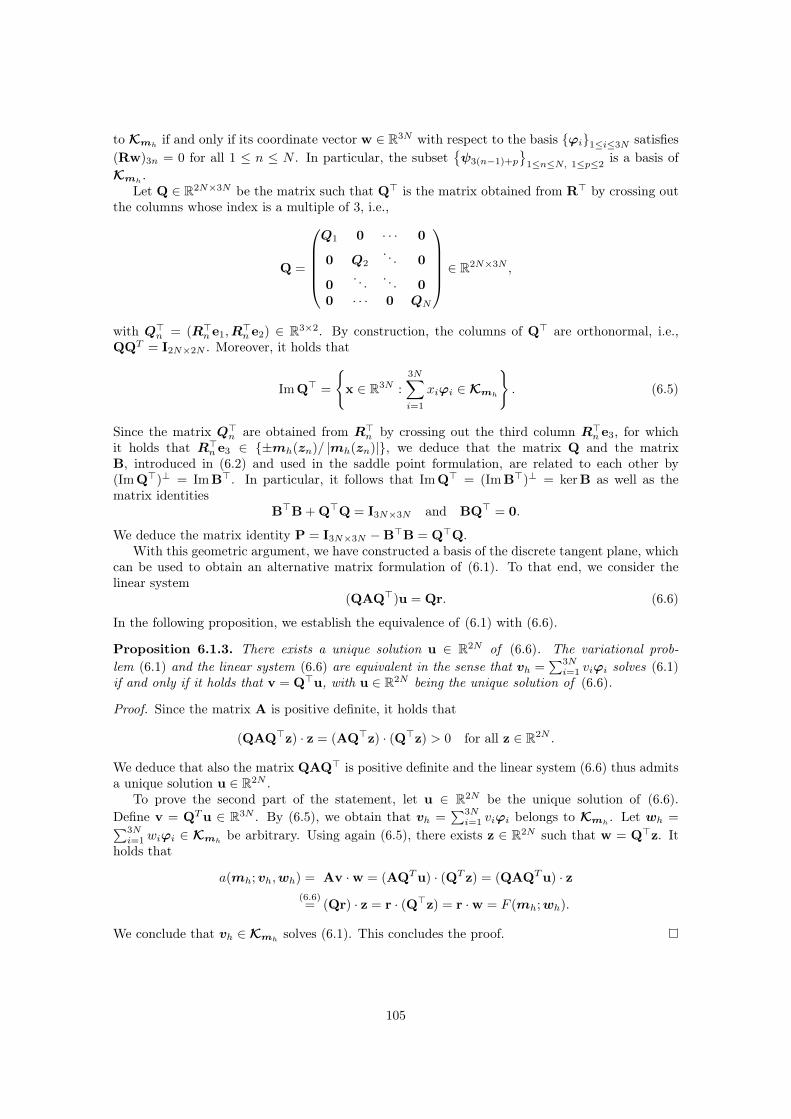
to Kmhif and only if its coordinate vector w ∈ R3N with respect to the basis ϕi1≤i≤3N satisfies

(Rw)3n = 0 for all 1 ≤ n ≤ N . In particular, the subsetψ3(n−1)+p

1≤n≤N, 1≤p≤2

is a basis ofKmh

.Let Q ∈ R2N×3N be the matrix such that Q> is the matrix obtained from R> by crossing out

the columns whose index is a multiple of 3, i.e.,

Q =

Q1 0 · · · 0

0 Q2. . . 0

0. . . . . . 0

0 · · · 0 QN

∈ R2N×3N ,

with Q>n = (R>n e1,R>n e2) ∈ R3×2. By construction, the columns of Q> are orthonormal, i.e.,

QQT = I2N×2N . Moreover, it holds that

Im Q> =

x ∈ R3N :

3N∑i=1

xiϕi ∈ Kmh

. (6.5)

Since the matrix Q>n are obtained from R>n by crossing out the third column R>n e3, for whichit holds that R>n e3 ∈ ±mh(zn)/ |mh(zn)|, we deduce that the matrix Q and the matrixB, introduced in (6.2) and used in the saddle point formulation, are related to each other by(Im Q>)⊥ = Im B>. In particular, it follows that Im Q> = (Im B>)⊥ = ker B as well as thematrix identities

B>B + Q>Q = I3N×3N and BQ> = 0.

We deduce the matrix identity P = I3N×3N −B>B = Q>Q.With this geometric argument, we have constructed a basis of the discrete tangent plane, which

can be used to obtain an alternative matrix formulation of (6.1). To that end, we consider thelinear system

(QAQ>)u = Qr. (6.6)

In the following proposition, we establish the equivalence of (6.1) with (6.6).

Proposition 6.1.3. There exists a unique solution u ∈ R2N of (6.6). The variational prob-lem (6.1) and the linear system (6.6) are equivalent in the sense that vh =

∑3Ni=1 viϕi solves (6.1)

if and only if it holds that v = Q>u, with u ∈ R2N being the unique solution of (6.6).

Proof. Since the matrix A is positive definite, it holds that

(QAQ>z) · z = (AQ>z) · (Q>z) > 0 for all z ∈ R2N .

We deduce that also the matrix QAQ> is positive definite and the linear system (6.6) thus admitsa unique solution u ∈ R2N .

To prove the second part of the statement, let u ∈ R2N be the unique solution of (6.6).Define v = QTu ∈ R3N . By (6.5), we obtain that vh =

∑3Ni=1 viϕi belongs to Kmh

. Let wh =∑3Ni=1 wiϕi ∈ Kmh

be arbitrary. Using again (6.5), there exists z ∈ R2N such that w = Q>z. Itholds that

a(mh;vh,wh) = Av ·w = (AQTu) · (QT z) = (QAQTu) · z(6.6)= (Qr) · z = r · (Q>z) = r ·w = F (mh;wh).

We conclude that vh ∈ Kmhsolves (6.1). This concludes the proof.

105

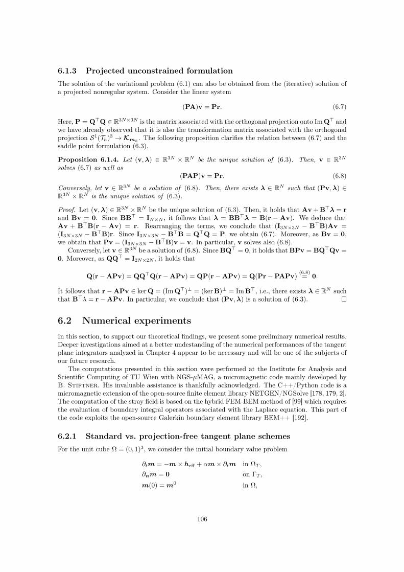
6.1.3 Projected unconstrained formulationThe solution of the variational problem (6.1) can also be obtained from the (iterative) solution ofa projected nonregular system. Consider the linear system

(PA)v = Pr. (6.7)

Here, P = Q>Q ∈ R3N×3N is the matrix associated with the orthogonal projection onto Im Q> andwe have already observed that it is also the transformation matrix associated with the orthogonalprojection S1(Th)3 → Kmh

. The following proposition clarifies the relation between (6.7) and thesaddle point formulation (6.3).

Proposition 6.1.4. Let (v,λ) ∈ R3N × RN be the unique solution of (6.3). Then, v ∈ R3N

solves (6.7) as well as(PAP)v = Pr. (6.8)

Conversely, let v ∈ R3N be a solution of (6.8). Then, there exists λ ∈ RN such that (Pv,λ) ∈R3N × RN is the unique solution of (6.3).

Proof. Let (v,λ) ∈ R3N ×RN be the unique solution of (6.3). Then, it holds that Av + B>λ = rand Bv = 0. Since BB> = IN×N , it follows that λ = BB>λ = B(r − Av). We deduce thatAv + B>B(r − Av) = r. Rearranging the terms, we conclude that (I3N×3N − B>B)Av =(I3N×3N − B>B)r. Since I3N×3N − B>B = Q>Q = P, we obtain (6.7). Moreover, as Bv = 0,we obtain that Pv = (I3N×3N −B>B)v = v. In particular, v solves also (6.8).

Conversely, let v ∈ R3N be a solution of (6.8). Since BQ> = 0, it holds that BPv = BQ>Qv =0. Moreover, as QQ> = I2N×2N , it holds that

Q(r−APv) = QQ>Q(r−APv) = QP(r−APv) = Q(Pr−PAPv)(6.8)= 0.

It follows that r−APv ∈ ker Q = (Im Q>)⊥ = (ker B)⊥ = Im B>, i.e., there exists λ ∈ RN suchthat B>λ = r−APv. In particular, we conclude that (Pv,λ) is a solution of (6.3).

6.2 Numerical experimentsIn this section, to support our theoretical findings, we present some preliminary numerical results.Deeper investigations aimed at a better undestanding of the numerical performances of the tangentplane integrators analyzed in Chapter 4 appear to be necessary and will be one of the subjects ofour future research.

The computations presented in this section were performed at the Institute for Analysis andScientific Computing of TU Wien with NGS-µMAG, a micromagnetic code mainly developed byB. Stiftner. His invaluable assistance is thankfully acknowledged. The C++/Python code is amicromagnetic extension of the open-source finite element library NETGEN/NGSolve [178, 179, 2].The computation of the stray field is based on the hybrid FEM-BEM method of [99] which requiresthe evaluation of boundary integral operators associated with the Laplace equation. This part ofthe code exploits the open-source Galerkin boundary element library BEM++ [192].

6.2.1 Standard vs. projection-free tangent plane schemesFor the unit cube Ω = (0, 1)3, we consider the initial boundary value problem

∂tm = −m× heff + αm× ∂tm in ΩT ,

∂nm = 0 on ΓT ,

m(0) = m0 in Ω,

106

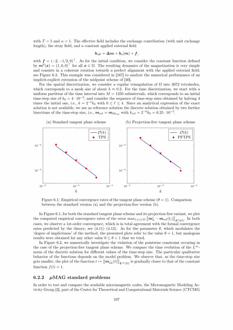
with T = 5 and α = 1. The effective field includes the exchange contribution (with unit exchangelength), the stray field, and a constant applied external field

heff = ∆m+ hs(m) + f ,

with f = (−2,−1/2, 0)>. As for the initial condition, we consider the constant function definedby m0(x) = (1, 0, 0)> for all x ∈ Ω. The resulting dynamics of the magnetization is very simpleand consists in a coherent rotation towards a perfect alignment with the applied external field;see Figure 6.3. This example was considered in [167] to analyze the numerical performance of animplicit-explicit extension of the midpoint scheme of [40].

For the spatial discretization, we consider a regular triangulation of Ω into 3072 tetrahedra,which corresponds to a mesh size of about h ≈ 0.2. For the time discretization, we start with auniform partition of the time interval into M = 1250 subintervals, which corresponds to an initialtime-step size of k0 = 4 · 10−3, and consider the sequence of time-step sizes obtained by halving 4times the initial one, i.e., k = 2−`k0 with 0 ≤ ` ≤ 4. Since an analytical expression of the exactsolution is not available, we use as reference solution the discrete solution obtained by two furtherbisections of the time-step size, i.e., mref = mhkref with kref = 2−6k0 = 6.25 · 10−5.

10−410−310−2

10−3

10−2

k

(a) Standard tangent plane scheme

O(k)TPS

10−410−310−2

10−3

10−2

k

(b) Projection-free tangent plane scheme

O(k)PFTPS

Figure 6.1: Empirical convergence rates of the tangent plane scheme (θ = 1). Comparisonbetween the standard version (a) and the projection-free version (b).

In Figure 6.1, for both the standard tangent plane scheme and its projection-free variant, we plotthe computed empirical convergence rates of the error max1≤i≤M

∥∥mih −mref(ti)

∥∥L2(Ω)

. In bothcases, we observe a 1st-order convergence, which is in total agreement with the formal convergencerates predicted by the theory; see (4.11)–(4.12). As for the parameter θ, which modulates the‘degree of implicitness’ of the method, the presented plots refer to the value θ = 1, but analogousresults were obtained for any other value 0 ≤ θ < 1 that we tried.

In Figure 6.2, we numerically investigate the violation of the pointwise constraint occuring inthe case of the projection-free tangent plane scheme. We compare the time evolution of the L∞-norm of the discrete solution for different values of the time-step size. The particular qualitativebehavior of the functions depends on the model problem. We observe that, as the time-step sizegets smaller, the plot of the function t 7→

∥∥m−hk(t)∥∥L∞(Ω)

is gradually closer to that of the constantfunction f(t) = 1.

6.2.2 µMAG standard problemsIn order to test and compare the available micromagnetic codes, the Micromagnetic Modeling Ac-tivity Group [3], part of the Center for Theoretical and Computational Materials Science (CTCMS)

107

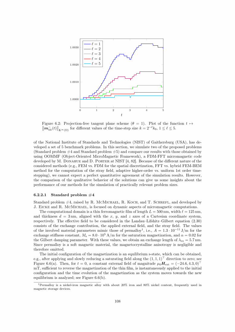
0 1 2 3 4 5

1.0000

1.0010

1.0020

1.0030

t

` = 1` = 2` = 3` = 4` = 5

Figure 6.2: Projection-free tangent plane scheme (θ = 1). Plot of the function t 7→∥∥m−hk(t)∥∥L∞(Ω)

for different values of the time-step size k = 2−`k0, 1 ≤ ` ≤ 5.

of the National Institute of Standards and Technologies (NIST) of Gaithersburg (USA), has de-veloped a set of 5 benchmark problems. In this section, we simulate two of the proposed problems(Standard problem #4 and Standard problem #5) and compare our results with those obtained byusing OOMMF (Object-Oriented MicroMagnetic Framework), a FDM-FFT micromagnetic codedeveloped by M. Donahue and D. Porter at NIST [4, 82]. Because of the different nature of theconsidered methods (e.g., FEM vs. FDM for the spatial discretization, FFT vs. hybrid FEM-BEMmethod for the computation of the stray field, adaptive higher-order vs. uniform 1st order time-stepping), we cannot expect a perfect quantitative agreement of the simulation results. However,the comparison of the qualitative behavior of the solutions can give us some insights about theperformance of our methods for the simulation of practically relevant problem sizes.

6.2.2.1 Standard problem #4

Standard problem #4, raised by R. McMichael, R. Koch, and T. Schrefl, and developed byJ. Eicke and R. McMichael, is focused on dynamic aspects of micromagnetic computations.

The computational domain is a thin ferromagnetic film of length L = 500 nm, width ` = 125 nm,and thickness d = 3 nm, aligned with the x, y, and z axes of a Cartesian coordinate system,respectively. The effective field to be considered in the Landau–Lifshitz–Gilbert equation (2.30)consists of the exchange contribution, the applied external field, and the stray field. The valuesof the involved material parameters mimic those of permalloy1, i.e., A = 1.3 · 10−11 J/m for theexchange stiffness constant, Ms = 8.0 · 105 A/m for the saturation magnetization, and α = 0.02 forthe Gilbert damping parameter. With these values, we obtain an exchange length of λex = 5.7 nm.Since permalloy is a soft magnetic material, the magnetocrystalline anisotropy is negligible andtherefore omitted.

The initial configuration of the magnetization is an equilibrium s-state, which can be obtained,e.g., after applying and slowly reducing a saturating field along the (1, 1, 1)> direction to zero; seeFigure 6.6(a). Then, for t = 0, a constant external field of magnitude µ0Hext = (−24.6, 4.3, 0)>

mT, sufficient to reverse the magnetization of the thin film, is instantaneously applied to the initialconfiguration and the time evolution of the magnetization as the system moves towards the newequilibrium is analyzed; see Figure 6.6(b).

1Permalloy is a nickel-iron magnetic alloy with about 20% iron and 80% nickel content, frequently used inmagnetic storage devices.

108

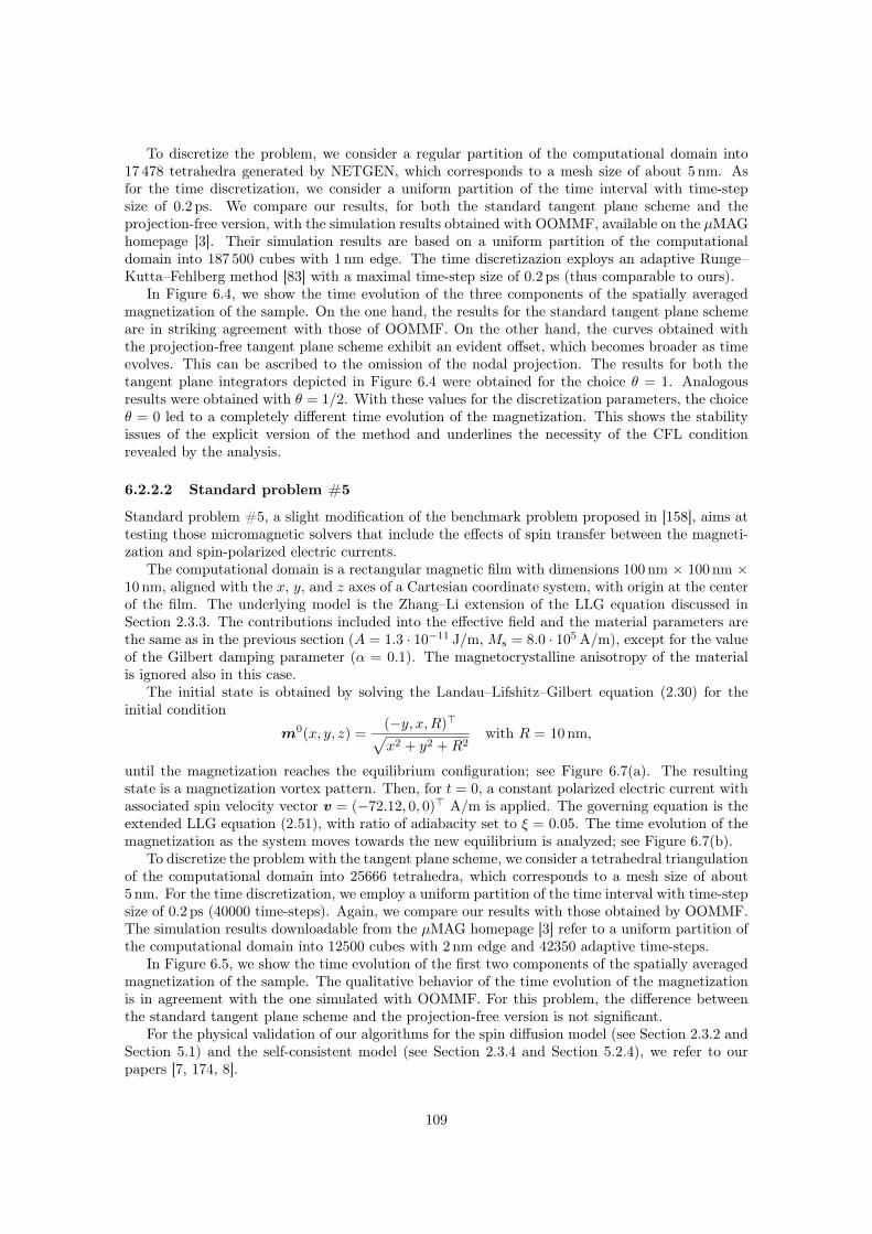
To discretize the problem, we consider a regular partition of the computational domain into17 478 tetrahedra generated by NETGEN, which corresponds to a mesh size of about 5 nm. Asfor the time discretization, we consider a uniform partition of the time interval with time-stepsize of 0.2 ps. We compare our results, for both the standard tangent plane scheme and theprojection-free version, with the simulation results obtained with OOMMF, available on the µMAGhomepage [3]. Their simulation results are based on a uniform partition of the computationaldomain into 187 500 cubes with 1 nm edge. The time discretizazion exploys an adaptive Runge–Kutta–Fehlberg method [83] with a maximal time-step size of 0.2 ps (thus comparable to ours).

In Figure 6.4, we show the time evolution of the three components of the spatially averagedmagnetization of the sample. On the one hand, the results for the standard tangent plane schemeare in striking agreement with those of OOMMF. On the other hand, the curves obtained withthe projection-free tangent plane scheme exhibit an evident offset, which becomes broader as timeevolves. This can be ascribed to the omission of the nodal projection. The results for both thetangent plane integrators depicted in Figure 6.4 were obtained for the choice θ = 1. Analogousresults were obtained with θ = 1/2. With these values for the discretization parameters, the choiceθ = 0 led to a completely different time evolution of the magnetization. This shows the stabilityissues of the explicit version of the method and underlines the necessity of the CFL conditionrevealed by the analysis.

6.2.2.2 Standard problem #5

Standard problem #5, a slight modification of the benchmark problem proposed in [158], aims attesting those micromagnetic solvers that include the effects of spin transfer between the magneti-zation and spin-polarized electric currents.

The computational domain is a rectangular magnetic film with dimensions 100 nm × 100 nm ×10 nm, aligned with the x, y, and z axes of a Cartesian coordinate system, with origin at the centerof the film. The underlying model is the Zhang–Li extension of the LLG equation discussed inSection 2.3.3. The contributions included into the effective field and the material parameters arethe same as in the previous section (A = 1.3 · 10−11 J/m, Ms = 8.0 · 105 A/m), except for the valueof the Gilbert damping parameter (α = 0.1). The magnetocrystalline anisotropy of the materialis ignored also in this case.

The initial state is obtained by solving the Landau–Lifshitz–Gilbert equation (2.30) for theinitial condition

m0(x, y, z) =(−y, x,R)>√x2 + y2 +R2

with R = 10 nm,

until the magnetization reaches the equilibrium configuration; see Figure 6.7(a). The resultingstate is a magnetization vortex pattern. Then, for t = 0, a constant polarized electric current withassociated spin velocity vector v = (−72.12, 0, 0)> A/m is applied. The governing equation is theextended LLG equation (2.51), with ratio of adiabacity set to ξ = 0.05. The time evolution of themagnetization as the system moves towards the new equilibrium is analyzed; see Figure 6.7(b).

To discretize the problem with the tangent plane scheme, we consider a tetrahedral triangulationof the computational domain into 25666 tetrahedra, which corresponds to a mesh size of about5 nm. For the time discretization, we employ a uniform partition of the time interval with time-stepsize of 0.2 ps (40000 time-steps). Again, we compare our results with those obtained by OOMMF.The simulation results downloadable from the µMAG homepage [3] refer to a uniform partition ofthe computational domain into 12500 cubes with 2 nm edge and 42350 adaptive time-steps.

In Figure 6.5, we show the time evolution of the first two components of the spatially averagedmagnetization of the sample. The qualitative behavior of the time evolution of the magnetizationis in agreement with the one simulated with OOMMF. For this problem, the difference betweenthe standard tangent plane scheme and the projection-free version is not significant.

For the physical validation of our algorithms for the spin diffusion model (see Section 2.3.2 andSection 5.1) and the self-consistent model (see Section 2.3.4 and Section 5.2.4), we refer to ourpapers [7, 174, 8].

109

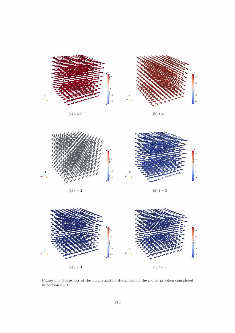
(a) t = 0 (b) t = 1

(c) t = 2 (d) t = 3

(e) t = 4 (f) t = 5

Figure 6.3: Snapshots of the magnetization dynamics for the model problem consideredin Section 6.2.1.

110

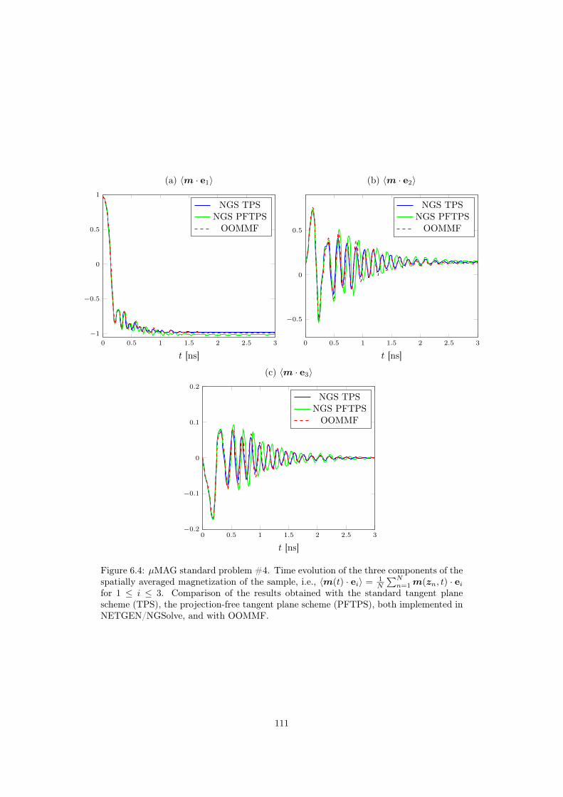
0 0.5 1 1.5 2 2.5 3

−1

−0.5

0

0.5

1

t [ns]

(a) 〈m · e1〉

NGS TPSNGS PFTPSOOMMF

0 0.5 1 1.5 2 2.5 3

−0.5

0

0.5

t [ns]

(b) 〈m · e2〉


0 0.5 1 1.5 2 2.5 3−0.2

−0.1

0

0.1

0.2

t [ns]

(c) 〈m · e3〉


Figure 6.4: µMAG standard problem #4. Time evolution of the three components of thespatially averaged magnetization of the sample, i.e., 〈m(t) · ei〉 = 1

N

∑Nn=1m(zn, t) · ei

for 1 ≤ i ≤ 3. Comparison of the results obtained with the standard tangent planescheme (TPS), the projection-free tangent plane scheme (PFTPS), both implemented inNETGEN/NGSolve, and with OOMMF.

111

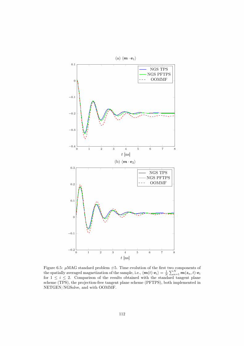
0 1 2 3 4 5 6 7 8−0.4

−0.3

−0.2

−0.1

0

0.1

t [ns]

(a) 〈m · e1〉


0 1 2 3 4 5 6 7 8−0.2

−0.1

0

0.1

0.2

0.3

t [ns]

(b) 〈m · e2〉


Figure 6.5: µMAG standard problem #5. Time evolution of the first two components ofthe spatially averaged magnetization of the sample, i.e., 〈m(t)·ei〉 = 1

N

∑Nn=1m(zn, t)·ei

for 1 ≤ i ≤ 2. Comparison of the results obtained with the standard tangent planescheme (TPS), the projection-free tangent plane scheme (PFTPS), both implemented inNETGEN/NGSolve, and with OOMMF.

112

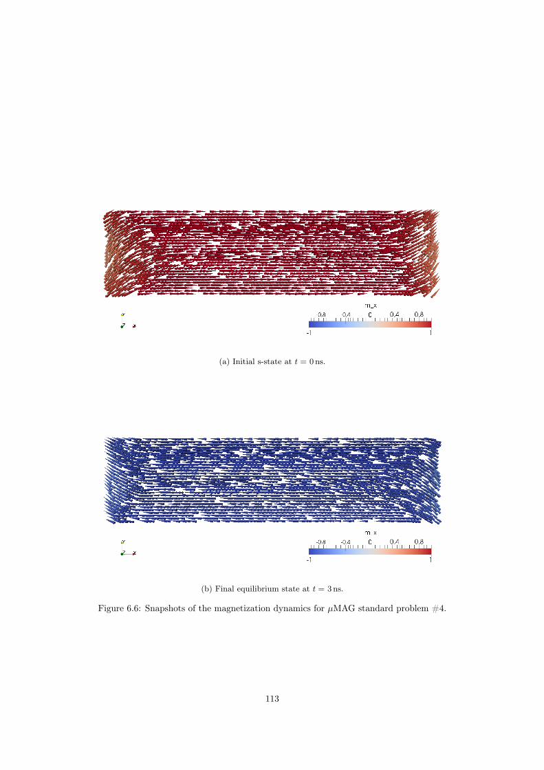
(a) Initial s-state at t = 0ns.

(b) Final equilibrium state at t = 3ns.

Figure 6.6: Snapshots of the magnetization dynamics for µMAG standard problem #4.

113

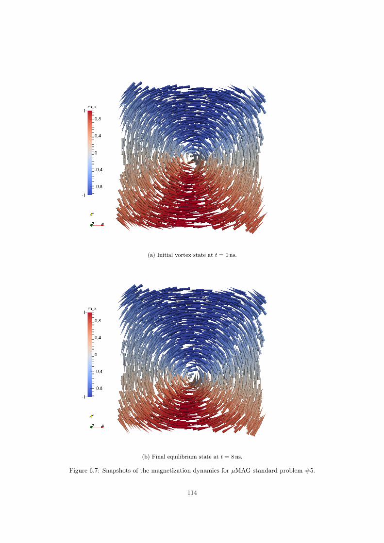
(a) Initial vortex state at t = 0ns.

(b) Final equilibrium state at t = 8ns.

Figure 6.7: Snapshots of the magnetization dynamics for µMAG standard problem #5.

114

Chapter 7

Perspectives and future work

With this dissertation, we have tried to contribute to the study of reliable and effective numericalmethods for the simulation of time-dependent micromagnetic phenomena. The main focus of ourwork has been on the development of (unconditionally) convergent integrators which are suitablefor the efficient treatment of coupled systems of PDEs, in which the LLG equation is coupled withanother equation that models a particular nonlocal effective field contribution. However, thereare a number of possible extensions and improvements of the presented results, related interestingquestions, and open problems that, in our opinion, are worth to be investigated. In this chapter,we aim to give a short outlook of some of them.

• Numerical analysis of tangent plane integrators

In Chapter 4, we have provided a unified analysis of the tangent plane scheme which combinesand extends the results of the original papers [14, 39, 12, 16, 56, 6]. Future work will addresssome of the aspects not covered by the present dissertation, such as the derivation of a priori errorestimates (recently proved in [93] for the projection-free variant of the scheme of [6], but still openfor the standard version of the method) and a posteriori error estimates, which will be the startingpoint for the development of adaptive algorithms for the LLG equation. Preliminary results in thisdirection can be found, e.g., in [22, 23].

One difficult task concerns the development of higher-order methods in both time and space.State-of-the-art numerical integrators for the LLG equation used in computational physics areusually based on higher-order black-box adaptive time discretizations; see, e.g., [194]. An (almost)2nd order version in time of the tangent plane scheme was introduced in [16, 15]. However,the proposed strategy is based on an implicit treatment of the lower-order effective field terms(including the nonlocal and expensive-to-compute stray field), which is not fully attractive fromthe computational point of view, as, in particular, it breaks the linearity of the scheme in thepresence of nonlinear field contributions. Extensions to higher-order methods in space would alsobe of great interest. In this context, the main difficulties stem from the nonconvex pointwiseconstraint. For instance, to our knowledge, it is not clear if the result of Proposition 3.4.11, i.e.,the fact that the nodal projection mapping does not increase the Dirichlet energy of piecewiselinear polynomials for weakly acute triangulations, can be transferred to higher-order polynomials.

Moreover, practically relevant problem sizes require efficient iterative solvers for the involvedlinear systems. Together with D. Praetorius and B. Stiftner, we are currently analyzing thepreconditioning for the solution strategies presented in Section 6.1; see [168]. The goal is to avoidthe recomputation of the preconditioners in each time step of the time-marching scheme, whichshould be possible as long as the time discretization is sufficiently fine so that the magnetizationdoes not change too rapidly.

• Numerical analysis of the midpoint scheme of [40]

Together with D. Praetorius, and B. Stiftner, we are investigating some open questions relatedto the midpoint scheme of [40]. We have recently shown that an implicit-explicit approach for the

115

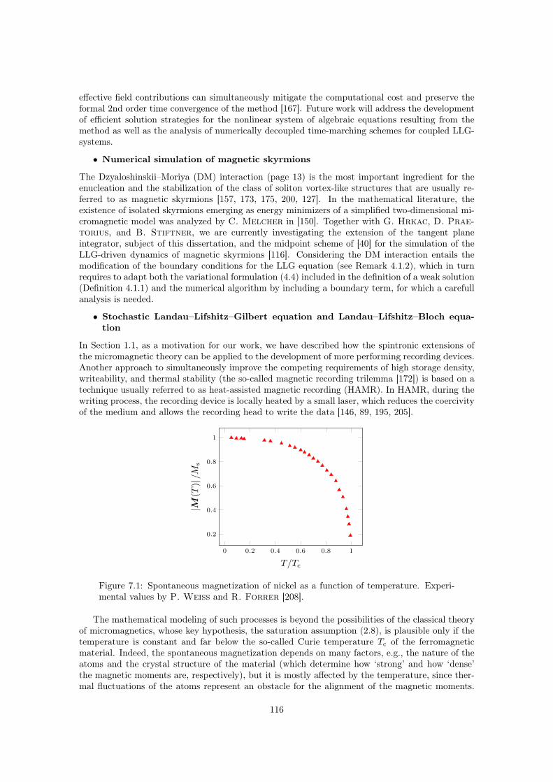
effective field contributions can simultaneously mitigate the computational cost and preserve theformal 2nd order time convergence of the method [167]. Future work will address the developmentof efficient solution strategies for the nonlinear system of algebraic equations resulting from themethod as well as the analysis of numerically decoupled time-marching schemes for coupled LLG-systems.

• Numerical simulation of magnetic skyrmions

The Dzyaloshinskii–Moriya (DM) interaction (page 13) is the most important ingredient for theenucleation and the stabilization of the class of soliton vortex-like structures that are usually re-ferred to as magnetic skyrmions [157, 173, 175, 200, 127]. In the mathematical literature, theexistence of isolated skyrmions emerging as energy minimizers of a simplified two-dimensional mi-cromagnetic model was analyzed by C. Melcher in [150]. Together with G. Hrkac, D. Prae-torius, and B. Stiftner, we are currently investigating the extension of the tangent planeintegrator, subject of this dissertation, and the midpoint scheme of [40] for the simulation of theLLG-driven dynamics of magnetic skyrmions [116]. Considering the DM interaction entails themodification of the boundary conditions for the LLG equation (see Remark 4.1.2), which in turnrequires to adapt both the variational formulation (4.4) included in the definition of a weak solution(Definition 4.1.1) and the numerical algorithm by including a boundary term, for which a carefullanalysis is needed.

• Stochastic Landau–Lifshitz–Gilbert equation and Landau–Lifshitz–Bloch equa-tion

In Section 1.1, as a motivation for our work, we have described how the spintronic extensions ofthe micromagnetic theory can be applied to the development of more performing recording devices.Another approach to simultaneously improve the competing requirements of high storage density,writeability, and thermal stability (the so-called magnetic recording trilemma [172]) is based on atechnique usually referred to as heat-assisted magnetic recording (HAMR). In HAMR, during thewriting process, the recording device is locally heated by a small laser, which reduces the coercivityof the medium and allows the recording head to write the data [146, 89, 195, 205].

0 0.2 0.4 0.6 0.8 1

0.2

0.4

0.6

0.8

1

T/Tc

|M(T

)|/M

s

Figure 7.1: Spontaneous magnetization of nickel as a function of temperature. Experi-mental values by P. Weiss and R. Forrer [208].

The mathematical modeling of such processes is beyond the possibilities of the classical theoryof micromagnetics, whose key hypothesis, the saturation assumption (2.8), is plausible only if thetemperature is constant and far below the so-called Curie temperature Tc of the ferromagneticmaterial. Indeed, the spontaneous magnetization depends on many factors, e.g., the nature of theatoms and the crystal structure of the material (which determine how ‘strong’ and how ‘dense’the magnetic moments are, respectively), but it is mostly affected by the temperature, since ther-mal fluctuations of the atoms represent an obstacle for the alignment of the magnetic moments.

116

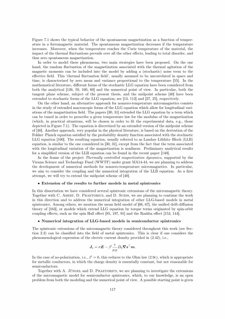
Figure 7.1 shows the typical behavior of the spontaneous magnetization as a function of temper-ature in a ferromagnetic material. The spontaneous magnetization decreases if the temperatureincreases. Moreover, when the temperature reaches the Curie temperature of the material, theimpact of the thermal fluctuations prevails over all the other effects, leading to total disorder, andthus zero spontaneous magnetization.

In order to model these phenomena, two main strategies have been proposed. On the onehand, the random fluctuation of the magnetization associated with the thermal agitation of themagnetic moments can be included into the model by adding a (stochastic) noise term to theeffective field. This ‘thermal fluctuation field’, usually assumed to be uncorrelated in space andtime, is characterized by zero mean and variance proportional to the temperature [55]. In themathematical literature, different forms of the stochastic LLG equation have been considered fromboth the analytical [126, 59, 160, 60] and the numerical point of view. In particular, both thetangent plane scheme, subject of the present thesis, and the midpoint scheme [40] have beenextended to stochastic forms of the LLG equation; see [13, 112] and [27, 25], respectively.

On the other hand, an alternative approach for nonzero-temperature micromagnetics consistsin the study of extended macroscopic forms of the LLG equation which allow for longitudinal vari-ations of the magnetization field. The papers [30, 31] extended the LLG equation by a term whichcan be tuned in order to prescribe a given temperature law for the modulus of the magnetization(which, in practical situations, will be chosen in order to fit the experimental data, e.g., thosedepicted in Figure 7.1). The equation is discretized by an extended version of the midpoint schemeof [40]. Another approach, very popular in the physical literature, is based on the derivation of theFokker–Planck equation satisfied by the probability density function associated with the stochasticLLG equation [100]. The resulting equation, usually referred to as Landau–Lifshitz–Bloch (LLB)equation, is similar to the one considered in [30, 31], except from the fact that the term associatedwith the longitudinal variation of the magnetization is nonlinear. Preliminary analytical resultsfor a simplified version of the LLB equation can be found in the recent paper [140].

In the frame of the project Thermally controlled magnetization dynamics, supported by theVienna Science and Technology Fund (WWTF) under grant MA14-44, we are planning to addressthe development of numerical methods for nonzero-temperature micromagnetics. In particular,we aim to consider the coupling and the numerical integration of the LLB equation. As a firstattempt, we will try to extend the midpoint scheme of [40].

• Extension of the results to further models in metal spintronics

In this dissertation we have considered several spintronic extensions of the micromagnetic theory.Together with C. Abert, D. Praetorius, and D. Suess, we are planning to continue the workin this direction and to address the numerical integration of other LLG-based models in metalspintronics. Among others, we mention the mean field model of [66, 67], the unified drift-diffusiontheory of [163], or models which extend LLG equation by torque terms originated by spin-orbitcoupling effects, such as the spin Hall effect [85, 197, 91] and the Rashba effect [153, 144].

• Numerical integration of LLG-based models in semiconductor spintronics

The spintronic extensions of the micromagnetic theory considered throughout this work (see Sec-tion 2.3) can be classified into the field of metal spintronics. This is clear if one considers thephenomenological expression of the electric current density provided in (2.42), i.e.,

Je = σE − β′ eµB

D0∇s>m.

In the case of no-polarization, i.e., β′ = 0, this reduces to the Ohm law (2.9c), which is appropriatefor metallic conductors, in which the charge density is essentially constant, but not reasonable forsemiconductors.

Together with A. Jüngel and D. Praetorius, we are planning to investigate the extensionsof the micromagnetic model for semiconductor spintronics, which, to our knowledge, is an openproblem from both the modeling and the numerical point of view. A possible starting point is given

117

by the spinorial matrix drift-diffusion model of [165], analyzed in [121], and discretized by a finitevolume method in the two-dimensional case in [64]. In the model, which consists of a nonlinearsystem of drift-diffusion equations for the charge density and the spin density that is further coupledto the electrostatic Maxwell equations for the electric potential, the magnetization is assumed to beconstant. We will remove this assumption and start by considering the finite element discretizationof the coupling of this system with the LLG equation, for which some preliminary analytical resultsare already available [210, 211]. We believe that our approach, based on the numerical decouplingof the time integration of the LLG equation and the coupled system, can be an effective tool forthe treatment of the strong nonlinearities which characterize the problem.

118

Appendix A

Physical quantities, constants andunits

For the convenience of the reader, in this appendix we collect the physical quantities and thephysical constants considered throughout the thesis. We use physical units in the InternationalSystem of Units (SI).

A.1 Physical quantities

Quantity Symbol UnitAngular momentum L J sAnisotropy constant K J/m3

Bloch parameter δ0 mBloch wall width δ mConductivity σ, σ A/(m V)Curie temperature Tc KDiffusion coefficient D0 m2/sDisplacement u mDM constant D J/m2

Electric charge density ρ C/m3

Electric current density Je, Je A/m2

Electric displacement field D C/m2

Electric field E V/mElectric permittivity ε, ε F/mElectric potential V VEnergy E JExchange integral J JExchange length λex mExchange stiffness constant A J/mGilbert damping parameter α –Magnetic field H A/mMagnetic flux density B TMagnetic hardness parameter q –Magnetic moment µ J/TMagnetic permeability µ N/A2

Magnetization M A/mMagnetization (normalized) m –

119

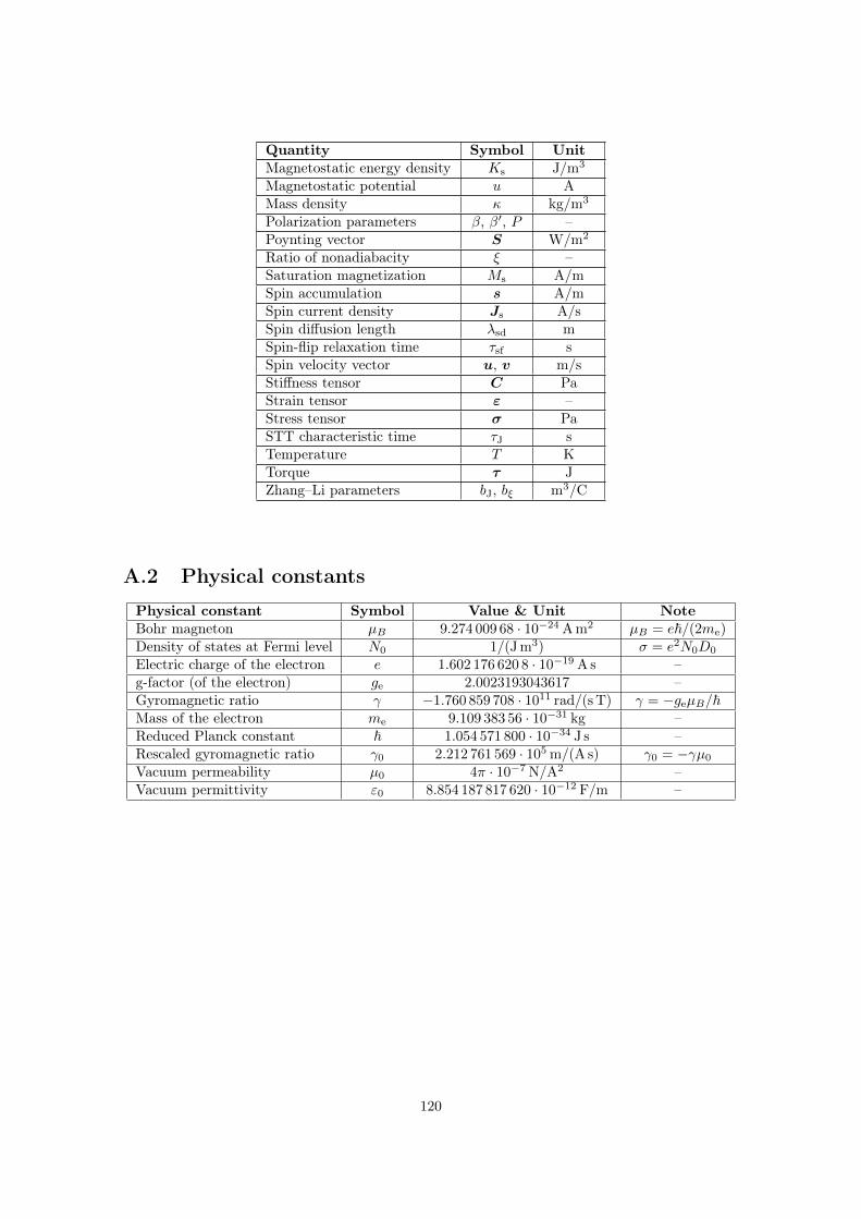
Quantity Symbol UnitMagnetostatic energy density Ks J/m3

Magnetostatic potential u AMass density κ kg/m3

Polarization parameters β, β′, P –Poynting vector S W/m2

Ratio of nonadiabacity ξ –Saturation magnetization Ms A/mSpin accumulation s A/mSpin current density Js A/sSpin diffusion length λsd mSpin-flip relaxation time τsf sSpin velocity vector u, v m/sStiffness tensor C PaStrain tensor ε –Stress tensor σ PaSTT characteristic time τJ sTemperature T KTorque τ JZhang–Li parameters bJ, bξ m3/C

A.2 Physical constants

Physical constant Symbol Value & Unit NoteBohr magneton µB 9.274 009 68 · 10−24 A m2 µB = e~/(2me)Density of states at Fermi level N0 1/(J m3) σ = e2N0D0

Electric charge of the electron e 1.602 176 620 8 · 10−19 A s –g-factor (of the electron) ge 2.0023193043617 –Gyromagnetic ratio γ −1.760 859 708 · 1011 rad/(s T) γ = −geµB/~Mass of the electron me 9.109 383 56 · 10−31 kg –Reduced Planck constant ~ 1.054 571 800 · 10−34 J s –Rescaled gyromagnetic ratio γ0 2.212 761 569 · 105 m/(A s) γ0 = −γµ0

Vacuum permeability µ0 4π · 10−7 N/A2 –Vacuum permittivity ε0 8.854 187 817 620 · 10−12 F/m –

120

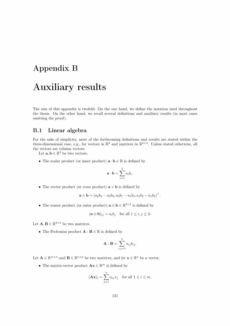
Appendix B

Auxiliary results

The aim of this appendix is twofold: On the one hand, we define the notation used throughoutthe thesis. On the other hand, we recall several definitions and auxiliary results (in most casesomitting the proof).

B.1 Linear algebraFor the sake of simplicity, most of the forthcoming definitions and results are stated within thethree-dimensional case, e.g., for vectors in R3 and matrices in R3×3. Unless stated otherwise, allthe vectors are column vectors.

Let a,b ∈ R3 be two vectors.

• The scalar product (or inner product) a · b ∈ R is defined by

a · b =

3∑i=1

aibi.

• The vector product (or cross product) a× b is defined by

a× b = (a2b3 − a3b2, a3b1 − a1b3, a1b2 − a1b2)>.

• The tensor product (or outer product) a⊗ b ∈ R3×3 is defined by

(a⊗ b)ij = aibj for all 1 ≤ i, j ≤ 3.

Let A,B ∈ R3×3 be two matrices.

• The Frobenius product A : B ∈ R is defined by

A : B =

3∑i,j=1

aijbij .

Let A ∈ Rm×n and B ∈ Rn×p be two matrices, and let x ∈ Rn be a vector.

• The matrix-vector product Ax ∈ Rm is defined by

(Ax)i =

n∑j=1

aijxj for all 1 ≤ i ≤ m.

121

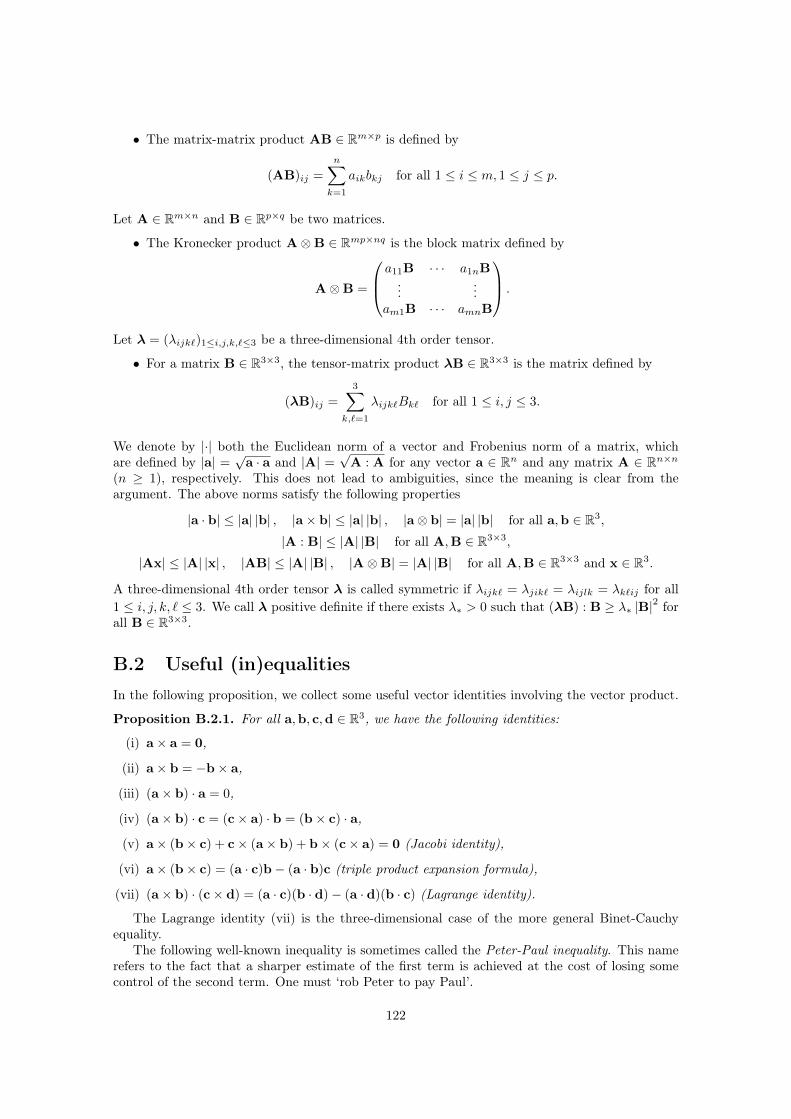
• The matrix-matrix product AB ∈ Rm×p is defined by

(AB)ij =

n∑k=1

aikbkj for all 1 ≤ i ≤ m, 1 ≤ j ≤ p.

Let A ∈ Rm×n and B ∈ Rp×q be two matrices.

• The Kronecker product A⊗B ∈ Rmp×nq is the block matrix defined by

A⊗B =

a11B · · · a1nB...

...am1B · · · amnB

.

Let λ = (λijk`)1≤i,j,k,`≤3 be a three-dimensional 4th order tensor.

• For a matrix B ∈ R3×3, the tensor-matrix product λB ∈ R3×3 is the matrix defined by

(λB)ij =

3∑k,`=1

λijk`Bk` for all 1 ≤ i, j ≤ 3.

We denote by |·| both the Euclidean norm of a vector and Frobenius norm of a matrix, whichare defined by |a| =

√a · a and |A| =

√A : A for any vector a ∈ Rn and any matrix A ∈ Rn×n

(n ≥ 1), respectively. This does not lead to ambiguities, since the meaning is clear from theargument. The above norms satisfy the following properties

|a · b| ≤ |a| |b| , |a× b| ≤ |a| |b| , |a⊗ b| = |a| |b| for all a,b ∈ R3,

|A : B| ≤ |A| |B| for all A,B ∈ R3×3,

|Ax| ≤ |A| |x| , |AB| ≤ |A| |B| , |A⊗B| = |A| |B| for all A,B ∈ R3×3 and x ∈ R3.

A three-dimensional 4th order tensor λ is called symmetric if λijk` = λjik` = λijlk = λk`ij for all1 ≤ i, j, k, ` ≤ 3. We call λ positive definite if there exists λ∗ > 0 such that (λB) : B ≥ λ∗ |B|2 forall B ∈ R3×3.

B.2 Useful (in)equalitiesIn the following proposition, we collect some useful vector identities involving the vector product.

Proposition B.2.1. For all a,b, c,d ∈ R3, we have the following identities:

(i) a× a = 0,

(ii) a× b = −b× a,

(iii) (a× b) · a = 0,

(iv) (a× b) · c = (c× a) · b = (b× c) · a,

(v) a× (b× c) + c× (a× b) + b× (c× a) = 0 (Jacobi identity),

(vi) a× (b× c) = (a · c)b− (a · b)c (triple product expansion formula),

(vii) (a× b) · (c× d) = (a · c)(b · d)− (a · d)(b · c) (Lagrange identity).

The Lagrange identity (vii) is the three-dimensional case of the more general Binet-Cauchyequality.

The following well-known inequality is sometimes called the Peter-Paul inequality. This namerefers to the fact that a sharper estimate of the first term is achieved at the cost of losing somecontrol of the second term. One must ‘rob Peter to pay Paul’.

122

Lemma B.2.2 (weighted Young’s inequality). For all a, b ∈ R and δ > 0, it holds that

ab ≤ δ

2a2 +

1

2δb2.

Proof. Since 2xy ≤ x2 + y2 for all x, y ∈ R, it follows that

ab ≤(√

δa)( 1√

δb

)≤ δ

2a2 +

1

2δb2,

which is the requested inequality.

The following lemma states a simple algebraic trick which often simplifies the computation andthe estimation of sums. It is named after N. H. Abel.

Lemma B.2.3 (Abel’s summation by parts). Given an integer j ≥ 1, let ai0≤i≤j ⊂ Rn. Then,it holds that

j−1∑i=0

(ai+1 − ai) · ai+1 =1

2|aj |2 −

1

2|a0|2 +

1

2

j−1∑i=0

|ai+1 − ai|2 .

Proof. Let 0 ≤ i ≤ j − 1. It holds that

2(ai+1 − ai) · ai+1 = |ai+1|2 − ai+1 · ai + (ai+1 − ai) · ai+1

= |ai+1|2 − ai+1 · ai + (ai+1 − ai) · ai+1 − |ai|2 + |ai|2

= |ai+1|2 − |ai|2 + (ai+1 − ai) · ai+1 − (ai+1 − ai) · ai= |ai+1|2 − |ai|2 + |ai+1 − ai|2 .

Summation over 0 ≤ i ≤ j − 1 yields the assertion.

The following lemma is a discrete counterpart of Gronwall’s inequality (also called Gronwall’slemma or Gronwall-Bellman inequality), an important tool to derive estimates in the theory ofordinary differential equations. The differential form of the result was proved by T. H. Gronwallin 1919.

Lemma B.2.4 (discrete Gronwall lemma). Let αjj≥0, βjj≥0, and wjj≥0 be sequences ofreal numbers such that

αj ≤ αj+1, βj ≥ 0, and wj ≤ αj +

j−1∑i=0

βiwi for all j ≥ 0.

Then, it holds that

wj ≤ αj exp

j−1∑i=0

βi for all j ≥ 0.

For the proof, we refer the interested reader to [199, Lemma 10.5].

B.3 Vector calculusLet Ω ⊂ R3 be an open set. The gradient of a scalar-valued function f : Ω → R is denoted by∇f = (∂1f, ∂2f, ∂3f)>. For a vector-valued function f = (f1, f2, f3)> : Ω → R3, we denote theJacobian by ∇f , i.e., (∇f)ij = ∂jfi for all 1 ≤ i, j ≤ 3, the divergence by ∇ · f , and the curl by∇×f . The Laplace operator of f is denoted by ∆f = ∇· (∇f). We define the divergence ∇ ·F ofa matrix-valued function F : Ω→ R3×3 as the vector of the divergences of the rows of the matrix,i.e., (∇ · F )i = ∇ · (Fi1, Fi2, Fi3)> for all 1 ≤ i ≤ 3. The Laplace operator of f is denoted by∆f = ∇ · (∇f) and coincides with the vector of the Laplace operator of the components of f . It

123

follows that ∇ × (∇f) = 0 and ∇ · (∇ × f) = 0. For the vector-valued functions f ,h : Ω → R3,abusing our notation, we write

∇f × h = (∂1f × h, ∂2f × h, ∂3f × h).

We define (f · ∇)h by

[(f · ∇)h]i =

3∑k=1

fk∂khi = f · ∇hi for all 1 ≤ i ≤ 3,

and note that (f · ∇)h coincides with the matrix-vector product of ∇h and f . From the well-known product rule ∂i(fg) = ∂if g + f ∂ig, simple (but possibly lengthy) computations prove theidentities collected in the following proposition.

Proposition B.3.1. Let Ω ⊂ R3 be an open set. For all sufficiently smooth functions f, h : Ω→ R,f ,h : Ω→ R3, we have the following product rules:

(i) ∇(fh) = f∇h+ h∇f ,

(ii) ∇(f · h) = ∇f>h+ ∇h>f = (f · ∇)h+ (h · ∇)f + f × (∇× h) + h× (∇× f),

(iii) ∇(f × h) = ∇f × h+ f ×∇h,

(iv) ∇(fh) = h⊗∇f + f∇h,

(v) ∇ · (fh) = ∇f · h+ f∇ · h,

(vi) ∇ · (f × h) = (∇× f) · h− (∇× h) · f ,

(vii) ∇ · (f ⊗ h) = (∇ · f)h+ (f · ∇)h,

(viii) ∇× (fh) = ∇f × h+ f∇× h,

(ix) ∇× (f × h) = (∇ · h)f − (∇ · f)h+ (h · ∇)f − (f · ∇)h,

(x) ∇× (∇× f) = ∇(∇ · f)−∆f ,

(xi) ∇(|f |) = |f |−1 ∇f>f ,

(xii) ∇(f/ |f |) = |f |−1(I − |f |−2

f ⊗ f)∇f .

124

References

[1] Hard disk drive. https://en.wikipedia.org/wiki/Hard_disk_drive. Accessed on Octo-ber 10, 2016.

[2] NGSolve Finite Element Library. https://sourceforge.net/projects/ngsolve/. Ac-cessed on September 24, 2016.

[3] NIST micromagnetic modeling activity group (µMAG) website. http://www.ctcms.nist.gov/~rdm/mumag.html. Accessed on October 10, 2016.

[4] The Object Oriented MicroMagnetic Framework (OOMMF) project at ITL/NIST. http://math.nist.gov/oommf/. Accessed on October 10, 2016.

[5] Abert, C., Exl, L., Bruckner, F., Drews, A., and Suess, D. magnum.fe: A mi-cromagnetic finite-element simulation code based on FEniCS. J. Magn. Magn. Mater. 345(2013), 29–35.

[6] Abert, C., Hrkac, G., Page, M., Praetorius, D., Ruggeri, M., and Suess, D.Spin-polarized transport in ferromagnetic multilayers: An unconditionally convergent FEMintegrator. Comput. Math. Appl. 68, 6 (2014), 639–654.

[7] Abert, C., Ruggeri, M., Bruckner, F., Vogler, C., Hrkac, G., Praetorius, D.,and Suess, D. A three-dimensional spin-diffusion model for micromagnetics. Sci. Rep. 5(2015), 14855.

[8] Abert, C., Ruggeri, M., Bruckner, F., Vogler, C., Manchon, A., Praetorius,D., and Suess, D. A self-consistent spin-diffusion model for micromagnetics. Accepted forpublication in Sci. Rep., preprint available at arXiv:1512.05519, 2016.

[9] Aharoni, A. Introduction to the theory of ferromagnetism, second ed., vol. 109 of Interna-tional Series of Monographs on Physics. Oxford University Press, 2001.

[10] Alonso Rodríguez, A., and Valli, A. Eddy current approximation of Maxwell equa-tions: Theory, algorithms and applications, vol. 4 of Modeling, Simulation and Applications.Springer, 2010.

[11] Alouges, F. A new algorithm for computing liquid crystal stable configurations: Theharmonic mapping case. SIAM J. Numer. Anal. 34, 5 (1997), 1708–1726.

[12] Alouges, F. A new finite element scheme for Landau–Lifchitz equations. Discrete Contin.Dyn. Syst. Ser. S 1, 2 (2008), 187–196.

[13] Alouges, F., de Bouard, A., and Hocquet, A. A semi-discrete scheme for the stochasticLandau–Lifshitz equation. Stoch. Partial Differ. Equ. Anal. Comput. 2, 3 (2014), 281–315.

[14] Alouges, F., and Jaisson, P. Convergence of a finite element discretization for theLandau–Lifshitz equation in micromagnetism. Math. Models Methods Appl. Sci. 16, 2 (2006),299–316.

125

https://en.wikipedia.org/wiki/Hard_disk_drive

https://sourceforge.net/projects/ngsolve/

http://www.ctcms.nist.gov/~rdm/mumag.html

http://www.ctcms.nist.gov/~rdm/mumag.html

http://math.nist.gov/oommf/

http://math.nist.gov/oommf/

https://arxiv.org/abs/1512.05519

[15] Alouges, F., Kritsikis, E., Steiner, J., and Toussaint, J.-C. A convergent andprecise finite element scheme for Landau–Lifschitz–Gilbert equation. Numer. Math. 128, 3(2014), 407–430.

[16] Alouges, F., Kritsikis, E., and Toussaint, J.-C. A convergent finite element approx-imation for Landau–Lifschitz–Gilbert equation. Physica B 407, 9 (2012), 1345–1349.

[17] Alouges, F., and Soyeur, A. On global weak solutions for Landau–Lifshitz equations:Existence and nonuniqueness. Nonlinear Anal. 18, 11 (1992), 1071–1084.

[18] Ansermet, J.-P. Classical description of spin wave excitation by currents in bulk ferro-magnets. IEEE Trans. Magn. 40, 2 (2004), 358–360.

[19] Baibich, M. N., Broto, J. M., Fert, A., Van Dau, F. N., Petroff, F., Eti-enne, P., Creuzet, G., Friederich, A., and Chazelas, J. Giant magnetoresistance of(001)Fe/(001)Cr magnetic superlattices. Phys. Rev. Lett. 61, 21 (1988), 2472–2475.

[20] Baňas, L. A numerical method for the Landau–Lifshitz equation with magnetostriction.Math. Methods Appl. Sci. 28, 16 (2005), 1939–1954.

[21] Baňas, L. Numerical methods for the Landau–Lifshitz–Gilbert equation. In Numericalanalysis and its applications, Z. Li, L. Vulkov, and J. Waśniewski, Eds., vol. 3401 of LectureNotes in Computer Science. Springer, 2005, pp. 158–165.

[22] Baňas, L. Adaptive methods for dynamical micromagnetics. In Numerical Mathematicsand Advanced Applications, A. Bermúdez de Castro, D. Gómez, P. Quintela, and P. Salgado,Eds. Springer, 2006, pp. 531–538.

[23] Baňas, L. Adaptive techniques for Landau–Lifshitz–Gilbert equation with magnetostriction.J. Comput. Appl. Math. 215, 2 (2008), 304–310.

[24] Baňas, L., Bartels, S., and Prohl, A. A convergent implicit finite element discretizationof the Maxwell-Landau–Lifshitz–Gilbert equation. SIAM J. Numer. Anal. 46, 3 (2008), 1399–1422.

[25] Baňas, L., Brzeźniak, Z., Neklyudov, M., and Prohl, A. A convergent finite-element-based discretization of the stochastic Landau–Lifshitz–Gilbert equation. IMA J. Numer.Anal. 34, 2 (2014), 502–549.

[26] Baňas, L., Brzeźniak, Z., Neklyudov, M., and Prohl, A. Stochastic ferromagnetism:Analysis and numerics, vol. 58 of Studies in Mathematics. De Gruyter, 2014.

[27] Baňas, L., Brzeźniak, Z., and Prohl, A. Computational studies for the stochasticLandau–Lifshitz–Gilbert equation. SIAM J. Sci. Comput. 35, 1 (2013), B62–B81.

[28] Baňas, L., Page, M., and Praetorius, D. A convergent linear finite element scheme forthe Maxwell–Landau–Lifshitz–Gilbert equations. Electron. Trans. Numer. Anal. 44 (2015),250–270.

[29] Baňas, L., Page, M., Praetorius, D., and Rochat, J. A decoupled and uncondi-tionally convergent linear FEM integrator for the Landau–Lifshitz–Gilbert equation withmagnetostriction. IMA J. Numer. Anal. 34, 4 (2014), 1361–1385.

[30] Baňas, L., Prohl, A., and Slodička, M. Modeling of thermally assisted magnetody-namics. SIAM J. Numer. Anal. 47, 1 (2008), 551–574.

[31] Baňas, L., Prohl, A., and Slodička, M. Numerical scheme for augmented Landau–Lifshitz equation in heat assisted recording. J. Comput. Appl. Math. 236, 18 (2012), 4775–4787.

126

[32] Bank, R. E., and Yserentant, H. On the H1-stability of the L2-projection onto finiteelement spaces. Numer. Math. 126, 2 (2014), 361–381.

[33] Bartels, S. Stability and convergence of finite-element approximation schemes for harmonicmaps. SIAM J. Numer. Anal. 43, 1 (2005), 220–238.

[34] Bartels, S. Constraint preserving, inexact solution of implicit discretizations of Landau–Lifshitz–Gilbert equations and consequences for convergence. PAMM 6, 1 (2006), 19–22.

[35] Bartels, S. Numerical analysis of a finite element scheme for the approximation of harmonicmaps into surfaces. Math. Comp. 79, 61 (2010), 1263–1301.

[36] Bartels, S. Numerical methods for nonlinear partial differential equations, vol. 47 ofSpringer Series in Computational Mathematics. Springer, 2015.

[37] Bartels, S. Projection-free approximation of geometrically constrained partial differentialequations. Math. Comp. 85, 299 (2016), 1033–1049.

[38] Bartels, S., Feng, X., and Prohl, A. Finite element approximations of wave maps intospheres. SIAM J. Numer. Anal. 46, 1 (2007), 61–87.

[39] Bartels, S., Ko, J., and Prohl, A. Numerical analysis of an explicit approximationscheme for the Landau–Lifshitz–Gilbert equation. Math. Comp. 77, 262 (2008), 773–788.

[40] Bartels, S., and Prohl, A. Convergence of an implicit finite element method for theLandau–Lifshitz–Gilbert equation. SIAM J. Numer. Anal. 44, 4 (2006), 1405–1419.

[41] Bartels, S., and Prohl, A. Constraint preserving implicit finite element discretizationof harmonic map flow into spheres. Math. Comp. 76, 260 (2007), 1847–1859.

[42] Bazaliy, Y. B., Jones, B. A., and Zhang, S.-C. Modification of the Landau–Lifshitzequation in the presence of a spin-polarized current in colossal- and giant-magnetoresistivematerials. Phys. Rev. B 57, 6 (1998), R3213–R3216.

[43] Benzi, M., Golub, G. H., and Liesen, J. Numerical solution of saddle point problems.Acta Numer. 14 (2005), 1–137.

[44] Berger, L. Emission of spin waves by a magnetic multilayer traversed by a current. Phys.Rev. B 54, 13 (1996), 9353–9358.

[45] Bergh, J., and Löfström, J. Interpolation space: An introduction, vol. 223 ofGrundlehren der mathematischen Wissenschaften. Springer, 1976.

[46] Bertotti, G., Magni, A., Mayergoyz, I. D., and Serpico, C. Landau–Lifshitz mag-netization dynamics and eddy currents in metallic thin films. J. Appl. Phys. 91 91, 10 (2002),7559.

[47] Bertotti, G., Mayergoyz, I. D., and Serpico, C. Nonlinear magnetization dynamicsin nanosystems. Elsevier Series in Electromagnetism. Elsevier, 2009.

[48] Bethuel, F., Coron, J.-M., Ghidaglia, J.-M., and Soyeur, A. Heat flows and relaxedenergies for harmonic maps. In Nonlinear diffusion equations and their equilibrium states 3,N. G. Lloyd, W. M. Ni, L. A. Peletier, and J. Serrin, Eds. Birkhäuser, 1992, pp. 99–109.

[49] Binasch, G., Grünberg, P., Saurenbach, F., and Zinn, W. Enhanced magnetoresis-tance in layered magnetic structures with antiferromagnetic interlayer exchange. Phys. Rev.B 39, 7 (1989), 4828–4830.

[50] Boffi, D., Brezzi, F., and Fortin, M. Mixed finite element methods and applications,vol. 44 of Springer Series in Computational Mathematics. Springer, 2013.

127

[51] Braess, D. Finite elements: Theory, fast solvers, and applications in solid mechanics,third ed. Cambridge University Press, 2007.

[52] Bramble, J. H., Pasciak, J. E., and Steinbach, O. On the stability of the L2 projectionin H1(Ω). Math. Comp. 71, 237 (2002), 147–156.

[53] Brenner, S. C., and Scott, L. R. The mathematical theory of finite element methods,third ed., vol. 15 of Texts in Applied Mathematics. Springer, 2008.

[54] Brown, W. F. Micromagnetics. Interscience tracts on physics and astronomy. IntersciencePublishers, 1963.

[55] Brown, W. F. Thermal fluctuations of a single-domain particle. Phys. Rev. 130, 5 (1963),1677–1686.

[56] Bruckner, F., Feischl, M., Führer, T., Goldenits, P., Page, M., Praetorius,D., Ruggeri, M., and Suess, D. Multiscale modeling in micromagnetics: Existence ofsolutions and numerical integration. Math. Models Methods Appl. Sci. 24, 13 (2014), 2627–2662.

[57] Bruckner, F., Vogler, C., Bergmair, B., Huber, T., Fuger, M., Suess, D., Feis-chl, M., Führer, T., Page, M., and Praetorius, D. Combining micromagnetismand magnetostatic Maxwell equations for multiscale magnetic simulations. J. Magn. Magn.Mater. 343 (2013), 163–168.

[58] Bruckner, F., Vogler, C., Feischl, M., Praetorius, D., Bergmair, B., Huber,T., Fuger, M., and Suess, D. 3D FEM-BEM-coupling method to solve magnetostaticMaxwell equations. J. Magn. Magn. Mater. 324, 10 (2012), 1862–1866.

[59] Brzeźniak, Z., Goldys, B., and Jegaraj, T. Weak solutions of a stochastic Landau–Lifshitz–Gilbert equation. Appl. Math. Res. Express. AMRX 2013, 1 (2013), 1–33.

[60] Brzeźniak, Z., and Li, L. Weak solutions of the stochastic Landau–Lifshitz–Gilbert equa-tions with nonzero anisotrophy energy. Appl. Math. Res. Express. AMRX 2016, 2 (2016),334–375.

[61] Carbou, G., Efendiev, M. A., and Fabrie, P. Global weak solutions for the Landau-Lifschitz equation with magnetostriction. Math. Methods Appl. Sci. 34, 10 (2011), 1274–1288.

[62] Carbou, G., and Fabrie, P. Time average in micromagnetism. J. Differential Equations147, 2 (1998), 383–409.

[63] Carbou, G., and Fabrie, P. Regular solutions for Landau-Lifschitz equation in a boundeddomain. Differential Integral Equations 14, 2 (2001), 213–229.

[64] Chainais-Hillairet, C., Jüngel, A., and Shpartko, P. A finite-volume scheme for aspinorial matrix drift-diffusion model for semiconductors. Numer. Methods Partial Differen-tial Equations 32, 3 (2015), 819–846.

[65] Chappert, C., Fert, A., and Van Dau, F. N. The emergence of spin electronics in datastorage. Nat. Mater. 6, 11 (2007), 813–823.

[66] Chen, J., García-Cervera, C. J., and Yang, X. Mean-field dynamics of the spin-magnetization coupling in ferromagnetic materials: Application to current-driven domainwall motions. IEEE Trans. Magn. 51, 6 (2015), 1400906.

[67] Chen, J., García-Cervera, C. J., and Yang, X. A mean-field model for spin dynamicsin multilayered ferromagnetic media. Multiscale Model. Simul. 13, 2 (2015), 551–570.

128

[68] Ciarlet, P. G. The finite element method for elliptic problems, vol. 4 of Studies in mathe-matics and its applications. Elsevier, 1988.

[69] Ciarlet, P. G. Mathematical elasticity. Volume 1: Three dimensional elasticity, vol. 20 ofStudies in mathematics and its applications. Elsevier, 1988.

[70] Ciarlet, P. G., and Raviart, P.-A. Maximum principle and uniform convergence forthe finite element method. Comput. Methods Appl. Mech. Engrg. 2, 1 (1973), 17–31.

[71] Cimrák, I. Error estimates for a semi-implicit numerical scheme solving the Landau–Lifshitzequation with an exchange field. IMA J. Numer. Anal. 25, 3 (2005), 611–634.

[72] Cimrák, I. Error analysis of a numerical scheme for 3D Maxwell–Landau–Lifshitz system.Math. Methods Appl. Sci. 30, 14 (2007), 1667–1683.

[73] Cimrák, I. Existence, regularity and local uniqueness of the solutions to the Maxwell–Landau–Lifshitz system in three dimensions. J. Math. Anal. Appl. 329, 2 (2007), 1080–1093.

[74] Cimrák, I. Regularity properties of the solutions to the 3D Maxwell–Landau–Lifshitz systemin weighted Sobolev spaces. J. Comput. Appl. Math. 215, 2 (2008), 320–327.

[75] Cimrák, I. A survey on the numerics and computations for the Landau–Lifshitz equationof micromagnetism. Arch. Comput. Methods Eng. 15, 3 (2008), 277–309.

[76] Cimrák, I. Convergence result for the constraint preserving mid-point scheme for micro-magnetism. J. Comput. Appl. Math. 228, 1 (2009), 238–246.

[77] Cimrák, I., and Van Keer, R. Higher order regularity results in 3D for the Landau–Lifshitz equation with an exchange field. Nonlinear Anal. 68, 5 (2008), 1316–1331.

[78] Coron, J.-M. Nonuniqueness for the heat flow of harmonic maps. Ann. Inst. H. PoincaréAnal. Non Linéaire 7, 4 (1990), 335–344.

[79] D’Aquino, M., Serpico, C., and Miano, G. Geometrical integration of Landau–Lifshitz–Gilbert equation based on the mid-point rule. J. Comput. Phys. 209, 2 (2005), 730–753.

[80] Daughton, J. M. Magnetic tunneling applied to memory. J. Appl. Phys. 81, 8 (1997),3758–3763.

[81] Diening, L., Kreuzer, C., and Schwarzacher, S. Convex hull property and maximumprinciple for finite element minimisers of general convex functionals. Numer. Math. 124, 4(2013), 685–700.

[82] Donahue, M. J., and Porter, D. G. OOMMF user’s guide, Version 1.0. InteragencyReport NISTIR 6376, National Institute of Standards and Technology, Gaithersburg, MD,1999.

[83] Dormand, J. R., and Prince, P. J. A family of embedded Runge–Kutta formulae. J.Comput. Appl. Math. 6, 1 (1980), 19–26.

[84] Dumas, E., and Sueur, F. On the weak solutions to the Maxwell–Landau–Lifshitz equa-tions and to the Hall-Magneto-Hydrodynamic equations. Comm. Math. Phys. 330, 3 (2014),1179–1225.

[85] Dyakonov, M. I. Magnetoresistance due to edge spin accumulation. Phys. Rev. Lett. 99,12 (2007), 126601.

[86] Dzyaloshinskii, I. A thermodynamic theory of ‘weak’ ferromagnetism of antiferromagnet-ics. J. Phys. Chem. Solids 4, 4 (1958), 241–255.

129

[87] E, W., and Wang, X.-P. Numerical methods for the Landau–Lifshitz equation. SIAM J.Numer. Anal. 38, 5 (2000), 1647–1665.

[88] Evans, L. C. Partial differential equations, second ed., vol. 19 of Graduate Studies inMathematics. American Mathematical Society, 2010.

[89] Evans, R. F. L., Chantrell, R. W., Nowak, U., Lyberatos, A., and Richter, H. J.Thermally induced error: density limit for magnetic data storage. Appl. Phys. Lett. 100, 10(2012), 102402.

[90] Evans, R. F. L., Hinzke, D., Atxitia, U., Nowak, U., Chantrell, R. W., andChubykalo-Fesenko, O. Stochastic form of the Landau–Lifshitz–Bloch equation. Phys.Rev. B 85, 1 (2012), 014433.

[91] Feiler, L., Sentker, K., Brinker, M., Kuhlmann, N., Stein, F.-U., and Meier, G.Inverse spin Hall effect voltage generation by nonlinear spin-wave excitation. Phys. Rev. B93, 6 (2016), 064408.

[92] Feischl, M., and Tran, T. The Eddy Current–LLG equations. Part I: FEM-BEM cou-pling. Submitted for publication, preprint available at arXiv:1602.00744, 2016.

[93] Feischl, M., and Tran, T. The Eddy Current–LLG equations. Part II: A priori errorestimates. Submitted for publication, preprint available at arXiv:1602.00745, 2016.

[94] Feischl, M., and Tran, T. Existence of arbitrarily smooth solutions of the LLG equationin 3D with natural boundary conditions. Submitted for publication, preprint available atarXiv:1606.00086, 2016.

[95] Fert, A., Cros, V., and Sampaio, J. Skyrmions on the track. Nat. Nanotechnol. 8, 3(2013), 152–156.

[96] Fidler, J., Chantrell, R. W., Schrefl, T., and Wongsam, M. A. Micromagnetics:Basic principles. In Encyclopedia of Materials: Science and Technology, K. H. J. Buschow,R. W. Cahn, M. C. Flemings, B. Ilschner, E. J. Kramer, S. Mahajan, and P. Veyssière, Eds.,second ed. Elsevier, Oxford, 2001, pp. 5642–5650.

[97] Fidler, J., and Schrefl, T. Micromagnetic modelling - the current state of the art. J.Phys. D: Appl. Phys. 33, 15 (2000), R135–R156.

[98] Fredkin, D. R., and Koehler, T. R. Numerical micromagnetics by the finite elementmethod. IEEE Trans. Magn. 23, 5 (1987), 3385–3387.

[99] Fredkin, D. R., and Koehler, T. R. Hybrid method for computing demagnetizationfields. IEEE Trans. Magn. 26, 2 (1990), 415–417.

[100] Garanin, D. A. Fokker–Planck and Landau–Lifshitz–Bloch equations for classical ferro-magnets. Phys. Rev. B 55, 5 (1997), 3050–3057.

[101] García-Cervera, C. J. Numerical micromagnetics: A review. Bol. Soc. Esp. Mat. Apl.SeMA 39 (2007), 103–135.

[102] García-Cervera, C. J., and Wang, X.-P. Spin-polarized currents in ferromagneticmultilayers. J. Comput. Phys. 224, 2 (2007), 699–711.

[103] García-Cervera, C. J., and Wang, X.-P. Spin-polarized transport: Existence of weaksolutions. Discrete Contin. Dyn. Syst. Ser. B 7, 1 (2007), 87–100.

[104] García-Cervera, C. J., and Wang, X.-P. A note on ‘Spin-polarized transport: Existenceof weak solutions’. Discrete Contin. Dyn. Syst. Ser. B 20, 8 (2015), 2761–2763.

130




[105] García-Palacios, J. L., and Lázaro, F. J. Langevin-dynamics study of the dynamicalproperties of small magnetic particles. Phys. Rev. B 58, 22 (1998), 14937–14958.

[106] Gilbarg, D., and Trudinger, N. S. Elliptic partial differential equations of second order,second ed. Classics in Mathematics. Springer, 2011.

[107] Gilbert, T. L. A Lagrangian formulation of the gyromagnetic equation of the magnetizationfields. Phys. Rev. 100 (1955), 1243. Abstract only.

[108] Gilbert, T. L. A phenomenological theory of damping in ferromagnetic materials. IEEETrans. Magn. 40, 6 (2004), 3443–3449.

[109] Goldenits, P. Konvergente numerische Integration der Landau–Lifshitz–Gilbert Gleichung.PhD thesis, TU Wien, 2012. In German.

[110] Goldenits, P., Hrkac, G., Praetorius, D., and Suess, D. An effective integratorfor the Landau–Lifshitz–Gilbert equation. In Proceedings of 7th Vienna International Con-ference on Mathematical Modelling (2012), vol. 7 of Mathematical Modelling, InternationalFederation of Automatic Control, pp. 493–497.

[111] Goldenits, P., Praetorius, D., and Suess, D. Convergent geometric integrator for theLandau–Lifshitz–Gilbert equation in micromagnetics. PAMM 11, 1 (2011), 775–776.

[112] Goldys, B., Le, K.-N., and Tran, T. A finite element approximation for the stochasticLandau–lifshitz–gilbert equation. J. Differential Equations 260, 2 (2016), 937–970.

[113] Guo, B., and Ding, S. Landau–Lifshitz equations, vol. 1 of Frontiers of Research with theChinese Academy of Sciences. World Scientific, 2008.

[114] Guo, B., and Hong, M.-C. The Landau–Lifshitz equation of the ferromagnetic spin chainand harmonic maps. Calc. Var. Partial Differential Equations 1, 3 (1993), 311–334.

[115] Hosomi, M., Yamagishi, H., Yamamoto, T., Bessho, K., Higo, Y., Yamane, K.,Yamada, H., Shoji, M., Hachino, H., Fukumoto, C., Nagao, H., and Kano, H.A novel nonvolatile memory with spin torque transfer magnetization switching: Spin-RAM.In Proceedings of the IEEE International Electron Devices Meeting 2005. IEDM TechnicalDigest. (2005), pp. 459–462.

[116] Hrkac, G., Praetorius, D., Ruggeri, M., and Stiftner, B. Convergent numericalsimulations of magnetic skyrmions. In preparation, 2016.

[117] Hrkac, G., Schrefl, T., Ertl, O., Suess, D., Kirschner, M., Dorfbauer, F., andFidler, J. Influence of eddy current on magnetization processes in submicrometer permalloystructures. IEEE Trans. Magn. 41, 10 (2005), 3097–3099.

[118] Hubert, A., and Schäfer, R. Magnetic domains: The analysis of magnetic microstruc-tures. Springer, 1998.

[119] Jackson, J. D. Classical electrodynamics, third ed. John Wiley & Sons, 1999.

[120] Johnson, M., and Silsbee, R. H. Interfacial charge-spin coupling: Injection and detectionof spin magnetization in metals. Phys. Rev. Lett. 55, 17 (1985), 1790–1793.

[121] Jüngel, A., Negulescu, C., and Shpartko, P. Bounded weak solutions to a matrixdrift-diffusion model for spin-coherent electron transport in semiconductors. Math. ModelsMethods Appl. Sci. 25, 5 (2015), 929–958.

[122] Jüngel, A., and Unterreiter, A. Discrete minimum and maximum principles for finiteelement approximations of non-monotone elliptic equations. Numer. Math. 99, 3 (2005),485–508.

131

[123] Karkulik, M., Pavlicek, D., and Praetorius, D. On 2D newest vertex bisection:Optimality of mesh-closure and H1-stability of L2-projection. Constr. Approx. 38, 2 (2013),213–234.

[124] Khvalkovskiy, A. V., Zvezdin, K. A., Gorbunov, Y. V., Cros, V., Grollier,J., Fert, A., and Zvezdin, A. K. High domain wall velocities due to spin currentsperpendicular to the plane. Phys. Rev. Lett. 102, 6 (2009), 067206.

[125] Koehler, T. R., and Fredkin, D. R. Finite element methods for micromagnetics. IEEETrans. Magn. 28, 2 (1992), 1239–1244.

[126] Kohn, R. V., Reznikoff, M. G., and Vanden-Eijnden, E. Magnetic elements at finitetemperature and large deviation theory. J. Nonlinear Sci. 15, 4 (2005), 223–253.

[127] Komineas, S., and Papanicolaou, N. Skyrmion dynamics in chiral ferromagnets. Phys.Rev. B 92, 6 (2015), 064412.

[128] Korotov, S., and Křížek, M. Acute type refinements of tetrahedral partitions of poly-hedral domains. SIAM J. Numer. Anal. 39, 2 (2002), 724–733.

[129] Korotov, S., and Křížek, M. Local nonobtuse tetrahedral refinements of a cube. Appl.Math. Lett. 16, 7 (2003), 1101–1104.

[130] Korotov, S., and Křížek, M. Global and local refinement techniques yielding nonobtusetetrahedral partitions. Comput. Math. Appl. 50, 7 (2005), 1105–1113.

[131] Korotov, S., and Křížek, M. Nonobtuse local tetrahedral refinements towards a polyg-onal face/interface. Appl. Math. Lett. 24, 6 (2011), 817–821.

[132] Korotov, S., and Křížek, M. Local nonobtuse tetrahedral refinements around an edge.Appl. Math. Comput. 219, 13 (2013), 7236–7240.

[133] Korotov, S., Křížek, M., and Neittaanmaki, P. Weakened acute type condition fortetrahedral triangulations and the discrete maximum principle. Math. Comp. 70, 233 (2001),107–119.

[134] Kronmüller, H. Theory of nucleation fields in inhomogeneous ferromagnets. Phys. StatusSolidi B 144, 1 (1987), 385–396.

[135] Kronmüller, H. General micromagnetic theory. In Handbook of Magnetism and AdvancedMagnetic Materials. John Wiley & Sons, Ltd, 2007.

[136] Kronmüller, H., and Fähnle, M. Micromagnetism and the Microstructure of Ferromag-netic Solids. Cambridge University Press, 2009.

[137] Kružík, M., and Prohl, A. Recent developments in the modeling, analysis, and numericsof ferromagnetism. SIAM Rev. 48, 3 (2006), 439–483.

[138] Křížek, M., and Qun, L. On diagonal dominance of stiffness matrices in 3D. East-WestJ. Numer. Math. 3, 1 (1995), 59–69.

[139] Landau, L., and Lifshitz, E. On the theory of the dispersion of magnetic permeabilityin ferromagnetic bodies. Phys. Zeitsch. der Sow. 8 (1935), 153–168.

[140] Le, K.-N. Weak solutions of the Landau–lifshitz–bloch equation. J. Differential Equations261, 12 (2016), 6699–6717.

[141] Le, K.-N., Page, M., Praetorius, D., and Tran, T. On a decoupled linear FEMintegrator for eddy-current-LLG. Appl. Anal. 94, 5 (2015), 1051–1067.

132

[142] Le, K.-N., and Tran, T. A convergent finite element approximation for the quasi-staticMaxwell–Landau–Lifshitz–Gilbert equations. Comput. Math. Appl. 66, 8 (2013), 1389–1402.

[143] Li, Z., and Zhang, S. Domain-wall dynamics and spin-wave excitations with spin-transfertorques. Phys. Rev. Lett. 92, 20 (2004), 207203.

[144] Martinez, E. The influence of the Rashba field on the current-induced domain wall dy-namics: A full micromagnetic analysis, including surface roughness and thermal effects. J.Appl. Phys. 111, 7 (2012), 07D302.

[145] Maxwell, J. C. A treatise on electricity and magnetism, third ed. Dover Books on Physics.Dover Publications, 1954.

[146] Mayer, L. Curie-point writing on magnetic films. J. Appl. Phys. 29, 6 (1958), 1003–1003.

[147] McLean, W. Strongly elliptic systems and boundary integral equations. Cambridge Univer-sity Press, 2000.

[148] Melcher, C. Existence of partially regular solutions for Landau–Lifshitz equations in R3.Comm. Partial Differential Equations 30, 4 (2005), 567–587.

[149] Melcher, C. Global solvability of the Cauchy problem for the Landau–Lifshitz–Gilbertequation in higher dimensions. Indiana Univ. Math. J. 61, 3 (2012), 1175–1200.

[150] Melcher, C. Chiral skyrmions in the plane. Proc. R. Soc. A 470, 2172 (2014).

[151] Melcher, C., and Ptashnyk, M. Landau–Lifshitz–Slonczewski equations: Global weakand classical solutions. SIAM J. Math. Anal. 45, 1 (2013), 407–429.

[152] Miltat, J. E., and Donahue, M. J. Numerical micromagnetics: Finite difference methods.In Handbook of Magnetism and Advanced Magnetic Materials. John Wiley & Sons, Ltd, 2007.

[153] Miron, I. M., Moore, T., Szambolics, H., Buda-Prejbeanu, L., Auffret, S., Rod-macq, B., Pizzini, S., Vogel, J., Bonfim, M., Schuhl, A., and Gaudin, G. Fastcurrent-induced domain-wall motion controlled by the rashba effect. Nat. Mater. 10, 6 (2011),419–423.

[154] Monk, P., and Sun, J. Analysis of an eddy current and micromagnetic model. Appl. Anal.85, 12 (2006), 1509–1525.

[155] Monk, P. B., and Vacus, O. Accurate discretization of a non-linear micromagnetic prob-lem. Comput. Methods Appl. Mech. Engrg. 190, 40 (2001), 5243–5269.

[156] Moriya, T. Anisotropic superexchange interaction and weak ferromagnetism. Phys. Rev.120, 91 (1960), 91.

[157] Nagaosa, N., and Tokura, Y. Topological properties and dynamics of magneticskyrmions. Nat. Nanotechnol. 8, 12 (2013), 899–911.

[158] Najafi, M., Krüger, B., Bohlens, S., Franchin, M., Fangohr, H., Vanhaverbeke,A., Allenspach, R., Bolte, M., Merkt, U., Pfannkuche, D., Möller, D. P. F.,and Meier, G. Proposal for a standard problem for micromagnetic simulations includingspin-transfer torque. J. Appl. Phys. 105, 11 (2009), 113914.

[159] Nakatani, Y., Uesaka, Y., and Hayashi, N. Direct solution of the Landau–Lifshitz–Gilbert equation for micromagnetics. âĂŐJpn. J. Appl. Phys 28, 12R (1989), 2485.

[160] Neklyudov, M., and Prohl, A. The role of noise in finite ensembles of nanomagneticparticles. Arch. Ration. Mech. Anal. 210, 499 (2013).

133

[161] Page, M. On dynamical micromagnetism. PhD thesis, TU Wien, 2013.

[162] Parkin, S. S. P., Hayashi, M., and Thomas, L. Magnetic domain-wall racetrack memory.Science 320, 5873 (2008), 190–194.

[163] Petitjean, C., Luc, D., and Waintal, X. Unified drift-diffusion theory for transversespin currents in spin valves, domain walls, and other textured magnets. Phys. Rev. Lett. 109,11 (2012), 117204.

[164] Podio-Guidugli, P. On dissipation mechanisms in micromagnetics. Eur. Phys. J. B 19, 3(2001), 417–424.

[165] Possanner, S., and Negulescu, C. Diffusion limit of a generalized matrix Boltzmannequation for spin-polarized transport. Kinet. Relat. Models 4, 4 (2011), 1159–1191.

[166] Praetorius, D. Analysis of the operator ∆−1div arising in magnetic models. Z. Anal.Anwend. 23, 3 (2004), 589–605.

[167] Praetorius, D., Ruggeri, M., and Stiftner, B. Convergence of an implicit-explicitmidpoint scheme for computational micromagnetics. Submitted for publication, preprintavailable at arXiv:1611.02465, 2016.

[168] Praetorius, D., Ruggeri, M., and Stiftner, B. Iterative solution and preconditioningfor the tangent plane scheme in computational micromagnetics. In preparation, 2016.

[169] Prohl, A. Computational micromagnetism. Advances in numerical mathematics. B. G.Teubner, 2001.

[170] Quarteroni, A., and Valli, A. Numerical approximation of partial differential equations,vol. 23 of Springer Series in Computational Mathematics. Springer, 1994.

[171] Rado, G. T., and Weertman, J. R. Spin-wave resonance in a ferromagnetic metal. J.Phys. Chem. Solids 11, 3–4 (1959), 315–333.

[172] Richter, H. J. The transition from longitudinal to perpendicular recording. J. Phys. D:Appl. Phys. 40, 9 (2007), R149.

[173] Romming, N., Hanneken, C., Menzel, M., Bickel, J. E., Wolter, B., vonBergmann, K., Kubetzka, A., and Wiesendanger, R. Writing and deleting singlemagnetic skyrmions. Science 341, 6146 (2013), 636–639.

[174] Ruggeri, M., Abert, C., Hrkac, G., Suess, D., and Praetorius, D. Coupling ofdynamical micromagnetism and a stationary spin drift-diffusion equation: A step towards afully self-consistent spintronics framework. Physica B 486 (2016), 88–91.

[175] Sampaio, J., Cros, V., Rohart, S., Thiaville, A., and Fert, A. Nucleation, sta-bility and current-induced motion of isolated magnetic skyrmions in nanostructures. Nat.Nanotechnol. 8, 11 (2013), 839–844.

[176] Sbiaa, R., and Chantrell, R. W. Domain wall oscillations induced by spin torque inmagnetic nanowires. J. Appl. Phys. 117, 5 (2015), 053907.

[177] Schabes, M. E., and Bertram, H. N. Magnetization processes in ferromagnetic cubes.J. Appl. Phys. 64, 3 (1988), 1347–1357.

[178] Schöberl, J. NETGEN An advancing front 2D/3D-mesh generator based on abstract rules.Comput. Vis. Sci. 1, 1 (1997), 41–52.

[179] Schöberl, J. C++11 implementation of finite elements in NGSolve. ASC Report No.30/2014, 2014.

134


[180] Scholz, W., Fidler, J., Schrefl, S., Suess, D., Dittrich, R., Forster, H., andTsiantos, V. Scalable parallel micromagnetic solvers for magnetic nanostructures. Comput.Mater. Sci. 28, 2 (2003), 366–383.

[181] Schrefl, T. Finite elements in numerical micromagnetics. Part I: granular hard magnets.J. Magn. Magn. Mat. 207, 1–3 (1999), 45–65.

[182] Schrefl, T. Finite elements in numerical micromagnetics. Part II: patterned magneticelements. J. Magn. Magn. Mat. 207, 1–3 (1999), 66–77.

[183] Schrefl, T., Fidler, J., Suess, D., Scholz, W., and Tsiantos, V. Micromagneticsimulation of dynamic and thermal effects. In Handbook of Advanced Magnetic Materials,Y. Liu, D. J. Sellmyer, and D. Shindo, Eds. Springer, 2006, pp. 128–146.

[184] Schrefl, T., Hrkac, G., Bance, S., Goncharov, A., Fidler, J., and Suess, D.Micromagnetism of nanoscale materials. InMagnetic materials: Current topics in amorphouswires, hard magnetic alloys, ceramics, characterization and modelling, I. Betancourt, Ed.Research Signpost, 2007, pp. 33–48.

[185] Schrefl, T., Hrkac, G., Bance, S., Suess, D., Ertl, O., and Fidler, J. Numer-ical methods in micromagnetics (Finite element method). In Handbook of Magnetism andAdvanced Magnetic Materials. John Wiley & Sons, Ltd, 2007.

[186] Schwab, C., and Sauter, S. A. Boundary Element Methods, vol. 39 of Springer Seriesin Computational Mathematics. Springer, 2011.

[187] Scott, L. R., and Zhang, S. Finite element interpolation of nonsmooth functions satis-fying boundary conditions. Math. Comp. 54, 190 (1990), 483–493.

[188] Shir, C. C. Computations of the micromagnetic dynamics in domain walls. J. Appl. Phys.49, 6 (1978), 3413–3421.

[189] Shpiro, A., Levy, P. M., and Zhang, S. Self-consistent treatment of nonequilibriumspin torques in magnetic multilayers. Phys. Rev. B 67, 10 (2003), 104430.

[190] Shu, Y. C., Lin, M. P., and Wu, K. C. Micromagnetic modeling of magnetostrictivematerials under intrinsic stress. Mech. Mater. 36, 10 (2004), 975–997.

[191] Slonczewski, J. C. Current-driven excitation of magnetic multilayers. J. Magn. Magn.Mat. 159, 1–2 (1996), L1–L7.

[192] Śmigaj, W., Betcke, T., Arridge, S., Phillips, J., and Schweiger, M. Solvingboundary integral problems with BEM++. ACM Trans. Math. Softw. 41, 2 (2015), 6:1–6:40.

[193] Sturma, M., Toussaint, J.-C., and Gusakova, D. Geometry effects on magnetizationdynamics in circular cross-section wires. J. Appl. Phys. 117, 24 (2015), 243901.

[194] Suess, D., Tsiantos, V., Schrefl, T., Fidler, J., Scholz, W., Forster, H., Dit-trich, R., and Miles, J. J. Time resolved micromagnetics using a preconditioned timeintegration method. J. Magn. Magn. Mater. 248, 2 (2002), 298–311.

[195] Suess, D., Vogler, C., Abert, C., Bruckner, F., Windl, R., Breth, L., and Fi-dler, J. Fundamental limits in heat-assisted magnetic recording and methods to overcomeit with exchange spring structures. J. Appl. Phys 117, 16 (2015), 163913.

[196] Sun, J., Collino, F., Monk, P. B., and Wang, L. An eddy-current and micromagnetismmodel with applications to disk write heads. Internat. J. Numer. Methods Engrg. 60, 10(2004), 1673–1698.

135

[197] Taniguchi, T., Grollier, J., and Stiles, M. D. Spin-transfer torques generated by theanomalous Hall effect and anisotropic magnetoresistance. Phys. Rev. Applied 3, 4 (2015),044001.

[198] Thiaville, A., Nakatani, Y., Miltat, J., and Suzuki, Y. Micromagnetic understandingof current-driven domain wall motion in patterned nanowires. Europhys. Lett. 69, 6 (2005),990–996.

[199] Thomée, V. Galerkin finite element methods for parabolic problems, second ed., vol. 25 ofSpringer Series in Computational Mathematics. Springer, 2006.

[200] Tomasello, R., Martinez, E., Zivieri, R., Torres, L., Carpentieri, M., andFinocchio, G. A strategy for the design of skyrmion racetrack memories. Sci. Rep. 4(2014), 6784.

[201] Trouilloud, P. L. Wall nucleation propagation for racetrack memory. Patent US 7768809,2010.

[202] Valet, T., and Fert, A. Theory of the perpendicular magnetoresistance in magneticmultilayers. Phys. Rev. B 48, 10 (1993), 7099–7113.

[203] Visintin, A. On Landau–Lifshitz’ equations for ferromagnetism. Japan J. Appl. Math. 2, 1(1985), 69–84.

[204] Vogler, C., Abert, C., Bruckner, F., Suess, D., and Praetorius, D. Areal densityoptimizations for heat-assisted magnetic recording of high-density media. J. Appl. Phys. 119,22 (2016), 223903.

[205] Vogler, C., Abert, C., Bruckner, F., Suess, D., and Praetorius, D. Heat-assistedmagnetic recording of bit-patterned media beyond 10 Tb/in2. Appl. Phys. Lett 108, 10(2016), 102406.

[206] Žutić, I., Fabian, J., and Das Sarma, S. Spintronics: Fundamentals and applications.Rev. Mod. Phys. 76, 2 (2004), 323–410.

[207] Wang, X.-P., García-Cervera, C. J., and E, W. A Gauss-Seidel projection methodfor micromagnetics simulations. J. Comput. Phys. 171, 1 (2001), 357–372.

[208] Weiss, P., and Forrer, R. Aimantation et phénomène magnétocalorique du nickel. Ann.Phys. (Paris) 5 (1926), 153–213.

[209] Wood, R. Future hard disk drive systems. J. Magn. Magn. Mater. 321, 6 (2009), 555–561.

[210] Zamponi, N. Analysis of a drift-diffusion model with velocity saturation for spin-polarizedtransport in semiconductors. J. Math. Anal. Appl. 420, 2 (2014), 1167–1181.

[211] Zamponi, N., and Jüngel, A. Analysis of a coupled spin drift-diffusion Maxwell–Landau–Lifshitz system. J. Differential Equations 260, 9 (2016), 6828–6854.

[212] Zhang, S., Levy, P. M., and Fert, A. Mechanisms of spin-polarized current-drivenmagnetization switching. Phys. Rev. Lett. 88, 23 (2002), 236601.

[213] Zhang, S., and Li, Z. Roles of nonequilibrium conduction electrons on the magnetizationdynamics of ferromagnets. Phys. Rev. Lett. 93, 12 (2004), 127204.

136

Curriculum Vitae

Michele Ruggeri

Personal information

Date of birth: April 12, 1988Place of birth: Bergamo, ItalyCitizenship: ItalianMarital status: MarriedPrivate address: Oswaldgasse 118/5/10, 1120, Vienna, AustriaWork address: TU Wien, Institute for Analysis and Scientific Computing (E101)

Wiedner Hauptstraße 8-10, 1040, Vienna, AustriaMail: [email protected]: http://www.asc.tuwien.ac.at/~mruggeri/

Scientific interests

Numerical approximation of PDEs; finite element methods; discontinuous Galerkin methods; com-putational electromagnetism; computational micromagnetics; boundary element methods.

Employment

Since 06/2013: TU Wien, Vienna, AustriaUniversity assistant

10/2009 – 06/2012: University of Pavia, Pavia, ItalyTutor

Education

06/2013 – 11/2016: TU Wien, Vienna, Austria(expected) PhD in Technical mathematics

Supervisor: Prof. Dirk Praetorius10/2007 – 10/2013: Institute for Advanced Study, Pavia, Italy

Diploma in Sciences and technologiesSupervisors: Prof. Daniele Boffi, Prof. Franco Brezzi

10/2010 – 04/2013: University of Pavia, Pavia, ItalyLaurea Magistrale (M.Sc.) in MathematicsSupervisor: Prof. Ilaria Perugia

10/2007 – 09/2010: University of Pavia, Pavia, ItalyLaurea (B.Sc.) in MathematicsSupervisor: Prof. Ilaria Perugia

10/2007 – 07/2012: Almo Collegio Borromeo, Pavia, Italy

137

mailto:[email protected]

http://www.asc.tuwien.ac.at/~mruggeri/

Awards

• Premio di Laurea Proff. Silvio Cinquini e Maria Cinquini Cibrario, for the best master thesisin mathematics presented in the period 01.09.2012/30.09.2014 at the University of Pavia.

Publications (articles, proceedings, and preprints)

8. D. Praetorius, M. Ruggeri, B. Stiftner: Convergence of an implicit-explicit midpoint schemefor computational micromagnetics. Submitted, preprint available at arXiv:1611.02465 (2016).

7. C. Abert, M. Ruggeri, F. Bruckner, C. Vogler, A. Manchon, D. Praetorius, D. Suess: A self-consistent spin-diffusion model for micromagnetics. Accepted for publication in Sci. Rep.(2016).

6. M. Ruggeri, C. Abert, G. Hrkac, D. Suess, D. Praetorius: Coupling of dynamical micromag-netism and a stationary spin drift-diffusion equation: A step towards a fully self-consistentspintronics framework. Physica B 486 (2016), 88–91.

5. C. Abert, M. Ruggeri, F. Bruckner, C. Vogler, G. Hrkac, D. Praetorius, D. Suess: A three-dimensional spin-diffusion model for micromagnetics. Sci. Rep. 5 (2015), 14855.

4. D. Boffi, L. Gastaldi, M. Ruggeri: Mixed formulation for interface problems with distributedLagrange multiplier, Comput. Math. Appl. 68 (2014), 2151–2166.

3. F. Bruckner, M. Feischl, T. Führer, P. Goldenits, M. Page, D. Praetorius, M. Ruggeri, D.Suess: Multiscale modeling in micromagnetics: Existence of solutions and numerical integra-tion, Math. Models Methods Appl. Sci. 24 (2014), 2627–2662.

2. C. Abert, G. Hrkac, M. Page, D. Praetorius, M. Ruggeri, D. Suess: Spin-polarized transport inferromagnetic multilayers: An unconditionally convergent FEM integrator, Comput. Math.Appl. 68 (2014), 639–654.

1. M. L. Della Vedova, M. Ruggeri, T. Facchinetti: On real-time physical systems, in Proceedingsof 18th International Conference on Real-Time and Network Systems (RTNS), November2010, Toulouse, France.

Additional information• Known languages: Italian (mother tongue), English, German.

• Main software skills: Linux, Microsoft Windows, Mac OS, ECDL Core, LaTeX, HTML,Matlab, C, C++, Python.

138

Coupling and numerical integration of the Landau Lifshitz ...

Documents

Transcript of Coupling and numerical integration of the Landau Lifshitz ...