Design and Analysis of Sequential and Parallel Single–Source
118
Design and Analysis of Sequential and Parallel Single–Source Shortest–Paths Algorithms Ulrich Meyer Dissertation zur Erlangung des Grades Doktor der Ingenieurwissenschaften (Dr.-Ing.) der Naturwissenschaftlich-Technischen Fakult¨ at I Universit¨ at des Saarlandes Saarbr¨ ucken, 2002
Transcript of Design and Analysis of Sequential and Parallel Single–Source

Design and Analysis of Sequential and Parallel
Single–Source Shortest–Paths Algorithms
Ulrich Meyer
Dissertationzur Erlangung des Grades
Doktor der Ingenieurwissenschaften (Dr.-Ing.)der Naturwissenschaftlich-Technischen Fakultat I
Universitat des Saarlandes
Saarbrucken, 2002
ii
Datum des Kolloquiums: 21.10.2002Dekan: Prof. Dr. Philipp SlusallekGutachter: Prof. Dr. Kurt Mehlhorn
Prof. Dr. Jop F. Sibeyn

iii
Abstract. We study the performance of algorithms for the Single-Source Shortest-Paths(SSSP) problem on graphs with � nodes and � edges with nonnegative random weights.All previously known SSSP algorithms for directed graphs required superlinear time. Wegive the first SSSP algorithms that provably achieve linear ������ average-case executiontime on arbitrary directed graphs with random edge weights. For independent edge weights,the linear-time bound holds with high probability, too. Additionally, our result implies im-proved average-case bounds for the All-Pairs Shortest-Paths (APSP) problem on sparsegraphs, and it yields the first theoretical average-case analysis for the “Approximate BucketImplementation” of Dijkstra’s SSSP algorithm (ABI–Dijkstra). Furthermore, we give con-structive proofs for the existence of graph classes with random edge weights on whichABI–Dijkstra and several other well-known SSSP algorithms require superlinear average-case time. Besides the classical sequential (single processor) model of computation we alsoconsider parallel computing: we give the currently fastest average-case linear-work parallelSSSP algorithms for large graph classes with random edge weights, e.g., sparse randomgraphs and graphs modeling the WWW, telephone calls or social networks.
Kurzzusammenfassung. In dieser Arbeit untersuchen wir die Laufzeiten von Algo-rithmen fur das Kurzeste-Wege Problem (Single-Source Shortest-Paths, SSSP) auf Graphenmit � Knoten, � Kanten und nichtnegativen zufalligen Kantengewichten. Alle bisheri-gen SSSP Algorithmen benotigten auf gerichteten Graphen superlineare Zeit. Wir stellenden ersten SSSP Algorithmus vor, der auf beliebigen gerichteten Graphen mit zufalligenKantengewichten eine beweisbar lineare average-case-Komplexitat ��� � �� aufweist.Sind die Kantengewichte unabhangig, so wird die lineare Zeitschranke auch mit hoherWahrscheinlichkeit eingehalten. Außerdem impliziert unser Ergebnis verbesserte average-case-Schranken fur das All-Pairs Shortest-Paths (APSP) Problem auf dunnen Graphen undliefert die erste theoretische average-case-Analyse fur die “Approximate Bucket Implemen-tierung” von Dijkstras SSSP Algorithmus (ABI-Dijkstra). Weiterhin fuhren wir konstruk-tive Existenzbeweise fur Graphklassen mit zufalligen Kantengewichten, auf denen ABI-Dijkstra und mehrere andere bekannte SSSP Algorithmen durchschnittlich superlineareZeit benotigen. Neben dem klassischen seriellen (Ein-Prozessor) Berechnungsmodell be-trachten wir auch Parallelverarbeitung; fur umfangreiche Graphklassen mit zufalligen Kan-tengewichten wie z.B. dunne Zufallsgraphen oder Modelle fur das WWW, Telefonanrufeoder soziale Netzwerke stellen wir die derzeit schnellsten parallelen SSSP Algorithmen mitdurchschnittlich linearer Arbeit vor.

iv
v
Acknowledgements
First of all, I would like to thank my Doktorvater, Kurt Mehlhorn, for his constant support,patience and generosity. He provided a very good balance between scientific freedom andscientific guidance. The same holds true for my co-advisor, Jop F. Sibeyn. I could be sureto fall on sympathetic ears with them whenever I wanted to discuss some new ideas.
Some of the material presented in this thesis has grown out of joint work with AndreasCrauser, Kurt Mehlhorn, and Peter Sanders. Working with them was fun and and taughtme a lot. I am also indebted to Lars Arge, Paolo Ferragina, Michael Kaufmann, Jop F.Sibeyn, Laura Toma, and Norbert Zeh for sharing their insights and enthusiasm with mewhile performing joint research on non-SSSP subjects.
The work on this thesis was financially supported through a Graduiertenkolleg graduatefellowship, granted by the Deutsche Forschungsgemeinschaft, and through a Ph. D. positionat the Max-Planck Institut fur Informatik at Saarbrucken. I consider it an honor and privilegeto have had the possibility to work at such a stimulating place like MPI. The members andguests of the algorithm and complexity group, many of them friends by now, definitelyplayed an important and pleasant role in my work at MPI. Thanks to all of you.
I would also like to acknowledge the hospitality and warm spirit during many short visitsand one longer stay with the research group of Lajos Ronyai at the Informatics Laboratoryof the Hungarian Academy of Sciences. Furthermore, many other people outside MPI andthe scientific circle have helped, taught, encouraged, guided, and advised me in several wayswhile I was working on this thesis. I wish to express my gratitude to all of them, especiallyto my parents.
Of all sentences in this thesis, however, none was easier to write than this one: Tomy wife, Annamaria Kovacs, who did a great job in checking and enforcing mathematicalcorrectness, and to my little daughter, Emilia, who doesn’t care about shortest-paths at all,this thesis is dedicated with love.
vi

Contents
1 Introduction 11.1 Motivation . . . . . . . . . . . . . . . . . . . . . . . . . . . . . . . . . . . 11.2 Worst-Case versus Average-Case Analysis . . . . . . . . . . . . . . . . . . 21.3 Models of Computation . . . . . . . . . . . . . . . . . . . . . . . . . . . . 4
1.3.1 Sequential Computing . . . . . . . . . . . . . . . . . . . . . . . . 41.3.2 Parallel Computing . . . . . . . . . . . . . . . . . . . . . . . . . . 4
1.4 New Results in a Nutshell . . . . . . . . . . . . . . . . . . . . . . . . . . . 61.4.1 Sequential Algorithms (Chapter 3) . . . . . . . . . . . . . . . . . . 61.4.2 Parallel Algorithms (Chapter 4) . . . . . . . . . . . . . . . . . . . 6
1.5 Organization of the Thesis . . . . . . . . . . . . . . . . . . . . . . . . . . 7
2 Definitions and Basic Concepts 82.1 Definitions . . . . . . . . . . . . . . . . . . . . . . . . . . . . . . . . . . . 82.2 Basic Labeling Methods . . . . . . . . . . . . . . . . . . . . . . . . . . . 102.3 Advanced Label-Setting Methods . . . . . . . . . . . . . . . . . . . . . . 132.4 Basic Probability Theory . . . . . . . . . . . . . . . . . . . . . . . . . . . 16
3 Sequential SSSP Algorithms 183.1 Previous and Related Work . . . . . . . . . . . . . . . . . . . . . . . . . . 18
3.1.1 Sequential Label-Setting Algorithms . . . . . . . . . . . . . . . . . 183.1.2 Sequential Label-Correcting Algorithms . . . . . . . . . . . . . . . 193.1.3 Random Edge Weights . . . . . . . . . . . . . . . . . . . . . . . . 20
3.2 Our Contribution . . . . . . . . . . . . . . . . . . . . . . . . . . . . . . . 213.3 Simple Bucket Structures . . . . . . . . . . . . . . . . . . . . . . . . . . . 22
3.3.1 Dial’s Implementation . . . . . . . . . . . . . . . . . . . . . . . . 223.3.2 Buckets of Fixed Width . . . . . . . . . . . . . . . . . . . . . . . 24
3.4 The New Algorithms . . . . . . . . . . . . . . . . . . . . . . . . . . . . . 243.4.1 Preliminaries . . . . . . . . . . . . . . . . . . . . . . . . . . . . . 243.4.2 The Common Framework . . . . . . . . . . . . . . . . . . . . . . 253.4.3 Different Splitting Criteria . . . . . . . . . . . . . . . . . . . . . . 253.4.4 The Current Bucket . . . . . . . . . . . . . . . . . . . . . . . . . . 263.4.5 Progress of the Algorithms . . . . . . . . . . . . . . . . . . . . . . 283.4.6 Target-Bucket Searches . . . . . . . . . . . . . . . . . . . . . . . . 30
3.5 Performance of the Label-Setting Version SP-S . . . . . . . . . . . . . . . 313.5.1 Average-Case Complexity of SP-S . . . . . . . . . . . . . . . . . . 32
vii

viii CONTENTS
3.5.2 Immediate Extensions . . . . . . . . . . . . . . . . . . . . . . . . 333.6 Performance of the Label-Correcting Version SP-C . . . . . . . . . . . . . 34
3.6.1 The Number of Node Scans . . . . . . . . . . . . . . . . . . . . . 353.6.2 Average–Case Complexity of SP-C . . . . . . . . . . . . . . . . . 37
3.7 Making SP-C More Stable . . . . . . . . . . . . . . . . . . . . . . . . . . 403.7.1 Performing Relaxations in Constant Time . . . . . . . . . . . . . . 41
3.8 A High–Probability Bound for SP-C* . . . . . . . . . . . . . . . . . . . . 423.8.1 A Revised Worst-Case Bound for SP-C* . . . . . . . . . . . . . . 433.8.2 Some Observations for Random Edge Weights . . . . . . . . . . . 443.8.3 The Event ���� and the Method of Bounded Differences . . . . . . 46
3.9 Implications for the Analysis of other SSSP Algorithms . . . . . . . . . . . 503.9.1 ABI-Dijkstra and the Sequential �-Stepping . . . . . . . . . . . . 503.9.2 Graphs with Constant Maximum Node-Degree . . . . . . . . . . . 523.9.3 Random Graphs . . . . . . . . . . . . . . . . . . . . . . . . . . . 52
3.10 Lower Bounds . . . . . . . . . . . . . . . . . . . . . . . . . . . . . . . . . 533.10.1 Emulating Fixed Edge Weights . . . . . . . . . . . . . . . . . . . . 553.10.2 Inputs for Algorithms of the List Class . . . . . . . . . . . . . . . 563.10.3 Examples for Algorithms with Approximate Priority Queues . . . . 593.10.4 Summary Difficult Input Graphs . . . . . . . . . . . . . . . . . . . 64
3.11 Conclusions Sequential SSSP . . . . . . . . . . . . . . . . . . . . . . . . . 643.11.1 Open Problems . . . . . . . . . . . . . . . . . . . . . . . . . . . . 65
4 Parallel Algorithms 674.1 Previous and Related Work . . . . . . . . . . . . . . . . . . . . . . . . . . 67
4.1.1 PRAM Algorithms (Worst-Case Analysis) . . . . . . . . . . . . . . 674.1.2 PRAM Algorithms (Average-Case Analysis) . . . . . . . . . . . . 694.1.3 Algorithms for Distributed Memory Machines . . . . . . . . . . . 69
4.2 Our Contribution . . . . . . . . . . . . . . . . . . . . . . . . . . . . . . . 704.3 Basic Facts and Techniques . . . . . . . . . . . . . . . . . . . . . . . . . . 724.4 Simple Parallel �-Stepping . . . . . . . . . . . . . . . . . . . . . . . . . . 74
4.4.1 Parallelizing a Phase via Randomized Node Assignment . . . . . . 744.5 Advanced Parallelizations . . . . . . . . . . . . . . . . . . . . . . . . . . . 78
4.5.1 Improved Request Generation . . . . . . . . . . . . . . . . . . . . 784.5.2 Improved Request Execution . . . . . . . . . . . . . . . . . . . . . 784.5.3 Conversion to Distributed Memory Machines . . . . . . . . . . . . 79
4.6 Better Bounds for Random Graphs . . . . . . . . . . . . . . . . . . . . . . 804.6.1 Maximum Shortest-Path Weight . . . . . . . . . . . . . . . . . . . 804.6.2 Larger Step Width . . . . . . . . . . . . . . . . . . . . . . . . . . 834.6.3 Inserting Shortcuts . . . . . . . . . . . . . . . . . . . . . . . . . . 83
4.7 Parallel Individual Step-Widths . . . . . . . . . . . . . . . . . . . . . . . . 844.7.1 The Algorithm. . . . . . . . . . . . . . . . . . . . . . . . . . . . 854.7.2 Performance for Random Edge Weights. . . . . . . . . . . . . . . 864.7.3 Fast Node Selection. . . . . . . . . . . . . . . . . . . . . . . . . . 894.7.4 Performance Gain on Power Law Graphs. . . . . . . . . . . . . . . 90
4.8 Conclusions . . . . . . . . . . . . . . . . . . . . . . . . . . . . . . . . . . 92

Chapter 1
Introduction
This thesis deals with a basic combinatorial-optimization problem: computing shortestpaths on directed graphs with weighted edges. We focus on the single-source shortest-paths (SSSP) version that asks for minimum weight paths from a designated source nodeof a graph to all other nodes; the weight of a path is given by the sum of the weights ofits edges. We consider SSSP algorithms under the classical sequential (single processor)model and for parallel processing, that is, having several processors working in concert.
Computing SSSP on a parallel computer may serve two purposes: solving the problemfaster than on a sequential machine and/or taking advantage of the aggregated memory inorder to avoid slow external memory computing. Currently, however, parallel and exter-nal memory SSSP algorithms still constitute major performance bottlenecks. In contrast,internal memory sequential SSSP for graphs with nonnegative edge weights is quite wellunderstood: numerous SSSP algorithms have been developed, achieving better and betterasymptotic worst-case running times. On the other hand, many sequential SSSP algorithmswith less attractive worst-case behavior perform very well in practice but there are hardlyany theoretical explanations for this phenomenon.
We address these deficits, by providing the first sequential SSSP algorithms that prov-ably achieve optimal performance on the average. Despite intensive research during the lastdecades, a comparable worst-case result for directed graphs has not yet been obtained. Wealso prove that a number of previous sequential SSSP algorithms have non-optimal average-case running times. Various extensions are given for parallel computing.
In Section 1.1 of this introduction, we will first motivate shortest-paths problems. Thenwe compare average-case analysis with worst-case analysis in Section 1.2. Subsequently,we sketch the different models of computation considered in this thesis (Section 1.3). Then,in Section 1.4, we give a first overview of our new results. Finally, Section 1.5 outlines theorganization of the rest of this thesis.
1.1 Motivation
Shortest-paths problems are among the most fundamental and also the most commonlyencountered graph problems, both in themselves and as subproblems in more complex set-tings [3]. Besides obvious applications like preparing travel time and distance charts [71],shortest-paths computations are frequently needed in telecommunications and transporta-
1
2 Introduction
tion industries [128], where messages or vehicles must be sent between two geographicallocations as quickly or as cheaply as possible. Other examples are complex traffic flowsimulations and planning tools [71], which rely on a large number of individual shortest-paths problems. Further applications include many practical integer programming prob-lems. Shortest-paths computations are used as subroutines in solution procedures for com-putational biology (DNA sequence alignment [143]), VLSI design [31], knapsack packingproblems [56], and traveling salesman problems [83] and for many other problems.
A diverse set of shortest-paths models and algorithms have been developed to accommo-date these various applications [37]. The most commonly encountered subtypes are: One-Pair Shortest-Paths (OPSP), Single-Source Shortest-Paths (SSSP), and All-Pairs Shortest-Paths (APSP). The OPSP problem asks to find a shortest path from one specified sourcenode to one specified destination node. SSSP requires the computation of a shortest pathfrom one specified source node to every other node in the graph. Finally, the APSP problemis that of finding shortest paths between all pairs of nodes. Frequently, it is not required tocompute the set of shortest paths itself but just the distances to the nodes; once the distancesare known the paths can be easily derived. Other subtypes deal with modified constraintson the paths, e.g., what is the shortest-path weight from node � to node � through a node �,what is the �-th shortest path from node � to node �, and so on. Further classifications con-cern the input graph itself. Exploiting known structural properties of the input graphs mayresult in simpler and/or more efficient algorithms.
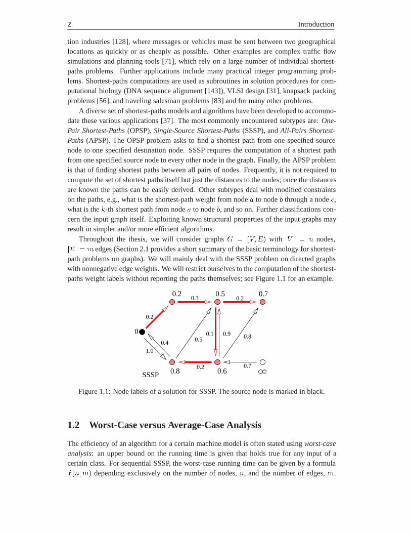
Throughout the thesis, we will consider graphs � � ��� with � � � � nodes,��� � � edges (Section 2.1 provides a short summary of the basic terminology for shortest-path problems on graphs). We will mainly deal with the SSSP problem on directed graphswith nonnegative edge weights. We will restrict ourselves to the computation of the shortest-paths weight labels without reporting the paths themselves; see Figure 1.1 for an example.
0.3 0.2
0.41.0
0.2 0.7
0.80.50.90.1
SSSP
0.2
0
0.2 0.5 0.7
0.60.8
Figure 1.1: Node labels of a solution for SSSP. The source node is marked in black.
1.2 Worst-Case versus Average-Case Analysis
The efficiency of an algorithm for a certain machine model is often stated using worst-caseanalysis: an upper bound on the running time is given that holds true for any input of acertain class. For sequential SSSP, the worst-case running time can be given by a formula����� depending exclusively on the number of nodes, �, and the number of edges, �.

1.2 Worst-Case versus Average-Case Analysis 3
Additional restrictions on edge weights, graph structures etc. may result in sharper upperbounds.
Shortest-paths algorithms commonly apply iterative labeling methods, of which twomajor types are label-setting and label-correcting (we will formally introduce these meth-ods in Section 2.2). Some sequential label-correcting algorithms have polynomial-timeupper-bounds, others even require exponential time in the worst case. In either case, thebest sequential label-setting algorithms have better worst-case bounds than that of any label-correcting algorithm. Hence, at first glance, label-setting algorithms seem to be the betterchoice. However, several independent experimental studies [25, 36, 39, 60, 64, 87, 111, 145]showed that SSSP implementations of label-correcting approaches frequently outperformlabel-setting algorithms. Thus, worst-case analysis sometimes fails to bring out the advan-tages of algorithms that perform well in practice.
Evaluating the performance of shortest-paths algorithms on the basis of real-world datais both desirable and problematic: clearly, testing and refining an algorithm based on con-crete and practically relevant instances (like road maps for SSSP) will be helpful to improvethe algorithmic performance on these very instances. However, benchmarks of real-life in-puts are usually restricted to some fixed-size instances, thus making it difficult to predictthe scalability of an algorithm. Furthermore, the actual running time may crucially de-pend on structural input properties that may or may not be represented by the benchmarks.Consequently, experimental evaluation frequently relies on synthetic input data that can begenerated in varying sizes and that are designed to more or less model real-word data.
Many input generators produce input instances at random according to a certain prob-ability distribution on the set of possible inputs of a certain size. For this input modelone can study the average-case performance, that is, the expected running time of the al-gorithm averaged according to the applied probability distribution for the input instances(Section 2.4 will supply some basic facts and pointers concerning probability theory). Itnearly goes without saying that the choice of the probability distribution on the set of pos-sible instances may crucially influence the resulting average-case bounds. A useful choiceestablishes a reasonable compromise between being a good model for real-world data (i.e.,producing “practically relevant” instances with sufficiently high probability) and still beingmathematically analyzable.
Frequently used input models for the experimental performance evaluation of SSSPalgorithms are random or grid-like graphs with independent random edge weights. The re-sulting inputs exhibit certain structural properties with high probability (whp)1, for exampleconcerning the maximum shortest-path weight or connectivity. However, for some of theseproperties it is doubtful whether they reflect real-life features or should rather be consid-ered as artifacts of the model, which possibly misdirect the quest for practically relevantalgorithms.
Mathematical average-case analysis for shortest-paths algorithms has focused on theAPSP problem for a simple graph model, namely the complete graph with random edgeweights. One of the main contributions of this thesis is a thorough mathematical average-case analysis of sequential SSSP algorithms on arbitrary directed graphs with random edge
1For a problem of size �, we say that an event occurs with high probability (whp) if it occurs with probabilityat least �������� for an arbitrary but fixed constant � � �.
4 Introduction
weights.
1.3 Models of Computation
The analysis of an algorithm must take into account the properties and restrictions of theunderlying machine model. In this section we sketch the models of computation used in thethesis.
1.3.1 Sequential Computing
The standard “von Neumann” model of computation (see e.g., [2]) assumes some uniformcost for any basic operation like accessing a memory cell, assigning, adding or comparingtwo values and so on.
There are further model distinctions concerning the set of supported basic operations:advanced algorithms often rely on additional constant time operations provided on the“RAM (Random Access Machine) with word size ” [2]. This model basically reflectswhat one can use in a programming language such as � and what is supported by currenthardware. In particular, it allows direct and indirect addressing, bitwise logical operations,arbitrary bit shifts and arithmetic operations on �� �-bit operands in constant time. Fre-quently, the values of variables may also take real numbers (standard RAM model withoutexplicit word size).
In contrast to the RAM, there is the pointer-machine model: it disallows memory-address arithmetic. Therefore, bucketing, which is essential to some of our algorithms,is impossible in this model. Also, there is the comparison based model, where weights mayonly be compared2.
The algorithms proposed in this thesis do not require any new machine model propertiesthat would not have been used before for other SSSP algorithms as well; the standard RAMmodel is sufficient. Some of our algorithms even work in the weaker models. By wayof contrast, a recent paper of Brodnik et.al. [21] strengthens the machine model in order toobtain a linear-time SSSP algorithm for directed graphs; its priority queue requires a specialmemory-architecture model with “byte overlap”, which is currently not supported by anyexisting hardware.
1.3.2 Parallel Computing
Large input sizes require algorithms that efficiently support parallel computing, both inorder to achieve fast execution and to take advantage of the aggregate memory of the par-allel system. The parallel random access machine (PRAM) [52, 72, 88] is one of the mostwidely studied abstract models of a parallel computer. A PRAM consists of � independentprocessors (processing units, PUs) and a shared memory, which these processors can syn-chronously access in unit time. Most of our parallel algorithms assume the arbitrary CRCW(concurrent-read concurrent-write) PRAM, i.e., in case of conflicting write accesses to thesame memory cell, an adversary can choose which access is successful. The strict PRAM
2(However, in order to facilitate any meaningful SSSP computation, at least addition of weights must beallowed.)

1.3 Models of Computation 5
model is mainly implemented on experimental parallel machines like the SB-PRAM [51].Still, it is valuable to highlight the main ideas of a parallel algorithm without tedious detailsof a particular architecture.
The performance of PRAM algorithms for input graphs with � nodes and � edgesis usually described by the two parameters time ������ (assuming an unlimited num-ber of available PUs) and work � ���� (the total number of operations needed). Let����� be the execution time for some fixed sequential SSSP algorithm. The obtainableSpeed-up ���� �� over this sequential algorithm due to parallelization is bounded by
��
������� �������� �������
�. Therefore, a fast and efficient parallel algorithm minimizes both
� ����� and � ����; ideally � ���� is asymptotic to the sequential complexity ofthe problem. A number of SSSP PRAM algorithms has been invented to fit the needs ofparallel computing. Unfortunately, most of them require significantly more work than theirsequential counterparts.
P P P P� � � �� � � �� � � �
Shared Memory
�more theoretical
Pure PRAM
P P P P� � � �
Distr ibute d Me mory
�more practical
��
��
DistributedMemory Machine
Modules
Network
PUs
� � �
� � �
� � �
Me mo ry
bu te d
Di st ri
P P P
P P P
P P P
ConcreteArchitecture
Figure 1.2: Different models of parallel computation.
Other models like BSP [142] and LogP [34] view a parallel computer as a so calleddistributed memory machine (DMM), i.e., a collection of sequential processors, each onehaving its own local memory. The PUs are interconnected by a network, which allowsthem to communicate by sending and receiving messages. Communication constraints areimposed by global parameters like latency, limited network bandwidth and synchronizationdelays. Clearly, worst-case efficient DMM algorithms are at least as hard to obtain as theirPRAM equivalents. Even more detailed models of a parallel computer are obtained byadditionally taking into consideration the concrete network architecture used to connectthe PUs, thus allowing more fine-grained performance predictions of the message passingprocedures. Figure 1.2 depicts the relation between parallel models of computation.

6 Introduction
1.4 New Results in a Nutshell
This section provides a very brief overview of our new results. More comprehensive listingsincluding pointers to previous and related work are given in the beginnings of the respectivechapters.
1.4.1 Sequential Algorithms (Chapter 3)
For arbitrary undirected networks with nonnegative edge costs, it is known that Single-Source Shortest-Paths problems can be solved in linear time in the worst case [136]. Itis unknown, however, whether this can also be achieved for directed networks. We provethat on average, a similar result indeed holds. Our problem instances are arbitrary directednetworks on � nodes and � edges whose edge weights are randomly chosen accordingto the uniform distribution on �� �, independently of each other. We present both label-setting and label-correcting algorithms that solve the SSSP problem on such instances intime ������ on the average. The time bound can also be obtained with high probability.
Only very little is known about the average-case performance of previous SSSP algo-rithms. Our research yields the first theoretical average-case analysis for the “ApproximateBucket Implementation” [25] of Dijkstra’s algorithm [42] (ABI–Dijkstra): for random edgeweights and either random graphs or graphs with constant maximum node degree we showhow the bucket width must be chosen in order to achieve linear ��� � �� average-caseexecution time. Furthermore, we give constructive existence proofs for graph classes withrandom edge weights on which ABI–Dijkstra and several other well-known SSSP algo-rithms are forced to run in superlinear time on average. While this is interesting in its ownright it also stresses the advantages of our new algorithms.
1.4.2 Parallel Algorithms (Chapter 4)
Besides the classical sequential (single processor) model of computation we also considerparallel processing. Unfortunately, for general graphs with nonnegative edge weights, nofast and work-efficient parallel SSSP algorithms are known.
We present new average-case results for a number of important graph classes; for exam-ple, we provide the first work-optimal PRAM algorithms that require sublinear average-casetime for sparse random graphs, and graphs modeling the WWW, telephone calls or socialnetworks. Most of our algorithms are derived from the new sequential label-correcting ap-proach exploiting the fact that certain operations can be performed independently on differ-ent processors or disks. The algorithms are analyzed in terms of quite general graph prop-erties like (expected) diameter, maximum shortest-path weight or node degree sequences.For certain parameter ranges, already very simple extensions provably do the job; other pa-rameters require more involved data structures and algorithms. Sometimes, our methods donot lead to improved algorithms at all, e.g., on graphs with linear diameter. However, suchinputs are quite atypical.
Preliminary accounts of the results covered in this thesis have been presented in [33, 103,104, 105, 106, 107]. The follow-up paper of Goldberg [67] on sequential SSSP was helpful

1.5 Organization of the Thesis 7
to streamline some proofs for our sequential label-setting algorithm.
1.5 Organization of the Thesis
The rest of the thesis is composed as follows: Chapter 2 provides the definitions for shortest-paths problems on graphs and reviews the basic solution strategies. In particular, it discussessimple criteria to verify that some tentative distance value is final. These criteria play acrucial role in our SSSP algorithms – independent of the machine model.
Throughout the thesis we will use probabilistic arguments; Chapter 2 also providesa few very basic facts about probability theory and offers references for further reading.Advanced probabilistic methods will be presented when needed.
Subsequently, there is a division into the parts sequential SSSP (Chapter 3) and parallelSSSP (Chapter 4). Each of these chapters starts with an overview of previous work and thenpresents our contributions. At the end of the chapters we will provide a few concludingremarks and highlights some open problems. Many concepts developed in Chapter 3 willbe reused for the parallel algorithms.

Chapter 2
Definitions and Basic Concepts
In this chapter we will provide a short summary of the basic terminology (Section 2.1) andsolution approaches (Section 2.2) for shortest-path problems on graphs. Readers familiarwith the SSSP problem may choose to skip these sections and refer to them when neces-sary. In Section 2.3 we present advanced strategies that turn out to be essential for our newalgorithms. Finally, Section 2.4 provides some basic facts about probability theory.
2.1 Definitions
A graph � � ��� consists of a set of nodes (or vertices) and a set � of edges (or arcs).We let � � � � denote the number of nodes in �, ��� � � represents the number of edges.
Directed Graphs
The edge set � of a directed graph consists of ordered pairs of nodes: an edge � fromnode � to node � is denoted by � � �� ��. Here � is also called the source, � the target, andboth nodes are called endpoints of �� ��. Furthermore, �� �� is referred to as one of �’soutgoing edges or one of �’s incoming edges, as an edge leaving � or an edge entering �.The number of edges leaving (entering) a node is called the out-degree (in-degree) of thisnode. The degree of a node is the sum of its in-degree and out-degree. The adjacency-listof a node � consists of all nodes � such that �� �� � �. Depending on the application, acorresponding member of the adjacency-list of node �may be interpreted as either the targetnode � or the edge �� ��. The adjacency-list of node � is also often called the forward starof �, �� ��� for short.
Undirected Graphs
Undirected graphs are defined in the same manner as directed graphs except that edgesare unordered pairs of nodes, i.e., �� �� stands for an undirected edge that connects thenodes � and �. Hence, in undirected graphs an edge can be imagined as a “two-way”connection, whereas in directed graphs it is just “one-way”. Consequently, there is nodistinction between incoming and outgoing edges. Two undirected edges are adjacent ifthey share a common endpoint.
8

2.1 Definitions 9
Networks
(Un)directed graphs whose edges and/or nodes have associated numerical values (e.g., costs,capacities, etc.) are called (un)directed networks. We shall often not formally distinguishbetween graphs and networks; for example, when we consider the unweighted breadth-firstsearch version of the shortest-path problem. However, our model for shortest-paths prob-lems are usually networks � � ���� � in which a function ���� assigns independent randomcosts, weights, to the edges of �. The weight of the edge �� �� is denoted by ��� ��.
Subgraphs
We say that a graph �� � � � ��� is a subgraph of � � ��� if � � and �� � �.Given a set � � , the subgraph of � induced by � is the graph �� � � � ���, where�� � ��� �� � � � � � ��. Furthermore, we shall often define subgraphs basedon a threshold �� on the weights of the edges in �: the subset of edges is given by �� �
��� �� � � ��� �� ���, and only nodes being either source or target of at least oneedge in �� are retained in �.
Paths and Cycles
A path � from � to in a directed graph � is a node sequence �� �� � � � �� for some� � �, such that the edges ��� ���, ��� ���, . . . , ���� �� are part of �, �� � �, and� � . The nodes �� and � are called the starting point and endpoint of � , respectively.If all nodes � on � are pairwise distinct then we say that the path is simple. Cycles arethose paths where the starting point and the endpoint are identical. Paths and cycles ofundirected graphs are defined equivalently on undirected edges. A graph is called acyclic ifit does not contain any cycle. We say that a node � is reachable from a node � in � if thereis a path � � � � �� in �. An undirected (directed) graph is called (strongly) connected ifit contains a path from � to � for each pair �� �� � . The weight of a path � �
�� � � � �� with edges ��� ���, ��� ���, . . . , ���� �� in � � ���� � is defined to be��� � �
����� ��� ����. In contrast, the size of a path denotes the number of edges on
the path.Using the notation above we can formally state the kind of SSSP problems we are
interested in:
Definition 1 Consider a network �� � ��� �� with a distinguished vertex � (“source”)and a function � assigning a nonnegative real-valued weight to each edge of �. The ob-jective of the SSSP is to compute, for each vertex � reachable from �, the minimum weight�� ��� ��, abbreviated �� ����, among all paths from � to �. We set �� ���� � �, and�� ��� �� � � if � is not reachable from �. We call a path of minimum weight from � to �a shortest path from � to �.
A valid solution for the SSSP problem implies certain properties for the underlying shortestpaths:
Property 1 If the path � � �� �� � � � ��� �� is a shortest path from node � to node �,then for every �, � � �� �, the sub-path � � �� � � � �� is a shortest path from node �to node �.

10 Definitions and Basic Concepts
Property 2 A directed path � � � � �� �� � � � ��� �� from the source node � tonode � is a shortest path if and only if �� ������ � �� ���� � ��� ���� for every edge�� ���� � � . Furthermore, the numbers �� ���� represent proper shortest-paths distancesif and only if they satisfy the following optimality condition:
�� ���� � � and �� ���� � ���������
�� ���� � ��� �� �� � � ����
We need to define two characteristic measures for weighted graphs, which play a crucialrole in the analysis of our parallel SSSP algorithms:
Definition 2 The maximum shortest-path weight for the source node � is defined as ���� �
��� ��� ��� �� ��� ��� �� ���, abbreviated �.
On graphs with edge weights in �� �, the value of � is bounded from above by the diame-ter �:
Definition 3 In a graph � � ���, let ��� ����� �� denote the minimum number ofedges (i.e., the size) needed among all paths from � to � if any, �� otherwise; then � �
�������� ���� ����� �� �� is called the diameter � of �.
The running times of our parallel SSSP algorithms are explicitly stated in dependence of thevalue �. Part of our research is concerned with the problem to find good upper bounds on �for certain graph classes: in Section 3.9.3 we will derive stronger bounds for � on randomgraphs by using known results on the diameter of appropriate subgraphs with bounded edgeweights.
2.2 Basic Labeling Methods
Shortest-paths algorithms are usually based on iterative labeling methods. For each node �in the graph they maintain a tentative distance label �������; ������� is an upper bound on�� ����. The value of ������� refers to the weight of the lightest path from � to � found sofar (if any). Initially, the methods set ������� � �, and ������� � � for all other nodes� �� �.
The generic SSSP labeling approach repeatedly selects an arbitrary edge �� �� where������� � ��� �� � �������, and resets ������� � ������� � ��� ��. Identifying such anedge �� �� can be done with ���� operations. The method stops if all edges satisfy
������� ������� � ��� �� ��� �� � �� (2.1)
By then, �� ���� � ������� for all nodes �; compare Property 2. If �� ���� � ������� thenthe label ������� is said to be permanent (or final); the node � is said to be settled in thatcase.
The total number of operations needed until the labeling approach terminates dependson the order of edge selections; in the worst case it is pseudo-polynomial for integer weights,���� ����� and ������� otherwise [3]. Therefore, improved labeling algorithms performthe selection in a more structured way: they select nodes rather than edges. In order to doso they keep a candidate node set � of “promising” nodes. We require � to contain thestarting node � of any edge �� �� that violates the optimality condition (2.1):

2.2 Basic Labeling Methods 11
Requirement 1 � � �� � ��� �� � � with ������� � ��� �� � ��������
The labeling methods based on a candidate set � of nodes repeatedly select a node � � �and apply the SCAN operation (Figure 2.1) to it until � finally becomes empty. Figure 2.2depicts the resulting generic SSSP algorithm.
procedure SCAN���
� � � � ���for all �� �� � � do
if ������� � ��� �� � ������� then������� � ������� � ��� ��
if � �� � then� � � � ���
Figure 2.1: Pseudo code for the SCAN operation.
algorithm GENERIC SSSP
for all � � do������� � �
������� � �
� � ���while � �� � do
select a node � � �SCAN���
Figure 2.2: Pseudo code for the generic SSSP algorithm with a candidate node set.
SCAN��� applied to a node � � � first removes � from � and then relaxes all1 outgo-ing edges of �, that is, the procedure sets
������� � ����������� ������� � ��� ��� ��� �� � �� ����
If the relaxation of an edge �� �� reduces ������� where � �� �, then � is also insertedinto �.
During the execution of the labeling approaches with a node candidate set � the nodesmay be in different states: a node � never inserted into � so far (i.e., ������� � �) is saidto be unreached, whereas it is said to be a candidate (or labeled or queued) while it belongsto �. A node � selected and removed from � whose outgoing edges have been relaxed issaid to be scanned as long as � remains outside of �.
The pseudo code of the SCAN procedure (Figure 2.1) immediately implies the follow-ing:
Observation 1 For any node �, ������� never increases during the labeling process.1There are a few algorithms that deviate from this scheme in that they sometimes only consider a subset of
the outgoing edges. We shall use such strategies later on as well.

12 Definitions and Basic Concepts
Furthermore, the SCAN procedure maintains � as desired:
Lemma 1 The SCAN operation ensures Requirement 1 for the candidate set �.
Proof: � is required to contain the starting node � of any edge � � �� �� that violatesthe optimality condition (2.1). Due to Observation 1, the optimality condition (2.1) canonly become violated when ������� is decreased, which, in turn, can only happen if someedge � �� into � is relaxed during a SCAN� � operation. However, if SCAN� � reduces������� then the procedure also makes sure to insert � into � in case � is not yet containedin it. Furthermore, at the moment when � is removed from � the condition (2.1) will notbecome violated because of the relaxation of �� ���.
In the following we state the so-called monotonicity property. It proves helpful to obtainbetter data structures for maintaining the candidate set �.
Lemma 2 (Monotonicity) For nonnegative edge weights, the smallest tentative distanceamong all nodes in � never decreases during the labeling process.
Proof: Let���� � ����������� � � ��. ���� will not decrease if a node is removedfrom �. The tentative distance of a node � can only decrease due to a SCAN��� operationwhere � � �, �� �� � �, and ������� � ��� �� � �������; if � is not queued at this time,then a reduction of ������� will result in � entering �. However, as all edge weights arenonnegative, SCAN��� updates ������� � ������� � ��� �� �����.
So far, we have not specified how the labeling methods select the next node to be scanned.The labeling methods can be subdivided into two major classes: label-setting approachesand label-correcting approaches. Label-setting methods exclusively select nodes � withfinal distance value, i.e., ������� � �� ����. Label-correcting methods may select nodeswith non-final tentative distances, as well.
In the following we show that whenever � is nonempty then it always contains a node� with final distance value. In other words, there is always a proper choice for the next nodeto be scanned according to the label-setting paradigm.
Lemma 3 (Existence of an optimal choice.) Assume ���� � � for all � � �.(a) After a node � is scanned with ������� � �� ����, it is never added to � again.(b) For any node � reachable from the source node � with ������� � �� ���� there is a node� � � with ������� � �� ����, where � lies on a shortest path from � to �.
Proof: (a) The labeling method ensures ������� � �� ���� at any time. Also, when � isadded to �, its tentative distance value ������� has just been decreased. Thus, if a node �is scanned from � with ������� � �� ����, it will never be added to � again later.(b) Let � � �� �� � � � � � �� be a shortest path from � to �. Then ������� � �� ���� � �
and ������� � �� ����. Let � be minimal such that ������� � �� ����. Then � � �,��������� � �� ������ and
������� � �� ���� � �� ������ � ����� �� � ��������� � ����� ���
Thus, by Requirement 1 for the candidate set, the node ��� is contained in �.

2.3 Advanced Label-Setting Methods 13
The basic label-setting approach for nonnegative edge weights is Dijkstra’s method [42]; itselects a candidate node with minimum tentative distance as the next node to be scanned.Figure 2.3 demonstrates an iteration of Dijkstra’s method.
unreachedscannedlabeled
0.2 0.5
0.1 8
1.00.2
0
1.30.3 1.0
0.7
0.3
SCAN(v)
0.2 0.5
1.0
0.1
0
0.7 1.5
0.2
0.3 1.0
ss
vv
Figure 2.3: SCAN step in Dijkstra’s algorithm.
The following lemma shows that Dijkstra’s selection method indeed implements thelabel-setting paradigm.
Lemma 4 (Dijkstra’s selection rule) If ���� � � for all � � � then ������� � �� ���� forany node � � � with minimal �������.
Proof: Assume otherwise, i.e., ������� � �� ���� for some node � � � with minimaltentative distance. By Lemma 3, there is a node � � � lying on a shortest path from � to� with ������� � �� ����. Due to nonnegative edge weights we have �� ���� �� ����.However, that implies ������� � �������, a contradiction to the choice of �.
Hence, by Lemma 3, label-setting algorithms have a bounded number of iterations (propor-tional to the number of reachable nodes), but the amount of time required by each iterationdepends on the data structures used to implement the selection rule. For example, in the caseof Dijkstra’s method the data structure must support efficient minimum and decrease keyoperations.
Label-correcting algorithms may have to rescan some nodes several times until theirdistance labels eventually become permanent; Figure 2.4 depicts the difference to label-setting approaches. Label-correcting algorithms may vary largely in the number of itera-tions needed to complete the computation. However, their selection rules are often verysimple; they frequently allow implementations where each selection runs in constant time.For example, the Bellman-Ford method [15, 50] processes the candidate set � in simpleFIFO (First-In First-Out) order.
Our new SSSP algorithms either follow the strict label-setting paradigm or they applylabel-correcting with clearly defined intermediate phases of label-setting steps.
2.3 Advanced Label-Setting Methods
In this section we deal with a crucial problem for label-setting SSSP approaches: identifyingcandidate nodes that have already reached their final distance values. Actually, several

14 Definitions and Basic Concepts
unreached labeled scanned & settled
scanned, but not settled
LABEL − CORRECTINGLABEL − SETTING
unreached labeled scanned & settled
Figure 2.4: States for a reachable non-source node using a label-setting approach (left) andlabel-correcting approach (right).
mutually dependent problems have to be solved: first of all, a detection criterion is neededin order to deduce that a tentative distance of a node is final. Secondly, the data structure thatmaintains the set� of candidate nodes must support efficient evaluation of the criterion andmanipulation of the candidate set, e.g. inserting and removing nodes. For each iteration ofthe labeling process, the criterion must identify at least one node with final distance value;according to Lemma 3 such a node always exists. However, the criterion may even detecta whole subset � � of candidate nodes each of which could be selected. We call theyield of a criterion.
Large yields may be advantageous in several ways: being allowed to select an arbitrarynode out of a big subset could simplify the data structures needed to maintain the can-didate set. Even more obviously, large yields facilitate concurrent node scans in parallelSSSP algorithms, thus reducing the parallel execution time. On the other hand, it is likelythat striving for larger yields will make the detection criteria more complicated. This mayresult in higher evaluation times. Furthermore, there are graphs where at each iteration ofthe labeling process the tentative distance of only one single node in � is final - even if �contains many nodes; see Figure 2.5.
1 2 30 i
11
11
1
1/n n−2 n−11/n 1/n 1/n 1/n 1/n 1/n 1/n
1
Figure 2.5: Input graph for which the candidate set � contains only one entry with finaldistance value: after settling nodes �, �, � � �, � � � the queue holds node � with (actual)distance �!�, and all other �� �� � queued nodes have tentative distance �.
In the following we will present the label-setting criteria used in this thesis. We have al-ready seen in Lemma 4 that Dijkstra’s criterion [42], i.e., selecting a labeled node with min-imum tentative distance as the next node to be scanned, in fact implements the label-settingparadigm. However, it also implicitly sorts the nodes according to their final distances.This is more than the SSSP problem asks for. Therefore, subsequent approaches have beendesigned to avoid the sorting complexity; they identified label-setting criteria that allow toscan nodes in non-sorted order. Dinitz [43] and Denardo and Fox [36] observed the follow-ing:
Criterion 1 (GLOB-criterion) Let � ����������� � � ��. Furthermore, let " �
�������� � � ��. Then ������� � �� ���� for any node � � � having ������� � �".
2.3 Advanced Label-Setting Methods 15
The GLOB-criterion of Dinitz and Denardo/Fox is global in the sense that it applies uni-formly to any labeled node whose tentative distance is at most � � ". However, if " �
���� ��� happens to be small2, then the criterion is restrictive for all nodes � � , eventhough its restriction may just be needed as long as the nodes �� and �� are part of the can-didate set. Therefore, it is more promising to apply local criteria: for each node � � � theyonly take into account a subset of the edge weights, e.g. the weights of the incoming edgesof �. The following criterion is frequently used in our algorithms:
Lemma 5 (IN-criterion) Let � ����������� � � ��. For nonnegative edge weights,the labeled nodes of the following sets have reached their final distance values:
�� � �� � � � �� � � ������� ���������� � �� � � � ��� �� � � ������� � � ��� ���
Proof: The claim for the set �� was established in Lemma 4 of Section 2.2. The prooffor the set �� follows the same ideas; assume ������� � �� ���� for some node � � ��.By Lemma 3 there is a node � � �, � �� �, lying on a shortest path from � to � with������� � �� ���� �� . However, since all edges into � have weight at least ��������� ,this implies �� ���� � �� ���� � ������� �� � �������, a contradiction.
Lemma 5 was already implicit in [36, 43]. However, for a long time, the IN-criterion has notbeen exploited in its full strength to derive better SSSP algorithms. Only recently, Thorup[136] used it to yield the first linear-time algorithm for undirected graphs. Our algorithmsfor directed graphs also rely on it. Furthermore, it is used in the latest SSSP algorithm ofGoldberg [67], as well.
The IN-criterion for node � is concerned with the incoming edges of �. In previouswork [33], we also identified an alternative version, the OUT-criterion.
Lemma 6 (OUT-criterion) Let
� ����������� � � �� � �
� � �� � � ������� � ��#��� � ��� ��� �������� � � � � �� � � ��� �
If #��� �� � �� and ���� � � for all � � � then ������� � �� ���� for all � � � .
Proof: In a similar way to the proof of Lemma 5, we assume ������� � �� ���� for somenode � � � . Again, by Lemma 3, there will be a node � � �, � �� �, lying on a shortestpath from � to � with ������� � �� ���� �� . Due to nonnegative edge weights, �� ���� ������� � �. Consequently, � � � . However, this implies �� ���� � �� ���� � #���. If#��� �� � �� then �� ���� �� �, a contradiction.
Applications of the OUT-criterion are not only limited to SSSP; it is also used for conser-vative parallel event-simulation [99].
So far we have provided some criteria to detect nodes with final distance values. In thefollowing chapters, we will identify data structures that efficiently support the IN-criterion.
2This is very likely in the case of independent random edge weights uniformly distributed in ��� �� as as-sumed for our average-case analyses.
16 Definitions and Basic Concepts
2.4 Basic Probability Theory
In this section we review a few basic definitions and facts for the probabilistic analysis ofalgorithms. More comprehensive presentations are given in [48, 49, 74, 112, 129].
Probability
For the average-case analyses of our SSSP algorithms we assume that the input graphsof a certain size are generated according to some probability distribution on the set of allpossible inputs of that size, the so-called sample space �. A subset � � � is called anevent. A probability measure � is a function that satisfies the following three conditions:� ��� � for each � � �, ��� � �, and ���� �
���� for pairwise disjoint
events �. A sample space together with its probability measure build a probability space.For a problem of size �, we say that an event � occurs with high probability (whp) if
��� � � ������� for an arbitrary but fixed constant $ � �.The conditional probability ������� � �������
���� refers to the probability that an exper-iment has an outcome in the set �� when we already know that it is in the set ��. Two events�� and �� are called independent if ������� � ����.
Boole’s inequality often proves helpful for dependent events: let �� � � � �� be any col-lection of events, then � ���
��� ��
��� ��.
Random Variables
Any real valued numerical function % � %�&� defined on a sample space � may be calleda random variable. If % maps elements in � to �� � ��� then it is called a nonnegativerandom variable. A discrete random variable is supposed to take only isolated values withnonzero probability. Typical representatives for discrete random variables are binary ran-dom variables, which map elements in � to �� ��. For any random variable % and any real
number ' � � we define
�%
��'
��
�& � � %�&�
��'
�. The distribution function (�
of a random variable % is given by (��'� � ��% '. A continuous random variable %is one for which (��'� can be expressed as (��'� �
� ��� ���'� )' where ���'� is the
so-called density function. For example if a random variable % is uniformly distributed in�� � (that is the case for the edge weights in our shortest-path problems) then ���'� � �
for � ' � and ���'� � � otherwise.For any two random variables % and * , % is said to (stochastically) dominate * (de-
noted by % � * ) if ��% � � � ��* � � for all � � �. Two random variables % and *are called independent if, for all ' + � �, ��% � ' � * � + � ��% � '.
Expectation
The expectation of a discrete random variable % is given by ��% ��
��� ' ���% � '.For a continuous random variable % we have ��% �
���� ' � ���'� )'. Here are a few
important properties of the expectation for arbitrary random variables % and * :
� If % is nonnegative, then ��% � �.
2.4 Basic Probability Theory 17
� � ��% � �� �%� .
� ��� �% � � ���%� for any � � �.
� ��% � * � ��% ���* (linearity of expectation).
� If % and * are independent, then ��% � * � ��% ���*
The conditional expectation of a random variable % with respect to an event � is defined by��%�� �
���� ' � ��% � ' � � . An important property of the conditional expectation
is that �� ��* �% � ��* for any two random variables % and * .
Tail Estimates
Frequently, we are interested in the probability that random variables do not deviate toomuch from their expected values. The Markov Inequality for an arbitrary nonnegative ran-dom variable % states that ��% � � ���
for any � � �. More powerful tail estimatesexist for the sum of independent random variables. Here is one version of the well-knownChernoff bound:
Lemma 7 (Chernoff bound [26, 77]) Let%� � � � % be independent binary random vari-ables. Let , � ��
����%� . Then it holds for all Æ � � that
�
����
%� � �� � � � ,� ��������� � (2.2)
Furthermore, it holds for all � � Æ � � that
�
����
%� �� � � � ,� ������ � (2.3)
We shall introduce further bounds in the subsequent chapters whenever the need arises.More material on tail estimates can be found for example in [41, 77, 100, 110, 127].

Chapter 3
Sequential SSSP Algorithms
This chapter deals with single-source shortest-paths algorithms for the sequential modelof computation. However, many of the concepts presented in here will be reused for theparallel and external-memory SSSP algorithms, as well.
The chapter is structured as follows: first of all, Section 3.1 sketches previous and re-lated work for the sequential machine model. An overview of our new contributions is givenin Section 3.2. In Section 3.3 we review some simple bucket-based SSSP algorithms. Thenwe present our new algorithms SP-S and SP-C (Section 3.4). Both algorithms run in lineartime on average. Even though the two approaches are very similar, the analysis of SP-S(Section 3.5) is significantly simpler than that of SP-C (Sections 3.6 and 3.8); in poeticjustice, SP-C is better suited for parallelizations (Chapter 4). Furthermore, once analy-sis of SP-C is established, it easily implies bounds for other label-correcting algorithms(Section 3.9). In Section 3.10, we demonstrate a general method to construct graphs withrandom edge weights, that cause superlinear average-case running-times with many tradi-tional label-correcting algorithms. Finally, Section 3.11 provides some concluding remarksand presents a few open problems.
3.1 Previous and Related Work
In the following we will list some previous shortest-paths results that are related to ourresearch. Naturally, due to the importance of shortest-paths problems and the intensiveresearch on them, our list cannot (and is not intended to) provide a survey of the wholefield. Appropriate overview papers for classical and recent sequential shortest-paths resultsare, e.g., [25, 37, 114, 124, 136, 146].
3.1.1 Sequential Label-Setting Algorithms
A large fraction of previous work is based on Dijkstra’s method [42], which we havesketched in Section 2.2. The original implementation identifies the next node to scan bylinear search. For graphs with � nodes, � edges and nonnegative edge weights, it runs in����� time, which is optimal for fully dense networks. On sparse graphs, it is more efficientto use a priority queue that supports extracting a node with smallest tentative distance andreducing tentative distances for arbitrary queued nodes. After Dijkstra’s result, most subse-
18

3.1 Previous and Related Work 19
quent theoretical developments in SSSP for general graphs have focused on improving theperformance of the priority queue: Applying William’s heap [144] results in a running timeof ��� � ��� ��. Taking Fibonacci heaps [53] or similar data structures [19, 44, 135], Dijk-stra’s algorithm can be implemented to run in ��� � ��� ���� time. In fact, if one sticksto Dijkstra’s method, thus considering the nodes in non-decreasing order of distances, then��� � ������� is even the best possible time bound for the comparison-addition model:any -�� � �����-time algorithm would contradict the ��� � ��� ��-time lower-bound forcomparison-based sorting.
A number of faster algorithms have been developed for the more powerful RAM model.Nearly all of these algorithms are still closely related to Dijkstra’s algorithm; they mainlystrive for an improved priority queue data structure using the additional features of theRAM model (see [124, 136] for an overview). Fredman and Willard first achieved ��� ��
��� �� expected time with randomized fusion trees [54]; the result holds for arbitrarygraphs with arbitrary nonnegative edge weights. Later they obtained the deterministic���� � � ����! ��� ��� ��-time bound by using atomic heaps [55].
The ultimate goal of a worst-case linear time SSSP algorithm has been partially reached:Thorup [136, 137] gave the first ������-time RAM algorithm for undirected graphs withnonnegative floating-point or integer weights fitting into words of length . His approachapplies label-setting, too, but deviates significantly from Dijkstra’s algorithm in that it doesnot visit the nodes in order of increasing distance from � but traverses a so-called componenttree. Unfortunately, Thorup’s algorithm requires the atomic heaps [55] mentioned above,which are only defined for � � ���
��. Hagerup [76] generalized Thorup’s approach to
directed graphs. The time complexity, however, becomes superlinear ��� � � � ��� �.The currently fastest RAM algorithm for sparse directed graphs is due to Thorup [138];it needs ��� � � � ��� ��� �� time. Alternative approaches for somewhat denser graphshave been proposed by Raman [123, 124]: they require ���� � ������ � ��� ��� �� and������� ���� ���� � time, respectively. Using an adaptation of Thorup’s component treeapproach, Pettie and Ramanchandran [119] recently obtained improved SSSP algorithmsfor the pointer machine model. Still, the worst-case complexity for SSSP on sparse directedgraphs remains superlinear.
In Section 3.3 we will review some basic implementations of Dijkstra’s algorithm withbucket based priority queues [3, 36, 38, 43]. Alternative bucket approaches include nested(multiple levels) buckets and/or buckets of different widths [4, 36]. So far, the best boundfor SSSP on arbitrary directed graphs with nonnegative integer edge-weights in �� � � � ��is ���� � � ������������ expected time for any fixed . � � [124].
3.1.2 Sequential Label-Correcting Algorithms
The classic label-correcting SSSP approach is the Bellman–Ford algorithm [15, 50]. It im-plements the set of candidate nodes� as a FIFO-Queue and achieves running time ������.There are many more ways to maintain � and select nodes from it (see [25, 59] for anoverview). For example, the algorithms of Pallottino [117], Goldberg and Radzik [69],and Glover et al. [64, 65, 66] subdivide � into two sets �� and �� each of which is im-plemented as a list. Intuitively, �� represents the “more promising” candidate nodes. The

20 Sequential SSSP Algorithms
algorithms always scan nodes from��. According to varying rules,�� is frequently refilledwith nodes from ��. These approaches terminate in worst-case polynomial time. However,none of the alternative label-correcting algorithms succeeded to asymptotically improve onthe ��� � ��-time worst-case bound of the simple Bellman-Ford approach. Still, a num-ber of experimental studies [25, 36, 39, 60, 64, 87, 111, 145] showed that some recentlabel-correcting approaches run considerably faster than the original Bellman–Ford algo-rithm and even outperform label-setting algorithms on certain data sets. So far, no profoundaverage-case analysis has been given to explain the observed effects. A striking example inthis respect is the shortest-paths algorithm of Pape [118]; in spite of exponential worst-casetime it performs very well on real-world data like road graphs.
We would like to note that faster sequential SSSP algorithms exist for special graph classeswith arbitrary nonnegative edge weights, e.g., there is a linear-time approach for planargraphs [81]. The algorithm uses graph decompositions based on separators that may havesize up to �������. Hence, it may in principle be applied to a much broader class of graphsthan planar graphs if just a suitable decomposition can be found in linear time. The algo-rithm does not require the bit manipulating features of the RAM model and works for di-rected graphs, thus it remains appealing even after Thorup’s linear-time RAM algorithm forarbitrary undirected graphs. Another example for a “well-behaved” input class are graphswith constant tree width; they allow for a linear-time SSSP algorithm as well [24].
3.1.3 Random Edge Weights
Average-case analysis of shortest-paths algorithms mainly focused on the All-Pairs Shortest-Paths (APSP) problem on either the complete graph or random graphs with ��� � �����
edges and random edge weights [32, 57, 80, 109, 133]. Average-case running times of���� � ����� as compared to worst-case cubic bounds are obtained by virtue of an initialpruning step: if � denotes a bound on the maximum shortest-path weight, then the algo-rithms discard insignificant edges of weight larger than �; they will not be part of the finalsolution. Subsequently, the APSP is solved on the reduced graph. For the inputs consideredabove, the reduced graph contains ��� � ����� edges on the average. This pruning idea doesnot work on sparse random graphs, let alone arbitrary graphs with random edge weights.
Another pruning method was explored by Sedgewick and Vitter [130] for the average-case analysis of the One-Pair Shortest-Paths (OPSP) problem on random geometric graphs��
��/�. Graphs of the class ����/� are constructed as follows: � nodes are randomly placed
in a )-dimensional unit cube, and each edge weight equals the Euclidean distance betweenthe two involved nodes. An edge �� �� is included if the Euclidean distance between � and� does not exceed the parameter / � �� �. Random geometric graphs have been intensivelystudied since they are considered to be a relevant abstraction for many real world situations[40, 130]. Assuming that the source node � and target node 0 are positioned in oppositecorners of the cube, Sedgewick and Vitter showed that the OPSP algorithm can restrictitself to nodes and edges being “close” to the diagonal between � and 0, thus obtainingaverage-case running-time ����.
Mehlhorn and Priebe [102] proved that for the complete graph with random edge weightsevery SSSP algorithm has to check at least ��� � ����� edges with high probability. Noshita

3.2 Our Contribution 21
[115] and Goldberg and Tarjan [70] analyzed the expected number of decreaseKey opera-tions in Dijkstra’s algorithm; for the asymptotically fastest priority queues, however, theresulting total average-case time of the algorithm does not improve on its worst-case com-plexity.
3.2 Our Contribution
We develop a new sequential SSSP approach, which adaptively splits buckets of an ap-proximate priority-queue data-structure, thus building a bucket hierarchy. The new SSSPapproach comes in two versions, SP-S and SP-C, following either the label-setting (SP-S)or the label-correcting (SP-C) paradigm. Our method is the first that provably achieveslinear ������ average-case execution time on arbitrary directed graphs.
In order to facilitate easy exposition we assume random edge weights chosen accordingto the uniform distribution on �� �, independently of each other. In fact, the result canbe shown for much more general random edge weights in case the distribution of edgeweights “is linear” in a neighborhood of zero. Furthermore, the proof for the average-case time-bound of SP-S does not require the edge weights to be independent. If, however,independence is given, then the linear-time bound for SP-S even holds with high probability.After some adaptations, the label-correcting version SP-C is equally reliable.
The worst-case times of the basic algorithms SP-S and SP-C are ��� ��� and ��� �� � ��� ��, respectively. SP-C can be modified to run in ��� � �� worst-case time aswell. Furthermore, running any other SSSP algorithm with worst-case time � ���� “inparallel” with either SP-S or SP-C, we can always obtain a combined approach featuringlinear average-case time and ��� ����� worst-case time.
Our result immediately yields an ���� �� ��� average-case time algorithm for APSP,thus improving upon the best previous bounds on sparse directed graphs.
Furthermore, our analysis for SP-C implies the first theoretical average-case analysisfor the “Approximate Bucket Implementation” [25] of Dijkstra’s SSSP algorithm (ABI–Dijkstra): assuming either random graphs or arbitrary graphs with constant maximum nodedegree we show how the bucket widths must be chosen in order to achieve linear ������
average-case execution time for random edge weights. The same results are obtained withhigh-probability for a slight modification of ABI–Dijkstra, the so-called sequential “�-Stepping” implementation.
Finally, we present a general method to construct sparse input graphs with random edgeweights for which several label-correcting SSSP algorithms require superlinear average-case running-time: besides ABI–Dijkstra and �-Stepping we consider the “Bellman–FordAlgorithm” [15, 50], “Pallottino’s Incremental Graph Algorithm” [117], the “Threshold Ap-proach” by Glover et al. [64, 65, 66], the basic version of the “Topological Ordering SSSPAlgorithm” by Goldberg and Radzik [69]. The obtained lower bounds are summarized inTable 3.1. It is worth mentioning that the constructed graphs contain only ���� edges, thusmaximizing the performance gap as compared to our new approaches with linear average-case time.
Preliminary accounts of our results on sequential SSSP have appeared in [104, 106]. Sub-

22 Sequential SSSP Algorithms
SSSP Algorithm Average-Case Time
Bellman–Ford Alg. [15, 50] ����� ���
Pallottino’s Incremental Graph Alg. [117] ����� ���
Basic Topological Ordering Alg. [69] ����� ���
Threshold Alg. [64, 65, 66] ��� � ��� �! ��� ��� ��
ABI–Dijkstra [25] ��� � ��� �! ��� ��� ��
�-Stepping [106] (Chap. 3.9.1) ��� ������! ��� �����
Table 3.1: Proved lower bounds on the average-case running times of some label-correctingalgorithms on difficult input classes with � � ���� edges and random edge weights.
sequently, Goldberg [68, 67] obtained the linear-time average-case bound for arbitrary di-rected graphs as well. He proposes a quite simple alternative algorithm based on radixheaps. For integer edge weights in �� � � � ��, where � is reasonably small, it achievesimproved worst-case running-time ��� � ���� ���, where � � denotes the ratio be-tween the largest and the smallest edge weight in �. However, for real weights in �� �
as used in our analysis, the value of � may be arbitrarily large. Furthermore, comparedto our label-correcting approaches, Goldberg’s algorithm exhibits less potential for paral-lelizations. We comment on this in Section 4.8.
Even though Goldberg’s algorithm is different from our methods, some underlying ideasare the same. Inspired by his paper we managed to streamline some proofs for SP-S, thussimplifying its analysis and making it more appealing. However, more involved proofs asthose in [104, 106] are still necessary for the analysis of the label-correcting version SP-C.
3.3 Simple Bucket Structures
3.3.1 Dial’s Implementation
Many SSSP labeling algorithms – including our new approaches – are based on keeping theset of candidate nodes� in a data structure with buckets. This technique was already used inDial’s implementation [38] of Dijkstra’s algorithm for integer edge weights in �� � � � ��:a labeled node � is stored in the bucket 1�� with index � � �������. In each iteration Dial’salgorithm scans a node � from the first nonempty bucket, that is the bucket 1��, where � isminimal with 1�� �� �. In the following we will also use the term current bucket, 1cur, forthe first nonempty bucket. Once 1cur � 1�� becomes empty, the algorithm has to changethe current bucket. As shown in Lemma 2, the smallest tentative distance among all labelednodes in � never decreases in the case of nonnegative edge weights. Therefore, the newcurrent bucket can be identified by sequentially checking 1�� � � 1�� � � � � � until thenext nonempty bucket is found.
Buckets are implemented as doubly linked lists so that inserting or deleting a node,finding a bucket for a given tentative distance and skipping an empty bucket can be done inconstant time. Still, in the worst case, Dial’s implementation has to traverse � � ��� �� � �
buckets. However, by reusing empty buckets cyclically, space for only � � � buckets isneeded. In that case 1�� is in charge of nodes � with ������� ��� �� � �� � �. That is, as

3.3 Simple Bucket Structures 23
d f ge h
d f ge h
d f ge h
e f g h
f g h
g h
d f ge h
d f ge h
d f ge h
d f ge h
d f ge h
hgfed
d f ge
d fe
d e
s qa b c
hg
def
0.5 0.30.7
0.1 0.1 0.1 0.1
1.0
0.6
d f ge h
d f ge h
d f ge h
d f ge h
s
a
b
c
q
q
q
q
h
s
a
a
b
q
q
b
c q
c
q
d
bucket width = 0.1 bucket width = 0.8
prog
ress
−> Label−setting −> Label−correcting
unvisited bucket
emptied bucket
current bucket
phas
es
phas
es
Figure 3.1: Impact of the bucket width �. The drawing shows the contents of the bucketstructure for ABI-Dijkstra running on a little sample graph. If � is chosen too small thenthe algorithm spends many phases with traversing empty buckets. On the other hand, taking� too large causes overhead due to node rescans: in our example, the node 2 is rescannedseveral times. Choosing � � ��� gives rise to �� edge relaxations, whereas taking � � ���
results in just �� edge relaxations but more phases.
the algorithm proceeds, 1�� hosts nodes with larger and larger tentative distances. In eachiteration, however, the tentative distances of all nodes currently kept in 1�� have the samevalue. This is an easy consequence of the fact that the maximum edge weight is boundedby � .

24 Sequential SSSP Algorithms
3.3.2 Buckets of Fixed Width
Dial’s implementation associates one concrete tentative distance with each bucket. Alter-natively, a whole interval of tentative distances may be mapped onto a single bucket: node� � � is kept in the bucket with index ��������!��. The parameter � is called the bucketwidth.
Let " denote the smallest edge weight in the graph. Dinitz [43] and Denardo/Fox [36]demonstrated that a label-setting algorithm is easily obtained if " � �: taking � ", allnodes in 1cur have reached their final distance; this is an immediate consequence of eitherCriterion 1 or Lemma 5 using the lower bound � � 3 �� if 1cur � 1�3. Therefore, thesenodes can be scanned in arbitrary order.
Choosing � � " either requires to repeatedly find a node with smallest tentative dis-tance in 1cur or results in a label-correcting algorithm: in the latter case it may be neededto rescan nodes from 1cur if they have been previously scanned with non-final distancevalue. This variant is also known as the “Approximate Bucket Implementation of Dijk-stra’s algorithm” [25] (ABI-Dijkstra) where the nodes of the current bucket are scanned inFIFO order. The choice of the bucket width has a crucial impact on the overall performanceof ABI-Dijkstra. On the one hand, the bucket width should be small in order to limit thenumber of node rescans. On the other hand, setting � very small may result in too manybuckets. Figure 3.1 depicts the tradeoff between these two parameters.
Sometimes, there is no good compromise for �: in Section 3.10.3 we will providea graph class with ���� edges and random edge weights, where each fixed choice of �
forces ABI-Dijkstra into superlinear average-case running time. Therefore, our new SSSPapproaches change the bucket width adaptively.
3.4 The New Algorithms
3.4.1 Preliminaries
In this section we present our new algorithms, called SP-S for the label-setting version andSP-C for the label-correcting version. For ease of exposition we assume real edge weightsfrom the interval �� �; any input with nonnegative edge weights meets this requirementafter proper scaling. The algorithms keep the candidate node set � in a bucket hierarchy�: they begin with an array 4� at level �. 4� contains � buckets, 1��� � � � 1�����, eachof which has width �� � ��� � �. The starting node � is put into the bucket 1��� with������� � �. Bucket 1��� , � 3 � �, represents tentative distances in the range �3 3 � ��.
Our algorithms may extend the initial bucket structure by creating new levels (and laterremoving them again). Thus, beside the initial � buckets of the first level, they may createnew buckets. All buckets of level � have equal width �, where � � ��� for some integer5 � �. The array 4�� at level � � � refines a single bucket 1� of the array 4 at level �.This means that the range of tentative distances �' ' � �� associated with 1� is dividedover the buckets of 4�� as follows: let 4�� contain ��� � �!��� � � buckets; then1���� , � 3 � ��� keeps nodes with tentative distances in the range �' � 3 � ��� ' �
�3 � �� � ����. Since level �� � covers the range of some single bucket of level � we alsosay that level �� � has total level width �.

3.4 The New Algorithms 25
The level with the largest index � is also referred to as the topmost or highest level.The height of the bucket hierarchy denotes the number of levels, i.e., initially it has heightone. The first or leftmost nonempty bucket of an array 4 denotes the bucket 1� where �is minimal with 1� �� �. Within the bucket hierarchy �, the current bucket 1cur alwaysrefers to the leftmost nonempty bucket in the highest level.
Our algorithms generate a new topmost level ��� by splitting the current bucket 1cur �
1� of width � at level �. When a node � contained in1� is moved to its respective bucketin the new level then we say that � is lifted. After all nodes have been removed from 1�,the current bucket is reassigned to be the leftmost nonempty bucket in the new topmostlevel.
3.4.2 The Common Framework
After initializing the buckets of level zero, setting 1cur � 1���, and inserting � into 1cur,our algorithms SP-S and SP-C work in phases. It turns out that each phase will settle at leastone node, i.e., it scans at least one node with final distance value. A phase first identifies thenew current bucket 1cur. Then it inspects the nodes in it, and takes a preliminary decisionwhether 1cur should be split or not.
If not, the algorithms scan all nodes from 1cur simultaneously1; we will denote thisoperation by SCAN ALL�1cur�. We call this step of the algorithm regular node scan-ning. As a result, 1cur is first emptied but it may be refilled due to the edge relaxations ofSCAN ALL�1cur�. This marks the regular end of the phase. If after a regular phase allbuckets of the topmost level are empty, then this level is removed. The algorithms stop afterlevel zero is removed.
Otherwise, i.e., if 1cur should be split, then the algorithms first identify a node set6��6� � 1cur (see Figure 3.2) whose labels are known to have reached their final distancevalues; note that in general 6� � 6� � 1cur. Then all these nodes are scanned, denoted bySCAN ALL�6��6��. This step of the algorithm is called early node scanning. It removes6��6� from1cur but may also insert additional nodes into it due to edge relaxations. If1cur
remains nonempty after SCAN ALL�6� � 6�� then the new level is actually created andthe remaining nodes of 1cur are lifted to their respective buckets of the newly created level.The phase is over; in that case we say that the phase found an early end. If, however, the newlevel was not created after all (because 1cur became empty after SCAN ALL�6� � 6��)then the phase still ended regularly.
3.4.3 Different Splitting Criteria
The label-setting version SP-S and the label-correcting version SP-C only differ in thebucket splitting criterion. Consider a current bucket 1cur. SP-S splits 1cur until it containsa single node �; by then ������� � �� ����. If there is more than one node in 1cur then thecurrent bucket is split into two new buckets; compare Figure 3.2.
In contrast, adaptive splitting in SP-C is applied to achieve a compromise between eitherscanning too many narrow buckets or incurring too many node rescans due to wide buckets:
1Actually, the nodes of the current bucket could also be extracted one-by-one in FIFO order. However, inview of our parallelizations (Chapter 4), it proves advantageous to consider them in phases.

26 Sequential SSSP Algorithms
SP-S (* SP-C *)
Create 4�, initialize �������, and insert � into 1���
� � �, � � �
while � � � dowhile nonempty bucket exists in 4 do
repeat������� := true /* Begin of a new phase */3 � ��� �� � � �1� �� ��1cur � 1�� , �cur � �
�� � # nodes in 1cur (* )� � ��� �degree��� � � � 1cur� *)if �� � � then (* if )� � �!�cur then *)6� � �� � 1cur � �� � 1cur ������� ��������6� � �� � 1cur � ��� �� � � ��� �� � �cur�SCAN ALL�6� � 6�� /* Early scanning */if 1cur �� �
Create 4�� with ��� � �cur!� (* with ��� � ������� ��� *)
Lift all remaining nodes from 1cur to 4��
������� := false, � � �� � /* Early end of a phase */until ������� = trueSCAN ALL�1cur� /* Regular scanning / end of a phase */
Remove 4, � � �� �
Figure 3.2: Pseudo code for SP-S. Modifications for SP-C are given in (* comments *).SCAN ALL denotes the extension of the SCAN operation (Figure 2.1) to sets of nodes.
let )� denote the maximum node degree (sum of in-degree plus out-degree) among all nodesin 1cur at the topmost level �. If )� � �!�, then SP-C splits 1cur into � � �!��� � �
new buckets having width ��� � ������� ��� each; compare Figure 3.2 and Figure 3.3.Both splitting criteria imply a simple upper bound on the bucket widths in the hierarchy:
initially, buckets of level � have width �� ��� � �. Each subsequent splitting of 1cur �
1�� at level � creates a new level � � � with at least two buckets of width ��� �!�.Therefore, we find by induction:
Invariant 1 Buckets of level � have width � ��.
For the label-correcting version SP-C, the invariant can be refined as follows:
Invariant 2 Let ) denote the maximum degree among all nodes in the current bucket1cur �
1�� at level � when the regular node scanning of SP-C starts. Then the bucket width � of1cur is at most ����������� �� ���.
In the following we will collect some more observations concerning the current bucket:
3.4.4 The Current Bucket
The algorithms stay with the same current bucket 1cur � 1�� until it is split or finallybecomes empty after a phase. Then a new current bucket must be found: the leftmost

3.4 The New Algorithms 27
B0,jB0,j−1 B0,j+1
= 1/4Δ
B1,3B1,2B1,1L
L
= 1Δ
B0,jB0,j−1 B0,j+1
1,0B
L = 1Δ
empty split unvisitedcurrent
u v
1
1
0
0
0 0
u
v
B0,1B0,0
B1,0 B1,1
B0,0 B0,1
B1,0 B1,1
= 1
1/8 1/8 1/8 1/8
L
L
L
L
= 1/2 = 1/2Δ
Δ
Δ
1/16
1/16
= 1
1/8 1/8 1/8 1/8
L
L
L
= 1/2 = 1/2
Δ
Δ Δ
3
2
1
0 0
1 1
0
1
2
0
1 1
Figure 3.3: (Left) Basic case in the label-correcting approach: detecting a node with degree� in 1��� of 4� forces a split into buckets of widths ������� �� � �!�. Nodes � and � arenot lifted but selected for early node scans (� has smallest tentative distance in 1cur, allincoming edges of � have weight larger than �cur). (Right) General situation: after a bucketsplit, the first nonempty bucket of the highest level becomes the new current bucket.
nonempty bucket of the topmost level. Thus, 1cur is reassigned in a way that maintains thefollowing invariant:
Invariant 3 When a phase of SP-S or SP-C starts then the current bucket 1cur containsa candidate node with smallest tentative distance. Furthermore, if some node � � � iscontained in 1cur, then any node � � � having ������� ������� is contained in 1cur aswell.
This is easily seen by induction: initially, the nodes with the smallest tentative distancesreside in the leftmost nonempty bucket of level zero; i.e., in 1cur. By the monotonicityproperty (Lemma 2) the smallest tentative distance in � never decreases. Therefore, if1cur � 1��� becomes empty after a phase, then the next nonempty bucket can be foundby linear search to the right, i.e., testing 1����� 1����� � � �. When level � � � comes intoexistence then it inherits the tentative distance range and the non-scanned nodes from thesingle bucket 1cur at level �. After lifting, the nodes with smallest tentative distances arefound in the leftmost nonempty bucket of level �� �, thus maintaining the invariant.
Reassigning 1cur at the new level �� � is done by linear search again, this time startingfrom the leftmost bucket of array 4��, 1����. Subsequent reassignments of 1cur on thetopmost level � � � continue the search from the previous current bucket of level � � �. Incase there is no further nonempty bucket on the topmost level then this level is removed andthe search continues at the first non-split bucket of the previous level, if any.
Remark 1 Note that the algorithms can keep counters for the number of nodes currentlystored in each level. Thus, if the counter for the topmost level is zero at the beginning ofa phase, this level can be instantly removed without further sequential search for anothernonempty bucket, which does not exist2.
2The usage of these counters does not influence the sequential complexity of the algorithms, but they will

28 Sequential SSSP Algorithms
Altogether we can summarize the crucial points about reassigning the current bucket asfollows:
Observation 2 Let 0 be the total number of newly created buckets. Keeping track of thecurrent bucket can be done in ���� 0� time.
3.4.5 Progress of the Algorithms
We continue with some observations concerning the efficiency of the scan operations:
Lemma 8 The tentative distances of all nodes in the set 6� � 6� are final.
Proof: Let 1cur be in charge of the distance range ��� � �cur�. Hence, ������� �
� � �cur for any node � � 6� � 6�. By Invariant 3, � ����������� � � ��.Therefore, we can apply the IN-criterion of Lemma 5 where 6� � �� and 6� � ��.
Observe that whenever SCAN ALL�1cur� is executed in SP-S then 1cur contains at mostone node. Together with Invariant 3 and Lemmas 4, 5 and 8 this implies
Corollary 1 SP-S implements the label-setting paradigm.
A further remark is in order concerning the IN-criterion:
Remark 2 Our algorithms may lift a node � several times. In that situation, a naive methodto check whether � belongs to the set 6� might repeatedly read the weights of all edges into �and recompute the minimum. This can result in a considerable overhead if the in-degree of �is large and � is lifted many times. Therefore, it is better to determine the smallest incomingedge weight of each node once and for all during the initialization. This preprocessing takes������ time; the result can be stored in an extra array. Afterwards, each check whethera node � belongs to 6� or not can be done in constant time by a lookup in the extra array.
In the following we turn to the number of phases:
Lemma 9 Each phase of SP-S or SP-C settles at least one node.
Proof: By Invariant 3, 1cur contains a candidate node � with smallest tentative distance.Furthermore, according to Lemma 4, ������� � �� ����. A phase with regular end scans allnodes from 1cur, hence � will be settled. In case of an early phase end, � belongs to the set6�. Therefore, it is scanned in that case, too.
At most ������� nodes are reachable from the source node �. Consequently, the algo-rithms require at most ������� phases. Each phase causes at most one splitting. As forSP-S, each splitting creates at most two new buckets. Hence, we immediately obtain thefollowing simple upper bounds:
Corollary 2 At any time the bucket hierarchy for SP-S contains at most ������� levels.SP-S creates at most � � ������� new buckets.
prove useful for subsequent parallelizations.
3.4 The New Algorithms 29
The splitting criterion of SP-C implies better bounds on the maximum height of the hierar-chy:
Lemma 10 At any time the bucket hierarchy for SP-C contains at most ���� �!� � levels.SP-C creates at most � �� new buckets.
Proof: A current bucket on level � having width � is only split if it contains a node withdegree ) � �!�. By Invariant 1, � ��. Furthermore, ) � � � (recall that ) is thesum of in-degree and out-degree). Therefore, � �� � �!� � � implies that splittings mayonly happen on level �, � � �, if � � ���� � � � ���� �! � �. In other words, there canbe at most ���� �! � � levels.
During the execution of SP-C, if a node � � 1cur is found that has degree ) � �!�cur
and all other nodes in 1cur have degrees at most ), then � causes a splitting of 1cur intoat most � � �) � �� new buckets. After node � caused a splitting it is either settled by thesubsequent early scan operations or it is lifted into buckets of width at most �!). Observethat � never falls back to buckets of larger width. Therefore, each node can cause at mostone splitting. Consequently, SP-C creates at most
���� � � �degree��� � �� � �� new
buckets.
The observations on the maximum hierarchy heights given above naturally bound the num-ber of lift operations for each node � � . However, we can provide sharper limits basedon the weights of the edges into �:
Lemma 11 Consider a reachable node � � with in-degree )�. Let �� � ��� �� � � � ��� �
���� �� denote its incoming edges. Furthermore, let 7 be an upper bound on the maximumheight of the bucket hierarchy. Node � is lifted at most
4��� � ���
�7� � ���
� � ��
�����
�
�����
��times.
Proof: Within the bucket hierarchy, nodes can only be moved upwards, i.e. to levels withhigher indices. This is obvious for SP-S; in the case of SP-C, note that a rescanned nodecan only reappear in the same 1cur it was previously scanned from, or in one of its refiningbuckets on higher levels. Thus, each node can be lifted at most 7 � � times. Let ��� �
���� � �� ����� be the weight of the lightest edge into node �. If � is lifted fewer than�����
����
�times or if
�����
����
�� 7, then the claim holds. Otherwise, after
�����
����
�lift
operations, � resides in a current 1cur of width at most �������
����
� ��� (by Invariant 1). If
1cur is split then � � 6� � 6�. Hence, � will be settled by early node scanning of 6� � 6�
(Lemma 8); on the other hand, if 1cur is not split, then � is eventually settled by regularlyscanning the nodes in 1cur. In both cases, � will not be lifted any more.
Using ���� � ��
�����
������
� �
� � ��
�����
������
�, Lemma 11 yields the follow-
ing simple inequality, which in general is far from being sharp:
Corollary 3 SP-S and SP-C perform at most�
�� �����
�����
�lift operations.

30 Sequential SSSP Algorithms
3.4.6 Target-Bucket Searches
We still have to specify how the SCAN ALL procedure works in the bucket hierarchy. Forthe relaxation of an edge � � �� �� it is necessary to find the appropriate target bucket thatis in charge of the decreased �������: either 1cur or a so far unvisited non-split bucket. Thetarget bucket search can be done by a simple bottom-up search: for 0 � �������, the searchstarts in the array 4� and checks whether the bucket 1� � ��� �� � �0� � ��0� �0� � ��
has already been split or not. In the latter case, � is moved into 1�, otherwise the searchcontinues in the array 4� and checks1� � ��� ����1� where �� � �����0� ���!�1���1.Generally, if the target bucket 1 � �� � � �� at level � has been split then the searchproceeds with bucket 1�� � ���� �������� where ��� � ����0� ��!������i+1.
Each level can be checked in constant time. In the worst case all levels of the currentbucket hierarchy must be examined, i.e., at most � levels for SP-S (Corollary 2), and atmost ���� �! � � levels for SP-C (Lemma 10); see also Figure 3.4. Better bounds can beobtained if we include the weight of the relaxed edge into our considerations (Lemma 12).Furthermore, in Section 3.7.1 (Lemma 19) we will give an extension that reduces the worst-case time for a target-bucket search to ����.
1 level
4 levels
2 levels
B0,1B0,0
B1,0 B1,1
= 1
L
L
L
L
= 1/2 = 1/2Δ
Δ
Δ
1/8 1/8
1/16
1/16
1/41/4
L
L
v ww
w
3
2
1
0 0
1 1
4
5
Figure 3.4: A worst-case setting for relaxations of the edge �� � with bottom-up searchfor the target bucket. The smaller the edge weight the more levels have to be checked.
Lemma 12 Let 7 be an upper bound on the maximum height of the bucket hierarchy. Thebottom-up target-bucket search for the relaxation of an edge � � �� � with weight ����
checks at most �� � � ����7
�����
�����
�� �
�levels.
Proof: When the edge � � �� � from the forward star �� ��� is relaxed, then � is scannedfrom a current bucket 1cur � 1�� at the topmost level �. Hence, the target-bucket searchfor examines at most � � � 7 levels. The claim trivially holds if the target bucketfor belongs to level �. Therefore, let us assume that the proper target bucket lies in alevel �� � �. Let � �/ / � ���� be the range of tentative distances level � � �
is in charge of; recall that the whole range of level � represents the range of a single splitbucket at level �� �. Due to the way buckets are split, � for � � �. Therefore,when � is relaxed we have ������� � / � /. The level �� of the target bucket must be in
3.5 Performance of the Label-Setting Version SP-S 31
charge of the new tentative distance ������� � ���� � /� � ����. Hence, ���� � ����. By
Invariant 1, ���� �����. After transformations we obtain �� ������
�����
�� �.
Remark 3 For non-negative edge weights the algorithms never relax self-loop edges �� ��.Hence, the total costs to scan a node � including edge relaxations is bounded by
��
� ��
��������� ��� �� ��
.
This concludes our collection of basic observations. In the next sections we will com-bine these partial results in order to obtain performance bounds for SP-S and SP-C.
3.5 Performance of the Label-Setting Version SP-S
In this section we will first prove that SP-S has worst-case time ��� ���. Then we showthat it runs in linear ������ time on the average. Finally, we prove that this bound alsoholds with high probability.
Initializing global arrays for tentative distances, level zero buckets, and pointers to thequeued nodes and storing the lightest incoming edge for each node (Remark 2) can clearlybe done in ��� ��� time for both algorithms SP-S and SP-C. By Lemma 9, there are atmost � phases, each of which requires constant time for setting control variables, etc. Theremaining costs of SP-S account for the following operations:
(a) Scanning nodes.
(b) Generating, traversing and removing new buckets.
(c) Lifting nodes in the bucket hierarchy.
As for (a), we have seen before that SP-S performs label-setting (Corollary 1); each nodeis scanned at most once. Consequently, each edge is relaxed at most once, as well. ByCorollary 2, the bucket hierarchy for SP-S contains at most � levels. Therefore, Lemma 12implies that the total number of levels checked during all relaxations is bounded by
���
�� ��
���
������
�
����
�� �
��� (3.1)
Concerning (b), we know from Corollary 2 that the algorithm creates at most
� � ������� (3.2)
new buckets. Traversing and finally removing them can be done in time linear in the numberof buckets; also compare Observation 2. Identifying the sets 6� and 6� during a split takestime linear in the number of nodes in the split bucket. Each of these nodes is either earlyscanned or lifted right after the split. Hence, the constant time share to check whether sucha node belongs to 6� � 6� can be added to its respective scan or lift operation.
Finally, the upper bound for (c) follows from Lemma 11 and Corollary 3 where 7 �,and at most ������� nodes are reachable from �: SP-S performs at most
���
�������� � �
���
�����
�
����
��lift operations. (3.3)

32 Sequential SSSP Algorithms
Combining the bounds above immediately yields the following result:
Theorem 1 SP-S requires ��
����� �� ����
���
�����
�����
���time.
In the following we will consider the average-case behavior of SP-S:
3.5.1 Average-Case Complexity of SP-S
Theorem 2 On arbitrary directed networks with random edge weights that are uniformlydrawn from �� �, SP-S runs in ������ average-case time; independence of the randomedge weights is not needed.
Proof: Define %� ������
�����
�. By Theorem 1, SP-S runs in � �
�����
�� %�
�time. Hence, it is sufficient to bound the expected value of
��� %�. Due to the linearity
of expectation we have ���
�� %�
��
��� � �%� . By the uniform distribution,
� �%� �
����
� �� �%� � � �
����
� � �� � � (3.4)
for any edge � � �. Therefore, ���
�� %�
�� ����.
Note once more that Theorem 2 does not require the random edge weights to be indepen-dent. However, if they are independent then the result even holds with high probability.This can be shown with a concentration result for the sum of independent, geometricallydistributed random variables:
Lemma 13 ([127], Theorem 3.38) Let %� � � � % be independent, geometrically distri-buted random variables with parameters �� � � � � � �� ��. Let , � ��
���%, and let
� � ���� �. Then for all Æ � � it holds that
�
��
��
% � �� � � � ,�
�� �
Æ � , � ��
�
� ���� � (3.5)
Proof: In [127] it is shown how (3.5) can be derived from the Chernoff bounds.
Theorem 3 SP-S requires ������ time with high probability on arbitrary directed net-works with random independent edge weights uniformly drawn from �� �.
Proof: Define%� ������
�����
�. As in the case of Theorem 2 we have to bound
��� %�.
Note that � �%� � � � ��!��, i.e., %� is a geometrically distributed random variable withparameter �� � �!�. Furthermore, ��%� � �. Hence, we can use Formula (3.5) withÆ � �, � � �!�, and , � � �� to see
�
����
%� � � ��� ��!��� �

3.5 Performance of the Label-Setting Version SP-S 33
3.5.2 Immediate Extensions
This section deals with a few simple extensions for SP-S: in particular, we consider a largerclass of distribution functions for the random edge weights, sketch how to improve theworst-case performance, and identify implications for the All-Pairs Shortest-Paths problem.
Other Edge Weight Distributions
Theorem 2 does not only hold for random edge weights uniformly distributed in �� �: fromits proof it is obvious that any distribution function for the random edge weights satisfying
�
� �����
�
����
� �� ����
is sufficient. The edge weights may be dependent, and even different distribution functionsfor different edge weights are allowed.
The uniform distribution in �� � is just a special case of the following much more gen-eral class: let us assume � ���� � has a distribution function (� with the properties that(���� � � and that ( ����� is bounded from above by a positive constant. These propertiesimply that (� can be bounded from above as follows: there is an integer constant $ � � sothat for all � ' ���, (��'� �� � '. Let *� be a random variable that is uniformlydistributed in �� ���. For all � ' �, �� ���� ' �� *� ' � ������ � ' ��.Consequently, for all integers � � �,
�
� �����
�
����
�� �
� �
� �����
�
*�
�� �
�� ������� ���
Thus,
�
� �����
�
����
� �
����
� � ������� �� $�����
��� $� � �� � � � $�
Other Splitting Criteria
If the current bucket 1cur contains �� � � nodes at the beginning of a phase then SP-S splits1cur into two new buckets. Actually, SP-S still runs in linear average-case time if 1cur issplit into ����� buckets: in that case the total number of newly generated buckets over thewhole execution of SP-S is linear in the total number of nodes plus the total number of liftoperations, i.e., ������ on the average.
Improved Worst-Case Bounds
The worst-case time ��� � �� can be trivially avoided by monitoring the actual resourceusage of SP-S and starting the computation from scratch with Dijkstra’s algorithm afterSP-S has consumed ��� � ���� � �� operations. Similarly, SP-S can be combined withother algorithms in order to obtain improved worst-case bounds for nonnegative integeredge weights [124].
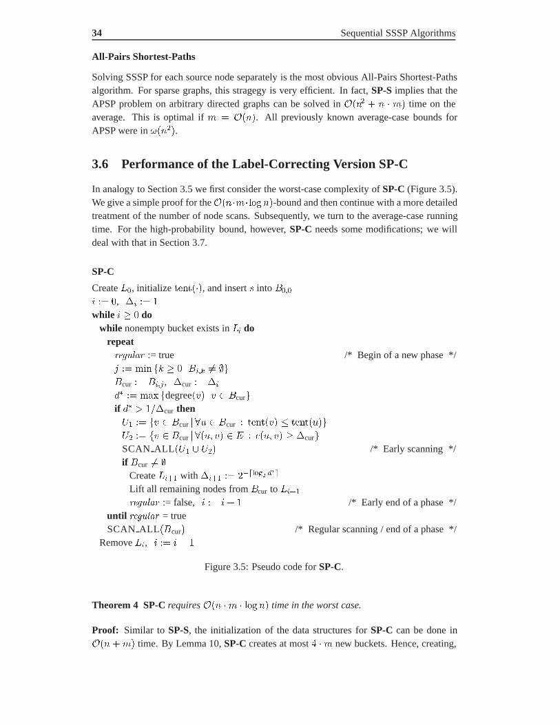
34 Sequential SSSP Algorithms
All-Pairs Shortest-Paths
Solving SSSP for each source node separately is the most obvious All-Pairs Shortest-Pathsalgorithm. For sparse graphs, this stragegy is very efficient. In fact, SP-S implies that theAPSP problem on arbitrary directed graphs can be solved in ���� � � � �� time on theaverage. This is optimal if � � ����. All previously known average-case bounds forAPSP were in &����.
3.6 Performance of the Label-Correcting Version SP-C
In analogy to Section 3.5 we first consider the worst-case complexity of SP-C (Figure 3.5).We give a simple proof for the �����������-bound and then continue with a more detailedtreatment of the number of node scans. Subsequently, we turn to the average-case runningtime. For the high-probability bound, however, SP-C needs some modifications; we willdeal with that in Section 3.7.
SP-C
Create 4�, initialize �������, and insert � into 1���
� � �, � � �
while � � � dowhile nonempty bucket exists in 4 do
repeat������� := true /* Begin of a new phase */3 � ��� �� � � �1� �� ��1cur � 1�� , �cur � �
)� � ��� �degree��� � � � 1cur�if )� � �!�cur then6� � �� � 1cur � �� � 1cur ������� ��������6� � �� � 1cur � ��� �� � � ��� �� � �cur�SCAN ALL�6� � 6�� /* Early scanning */if 1cur �� �
Create 4�� with ��� � ������� ���
Lift all remaining nodes from 1cur to 4��
������� := false, � � �� � /* Early end of a phase */until ������� = trueSCAN ALL�1cur� /* Regular scanning / end of a phase */
Remove 4, � � �� �
Figure 3.5: Pseudo code for SP-C.
Theorem 4 SP-C requires ��� �� � ��� �� time in the worst case.
Proof: Similar to SP-S, the initialization of the data structures for SP-C can be done in������ time. By Lemma 10, SP-C creates at most � �� new buckets. Hence, creating,

3.6 Performance of the Label-Correcting Version SP-C 35
traversing and removing all buckets can be done in ������ time (see also Observation 2).The bucket hierarchy for SP-C contains at most 7 � ����� �� levels (Lemma 10). Conse-quently, SP-C performs at most
���
�� � 7
���
�����
�
����
��� ��� � ��� ��
lift operations (Lemma 11 and Corollary 3). By Lemma 9, there are at most � phases, eachof which settles at least one node. Therefore, even though nodes may be rescanned, no nodeis scanned more than � times. That implies that altogether at most � �� edges are relaxed.Due to 7 � ����� ��, the target-bucket search for each relaxation requires at most �������
time. Hence, SP-C runs in ��� �� � ����� time in the worst-case.
In Section 3.7.1 (Lemma 19) we will give an extension that reduces the worst-case time fora target-bucket search to ����. After this modification, the asymptotic worst-case time forSP-C will be ��� ���. In the following we will have a closer look at the number of scanoperations.
3.6.1 The Number of Node Scans
Each node � that is reachable from the source node � will be inserted into the bucket struc-ture � and scanned from some current bucket at least once. Recall from the description ofthe algorithms in Section 3.4.2 that there are regular node scans and early node scans; foran early scan of �, the IN-criterion (Lemma 5) ensures ������� � �� ����. A re-insertionof � into � occurs if � was previously scanned with non-final distance value �������, andnow the relaxation of an edge into � reduces �������. A re-insertion of � later triggers arescan of � from some current bucket involving re-relaxations of �’s outgoing edges. Wedistinguish local rescans of �, i.e., � is rescanned from the same current bucket from whichit was scanned before, and nonlocal rescans of �, where � is rescanned from a differentcurrent bucket.
Lemma 14 (Number of Scan Operations) Let � � be an arbitrary node with degree) � � and in-degree )�, � )� ). Define ��� � ���� � �� ����� to be the weight of thelightest edge into node �. Let � be the subgraph of � that is induced by all vertices withdegree at most �. For each � � �, let ��
be the set of nodes � � � that are connectedto � by a simple directed path � � � � �� in � of total weight at most ��. Finally, let8��� denote the maximum size (i.e., number of edges) of any simple path in � with totalweight at most ��. SP-C performs at most
�� ��� � ���
� ���� �! � ����
��
�� ��� � �
� � )��
nonlocal rescans of node �
(3.6)and at most
����� �
����� ����������� ��
��� � local rescans of node �� (3.7)
For each current bucket of width �� there are at most 8��� � � regular scan phases.

36 Sequential SSSP Algorithms
Proof: By Invariant 2, the very first regular scan of node � (if any) takes place when � re-sides in a current bucket 1� having bucket width �� ������� ��. We first discuss nonlo-cal rescans:
Node � can only be rescanned from another current bucket after � moved upwards inthe bucket hierarchy. As there are at most ���� �! � � levels, this can happen at most ���� �! � � times. The new current buckets cover smaller and smaller ranges of tentativedistances: the �-th nonlocal rescan of � implies that � was previously (re-) scanned fromsome current bucket 1��� having bucket width ����
������� ����� whereas it is nowrescanned from a new current bucket 1� � ��� �� � ��� " 1��� of width �� ������� ��� at some higher level � � ���. As soon as � enters the current bucket 1�
we have ������� � �� � ������� ���. By then, the smallest tentative distance among allqueued candidate nodes is at least �� (Invariant 3). Therefore, if
��� � �
� � ) � ������� ��� for some � � � (3.8)
then ������� � �� ���� according to the IN-criterion (Lemma 5); in that case, the �-thnonlocal rescan of � will be the last time that � is scanned. The bound (3.6) of the lemmafollows by choosing the smallest nonnegative � satisfying the inequality (3.8).
Now we turn to the local rescans of �. Consider a current bucket 1cur � �� � � �cur�
from which � is rescanned. By Invariant 2, 1cur has bucket width �cur � �� for some� � ���� )!. We shall use the notation �������� to denote the tentative distance of � at thebeginning of phase 3. Let 0 denote the first regular scan phase for 1cur. Let 0� be the lastphase where � is rescanned from this 1cur. Hence, � � �����
���� constitutes the smallest
tentative distance found for � before 1cur is split or finally becomes empty. It follows thatthere are at most 0� � 0 local rescans of � from 1cur. Furthermore, � �� ���� � �
�� �cur, and �������� � ��������� for all 3 � 0�.
Let � � denote the set of nodes that were scanned and settled before phase 0; notethat � contains all nodes with �� ���� � �. Finally, let � � � � be the set of nodescontained in 1cur when the phase 0 starts. All nodes in � have degree at most �, i.e., theybelong to �. Furthermore, as long as the algorithm scans nodes and 1cur is neither splitnor emptied, the algorithm keeps exploring paths in �, starting from the nodes in � .
Let us fix a path � � �� ���� � � � ��� � �� whose exploration causes the last res-can of � from 1cur in phase 0� with tentative distance �: node �� , 0 3 0�, is scanned inphase 3; therefore, ������������� ��������� � ���� �����. On the other hand,������������� � ��������� � ���� ����� would imply that there is another path from� to � in � that results in �����
���� � �; this contradicts the choice of � . Thus,
������������� � ��������� � ���� �����. We conclude ��� � � ��������� � ��������� �
� � �cur � � � ��. In fact, � must be a simple path in �; otherwise – due to non-negative edge weights – � would already have been scanned in some phase 3 � 0� with�������� � �, thus contradicting our observation that �������� � �����
����. Therefore, �
can be reached from the nodes �� � � � ����� in � along paths of weight less than ��, i.e.,�� � � � ����� � ��
. Consequently, ��� � � 0� � 0. Since there are at most 0� � 0 local rescans
of � from 1cur their number is bounded by ��� �.

3.6 Performance of the Label-Correcting Version SP-C 37
The discussion above easily implies that � subsequent regular scan phases for 1cur re-quire at least one simple path in� having ��� edges and total weight at most ��. Hence,there are at most 8��� � � regular scan phases for this current bucket.
After having dealt with local rescans of node � from one particular current bucket ofwidth ��, we can easily bound the total number of local rescans of node �: the first localrescan of � (if any) takes place in a current bucket of width ��� , where �� � ���� )!.Further local rescans may happen for other current buckets of width ��� , ��� , . . . , where�� � �� � �� � � � �; hence, there are at most
������ ���������� �� ���
� local rescans of � in total.
Using Lemma 11 (for the number of lift operations), Lemma 12 and Remark 3 (for the costsof scan operations), and Lemma 14 (for the number of scan operations), we can restate theworst-case running time of SP-C as follows:
Corollary 4 Let 4���, �� �, �� ���, and ����� be defined as in Lemmas 11, 12, 14,and 14, respectively. SP-C runs in time
�
�����
����
����� �
�� � �� ��� � �����
��
�� �
���������� ���
���� �����
(3.9)
3.6.2 Average–Case Complexity of SP-C
This section serves to establish an average-case bound on the running time of SP-C underthe assumption of independent random edge weights that are uniformly drawn from �� �.According to Corollary 4 it is sufficient to find an upper bound for
�
�����
����
�4��� �
�� � �� ��� � �����
���
� ��
��������� ���
�� ����
�
Due to the linearity of expectation we can concentrate on the terms � �4��� and
�
��� � �� ��� � �����
���
� ��
��������� ���
�� ���� (3.10)
Recall from Lemma 14 that the values of �� ��� and ����� depend on the weights ofedges and simple paths into node �; they do not depend on the weights of any edge �� �, �� �, in the forward star of �. On the other hand, �� � solely depends on the weightof the edge �� �; see Lemma 12. Hence, as all edge weights are independent, the random
variables �� � �� ��� � ������ and�
� ��
��������� ��� �� ��
are independent, too.Consequently, the average-case running time for SP-C is bounded from above by
������ �
����
������� �
�� � ���� ��� � �������
��� �
������� ���
������ ��
�� (3.11)
Now we will show the following inequalities: For any node � � and any edge�� � � � we have
38 Sequential SSSP Algorithms
��4��� � � degree��� (Lemma 15)�� �� � � (Lemma 15)���� ��� � (Lemma 16)������� � � � (Lemma 18).
After inserting these inequalities in (3.11) we immediately obtain
Theorem 5 On arbitrary directed networks with random edge weights that are independentand uniformly drawn from �� �, SP-C runs in ������ average-case time.
In the remainder we prove the inequalities mentioned above.
Lemma 15 Let 4��� and �� � be defined as in Lemmas 11 and 12, respectively. For anynode � � and any edge �� � � � we have��4��� ����������� and�� �� � �.
Proof: For 4���, consider a reachable node � � with in-degree )�, � )� degree���.Let �� � ��� �� � � � ��� � ���� �� denote its )� incoming edges. 4��� is bounded from
above by�
� � ��
�����
������
�. By Inequality (3.4), we have
�
������
�
����
���
����
� ����
�����
����
�� �
��
����
� � �� � �
for any edge � � �. Hence, ��4��� � � )� � � degree���. Similarly, �� � �����
�������
�� � for any edge �� � � �. Thus, �� �� � � � � � �.
Lemma 16 For any node � � , let �� ��� be defined as in Lemma 14; then���� ��� �.
Proof: Let � have degree ) � � and in-degree )�, � )� ). Let ��� � ���� � �� �����
be the weight of the lightest edge into node �. From the definition of �� ��� we easily derive
�� ��� �����
�� ��� � �
� � )��
Due to the uniform edge weight distribution we have
�
���� � �
� � )�� � �
������
�
������ �
�
� � )�
� � � )� � �
� � ) � � � ���
Thus, ���� ��� � � � � �� and ���� ��� � � � � ��. Therefore,
���� ��� ����
���� ��� � � � � ����
���� ��� � � � �
����
���� � � � � �����
�� � � � ��

3.6 Performance of the Label-Correcting Version SP-C 39
Before we show the last missing inequality, ������� � � � , we first prove that long pathswith small total weight are unlikely for random edge weights. This observation will be usedto bound ������� in Lemma 18. In the following, a path without repeated edges and totalweight at most � will be called a �-path.
Lemma 17 Let # be a path of 5 non-repeated edges with independent and uniformly dis-tributed edge weights in �� �. The probability that # is a �-path equals ��!5 for � �.
Proof: Let % denote the weight of the �-th edge on the path. The total weight of the
path is then��
��%. We prove by induction over 5 that ����
��% �
� ��!5 for
� �: if 5 � � then due to the uniform distribution the probability that a single edgeweight is at most � � is given by � itself: � �%� � � �. Now we assume that
�
�����% �
� ��!5 for � � is true for some 5 � �. In order to prove the result
for a path of 5 � � edges, we split the path into a first part of 5 edges and a second part ofone edge. For a total path weight of at most �, we have to consider all combinations for� � � � so that the first part of 5 edges has weight at most � � � and the secondpart (one edge) has weight �. Thus,
�
�������% �
�
��� �
�����% � � �
)� �
� ��
��� ��
�� )� � ����
������
Lemma 18 Let ����� be defined as in Lemma 14. For any node � � , ������� � � �.
Proof: Recall that � denotes the subgraph of � that is induced by all vertices with degreeat most �. Furthermore, for any � � �, ��
denotes the set of nodes � � � that areconnected to � by a simple directed path � � � � �� in � of total weight at most ��. Forany node � with degree ), ����� �
������ ���������� �� ���
�.Let us define #�
to be the set of all simple ����-paths into � in �. Obviously, ��� �
�#� �. Hence,
������� ����� ����������� ��
� ��#� � �
Since all nodes in � have degree at most �, no more than ) � �������� simple paths of5 edges each enter node � in �. Taking into account the probability that these paths are����-paths (Lemma 17), we find
������� ����� ����������� ��
�����
) � ������ � ���!5
�
����� ����������� ��
)
��! ��
���
�
5
"
����
�� � � � � � � � (3.12)
40 Sequential SSSP Algorithms
Hence, by now we have provided the missing pieces in order to show that SP-C runs inlinear time on the average (Theorem 5).
As already mentioned in Section 3.5.2 for SP-S, SP-C can keep track of the actualresource usage: after ��� � ���� � �� operations it may abort and start the computationfrom scratch with Dijkstra’s algorithm. Thus, the worst-case total execution time is limitedby ��� ������� while the linear average-case bound is still preserved.
Unfortunately, SP-C is less reliable than its label-setting counterpart SP-S; the linear-time bound is not obtained with high probability. Why? In its current form – even thoughthe total number of node scans is bounded by �� � � � � � �� � � � �� � � on average(Lemmas 16 and 18) – SP-C may scan some nodes many more than �� times with non-negligible probability. If such a node � has out-degree ���� then SP-C may perform asuperlinear number of operations: each time � is scanned, all its outgoing edges are relaxed.In Section 3.7 we give the modifications for SP-C to cope with that problem; Section 3.8provides the adapted analysis for the high-probability bounds.
3.7 Making SP-C More Stable
Our modified version of SP-C, which we will call SP-C*, applies deferred edge relaxations:when a node � is scanned from a current bucket 1cur of width �cur, then only those edgesout of � that have weight at most �cur are relaxed immediately. The remaining edges oflarger weight are relaxed once and for all after ������� is guaranteed to be final.
The rationale behind this modification is the following: due to the correlation of bucketwidths and maximum node degrees it turns out that as long as ������� is not yet final,each (re-)scan of � in SP-C* relaxes at most a constant number of �’s outgoing edges inexpectation and not much more with high probability. Therefore, even if some nodes maybe rescanned much more often than the average, it becomes very unlikely that these nodescause a superlinear number of edge relaxations.
Furthermore, we describe an alternative for the simple bottom-up search in order to findtarget buckets in constant worst-case time. The fast relaxation procedure is not crucial toobtain the high-probability bound for SP-C*. However, being allowed to assume that any(re-)relaxation can be done in constant worst-case time somewhat simplifies our analysis.Subsequently, we describe our modifications in more detail:
1. For each node � � , SP-C* creates a list !�� that initially keeps all outgoing edgesof � in grouped order according to their weights as follows:
� !�� consists of at most ���� ��! � � groups;
� group 9, � � � ���� ��!, in !�� holds all outgoing edges �� � with���� � ��� � �� in arbitrary order;
� 9����� ��� keeps all edges of !�� with weight at most ������� ���;
� for all 3 � �, 9 appears before 9� in !�� .
The grouped order can be established in linear time by integer-sorting for small val-ues: edge weights ���� � ������� ��� are mapped onto ����� �!�����, thus creating

3.7 Making SP-C More Stable 41
integers from � to ���� ��! � �; smaller edge weights are mapped onto the inte-ger ���� ��!. After an integer-sorting by non-increasing order the largest integers(which account for the smallest edge weights) appear first.
2. Each bucket 1�� is equipped with an additional edge list ��� . Whenever a node � isdeleted from 1cur � 1�� (by either scanning or lifting), SP-C* moves all remainingedges � � !�� satisfying ���� � �cur from !�� to��� . Note that these edges constitutethe last groups in !�� . Hence, if � is rescanned from 1cur no transferable edges areleft in !��; this can be checked in constant time.
3. All edges in��� are relaxed as soon as 1cur � 1�� is empty after a phase or – in case1�� has been split – after its refining level �� � is removed. This is sufficiently early:we have ���� � � for any edge � � �� � � ���; hence, if �� �� � belongs to therange of 1�� , then �� ���� � ��� � � �� �� � since �� ���� lies in the range of 1��
as well; in that case a relaxation of �� � is not needed at all. On the other hand, if�� �� � is too large to be covered by 1�� , then �� � � ��� is relaxed before willbe scanned in its respective bucket. By the time �� � � ��� is relaxed, we have������� � �� ���� (this follows from the monotonicity property).
The total number of operations needed to perform the initial grouping and to maintain theadditional edge lists is bounded by ������.
3.7.1 Performing Relaxations in Constant Time
In the following we describe a method to perform edge relaxations in constant worst-casetime. Using this guided search routine instead of the simple bottom-up search improvesthe total worst-case time of SP-C and SP-C* to ��� ���. Additionally, it simplifies ouranalysis in Section 3.8. Therefore, from now on we will assume that SP-C* applies thisworst-case efficient method.
Lemma 19 The target bucket search for an edge relaxation can be performed in constantworst-case time.
Proof: For the relaxation of an edge � � �� ��, where � is in the current bucket 1cur � 1��
with bucket width � of the topmost level �, the algorithm has to find the highest level / �that can potentially contain the non-split target bucket for �. We distinguish two cases:���� ��� and ���� � ���.
Firstly, if ���� ��� (recall that ��� is the total level width of level �) then the targetbucket of � is either located in level �, hence / � �, or it is the immediate successor bucket:1 of the rightmost bucket in level �. Note that :1 is located in some level below � havingtotal level width at least ���. Upon creation of the new topmost level �, a pointer to :1
can be maintained as follows: if level � is a refinement of a bucket 1���� that is not therightmost bucket in level �� �, then :1 � 1������, otherwise :1 � :1��; see Figure 3.6for an example.
Secondly, consider the case ���� � ��� where the target bucket is definitely locatedin some array below 4. Let '� � ����� �!�����. For each level �, � � �, we maintainan additional array ��� with ���� �!��� entries: ��'� � / � � denotes the highest

42 Sequential SSSP Algorithms
L
L
L
L
empty split unvisited
3
2
1
0
Figure 3.6: Example for pointers to the immediate successor buckets.
level / potentially containing the target bucket of � for a relaxation of � � �� �� with� � 1cur � 1�� . As before, if � does not belong to level /, then it will fit into the immediatesuccessor bucket :1! of level /. The correctness follows inductively from the construction:
���� is an empty array. Now we show how ���, � � �, can be created from �����.The highest possible level for a target bucket of an edge � � �� �� with ���� � ��� islocated in some level / � �� �, independent of the position of � in level �� �. As before,this is an immediate consequence of the fact that the total width of level �� � is given by��� ����. By induction, the proper search level / can be identified in ���� time bylooking up ��������� �!����� � /. The new level � is just a refinement of some bucketfrom level �� �. Hence, for ���� � ���, all targets are still located in the same level/ � �� � as before. Consequently, we have ��� � ����� for � � � ���� �!���. Inother words, these entries can simply be copied from ����� to ���.
New entries are needed for ������ �!���, � � �, ������ �!��� � �, accounting foredge weights ��� � ���� ���. These weights are too large for a target within level �(which has total level width ���) but the target may be located in the array 4��; therefore,������ �!��� � �� �, � � �, ������ �!��� � � � �� �. On the other hand, if the targetdoes not lie in 4�� then the target bucket is definitely given by the immediate successorbucket of 4��, :1��, because :1�� has width at least ��� � ����.
Hence, all required lookups in the additional data structures for a relaxation of � can bedone in constant time. For SP-C and SP-C*, the costs to build ��� and to set the pointer to:1cur are bounded by ������degree����, where � is a node that caused the creation of level �by a bucket splitting. As each node is responsible for at most one splitting, the worst-casetotal costs to maintain the extra data structures are bounded by ������.
3.8 A High–Probability Bound for SP-C*
In this section we first give a revised worst-case bound for the running time of SP-C*. Thenwe prove linear average-case time for SP-C* using this revised bound. After some technicallemmas we can identify an event ����, which holds with high probability. The event ����
is used to show that the revised worst-case bound for the running time of SP-C* satisfiesthe so-called Bounded Martingale Difference Condition with suitable parameters for nearlyall instantiations of the random edge weights. At that point the high-probability bound forthe running time of SP-C* follows easily from a generalization of the Chernoff bounds.
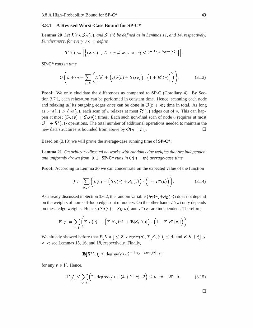
3.8 A High–Probability Bound for SP-C* 43
3.8.1 A Revised Worst-Case Bound for SP-C*
Lemma 20 Let 4���, �� ���, and ����� be defined as in Lemmas 11, and 14, respectively.Furthermore, for every � � define
���� �###��� � � � � �� ��� � ������� ����������
�### �SP-C* runs in time
�!����
����
�4��� �
��� ��� � �����
���
� � ������"
� (3.13)
Proof: We only elucidate the differences as compared to SP-C (Corollary 4). By Sec-tion 3.7.1, each relaxation can be performed in constant time. Hence, scanning each nodeand relaxing all its outgoing edges once can be done in ��� � �� time in total. As longas ������� � �� ����, each scan of � relaxes at most ���� edges out of �. This can hap-pen at most ��� ��� � ������ times. Each such non-final scan of node � requires at most��� � ����� operations. The total number of additional operations needed to maintain thenew data structures is bounded from above by ������.
Based on (3.13) we will prove the average-case running time of SP-C*:
Lemma 21 On arbitrary directed networks with random edge weights that are independentand uniformly drawn from �� �, SP-C* runs in ������ average-case time.
Proof: According to Lemma 20 we can concentrate on the expected value of the function
� �����
�4��� �
��� ��� � �����
���
� � ������� (3.14)
As already discussed in Section 3.6.2, the random variable ��� ���������� does not dependon the weights of non-self-loop edges out of node �. On the other hand, ���� only dependson these edge weights. Hence, ��� ��� � ������ and ���� are independent. Therefore,
��� �����
���4��� �
����� ��� ��������
���
� ��� �������
We already showed before that ��4��� � � ���������, ���� ��� �, and ������� � � �; see Lemmas 15, 16, and 18, respectively. Finally,
�� ���� ��������� � ������� ���������� �
for any � � . Hence,
��� ����
�� � ��������� � �� � � � �� � �
� � ��� �� � �� (3.15)
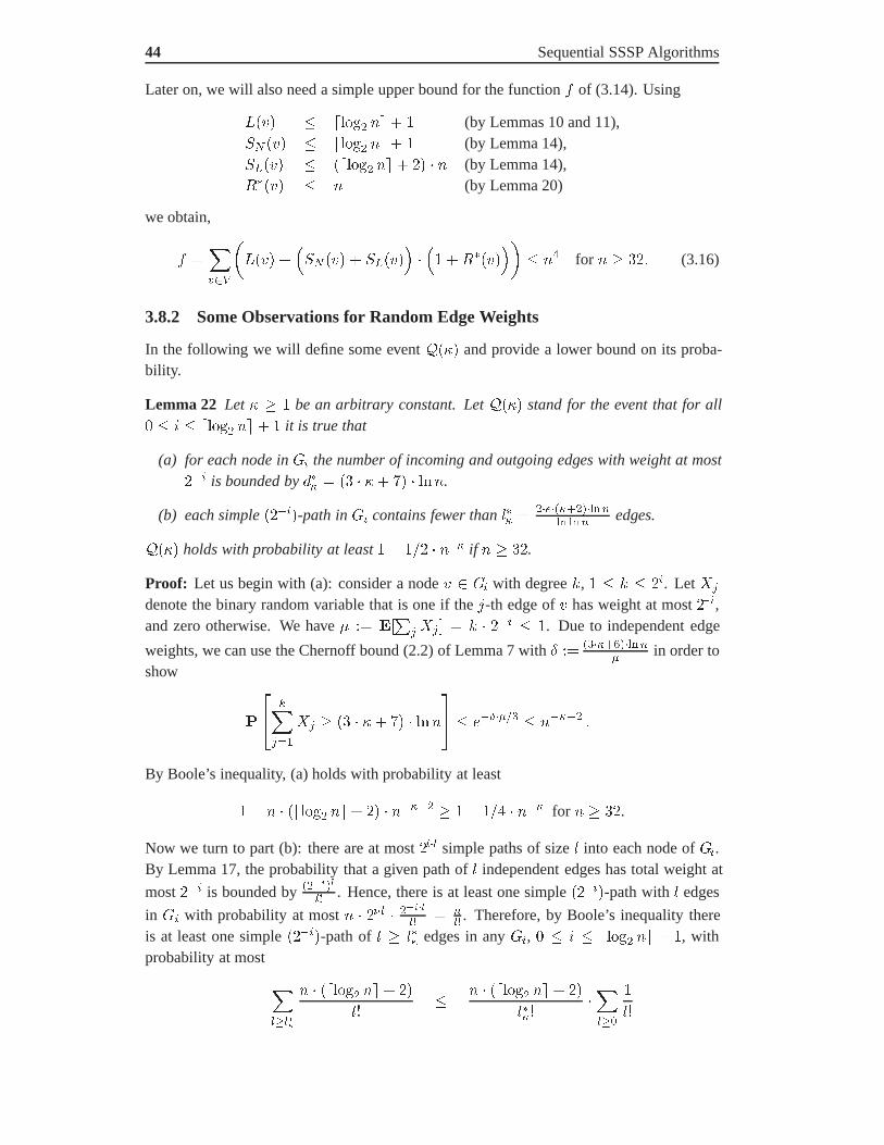
44 Sequential SSSP Algorithms
Later on, we will also need a simple upper bound for the function � of (3.14). Using
4��� ���� �! � � (by Lemmas 10 and 11),�� ��� ���� �! � � (by Lemma 14),����� � ���� �! � �� � � (by Lemma 14), ���� � (by Lemma 20)
we obtain,
� �����
�4��� �
��� ��� � �����
���
� � ������
�� for � � ��� (3.16)
3.8.2 Some Observations for Random Edge Weights
In the following we will define some event $��� and provide a lower bound on its proba-bility.
Lemma 22 Let � � � be an arbitrary constant. Let $��� stand for the event that for all� � ���� �! � � it is true that
(a) for each node in � the number of incoming and outgoing edges with weight at most�� is bounded by )�" � �� � �� �� � ���.
(b) each simple ����-path in � contains fewer than 5�" � ���"�������� ��� edges.
$��� holds with probability at least � � �!� � ��" if � � ��.
Proof: Let us begin with (a): consider a node � � � with degree �, � � �. Let %�
denote the binary random variable that is one if the 3-th edge of � has weight at most ��,and zero otherwise. We have , � ��
��%� � � � �� �. Due to independent edge
weights, we can use the Chernoff bound (2.2) of Lemma 7 with Æ � � "������� in order to
show
�
����
%� � �� � �� �� � ���
� ���� ��"�� �
By Boole’s inequality, (a) holds with probability at least
� � � � � ���� �! � �� � ��"�� � � � �!� � ��" for � � ��.
Now we turn to part (b): there are at most �� simple paths of size 5 into each node of �.By Lemma 17, the probability that a given path of 5 independent edges has total weight at
most �� is bounded by ������
�� . Hence, there is at least one simple ����-path with 5 edges
in � with probability at most � � �� � �����
�� � ��� . Therefore, by Boole’s inequality there
is at least one simple ����-path of 5 � 5�" edges in any �, � � ���� �! � �, withprobability at most �
����
� � � ���� �! � ��
5 � � � ���� �! � ��
5�" �����
�
5

3.8 A High–Probability Bound for SP-C* 45
� � � ���� �! � ��
� �� � ��� ��� � ; � 5�"
� � by the Stirling Approximation
��
� � � �� � ��
� ��
for � � ��
��"
��
For the last inequality consider an upper bound for 5�" in
'� � + % ' � ��' � �� + where + � �"�� � �� and ' � �� � : (3.17)
Since ' � � we have ��' � � and therefore ' �� +. Reinserting the last inequality in(3.17) yields the lower bound ' � �� #
�� �� # . If we repeat the reinsertion trick once more using
the lower bound just obtained, then we find ' �� #�� �� #��� �� �� # ��� #
�� �� # ��"��� ����� ��� .
Hence, the choice of 5�" � ���"�������� ��� ensures '� � �"��. Therefore, (b) holds with
probability at least � � �!� � ��".Combining the bounds for (a) and (b) by Boole’s inequality we find that $��� holds
with probability at least � � � � �!� � ��" � � � �!� � ��".
Using $���, we can also prove high-probability bounds on the sizes of the sets �� (which,in turn, define �����; see Lemma 14).
Lemma 23 Let � be an arbitrary node in�. Let �� be defined as in Lemma 14. Let $��
bethe set of nodes � � � that are connected to � by a simple directed path � � � � �� in� oftotal weight at most ��. Let � . � � be arbitrary constants. If $��� holds then there existpositive constants ���.� and <�.� so that ���
� �"$���� �� ��� and � $�� � �"$���� �� ���
with probability at least � � ��� for � � ���.�.
Proof: Let us start with $�� . We argue that the number of those nodes that are reached
from � via paths of length 5 can be bounded by the offspring in the 5-th generation of thefollowing branching process3
�: An individual (a node) � has its offspring defined by thenumber *� of edges leaving � that have weight at most ��. For independent edge weightsuniformly distributed in �� �, we find ��*� degree��� � �� � � �� � since eachnode in � has degree at most �. Let =� denote the total offspring after 5 generations whenbranching from node � (i.e., =� � *�).
As long as new edges are encountered when following paths out of �, the offspring ofthe branching process is an exact model for the number of paths emanating from � that useonly edges with weight at most ��. After a node � is found to be the target of multiple pathsout of �, the events on those paths would no longer be independent. However, all but one ofthe multiple paths would produce only duplicate entries into $��
. The additional paths aretherefore discarded from the branching process. All remaining events are independent.
In the following, we consider another branching process �� with identical and indepen-dent probabilities for the generation of new nodes: =�� � �, = �� is a nonnegative integer-
valued random variable, and =�� ��%�
���
�� * � where the random variables * � are distributed
3An introduction to branching processes can be found in [11, 79], for example.

46 Sequential SSSP Algorithms
like =�. Furthermore, the random variables * � are independent of each other and indepen-dent of =���. The branching factor of this branching process is given by > � ��=��. Forbranching processes of this kind we have ��=�� � >�. Additionally, it is shown in [91,Theorem 1] that for > � � and any constant . � �, =�� � ��>� � ����� with probability atleast � � �!� � ���; the involved constants depend on .. Taking > � � � �, the randomvariables =� of the first branching process � are stochastically dominated by the respectiverandom variables =�� of ��.
In order to asymptotically bound the sum�
� � =�� we can concentrate on the term
= �� because a growing exponential sum is dominated by its last summand:�
� � =�� �
���� � ��� �� whp. If $��� holds in addition, we have 5 � 5�" � ���"�������� ��� . In that
case, the number of nodes that are reached from � via simple ����-paths in � is at most
����� � ��� �� � ���
����� ���� �� � ��� �� with probability at least � � �!� � ���.
Now we turn to �� , which is symmetric to $��
in the sense that it considers pathsentering � instead of paths leaving �. Hence, the argument simply follows by traversing theedges during the branching process in the opposite direction. Therefore, if $��� holds, thereare positive constants ���.� and <�.� so that ���
� �"$���� �� ��� and � $�� � �"$���� �� ���
with probability at least � � ��� for � � ���.�.
3.8.3 The Event ���� and the Method of Bounded Differences
In the next lemma we introduce the event ���� and give a lower bound on its probability:
Lemma 24 Let � � � be an arbitrary constant. Let ������� and <����� be the constantsof Lemma 23 with . � �� �. We define ���� to be the event that
(a) $��� holds.
(b) ��� � �"$�"���� �� ��� and � $��
� �"$�"���� �� ��� for all � � ���� �! � �
and all � � �.
Then ���� holds with probability at least � � ��" for any � � ��������� �� ���.
Proof: By Lemma 22, (a) holds with probability at least � � �!� � ��" for � � ��. UsingBoole’s inequality, (a) and (b) hold with probability at least � � �!� ���" �� � � ���� �!�
�� � ��"�� � � � ��" for � � ��������� �� ���.
For technical reasons we will also need the events ����� and �������: let %� � �� �
denote the random variable associated with the weight of the 5-th edge of the input graphfor � 5 �; then ����� stands for the event that ���� holds if we just consider theedge weights associated with %� � � � %� . Equivalently, ������� denotes the event that���� holds if we restrict attention to the � � 3 random variables %��� � � � %�. Clearly,���� implies ����� & ������� for all � 3 �. Therefore, ���������������� ������� � ����". On the other hand, it does not necessarily follow from �����&�������
that ���� holds as well. Still, ����� & ������� implies that some event ����� similar to���� holds; it is easy to check that due to the contributions from two independent edgesets, the bounds of $��� are at most doubled and as a consequence the bounds on ��� �

3.8 A High–Probability Bound for SP-C* 47
and � $�� � are at most squared. So, more formally, ����� stands for the event that for all
� � ���� �! � � it is true that
(a) for each node in � the sum of incoming and outgoing edges with weight at most ��
is bounded by � � )�" � �" � �� ��� � ���.
(b) each simple ����-path in � contains fewer than � � 5�" � ���"�������� ��� edges.
(c) ��� � ��"$�"���� �� ��� and � $��
� ��"$�"���� �� ��� for all � � �.
Similarly, ������ & �������� with � 3� � 3� � implies ����� if we only take intoconsideration the edge weights associated with %� � � � %�� and %���� � � � %�. The events���� and ����� will be used later in connection with the following tail estimate:
Lemma 25 (Method of Bounded Martingale Differences [45, 100]) Let � � �%� � � �
%�� be a family of random variables with %� taking values in the set ?�. Let � � �
be the typographical shortcut for %� � ��, . . . , % � �. Let ���� be a function that sat-isfies the following condition concerning %� � � � %� with parameters 0� � � � 0�: for any� � ��� � � � ��� � %
�?� and any � � ?,
9��� � � ��� ���� � ���% � � ���� ���� � ��� � 0 (3.18)
for all � � �. Then
������ � ������ � 0 �� ��
���� ��� �
Moreover, let ' be any ‘bad’ subset of%
�?�, such that 9��� 0, � � � for each� �� ' . Then
������ � ������ � 0 �� ��
���� ��� ���� � '� (3.19)
Proof: See [100].
The function 9��� of (3.18) measures how much the expected value of ���� changes if it isrevealed that% takes the value �, conditioned on the fact that%� � �� � � � %�� � ���.If the random variables %� � � � %� are dependent then fixing % � � may influence thedistribution of %�� � � � %�. However, if %� � � � %� are independent then the distribu-tion of %�� � � � %� remains the same. In that case, 9��� can be rewritten as
� ������ � � � ��� � %�� � � � %�� ������� � � � ���%%�� � � � %�� � �
Hence, for independent random variables, 9��� can be obtained by comparing���� � � � ��� � '�� � � � '�� with������ � � � ���% '�� � � � '�� for each com-bination �'�� � � � '�� � %�
����?�, weighted with the respective probabilities for�'�� � � � '�� to occur. If we are just interested in upper bounds on 9���, then it is evensufficient to bound
���&��&���'�
## ���� � � � ��� � '�� � � � '�� � ���� � � � ��� �� '�� � � � '��
## (3.20)

48 Sequential SSSP Algorithms
for each �'�� � � � '�� � %�����?�, and then build the weighted sum over all combina-
tions.We shall use Lemma 25 as follows: %� � �� � denotes the weight of the 5-th edge of
the input graph for � 5 �; hence, the random variables %� � � � %� are independent.For � we substitute the function (3.14) concerning the running time of SP-C*. The ‘bad’subset ' contains those edge-weight vectors for which the event ���� does not hold. ByLemma 24, ������ � � � ��" for � � ��������� �� ���. Thus, ��� � ' ��".
It remains to bound 9��� for all � �� ' using (3.20): we know that ������ holds forthe prefix ��� � � � ����; if ������ also holds for the suffix �' � � � '�� then this implies����� concerning the first � � � edges and the last � � � edges of the graph. In that case(which happens for the overwhelming number of suffixes since �������� � ����") wecan use the knowledge that ����� holds in order to bound the maximum effect of arbitrarilychanging the value of the �-th coordinate in (3.20). In fact, for that case we will show inthe proof of Theorem 6 that (3.20) can be bounded from above by � � �(�"�� �� ��� where@��� � � is some constant, and � � ��������� �� ���.
Otherwise, i.e., in the unlikely case that ������ does not hold, then (3.20) can betrivially bounded by �� according to (3.16). It follows that for any � �� ' and all � � �,
9��� �� � ��"� � � � �(�"�� �� ��� � ���"
� � �(�"�� �� ��� � 0 for � � � and � � ��������� �� ����
Using Lemma 25 we find
��� � ��� �# � ����� �� ��������
���������� �� � �� ���" �� �
����� �� � �� ���" � ���"
if � � ������ � . Hence,
��� ��� � # � ����� � � � � � ��"
for any constant � � � and any � � ��������� �� ������ ��.
Theorem 6 On arbitrary directed networks with random edge weights that are independentand uniformly drawn from �� �, SP-C* runs in ������ time with high probability.
Proof: According to the discussion above it is sufficient to show that (3.20) can be boundedfrom above by � � �(�"�� �� ��� if the event ����� holds for all edge weights excluding���� ��, the weight of the �-th edge in the input graph. We rewrite � in the form
� �����
4��� �����
��� ��� �
�� � ����
���
����
������ �
�� � ����
���
In the following, let ��* � denote the maximum change of some random variable * after amodification of ���� ��.
By the definition of 4���, as given in Lemma 11, modifying ���� �� does not influence4��� unless � � �. Moreover, 4� �� is bounded by the maximum height of the buckethierarchy. Hence, after an alteration of ���� ��, the value 4� �� may change by at most ���� �!��. In other words, � �4� ��� ���� �!�� and �
����� 4���
� ���� �!��,
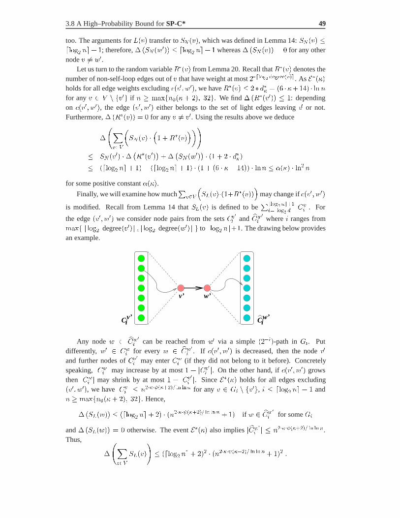
3.8 A High–Probability Bound for SP-C* 49
too. The arguments for 4��� transfer to �� ���, which was defined in Lemma 14: �� ��� ���� �! � �; therefore, � ��� � ��� ���� �! � � whereas � ��� ���� � � for any othernode � �� �.
Let us turn to the random variable ���� from Lemma 20. Recall that ���� denotes thenumber of non-self-loop edges out of � that have weight at most ������� ���������� . As �����
holds for all edge weights excluding ���� ��, we have ���� � ( )�" � �" ��� ��� � �� �for any � � � ���� if � � �������� � �� ���. We find � � ������ �: dependingon ���� ��, the edge ��� �� either belongs to the set of light edges leaving �� or not.Furthermore, � � ����� � � for any � �� ��. Using the results above we deduce
�
!����
��� ��� �
�� � ����
��" �� ���� � �
� �����
�� �
��� � ��
� � �� � � � )�"�
� ���� �! � �� � � ���� �! � �� � �� � �" � �� ���� � ��� $��� � ��� �
for some positive constant $���.
Finally, we will examine how much�
������������� �����
�may change if ���� ��
is modified. Recall from Lemma 14 that ����� is defined to be������ ����
������ �� ��� �. For
the edge ��� �� we consider node pairs from the sets ��� and $���
where � ranges from���� ���� degree����! ���� degree� ��! � to ���� �!��. The drawing below providesan example.
v’ w’
CCi iw’v’
Any node � $���
can be reached from � via a simple ����-path in �. Putdifferently, � � ��
for every � $���
. If ���� �� is decreased, then the node ��
and further nodes of ��� may enter ��
(if they did not belong to it before). Concretelyspeaking, ���
� may increase by at most � � ���� �. On the other hand, if ���� �� grows
then ��� � may shrink by at most � � ����
�. Since ����� holds for all edges excluding��� ��, we have ���
� ��"$�"���� �� ��� for any � � � � ����, � ���� �! � � and� � ��������� �� ���. Hence,
� ���� �� � ���� �! � �� � ���"$�"���� �� ��� � �� if � $���
for some �
and � ���� �� � � otherwise. The event ����� also implies �$���
� ��"$�"���� �� ���.Thus,
�
!����
�����
" � ���� �! � ��� � ���"$�"���� �� ��� � ��� �
50 Sequential SSSP Algorithms
It remains to incorporate the factor �� � �����:
�
!����
������ �
�� � ����
��"
������ � �� �����
�� �
!����
�����
"� �� � � � )�"�
� ���� �! � �� � ��"$�"���� �� ��� �
� ���� �! � ��� � ���"$�"���� �� ��� � ��� � �� � �" � �� ���� � ���
�(�"�� �� ��� for some positive constant @��� �
In fact, @��� can be chosen in a way that
���� �
!����
4���
"� �
!����
��� ��� �
�� � ����
��"�
�
!����
������ �
�� � ����
��" ���� �! � � � $��� � ��� �� �(�"�� �� ��� � � �(�"�� �� ���
if � � ��������� �� ���.
3.9 Implications for the Analysis of other SSSP Algorithms
In this section we will re-use the analysis for the bucket-splitting algorithms SP-C andSP-C* (Sections 3.6 and 3.8) in order to yield average-case results for simpler SSSP al-gorithms. We consider the “Approximate Bucket Implementation of Dijkstra’s algorithm”(ABI-Dijkstra) [25], which we already sketched in Section 3.3, and our refinement, thesequential �-Stepping.
3.9.1 ABI-Dijkstra and the Sequential �-Stepping
The �-Stepping algorithm maintains a one-dimensional array 1 of buckets where 1��
stores the set �� � � is queued and ������� � �� � � �� � �� � ���. As before, theparameter � is a positive real number, which is also called the “bucket width”. Let �max �
����� ���� denote the maximum edge weight. For maximum shortest-path weight � �
��� ��� ��� �� ��� ��� �� ���, the algorithm traverses& ��
'buckets. However, by cycli-
cally reusing empty buckets, only space for �max �&�max�
'� � buckets is needed. In that
case, a node � with tentative distance ������� is kept in bucket 1 � ��������!�� ��� �max .The �-Stepping approach distinguishes light edges and heavy edges: a light edge has
weight at most �, the weight of a heavy edge is larger than �. In each phase, the algorithmscans all 4 nodes from the first nonempty bucket (current bucket) and relaxes all light edges
4Similar to the bucket-splitting approaches, the nodes of the current bucket could also be scanned one-by-one in FIFO order. However, in view of the parallelizations in Chapter 4 we consider them in phases alreadynow.
3.9 Implications for the Analysis of other SSSP Algorithms 51
out of these nodes. The relaxation of heavy edges is not needed at this time since they canonly result in tentative distances outside of the scope of the current bucket, i.e., they willnot insert nodes into the current bucket. Once the current bucket finally remains emptyafter a phase, all nodes in its distance range have been assigned their final distance valuesduring the previous phase(s). Subsequently, all heavy edges emanating from these nodes arerelaxed once and for all. Then the algorithm sequentially searches for the next nonemptybucket. As in the case of SP-C and SP-C*, single buckets of the array can be implementedas doubly linked lists; inserting or deleting a node, finding a bucket for a given tentativedistance and skipping an empty bucket can be done in constant time. A simple preprocessingcan restructure the adjacency lists in order to support efficient access to the subsets of lightedges.
The ABI-Dijkstra algorithm can essentially be seen as the sequential �-Stepping with-out distinction between light and heavy edges, i.e., all outgoing edges of a scanned node arerelaxed immediately.
In the following we will transfer our analysis on the average-case number of node res-cans from SP-C and SP-C* to ABI-Dijkstra and �-Stepping, respectively:
Theorem 7 Consider directed graphs with � nodes,� edges and independent random edgeweights uniformly distributed in �� �. Let )� and �� denote upper bounds5 on the maximumnode degree ) and the maximum shortest-path weight �, respectively. Choosing the bucketwidth as � � ������� ��, ABI-Dijkstra and �-Stepping run in ��������) ��� time onthe average. Additionally, for � � ������� ���, the �-Stepping algorithm requires ��� �
� � )� � ��� time with high probability. Both algorithms need ��� ��� time in the worstcase.
Proof: We examine a reformulation of the algorithms SP-C and SP-C* with ������ �� �
� � � ) � � initial buckets at level �, each of them having width �� � ������� ��.Scanning low-degree nodes from buckets of reduced width will clearly not increase theprobability of rescans. Furthermore, due to the revised choice of �� none of the initialbuckets will ever be split. Hence, the bucket structure remains one-dimensional, and target-bucket searches always succeed in constant time. In other words, for the chosen bucketwidths, the reformulated algorithms SP-C and SP-C* coincide with ABI-Dijkstra and �-Stepping, respectively.
As compared to the standard versions of SP-C and SP-C*, at most�
����� �� ��
� ��)��
extra buckets may have to be traversed. Therefore, disregarding ����)��� additional oper-ations, the asymptotic average-case performances of ABI-Dijkstra and �-Stepping reduceto those of the standard versions SP-C and SP-C*, respectively. The average-case boundsfollow from Theorem 5 and Lemma 21. If ) )� and � �� then the high-probabilitybound for the �-Stepping is inherited from Theorem 6.
Using ) �� � ��� ��� for arbitrary edge weights in �� � the worst-case running-timesare easily derived from the proofs of Theorem 4 and Lemma 19.
5Actually, it is sufficient if these bounds hold with high probability.

52 Sequential SSSP Algorithms
3.9.2 Graphs with Constant Maximum Node-Degree
By Theorem 7, both ABI-Dijkstra and the sequential �-Stepping run in linear average-casetime on graphs with independent random edge weights uniformly distributed in �� � wherethe term ��) � � concerning the chosen source � is bounded by ��� ���. For the edgeweights under consideration, we have the trivial bound � � that is valid for arbitrarydirected graphs and any choice of the source node. Therefore:
Corollary 5 ABI-Dijkstra has linear average-case complexity on arbitrary directed graphswith random edge weights and constant maximum node degree. For the same graph class,the sequential �-Stepping algorithm runs in linear time with high probability.
Important graph families with small constant degree – thus implying linear average-casetime – frequently arise for transportation and communication problems. Furthermore, grid-graphs of small dimensions where a certain fraction of edges is missing frequently occur inapplications of percolation research [73].
Another important input family that can be efficiently tackled by ABI-Dijkstra and the�-Stepping is the class of random graphs with random edge weights, which we will con-sider in the next subsection.
3.9.3 Random Graphs
Over the last forty years, the theory of random graphs [17, 46] has developed into an in-dependent and fast-growing branch of mathematics with applications to reliability of trans-portation and communication networks or natural and social sciences. Frequently, randomgraphs are chosen to average the performance of an algorithm over all possible structuralinputs.
We use the random digraph model 8�� $)!��, which was introduced by Angluin andValiant [9]. An instance of 8�� $)!�� is a directed graph with � nodes where each edgeis present with probability $)!�, independently of the presence or absence of other edges.Hence, each node has expected out-degree (and in-degree) $).
Let us turn to the maximum node degree ) of a random graph. There are deep results onthis topic partially taking into account the whole degree sequence of random graphs, e.g.,see [16, 101, 126]. However, for our purposes, a very simple proof yields a sufficient bound:
Lemma 26 Let � � ��� be a random graph from 8�� $)!��. The maximum nodedegree ) satisfies ) � ��$)� ��� �� whp.
Proof: Define %��� to be the binary random variable that is one if �� � � �, and zerootherwise. Let �� (A�) denote the number of outgoing (incoming) edges of node �. Hence,���� �
���� ��%��� � $) and ��A� �
���� ��%��� � $)� Using the formula of the
Chernoff bound from Lemma 7 we find
���� � �� � Æ� � $) � ��A� � �� � Æ� � $) �����Æ��Æ ��� �
Note the dependence between�� and A� caused by the edge �� �. However, using Boole’sinequality, each in-degree and each out-degree of � is at most �� � Æ� � $) with probabilityat least � � � � � � �����Æ��Æ ��� . Choosing Æ � ������! $)� � �� � �� � ��� �� for

3.10 Lower Bounds 53
some arbitrary constant � � �, we find that the sum of maximum in-degree and maximumout-degree exceeds � � ����� � $) $)� � � ��� �� � ���� with probability at most ���.
Next we examine the maximum shortest-path weight � of random graphs with indepen-dent random edge weights uniformly distributed in �� �. Again, we can rely on intensiveprevious work: in order to bound � for sparse random graphs with random edge weightswe can use a known result on the their diameter. Let ��� ����� �� denote the minimumnumber of edges needed among all paths from � to � in a graph � � ��� if any, ��otherwise. Then the diameter of� is defined to be � � �������� ���� ����� �� ��. Reifand Spirakis [125] gave the following bound on the diameter of random graphs:
Lemma 27 ([125]) The diameter of a random directed graph from 8�� $)!�� is boundedby ����� �� with probability at least � � ��� for some arbitrary constant � � � and for all$)!� � �� � � ���!� � � ��!� where �� � � is some constant that depends on �.
Since each edge has weight at most one, � � ����� �� whp for nearly all choices of $).However, the more random edges are added to the graph, the smaller the expected max-imum shortest-path weight: based on a careful review of [57, 80], Priebe [120] shows� � �� ��� ��� � whp for $) � � ���� �where � is some sufficiently large constant. Combiningthese observations we can immediately deduce the following simple bound (we will show astronger result in Chapter 4):
Corollary 6 For a directed random graph from 8�� $)!�� with independent random edgeweights uniformly distributed in �� �, the maximum shortest-path weight � is bounded by�� ���
� ���
� whp for all $) � � � �� where �� � � is the constant from Lemma 27.
Consequently, by Lemma 26 and Corollary 6, ) � � � ���$) � ����� � ���� ���
� � ����� ��
with probability at least � � � � ��� for some arbitrary constant � � �. Hence, taking � � �
and recalling the worst-case bound ) � � � �����, this implies ��) � � ����� �� � � ���� � ����� � ����� ��. Therefore, we conclude the following from Theorem 7:
Corollary 7 Assuming independent random edge weights uniformly distributed in �� �,ABI-Dijkstra and �-Stepping run in linear average-case time on directed random graphsfrom 8�� $)!�� where $) � � � �� for the constant �� of Lemma 27. On this graph class, the�-Stepping even runs in linear time with high probability.
So far we have given upper bounds on the average-case complexity of some sequentialSSSP algorithms. In the following section we will provide superlinear lower bounds on theaverage-case running time of certain SSSP algorithms.
3.10 Lower Bounds
Looking at the average-case performance of the sequential SSSP approaches considered sofar, one might conclude that random edge weights automatically result in good algorithmicperformance. Limitations for simple algorithms like ABI-Dijkstra as seen for graph classeswith high maximum degree ) might be artifacts of a poor analysis. For example, up to

54 Sequential SSSP Algorithms
now we have not excluded that taking a bucket width ���!)� for ABI-Dijkstra would stillreasonably bound the overhead for node rescans while the resulting reduction of the numberof buckets to be traversed might facilitate linear average-case time. In this section we tacklequestions of that kind. We provide graph classes with random edge weights that forcea number of well-known label-correcting SSSP algorithms into superlinear average-casetime.
Worst-case inputs for label-correcting algorithms are usually based on the followingprinciple: Paths with a few edges are found earlier but longer paths have smaller totalweights and hence lead to improvements on the tentative distances. Each such improvementtriggers a node rescan (and potentially many edge re-relaxations), which eventually makethe computation expensive. We shall elucidate this strategy for the Bellman–Ford algorithm.
The shortest-paths algorithm of Bellman–Ford [15, 50], BF for short, is the classicallabel-correcting approach. It maintains the set of labeled nodes in a FIFO queue �. Thenext node � to be scanned is removed from the head of the queue; a node �� � whosetentative distance is reduced after the relaxation of the edge �� � is appended to the tail ofthe queue; if already belongs to � then it will not be appended. We define a round of BFby induction: the initialization, during which the source node is added to �, is round zero.For � � �, round � scans the nodes that were added to the queue during round �� �.
Fixed Edge Weights
Now we explicitly construct a difficult input graph class with fixed edge weights for BF; seeFigure 3.7 for a concrete instance. Let us call the class ��) �� /�. The shortest path fromthe single source � � �� to the node 2 � �! is given by # � �� �� � � � �!�� �!�. Eachedge on # has weight one. Furthermore, there are edges �� 2�, � � � /, having weight��� 2� � � � �/ � �� � �. Let us assume that these edges appear first in the adjacency listsof their respective source nodes. Finally, 2 has �� / � � outgoing edges to nodes that arenot part of # . Hence, for any choice of /, ��) �� /� consists of at most � � � edges.
1111
357
q=vvvvs=v 1 2 3 r0
Figure 3.7: Difficult input graph ��) ��� �� with fixed edge weights. It causes theBellman–Ford algorithm to scan node 2 four times.
For this graph class, �� shows the following behavior: at the beginning of round �,� � / � �, the nodes � and 2 are in � with �����2� � � � / � � and ������� � �,respectively. Due to the order of the adjacency lists and the FIFO processing, 2 will bescanned before � in round �. Scanning � first reduces �����2� to �����/����� � ��/����,thus adding 2 to � again; then the node scan of � also relaxes the edge �� ����, hencereducing ��������� to � � �. However, since the edge �� ���� is relaxed after the edge�� 2�, the node ��� is appended to � after 2 is already in � again. This maintains themalicious setting for the next round. Altogether, 2 is scanned / times. Each scan of 2
3.10 Lower Bounds 55
relaxes all its � � / � � outgoing edges. If we choose / � �!�, then BF performs �����
operations for this graph with ���� edges with fixed weights.For random edge weights it is unlikely that a given long path has a small total path
weight (e.g., compare Lemma 17 for paths of total weight at most 1). Moreover, the ex-pected path weight is linear in the number of edges. In fact, if we replace the fixed edgeweights in the graph class above by random edge weights then the expected number ofrescans of 2 is constant and therefore the expected time for BF is linear in that case.
3.10.1 Emulating Fixed Edge Weights
Our main idea for the construction of difficult graphs with random edge weights is to emu-late single edges � having fixed weight by whole subgraphs � with random edge weights.Each � contains exactly one source � and one sink 0. Furthermore, the subgraphs arepairwise edge-disjoint and can only share sources and sinks. Each subgraph � is built by achain of so-called �� � ��-gadgets:
Definition 4 An �� � ��-gadget consists of ��� nodes �, �, � � � � and the ��� edges�� � and � ��. The parameter � is called the blow-up factor of a gadget.
As before, we will assume that random edge weights are independent and uniformly drawnfrom �� �.
Lemma 28 The expected shortest path weight between � and � in a �� � ��-gadget is �,in a �� � ��-gadget it is ��!��.
Proof: For � � �, there is only one �-� path in the �� � ��-gadget and its expected totalweight is clearly � � �!� � �.
For � � �, let *� and *� be the random variables that denote the weight of the paths� � �� and � � ��, respectively. Let ���'� denote the density function for the weightof the single edge �:
���'� �
��
�for
� ' �
otherwise
Using the definition above, the density function for * is given by
�*��'� �
( ��
����������+� � ��������'� +� )+
�
( ������
��������� � � )+ �
�'
� � ' for� ' �
� � ' �
The distribution function for the shortest path weight in a �� � ��-gadget is given by
� ��� � � ��
� �(
��*��'� )'
���
� �(
��*��'� )'
��
�� �
� � ��
� �
� � � � � � " � �� � � � � � �for
� � �
� � � ��
Finally,
�� ����*� *�� �
( �
�' � �'� )'

56 Sequential SSSP Algorithms
where
��� �
��� � � � ��� � " � �� � �� � � � �
for� � �
� � � �
denotes the derivative of � ���. A simple calculation yields
�� ����*� *�� �
( �
��'� � � � '� )'�
( �
��'� � " � ' � �� � '� � � � ' )'
��
�#�
�
���
��
���
Large fixed edge weights are emulated by chains of 5 � � gadgets, each of which has blow-up factor one. Smaller fixed weights are emulated using either fewer gadgets or higherblow-up factors for a fraction of the gadgets in their respective subgraphs. If we take theparameter 5 large enough then the actual shortest path weights in the chain subgraphs ofgadgets will just slightly deviate from their expected values with high probability. In casethe gradations between these expected values are much higher than the deviations then theemulated behavior will be as desired.
3.10.2 Inputs for Algorithms of the List Class
Now we provide a concrete conversion example, which works for several SSSP label-correcting algorithms that apply simple list data-structures (like FIFO queues), among themthe Bellman–Ford algorithm. As a basis we use the input class ��) �� /� with fixed edgeweights of Figure 3.7. Let � � . � �!� be some arbitrary constant. The new input classwith random edge weights – called ���� .� – is derived as follows: the fixed-weight edgesentering the node 2 in ��) �� /� are replaced by / � ��� �� subgraphs �, � � � /,each of which consists of a chain with 5 � ��� gadgets. More specifically, � contains�� ���� ��� �� � ��-gadgets whereas the remaining 5� � ���� �� gadgets in � have blow-upfactor one. Altogether this accounts for ���� gadgets, that is at most � � ���� nodes andedges. Each � is reachable from � along a chain of � � � auxiliary edges; one furtheredge connects each � to 2. Thus, the shortest path # from � to 2 through � comprises� ���� � �� � edges. Figure 3.8 shows the principle. All these auxiliary edges account forat most another � ���� �� nodes and edges in the graph. Finally, 2 has outgoing edges to theremaining ���� nodes of the graph. Hence, ���� .� consists of ���� edges. Similarly to��) �� /�, the adjacency lists of the nodes � � �� �� � � � �!�� are ordered in a way thatthe edge �� �� is relaxed first when � is scanned.
Let � be the random variable denoting the weight of the shortest path # from � to 2through � in ���� .�. Due to the auxiliary edges that connect � with �, we find
��� � 5 � � � �!�� � ��� �� � ��� ��!��
Hence, ��� ������ � �!�� � ��� �� � �!�. We will make use of yet another variantof the Chernoff bounds in order to show that � � ��� with high probability:

3.10 Lower Bounds 57
S
S
S
S
qs v v v1 2 r−1
0
r−1
1
2
Figure 3.8: An instance of the graph class���� .� with random edge weights; it is designedto cause large average-case running-times for label-correcting SSSP algorithms of the listclass.
Lemma 29 ([45, 82]) Let the random variables %� � � � %� be independent, with � % � for each �, for some arbitrary reals �, �. Let % �
�%. Then for any 0 � �,
� � � % �� �% � � 0 � � ��%
� �� � 0���� � ���
�� (3.21)
Lemma 30 Let ) be the event that the random variables � for the weight of the shortestpath # from � to 2 through � in ���� .� satisfy
�� � �� � � � � � ����������
For every constant � � . � �!� and sufficiently large �, ) holds with probability at least� � ���� .
Proof: Lemma 29 is applied as follows: for � � �,� is the sum of ��� � �� � � ���� independent random variables: ��� random variables for the shortest-path distances of therespective ��� gadgets in �, and � � � random variables for the weights of the externaledges that connect � with � and 2. Each of these random variables takes values in theinterval �� �. Thus,
�
��� �� �� � � � � ��� ����
� � ��%
!�� � �" � ��� ��
� � ��� � �
"� � � ����� �
By Boole’s inequality, �� �� ��� � � � ��� ���� for all �, � � � ��� ��, withprobability at least � � � � ��� �� � ����� � � � ���� for � * �. We still have to checkthat �� �� ��� � � ��� ���� and ���� �� ����� � � ��� ���� together imply� � ���:
� ���� � � �� � � � ��� ���� ��� ���� � � � ��� ����
�� �!�� � ��� �� � �!� � � � ��� ���� � � for �* � �
58 Sequential SSSP Algorithms
If the event ) holds then we have achieved our main emulation goal: paths from � to 2 oflarger size (i.e., more edges) have smaller total weight. In the following we study how somelabel-correcting algorithms perform on graphs from ���� .� if ) holds.
The Bellman–Ford Algorithm
The graph class���� .� was derived from the input class��) �� /�, which had been tunedto the Bellman–Ford algorithm. Therefore, most of the subsequent observations are simpleconsequences of the discussion in Section 3.10. If the event ) of Lemma 30 holds then thefollowing actions take place: The node 2 is first reached via the shortest path #� through thesubgraph ��; 2 will be queued. However, 2 will have been removed from the queue beforethe outgoing edge of the last node in �� will be relaxed. The relaxation via #� improves�����2�; therefore, 2 is queued again. After the removal of 2, �����2� is improved via #�,etc. Consequently, the node 2 is scanned / times. Each time 2 is scanned, its ���� outgoingedges are relaxed. Thus, if ) holds, then BF requires non-linear ����� ��� operations ongraphs from ���� .�.
Lemma 31 There are input graphs with ���� nodes and edges and random edge weightssuch that the Bellman–Ford algorithm with a FIFO queue requires ����� ��� operationswhp for any constant � � . � �!�.
Proof: Follows immediately from the discussion above.
Implementations of the BF algorithm often apply the so-called parent-checking heuristic:the outgoing edges of a node � in the queue are only relaxed if �’s parent, �, concerningthe current shortest path tree is not in the queue as well; otherwise ������� was recentlyimproved and ������� is surely not final. Consequently, � is discarded from the queue.
The heuristic does not improve the performance of the Bellman-Ford algorithm ongraphs from ���� .�: the only nodes affected by this heuristic are the successor nodesof 2 when �����2� is improved. However, none of these nodes has outgoing edges; remov-ing them from the queue is asymptotically as costly as scanning them.
The input class ���� .� also yields poor performance on other SSSP label-correctingapproaches belonging to the category of list algorithms. In the following we briefly con-sider two examples: the incremental graph algorithm of Pallottino [117] and the topologicalordering algorithm of Goldberg and Radzik [69].
The Algorithms of Pallottino and Goldberg–Radzik
Pallottino’s algorithm [117] – PAL for short – maintains two FIFO queues �� and ��.Labeled nodes that have been scanned at least once are stored in �� whereas labeled nodesthat have never been scanned are maintained in ��. At any time, each node is in at mostone queue. The next node to be scanned is removed from the head of �� if this queue is notempty and from the head of �� otherwise. Initially, �� is empty and �� holds the sourcenode �. If ������� is reduced due a relaxation of the edge �� �� while scanning � then � isonly added to either �� or �� if it is currently not stored in any of them: if � was scannedbefore then it will be added to the tail of ��, or to the tail of �� otherwise. This approach
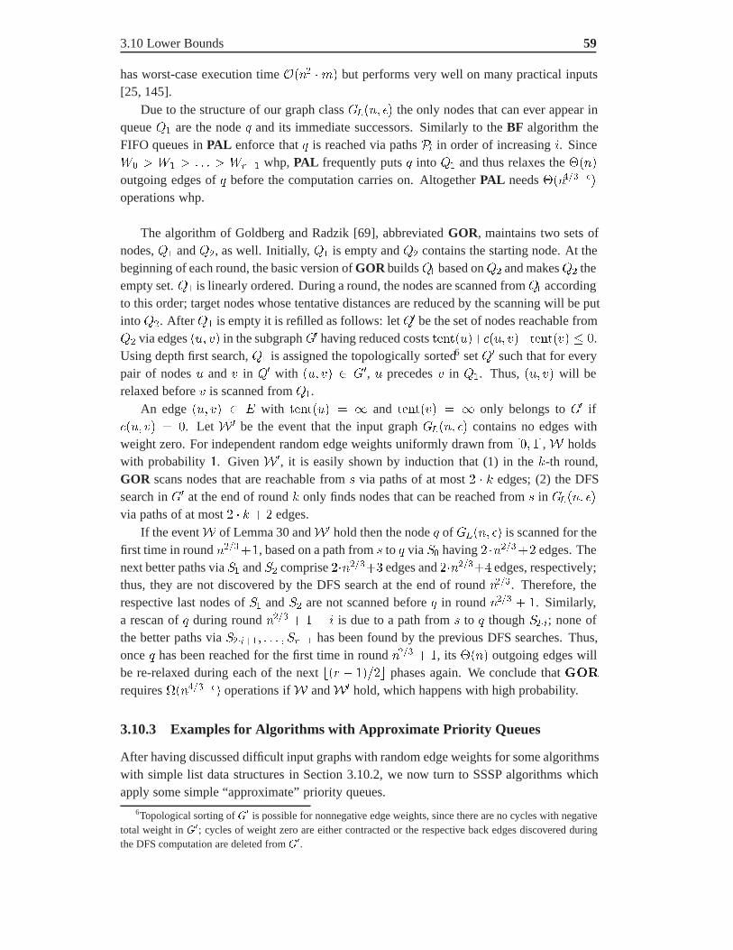
3.10 Lower Bounds 59
has worst-case execution time ���� ��� but performs very well on many practical inputs[25, 145].
Due to the structure of our graph class ���� .� the only nodes that can ever appear inqueue �� are the node 2 and its immediate successors. Similarly to the BF algorithm theFIFO queues in PAL enforce that 2 is reached via paths # in order of increasing �. Since�� � �� � � � � � �!�� whp, PAL frequently puts 2 into �� and thus relaxes the ����
outgoing edges of 2 before the computation carries on. Altogether PAL needs ����� ���
operations whp.
The algorithm of Goldberg and Radzik [69], abbreviated GOR, maintains two sets ofnodes, �� and ��, as well. Initially, �� is empty and �� contains the starting node. At thebeginning of each round, the basic version of GOR builds�� based on�� and makes�� theempty set. �� is linearly ordered. During a round, the nodes are scanned from�� accordingto this order; target nodes whose tentative distances are reduced by the scanning will be putinto ��. After�� is empty it is refilled as follows: let �� be the set of nodes reachable from�� via edges �� �� in the subgraph �� having reduced costs ����������� ���������� �.Using depth first search, �� is assigned the topologically sorted6 set �� such that for everypair of nodes � and � in �� with �� �� � ��, � precedes � in ��. Thus, �� �� will berelaxed before � is scanned from ��.
An edge �� �� � � with ������� � � and ������� � � only belongs to �� if��� �� � �. Let ) � be the event that the input graph ���� .� contains no edges withweight zero. For independent random edge weights uniformly drawn from �� �, )� holdswith probability �. Given )�, it is easily shown by induction that (1) in the �-th round,GOR scans nodes that are reachable from � via paths of at most � � � edges; (2) the DFSsearch in �� at the end of round � only finds nodes that can be reached from � in ���� .�
via paths of at most � � � � � edges.If the event ) of Lemma 30 and )� hold then the node 2 of���� .� is scanned for the
first time in round ��� ��, based on a path from � to 2 via �� having � ���� �� edges. Thenext better paths via �� and �� comprise ����� �� edges and ����� �� edges, respectively;thus, they are not discovered by the DFS search at the end of round ��� . Therefore, therespective last nodes of �� and �� are not scanned before 2 in round ��� � �. Similarly,a rescan of 2 during round ��� � � � � is due to a path from � to 2 though ��; none ofthe better paths via ���� � � � �!�� has been found by the previous DFS searches. Thus,once 2 has been reached for the first time in round ��� � �, its ���� outgoing edges willbe re-relaxed during each of the next ��/ � ��!�� phases again. We conclude that �requires ����� ��� operations if ) and )� hold, which happens with high probability.
3.10.3 Examples for Algorithms with Approximate Priority Queues
After having discussed difficult input graphs with random edge weights for some algorithmswith simple list data structures in Section 3.10.2, we now turn to SSSP algorithms whichapply some simple “approximate” priority queues.
6Topological sorting of �� is possible for nonnegative edge weights, since there are no cycles with negativetotal weight in ��; cycles of weight zero are either contracted or the respective back edges discovered duringthe DFS computation are deleted from ��.
60 Sequential SSSP Algorithms
Simple Bucket Approaches
Let us reconsider the sequential �-Stepping approach of Section 3.9.1 that applies an array1�� with buckets of width �. For maximum node degree ) and maximum shortest-pathweight �, our analysis showed that it is sufficient to take buckets of width � � ���!)�
in order to limit the average-case overhead for node rescans and edge re-relaxations by������. However, �!�! � ��� � )� buckets have to be traversed for that choice of �.The resulting total average-case time ������) ����� may be largely dominated by theterm ��� � ). To which extent can � be increased in order to find an optimal compromisebetween the number of traversed buckets and the overhead due to node rescans?
In the following we will show that there are graphs with ���� edges where any fixedbucket width � results in ��� ����� �! ��� ����� operations on the average. This providesanother motivation for the need of improved algorithms like the adaptive bucket splittingapproaches SP-C and SP-S.
In principle, we would like to re-use the graph class ���� .� of Section 3.10.2 in orderto construct difficult inputs for the �-Stepping. But there, in order to deal with randomdeviations, single fixed edge weights had been emulated by long chains of ��� gadgetswith random edge weights; each chain accounted for a total path-weight of ����� � onthe average. Our analysis for SP-C (and the �-Stepping), however, pointed out that noderescans can be attributed to paths of small total weight (at most � �). Therefore, wewill design another input class for the �-Stepping, featuring short chains and gadgets withrapidly increasing blow-up factors. The following lemma bounds the probability that theshortest path weight of a single �� � ��-gadget deviates too much from its expected value:
Lemma 32 The shortest path weight between the nodes � and � in a �� � ��-gadget, � ���� �, lies in the interval
���
��� ����
with probability at least � � �
��� �for � � ��.
Proof: As in the proof of Lemma 28, let * be the random variable denoting the weightof the path � �� via the intermediate node within the gadget. Furthermore, let= � ��� * be the weight of the shortest path between � and �. The density functionfor * is given by �*��'� � ' if � ' � (compare the proof of Lemma 28), hence��* ' � �!� � '� for � ' �. Therefore,
�
�= � ��
� � ���
��
�� � �
�� �
� � ��� �
�
� � � �
�� �
� � ��� �� � � � � �
��� ��
In order to show ��= ����
� � � �
��
��� �
�, let % be a binary random variable such
that % � � if both ��� � �����
and �� �� �����
, and % � � otherwise. Due to
independent random edge weights, ��% � � � �� ��� �� . Clearly, = ����
if�
% � �.Hence,
�
�= ����
�
�� �
��
% � �
�� � �
�� � ��� �
� � ��
� � � �� �� �� � � � �
��� �
for � � ��. Therefore, by Boole’s inequality, ��
�����
= ����
� � � �
��� ��

3.10 Lower Bounds 61
Lemma 32 is used in the construction of a difficult graph class for the �-Stepping algorithm:
Lemma 33 There are input graphs with ���� nodes and edges and random edge weightssuch that the �-Stepping algorithm requires ��� ������! ��� ��� �� operations on theaverage, no matter how � is chosen.
Proof: Consider the following graph class: from the starting node � to some node 2 with�!� outgoing edges there are / chains �� � � � �! of gadgets. Node � is the entering nodeof the first gadget of each chain. Similarly, 2 is the leaving node of the last gadget of eachchain. Chain �, � � /, consists of � gadgets � with blow-up factor � � ��� � each.Finally, a separate chain !� of �!� edges branches from node � as well; compare Figure 3.9.
k k
G G G
k k
k k
s q
G G
C~
G1 1
r r r
2 2
r r
2 2
1
Figure 3.9: Difficult input class for the �-Stepping algorithm. Chain � consists of � gad-gets � with blow-up factor � � ��� � each. An extra chain !� causes a high maximumshortest-path weight on the average.
Due to !� , the average-case maximum shortest-path weight in the graph satisfies ��� ��!". Thus, if the bucket width is chosen as � " �
)�� ������ ( � for � * �) then the
�-Stepping algorithm has to traverse at least ���!� � �
�� �
)���
�� ���
�buckets on the
average. Henceforth we will assume � � � � " �)
�� ������ .
Let %+ denote the number of light edges (���� �) emanating from node 2. Unless�����2� � �� ��2�, the �-Stepping algorithm only relaxes light edges out of 2. We find
��%+ � �!� � � � � � � �)
�� ������ . By Chernoff bounds (Lemma 7),
��%+ ��%+
� �������� ���
��
� ���� �
��for � � �� �
Having / chains ��, . . . , �! accounts for a total of�
� ! � � /� gadgets. We aim tochoose / large under the condition that all these gadgets contribute at most �!� nodes and� ��!� edges in total. It is sufficient to consider the inequality /� � �� � ���! �� �!�; aftersome simple transformations it turns out that / � ���
���� ��� is a feasible choice for � � ��.

62 Sequential SSSP Algorithms
By Lemma 32, the weight of the shortest path within each single gadget of � exceeds
the interval�
������
�����
with probability at most �
��� �if � � ��.
Let � be the event that the shortest-path weights of all gadgets are bounded as statedabove, and that node 2 has at least ��%+!� outgoing light edges. Hence,
��� � � � �
��� /� � �
��� �� � � �
��� ��� �
��� � ��� ������ �
��� �� � � �
��� �
���� &
���
Let � be the shortest-path weight of chain �. If � holds, then
� � ��� � ���
���� �� � ����� � �� �
���� �� � ����
���
���� (3.22)
and therefore �� � �� � � � � � �! with probability at least ��� . In other words, given
� , we managed to produce an input graph where paths from � to 2 of larger size (i.e., moreedges) have smaller total weight. How often 2 is scanned and how many outgoing (light)edges of 2 are relaxed during these scans depends on the chosen bucket width �: however,
if � holds and � � " �)
�� ������ , already the shortest-path from � to 2 through ��, � ���� 2�,
has total weight at most ������� �
� ���� �
� �. Therefore, �, ����, and 2 are scanned from thecurrent bucket 1�� in phases �, �, and �, respectively. In phase #, the node 2 is scannedfrom 1�� again since the �-Stepping finds a better path � ���� ���� ��� 2� through ��.
Altogether, if � holds and � � " �)
�� ������ then 2 is scanned / � ���
���� ��� times. Each
such scan involves the relaxation of at least ��%+!� � � �)
�� ������ light edges leaving 2.
Hence – given � – the �-Stepping performs at least ��� �
)���
�� ��� edge relaxations. Theclaim follows from the fact that � holds with probability at least &!��.
The “Approximate Bucket Implementation” [25] of Dijkstra’s algorithm (ABI-Dijkstra)essentially boils down to the sequential �-Stepping without distinction between light andheavy edges, i.e., all outgoing edges of a removed node are relaxed. Hence, repeating thetwo parts of the proof above for either � � �� ���! ��� or � � �� ���! ��� when alledges out of node 2 are relaxed after each removal of 2 yields:
Corollary 8 There are graphs with ���� nodes and edges and random edge weights suchthat ABI-Dijkstra requires ��� � ����! ��� ��� �� operations on the average.
A comparison between Lemma 33 and Corollary 8 seems to reveal an advantage of the�-Stepping over ABI-Dijkstra due to the distinction of light and heavy edges: for the un-derlying graph class and a proper choice of �, the �-Stepping approach computes SSSPin ��� � �����! ��� ��� �� time on the average, whereas ABI-Dijkstra requires ��� ���� �! ��� ����� operations on the average. However, it might still be possible to con-struct graphs with ���� nodes and edges and random edge weights where both approachesprovably need ��� � ��� �! ��� ��� �� operations on the average.
Threshold Algorithm
Glover et al. suggested several variants [64, 65, 66] of a method which combines ideas lyingbehind the algorithms of Bellman–Ford and Dijkstra: the set of queued nodes is partitioned
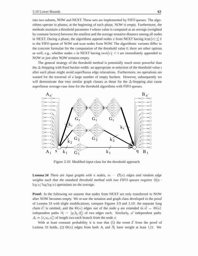
3.10 Lower Bounds 63
into two subsets, NOW and NEXT. These sets are implemented by FIFO queues. The algo-rithms operate in phases; at the beginning of each phase, NOW is empty. Furthermore, themethods maintain a threshold parameter 0whose value is computed as an average (weightedby constant factors) between the smallest and the average tentative distance among all nodesin NEXT. During a phase, the algorithms append nodes � from NEXT having ������� 0
to the FIFO queue of NOW and scan nodes from NOW. The algorithmic variants differ inthe concrete formulae for the computation of the threshold value 0; there are other optionsas well, e.g., whether nodes � in NEXT having ������� 0 are immediately appended toNOW or just after NOW remains empty.
The general strategy of the threshold method is potentially much more powerful thanthe �-Stepping with fixed bucket width: an appropriate re-selection of the threshold value 0after each phase might avoid superfluous edge relaxations. Furthermore, no operations arewasted for the traversal of a large number of empty buckets. However, subsequently wewill demonstrate that very similar graph classes as those for the �-Stepping also causesuperlinear average-case time for the threshold algorithms with FIFO queues.
k
G G
k k
A
A
B
B
kk
G
G k
G G
s q1
r r
2 2
n´
1
n´
1
rr
r
1 1
2 2
Figure 3.10: Modified input class for the threshold approach.
Lemma 34 There are input graphs with � nodes, � � ���� edges and random edgeweights such that the standard threshold method with two FIFO queues requires ��� ���� �! ��� ����� operations on the average.
Proof: In the following we assume that nodes from NEXT are only transferred to NOWafter NOW becomes empty. We re-use the notation and graph class developed in the proofof Lemma 33 with slight modifications, compare Figures 3.9 and 3.10: the separate longchain !� is omitted, and the ���� edges out of the node 2 are extended to �� � ����
independent paths 1 � 2 � ��� of two edges each. Similarly, �� independent paths? � � � ��� of length two each branch from the node �.
With at least constant probability it is true that (1) the event � from the proof ofLemma 33 holds, (2) ���� edges from both ? and 1 have weight at least �!�. We
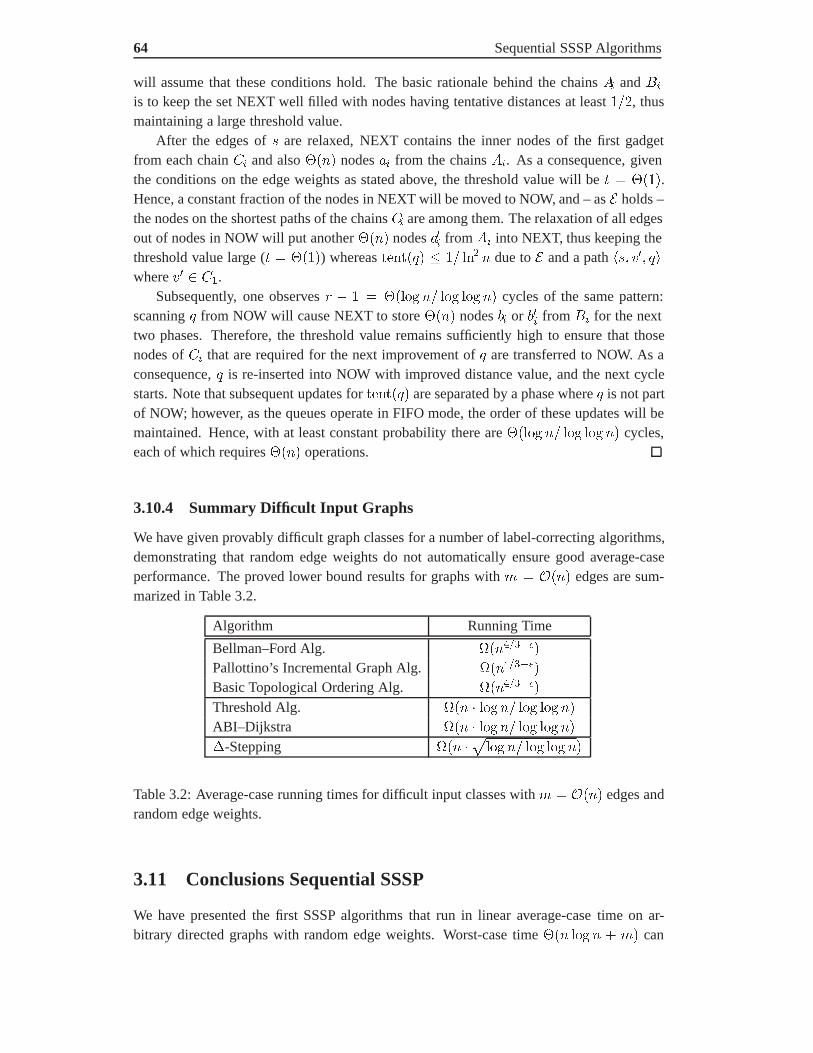
64 Sequential SSSP Algorithms
will assume that these conditions hold. The basic rationale behind the chains ? and 1
is to keep the set NEXT well filled with nodes having tentative distances at least �!�, thusmaintaining a large threshold value.
After the edges of � are relaxed, NEXT contains the inner nodes of the first gadgetfrom each chain � and also ���� nodes � from the chains ?. As a consequence, giventhe conditions on the edge weights as stated above, the threshold value will be 0 � ����.Hence, a constant fraction of the nodes in NEXT will be moved to NOW, and – as � holds –the nodes on the shortest paths of the chains � are among them. The relaxation of all edgesout of nodes in NOW will put another ���� nodes �� from ? into NEXT, thus keeping thethreshold value large (0 � ����) whereas �����2� �! ��� � due to � and a path � �� 2�where �� � ��.
Subsequently, one observes / � � � ����� �! ��� ����� cycles of the same pattern:scanning 2 from NOW will cause NEXT to store ���� nodes � or �� from 1 for the nexttwo phases. Therefore, the threshold value remains sufficiently high to ensure that thosenodes of � that are required for the next improvement of 2 are transferred to NOW. As aconsequence, 2 is re-inserted into NOW with improved distance value, and the next cyclestarts. Note that subsequent updates for �����2� are separated by a phase where 2 is not partof NOW; however, as the queues operate in FIFO mode, the order of these updates will bemaintained. Hence, with at least constant probability there are ����� �! ��� ����� cycles,each of which requires ���� operations.
3.10.4 Summary Difficult Input Graphs
We have given provably difficult graph classes for a number of label-correcting algorithms,demonstrating that random edge weights do not automatically ensure good average-caseperformance. The proved lower bound results for graphs with � � ���� edges are sum-marized in Table 3.2.
Algorithm Running Time
Bellman–Ford Alg. ����� ���
Pallottino’s Incremental Graph Alg. ����� ���
Basic Topological Ordering Alg. ����� ���
Threshold Alg. ��� � ����! ��� �����
ABI–Dijkstra ��� � ����! ��� �����
�-Stepping ��� ����� �! ��� ��� ��
Table 3.2: Average-case running times for difficult input classes with � � ���� edges andrandom edge weights.
3.11 Conclusions Sequential SSSP
We have presented the first SSSP algorithms that run in linear average-case time on ar-bitrary directed graphs with random edge weights. Worst-case time ��� ��� � � �� can
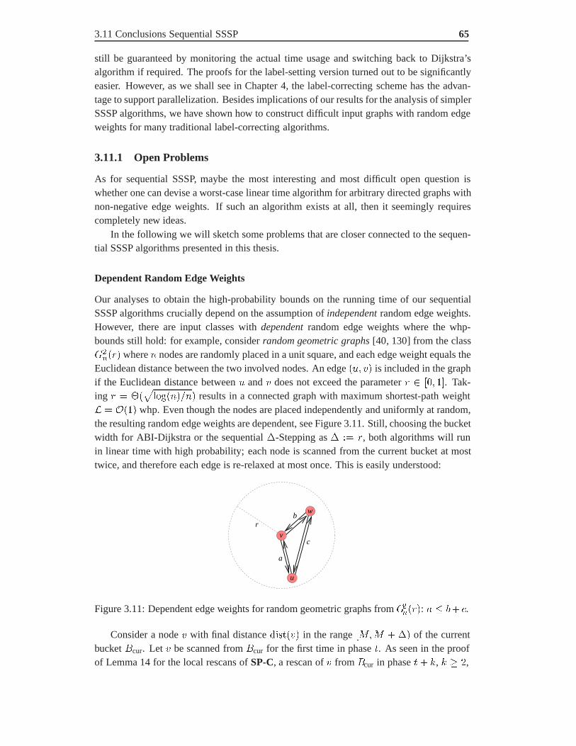
3.11 Conclusions Sequential SSSP 65
still be guaranteed by monitoring the actual time usage and switching back to Dijkstra’salgorithm if required. The proofs for the label-setting version turned out to be significantlyeasier. However, as we shall see in Chapter 4, the label-correcting scheme has the advan-tage to support parallelization. Besides implications of our results for the analysis of simplerSSSP algorithms, we have shown how to construct difficult input graphs with random edgeweights for many traditional label-correcting algorithms.
3.11.1 Open Problems
As for sequential SSSP, maybe the most interesting and most difficult open question iswhether one can devise a worst-case linear time algorithm for arbitrary directed graphs withnon-negative edge weights. If such an algorithm exists at all, then it seemingly requirescompletely new ideas.
In the following we will sketch some problems that are closer connected to the sequen-tial SSSP algorithms presented in this thesis.
Dependent Random Edge Weights
Our analyses to obtain the high-probability bounds on the running time of our sequentialSSSP algorithms crucially depend on the assumption of independent random edge weights.However, there are input classes with dependent random edge weights where the whp-bounds still hold: for example, consider random geometric graphs [40, 130] from the class��
��/� where � nodes are randomly placed in a unit square, and each edge weight equals theEuclidean distance between the two involved nodes. An edge �� �� is included in the graphif the Euclidean distance between � and � does not exceed the parameter / � �� �. Tak-ing / � ��
�������!�� results in a connected graph with maximum shortest-path weight
� � ���� whp. Even though the nodes are placed independently and uniformly at random,the resulting random edge weights are dependent, see Figure 3.11. Still, choosing the bucketwidth for ABI-Dijkstra or the sequential �-Stepping as � � /, both algorithms will runin linear time with high probability; each node is scanned from the current bucket at mosttwice, and therefore each edge is re-relaxed at most once. This is easily understood:
r
c
a
bw
v
u
Figure 3.11: Dependent edge weights for random geometric graphs from ����/�: � �� �.
Consider a node � with final distance �� ���� in the range ��� � �� of the currentbucket 1cur. Let � be scanned from 1cur for the first time in phase 0. As seen in the proofof Lemma 14 for the local rescans of SP-C, a rescan of � from 1cur in phase 0� �, � � �,
66 Sequential SSSP Algorithms
requires a path # � � � �� � � � � � �� of total weight ��#� � � such that node �is scanned from 1cur in phase 0 � �, and ������� � ��#� � �������. However, due to thedefinition of ��
��/�, if such a path exists in �, then the graph also contains the edge �� ��
having weight ��� �� ��#�. Hence, the relaxation of the edge �� �� after scanning� in phase 0 will immediately reduce ������� so much that no further improvement canbe achieved via the path # . Therefore, if at all, � is re-inserted at most once more forphase 0� �.
Random geometric graphs have a very special structure, and their edge weights obey thetriangle-inequality. It would be interesting to identify weaker conditions under which ouralgorithms reach the stated high-probability bounds even though the random edge weightsare dependent.
In order to show the linear average-case complexity of SP-C with improved edge re-laxations (Section 3.7) we used independence only in the proof of Lemma 17. It is unclearwhether the same result can be shown for dependent random edge weights.
Negative Edge Weights
Shortest-paths instances with (some) negative edge weights are apparently much more dif-ficult to solve than instances where all weights are non-negative: the best known worst-casebound for sequential SSSP with arbitrary edge weights, ��� � ��, is due to the classicBellman-Ford algorithm [15, 50]; only recently Fakcharoenphol and Rao [47] presented an��� � ��� �� algorithm for planar graphs. The best known average-case bound was givenby Cooper et al. [32]; they show ����� expected time for the complete graph with randomedge weights generated according to the vertex-potential model [25]. Their algorithm ex-ploits two structural properties that are exhibited on complete graphs with high probability.Firstly, the number of edges can be reduced significantly without changing the shortest-pathweights. Secondly, each shortest path consists of at most ����� �� edges.
However, for arbitrary graphs with random real edge weights, these conditions willusually not hold. It would be interesting to see whether our methods of adaptive bucket-splitting can result in any improvement for the average-case complexity of SSSP on suchgraphs.

Chapter 4
Parallel Algorithms
Having dealt with sequential single-source shortest-paths algorithms in the previous chapterwe now turn to parallel SSSP. Some of our results are straightforward parallelizations ofthe sequential label-correcting approaches with buckets of Chapter 3; we show how theoperations of a phase for the current bucket can be done in parallel and investigate howmany phases are needed. For certain graph classes this simple strategy already yields goodresults. However, with an alternative scanning rule the number of phases can sometimes bereduced significantly without increasing the total number of operations. In particular, wegive the first algorithms that achieve both sublinear average-case time and linear average-case work for random graphs, and graphs modeling the WWW, telephone calls or socialnetworks. In order to facilitate easy exposition we focus on CRCW PRAM algorithms andonly sketch extensions to DMMs.
This chapter is organized as follows: Section 4.1 provides an overview of previous andrelated work. Then we give a list of our contributions (Section 4.2). Before we discuss fur-ther details of our new algorithms we review some basic PRAM results and techniques inSection 4.3. Sections 4.4 and 4.5 deal with parallelizations of the sequential label-correctingalgorithms from Chapter 3. Further improvements for random graphs are discussed in Sec-tion 4.6. Eventually, Section 4.7 provides our most efficient parallel SSSP algorithm, whichuses different step widths on disjoint node sets at the same time. Some concluding remarks(also concerning potential parallelizations of Goldberg’s new algorithm [67]) are given inSection 4.8.
4.1 Previous and Related Work
4.1.1 PRAM Algorithms (Worst-Case Analysis)
The parallel SSSP problem has so far resisted solutions that are fast and work-efficientat the same time: no PRAM algorithm is known that terminates with ��� � ��� � � ��
work and sublinear running time for arbitrary digraphs with nonnegative edge weights. The��� � �������-work solution by Driscoll et al. [44] (refining a result of Paige and Kruskal[116]) has running time ��� � �����. An ����-time algorithm requiring ��� � ��� �� workwas presented by Brodal et al. [20]. The algorithms above scan the nodes one by one in theorder of Dijkstra’s algorithm; only edge relaxations are performed in parallel. Hence, using
67

68 Parallel Algorithms
this method there is no possibility to break the worst-case time-bound of ����. All otherknown SSSP algorithms for arbitrary graphs trade running time against efficiency.
The algorithm by Han et al. [78] (based on [35]) implicitly solves the APSP problem byreducing the shortest-paths computation to matrix multiplications over semirings: it needs������ �� time and ��� � ���� ��� �! ��� ���� � work. Applying randomized minimumcomputations [58] on a CRCW PRAM, the algorithm can also be implemented to run in����� �� time using ��� � ��� �� work. Deterministically, it is possible to achieve ��.�� ���� �� time using ��� �� � ����� work for an arbitrary constant . � �. Furthermore, thereis a randomized algorithm [92] for SSSP on sparse graphs with integral nonnegative edgeweights summing to� . It requires ��%��'������� �� time and ���������%��'������
� �� work. Recently, Mulmuley and Shah [113] gave a lower bound of ������� executiontime for SSSP on PRAMs without bit operations using a polynomial number of processors.The lower bound even holds when the bit lengths of the edge weights are restricted to be ofsize ����� ��.
Several parallel SSSP algorithms are based on the randomized parallel breadth-firstsearch (BFS) algorithm of Ullman and Yannakakis [141]. In its simplest form, the BFSalgorithm first performs �
�� � ��� ��-limited searches from ��
��� randomly chosen dis-
tinguished nodes in parallel. Then it builds an auxiliary graph of the distinguished nodeswith edge weights derived from the limited searches and solves an APSP problem on thisauxiliary graph. Finally, the distance values of non-distinguished nodes are updated. Thissimple BFS algorithm takes ��
�� � %��'������� time using ��
�� �� � %��'������� work
with high probability. A more involved version achieves ��0 � %��'������� time using���
�� ��� � ��!0� � !0�� � %��'������� work for any 0 �
� whp.
Klein and Subramanian [93] extended the BFS idea of Ullman and Yannakakis toweighted graphs. They gave a parallel randomized approximation scheme for �� � .�-approximate single-source shortest-paths computations that runs in ��
�� � .�� � ���� �
���� �� time using ���� �� � ��� �� work. Furthermore, they showed how to use the result
above to compute exact single-source shortest-paths with maximum path weight 4 by solv-ing a series of �����4� sub-instances. The algorithm takes ��
�� � ���4 � ��� � � ���� ��
time and ���� �� � ���4 � ��� �� work.
Similar results have been obtained by Cohen [28], and Shi and Spencer [131]. Recently,Cohen [29] gave an ���.�-approximation algorithm for undirected graphs that runs in poly-logarithmic time and takes near linear work. Unfortunately, there seems to be no way to useit for exact computations by repeated approximations. Cohen also proposed a SSSP algo-rithm for graphs with a given �����-separator decomposition that takes polylogarithmictime and ����� � �� � %��'������� work.
More efficient parallel SSSP algorithms have been designed for special graph classes.Here are some examples: Combining the data structure of [20] with the ideas from [140]gives an algorithm which solves the SSSP problem on planar digraphs with arbitrary non-negative edge weights in ����� � ����� time and ������� work on a CREW PRAM. Incontrast, the randomized algorithm of [92] requires planar graphs and integral edge weightssumming to � . It runs in ��%��'����� �� �� time using ��� � %��'������� �� work.Work-efficient SSSP algorithms for planar layered graphs have been proposed by Subrama-nian et al. [134] and Atallah et al. [10]. Furthermore, there is an ������ ��-time linear-work
4.1 Previous and Related Work 69
EREW PRAM algorithm for graphs with constant tree width [23].
4.1.2 PRAM Algorithms (Average-Case Analysis)
Random graphs [17, 46] with unit weight edges have been considered by Clementi et al.[27]: their solution is restricted to edge probabilities ���� or ����� �!�� for � � �. In thelatter case ������� �� time and optimal ��� � ��� �� work is needed on the average.
Reif and Spirakis [125] bounded the expected diameter of the giant component of sparserandom graphs with unit weights by �������. Their result implies that the matrix basedAPSP algorithm needs ����� ��� �� iterations on average provided that the edge weightsare nonnegative and satisfy the triangle inequality.
Frieze and Rudolph [58], and Gu and Takaoka [75] considered the APSP problem withrandom edge weights and showed that the standard matrix product algorithm can be imple-mented in ����� ����� time and ��� � ��� ��� �� work on average.
Crauser et al. [33] gave the first parallel label-setting algorithms that solve SSSP forrandom graphs with random edge weights in sublinear time using ��� � ��� � ��� workon the average. Their algorithms maintain the set of candidate nodes in a parallel priorityqueue, which is implemented by a number of sequential relaxed heaps [44] with randomnode assignment. The algorithms operate in phases: each phase first identifies a set ofcandidate nodes with final tentative distances; then these nodes are scanned in parallel.The OUT-approach applies the OUT-criterion of Lemma 6 in order to find scan-eligiblenodes. It needs ��
��� phases on the average. Similar performance on random graphs is
obtained if the OUT-criterion is replaced by the IN-criterion from Lemma 5 (IN-approach).Changing between IN- and OUT-criterion after each phase (INOUT-approach), may speed-up the computation; for random graphs, however, ����� � phases are still needed on theaverage.
The analysis for the OUT-approach was generalized in [103] to arbitrary graphs withrandom edge weights and maximum shortest-path weight � � ��� ��� ���� ��� ���� ���:the algorithm achieves �, � ����
�� �� � ��� �� average-case time using ��� � ��� ��
�� �,� work.
4.1.3 Algorithms for Distributed Memory Machines
PRAM algorithms can be emulated on distributed memory machines. The loss factors de-pend on the concrete parameters of the models; e.g. see [61] for emulation results on theBSP model. However, existing implementations [1, 22, 84, 85, 86, 139] on parallel comput-ers with distributed memory usually avoid such emulations; they rather apply some kind ofgraph partitioning, where each processor runs a sequential label-correcting algorithm on itssubgraph(s). Heuristics are used for the frequency of the inter-processor data-exchange con-cerning tentative distances, load-balancing, and termination detection. Depending on the in-put classes and parameter choices, some of these implementations perform fairly well, eventhough no speed-up can be achieved in the worst case. However, no theoretical average-caseanalysis has been given.

70 Parallel Algorithms
4.2 Our Contribution
We present new results on the average-case complexity of parallel SSSP assuming indepen-dent random edge weights uniformly drawn from �� �. The average-case performance ofour algorithms is expressed in terms of rather general properties of the input graph classeslike the maximum shortest-path weight or the node degree sequence. For the purpose of aneasy exposition we concentrate on the CRCW PRAM (Concurrent-Read Concurrent-WriteParallel Random-Access Machine) [52, 72, 88] model of computation. However, we shallsketch extensions to distributed memory machines when this is appropriate.
Straightforward Parallelizations
In Section 4.4 we prove that already a simple parallelization of the �-Stepping algorithmfrom Section 3.9.1 performs reasonably well on a large class of graphs: for maximumshortest-path weight � (see Definition 2) and maximum node degree ), the parallelizationtakes ����) � ) � �! � ���� �� time using ������ ��) � ) � �! � ���� �� work on theaverage. If �� � � and )� � ) denote high-probability bounds on � and ), then an improvedversion of the parallel �-Stepping presented in Section 4.5 achieves �� )� � ��! � ���� ��
time using ������ )� � ��! � ���� �� work whp.For several important graph classes with random edge weights, � is sufficiently small,
i.e., ) � �! � ���� � � -��� with high probability; in that case the improved parallel �-Stepping runs in sublinear time and linear work with high probability. A typical exampleare random graphs from the class 8�� $)!�� as defined in Section 3.9.3: by Lemma 26 andCorollary 6 we already know ) � ��$) � ����� and � � �� ���
� ���
� with high probability.This implies that SSSP on random graphs from 8�� $)!�� with random edge weights canbe solved in ������ �� ��! $)� � ���� �� time using linear work with high probability.
Improvements for Random Graphs
In Section 4.6 we reconsider random graphs with random edge weights. We will improvethe high-probability bound on � from Corollary 6 to ����!$)� � �����. For random graphsfrom 8�� $)!��, the step width for the advanced parallel �-Stepping algorithm may bechosen as big as � � ���!$)� instead of ���!� $) � ������. Together with an appropriatepreprocessing of the input graph this yields the following result: SSSP on random graphswith random edge weights can be solved in ������ �� time using linear work on the average.
Improved Parallelizations for Graphs with Unbalanced Node Degrees
For arbitrary graphs, the simple parallelizations above require ��) ��� phases. This is oftentoo much if ) and � happen to be large. In Section 4.7 we consider parallel SSSP for graphswith unbalanced node degrees, that is, input graphs, where the maximum node degree ) issignificantly larger than the average node degree $). Typical examples are degree sequencesthat follow a power law: the number of nodes, +, of a given in-degree ' is proportionalto '�( for some constant parameter @ � �. For most massive graphs, � � @ �: forexample, Kumar et al. [95] and Barabasi et al. [13] independently reported @ + ��� forthe in-degrees of the WWW graph, and the same value was estimated for telephone call

4.2 Our Contribution 71
graphs [5]. In spite of constant average in-degree $), one expects to observe at least onenode with in-degree ������(����, i.e., ) � ����-�� for @ � ���. The observed diametersare usually very small; however, � � ����.
Unfortunately, if � � ����, all parallelizations introduced above require ��)� time.This drawback is partially removed by our new parallel label-correcting method, the Par-allel Individual Step-Widths SSSP (PIS-SP) algorithm: it utilizes a number of differentapproximate priority-queue data structures in order to maintain nodes of similar degreesin the same queue. The algorithm applies different step widths for different queues at thesame time. The approach can be easily implemented with a collection of sequential relaxedheaps. In that case it requires
�, � ��
��� � � �����
* � � �! � �� � � in-degree��� � ��+�� time
using ��� � ���� �� � �,� work on average. By virtue of a split-free bucket structureand an improved node selection strategy, another logarithmic factor can be gained on bothrunning time and work. The resulting algorithm is the first to achieve -������ average-casetime and ������ work for graphs modeling the WWW or telephone calls.
Comparison
Table 4.1 provides an overview of our new parallel SSSP algorithms. For each algorithmwe list average-case time and work as functions of node degrees and maximum shortest-path weight. We have suitably instantiated these general formulae for three sample graphclasses in order to demonstrate the performance differences. As already discussed for ran-dom graphs, even better results can be obtained if additional knowledge concerning theinput graphs is used to optimize the parameter setting of the algorithms. For comparison wealso listed the respective numbers of the best previous ��� � ���� � ��-work algorithm,the label-setting OUT-approach of [33].
It turns out that for all graph classes listed in Table 4.1 at least one of the new algorithmsis both faster and requires less work than the OUT-approach. In particular, the PIS-SPalgorithm is uniformly better. For random graphs, the performance gain is significant. Infact, the average-case execution-time of the two algorithms comes closest for graphs with����
�� ��� nodes of degree ���!���� ��� each: in that case the OUT-approach
requires �� � ������ �� � ��� �� time on average using ��� � ������� ��� work
whereas PIS-SP succeeds after �� � ������ �� � ���� �� time with ��� � � � ���
work on the average.In fairness, however, it should be mentioned that the OUT-approach may be augmented
by intermediate applications of the IN-criterion (as it was done in [33] for random graphs).Still, the resulting average-case running times of the augmented algorithm will be in ����� �
for the general case, even if ) and � are small. Furthermore, on sparse graphs, the aug-mented algorithm will require superlinear average-case time. On the other hand, it is aninteresting open problem, whether the OUT-criterion (or some modification of it) can beprofitably included into our linear work algorithms based on buckets.
Early results on the average-case analysis of our parallel SSSP algorithms on random graphs
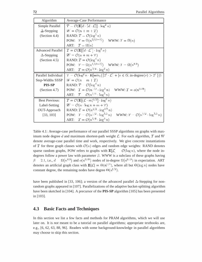
72 Parallel Algorithms
Algorithm Average-Case Performance
Simple Parallel � � ����) � ) � �! � ���� ��
�-Stepping � � ������ � �
(Section 4.4) RAND: � � ������ ��
POW: � � ������(���� WWW: � � ����
ART: � � ����
Advanced Parallel � � ���� ) � �! � ���� ��
�-Stepping � � ������ � �
(Section 4.5) RAND: � � ������ ��
POW: � � ������(���� WWW: � � ����-��
ART: � � ��� �� � ���� ��
Parallel Individual � � ������ � � ������ � � �! � �� � � in-degree��� � �����
Step-Widths SSSP � � ������ � �
PIS-SP RAND: � � ������ ��
(Section 4.7) POW: � � �����( � ��� �� WWW: � � -���-���
ART: � � ������ � ���� ��
Best Previous: � � ������ ������ � ��� ��
Label-Setting � � ��� � ��� ���� � �
OUT-Approach RAND: � � ������ � ��� -� ��
[33, 103] POW: � � ������ � ��� -� �� WWW: � � ������ � ��� -� ��
ART: � � ������ � ��� ��
Table 4.1: Average-case performance of our parallel SSSP algorithms on graphs with max-imum node degree ) and maximum shortest-path weight �. For each algorithm, � and �denote average-case parallel time and work, respectively. We give concrete instantiationsof � for three graph classes with ���� edges and random edge weights: RAND denotessparse random graphs, POW refers to graphs with ��� � ����� ��, where the node in-degrees follow a power law with parameter @. WWW is a subclass of these graphs having@ � ���, i.e., ) � ����-�� and -���-��� nodes of in-degree ����-��� in expectation. ARTdenotes an artificial graph class with ��� � �������, where all but ����� �� nodes haveconstant degree, the remaining nodes have degree �������.
have been published in [33, 106]; a version of the advanced parallel �-Stepping for non-random graphs appeared in [107]. Parallelizations of the adaptive bucket-splitting algorithmhave been sketched in [104]. A precursor of the PIS-SP algorithm [105] has been presentedin [103].
4.3 Basic Facts and Techniques
In this section we list a few facts and methods for PRAM algorithms, which we will uselater on. It is not meant to be a tutorial on parallel algorithms; appropriate textbooks are,e.g., [6, 62, 63, 88, 96]. Readers with some background-knowledge in parallel algorithmsmay choose to skip this section.

4.3 Basic Facts and Techniques 73
Our PRAM algorithms are usually described in the work-time framework, a gener-alization of Brent’s scheduling principle [18]: if a parallel algorithm does 2 operations(work) in time 0, then on � processors, the same algorithm can be done in time 0. where0. � ��0� +
. �. This “slow-down” feature facilitates the following accounting scheme: ifan algorithm ? consists of sub-algorithms ?� � � � ? , where? can be solved in 0 time us-ing 2 work for � � � � � � �, then ? can be executed in time ��
��� 0� using ��
��� 2�
work. In the following we will state the time bounds of a few basic work-optimal PRAMsub-algorithms; see also Table 4.2.
Algorithm Time Work Model(Segmented) Prefix/Suffix Sums [97] ����� �� ���� EREWFast Min/Max [132] ����� ����� ���� CRCWRandomized Min/Max [58] ���� whp ���� whp CRCWSorting � integers from �� � � � �� [122] ����� �� whp ���� whp CRCW
Table 4.2: Performances for some basic PRAM algorithms
Many parallel algorithms use prefix and suffix sums in order to assign sub-problems toprocessors: consider a sequence % � �'� '� � � � '�� of � elements from some set �together with a binary associative operation (, e.g., sum, product, minimum or maximum;the prefix sums of % are the � expressions � � '� ( '� ( � � � ( ', where � � �.Equivalently, the suffix sums are defined by �� � ' ( '�� ( � � � ( '�, for � � �. Thesegmented version of prefix sums assumes an additional Boolean array * of length � suchthat +� � +� � �; for each �� � �� where +� � +� � � and +� � � for all �� � 3 � ��, wewish to compute the prefix sums of the sub-array �'��� � � � '�� of % . For the segmentedsuffix sums we are interested in the sub-arrays �'� � � � '����. Using balanced binarytrees, all these prefix/suffix computations can be done in ����� �� time with ���� work[97].
Frequently, (small) sets of data must be copied to (many) other memory cells in parallel:let % � �'� '� � � � '�� be an array of � elements, and let 3� � � � 3� � � � � � 3/ � �
be a set of indices. The segmented broadcasting problem is that of computing the array* � �+� +� � � � +�� such that +� � '�� , for 3�� � 5 3 and � � �. It can be solvedwith the same resource usage as the prefix/suffix problems.
Computing a single minimum or maximum is a special case of the prefix sum prob-lem. On a CRCW PRAM, it can be done in ����� ��� �� time and linear work [132]. Thealgorithm uses the method of accelerated cascading [30] together with a constant-time algo-rithm that requires quadratic work. Based on this worst-case constant-time approach, Friezeand Rudolph [58] developed a randomized CRCW algorithm that runs in ���� time whilerequiring only linear work with high probability.
Integer sorting is a simple way to reorganize data items. In particular, it is useful tobundle distributed data items that belong together: it is sufficient to assign common integersto the items of the same sub-groups and then sort the items according to the associatedintegers. In [122] it is shown how � integers with values in �� � � � �� can be sorted in����� �� time using a linear number of operations with high probability.

74 Parallel Algorithms
4.4 Simple Parallel �-Stepping
After having listed a few general-purpose PRAM routines in Section 4.3 we now turn to ourfirst parallelization of an SSSP algorithm. Concretely speaking, we will provide a simpleparallel version of ABI-Dijkstra and the sequential �-Stepping from Section 3.9. Recallthat these algorithms keep the candidate nodes in an approximate priority-queue 1�� withbuckets of width � � ������ ��, where ) denotes the maximum node degree in the in-put graph. That is, a queued node � having tentative distance ������� is stored in bucket1���������!��. The current bucket 1cur denotes the first nonempty bucket of 1��. Ina phase, all nodes in the current bucket are scanned (where the �-Stepping initially onlyrelaxes light edges); after the current bucket becomes empty (and the �-Stepping has re-laxed the associated heavy edges as well), the algorithms sequentially search for the nextnonempty bucket. The simple parallelizations of this section will be restricted to the op-erations within a phase; searching for the next non-empty bucket is still done sequentially(in Section 4.7 we propose improved algorithms that support parallel search for the nextnon-empty buckets).
As already seen in Section 3.9, for maximum shortest-path weight �, the algorithmstraverse �!�! � �� ) � �!� buckets; also compare Remark 1 in Section 3.4.4. Thenumber of phases, however, may be bigger since scanned nodes can be re-inserted into thecurrent bucket. Hence, we are left with two problems:
(a) Providing efficient parallelizations for a phase.
(b) Bounding the number of phases.
The total work over all phases should be ��� � �� on the average. Disregarding someinitialization procedures, the total parallel time of the resulting algorithms will be given bythe sum of the times for the phases. An upper bound on the number of phases is easilyobtained: from Lemma 14 and Lemma 22 we can conclude that in the case of random edgeweights there are at most �� ��� �
��� ��� �� phases for each current bucket with high probability.As the current bucket is advanced at most �� ) � �!� times we find:
Corollary 9 For graphs with random independent edge weights uniformly distributed in�� �, maximum shortest-path weight � and maximum node degree ), both ABI-Dijkstraand �-Stepping require ���� ) � �! � ����
��� ��� �� phases on the average. If �� � � and)� � ) denote upper bounds (that hold with high probability) then the number of phases is�� )� � ��! � ��� �
��� ��� �� with high probability, too.
4.4.1 Parallelizing a Phase via Randomized Node Assignment
If it is possible to scan several nodes during a phase in parallel then this work has to bedistributed among the available � � processors in a load-balanced way. Furthermore,finding an appropriate distribution itself should not consume too much time and work. Asimple yet efficient load-balancing method is to apply an initial random assignment of graphnodes to processors. Using an array ����� of independent random PU indices uniformlydistributed in �� � � � �� ��, entry ����� gives the PU responsible for node �. The bucketstructure is distributed over the processors, too. In a phase, each PU does the work for the
4.4 Simple Parallel �-Stepping 75
nodes randomly assigned to its own structure. That is, for � � � �, PU � is in charge ofthe bucket array 1��, and a queued node � will be kept in 1��������������!��. A phaseof the simple parallelization comprises the following basic steps:
Step 1: Identifying the global value ��!��, where � � ����������� � queued �.
Step 2: Node removal from the respective buckets 1���!��.Step 3: Generating requests for edge relaxations.
Step 4: Assigning requests to their responsible PUs.
Step 5: Performing the relaxations according to the assigned requests.
Step 1: Finding ��!��. The key feature of ABI-Dijkstra and �-Stepping is to restrictnode scanning to those queued nodes � having ������� � ���!�� � �� � �, where �denotes the smallest tentative distance among all queued nodes. In the sequential version(without cyclical bucket re-usage), ��!�� is simply the index of the first non-empty bucket1���!��. Now that in the parallel version 1�� is distributed over � arrays 1��, thealgorithm needs to find the globally smallest index 3 �� ��!��� among all non-emptybuckets 1�3 and all � � � �.
Let � � denote the smallest tentative distance among all queued nodes at the beginningof the previous phase. Starting from 1��� �!��, for � � � �, PU � sequentiallysearches for the first non-empty bucket in 1��. Skipping � empty buckets can be done intime � �� � �����: each PU can traverse empty buckets of its dedicated bucket structurein constant time per bucket; every � ���� �� iterations it is checked whether any PU hasfound a nonempty bucket and, if so, the globally smallest index with a nonempty bucket isfound. The latter check can be done with the basic gather- and broadcasting algorithms ofSection 4.3 in ����� �� � ������� time.
Steps 2 and 3: Dequeuing nodes and generating requests. Once the value of ��!��has been detected, PU � removes all nodes from 1���!�� in Step 2. Let us denote theresulting node set by . Afterwards PU � is in charge of generating requests � ��������
��� �� for edges �� � � � emanating from nodes � � . Depending on whether weare parallelizing ABI-Dijkstra or the �-Stepping, requests are created for either all outgoingedges or (as long as the current bucket does not change) just for the light outgoing edges,which have weight at most �. Let ���� be the set of requests generated for node �. Thework of an arbitrary PU � for a node � � during steps 2 and 3 can a seen as job of size� � ������ � ��)� whose execution takes time linear in its size.
Due to the random assignment of nodes to processors, the work performed duringsteps 2 and 3 can be analyzed using classical results of the occupancy (“balls into bins”)problem [89, 94, 112, 129]. In particular, arguing along the lines of [7, Lemma 2] one finds:
Lemma 35 Consider any number of subproblems of size in �� �. Let B denote the sumof all subproblem sizes. If the subproblems are allocated uniformly and independently atrandom to � PUs, then the maximum load of any PU will be bounded by ��B!� � � ������� ��� with high probability.1
1The seemingly unrelated parameter � comes into play since we based our definition of “whp” on it.

76 Parallel Algorithms
Proof: Consider an arbitrary but fixed PU �. It suffices to show that PU � receives loadexceeding $ � �B!� � � � ���� � ��� with probability at most ��(!� for any @ � � andan appropriately chosen $ depending on @ only. Let there be / subproblems, where ��,. . . ,�!�� denote the respective sizes of the these subproblems. Define the 0-1 random variable%� to be one if and only if subproblem 3 is assigned to �. Let * �
�� �� �%�!� denote
the “normalized load” received by PU �. Note that ��* � B!�� � ��. Since the %� areindependent and the weights ��!� are in �� �, we can apply another version of the Chernoffbound [121, Theorem 1] which states that for any # � �,
� �* � # ���* ��0��
#0
���*
�
First we rewrite ����
0� � ����
���� �� ����
����� 0�0 . Then by setting # � ��* � $ � �B!�� � �
����� ��� we get # � $ � �� � � � �� � ����� ��!B� � $. Now we can start to simplify:
� �* � # � ��* ���� �
���� 0�0��*
� ���� �
���� 0���1�����������
���������������� ���������� for $ � ��
��������� � � �� �� � � �������!� �
Setting $ � ���*@ � � ��
+concludes the proof.
Thus, if a parallel phase of ABI-Dijkstra or �-Stepping with � � PUs removes � � nodesand generates �� � requests, then Steps 2 and 3 take � ��� � � �� ��!�� ) � ����� timewith high probability according to Lemma 35.
Steps 4 and 5: Assigning and performing relaxation requests. Let � be the set ofrequests generated by PU �. Any request � '� � � must now be transferred to thebucket structure associated with PU ������. Using Lemma 35, it can be seen that due to therandom indexing, each PU receives ���,�� �!�� ) � ��� �
�requests whp. The value
of �,�� � can be obtained and broadcast in � ���� �� time. Each PU sets up an emptyrequest buffer which is a constant factor larger than needed to accommodate the requestsdirected to it whp.
The requests are placed by “randomized dart throwing” [108] where PU � tries towrite � '� � � to a random position of the target buffer of PU ������ (see Figure 4.1).Several PUs may try to write to the same memory location. This is the only step of theparallelization that needs the CRCW PRAM. Due to the choice of the buffer sizes eachsingle placement succeeds with constant probability. Using Chernoff bounds it is straight-forward to see that the dart throwing terminates in time proportional to the buffer size,� ��,� ��!�� ) � ��� �
�whp. For the unlikely case that a buffer is too small, correct-
ness can be preserved by checking periodically whether the dart throwing has terminatedand increasing the buffer sizes if necessary.
In step 5, each PU examines all slots of its request buffer and performs the associatedrelaxations in the order they are found. Since no other PUs work on its nodes the relaxationswill be atomic.

4.4 Simple Parallel �-Stepping 77
0
1
2
3
0
1
2
3
P P PP0 1 2 3 0P P1 P2 P3
BUF
BUF
BUF
BUF
BUF
BUF
BUF
BUF
Figure 4.1: Placing requests into buffers by randomized dart-throwing. Processor �� suc-ceeds in placing its currently treated request in ���� and can turn to its next request. ��and �� contend for a free slot in ����. �� wins. �� has to probe another position in��� �. � fails because the chosen position is already occupied.
Theorem 8 (Simple Parallelization.) Consider directed graphs with � nodes, � edgesand independent random edge weights uniformly distributed in �� �. Let )� and �� denoteupper bounds2 on the maximum node degree ) and the maximum shortest-path weight �, re-spectively. On a CRCW PRAM, the simple parallelization of ABI-Dijkstra and �-Steppingwith � � ������� �� runs in � � ��) ��� ) ��! � ���� �� time using ������� � work onthe average. Additionally, for � � ������� �
��, the simple parallel �-Stepping algorithmrequires � � � ��)� � )� � ��! � ���� �� time and ������� �� work with high probability.
Proof: Using the basic algorithms of Section 4.3, the initialization of the data structuresand the reordering of the adjacency lists concerning light and heavy edges can be done in���� ���!� � ������� time. By Corollary 9, there are ���� ) � �! � ��� �� phases onthe average and �� )� � ��! � ��� �� phases with high probability. If the five steps of the�-th parallel phase remove � ��� nodes and generate ����� requests then this phase takes
��
�� ��� � �� ����!�� ) � ��� ��
time with high probability. From the discussion of
the sequential ABI-Dijkstra and �-Stepping in Section 3.9 we deduce ���
� ��� � ����
and���
�� ��� � ������; for the �-Stepping these bounds even hold with high prob-
ability. Thus, the total time is bounded by ������ � ) ��� ) � �! � ���� �
�on the average
and ������ � )� � )� � ��! � ���� �
�with high probability. The theorem follows by choos-
ing � � �������������� �! � � PUs for the average-case bound and � � ���
������������ �!PUs for the high-probability bound.
2Actually, it is sufficient if these bounds hold with high probability.

78 Parallel Algorithms
4.5 Advanced Parallelizations
The simple parallelization of the phases as shown above is already quite good for sparsegraphs like road-maps, where the maximum node degree ) is not much larger than �!�.However, if ) , �!� then the running time becomes less attractive. With an alternativeload-balancing, one can save a factor of ��)�:
Theorem 9 With the parameters and machine model defined as in Theorem 8, parallelSSSP can be solved in � � ���� ) � �! � ���� �� time using ������ � � work on theaverage. Additionally, the advanced parallel �-Stepping algorithm can be implemented torun in � � � ��)� � )� � ��! � ���� �� time using ������ � �� work with high probability.
In the following we describe the necessary modifications:
4.5.1 Improved Request Generation
The new feature we add is to explicitly organize the generation of requests. Instead ofgenerating the set of requests derived from the bucket structure of PU � exclusively by PU�, now all PUs cooperate to build the total set of requests. This can be done by computinga prefix sum over the adjacency list sizes of the nodes in the request set first and then assignconsecutive groups of nodes with about equal number of edges to the PUs. Nodes withlarge out-degree may cause several groups containing only edges which emanate from thisvery node. The extra time needed to compute the prefix sums and schedules is ����� �� perphase.
4.5.2 Improved Request Execution
What makes executing requests more difficult than generating them is that the in-degree ofa node does not convey how many requests will appear in a particular phase. If some targetnode � is contained in many requests of a phase then it might even be necessary to set asideseveral processors to deal with the request for �.
Instead of the brute-force randomized dart-throwing as in Section 4.4, we use an ex-plicit load balancing which groups different requests for the same target and only executingthe strictest relaxation. On CRCW PRAMs, grouping can be done efficiently using thesemi-sorting routine explained in Lemma 36. Then we can use prefix sums to schedule�� �(�)� �� ! �(�)�� PUs for blocks of size at least �(�)� !� and to assign smaller groupswith a total of up to �(�)� !� requests to individual PUs. The PUs concerned with a groupcollectively find a request with minimum distance in time � ��(�)� !�� ��� ��. Thus, eachtarget node receives at most one request for relaxation. These selected requests will be loadbalanced over the PUs whp due to the random assignment of nodes to PUs. Figure 4.2provides an illustration. Summing over all phases yields the desired bound.
Lemma 36 Semi-sorting � records with integer keys, i.e., permuting them into an array ofsize � such that all records with equal key form a consecutive block, can be performed intime � ��!�� ����� on a CRCW-PRAM with high probability.

4.5 Advanced Parallelizations 79
1
2
3
0
selectedrequests
request for a relaxation of edge (i,j)
P
P
P
P
dequeued nodeswith adjacency lists
generatedrequests
after inte−ger sorting
transferred totarget processors
i j
Figure 4.2: Load balancing for generating and performing requests: Requests are denotedby a box for the source node and a circle for the target node, colors are used to code nodeindices. The processors cooperate in building the total set of requests: Large adjacency listsare handled by groups of PUs. Subsequently, the generated requests are grouped by targetnodes using semi-sorting. Then superfluous requests are filtered out, and the remainingrequest are sent to the processors which host the appropriate bucket structures. Withoutthe balancing, processor �� would be over-loaded during the generation, and processor ��would receive too many requests.
Proof: First find a perfect hash function 7 * �� � � � � � �� for an appropriate constant�. Using the algorithm of Bast and Hagerup [14] this can be done in time � ��!�� ��� ��
(and even faster) whp. Subsequently, we apply a fast, work efficient sorting algorithm forsmall integer keys such as the one by Rajasekaran and Reif [122] to sort by the hash valuesin time � ��!�� ��� �� whp.
4.5.3 Conversion to Distributed Memory Machines
The straightforward way to obtain a DMM algorithm out of a PRAM algorithm is to usean efficient PRAM simulation method: given certain conditions, a step of a CRCW PRAMwith ��-processors can be simulated on a �-processors BSP machine in ����!�� time if�� � ���� for any constant . � �; see [142]. Hence, if � is defined as in Theorem 8, thedistributed algorithm runs in ���� � � � �����
� � time.Alternatively, for a direct coding on a DMM machine, one first has to solve the data
allocation problem. Fortunately, the simple PRAM algorithm from Section 4.4 is alreadyalmost a distributed memory algorithm. The index array ����� used in the PRAM algorithmcan be replaced by a hash function ������. PU � maintains the bucket structure 1��, and
80 Parallel Algorithms
also stores the adjacency lists of all nodes whose indices hash to the value �. Hence, therelaxation requests can be generated locally. The dart throwing process for assigning re-quests can be replaced by simply routing a request � '� to PU ���� �. The relaxationsfor the received requests happens locally again. As for the PRAM version, if the numberof processors, is reasonably bounded then the accesses to the memory modules are suf-ficiently load-balanced in each phase with high probability. Each phase of the algorithmcan be performed in a number of supersteps each of which consists of local computations,synchronization, and communication.
The advanced parallelization requires additional measures; for example long adjacencylists have to be spread over the local memories of the processors. Important ingredients forthe conversion are standard DMM implementations for tree based reduction and broadcast-ing schemes [88]. They are needed for prefix-sum / minimum computations and distributionof values, e.g., when all edges �� � of a high-degree node � are to be relaxed, then thevalue of ������� must be made available to all PUs that store outgoing edges of �. Thegrouping steps of the algorithm can be implemented by DMM integer-sorting algorithms,e.g., [12]. The choice of the sorting algorithm determines how many supersteps are neededto implement a phase of the PRAM algorithm, and hence how many processors can bereasonably used.
4.6 Better Bounds for Random Graphs
So far we collected the following results for random graphs with random edge weights fromclass the class 8�� $)!�� as defined in Section 3.9.3: by Lemma 26 and Corollary 6 weknow ) � �� $)� ����� and � � ����! $)� � ���� �� with high probability. For the advancedPRAM algorithm of the previous section (Theorem 9) this implies ������ ����! $)������ ��
time using linear work with high probability. In the following we will improve the high-probability bound on � to ����!$)� � ��� �� and sketch two further algorithmic modificationsfor random graphs.
4.6.1 Maximum Shortest-Path Weight
Theorem 10 There is a constant �� � � such that for random graphs from 8�� $)!��,$) � ����, with independent random edge weights uniformly drawn from �� �, the maximumshortest-path weight is bounded from above by ����!$)� � ����� whp.
Proof: Due to the results of [32, 57, 80, 120] on the maximum shortest-path weight fordense random graphs with random edge weights we can concentrate on the case � � �� �$) ������� where �� � � is the constant from Lemma 27.
The set of nodes reachable from �, denoted by ���, is either small, that is � ���� �
����! $)� � ��� �� whp, or giant, that is � ���� � ���� whp [90]. If ��� is small, thenTheorem 10 follows immediately: any node in ��� can be reached by a path of at most� ���� edges, each of which has weight at most one. Therefore, we may assume that � ����is giant.
Our proof proceeds as follows. First we show that a subgraph �� of � contains astrongly connected component �� of ���� nodes so that any pair of nodes from �� is con-

4.6 Better Bounds for Random Graphs 81
nected by a path of total weight ����!$)� � ��� �� whp. Then we prove that there is a pathfrom � to �� not exceeding the total weight ��� � ��!$)� � ��� �� whp. Finally, we show forall nodes in ��� that cannot be reached from � directly along a path of ������!$)� � ��� ��
edges, that these nodes can still be reached from �� via a path of weight ������!$)� � ��� ��
whp. For $) � ����� �� the above path weights sum up to ����!$)� � ��� �� whp. Figure 4.3depicts the such a concatenated path from the source node � to a target node � � ���.
C’s
v
t’ t’
Figure 4.3: Example for a concatenated path of small total weight from the source � to areachable node �: after at most 0� � �� ��� ��� � edges the strongly connected component ��
is reached. There is a light path within �� to an intermediate node from which � can bereached via a path of another 0� edges.
For this proof call edges with weight at most � � ��! $) tiny. Consider the subgraph�� � ���� of � obtained by retaining tiny edges only. �� is a random graph with edgeprobability � � ��!�; �� has a giant strong component �� of size $� � � with probability atleast � � ��� for some arbitrary constant $ � � where the positive constant $� depends onthe choice of $ (e.g. [8, 90]).
By Lemma 27, the diameter of the subgraph induced by the nodes in �� and its adjacentedges in �� is at most ������� with probability at least �����. Since all edges in �� haveweight at most � � ��! $), any pair of nodes from �� is connected by a path of total weight����! $)� � ��� �� with probability at least � � ���.
Now we show that there is a path from � to �� not exceeding the total weight ��� �
��! $)� � ��� �� whp. We apply the node exploration procedure of [90] and [8, Section 10.5]starting in the source node � and using the edges in �: Initially, � is active and all othernodes are neutral. In each iteration we select an arbitrary active node �, declare it dead andmake all neutral nodes with �� � � � active. The process terminates when there are noactive nodes left. Let *� be the number of active nodes after 0 iterations (*� � �). We areinterested in the set of nodes reached from � after 0� � (���
��iterations for some appropriate
constant @ � �. Let *+, �� � denote the binomial distribution with parameters � and �,i.e., the number of heads in � independent coin tosses with probability of heads �. Providedthat *��� � �, *� is distributed as follows [8, 90]: *+,
��� � � � �� � $)!���
�� � � 0,
i.e., *� is sharply concentrated around
9�0� � ��� �� � �� � �� � $)!���� � � � 0�

82 Parallel Algorithms
In fact, we can assume *���� � � since otherwise all nodes of ��� are reached using pathsof total weight ����! $)� � ��� ��. We use the inequality
�� � '�# � � � ' � + ��' � +��
�if ' � + � �
� � �
�� ' � + if � � ' � + � �
in order to derive a lower bound on 9�0��. Indeed we have � � ��� � 0� � �(
��� . Hence, for�* � and $) � � � �� � �, we find
9�0�� � ��� �� � �
�� $) � 0�!�� � � 0� �
$)
�� 0� �
@ � ���
��
Thus, for *���� � �, ��*�� � (��� . Furthermore, *�� � �@!"� � ��� with probability
at least � � ����*�� �� � � � ��(��� by the Chernoff bounds (Lemma 7). That is highprobability if the constant @ is chosen sufficiently large. So, there are *�� � �@!"� � ��� �
active nodes whp whose outgoing edges have not yet been inspected in the search procedurefrom �. Let ? be the set of these nodes. We are interested in the probability that there is atleast one edge from a node in ? to a node in �� (if the node sets overlap then we are doneas well).
We can assume that �� (and hence ��) has been generated without complete knowledgeof � in the following way: For every ordered pair of nodes �� � we first throw a biasedcoin with� ����� � ����! $) and only if it shows a head we find out whether �� � � �: inthis case we generate a random tiny edge weight, and �� � is put to ��. This informationsuffices to determine ��. Hence, looking at the two node sets ? and �� with �� � ? and � � � � it is still true that ��� �� � � with probability
��� , and these probabilities are
independent for all ordered pairs of nodes ��� ��. Therefore, we expect ���� � �?� � ��� edges
from ? to ��. Since �� �� � $� � � with probability at least � � ��� and �?� � �@!"� � ���
with probability at least ����(���, the probability that there exists at least one edge �� �
between ? and �� is at least
� � ��� � ��(��� ��
� �$)
�
�����(������
� � � ��� � ��(��� � ��!�����(����� �
� � � ��� � ��(��� � ����(�� (4.1)
which is high probability for appropriately chosen constants (in particular, we are free tochose $ and @ large). Consequently, there is a path from � to �� using at most ������! $)� ���� �� edges whp. Since all edges on this path have weight at most one, the desired boundon the total path weight from � to �� follows immediately.
The same technique is applied to show that any node � � ��� that neither belongs to� � nor is reached from � directly along a path of 0� edges, can still be reached from �� viaa path of ��� � ��! $)� � ��� �� edges whp. However, now the search procedure follows theedges in the opposite direction. Note that the different search procedures are not mutuallyindependent. Still, each single search succeeds with the probability bound given in (4.1).Hence, using Boole’s inequality all nodes from ��� can be reached along paths with totalweight ������! $)����� �� with probability at least ���������������(��������(���.This completes the proof of Theorem 10 for � � �� � $) �������.

4.6 Better Bounds for Random Graphs 83
4.6.2 Larger Step Width
In Section 3.9 we have seen that ABI-Dijkstra and �-Stepping cause ���� node rescans onthe average if the bucket width is chosen as � � ������� �� for maximum node degree ).The result was obtained by reducing the analysis to that of SP-C (Section 3.6) with a singlehierarchy level and buckets of width �. In particular, the number of times a node � isscanned on the average had been bounded by the expected number of simple paths of totalweight � into � (proof of Lemma 18); we argued that there are at most )� simple paths of 5edges into �. Using the fact that long paths with small total weight are unlikely (Lemma 17)it turned out that node � is rescanned at most
����� )
� � ���!5 times on average.
For random graphs from 8�� $)!��, we have seen ) � �� $) � ����� with high proba-bility (Lemma 26). However, due to the random graph structure, the average-case numberof simple paths with 5 edges into a node � is bounded by $) �. Thus, the number of rescansfor node � is at most
�����
$) � � ���!5 � ���� for � � �� ���� ��! on the average. In otherwords, for sparse random graphs we can choose the bucket width larger without riskingincreased overhead due to node rescans. This results in less phases for the parallel SSSPalgorithm.
4.6.3 Inserting Shortcuts
Our parallelizations of Sections 4.4 and 4.5 need ����� �! ��� ����� phases whp beforethey turn to the next non-empty bucket. However, under certain conditions, a constantnumber of phases per bucket suffices. We have already seen this behavior for randomgeometric graphs (Section 3.11.1): we exploited the fact that whenever there is a path# � � � �� � � � � � �� of total weight ��#� � � � �� ���� ��! in the input graph�, then � also contains the “shortcut” edge �� �� having weight ��� �� ��#�. Our ideafor random graphs is to manually insert these shortcut edges.
Shortcuts for random graphs from8�� $)!�� are found by exploring �-paths emanatingfrom all nodes in parallel. This is affordable for random edge weights because we know thatthere are only few simple �-paths: for each node we expect
�����
$) � ����!5 � ���� suchoutgoing paths. Furthermore, none of these paths is longer than ����� �! ��� ��� �� withhigh probability. The only additional complication is that we have to make sure that onlysimple paths are explored.
Figure 4.4 outlines a routine which finds shortcuts by applying a variant of the Bellman-Ford algorithm to all nodes in parallel. It solves an all-to-all shortest path problem con-strained to �-paths. The shortest connections found so far are kept in a hash table of ex-pected size ����. The set � stores active connections, i.e., triples �� � +� where + is theweight of a shortest known path from � to � and where paths �� � � � � � have not yet beenconsidered as possible shortest connections from � to with weight +���� �. In iteration� of the main loop, the shortest connections using � edges are computed and are then used toupdate ‘found’. Using similar techniques as in Section 4.5, this routine can be implementedto run in � �
���� �! ��� ��� ��
parallel time using � ����� work on average: we need����� �! ��� ����� iterations each of which takes time � ���� �� and work � ���� � �����whp. The overall work bound holds since for each simple �-path �� � � � ��, � �� can bea member of � only once. Hence, ��
� ��� � � ��� and ��
� ���� � � �����.
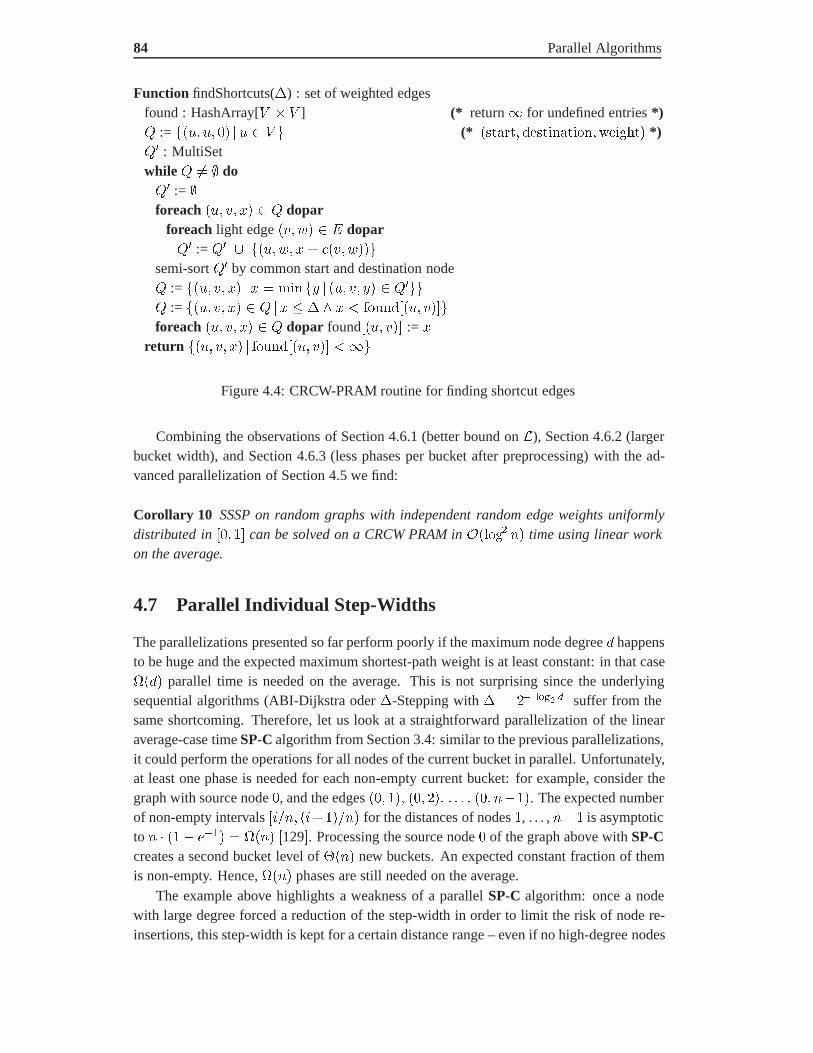
84 Parallel Algorithms
Function findShortcuts(�) : set of weighted edgesfound : HashArray[ ] (* return � for undefined entries *)� := ��� � �� �� � � (* � ������ ��������-���.�� *)�� : MultiSetwhile � �� � do�� := �foreach �� � '� � � dopar
foreach light edge �� � � � dopar�� := �� � ��� ' � ��� ���
semi-sort �� by common start and destination node� := ��� � '� �' � ��� �+ � �� � +� � ����� := ��� � '� � � �' � & ' � /�0����� ���foreach �� � '� � � dopar found��� �� := '
return ��� � '� � /�0����� �� ���
Figure 4.4: CRCW-PRAM routine for finding shortcut edges
Combining the observations of Section 4.6.1 (better bound on �), Section 4.6.2 (largerbucket width), and Section 4.6.3 (less phases per bucket after preprocessing) with the ad-vanced parallelization of Section 4.5 we find:
Corollary 10 SSSP on random graphs with independent random edge weights uniformlydistributed in �� � can be solved on a CRCW PRAM in ������ �� time using linear workon the average.
4.7 Parallel Individual Step-Widths
The parallelizations presented so far perform poorly if the maximum node degree ) happensto be huge and the expected maximum shortest-path weight is at least constant: in that case��)� parallel time is needed on the average. This is not surprising since the underlyingsequential algorithms (ABI-Dijkstra oder �-Stepping with � � ������� �� suffer from thesame shortcoming. Therefore, let us look at a straightforward parallelization of the linearaverage-case time SP-C algorithm from Section 3.4: similar to the previous parallelizations,it could perform the operations for all nodes of the current bucket in parallel. Unfortunately,at least one phase is needed for each non-empty current bucket: for example, consider thegraph with source node �, and the edges �� �� �� �� � � � �� ����. The expected numberof non-empty intervals ��!� �����!�� for the distances of nodes �, . . . , ��� is asymptoticto � � �� � ���� � ���� �129. Processing the source node � of the graph above with SP-Ccreates a second bucket level of ���� new buckets. An expected constant fraction of themis non-empty. Hence, ���� phases are still needed on the average.
The example above highlights a weakness of a parallel SP-C algorithm: once a nodewith large degree forced a reduction of the step-width in order to limit the risk of node re-insertions, this step-width is kept for a certain distance range – even if no high-degree nodes

4.7 Parallel Individual Step-Widths 85
remain in the new buckets of this range. In the following we will show how to remove thisdrawback.
4.7.1 The Algorithm.
In this section we introduce the new parallel SSSP algorithm called PIS-SP (for ParallelIndividual Step-Widths). The algorithm applies different step-widths on disjoint node setsat the same time using a new split-free bucket data structure.
PIS-SP applies a queue data structure� that consists of ���� buckets in total, organizedinto ������� arrays 1��: each array covers a total tentative distance range of width two.The buckets of each array are used in a cyclical fashion in order to subsequently store nodeswith larger and larger tentative distances. The array 1��, � � ���� �! � 7 consistsof ��� buckets of width � � ���� each. 1�� exclusively stores nodes with in-degree in���� � � � ����. Hence, for example a node � with in-degree ) � " and tentative distance������� � #�� is stored in the array 1��, � � ����� )� � � � �, and more concretely inbucket 1 ���#�� ��� ��!� � � 1 �����!���"�#� � 1 ���. Note that there is no arrayfor vertices with in-degree zero, as they cannot be reached anyway.
PIS-SP works as follows: initially, all nodes � reachable from the source node � viaan edge �� �� are put in parallel into their respective bucket arrays using the edge weights��� �� as tentative distances. After that, PIS-SP operates in phases: At the beginning ofa phase it first determines the globally smallest tentative distance � � �����2 �������
among all currently queued nodes. This step is quite intricate since the bucket structureonly implements an approximate priority queue. Hence, � is not readily available; nottoo many operations must be used to find it. In Section 4.7.3 we will show how � can beobtained efficiently. Knowing � , PIS-SP scans all nodes from 1 ���� ��� ��!�� inparallel for each �, � � 7. This may insert new nodes into � or reinsert previouslyscanned nodes with improved tentative distances. However, each phase settles at least onenode. The algorithm stops if there are no queued nodes left after a phase. Hence, it requiresat most � phases.
Each bucket is implemented by a separate array with dynamic space adjustment; addi-tional arrays are used in order to keep track of tentative distances and to remember in whichbucket and which array cell a queued node is currently stored. Removing nodes from buck-ets in parallel is clearly congestion-free. However, insertions must be organized more care-fully, see Figure 4.5: Having removed all nodes from the buckets 1�
-�� ��� ��!����
.
for a phase (resulting in a node set ), the set � of all edges emanating from nodes in is built. An immediate parallel relaxation of the set � might cause conflicts, there-fore � is first grouped by target nodes (using semi-sorting with small hashed values asseen in Section 4.5), and then the strictest relaxation request for each target node (group)is selected. The selected requests are grouped once more by target buckets and finally eachgroup is appended in parallel after the last used position in the array for the target bucket.If there are not sufficiently many contiguous free positions left (the free positions may bescattered due to nodes that have been moved to other buckets during edge relaxations), thenthe whole content of this bucket is compacted and then copied to a new array of twice thesize.
Each phase can be performed in ����� �� average-case time; the respective number of

86 Parallel Algorithms
PIS-SP
foreach �� �� � � dopar� � ����� indegree���� � �
Insert � into 1�-��� ��!����
.
while � �� � doDetermine � � �����2 ������� /* Phase starts */foreach � � ���� �! dopar
Empty bucket 1�-�� ��� ��!����
.
- node set Build set � for all edges out of .Group � by target nodes.foreach target node � of � dopar
Select best relaxation of an edge into �.Group selected edges by target buckets.Perform relaxations (& enlarge buckets if needed). /* Phase ends */
Figure 4.5: Pseudo-code for PIS-SP.
operations excluding array size adjustments is linear in � � � �� �. The total work neededto adjust the array sizes can be amortized over the total number of edge (re-) relaxations.
4.7.2 Performance for Random Edge Weights.
In the following we consider the expected numbers of node rescans and phases for PIS-SPon graphs with random edge weights:
Definition 5 Let � � �� � � � ��� be a path into an arbitrary node ��. � is called degree-weight balanced (dwb) if ����� �� ������� ���������������, for all �, � � � 3.
Lemma 37 For each node � � , the number of rescans during the execution of PIS-SP isbounded by the number of simple dwb paths into �.
Proof: Let �������� and �� denote the value of ������� and the set of nodes in � at thebeginning of phase 3, respectively; define �� � �����2� ��������. Clearly, for nonnega-tive edge weights, ���� � � � and ���������� �������� for all 3 � � and � � . Let� �� 3� denote the total number of rescans for node � during the phases � to 3; let �� � 0�
denote be the �-th rescan of he node � happening in phase 0.
The proof of the lemma is by induction; we show that all rescans of the phases � to 0can be injectively mapped onto simple paths. More specifically, a rescan of a node � � inphase 0 is mapped onto a simple dwb path � � �� � � � �� �� � �� of 5 0�� edges into �where �� is scanned in phase 0 � 3, and ��������������� � ������ ��� � �����������. Itfollows immediately that rescans of different nodes are mapped onto different simple paths.In the remainder we are concerned with different rescans of the same node.
Each node is scanned at most once per phase; no node is rescanned in the first phase.If the node � with degree )� is scanned for the first time in phase 3 then it is scanned from

4.7 Parallel Individual Step-Widths 87
bucket 1�
�-�� � ��� ��!��
.�where �� � ����� )�� � �, and
� � �� ���� �������� �-� �!��
. � �� � ��
� � � �� � � � � ������� ����� �
Now we consider �� � 0� where 0 � �� � � � (i.e., ���������� � �������� and � �� 0��� � � � �). As � was scanned for the first time in some phase 0� � 0, all nodes with finaldistances less than ��� were already settled at that time; their respective edges into �� (ifany) will neither be relaxed in phase 0� nor later. Therefore, �� � 0� requires that somenode �� �� � having ��� �� � � is scanned in phase 0 � � (i.e., �� ����� � � ��� � � ��)where �������� �
����������� � ���� �� � ���������� � � �� � ������� ������
These conditions imply ���� �� ������� �����.If � ��� 0� �� � � then �� � 0� can be uniquely mapped onto the edge ��� ��, which
is relaxed for the first time in phase 0� �. Obviously, �� �� is a simple dwb path into � ofat most 0� � edges because ���� �� ������� �����.
Otherwise, i.e., if � ��� 0 � �� � �� � � then ��� �� 0 � �� was inductively mappedonto some simple dwb path � � � ���� � � � ��� ��� � ��� of 5� 0 � � edges where ��� isscanned in phase 0 � � � 3, and ���������������� � ������� �
��� � ��������������. Hence,
�������������� ������������, whereas ������������ � ���������� � ������������ for all� 3 � 5�. Consequently, � is not part of ��. We map �� � 0� onto the path � � � � ��that is built from the concatenation of �� and ��� ��. As required, � is a simple dwb pathof at most 0 � � edges where the nodes are scanned in proper order and the equations forthe tentative distances hold. Furthermore, � is different from any other path !� � !� � ��constructed for some ��!� !0� where � !� � !0 � � 0: when constructing !� we eitherconsidered another edge ���� �� �� ��� ��, but then the subpaths � � and !� � end in differentnodes; or we considered different rescans ��� �� 0 � �� and ��� ��� !0 � �� of the samenode ��, but then these rescans were mapped on different paths �� and !� � by induction.
Lemma 38 For random edge weights uniformly drawn from �� �, PIS-SP rescans eachnode at most once on the average.
Proof: Let %��� denote the number of simple dwb paths of 5 � � edges into an arbitrary
node �� of a graph �. We first show ��%��� ���. The argument is by induction: let )
denote the in-degree of node �. Excluding self-loops there is a set �� of at most )� edgesinto node ��, hence ��%��
� )� � ������� ����� )� � �� ���� ���� � �!�.Now consider the set #� � ��� � � � �� of all simple paths with 5 edges into node �� in
�. By assumption ��%��� �
������ �� � is dwb ���.
For each � � � � � � ��� � #� there are at most ) edges into � so that the con-catenation with � results in a simple path of 5 � � edges into ��. In particular, for eachsuch path �� � � � � ���, the weight of the newly attached edge ��� �� is independentof the weights on � � � � ���. Therefore, �� �� � � � � ��� is dwb ������� ����� �
88 Parallel Algorithms
�� � � � � ��� is dwb . By linearity of expectation, ��%����� is bounded from above by�
�����) � ������� ����� ��� � � � � � � ��� is dwb
������
�!� ��� � is dwb �!� � ��%��� ������
By Lemma 37, �� is rescanned at most�
���%��� times, therefore the average-case number
of rescans of �� is at most�
�����%��� �
��� ��� � �.
Lemma 39 For graphs with random edge weights uniformly drawn from �� �, PIS-SPneeds / � ����� � � ����� � ��� � ���� phases on the average where � denotes themaximum shortest-path weight and �� is the number of graph vertices with in-degree atleast �.
Proof: Let ', � ' ���� �! � �, be some arbitrary integer. For the analysis, letus distinguish two kinds of phases for the algorithm: 1�-phases scan only nodes with in-degree less than �� whereas ��-phases scan at least one node with in-degree �� or larger.Let �� denote the number of ��-phases. By Lemma 38, each node is rescanned ���� timeson average. Hence, ���� � ������.
In the following we are interested in 1�-chunks: for some constant � � �, a 1�-chunkconsists of 0 � �� � #� � ���� � � � consecutive 1�-phases without any intermediate ��-phases. Observe that less than ��� � �� � 0 of all 1�-phases do not belong to any 1�-chunk.Let � � be the smallest tentative distance among queued nodes at the beginning of the 3-thphase of a 1�-chunk. We will show
�� �!��� � ���!��� with high probability� (4.2)
During the 3-th phase of the 1�-chunk, PIS-SP scans all nodes from the current buckets1
�-�� � ��� ��!�
.�, � � '. Let .� denote the set of these nodes. Observe that
(4.2) holds if-��� ��� ��!�
. �� -�� � ��� ��!�
.for at least one �, � � ',
i.e., PIS-SP has advanced at least one current bucket from 1��� � � � 1��� according tothe cyclical ordering. So, let us assume that the current buckets from 1��� � � � 1��� inphase 0 are those of phase �. But then there must be at least one node �� � .� with�������� � �
� � ��. In particular, there must be a simple dwb path � � �� � � � ��� oftotal weight less than �� � ����� where �� � .� , and all �� , � 3 0, have in-degreeless than ��. Into any node � � .� there are less than ������� such paths. As shown inLemma 17, the sum of 5 independent random edge weights (uniformly distributed in �� �)is at most � � with probability at most ��!5 . Hence, the probability that such a pathexists into any node � � .� is bounded by � � ������� � ����
� !�0 � �� � � ����� �����. That proves (4.2). Therefore, after �!��! 1�-chunks the current buckets havebeen advanced so much that no node remains in the bucket structure with probability atleast �� �!��! ������ � �������. This accounts for at most another ���� � � � �����
1�-phases with probability at least � � �����; as PIS-SP requires at most � phases in theworst case, it needs at most ���� ���� � ������ �������= ���� ���� � ����� additional1�-phases on the average.

4.7 Parallel Individual Step-Widths 89
Altogether the algorithm runs in ����� � ��� � ���� � ����� phases on the average.Since this analysis holds for any integer ', the average-case bound for all phases can berestated as ������� ���� � ��� � �����. Note once more that the algorithm itself doesnot have to find an optimal compromise between 1�-phases and ��-phases; they are just atheoretical concept of the analysis.
4.7.3 Fast Node Selection.
In the following we show how the bucket data structure can be modified in order to deter-mine� fast and efficiently: each array1�� is augmented by a pointer to the first nonemptybucket 1�
of range ��� �
� � � according to the cyclic ordering.
Lemma 40 For random edge weights uniformly drawn from �� �, the total number of oper-ations needed to maintain the pointers to 1� during the execution of PIS-SP is bounded by������ on the average. For each phase, maintaining the pointers takes at most �������
time.
Proof: 1� may have changed after a phase due to (i) an insertion of a node � into 1��, (ii)
a decrease of ������� where � � 1��, (iii) a scan of � from 1��. Cases (i) and (ii) arestraightforward: if � moves to a bucket dedicated to smaller tentative distances then 1� isset to this new bucket otherwise it stays unchanged. The grouping and selection proceduretaking place in each phase prior to parallel node insertions can be adapted such that for eacharray the smallest inserted tentative distance is determined as well. Only this value needs tobe checked for a possible update of 1� .
Maintaining 1� for case (iii) is only non-trivial if the bucket of the scanned node �
remains empty after a phase: all buckets of 1�� must be checked in order to find the newfirst nonempty bucket according to the cyclic ordering. On a PRAM this can be accom-plished using standard parallel prefix-sum and minimum computations [88] in �������
time and ������ work. These operations can be attributed to the degree of the scannednode �, which is at least ���. Since all degrees add up to ���� and since each node isscanned ���� times on average (Lemma 38), the total amount of operations needed for alloccurrences of case (iii) is bounded by ������ on the average, as well.
Finding the Minimum. We show how the values �� of the first nonempty buckets
1� � ���
�� � �� introduced above are used to identify the value � of the glob-
ally smallest tentative distance among all queued nodes. At the beginning of a phasePIS-SP computes the suffix-minima of the values ��
, i.e., for each �, it builds ���� �
������ �
��� � � � �
�3�� We set ��
� �� if 1�� is empty. Note that ���� � �
���� � ��. Next, the procedure refines safe estimates /� � $� for the globallysmallest tentative distance among all queued nodes: initially, we set /�� � ���� and$�� � ���� � ��. The minimum detection takes place in at most 7 stages:
For the first stage, PIS-SP checks the bucket 1�
�0�/�� ��� ��!��
1 : either, this
bucket is empty, or it constitutes the bucket 1�� keeping the node with smallest tentative
distance for the array 1���. All nodes from1�� � 1�
�0�/�� ��� ��!��
1 can be scanned

90 Parallel Algorithms
during the phase according to the scan criterion. Let �� be the smallest tentative distanceamong all nodes of 1�� (�� � � if 1�
� is empty). The value of �� is determined witha parallel minimum algorithm causing work linear in the number of elements stored inbucket 1�
� . If ������ $��� ���� then either the whole bucket structure is empty ora node �� with globally smallest tentative distance is stored in 1�� , and therefore � �
������ $���. The procedure stops. Otherwise, if ������ $��� � ����, the queued nodewith smallest tentative distance may still be found in one of the subsequent arrays 1���, . . . ,13��. Therefore, the procedure sets /�� � ����, $�� � ������ $������ � ���, and itcontinues with stage � on the bucket array 1���.
In general, if the detection procedure reaches stage � � � then we may assume by in-duction that it has identified estimates /� � � $� /� � �. The procedure computes
the smallest distance value � among the nodes in 1
�0�/� ��� ��!�
1 . Observe that
this bucket is either empty (then � � ��) or its nodes will be scanned by PIS-SP. There-fore, the work to identify � can be amortized over the node scans. Having computed �we may find ����� $�� ��� � ��, then ����� $�� definitely equals � ; the proce-dure stops. Otherwise, that is if ����� $�� � ��� � ��, we only know for sure that���� �� � ����� $����� �� � ����. The procedure will continue in 1����with the new estimates: /��� � ��� � �� and $��� � ����� $���� � �� � ����.After at most 7 � ������� stages, � is eventually determined. Figure 4.6 provides anexample.
Scanning the nodes from the examined buckets can be overlapped with the global mini-mum detection. However, asymptotically this does not improve the running time. The timerequired for a phase depends on the applied procedure for the ����� �� local minimum com-putations: with the standard approach based on balanced trees [88] a phase of PIS-SP needs������ �� time and ��� � ���� �� work where � denotes the number of nodes scanned inthat phase. Using the constant-time linear-work randomized minimum computation from[58] reduces the time by a logarithmic factor. Combining the results of this section we find:
Theorem 11 For graphs with random edge weights uniformly drawn from �� �, PIS-SPrequires � � ������ � � ����� � ��� � ���� average-case time using ��� �� � � �
operations on a CRCW PRAM where � denotes the maximum shortest-path weight and ��is the number of graph vertices with in-degree at least �.
4.7.4 Performance Gain on Power Law Graphs.
Many sparse massive graphs such as the WWW graph and telephone call graphs shareuniversal characteristics which can be described by the so-called “power law” [5, 13, 95]:the number of nodes, +, of a given in-degree ' is proportional to '�( for some constant@ � �. For most massive graphs, � � @ �: independently, Kumar et al. [95] andBarabasi et al. [13] reported @ + ��� for the in-degrees of the WWW graph, and the samevalue was estimated for telephone call graphs [5]. Further studies mentioned in [13] onsocial networks resulted in @ + ���, and for graphs of the electric power grid in the US,@ + �.
The observed diameters are usually very small; on random graph classes – with ����
edges – that are widely considered to be appropriate models of real massive graphs like

4.7 Parallel Individual Step-Widths 91
B : 32−63B : 16−31B : 8−15B : 4−7B : 2−3B : 1 3 4 5
1/4 1/8 1/16 1/32 1/64 1/128
1 2 6
M(1)
M(3)
M(4)
M(5)
M(2)
M
M(6)
Figure 4.6: Determination of the smallest tentative distance � in the bucket structure. Thecircles denote the smallest distance � in each array 1��. In this example, only the nodes inthe first nonempty buckets of 1���, 1 ��, and 1��� are examined to obtain � : after testingthe nodes from the first nonempty bucket of 1��� we find �� � ����; hence, the bucket1� ������� ��� ��!��� is tested, but this bucket is empty. As $�� �� ��� � ����, thesearch continues in 1 ������� ��� ��!� � where we find a new smallest element (� ),but it is still larger than ����. We continue in 1� ������� ��� ��!��� where no smallerelement is found. Finally, ��#� is larger than the smallest distance seen so far (� ). Thus,all other elements in 1��, � � # will be larger as well, therefore � � � .
the WWW it turns out that � � ����� �� whp [98]. For such graphs the number of nodeshaving in-degree at least )� is approximately given by ��������� '
�(�, which for constant@ � � and arbitrary )� � � can be bounded by ��� ����� '�( )'� � ��� �)��(���. Taking)� � ���( one expects ��� � ���(��(���� � �����(� nodes with in-degree at least )�.
On the other hand, we expect at least one node with in-degree ) � ����
��� � by solving� � )�(�� � �.
Therefore, assuming independent random edge weights uniformly distributed in �� �,the average-case time for SSSP on WWW-like graphs can be estimated as follows: The
parallel linear average-case work SSSP algorithm from Section 4.5 requires ����
��� � time
since it has to traverse ��)� � ����
��� � buckets sequentially. PIS-SP needs only ������ ������( � ��� �� ���(�� � �����( � ��� �� average-case time using linear ������ work.Hence, while retaining the linear work bound, the average-case running time could be im-proved by a factor of ������(
��(�! ��� ��.
92 Parallel Algorithms
4.8 Conclusions
Our parallel SSSP algorithms - different as they are - share a common feature: they operatein phases, and any node � that needs at least � edges to be reached from the source node �in the graph will not be found before phase �. Hence, the diameter of the input graph isa lower bound on the parallel time of our approaches. Any work-efficient algorithm withsublinear running time that is independent of the diameter would be of great interest.
For the future it would also be desirable to solve the SSSP on WWW-like graphs inpolylogarithmic time using at most ��� � ������� work.
In order to obtain fast SSSP algorithms with linear average-case work, one might also tryto parallelize Goldberg’s new sequential label-setting algorithm [67]. A parallel version ofthis algorithm can be seen as an improved implementation of the IN-approach [33] (see alsoLemma 5) in the sense that exact priority queues are not needed: the smallest used bucket-width of the radix heap equals the globally smallest edge weight. Hence, for random edgeweights there are still at most ����� �� buckets in the whole radix heap data structure whp;a linear number of operations can be achieved on the average. Both approaches maintain(explicitly or implicitly) a set ( that keeps nodes � having ������� � ���� �� �� �
where � denotes the smallest tentative distance currently stored in the heap. All nodes in( can be scanned in parallel (in a phase). The algorithms differ in the way ( is refilledafter a phase: the IN-approach considers all queued nodes whereas Goldberg’s algorithmonly checks a subset: namely those nodes whose tentative distances were just improvedor nodes in the first non-empty level of the radix heap. Thus, the total number of phasesfor Goldberg’s algorithm is definitely not smaller than that for the IN-approach. In thefollowing we prove comparably poor average-case performance of the IN-approach on asimple graph class:
Lemma 41 There are graphs with � nodes, ���� edges, independent random edge weightsuniformly distributed in �� �, and maximum shortest-path weight � � such that theIN-approach requires ��
��� phases on the average.
Proof: Let the node with index zero be the source. For the remaining nodes with index �,� � � � �, we include the edges �� �� and �� ��, thus resulting in a graph with� � � � � edges. Due to the simple star graph structure, after relaxing the outgoing edgesof �, all nodes are already assigned their final distances �� ���� �. However, some of theotherwise meaningless self-loop edges will have small edge weights, thus preventing theIN-approach to remove these nodes fast from the heap. Let B be the set of nodes having aself-loop edge of weight less than / � �!
��� �, then ���B� �
��� �. Furthermore,
let us subdivide the range of final node distance into pieces of width / � �!��� � each,
such that �� denotes the range �� � / �� � �� � /�. Finally, let � let denote the numberof distinct pieces of �� occupied by nodes of the set B; ��� � ��
���. Consider the
beginning of a phase for the IN-approach where some node � defines the minimum distance� among all nodes in the priority queue for this phase, i.e. � � �� ����. Let us assume�� ���� � �3, then the current phase is unable to remove any queued node � � B where�� ���� � �� and � � 3 � �:
������� � ������ �� � �3 � �� � / � / � �3 � �� � / � ��

4.8 Conclusions 93
Therefore, after ' phases of the IN-approach, the remaining number of queued nodes be-longing to the set B is at least � � � � '. Using ��� � ��
��� we see that ��
��� phases
are needed on the average to remove all nodes of from the queue.
The graph class used to show Lemma 41 features one node with degree ���� whereas allother nodes have constant degree, and � �. Hence, this graph class allows solving SSSPwith the PIS-SP algorithm in polylogarithmic time and linear work on the average. Alterna-tive constructions with constant maximum node degree3 result in similar lower bounds forthe IN-approach; ��
��! ��� �� phases are needed on the average, whereas even the simple
parallelizations of ABI-Dijkstra run in polylogarithmic average-case time and linear work.Reviewing the proof of Lemma 41, one might argue that both the IN-approach and
Goldberg’s algorithm could be properly adapted in order not to consider certain irrelevantincoming edges like self-loops or edges out of nodes that cannot be reached from � them-selves. However, even such an adapted criterion can still will be weak: we may augmentthe graph by an extra path path � � � � �� of ������� edges, thus increasing � to ����� ��;furthermore, we replace each self-loop �� �� by an edge �� ��. This modification will mostprobably not influence the distances of the previous nodes � in the star since �� ���� � but�� ���� � ������� with high probability. However, the adapted criterion will consider allincoming edges. Hence, even the adapted algorithm requires ��
��� phases on the average.
3For example, one can take a complete binary tree where the root is the source node and the edges aredirected towards the leafs. Additionally, each leaf node is equipped with a self-loop edge.

Bibliography
[1] P. Adamson and E. Tick. Greedy partitioned algorithms for the shortest path problem.International Journal of Parallel Programming, 20(4):271–298, 1991.
[2] A. V. Aho, J. E. Hopcroft, and J. D. Ullman. The design and analysis of computeralgorithms. Addison-Wesley, 1974.
[3] R. K. Ahuja, T. L. Magnanti, and J. B. Orlin. Network flows: Theory, Algorithms,and Applications. Prentice Hall, 1993.
[4] R. K. Ahuja, K. Mehlhorn, J. B. Orlin, and R. E. Tarjan. Faster algorithms for theshortest path problem. Journal of the ACM, 37(2):213–223, 1990.
[5] W. Aiello, F. Chung, and L. Lu. A random graph model for massive graphs. In Proc.32nd Annual ACM Symposium on Theory of Computing, pages 171–180. ACM, 2000.
[6] S. G. Akl. The Design and Analysis of Parallel Algorithms. Prentice-Hall, 1989.
[7] P. Alefragis, P. Sanders, T. Takkula, and D. Wedelin. Parallel integer optimizationfor crew scheduling. Annals of Operations Research, 99(1):141–166, 2000.
[8] N. Alon, J. H. Spencer, and P. Erdos. The Probabilistic Method. Wiley, 1992.
[9] D. Angluin and L. G. Valiant. Fast probabilistic algorithms for hamiltonian paths andmatchings. J. Comput. System Sci., 18:155–193, 1979.
[10] M. J. Atallah, D. Z. Chen, and O. Daescu. Efficient parallel algorithms for planar�0–graphs. In Proc. 8th. Int. Symp. Algorithms and Computation, volume 1350 ofLNCS, pages 223–232. Springer, 1997.
[11] K. B. Athreya and P. Ney. Branching Processes. Springer, 1972.
[12] D. A. Bader, D. R. Helman, and J. Jaja. Practical parallel algorithms for personalizedcommunication and integer sorting. Journal of Experimental Algorithms, 3(1):1–42,1996.
[13] A. Barabasi and R. Albert. Emergence of scaling in random networks. Science,286:509–512, 1999.
[14] H. Bast and T. Hagerup. Fast and reliable parallel hashing. In 3rd Symposium onParallel Algorithms and Architectures, pages 50–61, 1991.
94

BIBLIOGRAPHY 95
[15] R. Bellman. On a routing problem. Quart. Appl. Math., 16:87–90, 1958.
[16] B. Bollobas. Degree sequences of random graphs. Discrete Mathematics, 33:1–19,1981.
[17] B. Bollobas. Random Graphs. Academic Press, 1985.
[18] R. P. Brent. The parallel evaluation of general arithmetic expressions. Journal of theACM, 21(2):201–208, 1974.
[19] G. S. Brodal. Worst-case efficient priority queues. In Proc. 7th Ann. Symp. on Dis-crete Algorithms, pages 52–58. ACM–SIAM, 1996.
[20] G. S. Brodal, J. L. Traff, and C. D. Zaroliagis. A parallel priority queue with constanttime operations. Journal of Parallel and Distributed Computing, 49(1):4–21, 1998.
[21] A. Brodnik, S. Carlson, J. Karlsson, and J. I. Munro. Worst case constant time priorityqueues. In Proc. 12th Annual Symposium on Discrete Algorithms, pages 523–528.ACM–SIAM, 2001.
[22] K. M. Chandy and J. Misra. Distributed computation on graphs: Shortest path algo-rithms. Communications of the ACM, 25(11):833–837, 1982.
[23] S. Chaudhuri and C. D. Zaroliagis. Shortest paths in digraphs of small treewidth.Part II : Optimal parallel algorithms. Theoretical Computer Science, 203(2):205–223, 1998.
[24] S. Chaudhuri and C. D. Zaroliagis. Shortest paths in digraphs of small treewidth. PartI : Sequential algorithms. Algorithmica, 27(3/4):212–226, 2000.
[25] B. V. Cherkassky, A. V. Goldberg, and T. Radzik. Shortest path algorithms: Theoryand experimental evaluation. Math. Programming, 73:129–174, 1996.
[26] H. Chernoff. A measure of asymptotic efficiency for tests of a hypothesis based onthe sum of observations. Annals of Mathematical Statistics, 23:493–507, 1952.
[27] A. Clementi, J. Rolim, and E. Urland. Randomized parallel algorithms. In SolvingCombinatorial Problems in Parallel, volume 1054 of LNCS, pages 25–50, 1996.
[28] E. Cohen. Using selective path-doubling for parallel shortest-path computations.Journal of Algorithms, 22(1):30–56, January 1997.
[29] E. Cohen. Polylog-time and near-linear work approximation scheme for undirectedshortest paths. Journal of the ACM, 47:132–166, 2000.
[30] R. Cole and U. Vishkin. Approximate coin tossing with applications to list, tree andgraph porblems. In Proc. 27th Ann. Symp. on Foundations of Computer Science,pages 478–491. IEEE, 1986.
96 BIBLIOGRAPHY
[31] J. Cong, A. B. Kahng, and K. S. Leung. Efficient algorithms for the minimum shortestpath Steiner arborescence problem with applications to VLSI physical design. IEEETrans. on Computer-Aided Design of Integrated Circuits and Systems, 17(1):24–39,1998.
[32] C. Cooper, A. Frieze, K. Mehlhorn, and V. Priebe. Average-case complexity ofshortest-paths problems in the vertex-potential model. Random Structures and Al-gorithms, 16:33–46, 2000.
[33] A. Crauser, K. Mehlhorn, U. Meyer, and P. Sanders. A parallelization of Dijkstra’sshortest path algorithm. In Proc. 23rd Symp. on Mathematical Foundations of Com-puter Science, volume 1450 of LNCS, pages 722–731. Springer, 1998.
[34] D. E. Culler, R. M. Karp, D. Patterson, A. Sahay, E. E. Santos, K. E. Schauser,R. Subramanian, and T. von Eicken. LogP: A practical model of parallel computation.Communications of the ACM, 39(11):78–85, November 1996.
[35] E. Dekel, D. Nassimi, and S. Sahni. Parallel matrix and graph algorithms. SIAMJournal on Computing, 10(4):61–67, 1981.
[36] E. V. Denardo and B. L. Fox. Shortest route methods: 1. reaching pruning andbuckets. Operations Research, 27:161–186, 1979.
[37] N. Deo and C. Pang. Shortest–path algorithms: Taxonomy and annotation. Networks,14:275–323, 1984.
[38] R. B. Dial. Algorithm 360: Shortest-path forest with topological ordering. Commu-nications of the ACM, 12(11):632–633, 1969.
[39] R. B. Dial, F. Glover, D. Karney, and D. Klingman. A computational analysis of alter-native algorithms and labeling techniques for finding shortest path trees. Networks,9:215–248, 1979.
[40] J. Dıaz, J. Petit, and M. Serna. Random geometric problems on �� ��. In RAN-DOM: International Workshop on Randomization and Approximation Techniques inComputer Science, volume 1518 of LNCS, pages 294–306. Springer, 1998.
[41] J. Dıaz, J. Petit, and M. Serna. A guide on concentration bounds. In S. Rajasekaran,P. Pardalos, J. Reif, and J. Rolim, editors, Handbook of Randomized Computing,pages 457–507. Kluwer, 2001.
[42] E. W. Dijkstra. A note on two problems in connexion with graphs. Num. Math.,1:269–271, 1959.
[43] E. A. Dinic. Economical algorithms for finding shortest paths in a network. InTransportation Modeling Systems, pages 36–44, 1978.
[44] J. R. Driscoll, H. N. Gabow, R. Shrairman, and R. E. Tarjan. Relaxed heaps: An alter-native to Fibonacci heaps with applications to parallel computation. Communicationsof the ACM, 31(11):1343–1354, 1988.
BIBLIOGRAPHY 97
[45] D. P. Dubhashi and A. Panconesi. Concentration of measure for the analysis ofrandomized algorithms. Draft Manuscript, http://www.brics.dk/˜ale/papers.html, October 1998.
[46] P. Erdos and A. Renyi. On the evolution of random graphs. Publ. Math. Inst. Hungar.Acad. Sci., 5(A):17–61, 1960.
[47] J. Fakcharoenphol and S. Rao. Planar graphs, negative weight edges, shortest paths,and near linear time. In Proc. 42th Symp. on Foundations of Computer Science(FOCS). IEEE, 2001.
[48] W. Feller. An introduction to probability theory and its applications, volume I. Wiley,1968.
[49] W. Feller. An introduction to probability theory and its applications, volume II.Wiley, 1971.
[50] L. R. Ford and D. R. Fulkerson. Flows in Networks. Princeton Univ. Press, Princeton,NJ, 1963.
[51] A. Formella, J. Keller, and T. Walle. HPP: A high performance PRAM. InProc. Euro-Par 1996 Parallel Processing, volume 1124 II of LNCS, pages 425–434.Springer, 1996.
[52] S. Fortune and J. Wyllie. Parallelism in random access memories. In Proc. 10thSymp. on the Theory of Computing, pages 114–118. ACM, 1978.
[53] M. L. Fredman and R. E. Tarjan. Fibonacci heaps and their uses in improved networkoptimization algorithms. Journal of the ACM, 34:596–615, 1987.
[54] M. L. Fredman and D. E. Willard. Surpassing the information theoretic bound withfusion trees. J. Comput. System Sci., 47:424–436, 1993.
[55] M. L. Fredman and D. E. Willard. Trans-dichotomous algorithms for minimum span-ning trees and shortest paths. J. Comput. System Sci., 48:533–551, 1994.
[56] A. Frieze. Shortest path algorithms for knapsack type problems. Mathematical Pro-gramming, 11:150–157, 1976.
[57] A. M. Frieze and G. R. Grimmett. The shortest-path problem for graphs with randomarc-lengths. Discrete Applied Mathematics, 10:57–77, 1985.
[58] A. M. Frieze and L. Rudolph. A parallel algorithm for all-pairs shortest paths in arandom graph. In Proc. 22nd Allerton Conference on Communication, Control andComputing, pages 663–670, 1985.
[59] G. Gallo and S. Pallottino. Shortest path methods: A unifying approach. Math.Programming Study, 26:38–64, 1986.
[60] G. Gallo and S. Pallottino. Shortest path algorithms. Ann. Oper. Res., 13:3–79, 1988.

98 BIBLIOGRAPHY
[61] A. V. Gerbessiotis and L. G. Valiant. Direct bulk-synchronous parallel algorithms.Journal of Parallel and Distributed Computing, 22(2):251–267, August 1994.
[62] A. M. Gibbons and W. Rytter. Efficient Parallel Algorithms. Cambridge UniversityPress, 1988.
[63] A. M. Gibbons and W. Spirakis. Lectures on Parallel Computation. CambridgeUniversity Press, 1993.
[64] F. Glover, R. Glover, and D. Klingman. Computational study of an improved shortestpath algorithm. Networks, 14:23–37, 1984.
[65] F. Glover, D. Klingman, and N. Phillips. A new polynomially bounded shortest pathalgorithm. Operations Research, 33:65–73, 1985.
[66] F. Glover, D. Klingman, N. Phillips, and R. F. Schneider. New polynomial shortestpath algorithms and their computational attributes. Management Science, 31:1106–1128, 1985.
[67] A. V. Goldberg. A simple shortest path algorithm with linear average time. In Proc.9th Ann. European Symposium on Algorithms (ESA), number 2161 in LNCS, pages230–241. Springer, 2001.
[68] A. V. Goldberg. Shortest path algorithms: Engineering aspects. In Proc. 12th Intern.Symposium on Algorithms and Computation (ISAAC 2001), number 2223 in LNCS,pages 502–513. Springer, 2001.
[69] A. V. Goldberg and T. Radzik. A heuristic improvement of the Bellman-Ford algo-rithm. Applied Mathematics Letters, 6:3–6, 1993.
[70] A. V. Goldberg and R. E. Tarjan. Expected performance of Dijkstra’s shortest pathalgorithm. Technical Report TR-96-062, NEC Research, 1996.
[71] B. Golden and T. Magnanti. Transportation planning: Network models and theirimplementation. Studies in Operations Management, pages 365–518, 1978.
[72] L. M. Goldschlager. A unified approach to models of synchronous parallel machines.Journal of the ACM, 29(4):1073–1086, 1982.
[73] G. R. Grimmett. Percolation, volume 321 of Grundlehren der mathematischen Wis-senschaften. Springer, 2nd edition, 1999.
[74] G. R. Grimmett and D. R. Stirzaker. Probability and random processes. OxfordUniversity Press, 3. edition, 2001.
[75] Q. P. Gu and T. Takaoka. A sharper analysis of a parallel algorithm for the all pairsshortest path problem. Parallel Computing, 16(1):61–67, 1990.
[76] T. Hagerup. Improved shortest paths on the word RAM. In 27th Colloquium onAutomata, Languages and Programming (ICALP), volume 1853 of LNCS, pages 61–72. Springer, 2000.

BIBLIOGRAPHY 99
[77] T. Hagerup and C. Rub. A guided tour of Chernoff bounds. Information ProcessingLetters, 33:305–308, 1990.
[78] Y. Han, V. Pan, and J. Reif. Efficient parallel algorithms for computing all pairshortest paths in directed graphs. Algorithmica, 17(4):399–415, 1997.
[79] T. Harris. The Theory of Branching Processes. Springer, 1963.
[80] R. Hassin and E. Zemel. On shortest paths in graphs with random weights. Math.Oper. Res., 10(4):557–564, 1985.
[81] M. R. Henzinger, P. Klein, S. Rao, and S. Subramanian. Faster shortest-path algo-rithms for planar graphs. Journal of Computer and System Sciences, 55(1):3–23,August 1997.
[82] W. Hoeffding. Probability inequalities for sums of bounded random variables. Jour-nal of the American Statistical Association, 58:13–30, 1964.
[83] D. Houck, J. Picard, M. Queyranne, and R. Vemuganti. The traveling salesmanproblem as a constrained shortest path problem: Theory and computation experience.Opsearch (India), 17:94–109, 1980.
[84] M. R. Hribar and V. E. Taylor. Performance study of parallel shortest path algorithms:Characteristics of good decompositions. In Proc. 13th Ann. Conf. Intel Supercom-puters Users Group (ISUG), 1997.
[85] M. R. Hribar, V. E. Taylor, and D. E. Boyce. Termination detection for parallelshortest path algorithms. Journal of Parallel and Distributed Computing, 55:153–165, 1998.
[86] M. R. Hribar, V. E. Taylor, and D. E. Boyce. Implementing parallel shortest path forparallel transportation applications. Parallel Computing, 27(12):1537–1568, 2001.
[87] M. S. Hung and J. J. Divoky. A computational study of efficient shortest path algo-rithms. Comput. Oper. Res., 15(6):567–576, 1988.
[88] J. Jaja. An Introduction to Parallel Algorithms. Addison-Wesley, Reading, 1992.
[89] N. L. Johnson and S. Kotz. Urn Models and Their Applications. Wiley, 1977.
[90] R. M. Karp. The transitive closure of a random digraph. Random Structures andAlgorithms, 1(1):73–93, 1990.
[91] R. M. Karp and Y. Zhang. Finite branching processes and AND/OR tree evaluation.Technical Report TR-93-043, ICSI, Berkeley, 1993.
[92] P. N. Klein and S. Subramanian. A linear-processor polylog-time algorithm forshortest paths in planar graphs. In Proc. 34th Annual Symposium on Foundationsof Comptuer Science, pages 259–270. IEEE, 1993.

100 BIBLIOGRAPHY
[93] P. N. Klein and S. Subramanian. A randomized parallel algorithm for single-sourceshortest paths. Journal of Algorithms, 25(2):205–220, November 1997.
[94] V. F. Kolchin, B. A. Sevatyanov, and V. P. Chistiakov. Random Allocations. V. H.Winston, 1978.
[95] R. Kumar, P. Raghavan, S. Rajagopalan, and A. Tomkins. Trawling the web foremerging cyber-communities. In Proc. 8th International World-Wide Web Confer-ence, 1999.
[96] V. Kumar, A. Grama, A. Gupta, and G. Karypis. Introduction to Parallel Computing.Design and Analysis of Algorithms. Benjamin/Cummings, 1994.
[97] R. E. Ladner and M. J. Fischer. Parallel prefix computation. Journal of the ACM,27(4):831–838, 1980.
[98] L. Lu. The diameter of random massive graphs. In Proc. 12th Ann. Symp. on DiscreteAlgorithms, pages 912–921. ACM–SIAM, 2001.
[99] M. Marın. Asynchronous (time-warp) versus synchronous (event-horizon) simula-tion time advance in BSP. In Proc. Euro-Par 1998 Parallel Processing, volume 1470of LNCS, pages 897–905, 1998.
[100] C. McDiarmid. Concentration. In M. Habib, C. McDiarmid, J. Ramirez-Alfonsin,and B. Reed, editors, Probabilistic Methods for Algorithmic Discrete Mathematics,volume 16 of Algorithms and Combinatorics, pages 195–248. Springer, 1998.
[101] B. D. McKay and N. C. Wormald. The degree sequence of a random graph, I: Themodels. Random Structures and Algorithms, 11:97–118, 1997.
[102] K. Mehlhorn and V. Priebe. On the all-pairs shortest-path algorithm of Moffat andTakaoka. Random Structures and Algorithms, 10:205–220, 1997.
[103] U. Meyer. Heaps are better than buckets: Parallel shortest paths on unbalancedgraphs. In Proc. Euro-Par 2001 Parallel Processing, volume 2150 of LNCS, pages343–351. Springer, 2001.
[104] U. Meyer. Single-source shortest-paths on arbitrary directed graphs in linear average-case time. In Proc. 12th Ann. Symp. on Discrete Algorithms, pages 797–806. ACM–SIAM, 2001.
[105] U. Meyer. Buckets strike back: Improved parallel shortest paths. In Proc. 16th Intern.Parallel and Distributed Processing Symposium (IPDPS 2002). IEEE, 2002.
[106] U. Meyer and P. Sanders. �-stepping: A parallel single source shortest path algo-rithm. In Proc. 6th Ann. European Symposium on Algorithms (ESA), volume 1461 ofLNCS, pages 393–404. Springer, 1998.
[107] U. Meyer and P. Sanders. Parallel shortest path for arbitrary graphs. In Proc. Euro-Par 2000 Parallel Processing, volume 1900 of LNCS, pages 461–470. Springer,2000.

BIBLIOGRAPHY 101
[108] G. L. Miller and J. H. Reif. Parallel tree contraction, Part 1: Fundamentals. In S. Mi-cali, editor, Advances in Computing Research 5: Randomness and Computation. JAIPress, 1989.
[109] A. Moffat and T. Takaoka. An all pairs shortest path algorithm with expected time���� ��� ��. SIAM Journal on Computing, 16:1023–1031, 1987.
[110] M. Molloy. The Probabilistic Method. In M. Habib, C. McDiarmid, J. Ramirez-Alfonsin, and B. Reed, editors, Probabilistic Methods for Algorithmic Discrete Math-ematics, volume 16 of Algorithms and Combinatorics, pages 1–35. Springer, 1998.
[111] J.-F. Mondou, T. G. Crainic, and S. Nugyen. Shortest path algorithms: A compu-tational study with the C programming language. Comput. Oper. Res., 18:767–786,1991.
[112] R. Motwani and P. Raghavan. Randomized Algorithms. Cambridge University Press,1995.
[113] K. Mulmuley and P. Shah. A lower bound for the shortest path problem. In Proc.15th Annual Conference on Computational Complexity, pages 14–21. IEEE, 2000.
[114] M. Nonato, S. Pallottino, and B. Xuewen. SPT L shortest path algorithms: review,new proposals and some experimental results. Technical report TR-99-16, Universityof Pisa, Department of Computer Science, 1999.
[115] K. Noshita. A theorem on the expected complexity of Dijkstra’s shortest path algo-rithm. Journal of Algorithms, 6:400–408, 1985.
[116] R. C. Paige and C. P. Kruskal. Parallel algorithms for shortest path problems. InInternational Conference on Parallel Processing, pages 14–20. IEEE Computer So-ciety Press, 1985.
[117] S. Pallottino. Shortest-path methods: Complexity, interrelations and new proposi-tions. Networks, 14:257–267, 1984.
[118] U. Pape. Implementation and efficiency of Moore-algorithms for the shortest routeproblem. Math. Programming, 7:212–222, 1974.
[119] S. Pettie and V. Ramachandran. Computing shortest paths with comparisons andadditions. In Proc. 13th Ann. Symp. on Discrete Algorithms, pages 267–276. ACM-SIAM, January 6–8 2002.
[120] V. Priebe. Average-case complexity of shortest-paths problems. PhD thesis, Univer-sitat des Saarlandes, 2001.
[121] P. Raghavan. Probabilistic construction of deterministic algorithms: Approximatingpacking integer programs. Journal of Computer and System Sciences, 37:130–143,1988.
[122] S. Rajasekaran and J. H. Reif. Optimal and sublogarithmic time randomized parallelsorting algorithms. SIAM Journal on Computing, 18(3):594–607, 1989.

102 BIBLIOGRAPHY
[123] R. Raman. Priority queues: Small, monotone and trans-dichotomous. In 4th AnnualEuropean Symposium on Algorithms (ESA), volume 1136 of LNCS, pages 121–137.Springer, 1996.
[124] R. Raman. Recent results on the single-source shortest paths problem. ACM SIGACTNews, 28(2):81–87, June 1997.
[125] J. Reif and P. Spirakis. Expected parallel time and sequential space complexity ofgraph and digraph problems. Algorithmica, 7:597–630, 1992.
[126] O. Riordan and A. Selby. The maximum degree of a random graph. Combinatorics,Probability and Computing, 9:549–572, 2000.
[127] C. Scheideler. Probabilistic Methods for Coordination Problems. HNI–Verlags-schriftenreihe Vol. 78, University of Paderborn, 2000.
[128] M. Schwartz and T. E. Stern. Routing techniques used in computer communicationnetworks. IEEE Transactions on Communications, pages 539–552, 1980.
[129] R. Sedgewick and P. Flajolet. An Introduction to the analysis of algorithms. Addison-Wesley, 1996.
[130] R. Sedgewick and J. S. Vitter. Shortest paths in euclidean graphs. Algorithmica,1:31–48, 1986.
[131] H. Shi and T. H. Spencer. Time–work tradeoffs of the single-source shortest pathsproblem. Journal of Algorithms, 30(1):19–32, 1999.
[132] Y. Shiloach and U. Vishkin. Finding the maximum, merging and sorting in a parallelcomputation model. Journal of Algorithms, 2(1):88–102, 1981.
[133] P. M. Spira. A new algorithm for finding all shortest paths in a graph of positive arcsin average time ���� ���� ��. SIAM Journal on Computing, 2:28–32, 1973.
[134] S. Subramanian, R. Tamassia, and J. S. Vitter. An efficient parallel algorithm forshortest paths in planar layered digraphs. Algorithmica, 14(4):322–339, 1995.
[135] T. Takaoka. Theory of 2-3 heaps. In Computing and Combinatorics, volume 1627 ofLNCS, pages 41–50. Springer, 1999.
[136] M. Thorup. Undirected single-source shortest paths with positive integer weights inlinear time. Journal of the ACM, 46:362–394, 1999.
[137] M. Thorup. Floats, integers, and single source shortest paths. Journal of Algorithms,35:189–201, 2000.
[138] M. Thorup. On RAM priority queues. SIAM Journal on Computing, 30:86–109,2000.
[139] J. L. Traff. An experimental comparison of two distributed single-source shortestpath algorithms. Parallel Computing, 21:1505–1532, 1995.

BIBLIOGRAPHY 103
[140] J. L. Traff and C. D. Zaroliagis. A simple parallel algorithm for the single-sourceshortest path problem on planar digraphs. Journal of Parallel and Distributed Com-puting, 60(9):1103–1124, 2000.
[141] J. D. Ullman and M. Yannakakis. High-probability parallel transitive closure algo-rithms. SIAM Journal on Computing, 20(1):100–125, February 1991.
[142] L. G. Valiant. A bridging model for parallel computation. Communications of theACM, 33(8):103–111, 1990.
[143] M. S. Waterman. Mathematical Methods for DNA Sequences. CRC Press, BocaRaton, FL, 1988.
[144] J. W. J. Williams. Heapsort. Communications of the ACM, 7(6):347–348, 1964.
[145] F. B. Zhan and C. E. Noon. Shortest path algorithms: An evaluation using real roadnetworks. Transportation Science, 32:65–73, 1998.
[146] U. Zwick. Exact and approximate distances in graphs - a survey. In Proc. 9th Ann.European Symposium on Algorithms (ESA), number 2161 in LNCS, pages 33–48.Springer, 2001.

Summary
This thesis deals with the average-case complexity of algorithms for a basic combinatorial-optimization problem: computing shortest paths on directed graphs with weighted edges.We focus on the single-source shortest-paths (SSSP) version that asks for minimum weightpaths from a designated source node of a graph to all other nodes; the weight of a pathis given by the sum of the weights of its edges. Shortest-paths problems are among themost fundamental and also the most commonly encountered graph problems, both in them-selves and as subproblems in more complex settings. We consider SSSP algorithms underthe classical sequential (single processor) model and for parallel processing, that is, hav-ing several processors working in concert. Computing SSSP on a parallel computer mayserve two purposes: solving the problem faster than on a sequential machine and/or takingadvantage of the aggregated memory in order to avoid slow external memory computing.Currently, however, parallel and external memory SSSP algorithms still constitute majorperformance bottlenecks. In contrast, internal memory sequential SSSP for graphs withnonnegative edge weights is quite well understood: numerous SSSP algorithms have beendeveloped, achieving better and better asymptotic worst-case running times. On the otherhand, many sequential SSSP algorithms with less attractive worst-case behavior performvery well in practice but there are hardly any theoretical explanations for this phenomenon.Mathematical average-case analysis for shortest-paths algorithms has focused on the All-Pairs Shortest-Paths problem for a simple graph model, namely the complete graph withrandom edge weights.
One of the main contributions of this thesis is a thorough mathematical average-caseanalysis of sequential SSSP algorithms on arbitrary directed graphs. Our problem instancesare directed graphs with � nodes and � edges whose edge weights are randomly chosenaccording to the uniform distribution on �� �. We present both label-setting and label-correcting algorithms that solve the SSSP problem on such instances in time ��� � ��
on the average. For independently random edge weights, the average-case time-bound canalso be obtained with high probability. All previous algorithms required superlinear time.The new SSSP algorithms do not use exact priority queues, but simple hierarchical bucketstructures with adaptive splitting instead: The label-setting algorithm SP-S aims to split thecurrent bucket until a single vertex remains in it, whereas the label-correcting algorithm SP-C adapts the width of the current bucket to the maximum degree of the vertices containedin it. Our result also yields an ���� � � � �� average-case time algorithm for All-PairsShortest-Paths, thus improving upon the best previous bounds on sparse directed graphs.
Only very little is known about the average-case performance of previous SSSP algo-rithms. Our research yields the first theoretical average-case analysis for the “Approximate
104
Bucket Implementation” of Dijkstra’s algorithm (ABI–Dijkstra): for random edge weightsand either random graphs or graphs with constant maximum node degree we show how thebucket width must be chosen in order to achieve linear ��� ��� average-case executiontime.
Worst-case inputs for label-correcting SSSP algorithms are usually based on the follow-ing principle: Paths with a few edges are found earlier but longer paths have smaller totalweights and hence lead to many costly updates on the tentative distances. For random edgeweights, however, it is unlikely that a given long path has a small total path weight. Thus,the carefully constructed worst-case graphs will usually not cause large running times. Wepresent a general method to deal with this problem. We come up with constructive existenceproofs for graph classes with random edge weights on which ABI–Dijkstra and several otherwell-known SSSP algorithms are forced to run in superlinear time on average. It is worthmentioning that the constructed graphs contain only ���� edges, thus maximizing the per-formance gap as compared to our new approaches with linear average-case time.
The second part of the thesis deals with parallel SSSP algorithms. The parallel randomaccess machine (PRAM) is one of the most widely studied abstract models of a parallelcomputer. A PRAM consists of � independent processors and a shared memory, whichthese processors can synchronously access in unit time. The performance of PRAM algo-rithms is usually described by the two parameters time (assuming an unlimited number ofavailable PUs) and work (the total number of operations needed). A fast and efficient paral-lel algorithm minimizes both time and work; ideally the work is asymptotic to the sequentialcomplexity of the problem. A number of SSSP PRAM algorithms has been invented to fitthe needs of parallel computing. Unfortunately, most of them require significantly morework than their sequential counterparts.
We present new results for a number of important graph classes; for example, we pro-vide the first work-optimal PRAM algorithms that require sublinear average-case time forsparse random graphs, and graphs modeling the WWW, telephone calls or social networks.Most of our algorithms are derived from the new sequential label-correcting approach ex-ploiting the fact that certain operations can be performed independently on different proces-sors or disks. The algorithms are analyzed in terms of quite general graph properties like(expected) diameter, maximum shortest-path weight or node degree sequences. For certainparameter ranges, already very simple extensions provably do the job; other parameters re-quire more involved data structures and algorithms. Sometimes, our methods do not lead toimproved algorithms at all, e.g., on graphs with linear diameter. However, such inputs arequite atypical.
105
Zusammenfassung
In dieser Arbeit untersuchen wir die average-case-Komplexitat von Algorithmen fur dasKurzeste-Wege Problem mit einem Startpunkt (Single-Source Shortest-Paths, SSSP). Kur-zeste-Wege Probleme nehmen einen breiten Raum der kombinatorischen Optimierung einund haben viele praktische Anwendungen.
Um Aussagen uber das “durchschnittliche Verhalten” eines Algorithmus zu treffen wer-den die Eingaben gemaß einer Wahrscheinlichkeitsverteilung auf der Menge aller moglichenEingaben erzeugt. Eingaben fur SSSP bestehen aus gerichteten Graphen mit � Knoten, �Kanten und nichtnegativen Kantengewichten. Im Gegensatz zu den meisten fruheren Ar-beiten nehmen wir lediglich eine zufallige Verteilung der Kantengewichte an; die Graph-struktur kann beliebig sein. Deshalb konnen sich unsere Algorithmen nicht auf struk-turelle Eigenarten verlassen, die bei Graphen mit zufalliger Kantenverknupfung mit hoherWahrscheinlichkeit auftreten und die SSSP Berechnung erleichtern.
Alle bisherigen SSSP Algorithmen benotigten auf dunnen gerichteten Graphen super-lineare Zeit. Wir stellen den ersten SSSP Algorithmus vor, der auf beliebigen gerichtetenGraphen mit zufalligen Kantengewichten eine beweisbar lineare average-case-Komplexitat��� ��� besitzt. Sind die Kantengewichte unabhangig, so wird die lineare Zeitschrankeauch mit hoher Wahrscheinlichkeit eingehalten. Außerdem impliziert unser Ergebnis ver-besserte average-case-Schranken fur das All-Pairs Shortest-Paths (APSP) Problem auf Gra-phen mit -�� � ��� �� Kanten.
Der neue Algorithmus benutzt eine approximative Prioritats-Datenstruktur. Diese be-steht anfangs aus einem eindimensionalen Feld von Buckets. Je nachdem wie sich dieEintrage in der Datenstruktur verteilen, konnen die Buckets feiner unterteilt werden. Durchwiederholtes Aufspalten der Buckets bildet sich eine Hierarchie, die es ermoglicht kritischeEintrage schnell zu lokalisieren.
Unser neuer Ansatz kommt in zwei Varianten: SP-S folgt dem label-setting-Paradigma,wahrend SP-C einen label-correcting-Algorithmus darstellt. Die besten beweisbaren Lauf-zeitschranken fur SSSP wurden bisher durchgangig fur label-setting-Algorithmen gefun-den. Andererseits waren label-correcting-Ansatze in der Praxis oft erheblich schnellerals label-setting-Algorithmen. Unsere Arbeit zeigt, daß zumindest im average-case beideParadigmen eine asymptotisch optimale Leistung erlauben.
Quasi als Nebenprodukt der Analyse fur SP-C erhalten wir die erste theoretische aver-age-case-Analyse fur die “Approximate Bucket Implementierung” von Dijkstras SSSP Al-gorithmus (ABI-Dijkstra): insbesondere fur Zufallsgraphen und Graphen mit konstantenKnotengraden ist die durchschnittliche Laufzeit bei zufalligen Kantengewichten linear.
Zufallige nichtnegative Kantengewichte erleichtern das SSSP Problem insofern, als daß
106
das Auftreten langer Pfade mit kleinem Gesamtgewicht sehr unwahrscheinlich wird. An-dererseits beruhen worst-case-Eingaben fur viele altbekannte label-correcting-Algorithmenwie ABI-Dijkstra gerade auf einer Staffelung langer Pfade mit kleinen Gesamtgewichten:wahrend der Ausfuhrung findet der Algorithmus immer wieder bessere Verbindungen, diedas Korrigieren vieler Distanzwerte erfordern, und somit den Algorithmus ausbremsen.Dieses ausgeklugelte Schema fallt bei zufalligen Kantengewichten in der Regel vollkom-men in sich zusammen.
Wir stellen eine allgemeine Methode vor, um worst-case-Eingaben mit festen Kan-tengewichten in schwierige Eingaben mit zufalligen Kantengewichten zu verwandeln. Mit-tels dieser Methode zeigen wir, daß es Graphklassen mit zufalligen Kantengewichten gibt,auf denen eine Reihe etablierter SSSP Algorithmen superlineare average-case-Laufzeitenbenotigen. Fur den Bellman-Ford Algorithmus ergibt sich zum Beispiel eine durchschnit-tliche Laufzeit von ����� ��� fur beliebig kleine . � �; bei ABI-Dijkstra betragt die durch-schnittliche Laufzeit auf solchen Graphklassen immerhin noch ������� �! ��� �����. DieseErgebnisse unterstreichen die Bedeutung unseres neuen SSSP Algorithmus, der auf beliebi-gen Graphen mit zufalligen Kantengewichten in linearer average-case-Zeit terminiert.
Neben dem klassischen seriellen (Ein-Prozessor) Berechnungsmodell untersuchen wirdas SSSP Problem auch fur Parallelverarbeitung. Ein guter paralleler Algorithmus benotigtsowohl wenige parallele Schritte (Zeit) als auch eine moglichst geringe Gesamtzahl anOperationen (Arbeit). Leider gibt es bisher keine parallelen SSSP Algorithmen, die beibeiden Parametern beweisbar gut abschneiden. Wir erzielen Verbesserungen fur umfan-greiche Graphklassen mit zufalligen Kantengewichten, wie z.B. dunne Zufallsgraphen oderGraphen, die das WWW, Telefonanrufe oder soziale Netzwerke modellieren. Unsere Ansat-ze stellen die derzeit schnellsten parallelen SSSP Algorithmen mit durchschnittlich linearerArbeit dar.
Dabei betrachten wir zunachst einfache Parallelisierungen des ABI-Dijkstra Algorith-mus. Diese sind schon recht effizient, wenn der maximale Knotengrad nicht wesentlichgroßer ist als der durchschnittliche Knotengrad. Bei extrem unbalancierten Knotengradenstoßt diese Methode jedoch sehr schnell an ihre Grenzen: zu viele Buckets mussen nachein-ander durchlaufen werden. Eine direkte Parallelisierung von SP-C wurde das Problemnur teilweise beseitigen, da es durch dynamische Bucket-Spaltungen immer noch zu einergroßen Zahl zu traversierender Buckets kommen konnte. Deshalb haben wir eine spezielleparallele Variante entwickelt, die auf mehreren Bucketstrukturen unterschiedlicher Auspra-gung gleichzeitig arbeitet und ohne Bucket-Spaltungen auskommt. Innerhalb jeder Bucket-struktur konnen leere Buckets schnell ubersprungen werden. Bei durchschnittlich linearerArbeit kann SSSP auf Graphen wie sie zum Beispiel durch das World-Wide-Web gegebensind in -�
��� durchschnittlicher paralleler Zeit gelost werden.
107

Curriculum Vitae
Personal Data
Last name MeyerFirst names UlrichCitizenship GermanPlace of birth Dudweiler, GermanyDate of birth 10-11-1971Social status married, one daughter
Education
Secondary School 1982-1991 Staatliches Gymnasium Sulzbach
Study 1991 -1997
Computer Science (Minor: Economics) atUniv. des Saarlandes, Saarbrucken
Bachelor’s degree 1993 Grade : goodMaster’s degree 1997 Grade : very good
Ph.D. research 1997 - Max-Planck Institute (MPI) for ComputerScience, Saarbrucken. Advisor: Prof. Dr.Kurt Mehlhorn
Guest researcher 01/2002 - Computer and Automation Research Institute02/2002 of the Hungarian Academy of Sciences
Publications
Master Thesis:
[1] U. Meyer. Deterministische Simulation einer PRAM auf Gitterrechnern. Mastersthesis(in German), Universitat des Saarlandes, 1995.
108

Refereed Conference Papers:
[2] L. Arge, U. Meyer, L. Toma, and N. Zeh. On external-memory planar depth firstsearch. In Proc. 7th Intern. Workshop on Algorithms and Data Structures (WADS2001), volume 2125 of LNCS, pages 471–482. Springer, 2001.
[3] K. Brengel, A. Crauser, U. Meyer, and P. Ferragina. An experimental study of priorityqueues in external memory. In Proc. 3rd Intern. Workshop on Algorithm Engineering(WAE-99), volume 1668 of LNCS, pages 345–359. Springer, 1999.
[4] A. Crauser, K. Mehlhorn, U. Meyer, and P. Sanders. A parallelization of Dijkstra’sshortest path algorithm. In Proc. 23rd Symp. on Mathematical Foundations of Com-puter Science, volume 1450 of LNCS, pages 722–731. Springer, 1998.
[5] A. Crauser, P. Ferragina, K. Mehlhorn, U. Meyer, and E. A. Ramos. Randomizedexternal-memory algorithms for some geometric problems. In Proc. 14th ACM Sym-posium on Computational Geometry (SCG-98), pages 259–268. ACM, 1998.
[6] S. Edelkamp and U. Meyer. Theory and practice of time-space trade-offs in memorylimited search. In Proc. Joint German/Austrian Conference on Artificial Intelligence(KI-2001), volume 2174 of LNAI, pages 169–184. Springer, 2001.
[7] M. Kaufmann, U. Meyer, and J. F. Sibeyn. Towards practical permutation routing onmeshes. In Proc. 6th IEEE Symposium on Parallel and Distributed Processing, pages656–663. IEEE, 1994.
[8] M. Kaufmann, U. Meyer, and J. F. Sibeyn. Matrix transpose on meshes: Theory andpractice. In Proc. 11th International Parallel Processing Symposium (IPPS-97), pages315–319. IEEE, 1997.
[9] K. Mehlhorn and U. Meyer. External-memory breadth-first search with sublinear I/O.In Proc. 10th Ann. European Symposium on Algorithms (ESA), volume 2461 of LNCS,pages 723–735. Springer, 2002.
[10] U. Meyer. External memory BFS on undirected graphs with bounded degree. In Proc.12th Ann. Symp. on Discrete Algorithms, pages 87–88. ACM–SIAM, 2001.
[11] U. Meyer. Heaps are better than buckets: Parallel shortest paths on unbalanced graphs.In Proc. Euro-Par 2001 Parallel Processing, volume 2150 of LNCS, pages 343–351.Springer, 2001.
[12] U. Meyer. Single-source shortest-paths on arbitrary directed graphs in linear average-case time. In Proc. 12th Ann. Symp. on Discrete Algorithms, pages 797–806. ACM–SIAM, 2001.
[13] U. Meyer. Buckets strike back: Improved parallel shortest paths. In Proc. 16th Intern.Parallel and Distributed Processing Symposium (IPDPS 2002). IEEE, 2002.
109

[14] U. Meyer and P. Sanders. �-stepping: A parallel single source shortest path algorithm.In Proc. 6th Ann. European Symposium on Algorithms (ESA), volume 1461 of LNCS,pages 393–404. Springer, 1998.
[15] U. Meyer and P. Sanders. Parallel shortest path for arbitrary graphs. In Proc. Euro-Par2000 Parallel Processing, volume 1900 of LNCS, pages 461–470. Springer, 2000.
[16] U. Meyer and J. F. Sibeyn. Simulating the simulator: Determinstic pram simulationon a mesh simulator. In Eurosim ’95, pages 285–290. Elsevier, 1995.
[17] U. Meyer and J. F. Sibeyn. Gossiping large packets on full-port tori. In Proc. Euro-Par1998 Parallel Processing, volume 1470 of LNCS, pages 1040–1046. Springer, 1998.
[18] J. F. Sibeyn, J. Abello, and U. Meyer. Heuristics for semi-external depth first searchon directed graphs. In Proc. Symposium on Parallel Algorithms and Architectures(SPAA), pages 282–292. ACM, 2002.
Refereed Journal Papers:
[19] K. Brengel, A. Crauser, P. Ferragina, and U. Meyer. An experimental study of priorityqueues in external memory. Journal of Experimental Algorithmics, 5, 2000.
[20] A. Crauser, P. Ferragina, K. Mehlhorn, U. Meyer, and E. A. Ramos. I/O-optimalcomputation of segment intersections. In Proc. DIMACS Workshop on External Al-gorithms and Visualization, volume 50 of DIMACS Series in Discr. Math. and Theor.Comp. Sci., pages 131–138. AMS, 1999.
[21] A. Crauser, P. Ferragina, K. Mehlhorn, U. Meyer, and E. A. Ramos. Randomizedexternal-memory algorithms for line segment intersection and other geometric prob-lems. International Journal of Computational Geometry and Applications, 11(3):305–338, June 2001.
[22] M. Kaufmann, U. Meyer, and J. F. Sibeyn. Matrix transpose on meshes: Theory andpractice. Computers and Artificial Intelligence, 16(2):107–140, 1997.
[23] U. Meyer and P. Sanders. �-stepping: A parallelizable shortest path algorithm. Jour-nal of Algorithms, 2002. Accepted for publication.
[24] U. Meyer and J. F. Sibeyn. Oblivious gossiping on tori. Journal of Algorithms,42(1):1–19, 2002.
110