Development of an empirical model to determine results ... · Hemming is an operation used in the...

© 2010 Copyright DYNAmore GmbH

Development of an empirical model to determine results from FEA roller hemming processes

Entwicklung eines empirischen Modells zur Bestimmung von Ergebnisgrößen aus FEM-Rollfalzprozessen

Urs Eisele, Karl Roll

Daimler AG, Sindelfingen, Germany

Mathias Liewald

Institute for Metal Forming Technology, Stuttgart, Germany

Abstract: Roller hemming is an operation used in the construction of vehicle body parts and follows on from deep drawing, trimming and folding the flange to produce a metal-formed joint between the outer skin part and the inner part of vehicle body parts. The roll-in and the appearance of the hem can be pre-examined and optimized if necessary by means of the finite element method (FEM). This enables process planning and the commissioning process to be supported at an early stage. Alongside the targeted simulation-based investigation of individual processes, it is possible to conduct virtual FEA tests according to the methods of the “design of experiments” (DoE). As a result of study, an empirical model can be derived which quantitatively describes the correlation between the influencing factors investigated and the target figures (e.g. roll-in). This article describes the development of a response surface model on the basis of a quadratic regression approach and a neural network between FEA simulation results of certain factor combinations from pre-strain, geometry, flange length, rolling direction and pre-hemming robot paths. With the aid of this model, roll-in should be determined by means of known boundary conditions of different components, as well as the outer radius of the hem. The results from the empirical models are tested for applicability with the results of experimental tests using the example of a door. Keywords: Roller hemming, roll-in, metamodel, FEA simulation, response surface, neural network

9. LS-DYNA Forum, Bamberg 2010 Metallumformung I

C - I - 1


1 Introduction

During the start-up of roller hemming systems, it is often necessary to optimize the robot program, programmed offline, manually on site. One focus, for example, is on controlling the roll-in of the outer sheet in order to achieve as narrow and constant a gap dimension as possible after assembly. The robot programming for the roller trajectory is mostly based on individual empirical values. The roller hemming process can be tested and optimized during the planning phase by means of FEA simulations. Due to the necessary complexity of the FEA model and the multi-stage nature of the roller hemming process, relatively high computing power and/or time is required for just one variant. The computing time with 16 CPUs for an industrial component is, for example, currently in the region of 48 hours with explicit solvers. Depending on the boundary conditions, computing times of up to 36 days on 4 CPUs may be required [1]. There is theoretical potential for quicker support of the roller hemming planning process in empirical models, for example, which enable the use of mathematically described process experience from simulations or experiments. In order to generate this in a targeted way for a defined process window, numerous simulations and a high level of process understanding are needed at first. Later use of the empirical model in the planning phase requires very little time and in princible no computing capacity.

2 Basic principles

2.1 Description of the roller hemming process

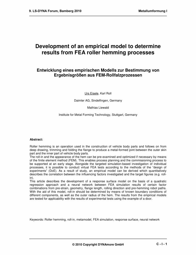
Hemming is an operation used in the construction of vehicle body parts and follows on from deep drawing, trimming and folding the flange to produce a metal-formed joint between the outer skin part and the inner part of the vehicle body.

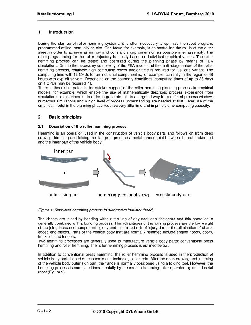
Figure 1: Simplified hemming process in automotive industry (hood) The sheets are joined by bending without the use of any additional fasteners and this operation is generally combined with a bonding process. The advantages of this joining process are the low weight of the joint, increased component rigidity and minimized risk of injury due to the elimination of sharp-edged end pieces. Parts of the vehicle body that are normally hemmed include engine hoods, doors, trunk lids and fenders. Two hemming processes are generally used to manufacture vehicle body parts: conventional press hemming and roller hemming. The roller hemming process is outlined below. In addition to conventional press hemming, the roller hemming process is used in the production of vehicle body parts based on economic and technological criteria. After the deep drawing and trimming of the vehicle body outer skin part, the flange is normally positioned using a folding tool. However, the hemming process is completed incrementally by means of a hemming roller operated by an industrial robot (Figure 2).

Metallumformung I 9. LS-DYNA Forum, Bamberg 2010

C - I - 2


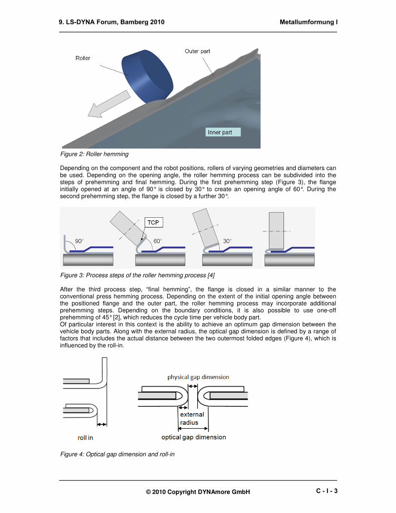
Figure 2: Roller hemming Depending on the component and the robot positions, rollers of varying geometries and diameters can be used. Depending on the opening angle, the roller hemming process can be subdivided into the steps of prehemming and final hemming. During the first prehemming step (Figure 3), the flange initially opened at an angle of 90° is closed by 30° to create an opening angle of 60°. During the second prehemming step, the flange is closed by a further 30°.

Figure 3: Process steps of the roller hemming process [4] After the third process step, “final hemming”, the flange is closed in a similar manner to the conventional press hemming process. Depending on the extent of the initial opening angle between the positioned flange and the outer part, the roller hemming process may incorporate additional prehemming steps. Depending on the boundary conditions, it is also possible to use one-off prehemming of 45° [2], which reduces the cycle time per vehicle body part. Of particular interest in this context is the ability to achieve an optimum gap dimension between the vehicle body parts. Along with the external radius, the optical gap dimension is defined by a range of factors that includes the actual distance between the two outermost folded edges (Figure 4), which is influenced by the roll-in.

Figure 4: Optical gap dimension and roll-in


C - I - 3


The roll-in incurred depends largely on the roller’s trajectory. For this reason, it is important to ensure that the roller’s actual trajectory is exactly reproduced within the simulation.

2.2 Basic principles of empirical models

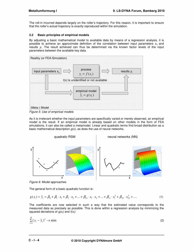
By adjusting a basic mathematical model to available data by means of a regression analysis, it is possible to achieve an approximate definition of the correlation between input parameters xn and results yi. The result achieved can thus be determined via the known factor levels of the input parameters between the available key data.

processprocessinput parameters xn results yi

empirical modelempirical model

)(ˆii xgy =

)( ii xfy =

f(x) is unidentified or not available

Realitiy (or FEA-Simulation)

(Meta-) Model

Figure 5: Use of empirical models As it is irrelevant whether the input parameters are specifically varied or merely observed, an empirical model is the result. If an empirical model is already based on other models in the form of FEA simulations, it can also be called a metamodel. Linear and quadratic terms find broad distribution as a basic mathematical description g(x), as does the use of neural networks.

**

**

* *

*

quadratic RSM

x

y

**

**

* *

*

neural networks (NN)

x

y

Figure 6: Model approaches The general form of a basic quadratic function is:

..........ˆ)(2

2222

2

111211222110+⋅+⋅++⋅⋅++⋅+⋅+== xxxxxxyxg ii ββββββ (1)

The coefficients are now selected in such a way that the estimated value corresponds to the measured data as precisely as possible. This is done within a regression analysis by minimizing the squared deviations of g(xi) and f(xi):

min)ˆ(2

1

→−∑=

ii

N

i

yy (2)


C - I - 4


After calculating the coefficients, it is possible to estimate the results within the design space not only for the existing sampling points but also for any factor levels in between. Neural networks can understand considerably more complex curve shapes than is possible with quadratic approaches. They are largely based on a type of summands (neurons) which receive a certain weighting factor W depending on the factor level of the input parameters. This means that each summand is individually networked with the input factors via the weighting factors, which is similar to a biological nerve structure [10]. Each neuron also has a transfer or activation function f(x) In this study, the following functions are used as per [3]:

∑ ∑= =

+⋅+=

H

h

K

k

khkhh xWWfWWWxY1 1

00),( with e.g.: x

exf

−+=

1

1)( (3)

H: Number of input factors K: Number of neurons The individual weighting factors W are adapted iteratively to the existing data basis by means of a training algorithm.

3 Development of a metamodel on the basis of basic geometries

The following section describes the development process of a metamodel for general predetermination of the roll-in and external radius process results.

3.1 Selection of process parameters in line with significance tests

Only relevant input parameters should be included for the process in the metamodel. For this reason, it is recommended to conduct a significance analysis according to methods of the design of experiments (DoE) in order to reduce calculation effort. Partial results have already been published for this purpose in [4]. Relevant input factors include: - geometry (concave, convex curvature) - thickness of the blank - radius of the flanging tool - position of the inner part - pre-strain of the outer blank - position of the roller during the two pre-hemming steps (including rigidity of the robot) - angle of the roller during pre-hemming - rolling direction of the blank - blank material - length of the flange As factors such as blank material, blank thickness and radius of the flanging tool are generally known during the planning process, these can be selected as constant for the first version of a metamodel. The input parameters to be used are therefore limited to the following input factors: geometry (curvature), pre-strain, positions of the roller during pre-hemming, rolling direction of the blank and length of the flange.


C - I - 5


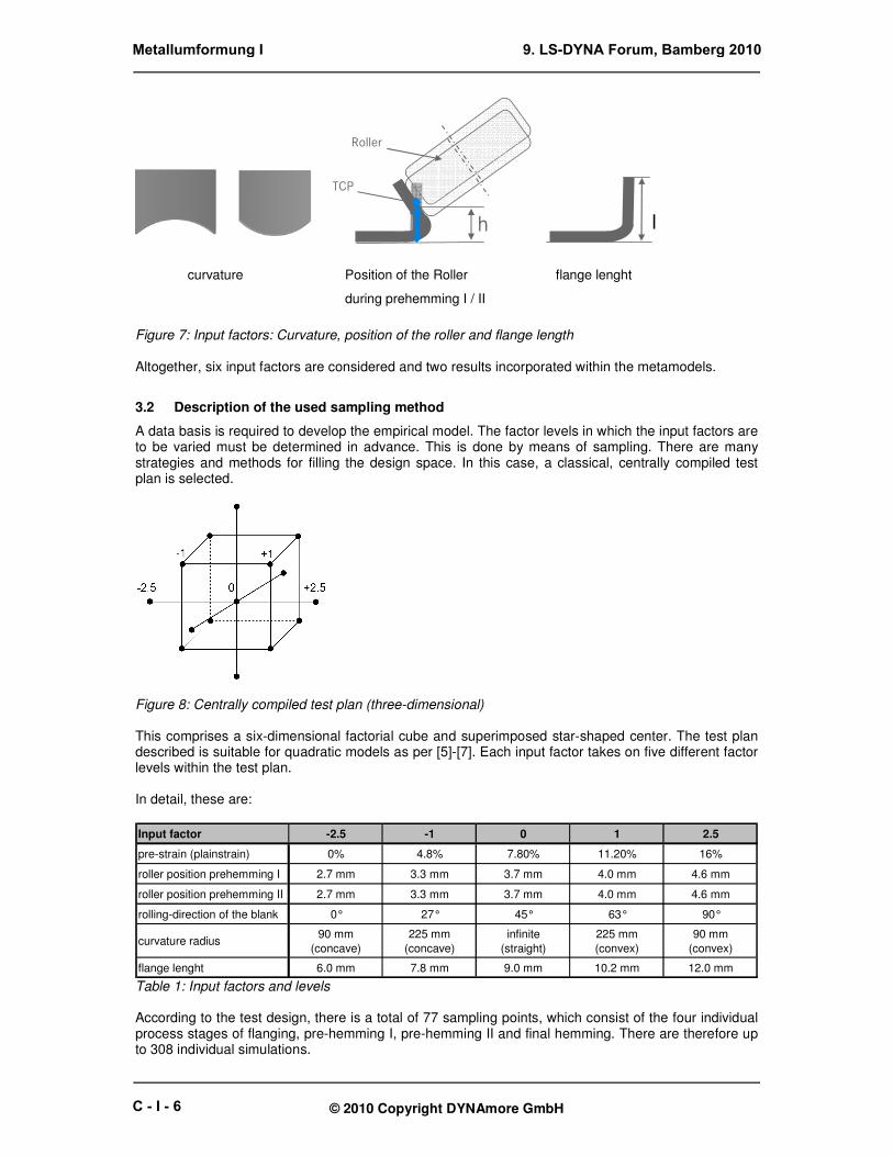
h

TCP

l

curvature Position of the Roller

during prehemming I / II

flange lenght

Roller

Figure 7: Input factors: Curvature, position of the roller and flange length Altogether, six input factors are considered and two results incorporated within the metamodels.

3.2 Description of the used sampling method

A data basis is required to develop the empirical model. The factor levels in which the input factors are to be varied must be determined in advance. This is done by means of sampling. There are many strategies and methods for filling the design space. In this case, a classical, centrally compiled test plan is selected.

Figure 8: Centrally compiled test plan (three-dimensional) This comprises a six-dimensional factorial cube and superimposed star-shaped center. The test plan described is suitable for quadratic models as per [5]-[7]. Each input factor takes on five different factor levels within the test plan. In detail, these are:

Input factor -2.5 -1 0 1 2.5

pre-strain (plainstrain) 0% 4.8% 7.80% 11.20% 16%

roller position prehemming I 2.7 mm 3.3 mm 3.7 mm 4.0 mm 4.6 mm

roller position prehemming II 2.7 mm 3.3 mm 3.7 mm 4.0 mm 4.6 mm

rolling-direction of the blank 0° 27° 45° 63° 90°

curvature radius90 mm

(concave)

225 mm

(concave)

infinite

(straight)

225 mm

(convex)

90 mm

(convex)

flange lenght 6.0 mm 7.8 mm 9.0 mm 10.2 mm 12.0 mm Table 1: Input factors and levels According to the test design, there is a total of 77 sampling points, which consist of the four individual process stages of flanging, pre-hemming I, pre-hemming II and final hemming. There are therefore up to 308 individual simulations.


C - I - 6


The 1.15 mm sheet thickness from sheet material AA6014 serves as a boundary condition for modeling. The folding radius is 1.5 mm, the sheet thickness of the inner part 2.0 mm and the roller diameter 60 mm. During the two pre-hemming stages, the flange is closed by 30° in each case. These limits are necessary to reduce the number of simulations necessary to a manageable amount.

3.3 Configuration of the FEA simulation

The FEA simulations were conducted with the LS-Dyna explicit code. The fully integrated type 16 shell element was used for this. The formulation in line with Barlat ’89 was used as the material model. The element edge length was 0.2 mm by 0.25 mm (height x width). The results were in each case determined from the middle of the test geometries.

Figure 9: FEA roller hemming model in LS-Dyna [8] The metamodels from the simulations were created using the program “Minitab 15” (quadratic response surface) and “LS-Opt 4.1” (neural network).

4 Result of empirical modeling

After the regression analysis has been performed, the following connection for the roll-in (RI) result is produced for the quadratic response surface (RSM):

2112

2

1116655443322110...ˆ xxxxxxxxxyi ⋅⋅+⋅+⋅++⋅+⋅+⋅+⋅+⋅+= βββββββββ + … (4)

x1: Radius of curvature: positive = convex, negative = concave, 0 = straight x2: Pre-strain x3: Position of the roller during pre-hemming I (Figure 7: h) x4: Position of the roller during pre-hemming II (Figure 7: h) x5: Length of the flange (Figure 7: l) x6: Rolling direction The model is optimized to a confidence interval of 95% during the regression. The rolling direction was classified as not significant in comparison to the other parameters.


C - I - 7


5 Validation of the metamodels by means of experimental data

The quality of the predictions for roll-in and external radius of the two metamodels is to be assessed by a comparison with experimental data. The test structure is described briefly below.

5.1 Description of experimental set-up and assessment

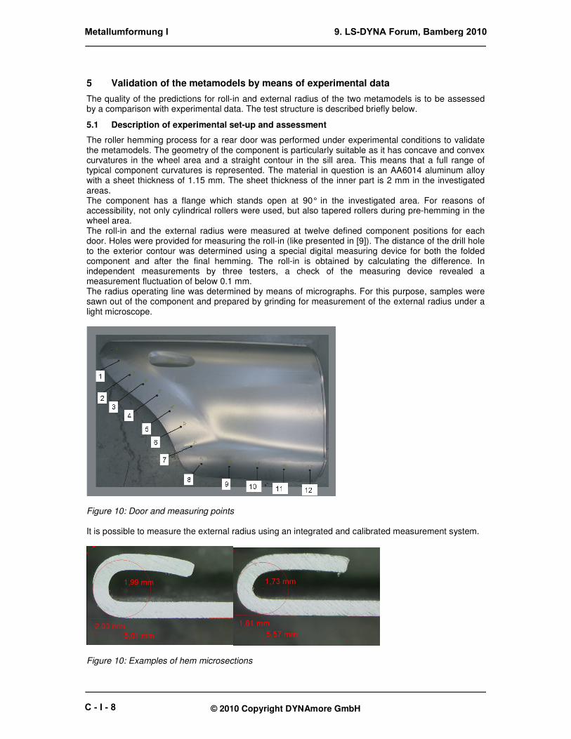
The roller hemming process for a rear door was performed under experimental conditions to validate the metamodels. The geometry of the component is particularly suitable as it has concave and convex curvatures in the wheel area and a straight contour in the sill area. This means that a full range of typical component curvatures is represented. The material in question is an AA6014 aluminum alloy with a sheet thickness of 1.15 mm. The sheet thickness of the inner part is 2 mm in the investigated areas. The component has a flange which stands open at 90° in the investigated area. For reasons of accessibility, not only cylindrical rollers were used, but also tapered rollers during pre-hemming in the wheel area. The roll-in and the external radius were measured at twelve defined component positions for each door. Holes were provided for measuring the roll-in (like presented in [9]). The distance of the drill hole to the exterior contour was determined using a special digital measuring device for both the folded component and after the final hemming. The roll-in is obtained by calculating the difference. In independent measurements by three testers, a check of the measuring device revealed a measurement fluctuation of below 0.1 mm. The radius operating line was determined by means of micrographs. For this purpose, samples were sawn out of the component and prepared by grinding for measurement of the external radius under a light microscope.

Figure 10: Door and measuring points It is possible to measure the external radius using an integrated and calibrated measurement system.

Figure 10: Examples of hem microsections


C - I - 8


In order to identify the true values of the position of the rollers during pre-hemming steps, the Krypton K600 measurement system was used, which was already for a roller hemming process in [8]. This ensures that no falsifications due to robot programming and insufficient robot rigidity affect the validation of the metamodels.

5.2 Description of the test program

So as to draw on as representative a spectrum of data as possible for the validation of the metamodels, the robot program was varied for the components used. Investigations were performed in advance to identify the path parameters in order to concentrate the roll-in characteristics in a typical range from 0 to 0.55 mm. This is the later target range for the productive application of the metamodels. A total of five different roller trajectories combinations were programmed, with repetition.

Programm h1* h2**

A 2,2 mm 3,2 mm

B 3,2 mm 2,2 mm

C 2,2 mm 2,2 mm

D 3,2 mm 3,2 mm

E 2,7 mm 2,7 mm

* about + 2 mm (caused by low robot rigidity)

** about + 0.65 mm (caused by low robot rigidity) Table 2: Robot programs The robot program entered differs from that actually performed as a result of low robot rigidity. Although during the second pre-hemming stage the overall spatial offset was greater than during the first with a smaller load due to the lower robot rigidity, the effect on the parameter h2 was effectively much less as a result of the wider roller angle (trigonometric function). A total of 120 representative measurement values are therefore available in reference to roll-in measurement. Furthermore, a total of 60 micrographs were created at positions with characteristic curvature (measuring points 1, 4, 5, 8, 9, 11).

5.3 Comparison of the roll-in

An estimate of the roll-in can be obtained as an answer from the metamodels by inserting the appropriate factor levels. The pre-strain figures were read out from the deep-drawing FEA simulation. The curvature values were determined by means of the CAD data. As there are up to 120 measurement values, it is recommended to make a statistical analysis of the errors in the metamodels in comparison with the experimental values. The average error can be calculated as follows:

∑=

−⋅=n

i

ModelExperiment yyn

y1

)(1

(6)

This value alone is not meaningful. Error fluctuation must also be taken into account in the form of standard deviation. This is estimated with (6) as follows:

∑=

−⋅−

=n

i

el yyn 1

2

mod)(

1

1σ (7)

The model errors can be described in good approximation within a normal distribution:

2

2

2

)(

2

1)( σ

σπ

yx

exg

−−

⋅⋅

= (8)


C - I - 9


Figure 11 shows the metamodel errors over the entire data volume with regard to the roll-in in the form of histograms.

0,40,30,20,10,0-0,1-0,2-0,3

25

20

15

10

5

0

0,40,30,20,10,0-0,1-0,2-0,3

RSM (whole part )

observed frequency

NN (whole part)

mean value -0,01942

Std. deviation 0,1219

N 120

RSM (whole part )

mean value 0,039


N 120

NN (whole part)

Roll-InError: Models versus experiments

Figure 11: Deviation between metamodels and experiments (roll-in; whole part) I Both models show a mean error of a few hundredths of a millimeter. However, both models have a standard deviation of approximately 0.12 mm to 0.13 mm. This engenders relative uncertainty with regard to each individual value.

0,480,320,160,00-0,16-0,32

24

18

12

6

0

0,480,320,160,00-0,16-0,32

24

18

12

6

00,480,320,160,00-0,16-0,32

RSM (straight)

observed frequency

RSM (conv ex) RSM (concav e)

NN (straight) NN (conv ex) NN (concav e)

mean error -0,06299

Std. dev iation 0,09682

N 50

RSM (straight)

mean error 0,03973


N 40

RSM (convex)

mean error -0,02567


N 30

RSM (concave)

mean error 0,01073


N 50

NN (straight)

mean error 0,08883


N 40

NN (convex)

mean error 0,01967


N 30

NN (concave)

Roll-InError: Models versus experiments

Figure 12: Deviation between metamodels and experiments (roll-in) II


C - I - 10


Different ranges of accuracy of the metamodels become clear by a separate analysis of the geometric boundary conditions. The following can be said: - over two-thirds of all measurement results in the case of concave curvature were predicted by the

RSM with an absolute error in the range of –0.114 mm to 0.063 mm. Given current tolerance requirements, this is a very acceptable result.

- over two-thirds of all measurement results in the case of straight contours were calculated by the NN with an absolute error in the range of –0.076 mm to 0.097 mm.

- over two-thirds of all measurement results, the error in the case of convex curvature was in the range of –0.11 mm to 0.19 mm (RSM), which represents twice the level of uncertainty.

In summary, the use of the quadratic RSM for concave geometric curvatures can be recommended with very good approximation on the basis of this validation. The NN has slight advantages for linear contour sections. Convex areas can be estimated with twice the level of uncertainty for both models.

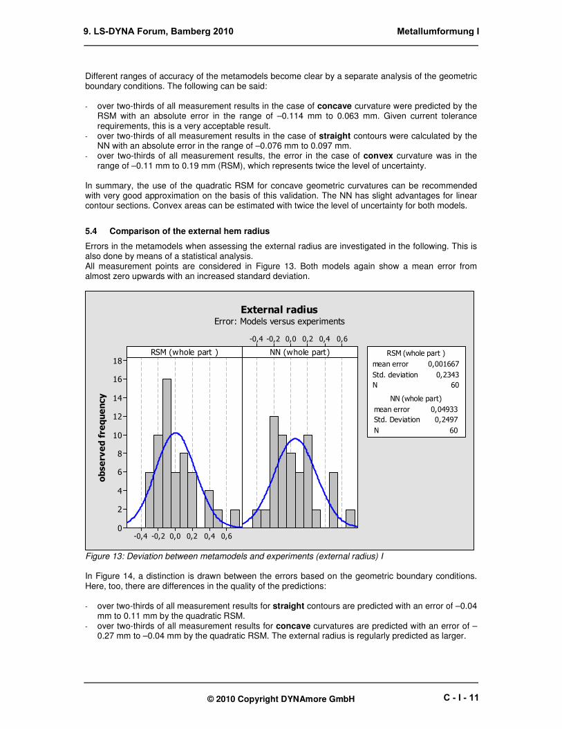
5.4 Comparison of the external hem radius

Errors in the metamodels when assessing the external radius are investigated in the following. This is also done by means of a statistical analysis. All measurement points are considered in Figure 13. Both models again show a mean error from almost zero upwards with an increased standard deviation.

0,60,40,20,0-0,2-0,4

18

16

14

12

10

8

6

4

2

0

0,60,40,20,0-0,2-0,4

RSM (whole part )

observed frequency

NN (whole part)

mean error 0,001667


N 60

RSM (whole part )

mean error 0,04933

Std. Deviation 0,2497

N 60

NN (whole part)

External radiusError: Models versus experiments

Figure 13: Deviation between metamodels and experiments (external radius) I In Figure 14, a distinction is drawn between the errors based on the geometric boundary conditions. Here, too, there are differences in the quality of the predictions: - over two-thirds of all measurement results for straight contours are predicted with an error of –0.04

mm to 0.11 mm by the quadratic RSM. - over two-thirds of all measurement results for concave curvatures are predicted with an error of –

0.27 mm to –0.04 mm by the quadratic RSM. The external radius is regularly predicted as larger.


C - I - 11


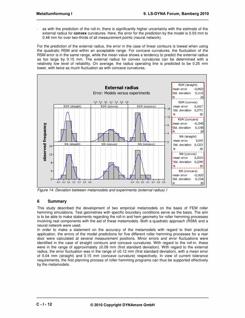
- as with the prediction of the roll-in, there is significantly higher uncertainty with the estimate of the external radius for convex curvatures. Here, the error for the prediction by the model is 0.03 mm to 0.48 mm for over two-thirds of all measurement points (neural network).

For the prediction of the external radius, the error in the case of linear contours is lowest when using the quadratic RSM and within an acceptable range. For concave curvatures, the fluctuation of the RSM error is in the same range, while the mean value shows a tendency to predict the external radius as too large by 0.15 mm. The external radius for convex curvatures can be determined with a relatively low level of reliability. On average, the radius operating line is predicted to be 0.25 mm lower, with twice as much fluctuation as with concave curvatures.

0,80,60,40,20,0-0,2-0,4

16

12

8

4

0

0,80,60,40,20,0-0,2-0,4

16

12

8

4

00,80,60,40,20,0-0,2-0,4

RS M (straight)

observed frequency

RS M (conv ex) RS M (concav e)

NN (straight) NN (conv ex) NN (concav e)

mean error -0,0422


N 20

RSM (straight)

mean error 0,1617


N 20

RSM (convex)

mean error -0,1545


N 20

RSM (concave)

mean error 0,019


N 20

NN (straight)

mean error 0,2515


N 20

NN (convex)

mean error -0,1625


N 20

NN (concave)

External radiusError: Models versus experiments

Figure 14: Deviation between metamodels and experiments (external radius) I

6 Summary

This study described the development of two empirical metamodels on the basis of FEM roller hemming simulations. Test geometries with specific boundary conditions serve as the basis. The aim is to be able to make statements regarding the roll-in and hem geometry for roller hemming processes involving real components with the aid of these metamodels. Both a quadratic approach (RSM) and a neural network were used. In order to make a statement on the accuracy of the metamodels with regard to their practical application, the errors of the model predictions for five different roller hemming processes for a rear door were calculated at several measurement positions. Minor errors and error fluctuations were identified in the case of straight contours and concave curvatures. With regard to the roll-in, these were in the range of approximately ±0.09 mm (first standard deviation). With regard to the external radius, the error fluctuation was in the range of ±0.12 mm (first standard deviation), with a mean error of 0.04 mm (straight) and 0.15 mm (concave curvature) respectively. In view of current tolerance requirements, the first planning process of roller hemming programs can thus be supported effectively by the metamodels.


C - I - 12


7 References

[1] Arroyo, A.; Pérez, I.; Gutiérrez, M.; Bahillo, J.; Toja, H.: “Simulation of roller hemming process

with Abaqus explicit”. Proceedings of the IDDR 2010, pp. 41-52. Golden 2010 [2] Le Maoût, N.; “Numerical Simulation of Flat-Surface Roll Hemming: Influence of geometry and

material models”; In Proceedings of the IDDRG 2006, No. 25, pp. 287-294; Porto 2006 [3] Stander, N.; Goel, T.: LS-OPT-Training class Handout “optimization theory”. Livermore Software

Technology Corporation; June 2010 [4] Eisele, U.; Roll, K.; “Integration von FEM-Rollfalzsimulationen in die virtuelle Prozesskette”; In

Bauteile der Zukunft – Methoden und Prozesse T31, pp. 337-358; EFB e.V., Hannover, Germany 2010, ISBN 978-3-86776-343-1

[5] Kleppmann, W. (2008): Taschenbuch Versuchsplanung: Fachbuch, 5th edition, Carl Hanser

Verlag München Wien, 2008 [6] Box, G.E.P./Draper, N.R.: Response Surfaces, Mixtures, and Ridge Analyses. John Wiley, New

York 2nd edition 2007 [7] Myers, R.H./Montgomery, D.C.: Response Surface Methodology. John Wiley, New York, 2nd

edition [8] Eisele, U.; Roll, K.; Liewald, M.: “New approaches for validation of roller hemming process

simulation”, in: Conference proceedings of the IDDRG 2010, pp. 851-860, Graz 2010. ISBN 978-3-85125-108-1

[9] Le Maoût, N.: “Analyse des procédés de sertissage de tôles métalliques“; Thése Docteur,

Université de Bretagne-Sud, 2009 [10] Karrenberg, U.: „Signale, Prozesse, Systeme“; Springer Verlag, Heidelberg, London, New York

2009, ISBN 978-3642018633


C - I - 13

Development of an empirical model to determine results ... · Hemming is an operation used in the...

Documents

Transcript of Development of an empirical model to determine results ... · Hemming is an operation used in the...