Development of MWL-AUC / CCD-C-AUC / SLS-AUC detectors for ...€¦ · Analytical...
123
Max-Planck Institut für Kolloid und Grenzflächenforschung Development of MWL-AUC / CCD-C-AUC / SLS-AUC Detectors for the Analytical Ultracentrifuge Dissertation zur Erlangung des akademischen Grades „doctor rerum naturalium“ (Dr. rer. nat.) in der Wissenschaftsdisziplin „Kolloidchemie“ eingereicht an der Mathematisch-Naturwissenschaftlichen Fakultät Universität Potsdam von Engin Karabudak Potsdam, im Mai 2009
Transcript of Development of MWL-AUC / CCD-C-AUC / SLS-AUC detectors for ...€¦ · Analytical...

Max-Planck Institut für Kolloid und Grenzflächenforschung
Development of
MWL-AUC / CCD-C-AUC / SLS-AUC Detectors
for the Analytical Ultracentrifuge
Dissertation zur Erlangung des akademischen Grades
„doctor rerum naturalium“ (Dr. rer. nat.)
in der Wissenschaftsdisziplin „Kolloidchemie“
eingereicht an der Mathematisch-Naturwissenschaftlichen Fakultät
Universität Potsdam
von Engin Karabudak
Potsdam, im Mai 2009

This work is licensed under a Creative Commons License: Attribution - Noncommercial - Share Alike 3.0 Germany To view a copy of this license visit http://creativecommons.org/licenses/by-nc-sa/3.0/de/deed.en Published online at the Institutional Repository of the University of Potsdam: URL http://opus.kobv.de/ubp/volltexte/2009/3992/ URN urn:nbn:de:kobv:517-opus-39921 http://nbn-resolving.org/urn:nbn:de:kobv:517-opus-39921

ii
TABLE OF CONTENTS:
CHAPTER 1 : THESIS INTRODUCTION........................................................................................................ 1
CHAPTER 2 : GENERAL REVIEW OF AUC ................................................................................................. 6
2.1. GENERAL ANALYTICAL ULTRACENTRIFUGATION................................................................................. 6 2.2. INSTRUMENTATION FOR COMMERCIAL AUC ........................................................................................ 8
2.2.1. Mechanical Parts ............................................................................................................................ 8 2.2.1.1. Rotors ......................................................................................................................................................... 8 2.2.1.2. Cells............................................................................................................................................................ 9
2.2.2. Electronic Parts ............................................................................................................................ 11 2.2.3. Optical Parts ................................................................................................................................. 12
2.2.3.1. Absorbance Optics.................................................................................................................................... 13 2.2.3.2. Interference Optics ................................................................................................................................... 14
2.3. THEORY OF ANALYTICAL ULTRACENTRIFUGE.................................................................................... 16 2.4. OTHER DETECTORS FOR XL-AUC...................................................................................................... 19
2.4.1. Schlieren Optics ............................................................................................................................ 20 2.4.2. Fluorescence Detector .................................................................................................................. 21 2.4.3. Turbidity Detector ......................................................................................................................... 21
2.5. TYPES OF EXPERIMENTS WITH AUC................................................................................................... 22 2.5.1. Sedimentation Velocity Experiment............................................................................................... 22 2.5.2. Sedimentation Equilibrium Experiment ........................................................................................ 23 2.5.3. Band (Zone) Centrifugation .......................................................................................................... 24
CHAPTER 3 : STATIC LIGHT SCATTERING DETECTOR FOR ANALYTICAL ULTRACENTRIFUGATION (SLS-AUC) ....................................................................................................... 26
3.1. INTRODUCTION ................................................................................................................................... 26 3.2. EXPERIMENTAL TESTS........................................................................................................................ 27
3.2.1. LAAPD with home-made power supply......................................................................................... 27 3.2.2. Modifying the commercial power supply of the LAAPD ............................................................... 29 3.2.3. First Prototype of SLS-AUC.......................................................................................................... 29 3.2.4. Tests with the prototype SLS-AUC ................................................................................................ 30
CHAPTER 4 : CCD CAMERA DETECTOR FOR THE ANALYTICAL ULTRACENTRIFUGE (CCD-C-AUC) ................................................................................................................................................................ 31
4.1. INTRODUCTION ................................................................................................................................... 31 4.2. EXPERIMENTAL TESTS........................................................................................................................ 32
4.2.1. Resolution Test .............................................................................................................................. 33 4.2.2. Monochromator of the Optima XL-I.............................................................................................. 34 4.2.3. Illumination test with SK2048DDE inside AUC with Xenon flash lamp....................................... 36 4.2.4. Owl Camera inside AUC with Xenon flash lamp .......................................................................... 36 4.2.5. Tests with Constant Light Sources in the Optima XL-I ................................................................. 36 4.2.6. Illumination tests on the Optical Bench with 75 W light ............................................................... 37 4.2.7. Construction of prototype test setup.............................................................................................. 37 4.2.8. Constant Light Source from Aviv Biomedical ............................................................................... 39 4.2.9. Constant Light Source, Test Setup with Monochromator.............................................................. 40 4.2.10. First Prototype CCD-C-AUC, taking UV/Vis spectra .............................................................. 41
CHAPTER 5 : MULTIWAVELENGTH DETECTOR FOR ANALYTICAL ULTRACENTRIFUGE (MWL-AUC) ....................................................................................................................................................... 45
5.1. INTRODUCTION ................................................................................................................................... 45 5.2. IMPROVEMENT OF THE MULTIWAVELENGTH DETECTOR...................................................................... 46
5.2.1. Flash Lamp.................................................................................................................................... 46 5.2.2. Detector Arm and Spectrometer Mount ........................................................................................ 47 5.2.3. Imaging Optics .............................................................................................................................. 48 5.2.4. Optical Tests.................................................................................................................................. 48
5.3. RESULTS ............................................................................................................................................. 49 5.3.1. General Aspects ............................................................................................................................ 49 5.3.2. Radial Resolution .......................................................................................................................... 52 5.3.3. Wavelength Accuracy.................................................................................................................... 53
iii
5.3.4. Absorbance Accuracy and Linearity ............................................................................................. 55 5.3.5. Intrinsic Noise of the Data ............................................................................................................ 57
5.4. DISCUSSION ........................................................................................................................................ 59
CHAPTER 6 : BIOLOGICAL APPLICATION OF MWL-AUC: PROTEIN MIXTURE.......................... 60
6.1. INTRODUCTION ................................................................................................................................... 60 6.2. RESULTS AND DISCUSSION ................................................................................................................. 60
CHAPTER 7 : INDUSTRIAL APPLICATION OF MWL-AUC: INVESTIGATION OF Β-CAROTENE-GELATIN COMPOSITE PARTICLES ........................................................................................................... 67
7.1. INTRODUCTION ................................................................................................................................... 67 7.2. MATERIAL AND METHODS.................................................................................................................. 68 7.3. RESULTS AND DISCUSSION ................................................................................................................. 69
CHAPTER 8 : APPLICATION OF MWL-AUC IN CHEMISTRY: CDTE NANOPARTICLES..... 76
8.1. INTRODUCTION ................................................................................................................................... 76 8.2. POLYDISPERSE TGA-CAPPED CDTE NANOCRYSTALS ......................................................................... 77
8.2.1. Experimental ................................................................................................................................. 77 8.2.1.1. Analysis Method of the MWL-AUC data................................................................................................. 78
8.2.2. Results and Discussions: ............................................................................................................... 79 8.2.2.1. Raw MWL-AUC Data:............................................................................................................................. 79 8.2.2.2. Analysis without Diffusion Correction ..................................................................................................... 79 8.2.2.3. Analysis with Diffusion Correction .......................................................................................................... 87 8.2.2.4. Growth mechanisms of CdTe nanoparticles ............................................................................................. 89
8.3. MONODIPERSE TGA-CAPPED CDTE NANOCRYSTALS ......................................................................... 98 8.3.1. Results and Discussion.................................................................................................................. 98
8.3.1.1. Raw MWL-AUC of a monodisperse sample ............................................................................................ 98 8.3.1.2. Determination of CdTe mixture composition by spectrum of the sample................................................. 98 8.3.1.3. Comparison of MWL-AUC results and Spectral Deconvolution results .................................................. 99
CHAPTER 9 : CONCLUSION........................................................................................................................ 101
APPENDIX........................................................................................................................................................ 105
ABBREVIATIONS ........................................................................................................................................... 108
REFERENCES.................................................................................................................................................. 109

iv
List of Figures: FIGURE 2-1: GENERAL SCHEMATIC FOR AN AUC .................................................................................................... 6 FIGURE 2-2: ROTORS ............................................................................................................................................... 8 FIGURE 2-3 : CELL ASSEMBLY OF AUC CELL......................................................................................................... 10 FIGURE 2-4 : VARIOUS AUC CENTERPIECES .......................................................................................................... 10 FIGURE 2-5: ELECTRONICS OF AUC ...................................................................................................................... 12 FIGURE 2-6 : SCHEMATICS OF ABSORBANCE OPTICS .............................................................................................. 13 FIGURE 2-7 : SCHEMATICS OF INTERFERENCE DETECTOR...................................................................................... 15 FIGURE 2-8: SCHEMATIC OF USER-MADE XL-SO AUC.......................................................................................... 20 FIGURE 2-9: AU-FDS PHOTOGRAPH AND DATA..................................................................................................... 21 FIGURE 2-10: DIFFERENT TYPES OF AUC EXPERIMENT ......................................................................................... 23 FIGURE 3-1: LAAPD TEST SETUP FOR SLS-AUC .................................................................................................. 27 FIGURE 3-2: PICTURE OF SLS-AUC DETECTOR PARTS.......................................................................................... 28 FIGURE 3-3: PHOTOGRAPH OF SLS-AUC WHICH IS PLACED IN THE OPTIMA XL-I................................................. 30 FIGURE 4-1: SCHEMATIC OF SK2048 DDE LINE CAMERA RESOLUTION TEST ........................................................ 33 FIGURE 4-2 : ORIGINAL TECHNICAL DRAWING OF MONOCHROMATOR OF OPTIMA XL-I (GIEBELER 1992)
REPRODUCED BY PERMISSION OF THE ROYAL SOCIETY OF CHEMISTRY............................................................ 34 FIGURE 4-3: TESTING OF SK2048DDE WITH PULSED LIGHT FROM AUC. ............................................................. 35 FIGURE 4-4: ILLUMINATION TEST OF THE CAMERA ON OPTICAL BENCH ................................................................. 37 FIGURE 4-5: PHOTOGRAPH OF PROTOTYPE TEST SETUP OF CCD-C-AUC............................................................. 38 FIGURE 4-6: PROTOTYPE CONSTANT LIGHT SOURCE FROM AVIV BIOMEDICAL..................................................... 39 FIGURE 4-7: PHOTO AND DATA OF MONOCHROMATIC TEST OF CCD-C-AUC........................................................ 40 FIGURE 4-8: CCD-C-AUC FINAL PROTOTYPE SETUP ............................................................................................. 42 FIGURE 4-9: UV/VIS SPECTRA WITH PROTOTYPE CCD-C-AUC ............................................................................ 43 FIGURE 5-1: SCHEMATICS OF THE MWL DETECTOR ARM. .................................................................................... 46 FIGURE 5-2: PHOTOGRAPHS OF MWL-AUC.......................................................................................................... 47 FIGURE 5-3: INTENSITY DISTRIBUTIONS OF USB2000 SPECTROMETER.................................................................. 50 FIGURE 5-4 : OPTICAL TESTS OF MWL-AUC AND OPTIMA XL-I WITH SLIT ........................................................ 51 FIGURE 5-5 : STEP MOTOR TESTS OF MWL-AUC AND OPTIMA XL-I.................................................................... 53 FIGURE 5-6 : WAVELENGTH ACCURACY OF THE OPTIMA XL-I AND THE MWL-AUC. .......................................... 54 FIGURE 5-7: ABSORBANCE ACCURACY OF THE MWL-AUC AT DIFFERENT WAVELENGTHS.................................. 55 FIGURE 5-8 : INTENSITY PROFILE OF LINEARITY TESTS.......................................................................................... 56 FIGURE 5-9: NOISE COMPARISON BETWEEN THE OPTIMA XL-I AND THE MWL-AUC........................................... 57 FIGURE 6-1: COMPARISON OF OPTIMA XL-I AND MWL-AUC IN C(S) AND GLOBAL FIT OF ALDOLASE ................. 60 FIGURE 6-2: THREE WAVELENGTHS, GLOBAL MULTISIGNAL ANALYSIS OF MWL-AUC AND OPTIMA XL-I .......... 61 FIGURE 6-3: REFERENCE INTENSITY OF MWL-AUC AND WAVELENGTH SCAN OF OPTIMA XL-I AND MWL-AUC63 FIGURE 6-4: MWL-AUC AND XL-I ANALYSIS RESIDUALS OF 280 NM ANALYSIS .................................................. 64 FIGURE 7-1: UV/VIS SPECTRA OF SHELL -CAROTENE/GELATIN SAMPLE .............................................................. 68 FIGURE 7-2 : STRUCTURE OF -CAROTENE MICROPARTICLE SYSTEM ..................................................................... 69 FIGURE 7-3: 3D SEDIMENTATION OF -CAROTENE MICROSYSTEM ......................................................................... 70 FIGURE 7-4: SEDIMENTATION COEFFICIENT DISTRIBUTIONS AT DIFFERENT WAVELENGTHS................................... 72 FIGURE 7-5: UV/VIS SPECTRA OF SEDIMENTING -CAROTENE MICROSYSTEM ....................................................... 73 FIGURE 7-6: STRUCTURE MODEL OF THE -CAROTENE MICROPARTICLE SYSTEM ON THE BASIS OF THE PRESENTED
AUC RESULTS. ............................................................................................................................................. 74 FIGURE 8-1: PRESENTATION OF CDTE EXPERIMENT............................................................................................... 77 FIGURE 8-2 : RAW MWL-AUC DATA: CDTE NANOPARTICLES SEDIMENTATING WITH BAND CENTRIFUGATION
METHOD; (SPEED 55K, 20 RADIAL SCANS 50 µM STEP SIZE).......................................................................... 78 FIGURE 8-3 : ANALYSIS OF MWL-AUC DATA, REFERENCE INTENSITY AND PSD .................................................. 80 FIGURE 8-4: COMBINED 3D DATA, WITH AXIS, PARTICLE SIZE, ABS, WAVELENGTH ............................................... 82 FIGURE 8-5: SPECTRAL COMPARISON OF SAMPLE .................................................................................................. 83 FIGURE 8-6: COMPARISON OF THE RESULTS WITH THEORY .................................................................................... 85 FIGURE 8-7 : MIXTURE EFFECT OF CDTE ............................................................................................................... 85 FIGURE 8-8 : RESULT OF 2DSA ANALYSIS ............................................................................................................. 87 FIGURE 8-9: DIFFUSION-CORRECTED RESULTS OF THE CDTE EXPERIMENT ........................................................... 88 FIGURE 8-10: DENSITY MODEL OF CDTE/TGA ..................................................................................................... 90 FIGURE 8-11: MOLECULAR WEIGHT OF 24 SPECIES (0-23) ..................................................................................... 93 FIGURE 8-12: ONE OF THE POSSIBLE MECHANISMS OF CDTE NANOPARTICLE CRYSTALLIZATION ......................... 93 FIGURE 8-13: RAW MWL-AUC DATA OF MONODISPERSE SAMPLE....................................................................... 97 FIGURE 8-14: SPECTRAL DECONVOLUTION OF MONODISPERSE CDTE SAMPLE....................................................... 99 FIGURE 8-15: COMPARISON OF SPECTRA DECONVOLUTION RESULT AND RAW MWL-AUC RESULTS.................. 100
v
List of Equations: EQUATION 2-1: CALCULATION OF ABSORPTION..................................................................................................... 14 EQUATION 2-2: CALCULATION OF THE CONCENTRATION FROM INTERFERENCE FRINGE SHIFT J(R) ...................... 16 EQUATION 2-3: EQUATION OF CENTRIFUGAL FORCE.............................................................................................. 16 EQUATION 2-4 : EQUATION OF BUOYANT FORCE.................................................................................................... 17 EQUATION 2-5: EQUATION OF FRICTIONAL FORCE ................................................................................................. 17 EQUATION 2-6: BALANCE OF FORCES INSIDE AUC................................................................................................ 17 EQUATION 2-7: REARRANGEMENT OF EQUATION 2.6............................................................................................. 17 EQUATION 2-8: EQUATION OF SVEDBERG UNIT..................................................................................................... 18 EQUATION 2-9: FRICTION COEFFICIENT DUE TO STOKES-EINSTEIN EQUATION ...................................................... 18 EQUATION 2-10: FRICTION COEFFICIENT DUE TO STOKES EQUATION .................................................................... 18 EQUATION 2-11: EQUATION OF PARTICLE SIZE VALID FOR HARD SPHERES............................................................. 18 EQUATION 2-12: LAMM EQUATION........................................................................................................................ 19 EQUATION 2-13: S VALUE FORMULA FOR SV EXPERIMENT.................................................................................... 22 EQUATION 2-14: SITUATION NEEDED FOR SE EXPERIMENTS.................................................................................. 24 EQUATION 2-15: MOLAR MASS OF THE SAMPLE IN SE EXPERIMENTS..................................................................... 24 EQUATION 3-1: SIMPLE MOLAR MASS CALCULATION EQUATION OF STATIC LIGHT SCATTERING............................ 27 EQUATION 8-1: FORMULA FOR CALCULATION OF THE SEDIMENTATION COEFFICIENT............................................ 79 EQUATION 8-2: CALCULATION OF PARTICLE SIZE FROM THE SEDIMENTATION COEFFICIENT.................................. 79 EQUATION 8-3: PARTICLE SIZE RANGE CORRECTION EQUATION FOR SMALL PARTICLES AT SCAN 18 ..................... 82 EQUATION 8-4: SVEDBERG EQUATION................................................................................................................... 90 EQUATION 8-5: CALCULATION OF DIFFUSION COEFFICIENT ................................................................................... 90 EQUATION 8-6: FRICTION COEFFICIENT EQUATION ................................................................................................ 91 EQUATION 8-7: EQUATION OBTAINED FROM FIGURE 8-12 ..................................................................................... 92 EQUATION 8-8: EQUATION OF TOTAL PARTICLE MASS DUE TO GROWTH MECHANISM (FIGURE 8-12)..................... 95


Chapter 1 : Thesis Introduction
Analytical ultracentrifugation (AUC) has made an important contribution to polymer and
particle characterization since its invention by Svedberg (Svedberg and Nichols 1923;
Svedberg and Pederson 1940) in 1923. In 1926, Svedberg won the Nobel price for his
scientific work on disperse systems including work with AUC. The first important discovery
performed with AUC was to show the existence of macromolecules. Since that time AUC has
become an important tool to study polymers in biophysics and biochemistry.
AUC is an absolute technique that does not need any standard. Molar masses between 200
and 1014 g/mol and particle size between 1 and 5000 nm can be detected by AUC. Sample
can be fractionated into its components due to its molar mass, particle size, structure or
density without any stationary phase requirement as it is the case in chromatographic
techniques. This very property of AUC earns it an important status in the analysis of
polymers and particles. The distribution of molar mass, particle sizes and densities can be
measured with the fractionation.
Different types of experiments can give complementary physicochemical parameters. For
example, sedimentation equilibrium experiments can lead to the study of pure
thermodynamics. For complex mixtures, AUC is the main method that can analyze the
system. Interactions between molecules can be studied at different concentrations without
destroying the chemical equilibrium (Kim et al. 1977). Biologically relevant weak
interactions can also be monitored (K ≈ 10-100 M-1).
An analytical ultracentrifuge experiment can yield the following information:
Molecular weight of the sample
Number of the components in the sample if the sample is not a single component
Homogeneity of the sample
Molecular weight distribution if the sample is not a single component
Size and shape of macromolecules & particles
Aggregation & interaction of macromolecules
Conformational changes of macromolecules

2
Sedimentation coefficient and density distribution
Such an extremely wide application area of AUC allows the investigation of all samples
consisting of a solvent and a dispersed or dissolved substance including gels, micro gels,
dispersions, emulsions and solutions. Another fact is that solvent or pH limitation does not
exist for this method. A lot of new application areas are still flourishing, although the
technique is 80 years old. In 1970s, 1500 AUC were operational throughout the world. At
those times, due to the limitation in detection technologies, experimental results were
obtained with photographic records. As time passed, faster techniques such as size exclusion
chromatography (SEC), light scattering (LS) or SDS-gel electrophoresis occupied the same
research fields with AUC. Due to these relatively new techniques, AUC began to loose its
importance. In the 1980`s, only a few AUC were in use throughout the world. In the
beginning of the 1990`s a modern AUC -the Optima XL-A - was released by Beckman
Instruments (Giebeler 1992). The Optima XL-A was equipped with a modern computerized
scanning absorption detector. The addition of Rayleigh Interference Optics is introduced
which is called XL-I AUC. Furthermore, major development in computers made the analysis
easier with the help of new analysis software.
Today, about 400 XL-I AUC exist worldwide. It is usually applied in the industry of
pharmacy, biopharmacy and polymer companies as well as in academic research fields such
as biochemistry, biophysics, molecular biology and material science. About 350 core
scientific publications which use analytical ultracentrifugation are published every year
(source: SciFinder 2008 ) with an increasing number of references (436 reference in 2008).
A tremendous progress has been made in method and analysis software after digitalization of
experimental data with the release of XL-I. In comparison to the previous decade, data
analysis became more efficient and reliable. Today, AUC labs can routinely use sophisticated
data analysis methods for determination of sedimentation coefficient distributions (Demeler
and van Holde 2004; Schuck 2000; Stafford 1992), molar mass distributions (Brookes and
Demeler 2008; Brookes et al. 2006; Brown and Schuck 2006), interaction constants (Cao and
Demeler 2008; Schuck 1998; Stafford and Sherwood 2004), particle size distributions with
Angstrom resolution (Cölfen and Pauck 1997) and the simulations determination of size and
shape distributions from sedimentation velocity experiments (Brookes and Demeler 2005;
Brookes et al. 2006). These methods are also available in powerful software packages that
combines various methods, such as, Ultrascan (Demeler 2005), Sedift/Sedphat (Schuck

3
1998; Vistica et al. 2004) and Sedanal (Stafford and Sherwood 2004). All these powerful
packages are free of charge. Furthermore, Ultrascan`s source code is licensed under the GNU
Public License (http://www.gnu.org/copyleft/gpl.html). Thus, Ultrascan can be further
improved by any research group. Workshops are organized to support these software
packages.
Despite of the tremendous developments in data analysis, hardware for the system has not
developed much. Although there are various user developed detectors in research
laboratories, they are not commercially available. Since 1992, only one new optical system
called “the fluorescence optics” (Schmidt and Reisner, 1992, MacGregor et al. 2004,
MacGregor, 2006, Laue and Kroe, in press) has been commercialized. However, except that,
there has been no commercially available improvement in the optical system. The interesting
fact about the current hardware of the XL-I is that it is 20 years old, although there has been
an enormous development in microelectronics, software and in optical systems in the last 20
years, which could be utilized for improved detectors.
As examples of user developed detector, Bhattacharyya (Bhattacharyya 2006) described a
Multiwavelength-Analytical Ultracentrifuge (MWL-AUC), a Raman detector and a small
angle laser light scattering detector in his PhD thesis. MWL-AUC became operational, but a
very high noise level prevented to work with real samples. Tests with the Raman detector
were not successful due to the low light intensity and thus high integration time is required.
The small angle laser light scattering detector could only detect latex particles but failed to
detect smaller particles and molecules due to low sensitivity of the detector (a photodiode
was used as detector).
The primary motivation of this work is to construct a detector which can measure new
physico-chemical properties with AUC with a nicely fractionated sample in the cell. The final
goal is to obtain a multiwavelength detector for the AUC that measures complementary
quantities. Instrument development is an option for a scientist only when there is a huge
potential benefit but there is no available commercial enterprise developing appropriate
equipment, or if there is not enough financial support to buy it. The first case was our
motivation for developing detectors for AUC.

4
Our aim is to use today’s technological advances in microelectronics, programming,
mechanics in order to develop new detectors for AUC and improve the existing MWL
detector to routine operation mode. The project has multiple aspects which can be listed as
mechanical, electronical, optical, software, hardware, chemical, industrial and biological.
Hence, by its nature it is a multidisciplinary project. Again by its nature it contains the
structural problem of its kind; the problem of determining the exact discipline to follow at
each new step. It comprises the risk of becoming lost in some direction. Having that fact in
mind, we have chosen the simplest possible solution to any optical, mechanical, electronic,
software or hardware problem we have encountered and we have always tried to see the
overall picture.
In this research, we have designed CCD-C-AUC (CCD Camera UV/Vis absorption detector
for AUC) and SLS-AUC (Static Light Scattering detector for AUC) and tested them. One of
the SLS-AUC designs produced successful test results, but the design could not be brought to
the operational stage. However, the operational state Multiwavelength Analytical
Ultracentrifuge (MWL-AUC) AUC has been developed which is an important detector in the
fields of chemistry, biology and industry. In this thesis, the operational state Multiwavelength
Analytical Ultracentrifuge (MWL-AUC) AUC is to be introduced. Consequently, three
different applications of MWL-AUC to the aforementioned disciplines shall be presented.
First of all, application of MWL-AUC to a biological system which is a mixture of proteins
lgG, aldolase and BSA is presented. An application of MWL-AUC to a mass-produced
industrial sample (β-carotene gelatin composite particles) which is manufactured by BASF
AG, is presented. Finally, it is shown how MWL-AUC will impact on nano-particle science
by investigating the quantum size effect of CdTe and its growth mechanism.
In this thesis, mainly the relation between new technological developments and detector
development for AUC is investigated. Pioneering results are obtained that indicate the
possible direction to be followed for the future of AUC. As an example, each MWL-AUC
data contains thousands of wavelengths. MWL-AUC data also contains spectral information
at each radial point. Data can be separated to its single wavelength files and can be analyzed
classically with existing software packages. All the existing software packages including
Ultrascan, Sedfit, Sedanal can analyze only single wavelength data, so new extraordinary
software developments are needed. As a first attempt, Emre Brookes and Borries Demeler
have developed mutliwavelength module in order to analyze the MWL-AUC data. This

5
module analyzes each wavelength separately and independently. We appreciate Emre
Brookes and Borries Demeler for their important contribution to the development of the
software. Unfortunately, this module requires huge amount of computer power and does not
take into account the spectral information during the analysis. New software algorithms are
needed which take into account the spectral information and analyze all wavelengths
accordingly. We would like also invite the programmers of Ultrascan, Sedfit, Sedanal and the
other programs, to develop new algorithms in this direction.

6
Chapter 2 : General Review of AUC
2.1. General Analytical Ultracentrifugation
Analytical Ultracentrifugation (AUC) is a very powerful absolute separation technique that
uses centrifugal force to separate particles from each other where particles can be dissolved in
a solution or dispersed in a liquid. Macromolecules, proteins, and colloidal systems in
solution can be put in the AUC cell and be spun at a controlled rotational speed within the
range of 1000–60,000 rpm (rotations per minute) in equipment such as the commercial
Beckman Analytical Ultracentrifuge at controlled temperatures. This rotation results in 73–
261.580 g (g = 9.81 m s-2) for a radial position of 6.5 cm (Planken 2008). This force is the
key factor for the ability of AUC to separate even small molecules and ions.
As mentioned in first part, Svedberg, who won the Nobel Prize for his work concerning gold
nanoparticles and biopolymer, first invented the analytical ultracentrifuge in 1924 (Svedberg
1926). Matthew Meselson and Frank Stahl proved the semi-conservative replication
mechanism of DNA owing to an analytical ultracentrifuge (AUC) experiment in 1958
(Medelson and Stahl 1958). A chronological list of important experiments in the history of
AUC can be found in (Schachman 1992).
Figure 2-1: General schematic for an AUC
AUC is classified as an analytical instrument because it has optical detectors. The optical
detector of AUC relies on visualization of particle concentration in determined radial
Rotor
Light Source
Detector
Sample Solution
7
position, time and temperature. The light that passes through the AUC cell and reaches the
detector and its interaction with the particle that sediment is the basic principle of optical
detection. Commercial ultracentrifuges use UV/Vis absorption and interference optics. There
are other detectors that have been developed for AUC by various scientists. Turbidity
detectors (Mächtle and Börger 2006), fluorescence detector (MacGregor et al. 2004), and
Schlieren optics are some other detection systems. In the subsection on Section2.4, these
detectors will be explained in detail.
The general working principle of analytical ultracentrifugation as sketched in Figure 2-1 is as
follows: While the rotor is spinning up to 60,000 rpm, the optical detector detects the light
that comes from the light source of the detector and passes through the cell. In order to
prevent aerodynamic turbulence and friction that come out due to the high rotation speed,
AUC works in a vacuum environment. On the other hand, the system, with its all mechanical
parts including cells, rotor, motor and optical systems, needs to be precise and vigorous so as
to overcome difficulties of vibration and mechanical stretching. These mechanical details are
explained in the following subsections of this chapter.
The direct output of an AUC experiment is the radial concentration distribution of the sample
at the given time or the time-dependent concentration distribution at given radius. Either of
the output is subsequently used to calculate the sedimentation coefficient (S), molecular mass
(M) or hydrodynamic radii. Mathematically, the sedimentation coefficient corresponds to the
particle speed divided by the acceleration that is applied to the system (Svedberg and
Pederson 1940). Molecular mass can also be directly available from the sedimentation
equilibrium. In addition, particle size distribution and molar mass distribution can be derived
from sedimentation coefficient distribution. The details of deriving the sedimentation
coefficient are explained in the subsection 2.3 on the theory of analytical ultracentrifugation.
There are different types of experiments that can be performed with AUC, such as
sedimentation velocity, sedimentation equilibrium, zone centrifugation, density gradient, and
synthetic boundary experiments. Details of different types of experiments are explained
further in this chapter.

8
2.2. Instrumentation for commercial AUC
From the very beginning, designing and construction of an analytical ultracentrifuge rely on
very sophisticated and multidisciplinary engineering problems. First of all, the optical system
needs to get data while the rotor is rotating at high speeds up to 60,000 rpm while the motor
control electronics keep the fast rotation speed constant. On the other hand, mechanical parts
need to cope with enormous gravitational forces. Consequently, while designing an analytical
ultracentrifuge, one has to deal with precise optical design, software engineering, and
mechanical engineering problems as well as analog and digital electronic problems. In this
subsection, the commercial Beckman Optima XL-I is introduced in terms of its mechanics,
optics, electronics and software.
2.2.1. Mechanical Parts
Despite all the technological developments, the analytical ultracentrifuge is still a mechanical
instrument. Mechanical parts of the AUC are the motor, rotors, cells, and vacuum chamber.
The main force that differentiates the particles from each other is centrifugal force which is
created by mechanical rotation of a rotor. Among mechanical parts, the rotors and cells
needed to be resisted the high gravitational force to which they are exposed due to the
rotation.
2.2.1.1. Rotors
Figure 2-2: Rotors
A: 4-hole rotor; B: 8-hole rotor

9
The rotor is the most crucial and also risky mechanical part of an AUC. Light needs to pass
through the rotor and the sample cell during an experiment. The rotors need to be able to
rotate in a range of 1000 rpm to 60,000 rpm (16–1000 rotations per second). If the rotor
cannot resist the high level of centrifugal force due to the rotation, or if any crack has been
formed in it, the rotor may explode and the mechanical parts of the rotor might skitter like a
bomb during the experiment. The most dangerous situation that may happen during an AUC
experiment is the explosion of the rotor. Consequently, rotor engineering and testing are
among the key engineering tasks of AUC.
Historically, rotors were first made of steel, then of aluminum (Mächtle and Börger 2006).
Today, Beckman uses single-piece titanium rotors. There are two types of rotor available,
four-hole and eight-hole rotors. These rotors are illustrated in Figure 2-2. One of the holes
being used for counterbalancing, a four-hole rotor can take three sample cells and an eight-
hole rotor can take seven sample cells. The counterbalance cell is a reference cell that makes
radial calibration and angular calibration possible. Radial calibration is performed in order to
calibrate the exact radial position for optical detectors whereas angular calibration is used to
determine the exact angular position of each cell in comparison to the counterbalance cell
during centrifugation.
Four-hole rotors have a speed limit of 60,000 rpm whereas eight-hole rotors have a speed
limit of 50,000 rpm. It is important to pay attention to the speed limit because it determines
the lifetime of the rotors. The heavy metallic titanium rotors usually expand by up to a couple
of millimeters in radius during centrifugation. Such working conditions can form cracks;
therefore, after some period of operation all rotors need to be tested by a specialist trained by
the manufacturer. Any crack formation is dangerous because it may cause rotor explosions.
The Beckman Optima XL-I automatically records each rotor’s working history including its
operating time at each speed. In addition, users need to keep a log book about history of each
rotor’s working conditions. These are the most important safety issues for the user.
2.2.1.2. Cells
Cells are the other important mechanical parts of analytical centrifugation. An AUC cell must
be able to withstand enormous centrifugal forces. At the same time, it is necessary for a cell
to be transparent to light. In addition, a cell needs to hold the sample solution without any
leakage which might occur due to the hydrodynamic pressure in the sample cell. Due to this

10
requirement the sample holder (cell) of the analytical ultracentrifuge is special with respect to
to other analytical techniques.
Figure 2-3 : Cell assembly of AUC cell
A: Cell housing; B: Window Holder, C: Window liner; D: Window; E: Centerpiece gasket; F: Centerpiece; G:
Centerpiece gasket; H: Window; I: Window Liner; J: Window Holder; K: Screw ring gasket; L: Screw Ring
Figure 2-4 : Various AUC centerpieces
A: Single Channel centerpiece; B: Double Sector centerpiece; C: Four-sector equilibrium cell; D: Six-sector
equilibrium cell; E: Vinograd cell; F: Meniscus-matching centerpiece designed by Walter Stafford
(SpinAnalytical 2008).
From the optical engineering point of view, the cell window is the most important part of the
cell. Cell window needs to be transparent to the light and should be resistant to any
deformation or breakage, which could occur due to hydrodynamic pressure of the sample
solvent. Hence, selection of the material for the cell window is important. The material needs
to be strong and transparent at the same time.

11
Two materials used commercially for cell windows are quartz and sapphire. The usual
thickness of windows is about 6 mm. Quartz has a higher UV/Vis transparency and lower
cost. Hence, for UV/Vis absorption experiments, quartz is generally preferred. Sapphire
windows have greater mechanical resistance and are therefore preferred for interference
experiments.
From the scientific and experimental point of view, the centerpiece is the most important part
of a cell. Centerpiece design is the most varied mechanical part of the AUC. Scientists have
designed and used various different centerpieces for specific usage. (Beams and Dixon 1953;
Kegeles 1952; Vinograd et al. 1963) The most common centerpiece is double-sector
centerpiece. In this centerpiece, one sector is filled with the sample and the other sector is
filled with reference solution. Four- and six-sector centerpieces are used in sedimentation
equilibrium experiments. A greater number of sectors allow investigation of more sample
solutions in one experiment. Vinograd centerpieces are used to make band centrifugation
(Vinograd et al. 1963) where the sample sector is filled with solution of a higher density
(density difference must be higher than 0.0001 g/ml) and the reservoir of the Vinograd cell is
filled with the concentrated sample. The reservoir is transferred to sample column by
centrifugal force via capillaries and layered on the solvent as a thin band allowing that the
sample sediments as a band. The meniscus-matching centerpiece was discovered by Walter
Stafford and is used to ensure that the meniscus position of the sample and the reference
sector becomes identical. Various types of centerpieces are shown in Figure 2-4 .
Material is another important property of centerpieces. Commercially, aluminum alloy,
titanium and reinforced epoxy and Kel-F are used for centerpieces. In experiments, the
solvent should not react with the centerpiece material. Thus, for different solvents, different
centerpiece materials are needed. Before an experiment, the reactivity of different solvents to
the centerpiece material must be checked from solvent tables.
2.2.2. Electronic Parts
Electronic parts of the Beckman Optima XL-I include control panel, electronic boards, power
supplies, computer connections and the multiplexer. The control panel is required to control
the machine manually. An AD/DA card is responsible for controlling the detectors. The
control board controls the other functions including vacuum, temperature and speed. The

12
main board supplies power for the motor, detectors etc. The electronic structure of the
Beckman Optima XL- I reflects 1990s technology. Its electronic equipment is quite old in
comparison to current technology. The main electronic parts can also be seen in Figure 2-5.
The computer connection is used to control the XL-I from a computer.
Figure 2-5: Electronics of AUC
(a) Control panel; (b) Data Acquisition AD/DA board; (c) CRT Control board; (d) Instrument Control
Electronics; (e) Computer connection; (f) Detector electronics
The multiplexer unit is another significant electronic unit enabling cell operation. The
multiplexer unit is responsible for triggering the Xenon flash lamp or interference laser when
a specific cell passes through the light source. The multiplexer measures rotation speed by a
hall sensor which receives a signal in each rotation. A small magnet ring is attached to the
rotor and when a specific angle of the magnet ring passes through the hall sensor, the sensor
produces a signal. The multiplexer also calculates the time to trigger the flash lamp or
interference laser.
2.2.3. Optical Parts
Detectors are utilized to detect radial concentration profiles. There exist two commercial
optical detectors available; absorbance and interference optics.

13
2.2.3.1. Absorbance Optics
Figure 2-6 : Schematics of absorbance optics
reproduced from (Ralston 1993)
Absorbance optics measures the UV/Vis absorbance in the range of 200 nm to 800 nm. The
standard system can only scan one wavelength at once. Therefore, it is necessary to select the
wavelength before measurement (Figure 2-6). The system uses a Xenon flash lamp that can
flash at 100 Hz. The electronic multiplexer triggers the Xenon lamp when the desired cell

14
comes under the absorbance optics. Light from the Xenon light source passes an aperture and
is reflected by a toroidal diffraction grating. This diffraction grating makes the light
monochromatic to the selected wavelength. After that the parallel light passes to a reflector.
The reflector reflects 8% of the light it receives to the incident light detector. The incident
light detector is used to detect the intensity variations of the Xenon light source between
different flashes. An imaging system for radial scanning is used to scan the radial position.
Light that passes through a specific radial position is selected by the lens-slit assembly. After
the lens-slit assembly, light reaches the detector sub-unit, which is a photomultiplier tube.
Afterwards the photomultiplier tube detects the intensity that reaches it. The absorbance is
then calculated by the Lambert-Beer Law.
acI
IA **lg 0
Equation 2-1: Calculation of absorption
A : Absorption; I : intensity that passes through sample sector; I0 : intensity passing through reference sector; ε :
extinction coefficient; a: thickness of the cell.
Advantages of absorption optics are selectivity and sensitivity. However limited number of
samples can be detected, because samples have to absorb at UV/Vis region in order to be
detected. Main drawback of UV/Vis detector is the time that is required to scan the cell,
because it scans the cell stepwise.
2.2.3.2. Interference Optics
The interference detector is of interest in terms of its principles. It uses the principle of a
Rayleigh interferometer (Lloyd 1974). Monochromatic parallel light passes from double-
sector cell (675 nm red laser, 30 mW). Afterwards, the parallel light beams are combined by
cylindirical lens to produce the interference pattern, and then the light reaches to a CDD line
camera. By this effect, one can detect particles during sedimentation, if the particle forms
enough refractive index difference.

15
Figure 2-7 : Schematics of Interference Detector
reproduced from (Ralston 1993)
The interference system uses a solid state laser source (675 nm, 30 mW). This solid state
laser works inside the vacuum. The laser assembly shapes the laser light and forms two
parallel beams. The two parallel beams pass from the double sector cell and reach the
condenser lens which is situated between vacuum and air. The system uses four different 90o
mirrors, cylindrical lens and camera lens since there is not much space directly under the
vacuum chamber. Interference detector sensitivity can be increased by using a lower
wavelength laser and replacement of the CCD line camera with a modern one.

16
At the interference detector, the interference pattern is seen as fringes which shift due to
differences in refractive index. If particles sediment and form a refractive index gradient in
6th digit, this can be detected by fringe shift. Concentration of a specific point can be
calculated with the help of Equation 2-2.
)()/(
)( rcdcdna
rJ r
Equation 2-2: Calculation of the concentration from interference fringe shift J(r)
Here Cr: concentration at measured point; λ: wavelength of light; J(r): vertical fringe shift; a: constant relating
concentration to fringe shift, Δn = (dc/dt) * c = refractive index difference between cells
However, the interference detector is not selective; it detects any refractive index
gradient in the cell. This gradient can be formed by a single component system or multi-
component system. Sometimes, the density gradient can be formed by the solvent or a salt
that is in the solution. Briefly, the key point for an interference detector is selecting the
correct reference solvent.
2.3. Theory of Analytical Ultracentrifuge
Particles are confronted with three major types of forces during centrifugation.
1st force: Centrifugal (sedimenting) force Fs given by the equation:
rN
MrmF ps
22
Equation 2-3: Equation of centrifugal force
Where mp is the mass of particle; ω is angular velocity; r is the radius; M is molar mass of the
particle, N is the Avogadro’s number.
2nd force: The buoyancy force Fb calculated by:
17
rvN
MrwvmrmF sspsb
222
Equation 2-4 : Equation of buoyant force
Where ms is the mass of displaced solvent; ω is the angular velocity; r is the radius;
1 pv is partial specific volume of solute, which is reciprocal of particle density.
3rd force: Frictional force Ff
fuFf
Equation 2-5: Equation of frictional force
Where f is the frictional coefficient, u is the sedimentation velocity of solute.
These three forces balance each other (Equation 2-6) in less than 10-6 seconds (Ralston 1993)
and the particle reaches a constant speed.
0 fbs FFF
Equation 2-6: Balance of forces inside AUC
Or equivalently:
022 furvN
Mr
N
Ms
Equation 2-7: Rearrangement of equation 2.6
Equation 2-7 above can be rearranged to obtain the sedimentation coefficient:
18
s
r
u
Nf
vM s
2
1
Equation 2-8: Equation of Svedberg Unit
The sedimentation coefficient s is called “the Svedberg unit” for honoring the Swedish
scientist Svedberg (30 August 1884–25 February 1971). s has a unit of 10-13 seconds.
f is a friction parameter of frictional coefficient (f/f0). It can be written in two equivalent
forms. The first form can be derived from the Stokes-Einstein equation as follows:
ND
RT
D
kTf
Equation 2-9: Friction coefficient due to Stokes-Einstein Equation
Where D is diffusion coefficient; k is Boltzmann constant; R is gas constant; T is temperature.
The second form can be derived from the Stokes equation as follows:
ps df 3
Equation 2-10: Friction coefficient due to Stokes Equation
Where dp is the diameter of particle (Equation 2-10 assumes that the particle is a hard
sphere); ηs is viscosity of the medium.
If Equation 2-8 and Equation 2-9 are substituted into Equation 2-10, we obtain:
sp
sp
sd
18
Equation 2-11: Svedberg equation of particle size valid for hard spheres
Thus, Svedberg equations (Equation 2-8 and Equation 2-11) are derived for the calculation of
sedimentation coefficient and particle size. To fit to the experimental data of AUC, a more

19
general equation is needed that includes concentration change and diffusion with a parameter
of time as well. This equation (Equation 2-12 ) was derived by O. Lamm (Lamm 1929):
cr
crs
r
c
rr
cD
dt
dc2
1 22
2
Diffusion term Sedimentation Term
Equation 2-12: Lamm Equation
The Lamm equation (Equation 2-12) is the main equation that describes the AUC data. There
is no analytical solution available to the Lamm equation (Equation 2-12). Therefore, software
programs use numerical solutions to the Lamm equation (Equation 2-12 ) in order to fit the
AUC data.
2.4. Other Detectors for XL-AUC
Analytical Ultracentrifugation (AUC) is a very powerful absolute fractionating technique.
Like all analytical techniques, Analytical Ultracentrifugation relies on a detection system. In
this case, it must allow the visualization of the concentration in the ultracentrifuge cell,
namely, the distribution of the solute under study as a function of time and/or radial distance
from the centre of rotation. Historically, absorption was among the first principles used to
follow sedimentation processes, and was soon followed by systems based on refractometry,
including Rayleigh interference, Schlieren optics, and Lavrenko optics (Lavrenko et al. 1999;
Schachman 1992; Scholtan and Lange 1972; Svedberg and Pederson 1940). Modern
commercial machines (like the Beckman Optima XL-I) are equipped with UV/Vis absorption
optics as well as a Rayleigh interference system. The limited detection capacity available
imposes practical limitations on exploring all the possibilities of the method, because in
principle every kind of sample consisting of a solvent and a dissolved or dispersed phase can
be investigated in an AUC. Therefore, development of detectors for Analytical
Ultracentrifuges has always been an important issue to expand the capabilities of this
powerful fractionating technique. Turbidity optics was developed for the determination of
particle size distributions (Mächtle 1992; Müller 1989; Scholtan and Lange 1972).
20
Fluorescence optics have also been described, one of which has recently become
commercially available (MacGregor et al. 2004; Schmidt and Riesner 1992).
2.4.1. Schlieren Optics
Figure 2-8: Schematic of user-made XL-SO AUC
Physical set-up and optical light path in the XL-SO AUC: 1 flash lamp, 2 Schlieren slit, 3 collimating lens, 4 90o glass prism, 5 XL drive, 6 heat sink, 7 vacuum-sealed window, 8 eight-cell rotor, 9 condensing lens, 10 vacuum chamber, 11 phase plate, 12 camera lens, 13 cylindrical lens, 14 deflecting mirror, 15 70 mm film reflex camera with no objective (reproduced from(Mächtle 1999b). Schlieren optics was an existing detector already at the era of Beckman model E Analytical
Ultracentrifuge. Nowadays, there is no commercially available Schlieren optics. Some users
have developed their own Schlieren detectors for the Beckman XL-I. In Figure 2-8, a user-
made Schlieren optics is shown. Schlieren optics is similar in optical components to
interference optics, and it has some advantages over interference optics. First, Schlieren
optics can work with monosector cells. Secondly, it can detect more acute density gradients
than interference optics (Mächtle and Börger 2006). The main advantage of Schlieren optics
is the variable sensitivity by variation of the phase plate angle.
21
2.4.2. Fluorescence Detector
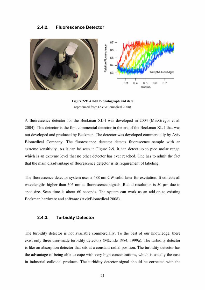
Figure 2-9: AU-FDS photograph and data
reproduced from (AvivBiomedical 2008)
A fluorescence detector for the Beckman XL-I was developed in 2004 (MacGregor et al.
2004). This detector is the first commercial detector in the era of the Beckman XL-I that was
not developed and produced by Beckman. The detector was developed commercially by Aviv
Biomedical Company. The fluorescence detector detects fluorescence sample with an
extreme sensitivity. As it can be seen in Figure 2-9, it can detect up to pico molar range,
which is an extreme level that no other detector has ever reached. One has to admit the fact
that the main disadvantage of fluorescence detector is its requirement of labeling.
The fluorescence detector system uses a 488 nm CW solid laser for excitation. It collects all
wavelengths higher than 505 nm as fluorescence signals. Radial resolution is 50 µm due to
spot size. Scan time is about 60 seconds. The system can work as an add-on to existing
Beckman hardware and software (AvivBiomedical 2008).
2.4.3. Turbidity Detector
The turbidity detector is not available commercially. To the best of our knowledge, there
exist only three user-made turbidity detectors (Mächtle 1984, 1999a). The turbidity detector
is like an absorption detector that sits at a constant radial position. The turbidity detector has
the advantage of being able to cope with very high concentrations, which is usually the case
in industrial colloidal products. The turbidity detector signal should be corrected with the
22
MIE theory of light scattering, since the light-scattering phenomenon also affects the signal
of turbidity.
2.5. Types of Experiments with AUC
2.5.1. Sedimentation Velocity Experiment
In a sedimentation velocity experiment, a sample-filled cell is directly accelerated to the
speed where sample notably sediments. The maximum speed limit of the Beckman Optima
XL-I is 60,000 rpm. However, the maximum speed for a sample is usually determined by the
sedimentation speed of the sample and the detector speed. Absorbance optics takes a scan of
a cell in about 1.5 minutes whereas interference optics takes a scan of a cell at about 10
seconds. On the other hand, at least 50 scans should be taken during centrifugation for an
efficient data analysis. Hence it is necessary to calculate the optimization of maximum
possible speed to make enough scans during sedimentation. In sediment velocity
experiments, sedimentation is dominant compared to diffusion. As a result, in the Lamm
equation (Equation 2-12), the diffusion term is not very effective.
The sedimentation coefficient (s) and the sedimentation coefficient distribution due to
sedimentation velocity experiments can be obtained by using the following formula:
t
rrs m
2
)/ln(
Equation 2-13: s value formula for SV Experiment
where s is sedimentation coefficient, r is the radius point of measurement point, rm is the
radius of meniscus, w2t is the time integral.

23
Figure 2-10: Different Types of AUC experiment
a) Sedimentation Velocity; b) Sedimentation Equilibrium; c) Band(zone) Centrifugation
In sedimentation velocity experiments, initially particles are homogenously distributed to all
radial positions. When a centrifugal field is applied to the system, all particles start to
sediment in the direction of the radial increase. After exhaustion of particles near the cell
meniscus, a boundary is formed. With respect to different sedimentation speeds of different
particles, the boundary may be sharp, or wide. Since the experiment finishes after all the
particles have sedimented, sedimentation velocity experiments are short experiments in time
scale in comparison with sedimentation equilibrium experiments (see 2.5.2). Schematics of
such an experiment can be seen in Figure 2-10(a).
2.5.2. Sedimentation Equilibrium Experiment
Sedimentation equilibrium experiments are quite long experiments in comparison with
sedimentation velocity experiments, lasting from 10 hours to 200 hours. In this type of
experiment, the particle-filled cell accelerates to moderate speeds at which sedimentation is
counter-balanced by diffusion. Hence, particles do not sediment fast. One needs to wait until
diffusion equilibrates to sedimentation. In long time intervals, scans are taken in order to
reach the point where there is no more change in the scan. The schematic of a sedimentation
equilibrium experiment is shown in Figure 2-10(b). The final state necessary for
sedimentation equilibrium is the state of equilibrium at which there is no longer any change

24
in the concentration at any radial points. Hence this can be expressed mathematically as
follows:
0dt
dc
Equation 2-14: Situation needed for SE experiments
where c denotes the concentration.
Further substituting the conditions of Lamm equation (Equation 2-12), molar mass can be
obtained (Equation 2-15).
22
ln
1
2
dr
cd
wv
RTM
Equation 2-15: Molar mass of the sample in SE experiments
The sedimentation equilibrium experiment is a key experiment for determining the absolute
molar mass and the reversible interactions of biological polymers and proteins. Before the
invention of gel electrophoresis it was the one of the most important methods to study
proteins (Mächtle and Börger 2006).
2.5.3. Band (Zone) Centrifugation
Band (zone) centrifugation is not a commonly used centrifugation method. It was invented by
Jerome Vinograd (Vinograd et al. 1963). The schematic of a Vinograd cell centerpiece and
experiment can be seen in Figure 2-10(c). In a Vinograd cell, a reservoir is seen, which can
be filled with a maximum 15 µl sample solution. There is a micro-capillary between the
reservoir and the sample cell sector. The micro-capillary allows the reservoir to transfer a
sample to the sample sector at about 3000 rpm. Hence, while accelerating to maximum speed
that sample sediments in required speed, at about 3000 rpm, the sample reservoir is being
transferred to the sample column. As particles start to sediment, they start to move in a radial
direction. Due to the diversity in their speeds, particles physically differentiate from each

25
other. Hence, it is band sedimentation rather than being boundary sedimentation, which is the
case for sedimentation velocity experiments.
In band centrifugation, particles are physically separated from each other, which could be
considered as the most advantageous part of band centrifugation owing to the fact that it
allows the user to take the spectra of different species. At each radial position, there is a
different particle. Particles are not overlaid to each other as they are at boundary
sedimentation.

26
Chapter 3 :Static Light Scattering Detector for Analytical
Ultracentrifugation (SLS-AUC)
3.1. Introduction
AUC is being ideal light scattering device as sample is free from disturbing dust and large
sample aggregates. In order to have the advantage of AUC and static light scattering at the
same time, we intended to develop a small angle SLS (static light scattering) detector
yielding M (molar mass) independent of Θ (scattering angle). Light scattering is a well
known technique and a static light detector can detect M and Rg(radius of gyration). On the
other hand, AUC technique can give us sedimentation coefficient distribution (S-
distribution). Hence, combining AUC and SLS would provide data on M-distribution and S-
distribution which also would give diffusion coefficient. As M is proportional to cube of
particle size, particle size of particles can also independently determined with both
techniques.
Previous tests for developing the SLS detector were performed by Bhattacharyya
(Bhattacharyya 2006). Bhattacharyya concluded that for SLS development, intensity must
always be taken from the same position of cell window, because cell window scatters the
light and its scattering amplitude changes among different positions. So reference intensity
can only be taken from the same sector after all sedimentation is finished. Bhattacharyya has
used standard photodiode detector to detect scattered light. In order to develop a light
scattering detector for AUC, detector is selected as a Large Area Avalanche Photodiode
(LAAPD) which was obtained from Advanced Photonix Inc. (California). The part number of
the diode is 394-70-74-591, and it has an active area of detection of about 10 mm. Avalanche
photodiode has higher sensitivity due to its working principle, that is called avalanche effect.
Our idea is to replace the SLS-AUC with the interference detector (Figure 2-7). In particular,
the plan was to replace the laser of the interference system with a new laser whose beam
profile is much better. Instead of interference camera and optics, it was planned to construct a
SLS-AUC.
27
wco MKII /
Equation 3-1: Simple molar mass calculation equation of static light scattering
Where I0 is the incident light, and I is the scattered light, Kc is constant depends on setup, wM is the average
molar mass
The simplest molar mass calculation of the particle can be calculated using Equation 3-1. Kc
needs to be determined for each different setup.
3.2. Experimental Tests
3.2.1. LAAPD with home-made power supply
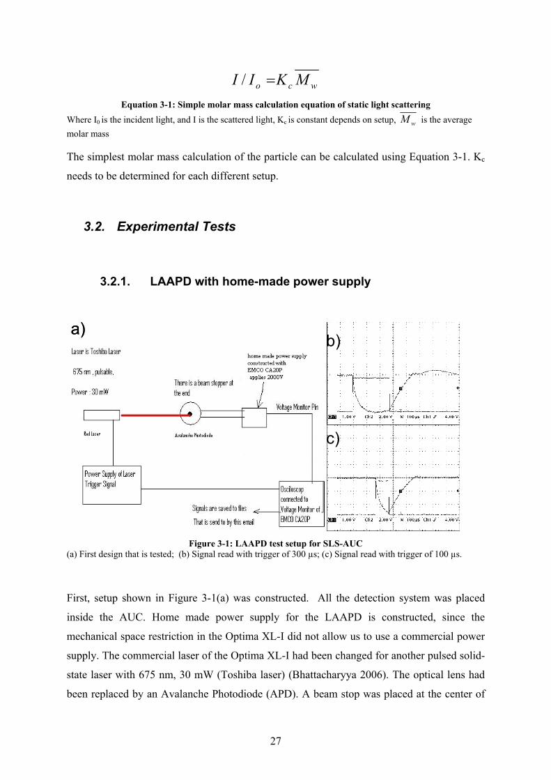
a)b)
c)
a)b)
c)
Figure 3-1: LAAPD test setup for SLS-AUC
(a) First design that is tested; (b) Signal read with trigger of 300 µs; (c) Signal read with trigger of 100 µs.
First, setup shown in Figure 3-1(a) was constructed. All the detection system was placed
inside the AUC. Home made power supply for the LAAPD is constructed, since the
mechanical space restriction in the Optima XL-I did not allow us to use a commercial power
supply. The commercial laser of the Optima XL-I had been changed for another pulsed solid-
state laser with 675 nm, 30 mW (Toshiba laser) (Bhattacharyya 2006). The optical lens had
been replaced by an Avalanche Photodiode (APD). A beam stop was placed at the center of

28
the APD. An external signal generator triggers both the laser and the LAAPD at the same
time. Photodiode is replaced with APD, because APD is more compact and sensitive. Also
APD does not need any lens in comparison to photodiode. Therefore optical setup is more
reliable and easy to construct.
Figure 3-1(a) shows that the APD does not respond properly to fast light pulses. Figure 3-1(b)
and Figure 3-1(c) show the plots of the oscilloscope data. The square pulse plot is the signal
from the signal generator that triggers the laser and the LAAPD. The other plot is the signal
that is read from the LAAPD. The LAAPD does not respond properly to the signal, although
its response time was 18 ns in the datasheet. After discussing the subject with Advanced
Photonix, it was decided to send the APD to be tested at Advanced Photonix laboratories in
California.
Figure 3-2: Picture of SLS-AUC detector parts
(a) Large Area Avalanche Photodiode attached to the mechanical adaptor of the condenser lens of the
interference detector system; (b) Extension board; (c) Commercial high voltage power supply of Large
Avalanche Photodiode; (d) Mechanical adaptation and power supply of solid laser; (e) Solid state laser; (f)
circuit board that supports power supply of LAAPD.

29
3.2.2. Modifying the commercial power supply of the LAAPD After the discussion with the manufacturer of the LAAPD, it was concluded that LAAPD was
working properly but the power supply was insufficient. Advanced Photonix offered us an
LAAPD with a power supply, but due to the space restrictions in AUC, it decided to have a
special modification at the power supply of the LAAPD. The power supply has to be 50 cm
away from the LAAPD, since there is not enough space for a power supply if it is directly
attached to the LAAPD. With the help of this small modification, LAAPD could be screwed
in the place of the condenser lens, with the high voltage power supply outside. However, this
modification was not that easy, because the cables need to carry 2000 Volts.
3.2.3. First Prototype of SLS-AUC Photos of the setup in parts are shown in Figure 3-2. The large picture shows the whole setup,
including cables. The Large Area Avalanche photodiode (LAAPD) that is attached to the
mechanical adapter is numbered as 1. With this mechanical adaptor the APD can be replaced
with a condenser lens of interference optics (Figure 2-7). Five cables of 50 cm are attached to
the APD. The ends of these cables can be plugged in to the APD with a specially ordered sit
circuit (Figure 3-2(b)). The sit circuit is connected to the commercial high-voltage power
supply (Figure 3-2(c)) of the LAAPD with a 50 cm cable. The high-voltage power supply is
connected to the low-voltage power supply (Figure 3-2(f)) with another 50 cm cable. Hence,
the detector modules which can be plugged in to each other can be replaced with the detector
module of the interference optics (Figure 2-7).
The laser assembly is also shown in Figure 3-2. The laser assembly includes a solid laser
(Figure 3-2(e)) of wavelength 675 nm with a power of 30 mW. The laser is placed on a
mechanical part that can be adjusted according to its x, y and z axes. Together with this
mechanical part, the laser can be attached to a mechanical adaptation part (Figure 3-2(e)).
With the mechanical adaptation part, the solid state laser assembly can be replaced with the
commercial interference laser (Figure 3-2(e)). The power supply of the solid state laser can
be seen in Figure 3-2(d).

30
3.2.4. Tests with the prototype SLS-AUC
2800 3000 3200 3400 3600 3800 4000 4200
0.155
0.156
0.157
0.158
0.159
0.160
0.161
0.162
10 20 30 40 502025303540455055606570
Sig
nal
from
AP
D (
a.u.
)
Time Unit (a.u.)
S200 @ 10 Krpm
Sig
nal f
rom
LA
AP
D (
a.u.
)
Time Units (a.u.)
S1000 @ 3 Krpma) b)
c)
d)
e) 2800 3000 3200 3400 3600 3800 4000 4200
0.155
0.156
0.157
0.158
0.159
0.160
0.161
0.162
10 20 30 40 502025303540455055606570
Sig
nal
from
AP
D (
a.u.
)
Time Unit (a.u.)
S200 @ 10 Krpm
Sig
nal f
rom
LA
AP
D (
a.u.
)
Time Units (a.u.)
S1000 @ 3 Krpma) b)
c)
d)
e)
Figure 3-3: Photograph of SLS-AUC which is placed in the Optima XL-I (a) SLS-AUC detector replaced with the interference detector; (b) SLS laser attached to the test setup (Figure 3-2); (c) Large Area Avalanche Photodiode screwed in place of the condenser lens (Figure 2-7) and covered by beam stopper. (d) Latex particle S1000 sedimenting at 3000 rpm; (e) Latex particle S200 sedimenting at 10,000 rpm.
The first prototype that was built into the Optima XL-I is shown in Figure 3-3. A solid state
laser is attached to the monochromator in place of the interference laser. The laser can also be
seen from a different side in Figure 3-3(b). The APD covered with the beam stop can be seen
in Figure 3-3(c). Some of the data that was taken using this system is shown in Figure 3-3(d).
Latex sample S1000 is shown as sedimenting at 3000 rpm (Figure 3-3(d)) and latex sample
S200 is shown as sedimenting at 10,000 rpm (Figure 3-3(e)). These data prove that the
system is fast enough to obtain data in real AUC working conditions (see section 7.1). Also
this data proves that the detector is adaptable to the Optima XL-I. Although detector can
detect latex particle sedimentation, protein BSA could not be detected. This shows that the
system is not highly sensitive to detecting smaller particles. The main disadvantage of the
system is that the cell windows of AUC are very thick (6mm) and also scatters light.
(Mächtle and Börger 2006). It is not easy to change the window, because thick windows are
needed to overcome high centrifugal forces. Finally, it was decided to improve our system’s
sensitivity by changing our laser for a more efficient one. For this reason, a green laser has
been ordered as scattered light intensity is proportional to λ-4. Further tests are beyond the
scope of this thesis. Thus, SLS-AUC has not yet reached its final development. However, the
test results shown in Figure 3-3 encourage us by showing that we are on the right track.

31
Chapter 4 : CCD Camera Detector for the Analytical
Ultracentrifuge (CCD-C-AUC)
4.1. Introduction
Development of new detector electronics has motivated us to attempt to use a CCD camera
UV/Vis absorption detector for AUC (CCD-C-AUC). The MWL-AUC detector detects all
wavelengths at one radial position. The idea of CCD-C-AUC is to detect all radial positions
at once which will make it possible to detect high-speed sedimentation and will increase the
detection speed of AUC. Successful construction of the CCD-C-AUC will make it possible to
detect very fast sedimentation that is not possible with the Beckman Coulter Optima XL-I
and will broaden the scope of AUC. Furthermore, very large particles which sediment very
fast even at the lowest speed can be detected by CCD-C-AUC. Hence, this will increase the
particle-size range of AUC. Secondly, high-speed detection of CCD-C-AUC, will make it
possible to see rapid chemical reactions during sedimentation, which is impossible with the
Optima XL-I. Therefore, CCD-C-AUC can broaden the scope of current usage of AUC.
Also by faster detection, the time needed for an AUC experiment will decrease, because even
at the highest speed, CCD-C-AUC would obtain enough scans in a short time. This is an
important parameter for AUC experiments. The experimental time is crucial in AUC and with
CCD-C-AUC a higher number of scans can be obtained in a short time.
It is needed to have a detector and light source that can handle the conditions of AUC. To
satisfy these requirements, a detector and light source combination needs to have these
following properties:
Property 1: To be fast enough.
The detector needs to work within an integration time of 1 µs. The maximum speed of a rotor
is 60,000 rpm, or 1000 rotations per second, so, in the fastest case, one rotation is 1 ms long.
One rotation is needed to divide into 1000, in order to gain a signal from a 0.36o sector of a
sample. Therefore, in order to catch a cell sector, detector needs to work within an integration
time of 1 µs. Any detector and light source combination needs to work in µs range.

32
Property 2: To be sensitive enough
Any detector that will work in µs range needs to be sensitive enough to receive a reasonable
signal at that short time scale. The detector may work in µs range, but it does not mean that
the signal is meaningful. Hence, the detector needs to be sensitive enough to receive the
desired signal from AUC also in the UV/Vis range.
Property 3: To have good resolution
The detector needs to have a spectral resolution of at least 10 µm. If the detector detects the
cell, ideally it has to have a radial resolution of 10 µm, which is the best scan interval of a
commercial absorption detector.
Property 4: To be mechanically adaptable to the existing Optima XL-I
The Beckman Coulter Optima XL-I is the only commercial analytical ultracentrifuge in the
world at the moment. Therefore, as a last property, any design needs to be adaptable to this
device, in terms of mechanical space and vacuum requirements.
These are the properties that are needed for any kind of detector and light source
combination. Our aim is to design and test such a detector and light source combination. If
these properties are achieved, prototype construction can be possible.
In this chapter, we summarize the tests we performed to construct the CCD-C-AUC. Our
final design, the first successful design that has been tested so far, is also presented.
4.2. Experimental Tests
The idea of developing a line camera detector began with the Schafter & Kirchhoff
SK2048DDE line camera. SK9192D line scan interface was used in order to control the line
camera. The line Camera has 2048 pixels and a typical AUC cell is 1.6 cm, so it corresponds
to 8 µm resolution. We began our tests using this line camera, since it was the cheapest and
easiest option to start with.
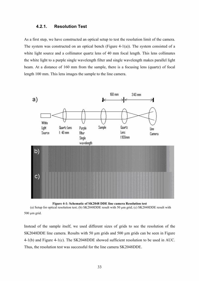
33
4.2.1. Resolution Test
As a first step, we have constructed an optical setup to test the resolution limit of the camera.
The system was constructed on an optical bench (Figure 4-1(a)). The system consisted of a
white light source and a collimator quartz lens of 40 mm focal length. This lens collimates
the white light to a purple single wavelength filter and single wavelength makes parallel light
beam. At a distance of 160 mm from the sample, there is a focusing lens (quartz) of focal
length 100 mm. This lens images the sample to the line camera.
Figure 4-1: Schematic of SK2048 DDE line camera Resolution test
(a) Setup for optical resolution test; (b) SK2048DDE result with 50 µm grid; (c) SK2048DDE result with
500 µm grid.
Instead of the sample itself, we used different sizes of grids to see the resolution of the
SK2048DDE line camera. Results with 50 µm grids and 500 µm grids can be seen in Figure
4-1(b) and Figure 4-1(c). The SK2048DDE showed sufficient resolution to be used in AUC.
Thus, the resolution test was successful for the line camera SK2048DDE.

34
Figure 4-2 : Original Technical Drawing of Monochromator of Optima XL-I (Giebeler 1992)
Reproduced by permission of The Royal Society of Chemistry
4.2.2. Monochromator of the Optima XL-I
Before commencing the resolution test, we needed to focus on the monochromator of the
Beckman Coulter Optima XL-I. Our idea was to use the monochromator of the Optima XL-I

35
absorption optic. This monochromator can be used to select various wavelengths from a
white light source. As it can be seen in Figure 4-2, the Xenon flash lamp is attached to the
monochromator. Light from the monochromator comes from a pinhole and reaches
diffraction grating. After reflection from the diffraction grating, only the selected wavelength
can be reflected and reaches the sample. After that, monochromatic light reaches the sample
and passes through the sample to the photomultiplier tube.
The first idea was to replace the photomultiplier tube with the line camera plus imaging lens
and to construct a line camera detector. In order to do that, we needed to perform a sensitivity
test. The weak point of the idea of using a monochromator is that monochromatic light has a
very low intensity in the Optima XL-I. Only a small fraction of the illumination from the
Xenon light source enters through a small hole to the monochromator. After entering the
monochromator, this small portion of the light reaches the diffraction grating. Afterwards,
only one wavelength among all the wavelengths in this small portion of light leaves the
diffraction grating. The thick windows of the sample cell further decrease the intensity of the
incoming light. Hence, the intensity of the light that reaches the detector is extremely small in
comparison to the overall optical power of the Xenon light source. Hence, the line camera
needs to cope with low light conditions. In order to test this, we have performed illumination
tests with the SK2048DDE camera.
a) b)a) b)
Figure 4-3: Testing of SK2048DDE with pulsed light from AUC.
(a) Setup that is used to sensitivity of line cameras with original Optima XL-I light source; (b)
Setup that is used to sensitivity of line cameras with 100 W Mercury fiber-coupled lamp.

36
4.2.3. Illumination test with SK2048DDE inside AUC with Xenon
flash lamp
After the resolution test, we have explored whether we can detect the signal of
monochromatic light of the Optima XL-I. In order to test the signal detection limits, we have
constructed the setup that is shown in Figure 4-3(a).
We have triggered the line camera with the same TTL pulse with a light source. However, the
setup of Figure 4-3(a) has shown us that the intensity of the Xenon light source is not enough
to detect via SK2048DDE.
4.2.4. Owl Camera inside AUC with Xenon flash lamp
Fairchild Imaging (Milpitas, California) was contacted, who kindly sent us a Fairchild
CAM/CMOS 2KRDI Owl camera to be tested. We have tested the Owl camera within the
setup of Figure 4-3(a). However, we could not see any signal even in the longest integration
time (5 ms), which implies that there is not enough light intensity. Line cameras do not have
any intensifiers.
4.2.5. Tests with Constant Light Sources in the Optima XL-I
As a next step, we tried changing the light source. We have tested the Owl camera and the
SK2048DDE with a constant light source a 100 W Mercury lamp. The source was coupled to
a fiber. We removed the original Xenon flash lamp of the Optima XL-I and replaced it with
the fiber end of a100 W Mercury lamp. We have tried to detect signals with this setup, which
is shown in Figure 4-3(b). We could not detect any signal with the Owl camera and the
SK2048DDE. Thus, the problem of low intensity could not be solved with this design. This
was most probably due to the low coupling of the fiber to the light source and while the light
is focusing to the monochromator. The reason was most probably due to home made
coupling of fiber to monochromator arm.
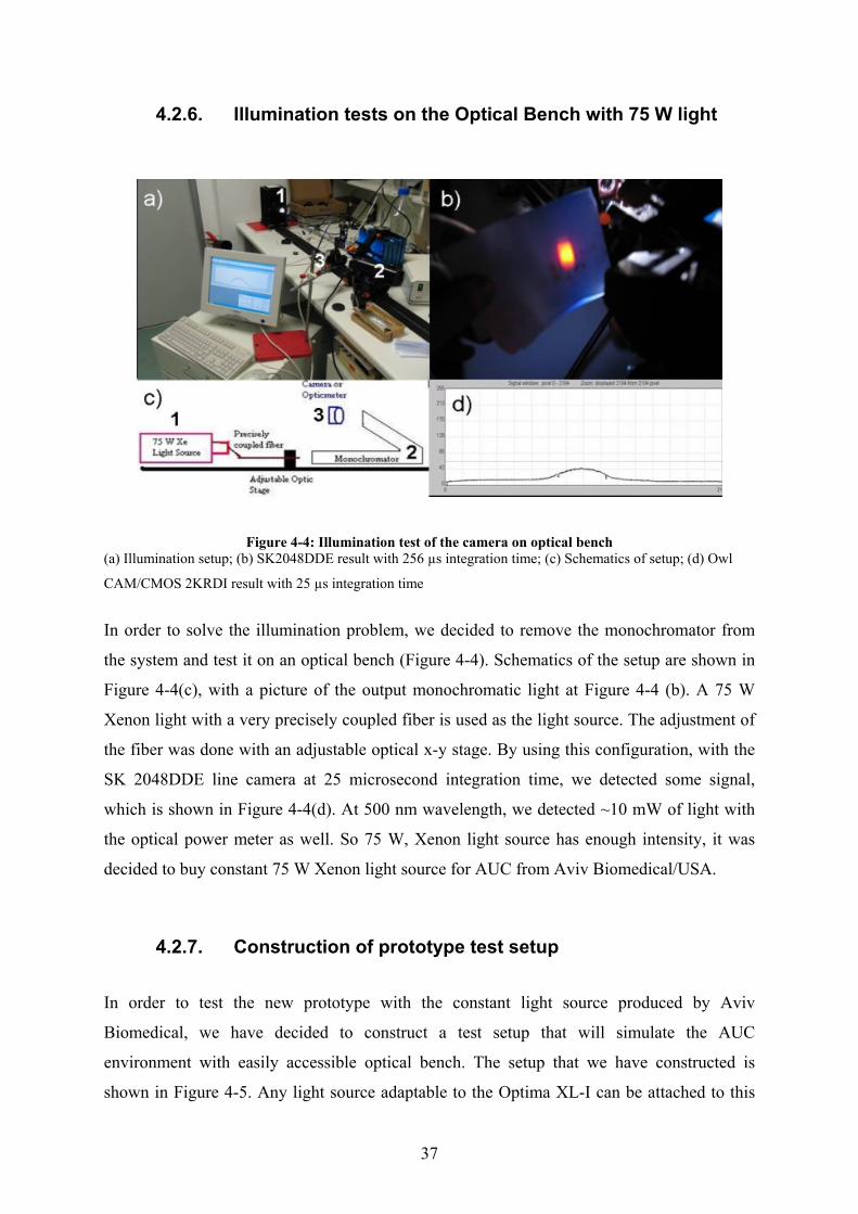
37
4.2.6. Illumination tests on the Optical Bench with 75 W light
Figure 4-4: Illumination test of the camera on optical bench (a) Illumination setup; (b) SK2048DDE result with 256 µs integration time; (c) Schematics of setup; (d) Owl
CAM/CMOS 2KRDI result with 25 µs integration time
In order to solve the illumination problem, we decided to remove the monochromator from
the system and test it on an optical bench (Figure 4-4). Schematics of the setup are shown in
Figure 4-4(c), with a picture of the output monochromatic light at Figure 4-4 (b). A 75 W
Xenon light with a very precisely coupled fiber is used as the light source. The adjustment of
the fiber was done with an adjustable optical x-y stage. By using this configuration, with the
SK 2048DDE line camera at 25 microsecond integration time, we detected some signal,
which is shown in Figure 4-4(d). At 500 nm wavelength, we detected ~10 mW of light with
the optical power meter as well. So 75 W, Xenon light source has enough intensity, it was
decided to buy constant 75 W Xenon light source for AUC from Aviv Biomedical/USA.
4.2.7. Construction of prototype test setup
In order to test the new prototype with the constant light source produced by Aviv
Biomedical, we have decided to construct a test setup that will simulate the AUC
environment with easily accessible optical bench. The setup that we have constructed is
shown in Figure 4-5. Any light source adaptable to the Optima XL-I can be attached to this

38
system via a light source connector (Figure 4-5(f)). The monochromator of the Optima XL-I
can be attached to the monochromator connector that is shown in Figure 4-5(a). The
wavelength selection pin can also be seen in the adjustment screw in Figure 4-5, the
micrometer to which that pin is connected is labeled as 4. By adjusting this micrometer, a
specific wavelength can be selected and determined with a spectrometer. The cell holder is
used to simulate the rotor. Thus, a monosector sample cell can be put into the sample holder.
The sample cell position can be adjusted by a mechanical x-y stage. There is also a hand-
controlled screw to tighten the cell. Under the cell holder, there exists an optical bench. This
optical bench includes one lens and one 90o mirror so that it focuses the image of the cell
onto the output of the light beam (Figure 4-5(c)). The light source connector used here is
identical to the Beckman light source connector. Therefore, any light source compatible with
the Optima XL-I can be attached to this connector.
Figure 4-5: Photograph of Prototype Test Setup of CCD-C-AUC
(a) Monochromator connector point with wavelength selection pin; (b) Cell holder assembly; (c) Output of light
beam; (d) Micrometer adjustment screw for adjusting wavelength; (e) 90o mirror; (f) Light source connector.

39
4.2.8. Constant Light Source from Aviv Biomedical
Figure 4-6: Prototype Constant Light Source from Aviv Biomedical
(a) 75 W Xenon light source container; (b) Mirror Assembly; (c) Light connector; (d) Power supply of Xenon
light; (e) Controller unit of the system.
As the next step, we aimed to attach our constant light source to our test setup. The constant
light source from Aviv Biomedical is shown in Figure 4-6. The Xenon light source container
(Figure 4-6(a)) contains the bulb of Xenon light. There is also a cooling system which is not
shown here. The mirror assembly (Figure 4-6(b)) contains an adjustable mirror, which
reflects incoming light into the pin hole of the absorbance optics with an opening angle
corresponding to that of the original flash lamp so that the diffraction grating of the
monochromator creates parallel light (the pinhole can be seen in Figure 4-2). Due to the light
connector unit (Figure 4-6(c)), the Xenon flash lamp of the Optima XL-I can be replaced by a
constant light source. The power supply unit of the light source (Figure 4-6(d)) is responsible
for creating the arc inside the Xenon bulb. The controller unit (Figure 4-6(e)) controls the
overall system and shows the status of the bulb and power supply. Also the usage of the bulb
is monitored by a counter that is existing on the controller. Overall current consumption can
be also monitored. With this light source we can continuously illuminate the sample with

40
parallel light. In the commercial Optima XL-I, the light source is triggered with an electronic
signal and it can only flash for 3–4 µs. Furthermore, the flash lamp of the Optima XL-I can
only flash at a rate of 100 Hz, so this limits the time interval of measurements. However, with
the help of our prototype light source, we can illuminate all cells continuously with parallel
light without any time limitation.
4.2.9. Constant Light Source, Test Setup with Monochromator
Figure 4-7: Photo and data of monochromatic test of CCD-C-AUC (a) Monochromator test setup (a1) Aviv Biomedical Constant Light Source; (a2) Test setup; (a3)
Monochromator; (a4) USB2000 spectrometer; (b) USB2000 data; (c) zoom in to graph (b); black line: raw data;
red line: Gaussian fit to peak b; blue line: FWHM of 4 nm.
In order to test our constant light source, we have constructed the setup shown in Figure 4-7.
The continuous light source is attached to the test setup. The light source is covered by
aluminum foil in order to prevent the user from any UV exposure. The light source (Figure
4-6) is attached to the light source connector (Figure 4-5(f)). The monochromator of the
Optima XL-I (Figure 4-2) is attached to the monochromator connector point (Figure 4-5(a)).
The cell holder assembly (Figure 4-5(b)) is replaced by a USB2000 spectrometer (Figure 4-7
(a)). With this setup, it is possible to detect the spectrum of incoming light due to the
monochromator which is illuminated by the constant light source. The monochromatic light

41
that comes from the monochromator can be adjusted manually by a micrometer (Figure 4-5
(d)). This micrometer moves the monochromator pin (Figure 4-5(a)) and this pin adjusts the
diffraction grating of the monochromator (Figure 4-2). We have adjusted the monochromatic
light close to the value of 700 nm. The intensity reading of USB2000 in counts can be seen in
Figure 4-7(b). An enlargement of the peak of Figure 4-7(b) is shown in Figure 4-7(c). The
black line refers to the raw data from the USB2000, where the red line is the Gaussian fit of
the raw data. The short blue line shows the full width at half maximum (FWHM) of the
Gaussian peak. The FWHM of the peak is found to be 4 nm. The FWHM of the absorbance
optics of the Optima XL-I is given as 3 nm (Laue 1996). Hence, to obtain a FWHM of 4 nm
is a reasonable result for the first experiment performed with a home-made test setup, without
any fine adjustment of the optical system. Thus, we conclude that the monochromator works
successfully in our setup.
4.2.10. First Prototype CCD-C-AUC, taking UV/Vis spectra
We have tested our already constant light source, test setup and monochromator and obtained
reasonable results. Now it is time to test our optical bench with a real sample. After our
unsuccessful test with the SK2048DDE and Owl CAM/CMOS2KRDI cameras, we decided
to change the camera. The Andor i-star ICCD camera has an optical gate that can be
controlled in 2 ns. Hence the camera is much faster than we need. This camera uses cathode
tubes to intensify the incoming light. We contacted LOT-Oriel (Darmstadt) as the German
supplier of Andor cameras and requested a trial of the Andor i-star ICCD DH734_18mm
camera. We received permission to test the camera in our laboratory for one day. We
prepared our constant light source, test setup, monochromator, sample cell, sample cell
holder, and optical bench before the test. A photograph of the test system with the Andor i-
star ICCD camera is seen in Figure 4-8. The light source is attached to the test setup (Figure
4-8(a2). The monochromator (Figure 4-8(a3) is attached to the test setup. The last opening of
the monochromator is covered by the double slit of the interference optics (Figure 2-7), in
order to make the output light very thin and much more monochromatic. We placed a gelatin-
filled monosector cell into the cell holder subunit in order to see the meniscus of the sample,
because the meniscus cannot be seen with liquid samples in such an orientation. We have
adjusted the x-y table of the sample holder. The lens and mirror of the optical setup was been
also adjusted in order to transfer the image of the cell into the center of the output of the light

42
beam part (Figure 4-5). As Andor i-star camera arrived, the lens of Andor i-star camera was
placed at the output of light beam.
Figure 4-8: CCD-C-AUC final prototype setup
(a) Test setup with Andor Camera; (a1) Constant light source; (a2) Test setup; (a3) Monochromator; (a4)
Monosector cell with a gel inside; (a5) Andor i-star DH734_18mm camera; (b) Image of gel-filled sample with
integration time of 200 times 0.1 µs, with wavelength selection of 500nm.
Figure 4-8(b) is a picture of the gelatin sample with 200 integration pulses of 1 µs length.
This picture proves that this design of the CCD-C-AUC detector is sensitive enough to detect
the sample. The meniscus of the sample is also seen in the picture. This test setup also proves
that the design in Figure 4-8 is fast enough to gain a meaningful signal with 1 µs integration
time. The setup itself proves that CCD-C-AUC can be built mechanically inside the Optima
XL-I without any mechanical problem. Adaptation to the Optima XL-I monochromator has
been also proved.

43
200 300 400 500 600 700 800-0.4-0.20.00.20.40.60.81.01.2
0 200 400 600 800 10000.00.20.40.60.81.01.21.4b)
Abs
orba
nce
Wavelength (nm)
UV/Vis spectra of gold nanoparticlestaken with comercial XL-A
Point at 500nmAbsorbance: 0.2856
AirBubble
Cell Bottom
Abs
orba
nce
Pixel number
CellTop
Scan of Cell in Final Prototype Setupat wavelength of 500 nm
a)
Figure 4-9: UV/Vis spectra with prototype CCD-C-AUC
(a) UV/Vis spectra of solution of gold nanoparticles with Optima XL-I; (b) Absorbance from final prototype CCD-C-AUC setup. Red line is absorbance value that we have measured with the commercial Optima XL-I; cell bottom, cell top and cell bubble can be seen. As a final test, we tried to gain absorbance data from the CCD-C-AUC final prototype setup.
We have prepared a gold nanoparticle solution, and put it into the AUC cell. The spectrum of
the solution that is taken by the commercial absorbance optics of the Optima XL-I is shown
in Figure 4-9(a). The absorbance value of the Optima XL-I at 500 nm is 0.2856. We then
measured the intensity spectra of a water-filled cell and a sample-filled cell in our setup
(Figure 4-8) and then calculated absorbance with the help of Equation 2-1.
The result of the absorbance calculation is seen in Figure 4-9(b). Cell bottom and cell top can
be recognized easily in this graph. The air bubble is not at the top of the cell because there is
no centrifugal force in the setup. It took 200 ms with integration pulses of 1 µs in intervals of
1 ms to gain the absorbance data. Hence, this time, conditions were identical to the time
constraints of the Optima XL-I. The thick red curve shows the absorbance value of 0.2856,

44
which was measured by the Optima XL-I. Figure 4-9(b) proves that our first prototype design
is capable of measuring the absorbance of the sample exactly.

45
Chapter 5 : Multiwavelength Detector for Analytical
Ultracentrifuge (MWL-AUC)
5.1. Introduction
The absorption optical system of the Optima XL-I from Beckman Coulter was introduced in
1991(section 2.2.3.1). It is based on a photomultiplier tube (PMT) which detects light at a
single, pre-selected wavelength delivered by a polychromatic flash lamp. This system has
remained unchanged since 1991. However, in the intervening years there has been a rapid
development in the semiconductor industry. The considerable decrease of the price and the
size of semiconductor products (e.g. spectrometers, counter cards, analog to digital
converters) and powerful programming techniques make it possible to develop more efficient
detectors. Spectrometer technology has made small, cheap, fast and precise detection systems
based on CCD arrays which are commercially available. Such a detection used in analytical
ultracentrifuge system would expand the possibilities of it, because multiwavelength analysis
perfectly suits to the studies of multiple, interacting components (Giebeler 1992) or colloidal
particles with size-dependent optical properties (quantum dots or metal nanoparticles)
(Cölfen et al. 1997).
Other advantages include: the possibility of a considerable reduction in experimental time,
even for a limited number of wavelengths, without a loss of information due to the very fast
detection, which is as short as 10 s with modern spectrometers. Accordingly, there is the
possibility of data averaging, and a fast detection speed for quickly sedimenting samples. If
such a spectrometer could be built into a preparative ultracentrifuge, the potential price for a
functional analytical ultracentrifuge is promising. Attempts to adapt such spectrometers to the
special situation of the ultracentrifuge have recently been described (Bhattacharyya 2006;
Bhattacharyya et al. 2006) and hold promise for future applications. The obvious advantages
of multiwavelength detection were already described for the first- generation detector,
together with some measurement examples and basic system performance (Bhattacharyya
2006; Bhattacharyya et al. 2006).
In this chapter, some modifications made to the original first- generation detector designed by
Bhattacharyya et al. (Bhattacharyya 2006; Bhattacharyya et al. 2006) will be described and
the performance of the current second-generation prototype design as compared with the

46
commercial system available in the Optima XL-I will be reported. Thus, current limitations
will become apparent, indicating directions for further improvements
5.2. Improvement of the multiwavelength detector
The prototype machine, the MWL-AUC, of the first generation (Bhattacharyya et al. 2006)
has been modified by simplifying the already existing hardware (Bhattacharyya 2006;
Bhattacharyya et al. 2006) as described below.
Figure 5-1: Schematics of the MWL detector arm.
a. 600 µm patch fiber UV/Vis (Ocean Optics), b. The collimating lens system (self built), f=20.6mm biconvex,
c. 90° Quartz Prism, d. Iris Diaphragm for reducing light intensity, e. Focusing biconvex lens (40 mm), f.
Spectrometer. The light path is also shown schematically.
5.2.1. Flash Lamp
The original flash lamp of the Optima XL-I (Hamamatsu L4633-01) with a maximum
repetition rate of 100 Hz and a self-built fiber coupling (Bhattacharyya et al. 2006) was
replaced by a faster Xenon flash lamp module (high power Xe flash lamp L-9456-12 from
Hamamatsu Phototonics GmbH, Herrsching, Germany, and a suitable power supply) which

47
can be directly coupled into an optical fiber via an SMA 905 adapter. It has a maximum flash
rate of 530 Hz which increases the repetition rate by more than five times which results in a
possible scan repetition speed of < 2 ms. The standard deviation of the light intensity as
stated by the manufacturer is 1.5%. Low flash-to-flash intensity variation is important as the
system does not have an intensity normalization routine.
Figure 5-2: Photographs of MWL-AUC
(a) Photograph of the detector arm: 1. Spectrometer, 2. Table with the possibility of x-y movement, 3. Step
motor, 4. Lens (40mm biconvex), 5. Iris 6. 90° quartz prism. (b) The arm fitted in the centrifuge. (c)
Photograph of the vacuum feedthrough: 1. Electronic feedthrough for step motor, 2. Electronic feedthrough for
spectrometer, 3. Electronic connection for TTL pulse for rpm measurements, 4. Optical feedthrough for fibers.
5.2.2. Detector Arm and Spectrometer Mount
In the first-generation setup, the light from the flash lamp was coupled with the centrifuge via
an optical fiber and a vacuum feedthrough. It passed the measurement cell and was imaged
onto a 25 µm or 50 m slit. Then it was fed back into a fiber out of the centrifuge until it
reached the entrance slit of the spectrometer (typically 25 m). The disadvantage of this setup
was that the light had to pass two narrow slits, which significantly limited the light intensity
available at the detector. We have improved the design in the second-generation detector in
such a way that the UV/Vis spectrometer entrance slit (Ocean Optics, USB 2000) is now
mounted on top of the detector arm at the focal position of the colliminating lens where the
light was coupled into the fiber again in the first-generation design. The new setup is shown
schematically in Figure 5-1. The advantage of this setup is the combined use of the
spectrometer entrance slit (25 m) as the radial and wavelength aperture for the spectrometer.
48
In this way, a much higher intensity can be obtained at the detector. The maximum intensity
can actually be so high that the spectrometer is saturated over the entire wavelength detection
range. This makes the application of an iris necessary limit the light intensity (4 in Figure
5-1). The entire setup of the second-generation detector arm is still modular – it can fit into
every preparative and analytical Beckman ultracentrifuge. Actually, the described detector
design is a modular replacement of the XL-I UV/V is absorption optics. Due to the reversible
detector setup, the detector can be exchanged for the Optima XL-I detector within one hour.
The hardware of the detector arm with mounted spectrometer is shown in Figure 5-2 as well
as the mounted detector arm in the ultracentrifuge. The socket of the flash lamp was replaced
by a mount for vacuum feedthroughs for fibers and cables as a hardware module for vacuum
feedthroughs (Figure 5-2(c))
5.2.3. Imaging Optics
In order to simplify the optical alignment, the optical path has been simplified as well: instead
of two collecting lenses as it is in the original first-generation design (f=20 mm, biconvex and
f=15 mm, biconvex) (Bhattacharyya et al. 2006) or the two biconvex lenses of f=60 mm and
f=12.5 mm described in (Bhattacharyya 2006), only one biconvex lens (f=40 mm) has been
used at a position optimized ex centrifugo on an optical bench to image the centre of the
ultracentrifuge cell onto the detector slit to allow a simplified detector alignment. This
minimizes chromatic aberration problems, which are inevitably associated with the use of
lenses for white light as well as the optical alignment procedure of the detector itself.
Briefly, the second-generation detector has a faster, more powerful flash lamp that is
combined with an improved hardware optical arm design, allowing a much higher light
intensity and a much simplified optical alignment than the first-generation detector
(Bhattacharyya 2006). All lenses were purchased from LINOS Photonics GmbH (Göttingen,
Germany).
5.2.4. Optical Tests
In order to determine the wavelength accuracy of both optical systems, an Ho2O3-centerpiece
was used (as supplied with the original purchase of the Optima XL-I AUC from Beckman
Coulter, Palo Alto, California). Characteristic sharp peaks were expected (among others) at
361/446/537 nm (BeckmanCoulter 1991). For determining the accuracy of the absorbance

49
readings at different wavelengths, two kinds of reference solutions were prepared. For
measuring data at 302 nm, solutions of KNO3 (Sigma) at various concentrations were freshly
prepared in water. Solutions of universal indicator pH 4-10 (Merck, Darmstadt, Germany)
were prepared in buffer solution of pH 4 (Metrohm, Herisau, Switzerland). These were
measured at 525 nm in the Optima XL-I and MWL-AUC. These solutions were then
measured on a benchtop spectrometer (lamba 2 UV/Vis-spectrometer from Perkin Elmer,
Überlingen, Germany), the Optima XL-I and the MWL-AUC. To obtain a measure of the
precision of the data, we recorded radial scans and averaged them over the entire length of
the solution column. No averaging was performed for the single data points. For the
measurements with the benchtop spectrometer, data points were recorded every 500 ms over
a total time of 60 s and averaged. Mean values and standard deviations thus obtained are
reported. Data were normalized to compensate for different optical path lengths (12 mm for
analytical ultracentrifuges and 10 mm for the benchtop spectrometer).
To determine the intrinsic noise and the baseline accuracy of the data at different
wavelengths, an empty hole of a rotor was flashed with 1, 10 and 100 points averaging over
the entire range of wavelengths available. Wavelength resolution was set to 1 nm for the
Optima XL-I. All measurements were performed at 3000 rpm in a fully evacuated centrifuge
chamber at 25 °C. The setting of the multiplexer of the MWL-AUC was adjusted so that only
a single flash was recorded per integration interval. The intensity of light impinging on the
spectrometer was limited to about 80% saturation at the most intensive peaks of the intensity
spectrum.
To determine the optical resolution, a 200 µm slit vaporized onto a standard AUC cell
window (provided by BASF AG) and it was imaged at several wavelengths. The slit window
was mounted together with a normal window on a one-sector cell such that the slit was facing
the inside surface of the centrepiece.
5.3. Results
5.3.1. General Aspects
Our modifications of the optics enhanced light intensity in the vacuum chamber to a great
extend, as compared with the first-generation detector (Bhattacharyya 2006) (Figure 5-3).

50
200 400 600 800
Vis, high intensity
Vis, low intensity
UV, low intensity
XL-A/I
no
rma
lize
d in
ten
sity
, o
ffse
t
wavelength [nm]
Figure 5-3: Intensity distributions of USB2000 Spectrometer
Intensity distributions for USB2000 spectrometers with different in-built diffraction gratings, as compared to
the Optima XL-I. Vis, diffraction grating optimized for the visible spectral range, high/low intensity, the iris
opened maximally/minimally. With the iris maximally opened, the maximum intensity of the spectrometer
(4000 counts) is reached and the spectrometer is maxed out at these wavelengths. UV, diffraction grating
optimized for the UV range. With the iris maximally opened, around 70% of the available channels are
saturated; this data is therefore not shown. Note that the flash lamp used in the MWL-AUC is different from that
of the Optima XL-I. Due to the design of the spectral dispersion/detection system in the USB2000
spectrometers, the raw intensity spectra for the different spectrometers are a convoluted function of both the
emission spectrum of the flash lamp and the preinstalled diffraction grating of the spectrometer itself.
This obviously leads to a better performance of the detection systems, especially in the UV
range, and allows some fine tuning of the intensity for the wavelength range that is most
suitable for the experiment by adjusting the amount of light via the iris. In this respect, the
spectrometer with a diffraction grating optimized for the visible region is certainly the most
flexible one. However, in terms of traditional protein measurements, the UV spectrometer is
more appropriate, as shown in Figure 5-3. The detected UV lamp spectra of the Optima XL-I
and MWL detectors agree quite well so that a similar performance can be expected in the UV
range. While the MWL UV signal decreased to zero at about 480 nm, the Optima XL-I signal
only slowly decreases up to 800 nm but at a very low intensity level as compared with the
UV. On the other hand, the MWL Visible signal still has sufficient intensity at wavelengths
up to > 800 nm, suggesting the interesting possibility of measuring in the near-IR (>800 nm)
with the existing flash lamp and spectrometer. A combination of a UV-optimized

51
spectrometer with one optimized for the Visible wavelength to near IR range is therefore
better for the detected intensities as compared with the broadband detection of the Optima
XL-I. However, it must be stated that, at maximum, 4000 counts are possible with the
currently applied 12-bit USB2000 spectrometer (Ocean Optics). Application of the current
modern USB4000 16-bit spectrometers (Ocean Optics) enable up to 16,000 counts, which can
enable a higher flexibility and dynamic range using this spectrometer.
0 1000 2000 3000
XL-A
norm
aliz
ed in
tens
ity [a
.u]
normalized distance [µM]
250 nm 450 nm 650 nm
MWL
Figure 5-4 : Optical Tests of MWL-AUC and Optima XL-I with Slit
A slit of 200 µm was imaged using the MWL-AUC and the Optima XL-I at different wavelengths. The thick
solid bar represents a distance of 200 µm. The wavelength resolution is dependent on wavelength. It is higher in
the UV-wavelength range for the MWL-AUC, but higher in the Visible range for the XL-I.
The data density for the Optima XL-I is in the order of 0.5–0.6 points/nm, as expected from
the limited precision of the gear train driving the diffraction grating, which has 4 nm
accuracy.
With the USB2000 spectrometers from Ocean Optics, the total number of data points
available is 2048 (3648 with the follow-up model USB 4000), therefore, as a function of the
spectral range of the spectrometer, the data density is in the order of 6 points/nm and 3
points/nm for the UV- and Vis-optimized spectrometers, respectively. Although this does not
reflect the actual wavelength resolution, which is limited, amongst other factors, by the band
pass of the diffraction grating and its groove density, it offers plenty of data points for

52
averaging, thus reducing the noise of the data without affecting the accuracy of the
wavelength positions.
5.3.2. Radial Resolution
In the current design of the MWL-AUC, a certain degree of wavelength dependence of the
radial resolution is expected, because lens optics is used with the associated chromatic
aberration problems. Such wavelength dependence of the radial resolution was indeed
observed in our measurements of a 200 m slit (Figure 5-4). The apparent radial resolution
decreases with increasing wavelength, quite in contrast to the situation with the Optima XL-I,
which is probably a result of optical alignments. It can also be seen from Figure 5-4 that the
MWL-AUC is already capable of delivering a higher radial resolution than the Optima XL-I,
especially in the UV-wavelength range most suitable for biological polymers. Note that the
step motor used in the MWL-AUC (Zaber T-LA-28-SV) is capable of delivering a radial
resolution of better than 1 µm. The accuracy of the radial positioning is ±0.1 µm, according
to Zaber Technologies Inc.
A possible means to eliminate the unwanted wavelength dependence of the radial resolution
would be to remove lenses altogether from the optical path. The use of a mirror-based optical
system could be a useful possibility to achieve this to maintain a beam of parallel light
illuminating the sample, as has already been discussed (Bhattacharyya et al. 2006), but the
required mirrors with small focal lengths have to be custom made (unpublished results).
We note that the radial step size of the Optima XL-I, though set to 10 µm, corresponded on
average to around 19 µm in these measurements, whereas it was 10 µm for the MWL-AUC,
as set in the software. Whether this is a characteristic of the individual Optima XL-I used in
these measurements or a more generalized phenomenon remains to be determined, but the 9
m inaccuracy of the Optima XL-I is well within the radial accuracy specifications of 50 m
given by Beckman Coulter. At any rate, the radial precision of the MWL-AUC’s step motor
greatly exceeds that of the Optima XL-I servo motor. As shown in Figure 5-5, the radial
spacing of the measurement points is very regular, especially when compared with the radial
spacing of data points from the Optima XL-I. Moreover, the radial position of the data points
obtained for the MWL-AUC is very reproducible without detectable radial variation, from
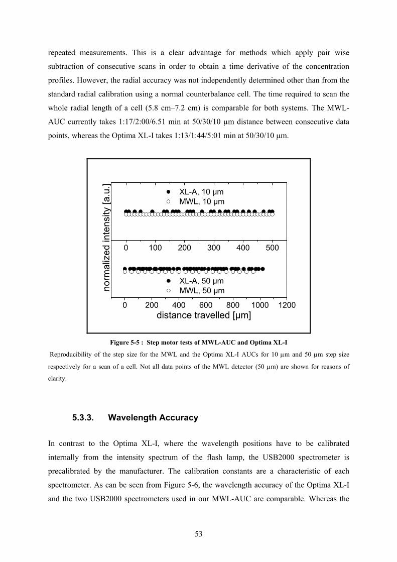
53
repeated measurements. This is a clear advantage for methods which apply pair wise
subtraction of consecutive scans in order to obtain a time derivative of the concentration
profiles. However, the radial accuracy was not independently determined other than from the
standard radial calibration using a normal counterbalance cell. The time required to scan the
whole radial length of a cell (5.8 cm–7.2 cm) is comparable for both systems. The MWL-
AUC currently takes 1:17/2:00/6.51 min at 50/30/10 µm distance between consecutive data
points, whereas the Optima XL-I takes 1:13/1:44/5:01 min at 50/30/10 µm.
0 100 200 300 400 500
0 200 400 600 800 1000 1200
XL-A, 10 µm MWL, 10 µm
norm
aliz
ed in
tens
ity [a
.u.]
distance travelled [µm]
XL-A, 50 µm MWL, 50 µm
Figure 5-5 : Step motor tests of MWL-AUC and Optima XL-I
Reproducibility of the step size for the MWL and the Optima XL-I AUCs for 10 m and 50 m step size
respectively for a scan of a cell. Not all data points of the MWL detector (50 m) are shown for reasons of
clarity.
5.3.3. Wavelength Accuracy
In contrast to the Optima XL-I, where the wavelength positions have to be calibrated
internally from the intensity spectrum of the flash lamp, the USB2000 spectrometer is
precalibrated by the manufacturer. The calibration constants are a characteristic of each
spectrometer. As can be seen from Figure 5-6, the wavelength accuracy of the Optima XL-I
and the two USB2000 spectrometers used in our MWL-AUC are comparable. Whereas the

54
specification of the wavelength accuracy according to the manufacturer (Beckman) is only 4
nm, the CCD array spectrometers can be tuned to a very high accuracy by choosing the
correct groove density or line spacing of the grating at the expense of the wavelength range
(OceanOptics 2008).
300 400 500 600
VIS
UV
XL-I
norm
aliz
ed O
D, o
ffse
t
wavelength [nm]
Figure 5-6 : Wavelength accuracy of the Optima XL-I and the MWL-AUC.
An Ho2O3 centrepiece was used to record absorbance spectra as shown. The dotted vertical lines indicate the
positions for three characteristic peaks at 361, 446, and 537 nm, respectively
In the spectrometers applied in this study, a groove density of 600 was chosen together with a
25 m slit and a wavelength range of 650–670 nm yielding a wavelength resolution of about
1.3 nm for the applied optical spectrometers (OceanOptics 2008). However, application of
higher groove densities will yield a higher wavelength resolution at the expense of the
wavelength range with the same 25 m slit, like 0.3 nm for a 2400 mm-1 grating with a
spectral range of only 140 nm (OceanOptics 2008). Nevertheless, the most reasonable
compromise appears to be a wavelength range of around 600 nm combined with a
wavelength resolution of 1.2–1.3 nm, which is more accurate and much more reproducible
than the wavelengths from the Optima XL-I. Therefore, the capability of around 3 pixels/nm
can already be used for effective data averaging without losing spectral resolution.
The USB2000 spectrometers with which the data in Figure 5-6 were recorded have been in
use in our laboratory for more than two years. In principle, wavelength positions can be
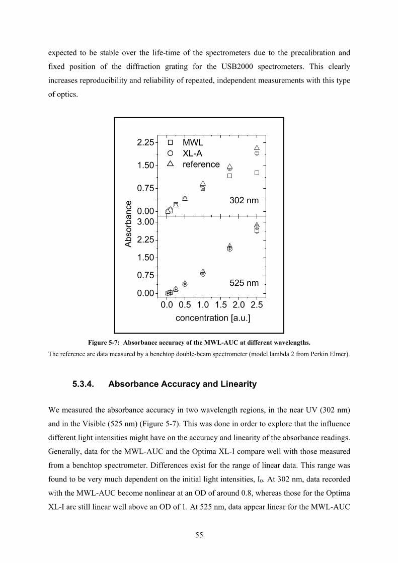
55
expected to be stable over the life-time of the spectrometers due to the precalibration and
fixed position of the diffraction grating for the USB2000 spectrometers. This clearly
increases reproducibility and reliability of repeated, independent measurements with this type
of optics.
0.0 0.5 1.0 1.5 2.0 2.50.00
0.75
1.50
2.25
3.000.00
0.75
1.50
2.25
525 nm
concentration [a.u.]
302 nm
A
bsor
banc
e
MWL XL-A reference
Figure 5-7: Absorbance accuracy of the MWL-AUC at different wavelengths.
The reference are data measured by a benchtop double-beam spectrometer (model lambda 2 from Perkin Elmer).
5.3.4. Absorbance Accuracy and Linearity
We measured the absorbance accuracy in two wavelength regions, in the near UV (302 nm)
and in the Visible (525 nm) (Figure 5-7). This was done in order to explore that the influence
different light intensities might have on the accuracy and linearity of the absorbance readings.
Generally, data for the MWL-AUC and the Optima XL-I compare well with those measured
from a benchtop spectrometer. Differences exist for the range of linear data. This range was
found to be very much dependent on the initial light intensities, I0. At 302 nm, data recorded
with the MWL-AUC become nonlinear at an OD of around 0.8, whereas those for the Optima
XL-I are still linear well above an OD of 1. At 525 nm, data appear linear for the MWL-AUC

56
and the Optima XL-I up to an OD of 1.5. From the intensity spectrum for the MWL-AUC for
these measurements (Figure 5-8) it is apparent that at 302 nm, I0 at the detector was 265
counts, which is a very low value. At 525 nm, I0 was around 3600 counts, close to the
maximum number of 4000 counts. However, the light intensity can be fine-tuned to a certain
degree via the iris (section 5.2.2) to improve I0 and hence linearity of the data in the desired
wavelength range.
200 400 600 8000
1000
2000
3000
4000
525 nm
302 nm
Inte
nsity
[a.u
]
wavelength [nm]
Figure 5-8 : Intensity profile of linearity tests
Reference intensities of the absorbance measurements are shown in Figure 5-6. The dotted vertical lines indicate
the two wavelengths at which data were recorded.
The dark noise of the spectrometer is on the order of 5–10 counts. The standard deviation of
the noise is slightly worse for the MWL-AUC than the Optima XL-I. It is in the order of
0.03 OD compared with 0.02 OD at 302 nm, whereas it was at 0.02 OD and 0.01 OD at
525 nm. The precision of the benchtop photometer was two orders of magnitude below these
values at both wavelengths. The slight decrease in wavelength precision for the MWL-AUC
appears to be caused by the raw intensities of the measurements, but also by other factors
specific to our setup.

57
250 500 750200 300 400-0.3
-0.2
-0.1
0.0
0.1
0.2
0.3
250 500 750
Vis
wavelength [nm]
Abs
orba
nce,
offs
et
UV
Xl-A
Figure 5-9: Noise comparison between the Optima XL-I and the MWL-AUC
Spectra were taken with 1/10/100 point averaging, shown as the bottom/middle/top spectrum, respectively.
Dotted horizontal lines indicate the offset true baselines. Due to the higher point density for the USB2000
spectrometers, the spectra appear broader as they are in reality. Note the differences in scale of the abscissae.
The respective statistical data are: UV(1): -0.016 +/- 0.029; UV(10): 0.007 +/- 0.009; UV(100): 0.001 +/- 0.005;
Vis(1): - 0.011 +/- 0.059; Vis(10): 0.004 +/- 0.010; Vis(100): -0.002 +/- 0.003; XL-I(1): -0.003 +/- 0.017; XL-
I(10): -0.001 +/- 0.006; XL-I(100): -0.002 +/- 0.004. UV scanned 200–500 nm; Vis scanned 250–800 nm and
Optima XL-I scanned 200–800 nm.
5.3.5. Intrinsic Noise of the Data
To qualitatively compare the intrinsic noise of the data at different wavelengths and the
baseline accuracy, we monitored an empty hole of a rotor over the full accessible wavelength
range and at a number of averages. It is possible to compare the noises of the data between
XL-I and MWL-AUC if the averaging is done. But without averaging, MWL-AUC is worse
then XL-I. One plausible explanation for this observation could be the absence of flash-to-
flash intensity normalization for the MWL-AUC, which quickly averages out. In future
designs, this normalization of the flash lamp intensity for every wavelength will be achieved
by a second identical spectrometer which monitors the intensity of the lamp after a small part
58
of the light was diverted to this spectrometer by a beam splitter. With 10 and 100 point
averaging, the noise level appears to be similar for the Optima XL-I and the MWL-AUC.
Baseline stability is satisfactory in all cases, provided enough averages are being taken. The
lack of baseline stability for measurements is a direct reflection of the absence of flash-to-
flash normalization as well.
One of the greatest possibilities of the new MWL-AUC can also be gathered from Figure 5-9:
it took only around 15 s to record a full wavelength spectrum with 100-points averaging with
the USB2000 spectrometers, whereas recording the spectrum with the Optima XL-I took
around 180 minutes. The reduction in experiment time without losing information is obvious.
Besides the noise generated by the variation of lamp intensity, a further source of noise is that
the computer for the detector control and data acquisition does not work in real time. In the
present labview-based program, the lack of real time operation generates slight variations in
the generation of the triggering of lamp and spectrometer, as we now use software triggering
of the spectrometer which allows for faster data acquisition (down to 2 ms for the applied
USB 2000) than the hardware triggering mode, which was applied in the earlier described
setup (50 ms integration time)(Bhattacharyya et al. 2006). With this change, we eliminated
the noise caused by the response time difference of the spectrometer and the flash lamp,
which were triggered by the same pulse. As the flash of the flash lamp is very short, in the
order of 3-4 s, slight variations of the trigger pulse timing will cause noise.
However, when using software triggering of the spectrometer with an integration that is long
enough for whole rotation of the rotor even at the highest rotational speed. The timing of the
spectrometer triggering with respect to the turning rotor cannot be determined anymore in
contrast to hardware triggering. There is a small probability that the spectrometer starts to
acquire data in the middle of a flash, which leads to a drop in the detected intensity. For
further development, we are planning to solve this problem by using much faster USB 4000
spectrometers with hardware triggering as fast as 10 s and to calibrate the response time of
the spectrometer and the flash lamp to the same trigger pulse. In addition, we will use a real-
time system to ensure correct timing.
59
5.4. Discussion
Comparing with the results presented in an earlier contribution on a first-generation MWL
detector (Bhattacharyya, 2006 ) progress has been made on the issue of light intensity
available at the detector. With the current modifications, it is possible to bring more light into
the vacuum chamber than the dynamic range of the CCD-chip can digest. This is a mandatory
requirement for precise, linear, accurate – and hence useful – measurements with the MWL-
AUC, and is clearly apparent from our data. Due to the very broad distributions of intensities
over the available wavelength range and the clear correlation with linearity of the recorded
data, we have added to the software of the MWL-AUC the feature that the spectrum of I0 is
being stored together with the corresponding measurements. This will allow for the definition
of linearity ranges after the experiment has been performed. The higher dynamic range of the
USB4000 spectrometers will be of great benefit in this respect, too.

60
Chapter 6 :Biological Application of MWL-AUC: Protein
Mixture
6.1. Introduction
In this chapter, we compare the performances of the commercially available Beckman
Coulter Optima XL-I and the MWL-AUC in characterizing a mixture of IgG, aldolase and
BSA, three non-interacting proteins, and discuss further improvements to the existing
machine. For the materials and the methods of the protein chapter, it was referred to
Appendix.
6.2. Results and Discussion
6 8 1 0 1 2 1 4 1 6 1 8 2 0
0 . 0
0 . 1
0 . 2
0 . 3
0 . 4
0 . 5
0 . 6
0 . 7
6 8 1 0 1 2 1 4 1 6 1 8 2 00 . 0
0 . 2
0 . 4
0 . 6
0 . 8
1 . 0
1 . 2
6 8 1 0 1 2 1 4 1 6 1 8 2 0
0 . 0
0 . 5
1 . 0
1 . 5
2 . 0
2 . 5
3 . 0
6 8 1 0 1 2 1 4 1 6 1 8 2 0
0 . 0
0 . 5
1 . 0
1 . 5
2 . 0
2 . 5
3 . 0
3 . 5
4 . 0
inte
nsity
(no
rmal
ized
)
s e d im e n t a t io n c o e f f ic ie n t [ S ]
G lo b a l F i t 2 8 0 n m 2 7 0 n m 2 6 0 n m
M W L - A U C A ld o la s e 0 .5 m g / m l
d )c )
b )
inte
nsity
(no
rmal
ized
)
s e d im e n t a t io n c o e f f ic ie n t [ S ]
G lo b a l F i t 2 8 0 n m 2 7 0 n m 2 6 0 n m
M W L - A U C / A ld o la s e 1 . 5 m g / m la )
inte
nsity
(no
rmal
ized
)
s e d im e n t a t io n c o e f f ic ie n t [ S ]
G lo b a l F i t I n t e r f e r e n c e 2 8 0 n m 2 5 0 n m
X L - I / A ld o la s e 0 . 5 m g / m l
inte
nsity
(no
rmal
ized
)
s e d im e n t a t io n c o e f f ic ie n t [ S ]
G lo b a l F i t I n t e r f e r e n c e 2 8 0 n m 2 5 0 n m
X L - I / A ld o la s e 1 .5 m g / m l
Figure 6-1: Comparison of Optima XL-I and MWL-AUC in c(s) and global fit of aldolase
Sedfit analyses of aldolase at different concentrations are shown in Figure 6-1. Figure 6-1(a)
shows sedfit analysis of single wavelength of 280 nm, 270 nm and 260 nm that is taken from
MWL data. So, in this chapter, we are not using all the wavelength information of MWL

61
data. In order to determine whether MWL data quality at a specific wavelength is better or
worse than Optima XL-I, we are only selecting three specific wavelengths from the set of
different wavelengths from MWL data. In Figure 6-1(a), c(s) analysis of aldolase with
concentration 0.5 mg/ml is shown. The selected wavelengths are 260, 270 and 280 nm. These
are selected point wavelengths from set of 500 wavelengths, ranging from 200nm to 550 nm.
Also, global fit of the data including 260, 270 and 280 nm are shown in the graph. In Figure
6-1(c), c(s) and global fit of XL-I data are shown. Interference and absorbance of 250 nm and
280 nm are shown. If we compare absorbance data of Figure 6-1(a) and Figure 6-1(c), we can
infer that both detectors produce similar peaks with the same peak positions. However, MWL
data peaks look wider. In this kind of analysis, Balbo et al. concluded that wideness of the
peaks can be attributed to regularization and noise in the data (Balbo et al. 2005).
Consequently, wider peaks can be attributed to high noise ratio and low intensity of MWL-
AUC in the UV region (this can also be seen in Figure 5-7 and Figure 5-8), which will be
discussed later. Despite high noise ratio, these plots show that MWL-AUC in the UV region
can be successfully used for single proteins. If we compare the global fit of Figure 6-1(a) and
Figure 6-1(c), then the global fit of the Optima XL-I data can be attributed to interference
optics that does not present in MWL-AUC.
2 4 6 8 10 12 14 16 18 200.00.10.20.30.40.50.60.70.80.91.0
0 2 4 6 8 10 12 14 16 18 20 22
0.00.10.20.30.40.50.60.70.80.91.0
2 4 6 8 10 12 14 16 18 200123456789
inte
nsity
(no
rmal
ized
)
sedimentation coefficient [S]
Aldolase IgG BSA
MWL-AUC / Mixture of Aldolase, lgG and BSA
Spectral ConvolutionAnalysis of MWL 280nm / 270nm / 260nm
inte
nsity
(no
rmal
ized
)
sedimentation coefficient [S]
Aldolase IgG BSA
MWL-AUC / Mixture of Aldolase, lgG and BSA
Spectral ConvolutionAnalysis with 250nm / 260 nm / 270 nm
c)
b)
inte
nsity
(no
rmal
ized
)
sedimentation coefficient [S]
Aldolase IgG BSA
XL-I / Mixture of Proteins
Spectral Convolution
a)
Figure 6-2: Three wavelengths, global multisignal analysis of MWL-AUC and Optima XL-I
62
In Figure 6-1(b), c(s) analysis and global fit of 1.5 mg/ml aldolase experiment with
wavelengths of 260, 270 and 280 nm are shown. The peak positions of Figure 6-1(a) and
Figure 6-1(c) are identical, but in Figure 6-1(b) the peaks are narrower. This is due to the
high signal-to-noise ratio of highly concentrated aldolase in comparison with less
concentrated aldolase. Noise makes the peaks wider (Balbo et al. 2005). In Figure 6-1(d), c(s)
and global fit of 1.5 mg/ml aldolase with 250 nm, 280 nm, and interference optics of the
Optima XL-I is presented. Similarly, in Figure 6-1(d) c(s) peaks of absorbance are at the
same position as in Figure 6-1(b), but they are narrower. Consequently, the noise level of
MWL-AUC is still higher than for the Optima XL-I. The thinner global fit of Figure 6-1(d)
can also be attributed to interference analysis that does not exist in MWL-AUC.
As a next step, analysis of three protein mixtures of aldolase, lgG and BSA is presented in
Figure 6-2. This analysis was performed by the global multisignal analysis module of
Sedphat. Three different wavelength scans (250, 260 and 280 nm) were uploaded by the
multisignal analysis module. This module tries to form spectra decomposition of different
protein distributions from these signals. Figure 6-2(a) shows the result of this analysis with
Optima XL-I data of absorbance at 250, 280 nm and interference. These results show
successful decomposition of S distribution of the three different proteins. Peak position of the
proteins agrees with previous study (Balbo et al. 2005). If we look at the result of analysis of
MWL-AUC data with 250, 260 and 280 nm in Figure 6-2(b), we cannot achieve the same
success. The S distribution of lgG shows a ghost peak at about 5 S. This is exactly the same
position as the main peak of aldolase. Consequently, this peak shows that the system could
not make spectral decomposition of three different proteins with three selected wavelengths
of MWL-AUC. These ghost peaks are referred to noise in data in the previous study (Balbo et
al. 2005). In Figure 6-2(c), the results of multisignal analysis of 250, 260 and 270 nm
wavelengths are shown. This analysis is performed in order to see the wavelength
dependence of the analysis result. However, changing the wavelength from 280 to 270 nm
does not solve the problem. The resulting graph still has a ghost peak of lgG, which is bigger
in this case.

63
240 260 280 300 320 3400.0
0.5
1.0
1.5
2.00
250
500
750
1000
b)
Abs
orb
ance
[O
D]
wavelength [nm]
a)
coun
ts [
a.u]
Figure 6-3: Reference intensity of MWL-AUC and wavelength scan of Optima XL-I and MWL-AUC
(a) Reference intensity of Xenon light taken from the reference sector of sample cell filled protein mixture; (b) Black Curve:UV/Vis spectra of the mixture sample with MWL-AUC; Red Curve: Wavelength Scans of mixture that is taken by XL-I with 5 replicates.
In order to observe the noise and the linearity problem of the MWL-AUC, we have prepared
Figure 6-3. The reference intensity of MWL-AUC in this UV range is shown in Figure
6-3(a). UV sensitive USB2000 was used to conduct these experiments (see sub-section 3.3.5).
Figure 6-3(a) shows the low intensity in this range. Low intensity reference light in UV
region makes MWL-AUC data noisier than Optima XL-I data. The wavelength scan of the
Optima XL-I in Figure 6-3 was taken with five replicates but MWL-DATA was taken as
single reading. For a better noise comparison, we refer to the section of intrinsic noise of the
data (sub-section 5.3.5). On the other hand, Figure 6-3(b) shows the linearity problem of
MWL-AUC data. Between 270 nm and 290 nm in Figure 6-3(b), the MWL-AUC spectrum
spectra differs from the Optima XL-I spectra, which indicates that linearity is lost in this
range. This is clearly due to the low UV intensity of the system (see Figure 5-7 and Figure
5-8). Linearity in relation to intensity has been discussed in the section on absorbance
accuracy and linearity (sub-section 5.3.4). Despite these disadvantages of the UV region of
the MWL-AUC data, we obtained the correct S distribution for the single protein mixture.
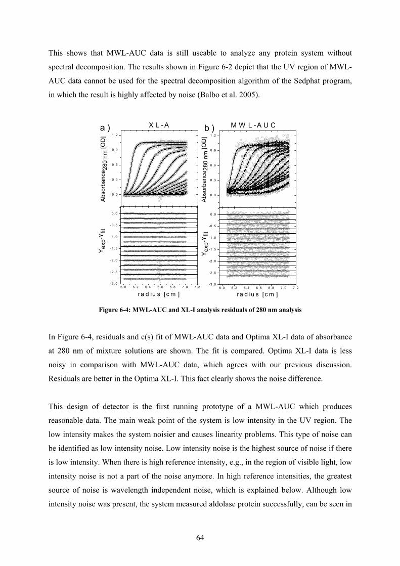
64
This shows that MWL-AUC data is still useable to analyze any protein system without
spectral decomposition. The results shown in Figure 6-2 depict that the UV region of MWL-
AUC data cannot be used for the spectral decomposition algorithm of the Sedphat program,
in which the result is highly affected by noise (Balbo et al. 2005).
0 .0
0 .3
0 .6
0 .9
1 .2
6 .0 6 .2 6 .4 6 .6 6 .8 7 .0 7 .2-3 .0
-2 .5
-2 .0
-1 .5
-1 .0
-0 .5
0 .0
0 .0
0 .3
0 .6
0 .9
1 .2
6 .0 6 .2 6 .4 6 .6 6 .8 7 .0 7 .2-3 .0
-2 .5
-2 .0
-1 .5
-1 .0
-0 .5
0 .0
Ab
sorb
anc
e 280
nm
[O
D]
X L - A M W L -A U C
Yex
p-Y
fit
r a d iu s [c m ]
Abs
orba
nce
280
nm [
OD
]
b )
Y
exp-
Yfit
r a d iu s [ c m ]
a )
Figure 6-4: MWL-AUC and XL-I analysis residuals of 280 nm analysis
In Figure 6-4, residuals and c(s) fit of MWL-AUC data and Optima XL-I data of absorbance
at 280 nm of mixture solutions are shown. The fit is compared. Optima XL-I data is less
noisy in comparison with MWL-AUC data, which agrees with our previous discussion.
Residuals are better in the Optima XL-I. This fact clearly shows the noise difference.
This design of detector is the first running prototype of a MWL-AUC which produces
reasonable data. The main weak point of the system is low intensity in the UV region. The
low intensity makes the system noisier and causes linearity problems. This type of noise can
be identified as low intensity noise. Low intensity noise is the highest source of noise if there
is low intensity. When there is high reference intensity, e.g., in the region of visible light, low
intensity noise is not a part of the noise anymore. In high reference intensities, the greatest
source of noise is wavelength independent noise, which is explained below. Although low
intensity noise was present, the system measured aldolase protein successfully, can be seen in
65
Figure 6-1. As explained before, the amplitude of low intensity noise only prevents the usage
of the spectral decomposition algorithm, but it does not prevent the usage of other analyses
without any spectral decomposition.
Secondly, another type of noise in this system comes from the variation in intensity of the
Xenon lamp. In MWL-AUC there is no intensity normalization. There are two well-known
noise types in the AUC field; radial independent and time independent noise (section 5.3.5).
The noise in our system is different from these classical types of noise. This new type of
noise can be called “wavelength independent noise”. Due to our observations, wavelength
independent noise is the second greatest source of noise in the low intensity conditions. In the
presence of high intensity, wavelength independence becomes the main source of the noise.
As explained above, wavelength independent noise is due to Xenon light fluctuations. In the
Optima XL-I, this problem was solved by using a reflector in the absorbance optic system
(Figure 2-6). This reflects a specific percentage of the incident light to an incident light
detector, which is a simple diode detector. This diode detector normalizes the fluctuations in
the Xenon flash lamp. This is easy to do in the Optima XL-I, because there is only one
wavelength in each scan. However, this task is multi-dimensional and complex in MWL-
AUC, since hundreds of wavelengths are recorded at once. The reflector and all optics will
work differently at each different wavelength. Furthermore, the system cannot work with a
diode incident light detector, as the incident diode detector can only detect one wavelength. A
proper incident light detector for MWL-AUC can only be another USB2000 CCD
spectrometer. However, there is not enough mechanical space inside the AUC vacuum
chamber to insert another CCD spectrometer. Although the user manual of the light source
we use (Hamamatsu L9546 Xenon flash lamp module) shows 5% intensity variation from
flash to flash (Hamamatsu 2006), we have observed a higher ratio than is claimed. Despite
the existence of wavelength independent noise, this noise is not the dominant source of noise
in the presence of low intensity noise.
Finally, in this chapter, we only used three different wavelengths among 300 wavelengths
(250–550nm). Comparison of only three wavelengths of MWL-AUC and the Optima XL-I,
shows that data from the latter has less noise, due to the fact that MWL-AUC has low
intensity in UV region. We conducted this test in order to repeat what was done by Balbo et
al. (Balbo et al. 2005). This analysis does not use overall information content of MWL-AUC,
due to the fact that the analysis uses just three different wavelengths among 300 wavelengths.
66
The reason for using only three wavelengths instead of 300 is due to the fact that Sedphat can
only accept three wavelengths to apply spectral decomposition. Furthermore, Sedphat can
only obtain information from a small portion of the MWL-AUC data content. This is why we
are waiting for further development of analysis software that can appropriately take all the
information content from MWL data, as Ultrascan can does very successfully with the CdTe
nanoparticle system (see chapter 8).

67
Chapter 7 : Industrial Application of MWL-AUC:
Investigation of β-Carotene-gelatin composite particles
7.1. Introduction
Combined with the fractionating power of the AUC, application of the MWL detector with its
additional structural and/or compositional information on light-absorbing samples can yield
distributions of the individual components in complex mixtures with respect to composition
and size/density related to different chromospheres. This can start with relatively
straightforward issues like sample homogeneity and purity but can then become increasingly
complex in the case of composite and/or interacting samples. Especially for such complex
samples, MWL-AUC has a huge potential, as spectral discrimination can synergistically
enhance the hydrodynamic resolution (Balbo et al. 2005). In this chapter, we will show the
capabilities of MWL-AUC for the analysis of an industrial composite sample of -carotene
and gelatin. This system was investigated previously with X-ray scattering, UV/Vis
absorption spectroscopy, FOQELS (Fiber-optic quasi-classical light scattering), and micro
electrophoresis and, on basis of these results, a core-shell structure was presented (Auweter et
al. 1999), as shown in Figure 7-2. The core structure, with a diameter of 120 nm, consists of
partially crystallized, partially amorphous -carotene as the active ingredient. The shell
structure consists of gelatin, functioning as a bio-degradable protection colloid. This hybrid
structure self-assembles in a carefully tuned co-precipitation of gelatin (from an aqueous
solution) and the active ingredient (from a lipophilic solvent). Such particulate formulations
can transport an active ingredient that is not water soluble across an aqueous phase with high
bioavailability, in this case provitamin A. These particles are not persistent, but disassemble
and are digested quickly in biological media.
Two forms of hydrosol are explained by Auweter and colleagues (Auweter et al. 1999). -
carotenes can precipitate as H aggregate or J aggregate; these two morphologies do not
interconvert and are regarded as being kinetically stable over years. The H aggregate is
observed in precipitation from dilute solutions (0.3 weight %), whereas the J aggregate is
observed at higher concentrations (1.0 weight %). Auweter calculated a 40 nm hypsochromic
shift observed for an H aggregate and a bathochromic shift in J aggregates (Auweter et al.

68
1999). This results in a significant color change of the product from yellow to red depending
on the precipitation conditions and hybrid particle size (Figure 7-1 and Figure 7-2). This
color change is the basis for the industrial application of the -carotenes as pigments for food
applications.
What is of interest for industrial applications is not only the purity of the sample concerning
the color characteristics (brilliance of color due to steep absorbance profiles) or the
homogeneity of the sample (different species or unbound gelatin), but furthermore any
possible transitions between different structures. This is a problem which can be
advantageously solved in a single MWL-AUC experiment, which we will describe in this
work.
7.2. Material and Methods
The -carotene product was obtained in powder form as a laboratory sample from BASF AG,
(Ludwigshafen, Germany). An aqueous dispersion in water was prepared with a
concentration of 0.05 g/l. The UV/Vis spectrum of the dispersion and of the free gelatin is
shown in Figure 7-1. Further details of AUC method and materials are explained in
Appendix.
300 400 500 6000.0
0.2
0.4
0.6
0.8
1.0
Abs
orb
anc
e
Wavelength (nm)
288
449 478518
Figure 7-1: UV/Vis spectra of shell -carotene/gelatin sample
Dashed line; UV/Vis spectrum of the core-shell -carotene/gelatin sample with 0.05 g/l concentration; Solid
line: UV/Vis spectrum of gelatin at 1 g/l.

69
7.3. Results and Discussion
Figure 7-2 : Structure of -carotene microparticle system
Left: Assumed structure of the -carotene microparticle system (Auweter et al. 1999). Right: Color change of
-carotene/gelatin microparticles due to particle size and structure.
In principle, the entire dataset can be evaluated globally, and efforts are underway to
incorporate such routines into the Ultrascan evaluation software package
(Demeler, 2005). However, even then we are confronted with a confounded polydispersity of
both optical and colloidal/hydrodynamic properties. On the left side of Figure 7-2, the
assumed core-shell structure of a -carotene microparticle is shown (Auweter et al. 1999).
Such a complex hybrid particle exhibits several levels of polydispersity, which impact the
distribution of sedimentation coefficients observed in an AUC:
(1) Diameter of the inner core;
(2) Chemical composition, especially oil content, of the inner core;
(3) Concentration of the adsorbed protection colloid (gelatin);
(4) Degree of swelling of the gelatin.
Parameters (1) and (2) determine the optical properties and bioavailability that are decisive
for the commercial application profile. For the smallest particle sizes, -carotene is an H
aggregate, while for the biggest particle sizes, -carotene forms J aggregates. Intermediate
particle sizes are assumed to integrate H and J aggregates in differing ratios (Auweter et al.
1999). Parameters (3) and (4) determine the thickness of the protection colloid layer, which is
typically 40 nm in pure water. The buoyant density of gelatin is rather high (above 1.3
g/cm3), and cannot be matched with a non-interfering solvent such as heavy water.

70
All parameters from (1) to (4) enter into the calculation of the effective density and the
hydrodynamic diameter of the hybrid particle. The frictional force under sedimentation
depends on the ion concentration and pH because the gelatin may collapse or swell, thus
changing the effective frictional forces (and thus changing the observable sedimentation
constant) although the chemical composition and buoyant density, which in principle could
be measured in a Krattky gauge or density gradient, stay the same. The swelling of the gelatin
corona alone impedes an exact conversion from measured sedimentation constants to
hydrodynamic diameters. Considering that parameters (1) and (2) also contribute to the
polydispersity in the observable distribution of sedimentation coefficients, we decided to
limit ourselves to a conservative evaluation on the level of sedimentation fractions, not sizes.
Figure 7-3: 3D sedimentation of -carotene microsystem Three-dimensional plots of the raw data from a band sedimentation experiment with -carotene detected with
the MWL detector. The axes are wavelength, absorbance and radial position. (a) Scan 1 (1.5 minutes); (b) Scan
10 (15 minutes); (c) Scan 18 (27 minutes); (d) Scan 40 (60 minutes).
We now discuss the optical properties that result from the specific colloidal microstructures
as discussed above. Due to different preparation conditions, the morphology of the -carotene

71
core changes. H and J aggregates have different UV/Vis spectra, shown as visual impression
on the right of Figure 7-2. In Figure 7-1, the dotted line curve shows the UV/Vis spectrum of
0.05 g/l product without any ultracentrifugation. Four peaks, at 288nm, 449nm, 478nm and
518 nm, can be seen. The three peaks in the visible can be attributed to the 1Ag- (S0) – 1Bu
+
(S2) transition with the vibrational progression 2–0, 1–0, 0–0 of the C-C stretch vibration
along the alternatingly double-bonded electronically conjugated backbone of the carotenoid
(Polivka and Sundstrom 2004). The UV peak can also be attributed partially to the carotenoid
transition 1Ag- –1Ag
+, which is forbidden by symmetry, but becomes allowed in the
crystalline assembly. The spectrum of the composite particle indicates the β-carotene J
aggregate (Auweter et al. 1999). In Figure 7-1 the solid curve shows the pure gelatin
spectrum for 1 g/l. It can be seen that gelatin only contributes to the UV region of the spectra
below 280 nm. However, the contribution of gelatin is vanishing compared with the three
times stronger absorption of the composite sample at 20 times lower overall concentration.
Another component that presumably contributes to the UV absorption is the dispersing agent
(a low-molar-mass organic acid) that is added during the co-precipitation.
Figure 7-3 shows four of the 40 experimental scans. If we put all these 40 scans in sequence,
we can create a 3D movie of the sedimentation. Figure 7-3(a) shows scan 1, where particles
have just been transferred from the reservoir to the sample column. The baseline offset is
0.05 (purple) due to the absorption calculation with an empty cell as reference. We see two
main peaks. The peak in the visible region is assigned to -carotene. In the UV range, there is
an overlay of two peaks, one is the UV peak of -carotene (see Figure 7-2) and the other is
the UV signal of gelatin. After 15 min of sedimentation, fractionation of the sample was
obvious and the first sedimentation fraction proceeds to the bottom of the cell. Scan 10 (15
min) is the last scan where the entire particle range can be seen before the first particles
reached the bottom. If we compare the height of the peak in the UV and visible region at
different radial positions, the ratio changes. For the faster sedimenting particles, the ratio of
-carotene to gelatin is higher. This is the first important result, demonstrating that the
sample is not homogenous. Instead, the particles change their colloidal properties in
correlation with the optical properties. The observed effect can be explained by a higher
content of stabilizing agent that induces smaller particle sizes. Note that the shape of the peak
at 288 nm (Figure 7-1) does not exactly match the gelatin absorption and that the expected
contribution of gelatin is weak at the applied concentrations, hinting at a combined action of
72
both gelatin and the dispersing agent added during the co-precipitation in particle synthesis.
The third part of Figure 7-3 shows the scan after 27 min. Here, the fastest particles have
sedimented already. In the fourth part of Figure 7-3, we saw the last fraction that remained
after 60 min of sedimentation, which is mainly composed of gelatin. However, some -
carotene absorption is still visible, which seems to be solubilized in small amounts by the
excess gelatin or excess dispersing agent. We didn’t detect free gelatin in the analysis. In an
independent experiment we measured the characteristic sedimentation behavior of gelatin
with the interference optics of the Beckman Optima XL-I AUC at 44,000 rpm. We found a
sedimentation constant distribution from 2 to 10 Sved. This confirms our assignment that the
last fraction cannot be pure gelatin.
To summarize the global evaluation, Figure 7-3 demonstrates the power of MWL-AUC. We
can differentiate particles, observe the full UV/Vis spectra of the particles and draw
conclusions about the different components in the complex sample mixture already without
any further evaluation, as the Y-axis shows the full UV/Vis wavelength range. This is a key
feature of MWL-AUC. Such analysis was impossible in analytical ultracentrifugation
experiments before.
0 50 100 150 200 2500.0
0.2
0.4
0.6
0.8
1.0
g (s
)
Sedimentation Coefficient (S)
260 nm 280 nm 450 nm 480 nm 520 nm
Figure 7-4: Sedimentation coefficient distributions at different wavelengths
We can also use projections of the data onto individual axes and proceed thus to a more
quantitative evaluation. In order to calculate the full s-distribution of all particles, we have
selected scan 10 for further evaluation, as this scan shows fractionation of the mixture while
73
no particles are yet lost due to complete sedimentation. More information is potentially
available with a global evaluation of the entire dataset. In Figure 7-4, the s-distribution of the
particles is shown for five different representative wavelengths out of 330 (250 nm to 750 nm
with a wavelength resolution of 1.5 nm). We have selected the wavelengths according to the
peaks of the -carotene microparticles: 260, 280, 450, 480 and 520 nm in Figure 7-1.
The s-distribution is obviously very broad. Due to the chemical heterogeneity of the particles
and the resulting density distribution, it is not possible to convert the sedimentation
coefficient to the particle size. However, all important sample characteristics can be discussed
for the s-distributions. From Figure 7-4 we conclude that there are at least three fractions in
the sample; small hybrid particles with s < 25 S, a main fraction around 100 S, and larger
particles around 200 S. Their absorption spectra (and chemical composition) are clearly
different, as can be seen in Figure 7-5.
430 435 440 445 450 455 460
0.95
0.96
0.97
0.98
0.99
1.00
1.01
250 300 350 400 450 500 550 6000.0
0.2
0.4
0.6
0.8
1.0
448439
Abs
orba
nce
(a.
u.)
Wavelength (nm)
11 S 49 S 86 S 124 S 160 S 196 S 232 S
Abs
orba
nce
(a.u
.)
Wavelength (nm)
11 S 49 S 86 S 124 S 160 S 196 S 232 S
Figure 7-5: UV/Vis spectra of sedimenting -carotene microsystem
Top: Normalized UV/Vis spectra of particles with different sedimentation coefficients, Bottom: Zoom the range
around 450 nm and peak positions of 10.6 S (448 nm) up to 232 S (439 nm).

74
In Figure 7-5, seven representative UV/Vis spectra are shown. The spectra agree well with
that of pure H aggregate (Auweter et al. 1999). However, the original sample contained J
aggregates too (Figure 7-1, dashed line). We believe that the J aggregates were already
precipitated before the first scan was taken in the AUC cell. Indeed precipitation of
particulate material inside the reservoir of the Vinograd cell was observed visually after cell
disassembly following the experiment. However, irrespective of the actual nature of the
particulate material that remained in the Vinograd cell reservoir, the result speaks for itself
that the coloristic polydispersity (Figure 7-1) is not due to an intra-particle but an inter-
particle distribution of morphologies (Figure 7-6). This result is contrary to the previous
assumption that is sketched in Figure 7-2, where H and J aggregates would coexist in the
particles.
Figure 7-6: Structure model of the -carotene microparticle system on the basis of the presented AUC results. The different color of the samples does not originate from the intraparticular coexistence of H and J aggregates as previously assumed (Figure 7-2) (Auweter et al. 1999), but instead separate particles contain pure H or J aggregates and the concentration ratio between these particles determines the color of the final sample. Note the difference to Figure 7-2.
The peak around 520 nm shifts slightly to a lower wavelength with increasing sedimentation
coefficient and the peak height also decreases. The same is true for the peak at 480 nm.
Therefore, this excitation of -carotene microparticles decreases with increasing
sedimentation coefficient. For the peak at 450 nm, only the spectral shift to lower wavelength
is observed with increasing sedimentation coefficient. The effects of this inhomogeneity were
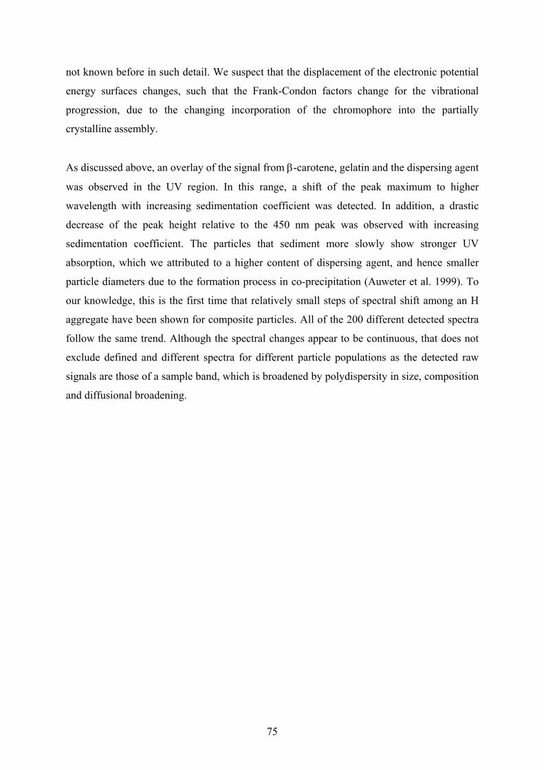
75
not known before in such detail. We suspect that the displacement of the electronic potential
energy surfaces changes, such that the Frank-Condon factors change for the vibrational
progression, due to the changing incorporation of the chromophore into the partially
crystalline assembly.
As discussed above, an overlay of the signal from -carotene, gelatin and the dispersing agent
was observed in the UV region. In this range, a shift of the peak maximum to higher
wavelength with increasing sedimentation coefficient was detected. In addition, a drastic
decrease of the peak height relative to the 450 nm peak was observed with increasing
sedimentation coefficient. The particles that sediment more slowly show stronger UV
absorption, which we attributed to a higher content of dispersing agent, and hence smaller
particle diameters due to the formation process in co-precipitation (Auweter et al. 1999). To
our knowledge, this is the first time that relatively small steps of spectral shift among an H
aggregate have been shown for composite particles. All of the 200 different detected spectra
follow the same trend. Although the spectral changes appear to be continuous, that does not
exclude defined and different spectra for different particle populations as the detected raw
signals are those of a sample band, which is broadened by polydispersity in size, composition
and diffusional broadening.

76
Chapter 8 :Application of MWL-AUC in Chemistry:
CdTe nanoparticles
8.1. Introduction
Semiconductors are of considerable importance in various key fields of (micro) electronic
technology and nanotechnology. Semiconductor particles of nanometer dimensions change
their optical and electronic properties with particle size, which allows for the design of tailor-
made nanoelectronic materials, wavelength-selective sun blockers, color-tuneable and -
adjustable LEDs, injection solar cells, and biological labels (Alivisatos 1996; Eychmüller
2000; Michalet et al. 2005).
Up to now, the dependence of the semiconductor band gap on particle size was determined
for close-to monodisperse fractions of nanoparticles by independently determining the
particle size and the absorption spectrum (Murray et al. 1993; Rogach et al. 1996). This is
experimentally demanding and time consuming. Moreover, the correlation between
absorption and particle size is impacted by the polydispersity of the samples. Especially for
new systems these experiments are tedious and often impossible to perform since they require
the synthesis of monodisperse nanoparticles with different sizes, which need to be determined
in a second step. AUC is particularly well suited for determining the size of nanoparticles
with the smallest accessible size, well below one nanometer (Cölfen and Pauck 1997; Cölfen
et al. 2002). The very high resolution of AUC particle size distributions in the Angström
range has already been demonstrated (Cölfen and Pauck 1997). On the basis of these
findings, attempts have been reported to determine spectral changes with particle size by
fractionation in a commercial AUC, however with severely limited resolution and quality
(Cölfen and Pauck 1997; Niederberger et al. 2004). These previous limitations can now be
overcome with the MWL-AUC, since the wavelength signal can now be acquired and
interpreted simultaneously with the hydrodynamic signal(Bhattacharyya et al. 2006). Figure
8-1 shows the design and experimental raw data of this experiment.

77
8.2. Polydisperse TGA-capped CdTe nanocrystals
8.2.1. Experimental
The sample for the ultracentrifugation experiment was prepared by mixing eight different
fractions of nanoparticles with absorbance maxima ranging from 450 to 620 nm. Absorbance
spectra of eight initial colloids and the resulting mixture are shown in Figure 8-1(a) and
8.1(b). The final mixed solution had a particle concentration of ca. 3×10⁻⁵ M. For the details
and synthesis and AUC method is explained in appendix.
Figure 8-1: Presentation of CdTe experiment (A) Eight different monodisperse CdTe samples were synthesized and the absorbance spectra of each sample
were taken, spectra are normalized. (B) The particles were then mixed and the absorbance spectrum of the
mixture was taken. (C) 15 µl of the mixture were measured by acquiring 20 sedimentation scans with the MWL-
AUC. Shown here is scan 9 of 20 band sedimentation scans (scan time after 12 minutes). The red shift of the
absorption with increasing radius is clearly visible in the experimental data, where the sedimenting boundary is
found at increasingly higher radial positions with increasing wavelength. The color scheme encodes the
absorption. The 3D graph (c) illustrates the continuous quantum size effect detected already in a single MWL-
AUC scan.

78
8.2.1.1. Analysis Method of the MWL-AUC data
To the best of our knowledge, our multiwavelength detector produces the first 3D data
obtained in the history of AUC. Normally AUC data are 2D because they usually include one
wavelength or other concentration-dependent signal. Consequently, all analysis software was
based on single wavelength analysis. There is no AUC software that can analyze 3D data
directly. That is why, at the beginning, we have performed an analysis with homemade
programs and scripts omitting diffusion correction. We have obtained interesting results even
without diffusion correction. These results are presented in sub-section 8.3.2. After we
obtained interesting results with our analysis, Borries Demeler’s group agreed to develop a
software program that can further analyze 3D data including diffusion correction. They have
developed their MWL module of the Ultrascan software further. Their findings are interesting
and are presented in section 8.3.3 on diffusion corrected analysis.
Figure 8-2 : Raw MWL-AUC Data: CdTe nanoparticles sedimentating with band centrifugation method;
(Speed 55K, 20 radial scans 50 µm step size)

79
8.2.2. Results and Discussions:
8.2.2.1. Raw MWL-AUC Data: A general summary of the MWL-AUC experiment is shown in Figure 8-1. Eight different
monodisperse samples of TGA-capped CdTe nanoparticles are synthesized (see sub-section
8.2.1). UV/Vis spectra of the samples are shown in Figure 8-1(a). All samples are mixed and
UV/Vis spectra of the mixture are shown in Figure 8-1(b). Only 15 µl of the mixture sample
is used for the whole experiment and the result was obtained in 32 minutes. Each scan
produces 3D data with axes of wavelength, radius and absorbance. The ninth scan out of 20 is
shown in Figure 8-2(c).
8.2.2.2. Analysis without Diffusion Correction The cell was scanned 20 times with radial intervals of 50 µm, yielding a 3D moving image of
sedimentation. Four of these scans can be seen in Figure 8-2. In one scan we have three
dimensions, radial position, absorbance and wavelength. The radial axis can be converted to
the particle size using the equations (Equation 8-1 and Equation 8-2) below:
t
rrs m
2
)/ln(ln
Equation 8-1: Formula for calculation of the sedimentation coefficient
sp
sp
sd
18
Equation 8-2: Calculation of particle size from the sedimentation coefficient
where s: sedimentation coefficient, r: radial position, ω: angular speed, t: time, d: hydrodynamic particle diameter, η: viscosity of the solvent, ρp : density of the particle, ρs : density of the solvent. One of the previous studies on the subject shows that these particles have spherical shapes in
TEM measurements(Rogach et al. 2007). Therefore, Equation 8-2 can be used with the
assumption that the particles are spherical. Hence, 20 scans in 3D with the axes of radial
position, absorbance and wavelength (Figure 8-2) can be converted to 20 scans in 3D with the
axes of particle size, absorbance and wavelength.

80
2 0 0 4 0 0 6 0 0 8 0 0
0
5 0 0
1 0 0 0
1 5 0 0
2 0 0 0
2 5 0 0
1 2 3 4 50 . 0
0 . 6
1 . 2
1 . 8
2 . 4
a.u
.
3 4 5 6 7 8 9 1 0 1 1 1 2 1 3 1 4 1 5 1 6 1 7 1 8
d P ( n m )
d )c )
Cou
nts
W a v e le n g t h ( n m )
1 . 5 2 . 0 2 . 5 3 . 0 3 . 5 4 . 0 4 . 5 5 . 00 . 0
0 . 6
1 . 2
1 . 8
b )
D i f f u s io n C o r r e c t e d p s d
r a w p s d f r o m S c a n 2 0
d H ( n m )
c(d
H)
a )
2 3 4 50 . 0
0 . 6
1 . 2
1 . 8
S e d f i t d i f f u s io n c o r r e c t e d p s d
d H ( n m )
c(d H
)
Figure 8-3 : Analysis of MWL-AUC data, reference intensity and psd (a) Reference intensity taken from reference sector; (b) Apparent particle size distributions of CdTe nanoparticles detected at 483 nm obtained by conversion of radial position to particle size without any diffusion correction; (c) Diffusion corrected particle size distribution at 483 nm with Sedfit; (d) Graphs show particle size range correction for scan 20 without diffusion correction; red curve is scan 20; black curve is the same as (c). To analyze the 3D data, as a first attempt, we focused on 2D slices of the scans. We selected
one slice from each of the 20 scans for a single wavelength (483nm), due to the fact that we
had a high intensity at 483 nm due to the spectrum of the Xenon lamp. The reference
intensity of the experiment can be seen in Figure 8-3(a) with a red start at 483 nm. High
intensity refers to a higher linear range (see sub-section 3.5.5). In Figure 8-3(b) we present 18
out of 20 2D slices of 20 3D data sets, which are the particle size distribution of particles
obtained from different scans. However, it should be noted that this amount of slices
corresponds to one slice out of 600, since we have selected only a single wavelength of 483
nm. Consequently, at each point in Figure 8-3(b) there is an additional wavelength axis that is
not shown. At each point of particle size distribution, UV/Vis spectra of this point can be
obtained, and this makes the MWL-AUC stronger over the other techniques.
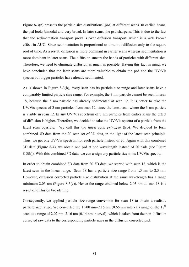
81
Figure 8-3(b) presents the particle size distributions (psd) at different scans. In earlier scans,
the psd looks bimodal and very broad. In later scans, the psd sharpens. This is due to the fact
that the sedimentation transport prevails over diffusion transport, which is a well known
effect in AUC. Since sedimentation is proportional to time but diffusion only to the square
root of time. As a result, diffusion is more dominant in earlier scans whereas sedimentation is
more dominant in later scans. The diffusion smears the bands of particles with different size.
Therefore, we need to eliminate diffusion as much as possible. Having this fact in mind, we
have concluded that the later scans are more valuable to obtain the psd and the UV/Vis
spectra but bigger particles have already sedimented.
As is shown in Figure 8-3(b), every scan has its particle size range and later scans have a
comparably limited particle size range. For example, the 3 nm particle cannot be seen in scan
18, because the 3 nm particle has already sedimented at scan 12. It is better to take the
UV/Vis spectra of 3 nm particles from scan 12, since the latest scan where the 3 nm particle
is visible in scan 12. In any UV/Vis spectrum of 3 nm particles from earlier scans the effect
of diffusion is higher. Therefore, we decided to take the UV/Vis spectra of a particle from the
latest scan possible. We call this the latest scan principle (lsp). We decided to form
combined 3D data from the 20-scan set of 3D data, in the light of the latest scan principle.
Thus, we get one UV/Vis spectrum for each particle instead of 20. Again with this combined
3D data (Figure 8-4), we obtain one psd at one wavelength instead of 20 psds (see Figure
8-3(b)). With this combined 3D data, we can assign any particle size to its UV/Vis spectra.
In order to obtain combined 3D data from 20 3D data, we started with scan 18, which is the
latest scan in the linear range. Scan 18 has a particle size range from 1.5 nm to 2.3 nm.
However, diffusion corrected particle size distribution at the same wavelength has a range
minimum 2.03 nm (Figure 8-3(c)). Hence the range obtained below 2.03 nm at scan 18 is a
result of diffusion broadening.
Consequently, we applied particle size range conversion for scan 18 to obtain a realistic
particle size range. We converted the 1.500 nm–2.16 nm (0.66 nm interval) range of the 18th
scan to a range of 2.02 nm–2.16 nm (0.14 nm interval), which is taken from the non-diffusion
corrected raw data to the corresponding particle sizes in the diffusion corrected psd.

82
Figure 8-4: Combined 3D data, with axis, particle size, abs, wavelength
3D representation of the quantum size effect in a CdTe mixture consisting of eight monodisperse fractions.
Spectra are normalized and the quantum size effect can be seen. All subgraphs are the different views of the
same graph from different directions. The graph contains about 150 spectra. This corresponds to 0.1 Angstrom
intervals in terms of particle size.
)(02.2)(66.0/)(14.0*)(5.1 nmnmnmnmpsps oldnew
Equation 8-3: Particle size range correction equation for small particles at scan 18 Where psnew : new particle size for the point; psold : particle size point that is in scan 18.
With the help of Equation 8-3, every particle size point at scan 18 in the range 1.500 nm–2.16
nm can be converted to a point in the range 2.02 nm–2.16nm. This corrects the particle size
range of scan 18. The conversion is shown in Figure 8-3(d).

83
400 450 500 550 600 6500.0
0.2
0.4
0.6
0.8
1.0
1.2
2.0 2.5 3.0 3.5 4.0 4.5 5.0
0.0
0.7
1.4
510 5400.0
0.2
0.4
0.6
0.8
1.0
1.2
400 450 500 550 600 6500.0
0.2
0.4
0.6
0.8
1.0
1.2
Wavelength, (nm)
Nor
mal
ized
abs
orpt
ion
Nor
mal
ized
Abs
orpt
ion
(a.u
.)
Wavelength (nm)
d)c)
b)
g
(dH
)
particle size (nm)
a)
No
rma
lize
d A
bso
rptio
n (
a.u
.)
Wavelength (nm)
2.40nm 2.41nm 2.42nm 2.43nm 2.44nm 2.45nm 2.46nm
Particle Size Resolution of 0.1 Å
Figure 8-5: Spectral comparison of sample (a) Particle size distribution calculated with the Sedfit program at 483 nm, triangles are the points whose spectras are shown with dashed lines in Figure 8-5(c), (b) 150 normalized UV/Vis spectra, from 2.02 nm to 3.5 nm with a resolution of 0.01 Å. Peak range changes from 444 nm to 595 nm. (c) UV/Vis spectra of the eight initial samples, from left to right, red: sample1; purple: sample2; green: sample3; blue: sample4; magenta: sample5; olive: sample6; dark yellow: sample7; orange: sample8, black is the spectrum of the mixture, solid lines indicate spectra before mixing and dashed lines are from combined 3D data with values shown in Figure 8-5(a) (triangles); d) Spectra with particle size resolution of 0.01 Å
After conversion we obtain the corrected particle size range and the UV/Vis spectra of each
particle at scan 18. We keep this (corrected scan 18) data as the first part of our combined 3D
data. Then we shift to scan 17, where we have the distribution of larger particles and their
UV/Vis spectra, which were already sedimented in scan 18. We did not apply any range
conversion to scan 17. Because for the particle size range >2.16 nm, it is not clear if the data
point in the non-diffusion corrected distribution needs to be corrected to a lower or higher
particle size. After scan 17, we shift to scan 16, and obtain the distribution of particles that
were already sedimented in scan 17 and their UV/Vis spectra. We continue like this until the

84
UV/Vis spectra of CdTe nanoparticles do not show any reasonable spectra anymore. As a
summary, this process includes the particles with sizes in the ranges: 2.02–2.16 nm from scan
18 with particle size range corrected; 2.165–2.333 nm from scan 17; 2.343–2.433nm from
scan 16; 2.444–2.52 nm from scan 15; 2.528–2.606 nm from scan 14 ; 2.61–2.668 nm from
scan 13 ; 2.677–2.75 nm scan 12; 2.788–3.148 nm from scan 11; 3.15–3.284 nm from scan
10; 3.296 –3.464 nm from scan 9; 3.467–3.513 nm from scan 8. At the end, we obtain
combined 3D data, for a particle size range from 2.0 nm to 3.5 nm, a wavelength ranges from
350 to 620 nm, and absorbance data. In order to make the combined 3D data presentable, we
normalized the absorbance of the peak point of the UV/Vis spectra to 1 in all 150 spectra.
The combined 3D data is presented in Figure 8-4.
Figure 8-4 clearly shows the quantum size shift. This is a 3D plot of the combined 3D data
explained above. The plot has an axis of particle size from 2 to 3.5 nm. In this range 150
different UV/Vis spectra were recorded. Consequently, particle size resolution is about 0.01
Å. Wavelength range is from 400 nm to 620 and its resolution is about 1 nm. Absorbance was
normalized in order to visualize the data. Normalization was done to produce the peak point
of the spectrum1. All the information used here was obtained from a 15 µl sample in only 32
minutes. This shows the power of the MWL-AUC as an analytical technique in the field of
semiconductor nanoparticles.
As a first step of reliability analysis of our combined 3D data, we compared this combined
data with UV/Vis spectra of initial monodisperse samples. From 2 nm to 3.5 nm, we had 150
UV/Vis spectra. These 150 spectra are shown in Figure 8-5(b). Among these 150 spectra, we
have selected the particle sizes whose spectra fit the spectra of eight monodisperse samples
that were synthesized in the beginning (Figure 8-1(a)) and which are close to theoretically
expected values much better than the previous results (Figure 8-6(b)). The selected particle
sizes are shown as triangles in Figure 8-1(a). On the other hand, Figure 8-3(c) shows their
spectra with dashed lines (Figure 8-5(c)). Solid lines are identical to the plots of Figure
8-1(a). As a result, Figure 8-5(c) shows that we reproduce the same spectra. Thus, MWL-
AUC is able to differentiate the mixture into its initial monodisperse components.
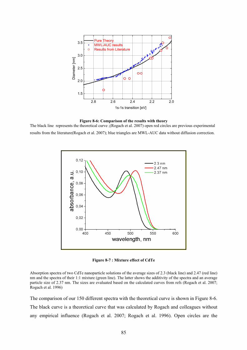
85
2.8 2.6 2.4 2.2 2.0
1.5
2.0
2.5
3.0
3.5 Pure Theory MWL-AUC results Results from Literature
Dia
me
ter
[nm
]
1s-1s transition [eV]
Figure 8-6: Comparison of the results with theory
The black line represents the theoretical curve ;(Rogach et al. 2007) open red circles are previous experimental
results from the literature(Rogach et al. 2007); blue triangles are MWL-AUC data without diffusion correction.
Figure 8-7 : Mixture effect of CdTe
Absorption spectra of two CdTe nanoparticle solutions of the average sizes of 2.3 (black line) and 2.47 (red line) nm and the spectra of their 1:1 mixture (green line). The latter shows the additivity of the spectra and an average particle size of 2.37 nm. The sizes are evaluated based on the calculated curves from refs (Rogach et al. 2007; Rogach et al. 1996) The comparison of our 150 different spectra with the theoretical curve is shown in Figure 8-6.
The black curve is a theoretical curve that was calculated by Rogach and colleagues without
any empirical influence (Rogach et al. 2007; Rogach et al. 1996). Open circles are the
86
previous experimental points that were achieved so far. The red curve is the fit of previous
experimental results that are shown as open circle points. The blue triangles are the results of
our 150 spectra. The 1s–1s transition is calculated from the UV/Vis spectra of the sample.
Wavelengths of peak points were converted to energy with the help of Planck’s formula. The
diameter of each particle is taken from our combined 3D data.
The particle size resolution of 0.01 Å in Figure 8-4 is an interesting result. Is the resolution of
0.01 Å realistic since the radius of Cd2+ and Te2- are 0.095 Å and 0.0221 Å This phenomenon
can be explained by a mixture effect. Mixture effect is seen in Figure 8-7. In this figure, two
fractions of particles with sizes of 2.3 nm and 2.47 nm are mixed. The spectra of the mixture
are identical to spectra of a particle with 2.37 nm. In fact, the particle of size 2.37 nm does
not exist; it is only a statistical effect. This effect can explain the resolution of 0.01 Å as, in
the case of a particle mixture the spectrum will correspond to the weighted average particle
size. The additivity of the spectra also allows us to calculate the average particle size from the
maximum in the UV-Vis absorption spectrum for a mixture, as demonstrated in Figure 8-7.
This opens up the possibility of calculating the particle size from each of the experiments
(Figure 8-6), an approach allowing the direct correlation of the optical properties with the
particle size. Only the band gap positions of the resolved species should be plotted in this
plot. For each of these spectra the first absorption maximum corresponds to the energy of the
1s–1s transition or in other words to the band gap position. The bandgap-size data points are
plotted in Figure 8-6. Those are compared with previously reported experimental data
(estimated from the statistical analysis of the TEM images) and the calculated values as
described in (Rogach et al. 2007; Rogach et al. 1996). From Figure 8-6, it can be seen that
these data points fit the theoretical curve for CdTe (Rogach et al. 2007) very well and much
better than the conventionally determined particle size dependence of the band gap(Rogach et
al. 2007). In the presented experiment, we have 150 such correlations available. This number
can be increased by scanning the solution column in the ultracentrifuge cell not with a 50 µm
step size as is current practice (ca. 150 data pairs) but instead with 10 µm or even 1 µm,
yielding 750 or 7500 data pairs respectively in a single experiment. Thus, the full particle size
dependence of the band gap becomes directly experimentally accessible for the first time with
steps as small as the addition of one Cd2+ or Tl2- ion to an existing particle.

87
8.2.2.3. Analysis with Diffusion Correction
Figure 8-8 : Result of 2DSA analysis
Frictional ratio plotted for the diffusion-corrected sedimentation coefficient distribution for the CdTe mixture as
a result of two-dimensional spectrum analysis. It is obvious that all particles in the disctrete distribution of
particles have a spherical shape (f/f0 = 1).
Diffusion causes broadening of the sedimenting boundary (Figure 8-3) which makes the
particle size distribution wider and obstructs from identifying individual species in a mixture.
There are various strong algorithms to correct the diffusion effect. Recently, two-dimensional
spectrum (2DSA) analysis has been developed (Brookes et al. 2006). With the help of Emre
Brookes, the 2DSA has been employed to resolve the heterogeneity and analyze the MWL-
AUC data. This method models sedimentation and diffusion processes for each species in the
mixture with ASTFEM-RA (adaptive space-time finite element method-reversible
associations) solution (Cao and Demeler 2008) of the Lamm equation(Equation 2-12). The
method is built for a regular grid of species extending over all species contained in a mixture.
By performing a non-negatively constrained linear least-squares optimization implemented
on a super computer, it finds the amplitudes of the species that are present (Brookes and
Demeler 2008).

88
Figure 8-9: Diffusion-corrected results of the CdTe experiment
(a) Composite sedimentation coefficient ( S20.W: sedimentation coefficient corrected to 20oC and water density
and viscosity) distribution plot of relative concentrations for all species and all wavelengths. The peak height
represents partial concentration. Each peak is the summation of all concentrations from all wavelengths. The
different species are labeled with numbers. Over 20 species can be clearly resolved. (b) The corresponding UV-
Vis spectra for the first seven species. (c) Diffusion-corrected sedimentation coefficient distribution after 2DSA
(Brookes et al. 2006) from 350 nm to 650 nm. The spectra are terminated at lower wavelengths due to higher
absorption that exceeds the linear range. The Z-axis (peak height) indicates the partial concentration of each
species in absorbance units. Data from all wavelengths were analyzed independently and showed identical
solutes but with different partial concentration. The red shift with increasing particle size is clearly visible in the
low S-value range (left side of plot) and extends from about 400 to 650 nm and 8 to 40 S. Smaller species are
more abundant than larger species. The 2DSA analysis results in a clear baseline separation of 24 individual
species consistently reproduced for all wavelengths. Overall analysis that is shown in this figure was performed
by Borries Demeler and Emre Brookes using a modified ultrascan software for MWL-AUC data.
400 450 500 550 600 650
0.0
0.2
0.4
0.6
0.8
1.0
Cu
mu
lativ
e A
bso
rba
nce
Wavelength (nm)
20 40 60 80 100
0.0
0.1
0.2
0.3
0.4
0.5
23
2221
2019
1817
1615
14
13
12
11
10
9
87
6
54
32
1
0Rel
ativ
e C
once
nta
riton
s
Sedimentation Coefficient, S20,W
ba
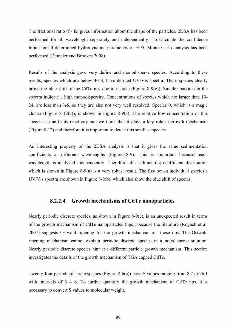
89
The frictional ratio (f / f0) gives information about the shape of the particles. 2DSA has been
performed for all wavelength separately and independently. To calculate the confidence
limits for all determined hydrodynamic parameters of %95, Monte Carlo analysis has been
performed (Demeler and Brookes 2008).
Results of the analysis gave very define and monodisperse species. According to these
results, species which are below 40 S, have defined UV/Vis spectra. These species clearly
prove the blue shift of the CdTe nps due to its size (Figure 8-9(c)). Smaller maxima in the
spectra indicate a high monodispersity. Concentrations of species which are larger than 10-
24, are less than %5, so they are also not very well resolved. Species 0, which is a magic
cluster (Figure 8-12(a)), is shown in Figure 8-9(a). The relative low concentration of this
species is due to its reactivity and we think that it plays a key role in growth mechanism
(Figure 8-12) and therefore it is important to detect this smallest species.
An interesting property of the 2DSA analysis is that it gives the same sedimentation
coefficients at different wavelengths (Figure 8-9). This is important because, each
wavelength is analyzed independently. Therefore, the sedimenting coefficient distribution
which is shown in Figure 8-9(a) is a very robust result. The first seven individual species`s
UV/Vis spectra are shown in Figure 8-9(b), which also show the blue shift of spectra.
8.2.2.4. Growth mechanisms of CdTe nanoparticles
Nearly periodic discrete species, as shown in Figure 8-9(c), is an unexpected result in terms
of the growth mechanism of CdTe nanoparticles (nps), because the literature (Rogach et al.
2007) suggests Ostwald ripening for the growth mechanism of these nps. The Ostwald
ripening mechanism cannot explain periodic discrete species in a polydisperse solution.
Nearly periodic discrete species hint at a different particle growth mechanism. This section
investigates the details of the growth mechanism of TGA capped CdTe.
Twenty-four periodic discrete species (Figure 8-6(c)) have S values ranging from 8.7 to 96.1
with intervals of 3–4 S. To further quantify the growth mechanism of CdTe nps, it is
necessary to convert S values to molecular weight.

90
)1( sD
sRTM
Equation 8-4: Svedberg Equation Where s: sedimentation coefficient; M: molecular weight; T : temperature; R: gas constant; D : diffusion
coefficient; : partial specific volume of particle; s : density of solvent.
Figure 8-10: Density Model of CdTe/TGA
(a) Length of the TGA molecule that is calculated with MS-Modeling (Accelrys), 4,087 Å is without hydrogen; 4,204 Å is with hydrogen (chemical bonding to CdTe is assumed via S, which eliminates H of the –SH group) (b) Crystalline structure of CdTe, with angles between atoms; (c) Density model parameters; (d) Particle size dependence of TGA capped CdTe, blue triangles(experimental) are our measurements with density meter, black triangles(literature) with error intervals are from Lars Börger`s pHd work. Model1, model2 and model3 are ploted with different colors.
The diffusion coefficient can be calculated with the equation below(Equation 8-5):
fN
RTD
A
Equation 8-5: Calculation of diffusion coefficient where f : the frictional ratio; NA : Avogadro constant. f/f0 is 1 for all 24 species (Figure 8-8), thus the equation below (Equation 8-6) for spherical particles can be used to calculate f.
a)
b) d)
1 2 3 4 5 6
2
3
4
5
experiimental literature Model1 Model2 Model3
Den
sity
(g/
ml)
Total diameter (nm)
Density Calculation Model1: Shell consists of %100 TGA Density Calculatiom Model2: Shell consists of %100 D2O Density lculatioCam Model3: Shell consists of %50 TGA and %50 D2O
c)
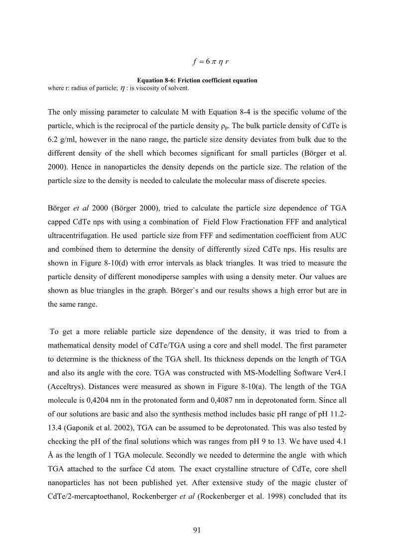
91
rf 6
Equation 8-6: Friction coefficient equation where r: radius of particle; : is viscosity of solvent.
The only missing parameter to calculate M with Equation 8-4 is the specific volume of the
particle, which is the reciprocal of the particle density ρp. The bulk particle density of CdTe is
6.2 g/ml, however in the nano range, the particle size density deviates from bulk due to the
different density of the shell which becomes significant for small particles (Börger et al.
2000). Hence in nanoparticles the density depends on the particle size. The relation of the
particle size to the density is needed to calculate the molecular mass of discrete species.
Börger et al 2000 (Börger 2000), tried to calculate the particle size dependence of TGA
capped CdTe nps with using a combination of Field Flow Fractionation FFF and analytical
ultracentrifugation. He used particle size from FFF and sedimentation coefficient from AUC
and combined them to determine the density of differently sized CdTe nps. His results are
shown in Figure 8-10(d) with error intervals as black triangles. It was tried to measure the
particle density of different monodiperse samples with using a density meter. Our values are
shown as blue triangles in the graph. Börger`s and our results shows a high error but are in
the same range.
To get a more reliable particle size dependence of the density, it was tried to from a
mathematical density model of CdTe/TGA using a core and shell model. The first parameter
to determine is the thickness of the TGA shell. Its thickness depends on the length of TGA
and also its angle with the core. TGA was constructed with MS-Modelling Software Ver4.1
(Acceltrys). Distances were measured as shown in Figure 8-10(a). The length of the TGA
molecule is 0,4204 nm in the protonated form and 0,4087 nm in deprotonated form. Since all
of our solutions are basic and also the synthesis method includes basic pH range of pH 11.2-
13.4 (Gaponik et al. 2002), TGA can be assumed to be deprotonated. This was also tested by
checking the pH of the final solutions which was ranges from pH 9 to 13. We have used 4.1
Å as the length of 1 TGA molecule. Secondly we needed to determine the angle with which
TGA attached to the surface Cd atom. The exact crystalline structure of CdTe, core shell
nanoparticles has not been published yet. After extensive study of the magic cluster of
CdTe/2-mercaptoethanol, Rockenberger et al (Rockenberger et al. 1998) concluded that its

92
structure is most probably similar to CdS structure with a different crystalline structure at
core. Herron et al (Herron et al. 1993) and Vosmeyer et al (Vossmeyer et al. 1995a;
Vossmeyer et al. 1995b) published the exact crystalline structure of CdS nanoparticles. In the
structures it is shown that the stabilizer has an angle to the particle surface, which follows the
core crystalline structure. The crystalline structure of bulk CdTe is shown in Figure 8-10(a).
Rockenberger et al (Rockenberger et al. 1998) showed that the ligand is attached to surface
Cd and that there are 2 ligands attached to 1 surface Cd atom. Therefore, the ligand most
probably has the same angle as Cd to Te in the crystal lattice. These angles are calculated by
MS-Modeling(Accelrys) and it is 35.2o. So we calculated the shell thickness as
0.4087nm*sin(35.2) which is 0.237 nm. Thus we took 0.237 nm as the thickness of the shell.
We took this distance as constant. We know the core density as 6.2 gr/ml which is the density
of bulk CdTe. Since we do not have exact information about the shell density, we employed
three different models that are shown in Figure 8-10(c). With this conclusion, a density
calculation model of TGA-capped CdTe nanoparticles have been developed .
Figure 8-10(d) illustrates the mathematical density calculation model that is used to obtain
the particle size dependence of density. Models 1, 2 and 3 (Figure 8-11(c-d) produced very
similar results, which indicates that the D2O content of the shell does not have a big effect on
particle density. This can be explained by the high density of the core CdTe. To further
calculate the molecular masses of the periodic 24 discrete species (Figure 8-6(c)), Model 3 is
used (50% TGA-50% D2O). Molecular masses are calculated with Equation 8-4. The
calculated molar masses are shown in Figure 8-11 as blue points. Molecular masses range
from 17500 g/mol K Dalton to 373000 g/mol with nearly constant difference. The
polynomial fit of the points gives an equation below (Equation 8-7):
)/(230)/(10358)/(14343 2 lomgXlmogXmolgM x
Equation 8-7: Equation obtained from Figure 8-12 where X is the species number (Figure 8-11(a)).
93
1 3 5 7 9 11 13 15 17 19 21 230
50k
100k
150k
200k
250k
300k
350k
400k
450ka)
y = a + bx + cx2
Par.: Value: Error:----------------------------------------a 14,343.46 1,076.37b 10,358.22 206.63c 230.37 8.36
Mo
lecu
lar
Wei
gh
t (D
alto
n)
Species
-2.0k
0.0
2.0k
b)
M
ole
cu
lar
Wei
gh
t a)
Figure 8-11: Molecular weight of 24 species (0-23)
(a) Residuals for fit in Figure 8-12(b); (b) Molecular weights of 24 discrete species (Figure 8-9(a)) calculated with the density calculation model3; red line is the polynomial fit of the molar masses of species.
Figure 8-12: One of the possible mechanisms of CdTe nanoparticle crystallization
(a) One of the possible structures of a [Cd54Te32(SR)52]8- cluster, S-R is the thiol that is used in synthesis; (b)
One of the possible mechanisms of TGA hydrolysis; (c) Cluster coalescence mechanism.

94
Near to constant periodicity of molar masses is much better illustrated in Figure 8-11. There
is a linear term of 10358 g/mol and a square term of 230 which is small in comparison with
the linear term. A constant molar mass difference about 10400 g/mol between the detected
species shows that the CdTe nanoparticles do not grow by classical crystal growth, implying
ion by ion deposition onto the growing CdTe nanoparticle. Instead, the constant molar mass
difference between the different, strictly monodisperse, growth species shows a nanoparticle-
based growth mechanism. In our case, attaching nanoparticles are [Cd54Te32(SR)52]8- with a
molar mass of 14890 g/mol with a deprotonated TGA stabilizing ligand. The smallest
detected species is a 17500 g/mol,species which then grows by subsequent addition of one
[Cd54Te32S22] (Figure 8-12). This growth mechanism was already detected earlier for Pt
nanoparticles (Cölfen and Pauck 1997). The applied two-dimensional spectrum analysis is
able to reveal the particle shape as well as the sedimentation coefficient distribution of the
sample. As Figure 8-9 shows, for all wavelengths, consistent data were obtained, which
reveal the discrete species already shown in Figure 8-8, but as additional information their
spherical shape is revealed as f/f0 = 1. Therefore, coalescing nanoparticles must have the
opportunity to fuse and minimize their surface to a spherical shape later on. Having all this
information, we illustrate one of the possible growth mechanisms in more detail in Figure
8-12.
Extensive study of the [Cd54Te32(SR)52]
8- cluster in literature shows that the structure is;
CdTe core, Cd(SR)2 layer at shell (Rockenberger et al. 1998). The cluster has a molar mass of
14890 g/mol. The exact crystalline structure is not yet published, but EAXS analysis
(Rockenberger et al. 1998) shows a structure similar to that in Figure 8-12(a). Illustrative
Figure 8-12(a) shows 32 units of core CdTe, 22 units of [C(SR)2] in shell and 8 S-R- in shell.
Hydrolysis of TGA is also reported in TGA-capped CdTe nps which results in breaking of
the S-R bond(Rogach et al. 2007), one of the possible mechanisms is shown in Figure
8-12(b). We suggest a possible intermediate stage in the process, which is the result of
hydrolysis of all TGA in the shell. The intermediate species shown in Figure 8-12(b), has a
molar mass of 10858 g/mol. Our cluster coalescence mechanism (Figure 8-12(c)) consists of
the addition of intermediate species to the [Cd54Te32S22] cluster. After coalescence of two
clusters, number of surface Cd atoms increases, and surface is covered by Cd(SR)2
minimization occurs because of the new surface-to-volume ratio. Each new coalescence of
the cluster adds mass of 10858 g/mol to total mass. In the core of structure, CdTe crystals
95
dissolve and form a bigger CdTe crystalline core. These type of reactions are called
isodesmic reactions. Isodesmic reactions are also common in nature, and the type that is
presented here is called mesonucleation (Cölfen and Antonietti 2008). This may explain the
linear 10358 X (g/mol) term in Equation 8-7, because the number 10860 of clusters that
coalesce is linear to the species number. An increase in the number of surface Cd atoms,
result in the increase of surface Cd(SR)2 complex this may explain the 230 X2 term in
Equation 8-7. The total equation for molar mass calculation according to the mechanism in
mechanism in Figure 8-12 results in the equation (Equation 8-8) below:
)/()/(10858)/(14480 2 molgXmolgXmolgM X
Equation 8-8: Equation of total particle mass due to growth mechanism (Figure 8-12) Further extensive literature research on the growth mechanism of CdTe revealed small
number of references indicating an aggregation mechanism at different conditions. However,
the reported results are not as exact as ours, so the main accepted mechanism for CdTe
growth was still Ostwald ripening. Therefore, a vast number of references refer to Ostwald
ripening.
Dagtepe et al (Dagtepe et al. 2007), studied the CdTe growth mechanism at high temperature
anhydrous synthesis. High temperature sythesis was used at 200 oC with in presence of
hexadecylamine (HDA), hexylphosphonic acid (HPA), and trioctylphosphine oxide (TOPO)
which is a different synthesis in comparison to the synthesis that we have used. UV/Vis
spectra of the reactor solution were taken continuously during the synthesis. Multiple peaks
were observed which was referred to quantized growth mechanism of CdTe. It was claimed
that discrete species exists with UV/Vis absorption peaks of 410, 449, 491, 501, 539 and 588
nm. Species with 449, 539 nm and 588 nm peaks were observed with HRTEM. These species
showed multiple domains which support the idea of aggregation based mechanism. However,
the species with 501 and 449 nm peaks could not be solved with HRTEM. Also band gap
dependence on particle size (as Figure 8-6) did not fit to the theoretical curve instead an
empirical curve is plotted. Magic cluster were observed after stopping the reaction in the
beginning, this yield CdTe with absorption peak at about 430 nm. Three different mechanism
were claimed, monomer assisted growth, coalescence of magic-size CdTe and monomer with
coalescence assisted growth of CdTe. They prefer the coalescence growth of the system, but

96
experimental results are not as detailed as in our case. Also a recent publication of Dagtepe et
al (Dagtepe and Chikan 2008), computer simulation is performed for growth mechanism. As
a result, coalescence mechanism of one magic cluster is ignored, and coalescence of two
different magic clusters is introduced. But the existence of second magic cluster can not be
shown experimentally. They also informed that observed sequential appearance of absorption
peaks in reaction chamber is not due to aggregation mechanism but magic cluster formation.
An important publication about CdTe nanoparticle based structure formation is Tang et al
(Tang et al. 2002). The authors showed how TGA capped CdTe nanoparticles forms 1D
single crystal nanowire at room temperature after partial removal of the stabilizer via
directional aggregation based mechanism. The reaction takes seven days at room
temperature. They calculated the dipole-dipole moment of TGA capped CdTe nps and claim
that the high dipole dipole moment of CdTe/TGA is the main driving force of directional
aggregation. This dipole-dipole moment interaction of CdTe/TGA nps also supports the idea
of our purposed aggregation based mechanism. This explains and supports how two nps come
together in our growth mechanim as shown in Figure 8-12(c). Tang et al (Tang et al. 2002)
also discussed, how it is possible that CdTe nps dissolve and recrystalline again at room
temperature after aggregation, due to a low activation energy of phase transition of CdTe.
This discussion also explains how is it possible to form a new crystalline structure when two
CdTe nps come together in our mechanism (Figure 8-12). However, the aggregation
mechanism was mainly accepted only for the formation of nanowires, not as growth
mechanism of CdTe nps.
Gaponik et al (Gaponik et al. 2002) showed that different stabilizers produce different
products, which shows that the stabilizer is the key factor for different particles obtained
with the same synthesis method. With 2-mercaptoethanol, there is only one cluster which is
called a magic cluster [Cd54Te32(SCH2CH2OH)32]8-. Therefore, stabilizer 2-mercaptoethanol
prevents aggregation mechanism, all mechanism that is shown in Figure 8-12 stops after
magic cluster formation step. This also shows that hydrolysis of TGA is the key factor that
affects and initiates the aggregation mechanism in our case. This supports our mechanism of
TGA hydrolysis and intermediate particle formation. There are also various publications that
studied the ligand effect on synthesis. Zhang et al (Zhang et al. 2008), studied the product
dependence of CdTe synthesis due to pH used and at different salt concentrations. They show
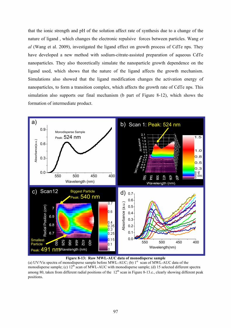
97
that the ionic strength and pH of the solution affect rate of synthesis due to a change of the
nature of ligand , which changes the electronic repulsive forces between particles. Wang et
al (Wang et al. 2009), investigated the ligand effect on growth process of CdTe nps. They
have developed a new method with sodium-citrate-assisted preparation of aqueous CdTe
nanoparticles. They also theoretically simulate the nanoparticle growth dependence on the
ligand used, which shows that the nature of the ligand affects the growth mechanism.
Simulations also showed that the ligand modification changes the activation energy of
nanoparticles, to form a transition complex, which affects the growth rate of CdTe nps. This
simulation also supports our final mechanism (b part of Figure 8-12), which shows the
formation of intermediate product.
Figure 8-13: Raw MWL-AUC data of monodisperse sample
(a) UV/Vis spectra of monodisperse sample before MWL-AUC; (b) 1st scan of MWL-AUC data of the monodisperse sample; (c) 12th scan of MWL-AUC with monodisperse sample; (d) 15 selected different spectra among 80, taken from different radial positions of the 12th scan in Figure 8-13.c., clearly showing different peak positions.
550 500 450 4000.0
0.3
0.6
0.9
Wavelength (nm)
Ab
sorb
an
ce(a
.u.)
Monodisperse Sample
Peak: 524 nm
550 500 450 4000.0
0.1
0.2
0.3
0.4
0.5
0.6
0.7
Abs
orba
nce
(a.u
.)
Wavelength(nm)
Scan12
Scan 1: Peak: 524 nm a) b)
d) c) Biggest Particle
Peak: 540 nm
Smallest Particle
Peak: 491 nm

98
8.3. Monodiperse TGA-capped CdTe nanocrystals
Monodipserse TGA-capped CdTe nanocrystals are synthesized as explained in the appendix.
It is of interest whether monodisperse samples, which were synthesized, consist of a single
particle species or not. We therefore subjected monodisperse samples to MWL-AUC.
8.3.1. Results and Discussion
8.3.1.1. Raw MWL-AUC of a monodisperse sample The UV/Vis spectrum of a monodisperse CdTe nanoparticle is shown in Figure 8-13.a with a
peak position of 524 nm. The 1st scan of MWL-AUC data on this sample also shows the
identical spectrum with a peak of 524 nm. This is the first scan after sample is transferred to
the sample column, in which fractionation has just started. Scan 12 of MWL-AUC is shown
in Figure 8-13.c. which is the last scan before the start of pelleting the sample to bottom of
the cell. In scan 12, monodisperse sample was clearly fractionated. A band gap shift was
observed even in monodisperse sample as shown in the Figure 8-13(d). These figures prove
that MWL-AUC can differentiate even in so far assumed monodisperse CdTe nanoparticles.
MWL-AUC proves that these particles are not exactly monodisperse and include different
particles. The biggest particle has a wavelength position of 540nm and the smallest particle
has a wavelength 491 nm. MWL-AUC captured 80 different spectra between 491 nm to 540
nm. 15 spectra among these 80 spectra are shown in Figure 8-13(d), which clearly shows -
spectrum at Figure 8-13(a) consist of different spectra.
8.3.1.2. Determination of CdTe mixture composition by spectrum of the sample
Spectral deconvolution is a method for the determination of the concentrations of the individual
components in a mixture via simple UV/Vis spectra. As we found that the CdTe particles that
are during growth are always of the same size, in this kind of synthesis of CdTe nanoparticles,
we can also use the spectral deconvolution of the UV/Vis spectra of any CdTe spectra.
Therefore, concentrations of each species can be obtained with this method from a simple
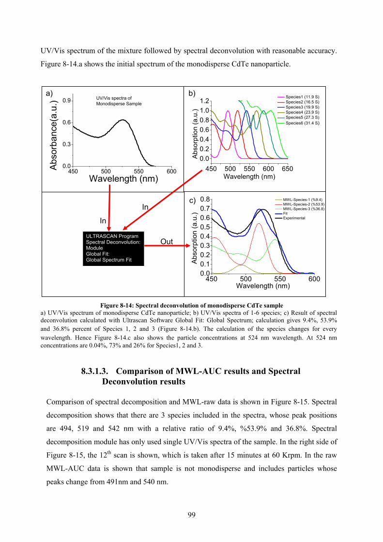
99
UV/Vis spectrum of the mixture followed by spectral deconvolution with reasonable accuracy.
Figure 8-14.a shows the initial spectrum of the monodisperse CdTe nanoparticle.
Figure 8-14: Spectral deconvolution of monodisperse CdTe sample
a) UV/Vis spectrum of monodisperse CdTe nanoparticle; b) UV/Vis spectra of 1-6 species; c) Result of spectral deconvolution calculated with Ultrascan Software Global Fit: Global Spectrum; calculation gives 9.4%, 53.9% and 36.8% percent of Species 1, 2 and 3 (Figure 8-14.b). The calculation of the species changes for every wavelength. Hence Figure 8-14.c also shows the particle concentrations at 524 nm wavelength. At 524 nm concentrations are 0.04%, 73% and 26% for Species1, 2 and 3.
8.3.1.3. Comparison of MWL-AUC results and Spectral Deconvolution results
Comparison of spectral decomposition and MWL-raw data is shown in Figure 8-15. Spectral
decomposition shows that there are 3 species included in the spectra, whose peak positions
are 494, 519 and 542 nm with a relative ratio of 9.4%, %53.9% and 36.8%. Spectral
decomposition module has only used single UV/Vis spectra of the sample. In the right side of
Figure 8-15, the 12th scan is shown, which is taken after 15 minutes at 60 Krpm. In the raw
MWL-AUC data is shown that sample is not monodisperse and includes particles whose
peaks change from 491nm and 540 nm.
450 500 550 6000.0
0.3
0.6
0.9
Wavelength (nm)
Abs
orba
nce(
a.u.
) UV/Vis spectra of Monodisperse Sample
a) b)
450 500 550 600 650
0.0
0.2
0.4
0.6
0.8
1.0
1.2 Species1 (11.9 S) Species2 (16.5 S) Species3 (19.9 S) Species4 (23.9 S) Species5 (27.3 S) Species6 (31.4 S)
Ab
sorp
tion
(a.u
.)
Wavelength (nm)
450 500 550 6000.00.10.20.30.40.50.60.70.8
Abs
orpt
ion
(a.u
.)
Wavelength (nm)
MWL-Species-1 (%9.4) MWL-Species-2 (%53.9) MWL-Species-3 (%36.8) Fit Experimental
c)
ULTRASCAN Program Spectral Deconvolution: Module Global Fit: Global Spectrum Fit
In
In
Out

100
This proves the spectral decomposition correctly determined the peaks of the sample, even
the raw data shows the same range. MWL-AUC determined the nature of the growth
mechanism. Furthermore, MWL-AUC determined that there are always identical particles
formed in different syntheses. This opened up the possibility of determining the particle
composition with using only single UV/Vis spectra of sample. Figure 8-15 proves that.
Figure 8-15: Comparison of Spectra deconvolution result and raw MWL-AUC results
a) Spectral deconvolution showing the peak position of smallest and largest particles which shows 494 nm peak for smallest particle and 542 nm peak for biggest particles; b) Scan 12 of MWL-AUC data (Figure 8-13.c); MWL data shows that the biggest particle has a peak of 540 nm and the smallest particle has a peak of 491 nm.
Scan12
b) Raw MWL-AUC data Biggest Particle
Peak: 540 nm
Smallest Particle
Peak: 491 nm
a) Spectral Deconvolution
450 500 550 6000.00.10.20.30.40.50.60.70.80.91.0
494
542
Ab
sorp
tion
(a
.u.)
Wavelength (nm)
MWL-Species-1 (%9.4) MWL-Species-2 (%53.9) MWL-Species-3 (%36.8) Fit Experimental
SmallestSpeciespeak:
494 nm
BiggestSpeciespeak:
542 nm

101
Chapter 9 : Conclusion
A prototype Static Light Scattering Detector for the analytical ultracentrifuge (SLS-AUC)
was constructed. The detector consists of a large area avalanche photodiode (LAAPD) and a
solid- state red laser. This system replaces the interference detector of the Optima XL-I.
Successful raw data measurements were taken for latex particles. Our prototype is fast, and
adaptable to the Optima XL-I. However, protein BSA could not be detected with this setup.
This shows the limitation of its sensitivity. It is concluded that further improvement of the
laser is needed. A new green laser to be tested was ordered for this purpose.
First prototype of the CCD-C-AUC has been developed. It has been proven to be rapid,
sensitive, having high resolution and adaptable to the Optima XL-I. The prototype CCD-C-
AUC is capable of gaining the absorbance of a real sample cell at all radial positions within
the time constraints of the working AUC. We are very pleased to have finalized the pre-
construction stage of this detector.
The new generation MWL-AUC is developed, whose performance is comparable or already
superior to the Optima XL-I, currently the only ultracentrifuge commercially available. This
is remarkable, as the MWL-AUC is still very much an experimental prototype and the
Optima XL-I is a finished product, for which clear specifications exist. Again, this can be
taken as an indication that we are only starting to gain glimpses of the speed, accuracy,
resolution and precision that will be possible with an optimized version of our design. It
should be pointed out that this increased performance does not come at a higher price. It is
estimated the total investment in an MWL machine to be about half the cost of purchasing an
Optima XL-I. As the design of the MWL-AUC is such that other detectors can be
accommodated as well, a cheap, precise and multidetector analytical ultracentrifuge appears
within reach. Also, each XL-I can be reversibly transferred to a MWL machine. The more
serious limitations of the current design are the absence of flash-to-flash-normalization,
which would increase the baseline accuracy of the absorbance readings at low degrees of
averaging, and the reliance on software for multiplexing the flash lamp. In our hands, this has
proven to be extremely sensitive to minor flaws in cables, insulations, soldering, etc. A
computer-independent hardware trigger is very much desired. Chromatic aberration is still an
issue which should be dealt with in future developments by the application of mirror optics.

102
From a practical point of view, however, as the radial resolution already achievable is equal
or superior to the Optima XL-I, this should not hinder the first experiments already taking
advantage of the increased information available with the MWL-AUC. It should also
encourage other users of the centrifuge to start building their own MWL-AUCs as it is a
modular system, which can be easily adapted to any of the Beckman XL ultracentrifuges and
probably also many older machines. Ideally the new users can contribute their ideas and
practical experiences to the development process and therefore make it available to the
scientific community.
For the analysis of proteins, MWL-AUC is so far only partly successful, as their s-
distribution was artificially broadened even with single wavelength data that are taken from
the multiwavelength data of MWL-AUC. Single wavelength data of MWL-AUC is shown to
be noisier than the single- wavelength data in the UV region in the Optima XL-I due to low
intensity of MWL-AUC in this region. The noise level of MWL-AUC data prevents the usage
of the spectral decomposition module of Sedphat which is a highly noise-affected method
(Balbo et al. 2005). Low intensity of reference light is the main source of noise which
prevents the usage of the spectral decomposition module of Sedphat, but it does not affect the
usage of c(s) and other analysis.
Industrial -carotene-gelatin composite particles are a highly heterogeneous system, both in
particle size and chemical composition. Fractionation of this mixture in MWL-AUC makes it
possible to resolve individual components in the mixture and detect compositional changes in
an experiment which takes only one hour. This proves the power of MWL-AUC as a direct
technique that can differentiate particles with respect to size and UV/Vis spectra. Although
our current analysis does not make it possible unambiguously to assign the spectra to defined
particles, as the particle density, swelling, composition and size may be varying
simultaneously, the presented multiwavelength analysis allows insights into this complex
system which were not previously possible using other techniques. We do not evaluate
further the directly experimentally determined sedimentation coefficients as, for our sample,
in addition to the above mentioned polydispersity, pH effects as well as charge interactions
between the colloids also have to be taken into account.
Despite these restrictions, we have shown the existence of H aggregates inside a sample that
was previously known as J aggregate, and detected spectral changes of different H-aggregate

103
populations as well as changes in the electronic potential energy surfaces of different hybrid
particles. We restricted ourselves to a semi-quantitative evaluation based on simple model-
free transformations of the data of one out of 40 scans without any prior knowledge. Clearly,
even richer phenomena can potentially be discovered with a global evaluation of the entire
dataset.
For CdTe nanoparticles, we have described a novel AUC technique allowing for the direct
experimental determination of the particle size dependence of optical and electronic
properties of CdTe semiconductor nanoparticles with atomic resolution. Furthermore, the
method determined the growth mechanism of CdTe/TGA nps. In addition, the particle size
distribution could be resolved hydrodynamically with Angström resolution together with the
UV-Vis spectra of the monodisperse species. Also continuous determination of band gap
dependence on particle size can be obtained. As the spectra of the individual components are
additive, this now makes it possible to determine the composition of CdTe mixtures by a
simple measurement of a UV-Vis spectrum and fitting to the concentration of individual
species. We need to show this by fitting the individual spectra to sums of Gaussians and then
fit the sums to the composite spectrum. From the high resolution particle size distribution, the
growth mechanism via coalescence of [Cd54Te32(SR)52]8- clusters could be revealed. Two-
dimensional spectrum analysis also showed that all CdTe nanoparticles are spherical in good
agreement with TEM data (Rogach et al. 2007). The presented technique is universally
applicable with very high resolution and adaptable to any system which shows particle-size
dependent optical properties. This is a significant advance, as MWL-AUC separates and
characterizes nanoparticles with Angström resolution (Cölfen and Pauck 1997) down to
particle sizes < 1 nm (Cölfen et al. 2002). It works directly in dispersion, has a very high
statistical accuracy as every nanoparticle is detected, has no principal solvent restrictions,
needs a very low amount of sample (15 l) and does not require prior sample fractionation
(in fact, it even works better with polydisperse samples as this gives a broader data range,
thus reducing the synthetic requirements for analysis). Furthermore, MWL-AUC showed that
monodisperse sample is not really monodisperse and includes discrete species. Additionally it
is fast, with typical experimental times of less than one hour. Within the same time span,
standard multi-hole rotors can analyze up to three colloidal mixtures with the same accuracy
in parallel, and seven mixtures are envisaged for parallel experiments in the future using an
eight-hole rotor. The described capabilities of our new AUC technique are a major

104
breakthrough for the analysis of small nanoparticles, as highly resolved particle size
distributions allow conclusions about the nanoparticle growth mechanism (Cölfen and Pauck
1997; Cölfen et al. 2002), which is important knowledge for rational synthesis design.
Therefore, application of our technique to a large number of different nanoparticle systems
can be envisaged.
Further reflections, MWL-AUC can be used to detect interactions of biopolymers (proteins-
DNA, protein-protein etc), size dependent colloid properties. MWL-AUC can also be used as
multi-sensitive turbidity detector as scattered intensity (I) is proportional to 1 / λ 4 (λ is the
wavelength of the light).
CCD-C-AUC can detect crystallization reactions faster than cyclotron detection systems.
Because cyclotron detector systems have time resolution of 50 ms (Bolze et al. 2002), while
CCD-C-AUC detector can detect a signal in the interval of 2 ms.
Future of AUC looks brilliant after announcement of Open AUC project. Open AUC project
is a combined project of all groups that are working on development of AUC. New machine
will have an open architecture, hardware standards and application interfaces for detector
developments. Software will be modular and open source so that everyone can improve the
control software by his or her own. In the future AUC will be modular based, so every user
will be able to adapt a detector to AUC, leading to their particular need. New technologies
would be easy to adapt with Open AUC project.

105
APPENDIX
Material and Methods of Protein Mixture This work is a partial recapitulation of a study published earlier (Balbo et al. 2005). The
mentioned gel-filtration standard kit has been discontinued by the manufacturer. Therefore,
BSA, IgG and rabbit muscle aldolase were purchased as individual components in
lyophylised form from SigmaAldrich. Single protein solutions were prepared by weighting
the desired protein amount and dissolving it in phosphate buffered saline (PBS) and used
without further manipulation. Protein concentrations were 1.5 mg/mL for BSA, 0.45 mg/mL
for IgG and 1.5 mg/mL for aldolase and were chosen such that the stock solutions yielded an
OD280 nm of around 1 in the standard 12 mm optical path length centerpieces used for AUC.
A mixture of these three proteins was prepared by mixing the stock solutions to equal volume
and hence signal fractions, based on OD280 nm. Single proteins were examined undiluted
and at 1:3 dilutions to mimic the signal amplitude in the mixed sample. A quantity of 400 µL
of the solution and buffer were filled in the sample and reference sector of 12 mm, double-
sector Ti centerpieces (Nanolytics, Potsdam, Germany) and capped with sapphire windows.
Experiments were simultaneously performed in a Beckman Coulter Optima XL-I and the
prototype MWL-AUC described earlier (Strauss et al. 2008)at 25 °C and 40,000 rpm on the
same solution to ensure comparability of the results. For the XL-I, sedimentation traces were
acquired at 250 nm, 280 nm and with the interference optics simultaneously. Wavelength
spectra were recorded from 230 to 350 nm with a nominal wavelength resolution of 1 nm and
five replicates for every datum point. Data from the MWL-AUC were saved over the same
wavelength range. Individual data files were created for wavelengths of 260, 270 and 280 nm
by the data acquisition software. Absorption data were acquired as fast as the respective
instrument would allow with a radial increment of 0.003 cm. Data were analyzed with Sedfit
or Sedphat. A confidence level of 0.9 was used for Thikonov-Phillips regularization.
106
Multi-wavelength analytical ultracentrifugation (MWL-AUC) method of β-
carotene microparticle system
A Multiwavelength AUC as described in (Bhattacharyya et al. 2006; Strauss et al. 2008)was
used at 25 °C. We applied a band centrifugation experiment using a Vinograd cell. In contrast
to conventional sedimentation velocity experiments, where the sample between the boundary
and the bottom of the cell is only diluted by radial dilution, in band centrifugation the sample
is diluted additionally by fractionation in the pure solvent. The reservoir is filled with a small
amount of the concentrated sample. Column and sample sectors are filled with D2O with a
density which is higher than that of the sample solution and lower than the density of the
dispersed solute. We prepared a 20 g/l solution and deposited 15 microliters of the solution
into the cell reservoir. After preliminary experiments, this concentration was chosen to ensure
that the individual components of the mixture are detected in as many scans as possible with
ODs < 1.4 in the experiment without too much dilution, which might cause noisy data.
After cell assembly, the AUC was accelerated to 5000 rpm for three minutes to transfer the
sample in the reservoir via capillaries to overlay the D2O column. Afterwards, the speed was
increased to 55,000 rpm. Forty scans were taken with a time interval of 90 seconds and a
radial step size of 50 m to observe the full sedimentation of the sample. The selected
wavelength range was from 250 nm to 750 nm. In the prototype setup, we apply the spectrum
acquired for an empty cell as a reference for the calculation of the absorption leading to a
baseline offset of 0.05 OD (see Figure 7-3(a)) After the experiment, while cleaning the cell,
we saw some precipitate in the cell reservoir. Thus, not all particles were transferred to the
sample column, but some large particles remained in the reservoir as they must have
completely sedimented already upon speeding up the rotor to 5000 rpm.
Each of the 40 scans produces a three-dimensional graph. We have radial position as x-
dimension, wavelength as y-dimension and absorbance as z-dimension. In the present
contribution, we will perform a semi-quantitative evaluation based on simple model-free
transformations of the data without any prior knowledge.
For evaluation, we have converted the radial position (r) to the sedimentation coefficient s by
using Equation 8-1.
107
The 3D absorption dataset can now be projected either onto the wavelength or the
sedimentation coefficient axis to visualize better the spectral changes with different
sedimentation coefficients or sedimentation coefficient distributions at different wavelengths.
Synthesis of TGA-capped CdTe nanocrystals and sample preparation for
AUC CdTe samples were obtained from Professor Dr. Alexander Eychmuller’s group at Dresden
Technical University. They were prepared using a technique previously reported (Gaponik et
al. 2002). Thioglycolic acid (TGA) was used as the stabilizer. The molar ratio of Cd2+/Te2-
/TGA was 1/0.5/1.3, and pH of the synthetic mixture was adjusted to 12 (Shavel et al. 2006).
The nucleation and growth of the nanocrystals proceeded by refluxing at 100 oC under open-
air conditions. The particle size was controlled by the reflux time. The as-prepared colloids
underwent post-preparative size-selective precipitation according to the procedure described
(Gaponik et al. 2002). The method consists of the gradual precipitation of the
NCs(nanocrystalles) induced by setwise addition of a non-solvent (2-propanol) into a
preliminary concentrated CdTe nanoparticle solution. This technique allows separation of the
initial colloid into several fractions of nanoparticles having narrowed size distributions.
Ultracentrifuge Method of CdTe/TGA system A solution of 15 µl CdTe was filled into the reservoir of a Vinograd zone centrifugation cell
(Figure 2-4(e)) The sample column was filled with 270 µl of D2O, the reference column with
290 µl. The experiments were performed at 25 °C on the modified Beckman Optima XL-80
K centrifuge (Beckman Coulter, Palo Alto, California) equipped with a multiwavelength
detector, as described in (Strauss et al. 2008). The experiment was started with a speed of
4000 rpm for 3 minutes in order to layer the sample in the reservoir onto the D2O in the
sample column. Then the speed was increased to 55,000 rpm. 20 radial scans with 50 µm step
size were taken at intervals of 1.5 min.

108
ABBREVIATIONS
2DSA
AD/DA
APD
ASTFEM-RA
AUC
BSA
CCD
CCD-C-AUC
CdTe
FOQELS
HDA
HPA
IgG
LAAPD
LS
MWL
MWL-AUC
OD
PBS
PMT
SEC
SDS
SLS-AUC
TGA
TOPO
UV/Vis
2 dimensional spectrum analysis
Analog to digital / digital to analog
Avalanche photodiode
Adaptive Space-Time Finite Element Method - Reversible
Associations
Analytical Ultracentrifuge
Bovine Serum Albumin
Charge-coupled device
CCD camera UV/Vis absorption detector for AUC
Cadmium Telluride
Fiber-optic quasi-classical light scattering
Hexadecylamine
Hexylphosphonic acid
Agarose
Large area avalanche photodiode
Light scattering
Multiwavelength
Multiwavelength detector for AUC
Optical density
Phosphate buffered saline
Photomultiplier tube
Size exclusion chromatography
Sodium dodecyl sulfate polyacrylamide gel electrophoresis
Static light scattering detector for AUC
Thioglycolic acid
Trioctylphosphine oxide
Static light scattering detector for AUC
109
REFERENCES
Alivisatos AP (1996) Semiconductor clusters, nanocrystals and quantum dots. Science 271:933-937
Auweter H, Haberkorn H, Heckmann W, Horn D, Luddecke E, Rieger J, Weiss H (1999) Supramolecular structure of precipitated nanosize beta-carotene particles. Angewandte Chemie-International Edition 38:2188-2191
AvivBiomedical (2008) The first commercially available fluorescence detector for analytical ultracentrifuges, Web page of Aviv Biomedical Company www.avivbiomedical.com
Balbo A, Minor KH, Velikovsky CA, Mariuzza RA, Peterson CB, Schuck P (2005) Studying multiprotein complexes by multisignal sedimentation velocity analytical ultracentrifugation. Proceedings of the National Academy of Sciences of the United States of America 102:81-86
Beams JW, Dixon HMI (1953) An ultracentrifuge double cell. Review of Scientific Instruments 24:228
BeckmanCoulter (1991) XL-A manual, Fullerton, USA Bhattacharyya SK (2006) Development of detector for analytical ultracentrifuge. Max Planck
Institutes of Colloids and Interfaces, vol PhD. Potsdam University, Potsdam Bhattacharyya SK, Maciejewska P, Börger L, Stadler M, Gülsun AM, Cicek HB, Cölfen H
(2006) Development of a fast fiber based UV-Vis multiwavelength detector for an ultracentrifuge. Progress in Colloid and Polymer Science, Analytical Ultracentrifugation VIII 131:9-22
Bolze J, Peng B, Dingenouts N, Panine P, Narayanan T, Ballauff M (2002) Formation and growth of amorphous colloidal CaCO3 precursor particles as detected by time-resolved SAXS. Langmuir 18:8364-8369
Börger L (2000) Biomimetische mineralisationsprozesse und deren charakterisierun Wissenchaftsdisziplin Physikalische Chemie, vol PhD. Univesitat Potsdam, Potsdam
Börger L, Cölfen H, Antonietti M (2000) Synthetic boundary crystallization ultracentrifugation: a new method for the observation of nucleation and growth of inorganic colloids and the determination of stabilizer efficiencies. Colloids and Surfaces A:Physicochemical and Engineering Aspects 163:29-38
Brookes E, Demeler B (2005) Genetic algorithm optimization for obtaining accurate molecular weight distributions from sedimentation velocity experiments. In: Wandrey C, Cölfen H (eds) 14th International Symposium on Analytical Ultracentrifugation. Springer-Verlag Berlin, Lausanne, Switzerland, pp 33-40
Brookes E, Demeler B (2008) Paralel computational techniques for the analysis of sedimentation velocity experiments in Ultrascan. Colloid & Polymer Science 286:138-148
Brookes EH, Boppana RV, Demeler B (2006) Computing large sparse multivariate optimization problems with an application in biophysics. Conference on High Performance Networking and Computing Proceedings of the 2006 ACM/IEEE conference on Supercomputing ACM 0-7695-2700-0/06
Brown PH, Schuck P (2006) Macromolecular size and shape distributions by sedimentation velocity analytical ultracentrifugation. Biophysical Journal 90:4651-4661
Cao WM, Demeler B (2008) Modeling analytical ultracentrifugation experiments with an adaptive space-time finite element solution for multicomponent reacting systems. Biophysical Journal 95:54-65
Cölfen H, Antonietti M (2008) Mesocrystals and nonclassical crystallization. John Wiley & Sons Ltd., West Sussex

110
Cölfen H, Pauck T (1997) Determination of particle size distributions with angstrom resolution. Colloid and Polymer Science 275:175-180
Cölfen H, Pauck T, Antonietti M (1997) Investigation of quantum size colloids using the XL-I ultracentrifuge Progress in Colloid and Polymer Science, Analytical Ultracentrifugation IV, vol 107, pp 136-147
Cölfen H, Schnablegger H, Fischer A, Jentoft FC, Weinberg G, Schlogl R (2002) Particle growth kinetics in zirconium sulfate aqueous solutions followed by dynamic light scattering and analytical ultracentrifugation: Implications for thin film deposition. Langmuir 18:3500-3509
Dagtepe P, Chikan V (2008) Effect of Cd/Te ratio on the formation of CdTe magic-sized quantum dots during aggregation. Journal of Physical Chemistry A 112:9304-9311
Dagtepe P, Chikan V, Jasinski J, Leppert VJ (2007) Quantized growth of CdTe quantum dots; Observation of magic-sized CdTe quantum dots. Journal of Physical Chemistry C 111:14977-14983
Demeler B (2005) UltraScan: A comprehensive data analysis softare package for analytical ultracentrifugation experiments. In: Scott DJ, Harding SE, Rowe AJ (eds) Modern Analytical Ultracentrifugation: Techniques and Methods. Royal Society of Chemistry, Cambridge, pp 210-229
Demeler B, Brookes E (2008) Monte carlo analysis of sedimentation experiments. Colloid & Polymer Science 286:139-137
Demeler B, van Holde KE (2004) Sedimentation velocity analysis of highly heterogeneous systems. Analytical Biochemistry 335:279-288
Eychmüller A (2000) Structure and photophysics of semiconductor nanocrystals. Journal of Physical Chemistry B 104:6514-6528
Gaponik N, Talapin DV, Rogach AL, Hoppe K, Shevchenko EV, Kornowski A, Eychmüller A, Weller H (2002) Thiol-capping of CdTe nanocrystals: An alternative to organometallic synthetic routes. Journal of Physical Chemistry B 106:7177-7185
Giebeler R (1992) The Optima XL-A: A new analytical ultracentrifuge with a novel precision absorption optical system. In: Harding SE, Rowe AJ, Horton J (eds) Analytical ultracentrifugation in biochemistry and polymer science. Royal Society of Chemistry, Cambridge, pp 16-25
Hamamatsu (2006) User Manual of Compact 5-Watt Xenon Flash Lamp Module; L9456. In: Hamamatsu (ed), Iwata city
Herron N, Calabrese JC, Farneth WE, Wang Y (1993) Crystal-structure and optical-properties of Cd32S14(SC6H5)36.DMF4, a cluster with a 15-angstrom CdS core. Science 259:1426-1428
Kegeles G (1952) A boundary forming technique for the ultracentrifuge. Journal of the American Chemical Society 74:5532
Kim H, Deonier RC, Williams JW (1977) Investigation of self-association reactions by equilibrium ultracentrifugation. Chemical Reviews 77:659-690
Lamm O (1929) Theory and methods of ultra-centrifuging. Zeitschrift fur Physikalische Chemie 143; 21 B:177; 1-190; 4
Laue TM (1996) Choosing which optical system of the optimaTM XL-I analytical ultracentrifuge to use. Beckman Instruments Inc, Fullerton
Lavrenko P, Lavrenko V, Tsvetkov V (1999) Shift interferometry in analytical ultracentrifugation of polymer solutions. In: Colfen H (ed) 11th Symposium on Analytical Ultracentrifugation. Springer-Verlag Berlin, Potsdam, Germany, pp 14-22
Lloyd PH (1974) Optical methods in ultracentrifugation, electrophoresis and diffusion: with a guide to the interpretation of records. Clarendon Press, Oxford

111
MacGregor IK, Anderson AL, Laue TM (2004) Fluorescence detection for the XLI analytical ultracentrifuge. Biophysical Chemistry 108:165-185
Mächtle W (1984) Charakterisierung von disperisionen durch gekopplete H2O/D2O-ultrazentrifugenmessungen. Macromol Chem 185:1025
Mächtle W (1992) Analysis of polymer dispersions with an eightcell-auc-multiplexer: high resolution particle size distributions and density gradient techniques. In: Harding SE, Rowe AJ, Horton J (eds) Analytical Ultracentrifugation in Biochemistry and Polymer Science. Royal Society of Chemistry, Cambridge, pp 147-175
Mächtle W (1999a) High-resolution, submicron particle size distribution analysis using gravitational-sweep sedimentation. Biophysical Journal 76:1080-1091
Mächtle W (1999b) The installation of an eight-cell Schlieren optics multiplexer in a Beckman Optima XLI/XL analytical ultracentrifuge used to measure steep refractive index gradients. Progress in Colloid and Polymer Science 113:1 - 9
Mächtle W, Börger L (2006) Analytical ultracentrifugation of polymers and nanoparticles. Springer, Berlin
Medelson M, Stahl FW (1958) The replication of DNA in Escherichia Coli. Proceedings of the National Academy of Sciences 44:671-682
Michalet X, Pinaud FF, Bentolila LA, Tsay JM, Doose S, Li JJ, Sundaresan G, Wu AM, Gambhir SS, Weiss S (2005) Quantum dots for live cells, in vivo imaging, and diagnostics. Science 307:538-544
Müller HG (1989) Automated determination of particle-size distributions of dispersions by analytical ultracentrifugation. Colloid and Polymer Science 267:1113-1116
Murray CB, Norris DJ, Bawendi MG (1993) Synthesis and characterization of nearly monodisperse CdE (E = S, Se, Te) semiconductor nanocrystallites. Journal of the American Chemical Society 115:8706-8715
Niederberger M, Garnweitner G, Krumeich F, Nesper R, Cölfen H, Antonietti M (2004) Tailoring the surface and solubility properties of nanocrystalline titania by a nonaqueous in situ functionalization process. Chemistry of Materials 16:1202-1208
OceanOptics (2008) Choosing a Grating & Wavelength Range: "USB" Optical Bench; http://www.oceanoptics.com/Products/bench_grating_usb.asp
Planken KL (2008) Analytical ultracentrifugation of inorganic colloids; sedimentation velocity of interacting and non-interacting particles, vol PhD. Universitei Utrecht, pp 166
Polivka T, Sundstrom V (2004) Ultrafast dynamics of carotenoid excited states - From solution to natural and artificial systems. Chemical Reviews 104:2021-2071
Ralston G (1993) Introduction to analytical ultracentrifguation. Beckman, California Rockenberger J, Troger L, Rogach AL, Tischer M, Grundmann M, Eychmuller A, Weller H
(1998) The contribution of particle core and surface to strain, disorder and vibrations in thiolcapped CdTe nanocrystals. Journal of Chemical Physics 108:7807-7815
Rogach AL, Franzl T, Klar TA, Feldmann J, Gaponik N, Lesnyak V, Shavel A, Eychmüller A, Rakovich YP, Donegan JF (2007) Aqueous synthesis of thiol-capped CdTe nanocrystals: State-of-the-art. Journal of Physical Chemistry C 111:14628-14637
Rogach AL, Katsikas L, Kornowski A, Su DS, Eychmuller A, Weller H (1996) Synthesis and characterization of thiol-stabilized CdTe nanocrystals. Berichte Der Bunsen Gesellschaft Physical Chemistry Chemical Physics 100:1772-1778
Schachman HK (1992) Is there a future for the ultracentrifuge? In: Harding SE, Rowe AJ, Horton J (eds) Analytical ultracentrifugation in biochemistry and polymer science. Royal Society of Chemistry, Cambridge, pp 3-31
Schmidt B, Riesner B (1992) A fluorescence detection system for the analytical ultracentrifuge and its applicaton to proteins, nucleic acids, viroids and viruses. In:

112
Harding SE, Rowe AJ, Horton J (eds) Analytical Ultracentrifugation in Biochemistry and Polymer Science. Royal Society of Chemistry, Cambridge, pp 176-207
Scholtan W, Lange H (1972) Determination of particle size distribution of latices with ultracentrifuges. Kolloid Zeitschrift und Zeitschrift Fur Polymere 250:782
Schuck P (1998) Sedimentation analysis of noninteracting and self-associating solutes using numerical solutions to the Lamm equation. Biophysical Journal 75:1503-1512
Schuck P (2000) Size-distribution analysis of macromolecules by sedimentation velocity ultracentrifugation and Lamm equation modeling. Biophysical Journal 78:1606-1619
Shavel A, Gaponik N, Eychmüller A (2006) Factors governing the quality of aqueous CdTe nanocrystals: Calculations and experiment. Journal of Physical Chemistry B 110:19280-19284
SpinAnalytical (2008) http://www.spinanalytical.com/Centerpieces.html?mode=preview. Spin Analytical, Durham
Stafford WF (1992) Boundary Analysis in sedimentation transport experiments - A procedure for obtaining sedimentation coefficient distributions using the time derivative of the concentration profile. Analytical Biochemistry 203:295-301
Stafford WF, Sherwood PJ (2004) Analysis of heterologous interacting systems by sedimentation velocity: curve fitting algorithms for estimation of sedimentation coefficients, equilibrium and kinetic constants. Biophysical Chemistry 108:231-243
Strauss HM, Karabudak E, Bhattacharyya S, Kretzschmar A, Wohlleben W, Colfen H (2008) Performance of a fast fiber based UV/Vis multiwavelength detector for the analytical ultracentrifuge. Colloid and Polymer Science 286:121-128
Svedberg T (1926) Nobel Lecture; http://nobelprize.org/nobel_prizes/chemistry/laureates/1926/svedberg-lecture.pdf
Svedberg T, Nichols JB (1923) Determination of size and distribution of size of particle by centrifugal methods. Journal of the American Chemical Society 45:2910-2917
Svedberg T, Pederson KO (1940) The Ultracentrifuge. Clarendon Press, Oxford Tang ZY, Kotov NA, Giersig M (2002) Spontaneous organization of single CdTe
nanoparticles into luminescent nanowires. Science 297:237-240 Vinograd J, Bruner R, Kent R, Weigle J (1963) Band-centrifugation of macromolecules and
viruses in self-generating density gradients. Proceedings of the National Academy of Sciences 49:902-910
Vistica J, Dam J, Balbo A, Yikilmaz E, Mariuzza RA, Rouault TA, Schuck P (2004) Sedimentation equilibrium analysis of protein interactions with global implicit mass conservation constraints and systematic noise decomposition. Analytical Biochemistry 326:234-256
Vossmeyer T, Reck G, Katsikas L, Haupt ETK, Schulz B, Weller H (1995a) A double diamond superlattice built up of Cd17S4(SCH2CH2OH)(26) clusters. Science 267:1476-1479
Vossmeyer T, Reck G, Schulz B, Katsikas L, Weller H (1995b) Double layer superlattice structure built up of Cd32S14(SCH2CH(OH)CH3)(36) . 4H2O clusters. Journal of the American Chemical Society 117:12881-12882
Wang CL, Zhang H, Xu SH, Lv N, Liu Y, Li MJ, Sun HZ, Zhang JH, Yang B (2009) sodium-citrate-assisted synthesis of aqueous CdTe nanocrystals: giving new insight into the effect of ligand shell. Journal of Physical Chemistry C 113:827-833
Zhang H, Liu Y, Zhang JH, Wang CL, Li MJ, Yang B (2008) Influence of interparticle electrostatic repulsion in the initial stage of aqueous semiconductor nanocrystal growth. Journal of Physical Chemistry C 112:1885-1889

113
Acknowledgements:
First of all, I would like to thank Prof. Dr. Markus Antonietti, for giving me an opportunity to
do my PhD at one of the most prestigious institutes not only in Germany but worldwide.
My supervisor, Dr. habil Helmut Coelfen, is sincerely acknowledged, believing me from the
very beginning, correcting the thesis, for numerous both scientific and non-scientific
discussions and for his kindness and keeping promises.
I am indebted to Borries Demeler, of the Center for Analytical Ultracentrifugation of
Macromolecular Assemblies, Texas, USA, for Ultrascan software, for the fruitful discussions
and his valuable comments.
I would like to thank Wendel Wohlleben from BASF AG, BASF SE; for his constant support
for the project, and discussions.
Prof. Dr. Tom M. Laue is thanked for the strong discussion about the constant light source
and about the detector development.
I would like to thank Dr. Glen Ramsay for his help while setting up the constant light source
and Jochen Mentges from LOT-Oriel Europe, for his help while testing a possible light
source.
Great gratitude goes to Antje Voelkel; thanks to Antje not only for AUC Measurements but
also her numerous scientific comments, very nice ideas and friendship.
I would like to express my sincere gratitude to Holger Strauss of Nanolytics, Potsdam,
Germany, for his help in conducting the tests and helping with his experience of earlier
designs of MWL-AUC, as well as his great help while doing experiments and analyzing the
results with Sedphat.
I would like to thank Emre Brookes, of the Center for Analytical Ultracentrifugation of
Macromolecular Assemblies, Texas, USA, for developing the multiwavelength developing
module for our data analysis.
Andreas Kretzschmar is thanked for his excellent work during the production of mechanical
parts and mechanical constructions.
The excellent work of Hendrik Pitas from the electronic workshop (Max Planck Institute of
Colloids and Interfaces) during the whole detector development is sincerely acknowledged.
Prof. Dr. Eychmuller, Dr. Nikoli Gaponik and Dr. Vladimir Lesynak of Dresden Technical
University are acknowledged for the synthesis of CdTe nanoparticles.

114
Arne Stark is thanked for his help while making the setup functional and for the contributions
with his knowledge of light scattering.
The companies, Advanced Photonix Inc. and Laser Components, are thanked for modifying
the LAAPD power supply for our design.
I would like to thank to my office mates; Denis Gebauer, Ruiqi Song for the friendly and
enjoyable working atmosphere.
One big thanks goes to my little Turkish community: Rezan & Mehmet, Emre, Ozlem, Yusuf,
Yasemin, Ozgur and Prof. Dr. A. Levent Demirel. And I also would like to thank all my
former/present friends and colleagues here at the institute: Antje, Michael, Arne T., Jelena,
Farnoosh, Jong, Philipp, Magda, Christine.
I want to express my gratitude to my family, Ayhan Karabudak, Vicdan Karabudak, Levent
Karabudak, Tulin Karabudak, who provided continuous understanding, patience, and energy.
They enabled the way for my education and allowed me great freedom in deciding my future.
Last but not least, I would like to thank Ozlem for her love, support and encouragement
which have sustained and uplifted me throughout this thesis.
BASF AG, BASF SE and the Max-Planck Society are also gratefully acknowledged for the
financial support of the Multiwavelength Detector project.

115
List of Publications
This thesis is partly based on the following publications
Published or Accepted Articles:
“The Open AUC Project”, Helmut Cölfen, Thomas N. Laue, Wendel Wohlleben, Kristian
Schilling, Engin Karabudak, Bradley W., Langhorst, Emre Brookes, Bruce Dubbs, Dan
Zollars, Mattia Rocco, Borries Demeler, (accepted to European Biophysics Journal)
“Investigation of -Carotene-gelatin composite particles with a Multiwavelength UV/Vis
detector for the Analytical Ultracentrifuge”, Engin Karabudak, Wendel Wohlleben, Helmut
Cölfen, (accepted to European Biophysics Journal)
“Performance of a fast fiber based UV/Vis multiwavelength detector for analytical
Ultracentrifugation”, Strauss HM., Karabudak E., Bhattacharyya S., Kretzschmar A.,
Wohlleben W., Coelfen H. , Colloid and Polymer Science, Volume 286, Issue 2, Pages 121-
128, Feb 2008.
Articles to be submitted:
“Determination of semiconductor band gap dependence on particle size with atomic
resolution”, Engin Karabudak, Emre Brookes, Holger Strauss, Vladimir Lesnyak, Nikolai
Gaponik, Alexander Eychmüller, Wendel Wohlleben, Borries Demeler, and Helmut Cölfen


![RELAXATIONSUNTERSUCHUNGEN IN UNTER- KÜHLTEN UND … · nachgewiesen werden [SKB 94], [MWL 98]. Mit der dielektrischen Spektroskopie ge- Mit der dielektrischen Spektroskopie ge- lang](https://static.fdokument.com/doc/165x107/5d5fb44b88c993ab538b54f0/relaxationsuntersuchungen-in-unter-kuehlten-und-nachgewiesen-werden-skb-94.jpg)