
Looking for -- Rig-Veda. Das Heilige Wissen. Erster Und Zweiter Liederkreis

Stephan Josel
Development of theForward Looking Terrain Avoidance
in aTerrain Awareness
and Warning System (TAWS)
MASTERARBEIT
zur Erlangung des akademischen GradesDiplom-Ingenieur
Masterstudium Geomatics Science
Technische Universität Graz
Betreuer:Ao.Univ.-Prof. Dipl.-Ing. Dr.techn. Manfred Wieser
Institut für Navigation
Graz, September 2012

Senat
Deutsche Fassung: Beschluss der Curricula-Kommission für Bachelor-, Master- und Diplomstudien vom 10.11.2008 Genehmigung des Senates am 1.12.2008
EIDESSTATTLICHE ERKLÄRUNG Ich erkläre an Eides statt, dass ich die vorliegende Arbeit selbstständig verfasst, andere als die angegebenen Quellen/Hilfsmittel nicht benutzt, und die den benutzten Quellen wörtlich und inhaltlich entnommene Stellen als solche kenntlich gemacht habe. Graz, am …………………………… ……………………………………………….. (Unterschrift) Englische Fassung:
STATUTORY DECLARATION
I declare that I have authored this thesis independently, that I have not used other than the declared
sources / resources, and that I have explicitly marked all material which has been quoted either
literally or by content from the used sources.
…………………………… ……………………………………………….. date (signature)

AcknowledgementsSince my childhood I have been fascinated by aviation and especially by the navigation
in an aircraft. My intimate desire was to become a commercial pilot. However, thatdream did not (until now) become true and I got the chance to study Geodesy. Thestudy seemed tailored perfectly to my interests for navigation and that proved true.During my study, I got the chance to gain deeper insight of navigation systems on boarda modern aircraft at my work for Axis Flight Training Systems. Finally, the companyoffered me to develop a new navigation system simulation that is based on this thesis.
In this way, I would like to thank my supervisor Univ.-Prof. Dipl.-Ing. Dr. ManfredWieser for letting me choose this very special topic and his support.
A big thanks to my (now former) employer Axis Flight Training Systems for gainingall the experience in avionics systems and the chance to write this thesis for the company.The last seven years were great and I will never forget them!
Furthermore I would like to thank my parents for supporting me in my study and mypassion in aviation by financing my pilot licenses. Especially I would like to thank mygirlfriend Sonja, who gave me motivation and hold during the last six months.
Last, but not least, I would like to thank Christoph Pöllabauer and Martin Steineggerfor reviewing this thesis and my colleagues from university for the great friendship andcommunity in the last years!
AbstractOne of the most dominant causes of accidents in aviation is still the Controlled Flight
Into Terrain (CFIT), where an airworthy aircraft under complete control of the pilot isinadvertently flown into terrain, water or an obstacle. Since the 1970s, several provisionshave been made to avoid CFIT and to mitigate its risk. One of the more recent avionicsnavigation systems for this purpose is the so-called “Terrain Awareness and WarningSystem” (TAWS). This system uses position data determined by the Global PositioningSystem (GPS) and an internal digital terrain database to warn the pilot of a hazardousapproach to terrain. In order to detect the approach, the aircraft position is predictedand intersected with the terrain database. This, so-called “Forward Looking TerrainAvoidance” (FLTA) method provides the pilot with an awareness and a warning of theterrain ahead of the aircraft.
This thesis presents the development of the FLTA in a TAWS as used in a full-flightsimulator. A mathematical model to predict the aircraft position is formulated. Thepositions predicted by this model serve as a base for establishing a so-called “SearchVolume”. The development of the search volume comprises the design of a volumeconsidering the regulatory requirements as well as the kinematics of an aircraft. Thesearch volume is eventually intersected with the terrain database. Furthermore, a modelfor a terrain database that allows fast intersection with the search volume is found.Finally, the generation of warnings for the pilot based on the result of the intersectionis addressed.

ZusammenfassungEine der dominierenden Unfallursachen in der Luftfahrt ist noch immer der “Con-
trolled Flight Into Terrain” (CFIT), bei dem ein voll funktionsfähiges Flugzeug unter derKontrolle des Piloten versehentlich in das Gelände, ins Wasser oder in ein Hindernis ges-teuert wird. Seit den 1970er Jahren wurden Vorkehrungen getroffen CFIT zu vermeidenund das Risiko dessen zu minimieren. Eines der neuesten Avionik-Navigationssysteme zudiesem Zweck ist das sogenannte “Terrain Awareness and Warning System” (TAWS). MitHilfe des Globalen Positionierung Systems (GPS) und einer internen digitalen Gelände-datenbank warnt das System den Piloten vor einer gefährlichen Annäherung an dasGelände. Das System prädiziert die Flugzeugposition und verschneidet die prädiziertenPositionen mit der Geländedatenbank. Diese Methode wird als “Forward Looking Ter-rain Avoidance” (FLTA) bezeichnet und verbessert das Bewusstsein des Piloten für dasvor dem Flugzeug liegende Gelände und warnt diesen gegebenenfalls davor.
Diese Diplomarbeit beschäftigt sich mit der Entwicklung der FLTA in einem TAWS,das in einem Full-Flight Simulator verwendet wird. Es wird ein mathematisches Mod-ell zur Prädiktion der Flugzeugposition entwickelt, das dem Erstellen eines Suchraumsdient. Die Erstellung des Suchraums berücksichtigt behördliche Auflagen als auch dieKinematik eines Flugzeugs. Letztendlich wird der Suchraum mit einer Geländedaten-bank verschnitten. Dazu wird ein Modell für eine Geländedatenbank vorgestellt, das eineschnelle Verschneidung mit dem Suchraum zulässt. Das Resultat der Verschneidung di-ent der Entwicklung einer Methode zur Auslösung von Warnungen für den Piloten.

Contents
Abbrevations and Acronyms 9
1 Introduction 111.1 Background . . . . . . . . . . . . . . . . . . . . . . . . . . . . . . . . . . 111.2 Accidents in Aviation . . . . . . . . . . . . . . . . . . . . . . . . . . . . . 121.3 TAWS System Overview . . . . . . . . . . . . . . . . . . . . . . . . . . . 14
1.3.1 History . . . . . . . . . . . . . . . . . . . . . . . . . . . . . . . . . 141.3.2 Motivation and Benefits . . . . . . . . . . . . . . . . . . . . . . . 171.3.3 System Design . . . . . . . . . . . . . . . . . . . . . . . . . . . . 181.3.4 Challenges in System Design . . . . . . . . . . . . . . . . . . . . . 20
1.4 Objective of this Thesis . . . . . . . . . . . . . . . . . . . . . . . . . . . 201.5 Definitions . . . . . . . . . . . . . . . . . . . . . . . . . . . . . . . . . . . 21
2 Position Prediction 222.1 General . . . . . . . . . . . . . . . . . . . . . . . . . . . . . . . . . . . . 222.2 Kinematics of an Aircraft . . . . . . . . . . . . . . . . . . . . . . . . . . 22
2.2.1 Position . . . . . . . . . . . . . . . . . . . . . . . . . . . . . . . . 222.2.2 Horizontal Velocity . . . . . . . . . . . . . . . . . . . . . . . . . . 232.2.3 Flightpath . . . . . . . . . . . . . . . . . . . . . . . . . . . . . . . 232.2.4 Yaw Rate . . . . . . . . . . . . . . . . . . . . . . . . . . . . . . . 24
2.3 Sensor Data . . . . . . . . . . . . . . . . . . . . . . . . . . . . . . . . . . 242.3.1 Global Positioning System (GPS) . . . . . . . . . . . . . . . . . . 242.3.2 Inertial Reference System (IRS) . . . . . . . . . . . . . . . . . . . 252.3.3 Air Data Computer (ADC) and Radio Altimeter (RA) . . . . . . 25
2.4 Aircraft Position Prediction . . . . . . . . . . . . . . . . . . . . . . . . . 262.4.1 Navigation Frame . . . . . . . . . . . . . . . . . . . . . . . . . . . 262.4.2 Detection of Straight and Turning Flight . . . . . . . . . . . . . . 262.4.3 Look Ahead Distance (LAD) . . . . . . . . . . . . . . . . . . . . . 302.4.4 Straight Flight Prediction . . . . . . . . . . . . . . . . . . . . . . 332.4.5 Turning Flight Prediction . . . . . . . . . . . . . . . . . . . . . . 352.4.6 Prediction Performance . . . . . . . . . . . . . . . . . . . . . . . . 38
3 Search Volume 403.1 General . . . . . . . . . . . . . . . . . . . . . . . . . . . . . . . . . . . . 403.2 Flight Phase Concept . . . . . . . . . . . . . . . . . . . . . . . . . . . . . 413.3 Horizontal Envelope . . . . . . . . . . . . . . . . . . . . . . . . . . . . . 42
3.3.1 TERPS / ICAO Requirements . . . . . . . . . . . . . . . . . . . . 42
6

Contents
3.3.2 ANP (Actual Navigation Performance) . . . . . . . . . . . . . . . 463.3.3 Construction of the Envelope . . . . . . . . . . . . . . . . . . . . 47
3.4 Vertical Envelope . . . . . . . . . . . . . . . . . . . . . . . . . . . . . . . 473.4.1 TSO-C151b Requirements . . . . . . . . . . . . . . . . . . . . . . 493.4.2 Construction of the Envelope . . . . . . . . . . . . . . . . . . . . 52
3.5 Combination of horizontal and vertical Envelope . . . . . . . . . . . . . . 603.5.1 Modeling the Volume . . . . . . . . . . . . . . . . . . . . . . . . . 613.5.2 Examples . . . . . . . . . . . . . . . . . . . . . . . . . . . . . . . 61
4 Intended Runway Search 654.1 General . . . . . . . . . . . . . . . . . . . . . . . . . . . . . . . . . . . . 654.2 Search Algorithm . . . . . . . . . . . . . . . . . . . . . . . . . . . . . . . 66
4.2.1 Runway Database . . . . . . . . . . . . . . . . . . . . . . . . . . . 664.2.2 Calculated Parameters . . . . . . . . . . . . . . . . . . . . . . . . 664.2.3 Score Function . . . . . . . . . . . . . . . . . . . . . . . . . . . . 674.2.4 Selection of Runways . . . . . . . . . . . . . . . . . . . . . . . . . 68
5 SearchVolume -Terrain Intersection 695.1 General . . . . . . . . . . . . . . . . . . . . . . . . . . . . . . . . . . . . 695.2 Terrain Database . . . . . . . . . . . . . . . . . . . . . . . . . . . . . . . 69
5.2.1 Definition . . . . . . . . . . . . . . . . . . . . . . . . . . . . . . . 695.2.2 Reference System . . . . . . . . . . . . . . . . . . . . . . . . . . . 705.2.3 Terrain Data Attributes and Quality Requirements . . . . . . . . 715.2.4 Resolution . . . . . . . . . . . . . . . . . . . . . . . . . . . . . . . 735.2.5 Database Model . . . . . . . . . . . . . . . . . . . . . . . . . . . . 745.2.6 Terrain Caching . . . . . . . . . . . . . . . . . . . . . . . . . . . . 80
5.3 Intersection . . . . . . . . . . . . . . . . . . . . . . . . . . . . . . . . . . 815.3.1 Terrain Cell Search . . . . . . . . . . . . . . . . . . . . . . . . . . 825.3.2 Threat Detection . . . . . . . . . . . . . . . . . . . . . . . . . . . 83
6 Alert Generation 856.1 General . . . . . . . . . . . . . . . . . . . . . . . . . . . . . . . . . . . . 856.2 Logic . . . . . . . . . . . . . . . . . . . . . . . . . . . . . . . . . . . . . . 85
6.2.1 Alert Triggering . . . . . . . . . . . . . . . . . . . . . . . . . . . . 856.2.2 Alert Cancellation . . . . . . . . . . . . . . . . . . . . . . . . . . 86
7 Implementation and Outlook 877.1 General . . . . . . . . . . . . . . . . . . . . . . . . . . . . . . . . . . . . 877.2 Prototype Development . . . . . . . . . . . . . . . . . . . . . . . . . . . . 877.3 Final Implementation . . . . . . . . . . . . . . . . . . . . . . . . . . . . . 887.4 Outlook . . . . . . . . . . . . . . . . . . . . . . . . . . . . . . . . . . . . 92
List of Figures 92
7

Contents
List of Tables 94
Bibliography 95
8

Abbrevations and Acronyms
ADC Air Data Computer
ANP Actual Navigation Performance
CFIT Controlled Flight Into Terrain
DTM Digital Terrain Model
EGM Earth Gravitational Model
EGPWS Enhanced Ground Proximity Warning System
FAA Federal Aviation Administration (U.S. Department of Air Transportation)
FAF Final Approach Fix
FLTA Forward Looking Terrain Avoidance
GPS Global Positioning System
GPWS Ground Proximity Warning System
HFOM Horizontal Figure of Merit
IAF Initial Approach Fix
ICAO International Civil Aviation Organization
IFR Instrument Flight Rules
ILS Instrument Landing System
IMS Inertial Measurement System
IRS Inertial Reference System
ITI Imminent Terrain Impact
LAD Look Ahead Distance
LOD Level of Detail
9

Abbrevations and Acronyms
MA Moving Average
MIP Multum in Parvo
MOC Minimum Obstacle Clearance
MSL Mean Sea Level
NDB Non Directional Beacon
NED North-East-Down
OAS Obstacle Assessment Surfaces
RA Radio Altimeter
RNAV Area Navigation
ROC Required Obstacle Clearance
RTC Reduced Terrain Clearance
SA Situational Awareness
SRTM Shuttle Radar Topography Mission
TA Terrain Awareness
TAWS Terrain Awareness and Warning System
TERPS Terminal Instrument Procedures (FAA)
VFOM Vertical Figure of Merit
VFR Visual Flight Rules
VOR VHF Omnidirectional Range
10

1 Introduction
1.1 Background
Since the first flight of a powered aircraft in 1903, aviation has undergone a meteoric rise.Today, traveling by plane has become a matter of course. Air transport has increasedsignificantly since the middle of the last century and will keep on doing so in the future.As with many technical and engineering disciplines, the technological advancement inaviation has been immense over the last 50 years. Aircraft have become larger, fasterand safer. Especially safety is of high importance in aviation. Piloting an aircraft canbe quite a challenging task. Loosely speaking, as the aircraft moves in three dimensionsand at high speed, the human operator can rather quickly become overburdened by histasks. The human with his “human factor” is therefore the dominant cause of accidentsin aviation. Hence, the aim of the aviation industry has always been to support thehuman operator by introducing new and better technology as well as by enhancing thetraining of pilots.
Nevertheless, one of the most dominant causes for aircraft accidents is still the Con-trolled Flight Into Terrain (CFIT), where an airworthy aircraft under complete controlof the pilot is inadvertently flown into terrain, water or an obstacle, cf. [10]. The analysisof accidents which happened the 1960s and 1970s lead to the development of a system toprevent these CFIT accidents. This development resulted in the invention of the GroundProximity Warning System (GPWS), which warns the crew of hazardous terrain closure.GPWS was mandated by the Federal Aviation Administration (FAA) to be installed inall U.S. large turbine and turbojet aircraft in 1974. The introduction of this system leadto a significant decrease in CFIT accidents.
As a consequence of those CFIT accidents that still existed, the GPWS was enhancedin the mid 1990s. New navigation technology such as the Global Positioning System(GPS) and new computer technology lead to the development of the Terrain Awarenessand Warning System (TAWS). The TAWS contains the GPWS functionality plus someenhancements. While the GPWS issues warnings based on the radio altimeter, theTAWS additionally uses position information and a digital terrain database to issuewarnings. The crew is warned earlier and the Situational Awareness (SA) is improved.
The FAA mandated the installation of a TAWS in March 2000 for all U.S. turbinepowered aircraft with six or more passenger seats. The International Civil AviationOrganization (ICAO) mandated the installation for all aircraft of a maximum certifiedtakeoff mass in excess of 5700 kg or authorized to carry more than nine passengers in2007 [22].
11

1 Introduction
0
200
400
600
800
1000
1200
1400
1600
1800
2000
LOC-I CFIT RE (Landing)+ ARC
+ USOS
UNK MAC SCF-NP RE (Takeoff) OTHR WSTRW FUEL RAMP F-NI SCF-PP
Fatalities by CAST/ICAO Common Taxonom y Team (CICTT) Aviation Occurre nce CategoriesFatal Accidents – Wor ldwide Commercial Jet Fleet – 2002 Through 2011
Number of fatal accidents (79 total)
Fatalities
External fatalities [Total 214]
Onboard fatalities [Total 4547]
Note: Principal categories as assigned by CAST.
1493 (80)
430 (0)
225 (0)156 (69)
1 (7)
121 (1) 96 (1)
154 (38)
1 (2)
1078 (0)
765 (16)
ARC Abnormal Runway ContactCFIT Controlled Flight Into or Toward TerrainF-NI Fire/Smoke (Non-Impact)FUEL Fuel RelatedLOC-I Loss of Control – In flight MAC Midair/Near Midair CollisionOTHR OtherRAMP Ground HandlingRE Runway Excursion (Takeoff or Landing)SCF-NP System/Component Failure or Malfunction (Non-Powerplant)SCF-PP System/Component Failure or Malfunction (Powerplant)UNK Unknown or UndeterminedUSOS Undershoot/OvershootWSTRW Windshear or Thunderstorm
No accidents were noted in the following principal categories:ADRM AerodromeAMAN Abrupt ManeuverATM Air Traffic Management/Communications, Navigation, SurveillanceBIRD Bird CABIN Cabin Safety EventsEVAC EvacuationF-POST Fire/Smoke (Post-Impact)GCOL Ground CollisionICE IcingLALT Low Altitude OperationsLOC-G Loss of Control – GroundRI-A Runway Incursion – AnimalRI-VAP Runway Incursion – Vehicle, Aircraft or PersonSEC Security RelatedTURB Turbulence Encounter
For a complete description go to: http://www.intlaviationstandards.org/
23 (0)4 (0)
External fatalitiesOnboard fatalities
18 15 4 2 2 1 818 22151
222011 STATISTICAL SUMMARY, JULY 2012 Copyright © 2012 Boeing. All rights reserved.
Figure 1.1: Boeing Accident Categories, taken from [3]
1.2 Accidents in Aviation
The investigation of accidents is a key to finding new and better technology to improvesafety, which plays an important role in aviation. Reports on the safety of air trafficare released annually. The aircraft manufacturer Boeing for example releases a statisticof commercial jet aircraft accidents [3] every year. Note that this statistic only coversaccidents with jet aircraft with a maximum take off weight of over 27 tons and excludesany accidents that happened with aircraft manufactured in the former USSR. Amongmore than 20 million flights per year, the statistic lists a total of 36 accidents. For adefinition of accident consult [3], p. 8. The following enumeration lists the top threecauses of accidents with fatalities (see also figure 1.1):
1. Loss of Control in Flight
2. Controlled Flight Into Terrain (CFIT)
3. Runway Excursion
These causes are compiled from data gathered between 2002 and 2011. CFIT is still thenumber two cause of the investigated accidents. CFIT is defined as follows (taken fromSKYbrary, a Wiki created by Eurocontrol and ICAO [11]):
“Controlled Flight into Terrain (CFIT) occurs when an airworthy aircraftunder the complete control of the pilot is inadvertently flown into terrain,
12

1 Introduction
water, or an obstacle. The pilots are generally unaware of the danger untilit is too late.”
The fact that the aircraft was still airworthy is notable. The crew was just unawareof its position relative to terrain and could not react early enough to avoid a collision.The effect of CFIT is mostly a collision with the ground, resulting in hull loss andfatalities. Hull loss defines the status of an aircraft which has been destroyed or hasbeen determined to have been damaged beyond economic repair, cf. [12].
As the crew was unaware of their position, they might have lost situational awareness(SA) of the surrounding terrain. The term situational awareness plays an importantrole in aviation since it contributes to the safety of the flight. Situational awareness isdefined in literature multiple times, one clear definition from the SKYbrary [13] reads:
“Situational awareness is defined as the continuous extraction of environmen-tal information, the integration of this information with previous knowledgeto form a coherent mental picture, and the use of that picture in directingfurther perception and anticipating future events.”
In terms of navigational awareness the questions “Where am I?” and “Where to go?”are of relevance ([18], p.2). The crew uses the information gathered from the cockpitenvironment (e.g. navigation displays) to determine the aircraft position as well as thesituation around the aircraft and to finally decide where and how to go next basedupon this position. Lack of knowledge of the true aircraft position leads to the lossof situational awareness and the loss of the ability to anticipate future events. Futureevents may be the start for descent for approach or the approach towards an area withmountainous terrain.
Losing the SA in portions of flight that are close to terrain such as departure orapproach can lead to CFIT. Contributory factors for CFIT are [11]:
• Adverse Weather Conditions
• Approach Design and Documentation
• Deficient Crew Resource Management
• Pilot Fatigue and Disorientation
Approaches in adverse weather conditions demand a higher workload of the crew thanin good conditions. A typical situation would be when the crew loses visual contactwith the runway on a visual approach and enters clouds. The design of an approachprocedure in mountainous terrain leads inevitably to predefined flight paths that areclose to terrain. Insufficient or bad documentation of the procedure may lead to the lossof SA. Deficient crew resource management (e.g. coordination between crew membersand division of workload) is also a contributing factor especially during challengingapproaches in mountainous regions. Finally, physiological factors such as fatigue anddisorientation lead to reduced pilot performance and ultimately to the loss of SA.
13

1 Introduction
Typical indications of CFIT are the deviation from procedures and/or a desired flightpath. During departure, the aircraft may not climb too steeply enough or climb belowthe desired climb path and thus get close to terrain. The same applies if the aircraftdeviates from its desired lateral flight path. During approach, the crew may have awrong altimeter setting of the local barometric pressure and therefore be too low. Lateraldeviation while simultaneously undershooting a minimum safe altitude may also lead toundesired closure to terrain. Lateral deviation may be the result of lost SA or radarvectoring during a radar guided approach by an air traffic controller. Finally, a prematuredescent on final approach could also cause a CFIT.
Some of the risk factors discussed above can be mitigated or even eliminated by usingequipment that helps the crew to improve their SA and that warns them of a hazardousclosure or even an impact to terrain. As mentioned above, the GPWS is an equipment ofthis type and was introduced in the 1970s. Later, as technology progressed, the TAWSwas introduced in the mid 1990s to enhance the GPWS. With respect to the risk factors,the following basic requirements can be stated for a TAWS:
• A TAWS should detect any hazardous terrain closure.
• A TAWS should warn the crew early enough to allow for evasive actions and toprevent a CFIT.
• A TAWS should improve the SA of the crew during all phases of flight.
1.3 TAWS System Overview
1.3.1 History
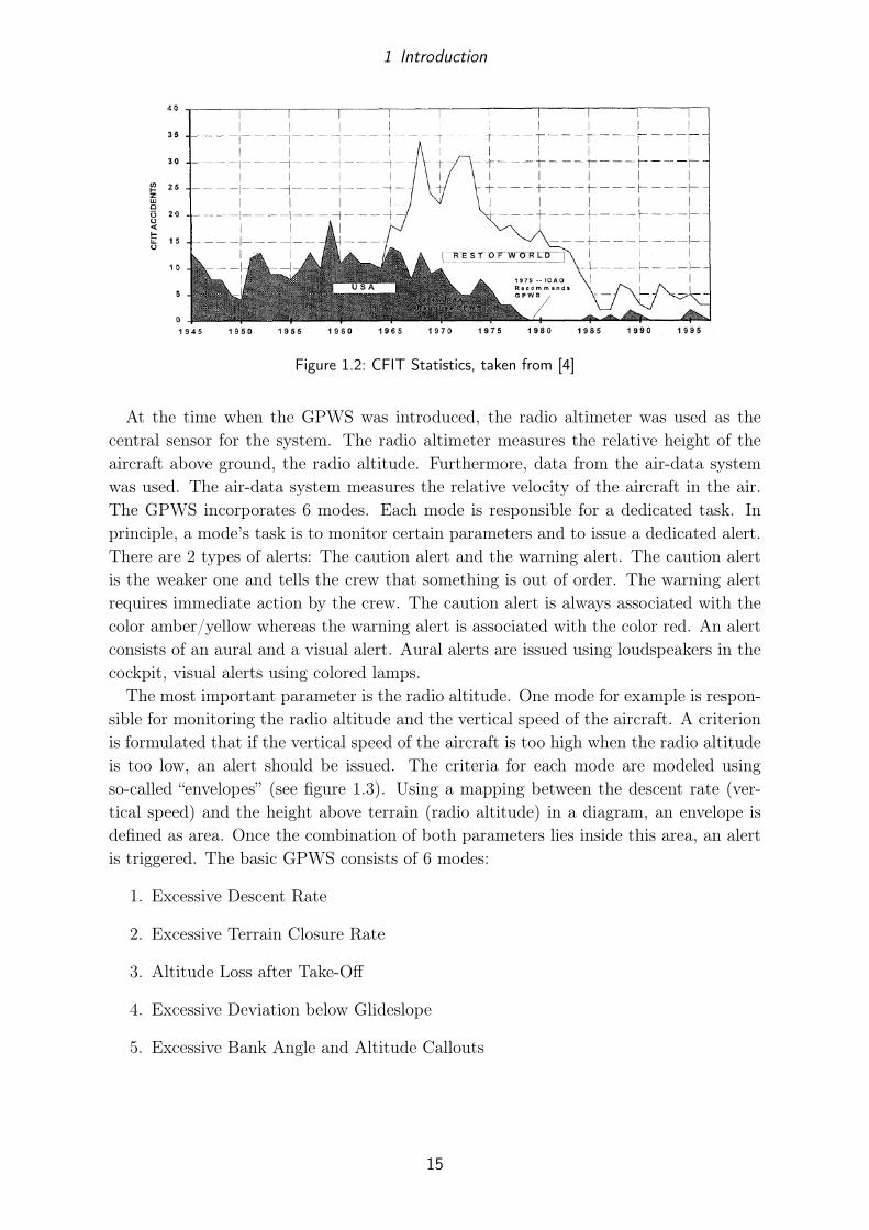
Accident investigations in the early 1970s revealed that CFIT was the most dominantcause for aircraft accidents [27]. Until then, no system preventing these types of accidentswas available. By 1974, the GPWS had been developed and mandated by the FAA to becarried on board on all U.S. large turbine and turbojet aircraft. With the introductionof the GPWS, the CFIT rate in the U.S. dropped dramatically (see figure 1.2). Theintroduction of a GPWS with enhanced functionality in 1996 lead to a further decline inthe number of CFIT accidents. 2004 was the first year without any CFIT for jet aircraftat all [5]. In 2006, the loss of control in flight took over as the leading accident cause inaviation for jet aircraft [6]. Reviewing these facts reveals the importance of the systemover almost the whole of the last 40 years. However, the number of CFIT accidents forthe turboprop aircraft is still significantly high [6].
One of the most recent CFIT accidents in aviation history, despite carrying a functionalTAWS, was the accident of a TU-154 in April 2010 near Smolensk (Russia), killing all96 people on board, among them the Polish president [7]. Another remarkable recentaccident was the crash of AirBlue flight 202, Airbus A321, in July 2010 near Islamabad(Pakistan), killing all 152 people on board [1].
14
1 Introduction
Figure 1.2: CFIT Statistics, taken from [4]
At the time when the GPWS was introduced, the radio altimeter was used as thecentral sensor for the system. The radio altimeter measures the relative height of theaircraft above ground, the radio altitude. Furthermore, data from the air-data systemwas used. The air-data system measures the relative velocity of the aircraft in the air.The GPWS incorporates 6 modes. Each mode is responsible for a dedicated task. Inprinciple, a mode’s task is to monitor certain parameters and to issue a dedicated alert.There are 2 types of alerts: The caution alert and the warning alert. The caution alertis the weaker one and tells the crew that something is out of order. The warning alertrequires immediate action by the crew. The caution alert is always associated with thecolor amber/yellow whereas the warning alert is associated with the color red. An alertconsists of an aural and a visual alert. Aural alerts are issued using loudspeakers in thecockpit, visual alerts using colored lamps.
The most important parameter is the radio altitude. One mode for example is respon-sible for monitoring the radio altitude and the vertical speed of the aircraft. A criterionis formulated that if the vertical speed of the aircraft is too high when the radio altitudeis too low, an alert should be issued. The criteria for each mode are modeled usingso-called “envelopes” (see figure 1.3). Using a mapping between the descent rate (ver-tical speed) and the height above terrain (radio altitude) in a diagram, an envelope isdefined as area. Once the combination of both parameters lies inside this area, an alertis triggered. The basic GPWS consists of 6 modes:
1. Excessive Descent Rate
2. Excessive Terrain Closure Rate
3. Altitude Loss after Take-Off
4. Excessive Deviation below Glideslope
5. Excessive Bank Angle and Altitude Callouts
15

1 Introduction
Figure 1.3: GPWS Mode 1 Envelope, taken from [15]
Each mode has its own envelope and alert characteristics. Some modes are active duringall phases of flight, while others are active only during, for example, take-off. Withrespect to the enhanced functionality in a TAWS, mode 2 is of interest.
Mode 2 tries to detect if the aircraft has an excessive terrain closure rate towardsterrain. Terrain closure may be caused when the aircraft either descends or when itflies at a certain level or climbs and the terrain is rising as illustrated in figure 1.4. Theclosure rate is calculated using the differentiated radio altitude with respect to time.When the radio altitude is too low and the terrain closure rate too high (defined bythe envelope), mode 2 initially issues the aural caution “Terrain-Terrain”, followed bythe continuous aural warning “Pull-Up”. One drawback of mode 2 is evident: As theradio altimeter measures the relative height of the aircraft above ground, a steep risingterrain ahead of the aircraft may be detected too late to allow for evasive maneuvers.The system simply does not look forward, it only looks down. This is one of the mostimportant factors that eventually caused the advancement to the TAWS.
The requirements for a TAWS are regulated. They define the minimum performancestandards that a TAWS must posses in order to certify it for airborne use. They areregulated in the FAA Technical Standard Order (TSO) C151b [15]: “Terrain Awarenessand Warning System”
Today, the market for GPWS and TAWS is dominated by Honeywell. Honeywell haspioneered the GPWS with the invention of the system and later on with the enhancedGPWS called Enhanced GPWS (EGPWS). Note that TAWS is the collective term usedby the FAA, whereas EGPWS is the implementation of a TAWS by Honeywell. Hon-eywell has delivered about 70,000 GPWS and EGPWS units. Other manufacturers areUniversal Avionics, Thales or Sandel Avionics.
16

1 Introduction
Figure 1.4: GPWS Mode 2 Envelope Illustration, taken from [20]
Radio AltimeterMeasurement
TERRAIN
Flight Path
Impact withTerrain
Aircraft
Figure 1.5: Downward Looking Concept
1.3.2 Motivation and Benefits
As discussed in the section above, the GPWS’s drawback is the nature of how it works.It simply looks downward by using the radio altitude. There is no anticipation of theterrain closure. Figure 1.5 illustrates this. At the aircraft position, the terrain is rising,but the terrain closure rate is too low to issue a GPWS mode 2 alert. However, terrainobstructs the flight path ahead. If the crew is not warned, a terrain impact is inevitable.This shortcoming that is characteristic of the GPWS lead to the development of theTAWS. Especially with the introduction of GPS, its full operational capability whichwas achieved in 1995 [19] and the availability of digital terrain databases, the foundationstones for an enhanced system with new capabilities were given.
Some basic requirements for a TAWS that stem from the “lessons learned” in the CFITaccidents are listed in section (1.2). The main drawback of the GPWS - the late issuing
17

1 Introduction
Envelope
TERRAIN
Flight Path
"Terrain-TerrainPull-Up Pull-Up"
GPS
Aircraft
Figure 1.6: Forward Looking Concept
of an alert - is eliminated by introducing a concept that looks ahead of the aircraft.Looking ahead requires knowing the aircraft position and predicting the flight path.While the GPWS measures the radio altitude to detect alerts, the TAWS uses a digitalterrain database and tries to find conflicting terrain that lies within the predicted flightpath. This method is called “Forward Looking Terrain Avoidance” (FLTA). In figure 1.6the same situation as in figure 1.5 is depicted. Figure 1.6 shows the enhancement of theGPWS. The aircraft position is determined using GPS, a virtual envelope is establishedand as the envelope penetrates the terrain, an aural alert, approximately 30-60 secondsahead of the terrain, “Terrain-Terrain Pull-Up Pull-Up” is issued. The crew can reactearly enough and initiate an evasive maneuver. Note that the basic GPWSmodes are stilloperating, they are just enhanced by the FLTA. The situational awareness is improvedby generating a picture of the terrain in the vicinity of the aircraft on the navigationdisplay in the cockpit. This generated picture is called terrain display. The combinedfunctionality of the FLTA and the terrain display is denoted as “Terrain Awareness”(TA).
1.3.3 System Design
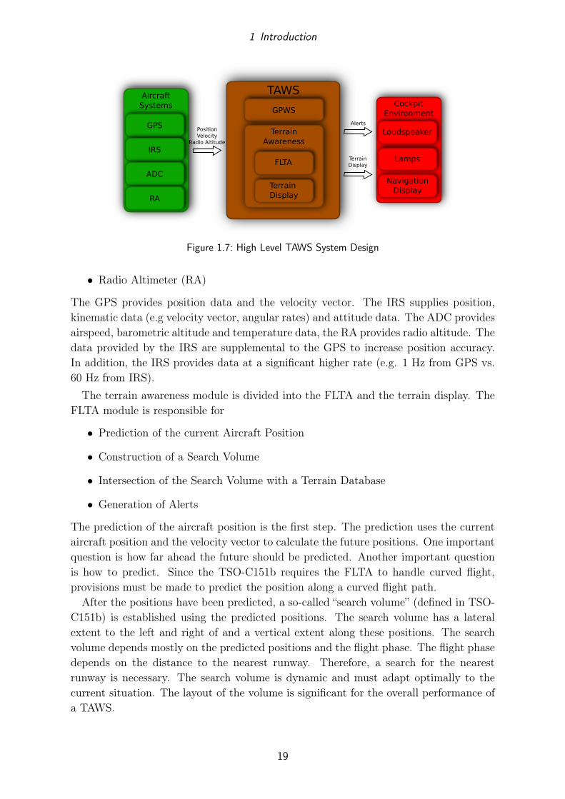
A high level system design of a TAWS is shown in figure 1.7. The TAWS receivesinputs from various aircraft systems and processes them in the main modules GPWSand terrain awareness. The GPWS and the terrain awareness modules generate alertsand the terrain display. The alerts are presented within the cockpit environment onloudspeaker and lamps, the terrain is displayed on the navigation display.
The following aircraft systems are commonly used:
• GPS
• Inertial Reference System (IRS)
• Air Data Computer (ADC)
18
1 Introduction
TAWSCockpit
Environment
LoudspeakerAlerts
TerrainDisplay
PositionVelocity
Radio Altitude
AircraftSystems
GPS
IRS
ADC
RA
GPWS
TerrainAwareness
FLTA
TerrainDisplay
Lamps
NavigationDisplay
Figure 1.7: High Level TAWS System Design
• Radio Altimeter (RA)
The GPS provides position data and the velocity vector. The IRS supplies position,kinematic data (e.g velocity vector, angular rates) and attitude data. The ADC providesairspeed, barometric altitude and temperature data, the RA provides radio altitude. Thedata provided by the IRS are supplemental to the GPS to increase position accuracy.In addition, the IRS provides data at a significant higher rate (e.g. 1 Hz from GPS vs.60 Hz from IRS).
The terrain awareness module is divided into the FLTA and the terrain display. TheFLTA module is responsible for
• Prediction of the current Aircraft Position
• Construction of a Search Volume
• Intersection of the Search Volume with a Terrain Database
• Generation of Alerts
The prediction of the aircraft position is the first step. The prediction uses the currentaircraft position and the velocity vector to calculate the future positions. One importantquestion is how far ahead the future should be predicted. Another important questionis how to predict. Since the TSO-C151b requires the FLTA to handle curved flight,provisions must be made to predict the position along a curved flight path.
After the positions have been predicted, a so-called “search volume” (defined in TSO-C151b) is established using the predicted positions. The search volume has a lateralextent to the left and right of and a vertical extent along these positions. The searchvolume depends mostly on the predicted positions and the flight phase. The flight phasedepends on the distance to the nearest runway. Therefore, a search for the nearestrunway is necessary. The search volume is dynamic and must adapt optimally to thecurrent situation. The layout of the volume is significant for the overall performance ofa TAWS.
19

1 Introduction
Once the search volume has been constructed, the next step is to intersect it witha terrain database. The TAWS contains a dedicated terrain database. The task is tofind all terrain that penetrates the volume. The terrain database is modeled to alloweffective access with the searchvolume -terrain intersection in mind.
Finally, if terrain that penetrates the volume was found, the alert generation is respon-sible for examining this terrain and issues an alert. Again, as described above (section1.3.1), two types of alert exist: The caution and the warning alert. Both types of alertare announced through the cockpit environment’s loudspeaker and lamps.
1.3.4 Challenges in System Design
The objective of a TAWS is to be a reliable navigation system that warns the crewearly enough against hazardous terrain closure and to improve the crew’s situationalawareness. However, when designing a TAWS, one must especially take care of thereliability of the system. One major problem of a TAWS is the generation of falsealerts or so-called “nuisance alerts”1 (defined in TSO-C151b [15], appendix 1, p. 3).These alerts occur inappropriately during normal safe operations. The crew may loseconfidence in the system if these alerts occur too often. The challenge in designing thesystem is to construct a search volume that does not cause nuisance alerts on the onehand but on the other hand does not discard a potential hazardous terrain closure.
Another challenge is to handle the large amount of terrain data contained in theterrain database. Since a TAWS may be used globally, effective methods for storing andaccessing the data have to be designed.
1.4 Objective of this Thesis
The objective of this thesis is to find solutions for the tasks executed by the FLTA. Thismeans to find a solution for the following points:
• Aircraft Position Prediction (chapter 2)
• Construction of a Search Volume (chapter 3)
• Method to find the nearest Runway (chapter 4)
• Intersection of the Search Volume with a Terrain Database (chapter 5)
• Method to generate Alerts (chapter 6)
The solutions found are used to develop a TAWS for a Full-Flight Simulator which isused for pilot training.
The chapter “Position Prediction” explores how to predict the aircraft position witha given set of parameters. This involves the setup of an appropriate algorithm.
1An inappropriate alert, occurring during normal safe procedures, that occurs as a result of a designperformance limitation of TAWS.
20

1 Introduction
The chapter “Search Volume” deals with the design of a search volume that generatesa minimum of nuisance alerts. Several parameters that influence the shape of the volumeare considered.
In the chapter “Intended Runway Search” a solution is found for detecting the nearestrunway in the vicinity of the aircraft.
Chapter “SearchVolume -Terrain Intersection” defines a design for a terrain databasethat is well fitted for the intersection with the search volume. Furthermore, an effectivemethod for the intersection of the search volume with the terrain database is described.
Chapter “Alert Generation” presents a method to generate alerts based on the resultsfrom the searchvolume -terrain intersection.
The last chapter “Implementation and Outlook” describes briefly the development andimplementation process.
1.5 Definitions
For the sake of completeness, table 1.1 lists the units and their description used through-out this thesis:
Table 1.1: Units used
Unit Name Descriptionft Feetkt Knots (Nautical Miles per Hour)NM Nautical Milesdeg Degreessecs SecondsG Earth’s Gravity
Figure 1.8 shows the symbology used for the aircraft in this document.
Horizontal Vertical
Figure 1.8: Aircraft Symbology
21

2 Position Prediction
2.1 General
The aim of the position prediction is to determine the aircraft position in the near future.Depending on the speed of the aircraft, the position is predicted for about 30 sec to 1 minahead in time. The prediction accounts for straight and turning flight. Vital aspects arethe accuracy and integrity of the predicted position. The following chapter will give ashort introduction into the kinematics of an aircraft and will then deal with the positionprediction itself.
2.2 Kinematics of an Aircraft
A TAWS requires input from various aircraft systems. The sensors of the systems(directly or indirectly) measure the kinematics of an aircraft. The kinematics of anaircraft is described by a set of parameters that are the result of the underlying dynamics.For the prediction in the TAWS the following parameters are needed:
• Position
• Horizontal Velocity
• Flightpath
• Yaw Rate
These parameters are used to find a suitable simplified “dynamics model” that formsthe base for the prediction. Precise information about the underlying dynamics is notavailable and not desirable since the prediction should work for any aircraft.
2.2.1 Position
The position is given in form of latitude (ϕ), longitude (λ) and altitude (h). The latitudeand longitude together define the horizontal position.
The altitude has to be treated separately. The primary altitude reference in aviationis barometric. The instruments in the cockpit display the altitude measured by barom-eters. These measurements are subject to various factors such as the local pressure ortemperature. As a TAWS primarily relies on the GPS position and altitude, it is com-plemented with other systems that measure for example the barometric altitude. With
22

2 Position Prediction
TT
n
e
ψ
vNED
n-e Plane
θ
γ vNEDδ
d
Figure 2.1: Illustration of Velocity Vector and associated Angles
respect to a terrain database, it is very important to find a common altitude referencesystem.
For the sake of completeness, the horizontal and vertical datum of the position mustmatch the horizontal and vertical datum of the used terrain database (see chapter 5).
2.2.2 Horizontal Velocity
For defining the velocity, a local level frame is introduced. The local level frame’s originis arbitrary. It is defined by a three-dimensional, right-handed Cartesian system withthe x1 axis pointing north, the x2 axis pointing east and the x3 axis pointing down indirection of the nadir. A vector in this system is comprised of components in north (n),east (e) and down (d) direction, indicated by the subscripts n, e and d. The frame isdenoted as N(orth)-E(ast)-D(own)-frame (NED).
The velocity vector contains the velocities along each axis of the NED-frame:
vNED =
vnvevd
(2.1)
Horizontal velocity (vNEDhor ) is derived from the individual components of the vector:
vNEDhor =√v2n + v2e (2.2)
2.2.3 Flightpath
The flightpath of an aircraft is derived from the velocity vector. The flightpath is definedas the direction in which the aircraft is flying with respect to the NED-frame. Therefore,the direction of the flightpath is split into a horizontal and a vertical component. Thevertical component is described by the angle γ, the horizontal component by the angleTT . γ is also known as the flightpath angle and TT is known as true track (subscript T
23
2 Position Prediction
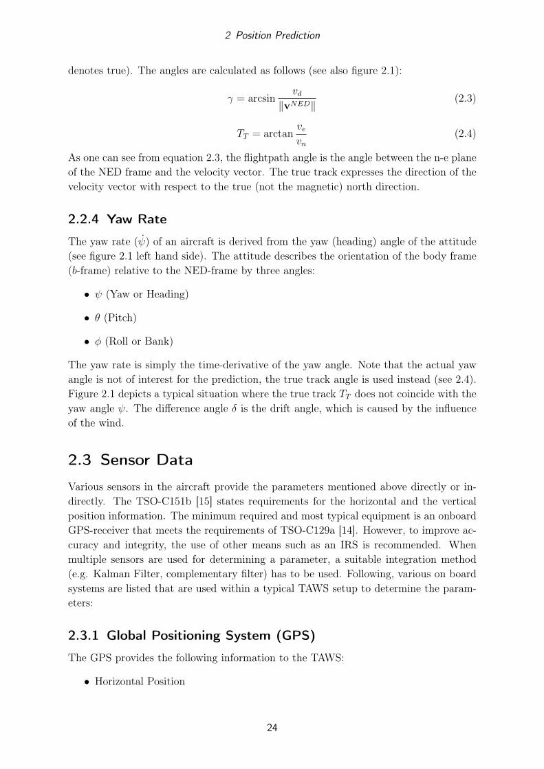
denotes true). The angles are calculated as follows (see also figure 2.1):
γ = arcsinvd
‖vNED‖(2.3)
TT = arctanvevn
(2.4)
As one can see from equation 2.3, the flightpath angle is the angle between the n-e planeof the NED frame and the velocity vector. The true track expresses the direction of thevelocity vector with respect to the true (not the magnetic) north direction.
2.2.4 Yaw Rate
The yaw rate (ψ) of an aircraft is derived from the yaw (heading) angle of the attitude(see figure 2.1 left hand side). The attitude describes the orientation of the body frame(b-frame) relative to the NED-frame by three angles:
• ψ (Yaw or Heading)
• θ (Pitch)
• φ (Roll or Bank)
The yaw rate is simply the time-derivative of the yaw angle. Note that the actual yawangle is not of interest for the prediction, the true track angle is used instead (see 2.4).Figure 2.1 depicts a typical situation where the true track TT does not coincide with theyaw angle ψ. The difference angle δ is the drift angle, which is caused by the influenceof the wind.
2.3 Sensor Data
Various sensors in the aircraft provide the parameters mentioned above directly or in-directly. The TSO-C151b [15] states requirements for the horizontal and the verticalposition information. The minimum required and most typical equipment is an onboardGPS-receiver that meets the requirements of TSO-C129a [14]. However, to improve ac-curacy and integrity, the use of other means such as an IRS is recommended. Whenmultiple sensors are used for determining a parameter, a suitable integration method(e.g. Kalman Filter, complementary filter) has to be used. Following, various on boardsystems are listed that are used within a typical TAWS setup to determine the param-eters:
2.3.1 Global Positioning System (GPS)
The GPS provides the following information to the TAWS:
• Horizontal Position
24

2 Position Prediction
• Altitude
• Horizontal Figure of Merit (HFOM)
• Vertical Figure of Merit (VFOM)
• True Track
• Flight Path Angle
• Ground Speed
The horizontal position contains the latitude and longitude in WGS84 coordinates. Thealtitude is ellipsoidal and must be converted finally to the same vertical datum as that ofthe terrain database, otherwise errors due to the different datums may occur later in theFLTA. The HFOM expresses the accuracy of the horizontal position in nautical miles,the VFOM the accuracy of the altitude in ft. Both represent the accuracy on a 95%confidence level and are important factors to determine the reliability of the suppliedinformation. The true track is provided along with the ground speed. The true track andground speed contain some lag because these informations are derived from positionsover time.
2.3.2 Inertial Reference System (IRS)
The IRS provides the following information to the TAWS:
• Horizontal Position
• Horizontal Figure of Merit (HFOM)
• True Track
• Flight Path Angle
• Ground Speed
• Yaw Rate
Similar to the GPS, the IRS provides information about the horizontal position andattitude. However, the IRS provides the information at a much higher rate than GPS(about 60Hz in case of IRS) and is also denoted as Inertial Measurement System (IMS)in geodesy.
2.3.3 Air Data Computer (ADC) and Radio Altimeter (RA)
The ADC provides barometric altitude to the TAWS. The barometric altitude must behandled with care because it is influenced by atmospheric conditions and pilot settings.The RA provides the radio altitude, which is the relative height of the aircraft abovethe ground.
25

2 Position Prediction
2.4 Aircraft Position Prediction
The aircraft position prediction predicts the horizontal position of the aircraft. Theobjective is to know where the aircraft will be in the future. The result of the prediction isa series of positions. The positions are sampled with a certain time step. The predictionmust account for straight (ψ = 0) and turning flight (ψ 6= 0). The altitude is notpredicted, since a kind of vertical prediction is done via construction of the verticalpart of the search volume. In general, the prediction is kept simple to minimize thecomputational effort. In the following section the model for prediction in straight andturning flight will be developed.
2.4.1 Navigation Frame
A special navigation frame is chosen for the model. Since the prediction is intended forshort term only, the earth is regarded as a non-rotating inertial frame. Terms resultingfrom the earth’s rotation, more precisely the coriolis and centrifugal acceleration, areneglected. These terms only have an impact if one predicts the position for long term.The navigation frame has its origin at the current aircraft position and the axes coincidewith the axes of the NED-frame.
2.4.2 Detection of Straight and Turning Flight
The prediction for both straight and turning flight is a requirement of the TSO-C151b[15]. The following requirement (appendix 1, chapter 3.1) is stated: “The FLTA functionshould be available during all airborne phases of flight including turning flight.” and “Thelateral search volume should expand as necessary to accommodate turning flight”. As thelateral search volume is built from the predicted positions, the prediction uses differentalgorithms for straight and turning flight. Before the prediction algorithm can predictthe position, the type of flight (straight or turning flight) is detected.In general, an aircraft is considered to be in turning flight when φ 6= 0, meaning thatthe aircraft is rolling. As a consequence of the rolling, the aircraft’s yaw angle ψ willchange with a certain rate ψ. Now, one may choose either φ or ψ to detect whether theaircraft is turning or not. This detection uses ψ. The main reason for that is that φmay be erratic during flight in turbulences, whereas ψ is more steady. A disadvantageemerges when using ψ, because ψ lags behind in time. The result of the detection is theflight type. The flight type can either be straight or turning flight. The detection filtersthe incoming ψ and then applies a hysteresis function to the filtered ψ. The hysteresisfunction’s result is the flight type. The usage of a filter and a subsequent hysteresisfunction is necessary to avoid erratic and wrong detection results.
The main reason for filtering ψ are the possible influences of turbulences. Further-more, pilot inputs that lead to a short-term change in ψ are suppressed. The result isa smoothed yaw rate. The influences that need to be filtered are high frequency com-ponents compared to the main signal ψ. Therefore, the used filter must provide the
26

2 Position Prediction
characteristics of a low pass filter. The frequency characteristics of the disturbing influ-ences are not known or vaguely known. An α-β-filter has been chosen as the filter thatfulfills the requirements. The α-β-filter is a filter often used in navigation applicationsto smooth data. It is closely related to the Kalman filter. The main advantage of theα-β-filter is that it does not require a detailed system model and that the computationaleffort is very small compared to a moving average filter for example. The α-β-filter isbased on the same “predict-update” concept as the Kalman filter. The main differencelies in the static weight factors that are applied when the prediction is updated withnew measurements.
2.4.2.1 Filter Algorithm
The α-β-filter assumes that the system is described by two states. The first state isobtained by the integration of the second state. The first state is called x, the second iscalled v. x can be interpreted as a position, v as a velocity. Integrating v over time yieldsx. The filter assumes that the system is the outcome of a motion with constant velocity.As we will see, this is not true for all applications. However, by keeping the integrationinterval small, the condition of motion with constant velocity can be achieved. Thefilter for epoch k with the measured position x, the estimated position x and predictedposition x works as follows:
Initialization:
x0 = initial position (2.5)
v0 = 0 (2.6)
Step 1: Prediction of the states:
xk = xk−1 + ∆T vk−1 (2.7)
vk = vk−1 (2.8)
Step 2: Calculation of a residual position:
rk = xk − xk (2.9)
Step 3: Measurement update (correction):
xk = xk + α rk (2.10)
vk = vk +β
∆Trk (2.11)
27

2 Position Prediction
The filter is initialized with an initial position and velocity 0. The first step of thefilter predicts the position of epoch k − 1 to the current epoch k. It therefore uses thepreviously calculated velocity vk−1 and the time step ∆T , which is the time that elapsedbetween the epoch k−1 and the current one. As the velocity is assumed to be constant,it is not predicted at all. The velocity from the last epoch is used. In the secondstep, a residual position error is calculated. This error arises from measurement noiseand changes in the dynamics that have not been considered in this simple model. Theresidual position error can be compared to the innovation in terms of Kalman Filtering(see [18], chap. 3.6.3). The last step involves the calculation of an estimated position xkand velocity vk. This calculation uses two static gain factors: α for the position and βfor the velocity. Both factors are determined experimentally (see 2.4.2.2). The residualposition error is used with the gain factors to correct the predicted position and velocity.
2.4.2.2 Choosing suitable Gain Factors
The gain factors α and β steer the behavior of the filter. They should lie in the range of0 to 1 in order to have a converging filter. α controls how new position measurements areweighted compared to the predicted ones. The more α approaches 1, the more the outputof the filter resembles the original data, since xk (equ. 2.10) will vanish. β is responsiblefor weighting the influence of the residual position error on the predicted velocity. Forthe case when β = 0, the estimated velocity stays constant. This will have the effectthat the residual position error becomes larger since the prediction assumes a constantvelocity which might be a wrong assumption for most cases. The gain factors for the yawrate filter were found empirically. Flight tests using a flight dynamics simulation wereconducted and recorded. The following situations were examined to evaluate suitablegain factors:
• Flight in turbulent air
• Direction change (from left turn to right turn)
• Pilot errors (yawing inputs from the pilot)
The α-β-filter was additionally compared to a standard moving average (MA) filter. Asone can see, the chosen gain factors of α = 0.08 and β = 0.002 fit very well for theintended application. The influence of turbulences is well reduced (see figure 2.2). Thefilter also performs well and does not lag behind much in case of rapid direction changes(see figures 2.3 and 2.4).
28

2 Position Prediction
0 100 200 300 400 500 600 700 800−0.5
0
0.5
1
1.5
2
2.5
3
3.5Raw and filtered data
sample
yaw
rate
[deg/s
]
raw data
α−β filtered data
moving average filtered data
Figure 2.2: Flight Test with Turbulence, α = 0.08, β = 0.002, 15 samples MA Filter
0 100 200 300 400 500 600 700 800 900−2.5
−2
−1.5
−1
−0.5
0
0.5
1
1.5
2
2.5Raw and filtered data
sample
yaw
rate
[deg/s
]
raw data
α−β filtered data
moving average filtered data
Figure 2.3: Flight Test with Direction Change, α = 0.08, β = 0.002, 15 samples MA Filter
0 100 200 300 400 500 600 700 800−3
−2
−1
0
1
2
3
4Raw and filtered data
sample
yaw
rate
[deg/s
]
raw data
α−β filtered data
moving average filtered data
Figure 2.4: Flight Test with Pilot Yawing, α = 0.08, β = 0.002, 15 samples MA Filter
29

2 Position Prediction
2.4.2.3 Hysteresis Function
The flight type is determined with a hysteresis function applied to the filtered yawrate. The flight type is considered turning when the yaw rate exceeds 0.5 deg/s and isconsidered straight again when the yaw rate drops below 0.3 deg/s. These values werefound empirically.
Turning Flight
Straight Flight
ψ
Figure 2.5: Hysteresis Function
2.4.3 Look Ahead Distance (LAD)
The prediction is restricted to a certain time or distance ahead of the aircraft. The choiceof this time or distance is important, since it will directly influence the performanceof the system in detecting real threats and discarding false threats. A real threat isconsidered as a serious, highly probable, hazardous terrain closure, whereas a false threatis considered as terrain closure that was wrongly interpreted as hazardous due to thedesign limitations of the TAWS system. If the time or distance chosen is too long,the system is prone to false threats. If the time or distance chosen is too short, thesystem may discard real threats. The definition of the LAD is made from a geometricpoint of view and considers an escape maneuver in the horizontal plane. An escapemaneuver in the vertical plane, that is considering the current aircraft performance (e.g.available thrust and kinetic energy), is not taken into account. The following approachcorresponds for the most part to the implementation of the LAD in Honeywell’s EGPWS.
2.4.3.1 LAD Calculation
The aircraft is considered to be in straight flight, flying a certain track angle (see figure2.6). There is terrain ahead. It is the ultimate aim to warn the pilot of the terrainahead in such a manner that there is enough time for a horizontal escape turn. Theradius of the escape turn depends mainly on the flown bank angle (φ) and groundspeed(vNEDhor ). The system issues a caution alert, the pilot may then have some time to reactand bank the aircraft to the desired bank angle, resulting in the aircraft flying distance
30

2 Position Prediction
Aircraft Track
B
A
C
D
Escape Maneuvers
TERRAIN
Caution Issue
Warning Issue
Figure 2.6: Illustration of Look Ahead Distance (LAD)
A meanwhile (figure 2.6). The pilot may turn with a high or low bank angle, resultingin a small or large escape turn. The small turn needs distance B, while the large turnneeds distance B + C. If the pilot does not initiate a turn after the caution alert, he isurged to do so when a warning is issued. This turn is assumed to be of high bank angleresulting in distance C. Finally, a safety margin distance D is introduced that is calledminimum terrain clearance. The total distance required is:
LAD = A + B + C + D
Distance A is calculated depending on a certain pilot response time tPilot:
A = tPilot vNEDhor (2.12)
Distance B and C correspond to the turning radius R with a certain escape maneuverbank angle φescape:
R =vNEDhor
2
G tanφescape(2.13)
The LAD is finally calculated as:
LAD = A+ 2R +D (2.14)
Table 2.1 lists and figure 2.7 displays a comparison of the LAD and associated LookAhead Times for different speeds.
31

2 Position Prediction
Table 2.1: Comparison of LAD Values
Speed [kt] LAD [NM] Look Ahead Time [secs]100 0.7 27150 1.4 35200 2.4 43250 3.6 52300 5.1 61350 6.8 70450 10.9 88550 16.1 106600 19.1 115
100 150 200 250 300 350 400 450 500 550 6000
2
4
6
8
10
12
14
16
18
20
Groundspeed [kts]
Look Ahead Distance (unlimited)
Dis
tanc
e[N
M]
100 150 200 250 300 350 400 450 500 550 60020
30
40
50
60
70
80
90
100
110
120
Tim
e[s
ec]
Figure 2.7: Plot of LAD and Look Ahead Times (Unlimited)
32

2 Position Prediction
Table 2.2: Comparison of LAD values, limited between 1 NM and 8 NM
Speed [kts] LAD [NM] Look Ahead Time [secs]100 1.0 36150 1.4 35200 2.4 43250 3.6 52300 5.1 61350 6.8 70450 8.0 64550 8.0 52600 8.0 48
2.4.3.2 LAD Limitation
As one can see from table 2.2, the LAD may become too short or too long when itis dependent on speed only. Therefore, a minimum LAD and a maximum LAD areintroduced (see table 2.2 and figure 2.8). The minimum LAD is 1 NM and the maximumLAD is 8 NM. At speeds where the LAD is bounded by the maximum LAD, the aircraftwould normally have enough energy to perform a climb in order to avoid the terrain. Atspeeds where the LAD is too short the aircraft may not have so much energy to performa climb. Therefore, it is reasonable to enlarge the LAD. This solution provides a goodcompromise and Look Ahead Times of less than 80 seconds.
2.4.4 Straight Flight Prediction
This algorithm predicts the aircraft’s path along an orthodrome for a certain time andis sampled at a certain time step. This results in N predicted positions. The algorithmuses the following inputs:
• Current Aircraft Position and Altitude (ϕA/C , λA/C , hA/C)
• Current True Track (TT )
• Current Horizontal Velocity (vNEDhor )
• Time to predict (tpred)
• Sample Time (∆tpred)
33

2 Position Prediction
100 150 200 250 300 350 400 450 500 550 6000
2.5
5
7.5
10
Groundspeed [kts]
Look Ahead Distance (Limited)
Dis
tance [N
M]
100 150 200 250 300 350 400 450 500 550 6000
20
40
60
80
Tim
e [sec]
Figure 2.8: Plot of LAD and Look Ahead Times limited between 1 NM and 8 NM
The result of the algorithm is a vector with predicted positions. A predicted position inthis vector is calculated as:
tpred = Look Ahead Time (2.15)
N =tpred
∆tpred(2.16)
dstep =∆tpred · vNEDhor
REARTH + hA/C(2.17)
FOR EACH PREDICTED POSITION i from 1 to N :
ϕpredi = ϕA/C + arcsin(sin(ϕA/C) cos(i · dstep) + cos(ϕA/C) sin(i · dstep) cos(TT )) (2.18)
λpredi = λA/C + arctan
(sin(TT ) sin(i · dstep) cos(ϕA/C)
cos(i · dstep)− sin(ϕA/C) sin(ϕpredi)
)(2.19)
The predicted positions coincide with the actual flown track if the wind does not changealong the predicted path. Since the prediction is calculated at least once per second,accelerations of the aircraft do not have much impact.
34

2 Position Prediction
2.4.5 Turning Flight Prediction
If the flight type is turning, an algorithm for predicting the aircraft position along acurved flight path is chosen. The algorithm considers the aircraft to be on an unaccel-erated curved flight path with constant bank angle. This assumption can be made sincethe prediction is calculated at least once per second. Any changes in velocity and/orbank angle will thus influence the predicted positions instantly. Unaccelerated flight andconstant bank angle yields a constant turn radius. The radius of a flown curve dependson the horizontal velocity and the bank angle:
R =vNEDhor
2
g tanφ(2.20)
The turn radius may also be expressed as:
R =vNEDhor
ψ(2.21)
2.4.5.1 Turning Flight Model
α
Circular Flight Path
n
e
x
ex
Figure 2.9: Turning Flight Model
In the following, a NED-frame as origin of the curve is considered. Then, a positionon the curved flight path is expressed as:
x =
[xnxe
]= R ·
[cos(α)
sin(α)
]= R · ex (2.22)
where α is the angle between the north axis and the vector to the position on the curve.ex denotes the unit vector. Note that both R and α depend on time. To propagate aposition to a future point in time one may use a taylor series and truncate it after thequadratic term:
xt0+dt = xt0 + xt0 dt+1
2xt0 dt
2 (2.23)
35

2 Position Prediction
The first and second derivative of x are needed:
x = R ex +R exα (2.24)
Assuming the unaccelerated flight with constant bank angle, the Radius remains con-stant, hence the first term vanishes:
x = R ·[− sin(α)
cos(α)
]· α = vNEDhor ·
[− sin(α)
cos(α)
](2.25)
The term R · α is the radial velocity which is the horizontal velocity vNEDhor (see equation2.21). The second derivative reads as follows:
x = vNEDhor ex + vNEDhor ex α (2.26)
Since vNEDhor = 0 (unaccelerated flight) only the second term remains:
x = vNEDhor ·[− cos(α)
− sin(α)
]· α (2.27)
The taylor series finally is:
xt0+dt = xt0 + vNEDhor ex dt+1
2vNEDhor α ex dt2 (2.28)
2.4.5.2 Algorithm
The prediction algorithm for turning flight takes the same input as the one for thestraight flight (see 2.4.4) and additionally the aircraft’s yaw rate ψ. This algorithmpredicts the aircraft’s path along a circular path using small segments of orthodromes.The result of the algorithm is again a vector containing the predicted positions. Again,the aircraft position ϕA/C ,λA/C serves as starting point. The algorithm uses a cumulatedtrack angle ψc to accumulate the track angle change of each orthodrome segment.
INITIALIZATION:
ϕpred0 = ϕA/C (2.29)
λpred0 = λA/C
ψc = TT
FOR EACH PREDICTED POSITION i from 1 to N :
36

2 Position Prediction
Calculate new center angle α and update cumulated track angle ψc:
α = ψc −π
2(2.30)
ψc = ψc + ψ∆tpred
Calculate the orthodrome segment:
dx =
[dn
de
]= vNEDhor ·
[− sin(α)
cos(α)
]·∆tpred −
1
2· vNEDhor · ψ ·
[cosα
sinα
]·∆t2pred (2.31)
Calculate the new predicted position:
% =|dx|
REARTH + hA/C(2.32)
ϑ = arctan(de
dn) (2.33)
ϕpredi = ϕpredi−1+ arcsin(ϕpredi−1
cos(%) + cos(ϕpredi−1) sin(%) cos(ϑ)) (2.34)
λpredi = λpredi−1+ arctan
(sin(ϑ) sin(%) cos(ϕpredi−1
)
cos(%)− sin(ϕpredi−1) sin(ϕpredi)
)(2.35)
As one can see, the small orthodrome segments are made of the previously introducedresult vector of the taylor series (see equation 2.28). Note that it is important to use smallenough time steps to yield accurate results. The yaw rate ψ is limited to a maximum
Predicted Pathdx
dx
dx
dxdx dx
dx
Figure 2.10: Turning Flight Prediction
yaw rate ψmax to prevent inappropriate predicted flight paths. This is important sincethe horizontal search volume (see chapter 3) depends on the predicted positions.
37

2 Position Prediction
2.4.6 Prediction Performance
The performance of the prediction is mainly influenced by three factors:
• Sensor Data Quality
• Wind
• Sampling Interval
2.4.6.1 Sensor Data Quality
The quality of the sensor data ultimately affects the quality of each predicted position.The quality of the current aircraft position, which is the starting point of the prediction,is of great importance. A typical TAWS installation uses a GPS and/or an IRS fordetermination of the current aircraft position. Typical values of position accuracies(95% confidence level) are 0.04 to 0.15 NM [8] for a system using GPS and IRS. As thepredicted positions are the base for building the search volume (see chapter 3), the searchvolume considers the accuracy of the current aircraft position. Appropriate modificationof the size and/or shape of the search volume will be made depending on the accuracy.
2.4.6.2 Wind Influence
Wind influences mainly the turning flight prediction. As the aircraft turns, it changesits heading and thus the influence of the wind on the ground track also changes. Figure2.11 shows a 180◦ left turn from heading north (360◦) to heading south (180◦). Thepositions with and without wind are shown. One can clearly see the influence of thewind. It is remarkable that the distance between the final no wind (end of nominal 180◦
curve) and wind position (end of wind deformed ground track) is constant for differentspeeds. For the simulation of the wind influence a wind speed of 40 kt was chosen.This gives a distance of about 1.3 NM. Unfortunately wind information is not availablein the TAWS. Therefore, the turning flight model does not consider any wind whenpredicting. However, the search space is normally large enough to compensate for thewind influence.
2.4.6.3 Sampling Interval
The sampling interval ∆tpred is chosen to be in balance with computational effort andeffectivity. It should not introduce any errors due to insufficient spacing of the samples.The sampling interval should consider the resolution of the terrain database.
38

2 Position Prediction
−6000 −5000 −4000 −3000 −2000 −1000 0
−1000
−500
0
500
1000
1500
2000
2500
3000
East [m]
No
rth
[m
]
Wind DIR = 90 deg Wind SPEED = 40 kt
−4000 −3000 −2000 −1000 0
−2000
−1500
−1000
−500
0
500
1000
1500
2000
East [m]
No
rth
[m
]
Wind DIR = 360 deg Wind SPEED = 40 kt
−3500 −3000 −2500 −2000 −1500 −1000 −500 0−500
0
500
1000
1500
2000
2500
East [m]
No
rth
[m
]
Wind DIR = 270 deg Wind SPEED = 40 kt
Position with wind
Position without wind
−4000 −3000 −2000 −1000 00
500
1000
1500
2000
2500
3000
East [m]
No
rth
[m
]
Wind DIR = 180 deg Wind SPEED = 40 kt
Figure 2.11: Wind Influence on a 180◦ left Turn from North to South, Aircraft Speed = 200 kt
39

3 Search Volume
3.1 General
A so-called “Search Volume” is needed, where the TAWS searches for a potential haz-ardous approach of the aircraft to terrain. The search volume is constructed ahead ofthe current aircraft position, along the predicted positions. It has a certain shape in thehorizontal and vertical plane depending on various parameters. The volume is finallyintersected with the terrain database. The result of the intersection is evaluated andalerts may be generated.
The TSO-C151b [15] states the following requirement:
“The search volume consists of a computed look ahead distance, a lateraldistance on both sides of the airplane’s flight path, and a specified look downdistance based upon the airplane’s vertical flight path. This search volumeshould vary as a function of phase of flight, distance from runway, and therequired obstacle clearance (ROC) in order to perform its intended functionand to minimize nuisance alerts. The lateral search volume should expandas necessary to accommodate turning flight. The TAWS search volumesshould consider the accuracy of the TAWS navigation source. The TAWSlateral search area should be less than the protected area defined by theUnited States Standard for Terminal Instrument Procedures (TERPS), FAAHandbook 8260.3B and ICAO PANSOPS 8168, volume 2, to prevent nuisancealerts.”
In accordance with the requirement above, this chapter provides the necessary stepsto construct the search volume. The search volume is separated into a horizontal anda vertical envelope. Each envelope is subject to varying input parameters that will beexamined in this chapter. The main and possibly most difficult objective when designingthe search volume is the prevention of nuisance alerts. A nuisance alert is defined inTSO-C151b [15] as:
“An inappropriate alert, occurring during normal safe procedures, that occursas a result of a design performance limitation of TAWS.”
A nuisance alert will in most cases arise from the design of the search volume (otherreasons may be errors in the terrain database for example). On the one hand, whenthe search volume is designed too large, it is prone to generate nuisance alerts, on theother hand, when the search volume is designed too small, it may discard real threatsand thus no alert will be generated.
40

3 Search Volume
Testing of the search volume and detection of design limitations that may cause nui-sance alerts is not easy. The large range of the varying input parameters, above all theaircraft position, and the resulting intersection with the terrain database anywhere onearth are elaborate.
3.2 Flight Phase Concept
The search volume requires to adapt to the current situation as the flight progresses. Aflight undergoes different flight phases. For this reason, the TSO-C151b [15] defines aset of phases. The requirements and thus the search volume change depending on thesephases. The phases are (in chronological order of a flight):
• Departure
• Enroute
• Terminal
• Approach
The definition of the phases is based on the distance to a runway in the vicinity of theaircraft position and the aircraft altitude. The TAWS must contain a flight phase logicto switch between these phases. As the phases depend on the distance to a runway in thevicinity, the TAWS searches for such runways. The runways are ordered by distance anda nearest runway is chosen for the flight phase logic. This search is treated separatelyin chapter 4.
The departure phase is defined from power-up of the system until the aircraft reaches1500 ft above the departure runway (which is the nearest runway). The logic also has todetermine whether the aircraft is airborne by using the ground speed and height abovethe departure runway. During the departure phase, the aircraft performs the initialclimb.
The enroute phase is defined as when the aircraft is more than 15 NM away from thenearest runway or whenever the conditions for the other phases are not met. Since thisdefinition is vague, the aircraft may be in climb, in cruise or in descent, having left theairway, towards the terminal area.
The terminal phase is defined as: The aircraft is within 15 NM of the nearest runway,the distance to this runway is decreasing and the aircraft altitude is below a certainaltitude profile starting at the nearest runway. The altitude profile is defined to be3500 ft above the nearest runway at 15 NM and then linearly decreasing to 1900 ft abovethe nearest runway at 5 NM. The aircraft in this flight phase is in climb on a standardinstrument departure route or in descent on a standard arrival route respectively orrather on initial approach.
The approach phase is defined as when the aircraft is less than 5 NM away from thenearest runway, the distance to this runway is decreasing and the aircraft’s height abovethe nearest runway is below 1900 ft. In this phase, the aircraft is on final approach.
41
3 Search Volume
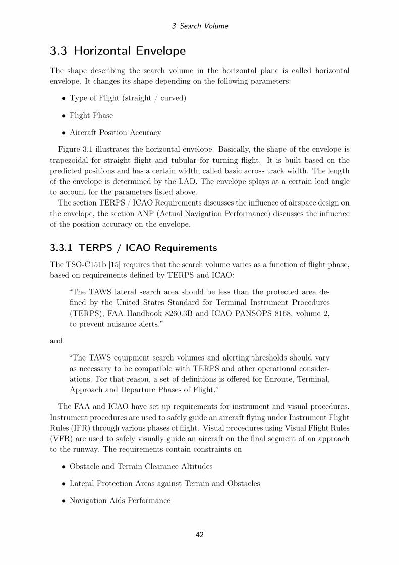
3.3 Horizontal Envelope
The shape describing the search volume in the horizontal plane is called horizontalenvelope. It changes its shape depending on the following parameters:
• Type of Flight (straight / curved)
• Flight Phase
• Aircraft Position Accuracy
Figure 3.1 illustrates the horizontal envelope. Basically, the shape of the envelope istrapezoidal for straight flight and tubular for turning flight. It is built based on thepredicted positions and has a certain width, called basic across track width. The lengthof the envelope is determined by the LAD. The envelope splays at a certain lead angleto account for the parameters listed above.
The section TERPS / ICAO Requirements discusses the influence of airspace design onthe envelope, the section ANP (Actual Navigation Performance) discusses the influenceof the position accuracy on the envelope.
3.3.1 TERPS / ICAO Requirements
The TSO-C151b [15] requires that the search volume varies as a function of flight phase,based on requirements defined by TERPS and ICAO:
“The TAWS lateral search area should be less than the protected area de-fined by the United States Standard for Terminal Instrument Procedures(TERPS), FAA Handbook 8260.3B and ICAO PANSOPS 8168, volume 2,to prevent nuisance alerts.”
and
“The TAWS equipment search volumes and alerting thresholds should varyas necessary to be compatible with TERPS and other operational consider-ations. For that reason, a set of definitions is offered for Enroute, Terminal,Approach and Departure Phases of Flight.”
The FAA and ICAO have set up requirements for instrument and visual procedures.Instrument procedures are used to safely guide an aircraft flying under Instrument FlightRules (IFR) through various phases of flight. Visual procedures using Visual Flight Rules(VFR) are used to safely visually guide an aircraft on the final segment of an approachto the runway. The requirements contain constraints on
• Obstacle and Terrain Clearance Altitudes
• Lateral Protection Areas against Terrain and Obstacles
• Navigation Aids Performance
42

3 Search Volume
Predicted Positions
Lead AngleLo
ok
Ah
ead
Dis
tan
ce (
LAD
)
Basic Across Track Width
(a) Horizontal Envelope for straight Flight
Basic Across Track Width
Look
Ahea
dDist
ance
(LAD)
Predicted Positions
Lead Angle
(b) Horizontal Envelope for curved Flight
Figure 3.1: Illustration of Horizontal Envelope
43

3 Search Volume
The FAA publishes the requirements through a “U.S. Standard for Terminal Instru-ment Procedures (TERPS)” [28], the ICAO through “ICAO DOC 8168 Aircraft Opera-tions - Volume II: Construction of Visual and Instrument Flight Procedures” [23].
The protection of the aircraft from obstacles and terrain is the most important con-sideration. The ICAO defines a primary and a secondary area for obstacle clearancealong any route that is part of an instrument procedure. The primary area is one halfof the total width, located in the middle of the route. The secondary area is actuallysplit into two parts, each spreading over one quarter of the total width, located at theside of the route. See figure 3.2 for an illustration. As one can see from figure 3.2, the
Figure 3.2: Route Obstacle Clearance (taken from ICAO DOC 8168 PANS-OPS [23])
primary area guarantees a Minimum Obstacle Clearance (MOC). In the secondary area,the MOC decreases from the full MOC to 0. The actual MOC values with respect to thedesign of the search volume are treated in 3.4.1. The total width varies as a function ofthe procedure that the route is part of. Procedures for departure, enroute, approach andarrival have different requirements for the lateral protection areas. There are too manyconsiderations regarding the protection areas made in the ICAO DOC 8168 [23] in orderto be fully discussed within this thesis. However, the minimum widths for departure,approach and enroute are given in the following sections.
3.3.1.1 Departure Requirements
For a straight departure without track guidance procedures, for example when the air-craft does not navigate along a track provided by a navigation facility as a VOR, theprotection area begins at the Departure End of Runway (DER) with a total width of300 m (0.16 NM) centered around the runway center line. It then splays at an angleof 15◦ on each side. This would give a total width of approx. 2.8 NM after 5 NM. Seefigure 3.3 for illustration.
44

3 Search Volume
Figure 3.3: Straight Departure Without Track Guidance Area (taken from ICAO DOC 8168 PANS-OPS [23])
3.3.1.2 Approach Requirements
An instrument approach may have five separate segments (see figure 3.4):
• Arrival
• Initial Approach
• Intermediate Approach
• Final Approach
• Missed Approach
Each of the segments end at designated fixes and for each segment the ICAO DOC8168 PANS-OPS defines its own area width. The initial approach width extends for 3.6km (2.5 NM) laterally on each side of the track and ends at the Initial Approach Fix(IAF). The IAF may be defined by a VOR, NDB or RNAV waypoint, and for a VORIAF for example has a width of 3.7 km (2.0 NM). The initial approach is succeeded bythe intermediate approach. The width at the beginning of the intermediate approachis the width at the IAF. It then reduces linearly so as to match the width of the finalapproach at the Final Approach Fix (FAF). The width of the final approach at theFAF depends on the considerations made for different so-called “Obstacle AssessmentSurfaces” (OAS). The OAS are used for assessing any obstacles within the final approacharea. The surfaces start at the runway and the shape (e.g. lateral, longitudinal andvertical coverage) is defined by the ICAO DOC 8168 PANS-OPS (see page 330). It mustbe ensured that no obstacles penetrate the OAS. For example, the basic ILS surface
45

3 Search Volume
Figure 3.4: Approach Segments (taken from ICAO DOC 8168 PANS-OPS [23])
initially extends 150 m (0.08 NM) on each side of the runway and then splays out at15% of the distance to a runway. This would give a width of 2.6 km (1.4 NM) on eachside of the runway center line after 5 NM (see figure 3.5).
Figure 3.5: ILS Surface (taken from ICAO DOC 8168 PANS-OPS)
3.3.1.3 Enroute Requirements
For straight enroute legs between two navigation fixes that are less than 100 NM long,a primary area of 5 NM on either side of the leg is used.
3.3.2 ANP (Actual Navigation Performance)
The TSO-C151b [15] requires the consideration of the TAWS navigation source:
“The TAWS search volumes should consider the accuracy of the TAWS nav-igation source.”
46
3 Search Volume
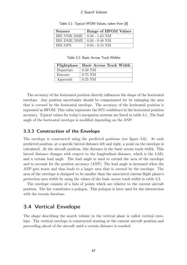
Table 3.1: Typical HFOM Values, taken from [8]
Sensors Range of HFOM ValuesIRS/VOR/DME 0.50 - 1.65 NMIRS/DME/DME 0.20 - 0.48 NMIRS/GPS 0.04 - 0.15 NM
Table 3.2: Basic Across Track Widths
Flightphase Basic Across Track WidthDeparture 0.50 NMEnroute 0.75 NMApproach 0.25 NM
The accuracy of the horizontal position directly influences the shape of the horizontalenvelope. Any position uncertainty should be compensated for by enlarging the areathat is covered by the horizontal envelope. The accuracy of the horizontal position isexpressed as HFOM. This value represents the 95% confidence in the horizontal positionaccuracy. Typical values for today’s navigation systems are listed in table 3.1. The leadangle of the horizontal envelope is modified depending on the ANP.
3.3.3 Construction of the Envelope
The envelope is constructed using the predicted positions (see figure 3.6). At eachpredicted position, at a specific lateral distance left and right, a point on the envelope iscalculated. At the aircraft position, this distance is the basic across track width. Thislateral distance changes with respect to the longitudinal distance, which is the LAD,and a certain lead angle. The lead angle is used to extend the area of the envelopeand to account for the position accuracy (ANP). The lead angle is increased when theANP gets worse and thus leads to a larger area that is covered by the envelope. Thearea of the envelope is designed to be smaller than the associated current flight phase’sprotection area width by using the values of the basic across track width in table 3.2.
The envelope consists of a lists of points which are relative to the current aircraftposition. The list constitutes a polygon. This polygon is later used for the intersectionwith the terrain database.
3.4 Vertical Envelope
The shape describing the search volume in the vertical plane is called vertical enve-lope. The vertical envelope is constructed starting at the current aircraft position andproceeding ahead of the aircraft until a certain distance is reached.
47

3 Search Volume
Extended Lead Angle
Look
Ah
ead
Dis
tan
ce (
LAD
)
Basic Across Track Width
ANP PositionUncertainty
Nominal Envelope
Extended Envelope
Extended AcrossTrack Width
ANP
Figure 3.6: Horizontal Envelope modified with respect to ANP
The design depends on the following parameters:
• Flight Phase
• Flight Path Angle
• Alert Type
All of the dependencies listed above are derived from the requirements stated in TSO-C151b [15]. This document lists minimum terrain clearances depending on the flightphase. The vertical envelope must consider these clearances. As the clearances and/orthe flight path angle changes, the envelope changes accordingly. The document alsodistinguishes between caution and warning alert and lists different minimum terrainclearances for each type. Therefore, a caution and a warning envelope for the respectivealert exists.
Section TSO-C151b Requirements discusses two concepts listed in TSO-C151b [15] ofhow an aircraft may undershoot a minimum safe height. The actual construction of the
48

3 Search Volume
Table 3.3: TAWS RTC by Flightphase (taken from TSO-C151b [15, table 3.1]
Flightphase ROC TAWS (RTC)Level Flight
TAWS (RTC)Descending
Enroute 1000 ft 700 ft 500 ftTerminal(Intermediate Segment)
500 ft 350 ft 300 ft
Approach 250 ft 150 ft 100 ftDeparture 48 ft/NM 100 ft 100 ft
envelope is discussed in section 3.4.2.
3.4.1 TSO-C151b Requirements
The requirements listed in TSO-C151b [15] basically define two scenarios of how anaircraft may undershoot a minimum safe height above terrain. The first scenario orconcept is the so-called “Reduced Required Terrain Clearance” (RTC) [15, sect. 3.1.1],the second one is the so-called “Imminent Terrain Impact” (ITI) [15, sect. 3.1.2]. Theconstruction of the vertical envelope must consider both concepts. As described in thefollowing section, the concepts may be combined.
3.4.1.1 RTC (Reduced Required Terrain Clearance) Concept
The RTC concept considers the case when the aircraft is currently above the terrainbut the amount of terrain clearance at some position along the flight path is consideredunsafe for the particular flight phase. In figure 3.7 you can see an illustration of theRTC concept. The aircraft on the left is flying level, the flight path is horizontal. Acertain offset distance below and always parallel to the flight path, a margin line isestablished. The offset distance is the required terrain clearance (RTC). The definitionof the required terrain clearance is listed in the TSO-C151b [15] and is derived from theTERPS Required Obstacle Clearances (ROC, see also 3.3.1), which considers airspacedesign. The RTC and ROC depend on the flight phase and on the question whether theaircraft is flying level or descending. The exact values are listed in table 3.3. As one cansee from table 3.3, the values for the RTC are slightly reduced so as to be lower thanthose for the ROC. The values for the ROC are associated with the caution envelopeand the values for the RTC are associated with the warning envelope. The reductionleaves a margin between the minimum obstacle clearance from airspace design and therequired terrain clearance that is used. This margin serves to desensitize the generationof alerts. Furthermore, the values for descending flight are lowered in order to preventnuisance alerts in the case of the pilot performing a level off.
In the situation depicted in figure 3.7, the aircraft at its present position is safe aboveterrain and clears any terrain by a vertical distance of at least the RTC. However, if itcontinues to fly level, it will violate the RTC at some point along the flight path because
49

3 Search Volume
TERRAIN
RTC
Flight Path
RTC Violation
Alt
itud
e
Along Track Distance
Figure 3.7: Reduced Required Terrain Clearance Concept
of the terrain that lies ahead and beneath.
3.4.1.2 ITI (Imminent Terrain Impact) Concept
The ITI concept considers the case when the aircraft is currently below the terrainbut the amount of terrain clearance at some position along the predicted flight path isconsidered unsafe for the particular flightphase. The required amount of terrain clearanceused here is the RTC for level flight (see table 3.3). In figure 3.8 an illustration of theITI concept can be seen. The aircraft on the left is currently below any terrain, theflight path is slightly climbing. At a certain offset distance below the aircraft and ata certain angle, the ITI-angle, a margin line is established. The offset distance is theRTC. The ITI angle is at least the flight path angle of the minimum climb performanceof the aircraft. However, when the current flight path angle becomes larger than theminimum climb performance flight path angle, the ITI angle becomes the current flightpath angle. This is the main difference between the RTC and the ITI concepts: Themargin line in the case of the ITI is not necessarily parallel to the flight path, whereasin the case of the RTC, the margin line is always parallel to the flight path.
In the situation depicted in figure 3.8, the aircraft at its present position is safe aboveany terrain but below some terrain that lies ahead of it. If it continues to fly along thepresent predicted flight path it will violate the RTC at some point because of the terrainthat lies ahead and above.
3.4.1.3 The Pull-Up Maneuver
Once the flight crew receives a caution or warning alert, they may take immediateaction. Possible actions comprise a vertical or horizontal escape maneuver. In the caseof the vertical maneuver a so called “Pull-Up” is executed (see figure 3.9). The pull-upmaneuver is initiated by pulling on the elevator control. The pulling is done with a
50

3 Search Volume
TERRAIN
RTC
Flight Path
ITI Angle
Along Track Distance
Alt
itud
e
RTC Violation
Figure 3.8: Imminent Terrain Impact Concept
certain load factor. The load factor is the vertical acceleration that acts on the aircraftand depends on the magnitude of the pull on the elevator control. Typically, the pilotshould not exceed a pull of 1.25 G. During the pulling the flight path angle increases andthe aircraft begins to climb. The pulling is stopped when the TAWS cancels the alert orwhen a maximum flight path angle is reached. The maximum flight path angle duringsuch a pull-up maneuver depends on various factors, the most important one being theairspeed. Under no circumstances, a safe airspeed, i.e. one that is well above the stallingairspeed must not be undershot.
TERRAIN
Flight Path
Alt
itud
e
Along Track Distance
"Terrain-TerrainPull-Up Pull-Up"
Pull-Up Maneuver
Figure 3.9: Pull-Up Maneuver
51

3 Search Volume
3.4.2 Construction of the Envelope
The final envelope is constructed out of a combination of both of the aforementionedconcepts. The combination of the two concepts yields optimal protection: By usingthe RTC concept, the aircraft is protected against terrain threats that lie beneath thecurrent aircraft altitude. By using the ITI concept, the aircraft is protected againstterrain threats that lie above the current aircraft altitude. A dedicated envelope isconstructed for both the caution alert and the warning alert. The caution envelope has,in principle, a larger extent since a caution alert precedes a warning alert.
The construction and thus the shape of the envelope is not static. It depends on variousfactors, the most important ones being the ground speed and vertical speed (whichdetermine the flight path angle γ). Furthermore, the flight phase and the accuracy of theused input data play an important role. Note that the following construction examplesemploy “perfect data”. In a concrete implementation of a TAWS, the construction isslightly modified to incorporate the accuracy of the input data.
The test cases given in TSO-C151b [15, Appendix 3, chap. 2 and 3] directly influencethe construction of the envelope. They discriminate between different flight phases aswell as between descending and level flight. To fulfill the requirements of the TSO-C151b, it must be shown that the test results of the TAWS implementation correspondwith the expected results.
3.4.2.1 RTC Protection in Level Flight
According to TSO-C151b [15], level flight is defined as when the aircraft having a verticalspeed that is within -500 feet/minute to +500 feet/minute. An example envelope forlevel flight that provides the RTC concept is shown in figure 3.10. Two envelopes areestablished:
• Warning Envelope (red envelope)
• Caution Envelope (amber envelope)
Both envelopes start at the aircraft position and extend vertically by the RTC value.The vertical extent of the envelope is called warning floor for the warning envelope andcaution floor for the caution envelope respectively. The RTC value depends on the flightphase (see table 3.3). The warning envelope extends horizontally, parallel to the flightpath, until the so-called “Warning Look Down Distance” is reached, the caution envelopeuntil the so-called “Caution Look Down Distance” is reached. The warning look downdistance is always calculated as: 0.5 · LAD whereas the caution look down distance iscalculated as 1 · LAD.
3.4.2.2 RTC Protection in Descending Flight
According to TSO-C151b [15], descending flight is defined as the aircraft having a ver-tical speed that is less than -500 feet/minute. In figure 3.11 an example envelope for
52

3 Search Volume
TERRAINWarning Envelope
RTC
Caution EnvelopeA
ltit
ude
Along Track Distance
Warning LookDown Distance
Flight Path
Caution Look Down Distance
Warn
ing F
loor
Cauti
on F
loor
Figure 3.10: RTC Protection in Level Flight
descending flight is shown. As for the level flight case, a dedicated envelope for bothwarning (red) and caution (amber) is established. As can be seen from the figure, theenvelopes again start at the aircraft position and reach down to the RTC value, thencontinue parallel to the flight path until reaching the warning or the caution floor re-spectively. When the corresponding floor is reached, the envelope continues horizontallyto either the warning or the caution look down distance respectively.
The calculation of the caution and the warning floor plays an important role. As onecan see from figure 3.11, the point in time of penetration of the envelope is determinedmainly by the vertical extent of the floors. When comparing this to the situation duringlevel flight (figure 3.10), one can see that there the penetration is determined mainly bythe LAD and thus by the horizontal extent of the envelope. The alerting criterion thatis bound to the LAD, which considers horizontal escape maneuvers, therefore has to becomplemented by vertical criteria that directly influence the vertical extent of the floors.
The requirements for the floors are derived from test cases for descending flight de-scribed in TSO-C151b [15, Appendix 3, chap. 2 and 3]. As an example the test casefor enroute descent is considered here (TSO-C151b [15, Appendix 3, chap. 1.2, EnrouteDescent Requirement]). The main requirement of this test case is to ensure that theTAWS issues a warning alert that make sure that the crew can react early enough andlevel the aircraft off with a minimum of 500 ft altitude clearance above the terrain, whichis the value for the RTC for enroute descending (see table 3.3). This requirement mustbe fulfilled within the operational flight envelope of the aircraft (operational range ofvertical and ground speed). Therefore, the test case contains a table (see TSO-C151b[15, Appendix 3, chap. 1.2, Table A]) that defines the minimum height above terrainwhen a warning alert must occur and the maximum height above terrain when a cautionalert may occur (see table 3.4).
Figure 3.12 illustrates the calculation of the warning floor. After receiving the warningalert, the crew may (in the worst case) not respond to the alert immediately. Therefore,
53

3 Search Volume
TERRAIN
RTC
Warning Envelope
Caution Envelope
Warn
ing
Flo
or
Cau
tion
Flo
or
Flight Path
Warning Look Down Distance
Caution Look Down Distance
Flight Path Angle
Along Track Distance
Alt
itud
e
Figure 3.11: RTC Protection in Descending Flight
Table 3.4: Enroute Descent Requirements
Vertical Speed [ft/min] MinimumWarning AlertHeight(above terrain) [ft]
MaximumCaution AlertHeight(above terrain) [ft]
1000 567 12002000 669 14004000 978 1800
the test assumes a response time (tResponse) of 3 seconds. This yields, using the currentvertical speed vd, the altitude lost due to pilot delay:
hPilot = vd · tResponse (3.1)
When 3 seconds have elapsed, the crew starts the pull-up maneuver. The pull-up ma-neuver assumes a constant acceleration of 0.25 G until level flight (0 feet/minute verticalspeed) is established. To calculate the altitude lost during the pull-up maneuver a con-stant acceleration motion in the vertical plane is assumed. The distance x traveledduring a constant acceleration motion is defined as follows (a being the acceleration andt time):
x =1
2· at2 (3.2)
After eliminating time and introducing velocity v, it reads:
x =1
2· v
2
a(3.3)
Finally the altitude lost during the pull-up maneuver to level flight is calculated as
54

3 Search Volume
follows:hPull−Up =
1
2· v2d
(0.25 ·G)(3.4)
The main requirement was to level off at 500 ft (the value for the RTC). Therefore, bothaltitude losses plus the RTC value yields the warning floor:
hWarn F loor = RTC + hPilot + hPull−Up (3.5)
This warning floor guarantees that the warning envelope penetrates the terrain when thecrew still has the chance to pull-up and level the aircraft off. This calculation method forthe warning floor adheres to the required values for the minimum warning alert heightabove terrain (see TSO-C151b [15, Appendix 3, chap. 1.2, Table A] or table 3.4).
The calculation of the caution floor is similar. Instead of using the RTC, the ROC isused.
TERRAIN
Flight Path
Alt
itud
e
Along Track Distance
"Terrain-TerrainPull-Up Pull-Up"
Lost Pull-Up Altitude
Lost Pilot Response Altitude
RTC
Figure 3.12: Floor Calculation
3.4.2.3 ITI Protection
As explained in section 3.4.1.2, the ITI concept protects the aircraft against terrainthreats that lie above the current aircraft altitude. The ITI protection must work forany kind of flight, so for descending as well as for level and climbing flight. The testcases for the ITI protection are described in TSO-C151b [15, Appendix 3, chap. 2].In figure 3.13 one can see the basic constitution of the envelope. Again, an envelopefor both warning and caution exists. The warning envelope extends horizontally untilthe so-called “Warning Look Up Distance” is reached, the caution envelope until theso-called “Caution Look Up Distance” is reached. The look up distances look beyondthe look down distances and are therefore typically 1.3 · LAD for the warning and 1.5 ·LAD for the caution envelope. The altitude where the envelope starts is determined bythe climb out floor. The slope is determined by the ITI-Angle.
55
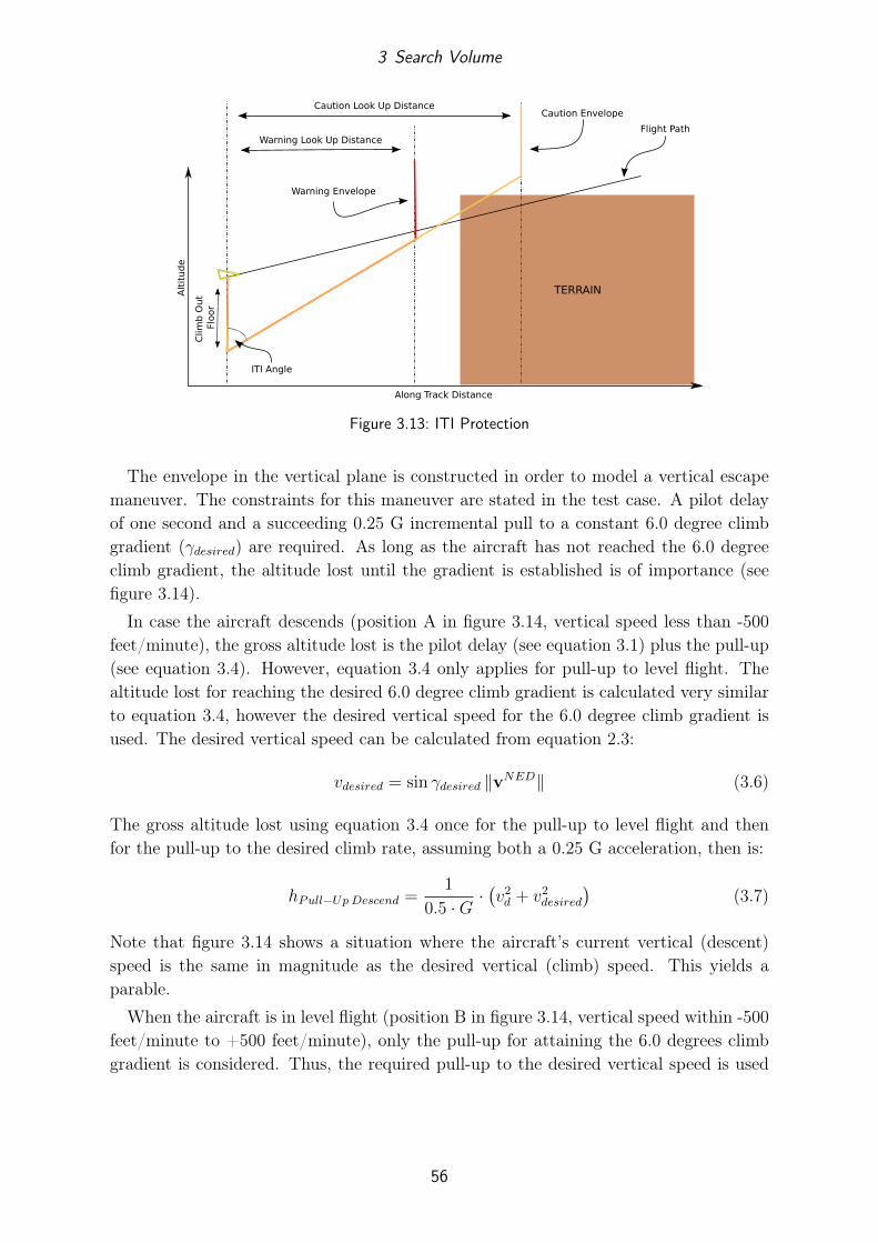
3 Search Volume
TERRAIN
Clim
b O
ut
Flo
or
Warning Envelope
Caution Envelope
Warning Look Up Distance
Caution Look Up Distance
Flight Path
ITI Angle
Alt
itude
Along Track Distance
Figure 3.13: ITI Protection
The envelope in the vertical plane is constructed in order to model a vertical escapemaneuver. The constraints for this maneuver are stated in the test case. A pilot delayof one second and a succeeding 0.25 G incremental pull to a constant 6.0 degree climbgradient (γdesired) are required. As long as the aircraft has not reached the 6.0 degreeclimb gradient, the altitude lost until the gradient is established is of importance (seefigure 3.14).
In case the aircraft descends (position A in figure 3.14, vertical speed less than -500feet/minute), the gross altitude lost is the pilot delay (see equation 3.1) plus the pull-up(see equation 3.4). However, equation 3.4 only applies for pull-up to level flight. Thealtitude lost for reaching the desired 6.0 degree climb gradient is calculated very similarto equation 3.4, however the desired vertical speed for the 6.0 degree climb gradient isused. The desired vertical speed can be calculated from equation 2.3:
vdesired = sin γdesired ‖vNED‖ (3.6)
The gross altitude lost using equation 3.4 once for the pull-up to level flight and thenfor the pull-up to the desired climb rate, assuming both a 0.25 G acceleration, then is:
hPull−Up Descend =1
0.5 ·G·(v2d + v2desired
)(3.7)
Note that figure 3.14 shows a situation where the aircraft’s current vertical (descent)speed is the same in magnitude as the desired vertical (climb) speed. This yields aparable.
When the aircraft is in level flight (position B in figure 3.14, vertical speed within -500feet/minute to +500 feet/minute), only the pull-up for attaining the 6.0 degrees climbgradient is considered. Thus, the required pull-up to the desired vertical speed is used
56
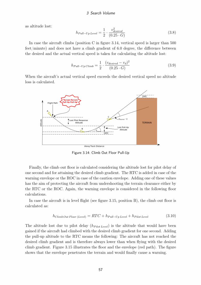
3 Search Volume
as altitude lost:hPull−Up Level =
1
2· v2desired
(0.25 ·G)(3.8)
In case the aircraft climbs (position C in figure 3.14, vertical speed is larger than 500feet/minute) and does not have a climb gradient of 6.0 degree, the difference betweenthe desired and the actual vertical speed is taken for calculating the altitude lost:
hPull−Up Climb =1
2· (vdesired − vd)2
(0.25 ·G)(3.9)
When the aircraft’s actual vertical speed exceeds the desired vertical speed no altitudeloss is calculated.
Lost Pull-Up Altitude
Lost Pilot Response Altitude
Flight Path
"Terrain-TerrainPull-Up Pull-Up"
RTC
γdesired
RTC
γdesired - γ
TERRAIN
Alt
itude
Along Track Distance
B
C
A
Figure 3.14: Climb Out Floor Pull-Up
Finally, the climb out floor is calculated considering the altitude lost for pilot delay ofone second and for attaining the desired climb gradient. The RTC is added in case of thewarning envelope or the ROC in case of the caution envelope. Adding one of these valueshas the aim of protecting the aircraft from undershooting the terrain clearance either bythe RTC or the ROC. Again, the warning envelope is considered in the following floorcalculations.
In case the aircraft is in level flight (see figure 3.15, position B), the climb out floor iscalculated as:
hClimb Out F loor (Level) = RTC + hPull−Up Level + hPilot Level (3.10)
The altitude lost due to pilot delay (hPilot Level) is the altitude that would have beengained if the aircraft had climbed with the desired climb gradient for one second. Addingthe pull-up altitude to the RTC means the following: The aircraft has not reached thedesired climb gradient and is therefore always lower than when flying with the desiredclimb gradient. Figure 3.15 illustrates the floor and the envelope (red path). The figureshows that the envelope penetrates the terrain and would finally cause a warning.
57

3 Search Volume
In case the of the aircraft descending, the climb out floor calculation is based on thecalculation for the level flight. As one can see in figure 3.15, position B is the positionwhere the aircraft is leveled off. Equation 3.10 shows how to calculate the climb outfloor at this position. At this position, the aircraft still has not reached the desiredclimb gradient. Going further back to position A, the aircraft is still in descent andhas not even leveled off. This means that the aircraft is always lower than when flyingwith the desired climb gradient until the desired climb gradient is reached. The timeneeded to reach the desired climb gradient is even longer than in the case of the levelflight. This means that the aircraft has a negative altitude budget that consists of thehPull−Up Descend and hPilot(Descent). hPilot(Descent) is defined here as the altitude lost whenthe aircraft descends with the current vertical speed for one second. Note that this is adifferent definition than in the case of the level flight. The climb out floor in case theaircraft descends is finally calculated as follows:
hClimb Out F loor (Descent) = RTC + hPull−Up Level + hPull−Up Descent + hPilot(Descent) (3.11)
When the aircraft climbs, the floor is calculated as:
hClimb Out F loor (Climb) = RTC + hPull−Up Climb + hPilot(Climb) (3.12)
The altitude lost due to pilot delay (hPilot(Climb)) is defined here as the altitude that wouldhave been gained if the aircraft had climbed with a climb rate of vdesired− vd. When theclimb rate is equal to or exceeds the desired climb rate, hPilot(Climb) and hPull−Up Climb isset to zero, thus setting the floor equal to the RTC (see position C in figure 3.15).
The envelope is then established starting from the aircraft altitude and going downthe distance of the respective climb out floor. From this point, a slope with an anglecorresponding to the ITI-angle is established. The ITI-angle depends on the desiredclimb gradient γdesired and the current climb gradient γ. If the current climb gradientexceeds the desired climb gradient, the ITI-angle is calculated as follows:
ITI-angle = 90− γ (3.13)
otherwise:ITI-angle = 90− γdesired (3.14)
As one can see in figure 3.15, the construction of the envelope in this manner ensuresprotection in each case (Position A (Descend), Position B (Level), Position C (Climb)).In each case the envelope would penetrate the terrain and thus cause a warning.
The construction of the caution envelope is similar. Instead of the RTC, the ROC isused.
58

3 Search Volume
Lost Pilot Response Altitude (hPilot (Descend))
Flight Path"Terrain-TerrainPull-Up Pull-Up"
RTC
γdesired
γdesired
ITI - Angle
TERRAIN
Alt
itud
e
Along Track Distance
hPull-Up Level + hPilot (Level)
+ RTC
hPull-Up Descend + hPilot (Descend)
Figure 3.15: ITI Envelope
3.4.2.4 Combination of RTC and ITI Protection
Finally, both concepts are combined into a common envelope. This envelope providesthe desired protection against any kind of terrain threats that lie below and/or abovethe current aircraft altitude. As previously mentioned, the envelope is not static anddepends on the following factors/parameters:
• Vertical Speed and Ground Speed (which determine the flight path angle γ)
• Flightphase
• Desensitization
• Accuracy of input data
The envelope is defined by the points labeled A-H (see figure 3.16) that are continuouslycalculated with respect to the above mentioned parameters. With this definition bypoints (which yields a path), one can easily calculate the altitude of the envelope atany point ahead of the aircraft. This will be important for the terrain-search volumeintersection.
In figures 3.16, 3.17 and 3.18 one can clearly see the difference in the envelope duringdifferent types of flight. The main steering (and most changing) parameter is the flightpath angle. As this angle decreases, the space below the aircraft is of more importanceas opposed to the level or climbing flight.
The flight phase mainly controls how sensitive the system should be by changing theminimum terrain clearance distance (RTC and ROC). The more sensitive it should be,the larger the vertical extent is. As the flight phase mainly depends on the distance tothe nearest runway (see also 3.2), the volume gets smaller as the aircraft approaches arunway and larger as the aircraft departs a runway.
59

3 Search Volume
Along Track Distance
Alt
itude
A
B
CD E
F
G
H
Predicted Flight Path
Figure 3.16: Example of the combined Envelope during descending Flight
As the aforementioned concepts use perfect input data, the real envelope has to bedesensitized and adapted with respect to the accuracy of the input data. Desensitizationtakes places especially near the aircraft by shifting the envelope or parts of it upwards.Adaption with respect to the accuracy of the input data happens by shifting the envelopeor parts of it downwards.
Along Track Distance
Alt
itude
A
B
C = D E
FG
HPredicted Flight Path
Figure 3.17: Example of the combined Envelope during level Flight
3.5 Combination of horizontal and vertical Envelope
Having examined the horizontal and the vertical envelope separately, both envelopes arenow combined to build a volume. This volume is used as a so-called “Search Volume”to search for terrain that penetrates this volume. The search volume is separated in thehorizontal plane by a closed polygon (see 3.3.3) and in the vertical plane by an open path(see 3.4.2.4). See figure 3.19 for illustration. As there are dedicated vertical envelopesfor both the caution and the warning alert, a dedicated search volume for each envelopealso exists.
60

3 Search Volume
Along Track Distance
Alt
itud
e
A
B
C = D
E = F = G
H
Predicted Flight Path
Figure 3.18: Example of the combined Envelope during climbing Flight
3.5.1 Modeling the Volume
One approach would be to model the volume by taking all points that enclose the volume(see figure 3.20). This approach models the volume exactly. However, for calculationof an intersection with the terrain, the model must be divided into smaller volumes(e.g. cubes or other geometric volumetric primitives) to apply standard point in volumetesting. The division can be seen on the right hand side in the figure. One drawback ofthis approach is that the division must constantly adapt to the shape of the envelope.The division might work for simple combinations of the horizontal and the verticalenvelope. However, if the horizontal envelope becomes curved (see figure 3.1(b)) or thevertical envelope is subject to change (see figures 3.16, 3.17 and 3.18) the division willnot work. To overcome this problem, the volume is finally not modeled as groups ofvolumes, but rather sampled at certain positions. At the sampled positions, a query forthe height of the envelope takes place. This procedure is dealt with in chapter 5 sinceit is closely related to the intersection of the search volume with the terrain.
3.5.2 Examples
For the sake of completeness, some details on the dimensions of the volume are given(see figure 3.21 for explanation of measures) here. Note that these measures are taken
+ =
Figure 3.19: Combination of horizontal and vertical Envelope
61
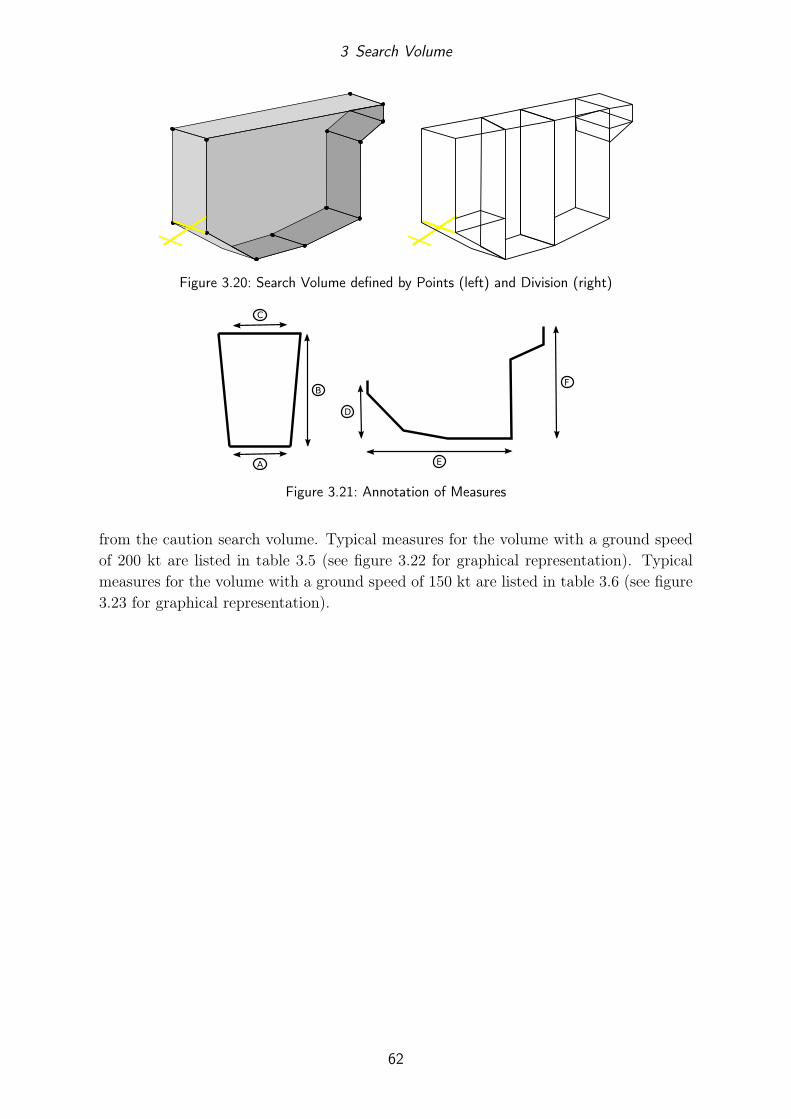
3 Search Volume
Figure 3.20: Search Volume defined by Points (left) and Division (right)
A
C
B
E
F
D
Figure 3.21: Annotation of Measures
from the caution search volume. Typical measures for the volume with a ground speedof 200 kt are listed in table 3.5 (see figure 3.22 for graphical representation). Typicalmeasures for the volume with a ground speed of 150 kt are listed in table 3.6 (see figure3.23 for graphical representation).
62
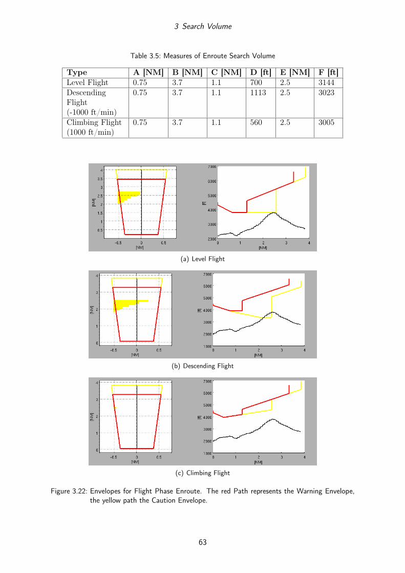
3 Search Volume
Table 3.5: Measures of Enroute Search Volume
Type A [NM] B [NM] C [NM] D [ft] E [NM] F [ft]Level Flight 0.75 3.7 1.1 700 2.5 3144DescendingFlight(-1000 ft/min)
0.75 3.7 1.1 1113 2.5 3023
Climbing Flight(1000 ft/min)
0.75 3.7 1.1 560 2.5 3005
(a) Level Flight
(b) Descending Flight
(c) Climbing Flight
Figure 3.22: Envelopes for Flight Phase Enroute. The red Path represents the Warning Envelope,the yellow path the Caution Envelope.
63
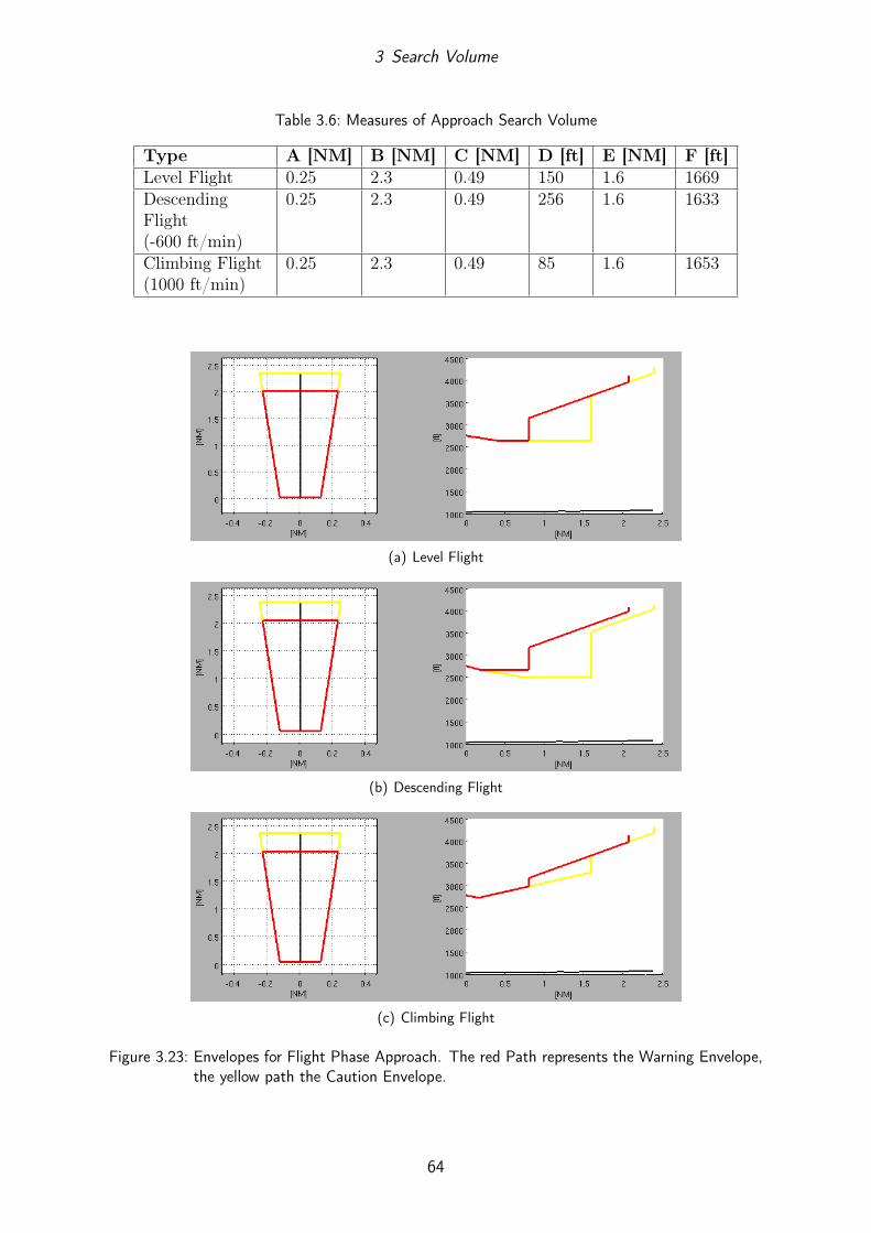
3 Search Volume
Table 3.6: Measures of Approach Search Volume
Type A [NM] B [NM] C [NM] D [ft] E [NM] F [ft]Level Flight 0.25 2.3 0.49 150 1.6 1669DescendingFlight(-600 ft/min)
0.25 2.3 0.49 256 1.6 1633
Climbing Flight(1000 ft/min)
0.25 2.3 0.49 85 1.6 1653
(a) Level Flight
(b) Descending Flight
(c) Climbing Flight
Figure 3.23: Envelopes for Flight Phase Approach. The red Path represents the Warning Envelope,the yellow path the Caution Envelope.
64

4 Intended Runway Search
4.1 General
As previously mentioned in section 3.1, the search volume depends amongst other thingson the distance from a runway. The distance from a runway directly influences theselected flight phase (see section 3.2) and hence the shape of the search volume.
The runway search tries to solve the following questions:
- What and where is the nearest runway?
- Is the aircraft on an approach to a runway?
The first question is necessary primarily for detecting the flight phase. The secondquestion is necessary to distinguish if the aircraft is approaching a runway or is headingtowards terrain. The runway that is most probably approached (for landing) is definedas the intended runway. This is necessary to turn off the system on final approach andto prevent any nuisance alerts during landing. See also figure 4.1 for an illustration ofthe problem.
Runway 02
Runway 04R
Runway 04L
?
Figure 4.1: Runway Search Illustration. Which runway is the Aircraft approaching?
65

4 Intended Runway Search
The TAWS has a dedicated runway database on which it periodically performs thesearch. The basic search is performed as follows:
1. Load all runways in the vicinity of the current aircraft position (ϕ, λ) from thedatabase
2. Determine the nearest runways
3. Determine the intended runway
The search uses the current aircraft position and true track (TT ) as input.
4.2 Search Algorithm
4.2.1 Runway Database
The runway database provides runway data for a specific area. Each runway has anentry with the following properties:
• Runway Identifier
• Airport Identifier
• Runway Threshold Position
• Runway Threshold Elevation
• Runway True Bearing
• Runway Length
Note that this database does not have a primary key since the search is based on theposition. The runway database is queried to load an area of interest within the vicinityof the current aircraft position into a cache. As the aircraft moves, the area of interestchanges and so does the cache. Typically, the cache area is quite large (e.g. 600 x 600NM) in order to minimize the number of reloads. The runways contained in the cacheserve as a base for the actual search.
4.2.2 Calculated Parameters
To detect the nearest and the intended runway, a couple of parameters are calculatedconstantly for each runway in the cache. Each parameter depends on the relative positionbetween the aircraft and the runway. See figure 4.2 for illustration.
Distance to RunwayThe distance to the runway threshold is calculated using spherical geometry and isdenoted as dRWY .
66

4 Intended Runway Search
Relative BearingThe bearing from the aircraft to the runway threshold is calculated using sphericalgeometry. The difference angle between the bearing aircraft to runway threshold andthe runway true bearing is the relative bearing, denoted as α.
Cross Track Error (XTE) and Along Track Error (ATE)The cross track error is defined as the lateral deviation from the runway axis. The alongtrack error is defined as the distance from the threshold along the runway axis. Bothare calculated using dRWY and α. The XTE determines how well the aircraft is alignedwith the runway axis.
Distance and Cross Track Error and RateRates for dRWY and XTE are constantly calculated and are denoted as dRWY and ˙XTE
respectively. The signs of the rates are used to distinguish if the aircraft is approachingor departing the runway.
Runway 36
dRWYATE
XTE
α
Figure 4.2: Runway Search Parameters
4.2.3 Score Function
A score function that determines a certain score value for each runway is used. The scorevalues express the probability of the aircraft departing or landing on a certain runway.The higher the value, the more probable it is that the crew has chosen the runway todepart or land. The algorithm uses the parameters given above to calculate a score. The
67
4 Intended Runway Search
calculation of the score is mathematically expressed as:
s = f1(dRWY ) + f2(XTE,ATE) + f3(dRWY , ˙XTE) (4.1)
Equation 4.1 contains three functions (f1−3) that all contribute to the total score.
The first function f1 calculates the score depending on the distance, e.g. the scoreincreases the closer the aircraft is to the runway. This simple approach acts as a coarsefilter to discard any distant runways.
The second function f2 determines the score based on how well the aircraft is alignedwith the runway axis. The alignment with the axis is determined by the XTE. Whenthe XTE approaches 0, the aircraft is perfectly aligned with the axis. The smaller theXTE gets, the more score is generated. The ATE is initially used to determine if theaircraft is on the correct side of the runway by checking the sign. If it is on the wrongside, the score is decremented significantly. The smaller the ATE gets, the more scoreis generated, which means that the aircraft is closer to the runway threshold.
Note that the last two described functions focus on parameters that are rather staticand that do not contain dynamic information. Using the rates dRWY and ˙XTE the lastfunction, f3, considers the dynamic information. The function uses the rate information(especially the sign of the rates) to detect if the aircraft is heading towards a runwayor not. The sign of the rate ˙XTE signals if the XTE is getting smaller or not, whichmeans that the aircraft is approaching the runway axis. The rate’s sign of dRWY providesinformation as to whether the aircraft is departing or approaching the runway. If the signof the rates signals an approach, the score is incremented, otherwise it is decremented.
4.2.4 Selection of Runways
Finally, the selection of the nearest and the intended runway takes place. The nearestrunway is simply selected by arranging the runways in an ascending order by the pa-rameter dRWY . The selection of the intended runway is based on the score. The runwaywith the highest score is chosen as the intended runway. However, before the intendedrunway is finally selected, the aircraft altitude is compared against an altitude profilethat starts at the supposed runway. This profile defines a standard approach profile.The examined runway is chosen as the intended runway only if the aircraft altitude isbelow this profile.
68

5 SearchVolume -Terrain Intersection
5.1 General
The previous chapters mainly dealt with the construction of a search volume. Thesearch volumes for caution and warning are now intersected with the terrain to detectany terrain that penetrates the volumes. The penetration of the terrain may eventuallylead to a caution- or a warning alert. For the intersection, the following questions are ofrelevance:
- Which terrain lies within the horizontal boundary of the search volume?
- Does the terrain that lies within the horizontal boundary penetrate the searchvolume?
In order to be able to answer these questions, the TAWS must have a terrain databaseas well as methods available to effectively access this database during the intersection.The terrain database contains a Digital Terrain Model (DTM) for a specific region.Furthermore, a method must be developed to effectively intersect the search volumewith the terrain database. All operations must work in real time, i.e. during flight.
5.2 Terrain Database
5.2.1 Definition
What is described in a terrain database is not clearly defined in the document TSO-C151b [15]. There is no definition of the term “terrain”. Since terrain and geographicinformation in general play an important role in aviation, provisions have been made toestablish standardization for the gathering, storing and exchanging of terrain, obstacleand aerodrome mapping information. Standardization documents provide the necessarydefinitions. The most important ones are:
• ICAO Annex 15: Aeronautical Information Services [21]
• ICAO Document 9881: Guidelines for Electronic Terrain, Obstacle and AerodromeMapping Information [24]
• Eurocontrol: Terrain and Obstacle Manual [9]
• RTCA DO-200A / EUROCAE ED 76: Standards for Processing Aeronautical Data[16]
69
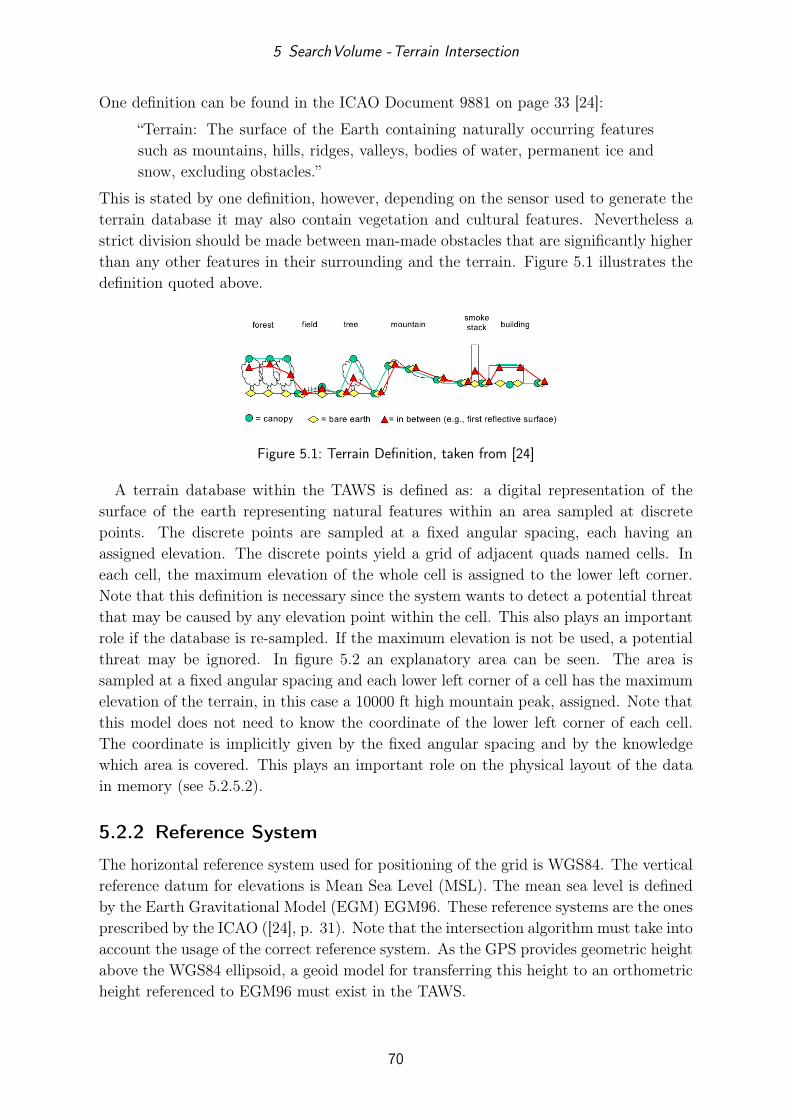
5 SearchVolume -Terrain Intersection
One definition can be found in the ICAO Document 9881 on page 33 [24]:
“Terrain: The surface of the Earth containing naturally occurring featuressuch as mountains, hills, ridges, valleys, bodies of water, permanent ice andsnow, excluding obstacles.”
This is stated by one definition, however, depending on the sensor used to generate theterrain database it may also contain vegetation and cultural features. Nevertheless astrict division should be made between man-made obstacles that are significantly higherthan any other features in their surrounding and the terrain. Figure 5.1 illustrates thedefinition quoted above.
Figure 5.1: Terrain Definition, taken from [24]
A terrain database within the TAWS is defined as: a digital representation of thesurface of the earth representing natural features within an area sampled at discretepoints. The discrete points are sampled at a fixed angular spacing, each having anassigned elevation. The discrete points yield a grid of adjacent quads named cells. Ineach cell, the maximum elevation of the whole cell is assigned to the lower left corner.Note that this definition is necessary since the system wants to detect a potential threatthat may be caused by any elevation point within the cell. This also plays an importantrole if the database is re-sampled. If the maximum elevation is not be used, a potentialthreat may be ignored. In figure 5.2 an explanatory area can be seen. The area issampled at a fixed angular spacing and each lower left corner of a cell has the maximumelevation of the terrain, in this case a 10000 ft high mountain peak, assigned. Note thatthis model does not need to know the coordinate of the lower left corner of each cell.The coordinate is implicitly given by the fixed angular spacing and by the knowledgewhich area is covered. This plays an important role on the physical layout of the datain memory (see 5.2.5.2).
5.2.2 Reference System
The horizontal reference system used for positioning of the grid is WGS84. The verticalreference datum for elevations is Mean Sea Level (MSL). The mean sea level is definedby the Earth Gravitational Model (EGM) EGM96. These reference systems are the onesprescribed by the ICAO ([24], p. 31). Note that the intersection algorithm must take intoaccount the usage of the correct reference system. As the GPS provides geometric heightabove the WGS84 ellipsoid, a geoid model for transferring this height to an orthometricheight referenced to EGM96 must exist in the TAWS.
70

5 SearchVolume -Terrain Intersection
Terrain Cell
5000 ft
10000 ft10000 ft
Terrain Cell
Figure 5.2: Terrain Grid
5.2.3 Terrain Data Attributes and Quality Requirements
Terrain Data AttributesWhen creating a terrain database for a real TAWS, a minimum set of terrain dataattributes that are described in the ICAO document 9881 are necessary. These attributesare present right from the creation and throughout the entire life cycle of the data. Thisensures that the data’s characteristics and quality satisfies the requirements of a concreteapplication.
Table 5.1 lists the attributes that the terrain data must possess. Some of them arediscussed in the following.
The post spacing expresses the angular (e.g. arc-seconds) or linear (e.g. meters)distance between two adjacent points in the grid. If an angular distance is used and alinear distance has to be maintained, the post spacing in latitude will differ from thepost spacing in longitude at higher latitudes due to the departure of the meridians.
One of the most important attribute defining the quality is the declaration of the accu-racy. Here, the accuracy can be judged by the attribute horizontal/vertical accuracy andthe associated horizontal/vertical confidence level. The accuracy expresses the degree ofconformance between the estimated or measured value and the true value, cf. [24]. Thestandard deviation must be provided here. The confidence level is the probability thaterrors in the data are within the limit specified by the accuracy, cf. [24]. The probabilityis declared as percentage.
The elevation reference holds information about how to interpret the associated ele-vation value of a point in the grid. The elevation may be interpreted as the elevation ofthe corner or the center of the cell, the average or the maximum elevation of the cell.
The recorded surface describes whether the data contains information about the el-evation of the bare earth (usually acquired by land surveying) or the reflective surface(acquired via remote sensing).
The integrity defines the level of assurance that states that the data has not beenaltered in such a way that it no longer reflects the original value, cf. [9]. The integrity isexpressed as the probability of any single data element of the terrain data having beenchanged inadvertently since the creation of the terrain data.
71

5 SearchVolume -Terrain Intersection
The ICAO specifies three levels of integrity ([24], p. 16):
1. Critical: 10−8
2. Essential: 10−5
3. Routine: 10−3
A change in the data could occur in the processing chain. As example, assuming a stan-dard 3 arc seconds Shuttle Radar Topography Mission (SRTM) tile of 1◦ x 1◦ along lati-tude/longitude that contains 1440000 elevation points, only 14 points may have changedwhen provisions were made to have an integrity of the level Essential. The question aboutintegrity plays an important role especially with SRTM and its characteristic voids andfilling of them. See [25] for examination of the integrity level of SRTM-based terraindatabases for aviation use.
Table 5.1: Minimum Set of Attributes for Terrain Data, taken from [24], Table 2.1
Attribute NameArea of CoverageData Source IdentifierAcquisition MethodPost SpacingHorizontal Reference SystemHorizontal ResolutionHorizontal AccuracyHorizontal Confidence LevelHorizontal Position DataElevationDatabase UnitsElevation ReferenceVertical Reference SystemVertical ResolutionVertical AccuracyVertical Confidence LevelSurface TypeRecorded SurfacePenetration LevelKnown VariationsIntegrityDate and Time Stamp
Quality RequirementsThe ICAO document states recommended requirements for the use of terrain data inaviation applications. Among them is the GPWS with forward looking terrain avoidance.
72
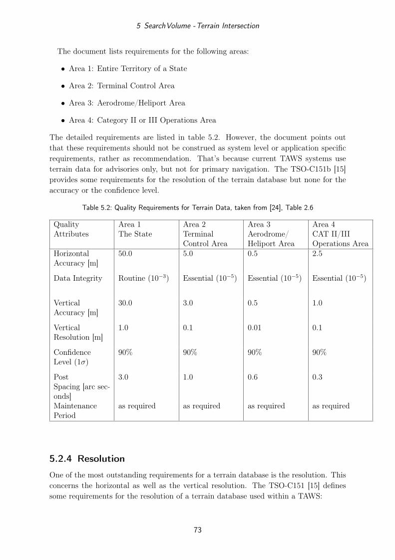
5 SearchVolume -Terrain Intersection
The document lists requirements for the following areas:
• Area 1: Entire Territory of a State
• Area 2: Terminal Control Area
• Area 3: Aerodrome/Heliport Area
• Area 4: Category II or III Operations Area
The detailed requirements are listed in table 5.2. However, the document points outthat these requirements should not be construed as system level or application specificrequirements, rather as recommendation. That’s because current TAWS systems useterrain data for advisories only, but not for primary navigation. The TSO-C151b [15]provides some requirements for the resolution of the terrain database but none for theaccuracy or the confidence level.
Table 5.2: Quality Requirements for Terrain Data, taken from [24], Table 2.6
QualityAttributes
Area 1The State
Area 2TerminalControl Area
Area 3Aerodrome/Heliport Area
Area 4CAT II/IIIOperations Area
HorizontalAccuracy [m]
50.0 5.0 0.5 2.5
Data Integrity Routine (10−3) Essential (10−5) Essential (10−5) Essential (10−5)
VerticalAccuracy [m]
30.0 3.0 0.5 1.0
VerticalResolution [m]
1.0 0.1 0.01 0.1
ConfidenceLevel (1σ)
90% 90% 90% 90%
PostSpacing [arc sec-onds]
3.0 1.0 0.6 0.3
MaintenancePeriod
as required as required as required as required
5.2.4 Resolution
One of the most outstanding requirements for a terrain database is the resolution. Thisconcerns the horizontal as well as the vertical resolution. The TSO-C151 [15] definessome requirements for the resolution of a terrain database used within a TAWS:
73

5 SearchVolume -Terrain Intersection
“Terrain and airport information must be of the accuracy and resolution suit-able for the system to perform its intended function. Terrain data should begridded at 30 arc seconds with 100 foot resolution within 30 nautical milesof all airports with runway lengths of 3500 feet or greater and whenever nec-essary (particularly in mountainous environments) 15 arc seconds with 100foot resolution (or even 6 arc seconds) within 6 nautical miles of the closestrunway. It is acceptable to have terrain data gridded in larger segments overoceanic and remote areas around the world.”
The requirement mentions gridded terrain data. This gridded nature of the data is ofimportance and will be discussed below in 5.2.5. The resolution requirement is nowa-days easily fulfilled by the most common databases. One example would be the SRTMdatabase that provides an almost global coverage with a 3 arc seconds horizontal and 1m vertical resolution.
5.2.5 Database Model
Figure 5.2 shows an explanatory detail of the terrain database. If we now return to theinitial question, which terrain lies within the horizontal boundary of the search volume,this leads to the problem of how to query the terrain database for elevation data. Thisproblem requires the introduction of a model that allows effective access. Effective accessin this context means primarily
• Fast Access
• Memory Saving Access
Fast access is necessary since the query happens in real time. Memory saving access isneeded due to limited memory during runtime. The greatest challenge for the modelis to deal with the immense amount of data. Imagine a TAWS having a global terraindatabase and thus allowing global operation. Finding the elevation data lying withinthe volume would require a search across the whole database. For the effective access,spatialization and a spatial structure for addressing the elevation data are introduced(see also [2], chapter 8.2).
5.2.5.1 Logical Layout
SpatializationAs illustrated in the example above, the TAWS contains in the worst case a globaldatabase. A short assessment of the amount of data contained in the database showsthe problem even more clearly:
Again, assuming a standard 3 arc seconds global coverage of tiles with dimension1◦ x 1◦ along latitude/longitude, each containing 1440000 elevation points, would yieldapproximately 9.33 · 1010 points.
74

5 SearchVolume -Terrain Intersection
Table 5.3: Level of Detail (LOD) Structure
Level Angular Spacing Number Child Segments0 3” 1200 x 12001 6” 600 x 6002 15” 240 x 2403 30” 120 x 1204 60” 60 x 605 1.5’ 40 x 406 3’ 20 x 207 6’ 10 x 108 12’ 5 x 59 30’ 2 x 210 1◦ 1 x 1
The spatialization of the data is done by dividing the global database recursively intosmaller segments. Each segment correspond to a specific Level of Detail (LOD). As thesegment gets smaller, more details appear. A top level and a bottom level of detailexist. The top LOD represents the lowest terrain resolution whereas the bottom LODrepresents the highest terrain resolution. The spatialization is done from top (globalscale) to bottom (local scale). Figure 5.3 illustrates this process. In the top LOD, whichis also called the parent segment, each segment covers an area with a dimension of 1◦ x1◦ along latitude/longitude. In the next step, the segment is divided by two in latitudeand longitude. Four new child segments are the result, each having a dimension of 30’ x30’. This division is repeated until the segment has a dimension of 3” x 3”. Note that thedivision is not entirely done by factor 2, but rather is adapted to the requirements of theTAWS and with respect to the spatial structure for addressing. With this parent-childarchitecture, one may access the desired LOD recursively. Once the parent segment isknown, the child segments are easily found. Table 5.3 shows the numerical values forthe LODs used within this system. In the third column, the number of child segmentscontained in the top LOD (1◦ x 1◦) for the respective LOD (e.g. 3” x 3”) can be seen.This division process is very similar to a quad-tree structure (see [2], chapter 8.2.1).
The transition from a segment that contains a geographic feature to terrain data isseamless. Since terrain data as previously defined in 5.2.1 is treated as a cell, eachsegment becomes a terrain cell. It is assumed that the terrain data is available in aresolution that is a multiply of 3 arc seconds. Then, each terrain cell can be used in thesegment structure above by simply re-sampling the terrain data to the desired LOD. Asmentioned earlier, the cell’s maximum elevation is stored in the lower left corner of thecell. This lower left corner will later on play an important role in addressing the cell.Figure 5.4 shows a sample terrain area of 1◦ x 1◦ that is re-sampled from 3 arc seconds toa resolution of 30 arc minutes. The figure illustrates clearly that the maximum elevationsare forwarded to the next level. Finally, the top LOD contains only 4 terrain cells that,however, represent the maximum elevation of the whole area.
75

5 SearchVolume -Terrain Intersection
1°
1°
30'
30' 12'
12'
6'
6'
3'3' 1.5'
1.5'
Figure 5.3: Spatialization. The resolution is increased from left to right, starting in the upper row.
76
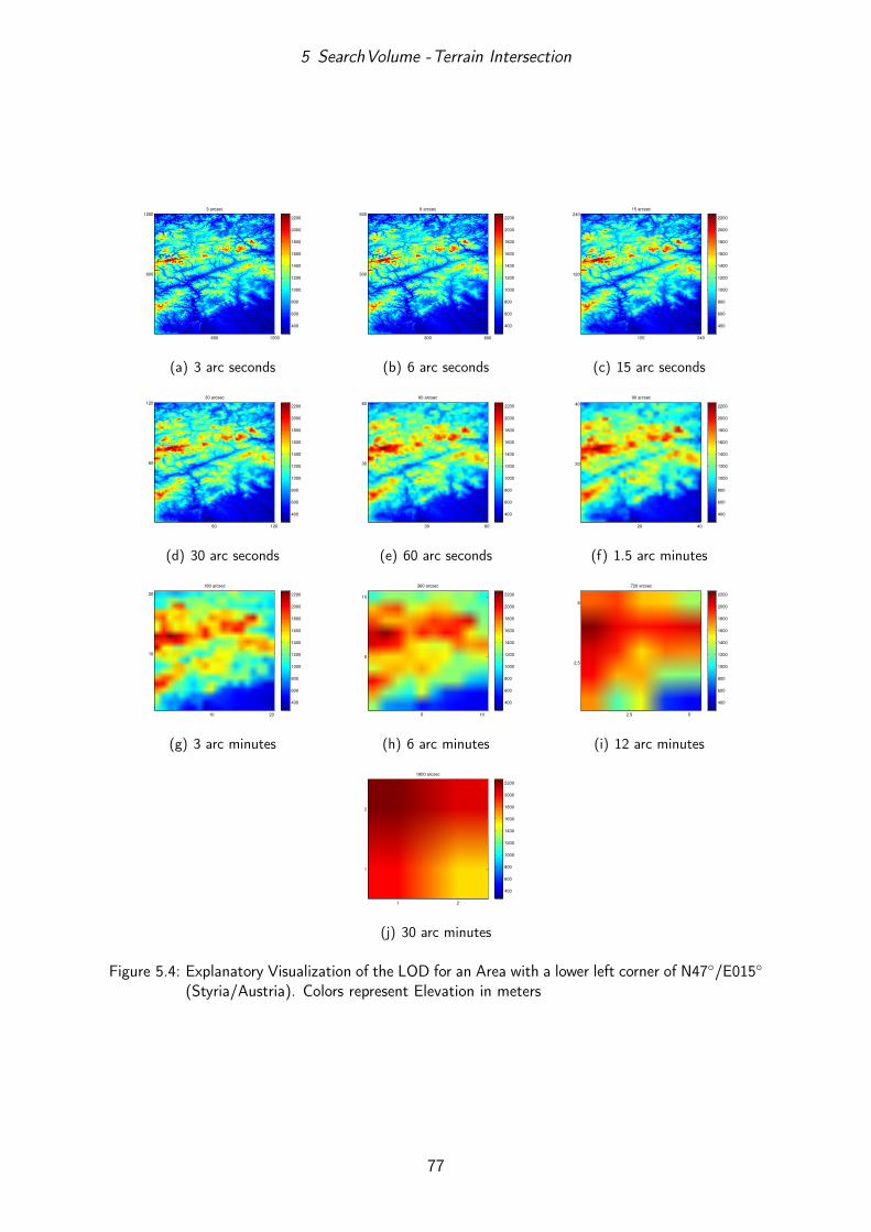
5 SearchVolume -Terrain Intersection
3 arcsec
600 1200
600
1200
400
600
800
1000
1200
1400
1600
1800
2000
2200
(a) 3 arc seconds
6 arcsec
300 600
300
600
400
600
800
1000
1200
1400
1600
1800
2000
2200
(b) 6 arc seconds
15 arcsec
120 240
120
240
400
600
800
1000
1200
1400
1600
1800
2000
2200
(c) 15 arc seconds
30 arcsec
60 120
60
120
400
600
800
1000
1200
1400
1600
1800
2000
2200
(d) 30 arc seconds
60 arcsec
30 60
30
60
400
600
800
1000
1200
1400
1600
1800
2000
2200
(e) 60 arc seconds
90 arcsec
20 40
20
40
400
600
800
1000
1200
1400
1600
1800
2000
2200
(f) 1.5 arc minutes
180 arcsec
10 20
10
20
400
600
800
1000
1200
1400
1600
1800
2000
2200
(g) 3 arc minutes
360 arcsec
5 10
5
10
400
600
800
1000
1200
1400
1600
1800
2000
2200
(h) 6 arc minutes
720 arcsec
2.5 5
2.5
5
400
600
800
1000
1200
1400
1600
1800
2000
2200
(i) 12 arc minutes
1800 arcsec
1 2
1
2
400
600
800
1000
1200
1400
1600
1800
2000
2200
(j) 30 arc minutes
Figure 5.4: Explanatory Visualization of the LOD for an Area with a lower left corner of N47◦/E015◦
(Styria/Austria). Colors represent Elevation in meters
77

5 SearchVolume -Terrain Intersection
Spatial Structure for AddressingThe previous sections discussed the division of an area into smaller segments and finallyinto terrain cells. The question that arises is: How can the terrain cells be addressed?Given a position (ϕ, λ), the next question would be: Which terrain cell is the nearestone and which elevation does it have?
The spatialization already provides the key feature for establishing a spatial structurefor addressing a terrain cell. Finding an addressing scheme is easy as the terrain cellsare laid out in a grid. As in the addressing scheme EXCELL (see [2], chapter 8.2.2),an address space is introduced. The address space utilizes the already existing gridstructure. The grid structure is considered as a matrix. Each element of a matrix A,with n rows and m columns, i (row) and j (column) has a unique linear index k definedas:
k = i ∗m+ j (5.1)
The calculation of the linear index is used as a hash function ([2], p. 280) to map therow index i and the column index j to a unique value k. Applying the hash function tothe terrain cells, the following addressing scheme is introduced:
Each terrain cell is uniquely addressed using two indices:
• Global Index (GI)
• Sub Index (SI)
The global index is defined as the linear index of the 1◦ x 1◦ terrain cells that coverthe whole earth. As the earth is defined by 180 parallels and 360 meridians, the hashfunction for the global index (using ϕ, λ in degrees) is:
GI = (floor(ϕ) + 90) · 360 + floor(λ) + 180 (5.2)
The floor function returns the largest integer not greater than the argument. Theglobal index runs from 0 to a maximum index of 180 · 360 = 64800 and maps a positionwithin a 1◦ x 1◦ terrain cell to the lower left corner of that cell. The position N47◦ 3’51.51” / E15◦ 27’ 11.40” for example has a global index of 49515.
Within a 1◦ x 1◦ terrain cell, the sub index is used to address any child terrain cell.As discussed before, it is important to take into account the division factor for eachLOD. Table 5.3 shows the angular spacing. A closer look at the angular spacing reveals,that each level has an integer multiply angular spacing of the base level, which is 3 arcseconds. This makes it possible to address any position within the 1◦ x 1◦ terrain cellwith a linear index that is based on 3 arc seconds. As one 1◦ x 1◦ terrain cell consists of3600 x 3600 1 arc seconds cells, the hash function for the sub index, using minutes (m)
78

5 SearchVolume -Terrain Intersection
and seconds (s) of ϕ and λ and the angular spacing ∆ang in arc seconds is defined as:
NSamples per Row =3600
∆ang
SI = floor
(mϕ · 60 + floor(sϕ)
∆ang
)·NSamples per Row + floor
(mλ · 60 + floor(sλ)
∆ang
)(5.3)
Fractional seconds are rounded to the largest previous integer second using the floorfunction. The result of the division by ∆ang is also rounded down to the nearest integer.Note that when ϕ or λ is negative, the calculation of the total seconds for ϕ becomesmϕ · 60 + floor(sϕ) + 3600 instead of mϕ · 60 + floor(sϕ) and for λ it becomes mλ · 60 +
floor(sλ) + 3600 instead of mλ · 60 + floor(sλ).For position N47◦ 3’ 51.51” / E15◦ 27’ 11.40” and an angular spacing of 3 arc seconds
(which yields NSamples per Row = 36003
= 1200) for example, the sub index is 92944. Thisaddressing scheme can be used for the LOD defined in table 5.3. The transformationfrom one resolution level to another is also easy since all angular spacings are an integermultiply of 3 arc seconds.
Using the global and sub index, an arbitrary position on earth can be mapped to aterrain cell in the database. Note that this mapping not necessarily returns the nearestterrain cell since the mapping involves rounding using the floor function. This drawbackis acceptable since the mapping error lies in the range of a maximum of 3 or 6 arc secondsif the intersection uses these resolutions. The calculation of the indices paired with asophisticated physical layout grants a fast access.
5.2.5.2 Physical Layout
The choice of the correct physical layout is of great importance. As stated above, afast and memory saving access is required. With the knowledge gained in the previoussection, the logical layout is now transformed into a corresponding physical layout.
As mentioned above, in the worst case the TAWS might use a global database. Assum-ing a 3 arc seconds resolution, one 1◦ x 1◦ terrain tile file has 1440000 elevation points.If each point requires 2 bytes of storage, the file requires 2812.5 kBytes. A databasefor the whole earth (360 · 180 files) requires approximately 173.81 GBytes. However,if terrain tile files that contain only sea level (assuming as an estimation that 71% ofthe earth are covered by sea) are discarded, the amount of storage needed is reducedto approximately 50 GBytes. This amount of data cannot be loaded into memory by aprogram during runtime. Therefore, two methods are used to overcome this problem:
• Caching
• Memory Mapping
The caching is dealt with in section 5.2.6 and is a method of transferring a section ofthe terrain database to a temporary memory. The memory mapping allows access toterrain tile files without extra consumption of runtime memory.
79

5 SearchVolume -Terrain Intersection
As mentioned in the section above, for a fast access to terrain data it is necessaryto have a sophisticated physical layout. The physical layout should integrate with thelogical layout seamlessly. The logical layout uses a spatialization in form of a LOD andterrain at high resolution is sampled to lower resolution. With respect to the FLTA andthe terrain display, this LOD structure is also used for the physical layout. The FLTAacts in the immediate vicinity and therefore uses a high resolution terrain. As the terraindisplay shows the terrain in the vicinity depending on the pilot’s selected display range(up to 320 NM), the resolution of the terrain has to be lower for large ranges than forshort ranges.
All the LOD levels are stored in one LOD file. This technique is very similar tothe “Multum in Parvo” (MIP) mapping technique [26], where a high resolution textureimage is sampled down to lower resolution texture images in order to have a fast access oncomputer graphics cards. Storing the LOD levels in one LOD file needs a preprocessingstep, where the high resolution terrain tile file (e.g. 3 arc seconds) is successively sampledto each LOD level shown in the table 5.3. Starting from level 0, all elevations of onelevel are packed into a contiguous memory block, ordered by the sub index and finallystored in the file. The ordering by the sub index is important since this facilities fastaccess. During runtime, when the sub index is calculated through equation 5.3, a pointerpointing to the first elevation in the memory block can easily be shifted by the sub index.The shifted pointer then points to the elevation that corresponds to a certain position.No search has to be performed and the only complex operation is the calculation of thesub index. Finally, a LOD file for each 1◦ x 1◦ terrain cell exists. Each LOD file containsa header representing the positions in the file memory where each LOD level starts andends. The collection of all the LOD files constitutes the terrain database.
To save runtime memory, the content of a LOD file, the elevations, are not loadedinto a runtime memory buffer. A runtime memory buffer would require the dynamicallocation of memory, which is a time and memory costly method. However, the contentof a LOD file is mapped into the runtime memory using a method called “memorymapping”. When a file is memory mapped, the program has access to the content of thefile as if it was available in runtime memory buffer, but does not use up any time andmemory as would be the case if the file was loaded.
5.2.6 Terrain Caching
The amount of data in the terrain database, as discussed previously, can be tremendous.One technique to overcome this problem was memory mapping the LOD files. As theterrain database is constituted by a collection of LOD files, which may cover the wholeearth, the TAWS must schedule the memory mapping of the files. This is necessary sincethe mapping cannot address an unlimited amount of memory, which has to do with theunderlying computer architecture (e.g. 32 bit versus 64 bit).
The caching makes sure that LOD files needed for the FLTA and the terrain displayare memory mapped. Therefore, a cache area and a reload area are defined. Bothareas use the arrangement of the 1◦ x 1◦ terrain cells and the associated global index.
80

5 SearchVolume -Terrain Intersection
Cache Area
Reload Area
Figure 5.5: Cache and Reload Area
As there is a LOD file for each 1◦ x 1◦ terrain cell, all the LOD files associated to aterrain cell within the cache area are memory mapped. The cache area is not static andmoves as the aircraft moves. A continuous moving of the cache area would result ina continuous memory mapping operation of the LOD files. However, most of the timethis is not necessary, since the movements of the aircraft are relatively small comparedto the dimension of the cache area. To avoid a continuous memory mapping operation,the reload area is used for triggering when new LOD files need to be memory mapped.Figure 5.5 illustrates both areas. The reload area (seen in red in the figure) is smallerthan the cache area (seen in green in figure, usually 80%) and moves constantly withthe aircraft. As the aircraft moves, the reload area is intersected with the cache areaand it is checked if the reload area is contained in the cache area. If the reload areais not contained in the cache area, the memory mapping is triggered. For each 1◦ x 1◦
terrain cell lying within the cache area, the corresponding LOD file is memory mapped.A pointer to this memory mapped file is stored in a lookup table that maps the globalindex of the LOD file to the pointer.
5.3 Intersection
The questions “Which terrain lies within the horizontal boundary of the search volume?”and “Does the terrain that lies within the horizontal boundary penetrate the searchvolume?” still remain. Chapter 3 dealt with the design and definition of the searchvolume. In section 5.2, the logical and physical structure for the terrain database wasintroduced. Next, a method must be found to intersect the search volume with theterrain database.
81

5 SearchVolume -Terrain Intersection
As the search volume is constituted by a horizontal and a vertical envelope, the in-tersection is also divided into a horizontal and a vertical part. The horizontal envelopeis defined by a closed polygon, the vertical one by an open path (see 3.5). For the hor-izontal part, all the terrain cells lying within the horizontal envelope have to be found,for the vertical part, the elevation of a terrain cell has to be compared with the altitudeof the envelope at the cell’s position.
5.3.1 Terrain Cell Search
The search for terrain cells that lie within the horizontal envelope uses the terrain cellstructure as a raster. The raster is spaced at an angular distance of ∆ang. The envelopeis available as a polygon that is defined as a set of points with ellipsoidal coordinatesϕ and λ. This definition is analytical. By regarding the cell structure as a raster (theterrain cells being the pixels) and the envelope polygon as vector graphic, the mostsimple solution for finding all terrain cells within the envelope is to convert the envelopepolygon to a raster representation. The intersection uses the highest terrain resolutionof the terrain database, which is 3 arc seconds.
Before the conversion can take place, a mutual mapping between the ellipsoidal co-ordinates and the raster coordinates has to be defined. A mapping between ellipsoidalcoordinates (ϕ, λ) and raster coordinates (u, v) is defined using the latitude ϕ0 of themost southern point and the longitude λ0 of the most western point of the envelopeas origin of the raster coordinate system and the angular spacing of the used terrainresolution (∆ang):
u = ∆ang · (λ− λ0)v = ∆ang · (ϕ− ϕ0)
(5.4)
ϕ = ϕ0 + ∆ang · vλ = λ0 + ∆ang · u
(5.5)
Each point of the envelope can now be converted to the corresponding raster coordinatesu and v, and the raster coordinates to the corresponding ellipsoidal coordinates ϕ andλ.The conversion of the envelope polygon to a raster representation is a standard task
of computer graphics. It is better known as vector-raster conversion and is used in everygraphics card to convert geometric primitives such as lines or polygons to their pixelrepresentation on the monitor. In this case, the task is to find all the pixels that liewithin the envelope polygon (see figure 5.6 for illustration). This task is accomplishedby using a so called “Scan-Line Algorithm”. This algorithm uses horizontal lines (“scan-lines”), spaced apart in 0.5 pixels vertically, to scan the vector geometry (see figure 5.7).Scanning means that the algorithm searches for intersections of the vector geometry withthe horizontal lines. Such an intersection can comprise an entry and an exit, or only asingle point. Between the entry and the exit point, the horizontal scan line is sampled
82

5 SearchVolume -Terrain Intersection
d Cell
HorizontalEnvelope
RasterCoordinateSystem
Figure 5.6: Terrain Cell Search
at each pixel position. These pixels are considered to lie inside the polygon. An examplealgorithm can be found in [17].
The scan-line algorithm returns a list of pixels that lie within the envelope polygon.The position of each pixel is converted to ellipsoidal coordinates using equation 5.5 andis stored in a so-called called hit list. For each position, the global and the sub indexare calculated (see equation 5.2 and 5.3 respectively) and stored in the hit list. Knowingthe indices, it is now possible to access the corresponding terrain cell from the databaseand thus also the elevation.
5.3.2 Threat Detection
In the previous section, the search for the terrain cells that lie within the horizontalenvelope was described. The result of this search is the hit list. Each entry in the hitlist contains the position, the global and the sub index of a terrain cell and is calleda hit cell. Using this information, the elevation HCell of the hit cell can be looked up.As described in section 5.2.6, the terrain caching supplies a lookup table between the
x
y
MinimumBounding
Box
Scan-LineInteriorPixels
Figure 5.7: Scan Line Algorithm
83

5 SearchVolume -Terrain Intersection
Along Track Distance
Alt
itud
e
A
B
CD E
F
G
H
dH
dCell
Figure 5.8: Threat Detection using vertical Envelope
global index and a pointer to a memory mapped LOD file. Using the global index of ahit cell as a key, the associated pointer to the memory mapped LOD file is retrieved.By dereferencing the pointer, the LOD file is accessed. The sub index serves to finallyfind the elevation of the hit cell. Therefore, a second pointer that points to the elevationdata of the file is used. It is shifted by the sub index. Dereferencing the second pointeryields the elevation HCell of the hit cell.
A hit cell that may cause a hazardous terrain closure is considered a threat cell. Thedetection of a threat cell is done using the vertical envelope. A threat cell’s elevationpenetrates the vertical envelope by a height of dH. Figure 5.8 shows such a threat cell(depicted as yellow rectangle). The distance dCell to the threat cell is measured alongthe track as shown in figures 5.6 and 5.8. Having the along track distance dCell to thethreat cell, the height of the envelope at that distance is calculated. This involves asearch for the previous and the next point among points A-H. Using these points, theheight of the envelope is interpolated linearly at a distance of dCell. Then, the aircraftaltitude is added to the calculated height to yield an absolute altitude HEnvelope. Finally,dH can be calculated as:
dH = HEnvelope −HCell (5.6)
If dH is negative, the hit cell becomes a threat cell. To avoid transient alerts, a threatcell does not necessarily lead to an alert and is handled by the alert generation. There-fore, each hit cell with a negative dH is stored in a threat list. Since the intersectionintersects both search volumes, i.e. caution and warning, a cell might be a threat cellthat penetrates the caution and warning search volume. Each threat cell therefore car-ries a specific type of information that describes which search volume is penetrated bythe threat cell. The threat list is examined by the alert generation and a caution orwarning alert may be triggered.
84

6 Alert Generation
6.1 General
The alert generation is responsible for the generation of caution and warning alerts. Cau-tion alerts are issued when the caution search volume penetrates the terrain, whereaswarning alerts are issued when the warning search volume penetrates the terrain. Thealert generation logic uses the threat list produced by the searchvolume -terrain inter-section (see 5.3.2) to trigger an alert. A penetration of the caution and warning searchvolume can be active concurrently, which would yield both alerts. However, the warningalert has priority over the caution alert. The logic tries to suppress possible nuisanceand transient alerts with delays, thresholds and hysteresis.
6.2 Logic
The logic for the alert generation is based on two tasks:
• Alert Triggering
• Alert Cancellation
The alert triggering is responsible for examining each threat cell and triggering a cautionor warning alert. It uses a certain kind of hysteresis that delays the triggering of alerts.In order to cancel present alerts, the alert cancellation task also examines each threatcell and also applies a certain kind of hysteresis that delays the cancellation of alerts.Figure 6.1 illustrates the described high level logic. On each TAWS execution cycle, thealert triggering is executed first, followed immediately by the alert cancellation.
6.2.1 Alert Triggering
In figure 6.1, the alert triggering logic can be seen on the left hand side. Each threatcell on the threat list is examined. A threat cell can become an alert cell. In order forthis to happen, a threat cell must fulfill some conditions. When a threat cell becomesan alert cell, the cell is saved in a separate list, called the “alert list”. Furthermore, eachthreat cell also has a “hit count”, that may be incremented or decremented by the logicon each TAWS execution cycle.
The first step of the logic is to check whether the threat cell is already an alert cell. Ifthis is the case, and if the alert cell previously caused a caution alert, it may now causea warning alert since the threat cell may already have penetrated the warning search
85

6 Alert Generation
Continue
Cell isAlert?
IncrementHit Count
Max.Count
reached?
TriggerCaution orWarning
Yes
No
No
Check forAlert TypeTransition
Yes
Cell isThreat?
DecrementHit Count
Min.Count
reached?
CancelCaution orWarning
ContinueYes
No
Yes
ContinueNo
For each Cell:
Alert Triggering Alert Cancellation
For each Cell:
Figure 6.1: Alert Generation and Cancellation Logic (High Level)
volume. Therefore, a check exists that may cause a transition from a caution alert to awarning alert.
If the cell is not yet an alert cell, the hit count is incremented based on some particularelaborate conditions. The next step is to check if the hit count has reached a certainmaximum hit count. If this is the case, a caution or warning alert, depending on whichsearch volume was penetrated by the threat cell, is triggered. The threat cell nowbecomes an alert cell and is stored in the alert list. The hit count serves as hysteresisand tries to prevent transient alerts. An alert is only triggered, if a threat cell remainsin a search volume for a certain amount of time.
6.2.2 Alert Cancellation
On the right hand side of figure 6.1, the logic for the alert cancellation can be seen. Allthe cells in the alert list are examined. The first step is to check if the alert cell stillposes a threat. If so, the next cell is examined.
If it is no longer a threat, the hit count is decremented. This is followed by a check, thatdetermines whether the cell’s hit count is below a minimum hit count. If the minimumhit count has been reached, the alert cell is released. A different minimum and maximumhit count has the effect of a hysteresis. A threat cell must have for example a hit countof 5 to become an alert cell, but to vanish it must have a hit count of 2.
Finally, if no alert cells exist, the alert is released.
86

7 Implementation and Outlook
7.1 General
The knowledge covered in the last six chapters was developed iteratively. First, theoret-ical considerations and then prototype implementations based on these considerationswere made. The prototype implementations used the programming languages Matlaband Python. Findings were acquired using the prototype implementations that helpedto enhance the theoretical part. Some of the functionalities were not implemented asprototype because of performance issues of the aforementioned programming languages.
The final (real-time) implementation was made using the programming language C++
under the Linux operating system and was integrated into three full-flight simulators ofthe company “Axis Flight Training Systems GmbH” in Lebring, Austria.
7.2 Prototype Development
The prototype of the core functionality was made using Matlab as it provides a good highlevel framework (e.g. plotting) with a lot of functionality. The design of the prototypeis strictly procedural and not object-oriented nor event driven. The prototype does notrun in real-time due to performance limitations encountered with Matlab.
The prediction model was tested with recorded aircraft kinematics generated by Axis.The vertical envelope model was developed alongside the TSO-C151b [15] test cases usingan interactive test GUI (see figure 7.1). A provisional SRTM terrain database was usedand a primitive caching mechanism implemented. However, the final terrain databasefunctionality was implemented in C++ because of performance issues. The searchvolume-terrain intersection with the vector to raster conversion was also implemented in theprototype. Finally, the alert generation logic was developed iteratively in the prototypeuntil the logic delivered acceptable results. The logic was unit tested using automatedtest procedures.
The functionality of the prototype was controlled using a dedicated GUI (see figure7.2). The GUI facilitates
• Starting and Stopping of the Prototype
• Loading of recorded Aircraft Kinematics
• Interactive control of the Aircraft Kinematics
• Inspection of internal Variables
87

7 Implementation and Outlook
Figure 7.1: Vertical Envelope Interactive Test GUI
• Visualization of the horizontal and vertical Envelope
• 2D-Visualization of the Search Volume-Terrain Intersection
• 3D-Visualization of the Search Volume-Terrain Intersection
The prototype is driven by aircraft kinematics either coming from a recorded flightpath or from aircraft kinematics generated in the prototype. In the latter case, theGUI allows the interactive control. The GUI shows the internal variables as well as avisualization of the horizontal and vertical envelope. A 2D and a 3D-visualization ofthe searchvolume -terrain intersection provide better understanding of the algorithm.The 2D-visualization shows the threat cells in the horizontal envelope plot and a terrainprofile in the vertical envelope plot (see upper part of figure 7.2). The 3D-visualizationshows a three-dimensional view of the searchvolume -terrain intersection (see figure 7.3).
7.3 Final Implementation
The final real-time implementation was done using C++ under the Linux operatingsystem and resulted in a dedicated TAWS program. Most of the Matlab code wasported to C++ seamlessly. The TAWS program is interfaced with the rest of the full-flight simulator in order to receive data from the subsystems. Outputs of the TAWS areused to control the aural alerts and the lamp alerts. Furthermore, the TAWS programincorporates the generation of a terrain picture of the terrain in the vicinity of theaircraft. This picture is shown on the navigation displays in the cockpit. The picture istransferred to these displays using the weather radar interface.
An example of the terrain picture is shown in figure 7.4. The terrain ahead of theaircraft is depicted using different patterns and colors depending on the relative altitudebetween the aircraft and the terrain. Every four seconds the picture is refreshed like a
88

7 Implementation and Outlook
Figure 7.2: Prototype GUI showing the threat Cells and a Terrain Profile
Figure 7.3: 3D-Visualization of the Search Volume-Terrain Intersection showing the mountain“Schoeckl” near Graz (Austria)
89
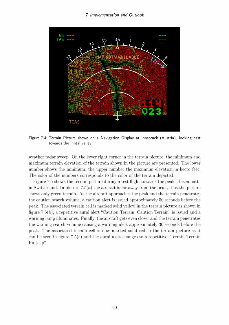
7 Implementation and Outlook
Figure 7.4: Terrain Picture shown on a Navigation Display at Innsbruck (Austria), looking easttowards the Inntal valley
weather radar sweep. On the lower right corner in the terrain picture, the minimum andmaximum terrain elevation of the terrain shown in the picture are presented. The lowernumber shows the minimum, the upper number the maximum elevation in hecto feet.The color of the numbers corresponds to the color of the terrain depicted.
Figure 7.5 shows the terrain picture during a test flight towards the peak “Hasenmatt”in Switzerland. In picture 7.5(a) the aircraft is far away from the peak, thus the pictureshows only green terrain. As the aircraft approaches the peak and the terrain penetratesthe caution search volume, a caution alert is issued approximately 50 seconds before thepeak. The associated terrain cell is marked solid yellow in the terrain picture as shown infigure 7.5(b), a repetitive aural alert “Caution Terrain, Caution Terrain” is issued and awarning lamp illuminates. Finally, the aircraft gets even closer and the terrain penetratesthe warning search volume causing a warning alert approximately 30 seconds before thepeak. The associated terrain cell is now marked solid red in the terrain picture as itcan be seen in figure 7.5(c) and the aural alert changes to a repetitive “Terrain-TerrainPull-Up”.
90

7 Implementation and Outlook
(a) Approaching the Peak
(b) The Caution Alert is issued
(c) The Warning Alert is issued
Figure 7.5: Terrain Picture shown on a Navigation Display during a Test Flight towards the peak“Hasenmatt” (Switzerland)
91
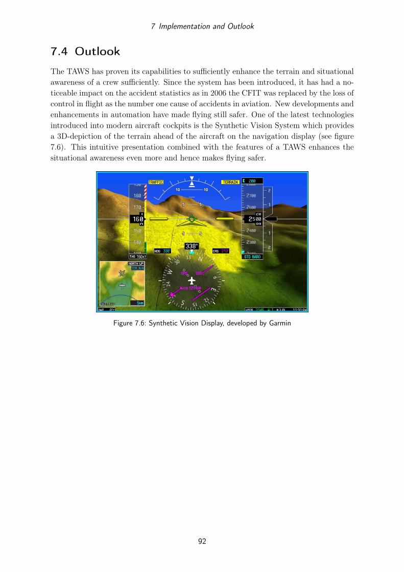
7 Implementation and Outlook
7.4 Outlook
The TAWS has proven its capabilities to sufficiently enhance the terrain and situationalawareness of a crew sufficiently. Since the system has been introduced, it has had a no-ticeable impact on the accident statistics as in 2006 the CFIT was replaced by the loss ofcontrol in flight as the number one cause of accidents in aviation. New developments andenhancements in automation have made flying still safer. One of the latest technologiesintroduced into modern aircraft cockpits is the Synthetic Vision System which providesa 3D-depiction of the terrain ahead of the aircraft on the navigation display (see figure7.6). This intuitive presentation combined with the features of a TAWS enhances thesituational awareness even more and hence makes flying safer.
Figure 7.6: Synthetic Vision Display, developed by Garmin
92
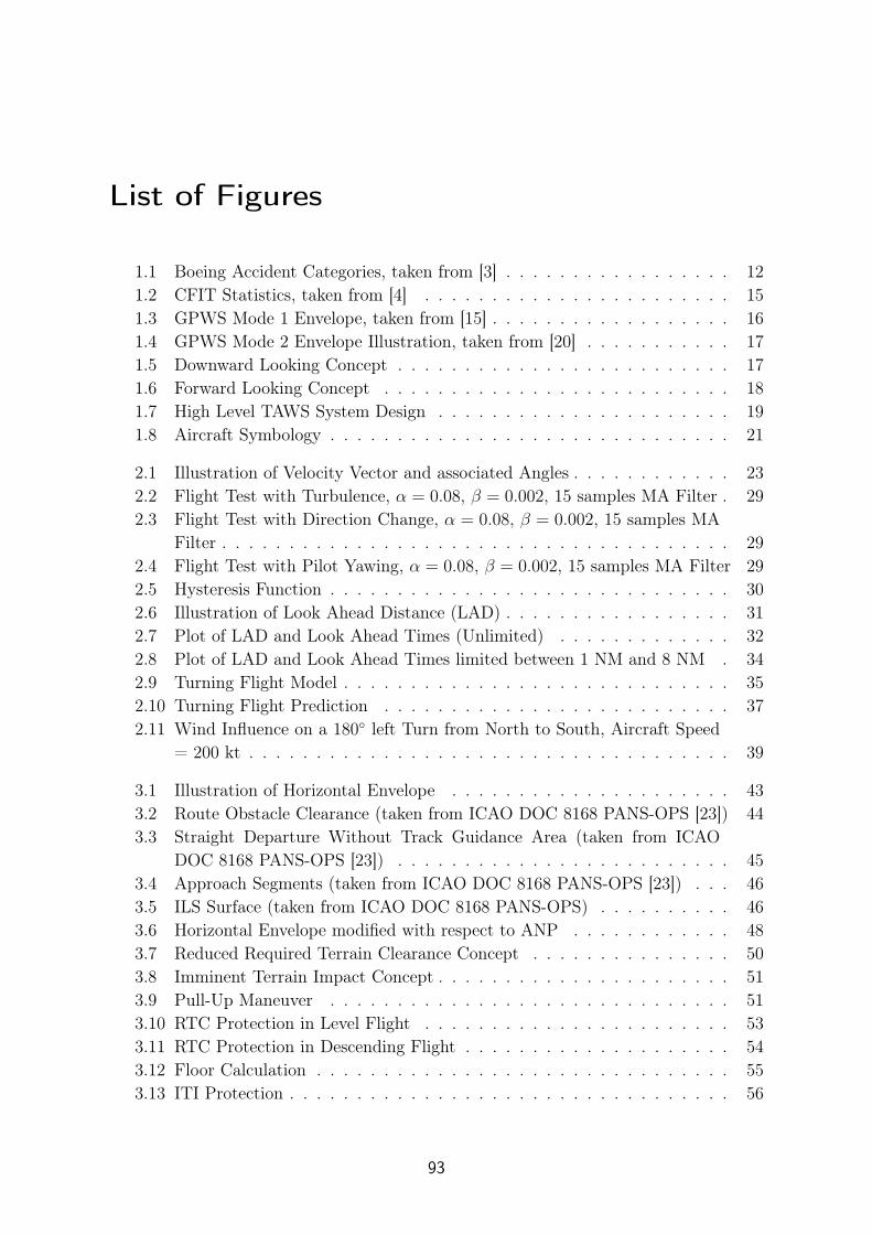
List of Figures
1.1 Boeing Accident Categories, taken from [3] . . . . . . . . . . . . . . . . . 121.2 CFIT Statistics, taken from [4] . . . . . . . . . . . . . . . . . . . . . . . 151.3 GPWS Mode 1 Envelope, taken from [15] . . . . . . . . . . . . . . . . . . 161.4 GPWS Mode 2 Envelope Illustration, taken from [20] . . . . . . . . . . . 171.5 Downward Looking Concept . . . . . . . . . . . . . . . . . . . . . . . . . 171.6 Forward Looking Concept . . . . . . . . . . . . . . . . . . . . . . . . . . 181.7 High Level TAWS System Design . . . . . . . . . . . . . . . . . . . . . . 191.8 Aircraft Symbology . . . . . . . . . . . . . . . . . . . . . . . . . . . . . . 21
2.1 Illustration of Velocity Vector and associated Angles . . . . . . . . . . . . 232.2 Flight Test with Turbulence, α = 0.08, β = 0.002, 15 samples MA Filter . 292.3 Flight Test with Direction Change, α = 0.08, β = 0.002, 15 samples MA
Filter . . . . . . . . . . . . . . . . . . . . . . . . . . . . . . . . . . . . . . 292.4 Flight Test with Pilot Yawing, α = 0.08, β = 0.002, 15 samples MA Filter 292.5 Hysteresis Function . . . . . . . . . . . . . . . . . . . . . . . . . . . . . . 302.6 Illustration of Look Ahead Distance (LAD) . . . . . . . . . . . . . . . . . 312.7 Plot of LAD and Look Ahead Times (Unlimited) . . . . . . . . . . . . . 322.8 Plot of LAD and Look Ahead Times limited between 1 NM and 8 NM . 342.9 Turning Flight Model . . . . . . . . . . . . . . . . . . . . . . . . . . . . . 352.10 Turning Flight Prediction . . . . . . . . . . . . . . . . . . . . . . . . . . 372.11 Wind Influence on a 180◦ left Turn from North to South, Aircraft Speed
= 200 kt . . . . . . . . . . . . . . . . . . . . . . . . . . . . . . . . . . . . 39
3.1 Illustration of Horizontal Envelope . . . . . . . . . . . . . . . . . . . . . 433.2 Route Obstacle Clearance (taken from ICAO DOC 8168 PANS-OPS [23]) 443.3 Straight Departure Without Track Guidance Area (taken from ICAO
DOC 8168 PANS-OPS [23]) . . . . . . . . . . . . . . . . . . . . . . . . . 453.4 Approach Segments (taken from ICAO DOC 8168 PANS-OPS [23]) . . . 463.5 ILS Surface (taken from ICAO DOC 8168 PANS-OPS) . . . . . . . . . . 463.6 Horizontal Envelope modified with respect to ANP . . . . . . . . . . . . 483.7 Reduced Required Terrain Clearance Concept . . . . . . . . . . . . . . . 503.8 Imminent Terrain Impact Concept . . . . . . . . . . . . . . . . . . . . . . 513.9 Pull-Up Maneuver . . . . . . . . . . . . . . . . . . . . . . . . . . . . . . 513.10 RTC Protection in Level Flight . . . . . . . . . . . . . . . . . . . . . . . 533.11 RTC Protection in Descending Flight . . . . . . . . . . . . . . . . . . . . 543.12 Floor Calculation . . . . . . . . . . . . . . . . . . . . . . . . . . . . . . . 553.13 ITI Protection . . . . . . . . . . . . . . . . . . . . . . . . . . . . . . . . . 56
93
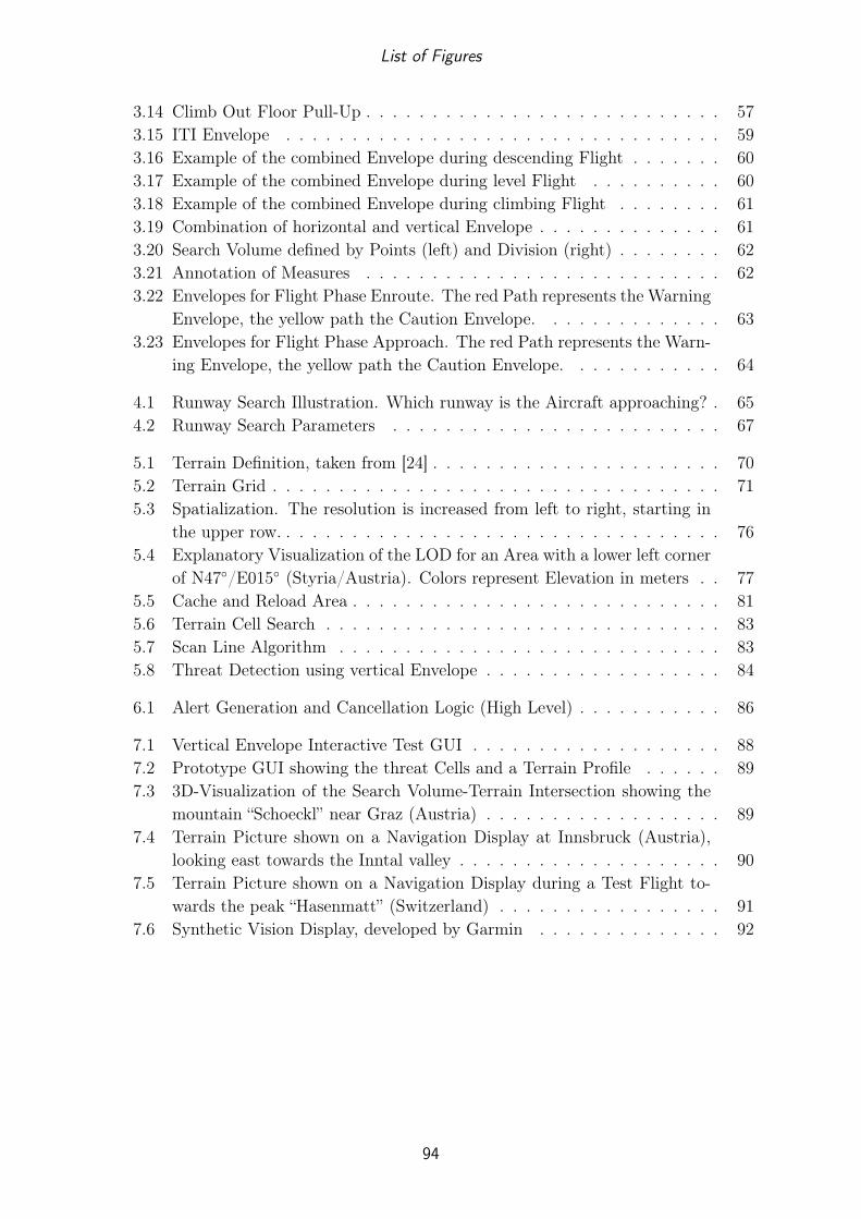
List of Figures
3.14 Climb Out Floor Pull-Up . . . . . . . . . . . . . . . . . . . . . . . . . . . 573.15 ITI Envelope . . . . . . . . . . . . . . . . . . . . . . . . . . . . . . . . . 593.16 Example of the combined Envelope during descending Flight . . . . . . . 603.17 Example of the combined Envelope during level Flight . . . . . . . . . . 603.18 Example of the combined Envelope during climbing Flight . . . . . . . . 613.19 Combination of horizontal and vertical Envelope . . . . . . . . . . . . . . 613.20 Search Volume defined by Points (left) and Division (right) . . . . . . . . 623.21 Annotation of Measures . . . . . . . . . . . . . . . . . . . . . . . . . . . 623.22 Envelopes for Flight Phase Enroute. The red Path represents the Warning
Envelope, the yellow path the Caution Envelope. . . . . . . . . . . . . . 633.23 Envelopes for Flight Phase Approach. The red Path represents the Warn-
ing Envelope, the yellow path the Caution Envelope. . . . . . . . . . . . 64
4.1 Runway Search Illustration. Which runway is the Aircraft approaching? . 654.2 Runway Search Parameters . . . . . . . . . . . . . . . . . . . . . . . . . 67
5.1 Terrain Definition, taken from [24] . . . . . . . . . . . . . . . . . . . . . . 705.2 Terrain Grid . . . . . . . . . . . . . . . . . . . . . . . . . . . . . . . . . . 715.3 Spatialization. The resolution is increased from left to right, starting in
the upper row. . . . . . . . . . . . . . . . . . . . . . . . . . . . . . . . . . 765.4 Explanatory Visualization of the LOD for an Area with a lower left corner
of N47◦/E015◦ (Styria/Austria). Colors represent Elevation in meters . . 775.5 Cache and Reload Area . . . . . . . . . . . . . . . . . . . . . . . . . . . . 815.6 Terrain Cell Search . . . . . . . . . . . . . . . . . . . . . . . . . . . . . . 835.7 Scan Line Algorithm . . . . . . . . . . . . . . . . . . . . . . . . . . . . . 835.8 Threat Detection using vertical Envelope . . . . . . . . . . . . . . . . . . 84
6.1 Alert Generation and Cancellation Logic (High Level) . . . . . . . . . . . 86
7.1 Vertical Envelope Interactive Test GUI . . . . . . . . . . . . . . . . . . . 887.2 Prototype GUI showing the threat Cells and a Terrain Profile . . . . . . 897.3 3D-Visualization of the Search Volume-Terrain Intersection showing the
mountain “Schoeckl” near Graz (Austria) . . . . . . . . . . . . . . . . . . 897.4 Terrain Picture shown on a Navigation Display at Innsbruck (Austria),
looking east towards the Inntal valley . . . . . . . . . . . . . . . . . . . . 907.5 Terrain Picture shown on a Navigation Display during a Test Flight to-
wards the peak “Hasenmatt” (Switzerland) . . . . . . . . . . . . . . . . . 917.6 Synthetic Vision Display, developed by Garmin . . . . . . . . . . . . . . 92
94
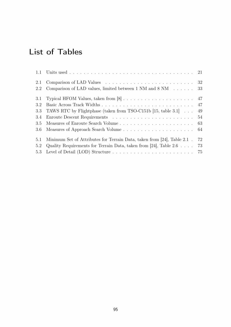
List of Tables
1.1 Units used . . . . . . . . . . . . . . . . . . . . . . . . . . . . . . . . . . . 21
2.1 Comparison of LAD Values . . . . . . . . . . . . . . . . . . . . . . . . . 322.2 Comparison of LAD values, limited between 1 NM and 8 NM . . . . . . 33
3.1 Typical HFOM Values, taken from [8] . . . . . . . . . . . . . . . . . . . . 473.2 Basic Across Track Widths . . . . . . . . . . . . . . . . . . . . . . . . . . 473.3 TAWS RTC by Flightphase (taken from TSO-C151b [15, table 3.1] . . . 493.4 Enroute Descent Requirements . . . . . . . . . . . . . . . . . . . . . . . 543.5 Measures of Enroute Search Volume . . . . . . . . . . . . . . . . . . . . . 633.6 Measures of Approach Search Volume . . . . . . . . . . . . . . . . . . . . 64
5.1 Minimum Set of Attributes for Terrain Data, taken from [24], Table 2.1 . 725.2 Quality Requirements for Terrain Data, taken from [24], Table 2.6 . . . . 735.3 Level of Detail (LOD) Structure . . . . . . . . . . . . . . . . . . . . . . . 75
95

Bibliography
[1] Pakistan Civil Aviation Authority. Investigation Report Air Blue Flight ABQ-202, Crashed on 28 July 2010 at Islamabad. http://www.caapakistan.com.pk/investigation.aspx, 2011.
[2] Norbert Bartelme. Geoinformatik - Modelle, Strukturen, Funktionen. Springer,Berlin, 4th edition edition, 2005.
[3] Boeing. Statistical Summary of Commercial Jet Airplane Accidents. 2011.
[4] Barry C. Breen. Controlled Flight Into Terrain and the Enhanced Ground ProximityWarning System. IEEE AES Systems Magazine, January 1999.
[5] Jim Burin. 2005: The year in review - return of the killers. AeroSafety World, July2006.
[6] Jim Burin. Leveling off. AeroSafety World, February 2011.
[7] Interstate Aviation Comittee. Accident Report of TU-154M, Aircraft Tail Number101, of the Republic of Poland on April 2010 near Smolensk. http://www.mak.ru/english/info/tu-154m_101.html, 2011.
[8] Boeing Dave Nakamura. FMS RNAV Workshop. February 2000.
[9] Eurocontrol. Terrain and Obstacle Manual. 2.0 edition, November 2011.
[10] Eurocontrol and International Civil Aviation Organization (ICAO). SKYbrary(Wiki). http://www.skybrary.aero.
[11] Eurocontrol and International Civil Aviation Organization (ICAO). SKYbrary(Wiki), CFIT Definition. http://www.skybrary.aero/index.php/Controlled_Flight_Into_Terrain.
[12] Eurocontrol and International Civil Aviation Organization (ICAO). SKYbrary(Wiki), Hull Loss Definition. http://www.skybrary.aero/index.php/Hull_Loss.
[13] Eurocontrol and International Civil Aviation Organization (ICAO). SKYbrary(Wiki), Situational Awareness Definition. http://www.skybrary.aero/index.php/Situational_Awareness.
[14] Federal Aviation Administration (FAA). Technical Standard Order TSO-C129a,Airborne Supplemental Navigation Equipment using the Global Positioning System(GPS). February 1996.
96

Bibliography
[15] Federal Aviation Administration (FAA). Technical Standard Order TSO-C151b,Terrain Awareness and Warning System. December 2002.
[16] Radio Technical Commission for Aeronautics (RTCA). DO-200: Standards forProcessing Aeronautical Data. 2002.
[17] Paul S. Heckbert. Concave Polygon Scan Conversion. Graphics Gems I, 1993.
[18] B. Hofmann-Wellenhof, K. Legat, and M. Wieser. Navigation - Principles of Posi-tioning and Guidance. Springer, 2003.
[19] B. Hofmann-Wellenhof, H. Lichtenegger, and J. Collins. GPS - Theory and Practice.Springer, 5th edition, 2001.
[20] Honeywell. MK VI and MK VIII, Enhanced Ground Proximity Warning System(EGPWS), Pilot’s Guide.
[21] International Civil Aviation Organization (ICAO). Annex 15 to the Convention onInternational Civil Aviation: Aeronautical Information Services. 12th edition, 2004.
[22] International Civil Aviation Organization (ICAO). Annex 6 to the Convention onInternational Civil Aviation: Operation of Aircraft, volume Part I. 12th edition,2004.
[23] International Civil Aviation Organization (ICAO). Procedures for Air NavigationServices, DOC 8168: Aircraft Operations - Volume II: Construction of Visual andInstrument Flight Procedures. 2006.
[24] International Civil Aviation Organization (ICAO). Doc 9881: Guidelines for Elec-tronic Terrain, Obstacle and Aerodrome Mapping Information. Undated.
[25] Jeppesen. Got Mountains? Challenges of Modeling SRTM and Other Terrain Datato Suit Aviation Applications, 2008.
[26] Dave Shreiner, Mason Woo, Jackie Neider, and Tom Davis. OpenGL ProgrammingGuide. Addison Wesley, 4th edition, 2004.
[27] FAA U.S. Department of Transportation. Installation of Terrain Awareness andWarning System (TAWS) Approved for Part 23 Airplanes. June 2000.
[28] FAA U.S. Department of Transportation. United States Standard for TerminalInstrument Procedures (TERPS). August 2011.
97