DFG-Schwerpunktprogramm 1324 · -the parameters s, p, and qof the Besov space,-the parameters , , ,...

DFG-Schwerpunktprogramm 1324

”Extraktion quantifizierbarer Information aus komplexen Systemen”

Adaptive Wavelet Methods for Elliptic StochasticPartial Differential Equations

P. A. Cioica, S. Dahlke, N. Dohring, S. Kinzel, F. Lindner, T. Raasch,K. Ritter, R. L. Schilling

Preprint 77

Edited by

AG Numerik/OptimierungFachbereich 12 - Mathematik und InformatikPhilipps-Universitat MarburgHans-Meerwein-Str.35032 Marburg

DFG-Schwerpunktprogramm 1324

”Extraktion quantifizierbarer Information aus komplexen Systemen”

Adaptive Wavelet Methods for Elliptic StochasticPartial Differential Equations

P. A. Cioica, S. Dahlke, N. Dohring, S. Kinzel, F. Lindner, T. Raasch,K. Ritter, R. L. Schilling

Preprint 77

The consecutive numbering of the publications is determined by theirchronological order.

The aim of this preprint series is to make new research rapidly availablefor scientific discussion. Therefore, the responsibility for the contents issolely due to the authors. The publications will be distributed by theauthors.

ADAPTIVE WAVELET METHODS FOR ELLIPTIC STOCHASTICPARTIAL DIFFERENTIAL EQUATIONS

P. A. CIOICA, S. DAHLKE, N. DOHRING, S. KINZEL, F. LINDNER,

T. RAASCH, K. RITTER, R. L. SCHILLING

Abstract. We study the Besov regularity as well as linear and nonlinear approximation

of random functions on bounded Lipschitz domains in Rd. The random functions are

given either (i) explicitly in terms of a wavelet expansion or (ii) as the solution of a

Poisson equation with a right-hand side in terms of a wavelet expansion. In the case (ii)

we derive an adaptive wavelet algorithm that achieves the nonlinear approximation rate

at a computational cost that is proportional to the degrees of freedom. These results are

matched by computational experiments.

1. Introduction

We study numerical algorithms for the Poisson equation

(1)−∆U = X in D,

U = 0 on ∂D

with random right-hand side X, and D ⊂ Rd a bounded Lipschitz domain. More precisely,X is a random function (random field) with realizations at least in L2(D), and we wish toapproximate the realizations of the random function U in H1(D). We investigate a newstochastic model for X that provides an explicit control of the Besov regularity, and weanalyse nonlinear approximation of both X and U . An average N -term approximationof the right-hand side X can be simulated efficiently, and the nonlinear approximationrate for the solution U is achieved by means of an adaptive wavelet algorithm. Theseasymptotic results are matched by numerical experiments.

Different numerical problems have been studied for Poisson equations, or more generally,for elliptic equations with a random right-hand side and/or a random diffusion coefficient.The computational task is to approximate either the realizations of the solution or atleast their moments, and different techniques like stochastic finite element methods, sparsegrids, or polynomial chaos decompositions are employed. A, by no means complete, listof papers includes [2, 12,27,36,40,47,51,55].

We construct efficient algorithms for nonlinear approximation of the random functionsX and U . While nonlinear approximation methods are extensively studied in the deter-ministic case, see [25] and the references therein for details and a survey, much less isknown for random functions. For the latter we refer to [9,11], where wavelet methods areanalysed, and to [13, 34] where free knot splines are used. In these papers the randomfunctions are given explicitly, and the one-dimensional case d = 1 is studied. Stochastic

Mathematics Subject Classification (2010). 60H35, 65C30, 65T60, 41A25, Secondary: 41A63.Key words and phrases. elliptic stochastic partial differential equation, wavelets, Besov regularity,

approximation rates, nonlinear approximation, adaptive methods.This work has been supported by the Deutsche Forschungsgemeinschaft (DFG, grants DA 360/13-1,

RI 599/4-1, SCHI 419/5-1) and a doctoral scholarship of the Philipps-Universitat Marburg.1

2 CIOICA ET AL.

differential equations, in general, yield implicitly given random functions, which holdstrue in particular for U in (1). For stochastic ordinary differential equations nonlinearapproximation of the solution process is studied in [13,43].

The random function X is defined in terms of a stochastic wavelet expansion

(2) X =∞∑j=j0

∑k∈∇j

Yj,kZ′j,kψj,k.

Here ψj,k : j ≥ j0, k ∈ ∇j is a wavelet Riesz basis for L2(D), where j denotes the scaleparameter and∇j is a finite set with, in order of magnitude, 2jd elements, and Yj,k and Z ′j,kare independent random variables. In a slightly simplified version of the stochastic model,Yj,k is Bernoulli distributed with parameter 2−βjd and Z ′j,k is normally distributed with

mean zero and variance 2−αjd, where 0 ≤ β ≤ 1 and α+ β > 1. Note that the sparsity ofthe expansion (2) depends monotonically on β. For β = 0, i.e., with no sparsity present, (2)is the Karhunen-Loeve expansion of a Gaussian random function X if the wavelets forman orthonormal basis of L2(D). The stochastic model (2) was introduced and analysed inthe context of Bayesian non-parametric regression in [1, 3].

Let us point to the main results. The random function X takes values in the Besovspace Bs

q(Lp(D)) with probability one if and only if

s < d ·(α− 1

2+β

p

),

see Theorem 2.6. In [1, 3] the result was stated for d = 1 and p, q ≥ 1. In particular, thesmoothness of X along the scale of Sobolev spaces Hs(D) = Bs

2(L2(D)) is determined byα + β, and for β > 0 with decreasing p ∈ ]0, 2] the smoothness can get arbitrarily large.

We study different approximations X of X with respect to the norm in L2(D); we

always consider the average error (E ‖X − X‖2L2(D))1/2 for any approximation X. For the

optimal linear approximation, i.e., for the approximation from an optimally chosen N -dimensional subspace of L2(D), the corresponding errors are asymptotically equivalent toN−% with

% =α + β − 1

2,

see Theorem 2.9. In contrast, for the best average N -term wavelet approximation we onlyrequire that the average number of non-zero wavelet coefficients is at most N . In this casethe corresponding errors are at most of order N−% with

% =α + β − 1

2(1− β)

and β < 1, see Theorem 2.11. The best average N -term approximation is superior tooptimal linear approximation if β > 0. The simulation of the respective average N -termapproximation is possible at an average computational cost of order N , which is crucialin computational practice.

Considering the Poisson equation (1) with a right-hand side given by (2), the solution Uof the Poisson equation is approximated with respect to the norm in H1(D). We consider

the average error (E ‖U − U‖2H1(D))1/2 for any approximation U . Here the space H1(D) is

the natural choice, since its norm is equivalent to the energy norm and the convergenceanalysis of adaptive wavelet algorithms relies on this norm. We study the N -term waveletapproximation under different assumptions on the domain D, and we establish upper

ADAPTIVE WAVELET METHODS FOR ELLIPTIC SPDES 3

bounds of the form N−(%−ε), which hold for every ε > 0. For any bounded Lipschitzdomain D in dimension d = 2 or 3 we obtain

% = min

(1

2(d− 1),α + β − 1

6+

2

3d

),

see Theorem 3.1. Regardless of the smoothness of X we have % ≤ 1/(2(d − 1)). On theother hand, uniform approximation schemes can only achieve the order N−1/(2d) on generalLipschitz domains D, and we always have % > 1/(2d). For more specific domains we fullybenefit from the smoothness of the right-hand side. First,

% =α + β

2

if D is a simply connected polygonal domain in R2, see Theorem 3.5, and

% =1

1− β

(α− 1

2+ β

)+

1

d

for bounded C∞-domains D ⊂ Rd, see Theorem 3.6.These rates for the best N -term approximation of U are actually achieved by suitable

adaptive wavelet algorithms, which have been developed for deterministic elliptic PDEs,see Section 4. Those algorithms converge for a large class of operators, including operatorsof negative order, and they are asymptotically optimal in the sense that they realize theoptimal order of convergence while the computational cost is proportional to the degreesof freedom, see [7, 8, 15]. Moreover, the algorithmic approach can be extended to waveletframes, i.e., to redundant wavelet systems, which are much easier to construct than waveletbases on general domains, see [18,44].

Numerical experiments are presented in Section 5. At first we illustrate some features ofthe stochastic model (2) for X, subsequently we determine empirical rates of convergencefor adaptive and uniform approximation of the solution U to the Poisson equation (1)in dimension d = 1. It turns out that the empirical rates fit very well to the asymptoticresults, and we observe superiority of the adaptive scheme already for moderate accuracies.

Throughout the paper we use the following notation. We write A B for mappingsA,B : M → [0,∞] on any set M , if there exists a constant c ∈ ]0,∞[ such that A(m) ≤cB(m) holds for every m ∈ M . Furthermore A B means A B and B A. In thesequel the constants may depend on

- the domain D, the wavelet basis ψj,k : j ≥ j0, k ∈ ∇j, and the orthonormalbasis ej,k : j ≥ j0, k ∈ ∇j employed in the proof of Theorem 2.9,

- the parameters s, p, and q of the Besov space,- the parameters α, β, γ, C1, and C2 of the random function, and- the parameter ε in Theorems 2.10, 3.1, 3.5, and 3.6.

The paper is organized as follows. In Sections 2 and 3 we study linear and nonlinearapproximations of X and U , respectively; to this end we analyse the Besov regularity ofthese random functions. In Section 4 we explain how to achieve the nonlinear approxi-mation rate by means of adaptive wavelet algorithms. In Section 5 we present numericalexperiments to complement the asymptotic error analysis.

4 CIOICA ET AL.

2. A Class of Random Functions in Besov Spaces

In this section we discuss linear and nonlinear approximations as well as the Besovregularity of random functions X : Ω→ L2(D) on a bounded Lipschitz domain D ⊂ Rd.The random functions are defined in terms of wavelet expansions according to a stochasticmodel that provides an explicit control for the Besov regularity and, in particular, inducessparsity of the wavelet coefficients. In the context of Bayesian non-parametric regressionthis model was introduced and analysed in [1] and generalized in [3] in the case D = [0, 1]for Besov spaces with parameters p, q ≥ 1.

2.1. The Basic Wavelet Setting. We briefly state the wavelet setting as far as it isneeded for our purposes. In general, a wavelet basis Ψ = ψλ : λ ∈ ∇ is a basis foran L2-space with specific properties outlined below. The indices λ ∈ ∇ typically encodeseveral types of information, namely the scale, often denoted by |λ|, the spatial location,and also the type of the wavelet. For instance, on the real line, |λ| = j ∈ Z denotes thedyadic refinement level and 2−jk with k ∈ Z stands for the location of the wavelet.

We will ignore any explicit dependence on the type of the wavelet from now on, sincethis only produces additional constants. Hence, we frequently use λ = (j, k) and

∇ = (j, k) : j ≥ j0, k ∈ ∇j,

where ∇j is some countable index set and |(j, k)| = j. Moreover, Ψ = ψλ : λ ∈ ∇denotes the dual wavelet basis, which is biorthogonal to Ψ, i.e.,

〈ψλ, ψλ′〉L2(D) = δλ,λ′ .

We assume that the domain D under consideration enables us to construct a waveletbasis Ψ with the following properties:

(A1) the wavelets form a Riesz basis for L2(D);(A2) the cardinalities of the index sets ∇j satisfy

#∇j 2jd;

(A3) the wavelets are local in the sense that

diam(supp ψλ) 2−|λ|;

(A4) the wavelets satisfy the cancellation property

|〈v, ψλ〉L2(D)| 2−|λ|(d2+m)|v|W m(L∞(supp ψλ))

for |λ| > j0 with some parameter m ∈ N;(A5) the wavelet basis induces characterizations of Besov spaces Bs

q(Lp(D)) of theform

‖v‖Bsq(Lp(D))

∞∑j=j0

2j(s+d(12− 1p))q

∑k∈∇j

|〈v, ψj,k〉L2(D)|pq/p

1/q

,

for 0 < p, q <∞ and all s with d(1p− 1)+ < s < s1 for some parameter s1 > 0.

In (A5) the upper bound s1 depends, in particular, on the smoothness and the approxi-mation properties of the wavelet basis.

For Section 3–5, we furthermore assume that the dual basis Ψ satisfies (A1)–(A5) withpossibly different parameters in (A4) and (A5). Using the fact that Bs

2(L2(D)) = Hs(D)


and by exploiting the norm equivalence (A5), a simple rescaling of Ψ immediately yieldsa Riesz basis for Hs(D) with 0 < s < s1. In Sections 4 and 5 we actually assume thatthe primal wavelet basis Ψ characterizes the Sobolev spaces Hs

0(D) with homogeneousDirichlet boundary conditions, instead of Hs(D). Suitable constructions of wavelets ondomains can be found in [4, 10, 22–24, 35, 38], and we also refer to [6] for a detaileddiscussion.

2.2. The Stochastic Model. The construction of the random function X : Ω→ L2(D)primarily depends on the parameters

α > 0, 0 ≤ β ≤ 1, γ ∈ R

with

α + β > 1.

Additionally, let C1, C2 > 0. The stochastic model is based on independent random vari-ables Yj,k and Zj,k for j ≥ j0 and k ∈ ∇j on some probability space (Ω,A, P ). Thevariables Yj,k are Bernoulli distributed with parameter

pj = min(1, C12

−βjd) , with P (Yj,k = 1) = pj and P (Yj,k = 0) = 1− pj.

The variables Zj,k are N(0, 1)-distributed and, in order to rescale their variances, we put

σ2j = C2j

γd2−αjd.

Since

E

( ∞∑j=j0

∑k∈∇j

σ2jY

2j,kZ

2j,k

)=

∞∑j=j0

#∇jσ2jpj

∞∑j=j0

jγd2−(α+β−1)jd <∞

by (A2), we use (A1) to conclude that

(3) X =∞∑j=j0

∑k∈∇j

σjYj,kZj,kψj,k

converges P -a.s. in L2(D).

Remark 2.1. Let ξ, ζ ∈ L2(D). We have E(〈ξ,X〉L2(D)) = 0, i.e., X is a mean zerorandom function. Moreover,

E(〈ξ,X〉L2(D)〈ζ,X〉L2(D)) =∞∑j=j0

σ2jpj

∑k∈∇j

〈ξ, ψj,k〉L2(D)〈ζ, ψj,k〉L2(D).

Using the dual basis we obtain

Qξ =∞∑j=j0

σ2jpj

∑k∈∇j

〈ξ, ψj,k〉L2(D)ψj,k

for the covariance operator Q associated with X. If Ψ is an orthonormal basis, then (3) isthe Karhunen-Loeve decomposition of X. Note that X is Gaussian if and only if pj = 1for all j ≥ j0, i.e., β = 0 and C1 ≥ 1.

6 CIOICA ET AL.

2.3. Besov Regularity. In the following we establish a necessary and sufficient conditionfor X ∈ Bs

q(Lp(D)) to hold with probability one. Consider the random variables

Sj,p =∑k∈∇j

Yj,k|Zj,k|p, j ≥ j0,

which form an independent sequence for every fixed 0 < p < ∞. Furthermore, we use νpto denote the p-th absolute moment of the standard normal distribution.

Lemma 2.2. Let Xn,ρ be binomially distributed with parameters n ∈ N and ρ ∈ [0, 1]. Forevery r > 0 there exists a constant c > 0 such that

E(Xrn,ρ) ≤ c (1 + (nρ)r)

for all n and ρ.

Proof. It suffices to consider r ∈ N. The upper bound clearly holds for r = 1. For r ≥ 2we have E(Xr

1,ρ) = ρ ≤ 1. Moreover, for n ≥ 2,

E(Xrn,ρ) =

n∑k=1

kr(n

k

)ρk(1− ρ)n−k

=n−1∑k=0

(k + 1)r−1n

(n− 1

k

)ρk+1(1− ρ)n−1−k

= nρE(1 +Xn−1,ρ)r−1.

Inductively we obtain

E(Xrn,ρ) nρ(1 + E(Xn−1,ρ)

r−1) nρ+ (nρ)r 1 + (nρ)r,

as claimed.

Lemma 2.3. Assume that 0 ≤ β < 1. Then

limj→∞

Sj,p#∇jpj

= νp

holds with probability one, and

supj≥j0

E(Srj,p)

(#∇jpj)r<∞

holds for every r > 0.

Proof. Clearly E(Sj,p) = #∇jpjνp and Var(Sj,p) = #∇jpj(ν2p − pjν2p). Hence

P (|Sj,p/(#∇jpj)− νp| ≥ ε) ≤ ε−2 (#∇jpj)−1(ν2p − pjν2p) ε−2 2−(1−β)jd

follows from Chebyshev’s inequality. It remains to apply the Borel-Cantelli Lemma toobtain the a.s. convergence of Sj,p/(#∇jpj).

Fix r > 0. By the equivalence of moments of Gaussian measures, see [49, p. 338], thereexists a constant c1 > 0 such that

E

((∑k∈∇j

yj,k|Zj,k|p)r)

= E

((∑k∈∇j

|yj,kZj,k|p)r)

≤ c1

(E∑k∈∇j

|yj,kZj,k|p)r

= c1νrp

(∑k∈∇j

yj,k

)r


for every j ≥ j0 and all yj,k ∈ 0, 1. The sequences (Yj,k)k and (Zj,k)k are independent.This gives E(Srj,p) ≤ c1ν

rp E(Srj,0). Finally, there exists a constant c2 > 0 such that E(Srj,0) ≤

c2(#∇jpj)r, see Lemma 2.2.

Let µ denote any probability measure on the real line, and let c > 0. By µ∗` we denotethe `-fold convolution of µ. The compound Poisson distribution with intensity measure

cµ is given by exp(−c)∑∞

`=0c`

`!µ∗`.

Lemma 2.4. Assume that β = 1 and

(4) limj→∞

#∇j2−jd = C0

for some C0 > 0. Let µp denote the distribution of |Zj,k|p, and let Sp be a compound Poissonrandom variable with intensity measure C0C1 · µp. Then (Sj,p)j converges in distributionto Sp, and

(5) supj≥j0

E(Srj,p) <∞

holds for every r > 0.

Proof. Let Z be N(0, 1)-distributed. The characteristic function ϕSp of Sp is given by

ϕSp(t) = E(exp(itSp)) = exp(C0C1(ϕ|Z|p(t)− 1)).

Furthermore, for the characteristic function ϕSj,p of Sj,p,

ϕSj,p(t) =(pjϕ|Z|p(t) + 1− pj

)#∇j=(

1 +1

#∇j

· pj#∇j

(ϕ|Z|p(t)− 1

) )#∇j.

We use (4) to conclude thatlimj→∞

ϕSj,p(t) = ϕSp(t),

which yields the convergence in distribution as claimed.Suppose that p ≥ 1. Then we take c1 > 0 such that zrp ≤ c1 exp(z) for every z ≥ 0 and

we put c2 = E(exp(|Zj,k|)) to obtain

E(Srj,p) ≤ E(Srpj,1) ≤ c1 E(exp(Sj,1)) = c1(1 + pj(c2 − 1))#∇j .

Note that the upper bound converges to c1 exp(C0C1(c2 − 1)). In the case 0 < p < 1 wehave Sj,p ≤ Sj,0+Sj,1. Hence it remains to observe that supj≥j0 E(Srj,0) <∞, which followsfrom Lemma 2.2.

Remark 2.5. In general, we only have (A2) instead of (4). For β = 1 the upper bound(5) remains valid in the general case, too. In all known constructions of wavelet baseson bounded domains, see, e.g., [4, 10, 22–24, 38], and also for wavelet frames [18, 44], thenumber #∇j of wavelets per level j > j0 is a constant multiple of 2jd. For those kinds ofbases, (4) trivially holds.

Theorem 2.6. Suppose that s > d · (1/p− 1)+. We have X ∈ Bsq(Lp(D)) with probability

one if and only if

(6) s < d ·(α− 1

2+β

p

)or

(7) s = d ·(α− 1

2+β

p

)and qγd < −2.

8 CIOICA ET AL.

Furthermore,

E ‖X‖qBsq(Lp(D)) <∞

if (6) or (7) is satisfied.

Proof. Let

aj = 2jq(s+d(12− 1p))σqj .

Since∞∑j=j0

aj(#∇jpj)q/p

∞∑j=j0

jqγd2 2δqjd

with

δ =s

d− α− 1

2− β

p,

it follows that the condition (6) or (7) is equivalent to

(8)∞∑j=j0

aj(#∇jpj)q/p <∞.

On the other hand, because of the characterization (A5), we have X ∈ Bsq(Lp(D)) with

probability one if and only if

(9)∞∑j=j0

ajSq/pj,p <∞ P -a.s.

Therefore, it is enough to show the equivalence of (8) and (9).In the case 0 ≤ β < 1 this follows immediately from Lemma 2.3. Suppose that β = 1.

Then #∇jpj 1, so that (8) is equivalent to

(10)∞∑j=j0

aj <∞.

On the other hand, since the random variables ajSj,p are non-negative and independent,(9) is equivalent to

∞∑j=j0

E

(ajS

q/pj,p

1 + ajSq/pj,p

)<∞,

see [42, p. 363]. We use Lemma 2.4 and Remark 2.5 to conclude that (10) implies

∞∑j=j0

E

(ajS

q/pj,p

1 + ajSq/pj,p

)≤

∞∑j=j0

aj E(Sq/pj,p ) <∞.

In the case∑∞

j=j0aj =∞ we put

c1 = infj≥j0

P (Sj,p ≥ 1).

We get c1 > 0 from Lemma 2.4, and so

∞∑j=j0

E

(ajS

q/pj,p

1 + ajSq/pj,p

)≥ c1

∞∑j=j0

aj1 + aj

=∞,

as claimed.


Finally, we consider the q-th moment of ‖X‖Bsq(Lp(D)), provided that (8) is satisfied. Weuse (A5) and Lemma 2.3 for 0 ≤ β < 1 as well as Lemma 2.4 and Remark 2.5 for β = 1to derive

E ‖X‖qBsq(Lp(D)) ∞∑j=j0

aj E(Sq/pj,p )

∞∑j=j0

aj(#∇jpj)q/p <∞,

as claimed.

For the conclusions in Theorem 2.6 to hold true we only assume (A1), (A2) and (A5).As a special case of Theorem 2.6, we consider the specific scale of Besov spaces Bs

τ (Lτ (D))with

(11)1

τ=s− td

+1

2

for s > t ≥ 0, which determines the approximation order of best N -term wavelet approxi-mation with respect to H t(D), see also Sections 2.4 and 3. In these sections average errorswill be defined by second moments, and therefore we also study second moments of thenorm in Bs

τ (Lτ (D)).

Corollary 2.7. Suppose that

0 ≤ t < d · α + β − 1

2

and s > t as well as

(1− β) · s < d · α + β − 1

2− β · t.

Let τ be given by (11). Then X ∈ Bsτ (Lτ (D)) holds with probability one, and

E ‖X‖2Bsτ (Lτ (D)) <∞.

Proof. Take p = q = τ and apply Theorem 2.6 to conclude that X ∈ Bsτ (Lτ (D)) holds

with probability one. Actually, X ∈ Bs+δ2 (Lτ (D)) holds with probability one if δ > 0 is

sufficiently small, and Bs+δ2 (Lτ (D)) is continuously embedded in Bs

τ (Lτ (D)). The momentbound from Theorem 2.6 therefore implies

E ‖X‖2Bsτ (Lτ (D)) E ‖X‖2Bs+δ2 (Lτ (D))

<∞,

which completes the proof.

Remark 2.8. It follows from Corollary 2.7 that by choosing the sparsity parameter βclose to one we get an arbitrarily high regularity in the nonlinear approximation scale ofBesov spaces, provided that the wavelet basis is sufficiently smooth. This is obviously notpossible in the classical L2-Sobolev scale, see Theorem 2.6 with p = q = 2.

2.4. Linear and Nonlinear Approximation. In this section we study the approxi-mation of X with respect to the L2-norm. For linear approximation one considers thebest approximation (i.e., orthogonal projection in our setting) from linear subspaces ofdimension at most N . The corresponding linear approximation error of X is given by

elinN (X) = inf(E ‖X − X‖2L2(D)

)1/2with the infimum taken over all measurable mappings X : Ω→ L2(D) such that

dim(span(X(Ω))) ≤ N.

10 CIOICA ET AL.

Theorem 2.9. The linear approximation error satisfies

elinN (X) (lnN)γd2 N−

α+β−12 .

Proof. Truncating the expansion (3) of X we get a linear approximation

(12) Xj1 =

j1∑j=j0

∑k∈∇j

σjYj,kZj,k ψj,k,

which satisfies

(13) E ‖X − Xj1‖2L2(D) ∞∑

j=j1+1

#∇jσ2jpj

∞∑j=j1+1

jγd2−(α+β−1)jd jγd1 2−(α+β−1)j1d.

Since dim(span(Xj1(Ω))) ∑j1

j=j0#∇j 2j1d, we get the upper bound as claimed.

In the proof of the lower bound we use the fact that ψj,k = Φej,k for an orthonormalbasis (ej,k)j,k in L2(D) and a bounded linear bijection Φ : L2(D)→ L2(D). This implies

elinN (X) elinN (Φ−1X).

Furthermore, elinN (Φ−1X) depends on Φ−1X only via its covariance operator Q, which isgiven by

(14) Qξ =∞∑j=j0

σ2jpj

∑k∈∇j

〈ξ, ej,k〉L2(D) ej,k,

cf. Remark 2.1. Consequently, the functions ej,k form an orthonormal basis of eigenfunc-

tions of Q with associated eigenvalues σ2jpj. Due to a theorem by Micchelli and Wahba,

see, e.g., [39, Prop. III.24], we get

elinN (Φ−1X) =

( ∞∑j=j1+1

#∇jσ2jpj

)1/2

if N =∑j1

j=j0#∇j.

The best N -term (wavelet) approximation imposes a restriction only on the number

η(g) = #λ ∈ ∇ : cλ 6= 0, g =

∑λ∈∇

cλ ψλ

of non-zero wavelet coefficients of g. Hence the corresponding error of best N-term ap-proximation for X is given by

eN(X) = inf(E ‖X − X‖2L2(D)


η(X(ω)) ≤ N P -a.s.

The analysis of eN(X) is based on the Besov regularity of X and the underlying waveletbasis Ψ. For deterministic functions x on D the error of best N -term approximation withrespect to the L2-norm is defined by

(15) σN(x) = inf‖x− x‖L2(D) : x ∈ L2(D), η(x) ≤ N.Clearly

eN(X) =(E(σ2

N(X)))1/2

.


Theorem 2.10. For every ε > 0, the error of best N-term approximation satisfies

eN(X)

N−1/ε, if β = 1

N−α+β−12(1−β)+ε, otherwise.

Proof. It suffices to consider the case β < 1. Let s and τ satisfy (11) with t = 0. Sincex ∈ Bs

τ (Lτ (D)) implies

σN(x) ‖x‖Bsτ (Lτ (D))N−s/d,

see [25] or [26] for this fundamental connection between Besov regularity and best N -termapproximation, it remains to apply Corollary 2.7.

For random functions it is also reasonable to impose a constraint on the average num-ber of non-zero wavelet coefficients only, and to study the error of best average N-term(wavelet) approximation

eavgN (X) = inf(E ‖X − X‖2L2(D)


E(η(X)) ≤ N.

Theorem 2.11. The error of best average N-term approximation satisfies

eavgN (X)

N

γd2 2−

αdN2 , if β = 1

(lnN)γd2 N−

α+β−12(1−β) , otherwise.

Proof. Let Nj1 = E(η(Xj1)) for Xj1 as in (12). Clearly

Nj1 =

j1∑j=j0

#∇jpj j1∑j=j0

2(1−β)jd

j1, if β = 1

2(1−β)j1d, otherwise.

In particular, 2j1d N1/(1−β)j1

if 0 ≤ β < 1. It remains to observe the error bound (13).

The asymptotic behaviour of the linear approximation error elinN (X) is determined by

the decay of the eigenvalues σ2jpj of the covariance operator Q, see (14), i.e., it is essentially

determined by the parameter α + β. According to Theorem 2.6, the latter quantity alsodetermines the regularity of X in the scale of Sobolev spaces Hs(D).

For 0 < β ≤ 1 nonlinear approximation is superior to linear approximation. Moreprecisely, the following holds true. By definition, eavgN (X) ≤ eN(X), and for β > 0 theconvergence of eN(X) to zero is faster than that of elinN (X). For 0 < β < 1 the upper boundsfor eavgN (X) and eN(X) slightly differ, and any dependence of eN(X) on the parameter γis swallowed by the term N ε in the upper bound. For linear and best average N -termapproximation we have

eavgN1−β(X) elinN (X) if 0 < β < 1

and

eavgc lnN(X) elinN (X) if β = 1

with a suitably chosen constant c > 0.

12 CIOICA ET AL.

Remark 2.12. We stress that for 0 < β ≤ 1 the simulation of the approximation Xj1 ,which achieves the upper bound in Theorem 2.11, is possible at an average computationalcost of order Nj1 . Let us briefly sketch the method of simulation. Put nj = #∇j. Foreach level j we first simulate a binomial distribution with parameters nj and pj, whichis possible at an average cost of order at most nj · pj. Conditional on a realization L(ω)of this step, the locations of the non-zero coefficients on level j are uniformly distributedon the set of all subsets of 0, . . . , nj of cardinality L(ω). Thus, in the second step, weemploy acceptance-rejection to collect the elements of such a random subset sequentially.If L(ω) ≤ nj/2, then all acceptance probabilities are at least 1/2, and otherwise we switchto complements to obtain the same bound for the acceptance probability. In this way, theaverage cost of the second step is of order nj · pj, too. In the last step we simulate thevalues of the non-zero coefficients. In total, the average computational cost for each levelj is of order nj · pj.

Remark 2.13. For Theorems 2.9 and 2.11 we only need the properties (A1) and (A2) ofthe basis Ψ, and (A2) enters only via the asymptotic behaviour of the parameters pj andσj. After a lexicographic reordering of the indices (j, k) the two assumptions essentiallyamount to

X =∞∑n=1

σnYnZnψn

with any Riesz basis (ψn)n∈N for L2(D), and

σn (lnn)γd/2n−α/2

as well as independent random variables Yn and Zn, where Zn is N(0, 1)-distributed andYn is Bernoulli distributed with parameter

pn n−β.

Hence, Theorems 2.9 and 2.11 remain valid beyond the wavelet setting. For instance, letpn = 1, which corresponds to β = 0 and C1 ≥ 1. Classical examples for Gaussian randomfunctions on D = [0, 1]d are the Brownian sheet, which corresponds to

α = 2 and γ = 2(d− 1)/d,

and Levy’s Brownian motion, which corresponds to

α = (d+ 1)/d and γ = 0.

Theorem 2.9 is due to [37,54] for the Brownian sheet and due to [52] for Levy’s Brownianmotion. See [39, Chap. VI] for further results and references on approximation of Gaussianrandom functions. For β > 0 our stochastic model provides sparse variants of generalGaussian random function.

3. Nonlinear Approximation for Elliptic Boundary Value Problems

We are interested in adaptive numerical wavelet algorithms for elliptic boundary valueproblems with random right-hand sides. As a particular, but nevertheless very important,model problem we are concerned with the Poisson equation on a bounded Lipschitz domainD ⊂ Rd,

(16)−∆U(ω) = X(ω) in D,

U(ω) = 0 on ∂D,


where the right-hand side X : Ω → L2(D) ⊂ H−1(D) is a random function as describedin Section 2.2. However, X is given as expansion in the dual basis Ψ.

As we will explain in the next section, the adaptive wavelet algorithms we want toemploy are optimal in the sense that they asymptotically realize the approximation orderof best N -term (wavelet) approximation. Such convergence analysis of adaptive algorithmsrelies on the energy norm, hence we study best N -term approximations of the randomfunction U : Ω→ H1(D) in H1(D). Analogously to (15) we introduce

σN,H1(D)(u) = inf‖u− u‖H1(D) : u ∈ H1(D), η(u) ≤ N.

The quantity σN,H1(D)(U(ω)), where U(ω) is the exact solution of (16), serves as bench-mark for the performance. To analyse the power of adaptive algorithms in the stochasticsetting, we investigate the error

eN,H1(D)(U) = inf(E ‖U − U‖2H1(D))1/2,

with the infimum taken over all measurable mappings U : Ω→ H1(D) such that

η(X(ω)) ≤ N P -a.s.

Clearly

eN,H1(D)(U) =(

E(σ2N,H1(D)(U))

)1/2.

Theorem 3.1. Suppose that d ∈ 2, 3 and that the right-hand side X in (16) is of theform (3). Put

% = min

(1

2(d− 1),α + β − 1

6+

2

3d

).

Then, for every ε > 0, the error of the best N-term approximation satisfies

eN,H1(D)(U) N−%+ε.

Proof. It is well known that for all d ≥ 1

(17) σN,H1(D)(u) ‖u‖Brτ (Lτ (D))N−(r−1)/d,

where1

τ=r − 1

d+

1

2,

see, e.g., [15] for details. The next step is to control the norm of a solution u in theBesov space Br

τ (Lτ (D)) in terms of the regularity of the right-hand side x of the Poissonequation. Let

−1

2< r∗ <

4− d2(d− 1)

,

and assume that x ∈ Hr∗(D). We may apply the results from [15, 16] to conclude thatu ∈ Br−δ

τ (Lτ (D)) for sufficiently small δ > 0, where

r =r∗ + 5

3,

1

τ=r − δ − 1

d+

1

2.

Moreover,

‖u‖Br−δτ (Lτ (D)) ‖x‖Br∗2 (L2(D))

and we can use (17), with r replaced by r − δ, to derive

σN,H1(D)(u) ‖x‖Br∗2 (L2(D))N−(r∗+2−3δ)/(3d).

14 CIOICA ET AL.

If, in addition, r∗/d < (α + β − 1)/2, then

eN,H1(D)(U) N−(r∗+2−3δ)/(3d)

follows from Theorem 2.6.

Remark 3.2. In Theorem 3.1, we have concentrated on nonlinear approximations inH1(D), since this norm is the most important one from the numerical point of view, as wehave briefly outlined above. In the deterministic setting, similar results for approximationsin other norms, e.g., in L2 or even weaker norms, also exist, see, e.g., [21] for details.

Remark 3.3. It is well known that the convergence order of classical nonadaptive uniformmethods does not depend on the Besov regularity of the exact solution but on its Sobolevsmoothness, see, e.g., [20, 21, 32] for details. However, on a Lipschitz domain, due tosingularities at the boundary, the best one can expect is U ∈ H3/2(D), even for verysmooth right-hand sides, see [31,33]. Therefore a uniform approximation scheme can onlygive the order N−1/(2d). In our setting, see Theorem 3.1, we have

% >1

2d,

so that for the problem (16) adaptive wavelet schemes are always superior when comparedwith uniform schemes.

Remark 3.4. With increasing values of α and β the smoothness of X increases, seeTheorem 2.6. On a general Lipschitz domain, however, this does not necessarily increasethe Besov regularity of the corresponding solution. This is reflected by the fact that theupper bound in Theorem 3.1 is at most of order N−1/(2(d−1)).

For more specific domains, i.e., for polygonal domains, better results are available. LetD denote a simply connected polygonal domain in R2. Then, it is well known that if theright-hand side X in (16) is contained in Hr−1(D) for some r ≥ 0, the solution U can beuniquely decomposed into a regular part UR and a singular part US, i.e., U = UR + US,where UR ∈ Hr+1(D) and US belongs to a finite-dimensional space that only depends onthe shape of the domain. This result was established by Grisvard, see [29], [30, Chapt. 4, 5],or [31, Sect. 2.7] for details.

Theorem 3.5. Suppose that D is a simply connected polygonal domain in R2 and thatthe right-hand side X in (16) is of the form (3). Put

% =α + β

2.

Then, for every ε > 0, error of the best N-term approximation satisfies

eN,H1(D)(U) N−%+ε.

Proof. We apply the results from [29–31]. Let us denote the segments of ∂D by Γ1, . . . ,ΓMwith open sets Γ` numbered in positive orientation. Furthermore, let Υ` denote the end-point of Γ` and let χ` denote the measure of the interior angle at Υ`. We introduce polarcoordinates (κ`, θ`) in the vicinity of each vertex Υ`, and for n ∈ N and ` = 1, . . . ,M weintroduce the functions

S`,n(κ`, θ`) = ζ`(κ`) · κλ`,n` sin(nπθ`/χ`),


when λ`,n = nπ/χ` is not an integer, and

S`,n(κ`, θ`) = ζ`(κ`) · κλ`,n` [log κ` sin(nπθ`/χ`) + θ` cos(nπθ`/χ`)]

otherwise. Here ζ` denotes a suitable C∞ truncation function.Consider the solution u = uR + uS of the Poisson equation with the right-hand side

x ∈ Hr−1(D), and assume that

r 6∈ λ`,n : n ∈ N, ` = 1, . . . ,M.

Then one has uR ∈ Hr+1(D) and uS ∈ N for

N = spanS`,n : 0 < λn,l < r

.

We have to estimate the Besov regularity of both, uS and uR, in the scale given by (11)with t = 1, i.e,

1

τ=s

2.

Classical embeddings of Besov spaces imply that uR ∈ Bsτ (Lτ (D)) for every s < r + 1.

Moreover, it has been shown in [14] that N ⊂ Bsτ (Lτ (D)) for every s > 0. We conclude

that u ∈ Bsτ (Lτ (D)) for every s < r + 1.

To estimate u, we argue as follows. Let γ` be the trace operator with respect to thesegment Γ`. Grisvard has shown that the Laplacian ∆ maps the direct sum

H =u ∈ Hr+1(D) : γ`u = 0, ` = 1, . . . ,M

+N

onto Hr−1(D), cf. [30, Thm. 5.1.3.5]. Note that (H, ‖ · ‖H) is a Banach space where

‖u‖H = ‖uR‖Hr+1(D) +M∑`=1

∑0<λ`,n<r

|c`,n|

for

uS =M∑`=1

∑0<λ`,n<r

c`,n S`,n.

It has been shown in [19] that the solution operator ∆−1 is continuous as a mapping fromHr−1(D) onto H. Therefore

‖u‖Bsτ (Lτ (D)) ‖uR‖Hr+1(D) +M∑`=1

∑0<λ`,n<t

|c`,n| = ‖u‖H ‖x‖Hr−1(D)

for every s < r + 1.Finally, by Theorem 2.6, X ∈ Hr−1(D) with probability one and E ‖X‖2Hr−1(D) <∞ if

r < α+ β. Now the upper bound for eN,H1(D)(U) follows by proceeding as in the proof ofTheorem 3.1.

Let us briefly discuss the case of a C∞-domain D. In this case, the problem is completelyregular and no singularities induced by the shape of the domain can occur. However,similar to Corollary 2.7, it is a remarkable fact that for β close to one an arbitrarily highorder of convergence can be realized.

16 CIOICA ET AL.

Theorem 3.6. Suppose that D is a bounded C∞-domain in Rd and that the right-handside X in (16) is of the form (3). Moreover, assume that β < 1 and put

% =1

1− β

(α− 1

2+ β

)+

1

d.

Then, for every ε > 0, the error of best N-term approximation satisfies

eN,H1(D)(U) N−%+ε.

Proof. In order to ensure that the condition s > d(1/τ − 1)+ is satisfied, let us considerthe scale

1

τ=s

d+ 1− δ

for some arbitrarily small parameter δ > 0. Given α and β, a similar calculation as inthe proof of Corollary 2.7 shows that X ∈ Bs

τ (Lτ (D)) holds with probability one andE ‖X‖2Bsτ (Lτ (D)) <∞ if

s <d

1− β

(α− 1

2+ β(1− δ)

).

Since the problem is regular, the solution u of the Poisson equation with right-hand sidex ∈ Bs

τ (Lτ (D)) satisfies u ∈ Bs+2τ (Lτ (D)) with

‖u‖Bs+2τ (Lτ (D)) ‖x‖Bsτ (Lτ (D)),

see [41, Chap. 3] or [48, Thm. 4.3]. By a classical embedding of Besov spaces we obtain

‖u‖Bs+2τ∗ (Lτ∗ (D)) ‖u‖Bs+2

τ (Lτ (D))

for the nonlinear approximation scale

1

τ ∗=

(s+ 2)− 1

d+

1

2.

An application of (17) yields

σN,H1(D)(u) ‖u‖Bs+2τ∗ (Lτ∗ (D))N

−(s+1)/d.

We conclude that

eN,H1(D)(U) N−(s+1)/d.

Let δ tend to zero to obtain the result as claimed.

For β = 1 the estimate from Theorem 3.6 is valid for arbitrarily large %, provided thatthe primal and dual wavelet bases are sufficiently smooth, cf. assumption (A5).

4. Adaptive Wavelet Methods for Elliptic Operator Equations

In this section, let us briefly review the class of deterministic adaptive wavelet algorithmsthat will be applied in the numerical discretisation of (16).


4.1. Elliptic PDEs in Wavelet Coordinates. The stochastic boundary value problemunder consideration can be written as an elliptic random operator equation

(18) AU(ω) = X(ω),

where ω ∈ Ω and A : H → H ′ is a linear, boundedly invertible mapping between aseparable Hilbert space H and its normed dual. The associated bilinear form a(u, v) =〈Au, v〉H′×H is bounded, |a(u, v)| ‖u‖H‖v‖H , and elliptic, a(u, u) ‖u‖2H . In case thatH = H1

0 (D), as in (16), and whenever we have a wavelet basis Ψ = ψλ : λ ∈ ∇ of L2(D)fulfilling the assumptions (A1)–(A5), the equation (18) has an equivalent reformulation

(19) AU(ω) = X(ω)

in wavelet coordinates, where we define A = (Aλ,µ) and X = (Xλ) by

Aλ,µ = 2−(|µ|+|λ|)a(ψµ, ψλ)

and

Xλ(ω) = 2−|λ|⟨X(ω), ψλ

⟩H−1(D)×H1

0 (D)

for all µ, λ ∈ ∇. Here equivalence means the following. For each solution U(ω) ∈ `2(∇)to (19), the associated wavelet expansion

U(ω) =∑λ∈∇

2−|λ|Uλ(ω)ψλ ∈ H

solves (18). Conversely, the unique expansion coefficients

U(ω)λ = 2|λ|〈ψλ, U(ω)〉H−1(D)×H10 (D)

of a solution U(ω) ∈ H to (18) satisfy (19).Such an equivalence still holds if the underlying wavelet basis is replaced by a wavelet

frame, i.e., a redundant wavelet system which allows for stable analysis and synthesisoperations. On general domains, e.g., polygonal domains in R2, wavelet frames are mucheasier to construct than bases, see [18, 44]. We tacitly assume that the chosen waveletframe fulfils assumptions (A2)–(A5), see [17] for details on the characterization of Besovspaces. In the case of frames, each solution U(ω) ∈ `2(∇) to (19) still expands into asolution U(ω) ∈ H to (18). However, uniqueness of the expansion coefficients U(ω) ofU(ω) can only be expected to hold within the range of A, being a proper subset of `2(∇).

4.2. Adaptive Wavelet Frame Methods. In the numerical experiments, we will em-ploy a class of adaptive wavelet methods that also works with frames. Let Ψ =

⋃Mi=1 Ψi

be a finite union of wavelet bases Ψi for L2(Di), subordinate to an overlapping partitionof D into patches Di. The properties (A1)–(A5) are assumed to hold for each basis Ψi ina patchwise sense. In that case, the main diagonal blocks Ai,i of A are invertible, so thatthe following abstract Gauss-Seidel iteration

(20) U(n+1) = U(n) + R(X(ω)−AU(n)), n = 0, 1, . . .

with

R = (Aj,j)−1j≤i

makes sense. The convergence properties of the iteration (20) and, in particular, of fullyadaptive variants involving inexact operator evaluations and inexact applications of thepreconditioner R have been recently analysed, see [46, 53]. In order to turn the abstractiteration (20) into an implementable scheme, all infinite-dimensional quantities have to

18 CIOICA ET AL.

be replaced by computable ones. Such realizations involve the inexact evaluation of theright-hand side X(ω) and of the various biinfinite matrix-vector products Ai,jv, bothenabled by the compression properties of the wavelet system Ψ. We refer to [6, 7, 44] fordetails and properties of the corresponding numerical subroutines.

A full convergence and cost analysis of the resulting wavelet frame domain decomposi-tion algorithm is available in case that a particular set of quadrature rules is used in theoverlapping regions of the domain decomposition, see [45], and under the assumption thatthe local subproblems Ai,iv = g are solved with a suitable adaptive wavelet scheme, e.g.,the wavelet-Galerkin methods from [7,28]. From the findings of [45, 46] and by the prop-erties of the aforementioned numerical subroutines, an implementable numerical routineSOLVE[ω, ε]→ Uε(ω) with the following key properties exists:

• For each ε > 0 and ω ∈ Ω, SOLVE outputs a finitely supported sequence Uε(ω)with guaranteed accuracy

‖U(ω)−Uε(ω)‖`2(∇) ≤ ε (convergence);

• Whenever the best N -term approximation of U(ω) with respect to Ψ convergesat a rate s > 0 in H1(D), i.e.,∥∥U(ω)

∥∥As(H1)

:= supN∈N0

N sσN,H1

(U(ω)

)<∞,

then the outputs Uε(ω) realize the same work/accuracy ratio, as ε→ 0, i.e.,

# suppUε(ω) ε−1/s∥∥U(ω)

∥∥1/sAs(H1)

(convergence rates);

• The associated computational work asymptotically scales in the same way,

# flopsε(ω) ε−1/s∥∥U(ω)

∥∥1/sAs(H1)

(linear cost).

Generalizations of these properties towards the average case setting are straightforward.In fact, the results from Sections 2 and 3 provide upper bounds for

∥∥U(ω)∥∥As(H1)

for

certain values of s in terms of suitable Besov norms of the right-hand side X(ω), and thelatter norms may be chosen to have arbitrarily high moments.

It is unclear whether these properties of SOLVE simultaneously hold for approxima-tions of U(ω) in weaker norms than H1(D). To our best knowledge, a counterpart ofNitsche duality arguments is so far unknown in the setting of adaptive wavelet approxi-mation. However, many numerical experiments on adaptive wavelet methods indicate thathigher convergence rates in weaker norms can indeed be expected.

5. Numerical Experiments

In this section we present numerical experiments to complement our analysis and todemonstrate its applicability. First, we consider the random functions as introduced inSection 2, and thereafter, we study the adaptive numerical treatment of elliptic stochasticequations as outlined in the Sections 3 and 4. Throughout this section we focus on theimpact of the parameters α and β of the stochastic model. So, we set γ = 0 and, in orderto simplify the presentation, we only consider the case β < 1.

On the domain D = [0, 1] the numerical experiments were performed by using abiorthogonal spline wavelet basis as constructed in [38]. The primal wavelets consist ofcardinal splines of order m = 3, i.e., they are piecewise quadratic polynomials, and the


condition (A4) is satisfied with m = 5. The wavelet basis satisfies (A5) along the nonlin-ear approximation scale with s1 = 3, while s1 = 2.5 along the linear approximation scale,see [25]. Moreover, j0 = 2 and #∇j0 = 10, while #∇j = 2j for j > j0.

In the stochastic model (3) for X we set

C1 = 2βj0 , C2 = 2αj0 ,

which means that sparsity is only induced at levels j > j0 and the coefficients at level j0are standard normally distributed. This ensures that we keep the entire polynomial partof X.

5.1. Realizations and Moments of Besov Norms of X. First, let us illustrate theimpact of the parameters α and β on individual realizations of X as well as on the sparsityand decay of its wavelet coefficients in the case D = [0, 1]. The parameter α influencesdecay, while β induces sparsity patterns in the wavelet coefficients.

In any simulation, only a finite number of coefficients can be handled. Therefore, we

truncate the wavelet expansion in a suitable way, i.e., Xj1 is the truncation of X at level

j1, see (12). Theorem 2.11 provides an error bound for the approximation of X by Xj1 in

terms of the expected number of non-zero coefficients. An efficient way of simulating Xj1

is presented in Remark 2.12. Specifically, we choose

α ∈ 2.0, 1.8, 1.5, 1.2

and

β = 2− α,which is motivated as follows. At first, α = 2 and β = 0 corresponds to the smoothness of aBrownian motion, see Remark 2.13, and secondly, according to Theorems 2.9 and 2.11 forour choice of α and β the order of linear approximation is kept constant while the order ofbest average N -term approximation increases with β. The two underlying scales of Besovspaces Bs

τ (Lτ (D)) are the linear approximation scale, where τ = 2, and the nonlinearapproximation scale, where 1/τ = s+ 1/2, see (11) with t = 0 for L2-approximation.

We set

Vj1 = maxj≤j1

maxk∈∇j

σjYj,k|Zj,k|

in order to normalize the absolute values of the coefficients. Figure 1 shows realizationsof the normalized absolute values σjYj,k|Zj,k|/Vj1 of all coefficients up to level

j1 = 11.

It exhibits that the parameter β induces sparsity patterns, for larger values of β morecoefficients are zero and the wavelet expansion of X is sparser. Figure 2 illustrates thecorresponding sample functions. We observe that for β = 0 the sample function is irregulareverywhere, and by increasing β the irregularities become more and more isolated. Thisdoes not affect the L2-Sobolev smoothness, while on the other hand it is well known thatpiecewise smooth functions with isolated singularities have a higher Besov smoothnesson the nonlinear approximation scale. According to Theorem 2.6 and Corollary 2.7, Xbelongs to a space on the linear approximation scale with probability one if and only if

(21) s <1

2,

20 CIOICA ET AL.

k

leve

l j

2

3

4

5

6

7

8

9

10

11

−6

−5

−4

−3

−2

−1

0

(a) α = 2.0, β = 0.0

k

leve

l j

2

3

4

5

6

7

8

9

10

11

−6

−5

−4

−3

−2

−1

0

(b) α = 1.8, β = 0.2

k

leve

l j

2

3

4

5

6

7

8

9

10

11

−6

−5

−4

−3

−2

−1

0

(c) α = 1.5, β = 0.5

k

leve

l j

2

3

4

5

6

7

8

9

10

11

−6

−5

−4

−3

−2

−1

0

(d) α = 1.2, β = 0.8

Figure 1. Absolute values of normalized coefficients of Xj1(ω)

while X belongs to a space on the nonlinear approximation scale with probability one ifand only if

(22) s <1

2(1− β).

Hence, these upper bounds reflect the orders of convergence for linear and best averageN -term approximation, respectively.

Moments of Besov norms or of equivalent norms on sequence spaces appear in unspec-ified constants in the error bounds that are derived in Sections 2 and 3. Here we considerD = [0, 1], and the moments of X along the linear and nonlinear approximation scale.

Put bj(s, τ) = 2j(s+( 12− 1τ))τ . By (A5) we get

‖X‖τBsτ (Lτ (D)) ∞∑j=j0

bj(s, τ)στj∑k∈∇j

Yj,k|Zj,k|τ .


0 0.1 0.2 0.3 0.4 0.5 0.6 0.7 0.8 0.9 1−1.5

−1

−0.5

0

0.5

1

1.5

(a) α = 2.0, β = 0.0

0 0.1 0.2 0.3 0.4 0.5 0.6 0.7 0.8 0.9 1−2

−1.5

−1

−0.5

0

0.5

1

1.5

(b) α = 1.8, β = 0.2

0 0.1 0.2 0.3 0.4 0.5 0.6 0.7 0.8 0.9 1−2

−1

0

1

2

3

4

(c) α = 1.5, β = 0.5

0 0.1 0.2 0.3 0.4 0.5 0.6 0.7 0.8 0.9 1−2

−1.5

−1

−0.5

0

0.5

1

1.5

(d) α = 1.2, β = 0.8

Figure 2. Sample function of Xj1(ω)

Denoting with ντ the absolute moment of order τ of the standard normal distribution,i.e., ντ = 2τ/2 Γ((τ + 1)/2)/π1/2, we obtain E ‖X‖τBsτ (Lτ (D)) M(s, τ) with

M(s, τ) = ντ

∞∑j=j0

bj(s, τ) #∇jστj pj.

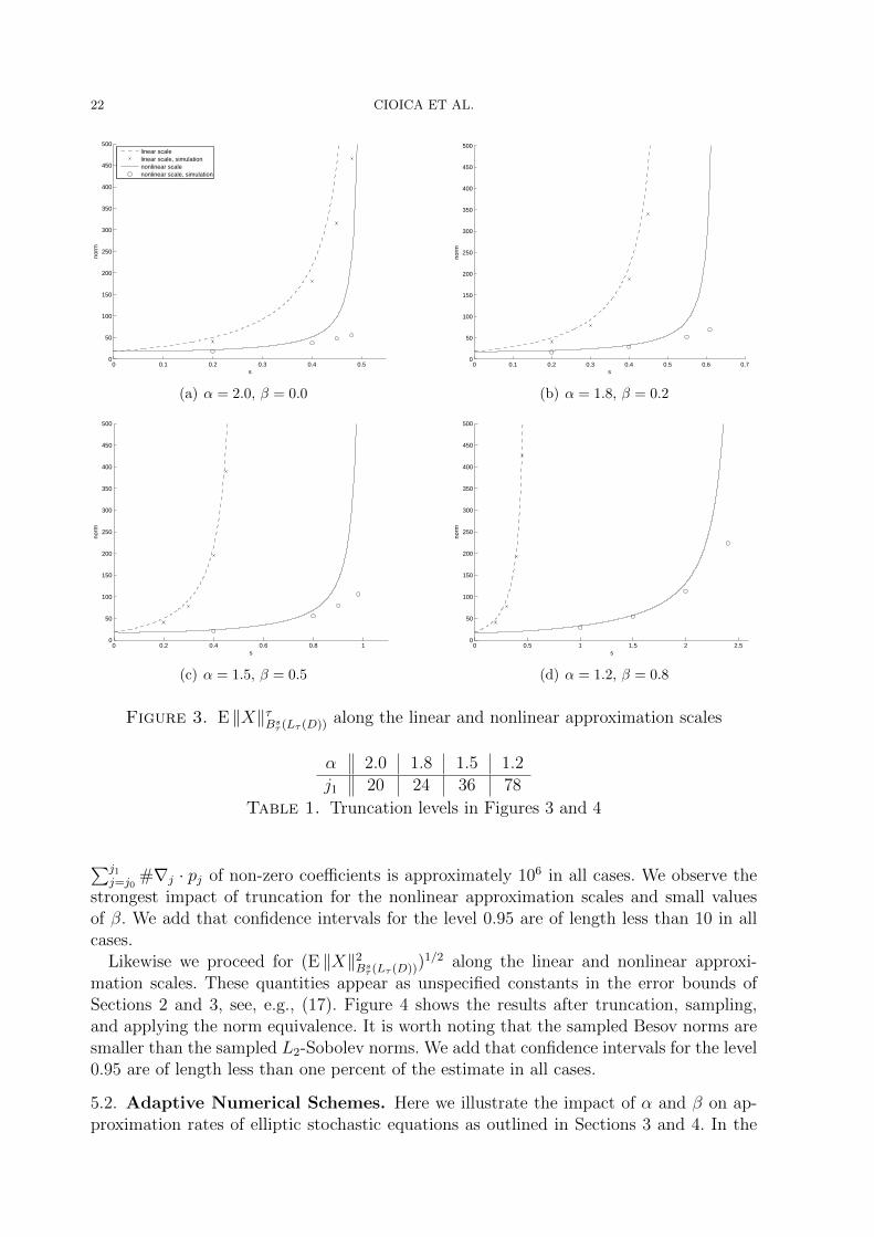
Figure 3 contains the graphs of M along the linear and nonlinear approximation scales,i.e., s 7→M(s, 2) and s 7→M(s, 1/(s+ 1/2)), for the selected values of α and β. Note thatthe upper bounds (21) and (22) also provide the location of the singularities of M alongthe two scales.

The effect of truncation and finite sample size is illustrated in Figure 3, too, by pre-senting sample means of the right-hand side in

‖Xj1‖τBsτ (Lτ (D)) j1∑j=j0

bj(s, τ) · στj∑k∈∇j

Yj,k|Zj,k|τ .

Specifically, for each scale and each choice of α and β we consider 4 different values ofs and use 1000 independent samples. Moreover, for each choice of the parameters α andβ, the truncation level j1 is chosen according to Table 1 so that the expected number

22 CIOICA ET AL.

0 0.1 0.2 0.3 0.4 0.50

50

100

150

200

250

300

350

400

450

500

s

norm

linear scalelinear scale, simulationnonlinear scalenonlinear scale, simulation

(a) α = 2.0, β = 0.0

0 0.1 0.2 0.3 0.4 0.5 0.6 0.70

50

100

150

200

250

300

350

400

450

500

s

norm

(b) α = 1.8, β = 0.2

0 0.2 0.4 0.6 0.8 10

50

100

150

200

250

300

350

400

450

500

s

norm

(c) α = 1.5, β = 0.5

0 0.5 1 1.5 2 2.50

50

100

150

200

250

300

350

400

450

500

s

norm

(d) α = 1.2, β = 0.8

Figure 3. E ‖X‖τBsτ (Lτ (D)) along the linear and nonlinear approximation scales

α 2.0 1.8 1.5 1.2

j1 20 24 36 78

Table 1. Truncation levels in Figures 3 and 4

∑j1j=j0

#∇j · pj of non-zero coefficients is approximately 106 in all cases. We observe thestrongest impact of truncation for the nonlinear approximation scales and small valuesof β. We add that confidence intervals for the level 0.95 are of length less than 10 in allcases.

Likewise we proceed for (E ‖X‖2Bsτ (Lτ (D)))1/2 along the linear and nonlinear approxi-

mation scales. These quantities appear as unspecified constants in the error bounds ofSections 2 and 3, see, e.g., (17). Figure 4 shows the results after truncation, sampling,and applying the norm equivalence. It is worth noting that the sampled Besov norms aresmaller than the sampled L2-Sobolev norms. We add that confidence intervals for the level0.95 are of length less than one percent of the estimate in all cases.

5.2. Adaptive Numerical Schemes. Here we illustrate the impact of α and β on ap-proximation rates of elliptic stochastic equations as outlined in Sections 3 and 4. In the


0 0.1 0.2 0.3 0.4 0.50

5

10

15

20

s

norm

linear scale, simulationnonlinear scale, simulation

(a) α = 2.0, β = 0.0

0 0.1 0.2 0.3 0.4 0.5 0.60

5

10

15

20

25

s

norm

(b) α = 1.8, β = 0.2

0 0.2 0.4 0.6 0.8 10

5

10

15

20

25

30

35

40

s

norm

(c) α = 1.5, β = 0.5

0 0.5 1 1.5 2 2.50

100

200

300

400

500

600

s

norm

(d) α = 1.2, β = 0.8

Figure 4. (E ‖X‖2Bsτ (Lτ (D)))1/2 along the linear and nonlinear approxima-

tion scales

one-dimensional case the equation is given by

−U ′′(·, ω) = X(·, ω),

U(0, ω) = U(1, ω) = 0

on D = [0, 1].The aim is to investigate if for this model problem adaptive wavelet algorithms are

superior when compared with uniform schemes. As we know the order of convergence ofuniform methods is determined by the L2-Sobolev regularity of the exact solution whereasthe order of convergence of adaptive schemes is determined by the Besov smoothness, see(17) and Remark 3.3.

We therefore study an example where the Sobolev smoothness of the right-hand sideX stays fixed while the Besov regularity changes. This is achieved by choosing parametervalues α and β such that the sum α + β, which determines the L2-Sobolev regularity, iskept constant, cf. Section 5.1. Then, letting β tend to one increases the Besov smoothnesssignificantly, see Corollary 2.7. Since the problem is completely regular, these interrelationsimmediately carry over to the exact solution, see [48, Theorem 4.3].

24 CIOICA ET AL.

The numerical experiment is carried out and evaluated as follows. On input δ > 0 the

adaptive wavelet scheme computes an N -term approximation U(·, ω) to U(·, ω), whoseerror with respect to the H1-norm is at most δ. The number N of terms depends onδ as well as on ω via the right-hand side X(·, ω), and only a finite number of wavelet

coefficients of X(·, ω) are used to compute U(·, ω). We determine U(·, ω) in a mastercomputation with a very high accuracy and then use the norm equivalence (A5) for thespace H1(D). The master computation employs a uniform approximation with truncationlevel j1 = 11 for the right-hand side. To get a reliable estimate for the average number

E(η(U)) of non-zero wavelet coefficients of U and for the error (E ‖U− U‖2H1(D))1/2 we use

1000 independent samples of truncated right-hand sides. This procedure is carried out for18 different values of δ; the results are presented together with a regression line, whoseslope yields an estimate for the order of convergence. For the uniform approximation weproceed in the same way. The only difference is that, instead of δ, a fixed truncation levelfor the approximation of the left-hand side is used, and therefore no estimate is needed forthe number of non-zero coefficients. As for the adaptive scheme we use 1000 independentsamples for six different truncation levels, j = 4, . . . , 9. We add that confidence intervalsfor the level 0.95 are of length less than three percent of the estimate in all cases.

In the first experiment we choose

α = 0.9, β = 0.2,

i.e., the right-hand side is contained in Hs(D) only for s < 0.05. Consequently, the solutionis contained in Hs(D) with s < 2.05. An optimal uniform approximation scheme withrespect to the H1-norm yields the approximation order 1.05 − ε for every ε > 0. Thisis observed in Figure 5(a), where the empirical order of convergence for the uniformapproximation is 1.113. For the relatively small value of β = 0.2, the Besov smoothness,and therefore the order of best N -term approximation, is not much higher. In fact, byinserting the parameters into Theorem 3.6 with d = 1, we get the approximation order%− ε with % = 19/16 = 1.1875. This is also reflected in Figure 5(a), where the empiricalorder of convergence for the adaptive wavelet scheme is 1.164. In both cases the numericalresults match very well the asymptotic error analysis, and both methods exhibit almostthe same order of convergence. Nevertheless, even in this case adaptivity slightly paysoff for the same regularity parameter, since the Besov norm is smaller than the Sobolevnorm, which yields smaller constants.

The picture changes for higher values of β. As a second test case, we choose

α = 0.4, β = 0.7.

Then, the Besov regularity is considerably higher. In fact, from Theorem 3.6 with d = 1we would expect the convergence rate % − ε with % = 7/3, provided that the waveletbasis indeed characterizes the corresponding Besov spaces. It is well known that a tensorproduct spline wavelet basis of order m in dimension d has this very property for Bs

τ (Lτ )with 1/τ = s − 1/2 and s < s1 = m/d, see [6, Theorem 3.7.7]. In our case, s1 = 3, so% = 2 is the best we can expect. From Figure 5(b), we observe that the empirical order ofconvergence is slightly lower, namely 1.425. The reason is that the Besov smoothness of thesolution is only induced by the right-hand side which, in a Galerkin approach, is expandedin the dual wavelet basis. Estimating the Holder regularity of the dual wavelet basis Ψ,see [50], it turns out that this wavelet basis is only contained in W s(L∞) for s < 0.55.Therefore, by using classical embeddings of Besov spaces, it is only ensured that this


1.6 1.8 2 2.2 2.4 2.6 2.8 3 3.2−4

−3.5

−3

−2.5

−2

−1.5

−1

log N

log

erro

r

uniformadaptive

(a) α = 0.9, β = 0.2

1.4 1.6 1.8 2 2.2 2.4 2.6 2.8 3 3.2−4.5

−4

−3.5

−3

−2.5

−2

−1.5

−1

log N

log

erro

r

uniformadaptive

(b) α = 0.4, β = 0.7

Figure 5. Error and (expected) number of non-zero coefficients

wavelet basis characterizes Besov spaces Bsτ (Lτ ), with the same smoothness parameter.

Consequently, the solution U is only contained in the spaces Bsτ (Lτ ) with 1/τ = s− 1/2

and s < 2.55 which gives an approximation order % − ε with % = 1.55. This is matchedvery well in Figure 5(b). For uniform approximation the empirical order of convergence is1.115 and thus does not differ from the result in the first experiment.

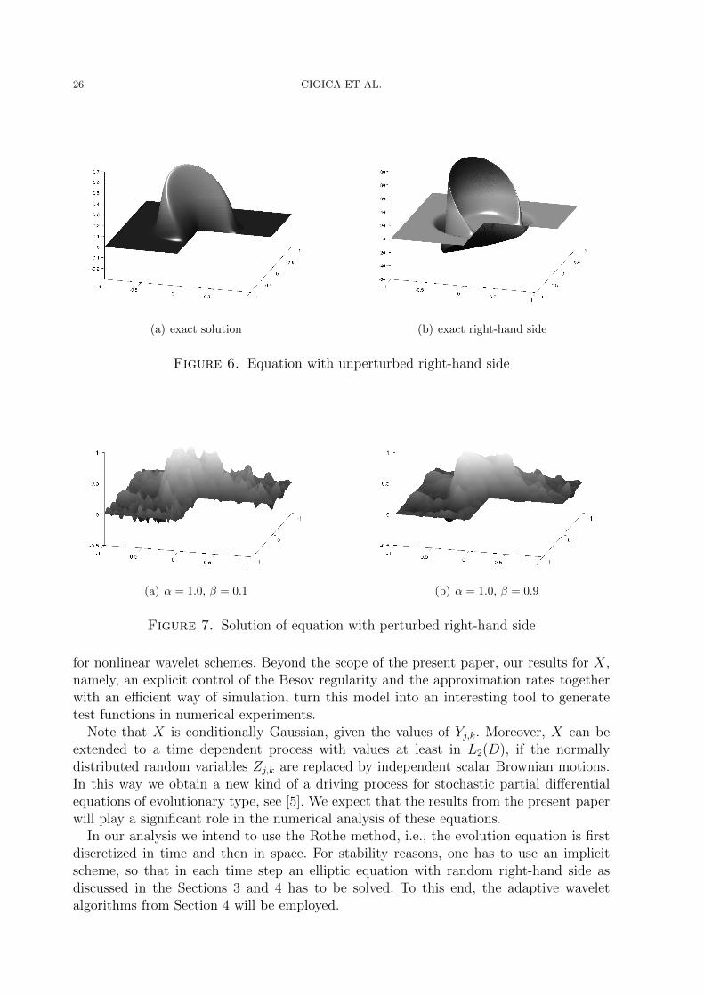
Our sample problem in the two-dimensional case is the Poisson equation (16) withzero-Dirichlet boundary conditions on the L-shaped domain

D = (−1, 1)2 \ [0, 1)2.

Here, as outlined in Section 4, we are going to apply domain decomposition methodsbased on wavelet frames. We consider the right-hand side X = x+ X, where x is a knowndeterministic function and X is generated by the stochastic model from Section 2.2, butbased on frame decompositions. This means that we add a noise term to a deterministicright-hand side. Specifically, we consider perturbed versions of the well-known equationthat is defined by the exact solution

u(r, θ) = ζ(r)r2/3 sin(2

3θ),

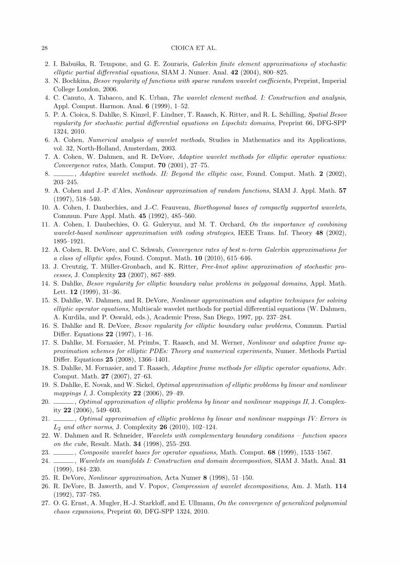
where (r, θ) are polar coordinates with respect to the re-entrant corner, see Figure 6. Then,u is one of the singularity functions as introduced in the proof of Theorem 3.5. It has arelatively low Sobolev regularity while its Besov smoothness is arbitrary high, see again theproof of Theorem 3.5 for details. For functions of this type we expect that adaptivity paysoff. In Figure 7 we show two solutions to realisations of X for the parameter combinationα = 1 together with β = 0.1 and its sparse counterpart β = 0.9.

6. Conclusion and Outlook

In this paper, we have studied a new type of random function, which is based onwavelet expansions. With probability one, the realizations have a prescribed regularity inSobolev as well as in Besov spaces. Essentially, the smoothness of the random functionX is controlled by two parameters α and β, where β is a sparsity parameter that can beused to increase the Besov smoothness in scales that determine the order of approximation

26 CIOICA ET AL.

(a) exact solution (b) exact right-hand side

Figure 6. Equation with unperturbed right-hand side

(a) α = 1.0, β = 0.1 (b) α = 1.0, β = 0.9

Figure 7. Solution of equation with perturbed right-hand side

for nonlinear wavelet schemes. Beyond the scope of the present paper, our results for X,namely, an explicit control of the Besov regularity and the approximation rates togetherwith an efficient way of simulation, turn this model into an interesting tool to generatetest functions in numerical experiments.

Note that X is conditionally Gaussian, given the values of Yj,k. Moreover, X can beextended to a time dependent process with values at least in L2(D), if the normallydistributed random variables Zj,k are replaced by independent scalar Brownian motions.In this way we obtain a new kind of a driving process for stochastic partial differentialequations of evolutionary type, see [5]. We expect that the results from the present paperwill play a significant role in the numerical analysis of these equations.

In our analysis we intend to use the Rothe method, i.e., the evolution equation is firstdiscretized in time and then in space. For stability reasons, one has to use an implicitscheme, so that in each time step an elliptic equation with random right-hand side asdiscussed in the Sections 3 and 4 has to be solved. To this end, the adaptive waveletalgorithms from Section 4 will be employed.


0.5 1 1.5 2 2.5 3 3.5−3.5

−3

−2.5

−2

−1.5

−1

−0.5

0

0.5

log N

log

erro

r

uniformadaptive

α = −48/55, β = 107/110

Figure 8. Error and (expected) number of non-zero coefficients

The numerical experiments in Section 5 as well as our theoretical analysis presentedin this paper indicate that adaptivity really pays off for these problems. Nevertheless, inparticular from the univariate examples in Section 5, we still observe a bottleneck. So far,we only discussed random functions with realizations being in smoothness spaces withpositive smoothness parameters. Then, in the univariate case, the solution immediatelypossesses Sobolev smoothness larger than two, so that uniform schemes already performquite well. We expect the picture to change for right-hand sides with negative smoothness.Indeed, choosing X ∈ H−1+ε(D) yields U ∈ H1+ε(D) for ε > 0, and the convergence orderof uniform schemes in H1(D) is only ε. Then, by choosing X in the Besov spaces as inTheorem 3.6, adaptive schemes would still show the same approximation order as before,so that the comparison of uniform and adaptive algorithms would be even more noticeable.Therefore, the generalization of our noise model to spaces of negative smoothness will bestudied in a forthcoming paper. We expect that our analysis can be generalized to thissetting, since these spaces also possess wavelet characterizations. The following numericalexperiments already support our conjecture.

For the moment, let us assume we were allowed to use negative values of α, i.e.,Theorem 2.6 carries over to the negative scale. Then, we can choose α = −48/55 andβ = 107/110, and we expect the corresponding right-hand side X to be contained inH−0.45(D). In this case, a uniform scheme has approximation order 0.55 − ε, which isreflected in Figure 8 an empirical order 0.619. Moreover, let us also assume that Theo-rem 3.6 carries over, so for adaptive schemes we would still obtain approximation order1.55− ε. Indeed, Figure 8 shows almost exactly this order, namely 1.476.

Acknowledgement. We are grateful to Natalia Bochkina for valuable discussions, andwe thank Tiange Xu for her contributions at an early stage of the project. Also, we thankWinfried Sickel for his comments on regularity theory.

References

1. F. Abramovich, T. Sapatinas, and B. W. Silverman, Wavelet thresholding via a Bayesian approach,

J. R. Stat. Soc., Ser. B, Stat. Methodol. 60 (1998), 725–749.

28 CIOICA ET AL.

2. I. Babuska, R. Tempone, and G. E. Zouraris, Galerkin finite element approximations of stochastic

elliptic partial differential equations, SIAM J. Numer. Anal. 42 (2004), 800–825.

3. N. Bochkina, Besov regularity of functions with sparse random wavelet coefficients, Preprint, Imperial

College London, 2006.

4. C. Canuto, A. Tabacco, and K. Urban, The wavelet element method. I: Construction and analysis,

Appl. Comput. Harmon. Anal. 6 (1999), 1–52.

5. P. A. Cioica, S. Dahlke, S. Kinzel, F. Lindner, T. Raasch, K. Ritter, and R. L. Schilling, Spatial Besov

regularity for stochastic partial differential equations on Lipschitz domains, Preprint 66, DFG-SPP

1324, 2010.

6. A. Cohen, Numerical analysis of wavelet methods, Studies in Mathematics and its Applications,

vol. 32, North-Holland, Amsterdam, 2003.

7. A. Cohen, W. Dahmen, and R. DeVore, Adaptive wavelet methods for elliptic operator equations:

Convergence rates, Math. Comput. 70 (2001), 27–75.

8. , Adaptive wavelet methods. II: Beyond the elliptic case, Found. Comput. Math. 2 (2002),

203–245.

9. A. Cohen and J.-P. d’Ales, Nonlinear approximation of random functions, SIAM J. Appl. Math. 57

(1997), 518–540.

10. A. Cohen, I. Daubechies, and J.-C. Feauveau, Biorthogonal bases of compactly supported wavelets,

Commun. Pure Appl. Math. 45 (1992), 485–560.

11. A. Cohen, I. Daubechies, O. G. Guleryuz, and M. T. Orchard, On the importance of combining

wavelet-based nonlinear approximation with coding strategies, IEEE Trans. Inf. Theory 48 (2002),

1895–1921.

12. A. Cohen, R. DeVore, and C. Schwab, Convergence rates of best n-term Galerkin approximations for

a class of elliptic spdes, Found. Comput. Math. 10 (2010), 615–646.

13. J. Creutzig, T. Muller-Gronbach, and K. Ritter, Free-knot spline approximation of stochastic pro-

cesses, J. Complexity 23 (2007), 867–889.

14. S. Dahlke, Besov regularity for elliptic boundary value problems in polygonal domains, Appl. Math.

Lett. 12 (1999), 31–36.

15. S. Dahlke, W. Dahmen, and R. DeVore, Nonlinear approximation and adaptive techniques for solving

elliptic operator equations, Multiscale wavelet methods for partial differential equations (W. Dahmen,

A. Kurdila, and P. Oswald, eds.), Academic Press, San Diego, 1997, pp. 237–284.

16. S. Dahlke and R. DeVore, Besov regularity for elliptic boundary value problems, Commun. Partial

Differ. Equations 22 (1997), 1–16.

17. S. Dahlke, M. Fornasier, M. Primbs, T. Raasch, and M. Werner, Nonlinear and adaptive frame ap-

proximation schemes for elliptic PDEs: Theory and numerical experiments, Numer. Methods Partial

Differ. Equations 25 (2008), 1366–1401.

18. S. Dahlke, M. Fornasier, and T. Raasch, Adaptive frame methods for elliptic operator equations, Adv.

Comput. Math. 27 (2007), 27–63.

19. S. Dahlke, E. Novak, and W. Sickel, Optimal approximation of elliptic problems by linear and nonlinear

mappings I, J. Complexity 22 (2006), 29–49.

20. , Optimal approximation of elliptic problems by linear and nonlinear mappings II, J. Complex-

ity 22 (2006), 549–603.

21. , Optimal approximation of elliptic problems by linear and nonlinear mappings IV: Errors in

L2 and other norms, J. Complexity 26 (2010), 102–124.

22. W. Dahmen and R. Schneider, Wavelets with complementary boundary conditions – function spaces

on the cube, Result. Math. 34 (1998), 255–293.

23. , Composite wavelet bases for operator equations, Math. Comput. 68 (1999), 1533–1567.

24. , Wavelets on manifolds I: Construction and domain decomposition, SIAM J. Math. Anal. 31

(1999), 184–230.

25. R. DeVore, Nonlinear approximation, Acta Numer 8 (1998), 51–150.

26. R. DeVore, B. Jawerth, and V. Popov, Compression of wavelet decompositions, Am. J. Math. 114

(1992), 737–785.

27. O. G. Ernst, A. Mugler, H.-J. Starkloff, and E. Ullmann, On the convergence of generalized polynomial

chaos expansions, Preprint 60, DFG-SPP 1324, 2010.


28. T. Gantumur, H. Harbrecht, and R. Stevenson, An optimal adaptive wavelet method without coars-

ening of the iterands, Math. Comput. 76 (2007), 615–629.

29. P. Grisvard, Behavior of solutions of elliptic boundary value problems in a polygonal or polyhedral

domain, Proc. 3rd Symp. numer. Solut. partial Differ. Equat., College Park 1975, 1976, pp. 207–274.

30. , Elliptic problems in nonsmooth domains, Monographs and Studies in Mathematics, vol. 24,

Pitman, Boston, 1985.

31. , Singularities in boundary value problems, Research Notes in Applied Mathematics, vol. 22,

Springer, Berlin, 1992.

32. W. Hackbusch, Elliptic differential equations: Theory and numerical treatment, Springer Series in

Computational Mathematics, vol. 18, Springer, Dordrecht, 1992.

33. D. Jerison and C. E. Kenig, The inhomogeneous Dirichlet problem in Lipschitz domains, J. Funct.

Anal. 130 (1995), 161–219.

34. M. Kon and L. Plaskota, Information-based nonlinear approximation: an average case setting, J.

Complexity 21 (2005), 211–229.

35. Y. Meyer, Wavelets and operators, Cambridge Studies in Advanced Mathematics, vol. 37, Cambridge

University Press, 1992.

36. F. Nobile, R. Tempone, and C. G. Webster, An anisotropic sparse grid stochastic collocation method

for partial differential equations with random input data, SIAM J. Numer. Anal. 46 (2008), 2411–2442.

37. A. Papageorgiou and G. W. Wasilkowski, On the average complexity of multivariate problems, J.

Complexity 6 (1990), 1–23.

38. M. Primbs, Stabile biorthogonale Spline-Waveletbasen auf dem Intervall, Dissertation, Universitat

Duisburg-Essen, 2006.

39. K. Ritter, Average-case analysis of numerical problems, Lecture Notes in Mathematics, vol. 1733,

Springer, Berlin, 2000.

40. K. Ritter and G. W. Wasilkowski, On the average case complexity of solving Poisson equations,

Mathematics of Numerical Analysis (J. Renegar, M. Shub, and S. Smale, eds.), Lectures in Appl.

Math. 32, AMS, Providence, 1996, pp. 677–687.

41. T. Runst and W. Sickel, Sobolev spaces of fractional order, Nemytskij operators and nonlinear partial

differential equations, vol. 3, de Gruyter Series in Nonlinear Analysis and Applications, Berlin, 1996.

42. A. N. Shiryayev, Probability, Graduate Texts in Mathematics, vol. 95, Springer, New York, 1984.

43. M. Slassi, A Milstein-based free knot spline approximation for stochastic differential equations,

Preprint, TU Darmstadt, Dept. of Math., 2010.

44. R. Stevenson, Adaptive solution of operator equations using wavelet frames, SIAM J. Numer. Anal.

41 (2003), 1074–1100.

45. R. Stevenson and M. Werner, Computation of differential operators in aggregated wavelet frame co-

ordinates, IMA J. Numer. Anal. 28 (2008), 354–381.

46. , A multiplicative Schwarz adaptive wavelet method for elliptic boundary value problems, Math.

Comput. 78 (2009), 619–644.

47. R. A. Todor and C. Schwab, Convergence rates for sparse chaos approximations of elliptic problems

with stochastic coefficients, IMA J. Numer. Anal. 27 (2007), 232–261.

48. H. Triebel, On Besov-Hardy-Sobolev spaces in domains and regular elliptic boundary value problems.

The case 0 < p ≤ ∞, Commun. Partial Differ. Equations 8 (1978), 1083–1164.

49. N. N. Vakhania, V. I. Tarieladze, and S. A. Chobanyan, Probability distributions on Banach spaces,

Mathematics and Its Applications, vol. 14, D. Reidel Publishing, Dordrecht, 1987.

50. L. F. Villemoes, Wavelet analysis of refinement equations, SIAM J. Math. Anal. 25 (1994), 1433–1460.

51. X. Wan and G. E. Karniadakis, Multi-element generalized polynomial chaos for arbitrary probability

measures, SIAM J. Sci. Comput. 28 (2006), 901–928.

52. G. W. Wasilkowski, Integration and approximation of multivariate functions: Average case complexity

with isotropic Wiener measure, J. Approx. Theory 77 (1994), 212–227.

53. M. Werner, Adaptive wavelet frame domain decomposition methods for elliptic operators, Dissertation,

Philipps-Universitat Marburg, 2009.

54. H. Wozniakowski, Average case complexity of linear multivariate problems, Part 1: Theory, Part 2:

Applications, J. Complexity 8 (1992), 337–372, 373–392.

30 CIOICA ET AL.

55. D. Xiu and G. E. Karniadakis, The Wiener-Askey polynomial chaos for stochastic differential equa-

tions, SIAM J. Sci. Comput. 24 (2002), 619–644.

Petru A. Cioica, Stephan Dahlke, and Stefan KinzelPhilipps-Universitat MarburgFB Mathematik und Informatik, AG Numerik/OptimierungHans-Meerwein-Strasse35032 Marburg, Germanycioica, dahlke, [email protected]

Nicolas Dohring and Klaus RitterTU KaiserslauternDepartment of Mathematics, Computational Stochastics GroupErwin-Schrodinger-Strasse67663 Kaiserslautern, Germanydoehring, [email protected]

Felix Lindner and Rene L. SchillingTU DresdenFB Mathematik, Institut fur Mathematische Stochastik01062 Dresden, Germanyfelix.lindner, [email protected]

Thorsten RaaschJohannes Gutenberg-Universitat MainzInstitut fur Mathematik, AG Numerische MathematikStaudingerweg 955099 Mainz, [email protected]

Preprint Series DFG-SPP 1324

http://www.dfg-spp1324.de

Reports

[1] R. Ramlau, G. Teschke, and M. Zhariy. A Compressive Landweber Iteration forSolving Ill-Posed Inverse Problems. Preprint 1, DFG-SPP 1324, September 2008.

[2] G. Plonka. The Easy Path Wavelet Transform: A New Adaptive Wavelet Transformfor Sparse Representation of Two-dimensional Data. Preprint 2, DFG-SPP 1324,September 2008.

[3] E. Novak and H. Wozniakowski. Optimal Order of Convergence and (In-) Tractabil-ity of Multivariate Approximation of Smooth Functions. Preprint 3, DFG-SPP1324, October 2008.

[4] M. Espig, L. Grasedyck, and W. Hackbusch. Black Box Low Tensor Rank Approx-imation Using Fibre-Crosses. Preprint 4, DFG-SPP 1324, October 2008.

[5] T. Bonesky, S. Dahlke, P. Maass, and T. Raasch. Adaptive Wavelet Methods andSparsity Reconstruction for Inverse Heat Conduction Problems. Preprint 5, DFG-SPP 1324, January 2009.

[6] E. Novak and H. Wozniakowski. Approximation of Infinitely Differentiable Multi-variate Functions Is Intractable. Preprint 6, DFG-SPP 1324, January 2009.

[7] J. Ma and G. Plonka. A Review of Curvelets and Recent Applications. Preprint 7,DFG-SPP 1324, February 2009.

[8] L. Denis, D. A. Lorenz, and D. Trede. Greedy Solution of Ill-Posed Problems: ErrorBounds and Exact Inversion. Preprint 8, DFG-SPP 1324, April 2009.

[9] U. Friedrich. A Two Parameter Generalization of Lions’ Nonoverlapping DomainDecomposition Method for Linear Elliptic PDEs. Preprint 9, DFG-SPP 1324, April2009.

[10] K. Bredies and D. A. Lorenz. Minimization of Non-smooth, Non-convex Functionalsby Iterative Thresholding. Preprint 10, DFG-SPP 1324, April 2009.

[11] K. Bredies and D. A. Lorenz. Regularization with Non-convex Separable Con-straints. Preprint 11, DFG-SPP 1324, April 2009.

[12] M. Dohler, S. Kunis, and D. Potts. Nonequispaced Hyperbolic Cross Fast FourierTransform. Preprint 12, DFG-SPP 1324, April 2009.

[13] C. Bender. Dual Pricing of Multi-Exercise Options under Volume Constraints.Preprint 13, DFG-SPP 1324, April 2009.

[14] T. Muller-Gronbach and K. Ritter. Variable Subspace Sampling and Multi-levelAlgorithms. Preprint 14, DFG-SPP 1324, May 2009.

[15] G. Plonka, S. Tenorth, and A. Iske. Optimally Sparse Image Representation by theEasy Path Wavelet Transform. Preprint 15, DFG-SPP 1324, May 2009.

[16] S. Dahlke, E. Novak, and W. Sickel. Optimal Approximation of Elliptic Problemsby Linear and Nonlinear Mappings IV: Errors in L2 and Other Norms. Preprint 16,DFG-SPP 1324, June 2009.

[17] B. Jin, T. Khan, P. Maass, and M. Pidcock. Function Spaces and Optimal Currentsin Impedance Tomography. Preprint 17, DFG-SPP 1324, June 2009.

[18] G. Plonka and J. Ma. Curvelet-Wavelet Regularized Split Bregman Iteration forCompressed Sensing. Preprint 18, DFG-SPP 1324, June 2009.

[19] G. Teschke and C. Borries. Accelerated Projected Steepest Descent Method forNonlinear Inverse Problems with Sparsity Constraints. Preprint 19, DFG-SPP1324, July 2009.

[20] L. Grasedyck. Hierarchical Singular Value Decomposition of Tensors. Preprint 20,DFG-SPP 1324, July 2009.

[21] D. Rudolf. Error Bounds for Computing the Expectation by Markov Chain MonteCarlo. Preprint 21, DFG-SPP 1324, July 2009.

[22] M. Hansen and W. Sickel. Best m-term Approximation and Lizorkin-Triebel Spaces.Preprint 22, DFG-SPP 1324, August 2009.

[23] F.J. Hickernell, T. Muller-Gronbach, B. Niu, and K. Ritter. Multi-level MonteCarlo Algorithms for Infinite-dimensional Integration on RN. Preprint 23, DFG-SPP 1324, August 2009.

[24] S. Dereich and F. Heidenreich. A Multilevel Monte Carlo Algorithm for Levy DrivenStochastic Differential Equations. Preprint 24, DFG-SPP 1324, August 2009.

[25] S. Dahlke, M. Fornasier, and T. Raasch. Multilevel Preconditioning for AdaptiveSparse Optimization. Preprint 25, DFG-SPP 1324, August 2009.

[26] S. Dereich. Multilevel Monte Carlo Algorithms for Levy-driven SDEs with GaussianCorrection. Preprint 26, DFG-SPP 1324, August 2009.

[27] G. Plonka, S. Tenorth, and D. Rosca. A New Hybrid Method for Image Approx-imation using the Easy Path Wavelet Transform. Preprint 27, DFG-SPP 1324,October 2009.

[28] O. Koch and C. Lubich. Dynamical Low-rank Approximation of Tensors.Preprint 28, DFG-SPP 1324, November 2009.

[29] E. Faou, V. Gradinaru, and C. Lubich. Computing Semi-classical Quantum Dy-namics with Hagedorn Wavepackets. Preprint 29, DFG-SPP 1324, November 2009.

[30] D. Conte and C. Lubich. An Error Analysis of the Multi-configuration Time-dependent Hartree Method of Quantum Dynamics. Preprint 30, DFG-SPP 1324,November 2009.

[31] C. E. Powell and E. Ullmann. Preconditioning Stochastic Galerkin Saddle PointProblems. Preprint 31, DFG-SPP 1324, November 2009.

[32] O. G. Ernst and E. Ullmann. Stochastic Galerkin Matrices. Preprint 32, DFG-SPP1324, November 2009.

[33] F. Lindner and R. L. Schilling. Weak Order for the Discretization of the StochasticHeat Equation Driven by Impulsive Noise. Preprint 33, DFG-SPP 1324, November2009.

[34] L. Kammerer and S. Kunis. On the Stability of the Hyperbolic Cross DiscreteFourier Transform. Preprint 34, DFG-SPP 1324, December 2009.

[35] P. Cerejeiras, M. Ferreira, U. Kahler, and G. Teschke. Inversion of the noisy Radontransform on SO(3) by Gabor frames and sparse recovery principles. Preprint 35,DFG-SPP 1324, January 2010.

[36] T. Jahnke and T. Udrescu. Solving Chemical Master Equations by AdaptiveWavelet Compression. Preprint 36, DFG-SPP 1324, January 2010.

[37] P. Kittipoom, G. Kutyniok, and W.-Q Lim. Irregular Shearlet Frames: Geometryand Approximation Properties. Preprint 37, DFG-SPP 1324, February 2010.

[38] G. Kutyniok and W.-Q Lim. Compactly Supported Shearlets are Optimally Sparse.Preprint 38, DFG-SPP 1324, February 2010.

[39] M. Hansen and W. Sickel. Best m-Term Approximation and Tensor Products ofSobolev and Besov Spaces – the Case of Non-compact Embeddings. Preprint 39,DFG-SPP 1324, March 2010.

[40] B. Niu, F.J. Hickernell, T. Muller-Gronbach, and K. Ritter. Deterministic Multi-level Algorithms for Infinite-dimensional Integration on RN. Preprint 40, DFG-SPP1324, March 2010.

[41] P. Kittipoom, G. Kutyniok, and W.-Q Lim. Construction of Compactly SupportedShearlet Frames. Preprint 41, DFG-SPP 1324, March 2010.

[42] C. Bender and J. Steiner. Error Criteria for Numerical Solutions ofBackward SDEs. Preprint 42, DFG-SPP 1324, April 2010.

[43] L. Grasedyck. Polynomial Approximation in Hierarchical Tucker Format by Vector-Tensorization. Preprint 43, DFG-SPP 1324, April 2010.

[44] M. Hansen und W. Sickel. Best m-Term Approximation and Sobolev-Besov Spacesof Dominating Mixed Smoothness - the Case of Compact Embeddings. Preprint 44,DFG-SPP 1324, April 2010.

[45] P. Binev, W. Dahmen, and P. Lamby. Fast High-Dimensional Approximation withSparse Occupancy Trees. Preprint 45, DFG-SPP 1324, May 2010.

[46] J. Ballani and L. Grasedyck. A Projection Method to Solve Linear Systems inTensor Format. Preprint 46, DFG-SPP 1324, May 2010.

[47] P. Binev, A. Cohen, W. Dahmen, R. DeVore, G. Petrova, and P. Wojtaszczyk.Convergence Rates for Greedy Algorithms in Reduced Basis Methods. Preprint 47,DFG-SPP 1324, May 2010.

[48] S. Kestler and K. Urban. Adaptive Wavelet Methods on Unbounded Domains.Preprint 48, DFG-SPP 1324, June 2010.

[49] H. Yserentant. The Mixed Regularity of Electronic Wave Functions Multiplied byExplicit Correlation Factors. Preprint 49, DFG-SPP 1324, June 2010.

[50] H. Yserentant. On the Complexity of the Electronic Schrodinger Equation.Preprint 50, DFG-SPP 1324, June 2010.

[51] M. Guillemard and A. Iske. Curvature Analysis of Frequency Modulated Manifoldsin Dimensionality Reduction. Preprint 51, DFG-SPP 1324, June 2010.

[52] E. Herrholz and G. Teschke. Compressive Sensing Principles and Iterative SparseRecovery for Inverse and Ill-Posed Problems. Preprint 52, DFG-SPP 1324, July2010.

[53] L. Kammerer, S. Kunis, and D. Potts. Interpolation Lattices for Hyperbolic CrossTrigonometric Polynomials. Preprint 53, DFG-SPP 1324, July 2010.

[54] G. Kutyniok and W.-Q Lim. Shearlets on Bounded Domains. Preprint 54, DFG-SPP 1324, July 2010.

[55] A. Zeiser. Wavelet Approximation in Weighted Sobolev Spaces of Mixed Orderwith Applications to the Electronic Schrodinger Equation. Preprint 55, DFG-SPP1324, July 2010.

[56] G. Kutyniok, J. Lemvig, and W.-Q Lim. Compactly Supported Shearlets.Preprint 56, DFG-SPP 1324, July 2010.

[57] A. Zeiser. On the Optimality of the Inexact Inverse Iteration Coupled with AdaptiveFinite Element Methods. Preprint 57, DFG-SPP 1324, July 2010.

[58] S. Jokar. Sparse Recovery and Kronecker Products. Preprint 58, DFG-SPP 1324,August 2010.

[59] T. Aboiyar, E. H. Georgoulis, and A. Iske. Adaptive ADER Methods Using Kernel-Based Polyharmonic Spline WENO Reconstruction. Preprint 59, DFG-SPP 1324,August 2010.

[60] O. G. Ernst, A. Mugler, H.-J. Starkloff, and E. Ullmann. On the Convergence ofGeneralized Polynomial Chaos Expansions. Preprint 60, DFG-SPP 1324, August2010.

[61] S. Holtz, T. Rohwedder, and R. Schneider. On Manifolds of Tensors of FixedTT-Rank. Preprint 61, DFG-SPP 1324, September 2010.

[62] J. Ballani, L. Grasedyck, and M. Kluge. Black Box Approximation of Tensors inHierarchical Tucker Format. Preprint 62, DFG-SPP 1324, October 2010.

[63] M. Hansen. On Tensor Products of Quasi-Banach Spaces. Preprint 63, DFG-SPP1324, October 2010.

[64] S. Dahlke, G. Steidl, and G. Teschke. Shearlet Coorbit Spaces: Compactly Sup-ported Analyzing Shearlets, Traces and Embeddings. Preprint 64, DFG-SPP 1324,October 2010.

[65] W. Hackbusch. Tensorisation of Vectors and their Efficient Convolution.Preprint 65, DFG-SPP 1324, November 2010.

[66] P. A. Cioica, S. Dahlke, S. Kinzel, F. Lindner, T. Raasch, K. Ritter, and R. L.Schilling. Spatial Besov Regularity for Stochastic Partial Differential Equations onLipschitz Domains. Preprint 66, DFG-SPP 1324, November 2010.

[67] E. Novak and H. Wozniakowski. On the Power of Function Values for the Ap-proximation Problem in Various Settings. Preprint 67, DFG-SPP 1324, November2010.

[68] A. Hinrichs, E. Novak, and H. Wozniakowski. The Curse of Dimensionality forMonotone and Convex Functions of Many Variables. Preprint 68, DFG-SPP 1324,November 2010.

[69] G. Kutyniok and W.-Q Lim. Image Separation Using Shearlets. Preprint 69, DFG-SPP 1324, November 2010.

[70] B. Jin and P. Maass. An Analysis of Electrical Impedance Tomography with Ap-plications to Tikhonov Regularization. Preprint 70, DFG-SPP 1324, December2010.

[71] S. Holtz, T. Rohwedder, and R. Schneider. The Alternating Linear Scheme forTensor Optimisation in the TT Format. Preprint 71, DFG-SPP 1324, December2010.

[72] T. Muller-Gronbach and K. Ritter. A Local Refinement Strategy for ConstructiveQuantization of Scalar SDEs. Preprint 72, DFG-SPP 1324, December 2010.

[73] T. Rohwedder and R. Schneider. An Analysis for the DIIS Acceleration Methodused in Quantum Chemistry Calculations. Preprint 73, DFG-SPP 1324, December2010.

[74] C. Bender and J. Steiner. Least-Squares Monte Carlo for Backward SDEs.Preprint 74, DFG-SPP 1324, December 2010.

[75] C. Bender. Primal and Dual Pricing of Multiple Exercise Options in ContinuousTime. Preprint 75, DFG-SPP 1324, December 2010.

[76] H. Harbrecht, M. Peters, and R. Schneider. On the Low-rank Approximation by thePivoted Cholesky Decomposition. Preprint 76, DFG-SPP 1324, December 2010.

[77] P. A. Cioica, S. Dahlke, N. Dohring, S. Kinzel, F. Lindner, T. Raasch, K. Ritter,and R. L. Schilling. Adaptive Wavelet Methods for Elliptic Stochastic PartialDifferential Equations. Preprint 77, DFG-SPP 1324, January 2011.

DFG-Schwerpunktprogramm 1324 · -the parameters s, p, and qof the Besov space,-the parameters , , ,...

Documents

Transcript of DFG-Schwerpunktprogramm 1324 · -the parameters s, p, and qof the Besov space,-the parameters , , ,...