Dielectric Relaxation Spectroscopy of Ionic Micelles and ... · Dielectric Relaxation Spectroscopy...
198
Dielectric Relaxation Spectroscopy of Ionic Micelles and Microemulsions Vorgelegt von Patrick Fernandez Regensburg 2002 Dissertation Zur Erlangung des Grades Doktor der Naturwissenschaften (Dr. rer. Nat.) der Naturwissenschaftlichen Fakultät IV Chemie und Pharmazie der Universität Regensburg Universität Regensburg Solution chemistry
Transcript of Dielectric Relaxation Spectroscopy of Ionic Micelles and ... · Dielectric Relaxation Spectroscopy...
Dielectric Relaxation Spectroscopy of Ionic Micelles and Microemulsions
Vorgelegt von Patrick Fernandez
Regensburg 2002
Dissertation Zur Erlangung des Grades
Doktor der Naturwissenschaften (Dr. rer. Nat.)
der Naturwissenschaftlichen Fakultät IV
Chemie und Pharmazie der Universität Regensburg
Uni ver sität Regensburg Solution chemistr y


Promotionsgesuch eingereicht am: 27.11.2002 Tag des Kolloquiums: 05.12.2002 Die Arbeit wurde angeleitet von: Prof. Dr. W. Kunz Prüfungsausschuss: Prof. Dr. H. Krienke, Vorsitzender Prof. Dr. W. Kunz Dr. Habil . R. Buchner Prof. Dr. C. Steinem


Šárka und meiner Famili e

Vorwort Die vorliegende Arbeit entstand in der Zeit von November 1998 bis März 2002 am Lehrstuhl für Physikalische und Theoretische Chemie – der naturwissenschaftlichen Fakultät IV – Chemie und Pharmazie – der Universität Regensburg. Besonderer Dank gebührt Herrn Dr. D. Touraud und Herrn Dr. Habil . R. Buchner für die Erteilung des interessanten Themas, und die wissenschaftliche Betreuung. Herrn Prof. Dr. W. Kunz danke ich für die finanzielle Unterstützung und die Bereitstellung von Büro- und Arbeitsmitteln. Herzlich danken möchte ich auch allen Mitarbeitern des Lehrstuhls, die mich in der wissenschaftlichen Arbeit unterstützt und zu einem angenehmen Arbeitsklima beigetragen haben. Namentlich möchte ich dafür Frau Dipl. Chem. Šárka Chrapáva, Herrn Dipl. Chem. Nicolas Papaiconomou, Frau Dr. Marie-Line Navarro-Touraud, Frau Dipl. Chem. Barbara Widera, Herrn Dr. Takaaki Sato, Herrn Dipl. Chem. John de Roche, Herrn Wolfgang Simon, Herrn Dipl. Chem. Simon Schrödle, Herrn Dr. Alexander Schmidt, Herrn Dr. Jürgen Bittner, Herrn. Dr. Jürgen Kroner, Herrn Dipl. Chem. Denys Zimin, Dr. Edith Schnell , und den Kollegen der Gruppe Dr. Gores danksagen. Ferner möchte ich Frau Dr. Conxita Solans und Herrn Prof. Dr. Barry Ninham für ihren informativen Besuche. Besonders danke ich mich bei der Deutschen Forschungsgemeinschaft für die großzügige Finanzierung einer Stelle eines wissenschaftlicher Mitarbeiters.

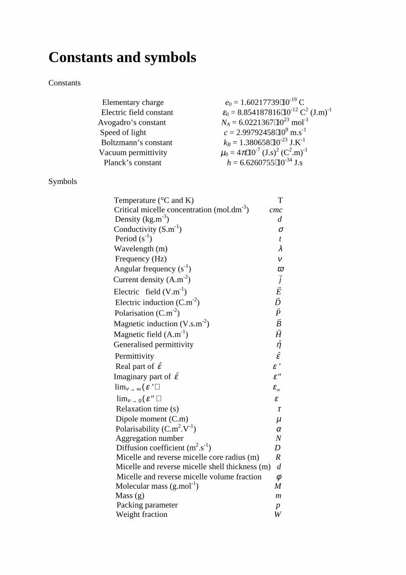
Constants and symbols
Constants
Elementary charge e0 = 1.60217739⋅10-19 C Electric field constant ε0 = 8.854187816⋅10-12 C2 (J.m)-1
Avogadro’s constant NA = 6.0221367⋅1023 mol-1 Speed of light c = 2.99792458⋅108 m.s-1 Boltzmann’s constant kB = 1.380658⋅10-23 J.K-1 Vacuum permittivity µ0 = 4π⋅10-7 (J.s)2 (C2.m)-1
Planck’s constant h = 6.6260755⋅10-34 J.s
Symbols
Temperature (°C and K) T Critical micelle concentration (mol.dm-3) cmc Density (kg.m-3) d Conductivity (S.m-1) σ Period (s-1) t Wavelength (m) λ Frequency (Hz) ν Angular frequency (s-1) ω Current density (A.m-2)
&j
Electric field (V.m-1) &E
Electric induction (C.m-2) &D
Polarisation (C.m-2) &P
Magnetic induction (V.s.m-2) &B
Magnetic field (A.m-1) &
H Generalised permittivity η
Permittivity ε Real part of ε ε ’ Imaginary part of ε ′′ε limν→ ∞ ( ε ’) ε∞ limν→ 0( ′′ε ) ε Relaxation time (s) τ Dipole moment (C.m) µ Polarisability (C.m2.V-1) α Aggregation number N Diffusion coefficient (m2.s-1) D Micelle and reverse micelle core radius (m) R Micelle and reverse micelle shell thickness (m) d Micelle and reverse micelle volume fraction φ Molecular mass (g.mol-1) M Mass (g) m Packing parameter p Weight fraction W

Table of contents General Introduction...................................................................................................................1 Chapter 1 I. Overview of basic aspects of microemulsions......................................................................................3
I. 1. Historical background.......................................................................................................... ..............4 I. 2. Formation................................................................................................................................................5 I. 3. Properties relevant to applications............................................................. .......... ..........................6 I. 4. Structure.................................................................... ............................................................................6 I. 5. General methods of characterisation........................................................................................ ..11
I. 5. 1. Phase behaviour....................................................................................................... .............11 I. 5. 2. Scattering techniques............................................................. ........................................ ...13 I. 5. 3. Nuclear Magnetic Resonance...................................................................................... .....14 I. 5. 4. Electron Microscopy...................................................................................................... ....14 I. 5. 5. Other methods...................................................................................................................... .14
II . Motivation.....................................................................................................................................................15 II . 1. DRS of microemulsions, general results.....................................................................16 II . 2. Choice of the systems investigated..................................................................... .......16 II . 3. Experiments.................................................................................................................19 II . 3. 1. SDS in water, water/SDS/1-pentanol, and water/SDS/1-pentanol/n-dodecane systems at 25°C.......................................20 II . 3. 2. Other water/SDS/n-alkanol/n-dodecane systems at 25°C................................23 II . 3. 3. Water/C12E23/1-alkanol systems at 25°C..........................................................26 II . 3. 4. D2O/SDS/1-pentanol/n-dodecane, D2O/SDS/1-hexanol/n-dodecane, and D2O/C12E23/1-hexanol systems at 25°C........................................... .......27 Chapter 2: Techniques I. Density measurements........................................................................................ ..................31 II . Conductivity measurements.................................................................................................31 III . Dielectric Relaxation Spectroscopy....................................................................................31 III . 1. Maxwell and constitutive equations.........................................................................31 III . 2. Wave equations........................................................................................................33 III . 3. Dielectric relaxation.................................................................................................35 III . 3. 1. Polarization.................................................................................................35 III . 3. 2. Response functions of the orientational polarization..................................37 III . 3. 3. Empirical equations for the description of dielectric relaxation....................................................................................38 III . 4. Equipment................................................................................................................39 III . 4. 1. Waveguide interferometers.........................................................................39 III . 4. 2. Time domain reflectometer.............................. ..........................................41 III . 4. 2. 1. Measurement procedure...........................................................43 III . 4. 2. 2. Cell calibration. .......................................................................45 III . 4. 2. 3. Padé calibration........................................................................45
Chapter three: Results and discussions I. SDS micelles in water............................................................................................................47 I. 1. SDS monomer self-association................................................................... .................47 I. 2. DRS spectra fitting procedure.......................................................................................47 I. 3. Analysis of low-frequency relaxation processes 1 and 2 in 4D, DCCD, and 3D models...............................................................................................................53 I. 3. 1. Grosse’s model...................................................................................................54 I. 3. 2. Model of Pauly and Schwan...............................................................................56 I. 3. 3. Choice of the input parameters...........................................................................58 I. 3. 4. Results and discussion........................................................................................59 I. 4. Analysis of high-frequency relaxation processes..........................................................64 I. 4. 1. Ion-pair calculations...........................................................................................64 I. 4. 2. Solvent relaxation analysis.................................................................................67 II . Water/SDS/1-pentanol ternary and water/SDS/1-pentanol/n-dodecane quaternary systems.................................................................................................................................71 II . 1. Use of conductivity measurements in the microemulsions study......................... ......71 II . 2. Results..........................................................................................................................75 II . 2. 1. Conductivity data..............................................................................................75 II . 2. 2. DRS spectra fitting procedure...........................................................................80 II . 3. SDS/1-pentanol swollen micelles................................................................................91 II . 3. 1. Effect of 1-pentanol on size and shape of SDS micelles..................................91 II . 3. 2. Analysis of the low-frequency relaxation processes 1 and 2 in 4D models.....92 II . 3. 3. Influence of 1-pentanol on packing parameter and charge dissociation..........94 II . 3. 4. Contribution of 1-pentanol molecules to the dielectric relaxation...................95 II . 3. 5. High-frequency DRS data analysis..................................................................98 II . 4. Bicontinuous structures...............................................................................................99 II . 4. 1. Theoretical aspects.........................................................................................100 II . 4. 2. DRS results.............................................................................................. ......102 II . 5. Reverse micelles........................................................................................................102 II . 5. 1. Conductivity of W/O microemulsions and reverse micelles..........................104 II . 5. 1. 1. Theory of percolation in W/O microemulsions..............................104 II . 5. 1. 2. Data analysis...................................................................................109 II . 5. 2. Low-frequency DRS data analysis.................................................................112 II . 5. 2. 1. DRS study of W/O microemulsions, state of the literature............113 II . 5. 2. 2. Comparison between literature data and low-frequency DRS results.............................................................114 II . 5. 2. 3. Model of Pauly and Schwan in W/O microemulsions....................116 II . 5. 2. 3. 1. Choice of the input parameters...................................116 II . 5. 2. 3. 2. Results........................................................................119 II . 5. 2. 4. Light scattering measurements........................................................121 II . 5. 3. High-frequency DRS data analysis.....................................................123 II . 5. 4. Importance of hydration in W/O microemulsions...............................128 II . 6. Conclusion.................................................................................................................129 Chapter 4: Annexes I. Other water/SDS/1-alkanol/n-dodecane systems at 25°C…………………….…….…….131 I. 1. Water/SDS/1-butanol/n-dodecane system at 25°C…………….………….…….….131 I. 2. Water/SDS/1-hexanol/n-dodecane system at 25°C…………….………….........….134

I. 3. Water/SDS/1-heptanol/n-dodecane system at 25°C…………….……………….....140 II . Water/C12E23/1-alkanol systems at 25°C…………………………………………...…….144 III . Deuterated microemulsion systems………………………………………………..……146 III . 1. D2O/ SDS/1-pentanol/n-dodecane system at 25°C……………………..…………146 III . 2. D2O/ SDS/1-hexanol/n-dodecane system at 25°C……….……………...……...…156 III . 3. D2O/C12E23/1-hexanol system at 25°C………………………………..……..……163 References…………………………………………………………………………………...171

General introduction 1
General introduction Microemulsions represent systems consisting of water, oil, and amphiphile(s). They are single-phase and thermodynamically stable isotropic solutions that find numerous commercial applications with high economic impact. For instance, microemulsions are used in petroleum industry for the recovery of oil entrapped in the porous rocks of oil reservoirs (enhancement oil recovery, EOR). Uses in pharmaceuticals (drug solubilization...), cosmetics or cleaning (for textiles, soils..) are other examples of microemulsion industrial basic applications. Development of these media for enzymatic reactions, polymerization, electrochemical reactions, synthesis of nanostructurated material, places microemulsions at the leading edge of bio- and nanotechnologies. It is evident that these kinds of media that are known since one century, and defined since only 40 years, will be in the future subject of more development. Although macroscopically homogeneous, microemulsions are microscopically heterogeneous and can show diverse structural organization that are water or oil droplets (spherical or elongated) dispersed in either oil (namely water-in-oil or W/O) or water (oil-in-water or O/W) with sizes in the order of 0.1 µm. With excess oil and water phases, bicontinuous microemulsions may co-exist. It is generally recognized that the spontaneous curvature, H0, of the amphiphile(s) monolayer at the oil/water interface dictates phase behavior and microstructure1-4. O/W microemulsions have H0 > 0 whereas, for W/O microemulsions H0 < 0. In the case of biconinuous microemulsions, H0 ≈ 0. Hydrophilic amphiphiles (or surfactants) produce O/W microemulsion, and hydrophobic surfactants favor W/O microemulsions. When the hydrophilic-lipophilic surfactant properties are balanced, bicontinuous microemulsions are formed and maximum solubilization of water and oil is achieved. Sometimes a cosurfactant, generally an alcohol, is needed for the micoemulsion formulation. A great variety of microemulsion systems, with or without cosurfactant, can be obtained resulting wide range of structures depending on the amphiphile(s) properties. Microemulsion characterization is an important, and unfortunately difficult, task due to the variety of structures and components involved in these systems. Microemulsion investigations require numerous techniques like nuclear magnetic resonance (NMR), electron microscopy, electrical conductivity, scattering techniques (neutron, X-rays, light scattering)... that may (and often must) be combined together in order provide appreciable results. In the case of charged micelles, dielectric relaxation spectroscopy (DRS) proved to be sensitive to all kinds of dipole moment fluctuations in the pico- and nanosecond time range that result from the reorientation of water molecules or ion pairs and from the motions of free and bound counterions surrounding the charged micelles5-10. Unfortunately, literature data concerning DRS of W/O microemulsions gave in the past limited interpretations. This is generally a consequence of a narrow measurement frequency range that is limited at the microwave region, involving loss of information, for example related to water motions. Another reason is that the theoretical interpretation of these dielectric spectra remains a complicated work, and often gives no satisfactory results. The material present in our laboratory allows us to measure at microwave frequencies up to 89 GHz, rendering water motions observable. Additionally, we propose an interpretation of W/O microemulsions DRS spectra using previous9,10 results found for ionic micelles in water. Unlike other authors11, 12, we propose a DRS study of microemulsions by using the continuity between sodium dodecyl sulfate (SDS) micelles in water and water-in-oil (W/O) microemulsions. This link exists through the single-phase domains of the ternary water/SDS/1-pentanol and of the quaternary microemulsion water/SDS/1-pentanol/dodecane
General introduction 2
(mass ratio SDS to 1-pentanol equal to 0.5; 1-pentanol was the cosurfactant) systems13 at 25°C. DRS measurements of SDS micelles in water were carried out and revealed results in accordance with those previously found for cationic micelles in water. Two low frequency relaxation processes were found related to counterion motions (free and bound sodium ions) and two high frequency relaxation processes were attributed to bound and free water. Addition of 1-pentanol led to the transition structure direct micelles → bicontinuous structures → reverse micelles and W/O microemulsions (upon n-dodecane addition). During both transitions that were asserted with help of conductivity measurements all relaxation steps showed strong changes, but it could be proved that water relaxation processes remained present. In W/O microemulsions, low frequency relaxation processes could be attributed to charge fluctuations and correlated to conductivity measurements. Therefore it could be argued that the relaxation processes in ionic micelles are the same as for ionic W/O micoemulsions. These dispersion steps were found dependent on the microscopic changes in the solution (i. e. percolation in W/O microemulsions, bicontinuous structures...). Absence of knowledge about cosurfactant partitioning prevented us to give a quantitative view of these microemulsions. Nevertheless our qualitative findings considerably complemented literature results and paved the way for further DRS investigations of other microemulsions systems, with the aim to standardize this technique for microemulsion study. As indicated by our results, DRS may be regarded as a powerful technique to investigate microemulsions.
Chapter 1: Microemulsion systems studied 3
Chapter 1: Microemulsion systems studied
I. Overview of basic aspects of microemulsions It is now well established that large amounts of two non-miscible liquids (i. e., water and oil) can be brought into a single phase, macroscopically homogeneous but microscopically heterogeneous, by addition of an appropriate surfactant or surfactant mixture. This unique class of optically clear solutions, called microemulsions, consists in colloidal systems that have attracted much scientific and technological interest over the past decade. This wide interest stems from their characteristic properties, namely ultralow interfacial tension, large interfacial area, and solubili zation capacity for both water- and oil -soluble compounds. These and other properties render microemulsions intriguing from a fundamental point of view and versatile for industrial applications. Microemulsions had already been used in technological and household applications well before they were scientifically described for the first time by Hoar and Schulman14 in 1943. These authors reported the spontaneous formation of a transparent or translucent solution upon mixing of oil , water, and ionic surfactant combined with a cosurfactant (i. e., a medium chain length alcool). At first Hoar and Schulman14 referred to this new type of colloidal dispersion as an oleophatic hydromicelle, and Bowcott and Schulman15 referred to it with other names, such as transparent emulsions, at later stages of their studies. 15 years after Schulman’s first publication on the subject, the term microemulsion16 was introduced, and prevailed for these systems. Microemulsions form under a wide range of surfactant concentrations, water-in-oil ratios, temperature, etc.; this is an indication of the occurence of diverse structural organizations. The picture that emerged from the earlier work of microemulsions14-16 was that of spherical water or oil droplets dispersed in either oil (namely water-in-oil or W/O) or water (oil -in-water or O/W) with radii of the order of 100 to 1000 Å. In addition to droplet-type structure, the existence of microemulsions with bicontinuous structures in which the surfactant forms interfaces of rapidly fluctuating curvature and both the water and oil domains are continuous was later established17. A great deal of debate about the definition of microemulsions originated from the different concepts of the nature of these systems. Whereas Schulman et al.14-16 viewed microemulsions as kinetically stable two-phase emulsions, Shinoda and Kunieda18 pointed out that microemulsions could not be considered as true emulsions, but are one-phase systems with solubili zed water or oil , identical to micellar solutions. Phase behaviour studies by Friberg et al.19-22 and Shinoda et al.23-26 confirmed that most of Schulman’s so-called microemulsions fall i n the one liquid phase regions of the phase diagrams of the corresponding systems; that is they were solubili zed solutions. Adamson27 suggested calli ng the microemulsions „micellar emulsions“. The debate concerning thermodynamic stabilit y of microemulsions continued in the 1980s. The definition of micromulsions suggested by Danielsson and Lindman28 as systems of water, oil , and an amphiphile(s), which are single-phase and thermodynamically stable isotropic solutions, is quite widely accepted. However, other authors consider that the condition of thermodynamic stabilit y is an unnecessary limitation and advocate a definition including, instead, the concept of spontaneous formation as more appropriate29.
Chapter 1: Microemulsion systems studied 4
I. 1. Historical background The history of the early growth and development of microemulsions of industrial interest is extensively described in reference (30), from which a part of Chapter one is extracted. The industrial development of microemulsions started in the 1930s, about 30 years before the term microemulsions was proposed16. However, applications of microemulsions at a domestic level were already known earlier. Indeed, it was reported31, 32 that a very eff icient recipe consisting of an oil -in-water microemulsion was widely used for washing wool more than a century ago in Australia. The formulation was made of water, soap flakes, methylated spirits, and eucalyptus oil . The first marketed microemulsions were dispersions of carnauba wax in water. They were prepared by adding a soap (i. e., potassium oleate) to melted wax followed by incorporation of boili ng water in small aliquots. The resulting opalescent formulations were used as a floor polisher and formed a glossy surface on drying. The opalescence of the dispersion obtained was interpreted as due to the presence of very small droplets (below 140 nm). The effectiveness and stabilit y of the liquid wax formulations stimulated the development of many other formulations consisting of either O/W or W/O microemulsions30. An example of a particularly successful application of microemulsions of the W/O type was the formulation of cutting oils. Mineral oil -in-water emulsions had been used as effective coolants and lubricants for machine tool operations. However, after several cycles of operation, their eff iciency decreased because of emulsion instabilit y. The development of stable cutting oil formulations represented a great improvement in this area. The first formulations consisted of mineral oil (the lubricant), soap, petroleum sulfonate (an emulsifier and corrosion inhibitor), ethylene glycol (a coupling agent), an antifoam agent, and water (the coolant). Generally, the water was added by the user and the “soluble oil ” , the rest of the ingredients was the commercial product 30. Later, other formulations to which the user added the oil were developed. Simultaneously with the development of the O/W-type microemulsion formulations, a cleaning solution that was a microemulsion of the W/O-type was introduced on the market. It consisted of pine oil , wood rosin, sodium oleate, and 6 % wt (6 % of the total weight) water. These solutions can be regarded as a precursor of the modern antiredeposition agents. On addition of this W/O microemulsion formulation to the washing solution, inversion to a microemulsion of the W/O-type occurred, provided that the initial concentration of soap was suff icient. Soon afterward, O/W microemulsions (based on pine oil) l ed to development as fluid cleaning systems for floors, walls, etc.30. In the next decades, the 1940s and 1950s, microemulsion formulation were introduced in several areas of applications, from foods (flavour oils) to agrochemicals (pesticides), detergents (dry textile cleaning), and paints (latex particles). The task of microemulsion formulators was greatly facilit ated by the commercial availabilit y of nonionic emulsifiers. Previously, soaps were almost the only emulsifiers used in industry. The high hydrophili c-lipophili c balance (HLB) of soaps rendered formulation of microemulsion diff icult, requiring the presence of long-chain alcohols as cosurfactants. The most important application of microemulsions that was that in tertiary oil recovery33. A considerable amount of oil i s trapped in the porous rocks of oil reservoirs after primary and secondary oil recovery; a surfactant solution is then injected. In order to remove this residual oil successfully, the interfacial tensions between oil and water should be lower than 10-2
mN/m. The main advantage of a microemulsion over other surfactant solution is the ultralow interfacial tension (lower than 10-3 mN/m) achieved when it coexists with an aqueous and oil
Chapter 1: Microemulsion systems studied 5
phase34-37. The application of microemulsions in oil recovery offered a large economic potential that stimulated enormously the development of theoretical and experimental research in the field of microemulsions. Even though microemulsions were considered appropriate systems for oil recovery since the early 1940s, increased interest in this application developed not before the 1960s. This has been reflected in numerous patents and publications.
I. 2. Formation The formation and thermodynamic stability of microemulsions were the issues that attracted most of the interest in the early research in this area. In this context, one of the important contributions by Schulman et al.14-16 was to realize that a reduction of the interfacial tension by three to four orders of magnitude is a requirement for the stability of these systems. This view was a natural consequence of their experimental approach to microemulsion formation. A typical experiment consists of adding a medium chain alcohol to an emulsion consisting of water, oil and a soap as the emulsifier. At a certain concentration of alcohol, a transition takes place spontaneously from a turbid emulsion to a transparent microemulsion. The spontaneous formation and thermodynamic stability of microemulsions were attributed to a further decrease of interfacial tension between water and oil by the effect of added alcohol, up to negative values. Ruckenstein and Chi38 considered the free energy of formation of microemuslion to consist of three contributions: • interfacial energy. • energy of interaction between droplets. • entropy of dispersion. Analysis of the thermodynamics factors showed that the contribution of the interaction between droplets was negligible and that the free energy of formation can be zero or negative if the interfacial tension is very low (of the order of 10-2-10-3 mN/m), although not necessarly negative. These studies led to the conclusion that microemulsions are thermodynamically stable because the interfacial tension between oil and water is low enough to be compensated by the entropy of dispersion. Surfactant with well-balanced hydrophilic-lipophilic (H-L) properties have the ability to reduce the interfacial tension to the values required for microemulsion formation. Surfactants with unbalanced H-L properties are unable to reduce the oil-water interfacial tension to values lower than about 1 mN/m; this is why a cosurfactant is often required to form microemulsions. Considering microemulsions directly related to micellar solutions rather than to emulsions18-
26 was a significant contribution to elucidation of the problem of the formation and stability of microemulsions. It was clearly shown that formation of microemulsions may take place on increasing the amount of oil added to a micellar solution without a phase transition. Furthermore, phase behaviour studies of nonionic surfactant systems as a function of temperature showed that the hydrophile-lipophile properties of ethoxylated nonionic surfactants are highly temperature dependent18-23, 25. Shinoda and Saito introduced the concept of HLB temperature or phase inversion temperature (PIT) as the temperature at which the hydrophilic-lipophilic properties of the surfactants are balanced. At this temperature, maximum solubilization of oil in water and ultralow interfacial tensions are achieved. Further
Chapter 1: Microemulsion systems studied 6
studies showed that the effects produced by temperature in nonionic surfactant systems were produced by salinity in ionic surfactant systems36, 39. The study of the phase behaviour of surfactant systems has made it possible to rationalize the formation of microemulsions and to predict their properties.
I. 3. Properties relevant to applications Spontaneous formation, clear appearance, thermodynamic stability, and low viscosity are some characteristics of microemulsions that render these systems attractive and suitable for many industrial applications. The widespread use of and interest in microemulsions are based mainly on the high solubilization capacity for both hydrophilic and lipophilic compounds, on their large interfacial area and on the ultralow interfacial tensions achieved when they coexist with excess aqueous and oil phases. The properties of microemulsions have been extensively reviewed40-46. In some applications, microemulsions and emulsions could be used. However, microemulsions have important advantages. Low energy input is required for their preparation (spontaneous formation) and stability36. Their isotropic or clear appearance not only is an esthetic property of interest for consumer products but allows applications such as photochemical reactions, for which emulsions are unsuitable. For other applications (for instance, when the surfactant system plays the role of a reservoir of surfactant molecules) microemulsions and micellar solutions can be equally suitable. However, for applications requiring high solubilization power (for example in the use in pharmacy, food, cosmetics agrochemicals and textile dyeing), microemulsions are with no doubt superior32. The main disadvantages of microemulsions reside in their high amount of surfactant required. The ultralow interfacial tension achieved in microemulsion systems has applications in several phenomena involved in oil recovery as well as in other extraction processes. Enhanced oil recovery, soil decontamination, and detergency are processes that benefits from ultralow interfacial tensions. The compartmentalized structure of microemulsions with hydrophobic and hydrophilic domains offers a great potential for applications as microreactors. The possibility that water- and oil-soluble reactants are in contact at large interfaces may lead to a remarkable increase in rates of heterogeneous reactions47. This property leads to applications in biotechnology. The fluidity of the surfactant layers may be also important in diffusion controlled reactions48, 49. The characteristic size of microemulsions (i. e., droplet radius) can be controlled by changing composition parameters, temperature, salinity, etc. This has application in the preparation of nanoparticle of a desired size and to give them structures with controlled organization50, 51.
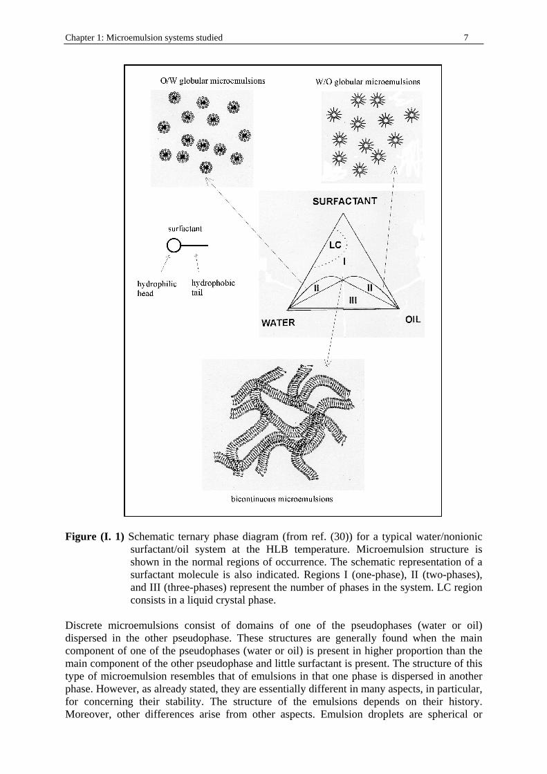
I. 4. Structure Two main general structures have been proposed and are accepted: discrete microemulsions and bicontinuous microemulsions. A schematic picture of a ternary phase diagram at constant temperature corresponding to a typical water/nonionic surfactant/oil system is shown in figure (I. 1). Microemulsions poor in either water or oil have a globular structure. Microemulsions containing similar amounts of oil and water and relatively high amounts of surfactants present bicontinuous structures. Frequently, liquid crystalline phases are also present in the phase diagrams.
Chapter 1: Microemulsion systems studied 7
Figure (I. 1) Schematic ternary phase diagram (from ref. (30)) for a typical water/nonionic
surfactant/oil system at the HLB temperature. Microemulsion structure is shown in the normal regions of occurrence. The schematic representation of a surfactant molecule is also indicated. Regions I (one-phase), II (two-phases), and III (three-phases) represent the number of phases in the system. LC region consists in a liquid crystal phase.
Discrete microemulsions consist of domains of one of the pseudophases (water or oil) dispersed in the other pseudophase. These structures are generally found when the main component of one of the pseudophases (water or oil) is present in higher proportion than the main component of the other pseudophase and little surfactant is present. The structure of this type of microemulsion resembles that of emulsions in that one phase is dispersed in another phase. However, as already stated, they are essentially different in many aspects, in particular, for concerning their stability. The structure of the emulsions depends on their history. Moreover, other differences arise from other aspects. Emulsion droplets are spherical or
Chapter 1: Microemulsion systems studied 8
nearly spherical; this form minimizes the interface, which gives a highly energetic term because of the interfacial tension. In microemulsions, because of the very low interfacial tension, the energetic term related to the interfacial tension and total surface is of less importance and therefore nonspherical droplets can be present without a large energy contribution. Because of the small size of the droplets and the low contribution of total surface to the total energy, the geometry of the surfactant molecules at the interface plays an important role. For microemulsions it is useful to consider the so-called criti cal packing parameter. This concept, put forward by Israelachvilli et al.52, considers that the amphiphili c molecules can be regarded as a two-piece structure: polar head and hydrophobic tail (see figure (I. 1)). The possible geometry of a film formed by the amphiphile molecules depends on their intrinsic geometry. The surfactant packing parameter p is calculated as
pV
alc
= (I. 1)
where a is the polar head area, lc the length of the hydrophobic tail of volume V. The area per polar head is usually measured at an air-water or oil -water interface using the Gibbs isotherm53. The length of the hydrophobic tail can be calculated from the values obtained by Tanford54, and an estimation of the maximum chain length in nm of a fully extended carbon chain of nc carbon atoms can be done as l nc c= +015 0127. . (I. 2) and the volume of the hydrocarbon tail can be calculated from the density of bulk hydrocarbon and (with nMe as the number of methyl groups which are twice the size of a CH2 group) be evaluated as
( )V n nc Me= +0027. (I. 3)
Critical packing parameters lower than 1/3 give a tendency to form globular structures, values around ½ favor cylindrical structures, and values close to 1 favor planar layers. Inverted cylinders and micelles are given by V > 1. This parameter allows the evaluation of the natural geometry of the amphiphile by itself. In microemulsions, hydrocarbon penetration and cosurfactant presence may completely change the structure from the natural tendency. Oil penetration in the hydrocarbon tail produces an increase in the apparent hydrophobic volume and thus an increase in the criti cal packing parameter. Cosurfactants, such as medium-chain alcohols, coadsorb at the interface producing an overall reduction of the criti cal packing parameter. When this occurs, the effective parameter, peff, of the mixed system can be calculated using the relationship proposed by Ninham56.
surfactantntcosurfacta
ntcosurfactantcosurfacta
surfactantntcosurfacta
surfactantsurfactant
surfactanttsurfacatan
xx
la
Vx
la
Vx
al
Vp
cc
effceff +
+
=
= (I. 4)
where x’s are the mole fractions of the species present at the interface.
Chapter 1: Microemulsion systems studied 9
A comparable, although quantitatively different, approach to analyzing microemulsions uses the curvature concept explicitely. In this approach, the critical parameter is not the surfactant packing parameter but the preferred mean curvature H of a surfactant film with4
HR R
= +
1
2
1 1
1 2
(I.5)
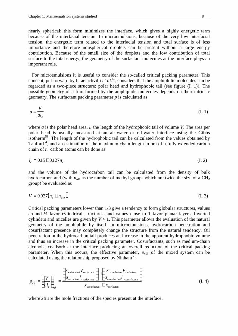
and where R1 and R2 are the radii of curvature in two perpendicular directions. For a sphere, R1 = R2 = R and H = 1/R, for a cylinder, R1 = R, R2 = ∞, and H = 1/2R, while for a planar bilayer, H = 0. A value of H = 0 also can occur on a saddle-shaped surface (figure (I. 2)) in which R1 = -R2. To assign a sign to the radii of curvature, one must define a normal direction, &
n , that is by convention positive when pointing toward the polar region, and therefore the curvature of inverted aggregates is negative.
Figure (I. 2) Radius of curvature4. For a surface of three dimensions, two mutually
perpendicular radii of curvature, R1 and R2, can be specified at each point. On a saddle-shaped surface, the two radii of curvature have opposite sign. Here R1 and R2 are shown at two different points on the surface.
The concentration of surfactant and the ratio of pseudophases play important roles in the structures as well. High amounts of ionic surfactant produce a high ionic strength with a subsequent reduction of the polar head area and a reduction of the surfactant packing parmeter. High amount of the internal pseudophase may produce phase separation if the total surfactant concentration is low. Other variables that influence the natural curvature of the amphiphile are electrolyte concentration (mainly for ionic surfactants57, although they influence nonionic as well) and temperature (mainly affecting nonionic surfactants58, 59). In contrast to the discrete microemulsion structure, which is relatively easy to treat theoretically, the structure of bicontinuous microemulsions is more difficult to visualize and
Chapter 1: Microemulsion systems studied 10
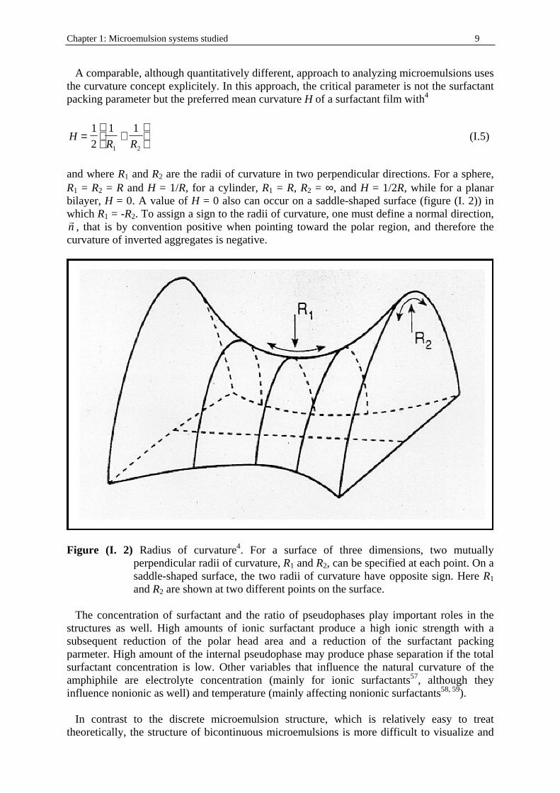
therefore its theoretical treatment is complicated. In a bicontinuous microemulsion both the aqueous and oil phases are continuous. This continuity means that it is possible to go from one end of the sample to the other by either dilution of oil (oil path) and water (aqueous path). This structure has an extremely large interfacial area, which is possible because of an extremely low interfacial tension, close to zero. In a microemulsion there is not a negative interfacial tension because this would mean production of energy as the interface increases. This could be the case in microemulsion formation but not at equili brium. Near-zero interfacial tension implies, at the same time, that the interfaces are unstable and can form and disappear without an energy increase. Interfacial energy of the order of kBT (T is the absolute temperature, and kB is the Boltzmann’s constant) has been considered to be a condition for the formation of bicontinuous structures60. Conditions for the formation of bicontinuous structures are a ratio of oil and water pseudophases close to one, large amounts of surfactant (enough to cover the interface), and zero mutual curvature of the interface. The theoretical treatment of a bicontinuous structure is complicated. Since this structure was proposed by Scriven17, several models have been proposed. The “random lattice” theory of Talmon and Prager61, 62 is based on tessellation of the space by a Voronoi structure; the cells of this tessellation are occupied by either oil or water in a random way. This model was improved by De Gennes and Taupin63, whose model is based on a cubic lattice. The cubes are occupied by either water or oil i n a random way. All these models are represented in figure (I. 3) (from ref. (64)). There is a criti cal water/oil ratio for which the percolation occurs; that is, an infinite path is possible in both phases.
Figure (I. 3) Schematic representations of bicontinuous micormulsions models52. (a) Talmon
and Prager49: random filli ng of Voronoi polyhedra with water or oil (top); unit water or oil cell (bottom). (b) De Gennes and Taupin51: random filli ng of cubes on a cubic lattice; the repetition distance equals the correlation length. (c) Scriven4: two examples of bicontinuous mesophase-like structures with minimal interfacial area.
The bicontinuous structure is consistent with most of the experimental observations of these systems. For instance, the self-diffusion coeff icients of oil , water, and surfactant are well
Chapter 1: Microemulsion systems studied 11
explained58. In these systems, the self-diffusion coeff icients are close to the self-diffusion coeff icients of these molecules in the pure liquids and the self-diffusion coeff icient of the surfactant is about one order of magnitude lower. This indicates “free” diffusion for water and oil , i.e., infinite domains, and the lower diffusion coeff icient of the surfactant is related to the positioning of the molecules at the interface. A useful picture of the structural transitions can be obtained by considering a surfactant solution in water with an increasing amount of oil . Surfactants above the criti cal micelle concentration form micelles in which some oil can be solubili zed. The limit of solubilit y in the micelles depends on the nature of the surfactant and the number of micelles. Ionic surfactants usually have large head groups and have a strong tendency to form spherical aggregates in water. The incorporation of oil i ncreases the size of the aggregates and therefore reduces the curvature. To reach a large amount of solubili zate the oil must penetrate the surfactant tail effectively, a cosurfacatant molecule should be added, electrolyte should be added, the temperature should be changed, or a combination of the four. On increasing the amount of oil pseudophase the percolation point will be reached and a bicontinuous structure formed. As said before, a large amount of surfactant is needed to prevent phase separation before this point is reached. Further increase of the oil pseudophase will make the system reach the percolation threshold for the water domains and discrete water domains will be formed.
I. 5. General methods of characterization The knowledge gained on the fundamental aspects of microemulsions has made possible the improvement of some established applications and the development of new ones. Therefore instruments and methods allowing microemulsions characterization are continuously developed. Since their characterization is a diff icult task, microemulsions have been studied using a great variety of techniques. This is due to their complexity, namely the variety of structures and components involved in these systems, as well as the limitations associated which each technique. Therefore, complementary studies using a combination of techniques are usually required to obtain a comprehensive view of the physiochemical properties and structure of microemulsions.
I. 5. 1. Phase behaviour Phase behaviour studies, with phase diagram determinations, are essential in the studies of surfactant systems. They provide information on the boundaries of the different phases as a function of composition variables and temperature, and, more important, structural organization can be also inferred. In addition, phase behaviour studies allow comparison of the eff iciency of different surfactants for a given application. It is important to note that simple measurements and equipment are required in this type of study. The boundaries of one-phase regions can be assessed easily by visual observation of samples of known composition. However, long equili bration times in multiphase regions, especially if liquid crystalli ne phases are involved, can make these determinations long and diff icult. The phase behaviour of interest for microemulsion studies involves at least three components: water, surfactant, and oil . Although most of the formulations of practical interest consist of more than three components, study of simple systems with the basic three, four, etc. components from which they are formulated is a prerequisite to understanding the behaviour of complex systems. The phase behaviour of three-component systems at fixed temperature and pressure is best represented by a ternary diagram (figure (I. 1)) and by a triangular prism
Chapter 1: Microemulsion systems studied 12
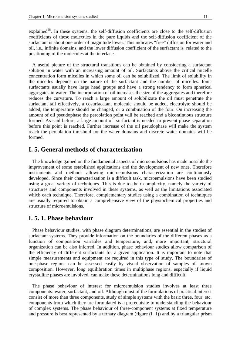
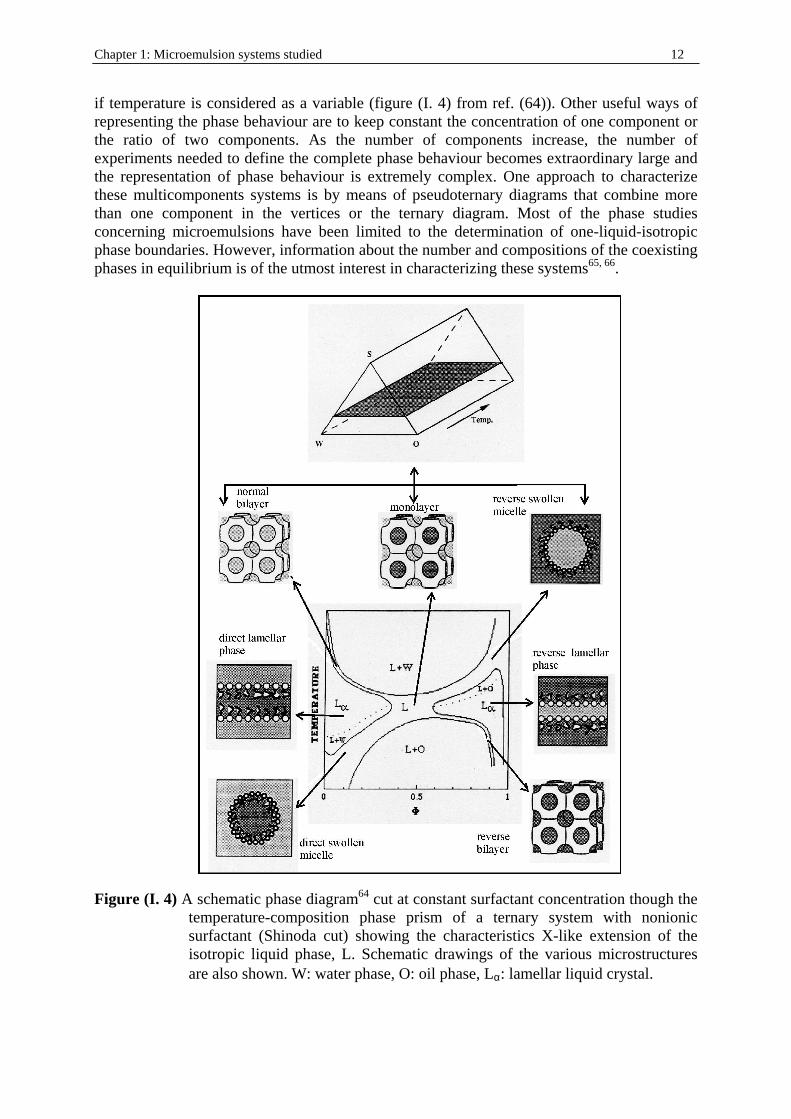
if temperature is considered as a variable (figure (I. 4) from ref. (64)). Other useful ways of representing the phase behaviour are to keep constant the concentration of one component or the ratio of two components. As the number of components increase, the number of experiments needed to define the complete phase behaviour becomes extraordinary large and the representation of phase behaviour is extremely complex. One approach to characterize these multicomponents systems is by means of pseudoternary diagrams that combine more than one component in the vertices or the ternary diagram. Most of the phase studies concerning microemulsions have been limited to the determination of one-liquid-isotropic phase boundaries. However, information about the number and compositions of the coexisting phases in equilibrium is of the utmost interest in characterizing these systems65, 66.
Figure (I. 4) A schematic phase diagram64 cut at constant surfactant concentration though the
temperature-composition phase prism of a ternary system with nonionic surfactant (Shinoda cut) showing the characteristics X-like extension of the isotropic liquid phase, L. Schematic drawings of the various microstructures are also shown. W: water phase, O: oil phase, Lα: lamellar liquid crystal.
Chapter 1: Microemulsion systems studied 13
I. 5. 2. Scattering techniques Scattering methods have been widely applied in the study of microemulsions. These include small-angle X-ray scattering (SAXS), small-angle neutron scattering (SANS), and static as well as dynamic light scattering techniques. The intensity of scattered radiation I(q) is measured as function of the scattering vector q, ( ) ( )q = 4 2π λ θ/ sin / where θ is the scattering angle and λ the wavelength of radiation. The general expression of the scattering intensity of monodispersed spheres interacting through hard sphere repulsion is
( ) ( ) ( )I q n P q S qd= , where nd is the number density of the spheres, ( )P q is the form factor,
which expresses the scattering cross section of the particle, and ( )S q is the structure factor,
which takes into account the particle-particle interaction. ( )P q and ( )S q can be estimated by
using appropriate analytical expressions. The lower limit of size that can be estimated by using these techniques is about 2 nm. The upper limit is about 100 nm for SANS and SAXS and a few micrometers for light scattering. These methods are very valuable for obtaining quantitative information on the size, shape, and dynamics of the structures. There is a major difficulty in the study of microemulsions with the use of scattering techniques: dilution of the sample, to reduce interparticle interaction, is not appropriate because it can modify the structure and the composition of the pseudophases. Nevertheless, successful determinations have been achieved by using a dilution technique that maintains the identity of droplets41 and extrapolating the results obtained at infinite dilution to obtain the size, shape, etc., or by measurements at very low concentrations. Small-angle X-ray scattering techniques have long been used to obtain information on droplet size and shape67, 68. Using Synchrotron radiation sources, with which sample-to-detector distances are bigger (4 m instead of 30-50 cm as with laboratory-based X-ray sources), significant improvements have been achieved. With synchrotron radiation more defined spectra are obtained and a wide range of systems can be studied, including those in which the surfactant molecules are poor X-ray scatterers58, 69. Small-angle neutron scattering allows selective enhancement of the different microemulsion pseudophases by using protonated or deuterated molecules (contrast variation technique). Therefore, this technique allows determination of the size and shape of the droplets as well as the characteristics of the amphiphilic layer without great perturbation of the system58, 70-72. Static light scattering techniques have also been widely used to determine microemulsion droplet size and shape. In these experiments the intensity of scattered light is generally measured at various angles and for different concentrations of microemulsion droplets. At sufficiently low concentrations, provided that the particles are small enough, the Rayleigh approximation can be applied. Droplet size can be estimated by plotting the intensity as a function of droplet volume fraction58, 71, 73, 74. Dynamic light scattering, also referred to as photon correlation spectroscopy (PCS), is used to analyze the fluctuations in the intensity of scattering by the droplets due to Brownian motion. The self-correlation function is measured and gives information on the dynamics of the system. This technique allows the determination of diffusion coefficients, D. In the absence of interparticle interactions, the hydrodynamic radius, RH, can be estimated from the diffusion coefficient using the Stockes-Einstein equation:
Chapter 1: Microemulsion systems studied 14
DkT
RH
=6πη
(I. 6)
where k is the Boltzmann constant, T is the absolute temperature, and η is the viscosity of the medium. Although dynamic light scattering measurements are relatively easy and fast, extrapolation of results to infinite dilution is not possible in most microemulsion systems and RH values obtained should be corrected because of interparticle interactions58, 70, 75, 76.
I. 5. 3. Nuclear Magnetic Resonance Nuclear magnetic resonance (NMR) techniques have been used to study the structure and dynamics of microemulsions. Self-diffusion measurements using different tracer techniques, generally radioactive labelling, supply information on the mobility of the components (self-diffusion coefficient). A limitation of this technique is that experiments are time-consuming and the use of labelled molecules is not practical77. However, the Fourier transform pulsed-gradient spin-echo (FT-PGSE) technique, in which magnetic field gradients are applied to the sample, allows simultaneous and rapid determination of the self-diffusion coefficients (in the range of 10-9 to 10-12 m2.s-1), of many components78. In water-in-oil microemulsions, water diffusion is slow and corresponds to that of the droplets (of the order of 10-11 m2.s-1), oil diffusion is high (of the order of 10-9 m2.s-1), and the diffusion of surfactant molecules, located at the interface, is the same order as that of the droplets. In contrast, in oil-in-water microemulsions the diffusion coefficients of water are higher than that of oil. In bicontinuous microemulsions the diffusion coefficients of water and oil are both high (of the order of 10-9 m2.s-1) and the diffusion coefficient of the surfactant has been found to be intermediate between the value of nonassociated surfactant molecules and the value for a droplet-type structure (of the order of 10-10 m2.s-1)79-82.
I. 5. 4. Electron Microscopy Several electron microscopic techniques have been attempted for the characterization of microemulsions. Because of the high lability of the samples and the danger of artefacts, electron microscopy used to be considered a misleading technique in microemulsions studies. However, images showing clear evidence of microstructures have been obtained58, 60. Freeze fracture electron microscopy, a well established method in the biological field has been successfully applied to microemulsions. Careful control of the temperature of the sample before freezing and ultrarapid cooling followed by fracture and replication of the fracture face yield images of the microstructure of these systems.
I. 5. 5. Other methods Interfacial tension measurements are useful in the study of the formation and properties of microemulsions. Ultralow values of interfacial tensions are correlated with phase behaviour, particularly the existence of surfactant phase or middle-phase microemulsions in equilibrium with aqueous and oil phases83, 84. Ultralow interfacial tensions can be measured with the spinning-drop apparatus. Interfacial tension are derived from the measurement of the shape of a drop of the low-density phase, rotating in a cylindrical capillary filled with the high-density phase85. Electrical conductivity has been widely used to determine the nature of the continuous phase and to detect phase inversion phenomena. The distinction between O/W (high
Chapter 1: Microemulsion systems studied 15
conductivity) and W/O (low conductivity) emulsions is quite straightforward. However, in microemulsions the behaviour is more complex. A sharp increase in conductivity in certain W/O microemulsions systems was observed at low volume fractions86. This behaviour was interpreted as an indication of a percolative behaviour or exchange of ions between droplets before the formation of bicontinuous structures. When the conductivity of nonionic surfactant system is measured, water is generally replaced by an electrolyte solution. If the electrolyte concentration is kept low (10-2-10-3 M), no effect on the structure is produced58. Viscosity measurements as a function of volume fraction have been used to determine the hydrodynamic radius of droplets, as well as interactions between droplets and deviations from spherical shape by fitting the results to appropriate models42. Some microemulsions show newtonian behaviour, and their viscosities are similar to that of water. For these microemulsions, the hydrodynamic volume of the particles can be calculated from Einstein’s equation for the relative viscosity ηr (η φr = +1 25. , where φ is the particle volume fraction) if φ is lower than ≈ 0.1 or from modifications of this equation if it is higher.
II. Motivation As indicated in the general introduction, dielectric relaxation spectroscopy (DRS) is able to monitor a wide range of dynamical processes related to micellar systems, from the reorientation of water molecules or ion pairs to the fluctuations of the cloud of more or less tightly bound counterions surrounding charged micelles5-10. In the present work, DRS measurements (in the frequency range 0.008 ≤ ν / GHz ≤ 89) of sodium dodecyl sulfate (SDS) ionic micellar system were carried out at 25°C. The results obtained were used, with help of the continuity of the clear and monophasic solution between SDS micelles and water/SDS/1-pentanol/n-dodecane W/O microemulsions, to enhance the present knowledge of DRS of microemulsions. Additionally, the devices present in our laboratory allow us measure at frequencies up to 89 GHz, and therefore bring broader dielectric spectra than that found in literature data (up to 10 GHz). In the last decades the majority of W/O microemulsion systems investigated by several techniques consist in a mixture of water, alkane, and a single surface-active agent: sodium bis(2-ethylhexyl) sulfoccinate, so-called Aerosol OT or AOT. The main advantage of this surfactant is that is does not imply any cosurfactant like alcohol (so that there is no problem of alcohol distribution between the microemulsion subphases) to form a W/O microemulsion. Additionally this surfactant has a low cmc (generally in the range of 10-3 to 10-4 mol.dm-3 depending on the solvent), so that it can be admitted that the whole surfactant is located at the interface. These characteristics render (neglecting oil penetration in the interfacial film) easy the evaluation of φ, and hence the understanding of the properties of such systems. On the other hand, these systems do not exhibit a transition O/W → W/O microemulsions, since in the phase diagram water/AOT/alkane, the realm-of existence of clear and monophasic solutions consists of two disjoined areas. The systems water/AOT/alkane are well -known but show a limited variety of structures. Therefore, experimental and theoretical results obtained with these systems cannot be easily extrapolated to other microemulsion systems. In the case of four-component microemulsions involving an alcohol as cosurfactant, a greater variety of systems (with or without the transition O/W → W/O microemulsions) can be reached rendering easier the extension of experimental and theoretical results to other microemulsion systems. Unfortunately, distribution of alcohol between the continuous phase (water and oil for O/W and W/O microemulsion, respectively), the disperse phase (water or oil droplets, plus surface-active agents), and the interfacial layer (surface-active agents) is often not known.
Chapter 1: Microemulsion systems studied 16
This makes diff icult the estimation of the volume fraction, φ, of the disperse phase. Despite this diff iculty, microemulsion systems involving more than three components are generally of a greater industrial interest. These reasons motivated us to investigate ionic microemulsions with cosurfactant by means of DRS.
II. 1. DRS of microemulsions, general results Various W/O microemulsion systems have been studied by DRS, most of them are of the type water/AOT/alkane, and were investigated changing oil nature11, adding electrolyte87, or varying temperature12, 88. Different alkane chain lengths (in the oil continuous phase) were also considered89-93. The corresponding results showed that when φ increases (increasing interparticle interaction) leading to a percolation, the dielectric relaxation is considerably affected. Chou and Sha indicated that the interfacial hydration94 plays also an important role in the observed changes of the DRS spectra. DRS investigations of W/O nonionic microemulsions with alcohol as cosurfactant have been also carried out95-98. It has been shown that local relaxation processes due to dipoles of water and alcohol occured. The W/O microemulsion system water/sodium dodecyl sulfate (SDS)/1-pentanol/n-dodecane has been previously investigated by Ponton et al.99. Their results were compared with our work. Given the complexity of the chemical makeup of microemulsions, especially in the case of W/O microemulsions reverse droplets, various theoretical and experimental sources of relaxation processes related to dynamic processes occur making a precise interpretation of the dielectric relaxation mode a diff icult task. Since our system is ionic, one or more dielectric relaxation contributions are expected to be related to counter ion polarization resulting from the movements of ions and/or surfactant counterions. It is evident that this counterion polarization may be under the influence of droplet and percolation cluster behaviour, droplets translations, rotations, colli sions, fusion, and shape fluctuations99. The relaxation can also be related to various components of the system containing active dipole groups, such as bound and free water. Since we decided to consider ionic microemulsions with alcohol as cosurfactant, an additional contribution arising from the alcohol −OH groups is expected. All these contributions cause or may cause complex dielectric behaviour.
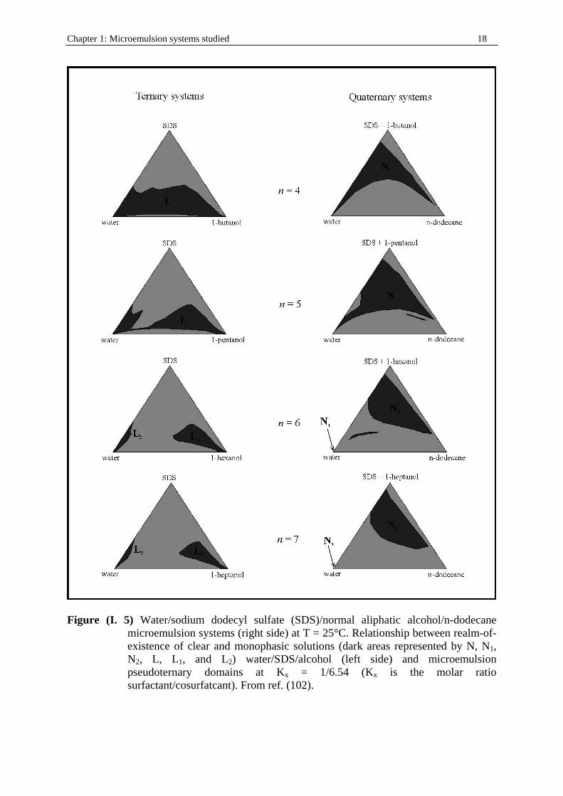
II. 2. Choice of the systems investigated Clausse et al.13 delineated the realms-of-existence of microemulsions, at T = 25°C, for a great number of systems incorporating water, sodium dodecyl sulfate, various straight or branched alkanols, and various hydrocarbons. In this way, two categories of water/SDS/alkanol/hydrocarbon systems (figure (I. 5)) could be defined in which the alkanol molecular structure has a strong influence on microemulsion solubili zation capacity: • The type S systems are characterized by the fact that, in a ternary phase diagram, the
realm-of-existence of the monophasic water/SDS/alkanol solutions consists of two disjoined areas, L1 which corresponds to a “direct” solubili zation (aqueous solution of alkanol) and L2 which corresponds to “ inverse” solubili zation (alkanol solution of water). Consequently, the three-dimensional microemulsion domain consists of two disjoined volumes. V1, the extension of the L1 area, corresponds to “direct” microemulsions (hydrocarbon in water), and V2, the extension of the L2 area, corresponds to “ reverse “ microemulsions (water in hydrocarbon).
Chapter 1: Microemulsion systems studied 17
• The type U systems are characterized by the fact that the realm-of-existence of the monophasic water/SDS/alkanol solutions is a large area L, which, in the ternary phase diagram, is stretched continuously from the W apex (100% water) to the C apex (100% alkanol). Consequently, the three-dimensional microemulsion domain is a vast all -in-one block volume V that generally spans the greater portion of the phase tetrahedron and diverse kind of structure are expected.
The existence of these two distinct types of microemulsion systems is correlated to two different microemulsion electroconductive and viscous behavior13. In the case of systems whose ionic surfactant is SDS and cosurfactant normal alkanol, the transition from type S to type U systems occurs, whatever the nature of the hydrophobic hydrocarbon, when 1-pentanol is substituted for 1-hexanol (the threshold value of n is therefore equal to 6). Therefore, the systems for which we decided to do dielectric measurements are water/SDS/1-pentanol (for which the definition of microemulsion is not true, since 1-pentanol cannot be considered as an oil) and water/SDS/1pentanol/n-dodecane (with ratio Km = mass SDS/ mass 1-pentanol = ½) systems at 25 °C. As it can be seen in figure (I. 6), a clear continuity exists between SDS micelles in water and W/O microemulsions and allows us to observe the transition: micellar systems → bicontinuous structures → reverse micellar systems → W/O microemulsions. In a first step, the system SDS in water beyond the criti cal micelle concentration (cmc) was investigated in the light of recent developments concerning DRS of charged micelles and carried out for cationic surfactants9, 10. The second step consisted to extend the results obtained with this system to reverse micelles and W/O microemulsions using the continuous link presented before (figure (I. 6)). The last part of the work was to consider dielectric measurements in the W/O part of water/SDS/1-butanol/n-dodecane, water/SDS/1-hexanol/n-dodecane, and water/SDS/1-heptanol/n-dodecane systems at 25 °C. Additional measurements of nonionic systems water/C12E23/1-alkanol (1-pentanol, 1-hexanol, 1-butanol) were also performed at 25 °C. This last part of the work constitutes the next step of the generalization of DRS to microemulsions study and is treated separately.
Chapter 1: Microemulsion systems studied 18
Figure (I. 5) Water/sodium dodecyl sulfate (SDS)/normal aliphatic alcohol/n-dodecane
microemulsion systems (right side) at T = 25°C. Relationship between realm-of-existence of clear and monophasic solutions (dark areas represented by N, N1, N2, L, L1, and L2) water/SDS/alcohol (left side) and microemulsion pseudoternary domains at Kx = 1/6.54 (Kx is the molar ratio surfactant/cosurfatcant). From ref. (102).
Chapter 1: Microemulsion systems studied 19
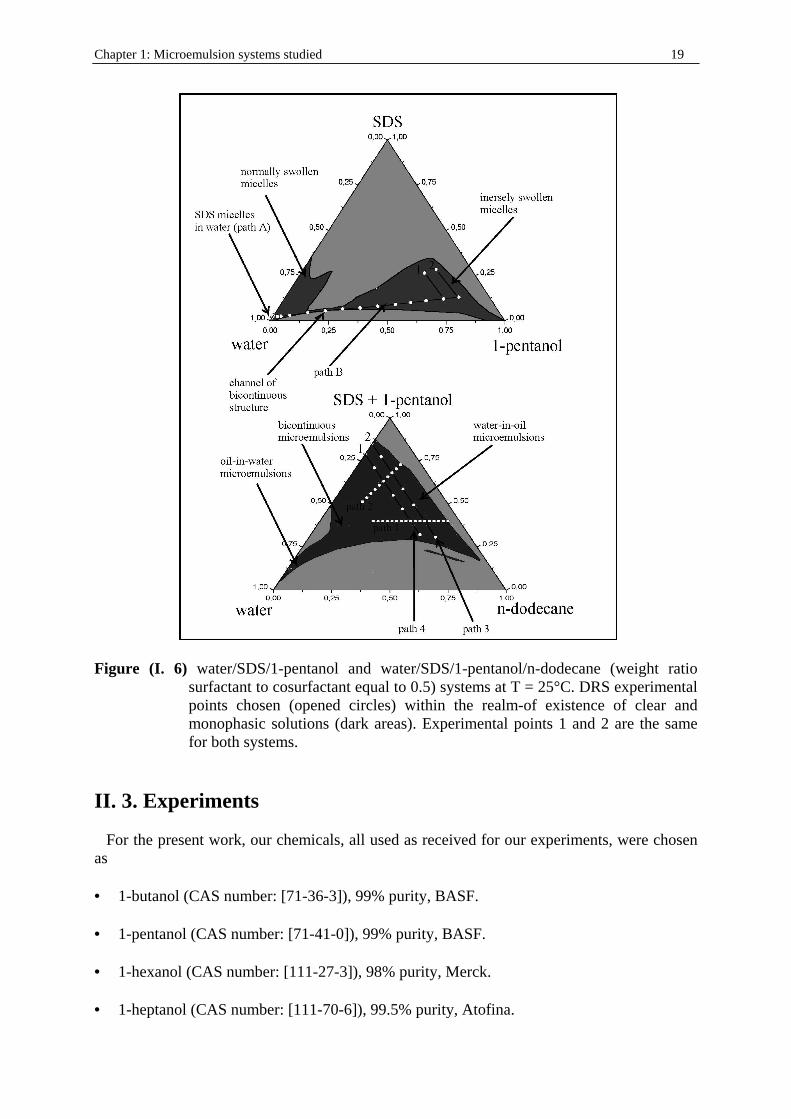
Figure (I. 6) water/SDS/1-pentanol and water/SDS/1-pentanol/n-dodecane (weight ratio
surfactant to cosurfactant equal to 0.5) systems at T = 25°C. DRS experimental points chosen (opened circles) within the realm-of existence of clear and monophasic solutions (dark areas). Experimental points 1 and 2 are the same for both systems.
II. 3. Experiments For the present work, our chemicals, all used as received for our experiments, were chosen as • 1-butanol (CAS number: [71-36-3]), 99% purity, BASF. • 1-pentanol (CAS number: [71-41-0]), 99% purity, BASF. • 1-hexanol (CAS number: [111-27-3]), 98% purity, Merck. • 1-heptanol (CAS number: [111-70-6]), 99.5% purity, Atofina.
Chapter 1: Microemulsion systems studied 20
• n-dodecane (CAS number: [112-40-3]), 99.9% purity, Merck. • sodium dodecyl sulfate (SDS) (CAS number: [151-21-3]), purity > 99%, from Merck. • polyoxyethylene (35) lauryl ether (C12E23), commercial name Brij35 (CAS number:
[9002-92-0]), 99% purity, Uniqema. • Milli pore water (with an electrical conductivity ~ 10-6 S/m) was used as the solvent. • Deuterated water, D2O, 99.9% purity, Euriso-Top. Solutions were prepared on scales, without considering corrections. Some of the compounds indicated here exhibit mutual solubili sation at 25°C. For example 1-pentanol and n-dodecane are co-soluble, and the solubili sation limit of 1-pentanol in water is about 2.2%w101, while that of water in pure 1-pentanol is about 10%w102.
II . 3. 1. SDS in water, water/SDS/1-pentanol, and water/SDS/1-pentanol systems at T = 25 °C
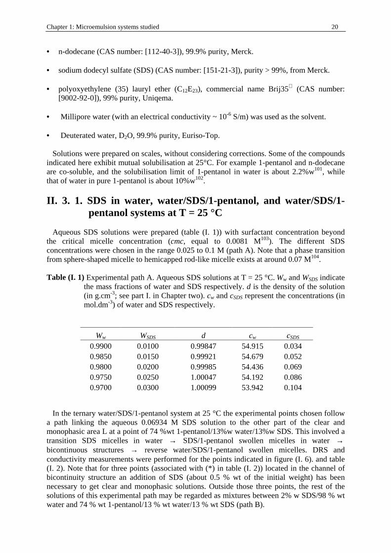
Aqueous SDS solutions were prepared (table (I. 1)) with surfactant concentration beyond the criti cal micelle concentration (cmc, equal to 0.0081 M103). The different SDS concentrations were chosen in the range 0.025 to 0.1 M (path A). Note that a phase transition from sphere-shaped micelle to hemicapped rod-like micelle exists at around 0.07 M104. Table (I . 1) Experimental path A. Aqueous SDS solutions at T = 25 °C. Ww and WSDS indicate
the mass fractions of water and SDS respectively. d is the density of the solution (in g.cm-3; see part I. in Chapter two). cw and cSDS represent the concentrations (in mol.dm-3) of water and SDS respectively.
Ww WSDS d cw cSDS 0.9900 0.0100 0.99847 54.915 0.034 0.9850 0.0150 0.99921 54.679 0.052 0.9800 0.0200 0.99985 54.436 0.069 0.9750 0.0250 1.00047 54.192 0.086 0.9700 0.0300 1.00099 53.942 0.104
In the ternary water/SDS/1-pentanol system at 25 °C the experimental points chosen follow a path linking the aqueous 0.06934 M SDS solution to the other part of the clear and monophasic area L at a point of 74 %wt 1-pentanol/13%w water/13%w SDS. This involved a transition SDS micelles in water → SDS/1-pentanol swollen micelles in water → bicontinuous structures → reverse water/SDS/1-pentanol swollen micelles. DRS and conductivity measurements were performed for the points indicated in figure (I. 6). and table (I. 2). Note that for three points (associated with (* ) in table (I. 2)) located in the channel of bicontinuity structure an addition of SDS (about 0.5 % wt of the initial weight) has been necessary to get clear and monophasic solutions. Outside those three points, the rest of the solutions of this experimental path may be regarded as mixtures between 2% w SDS/98 % wt water and 74 % wt 1-pentanol/13 % wt water/13 % wt SDS (path B).
Chapter 1: Microemulsion systems studied 21
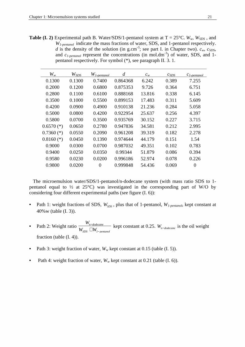
Table (I. 2) Experimental path B. Water/SDS/1-pentanol system at T = 25°C. Ww, WSDS , and
W1-pentanol indicate the mass fractions of water, SDS, and 1-pentanol respectively. d is the density of the solution (in g.cm-3; see part I. in Chapter two). cw, cSDS, and c1-pentanol represent the concentrations (in mol.dm-3) of water, SDS, and 1-pentanol respectively. For symbol (* ), see paragraph II . 3. 1.
Ww WSDS W1-pentanol d cw cSDS c1-pentanol 0.1300 0.1300 0.7400 0.864368 6.242 0.389 7.255 0.2000 0.1200 0.6800 0.875353 9.726 0.364 6.751 0.2800 0.1100 0.6100 0.888168 13.816 0.338 6.145 0.3500 0.1000 0.5500 0.899153 17.483 0.311 5.609 0.4200 0.0900 0.4900 0.910138 21.236 0.284 5.058 0.5000 0.0800 0.4200 0.922954 25.637 0.256 4.397 0.5800 0.0700 0.3500 0.935769 30.152 0.227 3.715
0.6570 (* ) 0.0650 0.2780 0.947836 34.581 0.212 2.995 0.7360 (* ) 0.0550 0.2090 0.961208 39.319 0.182 2.278 0.8160 (* ) 0.0450 0.1390 0.974644 44.179 0.151 1.54
0.9000 0.0300 0.0700 0.987032 49.351 0.102 0.783 0.9400 0.0250 0.0350 0.99344 51.879 0.086 0.394 0.9580 0.0230 0.0200 0.996186 52.974 0.078 0.226 0.9800 0.0200 0 0.999848 54.436 0.069 0
The microemulsion water/SDS/1-pentanol/n-dodecane system (with mass ratio SDS to 1-pentanol equal to ½ at 25°C) was investigated in the corresponding part of W/O by considering four different experimental paths (see figure (I. 6)): • Path 1: weight fractions of SDS, WSDS , plus that of 1-pentanol, W1-pentanol, kept constant at
40%w (table (I. 3)).
• Path 2: Weight ratio W
W Wn dodecane
SDS 1 pentanol
−
−+ kept constant at 0.25. Wn dodecane− is the oil weight
fraction (table (I. 4)). • Path 3: weight fraction of water, Ww kept constant at 0.15 (table (I. 5)). • Path 4: weight fraction of water, Ww kept constant at 0.21 (table (I. 6)).
Chapter 1: Microemulsion systems studied 22
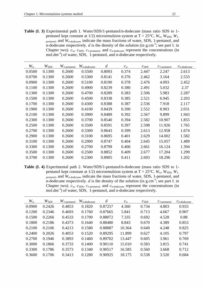
Table (I. 3) Experimental path 1. Water/SDS/1-pentanol/n-dodecane (mass ratio SDS to 1-
pentanol kept constant at 1/2) microemulsion system at T = 25°C. Ww, WSDS, W1-
pentanol, and Wn-dodecane indicate the mass fractions of water, SDS, 1-pentanol, and n-dodecane respectively. d is the density of the solution (in g.cm-3; see part I. in Chapter two). cw, cSDS, c1-pentanol, and cn-dodecane represent the concentrations (in mol.dm-3) of water, SDS, 1-pentanol, and n-dodecane respectively.
Ww WSDS W1-pentanol Wn-dodecane d cw cSDS c1-pentanol cn-dodecane 0.0500 0.1300 0.2600 0.5500 0.8093 0.374 2.447 2.247 2.613 0.0700 0.1300 0.2600 0.5300 0.8141 0.376 2.462 3.164 2.533 0.0900 0.1300 0.2600 0.5100 0.8190 0.378 2.476 4.093 2.452 0.1100 0.1300 0.2600 0.4900 0.8239 0.380 2.491 5.032 2.37 0.1300 0.1300 0.2600 0.4700 0.8289 0.383 2.506 5.983 2.287 0.1500 0.1300 0.2600 0.4500 0.8338 0.385 2.521 6.945 2.203 0.1700 0.1300 0.2600 0.4300 0.8388 0.387 2.536 7.918 2.117 0.1900 0.1300 0.2600 0.4100 0.8439 0.390 2.552 8.903 2.031 0.2100 0.1300 0.2600 0.3900 0.8489 0.392 2.567 9.899 1.943 0.2300 0.1300 0.2600 0.3700 0.8540 0.394 2.582 10.907 1.855 0.2500 0.1300 0.2600 0.3500 0.8591 0.397 2.598 11.926 1.765 0.2700 0.1300 0.2600 0.3300 0.8643 0.399 2.613 12.958 1.674 0.2900 0.1300 0.2600 0.3100 0.8695 0.401 2.629 14.002 1.582 0.3100 0.1300 0.2600 0.2900 0.8747 0.404 2.645 15.057 1.489 0.3300 0.1300 0.2600 0.2700 0.8799 0.406 2.661 16.124 1.394 0.3500 0.1300 0.2600 0.2500 0.8852 0.409 2.677 17.204 1.299 0.3700 0.1300 0.2600 0.2300 0.8905 0.411 2.693 18.296 1.202
Table (I. 4) Experimental path 2. Water/SDS/1-pentanol/n-dodecane (mass ratio SDS to 1-
pentanol kept constant at 1/2) microemulsion system at T = 25°C. Ww, WSDS, W1-
pentanol, and Wn-dodecane indicate the mass fractions of water, SDS, 1-pentanol, and n-dodecane respectively. d is the density of the solution (in g.cm-3; see part I. in Chapter two). cw, cSDS, c1-pentanol, and cn-dodecane represent the concentrations (in mol.dm-3) of water, SDS, 1-pentanol, and n-dodecane respectively.
Ww WSDS W1-pentanol Wn-dodecane d cw cSDS c1-pentanol cn-dodecane 0.0900 0.2426 0.4853 0.1820 0.87257 4.360 0.734 4.803 0.933 0.1200 0.2346 0.4693 0.1760 0.87665 5.841 0.713 4.667 0.907 0.1500 0.2266 0.4533 0.1700 0.88072 7.335 0.692 4.528 0.88 0.1800 0.2186 0.4373 0.1640 0.88480 8.843 0.670 4.389 0.853 0.2100 0.2106 0.4213 0.1580 0.88887 10.364 0.649 4.248 0.825 0.2400 0.2026 0.4053 0.1520 0.89295 11.899 0.627 4.105 0.797 0.2700 0.1946 0.3893 0.1460 0.89702 13.447 0.605 3.961 0.769 0.3000 0.1866 0.3733 0.1400 0.90110 15.010 0.583 3.815 0.741 0.3300 0.1786 0.3573 0.1340 0.90517 16.585 0.560 3.668 0.712 0.3600 0.1706 0.3413 0.1280 0.90925 18.175 0.538 3.520 0.684
Chapter 1: Microemulsion systems studied 23
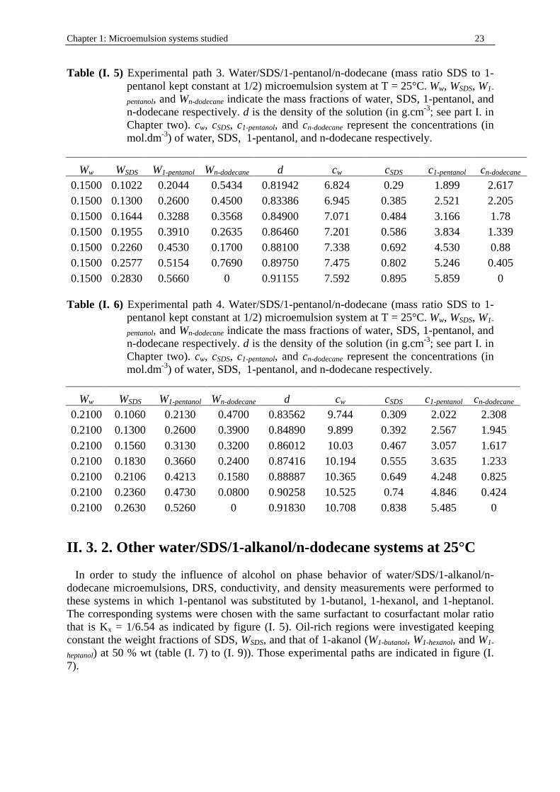
Table (I . 5) Experimental path 3. Water/SDS/1-pentanol/n-dodecane (mass ratio SDS to 1-pentanol kept constant at 1/2) microemulsion system at T = 25°C. Ww, WSDS, W1-
pentanol, and Wn-dodecane indicate the mass fractions of water, SDS, 1-pentanol, and n-dodecane respectively. d is the density of the solution (in g.cm-3; see part I. in Chapter two). cw, cSDS, c1-pentanol, and cn-dodecane represent the concentrations (in mol.dm-3) of water, SDS, 1-pentanol, and n-dodecane respectively.
Ww WSDS W1-pentanol Wn-dodecane d cw cSDS c1-pentanol cn-dodecane 0.1500 0.1022 0.2044 0.5434 0.81942 6.824 0.29 1.899 2.617 0.1500 0.1300 0.2600 0.4500 0.83386 6.945 0.385 2.521 2.205 0.1500 0.1644 0.3288 0.3568 0.84900 7.071 0.484 3.166 1.78 0.1500 0.1955 0.3910 0.2635 0.86460 7.201 0.586 3.834 1.339 0.1500 0.2260 0.4530 0.1700 0.88100 7.338 0.692 4.530 0.88 0.1500 0.2577 0.5154 0.7690 0.89750 7.475 0.802 5.246 0.405 0.1500 0.2830 0.5660 0 0.91155 7.592 0.895 5.859 0
Table (I . 6) Experimental path 4. Water/SDS/1-pentanol/n-dodecane (mass ratio SDS to 1-
pentanol kept constant at 1/2) microemulsion system at T = 25°C. Ww, WSDS, W1-
pentanol, and Wn-dodecane indicate the mass fractions of water, SDS, 1-pentanol, and n-dodecane respectively. d is the density of the solution (in g.cm-3; see part I. in Chapter two). cw, cSDS, c1-pentanol, and cn-dodecane represent the concentrations (in mol.dm-3) of water, SDS, 1-pentanol, and n-dodecane respectively.
Ww WSDS W1-pentanol Wn-dodecane d cw cSDS c1-pentanol cn-dodecane 0.2100 0.1060 0.2130 0.4700 0.83562 9.744 0.309 2.022 2.308 0.2100 0.1300 0.2600 0.3900 0.84890 9.899 0.392 2.567 1.945 0.2100 0.1560 0.3130 0.3200 0.86012 10.03 0.467 3.057 1.617 0.2100 0.1830 0.3660 0.2400 0.87416 10.194 0.555 3.635 1.233 0.2100 0.2106 0.4213 0.1580 0.88887 10.365 0.649 4.248 0.825 0.2100 0.2360 0.4730 0.0800 0.90258 10.525 0.74 4.846 0.424 0.2100 0.2630 0.5260 0 0.91830 10.708 0.838 5.485 0
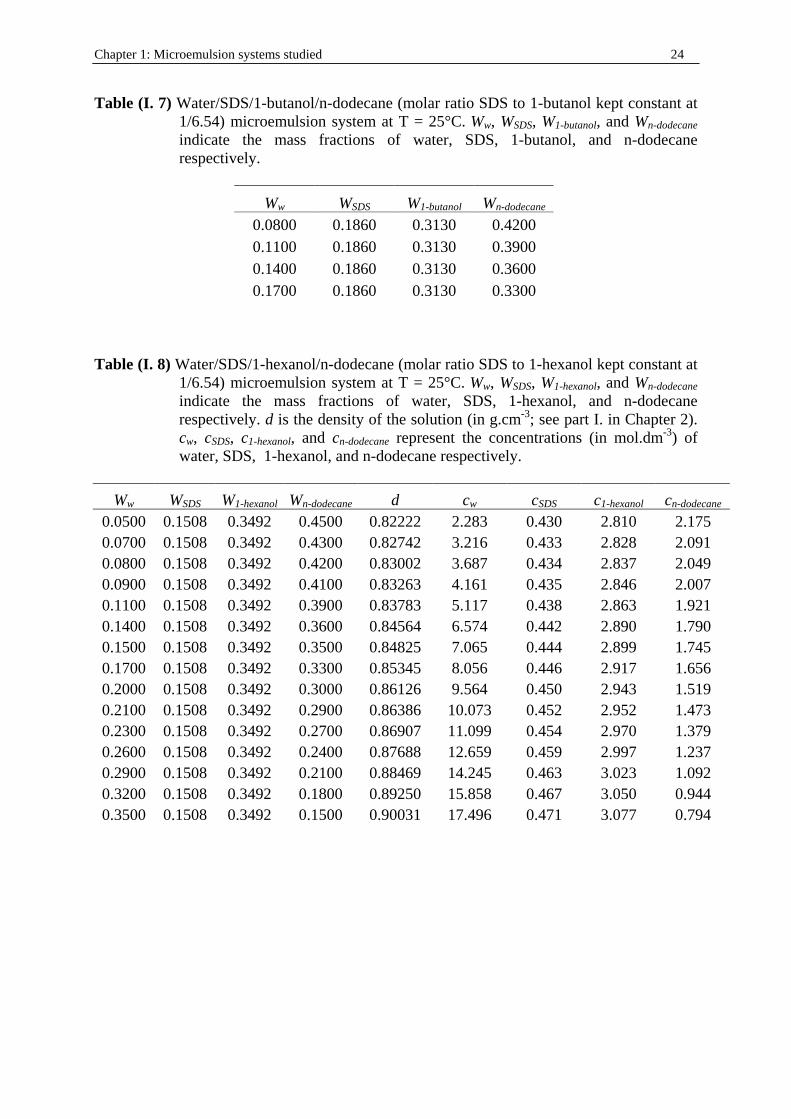
II . 3. 2. Other water/SDS/1-alkanol/n-dodecane systems at 25°C In order to study the influence of alcohol on phase behavior of water/SDS/1-alkanol/n-dodecane microemulsions, DRS, conductivity, and density measurements were performed to these systems in which 1-pentanol was substituted by 1-butanol, 1-hexanol, and 1-heptanol. The corresponding systems were chosen with the same surfactant to cosurfactant molar ratio that is Kx = 1/6.54 as indicated by figure (I. 5). Oil -rich regions were investigated keeping constant the weight fractions of SDS, WSDS, and that of 1-akanol (W1-butanol, W1-hexanol, and W1-
heptanol) at 50 % wt (table (I. 7) to (I. 9)). Those experimental paths are indicated in figure (I. 7).
Chapter 1: Microemulsion systems studied 24
Table (I. 7) Water/SDS/1-butanol/n-dodecane (molar ratio SDS to 1-butanol kept constant at 1/6.54) microemulsion system at T = 25°C. Ww, WSDS, W1-butanol, and Wn-dodecane indicate the mass fractions of water, SDS, 1-butanol, and n-dodecane respectively.
Ww WSDS W1-butanol Wn-dodecane 0.0800 0.1860 0.3130 0.4200 0.1100 0.1860 0.3130 0.3900 0.1400 0.1860 0.3130 0.3600 0.1700 0.1860 0.3130 0.3300
Table (I. 8) Water/SDS/1-hexanol/n-dodecane (molar ratio SDS to 1-hexanol kept constant at
1/6.54) microemulsion system at T = 25°C. Ww, WSDS, W1-hexanol, and Wn-dodecane indicate the mass fractions of water, SDS, 1-hexanol, and n-dodecane respectively. d is the density of the solution (in g.cm-3; see part I. in Chapter 2). cw, cSDS, c1-hexanol, and cn-dodecane represent the concentrations (in mol.dm-3) of water, SDS, 1-hexanol, and n-dodecane respectively.
Ww WSDS W1-hexanol Wn-dodecane d cw cSDS c1-hexanol cn-dodecane 0.0500 0.1508 0.3492 0.4500 0.82222 2.283 0.430 2.810 2.175 0.0700 0.1508 0.3492 0.4300 0.82742 3.216 0.433 2.828 2.091 0.0800 0.1508 0.3492 0.4200 0.83002 3.687 0.434 2.837 2.049 0.0900 0.1508 0.3492 0.4100 0.83263 4.161 0.435 2.846 2.007 0.1100 0.1508 0.3492 0.3900 0.83783 5.117 0.438 2.863 1.921 0.1400 0.1508 0.3492 0.3600 0.84564 6.574 0.442 2.890 1.790 0.1500 0.1508 0.3492 0.3500 0.84825 7.065 0.444 2.899 1.745 0.1700 0.1508 0.3492 0.3300 0.85345 8.056 0.446 2.917 1.656 0.2000 0.1508 0.3492 0.3000 0.86126 9.564 0.450 2.943 1.519 0.2100 0.1508 0.3492 0.2900 0.86386 10.073 0.452 2.952 1.473 0.2300 0.1508 0.3492 0.2700 0.86907 11.099 0.454 2.970 1.379 0.2600 0.1508 0.3492 0.2400 0.87688 12.659 0.459 2.997 1.237 0.2900 0.1508 0.3492 0.2100 0.88469 14.245 0.463 3.023 1.092 0.3200 0.1508 0.3492 0.1800 0.89250 15.858 0.467 3.050 0.944 0.3500 0.1508 0.3492 0.1500 0.90031 17.496 0.471 3.077 0.794
Chapter 1: Microemulsion systems studied 25
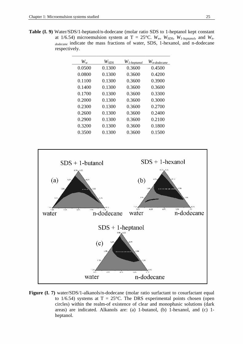
Table (I. 9) Water/SDS/1-heptanol/n-dodecane (molar ratio SDS to 1-heptanol kept constant at 1/6.54) microemulsion system at T = 25°C. Ww, WSDS, W1-heptanol, and Wn-
dodecane indicate the mass fractions of water, SDS, 1-hexanol, and n-dodecane respectively.
Ww WSDS W1-heptanol Wn-dodecane 0.0500 0.1300 0.3600 0.4500 0.0800 0.1300 0.3600 0.4200 0.1100 0.1300 0.3600 0.3900 0.1400 0.1300 0.3600 0.3600 0.1700 0.1300 0.3600 0.3300 0.2000 0.1300 0.3600 0.3000 0.2300 0.1300 0.3600 0.2700 0.2600 0.1300 0.3600 0.2400 0.2900 0.1300 0.3600 0.2100 0.3200 0.1300 0.3600 0.1800 0.3500 0.1300 0.3600 0.1500
Figure (I. 7) water/SDS/1-alkanols/n-dodecane (molar ratio surfactant to cosurfactant equal to 1/6.54) systems at T = 25°C. The DRS experimental points chosen (open circles) within the realm-of existence of clear and monophasic solutions (dark areas) are indicated. Alkanols are: (a) 1-butanol, (b) 1-hexanol, and (c) 1-heptanol.
Chapter 1: Microemulsion systems studied 26
II . 3. 3. Water/C12E23/1-alkanol systems at 25°C DRS measurements were also carried out for water/C12E23/1-alkanol systems at 25°C, the alcohols were chosen as 1-butanol, 1-pentanol, and 1-hexanol. Experimental paths were chosen with weight fractions of C12E23 kept constant at 40 % wt (tables (I. 10) to (I. 12)). The corresponding realm-of-existence of clear and monophasic solutions is available in references (102) and (105). Table (I . 10) Water/Brij35/1-butanol system at T = 25°C. Ww, WBij35, and W1-butanol, indicate
the mass fractions of water, Brij35, and 1-butanol, respectively.
Ww WBrij35 W1-butanol
0.0500 0.4000 0.5500 0.0800 0.4000 0.5200 0.1100 0.4000 0.4900 0.1400 0.4000 0.4600 0.1700 0.4000 0.4300 0.2000 0.4000 0.4000 0.2300 0.4000 0.3700 0.2600 0.4000 0.3400 0.2900 0.4000 0.3100 0.3200 0.4000 0.2800 0.3500 0.4000 0.2500 0.3800 0.4000 0.2200 0.4100 0.4000 0.1900
Table (I . 11) Water/Brij35/1-pentanol system at T = 25°C. Ww, WBij35, and W1-pentanol,
indicate the mass fractions of water, Brij35, and 1-pentanol, respectively.
Ww WBrij35 W1-pentanol 0.0500 0.4000 0.5500 0.0800 0.4000 0.5200 0.1100 0.4000 0.4900 0.1400 0.4000 0.4600 0.1700 0.4000 0.4300 0.2000 0.4000 0.4000 0.2300 0.4000 0.3700 0.2600 0.4000 0.3400 0.2900 0.4000 0.3100 0.3200 0.4000 0.2800 0.3500 0.4000 0.2500 0.3800 0.4000 0.2200 0.4100 0.4000 0.1900
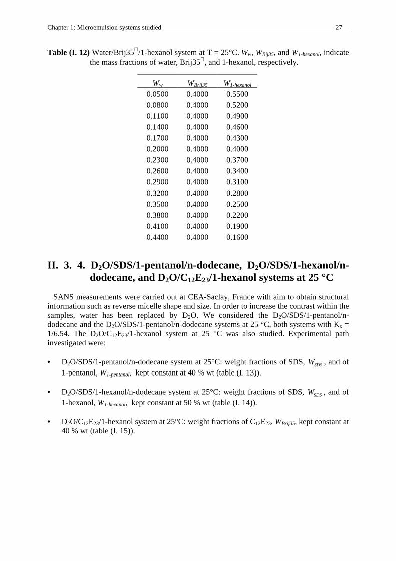
Chapter 1: Microemulsion systems studied 27
Table (I . 12) Water/Brij35/1-hexanol system at T = 25°C. Ww, WBij35, and W1-hexanol, indicate the mass fractions of water, Brij35, and 1-hexanol, respectively.
Ww WBrij35 W1-hexanol 0.0500 0.4000 0.5500 0.0800 0.4000 0.5200 0.1100 0.4000 0.4900 0.1400 0.4000 0.4600 0.1700 0.4000 0.4300 0.2000 0.4000 0.4000 0.2300 0.4000 0.3700 0.2600 0.4000 0.3400 0.2900 0.4000 0.3100 0.3200 0.4000 0.2800 0.3500 0.4000 0.2500 0.3800 0.4000 0.2200 0.4100 0.4000 0.1900 0.4400 0.4000 0.1600
II . 3. 4. D2O/SDS/1-pentanol/n-dodecane, D2O/SDS/1-hexanol/n-dodecane, and D2O/C12E23/1-hexanol systems at 25 °C
SANS measurements were carried out at CEA-Saclay, France with aim to obtain structural information such as reverse micelle shape and size. In order to increase the contrast within the samples, water has been replaced by D2O. We considered the D2O/SDS/1-pentanol/n-dodecane and the D2O/SDS/1-pentanol/n-dodecane systems at 25 °C, both systems with Kx = 1/6.54. The D2O/C12E23/1-hexanol system at 25 °C was also studied. Experimental path investigated were: • D2O/SDS/1-pentanol/n-dodecane system at 25°C: weight fractions of SDS, WSDS , and of
1-pentanol, W1-pentanol, kept constant at 40 % wt (table (I. 13)). • D2O/SDS/1-hexanol/n-dodecane system at 25°C: weight fractions of SDS, WSDS , and of
1-hexanol, W1-hexanol, kept constant at 50 % wt (table (I. 14)). • D2O/C12E23/1-hexanol system at 25°C: weight fractions of C12E23, WBrij35, kept constant at
40 % wt (table (I. 15)).
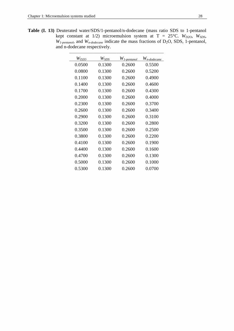
Chapter 1: Microemulsion systems studied 28
Table (I. 13) Deuterated water/SDS/1-pentanol/n-dodecane (mass ratio SDS to 1-pentanol kept constant at 1/2) microemulsion system at T = 25°C. WD2O, WSDS, W1-pentanol, and Wn-dodecane indicate the mass fractions of D2O, SDS, 1-pentanol, and n-dodecane respectively.
WD2O WSDS W1-pentanol Wn-dodecane 0.0500 0.1300 0.2600 0.5500 0.0800 0.1300 0.2600 0.5200 0.1100 0.1300 0.2600 0.4900 0.1400 0.1300 0.2600 0.4600 0.1700 0.1300 0.2600 0.4300 0.2000 0.1300 0.2600 0.4000 0.2300 0.1300 0.2600 0.3700 0.2600 0.1300 0.2600 0.3400 0.2900 0.1300 0.2600 0.3100 0.3200 0.1300 0.2600 0.2800 0.3500 0.1300 0.2600 0.2500 0.3800 0.1300 0.2600 0.2200 0.4100 0.1300 0.2600 0.1900 0.4400 0.1300 0.2600 0.1600 0.4700 0.1300 0.2600 0.1300 0.5000 0.1300 0.2600 0.1000 0.5300 0.1300 0.2600 0.0700
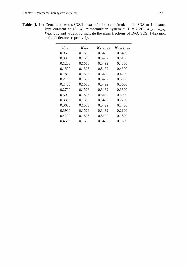
Chapter 1: Microemulsion systems studied 29
Table (I. 14) Deuterated water/SDS/1-hexanol/n-dodecane (molar ratio SDS to 1-hexanol kept constant at 1/6.54) microemulsion system at T = 25°C. WD2O, WSDS, W1-hexanol, and Wn-dodecane indicate the mass fractions of D2O, SDS, 1-hexanol, and n-dodecane respectively.
WD2O WSDS W1-hexanol Wn-dodecane 0.0600 0.1508 0.3492 0.5400 0.0900 0.1508 0.3492 0.5100 0.1200 0.1508 0.3492 0.4800 0.1500 0.1508 0.3492 0.4500 0.1800 0.1508 0.3492 0.4200 0.2100 0.1508 0.3492 0.3900 0.2400 0.1508 0.3492 0.3600 0.2700 0.1508 0.3492 0.3300 0.3000 0.1508 0.3492 0.3000 0.3300 0.1508 0.3492 0.2700 0.3600 0.1508 0.3492 0.2400 0.3900 0.1508 0.3492 0.2100 0.4200 0.1508 0.3492 0.1800 0.4500 0.1508 0.3492 0.1500
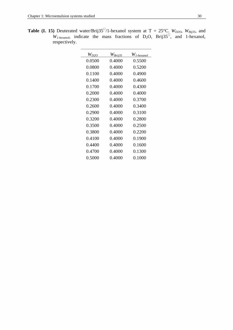
Chapter 1: Microemulsion systems studied 30
Table (I. 15) Deuterated water/Brij35/1-hexanol system at T = 25°C. WD2O, WBij35, and W1-hexanol, indicate the mass fractions of D2O, Brij35, and 1-hexanol, respectively.
WD2O WBrij35 W1-hexanol 0.0500 0.4000 0.5500 0.0800 0.4000 0.5200 0.1100 0.4000 0.4900 0.1400 0.4000 0.4600 0.1700 0.4000 0.4300 0.2000 0.4000 0.4000 0.2300 0.4000 0.3700 0.2600 0.4000 0.3400 0.2900 0.4000 0.3100 0.3200 0.4000 0.2800 0.3500 0.4000 0.2500 0.3800 0.4000 0.2200 0.4100 0.4000 0.1900 0.4400 0.4000 0.1600 0.4700 0.4000 0.1300 0.5000 0.4000 0.1000
Chapter 2: Techniques 31
Chapter 2: Techniques
I. Density measurements Densities of our solutions were obtained with a density measurement device DMA 60/601 HT (Paar). The corresponding measurement cell i s thermostatised with a precision of ± 0.01 K. The density d is calculated from the period t of the measured solution in the vibrating tube as106
( )BtAd −= 2 (II . 1) The instrument parameters A and B are calculated before each measurement by the values t of nitrogen (N2) and Milli pore water. Density of Milli pore water is known from the literature107, that of nitrogen may be calculated from the equation of van der Waals
RTM
d
M
db
M
dap =
−
+ 1
2
2
(II . 2)
where p is the current atmospheric pressure, M is the molar mass of nitrogen, R is the gas constant, and T is the absolute temperature. For nitrogen, the van der Waals coeff icients are a = 0.137 Pa.m6/mol2 and b = 3.87.10-5 m3/mol107.
II. Conductivity measurements Conductivity measurements were done with Consort Ion/EC Meter C733 and C831 using platinium electrodes. The device measures in three conductivity ranges • 0.001 µS/cm to 20 mS/cm. • 0.01 µS/cm to 200 mS/cm. • 0.1 µS/cm to 2000 mS/cm. in the frequency range 60 Hz to 5.8 kHz depending on the conductivity range.
III. Dielectric Relaxation Spectroscopy
III. 1. Maxwell and constitutive equations According to Maxwell’ s phenomenological theory, the macroscopic electromagnetic phenomena can be described by means of f ive vectors:
&E as the electrical field,
&H as the
magnetic field, &D as electric induction (or electric displacement),
&B as magnetic induction,
and &j as current density. For a static field the interactions between the medium and
electromagnetic waves are given by the four Maxwell equations108
rot& & & &
H jt
D= +∂∂
(II. 3)
Chapter 2: Techniques 32
rot& & &
Et
B= −∂∂
(II. 4)
div
&D el= ρ (II. 5)
div
&B = 0 (II. 6)
with constitutive equations available for static or quasistatic cases & &D E= εε0 (II. 7) & &j E= σ (II. 8)
& &B H= µµ0 (II. 9) where ε0 and ε describe the absolute permittivity of a vacuum and the static relative permittivity, respectively; µ and µ0 are the absolute magnetic permeability of the vacuum and the relative permeability, respectively. ρel is defined as the volume density of electrical
charge and σ the (specific) electric conductivity. The electrical field E&
is oscillating with &E0
as the amplitude and ω = 2πν as the angular frequency,
( ) ( )& &E t E t= 0 cos ω (II. 10) For molecular solutions, when measurement frequencies ν are higher 100 MHz the permanent dipole cannot follow the external field without a phase delay, ( )δ ω , between the electrical field and the electric displacement, so that
( ) ( )( )& &D t D t= −0 cos ω δ ω (II. 11) When ( )
&D t is developed, one obtains
( ) ( )( ) ( ) ( )( ) ( )& & &D t D t t D t t= +0 0cos cos sin sinδ ω δ ω (II. 12) and with
( )( ) ( )& &D E0 0 0cos δ ω ε ω ε= ′ (II. 13)
( )( ) ( )& &D E0 0 0sin δ ω ε ω ε= ′′ (II. 14) the resulting formula introduces the dielectric displacement
( ) ( ) ( ) ( ) ( )& & &D t E t E t0 0 0 0 0= ′ + ′′ε ω ε ω ε ω ε ωcos sin (II. 15) In this way, a direct relation between ( )
&D t and ( )
&E t is written with ′ε and ′′ε replacing the
amplitude &D0 and the phase delay ( )tan /δ ε ε= ′′ ′ . The dielectric displacement separates into:
Chapter 2: Techniques 33
a dispersive part ( ) ( )′ε ω ε ω0 0
&E tcos in phase with ( )
&E t0 ( ′ε is the frequency-dependent
permittivity), and a dissipative part ( ) ( )′′ε ω ε ω0 0
&E tsin with phase delay of π / 2 with respect
to ( )&E t0 . ′′ε is proportional to the dissipative energy and is called the dielectric loss or
dielectric absorption. For non-conductive systems, the frequency-dependent absorption energy vs. time and volume units is
( ) ( )( )ωδωεωεω∂
∂sin
22 00200 DEE
t
WW =′′== (II . 16)
In order to facilit ate the manipulation of periodic vectorial quantities ( )
&E t and ( )
&D t , both
are interpreted in terms of complex equations
( ) ( ) ( ) [ ]tiEtEitEtE ωωω expsincosˆ000
&&&&=+= (II . 17)
( ) ( ) ( ) ( )[ ]δωδωδω −=−+−= tiDtDitDtD expsincosˆ000
&&&& (II. 18)
In this way, the relation between the complex quantities E&
and D&
introduce the complex dielectric permittivity ( )ε ω
( ) ( ) ( )& &
D t E t= ε ω ε0 (II. 19)
Inserting equation (II. 17) into equation (II. 19) and comparing the resulting equation with the relation (II. 15) gives the complex dielectric permittivity
( ) ( ) ( )ε ω ε ω ε ω= ′ − ′′i (II. 20) Therefore, equation (II. 7) is generalized in the form of equation (II. 19) for dissipative systems. Equations (II. 8) and (II. 9) can be also be re-written in a complex form as it follows
( ) ( )& & j t E= σ ω (II. 21)
( ) ( ) ( )& &
B t H t= µ ω µ0 (II. 22)
with the complex conductivity
( ) ( ) ( )σ ω σ ω σ ω= ′ − ′′i (II. 23) and the complex relative magnetic permittivity
( ) ( ) ( )µ ω µ ω µ ω= ′ − ′′i (II. 24)
III. 2. Wave equations Equation (II. 3) may be written with help of equations (II. 19) and (II. 21) for harmonic oscillating fields ( ) [ ]
& &E t E i t= 0 exp ω and ( ) [ ]
& &H t H i t= 0 exp ω
Chapter 2: Techniques 34
( ) ( )( )rot
& & &H i E0 0 0= + σ ω ωε ω ε (II. 25)
and equation (II. 4) in combination with equation (II. 22) gives
( )rot& & &
E i H0 0 0= − ωµ ω µ (II. 26) Considering the rotation of equation (II. 25), the equation (II. 26) and the Lengendre vectorial identity, one obtains rot . rot grad . div& & & & & &
H H HO O= − ∇ 0 (II. 27) and reach with the Maxwell equation (II. 6) a reduced form of the wave equation ∇ + =2
02
0 0& &
H Hκ (II. 28) with complex wavenumber, κ . For dissipative media of relative permittivity ( )ε ω and specific conductivity ( )σ ω the propagation of a monochromatic wave of frequency ν is
characterized by the complex propagation coefficient k
( ) ( ) ( ) ( )
+=
0
20
2 ˆˆˆˆˆ
ωεωκωµωεωµ
ikk (II. 29)
In equation (II. 29), k0 is the propagation coefficient of the vacuum, defined as
0000
2
λπµεω ==k (II. 30)
c00 0
1=
ε µ (II. 31)
The parameter c0 is the speed of the light in the vacuum, and λ0 is the length of a monochromatic wave in vacuum. For a source-free medium (where div
&E = 0) , it is possible to
obtain a reduced wave equation for &E as
∇ + =20
20 0
& &E E
κ (II. 32) Equation (II. 29) is simplified in the case of non-magnetizable substances (so µ = 1) to
( ) ( ) ( )ωηωε
ωσωε ˆˆ
ˆˆ 20
0
20
2 ki
kk ≡
+= (II. 33)
with the generalized complex permittivity η η η= ′ − ′′i 109 with real part
Chapter 2: Techniques 35
( ) ( ) ( )′ = ′ −
′′η ω ε ω
σ ωωε0
(II. 34)
and imaginary part
( ) ( ) ( )0ωε
ωσωεωη′
+′′=′′ (II. 35)
In the last equations, the consequence of the Maxwell equations is that separate measurements of dielectric properties and effects based on the conductivity of the system are impossible. The theory form Debye and Falkenhagen110 for electrolyte solutions says that a dispersion of conductivity happens. On the other hand an indication exists that this is weak in comparison to experimental precision of ( )η ω in the microwave range111. So that generally, for simple electrolyte solutions, one obtains
( )′ =σ ω σ (II. 36)
( )′′ =σ ω 0 (II. 37) The neglecting of the dispersion arising from the conductivity leads then to the new definition of the real and imaginary parts of the frequency-dependant relative permittivity as
( ) ( )′ = ′ε ω η ω (II. 38)
( ) ( )0ωε
σωηωε −′′=′′ (II. 39)
From the experimental results giving ′η , ′′η , and σ the calculation of ′ε and ′′ε can then
be done. For each spectrum, the experimentally accessible ( )νη ′′ was corrected for the Ohmic loss according to equation (II. 39).
III. 3. Dielectric relaxation
III. 3. 1. Polarization Dielectric relaxation experiments in the microwave range gives insight in dynamical processes with characteristic times of pico-seconds to nano-seconds. These experiments are a tool for the study of fast processes in solution112. The observable quantity is the polarization &P (or electric moment per volume unit) of the system arising from the application of an
electric field &E which induces a displacement current.
&P is defined in its macroscopic form as
( )& &
P Eo= −ε ε 1 (II. 40)
Chapter 2: Techniques 36
The polarization &P t( ) commonly is split i nto
&P tα ( ) caused by the intramolecular
polarizabilit y and a &P tµ ( ) arising from permanent dipole moment and incorporating intra- and
intermolecular contributions; hence the microscopic form of &P is
& & & P P P= +µ α (II . 41)
It is then possible with equations (II . 40) and (II . 41) to link a measurable macroscopic effect with a molecular interpretation113:
( )ε ε µ α0 1 − = +& & &E P P (II . 42)
For simple liquids where intermolecular interactions are governed by dipole-dipole forces, &Pµ originates from the reorientation of the molecular dipole moments
&µk (with density ρk of
species k) by the external field in the form & &P k
kkµ ρ µ= ∑ (II . 43)
where&µk is the ensemble average of the permanent dipole moment of species k. The
induced polarization, &P tα ( ) , is defined by the polarizabilit y αk and the internal field ( )&
Ei kof
the components
( )& &P Ek kk
i kα ρ α= ∑ (II . 44)
The induced polarization is caused by the molecular polarizabilit y, i.e. the displacement of the electrons against the atomic nucleus (electron polarization) and also the displacement of the nuclei against themselves (atomic polarization). For solutions with a defined molecular mass, the orientational polarization is observable in the time scale of pico- to nanoseconds (Mega- to Terahertz). Kinetic processes may also contribute in more complex systems such as hydrogen-bonding liquids or electrolyte solutions. The response of the induced polarization is located at higher frequencies and the resonance processes implicated may be found in the IR and UV regions114. Between the sample and the electrical field, the following relations hold:
( )& &
P Eµ ε ε ε= − ∞0 (II . 45)
( )& & P Eα ε ε= −∞0 1 (II . 46)
In the time scale covering the mega-hertz to the giga-hertz range, &Pµ cannot follow without
delay the changes of the applied field &E . On the other hand, the induced polarization
&Pα still
reaches its equili brium value which is characterized by the “infinite frequency permittivity”
Chapter 2: Techniques 37
ε∞ , thus permitting the extraction of the dipole contribution &Pµ from the total polarization
&P and hence the deduction of structural information related to the interacting dipoles. III. 3. 2. Response functions of the orientational polarization For an isotropic linear dielectric exposed to a jump in the applied field strength at time
t0 0= , the time-dependent polarization &
( )P tµ can be represented by the equilibrium values
corresponding to the field at t t≤ 0 , ( )&Pµ 0 , and at t t> 0 , ( )
&Pµ ∞ , and by the step response
function ( )F tPor which controls the relaxation of the system to
&Pµ
∞ after the field jump.
( ) ( ) ( )& & P t P F tP
orµ µ= ⋅0 , ( )FP
or 0 1= , ( )FPor ∞ = 0 (II. 47)
with ( )F tP
or defined as
( )( ) ( )
( ) ( )F t
P t P
P PPor =
⋅
⋅
& &
& &µ µ
µ µ
0
0 0 (II. 48)
In equation (II. 48) the products ( ) ( )0µµ PtP&&
⋅ and ( ) ( )00 µµ PP&&
⋅ are ensemble average.
For a polarization decay following a first order law the step response function ( )F tP
or is determined by a single relaxation time τ .
( ) ( )F t tPor = −exp / τ (II. 49)
Usually the observed relaxation behavior of a sample is more complex and requires for its description either the superposition of exponentials with individual time constant τ i for n discernible relaxation processes or a continuous relaxation time distribution. For monochromatic harmonic fields ( ) ( )
& &E t E i t= 0 exp ω of angular frequency ω πν= 2 the
frequency dependence of the oriental polarization ( )&;P tµ ω is given by the Laplace transform
Liω of the pulse response function f Por , which is the negative time derivative of the step
response function:
( ) ( ) ( )[ ] ( )& & ; P t L f t E ti P
orµ ωω ε ε ε= − ′∞0 (II. 50)
with
( )( )f
F t t
t tPor P
or
= −− ′
− ′
∂∂
(II. 51)
Chapter 2: Techniques 38
( )[ ] ( ) ( )L f t i t f t dti Por
Por
ω ω′ = ′ ′ ′∞
∫ exp0
(II. 52)
and where the pulse response function is normalized as
( )f t dtPor
0
1∞
∫ ′ ′ = (II. 53)
Equation (II. 50) is conveniently expressed with the help of the complex permittivity
( ) ( ) ( ) ( ) ( )[ ]ε ω ε ω ε ω ε ε ε ω= ′ − ′′ = + − ′∞ ∞i L f ti Por (II. 54)
which is calculable from the attenuation and the phase shift of the electromagnetic wave in the sample. Equations (II. 51) to (II. 54) are used for both time domain and frequency domain.
III. 3. 3. Empirical equations for the description of dielectric relaxation
One finds in the literature equations which give a macroscopic description of the complex dielectric permittivity. The well-known Debye equation115, in which the dispersion curve is point-symmetric ( ( ) ( )( )′ =ε ω ωf ln ) and the absorption curve ( ( ) ( )( )′′ =ε ω ωf ln ) reaches a maximum at ω τ= 1 / ,
( )ε ω εε ε
ω= +
−+∞
∞
1 i t (II. 55)
with real and imaginary parts
( )′ = +−
+∞∞ε ω ε
ε εω τ1 2 2 (II. 56)
( ) ( )′′ =
−+
∞ε ωε ε ωτ
ω τ1 2 2 (II. 57)
which is generally followed by many liquids at room temperature if only data in a limited frequency range (typically 1 40≤ ≤ν / GHz ) are available. Extension of the accessible spectral range, especially to higher frequencies, and/or increased accuracy of the measurements always reveals systematic deviations from equations (II. 55) to (II. 57). Sometimes it may be necessary to use empirical relaxation-time distribution functions such as the Cole-Cole116, 117 (0 ≤ αj < 1; βj = 1; with a flatter dispersion curve and a flatter and broader absorption curve) or the Cole-Davidson118, 119 (αj = 0; 0 < βj ≤ 1; with dispersion and absorption curves both asymmetric) equations based on the Havriliak-Negami equation120:
Chapter 2: Techniques 39
( )( )( )βαωτ
εεεωε−
∞∞
+
−+=
11ˆ
i (II . 58)
Usually, the complex permittivity spectrum is spitted into n separate processes, equation (II . 58) is modified as
( ) ( )( )( ) jj
j
jn
j i
gβαωτ
εεεωε−
=∞∞
+−+= ∑
11 1
ˆ (II . 59)
Each process (j=1...n) contributes with relaxation time τj and weight
g j
j j=−−
∞
∞
ε εε ε
(II . 60)
ε εj j∞ += 1 (II . 61)
to the total dispersion ranging from the static permittivity ε ε= 1 to ε εν∞ →∞= ′lim . Other
fitting models are available in the literature and are for example extensively reviewed in ref. (121). The fits or the experimental data seems always possible with the semi-empirical approach of equations (II . 59) to (II . 61), provided that vibrational and inertial contributions to the spectra are negligible, i.e. for frequencies ω below 300 to 500 GHz. However, the choice of the “true” relaxation model is not always obvious and strongly depends on the frequency range and accuracy available112. Therefore the attribution of the individual dispersion steps to physical processes and the interpretation of the corresponding parameters ε ε α βj j j
j, , ,∞ and τ j
remains a time consuming task and is essential to validate the relaxation model.
III. 4. Equipment In the present work, the combination of time domain reflectometer (TDR)121, 123 with our transmission line system equipment122 allows the determination of complex permittivity spectra of moderately to highly absorbing liquids in the range 0008 89. /≤ ≤ν GHz with a precision better than 2% relative to the static permittivity of the sample.
III. 4. 1. Waveguide interferometers In the range from 10 GHz to 100 GHz, where the relaxation of most solvents occurs, waveguide equipment, described in figure (II . 1), is required for precise experiments124. For rectangular waveguides commonly used for cell construction and as transmission lines in the microwave region, cross-section a = 2b controls the propagation conditions of the electromagnetic waves125. Transmission line theory shows that in a waveguide fill ed with a dielectric of permittivity ′ε only frequencies higher than the cut-off f requencyνc
mn ,
Chapter 2: Techniques 40
νπ εc
mncmnc
k=′
⋅0
2 ; ( )k
m
a
n
bcmn 2
2 2
=
+
π π; m = 1,2,...; n = 0,1,2,... (II. 62)
are transmitted for the wave mode determined by (m, n). In the range ν ν νc c
10 102≤ < (where m = 1, and n = 0) the only transmittable wave is the so-called TE10-mode defining thus the frequency band commonly used for a given waveguide. The generalized permittivity
( )η ω is the only dielectric material property available from the experiment. For the TE10-mode the relationship
( )′ =
−
+
η ων λ
απ
c p
am
0
2 2 21
2
1
2 (II. 63)
( )′′ =
⋅η ω
να
πλc p
m
02
(II. 64)
are obtained with p = (20log(e)dB/Np)-1 as the conversion factor form decibel to neper. The determination of the attenuation coefficient α and the wavelength of the radiation in the sample λm is possible in one experiment by adjusting an interference minimum at a defined probe position x0, taking the interference curve on both sides over a sufficiently large range an then fitting the interference function
( ) ( ) ( ) ( )A x x A e x x ep x x
m
p x x− = + + − −
⋅
− − − −
0 02
010 1 22
0 0lg cosα απλ
(II. 65)
to the experimental data. In equation (II. 65) A0 is the relative intensity [dB] of the signal passing through the sample beam at position x0
122. Within the rectangular waveguides, the TE10-mode is only transmitted in the limited bandwidth 05 08. .≤ ≤λc , wherevλc is the cut-off wavelength determined by the cross section.
Four Mach-Zender interferomenters are used in our laboratory to cover 85. ≤ ν /GHz ≤ 89. The construction principle of these instruments is described in ref. (122). These interferometers were developed for the X-band (85. ≤ ν /GHz ≤ 12), Ku-band (12 4. ≤ ν /GHz ≤ 18), A-band ( 26 4. ≤ ν /GHz ≤ 40), and E-band ( 60 ≤ ν /GHz ≤ 90) regions and are appropriately adapted for computer control.
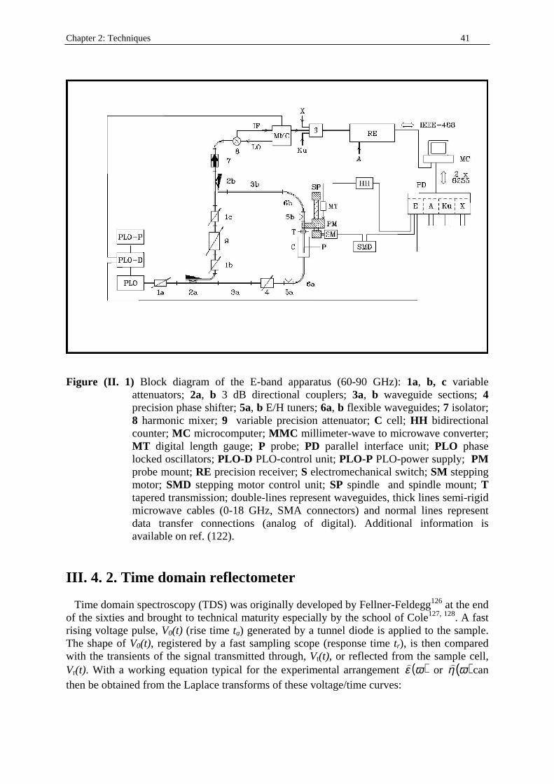
Chapter 2: Techniques 41
Figure (II. 1) Block diagram of the E-band apparatus (60-90 GHz): 1a, b, c variable
attenuators; 2a, b 3 dB directional couplers; 3a, b waveguide sections; 4 precision phase shifter; 5a, b E/H tuners; 6a, b flexible waveguides; 7 isolator; 8 harmonic mixer; 9 variable precision attenuator; C cell; HH bidirectional counter; MC microcomputer; MMC millimeter-wave to microwave converter; MT digital length gauge; P probe; PD parallel interface unit; PLO phase locked oscillators; PLO-D PLO-control unit; PLO-P PLO-power supply; PM probe mount; RE precision receiver; S electromechanical switch; SM stepping motor; SMD stepping motor control unit; SP spindle and spindle mount; T tapered transmission; double-lines represent waveguides, thick lines semi-rigid microwave cables (0-18 GHz, SMA connectors) and normal lines represent data transfer connections (analog of digital). Additional information is available on ref. (122).
III. 4. 2. Time domain reflectometer Time domain spectroscopy (TDS) was originally developed by Fellner-Feldegg126 at the end of the sixties and brought to technical maturity especially by the school of Cole127, 128. A fast rising voltage pulse, V0(t) (rise time ta) generated by a tunnel diode is applied to the sample. The shape of V0(t), registered by a fast sampling scope (response time tr), is then compared with the transients of the signal transmitted through, Vt(t), or reflected from the sample cell, Vr(t). With a working equation typical for the experimental arrangement ( )ε ω or ( )η ω can then be obtained from the Laplace transforms of these voltage/time curves:
Chapter 2: Techniques 42
( ) ( )[ ] ( ) ( )∫∞
==0
exp dttitVtVL jij ωωυ ω ; j=0, r, or t (II. 66)
The theoretical background of TDS is discussed in detail in references (129-131). A major advantage of TDS based on coaxial transmission lines for signal propagation is the large frequency range of several decades which (at least in principle) can be covered by single equipment. Figure (II. 2) shows the arrangement of our laboratory123, which consists of a Tektronik TEK 11802 sampling scope and two SD24 sampling heads of 0.02 ps maximum time resolution. Each SD24 has two independent measuring channels so that four reflection (or two transmission) experiments can be conducted simultaneously. The maximum bandwidth of the instrument 0.0004 ≤ ν / GHz ≤ 20, is determined by the total rise time (ta + tr) = 35 ps, at high
frequencies, and by the repetition rate of the pulse generator (200 kHz, ∆V0 = ( ) ( )V V0 00 − ∞
= 250 mV, ta = 17.5 ps) at low frequencies. The signal reflected from an open-ended transmission line, a so-called cutoff cell, is determined, which yields the total reflection coefficient ( )ρ ν
( ) ( ) ( )( ) ( )
ρ νω
υ ω υ ωυ ω υ ω
= ⋅−+
c
i glr
r
0 0
0
; ω πν= 2 (II. 67)
as the input for the calculation of ( ) ( ) η ν ρ ν⋅ is a function of the Laplace transforms (equation
(II. 66)) of the incoming ( )V t0 and the reflected signal ( )V tr . In equation (II. 67), l is electrical length of the cell. g = Z0/Z is the ratio of the feeding line impedance, Z0, to the impedance of the empty cell, Z; Z0 = 50 Ω. The product gl is the cell constant. For a cutoff cell of ideal geometry and for an ideal feeding line the total reflection coefficient ( )ρ ν is related to the total permittivity of the sample, ( )η ν , by the transcendental equation129, 130
( ) ( ) cotη ν ρ ν= z z ; ( ) ( )z l c= ω η ν/ 0 (II. 68)
and Z is determined by the diameters of inner conductor, d1, and outer conductor, d2, of the cell (µ0: permeability of the vacuum)
Zd
d=
1
20
0
2
1πµε
ln (II. 69)
Details on the cell construction are available in reference (123)
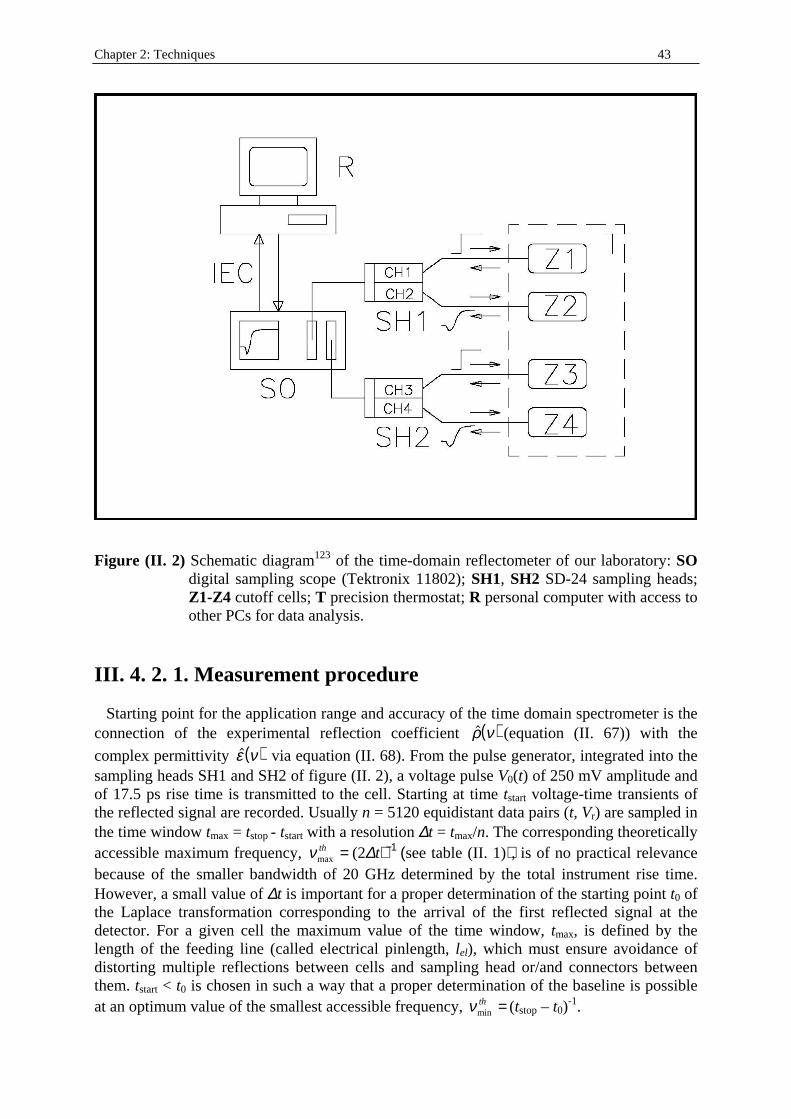
Chapter 2: Techniques 43
Figure (II. 2) Schematic diagram123 of the time-domain reflectometer of our laboratory: SO
digital sampling scope (Tektronix 11802); SH1, SH2 SD-24 sampling heads; Z1-Z4 cutoff cells; T precision thermostat; R personal computer with access to other PCs for data analysis.
III. 4. 2. 1. Measurement procedure Starting point for the application range and accuracy of the time domain spectrometer is the connection of the experimental reflection coeff icient ( )ρ ν (equation (II . 67)) with the
complex permittivity ( )ε ν via equation (II . 68). From the pulse generator, integrated into the sampling heads SH1 and SH2 of f igure (II . 2), a voltage pulse V0(t) of 250 mV amplitude and of 17.5 ps rise time is transmitted to the cell . Starting at time tstart voltage-time transients of the reflected signal are recorded. Usually n = 5120 equidistant data pairs (t, Vr) are sampled in the time window tmax = tstop - tstart with a resolution ∆t = tmax/n. The corresponding theoretically accessible maximum frequency, νmax
th = (2∆t)−1 (see table (II . 1)), is of no practical relevance because of the smaller bandwidth of 20 GHz determined by the total instrument rise time. However, a small value of ∆t is important for a proper determination of the starting point t0 of the Laplace transformation corresponding to the arrival of the first reflected signal at the detector. For a given cell the maximum value of the time window, tmax, is defined by the length of the feeding line (called electrical pinlength, lel), which must ensure avoidance of distorting multiple reflections between cells and sampling head or/and connectors between them. tstart < t0 is chosen in such a way that a proper determination of the baseline is possible at an optimum value of the smallest accessible frequency, νmin
th = (tstop – t0)-1.
Chapter 2: Techniques 44
Following Cole at al.129, we compare the signal reflected from the sample, Vrx(t), with the transient Vrr(t) obtained from the cell filled with a reference of known permittivity, ( )η νr = 1 . Time derivatives are used instead of the proper voltage transients for Laplace transformation. From the relative reflection coefficient ( )ρ νxr obtained in this way,
( )( ) ( )( )
( ) ( )( )
+
−
⋅=tVtV
dt
dL
tVtVdt
dL
gli
c
rxrri
rxrri
elxr
ω
ω
ωνρ 0ˆ (II. 70)
where lel is the electrical pinlength. The combination of equation (III. 70) with equation (II. 68) using the approximation z z Cz⋅ = −cot 1 2 (II. 71) leads to the working equation
( ) ( )( )
η ω
ρρx
xr
xr
Cz
z C g=
− +− +
1 1
102
02 2
; 0
0 c
lz elω
= (II. 72)
is obtained for the generalized complex permittivity ( )η νx of the sample. C = 1/3 for a cutoff cell of ideal geometry. Characteristics of cutoff cells used for DRS measurements of microemulsions and micellar systems are indicated in table (II. 1).
Chapter 2: Techniques 45
Table (II . 1) Cutoff cells used in the present work with following characteristics: mechanical and electrical pinlength lmech and lel. g is the ratio of the feeding line impedance to the impedance of the empty cell . t0 is the starting point of the time window of time increment ∆t.
Cutoff cell lmech / mm lel / mm g t0 / ns ∆t / ps T1 0 ~ 0.35 0.4416 79.2 1.0 T4 2.0 2.637 0.5178 119 10 T9 0.7 1.118 0.4282 95.5 2.1 TX 5.35 5.987 1.0018 172 20
After averaging over 256 single traces of each Vrr(t) and Vrx(t) the transients are available for data processing with a typical precision of < 0.6 mV (corresponding to 0.24% of the ampli tude of V0) and an accuracy of 1-3% depending on t – t0. However, from these data a direct estimation of accuracy and precision of ( )η ν is not possible because in addition to the statistical errors of the voltage measurements systematic deviations of unknown magnitude may contribute which are not easily separated after Laplace transformation. These errors may have different origins (non-ideal feeding line, truncation of the series expansion of z cot z...) and should be corrected empirically.
III . 4. 2. 2. Cell calibration Within the present work appropriate cutoff cells (TX, T9 and T4, see table (II . 1)) for microemulsion measurements had to be calibrated and used together with already calibrated cutoff cell T1 (see table (II . 1)). The adjustment of the effective (or electrical) cell l ength, lel, involves the use of pure liquids as standards for which relaxation model and static permittivity are well known. Those pure liquids of known permittivity were: methanol, ethanol, bi-distill ated water, dimethyl sulfoxide (DMSO). Each component was used either as reference or sample for the cell calibration.
III . 4. 2. 3. Padé calibration During the first microemulsions dielectric measurements a sharp increase in the static permittivity (from εs ∼5 up to ∼35) occurred upon raising water content. This effect, already observed in the literature89, 90, is related to the percolation phenomenon in W/O microemulsions. In this case several references of known permittivity have to be used rendering the work time consuming. An alternative approach was found with the use of the Padé approximation121. The idea of this method is, using empty cutoff cell as reference, to solve the TDR equation for an ideal cutoff cell and then to correct the systematic deviations with help of the complex Pade approximation
( ) ( )[ ] ( ) ( ) ( ) ( )[ ]( ) ( ) ( )[ ]
ε ω ε ω
ω ω ε ω ε ωω ε ω ε ω
corrected n
n
m
mPA A A
B B= =
+ + ⋅⋅ ⋅ ++ + ⋅ ⋅ ⋅ +
0 1
11 (II . 73)
where ( )ε ωcorrected and ( )ε ω are the corrected and non-corrected complex dielectric permittivites, n and m are the polynom degrees. For each frequency the n + m + 1 complex
correction parameters ( )A0 ω ... ( )An ω , and ( )B0 ω ... ( )Bn ω are necessary. These correction

Chapter 2: Techniques 46
parameters must be provided by several dielectric references (for each of them, the empty cutoff cell i s the reference) which TDR misprints ( )ε ωi and corresponding ideal relaxation
models ( )ε ωiideal . The complex correction parameters are calculated with routines already
installed in computer. Pure chemical (1-butanol, 2-propanol, butylene carbonate, DMSO, n-dodecane, ethanol, methyl acetate, methanol, propylene carbonate, and water) and mixtures of pure chemicals (methanol and CCl4 with known dielectric properties132) at 25°C were chosen for measurements references. The Padé approximation was used for all experimental points involving W/O microemulsions.
Chapter 3: Results and discussions 47
Chapter 3: Results and discussions
I. SDS micelles in water
I. 1. SDS monomer self-association The hydrophobic and electrostatic forces arising from the non-polar alkyl chains and the polar or ionic headgroups among ionic surfactant molecules play an essential role for the self-association and formation of micelles. The ability of these aqueous micellar systems to solubilize water-insoluble or sparingly soluble compounds by incorporating the hydrophobic molecules in the aggregated phase constitutes one of the most remarkable properties55, 133-135. This ability forms the basic functionalities of soap solutions and microemulsions26, 42, 136, 137. The free energy of a surfactant self-assembly in dilute solution is assumed to be made up of three terms: • A favorable hydrophobic contribution, due to the hydrocarbon chains sequestering
themselves within the interior of the aggregates. • A surface term that reflects the opposing tendencies of the surfactant head groups to
crowd close together to minimize hydrocarbon-water contacts and to spread apart, as a result of electrostatic repulsion, hydration, and steric hindrance.
• A packing term (see Chapter 1) which, at its simplest level, requires that the hydrophobic
interior of the aggregate to exclude water and head groups, thus limiting the geometrically accessible forms available to the aggregate.
Above the cmc, adding more surfactant simply produces more micelle over a considerable concentration range rather than further growth of existing micelles. SDS micelles in water are well studied systems and data related to their packing term, aggregation number, and surface term are well established in the literature.
I. 2. DRS spectra fitting procedure The best relaxation models that present minimum variance, s2, of the fit and an interpretable set of reliable relaxation parameters as a function of the surfactant concentration were obtained with three different models: • a sum of four Debye (4D model, figures (III. 1) and (III. 2), and table (III. 1)) relaxation
processes
( )ε νπντ
ε=+
+=
∞∑S
ij
jj 1 21
4
(III. 1)
• and with a sum of one Debye, one Cole-Cole, one Debye (DCCD model, figure (III. 3)
and table (III. 1)) relaxation processes as
( )( )
ε νπντ πντ πντ
εα=+
++
++
+− ∞
S
i
S
i
S
i1
1
2
2
13
31 2 1 2 1 2 (III. 2)
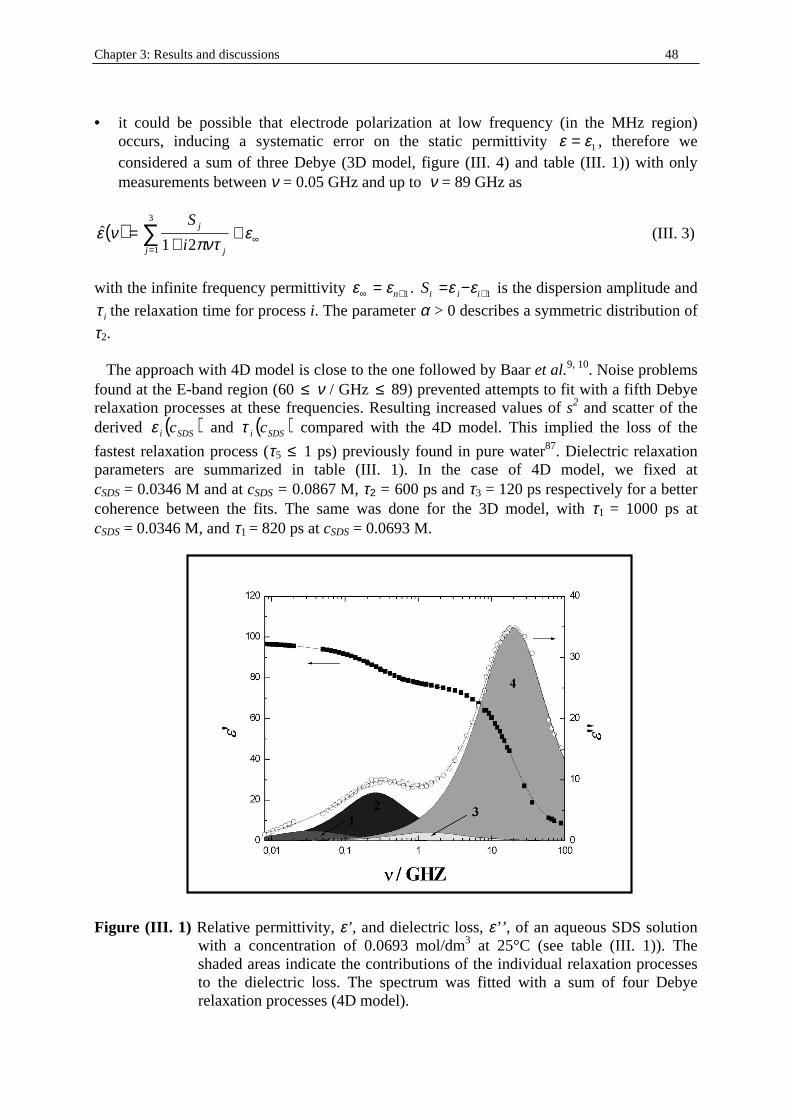
Chapter 3: Results and discussions 48
• it could be possible that electrode polarization at low frequency (in the MHz region)
occurs, inducing a systematic error on the static permittivity ε ε= 1 , therefore we considered a sum of three Debye (3D model, figure (III. 4) and table (III. 1)) with only measurements between ν = 0.05 GHz and up to ν = 89 GHz as
( )ε νπντ
ε=+
+=
∞∑S
ij
jj 1 21
3
(III. 3)
with the infinite frequency permittivity ε ε∞ += n 1 . Si i i= − +ε ε 1 is the dispersion amplitude and
τ i the relaxation time for process i. The parameter α > 0 describes a symmetric distribution of
τ2. The approach with 4D model is close to the one followed by Baar et al.9, 10. Noise problems found at the E-band region (60 ≤ ν / GHz ≤ 89) prevented attempts to fit with a fifth Debye relaxation processes at these frequencies. Resulting increased values of s2 and scatter of the derived ( )SDSi cε and ( )SDSi cτ compared with the 4D model. This implied the loss of the
fastest relaxation process (τ5 ≤ 1 ps) previously found in pure water87. Dielectric relaxation parameters are summarized in table (III. 1). In the case of 4D model, we fixed at cSDS = 0.0346 M and at cSDS = 0.0867 M, τ2 = 600 ps and τ3 = 120 ps respectively for a better coherence between the fits. The same was done for the 3D model, with τ1 = 1000 ps at cSDS = 0.0346 M, and τ1 = 820 ps at cSDS = 0.0693 M.
Figure (III. 1) Relative permittivity, ε’ , and dielectric loss, ε’’ , of an aqueous SDS solution
with a concentration of 0.0693 mol/dm3 at 25°C (see table (III . 1)). The shaded areas indicate the contributions of the individual relaxation processes to the dielectric loss. The spectrum was fitted with a sum of four Debye relaxation processes (4D model).
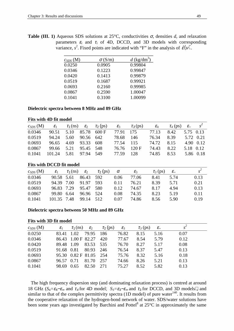
Chapter 3: Results and discussions 49
Table (III. 1) Aqueous SDS solutions at 25°C, conductivities σ, densities d, and relaxation
parameters εi and τi of 4D, DCCD, and 3D models with corresponding variance, s2. Fixed points are indicated with “F” in the analysis of ( )ε ν .
cSDS (M) σ (S/m) d (kg/dm3) 0.0250 0.0905 0.99804 0.0346 0.1223 0.99847 0.0420 0.1413 0.99879 0.0519 0.1687 0.99921 0.0693 0.2160 0.99985 0.0867 0.2590 1.00047 0.1041 0.3100 1.00099
Dielectric spectra between 8 MHz and 89 GHz Fits with 4D fit model cSDS (M) ε1 τ1 (ns) ε2 τ2 (ps) ε3 τ3 (ps) ε4 τ4 (ps) ε s2
0.0346 90.51 5.10 85.78 600 F 77.91 175 77.13 8.42 5.75 0.13 0.0519 94.24 5.60 90.56 642 78.68 146 76.34 8.39 5.72 0.21 0.0693 96.65 4.69 93.33 608 77.54 115 74.72 8.15 4.90 0.12 0.0867 99.66 5.21 95.45 548 76.76 120 F 74.43 8.22 5.18 0.12 0.1041 101.24 5.81 97.94 549 77.59 128 74.85 8.53 5.86 0.18 Fits with DCCD fit model cSDS (M) ε1 τ1 (ns) ε2 τ2 (ps) α ε3 τ3 (ps) ε s2
0.0346 90.58 5.61 86.43 592 0.06 77.06 8.41 5.74 0.13 0.0519 94.39 7.00 91.97 593 0.11 76.21 8.39 5.71 0.21 0.0693 96.83 7.29 95.47 580 0.12 74.67 8.17 4.94 0.13 0.0867 99.80 6.64 96.96 524 0.08 74.35 8.23 5.19 0.11 0.1041 101.35 7.48 99.14 512 0.07 74.86 8.56 5.90 0.19 Dielectric spectra between 50 MHz and 89 GHz Fits with 3D fit model cSDS (M) ε1 τ1 (ns) ε2 τ2 (ps) ε3 τ3 (ps) ε s2
0.0250 83.41 1.02 79.95 186 76.82 8.15 5.16 0.07 0.0346 86.43 1.00 F 82.27 420 77.67 8.54 5.79 0.12 0.0420 89.48 1.09 83.53 535 76.70 8.27 5.17 0.08 0.0519 91.68 0.81 80.93 246 76.54 8.37 5.47 0.13 0.0693 95.30 0.82 F 81.05 254 75.76 8.32 5.16 0.18 0.0867 96.57 0.71 81.70 257 74.66 8.26 5.21 0.13 0.1041 98.69 0.65 82.50 271 75.27 8.52 5.82 0.13
The high frequency dispersion step (and dominating relaxation process) is centred at around 18 GHz (S4=ε4−ε∞ and τ4 for 4D model; S3=ε3−ε∞ and τ3 for DCCD, and 3D models), and similar to that of the complex permittivity spectra (1D model) of pure water140. It results from the cooperative relaxation of the hydrogen-bond network of water. SDS/water solutions have been some years ago investigated by Barchini and Pottel8 at 25°C in approximately the same
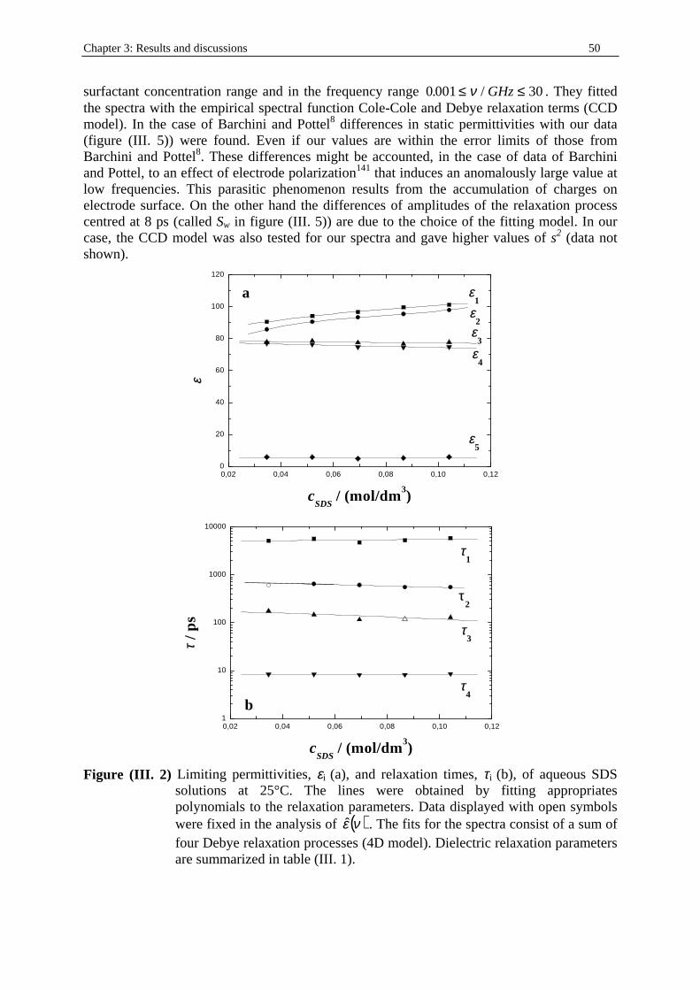
Chapter 3: Results and discussions 50
surfactant concentration range and in the frequency range 0001 30. /≤ ≤ν GHz . They fitted the spectra with the empirical spectral function Cole-Cole and Debye relaxation terms (CCD model). In the case of Barchini and Pottel8 differences in static permittivities with our data (figure (III . 5)) were found. Even if our values are within the error limits of those from Barchini and Pottel8. These differences might be accounted, in the case of data of Barchini and Pottel, to an effect of electrode polarization141 that induces an anomalously large value at low frequencies. This parasitic phenomenon results from the accumulation of charges on electrode surface. On the other hand the differences of amplitudes of the relaxation process centred at 8 ps (called Sw in figure (III . 5)) are due to the choice of the fitting model. In our case, the CCD model was also tested for our spectra and gave higher values of s2 (data not shown).
0,02 0,04 0,06 0,08 0,10 0,120
20
40
60
80
100
120
a
εε5
εε4
εε3
εε2
εε1
εε
cSDS
/ (mol/dm3)
0,02 0,04 0,06 0,08 0,10 0,121
10
100
1000
10000
b
ττ4
ττ3
ττ2
ττ1
ττ / p
s
cSDS
/ (mol/dm3)
Figure (III. 2) Limiting permittivities, εi (a), and relaxation times, τi (b), of aqueous SDS solutions at 25°C. The lines were obtained by fitting appropriates polynomials to the relaxation parameters. Data displayed with open symbols were fixed in the analysis of ( )νε . The fits for the spectra consist of a sum of four Debye relaxation processes (4D model). Dielectric relaxation parameters are summarized in table (III . 1).
Chapter 3: Results and discussions 51
0,02 0,04 0,06 0,08 0,10 0,120
20
40
60
80
100
120
a
εε4
εε3
εε2
εε1
εε
cSDS
/ (mol/dm3)
0,02 0,04 0,06 0,08 0,10 0,121
10
100
1000
10000
b
ττ3
ττ2
ττ1
ττ / p
s
cSDS
/ (mol/dm3)
Figure (III. 3) Limiting permittivities, εi (a), and relaxation times, τi (b), of aqueous SDS solutions at 25°C. The lines were obtained by fitting appropriates polynomials to the relaxation parameters. The fits for the spectra consist of a sum of Debye, Cole-Cole, Debye relaxation processes (DCCD model). Dielectric relaxation parameters are summarized in table (III . 1).
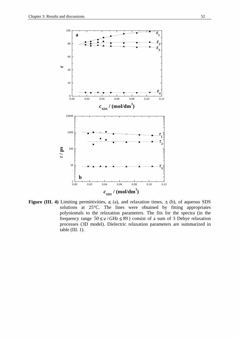
Chapter 3: Results and discussions 52
0,00 0,02 0,04 0,06 0,08 0,10 0,120
20
40
60
80
100
a
εε4
εε3
εε2
εε1
εε
cSDS
/ (mol/dm3)
0,00 0,02 0,04 0,06 0,08 0,10 0,121
10
100
1000
10000
b
ττ3
ττ2
ττ1
cSDS
/ (mol/dm3)
ττ / p
s
Figure (III. 4) Limiting permittivities, εi (a), and relaxation times, τi (b), of aqueous SDS
solutions at 25°C. The lines were obtained by fitting appropriates polyniomals to the relaxation parameters. The fits for the spectra (in the frequency range 89/50 ≤≤ GHzν ) consist of a sum of 3 Debye relaxation processes (3D model). Dielectric relaxation parameters are summarized in table (III . 1).
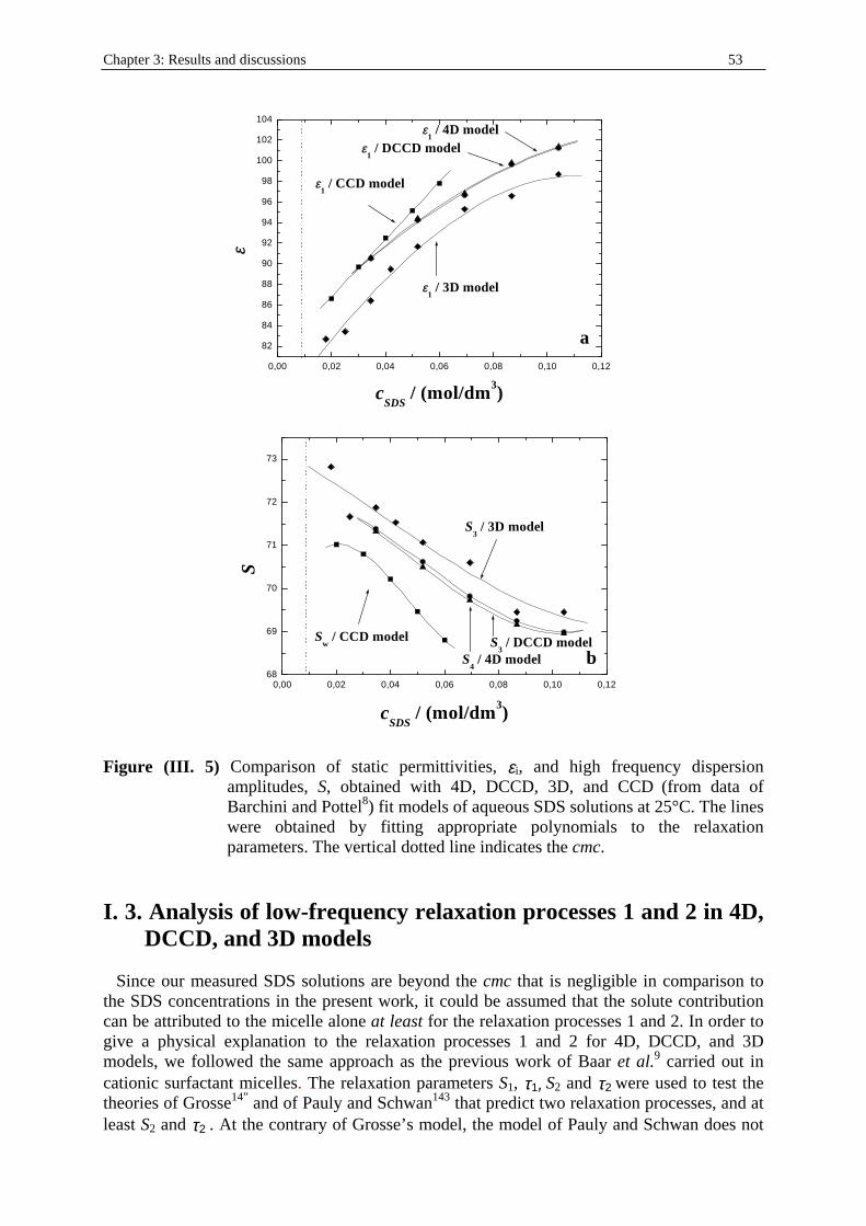
Chapter 3: Results and discussions 53
0,00 0,02 0,04 0,06 0,08 0,10 0,12
82
84
86
88
90
92
94
96
98
100
102
104
εε1 / 3D model
εε1 / DCCD model
εε1 / 4D model
εε1 / CCD model
a
εε
cSDS
/ (mol/dm3)
0,00 0,02 0,04 0,06 0,08 0,10 0,1268
69
70
71
72
73
S3 / 3D model
S3 / DCCD modelS
w / CCD model
S4 / 4D model b
S
cSDS
/ (mol/dm3)
Figure (III. 5) Comparison of static permittivities, εi, and high frequency dispersion amplitudes, S, obtained with 4D, DCCD, 3D, and CCD (from data of Barchini and Pottel8) fit models of aqueous SDS solutions at 25°C. The lines were obtained by fitting appropriate polynomials to the relaxation parameters. The vertical dotted line indicates the cmc.
I. 3. Analysis of low-frequency relaxation processes 1 and 2 in 4D, DCCD, and 3D models
Since our measured SDS solutions are beyond the cmc that is negligible in comparison to the SDS concentrations in the present work, it could be assumed that the solute contribution can be attributed to the micelle alone at least for the relaxation processes 1 and 2. In order to give a physical explanation to the relaxation processes 1 and 2 for 4D, DCCD, and 3D models, we followed the same approach as the previous work of Baar et al.9 carried out in cationic surfactant micelles. The relaxation parameters S1, τ1, S2 and τ2 were used to test the theories of Grosse14” and of Pauly and Schwan143 that predict two relaxation processes, and at least S2 and τ2 . At the contrary of Grosse’s model, the model of Pauly and Schwan does not
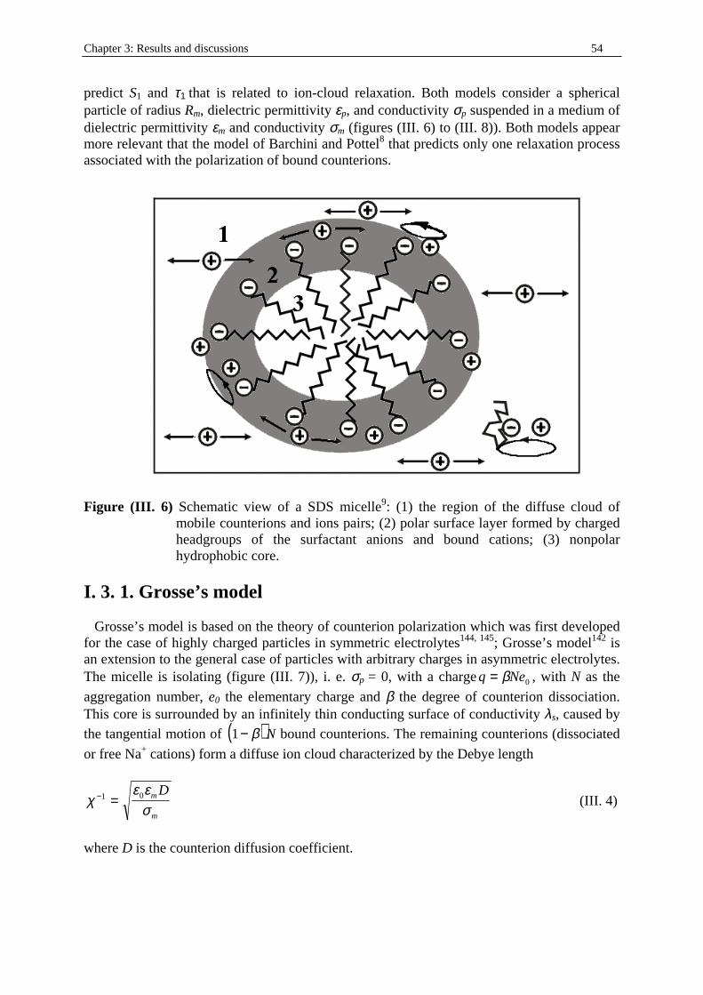
Chapter 3: Results and discussions 54
predict S1 and τ1 that is related to ion-cloud relaxation. Both models consider a spherical particle of radius Rm, dielectric permittivity εp, and conductivity σp suspended in a medium of dielectric permittivity εm and conductivity σm (figures (III . 6) to (III . 8)). Both models appear more relevant that the model of Barchini and Pottel8 that predicts only one relaxation process associated with the polarization of bound counterions.
Figure (III . 6) Schematic view of a SDS micelle9: (1) the region of the diffuse cloud of mobile counterions and ions pairs; (2) polar surface layer formed by charged headgroups of the surfactant anions and bound cations; (3) nonpolar hydrophobic core.
I . 3. 1. Grosse’s model Grosse’s model is based on the theory of counterion polarization which was first developed for the case of highly charged particles in symmetric electrolytes144, 145; Grosse’s model142 is an extension to the general case of particles with arbitrary charges in asymmetric electrolytes. The micelle is isolating (figure (III . 7)), i. e. σp = 0, with a chargeq Ne= β 0 , with N as the
aggregation number, e0 the elementary charge and β the degree of counterion dissociation. This core is surrounded by an infinitely thin conducting surface of conductivity λs, caused by the tangential motion of ( )1− β N bound counterions. The remaining counterions (dissociated
or free Na+ cations) form a diffuse ion cloud characterized by the Debye length
χε ε
σ− =1 0 m
m
D (III . 4)
where D is the counterion diffusion coeff icient.
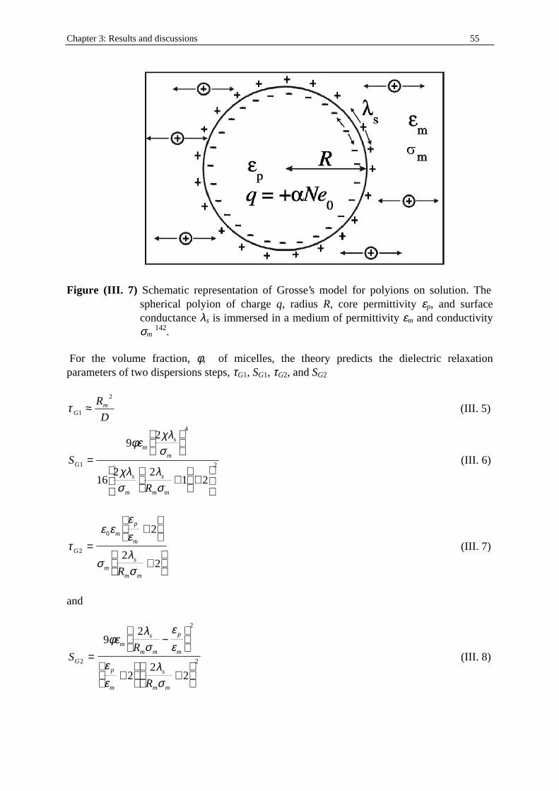
Chapter 3: Results and discussions 55
Figure (III. 7) Schematic representation of Grosse’s model for polyions on solution. The spherical polyion of charge q, radius R, core permittivity εp, and surface conductance λs is immersed in a medium of permittivity εm and conductivity σm 142.
For the volume fraction, φ, of micelles, the theory predicts the dielectric relaxation parameters of two dispersions steps, τG1, SG1, τG2, and SG2
D
RmG
2
1 ≈τ (III. 5)
S
R
G
ms
m
s
m
s
m m
1
4
2
92
162 2
1 2
=
+
+
φεχλσ
χλσ
λσ
(III. 6)
τε ε
εε
σλσ
G
m
p
m
ms
m mR
2
0 2
22
=+
+
(III. 7)
and
SR
R
G
ms
m m
p
m
p
m
s
m m
2
2
2
92
22
2
=−
+
+
φελσ
εε
εε
λσ
(III. 8)
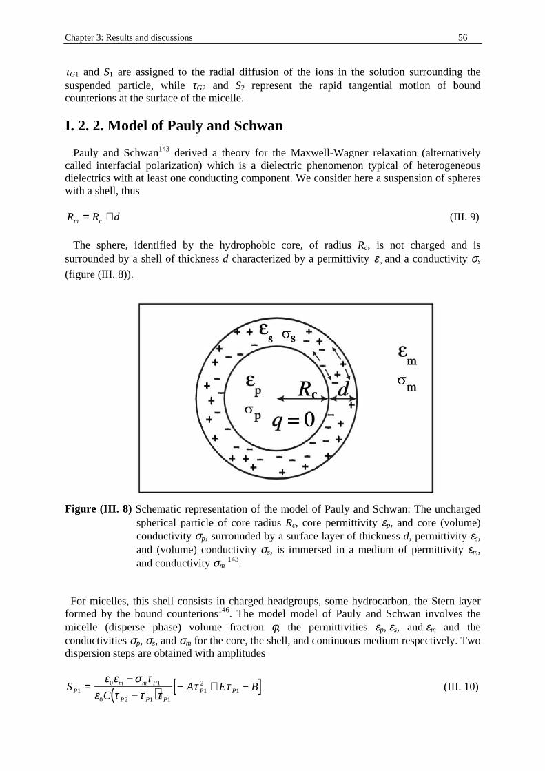
Chapter 3: Results and discussions 56
τG1 and S1 are assigned to the radial diffusion of the ions in the solution surrounding the suspended particle, while τG2 and S2 represent the rapid tangential motion of bound counterions at the surface of the micelle.
I. 2. 2. Model of Pauly and Schwan Pauly and Schwan143 derived a theory for the Maxwell-Wagner relaxation (alternatively called interfacial polarization) which is a dielectric phenomenon typical of heterogeneous dielectrics with at least one conducting component. We consider here a suspension of spheres with a shell, thus
dRR cm += (III. 9)
The sphere, identified by the hydrophobic core, of radius Rc, is not charged and is surrounded by a shell of thickness d characterized by a permittivity sε and a conductivity σs
(figure (III. 8)).
c
Figure (III. 8) Schematic representation of the model of Pauly and Schwan: The uncharged
spherical particle of core radius Rc, core permittivity εp, and core (volume) conductivity σp, surrounded by a surface layer of thickness d, permittivity εs, and (volume) conductivity σs, is immersed in a medium of permittivity εm, and conductivity σm 143.
For micelles, this shell consists in charged headgroups, some hydrocarbon, the Stern layer formed by the bound counterions146. The model model of Pauly and Schwan involves the micelle (disperse phase) volume fraction φ, the permittivities εp, εs, and εm and the conductivities σp, σs, and σm for the core, the shell, and continuous medium respectively. Two dispersion steps are obtained with amplitudes
( ) [ ]SC
A E BPm m P
P P PP P1
0 1
0 2 1 11
21=
−−
− + −ε ε σ τ
ε τ τ ττ τ (III. 10)
Chapter 3: Results and discussions 57
( ) [ ]SC
A E BPm m P
P P P
P P20 2
0 2 1 2
22
2=−−
− +ε ε σ τ
ε τ τ ττ τ (III. 11)
and relaxation times
−−=
21
411
2 F
DC
C
FPτ (III. 12)
−+=
22
411
2 F
DC
C
FPτ (III. 13)
with
( ) ( )A a bs m= + + −1 2 2 1φ σ φ σ (III. 14)
( ) ( ) 12
02
01221 dcB ms εεφεεφ −++= (III. 15)
( ) ( )C a bs m= − + +1 2φ σ φ σ (III. 16)
( ) ( ) 1
20
20 21 dcD ms εεφεεφ ++−= (III. 17)
( )( ) ( )( )E a c b ds s m m= + + + − +1 2 2 10 0 0 0 1φ ε ε ε σ φ ε ε ε σ (III. 18)
( )( ) ( )( )F a c b ds s m m= − + + + +1 20 0 0 0 1φ ε ε ε σ φ ε ε ε σ (III. 19)
( ) ( )a p s= + + −1 2 2 1υ σ υ σ (III. 20)
( ) ( )b p s= − + +1 2υ σ υ σ (III. 21)
( ) ( ) spc ευευ −++= 1221 (III. 22)
( ) ( ) spd ευευ ++−= 211 (III. 23)
3
+
=dR
R
c
cυ (III. 24)
For both models of Grosse and Pauly and Schwan, the volume fraction of micelle is
−
=N
cmccNR SDS
Am3
3
4 πφ (III. 25)
with N as micelle aggregation number and NA as Avogadro’s number.
Chapter 3: Results and discussions 58
I. 3. 3. Choice of the input parameters In our surfactant concentration range SDS micelles grow up slowly as function of the detergent concentration, as suggested by small angle neutron scattering experiments147, 148. The variations of N with cSDS may be represented as149
71.6147.17 += SDScN (III . 26)
Bezzotov et al.148 found that SDS micelles grow proportional to (cs)
1/4. This was confirmed later with time-resolved fluorescence quenching (TRFQ)150 and electron paramagnetic resonance (EPR)151 measurements. An explicit expression of the growth of SDS micelles was developed by Quina et al.152. Incorporating ( )1− β the degree of counterion attachment to the
micelle (equal to 0.73 from the cmc and up to 0.08 mol/dm3) found with activity measurements153, and the concentration of free SDS monomers, cmon, N can be written as
25.0
0081.0
73.027.02.49
+
= monSDS ccN (III . 27)
cmon is given by iteration of the relation
( ) ( )( ) ( )( )monmonSDSmon ccccmcc +−−= 27.0log73.0log73.1log (III . 28)
Equation (III . 28) involves that the monomer concentration decreases upon increasing cSDS. On the other hand cmon is so small i n comparison with cs that it can be considered as equal to the cmc154. Results of equations (III . 26) to (III . 28) are indicated in table (III . 2). An experimental evidence of SDS monomers below the cmc has been given by NMR155 spectroscopy studies that revealed a decrease of cmon upon increasing cs, in agreement with calculations of cmon with equation (III . 27). Table (III. 2) Calculated surfactant monomer concentration, cmon, and micelle aggregation
number, N, for aqueous SDS solutions at 25°C above the cmc.
cSDS (M) cmon (M) (eq. (III . 28)) Ν (eq. (III . 27)) N (eq. (III . 26))
0.0250 0.0063 53.5 62 0.0346 0.0056 55.8 62.3 0.0420 0.0051 58.2 62.4 0.0519 0.0046 59.6 62.6 0.0693 0.0040 62.9 62.9 0.0867 0.0035 65.8 63.2 0.1041 0.0030 68.4 63.5
Equations (III . 26) and (III . 27) give values of N well comparable with those found by Lianos and Zana156 (about approximately 63 in the same surfactant concentration range) and by Cabane et al.157 (about 70), but are lower than those proposed by Hayter and Penford147 (about 80). This difference may be explained by the bending103 of hydrocarbon chains of the surfactant molecules, involving a reduction of N, and not considered by the latter authors. For this reason SDS core radius was chosen equal to 18.4 Å, value from Cabane et al.157 rather than the extended dodecane chain length. SANS measurements revealed that in our
Chapter 3: Results and discussions 59
concentration range, the variation of Rm is only about 1 Å147 and the dispersion in the radii i s about 10%156, therefore the choice of an averaged micelle radius for all cSDS appeared as a reasonable assumption. The variation of the aggregation number whereas the micelle radius remains more or less constant would suggest structural changes of the SDS hydrophobic tails within the micellar core. This point is diff icult to verify since the lack of literature data about the variation of the micelle radius within our SDS concentration range. In order to yield the hydrodynamic micelle radius, we added to Rc two different values of d: a sum of diameters of Na+ and SO4
2- ions, with (corresponding to double solvent separated ion pair, 2SIP) and without (corresponding to a contact ion pair, CIP) the diameters of 2 water molecules i. e. 12.82 Å and 7.12 Å respectively (see part I. 3. 1. of this chapter). It has also been considered an adjustable Rm during the fitting procedure. The conductivity of the medium σm is equivalent to the experimental conductivity of the solutions (table (III . 1)). Due to the low concentrations of Na+ in the aqueous phase, it was reasonable to postulate that the the permittivity εm of the medium is the permittivity of pure water at 25°C140. The diffusion coeff icient ∞
+=Na
DD of sodium ion107 in water was inserted. As for pure hydrocarbon,
dielectric constant of the micellar core was chosen as 2=pε . In the absence of literature data,
the surface conductivity λs (which reflects the amount and mobilit y of bound counterions) was adjusted. Taking into account all these input parameters, Grosse’s model was applied fitting simultaneously τ1, τ2, S1, and S2. The model of Pauly and Schwan implied input parameters εp, εm, and σm identical to those from Grosse’s model. Note that the permittivity of the shell , εs = 46 is provided by different solvatochromic acid-base indicators158. Adjustable parameters are the thickness of the shell , d, and its conductivity, σs. The same fitting procedures as employed for Grosse’s model, in terms of f ixed micelle radii were done.
I. 3. 4. Results and discussion As indicated by figure (III . 8) and table (III . 3), Grosse’s model was able to describe the low-frequency dielectric relaxation processes 1 and 2. The model gave the best results (fits 1 and 2 in table (III . 3), and figure (III . 8)) when applied to 4D model and a micelle radius of 26.5 Å, approximately 1 to 3 Å higher than radii obtained from SANS measurements in the same surfactant concentration range and at 25°C147, 157. Better compatibilit y was found with DCCD model (Rm = 24.9 Å). But higher variance s2 values of the Grosse’s model were obtained with smaller or higher values of Rm for 4D model; additionally, s2 values are systematically higher for DCCD and 3D models. Therefore, the 4D model appears as the most reasonable DRS model. Differences between SANS and DRS data may be explained as follows. DRS in combination with the model of Grosse allows the detection of the counterion cloud around the micelle, giving an apparent Rm higher than the values found by SANS. In agreement with the results of Baar et al.9 no deviations between experimental and theoretical data occurred at the transition spherical-li ke to rod-like micelles104 (cSDS = 0.07 M) generally expected to lead to an increase of the micelle size and aggregation polydispersity since the incorporation of the surfactant occurs in the cylindrical part of the micelle159. Such effect could not be detected.
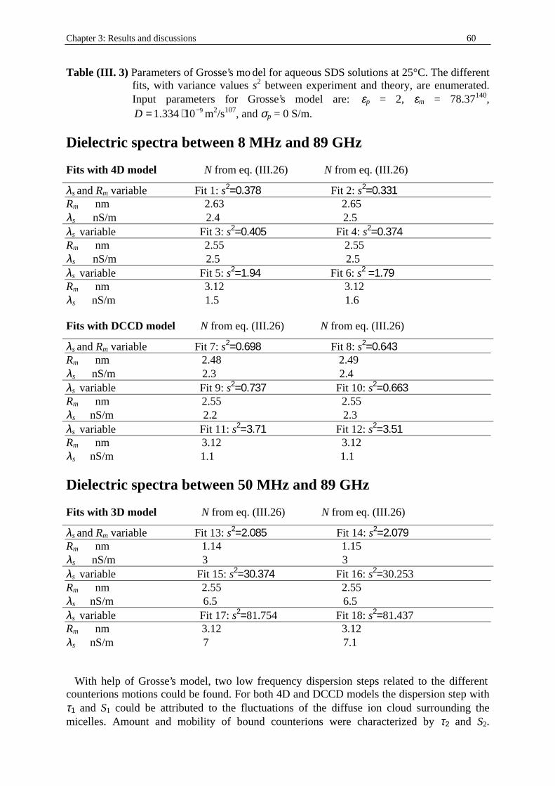
Chapter 3: Results and discussions 60
Table (III. 3) Parameters of Grosse’s model for aqueous SDS solutions at 25°C. The different fits, with variance values s2 between experiment and theory, are enumerated. Input parameters for Grosse’s model are: εp = 2, εm = 78.37140,
910334.1 −⋅=D m2/s107, and σp = 0 S/m.
Dielectric spectra between 8 MHz and 89 GHz Fits with 4D model N from eq. (III .26) N from eq. (III .26)
λs and Rm variable Fit 1: s2=0.378 Fit 2: s2=0.331 Rm nm 2.63 2.65 λs nS/m 2.4 2.5 λs variable Fit 3: s2=0.405 Fit 4: s2=0.374 Rm nm 2.55 2.55
λs nS/m 2.5 2.5 λs variable Fit 5: s2=1.94 Fit 6: s2 =1.79 Rm nm 3.12 3.12
λs nS/m 1.5 1.6 Fits with DCCD model N from eq. (III .26) N from eq. (III .26)
λs and Rm variable Fit 7: s2=0.698 Fit 8: s2=0.643 Rm nm 2.48 2.49 λs nS/m 2.3 2.4 λs variable Fit 9: s2=0.737 Fit 10: s2=0.663 Rm nm 2.55 2.55
λs nS/m 2.2 2.3 λs variable Fit 11: s2=3.71 Fit 12: s2=3.51 Rm nm 3.12 3.12
λs nS/m 1.1 1.1
Dielectric spectra between 50 MHz and 89 GHz Fits with 3D model N from eq. (III .26) N from eq. (III .26)
λs and Rm variable Fit 13: s2=2.085 Fit 14: s2=2.079 Rm nm 1.14 1.15 λs nS/m 3 3 λs variable Fit 15: s2=30.374 Fit 16: s2=30.253 Rm nm 2.55 2.55
λs nS/m 6.5 6.5 λs variable Fit 17: s2=81.754 Fit 18: s2=81.437 Rm nm 3.12 3.12
λs nS/m 7 7.1 With help of Grosse’s model, two low frequency dispersion steps related to the different counterions motions could be found. For both 4D and DCCD models the dispersion step with τ1 and S1 could be attributed to the fluctuations of the diffuse ion cloud surrounding the micelles. Amount and mobilit y of bound counterions were characterized by τ2 and S2.
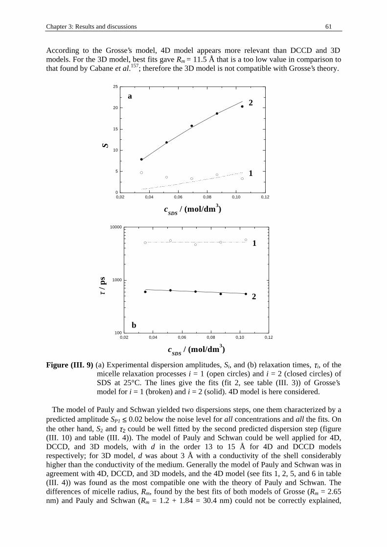
Chapter 3: Results and discussions 61
According to the Grosse’s model, 4D model appears more relevant than DCCD and 3D models. For the 3D model, best fits gave Rm = 11.5 Å that is a too low value in comparison to that found by Cabane et al.157; therefore the 3D model is not compatible with Grosse’s theory.
0,02 0,04 0,06 0,08 0,10 0,120
5
10
15
20
25
a
2
1
S
cSDS
/ (mol/dm3)
0,02 0,04 0,06 0,08 0,10 0,12100
1000
10000
b
2
1
ττ / p
s
cSDS
/ (mol/dm3)
Figure (III. 9) (a) Experimental dispersion amplitudes, Si, and (b) relaxation times, τi, of the micelle relaxation processes i = 1 (open circles) and i = 2 (closed circles) of SDS at 25°C. The lines give the fits (fit 2, see table (III . 3)) of Grosse’s model for i = 1 (broken) and i = 2 (solid). 4D model is here considered.
The model of Pauly and Schwan yielded two dispersions steps, one them characterized by a predicted amplitude SP1 ≤ 0.02 below the noise level for all concentrations and all the fits. On the other hand, S2 and τ2 could be well fitted by the second predicted dispersion step (figure (III . 10) and table (III . 4)). The model of Pauly and Schwan could be well applied for 4D, DCCD, and 3D models, with d in the order 13 to 15 Å for 4D and DCCD models respectively; for 3D model, d was about 3 Å with a conductivity of the shell considerably higher than the conductivity of the medium. Generally the model of Pauly and Schwan was in agreement with 4D, DCCD, and 3D models, and the 4D model (see fits 1, 2, 5, and 6 in table (III . 4)) was found as the most compatible one with the theory of Pauly and Schwan. The differences of micelle radius, Rm, found by the best fits of both models of Grosse (Rm = 2.65 nm) and Pauly and Schwan (Rm = 1.2 + 1.84 = 30.4 nm) could not be correctly explained,
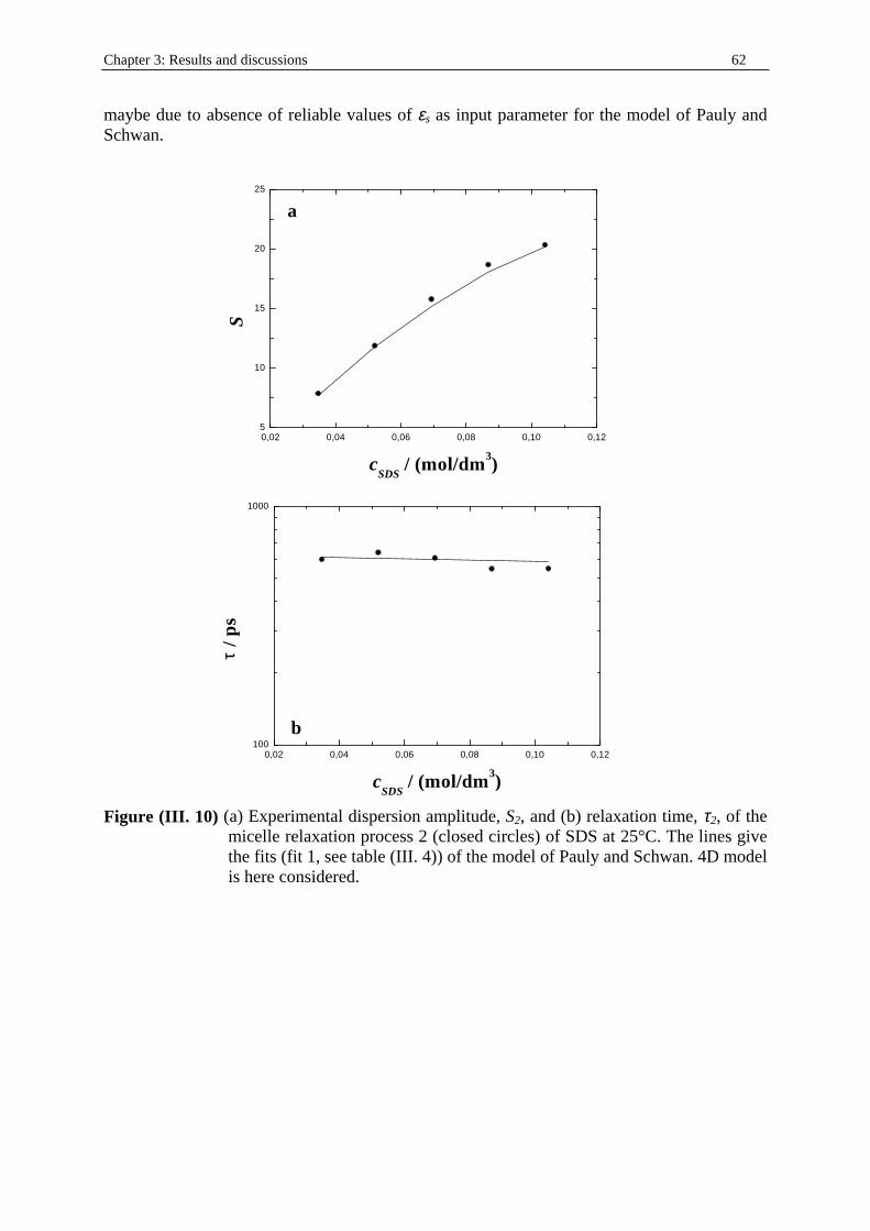
Chapter 3: Results and discussions 62
maybe due to absence of reliable values of εs as input parameter for the model of Pauly and Schwan.
0,02 0,04 0,06 0,08 0,10 0,125
10
15
20
25
a
S
cSDS
/ (mol/dm3)
0,02 0,04 0,06 0,08 0,10 0,12100
1000
b
ττ / p
s
cSDS
/ (mol/dm3)
Figure (III. 10) (a) Experimental dispersion amplitude, S2, and (b) relaxation time, τ2, of the micelle relaxation process 2 (closed circles) of SDS at 25°C. The lines give the fits (fit 1, see table (III . 4)) of the model of Pauly and Schwan. 4D model is here considered.
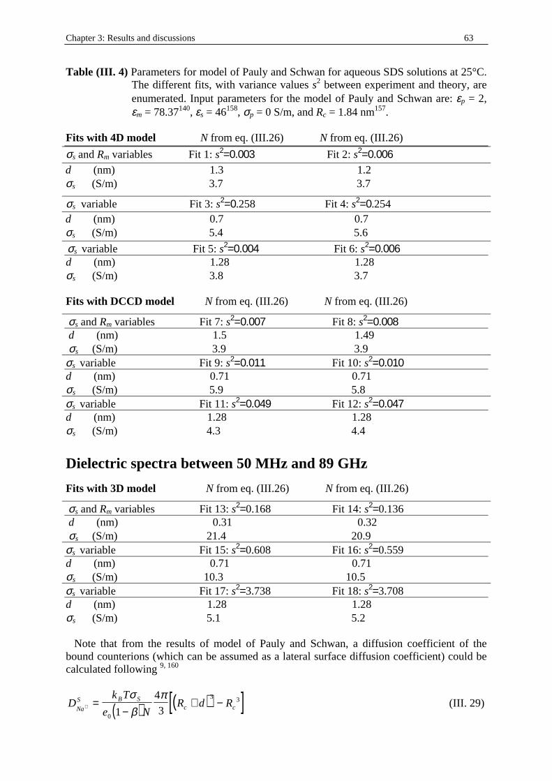
Chapter 3: Results and discussions 63
Table (III. 4) Parameters for model of Pauly and Schwan for aqueous SDS solutions at 25°C. The different fits, with variance values s2 between experiment and theory, are enumerated. Input parameters for the model of Pauly and Schwan are: εp = 2, εm = 78.37140, εs = 46158, σp = 0 S/m, and Rc = 1.84 nm157.
Fits with 4D model N from eq. (III .26) N from eq. (III .26)
σs and Rm variables Fit 1: s2=0.003 Fit 2: s2=0.006
d (nm) 1.3 1.2 σs (S/m) 3.7 3.7
σs variable Fit 3: s2=0.258 Fit 4: s2=0.254 d (nm) 0.7 0.7 σs (S/m) 5.4 5.6
σs variable Fit 5: s2=0.004 Fit 6: s2=0.006 d (nm) 1.28 1.28
σs (S/m) 3.8 3.7 Fits with DCCD model N from eq. (III .26) N from eq. (III .26)
σs and Rm variables Fit 7: s2=0.007 Fit 8: s2=0.008 d (nm) 1.5 1.49
σs (S/m) 3.9 3.9 σs variable Fit 9: s2=0.011 Fit 10: s2=0.010 d (nm) 0.71 0.71
σs (S/m) 5.9 5.8 σs variable Fit 11: s2=0.049 Fit 12: s2=0.047 d (nm) 1.28 1.28
σs (S/m) 4.3 4.4
Dielectric spectra between 50 MHz and 89 GHz Fits with 3D model N from eq. (III .26) N from eq. (III .26)
σs and Rm variables Fit 13: s2=0.168 Fit 14: s2=0.136 d (nm) 0.31 0.32
σs (S/m) 21.4 20.9 σs variable Fit 15: s2=0.608 Fit 16: s2=0.559 d (nm) 0.71 0.71
σs (S/m) 10.3 10.5 σs variable Fit 17: s2=3.738 Fit 18: s2=3.708 d (nm) 1.28 1.28
σs (S/m) 5.1 5.2 Note that from the results of model of Pauly and Schwan, a diffusion coeff icient of the bound counterions (which can be assumed as a lateral surface diffusion coeff icient) could be calculated following 9, 160
( ) ( )[ ]Dk T
e NR d R
Na
S B Sc c+ =
−+ −
σβ
π
0
3 3
1
4
3 (III . 29)
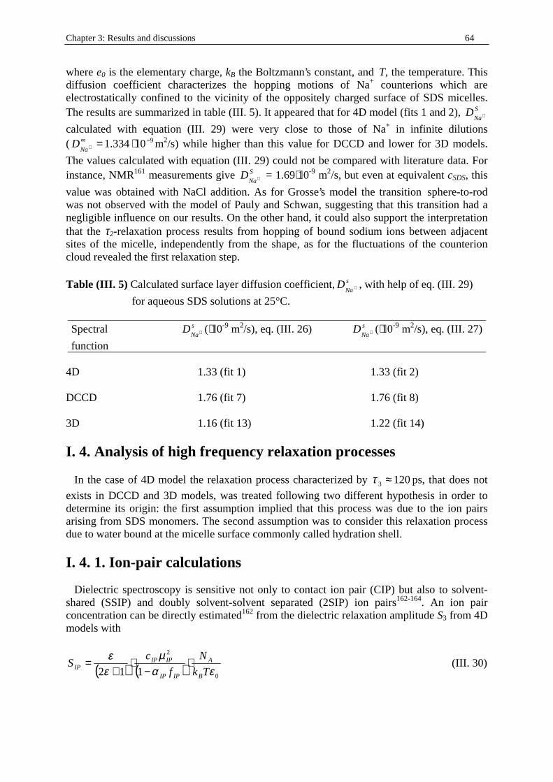
Chapter 3: Results and discussions 64
where e0 is the elementary charge, kB the Boltzmann’s constant, and T, the temperature. This diffusion coeff icient characterizes the hopping motions of Na+ counterions which are electrostatically confined to the vicinity of the oppositely charged surface of SDS micelles. The results are summarized in table (III . 5). It appeared that for 4D model (fits 1 and 2), S
NaD +
calculated with equation (III . 29) were very close to those of Na+ in infinite dilutions ( 910334.1 −∞ ⋅=+Na
D m2/s) while higher than this value for DCCD and lower for 3D models.
The values calculated with equation (III . 29) could not be compared with literature data. For instance, NMR161 measurements give S
NaD + = 1.69⋅10-9 m2/s, but even at equivalent cSDS, this
value was obtained with NaCl addition. As for Grosse’s model the transition sphere-to-rod was not observed with the model of Pauly and Schwan, suggesting that this transition had a negligible influence on our results. On the other hand, it could also support the interpretation that the τ2-relaxation process results from hopping of bound sodium ions between adjacent sites of the micelle, independently from the shape, as for the fluctuations of the counterion cloud revealed the first relaxation step. Table (III. 5) Calculated surface layer diffusion coeff icient, s
NaD + , with help of eq. (III . 29)
for aqueous SDS solutions at 25°C. Spectral s
NaD + (⋅10-9 m2/s), eq. (III . 26) s
NaD + (⋅10-9 m2/s), eq. (III . 27)
function 4D 1.33 (fit 1) 1.33 (fit 2) DCCD 1.76 (fit 7) 1.76 (fit 8) 3D 1.16 (fit 13) 1.22 (fit 14)
I. 4. Analysis of high frequency relaxation processes In the case of 4D model the relaxation process characterized by 1203 ≈τ ps, that does not
exists in DCCD and 3D models, was treated following two different hypothesis in order to determine its origin: the first assumption implied that this process was due to the ion pairs arising from SDS monomers. The second assumption was to consider this relaxation process due to water bound at the micelle surface commonly called hydration shell .
I. 4. 1. Ion-pair calculations Dielectric spectroscopy is sensitive not only to contact ion pair (CIP) but also to solvent-shared (SSIP) and doubly solvent-solvent separated (2SIP) ion pairs162-164. An ion pair concentration can be directly estimated162 from the dielectric relaxation amplitude S3 from 4D models with
( ) ( ) 0
2
112 εαµ
εε
Tk
N
f
cS
B
A
IPIP
IPIPIP ⋅
−⋅
+= (III . 30)
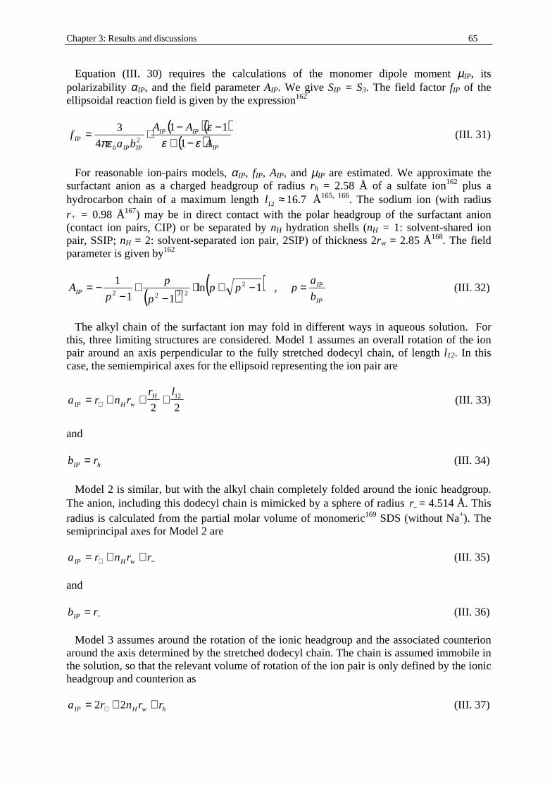
Chapter 3: Results and discussions 65
Equation (III . 30) requires the calculations of the monomer dipole moment µIP, its polarizabilit y αIP, and the field parameter AIP. We give SIP = S3. The field factor fIP of the elli psoidal reaction field is given by the expression162
( )( )
( ) IP
IPIP
IPIPIP A
AA
baf
εεε
πε −+−−
⋅=1
11
4
32
0
(III . 31)
For reasonable ion-pairs models, αIP, fIP, AIP, and µIP are estimated. We approximate the surfactant anion as a charged headgroup of radius rh = 2.58 Å of a sulfate ion162 plus a hydrocarbon chain of a maximum length 7.1612 ≈l Å165, 166. The sodium ion (with radius r+ = 0.98 Å167) may be in direct contact with the polar headgroup of the surfactant anion (contact ion pairs, CIP) or be separated by nH hydration shells (nH = 1: solvent-shared ion pair, SSIP; nH = 2: solvent-separated ion pair, 2SIP) of thickness 2rw = 2.85 Å168. The field parameter is given by162
( ) ( )1ln11
1 22/322
−+⋅−
+−
−= ppp
p
pAIP ,
IP
IP
b
ap = (III . 32)
The alkyl chain of the surfactant ion may fold in different ways in aqueous solution. For this, three limiting structures are considered. Model 1 assumes an overall rotation of the ion pair around an axis perpendicular to the fully stretched dodecyl chain, of length l12. In this case, the semiempirical axes for the elli psoid representing the ion pair are
a r n rr l
IP H wH= + + ++ 2 2
12 (III . 33)
and
hIP rb = (III . 34)
Model 2 is similar, but with the alkyl chain completely folded around the ionic headgroup. The anion, including this dodecyl chain is mimicked by a sphere of radius −r = 4.514 Å. This radius is calculated from the partial molar volume of monomeric169 SDS (without Na+). The semiprincipal axes for Model 2 are a r n r rIP H w= + ++ − (III . 35) and
−= rbIP (III . 36) Model 3 assumes around the rotation of the ionic headgroup and the associated counterion around the axis determined by the stretched dodecyl chain. The chain is assumed immobile in the solution, so that the relevant volume of rotation of the ion pair is only defined by the ionic headgroup and counterion as a r n r rIP H w h= + ++2 2 (III . 37)
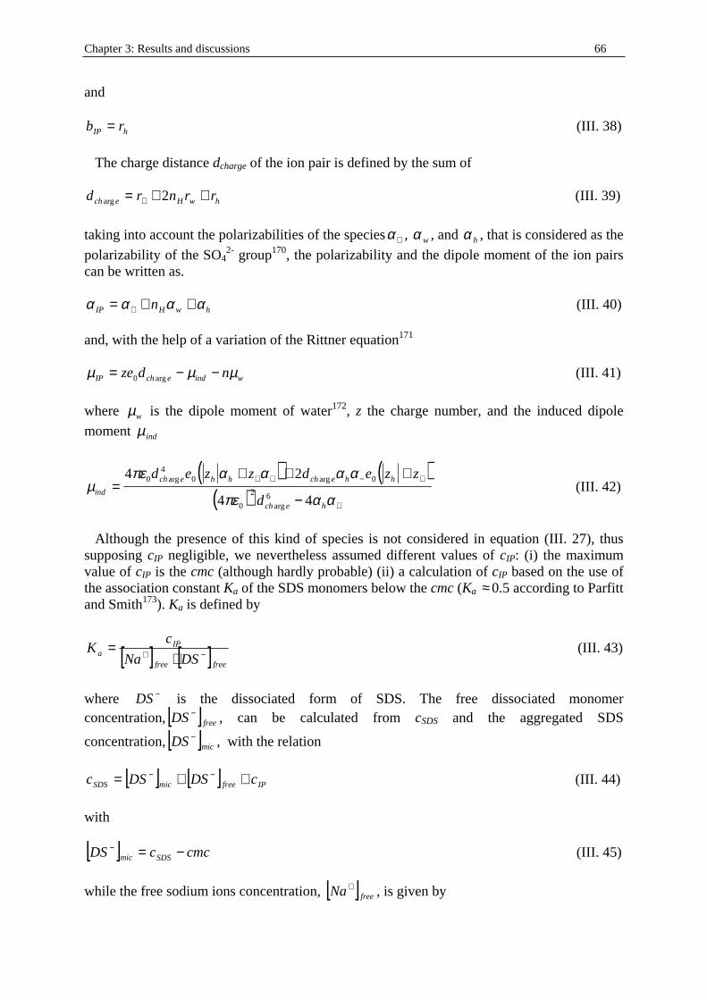
Chapter 3: Results and discussions 66
and
hIP rb = (III. 38)
The charge distance dcharge of the ion pair is defined by the sum of d r n r rch e H w harg = + ++ 2 (III. 39)
taking into account the polarizabilities of the speciesα+ , wα , and hα , that is considered as the
polarizability of the SO42- group170, the polarizability and the dipole moment of the ion pairs
can be written as. α α α αIP H w hn= + ++ (III. 40) and, with the help of a variation of the Rittner equation171 µ µ µIP ch e ind wze d n= − −0 arg (III. 41)
where µw is the dipole moment of water172, z the charge number, and the induced dipole
moment indµ
( ) ( )( )µ
πε α α α α
πε α αind
ch e h h ch e h h
ch e h
d e z z d e z z
d=
+ + +
−
+ + − +
+
4 2
4 4
04
0 0
0
2 6
arg arg
arg
(III. 42)
Although the presence of this kind of species is not considered in equation (III. 27), thus supposing cIP negligible, we nevertheless assumed different values of cIP: (i) the maximum value of cIP is the cmc (although hardly probable) (ii) a calculation of cIP based on the use of the association constant Ka of the SDS monomers below the cmc (Ka ≈ 0.5 according to Parfitt and Smith173). Ka is defined by
[ ] [ ]freefree
IPa DSNa
cK −+ ⋅
= (III. 43)
where −DS is the dissociated form of SDS. The free dissociated monomer concentration, [ ]freeDS − , can be calculated from cSDS and the aggregated SDS
concentration, [ ]micDS − , with the relation
[ ] [ ] IPfreemicSDS cDSDSc ++= −− (III. 44)
with [ ] cmccDS SDSmic −=− (III. 45)
while the free sodium ions concentration, [ ]freeNa + , is given by
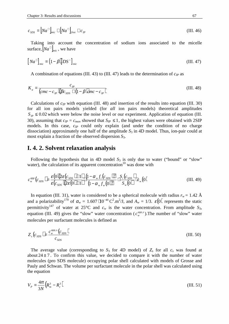
Chapter 3: Results and discussions 67
[ ] [ ] IPfreemicSDS cNaNac ++= ++ (III . 46)
Taking into account the concentration of sodium ions associated to the micelle surface,[ ]micNa + , we have
[ ] ( )[ ]Na DSmic mic
+ −= −1 β (III . 47)
A combination of equations (III . 43) to (III . 47) leads to the determination of cIP as
( ) ( )( )IPSDSIP
IPa ccmccccmc
cK
−−+−=
ββ 1 (III . 48)
Calculations of cIP with equation (III . 48) and insertion of the results into equation (III . 30) for all i on pairs models yielded (for all ion pairs models) theoretical amplitudes
02.0≤IPS which were below the noise level or our experiment. Application of equation (III . 30), assuming that cIP = cmon showed that SIP 1≤ , the highest values were obtained with 2SIP models. In this case, cIP could only explain (and under the condition of no charge dissociation) approximately one half of the amplitude S3 in 4D model. Thus, ion-pair could at most explain a fraction of the observed dispersion S3.
I. 4. 2. Solvent relaxation analysis Following the hypothesis that in 4D model S3 is only due to water (“bound” or “slow” water), the calculation of its apparent concentration10 was done with
( ) ( ) ( )( )( ) ( )( )
( )( )( )( )
( )( ) ( )0001
1
102
1202
2
ww
SDSi
ww
SDSiw
SDS
SDSSDS
appw c
S
cS
f
cf
c
ccc ⋅⋅
−−
⋅++
=α
αεε
εε (III . 49)
In equation (III . 31), water is considered to be a spherical molecule with radius rw = 1.42 Å and a polarizabilit y170 of αw = 4010607.1 −⋅ C2.m2/J, and Aw = 1/3. ( )0ε represents the static permittivity147 of water at 25°C and cw is the water concentration. From amplitude S3, equation (III . 49) gives the “slow” water concentration ( sapp
wc , ).The number of “slow” water
molecules per surfactant molecules is defined as
( ) ( )SDS
SDSsapp
wSDSs c
cccZ
,
= (III . 50)
The average value (corresponding to S3 for 4D model) of Zs for all cs was found at about 724± . To confirm this value, we decided to compare it with the number of water molecules (pro SDS molecule) occupying polar shell calculated with models of Grosse and Pauly and Schwan. The volume per surfactant molecule in the polar shell was calculated using the equation
( )33
3
4cmP RR
NV −= π
(III . 51)
Chapter 3: Results and discussions 68
then the hydration number of SDS micelles, Hyd, could be determined following reference (174)
( )Hyd
V V
V
P dry
H O
=−
2
(III . 52)
where Vdry is the volume inaccessible to water constituted by the sodium sulfate headgroup (about 66.4 Å3, from ref. (175)), and OHV
2 the volume of a water molecule.(about 30 Å3). In
the Grosse’s model, a value of Rm 3.26≈ Å with N from equation (III . 26) yielded Hyd = 24.3 while a value of Rm 5.26≈ Å with N from equation (III . 27) gaveHyd = ±256 1. . Those different Hyd values are in excellent agreement with Zs reported before. Using Rm from the model of Pauly and Schwan, gives values of H at about Hyd = 53 ± 14 with N from equation (III . 26) and Hyd = 47 ± 11 with N from equation (III . 27). Therefore, the assumption that S3 is arising from bound water at the micelle surface agreed with results from Grosse’s model and more generally with the 4D model. This water is located toward the micelle polar shell , hydrating sodium ions and close in terms of rotation rate (τ3 120≈ ps, around 10 times lower than in bulk water) to second hydration layer in hydrophili c sili ca gels176 previously found by DRS. The dominating dispersion amplitude of the solvent, Sw (S4 for 4D model or S3 for DCCD and 3D models, all centred at 8≈wτ ps) characterises the co-operative relaxation of the
hydrogen-bond network of water. For both fit models, Sw exhibits a weak decrease upon increasing cs suggesting possible ion-solvent interactions162, 177, although this may be accounted to the increasing of φ. Following the theory of Hubbard et al.178-180 we considered kinetic depolarisation as a further contribution to dielectric depression. This kinetic depolarisation results from the ionic movement opposite to the direction into which the solvent dipoles are orientated in the external field. This therefore produces a frictional force which lowers the ionic mobilit y and decreases the solvent permittivity proportionally to the conductivity. This effect participates to the dielectric depression, Sw, giving the equili brium amplitude of the solvent dispersion, eq
wS , as
( ) ( ) ( )SDSkdSDSwSDS
eqw ccScS ε∆+= (III . 53)
where the contribution arising from kinetic depolarisation, εkd∆ , was calculated with the
Hubbard-Onsager theory178-180
( ) ( )SDSSDSkd cc ξκε =∆ (III . 54)
and
( ) ( )( )
( )ξ
ε εε
τε
= ⋅−
⋅∞p0 0
0
0
0
(III . 55)
We considered three different values of εkd∆ . For p = 0, 0=∆ εkd (and hence ξ = 0) the
kinetic depolarisation is negligible, whereas for the slip and stick limits the values of p are 2/3 and 1, respectively. For all spectral functions, our results indicated that small differences within the experimental accuracy exist between the values of εkd∆ calculated with p = 0, 2/3,
Chapter 3: Results and discussions 69
and 1 (combining equation (III . 49) and equations (III . 53) to (III . 55)). This suggests that that kinetic depolarisation had a very small i nfluence on solvent relaxation in our surfactant concentration range (see figure (III . 11)). Thus considering only p = 0 and equation (III . 49) for Sw found with 4D model led to sapp
wbapp
ww ccc ,, +≈ , indicating the absence (or very low
amounts, within the error limits) of water molecules that does not contribute at all to ( )νε , such a water is expected to be strongly bounded to sodium ions as it is for NaCl or sodium sulfate solutions140, 162. The low SDS concentration is an explanation of such observation. On the other hand, it was possible for DCCD and 3D model to find and to give a number of irrotationally bound water pro SDS surfactant molecules (ZIB) as following for 4D model
( ) ( ) ( )[ ]SDS
SDSsapp
wSDSbapp
wSDSwIB c
ccccccZ
,, +−= (III . 56)
Equation (III . 56), when applied to 4D model, gave values around zero within the error limits. This was reduced for DCCD and 3D models to
( ) ( )SDS
SDSbapp
wSDSwIB c
ccccZ
,−= (III . 57)
For these calculations, we considered only the case of ( ) 4/1
SDScN ∝ . We found that ZIB
(close to zero in 4D model as said before) was about 23.7±1.8 for DCCD model while about 16.4±1 for 3D model. For DCCD model, Hyd has values of 18.2 from Grosse’s model (in agreement with solvent relaxation results) and 65.9±0.2 from Pauly and Schwan model. In the case of 3D model, Hyd was about 6.4±0.3 from the model of Pauly and Schwan. This was the unique case where a certain correspondence between data from the model of Pauly and Schwan and from solvent relaxation was found. Water molecules may deep penetrate into the micelle and hydrates surfactant headgroups140, 157, 175, 181-186 (inclusive counterions). At the present point of our study two different properties could be proposed for this water (i) along 4D model (that has been proved to give the best agreement between spectal function and models of Grosse and Pauly and Schwan), majority of this water could be characterised by a relaxation rate around 120 ps (ii) from DCCD and 3D models this water do not participate at all to the dielectric relaxation. We proposed a comparison between the different micelle volume fraction calculated from models of Grosse and Pauly and Schwan and from solvent relaxation (including hydration shell) with the relation
( ) ( ) ( )( )0
,,
w
SDSbapp
wbapp
wSDS c
cccmccc
−=φ (III . 58)
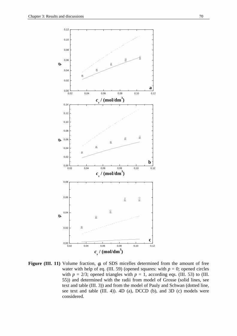
Chapter 3: Results and discussions 70
0,02 0,04 0,06 0,08 0,10 0,120,00
0,02
0,04
0,06
0,08
0,10
0,12
a
cs / (mol/dm3)
φφ
0,02 0,04 0,06 0,08 0,10 0,120,00
0,02
0,04
0,06
0,08
0,10
0,12
0,14
b
cs / (mol/dm3)
φφ
0,02 0,04 0,06 0,08 0,10 0,120,00
0,02
0,04
0,06
0,08
c
cs / (mol/dm3)
φφ
Figure (III. 11) Volume fraction, φ, of SDS micelles determined from the amount of free water with help of eq. (III. 59) (opened squares: with p = 0; opened circles with p = 2/3; opened triangles with p = 1, according eqs. (III. 53) to (III. 55)) and determined with the radii from model of Grosse (solid lines, see text and table (III. 3)) and from the model of Pauly and Schwan (dotted line, see text and table (III. 4)). 4D (a), DCCD (b), and 3D (c) models were considered.
Chapter 3: Results and discussions 71
Due to the low cmc of SDS, we modified equation (III . 58) to
( ) ( ) ( )( )0
0 ,
w
SDSbapp
wwSDS c
cccc
−=φ (III . 59)
Comparison of results from equation (III . 59) and those from fits of models of Pauly and Schwan and of Grosse revealed (figure (III . 11)) that this test was valid only with a φ arising from the best fits of Grosse’s model obtained with Rm 5.26≈ Å, specially the 4D model. This indicated that the models of 3D and DCCD could be considered as irrelevant in this study. In the light of the Grosse’s142 theory, DRS was able to detect the counterion cloud which is under the influence of the surfactant polar groups and the dissociated cations forming the diffuse layer thus gave an apparent Rm higher than those from SANS data. Our study confirmed the existence of relaxing hydration water species at the micellar surface and therefore the validity of the 4D model in the dielectric study of SDS micelles. This showed in addition to previous results in cationic micelles9, 10 that Grosse’s theory and Cavell equations usually used in simple electrolyte solutions can be extended to various ionic micellar systems, especially to the next part of the work with addition of 1-pentanol.
II. Water/SDS/1-pentanol ternary and water/SDS/1-pentanol/n-
dodecane quaternary systems We aimed to extend the DRS results of aqueous SDS solutions to reverse micelles and to microemulsions by addition of 1-pentanol and then of dodecane using the ternary water/SDS/1-pentanol and quaternary water/SDS/1-pentanol/n-dodecane (with mass ratio SDS to 1-pentanol equal to ½) systems at T = 25°C13as shown in figure (I. 6). We observed in this way the behavior of low-frequency relaxation processes related to counterion motions and of high frequency processes linked to solvent relaxation. With conductivity measurements, we could find the structural states (W/O, O/W, or bicontinuous microemulsions) respective to the points investigated by means of DRS.
II. 1. Analysis of the conductivity data With variation of electrical conductivity, the different structure transition in microemulsions (or Winsor IV systems187) can be defined13, 188. For the ternary and quaternary systems studied here, the boundaries of the composition ranges corresponding to different structural states may be determined by plotting, within the main clear and monophasic region, the composition points at which the variation mode of electrical conductivity changes. From low water to high water contents the conductive behavior represents, depending on the system investigated, a percolation phenomenon. The conductivity behavior at the bottom of the plot (figure (III . 12)) can be modeled using a scaling law189-192 (see part II. 5. 1. 1. of this chapter), while the linear upper part of the curve may be depicted through the Effective Medium Theory (EMT). The EMT has been originally developed for the interpretation of the electrical conductivity of binary composites193-197. Both parts are separated by the percolation threshold φw
p (φw considered as the volume fraction of the disperse phase consisting of water plus solute) that results form intercept of the linear part of the curve with x axis. Percolative conduction phenomena in microemulsions and related systems can be explained by assuming the existence of a progressive W/O droplet interlinking and clustering process (figure (III . 13)), as the water content is raised, the conduction mechanism being essentially interfacial since charges are carried by the surfactant molecules198-201. Past a criti cal water content (called φw
b ),
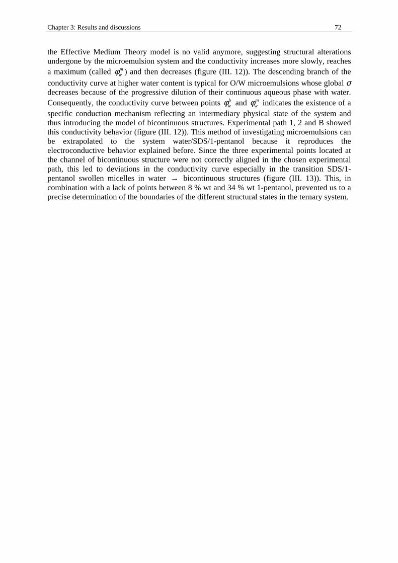
Chapter 3: Results and discussions 72
the Effective Medium Theory model is no valid anymore, suggesting structural alterations undergone by the microemulsion system and the conductivity increases more slowly, reaches a maximum (called φw
m ) and then decreases (figure (III. 12)). The descending branch of the
conductivity curve at higher water content is typical for O/W microemulsions whose global σ decreases because of the progressive dilution of their continuous aqueous phase with water. Consequently, the conductivity curve between points φw
b and φwm indicates the existence of a
specific conduction mechanism reflecting an intermediary physical state of the system and thus introducing the model of bicontinuous structures. Experimental path 1, 2 and B showed this conductivity behavior (figure (III. 12)). This method of investigating microemulsions can be extrapolated to the system water/SDS/1-pentanol because it reproduces the electroconductive behavior explained before. Since the three experimental points located at the channel of bicontinuous structure were not correctly aligned in the chosen experimental path, this led to deviations in the conductivity curve especially in the transition SDS/1-pentanol swollen micelles in water → bicontinuous structures (figure (III. 13)). This, in combination with a lack of points between 8 % wt and 34 % wt 1-pentanol, prevented us to a precise determination of the boundaries of the different structural states in the ternary system.
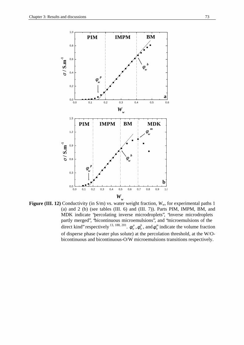
Chapter 3: Results and discussions 73
0,0 0,1 0,2 0,3 0,4 0,5 0,60,0
0,2
0,4
0,6
0,8
1,0
φφw
b
φφw
p
a
Ww
PIM BMIMPM
σσ /
S.m
-1
0,0 0,1 0,2 0,3 0,4 0,5 0,6 0,7 0,8 0,9 1,00,0
0,3
0,6
0,9
1,2
1,5
φφw
m
φφw
b
φφw
p
b
Ww
σσ /
S.m
-1
MDKBMIMPMPIM
Figure (III. 12) Conductivity (in S/m) vs. water weight fraction, Ww, for experimental paths 1
(a) and 2 (b) (see tables (III. 6) and (III. 7)). Parts PIM, IMPM, BM, and MDK indicate “percolating inverse microdroplets”, “inverse microdroplets partly merged”, “bicontinuous microemulsions”, and “microemulsions of the direct kind” respectively 13, 188, 201. p
wφ , bwφ , and m
wφ indicate the volume fraction
of disperse phase (water plus solute) at the percolation threshold, at the W/O-bicontinuous and bicontinuous-O/W microemulsions transitions respectively.
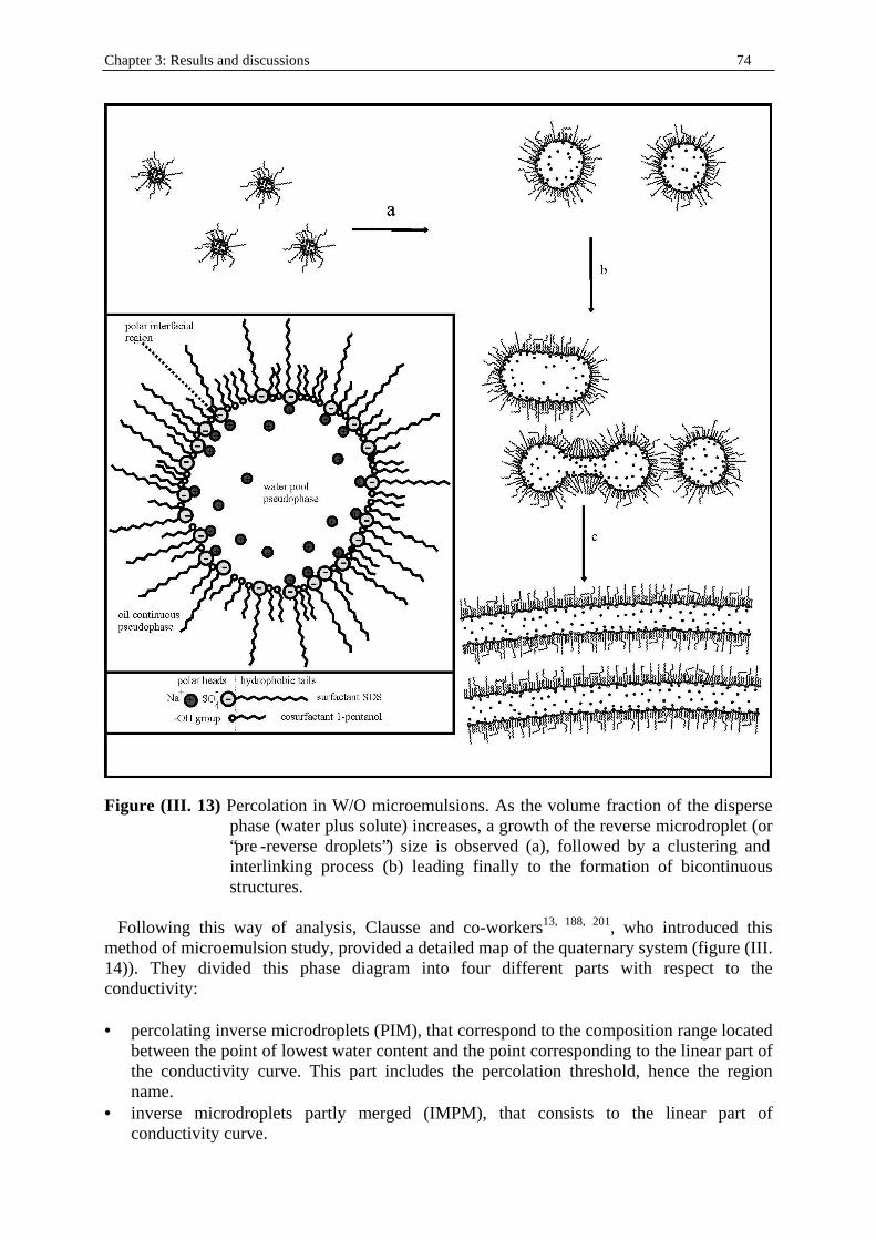
Chapter 3: Results and discussions 74
Figure (III. 13) Percolation in W/O microemulsions. As the volume fraction of the disperse
phase (water plus solute) increases, a growth of the reverse microdroplet (or “pre -reverse droplets”) size is observed (a), followed by a clustering and interlinking process (b) leading finally to the formation of bicontinuous structures.
Following this way of analysis, Clausse and co-workers13, 188, 201, who introduced this method of microemulsion study, provided a detailed map of the quaternary system (figure (III. 14)). They divided this phase diagram into four different parts with respect to the conductivity: • percolating inverse microdroplets (PIM), that correspond to the composition range located
between the point of lowest water content and the point corresponding to the linear part of the conductivity curve. This part includes the percolation threshold, hence the region name.
• inverse microdroplets partly merged (IMPM), that consists to the linear part of conductivity curve.
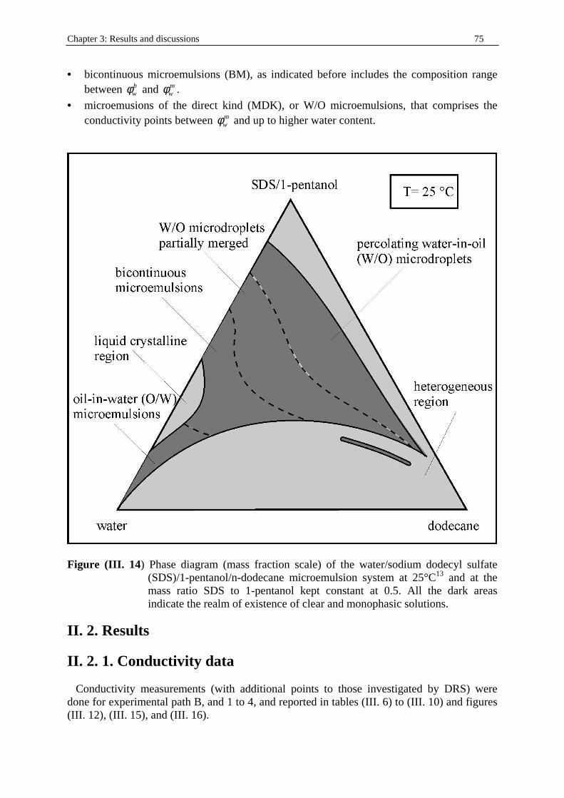
Chapter 3: Results and discussions 75
• bicontinuous microemulsions (BM), as indicated before includes the composition range between φw
b and φwm .
• microemusions of the direct kind (MDK), or W/O microemulsions, that comprises the conductivity points between φw
m and up to higher water content.
Figure (III. 14) Phase diagram (mass fraction scale) of the water/sodium dodecyl sulfate
(SDS)/1-pentanol/n-dodecane microemulsion system at 25°C13 and at the mass ratio SDS to 1-pentanol kept constant at 0.5. All the dark areas indicate the realm of existence of clear and monophasic solutions.
II. 2. Results
II. 2. 1. Conductivity data Conductivity measurements (with additional points to those investigated by DRS) were done for experimental path B, and 1 to 4, and reported in tables (III . 6) to (III . 10) and figures (III . 12), (III . 15), and (III . 16).
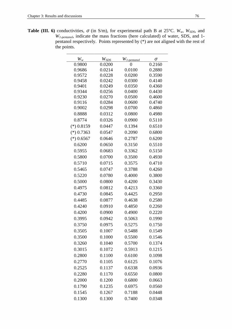
Chapter 3: Results and discussions 76
Table (III. 6) conductivities, σ (in S/m), for experimental path B at 25°C. Ww, WSDS, and W1-pentanol, indicate the mass fractions (here calculated) of water, SDS, and 1-pentanol respectively. Points represented by (* ) are not aligned with the rest of the points.
Ww WSDS W1-pentanol σ 0.9800 0.0200 0 0.2160 0.9686 0.0214 0.0100 0.2880 0.9572 0.0228 0.0200 0.3590 0.9458 0.0242 0.0300 0.4140 0.9401 0.0249 0.0350 0.4360 0.9344 0.0256 0.0400 0.4430 0.9230 0.0270 0.0500 0.4600 0.9116 0.0284 0.0600 0.4740 0.9002 0.0298 0.0700 0.4860 0.8888 0.0312 0.0800 0.4980 0.8774 0.0326 0.0900 0.5110
(* ) 0.8159 0.0447 0.1394 0.6510 (* ) 0.7363 0.0547 0.2090 0.6800 (* ) 0.6567 0.0646 0.2787 0.6200
0.6200 0.0650 0.3150 0.5510 0.5955 0.0683 0.3362 0.5150 0.5800 0.0700 0.3500 0.4930 0.5710 0.0715 0.3575 0.4710 0.5465 0.0747 0.3788 0.4260 0.5220 0.0780 0.4000 0.3800 0.5000 0.0800 0.4200 0.3430 0.4975 0.0812 0.4213 0.3360 0.4730 0.0845 0.4425 0.2950 0.4485 0.0877 0.4638 0.2580 0.4240 0.0910 0.4850 0.2260 0.4200 0.0900 0.4900 0.2220 0.3995 0.0942 0.5063 0.1990 0.3750 0.0975 0.5275 0.1750 0.3505 0.1007 0.5488 0.1549 0.3500 0.1000 0.5500 0.1546 0.3260 0.1040 0.5700 0.1374 0.3015 0.1072 0.5913 0.1215 0.2800 0.1100 0.6100 0.1098 0.2770 0.1105 0.6125 0.1076 0.2525 0.1137 0.6338 0.0936 0.2280 0.1170 0.6550 0.0800 0.2000 0.1200 0.6800 0.0663 0.1790 0.1235 0.6975 0.0560 0.1545 0.1267 0.7188 0.0448 0.1300 0.1300 0.7400 0.0348
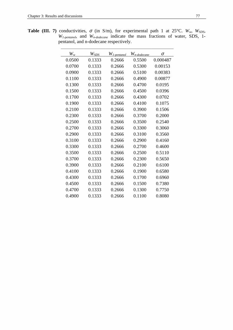
Chapter 3: Results and discussions 77
Table (III. 7) conductivities, σ (in S/m), for experimental path 1 at 25°C. Ww, WSDS, W1-pentanol, and Wn-dodecane indicate the mass fractions of water, SDS, 1-pentanol, and n-dodecane respectively.
Ww WSDS W1-pentanol Wn-dodecane σ 0.0500 0.1333 0.2666 0.5500 0.000487 0.0700 0.1333 0.2666 0.5300 0.00153 0.0900 0.1333 0.2666 0.5100 0.00383 0.1100 0.1333 0.2666 0.4900 0.00877 0.1300 0.1333 0.2666 0.4700 0.0195 0.1500 0.1333 0.2666 0.4500 0.0396 0.1700 0.1333 0.2666 0.4300 0.0702 0.1900 0.1333 0.2666 0.4100 0.1075 0.2100 0.1333 0.2666 0.3900 0.1506 0.2300 0.1333 0.2666 0.3700 0.2000 0.2500 0.1333 0.2666 0.3500 0.2540 0.2700 0.1333 0.2666 0.3300 0.3060 0.2900 0.1333 0.2666 0.3100 0.3560 0.3100 0.1333 0.2666 0.2900 0.4160 0.3300 0.1333 0.2666 0.2700 0.4600 0.3500 0.1333 0.2666 0.2500 0.5110 0.3700 0.1333 0.2666 0.2300 0.5650 0.3900 0.1333 0.2666 0.2100 0.6100 0.4100 0.1333 0.2666 0.1900 0.6580 0.4300 0.1333 0.2666 0.1700 0.6960 0.4500 0.1333 0.2666 0.1500 0.7380 0.4700 0.1333 0.2666 0.1300 0.7750 0.4900 0.1333 0.2666 0.1100 0.8080
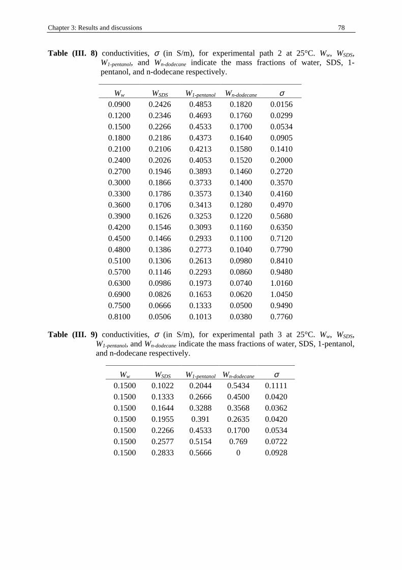
Chapter 3: Results and discussions 78
Table (III. 8) conductivities, σ (in S/m), for experimental path 2 at 25°C. Ww, WSDS, W1-pentanol, and Wn-dodecane indicate the mass fractions of water, SDS, 1-pentanol, and n-dodecane respectively.
Ww WSDS W1-pentanol Wn-dodecane σ 0.0900 0.2426 0.4853 0.1820 0.0156 0.1200 0.2346 0.4693 0.1760 0.0299 0.1500 0.2266 0.4533 0.1700 0.0534 0.1800 0.2186 0.4373 0.1640 0.0905 0.2100 0.2106 0.4213 0.1580 0.1410 0.2400 0.2026 0.4053 0.1520 0.2000 0.2700 0.1946 0.3893 0.1460 0.2720 0.3000 0.1866 0.3733 0.1400 0.3570 0.3300 0.1786 0.3573 0.1340 0.4160 0.3600 0.1706 0.3413 0.1280 0.4970 0.3900 0.1626 0.3253 0.1220 0.5680 0.4200 0.1546 0.3093 0.1160 0.6350 0.4500 0.1466 0.2933 0.1100 0.7120 0.4800 0.1386 0.2773 0.1040 0.7790 0.5100 0.1306 0.2613 0.0980 0.8410 0.5700 0.1146 0.2293 0.0860 0.9480 0.6300 0.0986 0.1973 0.0740 1.0160 0.6900 0.0826 0.1653 0.0620 1.0450 0.7500 0.0666 0.1333 0.0500 0.9490 0.8100 0.0506 0.1013 0.0380 0.7760
Table (III. 9) conductivities, σ (in S/m), for experimental path 3 at 25°C. Ww, WSDS, W1-pentanol, and Wn-dodecane indicate the mass fractions of water, SDS, 1-pentanol, and n-dodecane respectively.
Ww WSDS W1-pentanol Wn-dodecane σ 0.1500 0.1022 0.2044 0.5434 0.1111 0.1500 0.1333 0.2666 0.4500 0.0420 0.1500 0.1644 0.3288 0.3568 0.0362 0.1500 0.1955 0.391 0.2635 0.0420 0.1500 0.2266 0.4533 0.1700 0.0534 0.1500 0.2577 0.5154 0.769 0.0722 0.1500 0.2833 0.5666 0 0.0928
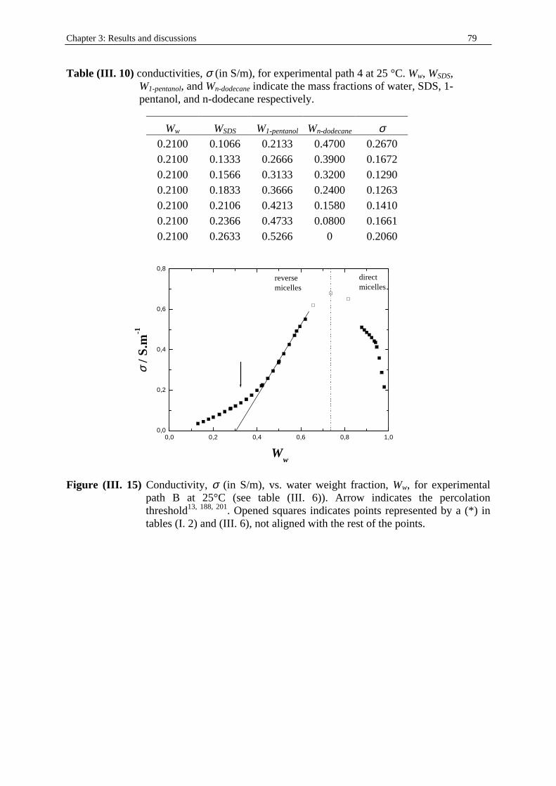
Chapter 3: Results and discussions 79
Table (III. 10) conductivities, σ (in S/m), for experimental path 4 at 25 °C. Ww, WSDS, W1-pentanol, and Wn-dodecane indicate the mass fractions of water, SDS, 1-pentanol, and n-dodecane respectively.
Ww WSDS W1-pentanol Wn-dodecane σ 0.2100 0.1066 0.2133 0.4700 0.2670 0.2100 0.1333 0.2666 0.3900 0.1672 0.2100 0.1566 0.3133 0.3200 0.1290 0.2100 0.1833 0.3666 0.2400 0.1263 0.2100 0.2106 0.4213 0.1580 0.1410 0.2100 0.2366 0.4733 0.0800 0.1661 0.2100 0.2633 0.5266 0 0.2060
0,0 0,2 0,4 0,6 0,8 1,00,0
0,2
0,4
0,6
0,8
σσ /
S.m
-1
reverse micelles
direct micelles
Ww
Figure (III. 15) Conductivity, σ (in S/m), vs. water weight fraction, Ww, for experimental path B at 25°C (see table (III . 6)). Arrow indicates the percolation threshold13, 188, 201. Opened squares indicates points represented by a (* ) in tables (I. 2) and (III . 6), not aligned with the rest of the points.
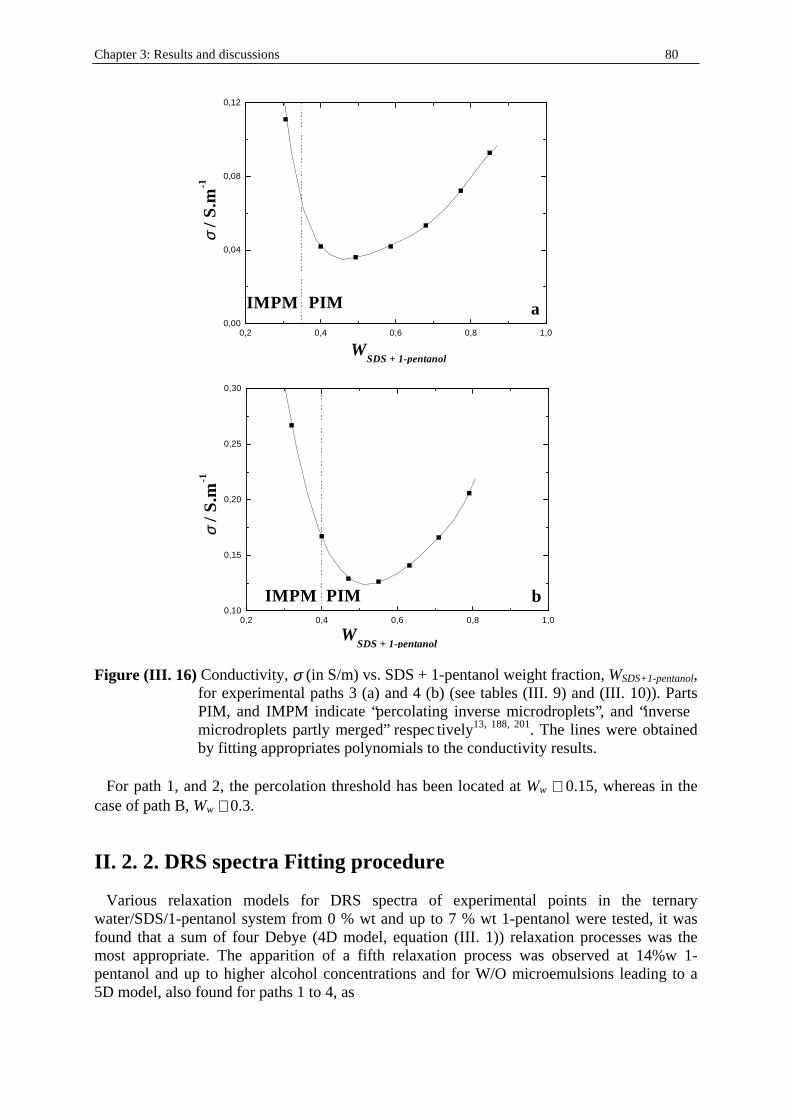
Chapter 3: Results and discussions 80
0,2 0,4 0,6 0,8 1,00,00
0,04
0,08
0,12
aIMPM PIM
WSDS + 1-pentanol
σσ /
S.m
-1
0,2 0,4 0,6 0,8 1,00,10
0,15
0,20
0,25
0,30
b
σσ /
S.m
-1
WSDS + 1-pentanol
PIMIMPM
Figure (III. 16) Conductivity, σ (in S/m) vs. SDS + 1-pentanol weight fraction, WSDS+1-pentanol, for experimental paths 3 (a) and 4 (b) (see tables (III. 9) and (III. 10)). Parts PIM, and IMPM indicate “percolating inverse microdroplets”, and “inverse microdroplets partly merged” respec tively13, 188, 201. The lines were obtained by fitting appropriates polynomials to the conductivity results.
For path 1, and 2, the percolation threshold has been located at Ww ∼ 0.15, whereas in the case of path B, Ww ∼ 0.3.
II. 2. 2. DRS spectra Fitting procedure Various relaxation models for DRS spectra of experimental points in the ternary water/SDS/1-pentanol system from 0 % wt and up to 7 % wt 1-pentanol were tested, it was found that a sum of four Debye (4D model, equation (III. 1)) relaxation processes was the most appropriate. The apparition of a fifth relaxation process was observed at 14%w 1-pentanol and up to higher alcohol concentrations and for W/O microemulsions leading to a 5D model, also found for paths 1 to 4, as
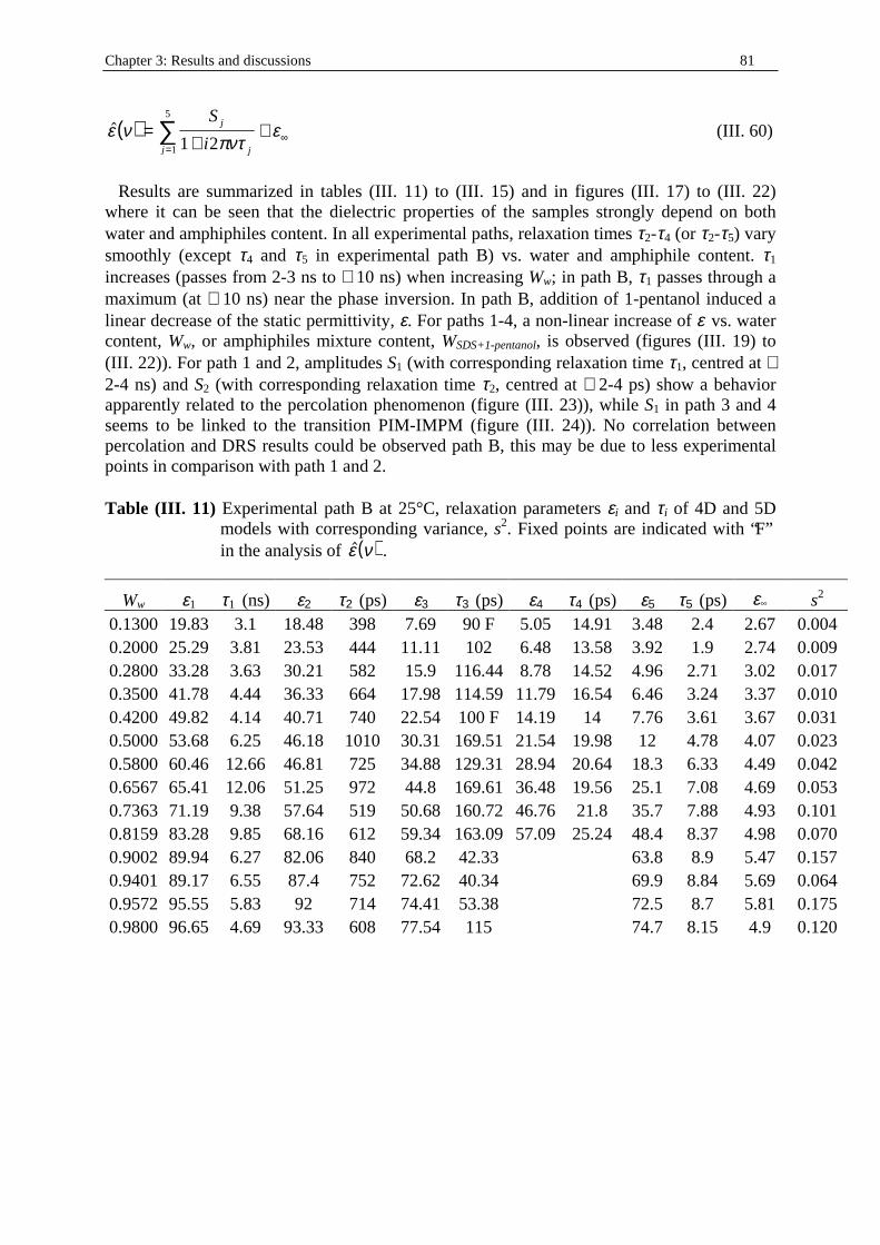
Chapter 3: Results and discussions 81
( )ε νπντ
ε=+
+=
∞∑S
ij
jj 1 21
5
(III . 60)
Results are summarized in tables (III . 11) to (III . 15) and in figures (III . 17) to (III . 22) where it can be seen that the dielectric properties of the samples strongly depend on both water and amphiphiles content. In all experimental paths, relaxation times τ2-τ4 (or τ2-τ5) vary smoothly (except τ4 and τ5 in experimental path B) vs. water and amphiphile content. τ1 increases (passes from 2-3 ns to ∼ 10 ns) when increasing Ww; in path B, τ1 passes through a maximum (at ∼ 10 ns) near the phase inversion. In path B, addition of 1-pentanol induced a linear decrease of the static permittivity, ε. For paths 1-4, a non-linear increase of ε vs. water content, Ww, or amphiphiles mixture content, WSDS+1-pentanol, is observed (figures (III . 19) to (III . 22)). For path 1 and 2, amplitudes S1 (with corresponding relaxation time τ1, centred at ∼ 2-4 ns) and S2 (with corresponding relaxation time τ2, centred at ∼ 2-4 ps) show a behavior apparently related to the percolation phenomenon (figure (III . 23)), while S1 in path 3 and 4 seems to be linked to the transition PIM-IMPM (figure (III . 24)). No correlation between percolation and DRS results could be observed path B, this may be due to less experimental points in comparison with path 1 and 2. Table (III. 11) Experimental path B at 25°C, relaxation parameters εi and τi of 4D and 5D
models with corresponding variance, s2. Fixed points are indicated with “F” in the analysis of ( )ε ν .
Ww ε1 τ1 (ns) ε2 τ2 (ps) ε3 τ3 (ps) ε4 τ4 (ps) ε5 τ5 (ps) ε s2 0.1300 19.83 3.1 18.48 398 7.69 90 F 5.05 14.91 3.48 2.4 2.67 0.004 0.2000 25.29 3.81 23.53 444 11.11 102 6.48 13.58 3.92 1.9 2.74 0.009 0.2800 33.28 3.63 30.21 582 15.9 116.44 8.78 14.52 4.96 2.71 3.02 0.017 0.3500 41.78 4.44 36.33 664 17.98 114.59 11.79 16.54 6.46 3.24 3.37 0.010 0.4200 49.82 4.14 40.71 740 22.54 100 F 14.19 14 7.76 3.61 3.67 0.031 0.5000 53.68 6.25 46.18 1010 30.31 169.51 21.54 19.98 12 4.78 4.07 0.023 0.5800 60.46 12.66 46.81 725 34.88 129.31 28.94 20.64 18.3 6.33 4.49 0.042 0.6567 65.41 12.06 51.25 972 44.8 169.61 36.48 19.56 25.1 7.08 4.69 0.053 0.7363 71.19 9.38 57.64 519 50.68 160.72 46.76 21.8 35.7 7.88 4.93 0.101 0.8159 83.28 9.85 68.16 612 59.34 163.09 57.09 25.24 48.4 8.37 4.98 0.070 0.9002 89.94 6.27 82.06 840 68.2 42.33 63.8 8.9 5.47 0.157 0.9401 89.17 6.55 87.4 752 72.62 40.34 69.9 8.84 5.69 0.064 0.9572 95.55 5.83 92 714 74.41 53.38 72.5 8.7 5.81 0.175 0.9800 96.65 4.69 93.33 608 77.54 115 74.7 8.15 4.9 0.120
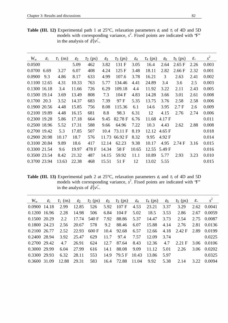
Chapter 3: Results and discussions 82
Table (III. 12) Experimental path 1 at 25°C, relaxation parameters εi and τi of 4D and 5D models with corresponding variance, s2. Fixed points are indicated with “F” in the analysis of ( )ε ν .
Ww ε1 τ1 (ns) ε2 τ2 (ps) ε3 τ3 (ps) ε4 τ4 (ps) ε5 τ5 (ps) ε s2 0.0500 5.09 462 3.82 131 F 3.05 16.4 2.64 2.65 F 2.26 0.003 0.0700 6.69 3.27 6.07 408 4.24 125 F 3.48 18.11 2.82 2.66 F 2.32 0.001 0.0900 9.3 4.86 8.17 633 4.99 107.6 3.78 16.21 3 2.63 2.41 0.002 0.1100 12.65 4.31 10.33 763 5.77 134.46 4.41 24.89 3.4 3.6 2.5 0.003 0.1300 16.18 3.4 11.66 726 6.29 109.18 4.4 11.92 3.22 2.11 2.43 0.005 0.1500 19.14 3.69 13.49 808 7.3 104 F 4.83 14.28 3.66 3.01 2.61 0.008 0.1700 20.3 3.52 14.37 683 7.39 97 F 5.35 13.75 3.76 2.58 2.58 0.006 0.1900 20.56 4.48 15.85 756 8.08 115.36 6.1 14.6 3.95 2.7 F 2.6 0.009 0.2100 19.89 4.48 16.15 681 8.8 98.3 6.31 12 4.15 2.76 2.74 0.006 0.2300 19.28 5.86 17.18 664 9.45 82.78 F 6.76 11.68 4.17 F 0.011 0.2500 18.96 5.52 17.31 588 9.66 64.96 7.22 10.3 4.43 2.62 2.88 0.008 0.2700 19.42 5.3 17.85 507 10.4 73.11 F 8.19 12.12 4.65 F 0.018 0.2900 20.98 10.17 18.7 576 11.73 66.92 F 8.32 9.95 4.92 F 0.014 0.3100 20.84 9.89 18.6 417 12.14 62.23 9.38 10.17 4.95 2.74 F 3.16 0.015 0.3300 21.54 9.6 19.97 478 F 14.34 58 F 10.65 12.55 5.49 F 0.016 0.3500 23.54 8.42 21.32 487 14.15 59.92 11.1 10.89 5.77 2.93 3.23 0.010 0.3700 23.94 13.63 22.38 468 15.51 51 F 12 13.02 5.55 0.015 Table (III. 13) Experimental path 2 at 25°C, relaxation parameters εi and τi of 4D and 5D
models with corresponding variance, s2. Fixed points are indicated with “F” in the analysis of ( )ε ν .
Ww ε1 τ1 (ns) ε2 τ2 (ps) ε3 τ3 (ps) ε4 τ4 (ps) ε5 τ5 (ps) ε s2 0.0900 14.18 2.99 12.85 526 5.92 107 F 4.53 23.21 3.37 3.29 2.62 0.0041 0.1200 16.96 2.28 14.98 506 6.84 104 F 5.02 18.5 3.53 2.86 2.67 0.0059 0.1500 20.29 2.2 17.74 540 F 7.92 88.86 5.37 14.47 3.73 2.54 2.75 0.0087 0.1800 24.23 2.56 20.67 578 9.2 88.46 6.07 15.88 4.14 2.76 2.81 0.0136 0.2100 26.77 2.52 22.93 600 F 10.4 92.68 6.57 12.66 4.18 2.42 F 2.89 0.0199 0.2400 28.94 3.92 25.47 629 11.7 97.4 7.57 12.09 3.74 0.0225 0.2700 29.42 4.7 26.91 624 12.7 87.64 8.43 12.36 4.7 2.21 F 3.06 0.0106 0.3000 29.99 6.04 27.99 616 14.1 88.08 9.09 11.12 5.01 2.26 3.06 0.0202 0.3300 29.93 6.32 28.11 553 14.9 79.5 F 10.43 13.86 5.97 0.0325 0.3600 31.09 12.88 29.31 583 16.4 72.88 11.04 9.92 5.38 2.14 3.22 0.0094
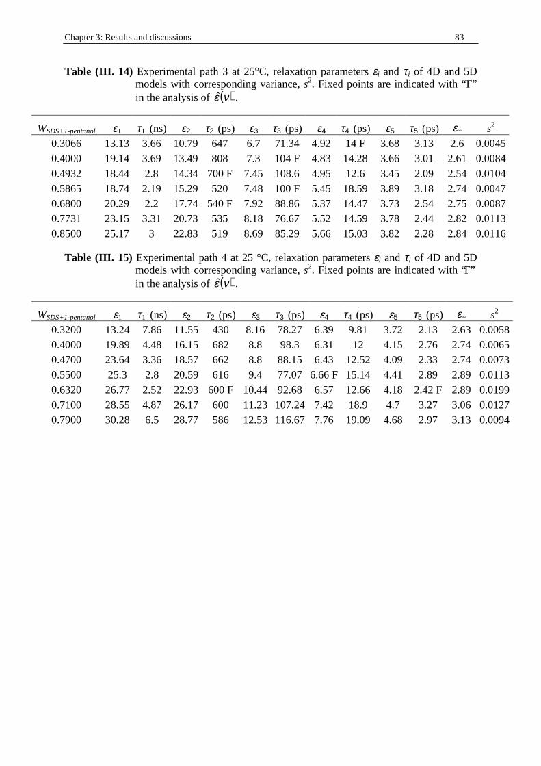
Chapter 3: Results and discussions 83
Table (III. 14) Experimental path 3 at 25°C, relaxation parameters εi and τi of 4D and 5D models with corresponding variance, s2. Fixed points are indicated with “F” in the analysis of ( )ε ν .
WSDS+1-pentanol ε1 τ1 (ns) ε2 τ2 (ps) ε3 τ3 (ps) ε4 τ4 (ps) ε5 τ5 (ps) ε s2 0.3066 13.13 3.66 10.79 647 6.7 71.34 4.92 14 F 3.68 3.13 2.6 0.0045 0.4000 19.14 3.69 13.49 808 7.3 104 F 4.83 14.28 3.66 3.01 2.61 0.0084 0.4932 18.44 2.8 14.34 700 F 7.45 108.6 4.95 12.6 3.45 2.09 2.54 0.0104 0.5865 18.74 2.19 15.29 520 7.48 100 F 5.45 18.59 3.89 3.18 2.74 0.0047 0.6800 20.29 2.2 17.74 540 F 7.92 88.86 5.37 14.47 3.73 2.54 2.75 0.0087 0.7731 23.15 3.31 20.73 535 8.18 76.67 5.52 14.59 3.78 2.44 2.82 0.0113 0.8500 25.17 3 22.83 519 8.69 85.29 5.66 15.03 3.82 2.28 2.84 0.0116
Table (III. 15) Experimental path 4 at 25 °C, relaxation parameters εi and τi of 4D and 5D models with corresponding variance, s2. Fixed points are indicated with “F” in the analysis of ( )ε ν .
WSDS+1-pentanol ε1 τ1 (ns) ε2 τ2 (ps) ε3 τ3 (ps) ε4 τ4 (ps) ε5 τ5 (ps) ε s2
0.3200 13.24 7.86 11.55 430 8.16 78.27 6.39 9.81 3.72 2.13 2.63 0.0058 0.4000 19.89 4.48 16.15 682 8.8 98.3 6.31 12 4.15 2.76 2.74 0.0065 0.4700 23.64 3.36 18.57 662 8.8 88.15 6.43 12.52 4.09 2.33 2.74 0.0073 0.5500 25.3 2.8 20.59 616 9.4 77.07 6.66 F 15.14 4.41 2.89 2.89 0.0113 0.6320 26.77 2.52 22.93 600 F 10.44 92.68 6.57 12.66 4.18 2.42 F 2.89 0.0199 0.7100 28.55 4.87 26.17 600 11.23 107.24 7.42 18.9 4.7 3.27 3.06 0.0127 0.7900 30.28 6.5 28.77 586 12.53 116.67 7.76 19.09 4.68 2.97 3.13 0.0094
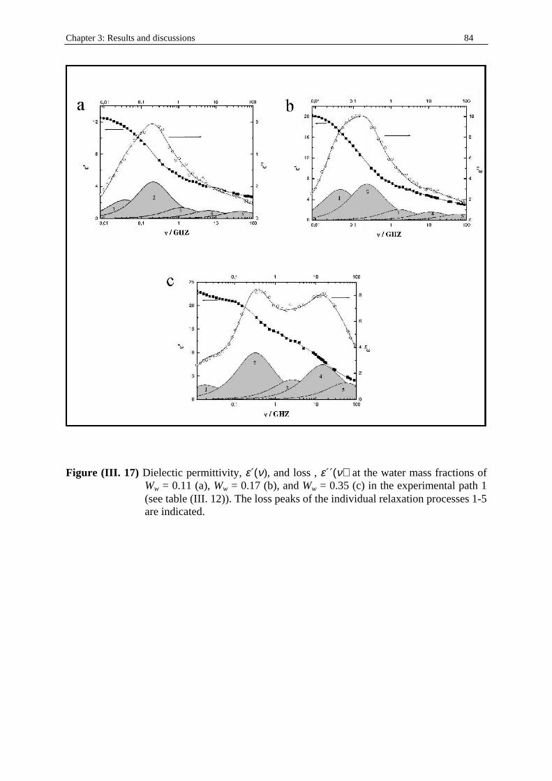
Chapter 3: Results and discussions 84
Figure (III. 17) Dielectic permittivity, ε´(ν), and loss , ε´´(ν) at the water mass fractions of
Ww = 0.11 (a), Ww = 0.17 (b), and Ww = 0.35 (c) in the experimental path 1 (see table (III . 12)). The loss peaks of the individual relaxation processes 1-5 are indicated.
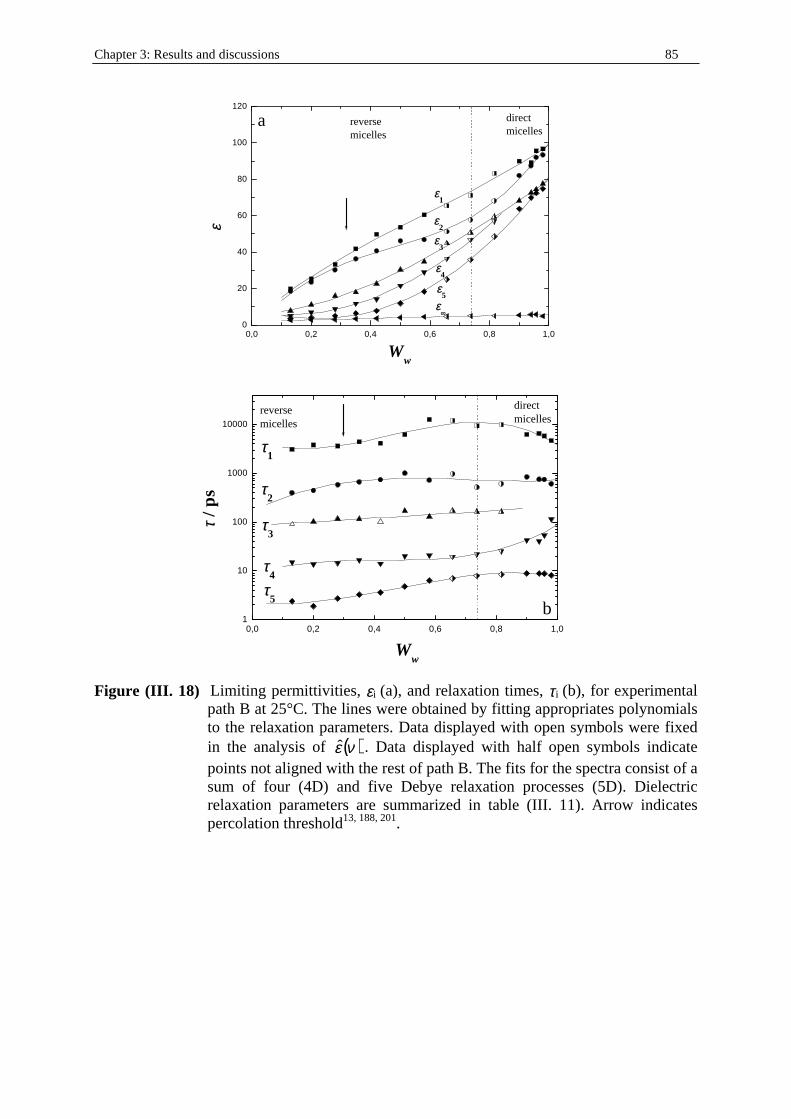
Chapter 3: Results and discussions 85
0,0 0,2 0,4 0,6 0,8 1,00
20
40
60
80
100
120
a direct micelles
reverse micelles
Ww
εε5
εε4
εε3
εε2
εε∞∞
εε1
εε
0,0 0,2 0,4 0,6 0,8 1,01
10
100
1000
10000
b
direct micelles
reverse micelles
Ww
ττ5
ττ4
ττ3
ττ2
ττ1
ττ / p
s
Figure (III. 18) Limiting permittivities, εi (a), and relaxation times, τi (b), for experimental path B at 25°C. The lines were obtained by fitting appropriates polynomials to the relaxation parameters. Data displayed with open symbols were fixed in the analysis of ( )νε . Data displayed with half open symbols indicate points not aligned with the rest of path B. The fits for the spectra consist of a sum of four (4D) and five Debye relaxation processes (5D). Dielectric relaxation parameters are summarized in table (III . 11). Arrow indicates percolation threshold13, 188, 201.
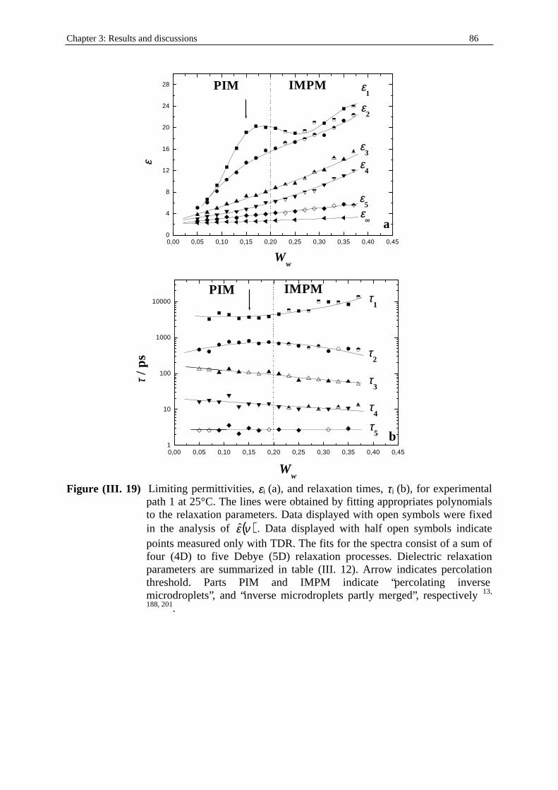
Chapter 3: Results and discussions 86
0,00 0,05 0,10 0,15 0,20 0,25 0,30 0,35 0,40 0,450
4
8
12
16
20
24
28
a
IMPMPIM
εε∞∞
εε5
εε4
εε3
εε2
εε1
εε
Ww
0,00 0,05 0,10 0,15 0,20 0,25 0,30 0,35 0,40 0,451
10
100
1000
10000
bττ
5
ττ4
ττ3
ττ2
ττ1
IMPMPIM
ττ / p
s
Ww
Figure (III. 19) Limiting permittivities, εi (a), and relaxation times, τi (b), for experimental path 1 at 25°C. The lines were obtained by fitting appropriates polynomials to the relaxation parameters. Data displayed with open symbols were fixed in the analysis of ( )νε . Data displayed with half open symbols indicate points measured only with TDR. The fits for the spectra consist of a sum of four (4D) to five Debye (5D) relaxation processes. Dielectric relaxation parameters are summarized in table (III . 12). Arrow indicates percolation threshold. Parts PIM and IMPM indicate “percolating inverse microdroplets”, and “inverse microdroplets partly merged”, respectively 13,
188, 201.
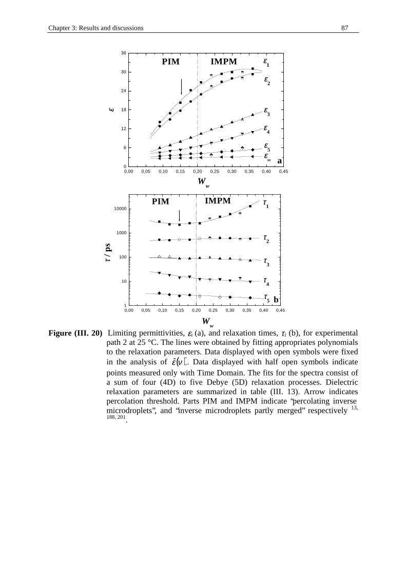
Chapter 3: Results and discussions 87
0,00 0,05 0,10 0,15 0,20 0,25 0,30 0,35 0,40 0,450
6
12
18
24
30
36
a
IMPMPIM
εε
Ww
εε∞∞
εε5
εε4
εε3
εε2
εε1
0,00 0,05 0,10 0,15 0,20 0,25 0,30 0,35 0,40 0,451
10
100
1000
10000
b
PIM IMPM
Ww
ττ / p
s
ττ5
ττ4
ττ3
ττ2
ττ1
Figure (III. 20) Limiting permittivities, εi (a), and relaxation times, τi (b), for experimental
path 2 at 25 °C. The lines were obtained by fitting appropriates polynomials to the relaxation parameters. Data displayed with open symbols were fixed in the analysis of ( )νε . Data displayed with half open symbols indicate points measured only with Time Domain. The fits for the spectra consist of a sum of four (4D) to five Debye (5D) relaxation processes. Dielectric relaxation parameters are summarized in table (III . 13). Arrow indicates percolation threshold. Parts PIM and IMPM indicate “percolating inverse microdroplets”, and “inverse microdroplets partly merged” respectively 13,
188, 201.
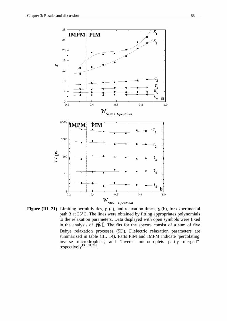
Chapter 3: Results and discussions 88
0,2 0,4 0,6 0,8 1,00
4
8
12
16
20
24
28
a
εε
WSDS + 1-pentanol
IMPM PIM
εε5
εε4
εε3
εε2
εε1
εε∞∞
0,2 0,4 0,6 0,8 1,01
10
100
1000
10000
b
PIMIMPM
ττ / p
s
WSDS + 1-pentanol
ττ5
ττ4
ττ3
ττ2
ττ1
Figure (III. 21) Limiting permittivities, εi (a), and relaxation times, τi (b), for experimental
path 3 at 25°C. The lines were obtained by fitting appropriates polynomials to the relaxation parameters. Data displayed with open symbols were fixed in the analysis of ( )νε . The fits for the spectra consist of a sum of f ive Debye relaxation processes (5D). Dielectric relaxation parameters are summarized in table (III . 14). Parts PIM and IMPM indicate “percolating inverse microdroplets”, and “inverse microdroplets partly merged” respectively13, 188, 201.
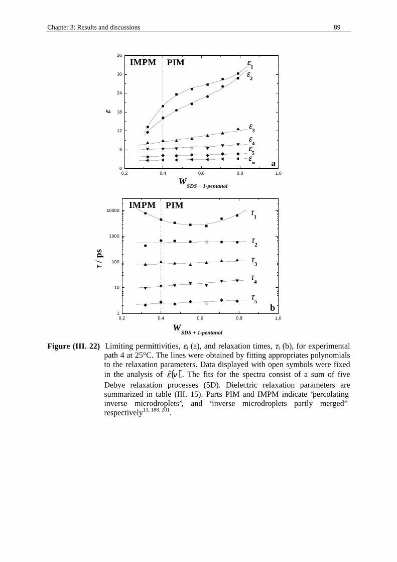
Chapter 3: Results and discussions 89
0,2 0,4 0,6 0,8 1,00
6
12
18
24
30
36
a
PIMIMPM
εε
WSDS + 1-pentanol
εε∞∞
εε5
εε4
εε3
εε2
εε1
0,2 0,4 0,6 0,8 1,01
10
100
1000
10000
bττ
5
ττ4
ττ3
ττ2
ττ1
ττ / p
s
WSDS + 1-pentanol
PIMIMPM
Figure (III. 22) Limiting permittivities, εi (a), and relaxation times, τi (b), for experimental
path 4 at 25°C. The lines were obtained by fitting appropriates polynomials to the relaxation parameters. Data displayed with open symbols were fixed in the analysis of ( )νε . The fits for the spectra consist of a sum of f ive Debye relaxation processes (5D). Dielectric relaxation parameters are summarized in table (III . 15). Parts PIM and IMPM indicate “percolating inverse microdroplets”, and “inverse microdroplets partly merged” respectively13, 188, 201.
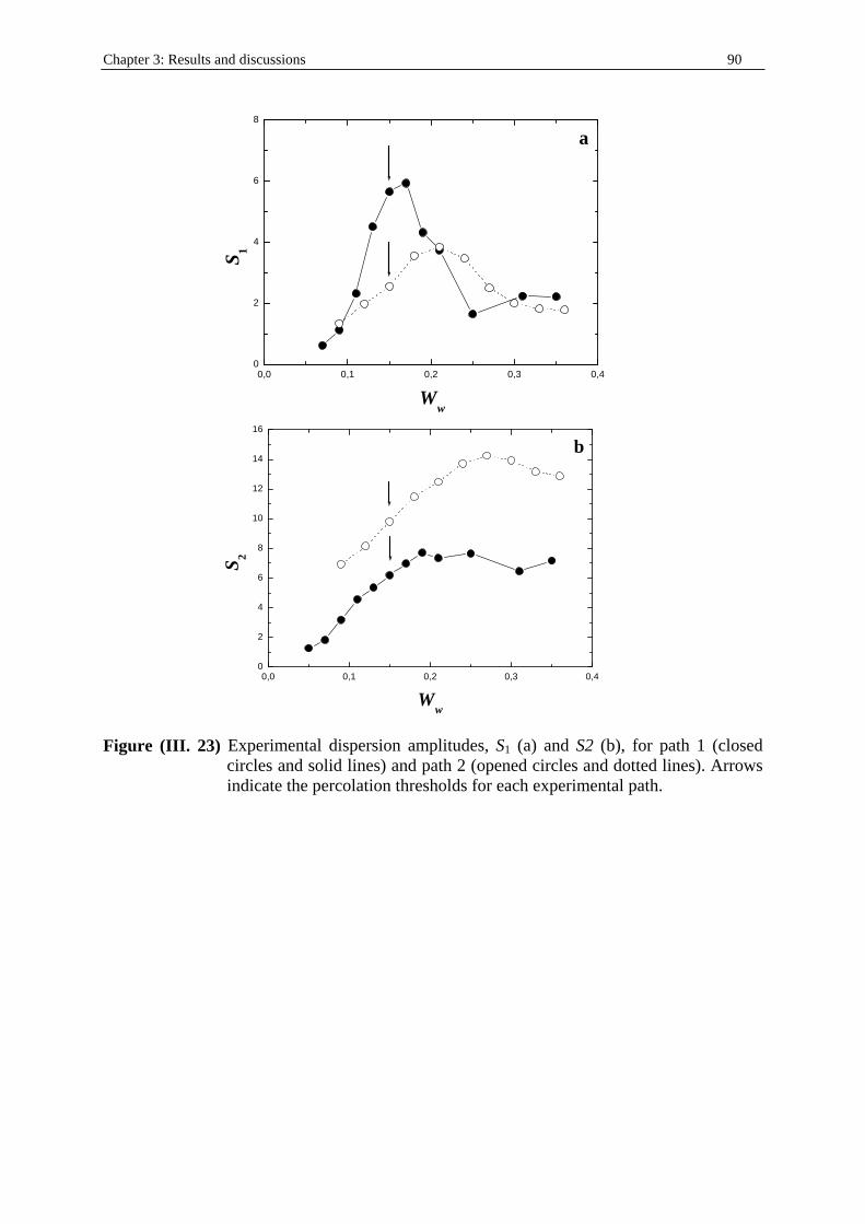
Chapter 3: Results and discussions 90
0,0 0,1 0,2 0,3 0,40
2
4
6
8
a
S 1
Ww
0,0 0,1 0,2 0,3 0,40
2
4
6
8
10
12
14
16
b
S 2
Ww
Figure (III. 23) Experimental dispersion amplitudes, S1 (a) and S2 (b), for path 1 (closed
circles and solid lines) and path 2 (opened circles and dotted lines). Arrows indicate the percolation thresholds for each experimental path.
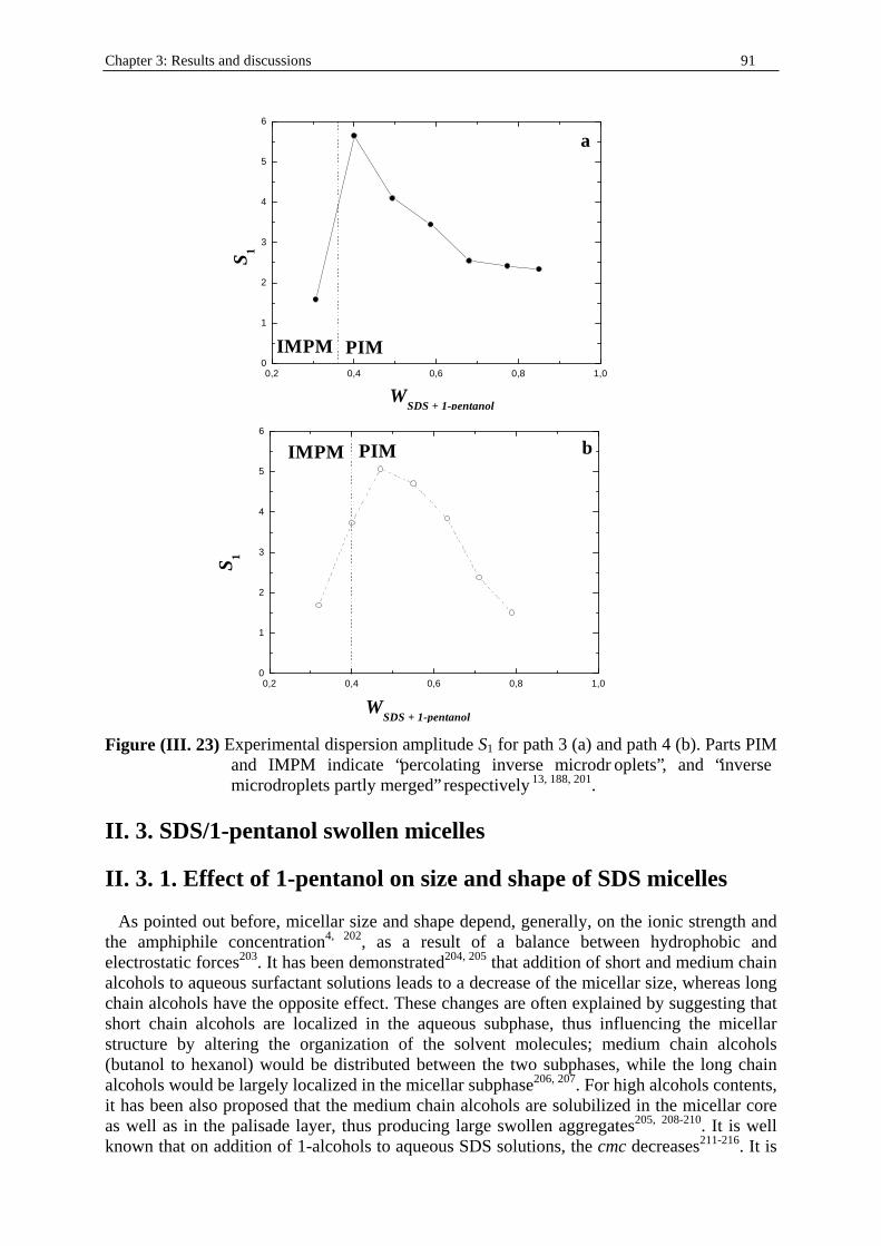
Chapter 3: Results and discussions 91
0,2 0,4 0,6 0,8 1,00
1
2
3
4
5
6
PIMIMPM
a
WSDS + 1-pentanol
S1
0,2 0,4 0,6 0,8 1,00
1
2
3
4
5
6
PIMIMPM b
S 1
WSDS + 1-pentanol
Figure (III. 23) Experimental dispersion amplitude S1 for path 3 (a) and path 4 (b). Parts PIM
and IMPM indicate “percolating inverse microdr oplets”, and “inverse microdroplets partly merged” respectively 13, 188, 201.
II. 3. SDS/1-pentanol swollen micelles
II. 3. 1. Effect of 1-pentanol on size and shape of SDS micelles As pointed out before, micellar size and shape depend, generally, on the ionic strength and the amphiphile concentration4, 202, as a result of a balance between hydrophobic and electrostatic forces203. It has been demonstrated204, 205 that addition of short and medium chain alcohols to aqueous surfactant solutions leads to a decrease of the micellar size, whereas long chain alcohols have the opposite effect. These changes are often explained by suggesting that short chain alcohols are localized in the aqueous subphase, thus influencing the micellar structure by altering the organization of the solvent molecules; medium chain alcohols (butanol to hexanol) would be distributed between the two subphases, while the long chain alcohols would be largely localized in the micellar subphase206, 207. For high alcohols contents, it has been also proposed that the medium chain alcohols are solubilized in the micellar core as well as in the palisade layer, thus producing large swollen aggregates205, 208-210. It is well known that on addition of 1-alcohols to aqueous SDS solutions, the cmc decreases211-216. It is
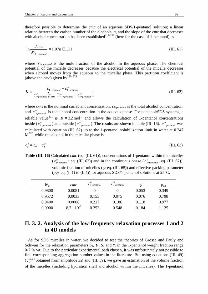
Chapter 3: Results and discussions 92
therefore possible to determine the cmc of an aqueous SDS/1-pentanol solution; a linear relation between the carbon number of the alcohols, n, and the slope of the cmc that decreases with alcohol concentration has been established217-219 (here for the case of 1-pentanol) as
11.107.1ln1
+=−
ndY
dcmc
pentanol
(III . 61)
where Y1-pentanol is the mole fraction of the alcohol in the aqueous phase. The chemical potential of the micelle decreases because the electrical potential of the micelle decreases when alcohol moves from the aqueous to the micellar phase. This partition coeff icient is (above the cmc) given by220, 221
( )wpentanolpentanolSDS
wpentanol
woltanpenoltanpen
cccc
ccK
−−−
−−
−+−
=111
11 (III . 62)
where cSDS is the nominal surfactant concentration; c1-pentanol is the total alcohol concentration, and w
lentanopc −1 is the alcohol concentration in the aqueous phase. For pentanol/SDS systems, a
reliable value221 is K = 32. mol-1 and allows the calculation of 1-pentanol concentrations inside ( m
lpentanoc −1 ) and outside ( wpentanolc −1 ). The results are shown in table (III . 16). m
lpentanoc −1 was
calculated with equation (III . 62) up to the 1-pentanol solubili zation limit in water at 0.247 M222, while the alcohol in the micellar phase is ca
m = ca − caw (III . 63)
Table (III. 16) Calculated cmc (eq. (III . 61)), concentrations of 1-pentanol within the micelles
( mlpentanoc −1 ; eq. (III . 62)) and in the continuous phase ( w
pentanolc −1 ; eq. (III . 62)),
volumic fraction of micelles (φ; eq. (III . 65)) and effective packing parameter (peff; eq. (I. 1) to (I. 4)) for aqueous SDS/1-pentanol solutions at 25°C.
Ww cmc w
pentanolc −1 mlpentanoc −1 φ peff
0.9800 0.0081 0 0 0.053 0.349 0.9572 0.0033 0.155 0.075 0.076 0.798 0.9400 0.0008 0.217 0.186 0.118 0.977 0.9000 8,7· 10-6 0.252 0.548 0.184 1.125
II. 3. 2. Analysis of the low-frequency relaxation processes 1 and 2 in 4D models
As for SDS micelles in water, we decided to test the theories of Grosse and Pauly and Schwan for the relaxation parameters S1, τ1, S2 and τ2 in the 1-pentanol weight fraction range 0-7 % wt. Due to the particular experimental path chosen, it was unfortunately not possible to find corresponding aggregation number values in the literature. But using equations (III . 49) ( bapp
wc , obtained from amplitude S4) and (III . 59), we gave an estimation of the volume fraction
of the micelles (including hydration shell and alcohol within the micelles). The 1-pentanol
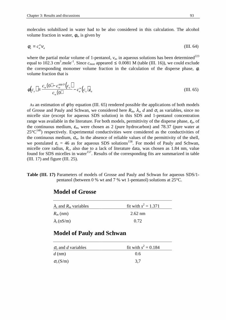
Chapter 3: Results and discussions 93
molecules solubili zed in water had to be also considered in this calculation. The alcohol volume fraction in water, φa, is given by φ νa a
wac= (III . 64)
where the partial molar volume of 1-pentanol, va, in aqueous solutions has been determined223 equal to 102.3 cm3.mole-1. Since cmon appeared ≤ 0.0081 M (table (III . 16)), we could exclude the corresponding monomer volume fraction in the calculation of the disperse phase, φ, volume fraction that is
( ) ( ) ( )( ) ( )φ c
c c c
cc c vs
w wapp b
s
waw
s a=−
−0
0
,
(III . 65)
As an estimation of φ by equation (III . 65) rendered possible the applications of both models of Grosse and Pauly and Schwan, we considered here Rm, λs, d and σs as variables, since no micelle size (except for aqueous SDS solution) in this SDS and 1-pentanol concentration range was available in the literature. For both models, permittivity of the disperse phase, εp, of the continuous medium, εm, were chosen as 2 (pure hydrocarbon) and 78.37 (pure water at 25°C140) respectively. Experimental conductivities were considered as the conductivities of the continuous medium, σm. In the absence of reliable values of the permittivity of the shell , we postulated εs = 46 as for aqueous SDS solutions158. For model of Pauly and Schwan, micelle core radius, Rc, also due to a lack of literature data, was chosen as 1.84 nm, value found for SDS micelles in water157. Results of the corresponding fits are summarized in table (III . 17) and figure (III . 25). Table (III. 17) Parameters of models of Grosse and Pauly and Schwan for aqueous SDS/1-
pentanol (between 0 % wt and 7 % wt 1-pentanol) solutions at 25°C.
Model of Grosse
λs and Rm variables fit with s2 = 1.371
Rm (nm) 2.62 nm
λs (nS/m) 0.72
Model of Pauly and Schwan
σs and d variables fit with s2 = 0.184 d (nm) 0.6
σs (S/m) 3,7
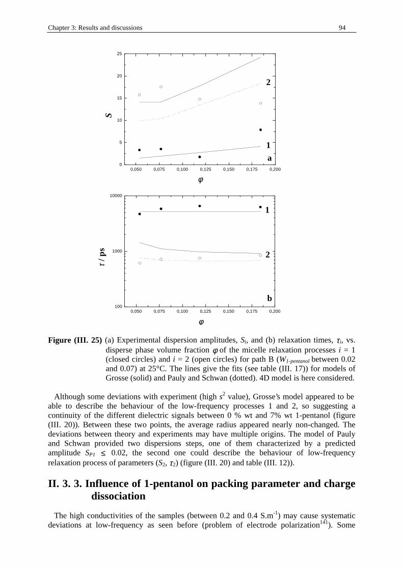
Chapter 3: Results and discussions 94
0,050 0,075 0,100 0,125 0,150 0,175 0,2000
5
10
15
20
25
2
1
a
S
φφ
0,050 0,075 0,100 0,125 0,150 0,175 0,200100
1000
10000
2
1
b
φφ
ττ / p
s
Figure (III. 25) (a) Experimental dispersion amplitudes, Si, and (b) relaxation times, τi, vs.
disperse phase volume fraction φ of the micelle relaxation processes i = 1 (closed circles) and i = 2 (open circles) for path B (W1-pentanol between 0.02 and 0.07) at 25°C. The lines give the fits (see table (III . 17)) for models of Grosse (solid) and Pauly and Schwan (dotted). 4D model is here considered.
Although some deviations with experiment (high s2 value), Grosse’s model appeared to be able to describe the behaviour of the low-frequency processes 1 and 2, so suggesting a continuity of the different dielectric signals between 0 % wt and 7% wt 1-pentanol (figure (III . 20)). Between these two points, the average radius appeared nearly non-changed. The deviations between theory and experiments may have multiple origins. The model of Pauly and Schwan provided two dispersions steps, one of them characterized by a predicted amplitude SP1 ≤ 0.02, the second one could describe the behaviour of low-frequency relaxation process of parameters (S2, τ2) (figure (III . 20) and table (III . 12)).
II. 3. 3. Influence of 1-pentanol on packing parameter and charge dissociation
The high conductivities of the samples (between 0.2 and 0.4 S.m-1) may cause systematic deviations at low-frequency as seen before (problem of electrode polarization141). Some
Chapter 3: Results and discussions 95
explanations for the deviations between theory (of Grosse and Pauly and Schwan) and experiments may be found in the literature. For instance 1-pentanol affects SDS micelle size and shape. 1-pentanol molecules solubili ze in the palisade layer221, 224 as well as in the micellar core in ionic micelles. When 1-pentanol molecules are solubili zed in the palisade layer of the micelle, they reduce the surface charge density and increase the counterion dissociation degree225-228 which effect may be explained as an increase of electrostatic repulsion between the sulfate polar heads, the micelles break down into smaller ones205, 222, 225. Surfactant enhanced ionization may increase the electrostatic repulsion between micelles and raise their total number229. Other authors213, 227 suggested that the penetration of alcohol molecules into the outer hydrophili c region should lower the electrostatic interaction between the surfactant headgroups, and makes the surfactant more energetically favourable for being a part of the micelles, and consequently a lowering the mixing free energy and cmc occurs. The presence of 1-pentanol molecules in the palisade layer promotes an increase of the effective packing parameter in the micelle (table (III . 12) and a swelli ng of the particle (the mean curvature tend to be more positive). As a consequence, shape transition that may occur should be of different types, for example to rod-like222, 230-233 or perhaps to oblate elli psoidal (disks) micelles225. These possible structural change would render inappropriate Grosse’s theory and the model of Pauly and Schwan in this surfactant and cosurfactant concentration range, although a certain agreement between experiment and theory could be found. Note also that micellar interaction would play an important role in the deviation between our experimental results and the theory, since this effect is ignored by both models of Grosse and Pauly and Schwan. Considering that all 1-pentanol molecules are located on the palisade layer and that the interaction between micelles remain weak, we made an evaluation of the effective packing parameter peff (equations (I. 1) to (I. 4)) with aSDS = 60 Å2 and a1-pentanol = 16 Å2. We observed that the effective packing parameter increased with increasing W1-pentanol (from 0 % wt to 7 % wt, peff passes from 0.34 to 1.16) supposing a transition spherical to elongated and bicontinuous structures (table (III . 16)). This observation is consistent with the apparition of bicontinuous structures (expected with the conductivity results) at higher WSDS and W1-pentanol
(~21 % wt). Another cause of experimental deviations to the model of Grosse may arise from the dielectric relaxation of alcohol molecules in both disperse and continuous phases. This point is treated in the next paragraph.
II. 3. 4. Contribution of 1-pentanol molecules to the dielectric relaxation
It has been shown that 1-pentanol present several relaxation processes in our frequency range. Garg and Smyth234 first analyzed their data in terms of three different relaxation times (three Debye model). This 3D model has been also succesfully applied to DRS spectra of shorter n-alkanols235, 236. In this spectral function the main dispersion located at several hundred of picoseconds is due to the cooperative process of hydrogen bonds (O-H· · · O) in the long-chain alcohol multimer. This cooperation induces a large dipole moment change so that the reorientation of monomers and dimers becomes less important in comparison; these high-frequency dispersion steps 2 and 3 were interpreted in terms of monomer relaxation and monomeric –CH2OH or –OH group rotation respectively234-236. With addition of nonpolar solvent some hydrogen bond in the alcohol multimer are broken and the chain length of multimers becomes shorter resulting in a decrease in the main relaxation time237-240. The same modifications in the main relaxation process are observed when substituting non-polar solvent by water241, 242.
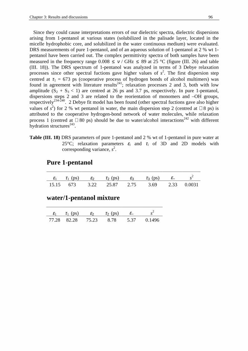
Chapter 3: Results and discussions 96
Since they could cause interpretations errors of our dielectric spectra, dielectric dispersions arising from 1-pentanol at various states (solubili zed in the palisade layer, located in the micelle hydrophobic core, and solubili zed in the water continuous medium) were evaluated. DRS measurements of pure 1-pentanol, and of an aqueous solution of 1-pentanol at 2 % wt 1-pentanol have been carried out. The complex permittivity spectra of both samples have been measured in the frequency range 0.008 ≤ ν / GHz ≤ 89 at 25 °C (figure (III . 26) and table (III . 18)). The DRS spectrum of 1-pentanol was analyzed in terms of 3 Debye relaxation processes since other spectral fuctions gave higher values of s2. The first dispersion step centred at τ1 = 673 ps (cooperative process of hydrogen bonds of alcohol multimers) was found in agreement with literature results241; relaxation processes 2 and 3, both with low amplitude (S2 + S3 < 1) are centred at 26 ps and 3.7 ps, respectively. In pure 1-pentanol, dispersions steps 2 and 3 are related to the reorientation of monomers and –OH groups, respectively234-240. 2 Debye fit model has been found (other spectral fuctions gave also higher values of s2) for 2 % wt pentanol in water, the main dispersion step 2 (centred at ∼ 8 ps) is attributed to the cooperative hydrogen-bond network of water molecules, while relaxation process 1 (centred at ∼ 80 ps) should be due to water/alcohol interactions242 with different hydration structures243. Table (III. 18) DRS parameters of pure 1-pentanol and 2 % wt of 1-pentanol in pure water at
25°C; relaxation parameters εi and τi of 3D and 2D models with corresponding variance, s2.
Pure 1-pentanol
ε1 τ1 (ps) ε2 τ2 (ps) ε3 τ3 (ps) ε s2 15.15 673 3.22 25.87 2.75 3.69 2.33 0.0031
water/1-pentanol mixture
ε1 τ1 (ps) ε2 τ2 (ps) ε s2 77.28 82.28 75.23 8.78 5.37 0.1496
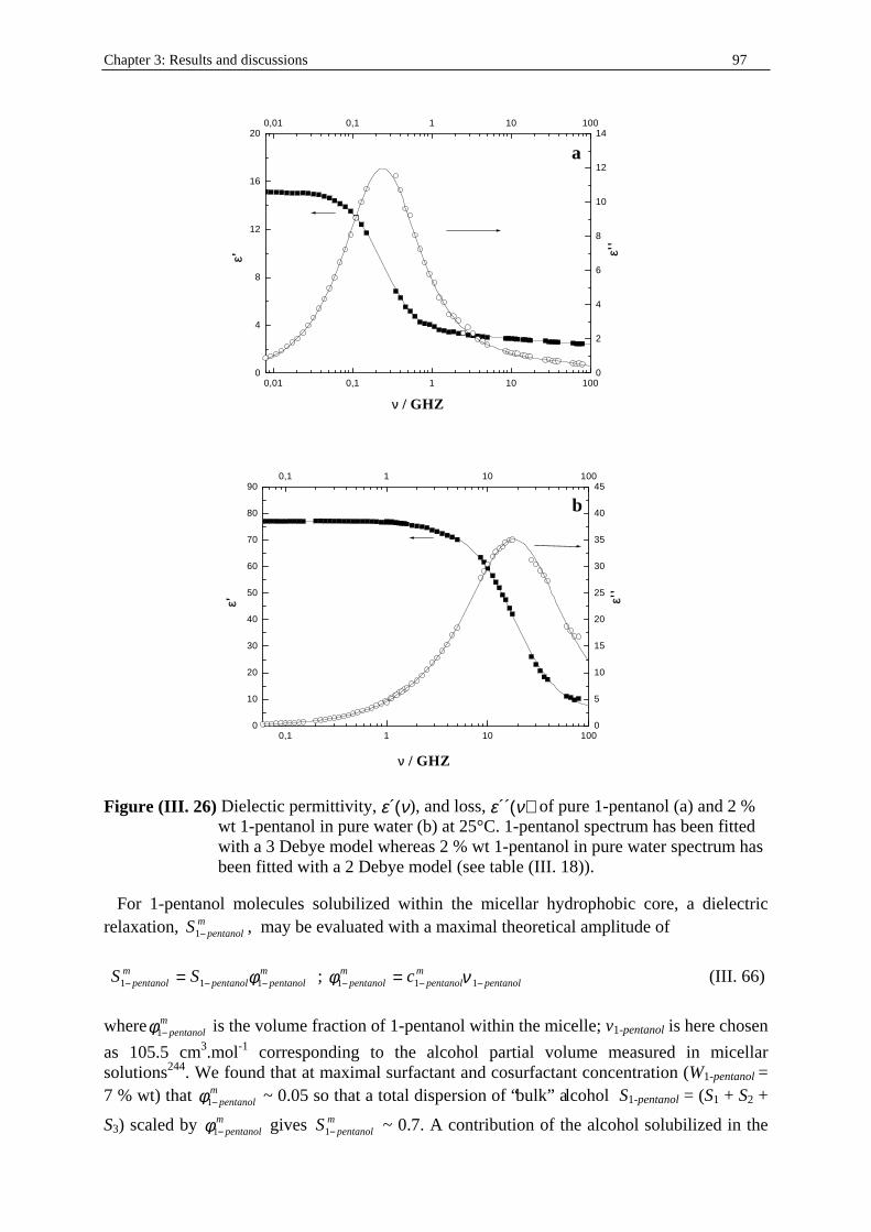
Chapter 3: Results and discussions 97
0,01 0,1 1 10 1000
4
8
12
16
20
a
νν / GHZ
εε ' εε ''
0,01 0,1 1 10 100
0
2
4
6
8
10
12
14
0,1 1 10 1000
10
20
30
40
50
60
70
80
90
b
νν / GHZ
εε ' εε ''
0,1 1 10 100
0
5
10
15
20
25
30
35
40
45
Figure (III. 26) Dielectic permittivity, ε´(ν), and loss, ε´´(ν) of pure 1-pentanol (a) and 2 %
wt 1-pentanol in pure water (b) at 25°C. 1-pentanol spectrum has been fitted with a 3 Debye model whereas 2 % wt 1-pentanol in pure water spectrum has been fitted with a 2 Debye model (see table (III . 18)).
For 1-pentanol molecules solubili zed within the micellar hydrophobic core, a dielectric relaxation, m
pentanolS −1 , may be evaluated with a maximal theoretical amplitude of
m
pentanolpentanolm
pentanol SS −−− = 111 φ ; pentanolm
pentanolm
pentanol c −−− = 111 νφ (III . 66)
where m
entanolp−1φ is the volume fraction of 1-pentanol within the micelle; v1-pentanol is here chosen
as 105.5 cm3.mol-1 corresponding to the alcohol partial volume measured in micellar solutions244. We found that at maximal surfactant and cosurfactant concentration (W1-pentanol = 7 % wt) that m
entanolp−1φ ~ 0.05 so that a total dispersion of “bulk” alcohol S1-pentanol = (S1 + S2 +
S3) scaled by mentanolp−1φ gives m
pentanolS −1 ~ 0.7. A contribution of the alcohol solubili zed in the
Chapter 3: Results and discussions 98
micelle should theoretically happen, but remember that a certain amount of this 1-pentanol should be located at the micelle surface and the alcohol molecules present within the core may interact with surfactant hydrophobic tails probably li ke in n-alkane/alcohol mixtures237-239. Therefore a dielectric relaxation arising from 1-pentanol within the core is considered as negligible. The alcohol molecules located at the micellar surface should also show a dielectric relaxation related to the rotation of their hydroxyl goups. This relaxation process in the case of pure 1-pentanol solutions is centred at around τ3 ∼ 3 ps with a dispersion amplitude of about 0.4. We suppose the alcohol molecule which hydrophobic tail “fixed” in the core and its C—OH group, orientated toward the external field. This assumption yields a theoretical amplitude, m
pentanolS −1 , that can be calculated (with help of equation (III . 30)) as
( )( )
( ) 0
2
1 112 εαµ
εε
Tk
N
f
cS
B
Am
ama
ma
mam
pentanol ⋅−
⋅+
=− (III . 67)
In equation (III . 67) the polarizabilit y αa
m (of 1.40861· 10-40 C2.m2/J) of the C—OH group was evaluated following Exner245 considering the semi-axes of the polarizabilit y. —OH group was assumed as a sphere of radius 0.9 Å and of dipole moment µOH corrected by the direction cosinus determined by the angle (θ-90) (where θ is the CCOH bond angle, equal to 107.4247°) of the dipole moment vector µOH and the given coordinates as
( )µ µ θam
OH= −cos 90 (III . 68) Sa
m was found varying from 0.0025 (2 % wt 1-pentanol) to 0.1 (74 % wt 1-pentanol). Therefore the dielectric increment related to a rotation of an alcohol hydroxyl group at the interface could be ignored. On the other hand the contribution of water/1-pentanol interaction in water can have a significant influence especially for high-frequency permittivity data. For 2 % wt 1-pentanol, the relaxation process centred at τ1 = 80 ps indicates hydrogen bonding247
resulting from water/1-pentanol interaction. This contribution has an amplitude of S1 ∼ 2 at alcohol concentration close to its solubilit y limit (at 2.2 % wt from Ginnings and Baum101). This makes that in path B, between 2 and 7 %wt 1-pentanol, the relaxation process centred at ∼ 50 ps may include both water-SDS headgroups and water-1-pentanol interactions.
II. 3. 5. High frequency DRS data analysis Between 0 % wt and 7 % wt 1-pentanol, the sum of amplitudes S3 + S4 increased linearly with the water content (figure (III . 27)) indicating that these signals are mainly due to different water motions, in accordance with the DRS results of water/SDS mixtures. As said before, this sum (S3 + S4) would include bulk and bound (to the micellar surface) water but also the solvent interaction with 1-pentanol as suggested by DRS measurement of a 2 % wt 1-pentanol in water solution (see part II. 3. 4.). Between 0 % wt and 7 % wt 1-pentanol, it has been found that the average number of irrotationally bound water, ZIB = 13 ± 5 (calculated with equations (III . 49) and (III . 57) from the sum (S3 + S4)). As indicated in table (I. 2), in this part of path B, the SDS concentration varies between 0.069 M and 0.102 M, concentrations for which nearly no irrotatinally bound water could be found in path A; this indicates that 1-pentanol favours the solvatation of SDS headgroups. This result emphasizes the role of 1-pentanol molecules on SDS counterion dissociation at the micellar surface.
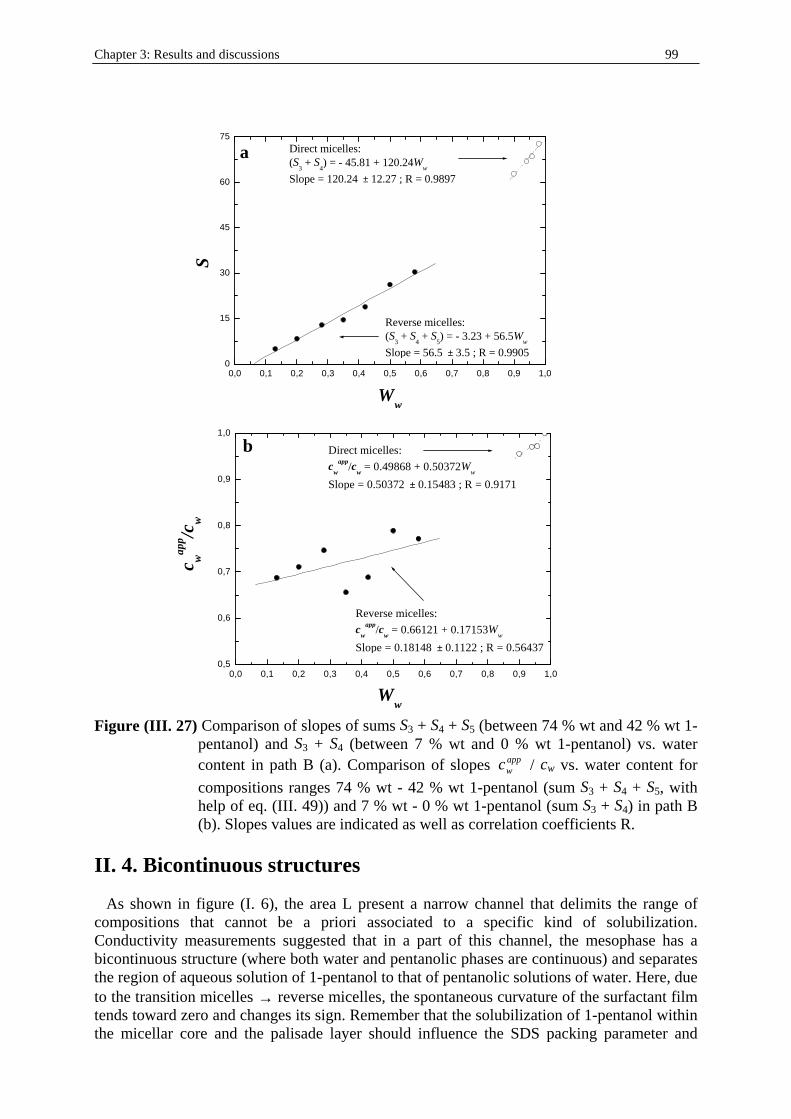
Chapter 3: Results and discussions 99
0,0 0,1 0,2 0,3 0,4 0,5 0,6 0,7 0,8 0,9 1,00
15
30
45
60
75
a
Direct micelles:(S
3 + S
4) = - 45.81 + 120.24W
w
Slope = 120.24 ± 12.27 ; R = 0.9897
Reverse micelles:(S
3 + S
4 + S
5) = - 3.23 + 56.5W
w
Slope = 56.5 ± 3.5 ; R = 0.9905
S
Ww
0,0 0,1 0,2 0,3 0,4 0,5 0,6 0,7 0,8 0,9 1,00,5
0,6
0,7
0,8
0,9
1,0
b
Reverse micelles:
cw
app/c
w = 0.66121 + 0.17153W
w
Slope = 0.18148 ± 0.1122 ; R = 0.56437
Direct micelles:
cw
app/c
w = 0.49868 + 0.50372W
w
Slope = 0.50372 ± 0.15483 ; R = 0.9171
Ww
c w
app /c
w
Figure (III. 27) Comparison of slopes of sums S3 + S4 + S5 (between 74 % wt and 42 % wt 1-
pentanol) and S3 + S4 (between 7 % wt and 0 % wt 1-pentanol) vs. water content in path B (a). Comparison of slopes app
wc / cw vs. water content for
compositions ranges 74 % wt - 42 % wt 1-pentanol (sum S3 + S4 + S5, with help of eq. (III. 49)) and 7 % wt - 0 % wt 1-pentanol (sum S3 + S4) in path B (b). Slopes values are indicated as well as correlation coefficients R.
II. 4. Bicontinuous structures As shown in figure (I. 6), the area L present a narrow channel that delimits the range of compositions that cannot be a priori associated to a specific kind of solubilization. Conductivity measurements suggested that in a part of this channel, the mesophase has a bicontinuous structure (where both water and pentanolic phases are continuous) and separates the region of aqueous solution of 1-pentanol to that of pentanolic solutions of water. Here, due to the transition micelles → reverse micelles, the spontaneous curvature of the surfactant film tends toward zero and changes its sign. Remember that the solubilization of 1-pentanol within the micellar core and the palisade layer should influence the SDS packing parameter and
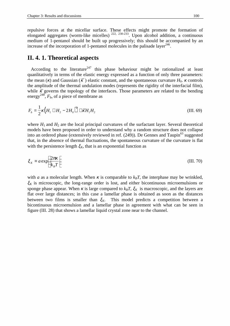
Chapter 3: Results and discussions 100
repulsive forces at the micellar surface. These effects might promote the formation of elongated aggregates (worm-like micelles) 222, 230-233. Upon alcohol addition, a continuous medium of 1-pentanol should be built up progressively; this should be accompanied by an increase of the incorporation of 1-pentanol molecules in the palisade layer246.
II. 4. 1. Theoretical aspects According to the literature247 this phase behaviour might be rationalized at least quanlitatively in terms of the elastic energy expressed as a function of only three parameters: the mean (κ) and Gaussian (κ ) elastic constant, and the spontaneous curvature H0. κ controls the amplitude of the thermal undulation modes (represents the rigidity of the interfacial film), while κ governs the topology of the interfaces. Those parameters are related to the bending energy248, Fb, of a piece of membrane as
( )F H H H H Hb = + − +1
221 2 0
2
1 2κ κ (III. 69)
where H1 and H2 are the local principal curvatures of the surfactant layer. Several theoretical models have been proposed in order to understand why a random structure does not collapse into an ordered phase (extensively reviewed in ref. (249)). De Gennes and Taupin63 suggested that, in the absence of thermal fluctuations, the spontaneous curvature of the curvature is flat with the persistence length ξK, that is an exponential function as
=
Tka
BK
πκξ 2exp (III. 70)
with a as a molecular length. When κ is comparable to kBT, the interphase may be wrinkled, ξK is microscopic, the long-range order is lost, and either bicontinuous microemulsions or sponge phase appear. When κ is large compared to kBT, ξK is macroscopic, and the layers are flat over large distances; in this case a lamellar phase is obtained as soon as the distances between two films is smaller than ξK. This model predicts a competition between a bicontinuous microemulsion and a lamellar phase in agreement with what can be seen in figure (III. 28) that shows a lamellar liquid crystal zone near to the channel.
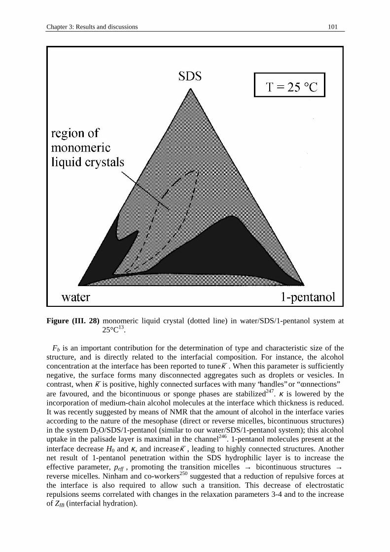
Chapter 3: Results and discussions 101
Figure (III. 28) monomeric liquid crystal (dotted line) in water/SDS/1-pentanol system at
25°C13. Fb is an important contribution for the determination of type and characteristic size of the structure, and is directly related to the interfacial composition. For instance, the alcohol concentration at the interface has been reported to tuneκ . When this parameter is suff iciently negative, the surface forms many disconnected aggregates such as droplets or vesicles. In contrast, when κ is positive, highly connected surfaces with many “handles” or “connections” are favoured, and the bicontinuous or sponge phases are stabili zed247. κ is lowered by the incorporation of medium-chain alcohol molecules at the interface which thickness is reduced. It was recently suggested by means of NMR that the amount of alcohol in the interface varies according to the nature of the mesophase (direct or reverse micelles, bicontinuous structures) in the system D2O/SDS/1-pentanol (similar to our water/SDS/1-pentanol system); this alcohol uptake in the palisade layer is maximal in the channel246. 1-pentanol molecules present at the interface decrease H0 and κ, and increaseκ , leading to highly connected structures. Another net result of 1-pentanol penetration within the SDS hydrophili c layer is to increase the effective parameter, peff , promoting the transition micelles → bicontinuous structures → reverse micelles. Ninham and co-workers250 suggested that a reduction of repulsive forces at the interface is also required to allow such a transition. This decrease of electrostatic repulsions seems correlated with changes in the relaxation parameters 3-4 and to the increase of ZIB (interfacial hydration).
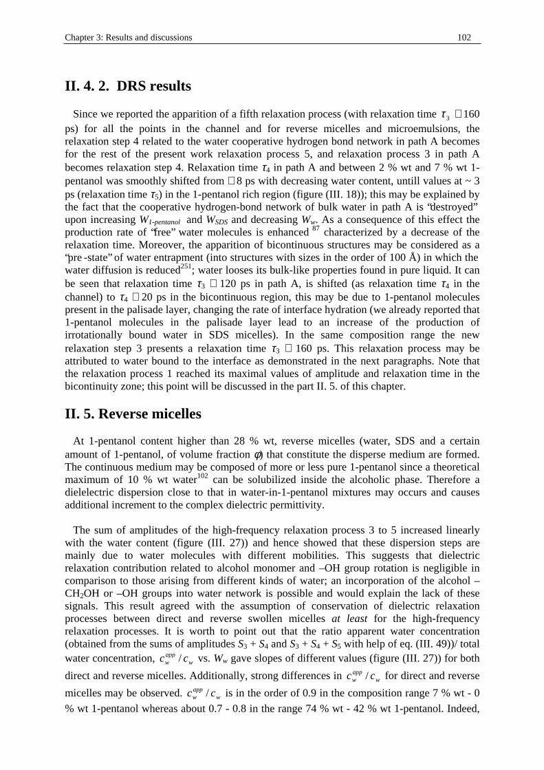
Chapter 3: Results and discussions 102
II. 4. 2. DRS results Since we reported the apparition of a fifth relaxation process (with relaxation time τ3 ∼ 160 ps) for all the points in the channel and for reverse micelles and microemulsions, the relaxation step 4 related to the water cooperative hydrogen bond network in path A becomes for the rest of the present work relaxation process 5, and relaxation process 3 in path A becomes relaxation step 4. Relaxation time τ4 in path A and between 2 % wt and 7 % wt 1-pentanol was smoothly shifted from ∼ 8 ps with decreasing water content, untill values at ~ 3 ps (relaxation time τ5) in the 1-pentanol rich region (figure (III . 18)); this may be explained by the fact that the cooperative hydrogen-bond network of bulk water in path A is “destroyed” upon increasing W1-pentanol and WSDS and decreasing Ww. As a consequence of this effect the production rate of “free” water molecules is enhanced 87 characterized by a decrease of the relaxation time. Moreover, the apparition of bicontinuous structures may be considered as a “pre-state” of water entrapment (into structures with sizes in the order of 100 Å) in which the water diffusion is reduced251; water looses its bulk-like properties found in pure liquid. It can be seen that relaxation time τ3 ∼ 120 ps in path A, is shifted (as relaxation time τ4 in the channel) to τ4 ∼ 20 ps in the bicontinuous region, this may be due to 1-pentanol molecules present in the palisade layer, changing the rate of interface hydration (we already reported that 1-pentanol molecules in the palisade layer lead to an increase of the production of irrotationally bound water in SDS micelles). In the same composition range the new relaxation step 3 presents a relaxation time τ3 ∼ 160 ps. This relaxation process may be attributed to water bound to the interface as demonstrated in the next paragraphs. Note that the relaxation process 1 reached its maximal values of amplitude and relaxation time in the bicontinuity zone; this point will be discussed in the part II. 5. of this chapter.
II. 5. Reverse micelles At 1-pentanol content higher than 28 % wt, reverse micelles (water, SDS and a certain amount of 1-pentanol, of volume fraction φ) that constitute the disperse medium are formed. The continuous medium may be composed of more or less pure 1-pentanol since a theoretical maximum of 10 % wt water102 can be solubili zed inside the alcoholic phase. Therefore a dielelectric dispersion close to that in water-in-1-pentanol mixtures may occurs and causes additional increment to the complex dielectric permittivity. The sum of amplitudes of the high-frequency relaxation process 3 to 5 increased linearly with the water content (figure (III . 27)) and hence showed that these dispersion steps are mainly due to water molecules with different mobiliti es. This suggests that dielectric relaxation contribution related to alcohol monomer and –OH group rotation is negligible in comparison to those arising from different kinds of water; an incorporation of the alcohol –CH2OH or –OH groups into water network is possible and would explain the lack of these signals. This result agreed with the assumption of conservation of dielectric relaxation processes between direct and reverse swollen micelles at least for the high-frequency relaxation processes. It is worth to point out that the ratio apparent water concentration (obtained from the sums of amplitudes S3 + S4 and S3 + S4 + S5 with help of eq. (III . 49))/ total water concentration, w
appw cc / vs. Ww gave slopes of different values (figure (III . 27)) for both
direct and reverse micelles. Additionally, strong differences in wappw cc / for direct and reverse
micelles may be observed. wappw cc / is in the order of 0.9 in the composition range 7 % wt - 0
% wt 1-pentanol whereas about 0.7 - 0.8 in the range 74 % wt - 42 % wt 1-pentanol. Indeed,
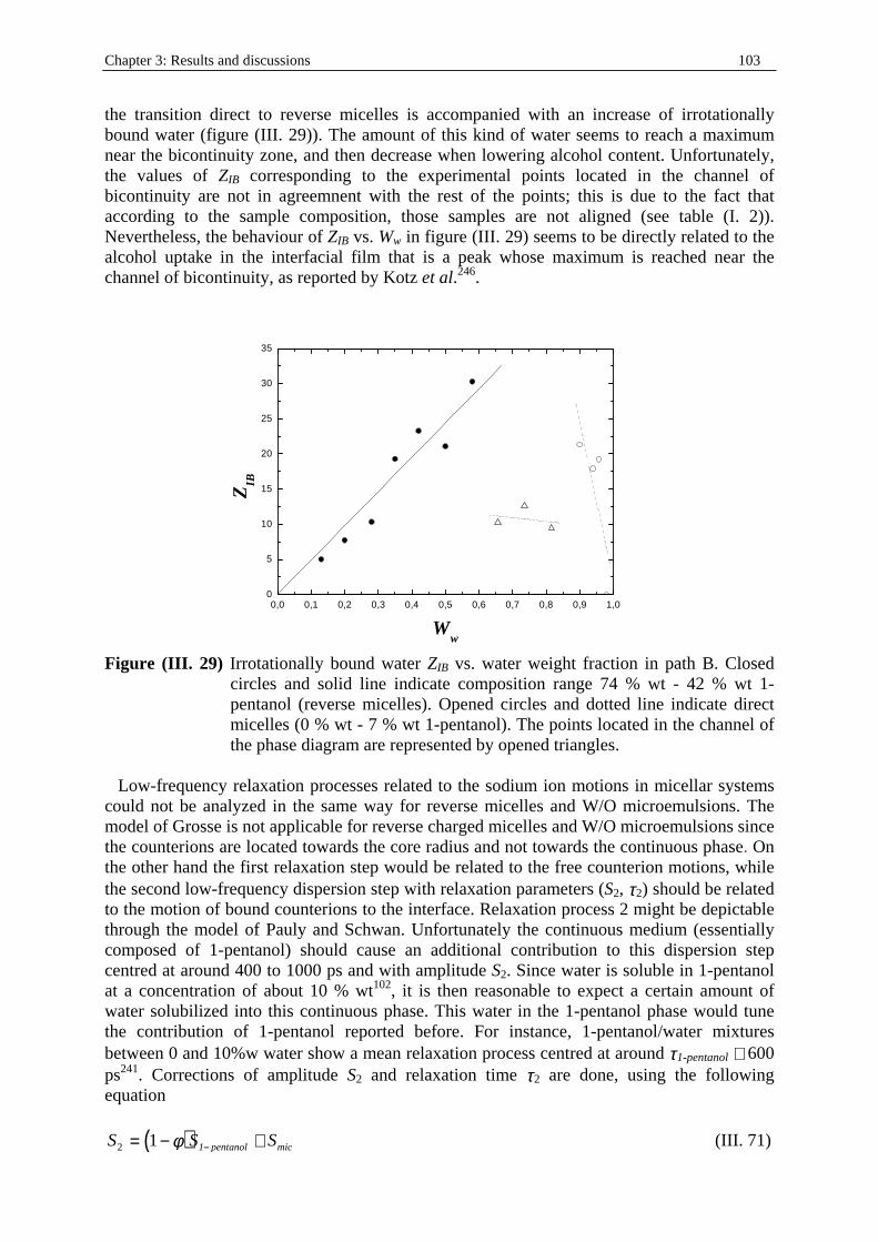
Chapter 3: Results and discussions 103
the transition direct to reverse micelles is accompanied with an increase of irrotationally bound water (figure (III. 29)). The amount of this kind of water seems to reach a maximum near the bicontinuity zone, and then decrease when lowering alcohol content. Unfortunately, the values of ZIB corresponding to the experimental points located in the channel of bicontinuity are not in agreemnent with the rest of the points; this is due to the fact that according to the sample composition, those samples are not aligned (see table (I. 2)). Nevertheless, the behaviour of ZIB vs. Ww in figure (III. 29) seems to be directly related to the alcohol uptake in the interfacial film that is a peak whose maximum is reached near the channel of bicontinuity, as reported by Kotz et al.246.
0,0 0,1 0,2 0,3 0,4 0,5 0,6 0,7 0,8 0,9 1,00
5
10
15
20
25
30
35
ZIB
Ww
Figure (III. 29) Irrotationally bound water ZIB vs. water weight fraction in path B. Closed
circles and solid line indicate composition range 74 % wt - 42 % wt 1-pentanol (reverse micelles). Opened circles and dotted line indicate direct micelles (0 % wt - 7 % wt 1-pentanol). The points located in the channel of the phase diagram are represented by opened triangles.
Low-frequency relaxation processes related to the sodium ion motions in micellar systems could not be analyzed in the same way for reverse micelles and W/O microemulsions. The model of Grosse is not applicable for reverse charged micelles and W/O microemulsions since the counterions are located towards the core radius and not towards the continuous phase. On the other hand the first relaxation step would be related to the free counterion motions, while the second low-frequency dispersion step with relaxation parameters (S2, τ2) should be related to the motion of bound counterions to the interface. Relaxation process 2 might be depictable through the model of Pauly and Schwan. Unfortunately the continuous medium (essentially composed of 1-pentanol) should cause an additional contribution to this dispersion step centred at around 400 to 1000 ps and with amplitude S2. Since water is soluble in 1-pentanol at a concentration of about 10 % wt102, it is then reasonable to expect a certain amount of water solubilized into this continuous phase. This water in the 1-pentanol phase would tune the contribution of 1-pentanol reported before. For instance, 1-pentanol/water mixtures between 0 and 10%w water show a mean relaxation process centred at around τ1-pentanol ∼ 600 ps241. Corrections of amplitude S2 and relaxation time τ2 are done, using the following equation
( )S S Smic2 1= − +−φ 1 pentanol (III. 71)
Chapter 3: Results and discussions 104
with Smic as the effect of bound counterion motions. There is no knowledge of the amount of solubilized water in the continuous phase, therefore the exact amplitude, S1-pentanol, modified by water interactions (in the case of pure 1-pentanol, this amplitude is about 12) is not known. The relaxation time τ2 is
9
( ) ( ) ( ) ( )( ) lpentanomic
pentanolmicmic
SS
SS
−
−
−+−+
=1
12 1
ln1lnln
φτφτ
τ (III. 72)
Application of equations (III. 72) and (III. 73) requires also the knowledge of φ that may be found with help of conductivity measurements. Remember that the model of Pauly and Schwan is applicable only to dilute systems since it neglects interparticle interactions. If applied, this model would be at most available at volume fraction φ < φP , whereφP is the volume fraction of the disperse phase at the percolation threshold. The choice of the input parameters for this model is complicated by the lack of literature data (permittivities of disperse phase and interfacial film...) and, as indicated before, there is no reliable data that provides a partitioning of the different compounds in the different phases. Nevertheless this information can be provided by analyzing the conductivity data with approximate equations for concentrated dispersions particles such as EMT. In order to give a comparable study of the pentanolic zone of the ternary system and of the W/O zone of the quaternary microemulsion system, both were treated at the same time.
II. 5. 1. Conductivity of W/O microemulsions and reverse micelles As previously reported by Schulman and co-workers252, 253, depending on the number and the arrangement of carbon atoms for both cosurfactant and oil, drastic changes in the electrocondutive behaviour of microemulsion-type media can be observed. Clausse et al.13 proved that the electroconductive behaviour of SDS/1-pentanol microemulsions can be depicted by means of equations derived from the percolation and effective medium theories193-201, whereas that of 1-hexanol cannot. More systematic investigations into this problem of the influence of constitution parameters on microemulsion physiochemical properties were carried out first by Heil and co-workers254, 255, on systems incorporating potassium oblate as surfactant, and later by Zradba, Nicolas-Morgantoni, and co-workers13,
256-259, on systems incorporating sodium dodecyl sulfate as surfactant. From the results thus obtained, it appears that a correlation exists between system type (U or S) and microemulsion transport properties such as viscosity and electrical conductivity. For instance, the electroconductive behaviour of the 1-butanol and 1-pentanol microemulsions (type U) is strikingly different from that of the 1-heptanol and 1-hexanol microemulsions. In the case of the shorter n-alkanols, the electrical conductivity increases continuously as the water content increases, and its variations may be depicted through the percolation and effective medium theories. In contrast, no percolation is observed in the case of the 1-heptanol and 1-hexanol microemulsions; their electrical conductivity remains quite low in comparison to that of U-type systems and is a non-monotonic function of the water content. Nearly similar comments may be made with regard to microemulsion viscous behaviour.
II. 5. 1. 1. Theory of percolation in W/O microemulsions It is considered that during percolation, association of water droplets occurs and either the surfactant ions travel by “hopping” mechanism 199, 201, 260, 261 or the counterions are exchanged
Chapter 3: Results and discussions 105
between droplets262-264 which effectively manifests in rapid increase of conductance. When a percolation phenomenon occurs in microemulsions, a dynamic or a static percolation may be identified188, 201, 265-268, corresponding respectively to the formation of clusters of droplets or to the coalescence of the droplets into water channels (bicontinuous structures). In the dilute region, the electrical conduction mechanism is interpreted in terms of the droplet charge fluctuations model269-271, i.e., the droplets, on the average electrically neutral, can carry excess charge due to spontaneous thermal fluctuations of composition, and migrate in an electric field. Two different ways of investigation of percolation phenomenon in microemulsion are considered; one is the power scaling law (PSL)265, 266, 272, the other is the effective medium theory193-201. In the PSL approach the conductivity follows the scaling laws
( )σ σ φ φ= −−
c m P
s
2 (III . 73)
below the percolation threshold, and
( ) ( )µφφσφφσσ Pds
Pm cc −+−′= −11 (III . 74)
above the percolation threshold. c1, c2, and ′c1 are constants. σm and σd are conductivity of
continuous and dispersed phases respectively. σ is the conductivity of the mixture, φ is the volume fraction of the microdisperse phase, and φP is the volume fraction at the percolation
threshold. The µ exponent is in the range from 1.5 to 2 for both static and dynamic percolation, whereas s = 0.6 to 0.7 for static and around 1.2 for dynamic percolation270, 271. Results agreeing272-276 with the theory are found in the literature. In the present work, since experimental paths 1, 2 and B lead by droplet coalescence to the formation of bicontinuous structures, the percolation is static. In the effective medium theory (EMT), the equation of Böttcher is equivalent to the scaling law under certain boundary conditions. For binary mixture having σm and σd, Böttcher proposed that the conductance of the mixture is related to the volume fraction of the dispersed phase by194
σ σ
σσ σσ σ
φ−
=−+
m d m
d3 2 (III . 75)
For a continuous medium of very low or practically zero conductances (σm = 0), Equation (III . 75) transforms into the scaling form for µ = 1:
σ σ φ= −
3
2
1
3d (III . 76)
The equation suggests a percolation threshold at φ = 1/3, and, if valid, it can evaluate the disperse-phase conductance σd (with c1 = 3/2) from the measured values of σ at several volumes fractions of the disperse phase. The EMT theory of Böttcher194 can be used for quantitative accounting of the structural parameters of microemulsions systems with cosurfactant277-279. For microheterogeneous dispersions of metal and metal oxides in suitable media196, the EMT has been shown to be often inadequate, and modifications have been put
Chapter 3: Results and discussions 106
forward. The percolation threshold (one-third of volume fraction of the dispersion) according to the EMT theory of Böttcher194 is not always a practical li mit. A number of authors189, 190,
196, 197, 280 suggested that the percolation threshold in practice is often≤ 1 3/ . Granqvist and Hunderi196 have shown that the lower percolation threshold can be theoretically accounted for dipole-dipole interactions among the dispersed entities. This theory has been termed as effective medium theory with dipole-dipole interactions (EMTDD). This kind of interaction may lead to the formation of chains or clusters in the dispersion. The EMT theory has considered only random distribution of spherical particles, aggregation leading to chain or cluster formation has been ignored. In the line of the modifications of Granqvist and Hunderi, Bernasconi and Wiesman197 (BW) introduced a relation for percolation for cluster forming dispersions, which also recognizes a lower percolation threshold than that given in the EMT theory. The validity of the above theories has been established for microdispersions of solids in suitable media and then successfully tested in W/O microemulsions277-279. The association of disperse particles due to interaction may form entities with shapes different from spheres. Aggregates of prolate and oblate geometry may come into existence in solution. The theories, therefore, can treat samples containing nonspherical inclusions. To test the validity of a percolation equation an estimate of the volume fraction of the disperse phase is essential. For a microemulsion system, this very often remains a guess owing to the well -defined interphase between oil and water, particularly in the presence of a cosurfactant. In the absence of a cosurfactant, this interphase layer is only constituted by the surfactant. The volume fraction of the disperse phase is, therefore, defined as the total sum of the fraction of water and the surfactant. When a cosurfactant is required for the preparation, its distribution among the oil phase, interphase and water phase is diff icult to know. A direct estimation of volume fraction of the droplets is hardly possible, and it is not easy to put the percolation theories to test. Fang and Venable277 as well as Bisal et al.278, 279 have ill ustrated an analytical approach to deal with the complexity of direct evaluation of conducting microdroplets. This makes microemulsions amenable to analysis in the light of the EMT theory. Theory of EMTDD is represented as follows
( )( )( )
1
3
1
20φλ
φ σ σσ σ
+− −
−=m d
m d
(III . 77)
where
( )( )
λσ σ
σ σ σ=
−
+ −
d
d d
1
3
(III . 78)
The factor λ is proportional to the polarizabilit y (for a sphere, the depolarization factor is 1/3).For randomly oriented elli psoid, the general form is
( )( )[ ]λ
σ σ
σ σ σ=
−
+ −=∑1
3 1
3d
d i di L (III . 79)
where Li denotes the triplet of depolarization factor dictated by the axial ratios. The combined form of equations (III . 77) and (III . 79) can describe the conductivity behaviour of nonspherical dispersions. Since aggregation of spheres can form infinite chains
Chapter 3: Results and discussions 107
(with overall prolate geometry) and closed-packed clusters (with overall oblate geometry), they can be considered as separate nonspherical entities to which the EMTDD theory can be applied. The above equations predict that the dipole-dipole interaction should always shift the percolation threshold toward lower concentration of the conducting material. For σm = 0, the φP
EMTDD becomes 0.271 for chains and 0.156 for clusters. The equivalent depolarization factors L1, L2, and L3 for isolated spheres are each equal to 1/3, which for single-stranded chain are 0.133, 0.435, and 0.435 respectively, and for close-packed lattice the values are 0.0865, 0.0865, and 0.827, respectively. Assuming σm = 0 and transforming equation (III . 79) and its subsequent insertion into equation (III . 78) yield the following relations: For isolated spheres the equation of Böttcher. For chains196
[ ]σ σ φ φ φ σ= − + + −01519 01566 17216 07292 3. . . .d d (III . 80)
For clusters196
[ ]σ σ φ φ σ= − + +00984 0539 05679 2. . .d d (III . 81)
It is imperative that precise values of σ and φ be determined for the verification of the theories and to derive σd. Bernasconi and Wiesman197 have proposed a cluster extension of the EMT and derived the equation
( )σ σ φ= −105 0157. .d for φ ≥ 0157. (III . 82)
The percolation threshold of EMTDDclusters (φP
EMTDD = 0.156) is in exact agreement with that in equation (III . 76). Bernasconi and Wiesman204 have shown that the theory may be valid up to φ ≤ 3 4/ . For greaterφ, the equation transforms into the form of EMT. Fang and Venable277 proposed a way to obtain the volume fraction of the disperse phase as
φρρ
= +
+
total
dS
CS
SWW r
M
MW1 (III . 83)
where ρd and ρtotal are the densities of the disperse phase and the total solution respectively. WS, and WW are the weight fractions of surfactant and water, respectively; MCS and MS are the molar masses of cosurfactant and surfactant respectively. The average ratio of surfactant to cosurfactant, r, in the interphase is given by
rn
nCSint
S
= (III . 84)
where nCS
int is the mole number of cosurfactant in the interphase, and nS is the mole number of
surfactant in the system. On the other hand, φ can be calculated using the partial volumes of each component with:
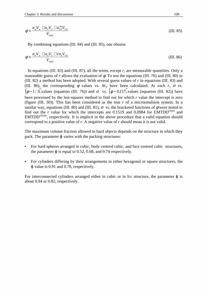
Chapter 3: Results and discussions 108
φ =+ +n V n V n V
Vw w S S CS
intCS
total
(III. 85)
By combining equations (III. 84) and (III. 85), one obtains
φ =+ +n V n V rn V
Vw w S S S CS
total
(III. 86)
In equations (III. 83) and (III. 87), all the terms, except r, are measurable quantities. Only a reasonable guess of r allows the evaluation of φ. To test the equations (III. 76) and (III. 80) to (III. 82) a method has been adopted. With several guess values of r in equations (III. 83) and (III. 86), the corresponding φ values vs. Ww have been calculated. At each r, σ vs.
( )φ − 1 3/ values (equation (III. 76)) and σ vs. ( )φ − 0157. values (equation (III. 82)) have
been processed by the lest-squares method to find out for which r value the intercept is zero (figure (III. 30)). This has been considered as the true r of a microemulsion system. In a similar way, equations (III. 80) and (III. 81), σ vs. the bracketed functions of φ were tested to find out the r value for which the intercepts are 0.1519 and 0.0984 for EMTDDchain and EMTDDcluster, respectively. It is implicit in the above procedure that a valid equation should correspond to a positive value of r. A negative value of r should mean it is not valid.
The maximum volume fraction allowed to hard objects depends on the structure in which they pack. The parameter ϕ varies with the packing structures: • For hard spheres arranged in cubic, body centred cubic, and face centred cubic structures,
the parameter ϕ is equal to 0.52, 0.68, and 0.74 respectively. • For cylinders differing by their arrangements in either hexagonal or square structures, the
ϕ value is 0.91 and 0.78, respectively. For interconnected cylinders arranged either in cubic or in fcc structure, the parameter ϕ is about 0.94 or 0.82, respectively.
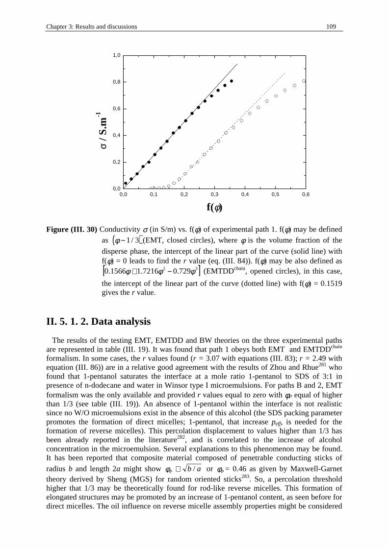
Chapter 3: Results and discussions 109
0,0 0,1 0,2 0,3 0,4 0,5 0,60,0
0,2
0,4
0,6
0,8
1,0
σσ / S
.m-1
f(φφ)
Figure (III. 30) Conductivity σ (in S/m) vs. f(φ) of experimental path 1. f(φ) may be defined
as ( )φ − 1 3/ (EMT, closed circles), where φ is the volume fraction of the
disperse phase, the intercept of the linear part of the curve (solid line) with f(φ) = 0 leads to find the r value (eq. (III. 84)). f(φ) may be also defined as
[ ]32 729.07216.11566.0 φφφ −+ (EMTDDchain, opened circles), in this case,
the intercept of the linear part of the curve (dotted line) with f(φ) = 0.1519 gives the r value.
II. 5. 1. 2. Data analysis The results of the testing EMT, EMTDD and BW theories on the three experimental paths are represented in table (III. 19). It was found that path 1 obeys both EMT and EMTDDchain formalism. In some cases, the r values found (r = 3.07 with equations (III. 83); r = 2.49 with equation (III. 86)) are in a relative good agreement with the results of Zhou and Rhue281 who found that 1-pentanol saturates the interface at a mole ratio 1-pentanol to SDS of 3:1 in presence of n-dodecane and water in Winsor type I microemulsions. For paths B and 2, EMT formalism was the only available and provided r values equal to zero with φP equal of higher than 1/3 (see table (III. 19)). An absence of 1-pentanol within the interface is not realistic since no W/O microemulsions exist in the absence of this alcohol (the SDS packing parameter promotes the formation of direct micelles; 1-pentanol, that increase peff, is needed for the formation of reverse micelles). This percolation displacement to values higher than 1/3 has been already reported in the literature282, and is correlated to the increase of alcohol concentration in the microemulsion. Several explanations to this phenomenon may be found. It has been reported that composite material composed of penetrable conducting sticks of
radius b and length 2a might show φP b a∝ / or φP = 0.46 as given by Maxwell-Garnet theory derived by Sheng (MGS) for random oriented sticks283. So, a percolation threshold higher that 1/3 may be theoretically found for rod-like reverse micelles. This formation of elongated structures may be promoted by an increase of 1-pentanol content, as seen before for direct micelles. The oil influence on reverse micelle assembly properties might be considered
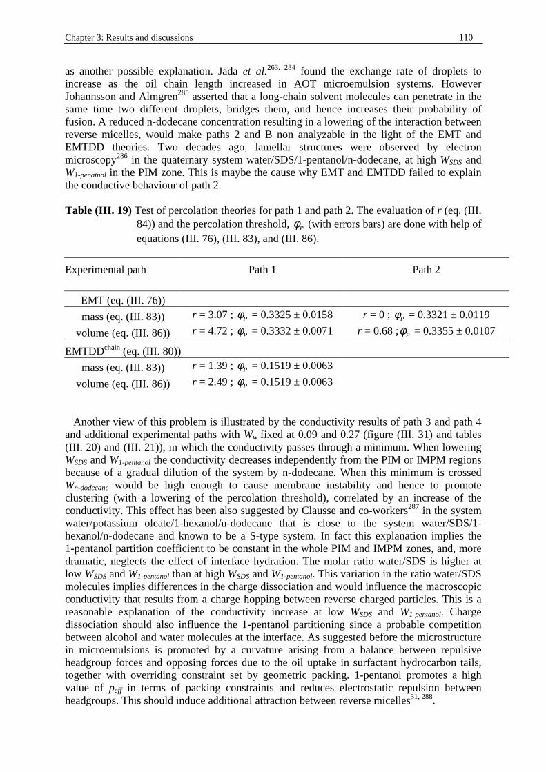
Chapter 3: Results and discussions 110
as another possible explanation. Jada et al.263, 284 found the exchange rate of droplets to increase as the oil chain length increased in AOT microemulsion systems. However Johannsson and Almgren285 asserted that a long-chain solvent molecules can penetrate in the same time two different droplets, bridges them, and hence increases their probabilit y of fusion. A reduced n-dodecane concentration resulting in a lowering of the interaction between reverse micelles, would make paths 2 and B non analyzable in the light of the EMT and EMTDD theories. Two decades ago, lamellar structures were observed by electron microscopy286 in the quaternary system water/SDS/1-pentanol/n-dodecane, at high WSDS and W1-penatnol in the PIM zone. This is maybe the cause why EMT and EMTDD failed to explain the conductive behaviour of path 2. Table (III. 19) Test of percolation theories for path 1 and path 2. The evaluation of r (eq. (III .
84)) and the percolation threshold, Pφ (with errors bars) are done with help of equations (III . 76), (III . 83), and (III . 86).
Experimental path Path 1 Path 2
EMT (eq. (III . 76))
mass (eq. (III . 83)) r = 3.07 ; Pφ = 0.3325 ± 0.0158 r = 0 ; Pφ = 0.3321 ± 0.0119
volume (eq. (III . 86)) r = 4.72 ; Pφ = 0.3332 ± 0.0071 r = 0.68 ; Pφ = 0.3355 ± 0.0107
EMTDDchain (eq. (III . 80))
mass (eq. (III . 83)) r = 1.39 ; Pφ = 0.1519 ± 0.0063
volume (eq. (III . 86)) r = 2.49 ; Pφ = 0.1519 ± 0.0063 Another view of this problem is ill ustrated by the conductivity results of path 3 and path 4 and additional experimental paths with Ww fixed at 0.09 and 0.27 (figure (III . 31) and tables (III . 20) and (III . 21)), in which the conductivity passes through a minimum. When lowering WSDS and W1-pentanol the conductivity decreases independently from the PIM or IMPM regions because of a gradual dilution of the system by n-dodecane. When this minimum is crossed Wn-dodecane would be high enough to cause membrane instabilit y and hence to promote clustering (with a lowering of the percolation threshold), correlated by an increase of the conductivity. This effect has been also suggested by Clausse and co-workers287 in the system water/potassium oleate/1-hexanol/n-dodecane that is close to the system water/SDS/1-hexanol/n-dodecane and known to be a S-type system. In fact this explanation implies the 1-pentanol partition coeff icient to be constant in the whole PIM and IMPM zones, and, more dramatic, neglects the effect of interface hydration. The molar ratio water/SDS is higher at low WSDS and W1-pentanol than at high WSDS and W1-pentanol. This variation in the ratio water/SDS molecules implies differences in the charge dissociation and would influence the macroscopic conductivity that results from a charge hopping between reverse charged particles. This is a reasonable explanation of the conductivity increase at low WSDS and W1-pentanol. Charge dissociation should also influence the 1-pentanol partitioning since a probable competition between alcohol and water molecules at the interface. As suggested before the microstructure in microemulsions is promoted by a curvature arising from a balance between repulsive headgroup forces and opposing forces due to the oil uptake in surfactant hydrocarbon tails, together with overriding constraint set by geometric packing. 1-pentanol promotes a high value of peff in terms of packing constraints and reduces electrostatic repulsion between headgroups. This should induce additional attraction between reverse micelles31, 288.
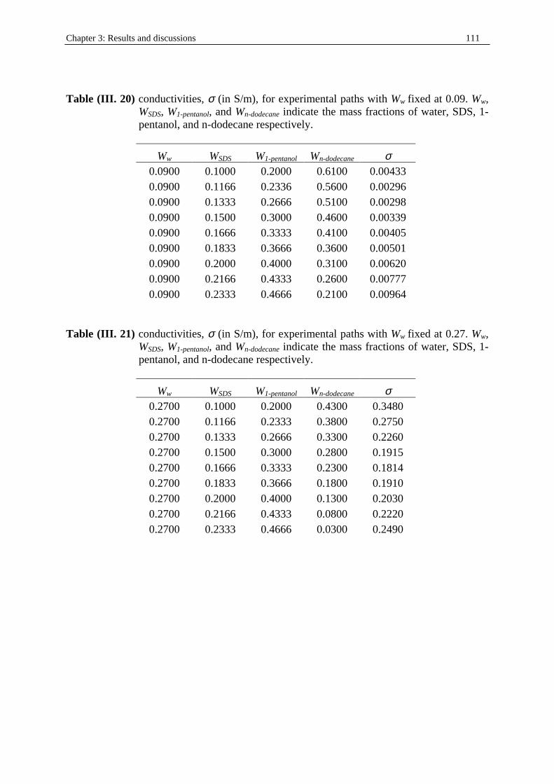
Chapter 3: Results and discussions 111
Table (III. 20) conductivities, σ (in S/m), for experimental paths with Ww fixed at 0.09. Ww,
WSDS, W1-pentanol, and Wn-dodecane indicate the mass fractions of water, SDS, 1-pentanol, and n-dodecane respectively.
Ww WSDS W1-pentanol Wn-dodecane σ 0.0900 0.1000 0.2000 0.6100 0.00433 0.0900 0.1166 0.2336 0.5600 0.00296 0.0900 0.1333 0.2666 0.5100 0.00298 0.0900 0.1500 0.3000 0.4600 0.00339 0.0900 0.1666 0.3333 0.4100 0.00405 0.0900 0.1833 0.3666 0.3600 0.00501 0.0900 0.2000 0.4000 0.3100 0.00620 0.0900 0.2166 0.4333 0.2600 0.00777 0.0900 0.2333 0.4666 0.2100 0.00964
Table (III. 21) conductivities, σ (in S/m), for experimental paths with Ww fixed at 0.27. Ww,
WSDS, W1-pentanol, and Wn-dodecane indicate the mass fractions of water, SDS, 1-pentanol, and n-dodecane respectively.
Ww WSDS W1-pentanol Wn-dodecane σ 0.2700 0.1000 0.2000 0.4300 0.3480 0.2700 0.1166 0.2333 0.3800 0.2750 0.2700 0.1333 0.2666 0.3300 0.2260 0.2700 0.1500 0.3000 0.2800 0.1915 0.2700 0.1666 0.3333 0.2300 0.1814 0.2700 0.1833 0.3666 0.1800 0.1910 0.2700 0.2000 0.4000 0.1300 0.2030 0.2700 0.2166 0.4333 0.0800 0.2220 0.2700 0.2333 0.4666 0.0300 0.2490
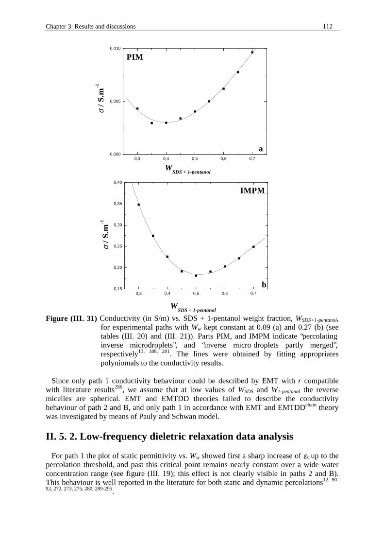
Chapter 3: Results and discussions 112
0,3 0,4 0,5 0,6 0,70,000
0,005
0,010
a
PIM
WSDS + 1-pentanol
σσ /
S.m
-1
0,3 0,4 0,5 0,6 0,70,15
0,20
0,25
0,30
0,35
0,40
b
IMPM
WSDS + 1-pentanol
σσ /
S.m
-1
Figure (III. 31) Conductivity (in S/m) vs. SDS + 1-pentanol weight fraction, WSDS+1-pentanol,
for experimental paths with Ww kept constant at 0.09 (a) and 0.27 (b) (see tables (III. 20) and (III. 21)). Parts PIM, and IMPM indicate “percolating inverse microdroplets”, and “inverse micro droplets partly merged”, respectively13, 188, 201. The lines were obtained by fitting appropriates polyniomals to the conductivity results.
Since only path 1 conductivity behaviour could be described by EMT with r compatible with literature results286, we assume that at low values of WSDS and W1-pentanol the reverse micelles are spherical. EMT and EMTDD theories failed to describe the conductivity behaviour of path 2 and B, and only path 1 in accordance with EMT and EMTDDchain theory was investigated by means of Pauly and Schwan model.
II. 5. 2. Low-frequency dieletric relaxation data analysis For path 1 the plot of static permittivity vs. Ww showed first a sharp increase of εs up to the percolation threshold, and past this critical point remains nearly constant over a wide water concentration range (see figure (III. 19); this effect is not clearly visible in paths 2 and B). This behaviour is well reported in the literature for both static and dynamic percolations12, 90-
92, 272, 273, 275, 280, 289-295.
Chapter 3: Results and discussions 113
II. 5. 2. 1. DRS study of W/O microemulsions, state of the literature
For W/O ionic microemulsions, various models of dielectric relaxation related to interfacial polarization (Maxwell-Wagner effect108, 296, 297) have been proposed and reviewed in ref. (298) and (299), most of the models proposed predict only the behaviour of the static permittivity. Different interpretations of DRS results of W/O microemulsion are found in the literature. In comparison to our data, they differ for both fitting model and frequency range (limited at high frequencies). Chou and Shah95 proposed a two Debye model for ionic microemulsions (with TRSIO-410 as surfactant) in the frequency range 0.5−100 MHz. They emphasized the importance of the interface to this phenomenon and showed, for isolated reverse micelles, that the low-frequency relaxation time is proportional to the square of the radius of dispersed water droplets and the high-frequency relaxation time is proportional to the radius. These authors explained this effect by the fact that low-frequency dielectric relaxation steps may imply both interfacial polarization of dispersion with thin shells143, 199, from which the model of Pauly and Schwan is derived, and the theory of double-layer polarization144, 251, 300 that considers the relaxation of ions diffusing in the bulk electrolyte. The results of Feldman and co-workers12, 301-303 indicated the apparition of a low frequency relaxation process at the percolation threshold; they presented this relaxation step as a cooperative relaxation process associated with the transfer of charge carriers along the aggregated structures. They found at higher frequencies another relaxation step, present below and above percolation threshold, attributed by these authors to W/O droplet polarizability depending on the distribution of ions within the double layer. Attention should be paid to the consideration of the data of Feldman and co-workers, since the kind of percolation they investigated is dynamic. In their case, the percolation is induced by an increase of cosurfactant concentration or by a raise of the temperature; in both cases, they observed a maximum in the static permittivity near the percolation threshold. In comparison to the static percolation we study in the present work, the dynamic percolation does not lead to the formation of bicontinuous structures by reverse droplet coalescence, but to a reverse micelle aggregation (clustering); this makes the work of Feldman’s team fundamentally different from our work. Other DRS measurements of AOT reverse micelles showed that when Ww is increased, a peak maximum in the amplitude is reached for low frequency relaxation process in a Cole-Cole-Debye fit model (CCD). The behaviour of the corresponding distribution (α, see eq. (II. 59)) was found dependent on the salt content, and on the counterion nature11, 304-306 related to the interfacial hydration88, 307. The behaviour of this low-frequency relaxation distribution found by Santucci’s team is very similar to those of S1 for both experimental path 1 and 2 (figure (III. 23)), for which peak maximum is reached near the percolation threshold. The same group found an increase of the Cole-Cole distribution parameter88 when small amount of water is added; this distribution parameter remains then more or less constant. This may be accounted to an increase and a maximum peak value of the low-frequency contribution (as observed for S1 in our case) amplitude, maybe submitted to the structural changes in the microemulsions during the percolation. Ponton et al.99 investigated the system water/SDS/1-pentanol/n-dodecane, and applied the four Cole-Cole fit model (4CC) in the frequency range 100 kHz−15 GHz. Despite the fact that the microemulsion system of Ponton et al. seems to be close to our system, its mass ratio, Km, SDS/1-pentanol of 0.3, is different, and the percolation investigated has been reported as a
Chapter 3: Results and discussions 114
dynamic; this is maybe the reason of the differences in the relaxation times observed (in their work, τ1 ~ 50 ns, τ2 ~ 2 ns, τ3 ~ 200 ps, and τ4 ~ 15 ps). The differences between the DRS data of Ponton et al. and our data may be also due to the different frequency range in which the DRS measurements were carried out and the respective relaxation models proposed. In accordance to other literature data (see before), Ponton et al.99 suggested that the two lowest frequency relaxation process have an ionic origin; whereas the fastest relaxation process is attribuable to water motions. Ponton and co-workers could not attribute correctly the relaxation process centred at ~ 200 ps; therefore their work should be considered as incomplete. The same group investigated before the system water/SDS/1-butanol/toluene or n-dodecane with a fixed Km at 0.5, in the frequency range 10 MHz-3 GHz308 (supplemented by microave cavity measurements at 3, 9, and 15 GHz) and 100 kHz-6 GHz309; in the former experiments a dielectric absorption was reported at ~ 1 GHz, suggested as bound water. For the measurements carried out in the frequency range 100 kHz-6 GHz, the presence of two relaxation processes was observed, but not correctly interpreted since imcomplete data.
II. 5. 2. 2. Comparison between literature data and low-frequency DRS results
Since for paths 1, 2 and B, conductivity exists below percolation threshold, interactions between conducting reverse micelles (or pre-micellar aggregates) are expected269. In experimental paths 1, 2, and B, the plots S1 vs. conductivity, reveal a linearity (figure (III. 32)), only below the percolation threshold, suggesting an ionic origin to this relaxation process that is related to charge hopping between reverse micelles; the loss of this proportionality beyond the percolation threshold is maybe linked to the changes in this charge hopping and the apparition of a three-dimensional network constituted of coalesced conductive reverse micelles, according to Lagourette et al.201. If we consider that this process remains the same between SDS (direct) micelles and our W/O microemulsions, the observed relaxation step 1, with parameters (S1, τ1) would be for the latter case related to the motions of free sodium ions, and hence comparable to the lowest frequency process found by Feldman and co-workers12, 301-303 who associated this to the transfer of charge carriers between reverse micelles and along mesoscale structures, in agreement with the work of Chou and Shah95 and Ponton et al.99 (see last paragraph). Interaction between reverse micelles does not only involve counterions exchange (as indicated by Eike et al.269), but also surfactant molecules would also move from particle to particle.
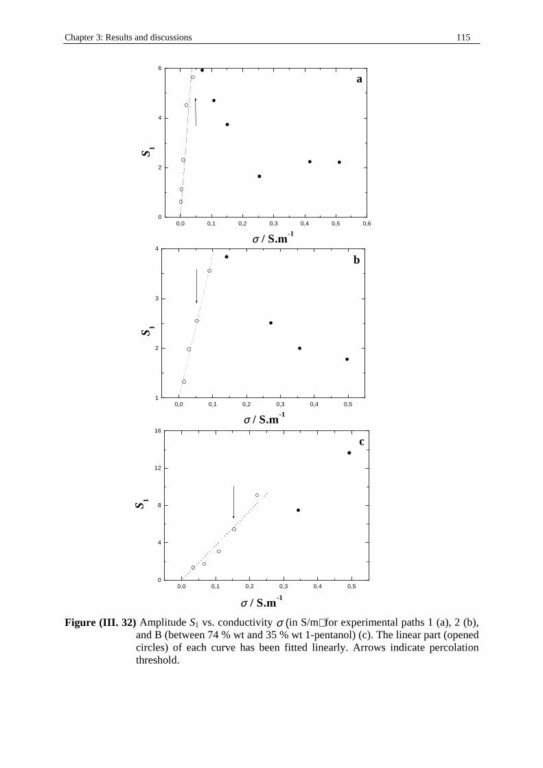
Chapter 3: Results and discussions 115
0,0 0,1 0,2 0,3 0,4 0,5 0,60
2
4
6
a
σσ / S.m-1
S 1
0,0 0,1 0,2 0,3 0,4 0,51
2
3
4
σσ / S.m-1
S1
b
0,0 0,1 0,2 0,3 0,4 0,50
4
8
12
16
S 1
σσ / S.m-1
c
Figure (III. 32) Amplitude S1 vs. conductivity σ (in S/m) for experimental paths 1 (a), 2 (b),
and B (between 74 % wt and 35 % wt 1-pentanol) (c). The linear part (opened circles) of each curve has been fitted linearly. Arrows indicate percolation threshold.
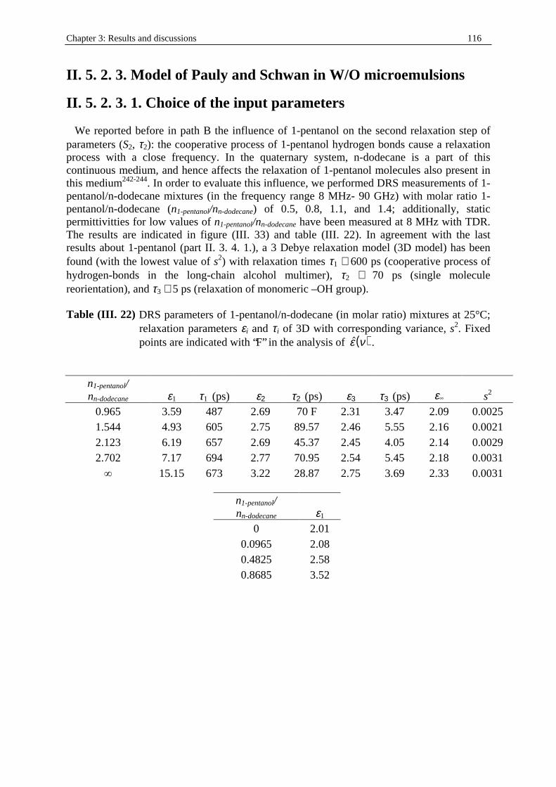
Chapter 3: Results and discussions 116
II. 5. 2. 3. Model of Pauly and Schwan in W/O microemulsions
II. 5. 2. 3. 1. Choice of the input parameters We reported before in path B the influence of 1-pentanol on the second relaxation step of parameters (S2, τ2): the cooperative process of 1-pentanol hydrogen bonds cause a relaxation process with a close frequency. In the quaternary system, n-dodecane is a part of this continuous medium, and hence affects the relaxation of 1-pentanol molecules also present in this medium242-244. In order to evaluate this influence, we performed DRS measurements of 1-pentanol/n-dodecane mixtures (in the frequency range 8 MHz- 90 GHz) with molar ratio 1-pentanol/n-dodecane (n1-pentanol/nn-dodecane) of 0.5, 0.8, 1.1, and 1.4; additionally, static permittivitties for low values of n1-pentanol/nn-dodecane have been measured at 8 MHz with TDR. The results are indicated in figure (III . 33) and table (III . 22). In agreement with the last results about 1-pentanol (part II . 3. 4. 1.), a 3 Debye relaxation model (3D model) has been found (with the lowest value of s2) with relaxation times τ1 ∼ 600 ps (cooperative process of hydrogen-bonds in the long-chain alcohol multimer), τ2 ∼ 70 ps (single molecule reorientation), and τ3 ∼ 5 ps (relaxation of monomeric –OH group). Table (III. 22) DRS parameters of 1-pentanol/n-dodecane (in molar ratio) mixtures at 25°C;
relaxation parameters εi and τi of 3D with corresponding variance, s2. Fixed points are indicated with “F” in the analysis of ( )ε ν .
n1-pentanol/ nn-dodecane ε1 τ1 (ps) ε2 τ2 (ps) ε3 τ3 (ps) ε s2
0.965 3.59 487 2.69 70 F 2.31 3.47 2.09 0.0025 1.544 4.93 605 2.75 89.57 2.46 5.55 2.16 0.0021 2.123 6.19 657 2.69 45.37 2.45 4.05 2.14 0.0029 2.702 7.17 694 2.77 70.95 2.54 5.45 2.18 0.0031 15.15 673 3.22 28.87 2.75 3.69 2.33 0.0031
n1-pentanol/ nn-dodecane ε1
0 2.01 0.0965 2.08 0.4825 2.58 0.8685 3.52
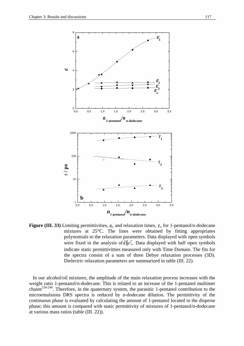
Chapter 3: Results and discussions 117
0,0 0,5 1,0 1,5 2,0 2,5 3,0 3,50
2
4
6
8
εε
a
εε∞∞
εε3
εε2
εε1
n1-pentanol
/nn-dodecane
0,0 0,5 1,0 1,5 2,0 2,5 3,0 3,51
10
100
1000
b
ττ3
ττ2
ττ1
ττ / p
s
n1-pentanol
/nn-dodecane
Figure (III. 33) Limiting permittivities, εi, and relaxation times, τi, for 1-pentanol/n-dodecane
mixtures at 25°C. The lines were obtained by fitting appropriates polynomials to the relaxation parameters. Data displayed with open symbols were fixed in the analysis of ( )νε . Data displayed with half open symbols indicate static permittivitties measured only with Time Domain. The fits for the spectra consist of a sum of three Debye relaxation processes (3D). Dielectric relaxation parameters are summarized in table (III . 22).
In our alcohol/oil mixtures, the amplitude of the main relaxation process increases with the weight ratio 1-pentanol/n-dodecane. This is related to an increase of the 1-pentanol multimer chains234-240. Therefore, in the quaternary system, the parasitic 1-pentanol contribution to the microemulsions DRS spectra is reduced by n-dodecane dilution. The permittivity of the continuous phase is evaluated by calculating the amount of 1-pentanol located in the disperse phase; this amount is compared with static permittivity of mixtures of 1-pentanol/n-dodecane at various mass ratios (table (III . 22)).
Chapter 3: Results and discussions 118
The mole number of 1-pentanol present in the continuous medium, mediumpentanol1n − is defined as
int
pentanol1pentanol1medium
pentanol1 nnn −−− −= (III . 87)
where pentanol1n − is the total mole number of 1-pentanol, and int
pentanol1n − the mole number of 1-
pentanol present in the interfacial region, calculated with equation (III . 84). Combining equations (III . 84) and (III . 87) we evaluate the mole ratio 1-pentanol present in the continuous phase/n-dodecane
dodecanen
SDSpentanol1
dodecanen
mediumpentanol1
n
rnn
n
n
−
−
−
− −= (III . 88)
Results of equation (III . 88) are used for the calculation of static permittivitty of the disperse phase. From results indicated in table (III . 22), εm is represented as a function of the molar ratio medium
pentanol1n − /nn-dodecane calculated with the following polynomial represented in figure (III .
33)
32
365.0392.1771.0016.2
+
+
+=
−
−
−
−
−
−
−
−
dodecanen
mediumpentanol1
dodecanen
mediumpentanol1
dodecanen
mediumpentanol1
dodecanen
mediumpentanol1
m n
n
n
n
n
n
n
nε (III . 89)
Eqs. (III . 88) and (III . 89) revealed that εm was in the order of 2.6 to 2.8 below the percolation threshold in path 1 Ww = 0.05 and Ww = 0.15. According to equations (III . 71) and (III . 72), the correction of the second relaxation step in DRS microemulsions spectra requires the knowledge of the disperse phase volume fraction, φ; this parameter, provided by conductivity results (application of EMT and EMTDD), is extremely important for the application of the model of Pauly and Schwan in SDS microemulsions. It is worth to remember that the model of Pauly and Schwan is only available for spherical reverse droplets, making this model only compatible with EMT. Our analysis of the low-frequency relaxation processes in SDS microemulsions is also limited by the fact that only the experimental path 1 could be depicted from EMT. EMT allows us to estimate (although we ignore here the oil penetration to the interface) both volume fraction, φ, and a conductivity, σd of the disperse phase (found equal to1.6846 S/m, with eq. (III . 84)). The model of Pauly and Schwan can be only applied with EMT in combination with equation (III . 83)) that gives r compatible with experimental values281. Other parameters necessary for the application of the model of Pauly and Schwan are found in the literature. SANS measurements performed in the quaternary system water/SDS/1-pentanol/cyclohexane310, 311, gave a shell thickness (polar headgroups plus hydrophobic tails, namely d) value of 9 Å; this value is smaller than the length of an extended surfactant chain, and is expected to be due to the alcohol penetration in the interface and the bending of SDS hydrophobic tails. We considered the conductivity of the continuous medium (dodecane plus solubili zed 1-pentanol), σm, as equal to zero. Various core radii were chosen (5 Å, 10 Å, 20 Å, 30 Å, and 40 Å), in combination with diverse static permittivity of the disperse phase, εd (8, 40, and 78.37) have been considered. In the present analyse, εd and σs were variables; the use of molecular probes able to give dielectric constant of microenvironment of microemulsions such as methyl orange for core312 or ET(30) for shell 313 (both probes have been only tested in other systems312,
313) would be suitable to complete input parameters of model of Pauly and Schwan.
Chapter 3: Results and discussions 119
The fitting procedure has been performed considering, in the calculation of deviations between theory and experiment, s2, both theoretical relaxation steps predicted by equations (III. 10) to (III. 24), if relatively close to another, are considered as one with amplitude SPtotal
21 PPPtotal SSS += (III. 90)
and relaxation time τPfinal
( ) ( )( )
++
=21
2211 lnlnexp
PP
PPPPPfinal SS
SS τττ (III. 91)
In the case of a deviation between theory and experiment acceptable, this does not mean that the fit is correct. For instance, if different orders of magnitude for τP1 and τP2 are found in the same fit, and with comparable predicted amplitudes SP2 and SP1, the model is not considered as correct. Additionally, if SP2 << SP1 or SP2 >> SP1, then the fit is correct, independently of the magnitudes of τP1 and τP2.
II. 5. 2. 3. 2. Results Due to deviations between theory and experiment, s2 is given only for Ww = 0.05 to Ww = 0.09. In the case of εp = 8, and for Rc = 2 nm to 4 nm, the predicted relaxation times τP1 and τP2 were not in the same order of magnitude, and the predicted amplitudes SP2 and SP1 were close to antother. Therefore the fits done with εp = 8, and for Rc = 2 nm to 4 nm, have been considered as non-relevant. The rest of the fits were correct (enumerated fits 1 to 12 in table (III. 23), see also figure (III. 34)). For nearly all those fits, the main contribution to SPfinal is due to SP2 and the relaxation times τP1 and τP2 have been found in the same order of magnitude. For instance, in the fits 3 to 7, we found that SP1 ≤ 0.03 whereas the fits 8 to 12 give SP1 ≤ 0.4, and SP1 ≤ 1.4 the fits 1 to 5 (SP1 ≤ 0.3 in fits 1 to 2). Since the fits 3 to 7 gave SP1 well below the noise level (in agreement with the results found with SDS micelles, and SDS/1-pentanol micelles, see before), they are considered as the most realistic for the fitting of S2 and τ2. In this way, the model of Pauly and Schwan showed a very limited compatibility with S2 and τ2, only for low water content (Ww = 0.05 and 0.07). At higher water concentrations, strong deviations between theory and experiments occurred (figure (III. 34)). Those deviations may be related to interparticle interaction, although it is difficult to demonstrate the existence of reverse micelles at the water contents where the model of Pauly and Schwan is in agreement with experiment. It is also worth to precise that we lack knowledge about the variations of input parameters. Therefore the model of Pauly and Schwan could not correctly explain the behaviour of S2 and τ2. Currently, there is no other model available that can describe the behaviour of either S2 and τ2 in the whole W/O microemulsion region.
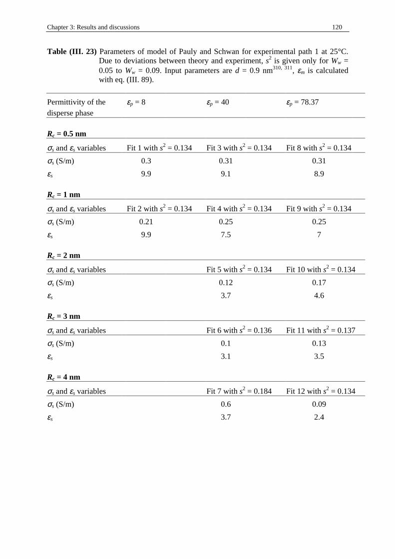
Chapter 3: Results and discussions 120
Table (III. 23) Parameters of model of Pauly and Schwan for experimental path 1 at 25°C. Due to deviations between theory and experiment, s2 is given only for Ww = 0.05 to Ww = 0.09. Input parameters are d = 0.9 nm310, 311, εm is calculated with eq. (III . 89).
Permittivity of the εp = 8 εp = 40 εp = 78.37 disperse phase
Rc = 0.5 nm
σs and εs variables Fit 1 with s2 = 0.134 Fit 3 with s2 = 0.134 Fit 8 with s2 = 0.134
σs (S/m) 0.3 0.31 0.31
εs 9.9 9.1 8.9
Rc = 1 nm
σs and εs variables Fit 2 with s2 = 0.134 Fit 4 with s2 = 0.134 Fit 9 with s2 = 0.134
σs (S/m) 0.21 0.25 0.25
εs 9.9 7.5 7
Rc = 2 nm
σs and εs variables Fit 5 with s2 = 0.134 Fit 10 with s2 = 0.134
σs (S/m) 0.12 0.17
εs 3.7 4.6
Rc = 3 nm
σs and εs variables Fit 6 with s2 = 0.136 Fit 11 with s2 = 0.137
σs (S/m) 0.1 0.13
εs 3.1 3.5
Rc = 4 nm
σs and εs variables Fit 7 with s2 = 0.184 Fit 12 with s2 = 0.134
σs (S/m) 0.6 0.09
εs 3.7 2.4
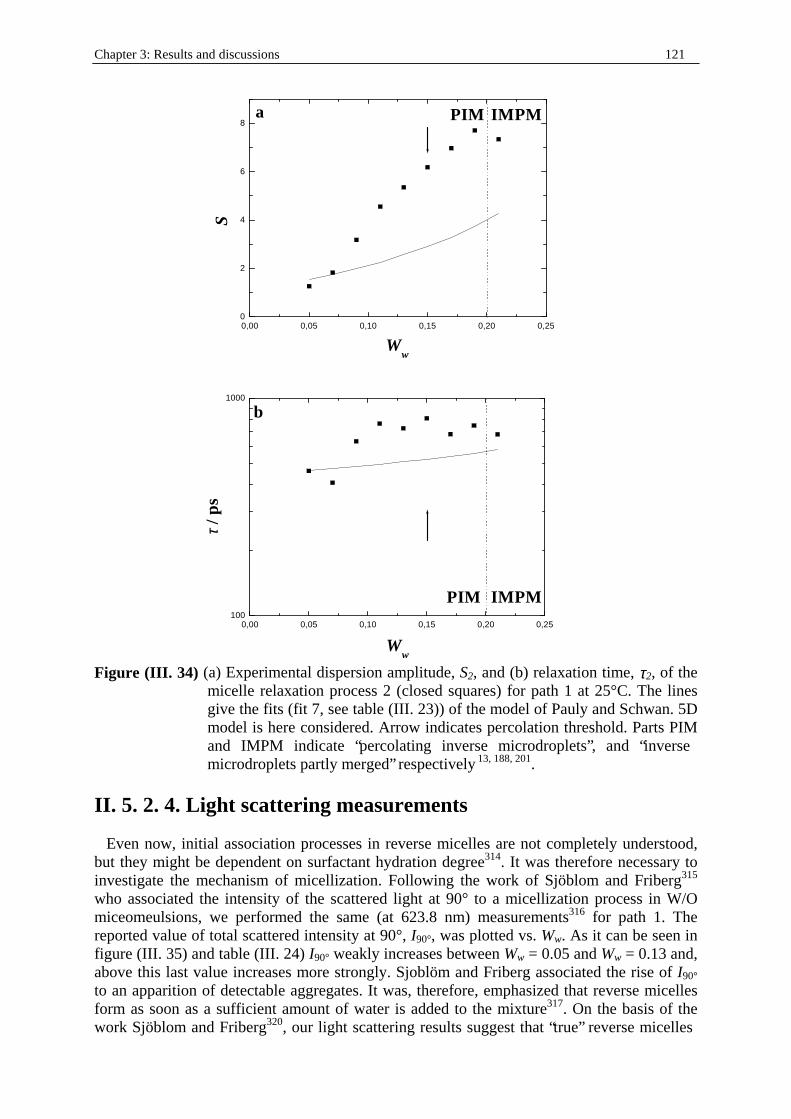
Chapter 3: Results and discussions 121
0,00 0,05 0,10 0,15 0,20 0,250
2
4
6
8a IMPMPIM
Ww
S
0,00 0,05 0,10 0,15 0,20 0,25100
1000
b
ττ / p
s
Ww
IMPMPIM
Figure (III. 34) (a) Experimental dispersion amplitude, S2, and (b) relaxation time, τ2, of the
micelle relaxation process 2 (closed squares) for path 1 at 25°C. The lines give the fits (fit 7, see table (III . 23)) of the model of Pauly and Schwan. 5D model is here considered. Arrow indicates percolation threshold. Parts PIM and IMPM indicate “percolating inverse microdroplets”, and “inverse microdroplets partly merged” respectively 13, 188, 201.
II. 5. 2. 4. Light scattering measurements Even now, initial association processes in reverse micelles are not completely understood, but they might be dependent on surfactant hydration degree314. It was therefore necessary to investigate the mechanism of micelli zation. Following the work of Sjöblom and Friberg315 who associated the intensity of the scattered light at 90° to a micelli zation process in W/O miceomeulsions, we performed the same (at 623.8 nm) measurements316 for path 1. The reported value of total scattered intensity at 90°, I90°, was plotted vs. Ww. As it can be seen in figure (III . 35) and table (III . 24) I90° weakly increases between Ww = 0.05 and Ww = 0.13 and, above this last value increases more strongly. Sjoblöm and Friberg associated the rise of I90° to an apparition of detectable aggregates. It was, therefore, emphasized that reverse micelles form as soon as a suff icient amount of water is added to the mixture317. On the basis of the work Sjöblom and Friberg320, our light scattering results suggest that “true” reverse micelles
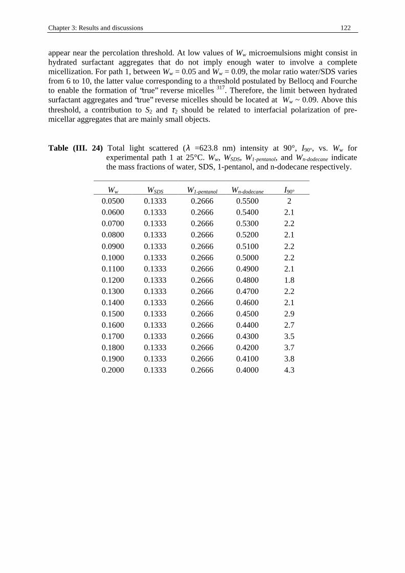
Chapter 3: Results and discussions 122
appear near the percolation threshold. At low values of Ww microemulsions might consist in hydrated surfactant aggregates that do not imply enough water to involve a complete micelli zation. For path 1, between Ww = 0.05 and Ww = 0.09, the molar ratio water/SDS varies from 6 to 10, the latter value corresponding to a threshold postulated by Bellocq and Fourche to enable the formation of “true” reverse micelles317. Therefore, the limit between hydrated surfactant aggregates and “true” reverse micelles should be located at Ww ~ 0.09. Above this threshold, a contribution to S2 and τ2 should be related to interfacial polarization of pre-micellar aggregates that are mainly small objects. Table (III. 24) Total li ght scattered (λ =623.8 nm) intensity at 90°, I90°, vs. Ww for
experimental path 1 at 25°C. Ww, WSDS, W1-pentanol, and Wn-dodecane indicate the mass fractions of water, SDS, 1-pentanol, and n-dodecane respectively.
Ww WSDS W1-pentanol Wn-dodecane I90° 0.0500 0.1333 0.2666 0.5500 2 0.0600 0.1333 0.2666 0.5400 2.1 0.0700 0.1333 0.2666 0.5300 2.2 0.0800 0.1333 0.2666 0.5200 2.1
0.0900 0.1333 0.2666 0.5100 2.2 0.1000 0.1333 0.2666 0.5000 2.2 0.1100 0.1333 0.2666 0.4900 2.1 0.1200 0.1333 0.2666 0.4800 1.8 0.1300 0.1333 0.2666 0.4700 2.2 0.1400 0.1333 0.2666 0.4600 2.1 0.1500 0.1333 0.2666 0.4500 2.9 0.1600 0.1333 0.2666 0.4400 2.7 0.1700 0.1333 0.2666 0.4300 3.5 0.1800 0.1333 0.2666 0.4200 3.7 0.1900 0.1333 0.2666 0.4100 3.8 0.2000 0.1333 0.2666 0.4000 4.3
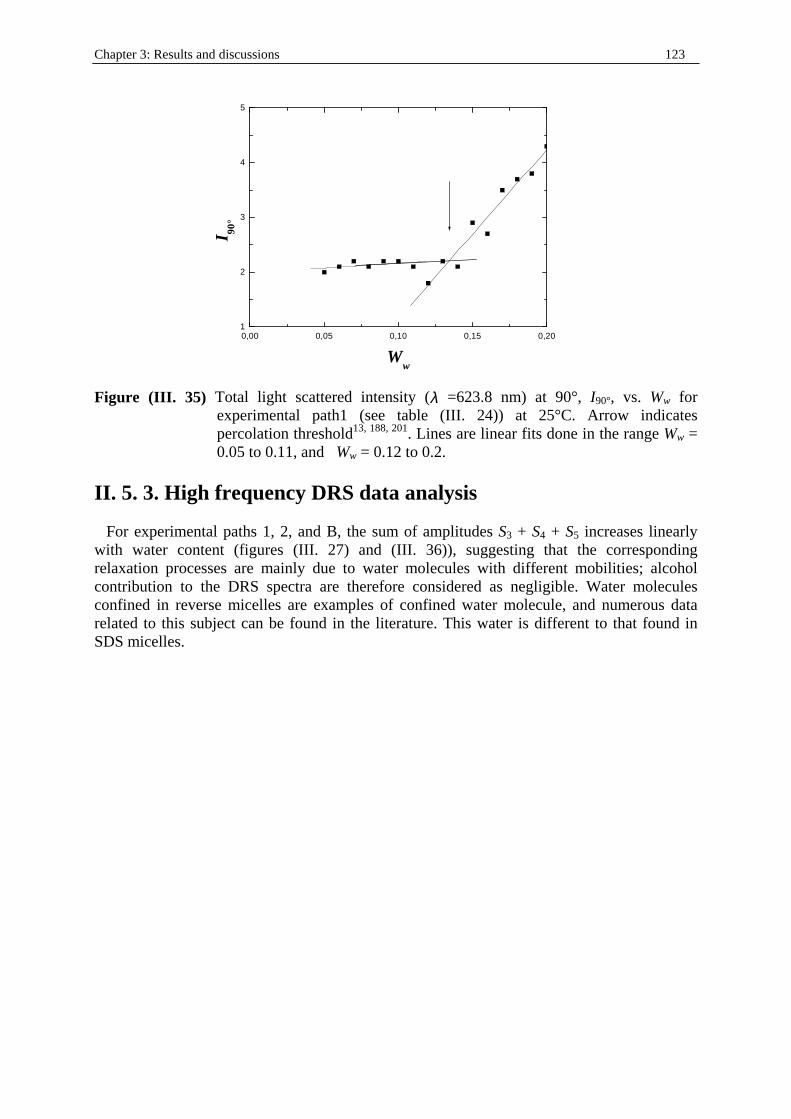
Chapter 3: Results and discussions 123
0,00 0,05 0,10 0,15 0,201
2
3
4
5
I 90°
Ww
Figure (III . 35) Total li ght scattered intensity (λ =623.8 nm) at 90°, I90°, vs. Ww for experimental path1 (see table (III . 24)) at 25°C. Arrow indicates percolation threshold13, 188, 201. Lines are linear fits done in the range Ww = 0.05 to 0.11, and Ww = 0.12 to 0.2.
II . 5. 3. High frequency DRS data analysis For experimental paths 1, 2, and B, the sum of amplitudes S3 + S4 + S5 increases linearly with water content (figures (III . 27) and (III . 36)), suggesting that the corresponding relaxation processes are mainly due to water molecules with different mobiliti es; alcohol contribution to the DRS spectra are therefore considered as negligible. Water molecules confined in reverse micelles are examples of confined water molecule, and numerous data related to this subject can be found in the literature. This water is different to that found in SDS micelles.
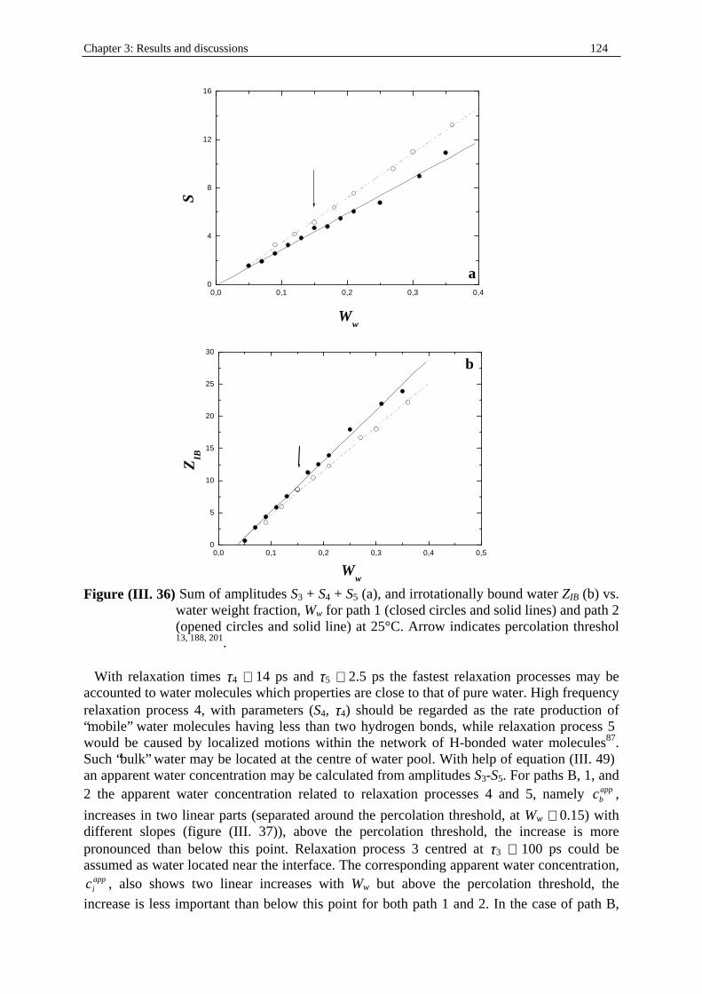
Chapter 3: Results and discussions 124
0,0 0,1 0,2 0,3 0,40
4
8
12
16
a
W
w
S
0,0 0,1 0,2 0,3 0,4 0,50
5
10
15
20
25
30
b
Ww
ZIB
Figure (III. 36) Sum of amplitudes S3 + S4 + S5 (a), and irrotationally bound water ZIB (b) vs.
water weight fraction, Ww for path 1 (closed circles and solid lines) and path 2 (opened circles and solid line) at 25°C. Arrow indicates percolation threshol 13, 188, 201.
With relaxation times τ4 ∼ 14 ps and τ5 ∼ 2.5 ps the fastest relaxation processes may be accounted to water molecules which properties are close to that of pure water. High frequency relaxation process 4, with parameters (S4, τ4) should be regarded as the rate production of “mobile” water molecules having less than two hydrogen bonds, while relaxation process 5 would be caused by localized motions within the network of H-bonded water molecules87. Such “bulk” water may be located at the centre of water pool. With help of equation (III . 49) an apparent water concentration may be calculated from amplitudes S3-S5. For paths B, 1, and 2 the apparent water concentration related to relaxation processes 4 and 5, namely app
bc ,
increases in two linear parts (separated around the percolation threshold, at Ww ∼ 0.15) with different slopes (figure (III . 37)), above the percolation threshold, the increase is more pronounced than below this point. Relaxation process 3 centred at τ3 ∼ 100 ps could be assumed as water located near the interface. The corresponding apparent water concentration,
appic , also shows two linear increases with Ww but above the percolation threshold, the
increase is less important than below this point for both path 1 and 2. In the case of path B,
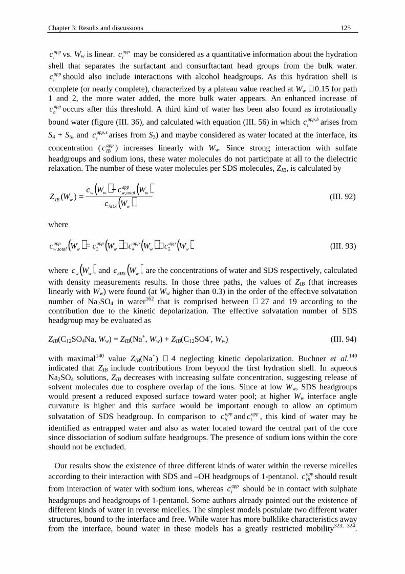
Chapter 3: Results and discussions 125
appic vs. Ww is linear. app
ic may be considered as a quantitative information about the hydration
shell that separates the surfactant and consurftactant head groups from the bulk water. appic should also include interactions with alcohol headgroups. As this hydration shell is
complete (or nearly complete), characterized by a plateau value reached at Ww ∼ 0.15 for path 1 and 2, the more water added, the more bulk water appears. An enhanced increase of
appbc occurs after this threshold. A third kind of water has been also found as irrotationally
bound water (figure (III. 36), and calculated with equation (III. 56) in which bappic , arises from
S4 + S5, and sappic , arises from S3) and maybe considered as water located at the interface, its
concentration ( appIBc ) increases linearly with Ww. Since strong interaction with sulfate
headgroups and sodium ions, these water molecules do not participate at all to the dielectric relaxation. The number of these water molecules per SDS molecules, ZIB, is calculated by
( ) ( )( )Z W
c W c W
c WIB w
w w w totalapp
w
SDS w
( ),=
− (III. 92)
where
( ) ( ) ( ) ( )c W c W c W c Ww totalapp
wapp
wapp
wapp
w, = + +3 4 5 (III. 93)
where ( )c Ww w and ( )c WSDS w are the concentrations of water and SDS respectively, calculated
with density measurements results. In those three paths, the values of ZIB (that increases linearly with Ww) were found (at Ww higher than 0.3) in the order of the effective solvatation number of Na2SO4 in water162 that is comprised between ∼ 27 and 19 according to the contribution due to the kinetic depolarization. The effective solvatation number of SDS headgroup may be evaluated as ZIB(C12SO4Na, Ww) = ZIB(Na+, Ww) + ZIB(C12SO4-, Ww) (III. 94) with maximal140 value ZIB(Na+) ∼ 4 neglecting kinetic depolarization. Buchner et al.140 indicated that ZIB include contributions from beyond the first hydration shell. In aqueous Na2SO4 solutions, ZIB decreases with increasing sulfate concentration, suggesting release of solvent molecules due to cosphere overlap of the ions. Since at low Ww, SDS headgroups would present a reduced exposed surface toward water pool; at higher Ww interface angle curvature is higher and this surface would be important enough to allow an optimum solvatation of SDS headgroup. In comparison to app
bc and appic , this kind of water may be
identified as entrapped water and also as water located toward the central part of the core since dissociation of sodium sulfate headgroups. The presence of sodium ions within the core should not be excluded. Our results show the existence of three different kinds of water within the reverse micelles according to their interaction with SDS and –OH headgroups of 1-pentanol. app
IBc should result
from interaction of water with sodium ions, whereas appic should be in contact with sulphate
headgroups and headgroups of 1-pentanol. Some authors already pointed out the existence of different kinds of water in reverse micelles. The simplest models postulate two different water structures, bound to the interface and free. While water has more bulklike characteristics away from the interface, bound water in these models has a greatly restricted mobility323, 324.
Chapter 3: Results and discussions 126
Several authors have pointed out the existence of a third type of water320-324. Along these authors water exists in three phases: water at the interface, bulklike phase, and water phase between these two phases. The existence of a fourth water species in W/O microemulsions has been reported by González-Blanco et al.325, 326 who suggested that the different kinds of water may differ from hydrogen bonding involved: hydrogen-bonded polymeric chain, dimers at the interface, monomers at the interface, and free monomers. Polymeric and free water may be considered as bulk water, and close to the water arising from amplitures S4 and S5 respectively. It is clear that AOT microemulsions without cosurfactant do not imply the same quantity of bounded water than SDS/1-pentanol microemulsions, these differences should be mainly due to surfactant nature; indeed a cosurfactant has a non negligible effect. As noted by Hauser et al.319, variation from method to method of investigation provides different values of water molecules tightly bound to AOT headgroups, this is due to differences involved in the sensitivity of the technique and on assumption made in the evaluation of the primary data. Therefore, comparison with literature data related to AOT microemulsions should be taken carefully. Some results found in the literature could be nevertheless compared to our work. For instance, molecular dynamics simulations performed327 on AOT reverse micelles showed that at very small water content nearly all the counterions remain bound to the surfactant; with rise of Ww, solvent separated ion pairs are formed and an increasing amount of the counterions become detached from the surfactant, a formation of solvent separated ion pairs may also occur; three different kinds of water were also found in this way, namely trapped in the interface, bound, and free, in accordance with our results. It was therefore suggested328 that the AOT headgroup ions and counterions form, at small reverse micelle sizes, a rigid “quasi -lattice” at the interface. As the reverse micelle size increases, the ion density decreases, leading to a breakup of the lattice and water penetration of the interfacial layer. Our results suggest the same phenomena as indicated by the behaviour of ZIB(Ww), the water implied in the SDS headgroup solvatation. Note that since 1-pentanol −OH headgroup represent a part of the interface, they should also interact with sodium sulfate headgroup and water, and would play an important role in the behaviour of app
ic and ZIB. Fioretto et al.329 emphasized AOT
headgroup hydration may enhance its free rotational diffusion. This increased mobilit y would make the interface more flexible and, therefore, reduce the interfacial bending energy.
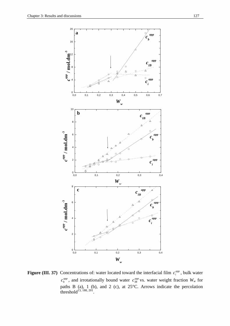
Chapter 3: Results and discussions 127
0,0 0,1 0,2 0,3 0,4 0,5 0,6 0,70
4
8
12
16
20
Ww
capp /
mol
.dm
-3
ci
app
cb
app
cIB
app
a
0,0 0,1 0,2 0,3 0,40
2
4
6
8
10
b cIB
app
cb
app
ci
app
capp /
mol
.dm
-3
Ww
0,0 0,1 0,2 0,3 0,40
2
4
6
8
Ww
capp /
mol
.dm
-3
c
ci
app
cb
app
cIB
app
Figure (III. 37) Concentrations of: water located toward the interfacial film appic , bulk water
appbc , and irrotationally bound water app
IBc vs. water weight fraction Ww for
paths B (a), 1 (b), and 2 (c), at 25°C. Arrows indicate the percolation threshold13, 188, 201.
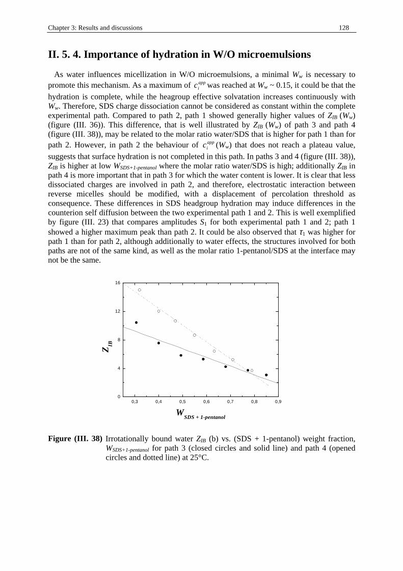
Chapter 3: Results and discussions 128
II. 5. 4. Importance of hydration in W/O microemulsions As water influences micelli zation in W/O microemulsions, a minimal Ww is necessary to promote this mechanism. As a maximum of app
ic was reached at Ww ~ 0.15, it could be that the
hydration is complete, while the heagroup effective solvatation increases continuously with Ww. Therefore, SDS charge dissociation cannot be considered as constant within the complete experimental path. Compared to path 2, path 1 showed generally higher values of ZIB (Ww) (figure (III . 36)). This difference, that is well ill ustrated by ZIB (Ww) of path 3 and path 4 (figure (III . 38)), may be related to the molar ratio water/SDS that is higher for path 1 than for path 2. However, in path 2 the behaviour of app
ic (Ww) that does not reach a plateau value,
suggests that surface hydration is not completed in this path. In paths 3 and 4 (figure (III . 38)), ZIB is higher at low WSDS+1-pentanol where the molar ratio water/SDS is high; additionally ZIB in path 4 is more important that in path 3 for which the water content is lower. It is clear that less dissociated charges are involved in path 2, and therefore, electrostatic interaction between reverse micelles should be modified, with a displacement of percolation threshold as consequence. These differences in SDS headgroup hydration may induce differences in the counterion self diffusion between the two experimental path 1 and 2. This is well exempli fied by figure (III . 23) that compares amplitudes S1 for both experimental path 1 and 2; path 1 showed a higher maximum peak than path 2. It could be also observed that τ1 was higher for path 1 than for path 2, although additionally to water effects, the structures involved for both paths are not of the same kind, as well as the molar ratio 1-pentanol/SDS at the interface may not be the same.
0,3 0,4 0,5 0,6 0,7 0,8 0,90
4
8
12
16
ZIB
WSDS + 1-pentanol
Figure (III. 38) Irrotationally bound water ZIB (b) vs. (SDS + 1-pentanol) weight fraction,
WSDS+1-pentanol for path 3 (closed circles and solid line) and path 4 (opened circles and dotted line) at 25°C.
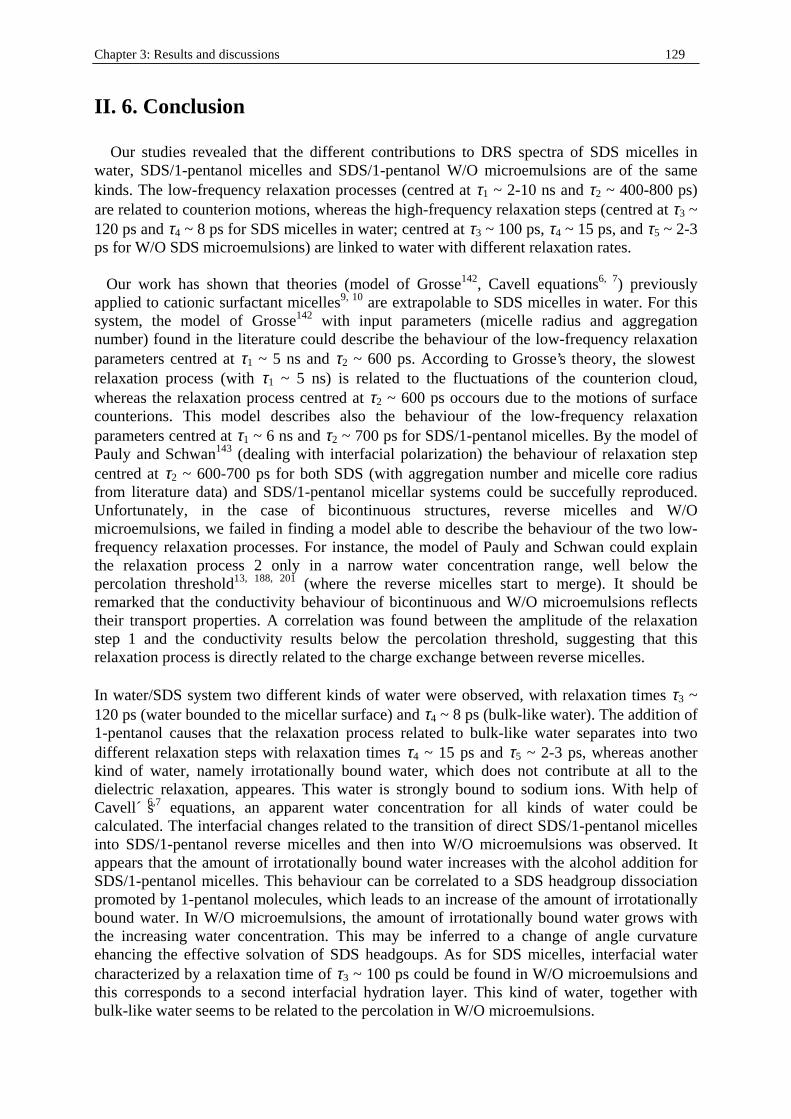
Chapter 3: Results and discussions 129
II. 6. Conclusion Our studies revealed that the different contributions to DRS spectra of SDS micelles in water, SDS/1-pentanol micelles and SDS/1-pentanol W/O microemulsions are of the same kinds. The low-frequency relaxation processes (centred at τ1 ~ 2-10 ns and τ2 ~ 400-800 ps) are related to counterion motions, whereas the high-frequency relaxation steps (centred at τ3 ~ 120 ps and τ4 ~ 8 ps for SDS micelles in water; centred at τ3 ~ 100 ps, τ4 ~ 15 ps, and τ5 ~ 2-3 ps for W/O SDS microemulsions) are linked to water with different relaxation rates. Our work has shown that theories (model of Grosse142, Cavell equations6, 7) previously applied to cationic surfactant micelles9, 10 are extrapolable to SDS micelles in water. For this system, the model of Grosse142 with input parameters (micelle radius and aggregation number) found in the literature could describe the behaviour of the low-frequency relaxation parameters centred at τ1 ~ 5 ns and τ2 ~ 600 ps. According to Grosse’s theory, the slowest relaxation process (with τ1 ~ 5 ns) is related to the fluctuations of the counterion cloud, whereas the relaxation process centred at τ2 ~ 600 ps occours due to the motions of surface counterions. This model describes also the behaviour of the low-frequency relaxation parameters centred at τ1 ~ 6 ns and τ2 ~ 700 ps for SDS/1-pentanol micelles. By the model of Pauly and Schwan143 (dealing with interfacial polarization) the behaviour of relaxation step centred at τ2 ~ 600-700 ps for both SDS (with aggregation number and micelle core radius from literature data) and SDS/1-pentanol micellar systems could be succefully reproduced. Unfortunately, in the case of bicontinuous structures, reverse micelles and W/O microemulsions, we failed in finding a model able to describe the behaviour of the two low-frequency relaxation processes. For instance, the model of Pauly and Schwan could explain the relaxation process 2 only in a narrow water concentration range, well below the percolation threshold13, 188, 201 (where the reverse micelles start to merge). It should be remarked that the conductivity behaviour of bicontinuous and W/O microemulsions reflects their transport properties. A correlation was found between the amplitude of the relaxation step 1 and the conductivity results below the percolation threshold, suggesting that this relaxation process is directly related to the charge exchange between reverse micelles. In water/SDS system two different kinds of water were observed, with relaxation times τ3 ~ 120 ps (water bounded to the micellar surface) and τ4 ~ 8 ps (bulk-like water). The addition of 1-pentanol causes that the relaxation process related to bulk-like water separates into two different relaxation steps with relaxation times τ4 ~ 15 ps and τ5 ~ 2-3 ps, whereas another kind of water, namely irrotationally bound water, which does not contribute at all to the dielectric relaxation, appeares. This water is strongly bound to sodium ions. With help of Cavell´ s6,7 equations, an apparent water concentration for all kinds of water could be calculated. The interfacial changes related to the transition of direct SDS/1-pentanol micelles into SDS/1-pentanol reverse micelles and then into W/O microemulsions was observed. It appears that the amount of irrotationally bound water increases with the alcohol addition for SDS/1-pentanol micelles. This behaviour can be correlated to a SDS headgroup dissociation promoted by 1-pentanol molecules, which leads to an increase of the amount of irrotationally bound water. In W/O microemulsions, the amount of irrotationally bound water grows with the increasing water concentration. This may be inferred to a change of angle curvature ehancing the effective solvation of SDS headgoups. As for SDS micelles, interfacial water characterized by a relaxation time of τ3 ~ 100 ps could be found in W/O microemulsions and this corresponds to a second interfacial hydration layer. This kind of water, together with bulk-like water seems to be related to the percolation in W/O microemulsions.

Chapter 3: Results and discussions 130
This work should be completed by examining of other W/O microemulsions systems, first by changing 1-pentanol by other n-alkanols, and then considering other surfactants. The necessary experiments have already begun (see Annexe) but are still incomplete.
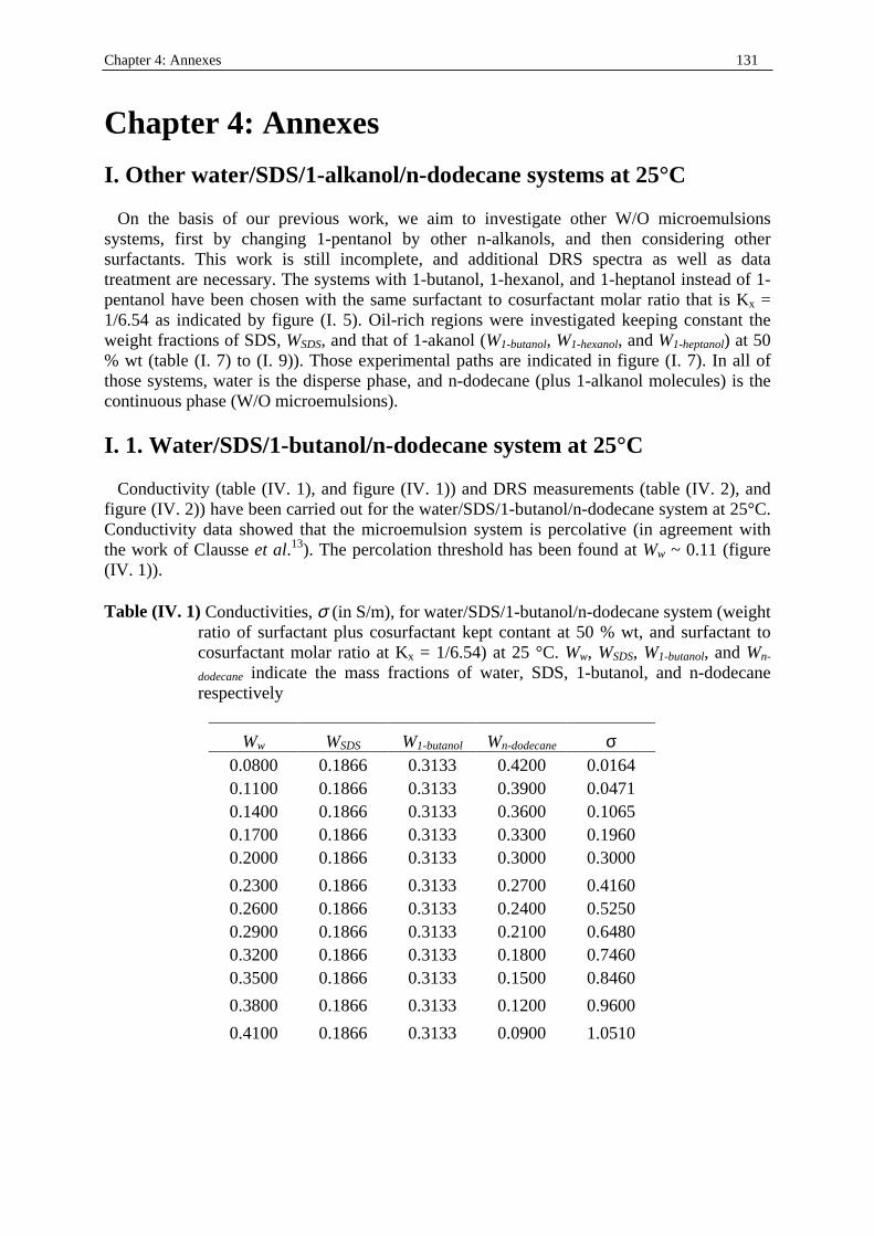
Chapter 4: Annexes 131
Chapter 4: Annexes
I . Other water/SDS/1-alkanol/n-dodecane systems at 25°C On the basis of our previous work, we aim to investigate other W/O microemulsions systems, first by changing 1-pentanol by other n-alkanols, and then considering other surfactants. This work is still i ncomplete, and additional DRS spectra as well as data treatment are necessary. The systems with 1-butanol, 1-hexanol, and 1-heptanol instead of 1-pentanol have been chosen with the same surfactant to cosurfactant molar ratio that is Kx = 1/6.54 as indicated by figure (I. 5). Oil -rich regions were investigated keeping constant the weight fractions of SDS, WSDS, and that of 1-akanol (W1-butanol, W1-hexanol, and W1-heptanol) at 50 % wt (table (I. 7) to (I. 9)). Those experimental paths are indicated in figure (I. 7). In all of those systems, water is the disperse phase, and n-dodecane (plus 1-alkanol molecules) is the continuous phase (W/O microemulsions).
I . 1. Water/SDS/1-butanol/n-dodecane system at 25°C Conductivity (table (IV. 1), and figure (IV. 1)) and DRS measurements (table (IV. 2), and figure (IV. 2)) have been carried out for the water/SDS/1-butanol/n-dodecane system at 25°C. Conductivity data showed that the microemulsion system is percolative (in agreement with the work of Clausse et al.13). The percolation threshold has been found at Ww ~ 0.11 (figure (IV. 1)). Table (IV. 1) Conductivities, σ (in S/m), for water/SDS/1-butanol/n-dodecane system (weight
ratio of surfactant plus cosurfactant kept contant at 50 % wt, and surfactant to cosurfactant molar ratio at Kx = 1/6.54) at 25 °C. Ww, WSDS, W1-butanol, and Wn-
dodecane indicate the mass fractions of water, SDS, 1-butanol, and n-dodecane respectively
Ww WSDS W1-butanol Wn-dodecane σ 0.0800 0.1866 0.3133 0.4200 0.0164 0.1100 0.1866 0.3133 0.3900 0.0471 0.1400 0.1866 0.3133 0.3600 0.1065 0.1700 0.1866 0.3133 0.3300 0.1960 0.2000 0.1866 0.3133 0.3000 0.3000
0.2300 0.1866 0.3133 0.2700 0.4160 0.2600 0.1866 0.3133 0.2400 0.5250 0.2900 0.1866 0.3133 0.2100 0.6480 0.3200 0.1866 0.3133 0.1800 0.7460 0.3500 0.1866 0.3133 0.1500 0.8460
0.3800 0.1866 0.3133 0.1200 0.9600
0.4100 0.1866 0.3133 0.0900 1.0510
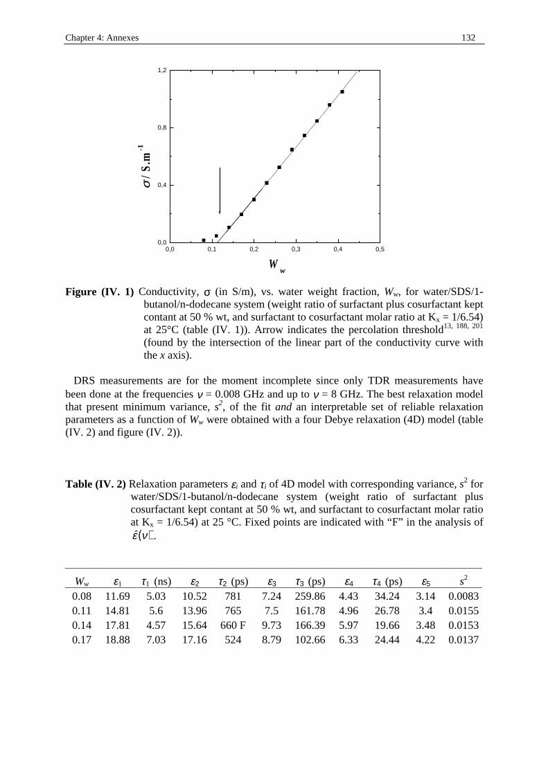
Chapter 4: Annexes 132
0,0 0,1 0,2 0,3 0,4 0,50,0
0,4
0,8
1,2
Ww
σσ / S
.m-1
Figure (IV. 1) Conductivity, σ (in S/m), vs. water weight fraction, Ww, for water/SDS/1-butanol/n-dodecane system (weight ratio of surfactant plus cosurfactant kept contant at 50 % wt, and surfactant to cosurfactant molar ratio at Kx = 1/6.54) at 25°C (table (IV. 1)). Arrow indicates the percolation threshold13, 188, 201 (found by the intersection of the linear part of the conductivity curve with the x axis).
DRS measurements are for the moment incomplete since only TDR measurements have been done at the frequencies ν = 0.008 GHz and up to ν = 8 GHz. The best relaxation model that present minimum variance, s2, of the fit and an interpretable set of reliable relaxation parameters as a function of Ww were obtained with a four Debye relaxation (4D) model (table (IV. 2) and figure (IV. 2)). Table (IV. 2) Relaxation parameters εi and τi of 4D model with corresponding variance, s2 for
water/SDS/1-butanol/n-dodecane system (weight ratio of surfactant plus cosurfactant kept contant at 50 % wt, and surfactant to cosurfactant molar ratio at Kx = 1/6.54) at 25 °C. Fixed points are indicated with “F” in the analysis of
( )ε ν .
Ww ε1 τ1 (ns) ε2 τ2 (ps) ε3 τ3 (ps) ε4 τ4 (ps) ε5 s2 0.08 11.69 5.03 10.52 781 7.24 259.86 4.43 34.24 3.14 0.0083 0.11 14.81 5.6 13.96 765 7.5 161.78 4.96 26.78 3.4 0.0155 0.14 17.81 4.57 15.64 660 F 9.73 166.39 5.97 19.66 3.48 0.0153 0.17 18.88 7.03 17.16 524 8.79 102.66 6.33 24.44 4.22 0.0137
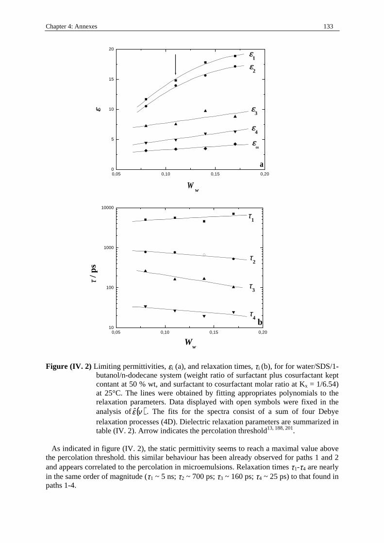
Chapter 4: Annexes 133
0,05 0,10 0,15 0,200
5
10
15
20
a
εε4
εε3
εε∞∞
εε2
εε1
εε
Ww
0,05 0,10 0,15 0,2010
100
1000
10000
ττ4
ττ3
ττ2
ττ1
b
Ww
ττ / p
s
Figure (IV. 2) Limiting permittivities, εi (a), and relaxation times, τi (b), for for water/SDS/1-
butanol/n-dodecane system (weight ratio of surfactant plus cosurfactant kept contant at 50 % wt, and surfactant to cosurfactant molar ratio at Kx = 1/6.54) at 25°C. The lines were obtained by fitting appropriates polynomials to the relaxation parameters. Data displayed with open symbols were fixed in the analysis of ( )νε . The fits for the spectra consist of a sum of four Debye relaxation processes (4D). Dielectric relaxation parameters are summarized in table (IV. 2). Arrow indicates the percolation threshold13, 188, 201.
As indicated in figure (IV. 2), the static permittivity seems to reach a maximal value above the percolation threshold. this similar behaviour has been already observed for paths 1 and 2 and appears correlated to the percolation in microemulsions. Relaxation times τ1-τ4 are nearly in the same order of magnitude (τ1 ~ 5 ns; τ2 ~ 700 ps; τ3 ~ 160 ps; τ4 ~ 25 ps) to that found in paths 1-4.
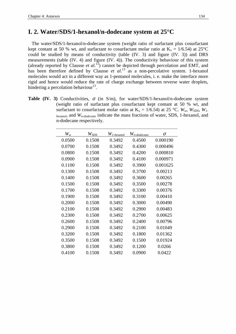
Chapter 4: Annexes 134
I . 2. Water/SDS/1-hexanol/n-dodecane system at 25°C The water/SDS/1-hexanol/n-dodecane system (weight ratio of surfactant plus cosurfactant kept contant at 50 % wt, and surfactant to cosurfactant molar ratio at Kx = 1/6.54) at 25°C could be studied by means of conductivity (table (IV. 3) and figure (IV. 3)) and DRS measurements (table (IV. 4) and figure (IV. 4)). The conductivity behaviour of this system (already reported by Clausse et al.13) cannot be depicted through percolation and EMT, and has been therefore defined by Clausse et al.13 as a non-percolative system. 1-hexanol molecules would act in a different way as 1-pentanol molecules, i. e. make the interface more rigid and hence would reduce the rate of charge exchange between reverse water droplets, hindering a percolation behaviour13. Table (IV. 3) Conductivities, σ (in S/m), for water/SDS/1-hexanol/n-dodecane system
(weight ratio of surfactant plus cosurfactant kept contant at 50 % wt, and surfactant to cosurfactant molar ratio at Kx = 1/6.54) at 25 °C. Ww, WSDS, W1-
hexanol, and Wn-dodecane indicate the mass fractions of water, SDS, 1-hexanol, and n-dodecane respectively.
Ww WSDS W1-hexanol Wn-dodecane σ 0.0500 0.1508 0.3492 0.4500 0.000190 0.0700 0.1508 0.3492 0.4300 0.000496 0.0800 0.1508 0.3492 0.4200 0.000810 0.0900 0.1508 0.3492 0.4100 0.000971 0.1100 0.1508 0.3492 0.3900 0.001625 0.1300 0.1508 0.3492 0.3700 0.00213 0.1400 0.1508 0.3492 0.3600 0.00265 0.1500 0.1508 0.3492 0.3500 0.00278 0.1700 0.1508 0.3492 0.3300 0.00376 0.1900 0.1508 0.3492 0.3100 0.00410 0.2000 0.1508 0.3492 0.3000 0.00490 0.2100 0.1508 0.3492 0.2900 0.00483 0.2300 0.1508 0.3492 0.2700 0.00625 0.2600 0.1508 0.3492 0.2400 0.00796 0.2900 0.1508 0.3492 0.2100 0.01049 0.3200 0.1508 0.3492 0.1800 0.01362 0.3500 0.1508 0.3492 0.1500 0.01924 0.3800 0.1508 0.3492 0.1200 0.0266 0.4100 0.1508 0.3492 0.0900 0.0422
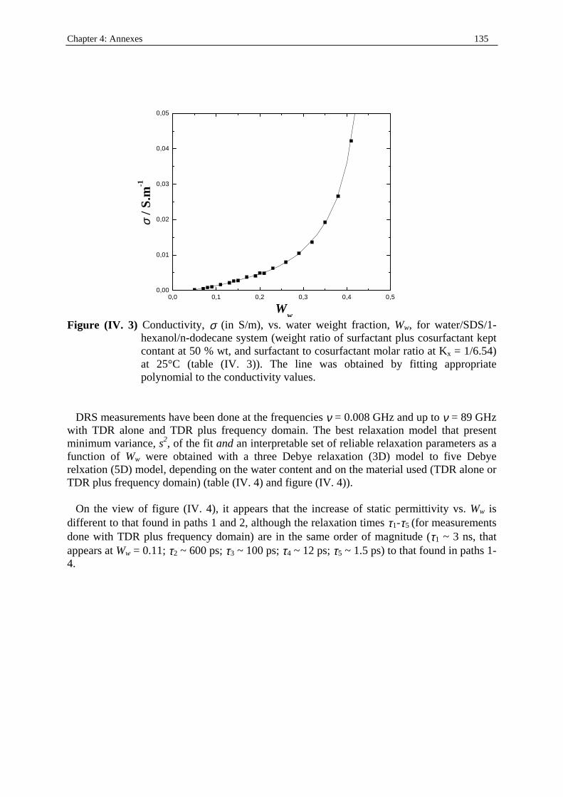
Chapter 4: Annexes 135
0,0 0,1 0,2 0,3 0,4 0,50,00
0,01
0,02
0,03
0,04
0,05
Ww
σσ / S
.m-1
Figure (IV. 3) Conductivity, σ (in S/m), vs. water weight fraction, Ww, for water/SDS/1-
hexanol/n-dodecane system (weight ratio of surfactant plus cosurfactant kept contant at 50 % wt, and surfactant to cosurfactant molar ratio at Kx = 1/6.54) at 25°C (table (IV. 3)). The line was obtained by fitting appropriate polynomial to the conductivity values.
DRS measurements have been done at the frequencies ν = 0.008 GHz and up to ν = 89 GHz with TDR alone and TDR plus frequency domain. The best relaxation model that present minimum variance, s2, of the fit and an interpretable set of reliable relaxation parameters as a function of Ww were obtained with a three Debye relaxation (3D) model to five Debye relxation (5D) model, depending on the water content and on the material used (TDR alone or TDR plus frequency domain) (table (IV. 4) and figure (IV. 4)). On the view of f igure (IV. 4), it appears that the increase of static permittivity vs. Ww is different to that found in paths 1 and 2, although the relaxation times τ1-τ5 (for measurements done with TDR plus frequency domain) are in the same order of magnitude (τ1 ~ 3 ns, that appears at Ww = 0.11; τ2 ~ 600 ps; τ3 ~ 100 ps; τ4 ~ 12 ps; τ5 ~ 1.5 ps) to that found in paths 1-4.
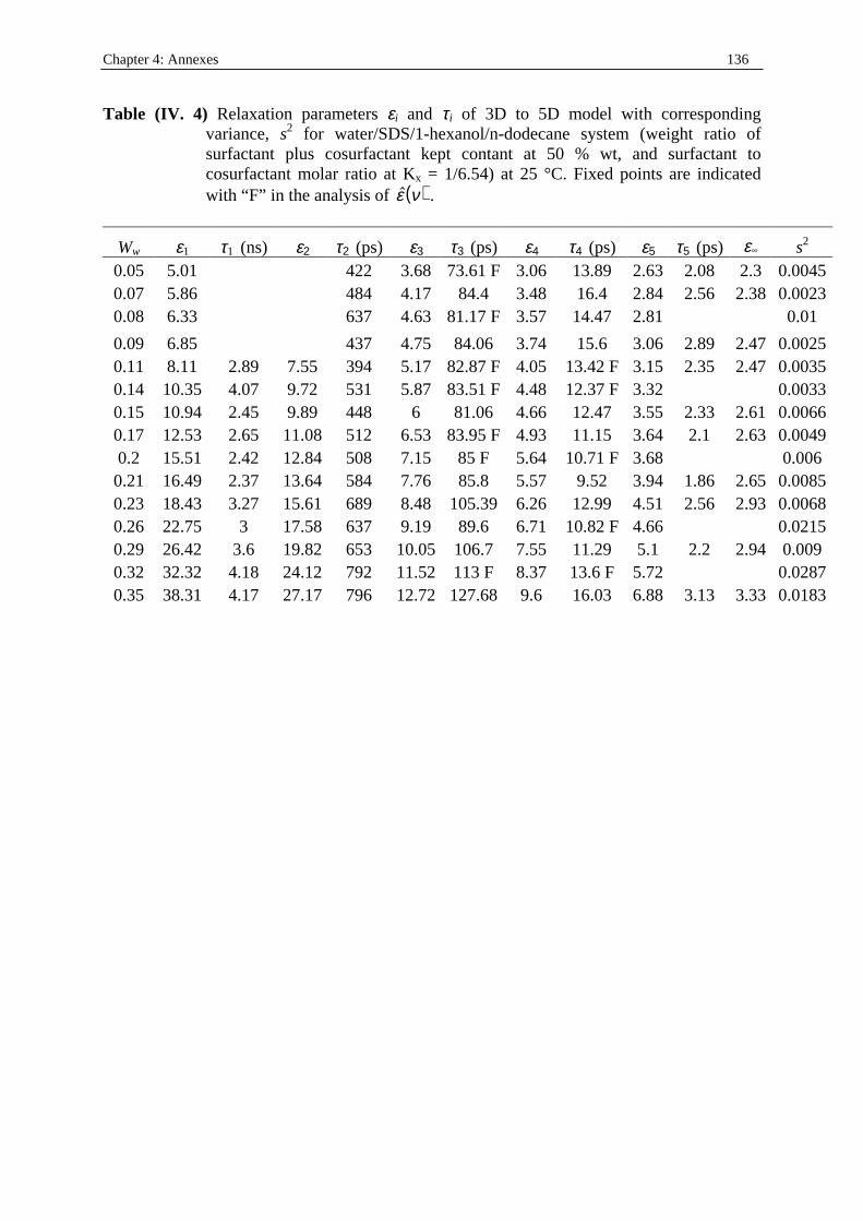
Chapter 4: Annexes 136
Table (IV. 4) Relaxation parameters εi and τi of 3D to 5D model with corresponding variance, s2 for water/SDS/1-hexanol/n-dodecane system (weight ratio of surfactant plus cosurfactant kept contant at 50 % wt, and surfactant to cosurfactant molar ratio at Kx = 1/6.54) at 25 °C. Fixed points are indicated with “F” in the analysis of ( )ε ν .
Ww ε1 τ1 (ns) ε2 τ2 (ps) ε3 τ3 (ps) ε4 τ4 (ps) ε5 τ5 (ps) ε s2 0.05 5.01 422 3.68 73.61 F 3.06 13.89 2.63 2.08 2.3 0.0045 0.07 5.86 484 4.17 84.4 3.48 16.4 2.84 2.56 2.38 0.0023 0.08 6.33 637 4.63 81.17 F 3.57 14.47 2.81 0.01
0.09 6.85 437 4.75 84.06 3.74 15.6 3.06 2.89 2.47 0.0025 0.11 8.11 2.89 7.55 394 5.17 82.87 F 4.05 13.42 F 3.15 2.35 2.47 0.0035 0.14 10.35 4.07 9.72 531 5.87 83.51 F 4.48 12.37 F 3.32 0.0033 0.15 10.94 2.45 9.89 448 6 81.06 4.66 12.47 3.55 2.33 2.61 0.0066 0.17 12.53 2.65 11.08 512 6.53 83.95 F 4.93 11.15 3.64 2.1 2.63 0.0049 0.2 15.51 2.42 12.84 508 7.15 85 F 5.64 10.71 F 3.68 0.006
0.21 16.49 2.37 13.64 584 7.76 85.8 5.57 9.52 3.94 1.86 2.65 0.0085 0.23 18.43 3.27 15.61 689 8.48 105.39 6.26 12.99 4.51 2.56 2.93 0.0068 0.26 22.75 3 17.58 637 9.19 89.6 6.71 10.82 F 4.66 0.0215 0.29 26.42 3.6 19.82 653 10.05 106.7 7.55 11.29 5.1 2.2 2.94 0.009 0.32 32.32 4.18 24.12 792 11.52 113 F 8.37 13.6 F 5.72 0.0287 0.35 38.31 4.17 27.17 796 12.72 127.68 9.6 16.03 6.88 3.13 3.33 0.0183
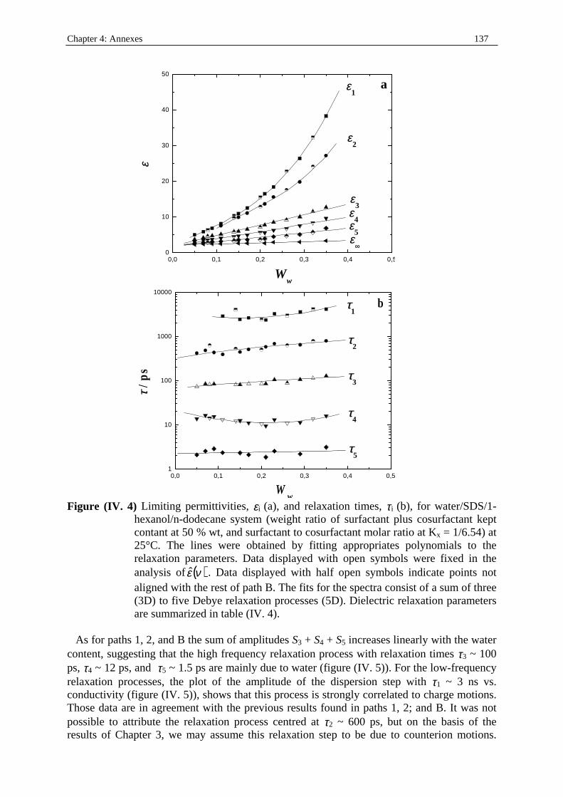
Chapter 4: Annexes 137
0,0 0,1 0,2 0,3 0,4 0,50
10
20
30
40
50
a
εε
Ww
εε5
εε4
εε3
εε2
εε1
εε∞∞
0,0 0,1 0,2 0,3 0,4 0,51
10
100
1000
10000
ττ5
ττ4
ττ3
ττ2
ττ1
ττ / p
s
b
Ww
Figure (IV. 4) Limiting permittivities, εi (a), and relaxation times, τi (b), for water/SDS/1-
hexanol/n-dodecane system (weight ratio of surfactant plus cosurfactant kept contant at 50 % wt, and surfactant to cosurfactant molar ratio at Kx = 1/6.54) at 25°C. The lines were obtained by fitting appropriates polynomials to the relaxation parameters. Data displayed with open symbols were fixed in the analysis of ( )νε . Data displayed with half open symbols indicate points not aligned with the rest of path B. The fits for the spectra consist of a sum of three (3D) to five Debye relaxation processes (5D). Dielectric relaxation parameters are summarized in table (IV. 4).
As for paths 1, 2, and B the sum of amplitudes S3 + S4 + S5 increases linearly with the water content, suggesting that the high frequency relaxation process with relaxation times τ3 ~ 100 ps, τ4 ~ 12 ps, and τ5 ~ 1.5 ps are mainly due to water (figure (IV. 5)). For the low-frequency relaxation processes, the plot of the amplitude of the dispersion step with τ1 ~ 3 ns vs. conductivity (figure (IV. 5)), shows that this process is strongly correlated to charge motions. Those data are in agreement with the previous results found in paths 1, 2; and B. It was not possible to attribute the relaxation process centred at τ2 ~ 600 ps, but on the basis of the results of Chapter 3, we may assume this relaxation step to be due to counterion motions.
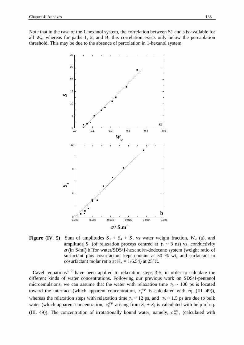
Chapter 4: Annexes 138
Note that in the case of the 1-hexanol system, the correlation between S1 and s is available for all Ww, whereas for paths 1, 2, and B, this correlation exists only below the percaolation threshold. This may be due to the absence of percolation in 1-hexanol system.
0,0 0,1 0,2 0,3 0,4 0,50
5
10
15
20
25
30
a
Ww
S
0,000 0,005 0,010 0,015 0,020 0,0250
4
8
12
b
S 1
σσ / S.m-1
Figure (IV. 5) Sum of amplitudes S3 + S4 + S5 vs water weight fraction, Ww (a), and
amplitude S1 (of relaxation process centred at τ1 ~ 3 ns) vs. conductivity σ (in S/m) (b) for water/SDS/1-hexanol/n-dodecane system (weight ratio of surfactant plus cosurfactant kept contant at 50 % wt, and surfactant to cosurfactant molar ratio at Kx = 1/6.54) at 25°C.
Cavell equations6, 7 have been applied to relaxation steps 3-5, in order to calculate the different kinds of water concentrations. Following our previous work on SDS/1-pentanol microemulsions, we can assume that the water with relaxation time τ3 ~ 100 ps is located toward the interface (which apparent concentration, app
ic is calculated with eq. (III . 49)),
whereas the relaxation steps with relaxation time τ4 ~ 12 ps, and τ5 ~ 1.5 ps are due to bulk water (which apparent concentration, app
bc arising from S4 + S5 is calculated with help of eq.
(III . 49)). The concentration of irrotationally bound water, namely, appIBc , (calculated with
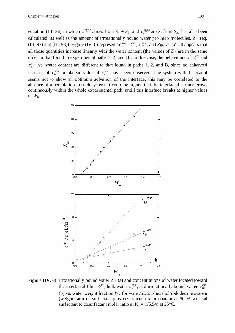
Chapter 4: Annexes 139
equation (III . 56) in which bappic , arises from S4 + S5, and sapp
ic , arises from S3) has also been
calculated, as well as the amount of irrotationally bound water pro SDS molecules, ZIB (eq. (III . 92) and (III . 93)). Figure (IV. 6) represents app
ic , appbc , app
IBc , and ZIB, vs. Ww. It appears that
all those quantities increase linearly with the water content (the values of ZIB are in the same order to that found in experimental paths 1, 2, and B). In this case, the behaviours of app
ic and appbc vs. water content are different to that found in paths 1, 2, and B, since no enhanced
increase of appbc or plateau value of app
ic have been observed. The system with 1-hexanol
seems not to show an optimum solvation of the interface, this may be correlated to the absence of a percolation in such system. It could be argued that the interfacial surface grows continuously within the whole experimental path, untill t his interface breaks at higher values of Ww.
0,0 0,1 0,2 0,3 0,4 0,50
5
10
15
20
25
a
Ww
ZIB
0,0 0,1 0,2 0,3 0,4 0,50
4
8
12
b
ci
app
cIB
app
cb
app
capp /
mol
.dm
-3
Ww
Figure (IV. 6) Irrotationally bound water ZIB (a) and concentrations of water located toward the interfacial film app
ic , bulk water appbc , and irrotationally bound water app
IBc
(b) vs. water weight fraction Ww for water/SDS/1-hexanol/n-dodecane system (weight ratio of surfactant plus cosurfactant kept contant at 50 % wt, and surfactant to cosurfactant molar ratio at Kx = 1/6.54) at 25°C.
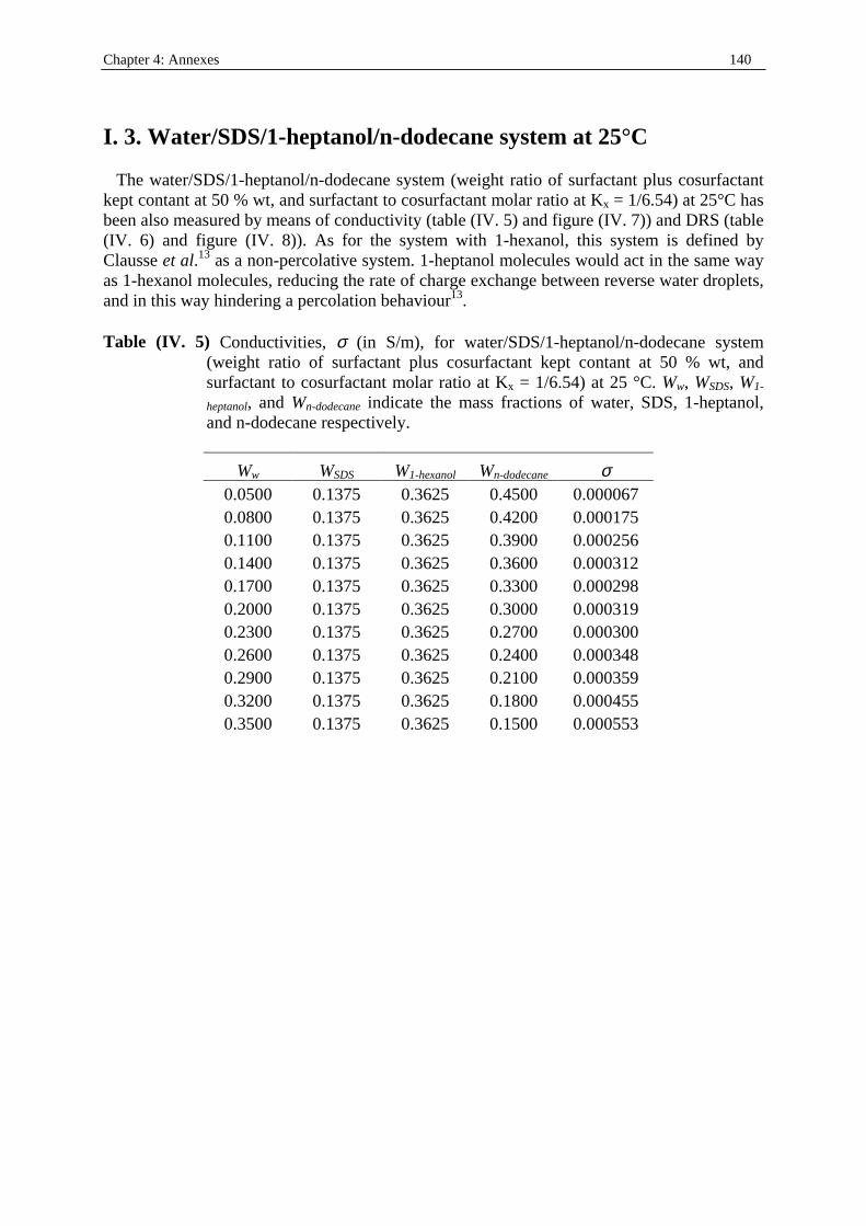
Chapter 4: Annexes 140
I . 3. Water/SDS/1-heptanol/n-dodecane system at 25°C The water/SDS/1-heptanol/n-dodecane system (weight ratio of surfactant plus cosurfactant kept contant at 50 % wt, and surfactant to cosurfactant molar ratio at Kx = 1/6.54) at 25°C has been also measured by means of conductivity (table (IV. 5) and figure (IV. 7)) and DRS (table (IV. 6) and figure (IV. 8)). As for the system with 1-hexanol, this system is defined by Clausse et al.13 as a non-percolative system. 1-heptanol molecules would act in the same way as 1-hexanol molecules, reducing the rate of charge exchange between reverse water droplets, and in this way hindering a percolation behaviour13. Table (IV. 5) Conductivities, σ (in S/m), for water/SDS/1-heptanol/n-dodecane system
(weight ratio of surfactant plus cosurfactant kept contant at 50 % wt, and surfactant to cosurfactant molar ratio at Kx = 1/6.54) at 25 °C. Ww, WSDS, W1-
heptanol, and Wn-dodecane indicate the mass fractions of water, SDS, 1-heptanol, and n-dodecane respectively.
Ww WSDS W1-hexanol Wn-dodecane σ 0.0500 0.1375 0.3625 0.4500 0.000067 0.0800 0.1375 0.3625 0.4200 0.000175 0.1100 0.1375 0.3625 0.3900 0.000256 0.1400 0.1375 0.3625 0.3600 0.000312 0.1700 0.1375 0.3625 0.3300 0.000298 0.2000 0.1375 0.3625 0.3000 0.000319 0.2300 0.1375 0.3625 0.2700 0.000300 0.2600 0.1375 0.3625 0.2400 0.000348 0.2900 0.1375 0.3625 0.2100 0.000359 0.3200 0.1375 0.3625 0.1800 0.000455 0.3500 0.1375 0.3625 0.1500 0.000553
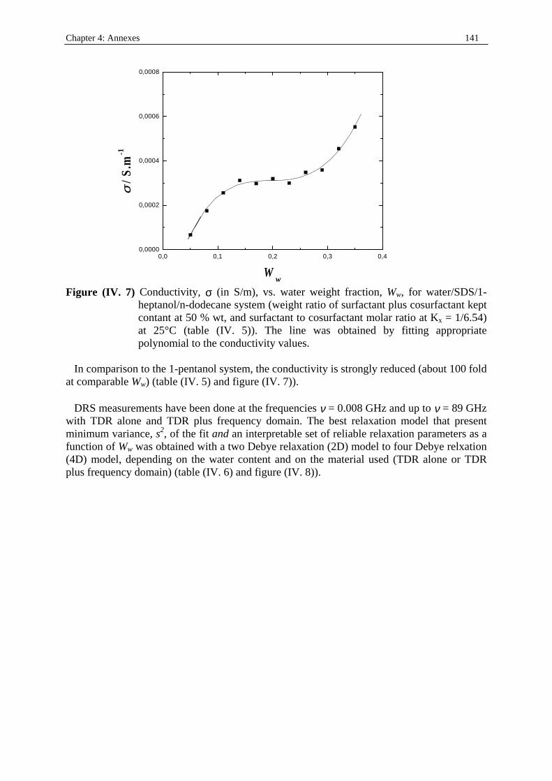
Chapter 4: Annexes 141
0,0 0,1 0,2 0,3 0,40,0000
0,0002
0,0004
0,0006
0,0008
Ww
σσ / S
.m-1
Figure (IV. 7) Conductivity, σ (in S/m), vs. water weight fraction, Ww, for water/SDS/1-
heptanol/n-dodecane system (weight ratio of surfactant plus cosurfactant kept contant at 50 % wt, and surfactant to cosurfactant molar ratio at Kx = 1/6.54) at 25°C (table (IV. 5)). The line was obtained by fitting appropriate polynomial to the conductivity values.
In comparison to the 1-pentanol system, the conductivity is strongly reduced (about 100 fold at comparable Ww) (table (IV. 5) and figure (IV. 7)). DRS measurements have been done at the frequencies ν = 0.008 GHz and up to ν = 89 GHz with TDR alone and TDR plus frequency domain. The best relaxation model that present minimum variance, s2, of the fit and an interpretable set of reliable relaxation parameters as a function of Ww was obtained with a two Debye relaxation (2D) model to four Debye relxation (4D) model, depending on the water content and on the material used (TDR alone or TDR plus frequency domain) (table (IV. 6) and figure (IV. 8)).
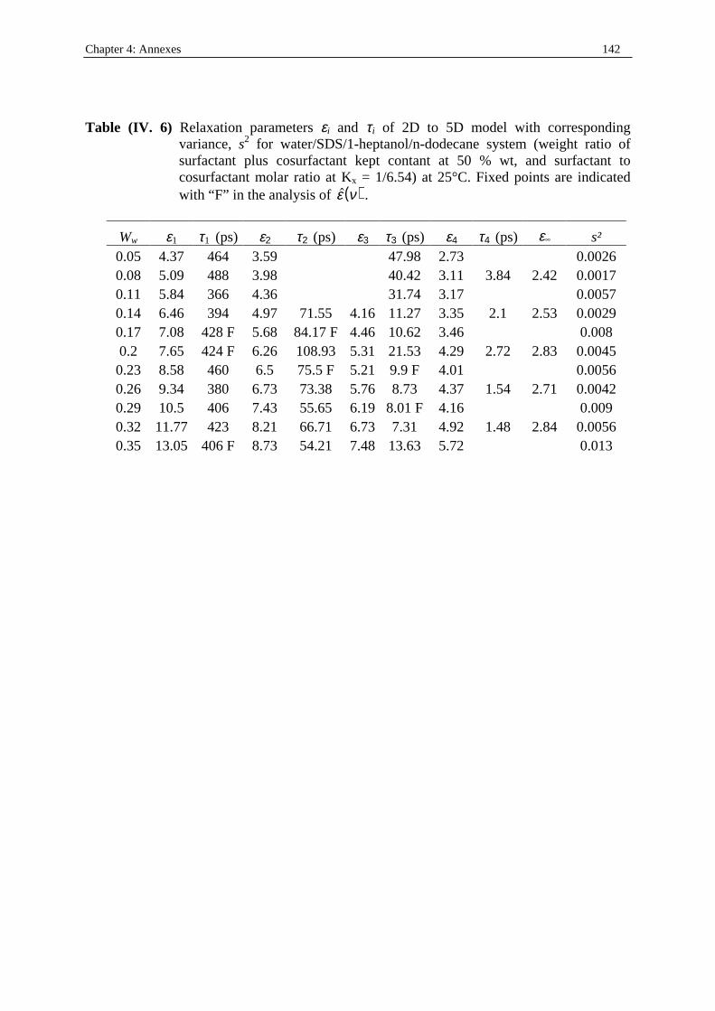
Chapter 4: Annexes 142
Table (IV. 6) Relaxation parameters εi and τi of 2D to 5D model with corresponding
variance, s2 for water/SDS/1-heptanol/n-dodecane system (weight ratio of surfactant plus cosurfactant kept contant at 50 % wt, and surfactant to cosurfactant molar ratio at Kx = 1/6.54) at 25°C. Fixed points are indicated with “F” in the analysis of ( )ε ν .
Ww ε1 τ1 (ps) ε2 τ2 (ps) ε3 τ3 (ps) ε4 τ4 (ps) ε s² 0.05 4.37 464 3.59 47.98 2.73 0.0026 0.08 5.09 488 3.98 40.42 3.11 3.84 2.42 0.0017 0.11 5.84 366 4.36 31.74 3.17 0.0057 0.14 6.46 394 4.97 71.55 4.16 11.27 3.35 2.1 2.53 0.0029 0.17 7.08 428 F 5.68 84.17 F 4.46 10.62 3.46 0.008 0.2 7.65 424 F 6.26 108.93 5.31 21.53 4.29 2.72 2.83 0.0045 0.23 8.58 460 6.5 75.5 F 5.21 9.9 F 4.01 0.0056 0.26 9.34 380 6.73 73.38 5.76 8.73 4.37 1.54 2.71 0.0042 0.29 10.5 406 7.43 55.65 6.19 8.01 F 4.16 0.009 0.32 11.77 423 8.21 66.71 6.73 7.31 4.92 1.48 2.84 0.0056 0.35 13.05 406 F 8.73 54.21 7.48 13.63 5.72 0.013

Chapter 4: Annexes 143
0,0 0,1 0,2 0,3 0,40
5
10
15
a
εε∞∞
εε4
εε3
εε2
εε1
Ww
εε
0,0 0,1 0,2 0,3 0,41
10
100
1000
ττ / p
s
ττ4
ττ3
ττ2
ττ1
b
Ww
Figure (IV. 8) Limiting permittivities, εi (a), and relaxation times, τi (b), for water/SDS/1-
heptanol/n-dodecane system (weight ratio of surfactant plus cosurfactant kept contant at 50 % wt, and surfactant to cosurfactant molar ratio at Kx = 1/6.54) at 25°C. The lines were obtained by fitting appropriates polynomials to the relaxation parameters. Data displayed with open symbols were fixed in the analysis of ( )νε . Data displayed with half open symbols indicate points not aligned with the rest of path B. The fits for the spectra consist of a sum of two (2D) to four Debye relaxation processes (4D). Dielectric relaxation parameters are summarized in table (IV. 6).
In figure (IV. 8), it appears that the increase of static permittivity vs. Ww is different to that found in paths 1 and 2 and similar to that found in 1-hexanol system.,The relaxation times τ1-τ4 (for measurements done with TDR plus frequency domain) are in the same order of magnitude (τ1 ~ 400 ps; τ2 ~ 70 ps, that appears at Ww = 0.14; τ3 ~ 8 ps; τ4 ~ 1.5 ps) to that found in paths 1-4,1-hexanol, and 1-butanol systems. No dispersion step centred at τ ~ 2-5 ns, as observed before in paths 1-4, in 1-hexanol, and 1-butanol systems could be observed. As for paths 1, 2, and B, and 1-hexanol system the sum of amplitudes S3 + S4 + S5 increases linearly with the water content, suggesting that the high frequency relaxation processes with
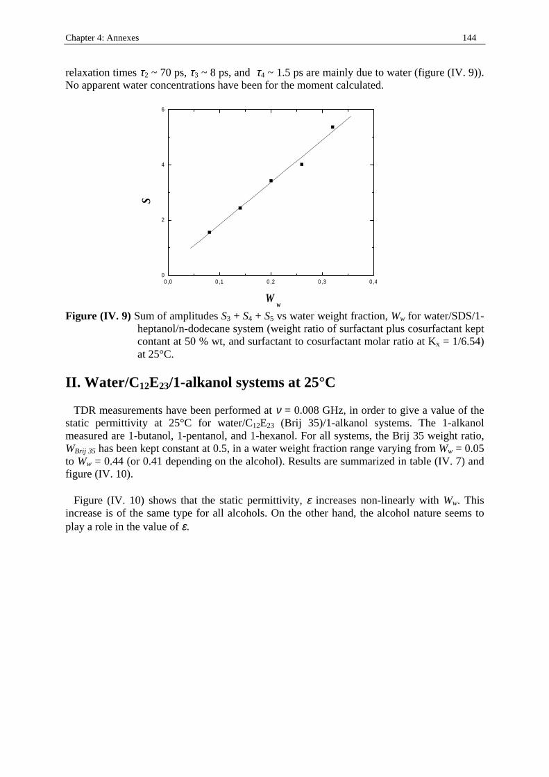
Chapter 4: Annexes 144
relaxation times τ2 ~ 70 ps, τ3 ~ 8 ps, and τ4 ~ 1.5 ps are mainly due to water (figure (IV. 9)). No apparent water concentrations have been for the moment calculated.
0,0 0,1 0,2 0,3 0,40
2
4
6
Ww
S
Figure (IV. 9) Sum of amplitudes S3 + S4 + S5 vs water weight fraction, Ww for water/SDS/1-
heptanol/n-dodecane system (weight ratio of surfactant plus cosurfactant kept contant at 50 % wt, and surfactant to cosurfactant molar ratio at Kx = 1/6.54) at 25°C.
II . Water/C12E23/1-alkanol systems at 25°C TDR measurements have been performed at ν = 0.008 GHz, in order to give a value of the static permittivity at 25°C for water/C12E23 (Brij 35)/1-alkanol systems. The 1-alkanol measured are 1-butanol, 1-pentanol, and 1-hexanol. For all systems, the Brij 35 weight ratio, WBrij 35 has been kept constant at 0.5, in a water weight fraction range varying from Ww = 0.05 to Ww = 0.44 (or 0.41 depending on the alcohol). Results are summarized in table (IV. 7) and figure (IV. 10). Figure (IV. 10) shows that the static permittivity, ε increases non-linearly with Ww. This increase is of the same type for all alcohols. On the other hand, the alcohol nature seems to play a role in the value of ε.
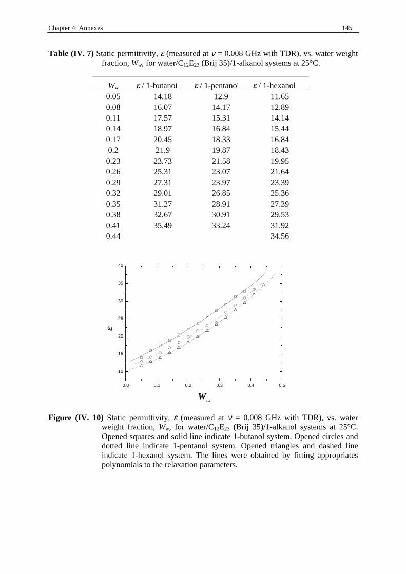
Chapter 4: Annexes 145
Table (IV. 7) Static permittivity, ε (measured at ν = 0.008 GHz with TDR), vs. water weight fraction, Ww, for water/C12E23 (Brij 35)/1-alkanol systems at 25°C.
Ww ε / 1-butanol ε / 1-pentanol ε / 1-hexanol 0.05 14.18 12.9 11.65 0.08 16.07 14.17 12.89 0.11 17.57 15.31 14.14 0.14 18.97 16.84 15.44 0.17 20.45 18.33 16.84 0.2 21.9 19.87 18.43 0.23 23.73 21.58 19.95 0.26 25.31 23.07 21.64 0.29 27.31 23.97 23.39 0.32 29.01 26.85 25.36 0.35 31.27 28.91 27.39 0.38 32.67 30.91 29.53 0.41 35.49 33.24 31.92 0.44 34.56
0,0 0,1 0,2 0,3 0,4 0,5
10
15
20
25
30
35
40
εε
Ww
Figure (IV. 10) Static permittivity, ε (measured at ν = 0.008 GHz with TDR), vs. water
weight fraction, Ww, for water/C12E23 (Brij 35)/1-alkanol systems at 25°C. Opened squares and solid line indicate 1-butanol system. Opened circles and dotted line indicate 1-pentanol system. Opened triangles and dashed line indicate 1-hexanol system. The lines were obtained by fitting appropriates polynomials to the relaxation parameters.
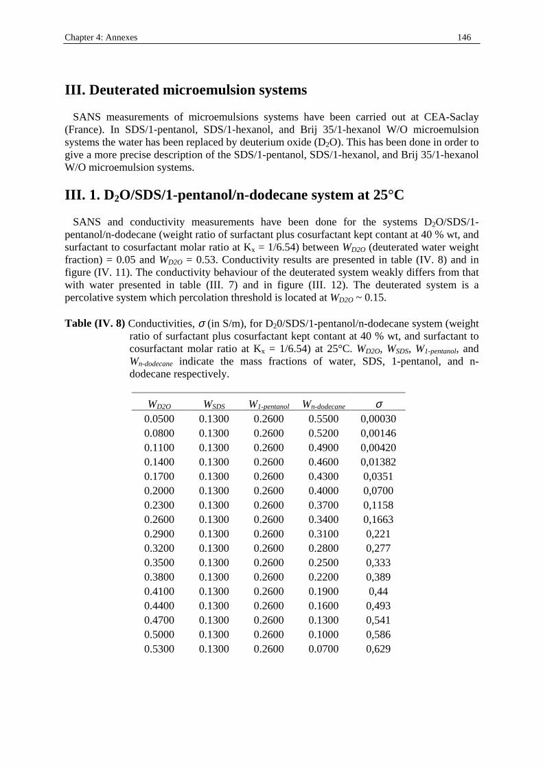
Chapter 4: Annexes 146
III . Deuterated microemulsion systems SANS measurements of microemulsions systems have been carried out at CEA-Saclay (France). In SDS/1-pentanol, SDS/1-hexanol, and Brij 35/1-hexanol W/O microemulsion systems the water has been replaced by deuterium oxide (D2O). This has been done in order to give a more precise description of the SDS/1-pentanol, SDS/1-hexanol, and Brij 35/1-hexanol W/O microemulsion systems.
III . 1. D2O/SDS/1-pentanol/n-dodecane system at 25°C SANS and conductivity measurements have been done for the systems D2O/SDS/1-pentanol/n-dodecane (weight ratio of surfactant plus cosurfactant kept contant at 40 % wt, and surfactant to cosurfactant molar ratio at Kx = 1/6.54) between WD2O (deuterated water weight fraction) = 0.05 and WD2O = 0.53. Conductivity results are presented in table (IV. 8) and in figure (IV. 11). The conductivity behaviour of the deuterated system weakly differs from that with water presented in table (III . 7) and in figure (III . 12). The deuterated system is a percolative system which percolation threshold is located at WD2O ~ 0.15. Table (IV. 8) Conductivities, σ (in S/m), for D20/SDS/1-pentanol/n-dodecane system (weight
ratio of surfactant plus cosurfactant kept contant at 40 % wt, and surfactant to cosurfactant molar ratio at Kx = 1/6.54) at 25°C. WD2O, WSDS, W1-pentanol, and Wn-dodecane indicate the mass fractions of water, SDS, 1-pentanol, and n-dodecane respectively.
WD2O WSDS W1-pentanol Wn-dodecane σ 0.0500 0.1300 0.2600 0.5500 0,00030 0.0800 0.1300 0.2600 0.5200 0,00146 0.1100 0.1300 0.2600 0.4900 0,00420 0.1400 0.1300 0.2600 0.4600 0,01382 0.1700 0.1300 0.2600 0.4300 0,0351 0.2000 0.1300 0.2600 0.4000 0,0700 0.2300 0.1300 0.2600 0.3700 0,1158 0.2600 0.1300 0.2600 0.3400 0,1663 0.2900 0.1300 0.2600 0.3100 0,221 0.3200 0.1300 0.2600 0.2800 0,277 0.3500 0.1300 0.2600 0.2500 0,333 0.3800 0.1300 0.2600 0.2200 0,389 0.4100 0.1300 0.2600 0.1900 0,44 0.4400 0.1300 0.2600 0.1600 0,493 0.4700 0.1300 0.2600 0.1300 0,541 0.5000 0.1300 0.2600 0.1000 0,586 0.5300 0.1300 0.2600 0.0700 0,629
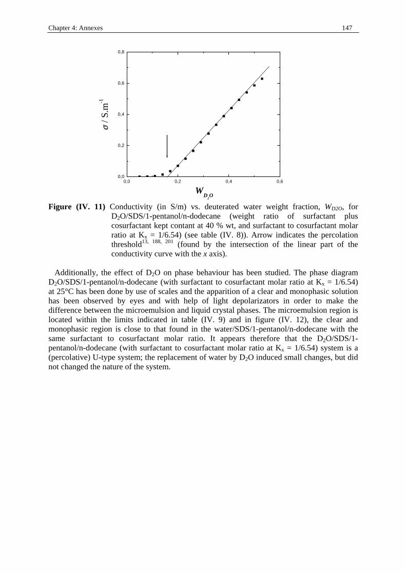
Chapter 4: Annexes 147
0,0 0,2 0,4 0,60,0
0,2
0,4
0,6
0,8
σσ / S
.m-1
WD
2O
Figure (IV. 11) Conductivity (in S/m) vs. deuterated water weight fraction, WD2O, for
D2O/SDS/1-pentanol/n-dodecane (weight ratio of surfactant plus cosurfactant kept contant at 40 % wt, and surfactant to cosurfactant molar ratio at Kx = 1/6.54) (see table (IV. 8)). Arrow indicates the percolation threshold13, 188, 201 (found by the intersection of the linear part of the conductivity curve with the x axis).
Additionally, the effect of D2O on phase behaviour has been studied. The phase diagram D2O/SDS/1-pentanol/n-dodecane (with surfactant to cosurfactant molar ratio at Kx = 1/6.54) at 25°C has been done by use of scales and the apparition of a clear and monophasic solution has been observed by eyes and with help of light depolarizators in order to make the difference between the microemulsion and liquid crystal phases. The microemulsion region is located within the limits indicated in table (IV. 9) and in figure (IV. 12), the clear and monophasic region is close to that found in the water/SDS/1-pentanol/n-dodecane with the same surfactant to cosurfactant molar ratio. It appears therefore that the D2O/SDS/1-pentanol/n-dodecane (with surfactant to cosurfactant molar ratio at Kx = 1/6.54) system is a (percolative) U-type system; the replacement of water by D2O induced small changes, but did not changed the nature of the system.
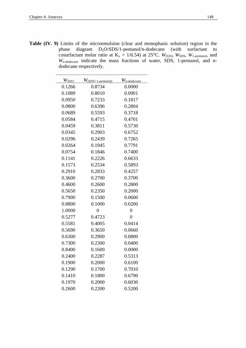
Chapter 4: Annexes 148
Table (IV. 9) Limits of the microemulsion (clear and monophasic solution) region in the
phase diagram D2O/SDS/1-pentanol/n-dodecane (with surfactant to cosurfactant molar ratio at Kx = 1/6.54) at 25°C. WD2O, WSDS, W1-pentanol, and Wn-dodecane indicate the mass fractions of water, SDS, 1-pentanol, and n-dodecane respectively.
WD2O W(SDS+1-pentanol) Wn-dodecane 0.1266 0.8734 0.0000 0.1089 0.8010 0.0901 0.0950 0.7233 0.1817 0.0800 0.6396 0.2804 0.0689 0.5593 0.3718 0.0584 0.4715 0.4701 0.0459 0.3811 0.5730 0.0345 0.2903 0.6752 0.0296 0.2439 0.7265 0.0264 0.1945 0.7791 0.0754 0.1846 0.7400 0.1141 0.2226 0.6633 0.1573 0.2534 0.5893 0.2910 0.2833 0.4257 0.3600 0.2700 0.3700 0.4600 0.2600 0.2800 0.5650 0.2350 0.2000 0.7900 0.1500 0.0600 0.8800 0.1000 0.0200 1.0000 0 0 0.5277 0.4723 0 0.5581 0.4005 0.0414 0.5690 0.3650 0.0660 0.6300 0.2900 0.0800 0.7300 0.2300 0.0400 0.8400 0.1600 0.0000 0.2400 0.2287 0.5313 0.1900 0.2000 0.6100 0.1290 0.1700 0.7010 0.1410 0.1800 0.6790 0.1970 0.2000 0.6030 0.2600 0.2200 0.5200
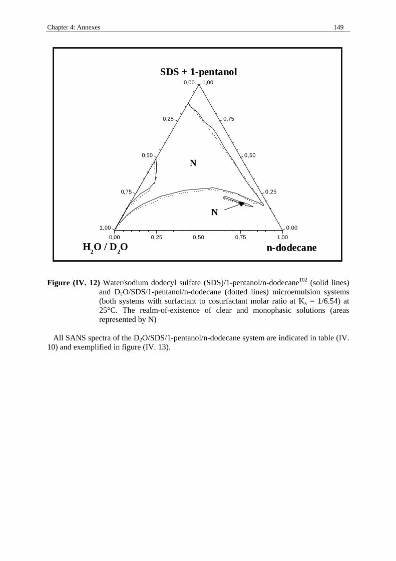
Chapter 4: Annexes 149
0,00 0,25 0,50 0,75 1,00
0,00
0,25
0,50
0,75
1,00 0,00
0,25
0,50
0,75
1,00
H2O / D
2O n-dodecane
SDS + 1-pentanol
Figure (IV. 12) Water/sodium dodecyl sulfate (SDS)/1-pentanol/n-dodecane102 (solid lines)
and D2O/SDS/1-pentanol/n-dodecane (dotted lines) microemulsion systems (both systems with surfactant to cosurfactant molar ratio at Kx = 1/6.54) at 25°C. The realm-of-existence of clear and monophasic solutions (areas represented by N)
All SANS spectra of the D2O/SDS/1-pentanol/n-dodecane system are indicated in table (IV. 10) and exempli fied in figure (IV. 13).
N
N
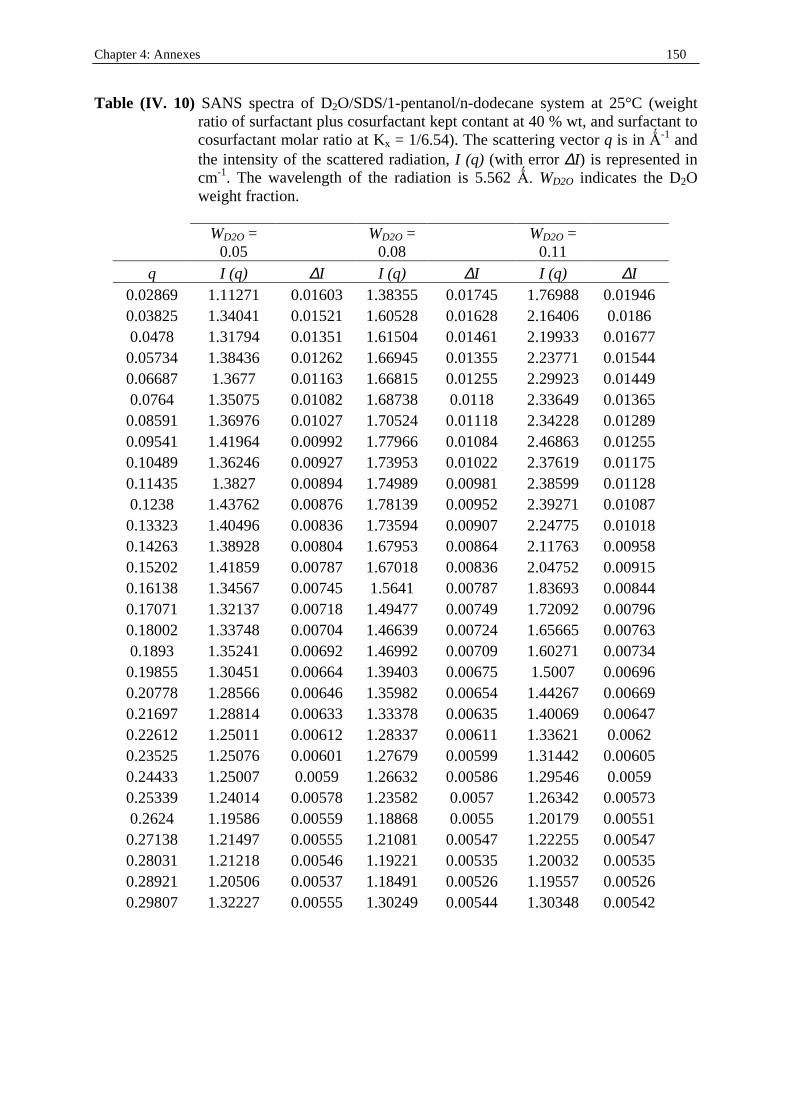
Chapter 4: Annexes 150
Table (IV. 10) SANS spectra of D2O/SDS/1-pentanol/n-dodecane system at 25°C (weight ratio of surfactant plus cosurfactant kept contant at 40 % wt, and surfactant to cosurfactant molar ratio at Kx = 1/6.54). The scattering vector q is in Ö-1 and the intensity of the scattered radiation, I (q) (with error ∆I) is represented in cm-1. The wavelength of the radiation is 5.562 Ö WD2O indicates the D2O weight fraction.
WD2O =
0.05 WD2O =
0.08 WD2O =
0.11 q I (q) ∆I I (q) ∆I I (q) ∆I
0.02869 1.11271 0.01603 1.38355 0.01745 1.76988 0.01946 0.03825 1.34041 0.01521 1.60528 0.01628 2.16406 0.0186 0.0478 1.31794 0.01351 1.61504 0.01461 2.19933 0.01677
0.05734 1.38436 0.01262 1.66945 0.01355 2.23771 0.01544 0.06687 1.3677 0.01163 1.66815 0.01255 2.29923 0.01449 0.0764 1.35075 0.01082 1.68738 0.0118 2.33649 0.01365
0.08591 1.36976 0.01027 1.70524 0.01118 2.34228 0.01289 0.09541 1.41964 0.00992 1.77966 0.01084 2.46863 0.01255 0.10489 1.36246 0.00927 1.73953 0.01022 2.37619 0.01175 0.11435 1.3827 0.00894 1.74989 0.00981 2.38599 0.01128 0.1238 1.43762 0.00876 1.78139 0.00952 2.39271 0.01087
0.13323 1.40496 0.00836 1.73594 0.00907 2.24775 0.01018 0.14263 1.38928 0.00804 1.67953 0.00864 2.11763 0.00958 0.15202 1.41859 0.00787 1.67018 0.00836 2.04752 0.00915 0.16138 1.34567 0.00745 1.5641 0.00787 1.83693 0.00844 0.17071 1.32137 0.00718 1.49477 0.00749 1.72092 0.00796 0.18002 1.33748 0.00704 1.46639 0.00724 1.65665 0.00763 0.1893 1.35241 0.00692 1.46992 0.00709 1.60271 0.00734
0.19855 1.30451 0.00664 1.39403 0.00675 1.5007 0.00696 0.20778 1.28566 0.00646 1.35982 0.00654 1.44267 0.00669 0.21697 1.28814 0.00633 1.33378 0.00635 1.40069 0.00647 0.22612 1.25011 0.00612 1.28337 0.00611 1.33621 0.0062 0.23525 1.25076 0.00601 1.27679 0.00599 1.31442 0.00605 0.24433 1.25007 0.0059 1.26632 0.00586 1.29546 0.0059 0.25339 1.24014 0.00578 1.23582 0.0057 1.26342 0.00573 0.2624 1.19586 0.00559 1.18868 0.0055 1.20179 0.00551
0.27138 1.21497 0.00555 1.21081 0.00547 1.22255 0.00547 0.28031 1.21218 0.00546 1.19221 0.00535 1.20032 0.00535 0.28921 1.20506 0.00537 1.18491 0.00526 1.19557 0.00526 0.29807 1.32227 0.00555 1.30249 0.00544 1.30348 0.00542
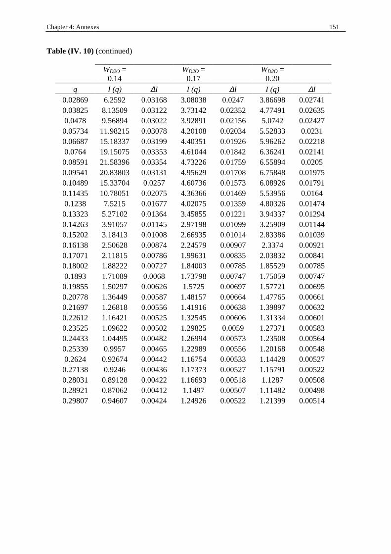
Chapter 4: Annexes 151
Table (IV. 10) (continued)
WD2O =
0.14 WD2O =
0.17 WD2O =
0.20 q I (q) ∆I I (q) ∆I I (q) ∆I
0.02869 6.2592 0.03168 3.08038 0.0247 3.86698 0.02741 0.03825 8.13509 0.03122 3.73142 0.02352 4.77491 0.02635 0.0478 9.56894 0.03022 3.92891 0.02156 5.0742 0.02427
0.05734 11.98215 0.03078 4.20108 0.02034 5.52833 0.0231 0.06687 15.18337 0.03199 4.40351 0.01926 5.96262 0.02218 0.0764 19.15075 0.03353 4.61044 0.01842 6.36241 0.02141
0.08591 21.58396 0.03354 4.73226 0.01759 6.55894 0.0205 0.09541 20.83803 0.03131 4.95629 0.01708 6.75848 0.01975 0.10489 15.33704 0.0257 4.60736 0.01573 6.08926 0.01791 0.11435 10.78051 0.02075 4.36366 0.01469 5.53956 0.0164 0.1238 7.5215 0.01677 4.02075 0.01359 4.80326 0.01474
0.13323 5.27102 0.01364 3.45855 0.01221 3.94337 0.01294 0.14263 3.91057 0.01145 2.97198 0.01099 3.25909 0.01144 0.15202 3.18413 0.01008 2.66935 0.01014 2.83386 0.01039 0.16138 2.50628 0.00874 2.24579 0.00907 2.3374 0.00921 0.17071 2.11815 0.00786 1.99631 0.00835 2.03832 0.00841 0.18002 1.88222 0.00727 1.84003 0.00785 1.85529 0.00785 0.1893 1.71089 0.0068 1.73798 0.00747 1.75059 0.00747
0.19855 1.50297 0.00626 1.5725 0.00697 1.57721 0.00695 0.20778 1.36449 0.00587 1.48157 0.00664 1.47765 0.00661 0.21697 1.26818 0.00556 1.41916 0.00638 1.39897 0.00632 0.22612 1.16421 0.00525 1.32545 0.00606 1.31334 0.00601 0.23525 1.09622 0.00502 1.29825 0.0059 1.27371 0.00583 0.24433 1.04495 0.00482 1.26994 0.00573 1.23508 0.00564 0.25339 0.9957 0.00465 1.22989 0.00556 1.20168 0.00548 0.2624 0.92674 0.00442 1.16754 0.00533 1.14428 0.00527
0.27138 0.9246 0.00436 1.17373 0.00527 1.15791 0.00522 0.28031 0.89128 0.00422 1.16693 0.00518 1.1287 0.00508 0.28921 0.87062 0.00412 1.1497 0.00507 1.11482 0.00498 0.29807 0.94607 0.00424 1.24926 0.00522 1.21399 0.00514
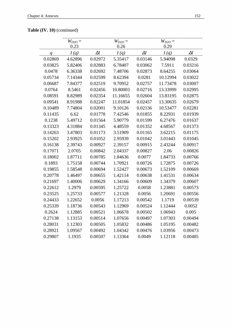
Chapter 4: Annexes 152
Table (IV. 10) (continued)
WD2O =
0.23 WD2O =
0.26 WD2O =
0.29 q I (q) ∆I I (q) ∆I I (q) ∆I
0.02869 4.62896 0.02972 5.35417 0.03146 5.94098 0.0329 0.03825 5.82406 0.02883 6.78407 0.03062 7.5911 0.03216 0.0478 6.36338 0.02692 7.48706 0.02873 8.64255 0.03064
0.05734 7.14344 0.02599 8.62394 0.0281 10.12994 0.03022 0.06687 7.84377 0.02519 9.70952 0.02757 11.73478 0.03007 0.0764 8.5461 0.02456 10.80003 0.02716 13.33999 0.02995
0.08591 8.82989 0.02354 11.16655 0.02604 13.83195 0.02875 0.09541 8.91988 0.02247 11.01854 0.02457 13.30635 0.02679 0.10489 7.74804 0.02001 9.10126 0.02136 10.53477 0.02281 0.11435 6.62 0.01778 7.42546 0.01855 8.22931 0.01939 0.1238 5.49712 0.01564 5.90779 0.01599 6.27476 0.01637
0.13323 4.31884 0.01345 4.48559 0.01352 4.68567 0.01373 0.14263 3.47803 0.01173 3.51909 0.01165 3.62215 0.01175 0.15202 2.93925 0.01052 2.95939 0.01042 3.01443 0.01045 0.16138 2.39743 0.00927 2.39157 0.00915 2.43244 0.00917 0.17071 2.0705 0.00842 2.04337 0.00827 2.06 0.00826 0.18002 1.87711 0.00785 1.84636 0.0077 1.84733 0.00766 0.1893 1.75158 0.00744 1.70921 0.00726 1.72875 0.00726
0.19855 1.58548 0.00694 1.52427 0.00673 1.52109 0.00669 0.20778 1.46497 0.00655 1.42114 0.00638 1.41531 0.00634 0.21697 1.40006 0.00629 1.34166 0.00609 1.34379 0.00607 0.22612 1.2979 0.00595 1.25722 0.0058 1.23881 0.00573 0.23525 1.25733 0.00577 1.21328 0.0056 1.20691 0.00556 0.24433 1.22652 0.0056 1.17213 0.00542 1.1719 0.00539 0.25339 1.18736 0.00543 1.12969 0.00524 1.12444 0.0052 0.2624 1.12885 0.00521 1.06678 0.00502 1.06943 0.005
0.27138 1.13153 0.00514 1.07656 0.00497 1.07303 0.00494 0.28031 1.12303 0.00505 1.05832 0.00486 1.05195 0.00482 0.28921 1.09567 0.00492 1.04342 0.00476 1.03956 0.00473 0.29807 1.1935 0.00507 1.13364 0.0049 1.12118 0.00485
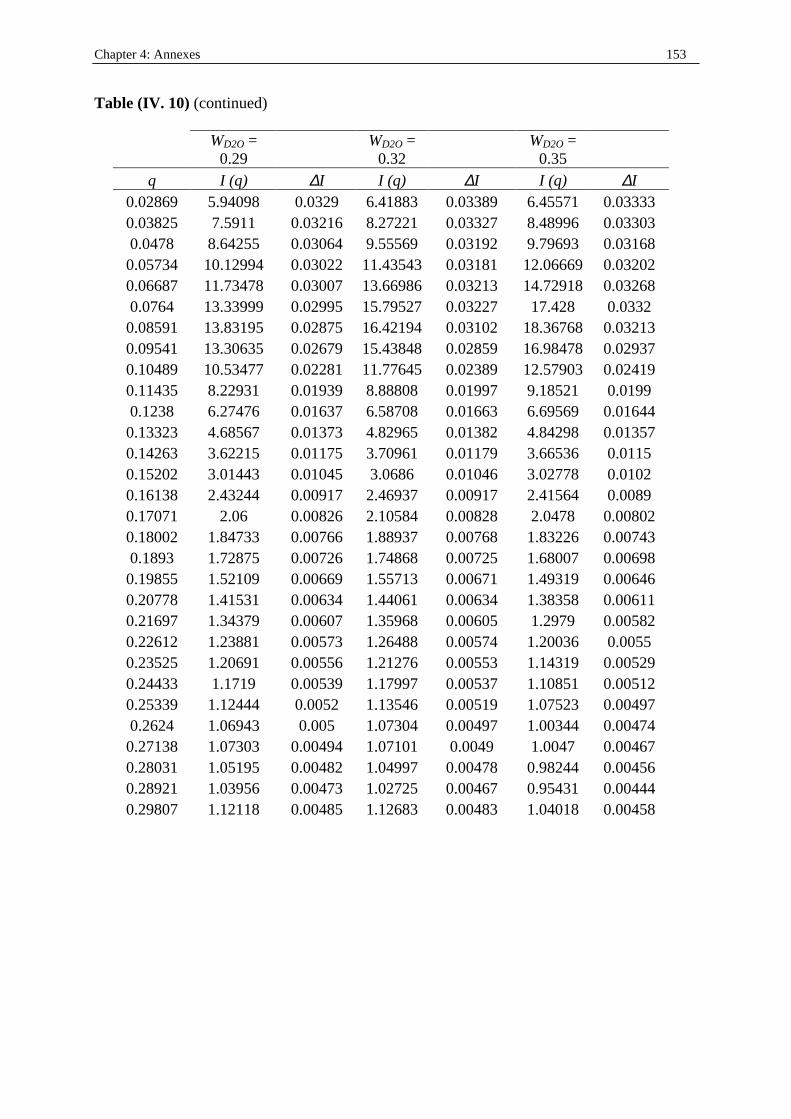
Chapter 4: Annexes 153
Table (IV. 10) (continued)
WD2O =
0.29 WD2O =
0.32 WD2O =
0.35 q I (q) ∆I I (q) ∆I I (q) ∆I
0.02869 5.94098 0.0329 6.41883 0.03389 6.45571 0.03333 0.03825 7.5911 0.03216 8.27221 0.03327 8.48996 0.03303 0.0478 8.64255 0.03064 9.55569 0.03192 9.79693 0.03168
0.05734 10.12994 0.03022 11.43543 0.03181 12.06669 0.03202 0.06687 11.73478 0.03007 13.66986 0.03213 14.72918 0.03268 0.0764 13.33999 0.02995 15.79527 0.03227 17.428 0.0332
0.08591 13.83195 0.02875 16.42194 0.03102 18.36768 0.03213 0.09541 13.30635 0.02679 15.43848 0.02859 16.98478 0.02937 0.10489 10.53477 0.02281 11.77645 0.02389 12.57903 0.02419 0.11435 8.22931 0.01939 8.88808 0.01997 9.18521 0.0199 0.1238 6.27476 0.01637 6.58708 0.01663 6.69569 0.01644
0.13323 4.68567 0.01373 4.82965 0.01382 4.84298 0.01357 0.14263 3.62215 0.01175 3.70961 0.01179 3.66536 0.0115 0.15202 3.01443 0.01045 3.0686 0.01046 3.02778 0.0102 0.16138 2.43244 0.00917 2.46937 0.00917 2.41564 0.0089 0.17071 2.06 0.00826 2.10584 0.00828 2.0478 0.00802 0.18002 1.84733 0.00766 1.88937 0.00768 1.83226 0.00743 0.1893 1.72875 0.00726 1.74868 0.00725 1.68007 0.00698
0.19855 1.52109 0.00669 1.55713 0.00671 1.49319 0.00646 0.20778 1.41531 0.00634 1.44061 0.00634 1.38358 0.00611 0.21697 1.34379 0.00607 1.35968 0.00605 1.2979 0.00582 0.22612 1.23881 0.00573 1.26488 0.00574 1.20036 0.0055 0.23525 1.20691 0.00556 1.21276 0.00553 1.14319 0.00529 0.24433 1.1719 0.00539 1.17997 0.00537 1.10851 0.00512 0.25339 1.12444 0.0052 1.13546 0.00519 1.07523 0.00497 0.2624 1.06943 0.005 1.07304 0.00497 1.00344 0.00474
0.27138 1.07303 0.00494 1.07101 0.0049 1.0047 0.00467 0.28031 1.05195 0.00482 1.04997 0.00478 0.98244 0.00456 0.28921 1.03956 0.00473 1.02725 0.00467 0.95431 0.00444 0.29807 1.12118 0.00485 1.12683 0.00483 1.04018 0.00458
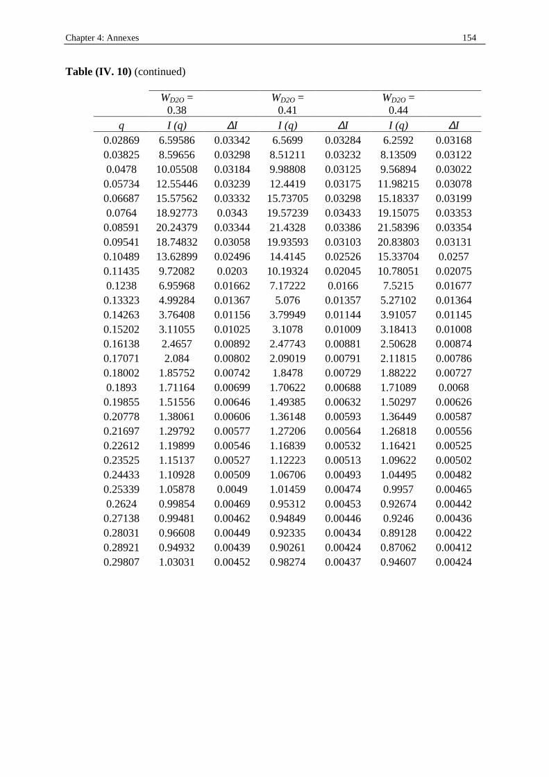
Chapter 4: Annexes 154
Table (IV. 10) (continued)
WD2O =
0.38 WD2O =
0.41 WD2O =
0.44 q I (q) ∆I I (q) ∆I I (q) ∆I
0.02869 6.59586 0.03342 6.5699 0.03284 6.2592 0.03168 0.03825 8.59656 0.03298 8.51211 0.03232 8.13509 0.03122 0.0478 10.05508 0.03184 9.98808 0.03125 9.56894 0.03022
0.05734 12.55446 0.03239 12.4419 0.03175 11.98215 0.03078 0.06687 15.57562 0.03332 15.73705 0.03298 15.18337 0.03199 0.0764 18.92773 0.0343 19.57239 0.03433 19.15075 0.03353
0.08591 20.24379 0.03344 21.4328 0.03386 21.58396 0.03354 0.09541 18.74832 0.03058 19.93593 0.03103 20.83803 0.03131 0.10489 13.62899 0.02496 14.4145 0.02526 15.33704 0.0257 0.11435 9.72082 0.0203 10.19324 0.02045 10.78051 0.02075 0.1238 6.95968 0.01662 7.17222 0.0166 7.5215 0.01677
0.13323 4.99284 0.01367 5.076 0.01357 5.27102 0.01364 0.14263 3.76408 0.01156 3.79949 0.01144 3.91057 0.01145 0.15202 3.11055 0.01025 3.1078 0.01009 3.18413 0.01008 0.16138 2.4657 0.00892 2.47743 0.00881 2.50628 0.00874 0.17071 2.084 0.00802 2.09019 0.00791 2.11815 0.00786 0.18002 1.85752 0.00742 1.8478 0.00729 1.88222 0.00727 0.1893 1.71164 0.00699 1.70622 0.00688 1.71089 0.0068
0.19855 1.51556 0.00646 1.49385 0.00632 1.50297 0.00626 0.20778 1.38061 0.00606 1.36148 0.00593 1.36449 0.00587 0.21697 1.29792 0.00577 1.27206 0.00564 1.26818 0.00556 0.22612 1.19899 0.00546 1.16839 0.00532 1.16421 0.00525 0.23525 1.15137 0.00527 1.12223 0.00513 1.09622 0.00502 0.24433 1.10928 0.00509 1.06706 0.00493 1.04495 0.00482 0.25339 1.05878 0.0049 1.01459 0.00474 0.9957 0.00465 0.2624 0.99854 0.00469 0.95312 0.00453 0.92674 0.00442
0.27138 0.99481 0.00462 0.94849 0.00446 0.9246 0.00436 0.28031 0.96608 0.00449 0.92335 0.00434 0.89128 0.00422 0.28921 0.94932 0.00439 0.90261 0.00424 0.87062 0.00412 0.29807 1.03031 0.00452 0.98274 0.00437 0.94607 0.00424

Chapter 4: Annexes 155
Table (IV. 10) (continued)
WD2O =
0.47 WD2O =
0.50 WD2O =
0.53
q I (q) ∆I I (q) ∆I I (q) ∆I 0.02869 5.98698 0.03059 5.57428 0.02902 5.0645 0.02722 0.03825 7.78035 0.03014 7.12588 0.02837 6.38625 0.02644 0.0478 9.07043 0.02904 8.25343 0.02724 7.19137 0.02504
0.05734 11.2196 0.0294 10.09489 0.02743 8.60579 0.02494 0.06687 14.20492 0.03054 12.60894 0.0283 10.49461 0.02542 0.0764 18.10339 0.03217 16.07309 0.0298 13.22464 0.02661
0.08591 20.93684 0.03259 19.10703 0.03059 15.98417 0.02753 0.09541 20.93244 0.03094 20.10311 0.02978 17.98054 0.02769 0.10489 15.84802 0.02576 16.04498 0.02544 15.54642 0.0246 0.11435 11.28299 0.02092 11.76823 0.02096 12.10562 0.02087 0.1238 7.88562 0.01692 8.2954 0.01703 8.69289 0.0171
0.13323 5.50157 0.01373 5.75336 0.01377 6.0495 0.01386 0.14263 4.06901 0.0115 4.2196 0.01149 4.43105 0.01155 0.15202 3.2945 0.0101 3.39801 0.01007 3.54328 0.01009 0.16138 2.5958 0.00877 2.64214 0.00868 2.73834 0.00867 0.17071 2.16765 0.00784 2.21407 0.00778 2.28661 0.00776 0.18002 1.92221 0.00724 1.94339 0.00714 2.0019 0.00712 0.1893 1.75444 0.00679 1.77426 0.0067 1.80462 0.00663
0.19855 1.52729 0.00622 1.53027 0.00612 1.55505 0.00605 0.20778 1.37617 0.00581 1.37778 0.00571 1.39738 0.00565 0.21697 1.27644 0.0055 1.26187 0.00538 1.27949 0.00532 0.22612 1.16078 0.00517 1.12633 0.00501 1.14326 0.00496 0.23525 1.0991 0.00496 1.0594 0.00479 1.05991 0.00471 0.24433 1.04141 0.00475 1.00558 0.0046 0.98965 0.00449 0.25339 0.99643 0.00459 0.94416 0.0044 0.9262 0.00429 0.2624 0.92171 0.00435 0.87375 0.00418 0.85439 0.00407
0.27138 0.91441 0.00428 0.86861 0.00411 0.84017 0.00399 0.28031 0.88355 0.00415 0.83712 0.00399 0.80239 0.00385 0.28921 0.85934 0.00404 0.80009 0.00385 0.77524 0.00374 0.29807 0.93495 0.00417 0.869 0.00397 0.83391 0.00384
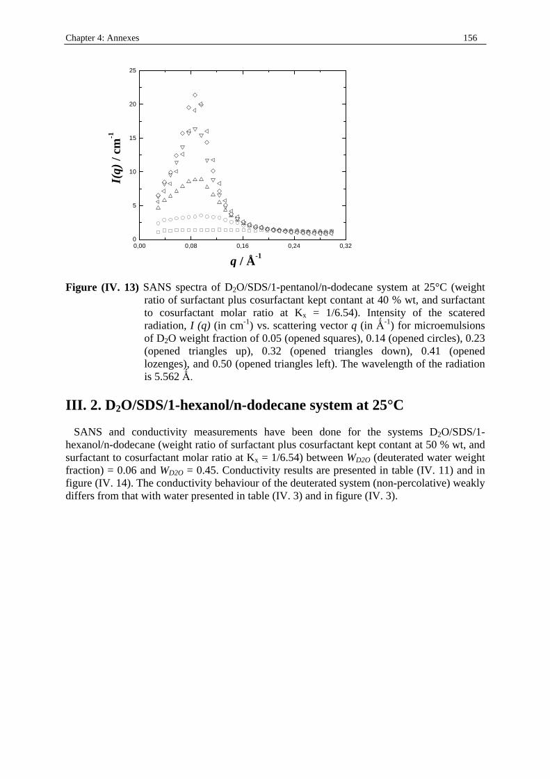
Chapter 4: Annexes 156
0,00 0,08 0,16 0,24 0,320
5
10
15
20
25
I(q)
/ cm
-1
q / Å -1
Figure (IV. 13) SANS spectra of D2O/SDS/1-pentanol/n-dodecane system at 25°C (weight
ratio of surfactant plus cosurfactant kept contant at 40 % wt, and surfactant to cosurfactant molar ratio at Kx = 1/6.54). Intensity of the scatered radiation, I (q) (in cm-1) vs. scattering vector q (in Ö-1) for microemulsions of D2O weight fraction of 0.05 (opened squares), 0.14 (opened circles), 0.23 (opened triangles up), 0.32 (opened triangles down), 0.41 (opened lozenges), and 0.50 (opened triangles left). The wavelength of the radiation is 5.562 Ö
III . 2. D2O/SDS/1-hexanol/n-dodecane system at 25°C SANS and conductivity measurements have been done for the systems D2O/SDS/1-hexanol/n-dodecane (weight ratio of surfactant plus cosurfactant kept contant at 50 % wt, and surfactant to cosurfactant molar ratio at Kx = 1/6.54) between WD2O (deuterated water weight fraction) = 0.06 and WD2O = 0.45. Conductivity results are presented in table (IV. 11) and in figure (IV. 14). The conductivity behaviour of the deuterated system (non-percolative) weakly differs from that with water presented in table (IV. 3) and in figure (IV. 3).
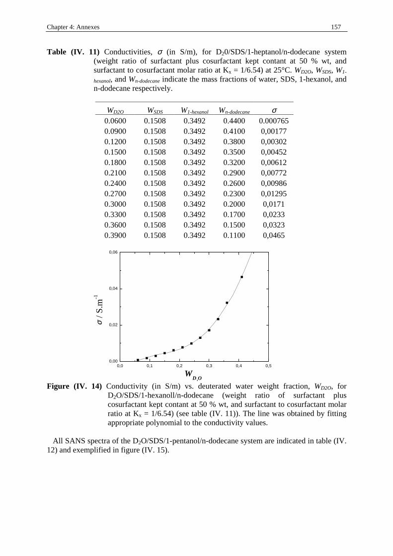
Chapter 4: Annexes 157
Table (IV. 11) Conductivities, σ (in S/m), for D20/SDS/1-heptanol/n-dodecane system (weight ratio of surfactant plus cosurfactant kept contant at 50 % wt, and surfactant to cosurfactant molar ratio at Kx = 1/6.54) at 25°C. WD2O, WSDS, W1-
hexanol, and Wn-dodecane indicate the mass fractions of water, SDS, 1-hexanol, and n-dodecane respectively.
WD2O WSDS W1-hexanol Wn-dodecane σ 0.0600 0.1508 0.3492 0.4400 0.000765 0.0900 0.1508 0.3492 0.4100 0,00177 0.1200 0.1508 0.3492 0.3800 0,00302 0.1500 0.1508 0.3492 0.3500 0,00452 0.1800 0.1508 0.3492 0.3200 0,00612 0.2100 0.1508 0.3492 0.2900 0,00772 0.2400 0.1508 0.3492 0.2600 0,00986 0.2700 0.1508 0.3492 0.2300 0,01295 0.3000 0.1508 0.3492 0.2000 0,0171 0.3300 0.1508 0.3492 0.1700 0,0233 0.3600 0.1508 0.3492 0.1500 0,0323 0.3900 0.1508 0.3492 0.1100 0,0465
0,0 0,1 0,2 0,3 0,4 0,50,00
0,02
0,04
0,06
σσ / S
.m-1
WD
2O
Figure (IV. 14) Conductivity (in S/m) vs. deuterated water weight fraction, WD2O, for
D2O/SDS/1-hexanoll/n-dodecane (weight ratio of surfactant plus cosurfactant kept contant at 50 % wt, and surfactant to cosurfactant molar ratio at Kx = 1/6.54) (see table (IV. 11)). The line was obtained by fitting appropriate polynomial to the conductivity values.
All SANS spectra of the D2O/SDS/1-pentanol/n-dodecane system are indicated in table (IV. 12) and exempli fied in figure (IV. 15).
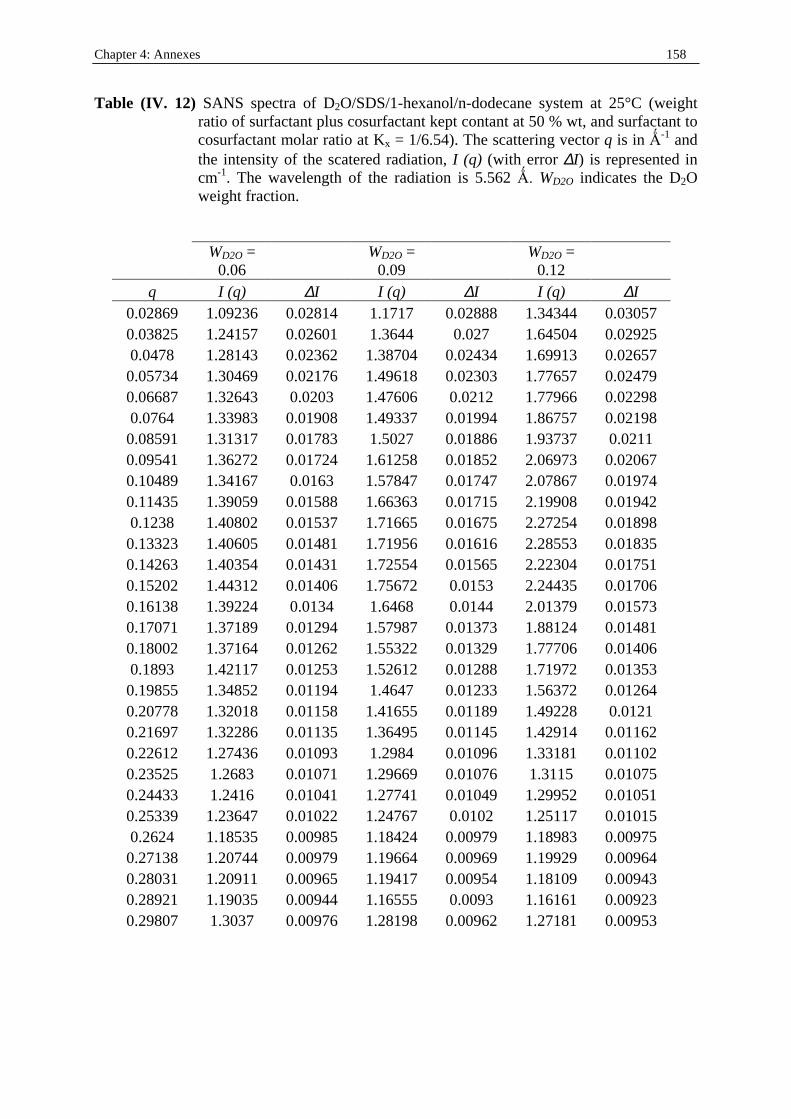
Chapter 4: Annexes 158
Table (IV. 12) SANS spectra of D2O/SDS/1-hexanol/n-dodecane system at 25°C (weight ratio of surfactant plus cosurfactant kept contant at 50 % wt, and surfactant to cosurfactant molar ratio at Kx = 1/6.54). The scattering vector q is in Ö-1 and the intensity of the scatered radiation, I (q) (with error ∆I) is represented in cm-1. The wavelength of the radiation is 5.562 Ö WD2O indicates the D2O weight fraction.
WD2O =
0.06 WD2O =
0.09 WD2O =
0.12 q I (q) ∆I I (q) ∆I I (q) ∆I
0.02869 1.09236 0.02814 1.1717 0.02888 1.34344 0.03057 0.03825 1.24157 0.02601 1.3644 0.027 1.64504 0.02925 0.0478 1.28143 0.02362 1.38704 0.02434 1.69913 0.02657 0.05734 1.30469 0.02176 1.49618 0.02303 1.77657 0.02479 0.06687 1.32643 0.0203 1.47606 0.0212 1.77966 0.02298 0.0764 1.33983 0.01908 1.49337 0.01994 1.86757 0.02198 0.08591 1.31317 0.01783 1.5027 0.01886 1.93737 0.0211 0.09541 1.36272 0.01724 1.61258 0.01852 2.06973 0.02067 0.10489 1.34167 0.0163 1.57847 0.01747 2.07867 0.01974 0.11435 1.39059 0.01588 1.66363 0.01715 2.19908 0.01942 0.1238 1.40802 0.01537 1.71665 0.01675 2.27254 0.01898 0.13323 1.40605 0.01481 1.71956 0.01616 2.28553 0.01835 0.14263 1.40354 0.01431 1.72554 0.01565 2.22304 0.01751 0.15202 1.44312 0.01406 1.75672 0.0153 2.24435 0.01706 0.16138 1.39224 0.0134 1.6468 0.0144 2.01379 0.01573 0.17071 1.37189 0.01294 1.57987 0.01373 1.88124 0.01481 0.18002 1.37164 0.01262 1.55322 0.01329 1.77706 0.01406 0.1893 1.42117 0.01253 1.52612 0.01288 1.71972 0.01353 0.19855 1.34852 0.01194 1.4647 0.01233 1.56372 0.01264 0.20778 1.32018 0.01158 1.41655 0.01189 1.49228 0.0121 0.21697 1.32286 0.01135 1.36495 0.01145 1.42914 0.01162 0.22612 1.27436 0.01093 1.2984 0.01096 1.33181 0.01102 0.23525 1.2683 0.01071 1.29669 0.01076 1.3115 0.01075 0.24433 1.2416 0.01041 1.27741 0.01049 1.29952 0.01051 0.25339 1.23647 0.01022 1.24767 0.0102 1.25117 0.01015 0.2624 1.18535 0.00985 1.18424 0.00979 1.18983 0.00975 0.27138 1.20744 0.00979 1.19664 0.00969 1.19929 0.00964 0.28031 1.20911 0.00965 1.19417 0.00954 1.18109 0.00943 0.28921 1.19035 0.00944 1.16555 0.0093 1.16161 0.00923 0.29807 1.3037 0.00976 1.28198 0.00962 1.27181 0.00953
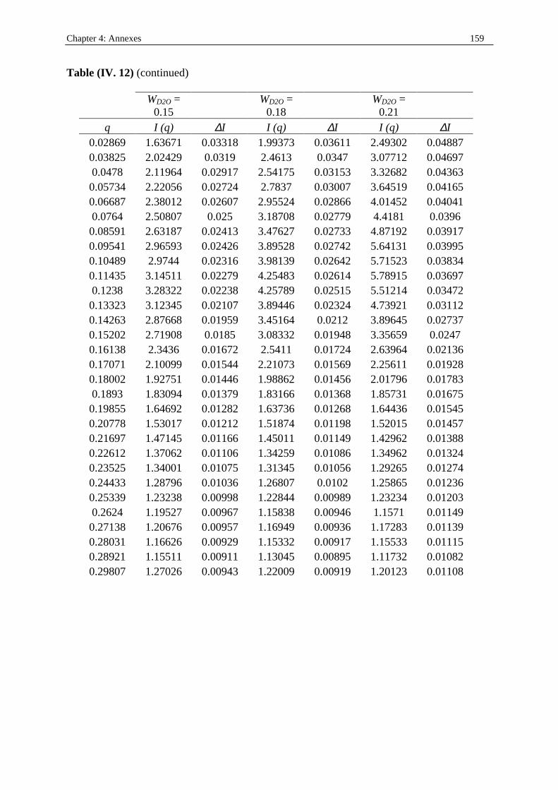
Chapter 4: Annexes 159
Table (IV. 12) (continued)
WD2O =
0.15 WD2O =
0.18 WD2O =
0.21 q I (q) ∆I I (q) ∆I I (q) ∆I
0.02869 1.63671 0.03318 1.99373 0.03611 2.49302 0.04887 0.03825 2.02429 0.0319 2.4613 0.0347 3.07712 0.04697 0.0478 2.11964 0.02917 2.54175 0.03153 3.32682 0.04363
0.05734 2.22056 0.02724 2.7837 0.03007 3.64519 0.04165 0.06687 2.38012 0.02607 2.95524 0.02866 4.01452 0.04041 0.0764 2.50807 0.025 3.18708 0.02779 4.4181 0.0396
0.08591 2.63187 0.02413 3.47627 0.02733 4.87192 0.03917 0.09541 2.96593 0.02426 3.89528 0.02742 5.64131 0.03995 0.10489 2.9744 0.02316 3.98139 0.02642 5.71523 0.03834 0.11435 3.14511 0.02279 4.25483 0.02614 5.78915 0.03697 0.1238 3.28322 0.02238 4.25789 0.02515 5.51214 0.03472
0.13323 3.12345 0.02107 3.89446 0.02324 4.73921 0.03112 0.14263 2.87668 0.01959 3.45164 0.0212 3.89645 0.02737 0.15202 2.71908 0.0185 3.08332 0.01948 3.35659 0.0247 0.16138 2.3436 0.01672 2.5411 0.01724 2.63964 0.02136 0.17071 2.10099 0.01544 2.21073 0.01569 2.25611 0.01928 0.18002 1.92751 0.01446 1.98862 0.01456 2.01796 0.01783 0.1893 1.83094 0.01379 1.83166 0.01368 1.85731 0.01675
0.19855 1.64692 0.01282 1.63736 0.01268 1.64436 0.01545 0.20778 1.53017 0.01212 1.51874 0.01198 1.52015 0.01457 0.21697 1.47145 0.01166 1.45011 0.01149 1.42962 0.01388 0.22612 1.37062 0.01106 1.34259 0.01086 1.34962 0.01324 0.23525 1.34001 0.01075 1.31345 0.01056 1.29265 0.01274 0.24433 1.28796 0.01036 1.26807 0.0102 1.25865 0.01236 0.25339 1.23238 0.00998 1.22844 0.00989 1.23234 0.01203 0.2624 1.19527 0.00967 1.15838 0.00946 1.1571 0.01149
0.27138 1.20676 0.00957 1.16949 0.00936 1.17283 0.01139 0.28031 1.16626 0.00929 1.15332 0.00917 1.15533 0.01115 0.28921 1.15511 0.00911 1.13045 0.00895 1.11732 0.01082 0.29807 1.27026 0.00943 1.22009 0.00919 1.20123 0.01108
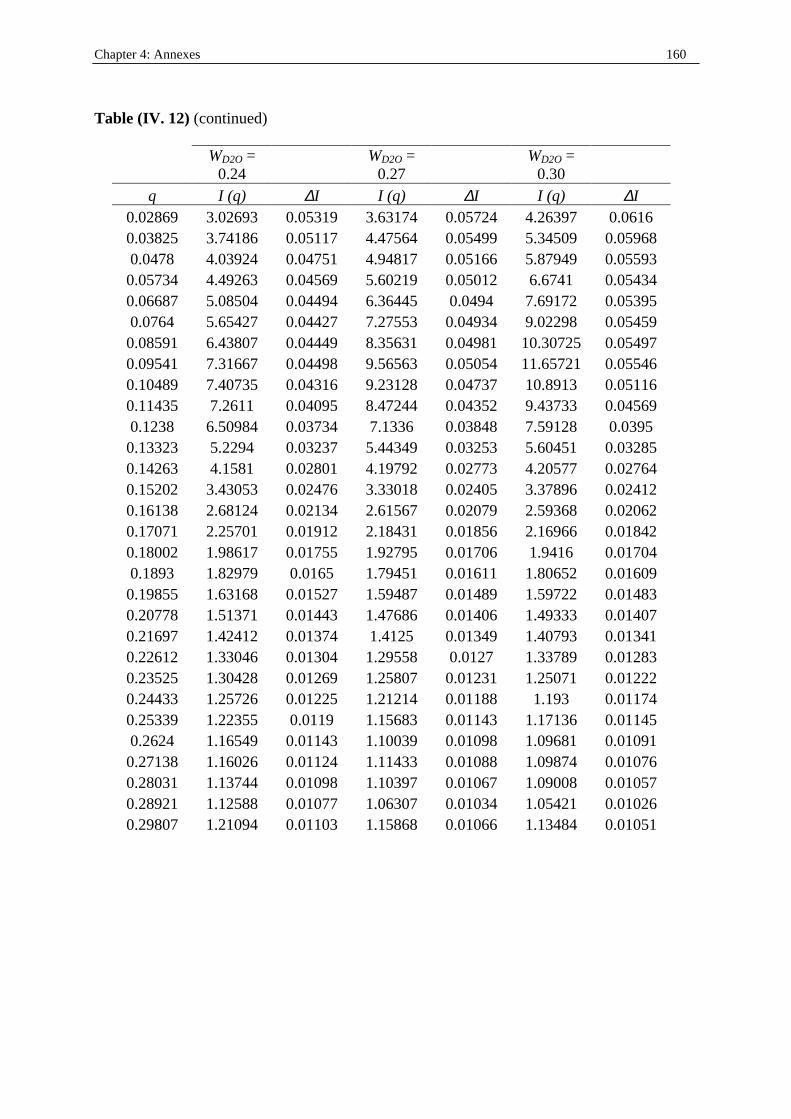
Chapter 4: Annexes 160
Table (IV. 12) (continued)
WD2O =
0.24 WD2O =
0.27 WD2O =
0.30 q I (q) ∆I I (q) ∆I I (q) ∆I
0.02869 3.02693 0.05319 3.63174 0.05724 4.26397 0.0616 0.03825 3.74186 0.05117 4.47564 0.05499 5.34509 0.05968 0.0478 4.03924 0.04751 4.94817 0.05166 5.87949 0.05593
0.05734 4.49263 0.04569 5.60219 0.05012 6.6741 0.05434 0.06687 5.08504 0.04494 6.36445 0.0494 7.69172 0.05395 0.0764 5.65427 0.04427 7.27553 0.04934 9.02298 0.05459
0.08591 6.43807 0.04449 8.35631 0.04981 10.30725 0.05497 0.09541 7.31667 0.04498 9.56563 0.05054 11.65721 0.05546 0.10489 7.40735 0.04316 9.23128 0.04737 10.8913 0.05116 0.11435 7.2611 0.04095 8.47244 0.04352 9.43733 0.04569 0.1238 6.50984 0.03734 7.1336 0.03848 7.59128 0.0395
0.13323 5.2294 0.03237 5.44349 0.03253 5.60451 0.03285 0.14263 4.1581 0.02801 4.19792 0.02773 4.20577 0.02764 0.15202 3.43053 0.02476 3.33018 0.02405 3.37896 0.02412 0.16138 2.68124 0.02134 2.61567 0.02079 2.59368 0.02062 0.17071 2.25701 0.01912 2.18431 0.01856 2.16966 0.01842 0.18002 1.98617 0.01755 1.92795 0.01706 1.9416 0.01704 0.1893 1.82979 0.0165 1.79451 0.01611 1.80652 0.01609
0.19855 1.63168 0.01527 1.59487 0.01489 1.59722 0.01483 0.20778 1.51371 0.01443 1.47686 0.01406 1.49333 0.01407 0.21697 1.42412 0.01374 1.4125 0.01349 1.40793 0.01341 0.22612 1.33046 0.01304 1.29558 0.0127 1.33789 0.01283 0.23525 1.30428 0.01269 1.25807 0.01231 1.25071 0.01222 0.24433 1.25726 0.01225 1.21214 0.01188 1.193 0.01174 0.25339 1.22355 0.0119 1.15683 0.01143 1.17136 0.01145 0.2624 1.16549 0.01143 1.10039 0.01098 1.09681 0.01091
0.27138 1.16026 0.01124 1.11433 0.01088 1.09874 0.01076 0.28031 1.13744 0.01098 1.10397 0.01067 1.09008 0.01057 0.28921 1.12588 0.01077 1.06307 0.01034 1.05421 0.01026 0.29807 1.21094 0.01103 1.15868 0.01066 1.13484 0.01051
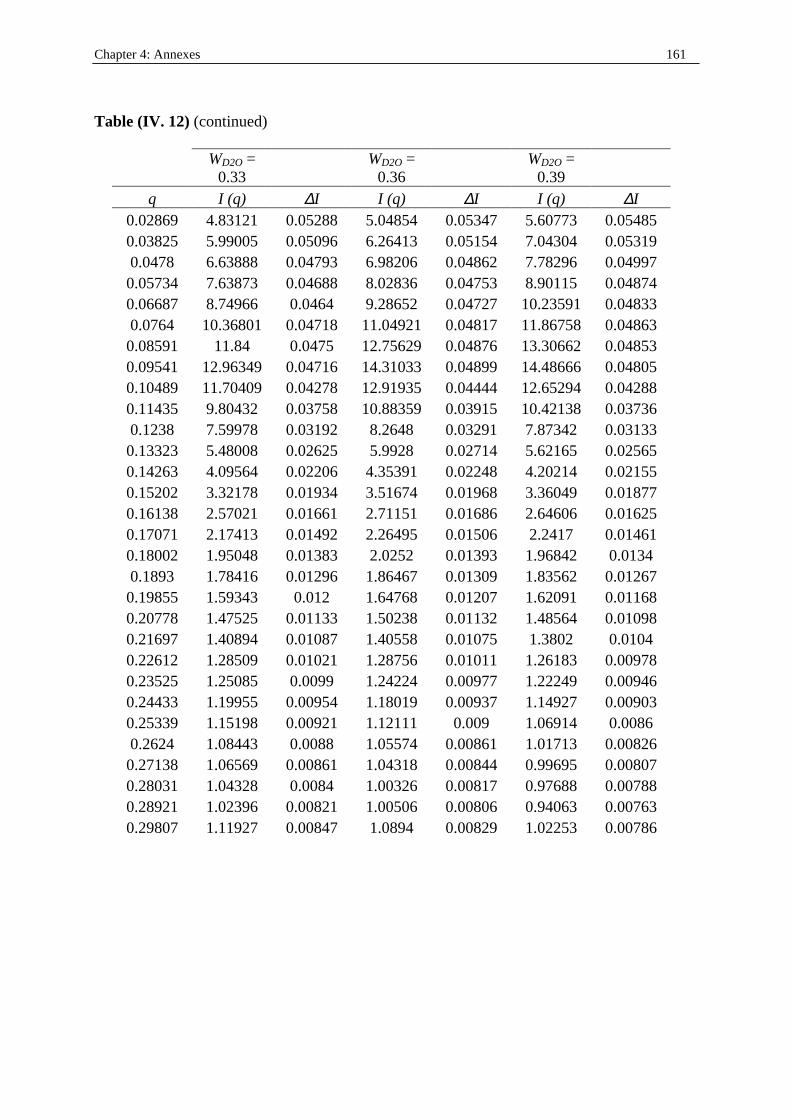
Chapter 4: Annexes 161
Table (IV. 12) (continued)
WD2O =
0.33 WD2O =
0.36 WD2O =
0.39
q I (q) ∆I I (q) ∆I I (q) ∆I 0.02869 4.83121 0.05288 5.04854 0.05347 5.60773 0.05485 0.03825 5.99005 0.05096 6.26413 0.05154 7.04304 0.05319 0.0478 6.63888 0.04793 6.98206 0.04862 7.78296 0.04997
0.05734 7.63873 0.04688 8.02836 0.04753 8.90115 0.04874 0.06687 8.74966 0.0464 9.28652 0.04727 10.23591 0.04833 0.0764 10.36801 0.04718 11.04921 0.04817 11.86758 0.04863
0.08591 11.84 0.0475 12.75629 0.04876 13.30662 0.04853 0.09541 12.96349 0.04716 14.31033 0.04899 14.48666 0.04805 0.10489 11.70409 0.04278 12.91935 0.04444 12.65294 0.04288 0.11435 9.80432 0.03758 10.88359 0.03915 10.42138 0.03736 0.1238 7.59978 0.03192 8.2648 0.03291 7.87342 0.03133
0.13323 5.48008 0.02625 5.9928 0.02714 5.62165 0.02565 0.14263 4.09564 0.02206 4.35391 0.02248 4.20214 0.02155 0.15202 3.32178 0.01934 3.51674 0.01968 3.36049 0.01877 0.16138 2.57021 0.01661 2.71151 0.01686 2.64606 0.01625 0.17071 2.17413 0.01492 2.26495 0.01506 2.2417 0.01461 0.18002 1.95048 0.01383 2.0252 0.01393 1.96842 0.0134 0.1893 1.78416 0.01296 1.86467 0.01309 1.83562 0.01267
0.19855 1.59343 0.012 1.64768 0.01207 1.62091 0.01168 0.20778 1.47525 0.01133 1.50238 0.01132 1.48564 0.01098 0.21697 1.40894 0.01087 1.40558 0.01075 1.3802 0.0104 0.22612 1.28509 0.01021 1.28756 0.01011 1.26183 0.00978 0.23525 1.25085 0.0099 1.24224 0.00977 1.22249 0.00946 0.24433 1.19955 0.00954 1.18019 0.00937 1.14927 0.00903 0.25339 1.15198 0.00921 1.12111 0.009 1.06914 0.0086 0.2624 1.08443 0.0088 1.05574 0.00861 1.01713 0.00826
0.27138 1.06569 0.00861 1.04318 0.00844 0.99695 0.00807 0.28031 1.04328 0.0084 1.00326 0.00817 0.97688 0.00788 0.28921 1.02396 0.00821 1.00506 0.00806 0.94063 0.00763 0.29807 1.11927 0.00847 1.0894 0.00829 1.02253 0.00786
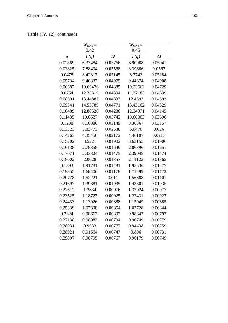
Chapter 4: Annexes 162
Table (IV. 12) (continued)
WD2O =
0.42 WD2O =
0.45 q I (q) ∆I I (q) ∆I
0.02869 6.33484 0.05766 6.90988 0.05941 0.03825 7.88404 0.05568 8.39686 0.0567 0.0478 8.42317 0.05145 8.7743 0.05184
0.05734 9.46337 0.04975 9.44374 0.04908 0.06687 10.66476 0.04885 10.23662 0.04729 0.0764 12.25319 0.04894 11.27183 0.04639
0.08591 13.44887 0.04833 12.4393 0.04593 0.09541 14.55789 0.04771 13.43162 0.04529 0.10489 12.88528 0.04286 12.34971 0.04145 0.11435 10.6627 0.03742 10.66083 0.03696 0.1238 8.10886 0.03149 8.36367 0.03157
0.13323 5.83773 0.02588 6.0478 0.026 0.14263 4.35456 0.02172 4.46107 0.0217 0.15202 3.5221 0.01902 3.63155 0.01906 0.16138 2.78358 0.01649 2.86396 0.01651 0.17071 2.33324 0.01475 2.39048 0.01474 0.18002 2.0628 0.01357 2.14123 0.01365 0.1893 1.91731 0.01281 1.95536 0.01277
0.19855 1.68406 0.01178 1.71299 0.01173 0.20778 1.52221 0.011 1.56688 0.01101 0.21697 1.39381 0.01035 1.43301 0.01035 0.22612 1.2834 0.00976 1.32024 0.00977 0.23525 1.18727 0.00925 1.22431 0.00927 0.24433 1.13026 0.00888 1.15049 0.00885 0.25339 1.07398 0.00854 1.07728 0.00844 0.2624 0.98667 0.00807 0.98647 0.00797
0.27138 0.98083 0.00794 0.96749 0.00779 0.28031 0.9533 0.00772 0.94438 0.00759 0.28921 0.91664 0.00747 0.896 0.00731 0.29807 0.98795 0.00767 0.96179 0.00749
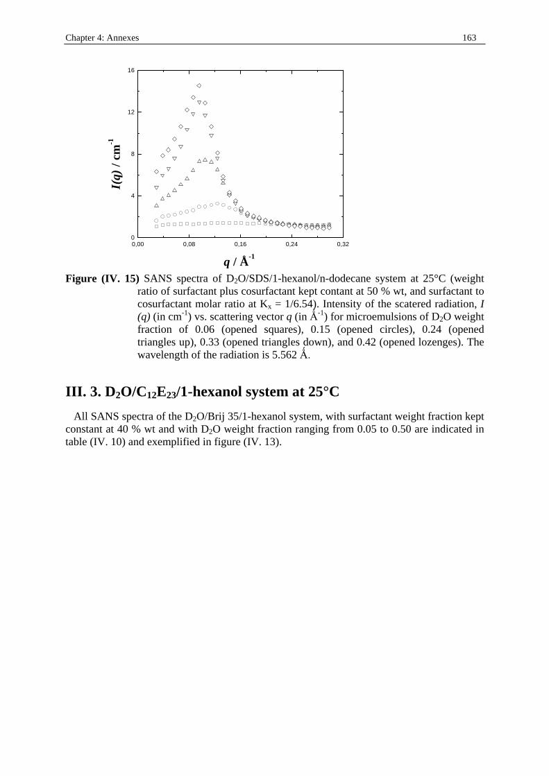
Chapter 4: Annexes 163
0,00 0,08 0,16 0,24 0,320
4
8
12
16
q / Å -1
I(q)
/ cm
-1
Figure (IV. 15) SANS spectra of D2O/SDS/1-hexanol/n-dodecane system at 25°C (weight
ratio of surfactant plus cosurfactant kept contant at 50 % wt, and surfactant to cosurfactant molar ratio at Kx = 1/6.54). Intensity of the scatered radiation, I (q) (in cm-1) vs. scattering vector q (in Ö-1) for microemulsions of D2O weight fraction of 0.06 (opened squares), 0.15 (opened circles), 0.24 (opened triangles up), 0.33 (opened triangles down), and 0.42 (opened lozenges). The wavelength of the radiation is 5.562 Ö
III . 3. D2O/C12E23/1-hexanol system at 25°C All SANS spectra of the D2O/Brij 35/1-hexanol system, with surfactant weight fraction kept constant at 40 % wt and with D2O weight fraction ranging from 0.05 to 0.50 are indicated in table (IV. 10) and exempli fied in figure (IV. 13).
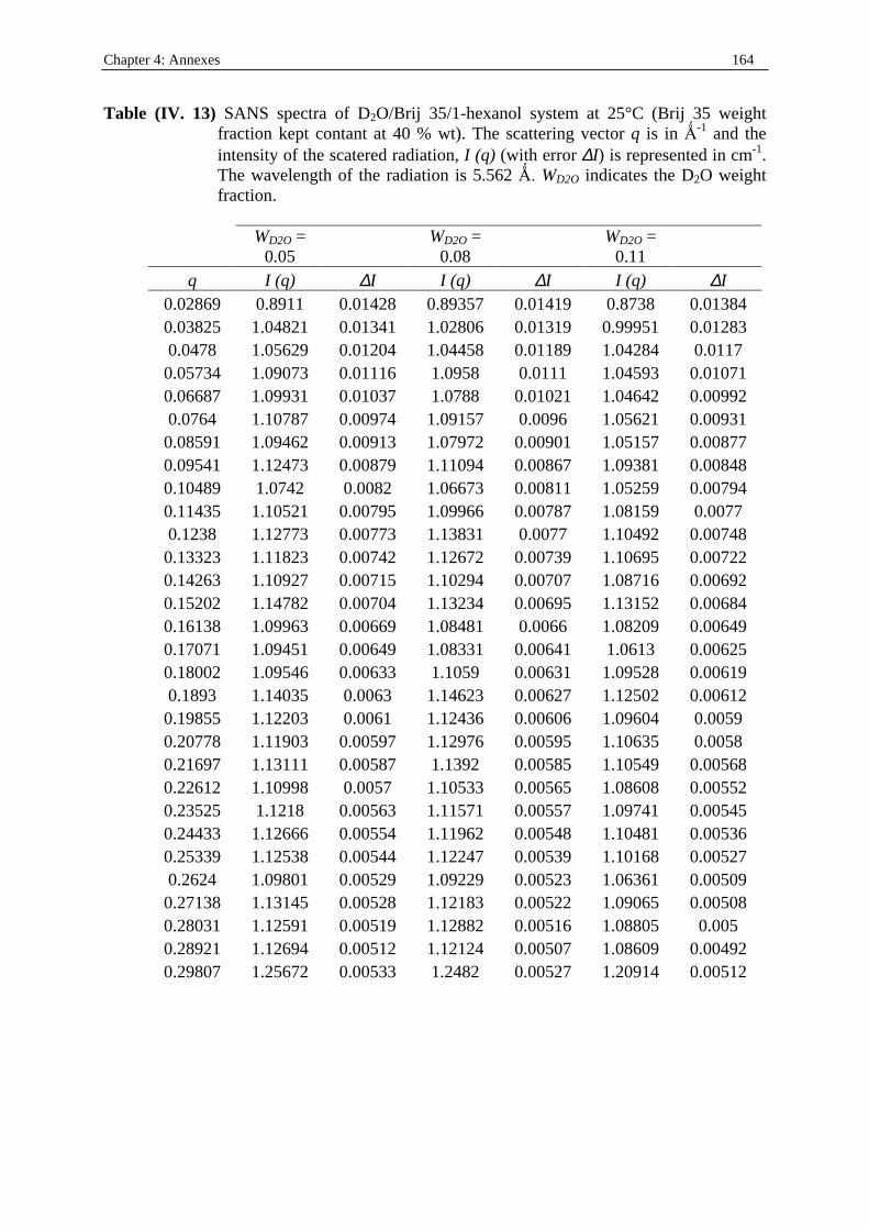
Chapter 4: Annexes 164
Table (IV. 13) SANS spectra of D2O/Brij 35/1-hexanol system at 25°C (Brij 35 weight fraction kept contant at 40 % wt). The scattering vector q is in Ö-1 and the intensity of the scatered radiation, I (q) (with error ∆I) is represented in cm-1. The wavelength of the radiation is 5.562 Ö WD2O indicates the D2O weight fraction.
WD2O =
0.05 WD2O =
0.08 WD2O =
0.11 q I (q) ∆I I (q) ∆I I (q) ∆I
0.02869 0.8911 0.01428 0.89357 0.01419 0.8738 0.01384 0.03825 1.04821 0.01341 1.02806 0.01319 0.99951 0.01283 0.0478 1.05629 0.01204 1.04458 0.01189 1.04284 0.0117 0.05734 1.09073 0.01116 1.0958 0.0111 1.04593 0.01071 0.06687 1.09931 0.01037 1.0788 0.01021 1.04642 0.00992 0.0764 1.10787 0.00974 1.09157 0.0096 1.05621 0.00931 0.08591 1.09462 0.00913 1.07972 0.00901 1.05157 0.00877 0.09541 1.12473 0.00879 1.11094 0.00867 1.09381 0.00848 0.10489 1.0742 0.0082 1.06673 0.00811 1.05259 0.00794 0.11435 1.10521 0.00795 1.09966 0.00787 1.08159 0.0077 0.1238 1.12773 0.00773 1.13831 0.0077 1.10492 0.00748 0.13323 1.11823 0.00742 1.12672 0.00739 1.10695 0.00722 0.14263 1.10927 0.00715 1.10294 0.00707 1.08716 0.00692 0.15202 1.14782 0.00704 1.13234 0.00695 1.13152 0.00684 0.16138 1.09963 0.00669 1.08481 0.0066 1.08209 0.00649 0.17071 1.09451 0.00649 1.08331 0.00641 1.0613 0.00625 0.18002 1.09546 0.00633 1.1059 0.00631 1.09528 0.00619 0.1893 1.14035 0.0063 1.14623 0.00627 1.12502 0.00612 0.19855 1.12203 0.0061 1.12436 0.00606 1.09604 0.0059 0.20778 1.11903 0.00597 1.12976 0.00595 1.10635 0.0058 0.21697 1.13111 0.00587 1.1392 0.00585 1.10549 0.00568 0.22612 1.10998 0.0057 1.10533 0.00565 1.08608 0.00552 0.23525 1.1218 0.00563 1.11571 0.00557 1.09741 0.00545 0.24433 1.12666 0.00554 1.11962 0.00548 1.10481 0.00536 0.25339 1.12538 0.00544 1.12247 0.00539 1.10168 0.00527 0.2624 1.09801 0.00529 1.09229 0.00523 1.06361 0.00509 0.27138 1.13145 0.00528 1.12183 0.00522 1.09065 0.00508 0.28031 1.12591 0.00519 1.12882 0.00516 1.08805 0.005 0.28921 1.12694 0.00512 1.12124 0.00507 1.08609 0.00492 0.29807 1.25672 0.00533 1.2482 0.00527 1.20914 0.00512
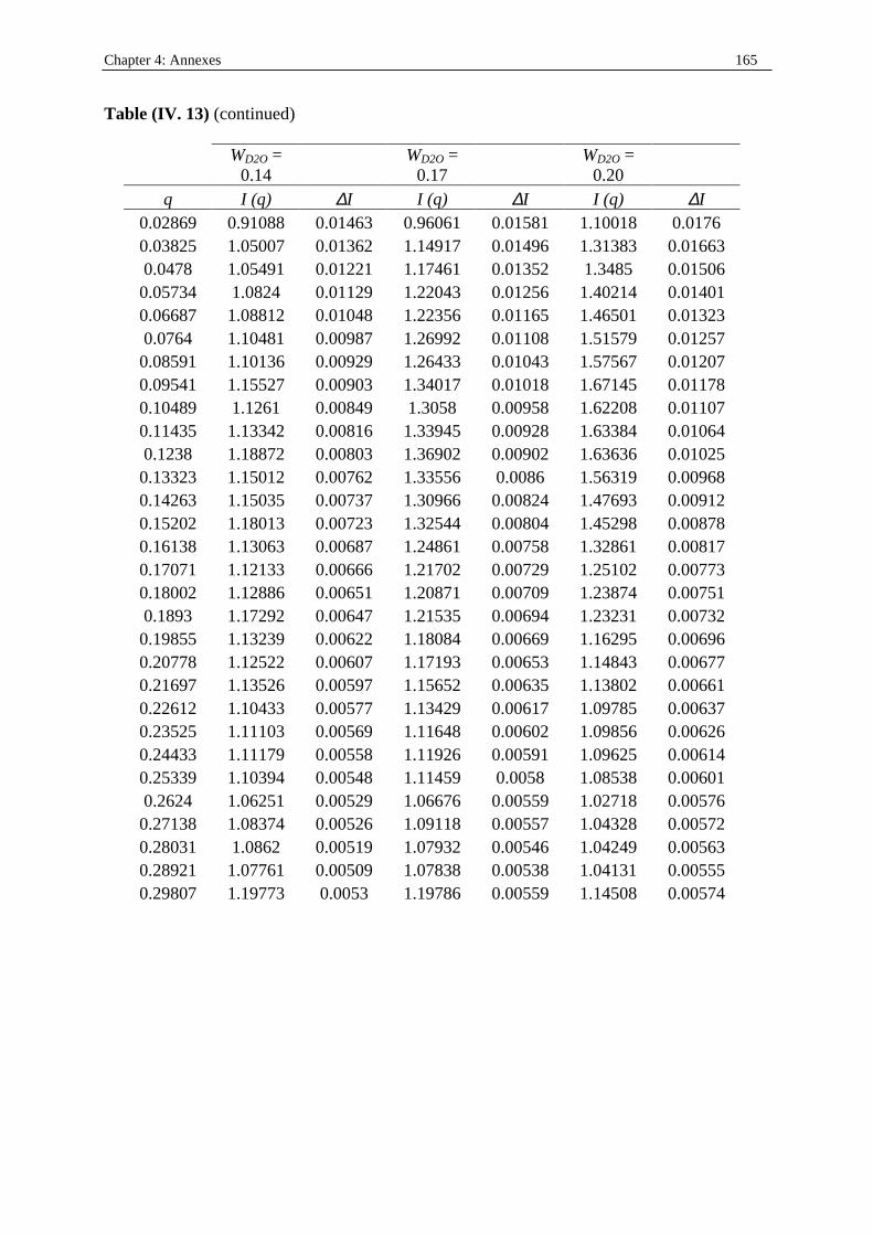
Chapter 4: Annexes 165
Table (IV. 13) (continued)
WD2O =
0.14 WD2O =
0.17 WD2O =
0.20 q I (q) ∆I I (q) ∆I I (q) ∆I
0.02869 0.91088 0.01463 0.96061 0.01581 1.10018 0.0176 0.03825 1.05007 0.01362 1.14917 0.01496 1.31383 0.01663 0.0478 1.05491 0.01221 1.17461 0.01352 1.3485 0.01506
0.05734 1.0824 0.01129 1.22043 0.01256 1.40214 0.01401 0.06687 1.08812 0.01048 1.22356 0.01165 1.46501 0.01323 0.0764 1.10481 0.00987 1.26992 0.01108 1.51579 0.01257
0.08591 1.10136 0.00929 1.26433 0.01043 1.57567 0.01207 0.09541 1.15527 0.00903 1.34017 0.01018 1.67145 0.01178 0.10489 1.1261 0.00849 1.3058 0.00958 1.62208 0.01107 0.11435 1.13342 0.00816 1.33945 0.00928 1.63384 0.01064 0.1238 1.18872 0.00803 1.36902 0.00902 1.63636 0.01025
0.13323 1.15012 0.00762 1.33556 0.0086 1.56319 0.00968 0.14263 1.15035 0.00737 1.30966 0.00824 1.47693 0.00912 0.15202 1.18013 0.00723 1.32544 0.00804 1.45298 0.00878 0.16138 1.13063 0.00687 1.24861 0.00758 1.32861 0.00817 0.17071 1.12133 0.00666 1.21702 0.00729 1.25102 0.00773 0.18002 1.12886 0.00651 1.20871 0.00709 1.23874 0.00751 0.1893 1.17292 0.00647 1.21535 0.00694 1.23231 0.00732
0.19855 1.13239 0.00622 1.18084 0.00669 1.16295 0.00696 0.20778 1.12522 0.00607 1.17193 0.00653 1.14843 0.00677 0.21697 1.13526 0.00597 1.15652 0.00635 1.13802 0.00661 0.22612 1.10433 0.00577 1.13429 0.00617 1.09785 0.00637 0.23525 1.11103 0.00569 1.11648 0.00602 1.09856 0.00626 0.24433 1.11179 0.00558 1.11926 0.00591 1.09625 0.00614 0.25339 1.10394 0.00548 1.11459 0.0058 1.08538 0.00601 0.2624 1.06251 0.00529 1.06676 0.00559 1.02718 0.00576
0.27138 1.08374 0.00526 1.09118 0.00557 1.04328 0.00572 0.28031 1.0862 0.00519 1.07932 0.00546 1.04249 0.00563 0.28921 1.07761 0.00509 1.07838 0.00538 1.04131 0.00555 0.29807 1.19773 0.0053 1.19786 0.00559 1.14508 0.00574
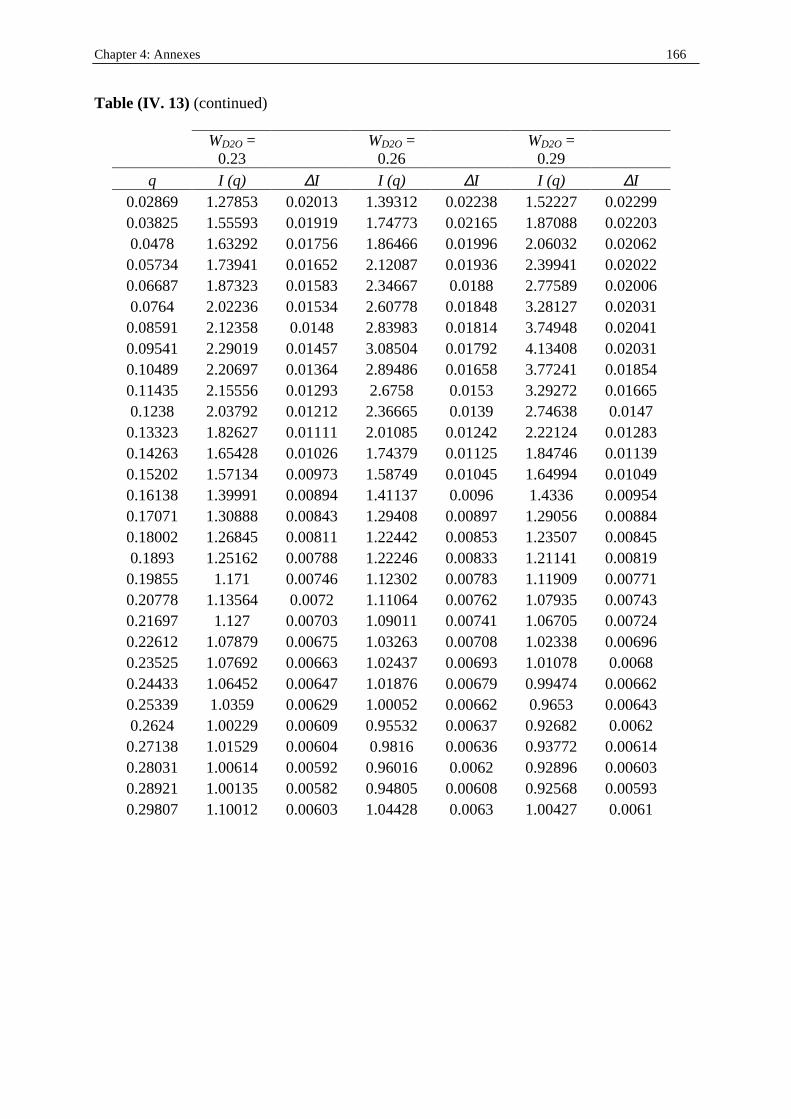
Chapter 4: Annexes 166
Table (IV. 13) (continued)
WD2O =
0.23 WD2O =
0.26 WD2O =
0.29 q I (q) ∆I I (q) ∆I I (q) ∆I
0.02869 1.27853 0.02013 1.39312 0.02238 1.52227 0.02299 0.03825 1.55593 0.01919 1.74773 0.02165 1.87088 0.02203 0.0478 1.63292 0.01756 1.86466 0.01996 2.06032 0.02062
0.05734 1.73941 0.01652 2.12087 0.01936 2.39941 0.02022 0.06687 1.87323 0.01583 2.34667 0.0188 2.77589 0.02006 0.0764 2.02236 0.01534 2.60778 0.01848 3.28127 0.02031
0.08591 2.12358 0.0148 2.83983 0.01814 3.74948 0.02041 0.09541 2.29019 0.01457 3.08504 0.01792 4.13408 0.02031 0.10489 2.20697 0.01364 2.89486 0.01658 3.77241 0.01854 0.11435 2.15556 0.01293 2.6758 0.0153 3.29272 0.01665 0.1238 2.03792 0.01212 2.36665 0.0139 2.74638 0.0147
0.13323 1.82627 0.01111 2.01085 0.01242 2.22124 0.01283 0.14263 1.65428 0.01026 1.74379 0.01125 1.84746 0.01139 0.15202 1.57134 0.00973 1.58749 0.01045 1.64994 0.01049 0.16138 1.39991 0.00894 1.41137 0.0096 1.4336 0.00954 0.17071 1.30888 0.00843 1.29408 0.00897 1.29056 0.00884 0.18002 1.26845 0.00811 1.22442 0.00853 1.23507 0.00845 0.1893 1.25162 0.00788 1.22246 0.00833 1.21141 0.00819
0.19855 1.171 0.00746 1.12302 0.00783 1.11909 0.00771 0.20778 1.13564 0.0072 1.11064 0.00762 1.07935 0.00743 0.21697 1.127 0.00703 1.09011 0.00741 1.06705 0.00724 0.22612 1.07879 0.00675 1.03263 0.00708 1.02338 0.00696 0.23525 1.07692 0.00663 1.02437 0.00693 1.01078 0.0068 0.24433 1.06452 0.00647 1.01876 0.00679 0.99474 0.00662 0.25339 1.0359 0.00629 1.00052 0.00662 0.9653 0.00643 0.2624 1.00229 0.00609 0.95532 0.00637 0.92682 0.0062
0.27138 1.01529 0.00604 0.9816 0.00636 0.93772 0.00614 0.28031 1.00614 0.00592 0.96016 0.0062 0.92896 0.00603 0.28921 1.00135 0.00582 0.94805 0.00608 0.92568 0.00593 0.29807 1.10012 0.00603 1.04428 0.0063 1.00427 0.0061
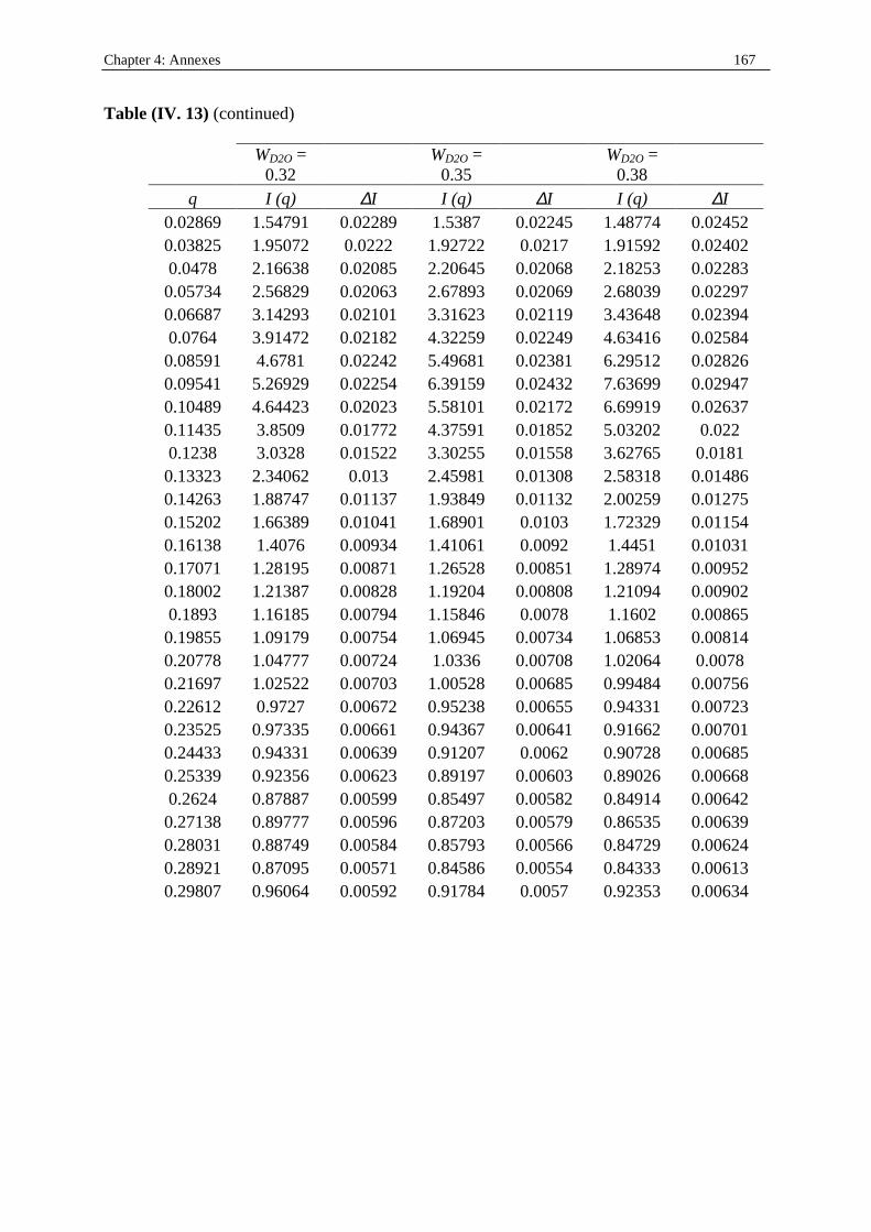
Chapter 4: Annexes 167
Table (IV. 13) (continued)
WD2O =
0.32 WD2O =
0.35 WD2O =
0.38
q I (q) ∆I I (q) ∆I I (q) ∆I 0.02869 1.54791 0.02289 1.5387 0.02245 1.48774 0.02452 0.03825 1.95072 0.0222 1.92722 0.0217 1.91592 0.02402 0.0478 2.16638 0.02085 2.20645 0.02068 2.18253 0.02283
0.05734 2.56829 0.02063 2.67893 0.02069 2.68039 0.02297 0.06687 3.14293 0.02101 3.31623 0.02119 3.43648 0.02394 0.0764 3.91472 0.02182 4.32259 0.02249 4.63416 0.02584
0.08591 4.6781 0.02242 5.49681 0.02381 6.29512 0.02826 0.09541 5.26929 0.02254 6.39159 0.02432 7.63699 0.02947 0.10489 4.64423 0.02023 5.58101 0.02172 6.69919 0.02637 0.11435 3.8509 0.01772 4.37591 0.01852 5.03202 0.022 0.1238 3.0328 0.01522 3.30255 0.01558 3.62765 0.0181
0.13323 2.34062 0.013 2.45981 0.01308 2.58318 0.01486 0.14263 1.88747 0.01137 1.93849 0.01132 2.00259 0.01275 0.15202 1.66389 0.01041 1.68901 0.0103 1.72329 0.01154 0.16138 1.4076 0.00934 1.41061 0.0092 1.4451 0.01031 0.17071 1.28195 0.00871 1.26528 0.00851 1.28974 0.00952 0.18002 1.21387 0.00828 1.19204 0.00808 1.21094 0.00902 0.1893 1.16185 0.00794 1.15846 0.0078 1.1602 0.00865
0.19855 1.09179 0.00754 1.06945 0.00734 1.06853 0.00814 0.20778 1.04777 0.00724 1.0336 0.00708 1.02064 0.0078 0.21697 1.02522 0.00703 1.00528 0.00685 0.99484 0.00756 0.22612 0.9727 0.00672 0.95238 0.00655 0.94331 0.00723 0.23525 0.97335 0.00661 0.94367 0.00641 0.91662 0.00701 0.24433 0.94331 0.00639 0.91207 0.0062 0.90728 0.00685 0.25339 0.92356 0.00623 0.89197 0.00603 0.89026 0.00668 0.2624 0.87887 0.00599 0.85497 0.00582 0.84914 0.00642
0.27138 0.89777 0.00596 0.87203 0.00579 0.86535 0.00639 0.28031 0.88749 0.00584 0.85793 0.00566 0.84729 0.00624 0.28921 0.87095 0.00571 0.84586 0.00554 0.84333 0.00613 0.29807 0.96064 0.00592 0.91784 0.0057 0.92353 0.00634
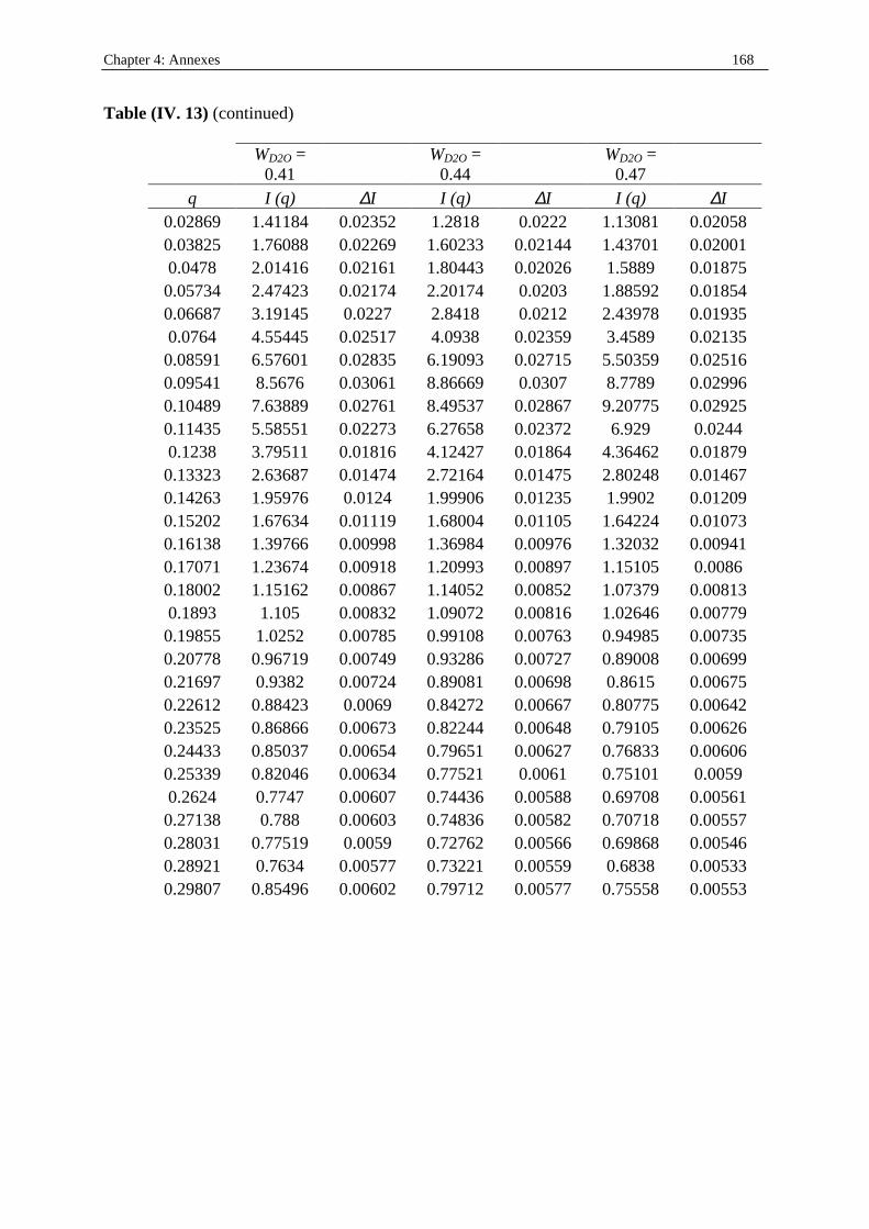
Chapter 4: Annexes 168
Table (IV. 13) (continued)
WD2O =
0.41 WD2O =
0.44 WD2O =
0.47 q I (q) ∆I I (q) ∆I I (q) ∆I
0.02869 1.41184 0.02352 1.2818 0.0222 1.13081 0.02058 0.03825 1.76088 0.02269 1.60233 0.02144 1.43701 0.02001 0.0478 2.01416 0.02161 1.80443 0.02026 1.5889 0.01875
0.05734 2.47423 0.02174 2.20174 0.0203 1.88592 0.01854 0.06687 3.19145 0.0227 2.8418 0.0212 2.43978 0.01935 0.0764 4.55445 0.02517 4.0938 0.02359 3.4589 0.02135
0.08591 6.57601 0.02835 6.19093 0.02715 5.50359 0.02516 0.09541 8.5676 0.03061 8.86669 0.0307 8.7789 0.02996 0.10489 7.63889 0.02761 8.49537 0.02867 9.20775 0.02925 0.11435 5.58551 0.02273 6.27658 0.02372 6.929 0.0244 0.1238 3.79511 0.01816 4.12427 0.01864 4.36462 0.01879
0.13323 2.63687 0.01474 2.72164 0.01475 2.80248 0.01467 0.14263 1.95976 0.0124 1.99906 0.01235 1.9902 0.01209 0.15202 1.67634 0.01119 1.68004 0.01105 1.64224 0.01073 0.16138 1.39766 0.00998 1.36984 0.00976 1.32032 0.00941 0.17071 1.23674 0.00918 1.20993 0.00897 1.15105 0.0086 0.18002 1.15162 0.00867 1.14052 0.00852 1.07379 0.00813 0.1893 1.105 0.00832 1.09072 0.00816 1.02646 0.00779
0.19855 1.0252 0.00785 0.99108 0.00763 0.94985 0.00735 0.20778 0.96719 0.00749 0.93286 0.00727 0.89008 0.00699 0.21697 0.9382 0.00724 0.89081 0.00698 0.8615 0.00675 0.22612 0.88423 0.0069 0.84272 0.00667 0.80775 0.00642 0.23525 0.86866 0.00673 0.82244 0.00648 0.79105 0.00626 0.24433 0.85037 0.00654 0.79651 0.00627 0.76833 0.00606 0.25339 0.82046 0.00634 0.77521 0.0061 0.75101 0.0059 0.2624 0.7747 0.00607 0.74436 0.00588 0.69708 0.00561
0.27138 0.788 0.00603 0.74836 0.00582 0.70718 0.00557 0.28031 0.77519 0.0059 0.72762 0.00566 0.69868 0.00546 0.28921 0.7634 0.00577 0.73221 0.00559 0.6838 0.00533 0.29807 0.85496 0.00602 0.79712 0.00577 0.75558 0.00553
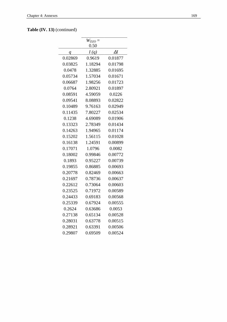
Chapter 4: Annexes 169
Table (IV. 13) (continued)
WD2O =
0.50
q I (q) ∆I 0.02869 0.9619 0.01877 0.03825 1.18294 0.01798 0.0478 1.32885 0.01695 0.05734 1.57034 0.01671 0.06687 1.98256 0.01723 0.0764 2.80921 0.01897 0.08591 4.59059 0.0226 0.09541 8.08893 0.02822 0.10489 9.76163 0.02949 0.11435 7.80227 0.02534 0.1238 4.69089 0.01906 0.13323 2.78349 0.01434 0.14263 1.94965 0.01174 0.15202 1.56115 0.01028 0.16138 1.24591 0.00899 0.17071 1.0796 0.0082 0.18002 0.99846 0.00772 0.1893 0.95227 0.00739 0.19855 0.86885 0.00693 0.20778 0.82469 0.00663 0.21697 0.78736 0.00637 0.22612 0.73064 0.00603 0.23525 0.71972 0.00589 0.24433 0.69183 0.00568 0.25339 0.67924 0.00555 0.2624 0.63686 0.0053 0.27138 0.65134 0.00528 0.28031 0.63778 0.00515 0.28921 0.63391 0.00506 0.29807 0.69509 0.00524
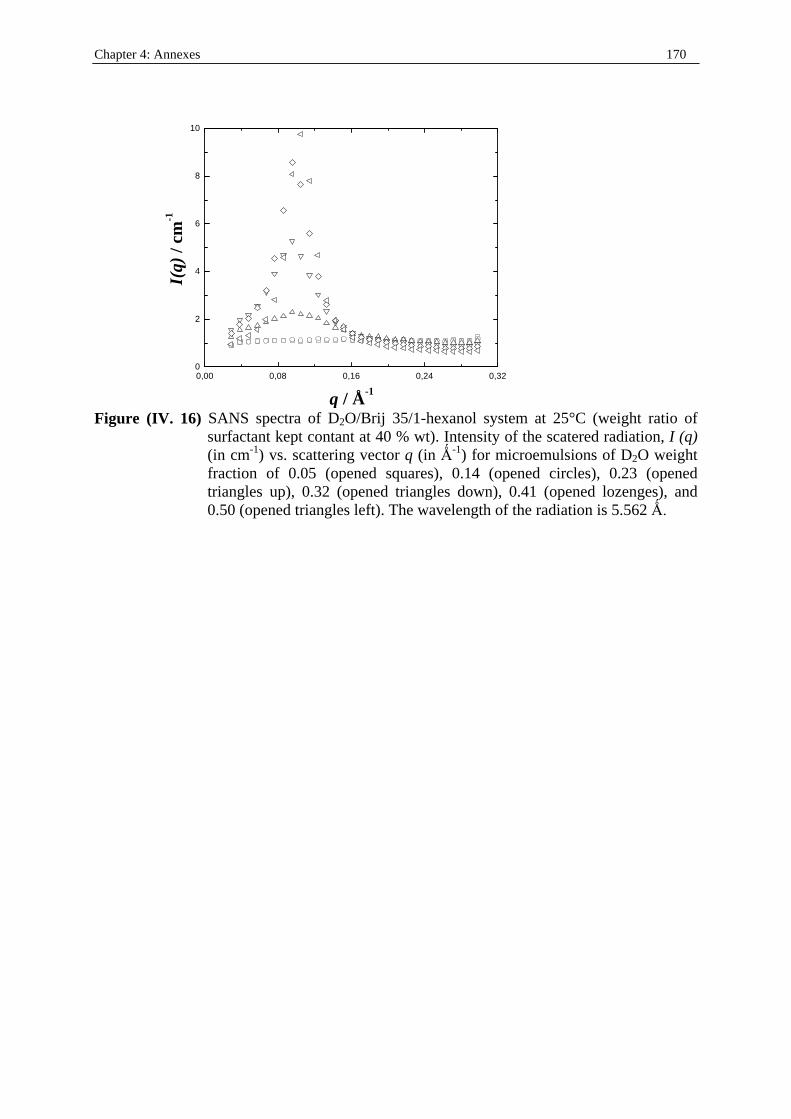
Chapter 4: Annexes 170
0,00 0,08 0,16 0,24 0,320
2
4
6
8
10
I(q)
/ cm
-1
q / Å -1
Figure (IV. 16) SANS spectra of D2O/Brij 35/1-hexanol system at 25°C (weight ratio of
surfactant kept contant at 40 % wt). Intensity of the scatered radiation, I (q) (in cm-1) vs. scattering vector q (in Ö-1) for microemulsions of D2O weight fraction of 0.05 (opened squares), 0.14 (opened circles), 0.23 (opened triangles up), 0.32 (opened triangles down), 0.41 (opened lozenges), and 0.50 (opened triangles left). The wavelength of the radiation is 5.562 Ö
References 171
References 1. Gradzielski, M., Langevin, D., and Farago, B., Prog. Colloid Polym. Sci. 1996, 100, 162.
2. Safran, S. A., and Tlusty, T., Ber. Bunsenges. Phys. Chem. 1996, 100, 252.
3. Strey, R., Curr. Opin. Colloid Interface Sci. 1996, 1, 402.
4. Evans, D. F., and Wennerström, H., The Colloidal Domain, 2nd edition, Wiley-VCH, p.
18, and p. 323, 1999.
5. Kaatze, U., Limberg, C. H., and Pottel, R., Ber. Bunsen-Ges. Phys. Chem. 1974, 78, 495.
6. Cavell , E. A. S., J. Colloid Interface Sci. 1977, 62, 495.
7. Cavell , E. A. S., J. Chem. Soc. Faraday Trans. 2 1984, 80, 447.
8. Barchini, R., Pottel, R. J., J. Phys. Chem. 1994, 98, 7899.
9. Baar, C., Buchner, R., and Kunz, W., J. Phys. Chem. B 2001, 105, 2914.
10. Baar, C., Buchner, R., and Kunz, W., J. Phys. Chem. B 2001, 105, 2906.
11. D’Angelo, M., Fioretto, D., Onori, G., and Santucci, A., Phys. Rev. E 1998, 58, 7657.
12. Alexandrov, Y., Kozlovich, N., Feldman, Y., and Texter, J., J. Chem. Phys. 1999, 111,
7023.
13. Clausse, M., Zradba, A., and Nicolas-Morgantini, L., Surfactant Sciences Series, Vol. 24,
Microemulsion Systems (H. L. Rosano and M. Clausse eds.), p. 19 and 387, Marcel
Dekker, New York, 1987.
14. Hoar, T. P., and Schulman, J. H., Nature (London) 1943, 329, 309.
15. Bowcott, J. E., and Schulman, J. H., Z. Electrochem. 1955, 59, 283.
16. Schulman, J. H., Stoekenius, W., and Prince, L. M., J. Phys. Chem. 1959, 63, 1677.
17. Scriven, L. E., Nature (London) 1976, 263, 123.
18. Shinoda, K., and Kunieda, H., J. Colloid Interface Sci. 1973, 42, 381.
19. Gill bert, G., Lehtinen, H., and Friberg, S. E., J. Colloid Interface Sci. 1970, 33, 215.
20. Ahamad, S. I., and Shinoda, K. , J. Colloid Interface Sci. 1974, 47, 32.
21. Friberg, S. E., Microemulsions. Theory and Practice, Prince, L. M., Eds., Academic
Press, New York, 1970, pp. 133-145.
22. Friberg S. E., and Buraczewska, I., Micellization, Solubilization and Microemulsions,
Mittal, K. L., Eds., Plenum, New York, 1977, vol. 2, p. 791.
23. Saito, H., and Shinoda, K., J. Colloid Interface Sci. 1967, 24, 10.
24. Shinoda, K., and Ogawa, T., J. Colloid Interface Sci. 1967, 24, 56.
25. Shinoda, K., and Saito, H., J. Colloid Interface Sci. 1968, 26, 70.
26. Shinoda, K., and Friberg, S. E., Adv. Colloid Interface Sci. 1975, 4, 281.
References 172
27. Adamson, W., J. Colloid Interface Sci. 1969, 29, 261.
28. Danielsson, I., and Lindman, B. , Colloid Surfaces 1981, 3, 391.
29. Friberg, S. E., Colloid Surfaces 1982, 4, 201.
30. Solans, C., Pons, R., and Kunieda, H., Industrial Applications of Microemulsions ; Solans,
C., and Kunieda, H., Eds.; Surfactant Science Series, Vol. 66, Marcel Dekker, New York,
1996.
31. Evans, D. F., Mitchell, D. J., and Ninham, B. W., J. Phys. Chem. 1986, 90, 2817.
32. Langevin, D., Reverse Micelles; Luisi, P. L., and Straub, B. E., Eds.; Plenum, New York,
1984, pp. 287-303.
33. Shah D. O., and Schechter, R. S., Eds, Improved Oil Recovery by Surfactant and Polymer
Flooding; Academic Press, New York, 1977.
34. Kunieda, H., and Shinoda, K., J. Colloid Interface Sci. 1980, 75, 601.
35. Kunieda, H., and Shinoda, K., Bull. Chem. Soc. Jpn. 1982, 55, 1777.
36. Bourel M., and Schechter, R. S., Microemulsions and Related Systems, Marcel Dekker,
New York, 1988.
37. Shah, D. O., Eds.; Surface Phenomena in Enhanced Oil Recovery, Plenum, New York,
1979.
38. Ruckenstein, E., and Chi, J. C., J. Chem. Soc. Faraday Trans. 1975, 71, 1690.
39. Miller, A., and Neogi, P., Interfacial Phenomena, Equilibrium, and Dynamic Effects,
Marcel Dekker, New York, 1985, pp. 140-179.
40. Robb, D., Eds.; Microemulsions, Plenum, New York, 1977.
41. Overbeek, J. T. G., de Bruy, P. L., and Verhoeckx, F., Surfactants; Tadros, Th. F., Eds.;
Academic Press, New York, 1984, pp. 111-131.
42. Tadros, Th. F., Surfactants in Solution; Mittal, K. L., and Lindman, B., Eds.; Plenum,
New York, 1984, pp. 1501-1532.
43. Shah, D. O., Eds.; Macro- and Microemulsions: Theory and Applications, ACS
Symposium Series 272, American Chemical Society, Washington DC, 1985.
44. Robinson, B. H., Nature (London) 1986, 320, 309.
45. Friberg S. E., and Bothorel, P., Eds.; Microemulsions: Structure and Dynamics, CRC
Press, Boca Raton, FL, 1987.
46. Leung, R., Jeng Hou, M., and Shah, D. O., Surfactants in Chemical/Process Engineering;
Wasan, D. T., Ginn, M. E., and Shah, D. O., Eds.; Marcel Dekker, New York, 1988, pp.
315-367.
References 173
47. Robinson, B. H., Reverse Micelle; Luisi, P. L., and Straub, B. E., Eds.; Plenum, New
York, 198, p.73.
48. Manabe, K., Mori, Y., Wakabayashi, T., Nagayama, S., and Kobayashi, S., J. Am. Chem.
Soc. 2000, 122, 7202.
49. Ichinohe, D., Muranaka, T., Sasaki, T., Kobayashi, M., and Kise, H., J. Polym. Sci. A
1998, 36, 2593.
50. Foos, E., Stroud, R. M., Berry, A. D., Snow, A W., and Armistead, J. P., J. Am. Chem.
Soc. 2000, 122, 7114.
51. Li, M., Schnablegger, H., and Mann, S., Nature (London) 1999, 402, 393.
52. Israelachvilli , J. N., Mitchell , D. J., and Ninham, B. W., J. Chem. Soc. Faraday Trans I
1976, 72, 1525.
53. Ross S., and Morrison, I. D., Colloidal Systems and Interfaces, Wiley, New York, 1988,
p. 176.
54. Tanford, C., The Hydrophobic Effect, Wiley, New York, 1980, p.52.
55. Evans, D. F., and Wennerström, H., The Colloidal Domain, 2nd edition, Wiley-VCH, p.
14, 1999.
56. Evans, D. F., and Ninham, B. W., J. Phys. Chem. 1986, 90, 226.
57. Auvray, L., Cotton, J. P., Ober, R., and Taupin, C., J. Phys. 1984, 45, 913.
58. Kahlweit, M., Strey, R., Haase, D., Kunieda, H., Schmeling, T., Faulhaber, B., Borkovec,
M., Eike, H. F., Busse, G., Eggers, F., Funk, Th., Rickmann, H., Magid, L., Söderman, O.,
Stilbs, P., Winkler, J., Dittrich, A., and Jahn, W., J. Colloid Interface. Sci. 1987, 118, 436.
59. Ravey, J. C., and Buzier, M., Surfactants in Solution; Mittal, K. L., and Lindman, B.,
Eds.; Plenum, New York, 1984, vol. 3, p. 1759.
60. Strey, R., Colloid Polym. Sci. 1994, 272, 1005.
61. Talmon, Y., and Prager, S., J. Chem. Phys. 1978, 69, 2984.
62. Talmon, Y., and Prager, S., J. Chem. Phys. 1982, 76, 1535.
63. De Gennes, P. G., and Taupin, C., J. Phys. Chem. 1982, 86, 2294.
64. Ezrahi, S., Aserin, A., and Garti, N., Handbook of Microemulsion Science and
Technology; Kumar, P., and Mittal, K. L., Eds.; Marcel Dekker, New York, 1999.
65. Laughlin, R. G., The Aqueous Phase Behavior of Surfactants, Academic Press, New York,
1994, pp. 102-176.
66. Kunieda, H., and Shinoda, K., J. Dispers. Sci. Technol. 1982, 3, 233.
67. Bohlm, S., Diss. Abs. Int. Ser. B 1990, 51, 1946.

References 174
68. Zemb, T. N., Hyde, S. T., Derian, P. J., Barnes, I. S., and Ninham, B. W., J. Phys. Chem.
1987, 91, 3874.
69. Hilfiker, R., Eike, H. F., Sager, W., Hofmeier, U., and Gehrke, R., Ber. Bunsenges Phys.
Chem. 1990, 94, 677.
70. Howe, M., Toprakcioglu, C., Dore, J. C., and Robinson, B. H., J. Chem. Soc. Farad.
Trans. I 1986, 82, 2411.
71. Cebula, D. J., Myers, D. Y., and Ottewill, R. H., Colloid Polym. Sci. 1982, 260, 96.
72. Caponetti, E., Griffith, W. L., Johnson, J. H., Triolo, R., and Compere, A. L., Langmuir
1988, 4, 606.
73. Baker, R. C., Florence, A. T., Ottewill, R. H., and Tadros, Th. F., J. Colloid Interface Sci.
1984, 100, 332.
74. Tadros, Th. F., Luckman, P. F., and Yanaranop, C., Structures, Microemulsions and
Liquid Crystals, ACS Symposium Series 384, American Chemical Society, Washington,
DC, 1989, p. 22.
75. Cazabat, M., Langevin, D., and Puchelon, A. J., J. Colloid Interface Sci. 1980, 73, 1.
76. Chang, N. J., and Kaler, E. W., Langmuir 1986, 2,184.
77. Lindman, B., Kamenka, N., Kathopoulis, T. M., Brun, B., and Nilsson, P. G., J. Phys.
Chem. 1980, 84, 2485.
78. Stilbs, P., Prog. NMR Spectrosc. 1987, 19, 1.
79. Nilsson, P. G., and Lindman, B., J. Phys. Chem. 1982, 86, 271.
80. Fontell, K., Ceglie, A., Lindman, B., and Ninham, B., Acta Chem. Scand. Ser A 1986, 40,
247.
81. Warnheim, T., Henriksson, U., and Soderman, O., Organized Solutions; Friberg, S. E.,
and Lindman, B., Eds.; Marcel Dekker, New York, 1992, pp. 221-235.
82. Solans, C., Pons, R., Zhu, S., Davis, H. T., Evans, D. F., Nakamura, K., and Kunieda, H.,
Langmuir 1993, 9, 1479.
83. Miller, A., and Neogi, P., Interfacial Phenomena, Equilibrium and Dynamic Effects,
Marcel Dekker, New York, 1985, pp. 140-179.
84. Kunieda, H., and Friberg, S. E., Bull. Chem. Soc. Jpn. 1981, 54, 1010.
85. Cayias, J. L., Schechter, R. S., and Wade, W. H., Absorption at Interfaces, ACS Syposium
Series, American Chemical Society, Washington, DC, 1975, 8, p. 234.
86. Clausse, M., Heil, J., Peyrelasse, J., and Boned, C., J. Colloid Interface Sci. 1982, 87, 584.
87. Buchner, R., Barthel, J., and Stauber, J., Chem. Phys. Lett. 1999, 306, 57.

References 175
88. Fioretto, D., Freda, M., Mannaioli , S., Onori, G., and Santucci, A., J. Phys. Chem. B 1999,
103, 2631.
89. Feldman, Y., Kozlovitch, N., Nir, I., and Garti, N., Phys. Rev. E. 1995, 51, 478.
90. Peyrelasse, J., and Boned, C., J. Phys. Chem. 1985, 89, 370.
91. Boned, C., Peyrelasse, J., and Saidi, Z., Phys. Rev. E 1993, 47, 468.
92. Peyrelasse, J., and Boned, C., Phys. Rev. A 1990, 41, 938.
93. Mathew, C., Saidi, Z., Peyrelasse, J., and Boned, C., Phys. Rev. A 1991, 43, 873.
94. Peyrelasse, J., Moha-Ouchane, M., and Boned, C., Phys. Rev. A 1988, 38, 904.
95. Chou, S. I., and Shah, D. O., J. Phys. Chem. 1981, 85, 1480.
96. Gestblom, B., and Sjöblom, J., Langmuir 1988, 4, 360.
97. Sjöblom, J., and Gestblom, B., J. Colloid Interfecace Sci. 1987, 115, 535.
98. Feldman, Y., Kozlovich. N., and Garti, N., Colloids Surf. A 1997, 128, 47.
99. Ponton, A., Nokazi, R., and Bose, T. K., J. Chem. Phys. 1992, 97, 8515.
100. Safran, S. A., J. Chem. Phys. 1983, 78, 2073.
101. Ginnings, P. M., and Baum, R., J. Am. Chem. Soc. 1937, 59, 1111.
102. Touraud, D., Thèse de doctorat de 3e cycle, Université Technologique de Compiègne,
France, 1991.
103. Evans, D. F., and Ninham, B. W., J. Phys Chem. 1983, 87, 5025.
104. Kim, J. S., Kim, C. K., Song, P. S., and Lee, K. M., J. Colloid Interface Sci. 1981, 80,
294.
105. Touraud, D., Mazzacco, F., Darnet, S., Meziani, A., and Clausse, M., Proc. 2nd World
Surfactants Congress, ASPA, Vol. 3, p. 192, Paris, 1988.
106. Kratky, O., Leopold, H., and Stabinger, H., Z. Angew. Phys. 1969, 27, 273.
107. Lide, D. R., in “CRC Handbook OF Chemistry and Physics, 76th ed.” , CRC Press,
Boca Raton, New York, London, Tokyo, 1995.
108. Maxwell , J. C., A Treatise in Electricity and Magnetism, Clarendon Press, Oxford,
1881.
109. Böttcher, C. F. J., and Bordewijk, P., Theory of Electric Polarization, Vol. 2, 2nd Ed.,
Elsevier, Amsterdam, 1978.
110. Falkenhagen, H., Theorie der Elektrolyte, Hirzel, Leipzig, 1971.
111. Wittmann, H.–J., Dissertation, Universität Regensburg, Germany, 1985.
112. Barthel, J., Buchner, R., Bachhuber, K., Hetzenauer, H., Kleebauer, M., and Ortmaier,
H., Pure Appl. Chem. 1990, 62, 2287.
References 176
113. Böttcher, C. F. J., Theory of electric polarization, Tome 2, 1st Ed., Elsevier,
Amsterdam, 1973.
114. Barthel, J., and Buchner, R., Chem. Soc. Rev. 1992, 21, 263.
115. Debye, P., Polar Molecules, Dover Publ., New York, 1930.
116. Cole, K. S., and Cole, R. H., J. Chem. Phys. 1941, 9, 341.
117. Cole, K. S., and Cole, R. H., J. Chem. Phys. 1942, 10, 98.
118. Davidson, D. W., and Cole, R. H., J. Chem. Phys. 1950, 18, 1417.
119. Davidson, D. W., and Cole, R. H., J. Chem. Phys. 1951, 19, 1484.
120. Havrili ak, S., and Negami, S., J. Polym. Sci. Part. C 1966, 14, 99.
121. Holzl, C., Dissertation, Universität Regensburg, Germany, 1997.
122. Barthel, J., Bachhuber, K., Buchner, R., Hetzenauer, H., and Kleebauer, M., Ber.
Bunsenges. Phys. Chem. 1991, 95, 853.
123. Buchner, R., and Barthel, J., Ber. Bunsenges. Phys. Chem. 1997, 101, 1509.
124. Buchner, R., and Barthel J., Annu. Rep. Prog. Chem., Sect. C 1994, 91, 71.
125. Pehl, E., Mikrowellentechnik, Hüthig, Heidelberg, 1984.
126. Fellner-Feldegg, H., J. Phys. Chem. 1969, 73, 616.
127. Cole, R. H., Ann. Rev. Phys. Chem. 1989, 40, 1.
128. Berberian, J. G., J. Mol. Liq. 1993, 56, 1.
129. Cole, R. H., Berberian, J. G., Mashimo, S., Chryssikos, G., Burns, A., and Tombari,
E., J. Appl. Phys. 1989, 66, 793.
130. Nozaki, R., and Bose, T. K., IEEE Trans. Instrum. Meas. 1990, 39, 945.
131. Bertolini, D., Cassettari, M., Salvetti, G., Tombari, E., and Veronesi, S., Rev. Sci.
Instrum. 1990, 61, 450.
132. Buchner, R., and Barthel, J., J. Mol. Liq. 1992, 52, 131.
133. Lindman, B., and Wennerstöm, Top. Curr. Chem. 1980, 87, 1.
134. Mukerjee, P., in “Solution Chemistry of Surfactants 1” (K. L. Mittal Ed.). Plenum,
New York, 1979.
135. Shinoda, K. in “Colloidal Surfactants” (K. Shinoda, B. Tamamushi, T. Nakagawa, and
T. Isemura Eds.). Academic Press, New York, 1963.
136. Schwuger, M. J., Stickdorn K., and Schomäcker, R., Chem. Rev. 1995, 95, 849.
137. Binks, B. P., Chemistry and Industry, No 14, July 1993.
138. Shikata, T., and Imai, S., Langmuir 1998, 14, 6804.
139. Scaife, B. K. P. in “Complex permittivity” , The English Universities Press, London,
1971.
References 177
140. Buchner, R., Hefter, G. T., and May, P. M., J. Phys. Chem. A 1999, 1. 103.
141. Feldman, Y., Polygalov, E., Ermolina, I., Polevaya, Y., and Tsentsiper, B., Meas. Sci.
Technol. 2001, 12, 1355.
142. Grosse, C., J. Phys. Chem. 1988, 92, 3905.
143. Pauly, H., and Schwan, H. P., Z. Naturforsch. B 1959, 14, 125.
144. Schwartz, G., J. Phys. Chem. 1962, 66, 2636.
145. Grosse, C., and Foster, K., J. Phys. Chem. 1987, 91, 6415.
146. Lin, C. C., and Jafvert, C. T., Langmuir 2000, 16, 2450.
147. Hayter, J. B., and Penford, J., Colloid and Polymer Sci. 1983, 261, 1022.
148. Bezzobotnov, V. Y., Borbély, S., Cser, L., Faragó, B., Gladkih, I. A., Ostanevich, Y.
M., and Vass, S., J. Phys. Chem. 1988, 92, 5738.
149. Duplâtre, G., Ferreira Marques, M. F., and da Graca Miguel M., J. Phys. Chem. B.
1996, 100, 16608.
150. Bales, B. L., and Almgren, M., J. Phys. Chem. 1995, 99, 15153.
151. Bales, B. L., and Stenland, C., Chem. Phys. Lett. 1992, 200, 475.
152. Quina, F. H., Nassar, P. M., Bonilha, J. B. S., and Bales, B. L., J. Phys. Chem. 1995,
99, 17028.
153. Sasaki, T., Hattori, M., Sasaki, J., Nukina, K., Bull. Chem. Soc. Jpn. 1975, 48, 1397.
154. Mukerjee, P., Adv. Colloid Interface Sci. 1967, 1, 241.
155. Lindman, B., Puyal, M.-C., Kamenka, N., Rymdén, R., and Stilbs, P., J. Phys. Chem.
1984, 88, 5048.
156. Lianos, P., and Zana, R., J. Colloid Interface Sci. 1981, 84, 100.
157. Cabane, B., Duplessix, R., and Zemb, T., J. Phys. (Les Ulis, Fr.) 1985, 46, 2161.
158. Drummond, C. J., Grieser, F., and Healy, T. W., J. Phys. Chem. 1988, 92, 2604.
159. Evans, D. F., and Wennerstöm, H., The Colloidal Domain; 2nd ed.; p.16, Wiley-VCH,
1999.
160. Bockris, J. O’M., Reddy, A. K. N., in “Modern Electrochemistry 1. Ionics, 2nd ed.”,
Plenum Press, New York, 1998.
161. Quist, P.-O, Halle, B., and Furó, I., J. Chem. Phys. 1995, 95, 6945.
162. Barthel, J., Buchner, R., Eberspächer, P.-N., Münsterer, M., Stauber, J., and Wurm,
B., J. Mol. Liq. 1998, 78, 83.
163. Buchner, R., Capewell , S. G., Hefter G., and May, P. M., J. Phys. Chem. B. 1999, 103,
1185.
164. Buchner, R., and Barthel, J., J. Mol. Liq. 1995, 63, 55.
References 178
165. Israelachvili , J. N., in “Intermolecular and Surfaces Forces”, Academic Press, London,
1992.
166. Tanford, C., J. Phys. Chem. 1972, 76, 3020.
167. Kim, J. S., Kim, C. K., Song, P. S., and Lee, K. M., J. Colloid Interface Sci. 1981, 80,
294.
168. Gibbs, J. H., Cohen, C., Fleming, P. D., and Porosoff , H., in “The Physical Chemistry
of Aqueous Systems “ (Kay, R. L., Ed.), Plenum, New York, 1973.
169. Tanaka, M., Kaneshina, S., Nishimoto, W., and Takabatake, H., Bull. Chem. Soc.
Japan 1973, 46, 364.
170. Pyper, N. C., Pike, C. G., and Edwards, P. P., Mol. Phys. 1992, 76, 353.
171. Rittner, E. S., J. Chem. Phys. 1951, 19, 1030.
172. Hasted, J. B., in “Water, a Comprehensive treatise”, Band 1, Plenum, New York,
1972.
173. Parfitt, G. D., and Smith, A. L., J. Phys. Chem. 1962, 66, 942.
174. Bales, B. L., Messina, L., Vidal, A., Peric, M., and Nascimento, O. R., J. Phys. Chem.
B 1998, 102, 10347.
175. Cabane, B. Small -Angle Scattering Methods. In Surfactant Solutions. New Methods of
Investigation; Zana, R., Ed.; Marcel Dekker: New York 1987; Vol. 22, p. 57.
176. Sakamoto, T., Nakamura, H., Vedaira, H., and Wada, A., J. Phys. Chem. 1989, 93,
357.
177. Kaatze, U. J., J. Solution Chem. 1997, 26, 1049.
178. Hubbard, J. B., and Onsager, L., J. Chem. Phys. 1977, 67, 4850.
179. Hubbard, J. B., J. Chem. Phys. 1978, 68, 1649.
180. Hubbard, J. B., Colonomos, P., and Wolynes, P. G., J. Chem. Phys. 1979, 71, 2652.
181. Aniansson, E. A. G., J. Phys. Chem. 1978, 82, 2895.
182. Lindman, B., Wennerström, H., Gustavsson, H., Kamenka, N., and Brun, B., Pure
Appl. Chem. 1980, 52, 1307.
183. Mukerjee, P., J. Phys. Chem. 1962, 66, 943.
184. Kale, K. M., and Zana, R., J. Colloid Interface Sci. 1977, 61, 312.
185. Lindman, B., and Ekwall , P., Mol. Cryst. 1968, 5, 79.
186. Gustavsson, H., and Lindman, B., J. Am. Chem. Soc. 1978, 100, 4647.
187. Winsor, P. A., Trans. Faraday Soc. 1948, 44, 376.
188. Clausse, M., Peyrelasse, J., Heil , J., Boned, C., and Lagourette, B., Nature (London)
1981, 293, 636.
References 179
189. Kirkpatrick, S., Phys. Rev. Lett. 1971, 27, 1722.
190. Kirkpatrick, S., Rev. Mod. Phys. 1973, 45, 574.
191. Cohen, M. H., and Jortner, J., Phys. Rev. Lett. 1973, 30, 696.
192. Webman, I., Jortner, J., and Cohen, Phys. Rev. B 1975, 11, 2885.
193. Bruggeman, D. A. G., Ann. Phys. 1935, 24, 636.
194. Böttcher, C. J. F., Rec. Trav. Chim. 1945, 64, 47.
195. Landauer, R., J. Appl. Phys. 1952, 27, 779.
196. Granqvist, C. G., and Hunderi, O., Phys. Rev. B 1976, 18, 1554.
197. Bernasconi, J., and Wiesman, H., Phys. Rev. B 1976, 13, 1131.
198. Lagues, M., Ober, R., and Taupin, C., J. Phys. Lett. Fr., 1978, 39, L487.
199. Lagues, M., J. Phys. Lett. Fr. 1979, 40, L331.
200. Lagues, M., J. Phys. Chem. 1980, 84, 3508.
201. Lagourette, B., Peyrelasse, J., Boned, C., and Clausse, M., Nature (London) 1979, 281,
60.
202. Missel, P. J., Mazer, N. A., Bedenek, J. B., and Carey, M. C., J. Phys. Chem. 1983, 87,
1264.
203. Israelachvili , J. N., Mitchell , B. J., and Ninham, B. W., J. Chem. Soc., Faraday Trans.
2 1976, 72, 1525.
204. Backlund, S., Rundt, K., Birdi, K. S., and Dalsager, S., J. Colloid Interface Sci. 1981,
79, 578.
205. Almgrem, and Swarup, S. J., J. Colloid Interface Sci. 1983, 91, 256.
206. Stilbs, P., J. Colloid Interface Sci. 1982, 87, 385.
207. Stilbs, P., J. Colloid Interface Sci. 1982, 89, 547.
208. Hirsch, E., Candau, S., and Zana, R., J. Colloid Interface Sci. 1984, 97, 318.
209. Høland, H., Blockhus, A. M., Kvammen, O. J., and Backlund, S. J., J. Colloid
Interface Sci. 1985, 107, 576.
210. Vikholm, I., Douheret, G., Backlund, S., and Høland , H., J. Colloid Interface Sci.
1987, 116, 582.
211. Ward, A. F. H., Proc. Roy. Soc. London, Ser. A 1940, 176, 412.
212. Shinoda, K., Bull. Chem. Soc. Jpn. 1953, 26, 101.
213. Shinoda, K., J. Phys. Chem. 1954, 58, 1136.
214. Nishikido, N., Moroi, Y., Uehara, and Matuura, R., Bull. Chem. Soc. Jpn. 1974, 47,
2634.
215. Flockhart, B. D., J. Colloid Sci. 1957, 12, 557.
References 180
216. Shirahama, K., and Kashiwabara, T., J. Colloid Interface Sci. 1971, 36, 65.
217. Hayase, K., and Hayano, S., Bull. Chem. Soc. Jpn. 1977, 50, 83.
218. Hayase, K., and Hayano, S., Bull. Chem. Soc. Jpn. 1978, 51, 933.
219. Hayase, K., and Hayano, S., J. Colloid Interface Sci. 1978, 63, 446.
220. Gettings, J., Hall , D., Jobling, P. L., Rassing, J. E., and Wyn-Jones, E., J. Chem. Soc.
Faraday Trans 2 1978, 74, 1957.
221. Zana, R., Yiv, S., Strazielle, C., and Lianos, P., J. Colloid Interface Sci. 1981, 80, 208.
222. Bockstahl, F., and Duplâtre, G., J. Phys. Chem B 2001, 105, 13.
223. Terasawa, S., Itsuki, H., and Arakwa, S., J. Phys. Chem. 1975, 79, 2345.
224. Blokhus, A. M., Høiland, H., Gilj e, E., and Backlund, S., J. Colloid Interface Sci.
1988, 124, 125.
225. Lianos, P., Lang, J., Strazielle, C., and Zana, R., J. Phys. Chem. 1982, 86, 1019.
226. Leung, R., and Shah, D. O., J. Colloid Interface Sci. 1986, 113, 484.
227. Georges, J., and Chen, J., W., J. Colloid Interface Sci. 1986, 113, 143.
228. Zana, R., Adv. Colloid Interface Sci. 1995, 57, 1.
229. Singh, H. N., Swarup, S., and Saleem, S., J. Colloid Interface Sci. 1979, 68, 128.
230. Nguyen, D., Bertrand, G. L., J. Phys. Chem. 1992, 96, 1994.
231. Førland, G. M., Samseth, J., Høiland, H., and Mortensen, K., J. Colloid Interface Sci.
1994, 164, 163.
232. Thimons, K. L., Brazdil , L. C., Harrison, D., and Fisch, M. R., J. Phys. Chem. B 1997,
101, 11087.
233. Førland, G. M., Samseth, J., Gjerde, M. I., Høiland, H., Jensen, A. Ø., and Mortensen,
K., J. Colloid Interface Sci. 1998, 203, 328.
234. Garg, S. K., and Smyth, C. P., J. Phys. Chem. 1965, 69, 1294.
235. Barthel, J., Bachhuber, K., Buchner R., and Hetzenauer, H., Chem. Phys. Lett. 1990,
165, 369.
236. Pickl, J., Dissertation, Universität Regensburg, 1998.
237. Grosseley, J., Glasser, L., and Smyth, C. P., J. Chem. Phys. 1970, 52, 6203.
238. Grosseley, J., Glasser, L., and Smyth, C. P., J. Chem. Phys. 1971, 55, 2197.
239. Grosseley, J., Glasser, L., and Smyth, C. P., J. Chem. Phys. 1972, 57, 3977.
240. Gestblom, B., and Sjöblom, J., Acta Chem. Scand., Ser. A 1984, A38, 47.
241. Mashimo, S., Kaburawa, S., Yagihara, S., and Hisagi, K., J. Chem. Phys. 1989, 90,
3292.
242. Terasawa, S., Itsuki, H., and Arakwa, S., J. Phys. Chem. 1975, 79, 2345.
References 181
243. Sato, T., Chiba, A., and Nozaki, R., J. Chem. Phys. 2000, 113, 9748.
244. Vikingstad, E., J. Colloid Interface Sci. 1979, 72, 79.
245. Exner, O., Dipole Moments in Organic Chemistry, p.136; Georg Thieme Ed.;
Stuttgart, 1975.
246. Wolf, G., Kötz, J., and Kleinpeter, E., Private communication.
247. Bellocq, A. M., Handbook of Microemulsion Science and Technology, p. 139; Kumar,
P., and Mittal, K. L., Eds.; Marcel Dekker, New York, 1999.
248. Helfrich, W., Z. Naturforsch. C 1973, 28, 693.
249. Gelbart, W. M., Ben-Shaul, A., and Roux, D., (Eds.), Micelles, Membranes and
Monolayers, p. 427, Springer-Verlag, New York, 1994.
250. Pashley, R. M., McGuiggan, P. M., and Ninham, B. W., J. Phys. Chem. 1986, 90,
5841.
251. Solans, C., Pons, R., Zhu, S., Davis, H. T., Evans, D. F., Nakamura, K., and Kunieda,
H., Langmuir 1993, 9, 1479.
252. Schulman, J. H., and McRoberts, T. S., Trans. Faraday Soc. 1946, 42B, 165.
253. Schulman, J. H., and Riley, D. P., J. Colloid Sci. 1948, 3, 383.
254. Heil , J., Clausse, M., Peyrelasse, J., and Boned, C., Colloid Polymer Sci. 1982, 260,
93.
255. Peyrelasse, J., Boned, C., Heil , J., and Clausse, M., J. Phys. C: Solid State Phys. 1982,
15, 7099.
256. Zradba, A., Thèse de Doctorat de 3ème Cycle, Université de Pau, France, 1983.
257. Nicolas-Morgantini, L., Thèse de Doctorat de 3ème Cycle, Université de Pau, France,
1984.
258. Zradba, A., and Clausse, M., Colloid Polymer Sci. 1984, 262, 754.
259. Clausse, M., Zradba. A., and Nicolas-Morgantini, L, Colloid Polymer Sci. 1985, 263,
767.
260. Kim, M., and Huang, J. S., Phys. Rev. A 1986, 34, 714.
261. Maitra, A., Mathew, C., and Varnshey, M., J. Phys. Chem 1990, 94, 5290.
262. Jada, A., Lang, J., Zana, R., Makhloufi, P., Hirsch, E., and Candau, S. J., J. Phys.
Chem. 1990, 94, 387.
263. Jada, A., Lang, J., and Zana, R., J. Phys. Chem. 1989, 93, 10.
264. Mukhopadhyay, L., Bhattacharya, P. K., and Moulik, S. P., Colloids Surf. 1990, 50,
295.
265. Safran, S. A., Webman, I., and Grest, G. S., Phys. Rev. A 1985, 32, 506.
References 182
266. Grest, G. S., Webman, I., Safran, S. A., and Bug, A., Phys. Rev. A 1986, 33, 2842.
267. Olsson, U., Shinoda, K., and Lindman, B., J. Phys. Chem. 1986, 90, 4083.
268. Koper, G. J. M., Sager, W. F. C., Smeets, J., and Bedeaux, D., J. Phys. Chem. 1995,
99, 13291.
269. Eike, H. F., Borkovec, M., and Das-Gupta, B., J. Phys. Chem. 1989, 93, 314.
270. Hall , D. G., J. Phys. Chem. 1990, 94, 429.
271. Kallay, N., and Chittofrani, A., J. Phys. Chem. 1990, 94, 4755.
272. Codastefano, P., Di Basio, A., Tartaglia, P., and Chen, S. H., Phys. Rev. A 1989, 40,
1962.
273. Capuzzi, G., Baglioni, P., Gambi, C. M., and Sheu, E. Y., Phys. Rev. E 1999, 60, 792;.
274. Antalek, B., Willi ams, A. J., Texter, J., Feldman, Y., and Garti, N., Colloid Surf. A
1997, 128, 1.
275. Geiger, S.; Eicke, H. F.; Spielmann, D., Z. Phys. B: Condens. Matter 1987, 68, 175.
276. Giri , M. G., Carlà, M., Gambi, C. M. C., Senatra, D., Chittofrati, A., and Sanguineti,
A., Progr. Colloid Polym. Sci. 1996, 100, 182.
277. Fang., J , and Venable, J. Colloid Interface Sci. 1987, 116, 269.
278. Bisal, S. R., Bhattacharya, P. K., and Moulik, S. P., J. Phys. Chem. 1990, 94, 350.
279. Paul, S., Bisal, S., and Moulik, S. P., J. Phys. Chem. 1992, 96, 896.
280. Clarkson, M. T., and Smedley, S. I., Phys. Rev. A 1988, 37, 2070.
281. Zhou, M., and Rhue, R. D., J. Colloid Interface Sci. 2000, 228, 18.
282. Gu, G., Wang, W., and Yan, H., J. Colloid Interface Sci. 1996, 178, 358.
283. Brouers, F., J. Phys. C 1986, 19, 7183.
284. Jada, A., Lang, J., and Zana, R., J. Phys. Chem. 1990, 94, 381.
285. Johannsson, R., and Almgren, M., Langmuir 1993, 9, 2879.
286. Biais, J., Mercier, M., Lalanne, P., Clin, B., Bellocq, A. -M., and Lemanceau, B., C. R.
Acad. Sci. Paris 1977, 285, Sér. C, 213.
287. Boned, C., Clausse, M., Lagourette, B., Peyrelasse, J., Mc Lean, V. E. R., and
Sheppard, R. J., J. Phys. Chem. 1980, 84, 1520.
288. Mitchell , D. J., and Ninham, B. W., J. Chem. Soc. Faraday Trans. 2 1981, 77, 601.
289. Henze, R., and Schreiber, U., Ber. Bunsenges. Phys. Chem. 1984, 88, 1075.
290. Henze, R., and Schreiber, U., Colloid Polym. Sci. 1985, 263, 164.
291. Clarkson, M. T., Phys. Rev. A 1988, 37, 2079.
292. Peyrelasse, J., Moha-Ouchane, M., and Boned, C., Phys. Rev. A 1988, 38, 904.
293. Peyrelasse, J., Boned, C., and Saidi, Z., Prog. Colloid Polym. Sci. 1989, 79, 263.
References 183
294. Bordi, F., Cametti, C., Rouch, J., Sciortino, F., and Tartaglia, P., J. Phys: Condens.
Matter 1996, 8, A19.
295. Codastefano, P., Sciortino, F., Tartaglia, P., Bordi, F., Di Basio, A., Colloid Surf. A
1998, 140, 269.
296. Wagner, K. W., Arch. Electrochem. 1914, 2, 371.
297. Wagner, K. W., Arch. Electrochem. 1914, 3, 100.
298. Clausse, M., Encyclopedia of Emulsion Technology; Becher, P. Ed.; p. 481, Marcel
Dekker, New York, 1983.
299. Hanai, T., Emulsion Science; Sherman, P., Ed.; Academic Press, London, 1968.
300. Schurr, J. M., J. Phys. Chem. 1964, 68, 2407.
301. Feldman, Y, Kozlovich, Y., Alexandrov, R., Nigmatulli n, R., and Ryabov, Y., Phys.
Rev. E 1996, 54, 5420.
302. Kozlovich, N., Puzenko, A., Alexandrov, Y., and Feldman, Y., Colloids Surf. A 1998,
140, 299.
303. Kozlovich, N., Puzenko, A., Alexandrov, Y., and Feldman, Y., Phys. Rev. E 1998, 58,
2179.
304. D’Angelo, M., Fioretto, D., Onori, G., Palmieri, L., and Santucci, A., Phys. Rev. E
1996, 54, 993.
305. D’Angelo, M., Fioretto, D., Onori, G., and Santucci, A., J. Mol. Structure 1996, 383,
157.
306. Freda, M., Onori, G., and Santucci, A., Progr. Colloid Polym. Sci. 2000, 115, 15.
307. D’Angelo, M., Fioretto, D., Onori, G., Palmieri, L., and Santucci, A., Phys. Rev. E
1995, 52, 4620.
308. Cole, R. H., Delbos, G., Winsor IV, P., Bose, T. K., and Moreau, J. M., J. Phys. Chem.
1985, 89, 3338.
309. Bose T. K., Delbos, G., and Merabet, M., J. Phys. Chem. 1989, 93, 867.
310. Ober, R., and Taupin, C., J. Phys. Chem. 1980, 84, 2418.
311. Dvolaitzky, M., Guyot, M., Laguës, M., Lepesant, J. P., Ober, R., Sauterey, C., and
Taupin, C., J. Chem. Phys. 1978, 69, 3279.
312. González-Blanco, C., Rodríguez, L. J., and Velàzquez, M. M., J. Colloid Interface Sci.
1999, 211, 380.
313. Lay, M. B., Drummond, C. J., Thistlethwaite, P. J., and Grieser, F., J. Colloid
Interface Sci. 1989, 128, 602.
References 184
314. Llor, A., and Zemb, T., Structure and Reactivity in Reverse Micelles; Pileni, M. P. Ed.;
p. 54, Elsevier, 1989.
315. Sjöblom, E., and Friberg, S., J. Colloid Interface Sci. 1978, 67, 16.
316. Preu, H., Dissertation, Universität Regensburg, Germany, 2001.
317. Bellocq, A. M., and Fourche, G., J. Colloid Interface Sci. 1980, 78, 275.
318. Wong, M., Thomas, J. K., and Nowak, T., J. Am. Chem. Soc. 1977, 99, 4730.
319. Hauser, H., Haering, G., Pande, A., and Luisi, P. L., J. Phys. Chem. 1989, 93, 7869.
320. Jain, T. K., Varshney, M., and Maitra, A., J. Phys. Chem. 1989, 93, 7409.
321. MacDonald, H., Bedwell , B., and Gulari, E., Langmuir 1986, 2, 704.
322. Onori, G., and Santucci, A., J. Phys. Chem. 1993, 97, 5430.
323. D’Angelo, M., Onori, G., and Santucci, A., J. Phys. Chem. 1994, 98, 3189.
324. D’Angelo, M., Martini, G., Onori, G., Ristori, S., and Santucci, A., J. Phys. Chem.
1995, 99, 1120.
325. González-Blanco, C., Rodríguez, L. J., and Velàzquez, M. M, Langmuir 1997, 13,
1938.
326. González-Blanco, C., Rodríguez, L. J., and Velàzquez, M. M., J. Colloid Interface Sci.
1999, 211, 380.
327. Faeder, J., and Ladanyi, B. M., J. Phys. Chem. B 2000, 104, 1033.
328. Shen, X. S., Gao, H., and Wang, X., Phys. Chem. Chem. Phys. 1999, 1, 463.
329. Fioretto, D., Freda, M., Mannaioli , S., Onori, G., and Santucci, A., J. Phys. Chem. B
1999, 103, 2631.