Dietmar Seipel, Michael Hanus,

Armin Wolf, Joachim Baumeister (Eds.)

17th International Conference on

Applications of Declarative Programming

and Knowledge Management (INAP 2007)

and

21st Workshop on (Constraint)

Logic Programming (WLP 2007)

Wurzburg, Germany, October 4–6, 2007

Proceedings

Technical Report 434, October 2007

Bayerische Julius–Maximilians–Universitat Wurzburg

Institut fur Informatik

Am Hubland, 97074 Wurzburg, Germany

Preface

This volume contains the papers presented at the 17th International Confer-ence on Applications of Declarative Programming and Knowledge Management(INAP 2007) and the 21st Workshop on (Constraint) Logic Programming (WLP2007), which were held jointly in Wurzburg, Germany, on October 4–6, 2007.

Declarative Programming is an advanced paradigm for the modeling andsolving of complex problems. This specification method has got more and moreattraction over the last years, e.g., in the domains of databases and the processingof natural language, for the modeling and processing of combinatorial problems,and for establishing systems for the Web.

INAP is a communicative conference for intensive discussion of applica-tions of important technologies around Prolog, Logic Programming, ConstraintProblem Solving and closely related advanced software. It comprehensively cov-ers the impact of programmable logic solvers in the Internet Society, its under-lying technologies, and leading edge applications in industry, commerce, govern-ment, and societal services.

The papers of the conference covered the topics described above, especially,but not excluding, different aspects of Declarative Programming, ConstraintProcessing and Knowledge Management as well as their use for DistributedSystems and the Web:

– Knowledge Management: Relational/Deductive Databases, Data Mining, De-cision Support, Xml Databases

– Distributed Systems and the Web: Agents and Concurrent Engineering, Se-mantic Web

– Constraints: Constraint Systems, Extensions of Constraint Logic Program-ming

– Theoretical Foundations: Deductive Databases, Nonmonotonic Reasoning,Extensions of Logic Programming

– Systems and Tools for Academic and Industrial Use

The WLP workshops are the annual meeting of the Society for Logic Pro-gramming (GLP e.V.). They bring together researchers interested in Logic Pro-gramming, Constraint Programming, and related areas like Databases and Arti-ficial Intelligence. Previous workshops have been held in Germany, Austria andSwitzerland.

Contributions were solicited on theoretical, experimental, and applicationaspects of Constraint Programming and Logic Programming, including, but notlimited to (the order does not reflect priorities):

i

– Foundations of Constraint/Logic Programming– Constraint Solving and Optimization– Extensions: Functional Logic Programming, Objects– Deductive Databases, Data Mining– Nonmonotonic Reasoning, Answer–Set Programming– Dynamics, Updates, States, Transactions– Interaction of Constraint/Logic Programming with other Formalisms like

Agents, Xml, Java

– Program Analysis, Program Transformation, Program Verification, MetaProgramming

– Parallelism and Concurrency– Implementation Techniques– Software Techniques (e.g., Types, Modularity, Design Patterns)– Applications (e.g., in Production, Environment, Education, Internet)– Constraint/Logic Programming for Semantic Web Systems and Applica-

tions– Reasoning on the Semantic Web– Data Modelling for the Web, Semistructured Data, and Web Query Lan-

guages

In the year 2007 the two conferences were organized together by the Institutefor Computer Science of the University of Wurzburg and the Society for LogicProgramming (GLP e.V.). We would like to thank all authors who submittedpapers and all workshop participants for the fruitful discussions. We are gratefulto the members of the programme committee and the external referees for theirtimely expertise in carefully reviewing the papers. We would like to expressour thanks to Petra Braun for helping with the local organization and to theDepartment for Biology for hosting the conference.

October 2007 Dietmar Seipel, Michael Hanus,

Armin Wolf, Joachim Baumeister

ii

Program Chair

Dietmar Seipel University of Wurzburg, Germany

Organization

Dietmar Seipel University of Wurzburg, GermanyJoachim Baumeister University of Wurzburg, Germany

Program Commitee of INAP

Dietmar Seipel University of Wurzburg, Germany (Chair)

Sergio A. Alvarez Boston College, USAOskar Bartenstein IF Computer Japan, JapanJoachim Baumeister University of Wurzburg, GermanyHenning Christiansen Roskilde University, DenmarkUlrich Geske University of Potsdam, GermanyParke Godfrey York University, CanadaPetra Hofstedt Technical University of Berlin, GermanyThomas Kleemann University of Wurzburg, GermanyIlkka Niemela Helsinki University of Technology, FinlandDavid Pearce Universidad Rey Juan Carlos, Madrid, SpainCarolina Ruiz Worcester Polytechnic Institute, USAOsamu Takata Kyushu Institute of Technology, JapanHans Tompits Vienna University of Technology, AustriaMasanobu Umeda Kyushu Institute of Technology, JapanArmin Wolf Fraunhofer First, GermanyOsamu Yoshie Waseda University, Japan

iii

Program Commitee of WLP

Michael Hanus Christian–Albrechts–University Kiel, Germany (Chair)

Slim Abdennadher German University Cairo, EgyptChristoph Beierle Fern–University Hagen, GermanyJurgen Dix Technical University of Clausthal, GermanyThomas Eiter Technical University of Vienna, AustriaTim Furche University of Munchen, GermanyUlrich Geske University of Potsdam, GermanyPetra Hofstedt Technical University of Berlin, GermanySebastian Schaffert Salzburg Research, AustriaTorsten Schaub University of Potsdam, GermanySibylle Schwarz University of Halle, GermanyDietmar Seipel University of Wurzburg, GermanyMichael Thielscher Technical University of Dresden, GermanyHans Tompits Vienna University of Technology, AustriaArmin Wolf Fraunhofer First, Berlin, Germany

External Referees for INAP and WLP

Martin Atzmueller Andreas BohmSteve Dworschak Stephan FrankMartin Gebser Martin GrabmullerMatthias Hintzmann Matthias HocheMarbod Hopfner Dirk KleeblattBenedikt Linse Andre MetznerSven Thiele Johannes Waldmann

iv

Table of Contents

Invited Talk

A Guide for Manual Construction of Difference–List Procedures . . . . . . . . 3

Ulrich Geske (Invited Speaker), Hans–Joachim Goltz

Constraints

Weighted–Task–Sum — Scheduling Prioritised Tasks on a Single Resource 23

Armin Wolf, Gunnar Schrader

Efficient Edge–Finding on Unary Resources with Optional Activities . . . . 35

Sebastian Kuhnert

Encoding of Planning Problems and their Optimizations in Linear Logic . 47

Lukas Chrpa, Pavel Surynek, Jiri Vyskocil

Partial Model Completion in Model Driven Engineering usingConstraint Logic Programming . . . . . . . . . . . . . . . . . . . . . . . . . . . . . . . . . . . . . 59

Sagar Sen, Benoit Baudry, Doina Precup

Dynamic Parser Cooperation for Extending a ConstrainedObject–Based Modeling Language . . . . . . . . . . . . . . . . . . . . . . . . . . . . . . . . . . . 70

Ricardo Soto, Laurent Granvilliers

Constraint–Based Examination Timetabling for the German Universityin Cairo . . . . . . . . . . . . . . . . . . . . . . . . . . . . . . . . . . . . . . . . . . . . . . . . . . . . . . . . . 79

Slim Abdennadher, Marlien Edward

Constraint–Based University Timetabling for the German University inCairo . . . . . . . . . . . . . . . . . . . . . . . . . . . . . . . . . . . . . . . . . . . . . . . . . . . . . . . . . . . . 88

Slim Abdennadher, Mohamed Aly

v

Databases and Data Mining

Compiling Entity–Relationship Diagrams into Declarative Programs . . . . . 101

Bernd Braßel, Michael Hanus, Marion Muller

Squash: A Tool for Designing, Analyzing and Refactoring RelationalDatabase Applications . . . . . . . . . . . . . . . . . . . . . . . . . . . . . . . . . . . . . . . . . . . . . 113

Andreas M. Boehm, Dietmar Seipel, Albert Sickmann, Matthias Wetzka

Tabling Logic Programs in a Database . . . . . . . . . . . . . . . . . . . . . . . . . . . . . . . 125

Pedro Costa, Ricardo Rocha, Michel Ferreira

Integrating XQuery and Logic Programming . . . . . . . . . . . . . . . . . . . . . . . . . 136

Jesus M. Almendros–Jimenez, Antonio Becerra–Teron, Francisco J.Enciso–Banos

Causal Subgroup Analysis for Detecting Confounding . . . . . . . . . . . . . . . . . . 148

Martin Atzmueller, Frank Puppe

Declarative Specification of Ontological Domain Knowledge forDescriptive Data Mining . . . . . . . . . . . . . . . . . . . . . . . . . . . . . . . . . . . . . . . . . . . 158

Martin Atzmueller, Dietmar Seipel

Logic Languages

LTL Model Checking with Logic Based Petri Nets . . . . . . . . . . . . . . . . . . . . . 173

Tristan Behrens, Jurgen Dix

Integrating Temporal Annotations in a Modular Logic Language . . . . . . . . 183

Vitor Nogueira, Salvador Abreu

Proposal of Visual Generalized Rule Programming Model for Prolog . . . . . 195

Grzegorz Nalepa, Igor Wojnicki

Prolog Hybrid Operators in the Generalized Rule Programming Model . . . 205

Igor Wojnicki, Grzegorz Nalepa

vi

The Kiel Curry System KiCS . . . . . . . . . . . . . . . . . . . . . . . . . . . . . . . . . . . . . . . 215

Bernd Braßel, Frank Huch

Narrowing for Non–Determinism with Call–Time Choice Semantics . . . . . . 224

Francisco J. Lopez–Fraguas, Juan Rodrıguez–Hortala, JaimeSanchez–Hernandez

Java Type Unification with Wildcards . . . . . . . . . . . . . . . . . . . . . . . . . . . . . . . 234

Martin Plumicke

System Demonstrations

A Solver–Independent Platform for Modeling Constrained ObjectsInvolving Discrete and Continuous Domains . . . . . . . . . . . . . . . . . . . . . . . . . . 249

Ricardo Soto, Laurent Granvilliers

Testing Relativised Uniform Equivalence under Answer–Set Projectionin the System ccT . . . . . . . . . . . . . . . . . . . . . . . . . . . . . . . . . . . . . . . . . . . . . . . . . 254

Johannes Oetsch, Martina Seidl, Hans Tompits, Stefan Woltran

spock: A Debugging Support Tool for Logic Programs under theAnswer–Set Semantics . . . . . . . . . . . . . . . . . . . . . . . . . . . . . . . . . . . . . . . . . . . . . 258

Martin Gebser, Jorg Puhrer, Torsten Schaub, Hans Tompits, StefanWoltran

Author Index . . . . . . . . . . . . . . . . . . . . . . . . . . . . . . . . . . . . . . . . . . . . . . . . 263

vii

viii

Invited Talk

1

2

A guide for manual construction of difference-list procedures

Ulrich Geske

University of Potsdam ugeske@uni-potsdam.de

Hans-Joachim Goltz Fraunhofer FIRST, Berlin goltz@first.fraunhofer.de

Abstract. Difference-list technique is an effective method for extending lists to the right without using the append/3-procedure. There exist some proposals for an automatic transformation of list-programs into difference-list programs. But, we are interested in a construction of difference-list programs by the programmer, avoiding the need of a transformation. In [Ge06] it was demonstrate, how left-recursive procedures with a dangling call of append/3 can be transformed into right-recursion using the unfolding technique. For some types of right-recursive procedures the equivalence of the accumulator technique and difference-list technique was shown and rules for writing corresponding difference-list programs were given. In the present paper an improved and simplified rule is derived which substitutes the formerly given ones. We can show that this rule allows to write difference-list programs which supply result-lists which are either constructed in top-down-manner (elements in append-order) or in bottom-up manner (elements in inverse order) in a simple schematic way. Keywords: Difference-lists, Logic Programming, Teaching

1. What are difference-lists? Lists are, on the one hand, a useful modelling construct in logic programming because of their not predefined length, on the other hand the concatenation of lists by append(L1,L2,L3) is rather inefficient because it copies the list L1. To avoid the invocation of the append/3-procedure an alternative possibility is the use of incomplete lists of the form [el1, ... elk | Var] in which the variable Var describes the tail of the list not yet specified completely. If there is an assignment of a concrete list for the variable Var in the program, it will results an efficient (physical) concatenation of the first list elements el1,...elk of L and Var without copying these first list elements. This physical concatenation does not consist in an extra-logically replacing of a pointer (a memory address) but is a purely logical operation since the reference to the list L and its tail Var was already created by their specifications in the program. From the mathematical point of view, the difference of the two lists [el1, ...,elk | Var] and Var denote the initial piece [el1, ..., elk] of the complete list. E.g., the difference [1,2,3] arises from the lists [1,2,3|X ] and X or arises from [1,2,3,4,5] and [4,5] or may arise from [1,2,3,a] and [a]. The first-mentioned possibility is the most general representation of the list difference [1, 2, 3]. Every list may be presented as a difference-list. The empty list can be expressed as a difference of the two lists L and L, the list List is the difference of the list List and the empty list ([]). The combination of the two list components [el1, ...,elk | Var] and Var in a structure with the semantics of the list difference will be denoted as a “difference-list”. Since such a combination which is based on the possibility of specifying incomplete lists, is always possible, the Prolog standard does not provide any special notation for this combination. A specification of a difference-list from the two lists L and R may be given by a list notation [L, R] or by the use of a separator, e.g. L-R or L\R (the used separator must be defined in the concrete Prolog system) or as two separate arguments separated by a comma in the argument list.

3

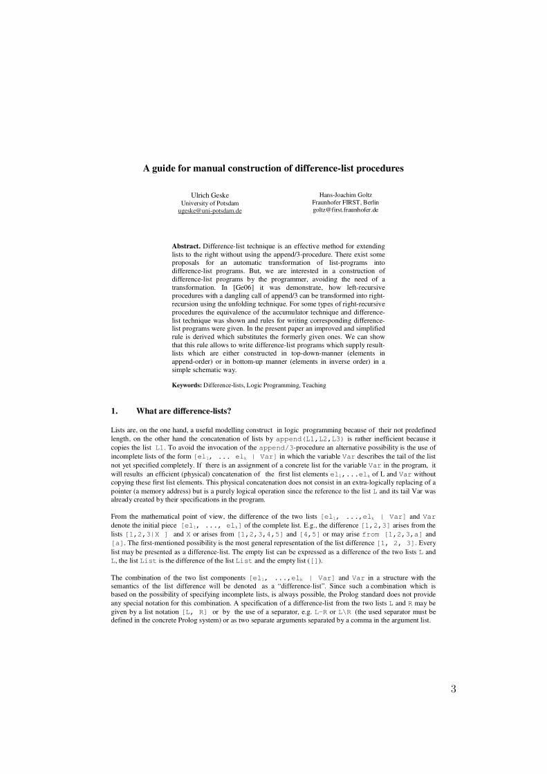
In practical programming, the concatenation of lists is very frequently expressed using an invocation of the append/3-procedure. The reason for it may be the inadequate explanations of the use of incomplete lists and of difference-list technique which uses such incomplete lists. Very different explanations of difference-lists and very different attitudes to them can be found in well-known manuals and textbooks for Prolog. Difference-lists in the literature Definition of difference-lists The earliest extended description of difference-lists was given by Clark and Tärnlund in [CT77]. They illustrated the difference-list or d-list notation by the graphical visualization of lists as it was used in the programming language LISP. One of their examples is given in Fig. 1. In this example the list [a, b, c, d] can be considered as the value of the pointer U. A sublist of U, the list [c, d], could be represented as the value of the pointer W. The list [a, b] between both pointers can be considered as the difference of both lists. In [CT77] this difference is denoted by the term <U, W> which is formed of both pointers. Other authors denote it by a term U\W [StSh91]. We prefer to use the representation U-W in programs like it is done in [OK90].

Fig. 1 Visualization of the difference-list <U, W> [a, b | W] - W = [a, b]

d-list [CT77] d-list(<U, W>) ↔ U = W ∨ ∃X∃VU = [X | V] & element(X) & d-list(V, W) The pair <U, W> represents the difference of the lists U and W and is therefore called a difference-list (d-list or dl for short). The difference includes all the elements of the list that begins at the pointer U and end with the pointer W to a list or to nil.

In a LISP-like representation the value of the difference of list U and W can be constructed by substitution of the pointer to W in U by the empty list. Let us introduce the notation Val(<U, W>) for the term which represents a difference-list <U, W> - the value of a difference-list <U, W>. Of course, the unification procedure in Prolog does not perform the computation of the value like it does not perform arithmetic computations in general. Clark and Tärnlund have given and proven the definition of construction and definition of the concatenation of difference-lists:

Concatenation of d-lists [CT77] d-list(<U, W>) ↔∃Vd-list(<U, V>) & d-list(V, W) If <[b, c, d | Z], Z> is a difference-list with V=[b, c, d | Z] and W=Z then the difference-list <U, W>= <[a, b, c, d | Z], Z> can be constructed where are X=a and U=[a, b, c, d | Z].

Concatenation of the difference-lists <U,V>=<[a,b|X],X> and <V,W>=<X,nil> results in the difference-list <U,W>=<[a,b,c,d],nil> as soon as X is computed to [c, d]. The concept of concatenation of difference-lists will strongly used for our rules for programming d-list programs. Automatic transformation of list-programs Several authors investigated automatic transformations of list programs into difference-list programs [MS88, ZG88, MS93, AFSV00]. Mariott and Sondergaard [MS93] have deeply analysed the problem and proposed an stepwise algorithm for such a transformation. The problem to solve is to ensure such a transformation is safe. Table 1 shows that semantics of programs may different changing programs from list notation to difference-list

4

notation. Essentially the missing occur-check in Prolog systems is due to the different behaviour of programs in list and d-list notation. But Table 1 also shows that in case the occur-check would be available different semantics of list-procedures and the corresponding d-list-procedures may occur. Looking for conditions for a safe automatic generation of difference-lists, Marriot and Søndergaard [MS93] start with the consideration of difference terms.

Difference term [MS93] A difference term is a term of the form <T, T’>, where T and T’ are terms. The term T’ is the delimiter of the difference term. The denotation of <T, T’> is the term that results when every occurrence of T’ in T is replaced by nil.

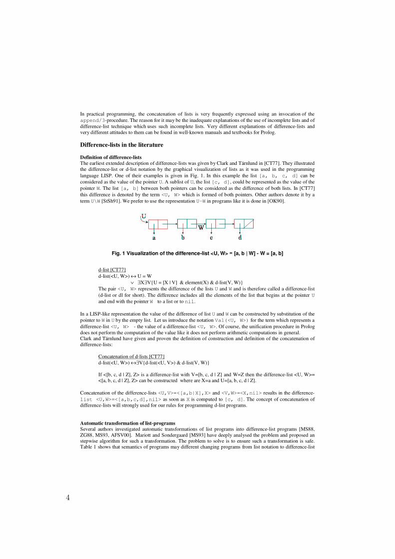
Fig. 2 represents some examples of difference-lists given in [MS93]. If both U and W point to the list [a], the difference-list <U,W> represents the empty list, i.e. Val(<[a],[a]>)=[]. If U points to a list T and W points to nil, the tail of T, then <U,W> represents T (the pointer to W in T is substituted by nil), i.e. Val(<T,nil>)=T. The difference-list <T,X> is a generalization of the difference-list <[a],[b]> if X is not part of (does not occur in) T. In such cases where the second part of the difference-list does not occur in the first part, there is nothing to change in the first part of the difference-list (no pointer is to substitute by nil) and the first part of the difference-list is the value, i.e. Val(<[a],[b]>)=[a] and Val(<T,X>)=T. In cases where W does not point to a list but to an element of a list, a similar substitution action can be performed to get the value of the difference-list. In <U,W>=<[a],a>, W points to the list element a. If one substitutes the pointer to a by nil one gets Val(<[a],a>=[nil]. A similar, but more complex example is given by the difference-list <g(X,X),X>. All pointers to X has to be substituted by nil which results altogether in g(nil,nil).

Table 1 Semantics of a program in list and difference-list representation

Intended meaning Prolog without occur-check Prolog with occur-check list-notation

?- quick([], [a]). > no ?- quick([],[a|Z]). > no

quick([],[]). ?- quick([], [a]). > no ?- quick([],[a|Z]). > no

quick([],[]). ?- quick([], [a]). > no ?- quick([],[a|Z]). > no

dl-notation quick([],X-X). ?-quick([],[a|Z]-Z). > no ?- quick([],[a|Z]-Y). > no

quick([],X-X). ?-quick([],[a|Z]-Z). > Z=[a,a,a…] yes ?- quick([],[a|Z]-Y). > Y=[a|X] yes

quick([],X-X). ?-quick([],[a|Z]-Z). > no ?- quick([],[a|Z]-Y). > Y=[a|X] yes

Fig. 2 Difference trees (visualization of examples of [StSh91])

(nil, /, and [] are synonyms for the empty list)

5

In the context of the transformation of list-procedures into corresponding d-list-procedures, two difference-terms should unify if the corresponding terms unify. This property is valid for simple difference-terms.

Simple difference term [MS93] A difference term is simple iff it is of the form <T,nil> or of the form <T,X> where X represents a variable.

Difference-list [MS93] A difference-list is a difference term that represents a list. It is closed iff the list that it represents is closed (that is, the difference-term is of the form <[T1, …, Tn], Tn>. The difference-list is simple, if Tn is nil or a variable.

The definition of difference-lists allows that W could be a pointer not only to a list but to any term. Therefore, each closed list can be represented as a difference-list, but not every difference-list is the representation of a closed list. The automatic transformation of lists to difference-list is safe if the generated difference-list is simple and T, Tn in <T, Tn> have non-interfering variables. Table 2 should remember that the problem of different semantics of programs is not a special problem for difference-list. Also in pure list processing the programmer has to be aware that bindings of variables to themself may occur during unification and may give rise to different behaviour depended from the programming system.

Table 2 Different semantics of programs

Intended meaning Prolog without occur-check Prolog with occur-check append([], X, X). ?- append([],[a|Z],Z). > no

append([], X, X). ?- append([], [a|Z],Z). > Z=[a,a,a,…] yes

append([], X, X). ?- append([], [a|Z],Z). > no

The authors investigate in [MS93] conditions for a save transformation of list-programs into d-list programs and present a algorithm for the transformation. Difference-lists in Prolog textbooks Clocksin has described the difference-list technique in a tutorial [Clock02] based on his book “Clause and Effect'” [Clock97] as “probably one of the most ingenious programming techniques ever invented yet neglected by mainstream computer science”. In the contrary, Dodds opinion [Dodd90] concerning a pair of variables (All, Temp) for the result All of a list operation and the used accumulator Acc is less emphatic: “some people find it helpful to think of All and Temp as a special data structure called difference-list. We prefer to rest our account of the matter on the logical reading of the variable as referring to any possible tail, rather than to speak of ‘lists with variable tails’”. In the classical Prolog textbook of Clocksin and Mellish [CM84] a certain relationship between accumulator-technique and difference-list technique is stated: "with difference-list we also use two arguments (comment: as for the use of accumulators), but with a different interpretation. The first is the final result, and the second argument is for a hole in the final result where further information can be put". O'Keefe [1] uses the same analogy: “A common thing to do in Prolog is to carry around a partial data structure and some of the holes in it. To extend the data structure, you fill in a hole with a new term which has some holes of its own. Difference-list are a special case of this technique where the two arguments we are passing around the positions a list.” The represented program code for a subset-relation corresponds in its structure to the bottom-up construction of lists. This structure is identified as “difference-list” notation.

Clark&McCabe [CMcC84] denote a difference-list as difference pair. It is used as substitute for an append/3-call. The effects are described by means of the procedure for the list reversal. If the list to be reversed is described by [X|Y], the following logical reading exists for the recursive clause: „[X|Y] has a reverse represented

6

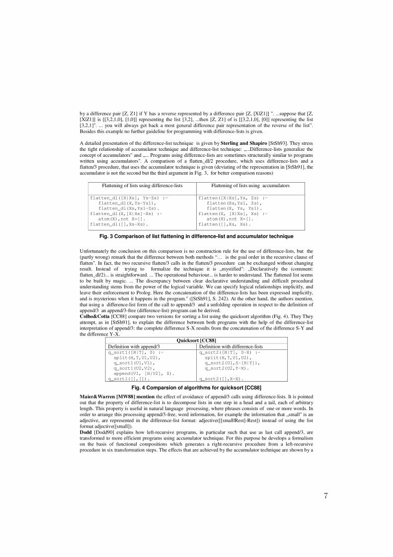
by a difference pair [Z, Z1] if Y has a reverse represented by a difference pair [Z, [X|Z1]] ". ...suppose that [Z, [X|Z1]] is [[3,2,1,0], [1,0]] representing the list [3,2], ...then [Z, Z1] of is [[3,2,1,0], [0]] representing the list [3,2,1]". ... you will always get back a most general difference pair representation of the reverse of the list”. Besides this example no further guideline for programming with difference-lists is given. A detailed presentation of the difference-list technique is given by Sterling and Shapiro [StSh93]. They stress the tight relationship of accumulator technique and difference-list technique: „...Difference-lists generalize the concept of accumulators" and „... Programs using difference-lists are sometimes structurally similar to programs written using accumulators". A comparison of a flatten_dl/2 procedure, which uses difference-lists and a flatten/3 procedure, that uses the accumulator technique is given (deviating of the representation in [StSh91], the accumulator is not the second but the third argument in Fig. 3, for better comparison reasons)

Flattening of lists using difference-lists Flattening of lists using accumulators

flatten_dl([X|Xs], Ys-Zs) :- flatten_dl(X,Ys-Ys1), flatten_dl(Xs,Ys1-Zs). flatten_dl(X,[X|Xs]-Xs) :- atom(X),not X=[]. flatten_dl([],Xs-Xs).

flatten([X|Xs],Ys, Zs) :- flatten(Xs,Ys1, Zs), flatten(X, Ys, Ys1). flatten(X, [X|Xs], Xs) :- atom(X),not X=[]. flatten([],Xs, Xs).

Fig. 3 Comparison of list flattening in difference-list and accumulator technique

Unfortunately the conclusion on this comparison is no construction rule for the use of difference-lists, but the (partly wrong) remark that the difference between both methods “… is the goal order in the recursive clause of flatten". In fact, the two recursive flatten/3 calls in the flatten/3 procedure can be exchanged without changing result. Instead of trying to formalize the technique it is „mystified": „Declaratively the (comment: flatten_dl/2)... is straightforward. ... The operational behaviour... is harder to understand. The flattened list seems to be built by magic. ... The discrepancy between clear declarative understanding and difficult procedural understanding stems from the power of the logical variable. We can specify logical relationships implicitly, and leave their enforcement to Prolog. Here the concatenation of the difference-lists has been expressed implicitly, and is mysterious when it happens in the program." ([StSh91], S. 242). At the other hand, the authors mention, that using a difference-list form of the call to append/3 and a unfolding operation in respect to the definition of append/3 an append/3-free (difference-list) program can be derived. Colho&Cotta [CC88] compare two versions for sorting a list using the quicksort algorithm (Fig. 4). They They attempt, as in [StSh91], to explain the difference between both programs with the help of the difference-list interpretation of append/3: the complete difference S-X results from the concatenation of the difference S-Y and the difference Y-X.

Quicksort [CC88] Definition with append/3 Definition with difference-lists q_sort1([H|T], S) :- split(H,T,U1,U2), q_sort1(U1,V1), q_sort1(U2,V2), append(V1, [H|V2], S). q_sort1([],[]).

q_sort2([H|T], S-X) :- split(H,T,U1,U2), q_sort2(U1,S-[H|Y]), q_sort2(U2,Y-X). q_sort2([],X-X).

Fig. 4 Comparsion of algorithms for quicksort [CC88]

Maier&Warren [MW88] mention the effect of avoidance of append/3 calls using difference-lists. It is pointed out that the property of difference-list is to decompose lists in one step in a head and a tail, each of arbitrary length. This property is useful in natural language processing, where phrases consists of one or more words. In order to arrange this processing append/3-free, word information, for example the information that „small" is an adjective, are represented in the difference-list format: adjective([[small|Rest]-Rest]) instead of using the list format adjective([small]). Dodd [Dodd90] explains how left-recursive programs, in particular such that use as last call append/3, are transformed to more efficient programs using accumulator technique. For this purpose he develops a formalism on the basis of functional compositions which generates a right-recursive procedure from a left-recursive procedure in six transformation steps. The effects that are achieved by the accumulator technique are shown by a

7

great number of problems and the relationship to the difference-list technique is mentioned and but there is no systematised approach for the use of accumulators or difference-lists. The different techniques which are possible for the generation of lists can be reduced to two methods which are essential for list processing: top-down- and bottom-up generation of structures. In [Ge06] we have shown that the difference-list notation could be considered as syntactic sugar since it can be derived from procedures programmed with the accumulator technique by a simple syntactic transformation. But, difference-lists are not only syntactic sugar, since a simple modelling technique using difference-lists instead of additional arguments or accumulators can offer advantages constructing result lists with certain order of elements, efficiently. Knowledge of the (simple) programming rules for difference-list procedures can make it easier to use difference-lists and promotes their use in programming. 2. Top-down and Bottom-up construction of lists The notions of top-down and bottom-up procedures for traversing structures like trees are well established. We will use the notions top-down constructions of lists and bottom-up construction of lists in this paper which should describe the process of building lists with a certain order of elements in relation to the order in which the elements are taken from the corresponding input list.

Top-down construction of lists The order el1’ – el2’ of two arbitrary elements el1’, el2’ in the constructed list corresponds to the order el1 – el2 in which the two elements el1, el2 are taken from the input term (maybe a list or a tree structure).

Bottom-up construction of lists The order el2’ – el1’ of two arbitrary elements el1’, el2’ in the constructed list corresponds to the order el1 – el2 in which the two elements el1, el2 are taken from the input term (maybe a list or a tree structure).

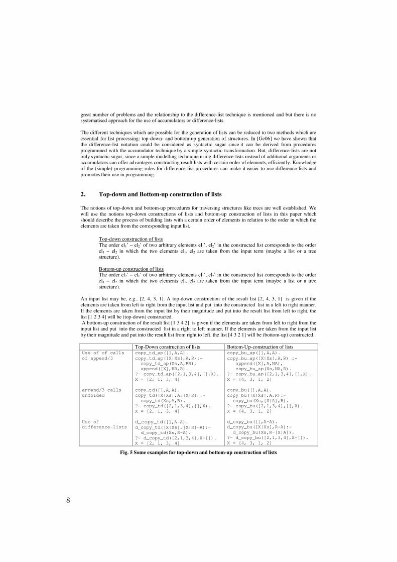
An input list may be, e.g., [2, 4, 3, 1]. A top-down construction of the result list [2, 4, 3, 1] is given if the elements are taken from left to right from the input list and put into the constructed list in a left to right manner. If the elements are taken from the input list by their magnitude and put into the result list from left to right, the list [1 2 3 4] will be (top-down) constructed. A bottom-up construction of the result list [1 3 4 2] is given if the elements are taken from left to right from the input list and put into the constructed list in a right to left manner. If the elements are taken from the input list by their magnitude and put into the result list from right to left, the list [4 3 2 1] will be (bottom-up) constructed. Top-Down construction of lists Bottom-Up-construction of lists Use of of calls of append/3 append/3-calls unfolded Use of difference-lists

copy_td_ap([],A,A). copy_td_ap([X|Xs],A,R):- copy_td_ap(Xs,A,RR), append([X],RR,R). ?- copy_td_ap([2,1,3,4],[],X). X = [2, 1, 3, 4] copy_td([],A,A). copy_td([X|Xs],A,[X|R]):- copy_td(Xs,A,R). ?- copy_td([2,1,3,4],[],X). X = [2, 1, 3, 4] d_copy_td([],A-A). d_copy_td([X|Xs],[X|R]-A):- d_copy_td(Xs,R-A). ?- d_copy_td([2,1,3,4],X-[]). X = [2, 1, 3, 4]

copy_bu_ap([],A,A). copy_bu_ap([X|Xs],A,R) :- append([X],A,NA), copy_bu_ap(Xs,NA,R). ?- copy_bu_ap([2,1,3,4],[],X). X = [4, 3, 1, 2] copy_bu([],A,A). copy_bu([X|Xs],A,R):- copy_bu(Xs,[X|A],R). ?- copy_bu([2,1,3,4],[],X). X = [4, 3, 1, 2] d_copy_bu([],A-A). d_copy_bu([X|Xs],R-A):- d_copy_bu(Xs,R-[X|A]). ?- d_copy_bu([2,1,3,4],X-[]). X = [4, 3, 1, 2]

Fig. 5 Some examples for top-down and bottom-up construction of lists

8

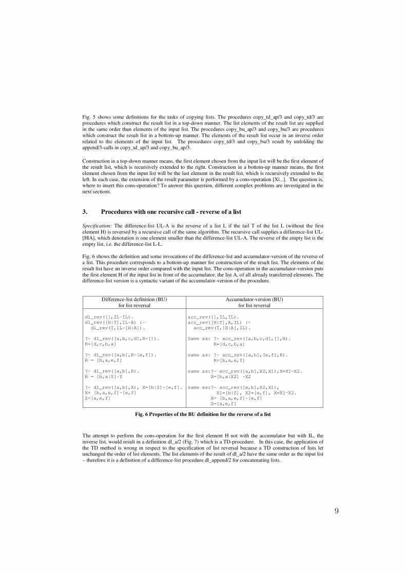
Fig. 5 shows some definitions for the tasks of copying lists. The procedures copy_td_ap/3 and copy_td/3 are procedures which construct the result list in a top-down manner. The list elements of the result list are supplied in the same order than elements of the input list. The procedures copy_bu_ap/3 and copy_bu/3 are procedures which construct the result list in a bottom-up manner. The elements of the result list occur in an inverse order related to the elements of the input list. The procedures copy_td/3 and copy_bu/3 result by unfolding the append/3-calls in copy_td_ap/3 and copy_bu_ap/3. Construction in a top-down manner means, the first element chosen from the input list will be the first element of the result list, which is recursively extended to the right. Construction in a bottom-up manner means, the first element chosen from the input list will be the last element in the result list, which is recursively extended to the left. In each case, the extension of the result parameter is performed by a cons-operation [X|...]. The question is, where to insert this cons-operation? To answer this question, different complex problems are investigated in the next sections. 3. Procedures with one recursive call - reverse of a list Specification: The difference-list UL-A is the reverse of a list L if the tail T of the list L (without the first element H) is reversed by a recursive call of the same algorithm. The recursive call supplies a difference-list UL-[H|A], which denotation is one element smaller than the difference-list UL-A. The reverse of the empty list is the empty list, i.e. the difference-list L-L. Fig. 6 shows the definition and some invocations of the difference-list and accumulator-version of the reverse of a list. This procedure corresponds to a bottom-up manner for construction of the result list. The elements of the result list have an inverse order compared with the input list. The cons-operation in the accumulator-version puts the first element H of the input list in front of the accumulator, the list A, of all already transferred elements. The difference-list version is a syntactic variant of the accumulator-version of the procedure.

Difference-list definition (BU) for list reversal

Accumulator-version (BU) for list reversal

dl_rev([],IL-IL). dl_rev([H|T],IL-A) :- dl_rev(T,IL-[H|A]). ?- dl_rev([a,b,c,d],R-[]). R=[d,c,b,a] ?- dl_rev([a,b],R-[e,f]). R = [b,a,e,f] ?- dl_rev([a,b],R). R = [b,a|Y]-Y ?- dl_rev([a,b],X), X=[b|Z]-[e,f]. X= [b,a,e,f]-[e,f] Z=[a,e,f]

acc_rev([],IL,IL). acc_rev([H|T],A,IL) :- acc_rev(T,[H|A],IL). Same as: ?- acc_rev([a,b,c,d],[],R). R=[d,c,b,a] same as: ?- acc_rev([a,b],[e,f],R). R=[b,a,e,f] same as:?- acc_rev([a,b],X2,X1),X=X1-X2. X=[b,a|X2] –X2 same as:?- acc_rev([a,b],X2,X1), X1=[b|Z], X2=[e,f], X=X1-X2. X= [b,a,e,f]-[e,f] Z=[a,e,f]

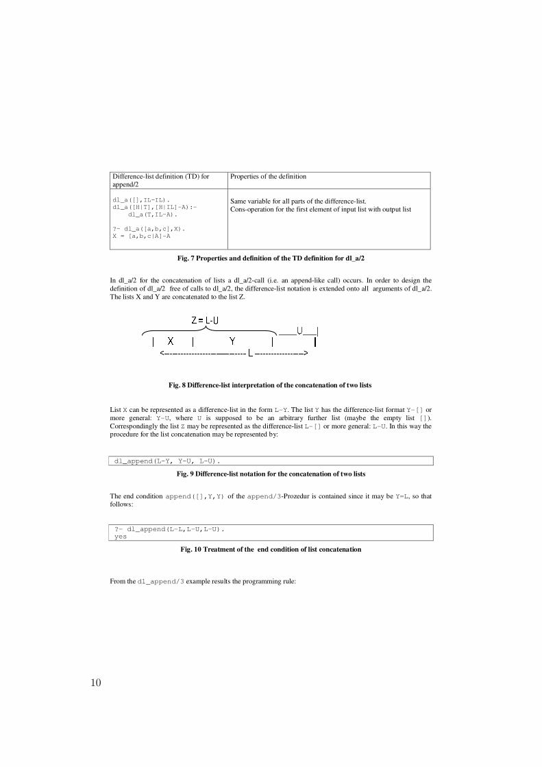
Fig. 6 Properties of the BU definition for the reverse of a list The attempt to perform the cons-operation for the first element H not with the accumulator but with IL, the inverse list, would result in a definition dl_a/2 (Fig. 7) which is a TD-procedure. In this case, the application of the TD method is wrong in respect to the specification of list reversal because a TD construction of lists let unchanged the order of list elements. The list elements of the result of dl_a/2 have the same order as the input list – therefore it is a definition of a difference-list procedure dl_append/2 for concatenating lists.

9

Difference-list definition (TD) for append/2

Properties of the definition

dl_a([],IL-IL). dl_a([H|T],[H|IL]-A):- dl_a(T,IL-A). ?- dl_a([a,b,c],X). X = [a,b,c|A]-A

Same variable for all parts of the difference-list. Cons-operation for the first element of input list with output list

Fig. 7 Properties and definition of the TD definition for dl_a/2

In dl_a/2 for the concatenation of lists a dl_a/2-call (i.e. an append-like call) occurs. In order to design the definition of dl_a/2 free of calls to dl_a/2, the difference-list notation is extended onto all arguments of dl_a/2. The lists X and Y are concatenated to the list Z.

List X can be represented as a difference-list in the form L-Y. The list Y has the difference-list format Y-[] or more general: Y-U, where U is supposed to be an arbitrary further list (maybe the empty list []). Correspondingly the list Z may be represented as the difference-list L-[] or more general: L-U. In this way the procedure for the list concatenation may be represented by: dl_append(L-Y, Y-U, L-U).

Fig. 9 Difference-list notation for the concatenation of two lists

The end condition append([],Y,Y) of the append/3-Prozedur is contained since it may be Y=L, so that follows: ?- dl_append(L-L,L-U,L-U). yes

Fig. 10 Treatment of the end condition of list concatenation

From the dl_append/3 example results the programming rule:

Fig. 8 Difference-list interpretation of the concatenation of two lists

10

From the existence of the difference-lists A-B and B-C can be deduced the existence of the difference-list A-C (and vice versa).

Rule 1 Composition of difference-lists

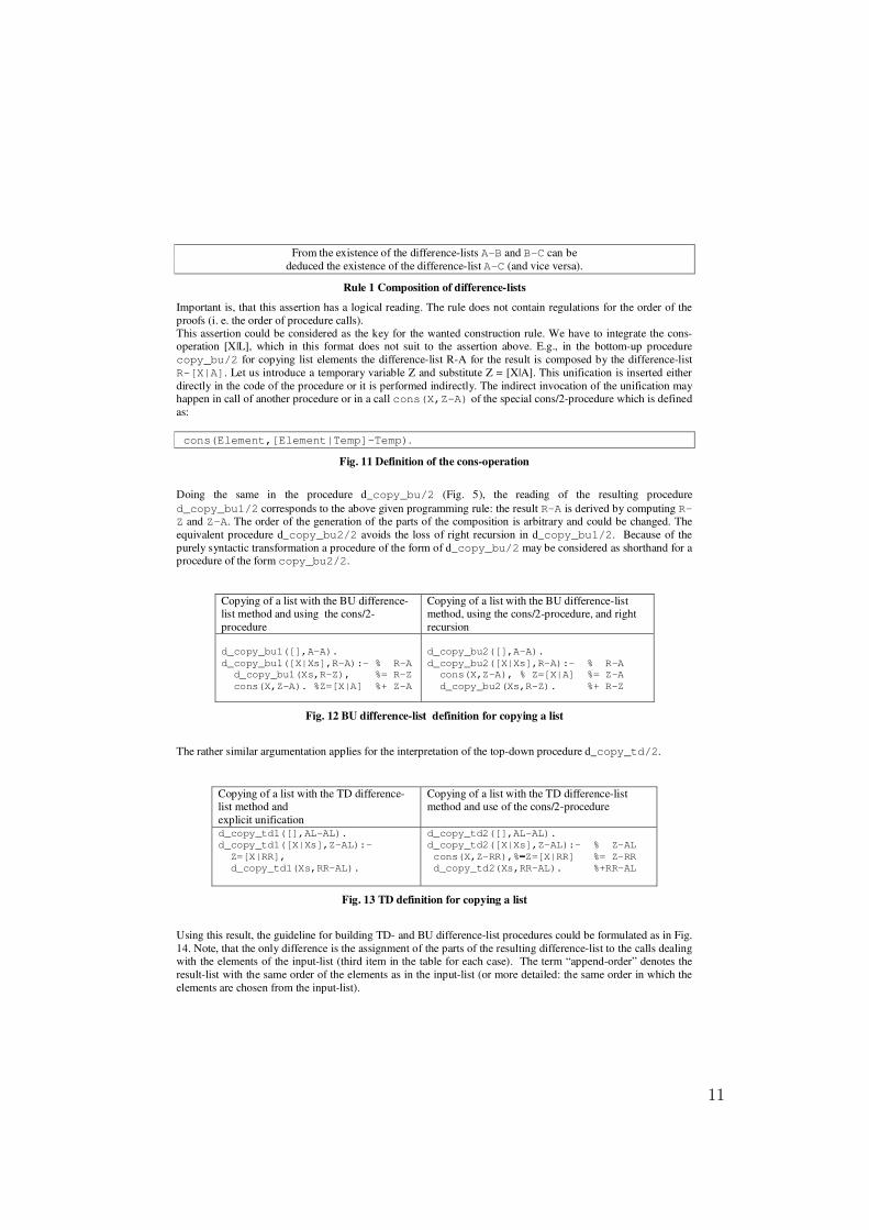
Important is, that this assertion has a logical reading. The rule does not contain regulations for the order of the proofs (i. e. the order of procedure calls). This assertion could be considered as the key for the wanted construction rule. We have to integrate the cons-operation [X|L], which in this format does not suit to the assertion above. E.g., in the bottom-up procedure copy_bu/2 for copying list elements the difference-list R-A for the result is composed by the difference-list R-[X|A]. Let us introduce a temporary variable Z and substitute Z = [X|A]. This unification is inserted either directly in the code of the procedure or it is performed indirectly. The indirect invocation of the unification may happen in call of another procedure or in a call cons(X,Z-A) of the special cons/2-procedure which is defined as: cons(Element,[Element|Temp]-Temp).

Fig. 11 Definition of the cons-operation

Doing the same in the procedure d_copy_bu/2 (Fig. 5), the reading of the resulting procedure d_copy_bu1/2 corresponds to the above given programming rule: the result R-A is derived by computing R-Z and Z-A. The order of the generation of the parts of the composition is arbitrary and could be changed. The equivalent procedure d_copy_bu2/2 avoids the loss of right recursion in d_copy_bu1/2. Because of the purely syntactic transformation a procedure of the form of d_copy_bu/2 may be considered as shorthand for a procedure of the form copy_bu2/2.

Copying of a list with the BU difference-list method and using the cons/2-procedure

Copying of a list with the BU difference-list method, using the cons/2-procedure, and right recursion

d_copy_bu1([],A-A). d_copy_bu1([X|Xs],R-A):- % R-A d_copy_bu1(Xs,R-Z), %= R-Z cons(X,Z-A). %Z=[X|A] %+ Z-A

d_copy_bu2([],A-A). d_copy_bu2([X|Xs],R-A):- % R-A cons(X,Z-A), % Z=[X|A] %= Z-A d_copy_bu2(Xs,R-Z). %+ R-Z

Fig. 12 BU difference-list definition for copying a list

The rather similar argumentation applies for the interpretation of the top-down procedure d_copy_td/2.

Copying of a list with the TD difference-list method and explicit unification

Copying of a list with the TD difference-list method and use of the cons/2-procedure

d_copy_td1([],AL-AL). d_copy_td1([X|Xs],Z-AL):- Z=[X|RR], d_copy_td1(Xs,RR-AL).

d_copy_td2([],AL-AL). d_copy_td2([X|Xs],Z-AL):- % Z-AL cons(X,Z-RR),% Z=[X|RR] %= Z-RR d_copy_td2(Xs,RR-AL). %+RR-AL

Fig. 13 TD definition for copying a list

Using this result, the guideline for building TD- and BU difference-list procedures could be formulated as in Fig. 14. Note, that the only difference is the assignment of the parts of the resulting difference-list to the calls dealing with the elements of the input-list (third item in the table for each case). The term “append-order” denotes the result-list with the same order of the elements as in the input-list (or more detailed: the same order in which the elements are chosen from the input-list).

11

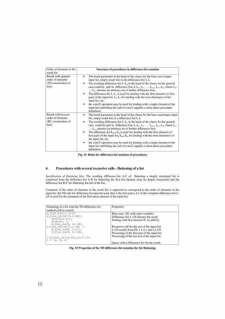
Order of elements in the result list

Structure of procedures in difference-list notation

Result with append- order of elements (TD construction of lists)

• The result parameter in the head of the clause for the base case (empty input list, empty result list) is the difference-list L-L.

• The resulting difference-list L-Ln in the head of the clause for the general case could be split in difference-lists L-L1, L1- …- Ln-1, Ln-1-Ln, where L1-…-Ln-1 denotes an arbitrary set of further difference-lists.

• The difference-list L-L1 is used for dealing with the first element (or first part) of the input list, L1-L2 for dealing with the next element(s) of the input list, etc.

• the cons/2-operation may be used for dealing with a single element of the input list (unfolding the call of cons/2 supplies a more dense procedure definition)

Result with inverse order of elements (BU construction of lists)

• The result parameter in the head of the clause for the base case(empty input list, empty result list) is a difference-list L-L

• The resulting difference-list L-Ln in the head of the clause for the general case could be split in difference-lists L-L1, L1- …- Ln-1, Ln-1-Ln, where L1-…-Ln-1 denotes an arbitrary set of further difference-lists.

• The difference-list Ln-1-Ln is used for dealing with the first element (or first part) of the input list, Ln-1-Ln for dealing with the next element(s) of the input list, etc.

• the cons/2-operation may be used for dealing with a single element of the input list (unfolding the call of cons/2 supplies a more dense procedure definition)

Fig. 14 Rules for difference-list notation of procedures

4. Procedures with several recursive calls - flattening of a list Specification of flattening lists: The resulting difference-list A-C of flattening a deeply structured list is composed from the difference-list A-B for flattening the first list element (may be deeply structured) and the difference-list B-C for flattening the tail of the list. Comment: If the order of elements in the result list is supposed to correspond to the order of elements in the input list, the TD-rule for difference-list must be used, that is the first part L-L1 of the complete difference-list L-LN is used for the treatment of the first taken element of the input list. Flattening of a list with the TD-difference-list method (call to cons/2)

Properties

d_flat_td([], L-L). d_flat_td([H|T],L-LN):- cons(H,L-L1), atom(H), !, d_flat_td(T, L1-LN). d_flat_td([H|T],L-LN) :- d_flat_td(H, L-L1), d_flat_td(T, L1-LN). ?-d_flat_td([a,[b],c],L-[]). L = [a, b, c]

Base case: DL with same variables. Difference-list L-LN denotes the result Dealing with first element H (L=[H|A]) Recursive call for the rest of the input list. L-LN results from DL’s L-L1 and L1-LN. Processing of the first part of the input list. Processing of the last rest of the input list. Query with a difference-list for the result.

Fig. 15 Properties of the TD difference-list notation for list flattening

12

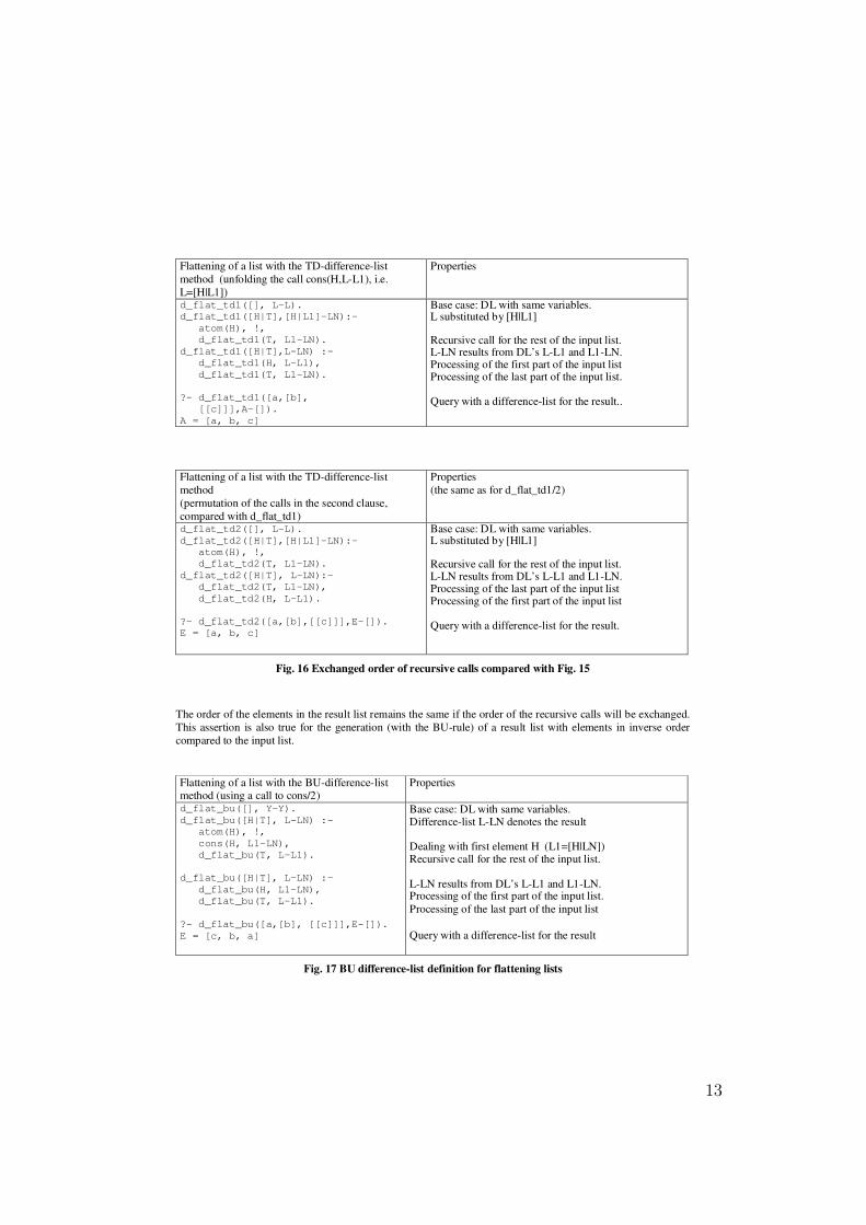
Flattening of a list with the TD-difference-list method (unfolding the call cons(H,L-L1), i.e. L=[H|L1])

Properties

d_flat_td1([], L-L). d_flat_td1([H|T],[H|L1]-LN):- atom(H), !, d_flat_td1(T, L1-LN). d_flat_td1([H|T],L-LN) :- d_flat_td1(H, L-L1), d_flat_td1(T, L1-LN). ?- d_flat_td1([a,[b], [[c]]],A-[]). A = [a, b, c]

Base case: DL with same variables. L substituted by [H|L1] Recursive call for the rest of the input list. L-LN results from DL’s L-L1 and L1-LN. Processing of the first part of the input list Processing of the last part of the input list. Query with a difference-list for the result..

Flattening of a list with the TD-difference-list method (permutation of the calls in the second clause, compared with d_flat_td1)

Properties (the same as for d_flat_td1/2)

d_flat_td2([], L-L). d_flat_td2([H|T],[H|L1]-LN):- atom(H), !, d_flat_td2(T, L1-LN). d_flat_td2([H|T], L-LN):- d_flat_td2(T, L1-LN), d_flat_td2(H, L-L1). ?- d_flat_td2([a,[b],[[c]]],E-[]). E = [a, b, c]

Base case: DL with same variables. L substituted by [H|L1] Recursive call for the rest of the input list. L-LN results from DL’s L-L1 and L1-LN. Processing of the last part of the input list Processing of the first part of the input list Query with a difference-list for the result.

Fig. 16 Exchanged order of recursive calls compared with Fig. 15

The order of the elements in the result list remains the same if the order of the recursive calls will be exchanged. This assertion is also true for the generation (with the BU-rule) of a result list with elements in inverse order compared to the input list. Flattening of a list with the BU-difference-list method (using a call to cons/2)

Properties

d_flat_bu([], Y-Y). d_flat_bu([H|T], L-LN) :- atom(H), !, cons(H, L1-LN), d_flat_bu(T, L-L1). d_flat_bu([H|T], L-LN) :- d_flat_bu(H, L1-LN), d_flat_bu(T, L-L1). ?- d_flat_bu([a,[b], [[c]]],E-[]). E = [c, b, a]

Base case: DL with same variables. Difference-list L-LN denotes the result Dealing with first element H (L1=[H|LN]) Recursive call for the rest of the input list. L-LN results from DL’s L-L1 and L1-LN. Processing of the first part of the input list. Processing of the last part of the input list Query with a difference-list for the result

Fig. 17 BU difference-list definition for flattening lists

13

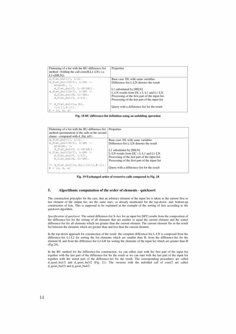
Flattening of a list with the BU-difference-list method (folding the call cons(H,L1-LN), i.e. L1=[H|LN])

Properties

d_flat_bu1([], L-L). d_flat_bu1([H|T], L-LN) :- atom(H), !, d_flat_bu1(T, L-[H|LN]). d_flat_bu1([H|T], L-LN) :- d_flat_bu1(H, L1-LN), d_flat_bu1(T, L-L1). ?- d_flat_bu1([a,[b], [[c]]],E-[]). E = [c, b, a]

Base case: DL with same variables. Difference-list L-LN denotes the result L1 substituted by [H|LN] L-LN results from DL’s L-L1 and L1-LN. Processing of the first part of the input list. Processing of the last part of the input list Query with a difference-list for the result

Fig. 18 BU difference-list definition using an unfolding operation

Flattening of a list with the BU-difference-list method (permutation of the calls in the second clause - compared with d_flat_td1)

Properties

d_flat_bu2([], L-L). d_flat_bu2([H|T], L-LN) :- atom(H), !, d_flat_bu2(T, L-[H|LN]). d_flat_bu2([H|T], L-LN) :- d_flat_bu2(T, L-L1), d_flat_bu2(H, L1-LN). ?- d_flat_bu2([a,[b],[[c]]],E-[]). E = [c, b, a]

Base case: DL with same variables. Difference-list L-LN denotes the result L1 substituted by [H|LN] L-LN results from DL’s L-L1 and L1-LN. Processing of the last part of the input list. Processing of the first part of the input list Query with a difference-list for the result

Fig. 19 Exchanged order of recursive calls compared to Fig. 18

5. Algorithmic computation of the order of elements - quicksort The construction principles for the case, that an arbitrary element of the input list is taken as the current first or last element of the output list, are the same ones, as already mentioned for the top-down- and. bottom-up construction of lists. This is supposed to be explained at the example of the sorting of lists according to the quicksort algorithm. Specification of quicksort: The sorted difference-list S-Acc for an input list [H|T] results from the composition of the difference-list for the sorting of all elements that are smaller or equal the current element and the sorted difference-list for all elements which are greater than the current element. The current element fits in the result list between the elements which are greater than and less than the current element. In the top-down approach for construction of the result the complete difference-list L-LN is composed from the difference-list L1-L2 for sorting the list elements which are smaller than H, from the difference-list for the element H, and from the difference-list L2-LH for sorting the elements of the input list which are greater than H (Fig.20). In the BU method for the difference-list construction, we can either start with the first part of the input list together with the last part of the difference-list for the result or we can start with the last part of the input list together with the initial part of the difference-list for the result. The corresponding procedures are called d_qsort_bu1/2 and d_qsort_bu3/2 (Fig. 21). The versions with the unfolded call of cons/2 are called d_qsort_bu2/2 and d_qsort_bu4/2.

14

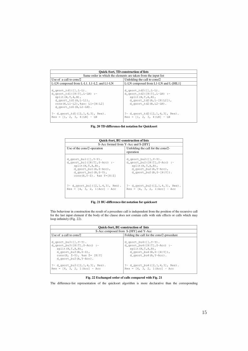
Quick-Sort, TD-construction of lists Same order in which the elements are taken from the input list

Use of a call to cons/2 Unfolding the call to cons/2 L-LN composed from L-L1, L1-L2, and L1-LN L-LN composed from L1-LN and L-[H|L1] d_qsort_td1([],L-L). d_qsort_td1([H|T],L-LN) :- split(H,T,A,B), d_qsort_td1(A,L-L1), cons(H,L1-L2),%as: L1=[H|L2] d_qsort_td1(B,L2-LN). ?- d_qsort_td1([2,1,4,3], Res). Res = [1, 2, 3, 4|LN] - LN

d_qsort_td2([],L-L). d_qsort_td2([H|T],L-LN) :- split(H,T,A,B), d_qsort_td2(A,L-[H|L2]), d_qsort_td2(B,L2-LN). ?- d_qsort_td2([2,1,4,3], Res). Res = [1, 2, 3, 4|LN] - LN

Fig. 20 TD difference-list notation for Quicksort

Quick-Sort, BU-construction of lists S-Acc formed from Y-Acc and S-[H|Y]

Use of the cons/2-operation Unfolding the call for the cons/2-operation

d_qsort_bu1([],Y-Y). d_qsort_bu1([H|T],S-Acc) :- split(H,T,A,B), d_qsort_bu1(A,Z-Acc), d_qsort_bu1(B,S-Y), cons(H,Y-Z). %as Y=[H|Z] ?- d_qsort_bu1([2,1,4,3], Res). Res = [4, 3, 2, 1|Acc] - Acc

d_qsort_bu2([],Y-Y). d_qsort_bu2([H|T],S-Acc) :- split(H,T,A,B), d_qsort_bu2(A,Y-Acc), d_qsort_bu2(B,S-[H|Y]). ?- d_qsort_bu2([2,1,4,3], Res). Res = [4, 3, 2, 1|Acc] – Acc

Fig. 21 BU-difference-list notation for quicksort

This behaviour in construction the result of a procedure call is independent from the position of the recursive call for the last input element if the body of the clause does not contain calls with side effects or calls which may loop infinitely (Fig. 22).

Quick-Sort, BU-construction of lists S-Acc composed from S-[H|Y] and Y-Acc

Use of a call to cons/2 Folding the call for the cons/2-procedure d_qsort_bu3([],Y-Y). d_qsort_bu3([H|T],S-Acc) :- split(H,T,A,B), d_qsort_bu3(B,S-Z), cons(H, Z-Y), %as Z= [H|Y] d_qsort_bu3(A,Y-Acc). ?- d_qsort_bu3([2,1,4,3], Res). Res = [4, 3, 2, 1|Acc] - Acc

d_qsort_bu4([],Y-Y). d_qsort_bu4([H|T],S-Acc) :- split(H,T,A,B), d_qsort_bu4(B,S-[H|Y]), d_qsort_bu4(A,Y-Acc). ?- d_qsort_bu4([2,1,4,3], Res). Res = [4, 3, 2, 1|Acc] – Acc

Fig. 22 Exchanged order of calls compared with Fig. 21

The difference-list representation of the quicksort algorithm is more declarative than the corresponding

15

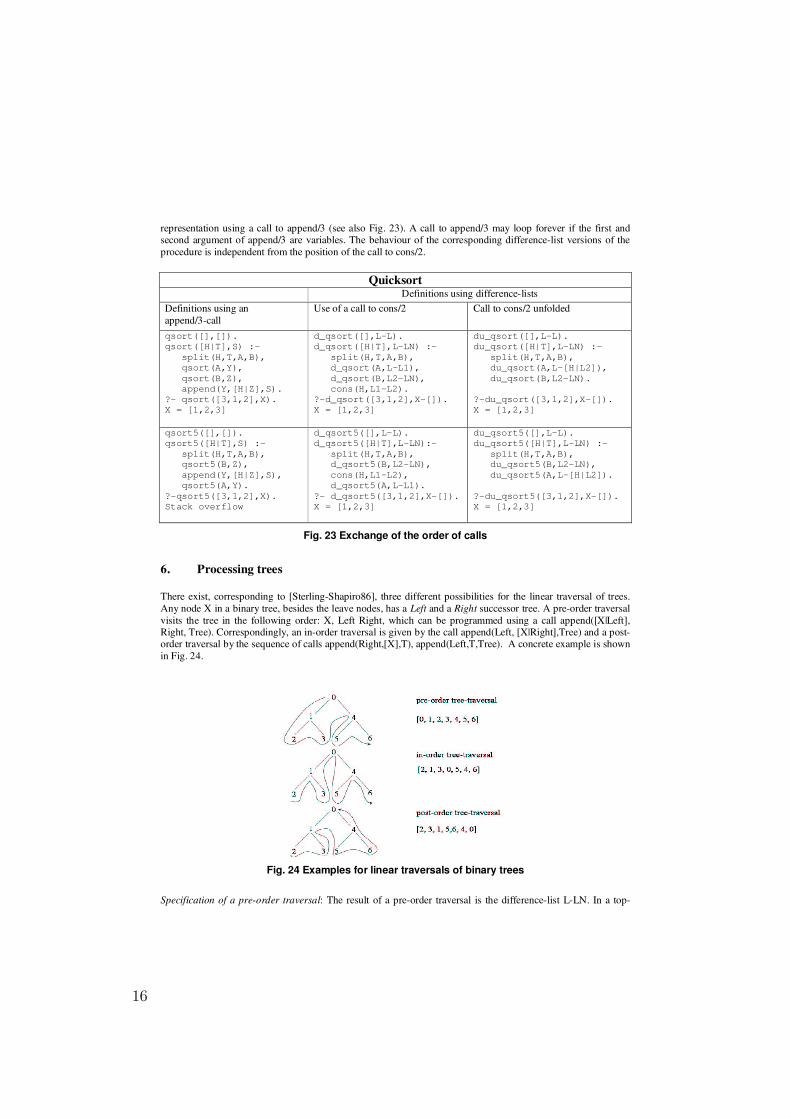
representation using a call to append/3 (see also Fig. 23). A call to append/3 may loop forever if the first and second argument of append/3 are variables. The behaviour of the corresponding difference-list versions of the procedure is independent from the position of the call to cons/2.

Quicksort Definitions using difference-lists Definitions using an append/3-call

Use of a call to cons/2 Call to cons/2 unfolded

qsort([],[]). qsort([H|T],S) :- split(H,T,A,B), qsort(A,Y), qsort(B,Z), append(Y,[H|Z],S). ?- qsort([3,1,2],X). X = [1,2,3]

d_qsort([],L-L). d_qsort([H|T],L-LN) :- split(H,T,A,B), d_qsort(A,L-L1), d_qsort(B,L2-LN), cons(H,L1-L2). ?-d_qsort([3,1,2],X-[]). X = [1,2,3]

du_qsort([],L-L). du_qsort([H|T],L-LN) :- split(H,T,A,B), du_qsort(A,L-[H|L2]), du_qsort(B,L2-LN). ?-du_qsort([3,1,2],X-[]). X = [1,2,3]

qsort5([],[]). qsort5([H|T],S) :- split(H,T,A,B), qsort5(B,Z), append(Y,[H|Z],S), qsort5(A,Y). ?-qsort5([3,1,2],X). Stack overflow

d_qsort5([],L-L). d_qsort5([H|T],L-LN):- split(H,T,A,B), d_qsort5(B,L2-LN), cons(H,L1-L2), d_qsort5(A,L-L1). ?- d_qsort5([3,1,2],X-[]). X = [1,2,3]

du_qsort5([],L-L). du_qsort5([H|T],L-LN) :- split(H,T,A,B), du_qsort5(B,L2-LN), du_qsort5(A,L-[H|L2]). ?-du_qsort5([3,1,2],X-[]). X = [1,2,3]

Fig. 23 Exchange of the order of calls

6. Processing trees There exist, corresponding to [Sterling-Shapiro86], three different possibilities for the linear traversal of trees. Any node X in a binary tree, besides the leave nodes, has a Left and a Right successor tree. A pre-order traversal visits the tree in the following order: X, Left Right, which can be programmed using a call append([X|Left], Right, Tree). Correspondingly, an in-order traversal is given by the call append(Left, [X|Right],Tree) and a post-order traversal by the sequence of calls append(Right,[X],T), append(Left,T,Tree). A concrete example is shown in Fig. 24.

Fig. 24 Examples for linear traversals of binary trees

Specification of a pre-order traversal: The result of a pre-order traversal is the difference-list L-LN. In a top-

16

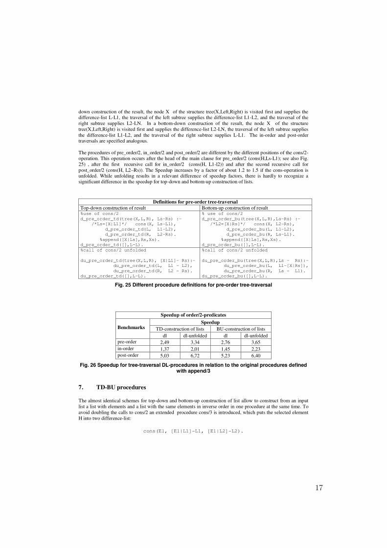
down construction of the result, the node X of the structure tree(X,Left,Right) is visited first and supplies the difference-list L-L1, the traversal of the left subtree supplies the difference-list L1-L2, and the traversal of the right subtree supplies L2-LN. In a bottom-down construction of the result, the node X of the structure tree(X,Left,Right) is visited first and supplies the difference-list L2-LN, the traversal of the left subtree supplies the difference-list L1-L2, and the traversal of the right subtree supplies L-L1. The in-order and post-order traversals are specified analogous. The procedures of pre_order/2, in_order/2 and post_order/2 are different by the different positions of the cons/2-operation. This operation occurs after the head of the main clause for pre_order/2 (cons(H,Ls-L1); see also Fig. 25) , after the first recursive call for in_order/2 (cons(H, L1-l2)) and after the second recursive call for post_order/2 (cons(H, L2–Rs)). The Speedup increases by a factor of about 1.2 to 1.5 if the cons-operation is unfolded. While unfolding results in a relevant difference of speedup factors, there is hardly to recognize a significant difference in the speedup for top-down and bottom-up construction of lists.

Definitions for pre-order tree-traversal Top-down construction of result Bottom-up construction of result %use of cons/2 d_pre_order_td(tree(X,L,R), Ls-Rs) :- /*Ls=[X|L1]*/ cons(X, Ls-L1), d_pre_order_td(L, L1-L2), d_pre_order_td(R, L2-Rs). %append([X|Ls],Rs,Xs). d_pre_order_td([],L-L).

% use of cons/2 d_pre_order_bu(tree(X,L,R),Ls-Rs) :- /*L2=[X|Rs]*/ cons(X, L2-Rs), d_pre_order_bu(L, L1-L2), d_pre_order_bu(R, Ls-L1). %append([X|Ls],Rs,Xs). d_pre_order_bu([],L-L).

%call of cons/2 unfolded du_pre_order_td(tree(X,L,R), [X|L1]- Rs):- du_pre_order_td(L, L1 - L2), du_pre_order_td(R, L2 - Rs). du_pre_order_td([],L-L).

%call of cons/2 unfolded du_pre_order_bu(tree(X,L,R),Ls - Rs):- du_pre_order_bu(L, L1-[X|Rs]), du_pre_order_bu(R, Ls - L1). du_pre_order_bu([],L-L).

Fig. 25 Different procedure definitions for pre-order tree-traversal

Speedup of order/2-predicates Speedup

TD-construction of lists BU-construction of lists Benchmarks

dl dl-unfolded dl dl-unfolded pre-order 2,49 3,34 2,76 3,65 in-order 1,37 2,01 1,45 2,23 post-order 5,03 6,72 5,23 6,40

Fig. 26 Speedup for tree-traversal DL-procedures in relation to the original procedures defined with append/3

7. TD-BU procedures The almost identical schemes for top-down and bottom-up construction of list allow to construct from an input list a list with elements and a list with the same elements in inverse order in one procedure at the same time. To avoid doubling the calls to cons/2 an extended procedure cons/3 is introduced, which puts the selected element H into two difference-list:

cons(El, [El|L1]-L1, [El|L2]-L2).

17

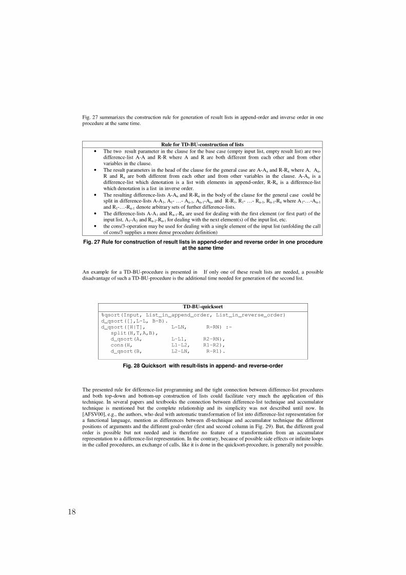
Fig. 27 summarizes the construction rule for generation of result lists in append-order and inverse order in one procedure at the same time.

Rule for TD-BU-construction of lists • The two result parameter in the clause for the base case (empty input list, empty result list) are two

difference-list A-A and R-R where A and R are both different from each other and from other variables in the clause.

• The result parameters in the head of the clause for the general case are A-An and R-Rn where A, An, R and Rn are both different from each other and from other variables in the clause. A-An is a difference-list which denotation is a list with elements in append-order, R-Rn is a difference-list which denotation is a list in inverse order.

• The resulting difference-lists A-An and R-Rn in the body of the clause for the general case could be split in difference-lists A-A1, A1- …- An-1, An-1-An, and R-R1, R1- …- Rn-1, Rn-1-Rn where A1-…-An-1

and R1-…-Rn-1 denote arbitrary sets of further difference-lists. • The difference-lists A-A1 and Rn-1-Rn are used for dealing with the first element (or first part) of the

input list, A1-A2 and Rn-2-Rn-1 for dealing with the next element(s) of the input list, etc. • the cons/3-operation may be used for dealing with a single element of the input list (unfolding the call

of cons/3 supplies a more dense procedure definition)

Fig. 27 Rule for construction of result lists in append-order and reverse order in one procedure at the same time

An example for a TD-BU-procedure is presented in If only one of these result lists are needed, a possible disadvantage of such a TD-BU-procedure is the additional time needed for generation of the second list.

TD-BU-quicksort %qsort(Input, List_in_append_order, List_in_reverse_order) d_qsort([],L-L, B-B). d_qsort([H|T], L-LN, R-RN) :- split(H,T,A,B), d_qsort(A, L-L1, R2-RN), cons(H, L1-L2, R1-R2), d_qsort(B, L2-LN, R-R1).

Fig. 28 Quicksort with result-lists in append- and reverse-order

The presented rule for difference-list programming and the tight connection between difference-list procedures and both top-down and bottom-up construction of lists could facilitate very much the application of this technique. In several papers and textbooks the connection between difference-list technique and accumulator technique is mentioned but the complete relationship and its simplicity was not described until now. In [AFSV00], e.g., the authors, who deal with automatic transformation of list into difference-list representation for a functional language, mention as differences between dl-technique and accumulator technique the different positions of arguments and the different goal-order (first and second column in Fig. 29). But, the different goal order is possible but not needed and is therefore no feature of a transformation from an accumulator representation to a difference-list representation. In the contrary, because of possible side effects or infinite loops in the called procedures, an exchange of calls, like it is done in the quicksort-procedure, is generally not possible.

18

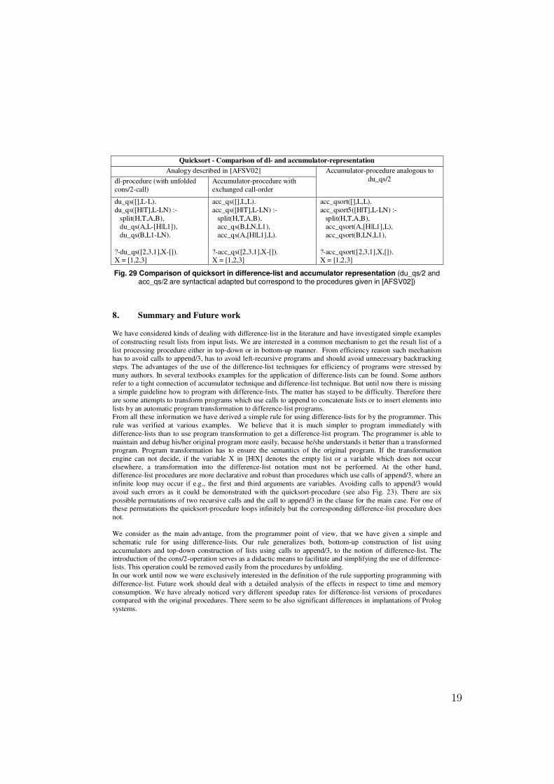
Quicksort - Comparison of dl- and accumulator-representation Analogy described in [AFSV02]

dl-procedure (with unfolded cons/2-call)

Accumulator-procedure with exchanged call-order

Accumulator-procedure analogous to du_qs/2

du_qs([],L-L). du_qs([H|T],L-LN) :- split(H,T,A,B), du_qs(A,L-[H|L1]), du_qs(B,L1-LN). ?-du_qs([2,3,1],X-[]). X = [1,2,3]

acc_qs([],L,L). acc_qs([H|T],L-LN) :- split(H,T,A,B), acc_qs(B,LN,L1), acc_qs(A,[H|L1],L). ?-acc_qs([2,3,1],X-[]). X = [1,2,3]

acc_qsort([],L,L). acc_qsort5([H|T],L-LN) :- split(H,T,A,B), acc_qsort(A,[H|L1],L), acc_qsort(B,LN,L1), ?-acc_qsort([2,3,1],X,[]). X = [1,2,3]

Fig. 29 Comparison of quicksort in difference-list and accumulator representation (du_qs/2 and acc_qs/2 are syntactical adapted but correspond to the procedures given in [AFSV02])

8. Summary and Future work We have considered kinds of dealing with difference-list in the literature and have investigated simple examples of constructing result lists from input lists. We are interested in a common mechanism to get the result list of a list processing procedure either in top-down or in bottom-up manner. From efficiency reason such mechanism has to avoid calls to append/3, has to avoid left-recursive programs and should avoid unnecessary backtracking steps. The advantages of the use of the difference-list techniques for efficiency of programs were stressed by many authors. In several textbooks examples for the application of difference-lists can be found. Some authors refer to a tight connection of accumulator technique and difference-list technique. But until now there is missing a simple guideline how to program with difference-lists. The matter has stayed to be difficulty. Therefore there are some attempts to transform programs which use calls to append to concatenate lists or to insert elements into lists by an automatic program transformation to difference-list programs. From all these information we have derived a simple rule for using difference-lists for by the programmer. This rule was verified at various examples. We believe that it is much simpler to program immediately with difference-lists than to use program transformation to get a difference-list program. The programmer is able to maintain and debug his/her original program more easily, because he/she understands it better than a transformed program. Program transformation has to ensure the semantics of the original program. If the transformation engine can not decide, if the variable X in [H|X] denotes the empty list or a variable which does not occur elsewhere, a transformation into the difference-list notation must not be performed. At the other hand, difference-list procedures are more declarative and robust than procedures which use calls of append/3, where an infinite loop may occur if e.g., the first and third arguments are variables. Avoiding calls to append/3 would avoid such errors as it could be demonstrated with the quicksort-procedure (see also Fig. 23). There are six possible permutations of two recursive calls and the call to append/3 in the clause for the main case. For one of these permutations the quicksort-procedure loops infinitely but the corresponding difference-list procedure does not. We consider as the main advantage, from the programmer point of view, that we have given a simple and schematic rule for using difference-lists. Our rule generalizes both, bottom-up construction of list using accumulators and top-down construction of lists using calls to append/3, to the notion of difference-list. The introduction of the cons/2-operation serves as a didactic means to facilitate and simplifying the use of difference-lists. This operation could be removed easily from the procedures by unfolding. In our work until now we were exclusively interested in the definition of the rule supporting programming with difference-list. Future work should deal with a detailed analysis of the effects in respect to time and memory consumption. We have already noticed very different speedup rates for difference-list versions of procedures compared with the original procedures. There seem to be also significant differences in implantations of Prolog systems.

19

References [AFSV00] Albert, E.; Ferri, C.; Steiner, F.; Vidal, G.: Improving Functional Logic-Programs by difference-lists. In He, J.; Sato, M.: Advances in Computing Sciece – ASIAN 2000. LNCS 1961. pp 237-254. 2000. [CC88] Colhoe, H.; Cotta, J. C.: Prolog by Example. Springer-Verlag, 1988. [Clock97] Clocksin, W. F.: Clause and Effect. Prolog Programming for the Working Programmer. Springer-Verlag. 1997. [Clock02] Clocksin, W. F.: Prolog Programming. Lecture “Prolog for Artificial Intelligence” 2001-02 at University of Cambridge, Computer Laboratory. 2002. [CM84] Clocksin, W. F.; Mellish, C. S.: Programming in Prolog. Springer-Verlag, 1981, 1984, 1987. [CMcC84] Clark, K. L.; McCabe, F. G.: micro-Prolog: Programming in Logic. Prentice Hall International, 1984. [CT77] Clark, K. L.; Tärnlund, S, Å: A First Order Theory of Data and Programs. In: Information Processing (B. Gilchrist, ed.), North Holland, pp. 939-944, 1977. [Dodd90] Dodd, T.: Prolog. A Logical Approach. Oxford University Press, 1990 [Ge06] Geske, U.: How to teach difference-lists. Tutorial.. http://www.kr.tuwien.ac.at/wlp06/T02-final.ps.gz (Online Proceedings – WLP 2006; last visited: Sept. 06, 2007), 2006. [MS88] Marriott, K.; Søndergaard, H.: Prolog Transformation by Introduction of Difference-Lists. TR 88/14. Dept. CS, The University of Melbourne, 1988. [MS93] Marriott, K.; Søndergaard, H.: Prolog Difference-list transformation for Prolog. New Generation Computing, 11 (1993), pp. 125-157, 1993. [MW88] Maier, D.; Warren, D. S.: Computing with Logic. The Benjamin/Cummings Publisher Company, Inc., 1988. [OK90] O'Keefe, Richard A.: The Craft of Prolog. The MIT Press. 1990. [StSh91] Sterling, L; Shapiro, E.: The Art of Prolog. The MIT Press, 1986. Seventh printing, 1991. [ZG88] Zhang, J.; Grant, P.W.: An automatic difference-list transformation algorithm for Prolog. In: Kodratoff, Y. (ed.): Proc. 1988 European Conf. Artificial Intelligence. Pp. 320-325. Pittman, 1988.

20

Constraints

21

22

Weighted-Task-Sum – Scheduling Prioritized

Tasks on a Single Resource?

Armin Wolf1 and Gunnar Schrader2

1 Fraunhofer FIRST, Kekulestr. 7, D-12489 Berlin, GermanyArmin.Wolf@first.fraunhofer.de

2 sd&m AG, Kurfurstendamm 22, D-10719 Berlin, Germanygunnar.schrader@sdm.de

Abstract. Optimized task scheduling is an NP-hard problem, especiallyif the tasks are prioritized like surgeries in hospitals. Better pruning algo-rithms for the constraints within such constraint optimization problems,even for the constraints representing the objectives to be optimized, willresult in faster convergence of branch & bound algorithms.This paper presents new pruning rules for weighted (task) sums wherethe addends are the start times of tasks to be scheduled on an exclusivelyavailable resource and weighted by the tasks’ priorities. The presentedpruning rules are proven to be correct and the speed-up of the optimiza-tion is shown in comparison with well-known general-purpose pruningrules for weighted sums.

1 Motivating Introduction

The allocation of non-preemptive activities (or tasks) on exclusively allocatableresources occurs in a variety of application domains: job-shop scheduling, timetabling as well as in surgery scheduling. Very often, the activities to be scheduledhave priorities that have to be respected.

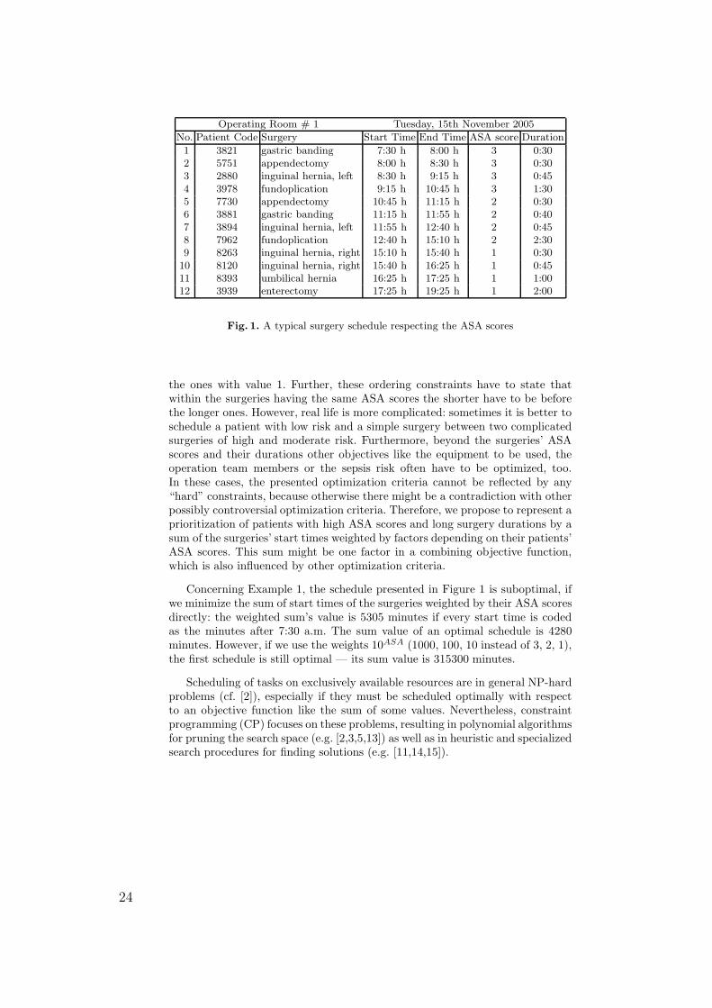
Example 1. Typically, the sequence of surgeries is organized with respect to thepatients’ ASA scores. These values, ranging from 1 to 5, subjectively categorizepatients into five subgroups by preoperative physical fitness and are named afterthe American Association of Anaesthetists (ASA). In the clinical practice, it isvery common to schedule high risk patients, i.e. with a high ASA score, as earlyas possible and short surgeries before the long ones: a typical schedule is shownin Figure 1.

In the given example it is easy to respect the priorities of the activities,i.e. the ASA scores of the surgeries and their durations: it is only necessary toestablish some ordering constraints stating that all surgeries with ASA score 3are scheduled before all surgeries with value 2, which have to be scheduled before

? The work presented in this paper is funded by the European Union (EFRE) and thestate of Berlin within the framework of the research project “inubit MRP”, grantno. 10023515.

23

Operating Room # 1 Tuesday, 15th November 2005

No. Patient Code Surgery Start Time End Time ASA score Duration

1 3821 gastric banding 7:30 h 8:00 h 3 0:302 5751 appendectomy 8:00 h 8:30 h 3 0:303 2880 inguinal hernia, left 8:30 h 9:15 h 3 0:454 3978 fundoplication 9:15 h 10:45 h 3 1:305 7730 appendectomy 10:45 h 11:15 h 2 0:306 3881 gastric banding 11:15 h 11:55 h 2 0:407 3894 inguinal hernia, left 11:55 h 12:40 h 2 0:458 7962 fundoplication 12:40 h 15:10 h 2 2:309 8263 inguinal hernia, right 15:10 h 15:40 h 1 0:30

10 8120 inguinal hernia, right 15:40 h 16:25 h 1 0:4511 8393 umbilical hernia 16:25 h 17:25 h 1 1:0012 3939 enterectomy 17:25 h 19:25 h 1 2:00

Fig. 1. A typical surgery schedule respecting the ASA scores

the ones with value 1. Further, these ordering constraints have to state thatwithin the surgeries having the same ASA scores the shorter have to be beforethe longer ones. However, real life is more complicated: sometimes it is better toschedule a patient with low risk and a simple surgery between two complicatedsurgeries of high and moderate risk. Furthermore, beyond the surgeries’ ASAscores and their durations other objectives like the equipment to be used, theoperation team members or the sepsis risk often have to be optimized, too.In these cases, the presented optimization criteria cannot be reflected by any“hard” constraints, because otherwise there might be a contradiction with otherpossibly controversial optimization criteria. Therefore, we propose to represent aprioritization of patients with high ASA scores and long surgery durations by asum of the surgeries’ start times weighted by factors depending on their patients’ASA scores. This sum might be one factor in a combining objective function,which is also influenced by other optimization criteria.

Concerning Example 1, the schedule presented in Figure 1 is suboptimal, ifwe minimize the sum of start times of the surgeries weighted by their ASA scoresdirectly: the weighted sum’s value is 5305 minutes if every start time is codedas the minutes after 7:30 a.m. The sum value of an optimal schedule is 4280minutes. However, if we use the weights 10ASA (1000, 100, 10 instead of 3, 2, 1),the first schedule is still optimal — its sum value is 315300 minutes.

Scheduling of tasks on exclusively available resources are in general NP-hardproblems (cf. [2]), especially if they must be scheduled optimally with respectto an objective function like the sum of some values. Nevertheless, constraintprogramming (CP) focuses on these problems, resulting in polynomial algorithmsfor pruning the search space (e.g. [2,3,5,13]) as well as in heuristic and specializedsearch procedures for finding solutions (e.g. [11,14,15]).

24

Thus, obvious and straightforward approaches to solve such optimizationproblems in CP would be based on a constraint for the tasks to be serialized onthe one hand and on the other hand on a weighted sum of the tasks’ start times.

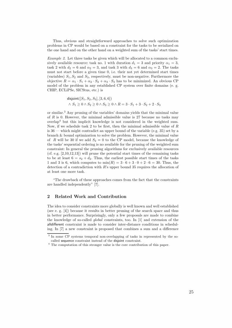
Example 2. Let three tasks be given which will be allocated to a common exclu-sively available resource: task no. 1 with duration d1 = 3 and priority α1 = 3,task 2 with d2 = 6 and α2 = 3, and task 3 with d3 = 6 and α3 = 2. The tasksmust not start before a given time 0, i.e. their not yet determined start times(variables) S1, S2 and S3, respectively, must be non-negative. Furthermore theobjective R = α1 · S1 + α2 · S2 + α3 · S3 has to be minimized. An obvious CPmodel of the problem in any established CP system over finite domains (e. g.CHIP, ECLiPSe, SICStus, etc.) is

disjoint([S1, S2, S3], [3, 6, 6])

∧ S1 ≥ 0 ∧ S2 ≥ 0 ∧ S3 ≥ 0 ∧R = 3 · S1 + 3 · S2 + 2 · S3

or similar.3 Any pruning of the variables’ domains yields that the minimal valueof R is 0. However, the minimal admissible value is 27 because no tasks mayoverlap4 but this implicit knowledge is not considered in the weighted sum.Now, if we schedule task 2 to be first, then the minimal admissible value of Ris 36 — which might contradict an upper bound of the variable (e.g. 35) set by abranch & bound optimization to solve the problem. However, the minimal valueof R will be 30 if we add S2 = 0 to the CP model, because the knowledge ofthe tasks’ sequential ordering is no available for the pruning of the weighted sumconstraint: In general the pruning algorithms for exclusively available resources(cf. e.g. [2,10,12,13]) will prune the potential start times of the remaining tasksto be at least 6 = s2 + d2. Thus, the earliest possible start times of the tasks1 and 3 is 6, which computes to min(R) = 3 · 6 + 3 · 0 + 2 · 6 = 30. Thus, thedetection of a contradiction with R’s upper bound 35 requires the allocation ofat least one more task.

“The drawback of these approaches comes from the fact that the constraintsare handled independently” [7].

2 Related Work and Contribution

The idea to consider constraints more globally is well known and well established(see e. g. [4]) because it results in better pruning of the search space and thusin better performance. Surprisingly, only a few proposals are made to combinethe knowledge of so-called global constraints, too. In [1] and extension of thealldifferent constraint is made to consider inter-distance conditions in schedul-ing. In [7] a new constraint is proposed that combines a sum and a difference

3 In some CP systems temporal non-overlapping of tasks in represented by the so-called sequence constraint instead of the disjoint constraint.

4 The computation of this stronger value is the core contribution of this paper.

25

constraint. To our knowledge, this is the first time a proposal is made that com-bines a disjoint constraint (cf. [2,10,12]) with a weighted sum (see e. g. [8]) andshows its practical relevance. New techniques for this new global constraint areintroduced that allows us to tackle the fact that the variables in the addendsof the considered weighted sums are the start times of tasks to be sequentiallyordered, i.e. allocated to an exclusively available resource. This knowledge yieldsstronger pruning resulting in earlier detections of dead ends during the searchfor a minimal sum value. This is shown by experimental results.

3 Definitions

Formally, a prioritized task scheduling problem like the scheduling of surgeriespresented in Example 1 is a constraint optimization problem (COP) over finitedomains. This COP is characterized by a finite task set T = t1, . . . , tn. Eachtask ti ∈ T has an a-priori determined, positive integer-valued duration di.However, the start times s1, . . . , sn of the tasks in T are initially finite-domainvariables having integer-valued finite potential start times, i.e. the constraintssi ∈ Si hold for i = 1, . . . , n, where Si is the set of potential start times of thetask ti ∈ T . Furthermore, each task ti ∈ T has fixed positive priority αi ∈ Q.

Basically, the tasks in T have to be scheduled non-preemptively and sequen-tially — neither with any break nor with any temporal overlap — on the ex-clusively available resource (e.g. a machine, an employee, etc. or especially anoperating room).

Ignoring other objectives and for simplicity’s sake, the tasks in T have tobe scheduled such that the sum of prioritized start times is minimal. Thus, theproblem is to find a minimal solution, i.e. some start times s1 ∈ S1, . . . , sn ∈ Sn

such that∧

1≤i<j≤n (si + di ≤ sj ∨ sj + dj ≤ si) is satisfied and the weighted

sum∑n

i=1 αi · si is minimal : for any other solution s′1 ∈ S1, . . . , s′n ∈ Sn such

that either s′i + di ≤ s′j or s′j + dj ≤ s′i holds for 1 ≤ i < j ≤ n the weighted sum

is suboptimal, i.e.∑n

i=1 αi · si ≤∑n

i=1 αi · s′i.In the following, we call this problem, which is characterized by a task set T ,

the Prioritized Task Scheduling Problem of T , or PTSP(T ) for short. Further-more, we call a PTSP(T ) solvable if a (minimal) solution exists.

4 Better Pruning for the PTSP

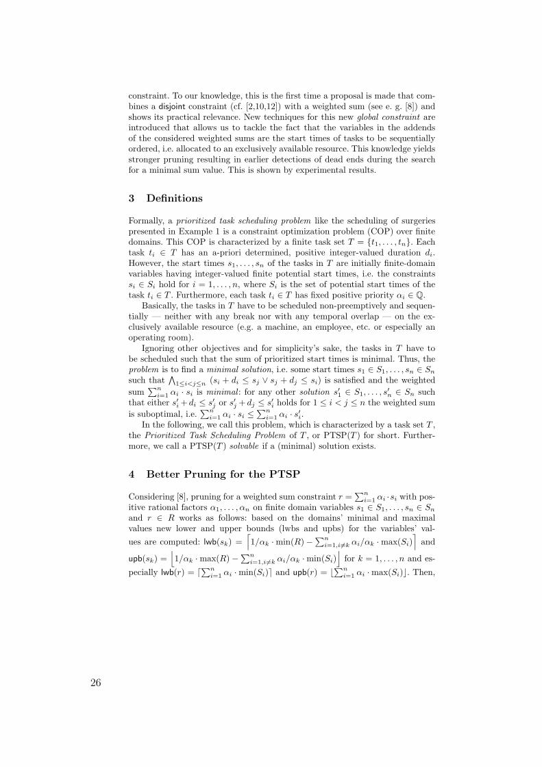
Considering [8], pruning for a weighted sum constraint r =∑n

i=1 αi ·si with pos-itive rational factors α1, . . . , αn on finite domain variables s1 ∈ S1, . . . , sn ∈ Sn

and r ∈ R works as follows: based on the domains’ minimal and maximalvalues new lower and upper bounds (lwbs and upbs) for the variables’ val-

ues are computed: lwb(sk) =⌈

1/αk ·min(R)−∑n

i=1,i6=k αi/αk ·max(Si)⌉

and

upb(sk) =⌊

1/αk ·max(R)−∑n

i=1,i6=k αi/αk ·min(Si)⌋

for k = 1, . . . , n and es-

pecially lwb(r) = d∑n

i=1 αi ·min(Si)e and upb(r) = b∑n

i=1 αi ·max(Si)c. Then,

26

the domains are updated with these bounds5: S′k = Sk ∩ [lwb(sk), upb(sk)] fork = 1, . . . , n and especially R′ = R ∩ [lwb(r), upb(r)] . Finally, this process isiterated until a fix-point is reached, i.e. none of the domains change anymore.

As shown in Example 2, this pruning procedure applied to an PTSP(T ) istoo general if the minimal start times of all tasks have almost the same value.In this case, the fact that the variables s1, . . . , sn are start times of tasks to beserialized is not considered. Also shown in Example 2, this results in rather poorpruning and rather late detection of dead ends during a branch & bound searchfor good or even best solutions where the greatest value of r is bound to theactual objective value. We must therefore look for an alternative approximationof the lower bound of the variable r using the knowledge about the variables inthe the sum’s addends.

A nontrivial approximation of a lower bound of r results from some theoret-ical examinations using an ordering on the tasks in T :

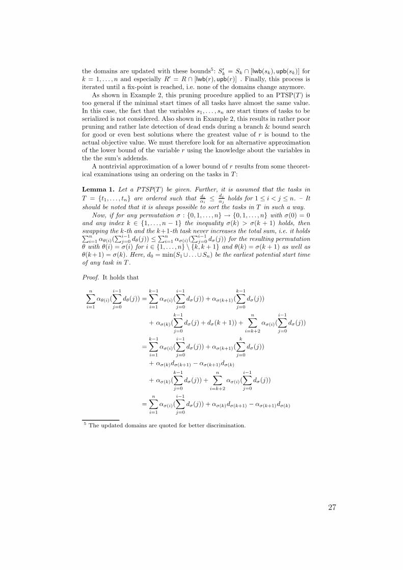
Lemma 1. Let a PTSP(T ) be given. Further, it is assumed that the tasks in

T = t1, . . . , tn are ordered such that di

αi≤

dj

αjholds for 1 ≤ i < j ≤ n. – It

should be noted that it is always possible to sort the tasks in T in such a way.Now, if for any permutation σ : 0, 1, . . . , n → 0, 1, . . . , n with σ(0) = 0

and any index k ∈ 1, . . . , n − 1 the inequality σ(k) > σ(k + 1) holds, thenswapping the k-th and the k+1-th task never increases the total sum, i.e. it holds∑n

i=1 αθ(i)(∑i−1

j=0 dθ(j)) ≤∑n

i=1 ασ(i)(∑i−1

j=0 dσ(j)) for the resulting permutationθ with θ(i) = σ(i) for i ∈ 1, . . . , n \ k, k + 1 and θ(k) = σ(k + 1) as well asθ(k+1) = σ(k). Here, d0 = min(S1∪ . . .∪Sn) be the earliest potential start timeof any task in T .

Proof. It holds that

n∑

i=1

αθ(i)(i−1∑

j=0

dθ(j)) =k−1∑

i=1

ασ(i)(i−1∑

j=0

dσ(j)) + ασ(k+1)(k−1∑

j=0

dσ(j))

+ ασ(k)(

k−1∑

j=0

dσ(j) + dσ(k + 1)) +

n∑

i=k+2

ασ(i)(

i−1∑

j=0

dσ(j))

=

k−1∑

i=1

ασ(i)(

i−1∑

j=0

dσ(j)) + ασ(k+1)(

k∑

j=0

dσ(j))

+ ασ(k)dσ(k+1) − ασ(k+1)dσ(k)

+ ασ(k)(k−1∑

j=0

dσ(j)) +n

∑

i=k+2

ασ(i)(i−1∑

j=0

dσ(j))

=

n∑

i=1

ασ(i)(

i−1∑

j=0

dσ(j)) + ασ(k)dσ(k+1) − ασ(k+1)dσ(k)

5 The updated domains are quoted for better discrimination.

27

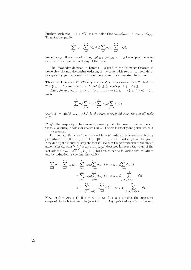
Further, with σ(k + 1) < σ(k) it also holds that ασ(k)dσ(k+1) ≤ ασ(k+1)dσ(k).Thus, the inequality

n∑

i=1

αθ(i)(i−1∑

j=0

dθ(j)) ≤n

∑

i=1

ασ(i)(i−1∑

j=0

dσ(j))

immediately follows: the addend ασ(k)dσ(k+1)−ασ(k+1)dσ(k) has no positive valuebecause of the assumed ordering of the tasks. ut

The knowledge deduced in Lemma 1 is used in the following theorem toprove that the non-decreasing ordering of the tasks with respect to their dura-tion/priority quotients results in a minimal sum of accumulated durations:

Theorem 1. Let a PTSP(T ) be given. Further, it is assumed that the tasks in

T = t1, . . . , tn are ordered such that di

αi≤ dj

αjholds for 1 ≤ i < j ≤ n.

Then, for any permutation σ : 0, 1, . . . , n → 0, 1, . . . , n with σ(0) = 0 itholds

n∑

i=1

αi(

i−1∑

j=0

dj) ≤n

∑

i=1

ασ(i)(

i−1∑

j=0

dσ(j)) ,

where d0 = min(S1 ∪ . . . ∪ Sn) be the earliest potential start time of all tasksin T .

Proof. The inequality to be shown is proven by induction over n, the numbers oftasks. Obviously, it holds for one task (n = 1): there is exactly one permutation σ— the identity.

For the induction step from n to n+1 let n+1 ordered tasks and an arbitrarypermutation σ : 0, 1, . . . , n, n+1 → 0, 1, . . . , n, n+1 with σ(0) = 0 be given.Now during the induction step the fact is used that the permutation of the first naddends in the sum

∑n+1i=1 ασ(i)(

∑i−1j=0 dσ(j)) does not influence the value of the

last addend ασ(n+1)(∑n

j=1 dσ(j)) . This results in the following two equalitiesand by induction in the final inequality:

n+1∑

i=1

ασ(i)(

i−1∑

j=0

dσ(j)) =

n∑

i=1

ασ(i)(

i−1∑

j=0

dσ(j)) + ασ(n+1)(

n∑

j=0

dσ(j))

=

n∑

i=1

ασ(i)(

i−1∑

j=0

dσ(j)) + ασ(n+1)(

n+1∑

j=0,j 6=σ(n+1)

dj)

≥n+1∑

i=1,i6=σ(n+1)

αi(

i−1∑

j=0

dj) + ασ(n+1)(

n+1∑

j=0,j 6=σ(n+1)

dj) .

Now, let k = σ(n + 1). If k 6= n + 1, i.e. k < n + 1 holds, the successiveswaps of the k-th task and the (n + 1)-th, . . . (k + 1)-th tasks yields to the sum

28

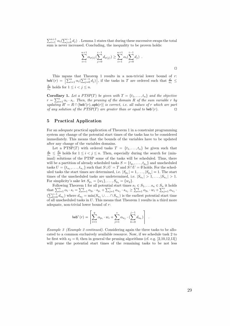
∑n+1i=1 αi(

∑i−1j=0 dj) . Lemma 1 states that during these successive swaps the total

sum is never increased. Concluding, the inequality to be proven holds:

n+1∑

i=1

ασ(i)(

i−1∑

j=0

dσ(j)) ≥n+1∑

i=1

αi(

i−1∑

j=0

dj) .

ut

This means that Theorem 1 results in a non-trivial lower bound of r:lwb’(r) =

⌈

∑n

i=1 αi(∑i−1

j=0 dj)⌉

, if the tasks in T are ordered such that di

αi≤

dj

αjholds for 1 ≤ i < j ≤ n.

Corollary 1. Let a PTSP(T ) be given with T = t1, . . . , tn and the objectiver =

∑n

i=1 αi · si. Then, the pruning of the domain R of the sum variable r byupdating R′ = R ∩ [lwb’(r), upb(r)] is correct, i.e. all values of r which are partof any solution of the PTSP(T ) are greater than or equal to lwb’(r). ut

5 Practical Application

For an adequate practical application of Theorem 1 in a constraint programmingsystem any change of the potential start times of the tasks has to be consideredimmediately. This means that the bounds of the variables have to be updatedafter any change of the variables domains.

Let a PTSP(T ) with ordered tasks T = t1, . . . , tn be given such thatdi

αi≤

dj

αjholds for 1 ≤ i < j ≤ n. Then, especially during the search for (min-

imal) solutions of the PTSP some of the tasks will be scheduled. Thus, therewill be a partition of already scheduled tasks S = tp1

, . . . , tpq and unscheduled

tasks U = tu1, . . . , tuv

such that S∪U = T and S∩U = ∅ holds. For the sched-uled tasks the start times are determined, i.e. |Sp1

| = 1, . . . , |Spq| = 1. The start

times of the unscheduled tasks are undetermined, i.e. |Su1| > 1, . . . , |Suv

| > 1.For simplicity’s sake let Sp1

= w1, . . . , Spq= wq.

Following Theorem 1 for all potential start times s1 ∈ S1, . . . sn ∈ Sn it holdsthat

∑ni=1 αi · si =

∑qi=1 αpi

· spi+

∑vj=1 αuj

· suj≥

∑qi=1 αpi

·wi +∑v

j=1 αuj·

(∑j−1

k=0 duk) where du0

= min(Su1∪ . . .∩ Suv

) is the earliest potential start timeof all unscheduled tasks in U . This means that Theorem 1 results in a third moreadequate, non-trivial lower bound of r:

lwb”(r) =

q∑

i=1

αpi· wi +

v∑

j=1

αuj· (

j−1∑

k=0

duk)

.

Example 3 (Example 2 continued). Considering again the three tasks to be allo-cated to a common exclusively available resource. Now, if we schedule task 2 tobe first with s2 = 0, then in general the pruning algorithms (cf. e.g. [2,10,12,13])will prune the potential start times of the remaining tasks to be not less

29

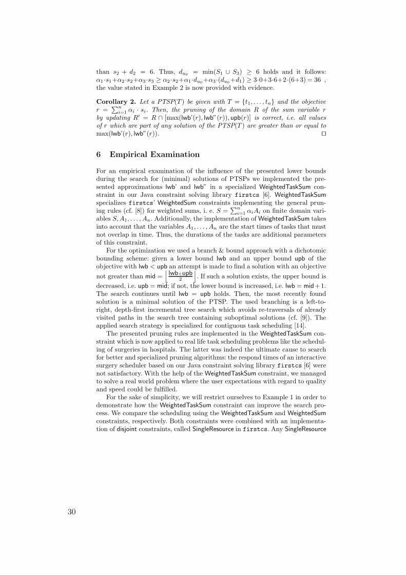
than s2 + d2 = 6. Thus, du0= min(S1 ∪ S3) ≥ 6 holds and it follows:

α1 ·s1+α2·s2+α3·s3 ≥ α2 ·s2+α1·du0+α3·(du0

+d1) ≥ 3·0+3·6+2·(6+3) = 36 ,the value stated in Example 2 is now provided with evidence.

Corollary 2. Let a PTSP(T ) be given with T = t1, . . . , tn and the objectiver =

∑n

i=1 αi · si. Then, the pruning of the domain R of the sum variable rby updating R′ = R ∩ [max(lwb’(r), lwb”(r)), upb(r)] is correct, i.e. all valuesof r which are part of any solution of the PTSP(T ) are greater than or equal tomax(lwb’(r), lwb”(r)). ut

6 Empirical Examination

For an empirical examination of the influence of the presented lower boundsduring the search for (minimal) solutions of PTSPs we implemented the pre-sented approximations lwb’ and lwb” in a specialized WeightedTaskSum con-straint in our Java constraint solving library firstcs [6]. WeightedTaskSum

specializes firstcs’ WeightedSum constraints implementing the general prun-ing rules (cf. [8]) for weighted sums, i. e. S =

∑n

i=1 αiAi on finite domain vari-ables S, A1, . . . , An. Additionally, the implementation of WeightedTaskSum takesinto account that the variables A1, . . . , An are the start times of tasks that mustnot overlap in time. Thus, the durations of the tasks are additional parametersof this constraint.

For the optimization we used a branch & bound approach with a dichotomicbounding scheme: given a lower bound lwb and an upper bound upb of theobjective with lwb < upb an attempt is made to find a solution with an objective

not greater than mid =⌊

lwb+upb2

⌋

. If such a solution exists, the upper bound is

decreased, i.e. upb = mid; if not, the lower bound is increased, i.e. lwb = mid+1.The search continues until lwb = upb holds. Then, the most recently foundsolution is a minimal solution of the PTSP. The used branching is a left-to-right, depth-first incremental tree search which avoids re-traversals of alreadyvisited paths in the search tree containing suboptimal solutions (cf. [9]). Theapplied search strategy is specialized for contiguous task scheduling [14].

The presented pruning rules are implemented in the WeightedTaskSum con-straint which is now applied to real life task scheduling problems like the schedul-ing of surgeries in hospitals. The latter was indeed the ultimate cause to searchfor better and specialized pruning algorithms: the respond times of an interactivesurgery scheduler based on our Java constraint solving library firstcs [6] werenot satisfactory. With the help of the WeightedTaskSum constraint, we managedto solve a real world problem where the user expectations with regard to qualityand speed could be fulfilled.

For the sake of simplicity, we will restrict ourselves to Example 1 in order todemonstrate how the WeightedTaskSum constraint can improve the search pro-cess. We compare the scheduling using the WeightedTaskSum and WeightedSum

constraints, respectively. Both constraints were combined with an implementa-tion of disjoint constraints, called SingleResource in firstcs. Any SingleResource

30

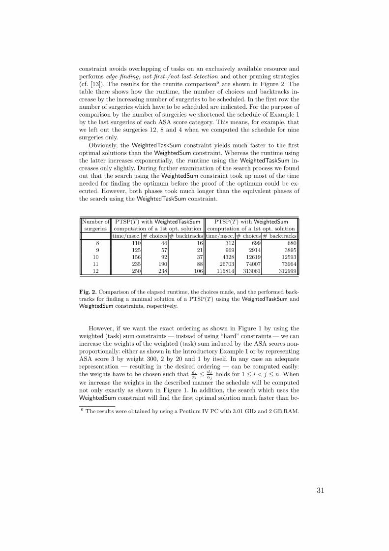
constraint avoids overlapping of tasks on an exclusively available resource andperforms edge-finding, not-first-/not-last-detection and other pruning strategies(cf. [13]). The results for the reunite comparison6 are shown in Figure 2. Thetable there shows how the runtime, the number of choices and backtracks in-crease by the increasing number of surgeries to be scheduled. In the first row thenumber of surgeries which have to be scheduled are indicated. For the purpose ofcomparison by the number of surgeries we shortened the schedule of Example 1by the last surgeries of each ASA score category. This means, for example, thatwe left out the surgeries 12, 8 and 4 when we computed the schedule for ninesurgeries only.

Obviously, the WeightedTaskSum constraint yields much faster to the firstoptimal solutions than the WeightedSum constraint. Whereas the runtime usingthe latter increases exponentially, the runtime using the WeightedTaskSum in-creases only slightly. During further examination of the search process we foundout that the search using the WeightedSum constraint took up most of the timeneeded for finding the optimum before the proof of the optimum could be ex-ecuted. However, both phases took much longer than the equivalent phases ofthe search using the WeightedTaskSum constraint.

Number of PTSP(T ) with WeightedTaskSum PTSP(T ) with WeightedSum

surgeries computation of a 1st opt. solution computation of a 1st opt. solution

time/msec. # choices # backtracks time/msec. # choices # backtracks

8 110 44 16 312 699 6809 125 57 21 969 2914 3895

10 156 92 37 4328 12619 1259311 235 190 88 26703 74007 7396412 250 238 106 116814 313061 312999

Fig. 2. Comparison of the elapsed runtime, the choices made, and the performed back-tracks for finding a minimal solution of a PTSP(T ) using the WeightedTaskSum andWeightedSum constraints, respectively.

However, if we want the exact ordering as shown in Figure 1 by using theweighted (task) sum constraints — instead of using “hard” constraints — we canincrease the weights of the weighted (task) sum induced by the ASA scores non-proportionally: either as shown in the introductory Example 1 or by representingASA score 3 by weight 300, 2 by 20 and 1 by itself. In any case an adequaterepresentation — resulting in the desired ordering — can be computed easily:the weights have to be chosen such that di

αi≤ dj

αjholds for 1 ≤ i < j ≤ n. When

we increase the weights in the described manner the schedule will be computednot only exactly as shown in Figure 1. In addition, the search which uses theWeightedSum constraint will find the first optimal solution much faster than be-

6 The results were obtained by using a Pentium IV PC with 3.01 GHz and 2 GB RAM.

31

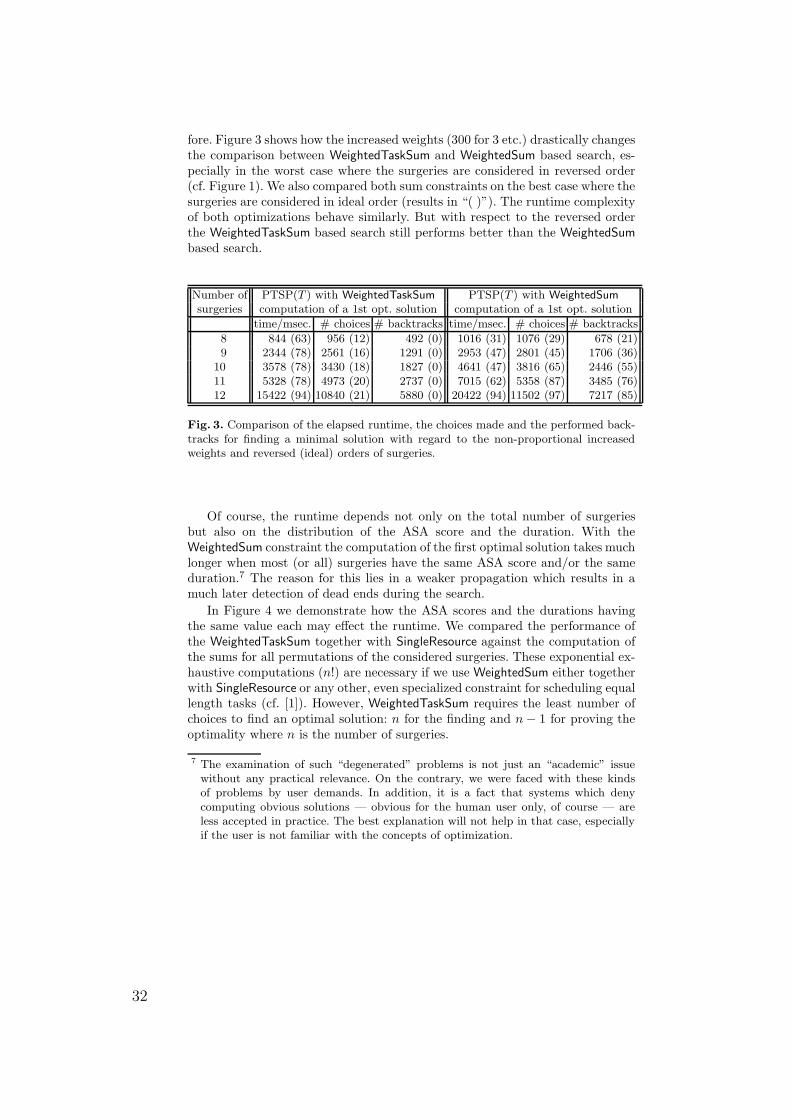
fore. Figure 3 shows how the increased weights (300 for 3 etc.) drastically changesthe comparison between WeightedTaskSum and WeightedSum based search, es-pecially in the worst case where the surgeries are considered in reversed order(cf. Figure 1). We also compared both sum constraints on the best case where thesurgeries are considered in ideal order (results in “( )”). The runtime complexityof both optimizations behave similarly. But with respect to the reversed orderthe WeightedTaskSum based search still performs better than the WeightedSum

based search.

Number of PTSP(T ) with WeightedTaskSum PTSP(T ) with WeightedSum

surgeries computation of a 1st opt. solution computation of a 1st opt. solution

time/msec. # choices # backtracks time/msec. # choices # backtracks

8 844 (63) 956 (12) 492 (0) 1016 (31) 1076 (29) 678 (21)9 2344 (78) 2561 (16) 1291 (0) 2953 (47) 2801 (45) 1706 (36)

10 3578 (78) 3430 (18) 1827 (0) 4641 (47) 3816 (65) 2446 (55)11 5328 (78) 4973 (20) 2737 (0) 7015 (62) 5358 (87) 3485 (76)12 15422 (94) 10840 (21) 5880 (0) 20422 (94) 11502 (97) 7217 (85)

Fig. 3. Comparison of the elapsed runtime, the choices made and the performed back-tracks for finding a minimal solution with regard to the non-proportional increasedweights and reversed (ideal) orders of surgeries.

Of course, the runtime depends not only on the total number of surgeriesbut also on the distribution of the ASA score and the duration. With theWeightedSum constraint the computation of the first optimal solution takes muchlonger when most (or all) surgeries have the same ASA score and/or the sameduration.7 The reason for this lies in a weaker propagation which results in amuch later detection of dead ends during the search.

In Figure 4 we demonstrate how the ASA scores and the durations havingthe same value each may effect the runtime. We compared the performance ofthe WeightedTaskSum together with SingleResource against the computation ofthe sums for all permutations of the considered surgeries. These exponential ex-haustive computations (n!) are necessary if we use WeightedSum either togetherwith SingleResource or any other, even specialized constraint for scheduling equallength tasks (cf. [1]). However, WeightedTaskSum requires the least number ofchoices to find an optimal solution: n for the finding and n − 1 for proving theoptimality where n is the number of surgeries.

7 The examination of such “degenerated” problems is not just an “academic” issuewithout any practical relevance. On the contrary, we were faced with these kindsof problems by user demands. In addition, it is a fact that systems which denycomputing obvious solutions — obvious for the human user only, of course — areless accepted in practice. The best explanation will not help in that case, especiallyif the user is not familiar with the concepts of optimization.

32

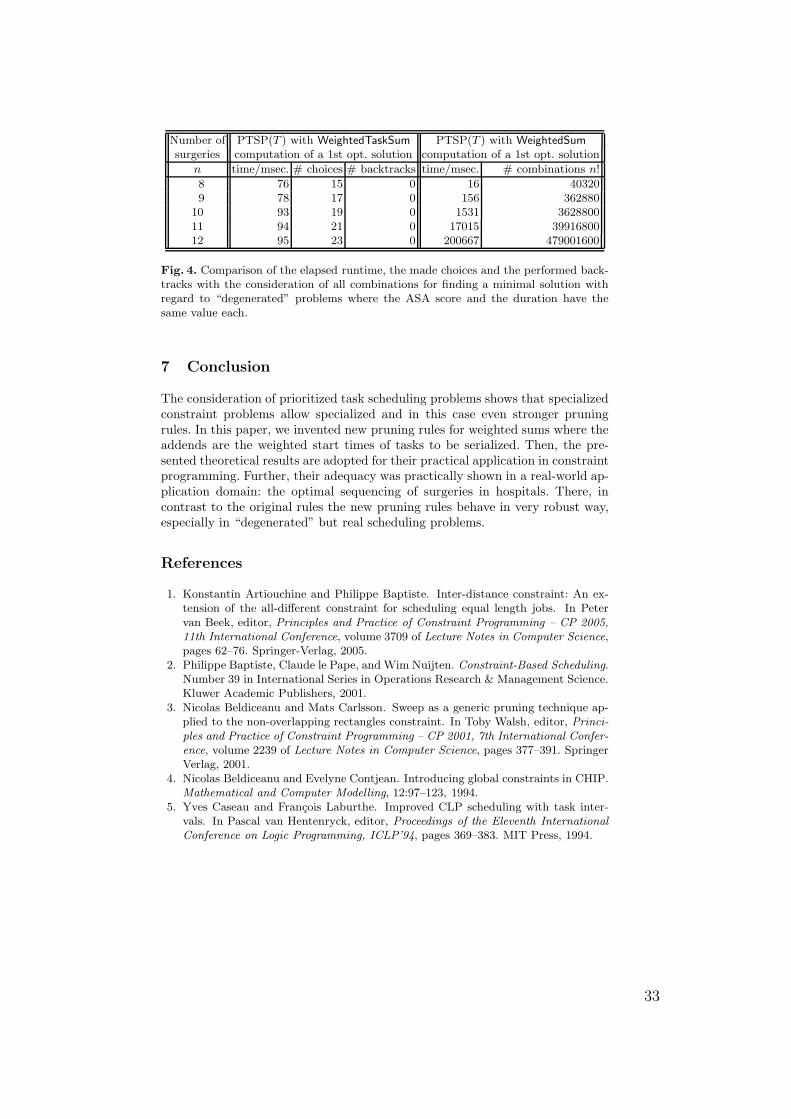
Number of PTSP(T ) with WeightedTaskSum PTSP(T ) with WeightedSum

surgeries computation of a 1st opt. solution computation of a 1st opt. solution

n time/msec. # choices # backtracks time/msec. # combinations n!

8 76 15 0 16 403209 78 17 0 156 362880

10 93 19 0 1531 362880011 94 21 0 17015 3991680012 95 23 0 200667 479001600

Fig. 4. Comparison of the elapsed runtime, the made choices and the performed back-tracks with the consideration of all combinations for finding a minimal solution withregard to “degenerated” problems where the ASA score and the duration have thesame value each.

7 Conclusion

The consideration of prioritized task scheduling problems shows that specializedconstraint problems allow specialized and in this case even stronger pruningrules. In this paper, we invented new pruning rules for weighted sums where theaddends are the weighted start times of tasks to be serialized. Then, the pre-sented theoretical results are adopted for their practical application in constraintprogramming. Further, their adequacy was practically shown in a real-world ap-plication domain: the optimal sequencing of surgeries in hospitals. There, incontrast to the original rules the new pruning rules behave in very robust way,especially in “degenerated” but real scheduling problems.

References

1. Konstantin Artiouchine and Philippe Baptiste. Inter-distance constraint: An ex-tension of the all-different constraint for scheduling equal length jobs. In Petervan Beek, editor, Principles and Practice of Constraint Programming – CP 2005,11th International Conference, volume 3709 of Lecture Notes in Computer Science,pages 62–76. Springer-Verlag, 2005.

2. Philippe Baptiste, Claude le Pape, and Wim Nuijten. Constraint-Based Scheduling.Number 39 in International Series in Operations Research & Management Science.Kluwer Academic Publishers, 2001.

3. Nicolas Beldiceanu and Mats Carlsson. Sweep as a generic pruning technique ap-plied to the non-overlapping rectangles constraint. In Toby Walsh, editor, Princi-ples and Practice of Constraint Programming – CP 2001, 7th International Confer-ence, volume 2239 of Lecture Notes in Computer Science, pages 377–391. SpringerVerlag, 2001.

4. Nicolas Beldiceanu and Evelyne Contjean. Introducing global constraints in CHIP.Mathematical and Computer Modelling, 12:97–123, 1994.

5. Yves Caseau and Francois Laburthe. Improved CLP scheduling with task inter-vals. In Pascal van Hentenryck, editor, Proceedings of the Eleventh InternationalConference on Logic Programming, ICLP’94, pages 369–383. MIT Press, 1994.

33

6. Matthias Hoche, Henry Muller, Hans Schlenker, and Armin Wolf. firstcs - A PureJava Constraint Programming Engine. In Michael Hanus, Petra Hofstedt, andArmin Wolf, editors, 2nd International Workshop on Multiparadigm ConstraintProgramming Languages – MultiCPL’03, 29th September 2003. Online availableat uebb.cs.tu-berlin.de/MultiCPL03/Proceedings.MultiCPL03.RCoRP03.pdf.

7. Jean-Charles Regin and Michel Rueher. A global constraint combining a sum con-straint and difference constraints. In Rina Dechter, editor, Principles and Practiceof Constraint Programming – CP 2000, 6th International Conference, volume 1894of Lecture Notes in Computer Science, pages 384–395, Singapore, September 18–212000. Springer Verlag.

8. Christian Schulte and Peter J. Stuckey. When do bounds and domain propagationlead to the same search space. In Harald Søndergaard, editor, Third InternationalConference on Principles and Practice of Declarative Programming, pages 115–126,Florence, Italy, September 2001. ACM Press.

9. Pascal van Hentenryck and Thierry le Provost. Incremental search in constraintlogic programming. New Generation Computing, 9(3 & 4):257–275, 1991.

10. Petr Vilım. O(n log n) filtering algorithms for unary resource constraint. In Pro-ceedings of the International Conference on Integration of AI and OR Techniquesin Constraint Programming for Combinatorical Optimisation Problems – CP-AI-OR’04, volume 3011 of Lecture Notes in Computer Science, pages 335–347. SpringerVerlag, 2004.

11. Petr Vilım. Computing explanations for the unary resource constraint. In In-tegration of AI and OR Techniques in Constraint Programming for Combinato-rial Optimization Problems: Second International Conference, CP-AI-OR 2005,Proceedings, volume 3524 of Lecture Notes in Computer Science, pages 396–409.Springer Verlag, 2005.

12. Petr Vilım, Roman Bartak, and Ondrej Cepek. Unary resource constraint withoptional activities. In Marc Wallace, editor, Principles and Practice of ConstraintProgramming – CP 2004, 10th International Conference, volume 3258 of LectureNotes in Computer Science, pages 62–76. Springer Verlag, 2004.

13. Armin Wolf. Pruning while sweeping over task intervals. In Francesca Rossi, editor,Principles and Practice of Constraint Programming – CP 2003, 9th InternationalConference, volume 2833 of Lecture Notes in Computer Science, pages 739–753.Springer Verlag, 2003.

14. Armin Wolf. Reduce-to-the-opt — a specialized search algorithm for contiguoustask scheduling. In K.R. Apt, F. Fages, F. Rossi, P. Szeredi, and J. Vancza,editors, Recent Advances in Constraints, volume 3010 of Lecture Notes in ArtificialIntelligence, pages 223–232. Springer Verlag, 2004.

15. Armin Wolf. Better propagation for non-reemptive single-resource constraint prob-lems. In B. Faltings, A. Petcu, F. Fages, and F. Rossi, editors, Recent Advancesin Constraints, Joint ERCIM/CoLogNET International Workshop on ConstraintSolving and Constraint Logic Programming, CSCLP 2004, Lausanne, Switzerland,June 23-25, 2004, Revised Selected and Invited Papers, volume 3419 of LectureNotes in Artificial Intelligence, pages 201–215. Springer Verlag, 2005.

34

Efficient Edge-Finding onUnary Resources with Optional Activities

Sebastian Kuhnert

Fraunhofer FIRST, Kekuléstr. 7, 12489 Berlin, Germany

Abstract. Unary resources play a central role in modeling schedulingproblems. Edge-finding is one of the most popular techniques to dealwith unary resources in constraint programming environments. Often itdepends on external factors if an activity will be included in the finalschedule, making the activity optional. Currently known edge-findingalgorithms cannot take optional activities into account. This paper intro-duces an edge-finding algorithm that finds restrictions for enabled andoptional activities. The performance of this new algorithm is studied formodified job-shop and random-placement problems.

Keywords: constraint-based scheduling, global constraints, optionaltasks and activities, unary resources

1 Unary Resources with Optional Activities

Many everyday scheduling problems deal with allocation of resources: Schoolsmust assign rooms to lectures, factories must assign machines to tasks, traincompanies must assign tracks to trains. Often an activity on a resource must befinished before a deadline and cannot be started before a release time. Formally,an activity i is described by its duration pi and its earliest and latest startingand completion times as shown in Figure 1. In constraint programming systemsthe start time is usually stored as a variable ranging from esti to lsti. Theduration is constant in most applications, in that case the completion times canbe derived as ecti = esti + pi and lcti = lsti + pi. Otherwise let pi denote theminimum duration for the purposes of this paper.1

1 The values of pi are used to restrict the domains of other variables. Using largervalues than the minimum duration might cause unwarranted restrictions.

t

i

esti lsti ecti lcti

pi

Fig. 1. Attributes of an activity i.

35

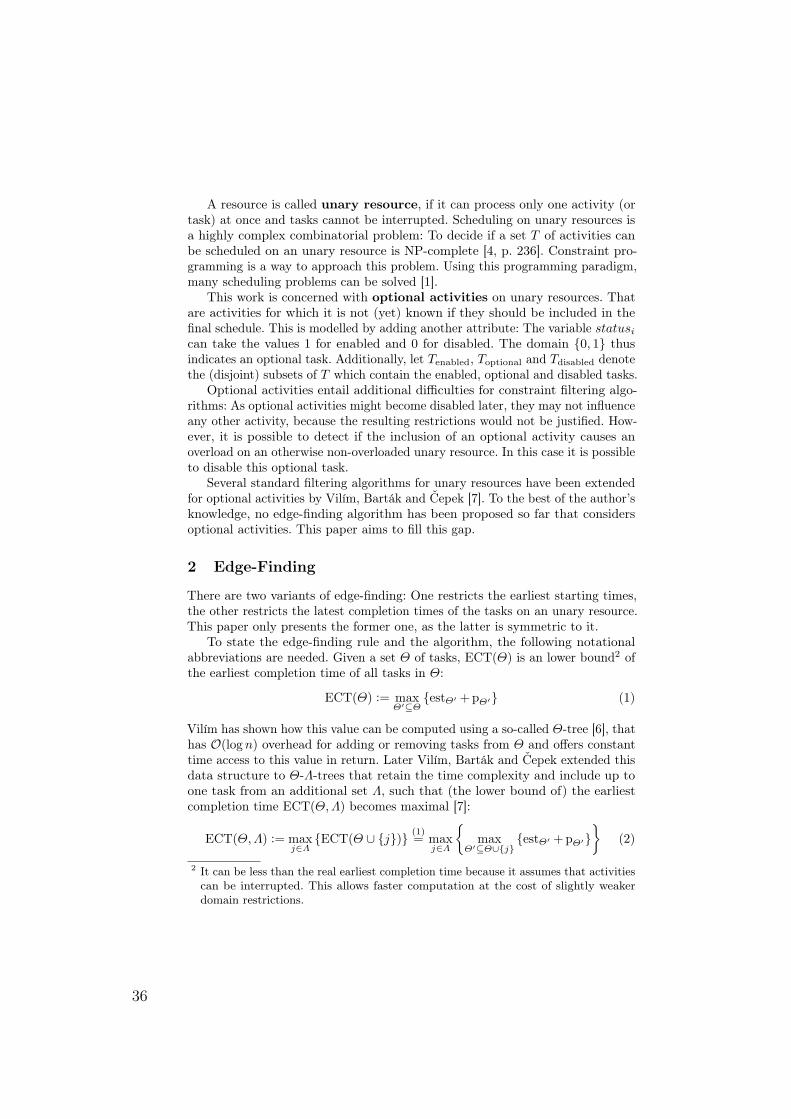
A resource is called unary resource, if it can process only one activity (ortask) at once and tasks cannot be interrupted. Scheduling on unary resources isa highly complex combinatorial problem: To decide if a set T of activities canbe scheduled on an unary resource is NP-complete [4, p. 236]. Constraint pro-gramming is a way to approach this problem. Using this programming paradigm,many scheduling problems can be solved [1].

This work is concerned with optional activities on unary resources. Thatare activities for which it is not (yet) known if they should be included in thefinal schedule. This is modelled by adding another attribute: The variable statusi

can take the values 1 for enabled and 0 for disabled. The domain 0, 1 thusindicates an optional task. Additionally, let Tenabled, Toptional and Tdisabled denotethe (disjoint) subsets of T which contain the enabled, optional and disabled tasks.

Optional activities entail additional difficulties for constraint filtering algo-rithms: As optional activities might become disabled later, they may not influenceany other activity, because the resulting restrictions would not be justified. How-ever, it is possible to detect if the inclusion of an optional activity causes anoverload on an otherwise non-overloaded unary resource. In this case it is possibleto disable this optional task.

Several standard filtering algorithms for unary resources have been extendedfor optional activities by Vilím, Barták and Čepek [7]. To the best of the author’sknowledge, no edge-finding algorithm has been proposed so far that considersoptional activities. This paper aims to fill this gap.

2 Edge-Finding

There are two variants of edge-finding: One restricts the earliest starting times,the other restricts the latest completion times of the tasks on an unary resource.This paper only presents the former one, as the latter is symmetric to it.

To state the edge-finding rule and the algorithm, the following notationalabbreviations are needed. Given a set Θ of tasks, ECT(Θ) is an lower bound2 ofthe earliest completion time of all tasks in Θ:

ECT(Θ) := maxΘ′⊆Θ

estΘ′ +pΘ′ (1)

Vilím has shown how this value can be computed using a so-called Θ-tree [6], thathas O(log n) overhead for adding or removing tasks from Θ and offers constanttime access to this value in return. Later Vilím, Barták and Čepek extended thisdata structure to Θ-Λ-trees that retain the time complexity and include up toone task from an additional set Λ, such that (the lower bound of) the earliestcompletion time ECT(Θ,Λ) becomes maximal [7]:

ECT(Θ, Λ) := maxj∈Λ

ECT(Θ ∪ j) (1)= max

j∈Λ

max

Θ′⊆Θ∪jestΘ′ +pΘ′

(2)

2 It can be less than the real earliest completion time because it assumes that activitiescan be interrupted. This allows faster computation at the cost of slightly weakerdomain restrictions.

36

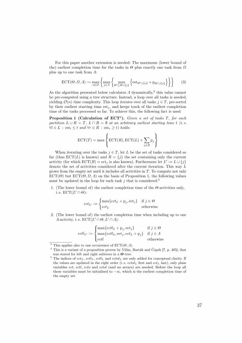
For this paper another extension is needed: The maximum (lower bound ofthe) earliest completion time for the tasks in Θ plus exactly one task from Ωplus up to one task from Λ:

ECT(Θ,Ω, Λ) := maxo∈Ω

maxj∈Λ

max

Θ′⊆Θ∪j

estΘ′∪o +pΘ′∪o

(3)

As the algorithm presented below calculates Λ dynamically,3 this value cannotbe pre-computed using a tree structure. Instead, a loop over all tasks is needed,yielding O(n) time complexity. This loop iterates over all tasks j ∈ T , pre-sortedby their earliest starting time estj , and keeps track of the earliest completiontime of the tasks processed so far. To achieve this, the following fact is used:

Proposition 1 (Calculation of ECT4). Given a set of tasks T , for eachpartition L ∪ R = T , L ∩ R = ∅ at an arbitrary earliest starting time t (i. e.∀l ∈ L : estl ≤ t and ∀r ∈ R : estr ≥ t) holds:

ECT(T ) = max

ECT(R),ECT(L) +∑j∈R

pj

When iterating over the tasks j ∈ T , let L be the set of tasks considered so

far (thus ECT(L) is known) and R = j the set containing only the currentactivity (for which ECT(R) = ectj is also known). Furthermore let L′ := L∪ jdenote the set of activities considered after the current iteration. This way Lgrows from the empty set until it includes all activities in T . To compute not onlyECT(Θ) but ECT(Θ,Ω, Λ) on the basis of Proposition 1, the following valuesmust be updated in the loop for each task j that is considered:5

1. (The lower bound of) the earliest completion time of the Θ-activities only,i. e. ECT(L′ ∩Θ):

ectL′ :=

maxectL + pj , ectj if j ∈ Θ

ectL otherwise

2. (The lower bound of) the earliest completion time when including up to oneΛ-activity, i. e. ECT(L′ ∩Θ, L′ ∩ Λ):

ectlL′ :=

maxectlL + pj , ectj if j ∈ Θ

maxectlL, ectj , ectL + pj if j ∈ Λ

ectl otherwise3 This applies also to one occurrence of ECT(Θ, Λ).4 This is a variant of a proposition proven by Vilím, Barták and Čepek [7, p. 405], that

was stated for left and right subtrees in a Θ-tree.5 The indices of ectL, ectlL, ectlL and ectolL are only added for conceptual clarity. If

the values are updated in the right order (i. e. ectolL first and ectL last), only plainvariables ect, ectl, ecto and ectol (and no arrays) are needed. Before the loop allthese variables must be initialised to −∞, which is the earliest completion time ofthe empty set.

37

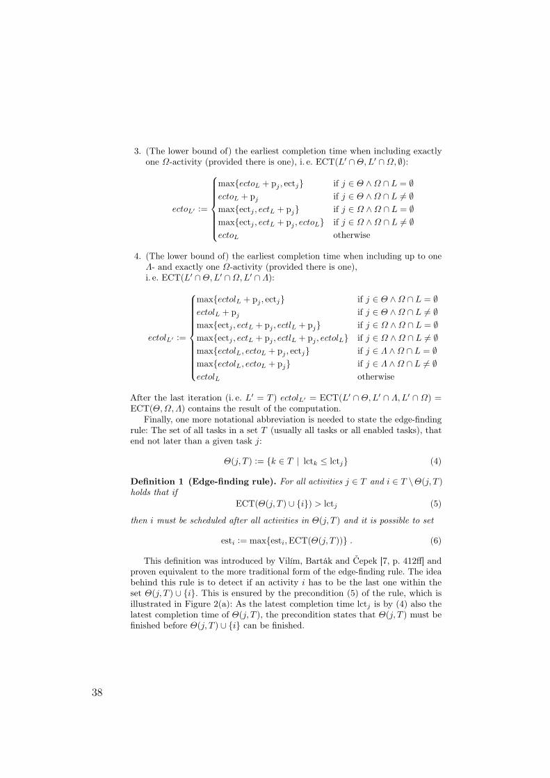
3. (The lower bound of) the earliest completion time when including exactlyone Ω-activity (provided there is one), i. e. ECT(L′ ∩Θ,L′ ∩Ω, ∅):

ectoL′ :=

maxectoL + pj , ectj if j ∈ Θ ∧Ω ∩ L = ∅ectoL + pj if j ∈ Θ ∧Ω ∩ L 6= ∅maxectj , ectL + pj if j ∈ Ω ∧Ω ∩ L = ∅maxectj , ectL + pj , ectoL if j ∈ Ω ∧Ω ∩ L 6= ∅ectoL otherwise

4. (The lower bound of) the earliest completion time when including up to oneΛ- and exactly one Ω-activity (provided there is one),i. e. ECT(L′ ∩Θ,L′ ∩Ω,L′ ∩ Λ):

ectolL′ :=

maxectolL + pj , ectj if j ∈ Θ ∧Ω ∩ L = ∅ectolL + pj if j ∈ Θ ∧Ω ∩ L 6= ∅maxectj , ectL + pj , ectlL + pj if j ∈ Ω ∧Ω ∩ L = ∅maxectj , ectL + pj , ectlL + pj , ectolL if j ∈ Ω ∧Ω ∩ L 6= ∅maxectolL, ectoL + pj , ectj if j ∈ Λ ∧Ω ∩ L = ∅maxectolL, ectoL + pj if j ∈ Λ ∧Ω ∩ L 6= ∅ectolL otherwise

After the last iteration (i. e. L′ = T ) ectolL′ = ECT(L′ ∩ Θ,L′ ∩ Λ, L′ ∩ Ω) =ECT(Θ, Ω, Λ) contains the result of the computation.

Finally, one more notational abbreviation is needed to state the edge-findingrule: The set of all tasks in a set T (usually all tasks or all enabled tasks), thatend not later than a given task j:

Θ(j, T ) := k ∈ T | lctk ≤ lctj (4)

Definition 1 (Edge-finding rule). For all activities j ∈ T and i ∈ T \Θ(j, T )holds that if

ECT(Θ(j, T ) ∪ i) > lctj (5)

then i must be scheduled after all activities in Θ(j, T ) and it is possible to set

esti := maxesti,ECT(Θ(j, T )) . (6)

This definition was introduced by Vilím, Barták and Čepek [7, p. 412ff] andproven equivalent to the more traditional form of the edge-finding rule. The ideabehind this rule is to detect if an activity i has to be the last one within theset Θ(j, T ) ∪ i. This is ensured by the precondition (5) of the rule, which isillustrated in Figure 2(a): As the latest completion time lctj is by (4) also thelatest completion time of Θ(j, T ), the precondition states that Θ(j, T ) must befinished before Θ(j, T ) ∪ i can be finished.

38

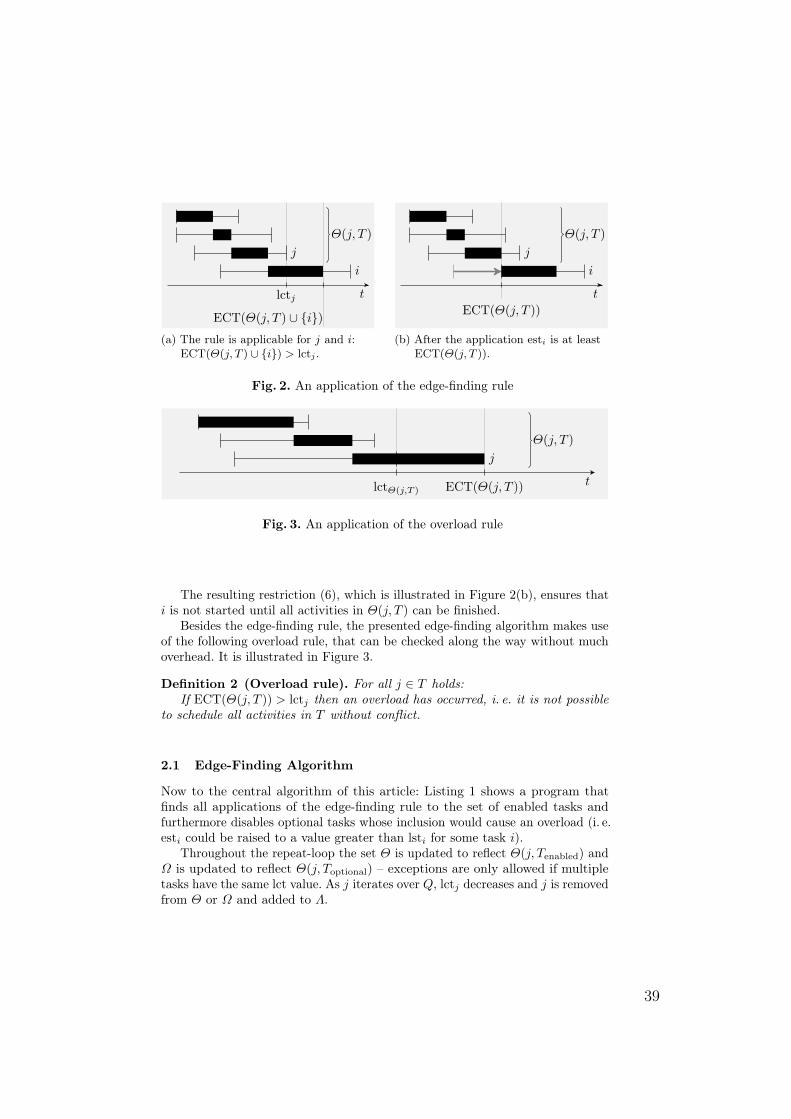
lctj

ECT(Θ(j, T ) ∪ i)

j

Θ(j, T )

i

t

(a) The rule is applicable for j and i:ECT(Θ(j, T ) ∪ i) > lctj .

ECT(Θ(j, T ))

j

Θ(j, T )

i

t

(b) After the application esti is at leastECT(Θ(j, T )).

Fig. 2. An application of the edge-finding rule

lctΘ(j,T ) ECT(Θ(j, T ))

j

Θ(j, T )

t

Fig. 3. An application of the overload rule

The resulting restriction (6), which is illustrated in Figure 2(b), ensures thati is not started until all activities in Θ(j, T ) can be finished.

Besides the edge-finding rule, the presented edge-finding algorithm makes useof the following overload rule, that can be checked along the way without muchoverhead. It is illustrated in Figure 3.

Definition 2 (Overload rule). For all j ∈ T holds:If ECT(Θ(j, T )) > lctj then an overload has occurred, i. e. it is not possible

to schedule all activities in T without conflict.

2.1 Edge-Finding Algorithm

Now to the central algorithm of this article: Listing 1 shows a program thatfinds all applications of the edge-finding rule to the set of enabled tasks andfurthermore disables optional tasks whose inclusion would cause an overload (i. e.esti could be raised to a value greater than lsti for some task i).

Throughout the repeat-loop the set Θ is updated to reflect Θ(j, Tenabled) andΩ is updated to reflect Θ(j, Toptional) – exceptions are only allowed if multipletasks have the same lct value. As j iterates over Q, lctj decreases and j is removedfrom Θ or Ω and added to Λ.

39

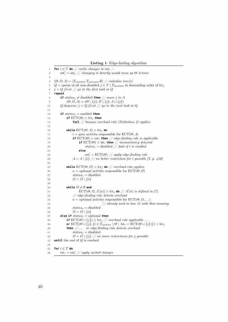
Listing 1. Edge-finding algorithm1 for i ∈ T do // cache changes to esti −2 est′

i = esti // changing it directly would mess up Θ-Λ-trees34 (Θ, Ω, Λ) = (Tenabled, Toptional, ∅) // initialise tree(s)5 Q = queue of all non-disabled j ∈ T \ Tdisabled in descending order of lctj

6 j = Q.first // go to the first task in Q7 repeat8 if statusj 6= disabled then // move j to Λ9 (Θ, Ω, Λ) = (Θ \ j, Ω \ j, Λ ∪ j)

10 Q.dequeue; j = Q.first // go to the next task in Q1112 if statusj = enabled then13 if ECT(Θ) > lctj then14 fail // because overload rule (Definition 2) applies1516 while ECT(Θ, Λ) > lctj do17 i = grey activity responsible for ECT(Θ, Λ)18 if ECT(Θ) > esti then // edge-finding rule is applicable19 if ECT(Θ) > lsti then // inconsistency detected20 statusi = disabled // fails if i is enabled21 else22 est′

i = ECT(Θ) // apply edge-finding rule23 Λ = Λ \ i // no better restriction for i possible [7, p. 416]2425 while ECT(Θ, Ω) > lctj do // overload rule applies26 o = optional activity responsible for ECT(Θ, Ω)27 statuso = disabled28 Ω = Ω \ o2930 while Ω 6= ∅ and31 ECT(Θ, Ω, Λ′(o)) > lctj do // Λ′(o) is defined in (7)32 // edge-finding rule detects overload33 o = optional activity responsible for ECT(Θ, Ω, . . .)34 // already used in line 31 with that meaning35 statuso = disabled36 Ω = Ω \ o37 else if statusj = optional then38 if ECT(Θ ∪ j) > lctj // overload rule applicable . . .39 or ECT(Θ ∪ j, i ∈ Tenabled \Θ | lsti < ECT(Θ ∪ j)) > lctj

40 then // . . . or edge-finding rule detects overload41 statusj = disabled42 Ω = Ω \ j // no more restrictions for j possible43 until the end of Q is reached4445 for i ∈ T do46 esti = est′

i // apply cached changes

40

Lines 13 to 23 handle enabled activities j and correspond closely to thealgorithm by Vilím, Barták and Čepek [7, p. 416], with the only change being thehandling of statusi = optional in lines 18 to 22: If ECT(Θ) > lsti (line 19) therestriction est′i = ECT(Θ) (line 22) would cause an inconsistency as no possiblestart time for i remains. In this case the activity i is set to disabled (line 20),which fails for enabled activities and is the proper restriction for optional ones.

There are several more additions to handle optional activities: Firstly, thecase statusj = optional is handled. It follows the scheme of the enabled case,bearing in mind that j is optional: The overload-condition ECT(Θ) > lctj online 13 carries over to ECT(Θ ∪ j) > lctj on line 38, where no immediatefailure is generated but the optional activity j which would cause the overload isdisabled.

If j is optional, the condition ECT(Θ,Λ) > lctj of the while-loop on line 16can only result in the disabling of j as no optional activity may influence others.For this, no while-loop is required and a simple if-condition suffices. It musthowever take care to choose an appropriate i ∈ Λ that leads to j being disabled.This is achieved by requiring i ∈ Tenabled and lsti < ECT(Θ∪j) in the conditionon line 39.

Secondly, the case statusj = enabled is extended with two more while-loops.They realise overload-detection and edge-finding for optional activities that arestill contained in Ω. The set Λ′(o), which is used in the condition of the secondwhile-loop, is defined as follows:

Λ′(o) :=

i ∈ Tenabled \Θ∣∣∣ lsti < ECT(Θ ∪ o)

∧ 6∃ i2 ∈ Tenabled \Θ :(

lsti2 ≥ ECT(Θ ∪ o)

∧ ECT(Θ ∪ i2) > ECT(Θ ∪ i))

(7)

Like for the algorithm by Vilím, Barták and Čepek, the algorithm in Listing 1must be repeated until it finds no further restrictions to make it idempotent.

Proposition 2 (Correctness). The algorithm presented in Listing 1 is correct,i. e. all restrictions are justified.

Proof. All restrictions are applications of the edge-finding and overload rules(Definitions 1 and 2). The correctness of these rules thus carries over to thealgorithm. ut

2.2 Complexity

Proposition 3 (Time Complexity). The time complexity of the edge-findingalgorithm presented in Listing 1 is O(n2), where n is the number of activities onthe unary resource.

41

Proof. To see this, observe that each loop is executed at most n times: The twosmall copy-loops in lines 1–2 and 45–46 directly loop over all tasks, the main loopin lines 12–43 loops over the subset of non-disabled tasks and the three innerloops in lines 16–23, 25–28 and 30–36 each remove a task from Λ or Ω. As eachtask is added to these sets at most once, each loop is executed at most n times.

Sorting the tasks by lct (line 5) can be done in O(n log n). All other lines(this includes all lines within the loops) bear at most O(n) complexity. Most areO(1), the more complicated ones are O(log n) or O(n), as discussed for (1) to(3).

Only the calculation of ECT(Θ,Ω, Λ′(o)) in line 31 needs special consideration,as o already references the task chosen from Ω. The definition of Λ′(o) in (7)makes it possible to calculate it in the following way:– When calculating ectlL′ take all activities from Tenabled \Θ in account, as it

is not yet known which o will be chosen.– For the cases with j ∈ Ω during the calculation of ectolL′ , consider ectlL +pj

for calculating the maximum only if the activity i chosen for ectlL satisfieslsti < ECT(Θ ∪ j).

– For the cases with j ∈ Λ during the calculation of ectolL′ , consider ectoL +pj

for the maximum only if the activity o chosen for ectoL satisfies lstj <ECT(Θ ∪ o).

To be able to access ECT(Θ ∪ o) in constant time for all o ∈ Ω, three arraysectAftero, pAftero and ectBeforeo can be used, where after/before refers to theposition of o in the list of tasks sorted by estj and the three values consider onlytasks from Θ. They can be computed based on Proposition 1 in linear time bylooping over the tasks pre-sorted by estj . It holds:

ECT(Θ ∪ o) = maxectAftero, ecto +pAftero, ectBeforeo + po +pAftero

Thus the overall time complexity of the algorithm is O(n2). ut

2.3 Optimality

For efficient restriction of the domains it is necessary that as many applicationsof the edge-finding rule as possible are found by the algorithm, while it is equallycrucial that it offers fast runtimes.

Proposition 4 (Optimality). The algorithm presented in Listing 1 finds allapplications of the edge-finding rule to enabled activities and disables almostall optional activities that would cause an overload that is detectable by theedge-finding rule.

Proof. First consider all applications of the edge-finding rule that involve onlyenabled tasks. Let therefore j ∈ Tenabled and i ∈ Tenabled \ Θ(j, Tenabled), suchthat ECT(Θ(j, Tenabled) ∪ i) < lctj . As argued above, the set Θ at some pointtakes the value of Θ(j, Tenabled) and i is contained in Λ. Then in line 18 i will bechosen (possibly after other i′ have been chosen and removed from Λ) and esti

will be adjusted or an overload detected.

42

If an optional activity o ∈ Toptional is involved, things are a bit more compli-cated. If the edge-finding rule is applicable for the set T ′ := Tenabled ∪ o, thefollowing cases can occur:

Case 1: o 6∈ Θ(j, T ′) ∪ iThe optional activity o is not involved and the edge-finding rule is equally ap-plicable to the set Tenabled. The resulting restriction is found by the algorithmas argued above.

Case 2: o = iThis case is handled together with non-optional i in lines 16 to 23.

Case 3: o = jIn this case esti may not be adjusted as the optional activity o may notinfluence the non-optional i. However, if esti can be adjusted to a valuegreater than lsti, the inclusion of o would cause an overload and o can bedisabled. This is done in lines 37 to 42.

Case 4: o ∈ Θ(j, T ′) \ jLike in the previous case the only possible restriction is disabling o if it causesan overload. This case is handled in lines 30 to 36. For optimal results Λ′(o)would have to be defined slightly differently, omitting the condition

6 ∃ i2 ∈ Tenabled\Θ :(

lsti2 ≥ ECT(Θ∪o)∧ECT(Θ∪i2) > ECT(Θ∪i)).

However, this would destroy the O(n2) complexity of the algorithm. As thiscase never occurs for any of the problem instances measured in the nextsection, omitting these restrictions appears to be a good choice. ut

2.4 Comparison with Other Edge-Finding Algorithms

The presented algorithm has been implemented for the Java constraint pro-gramming library firstcs [5] and compared to other algorithms. The followingalgorithms were considered:

New algorithm: The algorithm presented in Listing 1. It finds almost allpossible applications of the edge-finding rule in O(n2) time.

Simplified algorithm: Similar to the previous algorithm but without the loopin lines 30 to 36. This saves one of the two most expensive computations,though the asymptotic time complexity is still O(n2). Fewer restrictions arefound.

Active-only algorithm: The algorithm presented by Vilím, Barták and Če-pek [7, p. 416]. It runs at O(n log n) time complexity but takes no optionaltasks into account.

Iterative algorithm: Run the active-only algorithm once on Tenabled and thenfor each o ∈ Toptional on Tenabled ∪ o, adjusting or disabling o only. Thisalgorithm finds all restrictions to optional activities at the cost of O(n2 log n)runtime.

43

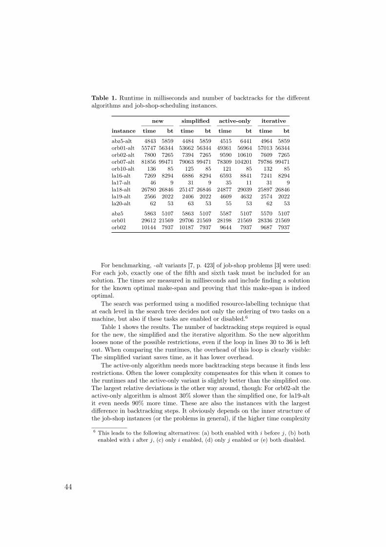
Table 1. Runtime in milliseconds and number of backtracks for the differentalgorithms and job-shop-scheduling instances.

new simplified active-only iterative

instance time bt time bt time bt time bt

abz5-alt 4843 5859 4484 5859 4515 6441 4964 5859orb01-alt 55747 56344 53662 56344 49361 56964 57013 56344orb02-alt 7800 7265 7394 7265 9590 10610 7609 7265orb07-alt 81856 99471 79063 99471 78309 104201 79786 99471orb10-alt 136 85 125 85 121 85 132 85la16-alt 7269 8294 6886 8294 6593 8841 7241 8294la17-alt 46 9 31 9 35 11 31 9la18-alt 26780 26846 25147 26846 24877 29039 25897 26846la19-alt 2566 2022 2406 2022 4609 4632 2574 2022la20-alt 62 53 63 53 55 53 62 53

abz5 5863 5107 5863 5107 5587 5107 5570 5107orb01 29612 21569 29706 21569 28198 21569 28336 21569orb02 10144 7937 10187 7937 9644 7937 9687 7937

For benchmarking, -alt variants [7, p. 423] of job-shop problems [3] were used:For each job, exactly one of the fifth and sixth task must be included for ansolution. The times are measured in milliseconds and include finding a solutionfor the known optimal make-span and proving that this make-span is indeedoptimal.

The search was performed using a modified resource-labelling technique thatat each level in the search tree decides not only the ordering of two tasks on amachine, but also if these tasks are enabled or disabled.6

Table 1 shows the results. The number of backtracking steps required is equalfor the new, the simplified and the iterative algorithm. So the new algorithmlooses none of the possible restrictions, even if the loop in lines 30 to 36 is leftout. When comparing the runtimes, the overhead of this loop is clearly visible:The simplified variant saves time, as it has lower overhead.

The active-only algorithm needs more backtracking steps because it finds lessrestrictions. Often the lower complexity compensates for this when it comes tothe runtimes and the active-only variant is slightly better than the simplified one.The largest relative deviations is the other way around, though: For orb02-alt theactive-only algorithm is almost 30% slower than the simplified one, for la19-altit even needs 90% more time. These are also the instances with the largestdifference in backtracking steps. It obviously depends on the inner structure ofthe job-shop instances (or the problems in general), if the higher time complexity

6 This leads to the following alternatives: (a) both enabled with i before j, (b) bothenabled with i after j, (c) only i enabled, (d) only j enabled or (e) both disabled.

44

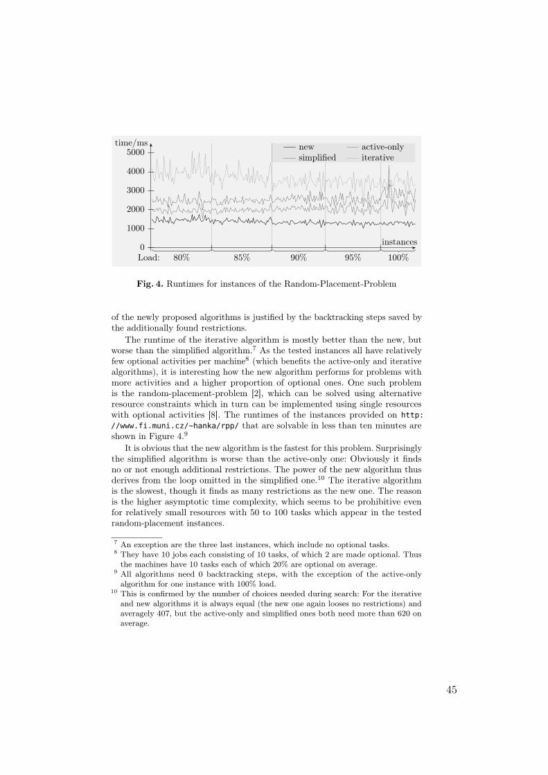
0

1000

2000

3000

4000

5000time/ms

instances

80% 85% 90% 95% 100%Load:

iterativesimplifiedactive-onlynew

Fig. 4. Runtimes for instances of the Random-Placement-Problem

of the newly proposed algorithms is justified by the backtracking steps saved bythe additionally found restrictions.

The runtime of the iterative algorithm is mostly better than the new, butworse than the simplified algorithm.7 As the tested instances all have relativelyfew optional activities per machine8 (which benefits the active-only and iterativealgorithms), it is interesting how the new algorithm performs for problems withmore activities and a higher proportion of optional ones. One such problemis the random-placement-problem [2], which can be solved using alternativeresource constraints which in turn can be implemented using single resourceswith optional activities [8]. The runtimes of the instances provided on http://www.fi.muni.cz/~hanka/rpp/ that are solvable in less than ten minutes areshown in Figure 4.9

It is obvious that the new algorithm is the fastest for this problem. Surprisinglythe simplified algorithm is worse than the active-only one: Obviously it findsno or not enough additional restrictions. The power of the new algorithm thusderives from the loop omitted in the simplified one.10 The iterative algorithmis the slowest, though it finds as many restrictions as the new one. The reasonis the higher asymptotic time complexity, which seems to be prohibitive evenfor relatively small resources with 50 to 100 tasks which appear in the testedrandom-placement instances.

7 An exception are the three last instances, which include no optional tasks.8 They have 10 jobs each consisting of 10 tasks, of which 2 are made optional. Thus

the machines have 10 tasks each of which 20% are optional on average.9 All algorithms need 0 backtracking steps, with the exception of the active-only

algorithm for one instance with 100% load.10 This is confirmed by the number of choices needed during search: For the iterative

and new algorithms it is always equal (the new one again looses no restrictions) andaveragely 407, but the active-only and simplified ones both need more than 620 onaverage.

45

3 Summary

This paper introduces a new edge-finding algorithm for unary resources. It dealswith optional activities correctly, finds all applications of the edge-finding rule tothe enabled activities and disables optional activities if they cause an overloaddetected by the edge-finding rule.

With O(n2) asymptotic time complexity it is slower than edge-finding algo-rithms that cannot take optional activities into account. The additionally foundrestrictions offer a significant reduction of the search decisions needed to find andprove the solution of a problem. Especially for problems with many activities, ofwhich a high proportion is optional, this leads to faster runtimes.

Future work can study the influence of different labelling strategies when itcomes to optional activities: Is it better to first establish an order of tasks andthen decide which tasks should be enabled? Another possible direction for futurework is studying for which problem structure the newly proposed algorithm yieldsbetter results, possibly implementing heuristics to decide which algorithm to use.

References

1. Philippe Baptiste, Claude Le Pape, and Wim Nuijten. ‘Constraint-Based Schedul-ing – Applying Constraint Programming to Scheduling Problems’. Boston: KluwerAcademic Publishers, 2001. isbn 0792374088.

2. Barták, Roman, Tomáš Müller and Hana Rudová. ‘A New Approach to Modelingand Solving Minimal Perturbation Problems’. In: Recent Advances in Constraints,CSCLP 2003. LNCS 3010. Berlin: Springer, 2004. isbn 978-3-540-21834-0. 233–249.

3. Yves Colombani. ‘Constraint programming: an efficient and practical approachto solving the job-shop problem’. In: Eugene C. Freuder, editor, Principles andPractice of Constraint Programming – CP96. LNCS 1118. Berlin: Springer, 1996.isbn 3-540-61551-2. 149–163.

4. Michael R. Garey and David S. Johnson. ‘Computers and Intractability – A Guideto the Theory of NP-Completeness’. New York: W. H. Freeman, 1979. isbn 0-7167-1045-5.

5. Matthias Hoche, Henry Müller, Hans Schlenker and Armin Wolf. ‘firstcs – APure Java Constraint Programming Engine’. In: Michael Hanus, Petra Hofstedtand Armin Wolf, editors, 2nd International Workshop on Multiparadigm ConstraintProgramming Languages – MultiCPL’03, 29th September 2003. url: http://uebb.cs.tu-berlin.de/MultiCPL03/Proceedings.MultiCPL03.RCoRP03.pdf.

6. Petr Vilím. ‘O(n log n) Filtering Algorithms for Unary Resource Constraint’. In:Jean-Charles and Régin Michel Rueher, editors, Integration of AI and OR Techniquesin Constraint Programming for Combinatorial Optimization Problems. LNCS 3011.Berlin: Springer, 2004. isbn 978-3-540-21836-4. 335–347.

7. Petr Vilím, Roman Barták and Ondřej Čepek. ‘Extension of O(n log n) Filtering Al-gorithms for the Unary Resource Constraint to Optional Activities’. In: Constraints10.4 (2005). 403–425.

8. Wolf, Armin, and Hans Schlenker. ‘Realising the Alternative Resources Constraint’.In: Applications of Declarative Programming and Knowledge Management, INAP2004. LNCS 3392. Berlin: Springer, 2005. isbn 978-3-540-25560-4. 185–199.

46

Encoding of Planning Problems and theirOptimizations in Linear Logic

Lukas Chrpa, Pavel Surynek and Jiri Vyskocil

Department of Theoretical Computer Science and Mathematical LogicFaculty of Mathematics and Physics

Charles University in Praguechrpa,surynek,vyskocil@kti.mff.cuni.cz

Abstract. Girard’s Linear Logic is a useful formalism which can be usedto manage a lot of problems with consumable resources. Its expressive-ness is quite good for easily understandable encoding of many problems.We concentrated on expressing planning problems by linear logic in thispaper. We observed a rich usage of a construct of consumable resource inplanning problem formulation. This fact motivates us to develop encod-ing of planning problems in linear logic. This paper shows how planningproblems can be encoded in Linear Logic and how to encode some opti-mizations of these planning problems which can be used to improve theefficiency of finding solutions (plans).

1 Introduction

Linear Logic is a useful formalism which can be used to formalize many problemswith consumable resources [2]. There is a lot of such problems that are handlingwith consumable and with renewable resources in practice. Linear Logic givesus a good expressiveness that help us with formalizing of these problems. Thisis because the problems are usually encoded in formulae with linear size withrespect to the length of the problems.

Previous research gave us some interesting results. Many of these results arein a theoretical area. One of the important results was connectivity of LinearLogic with the Petri Nets [17] which gave us more consciousness of the goodexpressiveness of Linear Logic.

Instead of the encoding of Petri nets in Linear Logic, there is a possibilityof encoding of planning problems in Linear Logic. Planning problems are animportant branch of AI and they are very useful in many practical applications.Previous research showed that planning problems can be simply encoded inLinear Logic and a problem of plan generation can be reduced to a problem offinding a proof in linear logic [16, 10, 3]. This paper shows that Linear Logicis not only able to encode planning problems directly, but Linear Logic is alsoable to encode many optimizations of planning problems which can be used toincrease the efficiency of finding solutions of these planning problems.

We provide a short introduction to Linear Logic and to planning problemsin Section 2. Description of the pure encoding of planning problems in Linear

47

Logic and an extension of this encoding which works with negative predicatesis provided in Section 3. Description of the encoding of optimizations such asencoding of static predicates, blocking actions, enforcing actions and assemblingactions is provided in Section 4. Section 5 give us the overview of related work inthis area and Section 6 will give us possible future work in this area and Section7 concludes.

2 Preliminaries

This section presents some basic information about Linear Logic and planningproblems that will be helpful to the reader to get through this paper.

2.1 Linear Logic

Linear Logic was introduced by Girard in 1987 [7]. Linear Logic is often called‘logic of resources‘, because unlike the ‘classical‘ logic, Linear Logic can handlewith expendable resources. The main difference between ‘classical‘ logic andLinear Logic is that if we say ”From A,A imply B we obtain B”, in ‘classical‘logic A is still available, but in Linear Logic A consumed which means that A isno longer available.

In addition to implication ((), there are more operators in linear logic.However we mention only those that are relevant for our encoding. One of theoperators in multiplicative conjunction (⊗) whose meaning is consuming (on theleft side of implication) or obtaining (on the right side of implication) resourcestogether. Another operator is exponential (!), which converts linear fact (ex-pendable resource) to ‘classical‘ fact (not expendable resource). At last, thereare additive conjunction (&) and additive disjunction (⊕) whose meaning isclose to modalities. Exactly when additive conjunction is used on the right sideof implication, then only one alternative must be proved, but when additive dis-junction is used on the right side of implication, then all the alternatives mustbe proved. If the additives are on the left side of implication, proving is quitesimilar, only the meaning of additive conjunction and additive disjunction isswapped.

Proving in Linear Logic is quite similar to proving in the ‘classical‘ logic,which is based on Gentzen’s style. Part of Linear Logic calculus which is neededin this paper is following:

Id A ` A Γ ` >,∆ R>

L⊗ Γ,A,B`∆Γ,(A⊗B)`∆

Γ1`A,∆1 Γ2`B,∆2Γ1,Γ2`(A⊗B),∆1∆2

R⊗

L( Γ1`A,∆1 Γ2,B`∆2Γ1,Γ2,(A(B)`∆1∆2

Γ`A,∆Γ`(A⊕B),∆

Γ`B,∆Γ`(A⊕B),∆ R⊕

W ! Γ`∆Γ,!A`∆

Γ,!A,!A`∆Γ,!A`∆ C !

D ! Γ,A`∆Γ,!A`∆

Γ,A`∆Γ,(∀x)A`∆ Forall

48

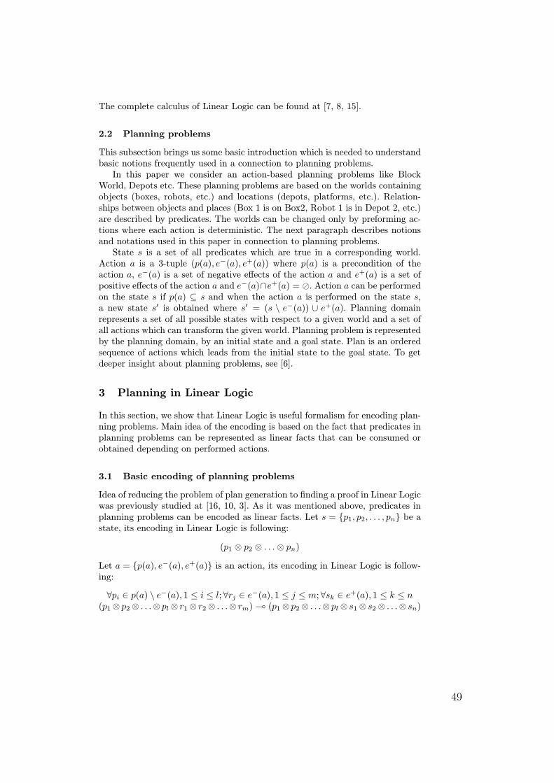
The complete calculus of Linear Logic can be found at [7, 8, 15].

2.2 Planning problems

This subsection brings us some basic introduction which is needed to understandbasic notions frequently used in a connection to planning problems.

In this paper we consider an action-based planning problems like BlockWorld, Depots etc. These planning problems are based on the worlds containingobjects (boxes, robots, etc.) and locations (depots, platforms, etc.). Relation-ships between objects and places (Box 1 is on Box2, Robot 1 is in Depot 2, etc.)are described by predicates. The worlds can be changed only by preforming ac-tions where each action is deterministic. The next paragraph describes notionsand notations used in this paper in connection to planning problems.

State s is a set of all predicates which are true in a corresponding world.Action a is a 3-tuple (p(a), e−(a), e+(a)) where p(a) is a precondition of theaction a, e−(a) is a set of negative effects of the action a and e+(a) is a set ofpositive effects of the action a and e−(a)∩e+(a) = ®. Action a can be performedon the state s if p(a) ⊆ s and when the action a is performed on the state s,a new state s′ is obtained where s′ = (s \ e−(a)) ∪ e+(a). Planning domainrepresents a set of all possible states with respect to a given world and a set ofall actions which can transform the given world. Planning problem is representedby the planning domain, by an initial state and a goal state. Plan is an orderedsequence of actions which leads from the initial state to the goal state. To getdeeper insight about planning problems, see [6].

3 Planning in Linear Logic

In this section, we show that Linear Logic is useful formalism for encoding plan-ning problems. Main idea of the encoding is based on the fact that predicates inplanning problems can be represented as linear facts that can be consumed orobtained depending on performed actions.

3.1 Basic encoding of planning problems

Idea of reducing the problem of plan generation to finding a proof in Linear Logicwas previously studied at [16, 10, 3]. As it was mentioned above, predicates inplanning problems can be encoded as linear facts. Let s = p1, p2, . . . , pn be astate, its encoding in Linear Logic is following:

(p1 ⊗ p2 ⊗ . . .⊗ pn)

Let a = p(a), e−(a), e+(a) is an action, its encoding in Linear Logic is follow-ing:

∀pi ∈ p(a) \ e−(a), 1 ≤ i ≤ l;∀rj ∈ e−(a), 1 ≤ j ≤ m; ∀sk ∈ e+(a), 1 ≤ k ≤ n(p1⊗ p2⊗ . . .⊗ pl⊗ r1⊗ r2⊗ . . .⊗ rm) ( (p1⊗ p2⊗ . . .⊗ pl⊗ s1⊗ s2⊗ . . .⊗ sn)

49

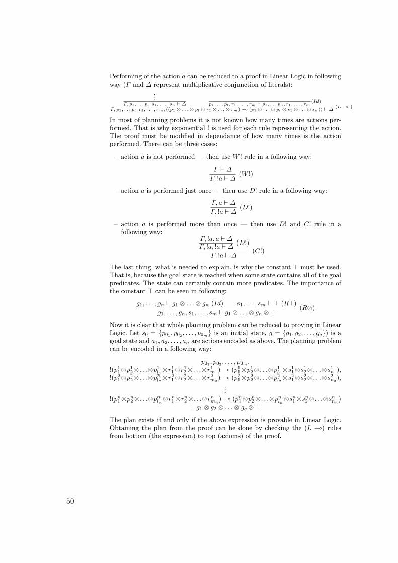
Performing of the action a can be reduced to a proof in Linear Logic in followingway (Γ and ∆ represent multiplicative conjunction of literals):

.

.

.Γ, p1, . . . pl, s1, . . . , sn ` ∆ p1, . . . pl, r1, . . . , rm ` p1, . . . pn, r1, . . . , rm

(Id)

Γ, p1, . . . pl, r1, . . . , rm, ((p1 ⊗ . . .⊗ pl ⊗ r1 ⊗ . . .⊗ rm) ( (p1 ⊗ . . .⊗ pl ⊗ s1 ⊗ . . .⊗ sn)) ` ∆(L ( )

In most of planning problems it is not known how many times are actions per-formed. That is why exponential ! is used for each rule representing the action.The proof must be modified in dependance of how many times is the actionperformed. There can be three cases:

– action a is not performed — then use W ! rule in a following way:

Γ ` ∆

Γ, !a ` ∆(W !)

– action a is performed just once — then use D! rule in a following way:

Γ, a ` ∆

Γ, !a ` ∆(D!)

– action a is performed more than once — then use D! and C! rule in afollowing way:

Γ, !a, a ` ∆Γ, !a, !a ` ∆

(D!)

Γ, !a ` ∆(C!)

The last thing, what is needed to explain, is why the constant > must be used.That is, because the goal state is reached when some state contains all of the goalpredicates. The state can certainly contain more predicates. The importance ofthe constant > can be seen in following:

g1, . . . , gn ` g1 ⊗ . . .⊗ gn (Id) s1, . . . , sm ` > (R>)g1, . . . , gn, s1, . . . , sm ` g1 ⊗ . . .⊗ gn ⊗> (R⊗)

Now it is clear that whole planning problem can be reduced to proving in LinearLogic. Let s0 = p01 , p02 , . . . , p0m is an initial state, g = g1, g2, . . . , gq) is agoal state and a1, a2, . . . , an are actions encoded as above. The planning problemcan be encoded in a following way:

p01 , p02 , . . . , p0m ,!(p1

1⊗p12⊗ . . .⊗p1

l1⊗r1

1⊗r12⊗ . . .⊗r1

m1) ( (p1

1⊗p12⊗ . . .⊗p1

l1⊗s1

1⊗s12⊗ . . .⊗s1

n1),

!(p21⊗p2

2⊗ . . .⊗p2l2⊗r2

1⊗r22⊗ . . .⊗r2

m2) ( (p2

1⊗p22⊗ . . .⊗p2

l2⊗s2

1⊗s22⊗ . . .⊗s2

n2),

...!(pn

1⊗pn2⊗. . .⊗pn

ln⊗rn

1⊗rn2⊗. . .⊗rn

mn) ( (pn

1⊗pn2⊗. . .⊗pn

ln⊗sn

1⊗sn2⊗. . .⊗sn

nn)

` g1 ⊗ g2 ⊗ . . .⊗ gq ⊗>The plan exists if and only if the above expression is provable in Linear Logic.Obtaining the plan from the proof can be done by checking the (L () rulesfrom bottom (the expression) to top (axioms) of the proof.

50

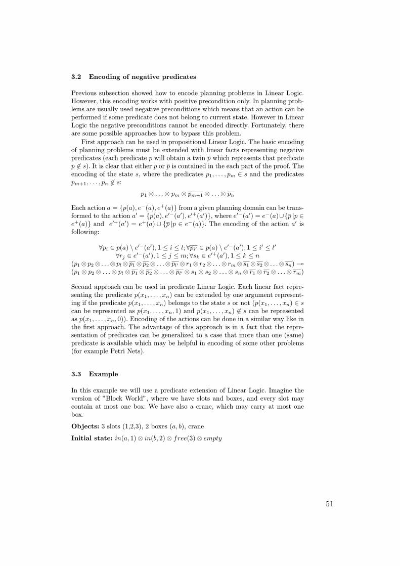
3.2 Encoding of negative predicates

Previous subsection showed how to encode planning problems in Linear Logic.However, this encoding works with positive precondition only. In planning prob-lems are usually used negative preconditions which means that an action can beperformed if some predicate does not belong to current state. However in LinearLogic the negative preconditions cannot be encoded directly. Fortunately, thereare some possible approaches how to bypass this problem.

First approach can be used in propositional Linear Logic. The basic encodingof planning problems must be extended with linear facts representing negativepredicates (each predicate p will obtain a twin p which represents that predicatep 6∈ s). It is clear that either p or p is contained in the each part of the proof. Theencoding of the state s, where the predicates p1, . . . , pm ∈ s and the predicatespm+1, . . . , pn 6∈ s:

p1 ⊗ . . .⊗ pm ⊗ pm+1 ⊗ . . .⊗ pn

Each action a = p(a), e−(a), e+(a) from a given planning domain can be trans-formed to the action a′ = p(a), e′−(a′), e′+(a′), where e′−(a′) = e−(a)∪p |p ∈e+(a) and e′+(a′) = e+(a) ∪ p |p ∈ e−(a). The encoding of the action a′ isfollowing:

∀pi ∈ p(a) \ e′−(a′), 1 ≤ i ≤ l; ∀pi′ ∈ p(a) \ e′−(a′), 1 ≤ i′ ≤ l′

∀rj ∈ e′−(a′), 1 ≤ j ≤ m; ∀sk ∈ e′+(a′), 1 ≤ k ≤ n(p1⊗ p2⊗ . . .⊗ pl⊗ p1⊗ p2⊗ . . .⊗ pl′ ⊗ r1⊗ r2⊗ . . .⊗ rm⊗ s1⊗ s2⊗ . . .⊗ sn) ((p1 ⊗ p2 ⊗ . . .⊗ pl ⊗ p1 ⊗ p2 ⊗ . . .⊗ pl′ ⊗ s1 ⊗ s2 ⊗ . . .⊗ sn ⊗ r1 ⊗ r2 ⊗ . . .⊗ rm)

Second approach can be used in predicate Linear Logic. Each linear fact repre-senting the predicate p(x1, . . . , xn) can be extended by one argument represent-ing if the predicate p(x1, . . . , xn) belongs to the state s or not (p(x1, . . . , xn) ∈ scan be represented as p(x1, . . . , xn, 1) and p(x1, . . . , xn) 6∈ s can be representedas p(x1, . . . , xn, 0)). Encoding of the actions can be done in a similar way like inthe first approach. The advantage of this approach is in a fact that the repre-sentation of predicates can be generalized to a case that more than one (same)predicate is available which may be helpful in encoding of some other problems(for example Petri Nets).

3.3 Example

In this example we will use a predicate extension of Linear Logic. Imagine theversion of ”Block World”, where we have slots and boxes, and every slot maycontain at most one box. We have also a crane, which may carry at most onebox.

Objects: 3 slots (1,2,3), 2 boxes (a, b), crane

Initial state: in(a, 1)⊗ in(b, 2)⊗ free(3)⊗ empty

51

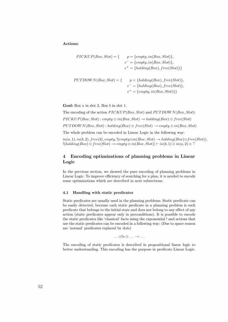
Actions:

PICKUP (Box, Slot) = p = empty, in(Box, Slot),e− = empty, in(Box, Slot),e+ = holding(Box), free(Slot)

PUTDOWN(Box, Slot) = p = holding(Box), free(Slot),e− = holding(Box), free(Slot),e+ = empty, in(Box, Slot)

Goal: Box a in slot 2, Box b in slot 1.

The encoding of the action PICKUP (Box, Slot) and PUTDOWN(Box, Slot):

PICKUP (Box, Slot) : empty ⊗ in(Box, Slot) ( holding(Box)⊗ free(Slot)

PUTDOWN(Box, Slot) : holding(Box)⊗ free(Slot) ( empty ⊗ in(Box, Slot)

The whole problem can be encoded in Linear Logic in the following way:

in(a, 1), in(b, 2), free(3), empty, !(empty⊗in(Box, Slot) ( holding(Box)⊗free(Slot)),!(holding(Box)⊗ free(Slot) ( empty⊗ in(Box, Slot)) ` in(b, 1)⊗ in(a, 2)⊗>

4 Encoding optimizations of planning problems in LinearLogic

In the previous section, we showed the pure encoding of planning problems inLinear Logic. To improve efficiency of searching for a plan, it is needed to encodesome optimizations which are described in next subsections.

4.1 Handling with static predicates

Static predicates are usually used in the planning problems. Static predicate canbe easily detected, because each static predicate in a planning problem is suchpredicate that belongs to the initial state and does not belong to any effect of anyaction (static predicates appear only in preconditions). It is possible to encodethe static predicates like ‘classical‘ facts using the exponential ! and actions thatuse the static predicates can be encoded in a following way: (Due to space reasonare ‘normal‘ predicates replaced by dots)

. . .⊗!a⊗ . . . ( . . .

The encoding of static predicates is described in propositional linear logic tobetter understanding. This encoding has the purpose in predicate Linear Logic.

52

4.2 Blocking of actions

To increase efficiency of solving planning problems it is quite necessary to usesome technique which helps the solver to avoid unnecessary backtracking. Typ-ically the way how to avoid a lot of unnecessary backtracking is blocking ofactions of what is known that wont lead to the solution (for example inverseactions).

The idea how to encode the blocking of actions is in adding a new predicatecan(a, x), where a is an action and x ∈ 0, 1 is representing a status of theaction a. If x = 0 then the action a is blocked and if x = 1 then the action ais unblocked. Now is clear that the encoding of the action a must be done in afollowing way: (Due to space reason are ‘normal‘ predicates replaced by dots)

can(a, 1)⊗ . . . ( can(a, 1)⊗ . . . , orcan(a, 1)⊗ . . . ( can(a, 0)⊗ . . .

The first expression means that a does not block itself and the second expressionmeans that a block itself.

Assume that an action b can block the action a. Encoding of the action b isfollowing (can(b, ?) means can(b, 1) or can(b, 0) like in the previous encoding ofthe action a):

∀X : can(b, 1)⊗ can(a,X)⊗ . . . ( can(b, ?)⊗ can(a, 0)⊗ . . .

The predicate can(a,X) from the expression above represents a fact that is notknown if a is blocked or not. If a is already blocked then X unifies with 0 andanything remains unchanged (can(a, 0) still holds). If a is not blocked then Xunifies with 1 which means that a become blocked, because can(a, 1) is no longertrue and can(a, 0) become true.

Now assume that an action c can unblock the action a. Encoding of theaction c is done by a similar way like the action b. The encoding of the action cis following (can(c, ?) means can(c, 1) or can(c, 0) like in the previous encodingof the action a):

∀X : can(c, 1)⊗ can(a,X)⊗ . . . ( can(c, ?)⊗ can(a, 1)⊗ . . .

The explanation how this encoding works is similar like the explanation in theprevious paragraph.

4.3 Enforcing of actions

Another optimization which can help the solver to find the solution faster isenforcing of actions. Typically, when some action is performed is necessary toperform some other action. It is possible to enforce some action by blocking ofthe other actions, but this may decrease the efficiency, because each single actionmust be blocked in the way described in the previous subsection which meansthat the formula rapidly increases its length.

53

The idea how to encode the enforcing of actions is also in adding new pred-icate can(a), where a is an only action which can be performed. Let can(1)represents the fact that all actions can be preformed. The encoding of an actiona which does not enforce any other action is following:

(can(a)⊕ can(1))⊗ . . . ( can(1)⊗ . . .

The expression can(a) ⊕ can(1) means that action a can be performed if andonly if a is enforced by other action (can(a) is true) or all actions are allowed(can(1) is true).

Now assume that an action b enforces the action a. The encoding of theaction b is following:

(can(b)⊕ can(1))⊗ . . . ( can(a)⊗ . . .

It is clear that in this encoding are one or all actions allowed in a certain step.This idea can be easily extended by adding some new symbols representing thata certain groups of actions are allowed.

4.4 Assembling actions into a single action

Another kind of optimizations in planning problems can be assembling actionsinto single action usually called macro action. This approach is based on a factthat some sequences of actions is used several times. Let a1, . . . , an is a sequenceof actions encoded in Linear Logic in a way described before. For further usagewill be used shortened notation of the encoding like that:

⊗

∀l∈Γi

l (⊗

∀r∈∆i

r ∀i ∈ 1, . . . , n

Assume that an action a is created by a assembling of the sequence of the actionsa1, . . . , an. Because a is also an action, the encoding is following:

⊗

∀l∈Γ

l (⊗

∀r∈∆

r

The following algorithm shows how to create the action a from the sequence ofthe actions a1, . . . , an.

Algorithm 1:INPUT: Γ1, . . . , Γn,∆1, . . . , ∆n (from the encoding of the actions a1, . . . , an)OUTPUT: Γ,∆ (from the encoding of the action a)

Γ := ∆ := ∅for i = 1 to n do

Λ:=∆ ∩ Γi

∆:=(∆ \ Λ) ∪∆i

Γ := Γ ∪ (Γi \ Λ)endfor

54

Proposition 1. The algorithm 1 is correct.

Proof. The correctness of the algorithm 1 can be proved inductively in a followingway:

For n = 1, it is easy to see that algorithm 1 works correctly for the onlyaction a1. The for cycle on lines 2-6 runs just once. On the line 3 is easy to seethat Λ = ∅, because ∆ = ∅. Now it can be seen that ∆ = ∆1 (line 4) andΓ = Γ1 (line 5), because Λ = ∅ and Γ and ∆ before line 4 (or 5) are also empty.

Assume that algorithm 1 works correctly for k actions. From this assumptionimply existence of an action a that is created by algorithm 1 (from some sequenceof actions a1, . . . , ak) after k steps of the for cycle in lines 2-6. Let s is a stateand s′ is a state which is obtained from s by applying the action a (without lossof generality assume that a can be applied on s). It is true that s′ = (s\Γ )∪∆).Let ak+1 is an action which is applied on the state s′ (without loss of generalityassume that a can be applied on s′). It is true that s′′ = (s′ \ Γk+1) ∪∆k+1 =((s \ Γ ) ∪ ∆) \ Γk+1) ∪ ∆k+1. After k + 1-th step of the for cycle (lines 2-6) an action a′ is created (from the sequence a1, . . . , ak, ak + 1). When a′ isapplied on the state s, s′′′ = (s \ Γ ′) ∪ ∆′). From lines 3-5 can be seen thatΓ ′ = Γ ∪ (Γk+1 \ (∆ ∩ Γk+1)) and ∆′ = (∆ \ (∆ ∩ Γk+1)) ∪ ∆k+1. Now s′′′ =(s \ (Γ ∪ (Γk+1 \ (∆ ∩ Γk+1)))) ∪ ((∆ \ (∆ ∩ Γk+1)) ∪∆k+1). To finish the proofis needed to prove that s′′ = s′′′. p ∈ s′′ iff p ∈ ∆k+1 or p ∈ ∆ ∧ p 6∈ Γk+1 orp ∈ s∧p 6∈ Γ∧(p 6∈ Γk+1∨p ∈ ∆). p ∈ s′′′ iff p ∈ ∆k+1 or p ∈ ∆∧p 6∈ (∆∩Γk+1) orp ∈ s∧p 6∈ Γ∧p 6∈ (Γk+1\(∆∩Γk+1)). It is easy to see that p ∈ ∆∧p 6∈ (∆∩Γk+1)is satisfied iff p ∈ ∆ ∧ p 6∈ Γk+1 is satisfied. p 6∈ (Γk+1 \ (∆ ∩ Γk+1)) is satisfiediff p 6∈ Γk+1 or p ∈ ∆ is satisfied. Now is clear that s′′ = s′′′.

2

The algorithm 1 works with planning problems encoded in propositional LinearLogic. The extension of the algorithm to predicate Linear Logic can be simplydone with adding constraints symbolizing which of actions’ arguments must beequal. This extension affect only the intersection (∆i ∩ Γj).

Following algorithm for assembling actions into a single action is based on aparadigm divide and conquer which can support parallel implementation.

Algorithm 2:INPUT: Γ1, . . . , Γn,∆1, . . . , ∆n (from the encoding of the actions a1, . . . , an)OUTPUT: Γ, ∆ (from the encoding of the action a)

Function Assemble(Γ1, . . . , Γn,∆1, . . .∆n):Γ, ∆if n = 1 then return(Γ1, ∆1) endifΓ ′,∆′:=Assemble(Γ1, . . . , Γdn

2 e,∆1, . . . ,∆dn2 e)

Γ ′′,∆′′:=Assemble(Γdn2 e+1, . . . , Γn,∆dn

2 e+1, . . . , ∆n)Λ := ∆′ ∩ Γ ′′

Γ := Γ ′ ∪ (Γ ′′ \ Λ)∆ := ∆′′ ∪ (∆′ \ Λ)return(Γ,∆)

endFunction

55

Proposition 2. The algorithm 2 is correct.

Proof. The correctness of the algorithm 2 can be proved in a following way:

n = 1 — It is clear that assembling one-element sequence of actions (a1) is equalto the action a1 itself.

n > 1 — Let a1, . . . an is a sequence of actions. In the lines 2 and 3 is the sequencesplit into two sequences (a1, . . . , adn

2 e and adn2 e+1, . . . , an) and the algorithm

2 is recursively applied on them. Because dn2 e < n when n > 1, is easy to

see that the recursion will finitely terminate (it happens when n = 1). Nowit is clear that a′ and a′′ are actions obtained by assembling the sequencesa1, . . . , adn

2 e and adn2 e+1, . . . , an. These actions are assembled into a single

action a at lines 4-6. The proof of correctness of this assembling is done inproof of proposition 1.

2

The algorithm 2 can be extended to predicate Linear Logic in a similar way likealgorithm 1.

5 Related work

Previous research showed that planning problems can be encoded in many dif-ferent formalisms. We consider the formalisms which are related to the logic. Itwas showed in [11] that planning problems can be solved by reduction to SAT.This approach brings very good results (for example SATPLAN [12] won last twoInternational Planning Competitions (IPC) in optimal deterministic planning).However, there seems to be a problem with extending the SAT based planners tobe able to solve planning problems with time and resources. Otherwise, LinearLogic (especially predicate Linear Logic) seems to be expressive enough for theencoding of planning problems with time and resources. The other logic formal-ism which can be used in connection to planning problems is Temporal Logic(especially Simple Temporal Logic). It is showed in [1] that Temporal Logic canbe used to improve searching for plans. This approach is used in several planners(for example TALplanner [5] which had very good results in IPC 2002). Tem-poral Logic is good for representing relationships between actions, but LinearLogic is able to represent whole planning problems.

First ideas of solving planning problems via theorem proving in Linear Logichas been shown at [16, 10]. These papers showed that M?LL fragment of Lin-ear Logic is strong enough to formalize planning problems. Another interestingwork in this area is [4] and it describes a possibility of recursive applying ofpartial plans. Analyzing planning problems encoded in Linear Logic via partialdeduction approach is described in [13].

One of the most important results was an implementation of a planning solvercalled RAPS [14] which in comparison between the most successful solvers inIPC 2002 showed very interesting results (especially in Depots domain). RAPSshowed us that the research in this area can be helpful in searching for the goodplanning solver.

56

This paper extends the previous research in this area by fact that manyoptimizations of planning problems, which helps a planner to find a solutionmore quickly, can be also easily encoded in Linear Logic.

6 Future work

Next paragraphs show possible directions of our future research in this area.One of possible directions how to implement the efficient algorithm for solving

planning problems encoded in Linear Logic is using the connection betweenLinear Logic and Petri Nets. It is not difficult to see that the encoding of theplanning problems is similar as an encoding of Petri Nets. The implementationof unfolding algorithm for reachability problem in Petri Nets for solving planningproblems has been done by [9] and showed very good results. We will study thepossibility of extending this algorithm in the way that the extended algorithmwill support the encoding of planning problems in predicate Linear Logic.

There is a possibility of extension of the presented encodings of planningproblems in Linear Logic into Temporal Linear Logic (to learn more about Tem-poral Linear Logic, see [18]). It seems to be very useful combination, becauseTemporal Logic can give us more possibilities for encoding of relationships be-tween actions.

Another possible way of our future research is using of the encodings of theoptimizations for transformation of planning domains. Transformed planningdomains can be used with existing planners and can reach better results, becausethe presented optimizations of planning problems can help the planners to prunethe search space.

At last, Linear Logic seems to be strong enough to encode planning problemswith time and resources. Basic idea of this extension comes from the fact thattime and resources can be also represented by linear facts. The usage of predicateLinear Logic seems to be necessary in this case.

7 Conclusion

The previous research showed that Linear Logic is a useful formalism for encod-ing many problems with expendable resources like planning problems, becausein comparison to the other logics, Linear Logic seems to be strong enough tosolve also planning problems with time and resources. This paper extended theprevious research in this area by the fact that many optimizations of planningproblems, which can help a planner to find a solution more quickly, can be en-coded in Linear Logic without huge growth of the length of the encoding. Mainadvantage of this approach is that an improvement of the Linear Logic solverleads to improved efficiency of the planner based on Linear Logic.

57

8 Acknowledgements

We thank the reviewers for the comments. The research is supported by theCzech Science Foundation under the contract no. 201/07/0205 and by the GrantAgency of Charles University (GAUK) under the contract no. 326/2006/A-INF/MFF.

References

1. Bacchus F., Kabanza F.: Using temporal logics to express search control knowledgefor planning. Artificial Intelligence 22:5-27. 1998.

2. Chrpa L. Linear Logic: Foundations, Applications and Implementations. In pro-ceedings of workshop CICLOPS 2006. 110-124. 2006.

3. Chrpa L. Linear logic in planning. In proceedings of Doctoral Consorcium ICAPS2006. 26-29. 2006.

4. Cresswell S., Smaill A., Richardson J. Deductive Synthesis of Recursive Plans inLinear Logic. In proceedings of ECP 1999. 252–264. 1999.

5. Doherty P., Kvanstrom J.: TALplanner: A temporal logic based planner. AIMagazine 22(3):95-102. 2001.

6. Ghallab M, Nau D., Traverso P. Automated planning, theory and practice. MorganKaufmann Publishers 2004. 2004.

7. Girard J.-Y. Linear logic. Theoretical computer science 50:1–102. 1987.8. Girard J.-Y. Linear Logic: Its Syntax and Semantics. Technical report, Cambridge

University Press. 1995.9. Hickmott S., Rintanen J., Thiebaux S., White L. Planning via Petri Net Unfolding

In proceedings of IJCAI 2007. 1904-1911. 200710. Jacopin E. Classical AI Planning as Theorem Proving: The Case of a Fragment of

Linear Logic In proccedings of AAAI 1993. 62–66. 1993.11. Kautz H. A., Selman B.: Planning as Satisfiability. In proccedings of ECAI 1992.

359-363. 1992.12. Kautz H. A., Selman B., Hoffmann J.: SatPlan: Planning as Satisfiability. In

proccedings of 5th IPC 2006.13. Kungas P. Analysing AI Planning Problems in Linear Logic - A Partial Deduction

Approach. IN proceedings of SBIA 2004. 52–61. 2004.14. Kungas P. Linear logic for domain-independent ai planning. Proceedings of Doc-

toral Consorcium ICAPS 2003. 2003.15. Lincoln P. Linear logic. Proceedings of SIGACT 1992. 1992.16. Masseron M. Tollu C., Vauzeilles J. Generating plans in linear logic i-ii. Theoretical

Computer Science. vol. 113, 349-375. 1993.17. Oliet N. M., Meseguer, J. From petri nets to linear logic. Springer LNCS 389.

1989.18. Tanabe M. Timed petri nets and temporal linear logic. In proceedings of Applica-

tion and Theory of Petri Nets. 156-174. 1997

This article was processed using the LATEX macro package with LLNCS style

58

Partial Model Completion in Model Driven Engineeringusing Constraint Logic Programming

Sagar Sen1,2, Benoit Baudry1, Doina Precup2

1 IRISA, Campus de Beaulieu35042 Rennes Cedex France

2 School of Computer Science, McGill University,Montreal, Quebec, Canada

ssen,bbaudry @irisa.fr , dprecup@cs.mcgill.ca

Abstract. In Model Driven Engineering a model is a graph of objects that con-forms to a meta-model and a set of constraints. The meta-model and the con-straints declaratively restrict models to a valid set. Models are used to representthe state and behaviour of software systems. They are specified in visual mod-elling environments or automatically synthesized for program testing. In suchapplications, a modeller is interested in specifying a partial model or a set of par-tial models which has a structure and associated properties that interests him/her.Completing a partial model manually can be an extremely tedious or an unde-cidable task since the modeller has to satisfy tightly-coupled and arbitrary con-straints. We identify this to be a problem and present a methodology to solve(if a solution can be found within certain time bounds) it using constraint logicprogramming. We present a transformation from a partial model, its meta-model,and additional constraints to a constraint logic program. We solve/query the CLPto obtain value assignments for undefined properties in the partial model. Wethen complete the partial model using the value assignments for the rest of theproperties.

1 Introduction

Model-driven engineering (MDE) [1] [2] [3] is an emerging trend that promises de-crease in development time of complex software systems. For this, MDE makes exten-sive use of models. A model is specified in a modelling language which is describeddeclaratively using a meta-model and a set of constraints. The Object ManagementGroup (OMG) [4] standard for specifying a meta-model is Meta-object Facility (MOF)[5]. The constraints on the properties described in the meta-model are specified in aconstraint language such as Object Constraint Language (OCL) [6].

Several tasks in MDE require building and manipulating models. Models are built invisual modelling environments [7] [8]. Models are automatically synthesized for testing[9] and verification [10]. The design space of models are explored for meeting require-ments in embedded systems [11]. In all these cases, a modeller would like to specifya partial model that interests him/her. The task of completing a model manually couldbe extremely tedious since the modeller will have to satisfy a set of restrictions that areimposed by the meta-model and constraints (for instance, completing models in a visualmodelling environment). We intend to automate this process.

59

In this paper we propose an approach where we use the idea that a partial model,its meta-model, and a set of constraints together result in a large set of constraints thatcan be represented as a constraint logic program (CLP). The CLP is solved/queried toobtain the missing elements in a partial model to give a complete model. We use thesimple Hierarchical Finite State Machine (HFSM) modelling language to illustrate ourapproach. However, our approach is extensible to any modelling language. In Section2 we describe meta-models, constraints on it and the resulting modelling language forspecifying models. Section 3 presents the algorithm for transforming a partial modelwith its meta-model and constraints to a constraint logic program. In Section 4 wepresent an example based on the Hierarchical Finite State Machine modelling language.We conclude in Section 5.

2 Meta-models and Constraints of a Modelling Language

In this section we define the concept of a meta-model and constraints on it to specifya modelling language. We present the Hierarchical Finite State Machine (HFSM) mod-elling language with its meta-model and constraints as an illustrative example. The basicprinciples for specifying any modelling language follow the same set of procedures weuse to discuss the HFSM modelling language.

2.1 Meta-models

A modelling language allows us to specify models. A model consists of objects andrelationships between them. The meta-model of the modelling language specifies thetypes of all the objects and their possible inter-relationships. The type of an object isreferred to as a class. The meta-model for the HFSM modelling language is presentedin Figure 1 (a). The classes in the meta-model are HFSM, Transition, AbstractState,State, and Composite.

In this paper we use the Object Management Group (OMG) [4] standard Meta-objectFacility (MOF) [5] for specifying a meta-model. MOF is a modelling language capable ofspecifying domain-specific modelling languages and its own meta-model. This propertyof MOF is known as bootstrapping. We use the visual language notation in MOF tospecify the meta-model for the HFSM modelling language in Figure 1 (a).

Each class in the meta-model has properties. A property is either an attribute or areference. An attribute is of primitive type which is either Integer, String, or Boolean.For instance, the attributes of the class State are isInitial and isFinal both of which areof primitive type Boolean. An example domain of values for the primitive attributes isgiven in Table 1. The String variable can be a finite set of strings or a regular expressionthat specifies a set of strings.

Describing the state of a class of objects with only primitive attributes is not suf-ficient in many cases. Modelling many real-world systems elicits the need to modelcomplex relationships such as modelling that an object contains another set of objectsor an object is related to another finite set of objects. This set of related objects is con-strained by a multiplicity. A reference property of a class allows its objects to be relatedto a set of objects. For instance, an object of class HFSM contains Transition objects.

60

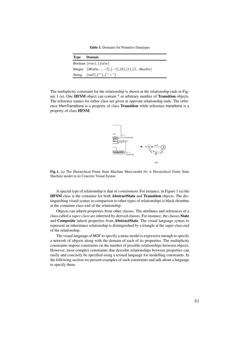
Table 1. Domains for Primitive Datatypes

Type Domain

Boolean true, f alseInteger MinInt, ..,−2,−1,0,1,2, ..MaxIntString null,””,”.+ ”

The multiplicity constraint for the relationship is shown at the relationship ends in Fig-ure 1 (a). One HFSM object can contain * or arbitrary number of Transition objects.The reference names for either class are given at opposite relationship ends. The refer-ence hfsmTransitions is a property of class Transition while reference transitions is aproperty of class HFSM.

Fig. 1. (a) The Hierarchical Finite State Machine Meta-model (b) A Hierarchical Finite StateMachine model in its Concrete Visual Syntax

A special type of relationship is that of containment. For instance, in Figure 1 (a) theHFSM class is the container for both AbstractState and Transition objects. The dis-tinguishing visual syntax in comparison to other types of relationships is black rhombusat the container class end of the relationship.

Objects can inherit properties from other classes. The attributes and references of aclass called a super class are inherited by derived classes. For instance, the classes Stateand Composite inherit properties from AbstractState. The visual language syntax torepresent an inheritance relationship is distinguished by a triangle at the super class endof the relationship.

The visual language of MOF to specify a meta-model is expressive enough to specifya network of objects along with the domain of each of its properties. The multiplicityconstraints impose constraints on the number of possible relationships between objects.However, most complex constraints that describe relationships between properties caneasily and concisely be specified using a textual language for modelling constraints. Inthe following section we present examples of such constraints and talk about a languageto specify them.

61

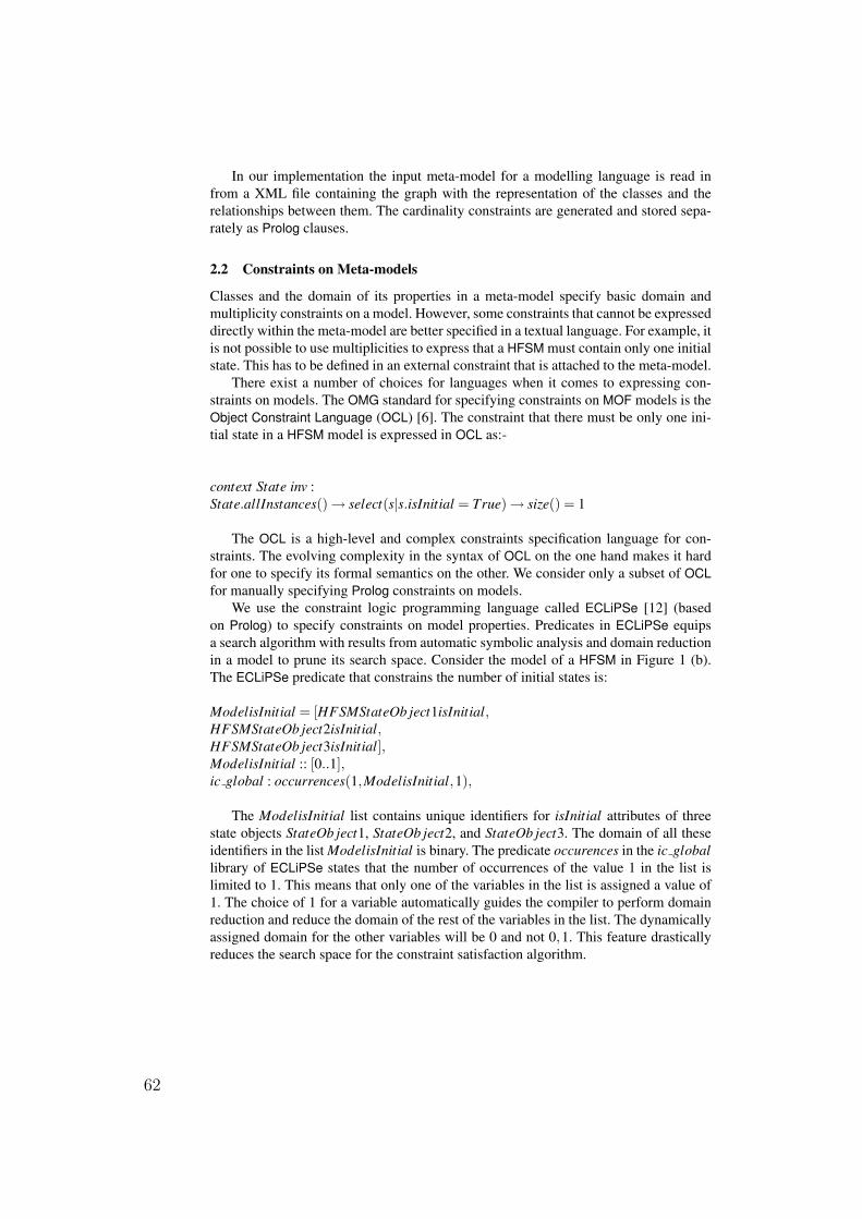
In our implementation the input meta-model for a modelling language is read infrom a XML file containing the graph with the representation of the classes and therelationships between them. The cardinality constraints are generated and stored sepa-rately as Prolog clauses.

2.2 Constraints on Meta-models

Classes and the domain of its properties in a meta-model specify basic domain andmultiplicity constraints on a model. However, some constraints that cannot be expresseddirectly within the meta-model are better specified in a textual language. For example, itis not possible to use multiplicities to express that a HFSM must contain only one initialstate. This has to be defined in an external constraint that is attached to the meta-model.

There exist a number of choices for languages when it comes to expressing con-straints on models. The OMG standard for specifying constraints on MOF models is theObject Constraint Language (OCL) [6]. The constraint that there must be only one ini-tial state in a HFSM model is expressed in OCL as:-

context State inv :State.allInstances()→ select(s|s.isInitial = True)→ size() = 1

The OCL is a high-level and complex constraints specification language for con-straints. The evolving complexity in the syntax of OCL on the one hand makes it hardfor one to specify its formal semantics on the other. We consider only a subset of OCLfor manually specifying Prolog constraints on models.

We use the constraint logic programming language called ECLiPSe [12] (basedon Prolog) to specify constraints on model properties. Predicates in ECLiPSe equipsa search algorithm with results from automatic symbolic analysis and domain reductionin a model to prune its search space. Consider the model of a HFSM in Figure 1 (b).The ECLiPSe predicate that constrains the number of initial states is:

ModelisInitial = [HFSMStateOb ject1isInitial,HFSMStateOb ject2isInitial,HFSMStateOb ject3isInitial],ModelisInitial :: [0..1],ic global : occurrences(1,ModelisInitial,1),

The ModelisInitial list contains unique identifiers for isInitial attributes of threestate objects StateOb ject1, StateOb ject2, and StateOb ject3. The domain of all theseidentifiers in the list ModelisInitial is binary. The predicate occurences in the ic globallibrary of ECLiPSe states that the number of occurrences of the value 1 in the list islimited to 1. This means that only one of the variables in the list is assigned a value of1. The choice of 1 for a variable automatically guides the compiler to perform domainreduction and reduce the domain of the rest of the variables in the list. The dynamicallyassigned domain for the other variables will be 0 and not 0,1. This feature drasticallyreduces the search space for the constraint satisfaction algorithm.

62

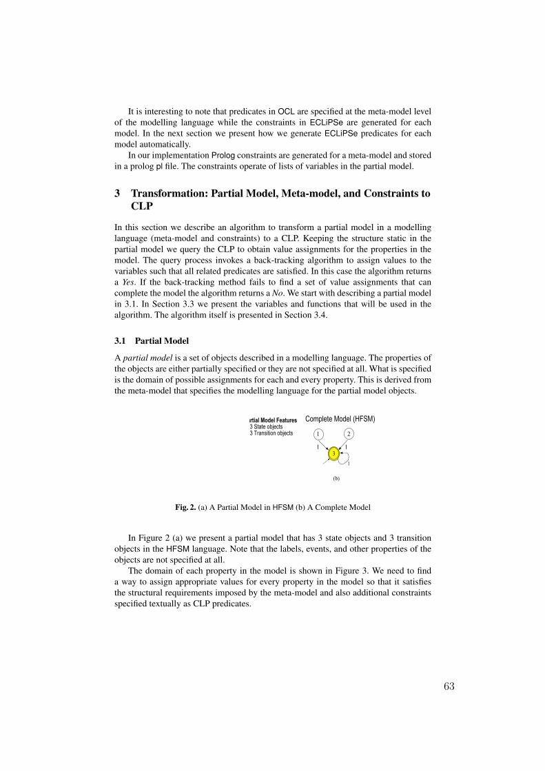
It is interesting to note that predicates in OCL are specified at the meta-model levelof the modelling language while the constraints in ECLiPSe are generated for eachmodel. In the next section we present how we generate ECLiPSe predicates for eachmodel automatically.

In our implementation Prolog constraints are generated for a meta-model and storedin a prolog pl file. The constraints operate of lists of variables in the partial model.

3 Transformation: Partial Model, Meta-model, and Constraints toCLP

In this section we describe an algorithm to transform a partial model in a modellinglanguage (meta-model and constraints) to a CLP. Keeping the structure static in thepartial model we query the CLP to obtain value assignments for the properties in themodel. The query process invokes a back-tracking algorithm to assign values to thevariables such that all related predicates are satisfied. In this case the algorithm returnsa Yes. If the back-tracking method fails to find a set of value assignments that cancomplete the model the algorithm returns a No. We start with describing a partial modelin 3.1. In Section 3.3 we present the variables and functions that will be used in thealgorithm. The algorithm itself is presented in Section 3.4.

3.1 Partial Model

A partial model is a set of objects described in a modelling language. The properties ofthe objects are either partially specified or they are not specified at all. What is specifiedis the domain of possible assignments for each and every property. This is derived fromthe meta-model that specifies the modelling language for the partial model objects.

Fig. 2. (a) A Partial Model in HFSM (b) A Complete Model

In Figure 2 (a) we present a partial model that has 3 state objects and 3 transitionobjects in the HFSM language. Note that the labels, events, and other properties of theobjects are not specified at all.

The domain of each property in the model is shown in Figure 3. We need to finda way to assign appropriate values for every property in the model so that it satisfiesthe structural requirements imposed by the meta-model and also additional constraintsspecified textually as CLP predicates.

63

Fig. 3. Domain of Properties in the Partial Model

Which value is taken by a property will be decided when we transform the partialmodel to a CLP and solve it. This transformation process and solution is discussed inthe next sections.

3.2 CLP as a Common Language

Requirements in MDE come from many sources. In this paper we focus on three sourcesof requirements.

1. The meta-model is a diagram specified in a meta-modelling language such as MOF2. The constraints are textually specified in OCL or directly in CLP3. The partial model is specified either diagrammatically or textually as an instance of

the meta-model.

There also could be many other sources of requirements such as pre-conditionsand post-conditions from programs that manipulate models and an objective functionthat is soft constraint on the properties of a model. These requirements are specifiedin different languages that are either graphical or textual and are usually expressedin the most convenient specification language such as OCL or MOF. Combining thedeclarative specifications from different sources into one common language is necessaryfor analysis on a common platform. The following section presents an algorithm thatsyntactically transforms constraints from various sources (the three that we consider)into a CLP.

64

3.3 Preliminaries

The input to the transformation consists of a partial model, the meta-model and theconstraints specification of a modelling language. In Table 2 we list out symbols andtheir descriptions we use for describing the algorithm in the next section.

Variable DescriptionM Partial modelM.properties Set of all properties(attributes and references) in MModel List of CLP variables for all properties in MModel property List of CLP variables for a relationship from a reference called propertyproperty.lowerBound Lower bound on multiplicity of a relationship from a reference called propertyproperty.upperBound Upper bound on multiplicity of a relationship from a reference called propertyproperty to re f erence A 0/1 variable for a relationship from a property to one of its re f erencesre f erence to property A 0/1 variable for a relationship from a re f erence to its propertyC Set of non-meta-model constraint predicatesModel constraint List of variables that are constrained by the constraint constraintconstraint.predicate Name of the CLP predicate for a constraint identifierconstraint.parameters String of additional comma separated parameters for a predicate

Table 2. Symbols we use in the model to CLP transformation algorithm

The transformation algorithm uses some handy functions which we list and describein Table 3.

Function DescriptionisAttribute(property) Returns 1 if the property is an attribute, otherwise 0isRe f erence(property) Returns 1 if the property is an reference, otherwise 0domainSet(property) Returns domain set of a propertyrelatedVariables(constraint) Returns a set of variables that are constrained by constraint

Table 3. Functions we use in the model to CLP transformation algorithm

The CLP we generate uses predicate libraries in ECLiPSe. The ic library containspredicates for hybrid integer/real interval arithmetic constraints. It also includes a solverfor these predicates. The ic global library contains predicates for specifying variousglobal constraints over intervals. The standard CLP predicates synthesized in the codeby the algorithm are described in the book [12]. In ECLiPSe each predicate is separatedby a ’,’ indicating that it is a logical and of the predicates.

3.4 Algorithm

We describe the algorithm to transform a partial model to a CLP in six phases. In Phase1 we synthesize CLP code to import library predicates ic and ic global. We then synthe-

65

size code to start the CLP procedure solveModel. In Phase 2 the algorithm synthesizesthe list, Model, of all the model properties in the partial model.

In Phase 3 the algorithm generates code to assign a domain of values to the at-tributes and relationships. The function domainSet returns a set of possible valuesfor each attribute. For each reference variable, property, in the model the domainSetreturns a set of possible related references in the model. A binary relationship vari-able property to re f erence is created and has the integer domain [0..1]. If a relation-ship variable property to re f erence is set to 1 by the back-tracking algorithm thenits corresponding relationship re f erence to property is also set to 1 by the constraintproperty to re f erence = re f erence to property. A list Model property stores all re-lationship variables from the property. The multiplicity constraints on a relationship areinserted in the CLP using the sum predicate on the list Model property. The number ofpossible relationships should be between property.lowerBound andproperty.upperBound

Now that constraints on domains of attributes and basic multiplicity are alreadyincluded we go on to Phase 4 of the algorithm. In this phase we create a dependentvariables list Model constraint for each constraint. In Phase 5 we insert the CLP pred-icate constraint.predicate for the constraint with parameters Model constraint andadditional parameters constraint.parameters, if necessary.

In the final Phase 6 we insert the predicate labeling(Model) which performs back-tracking search on the CLP variables. To execute the synthesized CLP we make a query :−solveModel(Model) in ECLiPSe after compiling the program. The result of the queryis the set of value assignments that satisfies the constraints.

The pseudo code for the transformation algorithm is presented as follows :-

Phase 1: Import predicate libraries and start the CLP procedure

1: print “:−lib(ic)”2: print “:−lib(ic global)”3: print “solveModel(Model) :−”

Phase 2: Synthesize CLP variables for all model properties4: printString←“Model = [”5: for property in M.properties do6: if isAttribute(property) then7: printString← printString + property+“,”8: else if isRe f erence(property) then9: for re f erence in domainSet(property) do

10: printString← printString + property+“ to ”+re f erence+“,”11: end for12: end if13: end for14: print printString.rstrip(′,′ ) + “];” rstrip strips printString of the last ,

Phase 3: Assign property domains and multiplicity constraints15: for property in M.properties do16: if isAttribute(property) then17: print property+“::”+“[”+domainSet(property)+“],”

66

18: end if19: if isRe f erence(property) then20: printString← “Model property = [”21: for re f erence in domainSet(property) do22: printString← printString + property+“ to ”+re f erence+“,”23: end for24: end if25: print printString.rstrip(′,′ )+“];”26: print “Model ”+property+“:: [0..1]”27: print “sum(Model ”+property+“)>=”+ property.lowerBound+“,”28: print “sum(Model ”+property+“) =<”+property.upperBound+“,”29: end for30: for re f erence in domainSet(property) do31: print property+“ to ”+re f erence = re f erence+“ to ”+property+“,”32: end for

Phase 4: Create dependent variable lists33: for constraint in C do34: printString← “Model constraint=[”35: for variable in relatedVariables(constraint) do36: printString← printString + variable+“,”37: end for38: print printString.rstrip(′,′ )39: end for

Phase 5: Impose constraints on lists40: for constraint in C do41: print constraint.predicate+“(”+constraint.parameters+“,”+Model constraint+“),”42: end for

Phase 6: Solve Model43: print “labeling(Model).”

4 An Example

We consider the partial model shown in Figure 2 (a) as our example. The simple HFSMhas three states and three transition objects. The algorithm presented in Section 3.4takes the partial model and the meta-model and constraints of the HFSM modellinglanguage as input. The output is a CLP program. We do not present the structure of theCLP program due to space limitations.

When the CLP is queried or solved the labeling predicate invokes a backtrackingsolver that selects values from the domain of each property such that the conjunctionof all the constraints is satisfied. Executing this predicate returns a Yes if the model issatisfied else it returns a No. If a Yes is returned then the compiler also prints a set ofvalid assignments for the variables. Assigning these values to the partial model resultsin a complete model. In the simplest case, when no property of the partial model is giventhe result is the complete model shown in Figure 2 (b). However, when certain valuesfor properties are already specified the synthesized CLP program has new domains for

67

these properties. These domains have only one value restricting the solver to choosejust one assignment.

5 Conclusion

The idea of completing a partially specified model can be extended in many ways. Forexample, when we want to test a program it is important that we test it with input mod-els that lead to covering most of its execution paths. Specific execution paths can bereached when some partial information about reaching it is already available. Such par-tial information can be specified in the form of a partial model with value assignmentsto some properties. The task of obtaining values of other properties is not directly con-sequential to identifying an error in a program but is necessary to produce a valid inputmodel. Our method to complete such a partial model can be extended to large scale gen-eration of test models to perform coverage-based testing of programs that manipulatemodels.

We solve a CLP using back-tracking as a means to achieve constraint satisfaction. Atthe moment we donot select different results based on back-tracking. The difference inthe result is due to the knowledge already given in the partial model. Nevertheless, sim-ply replacing a constraint satisfaction algorithm such as back-tracking with a constraintoptimization algorithm opens many possibilities. One such possibility is to synthesizea model that optimizes an objective by meeting soft constraints or requirements includ-ing hard constraints specified in the modelling language. In the domain of softwareengineering such a framework can be used to synthesize customized software.

References

1. Schmidt, D.C.: Model-driven engineering. IEEE Computer 39(2) (2006) 25–312. France, R.B., Ghosh, S., Dinh-Trong, T., Solberg, A.: Model-driven development using uml

2.0: Promises and pitfalls,. In: IEEE Computer Society Press. (2006)3. France, R., Rumpe, B.: Model-driven development of complex software: A research

roadmap,. In: FOSE ’07: 2007 Future of Software Engineering. (2007)4. OMG: OMG Home page. http://www.omg.org (2007)5. OMG: MOF 2.0 Core Final Adopted Specification. http://www.omg.org/cgi-bin/doc?ptc/03-

10-04 (2005)6. OMG: The Object Constraint Language Specification 2.0, OMG Document: ad/03- 01-07

(2007)7. de Lara Jaramillo, J., Vangheluwe, H., Moreno., M.A.: Using meta-modelling and graph

grammars to create modelling environments. Electronic Notes in Theoretical Computer Sci-ence with editors Paolo Bottoni and Mark Minas 72 (2003) 15

8. Ledeczi, A., Bakay, A., Maroti, M., Volgyesi, P., Nordstrom, G., Sprinkle, J., Karsai, G.:Composing domain-specific design environments. Computer (2001) 44–51

9. Brottier, E., Fleurey, F., Steel, J., Baudry, B., Traon., Y.L.: Metamodel-based test generationfor model transformations: an algorithm and a tool. In: Proceedings of ISSRE’06, Raleigh,NC, USA (2006)

10. Jackson, D.: Software Abstractions: Logic, Language, and Analysis. MIT Press (2006)

68

11. Neema, S., Szitpanovits, J., Karsai, G.: Constraint-based design space exploration and modelsynthesis. In: Proceedings of EMSOFT 2003, Lecture Notes in Computer Science. Number2855 (2003) 290–305

12. Apt, K.R., Wallace, M.G.: Constraint Logic Programming with ECLiPSe. Cambridge Uni-versity Press (2007)

69

Dynamic Parser Cooperation for Extending aConstrained Object-Based Modeling Language

Ricardo Soto1,2 and Laurent Granvilliers1

1 LINA, CNRS, Universite de Nantes, France2 Escuela de Ingenierıa Informatica

Pontificia Universidad Catolica de Valparaıso, Chilericardo.soto,laurent.granvilliers@univ-nantes.fr

Abstract. In this paper, we present a simple description language forextending the syntax of a modeling language for constrained objects. Theuse of this description language will be explained by means of a practicalexample. The process of extending the modeling language involves anautomatic update of the parsing system which will be detailed. Finally,the architecture for supporting this extension process will be presented.

1 Introduction

CP (Constraint programming) allows to describe systems in terms of variables,relations between the variables called constraints, and to calculate values ofthe variables satisfying the constraints. This is a general approach to tackleconstraint-based problems.

In the past years, several programming languages and libraries were designedfor CP and CLP (Constraint Logic Programming). For instance, ECLiPSe [17],ILOG SOLVER [12], and OZ [14]. In these approaches, a host language is usedto state control operations, a constraint language is used for modeling in termsof variables and constraints, and a strategy language may be used to tune thesolving process.

The expertise required by CP languages led to the development of modelinglanguages such as OPL [16]. Here, a higher-level of abstraction is provided. Thereis no need for dealing with operational concerns of the host language. The userstates the model and the system solves it by means of a fixed underlying solver.

A recent concern is to separate the modeling language from the underlyingsolver [13, 8]. To this end, a three-layered architecture is proposed, including amodeling language, a solver, and a middle tool mapping models (with a high-level of abstraction) to executable solver code (with a low-level of abstraction).This architecture gives the possibility to plug-in new solvers and to process asame model with different solvers.

An important inconvenience of this architecture is the non-existence of amechanism for updating the modeling language. For instance, if a new function-ality such as a new method, predicate or global constraint is added in the solver,the unique way to use it from the modeling layer is to update the grammar of

70

the modeling language and to recompile it by hand. Likewise, the mapping toolneeds to be modified. The translation of the new functionality from the modelinglanguage to the solver language must be included.

In this paper, we present a simple description language to extend the syntaxof a modeling language, in order to make the architecture adaptable to furtherupgrades of the solvers. In addition we present an interesting parsing system forhandling efficiently this extension process.

The extension language has been designed as part of the COMMA [2] system,a three-layered architecture for modeling constrained objects (objects subject toconstraints on their attributes [15]). In this architecture models can be translatedto three native solver models: ECLiPSe [17], Gecode/J [3] and RealPaver [10].

The COMMA modeling language is based on the constrained object modelingparadigm [11]. Indeed, the COMMA language is built from a combination of aconstraint language and an object-oriented framework. In this work, we willfocus on extending just the constraint language of COMMA. We see no apparentnecessity for extending the object-oriented framework.

The outline of this paper is as follows. In Section 2 we give an overview ofthe COMMA language. Section 3 describes the extension language. The parsingsystem is presented in Section 4. The process of updating the architecture isdescribed in Section 5, followed by the related work and conclusions.

2 COMMA Overview

In order to explain the means of extensions and the way to use it, let us firstshow the components of a COMMA model using the Perfect Squares Problem [9].The goal of this problem is to place a given set of squares in a square area.Squares may have different sizes and they must be placed in the square areawithout overlapping each other.

A COMMA model is represented by a set of classes. Each class is definedby attributes and constraints. Attributes may represent decision variables orconstrained objects. Decision variables must be declared with a type (Integer,Real or Boolean). Constants are given in a separate data file. A set of constraintzones can be encapsulated into the class with a given name. A constraint zonecan contain constraints, loops, conditional statements, optimization statements,and global constraints. Loops can use loop-variables which do not need to bedeclared (i and j in the example). There is no need for object constructors tostate a class, direct variable assignment can be done in the constraint zone.

Figure 1 shows a COMMA model for the Perfect Squares Problem. Three con-stant values are imported from an external data file called PerfectSquares.dat,sideSize represents the side size of the square area where squares must be placed,squares is the quantity of squares (8) to place and size is an array containingthe square sizes. At line 3, the definition of the class begins, PerfectSquares isthe name given to this class. Then, two integer arrays of decision variables aredefined, which represent respectively the x and y coordinates of the square area.So, x[2]=1 and y[2]=1 means that the second of the eight squares must be placed

71

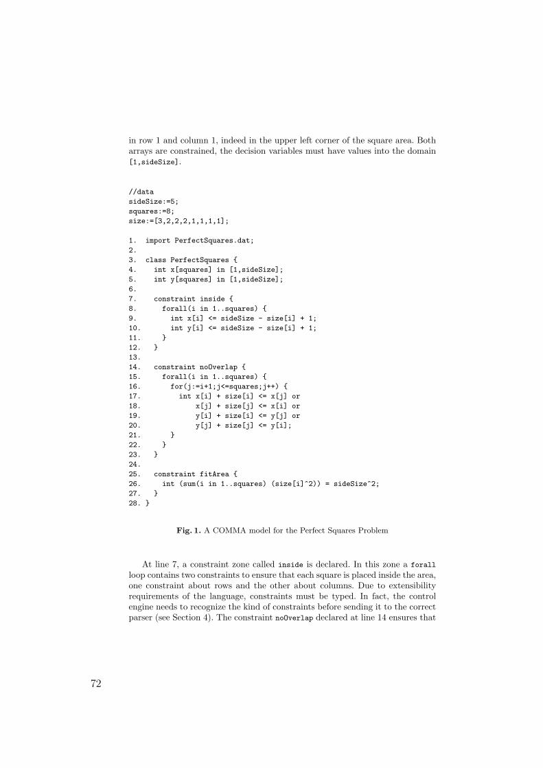
in row 1 and column 1, indeed in the upper left corner of the square area. Botharrays are constrained, the decision variables must have values into the domain[1,sideSize].

//data

sideSize:=5;

squares:=8;

size:=[3,2,2,2,1,1,1,1];

1. import PerfectSquares.dat;

2.

3. class PerfectSquares

4. int x[squares] in [1,sideSize];

5. int y[squares] in [1,sideSize];

6.

7. constraint inside

8. forall(i in 1..squares)

9. int x[i] <= sideSize - size[i] + 1;

10. int y[i] <= sideSize - size[i] + 1;

11.

12.

13.

14. constraint noOverlap

15. forall(i in 1..squares)

16. for(j:=i+1;j<=squares;j++)

17. int x[i] + size[i] <= x[j] or

18. x[j] + size[j] <= x[i] or

19. y[i] + size[i] <= y[j] or

20. y[j] + size[j] <= y[i];

21.

22.

23.

24.

25. constraint fitArea

26. int (sum(i in 1..squares) (size[i]^2)) = sideSize^2;

27.

28.

Fig. 1. A COMMA model for the Perfect Squares Problem

At line 7, a constraint zone called inside is declared. In this zone a forall

loop contains two constraints to ensure that each square is placed inside the area,one constraint about rows and the other about columns. Due to extensibilityrequirements of the language, constraints must be typed. In fact, the controlengine needs to recognize the kind of constraints before sending it to the correctparser (see Section 4). The constraint noOverlap declared at line 14 ensures that

72

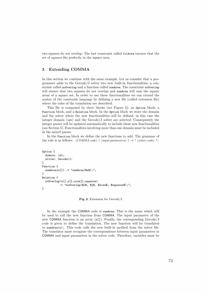
two squares do not overlap. The last constraint called fitArea ensures that theset of squares fits perfectly in the square area.

3 Extending COMMA

In this section we continue with the same example. Let us consider that a pro-grammer adds to the Gecode/J solver two new built-in functionalities: a con-straint called noOverlap and a function called sumArea. The constraint noOverlap

will ensure that two squares do not overlap and sumArea will sum the squareareas of a square set. In order to use these functionalities we can extend thesyntax of the constraint language by defining a new file (called extension file)where the rules of the translation are described.

This file is composed by three blocks (see Figure 2): an Option block, aFunction block, and a Relation block. In the Option block we state the domainand the solver where the new functionalities will be defined, in this case theinteger domain (int) and the Gecode/J solver are selected. Consequently theinteger parser will be updated automatically to include these new functionalities(see Section 5). Functionalities involving more than one domain must be includedin the mixed parser.

In the Function block we define the new functions to add. The grammar ofthe rule is as follows: 〈COMMA-code〉 ( 〈input-parameters〉 ) -> " 〈solver-code〉 ";

Option

domain: int;

solver: Gecode/J;

Function

sumArea(s[]) -> "sumArea($s$);";

Relation

noOverlap(x[],y[],size[],squares)

-> "noOverlap($x$, $y$, $size$, $squares$);";

Fig. 2. Extension for Gecode/J

In the example the COMMA code is sumArea. This is the name which willbe used to call the new function from COMMA. The input parameter of thenew COMMA function is an array (s[]). Finally, the corresponding Gecode/Jcode is given to define the translation. The new function will be translatedto sumArea(s);. This code calls the new built-in method from the solver file.The translator must recognize the correspondence between input parameters inCOMMA and input parameters in the solver code. Therefore, variables must be

73

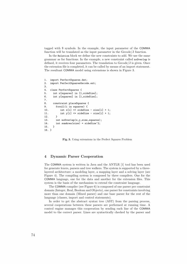
tagged with $ symbols. In the example, the input parameter of the COMMA

function will be translated as the input parameter in the Gecode/J function.In the Relation block we define the new constraints to add. We use the same

grammar as for functions. In the example, a new constraint called noOverlap isdefined, it receives four parameters. The translation to Gecode/J is given. Oncethe extension file is completed, it can be called by means of an import statement.The resultant COMMA model using extensions is shown in Figure 3.

1. import PerfectSquares.dat;

2. import PerfectSquaresGecode.ext;

3.

4. class PerfectSquares

5. int x[squares] in [1,sideSize];

6. int y[squares] in [1,sideSize];

7.

8. constraint placeSquares

9. forall(i in squares)

10. int x[i] <= sideSize - size[i] + 1;

11. int y[i] <= sideSize - size[i] + 1;

12.

13. int noOverlap(x,y,size,squares);

14. int sumArea(size) = sideSize^2;

15.

16.

Fig. 3. Using extensions in the Perfect Squares Problem

4 Dynamic Parser Cooperation

The COMMA system is written in Java and the ANTLR [1] tool has been usedfor generate lexers, parsers and tree walkers. The system is supported by a three-layered architecture: a modeling layer, a mapping layer and a solving layer (seeFigure 4). The compiling system is composed by three compilers. One for theCOMMA language, one for the data and another for the extension files. Thissystem is the basis of the mechanism to extend the constraint language.

The COMMA compiler (see Figure 6) is composed of one parser per constraintdomain (Integer, Real, Boolean and Objects), one parser for constraints involvingmore than one domain (Mixed parser) and one base parser for the rest of thelanguage (classes, import and control statements).

In order to get the abstract syntax tree (AST) from the parsing process,several cooperations between these parsers are performed at running time. Acontrol engine manages this cooperation by sending each line of the COMMA

model to the correct parser. Lines are syntactically checked by the parser and

74

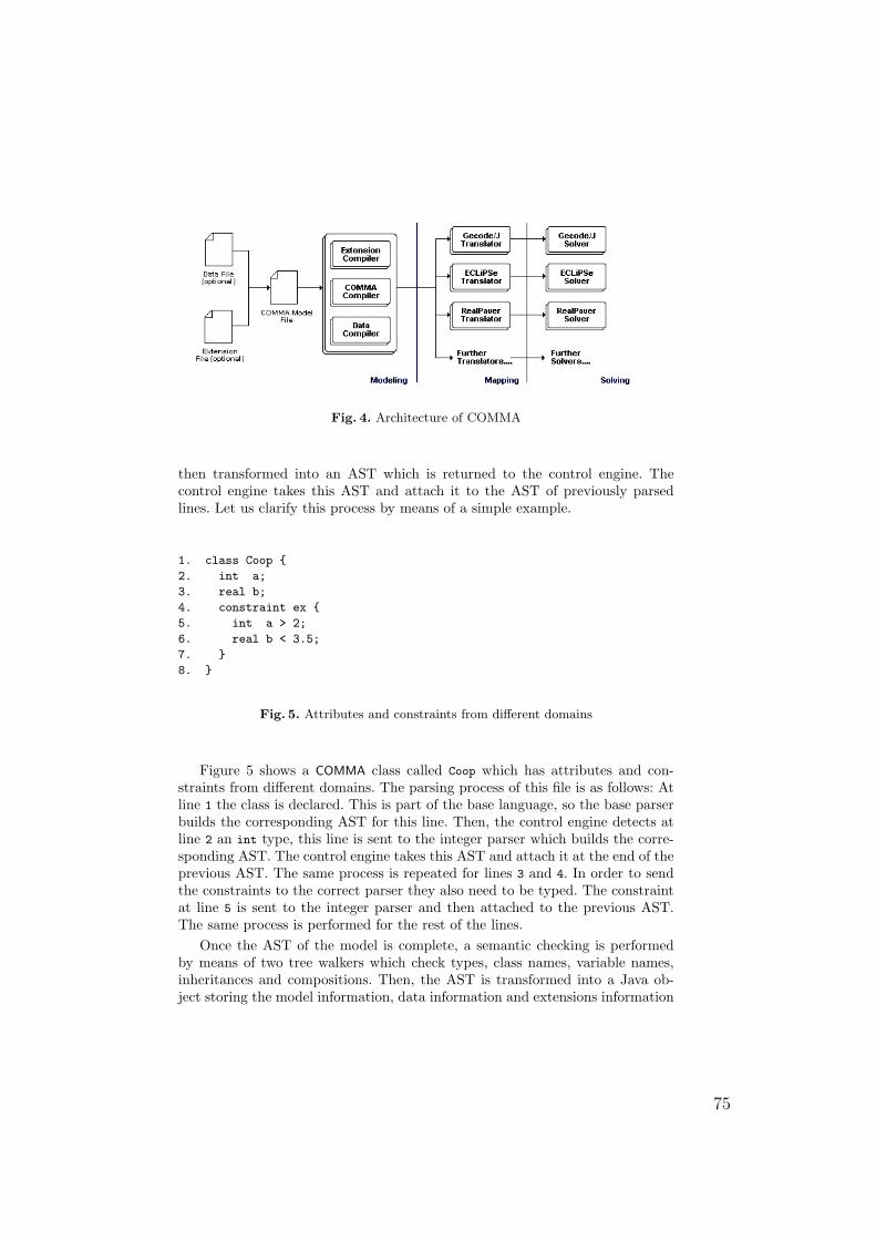
Fig. 4. Architecture of COMMA

then transformed into an AST which is returned to the control engine. Thecontrol engine takes this AST and attach it to the AST of previously parsedlines. Let us clarify this process by means of a simple example.

1. class Coop

2. int a;

3. real b;

4. constraint ex

5. int a > 2;

6. real b < 3.5;

7.

8.

Fig. 5. Attributes and constraints from different domains

Figure 5 shows a COMMA class called Coop which has attributes and con-straints from different domains. The parsing process of this file is as follows: Atline 1 the class is declared. This is part of the base language, so the base parserbuilds the corresponding AST for this line. Then, the control engine detects atline 2 an int type, this line is sent to the integer parser which builds the corre-sponding AST. The control engine takes this AST and attach it at the end of theprevious AST. The same process is repeated for lines 3 and 4. In order to sendthe constraints to the correct parser they also need to be typed. The constraintat line 5 is sent to the integer parser and then attached to the previous AST.The same process is performed for the rest of the lines.

Once the AST of the model is complete, a semantic checking is performedby means of two tree walkers which check types, class names, variable names,inheritances and compositions. Then, the AST is transformed into a Java ob-ject storing the model information, data information and extensions information

75

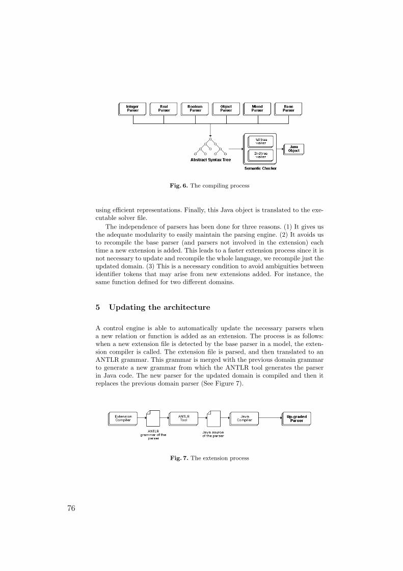
Fig. 6. The compiling process

using efficient representations. Finally, this Java object is translated to the exe-cutable solver file.

The independence of parsers has been done for three reasons. (1) It gives usthe adequate modularity to easily maintain the parsing engine. (2) It avoids usto recompile the base parser (and parsers not involved in the extension) eachtime a new extension is added. This leads to a faster extension process since it isnot necessary to update and recompile the whole language, we recompile just theupdated domain. (3) This is a necessary condition to avoid ambiguities betweenidentifier tokens that may arise from new extensions added. For instance, thesame function defined for two different domains.

5 Updating the architecture

A control engine is able to automatically update the necessary parsers whena new relation or function is added as an extension. The process is as follows:when a new extension file is detected by the base parser in a model, the exten-sion compiler is called. The extension file is parsed, and then translated to anANTLR grammar. This grammar is merged with the previous domain grammarto generate a new grammar from which the ANTLR tool generates the parserin Java code. The new parser for the updated domain is compiled and then itreplaces the previous domain parser (See Figure 7).

Fig. 7. The extension process

76

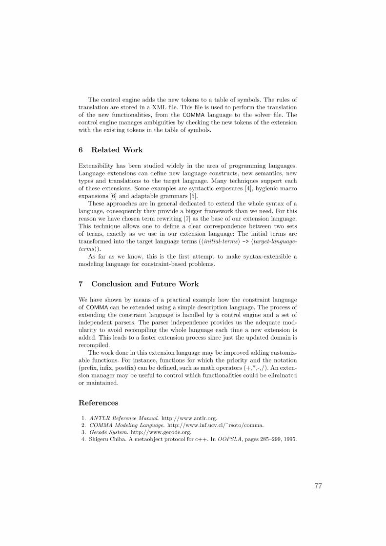
The control engine adds the new tokens to a table of symbols. The rules oftranslation are stored in a XML file. This file is used to perform the translationof the new functionalities, from the COMMA language to the solver file. Thecontrol engine manages ambiguities by checking the new tokens of the extensionwith the existing tokens in the table of symbols.

6 Related Work

Extensibility has been studied widely in the area of programming languages.Language extensions can define new language constructs, new semantics, newtypes and translations to the target language. Many techniques support eachof these extensions. Some examples are syntactic exposures [4], hygienic macroexpansions [6] and adaptable grammars [5].

These approaches are in general dedicated to extend the whole syntax of alanguage, consequently they provide a bigger framework than we need. For thisreason we have chosen term rewriting [7] as the base of our extension language.This technique allows one to define a clear correspondence between two setsof terms, exactly as we use in our extension language: The initial terms aretransformed into the target language terms (〈initial-terms〉 -> 〈target-language-terms〉).

As far as we know, this is the first attempt to make syntax-extensible amodeling language for constraint-based problems.

7 Conclusion and Future Work

We have shown by means of a practical example how the constraint languageof COMMA can be extended using a simple description language. The process ofextending the constraint language is handled by a control engine and a set ofindependent parsers. The parser independence provides us the adequate mod-ularity to avoid recompiling the whole language each time a new extension isadded. This leads to a faster extension process since just the updated domain isrecompiled.

The work done in this extension language may be improved adding customiz-able functions. For instance, functions for which the priority and the notation(prefix, infix, postfix) can be defined, such as math operators (+,*,-,/). An exten-sion manager may be useful to control which functionalities could be eliminatedor maintained.

References

1. ANTLR Reference Manual. http://www.antlr.org.2. COMMA Modeling Language. http://www.inf.ucv.cl/˜rsoto/comma.3. Gecode System. http://www.gecode.org.4. Shigeru Chiba. A metaobject protocol for c++. In OOPSLA, pages 285–299, 1995.

77

5. Henning Christiansen. A survey of adaptable grammars. SIGPLAN Notices,25(11):35–44, 1990.

6. William D. Clinger and Jonathan Rees. Macros that work. In POPL, pages 155–162, 1991.

7. Nachum Dershowitz and Jean-Pierre Jouannaud. Rewrite systems. In Handbook ofTheoretical Computer Science, Volume B: Formal Models and Sematics (B), pages243–320. 1990.

8. Alan M. Frisch et al. The design of essence: A constraint language for specifyingcombinatorial problems. In IJCAI, pages 80–87, 2007.

9. I. Gambini. Quant aux carres carreles. PhD thesis, L’Universite de la Mediterraneeaix-Marseille II, 1999.

10. L. Granvilliers and F. Benhamou. Algorithm 852: Realpaver: an interval solverusing constraint satisfaction techniques. ACM Trans. Math. Softw., 32(1):138–156, 2006.

11. B. Jayaraman and P.Y. Tambay. Constrained Objects for Modeling Complex Struc-tures. In OOPSLA, Minneapolis, USA, 2000.

12. J.F. Puget. A C++ implementation of CLP. In SCIS, Singapore, 1994.13. Reza Rafeh, Maria J. Garcıa de la Banda, Kim Marriott, and Mark Wallace. From

zinc to design model. In PADL, pages 215–229, 2007.14. G. Smolka. The oz programming model. In Computer Science Today, volume 1000

of LNCS, pages 324–343. 1995.15. R. Soto and L. Granvilliers. Exploring the canopy of constraint modeling languages.

In Constraint Modelling and Reformulation Workshop held in conjunction with CP2006, pages 88–101, Nantes, France, 2006.

16. P. Van Hentenryck. The OPL Optimization Programming Language. The MITPress, 1999.

17. M. Wallace, S. Novello, and J. Schimpf. Eclipse: A platform for constraint logicprogramming, 1997.

78

Constraint-Based Examination Timetabling for

the German University in Cairo

Slim Abdennadher and Marlien Edward

German University in Cairo, Department of Computer Science,5th Settlement New Cairo City, Cairo, Egypt

slim.abdennadher@guc.edu.eg,marlien.nekhela@student.guc.edu.eg

http://cs.guc.edu.eg

Abstract. Constraint programming is mainly used to solve combinato-rial problems such as scheduling and allocation, which are of vital impor-tance to modern business. In this paper, we introduce the examinationtimetabling problem at the German University in Cairo. As manual gen-eration of exam schedules is time-consuming and inconvenient, we showhow this problem can be modeled as a constraint satisfaction problemand can be solved using SICStus Prolog with its powerful constraintlibrary.

1 Introduction

Timetabling problems are real life combinatorial problems concerned with schedul-ing a certain number of events within a specific time frame. If solved manually,timetabling problems are extremely hard and time consuming and hence theneed to develop tools for their automatic generation [4].

The German University in Cairo (GUC) started in Winter 2003. Each yearthe number of students increases and the timetabling problem whether for coursesor examinations becomes slightly more difficult. For the past four years, schedulesfor both courses and exams has been generated manually. The process involvesattempting to assign courses/exams to time slots and rooms while satisfying acertain number of constraints. Processed manually the course timetabling tookon average three weeks, while the examination timetabling a week. With thegrowing number of students, the GUC timetabling problems have become toocomplex and time-consuming to be solved manually.

In this paper, we will only address the examination timetabling problem.Currently, at the GUC, there are 140 courses, 5500 students, and around 1300seats for which examinations should be scheduled. The examination schedulesare generated twice per semester. Once for the midterm examinations, whichoccur in the middle of the semester and are distributed over a one week period;and again during the final examinations, which occur at the end of the semesterand are distributed over a two weeks period.

The examination timetabling problem at the GUC is non-interruptible anddisjunctive. It is non-interruptible since once an examination starts it can not be

79

paused and resumed later. It is disjunctive since an examination room can onlycontain one exam at a specific time. A solution to the examination timetablingproblem aims at allocating a time slot and a room to every examination whilesatisfying a given set of constraints.

Several approaches have been used to solve such combinatorial problems [6],e.g. using an evolutionary search procedures such as ant colony optimization [3],or using a combination of constraint programming and local search techniques[5], or using graph coloring approach [2].

In this paper, we present an ongoing research to develop a constraint-basedsystem to solve the examination timetabling problem at the GUC. Constraintprogramming is a problem-solving technique that works by incorporating con-straints into a programming environment [1]. Constraints are relations whichspecify the domain of solutions by forbidding combinations of values. Constraintprogramming draws on methods from artificial intelligence, logic programming,and operations research. It has been successfully applied in a number of fieldssuch as scheduling, computational linguistics, and computational biology.

In this paper, we show how the GUC examination timetabling problem canbe formalized as a constraint satisfaction problem (CSP) and implemented bymeans of specialized constraint solving techniques that are available in a con-straint logic programming language (CLP) like SICStus Prolog. In solving theproblem, we have to deal with two types of constraints, hard constraints andsoft constraints. Hard constraints are constraints that must be satisfied. Theyrepresent regulations for examinations and resource (rooms) constraints. Softconstraints are constraints that should be satisfied but can be violated. Softconstraints can for example represent wishes of lecturers and students.

The paper is organized as follows. The next section introduces the GUCexamination timetabling problem and its requirements. Then we show how theproblem can be modeled as a CSP problem and how we implemented the differentconstraints in SICStus Prolog. Finally, we conclude with a summary and futurework.

2 Problem Description and Requirements

The GUC examination timetabling problem aims at producing examinationschedules for all courses given in a particular term. The GUC has four dis-tinct faculties where each faculty offers a variety of majors. Some of the majorsoffer the same courses which makes examination scheduling for these coursesinterdependent.

Students are enrolled in the different courses according to their major. Stu-dents in every major are divided into student groups depending on the coursesthey take. This grouping of students taking the same stream of courses simplifiesthe scheduling task since a large number of students can be dealt with as a singleentity with a certain number of students.

The examination slots at the GUC differ from the midterms to the finalexaminations. Usually the midterm examinations are distributed over a one week

80

period where the days are divided into four examination slots and the durationof each examination slot is 2 hours. The final examination period consist of twoweeks with three examination slots per day where each examination slot is 3hours.

The GUC examination timetabling problem consists of a set of courses anda set of students that need to be scheduled within limited resources of time andspace. The task is to assign the student groups to examination slots and thusproduce examination schedules for the midterm and final examinations. Sincescheduling of the student groups from the different faculties is interdependentas time, space and specific courses are shared, schedules for the different fac-ulties can not be produced separately and thus a single schedule for the wholeuniversity must be generated.

The GUC examination timetabling problem can be performed in two phases.In the first phase, the different course examinations are assigned to time slotswhile taking into account only the total number of students enrolled in thecourses and the total number of available seats. In the second phase, after pro-ducing the examination schedule for all student groups, distribution of studentsamong the rooms is done. In this paper, we will only model the first phase asa constraint satisfaction problem and solve it using constraint programming.The second phase does not require constraint techniques. A simple algorithmwas designed and implemented using Java to distribute the students among theexamination rooms and seats. In both phases, the different constraints that areimposed by the regulations of the GUC Examination Committee have to betaken into account. Dividing the examination scheduling problem into two partsreduces the complexity since the number of constraints that must be satisfiedper phase is decreased. This division is feasible since the total number of seatsis considered in the course scheduling (first) phase.

When assigning an examination to a certain time slot, several constraintsmust be considered.

Time Clash Constraint: A student group cannot have more than one exam-ination at the same time.

Semester Clash Constraint: Student groups from the same major but in dif-ferent semesters cannot have examinations at the same time. This is neededto enable students who are re-taking a course from a previous semester dueto poor performance to sit for the course examination.

Core Exam Constraint: A student group cannot take more than one coreexamination per day.

Exam Restriction Constraint: A student group cannot have more than acertain number of examinations per day.

Difficulty Constraint: A student group cannot have two difficult examina-tions in two consecutive days (difficulty rating for a course is assigned bythe course lecturer and students).

Capacity Constraint: The total number of students sitting for an examina-tion in a certain time slot cannot exceed a predefined limit. This constraintensures that the total number of students sitting for an examination at a

81

certain time slot do not exceed the total number of available seats in theuniversity campus.

Pre-assignment Constraint: An examination should be scheduled in a spe-cific time slot.

Unavailability Constraint: An examination should not be scheduled in a spe-cific time slot.

3 Modeling the Problem as a Constraint Satisfaction

Problem

Constraint satisfaction problems have been a subject of research in Artificialintelligence for many years [7].

A constraint satisfaction problem (CSP) is defined by a set of variables eachhaving a specific domain and a set of constraints each involving a set of variablesand restricting the values that the variables can take simultaneously.

The solution to a CSP is an assignment that maps every variable to a value.We may want to find just one solution, all possible solutions or an optimalsolution given some objective function defined in terms of some or all variables.Here we are speaking about a constraint satisfaction optimization problem.

In modeling the GUC examination timetabling problem as a CSP we use thefollowing notations :

- n is the number of courses to be scheduled.- D = 1, . . . , m indicates a set of m time slots.- T = T1, . . . , Tn represents the time slot variables for all examinations,

where Ti indicates the time slot assigned to an examination i.- l is the number of all student groups in the university.- The domain of every variable Ti is between 1 and m.

m is the number of available time slots and can be calculated by multiplyingthe number of days of the examination period by the number of slots per day.For example, if the examination period consists of 6 days and every day consistsof 3 time slots therefore the available number of time slots is 18.

Different constraints are applied on Ti eliminating the different values eachvariable can take and thus reducing the domains of every variable to improvethe efficiency of the search thus reaching a solution in an optimal time.

Now we describe the requirements of our problem in terms of SICStus prologusing the constraint solver over finite domains (clpfd).

Time clash constraint stating that no student can have more than one exam atthe same time slot can be enforced using the all_different/1 global constraint.We have to constrain the l sets of variables representing the courses for everygroup of students to be different.

Let Tgroup = [T1,...,Tj] be a list of variables that represent examinationtime slots of a specific group then applying the all_different/1 constraint onthis list would ensure that all exams for that group are held in different timeslots. Note that Tgroup is a subset of T

82

all_different(Tgroup)

In order to abide to the semester clash constraint, we have to take intoconsideration that all examinations of the same major should be scheduledat different time slots. Let Y be the number of courses of a certain major.Tmajor = [T1,...,TY] is a list of variables representing examination time slotsfor these courses. Applying the all_different/1 constraint on these variableswill ensure that all these exams are assigned to different time slots.

all_different(Tmajor)

Difficulty constraint has to be fulfilled in order to produce a valid examinationschedule. We cannot schedule two difficult exams consecutively. Knowing thedifficulty rating of every course, all time slot variables for difficult examinationscan be known. For every two variables representing difficult examinations of astudent group an inequality constraint (# ≤) is imposed on their difference. Thisdifference has to be greater than a certain number.

Enforcing the core exam constraint produces an acceptable examinationschedule. A student cannot take more than one core exam per day. We canimpose this constraint using the serialized/2 global constraint. In general,the constraint Serialized/2 constrains x tasks, each with a starting time andduration so that no tasks overlap. In our case, if we add to the duration of ev-ery core exam the number of slots per day, we can get a gap of at least oneday between every two core examinations. Let Z be the number of core coursesof a certain student group and Tcore = [T1,...,TZ] is a list variables thatrepresent the time slots for these course then applying the following constraint

serialized(Tcore,[Gaps_added_durations])

will ensure that the gaps between core examinations is at least one day.

Exam restriction constraint limits the number of examinations held per dayfor every student to be less than a certain number. The variables that representthe examination time slots for every student group are known. The global con-straint count/4 can be used to limit the number of variables assigned to the sameday to be less than a certain number. Let x be the number of courses assigned toa specific student group, T = [T1,...,Tx] is a list of variables representing theday of every examination slot and 1≤Y≤m, then count(Y, T, #<, 3) should beapplied m times for every group of students constraining the number of examsheld on every day to be less than 3.

In order to enforce the capacity constraint, the number of all students attend-ing an examination at a certain time slot should not exceed a certain limit. Thecumulative/4 global constraint can be used to assign a number of examinationsto the same time slot constraining the number of students to be less than thespecified limit.

cumulative(Starts, Durations, Capacities, limit)

83

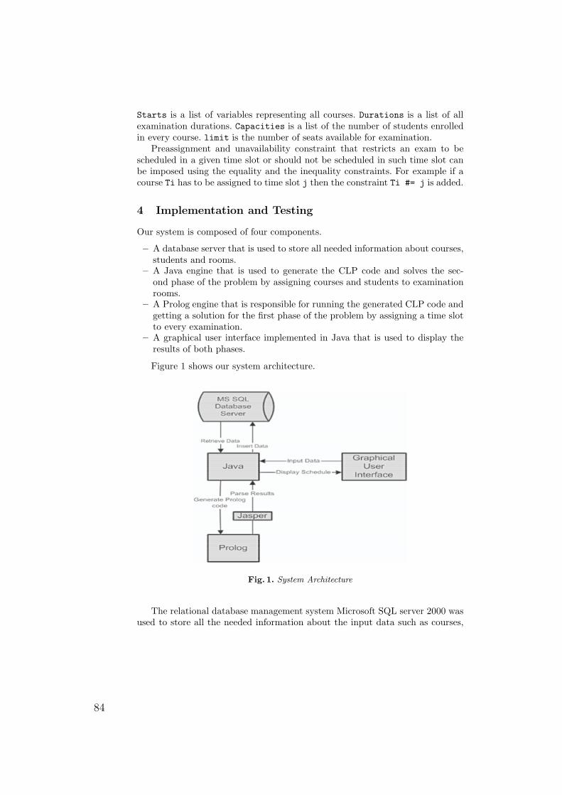
Starts is a list of variables representing all courses. Durations is a list of allexamination durations. Capacities is a list of the number of students enrolledin every course. limit is the number of seats available for examination.

Preassignment and unavailability constraint that restricts an exam to bescheduled in a given time slot or should not be scheduled in such time slot canbe imposed using the equality and the inequality constraints. For example if acourse Ti has to be assigned to time slot j then the constraint Ti #= j is added.

4 Implementation and Testing

Our system is composed of four components.

– A database server that is used to store all needed information about courses,students and rooms.

– A Java engine that is used to generate the CLP code and solves the sec-ond phase of the problem by assigning courses and students to examinationrooms.

– A Prolog engine that is responsible for running the generated CLP code andgetting a solution for the first phase of the problem by assigning a time slotto every examination.

– A graphical user interface implemented in Java that is used to display theresults of both phases.

Figure 1 shows our system architecture.

Fig. 1. System Architecture

The relational database management system Microsoft SQL server 2000 wasused to store all the needed information about the input data such as courses,

84

student groups and rooms as well as the output data such as the exams with theirexamination time slots and examination rooms. Relations between the differenttables of the database are maintained in order to specify the courses of everystudent group and the rooms in which every exam of a course is held. An instanceof an examination is expressed by a pair exam(C,T), where C is a unique courseidentifier and T is the examination time slot assigned to that course. Instancesof examinations of the different courses are the inputs to our problem.

In general, a CLP program consists of three basic parts. We begin by associ-ating domains to the different variables we have, then the different constraintsof the problem are specified, and finally a labeling strategy is defined to lookfor a feasible solution via a backtrack search or via a branch-and-bound search.Labeling, which is used to assign values to variables, is needed since constraintsolving is in general incomplete. We employed the first-fail strategy to select thecourse to be scheduled and a domain splitting strategy to select a period fromthe domain of the selected course. First-fail selects one of the most-constrainedvariables, i.e. one of the variables with the smallest domain. Domain splittingcreates a choice between X #=< M and X #> M, where M is the midpoint of thedomain of X. This approach yielded a good first solution to our problem. Theinput to a CLP program is usually in the form of a list. Constraints are expressedusing the predefined constraints implemented in the constraint solver over finitedomains clpfd.

Initially, we query the database using Java to obtain all the informationneeded to be able to produce a valid assignment. The CLP code is generated suchthat it restricts the solutions using the constraints already chosen by the userthrough the graphical interface. The input to our problem is a list of timetableinstances. While generating that list we constrain the values of the time slotvariables using the membership global constraint domain/3. After generatingthe list of instances, different constraints are applied to the variables eliminatingvalues of their domains until finally a solution is reached.

After generating the SICStus prolog code, Jasper1 is used to consult theprogram and parse the the values of the variables that represent the time slotsfor the different examinations. These values with their associated examinationinstances are stored in the database. A graphical user interface is then used todisplay the generated timetable. Figure 2 shows a sample output for a test runof our implementation.

Our system was tested on realistic data and constraints for the generation ofthe examination timetable for the final examinations of this term, Spring 2007.The test data consisted of 140 courses, 5500 students, and 1300 available seatsfor them. A solution was generated within few seconds. Our testing environmentwas a Microsoft Windows Vista Ultimate running on 32-bit processor at 1.73GHz with 1 GB of RAM.

1 a prolog interface to the java virtual machine

85

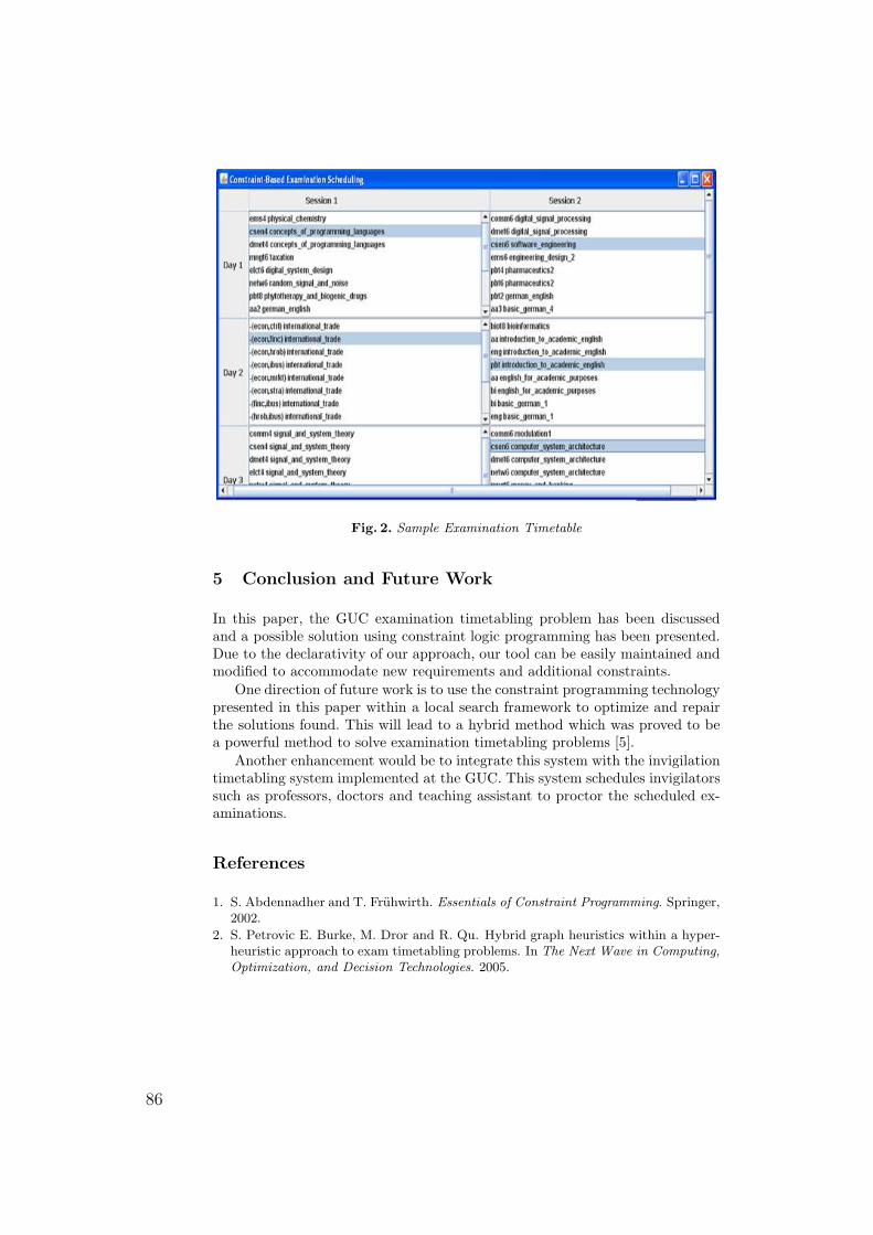
Fig. 2. Sample Examination Timetable

5 Conclusion and Future Work

In this paper, the GUC examination timetabling problem has been discussedand a possible solution using constraint logic programming has been presented.Due to the declarativity of our approach, our tool can be easily maintained andmodified to accommodate new requirements and additional constraints.

One direction of future work is to use the constraint programming technologypresented in this paper within a local search framework to optimize and repairthe solutions found. This will lead to a hybrid method which was proved to bea powerful method to solve examination timetabling problems [5].

Another enhancement would be to integrate this system with the invigilationtimetabling system implemented at the GUC. This system schedules invigilatorssuch as professors, doctors and teaching assistant to proctor the scheduled ex-aminations.

References

1. S. Abdennadher and T. Fruhwirth. Essentials of Constraint Programming. Springer,2002.

2. S. Petrovic E. Burke, M. Dror and R. Qu. Hybrid graph heuristics within a hyper-heuristic approach to exam timetabling problems. In The Next Wave in Computing,

Optimization, and Decision Technologies. 2005.

86

3. M. Eley. Ant algorithms for the exam timetabling problem. In Proceedings of the

6th International Conference on the Practice and Theory of Automated Timetabling,2006.

4. B. McCollum and N. Ireland. University timetabling: Bridging the gap betweenresearch and practice. In Proceedings of the 6th International Conference on the

Practice and Theory of Automated Timetabling, 2006.5. L. T.G. Merlot, N. Boland, B. D. Hughes, and P. J. Stuckey. A hybrid algorithm

for the examination timetabling problem. In Proceedings of the 6th International

Conference on the Practice and Theory of Automated Timetabling, 2002.6. Andrea Schaerf. A survey of automated timetabling. In 115, page 33. Centrum voor

Wiskunde en Informatica (CWI), ISSN 0169-118X, 30 1995.7. Edward Tsang. Foundation of Constraint Satisfaction. Academic Press, London

and San Diego, 1993.

87

Constraint-Based University Timetabling for theGerman University in Cairo

Slim Abdennadher and Mohamed Aly

German University in Cairo, Department of Computer Science,5th Settlement New Cairo City, Cairo, Egypt

slim.abdennadher@guc.edu.eg,mohamed.abdulazim@student.guc.edu.eg

http://cs.guc.edu.eg

Abstract. The course timetabling problem at the German University inCairo has been in existence ever since the establishment of the universityin 2003. Courses offered at the university, academic staff resources, androom resources make the problem over-constrained. Currently timetablesare manually designed. The process is effort and time consuming and theresults are often not satisfactory. In this paper, we provide a descriptionof the problem and we show how it can be modeled as a constraint satis-faction problem. Our system, implemented in SICStus Prolog, generatesa good timetable within some minutes instead of by hand some weeks.

1 Introduction

University course timetabling problems are combinatorial problems which con-sist in scheduling a set of courses within a given number of rooms and timeperiods. Generic solutions implemented and designed for such problems are notalways compatible with all universities due to the wide variety of constraints.Number of courses, academic resources, room resources, and university-specificrequirements are all factors which make the problem variant and hard. There-fore, universities design timetables manually or attempt to implement a tailoredsystem that suits their requirements and constraints. Generating a timetablemanually often requires a lot of time and effort. In addition, manually gener-ated schedules usually fail to satisfy all essential constraints which are criticalfor the operation of the university. Thus, automating the generation of coursetimetables is still a challenging task [1].

The German University in Cairo (GUC), established in 2003, currently has5500 students, and offers 140 courses through an academic staff of 300 mem-bers. Course timetabling has been a problem at the GUC ever since it started.Timetables are manually generated. The main goal is to generate a schedulewhich is personalized for all students in different faculties at the university. Manyproblems arise with the resulting schedules like teaching assistant allocation todifferent sessions in the same time slot or single room allocation to multiplesessions at the same instance. With an increasing number of students, academicstaff and room resources, the timetabling problem complexity is getting more

88

arduous. The amount of time, work, and effort invested in making a timetable isvery tremendous. Designing a valid timetable requires many iterations betweenthe person in charge and academic department heads. At the end, the schedule“does the job” but not satisfactorily.

Several approaches have been proposed to solve course timetabling problems[2]. The most popular technique is based on graph coloring algorithms [3]. Themain disadvantage of this approach is the difficulty of incorporating applicationspecific constraints into the problem formulation. Other methods include localsearch techniques, e.g. simulated annealing [4] and genetic algorithms [5, 6]. Inthis paper, we present a constraint-based system to solve the course timetablingproblem at the German University in Cairo. Constraint Programming drawson methods from artificial intelligence, logic programming, and operations re-search. It has been successfully applied in scheduling problems and proved tohave promising results [7–11].

The paper is organized as follows. Section 2 introduces the course timetablingproblem at the GUC and all constraints associated with it. In Section 3, wedescribe how the problem can be modeled as a constraint satisfaction problem. InSection 4, we give an overview of our implemented system. Finally, we concludewith a summary and directions for future work.

2 Problem Description

The GUC consists of four faculties, namely the faculty of Engineering, the facultyof Pharmacy and Biotechnology, the faculty of Management, and the faculty ofApplied Arts. Each faculty offers a set of majors. For every major, there is aset of associated courses. Courses are either compulsory or elective. Facultiesdo not have separate buildings, therefore all courses from all faculties should bescheduled taking into consideration shared room resources. Students registered toa major are distributed among groups for lectures (lecture groups) and groupsfor tutorials or labs (study groups). A study group consists of maximum 25students. Students registered to study groups are distributed among languagegroups. In each semester study groups are assigned to courses according to theircorresponding curricula and semester. Due to the large number of students ina faculty and lecture hall capacities, all study groups cannot attend the samelecture at the same time. Therefore, groups of study groups are usually assignedto more than one lecture group. For example, if there are 27 groups studyingMathematics, then 3 lecture groups will be formed.

The timetable at the GUC spans a week starting from Saturday to Thursday.A day is divided to five time slots, where a time slot corresponds to 90 minutes.An event can take place in a time slot. This can be either a lecture, exercise,or practical session and it is given by either a lecturer or a teaching assistant.Usually, lectures are given by lecturers and exercise and practical sessions aregiven by teaching assistants. In normal cases, lectures take place at lecture halls,exercise sessions at exercise rooms and practical sessions take place in specializedlaboratories depending on the requirements of a course. In summary, an event is

89

given by a lecturer or an assistant during a time slot in a day to a specific groupusing a specific room resource. This relationship is represented by a timetablefor all events provided that hard constraints are not violated. Hard constraintsare constraints that cannot be violated and which is considered to be of greatnecessity to the university operation. These constraints can be also added bysome lecturers like part timers or visiting professors. Hard constraints will beoutlined and discussed later in this section. The timetable tries to satisfy otherconstraints which are not very important or critical. Such constraints are knownas soft constraints that should be satisfied but maybe violated. For example,these constraints can come in form of wishes from various academic staff.

Courses have specific credit hours. The credit hours are distributed on lecture,exercise, or practical sessions. Every two credit hours correspond to a teachinghour. A teaching hour corresponds to a time slot on the timetable. Sessions withone credit hour corresponds to a biweekly session. These sessions are usuallyscheduled to take place with other biweekly sessions if possible. For example acourse with 3 lecture credit hours, 4 exercise credit hour and 0 practical credithours can be interpreted as having two lectures per week one being scheduledweekly and the other is biweekly, two exercise sessions per week and no practicalsessions. Lecture groups and study groups take the corresponding number ofsessions per week. Courses might have hard constraints. Some courses requirespecialized laboratories or rooms for their practical or exercise sessions. Forexample, for some language courses a special laboratory with audio and videoequipment is required. The availability of required room resources must be takeninto consideration while scheduling. Some lecturers have specific requirements onsession precedences. For example, in a computer science introductory course alecturer might want to schedule exercise sessions before practical sessions.

Furthermore, some constraints should be taken into consideration to improvethe quality of education. An important constraint is that no lectures should bescheduled in the last slot of any day. Another constraint requires that a certainday should have an activity slot for students, and a slot where all universityacademics can meet. For those slots no sessions should be scheduled. A studygroup should avoid spending a full day at the university. In other words, themaximum number of slots that a group can attend per day is 4. Therefore, if agroup starts its day on the first slot, then it should end its day at most on thefourth slot, and if it starts its day on the second slot, then it should end its day atmost on the fifth slot. Furthermore, The number of days off of a group dependson the total number of credit hours a group has. For example, if a group has atotal of 24 course credit hours in a semester, the total number of slots neededwould be 24

2 = 12 slots, which corresponds to 3 study days, then a group mayhave 6− 3 = 3 days off in a week.

A certain number of academics are assigned to a course at the beginning ofa semester. Teaching assistants are assigned to one course at a time. For coursesinvolving practical and exercise sessions, a teaching assistant can be assigned toboth an exercise and a practical session or one of them. This should be takeninto consideration when scheduling to avoid a possible clash. Furthermore, the

90

total numbers of teaching assistants assigned to a session should not exceed themaximum number of assistants assigned to the corresponding course at any time.A lecturer can be assigned to more than once course. This should be consideredwhen scheduling in order to avoid a possible overlap. Academics assigned tocourses have a total number of working and research hours per day and daysoff that need to be considered when scheduling. Courses should be scheduled ina manner such that the number of session hours given by an academic shouldnot exceed his or her teaching load per day taking into consideration days off.For some courses, part timer lecturers are assigned. Those lecturers impose hardconstraints most of the time. They might have special timing requirements orroom requirements. These constraints are considered of a high priority and mustbe taken into consideration.

Another problem that resides when scheduling is the GUC transportationproblem. The GUC provides bus transportation services for both students andacademics. Two bus rounds take place in the beginning of the day to transportstudents and academics from various meeting points in Cairo. Other bus roundstake place, one after the fourth slot and the other after the fifth slot to transportstudents and academics back home. The first round delivers students just beforethe first slot and the second round delivers students just before the second slot.The number of students coming each day at the GUC by bus should be asbalanced as possible in a way such that no limitation as possible is encounteredwith bus resources.

The GUC problem is too complex since a lot of constraints should be takeninto account when scheduling a session. Due to the complexity of the problem, agood heuristic and a good model is needed to solve the problem. Any generatedsolution would be acceptable as it would save weeks of manual work. The solutioncan then be manually edited and modified later on. After getting to a goodschedule minor amendments can be done to improve it.

3 Modeling the Problem as a Constraint SatisfactionProblem

In our model we have 5 slots in a day and 6 days in a week, our domain is chosento be from 1 to 30 where each number corresponds to a slot. For example, slot1 would correspond to the first slot on Saturday, and slot 23 would correspondto the third slot on Wednesday. Consequently, slots from 1 to 5 correspond toSaturday, 6 to 10 correspond to Sunday, 11 to 15 correspond to Monday, and soon. Figure 1 visualizes the timetable.

At each slot a group attends an instance of a course (lecture, tutorial, orpractical session). We define this relationship by the tuple(COURSE, GROUP, TY PE, SEQ, BI), where COURSE is a unique identifierof a certain course, GROUP is a unique identifier of a certain group, TY PEdeclares the course instance (LECT for a lecture session, EXER for an exercisesession, and PRAC for a practical session), SEQ enumerates the instance number(for example if two lectures are offered within the week, then two sequences are

91

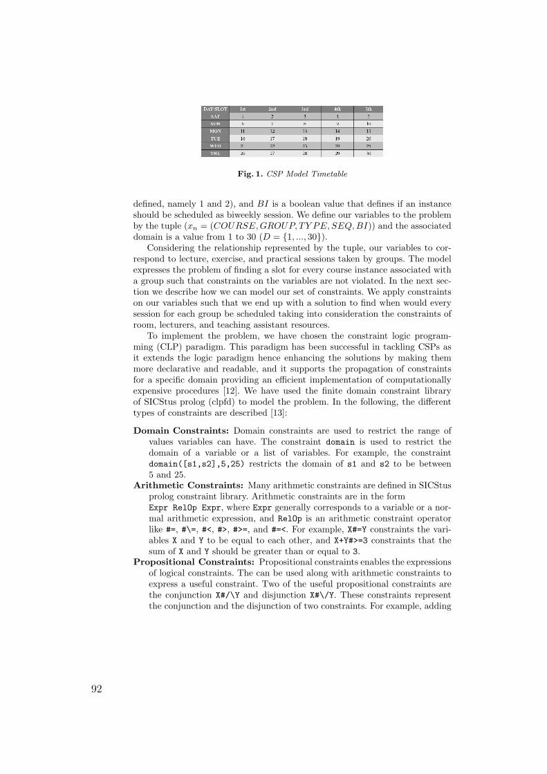
Fig. 1. CSP Model Timetable

defined, namely 1 and 2), and BI is a boolean value that defines if an instanceshould be scheduled as biweekly session. We define our variables to the problemby the tuple (xn = (COURSE,GROUP, TY PE, SEQ,BI)) and the associateddomain is a value from 1 to 30 (D = 1, ..., 30).

Considering the relationship represented by the tuple, our variables to cor-respond to lecture, exercise, and practical sessions taken by groups. The modelexpresses the problem of finding a slot for every course instance associated witha group such that constraints on the variables are not violated. In the next sec-tion we describe how we can model our set of constraints. We apply constraintson our variables such that we end up with a solution to find when would everysession for each group be scheduled taking into consideration the constraints ofroom, lecturers, and teaching assistant resources.

To implement the problem, we have chosen the constraint logic program-ming (CLP) paradigm. This paradigm has been successful in tackling CSPs asit extends the logic paradigm hence enhancing the solutions by making themmore declarative and readable, and it supports the propagation of constraintsfor a specific domain providing an efficient implementation of computationallyexpensive procedures [12]. We have used the finite domain constraint libraryof SICStus prolog (clpfd) to model the problem. In the following, the differenttypes of constraints are described [13]:

Domain Constraints: Domain constraints are used to restrict the range ofvalues variables can have. The constraint domain is used to restrict thedomain of a variable or a list of variables. For example, the constraintdomain([s1,s2],5,25) restricts the domain of s1 and s2 to be between5 and 25.

Arithmetic Constraints: Many arithmetic constraints are defined in SICStusprolog constraint library. Arithmetic constraints are in the formExpr RelOp Expr, where Expr generally corresponds to a variable or a nor-mal arithmetic expression, and RelOp is an arithmetic constraint operatorlike #=, #\=, #<, #>, #>=, and #=<. For example, X#=Y constraints the vari-ables X and Y to be equal to each other, and X+Y#>=3 constraints that thesum of X and Y should be greater than or equal to 3.

Propositional Constraints: Propositional constraints enables the expressionsof logical constraints. The can be used along with arithmetic constraints toexpress a useful constraint. Two of the useful propositional constraints arethe conjunction X#/\Y and disjunction X#\/Y. These constraints representthe conjunction and the disjunction of two constraints. For example, adding

92

the constraint X#=Y #/\ X#=Z constrains that X can either be equal to Y orZ.

Combinatorial Constraints: Combinatorial constraints vary in form. Two ofthe widely used constraints are all_different/1 and count/4. The in-put for the global constraint all_different constraint is a list. The con-straint ensures that all elements of the list are distinct. For example ifthe input list is a list of sessions from s1..N, then the constraint will beadded as all_different([s1,s2,...,sN]). Another combinatorial con-straint used is the count/4. The input to the constraint is in the formVal, List, RelOp, Count , where Val is a number, List is a list of vari-ables, RelOp is an arithmetic constraint operator, and Count is a number.The constraint is satisfied if N is the number of elements of List that areequal to Val and N RelOp Count. For example, count(1,[A,B,C],#<,2)constraints that the total number of elements in the list [A,B,C] having thevalue 1 should be less than 2.

The following describes the real constraints and how we used SICStus clpfdlibrary to model them:

Domain of Sessions is from 1 to 30: To restrict the domain of the sessions,we use the global constraint domain. In order to constraint the list L of allvariables, we add the constraint domain(L,1,30).

Group Session Overlap: The sessions of a study group should not overlap;i.e. a study group cannot attend two different courses at the same time. Theglobal constraint all_different is used to model constraints on sessionswhere no overlap should be encountered. For example, if sessions s1,s2,s3belong to a group, then we add a constraint all_different([s1,s2,s3]).

Lecturer giving more than a course: Academic members who teach morethan one course should not have their sessions overlapped while scheduling.To ensure this, we add an all_different constraint to constrain the sessionsgiven by an academic member.

Full Day Prevention Constraint: To avoid bringing a group for a full day,then their associated sessions in a day should not be scheduled either inthe first slot or in the last slot. To model this we use the inequality con-straint with the conjunction #/\ and the disjunction #\/ constraints toexclude the first session and the last session of each day for every group.For example, if the following sessions s1, s2, s3 are for a group and wewould like to constraint the first day (slots 1,2,3,4,5), we add the constraint(s1#\=1#/\ s2 #\= 1 #/\s3 #\= 1)#\/(s1 #\= 5 #/\s2 #\=5 #/\ s3 #\=5).

Course Precedence Requirements: For all courses that have special prece-dence requirements on sessions (i.e. if an exercise session must scheduledbefore a practical session), we use the less than constraint #<. For example,if s2 is before s1 we add the constraint s2#<s1.

Part Timer Constraints: If a part timer lecturer selects a certain slot to givea session, then all session variables given by this lecturer will be constrained,

93

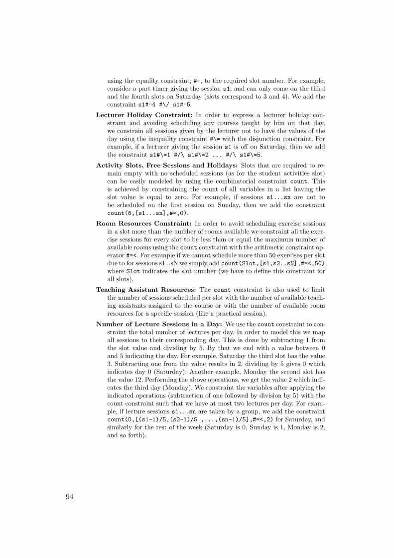
using the equality constraint, #=, to the required slot number. For example,consider a part timer giving the session s1, and can only come on the thirdand the fourth slots on Saturday (slots correspond to 3 and 4). We add theconstraint s1#=4 #\/ s1#=5.

Lecturer Holiday Constraint: In order to express a lecturer holiday con-straint and avoiding scheduling any courses taught by him on that day,we constrain all sessions given by the lecturer not to have the values of theday using the inequality constraint #\= with the disjunction constraint. Forexample, if a lecturer giving the session s1 is off on Saturday, then we addthe constraint s1#\=1 #/\ s1#\=2 ... #/\ s1#\=5.

Activity Slots, Free Sessions and Holidays: Slots that are required to re-main empty with no scheduled sessions (as for the student activities slot)can be easily modeled by using the combinatorial constraint count. Thisis achieved by constraining the count of all variables in a list having theslot value is equal to zero. For example, if sessions s1...sn are not tobe scheduled on the first session on Sunday, then we add the constraintcount(6,[s1...sn],#=,0).

Room Resources Constraint: In order to avoid scheduling exercise sessionsin a slot more than the number of rooms available we constraint all the exer-cise sessions for every slot to be less than or equal the maximum number ofavailable rooms using the count constraint with the arithmetic constraint op-erator #=<. For example if we cannot schedule more than 50 exercises per slotdue to for sessions s1...sN we simply add count(Slot,[s1,s2..sN],#=<,50),where Slot indicates the slot number (we have to define this constraint forall slots).

Teaching Assistant Resources: The count constraint is also used to limitthe number of sessions scheduled per slot with the number of available teach-ing assistants assigned to the course or with the number of available roomresources for a specific session (like a practical session).

Number of Lecture Sessions in a Day: We use the count constraint to con-straint the total number of lectures per day. In order to model this we mapall sessions to their corresponding day. This is done by subtracting 1 fromthe slot value and dividing by 5. By that we end with a value between 0and 5 indicating the day. For example, Saturday the third slot has the value3. Subtracting one from the value results in 2, dividing by 5 gives 0 whichindicates day 0 (Saturday). Another example, Monday the second slot hasthe value 12. Performing the above operations, we get the value 2 which indi-cates the third day (Monday). We constraint the variables after applying theindicated operations (subtraction of one followed by division by 5) with thecount constraint such that we have at most two lectures per day. For exam-ple, if lecture sessions s1...sn are taken by a group, we add the constraintcount(0,[(s1-1)/5,(s2-1)/5 ,...,(sn-1)/5],#=<,2) for Saturday, andsimilarly for the rest of the week (Saturday is 0, Sunday is 1, Monday is 2,and so forth).

94

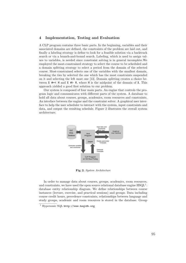
4 Implementation, Testing and Evaluation

A CLP program contains three basic parts. In the beginning, variables and theirassociated domains are defined, the constraints of the problem are laid out, andfinally a labeling strategy is define to look for a feasible solution via a backtracksearch or via a branch-and-bound search. Labeling, which is used to assign val-ues to variables, is needed since constraint solving is in general incomplete.Weemployed the most-constrained strategy to select the course to be scheduled anda domain splitting strategy to select a period from the domain of the selectedcourse. Most-constrained selects one of the variables with the smallest domain,breaking the ties by selected the one which has the most constraints suspendedon it and selecting the left most one [13]. Domain splitting creates a choice be-tween X #=< M and X #> M, where M is the midpoint of the domain of X. Thisapproach yielded a good first solution to our problem.

Our system is composed of four main parts. An engine that controls the pro-gram logic and communicates with different parts of the system. A database tohold all data about courses, groups, academics, room resources and constraints.An interface between the engine and the constraint solver. A graphical user inter-face to help the user scheduler to interact with the system, input constraints anddata, and output the resulting schedule. Figure 2 illustrates the overall systemarchitecture.

Fig. 2. System Architecture

In order to manage data about courses, groups, academics, room resources,and constraints, we have used the open source relational database engine HSQL1.database entity relationship diagram. We define relationships between courseinstances (lecture, exercise, and practical sessions) and groups. Data includingcourse credit hours, precedence constraints, relationships between language andstudy groups, academic and room resources is stored in the database. Group1 Hypersonic SQL http://www.hsqldb.org

95

and course instances have unique integer identifiers. A timetable instance isuniquely identified by the pair S(GID, IID), where GID is the unique groupidentifier and IID is the unique course instance identifier. Timetable instancesare the input variables to the problem. Depending on the constraint, we query thedatabase. For example, for a certain group we would like to add the constraintthat no sessions should overlap. For that, we need to choose all the sessionswhich correspond to the tutorials and lectures from the TUTPRAC_INSTANCE table(exercise and practical instances) and the LECT_INSTANCE lecture instances. Thisis done by querying the database with following query:

SELECT GID, IID FROM TUTPRAC_INSTANCE WHERE GID = ##UNIONSELECT LGID AS GID, IID FROM LECT_INSTANCE WHERE LGID = ##;

, where GID is a group identifier and LGID is a lecture group identifier (sincestudy groups belong to lecture groups).

We used Java2 to query the database and generate our SICStus prolog code.We use a simple file writer which outputs the constraints in a prolog file. Afterthe prolog program is generated, we use Jasper (a prolog interface to the Javavirtual machine) to run the CLP program. The input to our CLP program is aprolog list of schedule instances (group with course instance). The list identicallycorresponds to the schedule instances of the database. After the constraint solveris done with labeling and verifying the correctness of all values of the variables,we import the resulting schedule using Jasper back to the database. A graphicaluser interface, is designed and implemented to ease the constraint and datamanagement, and to display and export the generated timetables to variousformats.

We have tested the system on three main different study groups majoring intheir second semester with a total of 473 course instance variables (correspond-ing to lecture, exercise, and practical session) to be scheduled and we generateda good solution within a few seconds. Our testing environment was a MicrosoftWindows Vista Ultimate running on a 32-bit processor at 1.73 GHz with 1 GB ofRAM. With our test bench we had 623029 resumptions, 77689 constraint entail-ments, 167925 prunings, 2 backtracks and a total of 77915 constraints created.

5 Conclusion and Future Work

In this paper, we have presented how the course timetabling problem at the Ger-man University in Cairo can be modeled as a constraint satisfaction problem. Toimplement it, we have used the constraint logic programming language SICStusProlog. The time taken to implement, debug and test the software was about14 weeks. The use of a declarative paradigm means that the program can beeasily maintained and modified which is crucial for a young university like theGUC. Until now, we dealt only with hard constraints. One direction of future

2 http://www.java.com

96

work is to use the constraint programming technology presented in this paperwithin a local search framework to optimize and repair the solutions found. Thiswill lead to a hybrid method which was proved to be a powerful method to solvetimetabling problems, e.g. examination timetabling [14].

References

1. McCollum, B., Ireland, N.: University timetabling: Bridging the gap between re-search and practice. In: Proceedings of the 6th International Conference on thePractice and Theory of Automated Timetabling. (2006)

2. Schaerf, A.: A survey of automated timetabling. In: 115. Centrum voor Wiskundeen Informatica (CWI), ISSN 0169-118X (30 1995) 33

3. de Werra, D.: An introduction to timetabling. European Journal of OperationalResearch 19 (1985) 151 – 162

4. Abramson, D.: Constructing school timetables using simulated annealing: Sequen-tial and parallel algorithms. Management Science 37, 1 (1991) 98–113

5. Colorni, A., Dorigo, M., Maniezzo, V.: Genetic algorithms and highly constrainedproblems: the time-table case. In Schwefel, H.P., Manner, R., eds.: Parallel Prob-lem Solving from Nature - Proceedings of 1st Workshop, PPSN 1. Volume 496.,Dortmund, Germany, Springer-Verlag, Berlin, Germany (1-3 1991) 55–59

6. Perzina, R.: Solving the university timetabling problem with optimized enrolmentof students by a parallel self-adaptive genetic algorithm. In: Proceedings of the 6thInternational Conference on the Practice and Theory of Automated Timetabling.(2006)

7. Goltz, H., Matzke, D.: University timetabling using constraint logic programming.In: First International Workshop on Practical Aspects of Declarative Languages.(1999)

8. Rudov, H., Matyska, L.: Constraint-based timetabling with student schedules(2000)

9. Deris, S., Omatu, S., Ohta, H.: Timetable planning using the constraint-basedreasoning. Comput. Oper. Res. 27(9) (2000) 819–840

10. Abdennadher, S., Schlenker, H.: Nurse scheduling using constraint logic program-ming. In: AAAI/IAAI. (1999) 838–843

11. Azevedo, F., Barahona, P.: Timetabling in constraint logic programming. In:Proceedings of 2nd World Congress on Expert Systems, Estoril, Portugal (1994)

12. Fernandez, A.J., Hill, P.M.: A comparative study of eight constraint programminglanguages over the boolean and finite domains. Constraints 5(3) (2000) 275–301

13. Intelligent Systems Laboratory: SICStus Prolog User’s Manual. Swedish Instituteof Computer Science, PO Box 1263, SE-164 29 Kista, Sweden. (April 2001)

14. Merlot, L.T., Boland, N., Hughes, B.D., Stuckey, P.J.: A hybrid algorithm forthe examination timetabling problem. In: Proceedings of the 6th InternationalConference on the Practice and Theory of Automated Timetabling. (2002)

97

98

Databases and Data Mining

99

100

Compiling Entity-Relationship Diagramsinto Declarative Programs?

Bernd Braßel Michael Hanus Marion Muller

Institut fur Informatik, CAU Kiel, D-24098 Kiel, Germany.bbr|mh|mam@informatik.uni-kiel.de

Abstract. This paper proposes a framework to support high-level database program-ming in a declarative programming language. In order to ensure safe database up-dates, all access and update operations related to the database are generated fromhigh-level descriptions in the form of entity-relationship diagrams (ERDs). We pro-pose a representation of ERDs in the declarative language Curry so that they can beconstructed by various tools and then translated into this representation. Furthermore,we have implemented a compiler from this representation into a Curry program thatprovides access and update operations based on a high-level API for database pro-gramming.

1 Motivation

Many applications in the real world need databases to store the data they process. Thus, pro-gramming languages for such applications must also support some mechanism to organizethe access to databases. This can be done in a way that is largely independent on the under-lying programming language, e.g., by passing SQL statements as strings to some databaseconnection. However, it is well known that such a loose coupling is the source of securityleaks, in particular, in web applications [9]. Thus, a tight connection or amalgamation ofthe database access into the programming language should be preferred.

In principle, logic programming provides a natural framework for connecting databases(e.g., see [3, 5]) since relations stored in a relational database can be considered as factsdefining a predicate of a logic program. Unfortunately, the well-developed theory in thisarea is not accompanied by practical implementations. For instance, distributions of Prologimplementations rarely come with a standard interface to relational databases. An exceptionis Ciao Prolog that has a persistence module [2] that allows the declaration of predicateswhere the facts are persistently stored, e.g., in a relational database. This module supports asimple method to query the relational database, but updates are handled by predicates withside effects and transactions are not explicitly supported. A similar concept but with a clearseparation between queries and updates has been proposed in [7] for the multi-paradigmdeclarative language Curry [8]. This will be the basis for the current framework which hasthe following objectives:

– The methods to access and update the database should be expressed by language fea-tures rather than passing SQL strings around.

? This work was partially supported by the German Research Council (DFG) under grant Ha 2457/5-2.

101

– Queries to the database should be clearly separated from updates that might change theoutcome of queries.

– Safe transactions, i.e., sequence of updates that keep some integrity constraints, shouldbe supported.

– The necessary code for these operations should be derived from specifications when-ever possible in order to obtain more reliable applications.

For this purpose, we define an API for database programming in Curry that abstracts fromthe concrete methods to access a given database by providing abstract operations for thispurpose. In particular, this API exploits the type system of Curry in order to ensure a strictseparation between queries and updates. This is described in detail in Section 2. To specifythe logical structure of the database, we use the entity-relationship (ER) model [1], whichis well established for this purpose. In order to be largely independent of concrete spec-ification tools, we define a representation of ER diagrams in Curry so that concrete ERspecification tools can be connected by defining a translator from the format used in thesetools into this Curry representation. This representation is described in Section 3. Finally,we develop a compiler that translates an ER specification into a Curry module that containsaccess and update operations and operations to check integrity constraints according to theER specification. The generated code uses the database API described in Section 2. Thecompilation method is sketched in Section 4. Finally, Section 5 contains our conclusions.

2 Database Programming in Curry

We assume basic familiarity with functional logic programming (see [6] for a survey) andCurry [8] so that we sketch in the following only the basic concepts relevant for this paper.

Functional logic languages integrate the most important features of functional and logiclanguages to provide a variety of programming concepts to the programmer. For instance,the concepts of demand-driven evaluation, higher-order functions, and polymorphic typingfrom functional programming are combined with logic programming features like com-puting with partial information (logic variables), constraint solving, and non-deterministicsearch for solutions.

As a concrete functional logic language, we use Curry in our framework. From a syn-tactic point of view, a Curry program is a functional program extended by the possible in-clusion of free (logic) variables in conditions and right-hand sides of defining rules. Curryhas a Haskell-like syntax [10], i.e., (type) variables and function names usually start withlowercase letters and the names of type and data constructors start with an uppercase letter.The application of f to e is denoted by juxtaposition (“f e”). A Curry program consistsof the definition of functions and data types on which the functions operate. Functions arefirst-class citizens as in Haskell and are evaluated lazily. To provide the full power of logicprogramming, functions can be called with partially instantiated arguments and defined byconditional equations with constraints in the conditions. Function calls with free variablesare evaluated by a possibly nondeterministic instantiation of demanded arguments (i.e., ar-guments whose values are necessary to decide the applicability of a rule) to the requiredvalues in order to apply a rule.

Example 1. The following Curry program defines the data types of Boolean values, “pos-sible” (maybe) values, union of two types, and polymorphic lists (first four lines) and func-tions for computing the concatenation of lists and the last element of a list:

102

data Bool = True | False

data Maybe a = Nothing | Just a

data Either a b = Left a | Right b

data List a = [] | a : List a

conc :: [a] -> [a] -> [a]

conc [] ys = ys

conc (x:xs) ys = x : conc xs ys

last :: [a] -> a

last xs | conc ys [x] =:= xs = x where x,ys free

The data type declarations define True and False as the Boolean constants, Nothing andJust as the constructors for possible values (where Nothing is considered as no value),Left and Right to inject values into a union (Either) type, and [] (empty list) and : (non-empty list) as the constructors for polymorphic lists (a and b are type variables ranging overall types and the type “List a” is usually written as [a] for conformity with Haskell).

Curry also offers other standard features of functional languages, like higher-order func-tions (e.g., “\x -> e” denotes an anonymous function that assigns to each x the value ofe), modules, or monadic I/O [11] (e.g., an operation of type “IO t” is an I/O action, i.e., acomputation that interacts with the “external world” and returns a value of type t).

Logic programming is supported by admitting function calls with free variables (see“conc ys [x]” above) and constraints in the condition of a defining rule. Conditional pro-gram rules have the form l | c = r specifying that l is reducible to r if the conditionc is satisfied (see the rule defining last above). A constraint is any expression of thebuilt-in type Success. For instance, the trivial constraint success is an expression of typeSuccess that denotes the always satisfiable constraint. “c1 & c2” denotes the concurrentconjunction of the constraints c1 and c2, i.e., this expression is evaluated by proving bothargument constraints concurrently. An equational constraint e1 =:= e2 is satisfiable if bothsides e1 and e2 are reducible to unifiable constructor terms.

A relational programming style, which is typical for database applications, is supportedby considering predicates as functions with result type Success. For instance, a predicateisPrime that is satisfied if the argument (an integer number) is a prime can be modeled asa function with type

isPrime :: Int -> Success

The following rules define a few facts for this predicate:

isPrime 2 = success

isPrime 3 = success

isPrime 5 = success

Apart from syntactic differences, any pure logic program has a direct correspondence to aCurry program. For instance, a predicate isPrimePair that is satisfied if the argumentsare primes that differ by 2 can be defined as follows:

isPrimePair :: Int -> Int -> Success

isPrimePair x y = isPrime x & isPrime y & x+2 =:= y

In order to deal with information that is persistently stored outside the program (e.g., indatabases), [7] proposed the concept of dynamic predicates. A dynamic predicate is a pred-icate where the defining facts (see isPrime) are not part of the program but stored outside.

103

Moreover, the defining facts can be modified (similarly to dynamic predicates in Prolog).In order to distinguish between definitions in a program (that do not change over time) anddynamic entities, there is a distinguished type Dynamic for the latter. For instance, in orderto define a dynamic predicate prime to store prime numbers persistently, we have to defineit by

prime :: Int -> Dynamic

prime persistent "store"

where store specifies the storage mechanism, e.g., a directory for a lightweight file-basedimplementation or a database specification [4].

There are various primitives that deal with dynamic predicates. First, there are com-binators to construct complex queries from basic dynamic predicates. For instance, thecombinator

(<>) :: Dynamic -> Dynamic -> Dynamic

joins two dynamic predicates, and the combinator

(|>) :: Dynamic -> Bool -> Dynamic

restricts a dynamic predicate with a Boolean condition. Thus, the expression

prime x <> prime y |> x+2== y

specifies numbers x and y that are prime pairs. On the one hand, such expressions can betranslated into corresponding SQL statements [4] so that the programmer is freed of dealingwith details of SQL. On the other hand, one can use all elements and libraries of a universalprogramming language for database programming due to its conceptual embedding in theprogramming language.

Since the contents of dynamic predicates can change over time, one needs a careful con-cept of evaluating dynamic predicates in order to keep the declarative style of programming.For this purpose, we introduce a concept of queries that are evaluated in the I/O monad, i.e.,at particular points of time in a computation.1 Conceptually, a query is a method to computesolutions w.r.t. dynamic predicates. Depending on the number of requested solutions, thereare different operations to construct queries, e.g.,

queryAll :: (a -> Dynamic) -> Query [a]

queryOne :: (a -> Dynamic) -> Query (Maybe a)

queryAll and queryOne construct queries to compute all and one (if possible) solution toan abstraction over dynamic predicates, respectively. For instance,

qPrimePairs :: Query [(Int,Int)]

qPrimePairs = queryAll (\(x,y) -> prime x <> prime y |> x+2== y)

is a query to compute all prime pairs. In order to access the currently stored data, there isan operation runQ to execute a query as an I/O action:

runQ :: Query a -> IO a

For instance, executing the main expression “runQ qPrimePairs” returns prime pairs thatcan be derived from the prime numbers currently stored in the dynamic predicate prime.

In order to change the data stored in dynamic predicates, there are operations to addand delete knowledge about dynamic predicates:

1 Note that we only use the basic concept of dynamic predicates from [7]. The following interfaceto deal with queries and transactions is new and more abstract than the concepts described in [7].

104

addDB :: Dynamic -> Transaction ()

deleteDB :: Dynamic -> Transaction ()

Typically, these operations are applied to single ground facts (since facts with free vari-ables cannot be persistently stored), like “addDB (prime 13)”. In order to embed theseupdate operations into safe transactions, the result type is “Transaction ()” (in contrastto the proposal in [7] where these updates are I/O actions). A transaction is basically asequence of updates that is completely executed or ignored (following the ACID principlein databases). Similarly to the monadic approach to I/O, transactions also have a monadicstructure so that transactions can be sequentially composed by a monadic bind operator:

(|>>=) :: Transaction a -> (a -> Transaction b) -> Transaction b

Thus, “t1 |>>= \x -> t2” is a transaction that first executes transaction t1, which re-turns some result value that is bound to the parameter x before executing transaction t2. Ifthe result of the first transaction is not relevant, one can also use the specialized sequentialcomposition “|>>”:

(|>>) :: Transaction a -> Transaction b -> Transaction b

t1 |>> t2 = t1 |>>= \_ -> t2

A value can be mapped into a trivial transaction returning this value by the usual returnoperator:

returnT :: a -> Transaction a

In order to define a transaction that depend on some data stored in a database, one can alsoembed a query into a transaction:

getDB :: Query a -> Transaction a

For instance, the following expression exploits the standard higher-order functions map,foldr, and “.” (function composition) to define a transaction that deletes all known primesthat are smaller than 100:

getDB (queryAll (\i -> prime i |> i<100)) |>>=

foldr (|>>) (returnT ()) . map (deleteDB . prime)

To apply a transaction to the current database, there is an operation runT that executes agiven transaction as an I/O action:

runT :: Transaction a -> IO (Either a TError)

runT returns either the value computed by the successful execution of the transaction oran error in case of a transaction failure. The type TError of possible transaction errorscontains constructors for various kinds of errors:

data TError = TError TErrorKind String

data TErrorKind = KeyNotExistsError | DuplicateKeyError

| UniqueError | MinError | MaxError | UserDefinedError

(the string argument is intended to provide some details about the reason of the error).UserDefinedError is a general error that could be raised by the application programwhereas the other alternatives are typical errors due to unsatisfied integrity constraints. Anerror is raised inside a transaction by the operation

errorT :: TError -> Transaction a

where the specialization

failT :: String -> Transaction a

105

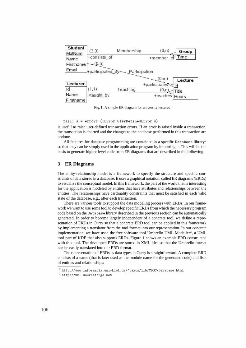
Fig. 1. A simple ER diagram for university lectures

failT s = errorT (TError UserDefinedError s)

is useful to raise user-defined transaction errors. If an error is raised inside a transaction,the transaction is aborted and the changes to the database performed in this transaction areundone.

All features for database programming are contained in a specific Database library2

so that they can be simply used in the application program by importing it. This will be thebasis to generate higher-level code from ER diagrams that are described in the following.

3 ER Diagrams

The entity-relationship model is a framework to specify the structure and specific con-straints of data stored in a database. It uses a graphical notation, called ER diagrams (ERDs)to visualize the conceptual model. In this framework, the part of the world that is interestingfor the application is modeled by entities that have attributes and relationships between theentities. The relationships have cardinality constraints that must be satisfied in each validstate of the database, e.g., after each transaction.

There are various tools to support the data modeling process with ERDs. In our frame-work we want to use some tool to develop specific ERDs from which the necessary programcode based on the Database library described in the previous section can be automaticallygenerated. In order to become largely independent of a concrete tool, we define a repre-sentation of ERDs in Curry so that a concrete ERD tool can be applied in this frameworkby implementing a translator from the tool format into our representation. In our concreteimplementation, we have used the free software tool Umbrello UML Modeller3, a UMLtool part of KDE that also supports ERDs. Figure 1 shows an example ERD constructedwith this tool. The developed ERDs are stored in XML files so that the Umbrello formatcan be easily translated into our ERD format.

The representation of ERDs as data types in Curry is straightforward. A complete ERDconsists of a name (that is later used as the module name for the generated code) and listsof entities and relationships:

2 http://www.informatik.uni-kiel.de/~pakcs/lib/CDOC/Database.html3 http://uml.sourceforge.net

106

data ERD = ERD String [Entity] [Relationship]

An entity has a name and a list of attributes, where each attribute has a name, a domain,and specifications about its key and null value property:

data Entity = Entity String [Attribute]

data Attribute = Attribute String Domain Key Null

data Key = NoKey | PKey | Unique

type Null = Bool

data Domain = IntDom (Maybe Int) | FloatDom (Maybe Float)

| StringDom (Maybe String) | ...

Thus, each attribute is part of a primary key (PKey), unique (Unique), or not a key (NoKey).Furthermore, it is allowed that specific attributes can have null values, i.e., can be undefined.The domain of each attribute is one of the standard domains or some user-defined type. Foreach kind of domain, one can also have a default value (modeled by the Maybe type inCurry).

Finally, each relationship has a name and a list of connections to entities (REnd), whereeach connection has the name of the connected entity, the role name of this connection, andits cardinality as arguments:

data Relationship = Relationship String [REnd]

data REnd = REnd String String Cardinality

data Cardinality = Exactly Int | Range Int (Maybe Int)

The cardinality is either a fixed integer or a range between two integers (where Nothing

as the upper bound represents an arbitrary cardinality).

4 Compiling ER Diagrams into Curry Programs

The transformation of ERDs into executable Curry code is done in the following order:

1. Translate an ERD into an ERD term.2. Represent the relationships occurring in an ERD term as entities.3. Map all entities into corresponding Curry code based on the Database library.

The first step depends on the format used in the ERD tool. As mentioned above, we haveimplemented a translation from the Umbrello UML Modeller into ERD terms. This part isrelatively easy thanks to the presence of XML processing tools.

4.1 Transforming ERDs

The second step is necessary since the relational model supports only relations (i.e.,database tables). Thus, entities as well as relationships must be mapped into relations. Themapping of entities into relations is straightforward by using the entity name as the nameof the relation and the attribute names as column names. The mapping of relationships ismore subtle. In principle, each relationship can be mapped into a corresponding relation.However, this simple approach might cause the creation of many relations or database ta-bles. In order to reduce them, it is sometimes better to represent specific relations as foreign

107

keys, i.e., to store the key of entity e1 referred by a relationship between e1 and e2 in entitye2. Whether or not this is possible depends on the kind of the relation. The different caseswill be discussed next. Note that the representation of relationships as relations causes alsovarious integrity constraints to be satisfied. For instance, if an entity has an attribute whichcontains a foreign key, the value of this attribute must be either null or an existing key inthe corresponding relation. Furthermore, the various cardinalities of each relationship mustbe satisfied. Each transaction should ensure that the integrity constraints are valid afterfinishing the transaction.

Now we discuss the representation of the various kinds of relationships in the ER model.For the sake of simplicity, we assume that each relationship contains two ends, i.e., tworoles with cardinality ranges (min, max) so that we can characterize each relationshipby their related cardinalities (minA, maxA) : (minB , maxB) between entities A and B

(where maxi is either a natural number greater than mini or ∞, i ∈ A, B).

Simple-simple (1:1) relations: This case covers all situations where each cardinality is atmost one. In the case (0, 1) : (1, 1), the key of entity B is added as an attribute to entityA containing a foreign key since there must be exactly one B entity for each A entity.Furthermore, this attribute is Unique to ensure the uniqueness of the inverse relation.The case (0, 1) : (0, 1) can be similarly treated except that null values are allowed forthe foreign key.

Simple-complex (1:n) relations: In the case (0, 1) : (minB , maxB), the key of entity A

is added as a foreign key (possibly null) to each B entity. If minB > 0 or maxB 6= ∞,the integrity constraints for the right number of occurrences must be checked by eachdatabase update. The case (1, 1) : (0, maxB) is similarly implemented except that nullvalues for the foreign key are not allowed.

Complex-complex (n:m) relations: In this case a new relation representing this relation-ship is introduced. The new relation is connected to entities A and B by two newrelationships of the previous kinds.

Note that we have not considered relationships where both minimal cardinalities are greaterthan zero. This case is excluded by our framework (and rarely occurs in practical data mod-els) since it causes difficulties when creating new entities of type A or B. Since each entityrequires a relation to an existing entity of the other type and vice versa, it is not possibleto create the new entities independently. Thus, both entities must be created and connectedin one transaction which requires specific complex transactions. Therefore, we do not sup-port this in our code generation. If such relations are required in an application (e.g., cyclicrelationships), then the necessary code must be directly written with the primitives of theDatabase library.

Based on this case distinction, the second step of our compiler maps an ERD term intoa new ERD term where foreign keys are added to entities and new entities are introduced torepresent complex-complex relations. Furthermore, each entity is extended with an internalprimary key to simplify the access to each entity by a unique scheme.

4.2 Code Generation for ERDs

After the mapping of entities and relationships into relations as described above, we cangenerate the concrete program code to organize the database access and update. As al-ready mentioned, we base the generated code on the functionality provided by the library

108

Database described in Section 2. The schemas for the generated code are sketched in thissection. We use the notation En for the name of an entity (which starts by convention withan uppercase letter) and en for the same name where the first letter is lowercase (this isnecessary due to the convention in Curry that data constructors and functions start withuppercase and lowercase letters, respectively).

The first elements of the generated code are data types to represent relations. For eachentity En with attributes of types at1, . . . , atn, we generate the following two type defini-tions:

data En = En Key at1...atn

data EnKey = EnKey Key

Key is the type of all internal keys for entities. Currently, it is identical to Int. Thus,each entity structure contains an internal key for its unique identification. The specifictype EnKey is later used to distinguish the keys for different entities by their types, i.e.,to exploit the type system of Curry to avoid confusion between the various keys. For eachrelation that has been introduced for a complex-complex relationship (see above), a similartype definition is introduced except that it does not have an internal key but only the keys ofthe connected entities as arguments. Note that only the names of the types are exported butnot their internal structure (i.e., they are abstract data types for the application program).This ensures that the application program cannot manipulate the internal keys.

In order to access or modify the attributes of an entity, we generate correspondingfunctions where we use the attribute names of the ERD for the names of the functions.If entity En has an attribute Ai of type ati (i = 1, . . . , n), we generate the following getterand setter functions and a function to access the key of the entity:

enAi :: En -> atienAi (En _ ... xi ... _) = xi

setEnAi :: En -> ati -> EnsetEnAi (En x1 ... _ ... xn) xi = En x1 ... xi ... xn

enKey :: En -> EnKeyenKey (En k _ ... _) = EnKey k

As described in Section 2, data can be persistently stored by putting them into a dynamicpredicate. Thus, we define for each entity En a dynamic predicate

enEntry :: En -> Dynamic

enEntry persistent "..."

Since the manipulation of all persistent data should be done by safe operations, this dy-namic predicate is not exported. Instead, a dynamic predicate en is exported that associatesa key with the data so that an access is only possible to data with an existing key:

en :: EnKey -> En -> Dynamic

en key obj | key=:= enKey obj = enEntry obj

Note that the use of a functional logic language is important here. For instance, the accessto an entity with a given key k can be done by solving the goal “en k o” where o is a freevariable that will be bound to the concrete instance of the entity.

For each role with name rn specified in an ERD, we generate a dynamic predicate oftype

rn :: E1Key -> E2Key -> Dynamic

109

where E1 and E2 are the entities related by this role. The implementation of these predi-cates depend on the kind of relationship according to their implementation as discussed inSection 4.1. Since complex-complex relationships are implemented as relations, i.e., per-sistent predicates (that are only internal and not exported), the corresponding roles canbe directly mapped to these. Simple-simple and simple-complex relationships are imple-mented by foreign keys in the corresponding entities. Thus, their roles are implemented byaccessing these keys. We omit the code details that depend on the different cases alreadydiscussed in Section 4.1.

Based on these basic implementations of entities and relationships, we also generatecode for transactions to manipulate the data and check the integrity constraints specifiedby the relationships of an ERD. In order to access an entity with a specific key, there is ageneric function that delivers this entity in a transaction or raises a transaction error if thereis no entry with this key:

getEntry :: k -> (k -> a -> Dynamic) -> Transaction a

getEntry key pred =

getDB (queryOne (\info -> pred key info)) |>>=

maybe (errorT (KeyNotExistsError "no entry for..."))

returnT

This internal function is specialized to an exported function for each entity:

getEn :: EnKey -> Transaction EngetEn key = getEntry key en

In order to insert new entities, there is a “new” transaction for each entity. If the ERDspecifies no relationship for this entity with a minimum greater than zero, there is no needto provide related entities so that the transaction has the following structure (if En hasattributes of types at1, . . . , atn):

newEn :: at1 -> · · · -> atn -> Transaction EnnewEn a1 ... an = check1 |>> ... |>> checkn |>> newEntry ...

Here, checki are the various integrity checks (e.g., uniqueness checks for attributes spec-ified as Unique) and newEntry is a generic operation (similarly to getEntry) to insert anew entity. If attribute Ai has a default value or null values are allowed for it, the type ati

is replaced by Maybe ati in newEn. If there are relationships for this entity with a mini-mum greater than zero, than the keys (in general, a list of keys) must be also provided asparameters to newEn. The same holds for the “new” operations generated for each complex-complex relationship. For instance, the new operation for lectures according to the ERD inFigure 1 has the following type:

newLecture :: LecturerKey -> Int -> String -> Maybe Int

-> Transaction Lecture

The first argument is the key of the lecturer required by the relationship Teaching, and thefurther arguments are the values of the Id, Title and Hours attributes (where the attributeHours has a default value so that the argument is optional).

Similarly to newEn, we provide also operations to update existing entities. These oper-ations have the following structure:

updateEn :: En -> Transaction ()

updateEn e = check1 |>> ... |>> checkn |>> updateEntry ...

110

Again, the various integrity constraints must be checked before an update is finally per-formed. In order to get an impression of the kind of integrity constraints, we discuss a fewchecks in the following.

If an attribute of an entity is Unique, this property must be checked before a newinstance of the entity is inserted. For this purpose, there is a generic transaction

unique :: a -> (b -> a) -> (b -> Dynamic) -> Transaction ()

where the first argument is the attribute value, the second argument is a getter function forthis attribute, and the third argument is the dynamic predicate representing this entity, i.e.,a typical call to check the uniqueness of the new value ai for attribute Ai of entity En is(unique ai enAi En). This transaction raises a UniqueError if an instance with thisattribute value already exists.

If an entity contains a foreign key, each update must check the existence of this foreignkey. This is the purpose of the generic transaction

existsDBKey :: k -> (a -> k) -> (a -> Dynamic) -> Transaction ()

where the arguments are the foreign key, a getter function (enKey) for the key in the for-eign entity and the dynamic predicate of the foreign entity. If the key does not exist, aKeyNotExistsError is raised. Furthermore, there are generic transactions to check min-imum and maximum cardinalities for relationships and lists of foreign keys that can raisethe transaction errors MinError, MaxError, or DuplicateKeyError. For each new andupdate operation generated by our compiler, the necessary integrity checks are insertedbased on the ER specification.

Our framework does not provide delete operations. The motivation for this is that safedelete operations require the update of all other entities where this entity could occur asa key. Thus, a simple delete could cause many implicit changes that are difficult to over-look. It might be better to provide only the deletion of single entities followed by a globalconsistency check (discussed below). A solution to this problem is left as future work.

Even if our generated transactions ensure the integrity of the affected relations, it issometimes useful to provide a global consistency check that is regularly applied to alldata. This could be necessary if unsafe delete operations are performed or the databaseis modified by programs that do not use the safe interface but directly accesses the data.For this purpose, we also generate explicit global consistency test operations that check allpersistent data w.r.t. the ER model (we omit the details here).

5 Conclusions

We have presented a framework to compile conceptual data models specified as entity-relationship diagrams into executable code for database programming in Curry. This com-pilation is done in three phases: translate the specific ERD format into a tool-independentrepresentation, transform the relationships into relations according to their complexity, andgenerate code for the safe access and update of the data.

Due to the importance of ERDs to design conceptual data models, there are also othertools with similar objectives. Most existing tools support only the generation of SQL code,like the free software tools DB-Main4 or DBDesigner45. The main motivation for our de-

4 http://www.db-main.be5 http://www.fabforce.net/dbdesigner4

111

velopment was the seamless embedding of database programming in a declarative pro-gramming language and the use of existing specification methods like ERDs as the basis togenerate most of the necessary code required by the application programs. The advantagesof our framework are:

– The application programmer must only specify the data model in a high-level format(ERDs) and all necessary code for dealing with data in this model is generated.

– The interface used by the application programs is type safe, i.e., the types specifiedin the ERD are mapped into types of the programming language so that ill-typed datacannot be constructed.

– Updates to the database are supported as transactions that automatically checks allintegrity constraints specified in the ERD.

– Checks for all integrity constraints are derived from the ERD for individual tables andthe complete database so that they can be periodically applied to verify the integrity ofthe current state of the database.

– The generated code is based on an abstract interface for database programming so thatit is readable and well structured. Thus, it can be easily modified and adapted to newrequirements. For instance, integrity constraints not expressible in ERDs can be easilyadded to individual update operations, or specific deletion operations can be insertedin the generated module.

References

1. P. P.-S. Chen. The Entity-Relationship Model—Toward a Unified View of Data. ACM Transac-tions on Database Systems, Vol. 1, No. 1, pp. 9–36, 1976.

2. J. Correas, J.M. Gomez, M. Carro, D. Cabeza, and M. Hermenegildo. A Generic PersistenceModel for (C)LP Systems (and Two Useful Implementations). In Proc. of the Sixth InternationalSymposium on Practical Aspects of Declarative Languages (PADL’04), pp. 104–119. SpringerLNCS 3057, 2004.

3. S.K. Das. Deductive Databases and Logic Programming. Addison-Wesley, 1992.4. S. Fischer. A Functional Logic Database Library. In Proc. of the ACM SIGPLAN 2005 Workshop

on Curry and Functional Logic Programming (WCFLP 2005), pp. 54–59. ACM Press, 2005.5. H. Gallaire and J. Minker, editors. Logic and Databases, New York, 1978. Plenum Press.6. M. Hanus. The Integration of Functions into Logic Programming: From Theory to Practice.

Journal of Logic Programming, Vol. 19&20, pp. 583–628, 1994.7. M. Hanus. Dynamic Predicates in Functional Logic Programs. Journal of Functional and Logic

Programming, Vol. 2004, No. 5, 2004.8. M. Hanus (ed.). Curry: An Integrated Functional Logic Language (Vers. 0.8.2). Available at

http://www.informatik.uni-kiel.de/˜curry, 2006.9. S.H. Huseby. Innocent Code: A Security Wake-Up Call for Web Programmers. Wiley, 2003.

10. S. Peyton Jones, editor. Haskell 98 Language and Libraries—The Revised Report. CambridgeUniversity Press, 2003.

11. P. Wadler. How to Declare an Imperative. ACM Computing Surveys, Vol. 29, No. 3, pp. 240–263,1997.

112

Squash: A Tool for Designing, Analyzing andRefactoring Relational Database Applications ⋆

Andreas M. Boehm1, Dietmar Seipel2, Albert Sickmann1 and Matthias Wetzka2

1 University of Würzburg, Rudolf-Virchow-Center for Experimental BiomedicineVersbacher Strasse 9, D-97078 Würzburg, Germany

Emails: ab@andiboehm.de, albert.sickmann@virchow.uni-wuerzburg.de2 University of Würzburg, Department of Computer Science

Am Hubland, D-97074 Würzburg, GermanyEmails: matthias.wetzka@web.de, seipel@informatik.uni-wuerzburg.de

Abstract. Theperformanceof a large biological application of relational data-bases highly depends on the quality of the database schema design, the resultingstructure of the tables, and the logical relations between them. In production re-ality, the performance mainly depends on the semantics comprised in the storeddata and the corresponding queries.We have developed a tool named Squash (SQL Query Analyzer and Schema En-Hancer) for designing, analyzing and refactoring relational database applications.Squash parses the SQL definition of the database schema and the queries intoan XML representation called SquashML . This information can be managed us-ing the declarative XML queryandtransformationlanguage FNQuery, which wehave implemented in SWI-PROLOG, thus allowing modification and dynamic pro-cessing of the schema data. Visualization of relationshipsand join paths of queriesis integrated, too. Using an online connection, Squash can determine characteris-tics from the current database, such as join selectivities or table sizes.Squash comes with a set of predefined methods for tuning the database schemaaccording to the load profile induced by the application, andwith methods forproposing changes in the database schema such as the creation of indexes, parti-tioning, splitting, or further normalization. SQL statements are adapted simulta-neously upon modification of the schema, and they are rewritten in considerationof database-specific statement processing rules includingthe integration of op-timizer hints. Moreover, the Squashframeworkis very flexible and extensible;user-defined methodsbased on ad-hoc FNQuery statements can be plugged in.

1 Introduction

During productive use, enterprise-class databases undergo a lot of changes in orderto keep up with ever-changing requirements. The growing space-requirements and thegrowing complexity of a productive database increase the complexity of maintaining agood performance of the database query execution. Performance is highly dependenton the database schema design [12]. In addition, a complex database schema is moreprone to design errors.

⋆ This work was supported by the Deutsche Forschungsgemeinschaft (FZT 82).

113

Increasing the performance and the manageability of a database usually requiresrestructuring the database schema and has effects on the application code. Additionally,tuning query execution is associated with adding secondarydata structures such as in-dexes or horizontal partitioning [8, 15, 2]. Because applications depend on the databaseschema, its modification implies the adaption of the queriesused in the applicationcode. The tuning of a complex database is usually done by specially trained expertshaving good knowledge of database design and many years of experience with tuningdatabases [21, 17]. Due to the lot of possibilities, the optimization of a database is avery complex and time-consuming task, even for professional database experts. In theprocess of optimization, many characteristic values for the database need to be calcu-lated and assessed in order to determine an optimal configuration. Special tuning toolscan help the database administrator to focus on the important information necessary forthe optimization and support the database administrator incomplex database schemamanipulations [21, 17]. More sophisticated tools can even propose optimized databaseconfigurations by using the database schema and a characteristic workload log as input[1, 6, 13].

During the last two decades, approaches towards self-tuning database managementsystems have been developed [7, 10, 17, 24–26]. These approaches have inherent accessto the most current load profile of the application. But they are limited to changes only inthe database that are transparent for the application code.Thus, they lack the possiblityto automatically update the underlying source code and are not capable of refactoringapplications completely. The approach presented in this paper aims at refactoring thedatabase schemas and the queries in the SQL code of the application at the same time.

The rest of the paper, which describes our system Squash, is organized as follows:Section 2 describes the management of SQL data with the query and transformationlanguage FNQuery. Section 3 is on the analysis and tuning of existing database applica-tions. Examples dealing with foreign key constraints and join conditions are presentedin Section 4 to illustrate how user-defined methods can be written. Finally, Section 5will briefly report on a case study for physical database optimization, that was con-ducted with Squash.

2 Managing SQL Data with FNQuery

We have developed an extensible XML representation called SquashML for SQL schemadefinitions and queries. The core of SquashML is predetermined by the SQL standard,but it also allows for system-specific constructs of different SQL dialects. For example,some definitions and storage parameters from the OracleTM database management sys-tem were integrated. SquashML is able to represent schema objects, as well as databasequeries obtained from application code or from logging data. This format allows foreasily processing and evaluating the database schema information. Currently, supportedschema objects include table and index definitions. The Squash parser was implementedin Perl. Other existing XML representations of databases like SQL/XML usually focuson representing the database contents, i.e. the tables, andnot the schema definition it-

114

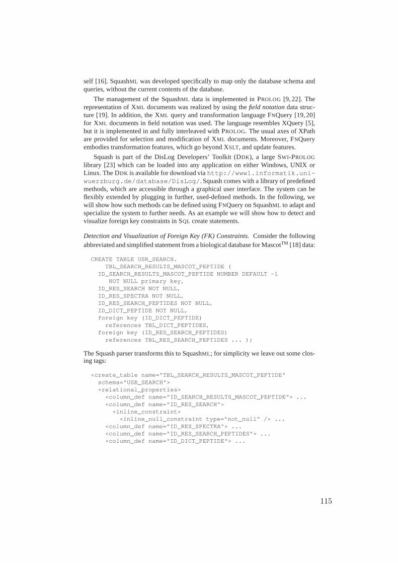
self [16]. SquashML was developed specifically to map only the database schema andqueries, without the current contents of the database.

The management of the SquashML data is implemented in PROLOG [9, 22]. Therepresentation of XML documents was realized by using thefield notationdata struc-ture [19]. In addition, the XML query and transformation language FNQuery [19, 20]for XML documents in field notation was used. The language resemblesXQuery [5],but it is implemented in and fully interleaved with PROLOG. The usual axes of XPathare provided for selection and modification of XML documents. Moreover, FNQueryembodies transformation features, which go beyond XSLT, and update features.

Squash is part of the DisLog Developers’ Toolkit (DDK), a large SWI-PROLOG

library [23] which can be loaded into any application on either Windows, UNIX orLinux. The DDK is available for download viahttp://www1.informatik.uni-wuerzburg.de/database/DisLog/. Squash comes with a library of predefinedmethods, which are accessible through a graphical user interface. The system can beflexibly extended by plugging in further, used-defined methods. In the following, wewill show how such methods can be defined using FNQuery on SquashML to adapt andspecialize the system to further needs. As an example we willshow how to detect andvisualize foreign key constraints in SQL create statements.

Detection and Visualization of Foreign Key (FK) Constraints. Consider the followingabbreviated and simplified statement from a biological database for MascotTM [18] data:

CREATE TABLE USR_SEARCH.TBL_SEARCH_RESULTS_MASCOT_PEPTIDE (

ID_SEARCH_RESULTS_MASCOT_PEPTIDE NUMBER DEFAULT -1NOT NULL primary key,

ID_RES_SEARCH NOT NULL,ID_RES_SPECTRA NOT NULL,ID_RES_SEARCH_PEPTIDES NOT NULL,ID_DICT_PEPTIDE NOT NULL,foreign key (ID_DICT_PEPTIDE)

references TBL_DICT_PEPTIDES,foreign key (ID_RES_SEARCH_PEPTIDES)

references TBL_RES_SEARCH_PEPTIDES ... );

The Squash parser transforms this to SquashML ; for simplicity we leave out some clos-ing tags:

<create_table name="TBL_SEARCH_RESULTS_MASCOT_PEPTIDE"schema="USR_SEARCH"><relational_properties>

<column_def name="ID_SEARCH_RESULTS_MASCOT_PEPTIDE"> ...<column_def name="ID_RES_SEARCH">

<inline_constraint><inline_null_constraint type="not_null" /> ...

<column_def name="ID_RES_SPECTRA"> ...<column_def name="ID_RES_SEARCH_PEPTIDES"> ...<column_def name="ID_DICT_PEPTIDE"> ...

115

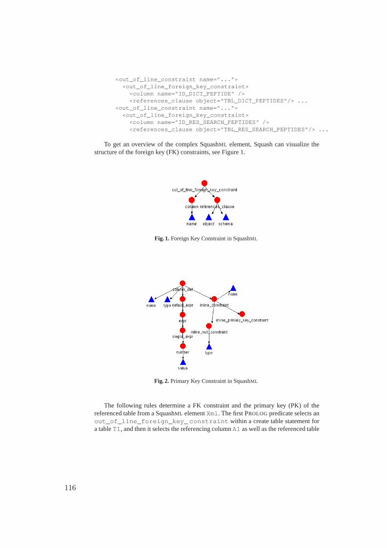
<out_of_line_constraint name="..."><out_of_line_foreign_key_constraint><column name="ID_DICT_PEPTIDE" /><references_clause object="TBL_DICT_PEPTIDES"/> ...

<out_of_line_constraint name="..."><out_of_line_foreign_key_constraint><column name="ID_RES_SEARCH_PEPTIDES" /><references_clause object="TBL_RES_SEARCH_PEPTIDES"/> ...

To get an overview of the complex SquashML element, Squash can visualize thestructure of the foreign key (FK) constraints, see Figure 1.

Fig. 1. Foreign Key Constraint in SquashML

Fig. 2. Primary Key Constraint in SquashML

The following rules determine a FK constraint and the primary key (PK) of thereferenced table from a SquashML elementXml. The first PROLOG predicate selects anout_of_line_foreign_key_ constraint within a create table statement fora tableT1, and then it selects the referencing columnA1 as well as the referenced table

116

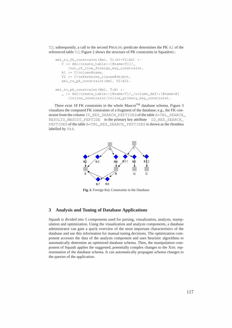
T2; subsequently, a call to the second PROLOG predicate determines the PKA2 of thereferenced tableT2; Figure 2 shows the structure of PK constraints in SquashML :

xml_to_fk_constraint(Xml, T1:A1=T2:A2) :-C := Xml/create_table::[@name=T1]/_

/out_of_line_foreign_key_constraint,A1 := C/column@name,T2 := C/references_clause@object,xml_to_pk_constraint(Xml, T2:A2).

xml_to_pk_constraint(Xml, T:A) :-_ := Xml/create_table::[@name=T]/_/column_def::[@name=A]

/inline_constraint/inline_primary_key_constraint.

There exist 18 FK constraints in the whole MascotTM database schema. Figure 3visualizes the computed FK constraints of a fragment of the database; e.g., the FK con-straint from the columnID_RES_SEARCH_PEPTIDESof the tableA=TBL_SEARCH_RESULTS_MASCOT_PEPTIDE to the primary key attribute ID_RES_SEARCH_PEPTIDES of the tableB=TBL_RES_SEARCH_ PEPTIDES is shown as the rhombuslabelled byfk4.

Fig. 3. Foreign Key Constraints in the Database

3 Analysis and Tuning of Database Applications

Squash is divided into 5 components used for parsing, visualization, analysis, manip-ulation and optimization. Using the visualization and analysis components, a databaseadministrator can gain a quick overview of the most important characteristics of thedatabase and use this information for manual tuning decisions. The optimization com-ponent accesses the data of the analysis component and uses heuristic algorithms toautomatically determine an optimized database schema. Then, the manipulation com-ponent of Squash applies the suggested, potentially complex changes to the XML rep-resentation of the database schema. It can automatically propagate schema changes tothe queries of the application.

117

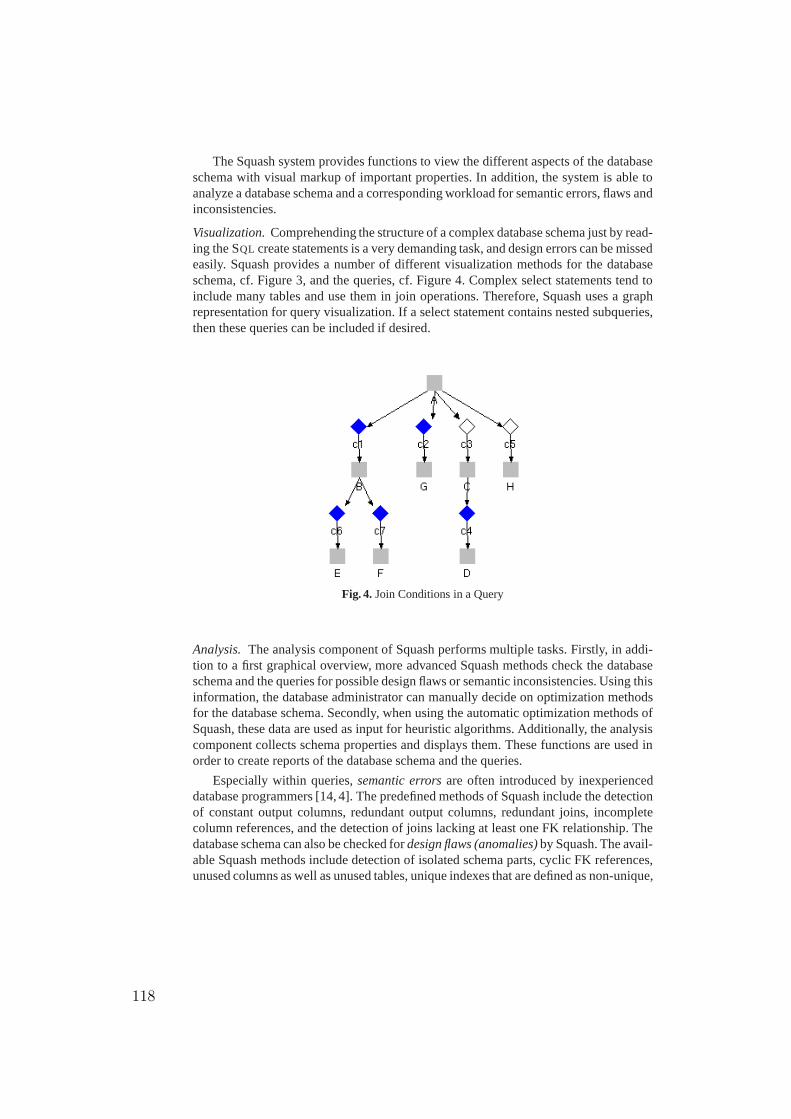
The Squash system provides functions to view the different aspects of the databaseschema with visual markup of important properties. In addition, the system is able toanalyze a database schema and a corresponding workload for semantic errors, flaws andinconsistencies.

Visualization.Comprehending the structure of a complex database schema just by read-ing the SQL create statements is a very demanding task, and design errors can be missedeasily. Squash provides a number of different visualization methods for the databaseschema, cf. Figure 3, and the queries, cf. Figure 4. Complex select statements tend toinclude many tables and use them in join operations. Therefore, Squash uses a graphrepresentation for query visualization. If a select statement contains nested subqueries,then these queries can be included if desired.

Fig. 4. Join Conditions in a Query

Analysis. The analysis component of Squash performs multiple tasks. Firstly, in addi-tion to a first graphical overview, more advanced Squash methods check the databaseschema and the queries for possible design flaws or semantic inconsistencies. Using thisinformation, the database administrator can manually decide on optimization methodsfor the database schema. Secondly, when using the automaticoptimization methods ofSquash, these data are used as input for heuristic algorithms. Additionally, the analysiscomponent collects schema properties and displays them. These functions are used inorder to create reports of the database schema and the queries.

Especially within queries,semantic errorsare often introduced by inexperienceddatabase programmers [14, 4]. The predefined methods of Squash include the detectionof constant output columns, redundant output columns, redundant joins, incompletecolumn references, and the detection of joins lacking at least one FK relationship. Thedatabase schema can also be checked fordesign flaws (anomalies)by Squash. The avail-able Squash methods include detection of isolated schema parts, cyclic FK references,unused columns as well as unused tables, unique indexes thatare defined as non-unique,

118

indexes of low quality, datatype conflicts, anonymous PK or FK constraints, missingprimary keys, and the detection (and improvement) of bad join orders.

Refactoring.The refactoring component allows for manipulating the database schemaas well as the corresponding application code based on the transformation and updatefeatures of FNQuery. Besides trivial manipulations such as adding or removing colums,the system also supports complex schema manipulations thataffect other parts of thedatabase schema and the queries, such as vertical partitioning and merging of tables.Squash is able to provide all queries in the workload with thebest set of indexes ac-cording to the heuristic function of the system, and it generates appropriate optimizerhints.

4 Analysis and Visualization of Join Conditions in SQL Queries

Squash can visualize and analyse complex SQL statements. E.g., the following SQL

select statement from the MascotTM database joins 8 tables:

SELECT *FROM TBL_SEARCH_RESULTS_MASCOT_PEPTIDE A,

TBL_RES_SEARCH_PEPTIDES B,... C, ... D, ... E, ... F, ... G, ... H

WHERE A.ID_DICT_PEPTIDE IN (SELECT B0.ID_PEPTIDEFROM TBL_RES_SEARCH_PEPTIDES B0WHERE B0.ID_RES_SEARCH = 2025GROUP BY ID_PEPTIDEHAVING COUNT(ID_RES_SEARCH_PEPTIDES) >=1 )

AND A.ID_RES_SEARCH = 2025AND c1 AND c2 AND A.FLAG_DELETE = 0AND c3 AND c6 (+) AND c7 (+)AND c4 AND c5 AND E.LEN >= 6AND A.SCORENORMALIZED >= 1.5ORDER BY D.ID_SEQ_SEQUENZ, B.ACC_ID_CLS, ...;

It uses the following 7 join conditions:

c1: A.ID_RES_SEARCH_PEPTIDES = B.ID_RES_SEARCH_PEPTIDESc2: A.ID_RES_SPECTRA = G.ID_RES_SPECTRAc3: A.ID_RES_SEARCH_PEPTIDES = C.ID_PEPTIDEc4: C.ID_SEQUENCE = D.ID_SEQ_SEQUENZc5: A.ID_RES_SEARCH = H.ID_RES_SEARCHc6: B.ID_PEPTIDE = E.ID_DICT_PEPTIDEc7: B.ID_PEPTIDE_MOD = F.ID_DICT_PEPTIDE

We wanted to know which of the join conditions of the query arevalid FK constraints,cf. Figure 3, since other join conditions might be design errors. The query is parsed intothe following SquashML element; for simplicity we leave out closing tags:

119

<select><subquery id="subquery_1">

<select_list><expr>

<simple_expr><object table_view="A" column="IDRESSEARCH"/> ...

<from><table_reference>

<query_table_reference><query_table_expression>

<simple_query_table_expressionobject="TBL_SEARCH_RESULTS_MASCOT_PEPTIDE"schema="USRSEARCH"/> ...

<alias name="A"/> ...<where> ...<order_by> ...

The conditions in the WHERE part look like follows:

<condition><simple_comparison_condition operator="=">

<left_expr><expr>

<simple_expr><object table_view="A"

column="ID_RES_SEARCH_PEPTIDES"/>...

<right_expr> ...table_view="B" column="ID_RES_SEARCH_PEPTIDES"/>

...

The following PROLOG rule selects a simple comparison condition with the operator“=”, or an outer join condition:

xml_to_join_condition(Xml, T1:A1=T2:A2) :-S := Xml/select,( Cond := S/_

/simple_comparison_condition::[@operator=(=)]; Cond := S/_

/outer_join_condition ),cond_to_pair(Cond, left_expr, T1:A1),cond_to_pair(Cond, right_expr, T2:A2).

Within the selected conditions, the following PROLOG rule determines the left and theright table/column-pair:

cond_to_pair(Cond, Tag, T:A) :-[T, A] := Cond/Tag/expr/simple_expr

/object@[table_view, column].

120

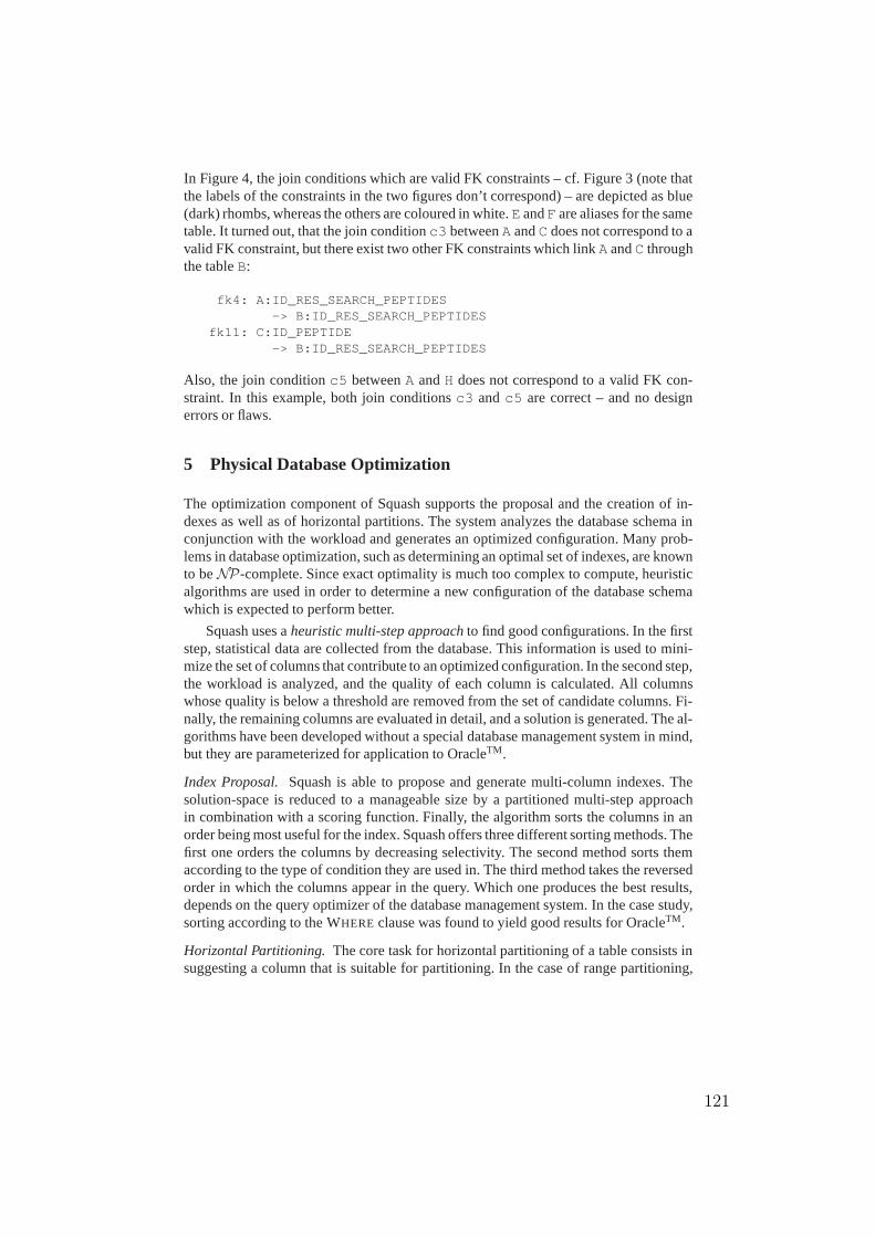
In Figure 4, the join conditions which are valid FK constraints – cf. Figure 3 (note thatthe labels of the constraints in the two figures don’t correspond) – are depicted as blue(dark) rhombs, whereas the others are coloured in white.E andF are aliases for the sametable. It turned out, that the join conditionc3 betweenA andC does not correspond to avalid FK constraint, but there exist two other FK constraints which linkA andC throughthe tableB:

fk4: A:ID_RES_SEARCH_PEPTIDES-> B:ID_RES_SEARCH_PEPTIDES

fk11: C:ID_PEPTIDE-> B:ID_RES_SEARCH_PEPTIDES

Also, the join conditionc5 betweenA andH does not correspond to a valid FK con-straint. In this example, both join conditionsc3 andc5 are correct – and no designerrors or flaws.

5 Physical Database Optimization

The optimization component of Squash supports the proposaland the creation of in-dexes as well as of horizontal partitions. The system analyzes the database schema inconjunction with the workload and generates an optimized configuration. Many prob-lems in database optimization, such as determining an optimal set of indexes, are knownto beNP-complete. Since exact optimality is much too complex to compute, heuristicalgorithms are used in order to determine a new configurationof the database schemawhich is expected to perform better.

Squash uses aheuristic multi-step approachto find good configurations. In the firststep, statistical data are collected from the database. This information is used to mini-mize the set of columns that contribute to an optimized configuration. In the second step,the workload is analyzed, and the quality of each column is calculated. All columnswhose quality is below a threshold are removed from the set ofcandidate columns. Fi-nally, the remaining columns are evaluated in detail, and a solution is generated. The al-gorithms have been developed without a special database management system in mind,but they are parameterized for application to OracleTM.

Index Proposal. Squash is able to propose and generate multi-column indexes. Thesolution-space is reduced to a manageable size by a partitioned multi-step approachin combination with a scoring function. Finally, the algorithm sorts the columns in anorder being most useful for the index. Squash offers three different sorting methods. Thefirst one orders the columns by decreasing selectivity. The second method sorts themaccording to the type of condition they are used in. The thirdmethod takes the reversedorder in which the columns appear in the query. Which one produces the best results,depends on the query optimizer of the database management system. In the case study,sorting according to the WHERE clause was found to yield good results for OracleTM.

Horizontal Partitioning. The core task for horizontal partitioning of a table consists insuggesting a column that is suitable for partitioning. In the case of range partitioning,

121

Fig. 5. Runtimes of Characteristic SQL Statements:

a) SequestTM statement with indexes proposed by Squash. The duration was7:46 min with-out any indexes. This could be reduced by manual tuning to 1:53 min, whereas tuningby Squash achieved a further reduction of about 49% down to 1:09 min, i.e. 14% of theoriginal time.

b) MascotTM statement with indexes proposed by Squash. The execution time was 3:31 with-out any indexes. This was not tuned manually before. Tuning by indexes proposed bySquash yielded a reduction to 0:26 min.

c) SequestTM statement with partitions proposed by Squash. The execution time was 1:53 min(manually tuned), whereas tuning by Squash and applicationof partitions achieved furtherreduction of about 19% to 1:33 min.

the borders of each partition are calculated by analysing the histograms of the partitionkey. The number of partitions for hash partitioning is calculated from the table volume.

Case Study on Index Proposal.A case study was conducted using a database systemdesigned for use in mass spectrometry-based proteomics, that provides support for largescale data evaluation and data mining. This system, which iscomposed of the two sub-systemsseqDB andresDB [3, 27], was temporarily ported to OracleTM for being an-alyzed by Squash. The complete database schema consists of 46 tables requiring about68.5 GB disk space, and it fulfills the definition of a data warehouse system.

Some characteristic SQL statements of the data evaluation partresDB were ana-lyzed, that were obtained from an application log and were submitted to Squash foranalysis in conjunction with the schema creation script. The statements perform thegrouping of peptide results into protein identification results that were obtained bySequestTM [11] and MascotTM [18], respectively.

For demonstration, the SequestTM statements were previously tuned manually byan experienced database administrator, the MascotTM queries were left completely un-tuned. The improvements resulting from the tuning are depicted in Figure 5; they werebetween 20% and 80%.

122

6 Conclusion

We have presented an extensible tool named Squash that applies methods from artificialintelligence to relational database design and tuning. Input and ouput are XML -based,and operations on these data are performed using the declarative XML query and trans-formation language FNQuery.

The Squash tool supports the refactoring of database applications and considersthe interactions between application code and database schema definition; both typesof code can be handled and manipulated automatically. Thus,application maintenanceis simplified, and the chance for errors is reduced, in sum yielding time and resourcesavings.

In the future we are planning to analyse and refactor database applications wherethe SQL code can beembeddedin other programming languages – such as Java andPHP – as well, based on XML representations of these languages, which we have alreadydeveloped.

References

1. AGRAWAL, S.; NARASAYYA , V. ; YANG, B.: Integrating Vertical and Horizontal Partition-ing into Automated Physical Database Design.Proc. ACM SIGMOD Intl. Conference onManagement of Data. ACM Press, 2004, pp. 359-370

2. BELLATRECHE,L.; KARLAPALEM ,K.; MOHANIA , M. K. ; SCHNEIDER,M.: What Can Par-titioning Do for Your Data Warehouses and Data Marts?Proc. Intl. Symposium on DatabaseEngineering and Applications (IDEAS 2000). IEEE Computer Society, 2000, pp. 437-446

3. BOEHM, A. M.; SICKMANN , A.: A Comprehensive Dictionary of Protein Accession Codesfor Complete Protein Accession Identifier Alias Resolving.In: Proteomics, Vol. 6(15), 2006,pp. 4223-4226

4. BRASS, S.; GOLDBERG, C.: Proving the Safety of SQL Queries.Proc. 5th Intl. Conferenceon Quality of Software 2005

5. CHAMBERLIN , D.: XQuery: a Query Language for XML.Proc. ACM SIGMOD Intl. Con-ference on Management of Data 2003. ACM Press, 2003, pp. 682-682

6. CHAUDHURI, S.; NARASAYYA , V.: Autoadmin What-If Index Analysis Utility.Proc. Intl.Conference on Management of Data Archives. Proc. ACM SIGMODIntl. Conference onManagement of Data 1988. ACM Press, 1998, pp. 367-378

7. CHAUDHURI, S.; WEIKUM , G.: Rethinking Database System Architecture: Towards a Self-tuning RISC-style Database System.Proc. 26th Intl. Conference on Very Large Data Bases(VLDB), 2000, pp. 1-10

8. CHOENNI, S.; BLANKEN , H. M. ; CHANG, T.: Index Selection in Relational Databases.Proc. 5th Intl. Conference on Computing and Information (ICCI), IEEE, 1993, pp. 491-496

9. CLOCKSIN, W. F.; MELLISH, C. S.:Programming in Prolog. 5th Edition, Springer, 200310. DIAS, K.; RAMACHER, M.; SHAFT, U.; VENKATARAMANI , V.; WOOD, G:. Automatic

Performance Diagnosis and Tuning in Oracle.Proc. 2nd Biennal Conference on InnovativeData Systems Research (CIDR), 2005, pp. 84-94

11. ENG, J. K.; MCCORMACK, A. L. ; YATES, J. R.: An Approach to Correlate Tandem MassSpectral Data of Peptides with Amino Acid Sequences in a Protein Database.Journal of theAmerican Society for Mass Spectrometry, Vol. 5(11), 1994, pp. 976-989

123

12. FAGIN, R.: Normal Forms and Relational Database Operators.Proc. ACM SIGMOD Intl.Conference on Management of Data1979

13. FINKELSTEIN,S.; SCHKOLNICK, M. ; TIBERIO, P.: Physical Database Design for RelationalDatabases.ACM Transactions on Database Systems (TODS), Vol. 13(1), 1988, pp. 91-128

14. GOLDBERG, C.; BRASS, S.: Semantic Errors in SQL Queries: A Quite Complete List.Proc.16. GI-Workshop Grundlagen von Datenbanken, 2004, pp. 58-62

15. GRUENWALD, L.; EICH, M.: Selecting a Database Partitioning Technique.Journal of Data-base Management, Vol. 4(3), 1993, pp. 27-39

16. INTL . ORGANIZATION FOR STANDARDIZATION : ISO/IEC 9075-14:2003 Informa-tion Technology – Database Languages – SQL – Part 14: XML-Related Specifications(SQL/XML). 2003

17. KWAN, E.; LIGHTSTONE, S.; SCHIEFER, B.; STORM, A. ; WU, L.: Automatic DatabaseConfiguration for DB2 Universal Database: Compressing Years of Performance Expertiseinto Seconds of Execution.10. Datenbanksysteme in Büro, Technik und Wissenschaft (BTW,Datenbanksysteme für Business, Technologie und Web), Bd. 26. Lecture Notes in Informatics(LNI), 2003, pp. 620–629

18. PERKINS, D. N.; PAPPIN, D. J. C.; CREASY, D. M. ; COTTRELL, J. S.: Probability-BasedProtein Identification by Searching Sequence Databases Using Mass Spectrometry Data.Electrophoresis, Vol. 20(18), 1999, pp. 3551-3567

19. SEIPEL, D.: Processing XML-Documents in Prolog. Proc. 17th Workshop on Logic Pro-grammierung (WLP) 2002

20. SEIPEL, D.; BAUMEISTER, J. ; HOPFNER, M.: Declarative Querying and Visualizing Knowl-edge Bases in XML.Proc. 15th Intl. Conference on Declarative Programming andKnowl-edge Management (INAP), 2004, pp. 140-151

21. TELFORD, R.; HORMAN, R.; LIGHTSTONE, S.; MARKOV, N.; O’CONNELL, S.; LOHMAN,G.: Usability and Design Considerations for an Autonomic Relational Database ManagementSystem.IBM Systems Journal, Vol. 42(4), 2003, pp. 568-581

22. WIELEMAKER, J.: An Overview of the SWI-Prolog Programming Environment. Proc. 13thIntl. Workshop on Logic Programming Environments (WLPE), 2003, pp. 1-16

23. WIELEMAKER, J.: SWI-Prolog. Version: 2007.http://www.swi-prolog.org/24. VALENTIN , G.; ZULIANI , M.; ZILIO , D. C.; LOHMAN, G.;SKELLEY , V.: DB2 Advisor: An

Optimizer Smart Enough to Recommend Its Own Indexes.Proc. 16th Intl. Conference onData Engineering, 2000, pp. 101-110

25. WEIKUM , G.; HASSE, C.; MÖNKEBERG, A.; ZABBACK , P.: The Comfort Automatic TuningProject.Information Systems, Vol. 19(5), 1994, pp. 381-432

26. WEIKUM , G.; MÖNKEBERG, A.; HASSE, C.; ZABBACK , P.: Self-tuning Database Technol-ogy and Information Services: from Wishful Thinking to Viable Engineering. Proc. 28thIntl. Conference on Very Large Data Bases (VLDB), 2002, pp. 20-31

27. ZAHEDI, R. P.; SICKMANN , A.; BOEHM, A. M.; W INKLER, C.; ZUFALL , N.; SCHÖNFISCH,B.; GUIARD, B.; PFANNER, N. ; MEISINGER, C.: Proteomic Analysis of the Yeast Mito-chondrial Outer Membrane Reveals Accumulation of a Subclass of Preproteins.MolecularBiology of the Cell, Vol. 17(3), 2006, pp. 1436-1450

124

Tabling Logic Programs in a Database

Pedro Costa, Ricardo Rocha, and Michel Ferreira

DCC-FC & LIACCUniversity of Porto, Portugal

c0370061@dcc.fc.up.pt ricroc,michel@ncc.up.pt

Abstract. Resolution strategies based on tabling are considered to beparticularly e!ective in Logic Programming. Unfortunately, when facedwith applications that store large and/or many answers, memory ex-haustion is a potential problem. A common approach to recover space istable deletion. In this work, we propose a di!erent approach, storing ta-bles externally in a relational database. Subsequent calls to stored tablesimport answers from the database, rather than performing a completere-computation. To validate this approach, we have extended the YapTabtabling system, providing engine support for exporting and importing ta-bles to and from the MySQL RDBMS. Two di!erent relational schemesfor data storage and two data-set retrieval strategies are compared.

1 Introduction

Tabling is an implementation technique where intermediate answers for subgoalsare stored and then reused when a repeated call appears. Resolution strategiesbased on tabling [1, 2] have proved to be particularly e!ective in logic programs,reducing the search space, avoiding looping and enhancing the termination prop-erties of Prolog models based on SLD resolution [3].

The performance of tabling largely depends on the implementation of thetable itself; being called upon often, fast look up and insertion capabilities aremandatory. Applications can make millions of di!erent calls, hence compact-ness is also required. Arguably, the most successful data structure for tabling istries [4]. Tries are trees in which there is one node for every common prefix [5].Tries meet the previously enumerated criteria of compactness and e"ciency quitewell. The YapTab tabling system [6] uses tries to implement tables.

Used in applications that pose many queries, possibly with a large number ofanswers, tabling can build arbitrarily many and very large tables, quickly fillingup memory. In general, there is no choice but to throw away some of the tables,ideally, the least likely to be used next. The common control mechanism imple-mented in most tabling systems is to have a set of tabling primitives that theprogrammer can use to dynamically abolish some of the tables. A more recentproposal has been implemented in YapTab, where a memory management strat-egy, based on a least recently used algorithm, automatically recovers space fromthe least recently used tables when memory runs out [7]. With this approach,the programmer can still force the deletion of particular tables, but can also

125

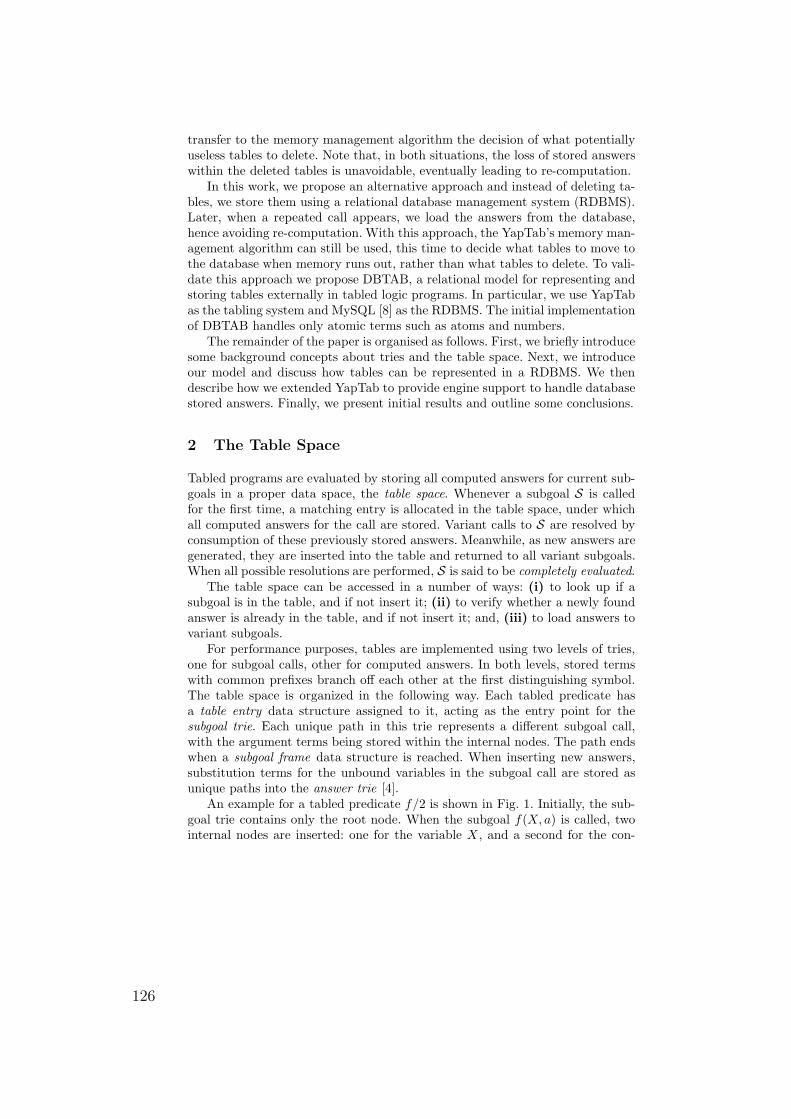
transfer to the memory management algorithm the decision of what potentiallyuseless tables to delete. Note that, in both situations, the loss of stored answerswithin the deleted tables is unavoidable, eventually leading to re-computation.

In this work, we propose an alternative approach and instead of deleting ta-bles, we store them using a relational database management system (RDBMS).Later, when a repeated call appears, we load the answers from the database,hence avoiding re-computation. With this approach, the YapTab’s memory man-agement algorithm can still be used, this time to decide what tables to move tothe database when memory runs out, rather than what tables to delete. To vali-date this approach we propose DBTAB, a relational model for representing andstoring tables externally in tabled logic programs. In particular, we use YapTabas the tabling system and MySQL [8] as the RDBMS. The initial implementationof DBTAB handles only atomic terms such as atoms and numbers.

The remainder of the paper is organised as follows. First, we briefly introducesome background concepts about tries and the table space. Next, we introduceour model and discuss how tables can be represented in a RDBMS. We thendescribe how we extended YapTab to provide engine support to handle databasestored answers. Finally, we present initial results and outline some conclusions.

2 The Table Space

Tabled programs are evaluated by storing all computed answers for current sub-goals in a proper data space, the table space. Whenever a subgoal S is calledfor the first time, a matching entry is allocated in the table space, under whichall computed answers for the call are stored. Variant calls to S are resolved byconsumption of these previously stored answers. Meanwhile, as new answers aregenerated, they are inserted into the table and returned to all variant subgoals.When all possible resolutions are performed, S is said to be completely evaluated.

The table space can be accessed in a number of ways: (i) to look up if asubgoal is in the table, and if not insert it; (ii) to verify whether a newly foundanswer is already in the table, and if not insert it; and, (iii) to load answers tovariant subgoals.

For performance purposes, tables are implemented using two levels of tries,one for subgoal calls, other for computed answers. In both levels, stored termswith common prefixes branch o! each other at the first distinguishing symbol.The table space is organized in the following way. Each tabled predicate hasa table entry data structure assigned to it, acting as the entry point for thesubgoal trie. Each unique path in this trie represents a di!erent subgoal call,with the argument terms being stored within the internal nodes. The path endswhen a subgoal frame data structure is reached. When inserting new answers,substitution terms for the unbound variables in the subgoal call are stored asunique paths into the answer trie [4].

An example for a tabled predicate f/2 is shown in Fig. 1. Initially, the sub-goal trie contains only the root node. When the subgoal f(X, a) is called, twointernal nodes are inserted: one for the variable X , and a second for the con-

126

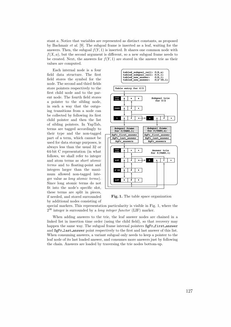
stant a. Notice that variables are represented as distinct constants, as proposedby Bachmair et al. [9]. The subgoal frame is inserted as a leaf, waiting for theanswers. Then, the subgoal f(Y, 1) is inserted. It shares one common node withf(X, a), but the second argument is di!erent, so a new subgoal frame needs tobe created. Next, the answers for f(Y, 1) are stored in the answer trie as theirvalues are computed.

Subgoal framefor f(VAR0,1)

SgFr_first_answerSgFr_last_answer

SgFr_answers

Table entry for f/2

Subgoal framefor f(VAR0,a)

a

VAR0

rootnode

1

0

rootnode

LIF

Subgoal triefor f/2

Answer triefor f(VAR0,1)

SgFr_first_answerSgFr_last_answer

SgFr_answers

tabled_subgoal_call: f(X,a)tabled_subgoal_call: f(Y,1)tabled_new_answer: f(0,1)tabled_new_answer: f(2^30,1)

2^30

LIF

Fig. 1. The table space organization

Each internal node is a fourfield data structure. The firstfield stores the symbol for thenode. The second and third fieldsstore pointers respectively to thefirst child node and to the par-ent node. The fourth field storesa pointer to the sibling node,in such a way that the outgo-ing transitions from a node canbe collected by following its firstchild pointer and then the listof sibling pointers. In YapTab,terms are tagged accordingly totheir type and the non-taggedpart of a term, which cannot beused for data storage purposes, isalways less than the usual 32 or64-bit C representation (in whatfollows, we shall refer to integerand atom terms as short atomicterms and to floating-point andintegers larger than the maxi-mum allowed non-tagged inte-ger value as long atomic terms).Since long atomic terms do notfit into the node’s specific slot,these terms are split in pieces,if needed, and stored surroundedby additional nodes consisting ofspecial markers. This representation particularity is visible in Fig. 1, where the230 integer is surrounded by a long integer functor (LIF) marker.

When adding answers to the trie, the leaf answer nodes are chained in alinked list in insertion time order (using the child field), so that recovery mayhappen the same way. The subgoal frame internal pointers SgFr first answerand SgFr last answer point respectively to the first and last answer of this list.When consuming answers, a variant subgoal only needs to keep a pointer to theleaf node of its last loaded answer, and consumes more answers just by followingthe chain. Answers are loaded by traversing the trie nodes bottom-up.

127

3 Extending the YapTab Design

The main idea behind DBTAB is straightforward. Every data transaction occursin the context of a specific execution session. In that context, a relational table isassigned to each tabled predicate. The relation’s name encloses the predicate’sfunctor and arity, the relation’s attributes equal the predicate’s arguments innumber and name. The dumping of a complete tabled subgoal answer set to thedatabase is triggered when the respective table is chosen for destruction by theleast recently used algorithm.

Data exchange between the YapTab engine and the RDBMS is mostly donethrough MySQL C API for prepared statements. Two major table space datastructures, table entries and subgoal frames, are expanded with new pointers toPreparedStatement data structures. Table entries are expanded with a pointerto an insert prepared statement. This statement is prepared to insert a fullrecord at a time into the predicate’s relational table, so that all subgoals hangingfrom the same table entry may use the same insert statement when storingtheir computed answers. Subgoal frames, on the other hand, are expanded witha pointer to a select prepared statement. This statement is used to speed up thedata retrieval, while reducing the resulting record-set at the same time. Groundterms in the respective subgoal trie branch are used to refine the statement’swhere clause - the corresponding fields in the relational representation neednot to be selected for retrieval since their values are already known.

3.1 The Relational Storage Model

The choice of an e!ective representation model for the tables is a hard task tofulfill. The relational model is expected to quickly store and retrieve answers,thus minimizing the impact on YapTab’s performance. With this concern inmind, two di!erent database schemes were developed.

Fig. 2. Multiple table schema

Multiple Table Schema Totake full advantage of the re-lational model, data regardingthe computed subgoal’s an-swers is stored in several ta-bles, aiming to keep the tablespace representation as smallas possible in the database.Figure 2 shows the multiple ta-ble relational schema for thef/2 tabled predicate intro-duced back in Fig. 1.

The tabled predicate f/2 ismapped into the relational table sessionk f2, where k is the current session id.Predicate arguments become the argi integer fields and the meta field is used totell apart the three kinds of possible records: a zero value signals an answer trie

128

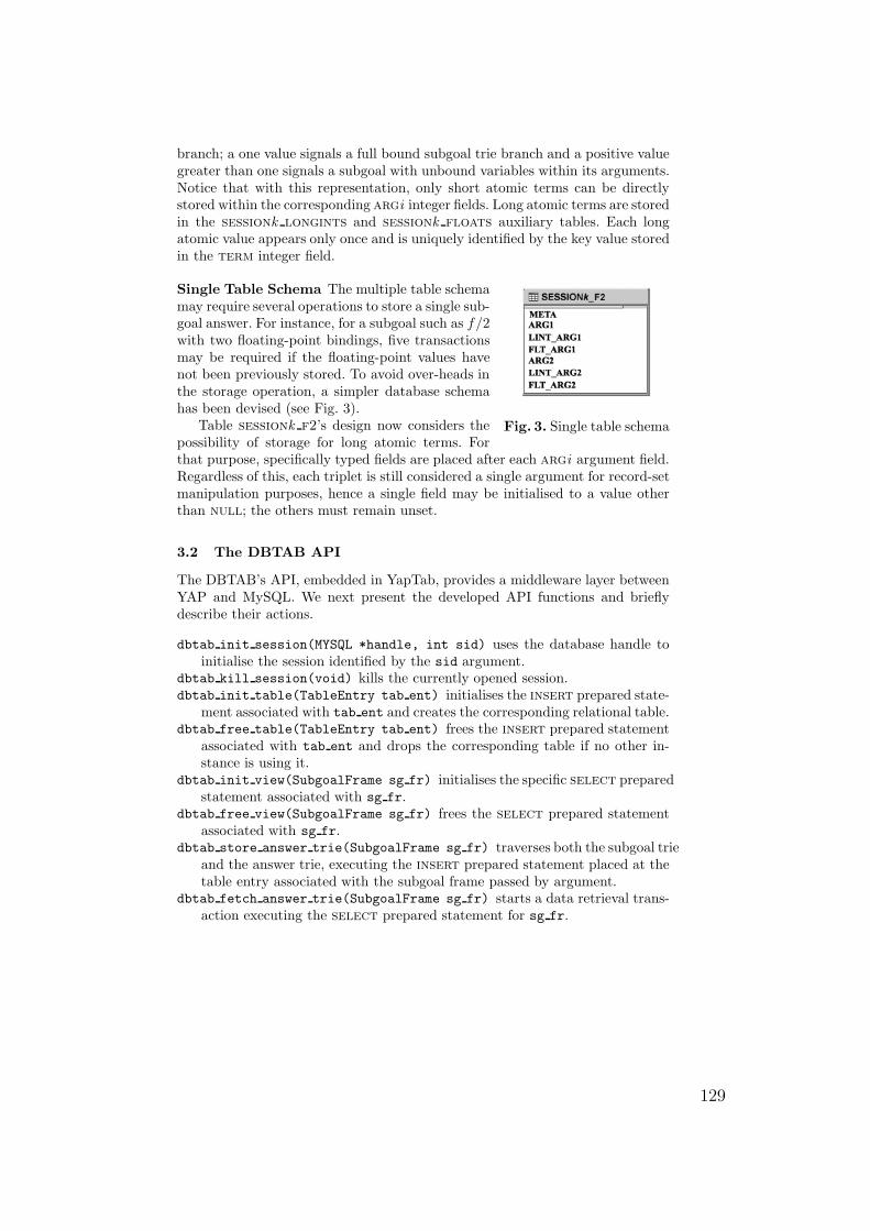
branch; a one value signals a full bound subgoal trie branch and a positive valuegreater than one signals a subgoal with unbound variables within its arguments.Notice that with this representation, only short atomic terms can be directlystored within the corresponding argi integer fields. Long atomic terms are storedin the sessionk longints and sessionk floats auxiliary tables. Each longatomic value appears only once and is uniquely identified by the key value storedin the term integer field.

Fig. 3. Single table schema

Single Table Schema The multiple table schemamay require several operations to store a single sub-goal answer. For instance, for a subgoal such as f/2with two floating-point bindings, five transactionsmay be required if the floating-point values havenot been previously stored. To avoid over-heads inthe storage operation, a simpler database schemahas been devised (see Fig. 3).

Table sessionk f2’s design now considers thepossibility of storage for long atomic terms. Forthat purpose, specifically typed fields are placed after each argi argument field.Regardless of this, each triplet is still considered a single argument for record-setmanipulation purposes, hence a single field may be initialised to a value otherthan null; the others must remain unset.

3.2 The DBTAB API

The DBTAB’s API, embedded in YapTab, provides a middleware layer betweenYAP and MySQL. We next present the developed API functions and brieflydescribe their actions.

dbtab init session(MYSQL *handle, int sid) uses the database handle toinitialise the session identified by the sid argument.

dbtab kill session(void) kills the currently opened session.dbtab init table(TableEntry tab ent) initialises the insert prepared state-

ment associated with tab ent and creates the corresponding relational table.dbtab free table(TableEntry tab ent) frees the insert prepared statement

associated with tab ent and drops the corresponding table if no other in-stance is using it.

dbtab init view(SubgoalFrame sg fr) initialises the specific select preparedstatement associated with sg fr.

dbtab free view(SubgoalFrame sg fr) frees the select prepared statementassociated with sg fr.

dbtab store answer trie(SubgoalFrame sg fr) traverses both the subgoal trieand the answer trie, executing the insert prepared statement placed at thetable entry associated with the subgoal frame passed by argument.

dbtab fetch answer trie(SubgoalFrame sg fr) starts a data retrieval trans-action executing the select prepared statement for sg fr.

129

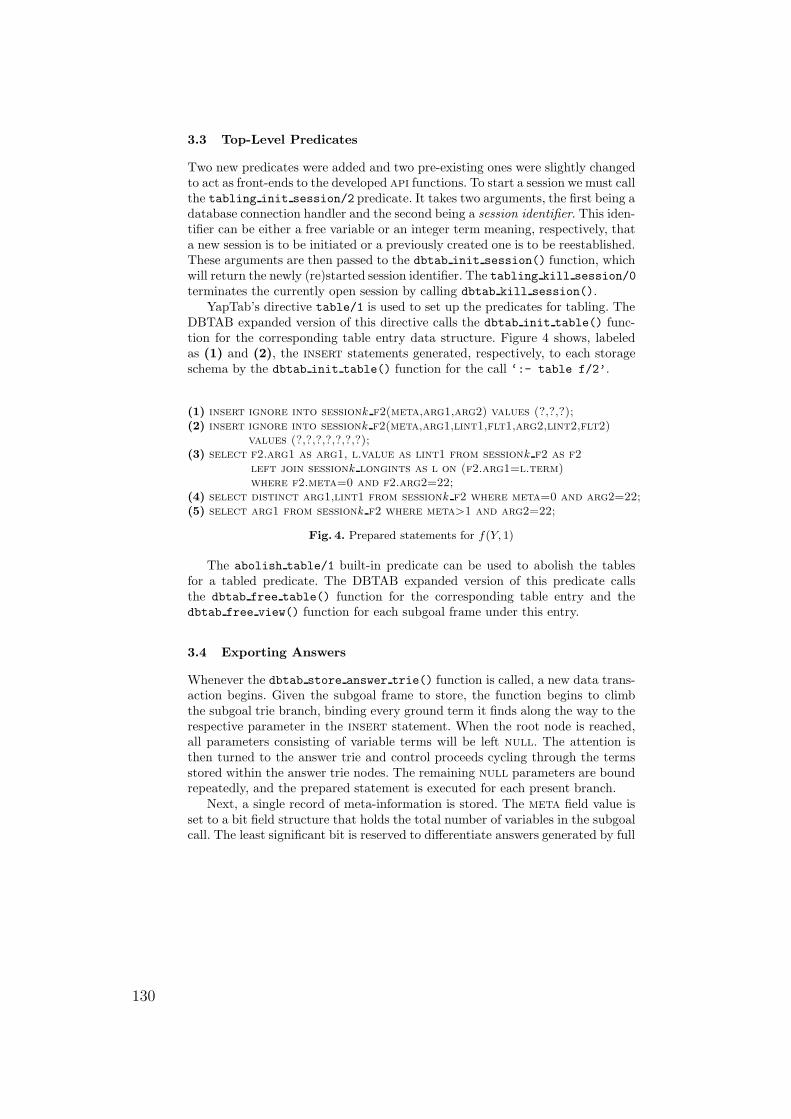
3.3 Top-Level Predicates

Two new predicates were added and two pre-existing ones were slightly changedto act as front-ends to the developed api functions. To start a session we must callthe tabling init session/2 predicate. It takes two arguments, the first being adatabase connection handler and the second being a session identifier. This iden-tifier can be either a free variable or an integer term meaning, respectively, thata new session is to be initiated or a previously created one is to be reestablished.These arguments are then passed to the dbtab init session() function, whichwill return the newly (re)started session identifier. The tabling kill session/0terminates the currently open session by calling dbtab kill session().

YapTab’s directive table/1 is used to set up the predicates for tabling. TheDBTAB expanded version of this directive calls the dbtab init table() func-tion for the corresponding table entry data structure. Figure 4 shows, labeledas (1) and (2), the insert statements generated, respectively, to each storageschema by the dbtab init table() function for the call ‘:- table f/2’.

(1) insert ignore into sessionk f2(meta,arg1,arg2) values (?,?,?);(2) insert ignore into sessionk f2(meta,arg1,lint1,flt1,arg2,lint2,flt2)

values (?,?,?,?,?,?,?);(3) select f2.arg1 as arg1, l.value as lint1 from sessionk f2 as f2

left join sessionk longints as l on (f2.arg1=l.term)where f2.meta=0 and f2.arg2=22;

(4) select distinct arg1,lint1 from sessionk f2 where meta=0 and arg2=22;(5) select arg1 from sessionk f2 where meta>1 and arg2=22;

Fig. 4. Prepared statements for f(Y, 1)

The abolish table/1 built-in predicate can be used to abolish the tablesfor a tabled predicate. The DBTAB expanded version of this predicate callsthe dbtab free table() function for the corresponding table entry and thedbtab free view() function for each subgoal frame under this entry.

3.4 Exporting Answers

Whenever the dbtab store answer trie() function is called, a new data trans-action begins. Given the subgoal frame to store, the function begins to climbthe subgoal trie branch, binding every ground term it finds along the way to therespective parameter in the insert statement. When the root node is reached,all parameters consisting of variable terms will be left null. The attention isthen turned to the answer trie and control proceeds cycling through the termsstored within the answer trie nodes. The remaining null parameters are boundrepeatedly, and the prepared statement is executed for each present branch.

Next, a single record of meta-information is stored. The meta field value isset to a bit field structure that holds the total number of variables in the subgoalcall. The least significant bit is reserved to di!erentiate answers generated by full

130

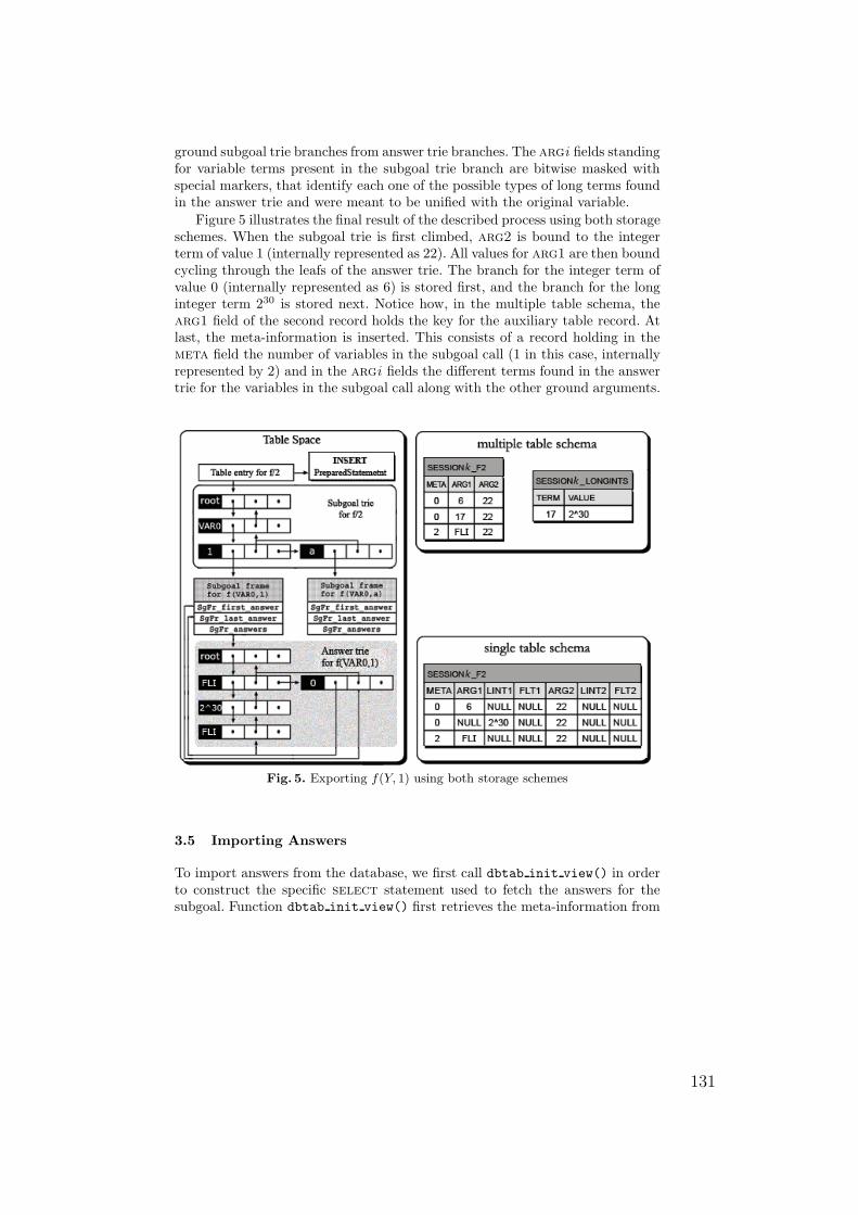
ground subgoal trie branches from answer trie branches. The argi fields standingfor variable terms present in the subgoal trie branch are bitwise masked withspecial markers, that identify each one of the possible types of long terms foundin the answer trie and were meant to be unified with the original variable.

Figure 5 illustrates the final result of the described process using both storageschemes. When the subgoal trie is first climbed, arg2 is bound to the integerterm of value 1 (internally represented as 22). All values for arg1 are then boundcycling through the leafs of the answer trie. The branch for the integer term ofvalue 0 (internally represented as 6) is stored first, and the branch for the longinteger term 230 is stored next. Notice how, in the multiple table schema, thearg1 field of the second record holds the key for the auxiliary table record. Atlast, the meta-information is inserted. This consists of a record holding in themeta field the number of variables in the subgoal call (1 in this case, internallyrepresented by 2) and in the argi fields the di!erent terms found in the answertrie for the variables in the subgoal call along with the other ground arguments.

Fig. 5. Exporting f(Y, 1) using both storage schemes

3.5 Importing Answers

To import answers from the database, we first call dbtab init view() in orderto construct the specific select statement used to fetch the answers for thesubgoal. Function dbtab init view() first retrieves the meta-information from

131

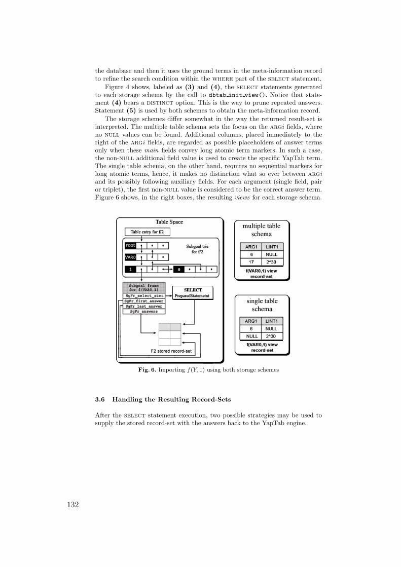
the database and then it uses the ground terms in the meta-information recordto refine the search condition within the where part of the select statement.

Figure 4 shows, labeled as (3) and (4), the select statements generatedto each storage schema by the call to dbtab init view(). Notice that state-ment (4) bears a distinct option. This is the way to prune repeated answers.Statement (5) is used by both schemes to obtain the meta-information record.

The storage schemes di!er somewhat in the way the returned result-set isinterpreted. The multiple table schema sets the focus on the argi fields, whereno null values can be found. Additional columns, placed immediately to theright of the argi fields, are regarded as possible placeholders of answer termsonly when these main fields convey long atomic term markers. In such a case,the non-null additional field value is used to create the specific YapTab term.The single table schema, on the other hand, requires no sequential markers forlong atomic terms, hence, it makes no distinction what so ever between argiand its possibly following auxiliary fields. For each argument (single field, pairor triplet), the first non-null value is considered to be the correct answer term.Figure 6 shows, in the right boxes, the resulting views for each storage schema.

Fig. 6. Importing f(Y, 1) using both storage schemes

3.6 Handling the Resulting Record-Sets

After the select statement execution, two possible strategies may be used tosupply the stored record-set with the answers back to the YapTab engine.

132

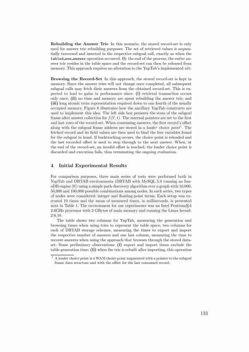
Rebuilding the Answer Trie In this scenario, the stored record-set is onlyused for answer trie rebuilding purposes. The set of retrieved values is sequen-tially traversed and inserted in the respective subgoal call, exactly as when thetabled new answer operation occurred. By the end of the process, the entire an-swer trie resides in the table space and the record-set can then be released frommemory. This approach requires no alteration to the YapTab’s implemented api.

Browsing the Record-Set In this approach, the stored record-set is kept inmemory. Since the answer tries will not change once completed, all subsequentsubgoal calls may fetch their answers from the obtained record-set. This is ex-pected to lead to gains in performance since: (i) retrieval transaction occursonly once; (ii) no time and memory are spent rebuilding the answer trie; and(iii) long atomic term representation required down to one fourth of the usuallyoccupied memory. Figure 6 illustrates how the ancillary YapTab constructs areused to implement this idea. The left side box presents the state of the subgoalframe after answer collection for f(Y, 1). The internal pointers are set to the firstand last rows of the record-set. When consuming answers, the first record’s o!setalong with the subgoal frame address are stored in a loader choice point1. Thefetched record and its field values are then used to bind the free variables foundfor the subgoal in hand. If backtracking occurs, the choice point is reloaded andthe last recorded o!set is used to step through to the next answer. When, atthe end of the record-set, an invalid o!set is reached, the loader choice point isdiscarded and execution fails, thus terminating the ongoing evaluation.

4 Initial Experimental Results

For comparison purposes, three main series of tests were performed both inYapTab and DBTAB environments (DBTAB with MySQL 5.0 running an Inn-oDB engine [8]) using a simple path discovery algorithm over a graph with 10,000,50,000 and 100,000 possible combinations among nodes. In each series, two typesof nodes were considered: integer and floating-point terms. Each setup was ex-ecuted 10 times and the mean of measured times, in milliseconds, is presentednext in Table 1. The environment for our experiments was an Intel Pentium R!42.6GHz processor with 2 GBytes of main memory and running the Linux kernel-2.6.18.

The table shows two columns for YapTab, measuring the generation andbrowsing times when using tries to represent the table space, two columns foreach of DBTAB storage schemes, measuring the times to export and importthe respective number of answers and one last column, measuring the time torecover answers when using the approach that browses through the stored data-set. Some preliminary observations: (i) export and import times exclude thetable generation time; (ii) when the trie is rebuilt after importing, this operation

1 A loader choice point is a WAM choice point augmented with a pointer to the subgoalframe data structure and with the o!set for the last consumed record.

133

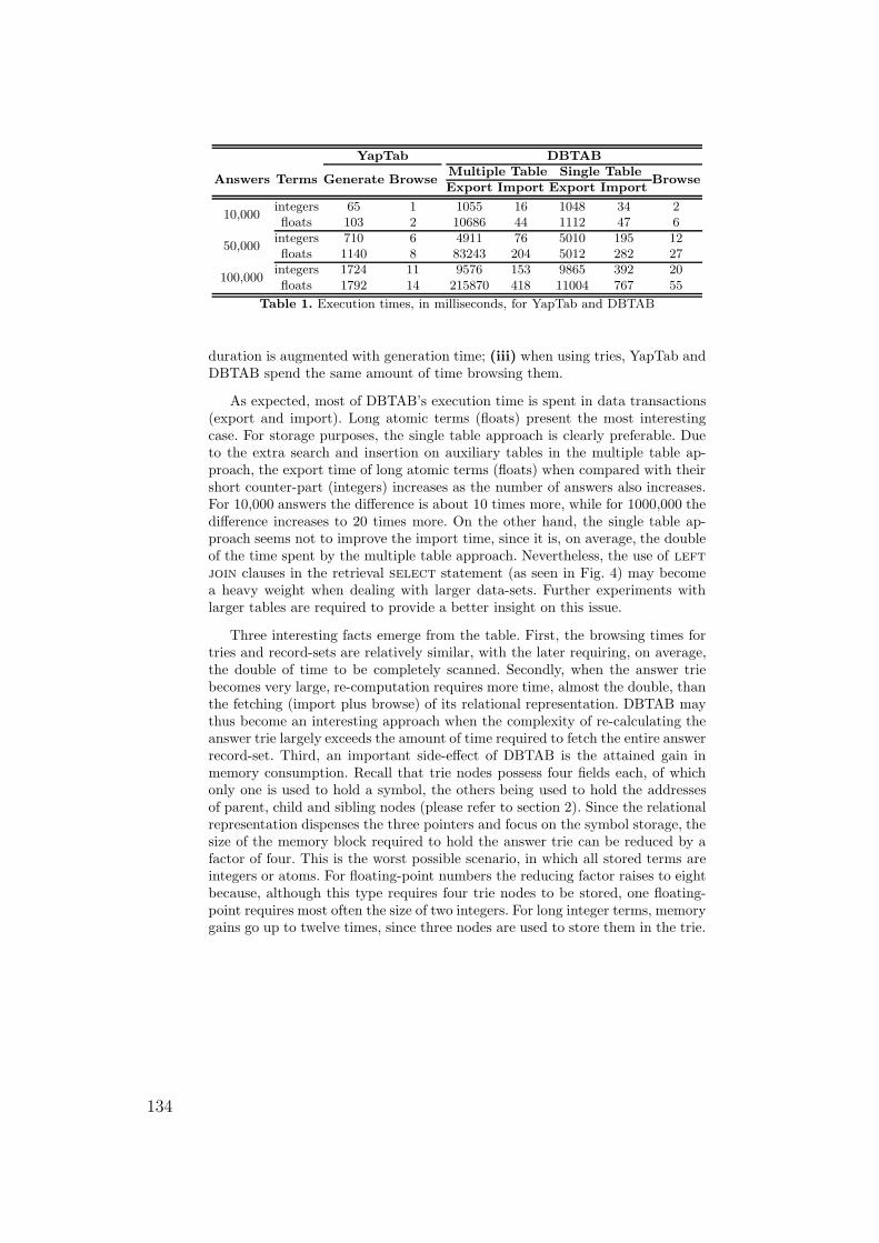
YapTab DBTAB

Answers Terms Generate BrowseMultiple Table Single Table

BrowseExport Import Export Import

10,000integers 65 1 1055 16 1048 34 2floats 103 2 10686 44 1112 47 6

50,000integers 710 6 4911 76 5010 195 12floats 1140 8 83243 204 5012 282 27

100,000integers 1724 11 9576 153 9865 392 20floats 1792 14 215870 418 11004 767 55

Table 1. Execution times, in milliseconds, for YapTab and DBTAB

duration is augmented with generation time; (iii) when using tries, YapTab andDBTAB spend the same amount of time browsing them.

As expected, most of DBTAB’s execution time is spent in data transactions(export and import). Long atomic terms (floats) present the most interestingcase. For storage purposes, the single table approach is clearly preferable. Dueto the extra search and insertion on auxiliary tables in the multiple table ap-proach, the export time of long atomic terms (floats) when compared with theirshort counter-part (integers) increases as the number of answers also increases.For 10,000 answers the di!erence is about 10 times more, while for 1000,000 thedi!erence increases to 20 times more. On the other hand, the single table ap-proach seems not to improve the import time, since it is, on average, the doubleof the time spent by the multiple table approach. Nevertheless, the use of leftjoin clauses in the retrieval select statement (as seen in Fig. 4) may becomea heavy weight when dealing with larger data-sets. Further experiments withlarger tables are required to provide a better insight on this issue.

Three interesting facts emerge from the table. First, the browsing times fortries and record-sets are relatively similar, with the later requiring, on average,the double of time to be completely scanned. Secondly, when the answer triebecomes very large, re-computation requires more time, almost the double, thanthe fetching (import plus browse) of its relational representation. DBTAB maythus become an interesting approach when the complexity of re-calculating theanswer trie largely exceeds the amount of time required to fetch the entire answerrecord-set. Third, an important side-e!ect of DBTAB is the attained gain inmemory consumption. Recall that trie nodes possess four fields each, of whichonly one is used to hold a symbol, the others being used to hold the addressesof parent, child and sibling nodes (please refer to section 2). Since the relationalrepresentation dispenses the three pointers and focus on the symbol storage, thesize of the memory block required to hold the answer trie can be reduced by afactor of four. This is the worst possible scenario, in which all stored terms areintegers or atoms. For floating-point numbers the reducing factor raises to eightbecause, although this type requires four trie nodes to be stored, one floating-point requires most often the size of two integers. For long integer terms, memorygains go up to twelve times, since three nodes are used to store them in the trie.

134

5 Conclusions and Further Work

In this work, we have introduced the DBTAB model. DBTAB was designed tobe used as an alternative approach to the problem of recovering space whenthe tabling system runs out of memory. By storing tables externally instead ofdeleting them, DBTAB avoids standard tabled re-computation when subsequentcalls to those tables appear. Another important aspect of DBTAB is the possiblegain in memory consumption when representing answers for floating-point andlong integer terms. Our preliminary results show that DBTAB may become aninteresting approach when the cost of recalculating a table largely exceeds theamount of time required to fetch the entire answer record-set from the database.As further work we plan to investigate the impact of applying DBTAB to a morerepresentative set of programs. We also plan to cover all possibilities for tablingpresented by YapTab and extend DBTAB to support lists and application terms.

Acknowledgments

This work has been partially supported by Myddas (POSC/EIA/59154/2004)and by funds granted to LIACC through the Programa de Financiamento Pluri-anual, Fundacao para a Ciencia e Tecnologia and Programa POSC.

References

1. Tamaki, H., Sato, T.: OLDT Resolution with Tabulation. In: International Confer-ence on Logic Programming. Number 225 in LNCS, Springer-Verlag (1986) 84–98

2. Chen, W., Warren, D.S.: Tabled Evaluation with Delaying for General Logic Pro-grams. Journal of the ACM 43 (1996) 20–74

3. Lloyd, J.W.: Foundations of Logic Programming. Springer-Verlag (1987)4. Ramakrishnan, I.V., Rao, P., Sagonas, K., Swift, T., Warren, D.S.: E"cient Access

Mechanisms for Tabled Logic Programs. Journal of Logic Programming 38 (1999)31–54

5. Fredkin, E.: Trie Memory. Communications of the ACM 3 (1962) 490–4996. Rocha, R., Silva, F., Santos Costa, V.: YapTab: A Tabling Engine Designed to

Support Parallelism. In: Conference on Tabulation in Parsing and Deduction. (2000)77–87

7. Rocha, R.: On Improving the E"ciency and Robustness of Table Storage Mecha-nisms for Tabled Evaluation. In: International Symposium on Practical Aspects ofDeclarative Languages. Number 4354 in LNCS, Springer-Verlag (2007) 155–169

8. Widenius, M., Axmark, D.: MySQL Reference Manual: Documentation from theSource. O’Reilly Community Press (2002)

9. Bachmair, L., Chen, T., Ramakrishnan, I.V.: Associative Commutative Discrimi-nation Nets. In: International Joint Conference on Theory and Practice of SoftwareDevelopment. Number 668 in LNCS, Springer-Verlag (1993) 61–74

135

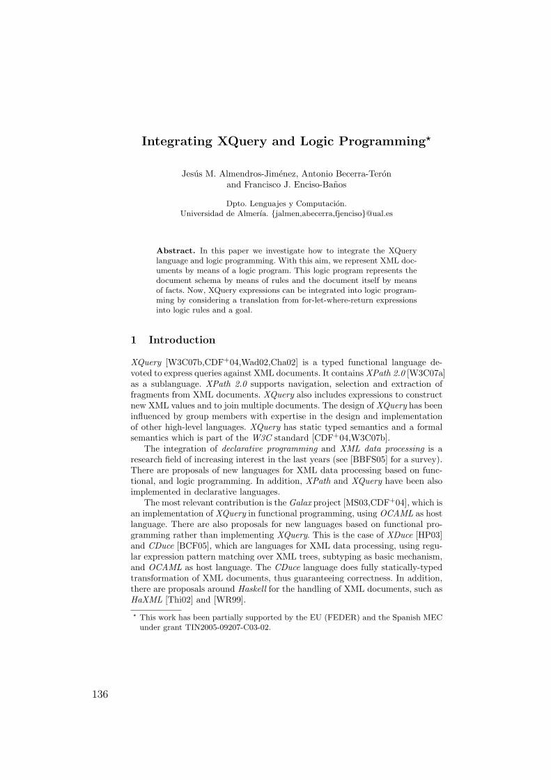
Integrating XQuery and Logic Programming?

Jesus M. Almendros-Jimenez, Antonio Becerra-Teronand Francisco J. Enciso-Banos

Dpto. Lenguajes y Computacion.Universidad de Almerıa. jalmen,abecerra,fjenciso@ual.es

Abstract. In this paper we investigate how to integrate the XQuerylanguage and logic programming. With this aim, we represent XML doc-uments by means of a logic program. This logic program represents thedocument schema by means of rules and the document itself by meansof facts. Now, XQuery expressions can be integrated into logic program-ming by considering a translation from for-let-where-return expressionsinto logic rules and a goal.

1 Introduction

XQuery [W3C07b,CDF+04,Wad02,Cha02] is a typed functional language de-voted to express queries against XML documents. It contains XPath 2.0 [W3C07a]as a sublanguage. XPath 2.0 supports navigation, selection and extraction offragments from XML documents. XQuery also includes expressions to constructnew XML values and to join multiple documents. The design of XQuery has beeninfluenced by group members with expertise in the design and implementationof other high-level languages. XQuery has static typed semantics and a formalsemantics which is part of the W3C standard [CDF+04,W3C07b].

The integration of declarative programming and XML data processing is aresearch field of increasing interest in the last years (see [BBFS05] for a survey).There are proposals of new languages for XML data processing based on func-tional, and logic programming. In addition, XPath and XQuery have been alsoimplemented in declarative languages.

The most relevant contribution is the Galax project [MS03,CDF+04], which isan implementation of XQuery in functional programming, using OCAML as hostlanguage. There are also proposals for new languages based on functional pro-gramming rather than implementing XQuery. This is the case of XDuce [HP03]and CDuce [BCF05], which are languages for XML data processing, using regu-lar expression pattern matching over XML trees, subtyping as basic mechanism,and OCAML as host language. The CDuce language does fully statically-typedtransformation of XML documents, thus guaranteeing correctness. In addition,there are proposals around Haskell for the handling of XML documents, such asHaXML [Thi02] and [WR99].

? This work has been partially supported by the EU (FEDER) and the Spanish MECunder grant TIN2005-09207-C03-02.

136

There are also contributions in the field of use logic programming for thehandling of XML documents. For instance, the Xcerpt project [SB02] proposes apattern and rule-based query language for XML documents, using the so-calledquery terms including logic variables for the retrieval of XML elements. Forthis new language a specialized unification algorithm for query terms has beenstudied. Another contribution of a new language is XPathLog (the LOPIX sys-tem) [May04] which is a Datalog-style extension of XPath with variable bindings.This is also the case of XCentric [CF03], which can represent XML documentsby means of logic programming, and handles XML documents by consideringterms with functions of flexible arity and regular types. Finally, FNPath [Sei02]is a proposal for using Prolog as query language for XML documents basedon a field-notation, for evaluating XPath expressions based on DOM. The RuleMarkup Language (RULEML) [Bol01,Bol00] is a different kind of proposal inthe research area. The aim of the approach is the representation of Prolog factsand rules into XML documents, and thus, the introduction of rule systems intothe Web. Finally, some well-known Prolog implementations include libraries forloading and querying XML documents, such as SWI-Prolog [Wie05] and CIAO[CH01].

In this paper, we investigate how to integrate the XQuery language and logicprogramming. With this aim:1. A XML document can be seen as a logic program, by considering facts and

rules for expressing both the XML schema and document. This approachwas already studied in our previous work [ABE07,ABE06].

2. A XQuery expression can be translated into logic programming by consideringa set of rules and a specific goal. Taking as starting point the translationof XPath of our previous work [ABE07,ABE06], the translation of XQueryintroduces new rules for the join of documents, and for the translation of for-let-where-return expressions into logic programming. In addition, a specificgoal is generated for obtaining the answer to an XQuery query.

3. Our technique allows the handling of XML documents as follows. Firstly,the XML documents are loaded. It involves the translation of the XMLdocuments into a logic program. For efficiency reasons the rules, which cor-respond to the XML document structure, are loaded in main memory, butfacts, which represent the values of the XML document, are stored in sec-ondary memory, whenever they do not fit in main memory (using appropriateindexing techniques). Secondly, the user can now write queries against theloaded documents. Now, XQuery queries are translated into a logic programand a specific goal. The evaluation of such goal uses the indexing in order toimprove the efficiency of query solving. Finally, the answer of the goal canbe represented by means of an output XML document.

As far as we know, this is the first time that XQuery is implemented inlogic programming. Previous proposals either define new query languages forXML documents in logic and functional programming or implement XQuery,but in functional programming. The advantages of such proposal is that XQueryis embedded into logic programming, and thus XQuery can be combined with

137

logic programs. For instance, logic programming can be used as inference engine,one of the requirements of the so-called Semantic Web (http://www.w3.org/2001/sw/), in the line of RuleML.

Our proposal requires the representation of XML documents into logic pro-gramming, which can be compared with those ones representing XML documentsin logic programming (for instance, [SB02,CF03]) and, with those ones represent-ing XML documents in relational databases (for instance, [BGvK+05]). In ourcase, rules are used for expressing the structure of well-formed XML documents,and XML elements are represented by means of facts. Moreover, our handlingof XML documents is more ”database-oriented” since we use secondary memoryand file indexing for selective reading of records. The reason for such decision isthat XML documents can usually be too big for main memory [MS03]. Our pro-posal uses as basis the implementation of XPath in logic programming studiedin our previous work [ABE07]. In addition, we have studied how to consider abottom-up approach to the same proposal of [ABE07] in [ABE06].

The structure of the paper is as follows. Section 2 will present the trans-lation of XML documents into Prolog; section 3 will review the translation ofXPath into logic programming; section 4 will provide the new translation ofXQuery expressions into logic programming; and finally, section 5 will concludeand present future work. A more complete version of our paper (with a biggerset of examples) can be found in http://www.ual.es/∼jalmen.

2 Translating XML Documents into Logic Programming

In order to define our translation we need to number the nodes of the XMLdocument. A similar numbering has been already adopted in some proposals forrepresenting XML in relational databases [OOP+04,TVB+02,BGvK+05].

Given an XML document, we can consider a new XML document callednode-numbered XML document as follows. Starting from the root element num-bered as 1, the node-numbered XML document is numbered using an attributecalled nodenumber1 where each j -th child of a tagged element is numberedwith the sequence of natural numbers i1 . . . . .it .j whenever the parent is num-bered as i1 . . . . .it : < tag att1 = v1, . . . , attn = vn,nodenumber= i1. . . . . it.j >elem1, . . . , elems < /tag >. This is the case of tagged elements. If the j-th childis of a basic type (non tagged) and the parent is an inner node, then the elementis labeled and numbered as follows: < unlabeled nodenumber = i1. . . . .it.j >elem < /unlabeled >; otherwise the element is not numbered. It gives to usa hierarchical and left-to-right numbering of the nodes of an XML document.An element in an XML document is further left in the XML tree than anotherwhen the node number is smaller w.r.t. the lexicographic order of sequence ofnatural numbers. Any numbering that identifies each inner node and leaf couldbe adapted to our translation.

In addition, we have to consider a new document called type and node-numbered XML document numbered using an attribute called typenumber as1 It is supposed that ”nodenumber” is not already used as attribute in the tags of the

original XML document.

138

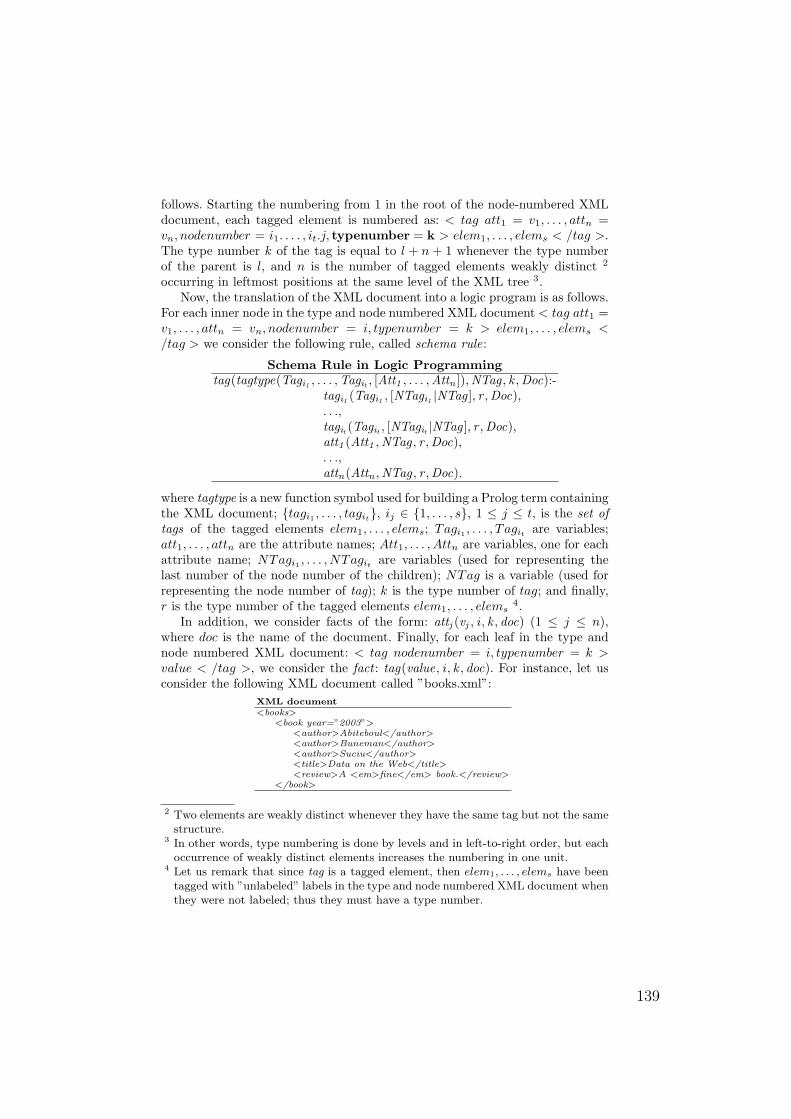
follows. Starting the numbering from 1 in the root of the node-numbered XMLdocument, each tagged element is numbered as: < tag att1 = v1, . . . , attn =vn, nodenumber = i1. . . . , it.j, typenumber = k > elem1, . . . , elems < /tag >.The type number k of the tag is equal to l + n + 1 whenever the type numberof the parent is l, and n is the number of tagged elements weakly distinct 2

occurring in leftmost positions at the same level of the XML tree 3.Now, the translation of the XML document into a logic program is as follows.

For each inner node in the type and node numbered XML document < tag att1 =v1, . . . , attn = vn, nodenumber = i, typenumber = k > elem1, . . . , elems </tag > we consider the following rule, called schema rule:

Schema Rule in Logic Programmingtag(tagtype(Tagi1 , . . . ,Tagit , [Att1 , . . . ,Attn ]),NTag , k ,Doc):-

tagi1 (Tagi1 , [NTagi1 |NTag ], r ,Doc),. . .,tagit (Tagit , [NTagit |NTag ], r ,Doc),att1 (Att1 ,NTag , r ,Doc),. . .,attn(Attn ,NTag , r ,Doc).

where tagtype is a new function symbol used for building a Prolog term containingthe XML document; tagi1 , . . . , tagit, ij ∈ 1, . . . , s, 1 ≤ j ≤ t, is the set oftags of the tagged elements elem1, . . . , elems; Tagi1 , . . . , Tagit are variables;att1, . . . , attn are the attribute names; Att1, . . . , Attn are variables, one for eachattribute name; NTagi1 , . . . , NTagit are variables (used for representing thelast number of the node number of the children); NTag is a variable (used forrepresenting the node number of tag); k is the type number of tag; and finally,r is the type number of the tagged elements elem1, . . . , elems

4.In addition, we consider facts of the form: attj (vj , i , k , doc) (1 ≤ j ≤ n),

where doc is the name of the document. Finally, for each leaf in the type andnode numbered XML document: < tag nodenumber = i, typenumber = k >value < /tag >, we consider the fact : tag(value, i , k , doc). For instance, let usconsider the following XML document called ”books.xml”:

XML document<books>

<book year=”2003”><author>Abiteboul</author><author>Buneman</author><author>Suciu</author><title>Data on the Web</title><review>A <em>fine</em> book.</review>

</book>

2 Two elements are weakly distinct whenever they have the same tag but not the samestructure.

3 In other words, type numbering is done by levels and in left-to-right order, but eachoccurrence of weakly distinct elements increases the numbering in one unit.

4 Let us remark that since tag is a tagged element, then elem1, . . . , elems have beentagged with ”unlabeled” labels in the type and node numbered XML document whenthey were not labeled; thus they must have a type number.

139

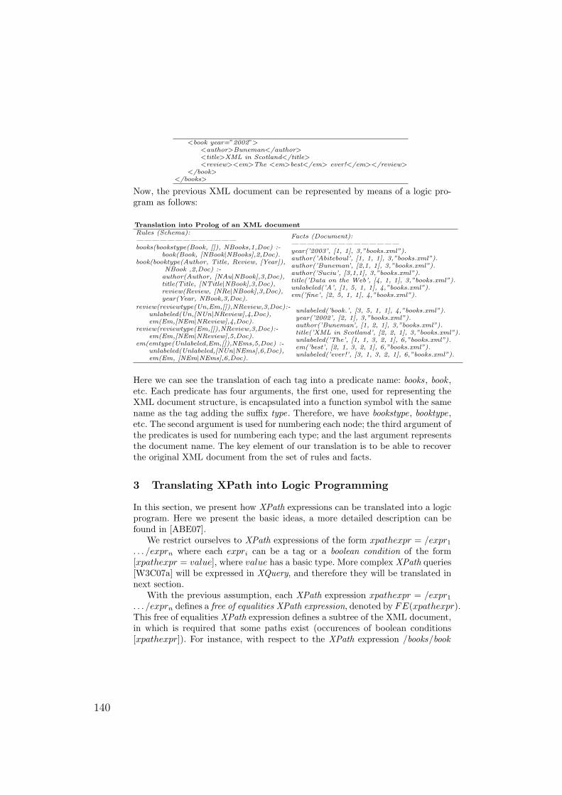
<book year=”2002”><author>Buneman</author><title>XML in Scotland</title><review><em>The <em>best</em> ever!</em></review>

</book></books>

Now, the previous XML document can be represented by means of a logic pro-gram as follows:

Translation into Prolog of an XML documentRules (Schema):—————————————books(bookstype(Book, []), NBooks,1,Doc) :-

book(Book, [NBook|NBooks],2,Doc).book(booktype(Author, Title, Review, [Year]),

NBook ,2,Doc) :-author(Author, [NAu|NBook],3,Doc),title(Title, [NTitle|NBook],3,Doc),review(Review, [NRe|NBook],3,Doc),year(Year, NBook,3,Doc).

Facts (Document):——————————————year(’2003’, [1, 1], 3,”books.xml”).author(’Abiteboul’, [1, 1, 1], 3,”books.xml”).author(’Buneman’, [2,1, 1], 3,”books.xml”).author(’Suciu’, [3,1,1], 3,”books.xml”).title(’Data on the Web’, [4, 1, 1], 3,”books.xml”).unlabeled(’A’, [1, 5, 1, 1], 4,”books.xml”).em(’fine’, [2, 5, 1, 1], 4,”books.xml”).

review(reviewtype(Un,Em,[]),NReview,3,Doc):-unlabeled(Un,[NUn|NReview],4,Doc),em(Em,[NEm|NReview],4,Doc).

review(reviewtype(Em,[]),NReview,3,Doc):-em(Em,[NEm|NReview],5,Doc).

em(emtype(Unlabeled,Em,[]),NEms,5,Doc) :-unlabeled(Unlabeled,[NUn|NEms],6,Doc),em(Em, [NEm|NEms],6,Doc).

unlabeled(’book.’, [3, 5, 1, 1], 4,”books.xml”).year(’2002’, [2, 1], 3,”books.xml”).author(’Buneman’, [1, 2, 1], 3,”books.xml”).title(’XML in Scotland’, [2, 2, 1], 3,”books.xml”).unlabeled(’The’, [1, 1, 3, 2, 1], 6,”books.xml”).em(’best’, [2, 1, 3, 2, 1], 6,”books.xml”).unlabeled(’ever!’, [3, 1, 3, 2, 1], 6,”books.xml”).

Here we can see the translation of each tag into a predicate name: books, book ,etc. Each predicate has four arguments, the first one, used for representing theXML document structure, is encapsulated into a function symbol with the samename as the tag adding the suffix type. Therefore, we have bookstype, booktype,etc. The second argument is used for numbering each node; the third argument ofthe predicates is used for numbering each type; and the last argument representsthe document name. The key element of our translation is to be able to recoverthe original XML document from the set of rules and facts.

3 Translating XPath into Logic Programming

In this section, we present how XPath expressions can be translated into a logicprogram. Here we present the basic ideas, a more detailed description can befound in [ABE07].

We restrict ourselves to XPath expressions of the form xpathexpr = /expr1

. . . /exprn where each expri can be a tag or a boolean condition of the form[xpathexpr = value], where value has a basic type. More complex XPath queries[W3C07a] will be expressed in XQuery, and therefore they will be translated innext section.

With the previous assumption, each XPath expression xpathexpr = /expr1

. . . /exprn defines a free of equalities XPath expression, denoted by FE(xpathexpr).This free of equalities XPath expression defines a subtree of the XML document,in which is required that some paths exist (occurences of boolean conditions[xpathexpr]). For instance, with respect to the XPath expression /books/book

140

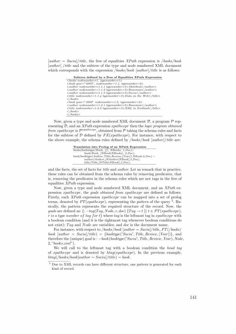
[author = Suciu]/title, the free of equalities XPath expression is /books/book[author ] /title and the subtree of the type and node numbered XML documentwhich corresponds with the expression /books/book [author ]/title is as follows:

Subtree defined by a Free of Equalities XPath Expression<books nodenumber=1, typenumber=1><book year=”2003”, nodenumber=1.1, typenumber=2><author nodenumber=1.1.1 typenumber=3>Abiteboul</author><author nodenumber=1.1.2 typenumber=3>Buneman</author><author nodenumber=1.1.3 typenumber=3>Suciu</author><title nodenumber=1.1.4 typenumber=3>Data on the Web</title></book><book year=”2002” nodenumber=1.2, typenumber=2><author nodenumber=1.2.1 typenumber=3>Buneman</author><title nodenumber=1.2.2 typenumber=3>XML in Scotland</title></book></books>

Now, given a type and node numbered XML document D, a program P rep-resenting D, and an XPath expression xpathexpr then the logic program obtainedfrom xpathexpr is Pxpathexpr, obtained from P taking the schema rules and factsfor the subtree of D defined by FE(xpathexpr). For instance, with respect tothe above example, the schema rules defined by /books/book [author ]/title are:

Translation into Prolog of an XPath Expressionbooks(bookstype(Book, []), NBooks, 1,Doc):-

book(Book, [NBook|NBooks], 2,Doc).book(booktype(Author,Title,Review,[Year]),NBook,2,Doc) :-

author(Author,[NAuthor|NBook],3,Doc),title(Title,[NTitle|NBook],3,Doc).

and the facts, the set of facts for title and author. Let us remark that in practice,these rules can be obtained from the schema rules by removing predicates, thatis, removing the predicates in the schema rules which are not tags in the free ofequalities XPath expression.

Now, given a type and node numbered XML document, and an XPath ex-pression xpathexpr, the goals obtained from xpathexpr are defined as follows.Firstly, each XPath expression xpathexpr can be mapped into a set of prologterms, denoted by PT (xpathexpr), representing the pattern of the query 5. Ba-sically, the pattern represents the required structure of the record. Now, thegoals are defined as: : −tag(Tag,Node, r, doc) Tag → t | t ∈ PT (xpathexpr),r is a type number of tag for t where tag is the leftmost tag in xpathexpr witha boolean condition (and it is the rightmost tag whenever boolean conditions donot exist); Tag and Node are variables; and doc is the document name.

For instance, with respect to /books/book [author = Suciu]/title, PT (/books/book [author = Suciu]/title) = booktype(′Suciu ′,Title,Review , [Year ]), andtherefore the (unique) goal is : −book(booktype(′Suciu ′,Title,Review ,Year),Node,2, ”books.xml”).

We will call to the leftmost tag with a boolean condition the head tagof xpathexpr and is denoted by htag(xpathexpr). In the previous example,htag(/books/book[author = Suciu]/title) = book.5 Due to XML records can have different structure, one pattern is generated for each

kind of record.

141

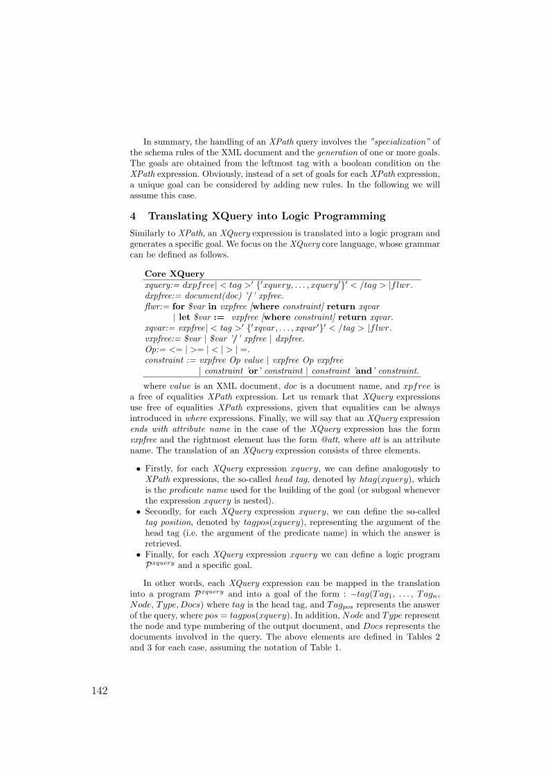
In summary, the handling of an XPath query involves the ”specialization” ofthe schema rules of the XML document and the generation of one or more goals.The goals are obtained from the leftmost tag with a boolean condition on theXPath expression. Obviously, instead of a set of goals for each XPath expression,a unique goal can be considered by adding new rules. In the following we willassume this case.

4 Translating XQuery into Logic Programming

Similarly to XPath, an XQuery expression is translated into a logic program andgenerates a specific goal. We focus on the XQuery core language, whose grammarcan be defined as follows.

Core XQueryxquery:= dxpfree| < tag >′ ′xquery, . . . , xquery′′ < /tag > |flwr.dxpfree:= document(doc) ’/’ xpfree.flwr:= for $var in vxpfree [where constraint] return xqvar

| let $var := vxpfree [where constraint] return xqvar.xqvar:= vxpfree| < tag >′ ′xqvar , . . . , xqvar ′′ < /tag > |flwr.vxpfree:= $var | $var ’/’ xpfree | dxpfree.Op:= <= | >= | < | > | =.constraint := vxpfree Op value | vxpfree Op vxpfree

| constraint ’or’ constraint | constraint ’and’ constraint.

where value is an XML document, doc is a document name, and xpfree isa free of equalities XPath expression. Let us remark that XQuery expressionsuse free of equalities XPath expressions, given that equalities can be alwaysintroduced in where expressions. Finally, we will say that an XQuery expressionends with attribute name in the case of the XQuery expression has the formvxpfree and the rightmost element has the form @att, where att is an attributename. The translation of an XQuery expression consists of three elements.

• Firstly, for each XQuery expression xquery, we can define analogously toXPath expressions, the so-called head tag, denoted by htag(xquery), whichis the predicate name used for the building of the goal (or subgoal wheneverthe expression xquery is nested).

• Secondly, for each XQuery expression xquery, we can define the so-calledtag position, denoted by tagpos(xquery), representing the argument of thehead tag (i.e. the argument of the predicate name) in which the answer isretrieved.

• Finally, for each XQuery expression xquery we can define a logic programPxquery and a specific goal.

In other words, each XQuery expression can be mapped in the translationinto a program Pxquery and into a goal of the form : −tag(Tag1, . . . , Tagn,Node, Type,Docs) where tag is the head tag, and Tagpos represents the answerof the query, where pos = tagpos(xquery). In addition, Node and Type representthe node and type numbering of the output document, and Docs represents thedocuments involved in the query. The above elements are defined in Tables 2and 3 for each case, assuming the notation of Table 1.

142

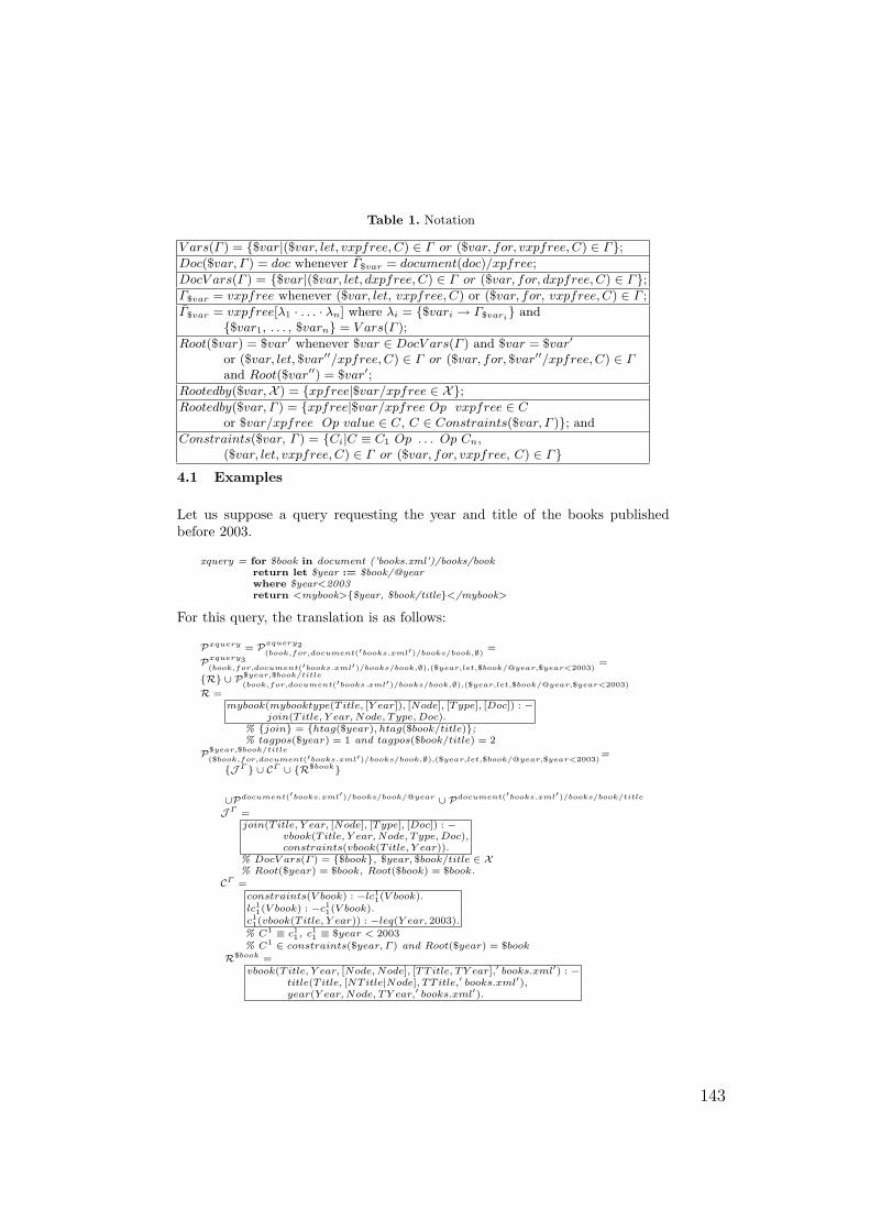
Table 1. Notation

V ars(Γ ) = $var|($var, let, vxpfree, C) ∈ Γ or ($var, for, vxpfree, C) ∈ Γ;Doc($var, Γ ) = doc whenever Γ$var = document(doc)/xpfree;

DocV ars(Γ ) = $var|($var, let, dxpfree, C) ∈ Γ or ($var, for, dxpfree, C) ∈ Γ;Γ$var = vxpfree whenever ($var, let, vxpfree, C) or ($var, for, vxpfree, C) ∈ Γ ;

Γ$var = vxpfree[λ1 · . . . · λn] where λi = $vari → Γ$vari and

$var1, . . . , $varn = V ars(Γ );

Root($var) = $var′ whenever $var ∈ DocV ars(Γ ) and $var = $var′

or ($var, let, $var′′/xpfree, C) ∈ Γ or ($var, for, $var′′/xpfree, C) ∈ Γand Root($var′′) = $var′;

Rootedby($var,X ) = xpfree|$var/xpfree ∈ X;Rootedby($var, Γ ) = xpfree|$var/xpfree Op vxpfree ∈ C

or $var/xpfree Op value ∈ C, C ∈ Constraints($var, Γ ); and

Constraints($var, Γ ) = Ci|C ≡ C1 Op . . . Op Cn,($var, let, vxpfree, C) ∈ Γ or ($var, for, vxpfree, C) ∈ Γ

4.1 Examples

Let us suppose a query requesting the year and title of the books publishedbefore 2003.

xquery = for $book in document (’books.xml’)/books/bookreturn let $year := $book/@yearwhere $year<2003return <mybook>$year, $book/title</mybook>

For this query, the translation is as follows:

Pxquery = Pxquery2(book,for,document(′books.xml′)/books/book,∅) =

Pxquery3(book,for,document(′books.xml′)/books/book,∅),($year,let,$book/@year,$year<2003)

=

R ∪ P$year,$book/title

(book,for,document(′books.xml′)/books/book,∅),($year,let,$book/@year,$year<2003)R =

mybook(mybooktype(Title, [Y ear]), [Node], [Type], [Doc]) : −join(Title, Y ear, Node, Type, Doc).

% join = htag($year), htag($book/title);% tagpos($year) = 1 and tagpos($book/title) = 2

P$year,$book/title

($book,for,document(′books.xml′)/books/book,∅),($year,let,$book/@year,$year<2003)=

J Γ ∪ CΓ ∪ R$book

∪Pdocument(′books.xml′)/books/book/@year ∪ Pdocument(′books.xml′)/books/book/title

J Γ =join(Title, Y ear, [Node], [Type], [Doc]) : −

vbook(Title, Y ear, Node, Type, Doc),constraints(vbook(Title, Y ear)).

% DocV ars(Γ ) = $book, $year, $book/title ∈ X% Root($year) = $book, Root($book) = $book.

CΓ =

constraints(V book) : −lc11(V book).

lc11(V book) : −c1

1(V book).c11(vbook(Title, Y ear)) : −leq(Y ear, 2003).

% C1 ≡ c11, c1

1 ≡ $year < 2003% C1 ∈ constraints($year, Γ ) and Root($year) = $book

R$book =vbook(Title, Y ear, [Node, Node], [TTitle, TY ear],′ books.xml′) : −

title(Title, [NTitle|Node], TT itle,′ books.xml′),year(Y ear, Node, TY ear,′ books.xml′).

143

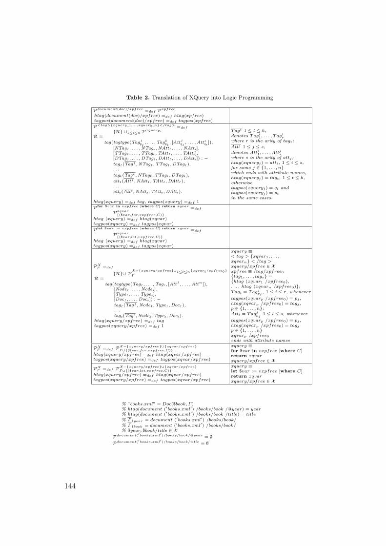
Table 2. Translation of XQuery into Logic Programming

Pdocument(doc)/xpfree =def Pxpfree

htag(document(doc)/xpfree) =def htag(xpfree)tagpos(document(doc)/xpfree) =def tagpos(xpfree)

P<tag>xquery 1,...,xquery n</tag> =def

R ∪1≤i≤n Pxqueryi

R ≡tag(tagtype(Tag1

p1, . . . , Tagk

pk, [Att1

q1, . . . , Atts

qs]),

[NTag1 , . . . , NTagk , NAtt1 , . . . , NAtts ],[TTag1 , . . . , TTagk , TAtt1 , . . . , TAtts ],[DTag1 , . . . , DTagk , DAtt1 , . . . , DAtts ]) : −tag1 (Tag1 , NTag1 , TTag1 , DTag1 ),. . .

tagk (Tagk , NTagk , TTagk , DTagk ),

att1 (Att1 , NAtt1 , TAtt1 , DAtt1 ),. . .

atts(Atts , NAtts , TAtts , DAtts).

htag(xquery) =def tag, tagpos(xquery) =def 1

Tagt 1 ≤ t ≤ k,denotes Tagt

1, . . . , Tagtr

where r is the arity of tagt;

Attj 1 ≤ j ≤ s,

denotes Attj1, . . . , Attj

swhere s is the arity of attj ;htag(xqueryj) = atti, 1 ≤ i ≤ s,for some j ∈ 1, . . . , nwhich ends with attribute names,htag(xqueryj) = tagt, 1 ≤ t ≤ k,otherwisetagpos(xqueryj) = qi andtagpos(xqueryj) = pt

in the same cases.

Pfor $var in vxpfree [where C] return xqvar =def

Pxqvar($var,for,vxpfree,C)

htag (xquery) =def htag(xqvar)tagpos(xquery) =def tagpos(xqvar)

Plet $var := vxpfree [where C] return xqvar =def

Pxqvar($var,let,vxpfree,C)

htag (xquery) =def htag(xqvar)tagpos(xquery) =def tagpos(xqvar)

PXΓ =def

R∪ PX−xquery/xpfree∪1≤i≤nxqvari/xpfree0Γ

R ≡tag(tagtype(Tag1 , . . . , Tagr , [Att1 , . . . , Attm ]),

[Node1 , . . . , Nodes ],[Type1 , . . . , Types ],[Doc1 , . . . , Docs ]) : −tag1 (Tag1 , Node1 , Type1 , Doc1 ),. . .

tags(Tags , Nodes , Types , Docs).htag(xquery/xpfree) =def tagtagpos(xquery/xpfree) =def 1

xquery ≡< tag > xqvar1, . . . ,xqvarn < /tag >xquery/xpfree ∈ Xxpfree ≡ /tag/xpfree0tag1, . . . , tags =htag (xqvar1 /xpfree0),. . . , htag (xqvarn /xpfree0);Tagi = Tagj

pj, 1 ≤ i ≤ r, whenever

tagpos(xqvarp /xpfree0) = pj ,htag(xqvarp /xpfree0) = tagj ,p ∈ 1, . . . , n;Attl = Tagj

pj1 ≤ l ≤ s, whenever

tagpos(xqvarp /xpfree0) = pj ,htag(xqvarp /xpfree0) = tagj

p ∈ 1, . . . , nxqvarp /xpfree0ends with attribute names

PXΓ =def PX−xquery/xpfree∪xqvar/xpfreeΓ∪($var,for,vxpfree,C)

htag(xquery/xpfree) =def htag(xqvar/xpfree)tagpos(xquery/xpfree) =def tagpos(xqvar/xpfree)

xquery ≡for $var in vxpfree [where C]return xqvarxquery/xpfree ∈ X

PXΓ =def PX−xquery/xpfree∪xqvar/xpfreeΓ∪($var,let,vxpfree,C)

htag(xquery/xpfree) =def htag(xqvar/xpfree)tagpos(xquery/xpfree) =def tagpos(xqvar/xpfree)

xquery ≡let $var := vxpfree [where C]return xqvarxquery/xpfree ∈ X

% ”books.xml” = Doc($book, Γ )% htag(document (′books.xml′) /books/book /@year) = year% htag(document (′books.xml′) /books/book /title) = title

% Γ $year = document (′books.xml′) /books/book/

% Γ $book = document (′books.xml′) /books/book/% $year, $book/title ∈ X

Pdocument(′books.xml′)/books/book/@year = ∅Pdocument(′books.xml′)/books/book/title = ∅

144

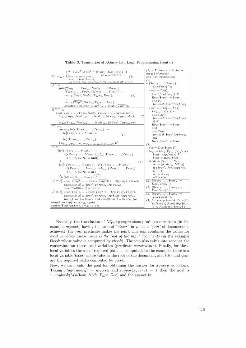
Table 3. Translation of XQuery into Logic Programming (cont’d)

PXΓ =def

J Γ ∪ CΓ ∪ R$var|$var ∈ DocV ars(Γ )S$var ∈ DocV ars(Γ ),

$var = Root($var′),

xpfree ∈ Rootedby($var′,X) ∪ Rootedby($var′, Γ )

PΓ$var/xpfree(1)

J Γ ≡join(Tag1, . . . , Tagm, [Node1, . . . , Noden],

[Type1, . . . , Typen], [Doc1, . . . , Docn]) : −vvar1(Tag1, Node1, Type1, Doc1),. . .

vvarn(Tagn, Noden, Typen, Docn),

constraints(vvar1(Tag1), . . . , vvarn(Tagn)).

(2)

R$var ≡vvar(Tag1, . . . , Tagn, Node, [Type1, . . . , Typen], doc) : −

tag1(Tag1, [Node11, . . . , Node1k1 |NTag], Type1, doc),. . . ,tagn(Tagn, [Noden1, . . . , Nodenkn |NTag], Typen, doc).

(3)

CΓ ≡ constraints(V var1, . . . , V varn) : −

lc11(V var1, . . . , V varn),

. . .lcn

1 (V var1, . . . , V varn).

∪$var∈V ars(Γ ),Cj∈constraints($var,Γ ) Cj

(4)

Cj ≡lcj

i (V var1, . . . , V varn) : −cj

i (V var1, . . . , V varn), lcji+1(V var1, . . . , V varn).

| 1 ≤ i ≤ n, Opi = and∪lcj

i (V var1, . . . , V varn) : −cji (V var1, . . . , V varn).

lcji (Vvar1 , . . . , Vvarn) : −lcj

i+1 (Vvar1 , . . . , Vvarn).| 1 ≤ i ≤ n, Opi = or

∪c

ji|Cj≡c

j1Op1...,Opnc

jnCj

i

(5)

Cji ≡ cj

i (vvar1(Tag1), . . . , vvarn(Tagn)) : −Op(Tagkj , value).

whenever cji ≡ $var′/xpfreej Op value

and Root($var′) = $vark

Cji ≡ cj

i (vvar(Tag1), . . . , vvar(Tagn)) : −Op(Tagkj , Tagm

r ).

whenever cji ≡ $var′/xpfreej Op $var′/xpfreer,

Root($var′) = $vark and Root($var′) = $varm (6)htag($var/xpfreej) =def jointagpos($var/xpfreej) =def j (7)

(1) – X does not includestagged elementsand flwr expressions(2)– $var1, . . . , $varn =

DocV ars(Γ );

– Tagj = Tagipj

$var′/xpfreej ∈ XRoot($var′) = $vari

one pj

for each $var′/xpfreej

– Tagi = Tagi1 . . . Tagi

s

Tagir, 1 ≤ r ≤ s

one Tagir

for each $var′/xpfreer

∈ XRoot($var′) = $vari

and

one Tagir

for each $var′/xpfreer

inΓRoot($var′) = $vari

(3)– doc = Doc($var, Γ )

– tagi = htag(Γ $var/xpfree)$var′ /xpfree ∈ X$var = Root($var′)

– Node = [N1, . . . , Nn]Ni = [Nodeiki

|NTag]if ($var′, for, vxpfree,C) ∈ ΓNi = NTagotherwise

(4) $var1, . . . , $varn =DocV ars(Γ );

(5) $var1, . . . , $varn =DocV ars(Γ ).

(6) $var1, . . . , $varn =DocV ars(Γ ).

(7) for every $var ∈ V ars(Γ ),xpfreej ∈ Rootedby($var,X ) ∪ Rootedby($var, Γ )

Basically, the translation of XQuery expressions produces new rules (in theexample mybook) having the form of ”views” in which a ”join” of documents isachieved (the join predicate makes the join). The join combines the values forlocal variables whose value is the root of the input documents (in the example$book whose value is computed by vbook). The join also takes into account theconstraints on these local variables (predicate constraints). Finally, for theselocal variables the set of required paths is computed. In the example, there is alocal variable $book whose value is the root of the document, and title and yearare the required paths computed by vbook.Now, we can build the goal for obtaining the answer for xquery as follows.Taking htag(xquery) = mybook and tagpos(xquery) = 1 then the goal is: −mybook(MyBook,Node, Type,Doc) and the answer is:

145

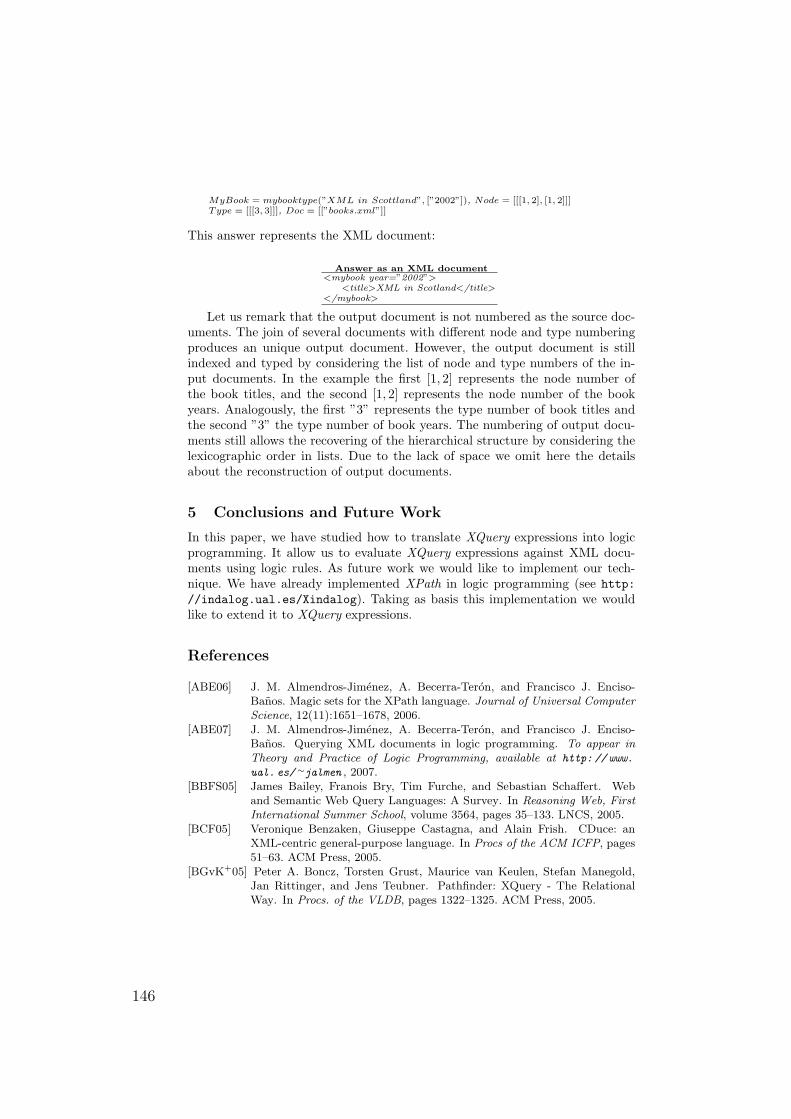
MyBook = mybooktype(”XML in Scottland”, [”2002”]), Node = [[[1, 2], [1, 2]]]Type = [[[3, 3]]], Doc = [[”books.xml”]]

This answer represents the XML document:

Answer as an XML document<mybook year=”2002”>

<title>XML in Scotland</title></mybook>

Let us remark that the output document is not numbered as the source doc-uments. The join of several documents with different node and type numberingproduces an unique output document. However, the output document is stillindexed and typed by considering the list of node and type numbers of the in-put documents. In the example the first [1, 2] represents the node number ofthe book titles, and the second [1, 2] represents the node number of the bookyears. Analogously, the first ”3” represents the type number of book titles andthe second ”3” the type number of book years. The numbering of output docu-ments still allows the recovering of the hierarchical structure by considering thelexicographic order in lists. Due to the lack of space we omit here the detailsabout the reconstruction of output documents.

5 Conclusions and Future Work

In this paper, we have studied how to translate XQuery expressions into logicprogramming. It allow us to evaluate XQuery expressions against XML docu-ments using logic rules. As future work we would like to implement our tech-nique. We have already implemented XPath in logic programming (see http://indalog.ual.es/Xindalog). Taking as basis this implementation we wouldlike to extend it to XQuery expressions.

References

[ABE06] J. M. Almendros-Jimenez, A. Becerra-Teron, and Francisco J. Enciso-Banos. Magic sets for the XPath language. Journal of Universal ComputerScience, 12(11):1651–1678, 2006.

[ABE07] J. M. Almendros-Jimenez, A. Becerra-Teron, and Francisco J. Enciso-Banos. Querying XML documents in logic programming. To appear inTheory and Practice of Logic Programming, available at http: // www.

ual. es/∼jalmen , 2007.[BBFS05] James Bailey, Franois Bry, Tim Furche, and Sebastian Schaffert. Web

and Semantic Web Query Languages: A Survey. In Reasoning Web, FirstInternational Summer School, volume 3564, pages 35–133. LNCS, 2005.

[BCF05] Veronique Benzaken, Giuseppe Castagna, and Alain Frish. CDuce: anXML-centric general-purpose language. In Procs of the ACM ICFP, pages51–63. ACM Press, 2005.

[BGvK+05] Peter A. Boncz, Torsten Grust, Maurice van Keulen, Stefan Manegold,Jan Rittinger, and Jens Teubner. Pathfinder: XQuery - The RelationalWay. In Procs. of the VLDB, pages 1322–1325. ACM Press, 2005.

146

[Bol00] H. Boley. Relationships between logic programming and XML. In Proceed-ings of the Workshop on Logic Programming, 2000.

[Bol01] H. Boley. The Rule Markup Language: RDF-XML Data Model, XMLSchema Hierarchy, and XSL Transformations. In Proc. of InternationalConference on Applications of Prolog, INAP, pages 124–139. Prolog Asso-ciation of Japan, 2001.

[CDF+04] D. Chamberlin, Denise Draper, Mary Fernandez, Michael Kay, JonathanRobie, Michael Rys, Jerome Simeon, Jim Tivy, and Philip Wadler. XQueryfrom the Experts. Addison Wesley, 2004.

[CF03] Jorge Coelho and Mario Florido. Type-based XML processing in logicprogramming. In Proceedings of the PADL 2003, pages 273–285. LNCS2562, 2003.

[CH01] D. Cabeza and M. Hermenegildo. Distributed WWW Programming using(Ciao-)Prolog and the PiLLoW Library. TPLP, 1(3):251–282, 2001.

[Cha02] D. Chamberlin. XQuery: An XML Query Language. IBM Systems Journal,41(4):597–615, 2002.

[HP03] H. Hosoya and B. C. Pierce. XDuce: A Statically Typed XML ProcessingLanguage. ACM Transactions on Internet Technology, TOIT, 3(2):117–148, 2003.

[May04] W. May. XPath-Logic and XPathLog: A Logic-Programming Style XMLData Manipulation Language. Theory and Practice of Logic Programming,TPLP, 4(3):239–287, 2004.

[MS03] A. Marian and J. Simeon. Projecting XML Documents. In Procs. of VLDB,pages 213–224. Morgan Kaufmann, 2003.

[OOP+04] Patrick O’Neil, Elizabeth O’Neil, Shankar Pal, Istvan Cseri, GideonSchaller, and Nigel Westbury. ORDPATHs: insert-friendly XML node la-bels. In Procs. of the ACM SIGMOD, pages 903 – 908. ACM Press, 2004.

[SB02] S. Schaffert and F. Bry. A Gentle Introduction to Xcerpt, a Rule-basedQuery and Transformation Language for XML. In Proc. of RuleML, 2002.

[Sei02] D. Seipel. Processing XML-Documents in Prolog. In Procs. of the Work-shop on Logic Programming 2002, 2002.

[Thi02] Peter Thiemann. A typed representation for HTML and XML documentsin Haskell. Journal of Functional Programming, 12(4&5):435–468, 2002.

[TVB+02] Igor Tatarinov, Stratis D. Viglas, Kevin Beyer, Jayavel Shanmugasun-daram, Eugene Shekita, and Chun Zhang. Storing and querying orderedxml using a relational database system. In Procs of the ACM SIGMOD,pages 204–215. ACM Press, 2002.

[W3C07a] W3C. XML Path language (XPath) 2.0. Technical report, www.w3.org,2007.

[W3C07b] W3C. XQuery 1.0: An XML Query Language. Technical report,www.w3.org, 2007.

[Wad02] P. Wadler. XQuery: A Typed Functional Language for Querying XML. InAdvanced Functional Programming, 4th International School, AFP, LNCS2638, pages 188–212. Springer, 2002.

[Wie05] J. Wielemaker. SWI-Prolog SGML/XML Parser, Version 2.0.5. Technicalreport, Human Computer-Studies (HCS), University of Amsterdam, March2005.

[WR99] Malcolm Wallace and Colin Runciman. Haskell and XML: Generic com-binators or type-based translation? In Proceedings of the InternationalConference on Functional Programming, pages 148–159. ACM Press, 1999.

147

Causal Subgroup Analysis for Detecting Confounding

Martin Atzmueller and Frank Puppe

University of Würzburg,Department of Computer Science VI

Am Hubland, 97074 Würzburg, Germanyatzmueller, puppe@informatik.uni-wuerzburg.de

Abstract. This paper presents a causal subgroup analysis approach for the de-tection of confounding: We show how to identify (causal) relations between sub-groups by generating an extended causal subgroup network utilizing backgroundknowledge. Using the links within the network we can identify relations that arepotentially confounded by external (confounding) factors. In a semi-automaticapproach, the network and the discovered relations are then presented to the useras an intuitive visualization. The applicability and benefit of the presented tech-nique is illustrated by examples from a case-study in the medical domain.

1 Introduction

Subgroup discovery (e.g., [1–4]) is a powerful approach for explorative and descriptivedata mining to obtain an overview of the interesting dependencies between a specifictarget (dependent) variable and usually many explaining (independent) variables. Theinteresting subgroups can be defined as subsets of the target population with a (dis-tributional) unusualness concerning a certain property we are interested in: The riskof coronary heart disease (target variable), for example, is significantly higher in thesubgroup of smokers with a positive family history than in the general population.

When interpreting and applying the discovered relations, it is often necessary toconsider the patterns in a causal context. However, considering an association as hav-ing a causal interpration can often lead to incorrect results, due to the basic tenet ofstatistical analysis that association does not imply causation (cf. [5]): A subgroup maynot be causal for the target group, and thus can be suppressed by other causal groups.Then, the suppressed subgroup itself is not interesting, but the other subgroups are bet-ter suited for characterizing the target concept. Furthermore, the estimated effect, i.e.,the quality of the subgroup may be due to associations with other confounding factorsthat were not considered in the quality computation. For instance, the quality of a sub-group may be confounded by other variables that are associated with the independentvariables, and are a direct cause of the (dependent) target variable. Then, it is necessaryto identify potential confounders, and to measure or to control their influence concern-ing the subgroup and the target concept. Let us assume, for example, that ice creamconsumption and murder rates are highly correlated. However, this does not necessarilymean that ice cream incites murder or that murder increases the demand for ice cream.Instead, both ice cream and murder rates might be joint effects of a common cause orconfounding factor, namely, hot weather.

148

In this paper, we present a semi-automatic causal subgroup analysis approach for thedetection of confounding. We use known subgroup patterns as background knowledgethat can be incrementally refined: These patterns represent subgroups that are acausal,i.e., have no causes, and subgroup patterns that are known to be directly causally relatedto other (target) subgroups. Additionally, both concepts can be combined, for example,in the medical domain certain variables such as Sex have no causes, and it is knownthat they are causal risk factors for certain diseases. Using the patterns contained in thebackground knowledge, and a set of subgroups for analysis, we can construct a causalnet containing relations between the subgroups. This network can be interactively in-spected and analyzed by the user: It directly provides a visualization of the (causal)relations between the subgroups, and also provides for a possible explanation of these.By traversing the relations in the network, we can then identify potential confounding.

The rest of the paper is organized as follows: First, we discuss the backgroundof subgroup discovery, the concept of confounding, and basic constraint-based causalanalysis methods in Section 2. After that, we present the causal analysis approach fordetecting confounding in Section 3. Exemplary results of the application of the pre-sented approach are given in Section 4 using data from a fielded system in the medicaldomain. Finally, Section 5 concludes the paper with a discussion of the presented work.

2 Background

In this section, we first introduce the necessary notions concerning the used knowledgerepresentation, before we define the setting for subgroup discovery. After that, we in-troduce the concept of confounding, criteria for its identification, and describe basicconstraint-based techniques for causal subgroup analysis.

2.1 Basic Definitions

Let ΩA denote the set of all attributes. For each attribute a ∈ ΩA a range dom(a) ofvalues is defined; VA is assumed to be the (universal) set of attribute values of the form(a = v), where a ∈ ΩA is an attribute and v ∈ dom(a) is an assignable value. Weconsider nominal attributes only so that numeric attributes need to be discretized ac-cordingly. Let CB be the case base (data set) containing all available cases (instances):A case c ∈ CB is given by the n-tuple c = ((a1 = v1), (a2 = v2), . . . , (an = vn)) ofn = |ΩA| attribute values, vi ∈ dom(ai) for each ai.

2.2 Subgroup Discovery

The main application areas of subgroup discovery (e.g., [1–4]) are exploration and de-scriptive induction, to obtain an overview of the relations between a (dependent) targetvariable and a set of explaining (independent) variables. As in the MIDOS approach [1],we consider subgroups that are, for example, as large as possible, and have the most un-usual (distributional) characteristics with respect to the concept of interest given bya binary target variable. Therefore, not necessarily complete relations but also partialrelations, i.e., (small) subgroups with "interesting" characteristics can be sufficient.

149

Subgroup discovery mainly relies on the subgroup description language, the qualityfunction, and the search strategy. Often heuristic methods (e.g., [3]) but also efficientexhaustive algorithms (e.g., the SD-Map algorithm [4]) are applied. The descriptionlanguage specifies the individuals belonging to the subgroup. For a common single-relational propositional language a subgroup description can be defined as follows:

Definition 1 (Subgroup Description). A subgroup description sd = e1∧ e2∧ · · ·∧ ek

is defined by the conjunction of a set of selectors ei = (ai, Vi): Each of these areselections on domains of attributes, ai ∈ ΩA, Vi ⊆ dom(ai). We define ΩE as the setof all possible selectors and Ωsd as the set of all possible subgroup descriptions.

A quality function measures the interestingness of the subgroups and is used torank these. Typical quality criteria include the difference in the distribution of the targetvariable concerning the subgroup and the general population, and the subgroup size.

Definition 2 (Quality Function). Given a particular target variable t ∈ ΩE , a qual-ity function q : Ωsd ×ΩE → R is used in order to evaluate a subgroup descriptionsd ∈ Ωsd, and to rank the discovered subgroups during search.

Several quality functions were proposed (cf. [1–4]), e.g., the functions qBT and qRG:

qBT =(p− p0) ·

√n√

p0 · (1− p0)·√

N

N − n, qRG =

p− p0

p0 · (1− p0), n ≥ TSupp ,

where p is the relative frequency of the target variable in the subgroup, p0 is the relativefrequency of the target variable in the total population, N = |CB | is the size of the totalpopulation, and n denotes the size of the subgroup.

In contrast to the quality function qBT (the classic binomial test), the quality func-tion qRG only compares the target shares of the subgroup and the total population mea-suring the relative gain. Therefore, a support threshold TSupp is necessary to discoversignificant subgroups.

The result of subgroup discovery is a set of subgroups. Since subgroup discoverymethods are not necessarily covering algorithms the discovered subgroups can over-lap significantly and their estimated quality (effect) might be confounded by externalvariables. In order to reduce the redundancy of the subgroups and to identify potentialconfounding factors, methods for causal analysis can then be applied.

2.3 The Concept of Confounding

Confounding can be described as a bias in the estimation of the effect of the subgroupon the target concept due to attributes affecting the target concept that are not containedin the subgroup description [6]. An extreme case for confounding is presented by Simp-son’s Paradox: The (positive) effect (association) between a given variable X and avariable T is countered by a negative association given a third factor F , i.e., X and Tare negatively correlated in the subpopulations defined by the values of F [7]. For theexample shown in Figure 1, let us assume that there is a positive correlation betweenthe event X that describes people that do not consume soft drinks and T specifying thediagnosis diabetes. This association implies that people not consuming soft drinks are

150

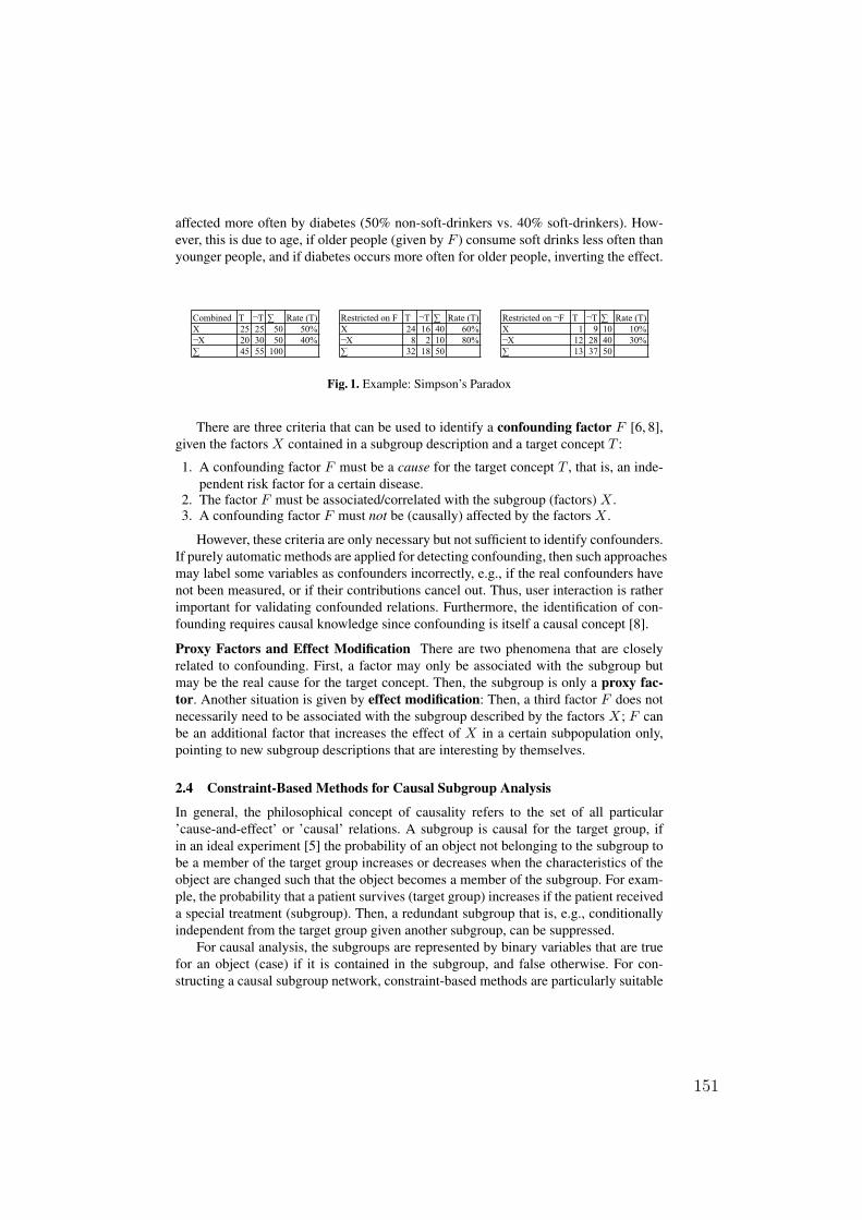
affected more often by diabetes (50% non-soft-drinkers vs. 40% soft-drinkers). How-ever, this is due to age, if older people (given by F ) consume soft drinks less often thanyounger people, and if diabetes occurs more often for older people, inverting the effect.

Combined T ¬T Rate (T) Restricted on F T ¬T Rate (T) Restricted on ¬F T ¬T Rate (T)

X 25 25 50 50% X 24 16 40 60% X 1 9 10 10%

¬X 20 30 50 40% ¬X 8 2 10 80% ¬X 12 28 40 30%

45 55 100 32 18 50 13 37 50

Fig. 1. Example: Simpson’s Paradox

There are three criteria that can be used to identify a confounding factor F [6, 8],given the factors X contained in a subgroup description and a target concept T :

1. A confounding factor F must be a cause for the target concept T , that is, an inde-pendent risk factor for a certain disease.

2. The factor F must be associated/correlated with the subgroup (factors) X .3. A confounding factor F must not be (causally) affected by the factors X .

However, these criteria are only necessary but not sufficient to identify confounders.If purely automatic methods are applied for detecting confounding, then such approachesmay label some variables as confounders incorrectly, e.g., if the real confounders havenot been measured, or if their contributions cancel out. Thus, user interaction is ratherimportant for validating confounded relations. Furthermore, the identification of con-founding requires causal knowledge since confounding is itself a causal concept [8].

Proxy Factors and Effect Modification There are two phenomena that are closelyrelated to confounding. First, a factor may only be associated with the subgroup butmay be the real cause for the target concept. Then, the subgroup is only a proxy fac-tor. Another situation is given by effect modification: Then, a third factor F does notnecessarily need to be associated with the subgroup described by the factors X; F canbe an additional factor that increases the effect of X in a certain subpopulation only,pointing to new subgroup descriptions that are interesting by themselves.

2.4 Constraint-Based Methods for Causal Subgroup Analysis

In general, the philosophical concept of causality refers to the set of all particular’cause-and-effect’ or ’causal’ relations. A subgroup is causal for the target group, ifin an ideal experiment [5] the probability of an object not belonging to the subgroup tobe a member of the target group increases or decreases when the characteristics of theobject are changed such that the object becomes a member of the subgroup. For exam-ple, the probability that a patient survives (target group) increases if the patient receiveda special treatment (subgroup). Then, a redundant subgroup that is, e.g., conditionallyindependent from the target group given another subgroup, can be suppressed.

For causal analysis, the subgroups are represented by binary variables that are truefor an object (case) if it is contained in the subgroup, and false otherwise. For con-structing a causal subgroup network, constraint-based methods are particularly suitable

151

because of scalability reasons (cf. [5, 9]). These methods make several assumptions(cf. [5]) w.r.t. the data and the correctness of the statistical tests. The crucial conditionis the Markov condition (cf. [5]) depending on the assumption that the data can be ex-pressed by a Bayesian network: Let X be a node in a causal Bayesian network, and letY be any node that is not a descendant of X in the causal network. Then, the Markovcondition holds if X and Y are independent conditioned on the parents of X .

The CCC and CCU rules [9] described below constrain the possible causal modelsby applying simple statistical tests: For subgroups s1, s2, s3 represented by binary vari-ables the χ2-test for independence is utilized for testing their independence ID(s1, s2),dependence D(s1, s2) and conditional independence CondID(s1, s2|s3), shown below(for the tests user-selectable thresholds are applied, e.g., T1 = 1, T2 = 3.84, or higher):

ID(s1, s2)←→ χ2(s1, s2) < T1 , D(s1, s2)←→ χ2(s1, s2) > T2 ,

CondID(s1, s2|s3)←→ χ2(s1, s2|s3 = 0) + χ2(s1, s2|s3 = 1) < 2 · T1

Thus, the decision of (conditional) (in-)dependence is threshold-based, which is a prob-lem causing potential errors if very many tests are performed. Therefore, we propose asemi-automatic approach featuring interactive analysis of the inferred relations.

Definition 3 (CCC Rule). Let X, Y, Z denote three variables that are pairwise de-pendent, i.e., D(X, Y ),D(X, Z),D(Y, Z); let X and Z become independent whenconditioned on Y . In the absence of hidden and confounding variables we may inferthat one of the following causal relations exists between X, Y and Z: X → Y → Z,X ← Y → Z, X ← Y ← Z . However, if X has no causes, then the first relation isthe only one possible, even in the presence of hidden and confounding variables.

Definition 4 (CCU Rule). Let X, Y, Z denote three variables: X and Y are dependent(D(X, Y )), Y and Z are dependent (D(Y, Z)), X and Z are independent (ID(X, Z)),but X and Z become dependent when conditioned on Y (CondD(X, Z|Y )). In theabsence of hidden and confounding variables, we may infer that X and Z cause Y .

3 Extended Causal Analysis for Detecting Confounding

Detecting confounding using causal subgroup analysis consists of two main steps thatcan be iteratively applied:1. First, we generate a causal subgroup network considering a target group T , a user-

selected set of subgroups U , a set of confirmed (causal) and potentially confoundingfactors C for any included group, a set of unconfirmed potentially confoundingfactors P given by subgroups significantly dependent with the target group, andadditional background knowledge described below. In addition to causal links, thegenerated network also contains (undirected) associations between the variables.

2. In the next step, we traverse the network and extract the potential confounded andconfounding factors. The causal network and the proposed relations are then pre-sented to the user for subsequent interpretation and analysis. After confoundingfactors have been confirmed, the background knowledge can then be extended.

In the following we discuss these steps in detail, and also describe the elements of thebackground knowledge that are utilized for causal analysis.

152

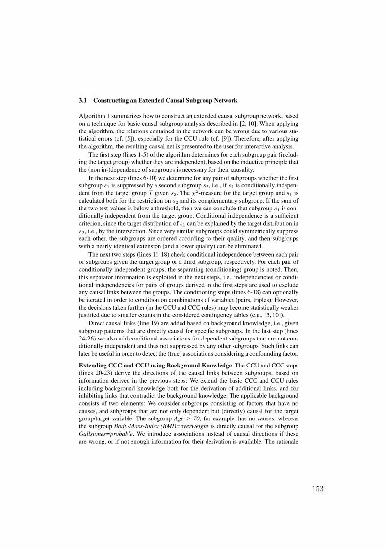
3.1 Constructing an Extended Causal Subgroup Network

Algorithm 1 summarizes how to construct an extended causal subgroup network, basedon a technique for basic causal subgroup analysis described in [2, 10]. When applyingthe algorithm, the relations contained in the network can be wrong due to various sta-tistical errors (cf. [5]), especially for the CCU rule (cf. [9]). Therefore, after applyingthe algorithm, the resulting causal net is presented to the user for interactive analysis.

The first step (lines 1-5) of the algorithm determines for each subgroup pair (includ-ing the target group) whether they are independent, based on the inductive principle thatthe (non in-)dependence of subgroups is necessary for their causality.

In the next step (lines 6-10) we determine for any pair of subgroups whether the firstsubgroup s1 is suppressed by a second subgroup s2, i.e., if s1 is conditionally indepen-dent from the target group T given s2. The χ2-measure for the target group and s1 iscalculated both for the restriction on s2 and its complementary subgroup. If the sum ofthe two test-values is below a threshold, then we can conclude that subgroup s1 is con-ditionally independent from the target group. Conditional independence is a sufficientcriterion, since the target distribution of s1 can be explained by the target distribution ins2, i.e., by the intersection. Since very similar subgroups could symmetrically suppresseach other, the subgroups are ordered according to their quality, and then subgroupswith a nearly identical extension (and a lower quality) can be eliminated.

The next two steps (lines 11-18) check conditional independence between each pairof subgroups given the target group or a third subgroup, respectively. For each pair ofconditionally independent groups, the separating (conditioning) group is noted. Then,this separator information is exploited in the next steps, i.e., independencies or condi-tional independencies for pairs of groups derived in the first steps are used to excludeany causal links between the groups. The conditioning steps (lines 6-18) can optionallybe iterated in order to condition on combinations of variables (pairs, triples). However,the decisions taken further (in the CCU and CCC rules) may become statistically weakerjustified due to smaller counts in the considered contingency tables (e.g., [5, 10]).

Direct causal links (line 19) are added based on background knowledge, i.e., givensubgroup patterns that are directly causal for specific subgroups. In the last step (lines24-26) we also add conditional associations for dependent subgroups that are not con-ditionally independent and thus not suppressed by any other subgroups. Such links canlater be useful in order to detect the (true) associations considering a confounding factor.

Extending CCC and CCU using Background Knowledge The CCU and CCC steps(lines 20-23) derive the directions of the causal links between subgroups, based oninformation derived in the previous steps: We extend the basic CCC and CCU rulesincluding background knowledge both for the derivation of additional links, and forinhibiting links that contradict the background knowledge. The applicable backgroundconsists of two elements: We consider subgroups consisting of factors that have nocauses, and subgroups that are not only dependent but (directly) causal for the targetgroup/target variable. The subgroup Age ≥ 70, for example, has no causes, whereasthe subgroup Body-Mass-Index (BMI)=overweight is directly causal for the subgroupGallstones=probable. We introduce associations instead of causal directions if theseare wrong, or if not enough information for their derivation is available. The rationale

153

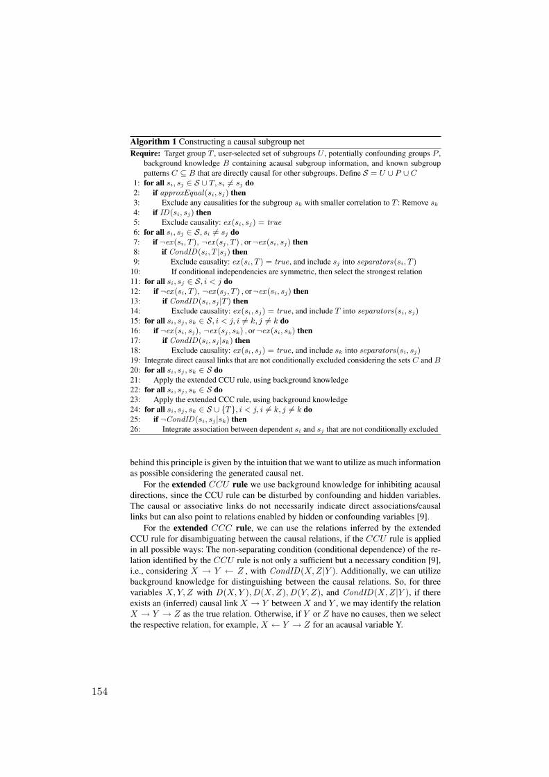
Algorithm 1 Constructing a causal subgroup netRequire: Target group T , user-selected set of subgroups U , potentially confounding groups P ,

background knowledge B containing acausal subgroup information, and known subgrouppatterns C ⊆ B that are directly causal for other subgroups. Define S = U ∪ P ∪ C

1: for all si, sj ∈ S ∪ T, si 6= sj do2: if approxEqual(si, sj) then3: Exclude any causalities for the subgroup sk with smaller correlation to T : Remove sk

4: if ID(si, sj) then5: Exclude causality: ex (si, sj) = true6: for all si, sj ∈ S, si 6= sj do7: if ¬ex (si, T ), ¬ex (sj , T ) , or¬ex (si, sj) then8: if CondID(si, T |sj) then9: Exclude causality: ex (si, T ) = true , and include sj into separators(si, T )

10: If conditional independencies are symmetric, then select the strongest relation11: for all si, sj ∈ S, i < j do12: if ¬ex (si, T ), ¬ex (sj , T ) , or¬ex (si, sj) then13: if CondID(si, sj |T ) then14: Exclude causality: ex (si, sj) = true , and include T into separators(si, sj)15: for all si, sj , sk ∈ S, i < j, i 6= k, j 6= k do16: if ¬ex (si, sj), ¬ex (sj , sk) , or¬ex (si, sk) then17: if CondID(si, sj |sk) then18: Exclude causality: ex (si, sj) = true , and include sk into separators(si, sj)19: Integrate direct causal links that are not conditionally excluded considering the sets C and B20: for all si, sj , sk ∈ S do21: Apply the extended CCU rule, using background knowledge22: for all si, sj , sk ∈ S do23: Apply the extended CCC rule, using background knowledge24: for all si, sj , sk ∈ S ∪ T, i < j, i 6= k, j 6= k do25: if ¬CondID(si, sj |sk) then26: Integrate association between dependent si and sj that are not conditionally excluded

behind this principle is given by the intuition that we want to utilize as much informationas possible considering the generated causal net.

For the extended CCU rule we use background knowledge for inhibiting acausaldirections, since the CCU rule can be disturbed by confounding and hidden variables.The causal or associative links do not necessarily indicate direct associations/causallinks but can also point to relations enabled by hidden or confounding variables [9].

For the extended CCC rule, we can use the relations inferred by the extendedCCU rule for disambiguating between the causal relations, if the CCU rule is appliedin all possible ways: The non-separating condition (conditional dependence) of the re-lation identified by the CCU rule is not only a sufficient but a necessary condition [9],i.e., considering X → Y ← Z , with CondID(X, Z|Y ). Additionally, we can utilizebackground knowledge for distinguishing between the causal relations. So, for threevariables X, Y, Z with D(X, Y ),D(X, Z),D(Y,Z), and CondID(X, Z|Y ), if thereexists an (inferred) causal link X → Y between X and Y , we may identify the relationX → Y → Z as the true relation. Otherwise, if Y or Z have no causes, then we selectthe respective relation, for example, X ← Y → Z for an acausal variable Y.

154

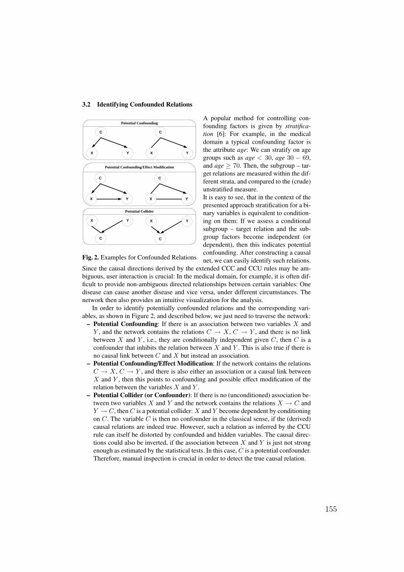
3.2 Identifying Confounded Relations

X Y

C

X Y

C

X Y

C

X Y

C

X Y

C

X Y

C

Potential Confounding

Potential Confounding/Effect Modification

Potential Collider

Fig. 2. Examples for Confounded Relations

A popular method for controlling con-founding factors is given by stratifica-tion [6]: For example, in the medicaldomain a typical confounding factor isthe attribute age: We can stratify on agegroups such as age < 30, age 30 − 69,and age ≥ 70. Then, the subgroup – tar-get relations are measured within the dif-ferent strata, and compared to the (crude)unstratified measure.It is easy to see, that in the context of thepresented approach stratification for a bi-nary variables is equivalent to condition-ing on them: If we assess a conditionalsubgroup – target relation and the sub-group factors become independent (ordependent), then this indicates potentialconfounding. After constructing a causalnet, we can easily identify such relations.

Since the causal directions derived by the extended CCC and CCU rules may be am-biguous, user interaction is crucial: In the medical domain, for example, it is often dif-ficult to provide non-ambiguous directed relationships between certain variables: Onedisease can cause another disease and vice versa, under different circumstances. Thenetwork then also provides an intuitive visualization for the analysis.

In order to identify potentially confounded relations and the corresponding vari-ables, as shown in Figure 2, and described below, we just need to traverse the network:

– Potential Confounding: If there is an association between two variables X andY , and the network contains the relations C → X , C → Y , and there is no linkbetween X and Y , i.e., they are conditionally independent given C, then C is aconfounder that inhibits the relation between X and Y . This is also true if there isno causal link between C and X but instead an association.

– Potential Confounding/Effect Modification: If the network contains the relationsC → X , C → Y , and there is also either an association or a causal link betweenX and Y , then this points to confounding and possible effect modification of therelation between the variables X and Y .

– Potential Collider (or Confounder): If there is no (unconditioned) association be-tween two variables X and Y and the network contains the relations X → C andY → C, then C is a potential collider: X and Y become dependent by conditioningon C. The variable C is then no confounder in the classical sense, if the (derived)causal relations are indeed true. However, such a relation as inferred by the CCUrule can itself be distorted by confounded and hidden variables. The causal direc-tions could also be inverted, if the association between X and Y is just not strongenough as estimated by the statistical tests. In this case, C is a potential confounder.Therefore, manual inspection is crucial in order to detect the true causal relation.

155

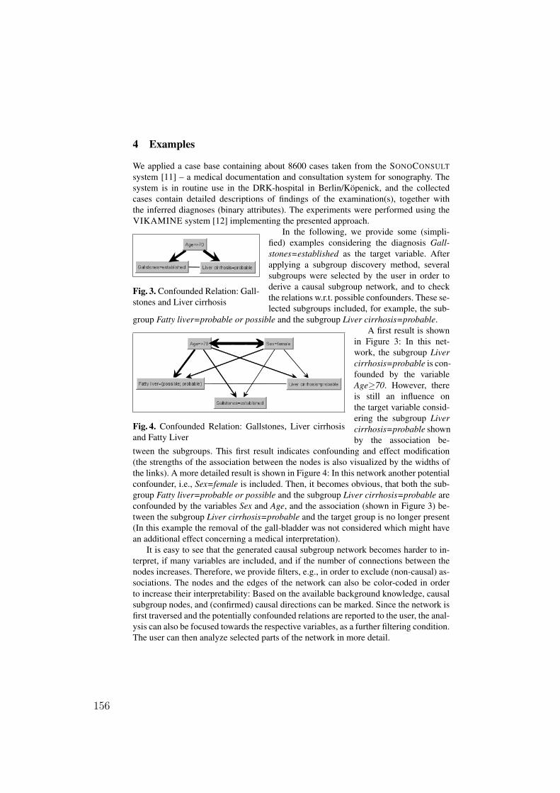
4 Examples

We applied a case base containing about 8600 cases taken from the SONOCONSULTsystem [11] – a medical documentation and consultation system for sonography. Thesystem is in routine use in the DRK-hospital in Berlin/Köpenick, and the collectedcases contain detailed descriptions of findings of the examination(s), together withthe inferred diagnoses (binary attributes). The experiments were performed using theVIKAMINE system [12] implementing the presented approach.

Fig. 3. Confounded Relation: Gall-stones and Liver cirrhosis

In the following, we provide some (simpli-fied) examples considering the diagnosis Gall-stones=established as the target variable. Afterapplying a subgroup discovery method, severalsubgroups were selected by the user in order toderive a causal subgroup network, and to checkthe relations w.r.t. possible confounders. These se-lected subgroups included, for example, the sub-

group Fatty liver=probable or possible and the subgroup Liver cirrhosis=probable.

Fig. 4. Confounded Relation: Gallstones, Liver cirrhosisand Fatty Liver

A first result is shownin Figure 3: In this net-work, the subgroup Livercirrhosis=probable is con-founded by the variableAge≥70. However, thereis still an influence onthe target variable consid-ering the subgroup Livercirrhosis=probable shownby the association be-

tween the subgroups. This first result indicates confounding and effect modification(the strengths of the association between the nodes is also visualized by the widths ofthe links). A more detailed result is shown in Figure 4: In this network another potentialconfounder, i.e., Sex=female is included. Then, it becomes obvious, that both the sub-group Fatty liver=probable or possible and the subgroup Liver cirrhosis=probable areconfounded by the variables Sex and Age, and the association (shown in Figure 3) be-tween the subgroup Liver cirrhosis=probable and the target group is no longer present(In this example the removal of the gall-bladder was not considered which might havean additional effect concerning a medical interpretation).

It is easy to see that the generated causal subgroup network becomes harder to in-terpret, if many variables are included, and if the number of connections between thenodes increases. Therefore, we provide filters, e.g., in order to exclude (non-causal) as-sociations. The nodes and the edges of the network can also be color-coded in orderto increase their interpretability: Based on the available background knowledge, causalsubgroup nodes, and (confirmed) causal directions can be marked. Since the network isfirst traversed and the potentially confounded relations are reported to the user, the anal-ysis can also be focused towards the respective variables, as a further filtering condition.The user can then analyze selected parts of the network in more detail.

156

5 Conclusion

In this paper, we have presented a causal subgroup analysis approach for the semi-automatic detection of confounding: Since there is no purely automatic test for con-founding [8] the analysis itself depends on background knowledge for establishing anextended causal model/network of the domain. Then, the constructed network can beused to identify potential confounders. In a semi-automatic approach, the network andthe potential confounded relations can then be evaluated and validated by the user.

In the future, we are planning to consider an efficient approach for detecting con-founding that is directly embedded in the subgroup discovery method. Related work inthat direction was described (e.g., [13]). Another interesting direction for future workis given by considering further background knowledge for causal analysis.

Acknowledgements

This work has been partially supported by the German Research Council (DFG) undergrant Pu 129/8-1.

References1. Wrobel, S.: An Algorithm for Multi-Relational Discovery of Subgroups. In: Proc. 1st Europ.

Symp. Principles of Data Mining and Knowledge Discovery, Berlin, Springer (1997) 78–872. Klösgen, W.: 16.3: Subgroup Discovery. In: Handbook of Data Mining and Knowledge

Discovery. Oxford University Press, New York (2002)3. Lavrac, N., Kavsek, B., Flach, P., Todorovski, L.: Subgroup Discovery with CN2-SD. Journal

of Machine Learning Research 5 (2004) 153–1884. Atzmueller, M., Puppe, F.: SD-Map - A Fast Algorithm for Exhaustive Subgroup Discov-

ery. In: Proc. 10th European Conf. on Principles and Practice of Knowledge Discovery inDatabases (PKDD 2006), Berlin, Springer (2006) 6–17

5. Cooper, G.F.: A Simple Constraint-Based Algorithm for Efficiently Mining ObservationalDatabases for Causal Relationships. Data Min. Knowl. Discov. 1(2) (1997) 203–224

6. McNamee, R.: Confounding and Confounders. Occup. Environ. Med. 60 (2003) 227–2347. Simpson, E.H.: The Interpretation of Interaction in Contingency Tables. Journal of the Royal

Statistical Society 18 (1951) 238–2418. Pearl, J.: 6.2 Why There is No Statistical Test For Confounding, Why Many Think There

Is, and Why They Are Almost Right. In: Causality: Models, Reasoning and Inference. Cam-bridge University Press (2000)

9. Silverstein, C., Brin, S., Motwani, R., Ullman, J.D.: Scalable Techniques for Mining CausalStructures. Data Mining and Knowledge Discovery 4(2/3) (2000) 163–192

10. Kloesgen, W., May, M.: Database Integration of Multirelational Causal Subgroup Mining.Technical report, Fraunhofer Institute AIS, Sankt Augustin, Germany (2002)

11. Huettig, M., Buscher, G., Menzel, T., Scheppach, W., Puppe, F., Buscher, H.P.: A DiagnosticExpert System for Structured Reports, Quality Assessment, and Training of Residents inSonography. Medizinische Klinik 99(3) (2004) 117–122

12. Atzmueller, M., Puppe, F.: Semi-Automatic Visual Subgroup Mining using VIKAMINE.Journal of Universal Computer Science 11(11) (2005) 1752–1765

13. Fabris, C.C., Freitas, A.A.: Discovering Surprising Patterns by Detecting Occurrences ofSimpson’s Paradox. In: Research and Development in Intelligent Systems XVI, Berlin,Springer (1999) 148–160

157

Declarative Specification of Ontological DomainKnowledge for Descriptive Data Mining

Martin Atzmueller and Dietmar Seipel

University of WürzburgDepartment of Computer Science

Am Hubland, 97074 Würzburg, Germanyatzmueller, seipel@informatik.uni-wuerzburg.de

Abstract. Domain knowledge is a valuable resource for improving the qualityof the results of data mining methods. In this paper, we present a methodologicalapproach for providing ontological domain knowledge in a declarative manner:We utilize Prolog facts and rules for the specification of properties of ontologi-cal concepts and for the derivation of further ad-hoc relations of the ontologicalconcepts. This enhances the documentation, extendability, and standardizationof the applied knowledge. Furthermore, the presented approach also provides forautomatic verification and improved maintenance options with respect to the useddomain knowledge.

1 Introduction

Domain knowledge is a natural resource for knowledge-intensive data mining meth-ods (e.g., [9, 12]), and can be exploited for improving the quality of the data miningresults significantly. Appropriate domain knowledge can increase the representationalexpressiveness and also focus the algorithm on the relevant patterns. Furthermore, forincreasing the efficiency of the search method the search space can often be constrained,e.g., [2, 4]. A prerequisite for the successful application and exploitation of domainknowledge is given by a concise description and specification of the domain know-ledge. A concise specification also provides for better documentation, extendability,and standardization. Furthermore, maintenance issues and verification of the applieddomain knowledge are also enhanced.

In this paper, we present a methodological approach using a declarative specifica-tion of ontological domain knowledge: Our context is given by a descriptive data miningmethod, i.e., we focus on methods that provide descriptive patterns for later inspectionby the user. These patterns need to be easy to comprehend and to interpret by the user.Thus, besides the objective quality of the patterns as rated by a quality function suchas, e.g., support or confidence for association rules (e.g., [1]), subjective measures arealso rather important: The interestingness of the patterns is also affected by the rep-resentational expressiveness of the patterns, and by the focus of the pattern discoverymethod on the relevant concepts of the domain ontology. In this way, patterns (associ-ations) containing irrelevant and non-interesting concepts can be surpressed in order toincrease the overall interestingness of the set of the mined patterns.

158

Knowledge acquisition is often challenging and costly (knowledge acquisition bot-tleneck). Thus, an important idea is to ease knowledge acquisition by reusing existingdomain knowledge, i.e., knowledge that is contained in existing ontologies or know-ledge bases. Furthermore, we can apply high-level knowledge such as properties of on-tological objects for deriving simpler constraint knowledge that can be directly includedin the data mining step, as discussed, e.g., in [2, 4]. For specifying such properties andrelations of the concepts contained in the domain ontology, we utilize Prolog rules as aversatile representation: using these, we obtain a suitable representation formalism forontological knowledge. Furthermore, we can automatically derive ad-hoc relations be-tween ontological concepts using simple rules, and thus also provide a comprehensiveoverview and summary for the domain specialist. Then, these rules can also be checkedwith respect to their consistency, i.e., the provided knowledge base and the derivationknowledge can be verified for its semantic integrity. Altogether, the resulting know-ledge base in terms of Prolog rules and facts automatically serves as a specification anddocumentation of the domain knowledge that is easy to comprehend, to interpret and toextend. Furthermore, new task-specific knowledge can be derived by extending and/ormodifying the knowledge base.

The rest of the paper is organized as follows: We first briefly introduce the context ofassociation patterns for descriptive data mining in Section 2. After that, we summarizeseveral types of domain knowledge in Section 3. Next, we describe how the ontologicalknowledge can be formalized and used for deriving ad-hoc relations, i.e., ontologicalconstraint knowledge in Section 4, and illustrate the approach with practical examples.Section 5 discusses a representation and transformation of the (derived) domain know-ledge to XML. Finally, we conclude the paper with a summary in Section 6, and pointout interesting directions for future work.

2 Discovering Association Patterns using Domain Knowledge

In the context of this work, we consider descriptive data mining methods for discover-ing interesting association patterns. Prominent approaches include subgroup discoverymethods, e.g., [3, 11, 14], and methods for learning association rules, e.g., [1, 7].

2.1 Association Patterns

Subgroup patterns [4, 10], often provided by conjunctive rules, describe ’interesting’subgroups of cases, e.g., "the subgroup of 16-25 year old men that own a sports carare more likely to pay high insurance rates than the people in the reference popula-tion." The main application areas of subgroup discovery [11, 14] are exploration anddescriptive induction, to obtain an overview of the relations between a target variableand a set of explaining variables, where variables are attribute/value assignments. Theexemplary subgroup above is then described by the relation between the independent(explaining) variables (Sex = male, Age ≤ 25, Car = sports car) and the dependent(target) variable (Insurance Rate = high). The independent variables are modeled byselection expressions on sets of attribute values. A subgroup pattern is thus describedby a subgroup description in relation to a specific target variable.

159

Let ΩA be the set of all attributes. For each attribute a ∈ ΩA a range dom(a) ofvalues is defined. An attribute/value assignment a = v, where a ∈ ΩA, v ∈ dom(a), iscalled a feature. We define the feature space VA to be the (universal) set of all features.A single-relational propositional subgroup description is defined as a conjunction

sd = e1 ∧ e2 ∧ · · · ∧ en

of (extended) features ei ⊆ VA , which are then called selection expressions, whereeach ei selects a subset of the range dom(a) of an attribute a ∈ ΩA. We define Ωsd asthe set of all possible subgroup descriptions.

An association rule (e.g., [1, 8]) is given by a rule of the form sdB → sdH , wheresdB and sdH are subgroup descriptions; the rule body sdB and the rule head sdH

specify sets of items. E.g., for the insurance domain we can consider an association ruleshowing a combination of potential risk factors for high insurance rates and accidents:

Sex = male ∧ Age ≤ 25 ∧ Car = sports car →Insurance Rate = high ∧ Accident Rate = high

A subgroup pattern is a special association rule, namely a horn clause sd → e, wheresd ∈ Ωsd is a subgroup description and the feature e ∈ VA is called the target variable.

In general, the quality of an association rule is measured by its support and con-fidence, and the data mining process searches for association rules with arbitray ruleheads and bodies. For subgroup patterns there exist various (more refined) qualitymeasures (e.g., [3, 11]): Since an arbitrary quality function can be applied, the anti-monotony property of support used in association rule mining cannot be utilized in thegeneral case. E.g., the used quality function can combine the difference of the confi-dence and the apriori probability of the rule head with the size of the subgroup. Sincemining for interesting subgroup patterns is more complicated, usually a fixed, atomicrule head is given as input to the search process.

2.2 Application of Domain Knowledge for Descriptive Data Mining

In the context of this paper we focus on pattern mining methods that discover descrip-tive patterns in the form of conjunctive rules, as outlined above. The knowledge classesdescribed in Section 3 can be directly integrated in the respective pattern discoverystep: While exclusion constraints restrict the search space by construction, aggregationconstraints do not necessarily restrict it, since new values are introduced, but they helpto find more understandable results. Also, combination constraints inhibit the examina-tion of specified sets of concepts and can prune large (uninteresting) areas of the searchspace. For increasing the representational expressiveness, modifications of the valuerange of an attribute can be utilized to infer values that are more meaningful for theuser. E.g., in the medical domain different aggregated age groups could be considered.

In contrast to existing approaches, e.g., [12, 15] we focus on domain knowledgethat can be easily declared in symbolic form. Furthermore, the presented approach fea-tures the ability of deriving ’simpler’ low-level knowledge (constraints) from high-levelontological knowledge. Alltogether, the complete knowledge base can be intuitivelydeclared, validated, and inspected by the user, as shown in the following sections.

160

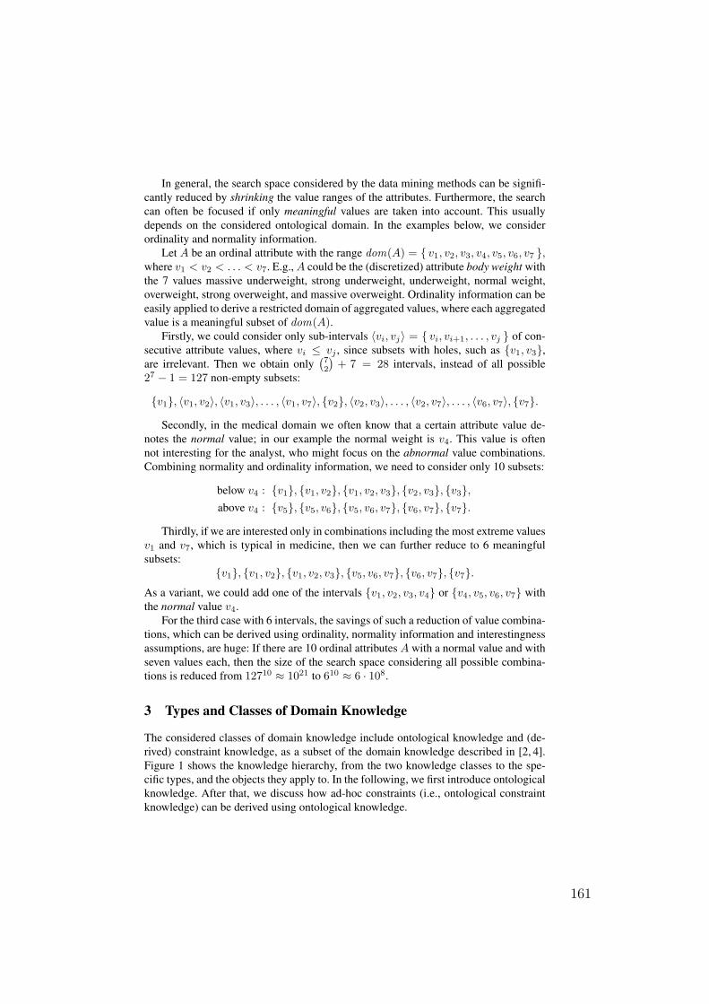
In general, the search space considered by the data mining methods can be signifi-cantly reduced by shrinking the value ranges of the attributes. Furthermore, the searchcan often be focused if only meaningful values are taken into account. This usuallydepends on the considered ontological domain. In the examples below, we considerordinality and normality information.

Let A be an ordinal attribute with the range dom(A) = v1, v2, v3, v4, v5, v6, v7 ,where v1 < v2 < . . . < v7. E.g., A could be the (discretized) attribute body weight withthe 7 values massive underweight, strong underweight, underweight, normal weight,overweight, strong overweight, and massive overweight. Ordinality information can beeasily applied to derive a restricted domain of aggregated values, where each aggregatedvalue is a meaningful subset of dom(A).

Firstly, we could consider only sub-intervals 〈vi, vj〉 = vi, vi+1, . . . , vj of con-secutive attribute values, where vi ≤ vj , since subsets with holes, such as v1, v3,are irrelevant. Then we obtain only

(72

)+ 7 = 28 intervals, instead of all possible

27 − 1 = 127 non-empty subsets:

v1, 〈v1, v2〉, 〈v1, v3〉, . . . , 〈v1, v7〉, v2, 〈v2, v3〉, . . . , 〈v2, v7〉, . . . , 〈v6, v7〉, v7.

Secondly, in the medical domain we often know that a certain attribute value de-notes the normal value; in our example the normal weight is v4. This value is oftennot interesting for the analyst, who might focus on the abnormal value combinations.Combining normality and ordinality information, we need to consider only 10 subsets:

below v4 : v1, v1, v2, v1, v2, v3, v2, v3, v3,above v4 : v5, v5, v6, v5, v6, v7, v6, v7, v7.

Thirdly, if we are interested only in combinations including the most extreme valuesv1 and v7, which is typical in medicine, then we can further reduce to 6 meaningfulsubsets:

v1, v1, v2, v1, v2, v3, v5, v6, v7, v6, v7, v7.As a variant, we could add one of the intervals v1, v2, v3, v4 or v4, v5, v6, v7 withthe normal value v4.

For the third case with 6 intervals, the savings of such a reduction of value combina-tions, which can be derived using ordinality, normality information and interestingnessassumptions, are huge: If there are 10 ordinal attributes A with a normal value and withseven values each, then the size of the search space considering all possible combina-tions is reduced from 12710 ≈ 1021 to 610 ≈ 6 · 108.

3 Types and Classes of Domain Knowledge

The considered classes of domain knowledge include ontological knowledge and (de-rived) constraint knowledge, as a subset of the domain knowledge described in [2, 4].Figure 1 shows the knowledge hierarchy, from the two knowledge classes to the spe-cific types, and the objects they apply to. In the following, we first introduce ontologicalknowledge. After that, we discuss how ad-hoc constraints (i.e., ontological constraintknowledge) can be derived using ontological knowledge.

161

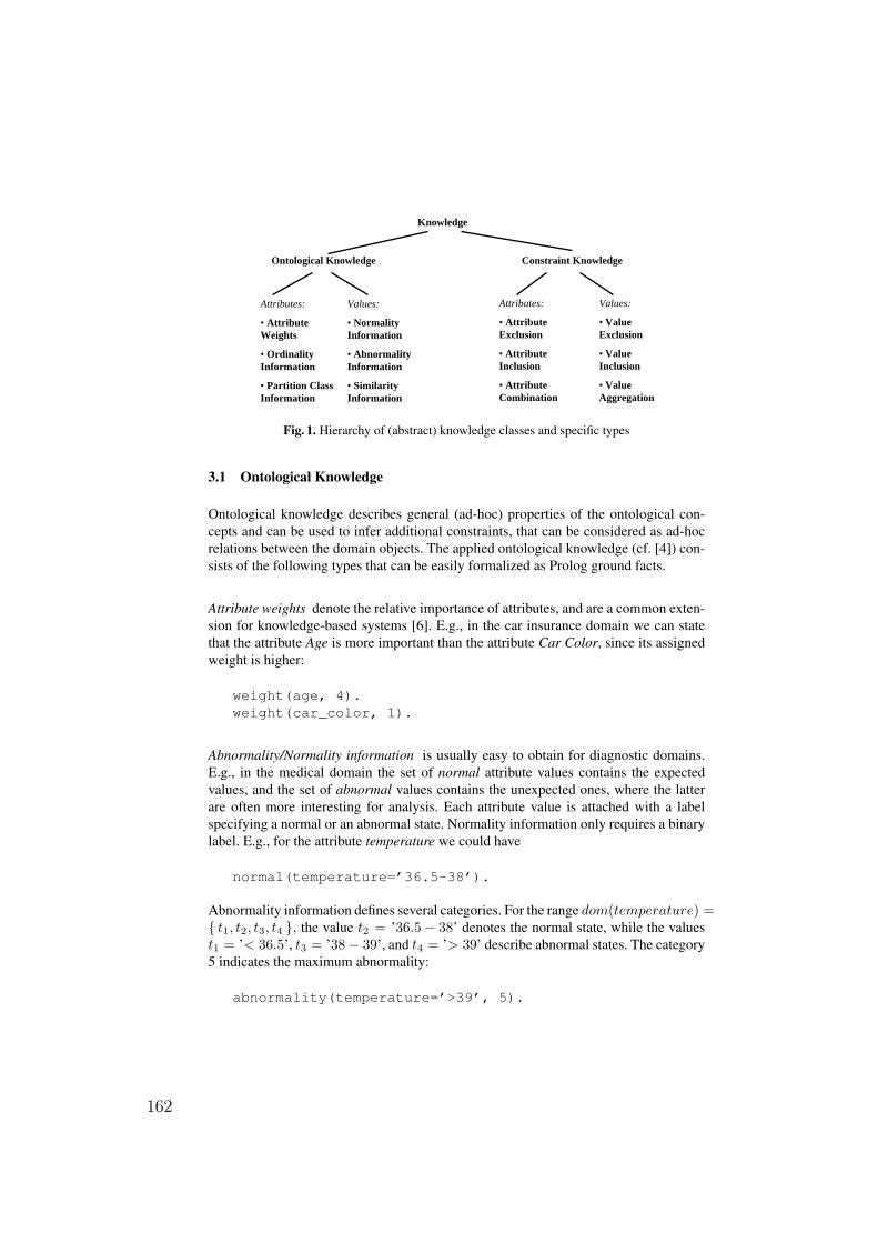
Knowledge

Attributes:

• AttributeExclusion

• AttributeInclusion

• AttributeCombination

Constraint Knowledge

Values:

• ValueExclusion

• ValueInclusion

• ValueAggregation

Ontological Knowledge

Values:

• NormalityInformation

• AbnormalityInformation

• SimilarityInformation

Attributes:

• AttributeWeights

• OrdinalityInformation

• Partition Class Information

Fig. 1. Hierarchy of (abstract) knowledge classes and specific types

3.1 Ontological Knowledge

Ontological knowledge describes general (ad-hoc) properties of the ontological con-cepts and can be used to infer additional constraints, that can be considered as ad-hocrelations between the domain objects. The applied ontological knowledge (cf. [4]) con-sists of the following types that can be easily formalized as Prolog ground facts.

Attribute weights denote the relative importance of attributes, and are a common exten-sion for knowledge-based systems [6]. E.g., in the car insurance domain we can statethat the attribute Age is more important than the attribute Car Color, since its assignedweight is higher:

weight(age, 4).weight(car_color, 1).

Abnormality/Normality information is usually easy to obtain for diagnostic domains.E.g., in the medical domain the set of normal attribute values contains the expectedvalues, and the set of abnormal values contains the unexpected ones, where the latterare often more interesting for analysis. Each attribute value is attached with a labelspecifying a normal or an abnormal state. Normality information only requires a binarylabel. E.g., for the attribute temperature we could have

normal(temperature=’36.5-38’).

Abnormality information defines several categories. For the range dom(temperature) = t1, t2, t3, t4 , the value t2 = ’36.5− 38’ denotes the normal state, while the valuest1 = ’< 36.5’, t3 = ’38− 39’, and t4 = ’> 39’ describe abnormal states. The category5 indicates the maximum abnormality:

abnormality(temperature=’>39’, 5).

162

Similarity information between attribute values is often applied in case-based reason-ing: It specifies the relative similarity between the individual attribute values. For exam-ple, for a nominal attribute Color with dom(Color) = white, gray , black , we canstate that the value white is more similar to gray than it is to black:

similarity(color=white, color=gray, 0.5).similarity(color=white, color=black, 0).

Here, the respective similarity value is s ∈ [0; 1].

Ordinality information specifies if the value range of a nominal attribute can be ordered.E.g., the qualitative attributes Age and Car Size are ordinal, while Color is not:

ordinal_attribute(age).ordinal_attribute(car_size).

Partition class information provides semantically distinct groups of attributes. Thesedisjoint subsets usually correspond to certain problem areas of the application domain.E.g., in the medical domain such partitions are representing different organ systems likeliver, kidney, pancreas, stomach, stomach, and intestine. For each organ system a list ofattributes is given:

attribute_partition(inner_organs, [[fatty_liver, liver_cirrhosis, ...],[renal_failure, nephritis, ...], ... ]).

3.2 Constraint Knowledge

Constraint knowledge can be applied, e.g., for filtering patterns by their quality and forrestricting the search space, as discussed below. We distinguish the following types ofconstraint knowledge, that can be explicitly provided as ground facts in Prolog. Furtherbasic constraints can be derived automatically as discussed in Section 4.

Exclusion constraints for attributes or features are applied for filtering the domains ofattributes and the feature space, respectively. The same applies for inclusion constraintsfor attributes or features, that explicitly state important values and attributes that shouldbe included:

dsdk_constraint(exclude(attribute), car_color).dsdk_constraint(include(attribute), age).dsdk_constraint(exclude(feature), age=30-50).

Value aggregation constraints can be specified in order to form abstracted disjunc-tions of attribute values, e.g., intervals for ordinal values. For example, for the attributeAge with dom(Age) = ’< 40’, ’40− 50’, ’50− 70’, ’> 70’ we can derive the ag-gregated values ’≤ 50’ (corresponding to the list [0-40,40-50]) and ’> 50’ (cor-responding to the list [50-70,70-100]). In general, aggregated values are not re-stricted to intervals, but can cover any combination of values.

dsdk_constraint(aggregated_values,age = [ [0-40,40-50], [50-70,70-100] ]).

163

Attribute combination constraints are applied for filtering/excluding certain combina-tions of attributes, e.g., if these are already known to the domain specialist.

dsdk_constraint(exclude(attribute_pair),[car_color, car_size]).

dsdk_constraint(include(attribute_pair),[age, car_size]).

The data mining process should not compute association rules that contain one of theattributes of an excluded attribute pair in the body and the other attribute in the head.

4 Deriving Constraint Knowledge

Figure 2 shows how ontological knowledge can be used to derive further ’basic’ con-straints.

Normality Information

Abnormality Information

Similarity Information

Ordinality Information

Attribute Weights

Partition Class

Information

Value Exclusion

Constraints

Value Aggregation Constraints

Attribute Exclusion

Constraints

Attribute Combination Constraints

Fig. 2. Deriving constraints using ontological knowledge

Below, we summarize how new constraints can be inferred using ontological know-ledge, and show the corresponding Prolog code for deriving the new constraints. Theuser can generate a summary of all facts derivable by the provided derivation rules formanual inspection by querying dsdk_constraint(X,Y) using backtracking.

4.1 Exclusion and Inclusion Constraints

We can construct attribute exclusion constraints using attribute weights to filter the setof relevant attributes by a weight threshold or by subsets of the weight space.

dsdk_constraint(exclude(attribute), A) :-weight(A, N), N =< 1.

dsdk_constraint(include(attribute), A) :-weight(A, N), N > 1.

We can apply complex rules for deriving constraints that can be specified by the user:

164

dsdk_constraint(include(attribute), A) :-weight(A, N), N >= 2,abnorm(A=_, 5).

Using abnormality/normality knowledge we can specify global exclusion constraintsfor the normal features, i.e. the features whose abnormality is at most 1 (the lowest cat-egory 0 denotes the don’t care value, while the category 1 explicitly indicates a normalvalue):

dsdk_constraint(exclude(feature), A=V) :-abnormality(A=V, N), N =< 1.

Partition class information can be used to infer attribute combination constraints inorder to prevent the combination of individual attributes that are contained in separatepartition classes. Alternatively, inverse constraints can also be derived, e.g., to specifi-cally investigate inter-organ relations in the medical domain.

dsdk_constraint(exclude(attribute_pair), [A1, A2]) :-attribute_partition(_, P),member(As1, P), member(As2, P), As1 \= As2,member(A1, As1), member(A2, As2).

Finally, we can use a generic Prolog rule for detecting conflicts w.r.t. these rules andthe derived knowledge:

dsdk_constraint(error(include_exclude(X)), Y) :-dsdk_constraint(include(X), Y),dsdk_constraint(exclude(X), Y).

4.2 Aggregation Constraints

Aggregation w.r.t. Abnormality. Using similarity or abnormality/normality informationwe can filter and model the value ranges of attributes. Global abnormality groups canbe defined by aggregating values with the same abnormality:

dsdk_constraint(aggregated_values, A=Values) :-attribute(A),findall( Vs,

abnormality_aggregate(A=Vs),Values ).

abnormality_aggregate(A=Vs) :-setof( V,

abnormality(A=V, _),Vs ).

For a given attribute A the helper predicate abnormality_aggregate/2 computesthe set Vs (without duplicates) of all values V which have the same abnormality N; thisgrouping is done using the Prolog meta-predicate setof/3.

165

Aggregation w.r.t. Similarity. Also, if the similarity between two attribute values isvery high, then they can potentially be analyzed as an aggregated value; this will form adisjunctive selection expression on the value range of the attribute. For example, in themedical domain similar attribute values such as probable and possible (with differentabnormality degrees) can often be aggregated.

The following predicate finds the list Values of all sublists Ws of the domain Vsof an attribute A, such that the values in Ws are similar in the following sense: if Ws =[w1, w2, . . . , wn], then similarity(A = wi, A = wi+1, si) must be given, and itmust hold Πn−1

i=1 si ≥ 0.5 :

dsdk_constraint(aggregated_values, A=Values) :-ordinal_attribute(A), aggregate_attribute(A),domain(A, Vs),findall( Ws,

similar_sub_sequence(A, 0.5, Vs, Ws),Values ).

Aggregation w.r.t. Normal Value. Ordinality information can be easily used to constructaggregated values, which are often more meaningful for the domain specialist. We canconsider all adjacent combinations of attribute values, or all ascending/descending com-binations starting with the minimum or maximum value, respectively. Whenever abnor-mality information is available, we can partition the value range by the given normalvalue and only start with the most extreme value. For example, for the ordinal attributeliver size with the values

1:smaller than normal, 2:normal, 3:marginally increased, 4:slightly increased,5:moderately increased, and 6:highly increased,

we partition by the normal value 2, and we obtain the following aggregated values:

[1], [3,4,5,6], [4,5,6], [5,6], [6]

Given the domain Vs of an ordinal attribute A, that should be aggregated. If the nor-mal value v for A is given, and Vs = [v1, . . . , vn−1, v, vn+1, . . . , vm], then all startingsequences Ws = [v1, v2, . . . , vi], where 1 ≤ i ≤ n − 1, for the sub-domain Vs1 =[v1, . . . , vn−1] of all values below v and all ending sequences Ws = [vi, . . . , vm], wheren + 1 ≤ i ≤ m, for the sub-domain Vs2 = [vn+1, . . . , vm] of all values above v areconstructed by backtracking. If the normal value for A is not given, then all starting(ending) sequences for the full domain Vs are constructed.

dsdk_constraint(aggregated_values, A=Values) :-ordinal_attribute(A), aggregate_attribute(A),domain(A, Vs),dsdk_split_for_aggregation(A, Vs, Vs1, Vs2),findall( Ws,

( starting_sequence(Vs1, Ws); ending_sequence(Vs2, Ws) ),Values ).

166

dsdk_split_for_aggregation(A, Vs, Vs1, Vs2),( normal(A=V),append(Vs1, [V|Vs2], Vs)

; \+ normal(A=_),Vs1 = Vs, Vs2 = Vs ).

This type of aggregation constraints using Prolog meta predicates usually has to beimplemented by Prolog experts.

5 XML Representation of the Knowledge

We can also formalize the factual ontological and constraint knowledge in XML – as astandard data representation and exchange format – and transform it to Prolog facts us-ing the XML query and transformation language FNQuery, cf. [13]. FNQuery has beenimplemented in Prolog and is fully interleaved with the reasoning process of Prolog.

For example, we are using the following XML format for representing constraintknowledge about attributes and classes of attributes:

<attribute name="temperature" id="a1" weight="2"normal="t2" ordinal="yes" aggregate="yes"><domain>

<value id="t1">&lt;36.5</value><value id="t2">36.5-38</value><value id="t3">38-39</value><value id="t4">&gt;39</value>

</domain><similarity value="0.2" val1="t3" val2="t4"/>...

</attribute>

<attribute name="fatty_liver" id="io1" ...<attribute name="liver_cirrhosis" id="io2" ...<attribute name="renal_failure" id="io3" ...<attribute name="nephritis" id="io4" ...

<class name="inner_organs"><attribute_partition>

<attributes><attribute id="io1"/> <attribute id="io2"/>

</attributes><attributes>

<attribute id="io3"/> <attribute id="io4"/></attributes>

</attribute_partition></class>

167

The derived Prolog facts can be transformed to XML using FNQuery. Then, usingthe Field Notation Grammars of FNQuery we can generate HTML reports from XMLfor an intuitive assessment of the (derived) knowledge by the user. Of course, by trans-forming the XML data we can also provide other specialized output formats, which can,e.g., be used for the integration with other tools.

6 Conclusions

In this paper we presented a methodological approach for the declarative specificationof domain knowledge for descriptive data mining. The respective knowledge classesand types can be comprehensively declared, validated, and inspected by the user. Thedifferent types of knowledge can be directly integrated in the pattern discovery step ofthe data mining process: Applying the domain knowledge the search space can be sig-nificantly pruned, uninteresting results can be excluded, and both the representationalexpressiveness of the ontological objects and the generated results can be increased.

The structured ontological domain knowledge and the rules for deriving constraintknowledge can be represented nicely in Prolog term structures using function symbols;the (factual) ontological domain knowledge can also be represented in XML. For rea-soning we make essential use of the following features of Prolog: backtracking, meta-predicates (such as findall, setof, etc.), ease of symbolic computations for term struc-tures. Moreover, using the XML query and transformation language FNQuery we canprovide a standard input/output format for high-level ontological and explicitly speci-fied or derived constraint knowledge. Thus, other declarative languages, such as answerset programming [5], could not be used.

We can imagine three kinds of users of the presented approach, depending on theirlevel of experience with the system and/or the presented types of knowledge: Unexperi-enced users just use the tool as a black box, possibly supported by a (simple) graphicaluser interface. For these users the applicable knowledge needs to be pre-formalized bya domain specialist or knowledge engineer. Experienced users can also enter factualknowledge, usually directly as Prolog facts, but also as knowledge formalized in XML,or supported by specialized (graphical) knowledge acquisition tools. Expert users canprogram further rules and flexibly extend the system for inferring (specialized) con-straints in Prolog.

In the future, we plan to extend the applicable set of domain knowledge by furtherknowledge elements. Furthermore, developing advanced graphical tools supporting in-experienced users is a worthwhile direction for further increasing the overall user ex-perience. Since the factual knowledge can either be represented in XML or Prolog, ap-propriate integration, extension, transformation and presentation of the (derived) know-ledge is usually easy to accomplish for (external) tools. Another interesting directionfor future work is given by an incremental approach for integrating ontological know-ledge bases with the obtained data mining results (patterns). E.g., the knowledge basescould be extended in a boot-strapping manner, or they could be directly validated usingthe discovered patterns.

168

References

1. Agrawal, R., Srikant, R.: Fast Algorithms for Mining Association Rules. In: Proc. 20th Int.Conf. Very Large Data Bases, (VLDB), Morgan Kaufmann (1994) 487–499

2. Atzmueller, M., Puppe, F.: A Methodological View on Knowledge-Intensive Subgroup Dis-covery. In Staab, S., Svátek, V., eds.: Managing Knowledge in a World of Networks, Proc.15th EKAW. Volume 4248 of LNCS., Springer (2006) 318–325

3. Atzmueller, M., Puppe, F.: SD-Map - A Fast Algorithm for Exhaustive Subgroup Discov-ery. In: Proc. 10th European Conf. on Principles and Practice of Knowledge Discovery inDatabases (PKDD 2006), Berlin, Springer (2006) 6–17

4. Atzmueller, M., Puppe, F., Buscher, H.P.: Exploiting Background Knowledge forKnowledge-Intensive Subgroup Discovery. In: Proc. 19th Intl. Joint Conference on Arti-ficial Intelligence (IJCAI-05), Edinburgh, Scotland (2005) 647–652

5. Baral, C.: Knowledge Representation, Reasoning and Declarative Problem Solving. Cam-bridge University Press, 2003.

6. Baumeister, J., Atzmueller, M., Puppe, F.: Inductive Learning for Case-Based Diagnosis withMultiple Faults. In: Advances in Case-Based Reasoning. Volume 2416 of LNAI., Berlin,Springer (2002) 28–42 Proc. 6th European Conference on Case-Based Reasoning.

7. Han, J., Pei, J., Yin, Y.: Mining Frequent Patterns Without Candidate Generation. In Chen,W., Naughton, J., Bernstein, P.A., eds.: 2000 ACM SIGMOD Intl. Conference on Manage-ment of Data, ACM Press (05 2000) 1–12

8. Han, J., Kamber, M.: Data Mining: Concepts and Techniques. Morgan Kaufmann, 2001.9. Jaroszewicz, S., Simovici, D.A.: Interestingness of Frequent Itemsets using Bayesian Net-

works as Background Knowledge. In: Proc. 10th Intl. Conference on Knowledge Discoveryand Data Mining (KDD ’04), New York, NY, USA, ACM Press (2004) 178–186

10. Klösgen, W.: 16.3: Subgroup Discovery. In: Handbook of Data Mining and KnowledgeDiscovery. Oxford University Press, New York (2002)

11. Klösgen, W.: Explora: A Multipattern and Multistrategy Discovery Assistant. In Fayyad,U.M., Piatetsky-Shapiro, G., Smyth, P., Uthurusamy, R., eds.: Advances in Knowledge Dis-covery and Data Mining. AAAI Press (1996) 249–271

12. Richardson, M., Domingos, P.: Learning with Knowledge from Multiple Experts. In: Proc.20th Intl. Conference on Machine Learning (ICML-2003), AAAI Press (2003) 624–631

13. Seipel, D.: Processing XML-Documents in Prolog. In: Proc. 17th Workshop on Logic Pro-gramming (WLP 2002). (2002)

14. Wrobel, S.: An Algorithm for Multi-Relational Discovery of Subgroups. In: Proc. 1st Europ.Symp. Principles of Data Mining and Knowledge Discovery, Berlin, Springer (1997) 78–87

15. Zelezny, F., Lavrac, N., Dzeroski, S.: Using Constraints in Relational Subgroup Discovery.In: Intl. Conference on Methodology and Statistics, University of Ljubljana (2003) 78–81

169

170

Logic Languages

171

172

LTL Model Checking with Logic Based Petri Nets

Tristan M. Behrens and Jurgen Dix

Department of Informatics, Clausthal University of TechnologyJulius-Albert-Straße 4, 38678 Clausthal, Germanybehrens,dix@in.tu-clausthal.de

Abstract. In this paper we consider unbounded model checking for systems thatcan be specified in Linear Time Logic. More precisely, we consider the modelchecking problem “N |= α”, where N is a generalized Petri net (SLPN) (whichwe have introduced in previous work), and α is an LTL formula. We solve thisproblem by using results about the equivalence of LTL formulae and Buchi au-tomata.

1 Introduction

Model checking [1] is the problem to decide M |= α: Is the system M a model of alogical formula α or not? Model checking together with theorem proving are two majortechniques for design validation at compile time. Whereas systems based on theoremprovers often rely heavily on user interaction, model checkers are fully automatic anddeliver in addition a counter-example if an invalid execution or state of a system isdetected.

Systems M are usually represented as Kripke structures. When dealing with con-current systems formulæ are often expressed in Computational Tree Logic (CTL) orLinear Time Logic (LTL) [2]. Established model checkers rely on different theoreticalfoundations. For example automata theory has been investigated in the past and themodel checking problem has been reduced to certain algorithms from graph theory.

Concurrent systems M can be described very nicely with Petri nets. Petri nets aremathematical structures based on simple syntax and semantics. They have been appliedto model and visualize parallelism, concurrency, synchronization and resource-sharing.Different Petri net formalisms share several basic principles so that many theoreticalresults can be transferred between them [3]. In previous work [4] the authors have in-troduced a new type of Petri nets, Simple Logic Petri Nets (SLPN), to model concurrentsystems that are based on logical atoms (e.g. multiagent systems specified in AgentS-peak).

In this paper we firstly recall the classical results about model checking and Buchiautomata (Section 2). Our own work starts with Section 3, where we recall the classSLPN of Simple Logic Petri nets introduced in [4]. Then we show how to construct aBuchi automaton from an SLPN (Section 4), via a Kripke structure. In Section 5 we usethe results from Sections 2–4 to solve the model checking problem. Finally, Section 6discusses related and future work. We conclude with Section 7.

173

2 Tristan M. Behrens and Jurgen Dix

2 LTL and Buchi Automata

Linear time logic (LTL) is a propositional logic with an additional operator for time.There is a very useful equivalence between LTL formula and Buchi automata—automatathat operate on infinite words—a relationship that is crucial for model checking.

Definition 1 (LTL Syntax [2]). Let AP be a set of atomic propositions. The languageLTLAP is constructed as follows:

– AP ⊂ LTLAP and >,⊥ ∈ LTLAP ,– if α ∈ LTLAP then ¬α ∈ LTLAP ,– if α, β ∈ LTLAP then α ∧ β ∈ LTLAP and α ∨ β ∈ LTLAP ,– if α, β ∈ LTLAP then©α ∈ LTLAP , [αUβ] ∈ LTLAP and [αRβ] ∈ LTLAP .

Definition 2 (Semantics of LTL). Let π : s0, s1, s2, . . . be an (infinite) sequence ofstates of a system, generally πi shall represent the sequence si, si+1, si+2, . . .. Further-more let pa be an atomic proposition and α and β LTL-formulæ. Then:

– π |= ap iff ap is true in s0 and π |= ¬α iff not π |= α– π |= α ∧ β iff π |= α and π |= β; π |= α ∨ β iff π |= α or π |= β– π |=©α iff π1 |= α– π |= [αUβ] iff ∃i ≥ 0 : πi |= β and ∀j, 0 ≤ j ≤ i : πj |= α– π |= [αRβ] iff π |= ¬[¬αU¬β]

The unary temporal operator ©α denotes that the formula α is true in the nextstate, whereas the binary temporal operator αUβ (until) denotes that the formula αholds until β becomes true and αRβ denotes that a α holds until it is released by β.We can express other modalities as follows: ♦α (finally, a formula will be true in thefuture) is equivalent to [>Uα] and α (globally, a formula is true in all time momentsfrom now on) is equivalent to [⊥Uα].

Buchi automata are finite automata that read infinite words. Infinite words are suit-able when dealing with nonterminating systems (operating systems, agents).

Definition 3 (Buchi Automaton [5]). The tuple B = Σ,Q,∆,Q0, A with

Σ a finite alphabet,Q a finite set of states,∆ ⊆ Q×Σ ×Q a transition relation,Q0 ⊆ Q a set of initial states,A ⊆ Q a set of accepting states,

is called Buchi automaton. It accepts an infinite word w if in the course of parsing it atleast one accepting state is visited infinitely often.

Buchi automata are well suited for LTL:

Theorem 1 (Gerth et al. ([6])). For each LTL formula α there exists a Buchi automa-ton Bα that generates exactly those infinite sequences Π of states for which α holds.

174

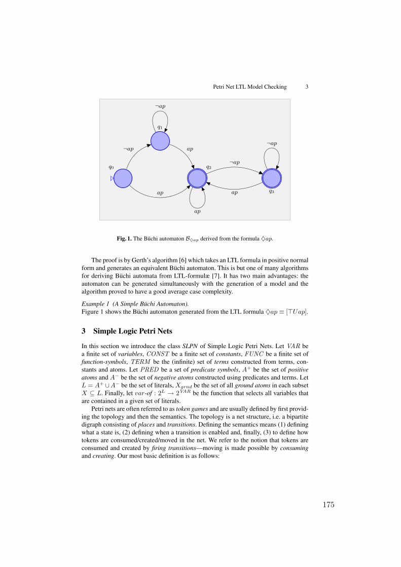
Petri Net LTL Model Checking 3

q0

q1

q2

q3

¬ap

ap

ap

¬ap

ap

¬ap

ap

¬ap

Fig. 1. The Buchi automaton B♦ap derived from the formula ♦ap.

The proof is by Gerth’s algorithm [6] which takes an LTL formula in positive normalform and generates an equivalent Buchi automaton. This is but one of many algorithmsfor deriving Buchi automata from LTL-formulæ [7]. It has two main advantages: theautomaton can be generated simultaneously with the generation of a model and thealgorithm proved to have a good average case complexity.

Example 1 (A Simple Buchi Automaton).Figure 1 shows the Buchi automaton generated from the LTL formula ♦ap ≡ [>Uap].

3 Simple Logic Petri Nets

In this section we introduce the class SLPN of Simple Logic Petri Nets. Let VAR bea finite set of variables, CONST be a finite set of constants, FUNC be a finite set offunction-symbols, TERM be the (infinite) set of terms constructed from terms, con-stants and atoms. Let PRED be a set of predicate symbols, A+ be the set of positiveatoms and A− be the set of negative atoms constructed using predicates and terms. LetL = A+ ∪A− be the set of literals, Xgrnd be the set of all ground atoms in each subsetX ⊆ L. Finally, let var-of : 2L → 2VAR be the function that selects all variables thatare contained in a given set of literals.

Petri nets are often referred to as token games and are usually defined by first provid-ing the topology and then the semantics. The topology is a net structure, i.e. a bipartitedigraph consisting of places and transitions. Defining the semantics means (1) definingwhat a state is, (2) defining when a transition is enabled and, finally, (3) to define howtokens are consumed/created/moved in the net. We refer to the notion that tokens areconsumed and created by firing transitions—moving is made possible by consumingand creating. Our most basic definition is as follows:

175

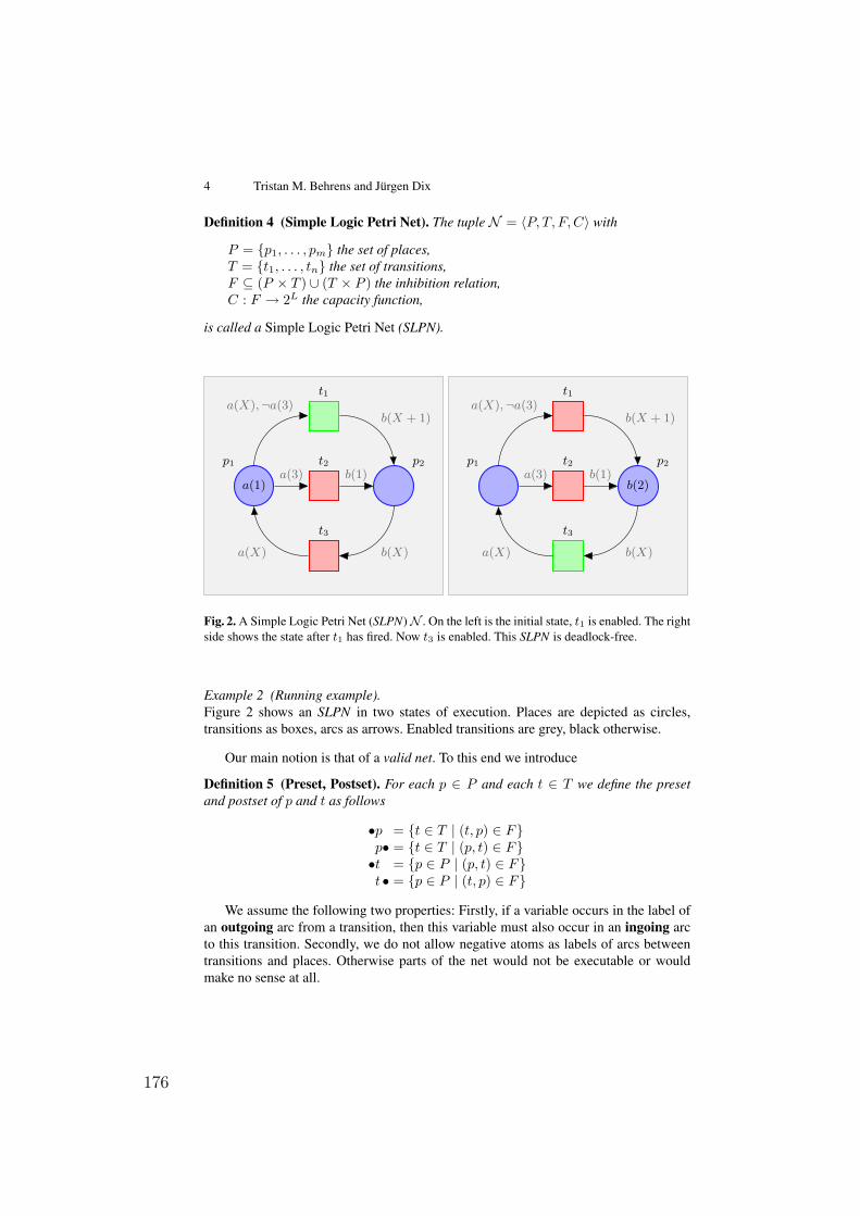
4 Tristan M. Behrens and Jurgen Dix

Definition 4 (Simple Logic Petri Net). The tuple N = 〈P, T, F,C〉 with

P = p1, . . . , pm the set of places,T = t1, . . . , tn the set of transitions,F ⊆ (P × T ) ∪ (T × P ) the inhibition relation,C : F → 2L the capacity function,

is called a Simple Logic Petri Net (SLPN).

a(1)

p1 t2

t1

t3

p2

a(X),¬a(3)

a(3)

a(X)

b(X + 1)

b(1)

b(X)

p1 t2

t1

t3

b(2)

p2

a(X),¬a(3)

a(3)

a(X)

b(X + 1)

b(1)

b(X)

Fig. 2. A Simple Logic Petri Net (SLPN)N . On the left is the initial state, t1 is enabled. The rightside shows the state after t1 has fired. Now t3 is enabled. This SLPN is deadlock-free.

Example 2 (Running example).Figure 2 shows an SLPN in two states of execution. Places are depicted as circles,transitions as boxes, arcs as arrows. Enabled transitions are grey, black otherwise.

Our main notion is that of a valid net. To this end we introduce

Definition 5 (Preset, Postset). For each p ∈ P and each t ∈ T we define the presetand postset of p and t as follows

•p = t ∈ T | (t, p) ∈ Fp• = t ∈ T | (p, t) ∈ F•t = p ∈ P | (p, t) ∈ Ft• = p ∈ P | (t, p) ∈ F

We assume the following two properties: Firstly, if a variable occurs in the label ofan outgoing arc from a transition, then this variable must also occur in an ingoing arcto this transition. Secondly, we do not allow negative atoms as labels of arcs betweentransitions and places. Otherwise parts of the net would not be executable or wouldmake no sense at all.

176

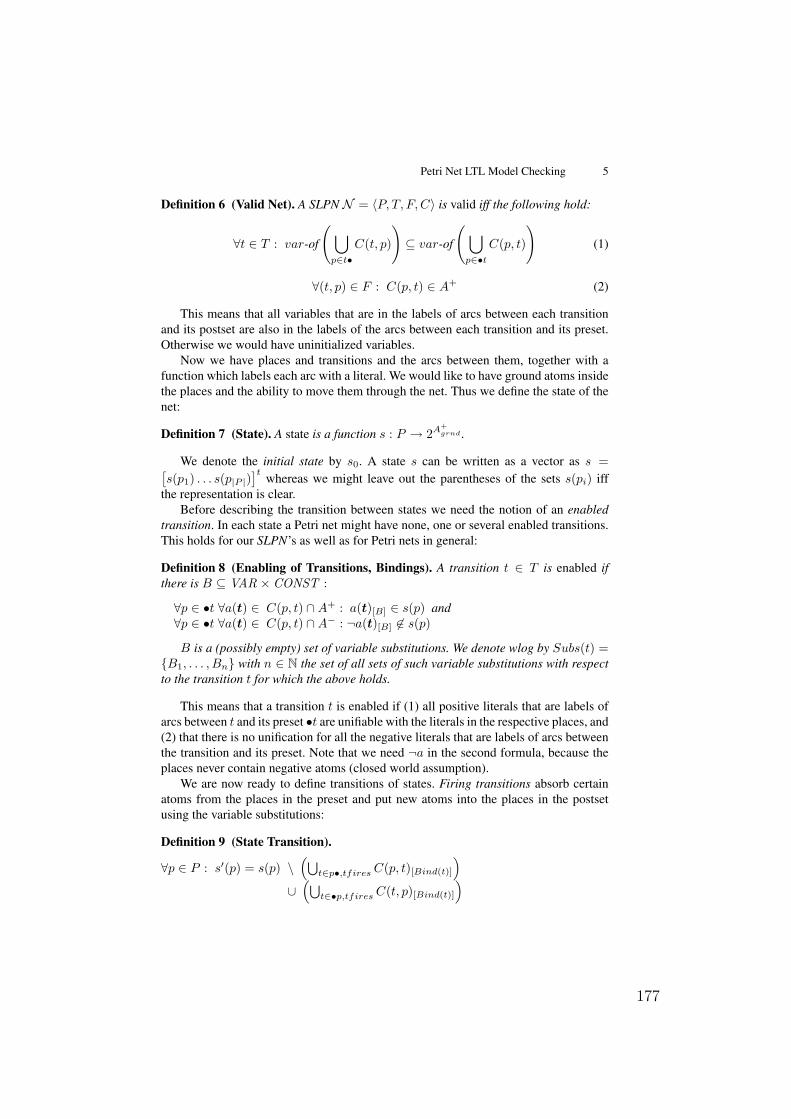
Petri Net LTL Model Checking 5

Definition 6 (Valid Net). A SLPN N = 〈P, T, F,C〉 is valid iff the following hold:

∀t ∈ T : var-of

(⋃p∈t•

C(t, p)

)⊆ var-of

(⋃p∈•t

C(p, t)

)(1)

∀(t, p) ∈ F : C(p, t) ∈ A+ (2)

This means that all variables that are in the labels of arcs between each transitionand its postset are also in the labels of the arcs between each transition and its preset.Otherwise we would have uninitialized variables.

Now we have places and transitions and the arcs between them, together with afunction which labels each arc with a literal. We would like to have ground atoms insidethe places and the ability to move them through the net. Thus we define the state of thenet:

Definition 7 (State). A state is a function s : P → 2A+grnd .

We denote the initial state by s0. A state s can be written as a vector as s =[s(p1) . . . s(p|P |)

]twhereas we might leave out the parentheses of the sets s(pi) iff

the representation is clear.Before describing the transition between states we need the notion of an enabled

transition. In each state a Petri net might have none, one or several enabled transitions.This holds for our SLPN’s as well as for Petri nets in general:

Definition 8 (Enabling of Transitions, Bindings). A transition t ∈ T is enabled ifthere is B ⊆ VAR × CONST :

∀p ∈ •t ∀a(t) ∈ C(p, t) ∩A+ : a(t)[B] ∈ s(p) and∀p ∈ •t ∀a(t) ∈ C(p, t) ∩A− : ¬a(t)[B] 6∈ s(p)

B is a (possibly empty) set of variable substitutions. We denote wlog by Subs(t) =B1, . . . , Bn with n ∈ N the set of all sets of such variable substitutions with respectto the transition t for which the above holds.

This means that a transition t is enabled if (1) all positive literals that are labels ofarcs between t and its preset •t are unifiable with the literals in the respective places, and(2) that there is no unification for all the negative literals that are labels of arcs betweenthe transition and its preset. Note that we need ¬a in the second formula, because theplaces never contain negative atoms (closed world assumption).

We are now ready to define transitions of states. Firing transitions absorb certainatoms from the places in the preset and put new atoms into the places in the postsetusing the variable substitutions:

Definition 9 (State Transition).

∀p ∈ P : s′(p) = s(p) \(⋃

t∈p•,tfires C(p, t)[Bind(t)])

∪(⋃

t∈•p,tfires C(t, p)[Bind(t)])

177

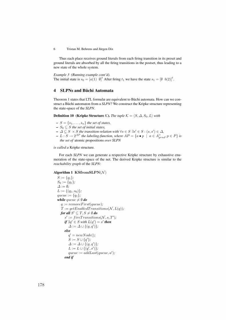
6 Tristan M. Behrens and Jurgen Dix

Thus each place receives ground literals from each firing transition in its preset andground literals are absorbed by all the firing transitions in the postset, thus leading to anew state of the whole system.

Example 3 (Running example cont’d).The initial state is s0 = [a(1) ∅]t After firing t1 we have the state s1 = [∅ b(2)]t.

4 SLPNs and Buchi Automata

Theorem 1 states that LTL formulæ are equivalent to Buchi automata. How can we con-struct a Buchi automaton from a SLPN? We construct the Kripke structure representingthe state-space of the SLPN.

Definition 10 (Kripke Structure K). The tuple K = 〈S,∆, S0, L〉 with

– S = s1, . . . , sn the set of states,– S0 ⊆ S the set of initial states,– ∆ ⊆ S × S the transition-relation with ∀s ∈ S ∃s′ ∈ S : (s, s′) ∈ ∆,– L : S → 2AP the labeling-function, where AP = a • p | a ∈ A+

grnd, p ∈ P isthe set of atomic propositions over SLPN

is called a Kripke structure.

For each SLPN we can generate a respective Kripke structure by exhaustive enu-meration of the state-space of the net. The derived Kripke structure is similar to thereachability graph of the SLPN:

Algorithm 1 KSfromSLPN(N )S := q1;S0 := q1;∆ := ∅;L := (q1, s0);queue := q1;while queue 6= ∅ doq := removeF irst(queue);T := getEnabledTransitions(N , L(q));for all S′ ⊆ T, S 6= ∅ dos′ := fireTransitions(N , s, T ′);if ∃q′ ∈ S with L(q′) = s′ then∆ := ∆ ∪ (q, q′);

elseq′ = newNode();S := S ∪ q′;∆ := ∆ ∪ (q, q′);L := L ∪ (q′, s′);queue := addLast(queue, a′);

end if

178

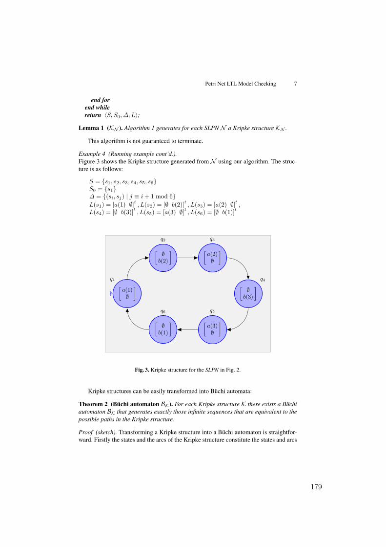
Petri Net LTL Model Checking 7

end forend whilereturn 〈S, S0, ∆, L〉;

Lemma 1 (KN ). Algorithm 1 generates for each SLPN N a Kripke structure KN .

This algorithm is not guaranteed to terminate.

Example 4 (Running example cont’d.).Figure 3 shows the Kripke structure generated from N using our algorithm. The struc-ture is as follows:

S = s1, s2, s3, s4, s5, s6S0 = s1∆ = (si, sj) | j ≡ i+ 1 mod 6L(s1) = [a(1) ∅]t , L(s2) = [∅ b(2)]t , L(s3) = [a(2) ∅]t ,L(s4) = [∅ b(3)]t , L(s5) = [a(3) ∅]t , L(s6) = [∅ b(1)]t

»a(1)∅

–q1

»∅b(2)

–q2

»∅b(1)

–q6

»a(2)∅

–q3

»a(3)∅

–q5

»∅b(3)

– q4

Fig. 3. Kripke structure for the SLPN in Fig. 2.

Kripke structures can be easily transformed into Buchi automata:

Theorem 2 (Buchi automaton BK). For each Kripke structure K there exists a Buchiautomaton BK that generates exactly those infinite sequences that are equivalent to thepossible paths in the Kripke structure.

Proof (sketch). Transforming a Kripke structure into a Buchi automaton is straightfor-ward. Firstly the states and the arcs of the Kripke structure constitute the states and arcs

179

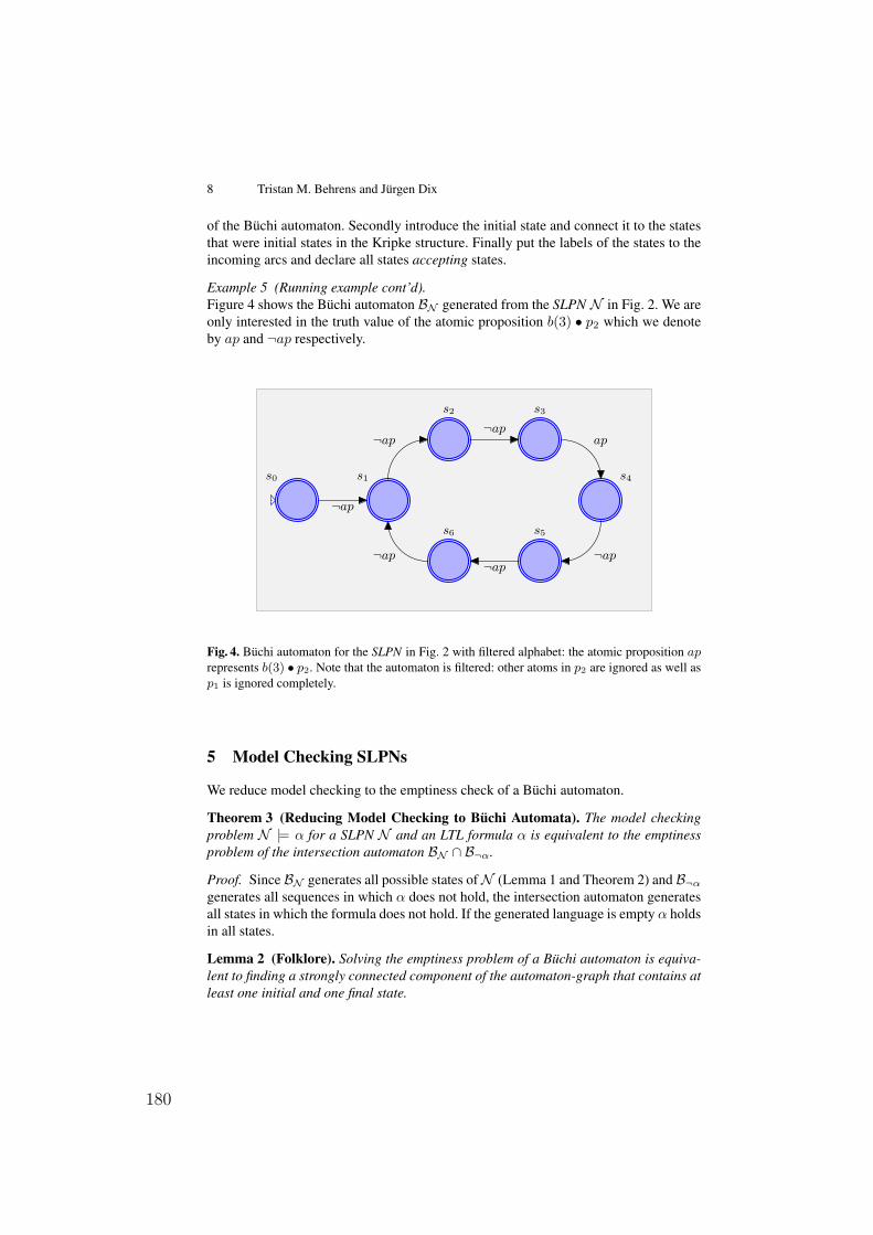
8 Tristan M. Behrens and Jurgen Dix

of the Buchi automaton. Secondly introduce the initial state and connect it to the statesthat were initial states in the Kripke structure. Finally put the labels of the states to theincoming arcs and declare all states accepting states.

Example 5 (Running example cont’d).Figure 4 shows the Buchi automaton BN generated from the SLPN N in Fig. 2. We areonly interested in the truth value of the atomic proposition b(3) • p2 which we denoteby ap and ¬ap respectively.

s1

s2

s6

s3

s5

s4

¬ap¬ap

ap

¬ap¬ap

¬ap

s0

¬ap

Fig. 4. Buchi automaton for the SLPN in Fig. 2 with filtered alphabet: the atomic proposition aprepresents b(3) • p2. Note that the automaton is filtered: other atoms in p2 are ignored as well asp1 is ignored completely.

5 Model Checking SLPNs

We reduce model checking to the emptiness check of a Buchi automaton.

Theorem 3 (Reducing Model Checking to Buchi Automata). The model checkingproblem N |= α for a SLPN N and an LTL formula α is equivalent to the emptinessproblem of the intersection automaton BN ∩ B¬α.

Proof. Since BN generates all possible states ofN (Lemma 1 and Theorem 2) and B¬αgenerates all sequences in which α does not hold, the intersection automaton generatesall states in which the formula does not hold. If the generated language is empty α holdsin all states.

Lemma 2 (Folklore). Solving the emptiness problem of a Buchi automaton is equiva-lent to finding a strongly connected component of the automaton-graph that contains atleast one initial and one final state.

180

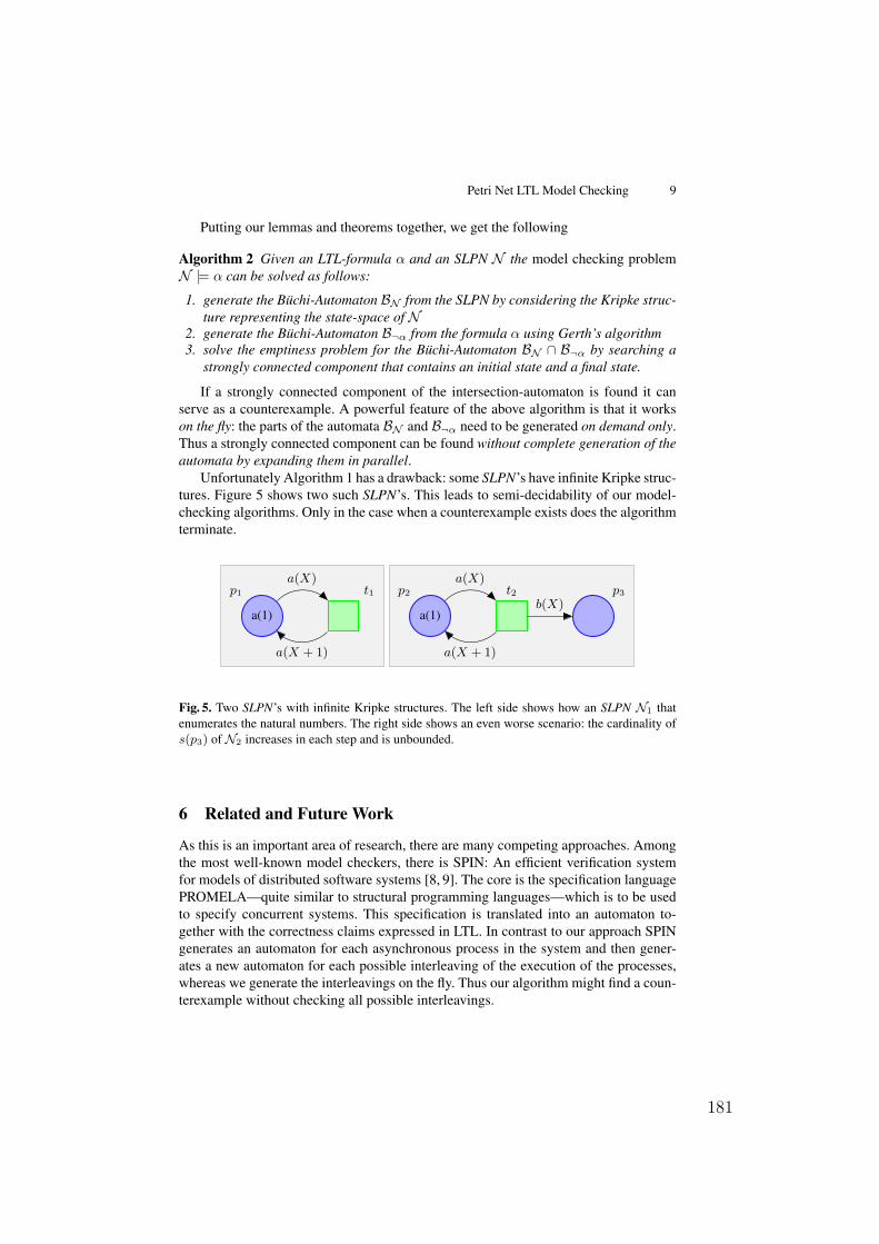
Petri Net LTL Model Checking 9

Putting our lemmas and theorems together, we get the following

Algorithm 2 Given an LTL-formula α and an SLPN N the model checking problemN |= α can be solved as follows:

1. generate the Buchi-Automaton BN from the SLPN by considering the Kripke struc-ture representing the state-space of N

2. generate the Buchi-Automaton B¬α from the formula α using Gerth’s algorithm3. solve the emptiness problem for the Buchi-Automaton BN ∩ B¬α by searching a

strongly connected component that contains an initial state and a final state.

If a strongly connected component of the intersection-automaton is found it canserve as a counterexample. A powerful feature of the above algorithm is that it workson the fly: the parts of the automata BN and B¬α need to be generated on demand only.Thus a strongly connected component can be found without complete generation of theautomata by expanding them in parallel.

Unfortunately Algorithm 1 has a drawback: some SLPN’s have infinite Kripke struc-tures. Figure 5 shows two such SLPN’s. This leads to semi-decidability of our model-checking algorithms. Only in the case when a counterexample exists does the algorithmterminate.

a(1)

p1 t1a(X)

a(X + 1)

a(1)

p2 t2 p3

a(X)

a(X + 1)

b(X)

Fig. 5. Two SLPN’s with infinite Kripke structures. The left side shows how an SLPN N1 thatenumerates the natural numbers. The right side shows an even worse scenario: the cardinality ofs(p3) ofN2 increases in each step and is unbounded.

6 Related and Future Work

As this is an important area of research, there are many competing approaches. Amongthe most well-known model checkers, there is SPIN: An efficient verification systemfor models of distributed software systems [8, 9]. The core is the specification languagePROMELA—quite similar to structural programming languages—which is to be usedto specify concurrent systems. This specification is translated into an automaton to-gether with the correctness claims expressed in LTL. In contrast to our approach SPINgenerates an automaton for each asynchronous process in the system and then gener-ates a new automaton for each possible interleaving of the execution of the processes,whereas we generate the interleavings on the fly. Thus our algorithm might find a coun-terexample without checking all possible interleavings.

181

10 Tristan M. Behrens and Jurgen Dix

– Recently we have made use of the Petri net infrastructure Petri Net Kernel [10](PNK). It is very useful for developers and scientists, because it allows a powerfularchitecture for basic Petri net tools like editors and simulators and it also permitsthe extension by versatile plugins. We use PNK for designing Petri nets and be-cause it comes along with the standardized data exchange format Petri Net MarkupLanguage (PNML) based on XML.

– We have implemented an SLPN-to-smodels-converter which takes an SLPN andgenerates a logic program, whose answer sets represent all possible bounded exe-cutions of the net. With it we are able to detect deadlocks [4].

– We are working on an AgentSpeak (F)-to-SLPN-converter with which we will testour model-checking-framework.

– We plan to examine the relationship between SLPN and the Petri-net-classes P/Tnets and Colored Petri nets as well as the operational semantics of SLPN.

7 Conclusion

SLPN is a class of specialized Petri nets with logical atoms as tokens and logical literalsas labels. It is well suited to describe agent languages based on logical atoms (like thefamily of AgentSpeak languages).

We gave a short summary on LTL model checking with automata: LTL formulæ aswell as Kripke structures can be transformed into Buchi automata, finding a final statethat is reachable from an initial state and from itself solves the model checking problem.

Finally we showed how to generate a Buchi automaton from a given SLPN andconcluded with how to perform LTL model checking on SLPN’s.

References

1. Clarke, E.M., Grumberg, O., Peled, D.A.: Model Checking. The MIT Press (2000) ISBN0262032708.

2. Emerson, E.A.: Temporal and modal logic. In: Handbook of Theoretical Computer Science,Volume B: Formal Models and Sematics (B). (1990) 995–1072

3. David, R., Alla, H.: Discrete, Continuous, and Hybrid Petri Nets. Springer Verlag (2005)ISBN 3540224807.

4. Behrens, T., Dix, J.: Model checking with logic based petri nets. Technical Report IfI-07-02,Clausthal University of Technology, Dept of Computer Science (May 2007)

5. Thomas, W.: Automata on infinite objects. In Leeuwen, V., ed.: Handbook of TheoreticalComputer Science. (1990) 133–164

6. Gerth, R., Peled, D., Vardi, M.Y., Wolper, P.: Simple on-the-fly automatic verification oflinear temporal logic. In: Protocol Specification Testing and Verification, Warsaw, Poland,Chapman & Hall (1995) 3–18

7. Vardi, M.Y., Wolper, P.: An automata-theoretic approach to automatic program verification(preliminary report). In: LICS, IEEE Computer Society (1986) 332–344

8. Holzmann, G.J.: The SPIN Model Checker. Addison-Wesley (2003) ISBN 0321228626.9. Holzmann, G.J.: Software model checking with spin. Advances in Computers 65 (2005)

78–10910. Kindler, E., Weber, M.: The petri net kernel - an infrastructure for building petri net tools.

International Journal on Software Tools for Technology Transfer 3(4) (2001) 486–497

182

Integrating Temporal Annotations in a ModularLogic Language

Vitor Nogueira and Salvador Abreu

Universidade de Evora and CENTRIA, Portugalvbn,spa@di.uevora.pt

Abstract Albeit temporal reasoning and modularity are very prolificfields of research in Logic Programming (LP) we find few examples oftheir integration. Moreover, in those examples, time and modularity areconsidered orthogonal to each other. In this paper we propose the addi-tion of temporal annotations to a modular extension of LP such that theusage of a module is influenced by temporal conditions. Besides illustra-tive examples we also provide an operational semantics together with acompiler, allowing this way for the development of applications based onsuch language.

1 Introduction

The importance of representing and reasoning about temporal information iswell known not only in the database community but also in the artificial in-telligence one. In the past decades the volume of temporal data has grownenormously, making modularity a requisite for any language suitable for de-veloping applications for such domains. One expected approach in devising alanguage with modularity and temporal reasoning is to consider that these char-acteristics co-exist without any direct relationship (see for instance the languageMuTACLP [BMRT02] or [NA06]). Nevertheless we can also conceive a scenariowhere modularity and time are more integrated, for instance where the usageof a module is influenced by temporal conditions. In this paper we follow thelater approach in defining a temporal extensions to a language called ContextualLogic Programming (CxLP) [MP93]. This language is a simple and powerful ex-tension of logic programming with mechanisms for modularity. Recent work notonly presented a revised specification of CxLP together with a new implemen-tation for it but also explained how this language could be seen as a shift intothe Object-Oriented Programming paradigm [AD03]. Finally, CxLP structure isvery suitable for integrating with temporal reasoning since its quite straightfor-ward to add the notion of time of the context and let that time help to decide ifa certain module is eligible or not to solve a goal.

For temporal representation and reasoning we chose Temporal AnnotatedConstraint Logic Programming (TACLP) [Fru94,Fru96] since this language sup-ports qualitative and quantitative (metric) temporal reasoning involving bothtime points and time periods (time intervals) and their duration. Moreover, itallows one to represent definite, indefinite and periodical temporal information.

183

The remainder of this article is structured as follows. In Sects. 2 and 3 webriefly overview CxLP and TACLP, respectively. Section 4 presents the temporalextension of CxLP and Sect. 5 relates it with other languages. Conclusions andproposals for future work follows.

2 An Overview of Contextual Logic Programming

For this overview we assume that the reader is familiar with the basic notions ofLogic Programming. Contextual Logic Programming (CxLP) [MP93] is a sim-ple yet powerful language that extends logic programming with mechanisms formodularity. In CxLP a finite set of Horn clauses with a given name is desig-nated by unit. Using the syntax of GNU Prolog/CX (recent implementation forCxLP [AD03]) consider a unit named employee to represent some basic factsabout university employees, using ta and ap as an abbreviation of teachingassistant and associate professor, respectively:

:-unit(employee(NAME, POSITION)).

item :- employee(NAME, POSITION).employee(bill, ta).employee(joe, ap).

name(NAME).position(POSITION).

The main difference between the example above and a plain logic program isthe first line that declares the unit name (employee) along with the unit argu-ments (NAME, POSITION). Unit arguments help avoid the annoying proliferationof predicate arguments, which occur whenever a global structure needs to bepassed around. A unit argument can be interpreted as a “unit global” variable,i.e. one which is shared by all clauses defined in the unit. Therefore, as soon as aunit argument gets instantiated, all the occurrences of that variable in the unitare replaced accordingly.

Suppose also that each employee’s position has an associated integer rhatwill be used to calculate the salary. Such relation can be easily expressed by thefollowing unit index:

:- unit(index(POSITION, INDEX)).

item :-index(POSITION, INDEX).

index(ta, 12).index(ap, 20).

index(INDEX).position(POSITION).

184

A set of units is designated as a contextual logic program. With the unitsabove we can build the program P = employee, index.

Given that in the same program we can have two or more units with thesame name but different arities, to be more precise besides the unit name weshould also refer its arity i.e. the number of arguments. Nevertheless, since mostof the times there is no ambiguity, we omit the arity of the units. If we considerthat employee and index designate sets of clauses, then the resulting programis given by the union of these sets.

For a given CxLP program, we can impose an order on its units, leading tothe notion of context. Contexts are implemented as lists of unit designators andeach computation has a notion of its current context. The program denoted bya particular context is the union of the predicates that are defined in each unit.Moreover, we resort to the override semantics to deal with multiple occurrencesof a given predicate: only the topmost definition is visible.

To construct contexts, we have the context extension operation denoted by:> . The goal U :> G extends the current context with unit U and resolves goalG in the new context. For instance to obtain Bill’s position we could do:

| ?- employee(bill, P) :> item

P = ta

In this query we extend the initial empty context [] 1 with unit employee ob-taining context [employee(bill, P)] and then resolve query item. This leadsto P being instantiated with ta.

Suppose also that the employee’s salary is obtained by multiplying the indexof its position by the base salary. To implement this rule consider the unitsalary:

:-unit(salary(SALARY)).

item :-position(P),[index(P, I)] :< item,base_salary(B),SALARY is I*B.

base_salary(100).

The unit above introduces a new operator (:<) called context switch: goal[index(P, I)] :< item invokes item in context [index(P, I)]. To bettergrasp the definition of this unit consider the goal:

| ?- employee(bill, P) :> (item, salary(S) :> item).

1 In the GNU Prolog/CX implementation the empty context contains all the standardProlog predicates such as =/2.

185

Since we already explained the beginning of this goal, lets see the remainingpart. After salary/1 being added, we are left with the context [salary(S),employee(bill,ta)]. The second item is evaluated and the first matching def-inition is found in unit salary. Goal position(P) is called and since there isno rule for this goal in the current unit (salary), a search in the context is per-formed. Since employee is the topmost unit that has a rule for position(P), thisgoal is resolved in the (reduced) context [employee(bill, ta)]. In an informalway, we queried the context for the position of whom we want to calculate thesalary, obtaining ta. Next, we query the index corresponding to such position,i.e. [index(ta, I)] :< item. Finally, to calculate the salary, we just need tomultiply the index by the base salary, obtaining S = 1200 with the final context[salary(1200), employee(bill, ta)].

3 Temporal Annotated Constraint Logic Programming

This section presents a brief overview of Temporal Annotated Constraint LogicProgramming (TACLP) that follows closely Sect. 2 of [RF00]. For a more detailedexplanation of TACLP see for instance [Fru96].

We consider the subset of TACLP where time points are totally ordered,sets of time points are convex and non-empty, and only atomic formulae can beannotated. Moreover clauses are free of negation.

Time can be discrete or dense. Time points are totally ordered by the relation≤. We call the set of time points D and suppose that a set of operations (suchas the binary operations +,−) to manage such points is associated with it. Weassume that the time-line is left-bounded by the number 0 and open the future(∞). A time period is an interval [r, s] with 0 ≤ r ≤ s ≤ ∞, r ∈ D, s ∈ D andrepresents the convex, non-empty set of time points t | r ≤ t ≤ s. Thereforethe interval [0,∞] denotes the whole time line.

Definition 1 (Annotated Formula). An annotated formula is of the formAα where A is an atomic formula and α an annotation. Let t be a time pointand I be a time period:

(at) The annotated formula A at t means that A holds at time point t.(th) The annotated formula A th I means that A holds throughout I, i.e. at every

time point in the period I.A th–annotated formula can be defined in terms of at as: A th I ⇔ ∀t (t ∈I → A at t)

(in) The annotated formula A in I means that A holds at some time point(s) inthe time period I, but there is no knowledge when exactly. The in annotationaccounts for indefinite temporal information.An in–annotated formula can also be defined in terms of at: A in I ⇔ ∃t (t ∈I ∧A at t).

The set of annotations is endowed with a partial order relation v which turnsinto a lattice. Given two annotations α and β, the intuition is that α v β if α is“less informative” than β in the sense that for all formulae A, Aβ ⇒ Aα.

186

In addition to Modus Ponens, TACLP has the following two inference rules:

Aα γ v αAγ

rule (v)Aα Aβ γ = α t β

Aγrule (t)

The rule (v) states that if a formula holds with some annotation, then it alsoholds with all annotations that are smaller according to the lattice ordering. Therule (t) says that if a formula holds with some annotation and the same formulaholds with another annotation then it holds in the least upper bound of theannotations. Assuming r1 ≤ s1, s1 ≤ s2 and s2 ≤ r2, we can summarize theaxioms for the lattice operation v by:

in[r1, r2] v in[s1, s2] v in[s1, s1] = at s1 = th[s1, s1] v th[s1, s2] v th[r1, r2]

The axioms of the least upper bound t can be restricted to 2:

th[s1, s2] t th[r1, r2] = th[s1, r2]⇔ s1 ≤ r1, r1 ≤ s2, s2 ≤ r2

A TACLP program is a finite set of TACLP clauses. A TACLP clause is aformula of the form Aα ← C1, . . . , Cn, B1α1, . . . , Bmαm (m,n ≥ 0) where Ais an atom, α and αi are optional temporal annotations, the Cj ’s are the con-straints and the Bi’s are the atomic formulae. Moreover, besides an interpreterfor TACLP clauses there is also a compiler that translates them into its CLPform.

4 Temporal Annotations and Contextual LogicProgramming

In CxLP with overriding semantics, to solve a goal G in a context C, a search isperformed until the topmost unit of C that contains clauses for the predicate ofG is found. We propose to adapt this basic mechanism of CxLP (called contextsearch) in order to include the temporal reasoning aspects. To accomplish thiswe add temporal annotations to contexts and to units and it will be the relationbetween those two annotations that will help to decide if a given unit is eligibleto match a goal during a context search.

The addition of time to a context is rather intuitive: instead of a list ofunit designators [u1, . . . , un] we now have a temporally annotated list of unitsdesignators [u1, . . . , un]α. This annotation α is called the time of the context andby default, contexts are implicitly annotated with the current time.

We could follow an approach for units similar to the one proposed for con-texts, i.e. to add a temporal annotation to a unit’s declaration. Hence we couldhave units definitions like :- unit(foo(X)) th [1,4].

Nevertheless, units and more specifically, units with arguments allow for a re-finement of the temporal qualification, i.e. instead of a qualifying the entire unit,we can have several qualifications, one for each possible argument instantiation.For the unit foo above we could have:2 The least upper bound only has to be computed for overlapping th annotations.

187

:- unit(foo(X)).foo(a) th [1,2].foo(b) th [3,4].

Where the first annotated fact states that unit foo with its argument instan-tiated to a has the annotation th [1,2]. With these annotations, unit foo willbe eligible to match a goal in the context [..., foo(a), ...] in [1,4] butits not eligible in the context [..., foo(b), ...] th [3,6] since in[1, 4] vth[1, 2] and th[3, 6] 6v th[3, 4]. We call those annotated facts the temporal condi-tions of the unit 3.

Each unit defines one temporally annotated predicate with the same nameas the unit and arity equal to the number of the unit arguments. For the caseof atemporal (timeless) units, it is assumed by default that we have the mostgeneral unit designator annotated with the complete time line.

We decided that these temporal annotations can only appear as heads of ruleswhose body is true, i.e. facts. Such restriction is motivated by efficiency reasonssince this way we can compute the least upper bound (t) of the th annotatedfacts before runtime and this way checking the units temporal conditions duringa context search is simplified to the verification of partial order (v) betweenannotations. Moreover, as we shall see in the examples, such restrictions arenot limitative since the expressiveness of contexts allow us to simulate TACLPclauses.

Revisiting the employee example, units employee and index can be writtenas:

:- unit(employee(NAME, POSITION)).

employee(bill, ta) th [2004, inf].employee(joe, ta) th [2002, 2006].employee(joe, ap) th [2007, inf].item.position(POSITION).name(NAME).

:- unit(index(POSITION, INDEX)).index(ta, 10) th [2000, 2005].index(ta, 12) th [2006, inf].index(ap, 19) th [2000, 2005].index(ap, 20) th [2006, inf].item.position(POSITION).index(INDEX).

As an exemplification, consider the goal:

?- at 2005 :> employee(joe, P) :> item.

In this goal, after asserting that the context temporal annotation is at 2005,unit employee is added to the context and goal item invoked. The evaluation ofitem is true as long as the unit is eligible in the current context, and this is trueif P is instantiated with ta (teaching assistant), therefore P = ta.

Unit salary can be defined as:3 The reader should notice that this way its still possible to annotate the entire unit,

since we can annotate the unit most general designator, for instance we could havefoo( )th[1, 10].

188

:- unit(salary(SALARY)).item :-

position(P), index(P, I) :> item,base_salary(B), SALARY is B*I.

base_salary(100).

There is no need to annotate the goals position(P) or index(P, I) :>item since they are evaluated in a context with the same temporal annotation.To find out joe’s salary in 2005 we can do:

?- at 2005 :> employee(joe, P) :> salary(S) :> item.P = taS=1000

In the goal above item is evaluated in the context [salary(S), employee(joe,P)] (at 2005). Since salary is the topmost unit that defines it, the body ofthe rule for such predicate is evaluated. In order to use the unit employee(joe,P) to solve position(P), such unit must satisfy the temporal conditions (at2005), that in this case stands for instantiating P with ta, therefore we obtainposition(ta). A similar reasoning applies for goal index(ta, I) :> item, i.e.this item is resolved in context [index(ta, 10), salary(S), employee(joe,ta)] (at 2005). The remainder of the rule body is straightforward, leading tothe answer P = ta and S = 1000.

4.1 Compiler

The compiler for this language can be obtained by combining a program trans-formation with the compiler for TACLP [Fru96]. Given a unit u, such trans-formation rewrites each predicate P in the head of a rule by P’ and add thefollowing clauses to u:

P :- Temporal_Conditions, !, P’.P :- :^ P.

stating the resolving P is equivalent to invoke P’, if the temporal conditionsare satisfied. Otherwise P must be solved in the supercontext (:^ P), i.e. P iscalled in the context obtained from removing u.

The temporal condition can be formalized as the conjunction :< [U | ] α, Uα,where the first conjunct queries the context for its temporal annotation (α) andits topmost unit (U), i.e. the current unit. The second conjunct checks if thecurrent unit satisfies the time of the context.

As it should be expected, the compiled language is CxLP with constraints.Finally, since GNU Prolog/CX besides the CxLP primitives also has a constraintsolver for finite domains (CLP(FD)), the implementation of this language isdirect on such a system.

189

4.2 Application to Legal Reasoning

Legal reasoning is a very productive field to illustrate the application of theselanguages. Not only a modular approach is very suitable for reasoning aboutlaws but also time is pervasive in their definition.

The following example was taken from the British Nationality Act and it waspresented in [BMRT02] to exemplify the usage of the language MuTACLP. Thereason to use an existing example is twofold: not only we consider it to be asimple and concise sample of legal reasoning but also because this way we cangive a more thorough comparison with MuTACLP. The textual description ofthis law can be given as a person X obtains the British Nationality at time T if:

– X is born in the UK at the time T– T is after the commencement– Y is a parent of X– Y is a British citizen or resident at time T.

Assuming that the temporal unit person represents the name and the placewhere a person was born:

:- unit(person(Name, Country)).person(john, uk) th [’1969-8-10’, inf].

The temporal annotation of this unit can be interpreted as the person timeframe, i.e. when she was born and when she died (if its alive, we represent it byinf).

Before presenting the rule for the nationality act we still need to representsome facts about who is a British citizen along with who is parent of whom:

:- unit(british_citizen(Name)).

british_citizen(bob)th [’1940-9-6’, inf].

:- unit(parent(Parent, Son)).

parent(bob, john)th [’1969-8-10’, inf].

Considering that the commencement date for this law is ’1955-1-1’, one for-malization of this law in our language is 4:

th [L, _] :> person(X, uk) :> item, fd_min(L, T),’1955-1-1’ #=< T,at T :> (parent(Y, X) :> item,

(british_citizen(Y) :> item;british_resident(Y) :> item)).

The explanation of the goal above is quite simple since each line correspondto one condition of the textual description of the law.

4 fd min(X, N) succeeds if N is the minimal value of the current domain of X.

190

5 Related Work

Since [BMRT02] relates MuTACLP with proposals such as Temporal Datalog[OM94] and the work on amalgamating knowledge bases [Sub94], we decided toconfine ourselves to the comparison between MuTACLP and our language. Mu-TACLP (Multi-Theory Temporal Annotated Constraint Logic Programming) isa knowledge representation language that provides facilities for modeling andhandling temporal information, together with some basic operators for combin-ing different knowledge bases. Although both MuTACLP and the language hereproposed use TACLP (Temporal Annotated Constraint Logic Programming) forhandling temporal information, it is in the way that modularity is dealt that theydiverge: we follow a dynamic approach (also called programming-in-the-small)while MuTACLP engages a static one (also called programming-in-the-large).

Moreover, the use of contexts allows for a more compact writing where someof the annotations of the MuTACLP version are subsumed by the annotationof the context. For instance, one of the rules of the MuTACLP version of theexample of legal reasoning is:

get_citizenship(X) at T <- T >= Jan 1 1955, born(X, uk) at T,parent(Y, X) at T,british_citizen(Y) at T.

In [NA06] a similar argument was used when comparing with relationalframeworks such as the one proposed by Combi and Pozzi in [CP04] for work-flow management systems, where relational queries were more verbose that itscontextual version.

6 Conclusion and Future Work

In this paper we presented a temporal extension of CxLP where time influencesthe eligibility of a module to solve a goal. Besides illustrative examples we alsoprovided a compiler, allowing this way for the development of applications basedon these languages. Although we provided (in the Appendix A) the operationalsemantics we consider that to obtain a more solid theoretical foundation thereis still need for a fixed point or declarative definition.

Besides the domain of application exemplified we are currently applying thelanguage proposed to other areas such as medicine and natural language. Fi-nally, it is our goal to continue previous work [AN06,ADN04] and show that thislanguage can act as the backbone for constructing and maintaining temporalinformation systems.

References

AD03. Salvador Abreu and Daniel Diaz. Objective: In minimum context. In Catus-cia Palamidessi, editor, ICLP, volume 2916 of Lecture Notes in ComputerScience, pages 128–147. Springer, 2003.

191

ADN04. Salvador Abreu, Daniel Diaz, and Vitor Nogueira. Organizational informa-tion systems design and implementation with contextual constraint logicprogramming. In IT Innovation in a Changing World – The 10th Interna-tional Conference of European University Information Systems, Ljubljana,Slovenia, June 2004.

AN06. Salvador Abreu and Vitor Nogueira. Towards structured contexts and mod-ules. In Sandro Etalle and Miroslaw Truszczynski, editors, ICLP, volume4079 of Lecture Notes in Computer Science, pages 436–438. Springer, 2006.

BMRT02. Paolo Baldan, Paolo Mancarella, Alessandra Raffaeta, and Franco Turini.Mutaclp: A language for temporal reasoning with multiple theories. In An-tonis C. Kakas and Fariba Sadri, editors, Computational Logic: Logic Pro-gramming and Beyond, volume 2408 of Lecture Notes in Computer Science,pages 1–40. Springer, 2002.

CP04. Carlo Combi and Giuseppe Pozzi. Architectures for a temporal workflowmanagement system. In SAC ’04: Proceedings of the 2004 ACM symposiumon Applied computing, pages 659–666, New York, NY, USA, 2004. ACMPress.

Fru94. T. Fruhwirth. Annotated constraint logic programming applied to tempo-ral reasoning. In M. Hermenegildo and J. Penjam, editors, ProgrammingLanguage Implementation and Logic Programming: 6th International Sym-posium (PLILP’94), pages 230–243. Springer, Berlin, Heidelberg, 1994.

Fru96. Thom W. Fruhwirth. Temporal annotated constraint logic programming.J. Symb. Comput., 22(5/6):555–583, 1996.

MP93. Luıs Monteiro and Antonio Porto. A Language for Contextual Logic Pro-gramming. In K.R. Apt, J.W. de Bakker, and J.J.M.M. Rutten, editors,Logic Programming Languages: Constraints, Functions and Objects, pages115–147. MIT Press, 1993.

NA06. Vitor Nogueira and Salvador Abreu. Temporal contextual logic program-

ming. In Francisco J. Lopez Fraguas, editor, Proceedings of the 15th

Workshop on Functional and (Constraint) Logic Programming (WFLP’06),Madrid, Spain, November 2006. Electronic Notes in Theoretical ComputerScience.

OM94. Mehmet A. Orgun and Wanli Ma. An overview of temporal and modallogic programming. In ICTL ’94: Proceedings of the First InternationalConference on Temporal Logic, pages 445–479, London, UK, 1994. Springer-Verlag.

RF00. Alessandra Raffaeta and Thom Fruhwirth. Labelled deduction, chapter Se-mantics for temporal annotated constraint logic programming, pages 215–243. Kluwer Academic Publishers, Norwell, MA, USA, 2000.

Sub94. V. S. Subrahmanian. Amalgamating knowledge bases. ACM Trans.Database Syst., 19(2):291–331, 1994.

A Operational Semantics

In this section we assume the following notation: C,C ′ for contexts, u for unit,θ, σ, ϕ, ε for substitutions, α, β, γ for temporal annotations and ∅, G for non-annotated goals.

We also assume a prior computation of the least upper bound for the unitsth annotations. This procedure is rather straightforward and can be describe as:

192

if A th I and B th J are in a unit u, such that I and J overlap, then removethose facts from u and insert A th(ItJ). This procedure stops when there are nomore facts in that conditions. Moreover, the termination is guaranteed becauseat each step we decrease the size of a finite set, the set of th annotated facts.

Null goal

Cα ` ∅[ε](1)

The null goal is derivable in any temporal annotated context, with the emptysubstitution ε as result.

Conjunction of goals

Cα ` G1[θ] Cαθ ` G2θ[σ]Cα ` G1, G2[θσdvars(G1, G2)]

(2)

To derive the conjunction derive one conjunct first, and then the other inthe same context with the given substitutions 5.Since C may contain variables in unit designators or temporal terms thatmay be bound by the substitution θ obtained from the derivation of G1,we have that θ must also be applied to Cα in order to obtain the updatedcontext in which to derive G2θ.

Context inquiry

Cα ` :> C ′β[θ]

θ = mgu(C,C ′)β v α (3)

In order to make the context switch operation (4) useful, there needs to be anoperation which fetches the context. This rule recovers the current contextC as a term and unifies it with term C ′, so that it may be used elsewhere inthe program. Moreover, the annotation β must be less (or equal) informativethan the annotation α (β v α).

Context switch

C ′β ` G[θ]Cα ` C ′β :< G[θ]

(4)

The purpose of this rule is to allow execution of a goal in an arbitrarytemporal annotated context, independently of the current annotated context.This rule causes goal G to be executed in context C ′β.

Reduction

5 The notation δdV stands for the restriction of the substitution δ to the variables inV .

193

(uCα) θσ ` Bθσ[ϕ]uC α ` G[θσϕdvars(G)]

H ← B ∈ uθ = mgu(G,H)(uθσ) β ∈ uα v β

(5)

This rule expresses the influence of temporal reasoning on context search. Inan informal way we can say that when a goal (G) has a definition (H ← B ∈ uand θ = mgu(G,H)) in the topmost unit (u) of the annotated context (uCα),and such unit satisfies the temporal conditions, to derive the goal we mustcall the body of the matching clause, after unification 6. The verificationof the temporal conditions stands for checking if there is a unit temporalannotation ((uθσ)β ∈ u) that is “more informative” than the annotation ofthe context (α v β), i.e. if (uθσ) α is true.

Context traversal:

Cα ` G[θ]uCα ` G[θ]

pred(G) 6∈ u (6)

When none of the previous rules applies and the predicate of G isn’t definedin the predicates of u (u), remove the top element of the context, i.e. resolvegoal G in the supercontext.

Application of the rules It is almost direct to verify that the inference rules aremutually exclusive, leading to the fact that given a derivation tuple Cα ` G[θ]only one rule can be applied.

6 Although this rule might seem complex, that has to do essentially with the abun-dance of unification’s (θσϕ)

194

Proposal of Visual Generalized RuleProgramming Model for Prolog?

Grzegorz J. Nalepa1 and Igor Wojnicki1

Institute of Automatics,AGH University of Science and Technology,Al. Mickiewicza 30, 30-059 Kraków, Polandgjn@agh.edu.pl, wojnicki@agh.edu.pl

Abstract. The rule-based programming paradigm is omnipresent in anumber of engineering domains. However, there are some fundamentalsemantical differences between it, and classic programming approaches.No generic solution for using rules to model business logic in classicsoftware has been provided so far. In this paper a new approach forGeneralized Rule-based Programming (GREP) is given. It is based ona use of advanced rule representation called XTT, which includes anextended attribute-based language, a non-monotonic inference strategy,with an explicit inference control on the rule level. The paper shows, howsome typical programming constructions, as well as classic programs canbe modelled in this approach. The paper also presents possibilities of anefficient integration of this technique with existing software systems.

1 Introduction

The rule-based programming paradigm is omnipresent in a number of engineer-ing domains such as control and reactive systems, diagnosis and decision support.Recently, there has been a lot of effort to use rules to model business logic inclassic software. However, there are some fundamental semantical differencesbetween it, and classic procedural, or object-oriented programming approaches.This is why no generic modelling solution has been provided so far. The moti-vation of this paper is to investigate the possibility of modelling some typicalprogramming structures with the rule-based programming with use of on ex-tended forward-chaining rule-based system.In this paper a new approach for generalized rule-based programming is given.

The Generalized Rule Programming (GREP) is based on the use of an advancedrule representation, which includes an extended attribute-based language [1],a non-monotonic inference strategy, with an explicit inference control at therule level. The paper shows, how some typical programming constructions (suchas loops), as well as classic programs (such as factorial) can be modelled inthis approach. The paper presents possibilities of efficient integration of thistechnique with existing software systems in different ways.? The paper is supported by the Hekate Project funded from 2007–2008 resources forscience as a research project.

195

In Sect. 2 some basics of rule-based programming are given, and in Sect. 3some fundamental differences between software and knowledge engineering areidentified. Then, in Sect. 4 the extended model for rule-based systems is consid-ered. The applications of this model are discussed in Sect. 5. This model could beintegrated in the classic software system in several ways. The research presentedin this paper is work-in-progress. Directions for the future research as well asconcluding remarks are given in Sect. 6.

2 Concepts of the Rule-Based Programming

Rule-Based Systems (RBS) constitute a powerful AI tool [2] for specificationof knowledge in design and implementation of systems in the domains such assystem monitoring and diagnosis, intelligent control, and decision support. Forthe state-of-the-art in RBS see [3,4,1].In order to design and implement a RBS in a efficient way, the knowledge

representation method chosen should support the designer introducing a scal-able visual representation. As the number of rules exceeds even relatively verylow quantities, it is hard to keep the rule-base consistent, complete, and cor-rect. These problems are related to knowledge-base verification, validation, andtesting. To meet security requirements a formal analysis end verification of RBSshould be carried out [5]. This analysis usually takes place after the design. How-ever, there are design and implementation methods, such as the XTT, that allowfor on-line verification during the design and gradual refinement of the system.Supporting rulebase modelling remains an essential aspect of the design pro-

cess. The simplest approach consists in writing rules in the low-level RBS lan-guage, such as one of Jess (www.jessrules.com). More sophisticated are basedon the use of some classic visual rule representations. This is a case of LPAVisiRule, (www.lpa.co.uk) which uses decision trees. Approaches such as XTTaim at developing new visual language for visual rule modelling.

3 Knowledge in Software Engineering

Rule-based systems (RBS) constitute today one of the most important classes ofthe so-called Knowledge Based Systems (KBS). RBS found wide range of indus-trial applications is some „classic AI domains” such as decision support, systemdiagnosis, or intelligent control. However, due to some fundamental differencesbetween knowledge (KE) and software engineering (SE) the technology did notfind applications in the mainstream software engineering.What is important about the KE process, is the fact that it should capture

the expert knowledge and represent it in a way that is suitable for processing(this is the task for a knowledge engineer). The level at which KE should operateis often referred to as the knowledge level [6]. In case of KBS there is no singleuniversal engineering approach, or universal modelling method (such as UML insoftware engineering).

196

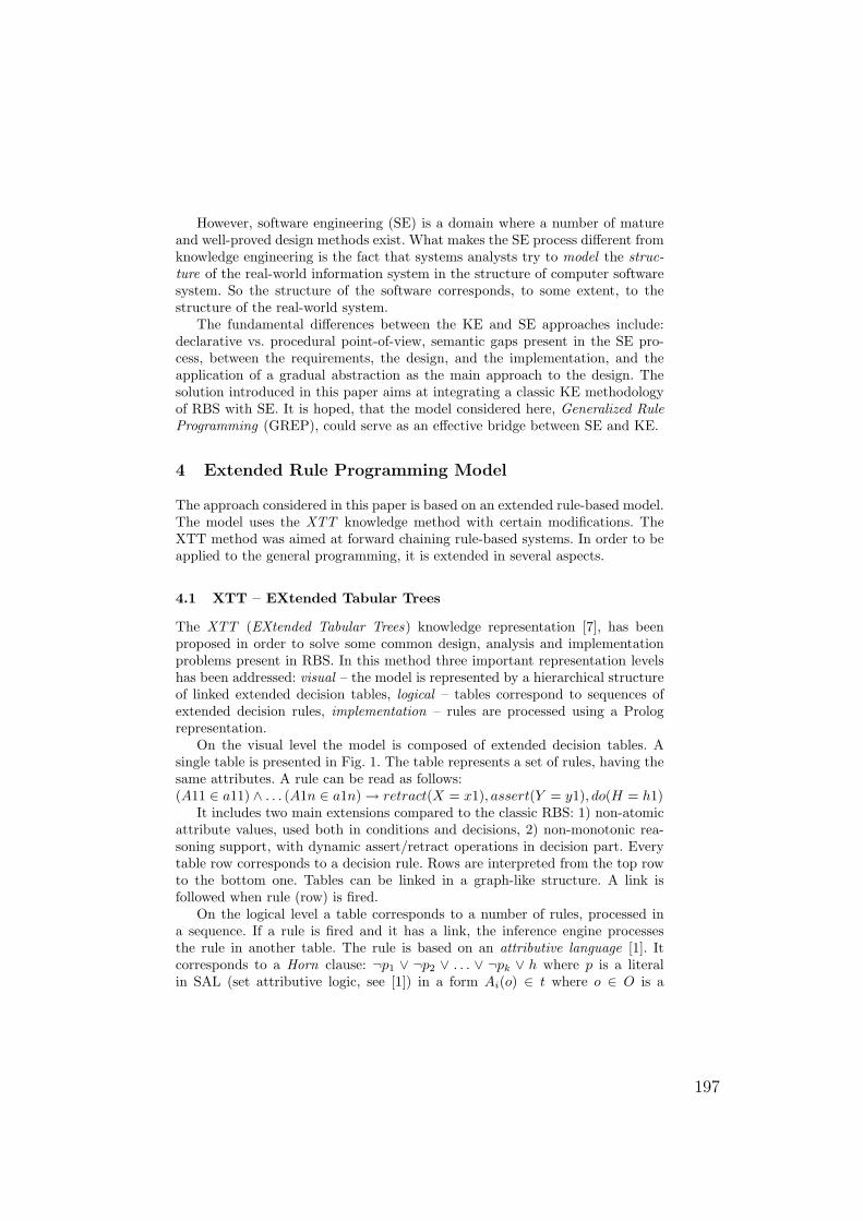
However, software engineering (SE) is a domain where a number of matureand well-proved design methods exist. What makes the SE process different fromknowledge engineering is the fact that systems analysts try to model the struc-ture of the real-world information system in the structure of computer softwaresystem. So the structure of the software corresponds, to some extent, to thestructure of the real-world system.The fundamental differences between the KE and SE approaches include:

declarative vs. procedural point-of-view, semantic gaps present in the SE pro-cess, between the requirements, the design, and the implementation, and theapplication of a gradual abstraction as the main approach to the design. Thesolution introduced in this paper aims at integrating a classic KE methodologyof RBS with SE. It is hoped, that the model considered here, Generalized RuleProgramming (GREP), could serve as an effective bridge between SE and KE.

4 Extended Rule Programming Model

The approach considered in this paper is based on an extended rule-based model.The model uses the XTT knowledge method with certain modifications. TheXTT method was aimed at forward chaining rule-based systems. In order to beapplied to the general programming, it is extended in several aspects.

4.1 XTT – EXtended Tabular Trees

The XTT (EXtended Tabular Trees) knowledge representation [7], has beenproposed in order to solve some common design, analysis and implementationproblems present in RBS. In this method three important representation levelshas been addressed: visual – the model is represented by a hierarchical structureof linked extended decision tables, logical – tables correspond to sequences ofextended decision rules, implementation – rules are processed using a Prologrepresentation.On the visual level the model is composed of extended decision tables. A

single table is presented in Fig. 1. The table represents a set of rules, having thesame attributes. A rule can be read as follows:(A11 ∈ a11) ∧ . . . (A1n ∈ a1n) → retract(X = x1), assert(Y = y1), do(H = h1)It includes two main extensions compared to the classic RBS: 1) non-atomic

attribute values, used both in conditions and decisions, 2) non-monotonic rea-soning support, with dynamic assert/retract operations in decision part. Everytable row corresponds to a decision rule. Rows are interpreted from the top rowto the bottom one. Tables can be linked in a graph-like structure. A link isfollowed when rule (row) is fired.On the logical level a table corresponds to a number of rules, processed in

a sequence. If a rule is fired and it has a link, the inference engine processesthe rule in another table. The rule is based on an attributive language [1]. Itcorresponds to a Horn clause: ¬p1 ∨ ¬p2 ∨ . . . ∨ ¬pk ∨ h where p is a literalin SAL (set attributive logic, see [1]) in a form Ai(o) ∈ t where o ∈ O is a

197

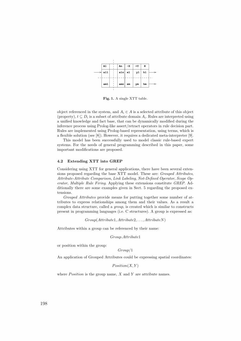
A1 An −X +Y H

a11 a1n x1 y1 h1

am1 amn xm ym hm

Fig. 1. A single XTT table.

object referenced in the system, and Ai ∈ A is a selected attribute of this object(property), t ⊆ Di is a subset of attribute domain Ai. Rules are interpreted usinga unified knowledge and fact base, that can be dynamically modified during theinference process using Prolog-like assert/retract operators in rule decision part.Rules are implemented using Prolog-based representation, using terms, which isa flexible solution (see [8]). However, it requires a dedicated meta-interpreter [9].This model has been successfully used to model classic rule-based expert

systems. For the needs of general programming described in this paper, someimportant modifications are proposed.

4.2 Extending XTT into GREP

Considering using XTT for general applications, there have been several exten-sions proposed regarding the base XTT model. These are: Grouped Attributes,Attribute-Attribute Comparison, Link Labeling, Not-Defined Operator, Scope Op-erator, Multiple Rule Firing. Applying these extensions constitute GREP. Ad-ditionally there are some examples given in Sect. 5 regarding the proposed ex-tensions.Grouped Attributes provide means for putting together some number of at-

tributes to express relationships among them and their values. As a result acomplex data structure, called a group, is created which is similar to constructspresent in programming languages (i.e. C structures). A group is expressed as:

Group(Attribute1, Attribute2, . . . , AttributeN)

Attributes within a group can be referenced by their name:

Group.Attribute1

or position within the group:Group/1

An application of Grouped Attributes could be expressing spatial coordinates:

Position(X, Y )

where Position is the group name, X and Y are attribute names.

198

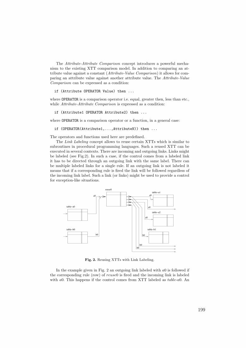
The Attribute-Attribute Comparison concept introduces a powerful mecha-nism to the existing XTT comparison model. In addition to comparing an at-tribute value against a constant (Attribute-Value Comparison) it allows for com-paring an attribute value against another attribute value. The Attribute-ValueComparison can be expressed as a condition:

if (Attribute OPERATOR Value) then ...

where OPERATOR is a comparison operator i.e. equal, greater then, less than etc.,while Attribute-Attribute Comparison is expressed as a condition:

if (Attribute1 OPERATOR Attribute2) then ...

where OPERATOR is a comparison operator or a function, in a general case:

if (OPERATOR(Attribute1,...,AttributeN)) then ...

The operators and functions used here are predefined.The Link Labeling concept allows to reuse certain XTTs which is similar to

subroutines in procedural programming languages. Such a reused XTT can beexecuted in several contexts. There are incoming and outgoing links. Links mightbe labeled (see Fig.2). In such a case, if the control comes from a labeled linkit has to be directed through an outgoing link with the same label. There canbe multiple labeled links for a single rule. If an outgoing link is not labeled itmeans that if a corresponding rule is fired the link will be followed regardless ofthe incoming link label. Such a link (or links) might be used to provide a controlfor exception-like situations.

table−a0

table−b0 table−b1

table−a1

table−a2

b0

a0

b0

b0

b0

a0

a0

a0

reuse0

Fig. 2. Reusing XTTs with Link Labeling.

In the example given in Fig. 2 an outgoing link labeled with a0 is followed ifthe corresponding rule (row) of reuse0 is fired and the incoming link is labeledwith a0. This happens if the control comes from XTT labeled as table-a0. An

199

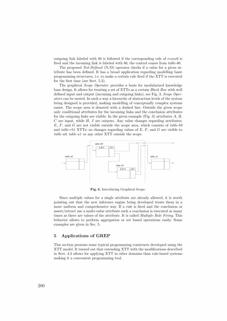
outgoing link labeled with b0 is followed if the corresponding rule of reuse0 isfired and the incoming link is labeled with b0; the control comes from table-b0.The proposed Not-Defined (N/D) operator checks if a value for a given at-

tribute has been defined. It has a broad application regarding modelling basicprogramming structures, i.e. to make a certain rule fired if the XTT is executedfor the first time (see Sect. 5.2).The graphical Scope Operator provides a basis for modularized knowledge

base design. It allows for treating a set of XTTs as a certain Black Box with welldefined input and output (incoming and outgoing links), see Fig. 3. Scope Oper-ators can be nested. In such a way a hierarchy of abstraction levels of the systembeing designed is provided, making modelling of conceptually complex systemseasier. The scope area is denoted with a dashed line. Outside the given scopeonly conditional attributes for the incoming links and the conclusion attributesfor the outgoing links are visible. In the given example (Fig. 3) attributes A, B,C are input, while H, I are outputs. Any value changes regarding attributes:E, F , and G are not visible outside the scope area, which consists of table-b0and table=b1 XTTs; no changes regarding values of E, F , and G are visible totable-a0, table-a1 or any other XTT outside the scope.

table−b0

A B C H I

table−b1

H IE F G

table−a1table−a0

Fig. 3. Introducing Graphical Scope.

Since multiple values for a single attribute are already allowed, it is worthpointing out that the new inference engine being developed treats them in amore uniform and comprehensive way. If a rule is fired and the conclusion orassert/retract use a multi-value attribute such a conclusion is executed as manytimes as there are values of the attribute. It is called Multiple Rule Firing. Thisbehavior allows to perform aggregation or set based operations easily. Someexamples are given in Sec. 5.

5 Applications of GREP

This section presents some typical programming constructs developed using theXTT model. It turned out that extending XTT with the modifications describedin Sect. 4.2 allows for applying XTT in other domains than rule-based systemsmaking it a convenient programming tool.

200

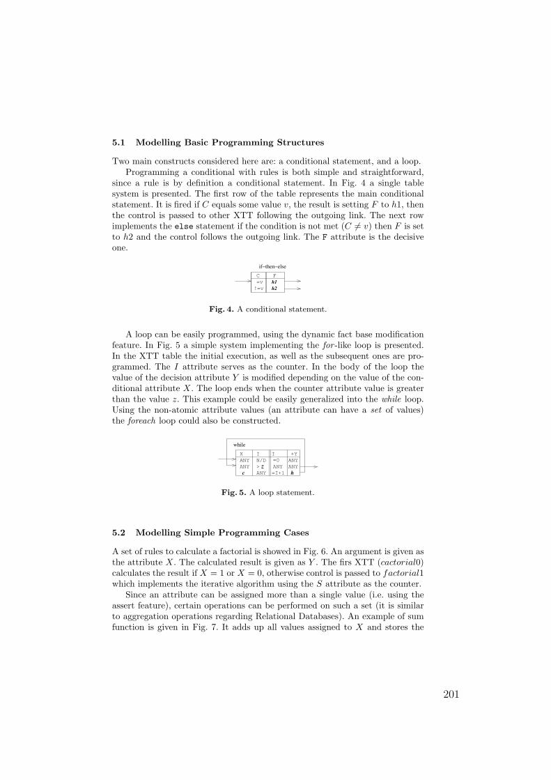
5.1 Modelling Basic Programming Structures

Two main constructs considered here are: a conditional statement, and a loop.Programming a conditional with rules is both simple and straightforward,

since a rule is by definition a conditional statement. In Fig. 4 a single tablesystem is presented. The first row of the table represents the main conditionalstatement. It is fired if C equals some value v, the result is setting F to h1, thenthe control is passed to other XTT following the outgoing link. The next rowimplements the else statement if the condition is not met (C 6= v) then F is setto h2 and the control follows the outgoing link. The F attribute is the decisiveone.

C

=v

!=v

h1

h2

if−then−else

F

Fig. 4. A conditional statement.

A loop can be easily programmed, using the dynamic fact base modificationfeature. In Fig. 5 a simple system implementing the for -like loop is presented.In the XTT table the initial execution, as well as the subsequent ones are pro-grammed. The I attribute serves as the counter. In the body of the loop thevalue of the decision attribute Y is modified depending on the value of the con-ditional attribute X. The loop ends when the counter attribute value is greaterthan the value z. This example could be easily generalized into the while loop.Using the non-atomic attribute values (an attribute can have a set of values)the foreach loop could also be constructed.

X

while

I

ANY

I

ANY ANY

=0 ANY

ANY

+Y

ANYc =I+1

>

N/D

h

z

Fig. 5. A loop statement.

5.2 Modelling Simple Programming Cases

A set of rules to calculate a factorial is showed in Fig. 6. An argument is given asthe attribute X. The calculated result is given as Y . The firs XTT (cactorial0)calculates the result if X = 1 or X = 0, otherwise control is passed to factorial1which implements the iterative algorithm using the S attribute as the counter.Since an attribute can be assigned more than a single value (i.e. using the

assert feature), certain operations can be performed on such a set (it is similarto aggregation operations regarding Relational Databases). An example of sumfunction is given in Fig. 7. It adds up all values assigned to X and stores the

201

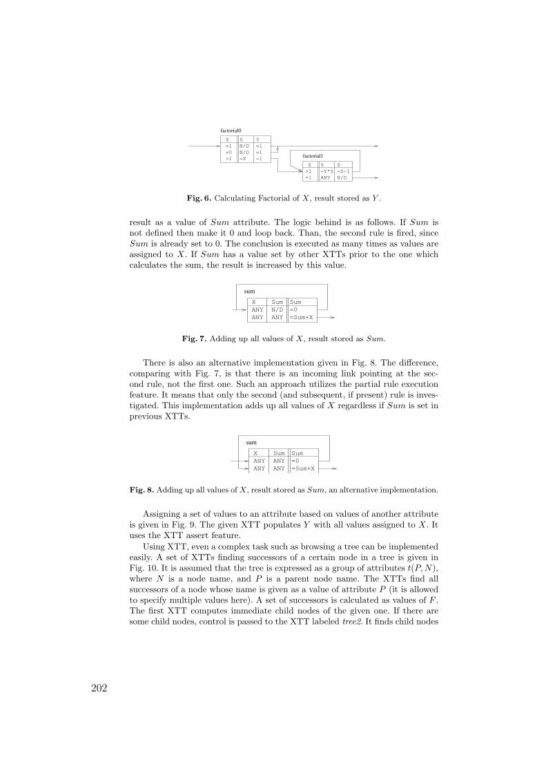
S

N/D

Y

=1

X

=1

=0

>1

factorial0

N/D

=X

=1

=1

S

factorial1

>1

=1

Y S

=Y*S =S−1

ANY N/D

Fig. 6. Calculating Factorial of X, result stored as Y .

result as a value of Sum attribute. The logic behind is as follows. If Sum isnot defined then make it 0 and loop back. Than, the second rule is fired, sinceSum is already set to 0. The conclusion is executed as many times as values areassigned to X. If Sum has a value set by other XTTs prior to the one whichcalculates the sum, the result is increased by this value.

X SumANY

SumN/D =0

ANY ANY =Sum+X

sum

Fig. 7. Adding up all values of X, result stored as Sum.

There is also an alternative implementation given in Fig. 8. The difference,comparing with Fig. 7, is that there is an incoming link pointing at the sec-ond rule, not the first one. Such an approach utilizes the partial rule executionfeature. It means that only the second (and subsequent, if present) rule is inves-tigated. This implementation adds up all values of X regardless if Sum is set inprevious XTTs.

sum

ANY

X

ANY

ANY

ANY

Sum Sum

=0

=Sum+X

Fig. 8. Adding up all values of X, result stored as Sum, an alternative implementation.

Assigning a set of values to an attribute based on values of another attributeis given in Fig. 9. The given XTT populates Y with all values assigned to X. Ituses the XTT assert feature.Using XTT, even a complex task such as browsing a tree can be implemented

easily. A set of XTTs finding successors of a certain node in a tree is given inFig. 10. It is assumed that the tree is expressed as a group of attributes t(P,N),where N is a node name, and P is a parent node name. The XTTs find allsuccessors of a node whose name is given as a value of attribute P (it is allowedto specify multiple values here). A set of successors is calculated as values of F .The first XTT computes immediate child nodes of the given one. If there aresome child nodes, control is passed to the XTT labeled tree2. It finds child nodes

202

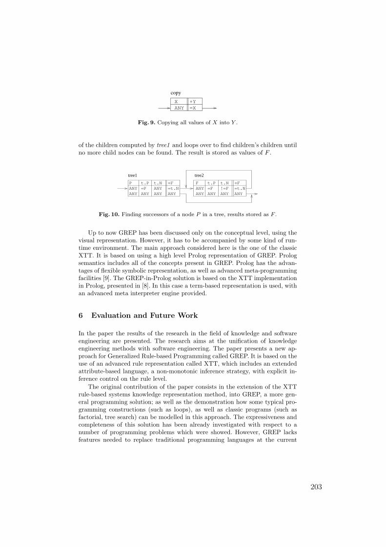
=X

+YX

ANY

copy

Fig. 9. Copying all values of X into Y .

of the children computed by tree1 and loops over to find children’s children untilno more child nodes can be found. The result is stored as values of F .

t.P t.NANY

+F=t.N

+F=t.N

t.PF=F

ANYANY

PANYANY

=P

tree1 tree2

ANYANYANYANY

t.N

ANYANY!=F

Fig. 10. Finding successors of a node P in a tree, results stored as F .

Up to now GREP has been discussed only on the conceptual level, using thevisual representation. However, it has to be accompanied by some kind of run-time environment. The main approach considered here is the one of the classicXTT. It is based on using a high level Prolog representation of GREP. Prologsemantics includes all of the concepts present in GREP. Prolog has the advan-tages of flexible symbolic representation, as well as advanced meta-programmingfacilities [9]. The GREP-in-Prolog solution is based on the XTT implementationin Prolog, presented in [8]. In this case a term-based representation is used, withan advanced meta interpreter engine provided.

6 Evaluation and Future Work

In the paper the results of the research in the field of knowledge and softwareengineering are presented. The research aims at the unification of knowledgeengineering methods with software engineering. The paper presents a new ap-proach for Generalized Rule-based Programming called GREP. It is based on theuse of an advanced rule representation called XTT, which includes an extendedattribute-based language, a non-monotonic inference strategy, with explicit in-ference control on the rule level.The original contribution of the paper consists in the extension of the XTT

rule-based systems knowledge representation method, into GREP, a more gen-eral programming solution; as well as the demonstration how some typical pro-gramming constructions (such as loops), as well as classic programs (such asfactorial, tree search) can be modelled in this approach. The expressiveness andcompleteness of this solution has been already investigated with respect to anumber of programming problems which were showed. However, GREP lacksfeatures needed to replace traditional programming languages at the current

203

stage. The problem areas include: general data structures support, limited ac-tions/operations in the decision and precondition parts, and input/output oper-ations, including environment communication.Future work will be focused on the GREP extensions, especially hybrid op-

erators and use cases. Hybrid operators, defined in a similar way as Prologpredicates, could offer extended processing capabilities for attributes, especiallygrouped ones, serving for generative, restrictive or triggering operations. Theseare to generate attribute values, restrict admissible attribute values, or triggerarbitrary code execution, respectively. Functionality of such operators would bedefined in a backward chaining manner to provide query-response characteristics.While proposing extensions to GREP, one should keep in mind, that in order

to be both coherent and efficient, GREP cannot make an extensive use of someof the facilities of other languages, even Prolog. Even though Prolog semanticsis quite close to the one of GREP there are some important differences – relatedto the different inference (forward in GREP, backward in Prolog) and someprogramming features such as recursion and unification. On the other hand,GREP offers a clear visual representation that supports a high level logic design.The number of failed visual logic programming attempts show, that the powerfulsemantics of Prolog cannot be easily modelled [10]. So from this perspective,GREP expressiveness is, and should remain weaker than that of Prolog.In its current stage GREP can successfully model a number of programming

constructs and approaches. This proves GREP can be applied as a general pur-pose programming environment. However, the research should be considered anexperimental one, and definitely a work in progress.

References

1. Ligęza, A.: Logical Foundations for Rule-Based Systems. Springer-Verlag, Berlin,Heidelberg (2006)

2. Negnevitsky, M.: Artificial Intelligence. A Guide to Intelligent Systems. Addison-Wesley, Harlow, England; London; New York (2002) ISBN 0-201-71159-1.

3. Liebowitz, J., ed.: The Handbook of Applied Expert Systems. CRC Press, BocaRaton (1998)

4. Jackson, P.: Introduction to Expert Systems. 3rd edn. Addison–Wesley (1999)ISBN 0-201-87686-8.

5. Vermesan, A., Coenen, F., eds.: Validation and Verification of Knowledge BasedSystems. Theory, Tools and Practice. Kluwer Academic Publisher, Boston (1999)

6. Newell, A.: The knowledge level. Artificial Intelligence 18 (1982) 87–1277. Nalepa, G.J., Ligęza, A.: A graphical tabular model for rule-based logic program-ming and verification. Systems Science 31 (2005) 89–95

8. Nalepa, G.J., Ligęza, A.: Prolog-based analysis of tabular rule-based systems withthe xtt approach. In Sutcliffe, G.C.J., Goebel, R.G., eds.: FLAIRS 2006: pro-ceedings of the 19th international Florida Artificial Intelligence Research Societyconference, AAAI Press (2006) 426–431

9. Covington, M.A., Nute, D., Vellino, A.: Prolog programming in depth. Prentice-Hall (1996)

10. Fisher, J.R., Tran, L.: A visual logic. In: SAC. (1996) 17–21

204

Prolog Hybrid Operators in the GeneralizedRule Programming Model?

Igor Wojnicki1 and Grzegorz J. Nalepa1

Institute of Automatics,AGH University of Science and Technology,Al. Mickiewicza 30, 30-059 Kraków, Polandgjn@agh.edu.pl, wojnicki@agh.edu.pl

Abstract. This paper describes the so-called Hybrid Operators in Pro-log – a concept which extends the Generalized Rule Based ProgrammingModel (GREP). This extension allows a GREP-based application to com-municate with the environment by providing input/output operations,user interaction, and process synchronization. Furthermore, it allows forthe integration of such an application with contemporary software tech-nologies including Prolog based code. The proposed Hybrid Operatorsextend GREP as a knowledge-based software development concept.

1 Introduction

Rule-Based Systems (RBS) constitute a powerful and well-known AI tool [1]for specification of knowledge. They are used in design and implementation ofsystems in the domains such as system monitoring and diagnosis, intelligentcontrol, and decision support (see [2,3,4]). From a point of view of classicalknowledge engineering (KE) a rule-based expert system consists of a knowledgebase and an inference engine. The KE process aims at designing and evaluatingthe knowledge base, and implementing the inference engine. In order to designand implement a RBS in a efficient way, the chosen knowledge representationmethod should support the designer introducing a scalable visual representation.Supporting rulebase modelling remains an essential aspect of the design pro-

cess. The simplest approach consists in writing rules in the low-level RBS lan-guage, such as one of Jess (www.jessrules.com). More sophisticated are basedon the use of some classic visual rule representations. This is a case of LPAVisiRule, (www.lpa.co.uk) which uses decision trees. Approaches such as XTTaim at developing new visual language for visual rule modelling.When it comes to practical implementation of RBS, a number of options

exist. These include expert systems shells such as CLIPS, or Java-based Jess; andprogramming languages. In the classic AI approach Prolog becomes the languageof choice, thanks to its logic-based knowledge representation and processing. Theimportant factor is, that Prolog semantics is very close to that of RBS.

? The paper is supported by the Hekate Project funded from 2007–2008 resources forscience as a research project.

205

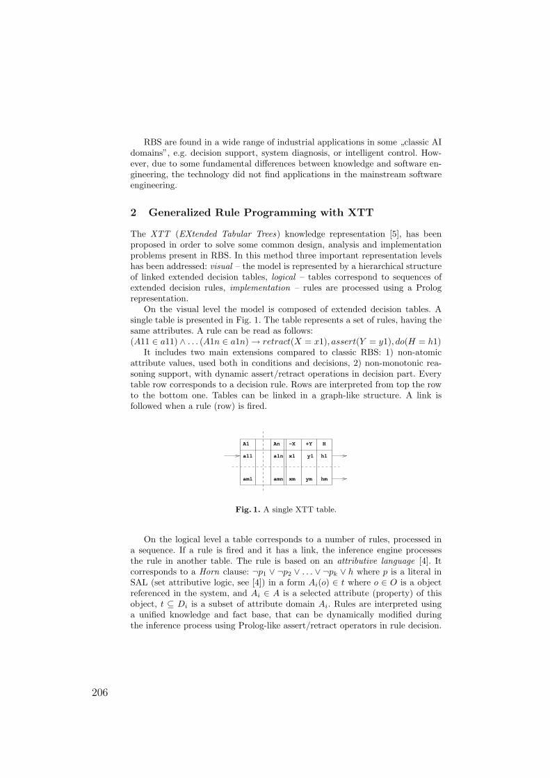
RBS are found in a wide range of industrial applications in some „classic AIdomains”, e.g. decision support, system diagnosis, or intelligent control. How-ever, due to some fundamental differences between knowledge and software en-gineering, the technology did not find applications in the mainstream softwareengineering.

2 Generalized Rule Programming with XTT

The XTT (EXtended Tabular Trees) knowledge representation [5], has beenproposed in order to solve some common design, analysis and implementationproblems present in RBS. In this method three important representation levelshas been addressed: visual – the model is represented by a hierarchical structureof linked extended decision tables, logical – tables correspond to sequences ofextended decision rules, implementation – rules are processed using a Prologrepresentation.On the visual level the model is composed of extended decision tables. A

single table is presented in Fig. 1. The table represents a set of rules, having thesame attributes. A rule can be read as follows:(A11 ∈ a11) ∧ . . . (A1n ∈ a1n) → retract(X = x1), assert(Y = y1), do(H = h1)It includes two main extensions compared to classic RBS: 1) non-atomic

attribute values, used both in conditions and decisions, 2) non-monotonic rea-soning support, with dynamic assert/retract operations in decision part. Everytable row corresponds to a decision rule. Rows are interpreted from top the rowto the bottom one. Tables can be linked in a graph-like structure. A link isfollowed when a rule (row) is fired.

A1 An −X +Y H

a11 a1n x1 y1 h1

am1 amn xm ym hm

Fig. 1. A single XTT table.

On the logical level a table corresponds to a number of rules, processed ina sequence. If a rule is fired and it has a link, the inference engine processesthe rule in another table. The rule is based on an attributive language [4]. Itcorresponds to a Horn clause: ¬p1 ∨ ¬p2 ∨ . . . ∨ ¬pk ∨ h where p is a literal inSAL (set attributive logic, see [4]) in a form Ai(o) ∈ t where o ∈ O is a objectreferenced in the system, and Ai ∈ A is a selected attribute (property) of thisobject, t ⊆ Di is a subset of attribute domain Ai. Rules are interpreted usinga unified knowledge and fact base, that can be dynamically modified duringthe inference process using Prolog-like assert/retract operators in rule decision.

206

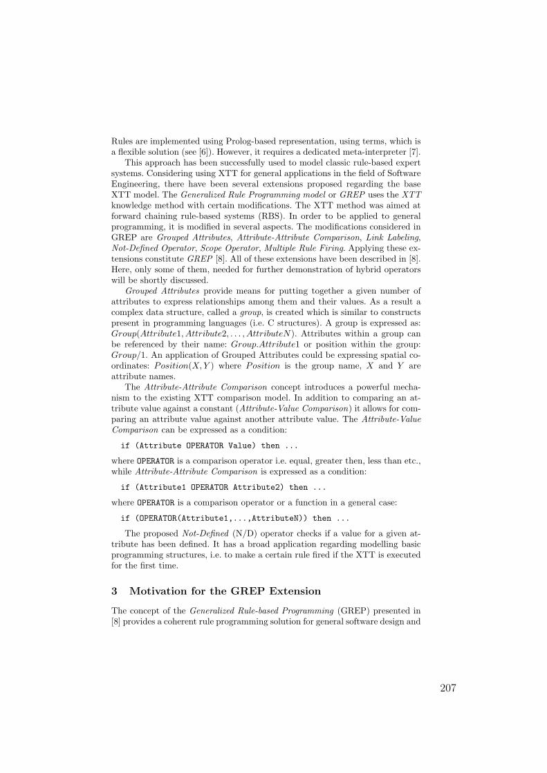
Rules are implemented using Prolog-based representation, using terms, which isa flexible solution (see [6]). However, it requires a dedicated meta-interpreter [7].This approach has been successfully used to model classic rule-based expert

systems. Considering using XTT for general applications in the field of SoftwareEngineering, there have been several extensions proposed regarding the baseXTT model. The Generalized Rule Programming model or GREP uses the XTTknowledge method with certain modifications. The XTT method was aimed atforward chaining rule-based systems (RBS). In order to be applied to generalprogramming, it is modified in several aspects. The modifications considered inGREP are Grouped Attributes, Attribute-Attribute Comparison, Link Labeling,Not-Defined Operator, Scope Operator, Multiple Rule Firing. Applying these ex-tensions constitute GREP [8]. All of these extensions have been described in [8].Here, only some of them, needed for further demonstration of hybrid operatorswill be shortly discussed.Grouped Attributes provide means for putting together a given number of

attributes to express relationships among them and their values. As a result acomplex data structure, called a group, is created which is similar to constructspresent in programming languages (i.e. C structures). A group is expressed as:Group(Attribute1, Attribute2, . . . , AttributeN). Attributes within a group canbe referenced by their name: Group.Attribute1 or position within the group:Group/1. An application of Grouped Attributes could be expressing spatial co-ordinates: Position(X, Y ) where Position is the group name, X and Y areattribute names.The Attribute-Attribute Comparison concept introduces a powerful mecha-

nism to the existing XTT comparison model. In addition to comparing an at-tribute value against a constant (Attribute-Value Comparison) it allows for com-paring an attribute value against another attribute value. The Attribute-ValueComparison can be expressed as a condition:

if (Attribute OPERATOR Value) then ...

where OPERATOR is a comparison operator i.e. equal, greater then, less than etc.,while Attribute-Attribute Comparison is expressed as a condition:

if (Attribute1 OPERATOR Attribute2) then ...

where OPERATOR is a comparison operator or a function in a general case:

if (OPERATOR(Attribute1,...,AttributeN)) then ...

The proposed Not-Defined (N/D) operator checks if a value for a given at-tribute has been defined. It has a broad application regarding modelling basicprogramming structures, i.e. to make a certain rule fired if the XTT is executedfor the first time.

3 Motivation for the GREP Extension

The concept of the Generalized Rule-based Programming (GREP) presented in[8] provides a coherent rule programming solution for general software design and

207

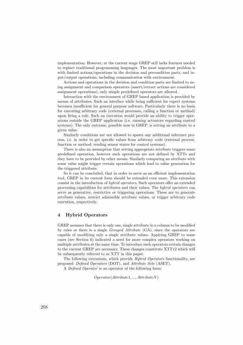
implementation. However, at the current stage GREP still lacks features neededto replace traditional programming languages. The most important problem iswith limited actions/operations in the decision and precondition parts, and in-put/output operations, including communication with environment.Actions and operations in the decision and condition parts are limited to us-

ing assignment and comparison operators (assert/retract actions are consideredassignment operations), only simple predefined operators are allowed.Interaction with the environment of GREP based application is provided by

means of attributes. Such an interface while being sufficient for expert systemsbecomes insufficient for general purpose software. Particularly there is no basisfor executing arbitrary code (external processes, calling a function or method)upon firing a rule. Such an execution would provide an ability to trigger oper-ations outside the GREP application (i.e. running actuators regarding controlsystems). The only outcome, possible now in GREP, is setting an attribute to agiven value.Similarly conditions are not allowed to spawn any additional inference pro-

cess, i.e. in order to get specific values from arbitrary code (external process,function or method; reading sensor states for control systems).There is also an assumption that setting appropriate attribute triggers some

predefined operation, however such operations are not defined by XTTs andthey have to be provided by other means. Similarly comparing an attribute withsome value might trigger certain operations which lead to value generation forthe triggered attribute.So it can be concluded, that in order to serve as an efficient implementation

tool, GREP in its current form should be extended even more. This extensionconsist in the introduction of hybrid operators. Such operators offer an extendedprocessing capabilities for attributes and their values. The hybrid operators canserve as generative, restrictive or triggering operations. These are to generateattribute values, restrict admissible attribute values, or trigger arbitrary codeexecution, respectively.

4 Hybrid Operators

GREP assumes that there is only one, single attribute in a column to be modifiedby rules or there is a single Grouped Attribute (GA), since the operators arecapable of modifying only a single attribute values. Applying GREP to somecases (see Section 6) indicated a need for more complex operators working onmultiple attributes at the same time. To introduce such operators certain changesto the current GREP are necessary. These changes constitute XTTv2 which willbe subsequently referred to as XTT in this paper.The following extensions, which provide Hybrid Operators functionality, are

proposed: Defined Operators (DOT), and Attribute Sets (ASET).A Defined Operator is an operator of the following form:

Operator(Attribute1, ..., AttributeN)

208

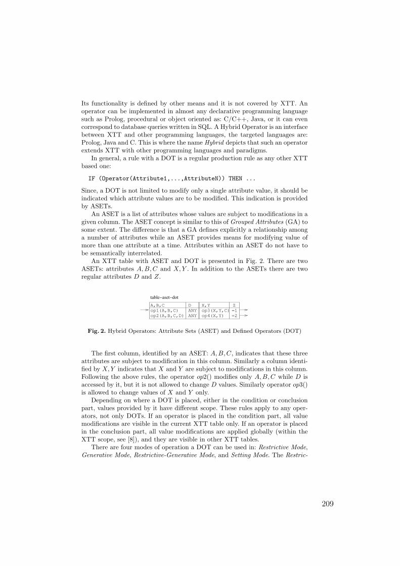
Its functionality is defined by other means and it is not covered by XTT. Anoperator can be implemented in almost any declarative programming languagesuch as Prolog, procedural or object oriented as: C/C++, Java, or it can evencorrespond to database queries written in SQL. A Hybrid Operator is an interfacebetween XTT and other programming languages, the targeted languages are:Prolog, Java and C. This is where the name Hybrid depicts that such an operatorextends XTT with other programming languages and paradigms.In general, a rule with a DOT is a regular production rule as any other XTT

based one:

IF (Operator(Attribute1,...,AttributeN)) THEN ...

Since, a DOT is not limited to modify only a single attribute value, it should beindicated which attribute values are to be modified. This indication is providedby ASETs.An ASET is a list of attributes whose values are subject to modifications in a

given column. The ASET concept is similar to this of Grouped Attributes (GA) tosome extent. The difference is that a GA defines explicitly a relationship amonga number of attributes while an ASET provides means for modifying value ofmore than one attribute at a time. Attributes within an ASET do not have tobe semantically interrelated.An XTT table with ASET and DOT is presented in Fig. 2. There are two

ASETs: attributes A,B, C and X, Y . In addition to the ASETs there are tworegular attributes D and Z.

table−aset−dot

D

ANY

ANY

X,Y

op4(X,Y)

A,B,C

op1(A,B,C)

op2(A,B,C,D)

op3(X,Y,C)

Z

=1

=2

Fig. 2. Hybrid Operators: Attribute Sets (ASET) and Defined Operators (DOT)

The first column, identified by an ASET: A,B, C, indicates that these threeattributes are subject to modification in this column. Similarly a column identi-fied by X, Y indicates that X and Y are subject to modifications in this column.Following the above rules, the operator op2() modifies only A,B, C while D isaccessed by it, but it is not allowed to change D values. Similarly operator op3()is allowed to change values of X and Y only.Depending on where a DOT is placed, either in the condition or conclusion

part, values provided by it have different scope. These rules apply to any oper-ators, not only DOTs. If an operator is placed in the condition part, all valuemodifications are visible in the current XTT table only. If an operator is placedin the conclusion part, all value modifications are applied globally (within theXTT scope, see [8]), and they are visible in other XTT tables.There are four modes of operation a DOT can be used in: Restrictive Mode,

Generative Mode, Restrictive-Generative Mode, and Setting Mode. The Restric-

209

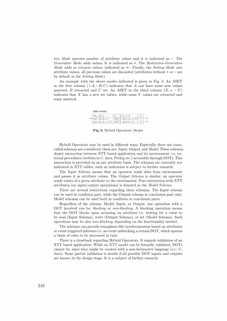
tive Mode narrows number of attribute values and it is indicated as -. TheGenerative Mode adds values. It is indicated as +. The Restrictive-GenerativeMode adds or retracts values; indicated as +-. Finally, the Setting Mode setsattribute values, all previous values are discarded (attributes without + or - areby default in the Setting Mode).An example with the above modes indicated is given in Fig. 3. An ASET

in the first column (+A,−B,C) indicates that A can have some new valuesasserted, B retracted and C set. An ASET in the third column (X, + − Y )indicates that X has a new set values, while some Y values are retracted andsome asserted.

D

ANY

ANY op4(X,Y)

op1(A,B,C)

op2(A,B,C,D)

op3(X,Y,C)

Z

=1

=2

table−modes

+A,−B,C X,+−Y

Fig. 3. Hybrid Operators: Modes

Hybrid Operators may be used in different ways. Especially three use cases,called schemas are considered, these are: Input,Output, andModel. These schemasdepict interaction between XTT based application and its environment, i.e. ex-ternal procedures (written in C, Java, Prolog etc.) accessible through DOTs. Thisinteraction is provided on an per attribute basis. The schemas are currently notindicated in XTT tables, such an indication is subject to further research.The Input Schema means that an operator reads data from environment

and passes it as attribute values. The Output Schema is similar: an operatorsends values of a given attribute to the environment. Pure interaction with XTTattributes (no input/output operations) is denoted as the Model Schema.There are several restrictions regarding these schemas. The Input schema

can be used in condition part, while the Output schema in conclusion part only.Model schemas can be used both in condition or conclusion parts.Regardless of the schema: Model, Input, or Output, any operation with a

DOT involved can be: blocking or non-blocking. A blocking operation meansthat the DOT blocks upon accessing an attribute i.e. waiting for a value tobe read (Input Schema), write (Output Schema), or set (Model Schema). Suchoperations may be also non-blocking, depending on the functionality needed.The schemas can provide semaphore-like synchronization based on attributes

or event triggered inference i.e. an event unblocking a certain DOT, which spawnsa chain of rules to be processed in turn.There is a drawback regarding Hybrid Operators. It regards validation of an

XTT based application. While an XTT model can be formally validated, DOTscannot be, since they might be created with a non-declarative language (i.e.: C,Java). Some partial validation is doable if all possible DOT inputs and outputsare known in the design stage. It is a subject of further research.

210

5 GREP Model Integration with HOP

The XTT model itself is capable of an advanced rule-based processing. However,interactions with the environment were not clearly defined. The Hybrid Opera-tors, introduced here, fill up this gap. An XTT based logic can be integrated withother components written in Prolog, C or Java. This integration is considered onan architectural level. It follows the Mode-View-Controller (MVC) pattern [9].In this case the XTT, together with Prolog based Hybrid Operators, is used tobuild the application logic: the model, where-as other parts of the applicationare built with some classic procedural or object-oriented languages such C orJava.

The application logic interfaces with object-oriented or procedural compo-nents accessible through Hybrid Operators. These components provide meansfor interaction with an environment which is user interface and general input-output operations. These components also make it possible to extend the modelwith arbitrary object-oriented code. There are several scenarios possible regard-ing interactions between the model and the environment. In general they canbe subdivided into two categories providing view and controller functionalitieswhich are output and input respectively.

An input takes place upon checking conditions required to fire a rule. A con-dition may require input operations. A state of such a condition is determinedby data from the environment. Such data could be user input, file contents, astate of an object, a result from a function etc. It is worth pointing out thatthe input operation could be blocking or non-blocking providing a basis for syn-chronization with environment. The input schema act as a controller regardingMVC.

The output schema takes place if a conclusion regards an output operation.In such a case, the operation regards general output (i.e. through user interface),spawning a method or function, setting a variable etc. The conclusion also carriesits state, which is true or false, depending on whether the output operationsucceeded or failed respectively. If the conclusion fails, the rule fails as well. Theoutput schema acts as the view regarding MVC.

There are several components to integrate to provide a working system. Theyare presented in Fig. 4. The application’s logic is given in a declarative way as theKnowledge Base using XTT. Interfaces with other systems (including Human-Computer Interaction) are provided in classical sequential manner through Hy-brid Operators. There is a bridging module between the Knowledge Base andthe sequential Code (C/Java language code): the Sequential Language INterface(SLIN). It allows communication in both directions. The Knowledge Base canbe extended, new facts or rules added by a stimulus coming through SLIN fromthe View/Interface. There are two types of information passed this way: eventsgenerated by the HeaRT (HEkate RunTime) and knowledge generated by theCode (through Hybrid Operators).

211

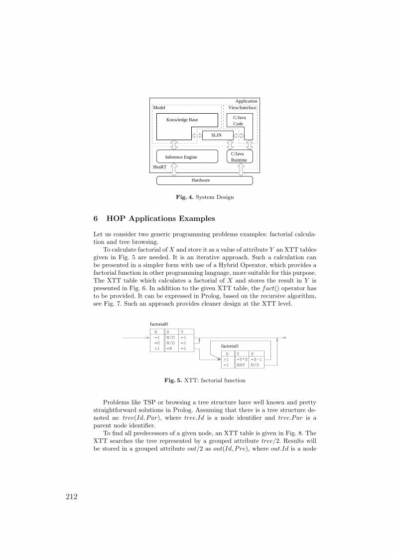
RuntimeC/Java

CodeC/Java

Hardware

SLIN

Inference Engine

HeaRT

View/Interface

Application

Model

Knowledge Base

Fig. 4. System Design

6 HOP Applications Examples

Let us consider two generic programming problems examples: factorial calcula-tion and tree browsing.To calculate factorial ofX and store it as a value of attribute Y an XTT tables

given in Fig. 5 are needed. It is an iterative approach. Such a calculation canbe presented in a simpler form with use of a Hybrid Operator, which provides afactorial function in other programming language, more suitable for this purpose.The XTT table which calculates a factorial of X and stores the result in Y ispresented in Fig. 6. In addition to the given XTT table, the fact() operator hasto be provided. It can be expressed in Prolog, based on the recursive algorithm,see Fig. 7. Such an approach provides cleaner design at the XTT level.

S

N/D

Y

=1

X

=1

=0

>1

factorial0

N/D

=X

=1

=1

S

factorial1

>1

=1

Y S

=Y*S =S−1

ANY N/D

Fig. 5. XTT: factorial function

Problems like TSP or browsing a tree structure have well known and prettystraightforward solutions in Prolog. Assuming that there is a tree structure de-noted as: tree(Id, Par), where tree.Id is a node identifier and tree.Par is aparent node identifier.To find all predecessors of a given node, an XTT table is given in Fig. 8. The

XTT searches the tree represented by a grouped attribute tree/2. Results willbe stored in a grouped attribute out/2 as out(Id, Pre), where out.Id is a node

212

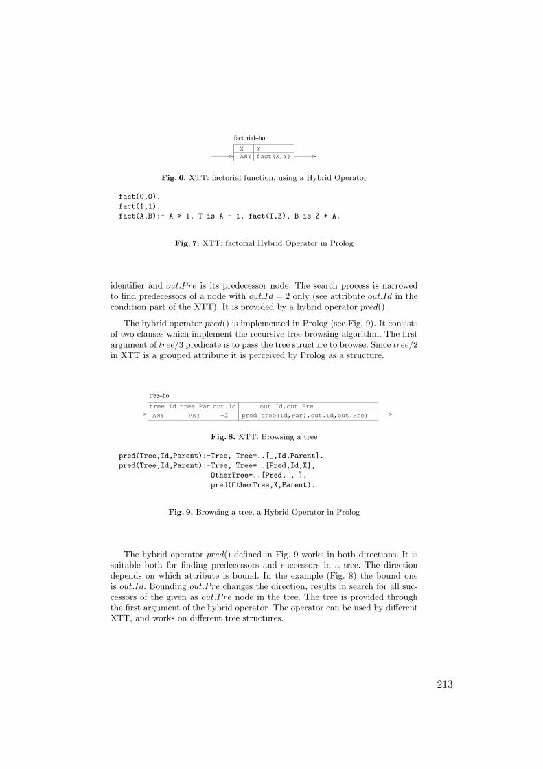
X

factorial−ho

ANY

Y

fact(X,Y)

Fig. 6. XTT: factorial function, using a Hybrid Operator

fact(0,0).fact(1,1).fact(A,B):- A > 1, T is A - 1, fact(T,Z), B is Z * A.

Fig. 7. XTT: factorial Hybrid Operator in Prolog

identifier and out.Pre is its predecessor node. The search process is narrowedto find predecessors of a node with out.Id = 2 only (see attribute out.Id in thecondition part of the XTT). It is provided by a hybrid operator pred().

The hybrid operator pred() is implemented in Prolog (see Fig. 9). It consistsof two clauses which implement the recursive tree browsing algorithm. The firstargument of tree/3 predicate is to pass the tree structure to browse. Since tree/2in XTT is a grouped attribute it is perceived by Prolog as a structure.

tree.Id

ANY

out.Id,out.Pre

tree−ho

out.Id

=2

tree.Par

ANY pred(tree(Id,Par),out.Id,out.Pre)

Fig. 8. XTT: Browsing a tree

pred(Tree,Id,Parent):-Tree, Tree=..[_,Id,Parent].pred(Tree,Id,Parent):-Tree, Tree=..[Pred,Id,X],

OtherTree=..[Pred,_,_],pred(OtherTree,X,Parent).

Fig. 9. Browsing a tree, a Hybrid Operator in Prolog

The hybrid operator pred() defined in Fig. 9 works in both directions. It issuitable both for finding predecessors and successors in a tree. The directiondepends on which attribute is bound. In the example (Fig. 8) the bound oneis out.Id. Bounding out.Pre changes the direction, results in search for all suc-cessors of the given as out.Pre node in the tree. The tree is provided throughthe first argument of the hybrid operator. The operator can be used by differentXTT, and works on different tree structures.

213

7 Concluding Remarks

The Generalized Rule Programming concept, extended with Hybrid Operatorsin Prolog becomes a powerful concept for software design. It strongly supportsMVC approach: the model is provided by XTT based application extended withProlog based Hybrid Operators; both View and Controller functionality (or inother words: communication with the environment, including input/output op-erations) are provided also through Hybrid Operators. These operators can beimplemented in Prolog or (in general case) other procedural or object-orientedlanguage such as Java or C.Hybrid Operators extend forward-chaining functionality of XTT with arbi-

trary inference, including Prolog based backward-chaining. They also providethe basis for an integration with existing software components written in otherprocedural or object-oriented languages. The examples showed in this paper in-dicate that GREP and the Hybrid Operators can be successfully applied as aSoftware Engineering approach. It is worth pointing out that this approach ispurely knowledge-based. It constitutes Knowledge based Software Engineering.The results presented herein should be considered a work in progress. Future

work will be focused on formulating a complete Prolog representation of GREPextended with HOPs, as well as use cases.

References

1. Negnevitsky, M.: Artificial Intelligence. A Guide to Intelligent Systems. Addison-Wesley, Harlow, England; London; New York (2002) ISBN 0-201-71159-1.

2. Liebowitz, J., ed.: The Handbook of Applied Expert Systems. CRC Press, BocaRaton (1998)

3. Jackson, P.: Introduction to Expert Systems. 3rd edn. Addison–Wesley (1999) ISBN0-201-87686-8.

4. Ligęza, A.: Logical Foundations for Rule-Based Systems. Springer-Verlag, Berlin,Heidelberg (2006)

5. Nalepa, G.J., Ligęza, A.: A graphical tabular model for rule-based logic program-ming and verification. Systems Science 31 (2005) 89–95

6. Nalepa, G.J., Ligęza, A.: Prolog-based analysis of tabular rule-based systems withthe xtt approach. In Sutcliffe, G.C.J., Goebel, R.G., eds.: FLAIRS 2006: proceedingsof the 19th international Florida Artificial Intelligence Research Society conference,AAAI Press (2006) 426–431

7. Covington, M.A., Nute, D., Vellino, A.: Prolog programming in depth. Prentice-Hall(1996)

8. Nalepa, G.J., Wojnicki, I.: Visual software modelling with extended rule-basedmodel. In: ENASE 2007: International Working Conference on Evaluation of NovelApproaches to Software Engineering. (2007)

9. Burbeck, S.: Applications programming in smalltalk-80(tm): How to use model-view-controller (mvc). Technical report, Department of Computer Science, Univer-sity of Illinois, Urbana-Champaign (1992)

214

The Kiel Curry System KiCS ?

Bernd Braßel and Frank HuchCAU Kiel, Germany

bbr,fhu@informatik.uni-kiel.de

Abstract. This paper presents the Kiel Curry System (KiCS) for thelazy functional logic language Curry. Its main features beyond otherCurry implementations are: flexible search control by means of searchtrees, referentially transparent encapsulation and sharing across non-determinism.

1 Introduction

The lazy functional logic programming language Curry [9, 1] combines the func-tional and the logical programming paradigms as seamlessly as possible. How-ever, existing implementations of Curry, like PAKCS [8], the Munster CurryCompiler (MCC) [10] and the Sloth system [5], all contain seams which cannoteasily be fixed within these existing systems.

To obtain a really seamless implementation, we developed a completely newimplementation idea and translation scheme for Curry. The basic idea of theimplementation is handling non-determinism (and free variables) by means oftree data structures for the internal representation of the search space. In allexisting systems this search space is directly traversed by means of a specialsearch strategy (usually depth-first search). This makes the integration of im-portant features like user-defined search strategies, encapsulation and sharingacross non-determinism almost impossible for these systems.

Since the logical features of Curry are now treated like data structures, theremaining part is more closely related to lazy functional programming (e.g. inHaskell [11]). As a consequence, we decided to use Haskell as target languagein our new compiler in contrast to Prolog, as in PAKCS and Sloth, or C inMCC. The advantage of using a lazy functional target language is that mostparts of the source language can be left unchanged (expecially the deterministicones) and the efficient machinery behind the Haskell compiler, e.g. the GlasgowHaskell Compiler (ghc), can be reused without large programming effort.

KiCS provides an interactive user interface in which arbitrary expressionsover the program can be evaluated and a compiler for generating a binary exe-cutable for a main function of a program, similar to other existing systems. Thenext sections present the new key features of the Curry implementation KiCS,which allow seamless programming within Curry.

? This work has been partially supported by the German Research Council (DFG)under grant Ha 2457/5-2.

215

2 Representing Search

To represent search in Haskell, our compiler employs the concept proposed in [3].There each non-deterministic computation yields a data structure representingthe actual search space in form of a tree. The definition of this representationis independent of the search strategy employed and is captured by the followingalgebraic data type:

data SearchTree a = Fail | Value a | Or [SearchTree a]

Thus, a non-deterministic computation yields either the successful computationof a completely evaluated term v (i.e., a term without defined functions) repre-sented by Value v, an unsuccessful computation (Fail), or a branching to severalsubcomputations represented by Or [t1, . . . , tn] where t1, . . . , tn are search treesrepresenting the subcomputations.

The important point is that this structure is provided lazily, i.e., search treesare only evaluated to head normal form. By means of pattern matching on thesearch tree, a programmer can explore the structure and demand the evalua-tion of subtrees. Hence, it is possible to define arbitrary search strategies on thestructure of search trees. Depth-first search can be defined as follows:

depthFirst :: SearchTree a -> [a]depthFirst (Val v) = [v]depthFirst Fail = []depthFirst (Or ts) = concatMap depthFirst ts

Evaluating the search tree lazily, this function evaluates the list of all values in alazy manner, too. As an example for the definition of another search strategies,breadth-first search can be defined as follows:

breadthFirst :: SearchTree a -> [a]breadthFirst st = unfoldOrs [st]

wherepartition (Value x) y = let (vs,ors) = y in (x:vs,ors)partition (Or xs) y = let (vs,ors) = y in (vs,xs++ors)partition Fail y = y

unfoldOrs [] = []unfoldOrs (x:xs) =

let (vals,ors) = foldr partition ([],[]) (x:xs)in vals ++ unfoldOrs ors

This search strategy is fair with respect to the SearchTree data structure.However, if some computation runs infinitely without generating nodes in theSearchTree, then other solutions within the SearchTree will not be found.

Our concept also allows to formulate a fair search, which is also tolerant withrespect to non-terminating, non-branching computations. Fair search is realizedby employing the multi-threading capabilities of current Haskell implementa-tions. Therefore the definition of fair search is primitive from the point of the

216

Curry system.

fairSearch :: SearchTree a -> IO [a]fairSearch external

Search trees are obtained by encapsulated search. In [3] it is shown in many exam-ples and considerations that the interactions between encapsulation and lazinessis very complicated and prone to many problems. [3] also contains a wishlistfor future implementations of encapsulation. KiCS is the first implementationto fully meet this wish list. Concretely, there are two methods to obtain searchtrees:

1. The current (top-level) state of search can only be accessed via an io-actiongetSearchTree :: a -> IO (SearchTree a).

2. A conceptual copy of a given term can be obtained by the primitive operationsearchTree :: a -> SearchTree a. This copy does not share any of thenon-deterministic choices of the main branch of computation, although alldeterministic computations are shared, i.e., only computed once, cf. the nextsubsection.

This two concepts of encapsulation avoid all known conflicts with the otherfeatures of functional logic languages.

3 Sharing across Non-Determinism

Another key feature for a seamless integration of lazy functional and logic pro-gramming is sharing across non-determinism, as the following example shows:

Example 1 (Sharing across Non-Determinism). We consider parser combinatorswhich can elegantly make use of the non-determinism of functional logic lan-guages to implement the different rules of a grammar. A simple set of parsercombinators can be defined as follows:

type Parser a = String -> (String,a)

success :: a -> Parser asuccess r cs = (cs,r)

symb :: Char -> Parser Charsymb c (c’:cs) | c==c’ = (cs,c)

(<*>) :: Parser (a -> b) -> Parser a -> Parser bp1 <*> p2) str = case p1 str of

(str1,f) -> case p2 str1 of(str2,x) -> (str2,f x)

(<$>) :: (a -> b) -> Parser a -> Parser bf <$> p = success f <*> p

217

parse :: Parser a -> String -> aparse p str = case p str of

("",r) -> r

As an example for a non-deterministic parser, we construct a parser for the inher-ently ambiguous, context-free language of palindromes without marked centerL = w←−w | w ∈ a, b. We restrict to this small alphabet for simplicity of theexample. If parsing is possible the parser returns the word w and fails otherwise:pal :: P Stringpal = ((\ c str -> c:str) <$> (symb ’a’ <*> p1 <*> symb ’a’))

? ((\ c str -> c:str) <$> (symb ’b’ <*> p1 <*> symb ’b’))? success ""

where ? :: a -> a -> a is the built-in operator for branching, defined asx ? _ = x_ ? y = y

In all Curry implementations the parser p1 analyses a String of length 100within milliseconds. We call this time tparse.

Unfortunately, this program does not scale well with respect to the time ittakes to compute the elements of the list to be parsed. Let’s assume that thetime to compute an element within the list [e1, . . . , e100] is t tparse andconstructing the list [e1, . . . , e100] takes time 100 · t. Then one would expectthe total time to compute parse pal [e1,...,e100] is 100 · t + tparse. Butmeasurements for the Curry implementation PAKCS ([8]) show that e.g., fort = 0.131s it takes more than 5000 · t to generate a solution for a palindrome[e1, . . . , e100] and 9910 · t to perform the whole search for all solutions. Weobtain similar results for all the other existing implementations of lazy functionallanguages.

The reason is that all these systems do not provide sharing across non-determinism. For each non-deterministic branch in the parser the elements of theremaining list are computed again and again. Only values which are evaluatedbefore non-determinism occurs are shared over the non-deterministic branches.This behavior is not only a matter of leaking implementations within these sys-tems. There also exists no formal definition for sharing across non-determinismyet.

The consequence of this example is that programmers have to avoid usingnon-determinism, if a function might later be applied to expensive computations.I.e., non-determinism has to be avoided completely. Laziness even complicatesthis problem: many evaluations are suspended until their value is demanded.A programmer cannot know which values are already computed and, hence,may be used within a non-deterministic computation. Thus, sadly, when lookingfor possibilities to improve efficiency, the programmer in a lazy functional logiclanguage is well advised to first and foremost try to eliminate the logic features

218

he might have employed, which does not sound like a seamless integration offunctional and logic programming.

KiCS provides sharing across non-determinism which becomes possible byhandling non-determinism by means of a tree data structure. There is only oneglobal heap in which all non-deterministic computations are performed. If theevaluation of a data structure in one non-deterministic branch is determinisiticit is automatically shared to all other branches.

4 Narrowing instead of Residuation

Implementations of functional and functional logic languages usually providenumbers as an external data type and reuse the default implementation of theunderlying language (e.g. C) for the implementation of operations like (+), (-),(<=), (==). This provides a very efficient implementation of pure computationswithin the high-level language.

However, in the context of functional logic languages, this approach resultsin a major drawback: numbers cannot be guessed by means of narrowing. As aconsequence, the semantic framework has to be extended, e.g., by residuation [6,7]. The idea is that all (externally defined) functions on numbers suspend on freevariables as long as their value is unbound. These residuated functions have to becombined with a generator which specifies all possible values of a free variable.As an example, we consider Pythagorean triples (a, b, c) with a2 + b2 = c2. Thisproblem can be implemented in the existing Curry implementations by meansof the test and generate pattern [2]:

pyt | a*a+b*b=:=c*c &c =:= member [1..] & b =:= member [1..c] &a =:= member [1..c]

= (a,b,c)where a,b,c free

member (y:ys) = y ? member ys

First, the search tests whether a combination of a, b and c is a Pythagoreantriple. Since in Curry natural numbers cannot be guessed this test is suspendedby means of residuation for external functions (+) and (*). Now the program-mer has to add good generator functions which efficiently enumerate the searchspace.

If, like common in Curry implementations, a depth first search strategy isused, it is especially important to restrict the search space for a and b to a finitedomain. In practical applications, finding good generator functions is often muchmore complicated than in this simple example.

Moreover, residuation sacrifices completeness and detailed knowledge of inter-nals is required to understand why the following very similar definition producesa run-time error (suspension):

219

pyt’ | a*a + b*b =:= c*c = generate a b c where a,b,c free

generate a b c | c =:= member [1..] & b =:= member [1..c] &a =:= member [1..c]

= (a,b,c)

On the other hand, the most beautiful standard examples for the expressivepower of narrowing are defined for Peano numbers:

data Peano = O | S Peano

add O m = madd (S n) m = S (add m n)

mult O _ = Omult (S n) m = add m (mult m n)

These functions cannot only be used for their intended purpose. We can also in-vert them to define new operations. For instance, the subtraction function canbe defined by means of add:

sub n m | add r m =:= n = rwhere r free

Note that we obtain a partial function, since there is no Peano number represen-tation for negative numbers. By means of narrowing, a solution for the constraintadd r m =:= n generates a binding for r. This binding is the result of sub.

For a solution of the Pythagorean triples, it is much easier to use Peanonumbers instead of predefined integers. We can easily define a solution to thisproblem as follows:

pyt | (a ‘mult‘ a) ‘add‘ (b ‘mult‘ b) =:= (c ‘mult‘ c) = (a,b,c)where a,b,c free

It is not necessary to define any generator functions at all. In combination withbreadth first search, all solutions are generated.

Furthermore, if the result c of the Pythagorean equation is already known(e.g., c = 20) and you are only interested in computing a and b, then it is evenpossible to compute this information with depth first search. The given equationalready restricts the search space to a finite domain.

pyt | c =:= intToPeano 20 &(a ‘mult‘ a) ‘add‘ (b ‘mult‘ b) =:= (c ‘mult‘ c) = (a,b,c)

where a,b,c free

We obtain the solutions: (a, b) ∈ (0, 20), (12, 16), (16, 12), (20, 0).Unfortunately, using Peano numbers is not appropriate for practical applica-

tions, as a simple computation using Peano numbers in PAKCS shows: comput-ing the square of 1000 already takes 7 seconds. As a consequence, the developersof Curry [9] proposed the external type Int in combination with residuating,external functions for numbers.

220

In KiCS numbers are implemented as binary encodings of natural numbers

data Nat = IHi | O Nat | I Nat

which in a second step are extend with an algebraic sign and a zero to representarbitrary integers.

data Int = Pos Nat | Zero | Neg Nat

To avoid redundant representations of numbers by leading zeros, the type Natencodes only positive numbers. The leading one of the binary encoding (its mostsignificant bit), terminates the Nat value. Applying the constructor O to a Natduplicates is while I duplicates and afterwards increments it. Similarly, in pat-tern matching even numbers can be matched by O and odd numbers by I.

The implementation of the standard operations for numbers is presented in[4]. To get an impression how the implementation works, we present the defini-tion of the addition for natural numbers here:add :: Nat -> Nat -> NatIHi ‘add‘ m = succ m 1 + m = m + 1O n ‘add‘ IHi = I n 2n + 1 = 2n + 1O n ‘add‘ O m = O (n ‘add‘ m) 2n + 2m = 2 · (n + m)O n ‘add‘ I m = I (n ‘add‘ m) 2n + (2m + 1) = 2 · (n + m) + 1I n ‘add‘ IHi = O (succ n) (2n + 1) + 1 = 2 · (n + 1)I n ‘add‘ O m = I (n ‘add‘ m) (2n + 1) + 2m = 2 · (n + m) + 1I n ‘add‘ I m = O (succ n ‘add‘ y) (2n + 1) + (2m + 1) = 2(n + 1 + m)

where succ is the successor function for Nat. Similarly, all standard definitionsfor numbers (Nats as well as Ints) can be implemented. In contrast to otherCurry implementation, KiCS uses this Int definition and the correspondingoperations ((+), (*), (-),. . . ) for arbitrary computations on numbers.

Using these numbers within KiCS, many search problems can be expressed aselegantly as using Peano numbers. For instance, all solutions for the Pythagoreantriples problem can in KiCS (in combination with breadth first search) be com-puted with the following expression:

let a,b,c free in a*a + b*b =:= c*c &> (a,b,c)

For a fixed c, e.g. previously bound by c =:= 20, all solutions are also computedby depth first search.

The same implementation is used for characters in KiCS, which allows toguess small strings as well. To avoid the overhead related to encoding charactersas binary numbers, internally a standard representation as Haskell character isused in the case when characters are not guessed by narrowing.

5 Performance

Although we did not invest much time in optimizing our compiler, performanceis promising, as the following benchmarks show:

221

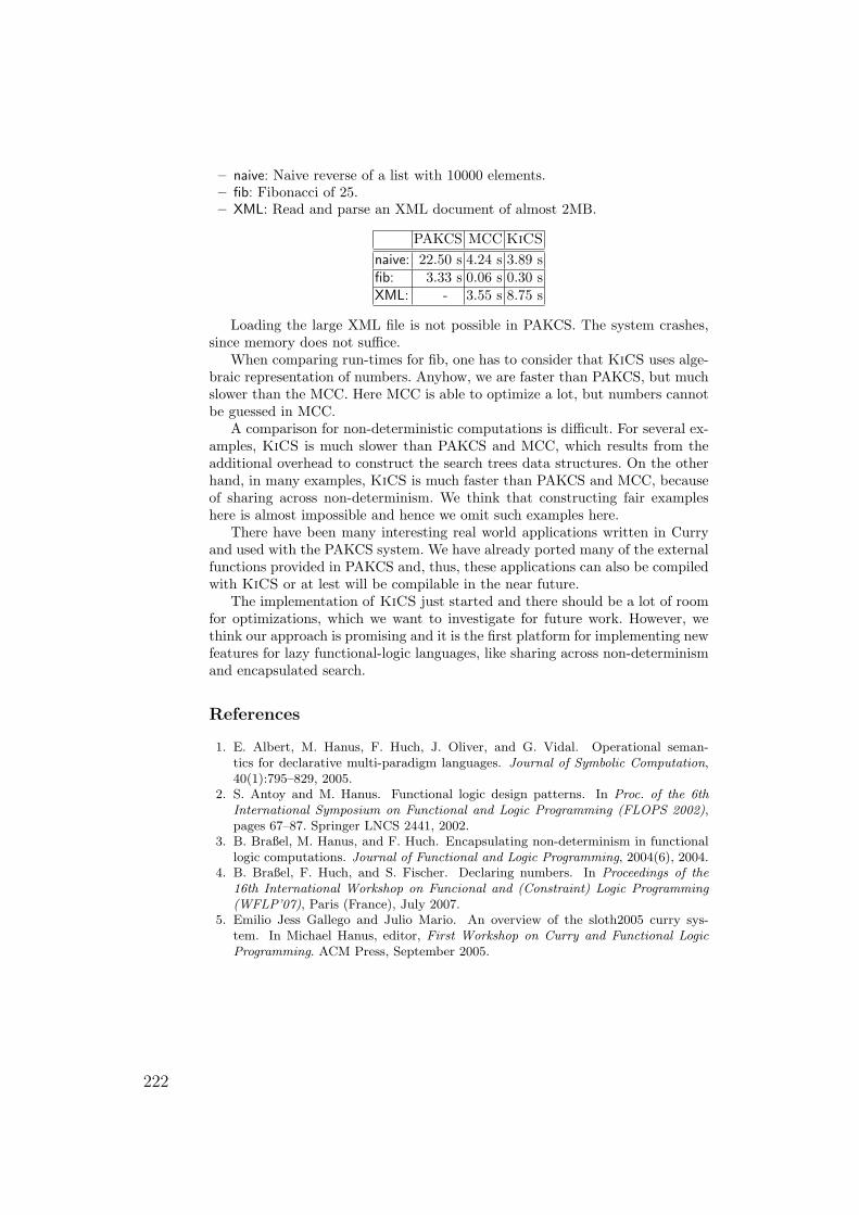
– naive: Naive reverse of a list with 10000 elements.– fib: Fibonacci of 25.– XML: Read and parse an XML document of almost 2MB.

PAKCS MCC KiCS

naive: 22.50 s 4.24 s 3.89 sfib: 3.33 s 0.06 s 0.30 sXML: - 3.55 s 8.75 s

Loading the large XML file is not possible in PAKCS. The system crashes,since memory does not suffice.

When comparing run-times for fib, one has to consider that KiCS uses alge-braic representation of numbers. Anyhow, we are faster than PAKCS, but muchslower than the MCC. Here MCC is able to optimize a lot, but numbers cannotbe guessed in MCC.

A comparison for non-deterministic computations is difficult. For several ex-amples, KiCS is much slower than PAKCS and MCC, which results from theadditional overhead to construct the search trees data structures. On the otherhand, in many examples, KiCS is much faster than PAKCS and MCC, becauseof sharing across non-determinism. We think that constructing fair exampleshere is almost impossible and hence we omit such examples here.

There have been many interesting real world applications written in Curryand used with the PAKCS system. We have already ported many of the externalfunctions provided in PAKCS and, thus, these applications can also be compiledwith KiCS or at lest will be compilable in the near future.

The implementation of KiCS just started and there should be a lot of roomfor optimizations, which we want to investigate for future work. However, wethink our approach is promising and it is the first platform for implementing newfeatures for lazy functional-logic languages, like sharing across non-determinismand encapsulated search.

References

1. E. Albert, M. Hanus, F. Huch, J. Oliver, and G. Vidal. Operational seman-tics for declarative multi-paradigm languages. Journal of Symbolic Computation,40(1):795–829, 2005.

2. S. Antoy and M. Hanus. Functional logic design patterns. In Proc. of the 6thInternational Symposium on Functional and Logic Programming (FLOPS 2002),pages 67–87. Springer LNCS 2441, 2002.

3. B. Braßel, M. Hanus, and F. Huch. Encapsulating non-determinism in functionallogic computations. Journal of Functional and Logic Programming, 2004(6), 2004.

4. B. Braßel, F. Huch, and S. Fischer. Declaring numbers. In Proceedings of the16th International Workshop on Funcional and (Constraint) Logic Programming(WFLP’07), Paris (France), July 2007.

5. Emilio Jess Gallego and Julio Mario. An overview of the sloth2005 curry sys-tem. In Michael Hanus, editor, First Workshop on Curry and Functional LogicProgramming. ACM Press, September 2005.

222

6. M. Hanus. On the completeness of residuation. In Proc. of the 1992 Joint Inter-national Conference and Symposium on Logic Programming, pages 192–206. MITPress, 1992.

7. M. Hanus. The integration of functions into logic programming: From theory topractice. Journal of Logic Programming, 19&20:583–628, 1994.

8. M. Hanus, S. Antoy, B. Braßel, M. Engelke, K. Hoppner, J. Koj, P. Niederau,R. Sadre, and F. Steiner. PAKCS: The Portland Aachen Kiel Curry System.Available at http://www.informatik.uni-kiel.de/~pakcs/, 2006.

9. M. Hanus (ed.). Curry: An integrated functional logic language (vers. 0.8.2). Avail-able at http://www.informatik.uni-kiel.de/~curry, 2006.

10. W. Lux and H. Kuchen. An efficient abstract machine for curry. In K. Beiersdorfer,G. Engels, and W. Schafer, editors, Informatik ’99 — Annual meeting of the Ger-man Computer Science Society (GI), pages 390–399. Springer, 1999.

11. S. Peyton Jones, editor. Haskell 98 Language and Libraries—The Revised Report.Cambridge University Press, 2003.

223

Narrowing for Non-Determinism with Call-TimeChoice Semantics?

F.J. Lopez-Fraguas, J. Rodrıguez-Hortala, and J. Sanchez-Hernandez

Departamento de Sistemas Informaticos y ComputacionUniversidad Complutense de Madrid, Spain

fraguas@sip.ucm.es, jrodrigu@fdi.ucm.es, jaime@sip.ucm.es

Abstract. In a recent work we have proposed let-rewriting, a simpleone-step relation close to ordinary term rewriting but able, via localbindings, to express sharing of computed values. In this way, let-rewritingreflects the call-time choice semantics for non-determinism adopted bymodern functional logic languages, where programs are rewrite systemspossibly non-confluent and non-terminating. Equivalence with CRWL, awell known semantic framework for functional logic programming, wasalso proved. In this paper we extend that work providing a notion of let-narrowing which is adequate for call-time choice as proved by a liftinglemma for let-rewriting similar to Hullot’s lifting lemma for ordinaryrewriting and narrowing.

1 Introduction

Programs in functional-logic languages (see [7] for a recent survey) are construc-tor based term rewriting systems possibly non-confluent and non-terminating,as happens in the following example:

coin→ 0 repeat(X) → X :repeat(X)coin→ 1 heads(X :Y :Y s) → (X,Y )

Here coin is a 0-ary non-deterministic function that can be evaluated to 0 or1, and repeat introduces non-termination on the system. The presence of non-determinism enforces to make a decision about call-time (also called singular)or run-time choice (or plural) semantics [10, 15]. Consider for instance the ex-pression heads(repeat(coin)):

• run-time choice gives (0, 0), (0, 1), (1, 0) and (1, 1) as possible results. Rewrit-ing can be used for it as in the following derivation:

heads(repeat(coin))→ heads(coin : coin : . . .)→(coin, coin)→ (0, coin)→ (0, 1)

• under call-time choice we obtain only the values (0, 0) and (1, 1) (coin isevaluated only once and this value must be shared).

? This work has been partially supported by the Spanish projects Merit-Forms-UCM(TIN2005-09207-C03-03) and Promesas-CAM (S-0505/TIC/0407).

224

Modern functional-logic languages like Curry [8] or Toy [12] adopt call-timechoice, as it seems more appropriate in practice. Although the classical theoryof TRS (term rewriting systems) is the basis of some influential papers in thefield, specially those related to needed narrowing [2], it cannot really serve astechnical foundation if call-time choice is taken into account, because ordinaryrewriting corresponds to run-time choice. This was a main motivation for theCRWL1 framework [5, 6], that is considered an adequate semantic foundation(see [7]) for the paradigm.

From an intuitive point of view there must be a strong connection betweenCRWL and classical rewriting, but this has not received much attention in thepast. Recently, in [11] we have started to investigate such a connection, by meansof let-rewriting, that enhances ordinary rewriting with explicit let-bindings toexpress sharing, in a similar way to what was done in [13] for the λ-calculus.A discussion of the reasons for having proposed let-rewriting instead of usingother existing formalisms like term graph-rewriting [14, 3] or specific operationalsemantics for FLP [1] can be found in [11].

In this paper we extend let-rewriting to a notion of let-narrowing. Our mainresult will be a lifting lemma for let-narrowing in the style of Hullot’s one forclassical narrowing [9].

We do not pretend that let-narrowing as will be presented here can replaceadvantageously existing versions of narrowing like needed narrowing [2] or nat-ural narrowing [4], which are well established as appropriate operational pro-cedures for functional logic programs. Let-narrowing is more a complementaryproposal: needed or natural narrowing express refined strategies with desirableoptimality properties to be preserved in practice, but they need to be patchedin implementations in order to achieve sharing (otherwise they are unsound forcall-time choice). Let-rewriting and let-narrowing intend to be the theoreticalbasis of that patch, so that sharing needs not be left anymore out of the scopeof technical works dealing with rewriting-based operational aspects of functionallogic languages. Things are then well prepared for recasting in the future theneeded or natural strategies to the framework of let-rewriting and narrowing.

The rest of the paper is organized as follows. Section 2 contains a short pre-sentation of let-rewriting. Section 3 tackles our main goal, extending let-rewritingto let-narrowing and proving its soundness and completeness. Finally, Section 4contains some conclusions and future lines of research. Omitted proofs can befound at gpd.sip.ucm.es/fraguas/papers/longWLP07.pdf.

2 Preliminaries

2.1 Constructor-based term rewrite systems

We consider a first order signature Σ = CS∪FS, where CS and FS are two dis-joint set of constructor and defined function symbols respectively, all them withassociated arity. We write CSn (FSn resp.) for the set of constructor (function)

1 CRWL stands for C onstructor-based ReW riting Logic.

225

symbols of arity n. We write c, d, . . . for constructors, f, g, . . . for functions andX,Y, . . . for variables of a numerable set V. The notation o stands for tuples ofany kind of syntactic objects.

The set Exp of expressions is defined as Exp 3 e ::= X | h(e1, . . . , en), whereX ∈ V, h ∈ CSn ∪ FSn and e1, . . . , en ∈ Exp. The set CTerm of constructedterms (or c-terms) is defined like Exp, but with h restricted to CSn (so CTerm ⊆Exp). The intended meaning is that Exp stands for evaluable expressions, i.e.,expressions that can contain function symbols, while CTerm stands for dataterms representing values. We will write e, e′, . . . for expressions and t, s, . . . forc-terms. The set of variables occurring in an expression e will be denoted asvar(e).

We will frequently use one-hole contexts, defined as Cntxt 3 C ::= [ ] |h(e1, . . . , C, . . . , en), with h ∈ CSn ∪ FSn. The application of a context Cto an expression e, written by C[e], is defined inductively as [ ][e] = e andh(e1, . . . , C, . . . , en)[e] = h(e1, . . . , C[e], . . . , en).

The set Subst of substitutions consists of mappings θ : V −→ Exp, whichextend naturally to θ : Exp −→ Exp. We write eθ for the application of θto e, and θθ′ for the composition, defined by X(θθ′) = (Xθ)θ′. The domainand range of θ are defined as dom(θ) = X ∈ V | Xθ 6= X and ran(θ) =⋃X∈dom(θ) var(Xθ). Given W ⊆ V we write by θ|W the restriction of θ to W ,

and θ|\D is a shortcut for θ|(V\D). We will sometimes write θ = σ[W ] insteadof θ|W = σ|W . In most cases we will use c-substitutions θ ∈ CSubst, verifyingthat Xθ ∈ CTerm for all X ∈ dom(θ). We say that e subsumes e′, and writee e′, if eθ = e′ for some θ; we write θ θ′ if Xθ Xθ′ for all variables X andθ θ′[W ] if Xθ Xθ′ for all X ∈W .

A constructor-based term rewriting system P (CTRS, also called programalong this paper) is a set of c-rewrite rules of the form f(t)→ e where f ∈ FSn,e ∈ Exp and t is a linear n-tuple of c-terms, where linearity means that variablesoccur only once in t. Notice that we allow e to contain extra variables, i.e.,variables not occurring in t. Given a program P, its associated rewrite relation→P is defined as: C[lθ]→P C[rθ] for any context C, rule l→ r ∈ P and θ ∈ Subst.Notice that in the definition of→P it is allowed for θ to instantiate extra variablesto any expression. We write ∗→P for the reflexive and transitive closure of therelation →P . In the following, we will usually omit the reference to P.

2.2 Rewriting with local bindings

In [11] we have proposed let-rewriting as an alternative rewriting relation forCTRS that uses let-bindings to get an explicit formulation of sharing, i.e., call-time choice semantics. Although the primary goal for this relation was to estab-lish a closer relationship between classical rewriting and the CRWL-frameworkof [6], let-rewriting is interesting in its own as a simple one-step reductionmechanism for call-time choice. This relation manipulates let-expressions, de-fined as: LExp 3 e ::= X | h(e1, . . . , en) | let X = e1 in e2, where X ∈ V,h ∈ CS ∪ FS, and e1, . . . , en ∈ LExp. The notation let X = a in e abbreviates

226

let X1 = a1 in . . . in let Xn = an in e. The notion of context is also extendedto the new syntax: C ::= [] | let X = C in e | let X = e in C | h(. . . , C, . . .).

Free and bound (or produced) variables of e ∈ LExp are defined as:

FV (X) = X; FV (h(e)) =⋃ei∈e FV (ei);

FV (let X = e1 in e2) = FV (e1) ∪ (FV (e2)\X);BV (X) = ∅; BV (h(e)) =

⋃ei∈eBV (ei);

BV (let X = e1 in e2) = BV (e1) ∪BV (e2) ∪ X

We assume a variable convention according to which the same variable symboldoes not occur free and bound within an expression. Moreover, to keep simplethe management of substitutions, we assume that whenever θ is applied to anexpression e ∈ LExp, the necessary renamings are done in e to ensure thatBV (e) ∩ (dom(θ) ∪ ran(θ)) = ∅. With all these conditions the rules definingapplication of substitutions are simple while avoiding variable capture:

Xθ = θ(X); h(e)θ = h(eθ); (let X = e1 in e2)θ = (let X = e1θ in e2θ)

The let-rewriting relation →l is shown in Figure 1. The rule (Fapp) per-forms a rewriting step in a proper sense, using a rule of the program. Note thatonly c-substitutions are allowed, to avoid copying of unevaluated expressionswhich would destroy sharing and call-time choice. (Contx) allows to select anysubexpression as a redex for the derivation. The rest of the rules are syntacticmanipulations of let-expressions. In particular (LetIn) transforms standard ex-pressions by introducing a let-binding to express sharing. On the other hand,(Bind) removes a let-construction for a variable when its binding expressionhas been evaluated. (Elim) allows to remove a binding when the variable doesnot appear in the body of the construction, which means that the correspondingvalue is not needed for evaluation. This rule is needed because the expected nor-mal forms are c-terms not containing lets. (Flat) is needed for flattening nestedlets, otherwise some reductions could become wrongly blocked or forced to di-verge (see [11]). Figure 2 contains a let-rewriting derivation for the expressionheads(repeat(coin)) using the program example of Sect. 1.

3 Let-narrowing

It is well known that in functional logic computations there are situations whererewriting is not enough, and must be lifted to some kind of narrowing, becausethe expression being reduced contains variables for which different bindingsmight produce different evaluation results. This might happen either becausevariables are already present in the initial expression to reduce, or due to thepresence of extra variables in the program rules. In the latter case let-rewritingcertainly works, but not in an effective way, since the parameter passing substi-tution ‘magically’ guesses the right values for those extra variables.

The standard definition of narrowing as a lifting of rewriting in ordinaryTRS says (adapted to the notation of contexts): C[f(t)] θ Cθ[rθ], if θ is a mgu

227

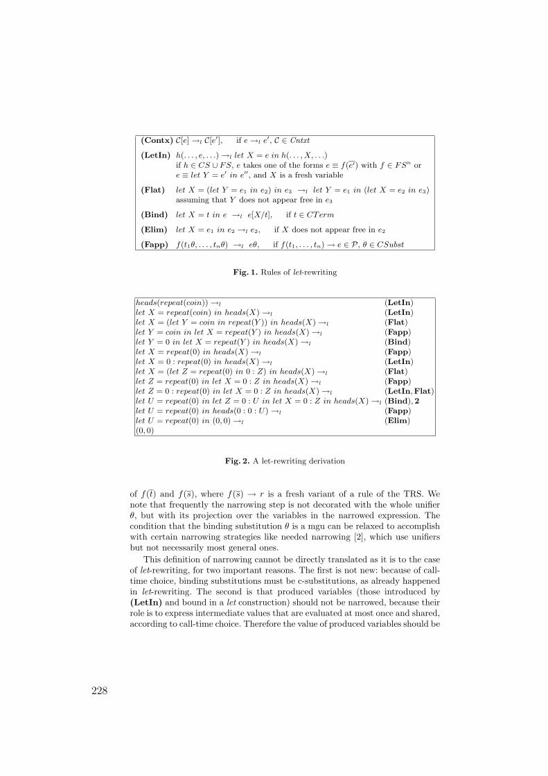
(Contx) C[e]→l C[e′], if e→l e′, C ∈ Cntxt

(LetIn) h(. . . , e, . . .)→l let X = e in h(. . . , X, . . .)if h ∈ CS ∪ FS, e takes one of the forms e ≡ f(e′) with f ∈ FSn ore ≡ let Y = e′ in e′′, and X is a fresh variable

(Flat) let X = (let Y = e1 in e2) in e3 →l let Y = e1 in (let X = e2 in e3)assuming that Y does not appear free in e3

(Bind) let X = t in e →l e[X/t], if t ∈ CTerm

(Elim) let X = e1 in e2 →l e2, if X does not appear free in e2

(Fapp) f(t1θ, . . . , tnθ) →l eθ, if f(t1, . . . , tn)→ e ∈ P, θ ∈ CSubst

Fig. 1. Rules of let-rewriting

heads(repeat(coin))→l (LetIn)let X = repeat(coin) in heads(X)→l (LetIn)let X = (let Y = coin in repeat(Y )) in heads(X)→l (Flat)let Y = coin in let X = repeat(Y ) in heads(X)→l (Fapp)let Y = 0 in let X = repeat(Y ) in heads(X)→l (Bind)let X = repeat(0) in heads(X)→l (Fapp)let X = 0 : repeat(0) in heads(X)→l (LetIn)let X = (let Z = repeat(0) in 0 : Z) in heads(X)→l (Flat)let Z = repeat(0) in let X = 0 : Z in heads(X)→l (Fapp)let Z = 0 : repeat(0) in let X = 0 : Z in heads(X)→l (LetIn,Flat)let U = repeat(0) in let Z = 0 : U in let X = 0 : Z in heads(X)→l (Bind),2let U = repeat(0) in heads(0 : 0 : U)→l (Fapp)let U = repeat(0) in (0, 0)→l (Elim)(0, 0)

Fig. 2. A let-rewriting derivation

of f(t) and f(s), where f(s) → r is a fresh variant of a rule of the TRS. Wenote that frequently the narrowing step is not decorated with the whole unifierθ, but with its projection over the variables in the narrowed expression. Thecondition that the binding substitution θ is a mgu can be relaxed to accomplishwith certain narrowing strategies like needed narrowing [2], which use unifiersbut not necessarily most general ones.

This definition of narrowing cannot be directly translated as it is to the caseof let-rewriting, for two important reasons. The first is not new: because of call-time choice, binding substitutions must be c-substitutions, as already happenedin let-rewriting. The second is that produced variables (those introduced by(LetIn) and bound in a let construction) should not be narrowed, because theirrole is to express intermediate values that are evaluated at most once and shared,according to call-time choice. Therefore the value of produced variables should be

228

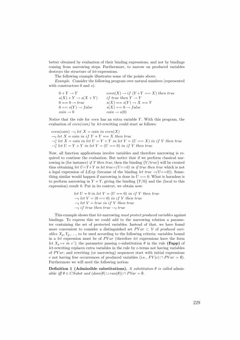
better obtained by evaluation of their binding expressions, and not by bindingscoming from narrowing steps. Furthermore, to narrow on produced variablesdestroys the structure of let-expressions.

The following example illustrates some of the points above.Example. Consider the following program over natural numbers (represented

with constructors 0 and s):

0 + Y → Y even(X)→ if (Y +Y == X) then trues(X) + Y → s(X + Y ) if true then Y → Y0 == 0→ true s(X) == s(Y )→ X == Y0 == s(Y )→ false s(X) == 0→ falsecoin→ 0 coin→ s(0)

Notice that the rule for even has an extra variable Y . With this program, theevaluation of even(coin) by let-rewriting could start as follows:

even(coin)→l let X = coin in even(X)→l let X = coin in if Y + Y == X then true→∗l let X = coin in let U = Y + Y in let V = (U == X) in if V then true→∗l let U = Y + Y in let V = (U == 0) in if V then true

Now, all function applications involve variables and therefore narrowing is re-quired to continue the evaluation. But notice that if we perform classical nar-rowing in (for instance) if V then true, then the binding V/true will be createdthus obtaining let U=Y+Y in let true=(U==0) in if true then true which is nota legal expression of LExp (because of the binding let true =(U==0)). Some-thing similar would happen if narrowing is done in U == 0. What is harmless isto perform narrowing in Y + Y, giving the binding Y/0 and the (local to thisexpression) result 0. Put in its context, we obtain now:

let U = 0 in let V = (U == 0) in if V then true→l let V = (0 == 0) in if V then true→l let V = true in if V then true→l if true then true→l true

This example shows that let-narrowing must protect produced variables againstbindings. To express this we could add to the narrowing relation a parame-ter containing the set of protected variables. Instead of that, we have foundmore convenient to consider a distinguished set PV ar ⊂ V of produced vari-ables Xp, Yp, . . ., to be used according to the following criteria: variables boundin a let expression must be of PV ar (therefore let expressions have the formlet Xp=e in e’ ); the parameter passing c-substitution θ in the rule (Fapp) oflet-rewriting replaces extra variables in the rule by c-terms not having variablesof PV ar; and rewriting (or narrowing) sequences start with initial expressionse not having free occurrences of produced variables (i.e., FV (e) ∩ PV ar = ∅).Furthermore we will need the following notion:

Definition 1 (Admissible substitutions). A substitution θ is called admis-sible iff θ ∈ CSubst and (dom(θ) ∪ ran(θ)) ∩ PVar = ∅.

229

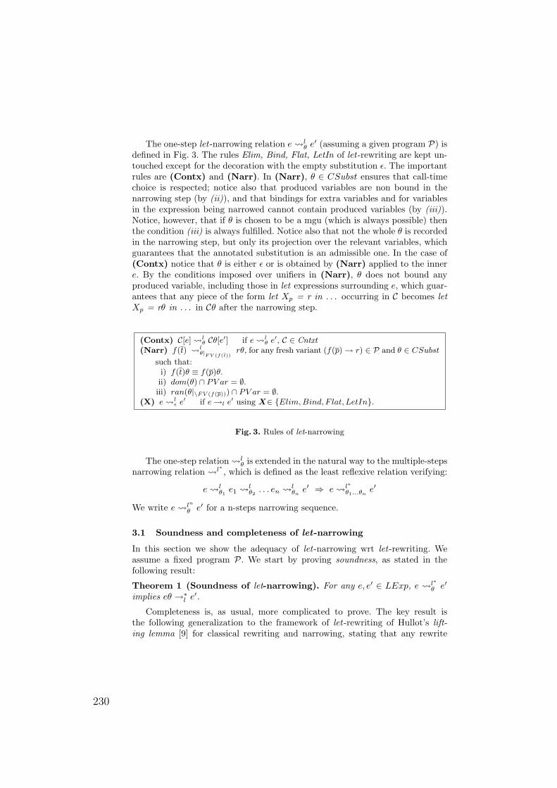
The one-step let-narrowing relation e lθ e′ (assuming a given program P) is

defined in Fig. 3. The rules Elim, Bind, Flat, LetIn of let-rewriting are kept un-touched except for the decoration with the empty substitution ε. The importantrules are (Contx) and (Narr). In (Narr), θ ∈ CSubst ensures that call-timechoice is respected; notice also that produced variables are non bound in thenarrowing step (by (ii)), and that bindings for extra variables and for variablesin the expression being narrowed cannot contain produced variables (by (iii)).Notice, however, that if θ is chosen to be a mgu (which is always possible) thenthe condition (iii) is always fulfilled. Notice also that not the whole θ is recordedin the narrowing step, but only its projection over the relevant variables, whichguarantees that the annotated substitution is an admissible one. In the case of(Contx) notice that θ is either ε or is obtained by (Narr) applied to the innere. By the conditions imposed over unifiers in (Narr), θ does not bound anyproduced variable, including those in let expressions surrounding e, which guar-antees that any piece of the form let Xp = r in . . . occurring in C becomes letXp = rθ in . . . in Cθ after the narrowing step.

(Contx) C[e] lθ Cθ[e′] if e l

θ e′, C ∈ Cntxt

(Narr) f(t) lθ|F V (f(t))

rθ, for any fresh variant (f(p)→ r) ∈ P and θ ∈ CSubstsuch that:

i) f(t)θ ≡ f(p)θ.ii) dom(θ) ∩ PV ar = ∅.

iii) ran(θ|\FV (f(p))) ∩ PV ar = ∅.(X) e l

ε e′ if e→l e

′ using X∈ Elim,Bind, F lat, LetIn.

Fig. 3. Rules of let-narrowing

The one-step relation lθ is extended in the natural way to the multiple-steps

narrowing relation l∗ , which is defined as the least reflexive relation verifying:

e lθ1 e1

lθ2 . . . en

lθne′ ⇒ e l∗

θ1...θne′

We write e ln

θ e′ for a n-steps narrowing sequence.

3.1 Soundness and completeness of let-narrowing

In this section we show the adequacy of let-narrowing wrt let-rewriting. Weassume a fixed program P. We start by proving soundness, as stated in thefollowing result:

Theorem 1 (Soundness of let-narrowing). For any e, e′ ∈ LExp, e l∗

θ e′

implies eθ →∗l e′.Completeness is, as usual, more complicated to prove. The key result is

the following generalization to the framework of let-rewriting of Hullot’s lift-ing lemma [9] for classical rewriting and narrowing, stating that any rewrite

230

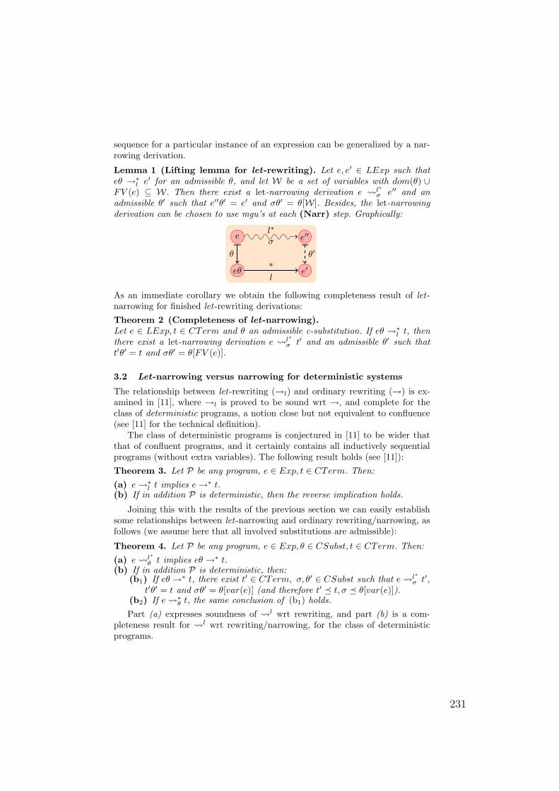
sequence for a particular instance of an expression can be generalized by a nar-rowing derivation.

Lemma 1 (Lifting lemma for let-rewriting). Let e, e′ ∈ LExp such thateθ →∗l e′ for an admissible θ, and let W be a set of variables with dom(θ) ∪FV (e) ⊆ W. Then there exist a let-narrowing derivation e l∗

σ e′′ and anadmissible θ′ such that e′′θ′ = e′ and σθ′ = θ[W]. Besides, the let-narrowingderivation can be chosen to use mgu’s at each (Narr) step. Graphically:

e e′′

eθ e′

l∗

σ

∗l

θ θ′

As an immediate corollary we obtain the following completeness result of let-narrowing for finished let-rewriting derivations:Theorem 2 (Completeness of let-narrowing).Let e ∈ LExp, t ∈ CTerm and θ an admissible c-substitution. If eθ →∗l t, thenthere exist a let-narrowing derivation e l∗

σ t′ and an admissible θ′ such thatt′θ′ = t and σθ′ = θ[FV (e)].

3.2 Let-narrowing versus narrowing for deterministic systems

The relationship between let-rewriting (→l) and ordinary rewriting (→) is ex-amined in [11], where →l is proved to be sound wrt →, and complete for theclass of deterministic programs, a notion close but not equivalent to confluence(see [11] for the technical definition).

The class of deterministic programs is conjectured in [11] to be wider thatthat of confluent programs, and it certainly contains all inductively sequentialprograms (without extra variables). The following result holds (see [11]):Theorem 3. Let P be any program, e ∈ Exp, t ∈ CTerm. Then:(a) e→∗l t implies e→∗ t.(b) If in addition P is deterministic, then the reverse implication holds.

Joining this with the results of the previous section we can easily establishsome relationships between let-narrowing and ordinary rewriting/narrowing, asfollows (we assume here that all involved substitutions are admissible):

Theorem 4. Let P be any program, e ∈ Exp, θ ∈ CSubst, t ∈ CTerm. Then:(a) e l∗

θ t implies eθ →∗ t.(b) If in addition P is deterministic, then:

(b1) If eθ →∗ t, there exist t′ ∈ CTerm, σ, θ′ ∈ CSubst such that e l∗

σ t′,t′θ′ = t and σθ′ = θ[var(e)] (and therefore t′ t, σ θ[var(e)]).

(b2) If e ∗θ t, the same conclusion of (b1) holds.Part (a) expresses soundness of l wrt rewriting, and part (b) is a com-

pleteness result for l wrt rewriting/narrowing, for the class of deterministicprograms.

231

4 Conclusions

Our aim in this work was to progress in the effort of filling an existing gap inthe functional logic programming field, where up to recently there was a lackof a simple and abstract enough one-step reduction mechanism close enoughto ordinary rewriting but at the same time respecting non-strict and call-timechoice semantics for possibly non-confluent and non-terminating constructor-based rewrite systems (possibly with extra variables), and trying to avoid thecomplexity of graph rewriting [14]. These requirements were not met by two wellestablished branches in the foundations of the field: one is the CRWL approach,very adequate from the point of view of semantics but operationally based onsomehow complicated narrowing calculi [6, 16] too far from the usual notion ofterm rewriting. The other approach focuses on operational aspects in the form ofefficient narrowing strategies like needed narrowing [2] or natural narrowing [4],based on the classical theory of rewriting, sharing with it the major drawbackthat rewriting is an unsound operation for call-time choice semantics of functionallogic programs. There have been other attempts of coping operationally withcall-time choice [1], but relying in too low-level syntax and operational rules.

In a recent work [11] we established a technical bridge between both ap-proaches (CRWL/classical rewriting) by proposing a notion of rewriting withsharing by means of local let bindings, in a similar way to what has been donefor sharing and lambda-calculus in [13]. Most importantly, we prove there strongequivalence results between CRWL and let-rewriting.

Here we continue that work by contributing a notion of let-narrowing (nar-rowing for sharing) which we prove sound and complete with respect to let-rewriting. We think that let-narrowing is the simplest proposed notion of narrow-ing that is close to the usual notions of TRS and at the same time is proved ade-quate for call-time choice semantics. The main technical insight for let-narrowinghas been the need of protecting produced (locally bound) variables against nar-rowing over them. We have also proved soundness of let-narrowing wrt ordinaryrewriting and completeness for the wide class of deterministic programs, thusgiving a technical support to the intuitive fact that combining sharing with nar-rowing does not create new answers when compared to classical narrowing, andat the same time does not lose answers in case of deterministic systems. As faras we know these results are new in the narrowing literature.

The natural extension of our work will be to add strategies to let-rewritingand let-narrowing, an issue that has been left out of this paper but is needed asfoundation of effective implementations. But we think that the clear script wehave followed so far (first presenting a notion of rewriting with respect to whichwe have been able to prove correctness and completeness of a a subsequent notionof narrowing, to which add strategies in future work) is an advantage rather thana lack of our approach.

232

References

1. E. Albert, M. Hanus, F. Huch, J. Oliver, and G. Vidal. Operational seman-tics for declarative multi-paradigm languages. Journal of Symbolic Computation,40(1):795–829, 2005.

2. S. Antoy, R. Echahed, and M. Hanus. A needed narrowing strategy. In Proc. ACMSymposium on Principles of Programming Languages (POPL’94), pages 268–279.ACM Press, 1994.

3. R. Echahed and J.-C. Janodet. Admissible graph rewriting and narrowing. InProceedings of the Joint International Conference and Symposium on Logic Pro-gramming, pages 325 – 340, Manchester, June 1998. MIT Press.

4. S. Escobar, J. Meseguer, and P. Thati. Natural narrowing for general term rewritingsystems. In RTA, pages 279–293, 2005.

5. J. C. Gonzalez-Moreno, T. Hortala-Gonzalez, F. Lopez-Fraguas, and M. Rodrıguez-Artalejo. A rewriting logic for declarative programming. In Proc. European Sym-posium on Programming (ESOP’96), pages 156–172. Springer LNCS 1058, 1996.

6. J. C. Gonzalez-Moreno, T. Hortala-Gonzalez, F. Lopez-Fraguas, and M. Rodrıguez-Artalejo. An approach to declarative programming based on a rewriting logic.Journal of Logic Programming, 40(1):47–87, 1999.

7. M. Hanus. Functional logic programming: From theory to Curry. Technical report,Christian-Albrechts-Universitat Kiel, 2005.

8. M. Hanus (ed.). Curry: An integrated functional logic language (version 0.8.2).Available at http://www.informatik.uni-kiel.de/~curry/report.html, March 2006.

9. J. Hullot. Canonical forms and unification. In Proc. 5th Conference on AutomatedDeduction, pages 318–334. Springer LNCS 87, 1980.

10. H. Hussmann. Non-Determinism in Algebraic Specifications and Algebraic Pro-grams. Birkhauser Verlag, 1993.

11. F. Lopez-Fraguas, J. Rodrıguez-Hortala, and J. Sanchez-Hernandez. A simplerewrite notion for call-time choice semantics. In Proc. Principles and Practice ofDeclarative Programming, ACM Press, pages 197–208, 2007.

12. F. Lopez-Fraguas and J. Sanchez-Hernandez. T OY: A multiparadigm declarativesystem. In Proc. Rewriting Techniques and Applications (RTA’99), pages 244–247.Springer LNCS 1631, 1999.

13. J. Maraist, M. Odersky, and P. Wadler. The call-by-need lambda calculus. J.Funct. Program., 8(3):275–317, 1998.

14. D. Plump. Essentials of term graph rewriting. Electr. Notes Theor. Comput. Sci.,51, 2001.

15. H. Søndergaard and P. Sestoft. Non-determinism in functional languages. TheComputer Journal, 35(5):514–523, 1992.

16. R. d. Vado-Vırseda. A demand-driven narrowing calculus with overlapping def-initional trees. In Proc. ACM SIGPLAN Conf. on Principles and Practice ofDeclarative Programming (PPDP’03), pages 213–227. ACM Press, 2003.

233

Java type unification with wildcards

Martin Plumicke

University of Cooperative Education Stuttgart/HorbFlorianstraße 15, D–72160 Horb

m.pluemicke@ba-horb.de

Abstract. With the introduction of Java 5.0 the type system has beenextended by parameterized types, type variables, type terms, and wild-cards. As a result very complex types can arise. The term

Vector<? extends Vector<AbstractList<Integer>>>

is for example a correct type in Java 5.0.In this paper we present a type unification algorithm for Java 5.0 typeterms. The algorithm unifies type terms, which are in subtype relation-ship. For this we define Java 5.0 type terms and its subtyping relation,formally.As Java 5.0 allows wildcards as instances of generic types, the subtypingordering contains infinite chains. We show that the type unification isstill finitary. We give a type unification algorithm, which calculates thefinite set of general unifiers.

1 Introduction

With the introduction of Java 5.0 [1] the type system has been extended byparameterized types, type variables, type terms, and wildcards. As a result verycomplex types can arise. For example the term

Vector<? extends Vector<AbstractList<Integer>>>is a correct type in Java 5.0.Considering all that, it is often rather difficult for a programmer to recognizewhether such a complex type is the correct one for a given method or not.This has caused us to develop a Java 5.0 type inference system which assiststhe programmer by calculating types automatically. This type inference systemallows us, to declare method parameters and local variables without type anno-tations. The type inference algorithm calculates the appropriate and principaltypes.Following the ideas of [2], we reduce the Java 5.0 type inference problem to aJava 5.0 type unification problem. The Java 5.0 type unification problem is givenas: For two type terms θ1, θ2 a substitution is demanded, such that

σ( θ1 )≤∗ σ( θ2 ), where ≤∗ is the Java 5.0 subtyping relation.The type system of Java 5.0 is very similar to the type system of polymorphicallyorder-sorted types, which is considered for the logical languages [3–6] and for thefunctional object–oriented language OBJ–P [7]. But in all approaches the typeunification problem was not solved completely.

234

In [8] we have done a first step solving the type unification problem. We restrictedthe set of type terms, by disallowing wildcards, and presented a type unificationalgorithm for this approach. This algorithm led to the Java 5.0 type inferencesystem presented in [9].In this paper we extend our algorithm to type terms with wildcards. This meansthat we solve the original type unification problem and give a complete typeunification algorithm. We will show, that the type unification problem is notstill unitary, but finitary.The paper is organized as follows. In the second section we formally describethe Java 5.0 type system including its inheritance hierarchy. In the third sectionwe give an overview of the type unification problem. Then, we present the typeunification algorithm and give an example. Finally, we close with a summaryand an outlook.

2 Subtyping in Java 5.0

The Java 5.0 types are given as type terms over a type signature TS of class/interfacenames and a set of bounded type variables BTV . While the type signature de-scribes the arities of the the class/interface names, a bound of a type variablerestricts the allowed instantiated types to subtypes of the bound. For a typevariable a bounded by the type ty we will write a|ty.

Example 1. Let the following Java 5.0 program be given:

class A<a> implements I<a> ...class B<a> extends A<a> ...class C<a extends I<b>,b> ...interface I<a> ...interface J<a> ...class D<a extends B<a> & J<b>, b> ...

Then, the corresponding type signature TS is given as: TS(a|Object) = A, B, I, J ,TS(a|I<b> b|Object) = C , and TS(a|B<a>&J<b> b|Object) = D .As A, I ∈ TS(a|Object) and Integer is a subtype of Object, the terms A<Integer>and I<Integer> are Java 5.0 types. As I<Integer> is a subtype of itself andA<Integer> is also a subtype of I<Integer>, the terms C<I<Integer>, Integer>and C<A<Integer>, Integer> are also type terms. But as J<Integer> is nosubtype of I<Integer> the term C<J<Integer>, Integer> is no Java 5.0 type.

For the definition of the inheritance hierarchy, the concept of Java 5.0 simpletypes and the concept of capture conversion is needed. For the definition ofJava 5.0 simple types we refer to [1], Section 4.5, where Java 5.0 parameterizedtypes are defined. We call them, in this paper, Java 5.0 simple types in contrast tothe function types of methods. Java 5.0 simple types consists of the Java 5.0 typesas in Example 1 presented and wildcard types like Vector<? extends Integer>.For the definition of the capture conversion we refer to [1] §5.1.10. The capture

235

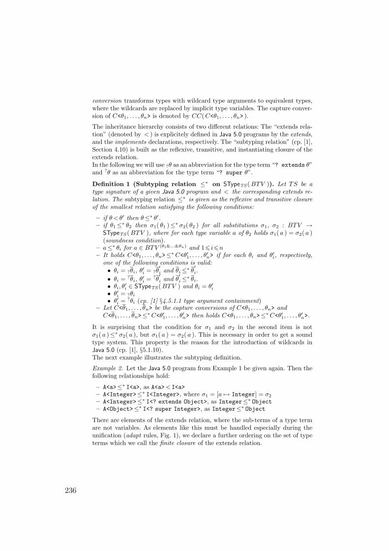
conversion transforms types with wildcard type arguments to equivalent types,where the wildcards are replaced by implicit type variables. The capture conver-sion of C<θ1, . . . , θn> is denoted by CC( C<θ1, . . . , θn> ).

The inheritance hierarchy consists of two different relations: The “extends rela-tion” (denoted by < ) is explicitely defined in Java 5.0 programs by the extends,and the implements declarations, respectively. The “subtyping relation” (cp. [1],Section 4.10) is built as the reflexive, transitive, and instantiating closure of theextends relation.In the following we will use ?θ as an abbreviation for the type term “? extends θ”and ?θ as an abbreviation for the type term “? super θ”.

Definition 1 (Subtyping relation ≤∗ on STypeTS ( BTV )). Let TS be atype signature of a given Java 5.0 program and < the corresponding extends re-lation. The subtyping relation ≤∗ is given as the reflexive and transitive closureof the smallest relation satisfying the following conditions:

– if θ < θ′ then θ≤∗ θ′.– if θ1≤∗ θ2 then σ1( θ1 )≤∗ σ2( θ2 ) for all substitutions σ1, σ2 : BTV →

STypeTS ( BTV ), where for each type variable a of θ2 holds σ1( a ) = σ2( a )(soundness condition).

– a≤∗ θi for a ∈ BTV (θ1&...&θn) and 16 i6n– It holds C<θ1, . . . , θn>≤∗ C<θ′1, . . . , θ

′n> if for each θi and θ′i, respectively,

one of the following conditions is valid:• θi = ?θi, θ′i = ?θ

′i and θi ≤∗ θ

′i.

• θi = ?θi, θ′i = ?θ′i and θ

′i ≤∗ θi.

• θi, θ′i ∈ STypeTS ( BTV ) and θi = θ′i

• θ′i = ?θi

• θ′i = ?θi (cp. [1] §4.5.1.1 type argument containment)– Let C<θ1, . . . , θn> be the capture conversions of C<θ1, . . . , θn> and

C<θ1, . . . , θn>≤∗ C<θ′1, . . . , θ′n> then holds C<θ1, . . . , θn>≤∗ C<θ′1, . . . , θ

′n>.

It is surprising that the condition for σ1 and σ2 in the second item is notσ1( a )≤∗ σ2( a ), but σ1( a ) = σ2( a ). This is necessary in order to get a soundtype system. This property is the reason for the introduction of wildcards inJava 5.0 (cp. [1], §5.1.10).The next example illustrates the subtyping definition.

Example 2. Let the Java 5.0 program from Example 1 be given again. Then thefollowing relationships hold:

– A<a>≤∗ I<a>, as A<a>< I<a>– A<Integer>≤∗ I<Integer>, where σ1 = [a 7→ Integer] = σ2

– A<Integer>≤∗ I<? extends Object>, as Integer≤∗ Object– A<Object>≤∗ I<? super Integer>, as Integer≤∗ Object

There are elements of the extends relation, where the sub-terms of a type termare not variables. As elements like this must be handled especially during theunification (adapt rules, Fig. 1), we declare a further ordering on the set of typeterms which we call the finite closure of the extends relation.

236

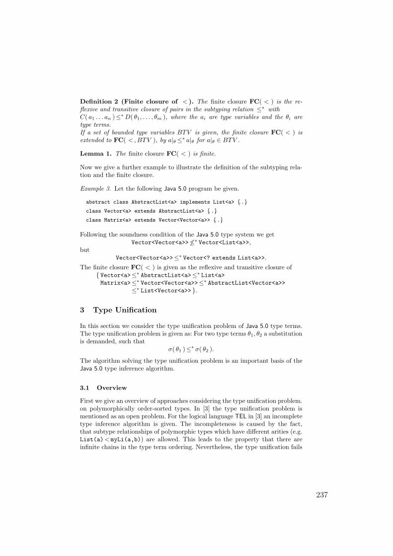
Definition 2 (Finite closure of < ). The finite closure FC( < ) is the re-flexive and transitive closure of pairs in the subtyping relation ≤∗ withC( a1 . . . an )≤∗ D( θ1, . . . , θm ), where the ai are type variables and the θi aretype terms.If a set of bounded type variables BTV is given, the finite closure FC( < ) isextended to FC( < , BTV ), by a|θ ≤∗ a|θ for a|θ ∈ BTV .

Lemma 1. The finite closure FC( < ) is finite.

Now we give a further example to illustrate the definition of the subtyping rela-tion and the finite closure.

Example 3. Let the following Java 5.0 program be given.

abstract class AbstractList<a> implements List<a> ...class Vector<a> extends AbstractList<a> ...class Matrix<a> extends Vector<Vector<a>> ...

Following the soundness condition of the Java 5.0 type system we getVector<Vector<a>> 6≤∗ Vector<List<a>>,

butVector<Vector<a>>≤∗ Vector<? extends List<a>>.

The finite closure FC( < ) is given as the reflexive and transitive closure of Vector<a>≤∗ AbstractList<a>≤∗ List<a>Matrix<a>≤∗ Vector<Vector<a>>≤∗ AbstractList<Vector<a>>

≤∗ List<Vector<a>> .

3 Type Unification

In this section we consider the type unification problem of Java 5.0 type terms.The type unification problem is given as: For two type terms θ1, θ2 a substitutionis demanded, such that

σ( θ1 )≤∗ σ( θ2 ).

The algorithm solving the type unification problem is an important basis of theJava 5.0 type inference algorithm.

3.1 Overview

First we give an overview of approaches considering the type unification problem.on polymorphically order-sorted types. In [3] the type unification problem ismentioned as an open problem. For the logical language TEL in [3] an incompletetype inference algorithm is given. The incompleteness is caused by the fact,that subtype relationships of polymorphic types which have different arities (e.g.List(a)< myLi(a,b)) are allowed. This leads to the property that there areinfinite chains in the type term ordering. Nevertheless, the type unification fails

237

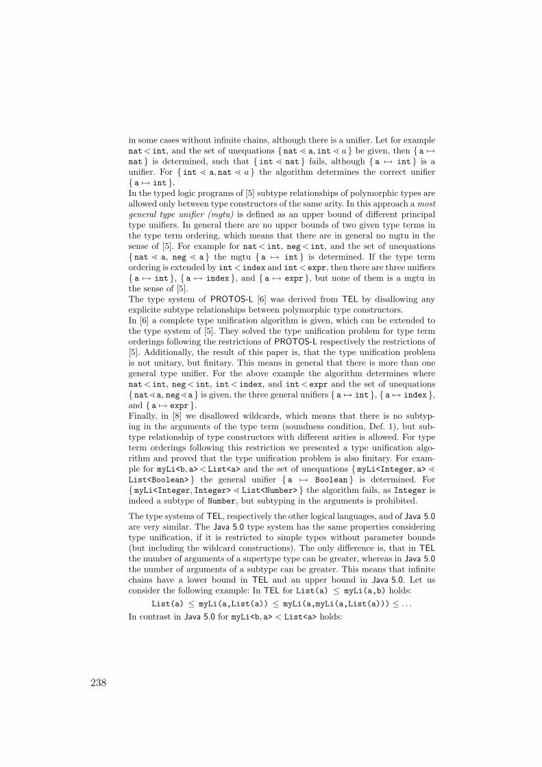
in some cases without infinite chains, although there is a unifier. Let for examplenat< int, and the set of unequations nat l a, int l a be given, then a 7→nat is determined, such that int l nat fails, although a 7→ int is aunifier. For int l a, nat l a the algorithm determines the correct unifier a 7→ int .In the typed logic programs of [5] subtype relationships of polymorphic types areallowed only between type constructors of the same arity. In this approach a mostgeneral type unifier (mgtu) is defined as an upper bound of different principaltype unifiers. In general there are no upper bounds of two given type terms inthe type term ordering, which means that there are in general no mgtu in thesense of [5]. For example for nat< int, neg< int, and the set of unequations nat l a, neg l a the mgtu a 7→ int is determined. If the type termordering is extended by int< index and int< expr, then there are three unifiers a 7→ int , a 7→ index , and a 7→ expr , but none of them is a mgtu inthe sense of [5].The type system of PROTOS-L [6] was derived from TEL by disallowing anyexplicite subtype relationships between polymorphic type constructors.In [6] a complete type unification algorithm is given, which can be extended tothe type system of [5]. They solved the type unification problem for type termorderings following the restrictions of PROTOS-L respectively the restrictions of[5]. Additionally, the result of this paper is, that the type unification problemis not unitary, but finitary. This means in general that there is more than onegeneral type unifier. For the above example the algorithm determines wherenat< int, neg< int, int< index, and int< expr and the set of unequations natla, negla is given, the three general unifiers a 7→ int , a 7→ index ,and a 7→ expr .Finally, in [8] we disallowed wildcards, which means that there is no subtyp-ing in the arguments of the type term (soundness condition, Def. 1), but sub-type relationship of type constructors with different arities is allowed. For typeterm orderings following this restriction we presented a type unification algo-rithm and proved that the type unification problem is also finitary. For exam-ple for myLi<b, a>< List<a> and the set of unequations myLi<Integer, a> lList<Boolean> the general unifier a 7→ Boolean is determined. For myLi<Integer, Integer> l List<Number> the algorithm fails, as Integer isindeed a subtype of Number, but subtyping in the arguments is prohibited.

The type systems of TEL, respectively the other logical languages, and of Java 5.0are very similar. The Java 5.0 type system has the same properties consideringtype unification, if it is restricted to simple types without parameter bounds(but including the wildcard constructions). The only difference is, that in TELthe number of arguments of a supertype type can be greater, whereas in Java 5.0the number of arguments of a subtype can be greater. This means that infinitechains have a lower bound in TEL and an upper bound in Java 5.0. Let usconsider the following example: In TEL for List(a) ≤ myLi(a,b) holds:

List(a) ≤ myLi(a,List(a)) ≤ myLi(a,myLi(a,List(a))) ≤ . . .

In contrast in Java 5.0 for myLi<b, a> < List<a> holds:

238

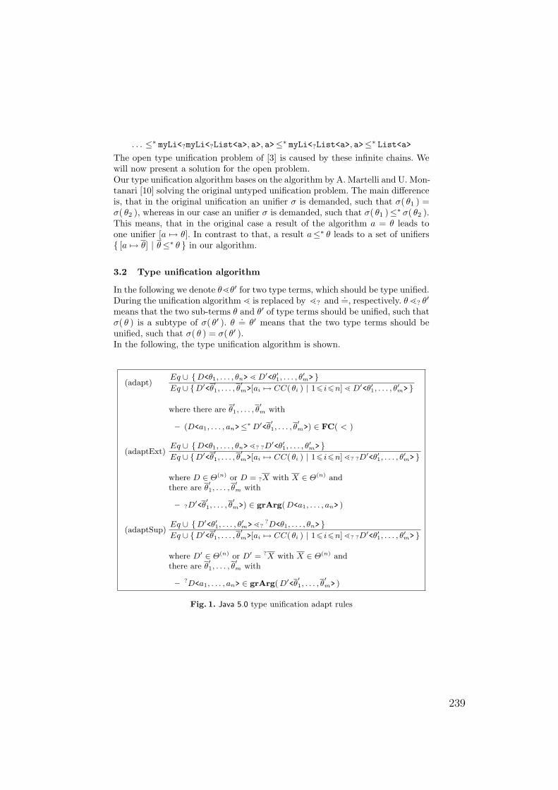
. . . ≤∗ myLi<?myLi<?List<a>, a>, a>≤∗ myLi<?List<a>, a>≤∗ List<a>

The open type unification problem of [3] is caused by these infinite chains. Wewill now present a solution for the open problem.Our type unification algorithm bases on the algorithm by A. Martelli and U. Mon-tanari [10] solving the original untyped unification problem. The main differenceis, that in the original unification an unifier σ is demanded, such that σ( θ1 ) =σ( θ2 ), whereas in our case an unifier σ is demanded, such that σ( θ1 )≤∗ σ( θ2 ).This means, that in the original case a result of the algorithm a = θ leads toone unifier [a 7→ θ]. In contrast to that, a result a≤∗ θ leads to a set of unifiers [a 7→ θ] | θ≤∗ θ in our algorithm.

3.2 Type unification algorithm

In the following we denote θlθ′ for two type terms, which should be type unified.During the unification algorithm l is replaced by l? and .=, respectively. θ l? θ′

means that the two sub-terms θ and θ′ of type terms should be unified, such thatσ( θ ) is a subtype of σ( θ′ ). θ

.= θ′ means that the two type terms should beunified, such that σ( θ ) = σ( θ′ ).In the following, the type unification algorithm is shown.

(adapt)Eq ∪ D<θ1, . . . , θn> l D′<θ′

1, . . . , θ′m>

Eq ∪ D′<θ′1, . . . , θ

′m>[ai 7→ CC( θi ) | 16 i6n] l D′<θ′

1, . . . , θ′m>

where there are θ′1, . . . , θ

′m with

– (D<a1, . . . , an>≤∗ D′<θ′1, . . . , θ

′m>) ∈ FC( < )

(adaptExt)Eq ∪ D<θ1, . . . , θn>l? ?D

′<θ′1, . . . , θ

′m>

Eq ∪ D′<θ′1, . . . , θ

′m>[ai 7→ CC( θi ) | 16 i6n] l? ?D

′<θ′1, . . . , θ

′m>

where D ∈ Θ(n) or D = ?X with X ∈ Θ(n) andthere are θ

′1, . . . , θ

′m with

– ?D′<θ

′1, . . . , θ

′m>) ∈ grArg( D<a1, . . . , an> )

(adaptSup)Eq ∪ D′<θ′

1, . . . , θ′m>l?

?D<θ1, . . . , θn> Eq ∪ D′<θ

′1, . . . , θ

′m>[ai 7→ CC( θi ) | 16 i6n] l? ?D

′<θ′1, . . . , θ

′m>

where D′ ∈ Θ(n) or D′ = ?X with X ∈ Θ(n) andthere are θ

′1, . . . , θ

′m with

– ?D<a1, . . . , an> ∈ grArg( D′<θ′1, . . . , θ

′m> )

Fig. 1. Java 5.0 type unification adapt rules

239

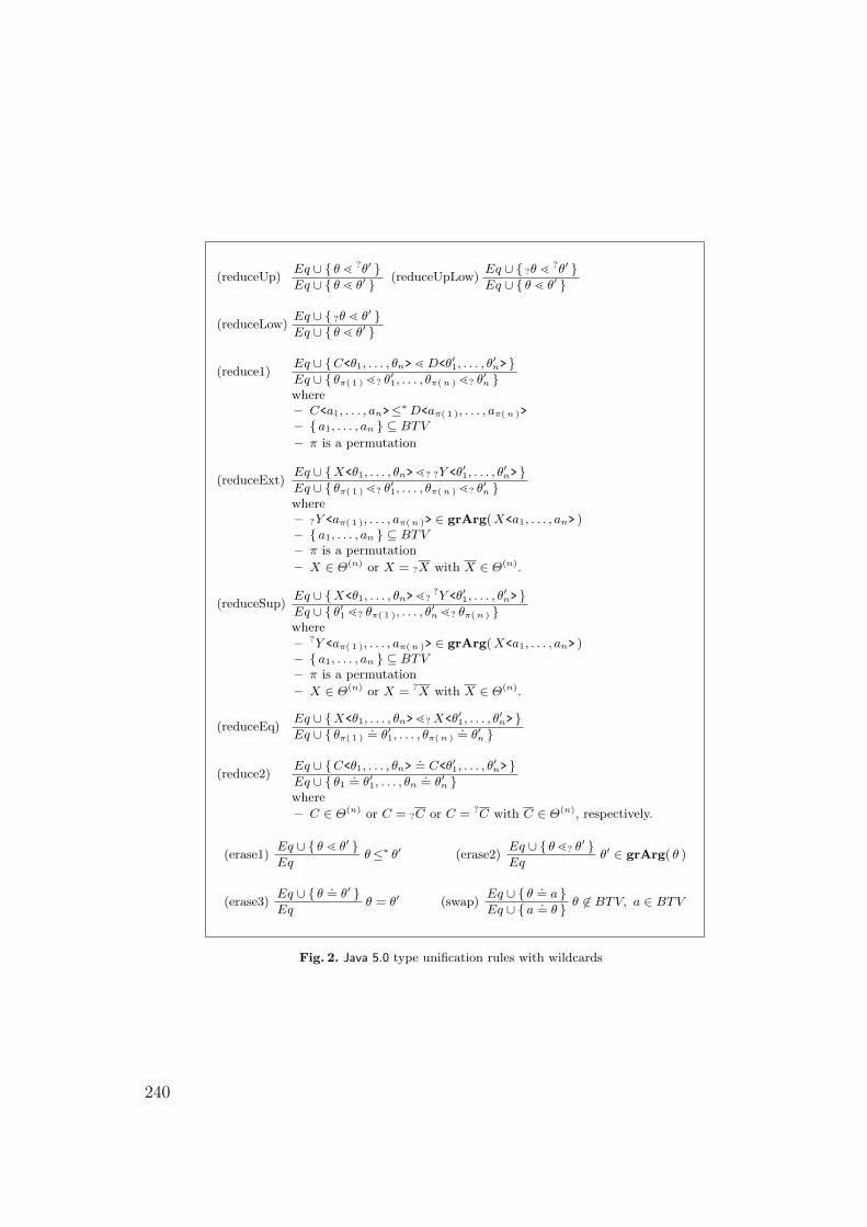
(reduceUp)Eq ∪ θ l ?θ′ Eq ∪ θ l θ′ (reduceUpLow)

Eq ∪ ?θ l ?θ′ Eq ∪ θ l θ′

(reduceLow)Eq ∪ ?θ l θ′ Eq ∪ θ l θ′

(reduce1)Eq ∪ C<θ1, . . . , θn> l D<θ′

1, . . . , θ′n>

Eq ∪ θπ( 1 ) l? θ′1, . . . , θπ( n ) l? θ′

n where– C<a1, . . . , an>≤∗ D<aπ( 1 ), . . . , aπ( n )>

– a1, . . . , an ⊆ BTV

– π is a permutation

(reduceExt)Eq ∪ X<θ1, . . . , θn>l? ?Y <θ′

1, . . . , θ′n>

Eq ∪ θπ( 1 ) l? θ′1, . . . , θπ( n ) l? θ′

n where– ?Y <aπ( 1 ), . . . , aπ( n )> ∈ grArg( X<a1, . . . , an> )– a1, . . . , an ⊆ BTV– π is a permutation

– X ∈ Θ(n) or X = ?X with X ∈ Θ(n).

(reduceSup)Eq ∪ X<θ1, . . . , θn>l?

?Y <θ′1, . . . , θ

′n>

Eq ∪ θ′1 l? θπ( 1 ), . . . , θ

′n l? θπ( n )

where

– ?Y <aπ( 1 ), . . . , aπ( n )> ∈ grArg( X<a1, . . . , an> )– a1, . . . , an ⊆ BTV– π is a permutation

– X ∈ Θ(n) or X = ?X with X ∈ Θ(n).

(reduceEq)Eq ∪ X<θ1, . . . , θn>l? X<θ′

1, . . . , θ′n>

Eq ∪ θπ( 1 ).= θ′

1, . . . , θπ( n ).= θ′

n

(reduce2)Eq ∪ C<θ1, . . . , θn>

.= C<θ′

1, . . . , θ′n>

Eq ∪ θ1.= θ′

1, . . . , θn.= θ′

n where

– C ∈ Θ(n) or C = ?C or C = ?C with C ∈ Θ(n), respectively.

(erase1)Eq ∪ θ l θ′ Eq

θ≤∗ θ′ (erase2)Eq ∪ θ l? θ′ Eq

θ′ ∈ grArg( θ )

(erase3)Eq ∪ θ

.= θ′

Eqθ = θ′ (swap)

Eq ∪ θ.= a

Eq ∪ a.= θ θ 6∈ BTV, a ∈ BTV

Fig. 2. Java 5.0 type unification rules with wildcards

240

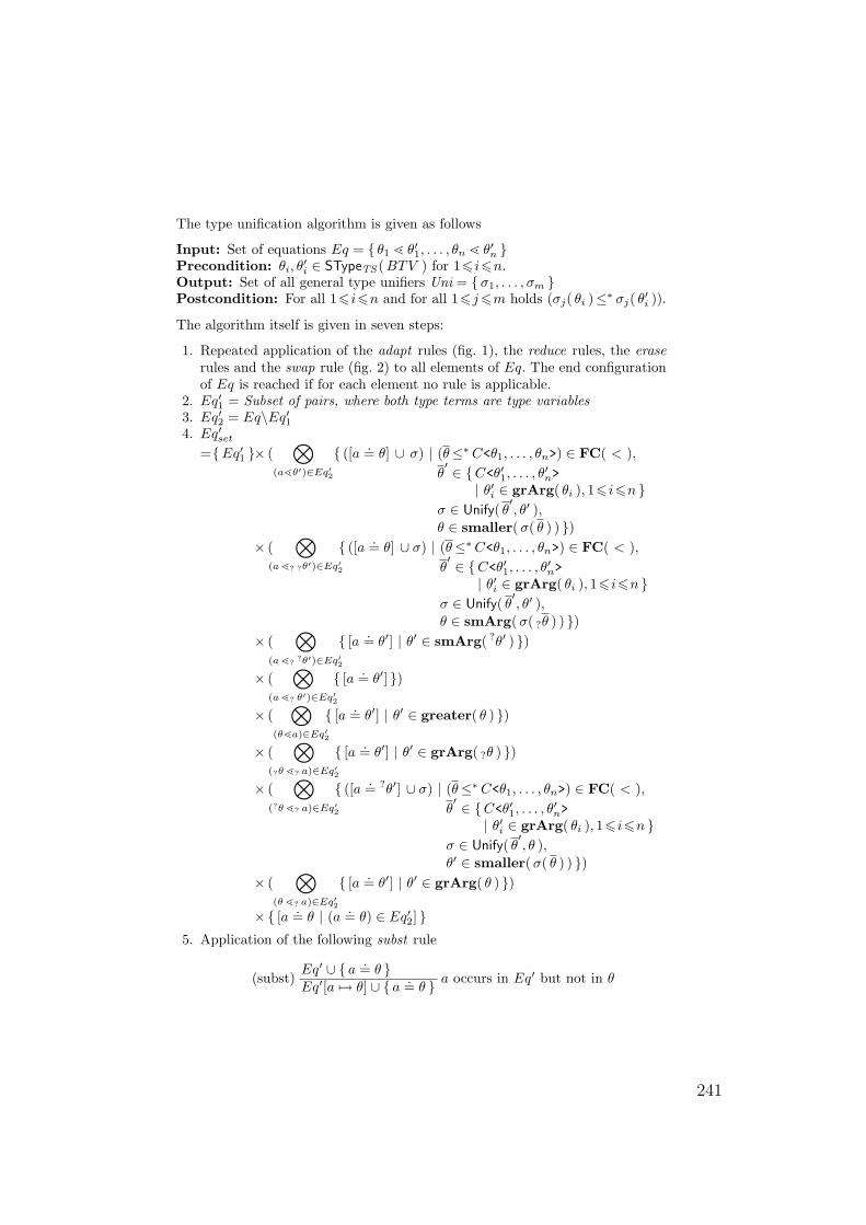
The type unification algorithm is given as follows

Input: Set of equations Eq = θ1 l θ′1, . . . , θn l θ′n Precondition: θi, θ

′i ∈ STypeTS ( BTV ) for 16 i6n.

Output: Set of all general type unifiers Uni = σ1, . . . , σm Postcondition: For all 16 i6n and for all 16j 6m holds (σj( θi )≤∗ σj( θ′i )).

The algorithm itself is given in seven steps:

1. Repeated application of the adapt rules (fig. 1), the reduce rules, the eraserules and the swap rule (fig. 2) to all elements of Eq. The end configurationof Eq is reached if for each element no rule is applicable.

2. Eq′1 = Subset of pairs, where both type terms are type variables3. Eq′2 = Eq\Eq′14. Eq′set

=Eq′1 × (⊗

(alθ′)∈Eq′2

([a .= θ] ∪ σ) | (θ≤∗ C<θ1, . . . , θn>) ∈ FC( < ),θ′ ∈ C<θ′1, . . . , θ

′n>

| θ′i ∈ grArg( θi ), 16 i6n σ ∈ Unify( θ

′, θ′ ),

θ ∈ smaller( σ( θ ) ) )× (

⊗(a l? ?θ′)∈Eq′

2

([a .= θ] ∪ σ) | (θ≤∗ C<θ1, . . . , θn>) ∈ FC( < ),θ′ ∈ C<θ′1, . . . , θ

′n>

| θ′i ∈ grArg( θi ), 16 i6n σ ∈ Unify( θ

′, θ′ ),

θ ∈ smArg( σ( ?θ ) ) )× (

⊗(a l?

?θ′)∈Eq′2

[a .= θ′] | θ′ ∈ smArg( ?θ′ ) )

× (⊗

(a l? θ′)∈Eq′2

[a .= θ′] )

× (⊗

(θla)∈Eq′2

[a .= θ′] | θ′ ∈ greater( θ ) )

× (⊗

(?θ l? a)∈Eq′2

[a .= θ′] | θ′ ∈ grArg( ?θ ) )

× (⊗

(?θ l? a)∈Eq′2

([a .= ?θ′] ∪ σ) | (θ≤∗ C<θ1, . . . , θn>) ∈ FC( < ),θ′ ∈ C<θ′1, . . . , θ

′n>

| θ′i ∈ grArg( θi ), 16 i6n σ ∈ Unify( θ

′, θ ),

θ′ ∈ smaller( σ( θ ) ) )× (

⊗(θ l? a)∈Eq′

2

[a .= θ′] | θ′ ∈ grArg( θ ) )

× [a .= θ | (a .= θ) ∈ Eq′2] 5. Application of the following subst rule

(subst)Eq′ ∪ a

.= θ Eq′[a 7→ θ] ∪ a

.= θ a occurs in Eq′ but not in θ

241

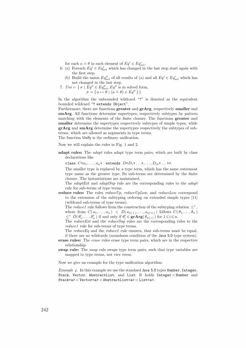
for each a.= θ in each element of Eq′ ∈ Eq′set.

6. (a) Foreach Eq′ ∈ Eq′set which has changed in the last step start again withthe first step.

(b) Build the union Eq′′set of all results of (a) and all Eq′ ∈ Eq′set which hasnot changed in the last step.

7. Uni = σ | Eq′′ ∈ Eq′′set, Eq′′ is in solved form,σ = a 7→ θ | (a .= θ) ∈ Eq′′

In the algorithm the unbounded wildcard “?” is denoted as the equivalentbounded wildcard “? extends Object”.Furthermore, there are functions greater and grArg, respectively smaller andsmArg. All functions determine supertypes, respectively subtypes by patternmatching with the elements of the finite closure. The functions greater andsmaller determine the supertypes respectively subtypes of simple types, whilegrArg and smArg determine the supertypes respectively the subtypes of sub-terms, which are allowed as arguments in type terms.The function Unify is the ordinary unification.

Now we will explain the rules in Fig. 1 and 2.

adapt rules: The adapt rules adapt type term pairs, which are built by classdeclarations likeclass C<a1, . . . , an> extends D<D1< . . . >, . . . , Dm< . . . >>.

The smaller type is replaced by a type term, which has the same outermosttype name as the greater type. Its sub-terms are determined by the finiteclosure. The instantiations are maintained.The adaptExt and adaptSup rule are the corresponding rules to the adaptrule for sub-terms of type terms.

reduce rules: The rules reduceUp, reduceUpLow, and reduceLow correspondto the extension of the subtyping ordering on extended simple types [11](wildcard sub-terms of type terms).The reduce1 rule follows from the construction of the subtyping relation ≤∗ ,where from C( a1, . . . , an ) < D( aπ( 1 ), . . . , aπ( n ) ) follows C( θ1, . . . , θn )≤∗ D( θ′1, . . . , θ

′n ) if and only if θ′i ∈ grArg( θπ( i ) ) for 16 i6n.

The reduceExt and the reduceSup rules are the corresponding rules to thereduce1 rule for sub-terms of type terms.The reduceEq and the reduce2 rule ensures, that sub-terms must be equal,if there are no wildcards (soundness condition of the Java 5.0 type system).

erase rules: The erase rules erase type term pairs, which are in the respectiverelationship.

swap rule: The swap rule swaps type term pairs, such that type variables aremapped to type terms, not vice versa.

Now we give an example for the type unification algorithm.

Example 4. In this example we use the standard Java 5.0 types Number, Integer,Stack, Vector, AbstractList, and List. It holds Integer< Number andStack<a>< Vector<a>< AbstractList<a>< List<a>.

242

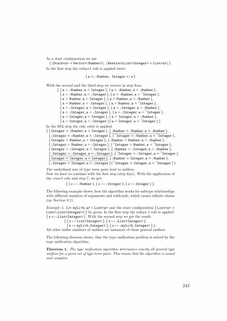
As a start configuration we use (Stack<a> l Vector<?Number>), (AbstractList<Integer> l List<a>) .

In the first step the reduce1 rule is applied twice:

al? ?Number, Integerl? a

With the second and the third step we receive in step four: a .= ?Number, a

.= Integer , a .= ?Number, a.= ?Number ,

a .= ?Number, a.= ?Integer , a

.= ?Number, a.= ?Integer ,

a .= Number, a.= Integer , a .= Number, a

.= ?Number , a .= Number, a

.= ?Integer , a.= Number, a

.= ?Integer , a .= ?Integer, a

.= Integer , a .= ?Integer, a.= ?Number ,

a .= ?Integer, a.= ?Integer , a

.= ?Integer, a.= ?Integer ,

a .= Integer, a.= Integer , a .= Integer, a

.= ?Number , a .= Integer, a

.= ?Integer a.= Integer, a

.= ?Integer In the fifth step the rule subst is applied: Integer .= ?Number, a

.= Integer , ?Number.= ?Number, a

.= ?Number , ?Integer

.= ?Number, a.= ?Integer , ?Integer

.= ?Number, a.= ?Integer ,

Integer .= Number, a.= Integer , ?Number

.= Number, a.= ?Number ,

?Integer.= Number, a

.= ?Integer , ?Integer.= Number, a

.= ?Integer , Integer .= ?Integer, a

.= Integer , ?Number.= ?Integer, a

.= ?Number , ?Integer

.= ?Integer, a.= ?Integer , ?Integer

.= ?Integer, a.= ?Integer ,

Integer .= Integer, a.= Integer , ?Number

.= Integer, a.= ?Number ,

?Integer.= Integer, a

.= ?Integer ?Integer.= Integer, a

.= ?Integer

The underlined sets of type term pairs lead to unifiers.Now we have to continue with the first step (step 6(a)). With the application ofthe erase3 rule and step 7, we get:

a 7→ ?Number , a 7→ ?Integer , a 7→ Integer .

The following example shows, how the algorithm works for subtype relationshipswith different numbers of arguments and wildcards, which causes infinite chains(cp. Section 3.1).

Example 5. Let myLi<b, a>< List<a> and the start configuration List<x> lList<?List<Integer>> be given. In the first step the reduce 1 rule is applied: xl? ?List<Integer> . With the second step we get the result:

x 7→ List<Integer> , x 7→ ?List<Integer> , x 7→ myLi<b, Integer> , x 7→ ?myLi<b, Integer> .

All other inifite numbers of unifiers are instances of these general unifiers.

The following theorem shows, that the type unification problem is solved by thetype unification algorithm.

Theorem 1. The type unification algorithm determines exactly all general typeunifiers for a given set of type term pairs. This means that the algorithm is soundand complete.

243

Now we give a sketch of the proof.

Proof. We do the proof in two steps. First we prove the soundness and then thecompleteness.

Soundness For the proof of the soundness, we take a substitution which is aresult of the algorithm. Then we show that this substitution is a general unifierof the algorithm input. We do this by proving for each transformation, that ifthe substitution is a general unifier of the result of the transformation then thesubstitution is also a general unifier of the input of the transformation.

Completeness For the completeness we prove that if there is a general unifierof a set of type term pairs then this general unifier is also determined by thealgorithm. We prove this, by showing for each transformation of the algorithm,that if a substitution is the general unifier of a set of type terms before thetransformation is done, then the substitution is also a general unifier of at leastone set of type term pairs after the transformation.

Step One: For step one for each rule of Fig. 1 and of Fig. 2 is showed: If σ isa general unifier before the application then σ is still a general unifier afterthe application.

Step two and three: There is nothing to prove, as the type term pairs areonly seperated in different sets.

Step four: There are different cases, which have to be considered. As the fol-lowing hold, there are always at least one set of type term pairs after theapplication, where σ is a general unifier after the application, if it has beena general unifier before the application: For σ with σ( a )≤∗ σ( θ′ ), there isa θ≤∗ θ′, where σ( a ) = σ( θ ) respectively for σ with σ( θ )≤∗ σ( a ), thereis a θ≤∗ θ′, where σ( a ) = σ( θ′ ).

Step five: As for a general unifier σ of a.= θ holds σ( a[a 7→ θ] ) = σ( θ ),

the subst rule preserves the general unifiers.Step six and seven: As the sets of type terms are unchanged the general uni-

fiers are preserved.

As step four of the type unification algorithm is the only possibility, where thenumber of unifiers are multiplied, we can, according to lemma 1 and theorem 1,conclude as follows.

Corollary 1 (Finitary). The type unification of Java 5.0 type terms with wild-cards is finitary.

Corollary 2 (Termination). The type unification algorithm terminates.

Corollary 1 means that the open problem of [3] is solved by our type unificationalgorithm.

244

4 Conclusion and Outlook

In this paper we presented an unification algorithm, which solves the type uni-fication problem of Java 5.0 type terms with wildcards. Although the Java 5.0subtyping ordering contains infinite chains, we showed that the type unificationis finitary. This means that we solved the open problem from [3].The Java 5.0 type unification is the base of the Java 5.0 type inference, as theusual unification is the base of type inference in functional programming lan-guages.We will extend our Java 5.0 type inference implementation [9] without wildcardsby wildcards, which means that we have to substitute the Java 5.0 type unifica-tion algorithm without wildcards [8] by the new unification algorithm presentedin this paper.

References

1. Gosling, J., Joy, B., Steele, G., Bracha, G.: The JavaTM Language Specification.3rd edn. The Java series. Addison-Wesley (2005)

2. Damas, L., Milner, R.: Principal type-schemes for functional programs. Proc. 9thSymposium on Principles of Programming Languages (1982)

3. Smolka, G.: Logic Programming over Polymorphically Order-Sorted Types. PhDthesis, Department Informatik, University of Kaiserslautern, Kaiserslautern, Ger-many (May 1989)

4. Hanus, M.: Parametric order-sorted types in logic programming. Proc. TAPSOFT1991 LNCS(394) (1991) 181–200

5. Hill, P.M., Topor, R.W.: A Semantics for Typed Logic Programs. In Pfenning, F.,ed.: Types in Logic Programming. MIT Press (1992) 1–62

6. Beierle, C.: Type inferencing for polymorphic order-sorted logic programs. In:International Conference on Logic Programming. (1995) 765–779

7. Plumicke, M.: OBJ–P The Polymorphic Extension of OBJ–3. PhD thesis, Univer-sity of Tuebingen, WSI-99-4 (1999)

8. Plumicke, M.: Type unification in Generic–Java. In Kohlhase, M., ed.: Proceedingsof 18th International Workshop on Unification (UNIF’04). (July 2004)

9. Plumicke, M., Bauerle, J.: Typeless Programming in Java 5.0. In Gitzel, R., Alek-sey, M., Schader, M., Krintz, C., eds.: 4th International Conference on Principlesand Practices of Programming in Java. ACM International Conference ProceedingSeries, Mannheim University Press (August 2006) 175–181

10. Martelli, A., Montanari, U.: An efficient unification algorithm. ACM Transactionson Programming Languages and Systems 4 (1982) 258–282

11. Plumicke, M.: Formalization of the Java 5.0 type system. In: 24. Workshop der GI-Fachgruppe Programmiersprachen und Rechenkonzepte, Bad Honnef, Christian–Albrechts–Universitat, Kiel (2. - 4. Mai 2007) (to appear).

245

246

System Demonstrations

247

248

A Solver-Independent Platform for Modeling

Constrained Objects Involving Discrete and

Continuous Domains

Ricardo Soto1,2 and Laurent Granvilliers1

1 LINA, CNRS, Universite de Nantes, France2 Escuela de Ingenierıa Informatica

Pontificia Universidad Catolica de Valparaıso, Chilericardo.soto,laurent.granvilliers@univ-nantes.fr

Abstract. The constrained object modeling paradigm allows to rep-resent systems as hierarchies of objects under constraints. This paperfocuses on the modeling of constrained objects involving discrete andcontinuous domains. To this end, a new solver-independent modelinglanguage called COMMA will be introduced. The mapping process fromthis language into the RealPaver solver will be explained.

1 Introduction

Complex structures as circuits, engines and molecules are in general entitiescomposed by many pieces. These pieces have features and a number of rules orlaws that define the structure assembly of the system. Modeling these structuresis not quite natural using either a pure logic or a pure declarative constraintlanguage. It seems more appropriate to adopt a compositional approach wherethe pieces of the system are represented by objects, the features of the piecesare represented by attributes and the rules are represented by constraints. Thisapproach is the basis of the constrained object modeling paradigm.

Although this approach seems to be a good candidate for modeling this classof problems, it has received little attention from the Constraint Programming(CP) community [6]. For instance, currently there is no modeling language avail-able based on this paradigm.

In this paper, we introduce the new modeling language COMMA [1], in or-der to extend previous work done under this paradigm [3, 10, 9, 7] by providingimportant features such as a richer constraint language (closer to OPL [13]),solver independence, extensibility, and the capability of modeling and solvingconstrained objects involving discrete and continuous domains.

The first implementation of COMMA is written in Java (20000 lines) wheremodels can be translated to three different solvers: ECLiPSe [14], Gecode/J [2],and RealPaver [8].

This paper is organized as follows: Section 2 gives a summary of the featuresof COMMA. Section 3 explains the mapping process from COMMA models toRealPaver models. Conclusions and future work are given in Section 4.

249

2 COMMA Features

The main features of the language are described in this section, namely the coreof the language, important characteristics from the user point of view, and thesystem architecture for parsing.

– Objects + Constraints COMMA is built from a combination of a constraintlanguage with an object-oriented language. The object part is an abstractionof the Java programming style. Classes and objects can be defined using asimple notation. The constraint language provides classical constructs likebasic data types, data structures, conditional statements, and iteration state-ments.

– Simplicity In COMMA we try to avoid the encoding concerns that make mod-els complex and difficult to state and understand. For instance, there is noneed for object constructors to state a class, direct variable assignment canbe done into the class. Other details such as object visibility (protected, pri-vate, public) have been omitted. We believe that these details are suitablefor programming (such as in Gecode [2] or ILOG SOLVER [11]), but not formodeling..

– Hierarchy The hierarchical class diagram is a good basis for managing largescale constraint problems especially from applications fields such as opera-tion research, engineering and design. Classes, data files, and extension filescan be gathered to build components.

– Reuse Abstraction, constraint encapsulation, composition, and inheritance,are main features of the language supporting reuse of existing components.

– Extensibility The constraint language is extensible [12]. New functions andrelations can be added to existent domains, extending the syntax of the con-straint language. This capability makes the architecture adaptable to furtherupgrades of the solvers.

– Solver independent modeling Solver independence is considered as very im-portant in modern modeling languages [5, 4]. This architecture gives thepossibility to plug-in new solvers and to process the same model with differ-ent solvers, which is useful to learn which solver is the best for it.

– Compiler The compiling system is composed by three independent compilers.One for the COMMA language, one for the data and another for the extensionfiles. The COMMA compiler is composed of one parser per constraint domain(Integer, Real, Boolean and Objects), one parser for constraints involvingmore than one domain (Mixed parser) and one base parser for the rest of thelanguage (classes, import and control statements). This approach allows oneto easy maintain the parsing engine, not to recompile the base language byhand. It requires specific rules to handle ambiguity and typing problems [12].

250

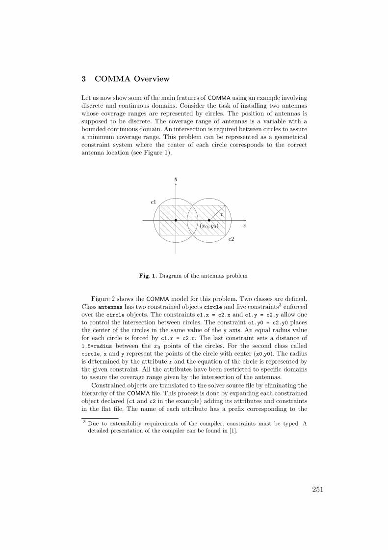
3 COMMA Overview

Let us now show some of the main features of COMMA using an example involvingdiscrete and continuous domains. Consider the task of installing two antennaswhose coverage ranges are represented by circles. The position of antennas issupposed to be discrete. The coverage range of antennas is a variable with abounded continuous domain. An intersection is required between circles to assurea minimum coverage range. This problem can be represented as a geometricalconstraint system where the center of each circle corresponds to the correctantenna location (see Figure 1).

b b

y

x

c1

c2

r

(x0, y0)

Fig. 1. Diagram of the antennas problem

Figure 2 shows the COMMA model for this problem. Two classes are defined.Class antennas has two constrained objects circle and five constraints3 enforcedover the circle objects. The constraints c1.x = c2.x and c1.y = c2.y allow oneto control the intersection between circles. The constraint c1.y0 = c2.y0 placesthe center of the circles in the same value of the y axis. An equal radius valuefor each circle is forced by c1.r = c2.r. The last constraint sets a distance of1.5*radius between the x0 points of the circles. For the second class calledcircle, x and y represent the points of the circle with center (x0,y0). The radiusis determined by the attribute r and the equation of the circle is represented bythe given constraint. All the attributes have been restricted to specific domainsto assure the coverage range given by the intersection of the antennas.

Constrained objects are translated to the solver source file by eliminating thehierarchy of the COMMA file. This process is done by expanding each constrainedobject declared (c1 and c2 in the example) adding its attributes and constraintsin the flat file. The name of each attribute has a prefix corresponding to the

3 Due to extensibility requirements of the compiler, constraints must be typed. Adetailed presentation of the compiler can be found in [1].

251

class antennas class circle

circle c1; real x in [-3,3];

circle c2; real y in [-3,3];

constraint intersection real r in [1.5, 2.5];

real c1.x = c2.x; int x0 in [0,5];

real c1.y = c2.y; int y0 in [0,5];

int c1.y0 = c2.y0; constraint radius

real c1.r = c2.r; real r^2 = (x-x0)^2 + (y-y0)^2;

real c1.x0 + 1.5*c1.r = c2.x0;

Fig. 2. A COMMA model for the antennas problem

concatenation of the names of objects of origin in order to avoid name redun-dancy. The process is done recursively. Constraints derived from the expansionof objects are added in the same way4 (see Figure 3).

Variables

real c1_x in [-3,3],

real c1_y in [-3,3],

real c1_r in [1.5,2.5],

...

real c2_x in [-3,3],

real c2_y in [-3,3],

real c2_r in [1.5,2.5],

...

Constraints

...

c1_r = c2_r,

c1_r^2 = (c1_x-c1_x0)^2 + (c1_y-c1_y0)^2,

c2_r^2 = (c2_x-c2_x0)^2 + (c2_y-c2_y0)^2;

Fig. 3. Flat RealPaver file

4 Conclusion and Future Work

We have shown by means of a practical example how COMMA is able to modelsystems using a compositional approach. This platform could be improved ex-tending the list of supported solvers. The definition of a UML profile will beuseful for modeling from a graphical perspective. Finally, we plan to make theCOMMA system open source for the research community.

4 The translation process to ECLiPSe and Gecode/J can be found in [1].

252

References

1. COMMA Modeling Language. http://www.inf.ucv.cl/˜rsoto/comma.2. Gecode System. http://www.gecode.org.3. A.H. Borning. The Programming Languages Aspects of ThingLab, a Constraint-

Oriented Simulation Laboratory. ACM TOPLAS, 3(4):353–387, 1981.4. Alan M. Frisch et al. The design of essence: A constraint language for specifying

combinatorial problems. In IJCAI, pages 80–87, 2007.5. R. Rafeh et al. From zinc to design model. In PADL, pages 215–229, 2007.6. F. Benhamou et al. Trends in Constraint Programming. ISTE, 2007.7. P. Fritzson and V. Engelson. Modelica – A Unified Object-Oriented Language for

System Modeling and Simulation. In ECOOP98, Brussels, 1998.8. L. Granvilliers and F. Benhamou. Realpaver: an interval solver using constraint

satisfaction techniques. ACM Trans. Math. Softw., 32(1):138–156, 2006.9. B. Jayaraman and P.Y. Tambay. Constrained Objects for Modeling Complex Struc-

tures. In OOPSLA, Minneapolis, USA, 2000.10. M. Paltrinieri. On the Design of Constraint Satisfaction Problems. In PPCP,

Orcas Island, USA, 1994.11. J.F. Puget. A C++ implementation of CLP. In SCIS, Singapore, 1994.12. R. Soto and L. Granvilliers. Dynamic parser cooperation for extending a con-

strained object-based modeling language. To appear in Proceedings of WLP 2007,Wuerzburg, Germany.

13. P. Van Hentenryck. The OPL Optimization Programming Language. The MITPress, 1999.

14. M. Wallace, S. Novello, and J. Schimpf. Eclipse: A platform for constraint logicprogramming, 1997.

253

Testing Relativised Uniform Equivalence underAnswer-Set Projection in the System cc⊤⋆

Johannes Oetsch1, Martina Seidl2, Hans Tompits1, and Stefan Woltran1

1 Institut fur Informationssysteme, Technische Universitat Wien,Favoritenstraße 9-11, A-1040 Vienna, Austriaoetsch,tompits@kr.tuwien.ac.at

woltran@dbai.tuwien.ac.at2 Institut fur Softwaretechnik, Technische Universitat Wien,

Favoritenstraße 9-11, A-1040 Vienna, Austriaseidl@big.tuwien.ac.at

Abstract. The systemcc⊤ is a tool for testing correspondence between logicprograms under the answer-set semantics with respect to different refined notionsof program correspondence. The underlying methodology ofcc⊤ is to reduce agiven correspondence problem to the satisfiability problem of quantified propo-sitional logic and to employ extant solvers for the latter language as back-endinference engines. In a previous version ofcc⊤, the system was designed to testcorrespondence between programs based onrelativised strong equivalence underanswer-set projection. Such a setting generalises the standard notion of strongequivalence by taking the alphabet of the context programs as well as the projec-tion of the compared answer sets to a set of designated output atoms into account.This paper outlines a newly added component ofcc⊤ for testing similarly pa-rameterised correspondence problems based onuniform equivalence.

1 General Information

An important issue in software development is to determine whether two encodings of agiven problem are equivalent, i.e., whether they yield the same result on a given probleminstance. Depending on the context of problem representations, different definitions of“equivalence” are useful and desirable. The systemcc⊤ [1] (short for “correspondence-checking tool”) is devised as a checker for a broad range of different such comparisonrelations defined betweendisjunctive logic programs(DLPs)under the answer-set se-mantics[2]. In a previous version ofcc⊤, the system was designed to test correspon-dence between logic programs based onrelativised strong equivalence under answer-set projection. Such a setting generalises the standard notion of strong equivalence [3]by taking the alphabet of the context programs as well as the projection of the com-pared answer sets to a set of designated output atoms into account [4]. The latter feature

⋆ This work was partially supported by the Austrian Science Fund (FWF) under grant P18019.The second author was also supported by the Austrian Federal Ministry of Transport, Inno-vation, and Technology (BMVIT) and the Austrian Research Promotion Agency (FFG) undergrant FIT-IT-810806.

254

reflects the common use of local (hidden) variables which maybe used in submodulesbut which are ignored in the final computation.

In this paper, we outline a newly added component ofcc⊤ for testing similarly pa-rameterised correspondence problems but generalisinguniform equivalence[5]—thatis, we deal with a component ofcc⊤ for testingrelativised uniform equivalence un-der answer-set projection. This notion, recently introduced in previous work [6], is lessrestrained, along with a slightly lower complexity than itsstrong pendant. However,in general, it is still outside a feasible means to be computed by answer-set solvers(provided that the polynomial hierarchy does not collapse). Yet, like relativised strongequivalence with projection, it can be efficiently reduced to the satisfiability problemof quantified propositional logic, an extension of classical propositional logic charac-terised by the condition that its sentences, generally referred to asquantified Booleanformulas(QBFs), are permitted to contain quantifications over atomic formulas. Thearchitecture ofcc⊤ takes advantage of this and uses existing solvers for quantifiedpropositional logic as back-end reasoning engines.

2 System Specifics

The equivalence notions under consideration are defined forground disjunctive logicprograms with default negation under the answer-set semantics [2]. LetAS (P ) be thecollection of the answer sets of a programP . Two programs,P andQ, arestronglyequivalentiff, for any programR, AS (P ∪R) = AS (Q∪R); they areuniformly equiv-alent iff, for any setF of facts,AS (P ∪F ) = AS (Q∪F ). While strong equivalence isrelevant for program optimisation and modular programmingin general [7–9], uniformequivalence is useful in the context of hierarchically structured program components,where lower-layered components provide input for higher-layered ones. In abstractingfrom strong and uniform equivalence, Eiteret al. [4] introduced the notion of acorre-spondence problemwhich allows to specify (i) acontext, i.e., a class of programs usedto be added to the programs under consideration, and (ii) therelation that has to holdbetween the answer sets of the extended programs. The concrete formal realisation ofrelativised uniform equivalence with projection is as follows [6]: Consider a quadrupleΠ = (P,Q, 2A,⊙B), whereP,Q are programs,A,B are sets of atoms,⊙ ∈ ⊆,=,andS ⊙B S

′ stands forI ∩B | I ∈ S ⊙ J ∩B | J ∈ S ′. Then,Π holdsiff, foreachF ∈ 2A, AS (P ∪ F ) ⊙B AS (Q ∪ F ). Furthermore,Π is called apropositionalquery equivalence problem(PQEP) if⊙B is given by=B , and apropositional queryinclusion problem(PQIP) if ⊙B is given by⊆B . Note that(P,Q, 2A,=B) holds iff(P,Q, 2A,⊆B) and(Q,P, 2A,⊆B) jointly hold.

For illustration, consider the programs

P = sad ∨ happy ←; sappy ← sad , happy ; confused ← sappy,Q = sad ← not happy ; happy ← not sad ; confused ← sad , happy,

which express some knowledge about the “moods” of a person, whereP uses an aux-iliary atomsappy . The programs can be seen as queries over a propositional databasewhich consists of facts from, e.g.,happy , sad. For the output, it would be naturalto consider the common intensional atomconfused . We thus considerΠ = (P,Q,

255

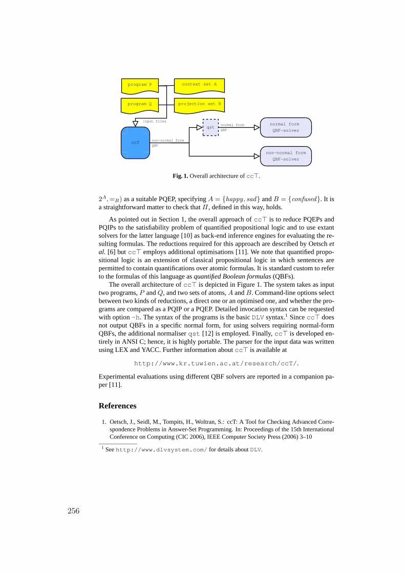
ccT

program P

program Q

context set A

projection set B

non-normal form

QBF-solver

normal form

QBF-solverqst

non-normal form

QBF

normal form

QBF

input files

Fig. 1.Overall architecture ofcc⊤.

2A,=B) as a suitable PQEP, specifyingA = happy , sad andB = confused. It isa straightforward matter to check thatΠ, defined in this way, holds.

As pointed out in Section 1, the overall approach ofcc⊤ is to reduce PQEPs andPQIPs to the satisfiability problem of quantified propositional logic and to use extantsolvers for the latter language [10] as back-end inference engines for evaluating the re-sulting formulas. The reductions required for this approach are described by Oetschetal. [6] but cc⊤ employs additional optimisations [11]. We note that quantified propo-sitional logic is an extension of classical propositional logic in which sentences arepermitted to contain quantifications over atomic formulas.It is standard custom to referto the formulas of this language asquantified Boolean formulas(QBFs).

The overall architecture ofcc⊤ is depicted in Figure 1. The system takes as inputtwo programs,P andQ, and two sets of atoms,A andB. Command-line options selectbetween two kinds of reductions, a direct one or an optimisedone, and whether the pro-grams are compared as a PQIP or a PQEP. Detailed invocation syntax can be requestedwith option-h. The syntax of the programs is the basicDLV syntax.1 Sincecc⊤ doesnot output QBFs in a specific normal form, for using solvers requiring normal-formQBFs, the additional normaliserqst [12] is employed. Finally,cc⊤ is developed en-tirely in ANSI C; hence, it is highly portable. The parser forthe input data was writtenusing LEX and YACC. Further information aboutcc⊤ is available at

http://www.kr.tuwien.ac.at/research/ccT/.

Experimental evaluations using different QBF solvers are reported in a companion pa-per [11].

References

1. Oetsch, J., Seidl, M., Tompits, H., Woltran, S.: ccT: A Tool for Checking Advanced Corre-spondence Problems in Answer-Set Programming. In: Proceedingsof the 15th InternationalConference on Computing (CIC 2006), IEEE Computer Society Press (2006) 3–10

1 Seehttp://www.dlvsystem.com/ for details aboutDLV.

256

2. Gelfond, M., Lifschitz, V.: Classical Negation in Logic Programs andDisjunctive Databases.New Generation Computing9 (1991) 365–385

3. Lifschitz, V., Pearce, D., Valverde, A.: Strongly Equivalent Logic Programs. ACM Transac-tions on Computational Logic2 (2001) 526–541

4. Eiter, T., Tompits, H., Woltran, S.: On Solution Correspondences in Answer Set Program-ming. In: Proceedings of the 19th International Joint Conference on Artificial Intelligence(IJCAI 2005). (2005) 97–102

5. Eiter, T., Fink, M.: Uniform Equivalence of Logic Programs underthe Stable Model Se-mantics. In: Proceedings of the 19th International Conference on Logic Programming (ICLP2003). Volume 2916 in Lecture Notes in Computer Science. Springer (2003) 224–238

6. Oetsch, J., Tompits, H., Woltran, S.: Facts do not Cease to Exist Because They are Ignored:Relativised Uniform Equivalence with Answer-Set Projection. In: Proceedings of the 22ndNational Conference on Artificial Intelligence (AAAI 2007), AAAI Press (2007) 458–464

7. Eiter, T., Fink, M., Tompits, H., Woltran, S.: Simplifying Logic Programs Under Uniformand Strong Equivalence. In Lifschitz, V., Niemela, I., eds.: Proceedings of the 7th Interna-tional Conference on Logic Programming and Nonmonotonic Reasoning(LPNMR-7). Vol-ume 2923 of Lecture Notes in Computer Science. Springer Verlag (2004) 87–99

8. Pearce, D.: Simplifying Logic Programs under Answer Set Semantics. In: Proceedings of the20th International Conference on Logic Programming (ICLP 2004). Volume 3132 of LectureNotes in Computer Science. Springer (2004) 210–224

9. Lin, F., Chen, Y.: Discovering Classes of Strongly Equivalent Logic Programs. In: Pro-ceedings of the 19th International Joint Conference on Artificial Intelligence (IJCAI 2005).(2005) 516–521

10. Le Berre, D., Narizzano, M., Simon, L., Tacchella, L.A.: The Second QBF Solvers Com-parative Evaluation. In: Proceedings of the 7th International Conference on Theory andApplications of Satisfiability Testing (SAT 2004). Revised Selected Papers.Volume 3542 ofLecture Notes in Computer Science., Springer (2005) 376–392

11. Oetsch, J., Seidl, M., Tompits, H., Woltran, S.: An Extension of the System cc⊤ for TestingRelativised Uniform Equivalence under Answer-Set Projection (2007). Submitted draft

12. Zolda, M.: Comparing Different Prenexing Strategies for Quantified Boolean Formulas(2004). Master’s Thesis, Vienna University of Technology

257

spock: A Debugging Support Tool for Logic Programsunder the Answer-Set Semantics⋆

Martin Gebser1, Jorg Puhrer2, Torsten Schaub1,Hans Tompits2, and Stefan Woltran2

1 Institut fur Informatik, Universitat Potsdam,August-Bebel-Straße 89, D-14482 Potsdam, Germanygebser,torsten@cs.uni-potsdam.de

2 Institut fur Informationssysteme, Technische Universitat Wien,Favoritenstraße 9–11, A–1040 Vienna, Austriapuehrer,tompits@kr.tuwien.ac.at

woltran@dbai.tuwien.ac.at

Abstract. Logic programs under the answer-set semantics are an acknowledgedtool for declarative problem solving and constitute the canonical instanceof thegeneralanswer-set programming (ASP) paradigm. Despite its semantic elegance,ASP suffers from a lack of software-development tools. In particular, there is aneed to support engineers in detecting erroneous parts of their programs. Un-like in other areas of logic programming, applying tracing techniques for debug-ging logic programs under the answer-set semantics seems rather unnatural sincesticking to imperative solving algorithms would undermine the declarative flavorof ASP. In this paper, we outline the systemspock, a debugging support toolfor answer-set programs making use of ASP itself. The implemented techniquesmaintain the declarative nature of ASP within the debugging process and are in-dependent from the actual computation of answer sets.

1 General Information

During the last decade, logic programs under the answer-setsemantics received in-creasing importance as an approach for declarative problemsolving. Their formal un-derpinnings are rooted in concepts from nonmonotonic reasoning, and they constitutethe canonical instance of the generalanswer-set programming (ASP) paradigm [1] inwhichmodels represent solutions rather thanproofs as in traditional logic programming.The nonmonotonicity of answer-set programs, however, is anaggravating factor for de-tecting sources of errors, since every rule of a program might significantly influence theresulting answer sets.

In this paper, we outline the basic features of the systemspock [2] that supportsdevelopers of answer-set programs to detect and locate errors in their programs, inde-pendent of specific ASP solvers. The theoretical backgroundof spock was introducedin previous work [3], and exploits and extends atagging technique as used by Delgrandeet al. [4] for compiling ordered logic programs into standard ones. In our approach, a

⋆ This work was partially supported by the Austrian Science Fund (FWF) under project P18019.

258

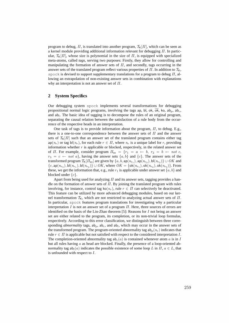
program to debug,Π, is translated into another program,TK[Π], which can be seen asa kernel module providing additional information relevantfor debuggingΠ. In partic-ular, TK[Π], whose size is polynomial in the size ofΠ, is equipped with specializedmeta-atoms, calledtags, serving two purposes: Firstly, they allow for controllingandmanipulating the formation of answer sets ofΠ, and secondly, tags occurring in theanswer sets of the translated program reflect various properties ofΠ. In addition toTK,spock is devised to support supplementary translations for a program to debugΠ, al-lowing an extrapolation of non-existing answer sets in combination with explanationswhy an interpretation is not an answer set ofΠ.

2 System Specifics

Our debugging systemspock implements several transformations for debuggingpropositional normal logic programs, involving the tagsap, bl, ok, ok, ko, abp, abc,andabl. The basic idea of tagging is to decompose the rules of an original program,separating the causal relation between the satisfaction ofa rule body from the occur-rence of the respective heads in an interpretation.

One task of tags is to provide information about the program,Π, to debug. E.g.,there is a one-to-one correspondence between the answer sets of Π and the answersets ofTK[Π] such that an answer set of the translated program contains either tagap(nr) or tagbl(nr), for each ruler ∈ Π, wherenr is a unique label forr, providinginformation whetherr is applicable or blocked, respectively, in the related answer setof Π. For example, consider programΠex = r1 = a ← b, r2 = b ← not c,

r3 = c ← not a, having the answer setsa, b and c. The answer sets of thetransformed programTK[Πex] are given bya, b, ap(nr1

), ap(nr2), bl(nr3

) ∪OK andc, ap(nr3

), bl(nr1), bl(nr2

) ∪OK , whereOK = ok(nr1), ok(nr2

), ok(nr3). From

these, we get the information that, e.g., ruler1 is applicable under answer seta, b andblocked underc.

Apart from being used for analyzingΠ and its answer sets, tagging provides a han-dle on the formation of answer sets ofΠ. By joining the translated program with rulesinvolving, for instance, control tagko(nr), rule r ∈ Π can selectively be deactivated.This feature can be utilized by more advanced debugging modules, based on our ker-nel transformationTK, which are not restricted to analyzing actual answer sets ofΠ.In particular,spock features program translations for investigating why a particularinterpretationI is not an answer set of a programΠ. Here, three sources of errors areidentified on the basis of the Lin-Zhao theorem [5]: Reasons for I not being an answerset are either related to the program, its completion, or itsnon-trivial loop formulas,respectively. According to this error classification, we distinguish between three corre-spondingabnormality tags,abp, abc, andabl, which may occur in the answer sets ofthe transformed program. The program-oriented abnormality tagabp(nr) indicates thatruler ∈ Π is applicable but not satisfied with respect to the considered interpretationI.The completion-oriented abnormality tagabc(a) is contained whenever atoma is in I

but all rules havinga as head are blocked. Finally, the presence of a loop-oriented ab-normality tagabl(a) indicates the possible existence of some loopL in Π, a ∈ L, thatis unfounded with respect toI.

259

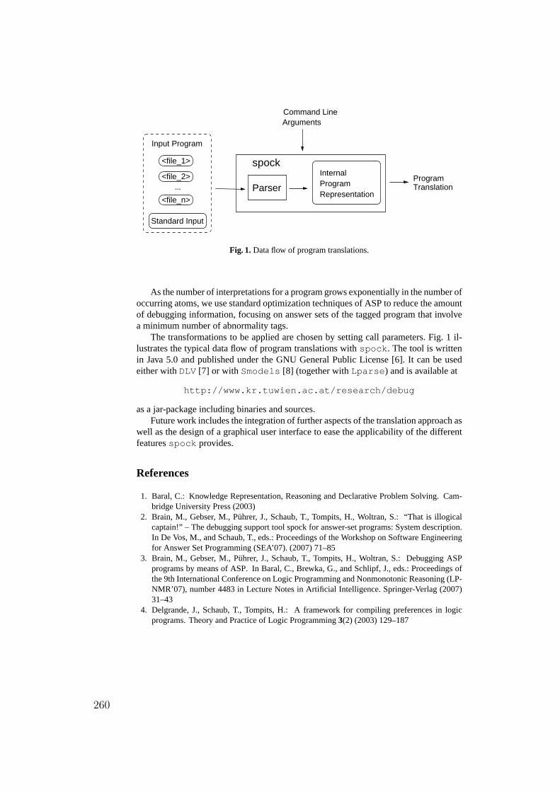
<file_n>

Translation

<file_1>

<file_2>... Parser

spock

Command Line

Standard Input

RepresentationProgramInternal

Arguments

Input Program

Program

Fig. 1.Data flow of program translations.

As the number of interpretations for a program grows exponentially in the number ofoccurring atoms, we use standard optimization techniques of ASP to reduce the amountof debugging information, focusing on answer sets of the tagged program that involvea minimum number of abnormality tags.

The transformations to be applied are chosen by setting callparameters. Fig. 1 il-lustrates the typical data flow of program translations withspock. The tool is writtenin Java 5.0 and published under the GNU General Public License [6]. It can be usedeither withDLV [7] or with Smodels [8] (together withLparse) and is available at

http://www.kr.tuwien.ac.at/research/debug

as a jar-package including binaries and sources.Future work includes the integration of further aspects of the translation approach as

well as the design of a graphical user interface to ease the applicability of the differentfeaturesspock provides.

References

1. Baral, C.: Knowledge Representation, Reasoning and Declarative Problem Solving. Cam-bridge University Press (2003)

2. Brain, M., Gebser, M., Puhrer, J., Schaub, T., Tompits, H., Woltran, S.: “That is illogicalcaptain!” – The debugging support tool spock for answer-set programs: System description.In De Vos, M., and Schaub, T., eds.: Proceedings of the Workshopon Software Engineeringfor Answer Set Programming (SEA’07). (2007) 71–85

3. Brain, M., Gebser, M., Puhrer, J., Schaub, T., Tompits, H., Woltran, S.: Debugging ASPprograms by means of ASP. In Baral, C., Brewka, G., and Schlipf, J., eds.: Proceedings ofthe 9th International Conference on Logic Programming and Nonmonotonic Reasoning (LP-NMR’07), number 4483 in Lecture Notes in Artificial Intelligence. Springer-Verlag (2007)31–43

4. Delgrande, J., Schaub, T., Tompits, H.: A framework for compiling preferences in logicprograms. Theory and Practice of Logic Programming3(2) (2003) 129–187

260

5. Lin, F., Zhao, Y.: ASSAT: Computing answer sets of a logic programby SAT solvers.Artificial Intelligence157(1-2) (2004) 115–137

6. Free Software Foundation Inc.: GNU General Public License - Version 2, June 1991 (1991)http://www.gnu.org/copyleft/gpl.html

7. Leone, N., Pfeifer, G., Faber, W., Eiter, T., Gottlob, G., Perri, S., Scarcello, F.: The DLVsystem for knowledge representation and reasoning. ACM Transactions on ComputationalLogic 7(3) (2006) 499–562

8. Simons, P., Niemela, I., Soininen, T.: Extending and implementing the stable model seman-tics. Artificial Intelligence138(1-2) (2002) 181–234

261

262

Author Index

Abdennadher, Slim 79, 88Abreu, Salvador 183Almendros–Jimenez, Jesus M. 136Aly, Mohamed 88Atzmueller, Martin 148, 158

Baudry, Benoit 59Becerra–Teron, Antonio 136Behrens, Tristan 173Boehm, Andreas M. 113Braßel, Bernd 101, 215

Chrpa, Lukas 47Costa, Pedro 125

Dix, Jurgen 173

Edward, Marlien 79Enciso–Banos, Francisco J. 136

Ferreira, Michel 125

Gebser, Martin 258Geske, Ulrich 3Goltz, Hans–Joachim 3Granvilliers, Laurent 70, 249

Hanus, Michael 101Huch, Frank 215

Kuhnert, Sebastian 35

Lopez–Fraguas, Francisco F. 224

Muller, Marion 101

Nalepa, Grzegorz 195, 205Nogueira, Vitor 183

Oetsch, Johannes 254

Puhrer, Jorg 258Plumicke, Martin 234Precup, Doina 59Puppe, Frank 148

Rocha, Ricardo 125Rodrıguez–Hortala, Juan 224

Sanchez–Hernandez, Jaime 224Schaub, Torsten 258Schrader, Gunnar 23Seidl, Martina 254Seipel, Dietmar 113, 158Sen, Sagar 59Sickmann, Albert 113Soto, Ricardo 70, 249Surynek, Pavel 47

Tompits, Hans 254, 258Vyskocil, Jiri 47

Wetzka, Matthias 113Wojnicki, Igor 195, 205Wolf, Armin 23Woltran, Stefan 254, 258

263

264