Diplomarbeit - FAMsgerhold/pub_files/theses/zrunek.pdf · Technische Universittä Wien Karlsplatz...

Technische Universität Wien

Karlsplatz 13, 1040 Wien

Diplomarbeit

Volatility Smile Expansions in Lévy models

Technische MathematikWintersemester 2013

Betreuer:

Privatdoz. Dipl.-Ing. Dr.techn. Stefan GerholdE105 Institut für WirtschaftsmathematikE-Mail-Adresse: [email protected]

Autor:

Axel Zrunek, BSc066 405 Finanz- und VersicherungsmathematikAnschrift: Sieveringerstraÿe 113/1/3

1190 WienE-Mail-Adresse: [email protected]

Statutory DeclarationI declare in lieu of an oath that I have written this master thesis myself and that I have notused any sources or resources other than stated for its preparation. This master thesis hasnot been submitted elsewhere for examination purposes.

Vienna, on December 12, 2013

Danksagung

Ich möchte mich an dieser Stelle bei Herrn Dr. Stefan Gerhold für die kompetente Betreuungmeiner Arbeit bedanken. Genauso danke ich Herrn Dr. Johannes Morgenbesser für diezahlreichen E-Mail Diskussionen und sein Working Paper über das Kou Modell, welchesdie Grundlage von Kapitel 2 stellt. Auÿerdem bin ich Johannes Heiny für seine vielenVerbesserungsvorschläge zu dieser Arbeit sehr dankbar.Mein Dank gilt meiner Familie dafür, dass sie mich beim Studium immer unterstützt hat.Besonders bedanken möchte ich mich bei meinen Eltern, Marja und Ulrich, sowie Groÿeltern,Leena und Reijo, dass sie mir das Studium ermöglicht und mich �nanziell unterstützt haben.Meinem Groÿvater Gerhard danke ich dafür, dass er meine mathematischen Interessen schonfrüh gefördert und mich somit zum Mathematikstudium gebracht hat.Zuletzt möchte ich mich bei all meinen Studienkollegen für die schöne Zeit bedanken. Ohneeuch hätte das Studium nicht so viel Spaÿ gemacht.

Herzlichen Dank,

Axel Zrunek

v

Abstract

This thesis is about investigating tail expansions for the call price and implied volatility atlarge strikes in exponential Lévy jump-di�usion models. Furthermore, the asymptotics ofthe density function and the tail probability are studied. To get these expansions, we use thesaddle-point method (method of deepest descent) on the Mellin transform of the call price,respectively density function and tail probability. Expansions for the implied volatility skeware derived by using transfer theorems, sharpening previous results from [BF08] and [BF09].We consider the double exponential Kou and the Merton Jump Di�usion model in this work.

Keywords: exponential Lévy jump di�usion models, Kou, Merton Jump Di�usion, saddle-

point approximation, tail expansions

vi Contents

Contents

Abstract v

1. Introduction 1

2. Kou model 3

2.1. Model de�nition . . . . . . . . . . . . . . . . . . . . . . . . . . . . . . . . . 32.2. Call price . . . . . . . . . . . . . . . . . . . . . . . . . . . . . . . . . . . . . 4

2.2.1. Saddle-point . . . . . . . . . . . . . . . . . . . . . . . . . . . . . . . 52.2.2. Central approximation . . . . . . . . . . . . . . . . . . . . . . . . . . 72.2.3. Estimation of the tails . . . . . . . . . . . . . . . . . . . . . . . . . . 9

2.3. Implied volatility . . . . . . . . . . . . . . . . . . . . . . . . . . . . . . . . . 112.4. Numerical tests . . . . . . . . . . . . . . . . . . . . . . . . . . . . . . . . . . 12

2.4.1. Call price . . . . . . . . . . . . . . . . . . . . . . . . . . . . . . . . . 122.4.2. Implied volatility . . . . . . . . . . . . . . . . . . . . . . . . . . . . . 14

3. Merton Jump Di�usion model 18

3.1. Model de�ntion and general results . . . . . . . . . . . . . . . . . . . . . . . 183.2. Call price . . . . . . . . . . . . . . . . . . . . . . . . . . . . . . . . . . . . . 20

3.2.1. Saddle-point . . . . . . . . . . . . . . . . . . . . . . . . . . . . . . . 203.2.2. Asymptotics of the cumulant generating function . . . . . . . . . . . 223.2.3. Central approximation . . . . . . . . . . . . . . . . . . . . . . . . . . 243.2.4. Estimation of the tails . . . . . . . . . . . . . . . . . . . . . . . . . . 26

3.3. Density function . . . . . . . . . . . . . . . . . . . . . . . . . . . . . . . . . 273.4. Tail probability . . . . . . . . . . . . . . . . . . . . . . . . . . . . . . . . . . 283.5. Implied volatility . . . . . . . . . . . . . . . . . . . . . . . . . . . . . . . . . 313.6. Numerical Tests . . . . . . . . . . . . . . . . . . . . . . . . . . . . . . . . . . 32

3.6.1. Call price . . . . . . . . . . . . . . . . . . . . . . . . . . . . . . . . . 333.6.2. Density . . . . . . . . . . . . . . . . . . . . . . . . . . . . . . . . . . 343.6.3. Tail probability . . . . . . . . . . . . . . . . . . . . . . . . . . . . . . 343.6.4. Implied volatility . . . . . . . . . . . . . . . . . . . . . . . . . . . . . 36

4. Conclusion 38

A. Landau notation 39

A.1. Basics . . . . . . . . . . . . . . . . . . . . . . . . . . . . . . . . . . . . . . . 39A.2. Some Taylor series . . . . . . . . . . . . . . . . . . . . . . . . . . . . . . . . 39

B. Mellin transform 41

B.1. Basic results . . . . . . . . . . . . . . . . . . . . . . . . . . . . . . . . . . . . 41

Contents vii

B.2. Applications of the Mellin transformation . . . . . . . . . . . . . . . . . . . 42B.2.1. Call price . . . . . . . . . . . . . . . . . . . . . . . . . . . . . . . . . 42B.2.2. Probability density function . . . . . . . . . . . . . . . . . . . . . . . 43B.2.3. Tail probability . . . . . . . . . . . . . . . . . . . . . . . . . . . . . . 43

C. Implementation in R 44

C.1. Kou model . . . . . . . . . . . . . . . . . . . . . . . . . . . . . . . . . . . . . 44C.2. Merton Jump Di�usion model . . . . . . . . . . . . . . . . . . . . . . . . . . 49

Bibliography 54

1

1. Introduction

The intention of this thesis is to get tail expansions for the call price and implied volatility atlarge strikes as well as for the density function and the tail probability by using the methodof saddle-point approximation as in [FG11]. The method basically consists of 3 steps:�nding a saddle-point, deriving an asymptotic expansion of the integral around the saddle-point and showing that the remaining tails are negligible. The book [FS09] by P. Flajoletand P. Sedgewick gives a good overview of the method and contains some combinatoricalexamples, which are similar to those considered here (Examples VIII.6 and VIII.7 in [FS09,p.560 �.]).In contrast to the above mentioned paper, where the stochastic volatility model of Heston isconsidered, is this thesis about exponential Lévy jump di�usion models. The general formof the stock process in this kind of models is

St = S0ert+Xt , t ∈ [0, T ∗]

where S0 < 0 is the initial stock value, r ≥ 0 is the riskless interest rate and T ∗ > 0 is a�nite time horizont.

Xt = γt+ σWt +

Nt∑i=1

Yi

is a Lévy jump di�usion process with γ ∈ R, di�usion volatility σ > 0, (Wt)t∈[0,T ∗] beinga standard Brownian motion, (Yi)i∈N real iid random variables and (Nt)t∈[0,T ∗] a Poissonprocess with jump intensity λ > 0. Throughout the work, it can be assumed without lossof generality r = 0 and S0 ≡ 1 (see [GL, p.4]). Hence, one gets

St = eXt . (1.1)

The two models considered in this thesis are the Kou model, where the Yi follow a doubleexponential distribution, and the Merton Jump Di�usion model, where the Yi are Gaussianrandom variables. [CT04] is a good source on Lévy models used in �nance and gives moretheoretical background information on this topic.We consider a European call option with maturity T < T ∗ and log-strike k := logK > 0

C(k, T ) = E[(ST − ek)+

],

where (x− y)+ := max (x− y, 0). Hence, we just need to focus on the random variable STand not on the whole stock process (St)t∈[0,T ∗] . Under these assumptions, the price of thecall option in the normalized Black Scholes model is

cBS(k, σ) = Φ(d1)− ekΦ(d2)

with σ > 0 being the constant unannualized (dimensionless) volatility in the Black Scholessetting, d1,2 := − k

σ ±σ2 and Φ(x) being the cumulative distribution function of a standard

2 CHAPTER 1. INTRODUCTION

Gaussian distribution.

Remark 1.1 Usually the Black Scholes formula is given with the annualized volatility σ,i.e.

cBS(k, σ) = Φ(d1)− ekΦ(d2)

with d1,2 = − kσ√T± σ

√T

2 .

The (unannualized) implied volatility is de�ned as the unique value V (k) > 0 such that

cBS(k, V (k)) = E[(ST − ek)+

].

As it can be seen later in (2.1), the Kou model exhibits moment explosion with criticalmoment λ+, i.e.

p∗ := sup (s ∈ R+ : E [(ST )s] <∞) = λ+ <∞.

From Roger Lee's moment formula and [BF08, Example 5.3], it is known that V has thefollowing asymptotics

limk→∞

V (k)

k1/2= Ψ1/2(λ+ − 1), (1.2)

where Ψ(x) is de�ned by

Ψ(x) = 2− 4(√x2 + x− x). (1.3)

For the Merton Jump Di�usion model all moments of ST exist, so the above mentionedprocedure cannot be applied. But as it was shown in [BF09, Example 5.4], the impliedvolatility V (k) satis�es

V (k) ∼√δk√

2√

2 log k,

where δ > 0 is the standard deviation of the jumps (see Section 3.1).These expansions will be re�ned in this thesis by using the saddle-point approximation.The starting point for this method is always an integral representation of the call price(respectively density and tail probability), which we get by using the Mellin transform. TheO-notation and the Mellin transform are used throughout the thesis, therefore some basicresults are explained in the appendix.

Finally, some frequently used notation is de�ned

f � g ⇔ f = O (g) ,

f ∼ g ⇔ limx→∞

f(x)

g(x)= 1.

The moment generating and cumulant generating function of a stochastic process (Xt)t∈Rare de�ned as

M(s, T ) := E [exp(sXT )] ,

m(s, T ) := logM(s, T )

for all s ∈ R, wherever this expectation exists, and T > 0 being the maturity of the option.

3

2. Kou model

2.1. Model de�nition

The Kou model ([K02]) is an exponential Lévy jump di�usion model as in (1.1) with (Yi)i∈Nbeing a sequence of iid double exponential random variables. So for i ∈ N the Yi have thedensity

f(y) = pλ+e−λ+y1[0,∞)(y) + (1− p)λ−eλ−y1(−∞,0)(y)

with parameters λ+ > 1, λ− > 0 and p ∈ (0, 1).We have

ST = eXT ,

where the log-price XT is determined by its moment generating function (see for example[GG13, p.7])

M(s, T ) = E [exp(sXT )] = exp

[T

(σ2s2

2+ bs+ λ

(λ+p

λ+ − s+λ−(1− p)λ− + s

− 1

))], (2.1)

where λ > 0 is the jump intensity and σ > 0 the di�usion volatility in (1.1). It follows thatthe cumulant generating function is

m(s, T ) = logE[esXT

]= T

(σ2s2

2+ bs+ λ

(λ+p

λ+ − s+λ−(1− p)λ− + s

− 1

)).

The parameter b ∈ R is chosen, such that ST becomes a martingale. A su�cient conditionfor this is (see [CT04])

E [ST ] = M(1, T ) = E [S0] = 1. (2.2)

Hence the parameter b has to be chosen such that m(1, T ) = 0, so it must satisfy

b = −(σ2

2+ λ

(λ+p

λ+ − 1+λ−(1− p)λ− + 1

− 1

)).

Remark 2.1 There is a typo for the characteristic function in [CT04, Table 4.3, p.124].

4 CHAPTER 2. KOU MODEL

Before starting the saddle-point approximation, let us summarize the two main results ofthis chapter. Let

α1 = λ+ − 1, α1/2 = −2(λλ+pT )1/2

and α0 = − logeTσ2λ2+

2+bTλ++

Tλλ−(1−p)λ−+λ+

−λT(λλ+pT )1/4

2√πλ+(λ+ − 1)

. (2.3)

Theorem 2.2 Let the parameters of the models as well as the maturity be �xed. Then the

price of a European call option satis�es for every ε > 0

C(k, T ) = exp(−α1k − α1/2k

−1/2 − α0

)k−3/4

(1 +O

(k−1/4+ε

))as k →∞.

Theorem 2.3 Under the assumptions of Theorem 2.2 , the implied volatiliy satis�es for

every ε > 0 the asymptotic formula (as k →∞)

V (k) = β1/2k1/2 + β0 + β`−1/2

log k

k1/2+ β−1/2

1

k1/2+O

(1

k3/4−ε

),

where

β1/2 = −2γ√α2

1 + α1 = Ψ1/2(λ+ − 1), β0 = γα1/2, β`−1/2 =γ

4,

β−1/2 =

(α0 + log

1− (1 + 1α1

)−1/2

√4πα1

)γ +

(1

2(2α1)3/2− 1

2(2α1 + 2)3/2

)α2

1/2

and

γ =

(1√

2α1 + 2− 1√

2α1

).

Theorem 2.3 shows clearly a re�nement of the expansion in (1.2)

V (k) ∼ Ψ(λ+ − 1)k1/2.

In Section 2.4 some numerical examples are given and it will be veri�ed that the expansiondoes give a better approximation of the volatility smile for large k values.

2.2. Call price

First an expansion for the price of a European call option with strike K will be derived (ask →∞). The starting point is the integral representation of a call price. Using the Mellintransform of C(k, T ), the inversion theorem implies (see Lemma B.5 in the appendix)

C(k, T ) =ek

2πi

∫ c+i∞

c−i∞e−ks

M(s, T )

s(s− 1)ds, k = logK, (2.4)

whenever 1 < c < λ+. Here i =√−1 is the imaginary unit.

2.2. CALL PRICE 5

2.2.1. Saddle-point

The idea of the considered method is to choose a saddle-point of the integrand for c in (2.4)and to estimate the central part of the integral with the Laplace method.It is easy to see that M(s, T ) has two singularities, at −λ− and λ+. As the call-price is anintegral on the positive side of the complex plane, we consider the blowup at λ+. So we getan approximate saddle-point by just considering the dominant term

∂e−ks exp(Tλ λ+p

λ+−s

)∂s

= 0.

A simple calculation yields the solution of this equation

s = λ+ −√λλ+pT

k,

which is greater than 1 for su�ciently large k. Using the notation ξ = λλ+pT , we get

s = λ+ − ξ1/2k−1/2 = λ+ +O(k−1/2

). (2.5)

Remark 2.4 The approximate saddle-point actually depends on the log-strike k. We writes instead of s(k) for ease of notation .

Before doing the central expansion, one must determine the asymptotics of the cumulantgenerating function. This is necessary to determine the interval around the saddlepoint, sowe can apply the Laplace method.

Lemma 2.5 The cumulant generating function of XT satis�es

m(s, T ) =Tσ2λ2

+

2+ bλ+T + ξ1/2k1/2 +

Tλλ−(1− p)λ− + λ+

− λT +O(k−1/2

),

m′(s, T ) = k +O (1) ,

m′′(s, T ) = 2ξ−1/2k3/2 +O (1)

and

m′′′(s+ it, T ) = O(k2)

for |t| < k−α, α > 0,

where all derivatives are with respect to s.

Proof: We have for −λ− < s < λ+

m(s, T ) = T

(σ2s2

2+ bs+ λ

(λ+p

λ+ − s+λ−(1− p)λ− + s

− 1

)),

m′(s, T ) = T

(σ2s+ b+ λ

(λ+p

(λ+ − s)2− λ−(1− p)

(λ− + s)2

)),

m′′(s, T ) = T

(σ2 + 2λ

(λ+p

(λ+ − s)3+λ−(1− p)(λ− + s)3

))and

m′′′(s, T ) = 6λT

(λ+p

(λ+ − s)4− λ−(1− p)

(λ− + s)4

).


Inserting s = λ+ − ξ1/2k−1/2 yields the asymptotics

m(s, T ) = T

(σ2s2

2+ bs+ λ

(λ+p

λ+ − s+λ−(1− p)λ− + s

− 1

))= T

(σ2(λ+ − ξ1/2k−1/2)2

2+ bλ+ + λ

(λ+p

ξ1/2k−1/2+

λ−(1− p)λ− + λ+ − ξ1/2k−1/2

− 1

))+ O

(k−1/2

).

Here we use (1 + x)ω = 1 +O (x) for small x and ω ∈ R. Hence we get,

m(s, T ) =Tσ2λ2

+

2+ bλ+T + ξ1/2k1/2 + Tλλ−(1− p) 1

λ− + λ+

(1− ξ1/2k−1/2

λ− + λ+

)−1

− λT

+ O(k−1/2

)=

Tσ2λ2+

2+ bλ+T + ξ1/2k1/2 +

Tλλ−(1− p)λ− + λ+

− λT +O(k−1/2

).

Similarly, one gets by using again the same argument from Lemma A.3

m′(s, T ) = T

(σ2(λ+ − ξ1/2k−1/2

)22

+ b+ λ

(λ+p

ξk−1+

λ−(1− p)(λ− + λ+ + ξ1/2k−1/2

)2))

= O (1) + k +Tλλ−(1− p)(λ− + λ+)2

(1 +

ξ1/2k−1/2

λ+ + λ−

)−2

= k +O (1) ,

as well as

m′′(s, T ) = T

(σ2 + 2λ

(λ+p

(ξ1/2k−1/2)3+

λ−(1− p)(λ− + λ+ + ξ1/2k−1/2)3

))

= Tσ2 + 2ξ−1/2k3/2 +Tλλ−(1− p)(λ− + λ+)3

(1 +

ξ1/2k−1/2

λ− + λ+

)−3

= Tσ2 + 2ξ−1/2k3/2 +Tλλ−(1− p)(λ− + λ+)3 +O(k−1/2) = 2ξ−1/2k3/2 +O(1).

For the third derivative we need to consider s = s+ it, in order to estimate the error termof the Taylor approximation in the Laplace method. So we get∣∣m′′′(s, T )

∣∣ = 6λT

∣∣∣∣ λ+p

(ξ1/2k−1/2 − it)4+

λ−(1− p)(λ− + λ+ − ξ1/2k−1/2 + it)4

∣∣∣∣≤ 6ξ∣∣ξ1/2k−1/2 − it

∣∣4 +λ−(1− p)∣∣λ− + λ+ − ξ1/2k−1/2 + it

∣∣4≤ 6ξ∣∣ξ1/2k−1/2

∣∣4 +λ−(1− p)λ− + λ+

(1 +O

(k−1/2

))= O

(k2).

�

2.2. CALL PRICE 7

Now we have derived the asymptotics of the cumulant generating function and its derivatives.This is crucial to �nd an interval for the central approximation and to apply Taylors theoremon M(s+ it, T ).

2.2.2. Central approximation

In the next step, the interval around the saddle-point s has to be chosen. Following theheuristic argument in [FS09, p.554], the length of the interval around the saddle-point(denoted by δ) has to be chosen such that the conditions

m′′(s, T )δ2 −−−→k→∞

∞,

m′′′(s, T )δ3 −−−→k→∞

0

are ful�lled. These conditions ensure that one gets a Gaussian integral for the secondderivative and that error term of the Taylor approximation (depending on the third deriva-tive m′′′(s+ it, T ) and some t ∈ δ) becomes arbitrarily small for large log-strikes k.Considering intervals of the form (s− k−α, s+ k−α) together with the results of Lemma2.5 , yields the conditions

m′′(s, T )4k−2α = O(k3/2−2α

)−−−→k→∞

∞

m′′′(s, T )8k−3α = O(k2−3α

)−−−→k→∞

0. (2.6)

Therefore the parameter α must ful�ll 23 < α < 3

4 . After having determined the interval(s− k−α, s+ k−α), we are ready to show the asymptotics of the central part in (2.4).

Lemma 2.6 Let 2/3 < α < 3/4. Then

ek

2πi

∫ s+ik−α

s−ik−αe−ks

M(s, T )

s(s− 1)ds

=eTσ2λ2+

2+bTλ++


−λTξ1/4

2√πλ+(λ+ − 1)

ek(1−λ+)+2ξ1/2k1/2k−3/4(1 +O

(k−3α+2

)).

Proof: Applying Taylor's theorem and using the results from Lemma 2.5 yields

m(s+ it, T ) = m(s, T ) + im′(s, T )t−m′′(s, T )t2/2 +O(t3k2

).

where |t| < k−α. Using m′(s, T ) = k +O (1) and that ex = 1 +O (x) for small x, we get

M(s+ it, T ) = exp (m(s+ it, T ))

= exp

(m(s, T ) + im′(s, T )t− m′′(s, T )

2t2 +O

(t3k2

))= exp

(m(s, T ) + itk +O (t)− m′′(s, T )

2t2 +O

(t3k2

))= exp

(m(s, T ) + itk − m′′(s, T )

2t2)(

1 +O(t3k2

)), |t| < k−α,


and by using (1 + x)−1 = 1 +O (x) for small x, we obtain

1

(s+ it)(s+ it− 1)=

1

λ+

(1− ξ1/2k−1/2 − it

λ+

)−11

λ+ − 1

(1− ξ1/2k−1/2 − it

λ+ − 1

)−1

=1

λ+(λ+ − 1)

(1 +O

(k−1/2

)).

Thus we get

ek

2πi

∫ s+ik−α

s−ik−αe−ks

M(s, T )

s(s− 1)ds =

ek(1−s)

2π

∫ k−α

−k−αe−itk

M(s+ it, T )

(s+ it)(s+ it− 1)dt

=ek(1−s)M(s, T )

2πλ+(λ+ − 1)

∫ k−α

−k−αexp

(−m

′′(s, T )

2t2)(

1 +O(k−3α+2

))dt.

Here we used the second condition in (2.6), which ensures that the error term O(k−3α+2

)tends to zero. Setting u := m′′(s, T )1/2, we get from Lemma 2.5

u =

√2k3/2

ξ1/2

(1 +O

(k−3/2

))=

√2k3/4

ξ1/4

(1 +O

(k−3/2

))and

1

u=

ξ1/4

√2k3/4

(1 +O

(k−3/2

)).

By substituting ω = ut and using the fact that Gaussian integrals have exponentially de-

caying tails, i.e.∫∞c e−t

2/2dt = O(e−c

2/2), c > 0 (see [FS09, p.557]), we get

∫ k−α

−k−αexp

(−m

′′(s, T )

2t2)dt =

1

u

∫ uk−α

−uk−αexp

(−ω

2

2

)dω

=1

u

(∫ ∞−∞

exp

(−ω

2

2

)dω +O

(e−u

2/(2k2α)))

=

√2π

u

(1 +O

(e−u

2/(2k2α)))

=√πk−3/4ξ1/4

(1 +O

(k−3/2

)).

Here we used the �rst condition in (2.6), which ensures that uk−α tends to in�nity, so weget Gaussian integrals with exponentially decaying tails.This implies

ek

2πi

∫ s+ik−α

s−ik−αe−ks

M(s, T )

s(s− 1)ds =

ek(1−s)M(s, T )ξ1/4

2√πλ+(λ+ − 1)

k−3/4(

1 +O(k−3/2

)+O

(k−3α+2

))=

ek(1−s)M(s, T )ξ1/4

2√πλ+(λ+ − 1)

k−3/4(1 +O

(k−3α+2

)).

Finally we use Lemma 2.5 to get

M(s, T ) = exp

(Tσ2λ2

+

2+ bTλ+ + ξ1/2k1/2 +

Tλλ−(1− p)λ− + λ+

− λT)(

1 +O(k−1/2

)).

2.2. CALL PRICE 9

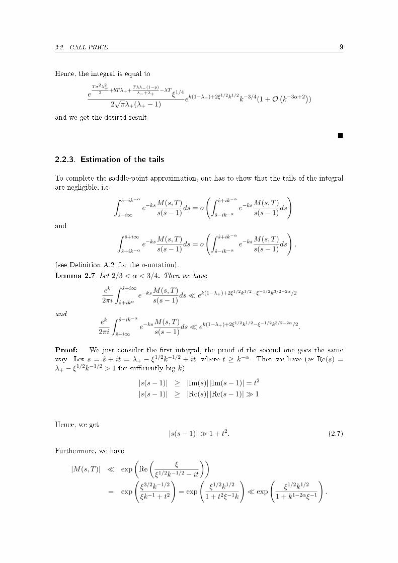
Hence, the integral is equal to

eTσ2λ2+

2+bTλ++


−λTξ1/4

2√πλ+(λ+ − 1)

ek(1−λ+)+2ξ1/2k1/2k−3/4(1 +O(k−3α+2

))

and we get the desired result.

�

2.2.3. Estimation of the tails

To complete the saddle-point approximation, one has to show that the tails of the integralare negligible, i.e. ∫ s−ik−α

s−i∞e−ks

M(s, T )

s(s− 1)ds = o

(∫ s+ik−α

s−ik−αe−ks

M(s, T )

s(s− 1)ds

)and ∫ s+i∞

s+ik−αe−ks

M(s, T )

s(s− 1)ds = o

(∫ s+ik−α

s−ik−αe−ks

M(s, T )

s(s− 1)ds

),

(see De�nition A.2 for the o-notation).

Lemma 2.7 Let 2/3 < α < 3/4. Then we have

ek

2πi

∫ s+i∞

s+ikαe−ks

M(s, T )

s(s− 1)ds� ek(1−λ+)+2ξ1/2k1/2−ξ−1/2k3/2−2α/2

andek

2πi

∫ s−ik−α

s−i∞e−ks

M(s, T )

s(s− 1)ds� ek(1−λ+)+2ξ1/2k1/2−ξ−1/2k3/2−2α/2.

Proof: We just consider the �rst integral, the proof of the second one goes the sameway. Let s = s + it = λ+ − ξ1/2k−1/2 + it, where t ≥ k−α. Then we have (as Re(s) =λ+ − ξ1/2k−1/2 > 1 for su�ciently big k)

|s(s− 1)| ≥ |Im(s)| |Im(s− 1)| = t2

|s(s− 1)| ≥ |Re(s)| |Re(s− 1)| � 1

Hence, we get|s(s− 1)| � 1 + t2. (2.7)

Furthermore, we have

|M(s, T )| � exp

(Re

(ξ

ξ1/2k−1/2 − it

))= exp

(ξ3/2k−1/2

ξk−1 + t2

)= exp

(ξ1/2k1/2

1 + t2ξ−1k

)� exp

(ξ1/2k1/2

1 + k1−2αξ−1

).


Using the fact 1/(1 +x) ≤ 1−x/2 for x ≤ 1 and that k1−2α is smaller than 1 for su�centlybig k, we get

|M(s, T )| � exp(ξ1/2k1/2 − ξ−1/2k3/2−2α/2

). (2.8)

So we get from (2.7) and (2.8)

ek

2π

∣∣∣∣e−ksM(s, T )

s(s− 1)

∣∣∣∣� ek(1−λ+)+2ξ1/2k1/2−ξ−1/2k3/2−2α/2

1 + t2,

and obtain

ek

2πi

∫ s+i∞

s+ik−αe−ks

M(s, T )

t(s− 1)ds� ek(1−λ+)+2ξ1/2k1/2−ξ−1/2k3/2−2α/2

∫ ∞k−α

dt

1 + t2

� ek(1−λ+)+2ξ1/2k1/2−ξ−1/2k3/2−2α/2.

�

After having derived an approximate saddle-point in (2.5), a central approximation inLemma 2.6 and estimating the remaining tails in Lemma 2.7 , we are ready to prove the�rst central result.

Proof (Theorem 2.2 ): We have

C(k, T ) =ek

2πi

∫ s+i∞

s−i∞e−ks

M(s, T )

s(s− 1)ds

=ek

2πi

∫ s−ik−α

s−i∞e−ks

M(s, T )

s(s− 1)ds+

ek

2πi

∫ s+ik−α

s−ik−αe−ks

M(s, T )

s(s− 1)ds

+ek

2πi

∫ s+i∞

s+ik−αe−ks

M(s, T )

s(s− 1)ds.

The second integral gives the main term, while the two others are asymptotically of smallerorder. Hence,

C(k, T ) =eTσ2λ2+

2+bTλ++


−λTξ1/4

2√πλ+(λ+ − 1)

ek(1−λ+)+2ξ1/2k1/2k−3/4

(1 +O

(k−3α+2

)+ O

(k3/4e−ξ

−1/2k3/2−2α))

=eTσ2λ2+

2+bTλ++

Tλλ−(1−p)λ−+λ+ ξ1/4

2√πλ+(λ+ − 1)

ek(1−λ+)+2ξ1/2k1/2k−3/4(1 +O

(k−3α+2

)),

= exp(−α1k − α1/2k

−1/2 − α0

)k−3/4

(1 +O

(k−3α+2

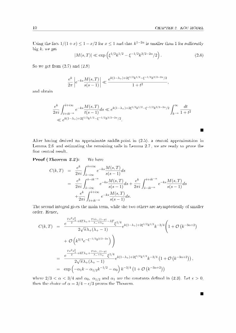
))where 2/3 < α < 3/4 and α0, α1/2 and α1 are the constants de�ned in (2.3). Let ε > 0,then the choice of α = 3/4− ε/3 proves the Theorem.

�

2.3. IMPLIED VOLATILITY 11

2.3. Implied volatility

To get an expansion for the implied volatility, we need the following result (see [GL, Corollary7.11]).

Lemma 2.8 If the absolute logarithm of the call price L := − logC(k, T ) satis�es

L = α1k + α1/2k1/2 + a` log k + α0 +O

(k−r),

where the αi are constants (with α1 > 0) for i = 0, 1/2, 1, ` and 0 < r < 1/2, then the

dimensionless implied volatility has the expansion

V (k) = β1/2k1/2 + β0 + β`−1/2

log k

k1/2+β−1/2

k1/2+O

(1

kr+1/2

),

where

β1/2 :=√

2α1 + 2−√

2α1,

β0 :=

(1√

2α1 + 2− 1√

2α1

)α1/2,

β`−1/2 :=

(1√

2α1 + 2− 1√

2α1

)(α` −

1

2

)and β−1/2 :=

(1√

2α1 + 2− 1√

2α1

)(α0 + log

1− (1 + 1/α1)−1/2

√4πα1

)

+

(1

2(2α1)3/2− 1

2(2α1 + 2)3/2

)α2

1/2.

Remark 2.9 The absolute log of the call price is actually a function in k, but for easeof notation we write simply L instead of L(k).

With this result, it is easy to prove Theorem 2.3 which gave an asymptotic expansion forthe implied volatility V (k).

Proof (Theorem 2.3 ):From the results in Theorem 2.2 , we see that the requirements for Lemma 2.8 are ful�lledwith α1 = λ+ − 1 > 0, α` = 3/4 and r = 1/2− ε.

�

Remark 2.10 Finally, it should be noted, that there already exist asymptotic expansionsfor the Kou model. In [AS09, Example 7.6], an expansion is given for the tail probability ofXT .


2.4. Numerical tests

2.4.1. Call price

Here we will test the accuracy of the constants in the expansion for the call price: α0, α1/2

and α1. A test can be based on the results of Theorem 2.2 . So we have

− log(C(k, T ))

k= α1 + α1/2k

−1/2 + α0k−1 +

3 log k

4k+O

(k−5/4+ε

)−−−→k→∞

α1, (A1)

− log (exp (α1k)C(k, T ))

k1/2= α1/2 + α0k

−1/2 +3 log k

4k1/2+O

(k−3/4+ε

)−−−→k→∞

α1/2, (A2)

− log(C(k, T ) exp

(α1k + α1/2k

1/2)k3/4

)= α0 +O

(k−1/4+ε

)−−−→k→∞

α0. (A3)

To calculate the call price we use its integral representation from (2.4) (with c = s)

C(k, T ) =ek

2πi

∫ s+i∞

s−i∞e−ks

M(s, T )

s(s− 1)ds

=ek

2π

∫ ∞−∞

e−k(s+is) M(s+ is, T )

(s+ is)(s− 1 + is)ds.

and integrate it numerically. We use the parameters in Table 2.1, which are taken from[M11, p.19] except for the riskfree interest rate r which is assumed to be zero.

r T σ λ λ+ λ− p

0.0 1 0.1 5 15 15 0.5

Table 2.1.: Parameters for the Kou model.

First, we have to determine the parameter b, so that (2.2) is ful�lled and the stock processbecomes a martingale. We get

b = −(σ2/2 + λ

(λ+p

λ+ − 1+λ−(1− p)λ− + 1

− 1

))= −0.027

and so the constants are (rounded to three decimal places)

α0 = −8.741, α1/2 = −12.247 and α1 = 14.

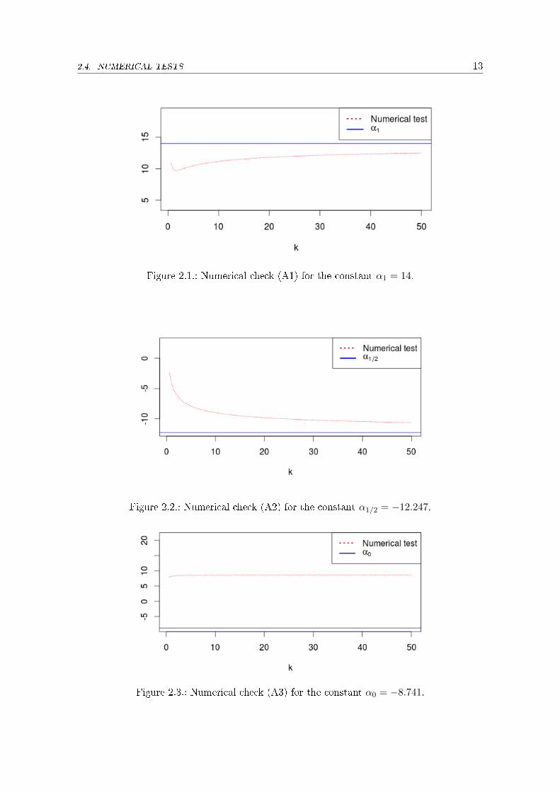
The plots of the numerical tests explained above are summarized in Figures 2.3 - 2.1. Onesees, that there is only a very slow convergence (even for big values k > 40). The plot of thetest (A3) for the coe�cient of the least dominant term, α0, does not show any convergenceat all. The plotting range is from k = 0 till k = 50, which is an unrealistically high valuefor a log-strike. Nevertheless these results can be used to do some qualitativve analysis (seeChapter 4).A reason for the slow convergence is, that we have used the approximated saddle-point s,in order to get the expansion for the call price. Figure 2.4 shows the di�erence between theapproximated and the numerically calculated exact saddle-point.

2.4. NUMERICAL TESTS 13

Figure 2.1.: Numerical check (A1) for the constant α1 = 14.

Figure 2.2.: Numerical check (A2) for the constant α1/2 = −12.247.

Figure 2.3.: Numerical check (A3) for the constant α0 = −8.741.


Figure 2.4.: Approximated saddle-point (dotted) and exact saddle-point(solid).

2.4.2. Implied volatility

The procedure to test the constansts of the expansion for V (k) is not much di�erent. FromTheorem 2.3 , we get

V (k)

k1/2= β1/2 +

β0

k+β−1/2

k+O

(k−5/4+ε

)−−−→k→∞

β1/2, (B1)

V (K)− β1/2k1/2 = β0 + β`−1/2

log k

k1/2+β−1/2

k1/2+O

(k−3/4+ε

)−−−→k→∞

β0, (B2)(V (k)− β1/2k

1/2 − β0

)k1/2

log k= β`−1/2 +

β−1/2

log k+O

(k−1/4+ε

log k

)−−−→k→∞

β`−1/2, (B3)(V (k)− β1/2k

1/2 − β0 − β`−1/2log k

k1/2

)k1/2 = β−1/2 +O

(k−1/4+ε

)−−−→k→∞

β−1/2. (B4)

By using the parameters from Table 2.1, we get for the constants (rounded to three decimalplaces)

β0 = 0.078, β1/2 = 0.186, β`−1/2 = −0.002 and β−1/2 = 0.144.

The plots of the numerical checks are summarized in Figures 2.5-2.8.In contrast to the previous test for the call price, the convergence to the constants of thesmile expansion is very good. Just the test for the coe�cient of the least dominant term,β−1/2, does not show much convergence. Here was the plotting range restricted to values ofk between 0 and 4, which are still very high values for log-strikes.


Figure 2.5.: Numerical check (B1) for the constant β1/2 = 0.186.

Figure 2.6.: Numerical check (B2) for the constant β0 = 0.078.

Figure 2.7.: Numerical check (B3) for the constant β`−1/2 = −0.002.


Figure 2.8.: Numerical check (B4) for the constant β−1/2 = 0.144.

Finally, the whole expansion for the implied volatility V (k) from Theorem 2.3 is plottedand is compared with the exact value as well as with the �rst-order expansion (1.2), whichwas given in [BF08]. This is done for di�erent parameters and maturities.

Figure 2.9.: Implied volatility (solid) compared with the fourth-order expansion (dotted)and Lee formula (dashed) in terms of log-strike. The parameters used here areT = 1, σ = 0.1, λ = 5, λ+ = 15, λ− = 15, p = 0.5.


Figure 2.10.: Implied volatility (solid) compared with the fourth-order expansion (dotted)and Lee formula (dashed) in terms of log-strike. The parameters used here areT = 0.1, σ = 0.2, λ = 10, p = 0.3, λ− = 25, λ+ = 50.

Figure 2.11.: Implied volatility (solid) compared with the fourth-order expansion (dotted)and Lee formula (dashed) in terms of log-strike. The parameters used here areT = 6, σ = 0.4, λ = 1, p = 0.2, λ− = 2, λ+ = 3.

18 CHAPTER 3. MERTON JUMP DIFFUSION MODEL

3. Merton Jump Di�usion model

3.1. Model de�ntion and general results

The Merton Jump Di�usion model ([M76]) is as the Kou model an exponential Lévy jumpdi�usion model. The di�erence lies in the distribution of the jumps Yi, which follow aGaussian distribution (mean µ ∈ R and variance δ2 > 0). So we have

ST = eXT

and XT is given by its moment generating function (see for example [FG13, p.5])

M(s, T ) = E [exp (sXT )] = exp

(T

(1

2σ2s2 + bs+ λ(eδ

2s2/2+µs − 1

)), s ∈ R,

where σ > 0 is the di�usion volatility and λ > 0 the jump intensity of the Poisson processin (1.1). The parameter b ∈ R is chosen, such that

E [ST ] = M(1, T ) = E [S0] = 1

is ful�lled, which ensures that ST becomes a martingale. Hence, we get

b = −(σ2/2 + λ

(eδ

2/2+µ − 1))

.

The cumulant generating function is hence

m(s, T ) = logM(s, T ) = T

(1

2σ2s2 + bs+ λ(eδ

2s2/2+µs − 1)

), s ∈ R.

The moment generating function M(s, T ) exists for all s ∈ R, hence the tail-wing formulaof Lee is not applicable, as there is no moment explosion. But in [BF09, Section 5.4] is anasymptotic formula for the (unannualized) implied volatility in the Merton Jump Di�usionmodel given

V (k) ∼ δ k

2√

2T log k, as k →∞.

The goal of this chapter is to re�ne this result.

3.1. MODEL DEFINTION AND GENERAL RESULTS 19

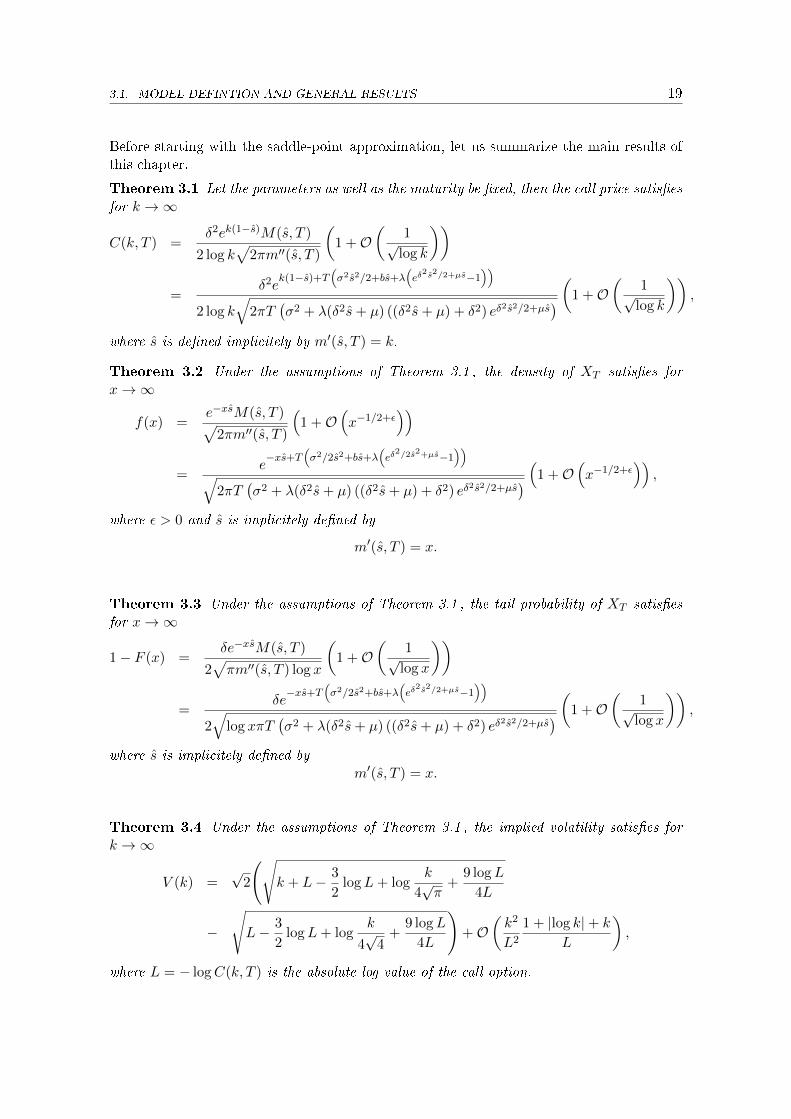
Before starting with the saddle-point approximation, let us summarize the main results ofthis chapter.

Theorem 3.1 Let the parameters as well as the maturity be �xed, then the call price satis�es

for k →∞

C(k, T ) =δ2ek(1−s)M(s, T )

2 log k√

2πm′′(s, T )

(1 +O

(1√

log k

))

=δ2e

k(1−s)+T(σ2s2/2+bs+λ

(eδ

2s2/2+µs−1))

2 log k√

2πT(σ2 + λ(δ2s+ µ) ((δ2s+ µ) + δ2) eδ2s2/2+µs

) (1 +O(

1√log k

)),

where s is de�ned implicitely by m′(s, T ) = k.

Theorem 3.2 Under the assumptions of Theorem 3.1 , the density of XT satis�es for

x→∞

f(x) =e−xsM(s, T )√

2πm′′(s, T )

(1 +O

(x−1/2+ε

))

=e−xs+T

(σ2/2s2+bs+λ

(eδ

2/2s2+µs−1))

√2πT

(σ2 + λ(δ2s+ µ) ((δ2s+ µ) + δ2) eδ2s2/2+µs

) (1 +O(x−1/2+ε

)),

where ε > 0 and s is implicitely de�ned by

m′(s, T ) = x.

Theorem 3.3 Under the assumptions of Theorem 3.1 , the tail probability of XT satis�es

for x→∞

1− F (x) =δe−xsM(s, T )

2√πm′′(s, T ) log x

(1 +O

(1√

log x

))

=δe−xs+T

(σ2/2s2+bs+λ

(eδ

2s2/2+µs−1))

2√

log xπT(σ2 + λ(δ2s+ µ) ((δ2s+ µ) + δ2) eδ2s2/2+µs

) (1 +O(

1√log x

)),

where s is implicitely de�ned by

m′(s, T ) = x.

Theorem 3.4 Under the assumptions of Theorem 3.1 , the implied volatility satis�es for

k →∞

V (k) =√

2

(√k + L− 3

2logL+ log

k

4√π

+9 logL

4L

−

√L− 3

2logL+ log

k

4√

4+

9 logL

4L

)+O

(k2

L2

1 + |log k|+ k

L

),

where L = − logC(k, T ) is the absolute log value of the call option.


3.2. Call price

3.2.1. Saddle-point

As previously in (2.4), the starting point is the Mellin transform of the call price

C(k, T ) =ek

2πi

∫ c+i∞

c−i∞e−ks

M(s, T )

s(s− 1)ds, k = logK > 0,

whenever 1 < c <∞.The denominator of the integrand is ignored in the calculation of the saddle-point. So thesaddle-point s is de�ned as the point satisfying(

e−ksM(s, T ))′

= 0,

where ′ denotes the partial derivative with respect to s. This is equivalent to

m′(s, T ) = k ⇔ T

(σ2s+ b+ λe

δ2s2

2+µs(δ2s+ µ)

)= k. (3.1)

The equation cannot be solved explicitly, so s is de�ned implicetely as the solution of (3.1).

Remark 3.5 Again we write s instead of s(k) for ease of notation.

In order to study the behaviour of m(s, T ) and its derivatives, we need an asymptoticrepresentation of s, which can be derived by using the bootstrapping method (see [B81,p.26]).

Lemma 3.6 The saddle-point s satis�es

δ2

2s2 = log k − µ

δ

√2 log k − log

√log k +

µ2

δ2− log

√2

δ+O

(log log k

log k

)and

s =

√2 log k

δ− µ

δ2+O

(log log k√

log k

),

as k →∞.

Proof: The idea of bootstrapping is to derive �rst a simple approximation of s and insertit into the original equation and to improve these approximations iteratively. From (3.1) itis easy to see that s is increasing in k, if we consider s as a function of k.

1. First we concentrate on the dominant term of the left-hand side in (3.1), so we havefor su�ciently big s

eδ2s2/2 ≤ T

(σ2s+ b+ λe

δ2s2

2+µs(δ2s+ µ)

)= k

or equivalently

δ2s2/2 ≤ log k,

so one gets the �rst estimate

s = O(√

log k). (3.2)

3.2. CALL PRICE 21

2. Again we concentrate on the dominant term and see that the following inequalitiesmust hold for su�ciently big s

λTδ2seδ2s2/2+µs ≤ k

⇔ log(λTδ2

)+ log s+ δ2s2/2 + µs ≤ log k. (3.3)

By using the asymptotics in (3.2) and that log s grows like log√

log k and hence slowlierthan µs, we get

δ2

2s2 = log k +O

(√log k

).

By factoring out the dominant term and using Lemma A.3 with (1 + x)1/2 = 1+O (x)for small x, we get the asymptotics for s

s2 =2 log k

δ2

(1 +O

(1√

log k

)),

s =

√2 log k

δ

(1 +O

(1√

log k

)).

3. From (3.3) we see

δ2s2

2+ µs+ log s = log k +O (1) ,

hence we get

δ2s2

2= −µ

δ

√2 log k +O (1) +O (log log k) + log k

= log k − µ

δ

√2 log k +O (log log k) . (3.4)

By factoring out the dominant term

s2 =2

δ2log k

(1−√

2µ

δ

1√log k

+O(

log log k

log k

))

and using√

1 + x = 1 + 12x+O

(x2)for small x, we get

s =

√2

δ

√log k

(1− µ√

2δ

1√log k

+O(

log log k

log k

))=

√2

δ

√log k − µ

δ2+O

(log log k√

log k

). (3.5)

4. Again, we re�ne the inequality and get by using log(1 + x) = x+O(x2)for small x

λT (δ2s+ µ)eδ2s2/2+µs ≤ k

⇔ log(λT ) + log(δ2s(1 +

µ

δ2s

)+ δ2s2/2 + µs ≤ log k

⇔ log(λTδ2) + log s+µ

δ2s+O

(1

s2

)+ δ2s2/2 + µs ≤ log k.


Putting all terms except δ2

2 s2 on the right side and using the asymptotics of s from

(3.4), yields

δ2s2

2= log k − µ

δ

√2 log k − log

√log k +

µ2

δ2− log

√2

δ− log

(λTδ2

)+ O

(log log k

log k

).

After factoring out the dominant term

δ2s2

2= log k

(1−

√2µ

δ√

log k− log

√log k

log k+

(µ2

δ2− log

√2

δ− log(λTδ2)

)1

log k

+ O(

log log k

(log k)2

))

and using again√

1 + x = 1+ x2 +O

(x2)for small x, we obtain the desired asymptotics

s =

√2 log k

δ

(1− µ

δ√

2 log k+O

(log log k

log k

))=

√2 log k

δ− µ

δ2+O

(log log k√

log k

).

�

Remark 3.7 One sees, that s tends to in�nity as k → ∞. Hence s is bigger than 1 forsu�ciently big k and it can be used as a saddle-point in (2.4).

3.2.2. Asymptotics of the cumulant generating function

After having derived an expansion for s in Lemma 3.6 , one has to investigate the behaviourof the cumulant generating function m(s, T ) and its derivatives, in order to determine aninterval for the central approximation.

Lemma 3.8 The cumulant generating function satis�es for k →∞

m(s, T ) =k

δ√

2 log k

(1 +O

(log log k

log k

)),

m′′(s, T ) = δk√

2 log k

(1 +O

(1√

log k

)),

and

m′′′(s+ it, T ) = 2k log k

(1 +O

(1

log k

)),

where |t| < k−α, α > 0.

3.2. CALL PRICE 23

Proof: We have for s ∈ R

m(s, T ) = T

(σ2

2s2 + b+ λ

(exp

(δ2

2s2 + µs

)− 1

)),

m′(s, T ) = T

(σ2s+ b+ λ

((δ2s+ µ) exp

(δ2

2s2 + µs

))),

m′′(s, T ) = T

(σ2 + λ

((δ2s+ µ

)2+ δ2

)exp

(δ2

2s2 + µs

))and

m′′′(s, T ) = λT exp

(δ2

2s2 + µs

)((δ2s+ µ)

((δ2s+ µ)2 + δ2

)+ 2δ2(δ2s+ µ)

).

First, one gets for the dominant term by using the asymptotics of s from Lemma 3.6

exp

(δ2

2s2 + µs

)= exp

(log k − log

√log k − log(λTδ2)− log

√2

δ+O

(log log k√

log k

))

=k

λδT√

2 log k

(1 +O

(log log k√

log k

)).

So we have

m(s, T ) = T

(σ2

2s2 + bs+ λ

(exp

(δ2

2s2 + µs

)− 1

))=

k

δ√

2 log k

(1 +O

(log log k√

log k

))and

m′′(s, T ) = T

(σ2 + λ

((δ2s+ µ

)2+ δ2

)exp

(δ2

2s2 + µs

))∼ λTδ4s2 exp

(δ2

2s2 + µs

)= δk

√2 log k

(1 +O

(1√

log k

)).

For the third derivative, one has to investigate the term((δ2(s+ it) + µ)

((δ2(s+ it) + µ)2 + δ2

)+ 2δ2(δ2(s+ it) + µ)

)= δ2s

(1 +O

(1√

log k

))δ2s2

(1 +O

(1

log k

))+ 2δ4s

(1 +O

(1√

log k

))= δ4s3

(1 +O

(1√

log k

))+ 2δ4s

(1 +O

(1√

log k

))= δ4s3

(1 +O

(1√

log k

))= δ(2 log k)3/2

(1 +O

(1√

log k

)).


So we get

∣∣m′′′(s+ it, T )∣∣ =

∣∣∣∣λT exp

(δ2

2(s+ it)2 + µ(s+ it)

)δ(2 log k)3/2

(1 +O

(1√

log k

))∣∣∣∣= λT exp

(δ2

2(s2 − t2) + µs

)δ(2 log k)3/2

(1 +O

(1√

log k

))≤ λT exp

(δ2

2s2 + µs

)δ(2 log k)3/2

(1 +O

(1√

log k

))= 2k log k

(1 +O

(1

log k

)).

�

As in the Kou model, the result of this Lemma is crucial, in order to determine the intervalfor the central approximation.

3.2.3. Central approximation

We have to determine the interval around the saddle-point which satis�es the two conditionsas in (2.6). By using the fact that log k grows slowlier than kε for any ε > 0, we get byusing Lemma 3.8

m′′(s)k−2α −−−→k→∞

∞⇔ α < 1/2

m′′′(s+ it)k−3α −−−→k→∞

0⇔ α > 1/3

We get the interval (s− k−α, s+ k−α) with 1/3 < α < 1/2.Before doing the central approximation, one needs to examine the denominator. By insertingthe asymptotics of s from Lemma 3.6 and using (1+x)−1 = 1+O (x) for small x, we obtain

1

(s+ it)(s− 1 + it)

=

(√2 log k

δ− µ

δ2+ it+O

(log log k√

log k

))−1(√2 log k

δ− µ

δ2− 1 + it+O

(log log k√

log k

))−1

=δ2

2 log k

(1 +O

(1√

log k

)). (3.6)

Putting (3.6) and the asymptotics of the cumulant generating functionm(s, T ) from Lemma 3.8together, gives us the following result.

Lemma 3.9 Let 1/3 < α < 1/2. Then the integral satis�es

ek

2πi

∫ s+ik−α

s−ik−αe−ks

M(s, T )

s(s− 1)ds =

δ2ek(1−s)M(s, T )

2 log k√

2πm′′(s, T )

(1 +O

(1√

log k

))

=δ2e


(eδ

2s2/2+µs−1))

2 log k√

2πT(σ2 + λ(δ2s+ µ) ((δ2s+ µ) + δ2) eδ2s2/2+µs

) (1 +O(

1√log k

)),

3.2. CALL PRICE 25

where s is implicitely de�ned by

m′(s, T ) = k. (3.7)

Proof: Applying Taylors theorem and using the results of the Lemma 3.8 , gives us

m(s+ it, T ) = m(s, T ) + itm′(s, T )− t2

2m′′(s, T ) +O

(t3k log k

)= m(s, T ) + itk − t2

2m′′(s, T ) +O

(k1−3α

).

Using exp(x) = 1 +O (x) for small x, we get

M(s+ it, T ) = exp (m(s+ it, T )) = exp

(m(s, T ) + itk − t2

2m′′(s, T ) +O

(k1−3α

))= M(s, T ) exp

(itk − t2

2m′′(s, T )

)(1 +O

(k1−3α

)).

Inserting this in the integral and the asymptotics of denominator from (3.6), yields

ek

2πi

∫ s+ik−α

s−ik−αe−ks

M(s, T )

s(s− 1)ds

=ek(1−s)

2π

∫ k−α

−k−αe−itk

M(s+ it, T )

(s+ it)(s− 1 + it)dt

=δ2ek(1−s)M(s, T )

4π log k

(1 +O

(1√

log k

))∫ k−α

−k−αe−

t2

2m′′(s,T )dt. (3.8)

After doing the substitution ω = ut (with u :=√m′′(s, T )) and using the fact that Gaussian

integrals have exponentially decaying tails, we get∫ k−α

−k−αe−

t2

2m′′(s,T )dt =

1

u

∫ uk−α

−uk−αe−ω

2/2dω =1

u

(∫ ∞−∞

e−ω2/2dω +O

(e−u

2/(2k2α)))

=

√2π√

m′′(s, T )

(1 +O

(e−u

2/(2k2α)))

.

So we have

δ2ek(1−s)M(s, T )

4π log k

(1 +O

(1√

log k

))∫ k−α

−k−αe−

t2

2m′′(s,T )dt

=δ2ek(1−s)M(s, T )

2√

2πm′′(s, T ) log k

(1 +O

(1√

log k

))

=δ2e


(eδ

2s2/2+µs−1))

2 log k√

2πT(σ2 + λ (δ2s+ µ) ((δ2s+ µ) + δ2) eδ2s2/2+µs

) (1 +O(

1√log k

)).

�


3.2.4. Estimation of the tails

Now one needs to show that the tails are negligible, to complete the approximation.

Lemma 3.10 Let 1/3 < α < 1/2. Then we have

ek

2πi

∫ s+i∞

s+ik−α

e−ksM(s, T )

s(s− 1)ds� ek(1−s)M(s, T )e−δk

1−2α/(2√

2 log k)

log k

andek

2πi

∫ s−ik−α

s−i∞

e−ksM(s, T )

s(s− 1)ds� ek(1−s)M(s, T )e−δk

1−2α/(2√

2 log k)

log k.

Proof: One just needs to consider the �rst integral, as the derivation of the second resultis the same due to the symmetry of t2. Let s = s+ it with t ≥ k−α. Then we get

|s(s− 1)| ≥ Re (s(s− 1)) = s(s− 1)� log k.

Furthermore we obtain

|M(s, T )| = exp

[Re

(T

(σ2

2s2 + bs+ λ

(eδ

2s2/2+µs − 1)))]

= exp

[(T

(σ2

2(s2 − t2) + bs+ λ

(cos(δ2t+ µt

)eδ

2(s2−t2)/2+µs − 1)))]

≤ exp

[(T

(σ2

2(s2 − t2) + bs+ λ

(eδ

2s2/2+µse−δ2k−2α/2 − 1

)))]

Usinge−δ

2k−2α/2 = 1− δ2k−2α/2 +O(k−4α

)and the result from Lemma 3.8

eδ2s2/2+µs ∼ k

λδT√

2 log k,

we getM(s, T )� e−Tσ

2t2/2M(s, T )e−δk1−2α/(2

√2 log k).

These estimates imply

ek

2π

∣∣∣∣e−ksM(s, T )

s(s− 1)

∣∣∣∣� ek(1−s)M(s, T )e−δk1−2α/(2

√2 log k)

log ke−Tσ

2t2/2

and so we obtain

ek

2πi

∫ s+i∞

s+ik−α

e−ksM(s, T )

s(s− 1)ds � ek(1−s)M(s, T )e−δk

1−2α/(2√

2 log k)

log k

∫ ∞k−α

e−σ2t2T/2dt

� ek(1−s)M(s, T )e−δk1−2α/(2

√2 log k)

log k.

�

3.3. DENSITY FUNCTION 27

Now all three main steps of the saddle-point method have been done and we can prove themain result for the call price

Proof (Theorem 3.1 ): The call price satis�es

C(k, T ) =ek

2πi

∫ s−k−α

s−i∞

e−ksM(s, T )

s(s− 1)ds+

ek

2πi

∫ s+k−α

s−k−α

e−ksM(s, T )

s(s− 1)ds

+ek

2πi

∫ s+i∞

s+k−α

e−ksM(s, T )

s(s− 1)ds.

The middle term gives the main term, as we can see by using the central approximationfrom Lemma 3.9

C(k, T ) =δ2ek(1−s)M(s, T )

2 log k√

2πm′′(s, T )

(1 +O

(1√

log k

)+O

(e−δk

1−2α/(2√

2 log k)

√k log k

))

=δ2ek(1−s)M(s, T )

2 log k√

2πm′′(s, T )

(1 +O

(1√

log k

)).

�

3.3. Density function

The density function of ST satis�es

f(x) =1

2πi

∫ c+i∞

c−i∞e−luM(u− 1, T )du =

e−l

2πi

∫ c+i∞

c−i∞e−ltM(t, T )dt (3.9)

with l := log x and c ∈ R (see (B.2)).Again, we de�ne our saddle-point implicitely by

m′(s, T ) = l

and in the same way as in Lemma 3.6 we get the asymptotics (for l→∞)

δ2s2

2= log l − µ

δ

√2 log l − log

√log l +

µ2

δ2− log

√2

δ− log

(λTδ2

)+ O

(log log l

log l

)(3.10)

= log l

(1−

√2µ

δ√

log l− log

√log l

log l+

(µ2

δ2− log

√2

δ− log(λTδ2)

)1

log l

+ O(

log log l

(log l)2

))and

s =

√2 log l

δ

(1− µ

δ√

2 log l+O

(log log l

log l

))(3.11)

=

√2 log l

δ− µ

δ2+O

(log log l√

log l

).


Similarly, the asymptotics for the cumulant generating function m(s, T ), its derivatives donot change and neither does the interval around the saddle-point for the approximation(s ± l−α with 1/3 < α < 1/2). Hence, the expansion for the density can be derived in thesame way as for the call price in Section 3.2.

Proof (Theorem 3.2 ): Let f(x) denote the density of ST , so we have

f(x) =e−l

2π

∫ ∞−∞

e−l(s+it)M(s+ it, T )dt,

where l = log x.Applying the Laplace method on the central interval as in Lemma 3.9 and estimating theremaining tails as in Lemma 3.10 , yields

f(x) =e−l(1+s)M(s, T )√

2πm′′(s, T )

(1 +O

(l1−3α

))=

e−l(1+s)+T

(σ2s2/2+bs+λ

(eδ

2s2/2+µs−1))

√2πT

(σ2 + λ(δ2s+ µ) ((δ2s+ µ) + δ2) eδ2s2/2+µs

) (1 +O(l1−3α

)),

where 1/3 < α < 1/2.To get the density of XT (denoted by f(x)), we have to use the relation

f(x) = exf(ex), x ∈ R.

So we have

f(ex) =e−x(1+s)M(s, T )√

2πm′′(s, T )

(1 +O

(x1−3α

)),

where s is implicitely de�ned bym′(s, T ) = x.

Multiplying the term with ex and choosing α = 12 −

ε3 completes the proof.

�

3.4. Tail probability

From (B.3) in the appendix we have the integral representation for the tail probability of ST

1− F (x) =1

2πi

∫ c+i∞

c−i∞

M(u, T )

ue−ludu (3.12)

where 1 < c <∞.Again, we ignore the denominator in the calculation of the saddle-point, so we can use thesame saddle-point as for the density function. The derivation of the expansion is also thesame, just the asymptotics of the denominator have to be added

1

(s+ it)=

(√2 log l

δ− µ

δ2+ it+O

(log log l√

log l

))−1

=δ√

2 log l

(1 +O

(1√log l

)). (3.13)

3.4. TAIL PROBABILITY 29

Lemma 3.11 The tail probability of ST satis�es

1− F (x) =δe−lsM(s, T )

2√πm′′(s, T ) log l

(1 +O

(1√log l

))

=δe−ls+T

(σ2/2s2+bs+λ

(eδ

2s2/2+µs−1))

2√πT log l

(σ2 + λ(δ2s+ µ) ((δ2s+ µ) + δ2) eδ2s2/2+µs

) (1 +O(

1√log l

)),

where l = log x and s is implicitely de�ned by

m′(s, T ) = l.

Proof:The proof goes along the same lines as for the density of ST in the proof of Theorem 3.2 ,one just has to add (3.13).

�

With this result, it is easy to prove the asymptotics for the tail probability of XT .

Proof (Theorem 3.3 ): One just needs the result for ST in Lemma 3.11 and to usethe simple tranformation

1− F (x) = 1− F (ex),

where F (x) is the cumulative distribution function of XT .

�

Finally, we compare the tails to the Gaussian and exponential distribution to verify a resultfrom [CT04].

Corollary 3.12 The tails of XT are heavier than Gaussian, but lighter than exponential,i.e.

1− FN (x) = o (1− F (x))

and1− F (x) = o (1− FEx(x)) ,

where FN and FEx are Gaussian, respectively Exponential, distribution functions and F isthe distribution function of XT .


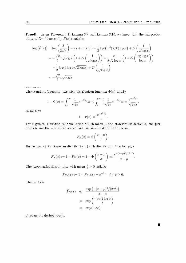
Proof: From Theorem 3.3 , Lemma 3.8 and Lemma 3.10, we know that the tail proba-bility of XT (denoted by F (x)) satis�es

log(F (x)

)= log

(δ

2√π

)− xs+m(s, T )− 1

2log(m′′(s, T ) log x

)+O

(1√

log x

)= −√

2

δx√

log x

(1 +O

(1√

log x

))+

x

δ√

2 log x

(1 +O

(log log x

log x

))− 1

2log(δ log x

√2 log x) +O

(1√

log x

)∼ −√

2

δx√

log x,

as x→∞.The standard Gaussian tails with distribution function Φ(x) satisfy

1− Φ(x) =

∫ ∞x

1√2πe−t

2/2dt ≤∫ ∞x

t

x

1√2πe−t

2/2dt =e−x

2/2

√2πx

,

so we have

1− Φ(x)� e−x2/2

x.

For a general Gaussian random variable with mean µ and standard deviation σ, one justneeds to use the relation to a standard Gaussian distribution function

FN (x) = Φ

(x− µσ

).

Hence, we get for Gaussian distributions (with distribution function FN )

FN (x) := 1− FN (x) = 1− Φ

(x− µσ

)� e−(x−µ)2/(2σ2)

x− µ.

The exponential distribution with mean 1λ > 0 satis�es

FEx(x) := 1− FEx(x) = e−λx for x ≥ 0.

The relation

FN (x) �exp

(−(x− µ)2/(2σ2)

)x− µ

� exp

(−x√

2 log x

δ

)� exp (−λx)

gives us the desired result.

�

3.5. IMPLIED VOLATILITY 31

Remark 3.13 This result is already mentioned in [CT04, Table 4.3, p.124].

Remark 3.14 In [BF09, Example 5.4], it is already mentioned that some Lévy tail estimateresults in [AB] can be used to derive the asymptotics

log F (x) ∼ −xδ

√2 log x,

where F (x) = 1− F (x).

3.5. Implied volatility

To get an expansion for the implied volatility, we need again a result from the paper [GL,Corollary 7.1.]

Lemma 3.15 If the absolute log of the call price L = − logC(k, T ) satis�es

k/L −−−→k→∞

0,

then the dimensionless implied volatility satis�es for k →∞∣∣∣∣G−(k, L− 3

2logL+ log

k

4√π

)− V (k)

∣∣∣∣ = O(

k

L3/2

),∣∣∣∣G−(k, L− 3

2logL+ log

k

4√π

+9 logL

4L

)− V (k)

∣∣∣∣ = O(

k

L3/2

),

where G−(κ, u) :=√

2(√u+ κ−

√u).

With this result, it is easy to proof the asymptotics for the implied volatility.

Proof (Theorem 3.4 ): By using Theorem 3.1 , Lemma 3.8 and the asymptotics of thesaddle-point s from Lemma 3.7, we get (similarly to the proof of Corollary 3.12 )

L = − log (C(k, T ))

= − log

(δ2

2√

2π

)− k(1− s)−m(s, T ) +

1

2log(m′′(s, T ) log k

)+ log log k +O

(1√

log k

)∼√

2

δk√

log k,

as k →∞.Because k/L→ 0 for k →∞, we can apply Lemma 3.15 and get the result.

�


3.6. Numerical Tests

The parameters from Table 3.1 are taken from [M11, p.14] (again except for the interestrate r which is set zero).

r T σ λ µ δ

0.0 1 0.1 5 -0.001 0.1

Table 3.1.: Parameters for the Merton Jump Di�usion model.

Again the martingale condition (2.2) has to be ful�lled, so we get

b = −(σ2/2 + λ

(eδ

2/2+µ − 1))

= −0.025.

Here the asymptotic expansions are compared with the exact call price (respectively thedensity, tail probability and implied volatility), which we get by numerical computation.The saddlepoint s is calculated numerically with the root-�nding procedure uniroot().


3.6.1. Call price

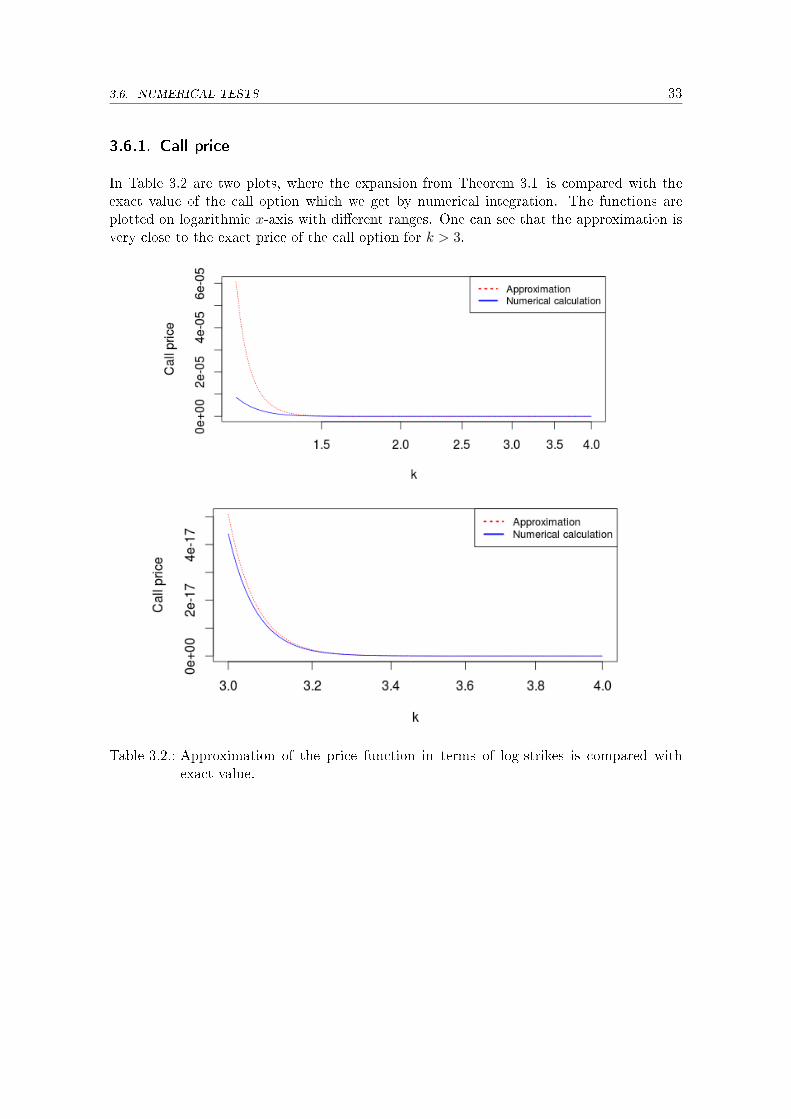
In Table 3.2 are two plots, where the expansion from Theorem 3.1 is compared with theexact value of the call option which we get by numerical integration. The functions areplotted on logarithmic x-axis with di�erent ranges. One can see that the approximation isvery close to the exact price of the call option for k > 3.

Table 3.2.: Approximation of the price function in terms of log-strikes is compared withexact value.


3.6.2. Density

In Table 3.3, one sees that the density can be approximated with our expansion very well.For values x > 0.4 the expansion and the numerically calculated density are almost identicaland they cannot be distinguished anymore in the plot.

Table 3.3.: Approximation of the density function is compared with exact density.

3.6.3. Tail probability

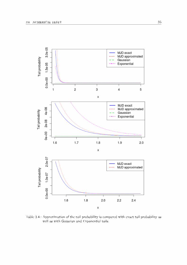
In Table 3.4 it is illustrated, that the tail probabilities do satisfy Corollary 3.12 , whichsaid that the log-price of the stock, XT = logST , has heavier tails than Gaussian distribu-tions, but lighter ones than the exponential distribution. Here was the Gaussian probabilitycalculated with the R-command pnorm() with mean 0 and standard deviation 0.1, the ex-ponential tail probability was calculated explicitely (with mean 0.1). It can also be seenthat the expansion approximates the tail probability fairly well for x > 1.5.


Table 3.4.: Approximation of the tail probability is compared with exact tail probability aswell as with Gaussian and Exponential tails.


3.6.4. Implied volatility

Finally the implied volatility is plotted against the expansion from Theorem 3.4 and theapproximation given in [BF09] for di�erent parameters and maturities. One sees that thehigher-order expansion from Theorem 3.4 yields clearly better results.

Table 3.5.: Comparison of implied volatility (solid) with the expansion from Theorem3.4 (dotted) and the expansion from [BF09] (dashed). Parameters used: T = 1,σ = 0.1, λ = 5, µ = −0.001, δ = 0.1 (�rst plot); T = 0.1, σ = 0.4, λ = 0.1,µ = 0.3 and δ = 0.4 (second plot).


Table 3.6.: Comparison of implied volatility (solid) with the expansion from Theorem3.4 (dotted) and the expansion from [BF09] (dashed). Parameters used: ; T = 4,σ = 0.6, λ = 3, µ = 0.2 and δ = 0.4.

38 CHAPTER 4. CONCLUSION

4. Conclusion

In the Kou model, the numerical tests for the constants in the expansion for the call priceshowed very slow convergence. Nevertheless, the results for the implied volatility skew werevery good and it was possible to show that the higher-order expansion does yield betterapproximations than the �rst-order expansion given in [BF08]. As it was already noted, thesaddle-point was approximated in the Kou model in contrast to the Merton Jump di�usionmodel, where it was de�ned implicitely and calculated exactly by a root �nding procedurefor the numerical tests. This explains, why the results in the Merton Jump Di�usion modelseem to be sharper. The call price approximation yields fairly good results for k > 3. Alsothe tail probability and especially the density expansion seem to be very accurate for valuesx > 2. Finally, we could also �nd a sharper approximation of the implied volatility andimprove the result for the Merton Jump Di�usion model, given in [BF09].One should add, that the approximations are becoming accurate for very high log-strikevalues (respectively stock values), which are not very relevant in the practical world. Nev-ertheless, this thesis contributes to the qualitative analysis. In the Kou model, one can seethat the critical moment λ+ is the only parameter that is needed to determine the �rst-order approximation. The jump intensity λ, the maturity T and p are the parameters, whichdetermine together with λ+ the constant in the second-order expansion for the call price.The other parameters σ, b and λ− are just in the α0 term. The same applies to the im-plied volatility, where the second-order expansion is entirely de�ned by the four parametersλ+, λ, T and p.

39

A. Landau notation

A.1. Basics

De�nition A.1 For f : D ⊆ C → C and g : D ⊆ C → C, f(x) = O (g) means that thereexist C > 0 and δ > 0 such that

|f(x)| ≤ C |g(x)| for x > δ.

De�nition A.2 For f : D ⊆ C→ C and g : D ⊆ C→ C, f(x) = o (g) means that

limx→∞

f(x)

g(x)= 0.

Lemma A.3 (see [H09]): Let f : D ⊆ C → C be analytic on some disk |x| < r for some

r > 0, i.e.

f(x) =

∞∑k=0

akxk.

Then for n ∈ N and |x| < r

f(x) =n∑k=0

akxk +O

(|x|n+1

).

Proof: The result follows immediately from Taylors theorem.

�

A.2. Some Taylor series

Here are the most important series listed that are used in thesis.

De�nition A.4 (Binomial series):

(1 + x)α =

∞∑k=0

(α

k

)xk (A.1)

converges for all x ∈ (−1, 1) and α ∈ R.

40 CHAPTER A. LANDAU NOTATION

De�nition A.5 (Exponential series):

exp(x) =∞∑k=0

xk

k!(A.2)

converges for all x ∈ R.

De�nition A.6 (Logarithmic series):

log(1 + x) =

∞∑n=1

(−1)n+1

nxn (A.3)

converges for |x| ≤ 1 except x = −1.

Most of the time these series are used together with Lemma A.3 . Finally, an example isgiven, in order to illustrate how the Lemma is used in the thesis.

Example A.7 Let f : C→ C satisfy

f(x) = x+O(x−2

), as x→∞.

Then we get by using (A.1) and Lemma A.3 , that

(1 + x)1/2 = 1 +O (x) , for small x

and hence √f(x) =

(x(1 +O

(x−3

)))1/2=√x(1 +O

(x−3

)).

41

B. Mellin transform

Most of the following results have been taken from [P96] and [H].

B.1. Basic results

De�nition B.1 (Mellin transform): For a function (on the positive real axis) f theMellin transform (named after the Finnish mathematician Hjalmar Mellin) is de�ned by

M(f ; s) ≡ F (s) :=

∫ ∞0

f(t)ts−1dt.

In general, the transform F exists only on a strip (or halfplane) in C.

Remark B.2 There exist slightly di�erent notations (see for example [H, p.2]).

Lemma B.3The Fourier transform of a function f

F(f ; s) ≡ f(s) :=

∫ ∞−∞

f(x)e−2πisxdx.

satis�es the following relationship to the Mellin transform

M(f(x); a+ 2bπi) = F(f(e−x)e−ax; b), a, b ∈ R.

Proof: By doing the substitution t = e−x we get the relation

M(f(t); a+ 2bπi) =

∫ ∞0

f(t)ta+2πbi−1dt

=

∫ ∞−∞

f(e−x)e−axe−2πbxidx = F(f(e−x)e−ax; b). (B.1)

�

42 CHAPTER B. MELLIN TRANSFORM

Lemma B.4 (Mellin Inversion): Let F (s) =M(f(x); s) denote the Mellin transform of

a function f and let us assume F ∈ L1, then the following holds

f(x) =1

2πi

∫ c+i∞

c−i∞F (s)x−sds,

where c has to be on the strip of de�nition of F .

Proof: By using the Fourier Inversion theorem

f(x) =

∫ ∞−∞

f(s)e2πxsids

and the relation (B.1), one gets easily the Mellin Inversion formula

f(e−x)eax =

∫ ∞−∞

F (s)e2πβxidβ

⇔ f(t) = t−a∫ ∞−∞

F (s)t−2πβidβ

⇔ f(t) =1

2πi

∫ a+i∞

a−i∞F (s)t−sds.

�

B.2. Applications of the Mellin transformation

B.2.1. Call price

First it is easy to see for the payo� function of a European call option f(x) := (x − ek)+

with log-strike k > 0, that

M((

x− ek)

+; s

)=

∫ ∞0

(x−ek)+xs−1dx =

∫ ∞ek

(x−ek)xs−1dx =ek(s+1)

s(s+ 1)for Re(s) < 1.

Lemma B.5 Let XT be the log-return of a stock and suppose that its moment generating

function M(t) exists for some t > 1. Then a call price can be written as

C(k, T ) =ek

2πi

∫ c+i∞

c−i∞e−ks

M(s, T )

s(s− 1)ds,

whenever 1 < c < T ∗ := sup {t ≥ 0 : M(t) <∞}.

Proof: By applying the inversion theorem we get

(x− ek)+ =1

2πi

∫ c+i∞

c−i∞

ek(s+1)

s(s+ 1)x−sds for Re(s) < 1.

B.2. APPLICATIONS OF THE MELLIN TRANSFORMATION 43

Setting XT := logST , k := logK and c < 1, applying Fubini's theorem yields (the expecta-tion is taken under the martingale measure) and doing the substitution s = −t, yields

E[(eXT − ek)+

]= E

[ek

2πi

∫ c+i∞

c−i∞

eks

s(s+ 1)e−sXT ds

]=

ek

2πi

∫ c+i∞

c−i∞

eks

s(s+ 1)E[e−sXT

]ds

=ek

2πi

∫ c+i∞

c−i∞

eks

s(s+ 1)M(−s)ds =

ek

2πi

∫ c+i∞

c−i∞

M(t, T )e−kt

t(t− 1)dt.

�

B.2.2. Probability density function

If the moment generating function of XT exists on an interval, one can recover the densityof ST , denoted by f(x), easily from

M(f(x); s) =

∫ ∞0

xs−1f(x)dx = E[Ss−1T

]= E

[e(s−1)XT

]= MXT (s− 1)

and by using the Mellin inversion theorem, we get

f(x) =1

2πi

∫ c+i∞

c−i∞M(u− 1)x−udu, (B.2)

where c has to be on the strip of de�nition of M(c− 1).

B.2.3. Tail probability

Assuming that M(t) exists for some t > 1, then one gets for the tail probability of ST (byapplying Fubini's theorem) for Re(s) > 1

M(1− F (x); s) =

∫ ∞0

(1− F (t)

)ts−1dt =

∫ ∞0

(∫ ∞t

f(x)dx

)ts−1dt

=

∫ ∞0

(∫ x

0ts−1dt

)f(x)dx

=

∫ ∞0

xs

sf(x)dx =

M(f(x); s+ 1)

s=MXT (s)

s

and hence the tail probability is given by

1− F (x) =1

2πi

∫ c+i∞

c−i∞

MXT (u)x−u

udu, (B.3)

where 1 < c < T ∗.

To get the density and tail probability of XT = logST (denoted by f(x) and its cumulativedistribution function by F (x)), we use

F (ex) = P(ST < ex) = P(XT < x) = F (x)

f(ex)ex = f(x) (B.4)

44 CHAPTER C. IMPLEMENTATION IN R

C. Implementation in R

Finally, the most important parts of the implementation in R are given.

C.1. Kou model

First the parameters and all constants of the expansions are de�ned as global variables.Futhermore the value k_critical is de�ned, which gives the k when the saddle-point s isgreater than 1. This is implemented in kou_param().The code carries out the numerical checks for the constants, given in the equations (A1)-(A3) and (B1)-(B4). Here is the call price numerically calculated by using the quadinf()

function on the integral representation of the call price

C(k, T ) =ek

2π

∫ ∞−∞

e−k(s+is) M(s+ is, T )

(s+ is)(s− 1 + is)ds.

The implied volatility can be calculated by using a root-�nding procedure. Here was theuniroot() function used.

#parameter definitions as global variables

kou_param<-function(param=c(0.15,0,1,10,25,50,0.3)){

param1<<-c(0.1,0,1,5,15,15,0.5)

param2<<-c(0.2,0,0.1,10,25,50,0.3)

param3<<-c(0.4,0,6,1,2,3,0.2)

sigma<<- param[1]

r<<- param[2]

bigT<<-param[3]

lambda<<-param[4]

lambdaminus<<-param[5]

lambdaplus<<-param[6]

p<<-param[7]

b<<--(sigma^2/2+lambda*(lambdaplus*p/(lambdaplus-1)

+lambdaminus*(1-p)/(lambdaminus+1)-1))

i<<-complex(real=0,imaginary=1)

xi<<-lambda*lambdaplus*p*bigT

alpha1<<-lambdaplus-1

C.1. KOU MODEL 45

alpha0.5<<- -2*sqrt(xi)

alpha0<<-log((exp((bigT*sigma^2*lambdaplus^2)/2+

b*lambdaplus*bigT+(bigT*lambda*lambdaminus*(1-p))/(lambdaminus+lambdaplus)

-lambda*bigT)*xi^(1/4))/(2*sqrt(pi)*lambdaplus*(lambdaplus-1)))

gamma_kou<<-1/(sqrt(2*alpha1+2))-1/sqrt(2*alpha1)

beta0 <<- gamma_kou*alpha0.5

beta0.5 <<- -2*gamma_kou*sqrt(alpha1^2+alpha1)

betaell <<- gamma_kou/4

betaminus <<- (alpha0+log((1-(1+1/alpha1)^(-1/2))/sqrt(4*pi*alpha1)))

*gamma_kou+(1/(2*(2*alpha1)^(3/2))-1/(2*(2*alpha1+2)^(3/2)))*alpha0.5^2

source("s_star.R")

f<-function(k) s_star(k) - 1

k_critical <<- uniroot(f,c(0.000001,50))$root

}

#approximated saddle-point

s_star<-function(k)

{

lambdaplus-xi^(1/2)*k^(-1/2)

}

#numerically calculated exact saddle-point

s_exact<-function(k){

f<-function(t) m1(t)/(t*(t-1))-k

uniroot(f,c(1.5,lambdaplus*0.99999))$root

}

#mgf

M<-function(s) {

as.complex(exp(bigT*((sigma^2*s^2)/2+b*s+

lambda*((lambdaplus*p)/(lambdaplus-s)+

(lambdaminus*(1-p))/(lambdaminus+s)-1))))

}

#first derivative of cumulant generating function

m1<-function(s){

bigT*(sigma^2*s+b+lambda*(lambdaplus*p/(lambdaplus-s)^2

-lambdaminus*(1-p)/(lambdaminus+s)^2))

}

#numerically calculated call price

Kou_Price<-function(k) {

exp(k)/(2*pi)*quadinf(function(s) Re(exp(-k*(s_star(k)+i*s))


*M(s_star(k)+ i*s)/((s_star(k)+i*s)*(s_star(k)-1+i*s))),-Inf, Inf)

}

#asymptotic expansion of the call price

kou_price_approx<-function(k){

exp(-alpha1*k - alpha0.5*sqrt(k)-alpha0)*k^(-3/4)

}

#normalized Black-Scholes price of a call option

#sig...denotes the unannualized volatility!

BS_Price<-function(k,sig=sigma,mat=bigT){

d1 = -k/sig+sig/2

d2 = -k/sig-sig/2

pnorm(d1)-exp(k)*pnorm(d2)

}

impvola<-function(k,mat=bigT){

f<-function(t) BS_Price(k,sig=t)-Kou_Price(k)

uniroot(f,c(0.00001,8))$root

}

#test of the constant alpha_0

Testalpha0<-function(kmin=k_critical+0.4,kmax=50){

test<-function(k){-log(Kou_Price(k)

*exp(alpha1*k+alpha0.5*sqrt(k))*k^(3/4))}

plot(Vectorize(test),kmin,kmax,ylim=c(alpha0,alpha0+30),

lty=3,xlab="k",ylab="",col="red")

abline(h=alpha0,col="blue")

legend("topright",c("Numerical test",expression(alpha[0])),

lty=c(3,1),lwd=c(2.5,2.5),col=c("red","blue"))

}

#numerical test of alpha_1/2

Testalpha0.5<-function(kmin=k_critical+0.4,kmax=50){

test<-function(k){-log(exp(alpha1*k)*Kou_Price(k))/sqrt(k)}

plot(Vectorize(test),kmin,kmax,xlab = "k", ylab ="",

ylim=c(alpha0.5,alpha0.5+15),lty=3,col="red")

abline(h=alpha0.5,col="blue")

legend("topright",c("Numerical test", expression(alpha[1/2])),

col=c("red","blue"),lty=c(3,1),lwd=c(2.5,2.5))

}

C.1. KOU MODEL 47

#numerical test of constant alpha_1

Testalpha1<-function(kmin=k_critical+0.4,kmax=50){

test<-function(k) -log(Kou_Price(k))/k


ylim=c(alpha1-10,alpha1+5), lty=3,col="red")

abline(h=alpha1,col="blue")

legend("topright",c("Numerical test",expression(alpha[1])),


}

#numerical test of the constand beta_0

Testbeta0<-function(kmin=k_critical+0.4,kmax=4){

test<-function(k) impvola(k)-k^(1/2)*beta0.5


ylim=c(beta0,beta0+0.3),lty=3,col="red")

abline(h=beta0,col="blue")

legend("topright",c("Numerical test", expression(beta[0])),


}

#numerical test of the constant beta_(1/2)

Testbeta0.5<-function(kmin=k_critical+0.4,kmax=4){

test<-function(k) impvola(k)/k^(1/2)


ylim=c(beta0.5-0.5,beta0.5+0.5),lty=3,col="red")

abline(h=beta0.5,col="blue")

legend("topright",c("Numerical test",expression(beta[1/2])),


}

#numerical test of the constant beta_(l-1/2)

Testbetaell<-function(kmin=1.1,kmax=3){

test<-function(k) (impvola(k)-k^(1/2)*beta0.5-beta0)*k^(1/2)/log(k)


ylim=c(betaell-1,betaell+1),lty=3,col="red")

abline(h=betaell,col="blue")

legend("topright",c("Numerical test",expression(beta[l-1/2])),



}

#numerical test of the constant beta_(-1/2)

Testbetaminus<-function(kmin=k_critical+0.4,kmax=4){

test<-function(k) (impvola(k)-k^(1/2)*beta0.5-

beta0-betaell*log(k)/k^(1/2))*k^(1/2)


ylim=c(betaminus-0.5,betaminus+0.5),lty=3,col="red")

abline(h=betaminus,col="blue")

legend("topright",c("Numerical test", expression(beta[-1/2])),


}

#plot of volatility smile and comparison of expansions

TestImpVola<-function(kmin=1.1,kmax=7,ymax=1.6){

Psi <-function(x) 2-4*(sqrt(x^2+x)-x)

fourth_order<-function(k) beta0.5*k^(1/2)

+beta0+betaell*log(k)*k^(-1/2)

+betaminus*k^(-1/2) #4th-order expansion

first_order<-function(k) sqrt(Psi(lambdaplus-1))*k^(1/2)

#first-order expansion

plot(Vectorize(impvola),kmin,kmax,xlab = "k",

ylab ="Unannualized implied volatility", ylim=c(0,ymax))

curve(fourth_order,add=TRUE, col="blue",lty=3) #,

curve(first_order, add=TRUE, col="green", lty=2) #

legend("topright",c("Unannualized implied volatility",

"First-order approximation ", "Fourth-order approximation"),lty=c(1,2,3),

lwd=c(2.5,2.5,2.5),col=c("black","green","blue"))

}

#comparison of approximated and exactly calculated saddle-point

Test_s<-function(kmin=k_critical+0.4,kmax=50){

plot(Vectorize(s_exact),kmin,kmax, xlab = "k", ylab ="",ylim=c(0,25))

curve(s_star, col="red",lty=3,add=TRUE)

legend("topright",c("approximated saddle-point","exact saddle-point"),

lty=c(3,1),lwd=c(2.5,2.5),col=c("red","black"))

}

C.2. MERTON JUMP DIFFUSION MODEL 49

C.2. Merton Jump Di�usion model

,The implementation in the Merton Jump di�usion model is very similar. First all constantsare de�ned as global variables which is realised in mjd_param(). The saddle-point s has tobe calculated numerically for every k. Here was again the uniroot() function used on theimplicit de�nition of s

m′(s, T ) = k.

The rest of the code plots the call price and the probabilities and compares the approxima-tions of the Theorems 3.1 -3.4 with the exact values. The quadinf() function is used tocalculate numerically the values of the call price, density and tail probability. The impliedvolatility can be calculated with uniroot().For the tail probability also Corollary 3.12 is veri�ed. Here was the exponential tail prob-ability calculated explicitely and the Gaussian tail probability with the function pnorm().

#parameter definition as global variables

mjd_param<-function(param){

param1<<-c(0,1,0.1,5,-0.001,0.1)

param2<<-c(0,0.1,0.4,0.1,0.3,0.4)

param3<<-c(0,4,0.6,3,0.2,0.2)

r<<-param[1]

bigT<<-param[2]

sigma<<-param[3]

lambda<<-param[4]

mu<<--param[5]

delta<<-param[6]

b<<- -(sigma^2/2+lambda*(exp(delta^2/2+mu)-1))

i<<-complex(real=0,imaginary=1)

}

#mgf

M<-function(s,mat=bigT){

as.complex(exp(mat*(sigma^2/2*s^2+b*s +

lambda*(exp(delta^2/2*s^2+mu*s)-1))))

}

#first derivative of the cumulant generating function

m1<-function(s,mat=bigT){

mat*(sigma^2*s +b+ lambda*exp(delta^2/2*s^2+mu*s)*(delta^2*s+mu))

}

#second derivative of the cumulant generating function

m2<-function(s){

bigT*(sigma^2 + lambda*exp(delta^2/2*s^2+mu*s)


*((delta^2*s+mu)^2+delta^2))

}

#saddle-point

s_hat<-function(k){

f<-function(t) m1(t)-k

uniroot(f,c(-100,100))$root

}

#expansion for the call price

mjd_price<-function(k){

S<-s_hat(k)

Re(delta^2*exp(k*(1-S))*M(S))/(2*log(k)*sqrt(2*pi*m2(S)))

}

#numerical calculation of the call price

mjd_price_numerically<-function(k){

exp(k)/(2*pi)*quadinf(function(s) Re(exp(-k*(s_hat(k)+i*s))

*M(s_hat(k)+ i*s)/((s_hat(k)+i*s)*(s_hat(k)-1+i*s))),-Inf, Inf)

}

#approximated density of X_T

mjd_density<-function(x){

Re(exp(-x*s_hat(x))*M(s_hat(x))/sqrt(2*pi*m2(s_hat(x))))

}

#numerically calculated density of X_T

mjd_density_numerically<-function(x){

i<-complex(real=0,imaginary=1)

1/(2*pi)*(quadinf(function(s) Re(exp(-x*(s_hat(x)+i*s))

*M(s_hat(x)+ i*s)),-Inf, Inf))

}

#approximated tail probability of X_T

mjd_tail<-function(x){

Re(delta/2*exp(-x*s_hat(x))*M(s_hat(x))/sqrt(log(x)*pi*m2(s_hat(x))))

}

#numerically calculated tail probability of X_T

mjd_tail_numerically<-function(x){

1/(2*pi)*(quadinf(function(s) Re(exp(-x*(s_hat(x)+i*s))

*M(s_hat(x)+ i*s)/(s_hat(x)+i*s)),-Inf, Inf))

}

#approximated implied volatility

mjd_impvola_approx<-function(k){

L<- -(log(mjd_price(k)))


G<-function(kappa,u) sqrt(2)*(sqrt(u+kappa)-sqrt(u))

approx<-G(k,L-3/2*log(L)+log(k/(4*sqrt(pi)))+9*log(L)/(4*L))

approx

}

#Black-Scholes price

#sig denotes the unannualized volatility!

BS_Price<-function(k,sig=sigma,s0=1,r=0,mat=bigT){

d1 = -k/sig+sig/2

d2 = -k/sig-sig/2

s0*pnorm(d1)-exp(k)*pnorm(d2)

}

#exact implied volatility

mjd_impvola<-function(k){

f<-function(t) BS_Price(k,sig=t)-mjd_price_numerically(k)

uniroot(f,c(0.00001,8))$root

}

#numerical test of call price

test_prices<-function(kmin=1.1, kmax=4,n=100){

delta = (kmax-kmin)/n

x<-seq(kmin,kmax, by=delta)

y<-rep(0,n+1)

for(i in 0:n){

y[i+1]<-mjd_price_numerically(kmin + i/n*(kmax-kmin))

}

plot(Vectorize(mjd_price),kmin,kmax,col="red",xlab="k",

ylab="Call price",lty=3,log="x")

lines(x,y,col="blue")

legend("topright",c("Approximation","Numerical calculation"),

cex=0.8,col=c("red","blue"),lty=c(3,1),lwd=c(2.5,2.5))

}

#numerical test of density

test_density<-function(Lmin=0.4, Lmax=1.5,n=1000){

delta = (Lmax-Lmin)/n

x<-seq(Lmin,Lmax, by=delta)

y<-rep(0,n+1)


for(i in 0:n){

y[i+1]<-mjd_density_numerically(Lmin + i*delta)

}

plot(Vectorize(mjd_density),Lmin,Lmax,col="red",xlab="x",

ylab="Density",lty=3,ylim=c(0,1.7))#

lines(x,y,col="blue",lty=1) #log(x)

legend("topright",c("Approximation","Numerical calculation")

,cex=0.8,col=c("red","blue"),lty=c(3,1),lwd=c(2.5,2.5))

}

#numerical test of tail probability

test_tail<-function(Lmin=1.1, Lmax=5,n=1000,sdev=sigma,mean=0.1){

#sdev... standard deviation of normal distribution

#mean...mean of exponential distribution

delta = (Lmax-Lmin)/n

x<-seq(Lmin,Lmax, by=delta)

y<-rep(0,n+1)

nor<-function(x) 1-pnorm(x,sd=sdev)

ex<-function(x) exp(-x/mean)

for(i in 0:n){

y[i+1]<-mjd_tail(Lmin + i*delta)

}

plot(Vectorize(mjd_tail_numerically),Lmin,Lmax,

col="blue",xlab="x",ylab="Tail probability")

curve(nor,add=TRUE,col="green",lty=2)

curve(ex,add=TRUE,col="magenta",lty=4)

lines(x,y,col="red",lty=3)

legend("topright",c("MJD exact","MJD approximated","Gaussian",

"Exponential"), col=c("blue","red","green","magenta"),

lty=c(1,3,2,4),lwd=c(2.5,2.5,2.5,2.5))

}

#numerical test of implied volatility

test_impvola<-function(min=1.1,max=4,n=100,ymax=1.6){

delta=(max-min)/n

x<-seq(min,max,by=delta)

firstorder<-function(k) sqrt(delta*k)/sqrt(2*sqrt(2*log(k)))

vola<-rep(0,n+1)

for(i in 0:n){

vola[i+1]<-mjd_impvola_approx(min+i*delta)


}

plot(Vectorize(mjd_impvola),min,max,xlab = "k",

ylab ="Unannualized implied volatility",ylim=c(0,ymax))

curve(firstorder, add=TRUE, col="green",lty=2)

lines(x,vola,lty=3,col="blue")

legend("topright",c("Unannualized implied volatility",

"Refined expansion", "First-order expansion"),

lty=c(1,3,2),col=c("black","blue","green"),lwd=c(2.5,2.5,2.5))

}

54 Bibliography

Bibliography

[AS09] J.M.P Albin and Mattias Sundén, On the Asymptotic Behaviour of Lévy Pro-

cesses. I. Subexponential and Exponential Processes, Stochastic Process. Appl. 119(2009), no. 1, p. 281-304.

[AB] J.M.P Albin and M. Bengtsson, On the Asymptotic Behaviour of Lévy Processes.

II. Subexponential and Exponential Processes, preprint.

[B81] Nicolaas Govert de Bruijn, Asymptotic methods in analysis, Dover Publications,New York 1981.

[BF08] Shalom Benaim and Peter Friz, Smile Asymptotics. II. Models with known

moment generating functions, J. Appl. Probab. 45 (2008), no. 1, 16-32.

[BF09] Shalom Benaim and Peter Friz, Regular Variation and Smile Asymptotics,

Math. Finance 19 (2009), no.1, 1-12.

[CT04] Rama Cont and Peter Tankov, Financial Modelling with Jump Processes,

Chapman&Hall, London 2004.

[FG11] Peter Friz, Stefan Gerhold, Archil Gulisashvili and Stephan Sturm,

On re�ned volatility smile expansion in the Heston model, Quant. Finance 11 (2011),no. 8, 1151-1164.

[FG13] Peter Friz, Stefan Gerhold and Marc Yor, How to make Dupire's volatility

work with jumps, preprint.

[FS09] Philippe Flajolet and Robert Sedgewick, Analytic Combinatorics, Cam-bridge University Press 2009.

[GG13] Stefan Gerhold and Ismail Cetin Gülüm, The small-maturity implied volatil-

ity slope for Lévy models, preprint.

[GL] Kun Gao and Roger Lee, Asymptotics of implied volatility to arbitrary order,

preprint.

[H] Friedrich Hubalek, On Fourier methods for simple, multi-asset and path-dependent

options - accuracy and e�ciency, working paper, Vienna University of Technology.

[H09] A.J. Hildebrand, Asymptotic Methods in Analysis, lecture notes, University ofIllinois 2009.

[K02] Steven Kou, A Jump Di�usion Model for Option Pricing, Management Science, 48(2002), 1086-1101.

[M11] Florian Mair, Zwei Anwendungen der Sattelpunktmethode in der Finanzmathe-

matik, Master thesis, Vienna University of Technology 2011.

Bibliography 55

[M76] Robert Merton, Option pricing when underlying stock returns are discontinuous,

J. Financial Economics, 3 (1976).

[P96] Alexander D. Poularikas, The transforms and applications handbook, CRCPress, Boca Raton, FL; IEEE Press, New York, 1996. viii+1103 pp.

Diplomarbeit - FAMsgerhold/pub_files/theses/zrunek.pdf · Technische Universittä Wien Karlsplatz...

Documents

Transcript of Diplomarbeit - FAMsgerhold/pub_files/theses/zrunek.pdf · Technische Universittä Wien Karlsplatz...