DIPLOMARBEIT - Uni Kiel
97
Transcript of DIPLOMARBEIT - Uni Kiel

Carl von OssietzkyUniversität Oldenburg
Diplomstudiengang Mathematik
DIPLOMARBEIT
Minimal Cyclic Convolutional Codes
Vorgelegt von: Barbara LangfeldBetreuende Gutachterin: PD Dr. Heide Glüsing-Lüerÿen
Zweiter Gutachter: Prof. Dr. Wiland Schmale
Eingereicht in Oldenburg am 30. Juni 2003
Das vorliegende Exemplar der Diplomarbeitunterscheidet sich an wenigen Stellen von der eingereichten Versionaufgrund von sprachlicher Glättung und Korrektur von Tippfehlern.
Augsburg im August 2003, Barbara Langfeld

2
Für meine Eltern

3
Contents
List of Symbols 5
0 Introduction 6
1 Basic Information on Block Codes and Convolutional Codes 9
1.1 Block Codes . . . . . . . . . . . . . . . . . . . . . . . . . . . . 91.2 Submodules of F[z]n . . . . . . . . . . . . . . . . . . . . . . . 101.3 Convolutional Codes . . . . . . . . . . . . . . . . . . . . . . . 14
2 First Order Representations of Submodules of F[z]n 18
2.1 Some Information on Matrix Pencils . . . . . . . . . . . . . . 192.2 PQR-Representations of Submodules of F[z]n . . . . . . . . . . 212.3 KLM-Representations of Convolutional Codes . . . . . . . . . 32
3 Cyclicity 36
3.1 Cyclic Block Codes . . . . . . . . . . . . . . . . . . . . . . . . 363.2 Cyclic Submodules of F[z]n and Cyclic Convolutional Codes . 37
3.2.1 A Generalized Concept of Cyclicity . . . . . . . . . . . 373.2.2 More Information on the Structure of A and AutF(A) 413.2.3 Properties of Cyclic Convolutional Codes . . . . . . . . 45
4 Minimal Cyclic Convolutional Codes 50
4.1 Minimality and First Properties . . . . . . . . . . . . . . . . . 504.2 Units in A[z;σ] . . . . . . . . . . . . . . . . . . . . . . . . . . 534.3 Existence of Minimal Cyclic Convolutional Codes . . . . . . . 584.4 Automorphisms Generating the same Cyclic Convolutional
Codes . . . . . . . . . . . . . . . . . . . . . . . . . . . . . . . 62
4
5 Cyclic Convolutional Codes of Dimension 1 66
5.1 Existence of 1-dimensional Cyclic Convolutional Codes . . . . 665.2 Generator Matrices of 1-dimensional Cyclic Convolutional Codes 685.3 Some Attempts of Constructing 1-dimensional Cyclic Convo-
lutional Codes . . . . . . . . . . . . . . . . . . . . . . . . . . 735.3.1 Construction via Irreducible Polynomials . . . . . . . . 735.3.2 Investigation of the Special Matrix G
(δ)l . . . . . . . . . 76
5.3.3 Construction of Cyclic (n, 1, δ)-Convolutional Codeswith Good Free Distance . . . . . . . . . . . . . . . . . 81
6 Some Open Problems 87
6.1 Some Questions which Arose in the Foregoing Sections . . . . 876.2 The Concept of Equivalence of Codes � A Case Study . . . . . 88
References 93
Index 96
5
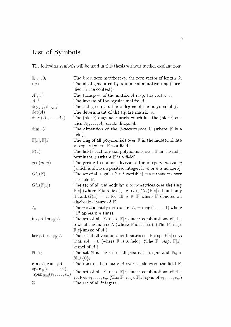
List of Symbols
The following symbols will be used in this thesis without further explanation:
0k×n, 0k The k×n zero matrix resp. the zero vector of length k.〈 g 〉 The ideal generated by g in a commutative ring (spec-
i�ed in the context).At, vt The transpose of the matrix A resp. the vector v.A−1 The inverse of the regular matrix A.degx f, degz f The x-degree resp. the z-degree of the polynomial f .det(A) The determinant of the square matrix A.diag (A1, . . . , An) The (block) diagonal matrix which has the (block) en-
tries A1, . . . , An on its diagonal.dimF U The dimension of the F-vectorspace U (where F is a
�eld).F[x],F[z] The ring of all polynomials over F in the indeterminate
x resp. z (where F is a �eld).F(z) The �eld of all rational polynomials over F in the inde-
terminate z (where F is a �eld).gcd(m,n) The greatest common divisor of the integers m and n
(which is always a positive integer, if m or n is nonzero).Gln(F) The set of all regular (i.e. invertible) n×n matrices over
the �eld F.Gln(F[z]) The set of all unimodular n× n-matrices over the ring
F[z] (where F is a �eld), i.e. G ∈ Gln(F[z]) if and onlyif rankG(a) = n for all a ∈ F where F denotes analgebraic closure of F.
In The n×n identity matrix, i.e. In = diag (1, . . . , 1) where"1" appears n times.
im FA, im F[z]A The set of all F- resp. F[z]-linear combinations of therows of the matrix A (where F is a �eld). (The F- resp.F[z]-image of A.)
ker FA, ker F[z]A The set of all vectors v with entries in F resp. F[z] suchthat vA = 0 (where F is a �eld). (The F- resp. F[z]-kernel of A.)
N,N0 The set N is the set of all positive integers and N0 isN ∪ {0}.
rankA, rank FA The rank of the matrix A over a �eld resp. the �eld F.span
F(v1, . . . , vn),
spanF[z](v1, . . . , vn)
The set of all F- resp. F[z]-linear combinations of thevectors v1, . . . , vn. (The F- resp. F[z]-span of v1, . . . , vn.)
Z The set of all integers.
6 Section 0
0 Introduction
There are many examples in everyday life, where some information mustbe stored or communicated. Examples are data storage on CD's or datatransmission via the internet or via satellites. But some data on a CD mightbe destroyed by a scratch and also the data which pass space runs the riskof being changed or lost ("the data pass a noisy channel"). So any part ofthis information must be protected from being mutilated by storing resp.communicating it with redundancy ("encoding"), and it must be possible torecover the original data from the possibly changed data ("decoding").
But how can we use the idea of redundancy for both encoding and de-coding our information easily and e�ciently? Coding theory is one attemptto deal with this problem. Coding theory as a mathematical branch startedwith the article of Shannon [Sha48] in the year 1948.
We assume that a certain message source is represented by the vectors inFk (the "message words"), where F is a �nite �eld. The encoding procedure
is described by an injective linear mapping Fk → Fn resp. with a full rank
matrix G ∈ Fk×n, n ≥ k, according to( · )G : Fk → F
n , u 7→ uG .
The set im FG is called a block code and the elements of im FG are calledcode words. Let two di�erent codewords u1G, u2G di�er in at least d entriesand assume that the codewords pass a noisy channel, where each codewordis changed in at most bd−1
2c components. It is a familiar result from coding
theory that in this case the original codewords can be recovered completelyfrom the changed ones and therefore the original message can be recoveredcompletely, too � at least at theory.
If we want to encode a whole sequence of message words m0, . . . ,mt wecan identify this sequence with the vector polynomial ∑t
i=0 mizi. For the
coding procedure we extend ( · )G to the mapping
( · )G : F[z]k → F[z]n ,
t∑i=0
mizi 7→
t∑i=0
(miG)zi .
Now ( · )G is an injective F[z]-module homomorphism. Note that in this set-ting the zj-th term of (
∑ti=0 miz
i)G only depends on mj because G hasconstant entries. In this sense, the encoder ( · )G has "no memory" and wecould apply G onto the single message words m0, . . . ,mt just as well.

Introduction 7
But if we assume that G has polynomial entries in z, i.e. that ( · )G isan arbitrary injective F[z]-module homomorphism, then in general the zj-thterm of (
∑ti=0 miz
i)G will not be determined only by mj (but of mj,mj−1, . . .)and ( · )G has some kind of "memory". In this sense the submodule im F[z]Ghas some advantage by comparison with block codes. If it satis�es somefurther desirable properties, it is called a convolutional code (cf. De�nition1.6).
For applications block codes resp. convolutional codes must have addi-tional properties like easy encoding and above all they must allow easy de-coding algorithms. The so called "cyclic block codes" are attractive from thispoint of view: They can be implemented easily and there are various prac-tical methods for decoding them. Consequently, it would be nice to have ageneralization to convolutional codes.
Yet, the theory of cyclic convolutional codes is still in the beginnings.This thesis wants to give a small contribution to the work that has alreadybeen done to shed some light on this point. We investigate the so called "min-imal cyclic convolutional codes" and, as a special case, 1-dimensional cyclicconvolutional codes. We are able to give to give a result about the existenceof minimal cyclic convolutional codes and to determine the structure of agenerator matrix of a 1-dimensional cyclic convolutional code.
A more detailed overview about the structure of this work is given now:In Section 1 we will recall basic de�nitions and statements from the theory
of block codes and convolutional codes. Convolutional codes are de�ned tobe direct summands of F[z]n (cf. De�nition 1.6).
Section 2 provides detailed information about the so called "PQR-representation" and "KLM-representation" of submodules of F[z]n. The mainresults (Theorems 2.12, 2.13, 2.15, 2.22, 2.23, 2.24) are not new and only The-orem 2.12 will be used later on. But � and this is the reason why we treatthis topic so intensively � we give purely (linear) algebraic proofs. To ourknowledge, this is the �rst time that the proofs do not rely on system theorybut only on linear algebra, matrix theory and the theory of convolutionalcodes.
In Section 3 we turn to the notion of cyclicity. First we sum up commonresults from the theory of cyclic block codes in Section 3.1. Then we introducea generalized concept of cyclicity for submodules in Section 3.2 which is dueto Piret [Pir76] and Roos [Roo79]. Based on the work of Schmale and Glüsing-Lüerÿen [GS02a] we provide the necessary tools for our further investigations.

8 Section 0
Minimal cyclic convolutional codes, the topic of this theses, will be de�nedto be those cyclic convolutional codes, which have no proper cyclic sub-codes.In Section 4 minimal cyclic convolutional codes are being investigated. Themain result is Theorem 4.15 which gives necessary and su�cient conditionsfor the existence of minimal cyclic convolutional codes with nonzero com-plexity.
Section 5 is concerned with 1-dimensional cyclic convolutional codes,which turn out to be special examples for minimal cyclic convolutional codes.We will deepen the result about the existence of minimal cyclic convolutionalcodes for 1-dimensional cyclic convolutional codes in Section 5.1. Moreover,the shape of generator matrices of 1-dimensional cyclic convolutional codesis determined in Section 5.2. This allows us to present some constructionmethods for 1-dimensional cyclic convolutional codes resp. the investigationof special 1-dimensional cyclic convolutional codes in Section 5.3.
Finally, Section 6 reminds us of some problems, which where not solvedin the present thesis (Section 6.1) and introduces a further research topic inSection 6.2.
Acknowledgements. I like to thank PD Dr. Heide Glüsing-Lüerÿenand Prof. Dr. Wiland Schmale. In the lectures of Wiland Schmale I becameaquainted with linear algebra and algebra. Heide Glüsing-Lüerÿen woke myinterest in coding theory. She attended to me carefully while I worked on thisthesis and had an ear for me almost at any time.Furthermore, I like to thank all the other people, who listened to me when Iwanted to discuss my mathematical problems. In particular, these are AisoHeinze and the people from the "KandidatInnen-Seminar" of Prof. Dr. UlrichKnauer. Moreover, I wish to thank Onno Meyer, who read this thesis beforesubmission and gave suggestions for improving my English.

Basic Information on Block Codes and Convolutional Codes 9
1 Basic Information on Block Codes and Con-
volutional Codes
Throughout this thesis, F denotes a �nite �eld. Sometimes the notation Fqis used to indicate that F has q elements. We will regard all vectors as rowvectors, as it is usual in coding theory. Thus
F[z]n := {(v1, . . . , vn) | vi ∈ F[z] for i = 1, . . . , n} .
Consequently, images and kernels of matrices will always denote left-imagesand left-kernels. Moreover, the symbols given on page 5 will be used withoutfurther explanation.Sometimes computations were made with the aid of the computer algebrasystem MAPLE (cf. [MAP01]). We will always indicate whether the computerwas used.
In the following we give necessary preliminaries and notations which weuse throughout this thesis. Most time we restrict ourselves to the presenta-tion of de�nitions and results; proofs are omitted.Section 1.1 deals with block codes. For details we refer to [MS78], [LC83] or[Bet98].In Sections 1.2 and 1.3 we introduce basics about submodules of F[z]n andconvolutional codes. More information is presented in the fundamental arti-cles [For70] and [For75] and, for instance, in the books [Pir88a], [JZ99] or inthe article [McE98].
1.1 Block Codes
A k-dimensional subspace C of the vectorspace Fn (equivalently a direct sum-mand of Fn with dimension k) is called a (n, k)-block code over F. Anelement of Fk is called a message word and an element of C is called acode word.
The Hamming weight or simply weight of a vector v ∈ Fn, denotedby wt (v), is the number of nonzero entries in v. Two di�erent codewords ofa block code C di�er in at least d (C) := min{wt(v) | 0 6= v ∈ C} entries,therefore d (C) is called the distance of C. It is easy to see (for example withLemma 1.1) that we have d (C) ≤ n − k + 1 for an (n, k)-bock code C. Thisbound is called the MDS-bound1 (for block codes). A block code reachingthis bound is called MDS-block code.
1"MDS" stands for maximum distance seperable.
10 Section 1
If the noisy channel which the codewords have to pass during thetransmission is "not too noisy", i.e. it changes any codeword in at mostb1
2(d (C)− 1)c entries, then any error can be corrected and the original mes-
sage word can be recovered completely (see e.g. [MS78, Ch. 1, �3, Thm. 2])� at least theoretically.
For any (n, k)-block code there exist matrices G ∈ Fk×n and H ∈ Fn×(n−k)
(both having full rank) such that C = im FG = ker FH. (We de�ne {0n} =:im FG for G ∈ F0×n and Fn =: ker FH for H ∈ Fn×0.) We call G a gene-rator matrix and H a parity check matrix of C. Generator matrix andparity check matrix are unique in the following sense: If G resp. H is anothergenerator matrix resp. parity check matrix of C, then G = UG for someU ∈ Glk(F) and H = HV for some V ∈ Gln−k(F).
If C ⊆ F is an (n, k)-block code with generator matrix G and parity checkmatrix H, then C⊥ := {v ∈ Fn | ∀ w ∈ C : vwt = 0} = ker FGt = im FH
t isa uniquely determined (n, n − k)-block code (see e.g. [MS78, Ch. 1, �8]). Itis called the dual code of C and satis�es (C⊥)⊥ = C.
Finally, we give a result which allows us to determine the distance of ablock code with the aid of a parity check matrix. This result will be usedlater in the proof of Theorem 5.22.
Lemma 1.1 cf. [LC83, Theorem 3.2 and Corollaries 3.2.1, 3.2.2]Let C be an (n, k)-block code with parity check matrix H ∈ Fn×(n−k). Thendfree (C) = d if and only if there exist d F-linear dependent rows in H andany selection of d− 1 rows of H is F-linear independent. 2
1.2 Submodules of F[z]n
A submodule C of the F[z]-module F[z]n of rank k is said to be an (n, k)-submodule over F. The weight of a vector v =
∑i≥0 viz
i ∈ F[z]n is de�nedas ∑i≥0 wt (vi), where wt (vi) is the Hamming weight of the vector vi ∈ Fn.It is also denoted by wt (v). The free distance dfree (C) := min{wt(v) | 0 6=v ∈ C} of a submodule is a canonical generalisation of the free distance of ablock code. As for block codes a codeword can be recovered completely if itwas changed in at most b1
2(dfree (C)− 1)c components (at least in theory).
The free distance of submodules (resp. convolutional codes, see De�nition1.6) will play a minor role in this thesis. However, we will often give the freedistance of the convolutional codes in our examples in order to have a morecomplete picture of the codes in question.
Basic Information on Block Codes and Convolutional Codes 11
Since every (n, k)-submodule C ⊆ F[z]n is free, it can be written asC = im F[z]G for some G ∈ F[z]k×n. Such a matrix G is called a gener-ator matrix of C and has full rank. (Here we put {0n} =: im F[z]G forG ∈ F[z]0×n. Furthermore, G ∈ F[z]0×n is de�ned to be right invertible.) Agenerator matrix of C is unique in the following sense: If G, G are two gen-erator matrices of an (n, k)-submodule, then G = UG for some unimodularmatrix U ∈ F[z]k×k. Since any unimodular matrix is a product of elementarymatrices (corresponding to so-called elementary operations) 2, we can alsoexpress uniqueness of a generator matrix in other terms:
Remark 1.2Consider two generator matrices G, G of an (n, k)-submodule C ⊆ F[z]n andlet G1, . . . , Gk denote the rows of G. Then G can be transformed successivelyto G by a �nite number of so called elementary operations over F[z], theseare:(O1) Rescaling a row of G by a factor λ ∈ F \ {0};(O2) exchanging two rows of G;
(O3) replacing Gi by Gi + f ·Gj where j 6= i and f ∈ F[z] \ {0} .
The maximal z-degree of the k-minors of a generator matrix G of an(n, k)-submodule C is independent of the choice of G and is called the com-plexity of C. If δ is the complexity of C, this submodule is also called an(n, k, δ)-submodule.
Rosenthal and Smarandache showed in [RS99] that the free distance ofan (n, k, δ)-submodule satis�es
dfree C ≤ (n− k)(bδ/kc+ 1) + δ + 1 . (1.1)
This bound is a generalisation for the MDS-bound in the case of block codesand is also called MDS-bound. A convolutional code reaching this boundis called MDS-convolutional code.
The z-degree or simply degree of a generator matrix G ∈ F[z]k×n of asubmodule C is de�ned as the sum of the z-degrees of its rows (which areidenti�ed as elements in Fn[z]) and it is denoted by deg G. A generator matrixwith minimal degree is called a minimal basis.
2 For the de�nition of elementary (unimodular) matrices we refer to [Gan60a, Ch. VI,�1]. The statement that any unimodular matrix is a product of elementary matrices canbe found in [Gan60a, Ch. VI, �2, 2., Corollary].

12 Section 1
Forney showed how the complexity of a submodule, its minimal basesand the (row-)degrees of generator matrices are related. Before we state hisfundamental result, we recall another common de�nition: For a matrix M ∈F[z]l×n (l ∈ N) with rows M1, . . . ,Ml and Mi 6= 0 for 1 ≤ i ≤ l the leadingz-coe�cient vector of Mi is denoted by lczMi ∈ Fn and the matrix
L(M) :=
lczM1
lczM2...lczMl
is called the leading coe�cient matrix of M .
Theorem 1.3 (Theorem of Forney) [For75, 3.]Let C ⊆ F[z]n be an (n, k, δ)-submodule and let G ∈ F[z]k×n be a generatormatrix with row degrees ν1 . . . , νk. Then the following statements are equiva-lent:(i) G is a minimal basis;
(ii) rank FL(G) = k ;
(iii) δ = degG, i.e. δ = ν1 + . . .+ νk ;
(iv) For all 0 6= (u1, . . . , uk) ∈ F[z]k one has degz uG = max1≤j≤k
(degz uj + νj) ;
(v) For all d ∈ N0 one has dimF{w ∈ im F[z]G | degz w < d} =k∑j=1νj≤d
(d−νj) .
2
Statement (iii) of the Theorem of Forney implies that a submodule havingcomplexity 0 has a constant generator matrix. Therefore such a submoduleis said to be a block code.
It is a consequence of Theorem 1.3 (v) that the row degrees of two minimalbasis of an (n, k)-submodule C are equal up to permutation. Therefore, therow-degrees of a minimal basis of C are called the Forney indices of C. InSection 2 we will use the following more general result:
Lemma 1.4Let C ⊆ F[z]n be an (n, k)-submodule and consider a matrix G ∈ F[z]l×n withrows G1, . . . , Gl such that im F[z]G = C (we allow l > k) and Gi 6= 0 for1 ≤ i ≤ l. Let µ1 ≤ . . . ≤ µl denote the row degrees of G. Furthermore, letG ∈ F[z]k×n be a minimal basis of C with row degrees ν1 ≤ . . . ≤ νk.

Basic Information on Block Codes and Convolutional Codes 13
(a) If Gj1 , . . . , Gjk is a selection of F[z]-linear independent rows of G wherej1 < . . . < jk, then
ν1 ≤ µj1 , . . . , νk ≤ µjk .
(b) If C has complexity δ, then δ ≤ µ1 + . . .+ µl .
Proof: Statement (b) is a direct consequence of (a) and Theorem 1.3(iii). For (a), we assume that µj1 ≤ . . . ≤ µjs < νs for some s ∈ {1, . . . , k}. Weknow that Gj1 , . . . , Gjk ∈ span
F[z]{G1 . . . , Gk}. Theorem 1.3 (iv) implies thatGj1 , . . . , Gjs ∈ span
F[z]{G1 . . . , Gs−1}. But span F[z]{G1 . . . , Gs−1} has rank atmost s−1 and therefore the rows Gj1 , . . . , Gjs are F[z]-linear dependent. Thelatter implies that the rows Gj1 , . . . , Gjk are F[z]-linear dependent. This is acontradiction, thus µjs ≥ νs. 2
We close this brief overview with a more specialized result, which will becrucial in Section 2. It states that the elementary operations in Remark 1.2can be speci�ed when dealing with minimal bases:
Proposition 1.5Let G, G ∈ F[z]k×n be two minimal bases of the (n, k)-submodule C ⊆ F[z]n
with Forney indices ν1, . . . , νk. Without loss of generality we assume that boththe row degrees of G and of G are given by ν1 ≤ . . . ≤ νk. Let G1, . . . , Gk
denote the rows of G. Then G can be transformed successively to G by a �nitenumber of operations of the type(O1) Rescaling a row of G by a factor λ ∈ F \ {0};(O2')exchanging two rows of G which have the same degree;
(O3')replacing Gi by Gi + zl ·Gj , where j 6= i, νj ≤ νi and 0 ≤ l ≤ νi − νj .Note that each of these transformations preserves the property "minimalbases" (which can be seen directly).
Outline of the Proof: We know that G = UG for some U =(ui,j)1≤i,j≤k ∈ Glk(F[z]). Theorem 2 in [MP79] states that UG is a mini-mal basis if and only if degz uij ≤ νi − νj for νj ≤ νi and uij = 0 for νj > νi.(In particular U is block-lower-triangular.) Now there exists a suitable de-composition of U into a product of elementary matrices 3 which correspond tothe operations (O1), (O2') and (O3'). If we transform a minimal basis withone of the operations (O1), (O2') or (O3'), then the resulting matrix has rowdegrees ν1 ≤ . . . ≤ νk. It is a minimal basis again, as we can readily see withTheorem 1.3. 2
3See footnote 2 on page 11.
14 Section 1
1.3 Convolutional Codes
Block codes are subspaces of Fn or, equivalently, direct summands of Fn.Therefore, there are at least two natural ways to de�ne convolutional codesas a generalization of block codes: Convolutional codes can be de�ned eitherto be submodules of F[z]n or to be direct summands of F[z]n. We choose thesecond way because it turns out that direct summands of F[z]n have someuseful properties.
De�nition 1.6A direct summand C of F[z]n (as an F[z]-module) of rank k having complex-ity δ is called an (n, k)-convolutional code or an (n, k, δ)-convolutionalcode. An element of F[z]k is called a message word and an element of Cis called a code word.
The follwing theorem shows that it is quite advantageous to de�ne convo-lutional codes this way. Before we state it, we give two other de�nitions: Some(n, k)-submodules C (but not all of them) can be written as C = ker F[z]H forsome H ∈ F[z]n×(n−k) (cf. Theorem 1.7). If this is possible, H is called a par-ity check matrix of C. (We say that H ∈ F[z]n×0 is a parity check matrixof the (n, n)-convolutional code F[z]n and we de�ne H to be left invertible.)If a Smith form4 of G ∈ F[z]k×n, k ≤ n, is [Ik | 0k×(n−k)], then G is calledbasic.
Theorem 1.7 cf. [For75, 9.], [McE98, Theorem A.1]Let C ⊆ F[z]n be an (n, k)-submodule with generator matrix G ∈ F[z]k×n andlet F denote an algebraic closure of F. Then the following statements areequivalent:(i) C is a convolutional code;
(ii) C has a parity check matrix, i.e. C = ker F[z]H for some H ∈ F[z]n×(n−k);
(iii) G is basic, i.e. [Ik | 0k×(n−k)] is a Smith-form of G;
(iv) rankG(a) = k for all a ∈ F;(v) there exists G ∈ F[z](n−k)×n such that
[G
G
]∈ Gln(F[z]), i.e. every F[z]-
basis of C can be completed to an F[z]-basis of F[z]n;
(vi) for all v ∈ F[z]n and all polynomials f ∈ F[z] \ {0} one has4For the de�nition of a Smith-form we refer to [Gan60a, Chapter VI,�3]. The word
"Smith-form" does not appear there. We call a "canonical diagonal matrix" as in [Gan60a,Thm. VI, �3, p.141] a Smith-form.

Basic Information on Block Codes and Convolutional Codes 15
fv ∈ C =⇒ v ∈ C ;
(vii) for all submodules C of rank k one hasC ⊆ C =⇒ C = C ;
(viii) G is right invertible over F[z], i.e. there exists W ∈ F[z]n×k such thatGW = Ik ;
(ix) im F(z)G ∩ F[z]n = im F[z]G .
We will give a Proof of this theorem (or at least some detailed hints),since the reader will possibly have di�culties to puzzle out a complete prooffrom the literature. We will organize the proof as follows:
(viii)m
(i)⇔ (v) ⇐= (iii) ⇔ (iv)⇓ ⇑(ii)⇒ (vi)⇒ (vii)
m(ix)
Part "(i)⇔(v)" is obvious.Part "(v)⇒(ii)" can be established as follows: De�ne [ GG ]−1
=: [H |H] ∈F[z]n×n where H has k columns and H has n − k columns. Now we showthat the matrix H ∈ F[z]n×(n−k) is a parity check matrix of C: Because of[H |H] ·
[G
G
]=[G
G
]· [H |H] = In we have GH = 0 and im F[z]G ⊆ ker F[z]H.
It remains to show that ker F[z]H ⊆ im F[z]G. Consider v ∈ F[z]n such thatvH = 0 and de�ne v[H |H] =: (a, 0). Then on the one hand v([H |H]·
[G
G
])=
vIn = v and on the other hand (v[H |H])·[G
G
]= (a, 0)
[G
G
]= aG. Thus
v = aG ∈ im F[z]G.For "(ii)⇒(vi)" we assume that H is a parity check matrix of C. If fv ∈
ker F[z]H = C for v ∈ F[z]n and f ∈ F[z] \ {0}, then v ∈ ker F[z]H = C, too.Part "(vi)⇒(vii)" can be shown indirectly: Let C ⊆ F[z]n be a submodule
of rank k with generator matrix G and C ⊆ C but C 6= C. Then there existsv ∈ C such that v 6∈ C. Since im F(z)G = im F(z)G there exists u ∈ F(z)k
such that uG = v. There exists some polynomial f ∈ F[z] \ {0} such thatfu ∈ F[z]k, hence fv ∈ im F[z]G = C but v 6∈ C.
For the "(vi)⇒(ix)"-part we observe that im F(z)G ∩ F[z]n ⊇ C is true inany case. It remains to show im F(z)G ∩ F[z]n ⊆ C: An element in im F(z)G ∩

16 Section 1
F[z]n can be written as 1fuG for some f ∈ F[z] \ {0} and u ∈ F[z]k. Now
f 1fuG = uG ∈ C. With (vi) we also have 1
fuG ∈ C.
Now we prove "(ix)⇒(vi)": Consider v ∈ F[z]n and f ∈ F[z] \ {0} suchthat fv ∈ C. Then 1
ffv = v ∈ im F(z)G ∩ F[z]n = im F[z]G = C.
For the remaining part of the proof we use a Smith-form of G. We consider�xed unimodular matrices U ∈ Gln(F[z]), V ∈ Glk(F[z]) such that V GU is aSmith-form of G. In particular, we have
V GU = [∆ | 0k×(n−k)] where ∆ = diag (d1, . . . , dk) and di ∈ F[z] .
Observe that (iii) is equivalent to ∆ ∈ Glk(F[z]).For "(iii)⇒(viii)" we have ∆ = Ik and we consider the matrix W :=
U[
Ik0(n−k)×k
]V ∈ F[z]n×k. It can be readily shown that W is a right inverse of
G.The inverse implication "(viii)⇒(iii)" can be established as follows: Let
W ∈ F[z]n×k be a right inverse of G and let M1 ∈ F[z]k×k denote the matrixconsisting of the �rst k rows of U−1M . We show that ∆ ∈ Glk(F[z]). Wecalculate Ik = (GU)(U−1M) = (V −1[∆ | 0])(U−1M) = V −1∆M1. Hence wehave 1 = det(V −1∆M1) = det(V −1) det(∆) det(M1). In particular we havedet(∆) ∈ F \ {0}, which implies that ∆ is unimodular.
For "(iii)⇔(iv)" we observe that rank G(a) = k for all a ∈ F if and only ifrank∆(a) = k for all a ∈ F. But this is the case if and only if ∆ ∈ Glk(F[z]).
"(vii)⇒(iii)" can be shown indirectly: Note that [∆ | 0k×(n−k)]U−1
is a generator matrix of C and that im F[z][∆ | 0k×(n−k)]U−1 ⊆
im F[z][Ik | 0k×(n−k)]U−1 =: C. If ∆ 6∈ Glk(F[z]), then C 6= C.
Finally we prove "(iii)⇒(v)": With G := [0k×k | In−k]U−1 we get[G
G
]=
[V −1[Ik | 0k×(n−k)]U
−1
[0k×k | In−k]U−1
]=
[V −1 0
0 In−k
]U−1 ∈ Gln(F[z]) .
2
Now we turn to the notion of dual codes in the context of convolutionalcodes. If C is an (n, k)-convolutional code with generator matrix G ∈ F[z]k×n,then it has a parity check matrix H ∈ F[z]n×(n−k) which can be constructedas in the proof of Theorem 1.7, part "(v)⇒(ii)". In this construction a par-ity check matrix H consists of some columns of a unimodular matrix. Thisimplies that H is left invertible and we conclude:

Basic Information on Block Codes and Convolutional Codes 17
Corollary 1.8An (n, k)-submodule C ⊆ F[z]n has a parity check matrix if and only if ithas a left invertible parity check matrix. 2
It can be readily shown that two left invertible parity check matricesH, H ∈ F[z]n×(n−k) of an (n, k)-convolutional code C di�er by a unimodularmatrix U ∈ Gln−k(F[z]). Precisely: There exists U ∈ Gln−k(F[z]) such thatH = H · U . As a consequence, the (n, n − k)-convolutional codes im F[z]H
t
and im F[z]Ht = im F[z](U
tHt) are the same. If we want to determine thecomplexity of this "new" code, we have to determine the minors of H. Thefollowing statement is very helpful:
Lemma 1.9 cf. [For75, 6., Theorem 3]If G ∈ F[z]k×n is a generator matrix of an (n, k)-convolutional code C and ifH ∈ F[z]n×(n−k) is a left invertible parity check matrix, then the k-minorsof G and the (n − k)-minors of H are the same up to permutation andmultiplication with constants in F\{0}. In particular, the convolutional codesC = im F[z]G and im F[z]H
t have the same complexity. 2
The following theorem and de�nition summarizes and extends the recentremarks:
Theorem and De�nition 1.10 [For75, 6.]If C ⊆ F[z]n is an (n, k, δ)-convolutional code and with generator matrix Gand if H is a left invertible parity check matrix of C, then
C⊥ := {v ∈ F[z]n | ∀ w ∈ C : vwt = 0} = im F[z]Ht = ker F[z]G
t
is called the dual code of C. It is an (n, n − k, δ)-convolutional code andsatis�es (C⊥)⊥ = C. 2
18 Section 2
2 First Order Representations of Submodules
of F[z]n
In this section we will investigate how an (n, k, δ)-submodule C ⊆ F[z]n canbe represented by a constant matrix triple (P,Q,R) ∈ F(δ+k)×δ × F(δ+k)×δ ×F
(δ+k)×n resp. (K,L,M) ∈ Fδ×(δ+n−k)×Fδ×(δ+n−k)×Fn×(δ+n−k) via the equa-tion
C =(ker F[z](zP +Q)
)·R resp. C =
(ker F[z]
[zK + LM
])·[
0δ×nIn
]. (2.1)
Such representations are called �rst order representations because theindeterminate z appears only linearly.
The main target of this section is to prove three theorems � roughlyspeaking these are:
� Any (n, k, δ)-submodule (resp. convolutional code) can be representedas in (2.1) and the matrix triples (P,Q,R), (K,L,M) have some further"nice properties" (cf. Theorems 2.12, 2.22).
� Every matrix triple (P,Q,R) (resp. (K,L,M)) of sizes as above andhaving these "nice properties" de�nes an (n, k, δ)-submodule or even a con-volutional code (cf. Theorems 2.13, 2.23).
� A representation (P,Q,R) (resp. (K,L,M)) of a submodule satisfyingthe "nice properties" is unique up to some matrix manipulations (cf. Theo-rems 2.15, 2.24).
These results, which will be speci�ed in the following, are well known(see the book of Kuijper [Kui94, Sections 3.4, 4.1, 4.4 and 5] or the articles[RSY96], [SGR98]). Since the tree statements can be formulated in the ter-minology of linear algebra and matrix theory, one might want to have proofsin this terminology, too. E�orts have been made to give purely (linear) alge-braic proofs, for example by Glüsing-Lüerÿen. She was able to prove the �rsttwo statements in this way (cf. [Glub]), but yet, no pure (linear) algebraicproofs of all three theorems were known. We succeeded to �ll this gap andfor this reason we publish our results in detail in this thesis, even though weuse just one result from this section (namely Theorem 2.12) later on.
We give some technicalities in Section 2.1, then we will formulate thethree theorems for each representation and give the proofs in Sections 2.2resp. 2.3.

First Order Representations of Submodules of F[z]n 19
2.1 Some Information on Matrix Pencils
In (2.1) there appear matrices of the shape zP + Q where P and Q haveconstant entries. Such a matrix zP + Q is called a matrix pencil. We willuse a "normal form" of a matrix pencil to deal with �rst order representations.Before we state a main result of this section in Theorem 2.2 we introducesome shorthand expressions in the following notation:
Notation 2.1For ν ∈ N0 we write
Lν :=
z
−1. . .. . . z
−1
∈ F[z](ν+1)×ν , Mν := Ltν ∈ F[z]ν×(ν+1)
and for ν1, . . . , νs ∈ N0 we write
L(ν1, . . . , νs) := diag (Lν1 , . . . , Lνs) ∈ F[z](∑si=1 νi+s)×(
∑si=1 νi)
and M(ν1, . . . , νs) := diag (Mν1 , . . . ,Mνs) ∈ F[z](∑si=1 νi)×(
∑si=1 νi+s) .
Note: If L0 occurs in L(ν1, . . . , νs) resp. if M0 occurs in M(ν1, . . . , νs), thenit induces a zero-row in L(ν1, . . . , νs) resp. a zero-column in M(ν1, . . . , νs).
Theorem and De�nition 2.2 [Gan60b, Chapter XII] 5
Let P,Q ∈ Fl×m. Then there exist matrices T ∈ Gll(F) and S ∈ Glm(F) anduniquely determined integers 0 ≤ ν1 ≤ . . . ≤ νs, 0 ≤ µ1 ≤ . . . ≤ µt andν0, µ0 ∈ N0 such that
T (zP +Q)S = diag (L(ν1, . . . , νs),M(µ1, . . . , µt), zIν0 + A, Iµ0 + zA) (2.2)
where zIν0 + A and Iµ0 + zA are (regular) matrix pencils. Furthermore, Aand A are constant matrices of appropriate sizes such that A is nilpotent6. Itis allowed that one or more blocks do not appear in (2.2).
5The normal form of zP +Q given in Theorem 2.2 is not exactly the normal form as in[Gan60b]. There the blocks Lνi and Mνi have "1"-entries instead of "−1"-entries and thezero-rows resp. zero-columns are placed at the top resp. at the left side of the matrix. Butof course we can deduce Theorem 2.2 from [Gan60b, Chapter XII].Observe that zero-rowsresp. zero-columns are represented by matrices of the form L0 resp. M0.
6This means Ar = 0 for some r ∈ N.

20 Section 2
The pencil T (zP + Q)S in (2.2) is called a canonical form of zP + Q. Ingeneral, it is not unique (because in our setting the choice of A, A is notunique), but it is unique if the regular submatrices zIν0 + A and Iµ0 + zA areabsent. In this case we can speak of the canonical form of zP +Q. 2
Example 2.3Let F = F3. An example for a canonical form is
diag (L(0, 1, 2),M(0, 1), [z + 2],
[1 z0 1
]) =
0 0 0 0 0 0 0 0 0z 0 0 0 0 0 0 0 0−1 0 0 0 0 0 0 0 00 z 0 0 0 0 0 0 00 −1 z 0 0 0 0 0 00 0 −1 0 0 0 0 0 00 0 0 0 z −1 0 0 00 0 0 0 0 0 z + 2 0 00 0 0 0 0 0 0 1 z0 0 0 0 0 0 0 0 1
.
For later purposes we must know under which conditions the blocksM(µ1, . . . , µt) and the regular block diag (zIν0 + A, Iµ0 + zA) is absent ina canonical form of zP +Q.
Lemma 2.4Let P,Q ∈ Fl×m. Then the following statements are equivalent:
(i) The canonical form of zP +Q is L(ν1, . . . , νs) for some ν1 ≤ . . . ≤ νs inN0;
(ii) The matrix P has full column rank and the pencil zP+Q is left invertible.
Proof: A transformation of zP +Q to T (zP +Q)S via T ∈ Gll(F) andS ∈ Glm(F) does not a�ect the properties given in (ii). Therefore we mayassume without loss of generality that zP + Q is given in a canonical form,i. e.
zP +Q = diag (L(ν1, . . . , νs),M(µ1, . . . , µt), zIν0 + A, Iµ0 + zA) ,

First Order Representations of Submodules of F[z]n 21
where A is nilpotent. Now (i)⇒(ii) is obvious (cf. Theorem 1.7 (iv)). For(ii)⇒(i) we argue as follows: If P has full column rank, there can be no blockofM(µ1 . . . , µt)-type, because it would induce zero-columns in P . There canbe no block of the form Iµ0 +zA either, because A is not invertible (since it isnilpotent) and this would cause that P has not full column rank. Moreover,left invertibility of zP +Q implies that there is no block of the form zIν0 + A,which can be obtained as follows: Assume that the block zIν0 + A is present(this means ν0 > 0) and let F denote an algebraic closure of F. With Theorem1.7 (iv) it is clear that left invertibility of zP + Q implies left invertibilityof zIν0 + A. But det(zIν0 + A) is a polynomial in z of degree ν0 > 0. HenceaIν0 + A has not full rank for every a ∈ F which in turn implies that zIν0 + Ais not left invertible, as Theorem 1.7 tells us. 2
2.2 PQR-Representations of Submodules of F[z]n
In this section we will investigate the so called "PQR-representation" of sub-modules of F[z]n. We will deal with the set (ker F[z](zP + Q)) · R which willbe de�ned in the following notation.
Notation 2.5Consider a matrix triple (P,Q,R) ∈ F(δ+k)×δ × F(δ+k)×δ × F(δ+k)×n wherek ≤ n and δ > 0. We will use the following abbreviation:
CP(P,Q,R) :=
{v ∈ F[z]n
∣∣∣ ∃ ζ ∈ F[z]δ+k :ζ(zP +Q) = 0
ζR = v
}=
{v ∈ F[z]n
∣∣∣ (0δ, v) ∈ im F[z][zP +Q |R]}
=(ker F[z](zP +Q)
)·R .
Of course, any matrix triple (P,Q,R) of the sizes as in Notation 2.5 givesrise to a submodule CP(P,Q,R) ⊆ F[z]n.
De�nition 2.6If a submodule C ⊆ F[z]n can be written as C = CP(P,Q,R) with (P,Q,R)as in Notation 2.5, then (P,Q,R) is called PQR-representation of C.
Some properties of (P,Q,R) will be of frequent use and we will introduceshorthand expressions:

22 Section 2
Properties 2.7Consider (P,Q,R) as in Notation 2.5. Properties of interest are:(P1) P has full column rank δ;(P2) [P |R] has full row rank δ + k;(P3) zP +Q is left invertible;(P4) [zP +Q |R] is right invertible.
It is an obvious question how two matrix triples (P,Q,R) and (P , Q, R) ofsizes as in Notation 2.5 are related, if they satisfy CP(P,Q,R) = CP(P , Q, R).This question is partly answered in the following remark, which can be provedstraightforwardly:
Remark 2.8Let (P,Q,R) be a matrix triple as in Notation 2.5 and let T ∈ Glδ+k(F) andS ∈ Glδ(F). Then we have CP(P,Q,R) = CP(TPS, TQS, TR). Furthermore,the transformation
(P,Q,R) 7→ (TPS, TQS, TR)
does not a�ect any of the properties (P1), (P2), (P3) or (P4), precisely:If one of these properties is true for (P,Q,R), then the transformed triple(TPS, TQS, TR) inherits this property.As a consequence, we can assume without loss of generality that zP + Q isgiven in a canonical form when we deal with the set CP(P,Q,R).
In fact, under some additional conditions CP(P,Q,R) = CP(P , Q, R) istrue if and only if (P , Q, R) is the result of a transformation as in Remark2.8 and we will specify and prove this statement in Theorem 2.15.
The next theorem tells us among other things how we can produce amatrix G satisfying im F[z]G = CP(P,Q,R) for a given matrix triple (P,Q,R).It will be a necessary tool to prove Theorem 2.12.
Theorem 2.9Let (P,Q,R) be a matrix triple as in Notation 2.5 and let zP +Q be given ina canonical form (which we can assume without loss of generality, cf. Remark2.8) with the data as in (2.2). Then the following statements hold:(a) The matrix zP + Q equals L(ν1, . . . , νs) ∈ F[z](
∑si=1 νi+s)×
∑si=1 νi if and
only if (P1) and (P3) are satis�ed. In this case we have s = k andδ =
∑si=1 νi.

First Order Representations of Submodules of F[z]n 23
(b) Let zP +Q = L(ν1, . . . , νk) and de�ne
Z(ν1, . . . , νk) :=
1 z · · · zν1
. . .1 z · · · zνk
∈ F[z]k×(δ+k)
and G := Z(ν1, . . . , νk)R ∈ F[z]k×n. Then we have
Z(ν1, . . . , νk)[zP +Q |R] = [0k×δ |G] and im F[z]G = CP(P,Q,R) .
We can identify R as the "list of coe�cient vectors" of G, the matrix Z"re-collects" the rows of G out of R.In particular we have degG ≤ δ and CP(P,Q,R) has rank at most k.
(c) Let zP +Q = L(ν1, . . . , νk). Furthermore, let G be de�ned as in (b). LetG1, . . . , Gk denote the rows of G. Accepting possible zero-coe�cients, wemay assume
Gi =νi∑j=0
gi,jzj where gij ∈ Fn for 1 ≤ i ≤ k .
We de�ne
L′(G) :=
g1,ν1
...gk,νk
.
(In general we will not have L′(G) = L(G).) Then we have:
(P2) is satis�ed⇐⇒ rankL′(G) = k
⇐⇒ G is a minimal basis with row degrees ν1, . . . , νk .
(d) Let zP +Q = L(ν1, . . . , νs) and let G be de�ned as in (b). Then we have:
G is right invertible ⇐⇒ (P4) is satis�ed .
In particular, we have: If zP +Q = L(ν1, . . . , νs), then CP(P,Q,R) is aconvolutional code if and only if (P4) holds.
Proof: (The proof uses results from Glüsing-Lüerÿen, cf. [Glub].)Part (a) is Lemma 2.4.For part (b) we write Z := Z(ν1, . . . , νk), for short. It is easy to check thatZ[zP + Q |R] = [0k×δ |G]. Thus it remains to show that G is a generatormatrix of CP(P,Q,R):

24 Section 2
Proof of im F[z]G ⊆ CP(P,Q,R): Consider v ∈ im F[z]G where v = uG,u ∈ F[z]k. With Z[zP + Q |R] = [0k×δ |G] we have uZ[zP + Q |R] = (0δ, v)and therefore (0δ, v) ∈ im F[z][zP +Q |R]. This implies v ∈ CP(P,Q,R).
Proof of CP(P,Q,R) ⊆ im F[z]G: Let v be an element of CP(P,Q,R), i.e.0 = ζ[zP + Q] and v = ζR for some ζ ∈ F[z]δ+k. We have to show thatv ∈ im F[z]G, i.e. that there exists a vector u ∈ F[z]k such that uG = v. It issu�cient to show that there exists u ∈ F[z]k such that uZ = ζ because thisimplies v = ζR = uZR = uG. Towards this end, we argue as follows:With Z(zP + Q) = 0k×δ we have im F(z)Z ⊆ ker F(z)(zP + Q). It is easyto see that both F(z)-vectorspaces have dimension k, hence they are equal.Furthermore, Theorem 1.7 "(vi)⇔(ix)" along with right invertibility of Z (cf.Theorem 1.7 (iv)) yields im F(z)Z ∩ F[z]n = im F[z]Z. With ζ ∈ ker F(z)(zP +Q) ∩ F[z]n = im F[z]Z we conclude that there exists u ∈ F[z]k such thatuZ = ζ.
Now we show (c) and (d): We have deg G ≤∑ki=1 νk = δ and
[P |R] =
g1,0
Iν1
...g1,ν1−1
0 · · · 0 g1,ν1. . . ...gk,0
Iνk...
gk,νk−1
0 · · · 0 gk,νk
, L′(G) =
g1,ν1...gk,νk
.
Therefore, [P |R] has full row rank if and only if L′(G) has full row rank.Observe that in this case L(G) = L′(G), in particular G has full row rank.We have L(G) = L′(G) if and only if G has row degrees ν1, . . . , νk. In thiscase G is a minimal basis if and only if rank L(G) = rankL′(G) = k (againwe used Theorem 1.3 (ii)). This proves (c).The matrix [zP + Q |R] can be transformed by elementary row operations

First Order Representations of Submodules of F[z]n 25
over F[z] of the type (O3) (cf. Remark 1.2) into
0 · · · 0 G1
g1,1
Hν1
...g1,ν1. . . ...
0 · · · 0 Gk
gk,1
Hνk
...gk,νk
where Hνi :=
−1 z
−1. . .. . . z−1
∈ Glνi(F[z]) .
Therefore, [zP + Q |R] is right invertible if and only if G is right invertible(use Theorem 1.7 (iv)). 2
We apply the results given in Theorem 2.9 (b) to an example in order toillustrate these �ndings:
Example 2.10Let F = F3. We consider
zP +Q := L(0, 1, 2) =
0 0 0z 0 0−1 0 00 z 00 −1 z0 0 −1
and R :=
1 1 11 0 20 2 12 0 00 0 01 2 2
.
Now the matrix
G := Z(0, 1, 2)R =
1 1 11 2z 2 + z
2 + z2 2z2 2z2
has degree degG = 0 + 1 + 2 = 3 and gives rise to the submodule im F[z]G =CP(P,Q,R) ⊆ F[z]3, which has rank at most 3. Lemma 1.4 (b) tells us thatCP(P,Q,R) has complexity at most 3.We can calculate that G has exactly rank 3 and that it is not basic, henceCP(P,Q,R) is a (3, 3)-submodule with generator matrix G, but it is not a(3, 3)-convolutional code. Furthermore, the leading coe�cient matrix of G hasfull rank and with Theorem 1.3 we conclude that CP(P,Q,R) has complexityexactly 3.

26 Section 2
The following corollary is not necessary for the remaining part of Section2.2, but it will be used in Section 5.3 in the proof of Theorem 5.22.
Corollary 2.11Let zP +Q = L(ν1, . . . , νk) and de�ne Z := Z(ν1, . . . , νk) as in Theorem 2.9(b). Then we have im F[z]Z = ker F[z][zP +Q].
Proof: Theorem 1.10 along with the right invertibility of the matrixpencil [zP + Q]t yields that ker F[z][zP + Q] is a convolutional code. WithTheorem 1.7 "(vi)⇔(ix)" we have ker F[z][zP +Q] = ker F(z)[zP +Q]∩ F[z]n.We saw in the proof of Theorem 2.9 (b) that im F[z]Z = ker F(z)(zP+Q)∩F[z]n
and this implies the assertion. 2
Now we are able to state and to prove our main results for PQR-representations, these are the Theorems 2.12, 2.13 and 2.15:
Theorem 2.12 (PQR-Realisation Theorem I: Existence) cf. [SGR98,Thm. 2.1] or (in system theoretical language) [Kui94, Thm. 5.1]Let C ⊆ F[z]n be a submodule of rank k ≤ n and complexity δ > 0. Thenthere exists a matrix triple
(P,Q,R) ∈ F(δ+k)×δ × F(δ+k)×δ × F(δ+k)×n
satisfying the conditions (P1) � (P3) such that C = CP(P,Q,R). If C is evenan (n, k, δ)-convolutional code, then C has a PQR-representation satisfying(P1) � (P4).
Proof: (The idea of the proof can be found in [Kui94].) Let C = im F[z]Gwhere G ∈ F[z]k×n is a minimal basis with rows G1, . . . , Gk and row de-grees ν1 ≤ . . . ≤ νk. In particular, Theorem 1.3 implies ∑k
i=1 νi = δ andrankL(G) = k. Now write
Gi =
νi∑j=0
gi,jzj for 1 ≤ i ≤ k where gi,j ∈ Fn
and de�ne
zP +Q := L(ν1, . . . , νk) ∈ F[z](δ+k)×δ , R :=
g1,0...g1,ν1...gk,0...gk,νk
∈ F[z](δ+k)×n .
First Order Representations of Submodules of F[z]n 27
Observe that Z(ν1, . . . , νk)R = G, where Z(ν1, . . . , νk) is de�ned as in Theo-rem 2.9 (b). Now Theorem 2.9 (a), (c) and (d) imply the assertion. 2
Theorem 2.13 (PQR-Realisation Theorem II: Parameters) cf.[SGR98, Thm. 2.2] or (in system theoretical language) [Kui94, Thm. 4.3]Consider a matrix triple (P,Q,R) ∈ F
(δ+k)×δ × F(δ+k)×δ × F
(δ+k)×n
where k ≤ n and δ > 0. Let δ denote the complexity of the submoduleCP(P,Q,R) ⊆ F[z]n. Then the following statements hold:(a) The submodule CP(P,Q,R) ⊆ F[z]n has complexity at most δ and rank
at most k + (δ − δ) .
(b) The submodule CP(P,Q,R) ⊆ F[z]n has complexity exactly δ if and onlyif (P1) � (P3) are satis�ed. In this case the submodule has rank exactlyk.
(c) The submodule CP(P,Q,R) is an (n, k, δ)-convolutional code if and onlyif the conditions (P1) � (P4) are satis�ed.
Proof: (The proof uses results from Glüsing-Lüerÿen, cf. [Glub].) WithRemark 2.8 we can assume without loss of generality that zP + Q is givenin a canonical form, i.e.
zP +Q =
L(ν1, . . . , νs)M(µ1, . . . , µt)
zA0 +B0
where zA0 + B0 is a regular matrix pencil (if it is present at all). We use apartition of R given by
R =
[R
R
]}∑s
i=1(νi + 1)}"rest" .
Proof of part (a): We have to investigate CP(P,Q,R) =(ker F[z](zP +Q))· R. Because the matrices M(µ1, . . . , µt) and the
matrix zA0 + B0 have full row rank (if they are present at all), they havetrivial left kernel and we remove the corresponding block-rows from zP +Qand R. Hence
CP(P,Q,R) =(ker F[z][L(ν1, . . . , νs), 0]
)· R .
Since presence or absence of zero-columns in [L(ν1, . . . , νs), 0] does not changeker F[z][L(ν1, . . . , νs), 0], we can make a further reduction-step by removingzero-columns. With zP + Q = L(ν1, . . . , νs) we get
CP(P,Q,R) =(ker F[z](zP + Q)
)· R = CP(P , Q, R) .
28 Section 2
With Theorem 2.9 (b) applied on (P , Q, R), we know that a generator matrixof CP(P , Q, R) = CP(P,Q,R) is given by G := Z(ν1, . . . , νs)R ∈ F[z]s×n
which has degree at most ∑si=1 νi. Furthermore, CP(P,Q,R) has rank at
most s.By Lemma 1.4 (b) and by comparing the sizes of zP +Q, zP + Q we obtain
δ ≤ deg G ≤s∑i=1
νi ≤ δ (2.3)
and
δ + k ≥s∑i=1
(νi + 1) =s∑i=1
νi + s ≥ δ + s , in particular s ≤ k + (δ − δ) .
This shows that the complexity δ of CP(P,Q,R) is less or equal δ and thatCP(P,Q,R) has rank less or equal k + (δ − δ).
Proof of the "if"-part of (b): With Theorem 2.9 (a) and (c) we know thatzP +Q = L(ν1, . . . , νk) and that the generator matrix G := Z(ν1, . . . , νk)R ∈F[z]k×n is a minimal basis with row degrees ν1, . . . , νk. The Theorem of Forney(Theorem 1.3) implies that δ = degG =
∑ki=1 νk = δ and the submodule
CP(P,Q,R) has complexity exactly δ (cf. Theorem 1.3).Proof of the "only if"-part of (b): If one of the properties (P1) or (P3) does
not hold, Theorem 2.9 (a) implies that zP +Q has a block ofM(µ1, . . . , µt)-type or a regular block zA0 +B0 . This implies
s∑i=1
νi < δ .
With (2.3) we obtain δ < δ, which contradicts the assumption thatCP(P,Q,R) has complexity exactly δ. Hence, (P1) and (P3) must hold andthus s = k. Again, we construct a generator matrix G := Z(ν1, . . . , νk)R ofCP(P,Q,R) as in Theorem 2.9 (b). Recall that degG ≤ δ by construction ofG. If (P2) does not hold, then Theorem 2.9 (c) yields that G is not a minimalbasis with row degrees ν1, . . . , νk, which in turn implies along with Theorem1.3 (iii) and Lemma 1.4 (b) that δ < degG. Hence δ < δ, which is the samecontradiction as above.In particular we proved that G is both a minimal basis and has the row de-grees ν1, . . . , νk if and only if CP(P,Q,R) has complexity exactly δ. In thiscase CP(P,Q,R) has rank exactly k which completes the proof of (b).Part (c) follows with (b) and Theorem 2.9 (d). 2

First Order Representations of Submodules of F[z]n 29
Remark 2.14There are examples of matrix triples (P,Q,R) ∈ F(δ+k)×δ×F(δ+k)×δ×F(δ+k)×n
satisfying k ≤ n and δ > 0, where CP(P,Q,R) has complexity δ < δ and
rank CP(P,Q,R) = k + (δ − δ). (A quite trivial example is δ + k = n,P = 0n×δ = Q and R = In, where CP(P,Q,R) = F[z]n has complexity
δ = 0 and rank n = k + δ − δ.) In these cases, the upper bound for therank of the submodule CP(P,Q,R) in Theorem 2.13 (a) is tight. Therefore,Theorem 2.13 (a) corrects Theorem 2.2 (i) of [SGR98], which states wronglythat CP(P,Q,R) has rank at most k in any case.
Theorem 2.15 (PQR-Realisation Theorem III: Uniqueness) cf.[SGR98, Thm. 2.3] or (in system theoretical language) [Kui94, Thm. 4.29]Let (P,Q,R) and (P , Q, R) be two matrix triples with the as sizes inNotation 2.5, both satisfying the conditions (P1), (P2) and (P3). Then
CP(P,Q,R) = CP(P , Q, R) ⇐⇒ (P , Q, R) = (TPS, TQS, TR)
for some T ∈ Glδ+k(F) and S ∈ Glδ(F).
Proof: The proof of the "⇐"-part is Remark 2.8. Thus we have to provethe "⇒"-part: Without loss of generality we can assume that both zP + Qand zP + Q are given in a canonical form. With Theorem 2.9 (a), (b) and(c) we obtain:
zP +Q = L(ν1, . . . , νk) , zP + Q = L(ν1, . . . , νk)
where ν1 ≤ . . . ≤ νk resp. ν1 ≤ . . . ≤ νk are the row degrees (Forneyindices) of the minimal basis G := Z(ν1, . . . , νk)R resp. G := Z(ν1, . . . , νk)R
of CP(P,Q,R). Since G, G have the same Forney indices, we have k = k andνi = νi for 1 ≤ i ≤ k, which in turn implies zP+Q = zP+Q = L(ν1, . . . , νk),
G = Z(ν1, . . . , νk)R and G = Z(ν1, . . . , νk)R .
We will continue like this: Proposition 1.5 allows us to assume withoutloss of generality that G can be transformed to G by only one elementaryoperation of the type(O1) rescaling a row of G by a factor λ ∈ F \ {0};(O2')exchanging two rows of G which have the same degree;(O3')replacing Gi by Gi + zl ·Gj , where j 6= i, νj ≤ νi and 0 ≤ l ≤ νi − νj .

30 Section 2
We will "translate" each of these operations into constant row operations on[zP+Q |R] to obtain [zP ′+Q′ | R] (this means transformation of [zP+Q |R]to T [zP+Q |R] = [zP ′+Q′ | R] by some T ∈ Glδ+k(F)). This will destroy thecanonical form of zP + Q, but we will see that we can make some constantcolumn operations on zP ′ +Q′ which undo the destruction of the canonicalform of zP + Q (this means transformation of T (zP + Q) = zP ′ + Q′ toT (zP +Q)S = zP +Q by some S ∈ Glδ(F)). This will �nish the proof.
Before we start with the "translation" of the three operations, we divideR and R into blocks, precisely
[R | R] =
R1 R1... ...Rk Rk
}ν1 + 1...
}νk + 1
.
Let us now "translate" (O1): We assume that G can be obtained from Gby multiplying the i-th row of G with 0 6= λ ∈ F. This is the case if and onlyif Rm = Rm for m 6= i and Ri = λRi. Scaling the whole i-th block row of[zP + Q |R] by λ we get a transformed matrix [zP ′ + Q′ | R]. Rescaling thei-th block column of [zP ′ +Q′ | R] by λ−1 we obtain [zP +Q | R].
Lν1. . .Lνi R
. . .Lνk
const.row op.∼
Lν1. . .λLνi R
. . .Lνk
const.col. op.∼
Lν1. . .
1λλLνi R
. . .Lνk
.
Now we "translate" (O2'): We assume that G can be obtained from G byexchanging the i-th and the j-th row of G, where both rows have the samedegree. This is the case if and only if Rm = Rm for i 6= m 6= j and Rj = Ri,Ri = Rj. Exchanging the i-th block row with the j-th block row of [zP+Q |R]
yields a transformed matrix [zP ′+Q′ | R]. Exchanging the i-th block columnwith the j-th block column of [zP ′ +Q′ | R] we obtain [zP +Q | R].
. . .Lνi
. . . RLνj
. . .
rowexchange∼
. . .0 Lνj
. . . RLνi 0
. . .
col.exchange∼
. . .Lνi
. . . RLνj
. . .
.

First Order Representations of Submodules of F[z]n 31
Before we "translate" (O3'), we point out to the reader that
Gi + zl ·Gj = (1, z, . . . , zνi) ·
Ri +
0l×nRj
0(νi−νj−l)×n
.
Now we "translate" (O3'): We assume that G can be obtained from G byreplacing Gi by Gi + zl ·Gj , where j 6= i, νj ≤ νi and 0 ≤ l ≤ νi − νj . This
is the case if and only if Rm = Rm for m 6= i and Ri = Ri +
0l×nRj
0(νi−νj−l)×n
.Hence, operation (O3') can be interpreted as adding the j-th block row
of [zP + Q |R] to a suitable sub-block row of the i-th bock row, precisely:We add the j-th block row to that sub-block row of the i-th bock row, whichconsists of the (l+ 1)-st up to the (l+ νj + 1)-st row of that block itself. Weobtain [zP ′ +Q′ | R] where
zP ′ +Q′ =
. . .Lνj . . .Lνj Lνi
. . .
.
This matrix can be transformed to zP + Q by constant column operations,because in the i-th block column of zP ′+Q′ there exists a suitable sub-blockcolumn which we can use to delete Lνj in the Lνj -block just by subtracting.
2
The following example might make the last part of the proof clearer.
Example 2.16Let F be the �eld F3. Consider
G :=
[z + 1 z zz2 + 1 z + 1 z2
]and G :=
[z + 1 z z
2z2 + z + 1 z2 + z + 1 2z2
].
Both matrices are minimal bases and G can be obtained from G by replacingG2 with G2+z ·G1. We choose canonical PQR-representations of im F[z]G and

32 Section 2
im F[z]G as in the proof of Theorem 2.12. These are denoted by [zP + Q |R]
resp. [zP + Q | R] and these matrices are given by
z 0 0 1 0 0−1 0 0 1 1 10 z 0 1 1 00 −1 z 0 1 00 0 −1 1 0 1
resp.
z 0 0 1 0 0−1 0 0 1 1 10 z 0 1 1 00 −1 z 1 1 00 0 −1 2 1 2
Now we illustrate the "translation" of (O3'):
[zP +Q |R]
rowop.∼
z 0 0 1 0 0−1 0 0 1 1 10 z 0 1 1 0z −1 z 1 1 0−1 0 −1 2 1 2
col.op.∼
z 0 0 1 0 0−1 0 0 1 1 10 z 0 1 1 00 −1 z 1 1 00 0 −1 2 1 2
.
2.3 KLM-Representations of Convolutional Codes
In this section we turn to the second representation which was introducedin (2.1), the so called "KLM-representation". We will see that we can use aPQR-representation of a convolutional code C ⊆ F[z]n to generate a KLM-representation of the dual code C⊥ and vice versa (cf. Theorem 2.21). Thisallows us to give short proofs for the main results, if these are formulated forcodes (and not for submodules in general): The equality (C⊥)⊥ = C makesit possible to translate KLM-representations of C to PQR-representations ofC⊥. We will apply our results for PQR-representations to C⊥ and then wewill re-translate them to C.We will not investigate the general case, where C is an arbitrary submodule,because then the proofs will be more sophisticated 7 and this would go beyondthe scope of this thesis.
Notation 2.17Consider a matrix triple (K,L,M) ∈ Fδ×(δ+n−k) × Fδ×(δ+n−k) × Fn×(δ+n−k)
7In this case it would also be possible to use a PQR-representation of C to generate aKLM-representation of the so called dual submodule C⊥ := {v ∈ F[z]n | vwt = 0 for all w ∈C} of C, which is always a convolutional code. However, we will not have the equality(C⊥)⊥ = C if C is not a convolutional code. So it is not possible in general to "transfer"results about C⊥ to C and vice versa.
First Order Representations of Submodules of F[z]n 33
where k ≤ n and δ > 0. We will use the following abbreviation:
CK(K,L,M) :={v ∈ F[z]n
∣∣∣ ∃ ζ ∈ F[z]δ : ζ(zK + L) + vM = 0}
=
{v ∈ F[z]n
∣∣∣ ∃ ζ ∈ F[z]δ : (ζ, v)
[zK + LM
]= 0
}=
{v ∈ F[z]n
∣∣∣ vM ∈ im F[z](zK + L)}
=
(ker F[z]
[zK + LM
])·[
0δ×nIn
].
Of course, any matrix triple (K,L,M) of the sizes as in Notation 2.17gives rise to a submodule CK(K,L,M) ⊆ F[z]n.
De�nition 2.18If a submodule C ⊆ F[z]n can be written as C = CK(K,L,M) with (K,L,M)as in Notation 2.17, then (K,L,M) is called KLM-representation of C.
As for (P,Q,R), some properties of (K,L,M) will be of frequent use andwe will introduce shorthand expressions:
Properties 2.19Consider (K,L,M) as in Notation 2.17. Properties of interest are:(K1) K has full row rank δ;
(K2)[KM
]has full column rank δ + n− k;
(K3)[zK + LM
]is left invertible;
(K4) zK + L is right invertible.
Remark 2.20These properties correspond to (P1) � (P4) in Properties 2.7, precisely: Re-placing k by n − k and transposing the matrices of interest, (K1) "equals"(P1), (K2) "equals" (P2), (K3) "equals" (P4) and (K4) "equals" (P3).The properties (K3) and (K4) seem to be interchanged, but this is due to thefollowing fact: We saw in Section 2.2 that (P4) is responsible for right invert-ibility of a generator matrix of the submodule CP(P,Q,R). For (K,L,M) theproperty (K4) causes right invertibility of a generator matrix of CK(K,L,M),cf. [RSY96, Lemma 3.2].
34 Section 2
As we already indicated, PQR-representations and KLM-representationsare linked by dualization:
Theorem 2.21 cf. (in system theoretical language) [Kui94, Lemma 3.26]Any PQR-representation (P,Q,R) of an (n, k, δ)-convolutional code C ofsizes as in Notation 2.5 de�nes a KLM-representation (P t, Qt, Rt) of C⊥.Any KLM-representation (K,L,M) of an (n, k, δ)-convolutional code C ofsizes as in Notation 2.17 and satisfying (K4) de�nes a PQR-representation(Kt, Lt,Mt) of C⊥.
Proof: (The proof stems from [Glub].) We only show the �rst part ofthe theorem, the second part follows with exactly the same arguments.First of all, note that (P3) is satis�ed because of Theorem 2.13 (c). LetC = CP(P,Q,R) =
(ker F[z](zP +Q))·R, where zP +Q is left invertible (i.e.
(P3)). Right invertibility of zP t + Qt along with Theorem and De�nition1.10 yields (ker F[z](zP +Q)
)⊥= im F[z](zP
t +Qt)
and this is used in the following chain of equivalent statements:
v ∈ C⊥ ⇐⇒ ∀ ζ ∈ ker F[z](zP +Q) : ζRvt = 0
⇐⇒ ∀ ζ ∈ ker F[z](zP +Q) : vRtζt = 0
⇐⇒ vRt ∈(ker F[z](zP +Q)
)⊥= im F[z](zP
t +Qt)
⇐⇒ v ∈ CK(P t, Qt, Rt) . 2
The foregoing Theorem 2.21 makes it possible to give short proofs for thethree main results of this section, which are the following Theorems 2.22,2.23 and 2.24.
Theorem 2.22 (KLM-Realisation Theorem for Codes I: Existence)cf. [RSY96, Thm. 3.1] or (in system theoretical language) [Kui94, Thm.5.14]Let C ⊆ F[z]n be an (n, k, δ)-convolutional code such that δ > 0. Then thereexists a matrix triple
(K,L,M) ∈ Fδ×(δ+n−k) × Fδ×(δ+n−k) × Fn×(δ+n−k)
satisfying the conditions (K1) � (K4) such that C = CK(K,L,M).

First Order Representations of Submodules of F[z]n 35
Proof: The dual code of C has a PQR-representation (Kt, Lt,Mt),which satis�es (P1) � (P4) because of Theorem 2.13 (c). Theorem 2.21along with Theorem and De�nition 1.10 yields that (K,L,M) is a KLM-representation of C. Obviously, the properties (K1) � (K4) hold (cf. Remark2.20). 2
Theorem 2.23 (KLM-Realisation Theorem for Codes II: Parameters)cf. (in system theoretical language) [Kui94, Thm. 4.28]Let (K,L,M) ∈ F
δ×(δ+n−k) × Fδ×(δ+n−k) × Fn×(δ+n−k) be a matrix triplesuch that k ≤ n, δ > 0 and satisfying the properties (K1) � (K4). ThenCK(K,L,M) is an (n, k, δ)-convolutional code.
Proof: With Theorem 2.13, the submodule C := CP(Kt, Lt,Mt) is an(n, n − k, δ)-convolutional code because (K1) � (K4) translate into (P1) �(P4). Theorem 2.21 along with Theorem and De�nition 1.10 yields that C⊥ =CK(K,L,M) is a (n, k, δ)-convolutional. 2
Theorem 2.24 (KLM-Realisation Theorem for Codes III: Uniqueness)[RSY96, Thm. 3.4] or (in system theoretical language) [Kui94, Thm. 4.35]Let (K,L,M) and (K, L, M) be two matrix triples with the sizes as inNotation 2.17 and both satisfying the conditions (K1) � (K4). Then
CK(K,L,M) = CK(K, L, M) ⇐⇒ (K, L, M) = (TKS, TLS,MS)
for some T ∈ Glδ(F) and S ∈ Glδ+n−k(F).
Proof: The proof of the "⇐"-part can be done straightforwardly (with-out use of the properties (K1) � (K4)).
Proof of the "⇒"-part: First note that C := CK(K,L,M) = CK(K, L, M)is a convolutional code because of Theorem 2.23. Hence the triples(Kt, Lt,Mt) and (Kt, Lt, Mt) both de�ne PQR-representations of C⊥. WithTheorem 2.15 there exist T ∈ Glδ(F) and S ∈ Glδ+n−k(F) such that
(Kt, Lt, Mt) = (SKtT, SLtT, SMt) 2
36 Section 3
3 Cyclicity
For the remaining part of this thesis n denotes a positive integer such thatthe characteristic of F does not divide n. (3.1)
This is a usual assumption in the theory of cyclic block codes and makes surethat the polynomial xn − 1 factors into di�erent prime polynomials over F.It is also familiar to index the entries of a vector v of length n with 0, . . . , n−1(i.e. v = (v0, . . . , vn−1)) when dealing with cyclic codes.
In Section 3.1 we will recall the concept of cyclicity for block codes andgive basic results. For details concerning the theory of cyclic block codeswe refer to [MS78, Chapter 7] or [LC83, Chapter 4]. In Section 3.2 we willintroduce the notion of cyclic convolutional codes. Our de�nitions and resultsare based on the fundamental articles [Pir76] and [Roo79] and, in particular,on the article [GS02a].
3.1 Cyclic Block Codes
A block code C ⊆ Fn is said to be cyclic if(v0, . . . , vn−1) ∈ C =⇒ (vn−1, v0, . . . , vn−2) ∈ C (3.2)
and we say that C is invariant under the cyclic shift .We can identify a block code C ⊆ F
n as a subset of the ring A :=F[x]/〈xn − 1 〉 via the F-isomorphism
p : Fn → A , v = (v0, . . . , vn−1) 7→ p(v) =n−1∑i=0
vixi , (3.3)
where A is displayed in the canonical wayA = {f ∈ F[x] | degx f < n} with multiplication modulo xn − 1 .
The set p(C) is called polynomial representation of C. The inverse map-ping of p is denoted by v (think of "vectorization").
One can readily show that a block code C is cyclic if and only if itspolynomial representation is an ideal in A, or in other words
C is cyclic if and only if [ a ∈ p(C) =⇒ xa ∈ p(C) ] . (3.4)
Cyclicity 37
Since each ideal in A is principal, the polynomial representation of a cyclic(n, k)-block code C can be written as p(C) = 〈 g 〉 for some g ∈ A. It is wellknown in the theory of cyclic block codes that we can choose g such thatg|(xn − 1). In this case we have degx g = n− k and
v(g)v(xg)...
v(xk−1g)
∈ Fk×n is a generator matrix of C . (3.5)
We can check cyclicity of an (n, k)-block code C as follows: If v1, . . . , vk is abasis of C, then C is cyclic if and only if xp(v1), . . . , xp(vk) ∈ p(C).
3.2 Cyclic Submodules of F[z]n and Cyclic Convolu-
tional Codes
Before we turn to the notion of cyclicity in the context of submodules andconvolutional codes, we want to point out to the reader that every submoduleC can be identi�ed as a subset of A[z] by an extension of the mapping p in(3.3) given by
p : F[z]n → A[z] ,∑ν≥0
zνvν 7→∑ν≥0
zνp(vν). (3.6)
The extended mapping p in (3.6) is an isomorphism of F[z]-(left-)modules.Again, the set p(C) is called polynomial representation of C and p−1 isdenoted by v.
3.2.1 A Generalized Concept of Cyclicity
The �rst attempt to generalize the concept of cyclicity to a convolutionalcode C by requiring (3.2) or, equivalently, by using the de�nition in (3.4)fails, as the following proposition tells us:
Proposition 3.1 [Pir76, Thm. 3.12], [Roo79, Thm. 6], [GS02a, Prop. 2.7]A convolutional code C ⊆ F[z]n satisfying (3.2) is a block code, i.e. it hascomplexity 0. 2

38 Section 3
In [Pir76] Piret suggested the following generalization of cyclicity for sub-modules: He called a submodule C ⊆ F[z]n cyclic if
g =∑ν≥0
zνgν ∈ p(C) =⇒ x ∗ g :=∑ν≥0
zνx(mν)gν ∈ p(C) ,
where n and m are coprime. This means (re-translated to C via v) thatthe coe�cient vector v(gν) of ∑ν≥0 z
νv(gν) ∈ C undergoes mν cyclic shifts(instead of one) and that the resulting vector is in C again. The conditiongcd(m,n) = 1 implies that the mapping x 7→ xm induces an F-automorphismon the ring A. This allowed Piret (loosely speaking) to introduce an F-algebrastructure on the left F[z]-module A[z]; then a submodule C is cyclic if andonly if p(C) is a left ideal in this F-algebra.
Roos generalized this concept of cyclicity to arbitrary F-automorphismsσ of A in his paper [Roo79]. We will adopt his de�nition of cyclicity. Sincethis de�nition depends on the choice of σ, we will use the name "σ-cyclicity":
De�nition 3.2 [Roo79]Consider σ ∈ AutF(A), where AutF(A) denotes the group of all F-algebraautomorphisms on A. A submodule C ⊆ F[z]n is called σ-cyclic if
g =∑ν≥0
zνgν ∈ p(C) =⇒ x ∗σ g :=∑ν≥0
zνσν(x)gν ∈ p(C) . (3.7)
Soon we give an example of a cyclic convolutional code. But before this,we show how one can check cyclicity of a submodule C with an F[z]-basisv1, . . . , vk in a �nite number of steps. Note that it is not clear whether it issu�cient to check if xp(v1), . . . , xp(vk) ∈ p(C).
Lemma 3.3Let C ⊆ F[z]n be an (n, k)-submodule with F[z]-basis v1, . . . , vk and let σ ∈AutF(A). Then C is σ-cyclic if and only if
x ∗σ p(v1), . . . , xn−1 ∗σ p(v1), . . . , x ∗σ p(vk), . . . , xn−1 ∗σ p(vk) ∈ p(C) . (3.8)
Proof: If C is σ-cyclic, then (3.8) is true by the de�nition of σ-cyclicity.This proves the "only if"-part. For the "if"-part, we observe that σi(x) ∈ Acan be identi�ed with a polynomial in F[x] with x-degree at most n − 1 forany i ∈ N0. Hence σi(x) ∗σ p(vj) is an F-linear combination of the codewordsp(vj), x ∗σ p(vj), . . . , x
n−1 ∗σ p(vj) for any i ∈ N0 and 1 ≤ j ≤ k. Therefore

Cyclicity 39
σi(x) ∗σ p(vj) is in p(C) since p(C) is an F[z]-left module.Now we consider an arbitrary codeword w :=
∑ki=1(∑
j≥0 fijzj)vi where fij ∈
F. We have to show that
x ∗σ p(w) =k∑i=1
∑j≥0
fijzj σj(x) ∗σ p(vi)︸ ︷︷ ︸∈ p(C)
is an element of p(C). Again, this is true because p(C) is an F[z]-left module.2
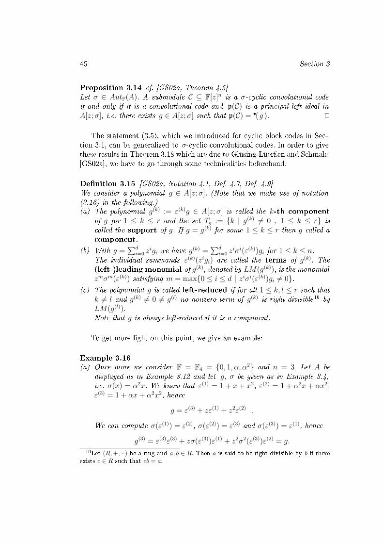
Example 3.4 cf. [GS02a, Example 2.11 (a)]We consider n = 3, F = F4 = {0, 1, α, α2}, σ ∈ AutF(A) de�ned by σ(x) =α2x (cf. Remark 3.5) and the matrix
G := [1 + z + z2, α + z + α2z2, α2 + z + αz2] .
It is readily shown that G is basic, hence C := im F[z]G is a convolutionalcode. Furthermore, C is σ-cyclic: If v denotes the �rst (and only) row of G,we have to show that x ∗σ p(v) and x2 ∗σ p(v) are in p(C) again, as Lemma3.3 tells us. We have
g := p(v) = 1 + αx + α2x2 + z(1 + x+ x2) + z2(1 + α2x+ αx2) .
We calculate
x ∗σ g = α2 + x+ αx2 + zα2(1 + x+ x2) + z2(α2 + αx + x2) = α2g ∈ p(C)
and therefore we have x2 ∗σ g = αg ∈ p(C).We even showed that C is the smallest σ-cyclic convolutional code containingthe codeword v(g). One can also show that dfree (C) = 9 (cf. [GS02a, Example2.11 (a)]), which is optimal among all (3, 1, 2)-submodules (recall the MDS-bound in (1.1)). Hence C is a MDS-convolutional code.
In the generalized concept of cyclicity we use automorphisms from thegroup AutF(A). This gives rise to the question how this group looks like.In particular we may ask, if there are nontrivial automorphisms in AutF(A)at all. We will answer this question in Section 3.2.2. For the moment thefollowing remark gives �rst information.
Remark 3.5 [GS02a, Example 2.13]Note that any F-algebra automorphism σ ∈ AutF(A) is completely determined
40 Section 3
by the value of σ(x) ∈ A. Furthermore, the elements 1, x, . . . , xn−1 ∈ A areF-linearly independent, hence 1, σ(x), . . . , σ(x)n−1 ∈ A are F-linearly inde-pendent, too. It is not hard to show that this condition is even su�cientto de�ne an automorphism σ, precisely: If a ∈ A satis�es an = 1 and if1, a, . . . , an−1 are F-linearly independent, then a := σ(x) de�nes an automor-phism σ ∈ AutF(A).For example we consider the case F = F4 = {0, 1, α, α2} and use thisbrute force method to determine the group AutF(A) (there are more sys-tematic ones, see Section 3.2.2). This yields AutF(A) = {σ | σ(x) ∈{x, x2, αx, α2x, αx2, α2x2}}.
Now we extend "∗σ" in order to obtain a (non-commutative) ring struc-ture on A[z] and to generalize the statement "codes can be identi�ed withideals" in this context:
De�nition and Theorem 3.6 [GS02a, Def. 2.9, Observation 2.10 (a)]Let σ ∈ AutF(A). The product g ∗σ h of the polynomials g =
∑ν≥0 z
νgν,h =
∑µ≥0 z
µhµ ∈ A[z] is de�ned as( ∑ν≥0
zνgν)∗σ( ∑µ≥0
zµhµ)
:=∑λ≥0
zλ∑ν+µ=λ
σµ(gν)hµ .
The set A[z] equipped with the usual addition and the multiplication " ∗σ" iscalled the Piret algebra (with parameters q = |F|, n, σ) and will be denotedby A[z;σ].Indeed, A[z;σ] is an F-algebra and it carries a canonical left F[z]-modulestructure. It is non-commutative if and only if σ(x) 6= x, i.e. σ is not theidentity on A. 2
If we compute the product g ∗σ h, then we can evaluate it distributivelyas usual (with respect to the rules in a non-commutative ring) and then shiftall coe�cients gν to the right side of z according to the rule
a ∗σ z = z ∗σ σ(a) for all a ∈ A .
In this setting σ-cyclic submodules appear as a natural generalisation ofcyclic block codes, because block codes are the (left) ideals in A and σ-cyclicsubmodules turn out to be left ideals in A[z;σ]:
Proposition 3.7 [GS02a, Observation 2.10 (b)]Let σ ∈ AutF(A). A submodule C ⊆ F[z]n is σ-cyclic if and only if its poly-nomial representation p(C) is a left ideal in A[z;σ]. 2
Cyclicity 41
3.2.2 More Information on the Structure of A and AutF(A)
It will be very helpful for further investigations to display A as a cartesianproduct of �elds as it is done in this section. We follow the lines of [GS02a,Section 3]. The notation as introduced here will also be used later on in thisthesis.
The assumption (3.1) implies that the normalized prime factorsπ1, . . . , πr ∈ F[x] of the prime factor decomposition
xn − 1 = π1 · . . . · πr (3.9)
are pairwise di�erent. Without loss of generality we assume that they areordered in the following way:
degx π1 = . . . = degx πr1 < . . . < degx π1+∑s−1i=1 ri
= . . . = degx π∑si=1 ri
(3.10)where r1 + . . .+rs = r. For later use we group the indices of the prime factorsaccording to their (the prime factors) degree:
R(j) := {1 +
j−1∑µ=1
rµ, 2 +
j−1∑µ=1
rµ, . . . ,
j∑µ=1
rµ} , 1 ≤ j ≤ s . (3.11)
Of course, the sets R(1), . . . , R(s) de�ne a disjoint partition of {1, . . . , r} and|R(j)| = rj for 1 ≤ j ≤ s.
Now F [x]/〈 πk 〉 is a �nite �eld, precisely it is a �nite Galois extension ofF of dimension degx πk for 1 ≤ k ≤ r and it is isomorphic to the �eld
Kk := {f ∈ F[x] | degx f < degx πk} with multiplication modulo πk .
We denote by ρk(a) ∈ Kk the remainder of a ∈ F[x] modulo πk and considerthe mapping
ρ : A→ K1 × . . .×Kr , a 7→ [ρ1(a), . . . , ρr(a)] , (3.12)
which is an isomorphism of rings due to the Chinese Remainder Theorem,where the cartesian product is endowed with component-wise addition andmultiplication. We can identify A with K1 × . . . × Kr, but to ensure thatwe do not mix up vectors and elements of the cartesian product we use thenotation
[[a1, . . . , ar]] := ρ−1([a1, . . . , ar]) . (3.13)

42 Section 3
The elementsε(k) := [[0, . . . , 0, 1, 0, . . . , 0]] , where the "1" is at the k-th position , (3.14)
will be an important tool to investigate cyclic convolutional codes. They arethe uniquely determined primitive 8 and pairwise orthogonal idempotents ofA. The k-th component of A, which is de�ned as
K(k) := ε(k)A = {ρ−1(a) | a ∈ 0× . . .× 0×Kk × 0× . . .× 0} , (3.15)is a �eld which is isomorphic to Kk. Hence A =
∑ri=1 K
(i). Any ideal of A(these "are" the cyclic block codes) can be written as
r∑i=1
Ui , where Ui ∈ {{0}, K(i)} for 1 ≤ i ≤ r .
Finally we consider the group AutF(A) and give some more informationon its structure. The basic idea is that any automorphism σ ∈ AutF(A)maps K(k) onto K(l) for some l, i.e. σ induces a permutation on the set{K(1), . . . , K(r)}. Furthermore, K(k) and K(l) must have the same cardinal-ity (this means degx πk = degx πl). This works (loosely speaking) the otherway round, too: Any permutation of the �elds {K(1), . . . , K(r)} which re-spects their cardinality combined with F-linear automorphisms of the �eldsthemselves induces an F-automorphism of A. We specify this in the followingtheorem.
Theorem 3.8 [GS02a, Theorem 3.1](a) There exist (usually non-unique) F-linear automorphisms of �elds
ψ1, . . . , ψr such that with ψ = (ψ1, . . . , ψr) the mapping
ψ ◦ ρ : Aρ→ K1 × . . .×Kr
(ψ1,...,ψr)→ Lr11 × . . .× Lrss
is a ring-automorphism and Lj is a �nite Galois extension of F which isisomorphic to Kk for any k ∈ R(j).
(b) Let the data be as in (a). Let Gj := AutF(Lj) be the group of all F-linearautomorphisms of Lj for 1 ≤ j ≤ s and let Sr1,...,rs be the subgroup of thesymmetric group Sr, which leaves all sets R(1), . . . , R(s) invariant. Thenthe group AutF(L
r11 × . . .× Lrss ) is given by
(Gr11 × . . .×Grs
s ) ◦ Sr1,...,rs ,
8An idempotent is called primitive if it cannot be written as a nontrivial sum of or-thogonal idempotents.

Cyclicity 43
where " ◦" is de�ned as
((γ1, . . . , γr) ◦ β)[a1, . . . , ar] := [γ1(aβ−1(1)), . . . , γr(aβ−1(r))]
for all [a1, . . . , ar] ∈ Lr11 × . . .×Lrss and all (γ1, . . . , γr) ∈ Gr11 × . . .×Grs
s ,β ∈ Sr1,...,rs.
(c) By virtue of (a) the group AutF(A) and the group AutF(Lr11 × . . .× Lrss )
are isomorphic. An isomorphism is given by : AutF(Lr11 × . . .× Lrss ) → AutF(A)
γ ◦ β 7→ γ ◦ β := ρ−1 ◦ ψ−1 ◦ γ ◦ β ◦ ψ ◦ ρ.
The following commutative diagram shall illustrate this:
Aγ◦β−→ A
ρ ↓ ↑ ρ−1
K1 × . . .×Kr K1 × . . .×Kr
ψ = (ψ1, . . . , ψr) ↓ ↑ (ψ−11 , . . . , ψ−1
r ) = ψ−1
Lr11 × . . .× Lrssγ◦β−→ Lr11 × . . .× Lrss
In other words: For all [[a1, . . . , ar]] ∈ A we have
(γ ◦ β)([[a1, . . . , ar]])
= [[ψ−11 (γ1(ψβ−1(1)(aβ−1(1)))), . . . , ψ
−1r (γr(ψβ−1(r)(aβ−1(r))))]] .
2
As a consequence of the foregoing theorem, we can determine the cardi-nality of AutF(A):
Corollary 3.9 [GS02a, Corollary 3.2]Let Lj be as in Theorem 3.8 and put dj := degx πi where i ∈ R(j), 1 ≤ j ≤ s.Then
|AutF(A)| = dr1i · · · drss · r1! . . . rs! . 2
The group-isomorphism which we speci�ed in Theorem 3.8 (c) appears tobe a bit cumbersome. But it has a nice property: The primitive idempotentsε(1), . . . , ε(r) are permuted by γ ◦ β ∈ AutF(A) according to the permutationβ:
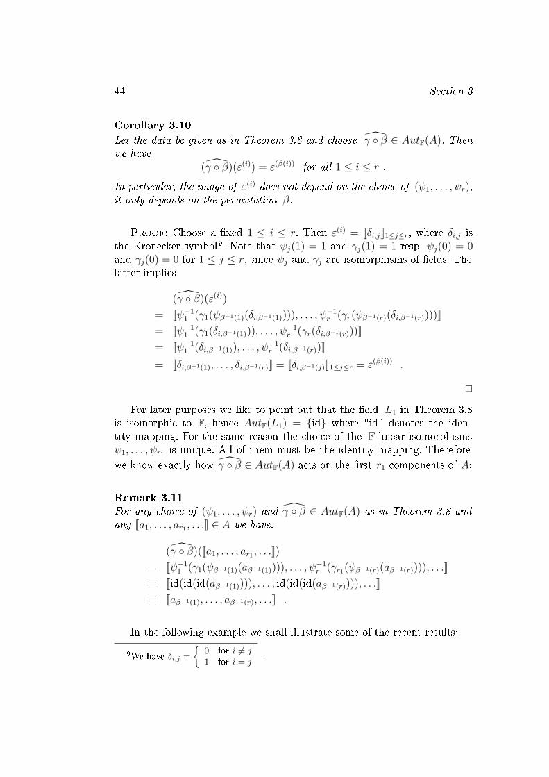
44 Section 3
Corollary 3.10Let the data be given as in Theorem 3.8 and choose γ ◦ β ∈ AutF(A). Thenwe have
(γ ◦ β)(ε(i)) = ε(β(i)) for all 1 ≤ i ≤ r .
In particular, the image of ε(i) does not depend on the choice of (ψ1, . . . , ψr),it only depends on the permutation β.
Proof: Choose a �xed 1 ≤ i ≤ r. Then ε(i) = [[δi,j]]1≤j≤r, where δi,j isthe Kronecker symbol9. Note that ψj(1) = 1 and γj(1) = 1 resp. ψj(0) = 0and γj(0) = 0 for 1 ≤ j ≤ r, since ψj and γj are isomorphisms of �elds. Thelatter implies
(γ ◦ β)(ε(i))
= [[ψ−11 (γ1(ψβ−1(1)(δi,β−1(1)))), . . . , ψ
−1r (γr(ψβ−1(r)(δi,β−1(r))))]]
= [[ψ−11 (γ1(δi,β−1(1))), . . . , ψ
−1r (γr(δi,β−1(r)))]]
= [[ψ−11 (δi,β−1(1)), . . . , ψ
−1r (δi,β−1(r))]]
= [[δi,β−1(1), . . . , δi,β−1(r)]] = [[δi,β−1(j)]]1≤j≤r = ε(β(i)) .
2
For later purposes we like to point out that the �eld L1 in Theorem 3.8is isomorphic to F, hence AutF(L1) = {id} where "id" denotes the iden-tity mapping. For the same reason the choice of the F-linear isomorphismsψ1, . . . , ψr1 is unique: All of them must be the identity mapping. Thereforewe know exactly how γ ◦ β ∈ AutF(A) acts on the �rst r1 components of A:
Remark 3.11For any choice of (ψ1, . . . , ψr) and γ ◦ β ∈ AutF(A) as in Theorem 3.8 andany [[a1, . . . , ar1 , . . .]] ∈ A we have:
(γ ◦ β)([[a1, . . . , ar1 , . . .]])
= [[ψ−11 (γ1(ψβ−1(1)(aβ−1(1)))), . . . , ψ
−1r (γr1(ψβ−1(r)(aβ−1(r)))), . . .]]
= [[id(id(id(aβ−1(1)))), . . . , id(id(id(aβ−1(r)))), . . .]]
= [[aβ−1(1), . . . , aβ−1(r), . . .]] .
In the following example we shall illustrate some of the recent results:9We have δi,j =
{0 for i 6= j1 for i = j
.

Cyclicity 45
Example 3.12Again, we consider F = F4 = {0, 1, α, α2} and n = 3. The polynomial xn − 1splits into linear prime divisors, precisely xn − 1 = (x + 1)(x + α)(x + α2).We display A as
ρ−1(F[x]/〈x+ 1 〉 ×
F[x]/〈x+ α 〉 ×F[x]/〈x+ α2 〉
).
Now ε(1) = 1 + x + x2, ε(2) = 1 + α2x + αx2, ε(3) = 1 + αx + α2x2, as onecan easily check by computing ε(i)(1), ε(i)(α), ε(i)(α2) for i = 1, 2, 3. We knowfrom Remark 3.5 that AutF(A) = {σ |σ(x) ∈ {x, x2, αx, α2x, αx2, α2x2}}.One can readily see that
[[1, α, α2]] = x , [[α, α2, 1]] = αx , [[α2, 1, α]] = α2x ,[[1, α2, α]] = x2 , [[α, 1, α2]] = αx2 , [[α2, α, 1]] = α2x2.
Theorem 3.8 tells us that AutF(A) ∼= S3. Actually, we get all automorphismsin AutF(A) if we permute the components in x = [[1, α, α2]].With Remark 3.11 we know that, for instance, the automorphism σ de�nedby σ(x) = αx satis�es σ(ε(1)) = ε(3), σ(ε(2)) = ε(1) and σ(ε(3)) = ε(2).
In the foregoing example, the �elds F[x]/〈 πi 〉 were isomorphic to F. For amore general example where K(i) 6∼= F for some 1 < i ≤ n we refer to [GS02a,Example 3.3 (b)].
3.2.3 Properties of Cyclic Convolutional Codes
In this section we consider a �xed automorphism σ ∈ AutF(A) and a �xedrepresentation of A as a cartesian product of �elds K1 × . . . × Kr. Let thedata be as in (3.9) � (3.15).
Furthermore, we will omit the symbol "∗σ" when multiplying polynomialsin the non-commutative F-algebra A[z;σ], i.e.
gh := g ∗σ h for all g, h ∈ A[z;σ] . (3.16)
Principal left ideals in A[z;σ] will play a crucial role (cf. Proposition 3.14)and we introduce the following notation:
Notation 3.13A principal left ideal in A[z;σ] generated by g ∈ A[z;σ] is denoted by •〈 g 〉.
46 Section 3
Proposition 3.14 cf. [GS02a, Theorem 4.5]Let σ ∈ AutF(A). A submodule C ⊆ F[z]n is a σ-cyclic convolutional codeif and only if it is a convolutional code and p(C) is a principal left ideal inA[z;σ], i.e. there exists g ∈ A[z;σ] such that p(C) = •〈 g 〉. 2
The statement (3.5), which we introduced for cyclic block codes in Sec-tion 3.1, can be generalized to σ-cyclic convolutional codes. In order to givethese results in Theorem 3.18 which are due to Glüsing-Lüerÿen and Schmale[GS02a], we have to go through some technicalities beforehand.
De�nition 3.15 [GS02a, Notation 4.1, Def. 4.7, Def. 4.9]We consider a polynomial g ∈ A[z;σ]. (Note that we make use of notation(3.16) in the following.)(a) The polynomial g(k) := ε(k)g ∈ A[z;σ] is called the k-th component
of g for 1 ≤ k ≤ r and the set Tg := {k | g(k) 6= 0 , 1 ≤ k ≤ r} iscalled the support of g. If g = g(k) for some 1 ≤ k ≤ r then g called acomponent.
(b) With g =∑d
i=0 zigi we have g(k) =
∑di=0 z
iσi(ε(k))gi for 1 ≤ k ≤ n.The individual summands ε(k)(zigi) are called the terms of g(k). The(left-)leading monomial of g(k), denoted by LM(g(k)), is the monomialzmσm(ε(k)) satisfying m = max{0 ≤ i ≤ d | ziσi(ε(k))gi 6= 0}.
(c) The polynomial g is called left-reduced if for all 1 ≤ k, l ≤ r such thatk 6= l and g(k) 6= 0 6= g(l) no nonzero term of g(k) is right divisible 10 byLM(g(l)).Note that g is always left-reduced if it is a component.
To get more light on this point, we give an example:
Example 3.16(a) Once more we consider F = F4 = {0, 1, α, α2} and n = 3. Let A be
displayed as in Example 3.12 and let g, σ be given as in Example 3.4,i.e. σ(x) = α2x. We know that ε(1) = 1 + x + x2, ε(2) = 1 + α2x + αx2,ε(3) = 1 + αx + α2x2, hence
g = ε(3) + zε(1) + z2ε(2) .
We can compute σ(ε(1)) = ε(2), σ(ε(2)) = ε(3) and σ(ε(3)) = ε(1), hence
g(3) = ε(3)ε(3) + zσ(ε(3))ε(1) + z2σ2(ε(3))ε(2) = g.10Let (R,+, · ) be a ring and a, b ∈ R. Then a is said to be right divisible by b if there
exists c ∈ R such that cb = a.

Cyclicity 47
This implies that g(1) = g(2) = 0 and that g is a component. Of course gis left-reduced.
(b) We continue with the example from part (a) but consider g where
g = ε(1) + zε(1) + z2ε(1) .
Now g(1) = ε(1), g(2) = z2ε(1) and g(3) = zε(1). The leading monomial ofg(1) is LM(g(1)) = ε(1) and the terms of g(2) and g(3) are right divisibleby ε(1). This shows that g is not reduced.If we consider C := •〈 g 〉, we have
C = •〈 g(1), g(2), g(3) 〉 = •〈 g(1), g(2) − z2g(1)︸ ︷︷ ︸= 0
, g(3) − zg(1)︸ ︷︷ ︸= 0
〉 = •〈 g(1) 〉 .
Hence C can be generated by g(1) = ε(1), which is a left-reduced polyno-mial.
(c) Finally we give an example for a left-reduced polynomial which is nota component. We consider g as in (a), but replace σ with the identity.Now g(1) = zε(1), g(2) = z2ε(2) and g(3) = ε(3) and no term of g(i) is rightdivisible by LM(g(j)) for i, j = 1, 2, 3, i 6= j, therefore g is left-reduced.
Theorem and De�nition 3.17 [GS02a, Cor. 4.13, Thm. 4.15 (b), Lemma4.3 (c)](a) Let C be a σ-cyclic convolutional code. Then there exists a left-reduced
polynomial g ∈ A[z;σ] such that p(C) = •〈 g 〉. Any left reduced polyno-mial with this property is called a generator polynomial of C (resp.p(C)).
(b) If g is a generator polynomial of C and p(C) = •〈 g 〉 for some g ∈ A[z;σ](which is not necessarily left-reduced), then g = ug for some unit u ∈A[z;σ]. If g is left-reduced, then g = ug for some unit u ∈ A.In particular, the support of a generator polynomial does not depend ofits choice and we call Tg the support of C (resp. p(C)).
Theorem 3.18 [GS02a, Theorem 7.8, Theorem 7.13]Let C ⊆ F[z]n be a σ-cyclic submodule and let p(C) = •〈 g 〉, where g is left-reduced. De�ne π(g) :=
∏k∈Tg πk, κk := degx πk and κ := degx π(g). Then we
have(a) A left F[z]-basis of •〈 g 〉 is given by g, xg, . . . , xκ−1g. As a consequence,
the matrix v(g)v(xg)...
v(xκ−1g)
∈ Fκ×n

48 Section 3
is a generator matrix of C, in particular, C is an (n, κ)-submodule.
(b) Let k ∈ Tg. The matrix
Gk :=
v(g(k))v(xg(k))
...v(xκk−1g(k))
∈ Fκk×nis a minimal basis of the σ-cyclic (n, κk)-submodule v(•〈 g(k) 〉). If C isa convolutional code, then v(•〈 g(k) 〉) is a (σ-cyclic) convolutional code,too.
(c) If Tg = {k1, . . . , kt} and Gk1 , . . . , Gkt are de�ned as in (b), then Gk1
...Gkt
∈ Fκ×nis a minimal basis of C. 2
The foregoing theorem allows us not only to determine a generator matrixor a minimal basis of C, but also the complexity of C and its Forney indices(recall Theorem 1.3). This is speci�ed in the following corollary.
Corollary 3.19 [GS02a, Corollary 7.15]Let C ⊆ F[z]n be a σ-cyclic convolutional code and let g be a generator poly-nomial. Furthermore, let Tg = {k1, . . . , kt} denote the support of C and writeκki := degx πki and δki := degx g(ki) for 1 ≤ i ≤ t. Then C has the Forneyindices
δk1 , . . . , δk1︸ ︷︷ ︸κk1 times
, . . . , δkt , . . . , δkt︸ ︷︷ ︸κkt times
and C has the complexity δ =∑
i∈Tg κiδki.
In particular, v(•〈 g(ki) 〉) is a σ-cyclic (n, κki)-convolutional code with Forneyindices δki , . . . , δki (κki times) and complexity κkiδki for 1 ≤ i ≤ t. 2
The next two propositions give more information about the di�erencebetween arbitrary σ-cyclic submodules on the one hand and σ-cyclic convo-lutional codes on the other hand.
We saw in Proposition 3.14 that p(C) is a principal left ideal in A[z;σ] ifC is a σ-cyclic convolutional code. But not every principal left ideal in A[z;σ]

Cyclicity 49
de�nes a σ-cyclic convolutional code. A characterization of those principal leftideals which are σ-cyclic convolutional codes as well is given in the followingproposition:
Proposition 3.20 [GS02a, Proposition 7.10]Let C ⊆ F[z]n be a submodule where p(C) = •〈 g 〉 is a principal left ideal inA[z;σ] and g ∈ A[z;σ] is left-reduced with z-free term g0. Then C is a (σ-cyclic) convolutional code if and only if there exists some unit u in A[z;σ]such that g = g0u. 2
A necessary condition for a σ-cyclic submodule to be a σ-cyclic convolu-tional code is given in the next proposition and concerns the support of thiscode. It is used in the proof of Theorem 4.2.
Proposition 3.21 [GS02a, Thm. 4.5, Thm. 5.1 (c)]Let C ⊆ F[z]n be a σ-cyclic convolutional code and let g be a generator poly-nomial with z-free term g0. Then we have Tg = Tg0, i.e.
ε(k)g 6= 0 ⇐⇒ ε(k)g0 6= 0 for all 1 ≤ k ≤ r .
Theorem 3.18 (b), (c) also provides a canonical decomposition of a σ-cyclic convolutional code into a direct sum of "small" σ-cyclic convolutionalsub-codes:
Corollary 3.22Let C ⊆ F[z]n be a σ-cyclic convolutional code and let g be a generator poly-nomial. Then we have the following decomposition of C and p(C) into a directsum of F[z]-left modules:
C =⊕i∈Tg
v(•〈 g(i) 〉) , p(C) =⊕i∈Tg
•〈 g(i) 〉
Furthermore, the summands in the decomposition of C are σ-cyclic convolu-tional codes themselves. 2
50 Section 4
4 Minimal Cyclic Convolutional Codes
Recall that we always assume that (3.1) holds. Furthermore, we considera �xed automorphism σ ∈ AutF(A) and a �xed representation of A as acartesian product of �elds K1 × . . . ×Kr. Let the data be given as in (3.9)� (3.15). The multiplication in the F-algebra A[z;σ] will be denoted as in(3.16).
We will introduce the notion of minimal σ-cyclic convolutional codes inSection 4.1. It will turn out that units in A[z;σ] play a crucial role in theinvestigation of minimal σ-cyclic convolutional codes (cf. Theorem 4.6) andtherefore we give some information about units in A[z;σ] in Section 4.2. InSection 4.3 we state our main result, this is Theorem 4.15 which gives neces-sary and su�cient conditions for the existence of minimal cyclic convolutionalcodes with nonzero complexity. Consequences of this Theorem are discussed.
4.1 Minimality and First Properties
Piret and Roos investigated in [Pir76] and [Roo79] how a σ-cyclic convo-lutional code can be decomposed into a direct sum of "minimal" or "irre-ducible" σ-cyclic sub-codes. They used the following notion of minimality:
De�nition 4.1A σ-cyclic convolutional code C is called minimal if and only if it has nonontrivial σ-cyclic convolutional sub-code, this means for any σ-cyclic con-volutional code C where {0} 6= C ⊆ C we have C = C. In this case we callp(C) minimal, too.
The following theorem is crucial for our further investigations. It statesthat σ-cyclic convolutional codes, whose support has cardinality 1, coincidewith minimal σ-cyclic convolutional codes:
Theorem 4.2Let C be a σ-cyclic convolutional code with generator polynomial g ∈ A[z;σ].Then the following statements are equivalent:(i) C is minimal;
(ii) g is a component, i.e. there exists l ∈ {1, . . . , r} such that g = ε(l)g = g(l).
Minimal Cyclic Convolutional Codes 51
Proof: The case C = {0} is trivial, hence we assume C 6= {0}."(ii)⇒(i)": We have 0 6= g = g(l) and Tg = Tg0 = {l} (cf. Proposition 3.21),where g0 ∈ ε(l)A denotes the z-free term of g . Let {0} 6= U ⊆ C be aσ-cyclic sub-code of C with generator polynomial 0 6= h ∈ A[z;σ]. Sincep(U) = •〈h 〉 ⊆ •〈 g 〉, we have h = ug for some u ∈ A[z;σ], in particular wehave h0 = u0g0 ∈ ε(l)A, where u0 resp. h0 denotes the z-free term of u resp.h. Proposition 3.21 implies that Th = Th0 , thus Th = {l} and 0 6= h = h(l).Theorem 3.18 (b) yields that U and C have the same rank as F[z]-modulesand with Theorem 1.7 (vii) we conclude C = U .
"(i)⇒(ii)": Let Tg = {k1, . . . , kt} where t ≥ 2. Corollary 3.22 yields that{0} 6= v(•〈 g(ki) 〉) ⊆ C is a σ-cyclic convolutional sub-code of C for 1 ≤ i ≤ tand it satis�es v(•〈 g(ki) 〉) 6= C. 2
A main structural result of Piret [Pir76, Theorem 3.11] and Roos [Roo79,Theorem 4 and the following text] is that every σ-cyclic convolutional codehas a decomposition into a direct sum of minimal σ-cyclic sub-codes. ThusTheorem 3.18 resp. Corollary 3.22 along with Theorem 4.2 recovers this resultand yields a method to construct such a decomposition, too.
Remark 4.3The decomposition of a σ-cyclic convolutional code C with generator polyno-mial g as in Corollary 3.22, i.e. C =
⊕i∈Tg v(•〈 g(i) 〉), is a decomposition into
a direct sum of minimal σ-cyclic convolutional codes (as F[z]-left modules).Moreover, it is obvious that a convolutional code C is σ-cyclic if and only ifit is a direct sum of minimal σ-cyclic convolutional codes (as F[z]-left mod-ules). In this sense we can think of minimal σ-cyclic convolutional codes asthe "smallest components" of σ-cyclic convolutional codes.
The next remark recalls how we can determine the dimension and com-plexity (resp. the Forney indices) of a minimal σ-cyclic convolutional code.
Remark 4.4Let C be a minimal σ-cyclic convolutional code with support {l} and generatorpolynomial g = g(l). De�ne k := degx πl and d := degz g. Then Corollary 3.19yields that C is an (n, k, kd)-submodule with Forney indices d, . . . , d (k times).In particular, the complexity of a minimal σ-cyclic convolutional code mustbe a multiple of its dimension.
We know that the support of a (minimal) σ-cyclic convolutional code isunique (cf. Theorem and De�nition 3.17). The following remark allows us to
52 Section 4
determine the support of a minimal σ-cyclic convolutional with the aid of aminimal basis.
Remark 4.5Let C be a minimal σ-cyclic (n, k)-convolutional code with support {l} andlet G be a minimal basis of C with rows G1, . . . , Gk. Then one has
{Tp(G1), . . . , Tp(Gk)} = {l}
and the support of C can be determined with the knowledge of only one rowof a minimal basis.
Proof: Let g = g(l) be a generator polynomial of C and de�ne Gi :=v(xi−1g) for 1 ≤ i ≤ k. Note that Tp(Gi)
= {l}, since x is a unit in A.With Theorem 3.18 (c) we know that the matrix G (consisting of the rowsG1, . . . , Gk) is a minimal basis of C, too. Since all row degrees of G resp. G arethe same, Theorem 1.3 (iv) implies that Gi must be an F-linear combinationof G1, . . . , Gk for 1 ≤ i ≤ k. Therefore we have Tp(Gi) = {l}. 2
At this point, we know that a minimal σ-cyclic convolutional code isgenerated by a component and we know how to determine the dimension,the complexity and the support of the code. But we do not know how we cantell from a given polynomial g = g(l) if the σ-cyclic submodule v(•〈 g 〉) is aconvolutional code. The following theorem answers this question.
Theorem 4.6Let {0} 6= C be a σ-cyclic submodule of F[z]n and let p(C) = •〈 g 〉 whereg = g(l) ∈ A[z;σ] for some 1 ≤ l ≤ r (in particular g is left reduced). Thenthe following statements are equivalent:(i) C is a (σ-cyclic, minimal) convolutional code;
(ii) g = g(l) is the l-th component of a unit u ∈ A[z;σ], i.e. we have u(l) = g.
In particular, any component u(l) of a unit u ∈ A[z;σ] de�nes a minimalσ-cyclic (n, k, dk)-convolutional code, where k := degx πl and d := degz u(l).
Proof: With Proposition 3.20 we know that the submodule •〈 g 〉 is aconvolutional code if and only if g = g0v for some unit v ∈ A[z;σ]. In thiscase we have
g = g(l) = ε(l)g = ε(l)g0v = g(l)0 ε(l)v = g
(l)0 v(l) .
Minimal Cyclic Convolutional Codes 53
Now de�ne g0 := g(l)0 +
∑ri=1,i6=l ε
(i). Then g0 is a unit in A, since ε(i)g0 6= 0for 1 ≤ i ≤ r (cf. Lemma 4.8) and therefore u := g0v is a unit in A[z;σ] andit satis�es g = ε(l)u = u(l). 2
The above leads to the question under which conditions there exist min-imal σ-cyclic convolutional codes with nonzero complexity. We will answerthis question in Theorem 4.15 after we collected enough information aboutunits in A[z;σ] and their components. But a �rst step towards the solutionof this problem can be introduced at this very time.
Lemma 4.7Let C be a minimal σ-cyclic convolutional code with support {l} and generatorpolynomial g = g(l). Then we have
ε(l)g = gε(l) ⇐⇒ C has complexity 0 .
In particular we have: If C has nonzero complexity, then ε(l)g 6= gε(l). Thisalso implies σ(ε(l)) 6= ε(l).
Proof: The proof of "⇒" stems from [GS02a, Proof of Proposition 3.4]:If ε(l)g = g = gε(l), then •〈 g 〉 ⊆ •〈 ε(l) 〉 =: J . Since Tg = Tε(l) = {l}, theconvolutional codes C and v(J) have the same dimension (cf. Theorem 3.18),they are equal by Theorem 1.7 (vii). With deg z ε(l) = 0 along with Remark4.4 we conclude that C has complexity δ = 0."⇐": Remark 4.4 implies that deg z g = 0, hence g ∈ A. Of course ε(l)g = gε(l)
is true in this case. 2
In other words Lemma 4.7 states that there can only exist (minimal)σ-cyclic convolutional codes with nonzero complexity if the automorphism
σ does not act like the identity mapping on ε(1), . . . , ε(r) . (4.1)Roos stated in [Roo79, Section VI] that the necessary condition (4.1) is suf-�cient, but he gave only a sketch of the proof. A complete proof is given in[GS02a, Theorem 3.4 and its proof] and that proof shows that (4.1) impliesthe existence of a minimal σ-cyclic (n, k, k)-convolutional code. But whatabout other complexities?
4.2 Units in A[z;σ]
Units in A[z;σ] (resp. their components) play a crucial role in the investi-gation of minimal cyclic convolutional codes (cf. Theorem 4.6). This sectiongives useful information about units in A[z;σ]. First of all, we recall how aunit in A looks like:

54 Section 4
Lemma 4.8 [GS02a, Lemma 4.3]An element a ∈ A is a unit in A if and only if ε(k)a 6= 0 for all 1 ≤ k ≤ r. 2
For a characterization of units in A[z;σ], we need the following de�nitionand remark:
De�nition 4.9Consider l ∈ {1, . . . , r} and σ ∈ AutF(A). Then the l-order of σ is de�nedas ol(σ) := ol := min{m ∈ N | σm(ε(l)) = ε(l)}.
Remark 4.10For l ∈ {1, . . . , r}, σ ∈ AutF(A) and σ(ε(l)) = ε(l′) we have ol = ol′.
The next theorem states (loosely speaking) that any unit in A[z;σ] is a�nite product of special, "simple" units. In this sense, we know all units anddue to Theorem 4.6 we know all minimal σ-cyclic codes.
De�nition and Theorem 4.11 (Inspired by [GS02a, Proof of Corollary4.13])(a) Consider a ∈ A, d ∈ N0 and m ∈ {1 . . . , r}. The element u(d,a,ε(m)) :=
1 + zdaε(m) satis�es u(d,a,ε(m)) = u(d,a(m),ε(m)). Furthermore, one has:
u(d,a,ε(m)) is a unit in A[z;σ] ⇐⇒{a(m) 6= −ε(m) if d = 0a(m) = 0 or om 6 | d if d ≥ 1
.
If u(d,a,ε(m)) is a unit, it has the inverse u(d,−a,ε(m)) and it is called anelementary unit.
(b) Any unit in A[z;σ] is a �nite product of elementary units. In particular,a unit a ∈ A can be written as a = u(0,a−1,ε(1)) · . . . · u(0,a−1,ε(r)).
Proof: (a): Obviously u(d,a,ε(m)) = u(d,a(m),ε(m)). If d = 0, thenu(d,a(m),ε(m)) = 1 + a(m) =: α ∈ A is a unit if and only if α(i) 6= 0 for 1 ≤ i ≤ r
(cf. Lemma 4.8), which is the case if and only if a(m) 6= −ε(m).Now we consider the case d ≥ 1. We can assume without loss of generalitythat a(m) 6= 0, because otherwise u(d,a,ε(m)) = u(d,−a,ε(m)) = 1. It remains toshow that
u(d,a,ε(m)) is a unit in A[z;σ] ⇐⇒ om 6 | d .
Minimal Cyclic Convolutional Codes 55
We prove "⇒" indirectly: Write u := u(d,a,ε(m)), for short. If om | d, thenε(m)u = u(m) = uε(m) and degz u(m) = d ≥ 1. If u was a unit, then The-orem 4.6 implies that C := v(•〈u(m) 〉) was a minimal σ-cyclic (n, k, dk)-convolutional code generated by u(m) with support m, where k := degx πm ≥1. But this is in contradiction to the fact that C must have complexity 0because of Lemma 4.7.The "⇐"-part of the proof can be established as follows: We show thatu(d,a,ε(m))u(d,−a,ε(m)) = u(d,−a,ε(m))u(d,a,ε(m)) = 1 if om 6 | d. Note that σd(ε(m)) 6=ε(m) if om 6 | d, hence σd(ε(m))ε(m) = 0. With the aid of the last equation wecalculate
u(d,a,ε(m))u(d,−a,ε(m)) =(1 + zdaε(m)
) (1− zdaε(m)
)= 1 + zdaε(m) − zdaε(m) − zdaε(m)zdaε(m)
= 1− z2dσd(a)aσd(ε(m))ε(m) = 1 .
The equation u(d,−a,ε(m))u(d,a,ε(m)) = 1 can be obtained with the same argu-ments (replace a with −a).(b): The proof of the equality a = u(0,a−1,ε(1)) · . . . · u(0,a−1,ε(r)) for a beinga unit in A can be done straightforwardly. (It is even true for a being anarbitrary element of A.)For the remaining part of the proof we use results from [GS02a]. Letu ∈ A[z;σ] be a unit. First of all, note that •〈u 〉 = A[z;σ] and that agenerator polynomial of the σ-cyclic convolutional code A[z;σ] must be aunit a ∈ A. From [GS02a, Cor. 4.13 (a) and its proof] we know that thereexist elementary units u−1
1 , . . . , u−1t ∈ A[z;σ] such that a = u−1
t · . . . · u−11 · u.
We already know that a can be written as a product of elementary units,hence u = u1 · . . . · ut · a can be written as a product of elementary units. 2
Now we know due to the foregoing theorem how to construct (all) unitsin A[z;σ]. If σ(ε(l)) 6= ε(l), we are even able to specify units whose l-th com-ponent has a prescribed degree. This is the subject of the following corollary:
Corollary 4.12Consider l ∈ {1, . . . , r} and σ ∈ AutF(A) such that σ(ε(l)) 6= ε(l). Then wehave:
(a) For any a ∈ A and i ∈ N0 the element ua(i) := 1 + zaσi(ε(l)) is anelementary unit in A[z;σ], its inverse is u−a(i).
(b) For any d ∈ N0 there exists a unit u ∈ A[z;σ] such that degz u(l) = d =degz u.

56 Section 4
Proof: Part (a) can be established as follows: We have ua(i) =u(1,a,σi(ε(l))). The case degz ua(i) = 0 is trivial. In the other case we havedegz ua(i) = 1 and therefore ol 6 | degz ua(i), because ol > 1. If we putσi(ε(l)) = ε(li), then Remark 4.10 implies that ol = oli > 1 and thereforeoli 6 | degz ua(i). Theorem 4.11 (a) implies the assertion.Now we show part (b): Without loss of generality we may assume that d > 0.De�ne u := ua1(1) · . . . · uad(d) where a1, . . . , ad are units in A. From part (a)we know that u is a unit in A[z;σ], its inverse is u−ad(d) · . . . · u−a1(1). It hasz-degree at most d. The zd-part of u is given by(
za1σ(ε(l)))·(za2σ
2(ε(l)))· . . . ·
(zadσ
d(ε(l)))
= zd(σd−1(a1)σd−2(a2) · . . . · σ(ad−1)ad︸ ︷︷ ︸
=: a
)(σd(ε(l)) · . . . · σd(ε(l))︸ ︷︷ ︸
= σd(ε(l))
).
Now we have u = 1 + f + zdaσd(ε(l)), where f =∑d−1
i=1 zifi is chosen appro-
priately. Hence
u(l) = ε(l)u = ε(l)(1 + f + zdaσd(ε(l))) = ε(l) + f (l) + zdaσd(ε(l)) .
Of course, a is a unit in A, since a1, . . . , ad are units in A. In particular wehave aσd(ε(l)) 6= 0 (cf. Lemma 4.8). We conclude that deg z u(l) = d = degz u.The proof is complete, but we like to mention that deg z u(l′) < d for anyl′ ∈ {1, . . . , r} \ {l}. 2
As a direct consequence of Corollary 4.12, we have the following resultconcerning the existence of minimal σ-cyclic (n, k, dk)-convolutional codesfor arbitrary d ∈ N0:
Corollary 4.13Consider l ∈ {1, . . . , r} and σ ∈ AutF(A) such that σ(ε(l)) 6= ε(l). Putk := degx πl. Then for any d ∈ N0 there exists a minimal σ-cyclic (n, k, dk)-convolutional code with support {l}.
Proof: With Theorem 4.6 along with Remark 4.4 we have to show theexistence of a unit u in A[z;σ] satisfying degz u(l) = d. This was done inCorollary 4.12 (b). 2
Corollary 4.12 (b) and its proof provide a construction method for min-imal σ-cyclic (n, k, dk)-convolutional codes and we will use this method togenerate an example:
Minimal Cyclic Convolutional Codes 57
Example 4.14(a) We consider F = F4 = {0, 1, α, α2} and n = 3 and the representation of
A as in Example 3.12, i.e. ε(1) = 1 + x + x2, ε(2) = 1 + α2x + αx2 andε(3) = 1+αx+α2x2. We choose the automorphism σ given by σ(x) = x2,this implies
σ(ε(1)) = ε(1) , σ(ε(2)) = ε(3) , σ(ε(3)) = ε(2) .
Now we want to construct minimal σ-cyclic (3, 1, 3)-convolutional codeswith support {2}. Towards this end we put l = 2 and consider the units
u := u1(1) · u1(2) · u1(3) = (1 + zε(3))(1 + zε(2))(1 + zε(3))
= 1 + zε(2) + z2(ε(2) + ε(3)) + z3ε(3) ,
u := uα(1) · u1(2) · u1(3) = (1 + zαε(3))(1 + zε(2))(1 + zε(3))
= 1 + z(ε(2) + α2ε(3)) + z2(αε(2) + ε(3)) + z3αε(3) .
The second component of u is u(2) = ε(2) + z2ε(2) + z3ε(3) and thusC := v(•〈u(2) 〉) is a minimal σ-cyclic (3, 1, 3)-convolutional code. WithTheorem 3.18, we have that
G := [v(u(2))] = [1 + z2 + z3, α2 + α2z2 + αz3, α + αz2 + α2z3]
is a generator matrix of C. Obviously we have dfree (C) ≤ 9. Indeed wehave dfree (C) = 9 as one can verify for example with the aid of MAPLEand [GS02b]. Of course this distance is not MDS.The second component of u is u(2) = ε(2) +zα2ε(3) +z2αε(2) +z3αε(3) andthus C := v(•〈 u(2) 〉) is a minimal σ-cyclic (3, 1, 3)-convolutional code. Agenerator matrix of this code is given by
G := [v(u(2))] = [1+α2z+αz2+αz3, α2+z+z2+α2z3, α+αz+α2z2+z3]
and the free distance of C is at most 12. MAPLE and [GS02b] yield thatdfree (C) = 12, which is MDS.
(b) Again we deal with F = F4 = {0, 1, α, α2}, but now we put n = 5. In thiscase xn − 1 = (x+ 1)(x2 + αx + 1)(x2 + α2x+ 1) and we display A as
A = ρ−1(F[x]/〈x+ 1 〉 ×
F[x]/〈x2 + αx + 1 〉 ×F[x]/〈x2 + α2x+ 1 〉
).
The primitive idempotents are given by ε(1) = 1 + x+ x2 + x3 + x4 and
ε(2) = αx + α2x2 + α2x3 + αx4 , ε(3) = α2x+ αx2 + αx3 + α2x4

58 Section 4
and the automorphism σ ∈ AutF(A) de�ned by σ(x) = x3 maps ε(2)
onto ε(3) and vice versa. So we are able to construct σ-cyclic mini-mal (5, 2, 2 · 3)-convolutional codes with support {2}. We put l = 2 andas in (a) we investigate the units u = u1(1) · u1(2) · u1(3) and u =uα(1)·u1(2)·u1(3) resp. their second components u(2) = ε(2)+z2ε(2)+z3ε(3)
and u(2) = ε(2) +zα2ε(3) +z2αε(2) +z3αε(3). In this setting C := v(•〈u(2) 〉)and C := v(•〈 u(2) 〉) are a minimal σ-cyclic (5, 2, 6)-convolutional codes.The MDS-bound for (5, 2, 6)-convolutional codes is 19, but with the gen-eralized Griesmer bound given in [GS03, Theorem 3.4] one �nds thatany (5, 2, 6)-convolutional code over F4 with Forney indices (3, 3) hasfree distance at most 16. A generator matrix of the code C is given by
G :=
[v(u(2))v(xu(2))
]=
0 α + αz2 + αz3
α + αz2 + α2z3 α2z2 + α2z3
α2 + α2z2 + αz3 α + α2z2
α2 + α2z2 + αz3 α2 + αz2 + α2z3
α + αz2 + α2z3 α2 + αz3
t
and both rows in G have weight 12. With the aid of MAPLE and [GS02b]we calculated dfree (C) = 10.The matrix
G :=
[v(u(2))v(xu(2))
]=
0 α + z + α2z2 + α2z3
α + αz + α2z2 + z3 z + z2 + z3
α2 + z + z2 + α2z3 α + αz + z2
α2 + z + z2 + α2z3 α2 + α2z2 + z3
α + αz + α2z2 + z3 α2 + αz + α2z3
t
is a generator matrix of the code C and both rows of G have weight 16.Again we used the computer to calculate dfree (C) = 14.
4.3 Existence of Minimal Cyclic Convolutional Codes
In the foregoing sections we gave some information about the existence ofminimal σ-cyclic convolutional codes with nonzero complexity: In Lemma 4.7and the following comments we learned that minimal σ-cyclic convolutionalcodes with nonzero complexity exist if and only if (4.1) is satis�ed. Corollary4.13 gave even deeper insight: It states that (4.1) implies the existence of min-imal σ-cyclic convolutional codes with support {l} and complexity degx πl · dfor any d ∈ N0. The following theorem combines these �ndings.
Minimal Cyclic Convolutional Codes 59
Theorem 4.15Let σ ∈ AutF(A) and l ∈ {1, . . . , r} and de�ne k := degx πl. Then thefollowing statements are equivalent:(i) σ(ε(l)) 6= ε(l) ;
(ii) v(•〈 ε(l) + zσ(ε(l)) 〉
)is a (minimal, σ-cyclic) convolutional code;
(iii) there exists a minimal σ-cyclic convolutional code with support {l} andnonzero complexity;
(iv) for any d ∈ N0 there exists a minimal σ-cyclic (n, k, kd)-convolutionalcode with support {l}.
Proof: "(i)⇒(ii)" was shown in [GS02a, Proof of Proposition 3.4]. Butwe can also develop a proof out of the present context: With Corollary 4.12(a), we know that ε(l) + zσ(ε(l)) is the l-th component of the unit u1(1) andwith Theorem 4.6 we conclude that v
(•〈 ε(l) + zσ(ε(l)) 〉) is a (minimal) σ-
cyclic convolutional code. "(ii)⇒(iii)" is obvious. "(iii)⇒(i)" and "(iv)⇒(i)"follow with Lemma 4.7. "(i)⇒(iv)" is a consequence of Corollary 4.13. 2
As a consequence, the existence of an automorphism σ ∈ AutF(A) whichgives rise to minimal σ-cyclic convolutional codes with nonzero complexityonly depends on the the prime factor decomposition of xn−1, as the followingcorollary shows:
Corollary 4.16For k ∈ {1, . . . , n− 1} the following statements are equivalent:(i) There exists σ ∈ AutF(A) such that there exist minimal σ-cyclic
(n, k, dk)-convolutional codes for any d ∈ N0;
(ii) there exist at least two prime divisors of xn − 1 over F of x-degree k.
The Proof is a simple consequence of Theorem 3.8. 2
With Corollary 3.22, we know that σ-cyclic convolutional codes withnonzero complexity do exist if and only if there are minimal σ-cyclic con-volutional codes with nonzero complexity. For sake of clarity we repeat thisresult in the following remark:
Remark 4.17A necessary and su�cient condition for the existence of a σ-cyclic convo-lutional code with nonzero complexity is the existence of a minimal σ-cyclicconvolutional code with nonzero complexity. Hence there exist σ-cyclic con-volutional codes with nonzero complexity if and only if the prime factor de-composition of xn−1 has at least two prime divisors of the same degree. Thisis a slightly modi�ed version of [GS02a, Proposition 3.4].

60 Section 4
Corollary 4.16 resp. Remark 4.17 gives rise to the question how the primefactor decomposition of xn − 1 over Fq looks like. The theory of cyclic blockcodes provides a complete answer to this question, see for example [MS78,Chapter 7, �5]. A helpful tool are the so-called "cyclotomic cosets", whichwill be investigated now. Recall that we always assume gcd(n, p) = 1 wherep denotes the characteristic of F = Fq. This is equivalent to gcd(n, q) = 1.
De�nition and Theorem 4.18 cf. [MS78, Chapter 7, �5]Let n, q be positive integers, q a prime power, where gcd(n, q) = 1. For j ∈ Zwe use the notation j for the remainder of j modulo n.(a) For i ∈ {0, 1, . . . , n− 1} we de�ne
Ci := {i, iq, iq2, . . . , iqdi−1} , where di := min{t ∈ N | iqt ≡ i mod n} .(4.2)
The sets C0, . . . , Cn−1 are called the cyclotomic cosets mod n. In par-ticular we have |Ci| = di for 0 ≤ i ≤ n− 1.
(b) There exists r ∈ N and i1, . . . , ir ∈ {0, 1, . . . , n− 1} such that
{0, 1, . . . , n− 1} =r⋃
ν=1
• Ciν (disjoint union of sets) .
(c) With the data as in (b) we have: The prime factor decomposition ofxn − 1 over Fq consists of r irreducible polynomials and the degrees ofthese irreducible factors are (up to permutation) given by di1 , . . . , dir .
Example 4.19(a) Consider n = 5, q = 2. Then the cyclotomic cosets mod 5 are given by
C0 = {0} , C1 = {1, 2, 4, 3} = C2 = C4 = C3
and x5 − 1 ∈ F2[x] has one linear prime divisor (namely x− 1) and oneof degree 4 (namely x4 + x3 + x2 + x + 1). In particular, every σ-cyclicconvolutional code has complexity 0 for any σ ∈ AutF2(A).
(b) Now we consider n = 8, q = 3. The cyclotomic cosets mod 8 are givenby
C0 ={0}, C1 ={1, 3}=C3, C2 ={2, 6}=C6, C4 ={4}, C5 ={5, 7}=C7
and x8 − 1 ∈ F3[x] has two linear prime divisors (these must be x − 1and x − 2) and three of degree 2. In particular, in this case there existautomorphisms σ ∈ AutF3(A) such that there exist minimal σ-cyclic(8, 1, d)- resp. (8, 2, 2d)-convolutional codes for any d ∈ N0.

Minimal Cyclic Convolutional Codes 61
Just to have a more complete picture of minimal σ-cyclic convolutionalcodes, we like to state that not all σ-cyclic (n, k, dk)-convolutional code areminimal:
Remark 4.20There exist σ-cyclic (n, k, dk)-convolutional codes, which are not minimalFor example, we consider a �eld F and n ≥ 3 where xn− 1 has at least threelinear prime divisors (for instance F = F4 and n = 9). Now ε(1), ε(2) and ε(3)
correspond to linear prime divisors and we choose σ ∈ AutF(A) such that
σ(ε(1)) = ε(2) , σ(ε(2)) = ε(3) , σ(ε(3)) = ε(1) .
(This is possible due to Theorem 3.8.)The polynomial g = (1+zε(3))(1+zε(2)) = 1+z(ε(2) +ε(3)) is a unit in A[z;σ]because it is a product of elementary units (cf. Corollary 4.12). The �rst andsecond component of g are given by g(1) = ε(1) + zε(2) and g(2) = ε(2) + zε(3).Hence Ci := v(•〈 g(i) 〉) is a minimal σ-cyclic (n, 1, 1)-convolutional code withsupport {i} for i = 1, 2 (cf. Theorem 4.6).The submodule C = C1⊕C2 = v(•〈 g(1) +g(2) 〉) is a σ-cyclic convolutional codebecause of Proposition 3.20: The z-free term of g := g(1)+g(2) is g0 = ε(1)+ε(2)
and we have g = g0g and g is a unit. Note that g is left-reduced, therefore Cis a σ-cyclic (n, 2, 2)-convolutional code, which is obviously not minimal.
We close this section with some remarks on the construction of minimalσ-cyclic convolutional codes via components of units (cf. Theorem 4.6). Weintend to demonstrate that it is not clear how to determine all minimal σ-cyclic (n, k, dk)-convolutional codes resp. how to construct "good" minimalσ-cyclic (n, k, dk)-convolutional codes.
Remark 4.21(a) The proof of Corollary 4.12 provides a method to construct minimal σ-
cyclic (n, k, dk)-convolutional codes. Here we used components of unitsof the form ua1(1) · . . . · uad(d), where a1, . . . , ad are units in A. It is notclear that an arbitrary minimal σ-cyclic (n, k, dk)-convolutional code canbe constructed in the same way, precisely: Let C be a minimal σ-cyclic(n, k, dk)-convolutional code with support {l} with generator polynomialg = g(l). We know from Theorem 4.6 that we can �nd a unit u ∈ A[z;σ]such that g = u(l). Is it possible to choose u = ua1(1) · . . . · uad(d) forsuitable units a1, . . . , ad ∈ A?

62 Section 4
(b) Consider a �xed d ∈ N0 and l ∈ {1, . . . , r}. It is not clear that all compo-nents u(l) having z-degree d of a unit u can be found just by investigatingunits having z-degree d, in other words: Do we have the equation
{u(l) | degz u(l) = d, u is a unit in A[z;σ]}= {u(l) | degz u(l) = d = degz u, u is a unit in A[z;σ]} ?
(c) What about the free distance of C := v(•〈u(l)) 〉 where u is a unit inA[z;σ]? If u is an elementary unit, then wt (v(u(l))) ≤ 2n as one canreadily show. Thus dfree (C) ≤ 2n and this is in general less than theoptimal bound dfree (C) ≤ (n− k)(bδ/kc + 1) + δ + 1 given in (1.1). Soif we wish to �nd minimal σ-cyclic (n, k, dk)-convolutional codes withgood free distance in this case, we must not investigate elementary unitsthemselves but rather their products.
4.4 Automorphisms Generating the same Cyclic Con-
volutional Codes
This section is a digression which deals (loosely speaking) with the questionhow many di�erent automorphisms in AutF(A) give rise to the same minimalcyclic codes with prescribed support.
In addition to the general assumptions which were made at the verybeginning of Section 4 we will now consider a �xed l ∈ {1, . . . , r}. Moreover,l is contained in one of the sets R(1), . . . , R(s) (see (3.11)) and we will denotethis set by R(L).
If C ⊆ F[z]n is a minimal σ-cyclic convolutional code with support {l}and generator polynomial g = g(l), then only the action of σ on the �eldsK(µ) = ε(µ)A, µ ∈ R(L), is of interest, precisely:
p(C) = •〈 g(l) 〉 = A[z;σ]ε(l)g(l) ⊆{ ∑
j≥0
zjaj∣∣ aj ∈ ∑
µ∈R(L)
K(µ)}.
This means that if two automorphisms σ, σ′ ∈ AutF(A) satisfy σ(h) = σ′(h)for all h ∈∑µ∈R(L) K(µ), a minimal σ-cyclic convolutional code with support{l} is σ′-cyclic and vice versa. In this sense σ, σ′ give rise to the same σ- resp.σ′-cyclic convolutional codes, although they may be "very" di�erent in theiraction on K(µ), µ 6∈ R(L). Our aim is to give some information about thealgebraic structure of automorphisms, which give rise to the same minimalσ-cyclic convolutional codes with support {l}.

Minimal Cyclic Convolutional Codes 63
We de�neH(L) := {σ ∈ AutF(A) | σ(h) = h for h ∈∑µ∈R(L) K(µ)} .
Then H(L) is a normal subgroup of AutF(A) because we have τ−1◦σ◦τ ∈ H(L)
for any τ ∈ AutF(A) and any σ ∈ H(L): For the proof it is su�cient to showthat h ∈∑µ∈R(L) K(µ) implies τ(h) ∈
∑µ∈R(L) K(µ). But this is a consequence
of Theorem 3.8 (which implies {K(µ) | µ ∈ R(L)} = {τ(K(µ)) | µ ∈ R(L)})along with the fact that τ is an F-automorphism of A.
We conclude thatAutF(A)/H(L) = {σH(L) | σ ∈ AutF(A)}
is a group again and σH(L) = {σ′ | σ(h) = σ′(h) for h ∈ ∑µ∈R(L) K(µ)} forσ ∈ AutF(A). Along with Theorem 3.8 we have
AutF(A)/H(L)
∼= GrLL ◦ SrL ,
where the notation "GL" and "◦" stems from Theorem 3.8. In particular,|AutF(A)/H(L)| = (degx πL)rL · rL! and there are at most (degx πL)rL · rL!"really di�erent" automorphisms which give rise to minimal cyclic convolu-tional codes with support {l}:
Theorem 4.22Let C ⊆ F[z]n be a convolutional code and let σ, σ′ ∈ AutF(A) satisfy σH(L) =σ′H(L). Then C is σ-cyclic and minimal with support {l} if and only if C isσ′-cyclic and minimal with support {l}. 2
If we have σ, σ′ ∈ AutF(A) and if each minimal σ-cyclic convolutionalcode with support {l} is σ′-cyclic, too, then it is not clear that this impliesσH(L) = σ′H(L). (This would be the inverse implication of Theorem 4.22.)In the case L = 1 this statement is true, as we will see in Theorem 4.25. But inthe case L ≥ 2 it is not true in general: For L ≥ 2 there exist σ, σ′ ∈ AutF(A)satisfying σ(ε(i)) = σ′(ε(i)) = ε(i) for 1 ≤ i ≤ r and σH(L) 6= σ′H(L), cf.Theorem 3.8. Theorem 4.15 implies that any minimal σ-cyclic convolutionalcode with support {l} has complexity 0, hence it is cyclic with respect toany automorphism in AutF(A). The latter implies that all minimal σ-cyclicconvolutional codes with support {l} are σ′-cyclic, too.
The following remark shows that we can not deduce σH(L) = σ′H(L) if wefound (just) one minimal σ-cyclic convolutional code with support {l} whichis σ′-cyclic, too, even if it has nonzero complexity and even if L = 1:
64 Section 4
Remark 4.23In general it is not true that σ, σ′ ∈ AutF(A) satisfy σH(L) = σ′H(L) ifthere exists a convolutional code which is both σ- and σ′-cyclic. A trivialcounterexample are block codes, but we can also give a counterexample forminimal cyclic codes with nonzero complexity:Consider some n ∈ N and a �eld F where there are three linear prime divisorsof xn − 1 corresponding to the primitive idempotent elements ε(1), ε(2) andε(3). Then by Theorem 3.8 there exist automorphisms σ, σ′ ∈ AutF(A) suchthat
σ(ε(1)) = ε(2) , σ(ε(2)) = ε(3) , σ(ε(3)) = ε(1)
σ′(ε(1)) = ε(3) , σ′(ε(2)) = ε(2) , σ′(ε(3)) = ε(1) .
Note that this implies σH(1) 6= σ′H(1). Now u := 1 + z5ε(3) is a unitboth in A[z;σ] and in A[z;σ′] (cf. Theorem 4.11) and its �rst componentis u(1) = ε(1) + z5ε(3) in both F-algebras. With Theorems 3.18 and 4.6we conclude that [v(ε(1) + z5ε(3))] ∈ F[z]1×n is a generator matrix of aconvolutional code, which is minimal and cyclic with respect to σ and σ′.
We �nish this section with an investigation of the case L = 1, i.e. l ∈{1, . . . , r1}. We have H(1) = {σ ∈ AutF(A) | σ(ε(i)) = ε(i) for 1 ≤ i ≤ r1} sinceK(i) ∼= F for 1 ≤ i ≤ r1. Furthermore, we have AutF(A)/H(1) ∼= Sr1 . In thiscase, we can specify an isomorphism between the two groups AutF(A)/H(1)
and Sr1 :
Proposition 4.24Let πi := x−bi for 1 ≤ i ≤ r1. In particular we have x = [[b1, . . . , br1 , x, . . . , x]].We know from Remark 3.11 that for any automorphism σ ∈ AutF(A)there exists a uniquely determined permutation βσ ∈ Sr1 such that σ(x) =[[bβ−1
σ (1), . . . , bβ−1σ (r1), . . .]]. In particular we have σ(ε(i)) = ε(βσ(i)) for 1 ≤ i ≤ r1
(cf. Corollary 3.10).Along with Theorem 3.8 we obtain that the mapping
β( · ) : AutF(A)→ Sr1 , σ 7→ βσ
is a surjective group homomorphism and {σ ∈ Aut(A) | βσ = id} = H(1).With the Homomorphism Theorem, we conclude that
AutF(A)/H(1) → Sr1 , σH(1) 7→ βσ (4.3)
is an isomorphism of the two groups. 2
Minimal Cyclic Convolutional Codes 65
All minimal σ-cyclic convolutional codes with support l ∈ {1, . . . , r1} are1-dimensional and vice versa, as we will see in the next section in Observation5.1. Therefore Theorem 4.22 can be reformulated and extended in this case:
Theorem 4.25For σ, σ′ ∈ AutF(A) we have σH(1) = σ′H(1) if and only if any σ-cyclic(n, 1)-convolutional code is σ′-cyclic.
Proof: The "only if"-part of the proof is Theorem 4.22. For the "if"-partwe assume that σH(1) 6= σ′H(1) and construct a 1-dimensional code, which iscyclic with respect to σ, but not with respect to σ′. If σH(1) 6= σ′H(1), thenthere exists l ∈ {1, . . . , r1} such that
ε(l) = σ(ε(l)) 6= σ′(ε(l)) = ε(l′) .
If ε(l) = ε(l), then Theorem 4.15 yields on the one hand that any σ-cyclic(n, 1)-convolutional code with support {l} has complexity 0. On the otherhand it tells us that there exist σ′-cyclic (n, 1)-convolutional codes with sup-port {l} and with nonzero complexity. Hence the proof is complete for thecase l = l.It remains to prove the case l 6= l. We consider the element u := ε(l) +zε(l). Inthe algebra A[z;σ] this is the l-th component of the elementary unit 1+zε(l),hence C := v(•〈u 〉) de�nes a σ-cyclic (n, 1)-convolutional code.If C was σ′-cyclic, too, then the left ideal I := A[z;σ′]·u must be contained inp(C). We show that this is impossible: Note that u is left reduced in A[z;σ′],since it has the two components ε(l) and zε(l) and l 6= l. Therefore v(I) is a σ′-cyclic submodule of F[z]n with �generator polynomial� u. Theorem 3.18 tellsus that v(I) has dimension 2. This means v(I) 6⊆ C and therefore I 6⊆ p(C).
2

66 Section 5
5 Cyclic Convolutional Codes of Dimension 1
Recall that we always assume that (3.1) holds. Furthermore, we considera �xed automorphism σ ∈ AutF(A) and a �xed representation of A as acartesian product of �elds K1×. . .×Kr. Again we make use of the frameworkas in (3.9) � (3.15) and the multiplication in the F-algebra A[z;σ] will bedenoted as in (3.16).
This section deals with 1-dimensional σ-cyclic convolutional codes, be-cause these are examples for minimal σ-cyclic convolutional codes, as thefollowing observation tells us:
Observation 5.1Let {0} 6= C ⊆ F[z]n be a σ-cyclic (n, k)-submodule and let p(C) =•〈 g 〉, where g is left-reduced. Recall Theorem 3.18 (a), which states thatg, xv(g), . . . , xk−1v(g) is a left F[z]-basis of C and that k = degx π(g), whereπ(g) :=
∏k∈Tg πk. This implies
C is 1-dimensional ⇐⇒ g = g(l) for some l ∈ {1, . . . , r1} = R(1) .
In particular we have that C is a 1-dimensional σ-cyclic convolutional codeif and only if C is a minimal σ-cyclic convolutional code with support {l} forsome l ∈ {1, . . . , r1}.
We will deepen the results about minimal σ-cyclic convolutional codesfrom the previous section for 1-dimensional cyclic convolutional codes inSection 5.1. In Section 5.2 we determine the shape of generator matrices of1-dimensional cyclic convolutional codes. This result is used to suggest somemethods for constructing 1-dimensional cyclic convolutional codes resp. theinvestigation of special 1-dimensional cyclic convolutional codes in Section5.3.
5.1 Existence of 1-dimensional Cyclic Convolutional
Codes
With Observation 5.1, we can reformulate Theorem 4.15 and Remark 4.17for 1-dimensional cyclic convolutional codes:

Cyclic Convolutional Codes of Dimension 1 67
Theorem 5.2Let σ ∈ AutF(A) and l ∈ {1, . . . , r1}. Then the following statements areequivalent:(i) σ(ε(l)) 6= ε(l) ;
(ii) [v(ε(l) + zσ(ε(l))
)] is basic;
(iii) there exists a σ-cyclic (n, 1, δ)-convolutional code for some δ ∈ N;(iv) there exists a σ-cyclic (n, 1, δ)-convolutional code for any δ ∈ N0. 2
Corollary 5.3The following statements are equivalent:(i) There exists σ ∈ AutF(A) such that there exists a σ-cyclic (n, 1, δ)-
convolutional code for some δ ∈ N;(ii) there exist at least two linear prime divisors of xn − 1 over F. 2
The problem, for which n, q the polynomial xn− 1 has at least two linearprime divisors over Fq, can be solved completely and we will develop ananswer now. Recall Theorem 4.18 and the notation Ci and di from (4.2). Wecan re-formulate the question for which n, q the polynomial xn − 1 has atleast two linear prime divisors over Fq by asking: For which n, q does thereexist a cyclotomic coset Ci where di = 1 and i ∈ {1, . . . , n− 1}? But di = 1if and only if iq ≡ i mod n, which is equivalent to n | i(q − 1).
Lemma 5.4For n, q ∈ N, n, q ≥ 2, the following statements are equivalent:(i) There exists i ∈ {1, . . . , n− 1} such that n | i(q − 1);
(ii) gcd(n, q − 1) 6= 1 .
Proof. (i)⇒(ii): If gcd(n, q − 1) = 1, then n | i(q − 1) is possible only ifn | i. This is impossible because of i < n.(ii)⇒(i): De�ne f := gcd(n, q − 1) > 1 and i := n
f. Then i ∈ {1, . . . , n − 1}
and i(q − 1) = n q−1f, hence n | i(q − 1). 2
Now the following theorem is obvious:
Theorem 5.5Let n ∈ N, let q be a prime power and consider F := Fq. (As always weassume gcd(n, q) = 1.) The following statements are equivalent:(i) The polynomial xn − 1 has at least two linear prime divisors over Fq;

68 Section 5
(ii) gcd(n, q − 1) 6= 1 ;
(iii) there exists σ ∈ AutF(A), such that there exists a σ-cyclic (n, 1, δ)-convolutional code for any δ ∈ N0. 2
We illustrate this by investigating some special �elds in the followingcorollary.
Corollary 5.6(a) There exists no σ-cyclic (n, 1, δ)-convolutional code over F2 for any n
(satisfying (3.1)) and σ ∈ AutF2(A) if we have δ ≥ 1. In other words:All 1-dimensional σ-cyclic convolutional codes over F2 have complexity0 and are block codes in this sense.Observe that F2 is an important �eld for applications and that the non-existence of 1-dimensional σ-cyclic convolutional codes over F2 withnonzero complexity is a pity from this point of view.
(b) Over F3 there exist σ-cyclic (n, 1, δ)-convolutional codes for δ ≥ 1 if andonly if 2 |n.
(c) Over F4 there exist σ-cyclic (n, 1, δ)-convolutional codes for δ ≥ 1 if andonly if 3 |n.
(d) If n ∈ N is even and F is a �nite �eld where char(F) 6= 2, then n andq − 1 are both multiples of 2. Hence there exists σ ∈ AutF(A) such thatthere exists a σ-cyclic (n, 1, δ)-convolutional code for any δ ∈ N0.
5.2 Generator Matrices of 1-dimensional Cyclic Convo-
lutional Codes
We intend to develop how generator matrices of 1-dimensional σ-cyclic con-volutional codes look like. For this purpose, we present a proposition whichprovides a �rst link between a generator polynomial and a generator matrixof a 1-dimensional σ-cyclic convolutional code.Throughout this section let σ denote a �xed automorphism in AutF(A).
Proposition 5.7(a) A generator matrix of an (n, 1)-submodule of F[z]n is unique up to mul-
tiplication with a constant factor in F \ {0}. In particular, a generatorpolynomial g of a σ-cyclic (n, 1)-convolutional code C is unique up tomultiplication with a constant factor in F \ {0} and v(g) is a minimalbasis of C.

Cyclic Convolutional Codes of Dimension 1 69
(b) Let v be an F[z]-basis of the (n, 1)-submodule C and let g := p(v) ∈ A[z;σ]satisfy g = g(l) for some l ∈ {1, . . . , r1}. Then C is σ-cyclic and we havep(C) = •〈 g 〉.
(c) If C is an (n, 1)-convolutional code with F[z]-basis v, thenC is σ-cyclic ⇐⇒ p(v) = p(v)(l) for some l ∈ {1, . . . , r1} .
Proof: The �rst statement of part (a) is obvious. The second one followsfrom the �rst along with Theorem 3.18 (a).
Part (b) can be proved as follows. If g = g(l) for some l ∈ {1, . . . , r1}, theng is left-reduced and it is an F[z]-basis of •〈 g 〉 by Theorem 3.18 (a). Thismeans v is an F[z]-basis both of C and of the σ-cyclic submodule C := v(•〈 g 〉),hence C = C. In particular C is σ-cyclic.
The "⇐"-part of (c) is a special case of (b). For the "⇒"-part we writep(C) = •〈 g 〉, where g = g(l) ∈ A[z;σ] for some l ∈ {1, . . . , r1} (cf. Observation5.1). Notice that g is left-reduced. Again Theorem 3.18 (a) implies that v(g)is an F[z]-basis of C and along with part (a) we have v = αv(g) for someα ∈ F \ {0}. Hence p(v) = αg and p(v) = p(v)(l). 2
Parts (b) and (c) of Proposition 5.7 tell us that a 1-dimensional submoduleC ⊆ F[z]n with generator matrix G = [v] ∈ F[z]1×n is a σ-cyclic convolutionalcode if and only if G is basic and p(v) = p(v)(l) for some l ∈ {1, . . . , r1}. Thismeans that the set of all generator matrices of σ-cyclic (n, 1)-convolutionalcodes with support {l}, l ∈ {1, . . . , r1}, is given by
Gl :={
[v(g(l))]∣∣ g ∈ A[z;σ] , [v(g(l))] is basic } . (5.1)
Obviously we can learn something about generator matrices of 1-dimensionalσ-cyclic convolutional if we investigate the components of a polynomial inA[z;σ]. If g =
∑δi=0 z
igi ∈ A[z;σ] is such a polynomial and l ∈ {1, . . . , r1},then
g(l) = ε(l)g =δ∑i=0
ziσi(ε(l))gi .
Notice that σi(ε(l)) = ε(l′) for some l′ ∈ {1, . . . , r1}, hence we have σi(ε(l))gi ∈ε(l′)A ∼= F. Therefore we can pretend that gi are elements in F, precisely: Forl ∈ {1, . . . , r1} we have
{g(l)
∣∣ g ∈ A[z;σ]}
={ δ∑
i=0
aiziσi(ε(l))
∣∣ δ ∈ N0 , a0, . . . , aδ ∈ F}.

70 Section 5
Consequently the set Gl de�ned in (5.1) is the set of all basic matrices of theform
[δ∑i=0
aiziv(σi(ε(l)))] , where δ ∈ N0 , a0, . . . , aδ ∈ F . (5.2)
Fortunately, we can determine exactly how v(ε(1)), . . . , v(ε(r1)) look like(and therefore we know how v(σi(ε(l))) looks like). Details are given now:Notation 5.8(a) We write πl = x− bl for 1 ≤ l ≤ r1.
(b) For a �xed l ∈ {1, . . . , r1} we use the notation
ε(li) := σi(ε(l)) and bσi := bli for any i ∈ N0 .
Note that bσi = bσi mod ol for any i ∈ N0. (For the de�nition of ol recallDe�nition 4.9.)
Lemma 5.9
For 1 ≤ l ≤ r1 and bl as in Notation 5.8 (a) we have ε(l) = n−1n−1∑i=0
bn−il xi, in
particularv(ε(l)) = n−1[1, bn−1
l , bn−2l , . . . , b2
l , bl] .
Proof: De�ne pl := xn−1x−bl
=∏r
i=1,i6=l πi. It is easy to see that pl equalsε(l) up to a constant in F \ {0}, precisely
ε(l) =(pl(bl)
)−1pl .
Note that in this setting bnl = 1 and therefore b−nl = 1. Dividing xn − 1 byπl = x − bl we calculate pl =
∑n−1i=0 b
n−(i+1)l xi. This yields pl(bl) = nbn−1
l =nb−1
l and ε(l) = n−1blpl = n−1∑n−1
i=0 bn−il xi. 2
Again, a matrix G ∈ F[z]1×n is a generator matrix of a σ-cyclic (n, 1)-convolutional code C with support {l} ⊆ {1, . . . , r1} if and only if G ∈ Gl(see (5.1) and (5.2)). Now we know exactly how the elements of Gl look like(cf. Lemma 5.9), indeed G ∈ Gl if and only if G is basic and
G = [δ∑i=0
aiziv(σi(ε(l)))] = [
δ∑i=0
aiziv(ε(li))]
=δ∑i=0
aizi · n−1 · [1, bn−1
σi, bn−2σi
, . . . , b2σi , bσi ]
= n−1 ·δ∑i=0
aizi[1, bn−1
σi, bn−2σi
, . . . , b2σi , bσi ] for some a0, . . . , aδ ∈ F ,

Cyclic Convolutional Codes of Dimension 1 71
where we made use of Notation 5.8 (b). Rescaling the matrix G with n wecan assume without loss of generality that
G =δ∑i=0
aizi[1, bn−1
σi, bn−2σi
, . . . , b2σi , bσi ] for some a0, . . . , aδ ∈ F .
We know from Proposition 5.7 (a) that G is a minimal basis. Hence, the codeim F[z]G has complexity exactly δ if and only if aδ 6= 0.
We summarize these statements in the following corollary.
Corollary 5.10Let C be an (n, 1, δ)-submodule. Then the following statements are equivalent:(i) C is a σ-cyclic (n, 1, δ)-convolutional code;
(ii) there exists some l ∈ {1, . . . , r1} and a0, . . . , aδ ∈ F satisfying a0 6= 0 6=aδ such that
δ∑i=0
aizi[1, bn−1
σi, bn−2σi
, . . . , b2σi , bσi ] is a basic generator matrix of C ,
where we made use of Notation 5.8 (b).In particular, a σ-cyclic (n, 1, δ)-convolutional code C having complexity δ > 0satis�es 2n ≤ dfree (C) ≤ |{i | ai 6= 0}| · n ≤ (δ + 1) · n. If C has complexity0 then dfree (C) = n.
Proof: Most parts of the proof are clear from the foregoing investiga-tions. It remains to show that for some σ-cyclic (n, 1, δ)-convolutional codeC the formula 2n ≤ dfree (C) ≤ |{i | ai 6= 0}| · n is true in the case δ > 0 andthat dfree (C) = n if δ = 0.Let G :=
∑δi=0 aiz
i[1, bn−1σi
, bn−2σi
, . . . , b2σi , bσi ] be a generator matrix of C. If
δ > 0, then every entry in G has a nonzero constant term and a nonzerocoe�cient of zδ. A nonzero codeword in C can be written as fG for somef ∈ F[z] \ {0} and we have degz fG > 0. Again, every entry in fG has anonzero constant term and the z-leading coe�cient is nonzero, too. Henceevery entry of fG has weight at least 2 and we conclude 2n ≤ dfree (C). Theupper bound for dfree (C) can be obtained with wt (G) = |{i | ai 6= 0}| · n.The case δ = 0 follows with the same arguments, but now the constant termand the zδ-term of every entry in G are the same. 2
The two bounds for dfree (C) which were given in Corollary 5.10 are tightin general. We give examples in the next remark.

72 Section 5
Remark 5.11Observe that the upper bound dfree (C) ≤ (δ + 1) · n is the MDS-boundfor (n, 1, δ)-codes (cf. (1.1)). Consequently all σ-cyclic (n, 1, 0)-convolutionalcodes are MDS block codes.Both the lower and the upper bound 2n ≤ dfree (C) ≤ |{i | ai 6= 0}| · n forσ-cyclic (n, 1, δ)-convolutional codes having complexity δ > 0 are tight, thesimplest example is the case δ = 1. Then 2n ≤ dfree (C) ≤ 2n and we con-clude that every σ-cyclic (n, 1, δ)-convolutional code having complexity δ = 0or δ = 1 is an MDS-convolutional code.There are also examples for both bounds being tight for δ ≥ 2: For the upperbound recall Example 3.4, which introduced a σ-cyclic (3, 1, 2)-convolutionalcode over F4 with optimal free distance 9. For the lower bound we considersome σ ∈ AutF(A) such that σ(ε(1)) = ε(2) and σ(ε(2)) = ε(1). We de�nean (n, 1, 3)-convolutional code C via the generator polynomial g = g(1) =ε(1) +z3ε(2), which is the �rst component of the elementary unit 1+z3ε(2) (seeTheorems 4.6 and 4.11). Now [v(g)] = [1 + z3, bn−1
σ0 + z3bn−1σ3 , . . . , bσ0 + z3bσ3 ]
is a generator matrix of C which has weight 2n, hence dfree (C) = 2n.
We close this section by a corollary which tells us how one can checkwhether a given basic matrix G ∈ F[z]1×n is a generator matrix of a σ-cyclic(n, 1)-convolutional code.
Corollary 5.12We know from Remark 4.5 that we can determine the support of a minimalσ-cyclic convolutional code C ⊆ F[z]n with the knowledge of one row of aminimal basis of C. In the 1-dimensional case every generator matrix G =[v] ∈ F[z]1×n is a minimal basis, hence Tp(v) is the support of C. But weknow even more in the 1-dimensional case, because the shape of G must beas described in Corollary 5.10 (ii).If G is a generator matrix of an (n, 1, δ)-convolutional code we can write
G =δ∑i=0
ai[1, gi,1, . . . , gi,n−1]zi
with suitable ai, gi,j ∈ F, 0 ≤ i ≤ δ, 1 ≤ j ≤ n−1. If we want to check whetherC is cyclic, we can �rst investigate g1,1. If g1,1 = b−1
l for some l ∈ {1, . . . , r1},then C might be cyclic with support {l}.Using Notation 5.8 (b) and choosing some σ ∈ AutF(A), we have
C is σ-cyclic ⇐⇒ ∀ 0 ≤ i ≤ δ where ai 6= 0 ∀ 1 ≤ j ≤ n− 1 : gi,j = bn−jσi
.

Cyclic Convolutional Codes of Dimension 1 73
By the way: We do not have to specify a certain σ ∈ AutF(A); we can startwith a permutation β ∈ Sr1 and use the Proposition 4.24 resp. the mappingin (4.3). The code C is cyclic with respect to any automorphism σ satisfyingβσ = β if and only if
∀ 0 ≤ i ≤ δ where ai 6= 0 ∀ 1 ≤ j ≤ n− 1 : gi,j = bn−jβi(l)
.
5.3 Some Attempts of Constructing 1-dimensional
Cyclic Convolutional Codes
Of course we can try to construct 1-dimensional σ-cyclic convolutional codes(or minimal σ-cyclic convolutional codes in general) via components of units(cf. Theorem 4.6). In the foregoing section we learned how generator matricesof 1-dimensional σ-cyclic convolutional codes look like. This provides anothermethod to construct these codes: We have to �nd or de�ne matrices whichhave the "right shape" and which are basic.
In Section 5.3.1 we present a method to construct 1-dimensional σ-cyclicconvolutional codes which uses irreducible polynomials over F[z]. In Section5.3.2 we investigate a special choice of a generator matrix of the "right shape"and try to �nd out under which condition this matrix is basic. Some resultswill be used in Section 5.3.3, where we introduce a method to construct1-dimensional σ-cyclic convolutional codes with a good free distance.
Throughout this section we consider a �xed l ∈ {1, . . . , r1} and a �xedσ ∈ AutF(A) such that σ(ε(l)) 6= ε(l). This means ol ≥ 2 (for the de�nitionof ol recall De�nition 4.9) and makes sure that we can �nd σ-cyclic (n, 1, δ)-convolutional codes for any δ ∈ N0 (cf. Theorem 5.2). We will also make useof Notation 5.8.
5.3.1 Construction via Irreducible Polynomials
We are able to describe a generator matrix of a σ-cyclic (n, 1, δ)-convolutionalcode with the aid of an irreducible polynomial in F[z] of degree δ > 0:
Lemma 5.13Choose an irreducible polynomial f =
∑δi=0 aiz
i ∈ F[z] with degree δ > 0.(This is always possible, cf. [LN97, Corollary 2.11].) Then
G :=δ∑i=0
aizi[1, bn−1
σi, bn−2σi
, . . . , bσi ]

74 Section 5
is a (basic) generator matrix of a σ-cyclic (n, 1, δ)-convolutional code with2n ≤ dfree (C) ≤ n · |{i | ai 6= 0}|.
Proof: Let f1 resp. f2 denote the �rst resp. the second entry of G. Weshow that f1 and f2 are coprime. This implies that G is basic. We have
bn−1σ0 · f1 = a0b
n−1σ0 + a1b
n−1σ0 z + . . .+ aδb
n−1σ0 zδ ,
f2 = a0bn−1σ0 + a1b
n−1σ1 z + . . .+ aδb
n−1σδ
zδ .
Now bn−1σ0 · f1 and f2 have the same z-free term and a di�erent z-coe�cient.
Since f1 was chosen irreducible, f2 must be coprime to f1. For the lower andthe upper bound of dfree (C) recall Corollary 5.10. 2
It is perhaps an advantage of this construction that we do not have to dealwith concrete units. But on the other hand it is not clear if the constructedcodes have good properties. For example, if we want to have a chance to ob-tain an MDS convolutional code via the construction method in Lemma 5.13,we have to �nd irreducible polynomials f =
∑δi=0 aiz
i ∈ F[z] with ai 6= 0,0 ≤ i ≤ δ. Even if we succeeded to �nd such an f , it can happen that thecorrespondinng code is not MDS (see Example 5.14).One may also argue that it is not so easy in general to �nd irreducible poly-nomials of prescribed degree over F. Fortunately, MAPLE is able to managethis task and the following example uses irreducible polynomials generatedby MAPLE via the command Randprime.
Example 5.14(a) We consider F = F7 and n = 4. The polynomial xn − 1 has the prime
factor decomposition xn − 1 = (x+ 1)(x+ 6)(x2 + 1). We display A as
A = ρ−1(F[x]/〈x+ 1 〉 ×
F[x]/〈x+ 6 〉 ×F[x]/〈x2 + 1 〉
).
We choose an automorphism σ ∈ AutF(A) which maps ε(1) = 2 + 5x +2x2 +5x3 onto ε(2) = 2+2x+2x2 +2x3 and vice versa. MAPLE suppliesus with the irreducible polynomial f := 5 + 3z + 3z2 + 4z3 + 6z4 + z5.Put G0 := [v(ε(1))] = [2, 5, 2, 5] and G1 := [v(ε(2))] = [2, 2, 2, 2]. Then thematrix
G := 5G0 + 3zG1 + 3z2G0 + 4z3G1 + 6z4G0 + z5G1
= 2 ·
5 + 3z + 3z2 + 4z3 + 6z4 + z5
2 + 3z + 4z2 + 4z3 + z4 + z5
5 + 3z + 3z2 + 4z3 + 6z4 + z5
2 + 3z + 4z2 + 4z3 + z4 + z5
t
Cyclic Convolutional Codes of Dimension 1 75
is a generator matrix of a σ-cyclic (4, 1, 5)-convolutional code C. Wehave dfree (C) ≤ 6 · 4 = 24. With MAPLE and [GS02b] we calculated 11
dfree (C) = 20, hence the code is not an MDS convolutional code.
(b) Once more we choose F = F4 = {0, 1, α, α2}, n = 3 and display A asin Example 3.12, i.e. v(ε(1)) = [1, 1, 1], v(ε(2)) = [1, α2, α] and v(ε(3)) =[1, α, α2]. The automorphism σ de�ned by σ(x) = α2x satis�es σ(ε(1)) =ε(2), σ(ε(2)) = ε(3) and σ(ε(3)) = ε(1). An irreducible polynomial of degree4 over F4 is f := 1 + αz + z3 + z4 and another one is f := α + α2z +z2 + α2z3 + z4. The matrix
G := [v(ε(1) + αzσ(ε(1)) + z3σ3(ε(1)) + z4σ4(ε(1)))]
= [1, 1, 1] + αz[1, α2, α] + z3[1, 1, 1] + z4[1, α2, α]
is a generator matrix of a σ-cyclic (3, 1, 4)-convolutional code C withsupport {1} and free distance dfree (C) ≤ 4 · 3 = 12. The code C is, ofcourse, not an MDS convolutional code.The matrix
G := [v(αε(1) + α2zσ(ε(1)) + z2σ2(ε(1)) + α2z3σ3(ε(1)) + z4σ4(ε(1))
= α[1, 1, 1] + α2z[1, α2, α] + z2[1, α, α2] + α2z3[1, 1, 1] + z4[1, α2, α]
is a generator matrix of a σ-cyclic (3, 1, 4)-convolutional code C withsupport {1} and free distance dfree (C) ≤ 5 · 3 = 15. The code C mightbe MDS. MAPLE and [GS02b] yield dfree (C) = 12 and dfree (C) = 14,in particular C is not MDS. Note that the generalized Griesmer boundgiven in [GS03] for (3, 1, 4)-convolutional codes over F4 is 14, thus C isoptimal.
We wish to mention that a generator matrix of a σ-cyclic (n, 1, δ)-convolutional code does not have one irreducible entry in general. Our very�rst Example 3.4 may illustrate this: There
G = [(z + α)(z + α2), α2(z + 1)(z + α2), α(z + 1)(z + α)]
is a generator matrix of a (3, 1, 2)-convolutional code over F4 = {0, 1, α, α2}which is cyclic with respect to σ given by σ(x) = α2x.
11Since the �rst and third resp. the second and fourth entry in G =: [g1, g2, g3, g4] arethe same, we tested G := [g1, g2] and found out that im F[z]G has free distance 10.
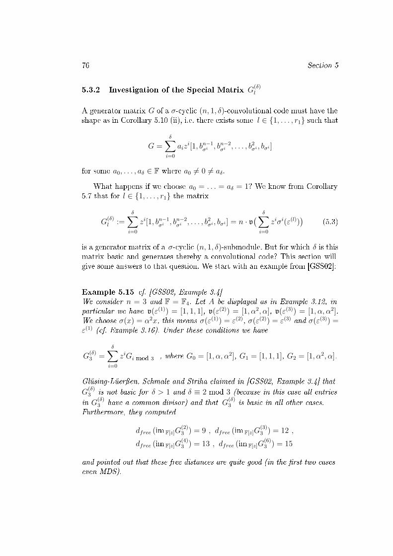
76 Section 5
5.3.2 Investigation of the Special Matrix G(δ)l
A generator matrix G of a σ-cyclic (n, 1, δ)-convolutional code must have theshape as in Corollary 5.10 (ii), i.e. there exists some l ∈ {1, . . . , r1} such that
G =δ∑i=0
aizi[1, bn−1
σi, bn−2σi
, . . . , b2σi , bσi ]
for some a0, . . . , aδ ∈ F where a0 6= 0 6= aδ.What happens if we choose a0 = . . . = aδ = 1? We know from Corollary
5.7 that for l ∈ {1, . . . , r1} the matrix
G(δ)l :=
δ∑i=0
zi[1, bn−1σi
, bn−2σi
, . . . , b2σi , bσi ] = n · v
( δ∑i=0
ziσi(ε(l))) (5.3)
is a generator matrix of a σ-cyclic (n, 1, δ)-submodule. But for which δ is thismatrix basic and generates thereby a convolutional code? This section willgive some answers to that question. We start with an example from [GSS02]:
Example 5.15 cf. [GSS02, Example 3.4]We consider n = 3 and F = F4. Let A be displayed as in Example 3.12, inparticular we have v(ε(1)) = [1, 1, 1], v(ε(2)) = [1, α2, α], v(ε(3)) = [1, α, α2].We choose σ(x) = α2x, this means σ(ε(1)) = ε(2), σ(ε(2)) = ε(3) and σ(ε(3)) =ε(1) (cf. Example 3.16). Under these conditions we have
G(δ)3 =
δ∑i=0
ziGi mod 3 , where G0 = [1, α, α2], G1 = [1, 1, 1], G2 = [1, α2, α].
Glüsing-Lüerÿen, Schmale and Striha claimed in [GSS02, Example 3.4] thatG
(δ)3 is not basic for δ > 1 and δ ≡ 2 mod 3 (because in this case all entries
in G(δ)3 have a common divisor) and that G(δ)
3 is basic in all other cases.Furthermore, they computed
dfree (im F[z]G(2)3 ) = 9 , dfree (im F[z]G
(3)3 ) = 12 ,
dfree (im F[z]G(4)3 ) = 13 , dfree (im F[z]G
(6)3 ) = 15
and pointed out that these free distances are quite good (in the �rst two caseseven MDS).

Cyclic Convolutional Codes of Dimension 1 77
We think that Example 5.15 justi�es a further investigation of matrices asdescribed in (5.3). It can be generalised immediately for the case δ > ol − 1,δ ≡ −1 mod ol:
Proposition 5.16Let δ > ol − 1 and δ ≡ −1 mod ol. Then the matrix G(δ)
l is not basic.
Proof: First of all, recall that bσi = bσi mod ol for any i ∈ N0 (cf. Notation5.8). If δ > ol − 1 and δ ≡ −1 mod ol, then (1 + zol + z2ol + . . . + zδ−(ol−1))
is a common factor of the entries in G(δ)l =
∑δi=0 z
i[1, bn−1σi
, . . . , bσi ], preciselyG
(δ)l = (1+zol +z2ol + . . .+zδ−(ol−1))[
∑ol−1i=0 zi,
∑ol−1i=0 bn−1
σizi, . . . ,
∑ol−1i=0 bσiz
i].2
There is a second case which is not hard to handle: If δ ≤ ol−1, then thematrix G(δ)
l is basic (under the general assumptions made at the beginningof Section 5.3):
Proposition 5.17For δ ≤ ol − 1 the matrix G(δ)
l is basic, hence G(δ)l is generator matrix of an
(n, 1, δ)-convolutional code.
Proof: A canonical PQR-representation (P,Q,R) of im F[z]G(δ)l is given
by
[zP+Q |R] :=
z 1 bn−1
σ0 bn−2σ0 . . . bσ0
−1. . . 1 bn−1
σ1 bn−2σ1 . . . bσ1
. . . z... ... ... ...
−1 1 bn−1σδ
bn−2σδ
. . . bσδ
∈ F[z](δ+1)×(δ+n) .
(We refer to Section 2.2, in particular to Theorem 2.12 and its proof.) Thematrix G(δ)
l is basic if and only if it is right invertible (cf. Theorem 1.7), andthis is the case if and only if [zP +Q |R] is right invertible (cf. Theorem 2.13(c)). Observe that, of course, ol ≤ n. Since we required δ ≤ ol − 1 ≤ n − 1,the elements bσ0 , . . . , bσδ ∈ F \ {0} are pairwise di�erent and the �rst δ + 1columns of R show a Vandermonde-structure 12 because bn−µσν = (b−1
σν )µ. (We12For a1, . . . , am ∈ F we have
det
1 a1 . . . am−1
1
1 a2 . . . am−12
......
...1 am . . . am−1
m
=∏i<j
(aj − ai) ,

78 Section 5
can also argue that the last δ+1 columns of R show a Vandermonde-structureup to multiplication of the rows of R with nonzero constants.) In particular,R has full rank. The latter implies that [zP + Q |R] is right invertible (cf.Theorem 1.7 (iv)). 2
In Propositions 5.16 and 5.17, we dealt on the one hand with the caseδ > ol − 1, δ ≡ −1 mod ol and on the other hand with the case δ ≤ ol − 1.In the following we give some results for the remaining case δ > ol − 1 andδ 6≡ −1 mod ol, but they are not as complete as in the other cases.
For the remaining part of this section we consider G(δ)l as in (5.3) where
δ > ol − 1 and δ 6≡ −1 mod ol.Let f1, f2 denote the �rst two entries in G
(δ)l , i.e. f1 =
∑δi=0 z
i andf1 =
∑δi=0 b
−1σizi. Inspired by [GSS02, Example 3.4] (see Example 5.15) we
tested coprimeness of f1 and f2 in many MAPLE-examples. (Coprimeness off1 and f2 implies that G(δ)
l is basic and that the submodule C := im F[z]G isa convolutional code.) In all our examples f1 and f2 were coprime (but wesuspect that this is not true in general).We will develop a criterion for coprimeness of f1 and f2, which will allow usto solve some special cases, namely ol = 2 (F arbitrary) and ol = 3 whereF = F4 (cf. Proposition 5.18). For this purpose, write
f1 =( ol−1∑
i=0
zi)
(1 + zol + . . .+ zrol) + z(r+1)ol(1 + z + . . .+ zm) ,
f2 =( ol−1∑
i=0
b−1σizi)
(1 + zol + . . .+ zrol) + z(r+1)ol(b−1σ0 + b−1
σ1 z + . . .+ b−1σmz
m)
with some r ∈ N0 and 0 ≤ m ≤ ol − 2. This is always possible via divisionwith remainder and since bσi = bσi mod ol for any i ∈ N0 (cf. Notation 5.8).Any common divisor of f1 and f2 must be a common divisor of
( ol−1∑i=0
b−1σizi)f1 −
( ol−1∑i=0
zi)f2
= z(r+1)ol( ol−1∑
i=0
b−1σizi
m∑i=0
zi −ol−1∑i=0
zim∑i=0
b−1σizi)
in particular this determinant (called the Vandermonde determinant) is nonzero if andonly if a1, . . . , am are pairwise di�erent. This is a well known result in linear algebra. Forreference see e.g. [Lan86, VII, �2, p. 208].
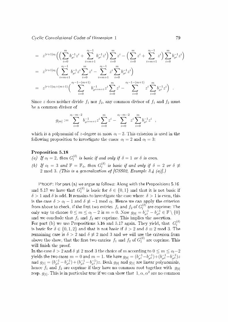
Cyclic Convolutional Codes of Dimension 1 79
= z(r+1)ol(( m∑
i=0
b−1σizi +
ol−1∑i=m+1
b−1σizi) m∑i=0
zi −( m∑i=0
zi +
ol−1∑i=m+1
zi) m∑i=0
b−1σizi)
= z(r+1)ol( ol−1∑i=m+1
b−1σizi
m∑i=0
zi −ol−1∑i=m+1
zim∑i=0
b−1σizi)
= z(r+1)ol+(m+1)( ol−1−(m+1)∑
i=0
b−1σi+m+1z
i
m∑i=0
zi −ol−1−(m+1)∑
i=0
zim∑i=0
b−1σizi).
Since z does neither divide f1 nor f2, any common divisor of f1 and f2 mustbe a common divisor of
g[m] :=
ol−m−2∑i=0
b−1σi+m+1z
i
m∑i=0
zi −ol−m−2∑i=0
zim∑i=0
b−1σizi ,
which is a polynomial of z-degree at most ol− 2. This criterion is used in thefollowing proposition to investigate the cases ol = 2 and ol = 3:
Proposition 5.18(a) If ol = 2, then G
(δ)l is basic if and only if δ = 1 or δ is even.
(b) If ol = 3 and F = F4, then G(δ)l is basic if and only if δ = 2 or δ 6≡
2 mod 3. (This is a generalization of [GSS02, Example 3.4 (a)].)
Proof: For part (a) we argue as follows: Along with the Propositions 5.16and 5.17 we have that G(δ)
l is basic for δ ∈ {0, 1} and that it is not basic ifδ > 1 and δ is odd. It remains to investigate the case where δ > 1 is even, thisis the case δ > ol − 1 and δ 6≡ −1 mod ol. Hence we can apply the criterionfrom above to check, if the �rst two entries f1 and f2 of G(δ)
l are coprime: Theonly way to choose 0 ≤ m ≤ ol − 2 is m = 0. Now g[0] = b−1
σ1 − b−1σ0 ∈ F \ {0}
and we conclude that f1 and f2 are coprime. This implies the assertion.For part (b) we use Propositions 5.16 and 5.17 again. They yield, that G
(δ)l
is basic for δ ∈ {0, 1, 2} and that it not basic if δ > 2 and δ ≡ 2 mod 3. Theremaining case is δ > 2 and δ 6≡ 2 mod 3 and we will use the criterion fromabove tho show, that the �rst two entries f1 and f2 of G(δ)
l are coprime. Thiswill �nish the proof.In the case δ > 2 and δ 6≡ 2 mod 3 the choice of m according to 0 ≤ m ≤ ol−2yields the two cases m = 0 andm = 1. We have g[0] = (b−1
σ1 −b−1σ0 )+(b−1
σ2 −b−1σ0 )z
and g[1] = (b−1σ2 − b−1
σ0 )+(b−1σ2 − b−1
σ1 )z. Both g[0] and g[1] are linear polynomials,hence f1 and f2 are coprime if they have no common root together with g[0]
resp. g[1]. This is in particular true if we can show that 1, α, α2 are no common

80 Section 5
roots of f1 and f2, where F4 = {0, 1, α, α2}. As for the common roots, weargue as follows:For ζ ∈ F \ {0} we have ζ3 = 1. If we put h1(ζ) = 1 + ζ + ζ2, h2(ζ) :=b−1σ0 + b−1
σ1 ζ + b−1σ2 ζ
2 we get
f1(ζ) = (r + 1)h1(ζ) +
{1 for m = 01 + ζ for m = 1
f2(ζ) = (r + 1)h2(ζ) +
{b−1σ0 for m = 0b−1σ0 + b−1
σ1 ζ for m = 1.
If r is odd, then
f1(ζ) =
{1 for m = 01 + ζ for m = 1
, f2(ζ) =
{b−1σ0 for m = 0b−1σ0 + b−1
σ1 ζ for m = 1.
In this case f1(ζ) = 0 implies m = 1 and ζ = 1. But then f2(ζ) = f2(1) =b−1σ0 + b−1
σ1 6= 0 since bσ0 6= bσ1 .If r is even, then
f1(ζ) =
{ζ + ζ2 for m = 0ζ2 for m = 1
, f2(ζ) =
{b−1σ1 ζ + b−1
σ2 ζ2 for m = 0
b−1σ2 ζ
2 for m = 1.
In this case f1(ζ) = 0 implies m = 0 and ζ = 1. But then f2(ζ) = f2(1) =b−1σ1 + b−1
σ2 6= 0 because bσ1 6= bσ2 .This shows that (f1(ζ), f2(ζ)) 6= (0, 0) for any ζ ∈ {1, α, α2}, hence f1 andf2 have no common roots in F4. 2
Although we have no complete solution for the case δ > ol − 1 and δ 6≡−1 mod ol, we have a complete solution for F ∈ {F3,F4} (for F = F2 recallCorollary 5.6 (a)): In the case F = F3 the polynomial xn − 1 has at mosttwo linear prime divisors and ol ≥ 2 implies ol = 2. In the case F = F4
the polynomial xn − 1 has at most three linear prime divisors, hence R(1) ={1, . . . , r1} ⊆ {1, 2, 3}. For l ∈ R(1) the l-order of an automorphism σ ∈AutF(A), which gives rise to 1-dimensional σ-cyclic convolutional codes withnonzero complexity and support {l}, is 2 or 3. As a consequence we knowexactly under which conditions G(δ)
l is basic, cf. Proposition 5.18:
Corollary 5.19(a) Consider F = F3. Then ol = 2 and G(δ)
l is basic if and only if δ = 1 orδ is even.
(b) Consider F = F4. Then ol = 2 or ol = 3 and we have: If ol = 2 then G(δ)l
is basic if and only if δ = 1 or δ is even. If ol = 3 then G(δ)l is basic if
and only if δ = 2 or δ 6≡ 2 mod 3. 2

Cyclic Convolutional Codes of Dimension 1 81
5.3.3 Construction of Cyclic (n, 1, δ)-Convolutional Codes withGood Free Distance
In this section we will deal with G(δ)l as in (5.3) where δ ≤ ol − 1. We know
from Proposition 5.17 that C := im F[z]G(δ)l is a σ-cyclic (n, 1, δ)-convolutional
code and that it satis�es2n ≤ dfree (C) ≤ n(δ + 1) ,
as we saw in Corollary 5.10. For δ = 1 the upper and the lower boundcoincide, but if δ > 1 we may wish to �nd better lower bounds for dfree (C)than 2n.
Roughly speaking, we intend to consider a special �eld F and to constructa special automorphism σ such that the formula(
n− δ
2
)(δ + 1) ≤ dfree (C) ≤ n(δ + 1) . (5.4)
holds true. The lower bound (n− δ2)(δ + 1) is better than 2n for n ≥ 4 and
δ > 1:
Lemma 5.20For n, δ ∈ N satisfying n ≥ 4 and n−1 ≥ δ ≥ 2 we have 2n < (n− δ
2)(δ+1).
Proof: After some manipulations we get that 2n < (n − δ2)(δ + 1) is
equivalent to 0 > δ2 +δ(1−2n)+2n. We investigate the polynomial f(D) :=D2 +D(1− 2n) + 2n, which has the two roots
δ+(n) := n− 1
2+
√n2 − 3n+
1
4and δ−(n) := n− 1
2−√n2 − 3n+
1
4
and we have to show that δ ∈ {d | f(d) < 0} for n ≥ 4. One can readily showthat n2 − 3n+ 1
4= (n− 3
2+√
2)(n− 32−√
2) is positive if and only if n ≥ 3(because n ∈ N), hence {d | f(d) < 0} 6= ∅ if and only if n ≥ 3.Now we assume n ≥ 3. In this case {d | f(d) < 0} = {d | δ−(n) < d < δ+(n)}.Note that δ ≤ n − 1 < n − 1
2< δ+(n). Furthermore, δ−(3) = 2 and one can
show that δ−(n) is decreasing for n ≥ 3, hence δ−(n) < 2 for n ≥ 4. Thereforeδ−(n) < δ if n ≥ 4. This implies the assertion. 2
If a σ-cyclic (n, 1, δ)-convolutional code C satis�es (5.4), then the foregoingLemma tells us that its free distance is better than 2n if n ≥ 4 and δ is nottoo big. However, so far it is not clear whether dfree (C) is "much" biggerthan 2n, i.e. whether C has "good" free distance. If n is much bigger than δ,then the next remark will allow us to say that C has good free distance:

82 Section 5
Remark 5.21(a) In the formula (5.4), the ratio of the lower and the upper bound is given
by (n− δ2)/n = 1− δ
2n. For �xed δ and "big" n this ratio is nearly 1. In
this sense, codes satisfying (5.4) are asymptotically MDS-convolutionalcodes for �xed δ and n going to in�nity.
(a) The di�erence between the lower and upper bound in (5.4) is 12δ(δ + 1),
which is independent from n. So, again, a code satisfying (5.4) is not farfrom being an MDS-code if δ is �xed and n is "big".
In the following we will deal with a �nite �eld F where xn − 1 splits intolinear prime divisors over F. In this case we know (e.g. from [MS78, Ch. 7,�5]) that there exists an n-th primitive root of unity α in F, i.e. αn = 1 andαm 6= 1 for 0 < m < n. Furthermore, the prime factor decomposition ofxn − 1 is given by
xn − 1 =n−1∏i=0
(x− αi) .
With this knowledge, we can construct a special automorphism σ ∈ AutF(A)and a special σ-cyclic (n, 1, δ)-code which satis�es (5.4).
Theorem 5.22Let α ∈ F be an n-th primitive root of unity. This implies xn − 1 =∏n−1
i=0 (x−αi). Furthermore, let ε(i) be the primitive idempotent element in Acorresponding to the prime divisor (x− αi). Then we have:(a) If σ ∈ AutF(A) is the (uniquely determined) automorphism which satis-
�es
σ(ε(1)) = ε(2) , σ(ε(2)) = ε(3) , . . . , σ(ε(n−1)) = ε(n) , σ(ε(n)) = ε(1)
and if we put β := α−1, then we have nv(ε(i)) = [1, βi, β2i, . . . , β(n−1)i]for 1 ≤ i ≤ n and
G(δ)1 =
δ∑i=0
zi[1, βi+1, β2(i+1), . . . , β(n−1)(i+1)]
for any δ ∈ N0, where G(δ)1 is de�ned as in (5.3).
(b) If n ≥ 4, σ was chosen as in (a) and if 2 ≤ δ ≤ n− 1, then the σ-cyclic(n, 1, δ)-convolutional code C := im F[z]G
(δ)l satis�es (5.4), precisely
2n <(n− δ
2
)(δ + 1) ≤ dfree (C) ≤ n(δ + 1) .

Cyclic Convolutional Codes of Dimension 1 83
Proof: Part (a): With Lemma 5.9 along with αn = 1 = βn we obtainnv(ε(i)) = [1, βi, β2i, . . . , β(n−1)i] for 1 ≤ i ≤ n. If we put l = 1 and if we useNotation 5.8, then the automorphism σ satis�es
bσi = αi+1 , b−1σi
= βi+1 .
This shows that G(δ)1 =
∑δi=0 z
i[1, βi+1, β2(i+1), . . . , β(n−1)(i+1)].For part (b) we recall Lemma 5.20, which proves that 2n <
(n− δ
2
)(δ+1).
It remains to show that (n− δ2
)(δ + 1) ≤ dfree (C).
We need PQR-representations again. In analogy to the proof of Proposition5.17 and with Theorem 2.12 and its proof we obtain that a canonical PQR-representation (P,Q,R) of im F[z]G
(δ)1 is given by
[zP +Q |R] :=
z 1 β β2 . . . βn−1
−1. . . 1 β2 β4 . . . β2(n−1)
. . . z... ... ... ...
−1 1 βδ+1 β(δ+1)2 . . . β(δ+1)(n−1)
∈ F[z](δ+1)×(δ+n) .
We have to show that wt (v) ≥ (n− δ2)(δ+ 1) for 0 6= v ∈ C. Towards this
end we de�ne for d ∈ {0, 1, . . . , δ} the matrices
Rd :=
1 β β2 . . . βn−1
1 β2 β4 . . . β2(n−1)
... ... ... ...1 βd+1 β(d+1)2 . . . β(d+1)(n−1)
∈ F(d+1)×n . (5.5)
Note, that the �rst d + 1 columns of Rd show a Vandermonde-structure 13.Hence the matrix Rd has full row rank for 0 ≤ d ≤ δ since 1, β, . . . , βd ∈F \ {0} are pairwise di�erent.With Corollary 2.11 we have C =
(im F[z][1, z, . . . , zδ])· Rδ. Hence 0 6= v ∈ C
can be written as ζRδ for some 0 6= ζ ∈ im F[z][1, z, . . . , zδ] and we have to
show that wt (ζRδ) ≥ (n− δ2)(δ + 1).
We write ζ = (∑
i≥0 ziui )[1, z, . . . , z
δ] =∑
i≥0 ζizi where ui ∈ F, ζi ∈
Fδ+1. Because of right invertibility of [1, z, . . . , zδ] along with Theorem 1.7 (vi)
we may assume without loss of generality that ζ0 6= 0, which means u0 6= 0.It is easy to see that ζi = [ui, ui−1, . . . , u1, u0, 0, . . . , 0] 6= 0 for 0 ≤ i ≤ δ andtherefore 0 6= ζiRδ ∈ im FRi for 0 ≤ i ≤ δ. We will show later that the blockcode im FRi has distance n− i, hence wt (ζiR) ≥ n− i for 0 ≤ i ≤ δ.
13See footnote 12 on page 77.
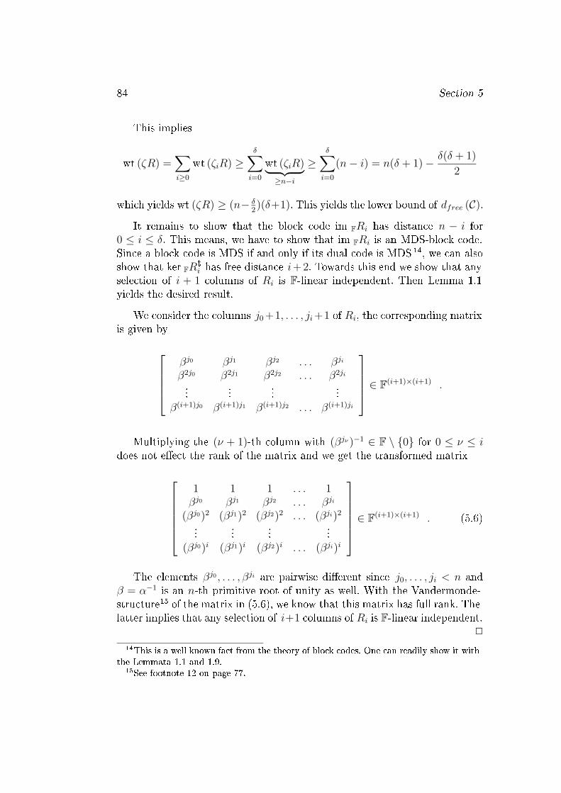
84 Section 5
This implies
wt (ζR) =∑i≥0
wt (ζiR) ≥δ∑i=0
wt (ζiR)︸ ︷︷ ︸≥n−i
≥δ∑i=0
(n− i) = n(δ + 1)− δ(δ + 1)
2
which yields wt (ζR) ≥ (n− δ2)(δ+1). This yields the lower bound of dfree (C).
It remains to show that the block code im FRi has distance n − i for0 ≤ i ≤ δ. This means, we have to show that im FRi is an MDS-block code.Since a block code is MDS if and only if its dual code is MDS 14, we can alsoshow that ker FRt
i has free distance i+ 2. Towards this end we show that anyselection of i + 1 columns of Ri is F-linear independent. Then Lemma 1.1yields the desired result.
We consider the columns j0 +1, . . . , ji+1 of Ri, the corresponding matrixis given by
βj0 βj1 βj2 . . . βji
β2j0 β2j1 β2j2 . . . β2ji
... ... ... ...β(i+1)j0 β(i+1)j1 β(i+1)j2 . . . β(i+1)ji
∈ F(i+1)×(i+1) .
Multiplying the (ν + 1)-th column with (βjν )−1 ∈ F \ {0} for 0 ≤ ν ≤ idoes not e�ect the rank of the matrix and we get the transformed matrix
1 1 1 . . . 1βj0 βj1 βj2 . . . βji
(βj0)2 (βj1)2 (βj2)2 . . . (βji)2
... ... ... ...(βj0)i (βj1)i (βj2)i . . . (βji)i
∈ F(i+1)×(i+1) . (5.6)
The elements βj0 , . . . , βji are pairwise di�erent since j0, . . . , ji < n andβ = α−1 is an n-th primitive root of unity as well. With the Vandermonde-structure15 of the matrix in (5.6), we know that this matrix has full rank. Thelatter implies that any selection of i+1 columns of Ri is F-linear independent.
2
14This is a well known fact from the theory of block codes. One can readily show it withthe Lemmata 1.1 and 1.9.
15See footnote 12 on page 77.
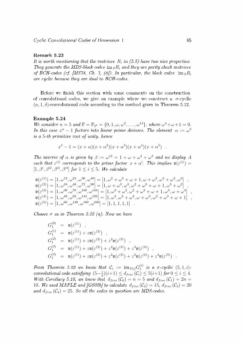
Cyclic Convolutional Codes of Dimension 1 85
Remark 5.23It is worth mentioning that the matrices Ri in (5.5) have two nice properties:They generate the MDS-block codes im FRi and they are parity check matricesof BCH-codes (cf. [MS78, Ch. 7, �6]). In particular, the block codes im FRi
are cyclic because they are dual to BCH-codes.
Before we �nish this section with some comments on the constructionof convolutional codes, we give an example where we construct a σ-cyclic(n, 1, δ)-convolutional code according to the method given in Theorem 5.22.
Example 5.24We consider n = 5 and F = F24 = {0, 1, ω, ω2, . . . , ω14}, where ω4 +ω+1 = 0.In this case xn − 1 factors into linear prime divisors. The element α := ω3
is a 5-th primitive root of unity, hence
x5 − 1 = (x+ α)(x+ α2)(x+ α3)(x+ α4)(x+ α5) .
The inverse of α is given by β := ω12 = 1 + ω + ω2 + ω3 and we display Asuch that ε(i) corresponds to the prime factor x + αi. This implies v(ε(i)) =[1, βi, βi2, βi3, βi4] for 1 ≤ i ≤ 5. We calculate
v(ε(1)) = [1, ω12, ω24, ω36, ω48] = [1, ω2 + ω3 + ω + 1, ω + ω3, ω3 + ω2, ω3] ,v(ε(2)) = [1, ω24, ω48, ω72, ω96] = [1, ω + ω3, ω3, ω2 + ω3 + ω + 1, ω3 + ω2] ,v(ε(3)) = [1, ω36, ω76, ω108, ω144] = [1, ω3 + ω2, ω2 + ω3 + ω + 1, ω3, ω + ω3] ,v(ε(4)) = [1, ω48, ω92, ω144, ω192] = [1, ω3, ω3 + ω2, ω + ω3, ω2 + ω3 + ω + 1] ,v(ε(5)) = [1, ω60, ω120, ω180, ω240] = [1, 1, 1, 1, 1] .
Choose σ as in Theorem 5.22 (a). Now we have
G(0)1 = v(ε(1)) ,
G(1)1 = v(ε(1)) + zv(ε(2)) ,
G(2)1 = v(ε(1)) + zv(ε(2)) + z2v(ε(3)) ,
G(3)1 = v(ε(1)) + zv(ε(2)) + z2v(ε(3)) + z3v(ε(4)) ,
G(4)1 = v(ε(1)) + zv(ε(2)) + z2v(ε(3)) + z3v(ε(4)) + z4v(ε(5)) .
From Theorem 5.22 we know that Ci := im F[z]G(i)1 is a σ-cyclic (5, 1, i)-
convolutional code satisfying (5− i2)(i+1) ≤ dfree (Ci) ≤ 5(i+1) for 0 ≤ i ≤ 4.
With Corollary 5.10, we know that dfree (C0) = n = 5 and dfree (C1) = 2n =10. We used MAPLE and [GS02b] to calculate dfree (C2) = 15, dfree (C3) = 20and dfree (C4) = 25. So all the codes in question are MDS-codes.
86 Section 5
There are some methods to construct a (not necessarily cyclic) convolu-tional code C, which guarantee that dfree (C) has quite a good lower bounddlow. For most of these methods, the construction of such a code uses a blockcode C with distance exactly dlow (examples are given in [Jus73] or [Pir88b]).In any case we may ask why we should use C to encode messages but ratherC � the structure of the code C is simpler than that one of C and its freedistance is in general (by construction) quite good.We want to illustrate this by sketching the method in [Pir88b]: Here Piretconstructs an (n, k, n − k)-convolutional code C ⊆ F[z]n over F2m with freedistance at least 2n − 2k + 1 =: dlow. Towards this end, he speci�es a par-ity check matrix H ∈ F[z]n×(n−k) of C of the form H = H0 + zH1, whereH0, H1 ∈ Fn×(n−k) show a strong structure (similar to that one of the ma-trices de�ned in (5.5)). Piret assumes that (n − k) ≤ n/2. For the proof ofdfree (C) ≥ dlow he uses that in his construction [H1, H2] ∈ Fn×(2n−2k) is aparity check matrix of an (n, 2k−n)-MDS-block code C, i.e. dfree (C) = dlow.Why not using the MDS-block code C for the encoding procedure instead ofthe convolutional code C?Theorem 5.22 provides a method to construct a σ-cyclic (n, 1, δ)-convolutional code C with free distance at least dlow := (n − δ
2)(δ + 1). We
would like to point out that in contrast to the references mentioned abovewe do not use a block code (with distance dlow) as the starting point of ourconstruction.
Some Open Problems 87
6 Some Open Problems
In this �nal section we will point out some problems which where not solvedin the present thesis (Section 6.1). After that we introduce a further researchtopic in Section 6.2 which deals with the so called "equivalence" of convolu-tional codes.
6.1 Some Questions which Arose in the Foregoing Sec-
tions
Uniqueness of a decomposition? In Corollary 3.22 resp. Remark 4.3, welearned how we can construct a decomposition of a σ-cyclic convolutionalcode into a direct sum of minimal σ-cyclic convolutional sub-codes (as leftF[z]-modules). Such decompositions are not unique. For example, we considerF = F4 = {0, 1, α, α2}, n = 3 and the automorphism σ de�ned by σ(x) = α2x.One can show that the σ-cyclic (block) code
C := im F[z]
[1 1 11 α2 α
]= im F[z][1, 1, 1]⊕ im F[z][1, α
2, α]
has the following decomposition into minimal σ-cyclic convolutional sub-codes, too:
C = im F[z][1 + z, 1 + α2z, 1 + αz]⊕ im F[z][1, α2, α] .
One would possibly prefer the �rst decomposition, because in the second onez appears, pretending that C has nonzero complexity. So di�erent decompo-sitions have di�erent quality.Consider a σ-cyclic (n, k, δ)-convolutional code C. Then the sum of the com-plexities of the direct summands in the decomposition of C as in Remark 4.3is equal to δ, we say "the decompositions respects the complexity of C". Thisis due to the fact that in this decomposition every summand is the F[z]-spanof some rows of a minimal basis of C. We expect (loosely speaking) that adecomposition, which respects the complexity of C, is linked with a minimalbasis and vice versa. If this is true: Can we �nd something like uniquenessof a decomposition into a direct sum of minimal σ-cyclic convolutional sub-codes which respects the complexity of C (up to certain operations with thesummands)? Is this analogous to Proposition 1.5?
Determination of units? With Theorem 4.6, we know that we candetermine all minimal σ-cyclic convolutional codes with the knowledge of all

88 Section 6
units in A[z;σ]. Theorem 4.11 (b) tells us that we can construct all units via�nite products of elementary units. But if we aim to construct all componentsof units with prescribed degree d, it is not clear how we can �nd these bybuilding products of elementary units without further rules or knowledge ofthe algebraic structure of the units (cf. Remark 4.21). So we may ask: Can we�nd more information about the algebraic structure of units? How "good" isthe description of units given in Theorem 4.11 (b) and do there exist morepowerful (or "beautiful") ones?
Free distance of a σ-cyclic convolutional code? We have only fewlower and upper bounds for the free distance of convolutional codes. Thecomputer packages which we applied to determine the free distances of thecodes in our examples did not use the cyclic structure of the codes in question.It is not clear if there is any link between the free distance and cyclicity ingeneral. If so: Are there any estimates for the free distance of a σ-cyclic codein terms of a reduced generator polynomial and of the automorphism σ?In this connection we may ask: Do the construction methods of 1-dimensionalσ-cyclic convolutional codes given in Sections 5.3.1 and 5.3.2 yield codes withgood free distance?For the codes constructed in Section 5.3.3 (cf. Theorem 5.22) we have quitea good lower bound, but in all examples (cf. Example 5.24) the codes wereMDS-convolutional codes. Are there examples where the lower bound givenin Theorem 5.22 is tight?
More information about G(δ)l ? In Section 5.3.2 we introduced the
matrix G(δ)l . We found out that G(δ)
l is not basic for δ > ol−1, δ ≡ −1 mod oland that it is basic for δ < ol − 1 (provided that σ(ε(l)) 6= ε(l)). But we werenot able determine in general whether G(δ)
l is basic or not in the remainingcase δ > ol − 1 and δ 6≡ −1 mod ol. What is the answer to that problem?Of course we can also ask if we can determine the free distance of im F[z]G
(δ)l .
6.2 The Concept of Equivalence of Codes � A Case
Study
Imagine that we have two convolutional codes C, C ⊆ F[z]n and a linearbijective mapping
ϕ : C → C satisfying wt (v) = wt (ϕ(v)) for all v ∈ C. (6.1)Two such codes may be di�erent, but they behave "equal" concerning theweight of their codewords. For theoretical investigations, it does not matter

Some Open Problems 89
if we use C or C for the encoding procedure. However, in applications one ofthe codes might be preferred (for example, because it can be implementedmore easily). From this point of view, it is worthwhile to know if two codessatisfy (6.1).
In the following we will use a stronger 16 de�nition of equivalence of codesleaving the weight distribution invariant.
De�nition 6.1 cf. [Bet98, p. 26f]Two (n, k)-submodules C, C ′ ⊆ F[z]n are called equivalent if there existα1, . . . , αn ∈ F \ {0} and a permutation π ∈ Sn such that
C ′ = {(α1vπ(1), . . . , αnvπ(n)) | (v1, . . . , vn) ∈ C} .
We can express this equivalently via a generator matrix G of C, because Cand C ′ are equivalent if and only if there exist α1, . . . , αn ∈ F \ {0} and apermutation matrix P ∈ Fn×n such that C ′ = im F[z](G ·P ·diag (α1, . . . , αn)).
Of course, we have an equivalence relation "∼" on the set of all (n, k)-convolutional codes de�ned by [ C ∼ C :⇔ C and C are equivalent ]. If weapply the concept of equivalence to 1-dimensional submodules of F[z]n, weget a very simple description because generator matrices of 1-dimensionalsubmodules are unique up to multiplication with a nonzero element in F (cf.Proposition 5.7 (a)):
Remark 6.2Let C ⊆ F[z]n be an (n, 1)-submodule with generator matrix G = [g1, . . . , gn] ∈F[z]1×n. An (n, 1)-submodule C ′ ⊆ F[z]n is equivalent to C if and only if thereexist α1, . . . , αn ∈ F \ {0} and a permutation π ∈ Sn such that
G′ = [α1gπ(1), . . . , αngπ(n)] is a generator matrix of C ′ .
We are interested in the question how the set of all cyclic (n, 1, δ)-convolutional codes (cyclic with respect to possibly di�erent automorphisms)over a �eld F decomposes into equivalence classes C1, . . . ,Cµ. Are there cer-tain patterns? And if we consider the subset of all cyclic (n, 1, δ)-convolutionalcodes with a prescribed support, do the equivalence classes have a similarstructure as C1, . . . ,Cµ?We will examine these questions in one speci�c example.
16So far it is unknown if the de�nition of equivalence given in De�nition 6.1 coincideswith the de�nition given in (6.1).

90 Section 6
A case study. We consider n = 3 and F = F4 = {0, 1, α, α2}. We havex3 − 1 = (x+ 1)(x+ α)(x+ α2) and we display A as
ρ−1(F[x]/〈x+ 1 〉 ×
F[x]/〈x+ α 〉 ×F[x]/〈x+ α2 〉
).
Our target is to �nd all cyclic (3, 1, δ)-convolutional codes for δ = 0, 1, 2, 3.(Here we mean cyclicity with respect to any automorphism σ ∈ AutF4(A),i.e. σ(x) ∈ {x, x2, αx, α2x, αx2, α2x2}, see Remark 3.5.) Then we want todetermine the equivalence classes both of all these codes and of those whichhave the same support.
We know from Corollary 5.10 that an (n, 1, δ)-submodule C ⊆ F[z]n is aσ-cyclic convolutional code if and only if it has a basic generator matrix ofthe shape
δ∑i=0
aizi[1, b2
σi , bσi ] , where bσi ∈ {1, α, α2}, ai ∈ F and a0 = 1, aδ 6= 0. (6.2)
The condition a0 = 1 is a normalization that makes sure that two dif-ferent matrices having the shape as in (6.2) give rise to di�erent (3, 1, δ)-submodules.
If the matrix in (6.2) is basic, then the convolutional code im F[z]G hassupport {1} if bσ0 = 1, it has support {2} if bσ0 = α2 and it has support {3}if bσ0 = α (cf. Corollary 5.12).• The case δ = 0: Obviously only the three matrices
[1, 1, 1] , [1, α, α2] and [1, α2, α]
are of interest and of course all three matrices are basic and cyclic withrespect to any automorphism σ ∈ AutF(A). Each of these matrices can betransformed to any other by rescaling the columns with nonzero constants.Hence we have three di�erent cyclic (3, 1, 0)-convolutional codes (resp. blockcodes), one for each support, and they are all equivalent.• The case δ = 1: A matrix which generates a cyclic (3, 1, 1)-convolutional
can be written as[1 + az, b2
σ0 + ab2σ1z, bσ0 + abσ1z] , where a 6= 0 and bσ0 6= bσ1 . (6.3)
There are three possibilities to choose a and two possibilities to chose bσ1
for �xed bσ0 . Hence there are six di�erent possibilities to write down sucha matrix for each support and therefore there are 18 di�erent matrices. We
Some Open Problems 91
can readily show that the three entries in a matrix as in (6.3) have pairwisedi�erent roots, therefore any two entries of such a matrix are coprime. Thelatter implies that the entries are given by z + 1, z + α, z + α2 (up topermutation and multiplication with nonzero constants). We conclude thatthere exist six di�erent cyclic (3, 1, 1)-convolutional codes for each support,altogether 18 di�erent cyclic (3, 1, 1)-convolutional codes, and they are allequivalent.• The case δ = 2 and δ = 3: Here we used MAPLE to generate all possible
matrices of the shape as in (6.2) for each support and the pairwise di�erentones were put into three lists, one for each support. Then the matrices inthe lists were checked if they where basic. Here are the preliminary resultsof these calculations:
There are 42 di�erent cyclic (3, 1, 2)-convolutional codes for each support,hence there are 126 cyclic (3, 1, 2)-convolutional codes over F4. There are 144di�erent cyclic (3, 1, 3)-convolutional codes for each support, hence there are432 cyclic (3, 1, 2)-convolutional codes over F4.
We wrote a simple algorithm to check equivalence of the matrices in agiven list L: The algorithm took the �rst entry of the list L (a representativeof the �rst equivalence class), generated the list L′ of all matrices which areequivalent to the �rst representative. Then each entry of L was taken and thealgorithm checked, if it appeared in L′. If so, this entry was removed from Land added to a new list, the �rst equivalence class. After that, the processstarted again with the �rst entry of the new list L (a representative of thesecond equivalence class) and so forth. We got the following results:
In the case δ = 2 the algorithm found seven equivalence classes for eachsupport, each consisting of six elements. We listed all 3 · 7 = 21 representa-tives of these equivalence classes and checked this new list on equivalence:Again, the algorithm found seven equivalence classes and each of the newequivalence classes had exactly three members. Hence the 126 cyclic (3, 1, 2)-convolutional codes over F4 fall into seven equivalence classes with 3 · 6 = 18elements each.
In the case δ = 3 the algorithm found 24 equivalence classes for eachsupport and � again � each consisted of six elements. We listed all 3 · 24 =72 representatives of these equivalence classes and checked this new list onequivalence: The algorithm found 24 equivalence classes and, again, eachof the new equivalence classes had exactly three members. Hence the 432cyclic (3, 1, 3)-convolutional codes over F4 fall into 24 equivalence classeswith 3 · 6 = 18 elements each.
92 Section 6
These are our results so far. We wish to conclude with some questionsabout these �ndings:
Is it by mere coincidence that all equivalence classes for prescribed sup-port have six elements in the cases δ = 1, 2, 3?
Why do all equivalence classes have the same cardinality for �xed δ?In the case study, one might suppose that the equivalence classes for the
cyclic (3, 1, δ)-convolutional codes with support {l} determine the equivalenceclasses of all cyclic (3, 1, δ)-convolutional codes with support {l′} 6= {l}. (Orloosely speaking: Maybe the knowledge of the equivalence classes for thecyclic (3, 1, δ)-convolutional codes with support {1} is "su�cient" to knoweverything about the equivalence classes for the supports {2} and {3}.)We can generalize this conjecture to cyclic codes in general: Do the equiv-alence classes of the set of all σ-cyclic (n, 1, δ)-convolutional codes (or even(n, k, δ)-convolutional codes) with support {l} ⊆ R(L) determine all the otherσ-cyclic (n, 1, δ)-convolutional codes (or even (n, k, δ)-convolutional codes)with support {l′} ⊆ R(L) \ {l}?

93
References
[Bet98] Anton Betten et. al. Codierungstheorie: Konstruktion und Anwen-dung linearer Codes . Springer-Verlag, Berlin, 1998.
[For70] G. David Forney, Jr. Convolutional codes I: Algebraic structure.IEEE Trans. Inform. Theory , 16:720�738, 1970. (See also correc-tions in IEEE Trans. Inf. Theory , Vol. 17, 1971, p. 360).
[For75] G. David Forney, Jr. Minimal bases of rational vector spaces, withapplications to multivariable linear systems. SIAM J. Control,13(3):493�520, 1975. (SIAM J. Contr. was passed into SIAM J.Contr. & Opt. after 1975).
[Gan60a] F. R. Gantmacher. The Theory of Matrices , volume 1. ChelseaPublishing Company, New York, 1960.
[Gan60b] F. R. Gantmacher. The Theory of Matrices , volume 2. ChelseaPublishing Company, New York, 1960.
[Glua] Heide Gluesing-Luerssen. Einführung in die Codierungstheorie.Unpublished manuscript. Carl von Ossietzky University Olden-burg, Germany, winter term 2000/2001.
[Glub] Heide Gluesing-Luerssen. Private communications and notes. 2002.
[GS02a] Heide Gluesing-Luerssen and Wiland Schmale. On cyclic convolu-tional codes. Submitted. The paper is available both as preprint(Otto-von-Guericke-University Magdeburg, Germany, Preprint Nr.5, 2003) and at http://front.math.ucdavis.edu/ with ID-number RA/0211040, 2002.
[GS02b] Heide Gluesing-Luerssen and Wiland Schmale. Procedures pro-grammed with MAPLE which provide commands concerning cyclicconvolutional coding and the determination of free distances. Carlvon Ossietzy University Oldenburg, 2002.
[GS03] Heide Gluesing-Luerssen and Wiland Schmale. Distance boundsfor convolutional codes and some optimal codes. Preprint.Available at http://front.math.ucdavis.edu/ with ID-numberRA/0305135, 2003.
94
[GSS02] Heide Gluesing-Luerssen, Wiland Schmale, and Melissa Striha.Some small cyclic convolutional codes. In Electronic Proceedingsof the 15th International Symposium on Mathematical Theory ofNetworks and Systems , Notre Dame, IN (USA), CD-Rom, 2002. (8pages).
[Jus73] Jørn Justesen. New convolutional code constructions and a classof asymptotically good time-varying codes. IEEE Trans. Inform.Theory, 19(2):220�225, 1973.
[JZ99] R. Johannesson and K. S. Zigangirov. Fundamentals of Convolu-tional Coding . IEEE Press, New York, 1999.
[Kui94] Margreet Kuijper. First-Order Representations of Linear Systems .Birkhäuser, Boston, 1994.
[Lan86] Serge Lang. Introduction to Linear Algebra . Springer-Verlag, NewYork, 2nd edition, 1986.
[LC83] Shu Lin and Daniel J. Costello, Jr. Error Control Coding: Fun-damentals and Applications . Prentice-Hall, Inc., Englewood Cli�s,2nd edition, 1983.
[LN97] Rudolf Lidl and Harald Niederreiter. Finite Fields . Encyclopedia ofmathematics and its applications; 20. Cambridge University Press,Cambridge, 2nd edition, 1997.
[MAP01] MAPLE 7.0. Computer-Software. Waterloo Maple Inc., 2001.[McE98] Robert J. McEliece. The algebraic theory of convolutional codes. In
Handbook of Coding Theory , volume 1, pages 1065�1138. Elsevier,Amsterdam, 1998.
[MP79] H. F. Münzner and D. Prätzel-Wolters. Minimal bases of polyno-mial modules, structural indices and Brunovsky-transformations.Int. J. Contr., 30:291�318, 1979.
[MS78] F. J. MacWilliams and N. J. A. Sloane. The Theory of Error-Correcting Codes . North-Holland, 1978.
[Pir76] Philippe Piret. Structure and constructions of cyclic convolutionalcodes. IEEE Trans. Inform. Theory , 22:147�155, 1976.
[Pir88a] Philippe Piret. Convolutional Codes; An Algebraic Approach . MITPress, Cambridge, MA, 1988.

95
[Pir88b] Philippe Piret. A convolutional equivalent to reed-solomon codes.Philips J. Res. , 43:441�458, 1988.
[Rom92] Steven Roman. Coding and Information Theory . Springer-Verlag,New York, 1992.
[Roo79] Cornelis Roos. On the structure of convolutional and cyclic con-volutional codes. IEEE Trans. Inform. Theory , 25:676�683, 1979.
[RS99] Joachim Rosenthal and Roxana Smarandache. Maximum distanceseparable convolutional codes. Appl. Algebra Engrg. Comm. Com-put., 10:15�32, 1999.
[RSY96] Joachim Rosenthal, J. M. Schumacher, and Eric V. York. On be-haviors and convolutional codes. IEEE Trans. Inform. Theory ,42:1881�1891, 1996.
[Sch] Wiland Schmale. Einführung in die Algebra. Unpublishedmanuscript. Carl von Ossietzky University Oldenburg, Germany,summer term 2000.
[SGR98] Roxana Smarandache, Heide Gluesing-Luerssen, and JoachimRosenthal. Generalized �rst order descriptions and canonical formsfor convolutional codes. In A. Beghi, L. Finesso, and G. Picci, ed-itors, Mathematical Theory of Networks and Systems , pages 1091�1094. Proceedings of the MTNS-98 Symposium held in Padova,Italy, 1998.
[Sha48] Claude Elwood Shannon. A mathematical theory of communi-cation. Bell Syst. Tech. J. , 27:379�423, 623�656, 1948. Available athttp://cm.bell-labs.com/cm/ms/what/shannonday/paper.html .
[Str] Melissa Striha. Struktur und Konstruktion zyklischer Fal-tungscodes. Diploma thesis. Fachbereich Mathematik of the Carlvon Ossietzky University Oldenburg, Germany, 2002.
Index
automorphisml-order of, 54group, 38�45
basic matrix, 14block code, 9, 12code word, 9, 14complexity, 11component, 42, 46convolutional codes, 14cyclicity
σ-cyclic, 38cyclic block codes, 36cyclic convolutional codes, 37�
40, 45�49cyclic shift, 36ideal, 36left ideal, 40left principal ideal, 45, 46minimality, 50�principal ideal, 37
cyclotomic coset, 60, 67degree of a matrix, 11direct summand, 14distance, 9
free distance, 10dual code, 10, 16�17dual submodule, 32elementary operations, 11, 13equivalence of codes, 89First Order Representations, 18�35
KLM-Representation, 32�35PQR-Representation, 21�32
ForneyForney indices, 12
Theorem of, 12free distance, 10generator matrix, 10, 11generator polynomial, 47Hamming weight, see weightirreducible polynomial, 73left (principal) ideal, 40, 45, 46left-leading monomial, 46left-reduced, 46matrix pencil, 19
canonical form, 19�21MDS-bound, 9, 11message word, 9, 14minimal basis, 11parity check matrix, 10, 14, 17Piret algebra, 40polynomial representation, 36, 37skew polynomial ring, 40Smith-form, 14submodules, 10�13support
of a cyclic convolutional code,47
of a polynomial, 46terms, 46unit, 52�58
elementary unit, 54Vandermonde determinant, 77, 78,
83, 84weight, 9, 10
96

97
Hiermit versichere ich, dass ich diese Arbeit selbstständig verfasst undkeine anderen als die angegebenen Hilfsmittel und Quellen benutzt habe.
Oldenburg, den 30. Juni 2003 (Barbara Langfeld)
![Diplomarbeit - Uni Trier: Willkommen · Bilddarbietung 4000ms -5000ms (Zufall) Anthort Wartezeit Zeit ms] 5000ms - 6000ms (Gleichverteilung)](https://static.fdokument.com/doc/165x107/5e0c34a2596d26696c531539/diplomarbeit-uni-trier-willkommen-bilddarbietung-4000ms-5000ms-zufall-anthort.jpg)