econstor www.econstor.eu

Der Open-Access-Publikationsserver der ZBW – Leibniz-Informationszentrum WirtschaftThe Open Access Publication Server of the ZBW – Leibniz Information Centre for Economics

Standard-Nutzungsbedingungen:

Die Dokumente auf EconStor dürfen zu eigenen wissenschaftlichenZwecken und zum Privatgebrauch gespeichert und kopiert werden.

Sie dürfen die Dokumente nicht für öffentliche oder kommerzielleZwecke vervielfältigen, öffentlich ausstellen, öffentlich zugänglichmachen, vertreiben oder anderweitig nutzen.

Sofern die Verfasser die Dokumente unter Open-Content-Lizenzen(insbesondere CC-Lizenzen) zur Verfügung gestellt haben sollten,gelten abweichend von diesen Nutzungsbedingungen die in der dortgenannten Lizenz gewährten Nutzungsrechte.

Terms of use:

Documents in EconStor may be saved and copied for yourpersonal and scholarly purposes.

You are not to copy documents for public or commercialpurposes, to exhibit the documents publicly, to make thempublicly available on the internet, or to distribute or otherwiseuse the documents in public.

If the documents have been made available under an OpenContent Licence (especially Creative Commons Licences), youmay exercise further usage rights as specified in the indicatedlicence.

zbw Leibniz-Informationszentrum WirtschaftLeibniz Information Centre for Economics

Hospido, Laura; Zamarro, Gema

Working Paper

Retirement Patterns of Couples in Europe

IZA Discussion Paper, No. 7926

Provided in Cooperation with:Institute for the Study of Labor (IZA)

Suggested Citation: Hospido, Laura; Zamarro, Gema (2014) : Retirement Patterns of Couples inEurope, IZA Discussion Paper, No. 7926

This Version is available at:http://hdl.handle.net/10419/93331

DI

SC

US

SI

ON

P

AP

ER

S

ER

IE

S

Forschungsinstitut zur Zukunft der ArbeitInstitute for the Study of Labor

Retirement Patterns of Couples in Europe

IZA DP No. 7926

January 2014

Laura HospidoGema Zamarro

Retirement Patterns of Couples in Europe

Laura Hospido Bank of Spain

and IZA

Gema Zamarro CESR, University of Southern California

Discussion Paper No. 7926 January 2014

IZA

P.O. Box 7240 53072 Bonn

Germany

Phone: +49-228-3894-0 Fax: +49-228-3894-180

E-mail: iza@iza.org

Any opinions expressed here are those of the author(s) and not those of IZA. Research published in this series may include views on policy, but the institute itself takes no institutional policy positions. The IZA research network is committed to the IZA Guiding Principles of Research Integrity. The Institute for the Study of Labor (IZA) in Bonn is a local and virtual international research center and a place of communication between science, politics and business. IZA is an independent nonprofit organization supported by Deutsche Post Foundation. The center is associated with the University of Bonn and offers a stimulating research environment through its international network, workshops and conferences, data service, project support, research visits and doctoral program. IZA engages in (i) original and internationally competitive research in all fields of labor economics, (ii) development of policy concepts, and (iii) dissemination of research results and concepts to the interested public. IZA Discussion Papers often represent preliminary work and are circulated to encourage discussion. Citation of such a paper should account for its provisional character. A revised version may be available directly from the author.

IZA Discussion Paper No. 7926 January 2014

ABSTRACT

Retirement Patterns of Couples in Europe* In this paper we study the retirement patterns of couples in a multi-country setting using data from the Survey of Health, Aging and Retirement in Europe. In particular we test whether women’s (men’s) transitions out of the labor force are directly related to the actual realization of their husbands’ (wives’) transition, using the institutional variation in country-specific early and full statutory retirement ages to instrument the latter. Exploiting the discontinuities in retirement behavior across countries, we find a significative joint retirement effect for women of 21 percentage points. For men, the estimated effect is insignificant. Our empirical strategy allows us to give a causal interpretation to the effect we estimate. In addition, this effect has important implications for policy analysis. JEL Classification: J26, D10, C21 Keywords: joint retirement, social security incentives Corresponding author: Laura Hospido Bank of Spain Research Division DG Economics, Statistics, and Research Alcalá 48 28014 Madrid Spain E-mail: laura.hospido@bde.es

* We thank Jorge Alonso, Marco Angrisani, Manuel Bagues, Olympia Bover, Pedro Mira, two anonymous referees, and the seminar participants at the Bank of Spain, the COSME Workshop in Madrid, the 2nd International SHARE User Conference in Mainz, the SAEe in Madrid and in Santander, the ESPE Meeting in Hangzhou, the Netspar International Pension Workshop in Amsterdam, and the ESEM meetings in Malaga for useful comments. All remaining errors are our own. This paper uses data from SHARE wave 4 release 1.1.1, as of March 28th 2013 or SHARE wave 1 and 2 release 2.6.0, as of November 29th 2013 or SHARELIFE release 1, as of November 24th 2010. The SHARE data collection has been primarily funded by the European Commission through the 5th Framework Programme (project QLK6-CT-2001-00360 in the thematic programme Quality of Life), through the 6th Framework Programme (projects SHARE-I3, RII-CT-2006-062193, COMPARE, CIT5- CT-2005-028857, and SHARELIFE, CIT4-CT-2006-028812) and through the 7th Framework Programme (SHARE-PREP, N° 211909, SHARE-LEAP, N° 227822 and SHARE M4, N° 261982). Additional funding from the U.S. National Institute on Aging (U01 AG09740-13S2, P01 AG005842, P01 AG08291, P30 AG12815, R21 AG025169, Y1-AG-4553-01, IAG BSR06-11 and OGHA 04-064) and the German Ministry of Education and Research as well as from various national sources is gratefully acknowledged (see www.share-project.org for a full list of funding institutions). The opinions and analyses are the responsibility of the authors and, therefore, do not necessarily coincide with those of the Bank of Spain or the Eurosystem.

1 Introduction

Continued improvements in life expectancy and fiscal insolvency of public pensions have led

to an increase in pension entitlement ages in several countries, especially for women for whom

eligibility ages for retirement pensions have been traditionally lower than for men. The success of

such policies, however, relies on how responsive individuals are to changes in pension eligibility. In

this paper we use longitudinal data from the Survey of Health, Aging and Retirement in Europe

(SHARE) to study the determinants of retirement decisions among European couples and how

responsive each member of the couple is to their own eligibility to retirement pensions, as well as

their partner’s eligibility induced retirement choice, after controlling for other factors that may

affect their retirement decisions.

Numerous studies have shown the importance of Social Security incentives for retirement

decisions. The timing of retirement has been found to be in part determined by the incentives

imbedded in the rules determining Social Security benefits, as well as employer-provided pension

benefits (see Hurd, 1990 and Lumsdaine and Mitchell, 1999 for reviews). Likewise, other cross-

national research published volumes edited by Gruber and Wise (1999, 2004) note that there is

a strong negative correlation between labor force participation at older ages and the generosity

of early retirement benefits. Finally, Coe and Zamarro (2011) find that offi cial retirement ages

in Europe are a strong predictor of retirement for men. However, these studies focused mostly

on men and little is known about the determinants of women’s retirement decisions.

Finally, this paper also contributes to the increasing literature that considers retirement as a

decision concerning the couple, rather than the individual (Ruhm, 1996; Gustman and Steinmeier,

2000, 2004, 2009; Blau and Gilleskie, 2006; Coile, 2004a, 2004b; Michaud, 2003; Michaud and

Vermeulen, 2004; Casanova, 2010; Stancanelli and van Soest, 2012a, 2012b; Stancanelli, 2012;

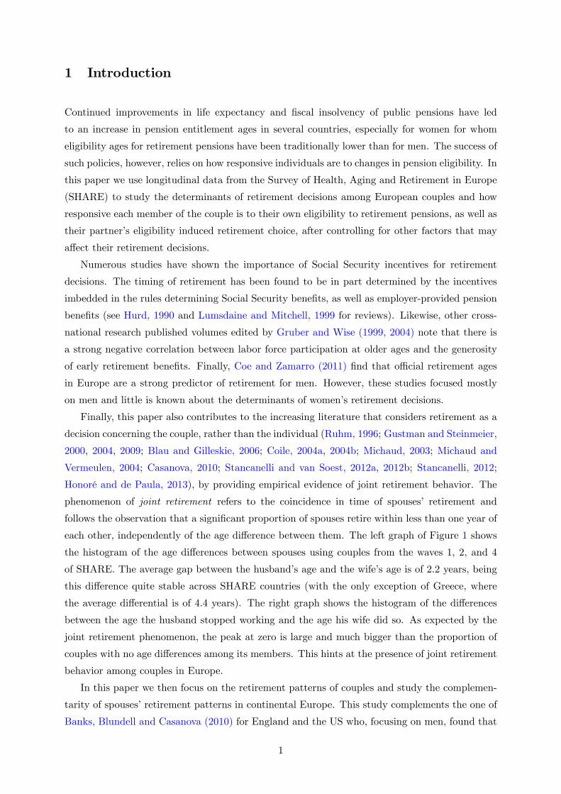
Honoré and de Paula, 2013), by providing empirical evidence of joint retirement behavior. The

phenomenon of joint retirement refers to the coincidence in time of spouses’ retirement and

follows the observation that a significant proportion of spouses retire within less than one year of

each other, independently of the age difference between them. The left graph of Figure 1 shows

the histogram of the age differences between spouses using couples from the waves 1, 2, and 4

of SHARE. The average gap between the husband’s age and the wife’s age is of 2.2 years, being

this difference quite stable across SHARE countries (with the only exception of Greece, where

the average differential is of 4.4 years). The right graph shows the histogram of the differences

between the age the husband stopped working and the age his wife did so. As expected by the

joint retirement phenomenon, the peak at zero is large and much bigger than the proportion of

couples with no age differences among its members. This hints at the presence of joint retirement

behavior among couples in Europe.

In this paper we then focus on the retirement patterns of couples and study the complemen-

tarity of spouses’retirement patterns in continental Europe. This study complements the one of

Banks, Blundell and Casanova (2010) for England and the US who, focusing on men, found that

1

Figure 1: Age gaps between spouses.

05

1015

Perc

ent

­10 ­5 0 5 10 15Husband Age ­ Wife Age

05

1015

Perc

ent

­10 ­5 0 5 10 15Reti rement Age Gap

Notes: Source: SHARE (waves 1, 2, and 4). Retirement age gap = weighted mean of differences betweenthe age of stop working for the husband and the age of stop working for his wife.

British men are from 14 to 20 percentage points more likely to retire when their wife reaches

state pension age at 60 than their American counterparts. Considering the numerous differences

in the labor markets, health insurance and social plans between the UK and US and many Eu-

ropean countries, there is no a priori reason to assume that their findings would still hold in

Europe. In addition, in contrast with Banks, Blundell and Casanova (2010), we are interested in

studying both women’s and men’s transitions out of the labor force and how they directly relate

to the actual realization of their husbands’(wives’) transition, using the institutional variation

in country-specific early and normal retirement ages to instrument the latter.

We find significant evidence of complementarity on spouses’transitions out of the labor force.

The probability of women leaving the labor force increases in around 21 percentage points when

their husbands also stop working. The effect for men, however, is insignificant. Controlling

for spouse’s working status reduces the impact of own eligibility for retirement pensions on

the probability of leaving the labor force. In particular, the effect for women is reduced in

about 2 percentage points for full retirement pensions. Therefore, by ignoring joint retirement,

governments would be overstating the impact of eligibility rules on retirement decisions. Our

empirical strategy allows us to give a causal interpretation to these effects we estimate as we

control for the potential endogeneity of spouse’s retirement decisions.

The rest of the paper proceeds as follows. Section 2 describes the data and key variables for

the analysis. Section 3 discusses the empirical reduced form model and identification strategy.

In section 4 we present econometric results from estimating our empirical model. Finally we

conclude in section 5.

2

2 Data

This paper uses data from SHARE, a multidisciplinary and cross-national panel database of

micro data on health, socioeconomic status and social and family networks of more than 40,000

individuals aged 50 or over. The main purpose of this survey is to provide detailed information

about the living conditions of middle-aged and older people for several countries in Europe.

There are currently four waves of data available in SHARE corresponding to the years 2004-

2005, 2006-2007, 2008-2009, and 2010-2011. However, the third wave of SHARE (2008-2009)

was devoted to a retrospective survey about life events of the respondents and did not collect

all the information available in other waves. For this reason, this paper focuses on analysis of

waves 1 (2004-2005), 2 (2006-2007), and 4 (2010-2011). The first wave of the SHARE dataset

contains a balanced representation of the various European regions, ranging from Scandinavia

(Denmark and Sweden), Central Europe (Austria, France, Germany, Switzerland, Belgium, and

the Netherlands) and Mediterranean countries (Spain, Italy and Greece). Further data have

been collected in 2005-06 and 2006-2007 in Israel. The Czech Republic, Poland and Ireland

joined SHARE in the wave 2006-2007. However, Ireland only participated in the wave 2006-2007.

Portugal also recently joined the SHARE team and participated in the survey during the last

wave of data 2010-2011. To maximize the number of waves of data available we decided to focus

our analysis on those OECD countries, for which information on retirement ages is available,

who participated in the survey for at least two consecutive waves (i.e. Austria, Belgium, Czech

Republic, Denmark, France, Germany, Greece, Italy, the Netherlands, Poland, Spain, Sweden,

and Switzerland).1

SHARE collects information on health variables (self-reported health, health conditions, phys-

ical and cognitive functioning, health behavior, use of health care facilities), biomarkers (grip

strength, body-mass index, peak flow), psychological variables (psychological health, well-being,

life satisfaction), economic variables (current work activity, job characteristics, opportunities to

work, retirement age, sources and composition of current income, wealth and consumption, hous-

ing, education), and social support variables (assistance within families, transfers of income and

assets, social networks, volunteer activities), both at the household and at the individual level.

This gives the possibility to analyze a wide variety of questions related to population ageing and

the quality of life of the elderly.

In addition, following Coe and Zamarro (2011) we supplemented the SHARE dataset with

information regarding country and gender specific statutory ages of eligibility for early and full re-

tirement pensions in order to construct instruments based on dummy variables indicating whether

the individual is above the full or early retirement ages set in his country. Table 1 reports the

statutory Early and Normal retirement ages in place in each country. Early and Normal re-

tirement ages are based on OECD’s definitions and represent eligibility ages for early and full

1Note that Israel is excluded from the group of countries we analyze because it did not join OECD until 2010

and by that time they did not participate in SHARE anymore.

3

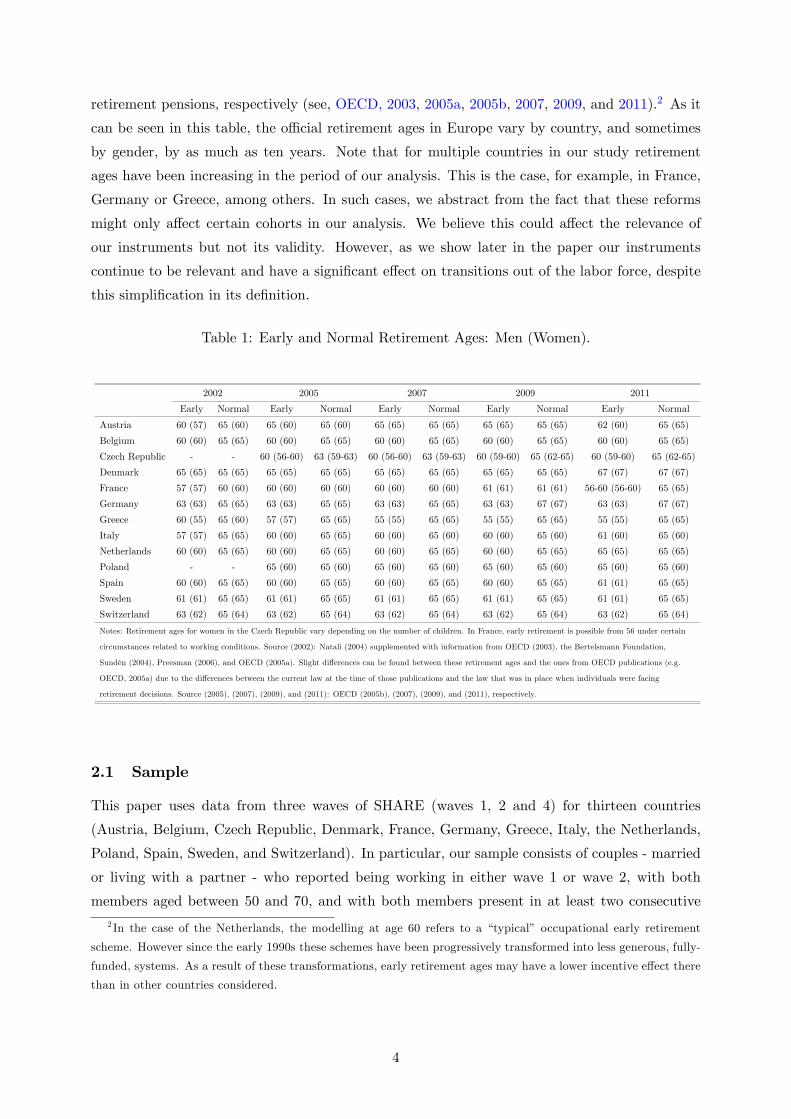
retirement pensions, respectively (see, OECD, 2003, 2005a, 2005b, 2007, 2009, and 2011).2 As it

can be seen in this table, the offi cial retirement ages in Europe vary by country, and sometimes

by gender, by as much as ten years. Note that for multiple countries in our study retirement

ages have been increasing in the period of our analysis. This is the case, for example, in France,

Germany or Greece, among others. In such cases, we abstract from the fact that these reforms

might only affect certain cohorts in our analysis. We believe this could affect the relevance of

our instruments but not its validity. However, as we show later in the paper our instruments

continue to be relevant and have a significant effect on transitions out of the labor force, despite

this simplification in its definition.

Table 1: Early and Normal Retirement Ages: Men (Women).

2002 2005 2007 2009 2011

Early Normal Early Normal Early Normal Early Normal Early Normal

Austria 60 (57) 65 (60) 65 (60) 65 (60) 65 (65) 65 (65) 65 (65) 65 (65) 62 (60) 65 (65)

Belgium 60 (60) 65 (65) 60 (60) 65 (65) 60 (60) 65 (65) 60 (60) 65 (65) 60 (60) 65 (65)

Czech Republic - - 60 (56-60) 63 (59-63) 60 (56-60) 63 (59-63) 60 (59-60) 65 (62-65) 60 (59-60) 65 (62-65)

Denmark 65 (65) 65 (65) 65 (65) 65 (65) 65 (65) 65 (65) 65 (65) 65 (65) 67 (67) 67 (67)

France 57 (57) 60 (60) 60 (60) 60 (60) 60 (60) 60 (60) 61 (61) 61 (61) 56-60 (56-60) 65 (65)

Germany 63 (63) 65 (65) 63 (63) 65 (65) 63 (63) 65 (65) 63 (63) 67 (67) 63 (63) 67 (67)

Greece 60 (55) 65 (60) 57 (57) 65 (65) 55 (55) 65 (65) 55 (55) 65 (65) 55 (55) 65 (65)

Italy 57 (57) 65 (65) 60 (60) 65 (65) 60 (60) 65 (60) 60 (60) 65 (60) 61 (60) 65 (60)

Netherlands 60 (60) 65 (65) 60 (60) 65 (65) 60 (60) 65 (65) 60 (60) 65 (65) 65 (65) 65 (65)

Poland - - 65 (60) 65 (60) 65 (60) 65 (60) 65 (60) 65 (60) 65 (60) 65 (60)

Spain 60 (60) 65 (65) 60 (60) 65 (65) 60 (60) 65 (65) 60 (60) 65 (65) 61 (61) 65 (65)

Sweden 61 (61) 65 (65) 61 (61) 65 (65) 61 (61) 65 (65) 61 (61) 65 (65) 61 (61) 65 (65)

Switzerland 63 (62) 65 (64) 63 (62) 65 (64) 63 (62) 65 (64) 63 (62) 65 (64) 63 (62) 65 (64)

Notes: Retirement ages for women in the Czech Republic vary depending on the number of children. In France, early retirement is possible from 56 under certain

circumstances related to working conditions. Source (2002): Natali (2004) supplemented with information from OECD (2003), the Bertelsmann Foundation,

Sundén (2004), Preesman (2006), and OECD (2005a). Slight differences can be found between these retirement ages and the ones from OECD publications (e.g.

OECD, 2005a) due to the differences between the current law at the time of those publications and the law that was in place when individuals were facing

retirement decisions. Source (2005), (2007), (2009), and (2011): OECD (2005b), (2007), (2009), and (2011), respectively.

2.1 Sample

This paper uses data from three waves of SHARE (waves 1, 2 and 4) for thirteen countries

(Austria, Belgium, Czech Republic, Denmark, France, Germany, Greece, Italy, the Netherlands,

Poland, Spain, Sweden, and Switzerland). In particular, our sample consists of couples - married

or living with a partner - who reported being working in either wave 1 or wave 2, with both

members aged between 50 and 70, and with both members present in at least two consecutive

2 In the case of the Netherlands, the modelling at age 60 refers to a “typical” occupational early retirement

scheme. However since the early 1990s these schemes have been progressively transformed into less generous, fully-

funded, systems. As a result of these transformations, early retirement ages may have a lower incentive effect there

than in other countries considered.

4

waves. After dropping observations with incomplete records, our sample has 3,058 such couples.3

Given that our aim is to measure the causal effect of joint retirement we focus the analysis

on working couples in one wave of data (waves 1 or 2) and study their retirement transitions

in the subsequent wave (waves 2 or 4). However, it should be stressed that, for some countries,

this sample would not be representative of the whole middle-age and older population, especially

for women. This is so because, as shown in Figure A.1, some European countries (notably the

Mediterranean countries) have very high proportions of women who never worked.

Moreover, a large proportion of women who ever worked but stopped before age 50 did so

at the early stages of their careers (see bimodal histogram shapes in Figure A.2 for females in

countries like Belgium, Italy, the Netherlands or Spain). Many of those early career stops are,

however, not related to retirement decisions and so they are excluded from our analysis.

2.2 Definition of retirement

We define retirement as making a transition out of work between two waves of data. That is, we

consider a respondent as having retired if she reports working as her current job status in one

wave and reports other working status (i.e. retired, unemployed, permanently sick or disabled, or

homemaker) in the subsequent wave of data. In our sample, the percentage of males transitioning

out of the labor force is 29 per cent, while for women the percentage is 25. The proportion actually

describing themselves as transitioning into retirement is 25 per cent for men, but only 17 per cent

for women.4

Figure 2 presents percentages of respondents out of the labor force by age intervals and

partner’s labor market status. We find that in our sample the fraction of workers that transition

out of the labor force is higher, for both men and women and at every age interval, when the

partner also makes such transition.

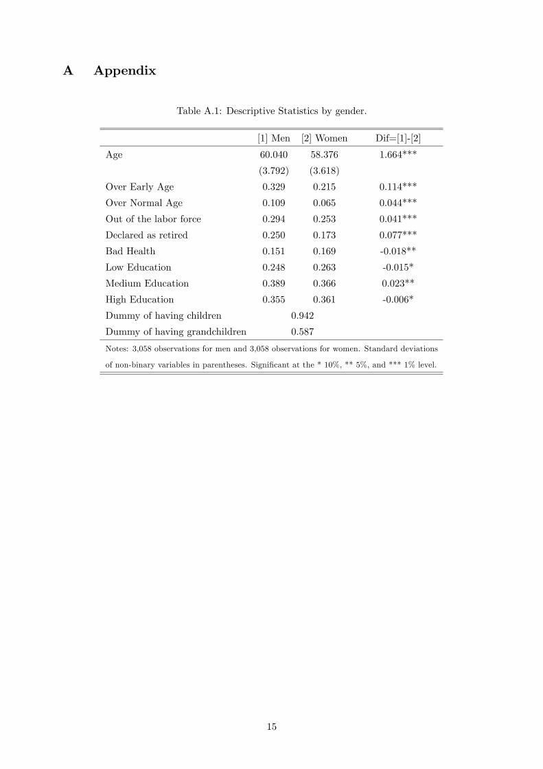
Some other descriptive statistics for our sample of working couples can be found in Table A.1.

The average age of men in our sample is 60 and 58 for women. Eleven per cent of men and a 6.5

percent of women are over the normal retirement age, while 33 and 21.5 percent, respectively,

are over the early retirement age. Finally, educational attainment and health status are similar

among males and females in our sample of couples.

3The distribution of number of couples by country is as follows: 70 couples in Austria, 350 couples in Belgium,

134 couples in Czechia, 454 couples in Denmark, 376 couples in France, 294 couples in Germany, 88 couples in

Greece, 128 couples in Italy, 334 couples in the Netherlands, 64 couples in Poland, 98 couples in Spain, 502 couples

in Sweden, and 166 couples in Switzerland.4Note that 4% of women in our couples reported transitioning from work to homemaker. This is in contrast

with only 0.4% of men that reported such transition. Not to lose these transitions from women, we focus on

transitions out of the labor force. Transitions to unemployment or disability were lower and did not show gender

differences (1.7 % of men reported transitioning to disability vs. 1.3% of women; 2.3% of men reported transitioning

to unemployment vs. 2.2 % of women). In any case, in the empirical analysis we also study only transitions to

self-reported retirement status as the dependent variable and results are robust to this alternative definition.

5

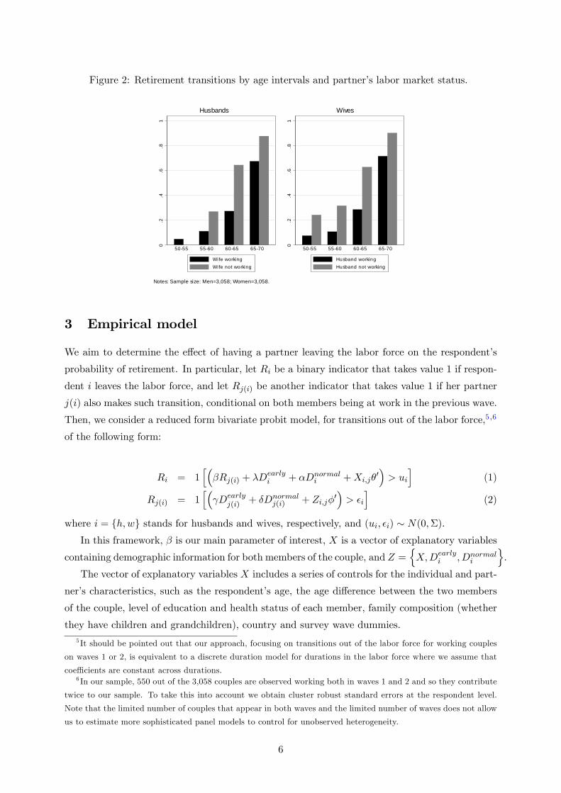
Figure 2: Retirement transitions by age intervals and partner’s labor market status.

0.2

.4.6

.81

50­55 55­60 60­65 65­70

Husbands

Wife workingWife not working

0.2

.4.6

.81

50­55 55­60 60­65 65­70

Wives

Husband workingHusband not working

Notes: Sample size: Men=3,058; Women=3,058.

3 Empirical model

We aim to determine the effect of having a partner leaving the labor force on the respondent’s

probability of retirement. In particular, let Ri be a binary indicator that takes value 1 if respon-

dent i leaves the labor force, and let Rj(i) be another indicator that takes value 1 if her partner

j(i) also makes such transition, conditional on both members being at work in the previous wave.

Then, we consider a reduced form bivariate probit model, for transitions out of the labor force,5 ,6

of the following form:

Ri = 1[(βRj(i) + λDearly

i + αDnormali +Xi,jθ

′)> ui

](1)

Rj(i) = 1[(γDearly

j(i) + δDnormalj(i) + Zi,jφ

′)> εi

](2)

where i = {h,w} stands for husbands and wives, respectively, and (ui, εi) ∼ N(0,Σ).

In this framework, β is our main parameter of interest, X is a vector of explanatory variables

containing demographic information for both members of the couple, and Z ={X,Dearly

i , Dnormali

}.

The vector of explanatory variables X includes a series of controls for the individual and part-

ner’s characteristics, such as the respondent’s age, the age difference between the two members

of the couple, level of education and health status of each member, family composition (whether

they have children and grandchildren), country and survey wave dummies.5 It should be pointed out that our approach, focusing on transitions out of the labor force for working couples

on waves 1 or 2, is equivalent to a discrete duration model for durations in the labor force where we assume that

coeffi cients are constant across durations.6 In our sample, 550 out of the 3,058 couples are observed working both in waves 1 and 2 and so they contribute

twice to our sample. To take this into account we obtain cluster robust standard errors at the respondent level.

Note that the limited number of couples that appear in both waves and the limited number of waves does not allow

us to estimate more sophisticated panel models to control for unobserved heterogeneity.

6

Dearlyi is an indicator for eligibility for early retirement pensions, which is defined as:

Dearlyi =

{1 if individual i’s age is above the early offi cial retirement age in the country

0 , otherwise,

and similarly Dnormali is an indicator for eligibility for full retirement pensions defined as:

Dnormali =

{1 if individual i’s age is above the full offi cial retirement age in the country

0 , otherwise.

Dearlyj(i) and Dnormal

j(i) are our external instruments for retirement decisions, that is, they are the

exclusion restrictions that allow identification of the model. Note that, identification then relies

on partner’s age being different than the individual’s age. As Figure 1 suggests, that is precisely

the case in our data. In addition, in our analysis we control for the age difference between the two

members of the couple to capture any unobservable characteristics at the couple level revealed

by choosing a partner with a certain age difference.7

In practice what we assume is that - conditional on observables - whether the partner is eligible

for retirement pensions only has an impact on the individual’s retirement decision through the

partner’s retirement decision, as opposed to directly having an effect. Note that our exogeneity

assumption does not imply that partner’s eligibility for retirement pensions does not affect ones’

retirement decisions. The assumption is that it does so but only through the actual retirement

decision of the partner. Under this assumption, our estimates of β are interpreted as the effect of

the partner’s retirement, induced through eligibility for retirement pensions, on the individual’s

retirement decision.

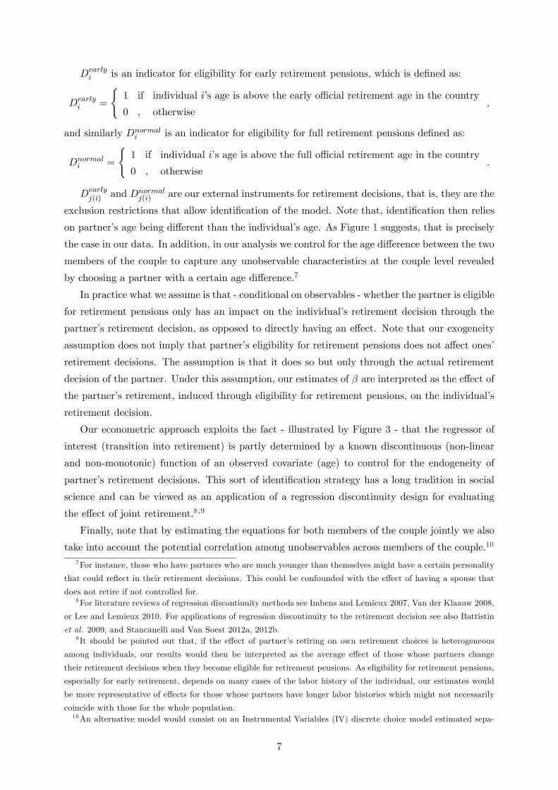
Our econometric approach exploits the fact - illustrated by Figure 3 - that the regressor of

interest (transition into retirement) is partly determined by a known discontinuous (non-linear

and non-monotonic) function of an observed covariate (age) to control for the endogeneity of

partner’s retirement decisions. This sort of identification strategy has a long tradition in social

science and can be viewed as an application of a regression discontinuity design for evaluating

the effect of joint retirement.8 ,9

Finally, note that by estimating the equations for both members of the couple jointly we also

take into account the potential correlation among unobservables across members of the couple.10

7For instance, those who have partners who are much younger than themselves might have a certain personality

that could reflect in their retirement decisions. This could be confounded with the effect of having a spouse that

does not retire if not controlled for.8For literature reviews of regression discontinuity methods see Imbens and Lemieux 2007, Van der Klaauw 2008,

or Lee and Lemieux 2010. For applications of regression discontinuity to the retirement decision see also Battistin

et al. 2009, and Stancanelli and Van Soest 2012a, 2012b.9 It should be pointed out that, if the effect of partner’s retiring on own retirement choices is heterogeneous

among individuals, our results would then be interpreted as the average effect of those whose partners change

their retirement decisions when they become eligible for retirement pensions. As eligibility for retirement pensions,

especially for early retirement, depends on many cases of the labor history of the individual, our estimates would

be more representative of effects for those whose partners have longer labor histories which might not necessarily

coincide with those for the whole population.10An alternative model would consist on an Instrumental Variables (IV) discrete choice model estimated sepa-

7

Figure 3: Probability of transitions out of the labor force by age.

0.2

.4.6

.81

­10 ­5 0 5 10Years to full retirement age

Notes: Source: SHARE (w aves 1, 2 and 4). Sample size: Men=17,883; Women=16,119.

4 Estimation Results

In this section we present the results of jointly estimating the system of equations (1-2). Table 2

reports, separately for men and women, average marginal effects of estimates of probit models for

the probability of leaving the labor force, given that both spouses were working in the previous

wave. The set of controls included in the regressions is the following: dummy variables for

the respondent being eligible for early or full retirement, the respondent’s age, the age difference

between the two members of the couple,11 country and survey wave dummies, education variables

for the two spouses, information on whether the couple has children and grandchildren as a

measure of care necessities, and health status controls for both spouses, lagged one period to

lessen endogeneity concerns. Within each section of the table we present results of models that

ignore the possibility of joint retirement by excluding information on the current working status of

the spouse, and preferred bivariate probit models where we include this variable and instrument

it with the dummies for spouse’s eligibility for retirement pensions.

Our results show that there is a significative joint retirement effect for women, of 21 percentage

points. For men, the estimated effect is insignificant. These results are similar in size to those

found by Banks, Blundell and Casanova (2010) for British men. Introducing information on

working status of the spouse reduces the impact of own eligibility for retirement pensions for

women in about 2 percentage points. Therefore, by ignoring joint retirement, governments would

be overstating the impact of eligibility rules on retirement decisions. The remainder of the

rately for men and women. However, this approach would be less effi cient than the simultaneous discrete choice

model models we estimate and it would not account for the potential correlation among unobservables across

spouses.11The age of the respondent is included as a continuous variable (measuring age in months), whereas the age

gap between spouses enters as dummies.

8

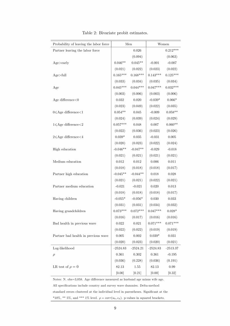
Table 2: Bivariate probit estimates.

Probability of leaving the labor force Men Women

Partner leaving the labor force 0.026 0.212***

(0.094) (0.063)

Age>early 0.046** 0.045** -0.001 -0.007

(0.021) (0.022) (0.023) (0.022)

Age>full 0.165*** 0.168*** 0.143*** 0.125***

(0.033) (0.034) (0.035) (0.034)

Age 0.045*** 0.044*** 0.047*** 0.032***

(0.003) (0.006) (0.003) (0.006)

Age difference<0 0.032 0.020 -0.039* 0.066*

(0.023) (0.049) (0.022) (0.035)

06Age difference<1 0.054** 0.045 -0.009 0.058**

(0.024) (0.039) (0.024) (0.029)

16Age difference<2 0.057*** 0.048 0.007 0.060**

(0.022) (0.036) (0.023) (0.026)

26Age difference<4 0.039* 0.035 -0.031 0.005

(0.020) (0.023) (0.022) (0.024)

High education -0.046** -0.047** -0.029 -0.018

(0.021) (0.021) (0.021) (0.021)

Medium education 0.012 0.012 0.006 0.011

(0.018) (0.018) (0.018) (0.017)

Partner high education -0.045** -0.044** 0.018 0.028

(0.021) (0.021) (0.022) (0.021)

Partner medium education -0.021 -0.021 0.020 0.013

(0.018) (0.018) (0.018) (0.017)

Having children -0.055* -0.056* 0.030 0.033

(0.031) (0.031) (0.034) (0.032)

Having grandchildren 0.073*** 0.072*** 0.047*** 0.028*

(0.016) (0.017) (0.016) (0.016)

Bad health in previous wave 0.022 0.021 0.071*** 0.071***

(0.022) (0.022) (0.019) (0.019)

Partner bad health in previous wave 0.005 0.002 0.039* 0.031

(0.020) (0.023) (0.020) (0.021)

Log-likelihood -2524.83 -2524.21 -2524.83 -2513.37

ρ 0.361 0.302 0.361 -0.195

(0.036) (0.228) (0.036) (0.191)

LR test of ρ = 0 82.13 1.55 82.13 0.99

[0.00] [0.21] [0.00] [0.32]

Notes: N. obs=3,058. Age difference measured as husband age minus wife age.

All specifications include country and survey wave dummies. Delta-method

standard errors clustered at the individual level in parentheses. Significant at the

*10%, ** 5%, and *** 1% level. ρ = corr(uh, εh). p-values in squared brackets.

9

variables have the expected effects. Higher levels of education lower the probability of leaving

the labor force but only for men, whereas bad health has a positive impact on the probability of

leaving the labor force only for women. Finally, having grandchildren increases the probability

of leaving the labor force for both men and women, while having children reduces the probability

of retirement only for men.12

In order for the offi cial retirement ages to be valid instruments, they must be exogenous and

relevant. With respect to the exogeneity assumption, we assume that if the husband (wife) reaches

the statutory retirement age, his (her) spouse’s retirement decision is only affected through his

(her) own transition. This assumption is not testable. Regarding relevance, statutory retirement

ages must be related to actual retirement behavior. To illustrate this latter point we estimated

probit regressions of the individual probability of leaving the labor force, separately for husbands

and wives. This set of regressions would represent a standard first-stage step in a two-stage

estimation procedure such as an IV model.13 Estimated marginal effects for these regressions

can be found in Table A.2 of the Appendix. Our results show that eligibility for retirement

pensions are a significant predictor of retirement decisions both for husbands and wives. In terms

of the model in equations (1-2), these results confirm that Dearlyj(i) and Dnormal

j(i) affect Rj(i), after

controlling for Dearlyi and Dnormal

i , and the rest of the control variables.14

To get a better insight of the effect of policies on pension entitlement ages on retirement

behaviors of couples, we also estimate bivariate models dividing the sample in two groups of

countries. Group 1 includes those countries with a low gap in participation rates by gender,

while group 2 contains those countries with high differentials in the participation rates between

men and women. According to Table A.3, the mean gender gap in employment/population ratios

for individuals aged 50-64 years in the thirteen countries considered in the analysis is 17.13.

Below that number are the countries with low gender gaps, that is, Belgium, Denmark, France,

Germany, Poland, and Sweden; whereas above the mean, we find countries with high gender

gaps like Austria, Czechia, Greece, Italy, Netherlands, Spain, or Switzerland. The estimated

marginal effects from these regressions are reported in Table 3. As before, the estimated joint

retirement effect is insignificant for men, both for groups 1 and 2. On the contrary, for women

12We also estimated models controlling for household income in the previous wave and household wealth but

this did not change our main results. Estimates for these models are available from the authors upon request.13 In practice, we follow a more effi cient approach and estimate the whole bivariate model by maximum likelihood

in a single step.14The estimated model in this paper is a simultaneous equation binary choice model where partner’s eligibility for

early and full retirement pensions is used as exclusion restrictions to identify the system. As such, the reduced form

probit models that we estimate just proxy what it would be a first step to assess the relevance of our instruments.

Moreover, in order to also approximate traditional Hausman/Sargan test for the joint validity of the instruments,

we have tried and estimate reduced form linear models for the probability of individual i leaving the labor force,

separately for men and women, by 2SLS. In these models, the partner’s transition out of the labor force, Ri(i), is

instrumented using the indicators Dearlyj(i) and Dnormal

j(i) . For these latter regressions, we obtain the Sargan test of

overidentifying restrictions. For men the corresponding p-value for the test is 0.274, whereas for women is 0.869;

meaning that in both cases we can not reject the null hypothesis that the over-identifying restrictions are valid.

10

we find that the significative joint retirement effect is wholly due to those countries where the

differences by gender in participation rates are small (that is, group 1, for which the estimated

effect is 28 percentage points). On the contrary, for women in countries with large differences in

participation rates by gender, the estimated effect of joint retirement is not statistically different

from zero.

Finally, to assess the robustness of our results to different definitions of retirement, we also

estimated models for the probability that the respondent describes herself as retired as opposed

to out of the labor force. The results of these regressions can be found in the Appendix in Table

A.4. Our results are still robust to this alternative definition of the dependent variable. For

women, we find a significant joint retirement effect, although the magnitude of the effect gets

reduced to about half the size (from 21 to 10 percentage points). For men we find an effect

similar in magnitude, but again insignificant. Another difference with previous results is that

lagged bad health does not seem to have an impact on retirement decisions for women in this

case. This suggests that bad health shocks might lead women to rather leave the labor force

without actually retiring. More research is needed to better understand the differences between

women’s transitions out of work to self-reported retirement or to homemaking.

5 Conclusions

Continued improvements in life expectancy and fiscal insolvency of public pensions have led to

an increase in pension entitlement ages in several countries. For example, the normal retirement

age in the US is currently rising from 65 to 67 for successive birth cohorts. England, Austria,

Germany and Italy are also phasing in increases in their retirement ages. However, the success

of such policies relies on how responsive individuals are to such changes in pension eligibility.

In this paper we use longitudinal data from SHARE to study the determinants of retirement

decisions among European couples and how responsive each member of the couple is to their own

eligibility to retirement pensions, as well as their partner’s eligibility induced retirement choice,

after controlling for other factors that may affect their retirement decisions.

Our empirical strategy exploits the discontinuities in retirement behavior across countries to

control for the endogeneity of partner’s labor participation decisions. This allows us to give a

causal interpretation to the effects we estimate. Our results show a significative joint retirement

effect for women of 21 percentage points. For men, the estimated effect is insignificant.

We also compare our estimates with models that do not control for the partner’s labor par-

ticipation decisions and found that introducing information on working status of the spouse

reduces the impact of own eligibility for retirement pensions for women in about 2 percentage

points. Therefore, by ignoring joint retirement, governments would be overstating the impact of

eligibility rules on retirement decisions.

Finally, our results are still robust to using self-reported retirement status as an alternative

definition of the dependent variable. In this case, we find a significant joint retirement effect for

11

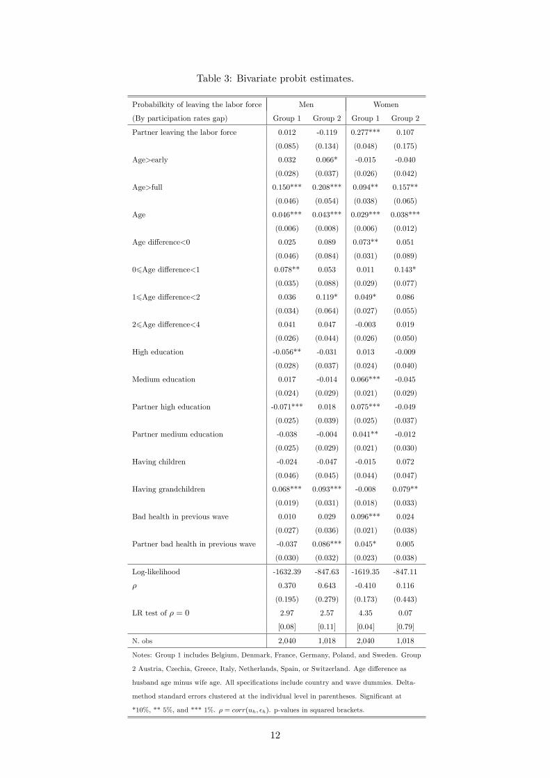
Table 3: Bivariate probit estimates.

Probabilkity of leaving the labor force Men Women

(By participation rates gap) Group 1 Group 2 Group 1 Group 2

Partner leaving the labor force 0.012 -0.119 0.277*** 0.107

(0.085) (0.134) (0.048) (0.175)

Age>early 0.032 0.066* -0.015 -0.040

(0.028) (0.037) (0.026) (0.042)

Age>full 0.150*** 0.208*** 0.094** 0.157**

(0.046) (0.054) (0.038) (0.065)

Age 0.046*** 0.043*** 0.029*** 0.038***

(0.006) (0.008) (0.006) (0.012)

Age difference<0 0.025 0.089 0.073** 0.051

(0.046) (0.084) (0.031) (0.089)

06Age difference<1 0.078** 0.053 0.011 0.143*

(0.035) (0.088) (0.029) (0.077)

16Age difference<2 0.036 0.119* 0.049* 0.086

(0.034) (0.064) (0.027) (0.055)

26Age difference<4 0.041 0.047 -0.003 0.019

(0.026) (0.044) (0.026) (0.050)

High education -0.056** -0.031 0.013 -0.009

(0.028) (0.037) (0.024) (0.040)

Medium education 0.017 -0.014 0.066*** -0.045

(0.024) (0.029) (0.021) (0.029)

Partner high education -0.071*** 0.018 0.075*** -0.049

(0.025) (0.039) (0.025) (0.037)

Partner medium education -0.038 -0.004 0.041** -0.012

(0.025) (0.029) (0.021) (0.030)

Having children -0.024 -0.047 -0.015 0.072

(0.046) (0.045) (0.044) (0.047)

Having grandchildren 0.068*** 0.093*** -0.008 0.079**

(0.019) (0.031) (0.018) (0.033)

Bad health in previous wave 0.010 0.029 0.096*** 0.024

(0.027) (0.036) (0.021) (0.038)

Partner bad health in previous wave -0.037 0.086*** 0.045* 0.005

(0.030) (0.032) (0.023) (0.038)

Log-likelihood -1632.39 -847.63 -1619.35 -847.11

ρ 0.370 0.643 -0.410 0.116

(0.195) (0.279) (0.173) (0.443)

LR test of ρ = 0 2.97 2.57 4.35 0.07

[0.08] [0.11] [0.04] [0.79]

N. obs 2,040 1,018 2,040 1,018

Notes: Group 1 includes Belgium, Denmark, France, Germany, Poland, and Sweden. Group

2 Austria, Czechia, Greece, Italy, Netherlands, Spain, or Switzerland. Age difference as

husband age minus wife age. All specifications include country and wave dummies. Delta-

method standard errors clustered at the individual level in parentheses. Significant at

*10%, ** 5%, and *** 1%. ρ = corr(uh, εh). p-values in squared brackets.

12

women, although the magnitude of the effect gets reduced to about half the size. For men, the

estimated effect remains insignificant.

As recent pension reforms that increase pension entitlement ages get established and new

waves of data get collected, it would be good to analyze how these reforms are affecting retirement

patterns of men and women. Lastly, additional waves of data would allow for the estimation of

panel data models that could better control for unobserved heterogeneity affecting transitions

out of the labor force.

References

[1] Banks, J., R. Blundell, and M. Casanova (2010), “The dynamics of retirement behavior incouples: Reduced-form evidence from England and the US”, mimeo.

[2] Battistin, E., A. Brugiavini, E. Rettore and G. Weber (2009), “The Retirement ConsumptionPuzzle: Evidence from a Regression Discontinuity Approach”, American Economic Review,99(5), 2209-2226.

[3] Blau, D. and D. Gilleskie (2006), “Health insurance and retirement of married couples”,Journal of Applied Econometrics, 21(7), 935-953.

[4] Casanova, M.(2010), “Happy Together: A Structural Model of Couples’Joint RetirementChoices”, mimeo.

[5] Coe, N. and G. Zamarro (2011), “Retirement effects on health in Europe”, Journal of HealthEconomics, Elsevier, 30(1), 77-86.

[6] Coile, C. (2004a), “Retirement incentives and couple’s retirement decisions”, Topics in Eco-nomics analysis and Policy, 4(1), article 17.

[7] – (2004b), “Health shocks and couple’s labor supply decisions”, NBER working paper 10810.

[8] Gustman A. and T. Steinmeier (2000), “Retirement in dual-career Families: A structuralmodel”, Journal of Labor Economics, 18(3), 503-545.

[9] – (2004), “Social Security, Pensions and Retirement Behaviour with the Family”, Journalof Applied Econometrics, 19, 723-737.

[10] – (2009), “Integrating Retirement Models”, NBER Working Paper 15607.

[11] Gruber, J. and D. Wise (1999, 2004), Social Security Programs and Retirement Around theWorld, University of Chicago Press: Chicago.

[12] Honoré, B. and A. de Paula (2013), “Interdependent durations in joint retirement”, cemmapworking paper CWP05/13.

[13] Hurd, M. D. (1990), “Research on the Elderly: Economic Status, Retirement, and Consump-tion and Savings”, Journal of Economic Literature, 28(June 1990b), 565-637.

[14] Imbens, G. and T. Lemieux (2007), “Regression Discontinuity Design: a Guide to Practice”,Journal of Econometrics, 142, 615-635.

[15] Lee, D.S. and T.Lemieux (2010), “Regression Discontinuity Designs in Economics”, Journalof Economic Literature, 48(2), 281-355.

13

[16] Lumsdaine, R. L. and O. S. Mitchell (1999), “New Developments in the Economic Analysisof Retirement”, in O. Ashenfelter and D. Card, eds., Handbook of Labor Economics, 3C,Amsterdam: North Holland, 3261-3307.

[17] Michaud, P. (2003), “Joint labor supply dynamics of older couples”, IZA DP 832.

[18] Michaud, P. and F. Vermeulen (2004), “A collective Retirement Model: Identification andEstimation in the Presence of Externalities”, IZA DP 1294.

[19] Natali, D. (2004), The Pension System Observatoire Social Européen. Research Project. "LAMETHODE OUVERTE DE COORDINATION (MOC) ENMATIERE DES PENSIONS ETDE L’INTEGRATION EUROPEENNE" Service Public Fédéral Sécurité Sociale.

[20] OECD (2003), "Economic Survey of Austria", chapter 3: Pensions.http://www.oecd.org/dataoecd/5/16/27424371.pdf

[21] – (2005a), "Vieillissement et politiques de l’emploi". France. Ageing and Employment Poli-cies. http://www.oecd.org/dataoecd/52/58/34591763.pdf

[22] – (2005b), OECD Pensions at a Glance 2005: Public Policies across OECD Countries,OECD Publishing.

[23] – (2007), Pensions at a Glance 2007: Public Policies across OECD Countries, OECD Pub-lishing.

[24] – (2009), Pensions at a Glance 2009: Retirement-Income Systems in OECD Countries,OECD Publishing.

[25] – (2011), Pensions at a Glance 2011: Retirement-income Systems in OECD and G20 Coun-tries, OECD Publishing.

[26] Preesman, L. (2006), "Dutch to Abolish Civil Service Retirement Age", IPE InternationalPublishers Ltd. Netherlands, June 28.

[27] Ruhm, C. J. (1996), “Do pensions increase the labor supply of older men?”, Journal of PublicEconomics, 59(2), 157-175.

[28] Stancanelli, E. (2012), “Spouses’Retirement and Hours of Work Outcomes: Evidence fromTwofold Regression Discontinuity”, mimeo.

[29] Stancanelli, E. and A. van Soest (2012a), “Retirement and Home Production: A RegressionDiscontinuity Approach”, American Economic Review, 102(3), 600-605.

[30] – (2012b), “Joint Leisure Before and After Retirement: A Double Regression DiscontinuityApproach”, IZA DP 6698.

[31] Sundén, A. (2004), "The Future of Retirement in Sweden", PRC WP 2004-16. PensionResearch Council Working Paper. Pension Research Council.

[32] The Bertelsmann Foundation, International Reform Monitor, Country info.http://www.reformmonitor.org/index.php3?mode=status

[33] Van der Klaauw, W. (2008), “Regression-Discontinuity Analysis: A Survey of Recent Devel-opments in Economics”, Labour, 102(3), 22(2), 219-245.

14

A Appendix

Table A.1: Descriptive Statistics by gender.

[1] Men [2] Women Dif=[1]-[2]

Age 60.040 58.376 1.664***

(3.792) (3.618)

Over Early Age 0.329 0.215 0.114***

Over Normal Age 0.109 0.065 0.044***

Out of the labor force 0.294 0.253 0.041***

Declared as retired 0.250 0.173 0.077***

Bad Health 0.151 0.169 -0.018**

Low Education 0.248 0.263 -0.015*

Medium Education 0.389 0.366 0.023**

High Education 0.355 0.361 -0.006*

Dummy of having children 0.942

Dummy of having grandchildren 0.587

Notes: 3,058 observations for men and 3,058 observations for women. Standard deviations

of non-binary variables in parentheses. Significant at the * 10%, ** 5%, and *** 1% level.

15

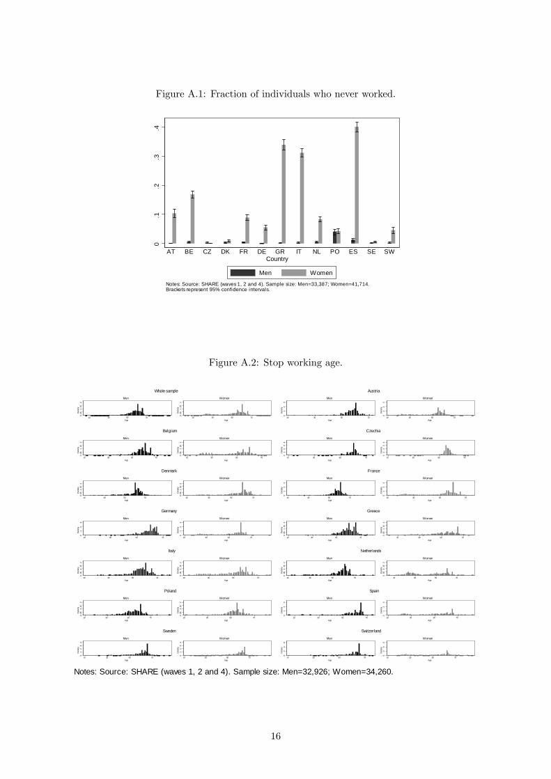
Figure A.1: Fraction of individuals who never worked.

0.1

.2.3

.4

AT BE CZ DK FR DE GR IT NL PO ES SE SWCountry

Men Women

Notes: Source: SHARE (waves 1, 2 and 4). Sample size: Men=33,387; Women=41,714.Brackets represent 95% confidence intervals.

Figure A.2: Stop working age.

0.0

5.1

.15

.2D

ensi

ty

10 30 50 70Age

Men

0.0

5.1

.15

.2D

ensi

ty

10 30 50 70Age

Women

Whole sample

0.1

.2.3

Den

sity

10 30 50 70Age

Men

0.1

.2.3

Den

sity

10 30 50 70Age

Women

Austria

0.0

5.1

.15

.2D

ensi

ty

10 30 50 70Age

Men

0.0

5.1

.15

.2D

ensi

ty

10 30 50 70Age

Women

Belgium

0.1

.2.3

.4D

ensi

ty

10 30 50 70Age

Men

0.1

.2.3

.4D

ensi

ty

10 30 50 70Age

Women

Czechia

0.0

5.1

.15

.2D

ensi

ty

10 30 50 70Age

Men

0.0

5.1

.15

.2D

ensi

ty

10 30 50 70Age

Women

Denmark

0.1

.2.3

Den

sity

10 30 50 70Age

Men

0.1

.2.3

Den

sity

10 30 50 70Age

Women

France

0.1

.2.3

Den

sity

10 30 50 70Age

Men

0.1

.2.3

Den

sity

10 30 50 70Age

Women

Germany

0.0

5.1

.15

.2D

ensi

ty

10 30 50 70Age

Men

0.0

5.1

.15

.2D

ensi

ty

10 30 50 70Age

Women

Greece

0.0

5.1

.15

.2D

ensi

ty

10 30 50 70Age

Men

0.0

5.1

.15

.2D

ensi

ty

10 30 50 70Age

Women

Italy

0.0

5.1

.15

.2D

ensi

ty

10 30 50 70Age

Men

0.0

5.1

.15

.2D

ensi

ty

10 30 50 70Age

Women

Netherlands

0.0

5.1

.15

.2D

ensi

ty

10 30 50 70Age

Men

0.0

5.1

.15

.2D

ensi

ty

10 30 50 70Age

Women

Poland

0.1

.2.3

Den

sity

10 30 50 70Age

Men

0.1

.2.3

Den

sity

10 30 50 70Age

Women

Spain

0.1

.2.3

.4D

ensi

ty

10 30 50 70Age

Men

0.1

.2.3

.4D

ensi

ty

10 30 50 70Age

Women

Sweden

0.2

.4.6

Den

sity

10 30 50 70Age

Men

0.2

.4.6

Den

sity

10 30 50 70Age

Women

Switzerland

Notes: Source: SHARE (waves 1, 2 and 4). Sample size: Men=32,926; Women=34,260.

16

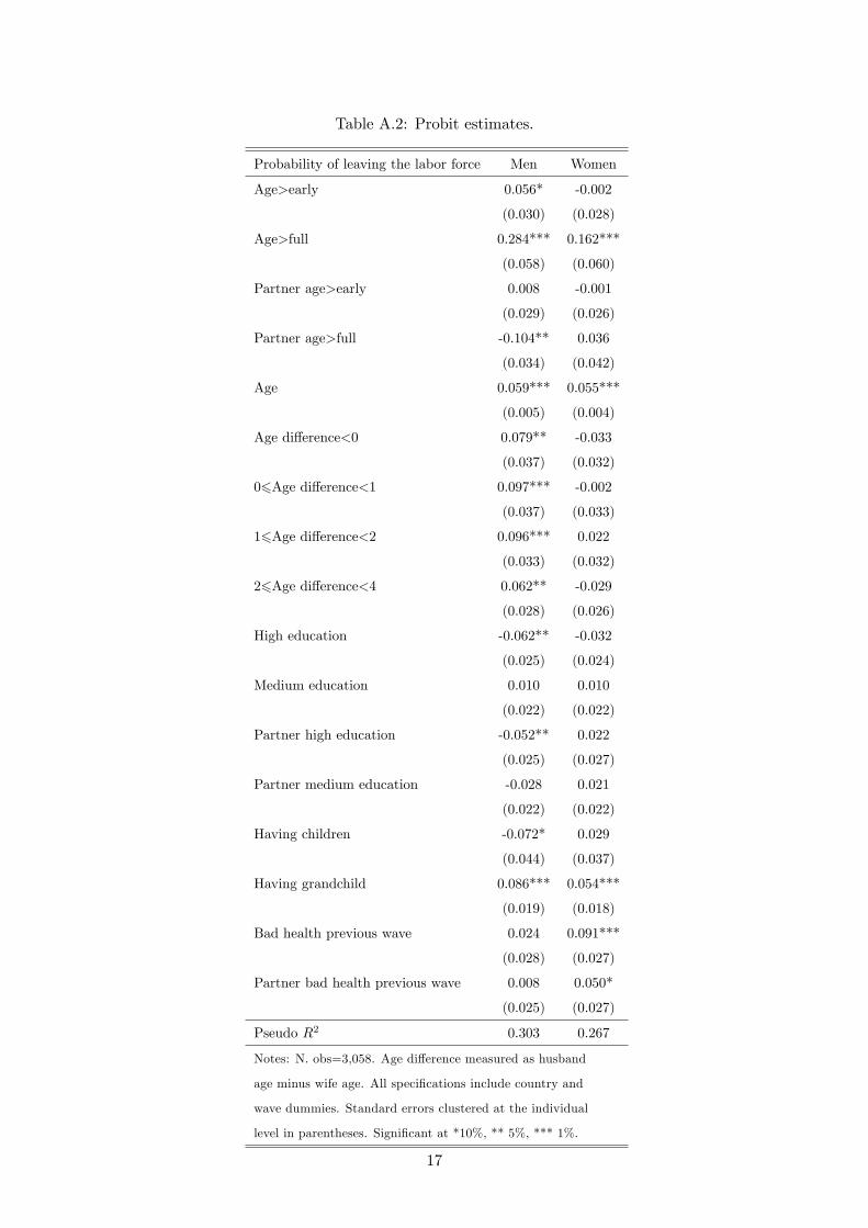
Table A.2: Probit estimates.

Probability of leaving the labor force Men Women

Age>early 0.056* -0.002

(0.030) (0.028)

Age>full 0.284*** 0.162***

(0.058) (0.060)

Partner age>early 0.008 -0.001

(0.029) (0.026)

Partner age>full -0.104** 0.036

(0.034) (0.042)

Age 0.059*** 0.055***

(0.005) (0.004)

Age difference<0 0.079** -0.033

(0.037) (0.032)

06Age difference<1 0.097*** -0.002

(0.037) (0.033)

16Age difference<2 0.096*** 0.022

(0.033) (0.032)

26Age difference<4 0.062** -0.029

(0.028) (0.026)

High education -0.062** -0.032

(0.025) (0.024)

Medium education 0.010 0.010

(0.022) (0.022)

Partner high education -0.052** 0.022

(0.025) (0.027)

Partner medium education -0.028 0.021

(0.022) (0.022)

Having children -0.072* 0.029

(0.044) (0.037)

Having grandchild 0.086*** 0.054***

(0.019) (0.018)

Bad health previous wave 0.024 0.091***

(0.028) (0.027)

Partner bad health previous wave 0.008 0.050*

(0.025) (0.027)

Pseudo R2 0.303 0.267

Notes: N. obs=3,058. Age difference measured as husband

age minus wife age. All specifications include country and

wave dummies. Standard errors clustered at the individual

level in parentheses. Significant at *10%, ** 5%, *** 1%.

17

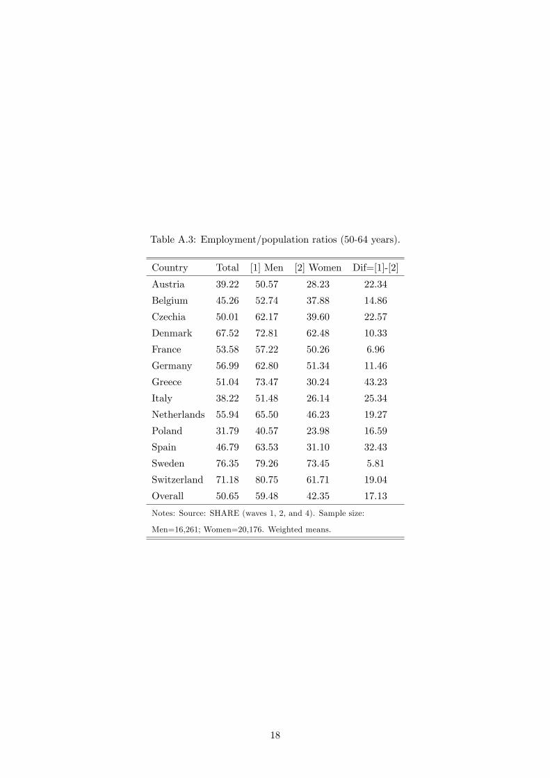
Table A.3: Employment/population ratios (50-64 years).

Country Total [1] Men [2] Women Dif=[1]-[2]

Austria 39.22 50.57 28.23 22.34

Belgium 45.26 52.74 37.88 14.86

Czechia 50.01 62.17 39.60 22.57

Denmark 67.52 72.81 62.48 10.33

France 53.58 57.22 50.26 6.96

Germany 56.99 62.80 51.34 11.46

Greece 51.04 73.47 30.24 43.23

Italy 38.22 51.48 26.14 25.34

Netherlands 55.94 65.50 46.23 19.27

Poland 31.79 40.57 23.98 16.59

Spain 46.79 63.53 31.10 32.43

Sweden 76.35 79.26 73.45 5.81

Switzerland 71.18 80.75 61.71 19.04

Overall 50.65 59.48 42.35 17.13

Notes: Source: SHARE (waves 1, 2, and 4). Sample size:

Men=16,261; Women=20,176. Weighted means.

18

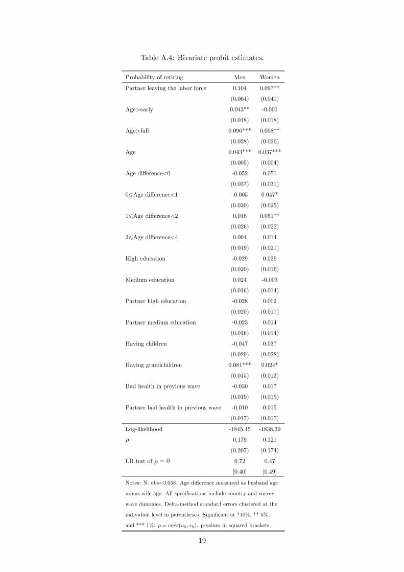
Table A.4: Bivariate probit estimates.

Probability of retiring Men Women

Partner leaving the labor force 0.104 0.097**

(0.064) (0.041)

Age>early 0.043** -0.001

(0.018) (0.018)

Age>full 0.096*** 0.058**

(0.028) (0.026)

Age 0.043*** 0.037***

(0.005) (0.004)

Age difference<0 -0.052 0.051

(0.037) (0.031)

06Age difference<1 -0.005 0.047*

(0.030) (0.025)

16Age difference<2 0.016 0.051**

(0.026) (0.022)

26Age difference<4 0.004 0.014

(0.019) (0.021)

High education -0.029 0.026

(0.020) (0.016)

Medium education 0.024 -0.003

(0.016) (0.014)

Partner high education -0.028 0.002

(0.020) (0.017)

Partner medium education -0.023 0.014

(0.016) (0.014)

Having children -0.047 0.037

(0.029) (0.028)

Having grandchildren 0.081*** 0.024*

(0.015) (0.013)

Bad health in previous wave -0.030 0.017

(0.019) (0.015)

Partner bad health in previous wave -0.010 0.015

(0.017) (0.017)

Log-likelihood -1845.45 -1838.39

ρ 0.179 0.121

(0.207) (0.174)

LR test of ρ = 0 0.72 0.47

[0.40] [0.49]

Notes: N. obs=3,058. Age difference measured as husband age

minus wife age. All specifications include country and survey

wave dummies. Delta-method standard errors clustered at the

individual level in parentheses. Significant at *10%, ** 5%,

and *** 1%. ρ = corr(uh, εh). p-values in squared brackets.

19