econstor www.econstor.eu

Der Open-Access-Publikationsserver der ZBW – Leibniz-Informationszentrum WirtschaftThe Open Access Publication Server of the ZBW – Leibniz Information Centre for Economics

Standard-Nutzungsbedingungen:

Die Dokumente auf EconStor dürfen zu eigenen wissenschaftlichenZwecken und zum Privatgebrauch gespeichert und kopiert werden.

Sie dürfen die Dokumente nicht für öffentliche oder kommerzielleZwecke vervielfältigen, öffentlich ausstellen, öffentlich zugänglichmachen, vertreiben oder anderweitig nutzen.

Sofern die Verfasser die Dokumente unter Open-Content-Lizenzen(insbesondere CC-Lizenzen) zur Verfügung gestellt haben sollten,gelten abweichend von diesen Nutzungsbedingungen die in der dortgenannten Lizenz gewährten Nutzungsrechte.

Terms of use:

Documents in EconStor may be saved and copied for yourpersonal and scholarly purposes.

You are not to copy documents for public or commercialpurposes, to exhibit the documents publicly, to make thempublicly available on the internet, or to distribute or otherwiseuse the documents in public.

If the documents have been made available under an OpenContent Licence (especially Creative Commons Licences), youmay exercise further usage rights as specified in the indicatedlicence.

zbw Leibniz-Informationszentrum WirtschaftLeibniz Information Centre for Economics

Gould, Eric D.

Working Paper

Explaining the Unexplained: Residual WageInequality, Manufacturing Decline, and Low-SkilledImmigration

IZA Discussion Papers, No. 9107

Provided in Cooperation with:Institute for the Study of Labor (IZA)

Suggested Citation: Gould, Eric D. (2015) : Explaining the Unexplained: Residual WageInequality, Manufacturing Decline, and Low-Skilled Immigration, IZA Discussion Papers, No.9107

This Version is available at:http://hdl.handle.net/10419/113984

DI

SC

US

SI

ON

P

AP

ER

S

ER

IE

S

Forschungsinstitut zur Zukunft der ArbeitInstitute for the Study of Labor

Explaining the Unexplained:Residual Wage Inequality, Manufacturing Decline, and Low-Skilled Immigration

IZA DP No. 9107

June 2015

Eric D. Gould

Explaining the Unexplained:

Residual Wage Inequality, Manufacturing Decline, and Low-Skilled Immigration

Eric D. Gould Hebrew University of Jerusalem,

IZA, CEPR and CReAM

Discussion Paper No. 9107 June 2015

IZA

P.O. Box 7240 53072 Bonn

Germany

Phone: +49-228-3894-0 Fax: +49-228-3894-180

E-mail: iza@iza.org

Any opinions expressed here are those of the author(s) and not those of IZA. Research published in this series may include views on policy, but the institute itself takes no institutional policy positions. The IZA research network is committed to the IZA Guiding Principles of Research Integrity. The Institute for the Study of Labor (IZA) in Bonn is a local and virtual international research center and a place of communication between science, politics and business. IZA is an independent nonprofit organization supported by Deutsche Post Foundation. The center is associated with the University of Bonn and offers a stimulating research environment through its international network, workshops and conferences, data service, project support, research visits and doctoral program. IZA engages in (i) original and internationally competitive research in all fields of labor economics, (ii) development of policy concepts, and (iii) dissemination of research results and concepts to the interested public. IZA Discussion Papers often represent preliminary work and are circulated to encourage discussion. Citation of such a paper should account for its provisional character. A revised version may be available directly from the author.

IZA Discussion Paper No. 9107 June 2015

ABSTRACT

Explaining the Unexplained: Residual Wage Inequality, Manufacturing Decline, and Low-Skilled Immigration*

This paper investigates whether the increasing “residual wage inequality” trend is related to manufacturing decline and the influx of low-skilled immigrants. There is a vast literature arguing that technological change, international trade, and institutional factors have played a significant role in the inequality trend. However, most of the trend is unexplained by observable factors. This paper attempts to “explain” the growth in the unexplained variance of wages by exploiting variation across locations (states or cities) in the United States in the local level of “residual inequality.” The evidence shows that a shrinking manufacturing sector increases inequality. In addition, an influx of low-skilled immigrants increases inequality, but this effect is concentrated in areas with a steeper manufacturing decline. Similar results are found for two alternative measures linked to increasing inequality: the increasing return to education and the decline in the employment rate of non-college men. The overall evidence suggests that the manufacturing and immigration trends have hollowed-out the overall demand for middle-skilled workers in all sectors, while increasing the supply of workers in lower skilled jobs. Both phenomena are producing downward pressure on the relative wages of workers at the low end of the income distribution. JEL Classification: J31 Keywords: inequality, manufacturing, low-skilled immigration Corresponding author: Eric D. Gould Department of Economics The Hebrew University of Jerusalem Mount Scopus Jerusalem 91905 Israel E-mail: eric.gould@huji.ac.il

* For many helpful comments, I thank David Autor and seminar participants at the Washington University in St. Louis, Ohio State, Boston University, and the University of Maryland. David Dorn provided help with the data from Autor, Dorn, and Hanson (2013). Sheri Band provided diligent research assistance and financial support was received from The Maurice Falk Institute for Economic Research. The first draft of this paper was written while visiting the Department of Economics at Georgetown University.

1

I. Introduction

This paper examines the steady growth in income inequality over the last

several decades in many advanced countries. Despite the vast literature on the topic,

concrete explanations for this phenomenon have proved elusive. The evidence points

to an important role for technological change, international trade, and changes in

institutions. However, most of the inequality trend is left unexplained by observable

factors like trade-flows, industrial and occupational shifts, changes in the education

and demographic composition of the workforce, and the returns to observable skills.

This paper attempts to “explain” the growth in the unexplained variance of log

wages by exploiting variation across locations (states or cities) in the United States in

the local level of “residual inequality.” A similar strategy has been used extensively in

the literature to test whether the growth in the college wage premium is due to

technological change, international trade, immigration, and other factors. However,

the college premium is responsible for only a small portion of the inequality trend.

This is the first paper to use a similar strategy to shed light on the growth in the

largest, previously unexplained, portion of the wage variance over time.

The focus of the analysis will be on the role of the steady decline in the

manufacturing industry and the influx of low-skilled immigrants in recent decades.

Both of these trends coincided with the dramatic increase in wage inequality. The

existing literature has found that the decline of the manufacturing sector, and the

accompanying growth of the service sector, explains little of the increase in inequality

over time. Similarly, low-skilled immigration has not been linked to significant

growth in wage variation.

However, existing work ignores the idea that a shrinking manufacturing sector

not only shifts workers across sectors of differing means and variances in wages, but

could also create a general equilibrium effect on the shape of the distribution of wages

within all sectors. Specifically, a decline in the demand for manufacturing workers

could translate into a decline in the demand for similar, middle-skilled workers across

all sectors of the local labor market. The hollowing-out in the demand for middle-

skilled workers could also lead to a labor supply shift away from middle-skilled jobs

into lower skilled jobs. In this manner, the wage distribution in sectors outside of

manufacturing could be affected by the deindustrialization trend over the last several

decades. Similarly, an influx of low-skilled immigrants could impact upon the wages

2

of workers in sectors which employ immigrant workers, and also in sectors which

employ native workers of similar skill levels.

In order to establish causality, the analysis controls for national trends and the

unobserved fixed-effect for each locality using a panel data set of cities or states in the

United States over time from 1970 to 2010. In addition, we use instrumental variables

for the local share of workers who are immigrants or in the manufacturing sector.

These instruments are based on the historical geographic patterns of immigrants and

industrial sectors, combined with national industrial shifts and national flows of

immigrants from different origin countries. These instruments are widely used in the

literature, but have never been used to estimate the causal impact of immigrants or the

manufacturing sector on residual inequality. In addition, we use a measure of the

local exposure to Chinese import competition from Autor, Dorn, and Hanson (2013)

to instrument for the shift in the local manufacturing sector after 1990.

There is a well-developed literature that documents, and attempts to explain,

the increase in wage inequality over recent decades. There is some quarreling over

when the trend began, but most of the evidence points to the early 1970’s (Juhn,

Murphy, and Pierce (1993)).1 However, the nature of the inequality trend has

changed over time. Wage variation within groups (by age, education, occupation,

etc.) increased since the 1970’s, while wage variation between education groups (i.e.

the return to education) increased since the 1980’s. Furthermore, inequality increased

initially due to both tails of the distribution spreading out, while increases after 1990

were concentrated in the upper tail of the distribution (Autor, Katz, and Kearney

(2008)).

Several explanations for these patterns have been explored in extensive detail

over the last few decades: skill-biased technological change (the computer and IT

revolution), international trade, shifts in the occupational and industrial composition,

the decline in unions, changes in the minimum wage, immigration from low-wage

countries, etc. The debate over the size and role of each one is ongoing, but a general

consensus has emerged that technological advances over the last several decades have

increased the demand for skill – increasing the returns to skill and leading to a

fanning-out of the wage distribution.

1 See Lemieux (2006) and Autor, Katz, and Kearney (2008).

3

The remaining factors are often found to play a significant role, at least during

certain stretches, but appear unlikely to account for the sustained increase in

inequality throughout the whole period along with the way it has changed over time.

For instance, the decline in the real minimum wage during the 1980’s may have

contributed to the increase in inequality at the bottom of the wage distribution during

this period, but is thought to be unrelated to the increase at the top of the distribution

along with its acceleration since 1990. Shifts in the occupational and industrial

structure, due to international trade and the expansion of the service sector, have been

difficult to reconcile with the increasing variance of wages within sectors over time

(Juhn, Murphy, and Pierce (1992)). Similarly, the decline in unions may have

increased wage variation within historically unionized sectors, but again seems unable

to explain why inequality is increasing within all sectors. The impact of low-skilled

immigration is heavily debated, but even studies that find a significant negative effect

on the wages of low-skilled natives do not suggest that immigration played a large

role in the upward trend in inequality between education groups (the college

premium). No study has looked at whether immigration affected the overall wage

variance, including the variation within education groups.

Direct evidence for the case that technological change is significantly altering

the wage structure comes from exploiting variation across states (or across industries,

cities, or countries) in the education premium, and showing a positive relationship

between investments in new technologies (computers, R&D, etc.) and the skill

premium.2 In addition, skill-upgrading – the increasing proportion of skilled workers

in a given sector or locality, is positively related to the skill premium.3 This finding is

consistent with technologically-driven demand shifts in favor of high-skilled workers.

Recent papers have also linked technological investments to the replacement

of workers performing tasks which are more routine in nature, and thus, highly

susceptible to be automated and replaced by computers and advanced equipment.4

Autor and Dorn (2013) exploit variation across locations (commuting zones) in the

US to show that areas which have an initially larger share of workers in routine-type

occupations underwent a larger polarization of workers into high-skilled and low- 2 See Berman, Bound, and Griliches (1994), Berman, Bound, and Machin (1998), Autor, Katz, and Krueger (1998), Machin and Van Reenen (1998), and Lindley and Machin (2013). 3 See Murphy and Welch (1992), Katz and Murphy (1992), Berman, Bound, and Griliches (1994), Berman, Bound, and Machin (1998), and Autor, Katz, and Kearney (2008). 4 See Autor, Levy, and Murnane (2002), Goos and Manning (2007), Autor, Katz, and Kearney (2008), Autor and Dorn (2013), Michaels, Natraj, and Van Reenen (2014).

4

skilled occupations. Specifically, they find that new technologies replaced workers

performing routine jobs, resulting in an increase in the wages and employment share

of low-wage service occupations.5 Their findings demonstrate how technology

adoption has hollowed out the demand for workers in occupations that are typically in

the middle of the wage distribution, while increasing the employment share and

wages in occupations at the tails of the distribution. These findings are consistent

with the stabilization of inequality at the lower tail since the 1990’s, and the

concurrent acceleration in the upper tail. However, their analysis is concerned with

how technology affects inequality through occupational shifts, and does not address

the increase in inequality within all sectors over time – the increase in “residual

inequality.”6

Recent work has shown that increasing levels of trade with China have altered

the structure of the U.S. labor market. Using variation across localities in their

exposure to Chinese imports (i.e. based on the initial local share of goods produced

that potentially compete with Chinese goods), Autor, Dorn, and Hanson (2013a) show

that trade with China displaced workers from manufacturing jobs. Workers shifting

to other sectors exerted downward pressure on wages in the service sector due to the

shift in labor supply and to a decline in demand for services.7 In follow-up work,

Autor, Dorn, and Hanson (2013b) find that exposure to Chinese imports adversely

affected the unemployment and non-employment rates of less-educated workers, with

much smaller effects on college-educated workers. Using longitudinal data, Autor,

Dorn, Hanson, and Song (2013) show that low-wage manufacturing workers exposed

to trade with China experienced larger wage losses than high-wage workers.

These findings suggest that trade with China may have implications for

inequality between, and perhaps within, education groups. However, this link has not

5 The increased wages of service workers depends theoretically on the assumption that goods and services are weakly complementary. In other words, computerization leads to a decline in the costs, and prices, of goods – and this leads to an increase in the demand for services which serves to increase the wages of service workers. See Autor and Dorn (2013). 6 However, Acemoglu and Autor (2012) show that inequality between occupations is becoming more important over time – they show that the explanatory power of occupations (and also tasks) is growing over time in a typical wage regression. 7 However, they find that the decline in wages was similar in magnitude for educated and less-educated workers, thus implying an ambiguous effect on overall inequality or inequality between education groups. The authors also find that the wages of workers remaining in the manufacturing sector did not decline in response to increase exposure to Chinese imports. This, however, may be due to the positive selection (in terms of wages) of workers remaining in the manufacturing sector, or due to an endogenous response of firms to adopt new technologies in order to compete with Chinese imports (Bloom, Draca, and Van Reenen (2011)).

5

yet been investigated directly. But, it is unlikely that trade with China is responsible

for much of the inequality trend, which started in the 1970’s and preceded the Chinese

import phenomena which began in the early 1990’s. For this reason, we examine the

general equilibrium effect of manufacturing decline on inequality, rather than

focusing on trade with China.

Examining the role of the manufacturing sector is also motivated by Moretti

(2010) who shows that 1.6 jobs in the non-tradable sector are created for every job

created in the manufacturing sector. This finding, along with the effects of trade with

China on sectors outside of manufacturing (cited above), provides additional evidence

in favor of the idea that the decline in manufacturing may generate important

spillovers on the structure of wages and employment in all sectors.

As noted above, there is a developed literature on the issue of whether

immigrants hurt the labor market outcomes of natives. The evidence is inconclusive

(Friedberg and Hunt (1995)). Borjas, Freeman, and Katz (1997) use the 1980 and

1990 U.S. Census data to examine whether an influx of immigrants at the local level

is associated with lower wages. In addition, they exploit variation in the immigrant

concentration by skill levels, and their overall findings point to a negative effect of

immigration on the wages of less-skilled natives. Borjas (2003) extends this analysis

to examine the flows of immigrants within education-experience levels, and finds

similar results.

Card (2005) reaches different conclusions by showing that there is no

correlation between the gap in wages between high school graduates and dropouts at

the city level and the fraction of high school dropouts in the city that are immigrants.

Card (2009) extends this analysis by looking at how immigrants are affecting relative

supplies of workers at different education levels by city, and finds little correlation

with relative wage levels in the cross-section for the 2000 Census.8 The endogenous

locational choices of immigrants are handled by using an instrumental variable based

on earlier immigrant settlement patterns along with the national trends for each type

of immigrant.

8 Friedberg (2001) examines whether the massive wave of Russian immigration into Israel affected the wages of workers, while exploiting variation across sectors in the increase in labor supply due to the Russian immigrants. Friedberg uses the sector choice of Russian immigrants prior to their emigration from Russia as an instrument for the allocation of immigrants across sectors in Israel, and finds little evidence that the new immigrants lowered the wages of natives. Ottaviano and Peri (2012) reach similar conclusions.

6

This paper follows the literature that exploits variation in the immigrant

concentration across localities and over time, as well as employing a similar

instrumental variable strategy. However, we make several contributions. First, we

examine how immigration affects residual wage inequality, not just the wage gaps

between skill levels. Second, we analyze a longer time horizon by using a panel of

localities for every ten years between 1970 and 2010. Third, we also examine the

effect of immigration on the employment rate of natives, since a decline in the

employment rate can be considered a manifestation of the inequality trend (Juhn

(1992)). Finally, we examine the role of immigration in conjunction with the decline

in manufacturing. These two phenomena may interact with each other if the

downward pressure on native wages due to an increased supply of low-skilled

immigrants is weaker (stronger) in areas where the manufacturing sector is robust

enough (too small) to prop up the demand for middle and lower skilled natives. Also,

Lewis (2009) argues that an influx of immigrants leads manufacturing firms to invest

less in labor-saving equipment and technology, thus mitigating the effect of

immigration on the wages of less-skilled workers. It naturally follows that the

mitigating effect of this mechanism should be related to the size of the manufacturing

sector, and therefore, implies that the effect of immigration and manufacturing should

be examined together.

Overall, our analysis uses established tools in order to examine a new

question: Is residual inequality affected by manufacturing decline and an influx of

immigrants? The analysis shows that the decline in manufacturing played a significant

role in the upward trend in inequality. This finding is robust across many dimensions:

different measures of inequality, different time periods, using OLS or IV, using states

versus cities as the unit of analysis, the inclusion or exclusion of additional control

variables, and controlling for location-specific time trends. In addition, the evidence

shows that low-skilled immigration has played a significant role as well, although the

size of the effect depends on the size the manufacturing sector. The concentration of

low-skilled immigrants in the local labor force increased residual wage inequality

while lowering the employment rates of non-college educated natives – but both

effects are stronger when the manufacturing sector is shrinking. Similar results are

obtained using the local “college premium” as the outcome variable of interest --

demonstrating that all three dramatic trends in the structure of the labor market (the

rising college premium, increasing residual inequality, and declining employment

7

rates of non-college men) are linked to one another and are influenced by common

factors. No previous paper has provided an empirical link between all three.

Overall, the results suggest that manufacturing decline and low-skilled

immigration have hollowed-out the overall demand for middle-skilled workers in all

sectors, while increasing the supply of workers in lower skilled jobs. As a result,

inequality is rising and employment rates are falling over the last several decades, and

the results indicate that most of this increase is due to the decline in the manufacturing

employment share combined with the influx of low-skilled immigrants.

The paper is organized as follows. The next section presents the data and

discusses the major labor market trends in inequality, employment rates,

manufacturing, and immigration. Section III describes the empirical model and

Section IV presents the results for the role of the manufacturing employment share on

inequality. Section V examines the manufacturing decline in conjunction with the

influx of low-skilled immigrants. Section VI examines two alternative measures of

inequality: the employment rate of non-college men and the “college premium.”

Section VII presents an analysis at the commuting zone level using the “China

Syndrome” instrument from Autor, Dorn, and Hanson (2013). Section VIII discuss

the size of the estimated effects, and Section IX concludes.

II. The Data

The analysis uses US Census data from 1970, 1980, 1990, and 2000. In

addition, the American Community Survey (ACS) for 2009, 2010, and 2011 are

combined and referred to as the “2010” period.9 In order to abstract from issues

related to race, gender, and ethnicity, our analysis focuses on white, native-born men

between the ages of 25-55. To compute our measures for inequality, the sample is

restricted to individuals who worked 30 hours per week, and are not self-employed,

living in group quarters, or in the armed forces. For this sample, log wages are

defined as total wage income divided by annual hours worked, which is computed

9 The data was downloaded from IPUMS (Ruggles et. al., 2010). The ACS is the largest representative survey that was conducted after 2000. Many existing studies examine inequality and other labor issues over time using the Census for years up to and including 2000, and the ACS for the post-2000 period. For example, see page 1050 of Acemoglu and Autor (2011) and page 1005 of Beaudry et. al. (2010).

8

using the responses for “usual number of weeks worked” and “usual number of

working hours per week”. Our main measure of wage inequality is the ratio between

the 90th and 10th percentiles of the log wage distribution.

Figure 1 displays the familiar rise in the 90/10 ratio over time. According to

the graph, the trend starts in the 1970’s and continues to the present day, with an

acceleration during the 1980’s. These patterns are consistent with Autor, Katz, and

Kearney (2008), as are the trends for inequality at the top versus the bottom of the

distribution.10 Figure 2 shows that inequality at the bottom of the wage distribution,

represented by the 50/10 wage ratio, increased during the 1970’s and 1980’s, and then

leveled off. In contrast, inequality at the top half (the 90/50 ratio) was stable during

the 1970’s, and has grown steadily ever since. These patterns are similar to the trends

in Acemoglu and Autor (2011), as displayed in Figure 3 for comparison purposes.

Figures 4 and 5 examine how much of the inequality levels and trends are due

to changes over time in the observable characteristics of individuals (education, age,

industry, and occupation) and the returns to these observable characteristics. The

figures demonstrate the importance of each component by graphing the residual 90/10

ratio in stages after controlling for an additional set of individual characteristics.

Controlling for age and education reduces the overall level of inequality considerably,

as does controlling for industry and occupation. Finally, the lowest level of inequality

in Figure 4 (the “UCM” graph) controls for all the variables mentioned above, but

allows the coefficients to vary over time.

Figures 4 and 5 show that most of the trend in inequality is left unexplained by

changes in the characteristics or returns to those characteristics over time. The overall

90/10 ratio increased from 1.12 to 1.50 from 1970 to 2010, while the residual measure

went from 0.91 to 1.17. That is, the overall measure increased by 0.38 log points,

while the residual variance increased by 0.26 log points. These results are consistent

with Juhn, Murphy, and Pierce (1993), and show that despite the increasing returns to

education (Katz and Murphy (1992)) and the “polarization” of workers into

occupations at the lower and upper tails of the wage distribution (Autor, Katz, and

Kearney (2008) and Autor and Dorn (2013)), most of the inequality trend is due to

inequality increasing within groups defined by education, occupation, and industry.

10 Our inequality trends using the Census and ACS data are very similar to the those using March CPS, which differs from the May/ORG CPS. See Autor, Katz, and Kearney (2008).

9

Explaining the increase in inequality within groups (i.e. “residual inequality”)

has proved allusive. To make progress on that front, our analysis will exploit

geographic variation across the United States in the inequality trends. Figure 6 shows

that residual inequality increased in all states from 1970-2000, but there is

considerable variation in the rate of increase. Figure 7 displays similar, but larger

changes between 1970 and 2010. Exploiting this variation will allow us to determine

why inequality increased in certain states more than others, while shedding light on

the factors underlying the aggregate trend as well.

The analysis will focus on the role of the manufacturing sector and the influx

of low-skilled immigrants. As described in Baily and Bosworth (2014), the share of

workers in the manufacturing sector has been declining steadily since the early

1970’s. Figure 8 shows a 15 percentage point reduction in the employment share of

this sector with our main sample. This contraction is largely due to international trade

and technological improvements in productivity (see also Autor, Dorn, and Hanson

(2013)). However, trade with China cannot be the main cause of deindustrialization,

since trade levels with China did not become significant until the early 1990’s.

The contraction of the manufacturing sector represents a significant decline in

the job opportunities of middle-wage earners over the last several decades. Figure 9

ranks the main industrial classifications according to their mean wage in 1970, and

manufacturing ranks firmly in the upper middle part of the wage spectrum. Perhaps

not surprisingly, manufacturing wages are relatively high, conditional on observable

characteristics of the individual. Appendix Figure 1 shows that the manufacturing

sector has the second highest mean residual wage, after controlling for age and

education.

Workers in manufacturing are well-paid, but typically have lower than average

education levels (Appendix Figures 2 and 3). However, as described above,

manufacturing jobs became increasingly scarce over time. Figure 10 shows that the

manufacturing sector is a clear outlier – it is the only sector which underwent a large

reduction in its employment share.11 The wage and employment patterns demonstrate

how the decline in the manufacturing sector can be considered a significant reduction

in the demand for well-paid, middle-class jobs. How this demand shift away from

11 The decline of the manufacturing sector was concentrated in the largest sectors as of 1970: Metal Industries, Transportation Equipment, Machinery and Computing, and Electronics. See Appendix Figures 5 and 6.

10

middle-class work affected the variation in wages within all sectors is the question

addressed in our analysis. A preliminary analysis in Figure 11 shows, however, that

the decline in manufacturing at the state level is strongly related to the size of the

state’s increase in inequality from 1980 to 2010.

As alternative measures of inequality, we will also examine the role of

manufacturing decline on the falling employment rate of non-college educated males

of prime working age, and the rise in the return to education. Figure 12 shows an

approximate 13 percentage point decline in the employment rate of non-college males

from 1970 to 2010, and Figure 13 displays the familiar fall in the “college premium”

during the 1970’s and the subsequent rise thereafter.12 Declining employment rates

have been linked to increasing inequality by Juhn (1992), while the increasing return

to education since 1980 is commonly thought to be driven by the same type of skill-

biased technological change that is suspected to be driving the residual inequality

trends. Since all three outcomes are thought to be related to each other, our analysis

examines all three as a robustness check, and provides the first empirical link between

them.

In addition to the decline in manufacturing, our analysis will examine the role

of increased low-skilled immigration over recent decades on the rise in inequality.

Figure 14 indicates that the share of the male population comprised of non-college

graduate immigrants rose from about 5 percent in 1970 to 15 percent in 2010.

Appendix Figure 7 shows that this phenomenon occurred in almost every state

throughout the US, but to varying degrees.

The influx of low-skilled immigrants represents an outward shift in the supply

of workers considering lower-paying jobs, in addition to the potential supply shift of

individuals who are increasingly not able to find employment in the manufacturing

sector. We will examine how both of these factors affected a state’s level of

inequality, and how the two factors may have interacted with each other. For

example, a large influx of immigrants may be more easily absorbed into a local labor

market with minimal wage repercussions on native workers if the local economy has a

thriving manufacturing sector.

12 The college premium is estimated by regressing log wages on age, state, year, and dummy variables for the main education groups (high school dropouts, high school graduates, college dropouts, college graduates, and those with more than a college degree). The “college premium” is the coefficient on “college graduate”, with high school graduates being the omitted category.

11

The main empirical analysis uses measures aggregated to the state-year level,

and summary statistics for the main variables of interest appear in Table 1. Table 1

displays the same patterns displayed in the figures described above using individual

level data. In addition, the table presents the means for some of the variables used to

test alternative mechanisms, such as union density, the minimum wage, patenting

levels, and the employment share of blue-collar workers.

III. Empirical Strategy

The empirical strategy to identify the causal effect of the manufacturing sector

on inequality is to exploit variation across states and over time with the following

equation:

Inequalityit = αMFGit +β Xit + µi + δt + εit (1)

where Inequalityit is a measure for the wage variation in state i in year t, MFGit

equals the percent of all men in our main sample who work in the manufacturing

sector for at least 20 hours a week in state i in year t, Xit is a vector of time-varying

state-level characteristics (the education and age composition), µi is a fixed-effect

unique to state i, and δt is an aggregate fixed-effect for each year t. Unobserved

components of a state’s level of inequality are captured by the error term, εit.

The main identifying assumption in equation (1) is that the employment share

of workers in the manufacturing sector in state i and year t (MFGit) is not correlated

with unobserved determinants of the local level of inequality. Support for this

assumption is provided by showing that the results are robust to the inclusion or

exclusion of various observed determinants of local inequality, as well as the

inclusion of state-specific linear time trends. Furthermore, an instrument for the local

employment share in manufacturing over time is created with information on the

initial industrial composition of workers across states and the aggregate trends of each

industry. This strategy is based on the idea that a national decline in a certain industry

will affect areas where this industry was heavily concentrated in the initial period,

relative to the rest of the country. The national decline in any particular industry is

12

considered to be exogenous to the local factors affecting a particular state’s level of

inequality over time. This instrument was developed in Bartik (1991) and Blanchard

and Katz (1992), and has been used recently to instrument for the local level of

manufacturing decline (Charles, Hurst, and Notowidigdo (2013)).

IV. The Impact of Manufacturing on Inequality

Table 2 shows the main OLS results of equation (1) for various measures of

inequality as the dependent variable. All of the regressions in the main text of the

paper are weighted by the local population in 1990. Robust standard errors clustered

at the state (or later at the metro area) level are reported in the tables.

The first column in Table 2 uses the unadjusted 90/10 ratio in log wages. The

significant, negative coefficient indicates that a decline in the manufacturing sector

increases inequality. Similar findings are displayed for the 90/10 ratio after adjusting

in incremental stages for age and education (column (2)), returns to age and education

over time (column (3)), and shifts in the occupation and industrial structure (column

(4)). The latter finding is notable since this measure of residual inequality already

controls for changes in the industrial and occupational composition of the local labor

market with dummy variables for each person’s sector of work. The finding that there

is still a strong, negative effect shows that the decline in the manufacturing sector is

creating a significant, general equilibrium effect on the variation of wages within all

sectors. The last column of Table 2 shows similar results for the state-level Gini

coefficient of household income – a different measure of inequality that was

computed by the Census Bureau.13

The significant effect of manufacturing on inequality is not dependent on our

measure of inequality or how the adjustments are made to create a measure of the

residual wage variance. For the sake of simplifying the presentation, the remainder of

the paper will focus on the measure of “residual inequality” used in column (4), since

the goal is to understand the rise in inequality that is least understood in the existing

literature.

Table 3 investigates the sensitivity of the findings in Table 2 to the inclusion

or exclusion of various control variables. The first column controls for state and year

13 The gini data is from: www.census.gov/hhes/www/income/data/historical/state/state4.html

13

fixed-effects only, while the following columns progressively add controls for the

mean average wage income, the age composition, and the education composition. In

addition, the specification in column 5 includes state-specific linear time trends, while

the final column uses control variables according to the respondent’s state of birth

rather than state of residence. The purpose of using state of birth is to abstract from

the endogenous moving of respondents between states in response to the local level of

inequality.

Across all specifications in Table 3, the coefficient on the manufacturing

employment share is very stable in magnitude and significance, including the addition

of state-specific time trends. These results demonstrate that the effect of the

manufacturing sector on inequality is not sensitive to the choice of control variables,

which supports the identifying assumption that the size of the manufacturing sector is

not correlated with unobserved factors affecting the local level of residual inequality.

Furthermore, the results are similar using state of birth instead of state of residence,

which shows that endogenous moving in response to local inequality is not

responsible for the main findings.

The coefficient on the manufacturing employment share is not only

statistically significant, but sizable in magnitude. The aggregate decline in the

manufacturing employment share was 15 percentage points from 1970 to 2010

(Figure 8). The coefficient in our main specification (column 4 in Table 3) is -0.913

which yields a predicted 0.149 increase in the 90/10 ratio. This increase is over half

of the 0.26 increase in the aggregate 90/10 ratio of residual wages in Figure 4.

Table 4 examines whether the results are sensitive to the level of aggregation

of the data. The first panel (left side) uses state-level data, but divides each state and

year into two age groups: 25-39 years of age and 40-55 years of age. This analysis

explains residual inequality defined by state and age group for each year with the

percent of workers in manufacturing in each state and age group by year. The

coefficient on the manufacturing share is very stable in terms of size and significance

with no controls (except for fixed-effects for state, age group, and year), as well as

adding the main control variables (mean wage, age composition of the state, education

composition of the state), state-specific trends, and using state of birth to calculate the

control variables.

The panel on the right side of Table 4 repeats the analysis at the city level

(Metro Area). The advantage of aggregating at the city level is that our measures for

14

the manufacturing employment share and residual inequality at the local level are

more likely to be relevant for the same effective labor market relative to aggregating

at the state level. The disadvantage of using cities is that it does not cover the entire

United States, and therefore, could be affected by the rural-urban migration of

manufacturing plants and workers. The results for the city-level analysis are very

similar – a significant, negative coefficient that is not sensitive to the inclusion or

exclusion of our main controls or city-specific time trends.

Table 5 examines whether the results for the manufacturing employment share

are robust to the inclusion of other factors which have been highlighted in the

literature on increasing inequality, technology, and the returns to education. This

analysis is conducted at the state level and the state-age group level. A city-level

analysis is not possible because some of these additional factors are not available at

the city level. Our main specification (depicted in column (4) of Table 3) appears in

the first column of each panel for comparison purposes when we add these additional

controls.

The first additional control variable is the state-level return to a college

education. Including this variable is designed to control for factors, such as skill-

biased technological progress, which have been linked to increasing the return to

education and are suspected to have increased residual inequality as well. Including

the estimated return to college as a control variable does not affect the coefficient on

the manufacturing share, despite the fact that states which experienced larger

increases in residual inequality also had larger increases in the return to college (as

seen by the positive, significant coefficient on the return to college in column (2)).

However, since both of these measures may be influenced by the size of the

manufacturing sector, our preferred specification does not include the return to

college as an exogenously considered control variable. Another measure for

technological progress at the local level that we use in Table 5 is the number of

patents issued to residents of each state.

Table 5 also includes specifications with additional controls for the blue-collar

employment share and the union density. These are likely to be correlated with the

size of the manufacturing sector, and could be at least partly responsible for our main

findings for the manufacturing share by having a direct effect on local inequality. For

example, unions often strive to reduce inequality, and therefore, a decline in unionism

in response to the decline in manufacturing could be driving our main results. Finally,

15

measures for the state effective minimum wage (the maximum of the federal and the

state minimum wage) are included directly and also relative to the state mean wage.

A higher minimum wage could reduce inequality by propping up the bottom tail of

the wage distribution.

Some of the variables mentioned above are not available for each year (1970-

2010), so the results across specifications in Table 5 could differ due to the addition of

a control variable or the change in the sample. However, the main coefficient of

interest – the manufacturing employment share – is stable in terms of size and

significance to the inclusion of all the additional controls and changes in the sample.

This is true for both levels of aggregation. The coefficients on the additional controls

are mostly in the expected direction and often significant. In particular, unions reduce

inequality while the same is true for a higher minimum wage (relative to the state’s

mean wage). The prevalence of new patents is positively related to inequality,

suggesting that a burgeoning high-tech sector increases wage dispersion. The blue-

collar employment share is not significant in any specification for the state-level

analysis. These findings should be considered with caution, since it is beyond the

scope of this paper to identify the causal effect of each additional mechanism. The

purpose of Table 5 is to see whether our findings for the manufacturing employment

share are robust to including measures for alternative mechanisms highlighted in the

literature. To that end, Table 5 displays no sensitivity at all for our main coefficient

of interest.

The first two columns in Table 6 examine whether the decline in

manufacturing is increasing inequality at the top or the low end of the wage

distribution. For each of the three levels of aggregation (state, state by age groups,

and cities), manufacturing has a significant effect on both the 50/10 ratio of residual

wages and the 90/50 ratio. However, the estimated effect on the lower tail of the

distribution is considerably larger.

Columns (3) to (8) in Table 6 investigate whether the results are sensitive to

the starting date of the sample. The estimates are very similar to including all years in

the sample (1970 to 2010), or starting the sample in 1980 or 1990. This is true for the

specifications with or without state or city-specific time trends.

To further support the causal interpretation of our estimates, Table 6 conducts

an IV estimation by using an instrument for the local manufacturing employment

share over time. The instrument predicts the local employment share from two

16

sources of information: (1) the initial composition of workers across industries within

manufacturing in locality i (state or city) in the base year t0 ; and (2) the aggregate

employment shares of workers across industries over time for the whole United

States. Formally, the predicted employment share is computed by:

𝑀𝑀𝑀𝑀𝑀𝑀𝚤𝚤𝚤𝚤� = ∑ 𝜋𝜋𝑗𝑗,𝑖𝑖,𝚤𝚤0�𝑃𝑃𝑗𝑗,𝚤𝚤 − 𝑃𝑃𝑗𝑗,𝚤𝚤0�𝐽𝐽𝑗𝑗=1 (2)

where 𝜋𝜋𝑗𝑗,𝑖𝑖,𝚤𝚤0 is the employment share of industry j in city i in the base year t0, and 𝑃𝑃𝑗𝑗,𝚤𝚤

is the national employment share (excluding the workers in city i) of industry j in year

t (including the base year t0).

This IV strategy is based on the idea that a national decline in a certain

industry will affect areas where this industry was heavily concentrated in the initial

period, relative to the rest of the country. In addition, the national decline in any

particular industry is considered to be exogenous to the unobserved local factors

affecting an area’s inequality level over time. This instrument was developed in

Bartik (1991) and Blanchard and Katz (1992), and was used recently in the literature

to instrument for the local level of manufacturing decline (Charles, Hurst, and

Notowidigdo (2013)).

Table 6 presents the IV results for different time periods – each one having a

different base year (1970, 1980 or 1990) and ending in the year 2010. The analysis is

performed with and without locality-specific (state or MA) time trends. The first

stage regressions (not shown in Table 6) indicate that the instrument is highly

correlated with the actual manufacturing employment share. Specifically, the t-

statistics on the instrument in the first stage for the state-level analysis are 9.60, 11.05,

and 4.96 for starting dates 1970, 1980, and 1990 respectively. The first stage t-

statistics for the state-level specifications which include state-specific time trends are

5.75, 7.26, and 3.33 for the same respective starting dates. Therefore, although the

instrument is powerful, it weakens when the starting period is later and when location-

specific time periods are included.

The IV coefficients in Table 6 are very similar in magnitude and significance

to the OLS estimates. This pattern is especially true for the specifications which start

at 1970 or 1980. Using 1990 as the base year and including location-specific time

trends makes the results a bit more unstable, but as noted above, these are the cases

17

where the instrument becomes weaker in the first stage. Overall, the IV results

confirm the overall findings of the OLS analysis, which once again adds further

support for the causal interpretation of the estimates.

V. The Impact of Low-Skilled Immigration on Inequality

The last several decades witnessed a decline in manufacturing employment

and an increase in inequality, but at the same time, an influx of low-skilled

immigrants altered the demographics of the labor market in a substantial way. Figure

14 illustrates this trend by showing that the share of non-college graduate immigrants

in the population more than doubled in the last four decades (0.053 in 1970 to 0.150

in 2010). Appendix Figure 7 shows that this increase occurred in almost every state,

but in degrees which vary considerably. This section exploits this geographic

variation in order to examine whether this supply shift in less-educated labor exerted

pressure on the low end of the wage distribution, thereby increasing the overall

dispersion of wages.

Table 7 performs an analysis identical to the one above for the effect of the

manufacturing sector on inequality, but adds the share of the population who are non-

college graduate immigrants as an additional treatment variable of interest. Adding

this variable has no effect on the coefficient on manufacturing in columns (1) to (3),

most likely because the local influx of immigrants is uncorrelated with the local

decline in manufacturing (Appendix Figure 8).

The lack of any direct effect of immigrants on native wages in columns (1) to

(3) in Table 7 is consistent with the existing literature that exploits geographic

variation as an estimation strategy (Card (2001, 2005, 2009). However, existing work

has not used as many Census years in the analysis, and focused on explaining

inequality between education groups (i.e. the college wage premium) rather than

inequality within groups (residual inequality).

However, it is possible that the impact of a surge in immigration interacts with

the size of the manufacturing sector. As stated above, a large influx of immigrants

may be more easily absorbed into the local labor market with minimal wage pressure

on native workers if the local manufacturing sector is robust. In addition, Lewis

(2009) argues that an influx of immigrants leads manufacturing firms to invest less in

labor-saving equipment and technology, thus perhaps mitigating the effect of

18

immigration on the wages of less-skilled workers. One could infer from this idea that

the extent of the mitigating effect should depend on the size of the manufacturing

sector. In areas where there is a large manufacturing sector, an influx of immigrants

can more easily be absorbed with limited downward pressure on wages if firms

increasingly utilize labor-intensive technologies. In areas with limited manufacturing

jobs, an influx of low skilled immigrants should create more downward pressure on

the wages of native workers that are more likely to compete with immigrants for

lower paying service sector jobs.

To test this hypothesis, columns (4) to (6) in Table 7 include an interaction

between the share of employment in manufacturing and the share of non-college

graduate immigrants in the population. For all three levels of aggregation, Table 7

reveals a striking pattern whereby the immigrant share is positive and significant, and

the interaction term is negative and significant. These coefficients suggest that in

influx of less-educated immigrants increases inequality, but the effect decreases with

the size of the manufacturing sector’s employment share. These findings support the

hypothesis that a robust manufacturing sector mitigates the negative impact of

immigration on native wages.

The last three columns of Table 7 perform the same analysis but with

instrumental variables. Each regression instruments for all three potentially

endogenous control variables: the manufacturing share of employment, the share of

non-college immigrants in the local population, and the interaction between the two.

The instrument for the manufacturing employment share is the same as described

above. The share of immigrants in the local population is based on the same idea as

the instrument for manufacturing. Following several studies in the immigration

literature (Card (2001, 2005, 2009), the instrument is constructed by using the cross-

sectional shares of immigrants from various countries across geographic units in the

United States in the base year, along with the national trends in the share of

immigrants from various countries. Essentially, the formula for the instrument is

depicted by equation (2), with j now referring to immigrants from country of origin j

instead of industry j.14

After instrumenting for all three variables of interest, the results in the last

three columns of Table 7 are similar to those obtained using OLS instead of IV. The 14 The instrument for the interaction of the manufacturing share and the immigrant share is the interaction of the instruments described above for each one.

19

size, direction, and significance of each coefficient in each specification are very

comparable, and confirm the idea that immigration does affect inequality, but in a

way that depends on the size of the manufacturing sector. One could also interpret

this from the other direction: the effect of manufacturing on inequality is strong and

negative (less manufacturing jobs increase inequality), but this effect increases with

the size of the immigrant population. In other words, the downward pressure on

wages in response to a decline in manufacturing will be greater if there is also supply

side pressure in the same direction. This effect could be due to the endogenous choice

of technology by manufacturing firms. But, it could also be exacerbated by the

overall fall in the demand for middle-skilled jobs, along with the increased supply of

labor for lower skilled jobs due to immigration and the outflow of natives from

relatively well-paid manufacturing work.

This interpretation, however, implies that the decline in manufacturing and the

influx of low-skilled immigrants are affecting inequality by putting downward

pressure on the low end of the wage distribution. This hypothesis is tested in Tables 8

and 9. Table 8 examines inequality at the top of the distribution (the 90/50 residual

wage ratio) and Table 9 which examines the bottom of the distribution (the 50/10

ratio). Although there are some statistically significant coefficients for inequality at

the top tail in Table 8, the estimates are much larger, significant, and robust across

specifications and levels of aggregation in Table 9. These findings confirm the idea

that the decline in manufacturing employment and the rise in low-skilled immigration

are putting downward pressure on the wages of less-skilled natives.

VI. Employment Rates and the College Premium

This section analyzes two additional measures of income inequality: the

employment rate of non-college educated white men of prime working age, and the

“college premium.” The goal is to test the robustness of our findings with these

alternative measures, and also to provide the first evidence that links all three

phenomena to each other. Juhn (1992) argued that greater inequality reduces the

labor supply of workers at the low end of the wage distribution, as potential wages fall

below the reservation wage for many workers on the lower end of the distribution.

But, no empirical evidence has linked the residual inequality trend with the increase in

20

the return to education, although they are widely suspected to be driven by skill-

biased technological change.

In addition, since our inequality measures in the previous section are

computed for a sample of full-time workers, it is possible that our findings understate

the true impact of the manufacturing sector and the immigrant share on inequality.

This could occur, for example, if both of these treatment variables are causing a

reduction in the employment rate of individuals who would typically be at the bottom

of the wage distribution. If workers at the bottom of the distribution drop out of the

labor market in response to the decline in manufacturing jobs, then the measured

increase in the 90/10 ratio among full-time workers would be increasingly truncated at

the bottom of the distribution. Under this scenario, our previous findings would

understate the true effect of manufacturing and immigration on inequality.

Table 10 examines the employment rate of non-college educated white men,

while Table 11 analyzes the estimated “college premium” for each level of

aggregation. The first three columns of Table 10 indicate a strong direct effect of both

treatment variables of interest on the employment rate. These estimates suggest that

employment rates decline as the manufacturing sector shrinks and the immigrant

share rises. Adding the interaction term in the next three columns reinforces our

findings that these two phenomena interact with each other to affect inequality. The

right side of Table 10 finds similar results using the IV strategy described above.

Overall, Table 10 presents additional evidence that the decline in

manufacturing and the influx of immigrants are interacting to put downward pressure

on the wages of the less-skilled men. This interpretation provides a consistent

explanation for the employment rate results in Table 10, along with the stronger

effects previously found for inequality at the bottom versus the top of the wage

distribution in Tables 8 and 9. An increase in lower tail inequality should manifest

itself in lower employment rates, and furthermore, the lower employment rates due to

manufacturing and immigration are likely causing an understatement of the estimates

on wage inequality since the lower tail of the wage distribution is increasingly

truncated due to the same treatment variables. In other words, the decline in

manufacturing and the influx of immigrants are reducing measured inequality by

truncating the bottom of the wage distribution, so that our findings that they increase

inequality are probably biased towards zero.

21

Table 11 uses the estimated “college premium” for each locality as the

outcome variable, instead of residual inequality or the employment rate. Overall, a

familiar pattern emerges: a shrinking manufacturing sector increases the return to

college, and more low-skilled immigration increases it. These results are found using

OLS and IV, although the direct effects of both tend to be stronger than the interaction

between the two treatment variables of interest. But, once again, the manufacturing

and immigration trends are linked to an alternative measure of inequality, and it is

worth pointing out that all three measures of inequality are using very different

sources of variation. The college premium exploits the wage gaps between education

groups, while the residual inequality measure abstracts from this variation completely.

The residual inequality and college premium measures are using variation within

workers with a strong attachment to the labor force, while the employment rate is

exploiting variation in the size of the population not working on a regular basis (i.e.

deleted from the inequality sample). So, the strikingly similar pattern of results across

all three distinct measures of inequality provides a useful robustness check, and

presents the first evidence that links all three outcomes together through their

dependence on the manufacturing sector and the immigrant share.

VII. Using Commuting Zones and the “China Syndrome” Instrument

A recent paper by Autor, Dorn, and Hanson (2013) (referred hereafter as

“ADH”) used a similar empirical strategy by exploiting geographic variation across

commuting zones in the United States to show that rising import competition from

China increased unemployment while reducing labor force participation and wages.

The authors measured the local exposure to Chinese imports using variation across

commuting zones in their initial industrial composition, while instrumenting for US

imports with changes in imports from China by other high income countries. ADH

did not examine the effect of Chinese imports on measures for inequality, and the rise

in Chinese imports beginning in the early 1990’s cannot explain the secular decline in

the manufacturing since the early 1970’s. So, the rise in imports from China cannot

explain the results presented above linking the decline in manufacturing and the surge

in immigration to the inequality trend since the early 1970’s.

22

However, ADH showed that increased import competition from China reduced

the local size of the manufacturing sector, so their instrument can be used as an IV for

changes in the size of the local manufacturing sector after 1990 in our analysis. To do

this, the data and variables used until now were constructed at the commuting zone

level, while merging variables from ADH for the local manufacturing share of male

employment and their instrument for the local exposure to Chinese imports mentioned

above. In addition, we made a few other adjustments to conform to their analysis:

abbreviating the time period (1990-2010) and using a “difference” regression

specification instead of locality fixed-effects.

The analysis at the commuting zone level is presented in Table 12. The top

panel uses the manufacturing share variable from ADH while the bottom panel uses

the same one in previous tables (at the commuting zone level). In both panels, the

instrument for the given manufacturing variable comes from ADH using the local

exposure to Chinese imports (using changes in imports from China by other high

income countries), and the instrument for low-skilled immigration is the same “shift-

share” instrument used in previous tables. While the first stage is strong for both, the

instrument for the interaction was not sufficiently strong (the t-statistics were below 3

for all three instruments in all three first stage regressions). Therefore, the results are

presented for specifications without the interaction term.

The OLS results in Table 12 show once again that a shrinking manufacturing

sector increases inequality at the commuting zone level during this truncated time

period, as does an influx of low-skilled immigrants. Significant estimates are also

obtained for the employment rate of non-college men. The IV results show a similar

pattern, although the coefficient for the manufacturing sector is not significant for the

overall level of inequality. However, the IV results using the ADH instrument are

significant for inequality at the low end of the wage distribution (50/10 ratio) and for

the employment rate. The latter two findings are consistent with manufacturing

having a significant effect on low wage workers, even though the two outcomes are

measured in very distinct ways as discussed above. Overall, the results in Table 12

reinforce the conclusion that inequality is indeed rising due to manufacturing decline

and the rise of less-skilled immigrants − despite all the changes to the time period,

data, variables, specification, and the instrument for manufacturing.

23

VIII. A Simple Demonstration of the Interaction and the Size of the Effects

This section discusses the size of the effects and presents a very simple

analysis to demonstrate the interaction between manufacturing and immigration on

inequality. The estimated effects in our main analysis above are not only significant

in the statistical sense, but also in magnitude. Between 1970 and 2010, the national

manufacturing employment share decreased by 15.0 percentage points and the share

of non-college immigrants increased by 9.7 percentage points. The implied effect of

these changes on the 90/10 residual wage ratio according to the estimates in column

(4) of Table 7 is equal to 0.22. The predicted increase of 0.22 represents most of the

increase in the 90/10 residual wage ratio at the aggregate level, which stands at 0.26.

The predicted effect on non-college employment rates using the estimates in column

(4) of Table 10 is a decline of 9.3 percentage points which is over two-thirds of the

actual decline of 13.4. These findings suggest that the decline in manufacturing and

the influx of low-skilled immigration are major determinants of the increase in

residual wage inequality over time.

Interestingly, there is no correlation between the local decline in

manufacturing and the influx of low-skilled immigrants. Appendix Figure 8 displays

no significant relationship between the two at the state level. However, the states that

experienced large shifts in both phenomena are clearly different in terms of their

inequality and employment trends from states that were largely untouched by both.

Table 13 divides all states into one of four categories according to whether they were

above or below the median in terms of the decline in the state’s manufacturing

employment share and the increase in the state’s share of non-college immigrants.

The four categories are: (1) below the median for both shocks (decline in

manufacturing and increase in non-college immigration); (2) below the median for

manufacturing but above the median for immigration; (3) above the median for

manufacturing but below the median for immigration; and (4) above the median for

both. Groups (1) and (4) are the most different in terms of what they experienced,

while the middle two groups were affected by a large shock in one dimension but a

smaller shock in the other.

Figure 15 examines whether these groups are not only different in terms of

their shocks, but also in their inequality outcomes. The pattern is quite striking:

residual inequality in the group of states that experienced big shocks in both

24

dimensions increased by 0.207, while inequality in states with small shocks in both

dimensions increased by only 0.111 on average. The increase in the other two groups,

which witnessed a big shock in only one dimension, lies in the middle of the two

extremes. Similar findings are displayed for the employment rates of non-college

native men in Figure 16. The employment rates in states that experienced small

shocks in both dimensions declined by 4.9 percentage points, while the employment

rates in states that underwent large shocks in both declined by 9.9 percentage points.

Again, the other states lie in between the two extremes. These patterns illustrate in a

simple way how the interaction between the two types of shocks affected local

inequality and employment rates.

IX. Conclusion

The last four decades have witnessed a dramatic change in the wage and

employment structure in the United States and many other developed countries. The

wage gap between earners at the top versus the bottom of the distribution have

widened, and research has been unable to explain this transformation with changes in

the quantities or the returns to observable factors like education, experience,

occupation, and industry. At the same time, the manufacturing sector has steadily

declined, while less-skilled immigrants have increasingly become a larger proportion

of the population in the United States.

This paper has revealed a striking pattern whereby states and cities that

underwent the largest decline in the manufacturing sector also experienced the largest

increase in wage inequality – including the “unexplained” portion of the wage

variance. This relationship is robust to the inclusion or exclusion of a large set of

control variables – including state or city-specific time trends. In addition, an IV

analysis is conducted using information on the initial industrial shares across locations

in the base period, and the national trends in industrial shares over time. This

instrument is commonly used as an instrument for geographic variation in the size of

the manufacturing sector over time, and this analysis confirms the causal

interpretation of our results.

One interpretation for these findings is that the decline in the manufacturing

sector has affected the distribution of earnings not only by workers shifting to

25

alternative sectors, but also through a general equilibrium effect on the variation of

wages within all sectors. The decline in the demand for mid-to-low educated workers

who earned high relative wages served to hollow-out the middle of the wage

distribution, while the shift to lower-paid service jobs generated a supply shock that

put downward pressure on the wages of less-skilled workers in all sectors. The

decline in the demand for skilled jobs in the manufacturing sector could have also

increased wage dispersion in all sectors by reducing the possibilities for workers to

pursue their comparative advantage by finding work in the manufacturing sector

(Gould (2002, 2005).

The analysis also reveals a significant role for the influx of less-skilled

immigrants on the inequality trends. Although the direct effect of immigration on

inequality is not significant, the analysis shows that there is an important interaction

between the size of the local manufacturing employment share and the share of non-

college graduate immigrants in the local population. The results show that an influx

of less-educated immigrants increases inequality, especially in areas that are

undergoing manufacturing decline. A similar interaction is shown to affect the

employment rate of non-college graduate native men – an increase in immigration

coupled with a decline in manufacturing lowers the employment rate of less-educated

men. The similarity of the results for inequality and the employment rate of non-

college men reinforce the interpretation that these two phenomena are putting

downward pressure on the wages of less skilled men – thus increasing inequality

primarily at the bottom half of the wage distribution and encouraging more and more

men to drop out of the labor market altogether.

The results regarding this interaction are robust across different specifications,

time periods, and three different measures of inequality: the residual 90/10 ratio in log

wages, the employment rate of non-college men, and the return to college. Also,

similar results are found using the commonly used “shift-share” instruments for the

size of the local manufacturing sector and the local share of immigrants – as well as

using the “China Syndrome” instrument for the local manufacturing sector from

Autor, Dorn, and Hanson (2013).

Overall, these findings support the recent literature that has found that

increased trade from China has created important changes in the wages of workers

inside of the tradable sector and in other sectors. However, the literature on the trade

effects with China has not looked at inequality per se and has examined the post-1990

26

period only. This paper has focused on inequality, and the inequality trend which

started in the 1970’s. Our findings complement the existing research on how

observable measures of technological change have increased the return to education

and also created a “polarization” of the workforce as workers shift out of relatively

well-paying, but highly routinized jobs that could be replaced by new technologies

like computers and advanced machines. This process led workers into lower-skill

service jobs or highly skilled occupations. These occupational shifts have

significantly altered the labor market, but have not been linked to increasing wage

variation within occupations and industries.

This paper establishes an important link between inequality within all sectors

and the general equilibrium impact of manufacturing decline and an influx of less-

skilled immigration. These two phenomena, which do not appear to be related to one

another (Appendix Figure 8), generated a decline in the overall demand for middle-

skilled work and an increase in the supply of workers looking to work in less-skilled

jobs. As a result, variation in the extent to which a city or state experienced either one

of these phenomena explains a large proportion of why the “unexplained” level of

inequality increased over time.

27

References

Acemoglu, Daron and David Autor. “Chapter 12 - Skills, Tasks and Technologies:

Implications for Employment and Earnings,” In: David Card and Orley Ashenfelter, Editors, Handbook of Labor Economics, Elsevier, 2011, Volume 4, Part B, Pages 1043-1171.

Autor, David H., and David Dorn. 2013. "The Growth of Low-Skill Service Jobs and

the Polarization of the US Labor Market." American Economic Review, 103(5): 1553-97.

Autor, David H., David Dorn, and Gordon H. Hanson. 2013a. "The China Syndrome:

Local Labor Market Effects of Import Competition in the United States." American Economic Review, 103(6): 2121-68.

Autor, David H., David Dorn and Gordon H. Hanson. 2013b. “Untangling Trade and

Technology: Evidence from Local Labor Markets,” NBER Working Paper 18938.

Autor, David H., David Dorn, and Gordon H. Hanson. “The Geography of Trade and

Technology Shocks in the United States.” American Economic Review 103.3 (2013): 220-25.

Autor, David H., David Dorn, Gordon H. Hanson, and Jae Song. 2013. “Trade

Adjustment: Worker Level Evidence,” NBER Working Paper No. 19226, July 2013. Quarterly Journal of Economics, forthcoming.

Autor, David H., Lawrence F. Katz and Melissa S. Kearney (2008) “Trends in U.S.

Wage Inequality: Revising the Revisionists,” Review of Economics and Statistics, 90(2): 300-323.

Autor, David H., Lawrence F. Katz and Alan Krueger . “Computing Inequality: Have

Computers Changed the Labor Market?” Quarterly Journal of Economics, 113 (4), November 1998, 1169-1214.

Autor, David H., Frank Levy, and Richard J. Murnane. 2003. “The Skill Content of

Recent Technological Change: An Empirical Investigation,” Quarterly Journal of Economics 118 (November 2003), 1279–1333.

Baily, Martin Neil, and Barry P. Bosworth. 2014. "US Manufacturing: Understanding

Its Past and Its Potential Future." Journal of Economic Perspectives, 28(1): 3-26.

Bartik, Timothy (1991). “Who Benefits From State and Local Economic

Development Policies,” W.E. Upjohn Institute for Employment Research: Kalamazoo, Mich.

Blanchard, Olivier and Lawrence F. Katz (1992). “Regional Evolutions,”” Brookings

Papers on Economic Activity, 23(1): 1-76.

28

Beaudry, Paul, Mark Doms, and Ethan Lewis. “Should the Personal Computer Be Considered a Technological Revolution? Evidence from U.S. Metropolitan Areas.” Journal of Political Economy 118.5 (2010): 988-1036

Berman, Eli, John Bound, and Zvi Griliches. “Changes in the Demand for Skilled

Labor within U.S. Manufacturing: Evidence from the Annual Survey of Manufacturers,” Quarterly Journal of Economics, Vol. 109, No. 2 (May, 1994), pp. 367-397

Berman, Eli, John Bound, and Stephen Machin, 1998. "Implications Of Skill-Biased

Technological Change: International Evidence," Quarterly Journal of Economics, 113(4), 1245-1279, November.

Bloom, Nicholas, Mirko Draca, and John Van Reenen. 2009. “Trade Induced

Technical Change? The Impact of Chinese Imports on Diffusion, Innovation, and Productivity.” Mimeo, Stanford University.

Borjas, George J. (2003). “The labor demand curve is downward sloping:

reexamining the impact of immigration on the labor market” Quarterly Journal of Economics, 118, 1335–74.

Borjas, George J., Richard B. Freeman, and Lawrence F. Katz. (1997). “How Much

Do Immigration and Trade Affect Labor Market Outcomes?” Brookings Papers on Economic Activity, 1: 1–67.

Borjas, George, Jeffrey Grogger, and Gordon H. Hanson. (2010). “Immigration and

the Economic Status of African-American Men,” Economica, 77, 255–282. Bound, John, and Holzer, Harry J. “Industrial Structure, Skill Levels, and the Labor

Market for White and Black Males.” Review of Economics and Statistics 75 (August 1993): 387–96.

Bound, John and Harry J. Holzer. 2000. “Demand Shifts, Population Adjustments,

and Labor Market Outcomes during the 1980s,” Journal of Labor Economics, 18(1): 20-54.

Card, David. (2001). “Immigrant Inflows, Native Outflows, and the Local Labor Market Impacts of Higher Immigration.” Journal of Labor Economics, 19(1): 22–64.

Card, David. (2005). “Is the New Immigration Really So Bad?” Economic Journal,

115(507): F300–23. Card, David. (2009). “Immigration and Inequality,” American Economic Review:

Papers & Proceedings, 99:2, 1–21. Charles, Kerwin Kofi, Erik Hurst, Matthew J. Notowidigdo. “Manufacturing Decline,

Housing Booms, and Non-Employment,” NBER Working Paper No. 18949, April 2013.

29

Cortés, Patricia, and José Tessada. 2011. "Low-Skilled Immigration and the Labor Supply of Highly Skilled Women." American Economic Journal: Applied Economics, 3(3): 88-123.

Dustmann, Christian, Tommaso Frattini, and Ian P. Preston, 2013. "The Effect of

Immigration along the Distribution of Wages," Review of Economic Studies, 80(1), pages 145-173.

Ebenstein, Avraham, Ann Harrison, Margaret McMillan, and Shannon Phillips.

Forthcoming. 2013. “Estimating the Impact of Trade and Offshoring on American Workers Using the Current Population Surveys.” Review of Economics and Statistics.

Friedberg Rachel M. (2001). “The Impact of Mass Migration on the Israeli Labor

Market,” Quarterly Journal of Economics, 116(4): 1373-1408 Friedberg, Rachel M. and Hunt, Jennifer (1995). “The Impact of Immigration on Host

Country Wages, Employment, and Growth,” Journal of Economic Perspectives, vol. 9 (Spring), pp. 23–44.

Goos, Maarten and Alan Manning, 2007. "Lousy and Lovely Jobs: The Rising

Polarization of Work in Britain," Review of Economics and Statistics, 89(1), 118-133, February.

Gould, Eric D., 2002. “Rising Wage Inequality, Comparative Advantage, and the

Growing Importance of General Skills in the United States,” Journal of Labor Economics, 20(1), January, 105-147.

Gould, Eric D., 2005. “Inequality and ability,” Labour Economics, 12(2), April, 169-

189. Juhn, Chinhui, (1992). “Decline of Male Labor Market Participation: The Role of

Declining Market Opportunities,” Quarterly Journal of Economics, 107 (1), 79-121.

Juhn, Chinhui, Kevin M. Murphy, and Brooks Pierce, “Wage Inequality and the Rise

in Returns to Skill,” Journal of Political Economy, 1993, vol. 101. Katz, Lawrence F. and Kevin M. Murphy, “Changes in Relative Wages, 1963-1987:

Supply and Demand Factors,” Quarterly Journal of Economics, February 1992.

Lee, David S., “Wage Inequality in the U.S. during the 1980s: Rising Dispersion or

Falling Minimum Wage?” Quarterly Journal of Economics 114 (August 1999), 977–1023.

Lemieux, Thomas. 2006. "Increasing Residual Wage Inequality: Composition Effects,

Noisy Data, or Rising Demand for Skill?" American Economic Review, 96(3): 461-498.

30

Lewis, Ethan. 2011. “Immigration, Skill Mix, and Capital Skill Complementarity,” Quarterly Journal of Economics (2011) 126 (2): 1029-1069.

Lindley, Joanne and Stephen Machin. “Spatial changes in labour market inequality,”

Journal of Urban Economics, 2013, forthcoming. Machin, Stephen and John Van Reenen, 1998. "Technology And Changes In Skill

Structure: Evidence From Seven OECD Countries," Quarterly Journal of Economics, MIT Press, vol. 113(4), pages 1215-1244, November.

Michaels, Guy, Ashwini Natraj, and John Van Reenen. 2014. “Has ICT Polarized

Skill Demand? Evidence from Eleven Countries over Twenty-Five Years,” Review of Economics and Statistics, March 2014, 96(1): 60–77.

Moretti Enrico, “Chapter 14 - Local Labor Markets”, In: David Card and Orley

Ashenfelter, Editors, Handbook of Labor Economics, Elsevier, 2011, Volume 4, Part B, Pages 1237-1313.

Moretti, Enrico. 2010. "Local Multipliers." American Economic Review, 100(2): 373-

77. Murphy, Kevin M., and Finis Welch, “The Structure of Wages,” Quarterly Journal of

Economics 107 (February 1992), 285–326. Ottaviano, Gianmarco I. P. and Giovanni Peri, 2012. "Rethinking the Effect of

Immigration On Wages," Journal of the European Economic Association, 10(1), February, 152-197.

Ruggles, Steven, Matthew Sobek, Trent Alexander, Catherine A. Fitch, Ronald

Goeken, Patricia Kelly Hall, Miriam King, and Chad Ronnander. 2010. Integrated Public Use Microdata Series: Version 3.0 [Machine-readable database]. Minneapolis, MN: Minnesota Population Center [producer and distributor].

Van Reenen, John, 2011. "Wage inequality, technology and trade: 21st century

evidence," Labour Economics, 18(6), pages 730-741.

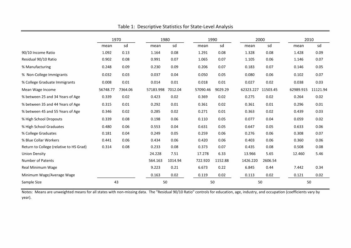
mean sd mean sd mean sd mean sd mean sd90/10 Income Ratio 1.092 0.13 1.164 0.08 1.291 0.08 1.328 0.08 1.428 0.09

Residual 90/10 Ratio 0.902 0.08 0.991 0.07 1.065 0.07 1.105 0.06 1.146 0.07

% Manufacturing 0.248 0.09 0.230 0.09 0.206 0.07 0.183 0.07 0.146 0.05

% Non-College Immigrants 0.032 0.03 0.037 0.04 0.050 0.05 0.080 0.06 0.102 0.07

% College Graduate Immigrants 0.008 0.01 0.014 0.01 0.018 0.01 0.027 0.02 0.038 0.03

Mean Wage Income 56748.77 7364.06 57183.998 7012.04 57090.46 9029.29 62323.227 11503.45 62989.915 11121.94

% between 25 and 34 Years of Age 0.339 0.02 0.423 0.02 0.369 0.02 0.275 0.02 0.264 0.02

% between 35 and 44 Years of Age 0.315 0.01 0.292 0.01 0.361 0.02 0.361 0.01 0.296 0.01

% between 45 and 55 Years of Age 0.346 0.02 0.285 0.02 0.271 0.01 0.363 0.02 0.439 0.03

% High School Dropouts 0.339 0.08 0.198 0.06 0.110 0.05 0.077 0.04 0.059 0.02

% High School Graduates 0.480 0.06 0.553 0.04 0.631 0.05 0.647 0.05 0.633 0.06

% College Graduates 0.181 0.04 0.249 0.05 0.259 0.06 0.276 0.06 0.308 0.07

% Blue Collar Workers 0.441 0.06 0.434 0.06 0.420 0.06 0.403 0.06 0.360 0.06

Return to College (relative to HS Grad) 0.314 0.08 0.233 0.08 0.373 0.07 0.435 0.08 0.508 0.08

Union Density 24.228 7.51 17.278 6.33 13.966 5.65 12.460 5.46

Number of Patents 564.163 1014.94 722.920 1152.88 1426.220 2606.54

Real Minimum Wage 9.223 0.21 6.673 0.22 6.845 0.44 7.442 0.34

Minimum Wage/Average Wage 0.163 0.02 0.119 0.02 0.113 0.02 0.121 0.02

Sample Size

Table 1: Descriptive Statistics for State-Level Analysis

Notes: Means are unweighted means for all states with non-missing data. The "Residual 90/10 Ratio" controls for education, age, industry, and occupation (coefficients vary by year).

1970 1980 1990 2000 2010

43 50 50 50 50

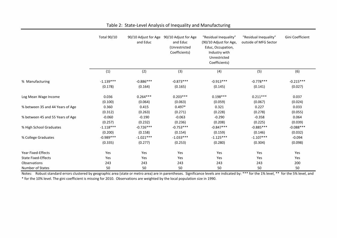
Total 90/10 90/10 Adjust for Age and Educ

90/10 Adjust for Age and Educ

(Unrestricted Coefficients)

"Residual Inequality" (90/10 Adjust for Age,

Educ, Occupation, Industry with Unrestricted Coefficients)

"Residual Inequality" outside of MFG Sector

Gini Coefficient

(1) (2) (3) (4) (5) (6)

% Manufacturing -1.139*** -0.886*** -0.873*** -0.913*** -0.778*** -0.215***(0.178) (0.164) (0.165) (0.145) (0.141) (0.027)

Log Mean Wage Income 0.036 0.264*** 0.203*** 0.198*** 0.211*** 0.037(0.100) (0.064) (0.063) (0.059) (0.067) (0.024)

% between 35 and 44 Years of Age 0.360 0.415 0.497* 0.321 0.227 0.033(0.312) (0.263) (0.271) (0.228) (0.278) (0.055)

% between 45 and 55 Years of Age -0.060 -0.190 -0.063 -0.290 -0.358 0.064(0.257) (0.232) (0.236) (0.208) (0.225) (0.039)

% High School Graduates -1.118*** -0.726*** -0.753*** -0.847*** -0.885*** -0.088***(0.200) (0.158) (0.154) (0.159) (0.146) (0.032)

% College Graduates -0.989*** -1.021*** -1.033*** -1.125*** -1.107*** -0.094(0.335) (0.277) (0.253) (0.280) (0.304) (0.098)

Year Fixed-Effects Yes Yes Yes Yes Yes YesState Fixed-Effects Yes Yes Yes Yes Yes YesObservations 243 243 243 243 243 200Number of States 50 50 50 50 50 50

Table 2: State-Level Analysis of Inequality and Manufacturing

Notes: Robust standard errors clustered by geographic area (state or metro area) are in parentheses. Significance levels are indicated by: *** for the 1% level, ** for the 5% level, and * for the 10% level. The gini coefficient is missing for 2010. Observations are weighted by the local population size in 1990.

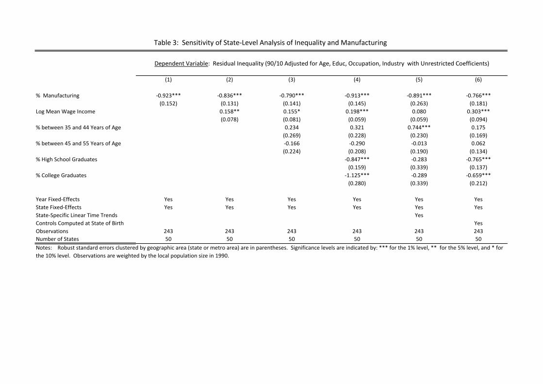
(1) (2) (3) (4) (5) (6)

% Manufacturing -0.923*** -0.836*** -0.790*** -0.913*** -0.891*** -0.766***(0.152) (0.131) (0.141) (0.145) (0.263) (0.181)

Log Mean Wage Income 0.158** 0.155* 0.198*** 0.080 0.303***(0.078) (0.081) (0.059) (0.059) (0.094)

% between 35 and 44 Years of Age 0.234 0.321 0.744*** 0.175(0.269) (0.228) (0.230) (0.169)

% between 45 and 55 Years of Age -0.166 -0.290 -0.013 0.062(0.224) (0.208) (0.190) (0.134)

% High School Graduates -0.847*** -0.283 -0.765***(0.159) (0.339) (0.137)

% College Graduates -1.125*** -0.289 -0.659***(0.280) (0.339) (0.212)

Year Fixed-Effects Yes Yes Yes Yes Yes YesState Fixed-Effects Yes Yes Yes Yes Yes YesState-Specific Linear Time Trends YesControls Computed at State of Birth YesObservations 243 243 243 243 243 243Number of States 50 50 50 50 50 50

Table 3: Sensitivity of State-Level Analysis of Inequality and Manufacturing

Dependent Variable: Residual Inequality (90/10 Adjusted for Age, Educ, Occupation, Industry with Unrestricted Coefficients)

Notes: Robust standard errors clustered by geographic area (state or metro area) are in parentheses. Significance levels are indicated by: *** for the 1% level, ** for the 5% level, and * for the 10% level. Observations are weighted by the local population size in 1990.

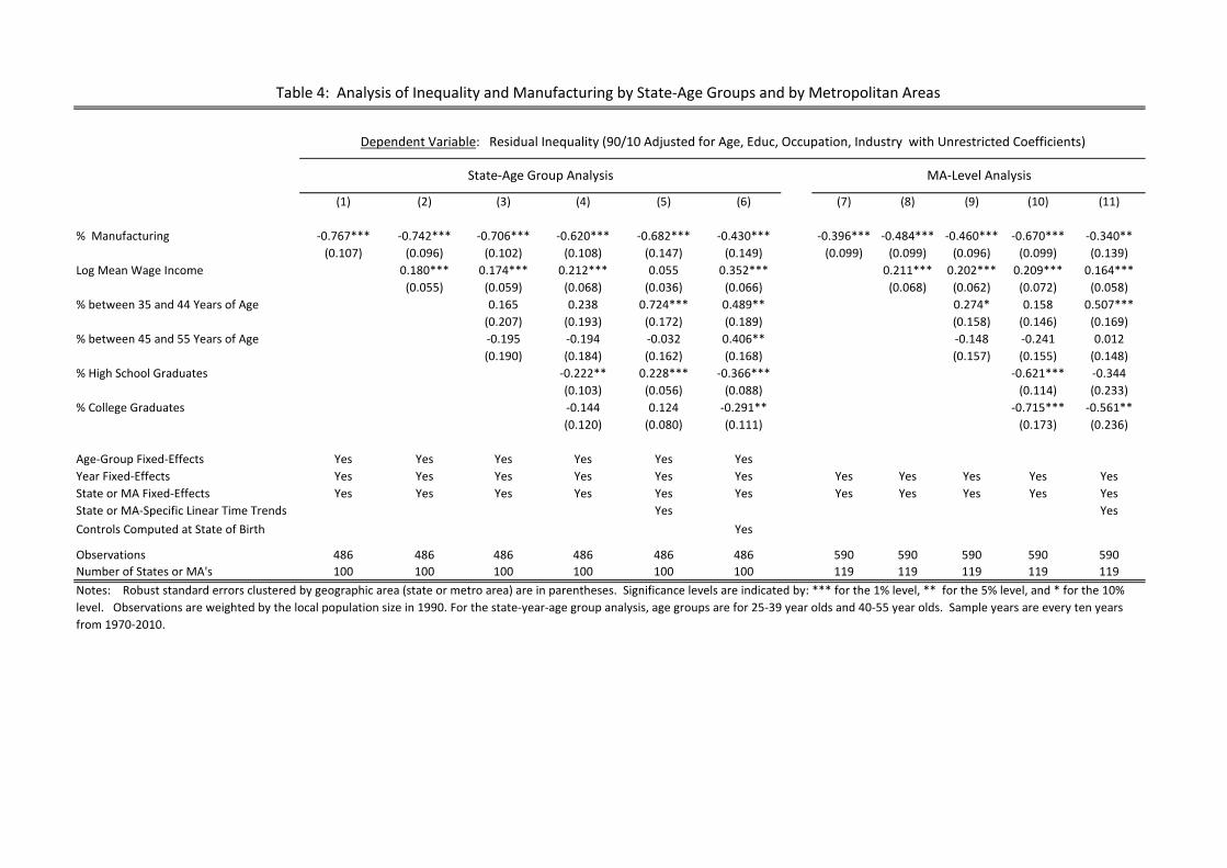
(1) (2) (3) (4) (5) (6) (7) (8) (9) (10) (11)

% Manufacturing -0.767*** -0.742*** -0.706*** -0.620*** -0.682*** -0.430*** -0.396*** -0.484*** -0.460*** -0.670*** -0.340**(0.107) (0.096) (0.102) (0.108) (0.147) (0.149) (0.099) (0.099) (0.096) (0.099) (0.139)

Log Mean Wage Income 0.180*** 0.174*** 0.212*** 0.055 0.352*** 0.211*** 0.202*** 0.209*** 0.164***(0.055) (0.059) (0.068) (0.036) (0.066) (0.068) (0.062) (0.072) (0.058)

% between 35 and 44 Years of Age 0.165 0.238 0.724*** 0.489** 0.274* 0.158 0.507***(0.207) (0.193) (0.172) (0.189) (0.158) (0.146) (0.169)

% between 45 and 55 Years of Age -0.195 -0.194 -0.032 0.406** -0.148 -0.241 0.012(0.190) (0.184) (0.162) (0.168) (0.157) (0.155) (0.148)

% High School Graduates -0.222** 0.228*** -0.366*** -0.621*** -0.344(0.103) (0.056) (0.088) (0.114) (0.233)

% College Graduates -0.144 0.124 -0.291** -0.715*** -0.561**(0.120) (0.080) (0.111) (0.173) (0.236)

Age-Group Fixed-Effects Yes Yes Yes Yes Yes YesYear Fixed-Effects Yes Yes Yes Yes Yes Yes Yes Yes Yes Yes YesState or MA Fixed-Effects Yes Yes Yes Yes Yes Yes Yes Yes Yes Yes YesState or MA-Specific Linear Time Trends Yes YesControls Computed at State of Birth Yes

Observations 486 486 486 486 486 486 590 590 590 590 590Number of States or MA's 100 100 100 100 100 100 119 119 119 119 119Notes: Robust standard errors clustered by geographic area (state or metro area) are in parentheses. Significance levels are indicated by: *** for the 1% level, ** for the 5% level, and * for the 10% level. Observations are weighted by the local population size in 1990. For the state-year-age group analysis, age groups are for 25-39 year olds and 40-55 year olds. Sample years are every ten years from 1970-2010.

Dependent Variable: Residual Inequality (90/10 Adjusted for Age, Educ, Occupation, Industry with Unrestricted Coefficients)

Table 4: Analysis of Inequality and Manufacturing by State-Age Groups and by Metropolitan Areas

State-Age Group Analysis MA-Level Analysis

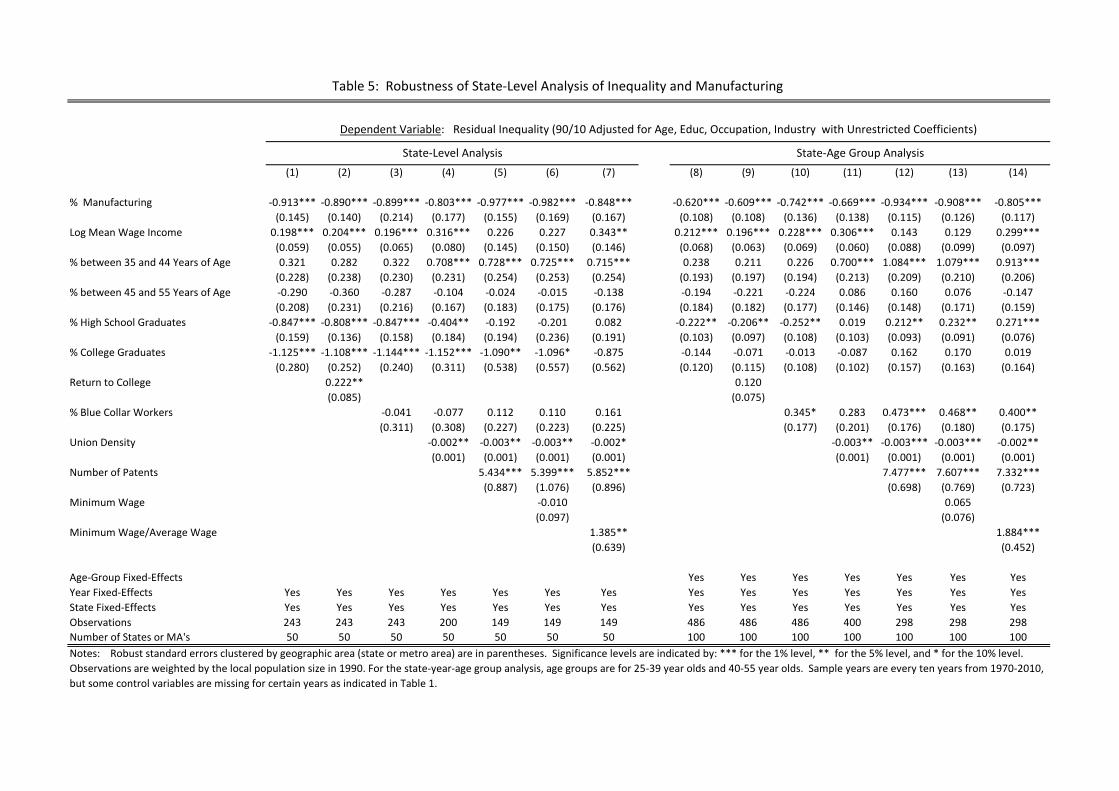
(1) (2) (3) (4) (5) (6) (7) (8) (9) (10) (11) (12) (13) (14)

% Manufacturing -0.913*** -0.890*** -0.899*** -0.803*** -0.977*** -0.982*** -0.848*** -0.620*** -0.609*** -0.742*** -0.669*** -0.934*** -0.908*** -0.805***(0.145) (0.140) (0.214) (0.177) (0.155) (0.169) (0.167) (0.108) (0.108) (0.136) (0.138) (0.115) (0.126) (0.117)

Log Mean Wage Income 0.198*** 0.204*** 0.196*** 0.316*** 0.226 0.227 0.343** 0.212*** 0.196*** 0.228*** 0.306*** 0.143 0.129 0.299***(0.059) (0.055) (0.065) (0.080) (0.145) (0.150) (0.146) (0.068) (0.063) (0.069) (0.060) (0.088) (0.099) (0.097)

% between 35 and 44 Years of Age 0.321 0.282 0.322 0.708*** 0.728*** 0.725*** 0.715*** 0.238 0.211 0.226 0.700*** 1.084*** 1.079*** 0.913***(0.228) (0.238) (0.230) (0.231) (0.254) (0.253) (0.254) (0.193) (0.197) (0.194) (0.213) (0.209) (0.210) (0.206)

% between 45 and 55 Years of Age -0.290 -0.360 -0.287 -0.104 -0.024 -0.015 -0.138 -0.194 -0.221 -0.224 0.086 0.160 0.076 -0.147(0.208) (0.231) (0.216) (0.167) (0.183) (0.175) (0.176) (0.184) (0.182) (0.177) (0.146) (0.148) (0.171) (0.159)

% High School Graduates -0.847*** -0.808*** -0.847*** -0.404** -0.192 -0.201 0.082 -0.222** -0.206** -0.252** 0.019 0.212** 0.232** 0.271***(0.159) (0.136) (0.158) (0.184) (0.194) (0.236) (0.191) (0.103) (0.097) (0.108) (0.103) (0.093) (0.091) (0.076)

% College Graduates -1.125*** -1.108*** -1.144*** -1.152*** -1.090** -1.096* -0.875 -0.144 -0.071 -0.013 -0.087 0.162 0.170 0.019(0.280) (0.252) (0.240) (0.311) (0.538) (0.557) (0.562) (0.120) (0.115) (0.108) (0.102) (0.157) (0.163) (0.164)

Return to College 0.222** 0.120(0.085) (0.075)

% Blue Collar Workers -0.041 -0.077 0.112 0.110 0.161 0.345* 0.283 0.473*** 0.468** 0.400**(0.311) (0.308) (0.227) (0.223) (0.225) (0.177) (0.201) (0.176) (0.180) (0.175)

Union Density -0.002** -0.003** -0.003** -0.002* -0.003** -0.003*** -0.003*** -0.002**(0.001) (0.001) (0.001) (0.001) (0.001) (0.001) (0.001) (0.001)

Number of Patents 5.434*** 5.399*** 5.852*** 7.477*** 7.607*** 7.332***(0.887) (1.076) (0.896) (0.698) (0.769) (0.723)

Minimum Wage -0.010 0.065(0.097) (0.076)

Minimum Wage/Average Wage 1.385** 1.884***(0.639) (0.452)

Age-Group Fixed-Effects Yes Yes Yes Yes Yes Yes YesYear Fixed-Effects Yes Yes Yes Yes Yes Yes Yes Yes Yes Yes Yes Yes Yes YesState Fixed-Effects Yes Yes Yes Yes Yes Yes Yes Yes Yes Yes Yes Yes Yes YesObservations 243 243 243 200 149 149 149 486 486 486 400 298 298 298Number of States or MA's 50 50 50 50 50 50 50 100 100 100 100 100 100 100

Table 5: Robustness of State-Level Analysis of Inequality and Manufacturing

State-Age Group AnalysisState-Level Analysis

Dependent Variable: Residual Inequality (90/10 Adjusted for Age, Educ, Occupation, Industry with Unrestricted Coefficients)

Notes: Robust standard errors clustered by geographic area (state or metro area) are in parentheses. Significance levels are indicated by: *** for the 1% level, ** for the 5% level, and * for the 10% level. Observations are weighted by the local population size in 1990. For the state-year-age group analysis, age groups are for 25-39 year olds and 40-55 year olds. Sample years are every ten years from 1970-2010, but some control variables are missing for certain years as indicated in Table 1.

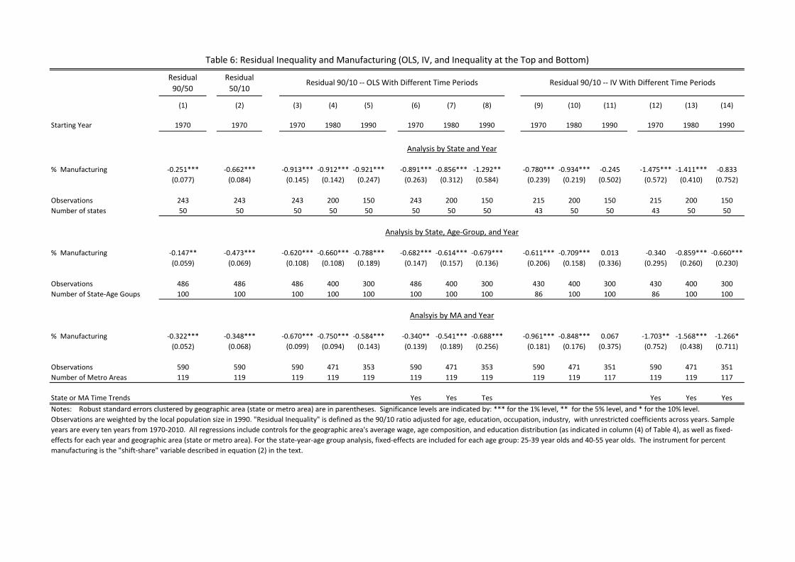
Residual 90/50

Residual 50/10

(1) (2) (3) (4) (5) (6) (7) (8) (9) (10) (11) (12) (13) (14)

Starting Year 1970 1970 1970 1980 1990 1970 1980 1990 1970 1980 1990 1970 1980 1990

% Manufacturing -0.251*** -0.662*** -0.913*** -0.912*** -0.921*** -0.891*** -0.856*** -1.292** -0.780*** -0.934*** -0.245 -1.475*** -1.411*** -0.833(0.077) (0.084) (0.145) (0.142) (0.247) (0.263) (0.312) (0.584) (0.239) (0.219) (0.502) (0.572) (0.410) (0.752)

Observations 243 243 243 200 150 243 200 150 215 200 150 215 200 150Number of states 50 50 50 50 50 50 50 50 43 50 50 43 50 50

% Manufacturing -0.147** -0.473*** -0.620*** -0.660*** -0.788*** -0.682*** -0.614*** -0.679*** -0.611*** -0.709*** 0.013 -0.340 -0.859*** -0.660***(0.059) (0.069) (0.108) (0.108) (0.189) (0.147) (0.157) (0.136) (0.206) (0.158) (0.336) (0.295) (0.260) (0.230)

Observations 486 486 486 400 300 486 400 300 430 400 300 430 400 300Number of State-Age Goups 100 100 100 100 100 100 100 100 86 100 100 86 100 100

% Manufacturing -0.322*** -0.348*** -0.670*** -0.750*** -0.584*** -0.340** -0.541*** -0.688*** -0.961*** -0.848*** 0.067 -1.703** -1.568*** -1.266*(0.052) (0.068) (0.099) (0.094) (0.143) (0.139) (0.189) (0.256) (0.181) (0.176) (0.375) (0.752) (0.438) (0.711)

Observations 590 590 590 471 353 590 471 353 590 471 351 590 471 351Number of Metro Areas 119 119 119 119 119 119 119 119 119 119 117 119 119 117

State or MA Time Trends Yes Yes Tes Yes Yes YesNotes: Robust standard errors clustered by geographic area (state or metro area) are in parentheses. Significance levels are indicated by: *** for the 1% level, ** for the 5% level, and * for the 10% level. Observations are weighted by the local population size in 1990. "Residual Inequality" is defined as the 90/10 ratio adjusted for age, education, occupation, industry, with unrestricted coefficients across years. Sample years are every ten years from 1970-2010. All regressions include controls for the geographic area's average wage, age composition, and education distribution (as indicated in column (4) of Table 4), as well as fixed-effects for each year and geographic area (state or metro area). For the state-year-age group analysis, fixed-effects are included for each age group: 25-39 year olds and 40-55 year olds. The instrument for percent manufacturing is the "shift-share" variable described in equation (2) in the text.

Table 6: Residual Inequality and Manufacturing (OLS, IV, and Inequality at the Top and Bottom)

Analysis by State and Year

Analysis by State, Age-Group, and Year

Analsyis by MA and Year

Residual 90/10 -- OLS With Different Time Periods Residual 90/10 -- IV With Different Time Periods

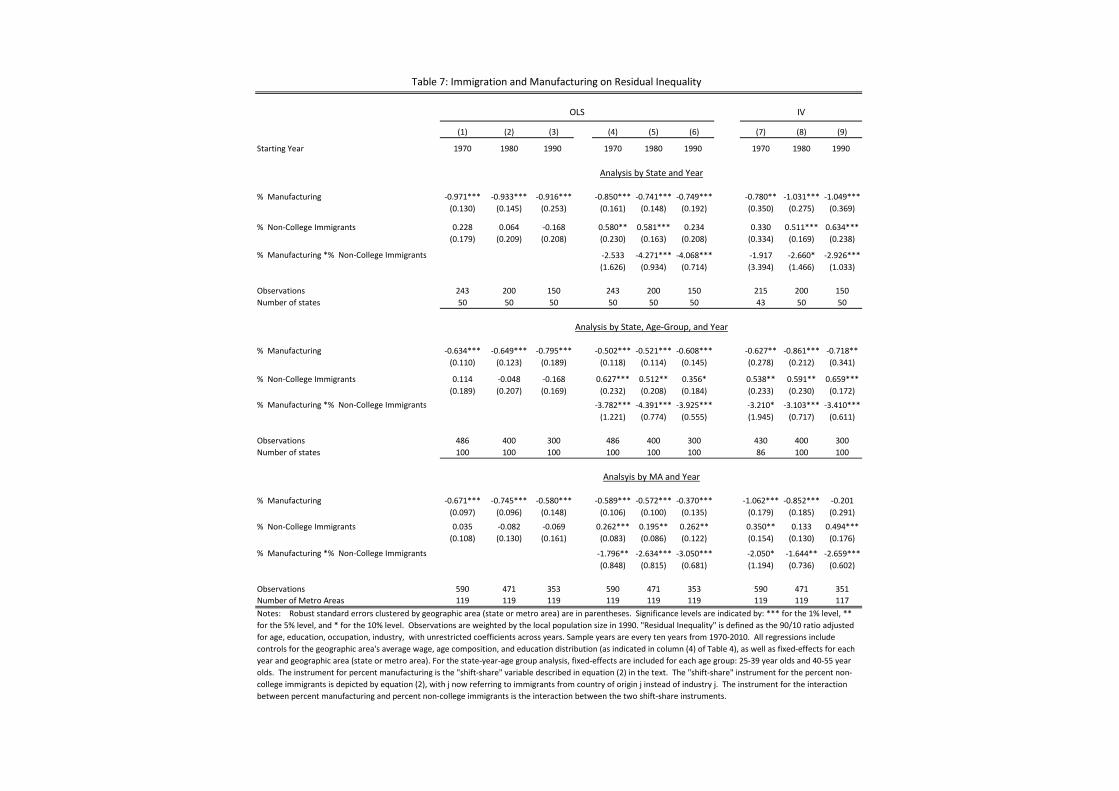
(1) (2) (3) (4) (5) (6) (7) (8) (9)

Starting Year 1970 1980 1990 1970 1980 1990 1970 1980 1990

% Manufacturing -0.971*** -0.933*** -0.916*** -0.850*** -0.741*** -0.749*** -0.780** -1.031*** -1.049***(0.130) (0.145) (0.253) (0.161) (0.148) (0.192) (0.350) (0.275) (0.369)

% Non-College Immigrants 0.228 0.064 -0.168 0.580** 0.581*** 0.234 0.330 0.511*** 0.634***(0.179) (0.209) (0.208) (0.230) (0.163) (0.208) (0.334) (0.169) (0.238)

% Manufacturing *% Non-College Immigrants -2.533 -4.271*** -4.068*** -1.917 -2.660* -2.926***(1.626) (0.934) (0.714) (3.394) (1.466) (1.033)

Observations 243 200 150 243 200 150 215 200 150Number of states 50 50 50 50 50 50 43 50 50

% Manufacturing -0.634*** -0.649*** -0.795*** -0.502*** -0.521*** -0.608*** -0.627** -0.861*** -0.718**(0.110) (0.123) (0.189) (0.118) (0.114) (0.145) (0.278) (0.212) (0.341)

% Non-College Immigrants 0.114 -0.048 -0.168 0.627*** 0.512** 0.356* 0.538** 0.591** 0.659***(0.189) (0.207) (0.169) (0.232) (0.208) (0.184) (0.233) (0.230) (0.172)

% Manufacturing *% Non-College Immigrants -3.782*** -4.391*** -3.925*** -3.210* -3.103*** -3.410***(1.221) (0.774) (0.555) (1.945) (0.717) (0.611)

Observations 486 400 300 486 400 300 430 400 300Number of states 100 100 100 100 100 100 86 100 100

% Manufacturing -0.671*** -0.745*** -0.580*** -0.589*** -0.572*** -0.370*** -1.062*** -0.852*** -0.201(0.097) (0.096) (0.148) (0.106) (0.100) (0.135) (0.179) (0.185) (0.291)

% Non-College Immigrants 0.035 -0.082 -0.069 0.262*** 0.195** 0.262** 0.350** 0.133 0.494***(0.108) (0.130) (0.161) (0.083) (0.086) (0.122) (0.154) (0.130) (0.176)

% Manufacturing *% Non-College Immigrants -1.796** -2.634*** -3.050*** -2.050* -1.644** -2.659***(0.848) (0.815) (0.681) (1.194) (0.736) (0.602)

Observations 590 471 353 590 471 353 590 471 351Number of Metro Areas 119 119 119 119 119 119 119 119 117Notes: Robust standard errors clustered by geographic area (state or metro area) are in parentheses. Significance levels are indicated by: *** for the 1% level, ** for the 5% level, and * for the 10% level. Observations are weighted by the local population size in 1990. "Residual Inequality" is defined as the 90/10 ratio adjusted for age, education, occupation, industry, with unrestricted coefficients across years. Sample years are every ten years from 1970-2010. All regressions include controls for the geographic area's average wage, age composition, and education distribution (as indicated in column (4) of Table 4), as well as fixed-effects for each year and geographic area (state or metro area). For the state-year-age group analysis, fixed-effects are included for each age group: 25-39 year olds and 40-55 year olds. The instrument for percent manufacturing is the "shift-share" variable described in equation (2) in the text. The "shift-share" instrument for the percent non-college immigrants is depicted by equation (2), with j now referring to immigrants from country of origin j instead of industry j. The instrument for the interaction between percent manufacturing and percent non-college immigrants is the interaction between the two shift-share instruments.

Table 7: Immigration and Manufacturing on Residual Inequality

OLS

Analysis by State and Year

Analsyis by MA and Year

Analysis by State, Age-Group, and Year

IV

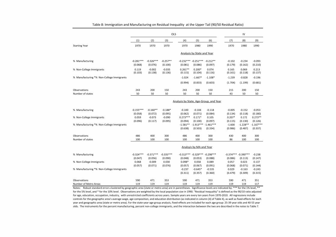
(1) (2) (3) (4) (5) (6) (7) (8) (9)

Starting Year 1970 1970 1970 1970 1980 1990 1970 1980 1990

% Manufacturing -0.281*** -0.326*** -0.257** -0.232*** -0.251*** -0.212** -0.102 -0.234 -0.093(0.068) (0.076) (0.100) (0.081) (0.086) (0.097) (0.179) (0.162) (0.210)

% Non-College Immigrants 0.119 -0.002 -0.035 0.261** 0.200* 0.074 0.165 0.069 0.213(0.103) (0.138) (0.136) (0.115) (0.104) (0.116) (0.161) (0.118) (0.137)

% Manufacturing *% Non-College Immigrants -1.024 -1.667* -1.108* -1.239 -0.828 -0.196

(0.994) (0.833) (0.603) (1.704) (1.199) (0.681)

Observations 243 200 150 243 200 150 215 200 150Number of states 50 50 50 50 50 50 43 50 50

% Manufacturing -0.155*** -0.160** -0.188* -0.100 -0.104 -0.118 -0.005 -0.152 -0.053(0.058) (0.072) (0.095) (0.062) (0.071) (0.084) (0.134) (0.118) (0.180)

% Non-College Immigrants 0.059 -0.073 -0.090 0.273*** 0.171* 0.105 0.207* 0.172 0.273**(0.096) (0.117) (0.095) (0.094) (0.100) (0.097) (0.115) (0.130) (0.126)

% Manufacturing *% Non-College Immigrants -1.581** -1.913*** -1.461*** -1.600 -1.228** -1.167***(0.638) (0.503) (0.334) (0.986) (0.487) (0.337)

Observations 486 400 300 486 400 300 430 400 300Number of states 100 100 100 100 100 100 86 100 100

% Manufacturing -0.324*** -0.371*** -0.335*** -0.313*** -0.329*** -0.298*** -0.374*** -0.390*** -0.238(0.047) (0.056) (0.090) (0.048) (0.053) (0.088) (0.086) (0.113) (0.147)

% Non-College Immigrants 0.068 -0.009 0.030 0.098* 0.058 0.089 0.057 0.023 0.137(0.057) (0.071) (0.076) (0.057) (0.067) (0.091) (0.068) (0.071) (0.144)

% Manufacturing *% Non-College Immigrants -0.237 -0.645* -0.535 0.029 -0.163 -0.243(0.311) (0.357) (0.360) (0.479) (0.309) (0.315)

Observations 590 471 353 590 471 353 590 471 351Number of Metro Areas 119 119 119 119 119 119 119 119 117Notes: Robust standard errors clustered by geographic area (state or metro area) are in parentheses. Significance levels are indicated by: *** for the 1% level, ** for the 5% level, and * for the 10% level. Observations are weighted by the local population size in 1990. "Residual Inequality" is defined as the 90/10 ratio adjusted for age, education, occupation, industry, with unrestricted coefficients across years. Sample years are every ten years from 1970-2010. All regressions include controls for the geographic area's average wage, age composition, and education distribution (as indicated in column (4) of Table 4), as well as fixed-effects for each year and geographic area (state or metro area). For the state-year-age group analysis, fixed-effects are included for each age group: 25-39 year olds and 40-55 year olds. The instruments for the percent manufacturing, percent non-college immigrants, and the interaction between the two are described in the notes to Table 7.

Analsyis by MA and Year

Table 8: Immigration and Manufacturing on Residual Inequality at the Upper Tail (90/50 Residual Ratio)

OLS IV

Analysis by State and Year

Analysis by State, Age-Group, and Year

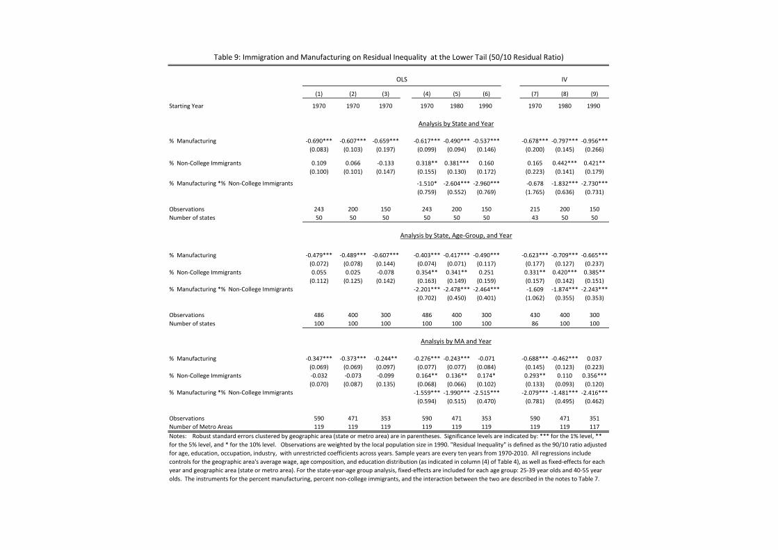
(1) (2) (3) (4) (5) (6) (7) (8) (9)

Starting Year 1970 1970 1970 1970 1980 1990 1970 1980 1990

% Manufacturing -0.690*** -0.607*** -0.659*** -0.617*** -0.490*** -0.537*** -0.678*** -0.797*** -0.956***(0.083) (0.103) (0.197) (0.099) (0.094) (0.146) (0.200) (0.145) (0.266)

% Non-College Immigrants 0.109 0.066 -0.133 0.318** 0.381*** 0.160 0.165 0.442*** 0.421**(0.100) (0.101) (0.147) (0.155) (0.130) (0.172) (0.223) (0.141) (0.179)

% Manufacturing *% Non-College Immigrants -1.510* -2.604*** -2.960*** -0.678 -1.832*** -2.730***(0.759) (0.552) (0.769) (1.765) (0.636) (0.731)

Observations 243 200 150 243 200 150 215 200 150Number of states 50 50 50 50 50 50 43 50 50

% Manufacturing -0.479*** -0.489*** -0.607*** -0.403*** -0.417*** -0.490*** -0.623*** -0.709*** -0.665***(0.072) (0.078) (0.144) (0.074) (0.071) (0.117) (0.177) (0.127) (0.237)

% Non-College Immigrants 0.055 0.025 -0.078 0.354** 0.341** 0.251 0.331** 0.420*** 0.385**(0.112) (0.125) (0.142) (0.163) (0.149) (0.159) (0.157) (0.142) (0.151)

% Manufacturing *% Non-College Immigrants -2.201*** -2.478*** -2.464*** -1.609 -1.874*** -2.243***(0.702) (0.450) (0.401) (1.062) (0.355) (0.353)

Observations 486 400 300 486 400 300 430 400 300Number of states 100 100 100 100 100 100 86 100 100

% Manufacturing -0.347*** -0.373*** -0.244** -0.276*** -0.243*** -0.071 -0.688*** -0.462*** 0.037(0.069) (0.069) (0.097) (0.077) (0.077) (0.084) (0.145) (0.123) (0.223)

% Non-College Immigrants -0.032 -0.073 -0.099 0.164** 0.136** 0.174* 0.293** 0.110 0.356***(0.070) (0.087) (0.135) (0.068) (0.066) (0.102) (0.133) (0.093) (0.120)

% Manufacturing *% Non-College Immigrants -1.559*** -1.990*** -2.515*** -2.079*** -1.481*** -2.416***(0.594) (0.515) (0.470) (0.781) (0.495) (0.462)

Observations 590 471 353 590 471 353 590 471 351Number of Metro Areas 119 119 119 119 119 119 119 119 117Notes: Robust standard errors clustered by geographic area (state or metro area) are in parentheses. Significance levels are indicated by: *** for the 1% level, ** for the 5% level, and * for the 10% level. Observations are weighted by the local population size in 1990. "Residual Inequality" is defined as the 90/10 ratio adjusted for age, education, occupation, industry, with unrestricted coefficients across years. Sample years are every ten years from 1970-2010. All regressions include controls for the geographic area's average wage, age composition, and education distribution (as indicated in column (4) of Table 4), as well as fixed-effects for each year and geographic area (state or metro area). For the state-year-age group analysis, fixed-effects are included for each age group: 25-39 year olds and 40-55 year olds. The instruments for the percent manufacturing, percent non-college immigrants, and the interaction between the two are described in the notes to Table 7.

Analsyis by MA and Year

Table 9: Immigration and Manufacturing on Residual Inequality at the Lower Tail (50/10 Residual Ratio)

OLS IV

Analysis by State and Year

Analysis by State, Age-Group, and Year

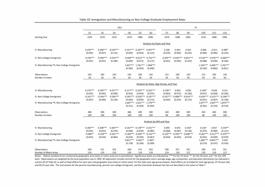
(1) (2) (3) (4) (5) (6) (7) (8) (9) (10) (11) (12)

Starting Year 1970 1970 1970 1970 1980 1990 1970 1980 1990 1970 1980 1990

% Manufacturing 0.239*** 0.268*** 0.529*** 0.151*** 0.187*** 0.447*** 0.100 0.043 0.023 0.068 -0.011 0.389*(0.045) (0.057) (0.131) (0.044) (0.056) (0.114) (0.076) (0.092) (0.225) (0.066) (0.085) (0.225)

% Non-College Immigrants -0.193*** -0.396*** -0.554*** -0.448*** -0.612*** -0.752*** -0.204*** -0.443*** -0.831*** -0.510*** -0.676*** -0.660***(0.041) (0.051) (0.180) (0.069) (0.071) (0.172) (0.051) (0.092) (0.322) (0.088) (0.096) (0.166)

% Manufacturing *% Non-College Immigrants 1.837*** 1.791*** 1.998*** 2.203*** 2.696*** 2.702***(0.585) (0.654) (0.690) (0.539) (0.860) (0.821)

Observations 243 200 150 243 200 150 215 200 150 215 200 150Number of states 50 50 50 50 50 50 43 50 50 43 50 50

% Manufacturing 0.176*** 0.239*** 0.417*** 0.117*** 0.192*** 0.332*** 0.128** 0.050 -0.091 0.100* 0.028 0.141(0.033) (0.045) (0.090) (0.032) (0.043) (0.075) (0.063) (0.073) (0.190) (0.057) (0.068) (0.200)

% Non-College Immigrants -0.161*** -0.344*** -0.360*** -0.391*** -0.550*** -0.597*** -0.197*** -0.408*** -0.614*** -0.426*** -0.525*** -0.538***(0.047) (0.069) (0.130) (0.050) (0.059) (0.112) (0.045) (0.074) (0.173) (0.051) (0.067) (0.138)

% Manufacturing *% Non-College Immigrants 1.695*** 1.621*** 1.779*** 1.877*** 1.837*** 1.874***(0.311) (0.364) (0.392) (0.361) (0.533) (0.519)

Observations 486 400 300 486 400 300 430 400 300 430 400 300Number of states 100 100 100 100 100 100 86 100 100 86 100 100

% Manufacturing 0.180*** 0.208*** 0.364*** 0.142*** 0.178*** 0.331*** 0.094 0.070 0.256* 0.136* 0.057 0.259**(0.045) (0.053) (0.079) (0.046) (0.059) (0.085) (0.068) (0.087) (0.136) (0.075) (0.089) (0.121)

% Non-College Immigrants -0.080** -0.218*** -0.261*** -0.184*** -0.266*** -0.314*** -0.129*** -0.295*** -0.408*** -0.262*** -0.317*** -0.379***(0.033) (0.034) (0.064) (0.033) (0.039) (0.067) (0.034) (0.043) (0.074) (0.042) (0.049) (0.070)

% Manufacturing *% Non-College Immigrants 0.821*** 0.456** 0.482* 1.284*** 0.855*** 0.505(0.178) (0.194) (0.289) (0.274) (0.247) (0.324)

Observations 590 471 353 590 471 353 590 471 351 590 471 351Number of Metro Areas 119 119 119 119 119 119 119 119 117 119 119 117

Analsyis by MA and Year

Notes: Robust standard errors clustered by geographic area (state or metro area) are in parentheses. Significance levels are indicated by: *** for the 1% level, ** for the 5% level, and * for the 10% level. Observations are weighted by the local population size in 1990. All regressions include controls for the geographic area's average wage, age composition, and education distribution (as indicated in column (4) of Table 4), as well as fixed-effects for each year and geographic area (state or metro area). For the state-year-age group analysis, fixed-effects are included for each age group: 25-39 year olds and 40-55 year olds. The instruments for the percent manufacturing, percent non-college immigrants, and the interaction between the two are described in the notes to Table 7.

OLS IV

Table 10: Immigration and Manufacturing on Non-College Graduate Employment Rates

Analysis by State, Age-Group, and Year

Analysis by State and Year

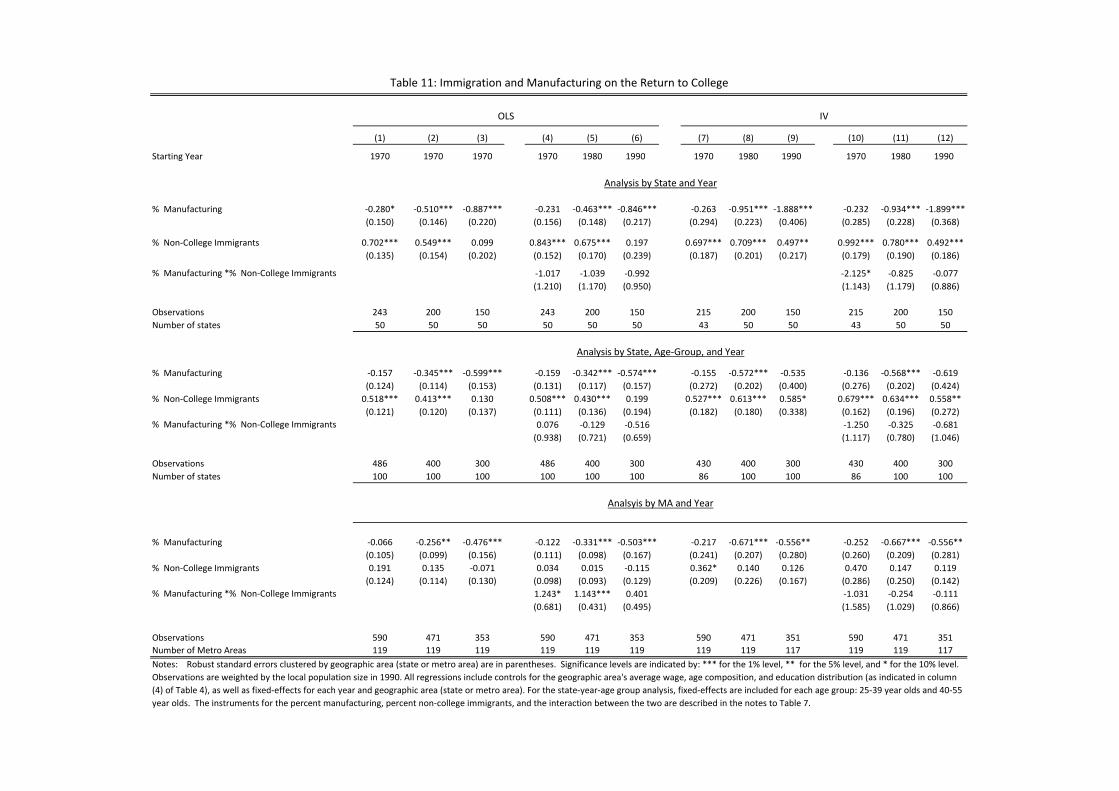
(1) (2) (3) (4) (5) (6) (7) (8) (9) (10) (11) (12)

Starting Year 1970 1970 1970 1970 1980 1990 1970 1980 1990 1970 1980 1990

% Manufacturing -0.280* -0.510*** -0.887*** -0.231 -0.463*** -0.846*** -0.263 -0.951*** -1.888*** -0.232 -0.934*** -1.899***(0.150) (0.146) (0.220) (0.156) (0.148) (0.217) (0.294) (0.223) (0.406) (0.285) (0.228) (0.368)

% Non-College Immigrants 0.702*** 0.549*** 0.099 0.843*** 0.675*** 0.197 0.697*** 0.709*** 0.497** 0.992*** 0.780*** 0.492***(0.135) (0.154) (0.202) (0.152) (0.170) (0.239) (0.187) (0.201) (0.217) (0.179) (0.190) (0.186)

% Manufacturing *% Non-College Immigrants -1.017 -1.039 -0.992 -2.125* -0.825 -0.077(1.210) (1.170) (0.950) (1.143) (1.179) (0.886)

Observations 243 200 150 243 200 150 215 200 150 215 200 150Number of states 50 50 50 50 50 50 43 50 50 43 50 50

% Manufacturing -0.157 -0.345*** -0.599*** -0.159 -0.342*** -0.574*** -0.155 -0.572*** -0.535 -0.136 -0.568*** -0.619(0.124) (0.114) (0.153) (0.131) (0.117) (0.157) (0.272) (0.202) (0.400) (0.276) (0.202) (0.424)

% Non-College Immigrants 0.518*** 0.413*** 0.130 0.508*** 0.430*** 0.199 0.527*** 0.613*** 0.585* 0.679*** 0.634*** 0.558**(0.121) (0.120) (0.137) (0.111) (0.136) (0.194) (0.182) (0.180) (0.338) (0.162) (0.196) (0.272)

% Manufacturing *% Non-College Immigrants 0.076 -0.129 -0.516 -1.250 -0.325 -0.681(0.938) (0.721) (0.659) (1.117) (0.780) (1.046)

Observations 486 400 300 486 400 300 430 400 300 430 400 300Number of states 100 100 100 100 100 100 86 100 100 86 100 100

% Manufacturing -0.066 -0.256** -0.476*** -0.122 -0.331*** -0.503*** -0.217 -0.671*** -0.556** -0.252 -0.667*** -0.556**(0.105) (0.099) (0.156) (0.111) (0.098) (0.167) (0.241) (0.207) (0.280) (0.260) (0.209) (0.281)

% Non-College Immigrants 0.191 0.135 -0.071 0.034 0.015 -0.115 0.362* 0.140 0.126 0.470 0.147 0.119(0.124) (0.114) (0.130) (0.098) (0.093) (0.129) (0.209) (0.226) (0.167) (0.286) (0.250) (0.142)

% Manufacturing *% Non-College Immigrants 1.243* 1.143*** 0.401 -1.031 -0.254 -0.111(0.681) (0.431) (0.495) (1.585) (1.029) (0.866)

Observations 590 471 353 590 471 353 590 471 351 590 471 351Number of Metro Areas 119 119 119 119 119 119 119 119 117 119 119 117Notes: Robust standard errors clustered by geographic area (state or metro area) are in parentheses. Significance levels are indicated by: *** for the 1% level, ** for the 5% level, and * for the 10% level. Observations are weighted by the local population size in 1990. All regressions include controls for the geographic area's average wage, age composition, and education distribution (as indicated in column (4) of Table 4), as well as fixed-effects for each year and geographic area (state or metro area). For the state-year-age group analysis, fixed-effects are included for each age group: 25-39 year olds and 40-55 year olds. The instruments for the percent manufacturing, percent non-college immigrants, and the interaction between the two are described in the notes to Table 7.

Table 11: Immigration and Manufacturing on the Return to College

OLS IV

Analysis by State and Year

Analysis by State, Age-Group, and Year

Analsyis by MA and Year

"

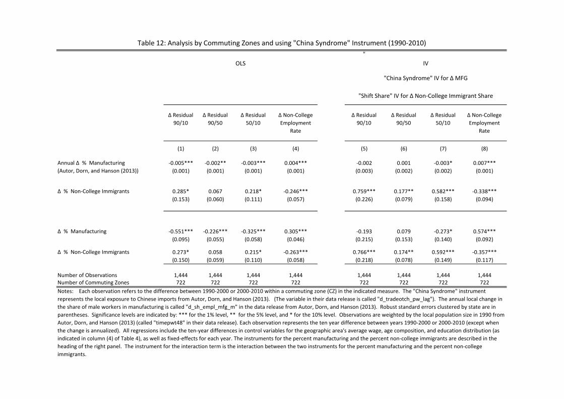
∆ Residual 90/10

∆ Residual 90/50

∆ Residual 50/10

∆ Non-College Employment

Rate

∆ Residual 90/10

∆ Residual 90/50

∆ Residual 50/10

∆ Non-College Employment

Rate

(1) (2) (3) (4) (5) (6) (7) (8)

Annual ∆ % Manufacturing -0.005*** -0.002** -0.003*** 0.004*** -0.002 0.001 -0.003* 0.007***(Autor, Dorn, and Hanson (2013)) (0.001) (0.001) (0.001) (0.001) (0.003) (0.002) (0.002) (0.001)

∆ % Non-College Immigrants 0.285* 0.067 0.218* -0.246*** 0.759*** 0.177** 0.582*** -0.338***(0.153) (0.060) (0.111) (0.057) (0.226) (0.079) (0.158) (0.094)

∆ % Manufacturing -0.551*** -0.226*** -0.325*** 0.305*** -0.193 0.079 -0.273* 0.574***(0.095) (0.055) (0.058) (0.046) (0.215) (0.153) (0.140) (0.092)

∆ % Non-College Immigrants 0.273* 0.058 0.215* -0.263*** 0.766*** 0.174** 0.592*** -0.357***(0.150) (0.059) (0.110) (0.058) (0.218) (0.078) (0.149) (0.117)

Number of Observations 1,444 1,444 1,444 1,444 1,444 1,444 1,444 1,444Number of Commuting Zones 722 722 722 722 722 722 722 722

Table 12: Analysis by Commuting Zones and using "China Syndrome" Instrument (1990-2010)

OLS IV

Notes: Each observation refers to the difference between 1990-2000 or 2000-2010 within a commuting zone (CZ) in the indicated measure. The "China Syndrome" instrument represents the local exposure to Chinese imports from Autor, Dorn, and Hanson (2013). (The variable in their data release is called "d_tradeotch_pw_lag"). The annual local change in the share of male workers in manufacturing is called "d_sh_empl_mfg_m" in the data release from Autor, Dorn, and Hanson (2013). Robust standard errors clustered by state are in parentheses. Significance levels are indicated by: *** for the 1% level, ** for the 5% level, and * for the 10% level. Observations are weighted by the local population size in 1990 from Autor, Dorn, and Hanson (2013) (called "timepwt48" in their data release). Each observation represents the ten year difference between years 1990-2000 or 2000-2010 (except when the change is annualized). All regressions include the ten-year differences in control variables for the geographic area's average wage, age composition, and education distribution (as indicated in column (4) of Table 4), as well as fixed-effects for each year. The instruments for the percent manufacturing and the percent non-college immigrants are described in the heading of the right panel. The instrument for the interaction term is the interaction between the two instruments for the percent manufacturing and the percent non-college immigrants.

"China Syndrome" IV for ∆ MFG

"Shift Share" IV for ∆ Non-College Immigrant Share

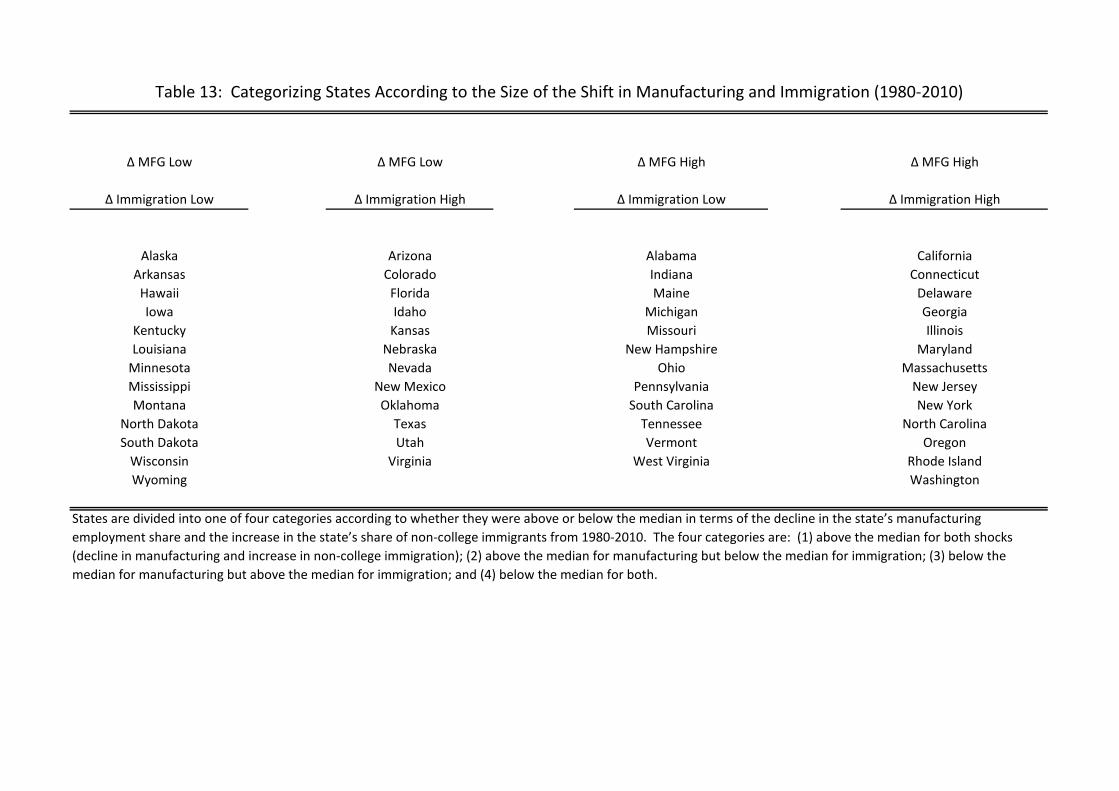
Δ MFG Low Δ MFG Low Δ MFG High Δ MFG High

Δ Immigration Low Δ Immigration High Δ Immigration Low Δ Immigration High

Alaska Arizona Alabama CaliforniaArkansas Colorado Indiana Connecticut

Hawaii Florida Maine DelawareIowa Idaho Michigan Georgia

Kentucky Kansas Missouri IllinoisLouisiana Nebraska New Hampshire Maryland

Minnesota Nevada Ohio MassachusettsMississippi New Mexico Pennsylvania New JerseyMontana Oklahoma South Carolina New York

North Dakota Texas Tennessee North CarolinaSouth Dakota Utah Vermont Oregon

Wisconsin Virginia West Virginia Rhode IslandWyoming Washington

Table 13: Categorizing States According to the Size of the Shift in Manufacturing and Immigration (1980-2010)

States are divided into one of four categories according to whether they were above or below the median in terms of the decline in the state’s manufacturing employment share and the increase in the state’s share of non-college immigrants from 1980-2010. The four categories are: (1) above the median for both shocks (decline in manufacturing and increase in non-college immigration); (2) above the median for manufacturing but below the median for immigration; (3) below the median for manufacturing but above the median for immigration; and (4) below the median for both.

 

 

 

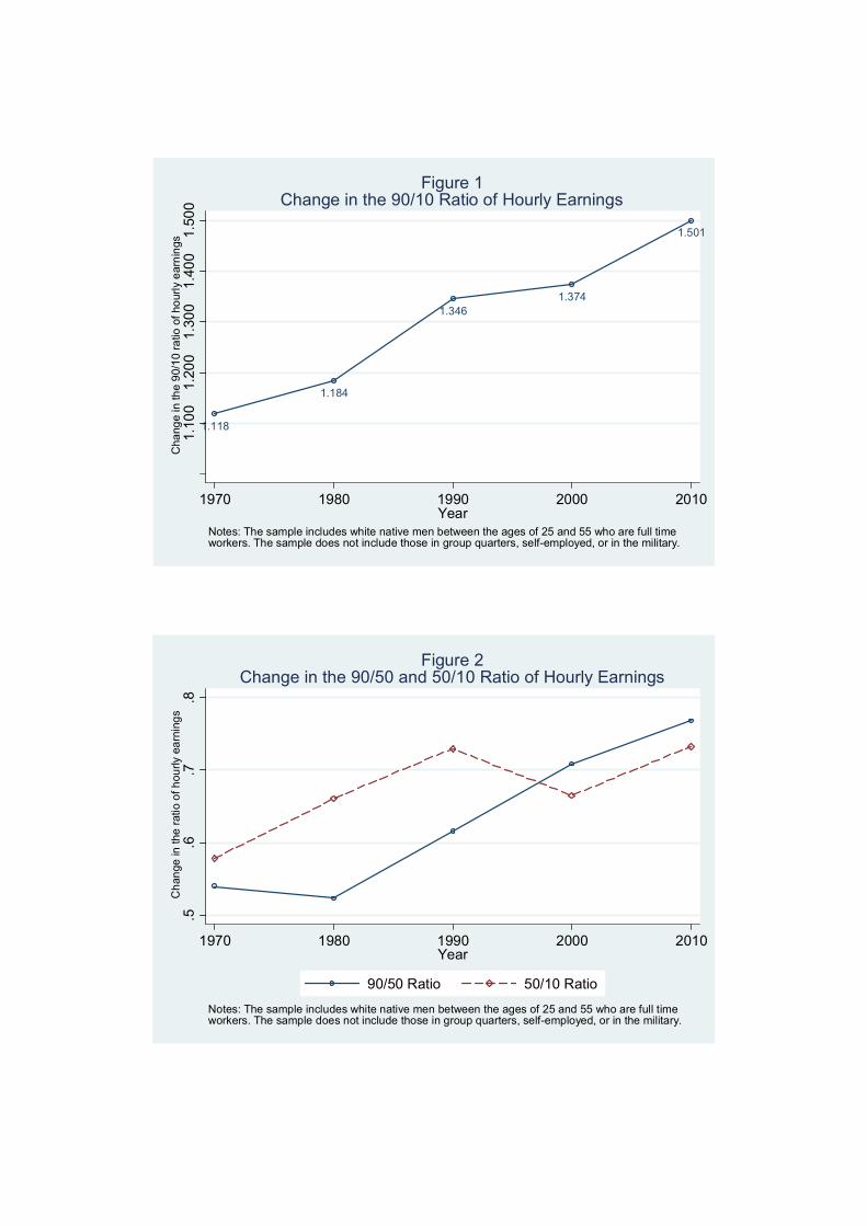
1.118

1.184

1.3461.374

1.501

1.10

01.

200

1.30

01.

400

1.50

0C

hang

e in

the

90/

10

ratio

of h

our

ly e

arn

ings

1970 1980 1990 2000 2010Year

Notes: The sample includes white native men between the ages of 25 and 55 who are full timeworkers. The sample does not include those in group quarters, self-employed, or in the military.

Figure 1Change in the 90/10 Ratio of Hourly Earnings

.5.6

.7.8

Ch

ange

in th

e r

atio

of h

ourly

ea

rnin

gs

1970 1980 1990 2000 2010Year

90/50 Ratio 50/10 Ratio

Notes: The sample includes white native men between the ages of 25 and 55 who are full timeworkers. The sample does not include those in group quarters, self-employed, or in the military.

Figure 2Change in the 90/50 and 50/10 Ratio of Hourly Earnings

 

 

 

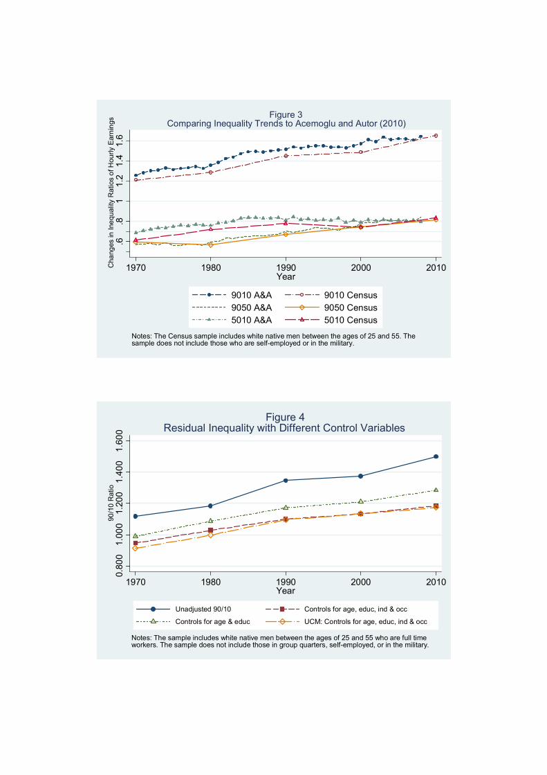
.6.8

11.

21.

41.

6C

hang

es in

Ine

qual

ity R

atio

s o

f Hou

rly E

arn

ings

1970 1980 1990 2000 2010Year

9010 A&A 9010 Census9050 A&A 9050 Census5010 A&A 5010 Census

Notes: The Census sample includes white native men between the ages of 25 and 55. Thesample does not include those who are self-employed or in the military.

Figure 3Comparing Inequality Trends to Acemoglu and Autor (2010)

0.80

01.

000

1.20

01.

400

1.60

090

/10

Rat

io

1970 1980 1990 2000 2010Year

Unadjusted 90/10 Controls for age, educ, ind & occ

Controls for age & educ UCM: Controls for age, educ, ind & occ

Notes: The sample includes white native men between the ages of 25 and 55 who are full timeworkers. The sample does not include those in group quarters, self-employed, or in the military.

Figure 4Residual Inequality with Different Control Variables

 

 

 

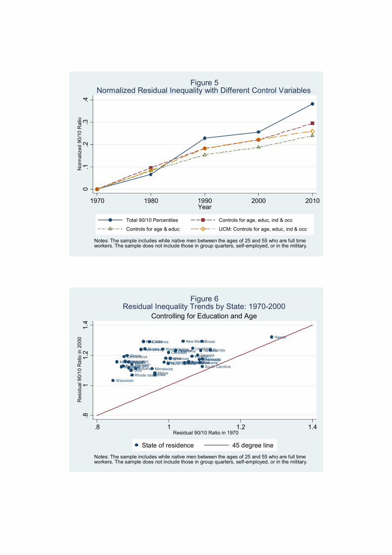
0.1

.2.3

.4N

orm

aliz

ed 9

0/1

0 R

atio

1970 1980 1990 2000 2010Year

Total 90/10 Percentiles Controls for age, educ, ind & occ

Controls for age & educ UCM: Controls for age, educ, ind & occ

Notes: The sample includes white native men between the ages of 25 and 55 who are full timeworkers. The sample does not include those in group quarters, self-employed, or in the military.

Figure 5Normalized Residual Inequality with Different Control Variables

Alabama

Alaska Arizona

Arkansas

California

ColoradoConnecticut

FloridaGeorgia

Hawaii

Illinois

Indiana

Iowa

KansasKentucky

Louisiana

Maine

MarylandMassachusetts

MichiganMinnesota

MississippiMissouri

Nebraska

Nevada

New Hampshire

New Jersey

New MexicoNew York

North Carolina

Ohio

Oklahoma

OregonPennsylvania

Rhode Island

South CarolinaTennessee

Texas

Utah

VirginiaWashington

West Virginia

Wisconsin

.81

1.2

1.4

Res

idua

l 90/

10

Ra

tio in

20

00

.8 1 1.2 1.4Residual 90/10 Ratio in 1970

State of residence 45 degree line

Notes: The sample includes white native men between the ages of 25 and 55 who are full timeworkers. The sample does not include those in group quarters, self-employed, or in the military.

Controlling for Education and Age

Figure 6Residual Inequality Trends by State: 1970-2000

 

 

 

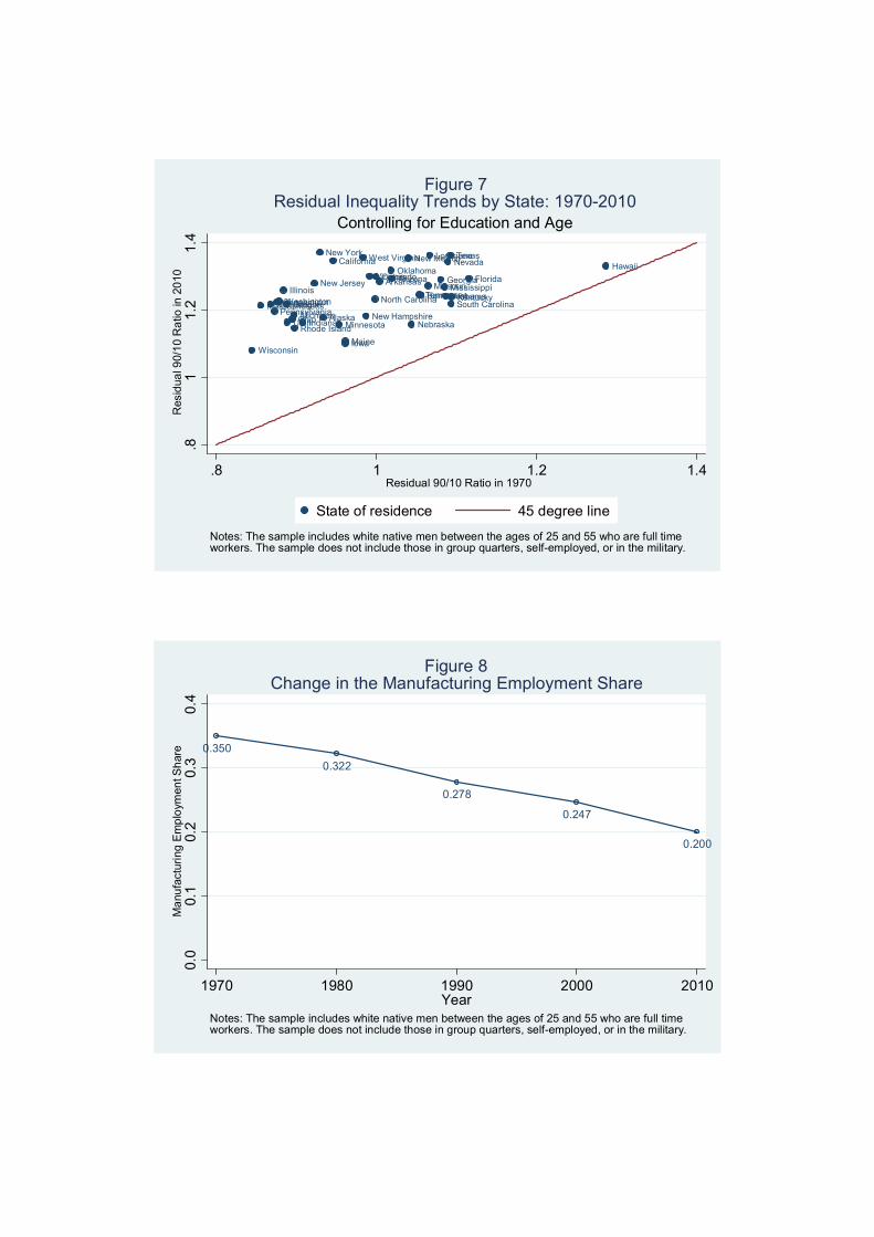
Alabama

Alaska

ArizonaArkansas

California

Colorado

Connecticut

FloridaGeorgia

Hawaii

Illinois

Indiana

Iowa

Kansas Kentucky

Louisiana

Maine

MarylandMassachusettsMichigan

Minnesota

MississippiMissouri

Nebraska

Nevada

New Hampshire

New Jersey

New MexicoNew York

North Carolina

Ohio

Oklahoma

OregonPennsylvania

Rhode Island

South CarolinaTennessee

Texas

Utah

Virginia

Washington

West Virginia

Wisconsin

.81

1.2

1.4

Res

idua

l 90/

10

Ra

tio in

20

10

.8 1 1.2 1.4Residual 90/10 Ratio in 1970

State of residence 45 degree line

Notes: The sample includes white native men between the ages of 25 and 55 who are full timeworkers. The sample does not include those in group quarters, self-employed, or in the military.

Controlling for Education and Age

Figure 7Residual Inequality Trends by State: 1970-2010

0.350

0.322

0.278

0.247

0.200

0.0

0.1

0.2

0.3

0.4

Ma

nufa

ctur

ing

Em

plo

ymen

t Sh

are

1970 1980 1990 2000 2010Year

Notes: The sample includes white native men between the ages of 25 and 55 who are full timeworkers. The sample does not include those in group quarters, self-employed, or in the military.

Figure 8Change in the Manufacturing Employment Share

   

 

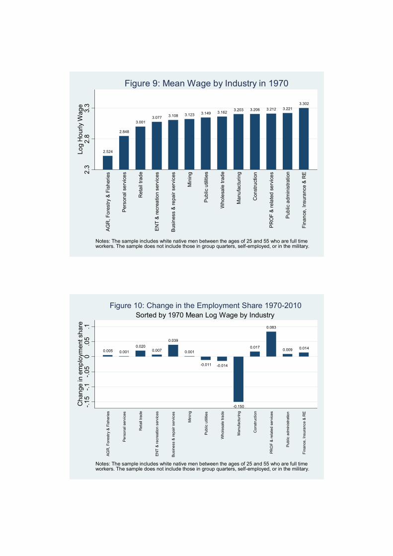
2.524

2.848

3.0013.077 3.108 3.123 3.149 3.162

3.203 3.206 3.212 3.2213.302

2.3

2.8

3.3

Log

Ho

urly

Wag

e

AG

R, F

ore

stry

& F

ish

erie

s

Per

son

al s

erv

ice

s

Ret

ail

trad

e

EN

T &

rec

rea

tion

serv

ices

Bus

ines

s &

re

pair

serv

ices

Min

ing

Pub

lic u

tiliti

es

Who

lesa

le tr

ade

Ma

nufa

ctur

ing

Con

stru

ctio

n

PR

OF

& r

ela

ted

se

rvic

es

Pub

lic a

dmin

istr

atio

n

Fin

ance

, Ins

ura

nce

& R

E

Notes: The sample includes white native men between the ages of 25 and 55 who are full timeworkers. The sample does not include those in group quarters, self-employed, or in the military.

Figure 9: Mean Wage by Industry in 1970

0.005 0.001

0.0200.007

0.039

0.001

-0.011 -0.014

-0.150

0.017

0.083

0.009 0.014

-.1

5-.

1-.

05

0.0

5.1

Ch

ange

in e

mp

loym

ent s

har

e

AG

R,

Fo

rest

ry &

Fis

her

ies

Pe

rso

nal s

ervi

ces

Ret

ail t

rade

EN

T &

rec

reat

ion

ser

vice

s

Bu

sine

ss &

re

pair

serv

ices

Min

ing

Pu

blic

util

ities

Wh

oles

ale

tra

de

Ma

nufa

ctur

ing

Co

nstr

uctio

n

PR

OF

& r

ela

ted

ser

vice

s

Pu

blic

adm

inis

trat

ion

Fin

anc

e, I

nsur

anc

e &

RE

Notes: The sample includes white native men between the ages of 25 and 55 who are full timeworkers. The sample does not include those in group quarters, self-employed, or in the military.

Sorted by 1970 Mean Log Wage by IndustryFigure 10: Change in the Employment Share 1970-2010

 

 

 

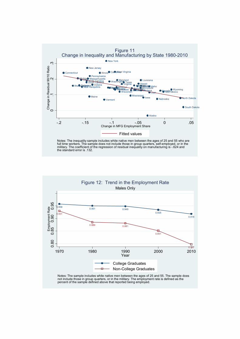
Alabama

Alaska

Arizona

Arkansas

California

Colorado

Connecticut

Delaware

FloridaGeorgia

HawaiiIdaho

Illinois

Indiana

Iowa

KansasKentucky

Louisiana

Maine

MarylandMassachusettsMichigan

Minnesota

Mississippi

MissouriMontana

Nebraska

Nevada

New Hampshire

New Jersey

New Mexico

New York

North Carolina

North Dakota

Ohio

OklahomaOregon

Pennsylvania

Rhode Island

South Carolina

South Dakota

Tennessee

Texas

Utah

Vermont

VirginiaWashington

West Virginia

WisconsinWyoming

0.1

.2.3

Cha

nge

in R

esi

dual

90

/10

Ra

tio

-.2 -.15 -.1 -.05 0 .05Change in MFG Employment Share

Fitted values

Notes: The inequality sample includes white native men between the ages of 25 and 55 who arefull time workers. The sample does not include those in group quarters, self-employed, or in themilitary. The coefficient of the regression of residual inequality on manufacturing is -.624 andthe standard error is .132.

Figure 11Change in Inequality and Manufacturing by State 1980-2010

0.9580.951 0.949

0.935

0.9180.931

0.886 0.881

0.851

0.7970.80

0.85

0.90

0.95

Em

plo

ymen

t Rat

e

1970 1980 1990 2000 2010Year

College Graduates Non-College Graduates

Notes: The sample includes white native men between the ages of 25 and 55. The sample doesnot include those in group quarters, or in the military. The employment rate is defined as thepercent of the sample defined above that reported being employed.

Males OnlyFigure 12: Trend in the Employment Rate

 

 

 

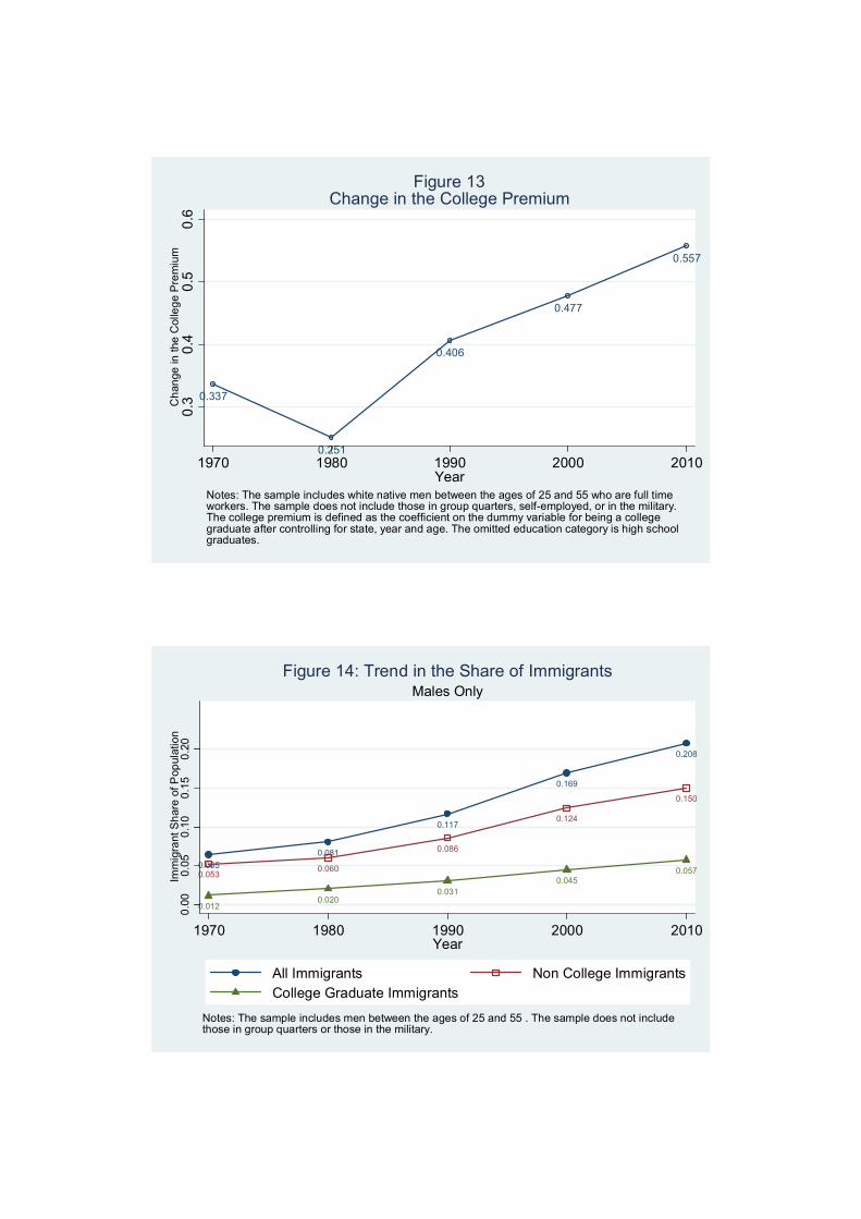
0.337

0.251

0.406

0.477

0.557

0.3

0.4

0.5

0.6

Ch

ange

in th

e C

olle

ge

Pre

miu

m

1970 1980 1990 2000 2010Year

Notes: The sample includes white native men between the ages of 25 and 55 who are full timeworkers. The sample does not include those in group quarters, self-employed, or in the military.The college premium is defined as the coefficient on the dummy variable for being a collegegraduate after controlling for state, year and age. The omitted education category is high schoolgraduates.

Figure 13Change in the College Premium

0.065

0.081

0.117

0.169

0.208

0.0530.060

0.086

0.124

0.150

0.0120.020

0.0310.045

0.057

0.0

00

.05

0.1

00

.15

0.2

0Im

mig

rant

Sh

are

of P

opul

atio

n

1970 1980 1990 2000 2010Year

All Immigrants Non College Immigrants College Graduate Immigrants

Notes: The sample includes men between the ages of 25 and 55 . The sample does not includethose in group quarters or those in the military.

Males OnlyFigure 14: Trend in the Share of Immigrants

 

 

 

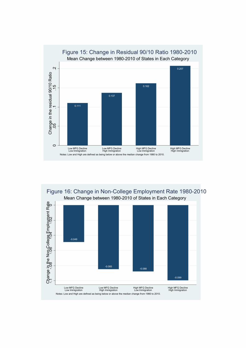
0.111

0.137

0.162

0.207

0.0

5.1

.15

.2C

han

ge in

the

resi

dual

90

/10

Ra

tio

Low MFG DeclineLow Immigration

Low MFG DeclineHigh Immigration

High MFG DeclineLow Immigration

High MFG DeclineHigh Immigration

Notes: Low and High are defined as being below or above the median change from 1980 to 2010.

Mean Change between 1980-2010 of States in Each CategoryFigure 15: Change in Residual 90/10 Ratio 1980-2010

-0.049

-0.085-0.088

-0.099

-.1

-.0

8-.

06

-.0

4-.

02

0C

han

ge in

the

No

n-C

olle

ge

Em

ploy

me

nt R

ate

Low MFG DeclineLow Immigration

Low MFG DeclineHigh Immigration

High MFG DeclineLow Immigration

High MFG DeclineHigh Immigration

Notes: Low and High are defined as being below or above the median change from 1980 to 2010.

Mean Change between 1980-2010 of States in Each CategoryFigure 16: Change in Non-College Employment Rate 1980-2010

 

  

 

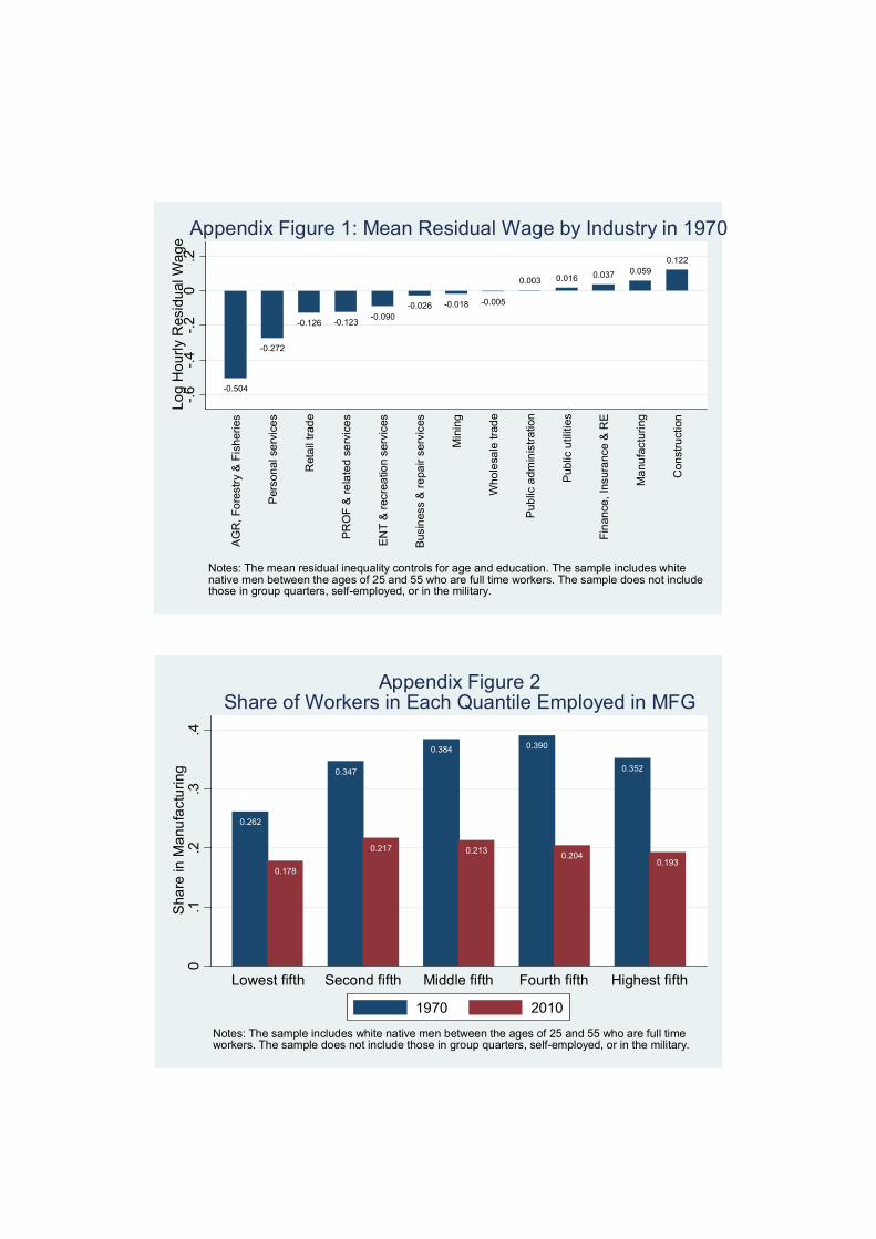
-0.504

-0.272

-0.126 -0.123-0.090

-0.026 -0.018 -0.005

0.003 0.016 0.037 0.0590.122

-.6

-.4

-.2

0.2

Log

Ho

urly

Res

idu

al W

age

AG

R, F

ore

stry

& F

ish

erie

s

Per

son

al s

erv

ice

s

Ret

ail

trad

e

PR

OF

& r

ela

ted

se

rvic

es

EN

T &

rec

rea

tion

serv

ices

Bus

ines

s &

re

pair

serv

ices

Min

ing

Who

lesa

le tr

ade

Pub

lic a

dmin

istr

atio

n

Pub

lic u

tiliti

es

Fin

ance

, Ins

ura

nce

& R

E

Ma

nufa

ctur

ing

Con

stru

ctio

n

Notes: The mean residual inequality controls for age and education. The sample includes whitenative men between the ages of 25 and 55 who are full time workers. The sample does not includethose in group quarters, self-employed, or in the military.

Appendix Figure 1: Mean Residual Wage by Industry in 1970

0.262

0.178

0.347

0.217

0.384

0.213

0.390

0.204

0.352

0.193

0.1

.2.3

.4S

hare

in M

anu

fact

urin

g

Lowest fifth Second fifth Middle fifth Fourth fifth Highest fifth

Notes: The sample includes white native men between the ages of 25 and 55 who are full timeworkers. The sample does not include those in group quarters, self-employed, or in the military.

Appendix Figure 2Share of Workers in Each Quantile Employed in MFG

1970 2010

  

 

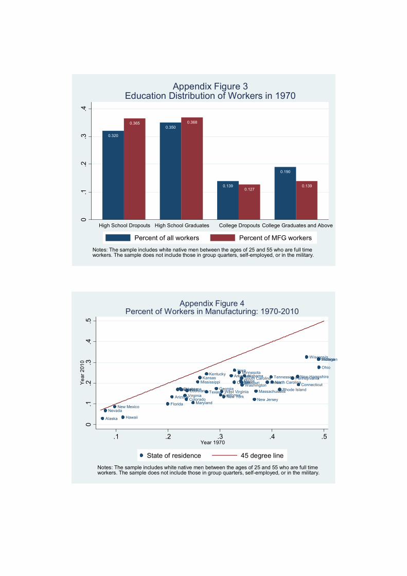
0.320

0.3650.350

0.368

0.1390.127

0.190

0.139

0.1

.2.3

.4

High School Dropouts High School Graduates College Dropouts College Graduates and Above

Notes: The sample includes white native men between the ages of 25 and 55 who are full timeworkers. The sample does not include those in group quarters, self-employed, or in the military.

Appendix Figure 3Education Distribution of Workers in 1970

Percent of all workers Percent of MFG workers

Alabama

Alaska

Arizona

Arkansas

CaliforniaColorado

Connecticut

Florida

Georgia

Hawaii

Illinois

Indiana

Iowa

KansasKentucky

Louisiana

Maine

Maryland

Massachusetts

Michigan

Minnesota

Mississippi Missouri

Nebraska

Nevada

New Hampshire

New Jersey

New Mexico

New York

North Carolina

Ohio

Oklahoma

OregonPennsylvania

Rhode Island

South Carolina Tennessee

TexasUtah

Virginia

Washington

West Virginia

Wisconsin

0.1

.2.3

.4.5

Ye

ar 2

010

.1 .2 .3 .4 .5Year 1970

State of residence 45 degree line

Notes: The sample includes white native men between the ages of 25 and 55 who are full timeworkers. The sample does not include those in group quarters, self-employed, or in the military.

Appendix Figure 4Percent of Workers in Manufacturing: 1970-2010

 

  

 

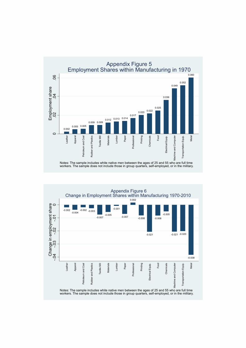
0.0020.005 0.005

0.009 0.0090.012 0.013 0.014

0.0170.020

0.0220.025

0.036

0.0490.052

0.060

0.0

2.0

4.0

6E

mpl

oym

ent

sh

are

Lea

the

r

App

are

l

Pe

trol

eum

and

Coa

l

Ru

bber

and

Pla

stic

s

Tex

tile

Mill

Mat

eria

ls

Lum

ber

Pa

per

Pro

fess

iona

l

Prin

ting

Ch

emic

als

Fo

od

Ele

ctri

cal E

qui

p.

Mac

hine

an

d C

om

put

er

Tra

nspo

rtat

ion

Equ

ip.

Me

tal

Notes: The sample includes white native men between the ages of 25 and 55 who are full timeworkers. The sample does not include those in group quarters, self-employed, or in the military.

Appendix Figure 5Employment Shares within Manufacturing in 1970

-0.002-0.004

-0.002 -0.003

-0.007-0.005

-0.001

-0.007

0.002

-0.008

-0.021

-0.008

-0.005

-0.021 -0.020

-0.038-.0

4-.

03

-.0

2-.

01

0C

han

ge in

em

plo

ymen

t sh

are

Lea

the

r

App

are

l

Pe

trol

eum

and

Coa

l

Rub

ber

and

Pla

stic

s

Tex

tile

Mill

Ma

teri

als

Lum

ber

Pap

er

Pro

fess

iona

l

Prin

ting

Ele

ctri

cal E

qui

p.

Foo

d

Ch

emic

als

Ma

chin

e a

nd

Co

mp

uter

Tra

nspo

rtat

ion

Eq

uip

.

Met

al

Notes: The sample includes white native men between the ages of 25 and 55 who are full timeworkers. The sample does not include those in group quarters, self-employed, or in the military.

Appendix Figure 6Change in Employment Shares within Manufacturing 1970-2010

 

 

 

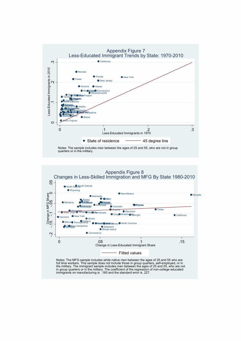
Alabama

Alaska

Arizona

Arkansas

California

Colorado

Connecticut

Florida

Georgia

Hawaii

Illinois

IndianaIowa

Kansas

KentuckyLouisiana

Maine

MarylandMassachusetts

Michigan

Minnesota

MississippiMissouri

Nebraska

Nevada

New Hampshire

New Jersey

New Mexico

New York

North Carolina

Ohio

Oklahoma

Oregon

Pennsylvania

Rhode Island

South CarolinaTennessee

Texas

UtahVirginia

Washington

West Virginia

Wisconsin

0.1

.2.3

Les

s-E

duc

ate

d Im

mig

ran

ts in

201

0

0 .1 .2 .3Less-Educated Immigrants in 1970

State of residence 45 degree line

Notes: The sample includes men between the ages of 25 and 55, who are not in groupquarters or in the military.

Appendix Figure 7Less-Educated Immigrant Trends by State: 1970-2010

Alabama

Alaska

ArizonaArkansas

California

Colorado

Connecticut

Delaware

Florida

Georgia

Hawaii

Idaho

IllinoisIndiana

Iowa Kansas

Kentucky

Louisiana

Maine

Maryland

Massachusetts

Michigan

Minnesota

Mississippi

Missouri

Montana

NebraskaNevada

New HampshireNew Jersey

New Mexico

New York

North Carolina

North Dakota

Ohio

Oklahoma

Oregon

Pennsylvania

Rhode Island

South Carolina

South Dakota

TennesseeTexas

Utah

Vermont

Virginia

WashingtonWest Virginia

Wisconsin

Wyoming

-.2

-.1

5-.

1-.

05

0.0

5C

hang

e in

MF

G S

har

e

0 .05 .1 .15Change in Less-Educated Immigrant Share

Fitted values

Notes: The MFG sample includes white native men between the ages of 25 and 55 who arefull time workers. This sample does not include those in group quarters, self-employed, or inthe military. The immigrant sample includes men between the ages of 25 and 55, who are notin group quarters or in the military. The coefficient of the regression of non-college educatedimmigrants on manufacturing is .160 and the standard error is .227.

Appendix Figure 8Changes in Less-Skilled Immigration and MFG By State 1980-2010