Dissertation Combined Faculties of the Natural Sciences ...
140
Dissertation submitted to the Combined Faculties of the Natural Sciences and Mathematics of the Ruperto-Carola-University of Heidelberg. Germany for the degree of Doctor of Natural Sciences Put forward by Alberto Rorai born in: San Daniele del Friuli (Italy) Oral examination: 14/11/2014
Transcript of Dissertation Combined Faculties of the Natural Sciences ...
Dissertation
submitted to the
Combined Faculties of the Natural Sciences and Mathematics
of the Ruperto-Carola-University of Heidelberg. Germany
for the degree of
Doctor of Natural Sciences
Put forward by
Alberto Rorai
born in: San Daniele del Friuli (Italy)
Oral examination: 14/11/2014

Measuring the Small Scale Structure of the Intergalactic Medium
Referees: Joseph F. Hennawi
Volker Springel

Topic in German: Die kleinskalige Struktur des intergalaktischen Mediums ist grundlegend für das Verständnis vonKosmologie und Strukturbildung. Obwohl die Baryonen den Fluktuationen der dunklen Matterie auf Skalen in derGrößenordnung von Megaparsec folgen, werden auf kleinen Skalen (~100 kpc) die Gaspertubationen durchhyrdodynamische Gleichungen reguliert. Es wird angenommen, dass sie unterhalb einer charaktersistischen Längenskalaaufgrund von Druckgradienten unterdrückt werden, analog zur klassischen Jeanslänge. Der Wert der Jeansfilterlänge λJ wirdfestgelegt durch ein Gleichgweicht zwischen Druck und Gravitationskräften und hat grundlegende kosmologischeAnwendungen. Erstens liefert es einen thermischen Indiz für die zugeführte Wärme von unltravioletten Photonen währendder Reionisation und bestimmt somit die thermische Geschichte des Universums. Zweitens bestimmt es die Verklumpungdes IGM und die minimale gravitative Masse für den Kollaps des IGM, die eine zentrale Rolle in der Galaxienentstehungund Reionisation spielt. Prinzpiell kann Jeansglättung durch rotverschobene Lyman-α Absorptionslinien in Spektren vonhoch rotverschobenen Quasaren nachgewiesen werden. Leider ist dies extrem schwierig, da die Auswirkungen desthermischen Dopplereffektes von Lyman-α Linien entlang der Beobachtungsrichtung von der Druckverbreiterung nicht klarzu trennen sind. In dieser Arbeit zeige ich explizit, welche Entartungen zwischen den thermischen Parametern auftreten, wenn ausschließlichBeobachtungen entlang einer Sichtlinie möglich sind. Dafür habe ich einen stabilen statistischen Alogrithmus basierend aufGaussprozessen und Markov Chain Monte Carlo Methoden entworfen, der auf einem Gitter eines semianalytischen Modellsdes IGM beruht. Ich führe dann eine neue Methode zum Messen der Jeanslänge ein, indem ich die transverse Kohärenz inSpektren benachbarter Quasarenpaare berechne (transverser Abstand < 1 Mpc). Diese Methode basiert auf derPhasendifferenz homologer Fouriermoden in dem Lyman-α Wald von Quasarenpaaren. Ich beweise, dass dies maximalempfindlich zu λJ ist und nur schwach von anderen Parametern abhängt. Die verfügbare Stichprobe von Quasarenpaarenwird unter sorgfältiger Kalibration des Rauschens, der Auflösung und anderer möglicher systematischer Effekteausgewertet. Unsere neue Methode auf diesen Datensatz angewendet gibt die erste Messung der Filterlänge des IGM. Einerster Vergleich unserer Ergebnisse mit hydrodynamischen Simultaionen lässt darauf schließen, dass die vom thermischenStandardmodell des IGM vorrausgesagte Filterlänge signifikant höher ist als beobachtet. Dies motiviert weitere theoretischeStudien zum Verständins dieser Diskrepanz.
Topic in English: The small-scale structure of the intergalactic medium (IGM) is fundamental to our understanding ofcosmology and structure formation. Although the baryons trace dark matter fluctuations on megaparsec scales, on smallscales (~100 kpc), gas perturbations are regulated by hydrodynamics and they are thought to be suppressed by pressurebelow a characteristic filtering scale λJ, analogous to the classic Jeans scale. The value of this Jeans filtering scale is set bythe interplay between pressure support and gravity across the cosmic history, and has fundamental cosmologicalimplications. First it provides a thermal record of heat injected by ultraviolet photons during cosmic reionization events, andthus constraints the thermal and reionization history of the universe. Second, it determines the clumpiness of the IGM andthe minimum mass for gravitational collapse from the IGM, playing a pivotal role in galaxy formation and reionization. Inprinciple, the sign of Jeans smoothing could be probed by the redshifted Lyman-α absorption lines in the spectra of high-redshift quasars (the Lyman-α forest). Unfortunately, this is extremely challenging to do because the thermal Dopplerbroadening of Lyman- α lines along the observing direction is highly degenerate with pressure smoothing. In this work, I explicitly show what degeneracies hold among the thermal parameters of the IGM when only line-of-sightobservations are possible. For this purpose, I devised a rigorous statistical algorithm based on Gaussian processes andMarkov-Chain Monte Carlo methods, trained on a grid of semianalytical models of the IGM. I then introduce a novelmethod able to measure the Jeans scale by estimating the transverse coherence in the spectra of close quasar pairs(transverse separation < 1 Mpc). This method is based on the phase differences of homologous Fourier modes in theLyman-α forests of quasar pairs, and I prove that it is maximally sensitive to λJ and only weakly dependent on the otherconsidered parameters. The available sample of quasar pairs is analyzed, after careful calibration of noise, resolution, andother possible systematics. Our new method applied to this dataset provides the first measurement of the filtering scale ofthe intergalactic medium. A first comparison of our findings with hydrodynamical simulations suggests that the filteringscale predicted by the standard thermal models of the IGM is significantly higher than what we observe, motivating furthertheoretical studies to understand this discrepancy.
Universitat Heidelberg
Doctoral Thesis
Measuring the Small Scale Structure ofthe Intergalactic Medium
Author:
Alberto Rorai
Supervisor:
Dr. Joseph Hennawi
A thesis submitted in fulfilment of the requirements
for the degree of Doctor in Astronomy
September 2014

Declaration of Authorship
I, Alberto Rorai, declare that this thesis titled, ’Measuring the Small Scale Structure
of the Intergalactic Medium’ and the work presented in it are my own. I confirm that:
This work was done wholly or mainly while in candidature for a research degree
at this University.
Where any part of this thesis has previously been submitted for a degree or any
other qualification at this University or any other institution, this has been clearly
stated.
Where I have consulted the published work of others, this is always clearly at-
tributed.
Where I have quoted from the work of others, the source is always given. With
the exception of such quotations, this thesis is entirely my own work.
I have acknowledged all main sources of help.
Where the thesis is based on work done by myself jointly with others, I have made
clear exactly what was done by others and what I have contributed myself.
Signed:
Date:
i
Overview
In this manuscript I present the bulk of the work that I have conducted during my PhD
under the supervision of Joseph F. Hennawi at the Max-Planck-Institut fur Astronomie.
The initial goal of the project was to understand whether a recently discovered sample
of quasar pairs could be used to probe the small-scale structure of the intergalactic
medium (IGM), by studying the transverse coherence of the redshifted Lyα absorption
in quasar spectra. The scientific motivations behind this objective are numerous. It
opens the possibility of studying the structure evolution in the quasi-linear regime at
the smallest length ever reached, which could be sensitive to unconstrained aspects of the
cosmological models. In this work we focus on the relation with reionization and with
the thermal evolution of the IGM: the pressure of the heated and ionized gas is expected
to quench the growth of density perturbation below a characteristic scale called Jeans
scale, or filtering scale (we will use the term as synonyms throughout the manuscript).
This scale, although theoretically predicted, has never been constrained, and it may
provide precious insights on galaxy formation and on the early stage of the reionization
(a broader discussion is provided in chapter 1). This work represent the first attempt of
measuring it at the redshifts of the Lyα forest.
The project has been carried on in two stages.
In the first stage we explored theoretically the sensitivity of the Lyα forest to the pa-
rameters that describe the thermal state of the IGM and in particular on the Jeans
scale. We developed an algorithm that enables a systematic study of the sensitivity
and degeneracies of Lyα-forest statistics with respect to the thermal parameter of the
IGM, based on a set of semianalytical models. I describe this method and the models
on which it relies in chapter 2. We then devised a new statistic specifically tailored to
extract transverse-coherence information from quasar pairs. This statistic is based on
the phase differences of homologous Fourier modes of the Lyα forests of two companion
quasars, and we show in chapter 3 that it is maximally sensitive to the Jeans scale and
practically insensitive on the other parameters that we analyze.
ii
Overview iii
In the second part we applied the phase-difference method to the observed sample of
quasar pairs, in the attempt of constraining the filtering scale of the IGM at redshift
2 < z < 3. The main challenge in doing that was a proper treatment of noise, resolution
and of the systematics (chapter 3), as well as understanding the exact meaning of the
measured filtering scale and the extent to which our DM-based model could be trusted
(chapter 6). The results we achieved, presented in chapter 5, indicate that the Jeans
filtering scale is significantly smaller than what hydrodynamic simulation predicts for
standard assumptions on the thermal history. The potentially controversial consequences
of this finding demand further consideration of the possible systematic that could bias
our measurement, and motivates a deeper theoretical exploration of the nature of the
filtering scale and in particular of its relation with the thermal history.
The first three chapters present material that I have published in [Rorai et al., 2013],
slightly adapted and reorganized to be inserted in this thesis, while the rest is unpub-
lished. The work described in chapters 1-5 represent my personal contribution, except
when I explicitly report results or methods from other studies. Chapter 6 contains results
achieved in our research group in the past month, in particular in collaboration with
Jose Onorbe and Girish Kulkarni, in which I have been actively involved. I personally
conducted the test described in § 6.2.2 to validate the calibration of my measurement
with dark-matter simulations. I contributed to the definition of filtering scale of the
IGM based on the Lyα absorption in 3d (§ 6.2), which will be published in Kulkarni et
al. (in prep.) and on the fitting procedure described in § 6.3 (to be published in Onorbe
et al., in prep.).

Contents
Declaration of Authorship i
Preface . . . . . . . . . . . . . . . . . . . . . . . . . . . . . . . . . . . . . . . . iii
Contents iv
1 Introduction 1
2 Parametric Study of the Intergalactic Medium 8
2.1 Simulation . . . . . . . . . . . . . . . . . . . . . . . . . . . . . . . . . . . . 9
2.1.1 Dark Matter Simulation . . . . . . . . . . . . . . . . . . . . . . . . 9
2.1.2 Description of the Intergalactic Medium . . . . . . . . . . . . . . . 9
2.2 emulator . . . . . . . . . . . . . . . . . . . . . . . . . . . . . . . . . . . . . 13
2.2.1 Models . . . . . . . . . . . . . . . . . . . . . . . . . . . . . . . . . 14
2.2.2 PCA . . . . . . . . . . . . . . . . . . . . . . . . . . . . . . . . . . . 14
2.2.3 Gaussian Process Interpolation . . . . . . . . . . . . . . . . . . . . 15
2.3 Power Spectra and Their Degeneracies . . . . . . . . . . . . . . . . . . . . 15
2.3.1 The Longitudinal Power Spectrum . . . . . . . . . . . . . . . . . . 16
2.3.2 Cross Power Spectrum . . . . . . . . . . . . . . . . . . . . . . . . . 18
3 Phase Analysis of the Lyman-α Forest of Quasar Pairs 20
3.1 A New Statistic: Phase Differences . . . . . . . . . . . . . . . . . . . . . . 21
3.1.1 Drawbacks of the Cross Power Spectrum . . . . . . . . . . . . . . . 21
3.1.2 An Analytical Form for the PDF of Phase Differences . . . . . . . 22
3.1.3 The Probability Distribution of Phase Differences of the IGM Den-sity . . . . . . . . . . . . . . . . . . . . . . . . . . . . . . . . . . . 24
3.1.4 The Probability Distribution of Phase Differences of the Flux . . . 29
3.1.5 The Covariance of the Phase Differences . . . . . . . . . . . . . . . 33
3.1.6 A Likelihood Estimator for the Jeans Scale . . . . . . . . . . . . . 35
3.2 How Well Can We Measure the Jeans Scale? . . . . . . . . . . . . . . . . . 36
3.2.1 The Likelihood for P (k) and π(k, r⊥) . . . . . . . . . . . . . . . . 37
3.2.2 Mock Datasets . . . . . . . . . . . . . . . . . . . . . . . . . . . . . 38
3.2.3 The Precision of the λJ Measurement . . . . . . . . . . . . . . . . 40
3.2.4 The Impact of Noise and Finite Spectral Resolution . . . . . . . . 43
3.2.5 Systematic Errors . . . . . . . . . . . . . . . . . . . . . . . . . . . 47
3.2.6 Is Our Likelihood Estimator Unbiased? . . . . . . . . . . . . . . . 48
4 Data Analysis 51
iv
Contents v
4.1 Data sample . . . . . . . . . . . . . . . . . . . . . . . . . . . . . . . . . . . 52
4.1.1 Spectroscopic Observations . . . . . . . . . . . . . . . . . . . . . . 52
4.1.2 Selection Criteria . . . . . . . . . . . . . . . . . . . . . . . . . . . . 53
4.1.3 Continuum Fitting and Data Preparation . . . . . . . . . . . . . . 59
4.2 Calculation of Phases from Real Spectra . . . . . . . . . . . . . . . . . . . 59
4.2.1 Method 1: Least-Square Spectral Analysis . . . . . . . . . . . . . . 60
4.2.2 method 2: Rebinning on a Regular Grid . . . . . . . . . . . . . . . 62
4.3 Calibrated Phase Analysis . . . . . . . . . . . . . . . . . . . . . . . . . . . 63
4.3.1 Transverse Separation . . . . . . . . . . . . . . . . . . . . . . . . . 63
4.3.2 Resolution . . . . . . . . . . . . . . . . . . . . . . . . . . . . . . . . 64
4.3.3 Noise . . . . . . . . . . . . . . . . . . . . . . . . . . . . . . . . . . 65
4.3.4 Forward-Modeling of the Simulation . . . . . . . . . . . . . . . . . 66
4.4 Effect of Noise on Phase Distribution . . . . . . . . . . . . . . . . . . . . . 68
5 Results 70
5.1 Implementation of the Statistical Analysis . . . . . . . . . . . . . . . . . . 71
5.1.1 Simulation . . . . . . . . . . . . . . . . . . . . . . . . . . . . . . . 71
5.1.2 Parameter Grid . . . . . . . . . . . . . . . . . . . . . . . . . . . . . 71
5.1.3 Likelihood . . . . . . . . . . . . . . . . . . . . . . . . . . . . . . . . 72
5.1.4 Interpolation . . . . . . . . . . . . . . . . . . . . . . . . . . . . . . 72
5.1.5 Resolution Limit on k|| . . . . . . . . . . . . . . . . . . . . . . . . . 73
5.2 Results . . . . . . . . . . . . . . . . . . . . . . . . . . . . . . . . . . . . . . 76
5.2.1 Phase Distributions of Real Pairs . . . . . . . . . . . . . . . . . . . 76
5.2.2 Constraints . . . . . . . . . . . . . . . . . . . . . . . . . . . . . . . 80
5.3 Consistency Tests . . . . . . . . . . . . . . . . . . . . . . . . . . . . . . . . 85
5.3.1 Data-Originated . . . . . . . . . . . . . . . . . . . . . . . . . . . . 85
5.3.1.1 Phase Calculation . . . . . . . . . . . . . . . . . . . . . . 85
5.3.1.2 Continuum Fitting . . . . . . . . . . . . . . . . . . . . . 87
5.3.1.3 Contaminants . . . . . . . . . . . . . . . . . . . . . . . . 88
5.3.2 Calibration . . . . . . . . . . . . . . . . . . . . . . . . . . . . . . . 88
5.3.2.1 Resolution . . . . . . . . . . . . . . . . . . . . . . . . . . 88
5.3.2.2 Skewer Extension . . . . . . . . . . . . . . . . . . . . . . 89
5.3.2.3 Noise . . . . . . . . . . . . . . . . . . . . . . . . . . . . . 91
5.3.3 Model Assumptions . . . . . . . . . . . . . . . . . . . . . . . . . . 92
5.3.4 Statistical Approximations . . . . . . . . . . . . . . . . . . . . . . 93
5.3.4.1 Wrapped-Cauchy Distribution . . . . . . . . . . . . . . . 93
5.3.4.2 Emulator . . . . . . . . . . . . . . . . . . . . . . . . . . . 94
5.3.4.3 MCMC convergence . . . . . . . . . . . . . . . . . . . . . 97
6 Interpretation and Discussion 98
6.1 Hydrodynamical Simulations . . . . . . . . . . . . . . . . . . . . . . . . . 99
6.2 The Filtering Scale in the Real-Flux Field . . . . . . . . . . . . . . . . . . 100
6.2.1 Is there any Jeans Scale of the IGM? . . . . . . . . . . . . . . . . . 101
6.2.2 Validation of the Dark-Matter Models . . . . . . . . . . . . . . . . 104
6.3 Definition of the Jeans Scale in Hydrodynamical Simulations . . . . . . . 105
6.4 Redshift Evolution and Comparison with Simulation . . . . . . . . . . . . 107
6.5 Future Work . . . . . . . . . . . . . . . . . . . . . . . . . . . . . . . . . . 110

Contents vi
7 Concluding Remarks 111
A Resolving the Jeans Scale with Dark-Matter Simulations 115
B Determining the Concentration Parameter ζ of the Wrapped-Cauchy
Distribution 117
C Phase Noise Calculation 118
Bibliography 120
Chapter 1
Introduction
The imprint of redshifted Lyman-α (Lyα) forest absorption on the spectra of distant
quasars provides an exquisitely sensitive probe of the distribution of baryons in the in-
tergalactic medium (IGM) at large cosmological lookback times. Among the remarkable
achievements of modern cosmology is the ability of cosmological hydrodynamical sim-
ulations to explain the origin of this absorption pattern, and reproduce its statistical
properties to percent level accuracy [e.g. Cen et al., 1994, Miralda-Escude et al., 1996,
Rauch, 1998]. But the wealth of information which can be gathered from the Lyα forest
is far from being exhausted. The thermal state of the baryons in the IGM reflects the
integrated energy balance of heating — due to the collapse of cosmic structures, radia-
tion, and possibly other exotic heat sources — and cooling due to the expansion of the
Universe [e.g. Hui & Gnedin, 1997, Hui & Haiman, 2003, Meiksin, 2009, Miralda-Escude
& Rees, 1994]. Cosmologists still do not understand how the interplay of these physical
processes sets the thermal state of the IGM, nor has this thermal state been precisely
measured.
There is ample observational evidence that ultraviolet radiation emitted by the first
star-forming galaxies ended the ‘cosmic dark ages’ ionizing hydrogen and singly ionizing
helium at z ∼ 10 [e.g. Barkana & Loeb, 2001, Ciardi & Ferrara, 2005, Fan et al.,
2006, Zaroubi, 2013]. A second and analogous reionization episode is believed to have
occurred at later times z ∼ 3 − 4 [Croft et al., 1997, Jakobsen et al., 1994, Madau &
Meiksin, 1994, Reimers et al., 1997], when quasars were sufficiently abundant to supply
the hard photons necessary to doubly ionized helium. The most recent observations from
HST/COS provide tentative evidence for an extended He II reionization from z ∼ 2.7−4
[Furlanetto & Dixon, 2010, Shull et al., 2010, Worseck et al., 2011, Worseck et al. 2013,
in preparation], with a duration of ∼ 1Gyr, longer than naively expected. Cosmic
reionization events are watersheds in the thermal history of the Universe, photoheating
1
Chapter 1. Introduction 2
the IGM to tens of thousands of degrees. Because cooling times in the rarefied IGM gas
are long, memory of this heating is retained [Haehnelt & Steinmetz, 1998, Hui & Gnedin,
1997, Hui & Haiman, 2003, Miralda-Escude & Rees, 1994, Theuns et al., 2002a,b]. Thus
an empirical characterization of the IGMs thermal history constrains the nature and
timing of reionization.
From a theoretical perspective, the impact of reionization events on the thermal state
of the IGM is poorly understood. Radiative transfer simulations of both hydrogen
[Bolton et al., 2004, Iliev et al., 2006, Tittley & Meiksin, 2007a] and helium [Abel &
Haehnelt, 1999, McQuinn et al., 2009, Meiksin & Tittley, 2012] reveal that the heat
injection and the resulting temperature evolution of the IGM depends on the details of
how and when reionization occurred. There is evidence that the thermal vestiges of H I
reionization heating may persist until as late as z ∼ 4 − 5, and thus be observable in
the Lyα forest [Cen et al., 2009, Furlanetto & Oh, 2009, Hui & Haiman, 2003], whereas
for HeII reionization at z ∼ 3, the Lyα forest is observable over the full duration of the
phase transition. Finally, other processes could inject heat into the IGM and impact
its thermal state, such as the large-scale structure shocks which eventually produce
the Warm Hot Intergalactic Medium [WHIM;e.g. Cen & Ostriker, 1999, Dave et al.,
2001, 1999], heating from galactic outflows [Cen & Ostriker, 2006, Kollmeier et al.,
2006], photoelectric heating of dust grains [Inoue & Kamaya, 2003, Nath et al., 1999],
cosmic-ray heating [Nath & Biermann, 1993], Compton-heating from the hard X-ray
background [Madau & Efstathiou, 1999], X-ray preheating [Ricotti et al., 2005, Tanaka
et al., 2012a], or blazar heating [Broderick et al., 2012, Chang et al., 2012, Pfrommer
et al., 2012, Puchwein et al., 2012]. Precise constraints on the thermal state of the IGM
would help determine the relative importance of photoheating from reionization and
these more exotic mechanisms.
Despite all the successes of our current model of the IGM, precise constraints on its ther-
mal state and concomitant constraints on reionization (and other exotic heat sources)
remain elusive. Attempts to characterize the IGM thermal state from Lyα forest mea-
surements have a long history. In the simplest picture, the gas in the IGM obeys a power
law temperature-density relation T = T0(ρ/ρ)γ−1, which arises from the balance between
photoionization heating, and cooling due to adiabatic expansion [Hui & Gnedin, 1997].
The standard approach has been to compare measurements of various statistics of the
Lyα forest to cosmological hydrodynamical simulations. Leveraging the dependence of
these statistics on the underlying temperature-density relation, its slope and amplitude
(T0, γ) parameters can be constrained. To this end a wide variety of statistics have been
employed, such as the power spectrum [Viel et al., 2009, Zaldarriaga et al., 2001] or anal-
ogous statistics quantifying the small-scale power like wavelets [Garzilli et al., 2012, Lidz
et al., 2009, Theuns et al., 2002b] or the curvature [Becker et al., 2011]. The flux PDF

Chapter 1. Introduction 3
[Bolton et al., 2008, Calura et al., 2012, Garzilli et al., 2012, Kim et al., 2007, McDonald
et al., 2000] and the shape of the b-parameter distribution [Bryan & Machacek, 2000,
Haehnelt & Steinmetz, 1998, McDonald et al., 2001, Ricotti et al., 2000, Rudie et al.,
2012, Schaye et al., 2000, Theuns et al., 2000, 2002a] have also been considered. Multiple
statistics have also been combined such as the PDF and wavelets [Garzilli et al., 2012],
or PDF and power spectrum [Viel et al., 2009]. Overall, the results of such comparisons
are rather puzzling. First, the IGM appears to be generally too hot, both at low (z ∼ 2)
and high (z ∼ 4) redshift [Hui & Haiman, 2003]. In particular, the high inferred temper-
atures at z ∼ 4 [e.g. Lidz et al., 2009, McDonald et al., 2001, Schaye et al., 2000, Theuns
et al., 2002b, Zaldarriaga et al., 2001] suggest that HeII was reionized at still higher red-
shift z > 4 [Hui & Haiman, 2003], possibly conflicting with the late z ∼ 2.7 reionization
of HeII observed in HST/COS spectra [Furlanetto & Dixon, 2010, Shull et al., 2010,
Syphers et al., 2012, Worseck et al., 2011, Worseck et al. 2013, in preparation]. Second,
Bolton et al. [2008] considered the PDF of high-resolution quasar spectra and concluded
that, at z ≃ 3 the slope of the temperature-density relation γ is either close to isother-
mal (γ = 1) or even inverted (γ < 1), suggesting “that the voids in the IGM may be
significantly hotter and the thermal state of the low-density IGM may be substantially
more complex than is usually assumed.” Although this result is corroborated by ad-
ditional work employing different statistics/methodologies [Calura et al., 2012, Garzilli
et al., 2012, Viel et al., 2009, but see Lee et al. 2012], radiative transfer simulations of
HeII reionization cannot produce an isothermal or inverted slope, unless a population
other than quasars reionized HeII [Bolton et al., 2004, McQuinn et al., 2009, Meiksin
& Tittley, 2012] , which would fly in the face of conventional wisdom. To summarize,
despite nearly a decade of theoretical and observational work, published measurements
of the thermal state of the IGM are still highly confusing, and concomitant constraints
on reionization scenarios are thus hardly compelling.
Fortunately, there is another important record of the thermal history of the Universe:
the Jeans pressure smoothing scale. Although baryons in the IGM trace dark matter
fluctuations on large Mpc scales, on smaller scales . 100 kpc, gas is pressure supported
against gravitational collapse by its finite temperature. Analogous to the classic Jeans
argument, baryonic fluctuations are suppressed relative to the pressureless dark matter
(which can collapse), and thus small-scale power is ‘filtered’ from the IGM [Gnedin
& Hui, 1998], which explains why it is sometimes referred to as the filtering scale.
Classically the comoving Jeans scale is defined as λ0J =√
πc2s/Gρ(1 + z), but in reality
the amount of Jeans filtering is sensitive to both the instantaneous pressure and hence
temperature of the IGM, as well as the temperature of the IGM in the past. This arises
because fluctuations at earlier times expanded or failed to collapse depending on the
IGM temperature at that epoch. Thus the Jeans scale reflects the competition between
Chapter 1. Introduction 4
gravity and pressure integrated over the Universe’s history, and cannot be expressed
as a mere deterministic function of the instantaneous thermal state. Heuristically, this
can be understood because reionization heating is expected to occur on the reionization
timescales of several hundreds of Myr, whereas the baryons respond to this heating
on the sound-crossing timescale λ0J/[cs(1 + z)] ∼ (Gρ)−1/2, which at mean density is
comparable to the Hubble time tH .
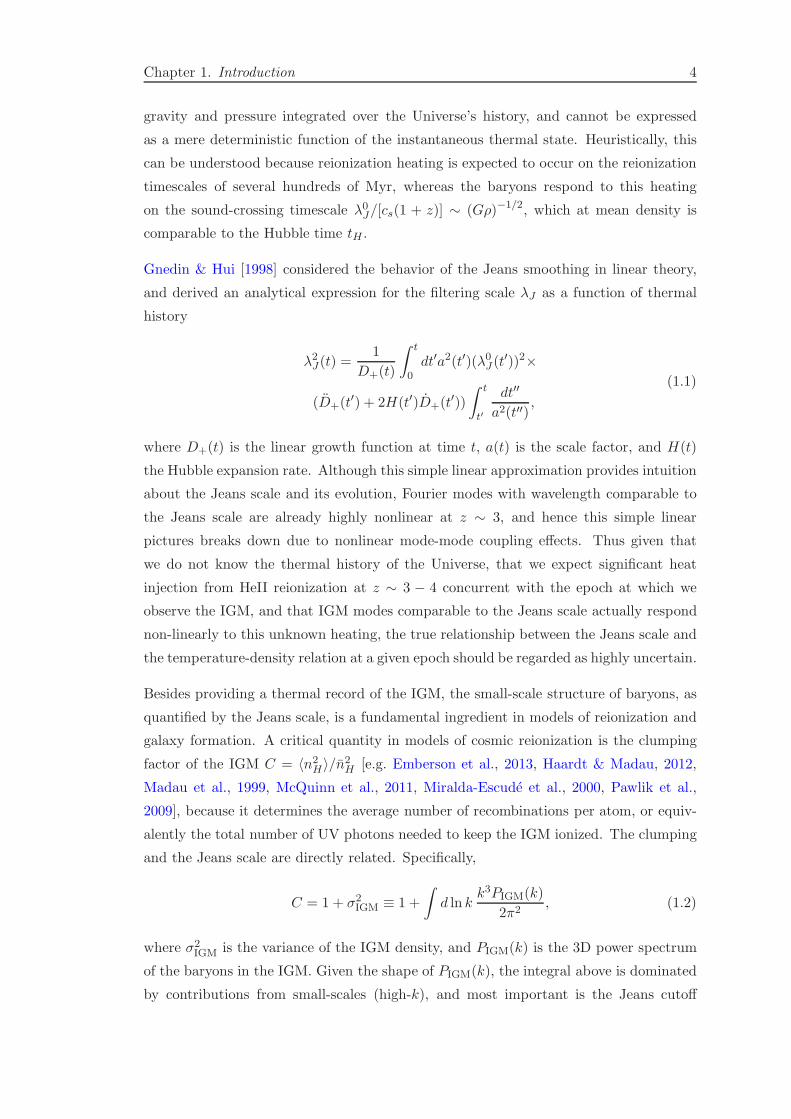
Gnedin & Hui [1998] considered the behavior of the Jeans smoothing in linear theory,
and derived an analytical expression for the filtering scale λJ as a function of thermal
history
λ2J(t) =1
D+(t)
∫ t
0dt′a2(t′)(λ0J (t
′))2×
(D+(t′) + 2H(t′)D+(t
′))
∫ t
t′
dt′′
a2(t′′),
(1.1)
where D+(t) is the linear growth function at time t, a(t) is the scale factor, and H(t)
the Hubble expansion rate. Although this simple linear approximation provides intuition
about the Jeans scale and its evolution, Fourier modes with wavelength comparable to
the Jeans scale are already highly nonlinear at z ∼ 3, and hence this simple linear
pictures breaks down due to nonlinear mode-mode coupling effects. Thus given that
we do not know the thermal history of the Universe, that we expect significant heat
injection from HeII reionization at z ∼ 3 − 4 concurrent with the epoch at which we
observe the IGM, and that IGM modes comparable to the Jeans scale actually respond
non-linearly to this unknown heating, the true relationship between the Jeans scale and
the temperature-density relation at a given epoch should be regarded as highly uncertain.
Besides providing a thermal record of the IGM, the small-scale structure of baryons, as
quantified by the Jeans scale, is a fundamental ingredient in models of reionization and
galaxy formation. A critical quantity in models of cosmic reionization is the clumping
factor of the IGM C = 〈n2H〉/n2H [e.g. Emberson et al., 2013, Haardt & Madau, 2012,
Madau et al., 1999, McQuinn et al., 2011, Miralda-Escude et al., 2000, Pawlik et al.,
2009], because it determines the average number of recombinations per atom, or equiv-
alently the total number of UV photons needed to keep the IGM ionized. The clumping
and the Jeans scale are directly related. Specifically,
C = 1 + σ2IGM ≡ 1 +
∫
d ln kk3PIGM(k)
2π2, (1.2)
where σ2IGM is the variance of the IGM density, and PIGM(k) is the 3D power spectrum
of the baryons in the IGM. Given the shape of PIGM(k), the integral above is dominated
by contributions from small-scales (high-k), and most important is the Jeans cutoff
Chapter 1. Introduction 5
λJ , which determines the maximum k-mode kJ ∼ 1/λJ contributing. The small-scale
structure of the IGM strongly influences the propagation of cosmological ionization
fronts during reionization [Iliev et al., 2005]. Furthermore, several numerical studies
have revealed that the hydrodynamic response of the baryons in the IGM to impulsive
reionization heating is significant [e.g. Ciardi & Salvaterra, 2007, Gnedin, 2000a, Haiman
et al., 2001, Kuhlen & Madau, 2005, Pawlik et al., 2009], indicating that a full treatment
of the interplay between IGM small-scale structure and reionization history probably
requires coupled radiative transfer hydrodynamical simulations.
Reionization heating also evaporates the baryons from low-mass halos or prevents gas
from collapsing in them altogether [e.g. Barkana & Loeb, 1999, Dijkstra et al., 2004],
an effect typically modeled via a critical mass, below which galaxies cannot form [Ben-
son et al., 2002a,b, Bullock et al., 2000, Gnedin, 2000b, Kulkarni & Choudhury, 2011,
Somerville, 2002]. Gnedin [2000b] used hydrodynamical simulations to show that this
scale is well approximated by the filtering mass, which is the mass-scale corresponding
to the Jeans filtering length, i.e. MF (z) = 4πρλ3J/3 [see also Hoeft et al., 2006, Okamoto
et al., 2008]. Finally, because the Jeans scale has memory of the thermal events in the
IGM (see eqn. 1.1), its value at later times can potentially constrain models of early
IGM preheating. In this scenario, heat is globally injected into the IGM at high-redshift
z ∼ 5 − 15 from blast-waves produced by outflows from proto-galaxies or miniquasars
[Benson & Madau, 2003, Cen & Bryan, 2001, Madau, 2000, Madau et al., 2001, Scan-
napieco et al., 2002, Scannapieco & Oh, 2004, Theuns et al., 2001, Voit, 1996] X-ray
radiation from early miniquasars [Parsons et al., 2013, Tanaka et al., 2012b], which sets
an entropy floor in the IGM and the raises filtering mass scale inhibiting the formation
of early galaxies.
A rough estimate of the filtering scale at z = 3 can be obtained from eqn. (1.1) and
the following simplified assumptions: the temperature at z = 3 is T (z = 3) ≈ 15000K
as suggested by measurements [e.g. Lidz et al., 2009, Ricotti et al., 2000, Schaye et al.,
2000, Zaldarriaga et al., 2001], temperature evolves as T ∝ 1+z, the typical overdensity
probed by the z = 3 Lyα forest is δ ∼ 2 [Becker et al., 2011]. One then obtains
λJ(z = 3) ≈ 340 kpc (comoving), smaller than the classical or instantaneous Jeans
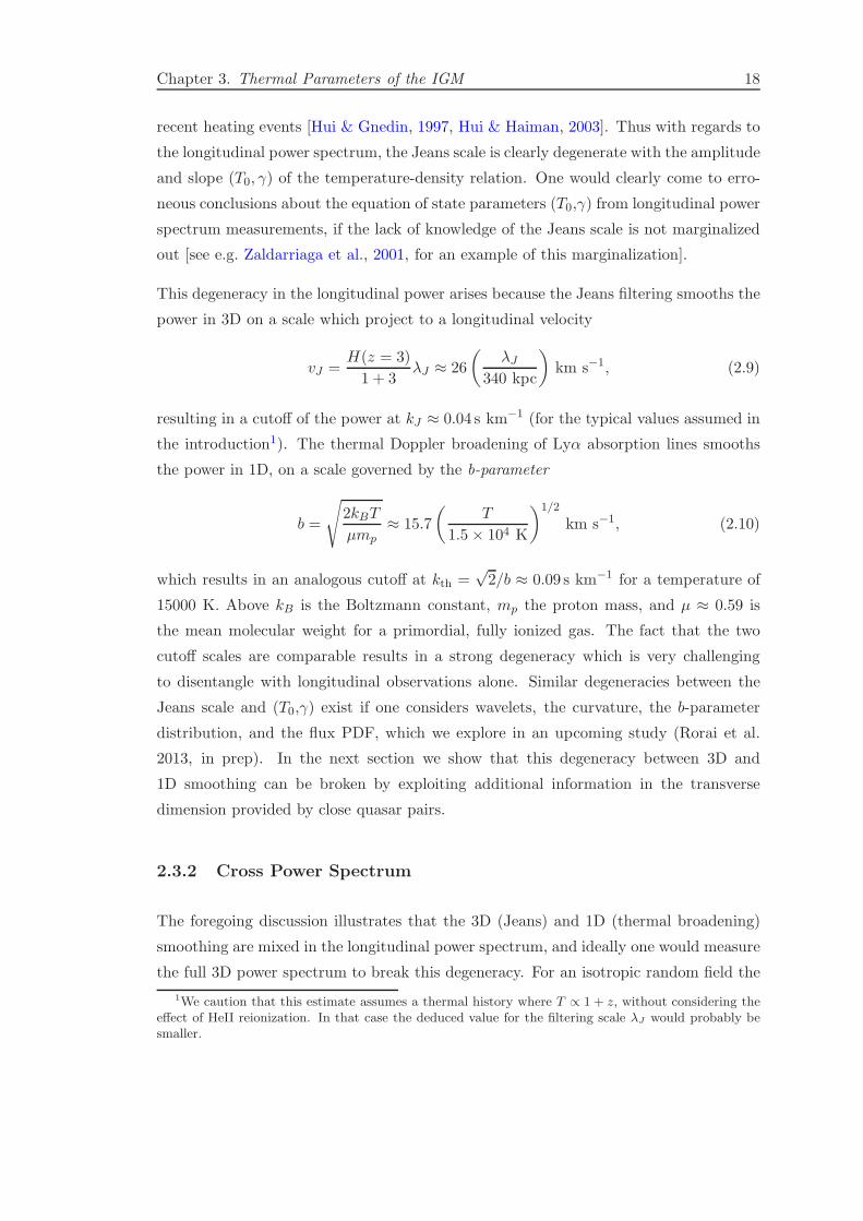
scale λ0J by a factor of ∼ 3. This distance maps to a velocity interval vJ = HaλJ ≈26 km s−1 along the line of sight due to Hubble expansion. Thermal Doppler broadening
gives rise to a cutoff in the longitudinal power spectrum, which occurs at a comparable
velocity vth ≈ 11.3 km s−1, for gas heated to the same temperature. The similarity of
the characteristic scale of 3D Jeans pressure smoothing and the 1D thermal Doppler
smoothing suggests that disentangling the two effects will be challenging given purely
longitudinal observations of the Lyα forest, as confirmed by Peeples et al. [2009a], who
considered the relative impact of thermal broadening and pressure smoothing on various

Chapter 1. Introduction 6
statistics applied to longitudinal Lyα forest spectra. Previous work that has aimed to
measure thermal parameters such as T0 and γ from Lyα forest spectra, have largely
ignored the degeneracy of the Jeans scale with these thermal parameters. The standard
approach has been to assume values of the Jeans scale from a hydrodynamical simulation
[e.g. Becker et al., 2011, Lidz et al., 2009, Viel et al., 2009], which as per the discussion
above, is equivalent to assuming perfect knowledge of the IGM thermal history. Because
of the degeneracy with the Jeans scale, it is thus likely that previous measurements of the
thermal parameters T0 and γ are significantly biased, and their error bars significantly
underestimated, if indeed Jeans scale takes on values different from those assumed (but
see Zaldarriaga et al. 2001 who marginalized over the Jeans scale, and Becker et al.
2011 who also considered its impact). We will investigate such degeneracies in detail
in chapter 2 with respect to power-spectra, and we consider degeneracies for a broader
range of IGM statistics in a future work (A.Rorai et al., in preparation).
The Jeans filtering scale can be directly measured using close quasar pair sightlines
which have comparable transverse separations r⊥ . 300 kpc (comoving; ∆θ . 40′′ at
z = 3). The observable signature of Jeans smoothing is increasingly coherent absorption
between spectra at progressively smaller pair separations resolving it [Peeples et al.,
2009b]. The idea of using pairs to constrain the small scale structure of the IGM is
not new. However, all previous measurements have either focused on lensed quasars,
which probe extremely small transverse distances r⊥ ∼ 1 kpc ≪ λJ [e.g. McGill, 1990,
Petry et al., 1998, Rauch et al., 2001, Smette et al., 1995, Young et al., 1981] such
that the Lyα forest is essentially perfectly coherent, or real physical quasar pairs with
r⊥ ∼ 1 Mpc ≫ λJ [D’Odorico et al., 2006] far too large to place useful constraints on
the Jeans scale. Observationally, the breakthrough enabling a measurement of the Jeans
scale is the discovery of a large number of close quasar pairs [Hennawi, 2004, Hennawi
et al., 2009, 2006b, Myers et al., 2008] with ∼ 100 kpc separations. By applying machine
learning techniques [Bovy et al., 2011, 2012, Richards et al., 2004] to the Sloan Digital
Sky Survey [SDSS; York et al., 2000] imaging, a sample of ∼ 300 close r⊥ < 700 kpc
quasar pairs at 1.6 < z . 4.31 has been uncovered [Hennawi, 2004, Hennawi et al., 2009,
2006b].
In this paper we introduce a new method which enabled the first determination of the
Jeans scale from a dataset of close quasar pair. We explicitly consider degeneracies
between the canonical thermal parameters T0 and γ, and the Jeans scale λJ , which
have been heretofore largely ignored. To this end, we use an approximate model of the
Lyα forest based on dark matter only simulations, allowing us to independently vary all
thermal parameters and simulate a large parameter space. The structure of the thesis
is as follows: we describe how we compute the Lyα forest flux transmission from dark
1The lower redshift limit is corresponds to Lyα forest absorption being above the atmospheric cutoff.
Chapter 1. Introduction 7
matter simulations, and our parametrization of the thermal state of the IGM in section
chapter 2. We focus in particular on the degeneracies between thermal parameters which
result when only longitudinal observations are available, and how the additional trans-
verse information provided by quasar pairs can break them. In chapter 3 we introduce
our new method to quantify absorption coherence using the difference in phase between
homologous longitudinal Fourier modes of each member of a quasar pair. We present
a Bayesian likelihood formalism that uses the phase angle probability distributions to
determine the Jeans scale, and we conduct a Markov Chain Monte Carlo (MCMC) anal-
ysis to determine the resulting precision on T0, γ, and λJ expected for realistic datasets,
explore parameter degeneracies, and study the impact of noise and systematic errors.
The sample of observed pairs and the treatment of noise, resolution and contaminants
are described in chapter 4, and the results obtained from the fully-calibrated phase
difference analysis are shown in chapter 5. We also test the robustness of these results
against a series of possible sources of bias. Chapter 6 addresses the problem of the
physical interpretation of the Jeans scale measurement, using a set of hydrodynamic
simulations, and illustrates a preliminary comparison of our estimate with the prediction
of the standard model of the IGM on λJ . We conclude and summarize in § 7.
Chapter 2
Parametric Study of the
Intergalactic Medium
Our goal is to quantitatively assess the sensitivity of the transverse coherence in quasar
pairs to the small-scale physics of the IGM, and to understand if the velocity-space
degeneracy between thermal broadening and pressure support could be broken. To do
this, we implement a machinery to rapidly predict Lyα-forest statistics in the space of
parameters that describe the thermal state of the IGM. This machinery is based on two
main components: a grid of thermal models of the IGM that sample the parameter space
and a fast and flexible interpolation algorithm.
The thermal models are based on a Nbody dark-matter simulation, assuming that
baryons trace dark matter and approximating the effect of pressure as a convolution
with a smoothing kernel (see § 2.1.2). The width of this kernel defines in our model
the Jeans filtering scale λJ . The temperature is obtained by assuming a deterministic
temperature-density relationship T = T0(1 + δ)γ−1. The triple T0, γ, λJ defines the
parameter space where the models reside.
A grid of models in this space constitutes the ”training grid” for the emulator(§ 2.2), analgorithm based on principal component decomposition and Gaussian-processes inter-
polation that allows to efficiently predict the Lyα-forest statistics at any value of T0, γ
and λJ .
We conclude the chapter showing an application of this emulator to the line-of-sight
power spectrum and the cross power spectrum (§ 2.3), showing explicitly the degeneracy
between the thermal parameters.
8

Chapter 3. Thermal Parameters of the IGM 9
Here and in the next chapter we use the ΛCDM cosmological model with the parameters
Ωm = 0.28,ΩΛ = 0.72, h = 0.70, n = 0.96, σ8 = 0.82. All distances quoted are in
comoving kpc.
2.1 Simulation
2.1.1 Dark Matter Simulation
Our model of the Lyα forest is based on a Nbody dark matter only simulation. In this
scheme, the dark matter simulation provides the dark matter density and velocity field
[Croft et al., 1998, Meiksin & White, 2001], and the gas density and temperature are
computed using simple scaling relations motivated by the results of full hydrodynami-
cal simulations [Gnedin et al., 2003, Gnedin & Hui, 1998, Hui & Gnedin, 1997]. Our
objective is then to explore the sensitivity with which close quasar pairs can be used
to constrain the thermal parameters defining these scaling relations, and in particular
the Jeans scale. To this end, we require a dense sampling of the thermal parameter
space, which is computationally feasible with our semi-analytical method applied to a
dark matter simulation snapshot, whereas it would be extremely challenging to simulate
such a dense grid with full hydrodynamical simulations. We do not model the redshift
evolution of the IGM, nor do we consider the effect of uncertainties on the cosmological
parameters, as they are constrained by various large-scale structure and CMB measure-
ments to much higher precision than the thermal parameters governing the IGM.
We used an updated version version of the TreePM code described in White [2002] to
evolve 15003 equal mass (3×10⁶ h−1M⊙) particles in a periodic cube of side length Lbox =
50h−1Mpc with a Plummer equivalent smoothing of 1.2h−1kpc. The initial conditions
were generated by displacing particles from a regular grid using second order Lagrangian
perturbation theory at z = 150. This TreePM code has been compared to a number of
other codes and has been shown to perform well for such simulations [Heitmann et al.,
2008]. Recently the code has been modified to use a hybrid MPI+OpenMP approach
which is particularly efficient for modern clusters.
In this and in the next chapter, we analyze the snapshot at z = 3
2.1.2 Description of the Intergalactic Medium
The baryon density field is obtained by smoothing the dark matter distribution; this
smoothing mimics the effect of the Jeans pressure smoothing. For any given thermal
Chapter 3. Thermal Parameters of the IGM 10
model, we adopt a constant filtering scale λJ , rather than computing it as a function of
the temperature, and this value is allowed to vary as a free parameter (see discussion
below). The dark matter distribution is convolved with a window functionWIGM, which,
in Fourier space, has the effect of quenching high-k modes
δIGM(~k) =WIGM(~k, λJ)δDM(~k) (2.1)
For example a Gaussian kernel with σ = λJ ,WIGM(k) = exp(−k2λ2J/2), would truncates
the 3D power spectrum at k ∼ 1/λJ .
Because we smooth the dark matter particle distribution in real-space, it is more con-
venient to adopt a function with a finite-support
δIGM(x) ∝∑
i
miK(|x− xi|, RJ ) (2.2)
where mi and xi are the mass and position of the particle i, K(r) is the kernel, and
RJ the smoothing parameter which sets the Jeans scale. We adopt the followoing cubic
spline kernel
K(r,RJ ) =8
πR3J
1− 6(
rRJ
)2+ 6
(
rRJ
)3rRJ
≤ 12
2(
1− rRJ
)312 <
rRJ
≤ 1
0 rRJ
> 1
. (2.3)
In the central regions the shape of K(r) very closely resembles a Gaussian with σ ∼RJ/3.25, and we will henceforth take this RJ/3.25 to be our definition of λJ , which
we will alternatively refer to as the ‘Jeans scale’ or the ‘filtering scale’. The analogous
smoothing procedure is also applied to the particle velocities; however, note that the ve-
locity field has very little small-scale power, and so the velocity distribution is essentially
unaffected by this pressure smoothing operation. As we discuss further in Appendix A,
the mean inter-particle separation of our simulation cube δl = Lbox/N1/3p sets the min-
imum Jean smoothing that we can resolve with our dark matter simulation, hence we
can safely model values of λJ > 42kpc.
At the densities typically probed by the Lyα forest, the IGM is governed by relatively
simple physics. Most of the gas has never been shock heated, is optically thin to ionizing
radiation, and can be considered to be in ionization equilibrium with a uniform UV
background. Under these conditions, the competition between photoionization heating
and adiabatic expansion cooling gives rise to a tight relation between temperature and
Chapter 3. Thermal Parameters of the IGM 11
density which is well approximated by a power law [Hui & Gnedin, 1997],
T (δ) = T0(1 + δ)γ−1 (2.4)
where T0, the temperature at the mean density, and γ, the slope of the temperature-
density relation, both depend on the thermal history of the gas. We thus follow the
standard approach, and parametrize the thermal state of the IGM in this way. Typ-
ical values for T0 are on the order of 104 K, while γ is expected to be around unity,
and asymptotically approach the value of γ∞ = 1.6, if there is no other heat injection
besides (optically thin) photoionzation heating. Recent work suggests that an inverted
temperature-density relation γ < 1 provides a better match to the flux probability dis-
tribution of the Lyα forest [Bolton et al., 2008], but the robustness of this measurement
has been debated [Lee, 2012].
The optical depth for Lyα absorption is proportional to the density of neutral hydrogen
nHI , which, if the gas is highly ionized (xHI ≪ 1) and in photoionization equilibrium,
can be calculated as [Gunn & Peterson, 1965]
nHI = α(T )n2H/Γ (2.5)
where Γ is the photoionization rate due to a uniform metagalactic ultraviolet background
(UVB), and α(T ) is the recombination coefficient which scales as T−0.7 at typical IGM
temperatures. These approximations result in a power law relation between Lyα optical
depth and overdensity often referred as the fluctuating Gunn-Petersonn approximation
(FGPA) τ ∝ (1+ δ)2−0.7(γ−1), which does not include the effect of peculiar motions and
thermal broadening. We compute the observed optical depth in redshift-space via the
following convolution of the real-space optical depth
τ(v) =
∫ ∞
−∞τ(x)Φ(Hax+ vp,‖(x)− v, b(x))dx, (2.6)
where Hax is the real-space position in velocity units, vp,‖(x) is the longitudinal com-
ponent of the peculiar velocity of the IGM at location x, and Φ is the normalized Voigt
profile (which we approximate with a Gaussian) characterized by the thermal width
b =√
2KBT/mc2, where we compute the temperature from the baryon density via the
temperature-density relation (see eqn. 2.4). The observed flux transmission is then given
by F (v) = e−τ(v).
We apply the aforementioned recipe to 2 × 1002 lines-of-sight (skewers) running par-
allel to the box axes, to generate the spectra of 1002 quasar pairs, and we repeat this
procedure for 500 different choices of the parameter set (T0, γ, λJ ). Half of the spectra
(the first member of each pair) are positioned on a regular grid in the y − z plane,
Chapter 3. Thermal Parameters of the IGM 12
λJ = 57 kpc
0.0
0.2
0.4
0.6
0.8
0.0
F
λJ = 164 kpc
0.0
0.2
0.4
0.6
0.8
0.0
F
0 1000 2000 3000v (km/s)
0.0
0.2
0.4
0.6
0.8
0.0
F
0 1000 2000 3000v (km/s)
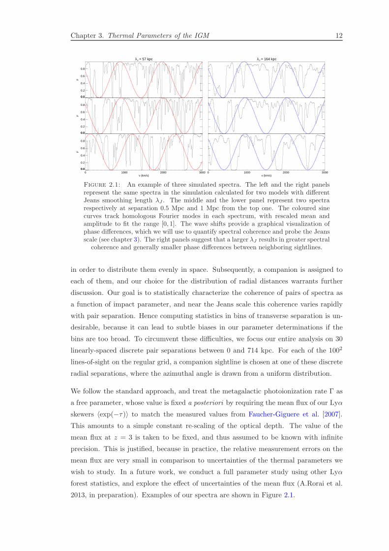
Figure 2.1: An example of three simulated spectra. The left and the right panelsrepresent the same spectra in the simulation calculated for two models with differentJeans smoothing length λJ . The middle and the lower panel represent two spectrarespectively at separation 0.5 Mpc and 1 Mpc from the top one. The coloured sinecurves track homologous Fourier modes in each spectrum, with rescaled mean andamplitude to fit the range [0, 1]. The wave shifts provide a graphical visualization ofphase differences, which we will use to quantify spectral coherence and probe the Jeansscale (see chapter 3). The right panels suggest that a larger λJ results in greater spectral
coherence and generally smaller phase differences between neighboring sightlines.
in order to distribute them evenly in space. Subsequently, a companion is assigned to
each of them, and our choice for the distribution of radial distances warrants further
discussion. Our goal is to statistically characterize the coherence of pairs of spectra as
a function of impact parameter, and near the Jeans scale this coherence varies rapidly
with pair separation. Hence computing statistics in bins of transverse separation is un-
desirable, because it can lead to subtle biases in our parameter determinations if the
bins are too broad. To circumvent these difficulties, we focus our entire analysis on 30
linearly-spaced discrete pair separations between 0 and 714 kpc. For each of the 1002
lines-of-sight on the regular grid, a companion sightline is chosen at one of these discrete
radial separations, where the azimuthal angle is drawn from a uniform distribution.
We follow the standard approach, and treat the metagalactic photoionization rate Γ as
a free parameter, whose value is fixed a posteriori by requiring the mean flux of our Lyα
skewers 〈exp(−τ)〉 to match the measured values from Faucher-Giguere et al. [2007].
This amounts to a simple constant re-scaling of the optical depth. The value of the
mean flux at z = 3 is taken to be fixed, and thus assumed to be known with infinite
precision. This is justified, because in practice, the relative measurement errors on the
mean flux are very small in comparison to uncertainties of the thermal parameters we
wish to study. In a future work, we conduct a full parameter study using other Lyα
forest statistics, and explore the effect of uncertainties of the mean flux (A.Rorai et al.
2013, in preparation). Examples of our spectra are shown in Figure 2.1.
Chapter 3. Thermal Parameters of the IGM 13
To summarize, our models of the Lyα forest are uniquely described by the three pa-
rameters (T0, γ, λJ), and we reiterate that these three parameters are considered to be
independent. In particular the Jeans scale is not related to the instantaneous tempera-
ture at mean density T0. Although this may at first appear unphysical, it is motivated
by the fact that λJ depends non-linearly on the entire thermal history of the IGM
(see eqn. 1.1), and both this dependence and the thermal history are not well under-
stood, as discussed in the introduction. Allowing λJ to vary independently is the most
straightforward parametrization of our ignorance. However, improvements in our theo-
retical understanding of the relationship between λJ and the thermal history of the IGM
(T0,γ) could inform more intelligent parametrizations. Furthermore, inter-dependencies
between thermal parameters can also be trivially included into our Bayesian methodol-
ogy for estimating the Jeans scale as conditional priors, e.g. P (λJ , T0), in the parameter
space.
2.2 emulator
Our goal is to define an algorithm to calculate ζ(k, r⊥|T0, γ, λJ ) as a function of the
thermal parameters, interpolating from the values determined on a fixed grid. As we
will also compare Jeans scale constraints from the phase angle PDF (eqn. 3.13), to those
obtained from other statistics, such as the longitudinal power P (k) and cross-power
π(k, r⊥) (see § 3.2), we also need to be able to smoothly interpolate these functions as
well. To achieve this, we follow the approach of the ’Cosmic Calibration Framework’
(CCF) to provide an accurate prediction scheme for cosmological observables [Habib
et al., 2007, Heitmann et al., 2006]. The aim of the CCF is to build emulators which act
as very fast – essentially instantaneous – prediction tools for large scale structure ob-
servables such as the nonlinear power spectrum [Heitmann et al., 2009, 2010, Lawrence
et al., 2010], or the concentration-mass relation [Kwan et al., 2012]. Three essential
steps form the basis of emulation. First, one devises a sophisticated space-filling sam-
pling scheme that provides an optimal sampling strategy for the cosmological parameter
space being studied. Second, a principle component analysis (PCA) is conducted on the
measurements from the simulations to compress the data onto a minimal set of basis
functions that can be easily interpolated. Finally, Gaussian process modeling is used
to interpolate these basis functions from the locations of the space filling grid onto any
value in parameter space. A detailed description of our IGM emulator will be described
in a forthcoming paper (A.Rorai et al., in preparation). Below we briefly summarize the
key aspects.

Chapter 3. Thermal Parameters of the IGM 14
2.2.1 Models
Whereas CCF uses more sophisticated space filling Latin Hypercube sampling schemes
[e.g. Heitmann et al., 2009], we adopt a simpler approach motivated by the shape of
the IGM statistics we are trying to emulate, which change rapidly at scales comparable
to either the Jeans or thermal smoothing scale. We opt for an irregular scattered grid
which fills subspaces more effectively than a cubic lattice. We consider parameter values
over the domain (T0, γ, λJ ) : T0 ∈ [5000, 40000]K; γ ∈ [0.5, 2]; λJ ∈ [43, 572] kpc. Thelower limit of 43 kpc for the Jeans scale is chosen because this is about the smallest value
we can resolve with our simulation (see Appendix A), while the upper limit of 572 kpc
is a conservative constraint deduced from the longitudinal power spectrum: a filtering
scale greater than this value would be inconsistent with the high−k cutoff, regardless of
the value of the temperature. The ranges considered for T0 and γ are consistent with
those typically considered in the literature and our expectations based on the physics
governing the IGM. We sample the 3D thermal parameter space at 500 locations, where
we consider a discrete set of 50 points in each dimension. A linear spacing of these points
is adopted for γ, whereas we find it more appropriate to distribute T0 and λJ such that
the scale of the cutoff of the power spectrum kf is regularly spaced. Since kf ∝ λ−1J for
Jeans smoothing and kf ∝ T−1/20 for thermal broadening, we choose regular intervals of
these parameters after transforming λJ → 1/λJ and T0 → 1/√T0. Each of the 50 values
of the parameters is then repeated exactly 10 times in the 500-point grid, and we use 10
different random permutations of their indices to fill the space and to avoid repetition.
For each thermal model in this grid, we generate 10,000 pairs of skewers at 30 linearly
spaced discrete pair separations between 0 and 714 kpc.
2.2.2 PCA
We then use these skewers to compute the IGM statistics ζ(k, r⊥), P (k), and π(k, r⊥)
for all k and r⊥ for each thermal model. A PCA decomposition is then performed in
order to compress the information present in each statistic and represent its variation
with the thermal parameters using a handful of basis functions φ. A PCA is an orthog-
onal transformation that converts a family of correlated variables into a set of linearly
uncorrelated combinations of principal components. The components are ordered by the
variance along each basis dimension, thus relatively few of them are sufficient to describe
the entire variation of a function in the space of interest, which is here the thermal pa-
rameter space. To provide a concrete example, the longitudinal power spectrum P (k)
is fully described by the values of the power in each k bin, but it is likely that some
of these P (k) values do not change significantly given certain combinations of thermal
Chapter 3. Thermal Parameters of the IGM 15
parameters. The PCA determines basis functions of the P (k) that best describe its
variation with thermal parameters, enabling us to represent this complex dependence
with an expansion onto just a few principal components
P (k|T0, γ, λJ ) =∑
i
ωi(T0, γ, λJ )Φi(k), (2.7)
where Φ(k) are the basis of principal components, and ω are the corresponding
coefficients which depend on the thermal parameters. The number of components for
a given function is set by the maximum tolerable interpolation errors of the emulator,
and these are in turn set by the size of the error bars on the statistic that one is
attempting to model. We note that the number of PCA components we used to fully
represent the functions ζ(k, r⊥), P (k), and π(k, r⊥) were 25, 15, and 25, respectively
(phase distribution and cross power spectrum are 2D functions, so they need more
components). We verified that adding further components did not change significantly
our main results, indicating that we achieve convergence.
2.2.3 Gaussian Process Interpolation
Gaussian process interpolation is then used to interpolate these PCA coefficients ωi(T0, γ, λJ )
from the irregular distribution of points in our thermal grid to any location of interest
in the parameter space. The only input for the Gaussian interpolation is the choice of
smoothing length, which quantifies the degree of smoothness of each function along the
direction of a given parameter in the space. We choose these smoothing lengths to be a
multiple of the spacing of our parameter grid. The choice of these smoothing lengths is
somewhat arbitrary, but we checked that the posterior distributions of thermal param-
eters (eqn. 3.13) inferred do not change in response to a reasonable variations of these
smoothing lengths. A full description of the calibration and testing of the emulator is
presented in an upcoming paper (Rorai et al., in prep).
2.3 Power Spectra and Their Degeneracies
Although many different statistics have been employed to isolate and constrain the ther-
mal information contained in Lyα forest spectra, the flux probability density function
(PDF; 1-point function) and the flux power spectrum or auto-correlation function (2-
point function), are among the most common[e.g. Kim et al., 2007, McDonald et al.,
2000, Viel et al., 2009, Zaldarriaga et al., 2001]. But because the Lyα transmission F
is significantly non-Gaussian, significant information is also contained in higher-order
statistics. For example wavelet decompositions, which contains a hybrid of real-space
Chapter 3. Thermal Parameters of the IGM 16
and Fourier-space information, have been advocated for measuring spatial temperature
fluctuations [Garzilli et al., 2012, Lidz et al., 2009, Zaldarriaga, 2002]. Several studies
have focused on the on the b-parameter distribution to obtain constraints on thermal
parameters [McDonald et al., 2001, Ricotti et al., 2000, Rudie et al., 2012, Schaye et al.,
2000], and recently Becker et al. [2011] introduced a ‘curvature’ statistic as an alternative
measure of spectral smoothness to the power spectrum.
As gas pressure acts to smooth the baryon density field in 3D, it is natural explore power
spectra as a means to constrain the Jeans filtering scale. A major motivation for working
in Fourier space, as opposed to the real-space auto-correlation function, is that it is much
easier to deal with limited spectral resolution in Fourier space. The vast majority of close
quasar pairs are too faint to be observed at echelle resolution FWHM ≃ 5 km s−1 where
the Lyα forest is completely resolved. Instead, spectral resolution has to be explicitly
taken into account. But to a very good approximation the smoothing caused by limited
spectral resolution simply low-pass filters the flux, and thus the shape of the flux power
spectrum is unchanged for k-modes less than the spectral resolution cutoff kres. Thus
by working in k-space, one can simply ignore modes k & kres and thus obviate the need
to precisely model the spectral resolution, which can be challenging for slit-spectra.
Finally, another advantage to k-space is that, because fluctuations in the IGM are only
mildly non-linear, some of the desirable features of Gaussian random fields, such as the
statistical independence of Fourier modes, are approximately retained, simplifying error
analysis. In what follows we consider the impact of Jeans smoothing on longitudinal
power spectrum, as well as the simplest 2-point function that can be computed from
quasar pairs, the cross-power spectrum.
2.3.1 The Longitudinal Power Spectrum
It is well known that the shape of the longitudinal power spectrum, and the high-k
thermal cutoff in particular, can be used constrain the T0 and γ [Viel et al., 2009,
Zaldarriaga et al., 2001]. This cutoff arises because thermal broadening smooths τ in
redshift-space (e.g. eqn. 2.6). In contrast to this 1D smoothing, the Jeans filtering
smooths the IGM in 3D, and it is exactly this confluence between 1D and 3D smoothing
that we want to understand [see also Peeples et al., 2009a,b]. We consider the quantity
δF (v) = (F − F )/F , where F is the mean transmitted flux, and compute the power
spectrum according to
P (k) = 〈|δF (k)|2〉, (2.8)
Chapter 3. Thermal Parameters of the IGM 17
0 100 200 300 400 500 600 700r⟂ [kpc]
cross power
cross modulus
10-2 10-1
k [s/km]
10-3
10-2
P(k)k/π
T0 =13000 K, γ=0.9, λJ =214 kpc
T0 =18000 K, γ=1.6, λJ =100 kpc
McDonald et al. 2000
Croft et al. 2002
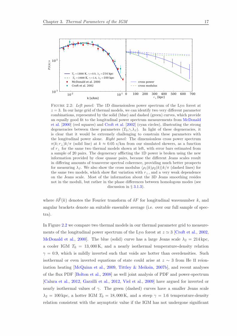
Figure 2.2: Left panel: The 1D dimensionless power spectrum of the Lyα forest atz = 3. In our large grid of thermal models, we can identify two very different parametercombinations, represented by the solid (blue) and dashed (green) curves, which providean equally good fit to the longitudinal power spectrum measurements from McDonaldet al. [2000] (red squares) and Croft et al. [2002] (cyan circles), illustrating the strongdegeneracies between these parameters (T0,γ,λJ). In light of these degeneracies, itis clear that it would be extremely challenging to constrain these parameters withthe longitudinal power alone. Right panel: The dimensionless cross power spectrumπ(k; r⊥)k/π (solid line) at k ≈ 0.05 s/km from our simulated skewers, as a functionof r⊥ for the same two thermal models shown at left, with error bars estimated froma sample of 20 pairs. The degeneracy afflicting the 1D power is broken using the newinformation provided by close quasar pairs, because the different Jeans scales resultin differing amounts of transverse spectral coherence, providing much better prospectsfor measuring λJ . We also show the cross modulus 〈ρ1(k)ρ2(k)〉k/π (dashed lines) forthe same two models, which show flat variation with r⊥, and a very weak dependenceon the Jeans scale. Most of the information about the 3D Jeans smoothing residesnot in the moduli, but rather in the phase differences between homologous modes (see
discussion in § 3.1.3).
where δF (k) denotes the Fourier transform of δF for longitudinal wavenumber k, and
angular brackets denote an suitable ensemble average (i.e. over our full sample of spec-
tra).
In Figure 2.2 we compare two thermal models in our thermal parameter grid to measure-
ments of the longitudinal power spectrum of the Lyα forest at z ≃ 3 [Croft et al., 2002,
McDonald et al., 2000]. The blue (solid) curve has a large Jeans scale λJ = 214 kpc,
a cooler IGM T0 = 13, 000K, and a nearly isothermal temperature-density relation
γ = 0.9, which is mildly inverted such that voids are hotter than overdensities. Such
isothermal or even inverted equations of state could arise at z ∼ 3 from He II reion-
ization heating [McQuinn et al., 2009, Tittley & Meiksin, 2007b], and recent analyses
of the flux PDF [Bolton et al., 2008] as well joint analysis of PDF and power-spectrum
[Calura et al., 2012, Garzilli et al., 2012, Viel et al., 2009] have argued for inverted or
nearly isothermal values of γ. The green (dashed) curves have a smaller Jeans scale
λJ = 100 kpc, a hotter IGM T0 = 18, 000K, and a steep γ = 1.6 temperature-density
relation consistent with the asymptotic value if the IGM has not undergone significant
Chapter 3. Thermal Parameters of the IGM 18
recent heating events [Hui & Gnedin, 1997, Hui & Haiman, 2003]. Thus with regards to
the longitudinal power spectrum, the Jeans scale is clearly degenerate with the amplitude
and slope (T0, γ) of the temperature-density relation. One would clearly come to erro-
neous conclusions about the equation of state parameters (T0,γ) from longitudinal power
spectrum measurements, if the lack of knowledge of the Jeans scale is not marginalized
out [see e.g. Zaldarriaga et al., 2001, for an example of this marginalization].
This degeneracy in the longitudinal power arises because the Jeans filtering smooths the
power in 3D on a scale which project to a longitudinal velocity
vJ =H(z = 3)
1 + 3λJ ≈ 26
(
λJ340 kpc
)
km s−1, (2.9)
resulting in a cutoff of the power at kJ ≈ 0.04 s km−1 (for the typical values assumed in
the introduction1). The thermal Doppler broadening of Lyα absorption lines smooths
the power in 1D, on a scale governed by the b-parameter
b =
√
2kBT
µmp≈ 15.7
(
T
1.5× 10⁴ K
)1/2
km s−1, (2.10)
which results in an analogous cutoff at kth =√2/b ≈ 0.09 s km−1 for a temperature of
15000 K. Above kB is the Boltzmann constant, mp the proton mass, and µ ≈ 0.59 is
the mean molecular weight for a primordial, fully ionized gas. The fact that the two
cutoff scales are comparable results in a strong degeneracy which is very challenging
to disentangle with longitudinal observations alone. Similar degeneracies between the
Jeans scale and (T0,γ) exist if one considers wavelets, the curvature, the b-parameter
distribution, and the flux PDF, which we explore in an upcoming study (Rorai et al.
2013, in prep). In the next section we show that this degeneracy between 3D and
1D smoothing can be broken by exploiting additional information in the transverse
dimension provided by close quasar pairs.
2.3.2 Cross Power Spectrum
The foregoing discussion illustrates that the 3D (Jeans) and 1D (thermal broadening)
smoothing are mixed in the longitudinal power spectrum, and ideally one would measure
the full 3D power spectrum to break this degeneracy. For an isotropic random field the
1We caution that this estimate assumes a thermal history where T ∝ 1 + z, without considering theeffect of HeII reionization. In that case the deduced value for the filtering scale λJ would probably besmaller.
Chapter 3. Thermal Parameters of the IGM 19
1D power spectrum P (k) and the 3D power P3D(k) are related according to
P3D =1
2π
1
k
dP (k)
dk. (2.11)
However, in the Lyα forest redshift-space distortions and thermal broadening result in
an anisotropies that render this expression invalid.
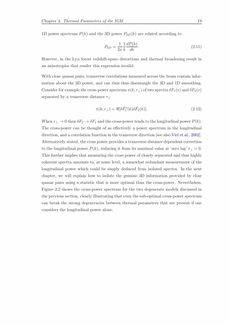
With close quasar pairs, transverse correlations measured across the beam contain infor-
mation about the 3D power, and can thus thus disentangle the 3D and 1D smoothing.
Consider for example the cross-power spectrum π(k, r⊥) of two spectra δF1(v) and δF2(v)
separated by a transverse distance r⊥
π(k; r⊥) = ℜ[δF ∗1 (k)δF2(k)]. (2.12)
When r⊥ → 0 then δF2 → δF1 and the cross-power tends to the longitudinal power P (k).
The cross-power can be thought of as effectively a power spectrum in the longitudinal
direction, and a correlation function in the transverse direction [see also Viel et al., 2002].
Alternatively stated, the cross power provides a transverse distance dependent correction
to the longitudinal power P (k), reducing it from its maximal value at ‘zero lag’ r⊥ = 0.
This further implies that measuring the cross power of closely separated and thus highly
coherent spectra amounts to, at some level, a somewhat redundant measurement of the
longitudinal power which could be simply deduced from isolated spectra. In the next
chapter, we will explain how to isolate the genuine 3D information provided by close
quasar pairs using a statistic that is more optimal than the cross-power. Nevertheless,
Figure 2.2 shows the cross-power spectrum for the two degenerate models discussed in
the previous section, clearly illustrating that even the sub-optimal cross-power spectrum
can break the strong degeneracies between thermal parameters that are present if one
considers the longitudinal power alone.
Chapter 3
Phase Analysis of the Lyman-α
Forest of Quasar Pairs
In the previous chapter I described the general method that we use to estimate the capa-
bility of a given Lyα-forest statistic of discriminating among different thermal models.
Now we need to decide which statistic we want to apply to quasar pairs in order to
extract the transverse coherence information. Our assessment of the ability of quasar
pairs in pinpointing the Jeans scale will be strongly dependent on this choice.
The ideal statistic would have the property of being sensitive to the real-space coherence
of density structure, while being independent on the velocity-space effect such as thermal
broadening and redshift distortions due to peculiar velocities. In doing so, we will elimi-
nate part of the information contained in the spectra which is intrinsically 1-dimensional.
There are at least two good reasons to proceed in this way: the 1-d properties of the
Lyαforest can be studied more effectively in spectra of individual QSOs at the same red-
shifts, which are more frequent and brighter than pairs; along the line of sight, real-space
and velocity-space effects exhibit degeneracies which are difficult to treat. Moreover, an
high sensitivity to redshift-space distortions would raise the requirements on our theo-
retical understanding and on the details of our model, challenging the capabilities of the
simple models that we employ.
In this chapter I will explain how this is achieved by adopting the phase-difference
statistic, whereas the use of the most obvious transverse statistic, i.e. the cross power
or the cross correlation function, would have been ineffective.
20
Chapter 3. Phase Differences 21
3.1 A New Statistic: Phase Differences
Although the cross-power has the ability to break the degeneracy between 3D and 1D
smoothing present in the longitudinal power, we demonstrate here that the cross-power
(or equivalently the cross-correlation function) is however not optimal, and indeed the
genuine 3D information is encapsulated in the phase differences between homologous
Fourier modes.
3.1.1 Drawbacks of the Cross Power Spectrum
Let us write the 1D Fourier transform of the field δF as
δF (k) = ρ(k)eiθ(k) (3.1)
where the complex Fourier coefficient is described by a modulus ρ and phase angle θ,
both of which depend on k. Note that for any ensemble of spectra P (k) = 〈ρ2(k)〉, hencethe modulus ρ(k) is a random draw from a distribution whose variance is given by the
power spectrum. From eqn. (2.12), the cross-power of the two spectra δF1(v) and δF2(v)
is then
π12(k) = ρ1(k)ρ2(k) cos(θ12(k)), (3.2)
where θ12(k) = θ1(k)− θ2(k) is the phase difference between the homologous k−modes.
The distribution of the moduli ρ1 and ρ2 are also governed by P (k), but at small im-
pact parameter they are not statistically independent because of spatial correlations.
Nevertheless, the moduli contain primarily information already encapsulated in the lon-
gitudinal power, and are thus affected by the same thermal parameter degeneracies
that we described in the previous section. For the purpose of constraining the Jeans
scale, we thus opt to ignore the moduli ρ1 and ρ2 altogether, in an attempt to isolate
the genuine 3D information, increasing sensitivity to the Jeans scale, while minimizing
the impact of thermal broadening, removing degeneracies with the temperature-density
relation parameters (T0,γ).
The foregoing points are clearly illustrated by the dashed curves in the right panel of
Figure 2.2, which compares the quantity 〈ρ1(k)ρ2(k)〉 as a function of impact parameter
r⊥ for the same pair of thermal models discussed in § 2.3.1, which are degenerate with
respect to the longitudinal power. The similarity of these two curves reflects the degen-
eracy of the longitudinal power for these two models, and one observes a flat trend with
r⊥ and a very weak dependence on the Jeans scale λJ , substantiating our argument that
the moduli contain primarily 1D information.

Chapter 3. Phase Differences 22
Figure 3.1: Schematic representation of the heuristic argument used to determinethe phase difference distribution: phase are determined by density filaments crossingthe lines of sight of two quasars. If the orientation of the filaments ϕ is isotropicallydistributed then θ′, dependent on the longitudinal distance L = r⊥ tanϕ, follows a
Cauchy distribution.
As the moduli contain minimal information about the 3D power, we are thus motivated
to explore how the phase difference θ12(k) can constrain the Jeans scale. In terms of
Fourier coefficients, θ12(k) can be written
θ12(k) = arccos
ℜ[δF ∗1 (k)δF2(k)]
√
|δF1(k)|2|δF2(k)|2
. (3.3)
Note that because the phase difference is given by a ratio of Fourier modes, it is com-
pletely insensitive to the normalization of δF , and hence to quasar continuum fitting
errors, provided that these errors do not add power on scales comparable to k. In the
remainder of this section, we provide a statistical description of the distribution of phase
differences and we explore the properties and dependencies of this distribution. To sim-
plify notation we will omit the subscript and henceforth denote the phase difference as
simply θ(k, r⊥) = θ1(k) − θ2(k), where r⊥ is the transverse distance between the two
spectra δF1(v) and δF2(v).
3.1.2 An Analytical Form for the PDF of Phase Differences
The phase difference between homologous k-modes is a random variable in the domain
[−π, π], which for a given thermal model, depends on two quantities: the longitudinal
mode in question k and the transverse separation r⊥. One might advocate computing
Chapter 3. Phase Differences 23
the quantity 〈cos θ(k, r⊥)〉 analogous to the cross-power (see eqn. 2.12), or the mean
phase difference 〈θ(k, r⊥)〉, to quantify the coherence of quasar pair spectra. However,
as we will see, the distribution of phase differences is not Gaussian, and hence is not
fully described by its mean and variance. This approach would thus fail to exploit all
the information encoded in its shape. Our goal is then to determine the functional form
of the distribution of phase differences at any (k, r⊥), and relate this to the thermal
parameters governing the IGM. This is a potentially daunting task, since it requires
deriving a unique function in the 2-dimensional space θ(k, r⊥) for any location in our
3-dimensional thermal parameter grid (T0, γ, λJ ). Fortunately, we are able to reduce
the complexity considerably by deriving a simple analytical form for the phase angle
distribution.
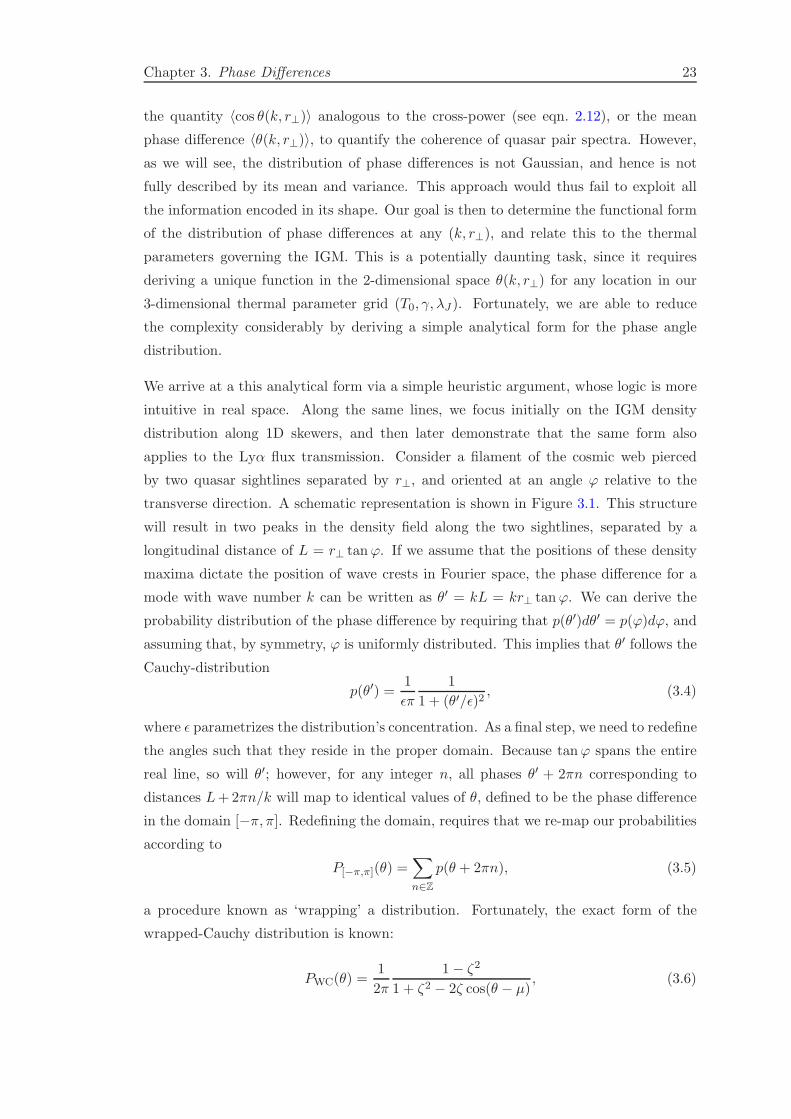
We arrive at a this analytical form via a simple heuristic argument, whose logic is more
intuitive in real space. Along the same lines, we focus initially on the IGM density
distribution along 1D skewers, and then later demonstrate that the same form also
applies to the Lyα flux transmission. Consider a filament of the cosmic web pierced
by two quasar sightlines separated by r⊥, and oriented at an angle ϕ relative to the
transverse direction. A schematic representation is shown in Figure 3.1. This structure
will result in two peaks in the density field along the two sightlines, separated by a
longitudinal distance of L = r⊥ tanϕ. If we assume that the positions of these density
maxima dictate the position of wave crests in Fourier space, the phase difference for a
mode with wave number k can be written as θ′ = kL = kr⊥ tanϕ. We can derive the
probability distribution of the phase difference by requiring that p(θ′)dθ′ = p(ϕ)dϕ, and
assuming that, by symmetry, ϕ is uniformly distributed. This implies that θ′ follows the
Cauchy-distribution
p(θ′) =1
ǫπ
1
1 + (θ′/ǫ)2, (3.4)
where ǫ parametrizes the distribution’s concentration. As a final step, we need to redefine
the angles such that they reside in the proper domain. Because tanϕ spans the entire
real line, so will θ′; however, for any integer n, all phases θ′ + 2πn corresponding to
distances L+2πn/k will map to identical values of θ, defined to be the phase difference
in the domain [−π, π]. Redefining the domain, requires that we re-map our probabilities
according to
P[−π,π](θ) =∑
n∈Z
p(θ + 2πn), (3.5)
a procedure known as ‘wrapping’ a distribution. Fortunately, the exact form of the
wrapped-Cauchy distribution is known:
PWC(θ) =1
2π
1− ζ2
1 + ζ2 − 2ζ cos(θ − µ), (3.6)

Chapter 3. Phase Differences 24
where µ = 〈θ〉 is the mean value (in our case µ = 0 by symmetry), and ζ is a concentra-
tion parameter between 0 and 1, which is the wrapped analog of ǫ above. In the limit
where ζ → 1 the distribution tends to a Dirac delta function δD(x), which is the behav-
ior expected for identical spectra. Conversely, ζ = 0 results in a uniform distribution,
the behavior expected for uncorrelated spectra. A negative ζ gives distributions peaked
at θ = π and is unphysical in this context.
3.1.3 The Probability Distribution of Phase Differences of the IGM
Density
We now show that this wrapped-Cauchy form does a good job of describing the real
distribution of phase differences for our simulated IGM density skewers. Note that for our
simple heuristic example of randomly oriented filaments, the concentration parameter
ζ only depends on the product of kr⊥; whereas, in the real IGM, one expects the
spectral coherence quantified by ζ to depend on the Jeans scale λJ . Because we do not
know how to directly compute the concentration parameter in terms of the Jeans scale
from first principles, we opt to calculate ζ from our simulations. At any longitudinal
wavenumber k, pair separation r⊥, and Jeans scale λJ , our density skewers provide a
discrete sampling of the θ distribution. We use the maximum likelihood procedure from
Jammalamadaka & Sengupta [2001] to calculate the best-fit value of ζ from an ensemble
of θ values, as described further in Appendix B. Figure 3.2 shows the distribution of
phases determined from our IGM density skewers (symbols with error bars) compared
to the best-fit wrapped-Cauchy distributions (curves) for different longitudinal modes k,
transverse separations r⊥, and values of the Jeans scale λJ . We see that the wrapped-
Cauchy distribution typically provides a good fit to the simulation data points to within
the precision indicated by the error bars. For very peaked distributions which correspond
to more spectral coherence (i.e. low-k or large λJ), there is a tendency for our wrapped-
Cauchy fits to overestimate the probability of large phase differences relative to the
simulated data, although our measurements of the probability are very noisy in this
regime. We have visually inspected similar curves for the entire dynamic range of the
relevant k, r⊥ and λJ , for which the shape of the wrapped-Cauchy distribution varies
from nearly uniform (ζ ≃ 0) to a very high degree of coherence (ζ ≃ 1), and find similarly
good agreement.
It is instructive to discuss the primary dependencies of the phase difference distribution
on wavenumber k, separation r⊥, and the Jeans scale λJ illustrated in Figure 3.2. At a
fixed wavenumber k, a large separation relative to the Jeans scale results in a flatter dis-
tribution of θ, which approaches uniformity for r⊥ ≫ λJ . The distribution approaches
the fully coherent limit of a Dirac delta function for r⊥ ≪ λJ , and the transitions from

Chapter 3. Phase Differences 25
0.01
0.10
1.00
10.00
p(θ)
k=4.7x10⁻³ s/kmλ = 17.9 Mpc
0.01
0.10
1.00
10.00
p(θ)
k=1.5x10⁻² s/kmλ = 5.6 Mpc
0.01
0.10
1.00
10.00
p(θ)
k=3.7x10⁻² s/kmλ = 2.2 Mpc
0 π/4 π/2 3π/4 θ
0.01
0.10
1.00
10.00
p(θ)
k=9.4x10⁻² s/kmλ = 0.9 Mpc
0 π/4 π/2 3π/4 θ
0 π/4 π/2 3π/4 θ
0 π/4 π/2 3π/4 θ
λJ = 50 kpc
λJ = 100 kpcλJ = 200 kpc
r⊥ = 71 kpc r⊥ = 142 kpc r⊥ = 333 kpc r⊥ = 666 kpc
Figure 3.2: Phase difference probability functions of the density fields at differentseparations r⊥, wavenumbers k and Jeans scale λJ . Points with errorbars represent thebinned phase distribution of the density field as obtained from the simulation, whilethe solid lines are the best-likelihood fit using a wrapped-Cauchy distribution. Whenthe spectra are highly correlated the phases are small and the distribution is peakedaround zero, whereas independent skewers result in flat probability functions. Theerror are estimated from the number of modes available in the simulation, assuming aPoisson distribution. By symmetry p(θ) must be even in θ, hence it is convenient toplot only the range [0, π], summing positive and negative probabilities (clearly obtainingp(|θ|) ) to increase the sampling in each bin. We express the scale of each mode bothgiving the wavelength λ in Mpc and the wave number k (in s km−1) in the transformedvelocity space. The wrapped-Cauchy function traces with good approximation thephase distribution obtained from the simulation, showing less accuracy in the casesof strongly concentrated peaks, where low-probability bins are noisy. Each color isa different smoothing length: λJ = 50, 100 and 200 kpc (respectively black, red andblue). It is important to notice that the relative distributions are different not onlyat scales comparable to λJ , but also for larger modes, because the 3D power of high-kmodes when projected on a 1D line contributes to all the low-k components (see thetext for a detailed discussion). Secondly, it is clear that the most relevant pairs are theclosest (r⊥ . λJ), because for wide separations the coherence is too low to get usefulinformation. These two consideration together explain why close quasar pairs are themost effective objects to measure the Jeans scale, even if they cannot be observed at
high resolution.

Chapter 3. Phase Differences 26
a strongly peaked distribution to a uniform one occurs when r⊥ is comparable to the
Jeans scale λJ . We see that quasar pairs with transverse separations r⊥ . 3λJ , contain
information about the Jeans scale, whereas this sensitivity vanishes for larger impact
parameters. At fixed r⊥, lower k-modes (i.e. larger scales) are more highly correlated
(smaller θ values) as expected, because sightlines spaced closely relative to the wave-
length of the mode kr⊥ ≪ 1, probe essentially the same large scale density fluctuation.
Overall, the dependencies in Figure 3.2 illustrate that there is information about the
Jeans smoothing spread out over a large range of longitudinal k-modes. Somewhat sur-
prisingly, even modes corresponding to wavelengths & 100 times larger than λJ can
potentially constrain the Jean smoothing.
This sensitivity of very large-scale longitudinal k-modes to a much smaller scale cutoff
λJ in the 3D power merits further discussion. First, note that the range of wavenum-
bers typically probed by longitudinal power spectra of the Lyα forest lie in the range
0.005 s km−1 < k < 0.1 s km−1 (see Figure 2.2), corresponding to modes with wave-
lengths 60 km s−1 < v < 1250 km s−1 or 830 kpc < λ < 17Mpc. Here the low-k cutoff
is set by systematics related to determining the quasar continuum [see e.g. Lee, 2012],
whereas the high-k cutoff is adopted to mitigate contamination of the small-scale power
from metal absorption lines [McDonald et al., 2000]. In principle high-resolution (echelle)
spectra FWHM= 5km s−1 probe even higher wavenumbers as large as k ≃ 3, however
standard practice is to only consider k . 0.1 in model-fitting [see e.g. Zaldarriaga et al.,
2001]. Thus even the highest k-modes at our disposable k ≃ 0.1 correspond to wave-
lengths ≃ 830 kpc significantly larger than our expectation for the Jeans scale ∼ 100 kpc.
Furthermore, we saw in § 2.3.1 that degenerate combinations of the Jeans smoothing
and the IGM temperature-density relation can produce the same small-scale cutoff in
the longitudinal power. Thus both metal-line contamination and degeneracies with ther-
mal broadening imply that while it is extremely challenging to resolve the Jeans scale
spectrally, the great advantage of close quasar pairs is that they resolve the Jeans scale
spatially, provided they have transverse separations r⊥ comparable to λJ . We will thus
typically be working in the regime where k/k⊥ ≪ 1, where we define k⊥ ≡ x0/aHr⊥,
where aHr⊥ is the transverse separation converted to a velocity and x0 = 2.4048 is a
constant the choice of which will become clear below.
In this regime, it is straightforward to understand why the phase differences between
large-scale modes are nevertheless sensitive to the Jeans scale. Consider the quantity
〈cos θ(k, r⊥)〉, which is related to the cross-power discussed in § 3.1.1. This ‘moment’ of
the phase angle PDF can be written
〈cos θ(k, r⊥)〉 =∫ π
−πP (θ(k, r⊥)) cos θ(k, r⊥)dθ, (3.7)
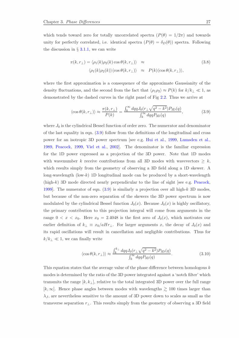
Chapter 3. Phase Differences 27
which tends toward zero for totally uncorrelated spectra (P (θ) = 1/2π) and towards
unity for perfectly correlated, i.e. identical spectra (P (θ) = δD(θ)) spectra. Following
the discussion in § 3.1.1, we can write
π(k, r⊥) = 〈ρ1(k)ρ2(k) cos θ(k, r⊥)〉 ≈ (3.8)
〈ρ1(k)ρ2(k)〉〈cos θ(k, r⊥)〉 ≈ P (k)〈cos θ(k, r⊥)〉,
where the first approximation is a consequence of the approximate Gaussianity of the
density fluctuations, and the second from the fact that 〈ρ1ρ2〉 ≈ P (k) for k/k⊥ ≪ 1, as
demonstrated by the dashed curves in the right panel of Fig 2.2. Thus we arrive at
〈cos θ(k, r⊥)〉 ≈π(k, r⊥)
P (k)=
∫∞k dqqJ0(r⊥
√
q2 − k2)P3D(q)∫∞k dqqP3D(q)
, (3.9)
where J0 is the cylindrical Bessel function of order zero. The numerator and denominator
of the last equality in eqn. (3.9) follow from the definitions of the longitudinal and cross
power for an isotropic 3D power spectrum [see e.g. Hui et al., 1999, Lumsden et al.,
1989, Peacock, 1999, Viel et al., 2002]. The denominator is the familiar expression
for the 1D power expressed as a projection of the 3D power. Note that 1D modes
with wavenumber k receive contributions from all 3D modes with wavevectors ≥ k,
which results simply from the geometry of observing a 3D field along a 1D skewer. A
long-wavelength (low-k) 1D longitudinal mode can be produced by a short-wavelength
(high-k) 3D mode directed nearly perpendicular to the line of sight [see e.g. Peacock,
1999]. The numerator of eqn. (3.9) is similarly a projection over all high-k 3D modes,
but because of the non-zero separation of the skewers the 3D power spectrum is now
modulated by the cylindrical Bessel function J0(x). Because J0(x) is highly oscillatory,
the primary contribution to this projection integral will come from arguments in the
range 0 < x < x0. Here x0 = 2.4048 is the first zero of J0(x), which motivates our
earlier definition of k⊥ ≡ x0/aHr⊥. For larger arguments x, the decay of J0(x) and
its rapid oscillations will result in cancellation and negligible contributions. Thus for
k/k⊥ ≪ 1, we can finally write
〈cos θ(k, r⊥)〉 ≈∫ k⊥k dqqJ0(r⊥
√
q2 − k2)P3D(q)∫∞k dqqP3D(q)
. (3.10)
This equation states that the average value of the phase difference between homologous k
modes is determined by the ratio of the 3D power integrated against a ‘notch filter’ which
transmits the range [k, k⊥], relative to the total integrated 3D power over the full range
[k,∞]. Hence phase angles between modes with wavelengths & 100 times larger than
λJ , are nevertheless sensitive to the amount of 3D power down to scales as small as the
transverse separation r⊥. This results simply from the geometry of observing a 3D field

Chapter 3. Phase Differences 28
0.01
0.10
1.00
10.00p(
θ)k=4.7x10⁻³ s/km
λ = 17.9 Mpc
0.01
0.10
1.00
10.00
p(θ)
k=1.5x10⁻² s/kmλ = 5.6 Mpc
0.01
0.10
1.00
10.00
p(θ)
k=3.7x10⁻² s/kmλ = 2.2 Mpc
0 π/4 π/2 3π/4 θ
0.01
0.10
1.00
10.00
p(θ)
k=9.4x10⁻² s/kmλ = 0.9 Mpc
0 π/4 π/2 3π/4 θ
0 π/4 π/2 3π/4 θ
0 π/4 π/2 3π/4 θ
λJ = 200 kpcλJ = 100 kpcλJ = 50 kpc
r⊥ = 71 kpc r⊥ = 142 kpc r⊥ = 333 kpc r⊥ = 666 kpc
Figure 3.3: Same plot of figure 3.2 but for the Lyα transmitted flux field instead ofdensity. We vary the Jeans scale λJ , keeping fixed the equation-of-state parameters,T0 = 10000 K and γ = 1.6. The properties of the distributions are analogous to theprevious plot, they follow with good approximation a wrapped-Cauchy profile and theyexhibit the same trends with r⊥, k and λJ . Overall, the flux shows an higher degree of
coherence and a slightly smaller sensitivity to λJ .
along 1D skewers, because the power in longitudinal mode k is actually dominated by
the superposition of 3D power from much smaller scales ≫ k. Provided that quasar pair
separations resolve the Jeans scale r⊥ ∼ λJ , even large scale modes with k ≪ k⊥ ∼ 1/λJ
are sensitive to the shape of the 3D power on small-scales, which explains the sensitivity
of low-k modes to the Jeans scale in Figure 3.2.
Finally, the form of eqn. (3.10) combined with eqn. (3.7) explains the basic qualitative
trends in Figure 3.2. For large r⊥ (small k⊥) the projection integral in the numer-
ator decreases, 〈cos θ(k, r⊥)〉 approaches zero, indicating that P (θ(k, r⊥)) approaches
uniformity. Similarly, as r⊥ → λJ , 〈cos θ(k, r⊥)〉 grows indicating that P (θ(k, r⊥)) is
peaked toward small phase angles, and in the limit r⊥ ≪ λJ 〈cos θ(k, r⊥)〉 → 1 and
P (θ(k, r⊥)) approaches a Dirac delta function. At fixed r⊥, lower k modes will result in
more common pathlength in the projection integrals in the numerator and denominator
of eqn. (3.10), thus 〈cos θ(k, r⊥)〉 is larger, P (θ(k, r⊥)) is more peaked, and the phase
angles are more highly correlated.
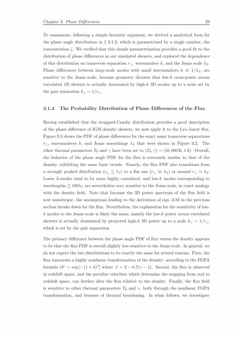
Chapter 3. Phase Differences 29
To summarize, following a simple heuristic argument, we derived a analytical form for
the phase angle distribution in § 3.1.2, which is parametrized by a single number, the
concentration ζ. We verified that this simple parametrization provides a good fit to the
distribution of phase differences in our simulated skewers, and explored the dependence
of this distribution on transverse separation r⊥, wavenumber k, and the Jeans scale λJ .
Phase differences between large-scale modes with small wavenumbers k ≪ 1/λJ , are
sensitive to the Jeans scale, because geometry dictates that low-k cross-power across
correlated 1D skewers is actually dominated by high-k 3D modes up to a scale set by
the pair separation k⊥ ∼ 1/r⊥.
3.1.4 The Probability Distribution of Phase Differences of the Flux
Having established that the wrapped-Cauchy distribution provides a good description
of the phase difference of IGM density skewers, we now apply it to the Lyα forest flux.
Figure 3.3 shows the PDF of phase differences for the exact same transverse separations
r⊥, wavenumbers k, and Jeans smoothings λJ that were shown in Figure 3.2. The
other thermal parameters T0 and γ have been set to (T0, γ) = (10, 000K, 1.6). Overall,
the behavior of the phase angle PDF for the flux is extremely similar to that of the
density, exhibiting the same basic trends. Namely, the flux PDF also transitions from
a strongly peaked distribution (r⊥ . λJ) to a flat one (r⊥ ≫ λJ) at around r⊥ ≃ λJ .
Lower k-modes tend to be more highly correlated, and low-k modes corresponding to
wavelengths & 100λJ are nevertheless very sensitive to the Jeans scale, in exact analogy
with the density field. Note that because the 3D power spectrum of the flux field is
now anisotropic, the assumptions leading to the derivation of eqn. 3.10 in the previous
section breaks down for the flux. Nevertheless, the explanation for the sensitivity of low-
k modes to the Jeans scale is likely the same, namely the low-k power across correlated
skewers is actually dominated by projected high-k 3D power up to a scale k⊥ ∼ 1/r⊥,
which is set by the pair separation.
The primary difference between the phase angle PDF of flux versus the density appears
to be that the flux PDF is overall slightly less sensitive to the Jeans scale. In general, we
do not expect the two distributions to be exactly the same for several reasons. First, the
flux represents a highly nonlinear transformation of the density: according to the FGPA
formula δF ∼ exp [−(1 + δ)β ] where β = 2 − 0.7(γ − 1). Second, the flux is observed
in redshift space, and the peculiar velocities which determine the mapping from real to
redshift space, can further alter the flux relative to the density. Finally, the flux field
is sensitive to other thermal parameters T0 and γ, both through the nonlinear FGPA
transformation, and because of thermal broadening. In what follows, we investigate

Chapter 3. Phase Differences 30
0.01
0.10
1.00
10.00p(
θ)k=4.7x10⁻³ s/km
λ = 17.9 Mpc
0.01
0.10
1.00
10.00
p(θ)
k=1.5x10⁻² s/kmλ = 5.6 Mpc
0.01
0.10
1.00
10.00
p(θ)
k=3.7x10⁻² s/kmλ = 2.2 Mpc
0 π/4 π/2 3π/4 θ
0.01
0.10
1.00
10.00
p(θ)
k=9.4x10⁻² s/kmλ = 0.9 Mpc
0 π/4 π/2 3π/4 θ
0 π/4 π/2 3π/4 θ
0 π/4 π/2 3π/4 θ
flux
densityflux, v=0
r⊥ = 71 kpc r⊥ = 142 kpc r⊥ = 333 kpc r⊥ = 666 kpc
Figure 3.4: Phase difference probability density functions for different separations r⊥and wavenumbers k. All models have the same Jeans scale λJ = 140 kpc. For clarity weplot only the best-fit wrapped-Cauchy function without simulated points with errorbars.The black and the red lines are the phase angle PDFs for the transmitted flux of theLyαforest and the IGM density field, respectively. The green line represents the case ofthe Lyαforest flux where peculiar velocities are set to zero. By comparing the green andthe black lines we see that in peculiar motions always increase the coherence betweenthe two sightlines, which partly explains the differences between the flux and densitydistributions, since the latter is calculated in real space. The flux and density furtherdiffer because of the non-linear FGPA transformation, which has a stronger effect on
smaller scale modes.
each of these effects in turn, and discuss how each alters the phase angle PDF and its
sensitivity to the Jeans scale.
In Figure 3.4 we show the flux PDF (black) alongside the density PDF (red) for various
modes and separations, again with the thermal model fixed to (T0, γ, λJ ) = (20, 000 K, 1.0, 140)
kpc. To isolate the impact of peculiar velocities, we also compute the phase angle PDF
of the real-space flux, i.e. without peculiar velocities (green). Specifically, we disable
peculiar velocities by computing the flux from eqn. (2.6) with vp,‖ set to zero. Overall,
the PDFs of the real-space flux and density (also real-space) are quite similar. For low
wavenumbers, the real-space flux skewers are always slightly more coherent than the
density (P (θ) more peaked) for all separations. However, at the highest k, the situation

Chapter 3. Phase Differences 31
0.01
0.10
1.00
10.00p(
θ)k=4.7x10⁻³ s/km
λ = 17.9 Mpc
0.01
0.10
1.00
10.00
p(θ)
k=1.5x10⁻² s/kmλ = 5.6 Mpc
0.01
0.10
1.00
10.00
p(θ)
k=3.7x10⁻² s/kmλ = 2.2 Mpc
0 π/4 π/2 3π/4 θ
0.01
0.10
1.00
10.00
p(θ)
k=9.4x10⁻² s/kmλ = 0.9 Mpc
0 π/4 π/2 3π/4 θ
0 π/4 π/2 3π/4 θ
0 π/4 π/2 3π/4 θ
T0 =1.4× 10⁴ K, γ =0.8T0 =2.4× 10⁴ K, γ =1.2T0 =0.7× 10⁴ K, γ =1.7
r⊥ = 71 kpc r⊥ = 142 kpc r⊥ = 333 kpc r⊥ = 666 kpc
Figure 3.5: Phase difference probability density functions for different separationsr⊥, wavenumbers k and equation-of-state parameters T0 − γ. Points with errorbars(estimated Poisson error) are the results of our simulations, while the coloured lines arethe best-likelihood fit using a wrapped-Cauchy distribution. All models have the sameJeans scale λJ = 140 kpc. This plot shows the most remarkable property of phases:they do not exhibit any relevant sensitivity to the equation of state, so they robustly
constrain the spatial coherence given by pressure support.
is reversed with the density being more coherent than the real-space flux. A detailed
explanation of the relationship between the phase angle PDF of the real-space flux and
the density fields requires a better understanding of the effect of the non-linear FGPA
transformation on the 2-point function of the flux, which is beyond the scope of the
present work. Here we only argue that the 3D power spectrum of the real-space flux
has in general a different shape than that of the density, and using our intuition from
eqn. (3.10), this will result in a different shape for the distribution of phase angles. The
net effect of peculiar velocities on the redshift-space flux PDF is to increase the amount
of coherence between the two sightlines (P (θ) more peaked) relative to the real-space
flux. This likely arises because the peculiar velocity field is dominated by large-scale
power, which makes the 3D power of the flux steeper as a function of k. Again based
on our intuition from eqn. (3.9), a steeper power spectrum will tend to increase the
coherence (〈cos(θ(k, r⊥))〉 closer to unity), because the projection integrals in the nu-
merator and denominator of eqn. (3.9) will both have larger relative contributions from
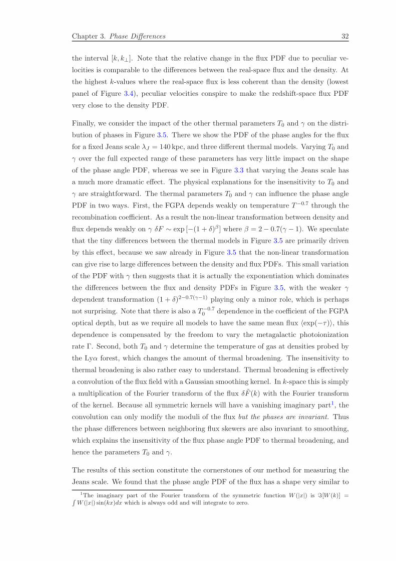
Chapter 3. Phase Differences 32
the interval [k, k⊥]. Note that the relative change in the flux PDF due to peculiar ve-
locities is comparable to the differences between the real-space flux and the density. At
the highest k-values where the real-space flux is less coherent than the density (lowest
panel of Figure 3.4), peculiar velocities conspire to make the redshift-space flux PDF
very close to the density PDF.
Finally, we consider the impact of the other thermal parameters T0 and γ on the distri-
bution of phases in Figure 3.5. There we show the PDF of the phase angles for the flux
for a fixed Jeans scale λJ = 140 kpc, and three different thermal models. Varying T0 and
γ over the full expected range of these parameters has very little impact on the shape
of the phase angle PDF, whereas we see in Figure 3.3 that varying the Jeans scale has
a much more dramatic effect. The physical explanations for the insensitivity to T0 and
γ are straightforward. The thermal parameters T0 and γ can influence the phase angle
PDF in two ways. First, the FGPA depends weakly on temperature T−0.7 through the
recombination coefficient. As a result the non-linear transformation between density and
flux depends weakly on γ δF ∼ exp [−(1 + δ)β ] where β = 2− 0.7(γ − 1). We speculate
that the tiny differences between the thermal models in Figure 3.5 are primarily driven
by this effect, because we saw already in Figure 3.5 that the non-linear transformation
can give rise to large differences between the density and flux PDFs. This small variation
of the PDF with γ then suggests that it is actually the exponentiation which dominates
the differences between the flux and density PDFs in Figure 3.5, with the weaker γ
dependent transformation (1 + δ)2−0.7(γ−1) playing only a minor role, which is perhaps
not surprising. Note that there is also a T−0.70 dependence in the coefficient of the FGPA
optical depth, but as we require all models to have the same mean flux 〈exp(−τ)〉, thisdependence is compensated by the freedom to vary the metagalactic photoionization
rate Γ. Second, both T0 and γ determine the temperature of gas at densities probed by
the Lyα forest, which changes the amount of thermal broadening. The insensitivity to
thermal broadening is also rather easy to understand. Thermal broadening is effectively
a convolution of the flux field with a Gaussian smoothing kernel. In k-space this is simply
a multiplication of the Fourier transform of the flux δF (k) with the Fourier transform
of the kernel. Because all symmetric kernels will have a vanishing imaginary part1, the
convolution can only modify the moduli of the flux but the phases are invariant. Thus
the phase differences between neighboring flux skewers are also invariant to smoothing,
which explains the insensitivity of the flux phase angle PDF to thermal broadening, and
hence the parameters T0 and γ.
The results of this section constitute the cornerstones of our method for measuring the
Jeans scale. We found that the phase angle PDF of the flux has a shape very similar to
1The imaginary part of the Fourier transform of the symmetric function W (|x|) is ℑ[W (k)] =∫W (|x|) sin(kx)dx which is always odd and will integrate to zero.
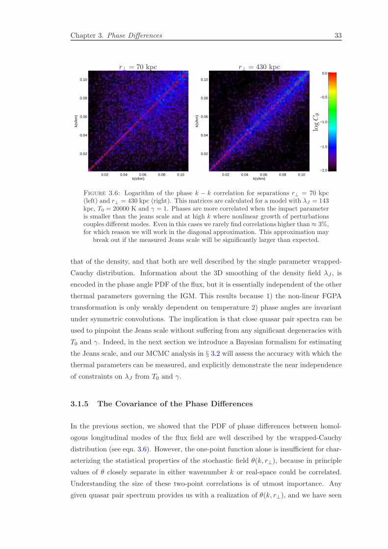
Chapter 3. Phase Differences 33
0.02 0.04 0.06 0.08 0.10k(s/km)
0.02
0.04
0.06
0.08
0.10k(
s/km
)
0.02 0.04 0.06 0.08 0.10k(s/km)
0.02
0.04
0.06
0.08
0.10
k(s/
km)
−2.0
−1.5
−1.0
−0.5
0.0
r⊥ = 70 kpc r⊥ = 430 kpc
logCθ
Figure 3.6: Logarithm of the phase k − k correlation for separations r⊥ = 70 kpc(left) and r⊥ = 430 kpc (right). This matrices are calculated for a model with λJ = 143kpc, T0 = 20000 K and γ = 1. Phases are more correlated when the impact parameteris smaller than the jeans scale and at high k where nonlinear growth of perturbationscouples different modes. Even in this cases we rarely find correlations higher than ≈ 3%,for which reason we will work in the diagonal approximation. This approximation may
break out if the measured Jeans scale will be significantly larger than expected.
that of the density, and that both are well described by the single parameter wrapped-
Cauchy distribution. Information about the 3D smoothing of the density field λJ , is
encoded in the phase angle PDF of the flux, but it is essentially independent of the other
thermal parameters governing the IGM. This results because 1) the non-linear FGPA
transformation is only weakly dependent on temperature 2) phase angles are invariant
under symmetric convolutions. The implication is that close quasar pair spectra can be
used to pinpoint the Jeans scale without suffering from any significant degeneracies with
T0 and γ. Indeed, in the next section we introduce a Bayesian formalism for estimating
the Jeans scale, and our MCMC analysis in § 3.2 will assess the accuracy with which the
thermal parameters can be measured, and explicitly demonstrate the near independence
of constraints on λJ from T0 and γ.
3.1.5 The Covariance of the Phase Differences
In the previous section, we showed that the PDF of phase differences between homol-
ogous longitudinal modes of the flux field are well described by the wrapped-Cauchy
distribution (see eqn. 3.6). However, the one-point function alone is insufficient for char-
acterizing the statistical properties of the stochastic field θ(k, r⊥), because in principle
values of θ closely separate in either wavenumber k or real-space could be correlated.
Understanding the size of these two-point correlations is of utmost importance. Any
given quasar pair spectrum provides us with a realization of θ(k, r⊥), and we have seen

Chapter 3. Phase Differences 34
that the distribution of these values depends sensitively on the Jeans scale λJ . In order
to devise an estimator for the thermal parameters in terms of the phase differences, we
have to understand the degree to which the θ(k, r⊥) are independent.
It is easy to rule out the possibility of spatial correlations among the θ values deduced
from distinct quasar pairs. Because quasar pairs are extremely rare on the sky, the
individual quasar pairs in any observed sample will typically be ∼ Gpc away from each
other, and hence different pairs will never probe correlated small-scale density fluctua-
tions. However, the situation is much less obvious when it comes to correlations between
θ values for different k-modes of the same quasar pair. In particular, nonlinear structure
formation evolution will result in mode-mode coupling, which can induce correlations
between mode amplitudes and phases [e.g. Chiang et al., 2002, Coles, 2009, Watts et al.,
2003]. We are thus motivated to use our simulated skewers to directly quantity the size
of the correlations between phase differences of distinct longitudinal k-modes.
We calculate the correlation coefficient matrix of θ between modes k and k′ defined as
Cθ(k, k′; r⊥) =
〈θ(k, r⊥)θ(k′, r⊥)〉√
〈θ2(k, r⊥)〉 〈θ2(k′, r⊥)〉. (3.11)
Our standard setup of 330 pairs at each discrete separation r⊥ results in a very noisy
estimate of Cθ(k, k′; r⊥), so we proceed by defining a new set of 80,000 skewers at two
distinct discrete transverse separations of r⊥ = 70 kpc and r⊥ = 430 kpc for a single
thermal model with (T0, γ, λJ ) = (20, 000K, 1, 143 kpc).
Figure 3.6 displays the correlation coefficient matrix for the two separations r⊥ that we
simulated. We find that the off-diagonal correlations between k-modes are highest at
high k values and for smaller impact parameters. This is the expected behavior, since
higher longitudinal k-modes will have a larger relative contributions from higher-k 3D
modes, which will be more non-linear and have larger mode-mode correlations. Likewise,
as per the discussion in § 3.1.3, phase differences at smaller pair separations r⊥ are
sensitive to higher k 3D power ∼ k⊥, and should similarly exhibit larger correlations
between modes. Note however that over the range of longitudinal k values which we will
use to constrain the Jeans scale 0.005 < k < 0.1, the size of the off-diagonal elements
are always very small, of the order of ∼ 1− 3%.
The small values of the off-diagonal elements indicates that the mode-mode coupling
resulting from non-linear evolution does not result in significant correlations between
the phase angles of longitudinal modes. This could result from the fact that the intrinsic
phase correlations of the 3D modes is small, and it is also possible that the projection of
power inherent to observing along 1D skewers (see § 3.1.3) dilutes these intrinsic phase
correlations, because a given longitudinal mode is actually the average over a large
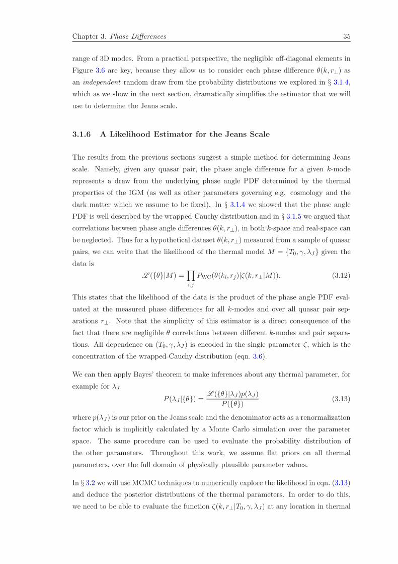
Chapter 3. Phase Differences 35
range of 3D modes. From a practical perspective, the negligible off-diagonal elements in
Figure 3.6 are key, because they allow us to consider each phase difference θ(k, r⊥) as
an independent random draw from the probability distributions we explored in § 3.1.4,
which as we show in the next section, dramatically simplifies the estimator that we will
use to determine the Jeans scale.
3.1.6 A Likelihood Estimator for the Jeans Scale
The results from the previous sections suggest a simple method for determining Jeans
scale. Namely, given any quasar pair, the phase angle difference for a given k-mode
represents a draw from the underlying phase angle PDF determined by the thermal
properties of the IGM (as well as other parameters governing e.g. cosmology and the
dark matter which we assume to be fixed). In § 3.1.4 we showed that the phase angle
PDF is well described by the wrapped-Cauchy distribution and in § 3.1.5 we argued that
correlations between phase angle differences θ(k, r⊥), in both k-space and real-space can
be neglected. Thus for a hypothetical dataset θ(k, r⊥) measured from a sample of quasar
pairs, we can write that the likelihood of the thermal model M = T0, γ, λJ given the
data is
L (θ|M) =∏
i,j
PWC(θ(ki, rj)|ζ(k, r⊥|M)). (3.12)
This states that the likelihood of the data is the product of the phase angle PDF eval-
uated at the measured phase differences for all k-modes and over all quasar pair sep-
arations r⊥. Note that the simplicity of this estimator is a direct consequence of the
fact that there are negligible θ correlations between different k-modes and pair separa-
tions. All dependence on (T0, γ, λJ ) is encoded in the single parameter ζ, which is the
concentration of the wrapped-Cauchy distribution (eqn. 3.6).
We can then apply Bayes’ theorem to make inferences about any thermal parameter, for
example for λJ
P (λJ |θ) =L (θ|λJ )p(λJ)
P (θ) (3.13)
where p(λJ) is our prior on the Jeans scale and the denominator acts as a renormalization
factor which is implicitly calculated by a Monte Carlo simulation over the parameter
space. The same procedure can be used to evaluate the probability distribution of
the other parameters. Throughout this work, we assume flat priors on all thermal
parameters, over the full domain of physically plausible parameter values.
In § 3.2 we will use MCMC techniques to numerically explore the likelihood in eqn. (3.13)
and deduce the posterior distributions of the thermal parameters. In order to do this,
we need to be able to evaluate the function ζ(k, r⊥|T0, γ, λJ) at any location in thermal
Chapter 3. Phase Differences 36
parameter space. This is a non-trivial computational issue, because we do not have a
closed form analytical expression for ζ which can be evaluated quickly, and thus have to
resort to our cosmological simulations of the IGM to numerically determine it for each
model, as described in Appendix B. In practice, computational constraints limit the size
of our thermal parameter grid to only 500 thermal models, and we thus evaluate ζ at
only these 500 fixed locations. The fast procedure described in the previous chapter
(the emulator) allows us to interpolate ζ from these 500 locations in our finite thermal
parameter grid, onto any value in thermal parameter space (T0, γ, λJ ).
To summarize, our method for measuring the Jeans scale of the IGM involves the fol-
lowing steps:
• Calculate the phase differences θ(k, r⊥) for each k-mode of an observed sample of
quasar pairs with separations r⊥.
• Generate Lyα forest quasar pair spectra for a grid of thermal models in the parame-
ter space (T0, γ, λJ ), using our IGM simulation framework. For each model, numer-
ically determine the concentration parameter ζ(k, r⊥|T0, γ, λJ ) at each wavenum-
ber k and separation r⊥, from the distribution of phase differences θ(k, r⊥).
• Emulate the function ζ(k, r⊥|T0, γ, λJ ), enabling fast interpolation of ζ from the
fixed values in the thermal parameter grid to any location in thermal parameter
space.
• Calculate the posterior distribution in eqn. (3.13) for λJ , by exploring the likeli-
hood function in eqn. (3.12) with an MCMC algorithm.
3.2 How Well Can We Measure the Jeans Scale?
Our goal in this section is to determine the precision with which close quasar pair spec-
tra can be used to measure the Jeans scale. To this end, we construct a mock quasar
pair dataset from our IGM simulations and apply our new phase angle PDF likelihood
formalism to it. A key question is how well constraints from our new phase angle tech-
nique compare to those obtainable from alternative measures, such as the cross-power
spectrum, applied to the same pair sample, or from the longitudinal power spectrum,
measured from samples of individual quasars. In what follows, we first present the likeli-
hood used to determine thermal parameter constraints for these two additional statistics.
Then we describe the specific assumptions made for the mock data. Next we quantify the
resulting precision on the Jeans scale, explore degeneracies with other thermal param-
eters, and compare to constraints from these two alternative statistics. We explore the
Chapter 3. Phase Differences 37
impact of finite signal-to-noise ratio and spectral resolution on our measurement accu-
racy, and discuss possible sources of systematic error. Finally, we explicitly demonstrate
that our likelihood estimator provides unbiased determinations of the Jeans scale.
3.2.1 The Likelihood for P (k) and π(k, r⊥)
For the longitudinal power P (k), we assume that the distribution of differences, between
the measured band powers of a k-bin and the true value, is a multi-variate Gaussian
[see e.g. McDonald et al., 2006], which leads to the standard likelihood for the power-
spectrum
L (Pd|M) = (2π)−N/2 det (Σ)−1/2 (3.14)
exp
[
−1
2(Pd − PM )TΣ−1(Pd − PM )
]
,
where Pd is a vector of N observed 1D band powers, PM is a vector of power spectrum
predictions for a given thermal model M = (T0, γ, λJ ), and
Σ(k, k′) = 〈[P (k)− PM (k)][P (k′)− PM (k′)]〉, (3.15)
is the full covariance matrix of the power spectrum measurement. As we describe in the
next subsection, we will choose a subset of the skewers from a fiducial thermal model
to represent the ‘data’ in this expression, which are then compared directly to thermal
models (T0, γ, λJ ), where the same emulator technique described in § 2.2 is used to
interpolate PM (k|T0, γ, λJ ) to parameter locations in the thermal space. To determine
the covariance of this mock data Σ(k, k′), we use the full ensemble of 2 × 10, 000 1D
skewers for the fiducial thermal model, directly evaluate the covariance matrix, and then
rescale it to the size of our mock dataset by multiplying by the ratio of the diagonal terms
σ2dataset/σ2full. This procedure of evaluating the covariance implicitly assumes that the
only source of noise in the measurement is sample variance, or that the instrument
noise is negligible. For the high-resolution and high signal-to-noise ratio spectra used
to measure the longitudinal power spectrum cutoff [Croft et al., 2002, McDonald et al.,
2000], this is a reasonable assumption. For reference, the relative magnitude of off-
diagonal terms of the covariance, Σ(k, k′)/√
Σ(k, k)Σ(k′, k′), are at most 20− 30% with
the largest values attained at the highest k.
For the cross-power spectrum π(k, r⊥), we follow the same procedure. Namely, a mock
dataset is constructed for the fiducial thermal model by taking a subset of the full
ensemble of quasar pair spectra. We again assume that the band power errors are
distributed according to a multi-variate Gaussian, but because we must now account for

Chapter 3. Phase Differences 38
the variation with separation r⊥, the corresponding likelihood is
L (π|M) =∏
i
L (πd(k, r⊥,i)|M), (3.16)
where L (πd(k, r⊥,i)|M) has the same form as the longitudinal power in eqn. (3.15).
In exact analogy with the longitudinal power, we compute the full covariance matrix
Σ(k, k′|r⊥) of the cross-power using our full ensemble of simulated pair spectra for our
fiducial model, but now at each value of r⊥.
3.2.2 Mock Datasets
To determine the accuracy with which we can measure the Jeans scale and study the
degeneracies with other thermal parameters, we construct a dataset with a realistic size
and impact parameter distribution, and use an MCMC simulation to explore the phase
angle likelihood in eqn. (3.12). We compare these constraints to those obtained from
the cross-power spectrum for the same mock pair dataset, by similarly using an MCMC
to explore the cross-power likelihood in eqn. (3.16). We also compare to parameter
constraints obtainable from the longitudinal power alone, by exploring the likelihood
in eqn. (3.15), for which we must also construct a mock dataset for longitudinal power
measurements.
For the mock quasar pair sample, we assume 20 quasar pair spectra at z = 3, with
fully overlapping absorption pathlength between Lyα and Lyβ. Any real quasar pair
sample will be composed of both binary quasars with full overlap and projected quasar
pairs with partial overlap, so in reality 20 represents the total effective pair sample,
whereas the actual number of quasar pairs required could be larger. The distribution of
transverse separations for these pairs is taken to be uniform in the range 24 < r⊥ < 714
kpc. Specifically, we require 200 pairs of skewers in order to build up the necessary path
length for 20 full Lyα forests, and these are randomly selected from our 10,000 IGM
pair skewers which have 30 discrete separations. We draw these pairs from a simulation
with a fiducial thermal model (T0, γ, λJ ) = (12, 000K, 1.0, 110, kpc), which lies in the
middle of our thermal parameter grid. Note that follow-up observations of quasar pair
candidates has resulted in samples of > 400 quasar pairs in the range 1.6 < z . 4.3
with r⊥ < 700 kpc, and for those with > 50% overlap, the total effective number of fully
overlapping pairs is ≃ 300 [Hennawi, 2004, Hennawi et al., 2009, 2006b, Myers et al.,
2008]. Many of these sightlines already have the high quality Lyα forest spectra required
for a Jeans scale measurement [e.g. Hennawi & Prochaska, 2007, 2008, Hennawi et al.,
2006a, Prochaska & Hennawi, 2009, Prochaska et al., 2012], hence the mock dataset

Chapter 3. Phase Differences 39
we have assumed already exists, and can be easily enlarged given the number of close
quasar pairs known.
Longitudinal power spectrum measurements which probe the small-scale cutoff of the
power have been performed on high-resolution (R ≃ 30, 000 − 50, 000; FWHM=6 −10 km s−1) spectra of the brightest quasars. Typically, the range of wavenumbers used
for model fitting is 0.005 s km−1 < k < 0.1 s km−1 (see Figure 2.2), where the low-k
cutoff is chosen to avoid systematics related to quasar continuum fitting [Lee, 2012], and
the high-k cutoff is adopted to mitigate contamination from metal absorption lines [Croft
et al., 2002, Kim et al., 2004, McDonald et al., 2000]. Because quasar pairs are very rare,
one must push to faint magnitudes to find them in sufficient numbers. In contrast with
the much brighter quasars used to measure the small-scale longitudinal power [Croft
et al., 2002, Kim et al., 2004, McDonald et al., 2000], quasar pairs are typically too faint
to be observable at echelle resolution (FWHM=6 − 10 km s−1) on 8m class telescopes.
However, quasar pairs can be observed with higher efficiency echellette spectrometers,
which deliver R ≃ 10, 000 or FWHM= 30km s−1. The cutoff in the power spectrum
induced by this lower resolution is kres = 1/σres = 2.358/FWHM = 0.08 s km−1, which
is very close to the upper limit k < 0.1 s km−1 set by metal-line contamination. For
these reasons, we will consider only modes in the range 0.005 s km−1 < k < 0.1 s km−1
in the likelihood in eqn. (3.12). We initially consider perfect data, ignoring the effect of
finite signal-to-noise rate and resolution. Then in § 3.2.4, we will explore how noise and
limited spectral resolution influence our conclusions.
For the mock sample used to study the longitudinal power, we assume perfect data,
which is reasonable considering that such analyses are typically performed on spectra
with signal-to-noise ratio S/N ∼ 30 and resolution FWHM= 6km s−1 [Croft et al., 2002,
Kim et al., 2004, McDonald et al., 2000] such that the Lyα forest, and in particular
modes with k < 0.1, are fully resolved. For the size of this sample, we again assume 20
individual spectra at z = 3 with full coverage of the Lyα forest, which is about twice
the size employed in recently published analyses [Croft et al., 2002, Kim et al., 2004,
McDonald et al., 2000]. However, the number of existing archival high-resolution quasar
spectra at z = 3 easily exceeds this number, so samples of this size are also well within
reach. Also, adopting a sample for the longitudinal power with the same Lyα forest
path length as the quasar pair sample, facilitates a straightforward comparison of the
two sets of parameter constraints.

Chapter 3. Phase Differences 40
Figure 3.7: Constraints on the γ − λJ and T0 − λJ planes. The contours showthe estimated 65% and 96% confidence levels obtained with the longitudinal power(blue) and the phase difference (red). The white dot marks the fiducial model in theparameter space. The degeneracy affecting the 1D power already shown in figure 2.2can now be seen clearly in the parameter space through the inclination of the blackcontours. Conversely, the fact that constraints given by the phase difference statisticare horizontal guarantees that this degeneracy is broken and that the measurement of
the Jeans scale is not biased by the uncertainties on the equation of state.
3.2.3 The Precision of the λJ Measurement
Given our mock dataset and the expression for the phase angle likelihood in eqn. (3.12),
and armed with our IGM emulator, which enables us to quickly evaluate this likelihood
everywhere inside our thermal parameter space, we are now ready to explore this likeli-
hood with an MCMC simulation to determine the precision with which we can measure
the Jeans scale and explore degeneracies with other thermal parameters.
We employ the publicly available MCMC package described in Foreman-Mackey et al.
[2012], which is particularly well adapted to explore parameter degeneracy directions.
The result of our MCMC simulation is the full posterior distribution in the 3-dimensional
T0−γ−λJ space for each likelihood that we consider. It is important to point out that,
in general, these posterior distributions will not be exactly centered on the true fiducial
thermal model (T0, γ, λJ ) = 12, 000K, 1, 110, kpc. Indeed, the expectation is that the
mean or mode of the posterior distribution for a given parameter will scatter around the
true fiducial value at a level comparable to the width of this distribution. Nevertheless,
the posterior distribution should provide an accurate assessment of the precision with
which parameters can be measured and the degeneracy directions in the parameter space.
In § 3.2.6 we will demonstrate that our phase angle PDF likelihood procedure is indeed
an unbiased estimator of the Jeans scale, by applying this method to a large ensemble of
mock datasets, and showing that on average, we recover the input fiducial Jeans scale.
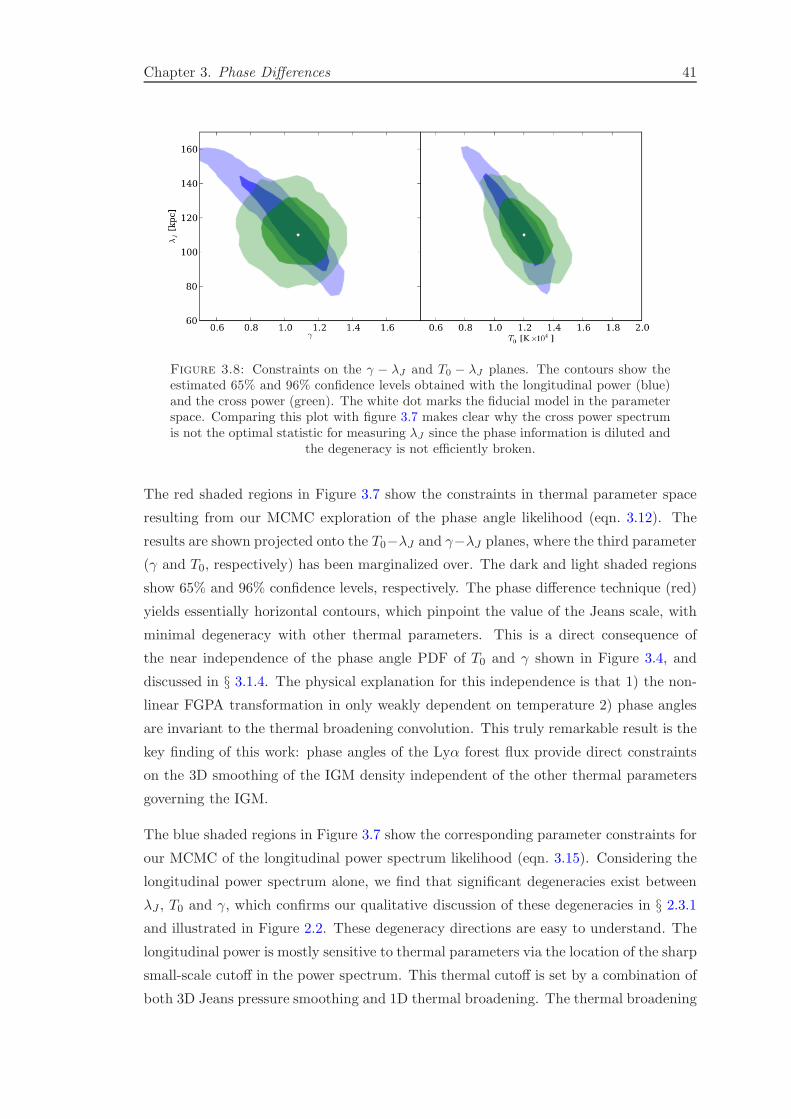
Chapter 3. Phase Differences 41
Figure 3.8: Constraints on the γ − λJ and T0 − λJ planes. The contours show theestimated 65% and 96% confidence levels obtained with the longitudinal power (blue)and the cross power (green). The white dot marks the fiducial model in the parameterspace. Comparing this plot with figure 3.7 makes clear why the cross power spectrumis not the optimal statistic for measuring λJ since the phase information is diluted and
the degeneracy is not efficiently broken.
The red shaded regions in Figure 3.7 show the constraints in thermal parameter space
resulting from our MCMC exploration of the phase angle likelihood (eqn. 3.12). The
results are shown projected onto the T0−λJ and γ−λJ planes, where the third parameter
(γ and T0, respectively) has been marginalized over. The dark and light shaded regions
show 65% and 96% confidence levels, respectively. The phase difference technique (red)
yields essentially horizontal contours, which pinpoint the value of the Jeans scale, with
minimal degeneracy with other thermal parameters. This is a direct consequence of
the near independence of the phase angle PDF of T0 and γ shown in Figure 3.4, and
discussed in § 3.1.4. The physical explanation for this independence is that 1) the non-
linear FGPA transformation in only weakly dependent on temperature 2) phase angles
are invariant to the thermal broadening convolution. This truly remarkable result is the
key finding of this work: phase angles of the Lyα forest flux provide direct constraints
on the 3D smoothing of the IGM density independent of the other thermal parameters
governing the IGM.
The blue shaded regions in Figure 3.7 show the corresponding parameter constraints for
our MCMC of the longitudinal power spectrum likelihood (eqn. 3.15). Considering the
longitudinal power spectrum alone, we find that significant degeneracies exist between
λJ , T0 and γ, which confirms our qualitative discussion of these degeneracies in § 2.3.1
and illustrated in Figure 2.2. These degeneracy directions are easy to understand. The
longitudinal power is mostly sensitive to thermal parameters via the location of the sharp
small-scale cutoff in the power spectrum. This thermal cutoff is set by a combination of
both 3D Jeans pressure smoothing and 1D thermal broadening. The thermal broadening

Chapter 3. Phase Differences 42
component is set by the temperature of the IGM at the characteristic overdensity probed
by the forest, which is δ ≈ 2 at z = 3 [Becker et al., 2011]. One naturally expects a
degeneracy between T0 and γ, because it is actually the temperature at T (δ ≈ 2) that
sets the thermal broadening. A degeneracy between λJ and T (δ ≈ 2) is also expected
because both smoothings contribute to the small-scale cutoff. Thus, a lower Jeans scale
can be compensated by more thermal broadening, which can result from either a steeper
temperature density relation (larger γ) or a hotter temperature at mean density T0, since
both produce a hotter T (δ ≈ 2).
Previous work that has aimed to measure thermal parameters such as T0 and γ, from the
longitudinal power spectrum [Viel et al., 2009, Zaldarriaga et al., 2001], the curvature
statistic [Becker et al., 2011], wavelets [Garzilli et al., 2012, Lidz et al., 2009, Theuns
et al., 2002b], and the b-parameter distribution [Bryan & Machacek, 2000, Haehnelt &
Steinmetz, 1998, McDonald et al., 2001, Ricotti et al., 2000, Rudie et al., 2012, Schaye
et al., 2000, Theuns et al., 2000, 2002a], have for the most part ignored the degeneracies
between these thermal parameters and the Jeans scale (but see Zaldarriaga et al. 2001
who marginalized over the Jeans scale, and Becker et al. 2011 who also considered its
impact). Neglecting the possible variation of the Jeans scale is equivalent to severely
restricting the family of possible IGM thermal histories. Because the phase angle method
accurately pinpoints the Jeans scale independent of the other parameters, it breaks the
degeneracies inherent to the longitudinal power spectrum and will enable accurate and
unbiased measurements of both T0 and γ, as evidence by the intersection of the red and
black contours in Figure 3.7. Similar degeneracies between the Jeans scale and (T0,γ)
exist when one considers other statistics such as the flux PDF [Bolton et al., 2008,
Calura et al., 2012, Garzilli et al., 2012, Kim et al., 2007, McDonald et al., 2000], which
we will explore in an upcoming study (Rorai et al., in prep). In light of these significant
degeneracies with the Jeans scale, it may be necessary to reassess the reliability and
statistical significance of previous measurements of T0 and γ.
Figure 3.8 shows the resulting thermal parameter constraints for our MCMC analysis of
the cross-power spectrum likelihood (eqn. 3.16) in green, determined from exactly the
same mock quasar pair sample that we analyzed for the phase angles. The confidence
regions for the longitudinal power are shown for comparison in blue. The cross-power
spectrum is a straightforward statistic to measure and fit models to, and the green confi-
dence regions clearly illustrate that it does exhibit some sensitivity to the Jeans scale, as
discussed in § 2.3.2 and shown in the right panel of Figure 2.2. However, a comparison
of the cross-power confidence regions in Figure 3.8 (green) with the phase angle PDF
confidence regions in Figure 3.7 (red) reveals that there is far more information about
the Jeans scale in quasar pair spectra than can be measured with the cross-power. The
cross-power produces constraints which are effectively a hybrid between the horizontal
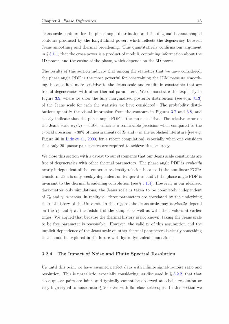
Chapter 3. Phase Differences 43
Jeans scale contours for the phase angle distribution and the diagonal banana shaped
contours produced by the longitudinal power, which reflects the degeneracy between
Jeans smoothing and thermal broadening. This quantitatively confirms our argument
in § 3.1.1, that the cross-power is a product of moduli, containing information about the
1D power, and the cosine of the phase, which depends on the 3D power.
The results of this section indicate that among the statistics that we have considered,
the phase angle PDF is the most powerful for constraining the IGM pressure smooth-
ing, because it is more sensitive to the Jeans scale and results in constraints that are
free of degeneracies with other thermal parameters. We demonstrate this explicitly in
Figure 3.9, where we show the fully marginalized posterior distribution (see eqn. 3.13)
of the Jeans scale for each the statistics we have considered. The probability distri-
butions quantify the visual impression from the contours in Figures 3.7 and 3.8, and
clearly indicate that the phase angle PDF is the most sensitive. The relative error on
the Jeans scale σλ/λJ = 3.9%, which is a remarkable precision when compared to the
typical precision ∼ 30% of measurements of T0 and γ in the published literature [see e.g.
Figure 30 in Lidz et al., 2009, for a recent compilation], especially when one considers
that only 20 quasar pair spectra are required to achieve this accuracy.
We close this section with a caveat to our statements that our Jeans scale constraints are
free of degeneracies with other thermal parameters. The phase angle PDF is explicitly
nearly independent of the temperature-density relation because 1) the non-linear FGPA
transformation is only weakly dependent on temperature and 2) the phase angle PDF is
invariant to the thermal broadening convolution (see § 3.1.4). However, in our idealized
dark-matter only simulations, the Jeans scale is taken to be completely independent
of T0 and γ; whereas, in reality all three parameters are correlated by the underlying
thermal history of the Universe. In this regard, the Jeans scale may implicitly depend
on the T0 and γ at the redshift of the sample, as well as with their values at earlier
times. We argued that because the thermal history is not known, taking the Jeans scale
to be free parameter is reasonable. However, the validity of this assumption and the
implicit dependence of the Jeans scale on other thermal parameters is clearly something
that should be explored in the future with hydrodynamical simulations.
3.2.4 The Impact of Noise and Finite Spectral Resolution
Up until this point we have assumed perfect data with infinite signal-to-noise ratio and
resolution. This is unrealistic, especially considering, as discussed in § 3.2.2, that that
close quasar pairs are faint, and typically cannot be observed at echelle resolution or
very high signal-to-noise ratio & 20, even with 8m class telescopes. In this section we
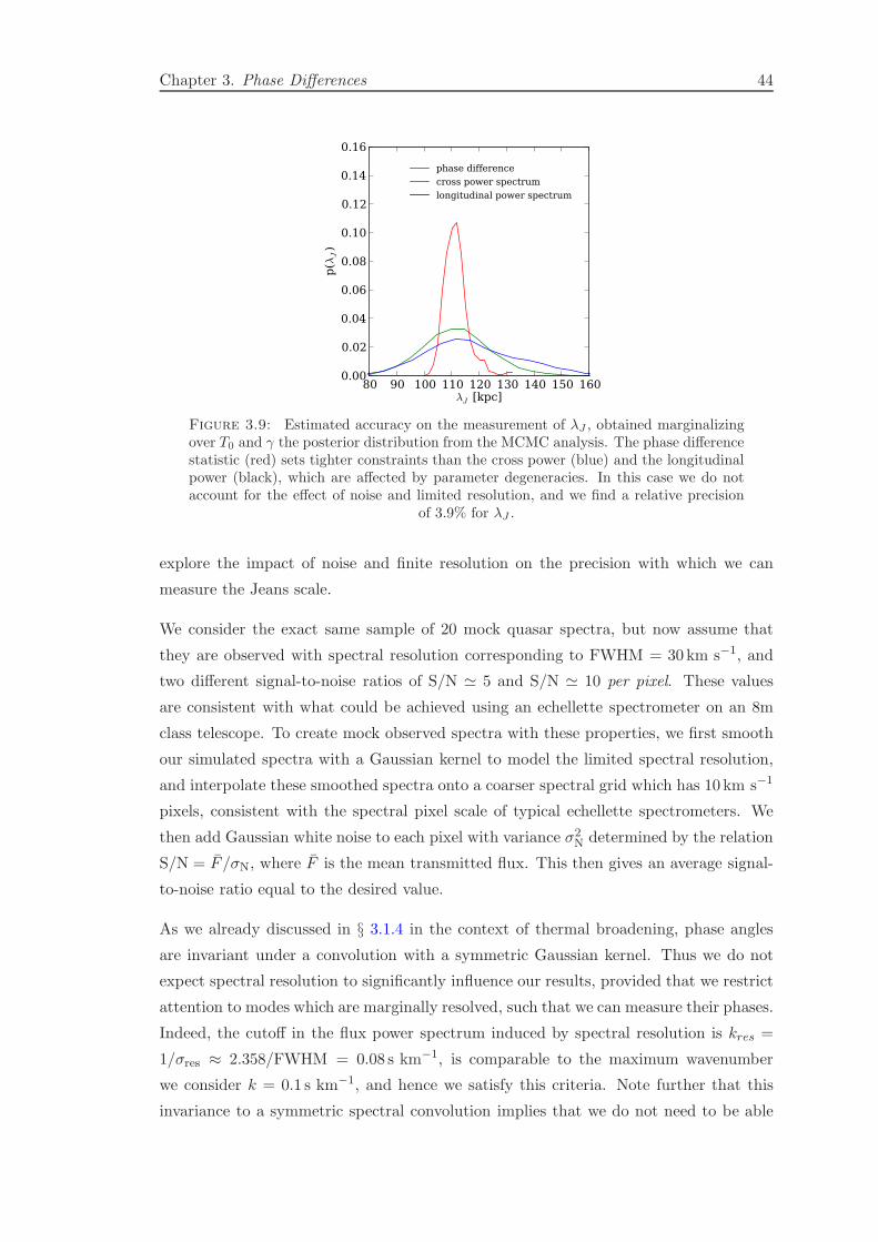
Chapter 3. Phase Differences 44
80 90 100 110 120 130 140 150 160λJ [kpc]
0.00
0.02
0.04
0.06
0.08
0.10
0.12
0.14
0.16
p(λ
J)
phase difference
cross power spectrum
longitudinal power spectrum
Figure 3.9: Estimated accuracy on the measurement of λJ , obtained marginalizingover T0 and γ the posterior distribution from the MCMC analysis. The phase differencestatistic (red) sets tighter constraints than the cross power (blue) and the longitudinalpower (black), which are affected by parameter degeneracies. In this case we do notaccount for the effect of noise and limited resolution, and we find a relative precision
of 3.9% for λJ .
explore the impact of noise and finite resolution on the precision with which we can
measure the Jeans scale.
We consider the exact same sample of 20 mock quasar spectra, but now assume that
they are observed with spectral resolution corresponding to FWHM = 30km s−1, and
two different signal-to-noise ratios of S/N ≃ 5 and S/N ≃ 10 per pixel. These values
are consistent with what could be achieved using an echellette spectrometer on an 8m
class telescope. To create mock observed spectra with these properties, we first smooth
our simulated spectra with a Gaussian kernel to model the limited spectral resolution,
and interpolate these smoothed spectra onto a coarser spectral grid which has 10 km s−1
pixels, consistent with the spectral pixel scale of typical echellette spectrometers. We
then add Gaussian white noise to each pixel with variance σ2N determined by the relation
S/N = F /σN, where F is the mean transmitted flux. This then gives an average signal-
to-noise ratio equal to the desired value.
As we already discussed in § 3.1.4 in the context of thermal broadening, phase angles
are invariant under a convolution with a symmetric Gaussian kernel. Thus we do not
expect spectral resolution to significantly influence our results, provided that we restrict
attention to modes which are marginally resolved, such that we can measure their phases.
Indeed, the cutoff in the flux power spectrum induced by spectral resolution is kres =
1/σres ≈ 2.358/FWHM = 0.08 s km−1, is comparable to the maximum wavenumber
we consider k = 0.1 s km−1, and hence we satisfy this criteria. Note further that this
invariance to a symmetric spectral convolution implies that we do not need to be able
Chapter 3. Phase Differences 45
80 90 100 110 120 130 140λJ [kpc]
0.00
0.02
0.04
0.06
0.08
0.10
0.12
0.14
0.16
p(λ
J)
S/N=∞S/N=10
S/N=5
Figure 3.10: The effect of noise and resolution in the measurement of λJ . The plotsshows the posterior distribution of the Jeans scale, marginalized over T0 and γ. Eachline represent a different degree of noise, assuming a resolution of FWHM=30 km/s.We selected a different subsample of the simulation as our mock dataset which has aprecision of 3.6% for S/N=∞ (black solid), 4.8% for S/N=10 (green dot-dashed) and
7.2% for S/N=5 (red dashed).
to precisely model the resolution, provided that it has a nearly symmetric shape and
does not vary dramatically across the spectrum. This is another significant advantage
of the phase angle approach, since the resolution of a spectrometer often depends on the
variable seeing, and can be challenging to accurately calibrate.
Although our results are thus likely to be very independent of resolution, noise intro-
duces fluctuations which are uncorrelated between the two sightlines, and this will tend
to reduce the coherence of the flux that the phase angle PDF quantifies. Noise will
thus modify the shape of the phase angle PDF away from the intrinsic shape shown in
Figure 3.3. In order to deal with noise and its confluence with spectral resolution, we
adopt a forward-modeling approach. Specifically, for each thermal model we smooth
all 10,000 IGM skewers to finite resolution, interpolate onto coarser spectral grids, and
add noise consistent with our desired signal-to-noise ratio. We then fit the resulting
distribution of phase angles to the wrapped-Cauchy distribution, determining the value
of the concentration parameter ζ(k, r⊥), at each k and r⊥ as we did before. We again
emulate the function ζ(k, r⊥|T0, γ, λJ ) using the same thermal parameter grid, but now
with noise and spectral resolution included, enabling fast evaluations of the likelihood in
eqn. (3.12). Thermal parameter constraints then follow from MCMC exploration of this
new likelihood, for which the impact of noise and resolution on the phase angle PDF
have been fully taken into account.
In Figure 3.10 we show the impact of noise on the fully marginalized constraints on
the Jeans scale from the phase angle PDF. The solid curve represents the posterior

Chapter 3. Phase Differences 46
distribution for a mock dataset with infinite resolution and signal-to-noise ratio, which
is identical to the red curve in Figure 3.9. The dotted and dashed curves illustrate
the impact of S/N = 10 and S/N = 5, respectively. Note that the slight shift in the
modes of these distributions from the fiducial value are expected, and should not be
interpreted as a bias. Different noise realizations generate scatter in the phase angles
just like the intrinsic noise from large-scale structure. The inferred Jeans scale for any
given mock dataset or noise realization will not be exactly equal to the true value, but
should rather be distributed about it with a scatter given by the width of the resulting
posterior distributions. The relative shifts in the mode of the posterior PDFs are well
within 1σ of the fiducial value, and are thus consistent with our expectations.
The upshot of Figure 3.10 is that noise and limited spectral resolution do not have a
significant impact on our ability to measure the Jeans scale. For a signal-to-noise ratio
of S/N = 10 per pixel we find that the relative precision with which we can measure
the Jeans scale is σλ/λJ = 4.8%, which is only a slight degradation from the precision
achievable from the same dataset at infinite signal-to-noise ratio and resolution σλ/
λJ = 3.9%. The small impact of noise on the Jeans scale precision is not surprising. For
the 10 km s−1 spectral pixels that we simulate, the standard deviation of the normalized
Lyα forest flux per pixel is√
〈δF 2〉 ≃ 32%, whereas for S/N = 10 our Gaussian noise
fluctuations are at a significantly smaller ≃ 10% level. Heuristically, these two ‘noise’
sources add in quadrature, and thus the primary source of ‘noise’ in measuring the phase
angle PDF results from the Lyα forest itself, rather than from noise in the data. For a
lower signal-to-noise ratio of S/N = 5 per pixel, the precision is further degraded to σλ/
λJ = 7.2%, which reflects the fact that noise fluctuations are becoming more comparable
to the intrinsic Lyα forest fluctuations.
These numbers on the scaling of our precision with signal-to-noise ratio S/N provide
intuition about the optimal observing strategy. For a given sample of pairs, it will
require four times more exposure time to increase the signal-to-noise ratio from S/N ≃ 5
to S/N ≃ 10, whereas the same telescope time allocation could be used to increase the
sample size by a factor of four at the same signal-to-noise ratio (assuming sufficient close
pair sightlines exist). For the latter case of an enlarged sample, the precision will scale
roughly as ∝√
Npairs, implying a σλ/λJ = 3.6% for a sample of 80 pairs observed at
S/N = 5. This can be compared to σλ/λJ = 4.8% for 20 pairs observed at S/N ≃ 10.
There is thus a marginal gain in working at lower S/N ≃ 5 and observing a larger pair
sample, although we have not considered various systematic errors which could impact
our measurement. However, higher signal-to-noise spectra are usually preferable for
the purposes of mitigating systematics, and hence one would probably opt for higher
signal-to-noise ratio, a smaller pair sample, and tolerate slightly higher statistical errors.

Chapter 3. Phase Differences 47
80 90 100 110 120 130 140λJ [kpc]
0.00
0.02
0.04
0.06
0.08
0.10
0.12
0.14
p(λ
J)
S/N=10
Overestimated S/N
Figure 3.11: The effect of overestimating the signal-to-noise ratio by a 20% factor(red, dashed line) when the real value is S/N= 10: we do not find any significant bias
on the measured value of the Jeans scale.
3.2.5 Systematic Errors
We now briefly discuss the systematic errors which could impact a measurement of
the Jeans scale. First, consider the impact of errors in the continuum normalization.
Because the phase angle is a ratio of Fourier modes of the normalized flux eqn. (3.3),
it is completely insensitive to the continuum normalization of δF , provided that the
continuum is not adding significant power on the scale of wavelength of the k-mode
considered. In the previous section, we argued that finite spectral resolution does not
have a significant impact the phase angle PDF, because phase angles are invariant under
convolutions with symmetric kernels. We do take resolution into account in our forward-
modeling of the phase angle PDF, but precise knowledge of the spectral resolution or
the line spread function is not required, since the line spread function will surely be
symmetric when averaged over several exposures, thus leaving the phase angles invariant.
The only requirement is that we restrict attention to modes less than the resolution cutoff
k . kres whose amplitudes are not significantly attenuated, such that we can actually
measure their phase angles.
Noise does modify the phase angle PDF, but our forward-modeling approach takes this
fully into account provided the noise estimates are correct. One potential systematic is
uncertainty in the noise model. The typical situation is that the standard-deviation of
a spectrum reported by a data reduction pipeline is underestimated at the ∼ 10− 20%
level (S/N overestimated), because of systematic errors related to the instrument and
data reduction [see e.g. Lee et al., 2013, McDonald et al., 2006]. To address this issue
we directly model the impact of underestimated noise for a case where we think the
S/N ≃ 10, but where in reality it is actually 20% lower S/N ≃ 8. Specifically, using
Chapter 3. Phase Differences 48
our same mock dataset we generate 20 quasar pair spectra with S/N ≃ 8. However,
when forward-modeling the phase angle PDF with the IGM simulations, we take the
signal-to-noise ratio to be the overestimated value of S/N ≃ 10. Excess noise above
our expectation would tend to reduce the coherence in the spectra (less peaked phase
angle PDF) mimicking the effect of a smaller Jeans scale. We thus expect a bias in the
Jeans scale to result from the underestimated noise. Figure 3.11 compares the posterior
distributions of the Jeans scale for the two cases S/N ≃ 10 (black curve) and signal-to-
noise ratio overestimated to be S/N ≃ 10 but actually equal to S/N ≃ 8 (red curve).
We see that ≃ 20% level uncertainties in the noise lead to a negligible bias in the Jeans
scale.
The only remaining systematic that could impact the Jeans scale measurement is metal-
line absorption within the forest. Metal absorbers cluster differently from the IGM, and
it is well known that metals add high-k power to the Lyα forest power spectrum because
the gas traced by metal lines tends to be colder than H I in the IGM [Croft et al., 2002,
Kim et al., 2004, Lidz et al., 2009, McDonald et al., 2000]. As this metal absorption is
not present in our IGM simulations, it can lead to discrepancies between model phase
angle PDFs and the actual data, resulting in a biased measurement. This is very unlikely
to be a significant effect. We restrict attention to large scale modes with k < 0.1 s km−1,
both because this is comparable to our expected spectral resolution cutoff, and because
below these wavenumbers metal line absorption results in negligible contamination of
the longitudinal power [Croft et al., 2002, Kim et al., 2004, Lidz et al., 2009, McDonald
et al., 2000]. Since the metal absorbers have a negligible effect on the moduli of these
large scale modes, we also expect them to negligibly change their phase angles.
We thus conclude that the phase angle PDF is highly insensitive to the systematics
that typically plague Lyα forest measurements, such as continuum fitting errors, lack of
knowledge of spectral resolution, poorly calibrated noise, and metal line absorption.
3.2.6 Is Our Likelihood Estimator Unbiased?
Finally, we determine whether our procedure for measuring the Jeans scale via the phase
angle likelihood (eqn. 3.12) outlined at the end of § 2.2, produces unbiased estimates. To
quantify any bias in our Jeans scale estimator we follow a Monte Carlo approach, and
generate 400 distinct quasar pair samples by randomly drawing 20 quasar pair spectra
(allowing for repetition) from our ensemble of 10,000 skewers. Note that the distribution
of transverse separations is approximately the same for all of these realizations, since we
only simulate 30 discrete separations, and the full sample of 20 overlapping pair spectra
requires 200 pairs of skewers, which are randomly selected from among the 30 available
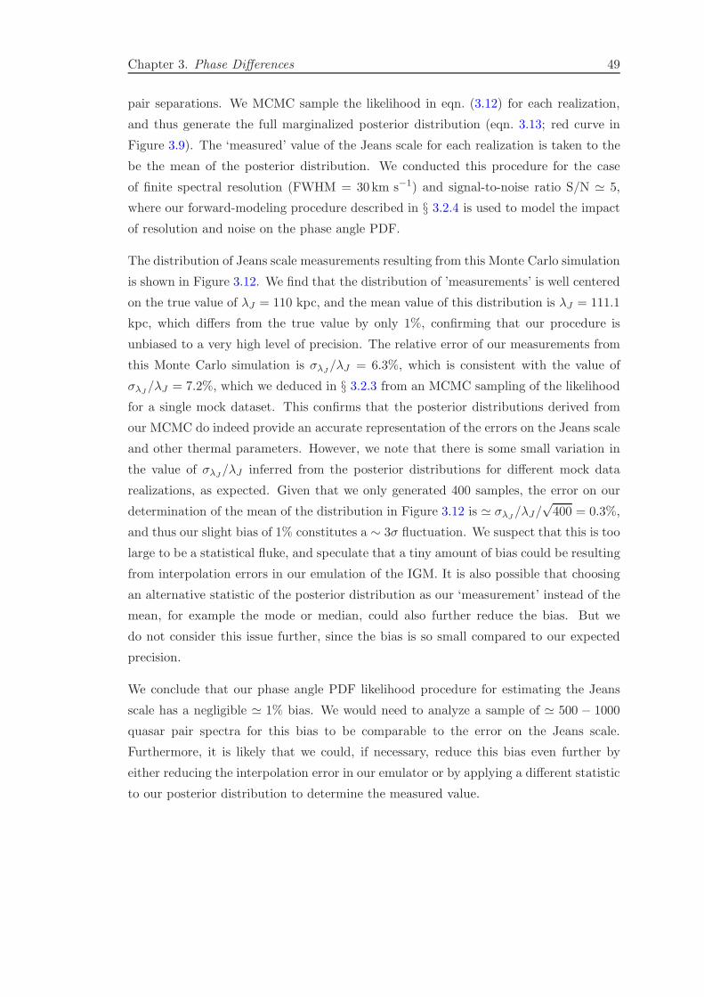
Chapter 3. Phase Differences 49
pair separations. We MCMC sample the likelihood in eqn. (3.12) for each realization,
and thus generate the full marginalized posterior distribution (eqn. 3.13; red curve in
Figure 3.9). The ‘measured’ value of the Jeans scale for each realization is taken to the
be the mean of the posterior distribution. We conducted this procedure for the case
of finite spectral resolution (FWHM = 30km s−1) and signal-to-noise ratio S/N ≃ 5,
where our forward-modeling procedure described in § 3.2.4 is used to model the impact
of resolution and noise on the phase angle PDF.
The distribution of Jeans scale measurements resulting from this Monte Carlo simulation
is shown in Figure 3.12. We find that the distribution of ’measurements’ is well centered
on the true value of λJ = 110 kpc, and the mean value of this distribution is λJ = 111.1
kpc, which differs from the true value by only 1%, confirming that our procedure is
unbiased to a very high level of precision. The relative error of our measurements from
this Monte Carlo simulation is σλJ/λJ = 6.3%, which is consistent with the value of
σλJ/λJ = 7.2%, which we deduced in § 3.2.3 from an MCMC sampling of the likelihood
for a single mock dataset. This confirms that the posterior distributions derived from
our MCMC do indeed provide an accurate representation of the errors on the Jeans scale
and other thermal parameters. However, we note that there is some small variation in
the value of σλJ/λJ inferred from the posterior distributions for different mock data
realizations, as expected. Given that we only generated 400 samples, the error on our
determination of the mean of the distribution in Figure 3.12 is ≃ σλJ/λJ/
√400 = 0.3%,
and thus our slight bias of 1% constitutes a ∼ 3σ fluctuation. We suspect that this is too
large to be a statistical fluke, and speculate that a tiny amount of bias could be resulting
from interpolation errors in our emulation of the IGM. It is also possible that choosing
an alternative statistic of the posterior distribution as our ‘measurement’ instead of the
mean, for example the mode or median, could also further reduce the bias. But we
do not consider this issue further, since the bias is so small compared to our expected
precision.
We conclude that our phase angle PDF likelihood procedure for estimating the Jeans
scale has a negligible ≃ 1% bias. We would need to analyze a sample of ≃ 500 − 1000
quasar pair spectra for this bias to be comparable to the error on the Jeans scale.
Furthermore, it is likely that we could, if necessary, reduce this bias even further by
either reducing the interpolation error in our emulator or by applying a different statistic
to our posterior distribution to determine the measured value.
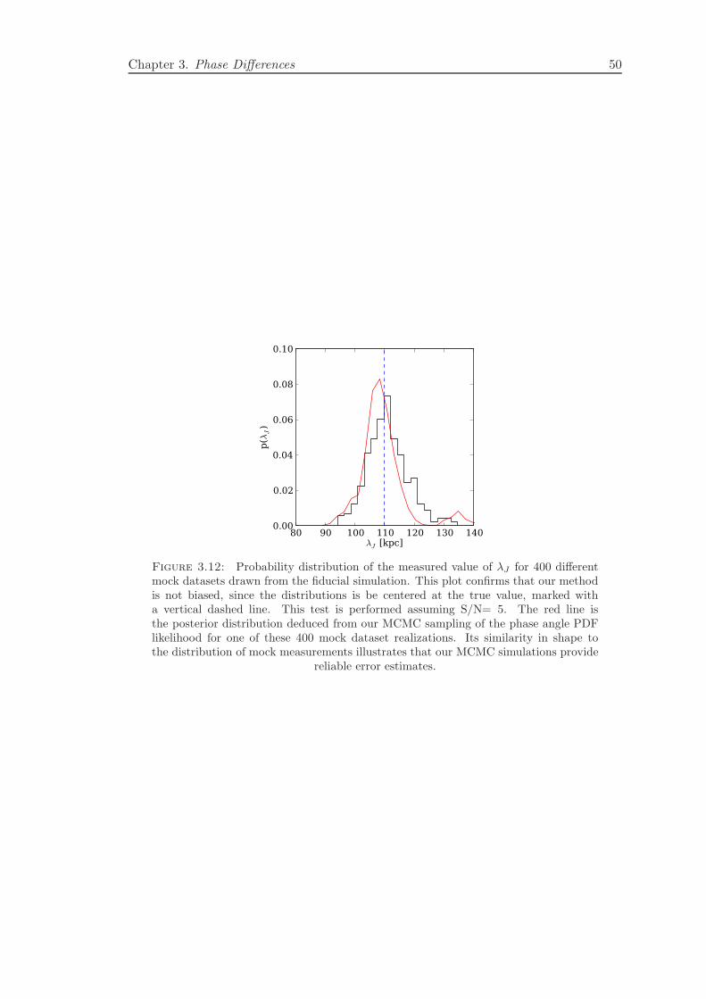
Chapter 3. Phase Differences 50
80 90 100 110 120 130 140λJ [kpc]
0.00
0.02
0.04
0.06
0.08
0.10
p(λ
J)
Figure 3.12: Probability distribution of the measured value of λJ for 400 differentmock datasets drawn from the fiducial simulation. This plot confirms that our methodis not biased, since the distributions is be centered at the true value, marked witha vertical dashed line. This test is performed assuming S/N= 5. The red line isthe posterior distribution deduced from our MCMC sampling of the phase angle PDFlikelihood for one of these 400 mock dataset realizations. Its similarity in shape tothe distribution of mock measurements illustrates that our MCMC simulations provide
reliable error estimates.

Chapter 4
Data Analysis
In the previous chapter, I described how a sample of quasar pairs at separations in the
range ≈ 50 − 500 ckpc can be used to constrain the filtering scale down to precision of
few percents. This prediction is based on a set of semi-analytical models based on a
N-body dark matter simulation. The next goal is to do the same analysis on a sample
of observed quasar pairs in order to measure λJ at different redshifts and provide a
rigorous estimation of its uncertainty.
To accomplish this task we have to face two main challenges:
• the formalism described in the previous chapters must be generalized to include a
consistent treatment of noise, resolution and other possible systematics present in
the data;
• we need to proof that our set of simplified IGM models, that do not include full
hydrodynamic, are accurate enough to yields meaningful results.
The present chapter focuses on how we address the first problem, while a discussion on
the second one is deferred to 6.
Although in § 3.2.4 we have discussed the effect of noise on phase distributions, this have
been done in a very simplified manner, by assuming a constant noise and resolution across
the whole box. Such analysis is not suitable for the sample of observed pairs that we
want to analyze. Their spectra have been collected using different instruments and under
different conditions, and therefore they have a wide range of resolutions and signal-to-
noise ratios (S/N), which are also wavelength-dependent. This diversity motivates a
specific calibration of phase differences for each single pair.
This chapter is structured as follows: in section 4.1 we briefly illustrate the pair sample
that we use and we specify the requirement we set on data. We describe in section
51
Chapter 5. Data Analysis 52
4.2 the method we adopt to calculate phases from the spectra and in § 4.3 how the
simulations are calibrated to the data sample in order to produce predictions for the
PDFs of observed phases.
4.1 Data sample
This project is based on a large sample of quasar pairs drawn mostly from the SDSS
[Abazajian et al., 2009] and BOSS[Ahn et al., 2012] and (in few cases) from the 2QZ[Croom
et al., 2004] surveys. Beside studying the transverse coherence of the Lyα forest, such
objects have been used for a number of scientific goals. Examples are the measure-
ment of the small-scale clustering of quasars [Hennawi et al., 2006b, Myers et al., 2008,
Shen et al., 2010] and the characterization of the circumgalactic medium of quasar hosts
[Hennawi & Prochaska, 2007, 2008, Hennawi et al., 2006a, Prochaska & Hennawi, 2009,
Prochaska et al., 2013, 2012].
Surveys such as SDSS and BOSS select against small separations of quasar pairs due to
fiber collision, setting a lower limit to the angular separation of 55′′, 62′′ and 30′′ for the
SDSS, BOSS and the 2QZ survey, respectively. These angles are unfortunately too wide
to probe the Jeans scale, thus follow-up spectroscopy is necessary in order both to dis-
cover close companions around quasars and to obtain science-quality spectroscopic data.
An alternative possibility to find close pairs is to use the SDSS five-band photometry to
select candidate companions around known quasars. A number of such candidates have
been spectroscopically confirmed using the Apache Point Observatory (APO)[Hennawi
et al., 2006b].
4.1.1 Spectroscopic Observations
A significant fraction of our dataset rely on spectra from SDSS and BOSS which have
a resolution of R ≈ 2000 and wavelength coverage of λ ≈ 3800 − 9000 Aand λ ≈3600 − 10000 A, respectively. The rest of the spectra have been collected with follow-
up spectroscopy on large-aperture telescopes, using instruments with a wide range of
capabilities which I list below.
Part of objects were observed at the Keck 10m telescope, including data from the
Echellette Spectrometer and Imager (ESI, Sheinis+2002), the Low Resolution Imag-
ing Spectrograph (LRIS; oke et al 1995), and the High Resolution Echelle Spectrom-
eter (HIRES, Vogt+94). Other spectra were collected using the Gemini MultiObject
Spectrograph (GMOS, hook+2004) on the 8m Gemini North and South telescopes, the
Chapter 5. Data Analysis 53
Magellan Echellette Spectrograph (MagE, Marshal+08) and the Magellan Inamori Ky-
ocera Echelle (MIKE, Bernstein+2003) on the 6m Magellan telescopes. Few pairs were
observed through the Multi-Object Double Spectrograph (MODS, Pogge+2012) on the
Large Binocular Telescope (LBT). We recently obtained new data from the X-Shooter
spectrometer at the Very Large Telescope (VLT), specifically selected for this project.
The GMOS spectra have been observed in the context of two different programs, in which
gratings of 600 lines/mm (GMOS600) and 1200 lines/mm (GMOS1200)were used.
An exhaustive description of the properties of the data sample can be found in Hennawi
& Prochaska [2008], Hennawi et al. [2006a], Prochaska et al. [2013].
4.1.2 Selection Criteria
We apply a first broad cut to select pairs suitable for the science goal of this study.
An obvious requisite is the existence of a segment of coeval Lyα forest, which can be
expressed as (1 + zfg)λLyα > (1 + zbg)λLyβ. However, we want to avoid cases where this
segment is too small to calculate meaningful statistics, especially considering that we
cannot use the wavelengths too close to the Lyα and Lyβ emission lines. We define the
”overlapping fraction” of the Lyα forest as
fov =(1 + zfg)λLyα − (1 + zbg)λLyα
(1 + zfg)(λLyα − λLyβ)(4.1)
and we set a lower threshold at fov = 0.3, removing in this way part of the projected
pairs with the highest redshift separation.
A second criterion is established according to the transverse separation. Our study of the
sensitivity of phases with simulations (see chapter 3) indicated that the most informative
pairs are those with impact parameter comparable to the Jeans scale. Considered that
the line-of-sight power of the forest excludes Jeans scales larger than ≈ 300−400kpc, we
focus our analysis on pairs closer than 500 kpc (comoving) at the f/g redshift. Only at
redshift z > 3 we loose this restriction up to 700 kpc, since the sample at this redshift is
considerably smaller and even the weak constraints coming from wide pairs are valuable.
We than exclude from the sample all pairs for which no science-quality spectra is available
because they have not been observed with one of the instrument listed in the previous
paragraph. Future programs of follow-up spectroscopy will allow this objects to be used
in the measurement.
The set of pairs selected at the end of this process is then visually inspected in order to
find contaminants. Some of the QSOs exhibit strong associated absorption lines known
as Broad Absorption Lines (BAL), which are thought to be produced in the vicinity of
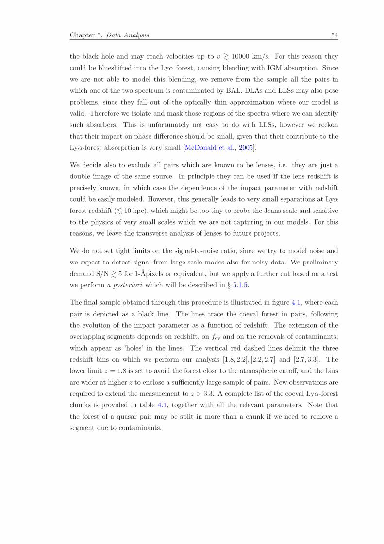
Chapter 5. Data Analysis 54
the black hole and may reach velocities up to v & 10000 km/s. For this reason they
could be blueshifted into the Lyα forest, causing blending with IGM absorption. Since
we are not able to model this blending, we remove from the sample all the pairs in
which one of the two spectrum is contaminated by BAL. DLAs and LLSs may also pose
problems, since they fall out of the optically thin approximation where our model is
valid. Therefore we isolate and mask those regions of the spectra where we can identify
such absorbers. This is unfortunately not easy to do with LLSs, however we reckon
that their impact on phase difference should be small, given that their contribute to the
Lyα-forest absorprtion is very small [McDonald et al., 2005].
We decide also to exclude all pairs which are known to be lenses, i.e. they are just a
double image of the same source. In principle they can be used if the lens redshift is
precisely known, in which case the dependence of the impact parameter with redshift
could be easily modeled. However, this generally leads to very small separations at Lyα
forest redshift (. 10 kpc), which might be too tiny to probe the Jeans scale and sensitive
to the physics of very small scales which we are not capturing in our models. For this
reasons, we leave the transverse analysis of lenses to future projects.
We do not set tight limits on the signal-to-noise ratio, since we try to model noise and
we expect to detect signal from large-scale modes also for noisy data. We preliminary
demand S/N & 5 for 1-Apixels or equivalent, but we apply a further cut based on a test
we perform a posteriori which will be described in § 5.1.5.
The final sample obtained through this procedure is illustrated in figure 4.1, where each
pair is depicted as a black line. The lines trace the coeval forest in pairs, following
the evolution of the impact parameter as a function of redshift. The extension of the
overlapping segments depends on redshift, on fov and on the removals of contaminants,
which appear as ’holes’ in the lines. The vertical red dashed lines delimit the three
redshift bins on which we perform our analysis [1.8, 2.2], [2.2, 2.7] and [2.7, 3.3]. The
lower limit z = 1.8 is set to avoid the forest close to the atmospheric cutoff, and the bins
are wider at higher z to enclose a sufficiently large sample of pairs. New observations are
required to extend the measurement to z > 3.3. A complete list of the coeval Lyα-forest
chunks is provided in table 4.1, together with all the relevant parameters. Note that
the forest of a quasar pair may be split in more than a chunk if we need to remove a
segment due to contaminants.
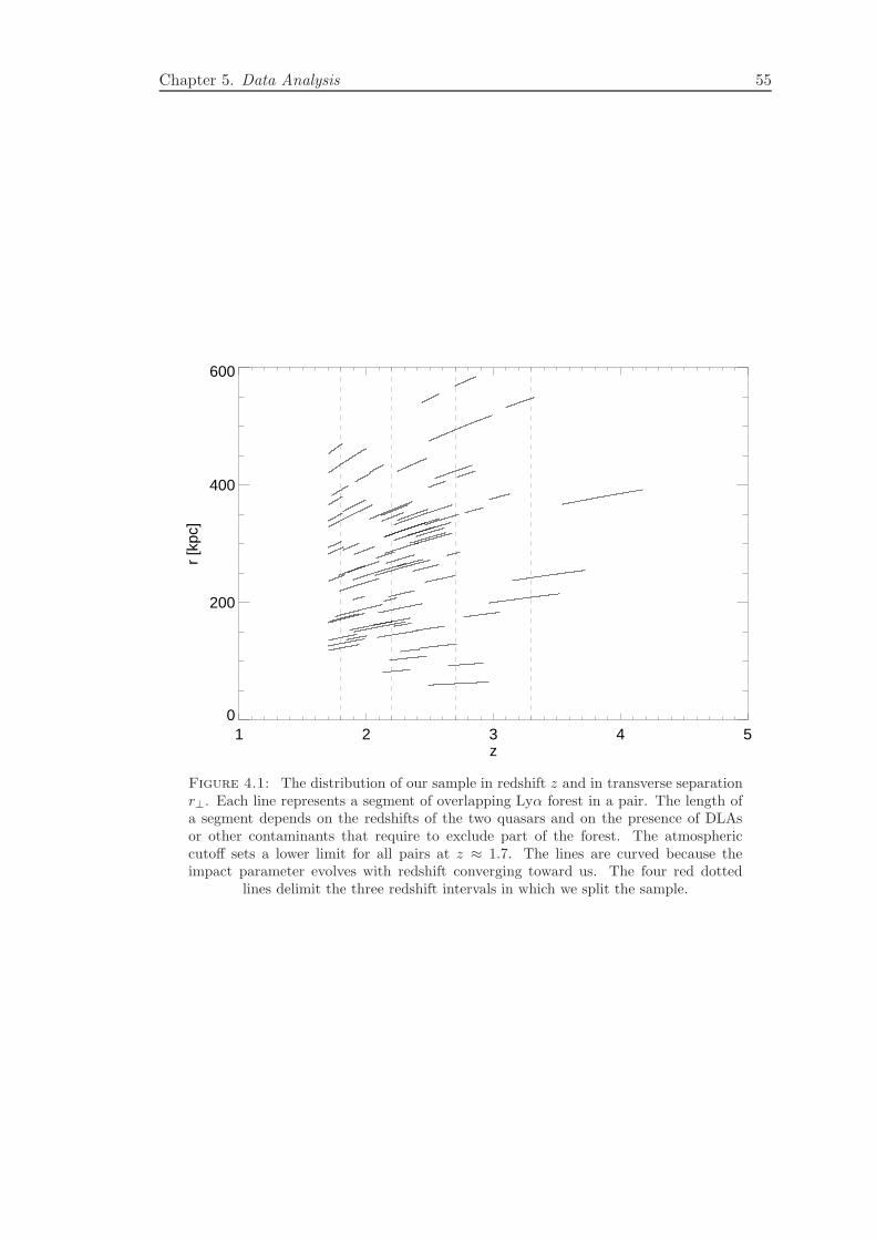
Chapter 5. Data Analysis 55
1 2 3 4 5z
0
200
400
600
r [k
pc]
Figure 4.1: The distribution of our sample in redshift z and in transverse separationr⊥. Each line represents a segment of overlapping Lyα forest in a pair. The length ofa segment depends on the redshifts of the two quasars and on the presence of DLAsor other contaminants that require to exclude part of the forest. The atmosphericcutoff sets a lower limit for all pairs at z ≈ 1.7. The lines are curved because theimpact parameter evolves with redshift converging toward us. The four red dotted
lines delimit the three redshift intervals in which we split the sample.

Chap
ter5.
Data
Analysis
56
Table 4.1: Complete list of the chunks of overlapping Lyα forest in the pair sample we analyze
Name zbga zfg
b zminc zmax
d θe r⊥f Instrument Rbg/fg
g S/Nbg/fgh
SDSSJ0034-1049 1.95 1.83 1.61 1.77 7.6 177 LRIS/LRIS 180/180 6.9/33.7
SDSSJ0054-0946 2.12 2.12 1.67 2.05 14.1 347 LRIS/LRIS 174/174 133.5/28.0
SDSSJ0117+3153 2.64 2.62 2.33 2.55 11.3 322 ESI/ESI 64/64 30.9/20.0
SDSSJ0214+0105 2.29 2.21 2.03 2.14 16.4 428 MODS/MODS 205/205 9.6/6.0
SDSSJ0332-0722 2.11 2.10 1.66 2.00 18.1 440 LRIS/LRIS 175/175 16.5/17.4
SDSSJ0735+2957 2.08 2.06 1.63 1.99 5.4 131 LRIS/LRIS 176/176 53.7/34.6
SDSSJ0750+2724 1.80 1.77 1.60 1.71 13.1 299 LRIS/LRIS 182/182 6.6/14.3
SDSSJ0752+4011 2.12 1.87 1.67 1.81 12.6 298 LRIS/LRIS 178/178 15.3/6.3
SDSSJ0813+1014 2.08 2.06 1.65 1.99 7.1 173 LRIS/LRIS 176/176 18.3/15.0
SDSSJ0814+3250 2.21 2.17 1.85 2.11 10.3 261 GMOS1200/GMOS1200 191/191 6.5/12.7
SDSSJ0837+3837 2.25 2.05 1.78 1.99 10.3 255 LRIS/LRIS 174/174 8.0/37.5
SDSSJ0853-0011 2.58 2.41 2.12 2.33 13.2 358 MAGE/MAGE 62/62 38.3/8.6
SDSSJ0913-0107 2.92 2.75 2.35 2.63 10.8 311 GMOS600/GMOS600 192/192 9.3/11.7
SDSSJ0920+1310 2.43 2.42 2.06 2.35 6.2 168 MAGE/MAGE 62/62 25.8/37.7
SDSSJ0924+3929 2.08 1.88 1.64 1.82 12.2 286 LRIS/LRIS 180/180 13.1/16.1
SDSSJ0937+1509 2.55 2.54 2.14 2.47 11.7 324 GMOS600/GMOS600 201/201 6.4/11.1
SDSSJ0938+5317 2.32 2.07 1.84 2.00 5.6 140 LRIS/LRIS 171/171 23.0/6.2
SDSSJ0956+2643 3.08 3.08 2.49 3.00 16.5 498 ESI/ESI 64/64 16.4/25.1
SDSSJ1006+4804 2.60 2.30 2.08 2.23 10.6 281 LRIS/LRIS 161/161 22.7/12.2
SDSSJ1009+2500 1.99 1.88 1.64 1.82 14.6 342 LRIS/LRIS 180/180 16.7/24.2
SDSSJ1021+1112 3.85 3.83 3.15 3.73 7.4 247 ESI/ESI 64/64 56.5/26.2
SDSSJ1026+0629 3.12 2.89 2.64 2.74 9.5 283 MAGE/MAGE 62/62 6.1/6.0
SDSSJ1053+5001 3.08 3.05 2.49 2.96 2.1 63 ESI/ESI 64/64 8.4/9.6
2QZJ1056-0059 2.13 2.12 1.71 1.94 7.2 175 LRIS/LRIS 177/177 13.2/10.5
SDSSJ1116+4118 3.00 2.94 2.49 2.63 13.8 402 LRIS/LRIS 130/130 22.4/45.9
SDSSJ1116+4118 3.00 2.94 2.71 2.86 13.8 419 LRIS/LRIS 123/123 26.0/52.9
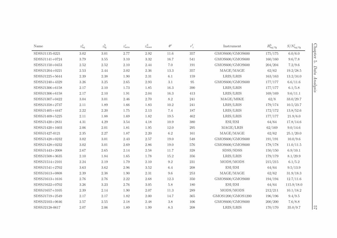
Chap
ter5.
Data
Analysis
57
Name zabg zbfg zcmin zdmax θe rf⊥ Instrument Rhbg/fg S/N i
bg/fg
SDSSJ1135-0221 3.02 3.01 2.77 2.92 11.6 357 GMOS600/GMOS600 175/175 6.0/6.0
SDSSJ1141+0724 3.79 3.55 3.10 3.32 16.7 541 GMOS600/GMOS600 160/160 9.6/7.8
SDSSJ1150+0453 2.52 2.52 2.10 2.44 7.0 191 GMOS600/GMOS600 204/204 7.2/9.6
SDSSJ1204+0221 2.53 2.44 2.02 2.36 13.3 357 MAGE/MAGE 62/62 19.2/28.5
SDSSJ1225+5644 2.39 2.38 1.90 2.31 6.1 159 LRIS/LRIS 163/163 13.2/34.0
SDSSJ1240+4329 3.26 3.25 2.65 2.93 3.1 95 GMOS600/GMOS600 177/177 6.6/11.6
SDSSJ1306+6158 2.17 2.10 1.73 1.85 16.3 390 LRIS/LRIS 177/177 6.1/5.8
SDSSJ1306+6158 2.17 2.10 1.91 2.04 16.3 413 LRIS/LRIS 169/169 9.6/11.1
SDSSJ1307+0422 3.04 3.01 2.46 2.70 8.2 241 MAGE/MIKE 62/8 33.0/29.7
SDSSJ1358+2737 2.11 1.89 1.66 1.83 10.2 241 LRIS/LRIS 179/174 10.5/23.7
SDSSJ1405+4447 2.22 2.20 1.75 2.13 7.4 187 LRIS/LRIS 172/172 13.8/52.6
SDSSJ1409+5225 2.11 1.88 1.69 1.82 19.5 462 LRIS/LRIS 177/177 21.9/6.0
SDSSJ1420+2831 4.31 4.29 3.54 4.18 10.9 380 ESI/ESI 64/64 17.8/14.6
SDSSJ1420+1603 2.06 2.01 1.81 1.95 12.0 295 MAGE/LRIS 62/169 9.0/14.6
SDSSJ1427-0121 2.35 2.27 1.87 2.20 6.2 161 MAGE/MAGE 62/62 25.1/20.0
SDSSJ1428+0232 3.02 3.01 2.43 2.57 19.0 548 GMOS600/GMOS600 191/191 10.0/9.6
SDSSJ1428+0232 3.02 3.01 2.69 2.86 19.0 576 GMOS600/GMOS600 178/178 11.0/11.5
SDSSJ1443+2008 2.67 2.65 2.14 2.58 11.7 328 SDSS/SDSS 150/150 6.9/10.1
SDSSJ1508+3635 2.10 1.84 1.65 1.78 15.2 356 LRIS/LRIS 179/179 8.1/29.9
SDSSJ1514+2101 2.24 2.19 1.79 2.10 9.2 231 MODS/MODS 215/215 6.1/5.2
SDSSJ1541+2702 3.63 3.62 2.96 3.52 6.4 208 ESI/ESI 64/64 9.5/13.9
SDSSJ1613+0808 2.39 2.38 1.90 2.31 9.6 253 MAGE/MAGE 62/62 31.9/18.3
SDSSJ1613+1616 2.76 2.76 2.22 2.68 12.3 350 GMOS600/GMOS600 194/194 12.7/11.6
SDSSJ1622+0702 3.26 3.23 2.76 3.05 5.8 180 ESI/ESI 64/64 115.9/18.0
SDSSJ1657+3105 2.39 2.14 1.90 2.07 11.3 289 MODS/MODS 212/211 10.1/18.2
SDSSJ1719+2549 2.17 2.17 1.82 2.00 14.7 365 GMOS1200/GMOS1200 196/196 9.4/9.5
SDSSJ2103+0646 2.57 2.55 2.18 2.48 3.8 106 GMOS600/GMOS600 200/200 7.6/8.8
SDSSJ2128-0617 2.07 2.06 1.89 1.99 8.3 208 LRIS/LRIS 170/170 35.0/9.7
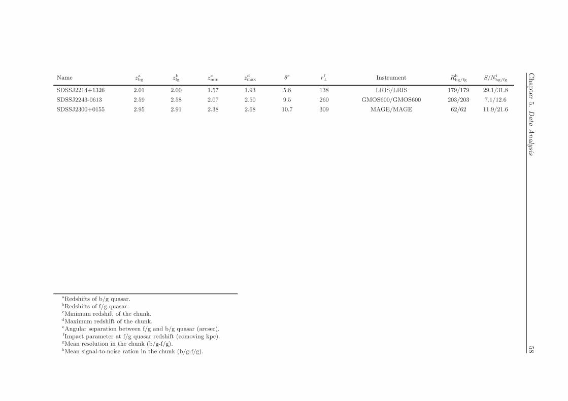
Chap
ter5.
Data
Analysis
58
Name zabg zbfg zcmin zdmax θe rf⊥ Instrument Rhbg/fg S/N i
bg/fg
SDSSJ2214+1326 2.01 2.00 1.57 1.93 5.8 138 LRIS/LRIS 179/179 29.1/31.8
SDSSJ2243-0613 2.59 2.58 2.07 2.50 9.5 260 GMOS600/GMOS600 203/203 7.1/12.6
SDSSJ2300+0155 2.95 2.91 2.38 2.68 10.7 309 MAGE/MAGE 62/62 11.9/21.6
aRedshifts of b/g quasar.bRedshifts of f/g quasar.cMinimum redshift of the chunk.dMaximum redshift of the chunk.eAngular separation between f/g and b/g quasar (arcsec).fImpact parameter at f/g quasar redshift (comoving kpc).gMean resolution in the chunk (b/g-f/g).hMean signal-to-noise ration in the chunk (b/g-f/g).
Chapter 5. Data Analysis 59
4.1.3 Continuum Fitting and Data Preparation
We fitted the continuum manually for those pairs which were not already fitted for
other projects. We used a fitting algorithm that perform a cubic spline interpolation
between manually-inserted guiding points. We stress the fact that the statistic we use
is not particularly sensitive to continuum-placement, as we will explicitly show in the
next chapter. In particular, it is completely insensitive to its renormalization, while it
could be affected by fluctuation on scales . 2000 km/s which we do not expect to find
in quasar spectra. The noise has been estimated following the standard pipeline of the
instruments.
We exclude the parts of spectrum close to the Lyαand Lyman−β emission lines, re-
stricting the analysis to the rest-frame wavelength interval [1040, 1190] nm. The over-
lapping forest in a pairs on which we calculate phases is thus defined by λ ∈ [1040(1 +
zbg), 1190(1 + zfg)], which is slightly narrower than the one implied by the fov defined
above.
Since phase differences are calculated in velocity space, we transform from wavelengths
to velocities according to the formula
∆v = c log(λ1/λ2), (4.2)
where ∆v is the relative velocity between two points responsible of resonant Lyα ab-
sorption at observed wavelengths λ1 and λ2. In the limit where peculiar velocities are
negligible, this corresponds to a comoving distance of
∆x =(1 + z)∆v
H(z). (4.3)
where the H(z) is the Hubble parameter at the observed redshift.
4.2 Calculation of Phases from Real Spectra
Applying Fourier-space statistics, such as phase difference, to the observed Lyα forest
is not a straightforward operation. While in simulations we generate mock spectra on
perfectly regular grids in velocity space, the pixels of observed spectra are in most of
the cases unevenly distributed. Since the discrete Fourier transformation is defined
for evenly-sampled functions, we have either to interpolate or rebin the data onto a
regular grid, or to use approximate methods without modifying the sampling. The two
methodologies have opposite advantages and disadvantages, so we decided to implement
both and check that they lead to consistent results.
Chapter 5. Data Analysis 60
4.2.1 Method 1: Least-Square Spectral Analysis
A widely-used approach to generalize Fourier transformation to irregularly-sampled se-
ries is the so called least-square spectral analysis (LSSA). Practically speaking, it con-
sists in fitting a function f(xi) with a linear combinations of trigonometric functions
cos(kjxi) and sin(kjxi), where xi is the set of points where f is sampled and kj are
the wavenumbers of the modes that we want to fit. This leads for example to the Lomb-
Scargle periodogram [Lomb, 1976], a method often employed to calculate the power
spectrum of a signal. It is also possible to follow this strategy to recover the phase
information, which is what we want to calculate in quasar spectra. We follow for this
purpose the method described in Mathias et al. [2004] which I briefly report here.
As mentioned above, the decomposition can be view as the minimization, for each dif-
ferent kj of
||f(x)− cj cos(kjx) + sj sin(kjx)|| (4.4)
where in our case x is the array of the velocity-space pixels in a spectrum, f is the
transmitted flux of the Lyα forest, ||g(x)|| = ∑i g2(xi) denotes the squared norm and
(cjsj) are the coefficients that we need to determine. Otherwise stated, we want to find
the projection of f on the functional subspace defined by the linear combinations of
cos(kjx) and sin(kjx). In the case where xi are evenly spaced and kj = 2πj/L, with
L being the total length of the spectrum, this is equivalent Fourier decomposition. For
generic xi and kj the linear subspaces relative to different k may not be orthogonal
and may not form a complete functional base, so this fitting procedure cannot be properly
regarded as a decomposition.
The minimization of expression 4.4 is obtained via the Moore-Penrose pseudo-inverse
matrix [Penrose, 1955] applied to the linear system
f(x) = (cj sj)Ωj (4.5)
where Ωj is defined as
Ωj =
(
cos(kjx1) ... sin(kjxn)
sin(kjx1) ... sin(kjxn)
)
. (4.6)
The pseudo inverse is then Ω+j = ΩT
j (ΩjΩTj )
−1 and the coefficients are estimated by
(cj sj) = f(x)Ω+j . (4.7)
According to the pseudo-inverse properties, this coefficients are exactly the ones that
minimizes ||f(x)− (cj sj)Ωj||, i.e. expression 4.4. When the system has a solution this
Chapter 5. Data Analysis 61
norm is zero, but for our problem this is never the case. Note also that this definition
of the pseudo-inverse requires that ΩjΩTj is invertible, which is however always satisfied
for reasonable pixel distributions.
By writing explicitly eq. 4.7 we obtain
(cj sj) =
(
∑
i f(xi) cos(kjxi)∑
i f(xi) sin(kjxi)
)T (∑
i cos2(kjxi)
∑
i cos(kjxi) sin(kjxi)∑
i cos(kjxi) sin(kjxi)∑
i sin2(kjxi)
)−1
(4.8)
where the diagonal terms are nonzero because sin(kjx) and cos(kjx) are not orthogonal
in general. Nevertheless it is possible to apply a phase shift to the coordinates such that,
for a given kj , the non diagonal terms vanish [Lomb, 1976]. It can be shown that the
shift is equal to
Tj =1
2karctan
∑
i sin(kjxi)∑
i cos(kjxi). (4.9)
After diagonalization, the equation above simplifies in
(cj sj) =
(∑
i f(xi) cos(kj(xi − Tj))∑
i cos2(kj(xi − Tj))
∑
i f(xi) sin(kj(xi − Tj))∑
i sin2(kj(xi − Tj))
)
(4.10)
Which is the expression are looking for. The power spectrum immediately follow from
this result as P (kj) = c2j + s2j .
If we need to recover phase information we must consider that phases are changed by
the Lomb shift, therefore we have to apply at each k the inverse translation. This is
easily done by defining the Fourier coefficients in the complex representation as
F (kj) = (cj + isj)eikjTj . (4.11)
We are now ready to calculate phase differences in the usual way
θ12(k) = arccos
(
ℜ[F ∗1 (k)F2(k)]
|F1(k)||F2(k)|
)
(4.12)
where F1 and F2 are the transmitted fluxes of the Lyα forest in the two spectra of the
pair.
A final caveats concerns non-orthogonality: if the Fourier components have non zero
cross products Cl,m =∑
i exp(−i(km−kl)xi), then the estimated Fourier coefficients are
correlated. This would be an undesirable complication when calculating the likelihood
function of phases, which we consider to be independent on the wake of or test in § 3.1.5.We solve this problem recursively: after calculating F (k0) we subtract this component
Chapter 5. Data Analysis 62
from the original function
F ′(x) = F (x)− F (k0)e−ik0x (4.13)
and then we calculate the next coefficient F (k1) on the residual function F ′(x). We
iterate this steps until all the coefficients are calculated. This algorithm is equivalent to
a Grahm-Schmidt process, and requires to specify the order on which the components
are subtracted. The most natural choice for us is starting with the large scale modes, i.e.
with the lowest wavenumber, which are the least affected by noise and other systematics.
4.2.2 method 2: Rebinning on a Regular Grid
A second possibility is to rebin the observed flux pixels into a regular grid, to allow the
standard calculation of the Fourier coefficients. The advantage of this method is that
we avoid approximations deriving from the least-square evaluation of the phases, but on
the other hand, we do not have a clear control on how the rebinning modifies the Fourier
phases. The pros and cons of this approach are complementary to the LSSA procedure
described in the previous section, therefore we decide to adopt both of them and check
that the results are consistent, assuring in this way that rebinning or LSSA are not a
source of bias (§ 5.3.1.1).
In order to consistently calculate phase differences, one need not only to bin the pixels
of each spectrum in a regular grid in velocity space, but also to use the same regular
grid for the two spectra of a pair. The common regular grid is defined from the original
arrays via a simple procedure. for a single spectrum with N irregular pixels located
at v0i , the step of the regularized array would be defined as ∆v = (v0N − v01)/N and
the full vector would be vi = v01 + i∆v. When considering two spectra with different
pixels arrays u0i and w0i , having respectively N and M points, we define the grid
in the common velocity interval I = [max(u01, w01),min(u0N , w
0M )]. We then count the
number of pixels encompassed within this interval for each of the two spectra, and we
take the smallest of two numbers to be the cardinality of the common grid grid ng. In
this way we avoid oversampling in the rare cases where one spectra is observed with
a smaller pixel density than the other. The spacing is then simply |I|/ng, where |I|is clearly the length of the interval. We finally rebin the transmitted fluxes onto the
newly-defined pixel vector and we are set to compute the phase differences by standard
Fourier analysis.
Chapter 5. Data Analysis 63
4.3 Calibrated Phase Analysis
In the previous section we described two ways of calculating phase differences from the
observed Lyα forest in quasar pairs. The final goal of this calculation is to quantitatively
assess the similarity of the measured phase distributions with those expected from the
simulations for different IGM parameters, following the statistical formalism we devised
in chapter 3.
However, we cannot calculate phase distributions directly from the simulated skewers.
The simple reason is that the differences between the phase PDFs of data and simulations
are also driven by non-astrophysical factors such as noise and resolution limit. If we want
to exploit the sensitivity of phases to the filtering scale, we need first to understand and
correct for the contribution of these disturbances. To this end, two different approaches
are possible: find a way of subtracting them directly from data, or adding them to the
simulations such that they are calibrated to the observations (forward-modeling). For the
purposes of the Jeans scale measurement we choose to follow the latter, motivated by the
simplicity of implementing forward-modeling in the context of our Bayesian machinery.
The calibration is done by creating, for each observed pair, an entire ensemble of simu-
lated pairs with the same data properties, in particular the same transverse separation,
the same noise amplitude and the same resolution. The next paragraphs of this section
are dedicated to illustrate in details this procedure.
4.3.1 Transverse Separation
Two quasars separated in the sky by an observed angle ψ have a transverse distance de-
pendent on their redshift. If we are studying Lyα absorption, the transverse separation
between the coeval forest in the two spectra is an evolving function of the wavelength,
since the sightlines are convergent toward us. The exact function depends on the cos-
mology, and can be written as
r⊥(zabs) = DA(zabs))ψ(1 + zabs) (4.14)
where zabs = λ/λα−1 is the Lyα absorption redshift andDA is the correspondent angular
distance. The variation of r⊥ across our redshift bins is not negligible, especially for the
longer chunks of forest, as figure 4.1 suggests. Since we know that phases are dependent
on r⊥, we should take this fact into account. Calculating the optical along arbitrary
directions in the simulation would be complicated to implement, so we prefer to follow
an alternative strategy. We keep choosing sightlines parallel to the box coordinates, but
Chapter 5. Data Analysis 64
for each observed pair we compute a full ensemble of synthetic pairs with separations
uniformly distributed over the range covered by r⊥(zabs) within the redshift limits of
the chunk. In practice, if the coeval Lyαforest of the pair lies between zmin and zmax, we
simulate 400 pairs randomly located in the box and with separation r = r⊥(zi), wherethe 400 redshifts zi are logarithmically spaced between zmin and zmax. The logarithmic
spacing is chosen to achieve linear spacing in v(z), which is the coordinate on which
Fourier coefficients are calculated.
4.3.2 Resolution
We know that phases have the mathematical property of being invariant under convolu-
tion with symmetric kernels. For this reason one may think that no corrections for the
resolution are required. Unfortunately, this invariance does not hold in presence of noise,
analogously to a general deconvolution problem. In fact, phase scattering due to noise
is enhanced at high-k where the signal from the forest is suppressed due to resolution
limit. Phases lose their alignment and their intrinsic probability distributions is flat-
tened depending on the noise level and the resolution kernel. A more precise description
of the relation between noise, mode amplitudes and phase dispersion is given in § 4.4.
The conclusion we draw from this argument is that the combined effect of resolution and
noise must be always taken into account, unless the data have exquisite signal-to-noise
ratio. We also conclude that when the power of the signal drops due to resolution, our
measurement are unreliable or in the best case useless, because we are only sensitive to
noise. For this reason we must set as an upper limit on the usable k−range near the
resolution cutoff, which is kR = 1/σR ≈ 2.355/FWHM, where σR is the width of the
resolution kernel and FWHM the relative width at half maximum. The exact choice of
this threshold will be discussed in the next chapter (§ 5.1.5).
In the forward-modeling approach we convolve the simulated spectra with a Gaussian,
with the FWHM defined by the resolution of the spectrograph. Although the resolution
is wavelength-dependent, we use a constant width for each Lyαforest chunk which is
specified in table 4.1. This width corresponds to the FWHM at the average wavelength
of each chunk, where the average is defined as the median in velocity space, which can
be shown to be
λ =λ1λ2 ln(λ2/λ1)
λ2 − λ1, (4.15)
where λ1 and λ2 are respectively the minimum and the maximum observed wavelength
of the chunk.
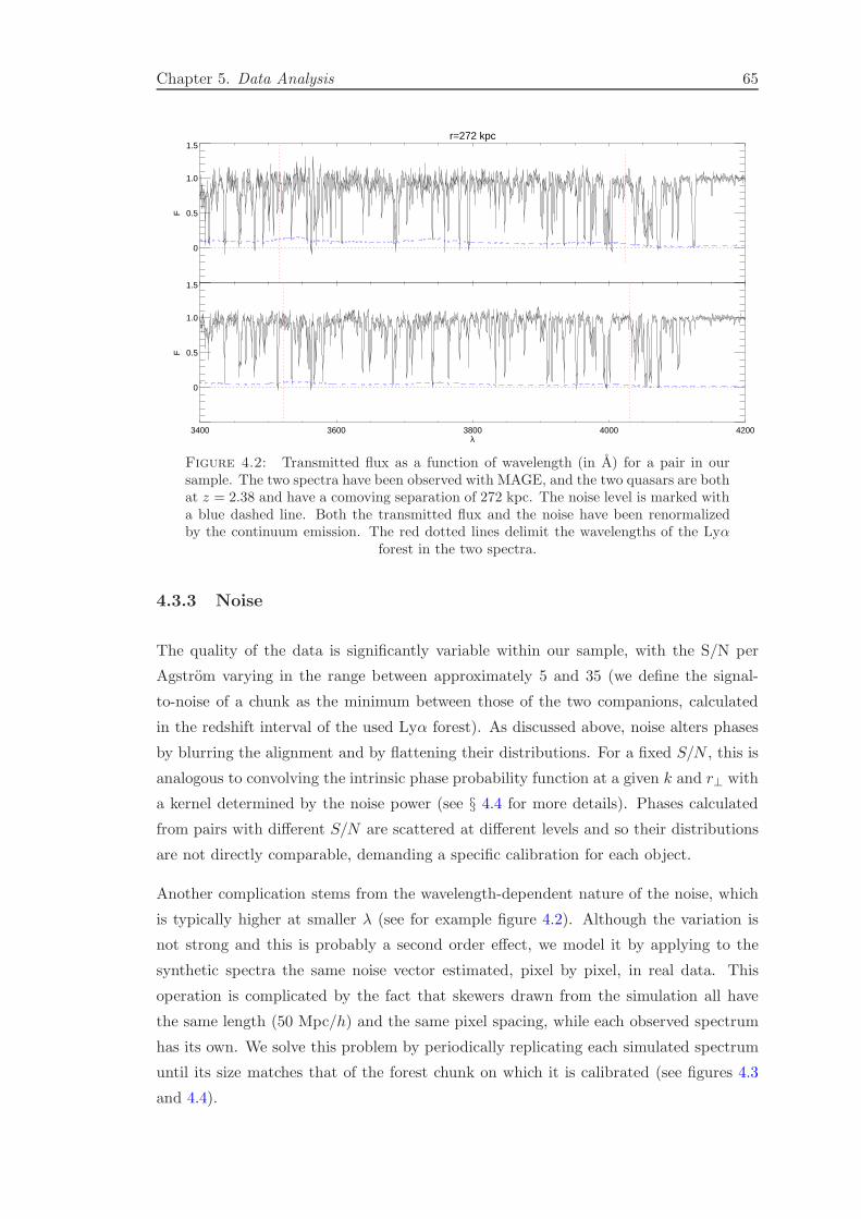
Chapter 5. Data Analysis 65
r=272 kpc
0
0.5
1.0
1.5
F
3400 3600 3800 4000 4200λ
0
0.5
1.0
1.5
F
Figure 4.2: Transmitted flux as a function of wavelength (in A) for a pair in oursample. The two spectra have been observed with MAGE, and the two quasars are bothat z = 2.38 and have a comoving separation of 272 kpc. The noise level is marked witha blue dashed line. Both the transmitted flux and the noise have been renormalizedby the continuum emission. The red dotted lines delimit the wavelengths of the Lyα
forest in the two spectra.
4.3.3 Noise
The quality of the data is significantly variable within our sample, with the S/N per
Agstrom varying in the range between approximately 5 and 35 (we define the signal-
to-noise of a chunk as the minimum between those of the two companions, calculated
in the redshift interval of the used Lyα forest). As discussed above, noise alters phases
by blurring the alignment and by flattening their distributions. For a fixed S/N , this is
analogous to convolving the intrinsic phase probability function at a given k and r⊥ with
a kernel determined by the noise power (see § 4.4 for more details). Phases calculated
from pairs with different S/N are scattered at different levels and so their distributions
are not directly comparable, demanding a specific calibration for each object.
Another complication stems from the wavelength-dependent nature of the noise, which
is typically higher at smaller λ (see for example figure 4.2). Although the variation is
not strong and this is probably a second order effect, we model it by applying to the
synthetic spectra the same noise vector estimated, pixel by pixel, in real data. This
operation is complicated by the fact that skewers drawn from the simulation all have
the same length (50 Mpc/h) and the same pixel spacing, while each observed spectrum
has its own. We solve this problem by periodically replicating each simulated spectrum
until its size matches that of the forest chunk on which it is calibrated (see figures 4.3
and 4.4).

Chapter 5. Data Analysis 66
The procedure of extending the segments of Lyα-forest reduces the fundamental fre-
quency in Fourier space and thus increases the density of modes. This new modes would
introduce spurious and redundant information which have a substantial effect on phase
distributions. The correct way of calculating phases after the extension is to split the
final spectra in chunks of size equal or smaller than the box length (the number of
replications may be a non-integer number), and extract their phases separately. The
sample created in this way can then be used to determine the probability distribution
function. Although there is still redundant information, such redundancy will only affect
the variance and not the mean of phase probability, since this procedure is equivalent
of resampling the same region of space more than once. The same chunking technique
cannot be done on data, since phases from consecutive segments of Lyα forest are likely
to be correlated, and such correlation is not included in our likelihood estimator. There-
fore phases are extracted from the observed spectra by applying the Fourier analysis to
the full length of the chunks.
The flux of the spectrum obtained after the periodical extension is finally rebinned into
the same pixel grid of the observed spectrum, which is always coarser than the one used
in our simulation. Once this is done, we are set to generate Gaussian noise matched
pixel by pixel to the estimated wavelength-dependent noise of data. The noise in the
Lyα forest is always renormalized by the continuum.
4.3.4 Forward-Modeling of the Simulation
The steps illustrated in the three previous paragraphs constitutes the forward-modeling
of our simulation. This consists in applying to the simulated transmitted flux the same
alterations that affect the real spectra when they are observed through a telescope with
finite resolution and integration time. Forward-modeled simulations can be safely com-
pared to observations, and allows to implement the same Bayesian formalism described
in chapter 3. The forward-modeling need to be tailored separately for each pair, and
must be applied to all the IGM models that we want to test. It is useful to summarize
the general procedure that we follow to perform the phase-difference analysis on our
data sample.
Suppose that we want to calibrate a model T0, γ, λJ to estimate the PDF of phases
measured from the Lyα forest of two quasars Q1 and Q2 separated in the sky by an
angle ψ, in the a redshift bin Z = [z1, z2]. This operation can be structured as follows:
• we determine the overlapping portion of the Lyα forest of the two QSOs which
intersects Z. This segment will have a comoving separation varying with redshift
Chapter 5. Data Analysis 67
as r⊥(z) = DA(z)ψ(1 + z) (see section § 4.3.1). From now on we will use the
velocity-space notation r⊥(v) for the impact parameter and F1(v), F2(v) for the
transmitted fluxes of the two spectra.
• we generate 400 pairs from the simulated box distributed in transverse separations
r⊥ depending on r⊥(v) as described in § 4.3.1.
• As in chapter 2, the optical depth is globally renormalized in order to match the
observed mean flux.
• All the 400 pairs are forward-modeled according to the properties of Q1 and Q2. In
each simulated pair one companion is associated to Q1 and the other to Q2, which
have in general different resolutions and S/N. This is done through the following
four steps:
1. convolving the flux skewers with a gaussian kernel, with FWHM defined by
the spectral resolution.
2. Replicating them periodically until they equal the length of the observed
segments of forest.
3. rebinning the simulated flux into the same pixel grid of data.
4. adding gaussian, uncorrelated noise to the simulated flux. The S/N matches
at each pixel the one estimated in the observed spectrum.
• We finally calculate phases from the skewers and estimate the wrapped-Cauchy
concentration parameters ζ at each bin in k. We predict in this way the probability
distribution of phases P (θ; k) as a function of k for the considered pair. Note that
having rebinned the skewers at step 3, we have to calculate phases with the LSSA
method as we do with data.
• Following the method elaborated in § 3.1.6 we write the likelihood as
L (θ|M) =∏
i
PWC(θ(ki)|ζ(k|M)) (4.16)
where θ(ki) are the phases of the real pair and ζ(k|M) the wrapped-Cauchy param-
eters estimated for the model M via forward modeling. Note that differently than
equation 3.12 there is no index over r⊥, because this likelihood refers to only one
observed pair. This likelihood is evaluated only below the limiting wavenumber
kMAX, which is the minimum between kR (resolution limit) and 0.1 s/km (limit
set by metal contamination).
This procedure is then repeated for each observed pair, for each IGM model and at each
redshift bin. This provides values of the likelihood function for all the pairs through the
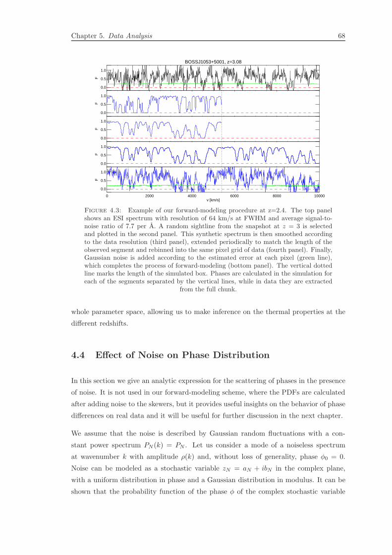
Chapter 5. Data Analysis 68
BOSSJ1053+5001, z=3.08
0.0
0.5
1.0
F
0.0
0.5
1.0
F
0.0
0.5
1.0
F
0.0
0.5
1.0
F
0 2000 4000 6000 8000 10000v [km/s]
0.0
0.5
1.0
F
Figure 4.3: Example of our forward-modeling procedure at z=2.4. The top panelshows an ESI spectrum with resolution of 64 km/s at FWHM and average signal-to-noise ratio of 7.7 per A. A random sightline from the snapshot at z = 3 is selectedand plotted in the second panel. This synthetic spectrum is then smoothed accordingto the data resolution (third panel), extended periodically to match the length of theobserved segment and rebinned into the same pixel grid of data (fourth panel). Finally,Gaussian noise is added according to the estimated error at each pixel (green line),which completes the process of forward-modeling (bottom panel). The vertical dottedline marks the length of the simulated box. Phases are calculated in the simulation foreach of the segments separated by the vertical lines, while in data they are extracted
from the full chunk.
whole parameter space, allowing us to make inference on the thermal properties at the
different redshifts.
4.4 Effect of Noise on Phase Distribution
In this section we give an analytic expression for the scattering of phases in the presence
of noise. It is not used in our forward-modeling scheme, where the PDFs are calculated
after adding noise to the skewers, but it provides useful insights on the behavior of phase
differences on real data and it will be useful for further discussion in the next chapter.
We assume that the noise is described by Gaussian random fluctuations with a con-
stant power spectrum PN (k) = PN . Let us consider a mode of a noiseless spectrum
at wavenumber k with amplitude ρ(k) and, without loss of generality, phase φ0 = 0.
Noise can be modeled as a stochastic variable zN = aN + ibN in the complex plane,
with a uniform distribution in phase and a Gaussian distribution in modulus. It can be
shown that the probability function of the phase φ of the complex stochastic variable

Chapter 5. Data Analysis 69
BOSSJ1613+0808, z=2.38
0.0
0.5
1.0
F
0.0
0.5
1.0
F
0.0
0.5
1.0
F
0.0
0.5
1.0
F
0 1•104 2•104 3•104
v [km/s]
0.0
0.5
1.0
F
Figure 4.4: Same as Figure 4.3 but at redshift z = 2. The top spectra was observedwith MAGE at resolution of 62 km/s (FWHM) and signal to noise of 17.7 per A. Com-pared to the previous plot the data quality is higher, there is sensibly less absorption
and the forest segment is longer, so we need to replicate the skewer more times.
F = F0 + FN is
pN (φ|η) = e−1/2η2
2π+
cosφ√
8πη2e−
sin2(φ)
2η2 erfc
(
− cosφ√
2η2
)
, (4.17)
where we define the ”noise parameter” η =√PN/ρ(k). The full derivation is given
in appendix , but it is interesting to note that the distribution follows the expected
behavior in the limiting cases. When the noise is very high (η → +∞), it reduces to
a flat distributions pN (φ) = 1/2π, meaning that phases have totally lost the original
coherence information. Conversely, when the signal dominates (η → 0), pN is well
approximated by a Gaussian in sinφ with variance η2.
Formula 4.17 expresses the noise scattering of the phase of a single mode. If we want
the dispersion of the phase difference of two homologous modes in a pair, we would need
to calculate the distribution of the sum of the noise phases φ1 and φ2, and that is given
by the convolution of the pN for the two modes. We do not attempt to derive a general
expression for this convolution, but we note that in the limit of low noise (η ≪ 1) it
reduces to a convolution of two Gaussians, which leads to another Gaussian with the
variances added in quadrature η2∆φ = η2φ1+ η2φ2
.
Chapter 5
Results
We have now developed all the tools that are needed to attempt a measurement of the
Jeans scale on quasar pairs.
In chapter 3 we showed that phase difference analysis applied to close quasar pairs is
capable of optimizing the sensitivity to the spatial coherence of the low-density IGM
and minimize the degeneracies with the thermal parameters T0 and γ. We devised a
statistical procedure that allows a rigorous probabilistic inference in parameter space,
estimating a potential precision of . 5% on the filtering scale λJ with a realistic sample
of 20 full high-quality pairs.
The current data set of quasar pairs described in the previous chapter does not reach
the same level of quality and quantity, but it allows the first step in the direction of a
high-precision measurement of the Jeans scale, setting for the first time constraints on
λJ . We illustrated how we calibrate the simulations to take into account the wide range
of noise and resolution of the spectra we want to analyze, following a forward-modeling
approach § 4.3. Such calibration enables the prediction of the expected phase difference
distributions for each of the pairs in our sample, given a theoretical (i.e. noiseless) model
for the IGM.
The combination of forward modeling and statistical analysis of phase-differences lead
to the results that we present in this chapter. The details of the implementation of the
statistical analysis are specified in § 5.1, and the constraints on the parameters at the
three redshift intervals are given in § 5.2. Finally we test the robustness of our results
for a series of possible bias source (§ 5.3).
70
Chapter 6. Results 71
5.1 Implementation of the Statistical Analysis
5.1.1 Simulation
This measurement was conducted using a Nbody simulation analogous to that described
in § 2.1.2, but on a smaller box, capable of resolving smaller Jeans scales. This choice
is motivated by preliminary results that indicated unexpectedly low values for λJ . We
use a cube of 30 Mpc/h of size and 20483 DM particles, which according to the criterion
established in appendix A enables to study Jeans scales of λJ ≈ 15 kpc. We also updated
the cosmological parameter to Planck results [Ade et al., 2014], i.e. ΩΛ = 0.68,Ωm =
0.32, h = 0.67. We focus on three snapshot at z = 2, 2.4, 3, approximately at the centers
of the redshift intervals in which we bin the data.
5.1.2 Parameter Grid
As explained in chapter 2, the interpolation of statistics in parameter space (i.e. the
emulator) takes great benefit from a careful designing of the training grid. In particular
it is important that the grid has good filling properties in parameter space, meaning
that all subspaces are sampled homogeneously and as densely as possible, which is not
achieved neither with regular nor with randomly generated sets of points. To conduct
our data analysis we employ e parameter grid of nm = 405 points in the T0 − γ − λJ
space. The fact that we use a smaller grid than in our theoretical study is motivated by
the fact that we expected a smaller precision from data compared to the perfect spectra
of simulation. It is anyway possible to refine such grid if required, either a posteriori
because the results do not converge or because of an improvement of the data sample.
We use a more efficient algorithm to generate a space-filling grid compared to what we
employed in Chapter 3. The properties of the parameter grids are the following:
• we use nm different values of T0 and nm different values of γ uniformly distributed
within the chosen range.We have only nJ = 45 values for the Jeans scale λJ , since
it is more computationally expensive to vary than the other two parameters. Each
of these value is used 9 times.
• we divide the T0 and γ ranges in 9 regular intervals (which we will call segments),
each with 45 points, and the λJ range in 5 segments, each with 81 points. This
subdivision defines in the T0 − γ 2d subspace a grid of 9 × 9 cells (from now on
quadrants). Each quadrant of this plane is populated with 5 points. Analogously,
Chapter 6. Results 72
we define two 5×9 grids in the λJ−T0 and in the λJ−γ planes, with each quadrant
having 9 points.
• the full 3d space T0 − γ − λJ is now naturally divided in 9 × 9 × 5 cells. Each of
them contains one point.
The three points express respectively the conditions for 1d,2d and 3d homogeneity for
all possible subspaces. A precise description of the details on how this grid is devised
are beyond the scope of this work.
5.1.3 Likelihood
In chapter 3 we have introduced the likelihood estimator for the phase difference statistic
as
L (θ|M) =∏
k,r⊥
PWC(θ(k, r⊥)|ζ(k, r⊥|M)) (5.1)
where θ(k, r⊥) is the phase difference between the k-modes of a quasar pair with impact
parameter r⊥, and ζ is the concentration parameter of the wrapped-Cauchy distribution.
ζ depends on k, r⊥ and on the IGM modelM = T0, γ, λJ. We now apply this likelihood
function to the phases calculated from real pairs with the least-square spectral analysis
technique (see § 4.2). The ζ parameters are obtained through our grid of DM-based
models, after careful calibration of noise and resolution (as described in § 4.3). The rangein k available for the analysis depends on one hand on the size of the simulated box, which
sets the lower mode, and on the other hand on the resolution of the instruments, that cuts
the signal of high-k modes. Regardless of the resolution, we never consider wavenumber
greater than k = 0.1 s/km due to metal contamination. A detailed description on how
we establish the limiting k as a function of the resolution will be given in § 5.1.5. The
ζ parameters are calculated for each r⊥ and for 13 different bins in k-space. This bins
are equally spaced in log k between k = 0.005 s/km and k = 0.1 s/km.
5.1.4 Interpolation
Analogous to our study in chapters 2-3 we use the models in the discrete set of 405
points in the grid to make prediction in the continuum of parameter space, by means of
Gaussian-processes interpolation. Differently than what we have done there, we do not
use the emulator to interpolate the full statistic that we are using, i.e. phase difference
distributions. We follow the simpler method of calculating the likelihood at each point
of the parameter grid with equation 5.1 and we interpolate only that single number.
This choice allows a much faster calculation than emulating the full statistic, which is
Chapter 6. Results 73
not required since we only need the likelihood probability to perform the measurement.
Moreover, if the results are converged they should be independent from the choice of
the interpolation algorithm.
The convergence of the emulator is achieved when the density of the training grid in
parameter space is consistent with the smoothness of the interpolated variable. If this is
not fulfilled, a refinement of the parameter grid is necessary. In the case of the likelihood,
the smoothness depends on the dimension of the sample: the more constraining the data,
the higher the requirements on the grid density. To make a simple example, if the in-
ferred 1σ region contains only one point of the parameter grid, the size and the shape
of our confidence levels would entirely depend on the choice of the interpolation param-
eters, and could not be trusted. In the context of Gaussian processes, the error would
be set by the correlation length in parameter space which determines the correlation
matrix. It is therefore required that we populate with enough grid points the regions of
parameter space where the posterior probability is not negligible. Instead of determining
a general criteria of ”filling density”, we adopt a simple a posteriori consistency check:
we use correlation lengths larger than the typical model-model separation in parameter
space and check that the results of the measurement do not sensibly change when we
vary these parameters (§ 5.3.4.2). In typical Gaussian process implementations this hy-
perparameters are determined by maximizing the likelihood of the sampled points, i.e.
in the training grid. We consider this approach too arbitrary for our study, since we use
GP for interpolation purposes but we do not have any good reason to believe that the
values of the likelihood are effectively drawn from a Gaussian process.
5.1.5 Resolution Limit on k||
Based on previous study on the line-of-sight power spectrum [McDonald et al., 2000],
we argued in chapter 3 that the Fourier modes in the forest with wavenumber k|| > 0.1
s/km should be excluded from the analysis because of contamination of narrow metal
lines. We also know that according to the instrument resolution the power of the signal
drops exponentially as exp[−(kσr)2], assuming that the resolution can be modeled as
a constant Gaussian kernel with width σr ≈FWHM/2.355. As the noise has a white
power spectrum, it will be the dominating source of power beyond this cutoff, erasing the
sensitivity to the Jeans scale. If we trusted completely our forward-modeling procedure,
these noisy high-k modes should not represent a problem, since they are consistently
calibrated in the simulation. In that case, including them in the analysis would only
add uninformative phases with flat distributions, with no effect on the final inference.
However, it could be that our assumption on the shape of the resolution kernel (Gaussian
with constant width) or on the properties of the noise (white Gaussian noise) are not
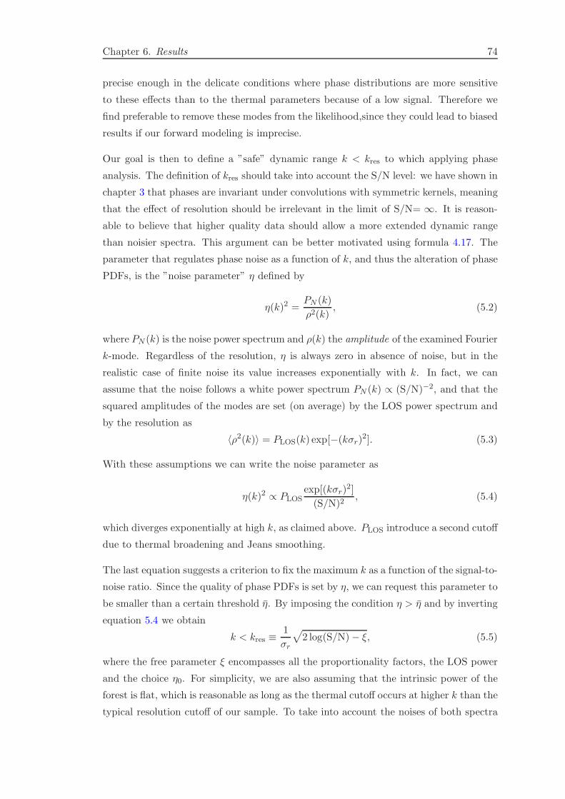
Chapter 6. Results 74
precise enough in the delicate conditions where phase distributions are more sensitive
to these effects than to the thermal parameters because of a low signal. Therefore we
find preferable to remove these modes from the likelihood,since they could lead to biased
results if our forward modeling is imprecise.
Our goal is then to define a ”safe” dynamic range k < kres to which applying phase
analysis. The definition of kres should take into account the S/N level: we have shown in
chapter 3 that phases are invariant under convolutions with symmetric kernels, meaning
that the effect of resolution should be irrelevant in the limit of S/N= ∞. It is reason-
able to believe that higher quality data should allow a more extended dynamic range
than noisier spectra. This argument can be better motivated using formula 4.17. The
parameter that regulates phase noise as a function of k, and thus the alteration of phase
PDFs, is the ”noise parameter” η defined by
η(k)2 =PN (k)
ρ2(k), (5.2)
where PN (k) is the noise power spectrum and ρ(k) the amplitude of the examined Fourier
k-mode. Regardless of the resolution, η is always zero in absence of noise, but in the
realistic case of finite noise its value increases exponentially with k. In fact, we can
assume that the noise follows a white power spectrum PN (k) ∝ (S/N)−2, and that the
squared amplitudes of the modes are set (on average) by the LOS power spectrum and
by the resolution as
〈ρ2(k)〉 = PLOS(k) exp[−(kσr)2]. (5.3)
With these assumptions we can write the noise parameter as
η(k)2 ∝ PLOSexp[(kσr)
2]
(S/N)2, (5.4)
which diverges exponentially at high k, as claimed above. PLOS introduce a second cutoff
due to thermal broadening and Jeans smoothing.
The last equation suggests a criterion to fix the maximum k as a function of the signal-to-
noise ratio. Since the quality of phase PDFs is set by η, we can request this parameter to
be smaller than a certain threshold η. By imposing the condition η > η and by inverting
equation 5.4 we obtain
k < kres ≡1
σr
√
2 log(S/N)− ξ, (5.5)
where the free parameter ξ encompasses all the proportionality factors, the LOS power
and the choice η0. For simplicity, we are also assuming that the intrinsic power of the
forest is flat, which is reasonable as long as the thermal cutoff occurs at higher k than the
typical resolution cutoff of our sample. To take into account the noises of both spectra
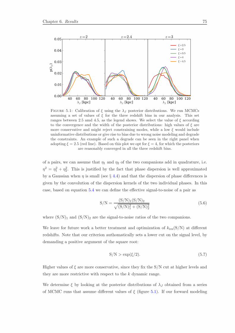
Chapter 6. Results 75
40 60 80 100 120λJ [kpc]
0.00
0.01
0.02
0.03
0.04
0.05
p(λ
J)
z=2
40 60 80 100 120λJ [kpc]
z=2.4
40 60 80 100 120λJ [kpc]
z=3
ξ=2.5
ξ=3
ξ=3.5
ξ=4
ξ=4.5
Figure 5.1: Calibration of ξ using the λJ posterior distributions. We run MCMCsassuming a set of values of ξ for the three redshift bins in our analysis. This setranges between 2.5 amd 4.5, as the legend shows. We select the value of ξ accordingto the convergence and the width of the posterior distributions: high values of ξ aremore conservative and might reject constraining modes, while a low ξ would includeuninformative distributions or give rise to bias due to wrong noise modeling and degradethe constraints. An example of such a degrade can be seen in the right panel whenadopting ξ = 2.5 (red line). Based on this plot we opt for ξ = 4, for which the posteriors
are reasonably converged in all the three redshift bins.
of a pairs, we can assume that η1 and η2 of the two companions add in quadrature, i.e.
η2 = η21 + η22 . This is justified by the fact that phase dispersion is well approximated
by a Gaussian when η is small (see § 4.4) and that the dispersion of phase differences is
given by the convolution of the dispersion kernels of the two individual phases. In this
case, based on equation 5.4 we can define the effective signal-to-noise of a pair as
S/N =(S/N)1(S/N)2
√
(S/N)21 + (S/N)22(5.6)
where (S/N)1 and (S/N)2 are the signal-to-noise ratios of the two companions.
We leave for future work a better treatment and optimization of kres(S/N) at different
redshifts. Note that our criterion authomatically sets a lower cut on the signal level, by
demanding a positive argument of the square root:
S/N > exp(ξ/2). (5.7)
Higher values of ξ are more conservative, since they fix the S/N cut at higher levels and
they are more restrictive with respect to the k dynamic range.
We determine ξ by looking at the posterior distributions of λJ obtained from a series
of MCMC runs that assume different values of ξ (figure 5.1). If our forward modeling
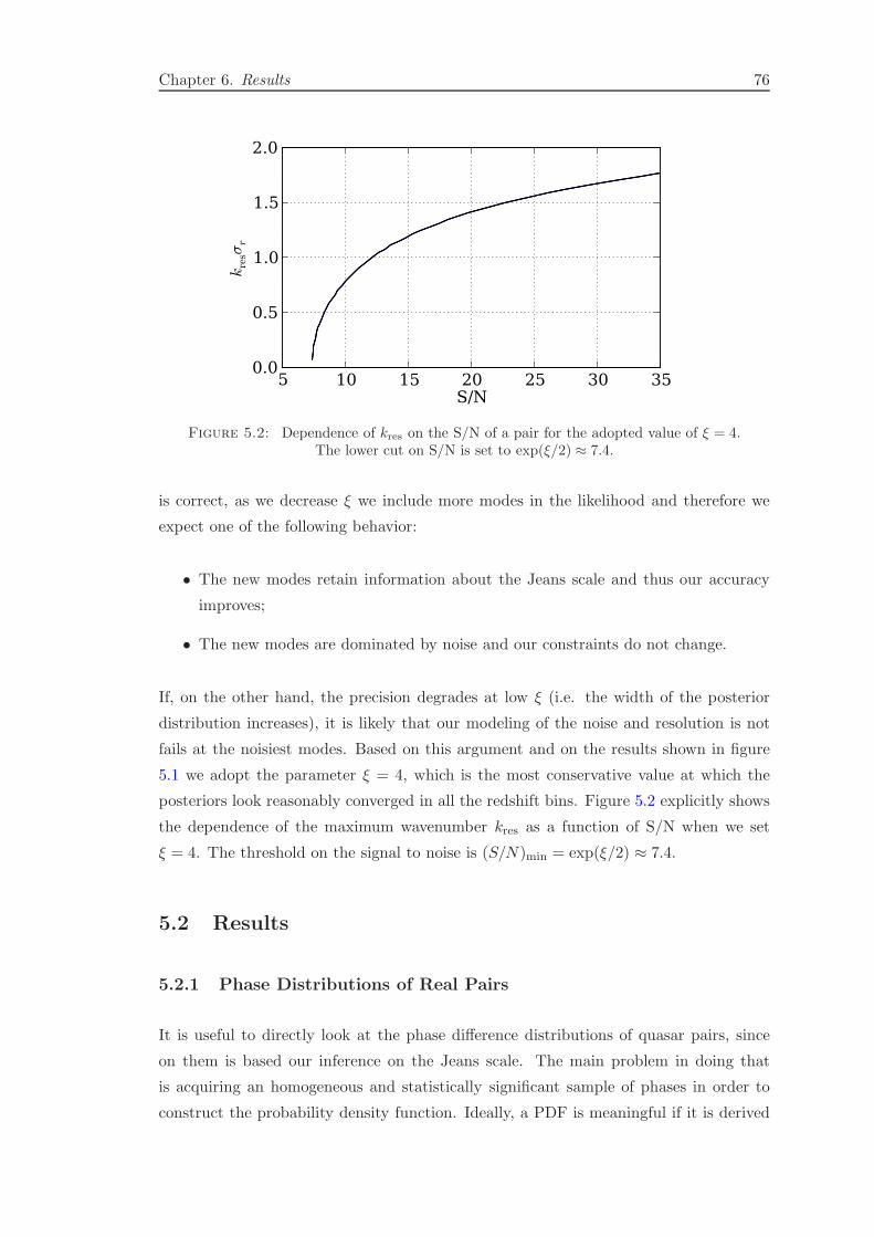
Chapter 6. Results 76
5 10 15 20 25 30 35S/N
0.0
0.5
1.0
1.5
2.0
kre
sσr
Figure 5.2: Dependence of kres on the S/N of a pair for the adopted value of ξ = 4.The lower cut on S/N is set to exp(ξ/2) ≈ 7.4.
is correct, as we decrease ξ we include more modes in the likelihood and therefore we
expect one of the following behavior:
• The new modes retain information about the Jeans scale and thus our accuracy
improves;
• The new modes are dominated by noise and our constraints do not change.
If, on the other hand, the precision degrades at low ξ (i.e. the width of the posterior
distribution increases), it is likely that our modeling of the noise and resolution is not
fails at the noisiest modes. Based on this argument and on the results shown in figure
5.1 we adopt the parameter ξ = 4, which is the most conservative value at which the
posteriors look reasonably converged in all the redshift bins. Figure 5.2 explicitly shows
the dependence of the maximum wavenumber kres as a function of S/N when we set
ξ = 4. The threshold on the signal to noise is (S/N)min = exp(ξ/2) ≈ 7.4.
5.2 Results
5.2.1 Phase Distributions of Real Pairs
It is useful to directly look at the phase difference distributions of quasar pairs, since
on them is based our inference on the Jeans scale. The main problem in doing that
is acquiring an homogeneous and statistically significant sample of phases in order to
construct the probability density function. Ideally, a PDF is meaningful if it is derived

Chapter 6. Results 77
0.5
1.0
1.5
2.0
p(θ)
k=7.1x10⁻³ s/km
0.5
1.0
1.5
2.0
p(θ)
k=2.0x10⁻² s/km
0 π/4 π/2 3π/4 θ
0.5
1.0
1.5
2.0
p(θ)
k=5.3x10⁻² s/km
0 π/4 π/2 3π/4 θ
0 π/4 π/2 3π/4 θ
λJ=42 kpcλJ=100 kpc
Data
r⊥ = 150 kpc r⊥ = 250 kpc r⊥ = 350 kpc
Figure 5.3: Phase difference probability distributions calculated from our data samplein the redshift interval z ∈ [1.8, 2.2] (Black squares). In order to have a significantsampling we need to group phases into r⊥ and k|| bins. The panels from left to the rightcorrespond to the r⊥−intervals [100−200], [200−300] and [300−400] kpc, respectively,while from top to bottom phases are split in the k||−intervals [0.005, 0.01], [0.01, 0.04]and [0.04, 0.07]. The values marked in the plot refers to the central values of the bins(logarithmical in the case of k||). It is worth reminding that the phases present ineach bin are not homogeneous, i.e. they derive from data with different resolutionand signal-to-noise ratio. We compare these distributions with the prediction of twofully forward-modeled simulations, with λj = 30 kpc (red diamonds) and λJ = 70 kpc(green diamonds). Using the calibrated models instead of the original ones assuresthat the PDFs can be directly compared, since they are obtained from analogous pairsamples.The solid lines are the wrapped-Cauchy fit of the models, which trace almost
perfectly the underlying distributions.

Chapter 6. Results 78
0.5
1.0
1.5
p(
θ)k=7.1x10⁻³ s/km
0.5
1.0
1.5
p(θ)
k=2.0x10⁻² s/km
0 π/4 π/2 3π/4 θ
0.5
1.0
1.5
p(θ)
k=5.3x10⁻² s/km
0 π/4 π/2 3π/4 θ
0 π/4 π/2 3π/4 θ
λJ=42 kpcλJ=100 kpc
Data
r⊥ = 150 kpc r⊥ = 250 kpc r⊥ = 350 kpc
Figure 5.4: Same as figure 5.3 but for the redshift interval [2.2, 2.7]
from phases with the same physical and instrumental parameter, which in our case
are z, k||, r⊥, the resolution and the signal-to-noise ratio. Unfortunately, our sample is
not large enough to allow such an high-dimensional splitting, so we adopt a different
approach. For each of the three analyzed redshifts we divide our data in relatively
large r⊥ bins (∆r⊥ = 100 kpc) and we calculate the phase distributions in three k||
intervals [0.005, 0.01], [0.01, 0.04] and [0.04, 0.07] km−1 s. The bins in k|| are defined
somehow arbitrarily in order to have a comparable number of modes in each of them.
The subsamples defined in this way are still hybrid, because they contain information
obtain from data of sparse quality. However, our forward-modeling procedure allows us
to produce analogous samples from the synthetic pairs of our simulations, which we can
compare with observations. The results are shown in figures 5.3, 5.4 and 5.5.
The black squares are the PDFs obtained from data, while the red and the green dia-
monds are calculated respectively from the models T0 = 8000 K, γ = 1.3, λJ = 42 kpc
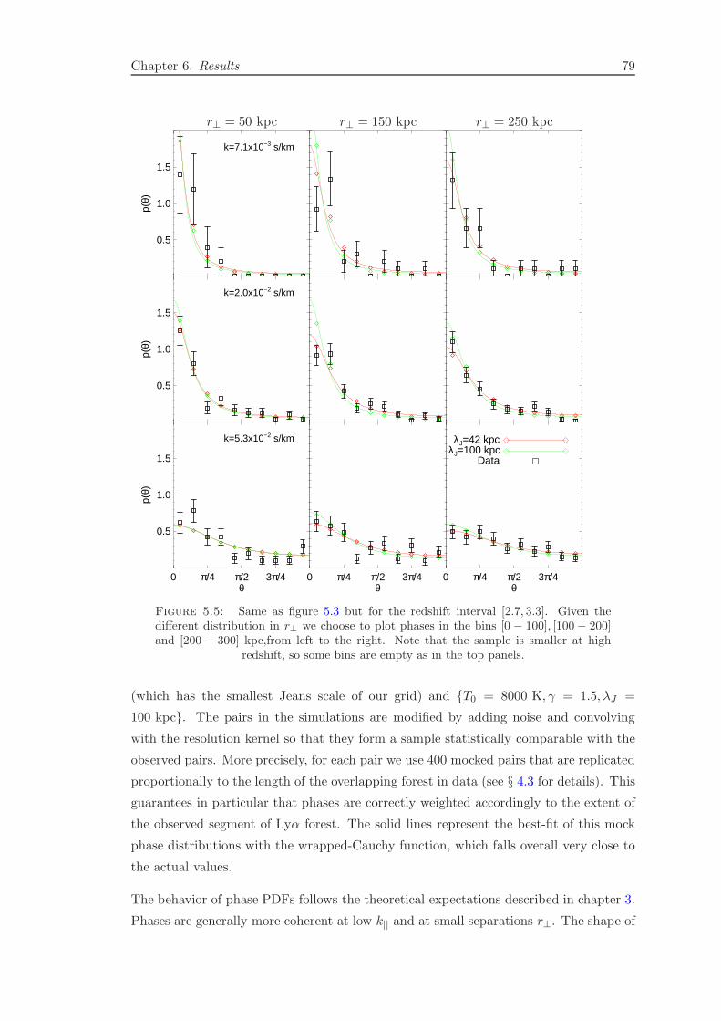
Chapter 6. Results 79
0.5
1.0
1.5
p(
θ)k=7.1x10⁻³ s/km
0.5
1.0
1.5
p(θ)
k=2.0x10⁻² s/km
0 π/4 π/2 3π/4 θ
0.5
1.0
1.5
p(θ)
k=5.3x10⁻² s/km
0 π/4 π/2 3π/4 θ
0 π/4 π/2 3π/4 θ
λJ=42 kpcλJ=100 kpc
Data
r⊥ = 150 kpc r⊥ = 250 kpcr⊥ = 50 kpc
Figure 5.5: Same as figure 5.3 but for the redshift interval [2.7, 3.3]. Given thedifferent distribution in r⊥ we choose to plot phases in the bins [0 − 100], [100− 200]and [200 − 300] kpc,from left to the right. Note that the sample is smaller at high
redshift, so some bins are empty as in the top panels.
(which has the smallest Jeans scale of our grid) and T0 = 8000 K, γ = 1.5, λJ =
100 kpc. The pairs in the simulations are modified by adding noise and convolving
with the resolution kernel so that they form a sample statistically comparable with the
observed pairs. More precisely, for each pair we use 400 mocked pairs that are replicated
proportionally to the length of the overlapping forest in data (see § 4.3 for details). This
guarantees in particular that phases are correctly weighted accordingly to the extent of
the observed segment of Lyα forest. The solid lines represent the best-fit of this mock
phase distributions with the wrapped-Cauchy function, which falls overall very close to
the actual values.
The behavior of phase PDFs follows the theoretical expectations described in chapter 3.
Phases are generally more coherent at low k|| and at small separations r⊥. The shape of
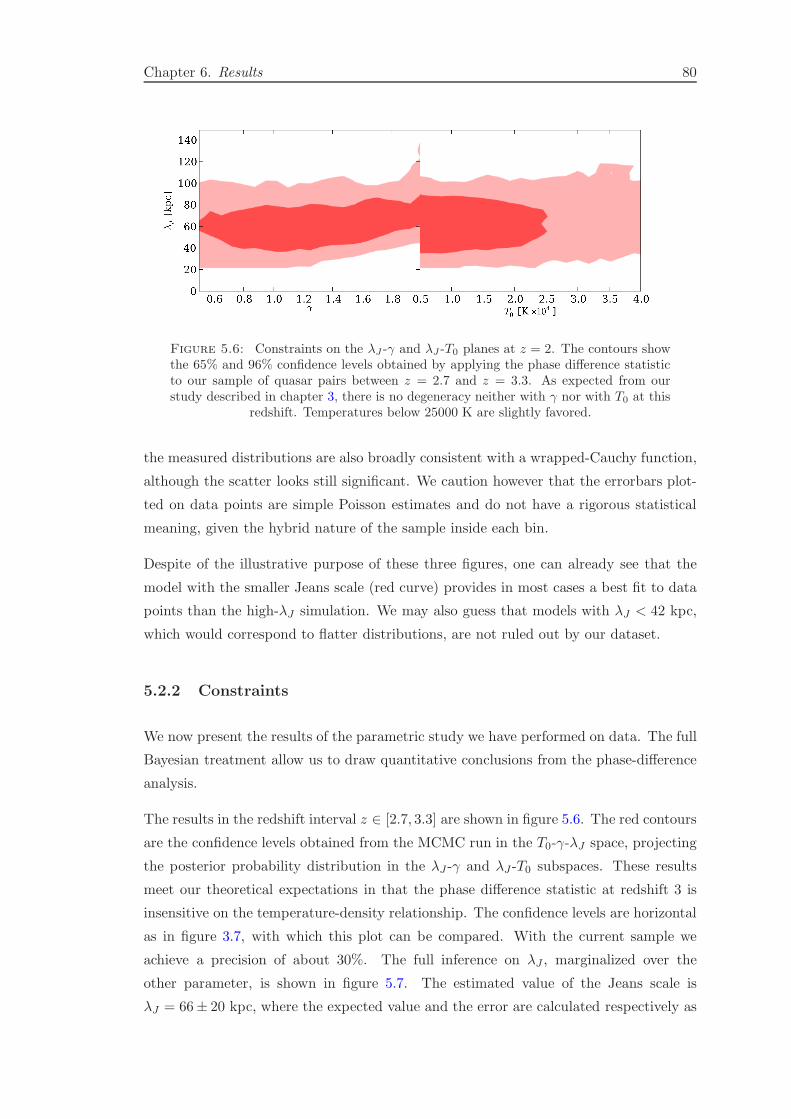
Chapter 6. Results 80
Figure 5.6: Constraints on the λJ -γ and λJ -T0 planes at z = 2. The contours showthe 65% and 96% confidence levels obtained by applying the phase difference statisticto our sample of quasar pairs between z = 2.7 and z = 3.3. As expected from ourstudy described in chapter 3, there is no degeneracy neither with γ nor with T0 at this
redshift. Temperatures below 25000 K are slightly favored.
the measured distributions are also broadly consistent with a wrapped-Cauchy function,
although the scatter looks still significant. We caution however that the errorbars plot-
ted on data points are simple Poisson estimates and do not have a rigorous statistical
meaning, given the hybrid nature of the sample inside each bin.
Despite of the illustrative purpose of these three figures, one can already see that the
model with the smaller Jeans scale (red curve) provides in most cases a best fit to data
points than the high-λJ simulation. We may also guess that models with λJ < 42 kpc,
which would correspond to flatter distributions, are not ruled out by our dataset.
5.2.2 Constraints
We now present the results of the parametric study we have performed on data. The full
Bayesian treatment allow us to draw quantitative conclusions from the phase-difference
analysis.
The results in the redshift interval z ∈ [2.7, 3.3] are shown in figure 5.6. The red contours
are the confidence levels obtained from the MCMC run in the T0-γ-λJ space, projecting
the posterior probability distribution in the λJ -γ and λJ -T0 subspaces. These results
meet our theoretical expectations in that the phase difference statistic at redshift 3 is
insensitive on the temperature-density relationship. The confidence levels are horizontal
as in figure 3.7, with which this plot can be compared. With the current sample we
achieve a precision of about 30%. The full inference on λJ , marginalized over the
other parameter, is shown in figure 5.7. The estimated value of the Jeans scale is
λJ = 66± 20 kpc, where the expected value and the error are calculated respectively as

Chapter 6. Results 81
0 20 40 60 80 100 120 140λJ [kpc]
0.00
0.01
0.02
0.03
0.04
0.05
p(λ
J)
Figure 5.7: Accuracy on the Jeans scale measurement at z = 3. The plot showsthe posterior probability distribution from the MCMC fully marginalized over the pa-rameters γ and T0. The expected value is λJ = 66 kpc, and the estimated 1-σ error is
∆λJ = 20 kpc, giving a relative uncertainty of 30%.
Figure 5.8: Same as figure 5.6, but in the redshift interval [2.2, 2.7]. Differently thanz = 3, a tilt appears in the λJ -γ contours, implying a degeneracy between the twoparameters whose origin is still under research (see the text for a discussion). Similarlyto z = 3, there is no degeneracy between λJ and T0, and low temperatures are favored.The sharp edge at λJ = 22 kpc correspond to the lower border of our parameter grid.
the mean and the standard deviation of the MCMC chain. As a consequence of phase
sensitivity, no constraints are set on γ and on T0, except a very shallow preference for
lower temperatures.
In figure 5.8 we present the same contours at redshift z = 2.4, obtained from the pair
sample in the interval z ∈ [2.2, 2.7]. The most significant difference with z = 3 is the tilt
of the confidence levels on the λJ -γ plane, revealing a significant degeneracy between
the two parameters. This degeneracy is an unexpected result, given our study at z = 3
and our understanding of phase difference statistic. It is somehow undesirable, since
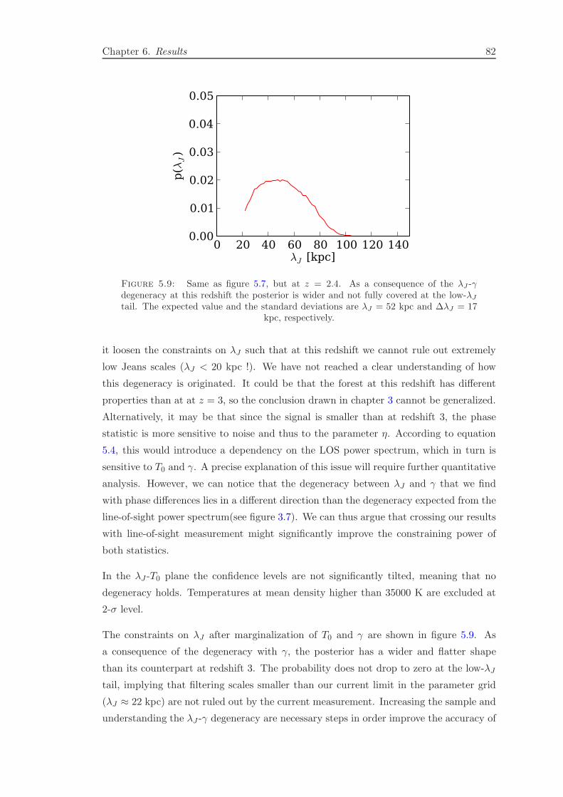
Chapter 6. Results 82
0 20 40 60 80 100 120 140λJ [kpc]
0.00
0.01
0.02
0.03
0.04
0.05
p(λ
J)
Figure 5.9: Same as figure 5.7, but at z = 2.4. As a consequence of the λJ -γdegeneracy at this redshift the posterior is wider and not fully covered at the low-λJtail. The expected value and the standard deviations are λJ = 52 kpc and ∆λJ = 17
kpc, respectively.
it loosen the constraints on λJ such that at this redshift we cannot rule out extremely
low Jeans scales (λJ < 20 kpc !). We have not reached a clear understanding of how
this degeneracy is originated. It could be that the forest at this redshift has different
properties than at at z = 3, so the conclusion drawn in chapter 3 cannot be generalized.
Alternatively, it may be that since the signal is smaller than at redshift 3, the phase
statistic is more sensitive to noise and thus to the parameter η. According to equation
5.4, this would introduce a dependency on the LOS power spectrum, which in turn is
sensitive to T0 and γ. A precise explanation of this issue will require further quantitative
analysis. However, we can notice that the degeneracy between λJ and γ that we find
with phase differences lies in a different direction than the degeneracy expected from the
line-of-sight power spectrum(see figure 3.7). We can thus argue that crossing our results
with line-of-sight measurement might significantly improve the constraining power of
both statistics.
In the λJ -T0 plane the confidence levels are not significantly tilted, meaning that no
degeneracy holds. Temperatures at mean density higher than 35000 K are excluded at
2-σ level.
The constraints on λJ after marginalization of T0 and γ are shown in figure 5.9. As
a consequence of the degeneracy with γ, the posterior has a wider and flatter shape
than its counterpart at redshift 3. The probability does not drop to zero at the low-λJ
tail, implying that filtering scales smaller than our current limit in the parameter grid
(λJ ≈ 22 kpc) are not ruled out by the current measurement. Increasing the sample and
understanding the λJ -γ degeneracy are necessary steps in order improve the accuracy of
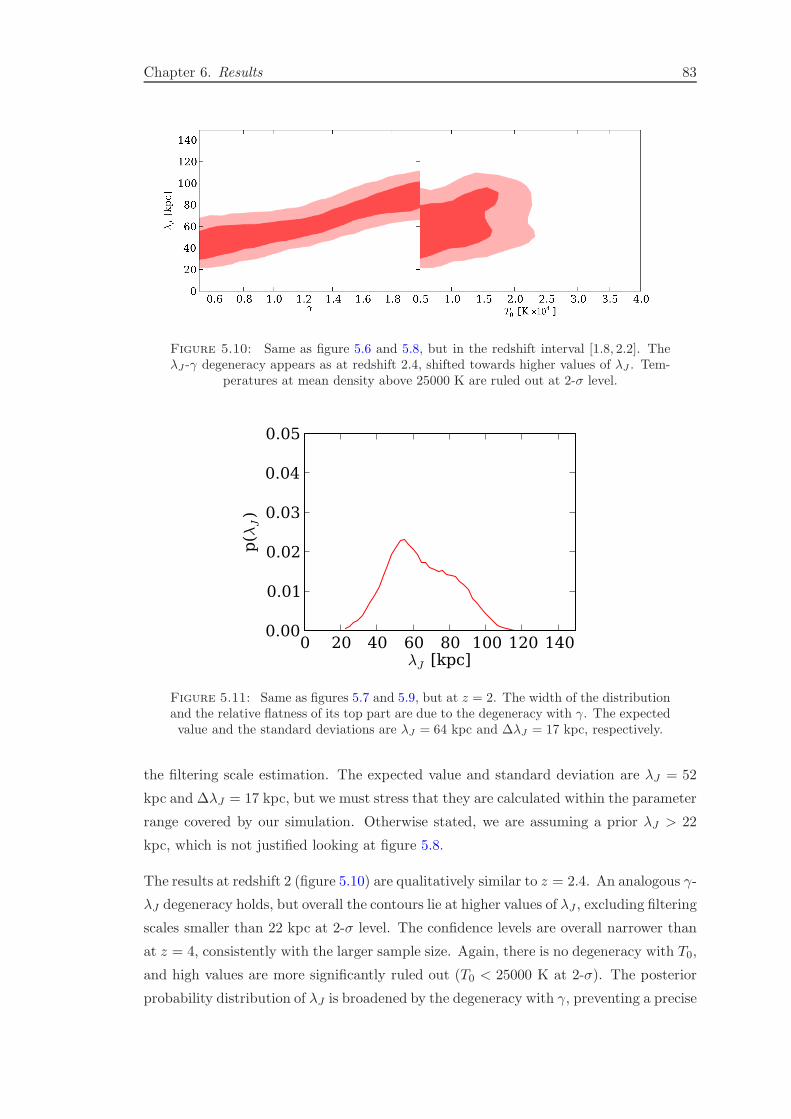
Chapter 6. Results 83
Figure 5.10: Same as figure 5.6 and 5.8, but in the redshift interval [1.8, 2.2]. TheλJ -γ degeneracy appears as at redshift 2.4, shifted towards higher values of λJ . Tem-
peratures at mean density above 25000 K are ruled out at 2-σ level.
0 20 40 60 80 100 120 140λJ [kpc]
0.00
0.01
0.02
0.03
0.04
0.05
p(λ
J)
Figure 5.11: Same as figures 5.7 and 5.9, but at z = 2. The width of the distributionand the relative flatness of its top part are due to the degeneracy with γ. The expectedvalue and the standard deviations are λJ = 64 kpc and ∆λJ = 17 kpc, respectively.
the filtering scale estimation. The expected value and standard deviation are λJ = 52
kpc and ∆λJ = 17 kpc, but we must stress that they are calculated within the parameter
range covered by our simulation. Otherwise stated, we are assuming a prior λJ > 22
kpc, which is not justified looking at figure 5.8.
The results at redshift 2 (figure 5.10) are qualitatively similar to z = 2.4. An analogous γ-
λJ degeneracy holds, but overall the contours lie at higher values of λJ , excluding filtering
scales smaller than 22 kpc at 2-σ level. The confidence levels are overall narrower than
at z = 4, consistently with the larger sample size. Again, there is no degeneracy with T0,
and high values are more significantly ruled out (T0 < 25000 K at 2-σ). The posterior
probability distribution of λJ is broadened by the degeneracy with γ, preventing a precise
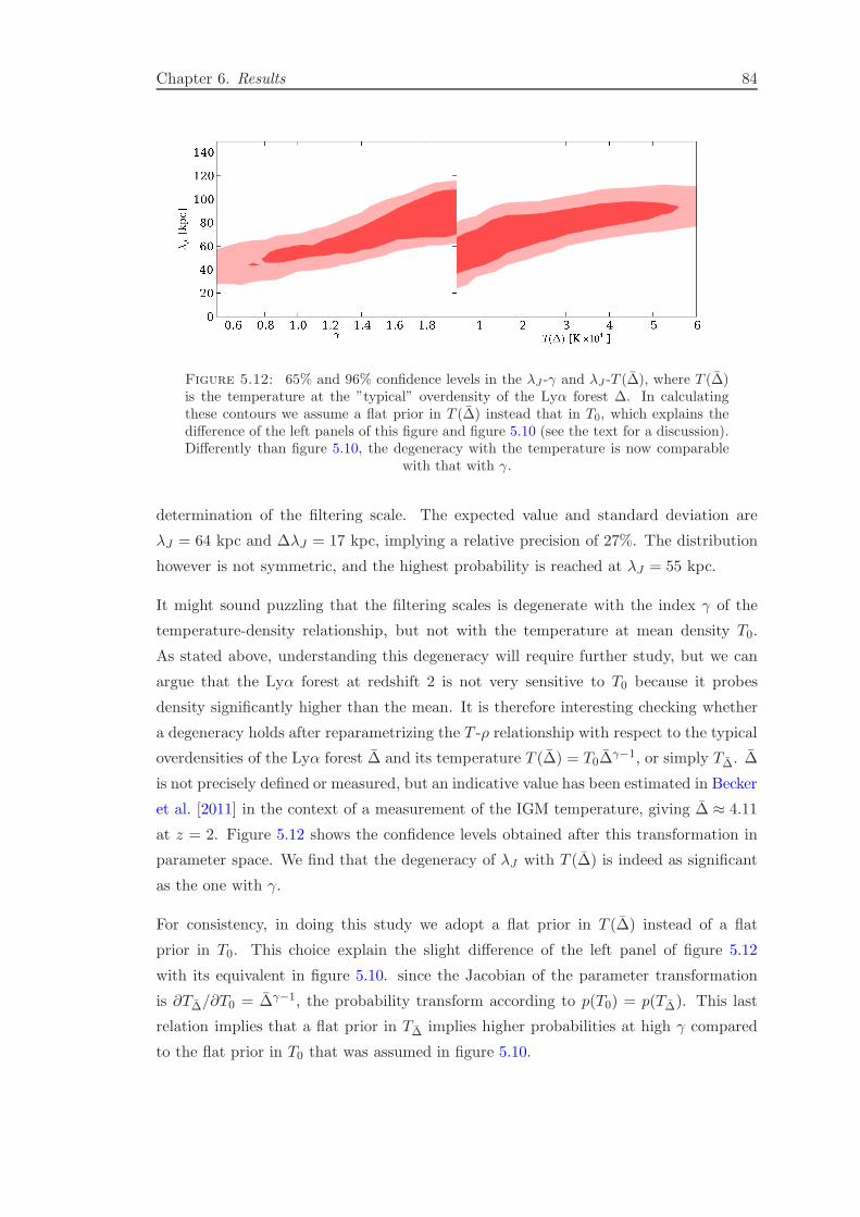
Chapter 6. Results 84
Figure 5.12: 65% and 96% confidence levels in the λJ -γ and λJ -T (∆), where T (∆)is the temperature at the ”typical” overdensity of the Lyα forest ∆. In calculatingthese contours we assume a flat prior in T (∆) instead that in T0, which explains thedifference of the left panels of this figure and figure 5.10 (see the text for a discussion).Differently than figure 5.10, the degeneracy with the temperature is now comparable
with that with γ.
determination of the filtering scale. The expected value and standard deviation are
λJ = 64 kpc and ∆λJ = 17 kpc, implying a relative precision of 27%. The distribution
however is not symmetric, and the highest probability is reached at λJ = 55 kpc.
It might sound puzzling that the filtering scales is degenerate with the index γ of the
temperature-density relationship, but not with the temperature at mean density T0.
As stated above, understanding this degeneracy will require further study, but we can
argue that the Lyα forest at redshift 2 is not very sensitive to T0 because it probes
density significantly higher than the mean. It is therefore interesting checking whether
a degeneracy holds after reparametrizing the T -ρ relationship with respect to the typical
overdensities of the Lyα forest ∆ and its temperature T (∆) = T0∆γ−1, or simply T∆. ∆
is not precisely defined or measured, but an indicative value has been estimated in Becker
et al. [2011] in the context of a measurement of the IGM temperature, giving ∆ ≈ 4.11
at z = 2. Figure 5.12 shows the confidence levels obtained after this transformation in
parameter space. We find that the degeneracy of λJ with T (∆) is indeed as significant
as the one with γ.
For consistency, in doing this study we adopt a flat prior in T (∆) instead of a flat
prior in T0. This choice explain the slight difference of the left panel of figure 5.12
with its equivalent in figure 5.10. since the Jacobian of the parameter transformation
is ∂T∆/∂T0 = ∆γ−1, the probability transform according to p(T0) = p(T∆). This last
relation implies that a flat prior in T∆ implies higher probabilities at high γ compared
to the flat prior in T0 that was assumed in figure 5.10.
Chapter 6. Results 85
5.3 Consistency Tests
The method presented in this study is completely new, and therefore its possible system-
atic errors have not been explored before. In particular the phase difference statistic has
never been used in the contest of the Lyα forest, and given the unexpected results that
we obtained it is necessary to carefully ponder all the possible effects that may change
our conclusions and to revise our main assumptions. For sake of clarity, we classify the
sources of uncertainty we could think of into four broad categories:
• Data-originated : calculating phases from the Lyα forest of observed pair is not a
straightforward operation, partly for mathematical reasons (see § 4.2) and partly
for the presence of contaminants and the uncertainty on the continuum emission;
• Calibration errors : we employ a forward-modeling approach in order to adapt
our set of simulation to the observations. This process involves several steps and
assumptions with which we could inadvertently introduce sources of bias;
• Model assumptions : we base our phase-distribution prediction on a grid of ther-
mal models built on top of a dark matter simulation. This clearly involves strong
assumptions on the distribution of gas in the IGM, raising doubts on the applica-
bility of this method to real data;
• Statistical approximation : the present method makes use of statistical tools such
as Gaussian process interpolation and MCMC, which are approximated algorithms
whose accuracy need to be tested.
In the following we will explain the test we perform in order to check the robustness
of our method against these potential source of biases and error. However we caution
that the validity of several of these tests is limited to the current level of accuracy. As
it is natural, when the amount and the quality of the data will permit measurements of
percent-level precision, also the requirements on the theoretical understanding and on
the modeling of biases will be tighter.
5.3.1 Data-Originated
5.3.1.1 Phase Calculation
In chapter 4 we presented two possible ways of calculating phases of irregularly sampled
functions: one employs least-square spectral analysis (LSSA), the other consists in re-
binning the function into a regular grid and subsequently applying the standard discrete
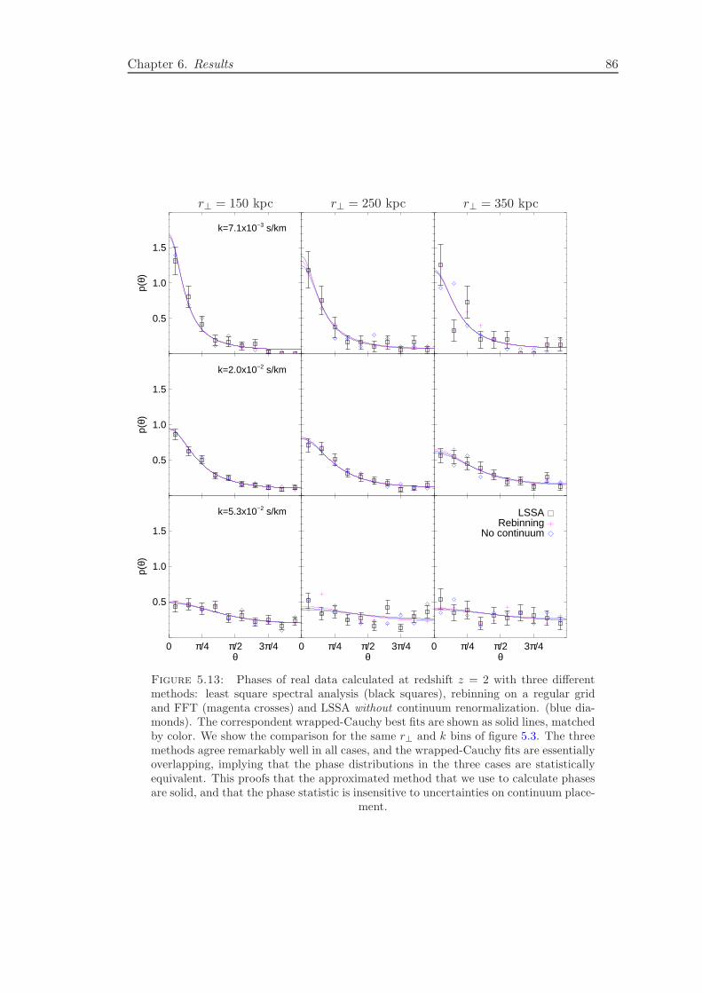
Chapter 6. Results 86
0.5
1.0
1.5
p(θ)
k=7.1x10⁻³ s/km
0.5
1.0
1.5
p(θ)
k=2.0x10⁻² s/km
0 π/4 π/2 3π/4 θ
0.5
1.0
1.5
p(θ)
k=5.3x10⁻² s/km
0 π/4 π/2 3π/4 θ
0 π/4 π/2 3π/4 θ
LSSARebinning
No continuum
r⊥ = 150 kpc r⊥ = 250 kpc r⊥ = 350 kpc
Figure 5.13: Phases of real data calculated at redshift z = 2 with three differentmethods: least square spectral analysis (black squares), rebinning on a regular gridand FFT (magenta crosses) and LSSA without continuum renormalization. (blue dia-monds). The correspondent wrapped-Cauchy best fits are shown as solid lines, matchedby color. We show the comparison for the same r⊥ and k bins of figure 5.3. The threemethods agree remarkably well in all cases, and the wrapped-Cauchy fits are essentiallyoverlapping, implying that the phase distributions in the three cases are statisticallyequivalent. This proofs that the approximated method that we use to calculate phasesare solid, and that the phase statistic is insensitive to uncertainties on continuum place-
ment.
Chapter 6. Results 87
Fourier transformation. Since the two methods imply complementary approximation,
checking that they lead to consistent phase distributions is a good check of the stability
of this calculation. In figure 5.13 we show phases of the observed forest of quasar pairs
binned as we have done for figure 5.3, adopting both the LSSA method (black squares)
and the rebinning procedure (magenta crosses). In almost all cases the two methods
agree extremely precisely, and most importantly the statistical estimator that we use in
the likelihood, i.e. the wrapped-Cauchy concentration parameters, are practically iden-
tical. This can be seen by comparing the best-fit wrapped-Cauchy functions of the two
distribution (black and magenta solid lines), which are indistinguishable at all r⊥ and
k||. We also stress that the approximated Fourier transformation enters the forward-
modeling of simulations, so even in the case where there was a significant effect on phase
distributions, it would have been taken into account in our calibration.
5.3.1.2 Continuum Fitting
Among the properties of phases listed in chapter 3 we claimed that they are robust
against uncertainties on continuum fitting. This was argued based on the mathematical
definition of phases, which are invariant under a global renormalization of the function.
If continuum error could be described as an uncertainty on the renormalization than
our statement would be exact. In the realistic case of a fluctuating continuum, phase
distributions are still untouched in an approximated sense if such continuum fluctuations
occur on scales larger than the typical modes that we want to use (v|| & 1500 km/s).
This could not be true in the presence of associated lines, like BALs, or near the Lyα
and Lyβ emission lines. As explained above, we exclude from the sample quasars with
recognizable BALs, and we do not attempt to use the forest in the vicinity of the two
emission lines. To proof explicitly that phases are not sensitive to continuum errors,
we estimated phase distributions without fitting the continuum of the spectra, directly
from the observed flux, and we compare them with the standard case of continuum-
renormalized spectra. The results of the calculation are shown as blue diamonds in
figure 5.13. The agreement is remarkable at all r⊥ and k||, both with the interpolation
and LSSA methods. Even where there are differences on the actual distribution, the
fitted wrapped-Cauchy function almost coincides with the continuum-corrected phases.
This test proofs that phases are insensitive to variation of the continuum, unless for some
reason other than BAL there are neglected fluctuations and wiggles at small velocity
scales.
Chapter 6. Results 88
5.3.1.3 Contaminants
It is possible that part of the absorption in the Lyα forest of our spectra is not caused
by neutral hydrogen in the diffuse IGM but from other systems that are not modeled in
our simulation. An examples are broad absorption lines (BAL) associated with quasars,
which can have high velocities and be blueshifted in the Lyα forest. As we have just
reminded, all the QSOs that exhibit such lines have been removed from the sample.
Similarly, we have excluded all the region of the forest where we could identify a Damped
LyαAbsorber (DLA), since they are not described by the optically-thin approximation
that we adopt. For the same reason also Lyman Limit Systems (LSS) should be removed,
but this is not possible because they are practically indistinguishable from the forest.
However, we doubt that they can generate a strong bias, given that they contribute to
the forest absorption by only a tiny amount [McDonald et al., 2005]. A similar arguments
holds for metal contamination. Moreover, metal lines are narrow, and they affect mostly
Fourier modes with k > 0.1 s/km [McDonald et al., 2000] which we exclude precisely
for this reason.
If metal contamination and LLSs have a stronger impact than expected, they might
cause a decrease in the transverse coherence of pairs, since they would not be strongly
correlated in space. This effect would lead to an underestimation of the Jeans filtering
scale, henceforth we plan for the future a more careful and quantitative test of the
robustness of our results with respect to these contaminants.
5.3.2 Calibration
5.3.2.1 Resolution
The first step of the forward modeling consists in convolving the simulated skewers
with a Gaussian kernel whose width is regulated according to the estimated resolution.
This operation does not change phase differences initially, but it cuts the longitudinal
power exponentially at high k, which have a significant effect on phases when noise is
added (see discussion in § 5.1.5). Moreover, the estimation of the resolution also set
the maximum k|| we will use in the phase likelihood for that pair. It is then natural to
ask what kind of bias we would get if the resolution we are assuming is underestimated
or overestimated. In order to explicitly check this, we perform a test using a mock
data sample from our simulation at z = 3. We generate skewers with S/N=10 and
resolution FWHM=100 km/s, which are average values for our quasar sample, chosen
from a fiducial model with λJ = 80 kpc. We then try to ”measure” the Jeans scale
of this mock sample applying our standard technique, but calibrating the simulations
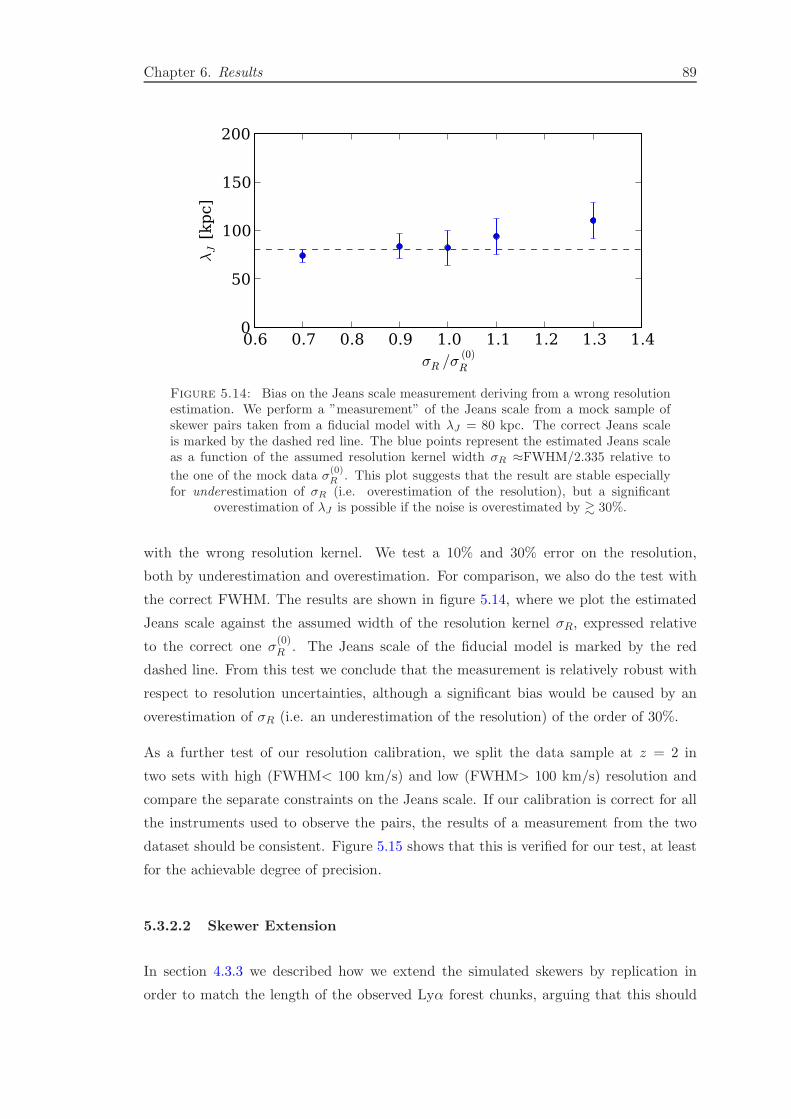
Chapter 6. Results 89
0.6 0.7 0.8 0.9 1.0 1.1 1.2 1.3 1.4 σR /σ
(0)
R
0
50
100
150
200
λJ [kpc]
Figure 5.14: Bias on the Jeans scale measurement deriving from a wrong resolutionestimation. We perform a ”measurement” of the Jeans scale from a mock sample ofskewer pairs taken from a fiducial model with λJ = 80 kpc. The correct Jeans scaleis marked by the dashed red line. The blue points represent the estimated Jeans scaleas a function of the assumed resolution kernel width σR ≈FWHM/2.335 relative to
the one of the mock data σ(0)R . This plot suggests that the result are stable especially
for underestimation of σR (i.e. overestimation of the resolution), but a significantoverestimation of λJ is possible if the noise is overestimated by & 30%.
with the wrong resolution kernel. We test a 10% and 30% error on the resolution,
both by underestimation and overestimation. For comparison, we also do the test with
the correct FWHM. The results are shown in figure 5.14, where we plot the estimated
Jeans scale against the assumed width of the resolution kernel σR, expressed relative
to the correct one σ(0)R . The Jeans scale of the fiducial model is marked by the red
dashed line. From this test we conclude that the measurement is relatively robust with
respect to resolution uncertainties, although a significant bias would be caused by an
overestimation of σR (i.e. an underestimation of the resolution) of the order of 30%.
As a further test of our resolution calibration, we split the data sample at z = 2 in
two sets with high (FWHM< 100 km/s) and low (FWHM> 100 km/s) resolution and
compare the separate constraints on the Jeans scale. If our calibration is correct for all
the instruments used to observe the pairs, the results of a measurement from the two
dataset should be consistent. Figure 5.15 shows that this is verified for our test, at least
for the achievable degree of precision.
5.3.2.2 Skewer Extension
In section 4.3.3 we described how we extend the simulated skewers by replication in
order to match the length of the observed Lyα forest chunks, arguing that this should
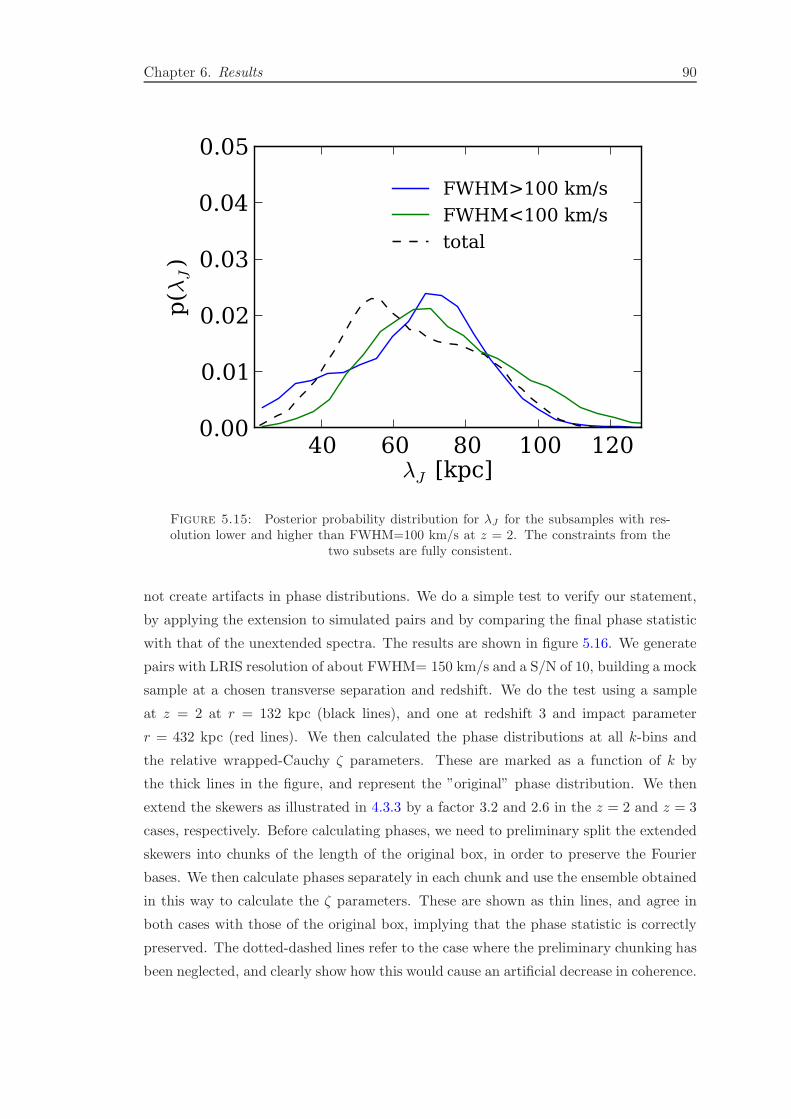
Chapter 6. Results 90
40 60 80 100 120λJ [kpc]
0.00
0.01
0.02
0.03
0.04
0.05p(λ
J)
FWHM>100 km/s
FWHM<100 km/s
total
Figure 5.15: Posterior probability distribution for λJ for the subsamples with res-olution lower and higher than FWHM=100 km/s at z = 2. The constraints from the
two subsets are fully consistent.
not create artifacts in phase distributions. We do a simple test to verify our statement,
by applying the extension to simulated pairs and by comparing the final phase statistic
with that of the unextended spectra. The results are shown in figure 5.16. We generate
pairs with LRIS resolution of about FWHM= 150 km/s and a S/N of 10, building a mock
sample at a chosen transverse separation and redshift. We do the test using a sample
at z = 2 at r = 132 kpc (black lines), and one at redshift 3 and impact parameter
r = 432 kpc (red lines). We then calculated the phase distributions at all k-bins and
the relative wrapped-Cauchy ζ parameters. These are marked as a function of k by
the thick lines in the figure, and represent the ”original” phase distribution. We then
extend the skewers as illustrated in 4.3.3 by a factor 3.2 and 2.6 in the z = 2 and z = 3
cases, respectively. Before calculating phases, we need to preliminary split the extended
skewers into chunks of the length of the original box, in order to preserve the Fourier
bases. We then calculate phases separately in each chunk and use the ensemble obtained
in this way to calculate the ζ parameters. These are shown as thin lines, and agree in
both cases with those of the original box, implying that the phase statistic is correctly
preserved. The dotted-dashed lines refer to the case where the preliminary chunking has
been neglected, and clearly show how this would cause an artificial decrease in coherence.
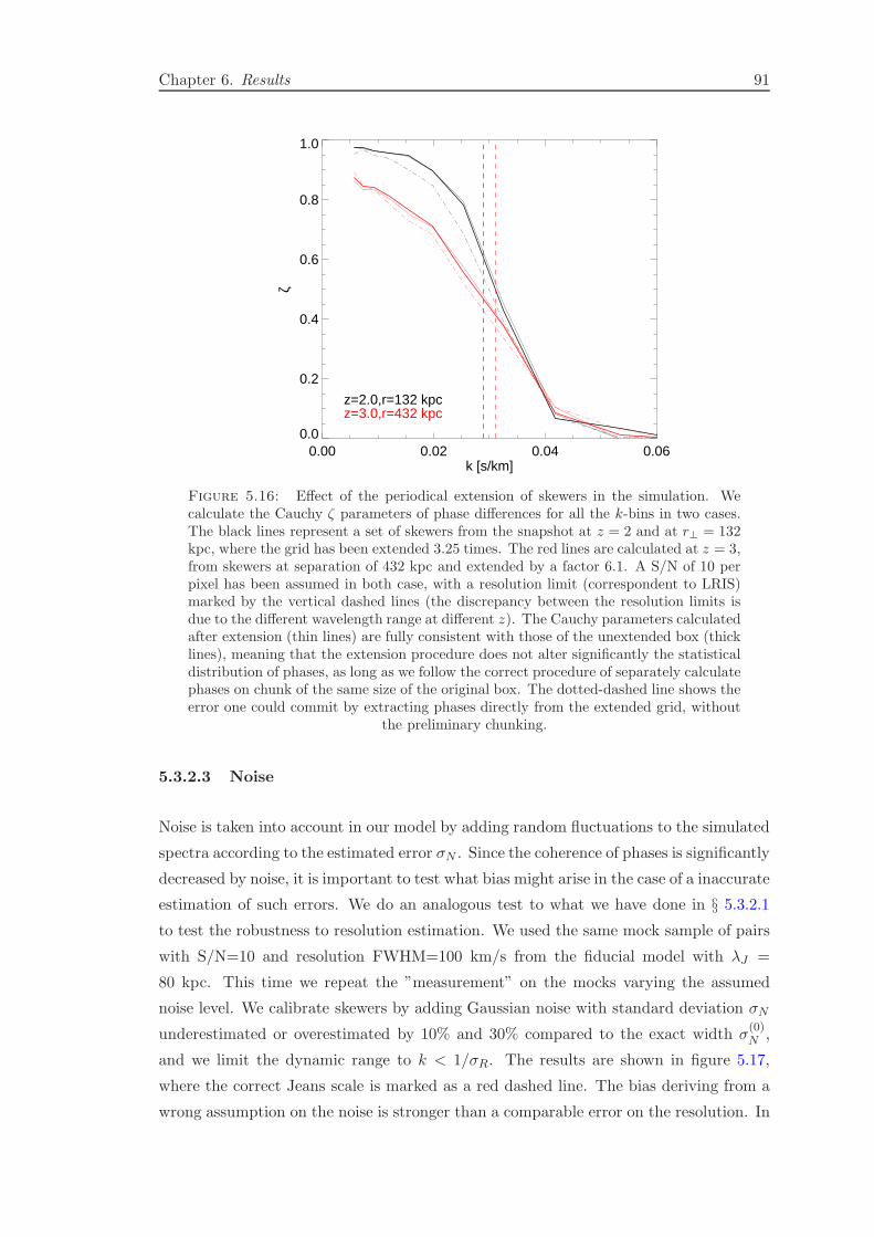
Chapter 6. Results 91
0.00 0.02 0.04 0.06k [s/km]
0.0
0.2
0.4
0.6
0.8
1.0
ζ
z=3.0,r=432 kpcz=2.0,r=132 kpc
Figure 5.16: Effect of the periodical extension of skewers in the simulation. Wecalculate the Cauchy ζ parameters of phase differences for all the k-bins in two cases.The black lines represent a set of skewers from the snapshot at z = 2 and at r⊥ = 132kpc, where the grid has been extended 3.25 times. The red lines are calculated at z = 3,from skewers at separation of 432 kpc and extended by a factor 6.1. A S/N of 10 perpixel has been assumed in both case, with a resolution limit (correspondent to LRIS)marked by the vertical dashed lines (the discrepancy between the resolution limits isdue to the different wavelength range at different z). The Cauchy parameters calculatedafter extension (thin lines) are fully consistent with those of the unextended box (thicklines), meaning that the extension procedure does not alter significantly the statisticaldistribution of phases, as long as we follow the correct procedure of separately calculatephases on chunk of the same size of the original box. The dotted-dashed line shows theerror one could commit by extracting phases directly from the extended grid, without
the preliminary chunking.
5.3.2.3 Noise
Noise is taken into account in our model by adding random fluctuations to the simulated
spectra according to the estimated error σN . Since the coherence of phases is significantly
decreased by noise, it is important to test what bias might arise in the case of a inaccurate
estimation of such errors. We do an analogous test to what we have done in § 5.3.2.1
to test the robustness to resolution estimation. We used the same mock sample of pairs
with S/N=10 and resolution FWHM=100 km/s from the fiducial model with λJ =
80 kpc. This time we repeat the ”measurement” on the mocks varying the assumed
noise level. We calibrate skewers by adding Gaussian noise with standard deviation σN
underestimated or overestimated by 10% and 30% compared to the exact width σ(0)N ,
and we limit the dynamic range to k < 1/σR. The results are shown in figure 5.17,
where the correct Jeans scale is marked as a red dashed line. The bias deriving from a
wrong assumption on the noise is stronger than a comparable error on the resolution. In
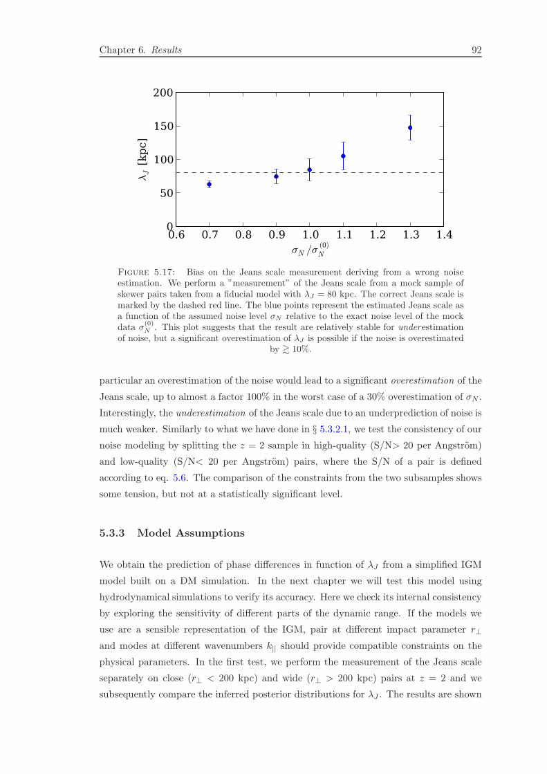
Chapter 6. Results 92
0.6 0.7 0.8 0.9 1.0 1.1 1.2 1.3 1.4 σN /σ
(0)
N
0
50
100
150
200
λJ [kpc]
Figure 5.17: Bias on the Jeans scale measurement deriving from a wrong noiseestimation. We perform a ”measurement” of the Jeans scale from a mock sample ofskewer pairs taken from a fiducial model with λJ = 80 kpc. The correct Jeans scale ismarked by the dashed red line. The blue points represent the estimated Jeans scale asa function of the assumed noise level σN relative to the exact noise level of the mockdata σ
(0)N . This plot suggests that the result are relatively stable for underestimation
of noise, but a significant overestimation of λJ is possible if the noise is overestimatedby & 10%.
particular an overestimation of the noise would lead to a significant overestimation of the
Jeans scale, up to almost a factor 100% in the worst case of a 30% overestimation of σN .
Interestingly, the underestimation of the Jeans scale due to an underprediction of noise is
much weaker. Similarly to what we have done in § 5.3.2.1, we test the consistency of our
noise modeling by splitting the z = 2 sample in high-quality (S/N> 20 per Angstrom)
and low-quality (S/N< 20 per Angstrom) pairs, where the S/N of a pair is defined
according to eq. 5.6. The comparison of the constraints from the two subsamples shows
some tension, but not at a statistically significant level.
5.3.3 Model Assumptions
We obtain the prediction of phase differences in function of λJ from a simplified IGM
model built on a DM simulation. In the next chapter we will test this model using
hydrodynamical simulations to verify its accuracy. Here we check its internal consistency
by exploring the sensitivity of different parts of the dynamic range. If the models we
use are a sensible representation of the IGM, pair at different impact parameter r⊥
and modes at different wavenumbers k|| should provide compatible constraints on the
physical parameters. In the first test, we perform the measurement of the Jeans scale
separately on close (r⊥ < 200 kpc) and wide (r⊥ > 200 kpc) pairs at z = 2 and we
subsequently compare the inferred posterior distributions for λJ . The results are shown
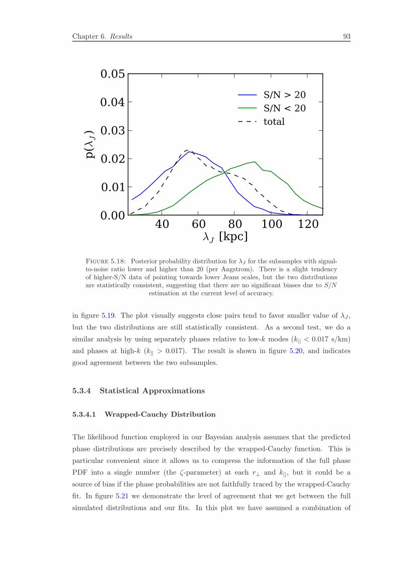
Chapter 6. Results 93
40 60 80 100 120λJ [kpc]
0.00
0.01
0.02
0.03
0.04
0.05p(λ
J)
S/N > 20
S/N < 20
total
Figure 5.18: Posterior probability distribution for λJ for the subsamples with signal-to-noise ratio lower and higher than 20 (per Angstrom). There is a slight tendencyof higher-S/N data of pointing towards lower Jeans scales, but the two distributionsare statistically consistent, suggesting that there are no significant biases due to S/N
estimation at the current level of accuracy.
in figure 5.19. The plot visually suggests close pairs tend to favor smaller value of λJ ,
but the two distributions are still statistically consistent. As a second test, we do a
similar analysis by using separately phases relative to low-k modes (k|| < 0.017 s/km)
and phases at high-k (k|| > 0.017). The result is shown in figure 5.20, and indicates
good agreement between the two subsamples.
5.3.4 Statistical Approximations
5.3.4.1 Wrapped-Cauchy Distribution
The likelihood function employed in our Bayesian analysis assumes that the predicted
phase distributions are precisely described by the wrapped-Cauchy function. This is
particular convenient since it allows us to compress the information of the full phase
PDF into a single number (the ζ-parameter) at each r⊥ and k||, but it could be a
source of bias if the phase probabilities are not faithfully traced by the wrapped-Cauchy
fit. In figure 5.21 we demonstrate the level of agreement that we get between the full
simulated distributions and our fits. In this plot we have assumed a combination of

Chapter 6. Results 94
40 60 80 100 120λJ [kpc]
0.00
0.01
0.02
0.03
0.04
0.05p(λ
J)
r⟂<200 kpc
r⟂>200 kpc
total
Figure 5.19: Posterior probability distributions for λJ for the subsamples of pairsat separation larger and smaller than 200 kpc. Data from closer pairs seems to favorslightly lower Jeans scales, but also in this case the two distributions are statistically
consistent.
resolution and S/N correspondent to our data sample, analogous to what we have done
in figure 5.3. The differences between the wrapped-Cauchy fits (solid lines) and the
actual distributions (diamonds) are almost unnoticeable for all the values of λj, r⊥ and
k that we show in the figure.
5.3.4.2 Emulator
We explained in § 5.1.4 that our emulator is reliable if the training grid is dense enough
with respect to the smoothness of the interpolated function in the parameter space.
When this condition is not fulfilled our results could be sensitive to the parameters we
choose in implementing the Gaussian-process interpolation. These parameters are the
smoothing lengths, which express the degree of correlation we assume when interpo-
lating in parameter space. Choosing large smoothing lengths prevent the interpolated
variable to vary strongly between the grid points, while small smoothing lengths cause
the prediction to fall quickly to zero when no neighbor points are present. To check that
our results are independent of this choice we repeat the measurement after varying the
smoothing length by ±20%. We then looked at the confidence levels and verify that they

Chapter 6. Results 95
40 60 80 100 120λJ [kpc]
0.00
0.01
0.02
0.03
0.04
0.05p(λ
J)
k||<0.017
k||>0.017
total
Figure 5.20: Posterior probability distributions for λJ splitting the phases bywavenumber. The constraints originated from the phases with k|| < 0.017 s/km are
statistically consistent with those obtained from phases at k|| > 0.017 s/km.
0.5
1.0
1.5
2.0
p(θ)
k=7.1x10⁻³ s/km
0 π/4 π/2 3π/4 θ
0.5
1.0
1.5
2.0
p(θ)
k=2.0x10⁻² s/km
0 π/4 π/2 3π/4 θ
λJ=42 kpc
λJ=100 kpc
r⊥ = 150 kpc r⊥ = 250 kpc
Figure 5.21: Example of wrapped-Cauchy fits to the distributions predicted by oursimulations. This figure show the phase PDFs at z = 2 for λJ = 42 kpc (red) andλJ = 100 kpc (green). The panels refer to the impact-parameter bins [100, 200] kpcand [200, 300] kpc (left to right) and the k-bins [0.005, 0.01] s/km and [0.01, 0.04] s/km(top to bottom). The wrapped-Cauchy function traces the actual distributions with
excellent agreement in all cases.

Chapter 6. Results 96
0.6 0.8 1.0 1.2 1.4 1.6 1.8 2.0γ
0
20
40
60
80
100
120
140
λJ [kpc]
Figure 5.22: Convergence of the emulator. We plot the 65% (solid lines) and 95%(dashed lines) confidence level in the λJ -γ plane, for three choices of the smoothing
lengths. The default choice is represented by the red lines, while the blue/green contoursare obtained by assuming 20% larger/smaller smoothing lengths. The lines trace eachother with high accuracy, implying that the emulator interpolation does not affect our
results.
0 20 40 60 80 100 120 140λJ [kpc]
0.00
0.01
0.02
0.03
0.04
0.05
p(λ
J)
Figure 5.23: Convergence of the MCMC chains for the posterior at z = 3. Thehistograms are calculated from chains with 180000 (blue) and 45000 (red) points.
are converged. We show this test for the most delicate case of the λJ -γ plane at z = 2,
where the contours are narrower and thus have the most demanding requirement on the
density of the training grid. Figure 5.22 demonstrates that the emulator is converged at
much higher precision than the accuracy of the measurement.

Chapter 6. Results 97
5.3.4.3 MCMC convergence
We check that our MCMCs are converged by running a longer chains and comparing the
posterior distribution for λJ . The calculation of the likelihood is relatively fast, since
it only requires the interpolation of one number (the logarithm of the likelihood on the
grid), and our parameter space has only 3 dimensions. Moreover, the likelihood function
is relatively smooth in the parameter space at the current level of precision. All these
factors favor a fast convergence of MCMC runs, as it is shown in figure 5.23.

Chapter 6
Interpretation and Discussion
In the previous chapter we presented our estimation of the IGM Jeans scale achieved
by calibrating phase differences on a set of models based on a dark matter N-body
simulation. In the context of our model, λJ is the width of the kernel with which we
smooth the dark matter density field in order to obtain the baryon distribution. In
a CDM universe, where dark matter has no smoothing length, this identifies λJ with
the smoothing length of baryons, or thinking in Fourier space, as the scale where the
3d matter power spectrum is truncated. This interpretation however only holds if the
assumptions made to build such models are a good approximation of the real IGM. We
need to understand if this smoothing length exists in the universe and if we are able to
probe it using our phase-difference method.
In this chapter we try to address this problem by means of full hydrodynamical simula-
tions (which I briefly present in § sims). By doing so we complete the task left open in
chapter 4 of demonstrating the validity of our method, and we also gain useful under-
standing on the meaning of the measured λJ . The key idea is that the Jeans filtering
can be identified once the appropriate density range is selected: in general density peaks
of collapsed objects dominate the matter power spectrum at small scales, and the sup-
pression due to pressure is completely concealed. Once the high densities are removed
from the analysis the power spectrum of the IGM emerges and the truncation due to
pressure support clearly appears. The fact the Lyα forest is only sensitive to the low-
density regions motivates this reasoning from an observational point of view, indicating
this filtering scale as a natural interpretation of the quantity we measure with quasar
pairs.
The properties of the Jeans filtering scales are still poorly understood, in particular its
sensitivity to the thermal history and the expected value at the Lyα-forest redshifts.
These and other related theoretical questions are now under research in our group, an
98
Chapter 6. Interpretation and Discussion 99
effort in which I have been directly involved in the last part of my PhD. I will illustrate
in the second part of this chapter some preliminary results that we obtained in this
direction, in particular the possible ways of defining the filtering scale in hydrodynamical
simulations (§ 6.3), and finally the comparison of the measured filtering scales with the
expected values for a set of thermal histories in § 6.4.
6.1 Hydrodynamical Simulations
I this section I will refer to a set of hydrodynamic simulations that have been run
for multiple IGM-related science goals. We used both the Lagrangian code Gadget3,
an improved version of the publicly available code Gadget2 [Springel, 2005], and the
recently developed Eulerian code Nyx [Almgren et al., 2013].
Gadget3 was run with 2 × 5123 gas and dark matter particles in a 10 Mpc/h box. To
optimize the calculation, we used the ”quick Lyα” flag, that converts gas into stars
above an overdensity threshold (in our case ∆ > 1000). This method does not affect the
IGM and speeds up significantly the simulation.
Nyx simulations are run on 10 Mpc/h size cube with 5123 cells. This boxsize and
resolutions are chosen in order to achieve convergence in the low-density IGM and in
particular of the phase-difference statistic of quasar pairs (Onorbe et al.,in prep.)
In both simulations we assume the gas to be optically thin and in ionization equilibrium
with a spatially homogeneous ultraviolet background (UVB). We adopt the UVB from
the the model of Haardt & Madau [2012]. In order to study different thermal history we
follow the procedure used in Becker et al. [2011]. The photoheating rates for HI,HeI and
HeII are rescaled in a density-dependent manner as ǫ = A∆Bǫ0, where ∆ = ρ/ρ is the
overdensity and ǫ0 the Haardt and Madau photoheating rates. A detailed description
of the simulation will be given in Onorbe et al. (in prep.) and Kulkarni et al. (in
prep.). For what concerns this chapter, we will use the results from the Nyx simulation
with B = 0 and A = 1, 0.5, 0.1, to which we will refer as NHM, N0.5HM and N0.1HM
respectively, and from Gadget 3 using B = 0 and A = 1 (GHM).
In these simulation we use the cosmological parameter Ωm = 0.275,Ωb = 0.046,ΩΛ =
0.725, h = 0.702 and σ8 = 0.816. The other details of the four simulations are specified
in table 6.1.
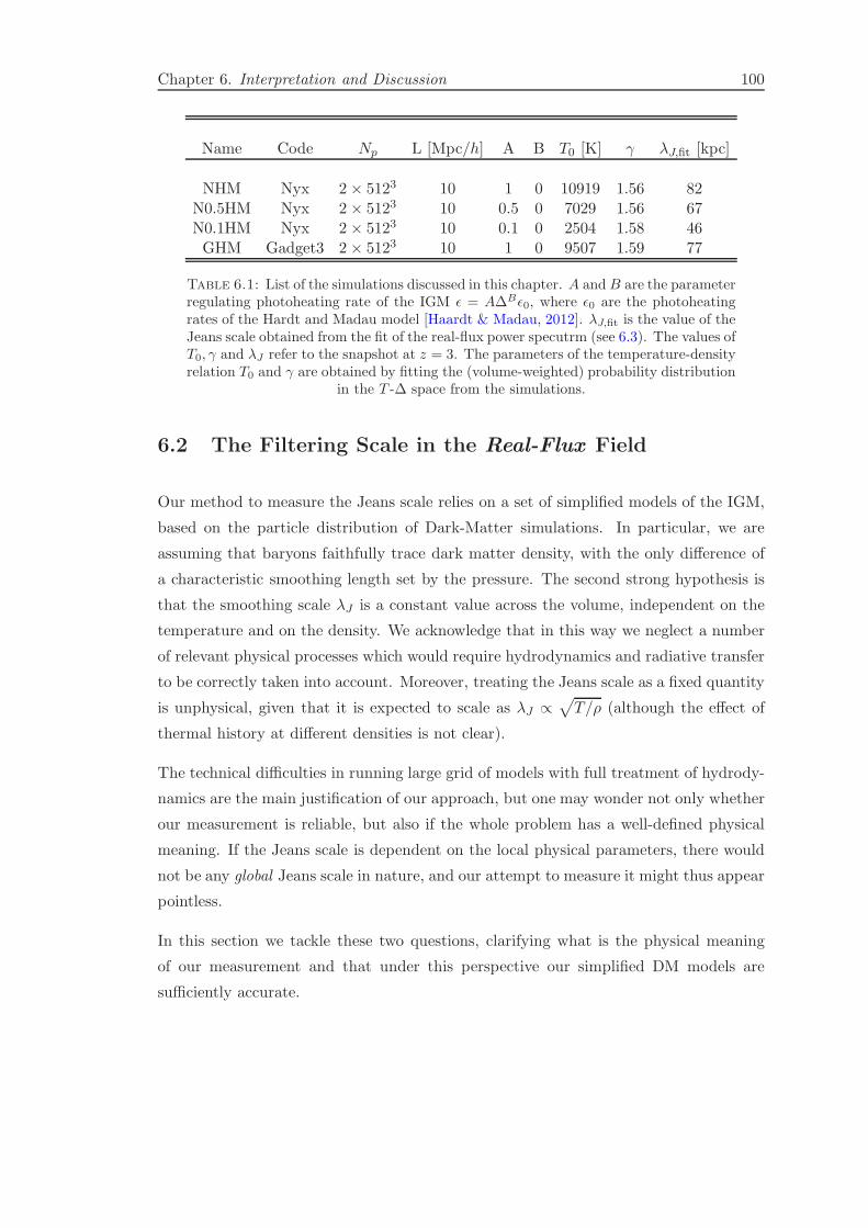
Chapter 6. Interpretation and Discussion 100
Name Code Np L [Mpc/h] A B T0 [K] γ λJ,fit [kpc]
NHM Nyx 2× 5123 10 1 0 10919 1.56 82N0.5HM Nyx 2× 5123 10 0.5 0 7029 1.56 67N0.1HM Nyx 2× 5123 10 0.1 0 2504 1.58 46GHM Gadget3 2× 5123 10 1 0 9507 1.59 77
Table 6.1: List of the simulations discussed in this chapter. A and B are the parameterregulating photoheating rate of the IGM ǫ = A∆Bǫ0, where ǫ0 are the photoheatingrates of the Hardt and Madau model [Haardt & Madau, 2012]. λJ,fit is the value of theJeans scale obtained from the fit of the real-flux power specutrm (see 6.3). The values ofT0, γ and λJ refer to the snapshot at z = 3. The parameters of the temperature-densityrelation T0 and γ are obtained by fitting the (volume-weighted) probability distribution
in the T -∆ space from the simulations.
6.2 The Filtering Scale in the Real-Flux Field
Our method to measure the Jeans scale relies on a set of simplified models of the IGM,
based on the particle distribution of Dark-Matter simulations. In particular, we are
assuming that baryons faithfully trace dark matter density, with the only difference of
a characteristic smoothing length set by the pressure. The second strong hypothesis is
that the smoothing scale λJ is a constant value across the volume, independent on the
temperature and on the density. We acknowledge that in this way we neglect a number
of relevant physical processes which would require hydrodynamics and radiative transfer
to be correctly taken into account. Moreover, treating the Jeans scale as a fixed quantity
is unphysical, given that it is expected to scale as λJ ∝√
T/ρ (although the effect of
thermal history at different densities is not clear).
The technical difficulties in running large grid of models with full treatment of hydrody-
namics are the main justification of our approach, but one may wonder not only whether
our measurement is reliable, but also if the whole problem has a well-defined physical
meaning. If the Jeans scale is dependent on the local physical parameters, there would
not be any global Jeans scale in nature, and our attempt to measure it might thus appear
pointless.
In this section we tackle these two questions, clarifying what is the physical meaning
of our measurement and that under this perspective our simplified DM models are
sufficiently accurate.
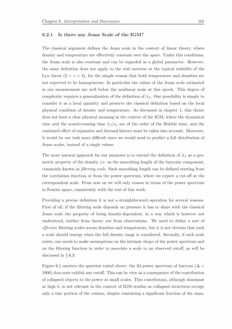
Chapter 6. Interpretation and Discussion 101
6.2.1 Is there any Jeans Scale of the IGM?
The classical argument defines the Jeans scale in the context of linear theory, where
density and temperature are effectively constant over the space. Under this conditions,
the Jeans scale is also constant and can be regarded as a global parameter. However,
the same definition does not apply to the real universe at the typical redshifts of the
Lyα forest (2 < z < 4), for the simple reason that both temperature and densities are
not expected to be homogeneous. In particular the values of the Jeans scale estimated
in our measurement are well below the nonlinear scale at this epoch. This degree of
complexity requires a generalization of the definition of λJ . One possibility is simply to
consider it as a local quantity and preserve the classical definition based on the local
physical condition of density and temperature. As discussed in chapter 1, this choice
does not have a clear physical meaning in the context of the IGM, where the dynamical
time and the sound-crossing time λJ/cs are of the order of the Hubble time, and the
combined effect of expansion and thermal history must be taken into account. Moreover,
it would be our task more difficult since we would need to predict a full distribution of
Jeans scales, instead of a single values.
The most natural approach for our purposes is to extend the definition of λJ as a geo-
metric property of the density, i.e. as the smoothing length of the baryonic component,
commonly known as filtering scale. Such smoothing length can be defined starting from
the correlation function or from the power spectrum, where we expect a cut-off at the
correspondent scale. From now on we will only reason in terms of the power spectrum
in Fourier space, consistently with the rest of this work.
Providing a precise definition it is not a straightforward operation for several reasons.
First of all, if the filtering scale depends on pressure it has to share with the classical
Jeans scale the property of being density-dependent, in a way which is however not
understood, neither from theory nor from observations. We need to define a sort of
effective filtering scales across densities and temperature, but it is not obvious that such
a scale should emerge when the full density range is considered. Secondly, if such scale
exists, one needs to make assumptions on the intrinsic shape of the power spectrum and
on the filtering function in order to associate a scale to an observed cutoff, as will be
discussed in § 6.3.
Figure 6.1 answers the question raised above: the 3d power spectrum of baryons (∆ <
1000) does note exhibit any cutoff. This can be view as a consequence of the contribution
of collapsed objects to the power at small scales. This contribution, although dominant
at high k, is not relevant in the context of IGM studies as collapsed structures occupy
only a tiny portion of the volume, despite containing a significant fraction of the mass.
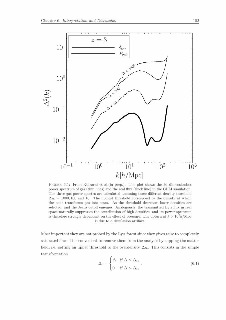
Chapter 6. Interpretation and Discussion 102
Figure 6.1: From Kulkarni et al.(in prep.). The plot shows the 3d dimensionlesspower spectrum of gas (thin lines) and the real flux (thick line) in the GHM simulation.The three gas power spectra are calculated assuming three different density threshold∆th = 1000, 100 and 10. The highest threshold correspond to the density at whichthe code transforms gas into stars. As the threshold decreases lower densities areselected, and the Jeans cutoff emerges. Analogously, the transmitted Lyα flux in realspace naturally suppresses the contribution of high densities, and its power spectrumis therefore strongly dependent on the effect of pressure. The upturn at k > 102h/Mpc
is due to a simulation artifact.
Most important they are not probed by the Lyα forest since they gives raise to completely
saturated lines. It is convenient to remove them from the analysis by clipping the matter
field, i.e. setting an upper threshold to the overdensity ∆th. This consists in the simple
transformation
∆c =
∆ if ∆ ≤ ∆th
0 if ∆ > ∆th
. (6.1)

Chapter 6. Interpretation and Discussion 103
Figure 6.1 shows how the cutoff appears and evolves as the overdensity limit ∆th de-
creases, corresponding to an increased suppression of structures. This behavior is ex-
pected for two reasons: the contribution of collapsed regions vanishes and pressure
support is more effective at low density, where gravity is weaker. It is natural to con-
sider the location of this cutoff as the filtering scale of the IGM, however the fact that
it shifts with ∆th brings us back to our initial problem of defining unambiguously the
filtering scale.
The Lyα forest offers a very natural solution to this problem. In a broad sense, the
transmitted flux can be considered as a clipped version of the density field, where the
suppression of high densities is originated in the exponentiation F = exp(−τ) and not as
a sharp threshold, but it is equally effective in removing the contribution of high densities
and isolating the property of the IGM. This suggests the possibility of applying the same
type of transformation to the density field of our simulation and define the IGM filtering
scale based on the geometrical properties of this field, in particular on the location of its
3d power spectrum. An important caveat is represented by the redshift-space nature of
the Lyα forest: the absorption is distorted along the sightline by thermal broadening and
the motion of the gas, so it does not faithfully trace the underlying matter distribution
and it is not an isotropic 3d field. We circumvent this problem by defining the real-
space transmitted flux Fr, i.e. the optical depth to Lyα absorption at each point in real
space. This quantity is equivalent to the Lyα forest absorption in the limit of a cold and
steady IGM, and it is given by the Fluctuating Gunn-Petersonn approximation [Gunn
& Peterson, 1965]:
Fr = exp
[
− πe2
mecfαλαH
−1(z)nHI
]
(6.2)
where fα is the oscillator strength of the Lyα line and nHI the density of neutral hy-
drogen. Studying this quantity has several advantages:
• it is by construction sensitive to the properties of the IGM and independent on
the physics of galaxies and high-density regions in general;
• the way it weights different densities is neither ambiguous nor arbitrary;
• differently than the velocity-space flux, it has no sensitivity to thermal broadening,
which would introduce degeneracies in the power spectrum and in particular on
the cutoff, as we have discussed in detail in chapter 2
• it is closely connected to the observed Lyα forest. Although relating the latter with
the real-space flux requires a precise modeling of peculiar motions and temperature,
we have shown that the phase difference statistic is practically independent on
them,suggesting that Fr can be directly probed using quasar pairs.

Chapter 6. Interpretation and Discussion 104
This properties lead us to conclude that the filtering scale obtained through our mea-
surement should be identified with the filtering scale of the real-space flux 3d field, as it
will be explained in the next section.
A minor disadvantage is due to the evolution of the Lyα absorption with redshift: as
the forest becomes more transparent due to expansion the range of densities probed by
Fr moves to higher values, making less intuitive the comparison between filtering scales
at different epochs.
6.2.2 Validation of the Dark-Matter Models
The identification of the Jeans scale λJ of our DM models with the cutoff of the power
spectrum of Fr is motivated following a logic analogous to the previous section. By
construction, the filtering scale of the density field is a constant parameter in our models.
As a consequence, the 3d power spectrum of the density exhibit a cutoff whose location
is invariant under the choice of different density ranges. As shown in the previous
section, this is very different than what we expect to find in the IGM and what we see in
hydrodynamical simulations. We must then explicitly state what is the equivalent of λJ
in the real universe, i.e. what is the physical meaning of our measurement. Equivalently,
we must specify at which density we expect our estimate for λJ to match the filtering
scale of the IGM. The fact that the statistic we are using, phase differences, is measured
on the Lyα forest and is insensitive to thermal broadening naturally leads us to conclude
that Fr defines the desired range of densities.
To be precise, Fr is the transformed of the density field that we expect to have the
smoothing length to which our method is sensitive to. Since Fr does not select exactly
one density, we could still expect a variable filtering scale. If this variability is significant,
our fixed-λJ approximation may be too imprecise. This is one of the reasons why we
need to test the method with simulations, but we can use the classic Jeans formula to
get a broad intuition of the dispersion of the Jeans scale in the Lyα forest. Using a
temperature-density relationship T ∝ ργ−1 and assuming λJ ∝√
T/ρ, one gets λJ ∝ρβ, with β = γ/2 − 1. For typical values of γ ∼ 1.2 − 1.6, this dependence is quite
shallow. Figure 6.1 shows that in any case an effective cutoff is clearly present in
the power spectrum of Fr in the simulation GHM. If we could proof that,despite of the
approximated models, our method is able to correctly predict the position of such cutoff,
than we would demonstrate its validity, also showing that the interpretation we propose
is correct.

Chapter 6. Interpretation and Discussion 105
We do this by ”measuring” the filtering scale in the hydrodynamical simulation GHM
at redshift 3 and by comparing the outcome with the cutoff of the 3d real-flux power
spectrum calculated from the simulation. Our test consists in the following:
• We draw synthetic pairs of skewers from the hydrodynamical simulation at various
separations, defining our mock (noiseless) dataset.
• We calculate phase differences for all the pairs in the mock sample, in the same
dynamical range utilized in data (k < 0.1 s/km).
• We evaluate the likelihood of the obtained set of phases using the probability
distributions predicted by our grid of DM-based models.
• The filtering scale of the simulation is defined as the Jeans scale λJ of the maximum-
likelihood DM model.
• Finally, we compare the 3d power spectrum of the real flux Fr for the hydrodynam-
ical simulation with that of the best-likelihood DM model. We remind that this
implies smoothing the DM particle distribution using a pseudo-Gaussian kernel
with σ = λJ and applying the FGPA to the field obtained in this way.
We performed this test on the GHM simulation (Figure 6.2) and on the NHM run
(Figure 6.3). Although the general shape of the power spectra generally differ between
hydros and our models, the location of the cutoff is remarkably well aligned in both
cases. The Jeans scales estimated for the two simulations are approximately 110 and
128 kpc for GHM and the NHM run, respectively. This test confirms our hypothesis on
the nature of the filtering scale measured via phase differences, and shows that no bias
arises from the approximations assumed on the DM models which we use to calibrate
phase distributions, at least at the current level of accuracy (∼ 20%).
6.3 Definition of the Jeans Scale in Hydrodynamical Sim-
ulations
In the previous section we have argued that the Jeans filtering scale should be defined
based on the cutoff of the 3d power spectrum of the real-flux field Fr. We have also
shown that the location of this cutoff is what the phase difference statistic is mostly
sensitive to. However, we have not provided yet a quantitative expression that defines
λJ in simulations and allows a direct comparison with the measurement. The most
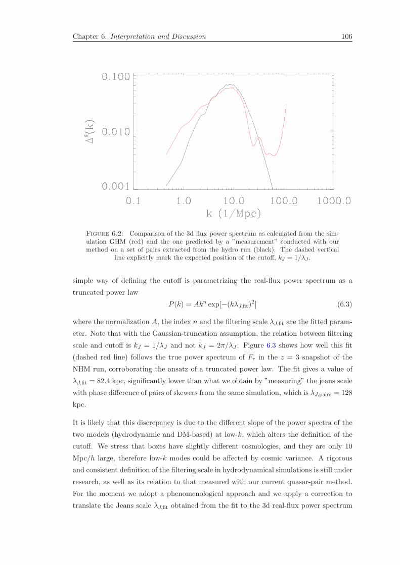
Chapter 6. Interpretation and Discussion 106
Figure 6.2: Comparison of the 3d flux power spectrum as calculated from the sim-ulation GHM (red) and the one predicted by a ”measurement” conducted with ourmethod on a set of pairs extracted from the hydro run (black). The dashed vertical
line explicitly mark the expected position of the cutoff, kJ = 1/λJ .
simple way of defining the cutoff is parametrizing the real-flux power spectrum as a
truncated power law
P (k) = Akn exp[−(kλJ,fit)2] (6.3)
where the normalization A, the index n and the filtering scale λJ,fit are the fitted param-
eter. Note that with the Gaussian-truncation assumption, the relation between filtering
scale and cutoff is kJ = 1/λJ and not kJ = 2π/λJ . Figure 6.3 shows how well this fit
(dashed red line) follows the true power spectrum of Fr in the z = 3 snapshot of the
NHM run, corroborating the ansatz of a truncated power law. The fit gives a value of
λJ,fit = 82.4 kpc, significantly lower than what we obtain by ”measuring” the jeans scale
with phase difference of pairs of skewers from the same simulation, which is λJ,pairs = 128
kpc.
It is likely that this discrepancy is due to the different slope of the power spectra of the
two models (hydrodynamic and DM-based) at low-k, which alters the definition of the
cutoff. We stress that boxes have slightly different cosmologies, and they are only 10
Mpc/h large, therefore low-k modes could be affected by cosmic variance. A rigorous
and consistent definition of the filtering scale in hydrodynamical simulations is still under
research, as well as its relation to that measured with our current quasar-pair method.
For the moment we adopt a phenomenological approach and we apply a correction to
translate the Jeans scale λJ,fit obtained from the fit to the 3d real-flux power spectrum
Chapter 6. Interpretation and Discussion 107
Figure 6.3: From Onorbe et al., in prep. The plot shows the 3d dimensionless powerspectrum of the real flux for the hydrodynamical simulation NHM (red solid line) andfor the model based on the dark matter distribution smoothed with the filtering scaleλJ,pairs. Here, λJ,pairs is the Jeans scale measured from a set of synthetic pairs extractedfrom the same hydro simulation, using the same method we applied to data. The reddotted line is the fit to the red solid line obtained assuming a truncated power lawP (k) = Akn exp[−(kλJ,fit)
2]. The position of the cutoff is again well matched, althoughthe values of the parameters λJ,pairs = 128 kpc and λJ,fit = 82.4 kpc differ.
in simulations with the one estimated with the pairs method λJ,pairs. We assume this
correction to be a multiplicative factor, which we tune on the snapshot at z = 3 of NHM
(figure 6.3), giving
λJ,pairs ≈ 1.4λJ,fit. (6.4)
We will apply this relation in the next section in order to compare the results of our
measurement with the prediction of the set of hydrodynamic simulation.
6.4 Redshift Evolution and Comparison with Simulation
Little attention has been devoted in the past in defining and predicting the filtering
scale of the IGM. For this reason we are not yet in the condition of stating whether
or not the results of our measurement meet the theoretical expectations of the typical
IGM models. With the recent work described in the previous sections, however, we
developed a consistent and physically motivated definition which allows us to draw the
first conclusions.
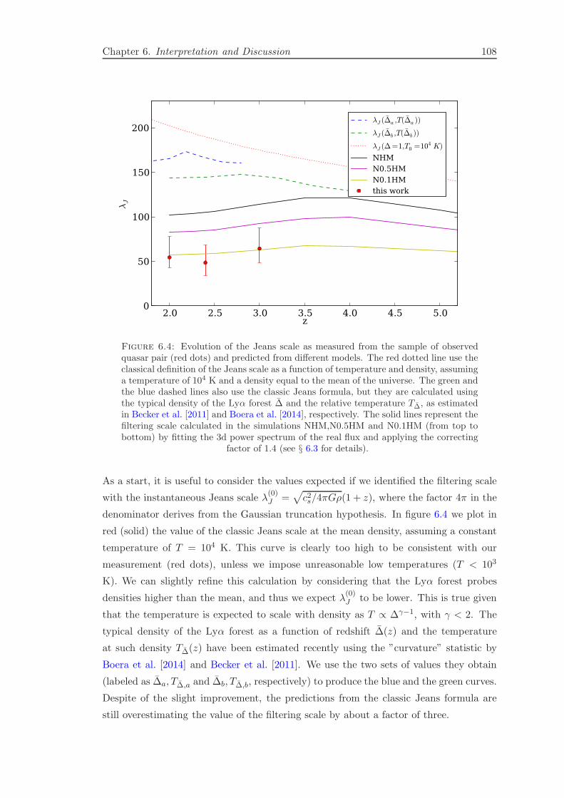
Chapter 6. Interpretation and Discussion 108
2.0 2.5 3.0 3.5 4.0 4.5 5.0z
0
50
100
150
200λJ
λJ (∆a ,T(∆a ))
λJ (∆b ,T(∆b ))
λJ (∆=1,T0 =104 K)
NHMN0.5HMN0.1HMthis work
Figure 6.4: Evolution of the Jeans scale as measured from the sample of observedquasar pair (red dots) and predicted from different models. The red dotted line use theclassical definition of the Jeans scale as a function of temperature and density, assuminga temperature of 104 K and a density equal to the mean of the universe. The green andthe blue dashed lines also use the classic Jeans formula, but they are calculated usingthe typical density of the Lyα forest ∆ and the relative temperature T∆, as estimatedin Becker et al. [2011] and Boera et al. [2014], respectively. The solid lines represent thefiltering scale calculated in the simulations NHM,N0.5HM and N0.1HM (from top tobottom) by fitting the 3d power spectrum of the real flux and applying the correcting
factor of 1.4 (see § 6.3 for details).
As a start, it is useful to consider the values expected if we identified the filtering scale
with the instantaneous Jeans scale λ(0)J =
√
c2s/4πGρ(1 + z), where the factor 4π in the
denominator derives from the Gaussian truncation hypothesis. In figure 6.4 we plot in
red (solid) the value of the classic Jeans scale at the mean density, assuming a constant
temperature of T = 104 K. This curve is clearly too high to be consistent with our
measurement (red dots), unless we impose unreasonable low temperatures (T < 103
K). We can slightly refine this calculation by considering that the Lyα forest probes
densities higher than the mean, and thus we expect λ(0)J to be lower. This is true given
that the temperature is expected to scale with density as T ∝ ∆γ−1, with γ < 2. The
typical density of the Lyα forest as a function of redshift ∆(z) and the temperature
at such density T∆(z) have been estimated recently using the ”curvature” statistic by
Boera et al. [2014] and Becker et al. [2011]. We use the two sets of values they obtain
(labeled as ∆a, T∆,a and ∆b, T∆,b, respectively) to produce the blue and the green curves.
Despite of the slight improvement, the predictions from the classic Jeans formula are
still overestimating the value of the filtering scale by about a factor of three.
Chapter 6. Interpretation and Discussion 109
The fact that the filtering scale should be smaller then the instantaneous Jeans scale
has already been shown by Gnedin & Hui [1998] in the context of linear theory (see also
chapter 1). The correction is typically a number between 1.5 and 3, but the precise value
depends on the past thermal history. Moreover, linear theory is not reliable to model
the Lyα forest, and hydrodynamic simulations are required to understand the precise
relation between filtering scale and temperature evolution.
The solid lines in figure 6.4 represent the filtering scale fitted in the simulations at
different redshifts and rescaled according to the procedure described in § 6.3. The NHMand N0.5HM simulations predict a higher Jeans scale then what we observe, and we need
to assume a photoheating rate 10 times smaller than the standard Haardt and Madau
model if we want to fit the measurement. Unfortunately, this model has a temperature
at the mean density of T0 = 2505 K, almost an order of magnitude than all the current
estimates (see chapter 1). However, we stress again that this comparison relies on
tuning the ratio λJ,pairs/λJ,fit1.4 between the the fitted cutoff of the real-flux power
spectrum of simulation and the value that would be defined using the phase difference
distributions calibrated on the set of DM-models. This correction has been tuned on
the z=3 snapshot of NHM and it may not apply at other redshifts and in different runs.
A rigorous comparison would require measuring the Jeans scale of the other simulations
by applying the phase method to mock samples of pairs at all redshifts, a test we defer
to future work.
Understanding the origin of such a small filtering scale will require more theoretical
exploration, however we can speculate on possible explanations.
The Jeans filtering scale is sensitive to the past thermal history, and responds to temper-
ature changes on timescales of the Hubble time. If at higher redshifts the temperature
was lower than what assumed in the simulations, λJ would retain memory of this cold
stage and remain at lower values. Whether this could quantitatively explain the dis-
crepancy shown in figure 6.4 should be verified in the future by means of hydrodynamic
simulation with different thermal history. An alternative explanation would be some
cosmological factor that enhanced the power of perturbations at small scales. It has
been argued that primordial magnetic fields could have produced a similar effect [Sub-
ramanian & Barrow, 1998, Wasserman, 1978].
From the observational point of view, it is possible that there are systematic in the
data which we are not correctly accounting for that decreases the coherence, inducing
an underestimation of the Jeans scale. The most obvious candidates are metals and
LLSs. Although their contribution to the Lyα forest absorption is modest, we have not
explicitly demonstrated that their effect on phases is negligible.

Chapter 6. Interpretation and Discussion 110
6.5 Future Work
The work conducted so far has opened several important questions and posed few puzzles
to our understanding of the IGM. The most relevant to solve is the explanation of the
tiny Jeans scale that quasar pairs seem to indicate. The answer should be sought on a
double track: theoretically and observationally. From the theoretical point of view, it is a
priority to reach a consistent definition of the Jeans filtering scale of the IGM that could
be used in hydrodynamic simulation and that could be related to the phase-difference
method. In doing this, we might explore further the reliability of the approximated
DM-based models on which the measurement is calibrated and characterize precisely
the differences with hydrodynamic simulations. We will also need to understand to
which extent the filtering scale is sensitive to the thermal history of higher redshifts,
and whether a filtering scale consistent with our measurement can be achieved without
making the IGM exceedingly cold.
From the observational perspective, it will be important to assess quantitatively the
impact of systematic that we have not modeled properly, such as metals and LLSs. It
is also crucial to understand the origin of the degeneracy between λJ and γ that holds
at z = 2 and z = 2.4, and whether this degeneracy can be broken by crossing the phase
difference statistic with line-of-sight statistics. At the same time, we will collect new
data in order to extend the analysis to higher redshifts z > 3.3 and to improve the
statistical significance of the results presented here.
Chapter 7
Concluding Remarks
In this thesis I presented the first measurement of the Jeans filtering scale of the inter-
galactic medium. This filtering scale corresponds to the coherence length of the baryons
set by the interplay between gravity and pressure across the history of the universe. It
has fundamental cosmological implications: it provides a thermal record of heat injected
by ultraviolet photons during cosmic reionization events, determines the clumpiness of
the IGM, a critical ingredient in reionization models, and sets the minimum mass of
galaxies to gravitationally collapse from the IGM. We elaborated a novel method to di-
rectly estimate the Jeans scale from the transverse coherence of Lyα absorption in quasar
pair spectra. Our technique is based on the probability distribution function (PDF) of
phase angle differences of homologous longitudinal Fourier modes in the spectra of the
pair.
To study the efficacy of this new method, we combined a semi-analytical model of the
Lyα forest with a dark matter only simulation, to generate a grid of 500 thermal models,
where the temperature at mean density T0, slope of the temperature-density relation γ,
and the Jeans scale λJ were varied. A Bayesian formalism is introduced based on
the phase angle PDF, and MCMC techniques are used to conduct a full parameter
study, allowing us to characterize the precision of a Jeans scale measurement, explore
degeneracies with the other thermal parameters, and compare parameter constraints
with those obtained from other statistics such as the longitudinal power and the cross-
power spectrum.
The primary conclusions of this study are:
• The longitudinal power is highly degenerate with respect to the thermal parameters
T0, γ and λJ , which arises because thermal broadening smooths the IGM along the
line-of-sight (1D) at a comparable scale as the Jeans pressure smoothing (3D). It is
111

Chapter 7. Concluding Remarks 112
extremely challenging to disentangle this confluence of 1D and 3D smoothing with
longitudinal observations alone. Similar degeneracies are likely to exist in other
previously considered statistics sensitive to small-scale power such as the wavelet
decomposition, the curvature, the b-parameter distribution, and the flux PDF.
Hence it may be necessary to reassess the reliability and statistical significance of
previous measurements of T0 and γ.
• The cross-power measured from close quasar pairs is sensitive to the 3D Jeans
smoothing, and can break degeneracies with the unknown Jeans scale. However,
it is not the optimal statistic, because it mixes 1D information in the moduli
of longitudinal Fourier modes, with the 3D information encoded in their phase
differences. We show that by focusing on the phase differences alone, via the
full PDF of phase angles, one is much more sensitive to 3D power and the Jeans
smoothing.
• Based on a simple heuristic geometric argument, we derived an analytical form for
the phase angle PDF. A single parameter family of wrapped-Cauchy distributions
provides a good fit to the phase differences in our simulated spectra for any k, r⊥,
the full range of T0,γ and λJ .
• Our phase angle PDFs indicate that phase differences between large-scale longi-
tudinal modes with small wavenumbers k ≪ 1/λJ , are nevertheless very sensitive
to the Jeans scale. We present a simple analytical argument showing that this
sensitivity results from the geometry of observing a 3D field along 1D skewers:
low-k cross-power across correlated 1D skewers is actually dominated by high-k
3D modes up to a scale set by the pair separation k⊥ ∼ 1/r⊥.
• The phase angle PDF is essentially independent of the temperature-density relation
parameters T0 and γ. This results because 1) the non-linear FGPA transformation
is only weakly dependent on temperature 2) phase angles of longitudinal modes
are invariant to the symmetric thermal broadening convolution.
• Our full Bayesian MCMC parameter analysis indicates that a realistic sample of
only 20 close quasar pair spectra observed at modest signal-to-noise ratio S/N ≃ 10
and resolution of FWHM=30 km/s, can pinpoint the Jeans scale to ≃ 5% precision,
fully independent of the amplitude T0 and slope γ of the temperature-density
relation. The freedom from degeneracies with T0 and γ is a direct consequence of
the near independence of the phase angle PDF of these parameters.
• Our new estimator for the Jeans scale is unbiased and insensitive to a battery
of systematics that typically plague Lyα forest measurements, such as continuum
Chapter 7. Concluding Remarks 113
fitting errors, imprecise knowledge of the noise level and/or spectral resolution,
and metal-line absorption.
Motivated by these results, we applied the phase-difference technique to the existent
sample of close quasar pairs. Adapting the method to real spectra requires significant
modifications, among which:
• Calculation of phase differences on irregular grids by means of least-square spectral
analysis. We have checked that alternative approximate methods (interpolation
on regular grids) lead to the same results, guaranteeing their reliability
• Careful modeling of noise and resolution, and removal of the most evident con-
taminants such as broad absorption lines systems and damped Lyα absorbers.
• Calibration of the dynamic range in Fourier space according to the noise and
resolution property of each spectrum, in order to exclude the noisiest mode at
high k.
We performed the measurement in three different redshift bins, defined by the intervals
[1.8, 2.2], [2.2, 2.6] and [2.7, 3.3]. The phase difference analysis gives λJ = 66± 20 kpc at
z = 3, λJ = 52±17 kpc at z = 3 and λJ = 64±17 kpc at z = 3. The current accuracy is
at the level of 30% at all redshifts. At z = 2 and z = 2.4 the precision is decreased by a
slight degeneracy of λJ with γ. Interestingly, the direction of this degeneracy appears to
be almost perpendicular to the same degeneracy expected from the line-of-sight power
spectrum, a promising result in the perspective of crossing our constraints with other
Lyα forest statistics.
We have tested that the results are stable with respect to the estimation of noise and
resolution with a tolerance of about 10%. Most important, in the light of our results,
the Jeans scale is hardly underestimated due to wrong noise/resolution assumptions.
We also verified that phase differences are not sensitive to uncertainties on continuum
placement.
In order for the parameter study presented here, with a large grid (500) of thermal
models, to be computationally feasible, we had to rely on a simplified model of the
IGM, based on a dark-matter only simulation and simple thermal scaling relations. In
particular, the impact of Jeans pressure smoothing on the distribution of baryons is
approximated by smoothing the dark-matter particle distribution with a Gaussian-like
kernel, and we allowed the three thermal parameters T0, γ, and λJ to vary completely
independently. Although the Gaussian filtering approximation is valid in linear theory
[Gnedin et al., 2003], the Jeans scale is highly nonlinear at z ≃ 3, hence a precise
Chapter 7. Concluding Remarks 114
description of how pressure smoothing alters the 3D power spectrum of the baryons
requires full hydrodynamical simulations. Furthermore, the three thermal parameters
we consider are clearly implicitly correlated by the underlying thermal history of the
Universe. Indeed, a full treatment of the impact of impulsive reionization heating on
the thermal evolution of the IGM and the concomitant hydrodynamic response of the
baryons, probably requires coupled radiative transfer hydrodynamical simulations.
Our approximate IGM model is thus justified by the complexity and computational cost
of fully modeling the Jeans smoothing problem, and despite its simplicity, it provides
a good fit to current measurements of the longitudinal power (see Figure 2.2). Most
importantly, by analyzing the spatial structure of the real-space flux in hydrodynamic
simulation, we proofed that calibrating phases on our simplified models is sufficient to
locate the cutoff in the power spectrum of the low-density IGM.
A preliminary comparison with the expectations from hydrodynamic simulations indi-
cates that the filtering scale we measured is too small to be explained with the standard
assumptions on the thermal history and on the small-scale physics of the IGM. This
discrepancy motivates further work to understand the theoretical implications of our
findings, and demands a careful search for further systematics that could affect the
phase difference statistic.
Appendix A
Resolving the Jeans Scale with Dark-Matter Simulations
The Lyα forest probes the structure of the very low density regions of the IGM, setting
strict requirements on the resolution of our dark-matter only simulation. In particular,
because our simulation is discrete in mass, each dark-matter particle represents a fixed
amount of gas distributed according to the gravitational softening length and the size
of the smoothing kernel that we use to represent Jeans smoothing (eqn. 2.3). At very
low densities, it is possible that a very large region is described by a single particle,
and that most of this void region is left empty. This undesirable situation occurs when
the mean inter-particle separation ∆l = Lbox/N1/3p , which defines the typical size of
regions occupied by each particle, is much larger than the Jeans scale λJ , which is the
minimum scale we want to resolve. Under such circumstances the density profile of
skewers through our simulation cube will have many pixels which are nearly empty,
because they have few or no neighboring particles. This insufficient sampling of the
volume due to large mean inter-particle separation will then manifest itself through the
appearance of artifacts in the volume-weighted probability distribution function (PDF)
of the density. On the other hand, if the inter-particle separation is sufficiently small,
the density field will be sufficiently sampled, and further decreasing the inter-particle
separation will not alter the density PDF. Therefore we can define our resolution criteria
for the mean inter-particle separation to be smaller than some multiple of the Jeans scale
∆l < αλJ , where the exact value of this coefficient α is determined by checking that
convergence is achieved in the density PDF.
We estimate α by plotting the PDF of log(∆) from our IGM skewers for a set of simula-
tions with varying mean inter-particle separation, where ∆ = ρ/ρ = 1+ δ is the density
in units of the mean. The employed simulations have mean inter-particle separations
∆l = 86, 171, 653 kpc, corresponding to box sizes Lbox = 100, 250, 720 Mpc/h with
Np = 15003, 20483, 18003 particles, respectively. In Figure A.1 we check for conver-
gence using three different values of λJ . The results indicate that a safe criterion for
resolving the jeans scale is ∆l < λJ or α ≃ 1. The simulation employed in this work
115
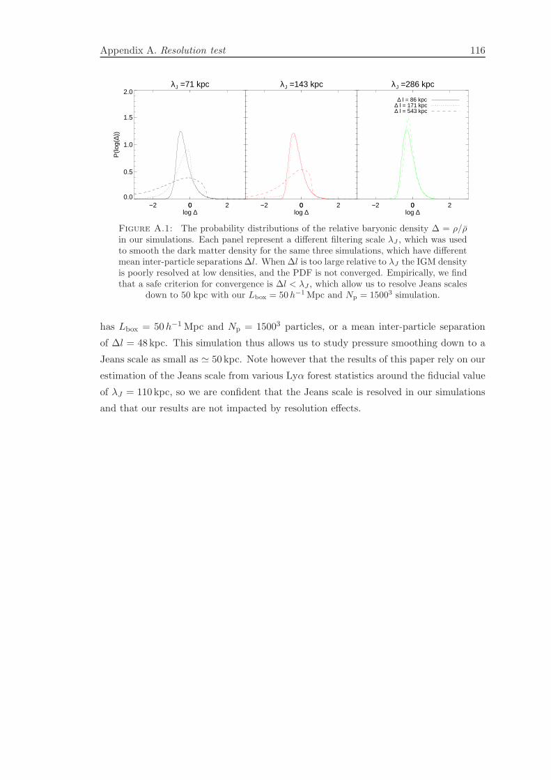
Appendix A. Resolution test 116
λJ =71 kpc
−2 0 20log ∆
0.0
0.5
1.0
1.5
2.0
P(lo
g(∆)
)
λJ =143 kpc
−2 0 20log ∆
λJ =286 kpc
−2 0 20log ∆
∆ l = 86 kpc
∆ l = 171 kpc∆ l = 543 kpc
Figure A.1: The probability distributions of the relative baryonic density ∆ = ρ/ρin our simulations. Each panel represent a different filtering scale λJ , which was usedto smooth the dark matter density for the same three simulations, which have differentmean inter-particle separations ∆l. When ∆l is too large relative to λJ the IGM densityis poorly resolved at low densities, and the PDF is not converged. Empirically, we findthat a safe criterion for convergence is ∆l < λJ , which allow us to resolve Jeans scales
down to 50 kpc with our Lbox = 50 h−1Mpc and Np = 15003 simulation.
has Lbox = 50h−1 Mpc and Np = 15003 particles, or a mean inter-particle separation
of ∆l = 48kpc. This simulation thus allows us to study pressure smoothing down to a
Jeans scale as small as ≃ 50 kpc. Note however that the results of this paper rely on our
estimation of the Jeans scale from various Lyα forest statistics around the fiducial value
of λJ = 110 kpc, so we are confident that the Jeans scale is resolved in our simulations
and that our results are not impacted by resolution effects.
Appendix B
Determining the Concentration Parameter ζ of the Wrapped-Cauchy
Distribution
For a given sample of phases θ we employ a maximum-likelihood algorithm to deter-
mine the best-fit concentration parameter ζ, which uniquely specifies a wrapped-Cauchy
distribution. This procedure is described in detail in Jammalamadaka & Sengupta
[2001]. Briefly, we first reparametrize the wrapped-Cauchy distribution (eqn. 3.6) by
writing ν = 2ζ/(1 + ζ2), which gives
P (θ) ∝ 1
1− ν cos(θ)≡ w(θ|ν). (B.1)
Following the standard recipe of maximizing the logarithm of the likelihood with respect
to the desired parameter, we sum the logarithms of the probability of all angles and
impose the condition that its derivative with respect to ν is zero, resulting in the equation
n∑
i=1
w(θi|ν)[cos(θi)− ν] = 0, (B.2)
which can be solved iteratively. The concentration parameter is then easily determined
by inverting the above relation to get ζ = (1 −√1− ν2)/ν. This procedure is repeated
for each distinct population of phases, parametrized by transverse separation r⊥ and
k-mode, θ(r⊥, k), and for each model in the thermal parameter grid (T0, γ, λJ ) that we
consider.
117

Appendix C
Phase Noise Calculation
In this appendix we show the derivation of formula 4.17. This formula expresses the
probability distribution of the phase variation due to noise on a Fourier mode with
coefficient F0. We assume for simplicity that F0 is real, without loss of generality since
the calculation that follows is invariant under rotation of the complex plane. The noise in
Fourier space FN can be regarded as a Gaussian 2d stochastic variable with variance σ2.
To simplify the calculation, we renormalize all the moduli (the distances in the complex
plane) such that |F0| = 1. This operation is allowed because it does not change angles.
With these assumptions F0 = 1 is real and has unitary modulus. The rescaled variance
of the noise will be η2 = σ2/|F0|2. We now want to obtain the probability distribution
function in the complex plan of the variable F ′ = F0 + FN , which represent the Fourier
coefficient after adding noise. Writing F ′ = x + iy in the Cartesian representation and
with the aforementioned assumption of the noise, we get
pN (x+ iy) =1
2πη2exp
[
−(1− x)2 + y2
2η2
]
. (C.1)
We now transform this probability function in polar coordinates, that gives
pN (r, φ) =r
2πη2exp
[
−r2 + 1− 2r cosφ
2η2
]
. (C.2)
where φ is exactly the phase variation with respect to the noiseless mode (see also
figure C.1). If we want to calculate the distribution for φ we need to integrate in r to
marginalize it out:
pN (φ) =
∫ +∞
0pN (r, φ)dr. (C.3)
To solve the integral, we first rewrite the exponent using the identity r2+1− 2r cosφ =
(r − cosφ)2 + sin2 φ, which leads to the expression
pN (φ) =e− sin2 φ/2η2
2πη2
∫ +∞
0re−(r−cosφ)2/2η2dr. (C.4)
118
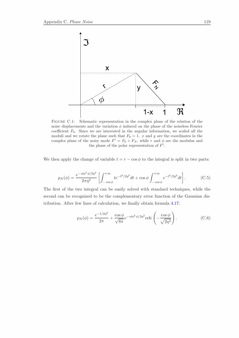
Appendix C. Phase Noise 119
1
y
x
1-x
φ
ℑ
ℜ
rFN
Figure C.1: Schematic representation in the complex plane of the relation of thenoise displacements and the variation φ induced on the phase of the noiseless Fouriercoefficient F0. Since we are interested in the angular information, we scaled all themoduli and we rotate the plane such that F0 = 1. x and y are the coordinates in thecomplex plane of the noisy mode F ′ = F0 + FN , while r and φ are the modulus and
the phase of the polar representation of F ′.
We then apply the change of variable t = r − cosφ to the integral is split in two parts:
pN (φ) =e− sin2 φ/2η2
2πη2
[∫ +∞
− cosφte−t2/2η2dt+ cosφ
∫ +∞
− cosφe−t2/2η2dt
]
. (C.5)
The first of the two integral can be easily solved with standard techniques, while the
second can be recognized to be the complementary error function of the Gaussian dis-
tribution. After few lines of calculation, we finally obtain formula 4.17:
pN (φ) =e−1/2η2
2π+
cosφ√8πe− sin2 φ/2η2erfc
(
− cosφ√
2η2
)
. (C.6)
Bibliography
Abazajian, K. N., Adelman-McCarthy, J. K., Agueros, M. A., Allam, S. S., Allende
Prieto, C., An, D., Anderson, K. S. J., Anderson, S. F., Annis, J., Bahcall, N. A., &
et al. 2009, ApJS, 182, 543
Abel, T., & Haehnelt, M. G. 1999, ApJ, 520, L13
Ade, P., et al. 2014, Astron.Astrophys.
Ahn, C. P., Alexandroff, R., Allende Prieto, C., Anderson, S. F., Anderton, T., Andrews,
B. H., Aubourg, E., Bailey, S., Balbinot, E., Barnes, R., & et al. 2012, ApJS, 203, 21
Almgren, A. S., Bell, J. B., Lijewski, M. J., Lukic, Z., & Van Andel, E. 2013, ApJ, 765,
39
Barkana, R., & Loeb, A. 1999, ApJ, 523, 54
—. 2001, Phys. Rep., 349, 125
Becker, G. D., Bolton, J. S., Haehnelt, M. G., & Sargent, W. L. W. 2011, MNRAS, 410,
1096
Benson, A. J., Frenk, C. S., Lacey, C. G., Baugh, C. M., & Cole, S. 2002a, MNRAS,
333, 177
Benson, A. J., Lacey, C. G., Baugh, C. M., Cole, S., & Frenk, C. S. 2002b, MNRAS,
333, 156
Benson, A. J., & Madau, P. 2003, MNRAS, 344, 835
Boera, E., Murphy, M. T., Becker, G. D., & Bolton, J. S. 2014, MNRAS, 441, 1916
Bolton, J., Meiksin, A., & White, M. 2004, MNRAS, 348, L43
Bolton, J. S., Viel, M., Kim, T., Haehnelt, M. G., & Carswell, R. F. 2008, MNRAS, 386,
1131
120
Bibliography 121
Bovy, J., Hennawi, J. F., Hogg, D. W., Myers, A. D., Kirkpatrick, J. A., Schlegel, D. J.,
Ross, N. P., Sheldon, E. S., McGreer, I. D., Schneider, D. P., & Weaver, B. A. 2011,
ApJ, 729, 141
Bovy, J., Myers, A. D., Hennawi, J. F., Hogg, D. W., McMahon, R. G., Schiminovich,
D., Sheldon, E. S., Brinkmann, J., Schneider, D. P., & Weaver, B. A. 2012, ApJ, 749,
41
Broderick, A. E., Chang, P., & Pfrommer, C. 2012, ApJ, 752, 22
Bryan, G. L., & Machacek, M. E. 2000, ApJ, 534, 57
Bullock, J. S., Kravtsov, A. V., & Weinberg, D. H. 2000, ApJ, 539, 517
Calura, F., Tescari, E., D’Odorico, V., Viel, M., Cristiani, S., Kim, T.-S., & Bolton,
J. S. 2012, MNRAS, 422, 3019
Cen, R., & Bryan, G. L. 2001, ApJ, 546, L81
Cen, R., McDonald, P., Trac, H., & Loeb, A. 2009, ArXiv e-prints
Cen, R., Miralda-Escude, J., Ostriker, J. P., & Rauch, M. 1994, ApJ, 437, L9
Cen, R., & Ostriker, J. P. 1999, ApJ, 514, 1
—. 2006, ApJ, 650, 560
Chang, P., Broderick, A. E., & Pfrommer, C. 2012, ApJ, 752, 23
Chiang, L.-Y., Coles, P., & Naselsky, P. 2002, MNRAS, 337, 488
Ciardi, B., & Ferrara, A. 2005, Space Sci. Rev., 116, 625
Ciardi, B., & Salvaterra, R. 2007, MNRAS, 381, 1137
Coles, P. 2009, in Lecture Notes in Physics, Berlin Springer Verlag, Vol. 665, Data
Analysis in Cosmology, ed. V. J. Martınez, E. Saar, E. Martınez-Gonzalez, & M.-J.
Pons-Borderıa, 493–522
Croft, R. A. C., Weinberg, D. H., Bolte, M., Burles, S., Hernquist, L., Katz, N., Kirkman,
D., & Tytler, D. 2002, ApJ, 581, 20
Croft, R. A. C., Weinberg, D. H., Katz, N., & Hernquist, L. 1997, ApJ, 488, 532
—. 1998, ApJ, 495, 44
Croom, S. M., Smith, R. J., Boyle, B. J., Shanks, T., Miller, L., Outram, P. J., &
Loaring, N. S. 2004, MNRAS, 349, 1397

Bibliography 122
Dave, R., Cen, R., Ostriker, J. P., Bryan, G. L., Hernquist, L., Katz, N., Weinberg,
D. H., Norman, M. L., & O’Shea, B. 2001, ApJ, 552, 473
Dave, R., Hernquist, L., Katz, N., & Weinberg, D. H. 1999, ApJ, 511, 521
Dijkstra, M., Haiman, Z., Rees, M. J., & Weinberg, D. H. 2004, ApJ, 601, 666
D’Odorico, V., Viel, M., Saitta, F., Cristiani, S., Bianchi, S., Boyle, B., Lopez, S., Maza,
J., & Outram, P. 2006, MNRAS, 372, 1333
Emberson, J. D., Thomas, R. M., & Alvarez, M. A. 2013, ApJ, 763, 146
Fan, X., Carilli, C. L., & Keating, B. 2006, ARA&A, 44, 415
Faucher-Giguere, C. ., Prochaska, J. X., Lidz, A., Hernquist, L., & Zaldarriaga, M. 2007,
ArXiv e-prints, 709
Foreman-Mackey, D., Hogg, D. W., Lang, D., & Goodman, J. 2012, ArXiv e-prints
Furlanetto, S. R., & Dixon, K. L. 2010, ApJ, 714, 355
Furlanetto, S. R., & Oh, S. P. 2009, ApJ, 701, 94
Garzilli, A., Bolton, J. S., Kim, T.-S., Leach, S., & Viel, M. 2012, MNRAS, 424, 1723
Gnedin, N. Y. 2000a, ApJ, 542, 535
—. 2000b, ApJ, 542, 535
Gnedin, N. Y., Baker, E. J., Bethell, T. J., Drosback, M. M., Harford, A. G., Hicks,
A. K., Jensen, A. G., Keeney, B. A., Kelso, C. M., Neyrinck, M. C., Pollack, S. E., &
van Vliet, T. P. 2003, ApJ, 583, 525
Gnedin, N. Y., & Hui, L. 1998, MNRAS, 296, 44
Gunn, J. E., & Peterson, B. A. 1965, ApJ, 142, 1633
Haardt, F., & Madau, P. 2012, ApJ, 746, 125
Habib, S., Heitmann, K., Higdon, D., Nakhleh, C., & Williams, B. 2007, Phys. Rev. D,
76, 083503
Haehnelt, M. G., & Steinmetz, M. 1998, MNRAS, 298, L21
Haiman, Z., Abel, T., & Madau, P. 2001, ApJ, 551, 599
Heitmann, K., Higdon, D., Nakhleh, C., & Habib, S. 2006, ApJ, 646, L1
Heitmann, K., Higdon, D., White, M., Habib, S., Williams, B. J., Lawrence, E., &
Wagner, C. 2009, ApJ, 705, 156
Bibliography 123
Heitmann, K., Lukic, Z., Fasel, P., Habib, S., Warren, M. S., White, M., Ahrens, J.,
Ankeny, L., Armstrong, R., O’Shea, B., Ricker, P. M., Springel, V., Stadel, J., &
Trac, H. 2008, Computational Science and Discovery, 1, 015003
Heitmann, K., White, M., Wagner, C., Habib, S., & Higdon, D. 2010, ApJ, 715, 104
Hennawi, J. F. 2004, PhD thesis, Ph.D dissertation, 2004. 232 pages; United States –
New Jersey: Princeton University; 2004. Publication Number: AAT 3151085. DAI-B
65/10, p. 5189, Apr 2005
Hennawi, J. F., Myers, A. D., Shen, Y., Strauss, M. A., Djorgovski, S. G., Fan, X., Glik-
man, E., Mahabal, A., Martin, C. L., Richards, G. T., Schneider, D. P., & Shankar,
F. 2009, ArXiv e-prints
Hennawi, J. F., & Prochaska, J. X. 2007, ApJ, 655, 735
—. 2008, ArXiv Astrophysics e-prints
Hennawi, J. F., Prochaska, J. X., Burles, S., Strauss, M. A., Richards, G. T., Schlegel,
D. J., Fan, X., Schneider, D. P., Zakamska, N. L., Oguri, M., Gunn, J. E., Lupton,
R. H., & Brinkmann, J. 2006a, ApJ, 651, 61
Hennawi, J. F., Strauss, M. A., Oguri, M., Inada, N., Richards, G. T., Pindor, B.,
Schneider, D. P., Becker, R. H., Gregg, M. D., Hall, P. B., Johnston, D. E., Fan, X.,
Burles, S., Schlegel, D. J., Gunn, J. E., Lupton, R. H., Bahcall, N. A., Brunner, R. J.,
& Brinkmann, J. 2006b, AJ, 131, 1
Hoeft, M., Yepes, G., Gottlober, S., & Springel, V. 2006, MNRAS, 371, 401
Hui, L., & Gnedin, N. Y. 1997, MNRAS, 292, 27
Hui, L., & Haiman, Z. 2003, ApJ, 596, 9
Hui, L., Stebbins, A., & Burles, S. 1999, ApJ, 511, L5
Iliev, I. T., Mellema, G., Pen, U.-L., Merz, H., Shapiro, P. R., & Alvarez, M. A. 2006,
MNRAS, 369, 1625
Iliev, I. T., Scannapieco, E., & Shapiro, P. R. 2005, ApJ, 624, 491
Inoue, A. K., & Kamaya, H. 2003, MNRAS, 341, L7
Jakobsen, P., Boksenberg, A., Deharveng, J. M., Greenfield, P., Jedrzejewski, R., &
Paresce, F. 1994, Nature, 370, 35
Jammalamadaka, S. R., & Sengupta, A. 2001
Bibliography 124
Kim, T.-S., Bolton, J. S., Viel, M., Haehnelt, M. G., & Carswell, R. F. 2007, MNRAS,
382, 1657
Kim, T.-S., Viel, M., Haehnelt, M. G., Carswell, R. F., & Cristiani, S. 2004, MNRAS,
347, 355
Kollmeier, J. A., Miralda-Escude, J., Cen, R., & Ostriker, J. P. 2006, ApJ, 638, 52
Kuhlen, M., & Madau, P. 2005, MNRAS, 363, 1069
Kulkarni, G., & Choudhury, T. R. 2011, MNRAS, 412, 2781
Kwan, J., Bhattacharya, S., Heitmann, K., & Habib, S. 2012, ArXiv e-prints
Lawrence, E., Heitmann, K., White, M., Higdon, D., Wagner, C., Habib, S., & Williams,
B. 2010, ApJ, 713, 1322
Lee, K.-G. 2012, ApJ, 753, 136
Lee, K.-G., Bailey, S., Bartsch, L. E., Carithers, W., Dawson, K. S., Kirkby, D., Lund-
gren, B., Margala, D., Palanque-Delabrouille, N., Pieri, M. M., Schlegel, D. J., Wein-
berg, D. H., Yeche, C., Aubourg, E., Bautista, J., Bizyaev, D., Blomqvist, M., Bolton,
A. S., Borde, A., Brewington, H., Busca, N. G., Croft, R. A. C., Delubac, T., Ebelke,
G., Eisenstein, D. J., Font-Ribera, A., Ge, J., Hamilton, J.-C., Hennawi, J. F., Ho, S.,
Honscheid, K., Le Goff, J.-M., Malanushenko, E., Malanushenko, V., Miralda-Escude,
J., Myers, A. D., Noterdaeme, P., Oravetz, D., Pan, K., Paris, I., Petitjean, P., Rich,
J., Rollinde, E., Ross, N. P., Rossi, G., Schneider, D. P., Simmons, A., Snedden, S.,
Slosar, A., Spergel, D. N., Suzuki, N., Viel, M., & Weaver, B. A. 2013, AJ, 145, 69
Lidz, A., Faucher-Giguere, C., Dall’Aglio, A., McQuinn, M., Fechner, C., Zaldarriaga,
M., Hernquist, L., & Dutta, S. 2009, ArXiv e-prints
Lomb, N. R. 1976, Ap&SS, 39, 447
Lumsden, S. L., Heavens, A. F., & Peacock, J. A. 1989, MNRAS, 238, 293
Madau, P. 2000, in Royal Society of London Philosophical Transactions Series A, Vol.
358, Astronomy, physics and chemistry of H+3 , 2021
Madau, P., & Efstathiou, G. 1999, ApJ, 517, L9
Madau, P., Ferrara, A., & Rees, M. J. 2001, ApJ, 555, 92
Madau, P., Haardt, F., & Rees, M. J. 1999, ApJ, 514, 648
Madau, P., & Meiksin, A. 1994, ApJ, 433, L53

Bibliography 125
Mathias, A., Grond, F., Guardans, R., Seese, D., Canela, M., & Diebner, H. H. 2004,
Journal of Statistical Software, 11, 1
McDonald, P., Miralda-Escude, J., Rauch, M., Sargent, W. L. W., Barlow, T. A., &
Cen, R. 2001, ApJ, 562, 52
McDonald, P., Miralda-Escude, J., Rauch, M., Sargent, W. L. W., Barlow, T. A., Cen,
R., & Ostriker, J. P. 2000, ApJ, 543, 1
McDonald, P., Seljak, U., Burles, S., Schlegel, D. J., Weinberg, D. H., Cen, R., Shih, D.,
Schaye, J., Schneider, D. P., Bahcall, N. A., Briggs, J. W., Brinkmann, J., Brunner,
R. J., Fukugita, M., Gunn, J. E., Ivezic, v., Kent, S., Lupton, R. H., & Vanden Berk,
D. E. 2006, ApJS, 163, 80
McDonald, P., Seljak, U., Cen, R., Bode, P., & Ostriker, J. P. 2005, MNRAS, 360, 1471
McGill, C. 1990, MNRAS, 242, 544
McQuinn, M., Lidz, A., Zaldarriaga, M., Hernquist, L., Hopkins, P. F., Dutta, S., &
Faucher-Giguere, C.-A. 2009, ApJ, 694, 842
McQuinn, M., Oh, S. P., & Faucher-Giguere, C.-A. 2011, ApJ, 743, 82
Meiksin, A., & Tittley, E. R. 2012, MNRAS, 423, 7
Meiksin, A., & White, M. 2001, MNRAS, 324, 141
Meiksin, A. A. 2009, Reviews of Modern Physics, 81, 1405
Miralda-Escude, J., Cen, R., Ostriker, J. P., & Rauch, M. 1996, ApJ, 471, 582
Miralda-Escude, J., Haehnelt, M., & Rees, M. J. 2000, ApJ, 530, 1
Miralda-Escude, J., & Rees, M. J. 1994, MNRAS, 266, 343
Myers, A. D., Richards, G. T., Brunner, R. J., Schneider, D. P., Strand, N. E., Hall,
P. B., Blomquist, J. A., & York, D. G. 2008, ApJ, 678, 635
Nath, B. B., & Biermann, P. L. 1993, MNRAS, 265, 241
Nath, B. B., Sethi, S. K., & Shchekinov, Y. 1999, MNRAS, 303, 1
Okamoto, T., Gao, L., & Theuns, T. 2008, MNRAS, 390, 920
Parsons, A. R., Liu, A., Aguirre, J. E., Ali, Z. S., Bradley, R. F., Carilli, C. L., DeBoer,
D. R., Dexter, M. R., Gugliucci, N. E., Jacobs, D. C., Klima, P., MacMahon, D. H. E.,
Manley, J. R., Moore, D. F., Pober, J. C., Stefan, I. I., & Walbrugh, W. P. 2013, ArXiv
e-prints

Bibliography 126
Pawlik, A. H., Schaye, J., & van Scherpenzeel, E. 2009, MNRAS, 394, 1812
Peacock, J. A. 1999, Cosmological physics; rev. version (Cambridge: Cambridge Univ.)
Peeples, M. S., Weinberg, D. H., Dave, R., Fardal, M. A., & Katz, N. 2009a, ArXiv
e-prints
—. 2009b, ArXiv e-prints
Penrose, R. 1955, Mathematical Proceedings of the Cambridge Philosophical Society,
51, 406
Petry, C. E., Impey, C. D., & Foltz, C. B. 1998, ApJ, 494, 60
Pfrommer, C., Chang, P., & Broderick, A. E. 2012, ApJ, 752, 24
Prochaska, J. X., & Hennawi, J. F. 2009, ApJ, 690, 1558
Prochaska, J. X., Hennawi, J. F., Lee, K.-G., Cantalupo, S., Bovy, J., Djorgovski, S. G.,
Ellison, S. L., Lau, M. W., Martin, C. L., Myers, A., Rubin, K. H. R., & Simcoe,
R. A. 2013, ApJ, 776, 136
Prochaska, J. X., Hennawi, J. F., & Simcoe, R. A. 2012, ArXiv e-prints
Prochaska, J. X., O’Meara, J. M., & Worseck, G. 2010, ApJ, 718, 392
Puchwein, E., Pfrommer, C., Springel, V., Broderick, A. E., & Chang, P. 2012, MNRAS,
423, 149
Rauch, M. 1998, ARA&A, 36, 267
Rauch, M., Sargent, W. L. W., Barlow, T. A., & Carswell, R. F. 2001, ApJ, 562, 76
Reimers, D., Kohler, S., Wisotzki, L., Groote, D., Rodriguez-Pascual, P., & Wamsteker,
W. 1997, A&A, 327, 890
Richards, G. T., Nichol, R. C., Gray, A. G., Brunner, R. J., Lupton, R. H., Vanden
Berk, D. E., Chong, S. S., Weinstein, M. A., Schneider, D. P., Anderson, S. F., Munn,
J. A., Harris, H. C., Strauss, M. A., Fan, X., Gunn, J. E., Ivezic, v., York, D. G.,
Brinkmann, J., & Moore, A. W. 2004, ApJS, 155, 257
Ricotti, M., Gnedin, N. Y., & Shull, J. M. 2000, ApJ, 534, 41
Ricotti, M., Ostriker, J. P., & Gnedin, N. Y. 2005, MNRAS, 357, 207
Rorai, A., Hennawi, J. F., & White, M. 2013, ApJ, 775, 81
Rudie, G. C., Steidel, C. C., & Pettini, M. 2012, ApJ, 757, L30
Bibliography 127
Scannapieco, E., Ferrara, A., & Madau, P. 2002, ApJ, 574, 590
Scannapieco, E., & Oh, S. P. 2004, ApJ, 608, 62
Schaye, J., Theuns, T., Rauch, M., Efstathiou, G., & Sargent, W. L. W. 2000, MNRAS,
318, 817
Shen, Y., Hennawi, J. F., Shankar, F., Myers, A. D., Strauss, M. A., Djorgovski, S. G.,
Fan, X., Giocoli, C., Mahabal, A., Schneider, D. P., & Weinberg, D. H. 2010, ApJ,
719, 1693
Shull, J. M., France, K., Danforth, C. W., Smith, B., & Tumlinson, J. 2010, ApJ, 722,
1312
Smette, A., Robertson, J. G., Shaver, P. A., Reimers, D., Wisotzki, L., & Koehler, T.
1995, A&AS, 113, 199
Somerville, R. S. 2002, ApJ, 572, L23
Springel, V. 2005, MNRAS, 364, 1105
Subramanian, K., & Barrow, J. D. 1998, Phys. Rev. D, 58, 083502
Syphers, D., Anderson, S. F., Zheng, W., Meiksin, A., Schneider, D. P., & York, D. G.
2012, AJ, 143, 100
Tanaka, T., Perna, R., & Haiman, Z. 2012a, MNRAS, 425, 2974
—. 2012b, MNRAS, 425, 2974
Theuns, T., Mo, H. J., & Schaye, J. 2001, MNRAS, 321, 450
Theuns, T., Schaye, J., & Haehnelt, M. G. 2000, MNRAS, 315, 600
Theuns, T., Schaye, J., Zaroubi, S., Kim, T., Tzanavaris, P., & Carswell, B. 2002a, ApJ,
567, L103
Theuns, T., Zaroubi, S., Kim, T., Tzanavaris, P., & Carswell, R. F. 2002b, MNRAS,
332, 367
Tittley, E. R., & Meiksin, A. 2007a, MNRAS, 380, 1369
—. 2007b, MNRAS, 380, 1369
Viel, M., Bolton, J. S., & Haehnelt, M. G. 2009, MNRAS, 399, L39
Viel, M., Matarrese, S., Mo, H. J., Haehnelt, M. G., & Theuns, T. 2002, MNRAS, 329,
848
Bibliography 128
Voit, G. M. 1996, ApJ, 465, 548
Wasserman, I. 1978, ApJ, 224, 337
Watts, P., Coles, P., & Melott, A. 2003, ApJ, 589, L61
White, M. 2002, ApJS, 143, 241
Worseck, G., Prochaska, J. X., McQuinn, M., Dall’Aglio, A., Fechner, C., Hennawi,
J. F., Reimers, D., Richter, P., & Wisotzki, L. 2011, ApJ, 733, L24
York, D. G., Adelman, J., Anderson, J. J. E., Anderson, S. F., Annis, J., Bahcall, N. A.,
Bakken, J. A., Barkhouser, R., Bastian, S., Berman, E., Boroski, W. N., Bracker,
S., Briegel, C., Briggs, J. W., Brinkmann, J., Brunner, R., Burles, S., Carey, L.,
Carr, M. A., Castander, F. J., Chen, B., Colestock, P. L., Connolly, A. J., Crocker,
J. H., Csabai, I., Czarapata, P. C., Davis, J. E., Doi, M., Dombeck, T., Eisenstein,
D., Ellman, N., Elms, B. R., Evans, M. L., Fan, X., Federwitz, G. R., Fiscelli, L.,
Friedman, S., Frieman, J. A., Fukugita, M., Gillespie, B., Gunn, J. E., Gurbani, V. K.,
de Haas, E., Haldeman, M., Harris, F. H., Hayes, J., Heckman, T. M., Hennessy,
G. S., Hindsley, R. B., Holm, S., Holmgren, D. J., Huang, C.-h., Hull, C., Husby,
D., Ichikawa, S.-I., Ichikawa, T., Ivezic, v., Kent, S., Kim, R. S. J., Kinney, E.,
Klaene, M., Kleinman, A. N., Kleinman, S., Knapp, G. R., Korienek, J., Kron, R. G.,
Kunszt, P. Z., Lamb, D. Q., Lee, B., Leger, R. F., Limmongkol, S., Lindenmeyer, C.,
Long, D. C., Loomis, C., Loveday, J., Lucinio, R., Lupton, R. H., MacKinnon, B.,
Mannery, E. J., Mantsch, P. M., Margon, B., McGehee, P., McKay, T. A., Meiksin,
A., Merelli, A., Monet, D. G., Munn, J. A., Narayanan, V. K., Nash, T., Neilsen,
E., Neswold, R., Newberg, H. J., Nichol, R. C., Nicinski, T., Nonino, M., Okada, N.,
Okamura, S., Ostriker, J. P., Owen, R., Pauls, A. G., Peoples, J., Peterson, R. L.,
Petravick, D., Pier, J. R., Pope, A., Pordes, R., Prosapio, A., Rechenmacher, R.,
Quinn, T. R., Richards, G. T., Richmond, M. W., Rivetta, C. H., Rockosi, C. M.,
Ruthmansdorfer, K., Sandford, D., Schlegel, D. J., Schneider, D. P., Sekiguchi, M.,
Sergey, G., Shimasaku, K., Siegmund, W. A., Smee, S., Smith, J. A., Snedden, S.,
Stone, R., Stoughton, C., Strauss, M. A., Stubbs, C., SubbaRao, M., Szalay, A. S.,
Szapudi, I., Szokoly, G. P., Thakar, A. R., Tremonti, C., Tucker, D. L., Uomoto, A.,
Vanden Berk, D., Vogeley, M. S., Waddell, P., Wang, S.-i., Watanabe, M., Weinberg,
D. H., Yanny, B., & Yasuda, N. 2000, AJ, 120, 1579
Young, P., Sargent, W. L. W., Oke, J. B., & Boksenberg, A. 1981, ApJ, 249, 415
Zaldarriaga, M. 2002, The Astrophysical Journal, 564, 153
Zaldarriaga, M., Hui, L., & Tegmark, M. 2001, ApJ, 557, 519

Bibliography 129
Zaroubi, S. 2013, in Astrophysics and Space Science Library, Vol. 396, Astrophysics and
Space Science Library, ed. T. Wiklind, B. Mobasher, & V. Bromm, 45

Acknowledgements
I am deeply thankful to my supervisor, Joseph Hennawi, first of all for offering me
the chance of working on a challenging and fascinating problem during these years in
Heidelberg. His guidance, beside guaranteeing a sane advancement of my research,
helped me in developing a rigorous and critic attitude toward my own ideas and a better
organized and efficient work style. I particularly value the fact that his advice went
always far beyond the pure scientific scope of the project, showing an authentic interest
in my general formation as a researcher.
This project would not have been possible without the support of prof. Martin White
from the University of Berkeley, who provided us with the Dark Matter simulations
we needed, and constantly discussed with us about the direction and the goals of the
projects.
I am grateful to all the current and past members of the ENIGMA group for the friendly
and stimulating working environment, and for the useful discussions during all the stages
of my PhD. I wish to thank in particular Jose Onorbe and Girish Kulkarni for their
crucial contribution to the final phase of my project and for comments and suggestions
that significantly improved this manuscript. I am also in debt with Xavier Prochaska
for patiently leading me in my first steps in the insidious world of continuum fitting. It
was really valuable the help of my friends and colleagues Rahul, Sladjana and Christina
in sorting out the last logistic and formal details during the hasty days before thesis
submission.
I want to thank the MPIA and IMPRS staffs for the great opportunities they guaranteed
me, not only on the academic side, and for making my stay in Heidelberg a totally
enjoyable experience.
I finally express my gratitude to all those persons who have been far from me in these
years for most of the time, but did not stop caring of me, despite of knowing me so well.
Among these, I want in particular to thank my parents, Daniela and Ernesto, my sister
Cecilia, and Claudia.
130