
DISSERTATION - TU Wien · ausgefu¨hrt zum Zwecke der Erlangung des akademischen Grades eines...
195
DISSERTATION Adaptation Techniques in large-scale Service-oriented Systems: Models, Metrics, and Algorithms ausgef¨ uhrt zum Zwecke der Erlangung des akademischen Grades eines Doktors der technischen Wissenschaften unter der Leitung von Univ.-Prof. Dr. Schahram Dustdar Institut f¨ ur Informationssysteme Abteilung f¨ ur Verteilte Systeme Technische Universit¨at Wien eingereicht an der Technischen Universit¨at Wien Fakult¨atf¨ ur Informatik von Mag. rer. soc. oec. Christoph Dorn [email protected] Matrikelnummer: 9825872 Alserstraße 32/27 A-1090 Wien, ¨ Osterreich Wien, September 2009
Transcript of DISSERTATION - TU Wien · ausgefu¨hrt zum Zwecke der Erlangung des akademischen Grades eines...

DISSERTATION
Adaptation Techniques in large-scale
Service-oriented Systems: Models,
Metrics, and Algorithms
ausgefuhrt zum Zwecke der Erlangung des akademischen Grades einesDoktors der technischen Wissenschaften
unter der Leitung von
Univ.-Prof. Dr. Schahram DustdarInstitut fur InformationssystemeAbteilung fur Verteilte Systeme
Technische Universitat Wien
eingereicht an der
Technischen Universitat WienFakultat fur Informatik
von
Mag. rer. soc. oec. Christoph Dorn
Matrikelnummer: 9825872Alserstraße 32/27
A-1090 Wien, Osterreich
Wien, September 2009

Kurzfassung
In den letzten Jahren gehen Menschen vermehrt ihren gemeinsamen Interessen onli-ne nach. Web-basierte Kollaborationsplattformen wie Facebook, Youtube oder Wikipediahaben enormen Zulauf erhalten. Diese Portale erlauben Zusammenarbeit in bisher unge-ahnten Dimensionen. Interessensgemeinschaften entstehen ad-hoc, wachsen auf tausendeTeilnehmer an und zerfallen schlussendlich wieder. Die zugrundeliegende Dynamik solcherKollaborationen ist weitgehend unvorhersehbar und fuhrt zu kontinuierlich wechselndenSystemanforderungen. Wahrend Menschen sich an unterschiedliche Umstande vergleichs-weise leicht anpassen konnen, passt sich Software von selbst, wenn uberhaupt, nur einge-schrankt an wechselnde Bedingungen an. Diese Dissertation behandelt das Problem wiesich Software - speziell Web Services - an den Gesamtkontext und die Anforderungen vonMassenzusammenarbeit anpassen kann.
Wenn tausende oder mehr technische und menschliche Entitaten zusammenarbeiten,kann kein einzelnes Element die Gesamtbedurfnisse erfassen. Infolgedessen erkennt nie-mand Situationen, welche die Umgestaltung des Gesamtsystems erfordern wurden. Ohneentsprechende Anpassungstechniken lauft die Zusammenarbeit Gefahr ineffizient zu werdenoder gar fruhzeitig auseinanderzubrechen.
Diese Dissertation prasentiert Techniken auf drei Ebenen. Den meisten Einfluss auferfolgreiche Zusammenarbeit haben Techniken, welche die Gesamtbedurfnisse feststellenund darauf aufbauend die benotigten Services bereitstellen. Daran anschließend werdenAlgorithmen beschrieben, welche es ermoglichen, dass die richtigen Services untereinanderkommunizieren. Drittens stellen Kontextverteilungsmechanismen sicher, dass die Servicesdie relevanten Kontextinformationen zur Adaption bekommen. Datenmodelle, Algorithmenund Prototypen sind an Hand von Simulationen sowie Experimenten mit Echtdaten einesweb-basierten Diskussionsforums evaluiert.

Abstract
Over the past years, people enthusiastically took up web-based services such as Face-book, Youtube, or Wikipedia to pursue joint interests. Large-scale collaborations emergein an ad-hoc fashion, have participants join in, and eventually dissolve again. Such dy-namic collaboration changes result in constantly shifting system requirements. Humanscan adapt to some extent to changing conditions, while software remains mostly rigid.Enabling system adaptation to meet these requirements is the main problem addressed inthis thesis.
In large-scale socio-technical networks, neither service nor human entities are able toobtain a complete picture of the overall context, constraints, and requirements. Conse-quently, no single entity perceives the need for reconfiguration. Without proper adaptationtechniques, collaborations yield poor performance and are prone to end prematurely.
In this thesis, we present a layered approach to adaptation techniques. Most im-portantly, infrastructure adaptation ensures provisioning of the required services. Sub-sequently, service adaptation techniques ensure interaction of the right services. Finally,we present techniques for delivering the relevant context information. We evaluate thesecontributions with a mixture of collaboration simulations and experiments on real-worlddata from an online discussion forum.

Acknowledgements
First and foremost, I would like to thank my advisor Prof. Schahram Dustdar for thegreat opportunity to carry out my thesis at the Distributed Systems Group. His continu-ous mentoring and supervision taught me the important aspects of conducting research. Igreatfully value the freedom I had to explore multiple research directions.
I greatly appreciate the feedback of my second advisor, Prof. Harald Gall. His valuablecomments and suggestions helped me to improve this thesis.
I would like to express my thanks to my colleagues, especially Daniel Schall and Hong-Linh Truong for exciting discussions on the various aspects of this work. Special thanksgo to Florian Skopik for providing the raw slashdot dataset.
I am in debt to my family and girlfriend for their understanding and limitless supportthat enabled me to pursue my research interests to such extent.
Finally, I’m thankful for financial support from the EU FP6 project inContext (IST-034718). It provided a unique opportunity to place my research in such an informativeproject context.
Christoph DornVienna, Austria, September 9, 2009

For Karin

Contents
1 Introduction 1
1.1 Motivating Scenarios . . . . . . . . . . . . . . . . . . . . . . . . . . . . . . 2
1.2 Preview of Results . . . . . . . . . . . . . . . . . . . . . . . . . . . . . . . 3
1.3 Structure . . . . . . . . . . . . . . . . . . . . . . . . . . . . . . . . . . . . 4
2 Related Work 5
2.1 Context Models and Frameworks . . . . . . . . . . . . . . . . . . . . . . . 6
2.1.1 Context Provisioning in Mobile Environments . . . . . . . . . . . . 8
2.2 Context Selection and Ranking . . . . . . . . . . . . . . . . . . . . . . . . 9
2.2.1 Ranking Functions . . . . . . . . . . . . . . . . . . . . . . . . . . . 9
2.3 Service Composition . . . . . . . . . . . . . . . . . . . . . . . . . . . . . . 10
2.4 Autonomic Service Adaptation . . . . . . . . . . . . . . . . . . . . . . . . . 11
3 Problem Statement 16
3.1 Analysis of Related Work . . . . . . . . . . . . . . . . . . . . . . . . . . . 17
3.2 Relevance to Real-World Problems . . . . . . . . . . . . . . . . . . . . . . 18
3.3 Approach . . . . . . . . . . . . . . . . . . . . . . . . . . . . . . . . . . . . 19
3.3.1 Assumptions . . . . . . . . . . . . . . . . . . . . . . . . . . . . . . . 19
3.3.2 Adaptation Methodology . . . . . . . . . . . . . . . . . . . . . . . . 19
3.4 Publications . . . . . . . . . . . . . . . . . . . . . . . . . . . . . . . . . . . 21
4 Ensemble Context Provisioning 23
4.1 Context Model . . . . . . . . . . . . . . . . . . . . . . . . . . . . . . . . . 23
4.1.1 Entity Model . . . . . . . . . . . . . . . . . . . . . . . . . . . . . . 24
4.1.2 Activity Model . . . . . . . . . . . . . . . . . . . . . . . . . . . . . 25
4.1.3 Resource Model . . . . . . . . . . . . . . . . . . . . . . . . . . . . . 26
i
Contents ii
4.1.4 Action Model . . . . . . . . . . . . . . . . . . . . . . . . . . . . . . 27
4.2 Context Capturing . . . . . . . . . . . . . . . . . . . . . . . . . . . . . . . 30
4.3 Context Ranking . . . . . . . . . . . . . . . . . . . . . . . . . . . . . . . . 30
4.3.1 Distance Metrics . . . . . . . . . . . . . . . . . . . . . . . . . . . . 32
4.3.1.1 Natural Distance Functions . . . . . . . . . . . . . . . . . 32
4.3.1.2 Context-based Distance Functions . . . . . . . . . . . . . 33
4.3.1.3 Interaction-based Distance Functions . . . . . . . . . . . . 36
4.3.2 Relevance Functions . . . . . . . . . . . . . . . . . . . . . . . . . . 39
4.3.3 Utility Functions . . . . . . . . . . . . . . . . . . . . . . . . . . . . 39
4.3.4 Ranking Algorithm . . . . . . . . . . . . . . . . . . . . . . . . . . . 40
4.3.5 Example Application of Context Ranking . . . . . . . . . . . . . . . 41
4.4 Evaluation of Context-based and Interaction-based Distance metrics . . . . 44
4.4.1 Fundamental Differences . . . . . . . . . . . . . . . . . . . . . . . . 44
4.4.2 Simulation-based evaluation . . . . . . . . . . . . . . . . . . . . . . 46
4.4.2.1 Pearson’s Correlation Coefficient . . . . . . . . . . . . . . 49
4.4.3 Distance metrics applied to real-world data . . . . . . . . . . . . . . 50
4.4.3.1 Introduction to Slashdot . . . . . . . . . . . . . . . . . . . 50
4.4.3.2 Slashdot Posting Aggregation . . . . . . . . . . . . . . . . 51
4.4.3.3 Analysis of Evolving Ranking Differences . . . . . . . . . . 55
4.4.3.4 Analysis of Aging Ranking Differences . . . . . . . . . . . 58
4.4.3.5 Summary on Distance Metric Differences . . . . . . . . . . 59
4.5 Context Provisioning for Mobile Service Ensembles . . . . . . . . . . . . . 60
4.5.1 Hierarchical Context Model . . . . . . . . . . . . . . . . . . . . . . 61
4.5.2 Hierarchy-based Sharing . . . . . . . . . . . . . . . . . . . . . . . . 65
4.5.3 Evaluation of hierarchical context sharing . . . . . . . . . . . . . . 66
5 Service Adaptation Mechanisms 70
5.1 Service Adaptation Approach . . . . . . . . . . . . . . . . . . . . . . . . . 70
5.1.1 Service Adaptation Scenario . . . . . . . . . . . . . . . . . . . . . . 71
5.1.2 Service Adaptation Process . . . . . . . . . . . . . . . . . . . . . . 72
5.2 Property Entropy Model . . . . . . . . . . . . . . . . . . . . . . . . . . . . 73
5.3 Property Impact Evaluation Algorithm . . . . . . . . . . . . . . . . . . . . 76
5.4 Service Ranking Algorithm . . . . . . . . . . . . . . . . . . . . . . . . . . . 79
5.4.1 Discussion of Computational Complexity . . . . . . . . . . . . . . . 79

Contents iii
5.5 Evaluation of Service Adaptation . . . . . . . . . . . . . . . . . . . . . . . 80
5.5.1 Scenario . . . . . . . . . . . . . . . . . . . . . . . . . . . . . . . . . 81
5.5.2 Simulation Setup . . . . . . . . . . . . . . . . . . . . . . . . . . . . 82
5.5.3 Measuring Scalability . . . . . . . . . . . . . . . . . . . . . . . . . . 83
5.5.4 Measuring Adaptiveness . . . . . . . . . . . . . . . . . . . . . . . . 84
5.5.5 Measuring Constraint Impact . . . . . . . . . . . . . . . . . . . . . 84
5.5.6 Experiment Discussion . . . . . . . . . . . . . . . . . . . . . . . . . 85
6 Service Infrastructure Adaptation Techniques 87
6.1 Infrastructure Adaptation Approach . . . . . . . . . . . . . . . . . . . . . 88
6.2 Adaptation Process . . . . . . . . . . . . . . . . . . . . . . . . . . . . . . . 88
6.2.1 Monitoring . . . . . . . . . . . . . . . . . . . . . . . . . . . . . . . 89
6.2.2 Analysis . . . . . . . . . . . . . . . . . . . . . . . . . . . . . . . . . 89
6.2.3 Planning . . . . . . . . . . . . . . . . . . . . . . . . . . . . . . . . . 91
6.2.4 Management . . . . . . . . . . . . . . . . . . . . . . . . . . . . . . . 92
6.3 Service Capabilities . . . . . . . . . . . . . . . . . . . . . . . . . . . . . . . 92
6.4 Ensemble Requirements . . . . . . . . . . . . . . . . . . . . . . . . . . . . 93
6.5 Capability Matching . . . . . . . . . . . . . . . . . . . . . . . . . . . . . . 97
6.5.1 Requirements Filtering . . . . . . . . . . . . . . . . . . . . . . . . . 97
6.5.2 Requirements Cluster Analysis . . . . . . . . . . . . . . . . . . . . . 99
6.5.2.1 Cluster Threshold Model . . . . . . . . . . . . . . . . . . . 101
6.5.3 Introduction to Fuzzy C-Means Clustering . . . . . . . . . . . . . . 103
6.5.4 Biased Clustering Algorithm . . . . . . . . . . . . . . . . . . . . . . 108
6.5.5 Cluster-specific ranking . . . . . . . . . . . . . . . . . . . . . . . . . 116
6.5.5.1 Measuring Clustering Benefit . . . . . . . . . . . . . . . . 117
6.6 Service Composition Recommendation . . . . . . . . . . . . . . . . . . . . 118
6.6.1 A brief Introduction to Simulated Annealing . . . . . . . . . . . . . 119
6.6.2 Simulated Annealing Energy Function . . . . . . . . . . . . . . . . 120
6.6.3 Simulated Annealing Neighborhood Function . . . . . . . . . . . . . 122
6.7 Evaluation of Weighted Clustering Techniques . . . . . . . . . . . . . . . . 122
6.7.1 Mapping Slashdot to Constraints and Utility functions . . . . . . . 123
6.7.2 Weighted Clustering Experiment Setup . . . . . . . . . . . . . . . . 124
6.7.3 Unbiased, Non-weighted Clustering Experiment Results . . . . . . . 124
6.7.4 Biased, Non-weighted Clustering Experiment Results . . . . . . . . 124

Contents iv
6.7.5 Biased, Weighted Clustering Experiment Results . . . . . . . . . . . 127
6.7.6 Discussion of Clustering Experiments . . . . . . . . . . . . . . . . . 132
6.8 Evaluation of Service Recommendation . . . . . . . . . . . . . . . . . . . . 132
6.8.1 Capability Assortativity . . . . . . . . . . . . . . . . . . . . . . . . 132
6.8.2 Simulated Annealing Aggregation Experiments . . . . . . . . . . . . 134
6.8.2.1 Aggregation of unbiased, non-weighted clustering results . 135
6.8.2.2 Aggregation of biased, non-weighted clustering results . . 135
6.8.2.3 Aggregation of biased, weighted clustering results . . . . . 135
6.8.3 Simulated Annealing Evaluation Summary . . . . . . . . . . . . . . 136
7 Design and Implementation 137
7.1 Architecture . . . . . . . . . . . . . . . . . . . . . . . . . . . . . . . . . . . 137
7.2 Ensemble Management Services . . . . . . . . . . . . . . . . . . . . . . . . 138
7.2.1 Capability Management Service . . . . . . . . . . . . . . . . . . . . 138
7.2.2 Activity Service . . . . . . . . . . . . . . . . . . . . . . . . . . . . . 139
7.2.3 Context Coupling Mechanisms . . . . . . . . . . . . . . . . . . . . . 141
7.3 Context Provisioning Services . . . . . . . . . . . . . . . . . . . . . . . . . 144
7.3.1 Context Sensing and Aggregation . . . . . . . . . . . . . . . . . . . 144
7.3.2 Query and Update Store Service . . . . . . . . . . . . . . . . . . . . 145
7.3.3 Context Retrieval . . . . . . . . . . . . . . . . . . . . . . . . . . . . 147
7.3.4 Mobile Context Provisioning . . . . . . . . . . . . . . . . . . . . . . 148
7.4 Adaptation Services . . . . . . . . . . . . . . . . . . . . . . . . . . . . . . . 149
7.4.1 Property Impact Evaluation . . . . . . . . . . . . . . . . . . . . . . 149
7.4.2 Infrastructure Adaptation . . . . . . . . . . . . . . . . . . . . . . . 150
8 Conclusions 153
A XML Schemata 166

List of Figures
2.1 Autonomic element: an autonomic manager observing and controlling themanaged element. . . . . . . . . . . . . . . . . . . . . . . . . . . . . . . . . 12
2.2 Emergence: individual elements interact (black lines) with their peers purelybased on local information (dashed circles). These actions at the micro-levelresult in desirable outcome on the macro-level. . . . . . . . . . . . . . . . . 14
3.1 Related Work: Ellipses depict context models; rectangles depict (service)selection, respectively ranking techniques; documents represent compositionmechanisms; and trapeziums represent adaptation techniques. The centraldiamond defines the research area of this thesis. . . . . . . . . . . . . . . . 18
3.2 Approach . . . . . . . . . . . . . . . . . . . . . . . . . . . . . . . . . . . . 20
4.1 Ensemble Entity model UML class diagram . . . . . . . . . . . . . . . . . 25
4.2 Activity model UML class diagram . . . . . . . . . . . . . . . . . . . . . . 26
4.3 Resource model UML class diagram . . . . . . . . . . . . . . . . . . . . . . 28
4.4 Action model UML class diagram . . . . . . . . . . . . . . . . . . . . . . . 29
4.5 Hierarchy transformation and labeling process for distance dp = 2, dc = 1,and ds = 2. Edges beginning at anonymous nodes with edge label 0 areomitted. . . . . . . . . . . . . . . . . . . . . . . . . . . . . . . . . . . . . . 33
4.6 4-partite labeled action graph for the action tuples T in Table 4.1. . . . . . 36
4.7 Minimal subgraph for calculating distance between elements v1l and v2l viaelement v3k. . . . . . . . . . . . . . . . . . . . . . . . . . . . . . . . . . . . 37
4.8 Context ranking utility functions . . . . . . . . . . . . . . . . . . . . . . . 41
4.9 Activity Graph excerpt. . . . . . . . . . . . . . . . . . . . . . . . . . . . . 43
4.10 Interaction-based and context-based monopartite distance graph for evolv-ing bipartite action graph. Line thickness in subfigures (c) to (h) representsnode similarity. . . . . . . . . . . . . . . . . . . . . . . . . . . . . . . . . . 47
4.11 Degree distribution for 5000 activities (a) and 5000 persons (b) in a bipartitegraph. . . . . . . . . . . . . . . . . . . . . . . . . . . . . . . . . . . . . . . 48
v

List of Figures vi
4.12 Degree Distribution for complete posting set (a) and cleaned of anonymouspostings (b). Degree distribution for child activities from aggregated postinghierarchy (c) and action distribution (d). All postings from stories in thelinux subdomain between Jan 1st, 2008 and July 1st, 2008. . . . . . . . . . 54
4.13 Emergence of unique elements versus growth of actions: (a) all persons,(b) all activities, (c) persons with degree > 14 in the overall graph, (d)activities with degree > 14 in the overall graph. Cleaned 21390 postingsfrom 96 stories in the linux subdomain between Jan 1st, 2008 and July 1st,2008. . . . . . . . . . . . . . . . . . . . . . . . . . . . . . . . . . . . . . . . 56
4.14 Distance ranking differences for every 10 additional stories in the linux sub-domain for (a) persons and (b) activities. . . . . . . . . . . . . . . . . . . . 57
4.15 Ranking differences of top persons distances for limited aging (a), normalaging(b), and normal aging(d) with reduced difference sampling interval (5).Distance differences for normal aging for top and random activities, as wellas random persons (c). . . . . . . . . . . . . . . . . . . . . . . . . . . . . . 59
4.16 Coordination scenario in a mobile ensemble. Service clients and communi-cation services reside on mobile devices. The composite Coordination Webservice, the Calendar Web service, and the Context Web service are deployedeither distributed or centrally provided by the infrastructure. The numberedlines represent the temporal information flow between nodes according tothe textual description. . . . . . . . . . . . . . . . . . . . . . . . . . . . . 62
4.17 Hierarchy definition and hierarchy instance UML class diagram. . . . . . . 64
5.1 Ensemble Adaptation framework. . . . . . . . . . . . . . . . . . . . . . . . 71
5.2 Property checking, evaluation, and ranking. . . . . . . . . . . . . . . . . . 73
5.3 Entropy limits (a), utility boundaries (b), and overall utility function (c) fors = 15 . . . . . . . . . . . . . . . . . . . . . . . . . . . . . . . . . . . . . . 75
5.4 Average benefit for service recommendation compared to trial-and-error se-lection. Numbers display aggregation of 50 new services within a servicenetwork growing from 50 to 10050 services. . . . . . . . . . . . . . . . . . . 84
5.5 Average benefit for each round following a property impact change. . . . . 85
5.6 Average benefit for service recommendation compared to trial-and-error ap-proach for increasing constraints. Numbers display aggregated benefit of 50consecutive measurements. . . . . . . . . . . . . . . . . . . . . . . . . . . . 85
5.7 Average penalty measurements and ± standard deviation for scalability,adaptivity, and constraints experiments; comparing recommended versustrial-and-error selection. . . . . . . . . . . . . . . . . . . . . . . . . . . . . 86
6.1 Infrastructure adaptation process overview . . . . . . . . . . . . . . . . . . 89
6.2 Infrastructure adaptation process flow . . . . . . . . . . . . . . . . . . . . . 90

List of Figures vii
6.3 Capability meta model UML class diagram . . . . . . . . . . . . . . . . . . 94
6.4 Metrics triggering rules which in turn generate constraints on capabilities(cap) with weight w. . . . . . . . . . . . . . . . . . . . . . . . . . . . . . . 96
6.5 Clustering threshold for different combinations of αs and δs with n = 2→ 20.103
6.6 FCM clustering result on data set (a) for two, three, and four clusters withfuzzy factor = 3 (b) and = 1.2 (c)(d)(e). Same colors and same iconsrepresent mutual cluster membership. . . . . . . . . . . . . . . . . . . . . . 106
6.7 Cluster entropy Hk for biased (a) and unbiased (b) clustering. . . . . . . . 113
6.8 Compactness and separation for biased (a) and unbiased (b) clustering. . . 114
6.9 Cluster Jaccard similarity for Top 10 (a), Top 50 (b), and Top 100 (c) usersfor unbiased, non-weighted constraints. . . . . . . . . . . . . . . . . . . . . 125
6.10 Cluster Jaccard similarity for Top 10 (a), Top 50 (b), and Top 100 (c) usersfor biased, non-weighted constraints. . . . . . . . . . . . . . . . . . . . . . 126
6.11 Cluster Jaccard similarity for Top 10 (a), Top 50 (b), and Top 100 (c) usersfor biased, weighted constraints. . . . . . . . . . . . . . . . . . . . . . . . . 130
6.12 Intra-cluster and inter-cluster Capability Assortativity for biased, unweightedclustering results of predicates Funny, Interesting, and Insightful for subdo-mains Ask, Entertainment, and Mobile. . . . . . . . . . . . . . . . . . . . . 134
7.1 Service Ensemble Adaptation Architecture overview. . . . . . . . . . . . . 138
7.2 Capability Change model UML class diagram . . . . . . . . . . . . . . . . 140
7.3 Context Coupling Mechanism. . . . . . . . . . . . . . . . . . . . . . . . . . 143
7.4 Context Provisioning Subsystem. . . . . . . . . . . . . . . . . . . . . . . . 145
7.5 Mobile Context Provisioning subsystem. . . . . . . . . . . . . . . . . . . . 149
7.6 Property Impact Evaluation Subsystem. . . . . . . . . . . . . . . . . . . . 150
7.7 Infrastructure Adaptation Subsystem. . . . . . . . . . . . . . . . . . . . . . 151
7.8 Ensemble Reconfiguration Recommendation model UML class diagram. . . 152
7.9 Ensemble configuration model UML class diagram . . . . . . . . . . . . . . 152

List of Tables
4.1 Distance calculation for two action sets of p1 and p2 applying Jaccard’sdistance function. . . . . . . . . . . . . . . . . . . . . . . . . . . . . . . . . 35
4.2 Global context significance for elements in Figure 4.6. . . . . . . . . . . . . 38
4.3 Intermediary and final ranking results: ranking values derive from the struc-ture and elements of the activity in Figure 4.9. . . . . . . . . . . . . . . . . 44
4.4 Significance, absolute entropy, and relative entropy derived for the interaction-based distance metric for graphs in Figure 4.10 (a) and (b). . . . . . . . . . 45
4.5 Pearson’s coefficient (and standard deviation σ) for node rank differencesderived from interaction-based and context-based distance metrics. . . . . . 50
4.6 Context hierarchy examples. . . . . . . . . . . . . . . . . . . . . . . . . . . 65
4.7 Subscriptions and Queries in the motivating scenario applying matching onlevel (not exact values), as this is sufficient here. . . . . . . . . . . . . . . . 67
4.8 Mobile context sharing protocol SOAP message size (excluding HTTP over-head). The values for Notification and Query Response messages omit thecontext payload. . . . . . . . . . . . . . . . . . . . . . . . . . . . . . . . . 67
4.9 Event count for level-based subscription mechanism (Nfy w/) and a hierarchy-unaware subscription mechanism (Nfy w/o). Subscriptions are evenly spreadacross levels (one at each level). Case (1) exhibits events occurring equallylikely at each level. In case (2), L5 events are five times more likely than L1events. . . . . . . . . . . . . . . . . . . . . . . . . . . . . . . . . . . . . . . 68
4.10 Average context query results in bytes for Activity hierarchy, Reachabilityhierarchy and DeviceStatus hierarchy. . . . . . . . . . . . . . . . . . . . . . 69
5.1 Symbols applied in the entropy model (upper section) and evaluation algo-rithm (lower section). . . . . . . . . . . . . . . . . . . . . . . . . . . . . . . 74
5.2 Runtime Complexity . . . . . . . . . . . . . . . . . . . . . . . . . . . . . . 80
5.3 PDE, limits, and utility values for Location, Organization, and Capabilityproperties. . . . . . . . . . . . . . . . . . . . . . . . . . . . . . . . . . . . . 81
5.4 Property Impact Evaluation Results . . . . . . . . . . . . . . . . . . . . . . 81
viii

List of Tables ix
5.5 Service network: weighted directed graph including ranking results for S15. 82
5.6 Example acceptance matrixM for four organization property valuesO1 . . .O4exhibiting maximal constraints. . . . . . . . . . . . . . . . . . . . . . . . . 83
6.1 Symbols applied in requirements clustering. . . . . . . . . . . . . . . . . . 99
6.2 Constraint ci to service sj capability match (Utility matrix U) includingunweighted, preliminary service rank r and constraint fulfillment degree fc.In all four cases, constraints are equally important (wi = 1/6 ∀ i = 1→ 6). 100
6.3 Service utility entropy H(s), (maxH(s) = 1.792) and constraint utility en-tropy H(c), (maxH(c) = 1.609) for unbiased utility values U . . . . . . . . . 101
6.4 Arithmetic mean for service utility entropy H(s), and constraint utility en-tropy H(c) for biased utility values Ub. . . . . . . . . . . . . . . . . . . . . 103
6.5 Symbols applied in Fuzzy C-Means clustering. . . . . . . . . . . . . . . . . 104
6.6 Constraints, weights, utility, and fulfillment for Case 5. For z = 2, µ(K1a)and µ(K2a) display membership degree for clustering with = 1.2; µ(K1b)and µ(K2b) with = 3. . . . . . . . . . . . . . . . . . . . . . . . . . . . . 109
6.7 Biased cluster algorithm configuration (zmax and ) and results for case 1to 4. Bold numbers highlight the top cluster membership degree. . . . . . . 116
6.8 Clustered Ranking algorithm results for case 1 to 4 compared to unclusteredranking results. . . . . . . . . . . . . . . . . . . . . . . . . . . . . . . . . . 118
6.9 Symbols applied in Simulated Annealing. . . . . . . . . . . . . . . . . . . . 121
6.10 Total Slashdot posting count and postings of minimum score 2 count fromthe subdomains Ask, Entertainment, and Mobile between Jan 1st, 2008 andJuly 1st, 2008, grouped by predicates. . . . . . . . . . . . . . . . . . . . . . 123
6.11 Cluster membership and importance vector T for biased constraints fromsubdomains Ask, Entertainment, and Mobile with predicates Funny, Insight-ful, and Interesting. . . . . . . . . . . . . . . . . . . . . . . . . . . . . . . . 126
6.12 Ranking differences of top 10, 50, and 100 users between each cluster andthe unclustered ranking order measured with Pearson’s correlation coeffi-cient (ρ) and Jaccard similarity (J). Unweighted, biased constraints fromsubdomains Ask, Entertainment, and Mobile with predicates Funny, Insight-ful, and Interesting. . . . . . . . . . . . . . . . . . . . . . . . . . . . . . . . 127
6.13 Top 10 ranked users for unclustered and clustered evaluation for biased,unweighted constraints. Pos indicates the clustered element’s position inthe unclustered ranking. . . . . . . . . . . . . . . . . . . . . . . . . . . . . 128
6.14 Cluster membership and importance vector T for biased, weighted con-straints from subdomains Ask, Entertainment, and Mobile with predicatesFunny, Insightful, and Interesting. . . . . . . . . . . . . . . . . . . . . . . . 129

List of Tables x
6.15 Ranking differences of top 10, 50, and 100 users between each cluster andthe unclustered ranking order measured with Pearson’s correlation coeffi-cient (ρ) and Jaccard similarity (J). Weighted, biased constraints from sub-domains Ask, Entertainment, and Mobile with predicates Funny, Insightful,and Interesting. . . . . . . . . . . . . . . . . . . . . . . . . . . . . . . . . . 130
6.16 Top 10 ranked users for unclustered and clustered evaluation for biased,weighted constraints. Pos indicates the clustered element’s position in theunclustered ranking. . . . . . . . . . . . . . . . . . . . . . . . . . . . . . . 131
7.1 Interaction Event properties. . . . . . . . . . . . . . . . . . . . . . . . . . . 144
7.2 Query/Update object. . . . . . . . . . . . . . . . . . . . . . . . . . . . . . 146

Chapter 1
Introduction
Over the past years we have observed a trend towards online collaboration. Web sites forsocial networking (e.g., Facebook, LinkedIn), collaborative tagging (e.g., Digg, Del.ici.us),content sharing (e.g., Youtube), or knowledge creation (e.g., Wikipedia) have attractedmillions of users. People increasingly utilize such tools to pursue joint interests and sharedgoals.
The scientific community in particular comes to profit from a tight interweaving ofsocial networks and technological networks (Jones, Wuchty, and Uzzi 2008). Barabasi(2005) highlights the tendency for research teams to grow in size. Guimera et al. (2005)describe the impact of social network dynamics on team performance. Scientific teamsemerge in an ad-hoc fashion, gather the persons with the required expertise, conductresearch, and dissolve again. At the same time as Internet technology is fostering suchdynamic collaboration, recent efforts aim to turn research results and research tools equally(re)usable and composable (Foster 2005,Hey and Trefethen 2005,Buetow 2005). Service-oriented computing promises to bring the same flexibility to research collaboration as itdoes in the domain of enterprise collaboration.
Service-oriented Computing (SOC) is a distributed programming paradigm. A serviceexhibits a public interface that describes its functionality in a standardized fashion. Servicecompositions provide the aggregated capabilities of multiple services. SOC supports loose-coupling, thus enabling a service client to discover and rebind to another service exhibitingthe same interface. In this thesis, we refer to systems comprising collaborating people andservices as Service Ensembles.
The scientific community is one example where collaboration emerges in large-scale,heterogeneous systems. Kleinberg (2008) notices the opportunity to observe the dynamicsand complexity of such systems that arise from the convergence of social and technicalnetworks in general. Several papers discuss the network topology of large-scale, complexsystems (McAuley et al. 2007,Gomez et al. 2008), and devise formalisms that simulatethe creation of these systems (Alava and Dorogovtsev 2005, Lieberman et al. 2005). Incontrast, system management is receiving notably little attention.
1

Chapter 1: Introduction 2
Due to scale, no single ensemble participant has a complete picture of the overallservice ensemble. Consequently, the lack of tools for system management causes poor per-formance and slow reaction to a changing environment: promising collaborations dissolveprematurely, helpful services remain unavailable as nobody becomes aware of the demand.As a result, enabling adaptivity is a prime concern in service ensembles.
Context is a key factor to achieving adaptation in service ensembles. It describes ca-pabilities, properties, and the environment of humans and services. To this end, contextalso models the interaction between humans, humans and services, and between services.This information gives rise to ensemble metrics. They describe high-level ensemble idiosyn-crasies. Ensemble metrics provide important guidance to determine necessary adaptationactions. Subsequent execution of adaptation actions, however, is non-trivial as serviceensembles inherently lack centralized control.
1.1 Motivating Scenarios
In service-oriented computing, we distinguish between client-driven or service-driven adap-tation. In the first case, the client executes the appropriate adaptation strategies. A personexchanges, for example, a simple document store service for a high-performance cloud stor-age service. In the second case, a client merely invokes a service. A storage service providermonitors, for example, resource consumption and adapts accordingly by raising its storagecapacity.
Both approaches exhibit considerable drawbacks as a result of limited, local informa-tion. Clients need to keep track of ensemble-wide requirements, which is hard, if notimpossible, to achieve in a multi-organizational environment. Moreover, ensembles havebecome too complex to be adapted by human administrators (Huebscher and Mccann2008). Services, on the other hand, need detailed information about their clients’ goals.Adaptation actions, however, depend not only on individual clients but have to considerthe clients interdependencies with other ensemble participants. The following scenarioshighlight this problem in three real-world settings.
Scenario 1 - Providing the right services
Suppose a project report leader delegates the writing of various chapters to individualpartners. The leader remains aware of these partners but has no means to observe anyfurther delegations and collaborations these partners trigger within their respective orga-nizations. Each participant in this ensemble perceives only a little part of the overall setof interactions.
Most participants will recognize the need for a document service, but none has therequired information about which capabilities such a service ideally should provide. Onthe service side, a simple document store service remains unaware of the structure, purpose,and involvement of participants, their document artifacts, and applied services. Lackingsuch knowledge it cannot realize how to adapt, or even recognize that it might be entirelyinappropriate for the underlying situation.

Chapter 1: Introduction 3
Scenario 2 - Utilizing the right services
A storage service receives a new document and has to decide where to send a copy forbackup to. The service maintains a list of some available storage services—a subset of theexisting storage services in the ensemble. These available storage services differ in theirproperties, for example location, capabilities, or owning organization.
The service client possesses no information on the policies and interactions that influ-ence the distribution of data amongst the storage services. A single storage service, onthe other hand, cannot consult neighboring services as services with different propertiesexhibit different interaction behavior.
Scenario 3 - Services doing the right thing
An ensemble participant utilizes a document search service to collect relevant documentsfor his/her underlying activity. The service has little additional information about whatdocuments are relevant other than the keywords provided. It lacks knowledge on theuser’s interaction structure, the people s/he works with, the documents these collaboratorscreated without the user’s involvement, nor the context in which such documents wherestored. The user, on the other hand, would have to communicate with his/her peers toobtain information on relevant documents. Additionally, in service ensembles that involvevast amounts of documents, a single participant has difficulties tracking the context of eachdocument to reason about the relevance for the situation at hand.
1.2 Preview of Results
Our main contributions in this thesis are:
Infrastructure Adaptation Techniques include a model, algorithm, and framework totrack ensemble-centric requirements and propose suitable services reconfigurations.A capability model describes service features and reconfiguration options. Ensemblemetrics describe changes in the ensemble configuration and trigger reevaluation ofrequirements. We match service capabilities against requirements to identify themost fitting service composition.
Service Adaptation Techniques consist of a metric model and algorithm that evalu-ate the impact of service properties on service interactions. We introduce a serviceranking algorithm that exploits these interaction trends.
Context-awareness Techniques comprise a context model—describing the propertiesand interactions between ensemble entities—and context distance metrics for estab-lishing the most relevant context for ensemble participants to use in a given situation.

Chapter 1: Introduction 4
1.3 Structure
This thesis is structured as follows: Chapter 2 provides a review of related work. Wediscuss the three main research streams: context-awareness, autonomic computing, andservice-oriented computing. Subsequently, Chapter 3 presents a concise problem statement,outlines the novelty of this thesis, and discusses the chosen approach.
The subsequent chapters 4 to 6 cover the main contributions of this thesis. Each chap-ter closes with a self-contained evaluation of the presented research results. Chapter 4introduces the ensemble context model. We define context-based and interaction-baseddistance metrics to describe similarity (i.e., relevance) between ensemble entities. We com-pare the two metrics utilizing real-world data from an online discussion forum. Part ofthis chapter provides additional concepts for sharing context in mobile ensembles. Chap-ter 5 outlines the importance of ensemble metrics. We propose a new algorithm thatevaluates the impact of service properties on ensemble service interactions. The discoveredinteraction characteristics are a central input for our novel service ranking algorithm. Sim-ulation demonstrates performance, robustness, and scalability of our approach. Chapter 6describes ensemble requirements tracking and subsequent adaptation. Our biased require-ments clustering algorithm determines suitable service compositions. A tradeoff betweenoptimal requirements fulfillment and minimum composition costs applies the similaritymetrics discussed in Chapter 4. Experiments on data from the online discussion forumconfirm the benefit of our clustering and service aggregation framework.
Subsequently, Chapter 7 discusses implementation-specific details. We provide serviceinterfaces and technical mechanisms of ensemble management, context provisioning, andensemble adaptation. Finally, Chapter 8 concludes this thesis. We summarize our resultsand provide a brief collection of open research ideas and questions.

Chapter 2
Related Work
In this chapter, we present the basic principles and building blocks which we utilize andextend in this thesis. There is no research domain single-handedly addressing the chal-lenges of adaptation in service ensembles. The three most influential research streams areautonomic computing, context-awareness, and service-oriented computing (SOC).
Service ensembles contain both human and software elements. We, therefore, discussrelated work from multiple viewpoints. We, additionally, outline the missing links requiredfor realizing a unified adaptation approach, covering the software and human side. Webriefly explain the role of the central research streams before we discuss related work indetail.
Context-awareness describes the ability of entities (human or software) to perceive therelevant aspects of their working environment (Morse et al. 2000,Dourish 2004,Bal-dauf et al. 2007). Instead of having the client (again, human or software) specifyall relevant information, context frameworks provide such information to enable theentity to perform its function appropriately. The application domain and entity roledetermines what the relevant context is. As context is fundamental to adaptation, itbecomes also a crucial factor in achieving autonomic adaptation (Salehie and Tahvil-dari 2009).
Service-oriented Computing in the scope of this thesis characterizes the underlyingtechnical infrastructure. In a service ensemble all active entities are modeled andrepresented as service providers and service clients. Schall et al. (2008) providemodels, mechanisms, and frameworks for unifying human and service interactions.In service-oriented environments, adaptation comes primarily in three forms: intra-service adaptation (service-driven actions), service selection (client-driven action),and service replacement (infrastructure driven actions).
Autonomic Computing provides a new paradigm for reducing the complexity of soft-ware systems. The central goal is reducing human control by turning software self-aware. Two broad design principles aim for such autonomous behavior. Autonomic
5

Chapter 2: Related Work 6
systems implementing a feedback loop (Kephart and Chess 2003) require a globalview of the system to enforce optimal adaptation actions (Di Nitto et al. 2008).Socially and biology-inspired systems exploit emerging phenomena (Babaoglu et al.2006). The collective behavior of system elements yields global desirable goals purelybased on local information.
Context models describe the structure of relevant information for adaptation. Weanalyze their comprehensiveness of covering the various ensemble adaptation requirements.Context frameworks capture, reason on, and ultimately provide the actual context toadaptive services. Subsequently, we outline current techniques that aim for service selectionand aggregation. Finally, we discuss related work on autonomous adaptation.
2.1 Context Models and Frameworks
The definition of context depends very much on its application area. Bazire and Brezillon(2005) collected 150 definitions from various areas of research. The definition by Dey andAbowd (2000) is widely adopted in the domain of computer science:
[. . . ] any information that can be used to characterize the situation ofan entity. An entity is a person, place, or object that is considered relevantto the interaction between a user and an application, including the user andapplications themselves.
We further extend our adapted definition in Dorn and Dustdar (2007) to highlight thenature of service ensembles:
Context is any information that can be used to characterize the situationof an entity. An entity is a person, place, object, or aggregation thereof that isconsidered relevant to the interaction between a user and a service as well asbetween services, including the user and services themselves.
The difference seems trivial, almost negligible, but has fundamental implications on themodeling and provisioning of context. First, relevant context is not simply a set of indi-vidual entities, but rather comprises an aggregation of multiple, heterogeneous elementsincluding their interaction characteristics. Second, context extends beyond the basic re-lationship of human and service (i.e., [user],[has available],[service]). Context needs todescribe the dependencies between services and humans as well as in-between service alike.
A context model enabling adaptation in service ensembles requires three different views:

Chapter 2: Related Work 7
Entity-centric Context captures the situation of individual entities. Traditional modelsdescribe human-centric context such as location, devices, presence information, time,and action (de Freitas and da Graca 2005,Belotti, Decurtins, Grossniklaus, Norrie,and Palinginis 2004,Gu, Pung, and Zhang 2005). Some models capture only partssuch as the COBRA-ONT (Chen, Finin, and Joshi 2003) ontology describing anagent’s location and actions, Amundsen and Eliassen (2008) describing user anddevices, or Anagnostopoulos, Mpougiouris, and Hadjiefthymiades (2005) involvingonly location. Ramparany et al. combine actions, devices, user preferences, andweather conditions (Ramparany, Euzenat, Broens, Bottaro, and Poortinga 2006).Yang et al. focus on user preferences specific to services such as cost, speed, QoS, andmobility (Yang, Mahon, Williams, and Pfeifer 2006). They also consider proximityof services to increase the performance of service compositions.
Other context models focus purely on service aspects. Maamar et al. introducecontext to describe available services instances, their execution status, and expectedtermination of service execution instances (Maamar, Kouadri, and Yahyaoui 2004,Maamar, Benslimane, Thiran, Ghedira, Dustdar, and Sattanathan 2007). Casatiet al. model service execution quality in the context of a specific process (Casati,Castellanos, Dayal, and Shan 2004). Mrissa et al. suggest contextual annotation ofservice interfaces to allow for correct interpretation and mediation (Mrissa, Ghedira,Benslimane, Maamar, Rosenberg, and Dustdar 2007).
Most models contain the concept of an activity. However, the general notion of suchactivities is usually limited to linking a user to an action (e.g., a user is walking,reading, attending class) or a service to an action (Bardram 2005).
Activity-centric Context puts individual actions into a larger perspective. They de-scribe the flow and dependencies of actions, thereby joining people, services, re-sources, and artifacts in a temporal manner. Dustdar first introduced the concept ofactivities in the domain of ad-hoc processes in Caramba (Dustdar 2004). Specifically,he focuses on process awareness for enabling users to perceive their role in the contextof the overall activity flow.
Other work recognizes the importance of activity context for task-awareness (Moody,Gruen, Muller, Tang, and Moran 2006), self adaptation (Garlan, Poladian, Schmerl,and Sousa 2004,Sousa, Poladian, Garlan, and Schmerl 2005), or resource recommen-dation (Ning, Gong, Decker, Chen, and O’sullivan 2007). These approaches, however,miss out on the potential of interaction analysis. Relations between activities, re-sources, and humans are configured during bootstrapping and remain unchangedthereafter.
Ensemble-centric Context describes ensemble characteristics that emerge at a globallevel. Modeling of such aspects has not received much attention. Related workis spread across multiple niches. Research in the domain of collaborative workingenvironments covers context such as availability and distribution of members, orga-nizational structure, or communication means. Vieira, Tedesco, and Salgado (2005)

Chapter 2: Related Work 8
include interaction and organization aspects in their context ontologies but includeactivities only as simple tasks without embedding them in an underlying activityflow.
Social network analysis investigates interaction characteristic of online communities.Information that potentially serves as context (e.g., Bird, Gourley, Devanbu, Gertz,and Swaminathan (2006) Valverde and Sole (2006)) is usually not available in near-realtime, nor does it include aspects beyond human-to-human communication.
2.1.1 Context Provisioning in Mobile Environments
da Rocha and Endler (2006) have proposed context granularity as an important part ofdistributed context-aware systems. Most research efforts on mobile context frameworks,however, tend to focus on architectural aspects. Some of the following frameworks exhibitsome notion of context hierarchy, but none of these approaches explicitly enables granularaccess to context information.
Biegel and Cahill (2004) present a framework for developing mobile, context-awareapplications. They introduce the concept of a context hierarchy. However, their hierarchyhas the notion of a task tree rather than structuring context information into various levelsof detail.
Web Service Context (WS-Context) (Little, Newcomer, and Pavlik 2004) is a specifica-tion proposed by OASIS to describe the context of an activity—composed of several Webservices. WS-Context defines methods to pass context by value or just by reference. In thelatter case, the receiving service obtains the actual information from the context managerservice. Context information itself can be structured hierarchically as WS Context includesan optional element, which refers to the parent context.
The service-oriented context-aware middleware (SOCAM) by Gu, Pung, and Zhang(2004) provides push- and pull-mechanisms for retrieving context information. However,such information is only gathered but not forwarded to other services and solely providedto the applications build on top of SOCAM.
Costa, Pires, van Sinderen, and Filho (2004) designed a platform for mobile context-aware applications. Context information is shared by subscribing to this platform usingthe WASP Subscription Language (WSL).
The Solar middleware by Chen and Kotz (2002) provides a platform for context-awaremobile applications consisting of one star and several planet nodes. Client applicationsneed not collect, aggregate or process context themselves but subscribe to context changesat the central star.
Other subscription enabled context frameworks include work by Sørensen, Wu, Sivaha-ran, Blair, Okanda, Friday, and Duran-Limon (2004) and Hinze, Malik, and Malik (2005).
A comprehensive survey on context-aware systems by Baldauf, Dustdar, and Rosenberg(2007) provides additional in-depth details on architecture, context model, and context life-cycle.

Chapter 2: Related Work 9
2.2 Context Selection and Ranking
In the scope of this thesis, we treat selection as a problem of choosing the best service(or resource) given a set of metadata (i.e., any type of information about a service otherthan the service interface description). In this process, ranking constitutes the penultimatestep, right before the final selection amongst the top rated elements. Particular to serviceselection, we do not consider interface matching or mediation as part of this problem.
Extensive research efforts focus on service selection based on Quality-of-Service (QoS)attributes (Yu and Lin 2005,Wang, Vitvar, Kerrigan, and Toma 2006,Rosenberg, Leitner,Michlmayr, Celikovic, and Dustdar 2009). In pure SOA-environments, Vu, Hauswirth, andAberer (2005), Maximilien and Singh (2004), and Maximilien and Singh (2005) extend thisapproach and include trust metrics. Skopik, Schall, and Dustdar (2009) introduce trust tomixed service-oriented systems for selection of both humans and services.
In contrast to automatically derived metrics, tagging-based frameworks —e.g., Tai, De-sai, and Mazzoleni (2006), Desai, Mazzoleni, and Tai (2007)—and recommendation-basedframeworks—e.g., Manikrao and Prabhakar (2005), Silva-Lepe, Subramanian, Rouvellou,Mikalsen, Diament, and Iyengar (2008)—collect meta-data directly from service users.
Approaches in the middle between these two extremes concentrate on past invocations.Birukou, Blanzieri, D’Andrea, Giorgini, and Kokash (2007) analyze similar requests, whileCasati, Castellanos, Dayal, and Shan (2004) observe the context of previous successfulprocesses to recommend suitable services.
Ning, Gong, Decker, Chen, and O’sullivan (2007) suggest a goal driven approach toresource recommendation. Based on the person’s use of resources (i.e., the context), thesystems infers his/her current goal and suggests additional suitable resources.
The dynamic ranking approach by (Bottaro and Hall 2007) comprises contextual scopes,filters, and scoring functions. Context itself is limited to information on services (e.g.,service state, capabilities, QoS) and traditional context such as location.
2.2.1 Ranking Functions
Ranking criteria based on QoS or trust metrics describe aggregations of raw data associatedwith individual elements (i.e., service, humans, resources). In contrast, service ensemblecontext includes interaction data between humans and services. Ranking functions oninteraction data make heavy use of graph metrics.
A prominent example of a graph-based global importance metric is Google’s pagerank (Brin and Page 1998). A context-aware version (Haveliwala 2003) yields total ranksby aggregating search-topic-specific ranks. Inspired by the page rank algorithm, Schall(2009) applies interaction intensities and skills to rank humans in mixed service-orientedenvironments.
Our approach differs in two important aspects. First, we do not apply global ranking.Ranking of elements in our k-partite action graph happens from a particular perspective

Chapter 2: Related Work 10
(i.e., we rank elements as seen from one chosen element within the graph). Second, similar-ity of two same-type elements (e.g., a person) is not merely restricted to direct interactionbetween two elements. Similarity derives from their involvement in joint activities, use ofcommon resources, or modification of the same artifacts.
2.3 Service Composition
Service composition describes the process of combining multiple services to provide a par-ticular functionality which none of the individual services can offer by itself. Service compo-sition relies on service selection and ranking to determine the most suitable candidates foraggregation. In a survey on Web service composition, Dustdar and Schreiner (2005) high-light a number of composition concerns such as message coordination between composedservices, transaction properties, context-awareness, and execution monitoring.
The fundamental process underlying most composition approaches consists of mappingabstract requirements (i.e., capabilities) onto concrete service instances. These abstractrequirements reside at various levels of granularity and need to be broken down into sub-requirements before the ultimate mapping occurs. Most approaches exhibit the implicitassumption that each requirement identifies one service type at the end of the mappingprocess. Subsequently, services of each particular type get ranked according to QoS metrics,policies, and context. The top scored services yield the composition.
Maamar et al. identify Web services, policies, and context as the key componentsto Web service composition (Maamar, Benslimane, Thiran, Ghedira, Dustdar, and Sat-tanathan 2007). They introduce a multi-level approach comprising component level (ser-vice capabilities and interfaces), composite level (service discovery and aggregation), se-mantic level (service interface heterogeneities), and resource level (service runtime environ-ment). Each level is associated with a corresponding context type (Maamar, Kouadri, andYahyaoui 2004). Such context defines which and how policies control the transition betweenlevels. At the composite level, service chart diagrams and state chart diagrams (Maamar,Benatallah, and Mansoor 2003) control how individual services are combined. These statecharts in combination with location and time context are also applied by Sheng, Benatallah,Maamar, Dumas, and Ngu (2004) to achieve personalized service composition.
Mrissa et al. propose context-sensitive semantic description of service interfaces to allowfor mediation of data heterogeneities in BPEL processes (Mrissa, Ghedira, Benslimane,Maamar, Rosenberg, and Dustdar 2007). Hull and Su (2005) provide an overview of toolsfor composite Web services.
Baresi, Bianchini, Antonellis, Fugini, Pernici, and Plebani (2003) describe the context-aware composition of communication services. They consider user location and QoS metricsto assemble the best combination and configuration of services on fixed and mobile stations.Compositions are modeled as generic micro flows, which are adapted to the executioncontext during runtime.

Chapter 2: Related Work 11
In the project Daidalos, Yang, Mahon, Williams, and Pfeifer (2006) apply an ontologyto identify required services fulfilling a user’s task. User context and preferences are keyfor adapting the composition as needed.
Quitadamo, Zambonelli, and Cabri (2007) demonstrate a knowledge-network-drivenapproach to service selection and aggregation. They link semantic models to input andoutput of services within the scope of an enzyme. Such enzymes represent data transitionbetween ontology concepts, rather than workflows. They aggregate when a single enzymecannot provide the necessary functionality.
Our work differs from traditional composition approaches in that we specifically focus onproviding suitable service agglomerations. Service requirements describe what capabilitiesare required but not how the respective services should be composed.
The approaches introduced above consider only a subset of an ensemble context duringcomposition. Adaptation and selection criteria usually build upon QoS metrics or contextabout the service execution environment. Involved user context comprises mostly location,devices, and preferences. None of these efforts evaluate the complete setting of humansand services in an ensemble.
2.4 Autonomic Service Adaptation
In recent years software management turned increasingly difficult as IT systems becomeever more complex. Systems do not only grow bigger in terms of lines of code. Theirinterconnection and dependency on other systems, often subject to different authorities,adds to the overall dilemma. In dynamic environments that yield changing requirementsand conditions, it becomes impossible to manually execute management tasks such as(re)configuration, maintenance, optimization, protection, or recovery. In 2001, IBM intro-duced the concept of Autonomic Computing (Horn 2001). The central idea to autonomiccomputing is self-management of software components.
The initial four self-* properties are self-configuration, self-healing, self-optimization,and self-protection (Kephart and Chess 2003). Self-configuration envisions componentsto install, setup, and integrate themselves solely based on some high-level policies. Self-healing seeks automatic discovery of internal, undesirable situations, and devises plans torecover from them. Self-optimization monitors the system status and adjusts parametersto increase performance when possible. Finally, self-protection aims for detection andmitigation of external threats (White, Hanson, Whalley, Chess, and Kephart 2004).
The conceptual architecture for autonomic computing envisions an autonomic managerobserving and controlling a managed element (see Figure 2.1), thereby creating an auto-nomic element (Kephart and Chess 2003, IBM 2005). The autonomic manager consists offive key components: Monitoring, Analysis, Planning, and Execution, all of which apply acommon set of Knowledge (i.e., the MAPE-K cycle).

Chapter 2: Related Work 12
Monitoring obtains information about the managed element and its environment. Mon-itoring forwards aggregated and cleaned data to the analysis component.
Analysis evaluates the current situation and determines if counteractions are required. Ifadaptation is required, planning becomes involved.
Planning determines how to react to a given situation. It devises the concrete adaptationmeasures.
Execution enforces the required adaptation steps. Actions apply to the managed elementsbut also include notification of or escalation to supervising autonomous entities.
Knowledge maintains information on the autonomous element’s embedding in its greaterenvironment. It provides guidance for the other four elements in form of requirements,rules, domain knowledge, and policies.
These five aspects are fundamental to any autonomous system—albeit some worksassign different names to these steps (Parashar and Hariri 2004,Dobson et al. 2006). Theyform a feedback loop together with the managed element.��������� ����
������� ������������ ���
������������ ������
Figure 2.1: Autonomic element: an autonomic manager observing and controlling themanaged element.
The initial concept of autonomic elements interacting with each other to appropriatelyself-adapt works well in environments that yield little interaction between autonomic ele-ments and rather simple compositions of autonomic elements. In such environments themain focus is adaptation of the managed element.

Chapter 2: Related Work 13
The Autonomic communications research domain addresses the challenges arising frommanaging communication networks (Dobson, Denazis, Fernandez, Gaıti, Gelenbe, Mas-sacci, Nixon, Saffre, Schmidt, and Zambonelli 2006, Schmid, Sifalakis, and Hutchison2006). Network infrastructures lack a single point of control, yield highly dynamic topol-ogy changes, and address conflicting client requirements. We cannot directly apply theautonomic feedback loop to achieve self-* properties.
Emergence-based adaptation describes a completely decentralized approach based oncollective interaction phenomena (Figure 2.2). Desirable behavior emerges from a group ofinteracting elements. Each element follows a set of rules, none of which directly accounts forthe overall behavior. The relevant fundamental characteristics of emergence are accordingto Wolf and Holvoet (2004):
Micro-Macro Effect: actions carried out by individual elements (micro-level) result ina specific behavior at the macro-level of the system.
Radical Novelty: from a top-down view, the macro-level behavior cannot be explainedby decomposing the system into the individual elements. From a bottom-up view,the rules determining the micro-level actions do not describe the macro-level result.The overall behavior is only implicitly described at the micro-level. The individualelements remain unaware of their global goal.
Interaction: behavior of individual elements must include interaction with other ele-ments. Such interaction can be direct or indirect (i.e., an element observes andreacts to the actions of another element).
Local View: in large-scale systems, individual elements cannot keep track of all otherelements. The view of the ’world’ is reduced to a subset of neighboring elements.Subsequently, any behavioral rules must not require complete awareness.
Decentralized Control: emerging behavior arises without any form of central control.Control mechanisms perceive only local information and enforce local actions.
Self-organizing, emergent systems are often based on multi-agent technology (Serugendoet al. 2003,Babaoglu et al. 2004,Wolf and Holvoet 2005). As this thesis concentrates onservice ensembles, we analyze SOA-related autonomic research efforts with respect to sup-ported context scope, adaptation architecture, and dynamic context relevance. In serviceensembles, autonomous adaptation must not restrict supported context to software systemelements. Context needs to describe the tight interdependencies between humans and ser-vices. Furthermore, adaptation needs to consider the overall ensemble configuration—notonly the individual user context or service context. However, tracking of detailed contextinformation for large-scale ensembles is not feasible. Any adaptation architecture, conse-quently, needs to remain decentralized to some degree. Finally, dynamic context relevancedescribes the ability to continuously identify (and subsequently adapt to) the most signif-icant impact factors in a system. To the best of our knowledge, current approaches fail inat least one of these three concerns.

Chapter 2: Related Work 14
Figure 2.2: Emergence: individual elements interact (black lines) with their peers purelybased on local information (dashed circles). These actions at the micro-level result indesirable outcome on the macro-level.
Current general-purpose autonomic techniques and toolkits such as Sterritt, Smyth,and Bradley (2005), Bigus, Schlosnagle, Pilgrim, Mills, and Diao (2002), or IBM (2004)primarily apply context about the software environment. These frameworks adhere to thebasic MAPE-K feedback loop, limiting the application of user context to properties such aslocation or device. In Self-Configuring Socio-Technical Systems Bryl and Giorgini (2006)describe a multi-agent system reacting to dynamic reconfiguration needs. They claim toapply both local and global information. Unfortunately, they lack details on the extent ofglobal information or specific aggregation mechanisms to support scalability in large-scalesystems. Goal-driven adaptation of service compositions such as Greenwood and Rimassa(2007) or Yu and Lin (2005) consider exclusively service context and require completecontrol over the aggregation.
Following research efforts yield some form of decentralized control, but completely lackuser-centric context. Andreolini, Casolari, and Colajanni (2008) exploit load trends forautonomic request forwarding between geographically distributed systems. Colman (2007)proposes a hybrid approach to self-organization services through hierarchical structur-ing of autonomic managers and services. The autonomic manager monitors and controlsall composed services, thereby severely limiting the size of manageable service composi-tions. Jennings, van der Meer, Balasubramaniam, Botvich, Foghlu, Donnelly, and Strass-ner (2007) discuss an architecture for autonomic management of communication networks.They suggest applying the MAPE-K cycle to a complete set of entities, thus limiting thearchitecture’s applicability to domains exhibiting a central set of goals.
Although autonomic computing is a well established paradigm for self-adaptiveness (Hariri,Khargharia, Chen, Yang, Zhang, Parashar, and Liu 2006), most systems (Huebscher andMccann 2008) still apply a stable set of impact properties.

Chapter 2: Related Work 15
Saffre, Tateson, Halloy, Shackleton, and Deneubourg (2008) present an algorithm thatresults in self-organizing behavior of services. Membership properties enable the algorithmto achieve the desirable behavior using again only local context information. However, thetype and impact of context information is defined a-priori.
Dynamically identifying the most relevant factors for self-adaptation includes researchby Zhang and Figueiredo (2006). Their Bayesian network-based autonomic feature selec-tion, however, focuses exclusively on service-internal measurements and thus neglects anyform of interaction metrics. Sterritt, Mulvenna, and Lawrynowicz (2004) make the case forbehavioral knowledge from which to compute metrics, but they remain at a general activity-focused level, not considering other ensemble aspects. Marinescu, Morrison, Yu, Norvik,and Siegel (2008) measure the importance of properties for system self-organization, butfocus on the impact of simulated gene diversity.

Chapter 3
Problem Statement
The principal research question is how to enable services to autonomously adapt to thedynamic changes in service ensembles. A key problem is achieving adaptation based onthe overall ensemble requirements—not just adaptation based on the needs of individualelements.
A Service Ensemble is composed of humans and services—the active ensemble entities.Interaction in service ensembles includes people communicating with other people, peopleutilizing services, service invoking other services.
Service ensembles are amalgamations of social and technical systems. An ensemblecannot be regarded as a pure social system, as services have great impact on how peopleinteract. Services determine how people are able to coordinate, communicate, and carryout their joint work. Neither can a service ensemble be regarded as a pure technical system.The social structure yields great influence on required service capabilities. Groups thatexhibit great trust amongst members want to collaborate more freely and unstructuredthan groups that follow a rigid organizational structure.
In an ensemble, each entity maintains connections to a neighboring subset of all entitiesdue to scale. It observes changes only in its vicinity. Emerging phenomena that arise fromthe complete set of interactions cannot be observed by an individual at all. Thus, an entityapplies only limited, local information when deciding what actions to execute next.
Ensembles grow from entities belonging to multiple organizations. There exists nocentral authority that controls growth and evolution of an ensemble. It emerges from thecommon goals its participants share. Changes occur as people shift their interests, aspeople leave the ensemble and new ones join in. Technical entities cause changes to equalextent: new services arise, existing service evolve, and some services disappear. Thesedynamic changes require constant adaptation to keep the ensemble working.
Interaction in service ensembles adheres to environmental constraints. At one point theorganizational structure determines best interaction partners. At other times, location ismost influential on communication patterns. The impact of the various aspects governing
16
Chapter 3: Problem Statement 17
entity behavior shifts continuously as ensembles dynamically evolve. The impact scope ofsuch aspects is often global. Individual entities find it non-trivial to recognize such trendsbased on local information only.
In the scope of this thesis, adaptation refers to the reconfiguration of an entity inorder to adjust to changing environmental conditions. To this end, adaptable entitiesinclude services, humans, and aggregations thereof. Adaptation actions include remodelinga composition, selecting a different communication partner, or exhibiting different internalbehavior. The adaptation techniques in this thesis target primarily services. However,they apply in a generic form to humans as well.
The main achievements necessary for enabling adaptation in service ensembles are:
• the ability to describe and detect overall ensemble requirements. Effective adaptationrelies on comparison of actual and desirable ensemble configuration on a global level.
• an infrastructure supporting adaptive services as services cannot trigger reconfigura-tion, replacement, or deployment themselves.
• services exhibiting adaptive behavior to continuously react to changes in their localenvironment.
• mechanisms providing the relevant context required for adaptation.
3.1 Analysis of Related Work
Adaptation techniques for service ensembles remain largely unexplored. In Figure 3.1,we place related research domains in perspective to this thesis. On the Focus axis, wedistinguish between research focusing on either human and social aspects or on technicalaspects. On the Scope axis, we separate approaches that focus on local context informationonly—thereby achieving local optimization only—and approaches that require completecontrol and context to achieve global optimization.
Context models describe either social aspects such as personal preferences or focus onservice-centric aspects. Activity-centric context takes a central role in this thesis, butis insufficient by itself for adaptation. Almost no model or metrics describe large-scaleensemble context. Analysis of social networks provides insight into the interaction structureof humans but addresses no technical concerns.
QoS-based and goal-driven selection techniques focus entirely on technical aspects.Goal-driven approaches consider user preferences and context, but remain ignorant ofhuman interactions. Trust-based selection considers merely the interaction between in-dividual elements. In contrast, global importance ranking requires complete interactioninformation to identify important ensemble entities.

Chapter 3: Problem Statement 18
Activity-Centric
Context This
Thesis
Emergence-
based
Adaptation
QoS-based
SelectionAutonomic
Adaptation
Local Context
Local Optimization
Global Control/Complete Context
Global Optimization
Social
Technical
Scope
Focus
Group-centric
Context
Goal-driven
SelectionService-centric
Context
Human-centric
Context
Social Network
Analysis
Trust-based
Selection
Global
Importance
Ranking
Autonomic
Adaptation
Service
Composition
Figure 3.1: Related Work: Ellipses depict context models; rectangles depict (service)selection, respectively ranking techniques; documents represent composition mechanisms;and trapeziums represent adaptation techniques. The central diamond defines the researcharea of this thesis.
Research in service composition almost exclusively concentrates on the aggregation oftechnical services. Although some user context is applied during service selection, socialinteraction aspects yield no impact on the final composition.
Autonomic adaptation reside on both ends of the scope axis. Frameworks implementingthe MAPE-K cycle achieve local optimization when utilizing local context, but requirecomplete control (and context) to achieve global optimization. Emergence-based techniquesare well suited for large-scale systems. They exploit interaction between elements to achieveoverall desirable behavior based on local information only. Emergence based frameworks—mostly agent based—require a central authority to a-priori configure the interaction rules.This approach is not feasible in service ensembles without centralized control.
3.2 Relevance to Real-World Problems
Current large-scale collaborative environments remain mainly simple and unstructured.Our mechanisms allow for more complex collaborations on a larger scale. Requirementstracking on a global level promises to improve efficiency of large-scale ensembles. Indi-vidual workers become increasingly aware of their overall ensemble requirements. Addi-tional services for coordination, communication, and execution are deployed just-in-time

Chapter 3: Problem Statement 19
when needed. Adaptation techniques ensure the configuration of role-based resource accessstrategies for ensembles exhibiting a growing number of involved organizations, while theyfocus on asynchronous communication and work monitoring services for ensembles thatspread over multiple time-zones.
The adaptation techniques in this thesis apply to collaborative working environments(CWE) in general. The introduction listed some motivating scenarios from the domainof scientific collaboration. Potential application domains, however, also include EnterpriseInteroperability, where efficient interaction between small- and medium-sized companiesbecomes ever more important.
3.3 Approach
3.3.1 Assumptions
The following assumptions are crucial in putting our approach into perspective. Humansand services participate in multiple ensembles simultaneously. As we introduce models,algorithms, and our framework, we focus only on one ensemble instance throughout thisthesis for sake of clarity. This includes entity interactions, context information, and entityproperties. Amongst these, context information plays a fundamental role for adaptation.While we present corresponding models and raw data extraction techniques in this thesis,we refer the reader interested in the actual context sensor logic to the inContext projectreport D2.2 (Dorn, Polleres, and Yi 2008).
Replacability of services is a fundamental problem in service-oriented systems. Exist-ing research work—e.g., Mrissa, Ghedira, Benslimane, Maamar, Rosenberg, and Dustdar(2007)—provides viable approaches upon which we build without going into detail. Specif-ically, we assume existing data mappings between incompatible services interfaces.
Other general aspects include security, reliability, integrity, and performance of services.These cross-cutting concerns would easily fill a thesis on their own. Here they remainout of scope. Finally, a graphical user interface and respective integration with servicesremains unaddressed. The inContext collaboration web portal (inContext Consortium2008) demonstrates a possible approach.
3.3.2 Adaptation Methodology
Service ensemble characteristics and respective challenges require addressing adaptationon multiple levels. We achieve the highest impact by providing the most suitable services.These services have to continuously adapt to provide their capabilities effectively. Subse-quently, they need the relevant context information. Figure 3.2 outlines this approach.
Adaptive Infrastructure derives and analyzes ensemble requirements. Comparison ofcurrent requirements and deployed service capabilities highlights potential adaptation

Chapter 3: Problem Statement 20
Context
Metrics
Adaptive Infrastructure
Adaptive Services
Context-aware
Services
Frequency
Impact
Ensemble Users Ensemble Services
Monitor
Analyse Plan
Execute
Figure 3.2: Approach
actions. Along these lines, the infrastructure recommends service deployment, un-deployment, replacement, and reconfiguration. Reconfiguration explicitly addressesswitching to a different adaptive behavior. At the infrastructure level, algorithmsonly decide on the best adaptation strategy. The actual adaptive behavior is internalto the implementing service.
Infrastructure-based adaptation targets long-term effects. Analysis of the overallensemble requires aggregation of entity interaction information. Scale and complexityof service ensembles limit this process’ execution frequency.
We discuss architecture, components and implementation of an adaptive infrastruc-ture framework in Chapter 6 and Chapter 7, respectively. Tracking of requirementsincludes ensemble-specific metrics, which we introduce in Chapter 5.
Adaptive Services are implicitly aware about the ensemble’s requirements through theircapabilities and configuration. However, they lack an overall picture of all relevantaspects. Neither can they trace these aspects. To execute their adaptation strategies,they need to be context aware.
In Chapter 5, we provide a self-stabilizing algorithm to guide newcomers when joininga service ensemble.
Context-aware Services know about the common context in which they are used andapply the correct context information. Context use is very frequent, but a service’sview remains limited to a neighboring set of ensemble entities. Subsequently, servicesadapt for short-term effects with limited scope.

Chapter 3: Problem Statement 21
Chapter 4 presents a context model describing both human and service aspects in en-sembles. Our relevance-based context sharing algorithm ensures services are workingwith the right set of context information.
3.4 Publications
Parts of this thesis are published as journals, conference papers, workshop papers, andtechnical reports. Specifically, we disseminated the following main contributions.
Context Model: We discussed core context aspects in service ensembles at the DMCworkshop (Dorn, Schall, Gombotz, and Dustdar 2007). These first design consid-erations guided the implementation of the context model provided in the technicalreport (Dorn, Polleres, and Yi 2007) (revised in (Dorn, Polleres, and Yi 2008)). Atthe 37th EUROMICRO conference, we demonstrated the role of the core activitymodel for self-adaptive collaboration services (Schall, Dorn, Dustdar, and Dadduzio2008). Section 4.1 presents a detailed description and discussion of the individualcontext model elements.
Addressing the needs of mobile ensembles, we explored the potential of hierarchicalcontext structures (Dorn, Schall, and Dustdar 2006). Section 4.5.1 specializes onresults of context modeling efforts for mobile environments.
Context Provisioning: The basic context ranking algorithm (introduced in Schall, Dorn,Dustdar, and Dadduzio (2008)) utilized two ranking criteria. Detailed implementa-tion details are given in the technical report (Casella, Dorn, Polleres, and Yi 2008).In Section 4.3 we revisit the ranking algorithm and extend on criteria and distancefunctions. For mobile environments, we additionally enable context sharing based onhierarchies. Section 4.5.2 presents the mechanisms previously outlined in a specialedition of the Distributed and Parallel Databases journal (Dorn and Dustdar 2007).
Adaptation Mechanisms: We explored emergent metrics describing service ensemblesin (Dorn, Truong, and Dustdar 2008). This paper presented an early version of theProperty Distribution Entropy (PDE). More Activity-specific metrics in Dorn, Schall,and Dustdar (2008) highlight the potential of dynamically choosing the relevantaspects for service adaptation. Self-stabilizing algorithms based on a revised PDEdefinition are discussed and evaluated in detail in Chapter 5. Our results will bepresented at ECOWS 2009 (Dorn, Schall, and Dustdar 2009b).
Adaptive Infrastructure: We described the infrastructure adaptation process includingcapability model and gracefully degrading matching algorithm in a paper (Dorn,Schall, and Dustdar 2009a) submitted to an international conference and are awaitingnotification.

Chapter 3: Problem Statement 22
Other publications related to this thesis but addressing different challenges are:- Schall, Dorn, Truong, and Dustdar (2008) outlining general techniques for facilitatingintegration of humans and services in ensembles.- Schall, Gombotz, Dorn, and Dustdar (2007) presenting specific mechanisms to integratehuman and services in mobile environments.- Reiff-Marganiec, Truong, Casella, Dorn, Dustdar, and Moretzki (2008) and Dorn, Dust-dar, Giuliani, Gombotz, Ning, Perray, Schall, and Tilly (2007) describing the inContextplatform.- Gombotz, Schall, Dorn, and Dustdar (2006) investigating interaction patterns for sharingcontext.

Chapter 4
Ensemble Context Provisioning
Context describes the underlying conditions and circumstances of a service ensemble. Tosupport adaptation, we need to model the significant ensemble aspects, capture the corre-sponding context information, and provide the subset of the overall context relevant for theparticular ensembles adaptation mechanisms. To this end we investigate in this chapter:
Ensemble Context Model detailing the context of humans, services, artifacts, re-sources, their coordination aspects, and fine-grained interactions.
Raw Context Capturing Mechanism extracting the fundamental configuration changesand interaction events that represent current constraints and conditions in a serviceensemble.
Context Ranking Techniques recommending the most significant context elementsbased on interaction-centric distance metrics. Such metrics describe the context-sensitive similarity between context entities (i.e., people, services, artifacts . . . ).
Mobile Context Provisioning proposing a hierarchical context modeling and sharingframework tailored to the device and network constraints in mobile service environ-ments.
4.1 Context Model
In (Dorn, Schall, Gombotz, and Dustdar 2007), we outline the relevant aspects for modelingthe context of service ensembles. The five main aspects comprise Location, Organization,Activity, Human (Interactions), and Resources. We discuss location related details inSection 4.5.1 in the scope of context provisioning for mobile service ensembles.
The context model consists of a set of submodels describing semi-static configurationsand relationships (e.g., organizational structure, humans, services, activity hierarchies). In
23

Chapter 4: Ensemble Context Provisioning 24
addition, we model the highly dynamic actions captured in the service ensemble. Specif-ically, the Action model captures actions exactly as they are carried out, providing anevent history. In contrast, the extended FOAF model, the Activity model, and the Re-source model specify the semi-rigid ensemble configuration.
4.1.1 Entity Model
Services and humans are the active elements in service ensembles. Organizational andinformal structures affect the interaction between and composition of these elements. Thus,we need to model both the background from which entities join an ensemble and theensemble structure itself.
We extend the FOAF (Friend-of-a-Friend) model which describes relations betweenpeople on the web. The original concepts fit roughly into five categories listed onhttp://xmlns.com/foaf/spec, namely FOAF Basics, Personal Info, Online Accounts andInstant Messaging, Project and Groups, as well as Documents and Images. We reuse thefollowing core concepts from FOAF Basics :
Agent represents any active entity in an ensemble such as a Person, an Organization, ora Group. An Agent can be member of a Group and exhibits a mbox (respectivelymbox sha1sum for privacy reasons) for identification purposes.
Person subclass of Agent represents any human being. In this thesis we describe a Per-son by firstName, and family name only. These properties do not serve as uniqueidentifier; instead we apply the agent’s mbox property.
Organization subclass of Agent represents semi-stable aggregations of agents such asorganizations or societies.
Group subclass of Agent applicable for ad-hoc or informal collection of agents. In contrastto an Organization a Group can contain multiple Agent, thereby creating a treehierarchy.
The original FOAF concepts insufficiently describe all active ensemble entities. We alsoneed to address the organizational aspects of services.
Service provides capabilities to a set of agents, belongs to an agent (the provider), andrefers to its representation as a resource in the Resource model.
Fundamentally, a service ensemble consists of a set of agents combining both humans andservices. Figure 4.1 visualizes the Ensemble Entity Model, including only the reused FOAFconcepts.

Chapter 4: Ensemble Context Provisioning 25
tService
tAgent«attribute» mbox : string [0..1]«attribute» mbox_sha1sum : string [0..1]«attribute» gender : string [0..1]«attribute» URI : anyURI
tOnlineAccount«attribute» accountName : string [0..1]«attribute» accountServiceHomepage : string [0..1]
holdsAccount0..*
tPersonknows : anyURI [0..*]«attribute» firstName : string [0..1]«attribute» family_name : string [0..1]
tGroup tOrganization
tService
member0..*
ServiceResource0..1
ProvidedBy0..1
ServesTo0..*
Figure 4.1: Ensemble Entity model UML class diagram
4.1.2 Activity Model
Ensembles combine services and humans to fulfill a specific purpose. Humans plan andexecute their actions depending on their current context. In doing so, they create and main-tain an implicit, mental process—flexibly linking individual work steps. Loosely coupledservices, in contrast, lack overall awareness of the ensemble context. They remain igno-rant of past service invocations, interdependent work steps, and relevant human actions.As humans—rather than predefined processes—drive the interaction with other humansand services, we need to provide a decentralized, decoupled means for tunneling contextbetween services.
The concept of activities goes beyond simply reflecting a mental work process. Contexttunneling based on activities facilitates coordination in ensembles where humans lack directcommunication. We present the underlying activity model here, giving details on thetunneling process in Section 4.2.
An activity (Figure 4.2) specifies coordination properties as well as relationship of hu-mans, services, artifacts, and resources. The activity context contains the overall structureof activities, dependencies between activities, the temporal flow of (future) activities, andhistory of activity changes. The central elements are the following: (Focusing on coordi-native aspects here, we define details of humans, services, and resources in the remainingmodels.)
Activity describes everything an agent has done, is doing, or will be doing in order tofulfil a goal. An Activity has a name and description, is identified by a URI, andprovides details inspired by iCal RFC 24451. We predominately structure activities in
1http://www.ietf.org/rfc/rfc2445.txt

Chapter 4: Ensemble Context Provisioning 26
a hierarchical fashion. Subactivities describe refinements of their parent activity. TherelatesTo link enables arbitrary graph structures for managing views which deviatefrom the main hierarchical structure.
InvolvementRole specifies the engagement of an agent in an activity. Basic role typesare Creator, Observer, Contributor, Responsible, and Supervisor. We can assignmultiple agents to a single activity, and a single agent to multiple activities.
Artifact is the subject of work being created or modified in an activity. An Artifact wrapsa Resource to highlight its special role in an activity. The same Resource can serveas input in one activity and be manipulated as an Artifact in another activity.
Resource is any preexisting form of capability enabling an activity’s execution. Theactivity models only links to a resource. The actual resource is defined in the separateresource model (see below).
Location specifies the place for carrying out the work.
Requirement informs about required and optional skills and roles the agents need toprovide in order to successfully carry out the activity.
tActivityActivityURI : anyURIDescription : string [0..1]Tags : string [0..*]Start : dateTime [0..1]End : dateTime [0..1]Duration : duration [0..1]Priority : integer [0..1]ParentActivity : anyURI [0..1]ChildActivities : anyURI [0..*]RelatedActivities : anyURI [0..*]LocationRefURI : anyURI [0..*]ApplyResourceRefURIs : anyURI [0..*]«attribute» Name : string [0..1]«attribute» Progress : integer [0..1]
tArtifactWrapsResourceURI : anyURI [0..1]Name : string [0..1]Description : string [0..1]ResourceType : anyURI [0..*]
EditArtifacts0..*
tMemberInvolvementFoafAgentURI : anyURIRole : tInvolvementRole [1..*]
MemberInvolvements0..*
tRequirementRoleRefURI : anyURI [0..1]SkillRefURI : anyURI [0..1]«attribute» Required : boolean [0..1] = false
Requirements0..*
Figure 4.2: Activity model UML class diagram
4.1.3 Resource Model
In service ensembles, a resources is anything services and human apply or consume forcompleting an activity. Some resources types create artifacts (i.e., resources themselves),

Chapter 4: Ensemble Context Provisioning 27
others manage artifacts, some manipulate artifacts. Resources represent tangible objectssuch as personal devices, other are purely virtual and serve as container for other resources.
We broadly distinguish between spatial resources that represent a real world, physicallylocatable entity, and virtual resources. Services connect these two types. Specifically wemodel:
Resource must be identified by a URI. Human readable name, description, and tagssupport additional, optional details. A reference to a WS Resource Catalog entryprovides details on the different means to access the resource. Sub classes includeSpatial Resource and Virtual resource. The location of a spatial resource exhibitsa textual, semantic description in addition to linking to the actual location details.Virtual resources are provided by services.
Service is a virtual resource. It exhibits URLs to service endpoint(s) and WSDL docu-ment(s). A service is deployed on one or multiple hosts. We distinguish between aservice in the Entity model as an active entity in the ensemble and a service in theresource model as a passive element. Services in the entity model exhibit a referenceto their resource counterpart.
Document Resource is any form of message as experienced by a human. Multiple MIMEtypes describe the distinct ways of interpreting the underlying virtual resource.
Host is a subclass of spatial resource and has at least one IP address. It can maintainmultiple domains. A Mobile Device is a subclass of host and represents personaldevices such as smartphones.
CommunicationChannel describes supported communication means to contact an agent.In distributed settings, humans need to interact via communication channels. Ser-vices can directly interact. A communication channel, however, does not representthe actual online account, neither a person’s availability. The CommProtocol specifiesfurther details on how to connect to the communication channel.
4.1.4 Action Model
Understanding the true, fine-grained interaction flows in service ensembles requires detaileddata. The managed information—defined in the models above—cannot accurately reflect aservice ensemble. With time, the documented configuration will no longer match the actualsituation. Additionally, activities are to coarse-grained to capture dynamic properties suchas workload on humans and services. Thus, we need to describe the actual work beingcarried out. Along these lines, we introduce Actions (Figure 4.4) to describe the atomicevents caused by interacting ensemble entities. Coordination types and communicationtypes are inspired by the activity primitives introduced in (Dustdar 2004).
Chapter 4: Ensemble Context Provisioning 28
tResourceResourceURI : anyURIDescription : string [0..1]Tags : string [0..*]«attribute» Name : string [0..1]«attribute» WSRCURI : anyURI [0..1]
tSpatialResource tVirtualResource
tHostIPaddress : string [1..*]HostedDomain : string [0..*]OpenPort : string [0..*]
tLocationLocationURI : anyURIDescription : string [0..1]Tags : string [0..*]«attribute» Name : string
CurrentLocation0..1
tMobileDeviceDeviceCategory : tDeviceCategory [0..*]
tCommunicationChannelOnlineStatus : tOnlineStatus [0..1]
CommunicationChannel0..*
tCommProtocolName : string [0..1]«attribute» ProtocolURI : anyURI
Protocol0..1
tServiceServiceEndpoint : string [0..*]WSDLDocumentURL : string [0..*]
ProvidedBy0..1
tDocumentResourceMimeType : string [0..*]
DeployedOn0..*
Figure 4.3: Resource model UML class diagram
Action refers to exactly one Activity and lists the involved Agents, Artifacts, and Re-sources participating in that Action. Specifically, we distinguish between the imme-diate source (i.e., InvokedByServiceClient) and the actual originator (i.e., Execute-dOnBehalfOfFoafAgent). Applying the timestamps for temporal ordering, we canestablish invocation traces across humans and services. Three sub classes specifyfurther details on coordination, communication, and execution.
CoordinationAction describes activity changes, delegations, and work notifications.

Chapter 4: Ensemble Context Provisioning 29
Changes include new, updated, and deleted activities. Delegation types consist ofRegular (single responsibility), Joint (combined responsibility), and Split (multipleactivity copies, each exhibiting a single responsibility). Delegation replies informabout accepted or denied delegation requests. Work notifications announce an entitystarting or stopping work on an activity.
CommunicationAction identifies communicating entities, the applied service, and op-tionally the type (RequestTodo, RequestConfirmation, RequestDiscussion, Request-Comment, RequestInformation, or Unknown). The involved communication serviceis responsible for capturing interaction duration and intensity.
ExecutionAction specifies the exact invoked service operation.
tActionInvokedByServiceClient : anyURI [0..*]ExecutedOnBehalfOfFoafAgent : anyURI [0..*]AppliedResource : anyURI [0..*]EditedArtifact : anyURI [0..*]«attribute» ActionURI : anyURI«attribute» DescribesActivityURI : anyURI«attribute» Timestamp : dateTime
tCoordinationActionToFoafAgent : anyURI [0..*]
tCommunicationActionNotificationType : tNotificationType [0..1]ToFoafAgent : anyURI [1..*]
tExecutionActionServiceOperation : anyURI [0..*]Description : string [0..1]
«choice»
tCoordinationTypeActivityChangeType : tActivityChangeTypeDelegateType : tDelegateTypeNotifyType : tNotifyTypeDelegateResponseType : tDelegateResponseType
CoordinationType1..1
Figure 4.4: Action model UML class diagram
We introduce these three action types to distinguish between different concerns of activeand passive entities. Coordination action focus on who is (supposed to) carry out the work,changes of responsibility, and tracking of work execution. Communication actions enablesynchronization of human entities. This is either unidirectional (a service or human noti-fying another human about a certain fact) or bidirectional (information exchange betweenhumans). Eventually communication actions result in coordination actions or executionactions. Execution actions capture the particular services used for advancing the activityprogress. Here, we focus on what happens; which service/resource enables creation andmodification of which artifact. Thus, separation into action types enables distinguishingbetween different activity types. Domain specific action intensities are another reason todistinguish between the three types. In one application we might experience frequent co-ordination actions, in another application we might encounter extensive execution actions.Hence, we are able to factor in such differences during action analysis.

Chapter 4: Ensemble Context Provisioning 30
4.2 Context Capturing
The MAPE-K cycle for autonomic computing highlights the fundamental importance ofmonitoring. Without continuous feedback, we cannot adapt to changing environmentalconditions. When we cannot directly measure these dynamic constraints, monitoringamounts to observing the actions of active entities.
In ensembles, service interaction mining becomes the main source of context informa-tion. The inContext platform (PCSA) (Reiff-Marganiec, Truong, Casella, Dorn, Dustdar,and Moretzki 2008) provides services for managing resources (especially services and files),tracking activities, providing human communication, establishing organizational struc-tures, and storing context. Humans and services need to manage the semi-static infor-mation on activities, organization, and resources themselves. Actions, however, requireautomatic sensing.
The PSCA exhibits a logging interface that provides detailed information on all ser-vice interactions. Specialized sensors further inspect request and response SOAP messagesto generate the appropriate action subclass. Activity services yield coordination actions,communication services yield communication actions, and all other services result in exe-cution actions. Listing 4.1 displays an example coordination action. Correlation of SOAPmessages, entities, and activities relies on additional SOAP header information. We pro-vide more technical details on logging and the context tunneling SOAP header extensionin Chapter 7.
Other forms of context sensing provide details on location, face-to-face communication,and non-service based actions. They remain, however, outside the scope of this thesis.Focus of such research lies in the domains of context-aware computing (Schilit, Adams, andWant 1994,Baldauf, Dustdar, and Rosenberg 2007), pervasive computing (Satyanarayanan2001,Henricksen, Indulska, and Rakotonirainy 2001), and ubiquitous computing (Endres,Butz, and MacWilliams 2005).
4.3 Context Ranking
Monitoring of service ensembles generates a considerable amount of raw context informa-tion. Determining the set of relevant information for the situation at hand becomes afundamental problem in service adaptation. Consider an entity having to continuouslychoose the most suitable storage service. It needs to known which service properties toconsider, and how to evaluate their utility.
In general, ranking of context candidates (e.g., locations, activities, services, resources)consists of four steps. First, we need to identify suitable metrics for measuring the distancebetween two candidates. Second, we have to determine the impact each of those distancefunctions should have on the overall ranking result. Third, we need to determine foreach criteria the appropriate utility evaluation function for comparing multiple candidates.

Chapter 4: Ensemble Context Provisioning 31
1 <?xml version ="1.0 " encoding ="UTF -8"?>
2 <act:CoordinationAction
3 xmlns:act ="http: //www.in -context .eu/ns/action "
4 xmlns:xsi ="http: //www.w3.org /2001/ XMLSchema -instance "
5 ActionURI ="http: //www.in -context .eu/action / CoordAction32547"
6 DescribesActivityURI ="http: // www.in -context .eu/activity /ReportReview#2"
7 Timestamp ="2008 -11 -28 T12:00:00 ">
8 <act:InvokedByServiceClient >
9 http: //www.in-context .eu/resource / mobileclient_3
10 </ act:InvokedByServiceClient >
11 <act:ExecutedOnBehalfOfFoafAgent >
12 http: //www.in-context .eu/user/Bob
13 </ act:ExecutedOnBehalfOfFoafAgent >
14 <act:AppliedResource >
15 http: //www.in-context .eu/service /CoreActivityService
16 </ act:AppliedResource >
17 <act:EditedArtifact >
18 http: //www.in-context .eu/files/ InternalReport_v2.pdf
19 </ act:EditedArtifact >
20 <act:CoordinationType >
21 <act:DelegateType >DelegateJoint</act:DelegateType >
22 </ act:CoordinationType >
23 <act:ToFoafAgent >
24 http: //www.in-context .eu/user/Alice
25 </ act:ToFoafAgent>
26 <act:ToFoafAgent >
27 http: //www.in-context .eu/user/Carol
28 </ act:ToFoafAgent>
29 </act:CoordinationAction >
Listing 4.1: Example CoordinationAction: Bob delegating a joint document review to Aliceand Carol.

Chapter 4: Ensemble Context Provisioning 32
Finally, we compute utility values for each criteria and aggregate all individual scoresaccording to the criteria weights.
4.3.1 Distance Metrics
There are three basic alternatives for measuring the distance between two elements of thesame type. We briefly outline these categories before discussing them in detail.
Natural distance measurement applies explicitly given information. We utilize Euclidean,chess board, or Manhattan distance for comparing locations. Activity and organiza-tion hierarchies rely on edge weights to derive distance to parent, child, and siblingelements. Temporal distance calculates the absolute difference of two timestamps.
Context based metrics consider the situation of two elements. For two activities wecompare the overlap of involved persons, invoked services, and utilized resources.For two services we analyze the set overlap of activities, persons, artifacts, and re-sources. Context-based distance measurement works on managed data (i.e., explicitlyconfigured activities and organizational structure) or captured action data.
Interaction based distance evaluation focuses on action volume and entity involvement.We apply only action data for determining the distance. Specifically, we consider theaction distribution of individual elements. Services that are utilized in every activity,for example, contribute no information for deriving the similarity of two activities.
Interaction based metrics yield the most expressive distance measurements. A newly estab-lish ensemble, however, lacks the required actions. In the early stages, individual actionsextensively distort the interaction based computation; here context based metrics suit bet-ter. Subsequently, we apply natural distance functions at the beginning, later switch tocontext based functions, and finally utilize interaction based metrics.
4.3.1.1 Natural Distance Functions
Distance measurements for location and time are well understood. We will not discussthese here. For Activity, Organization, and Role, we introduce a graph based distancemeasurement. The Activity model and Entity model provide primitives to establish a treestructure. For Roles, we define a domain-independent 3-level tree. The leaves representindividual entities (services and persons). The second level aggregates entities exhibitingthe same roles, with the top most level (i.e., the root node) combining the various roles.In this tree, comparable elements reside only in the leave nodes.
Let us define the distance between two elements in a hierarchy based on the relationeij :
dist(i, j) =
dc if eij ∈ child(i, j)
dp if eij ∈ parent(i, j)
ds if eij ∈ sibling(i, j)
(4.1)
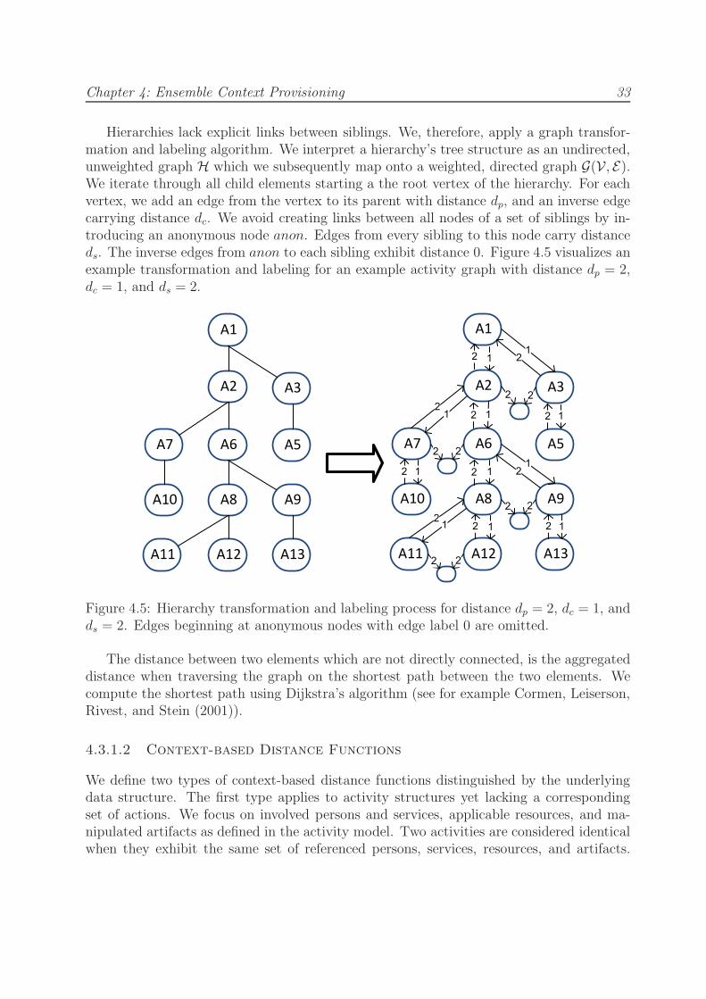
Chapter 4: Ensemble Context Provisioning 33
Hierarchies lack explicit links between siblings. We, therefore, apply a graph transfor-mation and labeling algorithm. We interpret a hierarchy’s tree structure as an undirected,unweighted graph H which we subsequently map onto a weighted, directed graph G(V, E).We iterate through all child elements starting a the root vertex of the hierarchy. For eachvertex, we add an edge from the vertex to its parent with distance dp, and an inverse edgecarrying distance dc. We avoid creating links between all nodes of a set of siblings by in-troducing an anonymous node anon. Edges from every sibling to this node carry distanceds. The inverse edges from anon to each sibling exhibit distance 0. Figure 4.5 visualizes anexample transformation and labeling for an example activity graph with distance dp = 2,dc = 1, and ds = 2.
A1
A13
A2 A3
A5A6A7
A8 A9A10
A11 A12
A1
A13
A2 A3
A5A6A7
A8 A9A10
A11 A12
2
2
2
2
2
2 22
2
2
2
1
1
1
1
1
1 1
11
1 1
2
2
2
2
2
2
2
2
Figure 4.5: Hierarchy transformation and labeling process for distance dp = 2, dc = 1, andds = 2. Edges beginning at anonymous nodes with edge label 0 are omitted.
The distance between two elements which are not directly connected, is the aggregateddistance when traversing the graph on the shortest path between the two elements. Wecompute the shortest path using Dijkstra’s algorithm (see for example Cormen, Leiserson,Rivest, and Stein (2001)).
4.3.1.2 Context-based Distance Functions
We define two types of context-based distance functions distinguished by the underlyingdata structure. The first type applies to activity structures yet lacking a correspondingset of actions. We focus on involved persons and services, applicable resources, and ma-nipulated artifacts as defined in the activity model. Two activities are considered identicalwhen they exhibit the same set of referenced persons, services, resources, and artifacts.

Chapter 4: Ensemble Context Provisioning 34
Algorithm 1 Transformation and Labeling algorithm Λ(H, dc, dp, ds).
function BuildGraph(H, dc, dp, ds)/* Initialize set of vertices and edges. */V ← ∅E ← ∅r ← rootV ertex(T )V ← rfor all v ∈ child(r) do
call AddNode(v,H, V, E, dc, dp, dsend for
call ConnectSiblings(child(r), V, E, dsG ← createDirectedGraph(V,E)return G
end function
function AddNode(n,H, V, E, dc, dp, ds)V ← n/* Add child to parent link. */E ← edge(n, parent(H, n), dp)/* Add parent to child link. */E ← edge(parent(H, n), n, dc)for all v ∈ child(n) do
call AddNode(v,H, V, E, dc, dp, dsend for
call ConnectSiblings(child(n), V, E, dsend function
function ConnectSiblings(N, V,E, ds)/* Only if there are siblings. */if |N | > 1 then
/* Create anonymous sibling connector vertex. */anon← vertex()V ← anonfor all n ∈ N do
E ← edge(n, anon, dc)E ← edge(anon, n, 0)
end for
end if
end function

Chapter 4: Ensemble Context Provisioning 35
Action 4-tuple set T Context 2-tuple setp1
< a1, {p1, p2}, {r3}, {} > < {a1, ·}, {a1, r3}, {·, r3} >< a1, {p1}, {r2, r3}, {o4} > < {a1, ·}, {a1, r2}, {a1, r3}, {a1, o4}, {·, r2}, {·, r3}, {·, o4},
{r2, o4}, {r3, o4} >< a2, {p1}, {}, {o4} > < {a2, ·}, {a2, o4}, {·, o4} >
Joined < {a1, ·}, {a1, r3}, {·, r3}, {a1, r2}, {a1, o4}, {·, r2}, {·, o4},{r2, o4}, {r3, o4}, {a2, ·}, {a2, o4} >
p2
< a1, {p1, p2}, {r3}, {} > < {a1, ·}, {a1, r3}, {·, r3} >< a3, {p2, p3}, {r2}, {} > < {a3, ·}, {a3, p3}, {a3, r2}, {·, r2}, {p3, r2} >
Joined < {a1, ·}, {a1, r3}, {·, r3}, {a3, ·}, {a3, p3}, {a3, r2}, {·, r2},{p3, r2} >|p1 ∪ p2| = 15; |p1 ∩ p2| = 4
Jaccard Distance 0.73
Table 4.1: Distance calculation for two action sets of p1 and p2 applying Jaccard’s distancefunction.
We limit the set overlap to activity references when comparing resources, service, persons,and artifacts as they lack direct relations in the activity model. The Jaccard distance isa commonly used set overlap function, defined as the difference between set union and setintersection, divided by the set union:
Jδ =|A ∪B| − |A ∩B|
|A ∪B|(4.2)
where sets A and B contain the references to persons, services, references, and artifactswhen comparing two activities aA and aB. Jδ becomes 0 when the two sets contain thesame elements and yields 1 when the two sets are completely disjoint.
The second type applies action data. We interpret actions as a collection of 4-tuplesTaction < A,P,R,O > comprising activity, persons (including services), resources, andartifacts. For each element v, there exist a corresponding set Taction(v) that containsall actions involving v. Subsequently, we map each action 4-tuple into a set of 2-tuplesthrough permutation of each element in the categories A,P,R, and O with each otherelement of different category. In both sets, we replace the compared elements i and jwith < · >. Subsequent joining of the 2-tuple sets ignores multiple instances of identical2-tuples. The Jaccard formula on the aggregated 2-tuple sets provides the correspondingdistance measurement. Table 4.1 gives an example of this process. In the example, thefirst tuples Taction of the persons pi, pj are identical as this was a joint action.

Chapter 4: Ensemble Context Provisioning 36
4.3.1.3 Interaction-based Distance Functions
Natural and context-based distance functions ignore the focus of individual elements. Thereis no difference between the same action tuple occurring once or 100 times. Resourcesapplied in every activity have the same impact as services applied in specific activitiesonly. The goal of inter-action based distance functions is weighting an elements localimpact according to its global significance.
To this end, we introduce a 4-partite, labeled action graph AG△(V, E). A 4-partitegraph (a specialization of a k-partite graph) comprises four vertex categories (K). Eachvertex v maps to exactly one category k ∈ K. Edges are undirected and exist only betweennodes of different categories. An edge ek,l links vertices of category k and l, with k 6= l.
The 4-partite action graph represents the four categories found in an action tupleTaction: activity, person, resource, and artifact. Edge labels provide the number of actionscontaining the particular 2-tuple. The graph in Figure 4.6 is equivalent to the tuples inTable 4.1. In contrast to the context-aware distance metric on actions, edges deriving fromjoint actions (i.e., involving multiple elements of the same category) are counted once only.We establish four 2-tuples from the action < a1, {p1, p2}, {}, {} > when comparing p1 andp2. The 4-partite graph for the same action yields only two edges, each labeled 1. Repeatedactions increase the edge label. As p1 engages in two actions within scope of activity a1,edge < a1, p2 > exhibits label 2.
p1
p2
p3
a1
a2
a3
r2
r3
o4
1
1
1
1
1
1
1
1
2
1
1
1
2
1
1
1
2
a
r
p
o
Person
Activity
Resource
Artifact1
Figure 4.6: 4-partite labeled action graph for the action tuples T in Table 4.1.
We measure the distance between two elements of the same category by analyzingshared elements within neighboring categories. The distance, for example, between twopersons is based on actions involving joint activities, joint resources, and joint artifacts. Ingeneral, the tighter two elements of category l are linked to identical elements of categoryk (with k 6= l), the smaller the distance. We define distance on a minimal subgraph

Chapter 4: Ensemble Context Provisioning 37
(Figure 4.7) comprising the two elements for comparison (v1l, v2l), the connecting thirdelement (v3k), and two edges (e1k,l(v1, v3), e2k,l(v2, v3)) with corresponding edge labelss1, s2.
s1, w1 v1L
v2L
v3Ks2, w2
Edge: e1LK(v1, v3)
Edge label: s1
Edge weight:
w2 = s2/(s1+s2)
Figure 4.7: Minimal subgraph for calculating distance between elements v1l and v2l viaelement v3k.
We consider the amount of shared elements, the magnitude of involvement, and involve-ment distribution. Two elements each linked with label 1 to the same three neighbors, yieldhigher distance than two elements each linked with label 10 to only one shared neighbor.Also, two elements linked with equally distributed labels (e.g., s1 = s2 = 6) are more sim-ilar than elements with unequally distributed labels (e.g., s1 = 2, s2 = 10). For comparingelements v1, v2, we compute the edge weight for each link to neighbor element v3. Edgeweights w1, w2 equal the corresponding, normalized edge labels such that w1 = s1/(s1 +s2)and w2 = s2/(s1 + s2). The distinct difference between edge labels and edge weights is theapplication scope. Edge weights exist only in the corresponding minimal subgraph. Theydescribe the action distribution from element v3 towards elements v1, v2. For any otherminimal subgraph containing one of the edges e1, e2, we need to recalculate the weightsw1 and w2.
We apply Shannon’s entropy definition (Shannon 1948) H(w) = −∑
(w ∗ log(w)) onedge weights w with
∑
w = 1 to describe the local focus of an element. We normalize theentropy H(w) to the interval [0, 1] by dividing by log(2) 2. The focus of an element will beminimal (i.e., maximal entropy H(w)/log(2) = 1) if actions are equally distributed. Thefocus will be maximal (i.e., H(c) = 0) when one of the edge labels is 0. The local distancebetween two elements v1, v2 via neighbor v3 is defined as:
distv3,k(v1, v2) =s1 + s2
2∗H(w)
log(2)(4.3)
Local edge weights and edge weight distribution are insufficient to sufficiently establishthe distance between two elements. We also consider the global significance of a neighbor-
2We divide by log(2) as there are two values aggregated by the entropy; i.e., the edge weights w1 andw2.

Chapter 4: Ensemble Context Provisioning 38
sig a1 a2 a3 p1 p2 p3 r2 r3 o4
a n/a n/a n/a 0,42 0,37 0 0,37 0 0,37p 0,42 0 0,37 n/a n/a n/a 0 0,42 0r 0,08 0 0 0,08 0 0 n/a n/a 0o - - - - - - - - n/a
Table 4.2: Global context significance for elements in Figure 4.6.
ing element in contributing to the distance measurement. For example, resource r2 exhibitsedges with identical labels to all persons. It should not be considered for comparing anytwo persons as it does not add any information about the distance between elements in theperson category. To this end, the global context significance metric applies Shannon’s en-tropy to describe the information content of an element’s edge labels for a specific category.The significance of element vk for edges ek,l is defined as:
sigk(vl) = 1−−∑
i(wv,i,k ∗ log(wv,i,k))
log(|k|)∀ k 6= l, |k| > 1 (4.4)
where wv,i,k is the normalized weight of the ith outgoing edge towards category k of ele-ment v such that
∑
i wv,i,k = 1; |k| denotes the number of elements in category k. Thenormalization yields a significance value in the interval [0, 1]. Significance is 0 when an ele-ment exhibits no focus (i.e., high entropy) and equally links to all elements of a particularcategory. Each element provides |K| − 1 = 3 global significance values; one for each neigh-boring category. Table 4.2 lists the significance values for elements in Figure 4.6. There areno results available for the artifact category as there occurs only one artifact. Resource r2is suitable for comparing only activities, while resource r3 applies only to persons. Personp3 and activity a2 yield no information for comparison at all.
The overall distance metric is the inverse sum of all weighted local distance measure-ments for all neighboring categories:
dist(v1l, v2l) =
∑
K
∑
N(k,v1,v2)
sigk(n) ∗ distn,k(v1, v2)
−1
∀ k 6= l (4.5)
where n is a vertex from the neighborhood set N containing joint neighbors of v1, v2for category k. The distance between two elements becomes infinity when they share noneighbor or only neighbors with significance 0.
To compare non-connected elements (e.g., a2 and a3), we calculate multi-hop distance onthe intra-category distance measurements. Direct distance measurement within a categoryyields an undirected, weighted, mono-partite graph. The distance in such a graph fortwo elements (v1l, v2l) h hops apart aggregates the distance measures on the shortestpath including a penalty distance for every additional required hop. Suppose element Acollaborates closely with element B, and B collaborates closely with C, but A and C have

Chapter 4: Ensemble Context Provisioning 39
few actions in common. To establish the distance between A and C, we cannot just add thedistance AB and BC. Instead we increase the distance BC as defined by a penalty function.The penalty function mimics the transitivity principle in trust propagation (Josang, Ismail,and Boyd 2007,Artz and Gil 2007). For our purpose, a simple exponential penalty functionis sufficient. Consequently the penalty increases for growing hops. The penalized distancefor two consecutive nodes va and vb on the shortest path between source node (v1) andtarget node (v2) is defined as:
distp(h, va, vb) = dist(va, vb) ∗ 22h−1 ∀ h > 0 (4.6)
where h is the hop count to va from the source node. Thus, the distance for the secondhop doubles, and quadruples for the third hop. The distance remains infinity for twoelements where each resides in one segment of a partitioned graph (i.e., the there exists noconnecting path of any hop count).
For distance between activity a2 and a3, we aggregate distance of a2 to a1 (dist = 1.0)and the penalized distance of a1 to a3 (distp(1) = 1.355). The final distance yields 3.71.For the remaining elements in Figure 4.6, we derive following distance measurements:p1, p2 = 0.792; p2, p3 = 2.71; p1, p3 = 6.222 and r2, r3 = 4.08.
Metrics merely describe how to measure the distance between two values. Any pref-erences of smaller over larger values (or vice versa) are expressed in the utility functionsintroduced further below.
4.3.2 Relevance Functions
Relevance function determine the impact individual metrics should exercise upon finalaggregation. Each metric i comes with a corresponding weight ωri. We assign equalimportance to every metric with ωri = 1/max(i). As configuration of weights is very casespecific, we cannot give generally valid recommendations for the various metrics. For theremainder of this chapter, we consider all metrics of equal importance.
4.3.3 Utility Functions
Utility functions express the decline of observed fitness as candidate values deviate fromthe optimum value. In many cases, a continuous function across the full value space is in-sufficient. The utility function templates in Figure 4.8 display exemplary linear restrictionson value ranges. The horizontal axis shows the relevance metric values and the verticalaxis returns the corresponding utility values. Limits a to d list the required configurationparameters. Services need to provide the configuration parameters, which can depend oncontext themselves. We define following function templates:
HardLowerDecliningOver 4.8 (a), specifies the optimum value as a hard lower limit,with higher values steadily decreasing.

Chapter 4: Ensemble Context Provisioning 40
HardUpperDecliningLower 4.8 (b), specifies benefit steadily rising until reaching anoptimum hard upper limit.
SoftLowerStableLimitedOver 4.8 (c) extends HardUpperDecliningLower with a rangeof equally optimal metric values.
SoftUpperStableLimitedLower 4.8(d) extends HardLowerDecliningUpper with a rangeof equally optimal metric values.
LimitedSoftLowerLimitedSoftUpper 4.8(e) defines an optimal value with (not nec-essary equally) decreasing utility on both sides.
LimitedSoftLowerPlateauLimitedSoftUpper 4.8(f) extends LimitedSoftLowerLimit-edSoftUpper with a range of equally optimal metric values. This function can emulateall previous functions.
Setting a negative impact weight ωri reverses the respective utility function. For ex-ample, HardLowerDecliningOver will treat values outside the limits a and b as rewarding,with utility declining from limit b towards limit a.
4.3.4 Ranking Algorithm
Let us define the set of relevance metric functions R = {r1(ce), r2(ce), . . . , rn(ce)} thatare associated with each candidate element and ωr as the weight assigned to metric rsuch that
∑
i=1,...,n |ωr| = 1. Utility functions U = {u1(r1(ce)), u2(r2(ce)), . . . , un(rn(ce))}express the fitness of candidate element ce given the respective relevance metric r. Thescore for a particular utility function, relevance metric, and candidate element is definedas follows:
score(u, r, ce) =max(u)− u(r(ce))
max(u)− min(u)(4.7)
where max(u) returns the utility function maximum over all candidate elements; min(u)returns the utility function minimum over all candidate elements; and u(r(ce)) provides theutility function result for the candidate element ce by applying the corresponding relevancemetric r. We avoid negative metric weights ω because negative weights are either implicitlyconsidered by selecting the appropriate utility function or explicitly considered by invertingthe utility function.
The scoring function score(ce, u, r) scales all scores for a particular metric to the interval[0, 1] such that the best candidate yields score 1 and the worst candidate yields score 0.
In the second step, we rank individual context elements according to the overall selectedset of metrics and weights. Our approach applies a simplified LSP method (see Dujmovic

Chapter 4: Ensemble Context Provisioning 41
1
0
Limit a Limit b
1
0
Limit a Limit b
1
0
Limit a Limit b Limit c
1
0
Limit a Limit b Limit c
1
0
Limit a Limit b Limit c
a) b)
c) d)
e) f)
Limit a Limit b Limit dLimit c
Figure 4.8: Context ranking utility functions
(2007) for a detailed overview). The global score of a candidate element is given as:
E(ce) =n∑
i=1
ωui∗ score(ce, ui, ri) ∗ 100 (4.8)
The separate application of utility functions constitutes the distinct advantage over thesimplified LSP method. The LSP applies scoring directly on the candidate elements, thustightly coupling metric computation and utility evaluation.
4.3.5 Example Application of Context Ranking
In the example in Figure 4.9, we select the natural, hierarchy-based activity distance w(d)and temporal distance w(t) for context elements. We apply the HardLowerDecliningOver

Chapter 4: Ensemble Context Provisioning 42
Algorithm 2 Ranking Algorithm RA(CE,R, {ω}).
function ComputeGlobalRank(CE,R, {ω})Require:
∑
ω = 1/* Set or ranked context elements */E ← ∅/* Aggregate individual weights */for all ce ∈ CE do
rankc ← 0for all r ∈ R do
rankc ← rankc + Util(ce, r) ∗ ωrend for
E[ce]← rankcend for
return sort(E)end function
utility function for both metrics. Context elements yield maximum utility when linkedto the activity at hand, applicable shortly in the past or future. The parameters forthe utility functions are 0 and maximum tree distance, respectively, maximum temporaldistance. Thus, for both metrics we prefer lower values over higher values, i.e., closeractivities and shorter time difference indicate more relevant context elements. Adjustingthe weights determines the importance of one metric over the others. In this scenario, weapply the same ranking weights w(d) = w(t) = 0.5 for every activity and context elementrespectively. For the activity distance utility function, we set the edge weights as: parentdp = 2, child dc = 1, and siblings ds = 2.
We have developed a Context Ranking Web service, which assists in searching for rele-vant documents. In dynamic ensembles, manual a-priori configuration of relevant servicesfor every activity is infeasible. Instead, the relevance ranking algorithm determines atrun-time the most promising services — in the given example Storage Web Services.
We trigger the ranking service in scope of activity A8 on the 28th January. The activitygraph in Figure 4.9 displays context elements of type Storage Web Service (SWS). Activitydistance is given in the upper right corner. Past dates indicate last access of SWS, whereasfuture dates indicate planned documents available as templates in a SWS. The hierarchystructure and timestamp values are manually generated for this scenario to highlight theeffect of the context ranking process.
The context elements used in our ranking example are Resources of type SWS. Candi-date SWS are those who are referenced within Action elements. In addition, we includeSWS that are scheduled for managing already existing document templates in future. Asboth actions and activities contain a timestamp, the ranking algorithm (Alg. 2) is able torank these context elements. Table 4.3 presents the resulting activity-distance rank R(d),temporal-distance rank R(t), and the aggregated rank R(M,AG).

Chapter 4: Ensemble Context Provisioning 43
A� ����� ���01�����
A6
��A9
��A8now28/01/
2008
+0
A �1��� ���01�����
A �
6
A7
�� A� ��
A1
��
A10
�5
a:���
06�01� ����
b:��� ����������
��� ���������� ��� � �� �������� ���
11����
7
��� ������������� � �� �����
1.2.
4.
A11
�1
A� �
A5
�9
���05�����������
11�������
7
��� ��������7
3. 5.
Figure 4.9: Activity Graph excerpt.
Context elements receiving high ranks in both time-distance metric and activity-distance metric will also rank high the overall results (e.g., SWS in A12). A good po-sition in a single ranking, however, does not guarantee final relevance, as this depends onthe distribution of the other context elements. For example, the SWS in A11 is ranked9th place in the time-distance metric, respectively ex aequo 1st in the activity ranking,ending up 2nd place in the overall ranking. In contrast, the SWS in A03 ranked 1st inthe time-distance metric, but ranked 10th in the activity-distance metric, winds up in themiddle on 7th place. The reason lies in the distribution of metric values. For a numberof values (i.e., timestamps) in close proximity (compared to the overall range) their intrametric ranking scores become less significant and the other metrics (i.e., activity distance)become dominant. When two context elements have almost equidistant timestamps fromthe current activity (A8) we cannot decide which one is more relevant. Thus, the respec-tive activity-distance measurements primarily influence the final rank. In the example,the activity metric dominates over the timestamp metric for following context elements:A10-b, A05, A07, A01 — all within a 0.04 R(t) range.

Chapter 4: Ensemble Context Provisioning 44
Act. d Date R(d) R(t) R(M,AG)A12 1 22.01.08 (1) 1.00 (2) 0.96 (1) 98.24A11 1 11.12.07 (1) 1.00 (9) 0.47 (2) 73.53A07 4 27.02.08 (5) 0.63 (6) 0.68 (3) 65.37A10-a 5 06.01.08 (7) 0.50 (3) 0.78 (4) 63.82A06 2 23.03.08 (3) 0.88 (10) 0.39 (5) 63.16A10-b 5 24.02.08 (7) 0.50 (4) 0.72 (6) 60.88A03 8 24.01.08 (10) 0.13 (1) 0.99 (7) 55.66A02 6 03.03.08 (9) 0.38 (8) 0.62 (8) 49.93A13 3 05.04.08 (4) 0.75 (12) 0.24 (9) 49.26A04 4 26.11.07 (5) 0.63 (11) 0.29 (10) 45.96A01 8 27.02.08 (10) 0.13 (6) 0.68 (11) 40.37A05 9 30.12.07 (12) 0.00 (5) 0.69 (12) 34.71
Table 4.3: Intermediary and final ranking results: ranking values derive from the structureand elements of the activity in Figure 4.9.
4.4 Evaluation of Context-based and Interaction-
based Distance metrics
Context-based and interaction-based distance metrics consider different aspects of an actionnetwork. Thus, we first discuss the fundamental difference based on a simple examplegraph. We then analyze a simulated action network to describe the conditions for whicheach of the two metrics yield most informative results. Ultimately, we apply the distancemetrics to a real world dataset and describe our findings.
4.4.1 Fundamental Differences
When comparing two entities, the context-based metric considers shared and individualaction links. Independent of the number of shared links, the distance between two entitiesincreases as the number of individual links grows. In contrast, the interaction-based metricpurely analyzes the distribution of actions across the set of shared links.
We limit our analysis to a bipartite graph comprising only persons and activities forsake of clarity. The distance metric principles, however, apply to any k-partite graph.Suppose the action network in Figure 4.10 (a). The example graph consists of threepersons involved in six activities. All the links carry equal weight 1 representing an initialensemble configuration. For this network configuration, Figure 4.10 provide the context-based distance measurements for activities (c) and persons (f). Subfigures (d) and (g)provide the respective interaction-based distance values.
The context-based distance metric yields measurements in the range [0, 1] while theinteraction-based metric yields values in the range [0,∞], Thus, we do not compare absolute

Chapter 4: Ensemble Context Provisioning 45
distance measurements but focus on the differences within each distance graph (c)-(h).
Observing the context-based activity distance values, we detect the shortest distanced = 0 between nodes a1 <> a2, a5 <> a6, and a7 <> a8. These activity pairs feature acomplete overlap of adjacent person nodes. The next closest links occur between activitiesthat have one adjacent person in common, with exactly one of the nodes linking to a secondperson (e.g., a1 and a5 connect via p1, with a1 also linking to p2.) The distance growswhen both nodes exhibit additional non-shared links (e.g., d(a1, a3) = 0.66 as besides theshared person p1, a1 links to p2 and a3 links to p3.)
For the initial graph, the interaction-based distance metric yields less distinguisheddifferences. Distance is shortest between activity pairs d(a3, a4) = 1.5 and d(a1, a2) = 2.2,with all other links yielding distance d = 4.4. The underlying reason is the interaction-based metric’s ignorance of non-shared links when comparing two elements. Differencesnevertheless arise from the significance values of connecting elements. Table 4.4 lists theglobal significance and entropy values for the elements of graph (a) and (b). Person p3 yieldshigher global significance than p1 and p2 as she links to merely two out of eight activities,while p1 and p2 exhibit involvement in five activities each. Consequently, activity a3 anda4 are considered closer than a1 and a2, even the latter ones yield two common personneighbors.
The person distance measurements in Figure 4.10 (f) and (g) provide similar results,e.g., the distance between p1 and p2 is smaller than both edges connecting p3. In moredetail, we observe that the interaction-based metric better highlights the difference ininvolvement (e.g., the distance between p1 and p2 is half that of p2 and p3). The context-based metric considers p2’s involvement in other activities, thereby reducing the effect ofp1 and p2 having more common activities than p2 and p3.
P1 P2 P3 A1 A2 A3 A4 A5 A6 A7 A8(a)Significance 0.226 0.226 0.667 0.369 0.369 0.369 0.369 1 1 1 1Abs. Entropy 1.609 1.609 0.693 0.693 0.693 0.693 0.693 0 0 0 0Rel. Entropy 1 1 1 1 1 1 1 0 0 0 0(b)Significance 0.279 0.279 0.667 0.369 0.369 0.369 0.369 1 1 1 1Abs. Entropy 1.499 1.499 0.693 0.693 0.693 0.693 0.693 0 0 0 0Rel. Entropy 0.931 0.931 1 1 1 1 1 0 0 0 0
Table 4.4: Significance, absolute entropy, and relative entropy derived for the interaction-based distance metric for graphs in Figure 4.10 (a) and (b).
We add additional actions to highlight further fundamental differences between context-based and interaction-based distance metrics. The graph in Figure 4.10 (b) comprises thesame nodes as graph (a) but contains additional actions. Specifically, the three personstripled their involvement in activities a1, a2, a3, and a4, i.e., they exhibit a focus on certainactivities.

Chapter 4: Ensemble Context Provisioning 46
For the evolved graph, we need only recalculate interaction-based distance measure-ments. The context-based values remain the same as long as we keep the number of nodesand the set of edges the same. We utilize Figure 4.10 graph (c) and (e) to compare activitydistance, and (f) and (h) to compare person distance in the evolved graph. Observingactivity distance, we notice that the interaction-based metric now provides more details.The distance in-between a1, a2 and a3, a4 decreases as well as the distance across thesefour nodes.
With the introduction of additional actions, the global significance values change. Sub-sequently, nodes that haven’t experienced additional actions yield different distance mea-surements. Activities a5 and a6, for example, become closer as the global significance ofp1 increases from 0.226 to 0.279 (see Table 4.4 lower part).
With respect to person distance, we observe the same relative differences as found inthe original graph. However, the interaction-based metric allows to distinguish betweentwo set of nodes (e.g., the set [p1, p2, p3] in graph (a) and (b), but not necessarily limitedto identical nodes) exhibiting the same distribution of actions, but different involvementmagnitude. Thus, we establish that the three persons reside in greater proximity in graph(b) than in graph (a).
To summarize the fundamental differences:
• As the name of the metrics already imply, context-based distance considers predom-inately the number of non-shared elements, while interaction-based distance focusesentirely on the involvement of common elements.
• Distances rapidly change when elements start to exhibit an unequal distribution ofactions. Context-based distance cannot detect elements focusing their actions on asubset of their overall action involvement.
• Context-based distance assigns the same distance values to two sets of elements withidentical link structure. In such a configuration, interaction-based distance provideslower distance for the set yielding the greater number of actions.
4.4.2 Simulation-based evaluation
We construct a simulated interaction network to analyze the distance differences for variousaction distributions. The underlying graph comprises 5000 persons involved in 5000 activi-ties. Similar to real-world complex networks (Albert, Jeong, and Barabasi 1999,Albert andBarabasi 2002), the graph exhibits node degrees following a power-law distribution. Wegenerate the link structure by modifying the original algorithm for monopartite graphs byBarabasi and Albert (1999) to produce a bipartite graph. Figure 4.11 displays the degreedistribution for activities (a) and persons (b).
We apply the following general procedure to measure the relative differences in distancevalues in two k-partite graphs AG1 and AG2 containing the same nodes but exhibitingdifferent edge weight characteristics.

Chapter 4: Ensemble Context Provisioning 47
p1 p3
p2
a2a1 a3 a4
a5 a6
a7 a8
11
1 1
11
1
1 1 1
11
p1 p3
p2
a2a1 a3 a4
a5 a6
a7 a8
33
3 3
11
3
3 3 3
11
p1
p3
p2
0.75
a2a1
a3
a4
a5
a6
a7
a8
0.833
0.833
p1
p3
p2
1.355
2.71
2.71
0.50.5
0.50.5
0.5
0.5
0.5 0.5
0.5 0.5
0.5
0.5
0
0
0
0.66 0.66
0.66
0.660.66
a2a1
a3
a4
a5
a6
a7
a8
4.44.4
4.44.4
4.4
4.4
4.4 4.4
4.4 4.4
4.4
4.4
2.2
4.4
4.4 4.4
1.5
4.44.4
p1
p3
p2
0.452
0.903
0.903
a2a1
a3
a4
a5
a6
a7
a8
2.22.2
2.22.2
2.2
2.2
2.2 2.2
2.2 2.2
2.2
3.6
0.6
3.6
1.2 1.2
0.5
1.21.2
(a) (b)
(c) (d) (e)
(f) (g) (h)
Figure 4.10: Interaction-based and context-based monopartite distance graph for evolvingbipartite action graph. Line thickness in subfigures (c) to (h) represents node similarity.

Chapter 4: Ensemble Context Provisioning 48
• For the two graphs, we calculate distance measurement for each node type (i.e., Ac-tivity, Person ...) creating the respective monopartite distance graphs (Dk1,Dk2 ∀ k =1 → K).
• For each node type k, we select a set of candidate nodes from one of the respectivedistance graphs. For each of these candidates, we select a set of random nodes withinthe distance graph, the candidate’s buddy set.
• For each candidate, we calculate the distance to each buddy and derive the rankingin descending order. For every candidate, we generate the distance rank in each ofthe two distance graphs (rk1, rk2).
• We apply Pearson’s Coefficient for every pair of rankings to measure the differencein element positions. We average over all coefficients for each node type to determinethe type specific difference between the two graphs AG1 and AG2.
This procedure also applies to graphs with non overlapping node sets when followingtwo conditions hold. First, the set of ranked elements needs to be a node subset in bothgraphs. Second, the set of ranked elements must be connected in both graphs (i.e., theremust exist a path between any two elements of the candidate set in each of the graphs).
100
101
102
103
100
101
102
103
104
exhibiting node degree x
Num
ber
of a
ctiv
ities
(a)
100
101
102
103
100
101
102
103
104
exhibiting node degree x
Num
ber
of P
erso
ns
(b)
Figure 4.11: Degree distribution for 5000 activities (a) and 5000 persons (b) in a bipartitegraph.

Chapter 4: Ensemble Context Provisioning 49
4.4.2.1 Pearson’s Correlation Coefficient
Pearson’s correlation coefficient ρ describes the similarity of two equal-length data setswith (−1 ≤ ρ ≤ 1). Identical data sets yield 1 and inverse ordered data sets yield −1. 0indicates no correlation. We apply the coefficient to describe the ranking difference betweenthe two distance metrics on the same graph, and also the ranking difference within oneparticular distance metric as the underlying graph evolves.
Pearson’s correlation coefficient is defined as:
ρk =m ∗ (
∑
rk1(i), rk2(i))− (∑
rk1(i))(∑
rk2(i))√
m ∗ (∑
rk1(i)2)− (∑
rk1(i))2√
m ∗ (∑
rk2(i)2)− (∑
rk2(i))2(4.9)
with m the number of elements (here the buddy set’s size), rk1(i) the rank for node i oftype k in graph AG1, and rk2(i) is the rank for node i of type k in graph AG2.
For our simulated interaction network, we observe the ranking difference for interaction-based distance metric caused by various action distributions. We further compare how thesedistributions differ from applying the context-based distance metric. Keeping the numberof elements and underlying link structure the same, we need not compare context-baseddistance metrics for the various action distributions. There will be no difference (ρ = 1).The three applied action distributions are:
Even - every person engages in exactly one action for any of its neighboring activities.
Linear decreasing - every person p engages in x∗degree(p) actions. Each person exhibitsa focus on the neighboring activity with the highest involvement of other persons,and linear decreasing focus on the remaining neighboring activities. Thus a particularperson engages in [(x ∗ degree(p) ∗ 0.5)− 1, . . . , 1] actions with its neighbors suchthat the average action per neighbor becomes x.
Logarithmic decreasing - similar to linear decreasing, every person engages on averagein x actions per neighboring activity. The focus, however, decreases logarithmically.The activity with the most involvement receives most actions. Any subsequent activ-ity receives half the actions of the previous activity until the last neighboring activityreceives a single action.
We derive three bipartite graphs AGev, AGlin, and AGlog, that comprise the sameactivity and person nodes connected via the same set of edges. The graphs merely differin the edge labels according to the three action distributions. In each of these graphs wederive distance rankings for the same 40 random candidate elements, each exhibiting aset of 40 random buddy elements. The upper part of Table 4.5 contains the Pearson’scoefficients for rankings derived from interaction-based distance measurements. In thelower part, we compare ranking differences of interaction-based, and context-based distancemeasurements.
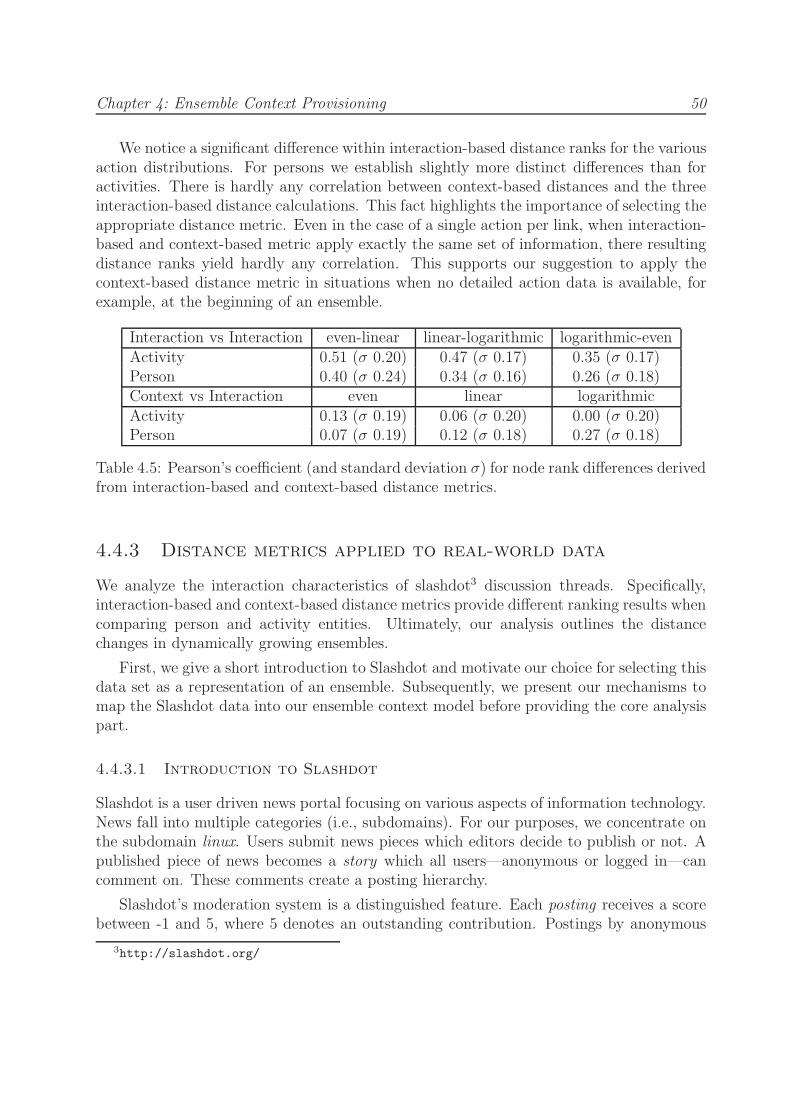
Chapter 4: Ensemble Context Provisioning 50
We notice a significant difference within interaction-based distance ranks for the variousaction distributions. For persons we establish slightly more distinct differences than foractivities. There is hardly any correlation between context-based distances and the threeinteraction-based distance calculations. This fact highlights the importance of selecting theappropriate distance metric. Even in the case of a single action per link, when interaction-based and context-based metric apply exactly the same set of information, there resultingdistance ranks yield hardly any correlation. This supports our suggestion to apply thecontext-based distance metric in situations when no detailed action data is available, forexample, at the beginning of an ensemble.
Interaction vs Interaction even-linear linear-logarithmic logarithmic-evenActivity 0.51 (σ 0.20) 0.47 (σ 0.17) 0.35 (σ 0.17)Person 0.40 (σ 0.24) 0.34 (σ 0.16) 0.26 (σ 0.18)Context vs Interaction even linear logarithmicActivity 0.13 (σ 0.19) 0.06 (σ 0.20) 0.00 (σ 0.20)Person 0.07 (σ 0.19) 0.12 (σ 0.18) 0.27 (σ 0.18)
Table 4.5: Pearson’s coefficient (and standard deviation σ) for node rank differences derivedfrom interaction-based and context-based distance metrics.
4.4.3 Distance metrics applied to real-world data
We analyze the interaction characteristics of slashdot3 discussion threads. Specifically,interaction-based and context-based distance metrics provide different ranking results whencomparing person and activity entities. Ultimately, our analysis outlines the distancechanges in dynamically growing ensembles.
First, we give a short introduction to Slashdot and motivate our choice for selecting thisdata set as a representation of an ensemble. Subsequently, we present our mechanisms tomap the Slashdot data into our ensemble context model before providing the core analysispart.
4.4.3.1 Introduction to Slashdot
Slashdot is a user driven news portal focusing on various aspects of information technology.News fall into multiple categories (i.e., subdomains). For our purposes, we concentrate onthe subdomain linux. Users submit news pieces which editors decide to publish or not. Apublished piece of news becomes a story which all users—anonymous or logged in—cancomment on. These comments create a posting hierarchy.
Slashdot’s moderation system is a distinguished feature. Each posting receives a scorebetween -1 and 5, where 5 denotes an outstanding contribution. Postings by anonymous
3http://slashdot.org/

Chapter 4: Ensemble Context Provisioning 51
users are automatically scored 0. Postings by authenticated users are scored 1 by default.The editors and a changing set of selected users possess a limited number of moderationpoints to raise or lower these initial posting scores. In addition, they can tag a postingwith a predicate such as Interesting, Insightful, Informative, Funny, etc. Users that receivehigher scores in their postings are more likely to become moderators than users with lowerscores. Predicates will not be used here but in the evaluation of Service InfrastructureAdaptation mechanisms in Chapter 6. We include them here for sake of completeness.
Slashdot exhibits similar characteristics as large-scale service ensembles. Some entitiesremain consistently active throughout all subdomains. Other entities join in an ad-hocmanner, participate for a limited period, and then vanish again. Postings in Slashdotresemble user actions in activities. Users are interested in providing their knowledge toimprove the quality and information content of a story (i.e., they fulfil a task.) Theyrarely engaging in direct communication with other users (Gomez, Kaltenbrunner, andLopez 2008, Skopik, Truong, and Dustdar 2009). We thus map user postings to actions,and users to person elements in our context model. Extraction of an appropriate activitystructure requires additional steps outlined in the following subsection.
4.4.3.2 Slashdot Posting Aggregation
A Slashdot posting provides details on user, time of posting, a unique id, and a referenceto its parent posting. A set of postings from the same story establish an action hierarchy,but no explicit mapping to an activity hierarchy. Treating each action as an individualactivity is straight forward, but will provide little information in the ultimate bi-partitegraph as every activity will then always link only two persons: the posting’s creator andthe posting parent’s creator.
We devised Algorithm 3 to aggregate a posting hierarchy. In the course of the algorithmmultiple actions are assigned to the scope of an activity. The story always becomes theroot activity (function Init). We also define an energy threshold e that defines when aposting should trigger the creation of a new activity. The posting then becomes an actionboth in the scope of the new activity and the parent activity.
Each posting exhibits energy based on its child postings and grand child posting (func-tion CalculateEnergy). The basic energy level corresponds directly to the number of childpostings. This value is increased dependent on the distribution of grandchildren. To thisend, we count the number of grandchildren each child exhibits and derive the correspond-ing entropy value. This entropy is then normalized to the interval [0, 1]. Posting structuresthat feature equally distributed grandchildren yield maximum entropy and thus doublethe basic energy level. Posting structures that exhibit no grand children, or only one childwith grandchildren yield minimum entropy and leave the basic energy level unchanged.Examples for the former configuration include three children with each two grandchildren,while an example for the latter configuration comprises three children with only one havingtwo children.

Chapter 4: Ensemble Context Provisioning 52
The current posting triggers a new activity when the posting specific energy combinedwith the amount received from the parent posting exceeds the energy threshold. Otherwise,the posting splits its energy equally across all its child postings. We have to propagateenergy from parents to children to avoid all postings being assigned to the root activity incase no single posting reaches the energy threshold by itself.
The idea behind this energy-based aggregation mechanism is following. Multiple childpostings indicate different views (i.e., different activity aspects) on the posting at hand.When these child postings exhibit themselves a set of (grand)children, we assume this viewsto be of substantial significance. Hence, when there are sufficiently many children, respec-tively sufficiently distributed grandchildren, we create a new activity. When a postingexhibits children that create a narrow (and potentially deep) hierarchy tree, we considerthese postings belonging together and thus the observed posting remains in the scope ofthe parent posting’s activity.
The energy threshold parameter controls the amount of activities created within astory. Setting e = 0 results in every posting becoming an activity. Even this yields morestructural information than simply turning postings into activities (as outlined above).Each posting would result in two actions: one belonging to the current activity, and oneassociated with the parent activity. For the other extreme, e → ∞, all postings within astory create actions belonging to a single activity.
We need to ensure that the aggregation algorithm preserved the posting characteristicsbefore we can continue to create and analyze the bipartite graph comprising persons andactivities. The posting-to-activity aggregation is not the only transformation of postinghierarchies. A considerable amount of postings rise from anonymous users. We need tofilter these postings without breaking the overall hierarchy. Starting at the root posting,we bridge every posting of an anonymous user, by rewiring the parent reference of all childpostings.
The underlying dataset comprises 3477 stories from 19 subdomains in the period ofJanuary 1st 2008 until July 1st 2008. In these six months, the linux subdomain exhibits 96stories. Figure 4.12 (a) prints the number of postings in the linux subdomain against theirchild count (i.e., direct replies) before any filtering. In subfigure (b), anonymous posts areremoved. This step completely preserves the node degree characteristics.
Subfigures (c) and (d) describe the activity hierarchy based on aggregated cleanedpostings. We apply an aggregation energy value of e = 3 throughout our experiments in thischapter. Observing subfigure (c), we note a shift to the left caused by aggregation. Thereare significantly less activities than postings. The steepness of data distribution, however,remains the same, thus preserving the degree characteristic. Finally, in subfigure (d),aggregation caused a dampening. The number of activities exhibiting only few actions (i.e.,postings) is greatly reduced. The energy threshold eliminates the possibility of activitieshaving no or only a few associated actions. The degree distribution for activities with 10 ormore actions yields the same steepness as for the original and cleaned postings. Ultimately,we derive the bipartite graph from the set of actions as outlined in Section 4.3.

Chapter 4: Ensemble Context Provisioning 53
Algorithm 3 Aggregate Postings to Activities Algorithm AGG(story, e).
function Init(story, e)/* Create a root activity for the story. */a← newActivity(story)/* Add the new activity to the set of activities. */A← afor all childPostings ∈ story do
call Aggregate(childPosting, 0, e, A, a)end for
return Aend function
function Aggregate(posting, topEnergy, e, A, currentActivity)currentEnergy ← CalculateEngery(posting, topEnergy)if currentEnergy > e then
aNew ← newActivity(posting)A← aNewaddAction(currentActivity, posting)addAction(aNew, posting)currentActivity ← aNewcurrentEnergy ← 0
else
addAction(currentActivity, posting)currentEngery ← currentEnergy/childCount(posting)
end if
for childPostings ∈ posting do
call Aggregate(childPosting, currentEnergy, e, A, posting)end for
end function
function CalculateEnergy(posting, parentEnergy)GC ←for childPosting ∈ posting do
GC ← childCount(childPosting)end for
entropy ← 0if |GC| > 1 then
ent← calcEntropy(GC)entropy ← ent/|GC|
end if
energy ← childCount(posting) ∗ (1 + entropy)return energy ← energy + parentEnergy
end function

Chapter 4: Ensemble Context Provisioning 54
100
101
102
103
100
101
102
103
104
exhibiting # number of direct replies
Num
ber
of P
ostin
gs
original
(a)
100
101
102
103
100
101
102
103
104
exhibiting x number of child activities
Num
ber
of a
ctiv
ities
(c)
100
101
102
103
100
101
102
103
104
exhibiting # number of direct replies
Num
ber
of P
ostin
gs
cleaned
(b)
100
101
102
103
100
101
102
103
104
exhibiting x numbers of child actions
Num
ber
of a
ctiv
ities
(d)
Figure 4.12: Degree Distribution for complete posting set (a) and cleaned of anonymouspostings (b). Degree distribution for child activities from aggregated posting hierarchy (c)and action distribution (d). All postings from stories in the linux subdomain between Jan1st, 2008 and July 1st, 2008.

Chapter 4: Ensemble Context Provisioning 55
4.4.3.3 Analysis of Evolving Ranking Differences
We analyze the rank differences for interaction-based and context-based distance metricsfor a growing bipartite graph. Thereafter, we introduce an aging mechanism that removesold actions from the bipartite graph. Our goal is to describe the effect of additional actionsentering the graph on the ranking order of activities and persons.
Slashdot data displays different characteristics of how persons and activities emerge forthe first time. Subfigures 4.13 (a) and (b) print the amount of unique persons, respectivelyactivities, against the number of actions (21390) in temporal order. For 7172 persons,we note a slightly concave increase in new entities across the whole duration. The 1992activities increase in a more linear manner. The difference becomes more obvious when welimit the analysis to elements with degree 14 and higher. The emergence of the most activeusers (subfigure (c)) happens rapidly: 75% of all regular users (267) submit a posting (i.e.,action) within the first 20% of postings. For the top connected activities (269) (subfigure(d)), we observe only a slight difference to the complete activity set. Activities, in contrastto persons, remain connected just within a story. Once a story has received its last posting,no more activities are added. Users, on the other hand, are free to submit in any otherupcoming story.
Similar to experiments on our simulated graph, we compare ranking differences of a setof entities for two different action configurations (i.e., original and evolved graph). Theexperiment runs identically for persons and activities, thus we outline the procedure onlyfor persons.
We select a subset of the overall persons from the bipartite graph within the linuxsubdomain. This subset comprises of 267 persons with degree equal or higher than 14 andis refered to as the top persons.
The initial bipartite graph consists of actions from the first 11 stories. The starter topperson set (147) denotes the persons that occur both in the top persons set and in the initialgraph. Thereof, we select random 20 persons—the candidates—from these set. For eachcandidate, we assign additional 20 random persons—the buddy set—from the starter topperson set. For each candidate, the various distance measurements to its buddies providesthe first ranking.
For the remaining duration, we select batches of 10 stories, add the actions to thebipartite graph and recalculate the distances. For two consecutive distance rankings, weapply again the Jaccard coefficient to provide the changes in distance values caused by theadditional actions. We continue to add actions and recalculate ranks for all stories withinthe linux subdomain.
Figure 4.14 (a) displays the average Jaccard coefficient for the 20 candidate personsfor interaction-based and context-based distance metrics. To compare the top persons tothe average person, we additionally selected 20 random members from the initial graph,assigned 20 random members again from the overall initial graph, and likewise deriveddistance rankings and their differences. Figure 4.14 (b) visualizes the same procedure foractivities.

Chapter 4: Ensemble Context Provisioning 56
0 0.2 0.4 0.6 0.8 1 1.2 1.4 1.6 1.8 2 2.2
x 104
0
1000
2000
3000
4000
5000
6000
7000
8000
Person Growth (All) VS. Action Growth
(a)
0 0.2 0.4 0.6 0.8 1 1.2 1.4 1.6 1.8 2 2.2
x 104
0
50
100
150
200
250
300
Person Growth (14+degree) VS. Action Growth
(c)
0 0.2 0.4 0.6 0.8 1 1.2 1.4 1.6 1.8 2 2.2
x 104
0
200
400
600
800
1000
1200
1400
1600
1800
2000
Activity Growth (All) VS. Action Growth
(b)
0 0.2 0.4 0.6 0.8 1 1.2 1.4 1.6 1.8 2 2.2
x 104
0
50
100
150
200
250
300
Activity Growth (14+degree) VS. Action Growth
(d)
Figure 4.13: Emergence of unique elements versus growth of actions: (a) all persons,(b) all activities, (c) persons with degree > 14 in the overall graph, (d) activities withdegree > 14 in the overall graph. Cleaned 21390 postings from 96 stories in the linuxsubdomain between Jan 1st, 2008 and July 1st, 2008.

Chapter 4: Ensemble Context Provisioning 57
1 2 3 4 5 6 7 8 90.4
0.5
0.6
0.7
0.8
0.9
1
Person Random ContextPerson Random InteractionPerson 14+Degree ContextPerson 14+Degree Interaction
(a)
1 2 3 4 5 6 7 8 90.4
0.5
0.6
0.7
0.8
0.9
1
Activity Random ContextActivity Random InteractionActivity 14+Degree ContextActivity 14+Degree Interaction
(b)
Figure 4.14: Distance ranking differences for every 10 additional stories in the linux sub-domain for (a) persons and (b) activities.
In Figure 4.14 (a), we observe the interaction-based rankings providing larger differencesthan context-based rankings for both top and random candidates. With exception tointerval 5, interaction-based metric for the top persons (×) outperforms the same metric(+) for random candidates. Similarly, for context-based distance ranking differences, thetop candidates (△) yield larger differences than the random candidates (�). The topcandidates are more likely to engage in additional actions and, in addition, are linked toother persons of high activity level. They are, thus, more prone to distance ranking changesthan a random person.
The final interval exhibits a rapid decrease for interaction-based differences (visibleas a sharp incline of the corresponding curves). This interval comprises only 5 additionalstories compared to the usual 10 and thus introduces fewer additional activities and persons.Interaction-based differences are already close the the difference minimum (1), thus do notdecrease further.
For activities, ranking differences between intervals are smaller overall. For the overallduration, the randomly chosen activity set outperforms the top activity candidates forboth metrics. The first 11 stories provide 191 activities, of which 22 exhibit overall degreeequal or greater than 14. As additional user involvement in an activity does not occur, anysource of distance changes are users engaging in new activities. Their actions, thus, haveless effect on the distance between the top activities than on random activities exhibitingon average little user involvement. In addition, we observe a Pearson coefficient greaterthan 0.9 for all activity sets from interval 6 onwards.
We notice an general decrease of ranking differences when comparing results of personsand activities. As the graph accumulates actions throughout the period, additional actionstowards the end have less impact on the action distribution and entity connectivity thanearly actions. Subsequently, we continue our analysis by introducing an aging mechanism.

Chapter 4: Ensemble Context Provisioning 58
4.4.3.4 Analysis of Aging Ranking Differences
In the previous experiment, actions remained in the bipartite graph for the complete du-ration. With the introduction of aging, we remove actions after a certain amount of time.The aging-aware analysis builds upon the basic growing graph experiment outlined in theprevious section. The selection of candidates and ranking difference calculation remainsthe same. The activity building process requires us to view each complete story as a stepin time. Thus, we cannot consider the actual time provided with each posting.
The main controlling parameter in this aging-aware experiment is the aging interval.It defines after which period of time an action is removed from the graph again. Reducingthe interval too much reduces the analysis to entities that occur in every story. Extendingthe interval reduces the period where we can observe the effect of aging. We apply anaging interval of 21 based on observations from our experiments. Thus, actions from thefirst story drop from the graph as the 21st story is added.
Removing an action does not necessarily imply that two connected entities will loosetheir common link. Instead, this process reduces the edge weight between these entities.Eventually the weight becomes 0, when no emerging action reenforces the link. We providetwo alternatives for handling the removal of actions. The first method reduces the weightof an edge to a minimum of 1. This preserves all links in the graph. Consequently, only theinteraction-based distance metric will yield different ranking results. The second methodactually removes the edge. The distance between a candidate and one of its buddiesbecomes infinity when the the last path between them is removed. Multiple disconnectedbuddies are equally distance from their candidate.
For the context-based metric, there is no difference between keeping a minimaledgeweight and the non-aging procedure. We apply this technique to demonstrate thesensitivity of the interaction-based metric to changes in entity focus. Figure 4.15 (a) com-pares the two distance measurements for the top person candidates. Interaction-basedrankings (×) yield significantly larger differences for the aging-enabled experiment, thanfor the non-aging experiment in Figure 4.13 (a). The context-based ranking differencesremain almost the same.
In subfigure (b), context-based and interaction-based distance metrics yield distinctranking differences as we remove edges once their weights drop to zero. Compared tolimited aging in subfigure (a), both metrics remain below or around 0.5 until the last agingiteration. Within slashdot, actions hardly carry weights larger than 3 (i.e., hardly anyuser posts three times within the same activity). Consequently, reduction of edge weightsmostly corresponds to removing the respective edge. This effect causes the context-basedmetric to perform as good as the interaction-based metric.
We reduced the distance measurement sampling interval in subfigure (d) to 5, whilekeeping the aging interval at 21. Ranking differences become smaller, as in each intervalonly half of the stories provide additional actions. The characteristics of the differencecurves, however, remain. The minimal ranking similarities at interval 2 and 4 in subfigure(b) correspond to the local minima in subfigure (d) at interval 4 and 8.

Chapter 4: Ensemble Context Provisioning 59
Aging-based analysis of distance differences is only sensible for entities, which we canexpect to engage in future actions. This is not the case for randomly selected persons andactivities in general. Figure 4.15 (c) demonstrates the steep raise in differences when theaging process comes into effect at interval 2. Immediately thereafter a sharp decline indifferences and rapid convergence to 1 indicates the graph-wise separation of candidatesand their buddies.
1 2 3 4 5 6 7 8 90.2
0.3
0.4
0.5
0.6
0.7
0.8
0.9
1
Person 14+Degree Context AgingPerson 14+Degree Interaction Aging
(a)
1 2 3 4 5 6 7 8 90.2
0.3
0.4
0.5
0.6
0.7
0.8
0.9
1
Activity Random Context AgingActivity Random Interaction AgingPerson Random Context AgingPerson Random Interaction AgingActivity 14+Degree Context AgingActivity 14+Degree Interaction Aging
(c)
1 2 3 4 5 6 7 8 90.2
0.3
0.4
0.5
0.6
0.7
0.8
0.9
1
Person 14+Degree Interaction AgingPerson 14+Degree Context Aging
(b)
2 4 6 8 10 12 14 16 180.2
0.3
0.4
0.5
0.6
0.7
0.8
0.9
1
Person 14+Degree Context AgingPerson 14+Degree Interaction Aging
(d)
Figure 4.15: Ranking differences of top persons distances for limited aging (a), normalaging(b), and normal aging(d) with reduced difference sampling interval (5). Distancedifferences for normal aging for top and random activities, as well as random persons (c).
4.4.3.5 Summary on Distance Metric Differences
Context-based and interaction-based distance metrics consider different aspects of the un-derlying action data set. Context-based distance focuses on the ratio of joint and individualneighbors of two entities in a k-partite graph. In contrast, interaction-based distance con-siders only the magnitude of involvement with common neighbors.
We have analyzed the metrics under various conditions to outline their sensitivity to-wards changes in the action structure. The context-based metric yields the same distance

Chapter 4: Ensemble Context Provisioning 60
measurements as long as the basic link structure remains the same. The interaction-basedmetric yields different results for different weight distributions on top of the same linkstructure.
In the case of k-partite graphs subject to aging, both metrics provide similarly changingranking differences when the majority of edge weights between two entities remains closeto 1.
4.5 Context Provisioning for Mobile Service En-
sembles
Mobile ensembles comprise static and mobile entities. Services and humans exhibit con-text switching when involved in several contexts at the same time. These context changesinclude work on different joint activities, relocation, shifting workload, and available hard-ware. Coordination and synchronization between entities becomes ever more important.To this end, we require additional modeling and context distribution effort. In this sectionwe motivate granular context modeling. We provide schemas for context hierarchies andintroduce a hybrid push/pull context provisioning mechanism. Eventually, we evaluatethe benefit of our granular approach compared to pure push or pure pull based provisiontechniques.
Suppose following mobile service ensemble. Alice collaborates with Bob, Carol, andDave on a joint activity. They are employed at different companies working from theiroffice, on the move, and also from home. In such a heterogeneous environment servicesreside on both mobile devices and static hosts.
At one point, Alice wishes to coordinate critical work with her colleges in a face-to-facefashion. She delegates this task to a Coordination Web service. This composite servicepossesses enough logic to coordinate persons, but requires further services for acquiringcalendar data, checking availability, executing a scheduling algorithm, and resolving arisingdate conflicts. Figure 4.16 visualizes involved entities and steps of the following description.
1. Alice invokes the Coordination Web service stating the corresponding activity.
2. The scheduling service retrieves involved persons and services from the context ser-vice, then contacts the shared Calendar Web service (2a) to retrieve the calendarsof all participating persons (including Alice). It also invokes the Context Web ser-vice (2b) to check for the users’ current reachability. We assume the context servicehas subscribed to all members respectively their devices for high-level availabilityand device status context information. Currently, Dave’s laptop and PDA as well asCarol’s smartphone are online, while Bob is unavailable for the moment.
3. Next, the service queries all available devices for their system load and capabilities(3a) and finally invokes the Scheduling Algorithm Web service on Dave’s laptop (3b),which is experiencing the least load.

Chapter 4: Ensemble Context Provisioning 61
4. In the meantime, the context service notifies (4a) the scheduling service that Bobis available now and Alice has become offline. In addition, Carol changes from hersmartphone to her laptop, yet this information is not propagated as also the awarenessservice has not subscribed at such level of granularity.
5. The Scheduling Algorithm Web service detects (5a) a conflict that requires humanintervention to be solved. As Alice is still offline, the cooridination service cannotcontact all necessary members. Hence, it subscribes (5b) to action information con-cerning the whole team at a very coarse-grained level, as all members prefer to becontacted when at work and not during their freetime.
6. The context service notifies (6b) the coordination service that all members are onlineonce Alice reports back. Thus using fine-grained reachability information directlyfrom all connected devices a Communication Web service on the best suited devicefor each participant connects all involved persons to agree on the proposed dateor another date. As the Communication Web service accesses activity information(task-related context information) it chooses the right means of communication: inthis case synchronous chat.
7. After the four have agreed on the meeting details, their calendar is updated and thecoordination service terminates.
This scenario highlights two ways of retrieving context information. The compositecoordination service subscribes and queries context information at different levels of gran-ularity. On the one hand it requires change events (for which it receives notifications) andon the other hand it accesses additional context facts once certain changes have occurred.For providing context in such a dynamic, non-deterministic environment, pure pull or purepush-based mechanisms yield extensive load on bandwidth and capacity constraint devices.
Combined granular structuring of context information with a hybrid sharing mechanismgreatly reduces the amount of information transferred between nodes. We benefit fromavoiding transferring unrelated context, or information on activities, devices, or persons ata too detailed level.
4.5.1 Hierarchical Context Model
A hierarchy describes context elements as layered pieces of information. A granular repre-sentation contains the most generic information at the highest level and the most detailedinformation at the bottom. Depending on the specific problem domain, such a hierarchyexhibits additional levels at the top and bottom. Each level contains one or more contexttypes. Thus, levels describe the granularity and position within a hierarchy, whereas typesdescribe the information structure.
The hierarchy metamodel distinguishes between hierarchy descriptions and hierarchyinstances. For service ensembles, we specify both parts as XML schema documents (see

Chapter 4: Ensemble Context Provisioning 62
Alice
Bob
Carol
Dave
1, 6b
2a, 75b, 6b
5b, 6b
3a3a, 3b, 5a, 5b, 6b
3a
2b, 4a, 6a
Coordination WS
Calendar WS
Sched. Alg. WS
Communication WS
Context WS
Sched. Alg. WS
Communication WS
Sched. Alg. WS
Communication WS
WS Client
Communication WS
Sched. Alg. WS
Communication WS
Communication WS
Figure 4.16: Coordination scenario in a mobile ensemble. Service clients and communi-cation services reside on mobile devices. The composite Coordination Web service, theCalendar Web service, and the Context Web service are deployed either distributed orcentrally provided by the infrastructure. The numbered lines represent the temporal in-formation flow between nodes according to the textual description.

Chapter 4: Ensemble Context Provisioning 63
Figure 4.17 for UML class diagrams). We extend the metamodel to describe specific contexttypes—thereby generating specific hierarchies. The generic hierarchy model comprises thefollowing elements:
HierarchyDef The containment element HierarchyDef exhibits identifier and versionproperty to enable adapting and evolving hierarchies. Name and a human read-able description provide information on the general purpose. The maximum numberof levels determines if the hierarchy can dynamically grow. The Hierarchy definitionelement refers to all defined levels.
Level Each hierarchy consists of a number of Level elements. Each level has an identi-fier, name and human readable description. Links to the parent level establish thehierarchical structure able to include additional levels later. Simple hierarchies con-sists of levels containing one Type each. Several types on the same level are treatedas alternative context representations. This mechanism enables horizontal hierarchyexpansion.
Type specifies the representation of a context element at the corresponding level of gran-ularity. A type links to its parent type to express a dependency relationship enforcedin a corresponding HierarchyInstance. This dependency relationship restricts use ofvalid types on the same level. Suppose a hierarchy containing three types T1 . . . T3on level L1 and three types T4 . . . L6 on level L2. If T4 defines a parent type linkto T3, any HierarchyInstance containing content of type T4 on level L2 must havecontent of type T3 on L1. Usually the number of branches and thus the complexityof the type tree will remain small.
HierarchyInstance contains the granular structure of a single context element—uniquelyidentified by entity type and URI. For each level, exactly one Context element pro-vides the granular representation of the context element.
Content provides metadata on context source, confidence, and extraction timestamp.References to level and type facilitate validity checking against the hierarchy defini-tion.
Table 4.6 lists different types of context hierarchies. Activity and Organization hierar-chy consist of five levels. Identical context types apply to multiple levels as the level onlyidentifies the expected granularity of context information, while the type describes theactual context data. The Activity model and entity model allow for unlimited hierarchies.We limit the hierarchies to five levels for practical reasons. Hierarchies for DeviceStatusand Reachability comprise four levels. Device Status provides increasing information abouthosted services. Reachability defines (general) availability on the upper levels and specificdevice capabilities and communication channel details on the lower levels. Potential otherhierarchies include location (similar to postal addresses including floor and room level),time, as well as temporal and spatial distance.

Chapter 4: Ensemble Context Provisioning 64
HierarchyDefName : stringMaxdepth : depthdefDescription : string«attribute» id : string«attribute» version : string
tLevelLevelname : stringLeveldescription : string«attribute» id : anyURI
Level0..*
Parent0..1
Child0..*
tTypeTypeDefURI : anyURI«any, element» wildcard [0..*]«attribute» id : anyURI«attribute» parentType : anyURI
Type1..*
HierarchyInstance«attribute» id : string«attribute» version : string«attribute» entityType : anyURI
tContentTypeRef : anyURILevelRef : anyURI«any, element» wildcard [0..*]«attribute» source : string«attribute» timestamp : dateTime«attribute» confidence : confdef
Content0..*
Figure 4.17: Hierarchy definition and hierarchy instance UML class diagram.
It is neither sensible nor possible to describe all available context information in agranular fashion. Only information subject to frequent changes should be structured thisway to allow for a fine-grained access and update mechanism. The further up in a hierarchyan update occurs, the more significant it is.
Defining hierarchies that structure context of a single type such as location or time israther straightforward. This process becomes more complex, once concepts from differentdomains are included that feature no natural ordering of granularity levels. Modelingensemble status including humans, services, roles, activities and resource distribution isnon-trivial. The context consumer decides whether, for example, information on collocatedentities or their activities describes more detailed information. This situation is resolvedby either defining an a-priori ordering of levels, or by dynamically arranging levels basedon context information.
Context hierarchies exhibit three major beneficial characteristics. First, granularityenables fine-grained access mechanisms for bandwidth economical context provisioning.We present a hybrid context sharing mechanism in the next section. Second, contextgranularity allows resource constraint devices to focus on their manageable level of detailand thus limit context processing and storage. Third, context hierarchies provide a meansto mitigate unreliable context information. In contrast to conventional context systems,granular context provides multiple confidence values for every context element. We requireall confidence values to grow monotonically from the most fine-grained up to the mostcoarse-grained level. This reflects the accuracy of a piece of context information and not

Chapter 4: Ensemble Context Provisioning 65
Activity type Organization typeL1 Environment [Work, Home] Organization IdentifierL2 Project Activity Section IdentifierL3 Activity Activity Department IdentifierL4 SubActivity Activity Group IdentifierL5 Execution Action Team Identifier
DeviceStatus type Reachability typeL1 AvailableServices ServiceInfo Connected [Yes, No]L2 AbstractLoad [LOW,MED,HIGH] Status [Online status][Away
status]L3 PercentageLoad [0,100] Device Device(s) detailsL4 RunningServices ServiceInfo ChannelDetails ContactInfo(s)
Table 4.6: Context hierarchy examples.
the sensor supplying raw data. Confidence values at every level yields another advantage.Context-aware applications need no longer consider the implicit confidence characteristicsof each sensor but can rely entirely on the value for each level.
4.5.2 Hierarchy-based Sharing
We introduce a hybrid, hierarchy-aware context sharing mechanism in this section. Imple-mentation specific details on framework architecture and interface descriptions are providedin Section 7.3.4.
Context provider and context requestor apply a combination of push and pull basedmechanisms for context transfer. Pure push-based techniques generate unnecessary trafficwhen propagating context events at inconvenient time or at overly detailed granularity.Pure pull-based techniques need to trade off network load and polling intervals. Contextevents occur too irregular to efficiently poll at regular intervals. Thus, short intervalsyield context in a timely fashion but cause excessive network load independent of availablecontext events. We combine and enhance these mechanisms in two ways.
First, we enable subscribers to define event conditions. Context requestors specify hi-erarchy, level of detail and context class independent of a-priori predefined topic trees.Condition-based subscriptions are not new per se but lack the notion of information gran-ularity.
Second, we couple context notifications with subsequent query requests. Local contextdetermines the relevance of incoming remote context information. Thus, client-side contextchanges can require querying for additional—more detailed—context information from thecontext provider. A viable strategy is subscribing to coarse-grained availability informationand subsequently retrieving fine-grained device status as required.
Our sharing mechanism builds on the usual three message types: Subscription, Query,and Notification (serving also as Query response).

Chapter 4: Ensemble Context Provisioning 66
Subscriptions define the entity (or role), level, and type for which to receive notifications.Optionally, it is possible to state a minimum confidence value, transition type (if anentity has reached a certain state, or left it), notification type (whether to receivean initial notification about the current state or just future events) and detail type(which segment of a hierarchy: only values at the exact given level, above, belowor all). The meeting service’s subscription on the team members’ activity status isgiven in Listing 4.2.
Queries contain the same details as subscriptions except for confidence value and notifi-cation type.
Notifications contain context data of exactly one possible path through a particularhierarchy tree. Each level contains only one type object. A notification comprisesof multiple type objects each stating their respective level and hierarchy. Each levelprovides context metadata such as confidence, context source, and timestamp. High-level context changes intrinsically include low-level context changes. Consequently, acontext event at a particular level triggers notifications for all subscriptions on thatlevel and below.
1 <Subscription xmlns:ns2 ="http: //ns1 /vimocos /sharing "
2 detailtype ="UPPERINCL "
3 notificationtype="ALL"
4 transitiontype="TO" xmlns="">
5 <ns2:entity >Alice </ns2:entity >
6 <ns2:hierarchyId >ns2 .activity .ActivityHierarchy </ ns2:hierarchyId>
7 <ns2:levelId >L3</ ns2:levelId >
8 <ns2:typeId >ns2.activity .Activity </ns2:typeId >
9 <ns2:minConfidence >50</ ns2:minConfidence >
10 </Subscription>
Listing 4.2: Example subscription statement: request notifications for any activity eventsconcerning Alice. L3 and UPPERINCL restrict the notifications to changes in thetop three levels of her activity hierarchy—expecting a minimum confidence of 50. Fol-lowing namespaces substitutions apply: ns1 for www.vitalab.tuwien.ac.at and ns2 forat.ac.tuwien.vitalab.vimocos.
4.5.3 Evaluation of hierarchical context sharing
We observe message sizes in a series of test runs to derive the average size for each messagetype given in Table 4.8. We then analyze the benefit of hierarchy-based context sharingby calculating the reduction of transferred context data for the following three aspects.
1. A hybrid approach of queries and subscriptions to context information reduces pro-tocol overhead compared to pure push-based solutions.

Chapter 4: Ensemble Context Provisioning 67
Nr From To S/Q Hierarchy Level Type
0a Context Alice, Bob, Carol, Dave Sub Reachability L1 exact0b Context All entities Sub DeviceStatus L1 exact2b Coordination Alice, Bob, Carol, Dave Query Reachability L1 exact3a Coordination DaveLaptop, Dave-
PDA, CarolSmart-phone
Query DeviceStatus L3 lowerincl
5b Coordination Alice, Bob, Carol, Dave Sub Activity L3 upperincl6b Coordination Alice, Bob, Carol, Dave Query Reachability L1 lowerincl
Table 4.7: Subscriptions and Queries in the motivating scenario applying matching on level(not exact values), as this is sufficient here.
Message type Size (byte)
Subscription Request 1200Subscription Response 810Unsubscribe Request 690Unsubscribe Response 690Notification Envelope 900Query Request 710Query Response Envelope 400
Table 4.8: Mobile context sharing protocol SOAP message size (excluding HTTP over-head). The values for Notification and Query Response messages omit the context payload.
2. Granularity-based subscriptions reduce the amount of overly detailed context notifi-cations.
3. Selection of partial hierarchies reduces context transfer to the requested levels ofdetail.
Our hybrid approach reduces the message overhead by substituting queries for short-lived subscriptions. We compare query request and response overhead to a subscriptionroundtrip (consisting of a subscribe request, response and one notification).
Based on the data from Table 4.8, the pull based approach outperforms short-livedsubscriptions by almost 3 to 1 (1100 bytes to 2910 bytes). These calculations do notinclude context payload. The advantage of the pull mechanism is even higher if we considerunsubscribe requests and responses. The scenario involves queries and subscriptions listedin Table 4.7.
We compare level-based subscription and hierarchy-unaware subscription for two set-tings (Table 4.9). For a five-level hierarchy we assume subscriptions to be evenly spread.In case 1, events occur on all levels with equal likelihood. In case 2, fine-grained changes

Chapter 4: Ensemble Context Provisioning 68
Level Sub. Events Nfy w/ Nfy w/o ImprovementCase 1
L1 1 1 1 5L2 1 1 2 5L3 1 1 3 5L4 1 1 4 5L5 1 1 5 5Total 15 25 40%
Case 2
L1 1 1 1 15L2 1 2 3 15L3 1 3 6 15L4 1 4 10 15L5 1 5 15 15Total 35 75 53%
Table 4.9: Event count for level-based subscription mechanism (Nfy w/) and a hierarchy-unaware subscription mechanism (Nfy w/o). Subscriptions are evenly spread across levels(one at each level). Case (1) exhibits events occurring equally likely at each level. In case(2), L5 events are five times more likely than L1 events.
happening more often that coarse-grained changes. In both cases, level-based subscriptionsignificantly reduces the number of notifications, in case 1 by 40% and in case 2 by 53%.
Finally, we evaluate further message size reductions by means of transmitting partialhierarchies. Table 4.10 lists the average context content size for events at each level forthree example hierarchies.
To obtain these data, we created random (within a certain scope of choice) hierarchydata for four (respectively six) entities4. Then, queries at each level and data type wereissued and the response size collected. We then aggregated the value of each level from theavailable entities and test runs. For queries and subscriptions in our scenario (as listed inTable 4.7), we achieved an improvement of 29% up to 76% of payload reduction.
Notifications and query responses exhibit the same data structure. Thus, push and pullbased context retrieval benefits from applying partial hierarchies on context data.
In general, the right choice of subscriptions and queries as well as the required leveland return type greatly influence the amount of data transmitted and exhibits a lot ofpotential for improvement beyond these results.
4The entities were: Alice, Bob, Carol, Dave as well as AlicePDA, BobLaptop, CarolLaptop, Carol-Smartphone, DavePDA, and DaveLaptop, respectively.

Chapter 4: Ensemble Context Provisioning 69
full exact lowerincl upperincl
ActivityL1 3368 636 3368 636L2 3368 783 2958 1193L3 3368 675 2442 1642L4 3368 1068 1953 2484L5 3368 1111 1111 3368
ReachabilityL1 2724 639 2724 639L2 2724 615 2318 1026L3 2724 831 1932 1624L4 2724 1334 1334 2724
DeviceStatusL1 2508 1043 2508 1043L2 2508 674 1705 1477L3 2508 692 1271 1929L4 2508 818 818 2508
Table 4.10: Average context query results in bytes for Activity hierarchy, Reachabilityhierarchy and DeviceStatus hierarchy.

Chapter 5
Service Adaptation Mechanisms
5.1 Service Adaptation Approach
Major challenges emerge from the unpredictable nature of interactions in service ensembles.Changing requirements cause some system properties to gain importance while other prop-erties lose significance. We define the impact of a property as the extent to which servicesof one property value (e.g., location A) forward requests to services exhibiting a differentproperty value (e.g., location B). One fundamental problem is to continuously identify themost important properties—location, organization, various service capabilities—for serviceadaptation.
Traditional approaches to service management are no longer feasible as ensembles pro-vide services for joint efforts involving a few participants up to a few thousand participants.The emerging complexity no longer allows for manual tracing of requirements and execu-tion of reconfigurations. Any approach to service self-adaptation needs to address followingkey service ensemble characteristics:
• The service’s decision to pass on a request is context dependent (e.g., load, poli-cies, neighboring services) and thus cannot be observed by looking at the service’scapabilities alone.
• Services hide their internal state. Only a limited set of properties is publicly accessible(e.g., owning organization, location, type, capabilities).
• The flow of service requests is non-deterministic; there are no predefined processdescriptions.
• A single service obtains merely a local view on all interactions. Due to scale, itobserves only service interactions with direct neighbors.
70

Chapter 5: Service Adaptation Mechanisms 71
We have discussed the two main design principles for autonomic adaptation in Sec-tion 2.4 of related work. Systems implementing an explicit feedback loop (Kephart andChess 2003) work on a central set of goals thereby requiring a complete view of all man-aged elements. Emergence-based systems exhibit no central control and yield self-adaptivebehavior arising from local interactions between elements (Wolf and Holvoet 2004). Theformer approach lacks scalability and requires centralized control, but enables simple detec-tion of adaptation needs. The latter approach exhibits the inverse properties. Individualelements cannot perceive the requirements of the overall ensemble. Moreover, individualelements have great difficulty detecting changes in relevant system properties.
We envision a framework combining these two design principles (Figure 5.1). Monitor-ing captures service interactions and public service properties. The Analysis componentidentifies promising properties for further Planning. Execution provides basic manage-ment functions such as service service selection and ranking. The Knowledge part providesensemble context and ensemble configuration. The framework approximates the MAPE-K cycle for autonomic elements (Kephart and Chess 2003). The lack of central control,however, requires the individual services to trigger the final execution phase.��������� ���� �� �� ���� � ����
������ ������� ��� �� ������������ ������
• ��� �! "#$�%&• ��'&()*&+��&,$-� .� �/&��' •0&,/ -& 1$�2 �%
•0&*&-� .� $�3".�4 %5,$� .�• 6,.7&,�! +(7$-� �/$*5$� .� •
+(7$-�89,&�3 "$*-5*$� .�• ��'&()*& ".��&:�• ��'&()*& ".�4 %5,$� .�
?
Figure 5.1: Ensemble Adaptation framework.
5.1.1 Service Adaptation Scenario
The following scenario motivates service self-configuration. Assume a storage serviceprovider participating in a global data service network. A research center becomes acustomer in the early phases of a data-intensive project. At the beginning, the need forextensive storage space is low, retrieval requests origin at a single location, and updates

Chapter 5: Service Adaptation Mechanisms 72
occur frequently. Thus requests will mostly happen within the service provider’s servicenetwork, locally concentrated.
The service interaction characteristics change once data intensive research results aremade available for a broader audience. Requests cross the storage provider’s boundaries,access to data occurs from multiple locations, while updates decrease.
Suppose a new storage service is about to join the ensemble. It does not know theclients it will serve. It is also unaware of the particular service interaction characteristicswhen serving these clients. The new service, however, needs to learn of the most significantimpact factors to optimally select amongst the existing services for storing and queryingdata in the ensemble (Figure 5.1 right most service). Services provide storage for multipleclients, thus we need to establish the relevant set of existing services for each of thesecontexts. For the remainder of this chapter, we discuss our approach and findings in thescope of one client for sake of clarity.
5.1.2 Service Adaptation Process
For a freshly added service, the significant services are the ones most likely to acceptforwarded requests. To this end, we need to identify the factors that determine whether arequest is accepted or not. Our approach, thus, focuses on public service information andobservable service interactions. In the early stages of our scenario, services with versioningcapability are suitable receivers. In later stages, services at remote storage providers (i.e.,different organizations) or different locations provide most benefit by distributing load.
Figure 5.2 visualizes the approach comprising the following steps: based on the distribu-tion of property values across services, we derive candidate properties (1). These candidatesyield high potential impact on service interaction. For example, when all observed servicesreside within a single data center, location yields no interaction impact. Similarly, theservice identifier property yields no impact neither, as every service exhibits a distinct ID.Thus, neither location nor service identifier become candidates. Any changes in serviceproperties (including new/leaving services) trigger recalculation of candidate properties.As long as requests traverse only services of one storage provider, Organization will notbecome a candidate. Once the customer in our example enables access to data for 3rdparties, requests from external services will occur. As multiple organization values emerge,the organization property becomes a potential impact factor.
The subsequent detailed interaction analysis (2) considers only the properties with high-est potential impact (e.g., versioning capability). Interaction analysis determines whetherservices tend to interact with services exhibiting the same or different properties (3). Inthe early stages of our scenario, services without versioning capability will forward requeststo services with versioning capability. These in turn, will forward only between their kind.
Impact magnitude influences the final ranking order of suitable services (4). The ver-sioning capability will exhibit highest impact on the ranking result, when forwarding oc-curs only from non-versioning to versioning services. Later in the scenario, we replace

Chapter 5: Service Adaptation Mechanisms 73
S3
...
...
S1
...
S4
...
S2
Sn
Prop P2-1 Prop P2-2
Prop P2-3
Prop P1: w=0.0
Prop P2: w=0.9
…
Prop Pk: w=0.1
ServiceId
Prop P1
Prop P2
...
Prop Pk
S1
P1-1
P2-1
…
Pk-3
S2
P1-1
P2-2
…
Pk-2
…
…
…
…
...
Sn
P1-1
P2-2
…
Pk-3
P2-1: t= 0.1
P2-2: t= 0.5
P2-3: t=-0.4
Rank Sn:
S1
S3
S2
S4 ...
3
1
4
2
Figure 5.2: Property checking, evaluation, and ranking.
the ranking criteria as capabilities become less significant, while spatial and organizationalproperties emerge.
In (Dorn, Truong, and Dustdar 2008), we introduced specific human-centric ensemblemetrics measuring location, organization, coordination, interaction, and resource utiliza-tion aspects. In the following sections, we concentrate on one especially versatile metricand demonstrate its applicability for emerging service selection. Specifically, this metricaims at determining the most relevant services to forward a request to. To this end, weidentify and analyze service properties (i.e., potential system impact factors) with the mostsignificant effect on service interactions.
5.2 Property Entropy Model
In large-scale service ensembles, service interaction analysis is a computationally intensivetask. Knowing which aspects will yield the most significant findings maximizes the effi-ciency of the analysis process. The primary purpose of a suitable metric is thus to identifythose properties that potentially have a measurable impact on interactions. Such a metricmust work on properties consisting of any number of values, and enable comparison ofproperties that differ in their amount of values. Example service properties include the or-

Chapter 5: Service Adaptation Mechanisms 74
ganization deploying the service, the service location, storage capacity, and request routingcapability (e.g., none, random neighbor, round-robin).
The following model and entropy metric calculates the distribution of properties acrossservices. Table 5.1 gives a summarized explanation of the symbols applied in the modeland impact algorithms.
The metric output for each property is in the interval [0, 1]. A metric value v towards 0describes a trend of services sharing the same property values, while a metric value towards1 denotes services exhibiting individual property values. Extreme cases include all serviceshaving the same property value (v = 0) and each service having a distinct property value(v = 1).
Symbol MeaningS the set of services s ∈ S in a service ensemble CP the set of public properties in the service ensemble CP a particular public property P ∈ P comprising any number of property
values pi → pn ∈ PF a function mapping each service s to one property value p for each
public property PPDE(S, P ) the property distribution entropy for particular property P and service
set SPDElower|upper a function describing the minimum (maximum) PDE values for a given
number of property values p ∈ Putilupper|lower a function describing the minimum (maximum) utility along the lower
(upper) PDE limits.E set of interaction edges in the directed service interaction graph GclusterP (i) set of services exhibiting the same property value pi ∈ PtrendP (i) interaction focus (internal or external) of a cluster associated to pi ∈ PimpP (i) interaction impact of a cluster associated to pi ∈ PimpP overall interaction impact of property Pz iteration count within the zero model analysis
Table 5.1: Symbols applied in the entropy model (upper section) and evaluation algorithm(lower section).
In our model, a service ensemble C(S,P) is defined as a set of services S exhibiting a setof public properties P. Each property P ∈ P consist of a set of non-overlapping propertyvalues p1 . . . pn. In addition, for each property P there exists a mapping F(S 7→ P) suchthat each service s ∈ S is assigned to exactly one value instance p ∈ P . For each propertyP , we define the Property Distribution Entropy (PDE) as follows:
PDE(S, P ) = 1−n∑
i=1
(
|pi|
2
)
∗
(
z
2
)−1
(5.1)
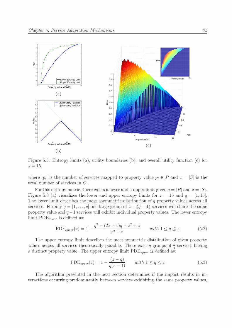
Chapter 5: Service Adaptation Mechanisms 75
0 5 10 150
0.1
0.2
0.3
0.4
0.5
0.6
0.7
0.8
0.9
1
Property values (S=15)
PD
E
Lower Entropy LimitUpper Entropy Limit
(a)
0 5 10 150
0.1
0.2
0.3
0.4
0.5
0.6
0.7
0.8
0.9
1
Property values (S=15)
Util
ity
Lower Utility FunctionUpper Utility Function
(b)
0.2
0.4
0.6
0.8
1
16
11 15
0
0.1
0.2
0.3
0.4
0.5
0.6
0.7
0.8
0.9
1
PDE
Property values
Util
ity
15
PDE
Property values
(c)
Figure 5.3: Entropy limits (a), utility boundaries (b), and overall utility function (c) fors = 15
where |pi| is the number of services mapped to property value pi ∈ P and z = |S| is thetotal number of services in C.
For this entropy metric, there exists a lower and a upper limit given q = |P | and z = |S|.Figure 5.3 (a) visualizes the lower and upper entropy limits for z = 15 and q = [1, 15].The lower limit describes the most asymmetric distribution of q property values across allservices. For any q = [1, . . . , c] one large group of z − (q − 1) services will share the sameproperty value and q−1 services will exhibit individual property values. The lower entropylimit PDElower is defined as:
PDElower(z) = 1−q2 − (2z + 1)q + z2 + z
z2 − zwith 1 ≤ q ≤ z (5.2)
The upper entropy limit describes the most symmetric distribution of given propertyvalues across all services theoretically possible. There exist q groups of z
qservices having
a distinct property value. The upper entropy limit PDEupper is defined as:
PDEupper(z) = 1−(z − q)
q(z − 1)with 1 ≤ q ≤ z (5.3)
The algorithm presented in the next section determines if the impact results in in-teractions occurring predominantly between services exhibiting the same property values,

Chapter 5: Service Adaptation Mechanisms 76
between services of different property values, or between services without any distinct in-teraction bias. First, we need to evaluates a property’s likelihood of having an impact oninteractions.
To this end, we introduce upper and lower entropy utility functions. These utilityfunctions describe the ratio of services that have a choice to communicate either withservices of the same property value or with services exhibiting different property values.Only these services generate interactions that exhibit potential property impact (Bollobas2001,Mcculloh, Lospinoso, and Carley 2007).
The lower entropy utility function utillower corresponds to the lower entropy limit(PDElower). It reflects the fact, that q − 1 services can only communicate with servicesexhibiting a different property value, and thus cannot be included in the impact calcula-tion. Consequently, as individual property values become more common (i.e., entropy value→ 1), the likelihood reaches 0. In contrast, as services increasingly share the same prop-erty value (i.e., entropy value → 0) any interactions across properties must be consideredoutliers and the likelihood similarly decreases towards 0.
utillower(z) = 0.5− | − 0.5−1− q
z − 1| 1 < z, 1 < q ≤ z (5.4)
The upper entropy utility function utilupper corresponds to the upper entropy limit(PDEupper). It peaks where all entities are equally distributed across two property valuesand decreases steadily as the number of distinct property values rise.
utilupper(z) =z − q
2− q∀0 < z, 2 < q ≤ z (5.5)
Figure 5.3 (b) visualizes the lower and upper entropy utility function for z = 15 andq = [1, 15]. We aggregate upper and lower utility functions in the overall utility functionutiltotal defined as follows:
utiltotal(z, pde) =(pde− PDElower)
PDEupper − PDElower∗ utilupper
+(PDEupper − pde)
PDEupper − PDElower∗ utillower (5.6)
where utilupper returns the utility value for the upper entropy limit, and utillower returns theutility value for the lower entropy limit. The total value combines the two utility valuesproportional to the distance of the entropy value and the respective upper and lowerboundaries (PDEupper, PDElower). Figure 5.3 (c) visualizes the overall utility functionwhich provides a likelihood measurement in the interval [0, 1].
5.3 Property Impact Evaluation Algorithm
The PDE model provides the means to identify promising impact factors. In the subse-quent step we need to evaluate whether these candidate properties have indeed an impact

Chapter 5: Service Adaptation Mechanisms 77
on service interactions. We define a positive impact of a property value on a group ofservices when these services tend to communicate with each other (i.e., internal commu-nication), rather than interacting with services exhibiting different property values. Anegative impact implies a tendency towards external communication.
We capture interactions between services applying logging mechanisms. The sum ofall logged service calls create an interaction network. We define this network as a di-rected1 graph G(S,E) consisting of interaction edges E and services S ∈ C deployed inthe ensemble. We denote the set of services exhibiting the same property value a networkcluster.
For the impact evaluation process (Algorithm 4), we select properties with highestutiltotal. For every cluster, the cRatio calculates the ratio of property internal to totalcommunication links. The natural link ratio nRatio of a cluster in an unbiased networkis |cluster| / |S|. To include the characteristics of the underlying interaction network,we create a zero model by distributing all services randomly across clusters of the samesize. Multiple rounds of randomization yield a natural deviation of each cluster ratio fromthe natural ratio. To enable comparison of clusters independent of their natural ratio(nRatio) any deviation from nRatio is mapped to the interval [−1,+1], where a trendP (c)of −1 indicates complete external orientation, and +1 complete internal orientation. Thisorientation is defined as:
trendP (c) =
{
cRatioc−nRatioc
1−nRatiocif cRatioc > nRatioc,
cRatioc−nRatioc
nRatiocif cRatioc ≤ nRatioc
(5.7)
and the impact of cluster c for Property P is defined as:
impP (c) =
{
trendP (c) if |trendP (c)| ∗ utiltotal(P ) > 2 ∗ devc
0 otherwise(5.8)
where utiltotal(P ) is the utility of property P and devc is the zero model deviation for thecluster c. Taking twice devc and reducing further by utiltotal(P ) ensures that also for lowlikelihood values the deviation is sufficiently distinct.
A property p needs not necessarily consist of uniform cluster trends. Internally oriented,externally oriented, and unbiased clusters can coexist. Aggregating all trends proportion-ally to their corresponding cluster size yields the overall property importance factor:
impP =
∑ni=1 |impP (i)| ∗ |clusterP (i)|
|S|(5.9)
We continue to consider only properties with the highest impact impP for furtherinteraction analysis as outlined in the following section.
1The approach also applies to undirected graphs with the following adaptation: cluster internal linksneed to be counted twice.

Chapter 5: Service Adaptation Mechanisms 78
Algorithm 4 Impact Evaluation Algorithm A(G(S,E), P ).
function CalculateImpact(G(S,E), P )Dev ← call AnalyzeZeroModel(P,G)for all Clusters c ∈ P do
nRatio← |c|/|V |cRatio← call CalcLinkRatio(c, G)diff = |nRatio− cRatio|if diff ∗ util(P ) > 2 ∗Dev[c] then
if cRatio > nRatio then /* Trend towards internal communication. */trend = diff/(1− nRatio)
else /* Trend towards external communication. */trend = diff/nRatio ∗ −1
end if
setTrend(c, trend)else
setTrend(c, 0)end if
end for
end function
function AnalyzeZeroModel(p,G)Dev[]← ∅for i = 1 to z do
R← randomizeAcrossPartitions(G, clusterSizes(P ))for all Clusterr ∈ R do
nRatio = |r|/|V |cRatio← call CalcLinkRatio(r, G)diff = |nRatio− cRatio|if cRatio > nRatio then
dev = diff/(1− nRatio)else
dev = diff/nRatioend if
Dev[r]← Dev[r] + devend for
end for
for i = 1 to |C| do
Dev[i]← Dev[i]/zend for
return Dev[]end function
function CalcLinkRatio(c, G)intra = countLinksWithinCluster(c, G)total = countLinksOfCluster(c, G)edgeRatio = intra/totalreturn edgeRatio
end function

Chapter 5: Service Adaptation Mechanisms 79
5.4 Service Ranking Algorithm
The calculation and evaluation of property utility, impact, and impact trend is node in-dependent. When a new service joins the ensemble, the ranking algorithm applies theseglobal metrics to generate a recommendation specific to the newcomer. For the propertieswith highest impact, we select the cluster identified by the newcomer’s properties. Foreach cluster, we derive its interaction affinity towards other clusters. The affinity functionaffinity(G, c1, c2) describes the likelihood of a new request in c1 being forwarded to c2. Thespecial case c1 = c2 covers internal request delegation. The function is defined as:
affinity(G, c1, c2) =|links(c1→ c2)|
|links(c1→ G)|(5.10)
where links(c1 → c2) selects all links starting in cluster c1 and ending in cluster c2,respectively ending anywhere in the network G including c1. In a directed graph, affinityis not reciprocal, thus affinity(G, c1, c2) 6= affinity(G, c2, c1)∀c1 6= c2.
Our ranking algorithm builds on top of any existing selection mechanism that fulfilsfollowing three conditions: (i) returned candidate services are potential communicationpartners, (ii) services are ranked by their domain specific capability, (iii) services map toranking scores that reflect the relative match amongst all selected services. A mere listrepresenting the service’s rank is insufficient. In case of failing these conditions, our rankingalgorithm considers all candidates as equally suitable.
The basic idea is to apply cluster affinity values to update the candidate’s rank. Algo-rithm 5 demonstrates the precise steps. For each candidate and all properties of significantimpact, as identified in the previous section, we select the newcomer’s cluster cnewcomer andthe candidate’s cluster ccandidate. We subsequently retrieve the affinity value of cnewcomertowards ccandidate. Candidates in clusters with low affinity are penalized more than can-didates in clusters of frequent request forwarding. Affinity values do not modify ranks totheir full extend but only proportional to the respective property impact impP (c). Foreach candidate the sum of all weighted affinity values determines the extend to which theranking result is reduced or increased. Finally, the updated candidate list is sorted again.The newcomer service can then select among the top ranked existing services for successfulrequest forwarding.
Recommending services from clusters that have received many requests in previousrounds achieves desirable preferential attachment characteristics. Independent from thenumber of services, the recommendation algorithm ensures its persisting applicability asthe service network grows.
5.4.1 Discussion of Computational Complexity
The computational complexity of our approach depends on following factors: the totalnumber of services S, the number of public properties P and their respective values p ∈ P ,

Chapter 5: Service Adaptation Mechanisms 80
Algorithm 5 Update Ranking Results A(new,R, PP ).
function RankingResultUpdate(new,R, PP )/* Modifies the ranking results based on property importance and affinity */for all ResultEntry r ∈ R do
/* affw collects all effects on candidate rank */affw = 0for all Property P ∈ PP do
cnewcomer ← getCluster(P, new)ccandidate ← getCluster(P, r)affinity = calcAffinity(cnewcomer, ccandidate)affw = affw + affinity ∗ impact(P )
end for
updateRank(r, getRank(r) ∗ affw)end for
sort(R)end function
the number of service interactions E, and the number of graph randomizations z. Table 5.2lists the worst case runtime complexity for the various processing steps.
Step ComplexityService to Property Mapping O(S ∗ P)Entropy Calculation O(P ∗ p)Interaction to Cluster Mapping O(E ∗ P)Cluster Analysis O(P ∗ p2)Zero Model Analysis O(E ∗ P ∗ z)
Table 5.2: Runtime Complexity
From this overview, the Cluster Analysis appears to inhibit scalability the most. How-ever, by restrict analysis to properties with highest entropy value PDE, the maximumvalue of observed property values p will grow slower than the number of total services.
5.5 Evaluation of Service Adaptation
This section demonstrates the effectiveness of our approach based on the motivating sce-nario. This includes a step by step walk-through of metric computation and analysis ofmultiple properties. The second part of this section focuses on simulation of a servicenetwork.

Chapter 5: Service Adaptation Mechanisms 81
Property PDE PDElower PDEupper utiltotalLoc 0.945 0.835 0.957 0.411Org 0.802 0.396 0.808 0.826Cap 0.626 0.275 0.718 0.772
Table 5.3: PDE, limits, and utility values for Location, Organization, and Capabilityproperties.
Property TotalLocation L1 L2 L3 L4 L5 L6 L7 L8 L9Impact 0 0 0 0 -1 0 0 0 0 0.07Organization O1 O2 O3 O4Impact 0 0 -0.95 0 0.20Capability C1 C2 C3Impact -0.86 -1 -0.92 0.92
Table 5.4: Property Impact Evaluation Results
5.5.1 Scenario
We observe a limited number of services in the ensemble network for sake of clarity. Therecommendation process observes three public properties: (i) Location (L1. . . L9), (ii) Or-ganization (O1. . .O4), and (iii) Capability (C1. . . C3). Table 5.5 (upper part) outlines themapping of 14 existing services and one newcomer (S15) to the three properties. This con-figuration yields the property distribution entropy metric (PDE), corresponding entropylimits (PDEupper, PDElower), and respective utility in Table 5.3.
Analyzing the weighted interaction graph in Table 5.5 (lower part), we detect the impactvalues depicted in Table 5.4. For Location and Organization, we derive impact only for L5,respectively O3, in both cases a strong external trend. For Capability, the interaction graphresults in a strong external trend for all three property values (C1, C2, and C3). Hence,for service S15 with properties (L9, O3, C1) and randomly chosen neighboring services(S2, S4, S7, S9, S11, S12, S14), we arrive at the ranking results printed in the rightmostcolumn of Table 5.5.
Service S2 is ranked highest. As property Capability has the strongest impact on theinteraction network, we put most weight on affinity values amongst property values C1,C2, and C3. In our scenario, services of type C1 tend to forward requests to service oftype C2, C2 to C3, and C3 back to C1. The ranking result thus recommends service S15to forward requests primarily to S2 as S2 is the only neighbor of S15 exhibiting propertyC2.

Chapter 5: Service Adaptation Mechanisms 82
Id S1 S2 S3 S4 S5 S6 S7 S8 S9 S10 S11 S12 S13 S14 S15
Loc L1 L2 L1 L2 L3 L4 L5 L6 L7 L8 L9 L4 L8 L9 L9Org O1 O2 O3 O4 O1 O2 O3 O4 O1 O2 O3 O4 O1 O2 O3Cap C1 C2 C3 C1 C2 C3 C1 C2 C3 C3 C3 C3 C3 C3 C1
S1 S2 S3 S4 S5 S6 S7 S8 S9 S10 S11 S12 S13 S14 Rank
S1 0 0 0 0 35 0 0 0 0 0 0 0 0 0 -S2 0 0 0 0 0 0 0 0 0 0 0 0 0 43 91.50S3 33 0 0 6 0 0 0 0 0 0 0 1 0 0 -S4 0 33 0 0 0 0 0 5 0 0 0 0 0 0 17.77S5 0 0 0 0 0 0 0 0 0 26 0 0 8 0 -S6 2 0 0 0 0 0 27 0 0 0 2 0 0 0 -S7 0 0 0 3 16 1 0 0 1 3 0 0 0 0 3.05S8 0 0 0 0 0 0 0 0 0 31 1 0 0 0 -S9 3 0 0 0 0 0 29 0 0 0 0 0 0 0 15.37S10 0 3 0 28 0 0 0 0 0 0 2 1 2 0 -S11 0 0 1 32 2 0 0 0 0 0 0 1 0 0 4.95S12 0 0 0 37 0 0 0 0 0 0 0 0 0 0 13.74S13 47 0 0 0 0 0 0 0 0 0 0 0 0 0 -S14 0 0 1 29 2 0 0 0 0 2 0 1 0 0 5.57
Table 5.5: Service network: weighted directed graph including ranking results for S15.
5.5.2 Simulation Setup
Simulation-based evaluation allows for analyzing our recommendation algorithm underchanging conditions with respect to property count, property impact, service network size,and impact fluctuations. We focus only on the behavioral characteristics of our algorithmand do not consider the costs of network monitoring. Chen et al. (Chen, Bindel, Song, andKatz 2007) follow an algebra-based approach to efficient network monitoring.
The simulation environment consists of |S| = n services. Each service exhibits |P| =m property values, corresponding to m distinct properties. Services have the capabilityto forward a received request to another service from their service neighborhood h orreject it. For each property, an acceptance matrix M simulates the impact of currentrequirements on the service interaction structure. The matrix provides the likelihood ofany service with property value pi to accept a request from a service with property valuepj. As the simulation progresses, we adapt the importance weight of the various propertymatrixes to reproduce the dynamic requirement changes. Table 5.6 provides a snapshot ofan acceptance matrix for property Organization comprising four property values. In thisexample, request forwarding occurs in a circle.
In each simulation round, services receive r randomly assigned requests. Each servicethen selects a member from its neighborhood to forward the request to. The receivingservice then chooses to accept or deny the request. In the former case, the request isconsidered successfully completed. In the latter case, the sending service receives 1 penaltypoint and has to find another service to forward the request to.

Chapter 5: Service Adaptation Mechanisms 83
from/to O1 O2 O3 O4O1 0 1 0 0O2 0 0 1 0O3 0 0 0 1O4 1 0 0 0
Table 5.6: Example acceptance matrixM for four organization property values O1 . . .O4exhibiting maximal constraints.
Although services apply the acceptance matrix for incoming requests, they do not uti-lize this information for outgoing requests. Instead, they engage the proposed rankingalgorithm. The algorithm then applies the analyzed public properties and service inter-actions as described in the previous sections. To eliminate any effects of domain specificranking, the simulation assumes all services are equally able to process a request. Wecalculate the benefit of our recommendation algorithm by comparing the penalty a new-comer service receives when contacting neighbors by trial-and-error and when contactingthe recommended neighbors.
In all experiment iterations, we assign random requests to services each round to sim-ulate service load fluctuations. To keep the overall network load constant, however, theaverage number of assigned requests per service is fixed at r = 20.
5.5.3 Measuring Scalability
First, we demonstrate the scalability of our approach. We increase the number of services(n), service neighborhood (h), and property values (pm). In each round, we measure foreach newly added service the penalty received in the process of successfully forwarding asingle request to a random neighbor, respectively a recommended neighbor.
The initial service network consists of n = 50 services, each having h = 24 randomneighbors. Four properties (P1 . . . P4) exhibiting |p| = 7, 5, 4, and 4 values respectivelyexert impact via their acceptance matrixes. As we add a new service, we connect itwith random 20 + log(n)2 existing services. Additionally, we link random log(n) existingservices with the newcomer. For the four properties (P1 . . . P4), the simulation introducesnew property values at a growth rate of log(n).
Figure 5.4 prints the average benefit for every 50 consecutive benefit measurements overmultiple experiment runs. On average, the recommendation-based approach outperformsthe trial-and-error approach across scales. At the end of the scalability experiment, thefinal service network comprises 10050 services, each linked to 105 neighbors on average.Each of the four properties exhibit nine more values, bringing the number of choices to|p| = 16, 15, 14, and 13 respectively. The recommendation algorithm yields similar goodresults for this configuration as for the initial service network.

Chapter 5: Service Adaptation Mechanisms 84
0 1000 2000 3000 4000 5000 6000 7000 8000 9000 10000
1.4
1.6
1.8
2
2.2
2.4
2.6
Service Count
Ben
efit
of R
ecom
men
datio
n ov
er T
rial−
and−
Err
or S
elec
tion
Avg Benefit of 50 Measurements linear fit
Figure 5.4: Average benefit for service recommendation compared to trial-and-error selec-tion. Numbers display aggregation of 50 new services within a service network growingfrom 50 to 10050 services.
5.5.4 Measuring Adaptiveness
We have shown scalability for fixed impact of the four properties (P1 . . . P4). Here, wedemonstrate the adaptability of our approach. Along these lines, we dynamically changethe impact weights of the respective acceptance matrixes (M1 . . .M4) every 10 roundswhile measuring the quality of the recommendation result every round. The number ofservices n = 50, their neighborhood size h = 24, and the property values (pm) remain con-stant. As we keep the number of services fixed, we select in each round a random existingservice to measure the penalties for recommended and trial-and-error neighbor selection.
We analyze 30 experiment iterations, each comprising 100 impact changes. Figure 5.5prints the benefit (and standard deviation) received for applying recommended selectionfor each of the 10 rounds after the property impact change. We observe lower—but stillpositive—benefit measurements for the first two rounds after a change. As the algorithmself-adjusts, average benefit increases to 2.
5.5.5 Measuring Constraint Impact
The realizable benefit heavily depends on the constraints on the service network. When lackof constraints result in high acceptance rates, any random neighbor will most likely be asuitable selection. The ranking algorithm will provide considerable benefit once constraintsemerge and begin to increasingly restrict service interactions.

Chapter 5: Service Adaptation Mechanisms 85
In the third experiment, we start with four properties (each having 10 property values)allowing interactions between any clusters (i.e., the corresponding acceptance matrixes arefilled with 1s). Every 10 rounds, we randomly select one particular property and increasethe constraints. As we continue to replace random 1s with 0s in the acceptance matrix, thetrial-and-error approach yields increasing penalties. We continue increasing the constraintsuntil every acceptance matrix M contains a single 1 on each row (e.g., Table 5.6). Thus,for every property P , a service of any particular property value px ∈ P only acceptsrequests from services exhibiting a single other property value py ∈ P (including x = y).Throughout the experiment, property impact and service count remain fixed.
Figure 5.6 presents the average penalty difference over 10 iterations of n = 50 serviceshaving on average h = 24 neighbors. Benefits start rising around round 1750. Around3800, this growth levels off as the constraints can no longer be intensified.
0 1 2 3 4 5 6 7 8 9 10 110
0.5
1
1.5
2
2.5
3
Rounds after Constraints Update
Ben
efit
of R
ecom
men
ded
over
Tria
l−an
d−E
rror
Sel
ectio
n
Avg Benefit +/− Standarddeviation
Figure 5.5: Average benefit for each roundfollowing a property impact change.
0 500 1000 1500 2000 2500 3000 3500 4000−0.5
0
0.5
1
1.5
2
2.5
3
3.5
4
4.5
5
Constraint Increase
Ben
efit
of R
ecom
men
ded
over
Tria
l−an
d−E
rror
Sel
ectio
n
Avg Benefit of 50 Measurements 5th degree best fit
Figure 5.6: Average benefit for service rec-ommendation compared to trial-and-error ap-proach for increasing constraints. Numbersdisplay aggregated benefit of 50 consecutivemeasurements.
5.5.6 Experiment Discussion
The simulation reflects the key challenges outlined in the introduction to reproduce theconstraints found in real world service networks. First, services provide only public in-formation on their various static properties. Second, the decision process for selecting asuitable receiving service relies purely on dynamic information. Third, services accept in-coming requests based only on internal, non-observable information (i.e., defined by the

Chapter 5: Service Adaptation Mechanisms 86
acceptance matrix). Finally, no service obtains a complete view on service interactions.
Despite these challenges, our model and algorithms perform significantly better thantrial-and-error service selection. When comparing average, absolute penalty measurements(Figure 5.7), the ranking algorithm results in 2.5 times lower penalties during the scalabilityexperiment, and 2.7 times lower penalties during the adaptivity experiment, respectively.The third experiment displays 2.1 times lower penalties averaged over the final 1500 rounds.For both scalability and adaptivity experiments, our algorithm requires on average slightlymore than a single forwarding retry (i.e., one rejected request). The trial-and-error ap-proach, in contrast, results in approximately three retries. The constraint measurementdisplays higher failure rates. Our recommendation algorithm requires less than 2.5 retries,while trial-and-error selection causes 5 rejections.
At this stage, we cannot predict the algorithm’s performance in real world implemen-tations. However, our simulations yield very promising results and demonstrate bothscalability and adaptiveness of our approach.
4
5
6
7
8
�� ���� � �0
1
2
3
4
Scal.
Trial
Scal.
Rec.
Adapt.
Trial
Adapt.
Rec.
Constr.
Trial
Constr.
Rec.
� ����
Figure 5.7: Average penalty measurements and ± standard deviation for scalability, adap-tivity, and constraints experiments; comparing recommended versus trial-and-error selec-tion.

Chapter 6
Service Infrastructure Adaptation
Techniques
Infrastructure Adaptation Techniques target adaptation at the level of a complete en-semble. Individual services apply context to adapt within the scope of their immediateensemble neighborhood. Services, however, cannot monitor the whole environment. Theyremain unaware whether their functionality and corresponding adaptive behavior is stillappropriate, or whether another service is better suited. Consequently, we propose separa-tion of concerns for adaptation techniques. Services focus on self-adjustment as required bytheir configuration and purpose. The infrastructure assumes responsibility for monitoringrequirement fulfillment and selection of system-wide ensemble adaptation actions. In thischapter, we introduce:
Adaptation Process introducing our infrastructure adaptation methodology based onthe MAPE-K cycle of autonomic computing.
Capability Model describing service metadata including configuration aspects.
Requirements Rules observe ensemble metrics and create appropriate capability con-straints. These constraints are matched against currently deployed services to identifyservice capability mismatches.
Requirements Clustering groups a set of requirements when service utility values indi-cate that a composition of multiple services provides better requirements satisfactionthan a single service.
Simulated Annealing-based Composition achieves an optimal trade-off between min-imal aggregation costs and maximal requirements fulfillment.
87

Chapter 6: Service Infrastructure Adaptation Techniques 88
6.1 Infrastructure Adaptation Approach
The infrastructure adaptation process (Figure 6.1) closely resembles the autonomic MAPE-K cycle comprising monitoring, analysis, planning, and execution phases. Specifically,we monitor service capability and ensemble events. Ensemble requirements tracking de-tects if these events trigger execution of the current set of requirement rules. Subsequentcapability-requirement mismatch evaluation determines the need for infrastructure adap-tation. Service utility calculation matches the set of available services against the set ofunsatisfied requirements. This process step considers not only single services. We alsoapply clustering to detect service aggregation of higher overall utility. A tradeoff betweenbest matching services, respectively aggregations, and deployment costs provides a rankedset of alterative adaptation configurations. Ultimately, management selects and executesone of the available choices. We outline only the very fundamental adaptation steps inFigure 6.1. The flow chart 6.2 in Section 6.2 contains additional information on involvedcomponents and branching conditions. The adaptation process relies upon five buildingblocks:
Ensemble Context events provide continuous information to update the ensemble con-text. Ensemble metrics provide various aggregated views of the overall ensemble.The ensemble context models have been discussed in Chapter 2.1.
Service Capabilities are metadata for effective service selection. Details include serviceclassification, usage constraints, and configuration alternatives.
Ensemble Requirements describe necessary and desirable service capabilities for agiven ensemble context.
Capability Matching evaluates currently deployed services against requirements for theunderlying context. Capability mismatches trigger the adaptation process to findbetter suited services, respectively service aggregations.
Service Composition Recommendation trades off services best fulfilling required ca-pabilities and costs for deployment, respectively aggregation. Previous service invo-cations and service aggregations determine suitable service candidates.
In the following section, we discuss the overall adaptation process in detail beforeproviding a comprehensive description of these major building blocks.
6.2 Adaptation Process
This section outline role and place of the core building parts in the adaptation process.In this chapter’s introduction, Figure 6.1 presented the general approach, here we go intomore detail and discuss the process visualized in Figure 6.2. Chapter 7 provides additionalimplementation specific details.
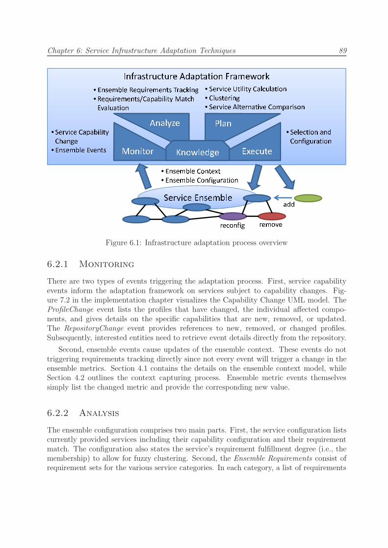
Chapter 6: Service Infrastructure Adaptation Techniques 89������������� ������ �� ����������� ��� ���������� �����������
��� � ������•� !"#$ %&'&(#)#*+%,&-. • /-0 1() /" -*0 •� ) $*#2- &-3%2-4#.5!&*#2-
• /-0 1() 6 75#! 1 -*0 8!&$9#-.• 6 75#! 1 -*0:%&'&(#)#*+ ;&*$,/"&)5&*#2- • � !"#$ <*#)#*+ %&)$5)&*#2-
• %)50* !#-.• � !"#$ =)* !-&*#" %21'&!#02-
• /-0 1() %2-* >*• /-0 1() %2-4#.5!&*#2- 33&33! $2-4#. ! 12"
Figure 6.1: Infrastructure adaptation process overview
6.2.1 Monitoring
There are two types of events triggering the adaptation process. First, service capabilityevents inform the adaptation framework on services subject to capability changes. Fig-ure 7.2 in the implementation chapter visualizes the Capability Change UML model. TheProfileChange event lists the profiles that have changed, the individual affected compo-nents, and gives details on the specific capabilities that are new, removed, or updated.The RepositoryChange event provides references to new, removed, or changed profiles.Subsequently, interested entities need to retrieve event details directly from the repository.
Second, ensemble events cause updates of the ensemble context. These events do nottriggering requirements tracking directly since not every event will trigger a change in theensemble metrics. Section 4.1 contains the details on the ensemble context model, whileSection 4.2 outlines the context capturing process. Ensemble metric events themselvessimply list the changed metric and provide the corresponding new value.
6.2.2 Analysis
The ensemble configuration comprises two main parts. First, the service configuration listscurrently provided services including their capability configuration and their requirementmatch. The configuration also states the service’s requirement fulfillment degree (i.e., themembership) to allow for fuzzy clustering. Second, the Ensemble Requirements consist ofrequirement sets for the various service categories. In each category, a list of requirements

Chapter 6: Service Infrastructure Adaptation Techniques 90
Ensemble Metric
Update
Candidate
Comparison
Matching
Aggregations
Aggregation
Costs
(Distance
Graph)
Set of ranked
Service alternatives
Selection and
Reconfiguration
Configuration
UpdateRequirements
Clustering+
Aggregation
Ensemble
Event
Service
Capability
Change
Ensemble Context
Ensemble
Requirements
Tracking
Capability Update
Ensemble Service
Configuration
Ensemble Context
Manager
Config
affected?
Yes
Requirements/
Capability Match
Evaluation
Mismatch >
threshold?
No
DONE
Yes
Service Utility
Calculation for
unfullfilled
Requirements
Cluster
requirements?
Yes No
Requirements Update
Monitoring
Analysis
Planning
Management
Figure 6.2: Infrastructure adaptation process flow

Chapter 6: Service Infrastructure Adaptation Techniques 91
identify capabilities and properties along with the parameters for the selected utility func-tion. Figure 7.9 in the implementation chapter visualizes the ensemble configuration UMLclass diagram.
Ensemble requirements tracking identifies those ensemble configurations that are af-fected by service capability events and ensemble metric events. In the latter case, we merelycheck if the changed ensemble metrics are decisive in any requirement (e.g., a thresholdhas now been crossed). If so, we updates the requirements in the ensemble configurationand proceed with matching of requirements to capabilities.
For capability changes, requirement tracking analyzes which ensemble configurationincludes the respective service. It subsequently determines if the current set of requirementsincludes the changed properties or capabilities.
Optionally, we check ensemble configurations for services that provide the same capa-bility, but have remained unchanged. We potentially replace the currently used servicewith the changed service when the service exchange promises to yield better requirementfulfillment.
In the next step, we rematch requirements and capabilities. In the case of changedservice capabilities, we compare existing requirements against updated capabilities. Inthe case of changed ensemble metrics, we compare updated requirements against existingservice capabilities.
We summarize across all mismatch values to evaluate if alterations in the set of providedservices is justified. We trigger the components in the planning phase, when the mismatchexceeds a given (domain specific) threshold. From the complete set of requirements, wepass only those requirements to the next stage that are poorly fulfilled.
6.2.3 Planning
Planning is concerned with identifying the best available services for a given set of require-ments. To this end, service utility calculation analyzes each service this is fulfilling at leastone requirement. Each service receives a utility score for each requirement.
For multiple requirements, the threshold model subsequently decides whether to in-voke the clustering process. Clustering assigns each constraint to a cluster with varyingfuzzyness. Services are then ranked for each cluster. Simulated Annealing determines anear-optimal aggregation taking into consideration aggregation costs. We focus purely onservice interaction distance as aggregation costs in the scope of this thesis. Ultimately, weobtain multiple aggregation candidates.
In case of skipping clustering, we continue directly to ranking the services according totheir utility score. We recommend only those services (respectively service aggregations)that provide a better requirement-capability match than the currently configured service(s).When no service provides high enough utility, no service is recommended.
Chapter 6: Service Infrastructure Adaptation Techniques 92
6.2.4 Management
The final procedure of selecting and configuring the recommended services remains outsidethe scope of this thesis. Potential approaches include automatic configuration such as thethe selection algorithm (Alg. 5) in Section 5.4.
6.3 Service Capabilities
Service capabilities describe behavior properties which cannot be directly derived fromthe service’s WSDL document. Example properties include limitations on simultaneousservice use, supported resource access strategies, or reconfigurability. Capabilities usuallychange when a service undergoes major modification. Adding a new operation or extendingservice back-end resources provides new or better functionality. Services might also chooseto reduce capabilities to remain available in spite of high load. This graceful degradingallows service clients to trade-off limited functionality and the cost of finding and invokingan alternative fully functional service. In any case, service capabilities explicitly excludehighly volatile information such as QoS parameters.
The service capability meta model shares some similarities with the Composite Capa-bility/Preference Profiles (CC/PP) specification. The original purpose of CC/PP foreseesclients to transmit their capabilities in order to allow service providers to adapt deliv-ered content accordingly. In contrast, our approach envisions services to describe theircapabilities to enable service clients to select the most suitable service.
The service capability model borrows the concepts of component and property but goesbeyond describing simple service characteristics. Selectable capabilities and supportedcapability compositions are the main distinct differences to the CC/PP model. Theseproperties are key to reconfiguration and adaptation. The capability meta model comprisesthe following elements:
Profile contains all capabilities of a single service. The WSDLlocation identifies the cor-responding service instance. The ServiceCategory and CategoryFit describe how wella service fits into a given ActionCategory or any additional domain-specific category.A profile consists of one or more Components.
Component describes a certain function or non-functional aspect of a service. A notifi-cation service, for example, will distinguish amongst publication related capabilitiesand subscription related capabilities. The same mechanism separates operationalcomponents from management components. Each component identifies the set ofWSDL operations for which the capabilities apply. Especially general purpose opera-tions will appear in multiple components. A component specifies regular capabilities,selectable capabilities, and supported configurations on the selectable capabilities.

Chapter 6: Service Infrastructure Adaptation Techniques 93
Capability comprises properties and optionally sub capabilities. Properties state theactual capability details while sub capabilities enable further structuring. Each ca-pability exhibits a fitness factor. This factor states how well the service supportsthe particular capability. It ranks the service’s behavior in the overall list of servicesexhibiting this capability. Any restrictions in applicability result in a lower fitnessvalue. This mechanism enables fine-grained service matching and replaceability. Tothis end, services describe capabilities outside their core competency. They provideexisting operations and components for a different purpose. Although they will notyield high fitness values, they become substitutes when specialized services are notavailable. For example, communication services can serve as coordination services tosome extent for a limited time.
Property identifies and provides details such as maximum number of requests per minute.The meta model defines five simple properties for integer, decimal, boolean, times-tamp, and string values. FileSize is an example complex property comprising sizeunit (e.g., kB, mB) and size value.
SelectableCapability describes capabilities that need selection and (optionally) config-uration before they become available to the client. The list of alternative capabilitiesconsists of regular capabilities or again selectable capabilities. For each choice, theSelectable Capability defines whether a selection is required and if there is a capabilityselected by default.
Combination originates in the WS-Policy specification to model valid compositions ofpolicies. Here, a Combination defines valid combinations of selectable capabilities.Note, the SelectableCapability element only defines the set of available choices. Se-lection identifies a SelectableCapability (i.e., representing a set of capabilities) or asingle Capability. All contains a set of SelectableCapabilities, expressing any possiblecapability combination. OneOf contains an exhaustive list of possible Combinations.If no other restrictions are specified, NoneOf implies that all combinations are validexcept for the listed ones.
Transition describes valid reconfiguration paths. Specifically, a transition contains a min-imum of one start configuration (i.e., Combination) and a minimum of one reachableend configuration. A set of positive transitions explicitly lists allowed reconfigura-tions. Negative transitions implicate all transitions are valid, except the listed ones.
6.4 Ensemble Requirements
Ensemble requirements depend on the current ensemble state and define a desirable ensem-ble configuration. To this end, we apply event-driven rules. A requirement rule describesmetric conditions and subsequent constraints applied to a particular capability. Changes

Chapter 6: Service Infrastructure Adaptation Techniques 94
tProfileWSDLlocation : anyURI«attribute» ProfileId : anyURI
tComponentWSDLoperationScope : anyURI [0..*]«attribute» ComponentId : anyURI
Component0..*
«choice»
tServiceCategoryActionCategory : tActionCategoryAnyCategory : anyURI«attribute» CategoryFit : t0to1
ServiceCategory1..*
tCapabilityCapabilityId : anyURI«attribute» FitnessLevel : t0to1
Capability0..*
tSelectableCapability«attribute» RequiredSelection : boolean«attribute» DefaultSelection : anyURI [0..1]
SelectableCapability0..*
tCombination
SupportedConfigurations0..1
tTransition«attribute» isPositive : boolean
SupportedTransitions0..*
SubCapability0..*
tProperty«attribute» PropertyId : anyURI
Property0..*
tDefaultProperty pResourceSizevalue : intunit : tUnit
Alternative1..*
«group, choice»
_Choice1Selection : anyURI
_choice10..*
StartCombination1..*
EndCombination1..*
«choice»
tSimplePropertyintValue : int [1..*]boolValue : boolean [1..*]decValue : decimal [1..*]timestampValue : dateTime [1..*]strValue : string [1..*]
value1..1
All1..1
OneOf1..1
NoneOf1..1
Figure 6.3: Capability meta model UML class diagram
in ensemble metrics fire corresponding rules which then define optimum service capabil-ities (i.e., constraints). In the proceeding sections, we then compare deployed serviceswith calculated constraints and compose the best reconfiguration plan given the availablecapabilities.
When designing rules, we have to consider a number of challenges. First, differentensembles will exhibit different metrics. Thus, rules cannot rely on having all metricsavailable. Second, ensembles have various goals which reflect in customized additionalrules and removal of nonessential rules. Rules must not rely on other rules being activeor available. Given the complexity and heterogeneity of requirements, tight coupling ofrules is not an option. Third, we need to provide the most fitting services regardless ofthe requirement fulfillment level available services exhibit. When services lack the requiredoptimum capabilities, we need to find services that support the next highest requirements.Consequently, rules need to enable smooth degradation of provided capabilities.
To this end, we design loosely coupled, weighted rules. Rules depend only on metrics,

Chapter 6: Service Infrastructure Adaptation Techniques 95
they do not reference any other rule. Fine-grained rules do not override coarse-grainedrules. Instead, they generate constraints of higher importance (i.e., constraints exhibitinga higher weight). When two requirements (not necessarily from the same rule) constrainthe same capability, the more important one takes precedence. This mechanism is vitalto smooth degrading. When most significant constraint cannot be satisfied, the next mostimportant constraint becomes active. We mitigate any implicit dependency on the firingof other rules by introducing default constraints. The default constraints describe basiccapabilities necessary for the service ensemble when no other rule generates more specificconstraints on the particular capabilities.
A requirement rule specifies following elements:
Rule Identifier enables requirement tracing. All constraints generated by the same rulecarry the same rule identifier.
Metric Conditions trigger the generation of constraints. Rules can aggregate any num-ber of metrics, but must refrain from applying results generated by other rules.
Capability Identifier determines the capability.
Property Identifier determines the property within the capability.
Utility Function Type defines whether the utility function compares linear properties,overlap of selectable capabilities, or extent of selectable capabilities.
Utility Function Identifier defines the candidate comparison function. Besides the lin-ear utility functions introduced in Section 4.3, we provide set comparison functions(see list below).
Utility Function Parameters for linear functions, the parameters provide the limits.For set functions, the parameters list the required capability elements.
Weight describes the importance of constraints. More specific constraints yield higherweights than general constraints. Constraints with weights equal to zero are ignored.We rate default constraints at 0.1 and specialized constraints between 0.5 and 1.
Service Category identifies the type of service the constraint applies to.
We provide the following set of utility functions:
ExistsUtility checks for the availability of a required capability, or non-existance of anundesired capability.
ChoiceUtilityHigh considers all services exhibiting the set of selectable capabilities, andincreases the score by additional selectable choices. Thus, services with high config-urability yield better scores than services providing the basic, required set.

Chapter 6: Service Infrastructure Adaptation Techniques 96
C4 w=0.1, cap=3
C8 w=0.1, cap=4
C1 w=0.1, cap=1
Metric 3
Metric 2
Metric 1
Rule 1
C2 w=0.5, cap=2
C3 w=1.0, cap=3
C5 w=0.5, cap=4
Rule 2
Rule 3
Rule 4 C7 w=0.5, cap=1
C6 w=1.0, cap=4
C9 w=0.1, cap=5
C8 w=0.1, cap=4
C4 w=0.1, cap=3
Metric 4
Metric 5
C1 w=0.1, cap=1
C2 w=0.5, cap=2
C3 w=1.0, cap=3
C5 w=0.5, cap=4
C7 w=0.5, cap=1
C6 w=1.0, cap=4
C9 w=0.1, cap=5
Figure 6.4: Metrics triggering rules which in turn generate constraints on capabilities (cap)with weight w.
ChoiceUtilityLow is the inverse of ChoiceUtilityHigh. Services that offer the requiredset of capabilities and nothing else yield better utility.
SelectionUtilityOne selects any service that exhibits one of the given capabilities.Matching more than one capability does not increase the rank.
SelectionUtilitySome extends SelectionUtilityOne. A higher overlap of given constraintcapability and provided service capabilities results in higher utility values.
SelectionUtilityAll requires all constraint capabilities to match the provided capabili-ties. ChoiceUtilityHigh and ChoiceUtilityLow extend this function.
Consider following example rule—written in DROOLS (for more technical details seeChapter 7). When the Ensemble Location Entropy value exceeds 0, the rule in Listing 6.1generates a resource storage constraint. The constraint specifies that a service with resourcestorage capability needs to support at least one folder for each location in the ensemble anddefines any service providing more than ten times the required amount as equally suitable.Finally, the rule stores the constraint for the particular ensemble and service category.
We aggregated constraints on identical capabilities and then sort constraints in descend-ing order of weight. Figure 6.4 visualizes the relations between metrics, rules, constraints,and constraint aggregation.

Chapter 6: Service Infrastructure Adaptation Techniques 97
1 rule " ELE_above_Threshold"
2 dialect "java"
3 when
4 metrics : Metrics (metrics .ele > 0)
5 then
6 TSimpleDecimalConstraint r = RequirementsFactory.getConstraint(
7 "ELE_abovethreshold_check -basic ",
8 URIs.CAP_ResStorage ,
9 URIs. PROP_MaxFoldersPerAccount_ResStorage ,
10 ValueUtilitySoftLowerStableLimitedOver .UTILITY_TYPE ,
11 ValueUtilitySoftLowerStableLimitedOver .class.getSimpleName()
12 new double []{ metrics .getLocationMetric (). getClusters (),
13 metrics .getLocationMetric (). getClusters ()*10 ,
14 Double . MAX_VALUE },
15 0.5d
16 );
17 rcc .addRequirement( metrics .getEnsembleURI(),
18 TActionCategory.EXECUTION , r);
19 end
Listing 6.1: Example DROOLS requirement rule generating a resource storage constraintwhen the Ensemble Location Entropy (ELE) exceeds 0.
6.5 Capability Matching
6.5.1 Requirements Filtering
Loose coupling of requirements rules renders the rule engine unaware of multiple require-ments constraining the same capability. Matching capabilities requires, therefore, priorfiltering of multiple—potentially conflicting—constraints on the same capability.
The Gracefully Degrading Matching Algorithm 6 determines which constraint comesinto operation. For sake of simplicity, suppose that each service profile consists of a singlecomponent. Further, let us define the set of candidate components s ∈ S that we collectfrom all available service profiles for a particular service category. We capture the con-straints aggregated for identical capabilities in RL = {R1 . . . Rn} such that all constraintsc ∈ Ri concern capability i. Each constraint c provides the details as outlined in theprevious section.
We evaluate requirements in descending order of weight within each requirement listR. If no capability fulfills the top requirement in R, we remove that requirement andevaluates the next highest. Once we have identified a requirement that can be fulfilledby at least one service, we drop all other less important constraints (i.e., those with lowerweight) on the same capability. Ultimately, each requirement list R ∈ RL contains only asingle requirement for each capability. The set of top requirements in RL become the setof constraints in the subsequent requirements cluster analysis.

Chapter 6: Service Infrastructure Adaptation Techniques 98
Algorithm 6 Gracefully Degrading Matching Algorithm GDM(C,RL).
function MatchCandidates(C,RL)/* Match candidate components against capability constraints. */for all RninRL do
sortDescending(Rn)end for
sortDecending(RL)/* Lists of constraint and constraints within these lists are sorted descending. */for all Rn ∈ RL do
for all c ∈ Rn do
maxUtiln ← 0/* Collect all utility values in the utility matrix U */U ← ∅for all s ∈ S do
/* Calculate for each component the utility function as specified in theconstraint. */
utils = calcUtil(c, s)U ← utilsif utils > maxUtiln then
(maxUtiln ← utils)end if
end for
if maxUtiln ≤ 0 then
/* No component s could satisfy the constraint c. */removeFromList(Rn, c)
else
/* At least one component s could satisfy the constraint c, thus neglectlower weighted constraints on the same capability.*/
clearList(Rn)addToList(Rn, c)rankCandidates(U , SC)
end if
end for
end for
/* RL contains now only one constraint element in each list. */return RL
end function

Chapter 6: Service Infrastructure Adaptation Techniques 99
Symbol Meaningci ∈ C constraint i belonging to set of constraints C.n number of constraints n = |C|.sj ∈ S service j belonging to set of services S.m number of services m = |S|.uij ∈ U service capability utility value for constraint i and service j.rj ∈ R normalized preliminary rank rj for service sj with
∑
j rj = 1.
fi ∈ F normalized constraint fulfillment degree fi for constraint ci with∑
i fi = 1.wi ∈ W normalized constraint weight wi for constraint ci with
∑
iwi = 1.τi ∈ T normalized importance factor, aggregating fi and wi with
∑
i τi = 1.H(s) Service utility entropy calculated on utility values for service s across all
n constraints.H(c) Constraint utility entropy calculated on utility values for constraint c
across all m services.ts, tc Thresholds for H(s) and H(c).δs, αs, δc, αc Configuration parameters for the threshold model calculating ts and tc.
Table 6.1: Symbols applied in requirements clustering.
6.5.2 Requirements Cluster Analysis
When we rank all services from a particular category, we implicitly assume they are ableto fulfill all top-weighted constraints. However, the more specialized the constraints be-come, the less likely a single service exhibits all required capabilities to sufficient degree.Two or more services often compensate for their individual shortcomings. We extend theservice matching and ranking approach to provide the optimum set of services matchingthe required constraints.
Consider following simple scenario comprising six constraints c1 . . . c6 compared to thecapabilities of five services s1 . . . s5. Table 6.2 displays utility results for matching of eachconstraint and capability. In the extreme Case 1 services s1 to s3 each match two constraintscompletely (x = 100) and fail to match the remaining constraints (x = 0). Services s4 ands5 exhibit mediocre, respectively bad matching results across all constraints. In Case 2,all services match the constraints to some extent. Ranking the complete set of serviceswill not yield practical results in Case 1. Splitting the services into multiple groups, andranking them separately, will provide more useful service recommendations.
The following process discovers whether services belong to different categories, andif so, defines service membership in these categories. In short, we introduce the serviceutility entropy and constraint utility entropy to detect potential existence of clusters. Sub-sequently we cluster related constraints and execute rankings for each cluster separately.Ultimately, we recommend the top service(s) from each cluster.
The service utility entropy applies Shannon’s entropy definition (Shannon 1948) on the

Chapter 6: Service Infrastructure Adaptation Techniques 100
S1 S2 S3 S4 S5 fc S1 S2 S3 S4 S5 fc
1 2
C1 100 0 0 40 10 0.156 100 80 70 20 50 0.191C2 100 0 0 60 10 0.177 80 20 80 30 50 0.155C3 0 100 0 40 10 0.156 30 100 0 50 45 0.134C4 0 100 0 60 10 0.177 80 20 30 50 45 0.134C5 0 0 100 40 10 0.156 70 100 80 20 80 0.208C6 0 0 100 60 10 0.177 80 20 50 70 80 0.179rs 0.208 0.208 0.208 0.313 0.063 0.262 0.202 0.185 0.143 0.208
3 4
C1 80 80 90 5 10 0.342 80 10 30 0 10 0.168C2 90 80 90 0 10 0.348 90 10 30 0 10 0.181C3 30 20 30 0 10 0.116 30 80 10 0 10 0.168C4 25 25 30 0 10 0.116 25 80 0 0 10 0.148C5 5 10 0 0 10 0.032 5 20 90 0 10 0.161C6 5 10 10 0 10 0.045 5 25 90 5 10 0.174rs 0.303 0.290 0.323 0.007 0.077 0.303 0.290 0.323 0.007 0.077
Table 6.2: Constraint ci to service sj capability match (Utility matrix U) including un-weighted, preliminary service rank r and constraint fulfillment degree fc. In all four cases,constraints are equally important (wi = 1/6 ∀ i = 1→ 6).
results of the basic matching process. The service utility entropy H(s) is defined as:
H(s) = −n∑
i=1
u(s)i∑
u(s)∗ log(
u(s)i∑
u(s)) (6.1)
where u(s)i is the function for deriving the utility of service s for constraint i. Table 6.3 liststhe service rank entropy for our scenario. Maximum entropy for n constraints is log(n).
We introduce a threshold value t to decide when to engage in cluster analysis. Weassume existence of two or more clusters if the arithmetic mean of all service utility entropyvalues drops below ts, with 0 ≤ ts ≤ log(n). Lower values of ts require more distinctservices. Extreme cases include ts = 0, where services need to match exactly one constraintand none else, and ts = log(n) where services exhibiting only minor differences in theirutility values are considered belonging to different categories.
The entropy average is a necessary but not a sufficient measurement to determinethe presence of different categories. The metric highlights merely unequal distribution ofconstraint satisfaction. It cannot distinguish in-between services matching the same ordifferent conditions. Case 3 and Case 4 in Table 6.2, for example, yield the same serviceentropy value for the same service.
We approach this shortcoming by calculating the constraint utility entropy H(c). Thedefinition of H(c) is the same as for H(s) but calculating across constraints instead ofservices. Constraint utility entropy values will be high when services exhibit high overlap

Chapter 6: Service Infrastructure Adaptation Techniques 101
H(s) s1 s2 s3 s4 s5
Case 1 0.693 0.693 0.693 1.792 1.748Case 2 1.742 1.560 1.555 1.687 1.758Case 3 1.399 1.471 1.373 0 1.792Case 4 1.399 1.471 1.373 0 1.792
H(c) s1 s2 s3 s4 s5 s6
Case 1 0.803 0.846 0.803 0.846 0.803 0.846Case 2 1.506 1.489 1.285 1.508 1.518 1.524Case 3 1.289 1.215 1.311 1.322 1.055 1.352Case 4 1.032 0.991 1.032 0.797 0.861 1.020
Table 6.3: Service utility entropy H(s), (maxH(s) = 1.792) and constraint utility entropyH(c), (maxH(c) = 1.609) for unbiased utility values U .
of matching constraints (see Table 6.3 Case 2 and Case 3). Whereas H(c) will be low whenservices yield little overlap of matching constraints (see Table 6.3 Case 1 and Case 4).
Analog to ts, we derive the arithmetic mean of H(c) and define a threshold tc, such that0 ≤ tc ≤ log(m), with m the number of services. Similar to H(s), the arithmetic mean ofH(c) is required but not sufficient to determine the presence of multiple categories.
6.5.2.1 Cluster Threshold Model
We define a joint criteria on H(s) and H(c) to decide when to trigger cluster analysis.We require the arithmetic mean of H(s) < ts and the arithmetic mean of H(c) < tc. Thecombined condition requires both entropy measurements to remain below the correspondingthresholds:
cluster if
∑mi=1H(si)
m< ts AND
∑nj=1H(cj)
n< tc (6.2)
The threshold model enables selection of appropriate entropy threshold values ts andtc. It works with three parameters: n (m), δs (δc), and αs (αc). The number of util-ity values included in calculating the entropy (n, respectively m) has significant impacton the entropy value and thus also on any threshold. Suppose a service exhibiting util-ity values [100, 100, 30, 30] yielding entropy 1.233. In this example, we consider such aconfiguration as qualifying for cluster analysis and set the respective threshold to 0.9 ofmaximum entropy (log(4) = 1.386). We then increase the constraint set to eight. We as-sume the service exhibits the same distribution of matching and non-matching constraints,i.e., [100, 100, 30, 30, 100, 100, 30, 30]. This yields an entropy of 1.926 and amounts to 0.93of the maximum entropy (log(8)). The service would no longer qualify for cluster analysis.
The other factors, δ and α, specify the desired distribution of utility values that indicatepotential clusters. Specifically, δ determines how much higher the average of best ratedutility values need to be compared to the average of remaining values. To this end, α divides

Chapter 6: Service Infrastructure Adaptation Techniques 102
the set of values into top-rated and bottom rated. Both, α and δ are within interval [0, 1].The threshold model mimics a prototype utility distribution. It assumes α% of elementsyielding maximum utility (x = 100), and the remaining 1− α% elements yielding δ utility(x = 100 ∗ δ). The following function returns the threshold for any given n, α, and δ. Thecalculation left of the + sign derives the entropy for the top n∗α elements, while the rightside calculates the entropy for the remaining n ∗ (1 − α) elements. The right most factornormalizes the total entropy to the interval [0, 1]:
t = −
(
n ∗ α ∗1
xsum∗ log(
1
xsum) + n ∗ (1− α) ∗
δ
xsum∗ log(
δ
xsum)
)
∗ log(n)−1 (6.3)
where xsum = n ∗α+ n ∗ (1−α) ∗ δ, the sum of all prototype utility values. An example:n = 5, α = 0.2 and δ = 0.4 selects the single best element (20% of 5), assumes itsutility to be 100, and expects the average of the remaining utility values to equal 40. Thisconfiguration equals to calculating the entropy for the utility set [100, 40, 40, 40, 40]. Thecorresponding relative entropy value (here 0.94) becomes the threshold. The entropy fora utility set with equal bottom average (ubottom = (1− α) ∗ 40) provides an upper bound.Any other set having the same average bottom partition (e.g., [100, 50, 50, 30, 30]) yieldsentropy values below the threshold.
Figure 6.5 displays various combinations for α and δ for n = 2 → 20. Configurationof the threshold model focuses on selecting α and δ as n derives automatically from thenumber of constraints. Parameter selection becomes a tradeoff between tolerating falsenegatives—potentially missing less distinct categories—and accepting false positives.
Figure 6.5 highlights the trend of any threshold configuration approaching the maximumentropy as n grows. It becomes increasingly hard to distinguish between a service set withand one without potential categories. To mitigate this shortcoming, we penalize servicesthat match hardly any constraints as they distort the average of entropy values. Wealso penalize little supported and less important constraints. This bias applies solely forderiving the threshold values ts and tc. The clustering process utilizes the unbiased utilitymatrix (U).
Specifically, we multiply the service utility table with the relative preliminary servicerank, constraint fulfillment degree and constraint weight. When calculating the entropyvalues on the biased matrix Ub, barely matching services yield little impact on the entropyaverage. Well matching services will exhibit high impact and raise the threshold for clusteranalysis. There is no need to search for clusters when there are sufficiently many wellmatching services. In addition, more important constraints (i.e., high constraint weightwc) will yield high impact. Constraints that are hardly supported (i.e., low fulfillmentdegree fc) will exhibit little impact as they should not trigger cluster analysis. The biasedutility matrix Ub is defined as:
Ub = U ×R× T (6.4)
where vector R contains the normalized preliminary rank ri for each service si with∑
i=1,...,n ri = 1; the importance vector T aggregates normalized constraint weights wj

Chapter 6: Service Infrastructure Adaptation Techniques 103
2 4 6 8 10 12 14 16 18 20
0.4
0.5
0.6
0.7
0.8
0.9
1
delta0.1 − alpha0.4delta0.2 − alpha0.3delta0.2 − alpha0.5delta0.4 − alpha0.3delta0.5 − alpha0.5
Figure 6.5: Clustering threshold for different combinations of αs and δs with n = 2→ 20.
Case 1 Case 2 Case 3 Case 4 α δ tMeana(H(s)) 0.627 0.912 0.517 0.674 0.3 0.2 0.828Meana(H(c)) 0.467 0.887 0.713 0.498 0.3 0.1 0.653
Table 6.4: Arithmetic mean for service utility entropy H(s), and constraint utility entropyH(c) for biased utility values Ub.
(∑
j=1,...,m |wj| = 1) and normalized constraint fulfillment degree fj with∑
j=1,...,m fj = 1such that:
τi =fi ∗ wi
∑
n fj ∗ wj(6.5)
Table 6.4 lists the arithmetic mean ofH(c) andH(s) for all four scenario cases, maximalentropy values, and respective thresholds.
6.5.3 Introduction to Fuzzy C-Means Clustering
Clustering algorithms distribute data elements into a set of meaningful partitions. Theyfall into two main categories: assigning each data element to exactly one particular cluster
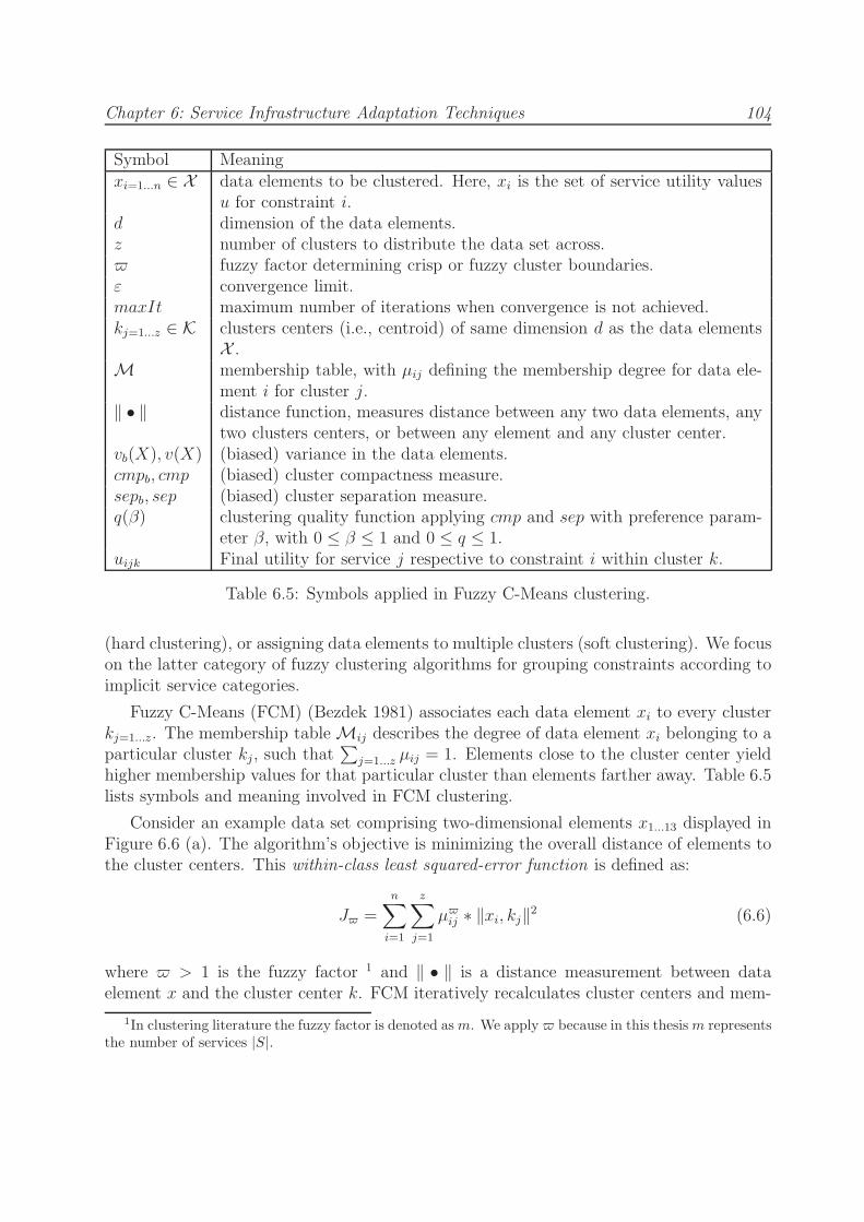
Chapter 6: Service Infrastructure Adaptation Techniques 104
Symbol Meaningxi=1...n ∈ X data elements to be clustered. Here, xi is the set of service utility values
u for constraint i.d dimension of the data elements.z number of clusters to distribute the data set across. fuzzy factor determining crisp or fuzzy cluster boundaries.ε convergence limit.maxIt maximum number of iterations when convergence is not achieved.kj=1...z ∈ K clusters centers (i.e., centroid) of same dimension d as the data elements
X .M membership table, with µij defining the membership degree for data ele-
ment i for cluster j.‖ • ‖ distance function, measures distance between any two data elements, any
two clusters centers, or between any element and any cluster center.vb(X), v(X) (biased) variance in the data elements.cmpb, cmp (biased) cluster compactness measure.sepb, sep (biased) cluster separation measure.q(β) clustering quality function applying cmp and sep with preference param-
eter β, with 0 ≤ β ≤ 1 and 0 ≤ q ≤ 1.uijk Final utility for service j respective to constraint i within cluster k.
Table 6.5: Symbols applied in Fuzzy C-Means clustering.
(hard clustering), or assigning data elements to multiple clusters (soft clustering). We focuson the latter category of fuzzy clustering algorithms for grouping constraints according toimplicit service categories.
Fuzzy C-Means (FCM) (Bezdek 1981) associates each data element xi to every clusterkj=1...z. The membership tableMij describes the degree of data element xi belonging to aparticular cluster kj, such that
∑
j=1...z µij = 1. Elements close to the cluster center yieldhigher membership values for that particular cluster than elements farther away. Table 6.5lists symbols and meaning involved in FCM clustering.
Consider an example data set comprising two-dimensional elements x1...13 displayed inFigure 6.6 (a). The algorithm’s objective is minimizing the overall distance of elements tothe cluster centers. This within-class least squared-error function is defined as:
J =n∑
i=1
z∑
j=1
µij ∗ ‖xi, kj‖2 (6.6)
where > 1 is the fuzzy factor 1 and ‖ • ‖ is a distance measurement between dataelement x and the cluster center k. FCM iteratively recalculates cluster centers and mem-
1In clustering literature the fuzzy factor is denoted as m. We apply because in this thesis m representsthe number of services |S|.

Chapter 6: Service Infrastructure Adaptation Techniques 105
bership degree until the objective function converges |J t − Jt−1 | < ε (where ε denotes the
convergence limit) or until the maximum number of iterations maxIt is reached.
For our purpose, the distance function is the euclidian distance, defined as:
distance =
(
d∑
i=1
|xi − yi|2
)1/2
(6.7)
with d the dimensions of the data elements x and y (in our example d = 2).
The cluster center (i.e., the centroid) is the means of all elements weighted by theirmembership degree. Elements further way—thus having lower membership degree—yieldlower impact on the center than closer elements. The centroid is defined as:
kj =
∑ni=1 µ
ij ∗ xi
∑ni=1 µ
ij
(6.8)
The membership of an element x belonging to a particular cluster k depends on theratio of distance between x and k and the distance from x to all centroids K:
µij =
(
z∑
l=1
(‖xi, kj‖
‖xi, kl‖)2/(−1)
)−1
(6.9)
Specifically, FCM applies the fuzzy factor to define the crispness of membershipdegree. In general, high values of implicate very fuzzy cluster boundaries whereas lowvalues result in clear cluster limits. For close to 1, FCM replicates the behavior of K-Means clustering (Macqueen 1967). With = 2, distance measurements are normalizedlinearly and for →∞, elements will belong to every cluster with equal degree. The basicFCM process applies the steps in Algorithm 7 to determine cluster membership degree.
In Figure 6.6 we cluster elements into two, three, or four clusters (z = 2 . . . 4) for fuzzyfactor = 3 (b) and = 1.2 (c)(d)(e). In subfigure (b) the top pie chart comprisesthe average membership of elements 1 . . . 4, the right, middle, and lower left pie chartsdescribe elements 5 . . . 8, 9 . . . 12, and 13, respectively. For each pie chart, the inner mostcircle visualizes fuzzy membership to two clusters, while the middle and outer most circlesdescribe membership for three, respectively four, clusters. For = 1.2, cluster membershipbecomes binary as elements belong completely to one cluster. Subfigures (c), (d), and (e)demonstrate how clusters break into smaller segments as we raise the value of z from 2 to4.
FCM exhibits some idiosyncrasies. Changes in initial membership randomizations mayyield different clustering results. Consequently, we derive data for any figure or table frommultiple iterations of the fuzzy clustering process.
The overall quality of the clustering process depends on appropriately selecting theconfiguration parameters (z,, ε,maxIt). The number of maximum maxIt iterations and

Chapter 6: Service Infrastructure Adaptation Techniques 106
0 10 20 30 40 50 60 70 80 90 100
0
10
20
30
40
50
60
70
80
90
100 1
2
3
4
56
78
9
1011
12
13
0 10 20 30 40 50 60 70 80 90 100
0
10
20
30
40
50
60
70
80
90
100 1
2
3
4
56
78
9
1011
12
13
(a) (b)
0 10 20 30 40 50 60 70 80 90100
0
20
40
60
80
100
0 10 20 30 40 50 60 70 80 90 100
0
20
40
60
80
100
0 10 20 30 40 50 60 70 80 90100
0
20
40
60
80
100
(c) (d) (e)
Figure 6.6: FCM clustering result on data set (a) for two, three, and four clusters withfuzzy factor = 3 (b) and = 1.2 (c)(d)(e). Same colors and same icons representmutual cluster membership.
convergence limit ε define the termination condition for any given selection of z and. Theamount of data and available time restrict the applicable values but other considerationsare not necessary. (Liu, Li, and Li 2008) suggest ε = 0.001. The number of clusters thatoptimally describe the data, and the optimal fuzzyness of the cluster boundaries are moresensitive choices.
We can select the number of iterations arbitrarily high, respectively ε arbitrarily low; wewill not obtain sensible clustering results when choosing z inappropriately. When groupingthe elements in Figure 6.6 (a) into two clusters (b, innermost circle) or (c), we cannot detectthe difference between elements 1 . . . 4 and 5 . . . 8.
A rule of thumb (McBratney and De Gruijter 1992) recommends selecting maxz ≈ n1/2
with n the number of elements. A computationally more intensive approach calculatesthe clustering quality for increasing number of clusters until reaching maximum quality.

Chapter 6: Service Infrastructure Adaptation Techniques 107
Algorithm 7 Basic Fuzzy C-Means Clustering Algorithm FCM(X, z,,maxIt, ε).
function PerformClustering(X, z,,maxIt, ε)M← initRandomMembership(X, z)lastJ ← 0for round = 0; round < maxIt; round+ + do
K ← calculateClusterCenters(M, )updateClusterMembership(X,K,)J = calculateObjectiveFct(X,K,)if |J − lastJ | < ε then
breakelse
lastJ ← Jend if
end for
returnMend function
(He, Tan, Tan, and Sung 2003) propose a combination of cluster compactness and clusterseparation for crisp clustering as a viable overall quality measure. Compactness describeshow well the clusters explain the variance in the data. The variance v of a set of vectors(here constraints) is defined as:
v(X) =
√
√
√
√
1
n
n∑
i=1
‖xi, x‖2 (6.10)
where ‖xi, x‖ computes the distance of xi to the mean x of all elements in X, withx = 1
n
∑
i xi. The less dispersed the elements, the smaller the variance. Next, wecompare the variance found in each cluster to the overall variance. We alter the definitionof compactness cmp to consider fuzzyness:
cmp =1
z
z∑
j=1
√
∑
i µij ∗ ‖xi, kj‖2
∑
i µij∗ v(X)−1 (6.11)
where√
••
calculates the variance of elements weighted by their degree of membership incluster kj. Compactness yields 0 for one cluster. With increasing clusters, the compactnesseventually increases to 1 at which point each data element resides in a separate cluster.We prefer higher compactness over lower compactness, but we need to avoid introducingtoo many clusters. To this end, we reuse the cluster separation metric by (He, Tan, Tan,and Sung 2003).
Cluster separation describes the heterogeneity between clusters. Clusters further apartexhibit more distinct elements than clusters close together. Separation is the coefficient of

Chapter 6: Service Infrastructure Adaptation Techniques 108
total pairwise distance between cluster centers and maximum possible distance. Separationreaches its maximum (sep = 1) when each cluster contains exactly one element. When onecluster comprises all elements, separation is zero. Again, we include the membership tableM in the definition:
sep =
∑z−1j=1
∑kl=j+1 ‖kj, kl‖
2
∑n−1i=1
∑np=i+1 ‖xi, xp‖
2(6.12)
The sum of pairwise distance between all elements yields computational complexity O(n2).However, the distance remains unchanged for all iterations of cluster counts z = 1 . . . n andthus needs computation only once.
The combined metrics identify the maximum clustering quality. For one cluster, com-pactness equals 1 and separation equals 0. For all elements in individual clusters, compact-ness yields 0 and separation 1. The quality function q(β) identifies the number of clustersthat best describe the underlying distribution:
q(β) = 1− (β ∗ cmp+ (1− β) ∗ sep) (6.13)
where β defines a preference on compactness or separation. A β value below 0.5 assignsmore weight on distinct clusters (sep) than on (lower) intra-cluster variance (cmp), andvice versa. The maximum quality value describes the best number of clusters k.
As outlined above, choosing too high yields inconclusive examples. Setting toolow results in FCM assigning elements equidistant to two cluster centers arbitrarily toone of them. For increasingly low values, the quality metric yields the highest values foradditional clusters, one of them containing only 13.
This concludes the introduction to fuzzy c-means. We discuss constraint-specific auto-matic selection of best values for and z in the following subsection.
6.5.4 Biased Clustering Algorithm
Numerous papers improve the fuzzy c-means algorithm to achieve robustness (Chintalapudiand Kam 1998,Zhang and Leung 2004,Leski 2003). These techniques apply data distribu-tion intrinsic metrics to identify and mitigate the effect of outliers and noise. We focus onachieving optimum clusters where significant services and constraints should influence theresult more than insignificant services or constraints. The basic FCM algorithm considersall data elements of equal importance; this is where we introduce our biased clusteringalgorithm.
Let us interpret the example visualized in Figure 6.6 as two services matching 13 con-straints. Service s1 matches well constraints c1 → c4 and s2 primarily matches constraintsc5→ c8. Constraints c9 → c13 are hardly supported by either s1 or s2.
A pure visual analysis of Figure 6.6 identifies two, three, or four clusters as sensibleconstraint partitions. For selecting the best number of service categories, we need to focuson clusters that contain (a) services which tend to fulfill complementary constraints well

Chapter 6: Service Infrastructure Adaptation Techniques 109
s1 s2 f H(c) wc µ(K1a) µ(K2a) µ(K1b) µ(K2b)
c1 60 100 0.115 0.662 0.12 1 0 0.857 0.125c2 60 90 0.108 0.673 0.12 1 0 0.848 0.152c3 70 100 0.122 0.677 0.12 1 0 0.870 0.130c4 70 90 0.115 0.685 0.12 1 0 0.832 0.168c5 100 60 0.115 0.662 0.12 0 1 0.125 0.875c6 90 60 0.108 0.673 0.12 0 1 0.152 0.848c7 100 70 0.122 0.677 0.12 0 1 0.130 0.870c8 90 70 0.115 0.685 0.12 0 1 0.168 0.832c9 5 5 0.007 0.693 0.008 0.501 0.499 0.500 0.500c10 10 10 0.014 0.693 0.008 0.501 0.499 0.500 0.500c11 5 10 0.011 0.637 0.008 0.536 0.464 0.503 0.497c12 10 5 0.011 0.637 0.008 0.466 0.534 0.497 0.503c13 25 25 0.036 0.693 0.008 0.501 0.499 0.500 0.500
r 0.5 0.5 wAvgH(c) 0.673 KS1 62.770 91.317 65.450 91.491H(s) 2.122 2.122 wAvgH(s) 2.122 KS2 91.282 62.791 95.491 65.450
Table 6.6: Constraints, weights, utility, and fulfillment for Case 5. For z = 2, µ(K1a) andµ(K2a) display membership degree for clustering with = 1.2; µ(K1b) and µ(K2b) with = 3.
and (b) services that tend to satisfy important constraints. On the one hand, we needto avoid partitioning according to different levels of constraint significance. On the otherhand, we need to avoid clustering according to overall constraint fulfillment which resultsin partitions of low, medium, and highly satisfied constraints.
First, we ensure that services determine the clustering result proportional to theirutility. To this end, we transform the utility values (X ) before clustering to reflect thepreliminary service rank. We multiply each xij with the service rank rj and renormalize thematrix such that services with average utility xi = xmaintain their utility value (X ·R·|R|).We thereby exploit the FCM’s sensitivity towards outliers. After the transformation betterranked services exhibit higher utility values compared to lower ranked services and thusyield more impact during the subsequent clustering process.
Second, we make sure that the cluster result comprises only the important and wellsupported constraints. Specifically, we integrate constraint weights and fulfillment intothe clustering process. For the sake of argument, suppose the constraint weights wc inTable 6.6 for the data underlying Figure 6.6.
The basic FCM algorithm is ignorant of constraints. For = 3, the quality mea-sure recommends three clusters with significant crispness (max(µij) > 0.75 ∀ i = 1 . . . 12)c1 . . . c4, c5 . . . c8, and c9 . . . c12, while putting c13 in the middle. For lower values, thesame partitioning persists with exception to c13 establishing a separate cluster. Consid-ering constraint weight wc: c1 to c8 yield high significance, and the remaining constraintsyield low significance. In this case, a better result yields only two clusters c1 . . . c4 andc5 . . . c8, without any preference for the the exact allocation of the less significant con-

Chapter 6: Service Infrastructure Adaptation Techniques 110
straints c9 . . . c13.
We adapt the clustering algorithm to drop the condition that∑
µi = 1. We bias themembership according to the importance vector T . After multiplying the membershiptable M with the importance vector, less significant elements yield little impact whencalculating the cluster center. Subsequent evaluation of membership degree resets
∑
µi =1, hence the need to bias the membership table in every iteration. The importance biasalso effects calculation of the mean vector x, variance v(X), total distance measurement,and separation.
The biased vector centroid xb for importance vector T and fuzzy factor is defined as:
xb =∑
i
xi ∗ τi
∑
i τi
(6.14)
The biased variance vb of a set of constraints and importance vector T is defined as:
vb(X) =
√
√
√
√
n∑
i=1
(‖xi, xb‖2 ∗ τ 2i ) ∗
(
∑
i
τ 2i
)−1
(6.15)
We update the function for calculating the total distance between constraints accordingly.Distance between important constraints gains significance, while distance between lessimportant or mixed important elements has little effect on the overall distance.
distX =n−1∑
i=1
n∑
j=i+1
‖xi, xj‖2 ∗
τi + τj2
(6.16)
For cluster separation, we have to adapt the distance measurement between clusters. Foreach cluster we compute the importance of the contained elements and apply the samebiased distance function as introduced above.
sepb =
z−1∑
j=1
z∑
p=j+1
(
‖ki, kj‖2 ∗
∑
i(τi ∗ µij) +∑
i(τi ∗ µip)
2
)
∗ dist−1X (6.17)
where∑
i τi ∗ µij defines the importance of cluster j.
In the last step, we normalize the membership degree. Algorithm 8 elaborates thedifferences to the basic FCM algorithm. The functions calculateClusterCenters, update-ClusterMembership, and calculateObjectiveFct remain unchanged.
We observe two phenomena when applying the importance vector T . First, with in-creasing z, clusters comprising the most significant elements rapidly split up into separate,roughly equal clusters. Clusters of less important elements form rather late (i.e., for highnumbers of z, close to |X |) if is low and do not form at all for > 3.
Figure 6.7 compares cluster entropy Hk for biased (a) and unbiased (b) clustering, with = 2. Cluster entropy measures for each element the membership degree distribution

Chapter 6: Service Infrastructure Adaptation Techniques 111
Algorithm 8 Biased FCM Clustering Algorithm BFCM(X , z, , ε,maxIt, T , β).
function PerformBiasedClustering(X , z, , ε,maxIt, T , β)M← initRandomMembership(X, z)/* Bias membership according to importance. */M←M∗ TlastJ ← 0maxDist← calculateTotalDistance(X , T )for round = 0; round < maxIt; round+ + do
K ← calculateClusterCenters(z,)updateClusterMembership(X , K,)/* Recalculating the cluster membership resets
∑
µi = 1, → bias membershipagain according to importance. */
M←M∗ TJ = calculateObjectiveFct(X , K,)if |J − lastJ | < ε then
breakelse
lastJ ← Jend if
end for
calculateQuality(X , T , K, β,M, maxDist,)normalizeMembership(M)return membership
end function
function calculateTotalDistance(X , T )for i = 0; i < |X| − 1; i+ + do
for j = i+ 1; j < |X|; j + + do
total← total + calcDistance(xi, xj)2 ∗ (τi + τj)/2
end for
end for
return totalend function
function normalizeMembership(M)/* Recalculate membership such that
∑
µi = 1. */for all constraint i ∈ C do
sumµ ← 0for all cluster k ∈ K do
sumµ ← sumµ + µikend for
for all cluster k ∈ K do
µik ← µik/sumµ
end for
end for
end function

Chapter 6: Service Infrastructure Adaptation Techniques 112
Algorithm 9 Continuing BFCM(X , K,, ε,maxIt, T ).
function calculateQuality(X , T , K, β,M, maxDist,)/* 1. Calculate compactness. */cmp← 0; var ← 0; totalBias← 0; xb ← ∅/* 1.1 Calculate biased center. */for i = 0; i < |X|; i+ + do
bias← sifor j = 0; j < dimensions(X); j + + do
xbj ← xbj + xij ∗ biasend for
totalBias← totalBias + biasend for
xbj ← xbj/totalBias; div ← 0/* 1.2 Calculate biased maximum variance. */for i = 0; i < |X|; i+ + do
var ← var + calcDistance(xi, xb)2 ∗ τ 2
i
div ← div + τ 2i
end for
var ← var1/2/div/* 1.3 Calculate biased intra-cluster variance. */dist← 0for all cluster k ∈ K do
sumµ ← 0for all constraint i ∈ C do
dist ← dist + calcDistance(i, k)2 ∗ µ2ik /* We need not include importance
vector s as we have multiplied it with membership already before. */sumµ ← sumµ + µ2
ik
end for
cmp← cmp + (dist/sumµ)1/2/var
end for
/* 2. Calculate separation. */sep← 0; clImp← ∅/* 2.1 Calculate cluster importance. */for all cluster k ∈ K do
for all constraint i ∈ C do
clImpk ← clImpk + µikend for
end for
/* 2.2 Calculate inter-cluster distance. */for i = 0; i < |K| − 1; i+ + do
for j = i+ 1; j < |K|; j + + do
clDist← clDist+ calcDistance(ki, kj)2 ∗ (clImpi + clImpj)/2
end for
end for
sep← clDist/maxDistreturn 1− (β ∗ cmp+ (1− β) ∗ sep)
end function

Chapter 6: Service Infrastructure Adaptation Techniques 113
2 4 6 8 10 12
2
4
6
8
10
12
0
0.2
0.4
0.6
0.8
1
1.2
1.4
1.6
1.8
2
(a)
2 4 6 8 10 12
2
4
6
8
10
120.1
0.2
0.3
0.4
0.5
0.6
0.7
0.8
0.9
1
(b)
Figure 6.7: Cluster entropy Hk for biased (a) and unbiased (b) clustering.
across all available clusters. Low entropy value (dark colors) indicate focus on one or afew clusters. Bright colors highlight elements that (equally) belong to many clusters. Eachcolumn comprises the entropy values for a particular element. The top row contains theentropy values for z = 1 clusters, down to the bottom row containing z = 13 clusters.
In the biased case, we notice how elements 1 . . . 8 break into smaller clusters beforepopulating individual clusters in row 8. The remaining elements equally belong to anincreasing number of cluster until after row 8 element 13 separates into a distinct cluster.Interestingly, elements 9 . . . 12 never form a cluster themselves.
In the unbiased case, elements 9 . . . 12 exhibit a similar behavior as element 1 . . . 8 inthe unbiased case. Round 2 and 3 yield crisp cluster membership (generally low clusterentropy values). After round 4, element 13 remains in a distinct cluster, the other elementsyield shifting membership. In contrast to the biased case, all elements eventually end upin individual clusters.
Second, we notice an early, sharp decline in compactness opposed to a late, steepincrease in separation. Compactness is minimal when elements populate individual clusters.As observed above, the most significant elements quickly scatter into separate groups. Ifinsignificant elements eventually occupy their own cluster, they barely reduce compactness.
The same effect determines the late, steep incline of cluster separation. Separationis maximal when each cluster contains a single element. As long as clusters of significantelements split into increasingly smaller clusters, the centroids remain close together, addinglittle to separation. The distance between centroids grows once less significant elementsform individual clusters clearly separated from the existing cluster centers.
Figure 6.8 displays compactness and separation for = [1.5, 2, 3] with biased andunbiased clustering side by side. We notice biased compactness reaching its minimum onceall important elements reside in separate clusters. Unbiased compactness drops similarlyfast at the beginning, but then phases out, reaching its minimum at z = n. Biased

Chapter 6: Service Infrastructure Adaptation Techniques 114
separation remains low until all important elements populate individual clusters, thenrising sharply. In contrast, the unbiased separation metric displays near-linear growth.
2 4 6 8 10 120
0.1
0.2
0.3
0.4
0.5
0.6
0.7
0.8
0.9
1
CMP m1.5CMP m2CMP m3SEP m1.5SEP m2SEP m3
2 4 6 8 10 120
0.1
0.2
0.3
0.4
0.5
0.6
0.7
0.8
0.9
1
CMP m1.5CMP m2CMP m3SEP m1.5SEP m2SEP m3
(a) (b)
Figure 6.8: Compactness and separation for biased (a) and unbiased (b) clustering.
We exploit the sharp incline in separation, respectively decline in compactness, forselecting the maximum number of clusters z. Specifically, we derive the amount of elementsexhibiting a importance value higher than the average of τ minus φ (where φ is twice thestandard deviation σ divided by the number of constraints) such that:
zmax = |Ttop| τi ∈ Ttop ∀τi ≥ (τ −2 ∗ στn
) (6.18)
The design of φ ensures that for a large number of constraints, low-performing elementsare still detected.
We subsequently measure the quality q for each additional cluster for z = 2 → zmax.And select the cluster count that yields the maximum increase in quality. We detail theselection process in Algorithm 10.
Finally, we determine the fuzzy factor . The entropy-based threshold values indicatethe existence of clusters. Hence, we restrict to the interval ]1, 3]. For two data sets, theone with lower weighted average service entropy Meana(H(s)) yields crisper clusters. Theratio of service entropy to entropy threshold determines the exact value for , specifically:
= 1 + 2 ∗Meana(H(s))
ts+ γ (6.19)
where qs is the service entropy threshold, and γ ensures that > 1. We set γ to 0.0001.
Table 6.8 lists the clustering result for case 1 . . . 4. We included case 2 —failing to meetthe either threshold criteria— and case 3—exceeding the constraint entropy threshold tc—for demonstration purpose. All constraint weights wc are 1/6.

Chapter 6: Service Infrastructure Adaptation Techniques 115
Algorithm 10 Best Cluster Quality Algorithm CQA(X , T ,R).
function selectBestMembership(X , T )z ← calcMaxCluster(X , T ) ← calcFuzzyFactor(X , T )Xb ← X ∗R ∗ Tµbest ← ∅qmax ← 0for k = 1→ z do
/* For each round, initialize empty cluster centers K. */K ← {k}µ← call PerformBiasedClustering(Xb, K,, ε,maxIt, T , β)q ← calcQuality(µ)if q > qmax then
qmax ← qµbest ← µ
end if
if q > qmax then
qmax ← qend if
end for
return µbestend function

Chapter 6: Service Infrastructure Adaptation Techniques 116
K1.1 K1.2 K1.3 K2.1 K2.2 K2.3 K3.1 K3.2 K4.1 K4.2 K3.3
C1 0.882 0.059 0.059 0.08 0.849 0.07 0.992 0.008 0.028 0.032 0.941
C2 0.931 0.035 0.035 0.032 0.019 0.949 0.993 0.007 0.019 0.022 0.959
C3 0.059 0.882 0.059 0.261 0.543 0.196 0.007 0.993 0.022 0.952 0.026C4 0.035 0.931 0.035 0.318 0.312 0.37 0.005 0.995 0.031 0.932 0.037C5 0.059 0.059 0.882 0.312 0.454 0.233 0.111 0.889 0.979 0.01 0.011C6 0.035 0.035 0.931 0.922 0.032 0.046 0.087 0.913 0.984 0.008 0.008
2.516 3.0 2.250 2.629zmax 3 3 2 4Hk 0.335 0.592 0.092 0.18
µ 0.3 0.3 0.3 0.321 0.368 0.311 0.634 0.366 0.33 0.343 0.327
Table 6.7: Biased cluster algorithm configuration (zmax and ) and results for case 1 to 4.Bold numbers highlight the top cluster membership degree.
As discussed above, the cluster entropy Hk describes how well constraints fit into theirclusters—the more focused on one cluster, the lower the entropy. Low Hk values for case1,3, and 4 reflect the crisp membership degree. As indicated by the threshold, we do notgain any insight from clustering Case 2. Clustering of constraints in case 3 demonstratesnicely the role of the constraint entropy. The resulting two clusters separate the constraintsaccording to high and low constraint fulfillment degree.
6.5.5 Cluster-specific ranking
Before the clustering, we match a single list of constraints to a set of services, calculatingutility values. The clustering process then partitions the set of constraints into multiplegroups for individual ranking. In the subsequent ranking phase, we evaluate all serviceswithin each cluster. We combine cluster weights w and membership degree µ, thus avoidingdefuzzyfication of the clustering result. A constraint belonging equally to two clusters willthus influence the ranking result in both clusters to the same degree. The service utilityfor a given constraint and cluster uijk is defined as:
uijk = xij ∗ wi ∗ µik (6.20)
where µik is the membership of constraint i in cluster k; for all constraints i ∈ C, allservices j ∈ S, and clusters k ∈ K.
We integrate the basic LSP ranking algorithm (Alg. 2) introduced in Section 4.3. Foreach cluster, Algorithm 11 updates the constraint weights, calls the LSP algorithm, andfinally returns a ranked service list for each cluster.
Evaluation of ranked cluster results is twofold. First we compare ranked clusters resultsto regular ranking results for case 1 to 4 in Table 6.8. Second, we compute the Pearsonproduct-momentum coefficient on ranks as a measure of correlation.

Chapter 6: Service Infrastructure Adaptation Techniques 117
Algorithm 11 Biased Ranking Algorithm BA(X , µ, w).
function PerformClusterspecificRanking(X , µ, w)/* Initialize array of rank results. */RR← ∅for all Cluster k ∈ K do
/* Initialize biased constraint weights. */biasedW ← ∅for all Constraint i ∈ C do
biasedWi ← µik ∗ wiend for
RR[k]← call LSPRankingAlgorithm(X , biasedW )end for
return RRend function
6.5.5.1 Measuring Clustering Benefit
We neglect composition costs and focus on comparing the benefit of selecting the topservices from each cluster to selecting the top service deriving from the regular rankingprocess. The clustering benefit Jbest is defined as the sum of top ranked service utilityweighted according to the relative size of cluster k where µk =
∑
i µik (listed in Table 6.6):
Jbest =∑
k
(µk ∗max(Rk)) (6.21)
where set Rk contains the ranked service utility values in cluster k. The ranking results inTable 6.8 remain non-normalized to preserve the differences in utility values. Also, we donot need normalization as all utility values derive from the same value range ([0, 100]).
In case 1, combining S1, S2, and S3 yields a 81.3% benefit increase over selecting S4.Even a combination of S4 (the second best choice in any cluster) and any top rated serviceprovides a 29% raise. Clustering in case 2 exhibits only marginal benefits (+6%). Also,service S1 is ranked best in cluster 1 and 3, placed second in cluster 2. We do not achieveany benefit in case 3, where the ranking order in both clusters equals the order originatingfrom the regular ranking process. Case 4 exhibits benefit from clustering. Combinationof S1, S2, and S3 result in 97% better constraint support than selecting S3 alone. For the2-tuples of these services we gain 57% (S1, S2), 57% (S1, S3), and 56% (S2, S3) in benefit.
We apply the Pearson’s coefficient—introduced in Chapter 4.2—to measure the differ-ence in ranking positions. We expect clusters to exhibit a distinctly different service order.We derive the overall difference between cluster and non-clustered ranks by aggregatingthe weighted (applying µk) Pearson’s correlation found between each set of cluster rankingsand the non-clustered ranking. We utilize the absolute rank positions for calculating thePearson coefficient ρ. Relative ranking result R1[50, 33.33, 33.33, 33.33, 10], for example,becomes [1, 3, 3, 3, 5]. Table 6.8 includes cluster specific correlation and total correlation

Chapter 6: Service Infrastructure Adaptation Techniques 118
K1.1 K1.2 K1.3 R1 K4.1 K4.2 K4.3 R4
1 S1(90.64) S2(90.64) S3(90.64) S4(50.0) S3(86.46) S2(77.53) S1(82.42) S3(41.67)2 S4(50.0) S4(50.0) S4(50.0) S1(33.33) S2(23.68) S1(28.87) S3(29.76) S1(39.17)3 S5(10.0) S5(10.0) S5(10.0) S2(33.33) S5(10.0) S5(10.0) S2(12.36) S2(37.5)4 S3(4.68) S3(4.68) S2(4.68) S3(33.33) S1(7.35) S3(6.54) S5(10.0) S5(10.0)5 S2(4.68) S1(4.68) S1(4.68) S5(10.0) S4(2.39) S4(0.02) S4(0.02) S4(0.83)ρ 0.224 0.224 0.238 0.229 0.7 0.3 0.9 0.628
K2.1 K2.2 K2.3 R2 K3.1 K3.2 R3
1 S1(73.15) S2(78.06) S1(81.14) S1(73.33) S3(81.98) S3(18.43) S3(41.67)2 S5(59.86) S1(65.48) S2(63.29) S5(58.33) S1(77.5) S1(17.07) S1(39.17)3 S4(52.89) S5(64.88) S3(53.97) S2(56.67) S2(73.39) S2(16.81) S2(37.5)4 S3(44.74) S3(57.49) S5(50.25) S3(51.67) S5(10.0) S5(10.0) S5(10.0)5 S2(32.84) S4(32.25) S4(32.72) S4(40.0) S4(2.26) S4(0.01) S4(0.83)ρ 0.6 0.7 0.7 0.668 1 1 1
Table 6.8: Clustered Ranking algorithm results for case 1 to 4 compared to unclusteredranking results.
values. As expected, examples with distinct clusters and high clustering benefit (case 1and 4) exhibit lower correlation than case 2 and 3. We notice the small difference betweenρCase2 and ρCase4 when we correlate the overall ranking set. Correlation is unbiased anddifferences (or lack thereof) at the bottom of the ranking list impact the result to the sameextent as differences at the top. Interested in changes amongst the best fitting service,we limit the selection to the top two services. Subsequently correlation of S1 and S5 inR2 yields ρ = 1, as in every of the three clusters, S1 is ranked higher than S5. The samelimitation on R4 yields ρ = −0.33, as S1 ranks higher than S3 in two out of three clusters.
6.6 Service Composition Recommendation
The clustering process offers a set of best suited services fulfilling the given requirements.Together, the top services from each cluster provide the most qualified aggregation, butnot necessarily the cheapest. Selecting the top members ignores any form of aggregationcosts.
In this thesis, we focus only on one form of aggregation costs: service distance. Ser-vices yielding close proximity have proven to function well in joint efforts. We, therefore,consider services that have often been utilizes in a common context to be more suitablefor aggregation than services that were rarely used together. Specifically, we apply thedistance metrics introduced in Chapter 4. Ultimately, we need to find a tradeoff betweenminimal aggregation costs (i.e., low overall service proximity) and high service utility.
The top cluster elements do not necessarily exhibit low service distance. We, there-fore, require an algorithm to test other services aggregations for similarly high utility butconsiderably lower distance.

Chapter 6: Service Infrastructure Adaptation Techniques 119
Brute-force testing of every possible combination yields unpractical for large sets ofservices and clusters as the underlying problem is NP hard. Testing the top m servicesof k clusters has O(mk) computational complexity. Our goal is to find a better solutionthan the aggregation of the top element in each cluster, not necessarily the best possiblesolution. For this purpose, we select Simulated Annealing (Kirkpatrick, Gelatt, and Vecchi1983, Cerny 1985), an optimization heuristic.
6.6.1 A brief Introduction to Simulated Annealing
Simulated Annealing (SA) is a heuristic for approximating a global optimum in complexmathematical problems. It is well suited for problems with discrete search space such asthe order of cities in the traveling sales man problem.
Simulated annealing is an iterative process building on following basic components:
Candidate Solution contains the current best problem solution which is gradually im-proved.
Solution Energy Function measures the quality of a given solution. SA aims to find asolution with the lowest possible energy.
Neighborhood Function provides a new candidate solution based on the current solu-tion. A good neighborhood function traverses the search space quickly, but producesnew solutions that yield similar energy level to the preceding solution.
Transition Function decides whether to accept a new solution or to stick with the cur-rent one.
Cooling function gradually reduces the temperature. Large solution changes are lesslikely for lower temperatures.
We briefly outline the iterative process in Algorithm 12 as provided in the JUNG1.7.6 framework2. We omit some configuration parameters for sake of clarity. Transitionfunction and Cooling function are problem independent, thus introduced here. We discussneighborhood function and energy function in the subsequent subsections. For now, wetreat these as blackboxes.
Simulated annealing takes an initial solution (i.e., the top service from every cluster)and derives the corresponding energy. Simulated Annealing continues to evaluated similarsolution as long as the temperature hasn’t reached zero and there are more available itera-tions. A new solution is always accepted when it yields lower energy. Worse solutions areaccepted with probability pSA defined as:
pSA = e−1∗δenergy
temp (6.22)
2http://jung.sourceforge.net/

Chapter 6: Service Infrastructure Adaptation Techniques 120
where δenergy is the energy difference between the current and new solution, temp is thecurrent annealing temperature, and e is Euler’s number 2.718 . . .. Transitions to solutionswith higher energy are possible as long as the temperature remains high, or the energydifference is very small.
The freezing process depends on the cooling rate and current iteration state. As long asthe number of successful transitions is high (i.e., success close to tries) the system remainsin a search space region that still provides many solutions with lower energy. The functionfor the temperature in the next iteration is defined as:
tempn = r(limitaccept−
successtries
)∗tries
cooling ∗ temp (6.23)
where tries, rcooling, and limitaccept are configuration parameters. For our experiments, weapply tries = 100, rcooling = 0.99, and limitaccept = 0.97
Algorithm 12 Simulated Annealing Algorithm SA(maxIt, startTemp).
function Annealing(maxIt, startTemp)A ← calcNewSolution(startTemp)nrg ← calcEnergy(S)temp← startTempiteration← 0while temp > 0 AND iteration < maxIt do
success← 0for tries do
/* Neighborhood function provides a new solution. */newSolution← calcNewSolution(S, temp)nrgnew ← calcEnergy(newSolution)δenergy = nrg − nrgnewif doTransition(δenergy, newSolution, temp) then
S ← newSolutionnrg ← nrgnewsuccess+ +
end if
end for
temp← calcTemperature(temp, success)iteration + +
end while
return Aend function
6.6.2 Simulated Annealing Energy Function
The energy function provides the tradeoff between requirement fulfilment (i.e., totalweighted utility uagg) and service distance (i.e., average interaction-based distance be-

Chapter 6: Service Infrastructure Adaptation Techniques 121
Symbol MeaningA Solution consisting of one selected service in each cluster.pSA Transition probability to accept solutions with higher energy.δenergy Energy difference between two solutions.tempn New temperature given the current temperature temp, and configuration pa-
rameters rcooling, limitaccept, and tries.xmax Maximum utility as provided by the top ranked service from each cluster.distmax Upper limit for interaction distance between top ranked services.nrg Energy of a given solution depending on xmax, distmax and solution specific
utility xagg(A) and distance distavg(A).ϕ Preference parameter for trade-off between maximum utility or minimum dis-
tance.tnh Neighborhood selection threshold.pnh Neighborhood selection probability.
Table 6.9: Symbols applied in Simulated Annealing.
tween selected services distavg). A solution consists of a service from each clusters. Thetotal weighted utility uagg combines the service utility values u for a given cluster weightedaccording to the clusters significance (sigcluster(k) =
∑
i µik ∗ wi). A cluster’s significanceraises with increasing membership of important constraints. The average distance distavgis the sum of distance between any two services in the corresponding interaction-baseddistance graph, divided by the cluster count.
First we need to scale uagg and distavg to the interval [0, 1] to combine them in a singlefunction. We obtain the maximum achievable weighted utility umax from selecting the topservice from every cluster. The maximum distance between service is unknown, but wehave an upper limit: the distance for the top services distmax. As no solution can yieldhigher utility than the top services, any solution with higher distance than distmax cansafely be discarded. The subsequent energy function for solution A is defined as:
nrg = ϕ ∗umaxuagg(A)
+ (1− ϕ) ∗distavg(A)
distmax(6.24)
where ϕ determines the preferences for achieving high overall quality, or rather low intra-service distance. With ϕ approaching 1, the top service in every cluster creates the bestsolution. Having ϕ approach 0, simulated annealing selects the same service for everycluster, thereby reducing the overall distance to zero.
The combination of top services yields an energy value of 1. Any better combinationmust exhibit lower energy by reducing the distance. Combinations that additionally comewith lower utility need to yield proportionally lower distance.
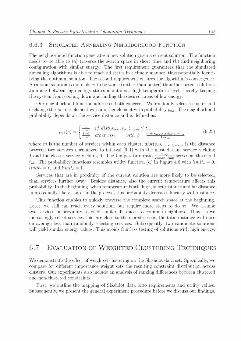
Chapter 6: Service Infrastructure Adaptation Techniques 122
6.6.3 Simulated Annealing Neighborhood Function
The neighborhood function generates a new solution given a current solution. The functionneeds to be able to (a) traverse the search space in short time and (b) find neighboringconfiguration with similar energy. The first requirement guarantees that the simulatedannealing algorithms is able to reach all states in a timely manner, thus potentially identi-fying the optimum solution. The second requirement ensures the algorithm’s convergence.A random solution is more likely to be worse (rather than better) than the current solution.Jumping between high energy states maintains a high temperature level, thereby keepingthe system from cooling down and finding the desired areas of low energy.
Our neighborhood function addresses both concerns. We randomly select a cluster andexchange the current element with another element with probability pnh. The neighborhoodprobability depends on the service distance and is defined as:
pnh(s) =
{
1m−1
if dist(snew, sold)norm ≤ tnh1−ψm−1
otherwise with ψ = dist(snew ,sold)norm−tnh
1−tnh
(6.25)
where m is the number of services within each cluster, dist(s, scurrent)norm is the distancebetween two services normalized to interval [0, 1] with the most distant service yielding1 and the closest service yielding 0. The temperature ratio temp
2∗maxTempserves as threshold
tnh. The probability functions resembles utility function (d) in Figure 4.8 with limita = 0,limitb = t, and limitc = 1.
Services that are in proximity of the current solution are more likely to be selected,than services further away. Besides distance, also the current temperature affects thisprobability. In the beginning, when temperature is still high, short distance and far distancejumps equally likely. Later in the process, this probability decreases linearly with distance.
This function enables to quickly traverse the complete search space at the beginning.Later, we still can reach every solution, but require more steps to do so. We assumetwo services in proximity to yield similar distances to common neighbors. Thus, as weincreasingly select services that are close to their predecessor, the total distance will raiseon average less than randomly selecting services. Subsequently, two candidate solutionswill yield similar energy values. This avoids fruitless testing of solutions with high energy.
6.7 Evaluation of Weighted Clustering Techniques
We demonstrate the effect of weighted clustering on the Slashdot data set. Specifically, wecompare for different importance weight sets the resulting constraint distribution acrossclusters. Our experiments also include an analysis of ranking differences between clusteredand non-clustered constraints.
First, we outline the mapping of Slashdot data onto requirements and utility values.Subsequently, we present the general experiment procedure before we discuss our findings.

Chapter 6: Service Infrastructure Adaptation Techniques 123
6.7.1 Mapping Slashdot to Constraints and Utility functions
As briefly outlined in subsection 4.4.3.1, slashdot postings are subject to a moderationsystem. Postings receive scores between −1 (low quality) and +5 (high quality). Postingsby known Slashdot members are rated 1 by default. Anonymous posts initially receivescore 0.
In addition, predicates enable classification of postings according to insightful, inter-esting, informative, funny, etc. content (Table 6.10). As the classification process remainsoptional, mostly valuable postings are scored. Notice the low count of negative postingstagged with Troll, Offtopic, Flamebait, or Redundant in Table 6.10. Constructive postingsusually receive scores higher than 1. Most postings, however, remain without predicate atall ( 75%).
Predicate Total Count Score ≥ 2None 55484 156Insightful 5494 5038Interesting 3599 3264Informative 3596 3294Funny 3383 3056Troll 678 1Offtopic 501 0Flamebait 461 0Redundant 287 0Total 73483 14809
Table 6.10: Total Slashdot posting count and postings of minimum score 2 count from thesubdomains Ask, Entertainment, and Mobile between Jan 1st, 2008 and July 1st, 2008,grouped by predicates.
We treat slashdot users as entities in an ensemble similar to the evaluation in Section 4.4.In our case, total scores (i.e., Score) and total posting counts (i.e., Count) serve as servicerequirements. Specifically, we derive for a user the total posting count and the total scoresummarized across these postings for a given subdomain and predicate. We prefer to keepthese two constraints separated, as relying on a single average user score favors users withvery few postings which were lucky to receive high ratings. In contrast, users contributingregularly are unlikely to receive continuously high scores. We consider total scores to beequally important to total postings throughout our experiments. Thus constraints weightsfor pairs of these statistics (respective to predicates) are always identical.
Within each constraint, users with the highest total score (respectively total postingcount) receive a utility value of 100, with the worst users having utility 0. The generalquestion we can answer applying our weighted clustering approach to the Slashdot data setis: Which clusters do arise from a given set of subdomains and predicates, and how muchdo we benefit from selecting the best users from clusters compared to a regular rankingprocess.

Chapter 6: Service Infrastructure Adaptation Techniques 124
6.7.2 Weighted Clustering Experiment Setup
We select a set of subdomains SD and identify all users who have submitted at least 5postings in these subdomains that scored 2 or higher. Given a set of predicates P we arriveat the constraints set C of size |P | ∗ |SD| ∗ 2. For each user, we derive the utility valuesfor all constraints.
We select three subdomains—Ask, Entertainment, and Mobile—and focus in particularon the scores of funny, interesting, and insightful postings arriving at 12 constraints (i.e.,Ask-Fun-Count, Ask-Fun-Score, Ask-Ins-Count, etc.). Across the three subdomains, weselect users having 5 or more postings rated 2+. We treat users below this initial thresholdas services exhibiting capabilities we are not interested in. As a side effect, reducing theinitial set of candidates (here 255 users) reduces the duration of the clustering process.
The clustering threshold model configuration with α = 0.3; δ = 0.4 for both constraintentropy and service entropy yields thresholds of tc = 0.98 and ts = 0.96, respectively. Both,constraint entropy and service entropy remain well below these limits (H(c) = 0.76;H(s) =0.64) thus clustering takes place with fuzzy factor m = 1.826.
6.7.3 Unbiased, Non-weighted Clustering Experiment Results
First, we analyze unbiased clustering, where we ignore constraint weights and work withthe unbiased utility matrix X . The cluster quality metric identifies 12 clusters to optimallydescribe the constraints. Specifically, the resulting cluster membership places Count andScore constraints of every subdomain and predicate in the same cluster except for the statis-tics describing Ask-Insightful, Entertainment-Funny and Entertainment-Interesting whichpopulate individual clusters. Cluster membership µ is larger than 0.9 for all constraints.
We calculate the pairwise Jaccard similarity between any two clusters for the top 10,50, and 100 users. Figure 6.9 visualizes the resulting similarity matrix. Row 13 and col-umn 13 contains the unclustered ranking set. We notice that even for the very small setof top 10 users some clusters yield high similarity. Specifically cluster 3 and 5 share eightusers, cluster 4 and 10 share eight users, and cluster 6 and 11 have 9 users in common.This overlap increases with 50 and 100 top users. Although all clusters yield significantdifferences to the unclustered ranking, the clustering process has created three pairs ofclusters that should belong together. Incidentally, these pairs comprise of the above men-tioned constraints, where Score and Count of the same subdomain and predicate end upin different clusters (Ask-Insightful, Entertainment-Funny and Entertainment-Interesting).Merging these pairs would not reduce the overall clustering benefit.
6.7.4 Biased, Non-weighted Clustering Experiment Results
Second, we cluster with equal constraint weights but biased utility matrix Xb. Constraintsthat exhibit low service fulfillment yield less importance during clustering than well sup-ported constraints. Table 6.11 provides the constraint membership in the resulting six

Chapter 6: Service Infrastructure Adaptation Techniques 125
2 4 6 8 10 12
2
4
6
8
10
12
0
0.2
0.4
0.6
0.8
1
2 4 6 8 10 12
2
4
6
8
10
120.1
0.2
0.3
0.4
0.5
0.6
0.7
0.8
0.9
1
2 4 6 8 10 12
2
4
6
8
10
120.2
0.3
0.4
0.5
0.6
0.7
0.8
0.9
1
(a) (b) (c)
Figure 6.9: Cluster Jaccard similarity for Top 10 (a), Top 50 (b), and Top 100 (c) usersfor unbiased, non-weighted constraints.
clusters. Most constraints yield crisp cluster membership (µ > 0.9) with exception to En-tertainment Funny, Entertainment Interesting, and Mobile Funny which do not stronglybelong to any cluster. The importance vector T is a good indicator on which constraintsare likely to yield crisp clusters. A low importance value by itself, however, is not suf-ficient. The constraints Ask-Funny-Score (τ = 0.804) exhibits lower importance thanEntertainment-Funny-Count (τ = 0.836) but ends up clearly assigned to cluster 1. Here,the close correlation of count and score values is decisive. The cluster weight aggregatesthe constraint weights proportional to their membership in that particular cluster.
We ensure that clusters provide more fitting elements than the unclustered rankingresult by pairwise comparing the top-k elements with Pearson’s correlation coefficient (ρ)and Jaccard similarity (J). Table 6.12 lists the ranking differences of the top 10, 50, and100 users. The Jaccard similarity measures the set overlap of users regardless of their rank.Pearson’s coefficient requires both sets to contain the same elements. We therefore take theunion of elements from both rankings (given in brackets in Table 6.12) and then computeρ.
Average Jaccard similarity increases with growing k, but remains still low for the top100 users (of 255 in total). In other numbers, of the top-10 nonclustered users, only 30%occur in both rankings. For the top-50 and top-100 users this percentage is marginallyhigher: 33% and 35%, respectively.
The average Pearson’s coefficient stresses the ranking differences even more. We observea slight negative correlation for the top 10 users, no correlation in ranks for the top 50users, and only a slight correlation for the top 100 users.
We compare also pairwise the six clusters to ensure that they constitute indeed distinctcollections of constraints. We print the Jaccard similarity between any combination ofclusters in Figure 6.10. The last row and column provides the overlap of the unclusteredranking as also provided in Table 6.12. In constrast to the first experiment, all overlapsbetween clusters remain low, even for the top 100 users. The highest similarity existsbetween clusters rankings and non-cluster ranking.
Evidently, clustering promotes distinctively different candidates than unclustered rank-

Chapter 6: Service Infrastructure Adaptation Techniques 126
Constraint τ Cl 1 Cl 2 Cl 3 Cl 4 Cl 5 Cl 6
Ask-Fun-Count 0.864 0.959 0.005 0.011 0.012 0.008 0.006Ask-Fun-Score 0.805 0.968 0.004 0.009 0.009 0.006 0.005Ask-Ins-Count 1.394 0.019 0.01 0.023 0.025 0.914 0.01Ask-Ins-Score 1.735 0.005 0.003 0.008 0.007 0.975 0.003Ask-Int-Count 1.185 0.009 0.004 0.006 0.969 0.008 0.005Ask-Int-Score 1.226 0.011 0.004 0.007 0.964 0.009 0.005Ent-Fun-Count 0.836 0.24 0.12 0.176 0.158 0.104 0.202Ent-Fun-Score 0.702 0.253 0.116 0.17 0.146 0.099 0.215Ent-Ins-Count 1.035 0.01 0.004 0.965 0.007 0.01 0.004Ent-Ins-Score 1.008 0.007 0.003 0.976 0.004 0.007 0.003Ent-Int-Count 0.513 0.338 0.09 0.179 0.156 0.105 0.132Ent-Int-Score 0.748 0.291 0.085 0.215 0.158 0.143 0.108Mob-Fun-Count 0.563 0.197 0.136 0.123 0.112 0.087 0.346
Mob-Fun-Score 0.563 0.205 0.13 0.127 0.11 0.087 0.341
Mob-Ins-Count 1.459 0.003 0.98 0.003 0.003 0.003 0.007Mob-Ins-Score 1.503 0.003 0.983 0.003 0.003 0.003 0.007Mob-Int-Count 0.814 0.006 0.011 0.005 0.006 0.004 0.969
Mob-Int-Score 1.046 0.008 0.016 0.006 0.008 0.005 0.957
Cluster Weight 0.196 0.15 0.167 0.159 0.143 0.185
Table 6.11: Cluster membership and importance vector T for biased constraints fromsubdomains Ask, Entertainment, and Mobile with predicates Funny, Insightful, and Inter-esting.
1 2 3 4 5 6 7
1
2
3
4
5
6
70
0.2
0.4
0.6
0.8
1
1 2 3 4 5 6 7
1
2
3
4
5
6
70.1
0.2
0.3
0.4
0.5
0.6
0.7
0.8
0.9
1
1 2 3 4 5 6 7
1
2
3
4
5
6
7 0.2
0.3
0.4
0.5
0.6
0.7
0.8
0.9
1
(a) (b) (c)
Figure 6.10: Cluster Jaccard similarity for Top 10 (a), Top 50 (b), and Top 100 (c) usersfor biased, non-weighted constraints.
ing. Table 6.13 provides a detailed view on the top 10 users of each cluster and the non-clustered rank. For each cluster, the table lists user id, cluster specific score, and positionin the non-clustered set. Bold user ids highlight the top 10 elements from the non-clusteredset.
There happens to be an outstanding user (957197) being ranked first in cluster 1, 3,4, and 5. However, the user resides on position 35 and 41 in cluster 1 and cluster 6,respectively. Other elements in the non-clustered top 10 list, perform much worse. The

Chapter 6: Service Infrastructure Adaptation Techniques 127
Top 10 Top 50 Top 100Cluster ρ J ρ J ρ J
Cl1 -0.379 (16) 0.25 0.016 (74) 0.351 0.105 (144) 0.389Cl2 -0.596 (17) 0.176 -0.152 (81) 0.235 -0.011 (147) 0.361Cl3 0.314 (15) 0.333 0.193 (71) 0.408 0.217 (139) 0.439Cl4 -0.316 (17) 0.176 0.014 (75) 0.333 0.005 (143) 0.399Cl5 0.065 (16) 0.25 0.031 (78) 0.282 0.119 (138) 0.449Cl6 -0.368 (17) 0.176 -0.061 (71) 0.408 0.194 (138) 0.449
Avg -0.213 (16.3) 0.227 0.007 (75) 0.336 0.105 (141.5) 0.414
Table 6.12: Ranking differences of top 10, 50, and 100 users between each cluster and theunclustered ranking order measured with Pearson’s correlation coefficient (ρ) and Jaccardsimilarity (J). Unweighted, biased constraints from subdomains Ask, Entertainment, andMobile with predicates Funny, Insightful, and Interesting.
3rd user (595695) is on position 53 in cluster 1 and 38th in cluster 6. User 65584 is 155thin cluster 4 and 137th in cluster 6. Non-clustered 7th place becomes 128th in cluster 2,while 8th place ends up at position 142 in cluster 3. Every top 10 element, however, ranksbetter in at least one particular cluster (e.g., User 22995 (7th) is ranked 4th in cluster 3).
We observe similar differences in the opposite direction. Well positioned clusteredusers rank very low in the unclustered set. As listed in Table 6.13, user 963289, 3rd incluster 2, is otherwise ranked 76th. User 1304191, on 7th place in cluster 6, ends up atposition 199. Additional differences exist in the ordering of element. Positioned 6th in theunclustered set, user 22995 ranks before position 5 and 2 in cluster 3. In cluster 2, initialrank 8 outperforms rank 4 and 6. The analysis of ranking orders highlights considerabledifferences between the intra cluster order and the unclustered ranking order. We, thus,can conclude that clustering successfully promotes specialized users.
Next, we inspect the intra cluster utility values to measure the increase in benefitcompared to the unclustered utility values. Table 6.13 includes the biased average forevery position across all six clusters. Utility values in each cluster are weighted accordingto the clusters contribution (see Table 6.12). There is a 23% benefit increase when selectingthe top users from every cluster compared to selecting the top unclustered user. The benefitincrease for the second position is 62%. Selecting an aggregation across the top 10 usersincreases utility by 38% on average. This value neglects any sort of aggregation costs.However, it neither includes the advantage of redundancy from having multiple elements.
6.7.5 Biased, Weighted Clustering Experiment Results
We introduce constraint weights to demonstrate the effect on the clustering result. In thisthird experiment, we increase the importance of following four constraints: Entertainment-Interesting-[Count|Score] (w = 0.08) and Mobile-Funny-[Count|Score] (w = 0.07). Theremaining constraints exhibit identical weights (w = 0.05) so the total weight equals 1 (see

Chapter 6: Service Infrastructure Adaptation Techniques 128
NonCl Cl 1 Cl 2 Cl 3Id u Id u Pos Id u Pos Id u Pos
957197 60.73 957197 76.17 1 238306 73.25 27 957197 76.33 1835522 39.33 817932 48.75 24 25149 71.67 31 655584 71.90 4595695 35.67 21727 47.46 36 963289 67.37 76 166417 60.29 13655584 34.59 722131 41.87 44 1207026 67.13 25 22995 54.86 7513215 34.29 898314 41.63 12 641858 67.10 8 513215 48.72 5135745 33.29 945258 36.94 41 655584 63.58 4 835522 46.20 222995 31.87 912633 36.48 10 717556 58.15 73 869638 42.56 15
641858 31.26 835522 36.32 2 135745 55.89 6 987471 42.02 22597831 31.16 513215 35.82 5 820751 54.60 11 95088 39.56 23912633 30.50 869638 32.82 15 132727 50.32 16 122034 39.27 48
All Cl Cl 4 Cl 5 Cl 6Avg Id u Pos Id u Pos Id u Pos
74.57 957197 78.15 1 957197 84.09 1 132727 61.92 1663.86 597831 70.05 9 595695 79.01 3 835522 49.20 253.50 1015143 47.14 14 74366 61.00 89 641858 42.19 849.40 12016 46.60 21 135745 57.82 6 680178 33.96 8547.53 513215 45.27 5 762201 54.13 82 1015143 33.68 1445.50 908688 44.62 100 655584 53.98 4 22995 33.46 743.22 627338 42.96 137 611928 51.75 17 1304191 32.47 19942.29 898314 41.12 12 50515 51.65 74 238306 31.60 2741.25 784150 39.78 72 121541 50.93 56 942385 31.46 3739.71 611928 38.78 17 15695 50.64 149 965620 31.13 90
Table 6.13: Top 10 ranked users for unclustered and clustered evaluation for biased, un-weighted constraints. Pos indicates the clustered element’s position in the unclusteredranking.

Chapter 6: Service Infrastructure Adaptation Techniques 129
also Table 6.14).
Clustering with these weights yield one more cluster. Also cluster membership haschanged for some constraints. Both, Entertainment-Interesting and Mobile-Funny popu-late now their own cluster exhibiting high crispness. On the other hand, Ask-Funny loosesits clear membership in a single cluster, now yielding fuzzy membership across all clus-ters. Entertainment-Funny maintains its fuzzyness but shares its largest membership withMobile-Funny instead of Entertainment-Interesting.
The clustering process does not provide the same mapping of constraints to clusters forsubsequent reruns. We reordered the cluster membership matrix in Table 6.14 to providethe best matching to the membership matrix of the previous experiment (Table 6.11).
Constraint w τ Cl 1 Cl 2 Cl 3 Cl 4 Cl 5 Cl 6 Cl 7
Ask-Fun-Count 0.05 0.822 0.253 0.07 0.169 0.186 0.117 0.092 0.114Ask-Fun-Score 0.05 0.766 0.26 0.067 0.166 0.183 0.115 0.091 0.118Ask-Ins-Count 0.05 1.325 0.019 0.011 0.024 0.027 0.901 0.01 0.009Ask-Ins-Score 0.05 1.649 0.005 0.003 0.007 0.007 0.973 0.003 0.002Ask-Int-Count 0.05 0.901 0.008 0.004 0.007 0.961 0.009 0.006 0.004Ask-Int-Score 0.05 0.932 0.008 0.004 0.007 0.961 0.01 0.006 0.004Ent-Fun-Count 0.05 0.795 0.167 0.099 0.143 0.134 0.087 0.155 0.215
Ent-Fun-Score 0.05 0.667 0.165 0.092 0.133 0.12 0.08 0.156 0.253
Ent-Ins-Count 0.05 0.984 0.008 0.004 0.967 0.006 0.008 0.004 0.004Ent-Ins-Score 0.05 0.958 0.008 0.003 0.97 0.005 0.007 0.003 0.004Ent-Int-Count 0.08 0.732 0.799 0.023 0.045 0.041 0.027 0.032 0.032Ent-Int-Score 0.08 1.066 0.945 0.006 0.014 0.011 0.01 0.007 0.007Mob-Fun-Count 0.07 0.91 0.002 0.002 0.002 0.002 0.001 0.004 0.987
Mob-Fun-Score 0.07 0.911 0.002 0.002 0.001 0.001 0.001 0.003 0.99
Mob-Ins-Count 0.05 1.387 0.003 0.976 0.003 0.003 0.003 0.008 0.004Mob-Ins-Score 0.05 1.429 0.003 0.98 0.003 0.003 0.003 0.007 0.003Mob-Int-Count 0.05 0.774 0.008 0.014 0.006 0.007 0.005 0.943 0.018Mob-Int-Score 0.05 0.994 0.003 0.007 0.003 0.003 0.002 0.976 0.006
Cluster Weight 0.177 0.119 0.135 0.115 0.119 0.126 0.209
Table 6.14: Cluster membership and importance vector T for biased, weighted constraintsfrom subdomains Ask, Entertainment, and Mobile with predicates Funny, Insightful, andInteresting.
Again, we pairwise compare the non-clustered ranking and each cluster for rankingdifferences. We find low average Jaccard similarity increasing with growing k—similarto the unweighted experiment. We notice even stronger ranking order differences whencomparing the average Pearson’s coefficients in Table 6.15 and Table 6.12. Both, Top 50and Top 100 users show hardly any rank correlation with the non-clustered user set.
Cluster 7 emerges not only due to the changed weights. We evaluate the pairwise clustersimilarity to ensure that the underlying data justifies this additional cluster. Figure 6.11provides the similarity matrix including the non-clustered set in the last row and column.

Chapter 6: Service Infrastructure Adaptation Techniques 130
Top 10 Top 50 Top 100Cluster ρ J ρ J ρ J
Cl1 -0.104 (15) 0.333 0.218 (71) 0.408 0.275 (138) 0.449Cl2 -0.635 (17) 0.176 -0.199 (83) 0.205 -0.062 (147) 0.361Cl3 0.207 (15) 0.333 0.097 (72) 0.389 0.161 (142) 0.408Cl4 -0.373 (17) 0.176 -0.043 (79) 0.266 -0.046 (150) 0.333Cl5 0.000 (16) 0.25 -0.062 (78) 0.282 0.011 (146) 0.37Cl6 -0.622 (18) 0.111 -0.164 (73) 0.37 0.099 (142) 0.408Cl7 -0.385 (18) 0.111 -0.148 (76) 0.316 0.117 (136) 0.471
Avg -0.273 (16.6) 0.213 -0.043 (76) 0.319 0.079 (143) 0.400
Table 6.15: Ranking differences of top 10, 50, and 100 users between each cluster and theunclustered ranking order measured with Pearson’s correlation coefficient (ρ) and Jaccardsimilarity (J). Weighted, biased constraints from subdomains Ask, Entertainment, andMobile with predicates Funny, Insightful, and Interesting.
Cluster 7 remains distinctively different from the other clusters for the top 10, 50, and 100users.
2 4 6 8
1
2
3
4
5
6
7
80
0.2
0.4
0.6
0.8
1
2 4 6 8
1
2
3
4
5
6
7
80.1
0.2
0.3
0.4
0.5
0.6
0.7
0.8
0.9
1
2 4 6 8
1
2
3
4
5
6
7
8 0.2
0.3
0.4
0.5
0.6
0.7
0.8
0.9
1
(a) (b) (c)
Figure 6.11: Cluster Jaccard similarity for Top 10 (a), Top 50 (b), and Top 100 (c) usersfor biased, weighted constraints.
The additional cluster allows for further specialization compared to the previous ex-periment. The benefit increase in the previous experiment is given in brackets. There isa 47% (23%) benefit increase when selecting the top users from every cluster comparedto selecting the top unclustered user. The benefit increase for the second position is 14%(62%). Most importantly, however, the set of top 10 users yield a utility increase by 51%(38%) on average.
Table 6.16 lists the top 10 members in the seven clusters, their cluster specific utilityvalue, and their position in the unclustered ranking. In the top 10 unclustered elementsexperience, new user 898314 (9th) replaces 597831 (formerly 9th). Across the seven clus-ters, 13 new users arise (in italics in Table 6.16), whereas three former users drop out.In total, the six clusters from the previous experiment exhibit 41 distinct users. With anadditional cluster, this experiment exhibits 51 distinct users.

Chapter 6: Service Infrastructure Adaptation Techniques 131
Clusters that display little membership differences to the previous experiment yieldmostly the same users in slightly different order. Cluster 5, for example, exhibits the sametop 10 users, of which the lower five lost (respectively gained) no more than three places.Clusters 2, 3, and 4 experience a single new user, with clusters 1 and 6 containing two newusers each. Within cluster 1, focus shifted from Ask-Funny to Entertainment-Interestingand in cluster 6 Mobile-Funny has no longer any impact as it now populates its own cluster(7). Unsurprisingly, cluster 7 yields seven new users. Users 86149, 243267, 945888, 622222,844560, 933028 reside on places between 27 and 105 in the non-clustered ranking.
The set of novel users in cluster 7 demonstrates the effectiveness of constraint weights.Promoting previously low fulfilment constraints—such as Mobile-Funny—creates clusterconfigurations that subsequently recommend users with the required capabilities.
NonCl Cl Cl 1 Cl 2 Cl 3Id u Avg Id u Pos Id u Pos Id u Pos
957197 58.20 84.45 957197 84.36 1 238306 82.63 33 957197 84.52 1835522 43.60 68.82 898314 83.74 9 25149 78.13 28 655584 76.72 522995 34.25 56.71 645701 55.65 62 963289 75.73 82 166417 64.44 16
595695 33.70 52.54 912633 48.70 8 1207026 74.30 23 22995 53.39 3655584 33.11 50.94 817932 47.39 18 641858 73.15 10 513215 52.87 6513215 31.96 47.92 679338 46.99 26 655584 70.19 5 869638 46.89 15135745 31.39 45.68 22995 40.08 3 717556 65.71 84 987471 46.27 21912633 30.54 44.31 595695 39.78 4 135745 61.69 7 33014 43.24 30898314 29.69 43.17 132727 39.27 14 820751 59.61 11 122034 41.75 54641858 29.47 41.34 25149 39.04 28 1280296 55.65 39 835522 41.47 2
Cl 4 Cl 5 Cl 6 Cl 7Id u Pos Id u Pos Id u Pos Id u Pos
957197 85.00 1 957197 90.88 1 132727 77.45 14 835522 85.76 2597831 71.23 13 595695 81.54 4 641858 47.92 10 86149 49.82 58
513215 48.00 6 74366 65.65 115 680178 44.68 99 243267 48.73 4312016 46.36 25 135745 62.36 7 1304191 42.76 202 945888 46.57 40
1015143 44.97 12 762201 58.23 116 238306 41.66 33 22995 44.80 3908688 42.58 124 121541 56.79 71 597831 39.51 13 622222 39.67 27602015 42.19 24 655584 55.89 5 1294206 39.31 227 722131 38.58 38784150 41.48 106 50515 55.44 92 913150 38.24 125 1015143 37.84 12627338 40.93 156 15695 54.53 161 835522 36.59 2 844560 36.75 67
898314 37.81 9 611928 52.99 17 965620 36.55 74 933028 33.26 105
Table 6.16: Top 10 ranked users for unclustered and clustered evaluation for biased,weighted constraints. Pos indicates the clustered element’s position in the unclusteredranking.

Chapter 6: Service Infrastructure Adaptation Techniques 132
6.7.6 Discussion of Clustering Experiments
The three experiments have shown how constraint weights influence the clustering result.Biased, non-weighted clustering highlights the constraints that are fulfilled by most users(i.e., services in an ensemble). Subsequently, biased, weighted clustering successfully shiftsthe focus onto the constraints considered more important. New, or changed, clusters emergeonly when the preferred constraints indeed meet a distinct difference in the underlyingcapability data compared to the remaining constraints.
Regular clustering, as tested in the unbiased experiment, produced too many clusters.However, both biased experiments exhibited very distinct clusters. Inter cluster Jaccardsimilarity remained in the range of [0, 0.25], [0.02, 0.28], and [0.13, 0.42] for the top-10,top-50, and top-100 users (out of 255), respectively. The corresponding similarity betweenthe unranked result and each cluster yielded slightly higher values.
Clustering also promotes users to the top elements in a cluster which are badly rankedin the non-clustered set. The Pearson’s correlation coefficient emphasized the elementpositioning difference between non-clustered and clustered ranking order for both biasedexperiments. We observed a negative correlation for the top-10 users, no correlation forthe top-50 users, and hardly a correlation for the top-100 users. The average benefitfor selecting the top-10 users in every cluster amounts to a 38% to 51% utility increasecompared to the unclustered ranking result.
6.8 Evaluation of Service Recommendation
In this section, we finally combine the Slashdot-based distance graph from Section 4.4, andthe Slashdot user statistics from Section 6.7. Before we provide the aggregation resultsfor the experiments in Section 6.7, we discuss one fundamental factor determining Simu-lated Annealing’s ability to provide better solutions than the set of top ranked elements:Capability Assortativity.
6.8.1 Capability Assortativity
Simulated Annealing is most helpful when users in a common neighborhood yield substi-tutable capabilities. Substitutable capabilities occur when closely connected users exhibitsimilar capabilities, while maintaining only weak links to users of different capabilities.The top users exhibit thus high intra-cluster connectivity, but low inter-cluster connec-tivity. Under these circumstances, Simulated Annealing can find a good tradeoff betweenshortest distance between clusters and selecting suitable elements.
On the other hand, when users yield complementary capabilities, the top elements fromthe clusters will most likely provide one of the best solutions. When the top ranked usersmaintain high inter-cluster connectivity, applying a heuristic such as Simulated Annealingmight not provide better results than brute force testing of the top few elements.

Chapter 6: Service Infrastructure Adaptation Techniques 133
The distance graph’s topology is one of the key factor determining a trend towardscomplementary or substitutable capabilities. We measure this trend with the assortativitymetric.
Assortativity, in general, describes the degree characteristics of nodes. An assortativegraph contains nodes of high degree connecting to other nodes of similarly high degree,while nodes of low degree have neighbors of equally low degree (Newman 2002,Newman2003). Dissortativity describes the inverse effect with high degree nodes linking to lowdegree nodes.
For our purpose, we apply the concept of assortativity on the neighborhood clusterrank. Specifically, we define intra-cluster assortativity and inter-cluster assortativity. Theformer describes if elements tend to connect to elements of similar rank position withina cluster. The latter describes whether elements in one cluster tends to link to similarranked elements in other clusters, or if they rather attach to better ranked elements.
The capability assortativity considers only ranked elements. Thus other users in thedistance graph that do not show up in the ranking order (because the do not fulfill a singlerequirement) are ignored. They would distort the result.
In addition, capability assortativity includes edge weights. Regular assortativity mea-surements focus only on degree. Here, we apply the distance between elements to givemore weight to ranks of closer neighbors, than to more distance neighbors.
The intra-cluster capability assortativity for an element s in cluster k is defined as:
CAintra(s, k) =
[
h∑
i
score(i, k) ∗1
dist(s, i)
]
∗ h−1 (6.26)
where h is the number of neighbors of s that are also ranked, score(i, k) determines thescore of element i in cluster k, and dist(s, i) provides the distance between elements s andi in the interaction-based distance graph.
The inter-cluster capability assortativity for an element s in cluster k is defined as:
CAinter(s, k) =
|K|∑
j
h∑
i
score(i, j) ∗1
dist(s, i)
∗ (h ∗ |K|)−1 ∀ j 6= k (6.27)
where |K| is the number of available clusters.
In Figure 6.12 we print the user’s ranking score against the intra-cluster and inter-cluster assortativity for each cluster. A negative slope indicates dissortativity, while apositive slope indicates assortativity (Lee, Kim, and Jeong 2006). Highlighted with linearbest fit, we observe a distinct capability assortativity within each cluster, and distinctcapability dissortativity across clusters. The clusters correspond to the biased, unweightedclustering experiment in the previous section (6.7) for predicates funny, interesting, andinsightful for the subdomains ask, entertainment, and mobile. Assortativity measurements
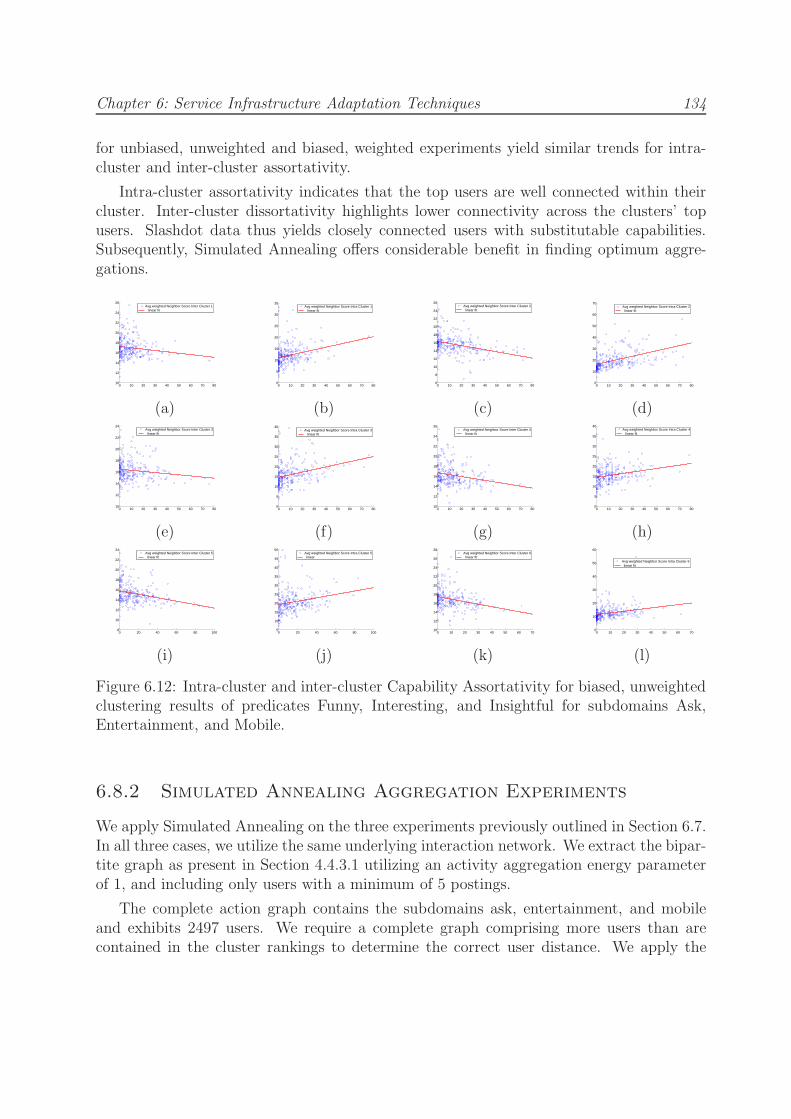
Chapter 6: Service Infrastructure Adaptation Techniques 134
for unbiased, unweighted and biased, weighted experiments yield similar trends for intra-cluster and inter-cluster assortativity.
Intra-cluster assortativity indicates that the top users are well connected within theircluster. Inter-cluster dissortativity highlights lower connectivity across the clusters’ topusers. Slashdot data thus yields closely connected users with substitutable capabilities.Subsequently, Simulated Annealing offers considerable benefit in finding optimum aggre-gations.
0 10 20 30 40 50 60 70 8010
12
14
16
18
20
22
24
26
Avg weighted Neighbor Score Inter Cluster 1 linear fit
0 10 20 30 40 50 60 70 800
5
10
15
20
25
30
35
Avg weighted Neighbor Score Intra Cluster 1 linear fit
0 10 20 30 40 50 60 70 806
8
10
12
14
16
18
20
22
24
26
Avg weighted Neighbor Score Inter Cluster 2 linear fit
0 10 20 30 40 50 60 70 800
10
20
30
40
50
60
70
Avg weighted Neighbor Score Intra Cluster 2 linear fit
(a) (b) (c) (d)
0 10 20 30 40 50 60 70 8010
12
14
16
18
20
22
24
Avg weighted Neighbor Score Inter Cluster 3 linear fit
0 10 20 30 40 50 60 70 800
5
10
15
20
25
30
35
40
Avg weighted Neighbor Score Intra Cluster 3 linear fit
0 10 20 30 40 50 60 70 8010
12
14
16
18
20
22
24
26
Avg weighted Neighbor Score Inter Cluster 4 linear fit
0 10 20 30 40 50 60 70 800
5
10
15
20
25
30
35
40
Avg weighted Neighbor Score Intra Cluster 4 linear fit
(e) (f) (g) (h)
0 20 40 60 80 1008
10
12
14
16
18
20
22
24
Avg weighted Neighbor Score Inter Cluster 5 linear fit
0 20 40 60 80 1005
10
15
20
25
30
35
40
45
50
Avg weighted Neighbor Score Intra Cluster 5 linear
0 10 20 30 40 50 60 7010
12
14
16
18
20
22
24
26
28
Avg weighted Neighbor Score Inter Cluster 6 linear fit
0 10 20 30 40 50 60 700
10
20
30
40
50
60
Avg weighted Neighbor Score Intra Cluster 6 linear fit
(i) (j) (k) (l)
Figure 6.12: Intra-cluster and inter-cluster Capability Assortativity for biased, unweightedclustering results of predicates Funny, Interesting, and Insightful for subdomains Ask,Entertainment, and Mobile.
6.8.2 Simulated Annealing Aggregation Experiments
We apply Simulated Annealing on the three experiments previously outlined in Section 6.7.In all three cases, we utilize the same underlying interaction network. We extract the bipar-tite graph as present in Section 4.4.3.1 utilizing an activity aggregation energy parameterof 1, and including only users with a minimum of 5 postings.
The complete action graph contains the subdomains ask, entertainment, and mobileand exhibits 2497 users. We require a complete graph comprising more users than arecontained in the cluster rankings to determine the correct user distance. We apply the

Chapter 6: Service Infrastructure Adaptation Techniques 135
interaction-based distance metric as we are interested in the focus of joint collaborationbetween users rather than their general involvement in common activities.
6.8.2.1 Aggregation of unbiased, non-weighted clustering results
Selection of top elements across 12 clusters yields a maximum weighted utility xmax = 97.93for a maximum distance distmax = 24.11. The set of top users comprises user 835522, 3x957197, 898314, 2x 912633, 597831, 132727, 238306, 595695, and 655584.
The simulated annealing process reduces the average utility to 90.84 but lowers thedistance even more: dist = 20.65. The optimized set consists of the same members withexception to user 820751 (position 38 with score 32.55) replacing 597831 (position 1 withscore 98.79) in cluster 7. The next best solution considered by the simulated annealingprocess is already the set of top elements.
6.8.2.2 Aggregation of biased, non-weighted clustering results
Biased, non-weighted clustering created six clusters. The best achievable capability ag-gregation consists of users 4x 957197, 238306, and 132727 yielding a utility benefit ofxmax = 74.57 with distance: distmax = 4.79.
Again, Simulated Annealing provides a better tradeoff between distance and utility.The set of users 3x 957197 (Cl1:1, Cl3:1, Cl4:1), 135745 (Cl2:8), 655584 (Cl5:6), 835522(Cl6:2) provides a slightly reduced utility (xagg = 65.31), as considerably reduced distance(dist = 1.23). Cluster membership and ranking position are given in brackets.
Here, adding (and replacing) users provides a better tradeoff than aggregating withfewer users. Simulated Annealing also identifies solutions with a less optimal tradeoff.These solutions either exhibit lower distance (combined with lower utility), or exhibithigher utility (with greater distance). Among the top 20 solutions, distance becomes aslittle 0.48, then generating utility 56.6. For this experiment, no solution (except the topcluster elements) provides better utility than the optimal tradeoff.
6.8.2.3 Aggregation of biased, weighted clustering results
The final clustering experiment highlighted seven clusters for biased, weighted constraints.Best top cluster elements comprise the familiar users of the previous experiments: 132727,4x 957197, 238306, and 835522. The corresponding aggregation yields utility xmax = 84.44at a distance of distmax = 6.07.
The best tradeoff comprises user 957197 for clusters 1 to 6, and user 835522 for theadditional cluster 7. These two users yield an aggregated utility value of 72.84 at distance0.34.
Sieving through the top 20 solutions, we find no aggregations with lower distance butsome with higher utility. These solutions include one aggregation instance additionally

Chapter 6: Service Infrastructure Adaptation Techniques 136
including user 135745 for cluster 2 at rank position 8. It thereby replaces user 957197formerly in cluster 2 at position 35. This combination provides a weighted utility valueof 75.01 but comes with a distance of 0.65. Another combination, albeit with a worsetradeoff, additionally adds users 595695 and 513215 in cluster 5 and 6, respectively. Thisaggregation yields a utility of 73.92 at distance 1.76.
6.8.3 Simulated Annealing Evaluation Summary
Simulated Annealing provides benefit when services with similar capabilities are looselyconnected. We applied the assortativity analysis of he Slashdot data underlying the clus-tering experiments. We found intra-cluster assortativity and inter-cluster dissortativity,subsequently demonstrating the need for Simulated Annealing.
Simulated Annealing found aggregations that provided a better tradeoff between ca-pability utility and distance than the top cluster elements for all of the three clusteringexperiments. The optimal tradeoff found for the unbiased, non-weighted experiment ex-hibited an energy value of 0.97, only a slight improvement over the top cluster elements(which always yield energy 1). We achieved an SA energy value of 0.7 for the biased,non-weighted experiment, and energy 0.62 for the third, biased and weighted clusteringprocess.

Chapter 7
Design and Implementation
7.1 Architecture
The Service Ensemble Adaptation Architecture encapsulates the main capabilities as Webservices. The architecture comprises core services for management, context provisioning,and adaptation of ensemble entities (see Figure 7.1).
The Ensemble Management Services enable modeling and tracking of service capabili-ties (Service Capability Mgmt), organization and structuring of activities (Activity Mgmt),managing of human communication channels (Account Mgmt), and aggregating humansand services according to organizations, teams, or groups (Group Mgmt). Logging com-ponents capture all interactions between core management services and other ensembleentities.
Context Provisioning Services consist of context sensors, context aggregation function-ality, ranking capabilities, and context provisioning endpoints. Logging is the main sourceof raw interaction data. Context Sensors analyze interactions and generate the appropri-ate actions. Context Aggregation determines ensemble-centric metrics. Context Rankingestablishes the relevant set of context for a specific situation and client. Finally, ContextProvisioning supplies push and pull based context updates.
Adaptation Services react to context and ensemble changes. Property Interaction Im-pact determines the significance of impact factors. Ensemble Service Recommender estab-lishes on demand the set of most suitable services to forward a request to given the currentcontext and property impact. Infrastructure Reconfiguration Recommender continuouslytracks ensemble requirements and publishes optimal service changes.
In a service ensemble, it is natural to provide context and adaptation capabilities asWeb services. Exchangeability and composability are amongst the main reasons to applySOA principles also within the adaptation framework. Customized adaptation servicescan provide recommendations tailored to the particular ensemble domain. We are able toaggregate sensor services from different providers, thereby adding new context sources or
137
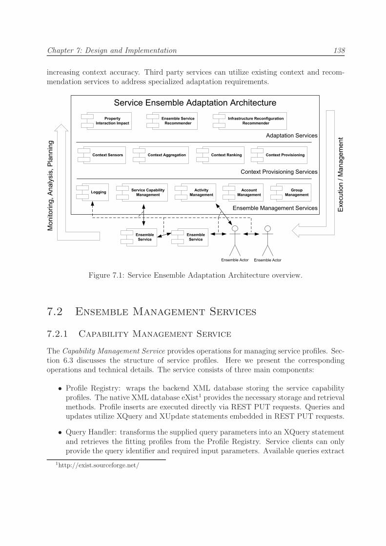
Chapter 7: Design and Implementation 138
increasing context accuracy. Third party services can utilize existing context and recom-mendation services to address specialized adaptation requirements.
Activity
Management
Account
Management
Group
Management
Context RankingContext Aggregation
Service Capability
ManagementLogging
Context Sensors
Adaptation Services
Ensemble Service
Recommender
Context Provisioning
Infrastructure Reconfiguration
Recommender
Ensemble
Service
Ensemble Actor
Service Ensemble Adaptation Architecture
Ensemble
Service
Ensemble Actor
Property
Interaction Impact
Context Provisioning Services
Ensemble Management Services
Monitoring, Analysis, Planning
Execution / Management
Figure 7.1: Service Ensemble Adaptation Architecture overview.
7.2 Ensemble Management Services
7.2.1 Capability Management Service
The Capability Management Service provides operations for managing service profiles. Sec-tion 6.3 discusses the structure of service profiles. Here we present the correspondingoperations and technical details. The service consists of three main components:
• Profile Registry: wraps the backend XML database storing the service capabilityprofiles. The native XML database eXist1 provides the necessary storage and retrievalmethods. Profile inserts are executed directly via REST PUT requests. Queries andupdates utilize XQuery and XUpdate statements embedded in REST PUT requests.
• Query Handler: transforms the supplied query parameters into an XQuery statementand retrieves the fitting profiles from the Profile Registry. Service clients can onlyprovide the query identifier and required input parameters. Available queries extract
1http://exist.sourceforge.net/

Chapter 7: Design and Implementation 139
profiles based on capability identifier and allow refinement by additionally specifyingrequired property identifier, property values, or property value range.
• Change Handler: evaluates profile updates and publishes corresponding change events(Figure 7.2). RepositoryChange events inform about highlevel changes, such as new,changed, or removed profiles. The actual changes are described in the ProfileChangeevent. Notifications are made available via Atom feed, JMS, and WS-Notification.All three types contain the same event format.
The service operations include:
registerService adds a complete service profile to the Profile Registry.
unregisterService removes a complete service profile from the Profile Registry.
updateServiceCategories replaces the existing service category membership.
updateServiceProfile replaces a complete service profile.
updateServiceComponent replaces a complete component within a profile.
updateServiceCapability replaces a complete capability within a component.
queryCapabilities supplies one or more queries (containing query identifier and queryparameters). The operation returns a set of matching service profiles. The serviceclient can configure whether multiple queries within a single query request are treateddisjunctive or conjunctive.
7.2.2 Activity Service
The Activity Service manages data instances of the activity model (introduced in Sec-tion 4.1). It supports structuring of ensemble activities (i.e., goals), and assignment ofroles, resources, artifacts; allows managing of deadlines and tracking of progress. Theservice provides coordination primitives are inspired by (Dustdar 2004). The three majorcomponents are:
• Coordination Handler: manages the structure of activities and handles Delegationrequests. A delegation remains in a user’s Inbox until s/he accepts or rejects thedelegation (using the respective RespondDelegation message). Users are also able tonotify about starting or stopping work on an activity.
• Activity Store: wraps the backend XML-enabled database. We utilize JDBC to con-nect to the IBM DB2 database. The hybrid approach allows us to combine SQL andXQuery statements. Activities create a hierarchy using URIs as references to parent

Chapter 7: Design and Implementation 140
tProfileChangeNewComponent : anyURI [0..*]RemovedComponent : anyURI [0..*]ChangedServiceCategories : anyURI [0..*]«attribute» Source : anyURI
tComponentChangeNewCapability : anyURI [0..*]RemovedCapability : anyURI [0..*]«attribute» ComponentURI : anyURI
ChangedComponent0..*
tCapabilityChangeNewProperty : anyURI [0..*]RemovedProperty : anyURI [0..*]«attribute» CapabilityURI : anyURI
ChangedCapability0..*
tSelectableCapabilityChangeNewAlternative : anyURI [0..*]RemovedAlternative : anyURI [0..*]«attribute» CapabilityURI : anyURI
SelectableCapability0..*
tPropertyChange«any, element» wildcard«attribute» PropertyURI : anyURI
ChangedProperty0..*
tRepositoryChangeNewServiceProfile : anyURI [0..*]ChangedServiceProfile : anyURI [0..*]RemovedServiceProfile : anyURI [0..*]«attribute» RepositoryURI : anyURI
Figure 7.2: Capability Change model UML class diagram
and child activities. Subsequently, each activity instance populates a separate rowin the database. SQL provides recursive iteration techniques to retrieve a completeactivity subtree (see Listing 7.1). We limit XML content in the database to the ac-tual activity data. Additional metadata for managing historical and deleted activityinstances remain as regular SQL columns (e.g., Listing 7.1 line 5: ISDELETED orline 6: ISNEWEST).
• Query Handler: accepts a reference to a query and the corresponding query inputencoded as XML. The Query Handler retrieves the query from the Query service (ifnot already cached) and replaces the placeholders in the query with the parametersfrom the query input. As context sensors and context clients make most use ofthe Query service, we provide details and design rationale in the next subsection.Three default queries enable retrieval of (i) all activities a user is involved in, (ii) allactivities within an activity subtree, and (iii) all activities delegated to but not yetaccepted by a particular user.
The Activity service supports following operations:
addActivities accepts multiple new activities at the same time. The client can providedifferent Activity subclasses within the same request. The service creates activityidentifiers upon successful storage. Consequently, the set of new activities withina request can refer only to stored activities, but cannot establish a tree structurethemselves. This has to be done using setDetails and addDetails operations.
setDetails manipulates all single-valued properties such as name, description, parent, orstart. The service overwrites all such properties, thus a clients need to provide alsoproperties that haven’t changed.

Chapter 7: Design and Implementation 141
addDetails affects only multi-valued properties such as tags, childActivities or member-Involvements. The provided activity instance needs to include only the difference(i.e., the added details). The service adds the provided properties to the set of exist-ing properties. Duplicate entries are removed, thus any tag, child activity, or resourceoccurs at maximum once.
removeDetails is the inverse operation to addDetails. The operation will remove allmulti-valued properties provided from the activity instance in the database.
deleteActivities marks the corresponding activities as deleted in the database, thus be-coming inactive. An Activity having active child activities cannot be removed.
getActivities returns all activities identified by their URI.
queryActivities retrieves the referenced query and inserts the provided query param-eters. Activities marked as deleted will not turn up in the result set unless thequery explicitly addresses deleted activities. The service supports only one query perrequest.
delegateActivity requests to change the responsible member(s) of an activity. A del-egation request consist of sender, receivers, activity identifier, and delegation type.The delegation type determines if the receiver is just a normal Delegate replacingthe sender, or a DelegateSplit to clone the delegated activity for each receiver, or aDelegateJoint to divide responsibility amongst multiple members.
respondDelegation indicates the acceptance or refusal to take over responsibility. Foraccepted delegations, the service updates the activity by replacing the responsibleperson. The formerly responsible person becomes an observer.
notifyWork informs involved members and services about an person starting or stoppingwork.
7.2.3 Context Coupling Mechanisms
Ensemble services require context information to adapt to the user, activity, and overallensemble. A service client is unlikely to know which context the service provider requires.It merely invokes the service which has to retrieve the required context by itself. Asservice clients potentially assume multiple roles within an ensemble, retrieval of the relevantcontext information becomes challenging.
Context coupling mechanisms provide a correlation of service invocations to client con-text. The client context includes the context changes of previously invoked services. Anewly invoked service receives the context correlation information to adapt to the relevantcontext. Figure 7.3 outlines this process. Correlation information consists of activity URIand user URI. The basic coupling steps are:

Chapter 7: Design and Implementation 142
1 WITH RAL (URI , ACTIVITYXML ) AS
2 ( SELECT ROOT.URI , ROOT.ACTIVITYXML
3 FROM $SCHEMA .ACTIVITY ROOT
4 WHERE
5 ROOT.ISDELETED = 0
6 AND ROOT.ISNEWEST = 1
7 AND xmlexists (’declare default element namespace
8 "http :// www.in -context .eu/ns/activity ";
9 $c/tActivity [ ParentActivity="$id "]’
10 passing ROOT. ACTIVITYXML as "c")
11 UNION ALL
12 SELECT CHILD.URI , CHILD .ACTIVITYXML
13 FROM RAL PARENT , $SCHEMA .ACTIVITY CHILD
14 WHERE
15 CHILD .ISDELETED = 0
16 AND CHILD.ISNEWEST = 1
17 AND xmlexists (’declare default element namespace
18 "http :// www.in -context .eu/ns/activity ";
19 $f/tActivity [ ParentActivity=$d]’
20 passing CHILD .ACTIVITYXML as "f",
21 PARENT .URI as "d")
22 )
23 SELECT URI , ACTIVITYXML FROM RAL
Listing 7.1: Recursive retrieval of sub activities within a activity hierarchy, starting atactivity URI ”$id”
Correlation Management consists of identifying the ensemble actor, and selecting thedesired activity. Composite services pass the correlation information they have ini-tially received to their embedded service client.
Correlation Establishment occurs when the client-side context coupling handler addsuser and activity identifier to the SOAP header of the outgoing service invocation.Listing 7.2 contains an example SOAP message with activity and user references inthe context coupling SOAP header extension.
Access Layer acts as transparent HTTP proxy, producing a copy of every SOAP requestand reply. Each copy is passed to the Logging Service.
Logging Service provides a subscription interface. Every subscriber receives a copy ofSOAP messages encapsulated in an interaction event (see Table 7.1). The next sectiondetails how context sensors subsequently generate context information.
Correlation Extraction The service-side handler extracts the correlation informationfrom the inbound SOAP message. The service utilizes the references as entry pointsfor accessing the actual context via the Context Retrieval services.
Most of the ensemble management services are part of the Pervasive CollaborationService Architecture (PCSA) devised in the inContext project 2. We designed and im-plemented the Activity Management Service and the Capability Management Service and
2http://www.in-context.eu
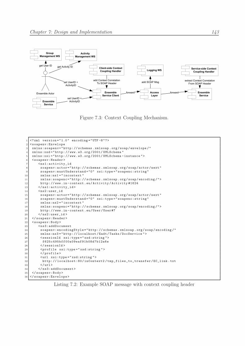
Chapter 7: Design and Implementation 143
Activity
Management WS
Ensemble Actor
Group
Management WS
Ensemble
Service Client
Ensemble
Service
Client-side Context
Coupling HandlerService-side Context
Coupling Handler
Access
Layerforward forward
Ensemble
Service
get User ID get Activity ID
set UserID +
ActivityID
set UserID +
ActivityID
add Context Correlation
To SOAP Headerextract Context Correlation
From SOAP Header
Logging WS
add SOAP Msg
Figure 7.3: Context Coupling Mechanism.
1 <?xml version ="1.0 " encoding ="UTF -8"?>
2 <soapenv:Envelope
3 xmlns:soapenv="http: // schemas .xmlsoap .org/soap/envelope /"
4 xmlns:xsd ="http: //www.w3.org /2001/ XMLSchema "
5 xmlns:xsi ="http: //www.w3.org /2001/ XMLSchema -instance ">
6 <soapenv:Header>
7 <ns1:activity_id
8 soapenv:actor="http: // schemas .xmlsoap .org/soap/actor/next"
9 soapenv:mustUnderstand ="0" xsi:type ="soapenc:string"
10 xmlns:ns1 ="incontext "
11 xmlns:soapenc="http: // schemas .xmlsoap .org/soap/encoding /">
12 http: //www .in -context .eu/ Activity /Activity #1624
13 </ ns1:activity_id>
14 <ns2:user_id
15 soapenv:actor="http: // schemas .xmlsoap .org/soap/actor/next"
16 soapenv:mustUnderstand ="0" xsi:type ="soapenc:string"
17 xmlns:ns2 ="incontext "
18 xmlns:soapenc="http: // schemas .xmlsoap .org/soap/encoding /">
19 http: //www .in -context .eu/User/User#7
20 </ ns2:user_id >
21 </ soapenv:Header>
22 <soapenv:Body>
23 <ns3:addDocument
24 soapenv:encodingStyle ="http: // schemas .xmlsoap .org/soap/encoding /"
25 xmlns:ns3 ="http: // localhost /Eadt/Tasks/DocService ">
26 <sessionId xsi:type ="xsd:string ">
27 f625c495bff00a09eaf91b08d7b12a6e
28 </sessionId >
29 <profile xsi:type =" xsd:string ">
30 </profile >
31 <url xsi:type ="xsd:string ">
32 http: // localhost:80/inContext2 /tmp_files_to_transfer /EC_link .txt
33 </url >
34 </ ns3:addDocument>
35 </ soapenv:Body>
36 </soapenv:Envelope >
Listing 7.2: Example SOAP message with context coupling header

Chapter 7: Design and Implementation 144
Property DescriptionclientIP the IP address of the service clientmessageType request or responsemessageCorrelationID for correlating request and response messagesserviceEndpoint the service endpoint addresssourceID the address of the Access Layer having intercepted the messagetimestamp the time at invocationuserURI the invoking user on behalf of which a service client is actingconsumerID the service client, which is invoking the actual service operationmessage a copy of the SOAP message
Table 7.1: Interaction Event properties.
participated in the development of the components enabling the context coupling process.Specifically, project deliverables D5.2 (inContext Consortium 2007b) and D5.3 (inContextConsortium 2007a) provide implementation details on the Account Management service,Group Management service (aka. Team Service and Team Management Service), andAccess Layer. Deliverable D4.2v2 (Casella, Dorn, Polleres, and Yi 2008) provides moreinformation on the context coupling SOAP header, while D2.2v2 (Dorn, Polleres, and Yi2008) discusses Logging service specific details.
7.3 Context Provisioning Services
The context provisioning process (Figure 7.4) commences with incoming SOAP logs at theLogging Subscriber Web service, subsequently distributed to the various Context Sensors.The sensors apply the Ensemble Management services to reason about the service invoca-tions before submitting context updates. The Query and Update Store Service providesthe detailed structure of context updates and queries. Metric Definitions describes whichensemble metrics the Ensemble Context Aggregation Service should calculate, and whichmetrics are available for subscription at the Metric Change Publisher Service. The Inter-action Graph Manager maintains distance measurements. The Context Ranking Serviceselects the most relevant context data given a set of context correlation identifiers whilethe Context Retrieval Service provides specific on-demand context information.
7.3.1 Context Sensing and Aggregation
The Logging Subscriber Service subscribes at the Logging Service. Upon receiving a newinteraction event, it extracts the service operation from the SOAP message before passingthe event to interested sensors. The main purpose of context sensors is transformingthe incoming raw SOAP message to raw action events. Where required, they access theensemble management services to obtain additional information. An email sensor, for
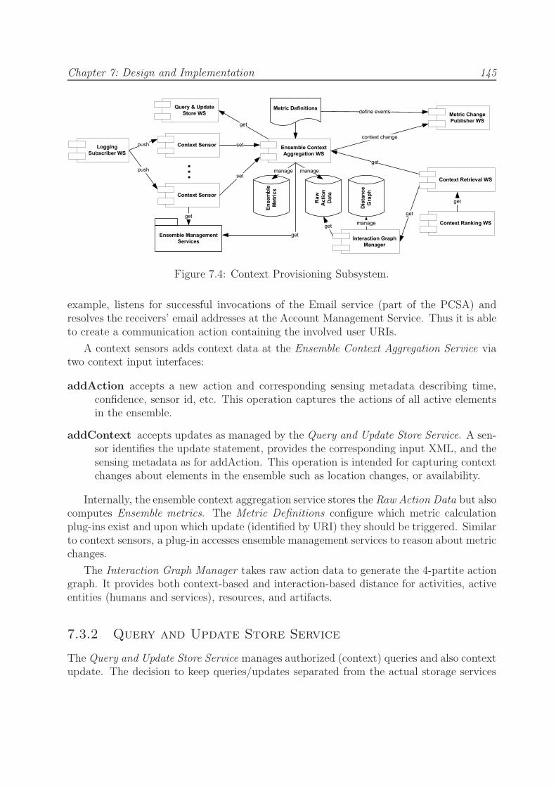
Chapter 7: Design and Implementation 145
Context Ranking WS
Ensemble Context
Aggregation WS
Logging
Subscriber WS
Context Sensor
Context Retrieval WS
Context Sensor
Ensemble Management
Services
Raw
Acti
on
Data
En
sem
ble
Metr
ics
get
Metric Change
Publisher WS
Metric Definitions
Interaction Graph
Manager
Dis
tan
ce
Gra
ph
push
push
set
context change
set
define events
get
get
get
getmanage
manage manage
get
Query & Update
Store WS
get
...
Figure 7.4: Context Provisioning Subsystem.
example, listens for successful invocations of the Email service (part of the PCSA) andresolves the receivers’ email addresses at the Account Management Service. Thus it is ableto create a communication action containing the involved user URIs.
A context sensors adds context data at the Ensemble Context Aggregation Service viatwo context input interfaces:
addAction accepts a new action and corresponding sensing metadata describing time,confidence, sensor id, etc. This operation captures the actions of all active elementsin the ensemble.
addContext accepts updates as managed by the Query and Update Store Service. A sen-sor identifies the update statement, provides the corresponding input XML, and thesensing metadata as for addAction. This operation is intended for capturing contextchanges about elements in the ensemble such as location changes, or availability.
Internally, the ensemble context aggregation service stores the Raw Action Data but alsocomputes Ensemble metrics. The Metric Definitions configure which metric calculationplug-ins exist and upon which update (identified by URI) they should be triggered. Similarto context sensors, a plug-in accesses ensemble management services to reason about metricchanges.
The Interaction Graph Manager takes raw action data to generate the 4-partite actiongraph. It provides both context-based and interaction-based distance for activities, activeentities (humans and services), resources, and artifacts.
7.3.2 Query and Update Store Service
The Query and Update Store Service manages authorized (context) queries and also contextupdate. The decision to keep queries/updates separated from the actual storage services

Chapter 7: Design and Implementation 146
Property Descriptionidentifier the unique identifier for the query/updatehumanReadableName a short name describing the query/updatehumanReadableDescription a longer description on how the query is used and what it
doesinputXSD specifies the XML schema, which describes the format of
the required XML inputinputExampleXML a sample XML input to be supplied by the query/update
invokerstatement the query/update statement interpreted by the query/up-
date engine together with the XML inputresultXSD specifies the format of the returned XML resultoutputExampleXML an example output
Table 7.2: Query/Update object.
(e.g., Activity Service, Ensemble Context Aggregation Service) enables a simple, staticservice interface. Queries and Updates can be added and removed as required withouthaving to change the services interface description. Service clients need not know thedetails of the query language which comes with following advantages:
1. Design and testing of queries is done by an expert familiar with the ensemble con-text model. This reduces the number of inefficient, incorrect, privacy infringing, orcomputationally complex queries.
2. Reuse of existing queries simplifies the process of writing new ones. Additionally,a known set of input and output XML schemas facilitate the provisioning of queryinput and processing of result data on the consumer side.
3. Service providers can validate the provided input XML.
4. Any changes to the context model can be evaluated against the necessary alterationsof update and query statements, thus simplifying change management.
5. Context sensors do not need to know the details of the update language.
Table 7.2 provides the query/update object properties. It contains all information requiredduring design-time to create queries/updates. During runtime the invoked service (e.g.,Activity Service) retrieves only the statement part. The example query statement inListing 7.3 returns all activities that have an artifact of given artifact type and givenresource reference. The first passing input statement declares that the placeholder $typein the query template is to be replaced with the value of the XPath statement executedon the provided input XML.

Chapter 7: Design and Implementation 147
1 <?xml version ="1.0 " encoding ="UTF -8" standalone ="yes"?>
2 <TXQueryTemplate xmlns="http: //www.in-context .eu/ns/contextquery">
3 <QueryStmt >
4 SELECT $SCHEMA .ACTIVITY .ACTIVITYXML
5 FROM $SCHEMA .ACTIVITY
6 WHERE $SCHEMA .ACTIVITY .ISDELETED = 0
7 AND $SCHEMA .ACTIVITY .ISNEWEST = 1
8 AND xmlexists (’declare default element namespace
9 "http: //www .in -context .eu/ns/activity " ;;
10 $c/tActivity / EditArtifacts[ WrapsResourceURI=& quot;$ref "
11 and ResourceType=& quot;$ type" ;]’
12 passing $SCHEMA .ACTIVITY . ACTIVITYXML as "c")
13 </QueryStmt >
14 <PassingInput
15 Placeholder ="$type"
16 InputXPathStatement ="/ ArtifactQuery[1]/ ResourceType/text ()"/>
17 <PassingInput
18 Placeholder ="$ref"
19 InputXPathStatement ="/ ArtifactQuery[1]/ ResourceRef /text()"/>
20 </TXQueryTemplate >
Listing 7.3: Example Query statement for retrieving activities that have an artifact ofgiven resource type and given resource reference
7.3.3 Context Retrieval
The Context Retrieval Service is the main source of on-demand context information. Itprovides two operations:
getAction accepts a query URI and corresponding input XML. The result is a set ofactions.
getContext takes the same input parameters as getAction but returns an XML string asdefined by the output schema of the corresponding query object.
Clients should use the Context Ranking Service when multiple context informationinstances (e.g., multiple Storage Services) occur in the ensemble. The context rankingservice determines the most relevant ones given the user and activity identifier. Specifically,it provides following operations:
getRankedContext requires user and activity URI, a reference to a context query, thecorresponding XML input, the maximum number of top ranked context elements,and whether to include the actions in which the desired entity was involved in. Theoperations returns a list of context resources (each as defined by the query) and thecorresponding rank.
getRankedContextURIs accepts the same input parameters as getRankedContext, dif-fering only in the format of the response message. This operation provides only theURI of the context object, rather than the complete representation.

Chapter 7: Design and Implementation 148
The Metric Change Publisher Service offers a subscription endpoint for ensemble metricupdates. The example subscription in Listing 7.4 expects notifications when the PropertyDistribution Entropy for location drops below 0.33 in ensemble Test1. The publisherservices utilizes WS-Notification for delivering the metric events.
1 <?xml version ="1.0 " encoding ="UTF -8" standalone ="yes"?>
2 <MetricSubscription xmlns="http: //www.in-context .eu/ns/contextquery">
3 <ThresholdType>
4 http: //www .in -context .eu/ns/EnsembleMetrics/ threshold_lowerbound
5 </ ThresholdType>
6 <EnsembleURI >
7 http: //www .vitalab .tuwien .ac.at/projects /taaf/Ensemble #Test1
8 </ EnsembleURI >
9 <MetricURI >
10 http: //www .in -context .eu/ns/EnsembleMetrics/PDE#Location
11 </MetricURI >
12 <Threshold >
13 0.33
14 </Threshold >
15 <NotificationEndpoint >
16 ... [WS -Addressing Endpoint Reference ] ...
17 </ NotificationEndpoint >
18 </MetricSubscription >
Listing 7.4: Ensemble metric subscription example
7.3.4 Mobile Context Provisioning
The ensemble management service and other context provisioning service run on standardserver hardware. The mobil context provisioning components target mobile devices suchas PDAs, smartphones, and laptops. The OSGi 3 specification describes a JAVA basedcontainer environment for devices with limited memory and processing power.
OSGi exhibits service-like properties. Components are deployed as bundles that aredynamically updated, found, bound, and invoked. Knopflerfish4 is the OSGi implementa-tion of our choice. It comes with Web service support, thereby exposing specific bundlesas Web services.
The mobile context provisioning subsystem (Figure 7.5) consists of several OSGi bun-dles. The Context Event Publisher and Context Event Subscriber are exposed as Webservices. The former provides context events to interested remote clients. The latter sub-scribes for context events at remote context provisioning subsystems. Multiple mobilecontext provisioning subsystems thus form a peer-to-peer network.
Internally, the Event Manager takes context events from local Context Sensor Bundlesand updates the Mobile Context Store as well as the event publishing bundle. The eventmanager also accepts incoming remote context events and merges them with the localcontext database.
3Open Service Gateway Initiative: http://www.osgi.org4http://www.knopflerfish.org/index.html

Chapter 7: Design and Implementation 149
The Subscription Manager triggers remote subscriptions when the local context storedoes not contain the data requested by the local Context Query Bundle. This bundle servescontext to the remaining bundles within the local OSGi container.
Subscription Manager
Mobile
Context
Store
getsubscribe Remote
Context Event
Publisher WS
Context Event
Subscriber WS
Context Sensor
Bundles
Context Query
Bundle
Event Manager
remote Context Events
manage
retrieve
local Context Events
local Context Events
Figure 7.5: Mobile Context Provisioning subsystem.
7.4 Adaptation Services
Adaptation services rely upon context change events, especially ensemble metric updates.Figure 7.6 outlines the Property Impact Evaluation subsystem, and Figure 7.7 displays theInfrastructure Adaptation subsystem.
7.4.1 Property Impact Evaluation
The Metric Change Subscriber observes property-specific metric updates. The MetricDefinitions specify which properties get monitored in the ensemble. The Property ImpactPotential component calculates the possible impact of the changed property distribution.It subsequently configures the Property Impact Evaluation component with respect to theproperties it should focus its interaction analysis on. In regular intervals, the PropertyImpact Evaluation component retrieves aggregated interaction data from the ensemblecontext services. Subsequently, it stores the actual interaction impact in the PropertyImpact Trends database.
When an ensemble service client invokes the Ensemble Service Recommender Service,it accesses the database to establish the best ranking for the invoking client. The ensemblemanagement services provide the required data on the client’s and neighboring services’property values. The Ensemble Service Recommender Service supports two operations:

Chapter 7: Design and Implementation 150
getRankedServices takes the identifiers of the invoking client and the set of servicesthat should be ranked. The identifiers enable extraction of the respective serviceproperties from the ensemble management services. Finally, the operation returns aranking score for each service.
getRankedPersons applies the same techniques as getRankedService but works withinteractions of and properties about human ensemble entities.
Property impact trends are also directly available via the Property Impact ProvisioningService. It provides two operations:
getImpact accepts a property identifier and returns the corresponding impact matrixlisting the impact between any two property values.
getImpactForValue limits the returned impact result to a particular row in the impactmatrix (defined by property value identifier).
Metric Change
Subscriber
Ensemble Service
Recommender WS
Property
Impact Potential
Ensemble Context
Services
Property
Impact Evaluation
Pro
pert
y
Impact
Tre
nds
Property Impact
Provisioning WS
get Interaction Data
getnotify
set
Metric
Definitions
define events
get
trigger
Ensemble Management
Services
get
define property identifiers and corresponding values
Figure 7.6: Property Impact Evaluation Subsystem.
7.4.2 Infrastructure Adaptation
Subscriptions to metric changes and capability changes provide the underlying data forinfrastructure adaptation. Based on these events, the Requirements Tracking componentapplies the JBoss rule system (DROOLS 5) to generate requirements. Listing 6.1 con-tains an example rule triggered upon changes in the location-centric property distributionentropy (ensemble location entropy: ELE).
Requirements that remain unfulfilled by the current ensemble configuration trigger anew instance of requirements matching. When requirements clustering provides sufficient
5http://www.jboss.org/drools/

Chapter 7: Design and Implementation 151
Capability Change
Subscriber
Metric Change
Subscriber
Simulated Annealing
Infrastructure Reconfiguration
Recommendation Publisher WS
Metric
Definitions
Requirements
Rule Files
Requirements TrackingRequirements Matching
& Clustering
Ensemble
Configuration
Ensemble Context
Services
notify
get
get
trigger
trigger
agglomerate
define events
insert
Ensemble Configuration WSget
Figure 7.7: Infrastructure Adaptation Subsystem.
benefit, Simulated Annealing retrieves the interaction network from the ensemble contextservices. The Infrastructure Reconfiguration Recommendation Publisher Service providesa subscription interface for reconfiguration events. These events (Figure 7.8) contain alist of unfulfilled requirements (RequirementRef ) and a set of recommended services, re-spectively persons. For each service, the event specifies the requirement fulfillment score(EntityMembership) in each cluster. For multi-cluster requirements, the event also includesthe top composition (Agglomerations) with the best trade-off between interaction distanceand joint requirements fulfillment (Tradeoff ). For single-cluster results, all requirementsremain in the same cluster (Scope).
Details on all current requirements and service configurations remain in the EnsembleConfiguration database, accessible via the Ensemble Configuration Service. Figure 7.9visualizes the ensemble configuration UML class diagram.

Chapter 7: Design and Implementation 152
tReconfigurationRecommendationRequirementRef : anyURI [1..*]«attribute» EnsembleURI : anyURI
tRequirementsFulfillment«attribute» ClusterNr : int«attribute» ClusterWeight : decimal [0..1]
Scope1..*
tAgglomeration«attribute» Energy : decimal
Tradeoff0..*
tClusterMembershipRequirementURI : anyURIClusterMembership : double
Member0..*
tEntityMembershipEntityURI : anyURIClusterNr : int«attribute» Score : decimal [0..1]
Element1..*
Figure 7.8: Ensemble Reconfiguration Recommendation model UML class diagram.
tEnsembleServiceConfig«attribute» EnsembleURI : anyURI
tServiceConfigUsedForRequirementsServiceCategory : tActionCategory«attribute» ServiceProfileURI : anyURI«attribute» ComponentURI : anyURI
ProvidedService0..*
tCapabilityConfigSelectableCapabilityType : anyURISelectedChoice : anyURI
CapabilityConfig0..*
tRequirementMatchRequirementsRef : anyURIMatch : t0to1Membership : t0to1
RequirementsMatch0..*
tEnsembleRequirements«attribute» EnsembleURI : anyURI
tRequirementSetRestrictedToServiceCategory : tActionCategory
RequirementsSet0..*
tRequirementCapabilityType : anyURIImportance : tMinus1toPlus1«attribute» RequirementURI : anyURI [0..1]«attribute» UtilFctId : anyURI«attribute» UtilFctTypeId : anyURI
Requirement0..*
tCapabilityExistsRequirementSelectionParameter : t0to1
tPropertyValueRequirement«attribute» PropertyType : anyURI
tCapabilitySelectionRequirementSelectionParameters : string [0..*]
tSimpleStringConstraintSelectionParameters : string [1..*]
tSimpleTimestampConstraintSelectionParameters : dateTime [1..*]
tSimpleIntConstraintSelectionParameters : integer [1..*]
tSimpleBoolConstraintSelectionParameters : boolean [1..*]
tSimpleDecimalConstraintSelectionParameters : decimal [1..*]
Figure 7.9: Ensemble configuration model UML class diagram

Chapter 8
Conclusions
In this thesis we have investigated adaptation techniques for large-scale service ensembles.We highlighted in the problem statement that adaptation has to address the requirementsof the overall ensemble, not merely the needs of individual humans or services. Our fun-damental findings in this thesis are:
1. Ensemble adaptation combines suitable techniques at the level of service composition,service selection, and service behavior.
2. Adaptation techniques at the infrastructure level apply ensemble metrics to determineensemble requirements. Matching requirements against deployed service capabilitiesreveals the demand for adaptation.
3. Efficient and effective composition trades off requirements fulfillment and compositioncosts. Composition costs derive from the interaction structure of ensemble entities.
4. Adaptation at the service selection level exploits service interaction patterns to de-termine influential service properties. These service properties determine suitableneighboring services to collaborate with.
5. Service behavior adaptation techniques rely on the most relevant context informa-tion. Context ranking requires distance metrics that describe the similarity betweenensemble entities. These distance metrics must take into account the underlyingensemble structure.
These ensemble adaptation principles have been applied to our main contributions:
1. We developed a framework for ensemble infrastructure adaptation. Ensemble metrics,rules, requirements, and capabilities are the fundamental building blocks for theadaptation process.
153

Chapter 8: Conclusions 154
2. Our biased fuzzy clustering algorithm groups requirements according to availableservice capabilities. More important requirements and better suited services yieldmore impact on the clustering result than less important requirements and less suitedservices.
3. We applied Simulated Annealing to achieve a trade-off between maximal requirementsfulfillment and minimal composition costs. Experiments on real-world interaction andrating data from an online discussion forum demonstrate the benefit of requirementsclustering and achieve a successful trade-off between fulfillment and costs.
4. The self-adjusting service recommendation algorithm analyzes the impact of serviceproperties on interaction patterns. Properties that correspond to significant trendsof service invocations enable service newcomers to communicate with the most suit-able services. Experiments on a simulated service ensemble proof scalability andadaptiveness.
5. The Property Distribution Entropy measures the property distribution across servicesin the ensemble and highlights those of potential high impact.
6. Context distance metrics establish the relevant context for a given situation. We in-troduced a context-centric distance metric, and an interaction-centric distance metric.Experiments on real-world interaction data from an online discussion forum show thatthe interaction-centric metric is more sensitive to changes than the context-centricmetric.
7. The context model describes persons, services, activities, artifacts, resources, andtheir interactions in a service ensemble.
This work has investigated the first set of adaptation techniques. Many new researchquestions arise from this thesis. Specifically, following research aspects provide interestingfuture work:- The current ensemble context model lacks the explicit notion of temporal flows. Althoughactions and activities include timestamps and deadlines, the current algorithms do notexploit the temporal order of events beyond the simple aging function applied by thedistance metric.- The underlying models and algorithms analyze the interdependencies between directlyinteracting ensemble elements. We expect interesting results from extending this analysisto short chains of interacting ensemble entities.- The service selection algorithm considers interaction data from all services as equallyimportant. We envision the integration of additional aspects such as reputation and localpolicies.- From an engineering point of view, interesting future work includes investigations on howto realize autonomic, decentralized ensemble composition enactment. Such work could pickup at the ensemble reconfiguration recommendations and advance the current framework.This would provide novel protocols to coordinate the adaptation plans.

References
Alava, M. J. and S. N. Dorogovtsev (2005). Complex networks created by aggregation.Physical Review E 71, 036107.
Albert, R. and A.-L. Barabasi (2002). Statistical mechanics of complex networks. Reviewsof Modern Physics 74, 47.
Albert, R., H. Jeong, and A.-L. Barabasi (1999). The diameter of the world wide web.CoRR cond-mat/9907038.
Amundsen, S. L. and F. Eliassen (2008). A resource and context model for mobilemiddleware. Personal Ubiquitous Comput. 12 (2), 143–153.
Anagnostopoulos, C., P. Mpougiouris, and S. Hadjiefthymiades (2005). Prediction intel-ligence in context-aware applications. In MEM ’05: Proceedings of the 6th interna-tional conference on Mobile data management, New York, NY, USA, pp. 137–141.ACM Press.
Andreolini, M., S. Casolari, and M. Colajanni (2008, Oct.). Autonomic request man-agement algorithms for geographically distributed internet-based systems. In Self-Adaptive and Self-Organizing Systems, 2008. SASO ’08. Second IEEE InternationalConference on, pp. 171–180.
Artz, D. and Y. Gil (2007). A survey of trust in computer science and the semantic web.Web Semant. 5 (2), 58–71.
Babaoglu, O., G. Canright, A. Deutsch, G. A. D. Caro, F. Ducatelle, L. M. Gambardella,N. Ganguly, M. Jelasity, R. Montemanni, A. Montresor, and T. Urnes (2006). De-sign patterns from biology for distributed computing. ACM Trans. Auton. Adapt.Syst. 1 (1), 26–66.
Babaoglu, O., M. Jelasity, and A. Montresor (2004). Grassroots approach to self-management in large-scale distributed systems. In UPP, pp. 286–296.
Baldauf, M., S. Dustdar, and F. Rosenberg (2007). A Survey on Context-Aware Systems.International Journal of Ad Hoc and Ubiquitous Computing 2 (4), 263–277.
Barabasi, A. and R. Albert (1999). Emergence of scaling in random networks. Sci-ence 286, 509–512.
155

REFERENCES 156
Barabasi, A.-L. (2005). SOCIOLOGY: Network Theory-the Emergence of the CreativeEnterprise. Science 308 (5722), 639–641.
Bardram, J. E. (2005, July). Activity-Based Computing: Support for Mobility andCollaboration in Ubiquitous Computing. Personal and Ubiquitous Computing 9 (5),312–322.
Baresi, L., D. Bianchini, V. D. Antonellis, M. G. Fugini, B. Pernici, and P. Plebani(2003, September). Context-aware composition of e-services. In TES, pp. 28–41.
Bazire, M. and P. Brezillon (2005, July). Understanding context before using it. In Mod-eling and Using Context: 5th International and Interdisciplinary Conference CON-TEXT 2005, pp. 29–41.
Belotti, R., C. Decurtins, M. Grossniklaus, M. C. Norrie, and A. Palinginis (2004, June).Modelling context for information environments. In Ubiquitous Mobile Informationand Collaboration Systems: Second CAiSE Workshop, UMICS 2004, pp. 43–56.
Bezdek, J. C. (1981). Pattern Recognition with Fuzzy Objective Function Algorithms.Norwell, MA, USA: Kluwer Academic Publishers.
Biegel, G. and V. Cahill (2004, March). A framework for developing mobile, context-aware applications. In Second IEEE Annual Conference on Pervasive Computing andCommunications, 2004. PerCom 2004, pp. 361–365.
Bigus, J. P., D. A. Schlosnagle, J. R. Pilgrim, W. N. Mills, and Y. Diao (2002). Able: Atoolkit for building multiagent autonomic systems. IBM Systems Journal 41 (3).
Bird, C., A. Gourley, P. Devanbu, M. Gertz, and A. Swaminathan (2006). Mining emailsocial networks. In MSR ’06: Proceedings of the 2006 international workshop onMining software repositories, New York, NY, USA, pp. 137–143. ACM Press.
Birukou, A., E. Blanzieri, V. D’Andrea, P. Giorgini, and N. Kokash (2007, Nov.-Dec.).Improving web service discovery with usage data. Software, IEEE 24 (6), 47–54.
Bollobas, B. (2001). Random Graphs. Cambridge University Press.
Bottaro, A. and R. Hall (2007). Dynamic Contextual Service Ranking, Chapter SoftwareComposition, pp. 129–143. Lecture Notes in Computer Science. Springer.
Brin, S. and L. Page (1998). The anatomy of a large-scale hypertextual web searchengine. Computer Networks and ISDN Systems 30 (1-7), 107–117. Proceedings of theSeventh International World Wide Web Conference.
Bryl, V. and P. Giorgini (2006). Self-configuring socio-technical systems: Redesign atruntime. ITSSA 2 (1), 31–40.
Buetow, K. H. (2005). Cyberinfrastructure: Empowering a ”Third Way” in BiomedicalResearch. Science 308 (5723), 821–824.
Casati, F., M. Castellanos, U. Dayal, and M.-C. Shan (2004). Probabilistic, context-sensitive, and goal-oriented service selection. In ICSOC ’04: Proceedings of the 2nd

REFERENCES 157
international conference on Service oriented computing, New York, NY, USA, pp.316–321. ACM.
Casella, G., C. Dorn, A. Polleres, and H. Yi (2008). Design and implementation of acontext tunnelling extension - version 2. Technical report, inContext Consortium.
Chen, G. and D. Kotz (2002, June). Solar: An open platform for context-aware mo-bile applications. In First International Conference on Pervasive Computing (ShortPaper), pp. 41–47.
Chen, H., T. Finin, and A. Joshi (2003). An ontology for context-aware pervasive com-puting environments. Special Issue on Ontologies for Distributed Systems, KnowledgeEngineering Review 18 (3), 197–207.
Chen, Y., D. Bindel, H. H. Song, and R. H. Katz (2007). Algebra-based scalable overlaynetwork monitoring: algorithms, evaluation, and applications. IEEE/ACM Trans.Netw. 15 (5), 1084–1097.
Chintalapudi, K. and M. Kam (1998, May). A noise-resistant fuzzy c means algorithmfor clustering. Fuzzy Systems Proceedings, 1998. IEEE World Congress on Compu-tational Intelligence., The 1998 IEEE International Conference on 2, 1458–1463.
Colman, A. (2007). Exogeneous management in autonomic service compositions. InICAS ’07: Proceedings of the Third International Conference on Autonomic andAutonomous Systems, Washington, DC, USA, pp. 25. IEEE Computer Society.
Cormen, T. H., C. E. Leiserson, R. L. Rivest, and C. Stein (2001). Dijkstra’s algorithm.In Introduction to Algorithms 2nd edition, Chapter 24. MIT Press.
Costa, P. D., L. F. Pires, M. van Sinderen, and J. P. Filho (2004, April). Towards aservice platform for mobile context-aware applications. In 1st International Workshopon Ubiquitous Computing - IWUC 2004, pp. 48–61.
da Rocha, R. C. A. and M. Endler (2006). Context management in heterogeneous,evolving ubiquitous environments. IEEE Distributed Systems Online 7 (4).
de Freitas and da Graca (2005). Toward a domain-independent semantic model forcontext-aware computing. pp. 10 pp.+.
Desai, N., P. Mazzoleni, and S. Tai (2007, Feb.). Service communities: A structuringmechanism for service-oriented business ecosystems. pp. 122–127.
Dey, A. and G. Abowd (2000, April). Towards a better understanding of context andcontext-awareness. In Workshop on the What, Who, Where, When, and How ofContext-Awareness at CHI 2000.
Di Nitto, E., C. Ghezzi, A. Metzger, M. Papazoglou, and K. Pohl (2008). A jour-ney to highly dynamic, self-adaptive service-based applications. Automated SoftwareEngg. 15 (3-4), 313–341.
Dobson, S., S. Denazis, A. Fernandez, D. Gaıti, E. Gelenbe, F. Massacci, P. Nixon,F. Saffre, N. Schmidt, and F. Zambonelli (2006). A survey of autonomic communi-cations. ACM Trans. Auton. Adapt. Syst. 1 (2), 223–259.

REFERENCES 158
Dorn, C. and S. Dustdar (2007). Sharing hierarchical context for mobile web services.Distributed and Parallel Databases 21, 85–111.
Dorn, C., S. Dustdar, G. Giuliani, R. Gombotz, K. Ning, S. Perray, D. Schall, andM. Tilly (2007). Encyclopedia of E-Collaboration (Edited by Ned Kock), ChapterInteraction and Context in Service-Oriented E-Collaboration Environments. IdeaGroup Reference.
Dorn, C., A. Polleres, and H. Yi (2007). Design and proof-of-concept implementation ofthe incontext context model version 1. Technical report, inContext Consortium.
Dorn, C., A. Polleres, and H. Yi (2008). Design and proof-of-concept implementation ofthe incontext context model version 2. Technical report, inContext Consortium.
Dorn, C., D. Schall, and S. Dustdar (2006, October). Granular context in collaborativemobile environments. In OTM Workshops 2006, LNCS 4278.
Dorn, C., D. Schall, and S. Dustdar (2008, October). Achieving team-awareness in sci-entific grid environments. In 7th International Conference on Grid and CooperativeComputing (GCC). IEEE Computer Society.
Dorn, C., D. Schall, and S. Dustdar (2009a). Context-aware adaptive service mashups.Submitted to IEEE Asia-Pacific Services Computing Conference (APSCC).
Dorn, C., D. Schall, and S. Dustdar (2009b, November). A model and algorithm forself-adaptation in service-oriented systems. In IEEE European Conference on WebServices (ECOWS).
Dorn, C., D. Schall, R. Gombotz, and S. Dustdar (2007, June). A view-based analysisof distributed and mobile teams. In 5th International Workshop on Distributed andMobile Collaboration (DMC 2007) at WETICE. IEEE Computer Society.
Dorn, C., H.-L. Truong, and S. Dustdar (2008, June). Measuring and analyzing emerg-ing properties for autonomic collaboration service adaptation. In 5th InternationalConference on Autonomic and Trusted Computing (ATC). Springer LNCS.
Dourish, P. (2004). What we talk about when we talk about context. Personal UbiquitousComputing 8 (1), 19–30.
Dujmovic, J. J. (2007). Continuous preference logic for system evaluation. In IEEETransactions on Fuzzy Systems, Volume 15, pp. 1082–1099. IEEE Computer Society.
Dustdar, S. (2004). ”Caramba Process-Aware Collaboration System Supporting Ad hocand Collaborative Processes in Virtual Teams”. Distributed Parallel Databases 15 (1),45–66.
Dustdar, S. and W. Schreiner (2005). A survey on web services composition. Int. J. WebGrid Serv. 1 (1), 1–30.
Endres, C., A. Butz, and A. MacWilliams (2005, Jan). A survey of software infrastruc-tures and frameworks for ubiquitous computing. Mobile Information Systems 1 (1),41–80.

REFERENCES 159
Foster, I. (2005, May). Service-oriented science. Science 208 (5723), 814–817.
Garlan, D., V. Poladian, B. R. Schmerl, and J. P. Sousa (2004). Task-based self-adaptation. In WOSS, pp. 54–57.
Gombotz, R., D. Schall, C. Dorn, and S. Dustdar (2006, November). Relevance-basedcontext sharing through interaction patterns. In 2nd International Conference onCollaborative Computing: Networking, Applications and Worksharing (Collaborate-Com).
Gomez, V., A. Kaltenbrunner, and V. Lopez (2008). Statistical analysis of the socialnetwork and discussion threads in slashdot. In WWW ’08: Proceeding of the 17thinternational conference on World Wide Web, New York, NY, USA, pp. 645–654.ACM.
Greenwood, D. and G. Rimassa (2007). Autonomic goal-oriented business process man-agement. In ICAS ’07: Proceedings of the Third International Conference on Auto-nomic and Autonomous Systems, Washington, DC, USA, pp. 43. IEEE ComputerSociety.
Gu, T., H. K. Pung, and D. Q. Zhang (2004, May). A middleware for building context-aware mobile services. In 59th Vehicular Technology Conference, 2004. VTC 2004,pp. 2656–2660.
Gu, T., H. K. Pung, and D. Q. Zhang (2005). A service-oriented middleware for buildingcontext-aware services. J. Netw. Comput. Appl. 28 (1), 1–18.
Guimera, R., B. Uzzi, J. Spiro, and L. A. N. Amaral (2005). Team Assembly Mech-anisms Determine Collaboration Network Structure and Team Performance. Sci-ence 308 (5722), 697–702.
Hariri, S., B. Khargharia, H. Chen, J. Yang, Y. Zhang, M. Parashar, and H. Liu (2006).The autonomic computing paradigm. Cluster Computing 9 (1), 5–17.
Haveliwala, T. (2003, July-Aug.). Topic-sensitive pagerank: a context-sensitive rankingalgorithm for web search. IEEE Transactions on Knowledge and Data Engineer-ing 15 (4), 784–796.
He, J., A.-H. Tan, C.-L. Tan, and S.-Y. Sung (2003). On Quantitative Evaluation ofClustering Systems. Kluwer Academic Publishers.
Henricksen, K., J. Indulska, and A. Rakotonirainy (2001). Infrastructure for pervasivecomputing: Challenges. In Workshop on Pervasive Computing INFORMATIK 01,Viena, pp. 214–222.
Hey, T. and A. E. Trefethen (2005, May). Cyberinfrastructure for e-science. Sci-ence 308 (5723), 817–821.
Hinze, A., R. Malik, and P. Malik (2005, August). Towards a tip 3.0 service-orientedarchitecture: Interaction design. Technical report, Department of Computer Science,University of Waikato.

REFERENCES 160
Horn, P. (2001, October). Autonomic computing: Ibm’s perspective on the state ofinformation technology. Technical report, IBM Corporation.
Huebscher, M. C. and J. A. Mccann (2008, August). A survey of autonomic computing—degrees, models, and applications. ACM Comput. Surv. 40 (3), 1–28.
Hull, R. and J. Su (2005). Tools for composite web services: a short overview. SIGMODRec. 34 (2), 86–95.
IBM (2004). Autonomic computing toolkit: Developer’s guide. http://www-128.ibm.com/developerworks/autonomic/books/fpy0mst.htm.
IBM (2005). An architectural blueprint for autonomic computing.
inContext Consortium (2007a). Design and implementation of the pcsa - intermediaryprototype. Technical report, inContext Consortium.
inContext Consortium (2007b). Software specification of the pcsa. Technical report,inContext Consortium.
inContext Consortium (2008). Design and implementation of the pcsa - final prototype.Technical report, inContext Consortium.
Jennings, B., S. van der Meer, S. Balasubramaniam, D. Botvich, M. Foghlu, W. Donnelly,and J. Strassner (2007, October). Towards autonomic management of communica-tions networks. Communications Magazine, IEEE 45 (10), 112–121.
Jones, B. F., S. Wuchty, and B. Uzzi (2008). Multi-University Research Teams: ShiftingImpact, Geography, and Stratification in Science. Science 322 (5905), 1259–1262.
Josang, A., R. Ismail, and C. Boyd (2007). A survey of trust and reputation systems foronline service provision. Decis. Support Syst. 43 (2), 618–644.
Kephart, J. O. and D. M. Chess (2003, January). The vision of autonomic computing.Computer 36 (1), 41–50.
Kirkpatrick, S., C. D. Gelatt, and M. P. Vecchi (1983). Optimization by simulatedannealing. Science, Number 4598, 13 May 1983 220, 4598, 671–680.
Kleinberg, J. (2008). The convergence of social and technological networks. Commun.ACM 51 (11), 66–72.
Lee, S. H., P.-J. Kim, and H. Jeong (2006, January). Statistical properties of samplednetworks. Physical Review E 73, 102–109.
Leski, J. (2003). Towards a robust fuzzy clustering. Fuzzy Sets Syst. 137 (2), 215–233.
Lieberman, E., C. Hauert, and M. A. Nowak (2005, January). Evolutionary dynamicson graphs. Nature 433 (7023), 312–316.
Little, M., E. Newcomer, and G. Pavlik (2004, November). Web Service Context Speci-fication (WS-Context). OASIS.

REFERENCES 161
Liu, N., J. Li, and N. Li (2008). A graph-segment-based unsupervised classificationfor multispectral remote sensing images. WSEAS Trans. Info. Sci. and App. 5 (6),929–938.
Maamar, Z., B. Benatallah, and W. Mansoor (2003, May). Service chart diagrams -description & application.
Maamar, Z., D. Benslimane, P. Thiran, C. Ghedira, S. Dustdar, and S. Sattanathan(2007). Towards a context-based multi-type policy approach for web services compo-sition. Data Knowl. Eng. 62 (2), 327–351.
Maamar, Z., S. Kouadri, and H. Yahyaoui (2004). A web services composition approachbased on software agents and context. In SAC ’04: Proceedings of the 2004 ACMsymposium on Applied computing, New York, NY, USA, pp. 1619–1623. ACM Press.
Macqueen, J. B. (1967). Some methods of classification and analysis of multivariate ob-servations. In Proceedings of the Fifth Berkeley Symposium on Mathematical Statis-tics and Probability, pp. 281–297.
Manikrao, U. S. and T. V. Prabhakar (2005). Dynamic selection of web services withrecommendation system. In NWESP ’05: Proceedings of the International Confer-ence on Next Generation Web Services Practices, Washington, DC, USA, pp. 117.IEEE Computer Society.
Marinescu, D., J. Morrison, C. Yu, C. Norvik, and H. Siegel (2008, Oct.). A self-organization model for complex computing and communication systems. In Self-Adaptive and Self-Organizing Systems, 2008. SASO ’08. Second IEEE InternationalConference on, pp. 149–158.
Maximilien, E. and M. Singh (2005, June). Self-adjusting trust and selection for webservices. pp. 385–386.
Maximilien, E. M. and M. P. Singh (2004). Toward autonomic web services trust andselection. In ICSOC ’04: Proceedings of the 2nd international conference on Serviceoriented computing, New York, NY, USA, pp. 212–221. ACM.
McAuley, J. J., L. da Fontoura Costa, and T. S. Caetano (2007). Rich-club phenomenonacross complex network hierarchies. Applied Physics Letters 91 (8), 084103.
McBratney, A. and J. De Gruijter (1992). A continuum approach to soil classificationby modified fuzzy k-means with extragrades. Journal of Soil Science 43, 159–175.
Mcculloh, I. A., J. Lospinoso, and K. Carley (2007). Social network probability me-chanics. In MATH’07: Proceedings of the 12th WSEAS International Conference onApplied Mathematics, Stevens Point, Wisconsin, USA, pp. 319–323. World Scientificand Engineering Academy and Society (WSEAS).
Moody, P., D. Gruen, M. J. Muller, J. Tang, and T. P. Moran (2006). Business ActivityPatterns: A New Model for Collaborative Business Applications.

REFERENCES 162
Morse, D. R., S. Armstrong, and A. K. Dey (2000). The what, who, where, when, whyand how of context-awareness. In CHI ’00: CHI ’00 extended abstracts on Humanfactors in computing systems, New York, NY, USA, pp. 371–371. ACM Press.
Mrissa, M., C. Ghedira, D. Benslimane, Z. Maamar, F. Rosenberg, and S. Dustdar(2007). A context-based mediation approach to compose semantic web services. ACMTrans. Internet Technol. 8 (1), 4.
Newman, M. E. J. (2002, Oct). Assortative mixing in networks. Phys. Rev. Lett. 89 (20),208701.
Newman, M. E. J. (2003, Feb). Mixing patterns in networks. Phys. Rev. E 67 (2), 026126.
Ning, K., R. Gong, S. Decker, Y. Chen, and D. O’sullivan (23-26 July 2007). A context-aware resource recommendation system for business collaboration. Int. Conf. onE-Commerce Technology and the 4th IEEE Int. Conf. on Enterprise Computing(CEC/EEE 2007)., 457–460.
Parashar, M. and S. Hariri (2004). Autonomic computing: An overview. In UPP, pp.257–269.
Quitadamo, R., F. Zambonelli, and G. Cabri (2007, May). The service ecosystem: Dy-namic self-aggregation of pervasive communication services. In Software Engineeringfor Pervasive Computing Applications, Systems, and Environments, 2007. SEPCASE’07. First International Workshop on, pp. 1–10.
Ramparany, F., J. Euzenat, T. H. F. Broens, A. Bottaro, and R. Poortinga (2006, April).Context management and semantic modelling for ambient intelligence. Technical Re-port TR-CTIT-06-52, Enschede.
Reiff-Marganiec, S., H.-L. Truong, G. Casella, C. Dorn, S. Dustdar, and S. Moretzki(2008, December). The incontext pervasive collaboration services architecture. InServiceWave. Springer.
Rosenberg, F., P. Leitner, A. Michlmayr, P. Celikovic, and S. Dustdar (2009, 29 2009-April 2). Towards composition as a service - a quality of service driven approach. pp.1733–1740.
Saffre, F., R. Tateson, J. Halloy, M. Shackleton, and J. L. Deneubourg (2008). Ag-gregation Dynamics in Overlay Networks and Their Implications for Self-OrganizedDistributed Applications. The Computer Journal , bxn017.
Salehie, M. and L. Tahvildari (2009). Self-adaptive software: Landscape and researchchallenges. ACM Trans. Auton. Adapt. Syst. 4 (2), 1–42.
Satyanarayanan, M. (2001, Aug). Pervasive computing: vision and challenges. PersonalCommunications, IEEE 8 (4), 10–17.
Schall, D. (2009). Human Interactions in Mixed Systems - Architecture, Protocols, andAlgorithms. PhD Thesis in Computer Science, Information Systems Institute – Vi-enna University of Technology (TU Wien), Distributed Systems Group, Argentinier-strasse 8184-1, 1040 Wien, Austria.

REFERENCES 163
Schall, D., C. Dorn, S. Dustdar, and I. Dadduzio (2008, September). Viecar - enablingself-adaptive collaboration services. In 34th EUROMICRO Conference on SoftwareEngineering and Advanced Applications (SEAA). IEEE Computer Society.
Schall, D., C. Dorn, H.-L. Truong, and S. Dustdar (2008, December). On supportingthe design of human-provided services in soa. In 4th International Workshop onEngineering Service-Oriented Applications: Analysis and Design (WESOA’08), Co-located with International Conference on Service Oriented Computing (ICSOC) 2008.Springer.
Schall, D., R. Gombotz, C. Dorn, and S. Dustdar (2007, July). Human interactions indynamic environments through mobile web services. In International Conference onWeb Services (ICWS). IEEE Computer Society.
Schall, D., H.-L. Truong, and S. Dustdar (2008, May/June). Unifying human and soft-ware services in web-scale collaborations. IEEE Internet Computing 12 (3), 62–68.
Schilit, B., N. Adams, and R. Want (1994, Dec.). Context-aware computing applications.pp. 85–90.
Schmid, S., M. Sifalakis, and D. Hutchison (2006). Towards autonomic networks. InAutonomic Networking, pp. 1–11.
Serugendo, G. D. M., N. Foukia, S. Hassas, A. Karageorgos, S. K. Mostefaoui,O. F. Rana, M. Ulieru, P. Valckenaers, and C. van Aart (2003). Self-organisation:Paradigms and applications. In Engineering Self-Organising Systems, pp. 1–19.
Shannon, C. E. (1948). A mathematical theory of communication. Bell system technicaljournal 27.
Sheng, Q. Z., B. Benatallah, Z. Maamar, M. Dumas, and A. H. H. Ngu (2004). Enablingpersonalized composition and adaptive provisioning of web services. In CAiSE, pp.322–337.
Silva-Lepe, I., R. Subramanian, I. Rouvellou, T. Mikalsen, J. Diament, and A. Iyen-gar (2008). Soalive service catalog: A simplified approach to describing, discoveringand composing situational enterprise services. In ICSOC ’08: Proceedings of the 6thInternational Conference on Service-Oriented Computing, Berlin, Heidelberg, pp.422–437. Springer-Verlag.
Skopik, F., D. Schall, and S. Dustdar (2009, August). The cycle of trust in mixed service-oriented systems.
Skopik, F., H.-L. Truong, and S. Dustdar (2009, June). Trust and reputation mining inprofessional virtual communities. In 9th International Conference on Web Engineer-ing (ICWE). Springer.
Sørensen, C.-F., M. Wu, T. Sivaharan, G. S. Blair, P. Okanda, A. Friday, and H. Duran-Limon (2004, October). Context-aware middleware for applications in mobile adhoc environments. In ACM/IFIP/USENIX International Middleware conference 2nd

REFERENCES 164
Workshop on Middleware for Pervasive and Ad-Hoc Computing (online proceedings),Toronto, Canada.
Sousa, J. P., V. Poladian, D. Garlan, and B. R. Schmerl (2005). Capitalizing on awarenessof user tasks for guiding self-adaptation. In CAiSE Workshops (2), pp. 83–96.
Sterritt, R., M. D. Mulvenna, and A. Lawrynowicz (2004). Dynamic and contextualisedbehavioural knowledge in autonomic communications. In Proceedings of the 1st In-terational Workshop on Autonomic Communication, WAC, pp. 217–228.
Sterritt, R., B. Smyth, and M. Bradley (2005). Pact: personal autonomic computingtools. In EASe Workshop at ECBS 2005, pp. 519–527.
Tai, S., N. Desai, and P. Mazzoleni (2006, Nov.). Service communities: Applications andmiddleware.
Valverde, S. and R. V. Sole (2006). Self-organization and hierarchy in open source socialnetworks. Technical report, DELIS – Dynamically Evolving, Large-Scale InformationSystems.
Cerny, V. (1985, January). Thermodynamical approach to the traveling salesman prob-lem: An efficient simulation algorithm. Journal of Optimization Theory and Appli-cations 45 (1), 41–51.
Vieira, V., P. A. Tedesco, and A. C. Salgado (2005). Towards an ontology for con-text representation in groupware. In Proceedings of the International Workshop onGroupware, CRIWG, pp. 367–375.
Vu, L.-H., M. Hauswirth, and K. Aberer (2005). Qos-based service selection and rankingwith trust and reputation management. In OTM Conferences (1), pp. 466–483.
Wang, X., T. Vitvar, M. Kerrigan, and I. Toma (2006). A qos-aware selection model forsemantic web services. In ICSOC, pp. 390–401.
White, S. R., J. E. Hanson, I. Whalley, D. M. Chess, and J. O. Kephart (2004). Anarchitectural approach to autonomic computing. In ICAC ’04: Proceedings of theFirst International Conference on Autonomic Computing, Washington, DC, USA,pp. 2–9. IEEE Computer Society.
Wolf, T. D. and T. Holvoet (2004). Emergence versus self-organisation: Different con-cepts but promising when combined. In Engineering Self-Organising Systems, pp.1–15.
Wolf, T. D. and T. Holvoet (2005). Towards a methodology for engineering self-organising emergent systems. In SOAS, pp. 18–34.
Yang, Y., F. Mahon, M. H. Williams, and T. Pfeifer (2006). Context-aware dynamicpersonalised service re-composition in a pervasive service environment. In UIC, pp.724–735.
Yu, T. and K.-J. Lin (2005, April). Adaptive algorithms for finding replacement servicesin autonomic distributed business processes. In Autonomous Decentralized Systems,2005. ISADS 2005. Proceedings, pp. 427–434.

REFERENCES 165
Zhang, J. and R. Figueiredo (2006, June). Autonomic feature selection for applicationclassification. In Autonomic Computing, 2006. ICAC ’06. IEEE International Con-ference on, pp. 43–52.
Zhang, J.-S. and Y.-W. Leung (2004, April). Improved possibilistic c-means clusteringalgorithms. Fuzzy Systems, IEEE Transactions on 12 (2), 209–217.

Appendix A
XML Schemata
166

Appendix A 167
1 <?xml version ="1.0 " encoding ="UTF -8"?>
2 <xs:schema xmlns:xs ="http: //www.w3.org /2001/ XMLSchema "
3 xmlns ="http: //www .in -context .eu/ns/activity "
4 targetNamespace="http: //www.in -context .eu/ns/activity " elementFormDefault="qualified "
5 version ="0.5">
6
7 <xs:element name="Activity " type="tActivity "/>
8 <xs:complexType name="tActivity ">
9 <xs:sequence >
10 <xs:element name="ActivityURI " type="xs:anyURI " nillable ="true"/>
11 <xs:element name="Description " type="xs:string " minOccurs ="0" maxOccurs ="1"/>
12 <xs:element name="Tags" type="xs:string " minOccurs ="0" maxOccurs ="unbounded "/>
13 <xs:element name="Start" type="xs:dateTime " minOccurs ="0" maxOccurs ="1"/>
14 <xs:element name="End" type="xs:dateTime " minOccurs ="0" maxOccurs ="1"/>
15 <xs:element name="Duration " type="xs:duration " minOccurs ="0" maxOccurs ="1"/>
16 <xs:element name="Priority " type="xs:integer " minOccurs ="0" maxOccurs ="1"/>
17 <xs:element name="ParentActivity" type="xs:anyURI " minOccurs ="0" maxOccurs ="1"/>
18 <xs:element name=" ChildActivities" type="xs:anyURI "
19 minOccurs ="0" maxOccurs ="unbounded "/>
20 <xs:element name=" RelatedActivities" type="xs:anyURI "
21 minOccurs ="0" maxOccurs ="unbounded "/>
22 <xs:element name="LocationRefURI" type="xs:anyURI "
23 minOccurs ="0" maxOccurs ="unbounded "/>
24 <xs:element name="EditArtifacts" type="tArtifact "
25 minOccurs ="0" maxOccurs ="unbounded "/>
26 <xs:element name=" ApplyResourceRefURIs" type="xs:anyURI "
27 minOccurs ="0" maxOccurs ="unbounded "/>
28 <xs:element name=" MemberInvolvements" type="tMemberInvolvement"
29 minOccurs ="0" maxOccurs ="unbounded "/>
30 <xs:element name="Requirements" type="tRequirement"
31 minOccurs ="0" maxOccurs ="unbounded "/>
32 </ xs:sequence >
33 <xs:attribute name="Name" type="xs:string " use ="optional "/>
34 <xs:attribute name="Progress " type="xs:integer " use="optional "/>
35 </xs:complexType>
36
37 <xs:complexType name="tRequirement">
38 <xs:sequence >
39 <xs:element name="RoleRefURI " type="xs:anyURI " minOccurs ="0" maxOccurs ="1"/>
40 <xs:element name="SkillRefURI " type="xs:anyURI " minOccurs ="0" maxOccurs ="1"/>
41 </ xs:sequence >
42 <xs:attribute name="Required " type="xs:boolean " default ="false"/>
43 </xs:complexType>
44
45 <xs:complexType name="tArtifact ">
46 <xs:sequence >
47 <xs:element name=" WrapsResourceURI" type="xs:anyURI " minOccurs ="0" maxOccurs ="1"/>
48 <xs:element name="Name" type="xs:string " minOccurs ="0" maxOccurs ="1"/>
49 <xs:element name="Description " type="xs:string " minOccurs ="0" maxOccurs ="1"/>
50 <xs:element name="ResourceType" type="xs:anyURI " minOccurs ="0" maxOccurs ="unbounded "/>
51 </ xs:sequence >
52 </xs:complexType>
53
54 <xs:complexType name="tMemberInvolvement">
55 <xs:sequence >
56 <xs:element name="FoafAgentURI" type="xs:anyURI " minOccurs ="1" maxOccurs ="1"/>
57 <xs:element name="Role" type=" tInvolvementRole" minOccurs ="1" maxOccurs ="unbounded "/>
58 </ xs:sequence >
59 </xs:complexType>
60
61 <xs:simpleType name=" tInvolvementRole">
62 <xs:restriction base="xs:string ">
63 <xs:enumeration value="Creator "/>
64 <xs:enumeration value="Observer "/>
65 <xs:enumeration value="Contributor "/>
66 <xs:enumeration value="Responsible "/>
67 <xs:enumeration value="Supervisor "/>
68 </ xs:restriction>
69 </xs:simpleType>
70 </xs:schema >
Listing A.1: Activity Model XML Schema

Appendix A 168
1 <?xml version ="1.0 " encoding ="UTF -8"?>
2 <xs:schema xmlns:xs ="http: //www.w3.org /2001/ XMLSchema "
3 xmlns ="http: //www .in -context .eu/ns/extFOAF "
4 xmlns:res ="http: //www.in -context .eu/ns/resource "
5 targetNamespace="http: //www.in -context .eu/ns/extFOAF "
6 elementFormDefault=" qualified " version ="0.1 ">
7 <xs:import namespace ="http: //www.in -context .eu/ns/resource "
8 schemaLocation="resourcemodel.xsd"/>
9
10 <xs:element name=" FoafAgent " type="tAgent "/>
11 <xs:complexType name="tAgent ">
12 <xs:sequence >
13 <xs:element name=" holdsAccount" type=" tOnlineAccount"
14 minOccurs ="0" maxOccurs ="unbounded "/>
15 </xs:sequence >
16 <xs:attribute name="mbox" type="xs:string " use="optional "/>
17 <xs:attribute name="mbox_sha1sum" type="xs:string " use ="optional "/>
18 <xs:attribute name="gender " type="xs:string " use ="optional "/>
19 <xs:attribute name="URI" type="xs:anyURI " use ="required "/>
20 </xs:complexType>
21
22 <xs:complexType name="tPerson ">
23 <xs:complexContent >
24 <xs:extension base="tAgent ">
25 <xs:sequence >
26 <xs:element name="knows" type="xs:anyURI "
27 minOccurs ="0" maxOccurs ="unbounded "/>
28 </xs:sequence >
29 <xs:attribute name="firstName " type="xs:string " use ="optional "/>
30 <xs:attribute name="family_name " type="xs:string " use="optional "/>
31 </xs:extension>
32 </ xs:complexContent >
33 </xs:complexType>
34
35 <xs:complexType name="tGroup ">
36 <xs:complexContent >
37 <xs:extension base="tAgent ">
38 <xs:sequence >
39 <xs:element name="member " type="tAgent "
40 minOccurs ="0" maxOccurs ="unbounded "/>
41 </xs:sequence >
42 </xs:extension>
43 </ xs:complexContent >
44 </xs:complexType>
45
46 <xs:complexType name="tOrganization">
47 <xs:complexContent >
48 <xs:extension base="tAgent ">
49 <xs:sequence />
50 </xs:extension>
51 </ xs:complexContent >
52 </xs:complexType>
53
54 <xs:complexType name="tService ">
55 <xs:complexContent >
56 <xs:extension base="tAgent ">
57 <xs:sequence >
58 <xs:element name="ProvidedBy " type="tAgent " minOccurs ="0" maxOccurs ="1"/>
59 <xs:element name="ServesTo " type="tAgent "
60 minOccurs ="0" maxOccurs ="unbounded "/>
61 <xs:element name="ServiceResource" type="res:tService"
62 minOccurs ="0" maxOccurs ="1"/>
63 </xs:sequence >
64 </xs:extension>
65 </ xs:complexContent >
66 </xs:complexType>
67
68 <xs:complexType name="tOnlineAccount">
69 <xs:attribute name="accountName " type="xs:string " use="optional "/>
70 <xs:attribute name="accountServiceHomepage " type="xs:string " use="optional "/>
71 </xs:complexType>
72 </xs:schema >
Listing A.2: Entity Model XML Schema

Appendix A 169
1 <?xml version ="1.0 " encoding ="UTF -8"?>
2 <xs:schema xmlns:xs ="http: //www.w3.org /2001/ XMLSchema "
3 xmlns="http: //www.in-context .eu/ns/action "
4 targetNamespace="http: // www.in -context .eu/ns/action "
5 elementFormDefault="qualified "
6 version ="0.4 ">
7
8 <xs:element name="Action " type="tAction "/>
9 <xs:complexType name="tAction ">
10 <xs:sequence >
11 <xs:element name=" InvokedByServiceClient " type=" xs:anyURI "
12 minOccurs ="0" maxOccurs ="unbounded "/>
13 <xs:element name=" ExecutedOnBehalfOfFoafAgent " type="xs:anyURI "
14 minOccurs ="0" maxOccurs ="unbounded "/>
15 <xs:element name=" AppliedResource" type="xs:anyURI "
16 minOccurs ="0" maxOccurs ="unbounded "/>
17 <xs:element name="EditedArtifact" type="xs:anyURI "
18 minOccurs ="0" maxOccurs ="unbounded "/>
19 </ xs:sequence >
20 <xs:attribute name=" ActionURI " type="xs:anyURI " use="required "/>
21 <xs:attribute name=" DescribesActivityURI " type="xs:anyURI " use=" required "/>
22 <xs:attribute name=" Timestamp " type="xs:dateTime " use="required "/>
23 </xs:complexType>
24
25 <xs:element name=" CoordinationAction" type=" tCoordinationAction"/>
26 <xs:complexType name="tCoordinationAction ">
27 <xs:complexContent >
28 <xs:extension base="tAction ">
29 <xs:sequence >
30 <xs:element name="CoordinationType" type=" tCoordinationType"
31 minOccurs ="1" maxOccurs ="1"/>
32 <xs:element name="ToFoafAgent " type="xs:anyURI "
33 minOccurs ="0" maxOccurs ="unbounded "/>
34 </xs:sequence >
35 </xs:extension>
36 </ xs:complexContent >
37 </xs:complexType>
38
39 <xs:element name=" CommunicationAction" type="tCommunicationAction "/>
40 <xs:complexType name="tCommunicationAction ">
41 <xs:complexContent >
42 <xs:extension base="tAction ">
43 <xs:sequence >
44 <xs:element name="NotificationType" type=" tNotificationType"
45 minOccurs ="0" maxOccurs ="1"/>
46 <xs:element name="ToFoafAgent " type="xs:anyURI "
47 minOccurs ="1" maxOccurs ="unbounded "/>
48 </xs:sequence >
49 </xs:extension>
50 </ xs:complexContent >
51 </xs:complexType>
52
53 <xs:element name=" ExecutionAction" type=" tExecutionAction"/>
54 <xs:complexType name="tExecutionAction">
55 <xs:complexContent >
56 <xs:extension base="tAction ">
57 <xs:sequence >
58 <xs:element name="ServiceOperation" type="xs:anyURI "
59 minOccurs ="0" maxOccurs ="unbounded "/>
60 <xs:element name="Description " type="xs:string "
61 minOccurs ="0" maxOccurs ="1"/>
62 </xs:sequence >
63 </xs:extension>
64 </ xs:complexContent >
65 </xs:complexType>
Listing A.3: Action Model XML Schema Part 1
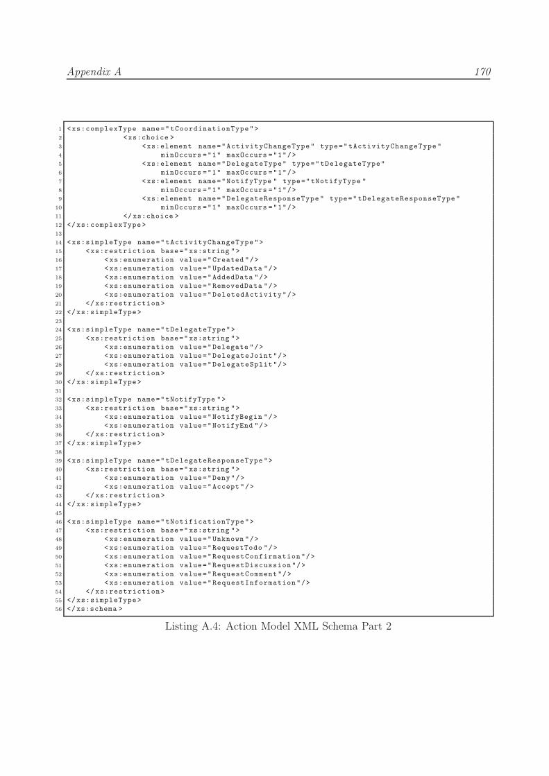
Appendix A 170
1 <xs:complexType name="tCoordinationType">
2 <xs:choice >
3 <xs:element name="ActivityChangeType" type="tActivityChangeType "
4 minOccurs ="1" maxOccurs ="1"/>
5 <xs:element name="DelegateType" type="tDelegateType"
6 minOccurs ="1" maxOccurs ="1"/>
7 <xs:element name="NotifyType " type="tNotifyType "
8 minOccurs ="1" maxOccurs ="1"/>
9 <xs:element name="DelegateResponseType " type=" tDelegateResponseType "
10 minOccurs ="1" maxOccurs ="1"/>
11 </xs:choice >
12 </xs:complexType>
13
14 <xs:simpleType name=" tActivityChangeType">
15 <xs:restriction base="xs:string ">
16 <xs:enumeration value="Created "/>
17 <xs:enumeration value="UpdatedData "/>
18 <xs:enumeration value="AddedData "/>
19 <xs:enumeration value="RemovedData "/>
20 <xs:enumeration value="DeletedActivity"/>
21 </ xs:restriction>
22 </xs:simpleType>
23
24 <xs:simpleType name=" tDelegateType">
25 <xs:restriction base="xs:string ">
26 <xs:enumeration value="Delegate "/>
27 <xs:enumeration value="DelegateJoint"/>
28 <xs:enumeration value="DelegateSplit"/>
29 </ xs:restriction>
30 </xs:simpleType>
31
32 <xs:simpleType name=" tNotifyType ">
33 <xs:restriction base="xs:string ">
34 <xs:enumeration value="NotifyBegin "/>
35 <xs:enumeration value="NotifyEnd "/>
36 </ xs:restriction>
37 </xs:simpleType>
38
39 <xs:simpleType name=" tDelegateResponseType ">
40 <xs:restriction base="xs:string ">
41 <xs:enumeration value="Deny"/>
42 <xs:enumeration value="Accept "/>
43 </ xs:restriction>
44 </xs:simpleType>
45
46 <xs:simpleType name=" tNotificationType">
47 <xs:restriction base="xs:string ">
48 <xs:enumeration value="Unknown "/>
49 <xs:enumeration value="RequestTodo "/>
50 <xs:enumeration value="RequestConfirmation "/>
51 <xs:enumeration value="RequestDiscussion"/>
52 <xs:enumeration value="RequestComment"/>
53 <xs:enumeration value="RequestInformation"/>
54 </ xs:restriction>
55 </xs:simpleType>
56 </xs:schema >
Listing A.4: Action Model XML Schema Part 2

Appendix A 171
1 <?xml version ="1.0 " encoding ="UTF -8"?>
2 <xs:schema xmlns:xs ="http: //www.w3.org /2001/ XMLSchema "
3 xmlns="http: //www.in -context .eu/ns/resource "
4 xmlns:loc ="http: //www.in-context .eu/ns/location "
5 targetNamespace="http: //www .in -context .eu/ns/resource " elementFormDefault="qualified "
6 version ="0.12">
7 <xs:import namespace ="http: //www.in -context .eu/ns/location " schemaLocation=" locationmodel.xsd"/>
8
9 <xs:element name="Resource " type="tResource "/>
10 <xs:complexType name="tResource ">
11 <xs:sequence minOccurs ="1">
12 <xs:element name=" ResourceURI " type="xs:anyURI " nillable ="true"/>
13 <xs:element name=" Description " type="xs:string " minOccurs ="0" maxOccurs ="1"/>
14 <xs:element name="Tags" type="xs:string " minOccurs ="0" maxOccurs ="unbounded "/>
15 </xs:sequence >
16 <xs:attribute name="Name" type="xs:string " use="optional "/>
17 <xs:attribute name="WSRCURI " type="xs:anyURI " use="optional "/>
18 </xs:complexType>
19
20 <xs:element name=" SpatialResource" type=" tSpatialResource"/>
21 <xs:complexType name="tSpatialResource">
22 <xs:complexContent >
23 <xs:extension base="tResource ">
24 <xs:sequence >
25 <xs:element name="CurrentLocation" type="loc:tLocation"
26 minOccurs ="0" maxOccurs ="1"/>
27 </xs:sequence >
28 </xs:extension>
29 </ xs:complexContent >
30 </xs:complexType>
31
32 <xs:element name="Host" type="tHost "/>
33 <xs:complexType name="tHost ">
34 <xs:complexContent >
35 <xs:extension base="tSpatialResource">
36 <xs:sequence >
37 <xs:element name="IPaddress " type="xs:string "
38 minOccurs ="1" maxOccurs ="unbounded "/>
39 <xs:element name="HostedDomain" type="xs:string "
40 minOccurs ="0" maxOccurs ="unbounded "/>
41 <xs:element name="OpenPort " type="xs:string "
42 minOccurs ="0" maxOccurs ="unbounded "/>
43 </xs:sequence >
44 </xs:extension>
45 </ xs:complexContent >
46 </xs:complexType>
47
48 <xs:element name=" MobileDevice" type=" tMobileDevice"/>
49 <xs:complexType name="tMobileDevice">
50 <xs:complexContent >
51 <xs:extension base="tHost ">
52 <xs:sequence >
53 <xs:element name="CommunicationChannel " type=" tCommunicationChannel "
54 minOccurs ="0" maxOccurs ="unbounded "/>
55 <xs:element name="DeviceCategory" type=" tDeviceCategory"
56 minOccurs ="0" maxOccurs ="unbounded "/>
57 </xs:sequence >
58 </xs:extension>
59 </ xs:complexContent >
60 </xs:complexType>
Listing A.5: Resource Model XML Schema Part 1

Appendix A 172
1 <xs:simpleType name=" tDeviceCategory">
2 <xs:restriction base="xs:string ">
3 <xs:enumeration value="Laptop "/>
4 <xs:enumeration value="Smartphone "/>
5 <xs:enumeration value="PDA"/>
6 <xs:enumeration value="MobilePhone "/>
7 <xs:enumeration value="Walkytalky "/>
8 <xs:enumeration value="GPSNavigator"/>
9 <xs:enumeration value="Walkytalky "/>
10 <xs:enumeration value="Other "/>
11 </ xs:restriction>
12 </xs:simpleType>
13
14 <xs:element name=" VirtualResource" type=" tVirtualResource"/>
15 <xs:complexType name="tVirtualResource">
16 <xs:complexContent >
17 <xs:extension base="tResource ">
18 <xs:sequence >
19 <xs:element name="ProvidedBy " type="tService " minOccurs ="0" maxOccurs ="1"/>
20 </xs:sequence >
21 </xs:extension>
22 </ xs:complexContent >
23 </xs:complexType>
24
25 <xs:element name="Service " type=" tService "/>
26 <xs:complexType name="tService ">
27 <xs:complexContent >
28 <xs:extension base="tVirtualResource">
29 <xs:sequence >
30 <xs:element name="ServiceEndpoint" type="xs:string "
31 minOccurs ="0" maxOccurs ="unbounded "/>
32 <xs:element name="WSDLDocumentURL" type="xs:string "
33 minOccurs ="0" maxOccurs ="unbounded "/>
34 <xs:element name="DeployedOn " type="tHost"
35 minOccurs ="0" maxOccurs ="unbounded "/>
36 </xs:sequence >
37 </xs:extension>
38 </ xs:complexContent >
39 </xs:complexType>
40
41 <xs:element name=" CommunicationChannel " type="tCommunicationChannel "/>
42 <xs:complexType name="tCommunicationChannel ">
43 <xs:complexContent >
44 <xs:extension base="tVirtualResource">
45 <xs:sequence >
46 <xs:element name="Protocol " type=" tCommProtocol"
47 minOccurs ="0" maxOccurs ="1"/>
48 <xs:element name="OnlineStatus" type="tOnlineStatus"
49 minOccurs ="0" maxOccurs ="1"/>
50 </xs:sequence >
51 </xs:extension>
52 </ xs:complexContent >
53 </xs:complexType>
54
55 <xs:complexType name="tCommProtocol">
56 <xs:sequence >
57 <xs:element name="Name" type="xs:string "
58 minOccurs ="0" maxOccurs ="1"/>
59 </ xs:sequence >
60 <xs:attribute name=" ProtocolURI " type="xs:anyURI " use="required "/>
61 </xs:complexType>
Listing A.6: Resource Model XML Schema Part 2

Appendix A 173
1 <xs:simpleType name=" tOnlineStatus">
2 <xs:restriction base="xs:string ">
3 <xs:enumeration value="ONLINE "/>
4 <xs:enumeration value="OFFLINE "/>
5 <xs:enumeration value="UNKNOWN "/>
6 <xs:enumeration value="BUSY"/>
7 <xs:enumeration value="AWAY"/>
8 </ xs:restriction>
9 </xs:simpleType>
10
11 <xs:element name=" DocumentResource" type="tDocumentResource"/>
12 <xs:complexType name="tDocumentResource">
13 <xs:complexContent >
14 <xs:extension base="tVirtualResource">
15 <xs:sequence >
16 <xs:element name="MimeType " type="xs:string "
17 minOccurs ="0" maxOccurs ="unbounded "/>
18 </xs:sequence >
19 </xs:extension>
20 </ xs:complexContent >
21 </xs:complexType>
22 </xs:schema >
Listing A.7: Resource Model XML Schema Part 3
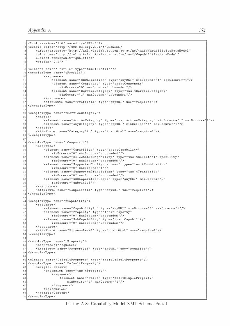
Appendix A 174
1 <?xml version ="1.0 " encoding ="UTF -8"?>
2 <schema xmlns="http: //www.w3.org /2001/ XMLSchema "
3 targetNamespace="http: //xml.vitalab .tuwien .ac.at/ns/taaf/ CapabilitiesMetaModel "
4 xmlns:tns ="http: //xml.vitalab .tuwien .ac.at/ns/taaf/ CapabilitiesMetaModel "
5 elementFormDefault=" qualified "
6 version ="0.1">
7
8 <element name="Profile " type=" tns:tProfile"/>
9 <complexType name="tProfile ">
10 <sequence >
11 <element name=" WSDLlocation" type="anyURI " minOccurs ="1" maxOccurs ="1"/>
12 <element name=" Component " type=" tns:tComponent"
13 minOccurs ="0" maxOccurs ="unbounded "/>
14 <element name=" ServiceCategory" type=" tns:tServiceCategory"
15 minOccurs ="1" maxOccurs ="unbounded "/>
16 </sequence >
17 <attribute name="ProfileId " type="anyURI " use ="required "/>
18 </complexType >
19
20 <complexType name="tServiceCategory">
21 <choice >
22 <element name="ActionCategory" type="tns:tActionCategory" minOccurs ="1" maxOccurs ="1"/>
23 <element name="AnyCategory " type="anyURI " minOccurs ="1" maxOccurs ="1"/>
24 </choice >
25 <attribute name=" CategoryFit " type="tns:t0to1 " use="required "/>
26 </complexType >
27
28 <complexType name="tComponent ">
29 <sequence >
30 <element name="Capability " type=" tns:tCapability"
31 minOccurs ="0" maxOccurs ="unbounded "/>
32 <element name=" SelectableCapability" type="tns:tSelectableCapability "
33 minOccurs ="0" maxOccurs ="unbounded "/>
34 <element name=" SupportedConfigurations " type="tns:tCombination"
35 minOccurs ="0" maxOccurs ="1"/>
36 <element name=" SupportedTransitions" type="tns:tTransition"
37 minOccurs ="0" maxOccurs ="unbounded "/>
38 <element name=" WSDLoperationScope" type="anyURI " minOccurs ="0"
39 maxOccurs ="unbounded "/>
40 </sequence >
41 <attribute name=" ComponentId " type="anyURI " use="required "/>
42 </complexType >
43
44 <complexType name="tCapability ">
45 <sequence >
46 <element name="CapabilityId" type="anyURI " minOccurs ="1" maxOccurs ="1"/>
47 <element name="Property " type="tns:tProperty"
48 minOccurs ="0" maxOccurs ="unbounded "/>
49 <element name="SubCapability" type=" tns:tCapability"
50 minOccurs ="0" maxOccurs ="unbounded "/>
51 </sequence >
52 <attribute name=" FitnessLevel" type="tns:t0to1 " use="required "/>
53 </complexType >
54
55 <complexType name="tProperty ">
56 <sequence ></sequence >
57 <attribute name=" PropertyId " type="anyURI " use ="required "/>
58 </complexType >
59
60 <element name=" DefaultProperty" type=" tns:tDefaultProperty"/>
61 <complexType name="tDefaultProperty">
62 <complexContent>
63 <extension base="tns:tProperty">
64 <sequence >
65 <element name="value " type=" tns:tSimpleProperty"
66 minOccurs ="1" maxOccurs ="1"/>
67 </sequence >
68 </extension >
69 </ complexContent>
70 </complexType >
Listing A.8: Capability Model XML Schema Part 1

Appendix A 175
1 <complexType name="tSimpleProperty">
2 <choice >
3 <element name="intValue " type="int "
4 maxOccurs ="unbounded " minOccurs ="1"/>
5 <element name="boolValue " type="boolean "
6 maxOccurs ="unbounded " minOccurs ="1"/>
7 <element name="decValue " type="decimal "
8 maxOccurs ="unbounded " minOccurs ="1"/>
9 <element name="timestampValue" type="dateTime "
10 maxOccurs ="unbounded " minOccurs ="1"/>
11 <element name="strValue " type="string "
12 maxOccurs ="unbounded " minOccurs ="1"/>
13 </choice >
14 </complexType >
15
16 <complexType name="pResourceSize">
17 <complexContent>
18 <extension base="tns:tProperty">
19 <sequence >
20 <element name="value " type="int "
21 maxOccurs ="1" minOccurs ="1"/>
22 <element name="unit" type="tns:tUnit "
23 maxOccurs ="1" minOccurs ="1"/>
24 </sequence >
25 </extension >
26 </ complexContent>
27 </complexType >
28
29 <complexType name="tSelectableCapability ">
30 <complexContent>
31 <extension base="tns:tCapability">
32 <sequence >
33 <element name="Alternative " type=" tns:tCapability"
34 minOccurs ="1" maxOccurs ="unbounded "/>
35 </sequence >
36 <attribute name=" RequiredSelection" type="boolean " use=" required "/>
37 <attribute name=" DefaultSelection" type="anyURI " use="optional "/>
38 </extension >
39 </ complexContent>
40 </complexType >
41
42 <complexType name="tCombination">
43 <sequence >
44 <choice minOccurs ="0" maxOccurs ="unbounded ">
45 <!-- the given strategy or strategy set -->
46 <element name=" Selection " type="anyURI " />
47 <!-- select any combination of entries from the given strategy SETs! -->
48 <element name="All" type=" tns:tCombination" />
49 <!-- select any entry from the given combinations of strategies -->
50 <element name="OneOf" type="tns:tCombination" />
51 <!-- may not select any entry from the given combinations of strategies ->
52 <element name="NoneOf " type=" tns:tCombination" />
53 </choice >
54 </sequence >
55 </complexType >
56
57 <complexType name="tTransition ">
58 <sequence >
59 <element name=" StartCombination" type="tns:tCombination"
60 minOccurs ="1" maxOccurs ="unbounded "/>
61 <element name=" EndCombination" type="tns:tCombination"
62 minOccurs ="1" maxOccurs ="unbounded "/>
63 </sequence >
64 <attribute name="isPositive " type="boolean " use="required " />
65 </complexType >
Listing A.9: Capability Model XML Schema Part 2

Appendix A 176
1 <simpleType name="tUnit">
2 <restriction base="string ">
3 <enumeration value="Byte"/>
4 <enumeration value="kB"/>
5 <enumeration value="mB"/>
6 <enumeration value="gB"/>
7 <enumeration value="tB"/>
8 </ restriction >
9 </simpleType >
10
11 <simpleType name=" tActionCategory">
12 <restriction base="string ">
13 <enumeration value="Communication"/>
14 <enumeration value="Coordination"/>
15 <enumeration value="Execution "/>
16 </ restriction >
17 </simpleType >
18
19 <simpleType name="t0to1">
20 <restriction base="decimal ">
21 <minInclusive value ="0"/>
22 <maxInclusive value ="1"/>
23 </ restriction >
24 </simpleType >
25 </schema >
Listing A.10: Capability Model XML Schema Part 3

Appendix A 177
1 <?xml version ="1.0 " encoding ="UTF -8"?>
2 <schema xmlns="http: //www.w3.org /2001/ XMLSchema "
3 targetNamespace="http: //xml.vitalab .tuwien .ac.at/ns/taaf/ CapabilityChangeEvents "
4 xmlns:tns ="http: //xml.vitalab .tuwien .ac.at/ns/taaf/ CapabilityChangeEvents "
5 elementFormDefault=" qualified ">
6
7 <element name=" ServiceCapabilityChange " type="tns:tProfileChange"/>
8 <complexType name="tProfileChange">
9 <sequence >
10 <element name="NewComponent" type="anyURI " minOccurs ="0" maxOccurs ="unbounded "/>
11 <element name=" ChangedComponent" type=" tns:tComponentChange"
12 minOccurs ="0" maxOccurs ="unbounded "/>
13 <element name=" RemovedComponent" type="anyURI "
14 minOccurs ="0" maxOccurs ="unbounded "/>
15 <element name=" ChangedServiceCategories " type="anyURI "
16 minOccurs ="0" maxOccurs ="unbounded "/>
17 </sequence >
18 <attribute name="Source " type="anyURI " use="required "/>
19 </complexType >
20
21 <complexType name="tComponentChange">
22 <sequence >
23 <element name="NewCapability" type="anyURI " minOccurs ="0" maxOccurs ="unbounded "/>
24 <element name=" ChangedCapability" type="tns:tCapabilityChange "
25 minOccurs ="0" maxOccurs ="unbounded "/>
26 <element name=" RemovedCapability" type="anyURI "
27 minOccurs ="0" maxOccurs ="unbounded "/>
28 <element name=" SelectableCapability" type="tns:tSelectableCapabilityChange "
29 minOccurs ="0" maxOccurs ="unbounded "/>
30 </sequence >
31 <attribute name=" ComponentURI" type="anyURI " use="required "/>
32 </complexType >
33
34 <complexType name="tCapabilityChange">
35 <sequence >
36 <element name="NewProperty " type="anyURI " minOccurs ="0" maxOccurs ="unbounded "/>
37 <element name="ChangedProperty" type="tns:tPropertyChange "
38 minOccurs ="0" maxOccurs ="unbounded "/>
39 <element name="RemovedProperty" type="anyURI " minOccurs ="0" maxOccurs ="unbounded "/>
40 </sequence >
41 <attribute name=" CapabilityURI" type="anyURI " use ="required "/>
42 </complexType >
43
44 <complexType name="tSelectableCapabilityChange ">
45 <sequence >
46 <element name="NewAlternative" type="anyURI " minOccurs ="0" maxOccurs ="unbounded "/>
47 <element name=" RemovedAlternative" type="anyURI "
48 minOccurs ="0" maxOccurs ="unbounded "/>
49 </sequence >
50 <attribute name=" CapabilityURI" type="anyURI " use ="required "/>
51 </complexType >
52
53 <complexType name="tPropertyChange">
54 <sequence >
55 <any namespace ="## other" processContents="lax " />
56 </sequence >
57 <attribute name=" PropertyURI " type="anyURI " use="required "/>
58 </complexType >
59
60 <element name=" ServiceCapabilityRepositoryChange " type=" tns:tRepositoryChange "/>
61 <complexType name="tRepositoryChange">
62 <sequence >
63 <element name=" NewServiceProfile" type="anyURI "
64 minOccurs ="0" maxOccurs ="unbounded "/>
65 <element name=" ChangedServiceProfile " type="anyURI "
66 minOccurs ="0" maxOccurs ="unbounded "/>
67 <element name=" RemovedServiceProfile " type="anyURI "
68 minOccurs ="0" maxOccurs ="unbounded "/>
69 </sequence >
70 <attribute name=" RepositoryURI" type="anyURI " use ="required "/>
71 </complexType >
72 </schema >
Listing A.11: Capability Change Event Model XML Schema

Appendix A 178
1 <?xml version ="1.0 " encoding ="UTF -8"?>
2 <schema xmlns="http: //www.w3.org /2001/ XMLSchema "
3 targetNamespace="http: //xml.vitalab .tuwien .ac.at/ns/taaf/ EnsembleServiceConfig "
4 xmlns:tns ="http: //xml.vitalab .tuwien .ac.at/ns/taaf/ EnsembleServiceConfig "
5 xmlns:cmm ="http: //xml.vitalab .tuwien .ac.at/ns/taaf/ CapabilitiesMetaModel "
6 elementFormDefault=" qualified ">
7
8 <import
9 namespace ="http: //xml.vitalab .tuwien .ac.at/ns/taaf/ CapabilitiesMetaModel "
10 schemaLocation=" CapabilitiesMetaModel .xsd"/>
11
12 <element name=" EnsembleServiceConfig " type=" tns:tEnsembleServiceConfig "></element >
13 <complexType name="tEnsembleServiceConfig ">
14 <sequence >
15 <element name="ProvidedService" type="tns:tServiceConfig"
16 minOccurs ="0" maxOccurs ="unbounded "/>
17 </sequence >
18 <attribute name=" EnsembleURI " type="anyURI " use="required "/>
19 </complexType >
20
21 <complexType name="tServiceConfig">
22 <sequence >
23 <element name=" CapabilityConfig" type=" tns:tCapabilityConfig "
24 minOccurs ="0" maxOccurs ="unbounded "/>
25 <element name=" RequirementsMatch" type="tns:tRequirementMatch "
26 minOccurs ="0" maxOccurs ="unbounded "/>
27 <element name=" UsedForRequirementsServiceCategory " type=" cmm:tActionCategory"
28 minOccurs ="1" maxOccurs ="1"/>
29 </sequence >
30 <attribute name=" ServiceProfileURI" type="anyURI " use="required "/>
31 <attribute name=" ComponentURI" type="anyURI " use="required "/>
32 </complexType >
33
34 <complexType name="tCapabilityConfig">
35 <sequence >
36 <element name=" SelectableCapabilityType " type="anyURI "
37 minOccurs ="1" maxOccurs ="1"/>
38 <element name="SelectedChoice" type="anyURI "
39 minOccurs ="1" maxOccurs ="1"/>
40 </sequence >
41 </complexType >
42
43 <complexType name="tRequirementMatch">
44 <sequence >
45 <element name="RequirementsRef" type="anyURI " minOccurs ="1" maxOccurs ="1"/>
46 <element name="Match" type="tns:t0to1 " minOccurs ="1" maxOccurs ="1"/>
47 <element name="Membership " type="tns:t0to1 " minOccurs ="1" maxOccurs ="1"/>
48 </sequence >
49 </complexType >
50
51 <element name=" EnsembleRequirements " type="tns:tEnsembleRequirements "/>
52 <complexType name="tEnsembleRequirements ">
53 <sequence >
54 <element name="RequirementsSet" type="tns:tRequirementSet "
55 minOccurs ="0" maxOccurs ="unbounded "/>
56 </sequence >
57 <attribute name=" EnsembleURI " type="anyURI " use="required "/>
58 </complexType >
59
60 <complexType name="tRequirementSet">
61 <sequence >
62 <element name=" RestrictedToServiceCategory " type=" cmm:tActionCategory"
63 minOccurs ="1" maxOccurs ="1"/>
64 <element name="Requirement " type="tns:tRequirement"
65 minOccurs ="0" maxOccurs ="unbounded "/>
66 </sequence >
67 </complexType >
Listing A.12: Ensemble Service Config Model XML Schema Part 1

Appendix A 179
1 <complexType name="tRequirement">
2 <sequence >
3 <element name="CapabilityType" type="anyURI " minOccurs ="1" maxOccurs ="1"/>
4 <element name="Importance " type=" tns:tMinus1toPlus1" minOccurs ="1" maxOccurs ="1"/>
5 </sequence >
6 <attribute name=" RequirementURI" type="anyURI "/>
7 <attribute name=" UtilFctId " type="anyURI " use="required "/>
8 <attribute name=" UtilFctTypeId" type="anyURI " use ="required "/>
9 </complexType >
10
11 <complexType name="tCapabilityExistsRequirement ">
12 <complexContent>
13 <extension base="tns:tRequirement">
14 <sequence >
15 <element name="SelectionParameter" type="tns:t0to1 "/>
16 </sequence >
17 </extension >
18 </ complexContent>
19 </complexType >
20
21 <complexType name="tPropertyValueRequirement ">
22 <complexContent>
23 <extension base="tns:tRequirement">
24 <attribute name="PropertyType" type="anyURI " use="required "/>
25 </extension >
26 </ complexContent>
27 </complexType >
28
29 <complexType name="tCapabilitySelectionRequirement ">
30 <complexContent>
31 <extension base="tns:tRequirement">
32 <sequence >
33 <element name="SelectionParameters " type="string "
34 minOccurs ="0" maxOccurs ="unbounded "/>
35 </sequence >
36 </extension >
37 </ complexContent>
38 </complexType >
39
40 <complexType name="tSimpleStringConstraint ">
41 <complexContent>
42 <extension base="tns:tPropertyValueRequirement ">
43 <sequence >
44 <element name="SelectionParameters " type="string "
45 maxOccurs ="unbounded " minOccurs ="1"/>
46 </sequence >
47 </extension >
48 </ complexContent>
49 </complexType >
50
51 <complexType name="tSimpleTimestampConstraint ">
52 <complexContent>
53 <extension base="tns:tPropertyValueRequirement ">
54 <sequence >
55 <element name="SelectionParameters " type="dateTime "
56 maxOccurs ="unbounded " minOccurs ="1"/>
57 </sequence >
58 </extension >
59 </ complexContent>
60 </complexType >
Listing A.13: Ensemble Service Config Model XML Schema Part 2

Appendix A 180
1 <complexType name="tSimpleIntConstraint ">
2 <complexContent>
3 <extension base="tns:tPropertyValueRequirement ">
4 <sequence >
5 <element name="SelectionParameters " type="integer "
6 maxOccurs ="unbounded " minOccurs ="1"/>
7 </sequence >
8 </extension >
9 </ complexContent>
10 </complexType >
11
12 <complexType name="tSimpleBoolConstraint ">
13 <complexContent>
14 <extension base="tns:tPropertyValueRequirement ">
15 <sequence >
16 <element name="SelectionParameters " type="boolean "
17 maxOccurs ="unbounded " minOccurs ="1"/>
18 </sequence >
19 </extension >
20 </ complexContent>
21 </complexType >
22
23 <complexType name="tSimpleDecimalConstraint ">
24 <complexContent>
25 <extension base="tns:tPropertyValueRequirement ">
26 <sequence >
27 <element name="SelectionParameters " type="decimal "
28 maxOccurs ="unbounded " minOccurs ="1"/>
29 </sequence >
30 </extension >
31 </ complexContent>
32 </complexType >
33
34
35 <complexType name="tFileSizeConstraint ">
36 <complexContent>
37 <extension base="tns:tPropertyValueRequirement ">
38 <sequence >
39 <element name="SelectionParameters " type=" cmm:pResourceSize"
40 maxOccurs ="unbounded " minOccurs ="0"/>
41 </sequence >
42 </extension >
43 </ complexContent>
44 </complexType >
45
46 <simpleType name=" tMinus1toPlus1">
47 <restriction base="decimal ">
48 <minInclusive value =" -1"/>
49 <maxInclusive value ="1"/>
50 </ restriction >
51 </simpleType >
52
53 <simpleType name="t0to1">
54 <restriction base="decimal ">
55 <minInclusive value ="0"/>
56 <maxInclusive value ="1"/>
57 </ restriction >
58 </simpleType >
59 </schema >
Listing A.14: Ensemble Service Config Model XML Schema Part 3