Dynam ics and St abi lity of P uls es and P ulse T rai ns ... · w e obse rve the eme rge n ce of...
130
Dynamics and Stability of Pulses and Pulse Trains in Excitable Media vorgelegt von Diplom-Physiker Grigory Bordyugov aus Saratov Von der Fakult¨ at II - Mathematik und Naturwissenschaften der Technischen Universit¨ at Berlin zur Erlangung des akademischen Grades Doktor der Naturwissenschaft - Dr. rer. nat. - genehmigte Dissertation Promotionsausschuss: Vorsitzender: Prof. Dr. C. Thomsen Berichter: Prof. Dr. H. Engel Berichter: Prof. Dr. A. Pikovsky Zus¨ atzlicher Gutachter: Prof. Dr. B. Sandstede Tag der wissenschaftlichen Aussprache: 20.10.2006 Berlin 2006 D 83
Transcript of Dynam ics and St abi lity of P uls es and P ulse T rai ns ... · w e obse rve the eme rge n ce of...

Dynamics and Stability of Pulses
and Pulse Trains in Excitable Media
vorgelegt von Diplom-Physiker
Grigory Bordyugov
aus Saratov
Von der Fakultat II - Mathematik und Naturwissenschaften
der Technischen Universitat Berlin
zur Erlangung des akademischen Grades
Doktor der Naturwissenschaft
- Dr. rer. nat. -
genehmigte Dissertation
Promotionsausschuss:
Vorsitzender: Prof. Dr. C. Thomsen
Berichter: Prof. Dr. H. Engel
Berichter: Prof. Dr. A. Pikovsky
Zusatzlicher Gutachter: Prof. Dr. B. Sandstede
Tag der wissenschaftlichen Aussprache: 20.10.2006
Berlin 2006
D 83


Abstract
The present Thesis deals with the dynamics and stability of pulses and spatially periodic
pulse trains in excitable media. Such pulses represent nonlinear waves in active systems
far from the thermodynamic equilibrium. They are very important for the understanding
of such phenomena as the conduction of excitation in neuronal systems, intracellular
calcium dynamics, electrical activity in the heart muscle, structure formation in the
Belousov-Zhabotinsky reaction and many others.
We analyze two qualitatively di!erent types of solitary pulses. The first one has a
monotonous decay behind the high-amplitude pulse head and the second one decays in
an oscillatory manner. This di!erence in the decay essentially influences the interaction
between pulses in a spatially periodic pulse train or in a pulse pair.
The presence of the tail oscillations leads to the so far unknown coexistence of pulse
trains of the same wavelength and di!erent velocities. This coexistence is reflected in the
bistable domains in the dispersion relation of spatially periodic pulse trains. A large part
of the dissertation addresses the stability of the pulse trains in such bistable domains.
We show that oscillatory decay is typical for excitation pulses close to the transition
between trigger and phase waves and describe several stages of the transition. First,
we observe the emergence of small-amplitude damped oscillations in the wake of the
solitary pulse under increase of the excitability of the system. Further increase of the
excitability results in the emergence of undamped tail oscillations. Dispersion curve of
spatially periodic pulse trains displays damped and undamped oscillations as well in
accordance to the decay type behind the solitary pulse. The depiction of the transition
between trigger and phase waves demanded a detailed analysis of the stability of the
waves in the transition region.
We also studied pulses with monotonous tails under influence of non-local coupling.
In numerous systems nonlocal coupling must be considered besides local di!usive cou-
pling. Examples for such systems include brain tissue and electro-chemical reactions.
We show that an arbitrary small, exponentially decaying nonlocal coupling leads to the
emergence of bound states. The emergence of bound states is model-independent given
that the model supports propagation of stable solitary pulses.


Zusammenfassung
Die vorliegende Dissertation handelt von der Dynamik und Stabilitat von Pulsen und
Pulsfolgen in erregbaren Medien. Diese Pulse stellen nichtlineare Wellen in aktiven
Systemen fern vom thermodynamischen Gleichgewicht dar und sind wichtig fur das
Verstandnis solcher Phanomene wie die Erregungsleitung in neuronalen Systemen, in-
trazellulare Kalziumwellen, elektrische Erregungswellen im Herzmuskel, Musterbildung
in der Belousov-Zhabotinsky Reaktion und viele andere.
Zwei qualitativ verschiedene Pulstypen werden untersucht. Bei dem ersten hat der
Einzelpuls einen monotonen Auslaufer, wahrend der zweite Typ kleinamplitudige Oszilla-
tionen im Auslaufer besitzt. Dieser Unterschied im Auslaufer des Einzelpulses beeinflusst
wesentlich die Wechselwirkung zwischen Pulsen innerhalb einer raumlich periodischen
Pulsfolge oder eines Pulspaares.
Die Oszillationen im Auslaufer verursachen die bislang unbekannte Koexistenz von
Pulsfolgen mit gleicher Wellenlange aber unterschiedlichen Ausbreitungsgeschwindig-
keiten. Diese Koexistenz findet ihren Ausdruck in bistabilen Bereichen in der Disper-
sionskurve von raumlich periodischen Pulsfolgen. Ein grosser Teil der Dissertation be-
fasst sich mit der Untersuchung der Stabilitat der Pulsfolgen in den bistabilen Bereichen
der Dispersionskurve.
Wir zeigen, dass Pulse mit oszillatorischen Auslaufern typischerweise in der Nahe
des Ubergangsbereiches zwischen Trigger- und Phasenwellen existieren und beschreiben
mehrere Stufen dieses Uberganges. Mit zunehmender Erregbarkeit entstehen zunachst
gedampfte Oszillationen im Auslaufer des Einzelpulses, die mit weiterer Zunahme der Er-
regbarkeit ungedampft werden. In Ubereinstimmung damit zeigen die raumlich periodis-
chen Pulsfolgen gedampfte bzw. ungedampfte Oszillationen in der Dispersionskurve. Der
Ubergang wird durch eine Kollision der Dispersionkurven von Phasen- und Triggerwellen
abgeschlossen. Die Beschreibung des Uberganges erforderte Stabilitatsuntersuchungen
von Trigger- und Phasenwellen im Ubergangsbereich.
Pulse mit monotonen Auslaufern unter dem Einfluss von nichtlokaler Kopplung wer-
den auch untersucht. In zahlreichen Systemen wie in neuronalen Geweben oder bei elek-
trochemischen Reaktionen sind neben kurzreichweitigen auch langreichweitige raumliche

Kopplungen zu berucksichtigen. Es wurde gezeigt, dass eine beliebig schwache, expo-
nentiell abklingende nichtlokale Kopplung zur Ausbildung von Pulspaaren fuhrt. Die
Entstehung von Pulspaaren ist unabhangig vom verwendeten Modell, vorausgesetzt,
dieses besitzt ohne nichtlokale Kopplung stabile Einzelpulse.

Acknowledgments
I am very thankful to Prof. Dr. Harald Engel for the possibility to complete my PhD The-
sis in his group. He provided me with excellent working conditions for my research, and
his professional help and guidance during the whole time can be hardly overestimated.
I would like to thank mathematicians Prof. Dr. Bjorn Sandstede, Prof. Dr. Arnd
Scheel and Dr. Jens Rademacher since I really learned a lot from their papers and from
our private communications.
Also I am very grateful to Georg Roder and Nils Fischer for their readiness to discuss
and to continue some common research projects further.
For the nice working atmosphere in the group I would like to thank Jan Schlesner,
Valentina Beato, Vladimir Zykov, Hermann Brandtstadter, Ingeborg Gerdes and Martin
Braune.
The acknowledgment list would not be complete without Alexander Balanov, Na-
talia Janson, Olexandr Popovich, Markus Bar, Lutz Brusch, Oliver Rudzick, Vanessa
Casagrande, Martin Falcke, Oliver Steinbock, Dmitry Turaev and Ernesto Nicola.


Contents
1 Introduction 1
1.1 Overview of nonlinear wave phenomena . . . . . . . . . . . . . . . . . . . 1
1.2 Statement of the problem . . . . . . . . . . . . . . . . . . . . . . . . . . . 6
1.3 Grasshopper’s guide to the Thesis . . . . . . . . . . . . . . . . . . . . . . 8
2 Nonlinear waves in reaction-di!usion systems 11
2.1 Reaction-di!usion systems . . . . . . . . . . . . . . . . . . . . . . . . . . . 11
2.1.1 Oregonator model for BZ reaction . . . . . . . . . . . . . . . . . . 12
2.1.2 Excitable and oscillatory Oregonator kinetics . . . . . . . . . . . . 14
2.2 Profile equations . . . . . . . . . . . . . . . . . . . . . . . . . . . . . . . . 16
2.2.1 Co-moving frame approach . . . . . . . . . . . . . . . . . . . . . . 17
2.2.2 Some examples of travelling waves . . . . . . . . . . . . . . . . . . 18
2.3 Homoclinics and accompanying periodic orbits . . . . . . . . . . . . . . . 21
2.3.1 Real leading eigenvalues . . . . . . . . . . . . . . . . . . . . . . . . 26
2.3.2 Complex-conjugate leading eigenvalues . . . . . . . . . . . . . . . . 31
2.4 Stability of waves . . . . . . . . . . . . . . . . . . . . . . . . . . . . . . . . 34
2.4.1 Spectral approach . . . . . . . . . . . . . . . . . . . . . . . . . . . 34
2.4.2 Stability of pulse trains with large wavelength . . . . . . . . . . . . 38
2.4.3 Numerical computation of spectra . . . . . . . . . . . . . . . . . . 41
3 Bistable dispersion and coexisting wave trains 45
3.1 Overview of dispersion types . . . . . . . . . . . . . . . . . . . . . . . . . 45
3.2 Three-component Oregonator . . . . . . . . . . . . . . . . . . . . . . . . . 46
3.2.1 Point spectrum of pulses on a ring . . . . . . . . . . . . . . . . . . 51
3.2.2 Essential spectrum . . . . . . . . . . . . . . . . . . . . . . . . . . . 53
vii

viii CONTENTS
3.2.3 Extrema of the dispersion curve . . . . . . . . . . . . . . . . . . . 56
3.2.4 Numerical simulations . . . . . . . . . . . . . . . . . . . . . . . . . 58
3.3 Bistability of dispersion in FitzHugh-Nagumo model . . . . . . . . . . . . 59
3.4 Summary . . . . . . . . . . . . . . . . . . . . . . . . . . . . . . . . . . . . 59
4 Transition between trigger and phase waves 61
4.1 Introduction and Motivation . . . . . . . . . . . . . . . . . . . . . . . . . . 61
4.2 Model and methods . . . . . . . . . . . . . . . . . . . . . . . . . . . . . . 64
4.2.1 Model . . . . . . . . . . . . . . . . . . . . . . . . . . . . . . . . . . 64
4.2.2 Methods . . . . . . . . . . . . . . . . . . . . . . . . . . . . . . . . . 65
4.3 Trigger Waves . . . . . . . . . . . . . . . . . . . . . . . . . . . . . . . . . . 67
4.3.1 Solitary pulses . . . . . . . . . . . . . . . . . . . . . . . . . . . . . 67
4.3.2 Trigger wave trains . . . . . . . . . . . . . . . . . . . . . . . . . . . 71
4.4 Phase Waves . . . . . . . . . . . . . . . . . . . . . . . . . . . . . . . . . . 73
4.5 Collision of dispersion curves . . . . . . . . . . . . . . . . . . . . . . . . . 77
4.6 Discussion and Outlook . . . . . . . . . . . . . . . . . . . . . . . . . . . . 79
5 Creating bound states by means of non-local coupling 81
5.1 Introduction . . . . . . . . . . . . . . . . . . . . . . . . . . . . . . . . . . . 81
5.2 Results with Oregonator model . . . . . . . . . . . . . . . . . . . . . . . . 83
5.2.1 Emergence of bound states . . . . . . . . . . . . . . . . . . . . . . 83
5.2.2 Stability of bound states in Oregonator . . . . . . . . . . . . . . . 85
5.3 General description of the case µ = 0 . . . . . . . . . . . . . . . . . . . . . 88
5.3.1 Profile equations with non-local coupling . . . . . . . . . . . . . . 88
5.3.2 Codimension-2 bifurcations of homoclinic orbits . . . . . . . . . . . 91
5.3.3 Resonance and Inclination flips for µ = 0 . . . . . . . . . . . . . . 93
5.3.4 Geometrical interpretation . . . . . . . . . . . . . . . . . . . . . . . 94
5.3.5 Summary: Codimension-4 homoclinic orbit . . . . . . . . . . . . . 96
5.3.6 Stability of bound states . . . . . . . . . . . . . . . . . . . . . . . . 97
5.4 Discussion and outlook . . . . . . . . . . . . . . . . . . . . . . . . . . . . . 98
6 Conclusions 101
6.1 Pulses with oscillations in the tail . . . . . . . . . . . . . . . . . . . . . . . 101
6.2 Pulses with monotonous tails . . . . . . . . . . . . . . . . . . . . . . . . . 102

CONTENTS ix
6.3 Suggestions for further studies . . . . . . . . . . . . . . . . . . . . . . . . . 103
A Group velocity of periodic wave train and its spectrum 105
B Law of Mass Action 109

x CONTENTS

Chapter 1
Introduction
1.1 Overview of nonlinear wave phenomena
In 2002, a short article about the Mexican wave (or La Ola) was published by Nature [1].
The name of the phenomenon originates from the 1986 World Football Cup in Mexico.
The Mexican wave represents a surge of people, rapidly rising from their seats; the wave
propagates through the rows of audience in a stadium at an average speed 12 metres (or
20 seats) per second. Usually, one needs no more than a few dozens of people to ignite
such a wave. This wave is essentially nonlinear, i.e. two Mexican waves do not interfere
and cannot run through each other, which can be easily seen from the unwillingness of the
participators to get up again immediately after the first wave. A quantitative treatment
for this phenomenon was developed, and this treatment could accurately reproduce the
details of the wave activity. On the homepage of the project1 one can start an interactive
simulation of the Mexican wave and play with the parameters, which are responsible for
the propagation of the wave.
The apparent simplicity of the Mexican wave assumes a simple model, which can
describe the phenomenon qualitatively. The audience, or the medium, consists of the
individuals which need to be connected somehow in order to provide the wave propa-
gation. Since the wave can propagate in both directions (clock-wise as well as counter
clock-wise) around the football field, we can assume that the connection between the
viewers is symmetric with respect to the left and right. A short consideration shows that
the connection between the viewers is of the di!usional type: it means that the di!erence
1http://angel.elte.hu/wave/
1
2 CHAPTER 1. INTRODUCTION
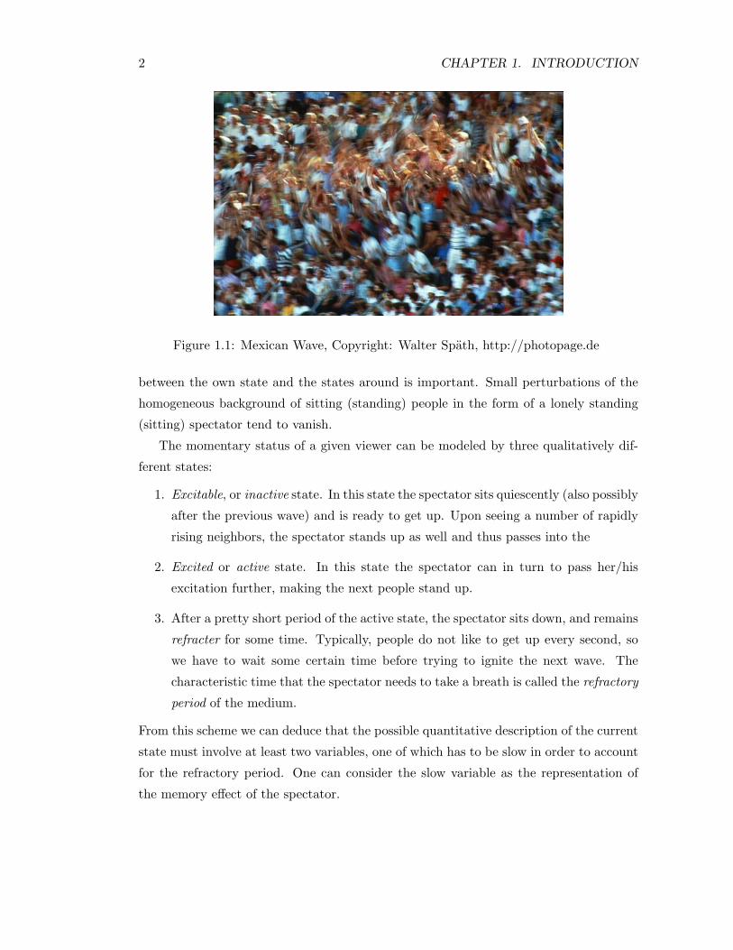
Figure 1.1: Mexican Wave, Copyright: Walter Spath, http://photopage.de
between the own state and the states around is important. Small perturbations of the
homogeneous background of sitting (standing) people in the form of a lonely standing
(sitting) spectator tend to vanish.
The momentary status of a given viewer can be modeled by three qualitatively dif-
ferent states:
1. Excitable, or inactive state. In this state the spectator sits quiescently (also possibly
after the previous wave) and is ready to get up. Upon seeing a number of rapidly
rising neighbors, the spectator stands up as well and thus passes into the
2. Excited or active state. In this state the spectator can in turn to pass her/his
excitation further, making the next people stand up.
3. After a pretty short period of the active state, the spectator sits down, and remains
refracter for some time. Typically, people do not like to get up every second, so
we have to wait some certain time before trying to ignite the next wave. The
characteristic time that the spectator needs to take a breath is called the refractory
period of the medium.
From this scheme we can deduce that the possible quantitative description of the current
state must involve at least two variables, one of which has to be slow in order to account
for the refractory period. One can consider the slow variable as the representation of
the memory e!ect of the spectator.

1.1. OVERVIEW OF NONLINEAR WAVE PHENOMENA 3
The authors of the article stress that the emergence and propagation of the Mexican
wave perfectly fits in the more general theory of the so-called excitable media, which
describes nonlinear phenomena in many physical, chemical and biological systems [2, 3].
We would like to note that the term “excitable” is perhaps the most telling description
of the Mexican wave phenomenon, since the audience in a football match is typically
very emotional.
Plenty of interest in the phenomenon of excitability was triggered in the fifties of the
twentieth century by the discovery of the famous auto-catalytic Belousov-Zhabotinsky
reaction [4]. This reaction was first discovered to be oscillatory, i.e. the result of the
reaction was the establishment of temporally periodic concentrations of the reagents.
Sometimes the reaction is referred to as “chemical clocks”. Under a certain choice of
the chemical parameters, the homogeneous stationary state can be stable; however, the
reaction can respond to small perturbations with a burst of activity, this is exactly what
one refers to as excitability. The small perturbation can come, for instance, from the
neighborhood of a given point through the di!usive flow of the reagents in the case if
the solution is not stirred so that the gradients of concentrations can appear.
The Belousov-Zhabotinsky reaction has proven to be an excellent experimental model
for studies of waves in reaction-di!usion systems. There are a number of particular ver-
sions of the reaction, the most important element of them is the presence of an acid and
bromine. Usually, the experiments with the reaction are carried out either in a Petri dish
or in the so-called open reactors, where it is possibly to keep the concentration of the
reagents on the appropriate level. The reaction occurs under common laboratory condi-
tions. The solution has di!erent color and transparency depending on the concentration
of the oxidized form of the catalyst. Typical timescales of the reaction can vary from
a few dozens of second to several minutes and typical wavelengths of the patterns are
several millimeters, which advantageously distinguishes this reaction from the Mexican
wave in connection to the experiments and observations. The more recent versions of
the Belousov-Zhabotinsky use a photo-sensitive catalyst, which make possible to control
the reaction by means of light. A typical experimental set-up is thus pretty simple and
consist of an open reaction together with a video camera and a beamer or a compa-
rable device which can throw a given light pattern upon the medium. Characteristic
wave patterns in the Belousov-Zhabotinsky reaction include solitary waves, wave trains,
two-dimensional target patterns, spiral waves and scroll waves in three dimensions.

4 CHAPTER 1. INTRODUCTION
Figure 1.2: Left panel: A photograph of the Belousov-Zhabotinsky. Right panel: variety
of patterns in the Belousov-Zhabotinsky reaction.
One of the first and most eminent contribution to the role of reaction-di!usion sys-
tem in biology was made by Alan Turing [5]. He proved that a spatially homogeneous
distribution of certain chemical substances, called morphogens, can become unstable due
to the presence of di!usive coupling. This instability may lead to development of spatial
structures and patterns, which include both standing and propagating waves. It was
suggested that stationary waves in two dimensions can account for phyllotaxis (arrange-
ment of leaves on the shoot of a plant) and can provide various stripe, circular and spot
patterns of zebras, leopards, certain fishes and many other animals. In three spatial
dimensions, the instability of a spherically symmetrical zygote can break the symmetry
and lead to principally new forms of the growing organism. However, the stationary
patterns predicted by Turing were experimentally observed in a chemical reaction only
in 1990 [6]. The instability, which lead to the appearance of standing waves is now
referred to as the Turing instability.
Another important example of non-linear phenomena is represented by calcium waves
in living cells [7], which are believed to be one of the major signaling mechanisms. One
distinguishes between four types of those: ultrafast, fast, slow and ultraslow calcium
waves. The propagation of the fast calcium waves was found to be provided by the
reaction-di!usion nature of the underlying processes. Again, a rich variety of dynamical
behavior is reported, including the mentioned above spiral waves, which were found both
in experiments and numerical simulations with the derived models. Recently, the role of

1.1. OVERVIEW OF NONLINEAR WAVE PHENOMENA 5
fluctuations in the calcium dynamics was demonstrated to be fundamental due to the
relatively small number of interacting elements.
The propagation of neural activity was also found to be of reaction-di!usion type.
Pulses of such activity in the axons of giant squids [8] were successfully modeled by a set
of non-linear ordinary di!erential equations, which can be coupled di!usively in order
to get a one-dimensional model of the axon. In this case, the equations describe the
currents and potentials across the cell membrane rather then concentration of chemical
species from the above examples. A simplification of the Hodgkin-Huxley model lead to
the two-component FitzHugh-Nagumo system [9, 10], which is considered as the most
generic model for an excitable medium and is capable to reproduce a plethora of non-
linear wave phenomena.
Maybe the most important application of the theoretical studies of non-linear waves
in excitable systems is the problem of ventricular fibrillation. This pathological mal-
function of heart causes several hundred thousands deaths annualy in the USA only.
In [11] it was proposed that ventricular fibrillation can be caused by multiple wave
segments that propagate chaotically in the heart muscle. If the refractory period be-
tween two waves becomes shorter than the normal refractory period of healthy heart,
the cells fail to respond. The initial model of the heart tissue was based on the cellular
automata model, whereas in the meantime it is possible to study the problem using
realistic reaction-di!usion heart models [12].
We would like to recall some recent theoretical and mathematical results on the wave
propagation in reaction-di!usion systems. The most common tool to analyze the prop-
agation of waves is the bifurcation theory for non-linear ordinary and partial di!erential
equations. Considering one-dimensional systems, it is often possible to reduce the prob-
lem to the level of ordinary di!erential equation instead of solving the original PDE. The
bifurcation theory for non-linear ODE (see [13] and numerous references within) insures
that many wave phenomena in di!erent systems can be classified in a relatively small
number of known bifurcations. This often allows to make generic statements about the
behavior of waves in dependence on the change of parameters of the system. We would
like to mention a nice review on the theory of stability of travelling waves [14], which
can be seen as the first reading suggestion for the recent results on the field.

6 CHAPTER 1. INTRODUCTION
L +!L0
L -!L0
L0
c0
Figure 1.3: Kinematic approach to dispersion and pulse interaction in a pulse train, see
text.
1.2 Statement of the problem
The central problem that the present Thesis deals with is the dynamics and stability of
non-linear waves in excitable media.
Unlike classical waves (for instance, electromagnetic waves), non-linear waves can
propagate either alone in form of solitary pulses or form pulse trains. In the latter case
the velocity of pulses depends on the interpulse distance. In the case of spatially periodic
pulse trains, all interpulse distances are equal and hence, typically, all pulses in the pulse
train propagate at the same velocity. The so-called (nonlinear) dispersion relates the
velocity of pulse train c with the interpulse distance L
c = c(L).
It is widely believed that the slope of the dispersion ddLc(L) determines the stability
of the pulse train and the interaction between the pulses. Indeed, for the case of large
interpulse distances L ! ", the interaction between the pulses is weak and mutual
influence of pulses is reduced to small velocity corrections. The reason for this is that
the pulses are strongly (actually, exponentially) localized in the space and can be thought
of as particles, whose velocity depends only on the distance to the next one.
In order to illustrate this approach, which is often called kinematic approach [15],
suppose for a moment that we have a pulse train of interpulse distance L0 and velocity c0.
Suppose further that ddLc(L0) > 0. Now let us virtually shift one of the pulses in the
pulse train by "L and look what happens in this case. The e!ective interpulse distance

1.2. STATEMENT OF THE PROBLEM 7
in front of the shifted pulse increases L0 + "L > L0. As a result, the velocity of the
shifted pulse becomes larger, since ddLc(L0) > 0, which compensates the shift. So the
perturbation in the form of shifting of individual pulses would decay with the time. It
means in turn that a positive slope of the dispersion curve c = c(L) corresponds to
the stability of the pulse train with respect to the perturbation in a form of shifting of
individual pulses.
The positive slope of dispersion implies also the repulsive interaction of two pulses
under the assumption that the distance between two pulses is large. The first pulse in
a pulse pair “sees” no pulse in front of it and hence propagates at the velocity of the
solitary pulse. The second pulse is however always slower than the first one since there
is always a finite distance to the first one. In this case one speaks about a repulsive
interaction of pulses in a pulse pair.
The case of negative slope of the dispersion ddLc(L0) < 0 delivers a quite opposite
result: the pulse train turns out to be unstable, since the shifted pulse becomes slower
upon increase of the interpulse distance in front of it. Perturbations in the form of shifting
of individual pulses do not decay. The periodicity of the pulse train tends to break up,
whereas pairs of pulses are formed. Analogously, negative slope of the dispersion can
lead to an attractive interaction between solitary pulses and to the formation of pulse
pairs.
Suppose now that the slope of dispersion c(L) changes the sign in dependence on L.
This would mean that spatially periodic pulse trains can be either stable or unstable
depending on the interpulse distance. The interaction between solitary pulses, either
attractive or repulsive, would also depend on L.
The recent mathematical studies on the stability of pulse trains with large wave-
lengths [16, 17] rigorously prove the intuitive considerations above. The following impor-
tant result was proven: the stability properties of a given pulse train can be unambigu-
ously read o! from the exponential tails of the corresponding solitary pulse. However,
this result is applicable again only for large L.
The plethora of pulse interaction patterns was experimentally found in many physi-
cal, biological and chemical systems, see for example [18, 19, 20, 21, 22, 23, 24] (we will
give more specific references in the following chapters). However, in many real experi-
mental situations the interaction of pulses is not weak, in contrast the interaction can
even be so strong that it can lead to merging of pulses or propagation failure. Thus

8 CHAPTER 1. INTRODUCTION
there is a clear need for the comprehensive study of pulse propagation, which can be
conducted without the assumption on the large interpulse distance.
The aim of the Thesis is to describe the dynamics and stability of pulses and pulse
trains in the domain of wavelengths where kinematic theory is not applicable and the
interaction cannot be considered as weak. This means that we cannot reduce the problem
of interaction to the “particle” level, i.e. we have to solve the existence and stability
problems with respect to the whole underlying partial di!erential equation. We use
the results of the large wavelength limit in order to check the numerous computational
methods and compare our numerical results with the analytically known expressions for
L !".
More specifically, the results of the thesis can be classified in two cases, depending
on the decay properties of the solitary pulse. In the first case, the solitary pulse has an
oscillating decay, which gives rise to complicated dynamics of both solitary and periodic
waves. The oscillatory wake is provided by the complex-conjugate eigenvalues of the
linearization in the rest state in the profile equation. We report on the bistable dispersion
curve for periodic wave trains and discuss the stability of the corresponding waves.
Moreover, we found that the aforementioned emergence of small amplitude oscillations
occurs close to the transition between trigger and phase waves. We extensively describe
the bifurcation scenario of this transition and present numerous results on their stability.
The second case is presented by pulses with monotonous decay, which propagate
in an excitable medium subjected to non-local coupling. This type of coupling can be
reformulated in terms of an additional reaction-di!usion equation, which is coupled to
the original system. The presence of non-local coupling a!ects the decay properties of
monotonous wake behind the pulse and makes possible the emergence of bound states
(or pulse pairs). For this case, we show that the emergence of bound states is model-
independent and is provided only by the exponentially decaying coupling kernel. We
discuss the stability of the corresponding pulse trains and bound states in details.
1.3 Grasshopper’s guide to the Thesis
This thesis consists of the introduction, four chapters and conclusion.
1. The first chapter is the Introduction.
2. The second chapter can be divided in two unequal parts. In the first part we will

1.3. GRASSHOPPER’S GUIDE TO THE THESIS 9
give a brief introduction to reaction-di!usion systems. Excitable and oscillatory
media will be considered in more detail. We will introduce the modified Orego-
nator model, which was originally derived to describe the light-sensitive Belousov-
Zhabotinsky reaction. We will also show that the Oregonator model is capable to
reproduce two main types of the local dynamics, namely, excitable and oscillatory,
which allows us to use it for the study of di!erent wave types. Then we will proceed
to the coherent structures approach, which makes possible to reduce the problem
from the level of partial di!erential equations to ordinary di!erential equations,
that describe the profile of the wave. In particular, we will be interested in solitary
waves and the accompanying periodic wave trains with large spatial period. Such
waves correspond to the so-called homoclinic and periodic orbits with large period
in the profile equation. With the known profile and velocity of the wave, we will
turn to the question of its stability. The description of the stability theory for
di!erent wave types and boundary conditions completes the second chapter.
3. In the third chapter, we discuss the bistability of periodic wave trains due to
anomalous oscillatory dispersion, which is distinguished by the presence of bistable
domains. In such domains alternative stable pulse trains with the same wavelength
and di!erent velocities coexist. We present a detailed study of the stability of the
coexisting pulse trains in the bistable domains. The phenomenon of bistability is
found to be provided by the oscillatory recovery of excitations which causes small
amplitude oscillations in the refractory tail of pulses. Crucial for the bistability is
that the pulses in the trains are locked into one oscillation maximum in the tail of
the preceding pulse in the train. It is found that such regime is typical for excitable
media close to the transition to oscillatory local dynamics through a supercritical
Hopf bifurcation, followed by a canard explosion of the limit cycle. This fact
connects the phenomenon of bistability with the transition between trigger and
phase waves.
4. In the fourth chapter, we will present new results on the transition between trigger
and phase waves, which represent the “natural” waves for excitable and oscillatory
kinetics, respectively. In many system the local dynamics can be switched between
oscillatory and excitable with a single parameter. For example, the light-sensitive
Belousov-Zhabotinsky reaction demonstrate oscillatory kinetics for low intensity
of the applied light and excitable kinetics for high values of the light intensity. In
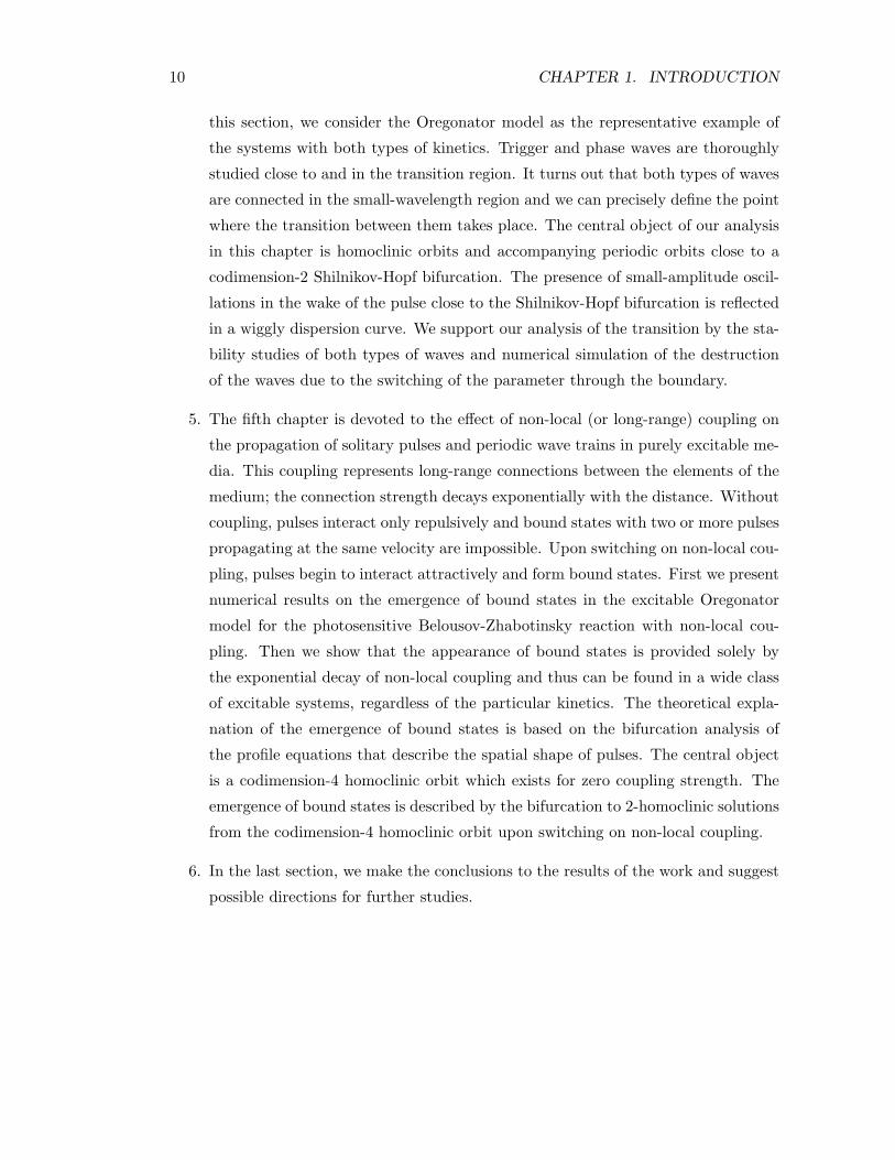
10 CHAPTER 1. INTRODUCTION
this section, we consider the Oregonator model as the representative example of
the systems with both types of kinetics. Trigger and phase waves are thoroughly
studied close to and in the transition region. It turns out that both types of waves
are connected in the small-wavelength region and we can precisely define the point
where the transition between them takes place. The central object of our analysis
in this chapter is homoclinic orbits and accompanying periodic orbits close to a
codimension-2 Shilnikov-Hopf bifurcation. The presence of small-amplitude oscil-
lations in the wake of the pulse close to the Shilnikov-Hopf bifurcation is reflected
in a wiggly dispersion curve. We support our analysis of the transition by the sta-
bility studies of both types of waves and numerical simulation of the destruction
of the waves due to the switching of the parameter through the boundary.
5. The fifth chapter is devoted to the e!ect of non-local (or long-range) coupling on
the propagation of solitary pulses and periodic wave trains in purely excitable me-
dia. This coupling represents long-range connections between the elements of the
medium; the connection strength decays exponentially with the distance. Without
coupling, pulses interact only repulsively and bound states with two or more pulses
propagating at the same velocity are impossible. Upon switching on non-local cou-
pling, pulses begin to interact attractively and form bound states. First we present
numerical results on the emergence of bound states in the excitable Oregonator
model for the photosensitive Belousov-Zhabotinsky reaction with non-local cou-
pling. Then we show that the appearance of bound states is provided solely by
the exponential decay of non-local coupling and thus can be found in a wide class
of excitable systems, regardless of the particular kinetics. The theoretical expla-
nation of the emergence of bound states is based on the bifurcation analysis of
the profile equations that describe the spatial shape of pulses. The central object
is a codimension-4 homoclinic orbit which exists for zero coupling strength. The
emergence of bound states is described by the bifurcation to 2-homoclinic solutions
from the codimension-4 homoclinic orbit upon switching on non-local coupling.
6. In the last section, we make the conclusions to the results of the work and suggest
possible directions for further studies.

Chapter 2
Nonlinear waves in
reaction-di!usion systems
2.1 Reaction-di!usion systems
As we have already mentioned in the introduction, the main motivation for the so-
called reaction-di!usion systems came from the discovery of the oscillating Belousov-
Zhabotinsky reaction in the fifties of the twentieth century. However, already in 1920
Lotka suggested that the following hypothetical chemical autocatalytic reactions
A + X ! 2X,
X + Y ! 2Y,
Y ! P
(2.1)
can lead to the emergence of temporal oscillations of the concentration of reagents X
and Y [25]. Nevertheless, the oscillations in the system given by (2.1) are not limit
cycle oscillation. In contrast, the oscillatory regime is sensitive to the initial conditions
and starting the reaction from di!erent concentrations of X and Y leads to di!erent
temporal evolutions of the reaction.
In the beginning of the seventies, another chemical reaction was proposed in Brussels
A ! X,
B + X ! Y + D,
2X + Y ! 3X,
X ! E,
(2.2)
11

12 CHAPTER 2. NONLINEAR WAVES IN REACTION-DIFFUSION SYSTEMS
which allowed for the limit cycle behavior [26, 27, 28]. This “Brusselator” reaction was
shown to exhibit complex spatial and temporal structures in a good comparison to the
experiments.
2.1.1 Oregonator model for BZ reaction
In 1972, Field with co-authors came up with a new and relatively simple explanation
of the Belousov-Zhabotinsky (BZ) reaction, which is believed to include more than 20
intermediate steps [29, 25]. The main idea was to understand that there are two inde-
pendent processes A and B that can occur in the solution, depending on the bromide
ion concentration. Above a critical concentration, the process A dominates, otherwise
the dominant process is B. Oscillations are possible due to the fact that the process A
consumes the bromide ion and the process B produces it.
The Field-Koros-Noyes (FKN) mechanism of the Belousov-Zhabotinsky reaction is
given by
A + Y ! X,
X + Y ! P,
B + X ! 2X + Z,
2X ! Q,
Z ! fY.
(2.3)
The double-arrows denote the reversibility of the reactions and f is the stoichiometric
factor, which must be determined to provide a zero net production of X, Y and Z. Here,
the identities are
X # HBrO2,
Y # Br!,
Z # Ce(IV ),
A # B # BrO!3 .
(2.4)
By the law of mass action (see Appendix) and appropriate rescaling of the variables,
one obtains the following three equations for dimensionless variables α $ X, η $ Y and

2.1. REACTION-DIFFUSION SYSTEMS 13
ρ $ Z:
α = s(η % ηα + α% qα2),
η = s!1(%η % ηα + fρ),
ρ = w(α% ρ).
(2.5)
The parameters s, w and q are determined from the rates of the reactions, see [29, 25].
Krug et al. introduced in [30] the modified Oregonator model, which describes the
light sensitivity of the Belousov-Zhabotinsky reaction. For this purpose, the reaction
scheme (2.3) was extended by a simple reaction, corresponding to the light-induced
bromide flow!%! Y,
which leads to the modified three-component Oregonator model, given by
εx = x(1% x) + y(q % x),
ε"y = φ + fz % y(q + x),
z = x% z.
(2.6)
The parameter φ accounts for the light intensity. The following parameter values were
suggested: q = 2& 10!3, f = 2.1, ε = 0.05, ε" = ε/8. With this set of parameters, it was
found that for φ = 1.762 & 10!3 the stable equilibrium in Eq. (2.6) undergoes a Hopf
bifurcation, thus giving access to both excitable (monostable) and oscillatory reaction
kinetics upon variation of the parameter φ near the bifurcation value.
Often, one can exploit the smallness of the parameter ε" and set the left-hand side
of the second equation in Eq. (2.6) equal zero. In this case the model can be further
reduced to the so-called two-component version of Oregonator, which reads
u =1ε
!u% u2 % (fv + φ)
u% q
u + q
",
v = u% v.
(2.7)
We would like to mention that Eq. (2.7) is qualitatively similar to the FitzHugh-Nagumo
equation [9, 10], which describes the propagation of the action potential in the squid
axons.
For spatially extended Belousov-Zhabotinsky reaction we must account for di!usion:
∂tu =1ε
!u% u2 % (fv + φ)
u% q
u + q
"+ D"u,
∂tv = u% v.
(2.8)

14 CHAPTER 2. NONLINEAR WAVES IN REACTION-DIFFUSION SYSTEMS
The u variable is supposed to di!use, whereas the catalyst v is often immobilized in a
gel matrix. Since there is only one di!usive variable, we can always rescale the space
and set the di!usive coe#cient D = 1. Eq. (2.8) represents a typical reaction-di!usion
system, which can be generalized for the case of N species as
∂tu = f(u; p) + D"u, u ' RN , p ' RP . (2.9)
Here, f(u; p) denotes the non-linear local dynamics (or, equivalently, kinetics), which
can be controlled by P parameters p. The matrix D = diag(dj), j = 1, . . . , N with
non-negative entries describes the local di!usive coupling between the elements of the
medium.
2.1.2 Excitable and oscillatory Oregonator kinetics
The Oregonator kinetics
u = F (u, v) :=1ε
!u% u2 % (fv + φ)
u% q
u + q
",
v = G(u, v) := u% v
(2.10)
belongs to the wide class of activator-inhibitor models with two well-separated time
scales (ε is assumed to be small) and a typical “s”-shaped nullcline F (u, v) = 0. The
Oregonator kinetics (2.10) has only one fixpoint, which can be either stable or unstable,
which roughly corresponds to the excitable and oscillatory kinetics, respectively.
In what follows we discuss two types of the Oregonator kinetics (excitable and oscil-
latory) in more detail. We fix the following parameters values
ε!1 = 20, f = 2.1, q = 0.002.
Excitable kinetics is distinguished by the stability of the fixed point, which is given
by the intersection of both nullclines. The linear stability of the equilibrium implies that
small perturbations decay. However, introducing a supra-threshold perturbation, it is
possible to get a large-amplitude response from the excitable system.
A typical large-amplitude response is qualitatively depicted in Fig. 2.1 (a). There
are four phases of the excitation excursion in the phase space of the excitable system:
2.1. REACTION-DIFFUSION SYSTEMS 15
u
v
0.01
0.1
0.01 0.1 1u
v
0.01
0.1
0.01 0.1 1
I
II
III
IV
(a) (b)
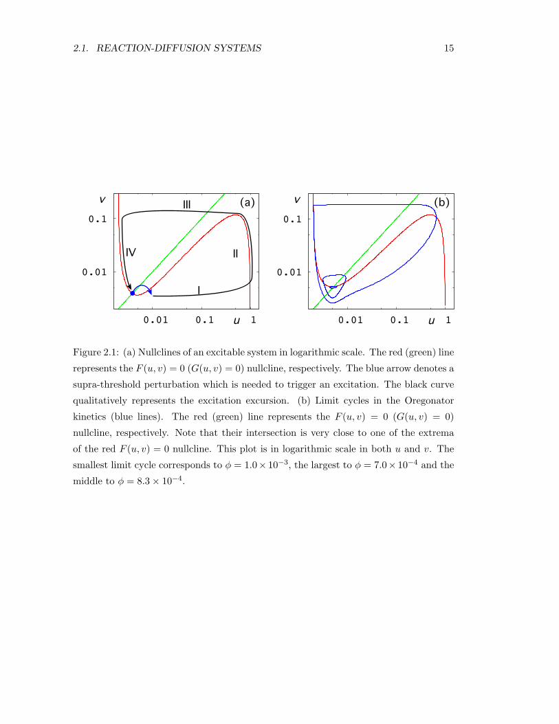
Figure 2.1: (a) Nullclines of an excitable system in logarithmic scale. The red (green) line
represents the F (u, v) = 0 (G(u, v) = 0) nullcline, respectively. The blue arrow denotes a
supra-threshold perturbation which is needed to trigger an excitation. The black curve
qualitatively represents the excitation excursion. (b) Limit cycles in the Oregonator
kinetics (blue lines). The red (green) line represents the F (u, v) = 0 (G(u, v) = 0)
nullcline, respectively. Note that their intersection is very close to one of the extrema
of the red F (u, v) = 0 nullcline. This plot is in logarithmic scale in both u and v. The
smallest limit cycle corresponds to φ = 1.0& 10!3, the largest to φ = 7.0& 10!4 and the
middle to φ = 8.3& 10!4.
16 CHAPTER 2. NONLINEAR WAVES IN REACTION-DIFFUSION SYSTEMS
1. Usually, one needs to perturb the variable u about the middle branch of the null-
cline F (u, v) = 0 in order to get an excitation. After the perturbation, the phase
trajectory rapidly jumps to the right branch of the F (u, v) = 0 nullcline (part I in
Fig. 2.1 (a)).
2. After that, the trajectory slowly moves along the nullcline up to its extremum
(part II in Fig. 2.1 (a)).
3. At the maximum of the nullcline the trajectory jumps rapidly to another branch
of the nullcline again (part III in Fig. 2.1 (a)).
4. Then the phase point slowly relaxes to the stable equilibrium (part IV in Fig. 2.1
(a)). It is impossible to trigger a new excitation before the system is su#ciently
close to the equilibrium.
The separation between the fast parts (I and III) and slow parts (II and IV ) of the
excursion is provided by the small parameter ε.
Oscillatory kinetics The stable fixed point can undergo a supercritical Hopf bifurca-
tion at some value of the parameter φhb = 1.04&10!3. Under further decrease of φ the
stable limit cycle passes through a so-called canard explosion at φc and its size rapidly
grows up. In Fig. 2.1 (b) we present di!erent limit cycles at di!erent values of the
parameter φ. A detailed theoretical analysis of the canard behavior and its relation to
the excitability properties of the spatially extended system can be found in [31].
2.2 Profile equations
For some simple reaction-di!usion systems it is possible to analyze propagation of waves
considering only the kinetics of the system. For example, in [32] the authors calculated
the velocity of waves projecting the dynamics of the PDE on the phase space of a single
excitable element. The main idea was to calculate the velocities of the front and back of
the wave in dependence on the slow variable and find the conditions, under which both
velocities are equal. However, under many circumstances we can not just “forget” about
the di!usive coupling and treat the problem only from the viewpoint of the kinetics.
In what follows we present an approach which allows to reduce the reaction-di!usion
system from PDE to an ODE, which describes the profile of the wave. The only as-

2.2. PROFILE EQUATIONS 17
sumption that we need is that the wave propagates at a constant velocity and without
changing its profile. We will obtain equations, in which the evolution variable is rep-
resented by the spatial coordinate, giving the profile as a function of space. Thus the
stability of the solutions of the profile equation are irrelevant for the stability of the wave
with respect to the full PDE.
2.2.1 Co-moving frame approach
Suppose that we have a reaction-di!usion equation with N species U and kinetics F
∂tU = F (U) + D ∂xxU, (2.11)
with a di!usion matrix D = diag(dj), j = 1, . . . , N with non-negative entries. In a
moving frame z = x% Ct with velocity C we have to transform
U(x, t) ! U(x% Ct, t) = U(z, t),
and Eq. (2.11) reads
∂tU = F (U) + C ∂zU + D ∂zzU. (2.12)
We make now an assumption that will be very important for our whole considerations
later or. We interested only in those solutions U(z, t) to Eq. (2.12) that propagate with
a certain velocity C = c without changing their profile. It means that in Eq. (2.12) with
C = c they are stationary solutions, i.e. ∂tU = 0. They thus obey the following ODE
F (U) + cU " + D U "" = 0, (2.13)
where the prime denotes a derivative with respect to the moving coordinate z.
We obtained an ordinary di!erential equation (2.13) which governs the spatial profile
of the solution U(z). We cast this profile equation as a system of first-oder ODE. For
those components Ui of U that di!use we have
diU""i + cU "
i + Fi(U) = 0,
which leads to two first-order equations
U "i = Vi,
V "i = %d!1
i (cVi + Fi(U)).

18 CHAPTER 2. NONLINEAR WAVES IN REACTION-DIFFUSION SYSTEMS
For those species Ui that do not di!use (di = 0), the equation reads
U "i = %c!1Fi(U).
We obtain a set of k, N ( k ( 2N ordinary di!erential equations of first order.
Often it is more advantageous to assume that all N species di!use, but some of the
di!usional constants dj are vanishingly small. In this case the structure of the first-
order ODE system is more regular, which simplifies analytical manipulations with the
equations and implementation of numerical methods. For the sake of simplicity, we write
the system of the profile equation as
u" = f(u; c), u ' R2N ,
where f(u; c) is accordingly adapted right hand-sides of the equations above. We empha-
size that the dependence of the function f(u; c) on the velocity c is essential: We have
to tune the parameter of nonlinearity in order to obtain the correct solution. Physically
that means that for a given reaction-di!usion system the wave typically propagates at
a certain velocity c. Upon changing parameters of the reaction-di!usion system, for
instance, the di!usion coe#cients, the propagation velocity c changes as well. From
the viewpoint of dynamical systems, the solutions of the profile equation are usually of
codimension-1.
2.2.2 Some examples of travelling waves
Homogeneous states are the simplest class of the solutions to the profile equation.
Their existence just follows from the fact that every equilibrium of the kinetics is an
equilibrium in the profile equation (2.13) for every velocity c.
Periodic wave trains of wavelength L are represented by limit cycles of period L in
the profile equation. Here, the dependence on the velocity c is essential. In fact, we have
the following boundary-value problem
F (U) + cU " + D U "" = 0, 0 < z < L,
U(L) = U(0),(2.14)
solutions of which depend, of course, on the velocity c, which plays the role of the
parameter to be solved for in order to fulfill the boundary conditions. We can also

2.2. PROFILE EQUATIONS 19
consider the first-order formulation, using the rescaled variable ζ = z/L, we obtain then
∂!u = Lf(u; c), u ' R2N , 0 < ζ < 1,
u(1) = u(0)(2.15)
where the prime denotes a derivative with respect to ζ. Usually we expect that periodic
wave trains come in families, depending on the wavelength L, we denote the correspond-
ing dependence of the velocity on the wavelength
c = c(L)
as the nonlinear dispersion relation for spatially periodic wave trains. It turns out that
the slope of the dispersion curved
dLc(L)
is of certain importance for their stability properties and interaction between waves in
a wave train.
Solitary pulses and bound states are represented by homoclinic orbits in the profile
equation. They converge to the same asymptotic value U0 as z ! ±". They propagate
at a certain velocity c, which is reflected by the fact that the homoclinic orbits are of
codimension-1 in the profile equations.
Solitary pulses are accompanied by families of spatially periodic wave trains. The
asymptotic profile of the solitary pulse plays a crucial role for the dispersion relation
of the wave trains of large wavelength. We will discuss this in more detail in the next
section.
Under certain conditions, solitary pulses can form so-called bound states with two
or more pulses propagating at the same velocity. Such bound states are described by
N -homoclinic orbits in the profile equations. There is a number of bifurcations which
can produce N -homoclinic orbits, given the 1-homoclinic orbit exists; we will comment
on this later on.
Fronts can be seen as a generalization of solitary pulses in the sense that they are
spatial structures connecting two di!erent asymptotic states for z ! ±". The asymp-
totic states can be either homogeneous states or periodic wave trains. For fronts the
uniqueness of the propagation velocity is sometimes violated. For the same parameters
of the kinetics there can coexist di!erent fronts with di!erent profiles and propagation
velocities, see [33].

20 CHAPTER 2. NONLINEAR WAVES IN REACTION-DIFFUSION SYSTEMS
Profile ODE !
phase space
Physical PDE space
Figure 2.2: Representation of di!erent travelling patterns in the phase space of the
profile ODE.

2.3. HOMOCLINICS AND ACCOMPANYING PERIODIC ORBITS 21
2.3 Homoclinics and accompanying periodic orbits
In this section we consider special biasymptotic solutions to an ordinary di!erential
equation
u" = f(u; p), u ' RN , N ) 2 (2.16)
with a parameter p.
In what follows we use t as the evolution variable of Eq. (2.16) in order to be
able to speak about the evolution in “forward” and “backward” time. In the equations
that describe the profile of a wave solution in the reaction-di!usion system we use the
co-moving coordinate z as the evolution variable.
For the sake of simplicity we assume that f(0; p) = 0 for all p, i.e. the equation has
an equilibrium at zero. We will call the stable manifold W s all solutions that converge
to the equilibrium forwards in time (i.e. for t ! ") and the unstable manifold W u all
solutions that converge to the equilibrium backwards in time (i.e. for t ! %").
We are interested in such solutions q(t) to Eq. (2.16), which asymptotically approach
the equilibrium in both forward and backward time
limt#±$
q(t) = 0. (2.17)
These solutions are called homoclinic solutions. Clearly, the homoclinic solutions belong
to the intersection of the stable manifold W s and the unstable manifold W u of the
equilibrium.
We consider homoclinic solutions to a hyperbolic equilibrium, it means that the
dimensions of the stable and unstable manifolds sum up to the dimension of our phase
space N . This means that the codimensions1 of the stable and unstable manifolds also
sum up to N . It is also known that the codimensions of two intersecting manifolds
sum up (at most) to N , where N is exactly achieved only for transversal2 intersections3.
However, the intersection of the stable and unstable manifold is not transversal, since the1We denote the di!erence between the dimension of the space N and the dimension of a given object
(manifold or subspace) as its codimension, i.e. codim A = N ! dim A.2An intersection of two manifolds in RN is called transversal if in every point of the intersection there
exist N linearly independent vectors which are tangent to one of both manifolds.3In R2, for instance, a line is of dimension 1 and of codimension 1. If the intersection of two lines is
transversal than the codimension of the intersection (a point in this case) is 1+1 = 2, for non-transversal
intersection this does not hold. For example, two co-axial circles intersect only non-transversally, result-
ing in an intersection of dimension 1 and codimension 1.

22 CHAPTER 2. NONLINEAR WAVES IN REACTION-DIFFUSION SYSTEMS
bounded solution v to the linearized equation (see Eq. (2.18) below) is tangent to both
stable and unstable manifold for every intersection point (i.e. belonging to the homoclinic
orbit). It means that we can find only N % 1 linearly independent vectors, which are
tangent to one of both manifolds. The non-transversality of the intersection means that
this intersection does not persist under parameter change, i.e. is not structurally stable.
In the connection to travelling waves, we have always to tune the velocity c in order to
obtain the corresponding homoclinic connection.
For the further study of homoclinic orbits the solutions of two linear equations are
of certain importance. First, one assumes that there exists an unique solution to the
linearized equation
v" = A(t)v, where A(t) = ∂uf(q(t)), (2.18)
given by v = q"(t) (this can be seen taking a derivative with respect to t of Eq. (2.16))
and an unique solution to the adjoint variational equation
ψ" = %A%(t)ψ, (2.19)
We can immediately see that the solution ψ(t) to Eq. (2.19) is always perpendicular to
the solution v(t) of the variational equation Eq. (2.18). We consider
d
dt*v,ψ+ =
= *v",ψ++ *v,ψ"+ =
= *A(t)v,ψ+ % *v,A%(t)ψ+ = *A(t)v,ψ+ % *A(t)v,ψ+ =
= 0
(2.20)
together with
*v,ψ+##±$= 0
which leads to
*v,ψ+ = 0
for all t.
So the solution ψ(t) of the adjoint equation is always perpendicular to the solution
of the linearized equation (2.18). Moreover, one can show that ψ(t) is perpendicular to
the tangent spaces of both the stable and unstable manifolds of the equilibrium [13].
With the help of ψ(t) one defines the orientation of the homoclinic orbit as
O(q) = limt#$
sign*ψ(t), q(%t)+ · *ψ(%t), q(t)+, (2.21)

2.3. HOMOCLINICS AND ACCOMPANYING PERIODIC ORBITS 23
! !
Figure 2.3: Left: Real leading eigenvalues. Right: leading stable eigenvalues are complex
conjugate.
if this limit exists, see [34].
The asymptotic flow near the equilibrium is given by
v" = A(0)v. (2.22)
Since f(u) is a real-valued function, the eigenvalues of the matrix A(t) are either real
or complex-conjugate. Moreover, we assume that the equilibrium is hyberbolic, which
means that spec(A(0)) , iR = -. The closest to the imaginary axis eigenvalues (i.e. with
smallest real parts) of the linearization in the equilibrium A(0) are called leading stable
and leading unstable eigenvalues. The corresponding eigenvectors are called leading
stable and unstable eigenvectors. For a codimension-1 homoclinic orbit the leading stable
(unstable) eigenvector is tangent to the stable (unstable) manifold in the equilibrium,
respectively.
We define also a saddle quantity σ of a saddle or saddle-focus as the sum of the real
parts of the leading eigenvalues.
Two types of homoclinic solutions can be distinguished pretty artificially. The first
one is represented by the so-called 1-homoclinics, with a single loop of the phase tra-
jectory. The second class is the 2- and N -homoclinics, with the phase trajectory fol-
lowing the primary loop 2 or N times. In the context of pulses in excitable systems
N -homoclinics describe bound states with N pulses, which propagate at the same ve-
locity. Sometimes we will refer to both 2- and N -homoclinics as merely N -homoclinic
solutions.
There is another classification of homoclinic orbits, depending on the type of the
leading eigenvalues of A(0). For a general homoclinic orbit of codimension-1 the lead-
ing eigenvalues determine the asymptotical behavior for t ! ±". If the leading stable
(unstable) eigenvalues are complex-conjugate, the homoclinic orbit approaches the equi-

24 CHAPTER 2. NONLINEAR WAVES IN REACTION-DIFFUSION SYSTEMS
p < 0 p = 0 p > 0
Figure 2.4: Unfolding of homoclinic bifurcation in R2 for saddle quantity σ < 0. Red
curve denotes the stable manifold W s of the equilibrium, blue curve denotes the unstable
manifold W u of the equilibrium.
Figure 2.5: 2-homoclinic orbit.

2.3. HOMOCLINICS AND ACCOMPANYING PERIODIC ORBITS 25
librium in an oscillating manner for t ! %" (t ! +"), respectively. It turns out
that oscillating asymptotic behavior of a homoclinic orbit has a great impact on the
properties of the homoclinics and possible bifurcations of it.
Homoclinic solutions are accompanied in the parameter space by periodic solutions.
One of the most important theoretical results on the accompanying periodic solutions
is that their period exponentially scales the distance to the homoclinic orbit in the
parameter space. For the solitary pulses in reaction-di!usion systems it means the
following: the velocity of a periodic wave train depends exponentially on its wavelength.
One can summarize the results on the accompanying periodic orbits:
1. For real leading eigenvalues there exist one limit cycle close to the primary homo-
clinic orbit independently on the saddle quantity σ.
2. For complex-conjugate eigenvalues there exist one limit cycles close to the primary
homoclinic orbit for σ < 0 and infinitely many of them for σ > 0.
More specifically, the following relation between the bifurcation parameter p and
period of limit cycle L
p = p0 +1M
$*ψ(%L), q(L)+ % *ψ(L), q(%L)+
%(2.23)
holds for large L. The homoclinic bifurcation is given by p = p0. Here, q(z) and
ψ(z) denote the homoclinic solution and the bounded solution to the adjoint problem,
respectively. The constant M is a Melnikov integral, given by
M = %$&
!$
*ψ(z), ∂pf(q(z), p0)+ dz .= 0.
We note that, depending on the sign of σ one of the scalar products in (2.23) dominates
over the other one, which allows to consider only one of them.
The found dependence of the period of limit cycles on a parameter close to a ho-
moclinic orbit is important for the dispersion relation of periodic wave trains, which
accompany the solitary pulse. In application to the profile equation, the relative veloc-
ity of the wavetrain c plays the role of the parameter p. The period of the limit cycles is
the wavelength L of the spatially periodic wavetrain. The dependence of the wave train
velocity c on L for large L reads then
c = c0 +1M
$*ψ(%L), q(L)+ % *ψ(L), q(%L)+
%, (2.24)

26 CHAPTER 2. NONLINEAR WAVES IN REACTION-DIFFUSION SYSTEMS
where c0 is the velocity of solitary pulse. For pulses, the sign of the saddle quantity σ
determines whether the front or the back of the pulse decays slower. The sign of the
scalar products can be estimated for large L, where ψ(±L) and q(±L) can be read o!
from the eigenvectors of the matrix A(0).
In the following subsections we will shortly review some well-known results on the
homoclinic orbits for the case of real and complex-conjugate leading eigenvalues.
2.3.1 Real leading eigenvalues
For the sake of simplicity, we consider a homoclinic orbit to an equilibrium with real
leading eigenvalues in a three-dimensional phase space, i.e. N = 3. The 3 & 3 matrix
A(0) has three real eigenvalues %λss < %λs < 0 < λu. However, for a codimension-1
homoclinic orbit, the dynamics is e!ectively only two-dimensional and sometimes we
may consider Eq. (2.16) only in R2.
Let us recall three general assumptions on the homoclinics of codimension one [13]:
1. the leading eigenvalues are not in resonance λu .= λs,
2. the solution v(t) to the linearized problem Eq. (2.18) converges to zero along the
leading eigenvectors of the linearization in the fixed point and
3. the same applies to the solution ψ(t) of the adjoint problem Eq.(2.19).
The last assumption is sometimes called the strong inclination property, for homo-
clinic orbit in R3 it means that the two-dimensional stable manifold comes to the fixed
point tangent to the strong stable direction (see Fig. 2.6 and Fig. 2.7). A homoclinic
orbit of codimension-1 can be orientable or twisted, depending on the orientation of
the strip of the two-dimensional manifold, which can be characterized by the orienta-
tion O(q), see Eq. (2.21). The stable manifold is topologically either a cylinder or a
Mobius strip. The orientation of a homoclinic orbit can be changed upon one of the
codimension-2 bifurcations.
Codimension-2 bifurcations
If one of the assumption on the codimension-1 homoclinic orbit fails, one speaks of a
codimension-2 bifurcation. There are three kinds of those:
1. resonance homoclinic orbit, characterized by λs = λu,

2.3. HOMOCLINICS AND ACCOMPANYING PERIODIC ORBITS 27
Figure 2.6: Orientable homoclinic orbit to a saddle. Red arrows denote the solution to
the adjoint variational equation. Blue strip shows the two-dimensional stable manifold
close to homoclinic orbit.
Figure 2.7: Twisted homoclinic orbit to a saddle. Red arrows denote the solution to the
adjoint variational equation. Blue strip shows the two-dimensional stable manifold close
to homoclinic orbit.

28 CHAPTER 2. NONLINEAR WAVES IN REACTION-DIFFUSION SYSTEMS
2. orbit flip, for which the solution of the linearized equation (2.18) approaches zero
along a strongly (un)stable eigenvector and
3. inclination flip, for which the solution of the adjoint equation (2.19) approaches
zero along a strongly (un)stable eigenvector.
We are interested in those bifurcations, since they can produce 2- and N -homoclinics
(or, equivalently, bound states for pulses in reaction-di!usion system). The resonant
bifurcation can produce only 2-homoclinics, the orbit flip and the inclination flip can
both produce 2- and N -homoclinics, depending on the ratio between λss, λs and λu (see
Table I and Table II in [34]). A flip bifurcation, either orbit or inclination, corresponds
to a switching of the solution of the linear equation through the strongly (un)stable
subspace of A(0). We need an additional parameter µ in order to unfold a codimension-
2 bifurcation of the homoclinic orbit.
Resonant homoclinic orbits were investigated in [35] and can already be found in
R2.
There are two cases which have to be discussed separately.
1. If the original homoclinic orbit is orientable, the bifurcation involves emergence of
a saddle-node bifurcation of limit cycles. For µ > 0, limit cycles bifurcate from the
original homoclinics for p > 0 and for µ < 0 this occurs for p < 0.
2. For a twisted homoclinics, the resonance bifurcation involves a period doubling
and bifurcation to a 2-homoclinic orbit. The period-doubling bifurcation stems
from (p, µ) = (0, 0). The period of the bifurcating periodic orbit goes to infinity
as µ ! 0.
Homoclinic flips, namely, the orbit flip and the inclination flip are purely three-
dimensional phenomena. They both are characterized by a change of the orientation of
the strip of the (un)stable manifold close to the homoclinic orbit, see [36, 37, 38].
In a homoclinic flip bifurcation solutions of the linearized equation or adjoint varia-
tional equation flips through the strongly (un)stable eigenspace of A(0). In the orbit flip
bifurcation the homoclinic orbit approaches the equilibrium along a strongly (un)stable
eigenvector (see Fig. 2.8 and Fig. 2.9). In the inclination flip, the solution of the adjoint

2.3. HOMOCLINICS AND ACCOMPANYING PERIODIC ORBITS 29
Figure 2.8: Codimension-2 orbit flip of homoclinic orbit. Red arrows indicate the solution
to the adjoint equation ψ(t).
Figure 2.9: Details of the orbit flip bifurcation. Red arrows indicate the solution to
the adjoint equation ψ(t). Left: structure of stable manifold before bifurcation, center:
structure of stable manifold in the bifurcation point, right: structure of stable manifold
after the bifurcation.

30 CHAPTER 2. NONLINEAR WAVES IN REACTION-DIFFUSION SYSTEMS
Figure 2.10: Codimension-2 inclination flip of homoclinic orbit. Red arrows indicate the
solution to the adjoint equation ψ(t).
variational equation (2.19 approaches zero along the strongly (un)stable eigenvector (see
Fig. 2.10 and Fig. 2.11).
In dependence on the ratio between λss, λs and λu, here are three cases to be con-
sidered separately
1. No extra bifurcations occur.
2. Bifurcation to 2-homoclinic orbit occurs together with appearance of a branch of
period-doubling bifurcation for the accompanying limit cycles.
3. Bifurcation to N -homoclinics (N ) 3) occurs. There also appear branches of
n-periodic solutions and period-doubling bifurcations.
It is possible to detect all three bifurcations numerically with the help of the available
numerical bifurcation analysis software AUTO [39]. For the resonant bifurcation we have
to monitor the simple resonance condition on the leading eigenvalues of the matrix A(0) ,
whereas the detection of the homoclinic flips is more involved and needs the computation
of the solution to the adjoint variational equation.
Three discussed codimension-2 bifurcations of homoclinic orbits to a saddle with real
leading eigenvalues seem to be the only mechanisms to produce N -homoclinics. This

2.3. HOMOCLINICS AND ACCOMPANYING PERIODIC ORBITS 31
Figure 2.11: Details of the inclination flip bifurcation. Red arrows indicate the solution
to the adjoint equation ψ(t). Left: structure of stable manifold before bifurcation, center:
structure of stable manifold in the bifurcation point, right: structure of stable manifold
after the bifurcation.
fact simplifies the study of multiple pulse branching. If one has N -homoclinics solutions
somewhere in the parameter space, one can continue the N -homoclinics solution to the
point in the parameter space where it nearly coincides with the primary 1-homoclinics
and expect that the 1-homoclinics undergoes one of the discussed codimension-2 bi-
furcations. In this sense, codimension-2 bifurcation act as organizing center for the
appearance of N -homoclinics.
2.3.2 Complex-conjugate leading eigenvalues
The transition from saddle to saddle-focus can actually be seen as a fourth type of
codimension-2 bifurcation of homoclinic orbits. Here we will consider a case with two
stable complex-conjugate eigenvalues. Historically, the main results on the homoclinic
orbit to saddle-foci were obtained by Shilnikov [40, 41, 42] (see also [43]), who proved,
among others, the existence of an infinite number of periodic orbits close to the homo-
clinic one.
In Fig. 2.12 we can see an example of such homoclinic orbit in R3. The stable mani-
fold is again two-demensional, and the unstable manifold is one-dimensional. The homo-
clinic orbit approaches the equilibrium in an oscillating manner in forward time. It was
shown that at the point of transition to the saddle-focus, new branches of N -homoclinic
solutions appear (see numerous references in [13], Chap. 6.3). So as soon as we have a
1-homoclinic orbit to a saddle-focus with complex-conjugate leading eigenvalues, there
exist further homoclinic solutions with N -loops. Sometimes such N -homoclinics are

32 CHAPTER 2. NONLINEAR WAVES IN REACTION-DIFFUSION SYSTEMS
Figure 2.12: Left: Homoclinic orbit to a saddle-focus. Right: a periodic orbit (black)
close to the primary homoclinic orbit (red).
referred to as subsidiary homoclinic orbits [44].
Homoclinic orbits to saddle-focus are as well accompanied by a family of periodic
solutions. In the same way as for homoclinic orbits to a saddle, we can map an appro-
priate Poincare section in itself close to the homoclinic orbit and study the fixed points
of this map in dependence on the bifurcation parameter p. We refer to [44, 13] for the
analysis of the map. Depending on the saddle quantity σ, we have two possibilities for
the dependence of the period of the periodic solutions on p:
1. For saddle quantity σ < 0, the curve p(T ) for periodic orbits is monotonous.
2. For saddle quantity σ > 0, p(T ) is a wiggly curve, shown in Fig. 2.13. For p = 0
there exist infinitely many periodic orbits.
Limit cycles that belong to di!erent parts of the curve p(T ) have qualitatively dif-
ferent portraits. The first part of the curve p(T ) with positive slope is represented
by the limit cycles, consisting of one large excursion near the primary homoclinic
orbit and typically have only one maximum on the period. For every maximum on
the p(T ) curve, the corresponding limit cycles make an additional small-amplitude
winding around the equilibrium. The right panel in Fig. 2.12 shows a limit cycle
with two windings around the equilibrium. The global shape of the homoclinic or-

2.3. HOMOCLINICS AND ACCOMPANYING PERIODIC ORBITS 33
T
p
PD
PDPD
PD
PDPD
PDPD
Figure 2.13: Dependence of the period of limit cycles on p for the case of homoclinic
orbit to saddle-focus with saddle quantity σ > 0.
bit is nearly repeated by the periodic solution. Periodic orbits with large periods
T !" have a growing number of windings around the equilibrium.
Close to each maximum of the curve p(T ) the limit cycle undergoes a period-
doubling bifurcation. This bifurcation results in a new periodic orbit which also
belongs to some other curve p2(T ), which is also a wiggly curve. The secondary (or
subsidiary) periodic orbits converge to 2-homoclinics for large T as well and also
can undergo further period-doubling bifurcations close to the maxima of p2(T ),
giving raise to pretty reach dynamics.
Summarizing, in the parameter space near a 1-homoclinic orbit to a saddle-node with
a saddle quantity σ > 0 (or equivalently δ < 1) we find a complex structure, consisting
of primary periodic orbits and subsidiary homoclinic and periodic orbits. It is possible
to find any solution consisting of a given number of large and small oscillations. For the
waves in reaction-di!usion systems it means that we can always construct a bound state
with any given number of excitation pulses with small oscillations in between.

34 CHAPTER 2. NONLINEAR WAVES IN REACTION-DIFFUSION SYSTEMS
2.4 Stability of waves
For a comprehensive understanding of the wave dynamics a detailed stability analysis
of the wave turns out to be essential. Moreover, as only stable travelling wave solutions
can be observed experimentally, stability considerations are crucial for experimental
verification of theoretical results.
To study the stability of the solutions to the reaction-di!usion system we use a
straight-forward approach, linearizing the equation about the studied solution [14]. The
elements of the spectrum of the obtained linear operator are the growth rates of small
perturbations: instability of the solution is reflected by the presence of spectrum in the
right complex half-plane.
In this section we will deal mainly with the stability of waves in reaction-di!usion
equations posed on the whole real axis and on large domains with periodic boundary con-
ditions. The stability of waves on bounded domains and the so-called absolute stability
will be discussed only briefly.
2.4.1 Spectral approach
We suppose that we have found a solution to a reaction-di!usion system
∂tU = F (U) + D∂xxU, U ' RN (2.25)
in the form of a running wave Q(z) = Q(x% ct) with constant shape and velocity c. As
we have seen before, the function Q(z) obeys the profile equation
DU "" + cU " + F (U) = 0, (2.26)
that can be cast as a first-order system
u" = f(u; c), u ' R2N (2.27)
where prime denotes a derivative with respect to the co-moving coordinate z.
For a given solution Q(z) of (2.26) we can formulate the corresponding linearized
problem in the co-moving frame:
∂tW = FU (Q(z))W + c∂zW + D∂zzW, W ' CN (2.28)
where FU denotes the linearization of the function F . With a separation ansatz
W (t, z) = e"tV (z),

2.4. STABILITY OF WAVES 35
we obtain the following equation for λ and V (z)
λV = FU (Q(z))V + cV " + DV "", V ' CN , " def= ∂z (2.29)
or
LV = λV, (2.30)
where the operator L is given by
L = D∂zz + c∂z + FU (Q(z)).
Again, we cast Eq. (2.29) as a first-order system
v" = A(z;λ)v, v ' C2N (2.31)
where
A(z;λ) = A(z) + λB.
Matrices A(z) and B are given by
A(z) =
'0 id
%D!1FU (Q(z)) %cD!1
(, B =
'0 0
D!1 0
(. (2.32)
The translation symmetry of the problem (2.25) provides that for non-constant Q(z)
Eq. (2.29) always has a bounded solution for λ = 0, which is given by V (z) = Q"(z).
We can easily check it by taking a derivative with respect to z of Eq. (2.26):
D(U ")"" + c(U ")" + FU (Q)U " = 0 · U ".
Definition of spectrum We consider the family of operators
T (λ) : u /%! du
dz%A(·;λ)u (2.33)
defined on the appropriate space [14]. λ acts as a parameter for the family.
We say that λ is in the spectrum $ of T if T (λ) is not invertible, i.e. if the inverse
operator does not exist or is not bounded. We say that λ ' $ is in the point spectrum
$pt of T or, alternatively, that λ ' $ is an eigenvalue of T if T (λ) is a Fredholm operator
with index zero. The complement $ \$pt =: $ess is called the essential spectrum. The
complement of $ in C is the resolvent set of T [14].
Below we give a short overview of the spectra of di!erent wave types. For the sake
of comparison, we qualitatively consider quantum mechanical problems for a particle in
one spatial dimension with di!erent types of potentials.

36 CHAPTER 2. NONLINEAR WAVES IN REACTION-DIFFUSION SYSTEMS
Homogeneous rest states Q(z) = Q0. In this case the linearization has constant
coe#cients
v" = A(Q0;λ)v = A0(λ)v.
This equation has a bounded solutions on R if, and only if, the matrix A0(λ) is non-
hyperbolic. λ is in the essential spectrum of T if, and only if,
d0(λ, k) = det[A0(λ)% ik] = 0
has a solution k ' R.
The function d0(λ, k) is referred to as the linear dispersion relation. The essential
spectrum consists of curves λ(k) in the complex plane.
We can define the group velocity
cg = % d
dkIm λ(k),
which represents the velocity of the wave packets centered near the wavenumber k in
the linear equation Ut = LU .
The point spectrum of homogeneous rest state is empty.
Traditionally, four types of instability of homogeneous rest state are distinguished.
Supposed that at the onset of the instability there is a single kcr with Re λ(kcr) = 0.
Then we have the following cases:
1. kcr = 0, Im λ(kcr) = 0 corresponds to homogeneous saddle-node bifurcation.
2. kcr = 0, Im λ(kcr) .= 0 corresponds to homogeneous Hopf bifurcation.
3. kcr .= 0, Im λ(kcr) = 0 is referred to as Turing instability.
4. kcr .= 0, Im λ(kcr) .= 0 is referred to as wave instability. Sometimes terms like
Turing-Hopf or Turing-II are used.
Quantum mechanical analogy: If we have a particle in a force-free space, every state
of it is a free state. The energy levels form a continuous spectrum and every energy
value is two-fold degenerated.

2.4. STABILITY OF WAVES 37
Periodic wave trains of period L. In this case the matrix A(z;λ) is L-periodic, i.e.
A(z + L;λ) = A(z;λ)
for all z. The linearization around the wave train
v" = A(z;λ)v. (2.34)
has periodic coe#cients. By Floquet theory, the solutions of Eq. (2.34) have the following
form
v = e#(")zqL(z;λ), (2.35)
where qL(z + L;λ) = qL(z;λ) is an L-periodic function. Casting the corresponding
boundary-value problem for v, we obtain
v = (∂uf(u(z); c) + λB) v, 0 < z < L,
v(L) = ei$v(0).(2.36)
λ is in the essential spectrum of T if, and only if, Eq. (2.36) has a solution for some
γ ' R. λ = 0 is contained in the essential spectrum with the Goldstone mode given by
Q"(z). Near the origin, the spectrum λ(γ) is approximated by
λ(γ) = %icgγ % dγ2 +O(γ3),
where cg denotes the group velocity. The sign of the constant d decides upon the stability,
given the rest of the spectrum is contained in the left open half-plane. The Eckhaus
instability is characterized by d = 0.
Spatially period wave trains usually live in families on the so-called dispersion curves
c(L). In the Appendix, we show that
d
dγIm λ(γ)
####$=0
= %cg =d
dLc(L),
so the slope of the dispersion curve c(L) coincides with the first coe#cient of the expan-
sion of spectrum at zero.
The point spectrum of a wave train is empty.
In the solid-state physiscs the representation given by Eq. (2.35) is known as Bloch-
wave decomposition. For a particle in a periodic potential, the possible energy values
form continuous bands.

38 CHAPTER 2. NONLINEAR WAVES IN REACTION-DIFFUSION SYSTEMS
Pulses on homogeneous background. In this case Q(z) approaches a constant
value as z ! ±", i.e.
limz#±$
Q(z) = Q0.
The matrix A has then also a limit value
limz#±$
A(z;λ) = A0(λ).
The essential spectrum of the pulse Q(z) in this case is given by the essential spectrum
of Q0.
Q"(z) is an eigenfunction of the linearization operator L to the eigenvalue λ = 0.
There can also be some further eigenvalues in the point spectrum.
Quantum mechanical analogy: consider a particle in a localized potential. There
are discrete energy levels, corresponding to the bound states and continuous energy
spectrum of free states.
2.4.2 Stability of pulse trains with large wavelength
Solitary pulses in reaction-di!usion systems are known to be accompanied by spatially
periodic pulse trains. Those pulse trains can be characterized by the dispersion relation,
which expresses the dependence of the pulse train velocity c on its wavelength L. The
aim of this subsection is to give a short overview of the theoretical results [16] on the
stability of the periodic pulse trains with large L.
We suppose that we have a profile equation
u" = f(u, c), (2.37)
which allows for a homoclinic solution q(z) for c = c0. This homoclinic solution rep-
resents the primary solitary pulse in the reaction-di!usion system. We assume that
f(0, c) = 0 holds for all c and this equilibrium is hyperbolic for c = c0.
Next, we cast the linearization around the pulse q(z) as a system of first-order dif-
ferential equations
v" = [∂uf(q(z), c0) + λB]v,
compare the previous sections. We assume that the only solution to the above equation
for λ = 0 is given by q"(z), so λ = 0 is an isolated eigenvalue. We assume the stability
of the primary pulse q(z), which means that the rest of the spectrum of the pulse is
contained in the open left half-plane.

2.4. STABILITY OF WAVES 39
Furthermore, we assume that there exists a 2L-periodic solution pL(z) to the profile
equation (2.37) with cL and pL(%L) = pL(L). We are interested in large L, so the
velocity of the 2L-periodic pulse train cL must be close to c0. From the previous section,
we know that λ is in the spectrum of 2L-periodic pulse train pL(z) if, and only if, the
boundary-value problem
u" = [∂uf(pL(z), cL) + λB]u, |z| < L
u(L) = ei$ u(%L)(2.38)
has a solution u(z) for some real γ.
Gardner [45] proved that the essential spectrum of the primary solitary pulse is
approximated by the essential spectrum of the 2L-periodic solution pL(z). Moreover,
for any λ% ' $pt(q) with multiplicity m and for every fixed spatial Floquet exponent
γ ' [0, 2π), Eq. (2.38) has precisely m solutions in a certain ε-neighborhood of λ%. It
means that we obtain circles (or closed curves) of essential spectra near every point of
point spectrum of solitary pulse upon cloning the latter periodically in space with large
enough interpulse distance.
The main result of [16] concerns the location of the circle of eigenvalues which arises
from the eigenvalue λ = 0 of the pulse q(z) . We supposed that the pulse q(z) is stable,
so the location of this circle decides upon the stability of the 2L-periodic solution pL(z).
The expansion of λ(γ) near λ = 0 is given by
λ =1M
$(ei$ % 1)*ψ(L), q"(%L)++ (1% e!i$)*ψ(%L), q"(L)+
%+ R(γ, L) (2.39)
with the rest term
R(γ, L) = (ei$ % 1)O(e!3%L) + (1% e!i$)O(e!3%L),
where ρ is related to the magnitude of the eigenvalues of ∂uf(0, c0).
The corresponding solutions of Eq. (2.38) are given by
u(z) = eik$q"(z) +O(e!%L), z ' [(2k % 1)L, (2k + 1)L], k ' Z.
Here, M is a Melnikov integral, given by
M = %$&
!$
*ψ(z), ∂cf(q(z), c0)+ dz =$&
!$
*ψ(z), Bq"(z)+ dz .= 0.

40 CHAPTER 2. NONLINEAR WAVES IN REACTION-DIFFUSION SYSTEMS
! !
Figure 2.14: Spectrum of primary solitary pulse q(z) is shown in black curves and dots.
Spectra of 2L- periodic solutions shown in blue lines. Left panel shows spectra of stable
periodic solutions, right panel shows spectra of unstable periodic solutions. Note the
location of the circle of critical eigenvalues near the origin.
Again, ψ(z) denotes the solution of the adjoint variational equation
ψ" = %∂uf%(q(z), c0)ψ.
The sign of the curvature of the circle of critical eigenvalues
d2
dγ2Re γ
####$=0
=1M
$(%*ψ(L), q"(%L)++ *ψ(%L), q"(L)+
%
shows whether the circle of critical eigenvalues lies in the right or in the left complex
half-plane, i.e. whether the 2L-periodic pulse train is stable or not. We refer to Fig.
2.14 for the structure of the spectra of periodic pulse trains close to the primary solitary
pulse.
We can interpret the above results as follows. The expansion of λ(γ) near the origin
consists of the scalar products of the solutions to the adjoint equation ψ(z) and the
derivative of the pulse profile q"(z) for large z. These are determined by the leading
eigenvalue ν of the matrix ∂uf(0, c0), which we assume to be real and, say, negative.
Referring to [16], we obtain
q"(z) = e#zv0 +O(e!(|#|+&)z), q"(%z) = e#zw0 +O(e!(|#|+&)z),
for a some constant δ, where v0 and w0 are the corresponding eigenvectors of ∂uf(0, c0)
and ∂uf%(0, c0), respectively. We obtain then the expansion
λ =*v0, w0+
M(1% e!i$)e2#L.

2.4. STABILITY OF WAVES 41
The term
*ψ(z), q"(%z)+
can be neglected, since it decays faster than e!2#z (recall our assumption on the leading
eigenvalue ν). Finally, we obtain that the spatially periodic pulse trains are stable if
M*v0, w0+ < 0.
In the exactly same way we can obtain the expansion for a pair of complex-conjugate
leading eigenvalues ν, ν
λ =a
Msin(2L Im ν + b)(1% e!i$)e2L Re # ,
where a and b are real constants. The stability of the pulse trains which accompany a
solitary pulse with oscillating wake changes periodically in dependence on L. The circle
of critical eigenvalues flips over the imaginary axis on the period-doubling bifurcation
of the limit cycles, belonging to the wiggly curve c = c(L) (recall the section on the
homoclinic orbits).
2.4.3 Numerical computation of spectra
We have to deal with two problems if we want to compute the stability of a given wave
numerically. Firstly, we need an e#cient and precise method of locating the spectrum and
secondly we have to care about the boundary conditions since in numerical computations
it is impossible to simulate wave dynamics on unbounded domains.
Below we shortly present the method of computing essential spectra of periodic wave
trains. One can find a deeper insight in the method with a number of examples (including
actual code) in [46].
Suppose that we have found a L-periodic wave train Q(z). As we have seen already
in the previous sections, λ is in the spectrum of the linearization about Q(z) if, and only
if, the boundary-value problem
v" = f(v; c),
u" = A(z;λ)u, 0 < z < L
u(L) = ei$+'u(0)
(2.40)
has a solution for η = 0 and some real γ. Note that we have also to solve for the
profile of the wave, since the coe#cients of the matrix A(z;λ) depend on Q(z). If we
have a good starting solution to Eq. (2.40), we can continue it in (γ, λ) ' R & C and

42 CHAPTER 2. NONLINEAR WAVES IN REACTION-DIFFUSION SYSTEMS
obtain a curve of the essential spectrum λ(γ). As the starting solution, we can use
γ = η = λ = 0, u(z) = Q"(z), which is always in the spectrum. Another possibility is to
find an initial condition for the continuation of Eq. (2.40) by computing the eigenvalues
and the corresponding eigenfunctions of the discretized operator L.
The parameter η in Eq. (2.40) is normally set to zero, this is the condition for
λ ' $ess. However, with η .= 0 it is possible to compute the spectrum on weighted spaces,
which can be used to compute the direction of propagation of the possible unstable
modes. Computations with η .= 0 are also needed for the calculation of the absolute
spectrum, which is discussed below; in this case we can tell apart between the absolute
and convective instabilities of the travelling wave.
We would like to note that using the continuation techniques for computing spectra
delivers very accurate results. The accuracy can be easily controlled and the computation
of the relevant branches of the essential spectrum usually take no longer than several
minutes. It is also possible to reach branches which can firstly be not connected to the
branches with known starting solution, performing the continuation along the parameters
of the non-linearity or in the dispersion plane (L, c).
It is also possible to use the continuation method to get an approximation of the
point spectrum of solitary pulses. In this case, we can use the results on the stability of
pulse trains with large spatial period that accompany the solitary pulse. Every λ in the
point spectrum of the original pulse will be approached by a piece (typically, a circle) of
the essential spectrum of the pulse train. The essential spectrum of the solitary pulse is
approximated by the essential spectrum of the periodic pulse train.
The next paragraphs explain how to interpret the possible results of the calculation
of the spectrum on bounded intervals. Here we have to distinguish between periodic and
separated boundary conditions.
Periodic boundary conditions. Suppose we would like to estimate the spectrum $
of a solitary pulse Q(z). $ consists of the point spectrum $pt and the essential spectrum
$ess. With this purpose we consider a solution QL(z) on large interval of length L with
periodic boundary conditions. We denote by $perL the spectrum of QL(z), this spectrum
consists only of point spectrum. In [47] the following statements were proven:
• For every eigenvalue λ% with multiplicity l in $pt, there are precisely l elements in
$perL , counted with multiplicity, close to λ%, and these elements converge to λ% as
2.4. STABILITY OF WAVES 43
L ! ". In other words, isolated eigenvalues of the pulse Q(z) are approximated
by elements in $perL , counting multiplicity.
• Every λ% ' $ess is approached by infinitely many eigenvalues in $perL as L !".
So the spectrum $perL of the solution on the truncated domain with periodic boundary
conditions converges to the spectrum $ of the original pulse as L !".
Separated boundary conditions and absolute spectrum. In this case the stabil-
ity of a travelling wave di!ers from that on the unbounded domain pretty dramatically.
We suppose that we have a travelling wave solution Q(z) with two asymptotically
states Q±(z), which can be either a constant or a periodic ones. The matrix A(z;λ) of
the linearized problem
u" = A(z;λ)u
has then also asymptotics given by A±(λ) for z ! ±". We assume that A±(λ) are both
hyberbolic.
We denote by $sepL the spectrum of our solution on a large bounded domain of size
L with separated boundary conditions. $sepL consists only of point spectrum. Below we
will see that $sepL does not approach to $ as L !", but to a quite di!erent set that is
called the absolute spectrum.
We need first to order the eigenvalues of A±(λ) according to their real parts
Re ν±1 (λ) ) . . .Re ν±n/2(λ) ) Re ν±n/2+1(λ) ) . . .Re ν±n (λ).
We define $+abs = {λ ' C; Re ν+
n/2(λ) = Re ν+n/2+1(λ)} and $!abs = {λ ' C; Re ν!n/2(λ) =
Re ν!n/2+1(λ)}. The absolute spectrum $abs is the union of $+abs and $!abs.
It can be shown that the point spectrum of a travelling wave approaches the so-called
pseudo-point spectrum $pt as L !".
The next result proven in [47] states that the spectrum $sepL does not approximate
the spectrum $ = $pt 0 $ess, but the set $pt 0 $abs :
• For every λ% ' $pt with multiplicity l, there are precisely l elements in $sepL ,
counted with their multiplicity, close to λ%, and these elements converge to λ% as
L !".
• Every λ% ' $abs is approached by infinitely many eigenvalues in $sepL as L !".

44 CHAPTER 2. NONLINEAR WAVES IN REACTION-DIFFUSION SYSTEMS
The nice thing about the absolute spectrum is that it depends only on the asymptotic
states Q±(z) and can be computed with the help of the continuation techniques [46].
Sometimes it is possible to estimate the location of the absolute spectrum without
computing it [48, 46, 49]:
• Typically, the absolute spectrum is to the left of the essential spectrum. This
indicates that the convective instability develops prior to the absolute one. The
essential spectrum can be already in the right half-plane, while the absolute spec-
trum in the left one.
• A closed piece of essential spectrum sometimes contains a piece of absolute spec-
trum in it.
• A point, where two curves of essential spectrum cross, belongs to the absolute
spectrum.
We would like to refer to [50] for colorful results on the absolute spectrum of spiral
waves.

Chapter 3
Bistable dispersion and coexisting
wave trains
3.1 Overview of dispersion types
Travelling excitation pulses are one of the basic types of patterns in active media [2, 51].
They can form periodic wave trains that propagate through the medium with constant
velocity and profile. An important characteristic of these pulse trains is the dispersion
relation which expresses their velocity c as a function of their wavelength L. In the
large-wavelength approximation, the form of the dispersion curve defines the type of
interaction between the pulses in the train. Positive (negative) slope of the dispersion
curve corresponds to repulsive (attractive) interaction.
So far three main types of dispersion curves are distinguished in reaction-di!usion sys-
tems [19]: (i) monotonic where c(L) is a monotonously increasing function that asymp-
totically approaches a maximum value which equals the velocity of the solitary pulse
c0, (ii) nonmonotonic with a negative slope domain, corresponding to attraction be-
tween neighbouring pulses, and (iii) oscillatory with damped oscillations giving rise to
alternating attractive and repulsive pulse interaction. The first case is called normal
dispersion, while the last two possibilities are referred to as anomalous dispersion.
Theoretical analysis of oscillatory dispersion in excitable media has attracted much
interest [52]. It was proven that a one-dimensional medium with this type of dispersion
can provide infinitely many equally spaced wave trains with wavelengths ranging up to
infinity moving with the same velocity. In a more general mathematical context, this is
45

46 CHAPTER 3. BISTABLE DISPERSION AND COEXISTING WAVE TRAINS
another manifestation of the results on the periodic orbits near a homoclinics to a saddle-
focus, which was discussed in the previous chapter. In two-dimensional media oscillatory
dispersion can lead to coexisting non-planar fronts [53] and cause the coexistence of free
spirals of di!erent wavelengths [18].
Indications for anomalous dispersion have been found in natural systems, for exam-
ple, in experiments on chemical waves that organize the early stages of aggregation in the
life cycle of the cellular slime mould Dictyostelium discoideum [54] and in the reduction
of NO with CO on Pt(100) surfaces [20].
The Belousov-Zhabotinsky (BZ) reaction [51, 4], which has been intensively stud-
ied as an easily controllable excitable medium, shows essentially normal dispersion [55].
This reaction involves the oxidation of an organic compound by bromate in acidic so-
lution. Experimental results on anomalous dispersion with a negative slope part have
been reported for a modified BZ system, in which the reaction is carried out with 1,4-
cyclohexanedione in contrast to the classical case that employs malonic acid as the
organic reactant [56].
In all referred above cases the dispersion curve is single-valued: for a given wavelength
it defines an unique propagation velocity of stable pulse trains. This chapter reports on
the oscillatory dispersion relation with a multivalued dependence of the propagation
velocity on the wavelength. As a consequence, in one medium two alternative planar
wave trains can exist having the same wavelength but di!erent velocities. We analyze
the stability of the coexisting pulse trains and compare the results with direct numerical
simulations. Dominance of the faster pulse train over the slower one in head-on collision
is illustrated by the shift of the annihilation position between the pulse trains.
3.2 Three-component Oregonator
In this chapter we use the modified three-variable Oregonator model for the photosensi-
tive BZ reaction in one spatial dimension [30]
∂tu = ε!1(u% u2 % w(u% q)) + Du∂2xu
∂tv = u% v (3.1)
∂tw = ε!!1(fv + φ% w(u + q)) + Dw∂2
xw.
Here u, v and w denote the dimensionless concentrations of bromous acid, the ox-
idized form of the photosensitive catalyst and bromide, respectively. The ratio of the

3.2. THREE-COMPONENT OREGONATOR 47
1.5 2.0-3
-2
-1
1log(v)
φ x104φhbφc
0 120 240 360 480-3
-2
-1
x
log(v)
c (b)
(a)
Figure 3.1: (a) Bifurcation diagram of the local dynamics described by eqs. (3.1). With
the chosen parameter values for ε, ε!, f and q (compare text) a Hopf bifurcation occurs
at φhb = 1.76&10!4, for the canard point we find φc = 1.61&10!4. Solid line shows the
amplitude of oscillations around the unstable HSS (dashed line) below φhb. (b) Profile
of the v variable of the stable solitary pulse propagating with velocity c to the right.
Note the small amplitude oscillations in the refractory tail ( φ = 2.0&10!4).

48 CHAPTER 3. BISTABLE DISPERSION AND COEXISTING WAVE TRAINS
di!usion coe#cients for bromous acid and bromide δ = Dw/Du can be estimated from
the molecular weights of the two species yielding δ = 1.12. Di!usion of v is omitted be-
cause in most experiments the catalyst is immobilized in a gel matrix. The time scales ε
and ε! follow from the recipe concentrations [30]. In this chapter, all parameters except
φ are fixed at the following values ε = 0.09, ε! = ε/8, f = 1.5 and q = 0.001. The param-
eter φ is proportional to the intensity of applied illumination. It will be considered as
the main bifurcation parameter which controls the local dynamics as well as the profile
and the velocity of excitation pulses.
For the choosen parameters the system has only one homogeneous steady state, which
undergoes a supercritical Hopf bifurcation at φhb (see Fig. 3.1(a)). With further decrease
of φ the stable limit cycle born at φhb passes through a so-called canard explosion at φc
and its size rapidly grows up.
We emphasize that the medium remains excitable in the parameter range φc < φ <
φhb. Triggered by a supra-threshold perturbation, a high-amplitude excitation relaxes
to the tiny limit cycle around the unstable equilibrium.
Above the canard point φc the medium admits two solitary pulses: a fast stable
one, presented in Fig. 3.1 (b), and a slow unstable pulse. The velocities of these pulses
depend on φ, coinciding in a fold bifurcation point at some φext (for our parameters
choice φext = 3.7&10!3, not shown in the figure). Often φext is referred to as extinction
threshold because beyond this value the medium does not support pulse propagation.
Below the canard point φc, solutions in the form of solitary running pulses do not exist
and the system relaxes to homogeneous oscillations or phase waves. The amplitude of
the stable fast pulse close to φc is approximately equal to the amplitude of the large
limit cycle after the canard explosion. Below we will refer to the high-amplitude part
of the pulse as to the “head” of the pulse, and to the oscillatory refractory zone behind
the pulse head as to the “pulse tail”.
Since the velocity of the solitary pulse is uniquely defined for given parameters, we
can transform to a co-moving frame by setting u(x, t), v(x, t) and w(x, t) to be functions
of a single variable z = x%ct. The partial di!erential equations (3.1) can be reduced to a
set of ordinary di!erential equations in a five-dimensional phase space spanned by u(z),
v(z), w(z) and their derivatives uz(z) and wz(z) with c (the velocity of the co-moving

3.2. THREE-COMPONENT OREGONATOR 49
0 300 6002.5
3.0
3.5
L
cc 0
150 1603.2
3.4
3.6
L
c SN
SN
1
2
0 0.4 0.8-3
-2
-1
x / L
log(
v)
(a)
(b)
Figure 3.2: (a) Dispersion curve for pulse trains for φ = 2.0&10!4 > φhb. The inset
shows one enlarged part of the dispersion curve. Circles have been obtained from one-
dimensional simulations of the underlying Oregonator model under slow increase of the
integration domain size L, while diamonds correspond to slow decrease of L. (b) v
profiles of one pulse in the train belonging to the upper (solid line) resp. lower (dashed
line) stable branch in the inset of (a).
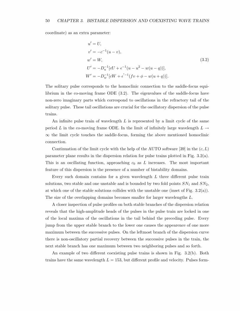
50 CHAPTER 3. BISTABLE DISPERSION AND COEXISTING WAVE TRAINS
coordinate) as an extra parameter:
u" = U,
v" = %c!1(u% v),
w" = W,
U " = %D!1u [cU + ε!1(u% u2 % w(u% q))],
W " = %D!1w [cW + ε
!!1(fv + φ% w(u + q))].
(3.2)
The solitary pulse corresponds to the homoclinic connection to the saddle-focus equi-
librium in the co-moving frame ODE (3.2). The eigenvalues of the saddle-focus have
non-zero imaginary parts which correspond to oscillations in the refractory tail of the
solitary pulse. These tail oscillations are crucial for the oscillatory dispersion of the pulse
trains.
An infinite pulse train of wavelength L is represented by a limit cycle of the same
period L in the co-moving frame ODE. In the limit of infinitely large wavelength L !" the limit cycle touches the saddle-focus, forming the above mentioned homoclinic
connection.
Continuation of the limit cycle with the help of the AUTO software [39] in the (c, L)
parameter plane results in the dispersion relation for pulse trains plotted in Fig. 3.2(a).
This is an oscillating function, approaching c0 as L increases. The most important
feature of this dispersion is the presence of a number of bistability domains.
Every such domain contains for a given wavelength L three di!erent pulse train
solutions, two stable and one unstable and is bounded by two fold points SN1 and SN2,
at which one of the stable solutions collides with the unstable one (inset of Fig. 3.2(a)).
The size of the overlapping domains becomes smaller for larger wavelengths L.
A closer inspection of pulse profiles on both stable branches of the dispersion relation
reveals that the high-amplitude heads of the pulses in the pulse train are locked in one
of the local maxima of the oscillations in the tail behind the preceding pulse. Every
jump from the upper stable branch to the lower one causes the appearence of one more
maximum between the successive pulses. On the leftmost branch of the dispersion curve
there is non-oscillatory partial recovery between the successive pulses in the train, the
next stable branch has one maximum between two neighboring pulses and so forth.
An example of two di!erent coexisting pulse trains is shown in Fig. 3.2(b). Both
trains have the same wavelength L = 153, but di!erent profile and velocity. Pulses form-
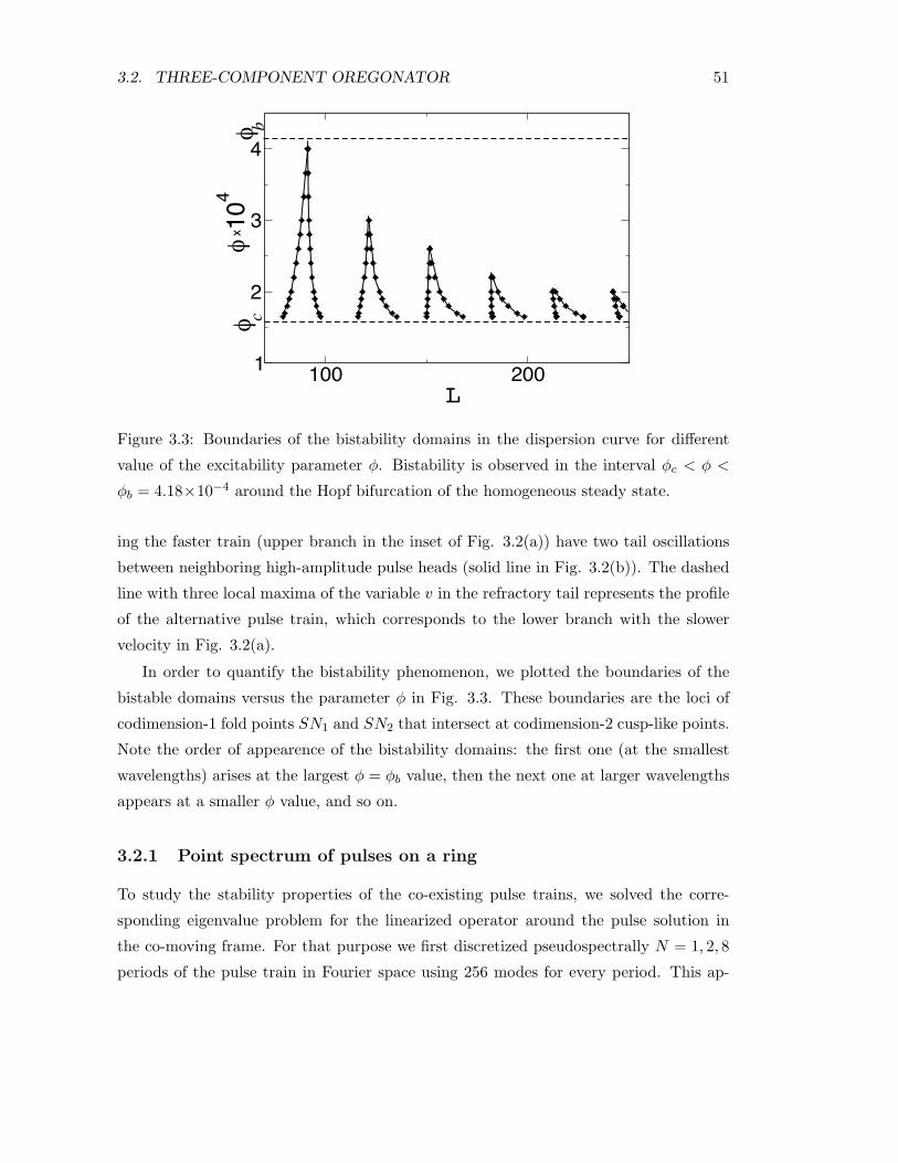
3.2. THREE-COMPONENT OREGONATOR 51
100 2001
2
3
4
φ x 1
04φ c
φ b
L
Figure 3.3: Boundaries of the bistability domains in the dispersion curve for di!erent
value of the excitability parameter φ. Bistability is observed in the interval φc < φ <
φb = 4.18&10!4 around the Hopf bifurcation of the homogeneous steady state.
ing the faster train (upper branch in the inset of Fig. 3.2(a)) have two tail oscillations
between neighboring high-amplitude pulse heads (solid line in Fig. 3.2(b)). The dashed
line with three local maxima of the variable v in the refractory tail represents the profile
of the alternative pulse train, which corresponds to the lower branch with the slower
velocity in Fig. 3.2(a).
In order to quantify the bistability phenomenon, we plotted the boundaries of the
bistable domains versus the parameter φ in Fig. 3.3. These boundaries are the loci of
codimension-1 fold points SN1 and SN2 that intersect at codimension-2 cusp-like points.
Note the order of appearence of the bistability domains: the first one (at the smallest
wavelengths) arises at the largest φ = φb value, then the next one at larger wavelengths
appears at a smaller φ value, and so on.
3.2.1 Point spectrum of pulses on a ring
To study the stability properties of the co-existing pulse trains, we solved the corre-
sponding eigenvalue problem for the linearized operator around the pulse solution in
the co-moving frame. For that purpose we first discretized pseudospectrally N = 1, 2, 8
periods of the pulse train in Fourier space using 256 modes for every period. This ap-

52 CHAPTER 3. BISTABLE DISPERSION AND COEXISTING WAVE TRAINS
0 0.4 0.8-3
-2
-1
x / Llog
(v)
-2 -1 0
-10
0
10
Re(λ )
Im(λ
)
(a)
(b)
Figure 3.4: (a) Profiles of the stable (solid line) and the unstable (dashed line) pulse
train for L = 153. Only one spatial period of the v variable is shown. (b) Leading
parts of the eigenvalue spectra of the stable faster pulse train (empty diamonds) and the
unstable pulse train (filled boxes), which is shown in (a).
proach was successfully used to study di!erent pulse instabilities in reaction-di!usion
systems and transition to turbulence [57, 58]. The choice of the periodic functions basis
naturally corresponds to periodic boundary conditions. The point spectra of both stable
and unstable pulse trains are plotted in Fig.3.4 (b). The instability of the pulses on
the middle branch in the bistability domain is provided by N eigenvalues with positive
real part. They cross through the imaginary axis in the bifurcation point close to SN1
and SN2. However, we could not resolve the underlying structure of these eigenvalues
computing the eigenvalues of the discretized operator.

3.2. THREE-COMPONENT OREGONATOR 53
3.2.2 Essential spectrum
In order to get a better picture of the instabilities in the bistable domain, we calculated
the essential spectrum of the wave trains using the continuation technique, as described
in the previous chapter. The key idea here is to cast the eigenvalue problem in the form
of the boundary-value problem
u" = A(z;λ) u, 0 < z < L
u(L) = ei2($u(0),(3.3)
where the eigenvalue λ acts as a parameter. Note that we here renormalized the pa-
rameter γ so that for γ = 0, 1, 2, 3, . . . the eigenfunctions u(z) are L-periodic in space.
Starting with a known solution (for example, from the Goldstone mode), we can con-
tinue the solution of the linearized problem along the branches of the essential spectrum,
which is parameterized by the wavenumber γ of the eigenfunction u(z).
In Fig. 3.5 the qualitative scheme of the upper part of a bistable dispersion domain
is shown. The corresponding spectra of the wave trains are presented in Fig. 3.61.
Note that here the dispersion curve and the location of the bifurcation points are pre-
sented only qualitatively, since in the real computation the corresponding values of L
are distinguished only in the seventh decimal place.
Far away from the extrema of the dispersion curve we find a single spectral curve,
going through the origin of the complex λ plane, see plot (a). Between (b) and (c), the
co-called circle of critical eigenvalues nucleates from the rest of the essential spectrum.
The circle of critical eigenvalues can be thought of as a blow-up of the Goldstone mode
of the solitary pulse [16]. So the whole spectrum of the trigger wave breaks up into
two pieces: the spectrum of the background state and the circle, originating from the
Goldstone mode of the primary solitary pulse. Given the background state is stable,
the stability of the wave train is thus determined by the location of the circle of critical
eigenvalues.
In the point (d) the wave train becomes unstable through a long-wavelength insta-
bility, which is characterized by the condition
d2
dγ2Re (λ)
####$=0
= 0.
1For the sake of simplicity, we will omit the whole references to both figures Fig. 3.5 and Fig. 3.6 in
the following paragraphs and will only refer to the spectra by calling the legend letter like (a) or (k).
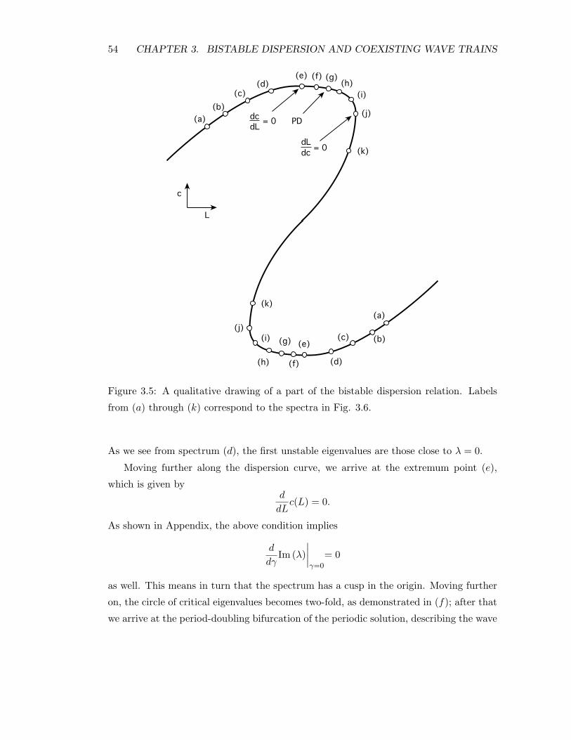
54 CHAPTER 3. BISTABLE DISPERSION AND COEXISTING WAVE TRAINS
(a)
(b)
(c)(d)
(e)
(j)
(f)
(g)
(h)
(i)
(k)
dcPD
dL
dc= 0
dL= 0
L
c
(j)
(e)
(k)
(i)
(d)
(c) (b)
(a)
(f)(h)
(g)
Figure 3.5: A qualitative drawing of a part of the bistable dispersion relation. Labels
from (a) through (k) correspond to the spectra in Fig. 3.6.
As we see from spectrum (d), the first unstable eigenvalues are those close to λ = 0.
Moving further along the dispersion curve, we arrive at the extremum point (e),
which is given byd
dLc(L) = 0.
As shown in Appendix, the above condition implies
d
dγIm (λ)
####$=0
= 0
as well. This means in turn that the spectrum has a cusp in the origin. Moving further
on, the circle of critical eigenvalues becomes two-fold, as demonstrated in (f); after that
we arrive at the period-doubling bifurcation of the periodic solution, describing the wave
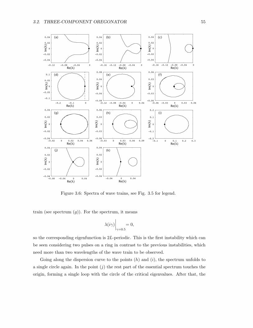
3.2. THREE-COMPONENT OREGONATOR 55
-0.06
-0.03
0
0.03
0.06
-0.06 -0.03 0 0.03 0.06
-0.04
-0.02
0
0.02
0.04
-0.02 0 0.02 0.04 0.06-0.06
-0.03
0
0.03
0.06
-0.03 0 0.03 0.06 0.09-0.2
-0.1
0
0.1
0.2
-0.1 0 0.1 0.2 0.3
-0.04
-0.02
0
0.02
0.04
-0.12 -0.08 -0.04 0
Re(!)
Im(!
)
-0.04
-0.02
0
0.02
0.04
-0.16 -0.12 -0.08 -0.04 0
Re(!)
Im(!
)
-0.04
-0.02
0
0.02
0.04
-0.16 -0.12 -0.08 -0.04 0
Re(!)
Im(!
)
-0.08
-0.04
0
0.04
0.08
-0.12 -0.08 -0.04 0 0.04
Re(!)
Im(!
)
Im(!
)
Re(!)
Re(!)
Im(!
)
Re(!)
Im(!
)
Im(!
)
Re(!)
-0.04
-0.02
0
0.02
0.04
-0.08 -0.04 0 0.04-0.04
-0.02
0
0.02
0.04
-0.04 0 0.04
Re(!)Re(!)
Im(!
)
Im(!
)
(a) (b) (c)
(d) (e) (f)
(g) (h) (i)
(j)
-0.1
-0.05
0
0.05
0.1
-0.2 -0.1 0
Im(!
)
Re(!)
(k)
Figure 3.6: Spectra of wave trains, see Fig. 3.5 for legend.
train (see spectrum (g)). For the spectrum, it means
λ(iγ)####$=0.5
= 0,
so the corresponding eigenfunction is 2L-periodic. This is the first instability which can
be seen considering two pulses on a ring in contrast to the previous instabilities, which
need more than two wavelengths of the wave train to be observed.
Going along the dispersion curve to the points (h) and (i), the spectrum unfolds to
a single circle again. In the point (j) the rest part of the essential spectrum touches the
origin, forming a single loop with the circle of the critical eigenvalues. After that, the

56 CHAPTER 3. BISTABLE DISPERSION AND COEXISTING WAVE TRAINS
circle detaches from the origin, see (k).
Moving on further, we observe the reversed scenario: the detached circle of critical
eigenvalues moves back to the origin, attaches to zero, flips back to the left half-plane
and unites with another spectral curve. Up to the specific locations of the bifurcation
points this instability scheme is qualitatively the same for all overlapping regions of the
wiggly dispersion curve.
The instability between points (d) and (j) di!ers from that of the middle branch
between two points (j). The first one can be observed only considering two or more
equidistant pulses on a ring. The unstable eigenfunction has a period larger than L.
The instability between two points (j) of the middle part of the bistable region can
already be seen with one pulse on a ring of length L, since there exist an unstable
eigenfunction of period L.
We would like to note that the sign of the slope of the dispersion nearly coincides
in our case with the curvature of the spectrum at the origin. Points (d) and (e) are
found to be very close to each other, so the circle of the critical eigenvalues flips through
the imaginary axis near the extremum of the dispersion curve. For the parts of the
dispersion with positive slope we nearly always find positive curvature of the spectrum,
but there may exist another branch of the spectrum in the right complex half-plane (see
the case with the detached circle of critical eigenvalues).
3.2.3 Extrema of the dispersion curve
It is possible to show that λ = 0 has an algebraic multiplicity two at the extrema of
dispersion curve. We would like first to comment on the points (e). They are given by
d
dLc(L) = 0. (3.4)
We recall the profile equation written as a first order system
u" = f(u; c(L)).
We assume that there exist a family of wave trains, parameterized by the wavelength L.
For the profile u we substitute then u = u(z;L). Upon rescaling the spatial coordinate
z ! z/L, we obtain for the profile equation
u"
L= f(u(z;L); c(L)).

3.2. THREE-COMPONENT OREGONATOR 57
We take the first derivative of the above equation with respect to L:
u"L(z;L)L
% u"(z;L)L2
= fu(u(z;L); c(L))uL(z;L) + fc(u(z;L); c(L)) cL)*+,=0
, (3.5)
which leads to! 1L
∂z % fu(u(z;L); c(L))"uL =
1L2
u"(z;L).
With Eq. (3.4) we obtain finally
T (0)uL(z;L) =1L2
u"(z;L), (3.6)
where the family of operators T (λ) is defined as
T (λ) : v /%! 1L
∂zv %A(·;λ)v +iγ
Lv, A = fu(u(z;L); c(L)) + λB, (3.7)
(see also the second chapter and the first Appendix).
We recall that u"(z;L) belongs to the null-space of the operator T (0). Eq. (3.6)
means that the operator T (0) has a generalized eigenfunction, given by ∂Lu(z;L). So the
eigenvalue λ = 0 has an algebraic multiplicity equal two in the points on the dispersion
curve where (3.4) holds.
A similar consideration is applicable for the points (j), where
dL
dc= 0. (3.8)
Here, we use the second-order formulation of the profile equation
D1L2
U "" + c1L
U " + F (U) = 0, (3.9)
which we can derive with respect to the velocity c, obtaining with dLdc = 0
D1L2
U ""c + c
1L
U "c + FU Uc = % 1
LU ", (3.10)
which we write with the help of the operator
L :=D
L2∂zz +
c
L∂z + FU (3.11)
as
LUc = % 1L
U ". (3.12)
Again, we recall that U " is in the null-space of L, the previous equation then means that
Uc is a generalized eigenfunction to L in the points on the dispersion curve with dLdc = 0.
It means that the algebraic multiplicity of λ = 0 is here equal two.

58 CHAPTER 3. BISTABLE DISPERSION AND COEXISTING WAVE TRAINS
X
t
Figure 3.7: Space-time plot of annihilating pulse trains that have the same wavelength
but di!erent velocities. The logarithm of the v variable is coded in grey-scale with light
(dark) colours corresponding to high (low) values, respectively. The collision position
drifts towards the slower pulse train.
3.2.4 Numerical simulations
To complement the stability analysis, we performed direct simulations of the full PDE
system. For this purpose, we integrated Eq. (3.1) with periodic boundary conditions in
a one-dimensional spatial domain of size L. Results obtained as L is slowly increased
(decreased) are plotted in the inset of Fig. 3.2(a) as circles (diamonds). As we choose
the initial conditions on the upper branch of the dispersion curve and slowly increase the
size of the domain, the system follows this branch until the point SN1 and rapidly jumps
to the lower stable branch. Moving now in the opposite direction by decreasing L, the
lower branch remains stable up to the SN2 point, where the system jumps back to the
upper branch. Thus, in accordance with the results obtained within the co-moving frame
ODE approach we find coexistence of fast and slow pulse trains. The phenomenon of
bistability manifests itself in hysteresis-like transitions between alternative stable pulse
trains.
The di!erence in the propagation velocities leads to the domination of the faster pulse
train over the slower one in head-on collision. As shown in Fig. 3.7, due to di!erent
propagation velocities of the colliding pulse trains the annihilation point shifts with the
time towards the slower pulse train. From the viewpoint of [33], the line of the head-on
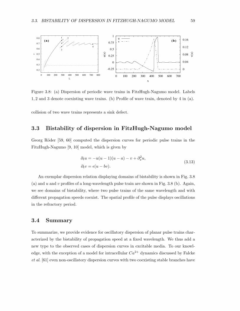
3.3. BISTABILITY OF DISPERSION IN FITZHUGH-NAGUMO MODEL 59
0.2
0.3
0.4
0.5
0.6
0.7
0.8
0 100 200 300 400 500 600 700 800
c
L
1 2
34
-0.25
0
0.25
0.5
0.75
1
0 100 200 300 400 500 600 700
0
0.04
0.08
0.12
0.16
u(x)
v(x)
x
uv(a) (b)
Figure 3.8: (a) Dispersion of periodic wave trains in FitzHugh-Nagumo model. Labels
1, 2 and 3 denote coexisting wave trains. (b) Profile of wave train, denoted by 4 in (a).
collision of two wave trains represents a sink defect.
3.3 Bistability of dispersion in FitzHugh-Nagumo model
Georg Roder [59, 60] computed the dispersion curves for periodic pulse trains in the
FitzHugh-Nagumo [9, 10] model, which is given by
∂tu = %u(u% 1)(u% a)% v + ∂2xu,
∂tv = ε(u% bv).(3.13)
An exemplar dispersion relation displaying domains of bistability is shown in Fig. 3.8
(a) and u and v profiles of a long-wavelength pulse train are shown in Fig. 3.8 (b). Again,
we see domains of bistability, where two pulse trains of the same wavelength and with
di!erent propagation speeds coexist. The spatial profile of the pulse displays oscillations
in the refractory period.
3.4 Summary
To summarize, we provide evidence for oscillatory dispersion of planar pulse trains char-
acterized by the bistability of propagation speed at a fixed wavelength. We thus add a
new type to the observed cases of dispersion curves in excitable media. To our knowl-
edge, with the exception of a model for intracellular Ca2+ dynamics discussed by Falcke
et al. [61] even non-oscillatory dispersion curves with two coexisting stable branches have

60 CHAPTER 3. BISTABLE DISPERSION AND COEXISTING WAVE TRAINS
not been discussed before. In the cited work one of the stable branches is stable over the
almost entire wavelength range. The coexistence of two stable wave trains propagating
with di!erent velocity has not been discussed in that paper.
Although our calculations are carried out only for the Oregonator and FitzHugh-
Nagumo models, we expect that other models of excitable media can obey bistable
dispersion relations in a parameter range close to the transition from locally excitable to
oscillatory behavior. Accordingly, coexisting stable pulse trains should be characteristic
for a variety of physical, chemical and biological excitable media.
Possibly, the presented results can modify the existing view on alternative types of
spiral wave with di!erent wavelengths in two-dimensional excitable media [18], since a
spiral wave far from its core can be modeled by a one-dimensional pulse train.

Chapter 4
Transition between trigger and
phase waves
4.1 Introduction and Motivation
Both trigger and phase waves belong to the basic types of the patterns in active media
and can arise in many physical, chemical and biological systems [2, 51]. Trigger waves are
typical for excitable media [32], where an element of such medium can produce a burst
of activity, triggered by a supra-threshold perturbation, produced by the di!usional flow
from its neighborhood. After the activity burst, the element of the excitable medium
slowly relaxes to the typically stable rest state. The velocity of such waves depends
strongly on the di!usion. Trigger waves can propagate either alone or form trigger wave
trains. Spatially periodic trigger wave trains can be characterized by a dispersion curve,
which describes the dependence of the wave train velocity c on its wavelength L. 1
Phase waves are merely phase-shifted oscillations of the bulk of the medium, they
exist if the kinetics of the underlying reaction-di!usion system is oscillatory. The prop-
agation velocity of phase waves is reciprocal to the initially introduced phase gradient,
resulting in linear dispersion curve. The di!usion does not significantly a!ect their
velocity. The dynamics of phase waves can be well understood in generic models like
amplitude equations [62, 3]. In the parameter plane including the wavenumber k and the
time scale ratio ε there are well-known regions of existence and stability of such waves.
1In the following we reserve the term “trigger waves” for both solitary and spatially periodic struc-
tures.
61

62 CHAPTER 4. TRANSITION BETWEEN TRIGGER AND PHASE WAVES
Wavelength
Trigger waves
Phase waves
Li
velo
city
C 0
I
Figure 4.1: Dispersion curves of phase waves (solid line) and dispersion of trigger waves
(dashed line). They nearly coincide up to some wavelength Li. The velocity of trigger
waves has limit c0 - the velocity of solitary pulse. I denotes the inflection point.
The stability boundaries are the Eckhaus boundary [63] and the so-called zigzag bound-
ary [64]. Phase waves in real systems like the BZ-reaction are often considered to be
produced by an inhomogeneity, which introduces a phase gradient in stable homogeneous
bulk oscillations [65].
One of the first theoretical studies on the transition between trigger and phase waves
in a model of the Zhabotinsky reaction was presented in [66]. In the case of oscillatory
kinetics trigger waves can coexist with phase waves. If the velocity of the phase wave is
smaller than the velocity of the coexisting trigger wave, the former can initiate a new
trigger wave. A stricter distinction between phase and trigger wave trains, based on the
shape of their dispersion curves was proposed in [67]. First, it was demonstrated that
up to a certain wavelength phase and trigger waves have roughly the same dispersion
(inflection point I in Fig. 4.1). Then, depending on the type of the wave, under further
increase of wavelength the velocity of the wave can either grow infinitely – this corre-
sponds to the phase waves, or saturate, approaching the limit c0. In the latter case the
wave is of trigger type and c0 is the velocity of the solitary pulse.
In the same time many qualitatively di!erent types of dispersion curves for trigger
waves were found [19], which can be classified into: (i) monotonous, (ii) non-monotonic
with a negative slope domain and (iii) oscillatory, which gives rise to alternating attrac-

4.1. INTRODUCTION AND MOTIVATION 63
tive and repulsive pulse interaction.
The more interesting case, namely oscillatory dispersion, is shown to be provided
by the oscillatory decay of excitation behind a solitary pulse. It often occurs close to
a supercritical Hopf bifurcation in the kinetics of the reaction-di!usion system. Due to
the oscillation in the pulse tail, one can construct infinitely many equally spaced wave
trains with wavelengths ranging up to infinity moving with the same velocity [52, 18].
The resulting wave train changes its stability depending on the interpulse distance peri-
odically [18, 16]. Experimental evidence for oscillatory dispersion was reported as well,
for example, in gas discharge experiments [24]. The interaction between the oscillatory
tail and the head of the successive pulses can be so strong that it leads to locking-type
phenomena, described theoretically in [68, 69, 70], see also previous chapter. Such lock-
ing results in the coexistence of two stable pulse trains with the same wavelength, but
di!erent propagation velocities.
There are many examples that in the same reaction-di!usion system both kinds of
waves can exist at di!erent parameters values [71], but the question of the transition
between those wave types remains to our knowledge open. Moreover, waves at the
boundary between phase and trigger dynamics are rich in instabilities, which can lead
to new patterns like trace- and backfiring [72]. The purpose of the present chapter
is to capture the bifurcation scenario of the transition between two types of waves in
specific details, including the stability of waves in the transition region. The analysis of
travelling waves is reduced to the study of their profiles and velocities in the so-called
travelling wave ODE (profile ODE) assuming that the propagation velocity of the waves
is constant.
First, we describe the origin of trigger and phase waves. Spatially periodic trigger
wave trains are constructed of infinitely many periodic replications of the primary soli-
tary pulse. In the phase space of the travelling wave ODE the limit cycles, representing
these wave trains, exist close to the homoclinic solution, which describes the solitary
pulse. The profile of phase waves is represented by periodic solutions that stem from a
Hopf bifurcation of the homogeneous rest state of the PDE. In the limit of large wave-
lengths, trigger wave trains converge to solitary pulses with finite velocity. The profile
of phase waves of large wavelengths approximates the limit cycle in the kinetics of the
reaction-di!usion system under infinite increase of the propagation velocity. However,
the large-wavelength limit is not always accessible in experiments (for example, spiral

64 CHAPTER 4. TRANSITION BETWEEN TRIGGER AND PHASE WAVES
waves usually send out short-wavelength wave trains), that is why we are interested in
the connection between trigger and phase waves in the short-wavelength region.
Upon varying the control parameter from the regime of trigger waves to the regime
of phase waves, we first observe twisted trigger wave dispersion, which is essentially
provided by the oscillatory decay behind the solitary pulse. After the Hopf bifurcation
in the appropriate co-moving frame, a branch of phase waves appears. At the critical
point the dispersion curve of phase waves collides with the dispersion curve of trigger
waves in the region of small wavelengths. The curve of the dispersion of the trigger
waves collapses in a series of saddle-node bifurcations. The only dispersion curve, which
persists in the “wavelength - velocity” parameter plane, is the dispersion of phase waves.
In order to get a thorough insight in the studied transition, we discuss in detail the
stability properties of both types of waves close to the transition threshold. We elaborate
the stability of the phase waves close to the transition region as well and show that phase
waves first appear as unstable small-amplitude pattern and then stabilize, reaching large
amplitude. We support our studies of the conversion between trigger and phase waves
by one-dimensional simulations, which can be thought of as the first starting point for
experimental proof of our results.
4.2 Model and methods
4.2.1 Model
In this chapter, as a representative model displaying for appropriately chosen parameter
values both oscillatory as well as excitable kinetics, we consider the two-component
Oregonator model modified to describe the photosensitive version of the BZ reaction
[30]. In this reaction trigger and phase waves have been extensively studied for a long
time [51]. The equations for the dimensionless concentration of bromous acid u, and the
oxidized form of the catalyst v, read
∂tu =1ε
!u% u2 % (fv + φ)
u% q
u + q
"+ ∂2
xu,
∂tv = u% v.
(4.1)
Di!usion of v is omitted because in most experiments the catalyst is immobilized in
a gel matrix. The time scale ratio ε follows from the recipe concentrations [30]. In this
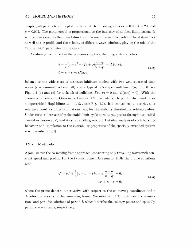
4.2. MODEL AND METHODS 65
chapter, all parameters except φ are fixed at the following values ε = 0.05, f = 2.1 and
q = 0.002. The parameter φ is proportional to the intensity of applied illumination. It
will be considered as the main bifurcation parameter which controls the local dynamics
as well as the profile and the velocity of di!erent wave solutions, playing the role of the
“excitability” parameter in the system.
As already mentioned in the previous chapters, the Oregonator kinetics
u =1ε
!u% u2 % (fv + φ)
u% q
u + q
"=: F (u, v),
v = u% v =: G(u, v)(4.2)
belongs to the wide class of activator-inhibitor models with two well-separated time
scales (ε is assumed to be small) and a typical “s”-shaped nullcline F (u, v) = 0 (see
Fig. 4.2 (b) and (c) for a sketch of nullclines F (u, v) = 0 and G(u, v) = 0). With the
chosen parameters the Oregonator kinetics (4.2) has only one fixpoint, which undergoes
a supercritical Hopf bifurcation at φhb (see Fig. 4.2). It is convenient to use φhb as a
reference point for other bifurcations, say, for the stability threshold of solitary pulses.
Under further decrease of φ the stable limit cycle born at φhb passes through a so-called
canard explosion at φc and its size rapidly grows up. Detailed analysis of such bursting
behavior and its relation to the excitability properties of the spatially extended system
was presented in [31].
4.2.2 Methods
Again, we use the co-moving frame approach, considering only travelling waves with con-
stant speed and profile. For the two-component Oregonator PDE the profile equations
read
u"" + cu" +1ε
!u% u2 % (fv + φ)
u% q
u + q
"= 0,
cv" + u% v = 0,
(4.3)
where the prime denotes a derivative with respect to the co-moving coordinate and c
denotes the velocity of the co-moving frame. We solve Eq. (4.3) for homoclinic connec-
tions and periodic solutions of period L which describe the solitary pulses and spatially
periodic wave trains, respectively.
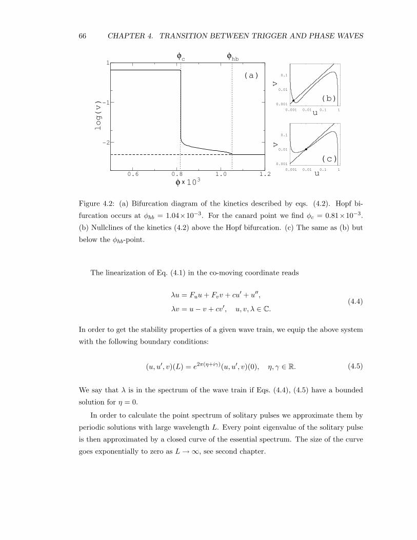
66 CHAPTER 4. TRANSITION BETWEEN TRIGGER AND PHASE WAVES
0.001
0.01
0.1
0.001 0.01 0.1 1
0.001
0.01
0.1
0.001 0.01 0.1 1
0.6 0.8 1.0 1.2! x 103
-2
-1
1
log(
v)
!c !hb
v
u
v
u
(a)
(b)
(c)
Figure 4.2: (a) Bifurcation diagram of the kinetics described by eqs. (4.2). Hopf bi-
furcation occurs at φhb = 1.04&10!3. For the canard point we find φc = 0.81&10!3.
(b) Nullclines of the kinetics (4.2) above the Hopf bifurcation. (c) The same as (b) but
below the φhb-point.
The linearization of Eq. (4.1) in the co-moving coordinate reads
λu = Fuu + Fvv + cu" + u"",
λv = u% v + cv", u, v,λ ' C.(4.4)
In order to get the stability properties of a given wave train, we equip the above system
with the following boundary conditions:
(u, u", v)(L) = e2(('+i$)(u, u", v)(0), η, γ ' R. (4.5)
We say that λ is in the spectrum of the wave train if Eqs. (4.4), (4.5) have a bounded
solution for η = 0.
In order to calculate the point spectrum of solitary pulses we approximate them by
periodic solutions with large wavelength L. Every point eigenvalue of the solitary pulse
is then approximated by a closed curve of the essential spectrum. The size of the curve
goes exponentially to zero as L !", see second chapter.

4.3. TRIGGER WAVES 67
4.3 Trigger Waves
As mentioned above, trigger waves are slow di!usion-dependent propagating structures.
They can appear either as solitary pulses or form spatially periodic trigger wave trains.
The dispersion curve and the stability properties of the latter are strongly determined
by the type of decay behind the corresponding solitary pulse [73, 74, 45]. Under decrease
of parameter φ (increase of excitability), three qualitatively di!erent types of solitary
pulses and dispersion curves of the accompanying wave trains are found.
4.3.1 Solitary pulses
The reaction-di!usion system (4.1) supports propagation of solitary excitation pulses
in the parameter region φ > φc. We obtain the dependence of the pulse velocity on φ
performing continuation of the corresponding homoclinic solution of Eq. (4.3) in the
(φ, c) parameter plane (Fig. 4.3 (a)). For a given φ value there simultaneously exist two
pulses, one stable and one unstable. They collide in a saddle-node bifurcation SN at
φ = φSN parameter value (for comparison, see analytical results on FitzHugh-Nagumo
model in [75]). The present work focuses on the stable pulses belonging to the upper
branch.
This branch is divided by point F (Fig. 4.3 (a)). At this point the equilibrium in the
travelling wave ODE (4.3) undergoes a saddle to saddle-focus transition and the homo-
clinic trajectory approaches the equilibrium in an oscillating manner. The equilibrium
has for φH < φ < φF one unstable one-dimensional manifold (for the pulses, propagating
to the left, as shown by Fig. 4.3), which describes the front of the pulse. The stable two-
dimensional manifold with the corresponding complex-conjugated eigenvalues describes
the decay behind the pulse (Fig. 4.3, compare panels (c) and (d)). For the pulses that
propagate in the opposite direction with velocity %c0, the fixpoint has contrariwise two
unstable complex-conjugated eigenvalues that render the oscillatory tail of the pulse,
and one stable eigenvalue, which is responsible for the front of the pulse.
With further decrease of φ parameter the equilibrium of the profile equations un-
dergoes a Hopf bifurcation (point H in Fig. 4.3) at φH = 9.0 & 10!4, and the pair of
complex-conjugated eigenvalues crosses the imaginary axis, moving from the right to
the left complex half-plane. The pulse solution below this bifurcation corresponds to
a heteroclinic connection between the equilibrium and the small-amplitude limit cycle,
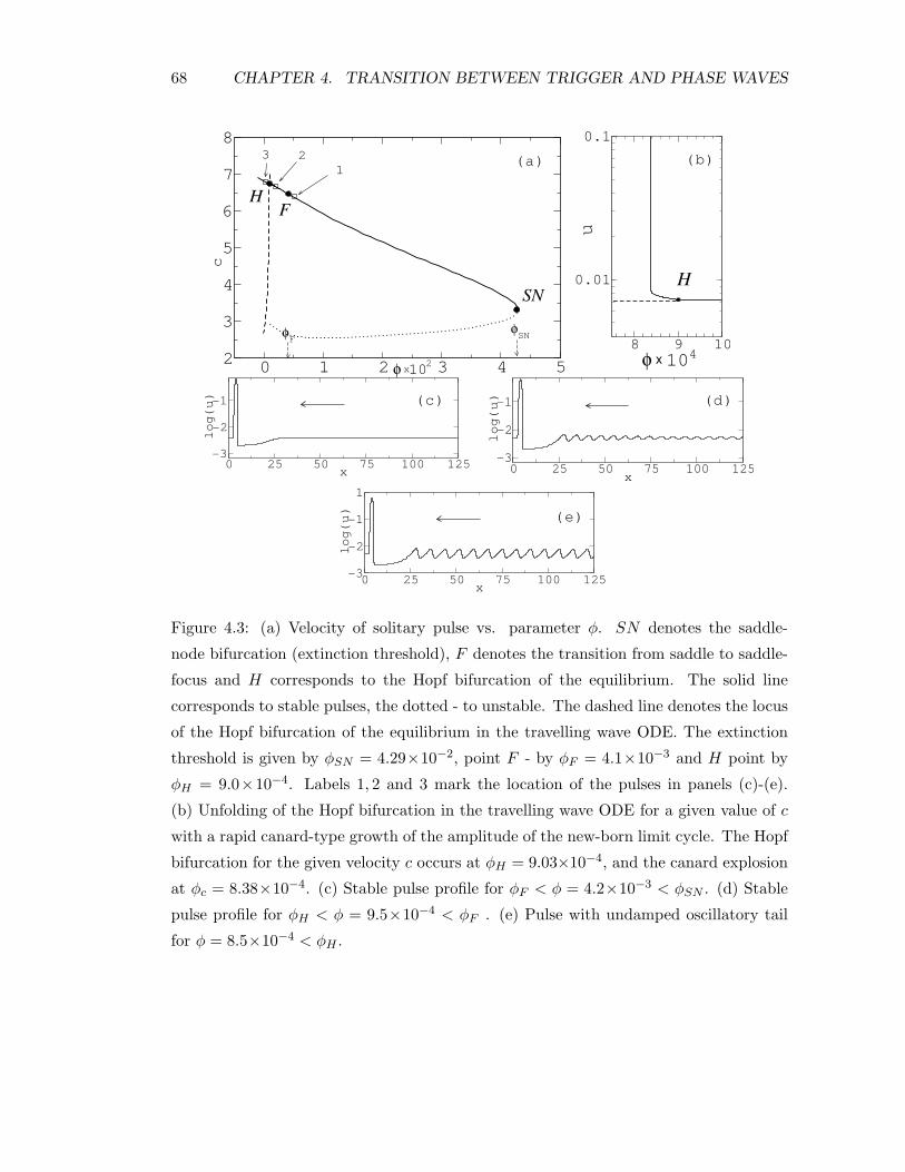
68 CHAPTER 4. TRANSITION BETWEEN TRIGGER AND PHASE WAVES
0 1 2 3 4 52
3
4
5
6
7
8
SN
FH
123
!F!SN
0 25 50 75 100 125x -3
-2
-1
log(
u)
0 25 50 75 100 125x -3
-2
-1
log(
u)
0 25 50 75 100 125x -3
-2
-1
1
log(u)
8 9 10
0.01
0.1
H
! x 104
u
(a)
(e)
(c) (d)
(b)
x! 10
c
2
Figure 4.3: (a) Velocity of solitary pulse vs. parameter φ. SN denotes the saddle-
node bifurcation (extinction threshold), F denotes the transition from saddle to saddle-
focus and H corresponds to the Hopf bifurcation of the equilibrium. The solid line
corresponds to stable pulses, the dotted - to unstable. The dashed line denotes the locus
of the Hopf bifurcation of the equilibrium in the travelling wave ODE. The extinction
threshold is given by φSN = 4.29&10!2, point F - by φF = 4.1&10!3 and H point by
φH = 9.0&10!4. Labels 1, 2 and 3 mark the location of the pulses in panels (c)-(e).
(b) Unfolding of the Hopf bifurcation in the travelling wave ODE for a given value of c
with a rapid canard-type growth of the amplitude of the new-born limit cycle. The Hopf
bifurcation for the given velocity c occurs at φH = 9.03&10!4, and the canard explosion
at φc = 8.38&10!4. (c) Stable pulse profile for φF < φ = 4.2&10!3 < φSN . (d) Stable
pulse profile for φH < φ = 9.5&10!4 < φF . (e) Pulse with undamped oscillatory tail
for φ = 8.5&10!4 < φH .

4.3. TRIGGER WAVES 69
-4 -2 0Re(!)
-40
-20
0
20
40
Im(!)
x
t
t
x
c)
(a) (b)
Figure 4.4: (a) Solid line shows the leading part of the essential spectrum of the small-
amplitude wave train behind the pulse head. Dashed line shows the spectrum in the
weighted space with weight η = 5.26 & 10!1. (b) Space-time plot of a running solitary
pulse in the co-moving frame. The logarithm of the u variable is coded in gray-scale
with light (dark) colors corresponding to high (low) values, respectively. The simulations
were made with Dirichlet boundary conditions in the front of the pulse and Neumann
boundaries behind it. (c) Space-time plot of simulations of the periodic wave train, the
color coding is renormalized to the actual maximal and minimal values of the variable.
Periodic boundary conditions are applied.

70 CHAPTER 4. TRANSITION BETWEEN TRIGGER AND PHASE WAVES
t
x
Figure 4.5: Appearance of high-amplitude pulse heads behind the primary pulse (φ =
8.405&10!4). Dirichlet boundary conditions and co-moving coordinate system.
which is born in the bifurcation point (Fig. 4.3(e)). This bifurcation is of very special
meaning for the pulses in the reaction-di!usion system: it describes the appearance of
undamped tail oscillations behind the pulse. From the mathematical point of view, this
is a codimension-2 Shilnikov-Hopf bifurcation [76].
Now we turn to the stability properties of the solitary pulses. Pulses belonging to
the faster branch, are found to be stable for φhb < φ < φSN . We checked this fact by
simulating the time evolution of the corresponding profiles. The essential spectrum of
the solitary pulse is contained in the left half-plane, since the homogeneous background
is stable for φ > φhb. The isolated eigenvalues were checked numerically by direct
computation of the eigenvalues of the discretized linear operator.
Next, we discuss the pulses below the H point with the undamped oscillations in
the tail. Numerical simulations reveal that they are stable on bounded domains due
to the convective nature of the instability of the periodic wave train behind the pulse
head (Fig. 4.4(b), see also section “Phase Waves”). The essential spectrum of the small-
amplitude wave train is shown on Fig. 4.4(a). The instability is of a long-wavelength
type, since d2
d$2 Re(λ) > 0 (see Eq. (4.5)) near the origin. Moreover, the instability is
only convective, because we can shift the spectrum completely in the left half-plane,
introducing an exponential weight η .= 0 (see Eq. (4.5)). Simulations of the small-
amplitude wave train with periodic boundaries uncovers the essential instability (Fig.
4.4(c)).
Under further decrease of parameter φ we see the phenomenon, which is often referred

4.3. TRIGGER WAVES 71
to as trace- and backfiring [72]. A pair of the high-amplitude pulse heads emerges behind
the primary pulse (Fig. 4.5). After a certain transient time, the whole domain behind
the pulse is occupied by the high-amplitude wave train. This stationary pattern can be
thought of as a heteroclinic connection between the equilibrium and a periodic orbit,
representing the wave train, triggered by the running pulse. We would like to note that
the discussed appearance of the new high-amplitude pulse heads seems also to be of the
canard-like nature, because small changes in the parameter values lead to a significant
transformation of the solution.
4.3.2 Trigger wave trains
Now we would like to construct periodic wave trains of pulses with identical profiles.
The interaction and stability of such wave trains will be determined mostly by the decay
behind the corresponding solitary pulse, which was discussed in the previous subsection.
In Fig. 4.6 we compare the type of the dispersion relation with the corresponding
type of the decay behind the associated solitary pulses (Fig. 4.3). Low excitability
of the system, which causes the tail of the solitary pulse to relax to the background
state monotonously, results in a monotonous dispersion relation for the associated wave
trains. After the transition from saddle to saddle-focus, marked as the F -point in Fig.
4.3 (a), below which a solitary pulse displays damped tail oscillations, the dispersion
curve becomes non-monotonous, combining parts with negative and positive slope.
The corresponding periodic orbits include a high-amplitude part and small-amplitude
windings, whose number grows for large periods L. This picture is general for periodic
orbits near a homoclinic connection of the Shilnikov type [40, 41]. The interaction
between the pulses in such a wave train, either attractive or repulsive, depends on the
interpulse distance. Note also that there can coexist infinitely many wave trains with
the same velocity, but of di!erent wavelengths.
Crossing the line of the Hopf bifurcation under decrease of φ, we observe a qualita-
tively new type of dispersion curve (Fig. 4.6 (c)). From the dynamical systems view-
point, for L !" we have a codimension-zero situation with two homoclinic trajectories
to a limit cycle, accompanied by a set of periodic orbits. These periodic orbits form
a wiggly curve with fold points, accumulating at homoclinic tangencies [76, 77]. The
small-amplitude windings of the limit cycles are very close to the small periodic orbit,
which was born in the Hopf bifurcation. Another important feature of this dispersion is

72 CHAPTER 4. TRANSITION BETWEEN TRIGGER AND PHASE WAVES
2
3
4
5
6
7
0 20 40 60 80 100 120
2
3
4
5
6
7
0 20 40 60 80 100 120 2
3
4
5
6
7
0 20 40 60 80 100 120
L
cc
c(a) (b)
(c)
LL
Figure 4.6: Di!erent dispersion curves of trigger wave trains as parameter φ is decreased
(increasing excitability). Solid lines show stable solutions, dashed lines show unstable
solutions. (a) Just above the F point, φ = 4.2&10!3. Solitary pulse has monotonously
decaying tail, compare with Fig. 4.3 (c). (b) Between the Hopf bifurcation and the F
point, φ = 9.5&10!4. Solitary pulse has decaying oscillatory tail, compare with Fig.
4.3 (d). (c) Below the Hopf bifurcation φ = 8.5&10!4. Solitary pulse has non-damped
oscillatory tail, compare with Fig. 4.3 (e).

4.4. PHASE WAVES 73
the presence of domains of bistability. Every such section contains three coexisting wave
train solutions, two of them are stable and separated by an unstable one.
The phenomenon of the bistability of wave trains was first reported in [70] (see also
the previous chapter). However, in the case of the three-component Oregonator model,
the phenomenon of coexistence occurs above the Hopf bifurcation and, as a consequence,
the size of the bistability domains decreases with L. In the present case the bistability
domains become larger with increasing L. Considering the stability of the wave trains
belonging to the domains of bistability, we found for the two-component Oregonator
qualitatively the same results as reported in the previous chapter. Here, we omit the
details on the stability of periodic wave trains which belong to the domains of bistability.
The last part of this section on trigger waves we would like to address to their
instabilities, caused by an increase of the excitability of the system (decrease of φ).
Let us take a look at the dependence of the velocity of a particular trigger wave train
of wavelengths L = 48 on parameter φ (see Fig. 4.7). We chose this wavelength,
because the corresponding wave train belongs to the middle of the stable branch of the
dispersion curve and is not subjected to the instability, which is related to the circle of
critical eigenvalues and negative slope of the dispersion curve. In point U the wave train
becomes unstable, this instability is of long-wavelength type, as it can be seen from Fig.
4.7 (b). Numerical simulations (Fig. 4.7 (c)) reveal that the wave head tends to solder
with the minor maximum in front of it, e!ectively increasing the propagation velocity
of the whole wave train. After a long transient process (not shown in Fig. 4.7(c)), we
obtain a new wave train without secondary maxima between the successive pulse heads,
propagating at a larger velocity (see section below).
In point SN in Fig. 4.7 (a) two limit cycles, one from the upper part of the dispersion
curve and one from the lower unstable part, collide upon decrease of φ. Globally this
leads to the disappearance of the whole dispersion curve of trigger waves for smaller
values of the parameter φ. This fact will be important for the transition from trigger
waves to phase waves, see the corresponding section below.
4.4 Phase Waves
Phase waves are simpler objects than trigger wave trains in the sense that their form
and properties do not depend on the wavelength as dramatically.

74 CHAPTER 4. TRANSITION BETWEEN TRIGGER AND PHASE WAVES
8.38 8.4 8.426.2
6.4
6.6
6.8
SNU
! x 104
c
-0.0005 0Re(")
-0.2
0
0.2
Im(")
(a) (b)
t
x
~
(c)
Figure 4.7: (a) Bifurcation diagram for a particular trigger wave train, showing the
instability point U and the point of the collision with the twin wave train, belonging
to the slower unstable dispersion branch. (b) Leading part of the eigenvalue spectrum
of trigger wave train between U and SN points. (c) Space-time plot of a numerical
simulation displaying the destruction of a trigger wave train. The parameter φ was
initially set to φ = 8.4&10!4 and than changed to the value φ = 8.0&10!4. The arrow
shows the parameter adjustment. The long transition process between the first and the
last parts of the plot is cut out.
If u(z) is a periodic solution of the profile equation
Du"" + cu" + f(u) = 0, " := ∂z
then, introducing a new variable ξ = cz, we obtain
f(u) + ∂)u + c!2D ∂2) u = 0.
In the limit of fast waves, c ! ", the di!usive term can be neglected (c!2 ! 0),
and we end up with
∂zu = %c!1f(u). (4.6)
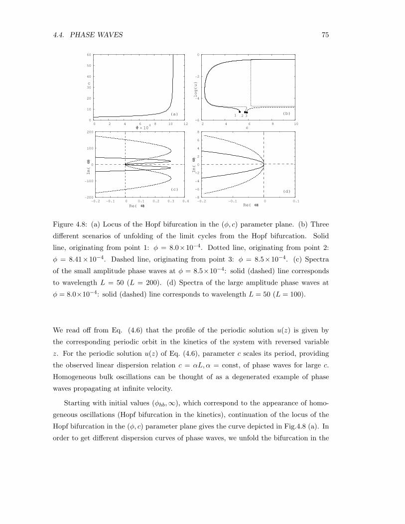
4.4. PHASE WAVES 75
0
10
20
30
40
50
60
0 2 4 6 8 10 12-6
-4
-2
0
2 4 6 8 10
-8
-6
-4
-2
0
2
4
6
8
-0.2 -0.1 0 0.1-200
-100
0
100
200
-0.2 -0.1 0 0.1 0.2 0.3 0.4
c
c
Im( )
! !
! !log(u)
Re( )
Im( )
Re( )
(a) (b)
(c) (d)
" 104
x
321
Figure 4.8: (a) Locus of the Hopf bifurcation in the (φ, c) parameter plane. (b) Three
di!erent scenarios of unfolding of the limit cycles from the Hopf bifurcation. Solid
line, originating from point 1: φ = 8.0&10!4. Dotted line, originating from point 2:
φ = 8.41&10!4. Dashed line, originating from point 3: φ = 8.5&10!4. (c) Spectra
of the small amplitude phase waves at φ = 8.5&10!4: solid (dashed) line corresponds
to wavelength L = 50 (L = 200). (d) Spectra of the large amplitude phase waves at
φ = 8.0&10!4: solid (dashed) line corresponds to wavelength L = 50 (L = 100).
We read o! from Eq. (4.6) that the profile of the periodic solution u(z) is given by
the corresponding periodic orbit in the kinetics of the system with reversed variable
z. For the periodic solution u(z) of Eq. (4.6), parameter c scales its period, providing
the observed linear dispersion relation c = αL,α = const, of phase waves for large c.
Homogeneous bulk oscillations can be thought of as a degenerated example of phase
waves propagating at infinite velocity.
Starting with initial values (φhb,"), which correspond to the appearance of homo-
geneous oscillations (Hopf bifurcation in the kinetics), continuation of the locus of the
Hopf bifurcation in the (φ, c) parameter plane gives the curve depicted in Fig.4.8 (a). In
order to get di!erent dispersion curves of phase waves, we unfold the bifurcation in the

76 CHAPTER 4. TRANSITION BETWEEN TRIGGER AND PHASE WAVES
7.5 8 8.5
8
10
12
Uc! x 104
SN-0.2 -0.1 0
-10
0
10
Re(")
Im(")
t
x
(c)
(a) (b)
Figure 4.9: (a) Dependence of the propagation velocity of a phase wave train on the
φ parameter. The U point denotes the instability of the wave train, the corresponding
φ value is φU = 8.22&10!4. The SN points denotes a saddle-node bifurcation of the
corresponding limit cycles in the travelling wave ODE. (b) Part of the essential spectrum
of the unstable phase wave train slightly above the U point, φ = 8.23&10!4 (c) Space-
time plot of phase wave train in the co-moving frame, subjected to parameter jump
from φ = 8.0&10!4 to φ = 8.5&10!4. Logarithmic grayscale coding and co-moving
frame coordinates as in the figures above. The vertical arrow shows the moment of the
parameter switching.
(c, L) parameter plane for di!erent values of φ (Fig.4.8 (b)).
There are two qualitatively di!erent scenarios of unfolding of the phase waves from
the Hopf bifurcation. The result of the first one is the appearance of large-amplitude
phase waves. This scenario occurs for smaller values of φ, see the solid line in Fig.4.8(b).
The velocity of the wave together and its wavelength both go to infinity, while the profile
remains the same. If we unfold the bifurcation at a larger value of parameter φ, a large-
amplitude wave doesn’t emerge, see Fig.4.8(b), the long-dashed line. The profile of the
wave again converges to the limit cycle of the kinetics as the velocity and the wavelength
go to infinity. There is also some intermediate scenario, in which the wave first achieves

4.5. COLLISION OF DISPERSION CURVES 77
the full amplitude, but then becomes smaller again (Fig.4.8(b), short-dashed line).
We found that the small-amplitude phase waves are unstable in the whole wavelength
range up to infinity (Fig.4.8(c)). Changing the wavelength and the velocity of the wave
scales the spectrum of it in respect to the imaginary axis. The large-amplitude phase
waves are found to be stable in the whole wavelength range with the same scaling
property of their spectrum (Fig.4.8(d)).
Now we would like to describe the instabilities of the phase waves under variation of
parameter φ. As we can see from the bifurcation diagram and the essential spectrum of
the wave (Fig. 4.9 (a) and (b)), the phase wave train becomes linearly unstable. This
instability occurs at a finite wavelength. Numerical simulations (Fig. 4.9 (b)) show that
the instability of the phase waves leads to the appearance of a number of secondary
maxima between two successive high-amplitude wave parts. The wave tries to “localize”
itself, tending to form a trigger wave train, which propagates at a slower velocity.
It is worthwhile to compare the destruction of phase waves under increase of φ and
the break-up of trigger waves while the parameter φ is decreased. Both Fig. 4.7 (c)
and Fig. 4.9 (c) look very similar under reversion of time. Whereas the high-amplitude
heads of the trigger waves tends to merge with the next maximum, the high-amplitude
part of the phase wave train breaks down, sprouting a new small-amplitude maximum
in front of it.
4.5 Collision of dispersion curves
It turns out that this transition can be captured in the dispersion plane, where trigger
and phase waves are clearly distinguishable by the shape of their dispersion curve.
Fig. 4.10 (a) shows the initial situation before the transition: the line, which unfolds
from the Hopf bifurcation, is the branch of phase waves, and the branch of trigger waves is
presented by the comb-like dispersion (Fig. 4.10 (a)). Adjusting to φ = 8.41&10!4 (Fig.
4.10 (b)), the dispersion of phase waves collides with the lower branch of the dispersion
of trigger waves. Looking at the resulting joint curve we note that the dispersion that
descends from the Hopf bifurcation goes now along the skeleton of the trigger wave
dispersion towards large L, nearly repeating its shape. After that the curve turns back
in point C and goes again towards infinity along the linear part of the dispersion. At
φ = 8.2&10!4 (Fig. 4.10 (c)) we observe a simple dispersion, originating from the Hopf
bifurcation, with a linear part, which goes towards infinity without winding around the

78 CHAPTER 4. TRANSITION BETWEEN TRIGGER AND PHASE WAVES
2
3
4
5
6
7
8
9
10
0 20 40 60 80 100 120
2
3
4
5
6
7
8
0 20 40 60 80 100 120 2
3
4
5
6
7
8
0 20 40 60 80 100 120
L
!
cc
c
L
L
(a) (b)
(c)
H
H
H
C
I
Figure 4.10: (a) Dispersion relation for trigger and phase waves for φ = 8.42&10!4.
The dotted curve, originating from point H represents phase waves. The curve with
the comb-like upper branch is the dispersion relation of trigger waves. The arrows
show the location of the up-coming transcritical collision between both curves. (b)
Both dispersions, just after the transcritical collision, φ = 8.41&10!4. C denotes the
turning point, see text. (c) Dispersion relation of phase waves at an even lower value
φ = 8.0&10!4. The thin dashed gray line shows the dispersion of trigger waves at a
di!erent φ value for sake of comparison. I denotes the inflection point, see text.

4.6. DISCUSSION AND OUTLOOK 79
“skeleton” structure of the trigger wave dispersion.
Concerning the position of the turning point C, we make the following observations.
If φ is slightly smaller than the critical value φtr = 8.418 & 10!4, the point C is lo-
cated at large values of L. Upon further decrease of φ , point C shifts to the left and
disappears. At φ = 8.2 & 10!4 the dispersion curve leaves the skeleton in the I point,
as described by Fig. 4.10 (c). Point C is closely related to the disappearance of the
trigger waves, since it gives the section of the line of fold bifurcations of trigger waves (in
three-dimensional parameter space (c, L,φ)) with parameter plane (c, L) . The section
of the fold bifurcation line with plane (φ, c) is given by point SN in Fig. 4.7 (a).
We can define the parameter value φtr, at which the collision between dispersion
curves of phase and trigger waves takes place, as the boundary, which delimits the
regimes of phase and trigger waves. Above φtr there coexist stable trigger waves and
unstable small-amplitude phase waves. Below the boundary the only waves that exist
are phase waves. The value φtr is bracketed by the Hopf bifurcation φhb and the canard
explosion φc of the limit cycle in the kinetics of the reaction-di!usion system.
4.6 Discussion and Outlook
In this chapter we reveal fine details of the transition between phase waves and triggers
waves in a general two-component reaction-di!usion system with a cubic nonlinearity
and well-separated time scales. The kinetics of the system can be controlled between
excitable and oscillatory dynamics with a single parameter. Trigger waves and phase
waves are “natural” spatial solutions for those two types of the kinetics.
The scheme of the transition between trigger and phase waves includes: (i) emergence
of oscillations behind the solitary pulse, first damped. These cause damped oscillations
in the dispersion relation of trigger wave trains. (ii) introduction of phase waves via
the Hopf bifurcation in the travelling wave ODE, first at infinite velocity (bifurcation in
the kinetics), then continuously in the co-moving frames with the appropriate velocity.
The oscillations in the decay behind the solitary pulse and in the dispersion of trigger
wave trains become undamped. (iii) The collision of the phase wave dispersion with
the dispersion of trigger waves. (iv) Successive disappearance of trigger waves of large
periods in a series of saddle-node bifurcations. Similar results on the studied transition
were obtained for FitzHugh-Nagumo and Barkley models [59], which suggests that the
observed scenario is generic for the whole class of active media, possessing in dependence

80 CHAPTER 4. TRANSITION BETWEEN TRIGGER AND PHASE WAVES
on a parameter both excitable (with one fixpoint) and oscillatory kinetics.
Being guided by the observation above, we find that the following classification be-
tween trigger and waves can be extremely useful. Phase waves are described by the
periodic solutions of the travelling wave ODE, which descend from the Hopf bifurcation
of the equilibrium. Trigger wave trains are described by periodic solutions, which exist
close to the homoclinic orbit, that renders the shape of the appropriate solitary pulse.
The origin of trigger and phase waves is reflected in the peculiarities in their dispersion
curves, making the analysis of the dispersion curves a very suitable tool in the presented
study.
We present results of the linear stability analysis of phase and trigger waves belonging
to the colliding dispersion curves. For phase waves, we find that small-amplitude phase
waves are unstable in the whole range of wavelengths and the full-developed, high-
amplitude phase waves are stable.
We strongly believe that the experimental verification of the reported scenario of
the transition between phase and trigger waves should be the next step on the field.
One of the main objectives of the experimental proof is the existence of the small-
amplitude phase waves, which play quite a deciding role in our study and which are
experimentally not yet found to the best of our knowledge. However, the experimental
evidences of trace- and backfiring can be thought of as hints for the existence of these
small-amplitude oscillations.

Chapter 5
Creating bound states by means
of non-local coupling
5.1 Introduction
Propagation of pulses in excitable media is an important phenomenon in physical, chem-
ical and biological systems, including chemical reactions, signal propagation in neuronal
tissue, brain activity and calcium waves in living cells [3]. Typically such pulses can
propagate due to local di!usive coupling between the excitable elements of the medium.
The interaction between two pulses that propagate in the same direction is usually re-
pulsive, which means that the second pulse in a pulse pair runs more slowly than the
first one [2].
However, pulses in reaction-di!usion systems do not always interact only repulsively,
but can form so-called bound states with two or more pulses that propagate at the
same velocity. Such bound states were found in chemical reaction-di!usion systems
experimentally [20, 23, 22, 21]. A kinematic approach was introduced in [15, 78], where
the existence of bound states was closely related to the anomalous dispersion of periodic
pulse trains.
The main motivation for the consideration of non-local coupling comes from neuro-
science – it was shown that neurons communicate by means of long-range interactions
[79, 80]. Non-local coupling plays an important role in certain electrochemical reactions
[81, 82] as well. Recent theoretical findings include the improvement of synchroniza-
tion of coupled oscillators [83], the emergence of completely new dynamical regimes (the
81

82CHAPTER 5. CREATING BOUND STATES BY MEANS OF NON-LOCAL COUPLING
so-called chimera states) [84], spiral waves with randomized core [85], chemical turbu-
lence induced by non-local coupling [86], and many others. Nicola et al. reported a
codimension-2 Turing-wave bifurcation and a region of bistability between Turing and
wave patterns resulting from inhibitory non-local coupling [87, 88]. Spiral patterns on
a stationary background have been observed recently in experiments with the Belousov-
Zhabotinsky reaction under influence of non-local coupling with short-range activation
and long-range inhibition [89]. For the Oregonator model of the Belousov-Zhabotinsky
reaction it has been shown that non-local coupling can induce Turing and wave insta-
bilities of the homogeneous steady state. While a long-range activation was found to
induce travelling waves, long-range inhibition leads to stationary Turing patterns [90].
While most of the results on the impact of non-local coupling obtained so far are related
to the instabilities of the homogeneously steady state, in this chapter we focus on the
e!ect of non-local coupling on the interaction of propagating excitation pulses.
The main result of the present chapter is the following. Suppose that we have
a reaction-di!usion system that supports propagation of solitary pulses of excitation,
which interact repulsively through their monotonic refractory tails. Introducing non-
local coupling in the form of a convolution of the pulse profile with an exponentially
decaying kernel results in the attractive interaction of pulses and the emergence of bound
states. Regardless of the particular excitable kinetics, bound states bifurcate from the
primary solitary pulse at non-local coupling strength µ = 0. More specifically, we show
that the solitary pulse for µ = 0 is represented by a homoclinic orbit of codimension-4,
which is unfolded upon setting µ .= 0. In this description, bound states are represented
by 2-homoclinic orbits which bifurcate at µ = 0 from the primary one, corresponding to
the solitary pulse. We illustrate our analysis by numerical calculations with a model for
the light-sensitive Belousov-Zhabotinsky reaction [51].
From the mathematical viewpoint, the stability theory of multi-bump pulses (bound
states of pulses) and weak interaction of pulses are developed in [17] and thoroughly
reviewed in a more general context in [14]. The mathematical background for the bi-
furcation and the existence of bound states is provided by the theory of codimension-2
bifurcations of homoclinic orbits in RN , N ) 3, see [13]. For a review and analytical de-
scription of codimension-2 homoclinic orbits in a simple toy model see [34] and references
therein. We refer also to [91, 92] for codimension-3 resonant flip bifurcations.
This chapter is organized as follows. First, we present our numerical observations on

5.2. RESULTS WITH OREGONATOR MODEL 83
bound states in the Oregonator model with non-local coupling and give a simple model-
specific explanation how these bound states come into play due to non-local coupling.
Then we consider an abstract reaction-di!usion equation with non-local coupling and
show that the emergence of bound states occurs independently on the specific kinetics of
the model. In our considerations we will need some essential results on the codimension-2
bifurcations of homoclinic orbits, which will be discussed briefly in Section 5.3.2.
5.2 Results with Oregonator model
5.2.1 Emergence of bound states
We consider first solitary pulses in the Oregonator model for the excitable light-sensitive
Belousov-Zhabotinsky reaction [30]
∂tu = ε!1!u% u2 % (fv + φ)
u% q
u + q
"+ ∂xxu,
∂tv = u% v,(5.1)
subjected to a non-local coupling through the field φ(x) of characteristic coupling range
σ!1 1 1 and strength µ
φ(x) = φ0 + µ
$&
!$
e!*|y|[v(x + y)% v(x)]dy. (5.2)
The activator variable u is proportional to the concentration of bromous acid and the
inhibitor v represents the oxidized form of the catalyst. In this section, we fix the
parameters values as follows: ε!1 = 20, f = 2.1, q = 0.002,φ0 = 0.008,σ = 0.1. This
choice of the parameters corresponds to excitable local dynamics of Eq. (5.1).
With the above set of parameters and µ = 0, Eq. (5.1) supports propagation of
stable solitary pulses of excitation, see Fig. 5.1 (a). The parameter φ0 describes an
additional light-induced inhibitor production and setting it to larger values makes the
pulses of excitation propagate slower (Fig. 5.1(b)), which will be an important fact for
our considerations later on. From this viewpoint, µ > 0 corresponds to an inhibitory non-
local coupling, while choosing µ < 0 makes non-local coupling (5.2) be of an activatory
type.
Without non-local coupling (i.e. for µ = 0), pulses in Eq. (5.1) interact only repul-
sively, which can be seen from the positive slope of the dispersion curve for pulse trains

84CHAPTER 5. CREATING BOUND STATES BY MEANS OF NON-LOCAL COUPLING
10
µ
10φ
φ
0.0
0.4
0.8
1.2
1.6
2.0
40 80 120 160 2003.5
4.0
4.5
5.0
5.5
6.0
6.5
0 50 100 150 200 250
6.8
6.82
6.84
6.86
50 100 150 200-2.0
-1.0
0.0
1.0
2.0
40 80 120 160 200 240 280
2.0
3.0
4.0
5.0
6.0
7.0
0 1 2 3 4 5
0.0
0.1
0.2
0.3
0.4
-8 -6 -4 -2 0 2
(a) (b)
L
c
PD
c
(f)
(c)
(e)(d)
c
L
SN
PD2−pulse
1−pulse
10 v,
x
x
010(c−c )
10 v,
102φ
103
Figure 5.1: (a) Profile of a solitary pulse in Eq. (5.1) for µ = 0, where rescaled variable
v(x) is shown by the solid line and the rescaled value of the integral in Eq. (5.2) is shown
by the dashed line. (b) Dependence of the velocity of a solitary pulse c on the parameter
φ0. Solid (dashed) line represents stable (unstable) solitary pulses, respectively. (c)
Dispersion curve of spatially periodic pulse trains for µ = 0 showing the velocity of pulse
train c versus the interpulse distance L. (d) Profile of a bound state for µ = %8.0&10!3,
solid and dashed line show rescaled v(x) and rescaled φ(x), respectively. (e) Dispersion
curve for µ = %8.0 & 10!3. Point PD indicates period doubling, see text. Dashed
line displays the dispersion curve for pulse trains with doubled interpulse distance. (f)
Relative velocity of two-pulse solutions (dashed line) and that of the pulse trains that
undergo the period-doubling bifurcations PD (solid line) in comparison with the velocity
of solitary pulse c0 versus the non-local coupling strength µ.
with large interpulse distances (Fig. 5.1 (c)). Upon switching on the coupling strength
to the value µ = %8.0&10!3, we observe that pulses do not interact repulsively anymore,
but can in contrast form bound states with two pulses propagating at the same velocity
(Fig. 5.1 (d)). Our numerical computations show that the emerged bound state is lin-
early stable, see next subsection. The dispersion curve for spatially periodic pulse trains
for µ = %8.0 & 10!3 displays an overshoot followed by a domain with a negative slope
(Fig. 5.1 (e)). Near the maximum of the dispersion curve we find a period-doubling
bifurcation that corresponds to the emergence of non-equidistant pulse trains.
Plotting the relative velocity of the double-pulse solution (i.e. compared to the
velocity of the solitary pulse c0 for the same value of µ) and that of the period-doubling

5.2. RESULTS WITH OREGONATOR MODEL 85
bifurcation versus the coupling strength µ, we see that the two-pulse solutions and the
period-doubling bifurcation stem exactly from the point µ = 0 (Fig. 5.1(f)). The
interpulse distance of the pulse trains that undergo the period-doubling bifurcation PD
approaches infinity for µ ! 0 (not shown in figures).
Using the fact that the field φ(x) acts as a second inhibitor in Eq. (5.1), we can give
a heuristic explanation for the emergence of bound states. For σ!1 1 1, the profile of
φ(x) is much broader in comparison with u(x) und v(x), and the interaction of pulses
within a bound state is dominated by the interaction of the second pulse with the φ-wake
of the first pulse. If µ > 0, the values of φ(x) are larger than φ0, and the φ-wake of
the first pulse slows down the second one, making bound states impossible. In the case
of µ < 0, the profile of φ(x) behind the first pulse approaches φ0 from below, which
e!ectively makes the second pulse propagate faster until it abuts against the stronger
inhibitory tail of the variable v(x). We stress that for every negative µ ! 0 there exist
a bound state, since for large interpulse distance the attracting interaction with longer
tail of φ always dominates the repulsive interaction with the faster decaying inhibitory
v-tail.
Summarizing the results with the Oregonator model, we conclude that bound states
emerge due to the interplay between long-range attraction through the non-local coupling
and short-range repulsion, provided by the inhibitory wake of the variable v behind the
pulse.
5.2.2 Stability of bound states in Oregonator
We computed the linear stability of bound states, in which we linearized the reaction-
di!usion system Eq. (5.1) with the non-local coupling, given by Eq. (5.2). The elements
λ of the spectrum of the resulting linear operator represent the growth rates of a small
perturbation around the original wave. A possible instability is reflected by the presence
of eigenvalues with positive real parts. In what follows we shortly describe the method
of computing the spectrum of a given travelling wave.
As shown in the next section, we can cast the Oregonator equations with non-local
coupling in the form of the following reaction-di!usion equation
T ∂tu = F (u) + D ∂xxu, u ' R3. (5.3)
where D is a diagonal di!usion matrix with non-negative elements and F (u) incorpo-

86CHAPTER 5. CREATING BOUND STATES BY MEANS OF NON-LOCAL COUPLING
-0.02
0
0.02
0 0.02 0.04 0.06
-0.02
0
0.02
-0.02 -0.01 0
-0.04
-0.02
0
0.02
0.04
-0.08 -0.06 -0.04 -0.02 0
-0.04
-0.02
0
0.02
0.04
-0.12 -0.09 -0.06 -0.03 0
-0.004
-0.002
0
0.002
0.004
-0.004 -0.002 0
Im(!
)
Re(!)
(d)
Im(!
)
Re(!)
(c)
Im(!
)
Re(!)
(b)
Im(!
)
Re(!)
-0.002
-0.001
0
0.001
0.002
0 0.03 0.06 0.09 0.12Im
(!)
Re(!)
Im(!
)
Re(!)
(e)
(f) (g)
period-doubling
6.8
6.82
6.84
6.86
50 100 150 200
(b)
(c)(d) (a)
(f)
(e)
L
c
(g)
Figure 5.2: Stability of bound states for µ = %8.0 & 10!3. (a) Dispersion curve of
periodic pulse trains, displaying an overshoot. Velocity of L-periodic (2L-periodic) wave
trains is shown by the solid (dashed) line, respectively. Empty dots (b) % (g) denote
the points for which the essential spectrum was computed. (b)-(g) The corresponding
essential spectra.
rates the nonlinear Oregonator kinetics and the non-local coupling terms. The matrix T
accounts for the fact that the equation for the non-local field (5.11) has no time depen-
dence, i.e. we set T = diag(1, 1, 0).
In the frame z = x% ct which moves with the velocity c we obtain from Eq. (5.3)
T ∂tu = F (u) + cT∂zu + D ∂zzu. (5.4)
The profile u(z) of travelling waves with constant velocity and shape is thus governed
by the following ODE
D u"" + cTu" + F (u) = 0, (5.5)
where the prime denotes a derivative with respect to the co-moving coordinate z = x%ct.
We consider first the stability of periodic pulse trains uL(z) = uL(z + L). The

5.2. RESULTS WITH OREGONATOR MODEL 87
eigenvalue problem is then given by the following system
λTw = ∂uF (uL(z))w + cTw" + D w"", w ' C3,
(w,w")(L) = ei2($(w,w")(0).(5.6)
We say that λ is in the spectrum of the wave train uL(z), if Eq. (5.6) has a bounded
solution for some γ ' R [47, 14, 73]. In order to obtain the spectrum of a given wave train,
we solve the boundary-value problem (5.6) using the continuation software AUTO [39,
46]. The spectrum comes up in curves λ = λ(iγ) in the complex plane. Note that λ = 0
with the eigenfunction given by w(z) = u"L(z) (the so-called Goldstone mode) is always
in the spectrum due to the translation symmetry of the problem.
For L ! " the spectrum of periodic wave trains exponentially converges to the
spectrum of solitary pulses [47]. For wave trains of large spatial period, there is a circle
of critical eigenvalues attached to the origin, which can be thought of as a blow-up of
the isolated Goldstone eigenvalue of the solitary pulse [16]. Given the solitary pulse
is stable, the location of this circle of critical eigenvalues (either in the left or right
complex half-plane) describes the stability and interaction of pulses in wave trains with
large wavelengths.
We calculated the leading parts of the spectrum of wave trains belonging to the
di!erent parts of the dispersion curve with an overshoot, see Fig. 5.2. The wave trains on
the part of dispersion with positive slope dc/dL > 0 are found to be stable (Fig. 5.2(b)).
As predicted by the theory [14], at the extremum of the dispersion curve dc/dL = 0 we
obtain spectrum withd
d(iγ)Im(λ)
####"=0
= 0,
compare Fig. 5.2(c). Moving along the dispersion curve further, we observe a long-
wavelength instability of wave trains, which is characterized by
d2
d(iγ)2Re(λ)
####"=0
= 0,
see Fig. 5.2(d). In Fig. 5.2(e) we present the spectrum of a periodic wave train which
undergoes the period-doubling bifurcation. We read from the spectrum that λ = 0 is
two-fold degenerated, for the second eigenfunction we find γ = 0.5, which means that
this eigenfunction has period 2L. Exactly at this point, the branch of wave trains of
doubled wavelength emerges from the primary dispersion curve.

88CHAPTER 5. CREATING BOUND STATES BY MEANS OF NON-LOCAL COUPLING
Both L-periodic and 2L-periodic wave trains are found to be unstable on unbounded
domains for wavelengths larger then the wavelength of the period-doubling bifurcation,
see Fig. 5.2(f) and (g), where the circle of critical eigenvalues belongs to the right half-
plane. The instability of periodic wave trains reflects the attractive interaction between
the pulses within a train, which causes a breakup of periodic structure and formation of
pulse pairs. However, as L !" the critical circle of eigenvalues shrinks to the Goldstone
eigenvalue λ = 0, and solitary pulses and bound states are thus stable.
For 2L-periodic wave trains we found another part of spectrum in the left half-plane
(Fig. 5.2(g)), which shrinks to a point eigenvalue for L ! ", i.e. for a solitary bound
state. This point eigenvalue of the bound state can be thought of as the eigenvalue of
the weak interaction between two pulses in the bound state [17]. In general, however,
the interaction eigenvalue can belong to the right half-plane, making the bound state
unstable. We refer to Section 5.3.6 for a more general discussion of the stability of bound
states.
5.3 General description of the case µ = 0
The aim of this section is to show that the emergence of bound states that are induced
by non-local coupling is model-independent. We show that a solitary pulse undergoes a
certain bifurcation at µ = 0 and that this bifurcation produces bound states regardless
of the specific underlying kinetics of the reaction-di!usion system.
5.3.1 Profile equations with non-local coupling
We consider a reaction-di!usion system in one spatial dimension with N species and
kinetics f
∂tu = f(u, φ(x)) + D∂xxu, u ' RN (5.7)
with a di!usion matrix D = diag(dj), j = 1, . . . , N . The field φ(x) represents non-local
coupling given by
φ(x) = φ0 + µ
$&
!$
e!*|y|[ui(x + y)% ui(x)]dy, (5.8)
where we take the i-th species of u to construct φ(x). Again, the value σ!1 is considered
to be large.
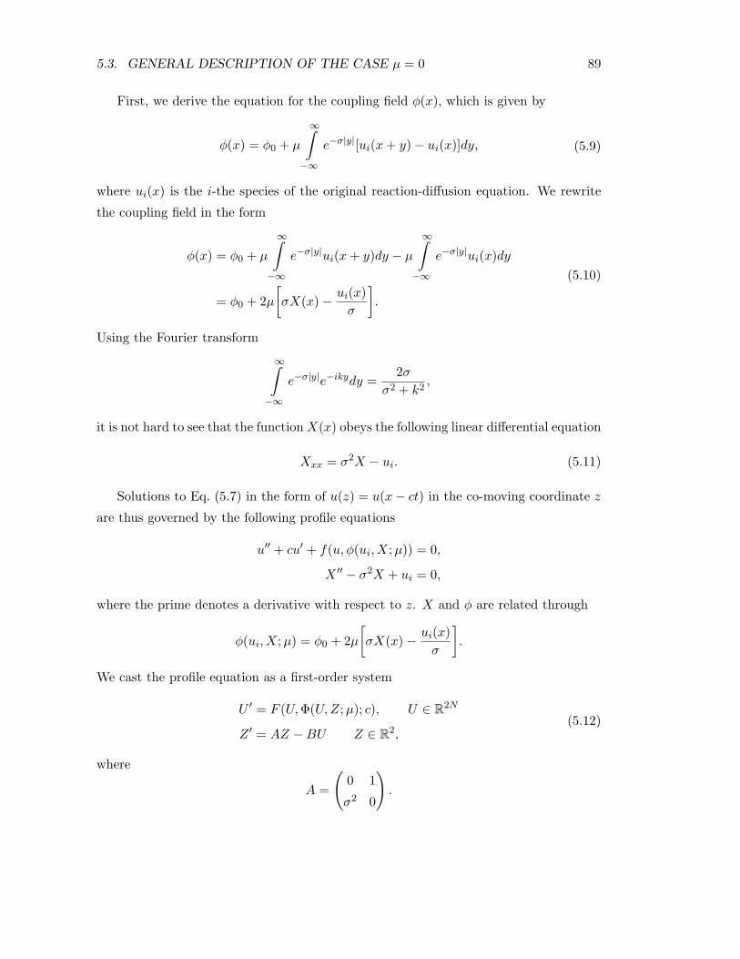
5.3. GENERAL DESCRIPTION OF THE CASE µ = 0 89
First, we derive the equation for the coupling field φ(x), which is given by
φ(x) = φ0 + µ
$&
!$
e!*|y|[ui(x + y)% ui(x)]dy, (5.9)
where ui(x) is the i-the species of the original reaction-di!usion equation. We rewrite
the coupling field in the form
φ(x) = φ0 + µ
$&
!$
e!*|y|ui(x + y)dy % µ
$&
!$
e!*|y|ui(x)dy
= φ0 + 2µ
$σX(x)% ui(x)
σ
%.
(5.10)
Using the Fourier transform
$&
!$
e!*|y|e!ikydy =2σ
σ2 + k2,
it is not hard to see that the function X(x) obeys the following linear di!erential equation
Xxx = σ2X % ui. (5.11)
Solutions to Eq. (5.7) in the form of u(z) = u(x% ct) in the co-moving coordinate z
are thus governed by the following profile equations
u"" + cu" + f(u, φ(ui, X;µ)) = 0,
X "" % σ2X + ui = 0,
where the prime denotes a derivative with respect to z. X and φ are related through
φ(ui, X;µ) = φ0 + 2µ
$σX(x)% ui(x)
σ
%.
We cast the profile equation as a first-order system
U " = F (U,%(U,Z;µ); c), U ' R2N
Z " = AZ %BU Z ' R2,(5.12)
where
A =
'0 1
σ2 0
(.

90CHAPTER 5. CREATING BOUND STATES BY MEANS OF NON-LOCAL COUPLING
Functions %(U,Z;µ) and F (U,%(U,X;µ); c) are obtained from given φ(u, X;µ) and
f(u, φ(u, X;µ)) in a straight-forward way. The matrix B accounts for the coupling
between the appropriate components of U and Z. Non-local coupling e!ectively extends
the phase space of the profile equation in a linear way by two dimensions. The asymptotic
flow in the Z-subspace is given by the simple equation
Z "± = ±σZ±, (5.13)
where Z± are the eigenvectors of the matrix A.
In our following analysis we consider the case µ = 0. We assume that without
non-local coupling the reaction-di!usion system supports propagation of stable solitary
pulses. This means that there exist a homoclinic solution (U0, Z0)(z) to the profile
equation
U " = F (U,φ0; c)
Z " = AZ %BU.(5.14)
with some c = c0. Then the linearization of Eq. (5.14) around (U0, Z0)(z)
v" = A(z)v, v ' C2N+2, (5.15)
has a bounded solution given by v(z) = ∂z(U0, Z0)(z). The adjoint linearized problem
ψ" = %A%(z)ψ, ψ ' C2N+2. (5.16)
has a bounded solution as well [14]. The solution of the adjoint variational equation is
perpendicular to the tangent spaces of the stable and unstable manifolds of the equi-
librium, which is used in order to define the orientation of the homoclinic orbit later
on.
The Jacobian matrix of Eq.(5.12) in the fixed point for µ = 0 is given by
A(0) =
'∂UF (0,φ0; c) 0
%B A
(. (5.17)
The eigenvalues of A(0) are exactly those of the matrices ∂UF (0,φ0; c) and A. The
leading eigenvalues of A(0) (those with smallest real parts) are then ±σ (see inset in
Fig.5.4) and the corresponding leading eigenvectors are given by (0, . . . , 0) *+ ,2N
, 1,±σ)T . Note
that in the case µ = 0 the leading eigenvectors are always perpendicular to the U -
subspace, this corresponds to the fact that the profile of u(x) is not a!ected by the
variable φ(x) for µ = 0.

5.3. GENERAL DESCRIPTION OF THE CASE µ = 0 91
(b)(a)
(c) (d)
Figure 5.3: Sketches of homoclinic orbits. Filled circles denote the equilibrium. Leading
directions are shown by single arrows, strong stable direction is shown by doubled arrows.
Arrows perpendicular to the homoclinics indicate the solution to the adjoint variational
equation. The gray strip shows the stable manifold of the fixed point close to the
homoclinic orbit. (a) Generic codimension-1 orientable homoclinic orbit. (b) Generic
codimension-1 twisted homoclinic orbit. (c) Codimension-2 orbit flip of homoclinic orbit.
(d) Codimension-2 inclination flip of homoclinic orbit.
5.3.2 Codimension-2 bifurcations of homoclinic orbits
Now let us recall three general assumptions on the homoclinics of codimension one to a
saddle equilibrium with real eigenvalues %λss < %λs < 0 < λu [13]:
1. the leading eigenvalues are not in resonance λu .= λs,
2. the solution v(z) to the linearized problem Eq. (5.15) converges to zero along the
leading eigenvectors of the linearization in the fixed point and
3. the same applies to the solution ψ(z) of the adjoint problem Eq.(5.16).

92CHAPTER 5. CREATING BOUND STATES BY MEANS OF NON-LOCAL COUPLING
codim-2
codim-1
codim-1 codim-1
!
""
PD
Figure 5.4: A codimension-2 bifurcation of a homoclinic orbit, the emergence of a 2-
homoclinic orbit (solid line) and a period-doubling bifurcation PD (dashed line). Inset:
Empty circles denote the eigenvalues of the matrix A, full circles show the eigenvalues
of ∂UF (0,φ0; c).
The last assumption is sometimes called the strong inclination property, for homoclinics
in R3 it means that the two-dimensional stable manifold comes in backward time tangent
to the strong stable direction of the fixed point (see Fig. 5.3). A homoclinic orbit of
codimension-1 can be orientable or twisted, depending on the orientation of the strip of
the two-dimensional manifold, see Fig. 5.3 (a) and (b). One defines the orientation Oof a given homoclinic orbit with the help of the solution ψ(z) to the adjoint variational
equation (5.16) as
O = limz#$
sign*ψ(z), v(%z)+ · *ψ(%z), v(z)+, (5.18)
where v(z) denotes the solution to the linearized equation (5.15).
If one of the above assumptions is violated, one speaks of codimension-2 bifurcations
of homoclinic orbits [13]. These are, in the order of the assumptions above:
1. resonance homoclinic orbit,
2. orbit flip and

5.3. GENERAL DESCRIPTION OF THE CASE µ = 0 93
3. inclination flip.
The resonance bifurcation can produce 2-homoclinics and both flip bifurcations can
produce 2- and N -homoclinics. A branch of period-doubling bifurcation emerges from
the bifurcation point as well (see Fig. 5.3 (c,d) and Fig. 5.4 for a qualitative picture of
a codimension-2 bifurcation and the emergence of 2-homoclinics). In orbit (inclination)
flip bifurcation, the vector v(z) (ψ(z)) for z ! ±" switches through the strongly stable
eigenspace of A(0), respectively. Both flip bifurcations correspond to the change of the
sign of the scalar products that contribute to the orientation O and can be detected as
zeroes of the orientation.
In our analysis of the e!ect of non-local coupling on the pulse dynamics we are
particularly interested in the inclination flip. Let us recall the details of the inclination
flip bifurcation of a homoclinic orbit in R3 to a saddle with one-dimensional unstable and
two-dimensional stable manifold (see Fig. 5.5 (a)). Before and after the bifurcation the
solution of the adjoint variation equation approaches zero along the leading eigenvector,
as mentioned above. The two-dimensional stable manifold approaches the saddle point
in backward time tangent to the strongly stable eigenvector. In the bifurcation point
the solution of the adjoint equation picks the non-leading eigenvector of the linearization
in the equilibrium for z ! %". The two-dimensional stable manifold approaches the
equilibrium in the backward time tangent to the weakly stable eigenvector.
5.3.3 Resonance and Inclination flips for µ = 0
We can immediately see that non-local coupling for µ = 0 breaks the first assumption,
since the leading eigenvalues ±σ of the linearization (5.17) are obviously in resonance.
The second assumption about the asymptotics of the homoclinic orbit holds. It
physically means that the non-local field decays in space much slower than the u-profile
of the pulse.
The strong inclination property is violated at µ = 0 with respect to both stable and
unstable manifolds. It means that the homoclinic orbit that describes a solitary pulse in
the absence of non-local coupling undergoes two inclination flip bifurcations if considered
in the phase space extended by the coupling variable Z in Eq. (5.14). Let us consider
the adjoint variational equation (5.16) together with Eq. (5.17) for µ = 0'
U
Z
("
= %'
∂UF %(U(z),φ0; c) %B%
0 A%
( 'U
Z
(. (5.19)

94CHAPTER 5. CREATING BOUND STATES BY MEANS OF NON-LOCAL COUPLING
We see that the Z-subsystem is completely decoupled from the U -part. The equation
for Z " is simply given by
Z " = %A%Z, A% =
'0 σ2
1 0
(, (5.20)
and the variable U has no influence on the flow of Z, which is the counterpart of the
fact that in the linearized equation (5.15) the U subsystem is not a!ected by Z.
We seek for a solution (U,Z)(z) to Eq. (5.19), which vanishes for large z, i.e.
(U,Z) ! 0 as z ! ±". For a codimension-1 homoclinic orbit, we expect that this solu-
tion approaches zero along the leading eigenvectors of%A%(0), given by (0, . . . , 0, 1,±σ)T .
However, the only bounded solution to Eq. (5.20) for z ! ±" is given by Z = 0, which
means that the solution (U,Z)(z) to Eq. (5.19) must pick the non-leading eigenvectors
of A(0), given by (U±, 0, 0)T , in order to converge to zero for z ! ±". Here, U±
represent the leading eigenvectors of the matrix ∂UF %(U(z),φ0; c).
Finally we write
ψ(z) =
-
../
U±
0
0
0
112 e&*z, for z ! ±"
for the solution ψ(z) of the adjoint problem and
v(z) =
-
../
0
1
±σ
0
112 e&*z, for z ! ±"
for the solution v(z) of the linearized problem, given by Eq. (5.15). Substituting the
above expressions for v(z) and ψ(z) in Eq. (5.18)
O = limz#$
sign*ψ(z), v(%z)+ · *ψ(%z), v(z)+,
we immediately see that both scalar products vanish, rendering two inclination flips with
respect to the stable and the unstable manifolds.
5.3.4 Geometrical interpretation
We simplify the problem, exploring the extension of the profile equation only by one
stable direction Y :
U " = F (U,φ0; c)
Y " = %σY %BU.(5.21)

5.3. GENERAL DESCRIPTION OF THE CASE µ = 0 95
2
(a)
I
YU1
(b)
Σ
(c)
Σ
γ
γ
I
Γ Γ
2U
γ
γ
U1
U
Figure 5.5: (a) Details of inclination flip bifurcation. Left panel: stable 2D manifold
of the fixed point before the bifurcation. Middle panel: stable 2D manifold in the
bifurcation point, note that the solution to the adjoint equation is directed along the
strongly stable direction. Right panel: the same 2D stable manifold after the bifurcation.
(b) Illustration of the inclination flip in the extended system (5.21). Empty dot I shows
the initial condition in the stable manifold for the integrating in backward time, $ shows
the Poincare section, γ denotes the unfeasible hypothetic trajectories that start in the
phase point I, and & denotes the feasible trajectories, see text. (c) Projection of the
homoclinic orbit in Eq. (5.21) on the U -subspace. I, $ and γ have the same meaning
as in (b)
We are interested in the behavior of the stable manifold of the equilibrium of Eq. (5.21)
in backward time.
We emphasize once again that we work with non-local coupling switched o!, i.e.
µ = 0, and assume that there exists a homoclinic orbit in the U -subsystem of Eq.
(5.21). This implies that in the extended system there exists a homoclinic orbit as well,
and the homoclinic orbit in the extended system approaches the equilibrium along the
Y direction, since the Y axis is the leading stable eigenvector to the leading eigenvalue
%σ of the Jacobian of Eq. (5.21).
We refer to Fig. 5.5 (b) for the geometry of the eigendirections and the stable
manifold in the system. Our idea is to compare the full phase space of the extended

96CHAPTER 5. CREATING BOUND STATES BY MEANS OF NON-LOCAL COUPLING
system with its projection on the U variables, where the actual dynamics takes place.
The U -subspace of Eq.(5.21) is decomposed in the leading unstable direction U2 and the
strongly stable eigendirection U1. The leading stable eigendirection is Y .
We choose a Poincare section $ across the leading unstable eigenvector close to the
equilibrium. Next, we put an initial condition (marked by I in Fig. 5.5 (b)) close to the
homoclinic orbit in the two-dimensional stable manifold, and follow it in backward time
along the homoclinic orbit. An important question is how this trajectory returns to the
previously chosen Poincare section. For a generic codimension-1 homoclinic orbit, the
trajectory from our initial condition returns along one of the dashed lines with the arrows
marked by γ in Fig. 5.5 (b). In the projection on the U plane it would mean, however,
that the trajectory does not remain on the homoclinic orbit, which is impossible because
the starting point belongs to the homoclinic orbit in the U -subspace, which in turn is
an invariant trajectory (see Fig. 5.5(c) for the projections of the hypothetical trajectory
marked by γ). In other words, the U components of our hypothetical trajectory must
be the original homoclinic orbit in the original profile equation
U " = F (U,φ0; c)
without non-local coupling. Last means that the feasible trajectory of point I in back-
ward time must come to the section $ along the vectors marked by &.
Comparing Fig.5.5(a) and Fig.5.5(b), we conclude that for µ = 0 our system displays
an inclination flip with respect to the stable manifold. In exactly the same way one
can show an inclination flip with respect to the unstable direction while considering the
extension of the profile equation by one unstable direction (with +σ)
U " = F (U,φ0; c)
Y " = σY %BU.(5.22)
In this case the same considerations can be applied, keeping in mind that Y becomes
now the leading unstable direction of Eq.(5.22) and Fig. 5.5(b) can be used with the
reversed directions of the arrows.
5.3.5 Summary: Codimension-4 homoclinic orbit
Summarizing our results for µ = 0, we find a codimension-4 homoclinic orbit in the
profile equation for travelling waves in the reaction-di!usion system (5.7) with non-local

5.3. GENERAL DESCRIPTION OF THE CASE µ = 0 97
coupling given by Eq. (5.8). Here, we present the list of the bifurcations together with
the assumptions, under which we find the degeneracies:
1. Inclination flip with respect to the stable manifold (extended equation (5.21)). As-
sumption: %σ is the leading stable eigenvalue ofA(0), i.e. the matrix ∂UF (0,φ0; c0)
has no eigenvalues with real part between %σ and 0.
2. Inclination flip with respect to the unstable manifold (extended equation (5.22)).
Assumption: σ is the leading unstable eigenvalue ofA(0), i.e. the matrix ∂UF (0,φ0; c0)
has no eigenvalues with real part between 0 and σ.
3. Resonance condition for the leading eigenvalues ±σ. Assumption: the matrix A
has a specific form, given by Eq. (5.13). This can be violated, for example, by the
choice of temporarily inertial non-local coupling like in [93].
4. Existence of the homoclinic orbit itself (existence of solitary pulse in PDE for
µ = 0). Assumption: there exists a solitary pulse without non-local coupling.
We would like to stress that the high codimension of the bifurcation at µ = 0 does not
depend on the particular system and is solely provided by the non-local coupling. The
first two assumptions can be fulfilled by the choice of su#ciently large coupling range,
i.e. by the smallness of σ, while the third one follows naturally from the symmetry of
the coupling function e!*|y|. In this sense the high codimension of the solitary pulse at
µ = 0 and the bifurcation to pulse pairs is a generic feature of systems with non-local
coupling.
Three of the four bifurcation are unfolded upon switching on non-local coupling by
setting µ .= 0. Each of the found homoclinic bifurcations can produce 2-homoclinic
orbits, see Table I and Table II in [34]. Bifurcations to 2-homoclinic orbit for the profile
equation (5.14) correspond to the emergence of bound states with 2 pulses with the
same velocity in the full PDE system. All three bifurcations were precisely detected
numerically in the Oregonator model at µ = 0 by the continuation software AUTO [39].
5.3.6 Stability of bound states
Stability of the bifurcating bound states can be determined in the general framework of
the stability of multi-bump pulses [17]. Under assumption of large interpulse distance
98CHAPTER 5. CREATING BOUND STATES BY MEANS OF NON-LOCAL COUPLING
the interaction of the pulses within a bound state is weak and can be estimated from
the decay properties of the corresponding solitary pulse.
Suppose that we have found a bound state for µ = µ0 close to µ = 0. The interpulse
distance Lp in the bound state is considered to be large. To simplify our analysis, we
assume that the leading eigenvalues of the matrix A(0) for µ = µ0 are given by νs < 0
and νu > 0, where νu > %νs. The last means that the exponential wake behind the
pulse decays slower that in the front of it, which is quite often the case if the velocity
of the pulse is not zero. The critical spectrum of the bound state with two pulses is
then given by two point eigenvalues, one of which is necessarily λ = 0, representing the
translation invariance of the pulse pair.
The second eigenvalue describes the interaction of pulses within a bound state and
thus decides upon the stability of the pulse pair. Under the above assumptions on the
matrix A(0), this eigenvalue is given by [14, 17]
λi = % 1M*ψ(Lp/2), v(%Lp/2)+,
where M is the Melnikov integral for the solitary pulse, v(z) and ψ(z) are the solutions
to the linear equations (5.15) and (5.16) for the solitary pulse.
The easiest way to determine the sign of λi is to check the stability of periodic pulse
trains with interpulse distance Lp. The sign of
% 1M*ψ(Lp/2), v(%Lp/2)+
decides upon the stability of periodic pulse trains as well [16]. Equivalently, the location
of the circle of the critical eigenvalues is determined by the above scalar product.
As a result, a pulse pair with interpulse distance Lp is stable if the corresponding
spatially periodic pulse train with the same wavelength is stable. For large wavelengths,
there is a relation between the slope of the dispersion c(L) and the stability of wave
trains, which says that for ddL c(L) > 0 the wave trains are stable [15]. Thus it is
possible to predict the stability of the bound state from the slope of the dispersion curve
for the appropriate periodic pulse trains with the wavelength L = Lp.
5.4 Discussion and outlook
In this chapter, we have shown that non-local coupling in the form of exponentially de-
caying connections between the elements of the medium leads to the emergence of bound

5.4. DISCUSSION AND OUTLOOK 99
states of pulses. The results of our analysis were obtained under general assumptions
on the underlying equations and thus are applicable to a wide class of reaction-di!usion
systems under influence of non-local coupling with exponentially decaying strength.
The central point of our analysis was the case where the coupling strength µ was equal
to zero. The homoclinic orbit which describes the solitary pulse for µ = 0 was shown to
be of codimension-4. Upon switching on non-local coupling, the homoclinic orbit became
a generic one of codimension-1. This unfolding of the codimension-4 bifurcation leads to
the emergence of N -homoclinics that correspond to bound states in the reaction-di!usion
system with non-local coupling. Our results also apply to a non-local coupling with a
su#ciently small temporal inertiality τ [93]; in this case the matrix A in Eq. (5.12) is
slightly di!erent and the leading eigenvalues of A are not in resonance anymore. We
would still have a codimension-3 homoclinic orbit, which can bifurcate to double pulses.
We stress that the high codimension of the bifurcation is provided essentially by the
form of the non-local coupling and does not depend on the particular properties of the
pulses in the reaction-di!usion system. In our numerical computation with continuation
software the predicted bifurcations were accurately detected, which can be considered
as a numerical proof of the theoretical analysis. Additionally, in the numerically investi-
gated example the bound state has been shown to be linearly stable, which can be seen
as a first step towards real experimental verification of the results.
There are still some open questions about the considered bifurcations. We have
shown two inclination flips and resonant homoclinic orbit simultaneously for µ = 0.
Both flip bifurcation and resonance condition can produce 2-homoclinics and so far it is
not clear which specific bifurcation leads to the emergence of bound states. The interplay
of two inclination flip bifurcations with the resonance condition assures an even more
intriguing dynamical behaviour than near a codimension-3 point [91, 92].

100CHAPTER 5. CREATING BOUND STATES BY MEANS OF NON-LOCAL COUPLING

Chapter 6
Conclusions
In the presented Thesis we theoretically studied the dynamics and stability of solitary
pulses and periodic pulse trains in excitable media. Despite the great variety of the
particular profiles of pulses, two generic cases can be distinguished: i) pulses with os-
cillations in the tail and ii) pulses with monotonous tail. For pulses of both types we
report the phenomenon of anomalous dispersion and alternating pulse interaction in
dependence on the interpulse distance.
6.1 Pulses with oscillations in the tail
Pulses with oscillatory tails provide a potentially richer dynamics, which can be already
seen on the level of profile equations. Such pulses are described by a homoclinic orbit
to an equilibrium with complex-conjugate eigenvalues, which provide the oscillations in
the asymptotic behavior. Since the works of Shilnikov it was known that such pulses are
accompanied by a set of multi-pulses (or, equivalently, bound states in the language of
reaction-di!usion systems) and infinitely many periodic solutions.
For reaction-di!usion systems this type of pulses is shown to exist close to the tran-
sition between excitable and oscillatory kinetics. In the same time, this is the region of
the transition between trigger and phase waves, which are natural spatial solutions for
excitable and oscillatory local dynamics, respectively. With the help of model equations,
which describe the light-sensitive Belousov-Zhabotinsky reaction, we clearly resolved the
transition to the pulses with oscillatory tails and then the transition to phase waves.
Under increase of the ”excitability” parameter of the system, the transition from
101

102 CHAPTER 6. CONCLUSIONS
trigger to phase waves includes the following steps: (i) Emergence of tail oscillations
behind the solitary pulse. In the same time the dispersion curve of trigger pulse trains
becomes oscillatory. (ii) Hopf bifurcation in the profile equation, which corresponds to
the emergence of undamped tail oscillations of the solitary pulse. The oscillations in
the dispersion curve of periodic waves becomes also undamped. This Hopf bifurcation
introduces the phase waves with finite velocity.(iii) Collision of branches of trigger waves
and phase waves and successful disappearance of trigger wave trains in series of saddle-
node collisions. The only waves that survive are the phase waves. The point of the
collision of trigger and phase waves branches defines the boundary between regimes of
trigger waves and phase waves.
The bifurcation parameter which gives us access to di!erent regimes represents the
intensity of the applied light illumination in the experiment. This suggests that the
found phenomenon can be found in future experiments.
As mentioned above, for the pulses with oscillations in the wake we find wiggly dis-
persion curve of periodic pulse trains. A new particular feature of this kind of dispersion
is the presence of domain of bistability, where two pulse trains with the same wavelength
can propagate at di!erent velocities. Two stable solutions are separated by the unstable
one. We presented a detailed stability analysis of the coexisting pulse trains, belonging
to the same domain of bistability. The possible instabilities of wave trains of wavelength
L include: (i) period-doubling bifurcation, which can be seen on a periodic domain of
length 2L. (ii) Long-wavelength or Eckhaus instability, which is characterized by the
change of the curvature sign of spectrum at the origin. (iii) A short-wavelength insta-
bility, which can be already be seen on periodic domains of length L. This instability is
described by the circle of critical eigenvalues detached from the origin.
6.2 Pulses with monotonous tails
Oscillatory tails of pulses are not the only reason for the existence of locking-type phe-
nomena between pulses. Monotonous tails can provide attractive interaction and thus
anomalous dispersion as well. In this case, however, the type of interaction does not
alternate periodically with the interpulse distance.
In the last part of the Thesis we show that including non-local interaction in the
form of long-range coupling between the elements of the medium leads to new features
of pulse interaction, including the emergence of bound states and anomalous dispersion.

6.3. SUGGESTIONS FOR FURTHER STUDIES 103
Physically the phenomenon can be understood as the interplay between activating and
inhibiting type of non-local coupling, which is controlled by the sign of the coupling
strength µ. The emergence of bound states and anomalous dispersion was analytically
proven to occur precisely at µ = 0.
More detailed theoretical considerations base on the analysis of the profile equation,
where we analytically showed that the solitary pulse at µ = 0 undergoes a certain
bifurcation of a high codimension. Unfolding of this bifurcation (turning on the non-
local coupling) leads to the emergence of N -pulses (or bound states). In the same
time the dispersion of periodic pulse trains demonstrate an overshoot, followed by an
anomalous part with negative slope. We calculated the spectra of periodic solutions
close to the overshoot and revealed the fine details of the stability of pulse trains. It
turned out that the pulse trains become unstable through a long-wavelength instability
prior to the period doubling. However, the period-doubling instability can be relevant if
we consider the system on a relatively small domain with a length of several wavelengths
of the pulse train.
The results of the last chapter are applicable to the wide class of reaction-di!usion
systems since we have proven the bifurcation to N -pulses to be model-independent.
The only assumptions were on the exponential decay of the coupling function and the
broadness of the non-local coupling field. The results of the analysis can be applied to
non-local coupling with a small temporal inertiality, which makes the codimension of
the bifurcation be smaller by one.
6.3 Suggestions for further studies
Concerning non-local coupling, there is a plethora of possible further investigations, both
theoretically and experimentally. To the best of our knowledge, the dynamics of spiral
waves in excitable media under non-local coupling (or, equivalently, with a strongly
di!usive species) has not been studied. We can speculate that the presence of another
spatial scale can drastically modify the dynamics of spiral waves. In the radial direction
the non-local field should slowly approach some limit state, corresponding to the non-
local field over a plane wave. If we could tune the parameters of the system so that the
asymptotic state of the non-local field suppresses the propagation of the spiral fronts, it
were possible to create localized spiral waves on homogeneous background.
A possible two-dimensional study is also interesting for the case of oscillatory pulse
104 CHAPTER 6. CONCLUSIONS
tails. Winfree [18] has already demonstrated theoretically the coexistence of alternating
spiral waves due to the oscillations in the pulse tail, but the phenomenon of velocity
locking was not considered.
One of the experimental challenges might be the uncovering of the small oscillations
behind the pulse in the realistic Belousov-Zhabotinsky reaction. The experiments in the
laboratory of group of Prof. Engel showed some indirect tips to the existence of those
small-amplitude oscillations, but there is still no convincing evidences on that.

Appendix A
Group velocity of periodic wave
train and its spectrum
Here, our aim is to show that the slope of the dispersion curve c(L) which we will call
here group velocity of the wave train, is equal to the first derivative of the essential
spectrum λ(iγ) at the origin
%cg =d
dLc(L) =
d
dγIm λ(γ)
####$=0
.
The derivation is an adapted first-order version of the analogous proof in [94]. Another
di!erence is that we use the formulation of dispersion in terms of wavelength L and
phase velocity c instead of wave number k and frequency ω as in [94].
We consider wave trains, i.e. periodic solutions to the profile equation
DU "" + cU " + F (U) = 0, " = ∂z
cast as a first-order system
u" = f(u; c), 0 < z < L (A.1)
where
u =
'U
V
(, f =
'V
D!1[%cV % F (U)]
(. (A.2)
The linearization around the wave train, given by
DV "" + cV " + FU (U)V = λV (A.3)
105

106APPENDIX A. GROUP VELOCITY OF PERIODIC WAVE TRAIN AND ITS SPECTRUM
can be written as a first order system as well
v" = A(z;λ)v (A.4)
with the matrix A is given by
A(z;λ) = ∂uf(u(x); c) + λB, B =
'0 0
D!1 0
(. (A.5)
We note from Eq. (A.2) and Eq. (A.5) that
∂cf = %Bu", " = ∂z. (A.6)
We can reformulate the eigenvalue problem (A.5) with the help of the operator
T (λ) : v /%! dv
dz%A(·;λ)v (A.7)
in the following form
T (λ)v = 0.
Later on we will need a solution ψ of the adjoint problem
T %(λ)ψ = 0.
We recall that λ is in the essential spectrum of the wave train if, and only if, the
boundary-value problem
v" = A(z;λ)v, 0 < z < L
v(L) = ei$v(0)(A.8)
has a solution for some γ ' R.
Typically, periodic wave trains live in families on the dispersion curves c = c(L). We
rescale the co-moving coordinate by introducing a new coordinate x = z/L. From now
on we have" := ∂x = L∂z.
The profile equation reads then
1L
u" = f(u; c), 0 < x < 1 (A.9)

107
and the linearized problem Eq. (A.8)
1L
v" = A(x;λ)v, 0 < x < 1
v(1) = ei$v(0),(A.10)
where we omitted the rescaling of γ. With v = ei$xw we obtain from Eq. (A.10)
1L
w" =$A(x;λ)% iγ
L
%w,
w(1) = w(0).(A.11)
For the operator T (λ) we obtain then
T (λ) : v /%! 1L
dv
dx%A(·;λ)v +
iγ
Lv, A = ∂uf(u(x;L); c(L)) + λB (A.12)
With the substitution u = u(x;L), we take the first derivative of Eq. (A.9) with
respect to L
1L
∂Lu" % 1L2
u" = ∂uf(u(x;L), c(L)) ∂Lu + ∂cf(u(x;L), c(L))d
dLc(L),
which we rewrite with the help of the operator T (λ) from Eq. (A.12)
T (0) ∂Lu =1L2
u" + ∂cf(u(x;L), c(L))d
dLc(L). (A.13)
Next, we substitue w = w(x; γ) and take the first derivative of Eq. (A.11), evaluating
it at γ = λ = 0
1L
∂$w" = ∂uf(u(x;L); c(L)) ∂$w +d
dγλ(γ) Bw + λB ∂$w
) *+ ,=0
% i
Lw % iγ
L∂$w
) *+ ,=0
,
which again can be reformulated with the operator T (λ) (see Eq. (A.12)) as
T (0) ∂$w =d
dγλ(γ) Bw % i
Lw. (A.14)
We note that the functions on the right-hand sides of Eq. (A.13) and Eq. (A.14)
belong to the range of the operator T (0). This means that their product with a function
ψ from the null-space of the adjoint operator T %(0) must vanish:
*ψ,1L2
u" % d
dLc(L) Bw+ = 0,
*ψ,d
dγλ(γ) Bw % i
Lw+ = 0,
(A.15)

108APPENDIX A. GROUP VELOCITY OF PERIODIC WAVE TRAIN AND ITS SPECTRUM
where we used Eq. (A.6) with ∂z = L!1∂x
∂cf(u(x;L); c(L)) = % 1L
Bu"
together with w(x; 0) = u"(x;L). Eliminating *ψ, Bw+ from Eq. (A.15) and using the
normalization
*ψ, u"+ = 1,
we obtaind
dLc(L) =
d
dγIm λ(γ)
####$=0
,
which means that the sign of the slope of the dispersion curve c(L) coincides with the
orientation of the curve of the essential spectrum at zero.
Appendix B
Law of Mass Action
Suppose that we have a reversible chemical reaction with N reagents Rj , j = 1, . . . , N
and M products Pj , j = 1, . . . ,M , given byN3
j
αjRj !M3
j
βjPj ,
where αj and βj are natural numbers that denote the number of molecules of reagents
and products involved in a single reaction step.
The rates of the forward and backward reactions are then given by [95]
[forward rate] = k1
N4
j
R+j
j ,
[reverse rate] = k!1
M4
j
P,j
j .
(B.1)
The above formulae show that the rate of the reaction is directly proportional to the
product of the n-th orders of the reagent concentration. Physically it means that the
rate of the reactions depend on the probability of (nearly) simultaneous collision of the
corresponding number of the reagents molecules.
For the following hypothetic reaction
A + 2B ! C
the rate would be proportional to the concentration of A and to the square of the
concentration of B, i.e.
[forward rate] = k1[NA][NB]2. (B.2)
109

110 APPENDIX B. LAW OF MASS ACTION
The constant k is determined by the conditions like temperature, pressure and so on. We
can immediately write down the di!erential equation, describing the temporal evolution
of the concentration of the reagent A:
d
dt[NA] = k1[NA][NB]2.
From Eq. (B.1) we can derive the condition for the stationary non-equilibrium state
[forward rate] = [reverse rate],
which reads
k1
k!1=
N5j
R+j
j
M5j
P,j
j
= const.
The above equation is the statement of the law of mass action. In words it means: when
a reversible reaction has attained equilibrium, the reaction quotient1 remains constant.
1The reaction quotient is the ratio of molar concentrations of the reactants to those of the products,
each concentration being raised to the power equal to the coe"cient in the equation.

Bibliography
[1] I. Farkas, D. Helbing, and T. Vicsek, Mexican waves in an excitable medium, Nature
419, 131, 2002.
[2] A. S. Mikhailov, Foundation of Synergetics i: Distributed Active Systems, Springer
Berlin, 1991.
[3] M.C. Cross and P. C. Hohenberg, Pattern formation outside of equilibrium, Rev.
Mod. Phys. 65, 851–1112, 1993.
[4] J. J. Tyson, What everyone should know about the Belousov-Zhabotinsky reaction,
Lecture Notes in Biomathematics (S.A. Levin, ed.), vol. 100, Springer, New York,
1994, pp. 569–587.
[5] A. M. Turing, The chemical basis of morphogenesis, Philos. Trans. R. Soc. London
B 237, 37–72, 1952.
[6] V. Castets, V. Dulos, J. E. Boissonade, and P. De Kepper, Experimental evidence of
a sustained standing Turing-type nonequilibrium chemical pattern, Phys. Rev. Lett
64, 2953–2956, 1990.
[7] M. Falcke, Reading the patterns in living cells - the physics of Ca2+ signaling, Ad-
vances in Physics 53, 255, 2004.
[8] A. Hodgkin and A. Huxley, A quantitative description of membrane current and its
application to conduction and excitation in nerve, J. Physiol 117, 500–544, 1952.
[9] Richard Fitzhugh, Impulses and physiological states in theoretical models of nerve
membrane, Biophysical Journal 1, 445–466, 1961.
111

112 BIBLIOGRAPHY
[10] J. Nagumo, S. Arimoto, and S. Yoshizawa, An active pulse transmission line simu-
lating nerve axon, Proc. IRE 50, 2061–2070, 1964.
[11] G. K. Moe, W. C. Rheinbolt, and J. A. Abildskov, A computer model of atrial
fibrillation, Amer. Heart J. 67, 200–220, 1964.
[12] Alexander Panfilov and Arkady Pertsov, Ventricular fibrillation: evolution of the
multiple-wavelet, Phil Trans. R. Soc. Lond. 359, 1315–1325, 2001.
[13] Yu. A. Kuznetsov, Elements of applied bifurcation theory, Springer Berlin, 1995,
1998, 2004.
[14] Bjorn Sandstede, Handbook of Dynamical Systems, v. 2 (edt. by B. Fiedler), North-
Holland, 2002.
[15] Michal Or-Guil, Ioannis G. Kevrekidis, and Markus Bar, Stable bound states of
pulses in an excitable medium, Physica D 135, 154–174, 2000.
[16] Bjorn Sandstede and Arnd Scheel, On the stability of periodic travelling waves with
large spatial period, J. Di!. Eq. 172, 134–188, 2001.
[17] B. Sandstede, Stability of multiple-pulse solutions, Trans. Amer. Math. Soc. 350,
429–472, 1998.
[18] A. T. Winfree, Alternative stable rotors in an excitable medium, Physica D 49,
125–140, 1991.
[19] C. Elphick, E. Meron, J. Rinzel, and E. A. Spiegel, Impulse patterning and relax-
ational propagation of excitable media, Jour. Theor. Biol. 146, 249–268, 1990.
[20] J. Christoph, M. Eiswirth, N. Hartmann, R. Imbihl, I. Kevrekidis, and M. Bar,
Anomalous dispersion and pulse interaction in an excitable surface reaction, Phys.
Rev. Lett. 82(7), 1586–1589, 1999.
[21] V. K. Vanag and I. R. Epstein, Packet waves in a reaction-di!usion system, Phys.
Rev. Lett. 88, 088303, 2002.
[22] N. Manz, S. C. Muller, and O. Steinbock, Anomalous dispersion of chemical waves
in a homogeneously catalyzed reaction system, J. Phys. Chem. A 104, 5895, 2000.

BIBLIOGRAPHY 113
[23] N. Manz, C. T. Hamik, and O. Steinbock, Tracking waves and vortex nucleation in
excitable systems with anomalous dispersion, Phys. Rev. Lett. 92, 248301, 2004.
[24] H. U. Bodeker, A. W. Liehr, T. D. Frank, R. Friedrich, and H.-G. Purwins, Mea-
suring the interaction law of dissipative solitons, New J. of Phys. 6, 62, 2004.
[25] R. J. Field and R. M. Noyes, Oscillations in chemical systems IV. Limit cycle
behavior in a model of a real chemical reaction, J. Amer. Chem. Soc. 60, 1877–
1884, 1974.
[26] P. Glandsdor! and I. Prigogine, Thermodynamic theory of structure, stability and
fluctutations, Wiley, New York, 1971.
[27] G. Nicolis, Advan. Chem. Phys. 19, 209, 1971.
[28] J. J. Tyson, Some further studies of nonlinear oscillations in chemical systems, J.
Chem. Phys. 58, 209, 1973.
[29] R. J. Field, E. Koros, and R. M. Noyes, Oscillations in chemical systems II. Through
analysis of temporal oscillations in the bromate-cerium-malonic acid system, J.
Amer. Chem. Soc. 94, 8649–8664, 1972.
[30] H.-J. Krug, L. Pohlmann, and L. Kuhnert, Analysis of the modified complete orego-
nator accounting for oxygen sensitivity and photosensitivity of Belousov-Zhabotinsky
reaction, J. Phys. Chem. 94, 4862–4865, 1990.
[31] Morten Brøns and Kedma Bar-Eli, Canard explosion and excitation in a model of
Belousov-Zhabotinsky reaction, J. Phys. Chem. 95, 8706–8713, 1991.
[32] J.J. Tyson and J.P. Keener, Singular perturbation theory of travelling waves in
excitable media (a review), Physica D 32, 327, 1988.
[33] B. Sandstede and A. Scheel, Defects in oscillatory media: toward a classification,
IAM J. Appl. Dyn. Sys. 3, 1–68, 2004.
[34] Bjorn Sandstede, Constructing dynamical systems having homoclinic bifurcation
points of codimension two, J. Dyn. Di!. Eq. 9, 269, 1997.
[35] S. N. Chow, B. Deng, and B. Fiedler, Homoclinic bifurcation at resonant eigenval-
ues, J. Dyn. Di!. Eq. 2(2), 177–244, 1990.

114 BIBLIOGRAPHY
[36] S. Nii, N-homoclinic bifurcation for homoclinic orbits changing their twisting, J.
Dyn. Di!. Eq. 8, 549–572, 1996.
[37] E. Yanagida, Branching of double pulse solutions from single solutions in nerve axon
equations, J. Di!. Eq. 66, 243–262, 1987.
[38] Bjorn Sandstede, Verzweigungstheorie homokliner verdopplungen. PhD thesis, Uu-
niversity of Stuttgart, 1993.
[39] E. Doedel, R.C. Pa!enroth, A.R. Champneys, T.F. Fairgrieve, Yu.A. Kuznetsov,
B.E. Oldeman, B. Sandstede, and X. Wang, AUTO2000: Continuation and bifur-
cation software for ordinary di!erential equations (with HOMCONT), Concordia
University, Montreal, 2002.
[40] L. Shilnikov, Some cases of generation of periodic motions from singular trajectories,
Mat. Sbornik 61(103), 443–466, 1963.
[41] L. Shilnikov, A case of existence of a countable number of periodic motions, Soviet.
Math. Dokl. 6, 163–166, 1965.
[42] J. Neimark and L. Shilnikov, A case of generation of periodic motions, Soviet. Math.
Dokl. 6, 305–309, 1965.
[43] B. Deng, The Shilnikov problem, exponential expansion, strong λ-lemma, c1-
linearization, and homoclinic bifurcation, J. Di!. Eq. 79, 189–231, 1989.
[44] P.Glendinning and C.Sparrow, Local and global behaivour near homoclinic orbits, J.
Stat. Phys 35, 645–696, 1984.
[45] R. Gardner, Spectral analysis of long wavelength periodic waves and applications, J.
Reine Angew. Math 491, 149–181, 1997.
[46] J.D.M. Rademacher, B. Sandstede, and A. Scheel, Computing absolute and essential
spectra using continuation, preprint.
[47] Bjorn Sandstede and Arnd Scheel, Absolute and convective instabilities of waves on
unbounded and large bounded domains, Physica D 145, 233, 2000.
[48] J.Rademacher, Private communications, 2004.
BIBLIOGRAPHY 115
[49] J. D. M. Rademacher, Geometric relations of absolute and essential spectra of wave
trains, preprint.
[50] P. Wheeler and D. Barkley, Computation of spiral spectra, SIADS 5, 157–177, 2006.
[51] Raymond Kapral and Kenneth Showalter (eds.), Chemical Waves and Patterns,
Kluwer Academic Publishers, 1995.
[52] C. Elphick, Ehud Meron, and E. A. Spiegel, Spatiotemporal complexity in travelling
patterns, Phys. Rev. Lett. 61(5), 496–499, 1988.
[53] Oliver Steinbock, Excitable front geometry in reaction-di!usion systems with
anomalous dispersion, Phys. Rev. Lett. 88, 228302, 2002.
[54] C. van Oss, A. V. Panfilov, P. Hogeweg, F. Siegert, and C. J. Weijer, Spatial pattern
formation during aggregation of the slime mould dictyostelium discoideum, J. Theor.
Biol. 181, 203–213, 1996.
[55] J.-M. Flessels, A. Belmonte, and V. Gaspar, Dispersion relation for wave in the
Belousov-Zhabotinsky reaction, J. Chem. Soc., Faraday Trans. 94, 851, 1998.
[56] Chad T. Hamik, Niklas Manz, and Oliver Steinbock, Anomalous dispersion and
attractive pulse interaction in the 1,4-Cyclohexanedione Belousov-Zhabotinsky reac-
tion, J. Phys. Chem. 105, 6144–6153, 2001.
[57] M.G.Zimmerman, S.Firle, M.Natiello, M.Hildebrand, M.Eiswirth, M.Bar,
A.K.Bangia, and I.G.Kevrekidis, Pulse bifurcation and transition to spatiotempo-
ral chaos in an excitable reaction-di!usion model., Physica D 110, 92–104, 1997.
[58] M. Or-Guil, J. Krishnan, I. G. Kevrekidis, and M. Bar, Pulse bifurcations and
instabilities in an excitable medium: Computation in finite ring domains, Phys.
Rev. E 64, 046212, 2001.
[59] G. Roder, Diploma thesis, Technische Universitat Berlin, 2005.
[60] G. Roder, G. Bordyugov, M. Falcke, and H. Engel, In preparation, Phys. Rev. E,
2006.

116 BIBLIOGRAPHY
[61] Martin Falcke, Michal Ol-Guil, and Markus Bar, Dispersion gap and localized spiral
waves in a model for intracellular ca2+ dynamics, Phys. Rev. Lett. 84(20), 4753–
4756, 2001.
[62] Y. Kuramoto, Chemical Oscillations, Waves, and Turbulence, Springer Berlin, 1984.
[63] Wiktor Eckhaus, Studies in nonlinear stability theory, springer tracts in natural
philosophy, Springer-Verlag, Berlin, 1965.
[64] A. C. Newell and J. A. Whitehead, Finite bandwidth, finite amplitude convection,
J. Fluid. Mech. 38, 279, 1969.
[65] P. Ortoleva and J. Ross, Phase waves in oscillatory chemical reaction, J. Chem.
Phys 58, 5673–5680, 1973.
[66] Edward J. Reusser and Richard J. Field, The transition from phase waves to trigger
waves in a model of the Zhabotinskii reaction, Journal of the American Chemical
Society 101(5), 1063–1071, 1979.
[67] Rubin R. Aliev and Vadim N. Biktashev, Dynamics of the oscillation phase distri-
bution in the bz reaction, J. Phys. Chem 98, 9676–9681, 1994.
[68] C. P. Schenk, P. Schutz, M. Bode, and H.-G. Purwins, Interaction of self-orginized
quasiparticles in a two-dimensional reaction-di!usion system: The formation of
molecules, Phys. Rev. E 57, 6480–6486, 1998.
[69] M. Bode, A. W. Liehr, C. P. Schenk, and H.-G. Purwins, Interaction of dissipa-
tive solitons: Particle-like behaviour of localized structures in a three-component
reaction-di!usion system, Physica D 161, 45–66, 2002.
[70] G. Bordiougov and H. Engel, Oscillatory dispersion and coexisting stable pulse trains
in an excitable medium, Phys. Rev. Lett. 90(14), 148302, 2003.
[71] John Ross, Stefan C. Muller, and Christian Vidal, Chemical Waves, Science 240,
460–645, 1988.
[72] J.Rademacher, Phd thesis, university of minnesota, 2004.
[73] Bjorn Sandstede and Arnd Scheel, Absolute versus convective instability of spiral
waves, Phys. Rev. E 62(6), 7708, 2000.

BIBLIOGRAPHY 117
[74] R. Gardner, On the structure of the spectra of periodic travelling waves, J. Math.
Pures Appl. 72, 415–439, 1993.
[75] Martin Krupa, Bjorn Sandstede, and Peter Szmolyan, Fast and slow waves in the
FitzHugh-Nagumo equation, J. Di!. Eq. 133, 49–97, 1997.
[76] P. Hirschberg and E. Knobloch, Sil’nikov-Hopf bifurcation, Physica D 62, 202–216,
1993.
[77] A. R. Champneys and A. J. Rodriguez-Luis, The non-transverse Shil’nikov-Hopf
bifurcation: uncoupling of homoclinic orbits and homoclinic tangencies, Physica D
128, 130–158, 1999.
[78] N. Manz and O. Steinbock, Dynamics of excitation pulses with attractive interac-
tion: Kinematic analysis and chemical wave experiments, Phys. Rev. E. 70, 066213,
2004.
[79] M. Abeles, Corticonics, Cambridge University Press, England, 1991.
[80] G.B. Ermentrout and J.D. Cowan, A mathematical theory of visual hallucination
patterns, Biological Cybernetics 34, 137–150, 1979.
[81] J. Christoph and M. Eiswirth, Theory of electrochemical pattern formation, Chaos
12, 215, 2002.
[82] F. Plenge, H. Varela, and K. Krischer, Asymmetric target patterns in one-
dimensional oscillatory media with genuine nonlocal coupling, Phys. Rev. Lett. 94,
198301, 2005.
[83] Mauricio Barahona and Louis M. Pecora, Synchronization in small-world systems,
Phys. Rev. Lett. 89, 054101, 2002.
[84] Daniel M. Abrams and Steven H. Strogatz, Chimera states for coupled oscillators,
Phys. Rev. Lett. 93, 174102, 2004.
[85] Shinichiro Shima and Yoshiki Kuramoto, Rotating spiral waves with phase-
randomized core in nonlocally coupled oscillators, Phys. Rev. E 69, 036213, 2004.
[86] Yoshiki Kuramoto, Dorjsuren Battogtokh, and Hiroya Nakao, Multia"ne chemical
turbulence, Phys. Rev. Lett. 81, 3543–3546, 1998.

118 BIBLIOGRAPHY
[87] Ernesto Nicola, PhD thesis, Technische Universitat Dresden, 2001.
[88] Ernesto M. Nicola, Michal Or-Guil, Wilfried Wolf, and Markus Bar, Drifting pattern
domains in a reaction-di!usion system with nonlocal coupling, Phys. Rev. E 65,
055101, 2002.
[89] M. Hildebrand, H. Skødt, and K. Showalter, Spatial symmetry breaking in the
Belousov-Zhabotinsky reaction with light-induced remote communication, Phys. Rev.
Lett. 87, 088303, 2001.
[90] Ernesto M. Nicola, Markus Bar, and Harald Engel, Wave instability induced by non-
local spatial coupling in a model of the light-sensitive Belousov-Zhabotinsky reaction,
Phys. Rev. E NN, accepted, 2006.
[91] A.J. Homburg and B. Krauskopf, Resonant homoclinic flip bifurcations, J. Dyn.
Di!. Eq. 12, 749–774, 2000.
[92] B. E. Oldeman, B. Krauskopf, and A. R. Champneys, Numerical unfoldings of
resonant homoclinic flip bifurcations, Nonlinearity 14, 597, 2001.
[93] Dan Tanaka and Yoshiki Kuramoto, Complex Ginzburg-Landau equation with non-
local coupling, Phys. Rev. E. 68, 026219, 2003.
[94] A. Doelman, B. Sandstede, A. Scheel, and G. Schneider, The dynamics of modulated
wave trains, preprint.
[95] http://scienceworld.wolfram.com/chemistry/lawofmassaction.html.