
Dynamic Oligopoly Pricing: Evidence from the Airline · PDF fileDynamic Oligopoly Pricing:...
46
Sonderforschungsbereich/Transregio 15 · www.sfbtr15.de Universität Mannheim · Freie Universität Berlin · Humboldt-Universität zu Berlin · Ludwig-Maximilians-Universität München Rheinische Friedrich-Wilhelms-Universität Bonn · Zentrum für Europäische Wirtschaftsforschung Mannheim Speaker: Prof. Dr. Klaus M. Schmidt · Department of Economics · University of Munich · D-80539 Munich, Phone: +49(89)2180 2250 · Fax: +49(89)2180 3510 * University of Munich ** Toulouse School of Economics March 2014 Financial support from the Deutsche Forschungsgemeinschaft through SFB/TR 15 is gratefully acknowledged. Discussion Paper No. 463 Dynamic Oligopoly Pricing: Evidence from the Airline Industry Caspar Siegert * Robert Ulbricht **
Transcript of Dynamic Oligopoly Pricing: Evidence from the Airline · PDF fileDynamic Oligopoly Pricing:...

Sonderforschungsbereich/Transregio 15 · www.sfbtr15.de Universität Mannheim · Freie Universität Berlin · Humboldt-Universität zu Berlin · Ludwig-Maximilians-Universität München
Rheinische Friedrich-Wilhelms-Universität Bonn · Zentrum für Europäische Wirtschaftsforschung Mannheim
Speaker: Prof. Dr. Klaus M. Schmidt · Department of Economics · University of Munich · D-80539 Munich, Phone: +49(89)2180 2250 · Fax: +49(89)2180 3510
* University of Munich ** Toulouse School of Economics
March 2014
Financial support from the Deutsche Forschungsgemeinschaft through SFB/TR 15 is gratefully acknowledged.
Discussion Paper No. 463
Dynamic Oligopoly Pricing: Evidence from the Airline
Industry
Caspar Siegert * Robert Ulbricht **
Dynamic Oligopoly Pricing:
Evidence from the Airline Industry∗
Caspar Siegert
University of Munich
Robert Ulbricht
Toulouse School of Economics
March 23, 2014
Abstract
We explore how pricing dynamics in the European airline industry vary with the
competitive environment. Our results highlight substantial variations in pricing dynamics
that are consistent with a theory of intertemporal price discrimination. First, the rate
at which prices increase towards the scheduled travel date is decreasing in competition,
supporting the idea that competition restrains the ability of airlines to price-discriminate.
Second, the sensitivity to competition is substantially increasing in the heterogeneity of the
customer base, reflecting further that restraints on price discrimination are only relevant if
there is initial scope for price discrimination. These patterns are quantitatively important,
explaining about 83 percent of the total within-flight price dispersion, and explaining 17
percent of the observed cross-market variation of pricing dynamics.
Keywords: Airline industry, capacity constraints, dynamic oligopoly pricing, intertem-
poral price dispersion, price discrimination.
JEL Classification: D43, D92, L11, L93.
∗We are extremely grateful to Anton Vasilev for invaluable help and technical support throughoutthe process of collecting our dataset. We also would like to thank Ken Boyer, Meghan Busse,Sarit Markovich, Niko Matouschek, Mar Reguant, Klaus M. Schmidt, Mauricio Varela, and seminarparticipants at the University of Munich, Northwestern, and the 2011 IIOC conference for usefulcomments and discussions. Financial support from the Deutsche Forschungsgemeinschaft throughSFB/TR 15 and GRK 801 is gratefully acknowledged. Finally, we like to thank Xueqian Chen andMarkus Deak for excellent research assistance. Email Addresses: [email protected],[email protected].
1 Introduction
The tendency for airline ticket prices to rise as the scheduled departure date approaches
is one of the most well-known regularities of dynamic oligopoly pricing. This tendency
is often regarded as a prime example of intertemporal price discrimination, reflecting
that customers in the airline industry are likely to have different demand elasticities
correlating with their ability or willingness to book in advance.1 While there is now a
small literature with a focus on intertemporal price discrimination when firms have
monopoly power (e.g., Lazarev, 2013; Williams, 2013), our understanding on the scope
and working of intertemporal price discrimination in oligopoly markets is still limited.
However, many important markets are oligopolistic and it is far from obvious how
insights into intertemporal price discrimination from monopoly markets extend to
oligopolies.
In this paper, we take a step towards filling this gap using new data on the time
path of prices from the European airline industry. In particular, we empirically explore
how pricing dynamics vary with the competitive environment and to what extend the
identified variations are consistent with intertemporal price discrimination.
From an empirical perspective, the analysis of pricing dynamics has proved difficult
mainly due to a lack of public data. In the airline industry, price data has been
available at a (quarterly) level that does not allow to differentiate intertemporal
price variations for a given flight from variations across different travel dates and
from variations across different flights on a given route. This has led the empirical
price discrimination literature to focus on the impact of competition on broader
dispersion measures that do not differentiate among different dimensions of dispersion
(e.g, Borenstein and Rose, 1994; Hayes and Ross, 1998; Gerardi and Shapiro, 2009).
We address this issue using manually collected price data from the internet.2 In
particular, we construct a panel including about 1.4 million prices for airline tickets
on the intra-European market where for each route-date pair (which we refer to as a
“market”) we record a time series of prices ranging from 10 weeks to 1 day prior to
1The usual example are business travelers who learn about travel requirements on short noticeand have a high willingness to pay in contrast to leisure travelers with longer planning horizons.
2Recent studies using similar approaches to collect airline price data include Lazarev (2013) andWilliams (2013) who also explore pricing dynamics, but focus on monopoly markets. In contrast,McAfee and Te Velde (2007), Gaggero and Piga (2011), Escobari (2012), and Escobari, Rupp andMeskey (2013) have access to competitive price data, but are interested in the determinants of pricelevels and dispersion rather than pricing dynamics and their determinants.
1

departure. Using this time series dimension permits us to shift the focus on pricing
dynamics and their determinants.
We begin our analysis by estimating the intertemporal slope of prices and its sensi-
tivity to competition. Overall, we find that prices in our sample increase substantially
over time, but at a rate that is highly sensitive to competition. While monopoly
prices increase by an average of 1.31 percent with every day that a customer waits
to book, this slope is reduced to 1.19 percent in duopolies and continues to decrease
monotonically to a slope of only 0.68 percent in markets with six competing airlines.
A nonparametric treatment of pricing dynamics further reveals that these differences
are mainly driven by the last 5 weeks before departure, where prices differentially
steepen, implying a cumulative increase of 95 percent in monopolies compared to
about 50 percent in markets with six competitors.
At a first sight, these pricing dynamics are consistent with a theory of competitive
price discrimination, reflecting the idea that competition restrains the ability of airlines
to price-discriminate between customers with long planning horizons and customers
who book at short notice. In an effort to make this argument more rigorous, we use
hotel bookings data to construct measures for the tourist intensity in a given market
and to identify variations in customer heterogeneity. If price discrimination is a major
aspect of dynamic oligopoly pricing, then the degree to which an airline’s ability
to price-discriminate becomes restrained as competition intensifies should depend
on how much it would discriminate if it were unconstrained. Accordingly, if price
discrimination plays an important role, competition should have a stronger impact on
the intertemporal slope in markets with considerable customer heterogeneity.
Consistent with these considerations, we find that the sensitivity of the pricing
dynamics to competition varies substantially with the identified heterogeneity. In
markets characterized by a highly heterogeneous customer base, competition flattens
the intertemporal slope from a daily rate of 1.42 percent in monopolies to 0.77 percent
in markets with 6 competitors. In contrast, we find that in markets characterized by
little customer heterogeneity, competition has virtually no impact on the intertemporal
slope.
Comparing our results to the empirical price discrimination literature, the negative
relation between competition and the intertemporal slope appears to be in line with
the finding of Gerardi and Shapiro (2009) that competition decreases dispersion
(measured by the Gini coefficient on a given route across flights and travel dates), but
2
disagree with Borenstein and Rose (1994) who find the opposite. Using the ability
to distinguish between the different dimensions of dispersion in our data, we show
that the negative relation between competition and price dispersion is strongest when
dispersion is defined as intertemporal within-flight dispersion, i.e. the dispersion in
prices paid for the same physical flight. When dispersion is, in contrast, defined by
pooling either across travel dates or across flights (on the same route), the relation
becomes diluted (in the former case) or overturned (in the latter case). Hence, while
we find competition to have an unambiguous negative impact on intertemporal price
dispersion, the relation between competition and cross-flight dispersion in our data is
less clear and may explain seemingly contradicting findings in the earlier literature.
In the context of the empirical price discrimination literature, it is natural to ask:
how much of the intertemporal price dispersion observed in our data is due to the
pricing dynamics described above, and how much is due to unsystematic volatility
within flights? We find that for the average flight the identified pricing dynamics
account for 83 percent of the overall within-flight dispersion. That is, while there is a
random component in prices that is consistent with stochastic demand fluctuations, a
large share of the pricing dynamics that we observe follows a pre-determined path.
Looking, by comparison, at the differences in pricing dynamics across markets,
about 17 percent of the observed variation can be explained by our measures of
customer heterogeneity. On the one hand, this underscores again the significant
impact of customer heterogeneity on pricing dynamics. At the same time this leaves,
however, also a substantial amount of unexplained variation in pricing dynamics. This
suggests that, while the impact of stochastic demand fluctuations on prices is small
compared to the systematic trend of prices to increase, idiosyncratic fluctuations are
likely to play a distinct role in resolving the existing variations in this trend across
markets.3
The paper relates most closely to two areas of the literature: the empirical price
dispersion literature and the literature on dynamic pricing schemes in oligopoly
markets. In the context of the price dispersion literature (Borenstein and Rose, 1994;
Hayes and Ross, 1998; Stavins, 2001; Gerardi and Shapiro, 2009), it is closely related
to the works of Gaggero and Piga (2011) and Puller, Sengupta and Wiggins (2012),
isolating specific dimensions of price dispersion to provide an explicit mapping to
3See also, Alderighi, Nicolini and Piga (2012) and Williams (2013) for empirical evidence thatairlines dynamically adjust prices in response to demand fluctuations.
3
certain theoretical channels.4 Our paper provides a unifying perspective to these
works by disentangling various dimensions of price dispersion and by linking them to
a more structured identification of pricing dynamics.
Our investigation of pricing dynamics also complements a growing literature that
examines dynamic pricing strategies in various industries.5 In the airline industry,
Lazarev (2013) and Williams (2013) have recently used structural models to quantify
the effects of price discrimination in monopoly markets, but do not consider changes
in the market structure. At a methodological level, our reduced form identification
approach is more closely related to Escobari (2012), who explores how prices adjust
to demand shocks, and to Escobari, Rupp and Meskey (2013), who study price-
discrimination between bookings in business hours versus bookings in the evening. To
the best of our knowledge, this is the first paper which investigates empirically how
(and why) pricing dynamics vary with the competitive environment.
The paper is structured as follows. Section 2 describes the data. Section 3 estimates
the pricing dynamics and how they vary with the competitive environment. Section 4
introduces our customer heterogeneity measures and investigates the explanatory role
of price discrimination. Section 5 explores how intertemporal price dispersion compares
to various alternative dispersion categories. Section 6 explores the explanatory power
of systematic pricing dynamics relative to idiosyncratic fluctuations, and Section 7
concludes.
2 Data
We use newly collected panel data for airline ticket prices on 92 intra-European routes
and 41 distinct travel dates, where for each route-date pair we record a time series
of prices ranging from 10 weeks to 1 day prior to departure. Figures 1 provides an
overview over the cross-section of routes; details on the selection process and a full
4In particular, Puller, Sengupta and Wiggins (2012) study within-route price dispersion toempirically evaluate the “peak-load” pricing mechanisms formalizes by Gale and Holmes (1992, 1993)and Dana (1998, 1999a,b, 2001). Similar to our analysis in Section 5, Gaggero and Piga (2011) lookat several intertemporal price dispersion measures, but do not explore how these compare againstother dimensions of dispersion and do not consider any of the dynamic pricing analysis which is atthe core of our contribution.
5Outside the airline industry, Leslie (2004) and Courty and Pagliero (2012) have recently assessedintertemporal price discrimination in the market for Broadway theater and concert tickets. Similarly,Nair (2007) and Hendel and Nevo (2013) have recently explored intertemporal price discriminationfor storable goods (video games and beverages, respectively).
4
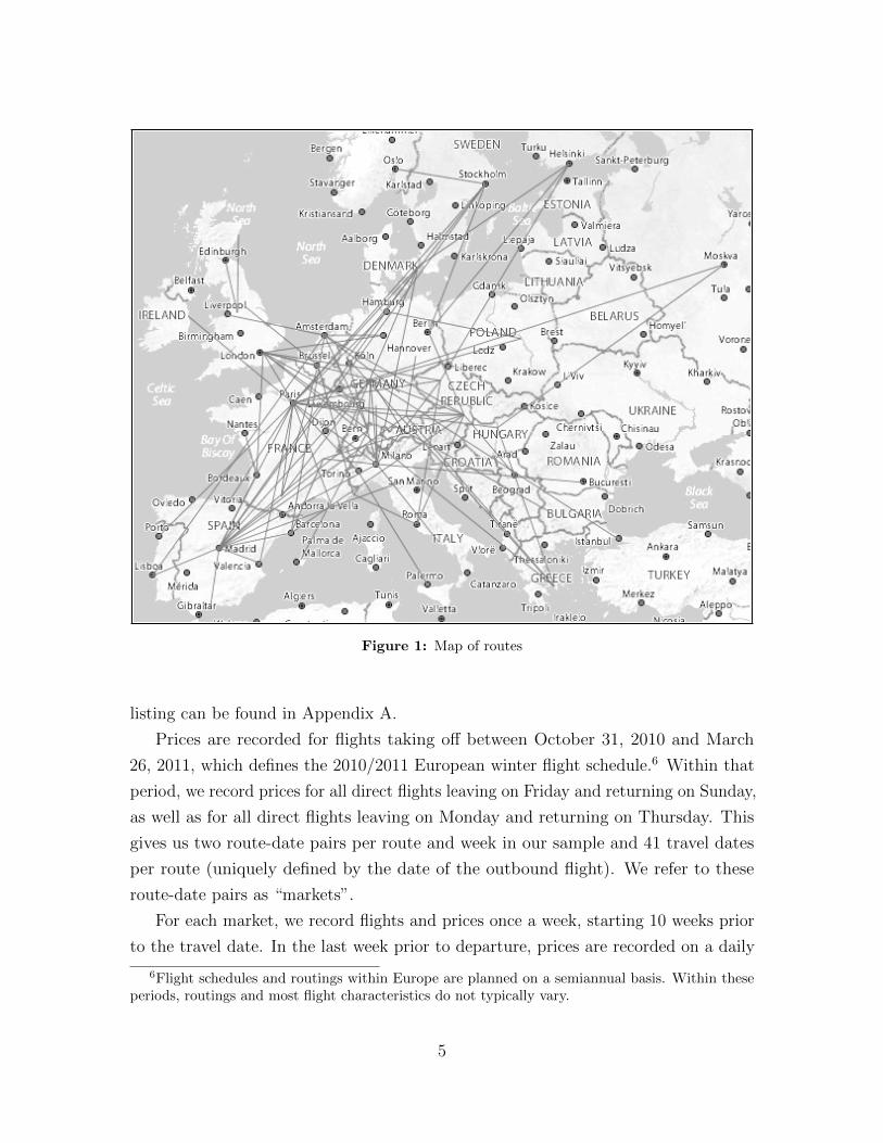
Figure 1: Map of routes
listing can be found in Appendix A.
Prices are recorded for flights taking off between October 31, 2010 and March
26, 2011, which defines the 2010/2011 European winter flight schedule.6 Within that
period, we record prices for all direct flights leaving on Friday and returning on Sunday,
as well as for all direct flights leaving on Monday and returning on Thursday. This
gives us two route-date pairs per route and week in our sample and 41 travel dates
per route (uniquely defined by the date of the outbound flight). We refer to these
route-date pairs as “markets”.
For each market, we record flights and prices once a week, starting 10 weeks prior
to the travel date. In the last week prior to departure, prices are recorded on a daily
6Flight schedules and routings within Europe are planned on a semiannual basis. Within theseperiods, routings and most flight characteristics do not typically vary.
5
basis to account for an increased frequency of price changes. Hence, we obtain up to
17 different prices for each physical flight.
In what follows, we will use the term “itinerary” to refer to a specific roundtrip
itinerary, characterized by the combination of outbound and return flight identification
numbers.7 For example, in our terminology one “itinerary” on the route Paris–London
would be using flight number BA 333 on the outbound flight and flight number BA 334
on the return flight. We reserve the term “flight” for the combination of an itinerary
and a specific travel date.
Overall we have data on 3762 out of 3772 distinct markets (41 travel dates times
92 routes).8 Each market averages 377 prices that are recorded over up to 17 different
dates prior to departure for an average of 41.9 flights (i.e., roundtrip combinations)
per market. In total, our data set consists of 1.42 million individual prices (92 routes
times 41 travel dates times 377 recorded prices per market). Routes are on average 560
miles long and connect metropolitan areas with an average of 3.9 million inhabitants.9
The share of domestic routes in our sample is roughly 13 percent (12 out of 92 routes).
Prices constitute offers by a leading website for airline ticket purchases, which
accounts for a major share of bookings on the European market. The recorded prices
in our sample range from 27 to 2581 Euros, with a weekly average of 364 Euros and a
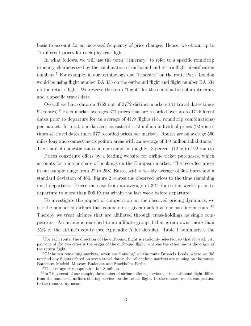
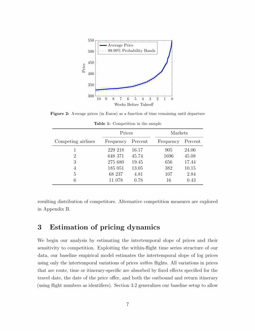
standard deviation of 466. Figure 2 relates the observed prices to the time remaining
until departure. Prices increase from an average of 327 Euros ten weeks prior to
departure to more than 500 Euros within the last week before departure.
To investigate the impact of competition on the observed pricing dynamics, we
use the number of airlines that compete in a given market as our baseline measure.10
Thereby we treat airlines that are affiliated through cross-holdings as single com-
petitors. An airline is matched to an affiliate group if that group owns more than
25% of the airline’s equity (see Appendix A for details). Table 1 summarizes the
7For each route, the direction of the outbound flight is randomly selected, so that for each citypair one of the two cities is the origin of the outbound flight, whereas the other one is the origin ofthe return flight.
8Of the ten remaining markets, seven are “missing” on the route Brussels–Leeds, where we didnot find any flights offered on seven travel dates; the other three markets are missing on the routesBordeaux–Madrid, Moscow–Budapest and Stockholm–Berlin.
9The average city population is 1.8 million.10In 7.9 percent of our sample, the number of airlines offering services on the outbound flight differs
from the number of airlines offering services on the return flight. In these cases, we set competitionto the rounded up mean.
6
012345678910300
350
400
450
500
550
Weeks Before Takeoff
Pri
ce
Average Price
99.99% Probability Bands
Figure 2: Average prices (in Euros) as a function of time remaining until departure
Table 1: Competition in the sample
Prices Markets
Competing airlines Frequency Percent Frequency Percent
1 229 218 16.17 905 24.062 648 371 45.74 1696 45.083 275 680 19.45 656 17.444 185 051 13.05 382 10.155 68 237 4.81 107 2.846 11 078 0.78 16 0.43
resulting distribution of competitors. Alternative competition measures are explored
in Appendix B.
3 Estimation of pricing dynamics
We begin our analysis by estimating the intertemporal slope of prices and their
sensitivity to competition. Exploiting the within-flight time series structure of our
data, our baseline empirical model estimates the intertemporal slope of log prices
using only the intertemporal variations of prices within flights. All variations in prices
that are route, time or itinerary-specific are absorbed by fixed effects specified for the
travel date, the date of the price offer, and both the outbound and return itinerary
(using flight numbers as identifiers). Section 3.2 generalizes our baseline setup to allow
7
for nonlinear pricing dynamics and Appendix B provides some robustness analysis for
alternative competition measures.
3.1 Baseline specification
Let Priceijtd denote the price for a round trip that involves the outbound itinerary i
and the return itinerary j (both identified by their flight numbers), for which the
outbound flight departs at date t, and which is offered for sale at date d. Further, let
Compijt denote a vector of dummy variables that covers all competition categories,
and let Dayslefttd denote the difference between t and d in days. As a baseline, we
estimate the following equation:
ln(Priceijtd) = (α + βDayslefttd)× Compijt + λi + µj + νt + ξd + εijtd, (1)
where we treat λi, µj, νt, and ξd as fixed effects.11 Here, α is a vector of competition-
specific constants and β is the relevant coefficient-vector on the interaction term
Compijt ×Dayslefttd. Note that λi and µj both nest a complete set of route specific
fixed effects since any flight number uniquely pins down the corresponding city-pair.
Together the specified set of fixed effects absorbs all itinerary-related effects such as
departure time or length of flight; all route characteristics such as connected cities or
alternative means of transportation; and all time-related effects such as travel dates,
and dates of price offer.
The impact of competition on the observed pricing dynamics is captured by our
estimates of β. Table 2 reports the estimated coefficients. Our estimates for the
corresponding standard errors are adjusted for clustering at the market level. All
reported coefficients are economically and statistically significant (at any reasonable
level).12
11Because our sampling is weekly for all but the last week before departure, a daily specification offixed effects for d would completely absorb all last week effects of Dayslefttd; ξd is therefore modeledon a weekly level.
12The (unreported) competition-specific constants are only weakly identified in our sample byvariations across travel dates but within routes since competition typically does not vary withinroutes for a given flight schedule. With this qualification in mind, we observe a hump-shaped relationbetween price levels and competition, peaking at three competitors. While the decreasing relationon the competitive side is in line with standard textbook theories, we can only conjecture aboutthe increasing part on the monopolistic side. A possible explanation would be that within-routevariations in competition are positively correlated with a high market demand.
8
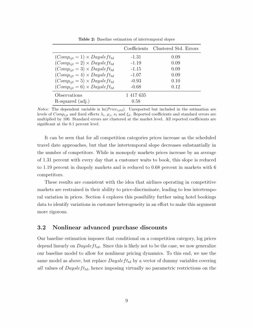
Table 2: Baseline estimation of intertemporal slopes
Coefficients Clustered Std. Errors
(Compijt = 1)×Dayslefttd -1.31 0.09(Compijt = 2)×Dayslefttd -1.19 0.09(Compijt = 3)×Dayslefttd -1.15 0.09(Compijt = 4)×Dayslefttd -1.07 0.09(Compijt = 5)×Dayslefttd -0.93 0.10(Compijt = 6)×Dayslefttd -0.68 0.12
Observations 1 417 635R-squared (adj.) 0.58
Notes: The dependent variable is ln(Priceijtd). Unreported but included in the estimation arelevels of Compijt and fixed effects λi, µj , νt and ξd. Reported coefficients and standard errors aremultiplied by 100. Standard errors are clustered at the market level. All reported coefficients aresignificant at the 0.1 percent level.
It can be seen that for all competition categories prices increase as the scheduled
travel date approaches, but that the intertemporal slope decreases substantially in
the number of competitors. While in monopoly markets prices increase by an average
of 1.31 percent with every day that a customer waits to book, this slope is reduced
to 1.19 percent in duopoly markets and is reduced to 0.68 percent in markets with 6
competitors.
These results are consistent with the idea that airlines operating in competitive
markets are restrained in their ability to price-discriminate, leading to less intertempo-
ral variation in prices. Section 4 explores this possibility further using hotel bookings
data to identify variations in customer heterogeneity in an effort to make this argument
more rigorous.
3.2 Nonlinear advanced purchase discounts
Our baseline estimation imposes that conditional on a competition category, log prices
depend linearly on Dayslefttd. Since this is likely not to be the case, we now generalize
our baseline model to allow for nonlinear pricing dynamics. To this end, we use the
same model as above, but replace Dayslefttd by a vector of dummy variables covering
all values of Dayslefttd, hence imposing virtually no parametric restrictions on the
9
012345678910−120
−100
−80
−60
−40
−20
0
Weeks Before Takeoff
Pri
ceC
han
ge
(%)
Compijt = 1Compijt = 2Compijt = 3Compijt = 4Compijt = 5Compijt = 6
012345678910−20
0
20
40
60
80
100
Weeks Before Takeoff
Pri
ceC
han
ge(%
)
Compijt = 1Compijt = 2Compijt = 3Compijt = 4Compijt = 5Compijt = 6
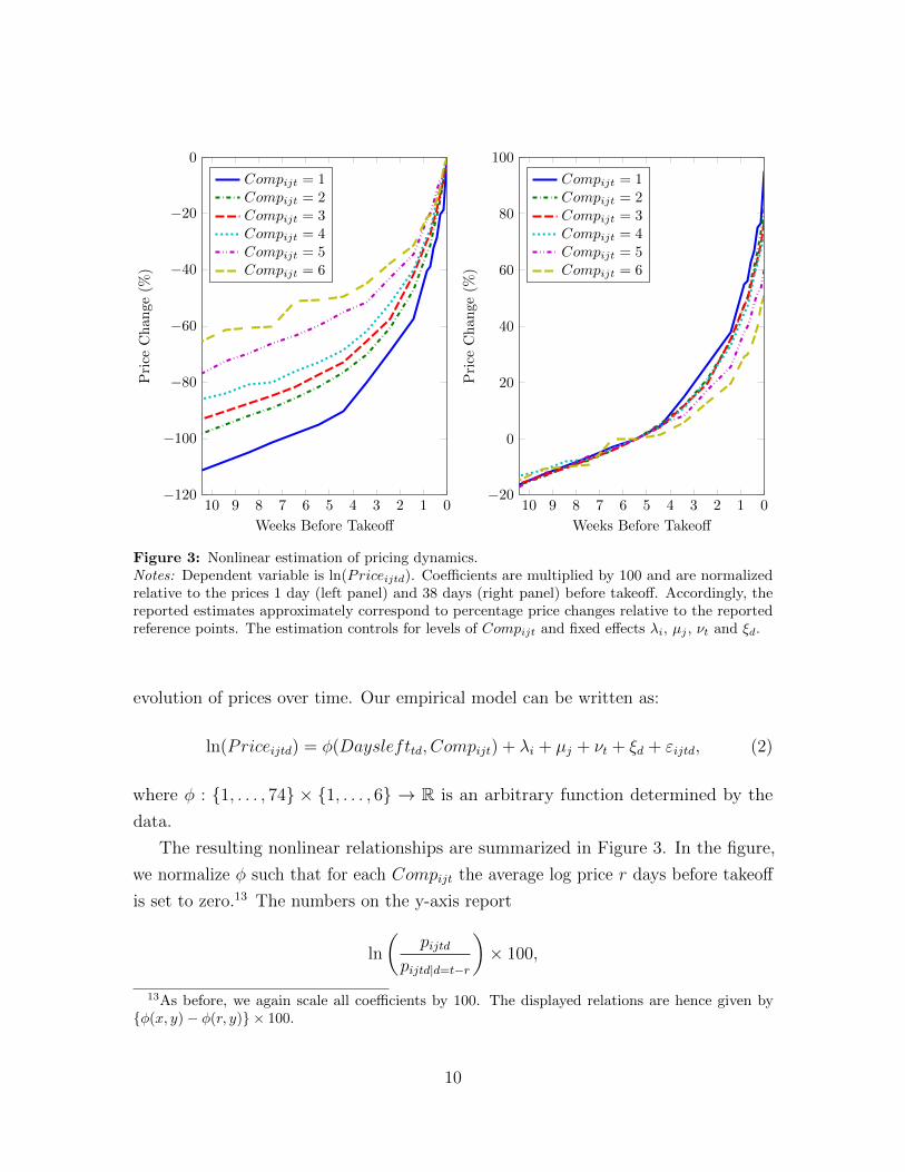
Figure 3: Nonlinear estimation of pricing dynamics.Notes: Dependent variable is ln(Priceijtd). Coefficients are multiplied by 100 and are normalizedrelative to the prices 1 day (left panel) and 38 days (right panel) before takeoff. Accordingly, thereported estimates approximately correspond to percentage price changes relative to the reportedreference points. The estimation controls for levels of Compijt and fixed effects λi, µj , νt and ξd.
evolution of prices over time. Our empirical model can be written as:
ln(Priceijtd) = φ(Dayslefttd, Compijt) + λi + µj + νt + ξd + εijtd, (2)
where φ : {1, . . . , 74} × {1, . . . , 6} → R is an arbitrary function determined by the
data.
The resulting nonlinear relationships are summarized in Figure 3. In the figure,
we normalize φ such that for each Compijt the average log price r days before takeoff
is set to zero.13 The numbers on the y-axis report
ln
(pijtd
pijtd|d=t−r
)× 100,
13As before, we again scale all coefficients by 100. The displayed relations are hence given by{φ(x, y)− φ(r, y)} × 100.
10

which approximately amounts to the difference in prices between date t and date r,
expressed in percent of the price charged r days before departure.
In the left panel, we set r = 1. The y-axis thus approximately reflects the estimated
advanced purchase discount relative to the price charged one day before departure. It
can be seen that, although nonlinear, the slopes are again monotonically decreasing in
the number of competitors. Accordingly, the relative discount for booking a flight in
advance is less pronounced on routes that are served by a larger number of competitors,
reinstating the conclusion drawn from our baseline estimation.
Taking a closer look at the identified pricing dynamics, it can further be seen that
prices are increasing at similar slopes until about five weeks before takeoff. Only in
the last five weeks, prices in less competitive routes have a significantly steeper slope
than prices in more competitive routes. To illustrate this further, we set r = 38 in the
right panel. Until about five weeks before takeoff log prices increase virtually along
a single line across all competitive environments, showing an increase of about 0.45
percent for each day a customer waits to book. This translates into an overall discount
of approximately 16% for purchasing tickets ten weeks before departure compared to
five weeks before departure.
Starting about five weeks before departure, prices increase significantly faster, with
prices on the least competitive environments increasing the fastest. On monopoly
routes, customers pay a premium of 95.09 percent for purchasing their ticket a day
before takeoff rather than five weeks in advance (the intercept with the y-axis on the
right). This premium is reduced to 81.70 percent in duopoly markets, and is further
reduced to 77.16 percent in markets with three competitors, 72.81 percent in markets
with four competitors, 59.84 percent in markets with 5 competitors, and 50.83 percent
in markets with 6 competitors.
In sum, the nonlinear estimation reinforces the clear pattern of dynamic oligopoly
pricing revealed by our baseline specification: While airlines offer substantial advanced
purchase discounts across all market structures, the magnitude of these discounts
is highly sensitive to competition, suggesting that airlines operating in competitive
markets are restrained in their ability to price-discriminate. The next section explores
this possibility in more detail.
11
4 Intertemporal price discrimination
We now turn to the question whether price discrimination can explain the pricing
dynamics identified in this paper. Above we have already argued that the observed
“flattening” of the intertemporal slope for more competitive routes is in line with
airlines being more restrained in their ability to price-discriminate. In this section, we
construct a number of measures for the heterogeneity in the customer base in a given
market in an effort to make this argument more rigorous.
The idea is that the degree to which an airline’s ability to price-discriminate
becomes restrained in more competitive markets should depend on how much it would
discriminate among customers if it were unconstrained (i.e., in a monopoly). In the
extreme case where customers are completely homogeneous, we would not expect any
price discrimination even in monopoly markets. Accordingly, if price discrimination is
the driver behind the observed pricing dynamics, then competition should have less of
an impact on the intertemporal slope in more homogenous markets.
4.1 Customer heterogeneity measures
In the airline industry the co-existence between tourists (and other leisure travelers)
and business customers is arguably the largest source of heterogeneity in the customer
base. Our approach to evaluating customer heterogeneity is therefore aimed at
measuring the tourist intensity in a given market. In particular, we use Eurostat
data on hotel bookings to construct two heterogeneity measures that are likely to
be positively correlated with tourist intensity. Some alternatives are discussed in
Appendix B.
Our first measures (Durationij) computes the average number of nights per visit
booked in hotels and similar residencies at the destination.14 Here the idea is that
the average duration of a given booking is larger for tourists, so that small values
of Durationij are likely to reflect a high fraction of business travelers, whereas high
values should reflect a larger share of tourists. Our second measure (NightsPCij)
is defined by the number of nights booked in hotels and similar residencies relative
14The measure is computed using Eurostat data at the NUTS-2 level. For large cities the NUTS-2level typically coincides with the city level (e.g., Berlin, Lisbon or Prague), while smaller cities orless densely populated areas are typically clustered into urban areas or regions (e.g., Manchester intoGreater Manchester or Aberdeen into North Eastern Scotland).
12
1 2 3 4 5 6
0
10
20
30
Competition
Du
rati
on
1 2 3 4 5 6
0
20
40
60
Competition
Nig
hts
PC
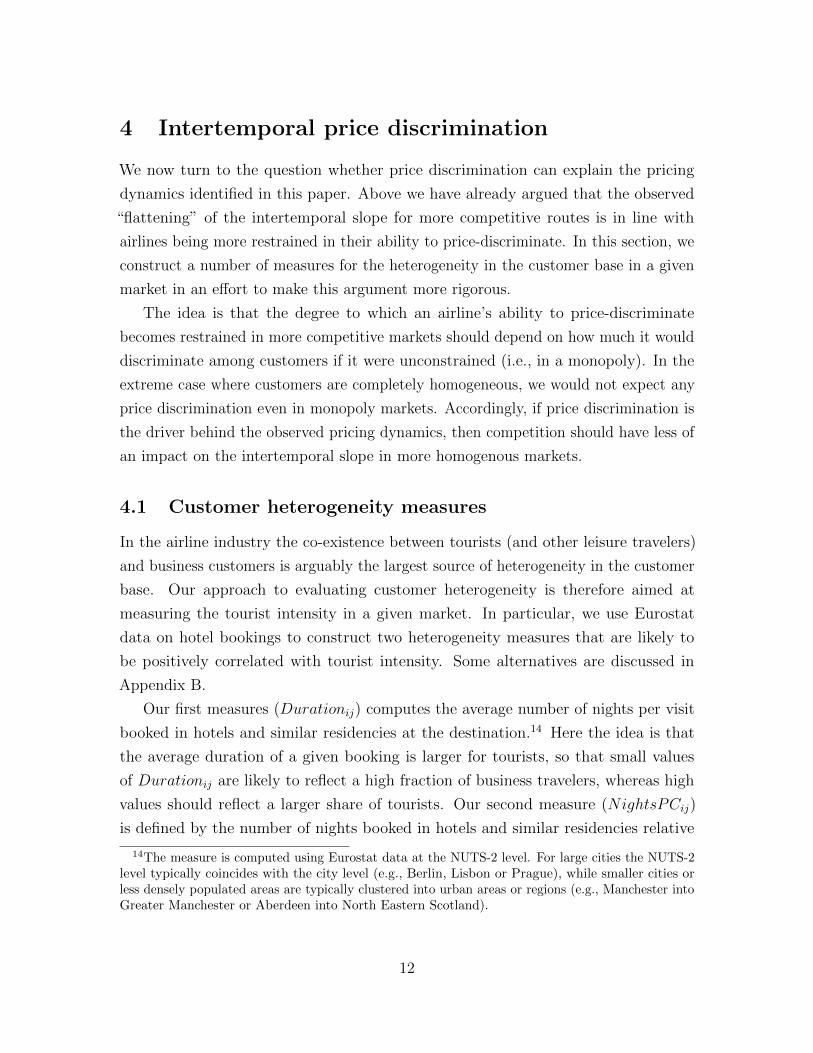
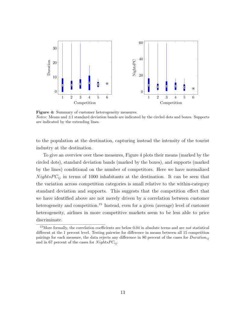
Figure 4: Summary of customer heterogeneity measures.Notes: Means and ±1 standard deviation bands are indicated by the circled dots and boxes. Supportsare indicated by the extending lines.
to the population at the destination, capturing instead the intensity of the tourist
industry at the destination.
To give an overview over these measures, Figure 4 plots their means (marked by the
circled dots), standard deviation bands (marked by the boxes), and supports (marked
by the lines) conditional on the number of competitors. Here we have normalized
NightsPCij in terms of 1000 inhabitants at the destination. It can be seen that
the variation across competition categories is small relative to the within-category
standard deviation and supports. This suggests that the competition effect that
we have identified above are not merely driven by a correlation between customer
heterogeneity and competition.15 Instead, even for a given (average) level of customer
heterogeneity, airlines in more competitive markets seem to be less able to price
discriminate.
15More formally, the correlation coefficients are below 0.04 in absolute terms and are not statisticaldifferent at the 1 percent level. Testing pairwise for difference in means between all 15 competitionpairings for each measure, the data rejects any difference in 80 percent of the cases for Durationijand in 67 percent of the cases for NightsPCij .
13
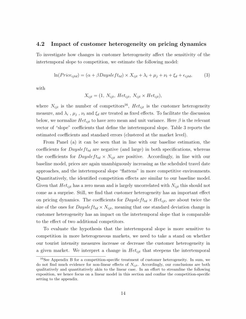
4.2 Impact of customer heterogeneity on pricing dynamics
To investigate how changes in customer heterogeneity affect the sensitivity of the
intertemporal slope to competition, we estimate the following model:
ln(Priceijtd) = (α + βDayslefttd)×Xijt + λi + µj + νt + ξd + εijtd, (3)
with
Xijt = (1, Nijt, Hetijt, Nijt ×Hetijt),
where Nijt is the number of competitors16, Hetijt is the customer heterogeneity
measure, and λi , µj , νt and ξd are treated as fixed effects. To facilitate the discussion
below, we normalize Hetijt to have zero mean and unit variance. Here β is the relevant
vector of “slope” coefficients that define the intertemporal slope. Table 3 reports the
estimated coefficients and standard errors (clustered at the market level).
From Panel (a) it can be seen that in line with our baseline estimation, the
coefficients for Dayslefttd are negative (and large) in both specifications, whereas
the coefficients for Dayslefttd × Nijt are positive. Accordingly, in line with our
baseline model, prices are again unambiguously increasing as the scheduled travel date
approaches, and the intertemporal slope “flattens” in more competitive environments.
Quantitatively, the identified competition effects are similar to our baseline model.
Given that Hetijt has a zero mean and is largely uncorrelated with Nijt this should not
come as a surprise. Still, we find that customer heterogeneity has an important effect
on pricing dynamics. The coefficients for Dayslefttd × Hetijt, are about twice the
size of the ones for Dayslefttd ×Nijt, meaning that one standard deviation change in
customer heterogeneity has an impact on the intertemporal slope that is comparable
to the effect of two additional competitors.
To evaluate the hypothesis that the intertemporal slope is more sensitive to
competition in more heterogeneous markets, we need to take a stand on whether
our tourist intensity measures increase or decrease the customer heterogeneity in
a given market. We interpret a change in Hetijt that steepens the intertemporal
16See Appendix B for a competition-specific treatment of customer heterogeneity. In sum, wedo not find much evidence for non-linear effects of Nijt. Accordingly, our conclusions are bothqualitatively and quantitatively akin to the linear case. In an effort to streamline the followingexposition, we hence focus on a linear model in this section and confine the competition-specificsetting to the appendix.
14
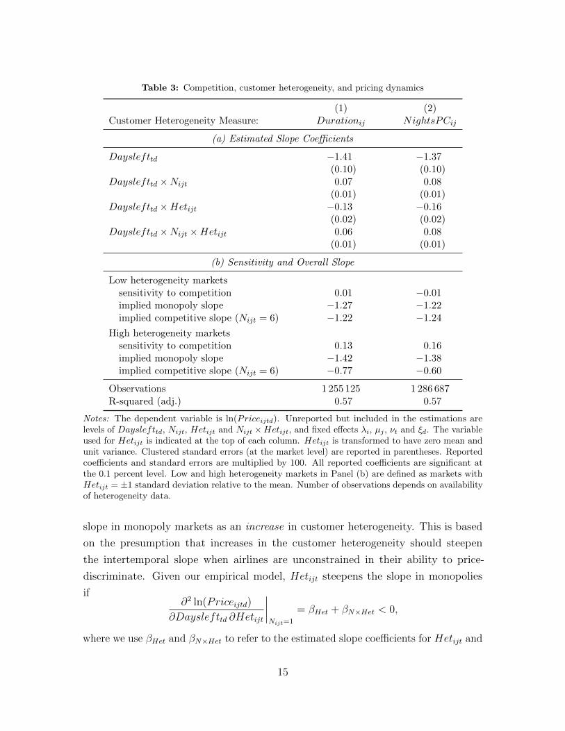
Table 3: Competition, customer heterogeneity, and pricing dynamics
(1) (2)Customer Heterogeneity Measure: Durationij NightsPCij
(a) Estimated Slope Coefficients
Dayslefttd −1.41 −1.37(0.10) (0.10)
Dayslefttd ×Nijt 0.07 0.08(0.01) (0.01)
Dayslefttd ×Hetijt −0.13 −0.16(0.02) (0.02)
Dayslefttd ×Nijt ×Hetijt 0.06 0.08(0.01) (0.01)
(b) Sensitivity and Overall Slope
Low heterogeneity marketssensitivity to competition 0.01 −0.01implied monopoly slope −1.27 −1.22implied competitive slope (Nijt = 6) −1.22 −1.24
High heterogeneity marketssensitivity to competition 0.13 0.16implied monopoly slope −1.42 −1.38implied competitive slope (Nijt = 6) −0.77 −0.60
Observations 1 255 125 1 286 687R-squared (adj.) 0.57 0.57
Notes: The dependent variable is ln(Priceijtd). Unreported but included in the estimations arelevels of Dayslefttd, Nijt, Hetijt and Nijt ×Hetijt, and fixed effects λi, µj , νt and ξd. The variableused for Hetijt is indicated at the top of each column. Hetijt is transformed to have zero mean andunit variance. Clustered standard errors (at the market level) are reported in parentheses. Reportedcoefficients and standard errors are multiplied by 100. All reported coefficients are significant atthe 0.1 percent level. Low and high heterogeneity markets in Panel (b) are defined as markets withHetijt = ±1 standard deviation relative to the mean. Number of observations depends on availabilityof heterogeneity data.
slope in monopoly markets as an increase in customer heterogeneity. This is based
on the presumption that increases in the customer heterogeneity should steepen
the intertemporal slope when airlines are unconstrained in their ability to price-
discriminate. Given our empirical model, Hetijt steepens the slope in monopolies
if∂2 ln(Priceijtd)
∂Dayslefttd ∂Hetijt
∣∣∣∣Nijt=1
= βHet + βN×Het < 0,
where we use βHet and βN×Het to refer to the estimated slope coefficients for Hetijt and
15

Nijt×Hetijt in model (3). From the estimated coefficients, we can see that this is the
case for both our measures, suggesting that Hetijt increases customer heterogeneity.
A potential concern regarding this interpretation of Hetijt is that changes in
the tourist intensity may have a non-monotonic impact on customer heterogeneity.
For instance, on routes where there is a small number of tourists, any additional
tourists may increase the heterogeneity of the customer base, while on markets with a
large share of tourists, the same change may reduce the heterogeneity. We explore
this concern in Appendix B using a quadratic specification in Hetijt, but do not
find any evidence for non-monotonicity. Both measures unambiguously steepen the
intertemporal monopoly slope over their complete support. With this in mind, we
henceforth interpret increases in Hetijt as increases in the customer heterogeneity.
Based on our interpretation of Hetijt, does the sensitivity to competition increase
in customer heterogeneity as it should when price discrimination is the major source
behind the observed pricing dynamics? Looking at the estimated slope coefficients of
Nijt ×Hetijt, it turns out that this is indeed the case: The estimated slope coefficient
of Nijt ×Hetijt is statistically significant and positive in both specifications.
To assess the economic significance of this heterogeneity-caused variation in the
sensitivity, we use the estimated model to compute the sensitivity for values of Hetijt
at one standard deviation above and below its mean (meant to indicate markets with
high and low customer heterogeneities, respectively). Exploiting the fact that we have
normalized Hetijt to have zero mean and unit variance, these sensitivities are given by
∂2 ln(Price)
∂Dayslefttd ∂Nijt
∣∣∣∣Hetijt=±1
= βN ± βN×Het.
Panel (b) of Table 3 reports the computed sensitivities and the implied overall
slope. Driving down the heterogeneity to one standard deviation below its mean
virtually shuts down the sensitivity of the intertemporal slope to competition. This is
consistent with the idea that in the absence of customer heterogeneity airlines do not
discriminate much to begin with and, hence, they are also not getting restrained in
their ability to price-discriminate when competition intensifies. Conversely, in high
heterogeneity markets the slope of prices is highly sensitive to changes in competition.
Here, an increase in competition “flattens” the intertemporal slope by between 0.13
and 0.16 percentage points per day.
Put into relation to the overall intertemporal slope, these findings suggest a
16
substantial impact of competition on pricing dynamics in the presence of customer
heterogeneity. Specifically, while in low heterogeneity markets the difference in the
intertemporal slope between monopolies and competitive markets with Nijt = 6
amounts to only 0.05 percentage points per day, the gap rises to 0.65 percentage points
per day in high heterogeneity markets. We interpret the 0.60 percentage points per
day difference in these gaps due to variations in customer heterogeneity as being likely
to be caused by price discrimination. Compared to the overall slope in markets with
Nijt = 6, this amounts to nearly a doubling of the intertemporal slope, suggesting that
intertemporal price discrimination is an important driver of the dynamic oligopoly
pricing patterns that we have identified in this paper.
5 Decomposing price dispersion
To reconcile our study of pricing dynamics with the empirical price dispersion literature,
we now construct a measure of intertemporal price dispersion and contrast it with
more broadly defined dispersion measures used by the previous literature.
Due to limitations in the available data, the empirical price dispersion literature has
so far focused on dispersion measures for airfares that do not disentangle intertemporal
dispersion within flights from the dispersion in prices across different flights (pooling
both, different itineraries and different travel dates). Different studies have thereby
reached different conclusions regarding the relation between competition and these
dispersion measures, ranging from positive (Borenstein and Rose, 1994), over no clear
relation (Hayes and Ross, 1998), to negative (Gerardi and Shapiro, 2009).
We use the two time series dimensions of our panel to distinguish the impact
of competition on intertemporal price dispersion for a given flight from its impact
on various types of cross-flight dispersion. Following the literature, we use the Gini
coefficient to measure the dispersion within a given set of prices. Intuitively, the Gini
coefficient corresponds to half the expected price difference in terms of the average
price. A Gini coefficient of 0.10 would accordingly represent an expected absolute
difference between two randomly selected prices of 20 percent of the average price.17
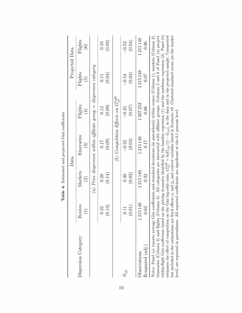
Panel (a) of Table 4 summarizes the average Gini coefficients in our data set.
17To make the Gini coefficients comparable to the previous literature, we compute all Ginicoefficients after up-sampling observations with more than seven days left to departure in order tocompensate for the increased sampling frequency in the last week.
17

Column 1 reports the average price dispersion across all flights (and dates of ticket
offers) offered by a given competitor on a given route. As in the previous literature,
this pools together different itineraries (within the same route) and different flights
across different travel dates. We find an average dispersion within routes of 64 percent
of the average offer.18 Column 4 shows in contrast the intertemporal dispersion within
a given flight (defined by a particular itinerary at a particular travel date). We see
that the intertemporal dispersion is substantially smaller (24 percent of the average
price offer).
The two intermediate cases where we pool flights only across itineraries (within
markets) or only across travel dates (within itineraries) are reported in Columns 2
and 3. As expected, pooling along either dimension increases the dispersion relative
to Column 4. The increase in dispersion due to specific flight characteristics (e.g.,
departure time) thereby appears to be higher than the dispersion due to travel date
characteristics (e.g., flights departing on Monday versus flights departing on Friday).
In the following we explore the relation between competition and the different
dispersion measures. We do no longer include itinerary specific fixed effects, since
these would absorb any dispersion on the itinerary and route level. Instead we include
a large number of control variables Xijt that were previously nested into λi and µj.19
Moreover, since the Gini coefficient is bounded between zero and one, we follow the
previous literature and transform it into an unbounded statistic, using instead the
Gini log-odds ratio Gloddijt = ln[Gijt/(1−Gijt)].
We estimate the following empirical model:
Gloddijt = α + β ×Nijt + γ ×Xijt + νt + ξd + εijt, (4)
where Nijt is the number of competitors20, Xijt contains our set of control variables,
and νt and ξd are vectors of fixed effects for the travel date and the date of the price
18Since the within-route dispersion is strongly right-skewed in our sample, the median dispersionis somewhat smaller, evaluating to 56 percent of the average offer.
19Specifically, Xijt includes a full set of dummies for the departure city, destination city, and thetime of the day of the outgoing and returning itineraries (at an hourly level); as well as measures forthe market size, share, and symmetry; GDP and weather data of the connected cities; the weekdayand length of the itineraries; holidays; and the tourist intensity in a given market (see Section 4 for adetailed presentation of these measures).
20Using the number of competitors Nijt instead of a vector of dummy variables allows us tocompare the impact of competition on the different dispersion measures in a straightforward way.
18
Tab
le4:
Est
imate
dan
dp
roje
cted
Gin
ico
effici
ents
Dat
aP
roje
cted
Dat
a
Dis
per
sion
Cat
egor
y:
Rou
tes
Mar
kets
Itin
erar
ies
Fligh
tsF
ligh
tsF
ligh
ts(1
)(2
)(3
)(4
)(5
)(6
)
(a)
Pri
cedi
sper
sion
wit
hin
affili
ate
grou
p×
disp
ersi
onca
tego
ry
0.32
0.28
0.17
0.12
0.11
0.10
(0.1
3)(0.1
4)(0.0
9)(0.0
9)(0.0
4)(0.0
3)
(b)
Com
peti
tion
Eff
ects
onG
lodd
ijt
Nijt
0.11
0.30
−0.
22−
0.45
−0.
54−
0.52
(0.0
1)(0.0
3)(0.0
3)(0.0
7)(0.0
4)(0.0
4)
Obse
rvat
ions
121
514
81
215
148
121
514
81
207
253
121
514
81
215
148
R-s
quar
ed(a
dj.
)0.
620.
320.
170.
060.
070.
06
Note
s:P
an
el(a
)re
port
sav
erage
Gin
ico
effici
ents
an
dst
an
dard
dev
iati
on
s(i
np
are
nth
esis
)w
ith
inro
ute
s(C
olu
mn
1),
mark
ets
(Colu
mn
2),
itin
erari
es(C
olu
mn
3)
and
flig
hts
(Colu
mn
4).
All
cate
gori
esare
inte
ract
edw
ith
affi
liate
gro
ups.
Colu
mns
5and
6of
Panel
(a)
pro
ject
wit
hin
-flig
ht
Gin
ico
effici
ents
bas
edon
the
pri
cing
dynam
ics
iden
tified
by
the
bas
elin
ere
gres
sion
(1)
and
the
non
linea
rre
gres
sion
(2).
Pan
el(b
)es
tim
ates
the
effec
tof
com
pet
itio
non
the
Gin
ilo
g-odds
rati
o,G
lodd
ijt
=ln
[Gijt/(1−G
ijt],
inth
edat
aan
din
the
pro
ject
edsa
mple
.U
nre
por
ted
but
incl
uded
inth
ees
tim
atio
ns
are
fixed
effec
tsν t
andξ d
and
contr
olva
riab
les
list
edin
Foot
not
e19
.C
lust
ered
stan
dar
der
rors
(at
the
mar
ket
leve
l)ar
ere
por
ted
inp
aren
thes
es.
All
rep
orte
dco
effici
ents
are
sign
ifica
nt
at
the
0.1
per
cent
leve
l.
19
offer. The estimated coefficients are reported in Panel (b) of Table 4. All reported
coefficients are significant at the 0.1 percent level (using standard errors that are
clustered at the market level).
In line with the pricing dynamics identified above, competition has a negative
impact on the intertemporal price dispersion (Column 4).21 Adding one additional
competitor on a given market decreases the log odds ratio by 0.46 which corresponds
to 0.10 standard deviations of Gloddijt . Moving from a monopoly to an environment
with six competitors hence decreases the dispersion by 1/2 standard deviation.
Comparing this to the estimated coefficients in Columns 1 to 3, we see that the
negative impact of competition on price dispersion is diluted (Column 3) or even
overturned (Columns 1 and 2) when using one of the broader dispersion measures.
Intertemporal price dispersion therefore seems to be more sensitive to competition
than the dispersion among other dimensions, possibly because the dispersion among
other dimensions is more likely to reflect differences in product characteristics rather
than reflecting price discrimination.
In sum, while we find an unambiguously negative impact of competition on
intertemporal price dispersion, once we include cross-flight dispersion the impact
depends on the precise definition of the dispersion measure. This suggest that the
seemingly contradicting findings in the earlier literature may be driven by a confounding
of different dimensions of dispersion. In particular, the fact that we find a negative
competition effect of −0.45 on the within-flight dispersion, but obtain a positive effect
of 0.30 on the within-market dispersion indicates that the price dispersion across
itineraries is increasing in competition.22 Whether or not the impact of competition
on within-market dispersion (or even broader: on within-route dispersion) is positive
or negative is therefore likely to depend on various factors, such as the number of price
observations for a given flight relative to the number of different flights contained in
the sample. This can explain why the literature so far (which pools prices within and
across flights) has obtained ambiguous results regarding the impact of competition on
price dispersion.
21See also, Gaggero and Piga (2011).22While this positive relation may at first seem puzzling, Borenstein (1985) and Holmes (1989)
have shown that the theoretical relation between dispersion across flights and competition is indeedambiguous and may be positive when consumers’ cross-price elasticities between different airlines islower than the elasticity of industry demand. See also, Armstrong and Vickers (2001).
20

6 Stochastic pricing dynamics
This section analyzes the relevance of the systematic pricing dynamics identified in
Sections 3 and 4 relative to residual pricing dynamics. While we do not attempt
to explain the residual components, an obvious source consistent with the residual
variations documented below are random demand fluctuations that cause airlines to
dynamically adjust their prices.23
6.1 Systematic vs. unsystematic pricing dynamics
We start by asking how much of the intertemporal dispersion documented in the last
section is due to the systematic advanced purchase discounts documented in Section 3
(instead of random price fluctuations).
To answer this question, we use our estimates of the baseline model (1) and of
the nonlinear model (2) to project samples of counterfactual price data in which the
intertemporal variation in prices is fully determined by the identified intertemporal
slopes. For these samples, we then compute the intertemporal dispersion on the flight
level, defining the systematic dispersion implied by the estimated pricing dynamics.
Columns 5 and 6 of Panel (a) in Table 4 report these intertemporal price dispersion
measures in the two samples.
It can be seen that for the average flight the within-flight price dispersion pro-
jected from our baseline estimation (Column 5) closely resembles the one in the data
(22 percent of the average price), whereas the dispersion implied by our nonlinear
estimation (Column 6) is somewhat smaller (20 percent of the average price).24 Based
on the nonlinear estimation, 83 percent of the within-flight dispersion of the average
flight (0.10 out of 0.12) can be attributed to the identified pricing dynamics seen in
Figure 3. Systematic advanced purchase discounts therefore seem to be the major
23See, for instance, Alderighi, Nicolini and Piga (2012), Williams (2013), and Puller, Sengupta andWiggins (2012). On the theory side, on particular channel why random demand fluctuations maycause variations in pricing dynamics in ex ante identical markets is modeled by the peak-load pricingliterature (Gale and Holmes, 1992, 1993; Dana, 1998, 1999a,b, 2001).
24The difference between the two estimations is likely due to the increased sampling frequencyin the last week before departure. Because prices are generally increasing at a steeper slope duringthat period, the sample-average slope exceeds the time-average in our sample. Projecting thesample-average slope throughout the ten week horizon does therefore overestimate the contributionof systematic advanced purchase discounts relative to unsystematic volatility. This bias vanishes,once we allow slopes to vary with the time left until departure, as we do in the projection based onour nonlinear estimation.
21
source of within-flight price dispersion, as opposed to unsystematic volatility around
the price trend.25
We also use the projected price data to relate the (projected) Gini coefficient to the
number of competitors. Using exactly the same specification as in the previous section,
we find that the impact of competition on the dispersion that is due to systematic
advanced purchase discounts is slightly higher (in absolute terms) than the impact
on its empirical counterpart (Columns 5 and 6 in Panel (b) of Table 4 compared to
Column 4). This suggests that the impact of competition on price dispersion is mainly
driven by its impact on the intertemporal slope.26
6.2 Systematic vs. unsystematic variations
in pricing dynamics
Given that systematically increasing prices appear to account for a large share of the
price dispersion on the average flight, we now address the related issue of how much
of the variation in pricing dynamics across markets can be systematically explained.
In particular, we are interested in the combined explanatory power of competition
and customer heterogeneity. (See Figure 8 in Appendix C for a schematic illustration
how this differs from the exercise in the previous subsection.)
We proceed in two stages. In stage 1, we split our data into 3762 market-specific
sub-samples, defined by the combination of a route r and a travel date t. In each of
these market samples, we run the following first stage regression:
ln(Priceijtd) = αrt + SrtDayslefttd + εijtd,
where αrt and Srt are the estimated market-specific coefficients. Collecting Srt from
all regressions, this gives us a sample of market-specific intertemporal slopes.
25Because the intertemporal slope maps nonlinearly to the projected Gini, our estimate is notidentical to the one obtained from estimating the intertemporal slope for each flight and then usingthe flight-specific estimations to project the Gini. While such an exercise would be meaningless forthe nonlinear estimation (for each flight, the identified nonlinear price path would be identical tothe observed price path, so that the resulting Gini would perfectly predict the empirical one), it isfeasible for the linear estimation. Doing so, we find a slightly higher average Gini of 0.12, suggestingthat our results (slighly) underpredict the systematic contribution of pricing dynamics compared torandom price fluctuations.
26In fact, consistent with the idea that the impact of competition on the empirical dispersionis primarily due to its impact on the systematic trend of prices to increase, the ratio of slopes0.450.52 ≈ 0.865 is very similar to the identified systematic dispersion share of 83 percent.
22
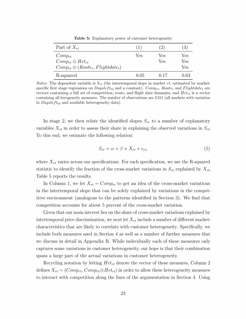
Table 5: Explanatory power of customer heterogeneity
Part of Xrt (1) (2) (3)
Comprt Yes Yes YesComprt ⊗Hetrt Yes YesComprt ⊗ (Router, F lightdatet) Yes
R-squared 0.05 0.17 0.63
Notes: The dependent variable is Srt (the intertemporal slope in market rt, estimated by market-specific first stage regressions on Dayslefttd and a constant). Comprt, Router and Flightdatet arevectors containing a full set of competition, route, and flight date dummies, and Hetrt is a vectorcontaining all herogeneity measures. The number of observations are 3 311 (all markets with variationin Dayslefttd and available heterogeneity data).
In stage 2, we then relate the identified slopes Srt to a number of explanatory
variables Xrt in order to assess their share in explaining the observed variations in Srt.
To this end, we estimate the following relation:
Srt = α + β ×Xrt + εrt, (5)
where Xrt varies across our specifications. For each specification, we use the R-squared
statistic to identify the fraction of the cross-market variations in Srt explained by Xrt.
Table 5 reports the results.
In Column 1, we let Xrt = Comprt to get an idea of the cross-market variations
in the intertemporal slope that can be solely explained by variations in the compet-
itive environment (analogous to the patterns identified in Section 3). We find that
competition accounts for about 5 percent of the cross-market variation.
Given that our main interest lies on the share of cross-market variations explained by
intertemporal price discrimination, we next let Xrt include a number of different market-
characteristics that are likely to correlate with customer heterogeneity. Specifically, we
include both measures used in Section 4 as well as a number of further measures that
we discuss in detail in Appendix B. While individually each of these measures only
captures some variations in customer heterogeneity, our hope is that their combination
spans a large part of the actual variations in customer heterogeneity.
Recycling notation by letting Hetrt denote the vector of these measures, Column 2
defines Xrt = (Comprt, Comprt⊗Hetrt) in order to allow these heterogeneity measures
to interact with competition along the lines of the argumentation in Section 4. Using
23
this Xrt, the share of variations in Srt that is explained by Xrt is 17 percent. Under the
conjecture that Hetrt spans most of the empirical variations in customer heterogeneity,
this suggests that in addition to customer heterogeneity there exist a number of
unrelated factors that explain a large part of the variations in the intertemporal slopes
across markets.
To get some idea at which level these factors are likely to operate, we lastly let Xrt
include a set of route and travel date fixed effects (again interacted with Comprt). The
explanatory power of this fixed effects specification is 63 percent, providing an upper
bound on the explanatory power of any route or travel data specific characteristics.
The remaining 37 percent are only explainable using factors that vary across travel
dates and routes. While it is beyond the scope of this paper to identify the source
of these residual variations in the intertemporal slope, we find it hard to reconcile
them fully with any deterministic pricing scheme. We therefore conjecture that they
represent, at least in parts, the adjustments of prices (and, hence, measured slopes) in
response to demand shocks that materialize within the last ten weeks before departure.
7 Summary
This study documents two systematic variations of airline pricing dynamics. First, the
rate at which airline ticket prices increase as the scheduled departure date approaches is
highly sensitive to the number of airlines active in a given market. While in monopoly
markets prices increase by an average of 1.31 percent per day, this slope is reduced
to 1.19 percent in duopoly markets, and is further decreasing in competition to 0.68
percent in markets with six competitors (the most competitive ones in our sample).
Second, this sensitivity of the intertemporal slope to competition varies substantially
with the heterogeneity among customers. With an highly heterogeneous customer
base, prices on monopoly routes increase by 0.65 percentage points per day more than
prices on markets with six competitors. Conversely, on markets with very homogenous
customers, this difference is almost zero.
We interpret these findings as evidence for intertemporal price discrimination
being a major source of the observed pricing dynamics: Competition is likely to
restrain an airline’s ability to price-discriminate, but this constraint is more relevant
in markets with an highly heterogeneous customer base where there is scope for
price-discrimination in the first place.
24
Our results suggests that these forces are quantitatively important. Systematic
advanced purchase discounts explain about 83 percent of the total within-flight
dispersion on the average flight. Moreover, competition and customer heterogeneity
explain 17 percent of the observed variation in the intertemporal slope across markets.
These numbers suggest that while systematically increasing prices are the main
source behind intertemporal price dispersion, there are likely a number of factors
alongside price discrimination that are responsible for the observed variations in the
intertemporal slope. In particular, we find that 37 percent of the cross-market variation
can only be accounted by factors that vary across travel dates and routes. While it
is beyond the scope of this paper to identify the source of these residual variations,
we conjecture that price adjustments in response to random demand fluctuations are
likely to play an important role in explaining these variations.
25
A Data construction (for online publication)
A.1 Routes
Our cross-section of routes is sampled from the existing connections between a set of
60 European cities with international airports. All routes are defined on the city-level.
In case there exist multiple airports within one city, we include routes to all airport
combinations (e.g., routes between London and Paris cover all offered combinations
between {LCY, LGW, LHR, LTN} and {CDG, ORY}).The 60 cities were chosen to ensure regional variety as well as variety in the size and
importance of the residing airports. To this end, the set includes the cities with the
four largest airports in each of the EU5 countries (measured by 2009 total passenger
traffic):
• France: Paris, Nice, Lyon, Marseille
• Germany: Frankfurt, Munich, Duesseldorf, Berlin
• Italy: Rom, Milan, Venice, Catania
• Spain: Madrid, Barcelona, Palma de Mallorca, Malaga
• UK: London, Manchester, Edinburgh, Birmingham
The remaining 40 cities are selected from both the EU5 and the rest of Europe
(including Russia and Turkey): Aberdeen, Amsterdam, Athens, Belgrade, Bilbao,
Bologna, Bordeaux, Brussels, Bucharest, Budapest, Copenhagen, Dublin, Geneva,
Hamburg, Hannover, Helsinki, Innsbruck, Istanbul, Leeds, Leipzig, Lisbon, Liverpool,
Moscow, Nantes, Naples, Nuernberg, Oporto, Oslo, Palermo, Prague, Sofia, Stockholm,
Strasbourg, Stuttgart, Toulouse, Turin, Valencia, Vienna, Warsaw, and Zurich.
From the simplex of routes spanned by those 60 cities, we then sampled 100 random
routes, disregarding all routes for which not at least one direct daily connection was
offered at the beginning of our sampling period (October 31, 2010). To this routes,
we added, if not yet contained, the ten routes connecting the cities with the largest
airports in each of the EU5 countries (Paris, Frankfurt, Milan, Madrid, and London).
A limitation of our data source is that it does not contain prices set by Ryanair,
a major competitor in the intra-European market. To prevent our data from being
affected by an unobserved competitor, we therefore excluded all routes that were
26

served by Ryanair within a 40 miles (65 km) radius of the corresponding city centers.
From the above city list, this applies to all (existing) Ryanair route combinations
between the following cities: Barcelona, Birmingham, Berlin, Bologna, Bordeaux,
Brussels, Budapest, Catania, Dublin, Edinburgh, Leeds, Leipzig, Lisbon, Liverpool,
London, Madrid, Malaga, Manchester, Marseille, Milan, Nantes, Nice, Nuernberg,
Oporto, Palma de Mallorca, Palermo, Rome, Strasbourg, Turin, Valencia, Venice, and
Warsaw. However, the majority of the possible combinations among those cities are
not served by Ryanair, so that only a small number of drawn routes were affected.
These steps give the 92 connections between cities underlying our final sample.
For each of them, we randomly assigned one of the two cities as departing city for the
outbound flight and the other one as the departing city for the return flight. Table 6
lists the resulting cross-section of routes.
A.2 Affiliate groups
Our baseline measure for competition treats airlines that are affiliated through cross-
holdings as single competitors. An airline is matched to an affiliate group if a member
of that group owns more than 25% of the airline’s equity. Out of the airlines observed
in our sample, we have identified the following affiliate groups based on this criterion.
• Aegean, Aegean Airlines, Olympic
• Air France, KLM
• Air One, Alitalia, Meridiana fly, Wind Jet
• British Airways, Iberia, Vueling Airlines
• Air Dolomiti, Austrian Airlines, bmi, Brussels Airlines, Condor, Germanwings,
Lufthansa, SunExpress, Swiss International Air Lines
• Blue 1, Cimber Sterling, Norwegian Air Shuttle, SAS, Spanair
• airberlin, Niki
• LAN Airlines, TAM Airlines, TAM Brazilian Airlines
• Singapore Airlines, Virgin Atlantic
27

Table 6: List of routes
Origin Destination Origin Destination Origin Destination
Aberdeen Manchester London Bordeaux Paris DublinAmsterdam Barcelona London Frankfurt Paris HamburgAmsterdam Zurich London Hannover Paris LondonAthens Budapest London Prague Paris MadridAthens London London Sofia Paris MarseilleBarcelona Lyon London Zurich Paris PragueBelgrade Vienna Liverpool Amsterdam Paris StockholmBerlin Helsinki Lyon Madrid Paris TurinBerlin Vienna Madrid Barcelona Paris ValenciaBilbao Paris Madrid Copenhagen Paris WarsawBologna Madrid Madrid Lisbon Palermo TurinBordeaux Madrid Madrid Milan Prague HelsinkiBordeaux Nantes Madrid Stockholm Prague MilanBrussels Leeds Madrid Valencia Prague RomeBrussels London Madrid Zurich Rome NiceBucharest Milan Malaga Madrid Rome ViennaBudapest Munich Milan Copenhagen Stockholm BerlinCopenhagen Geneva Milan Duesseldorf Stockholm DuesseldorfCopenhagen Helsinki Milan Frankfurt Stockholm OsloDuesseldorf Athens Milan Lyon Stuttgart MilanEdinburgh Manchester Milan Paris Strasbourg ParisFrankfurt Innsbruck Moscow Budapest Toulouse BrusselsFrankfurt Istanbul Munich Athens Toulouse ParisFrankfurt Madrid Munich Madrid Vienna AmsterdamFrankfurt Moscow Munich Paris Vienna BarcelonaFrankfurt Paris Munich Vienna Vienna FrankfurtFrankfurt Toulouse Naples Milan Vienna LyonHamburg Warsow Nice Brussels Vienna ParisHannover Amsterdam Nuremberg Amsterdam Zurich FrankfurtLeipzig Munich Oporto Paris Zurich MallorcaLisbon Amsterdam Paris Copenhagen
Notes: Prices are recorded for 41 distinct travel dates for each route. In 10 instances, we did notfind any of our roundtrip combinations offered; 7 of them missing on the route Brussels–Leeds; theremaining 3 markets are missing on the routes Bordeaux–Madrid, Moscow–Budapest and Stockholm–Berlin.
28

• Air Seychelles, Etihad Airways
• Aeroflot-Russian Airlines, Malev Hungarian Airlines
B Robustness specifications (for online publication)
B.1 Alternative competition measures
This appendix contains some robustness analysis with respect to our baseline approach
to measure competition.
First, we consider two variations of our baseline approach to identify the number
of competitors. Specifically, in our baseline measure, we treat codesharing airlines as
competitors. Accordingly, if the same physical connection is marketed under different
flight numbers that correspond to different (non-affiliated) airlines, this increases our
measure of competition. The reasoning behind this choice is that in so-called “block
space” codeshare agreements, each of the codesharing partner still controls a distinct,
ex ante fixed amount of seats. In practice, by the pricing agreements between the
carrier operating a service and the codesharing partner, the codesharer is usually
granted considerable freedom to set prices independently.27 In line with that, prices
in our data differ indeed substantially across different codesharers.28
To evaluate whether implicit pricing agreements between codesharing airlines
systematically affect our findings, we consider N cshijt as a first alternative, which defines
competition as the number of airlines that operate their own services on a particular
market.29 Similarly, we also consider Nallieijt , which counts the number of competing
airline alliances, for which a similar concern might be raised.30 Finally, we also use
27See, e.g., the report by the European Commission, “Competition impact of airline code-shareagreements: Final report” (2007), available on the EC Website (last checked: October 2012).
28In our data set, 33.5 percent of the same physical roundtrip combinations ij for a given traveldate t and a given date of the ticket offer d are offered by a codesharing operator. Among thoseobservations, the within-ijtd standard deviation across codesharers (i.e., the standard deviationamong tickets sold at the same day for the same physical flight by different codesharers) is onaverage 137.45 Euros. While this large value is driven by a strongly right-skewed distribution, amedian standard deviation of 21.73 Euros and an average standard deviation among the first 90percentiles of 75.09 Euros, suggest that there is indeed significant leeway for independent pricingamong codesharing partners.
29To be consistent with this approach, we also pool all physically identical roundtrips into a singleobservation, where at each date the pooled roundtrip is assigned the lowest price offered by any ofthe codesharing partners.
30Specifically, Nallieijt treats all airlines within “Star Alliance”, “Sky Team” and “One World” as
29
the Herfindahl index, which is a common alternative used in the literature.31 For each
of these measures, we consider both a log and a level variant.32
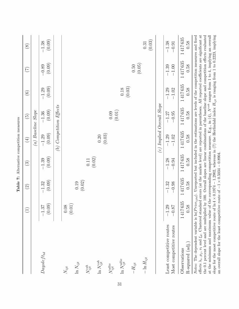
Table 7 reports the results to the following estimation:
ln(Priceijtd) = (α + βDayslefttd)× Compijt + λi + µj + νt + ξd + εijtd, (6)
where Compijt is a stand-in for the eight competition measures that we consider, and
where λi, µj, νt, and ξd are treated as fixed-effects.
The first thing to note, as can be seen in Panel (b), is that all competition measures
yield the same qualitative conclusions as our baseline setup. In order to assess the
quantitative implications across the variety of competition measures, we compute the
linear combination of the baseline slope (Panel a) with the competition effects for the
minimum and maximum realization of competition for each of the measures. The
implied range of intertemporal slopes for each of our measures is reported in Panel (c).
Here it can be seen that also quantitatively, the different measures yield very similar
conclusions: While the different measures find a daily price increase ranging from 1.27
percent to 1.39 percent for the least competitive routes in our sample, the daily price
increase estimated for the most competitive routes ranges from 0.87 percent to 1.02
percent.
B.2 Alternative customer heterogeneity measures
In this appendix, we consider some alternatives to the customer heterogeneity measures
considered in the main body of the paper.
As a first alternative, we use two measures aimed at capturing variations in the
customer heterogeneity across time. Specifically, we use dummy variables (Weekendt
and Holidayst) to distinguish weekend trips (departing on Friday and returning on
Sunday) from trips that depart on Monday and return on Thursday, and to identify
single competitors. Airlines not belonging to any of these alliances are counted as independentcompetitors according to our baseline competition measure.
31Since a Herfindahl index of one indexes the highest concentration of market power, we use −Hijt
to make it qualitatively comparable with the other measures.32To facilitate the comparison across the different measures which share different supports (the
Herfindahl index is defined on the real line, whereas Nijt, Ncshijt , and Nallie
ijt are natural numberswith different ranges), we adopt linear specifications for each of the competition measures in ourestimation.
30
Tab
le7:
Alt
ern
ati
veco
mp
etit
ion
mea
sure
s
(1)
(2)
(3)
(4)
(5)
(6)
(7)
(8)
(a)
Bas
elin
eS
lope
Daysleft td
−1.
37−
1.32
−1.
39−
1.29
−1.
36−
1.29
−0.
89−
1.38
(0.0
9)(0.0
9)(0.0
9)(0.0
9)(0.0
9)(0.0
9)(0.0
9)(0.0
9)
(b)
Com
peti
tion
Eff
ects
Nijt
0.08
(0.0
1)lnN
ijt
0.19
(0.0
2)N
csh
ijt
0.11
(0.0
2)lnN
csh
ijt
0.20
(0.0
3)N
allie
ijt
0.09
(0.0
1)lnN
allie
ijt
0.18
(0.0
3)−H
ijt
0.50
(0.0
5)−
lnH
ijt
0.31
(0.0
3)
(c)
Impl
ied
Ove
rall
Slo
pe
Lea
stco
mp
etit
ive
route
s−
1.29
−1.
32−
1.28
−1.
29−
1.27
−1.
29−
1.39
−1.
38M
ost
com
pet
itiv
ero
ute
s−
0.87
−0.
98−
0.94
−1.
02−
0.95
−1.
02−
1.00
−0.
91
Obse
rvat
ions
141
763
51
417
635
141
763
51
417
635
141
763
51
417
635
141
763
51
417
635
R-s
quar
ed(a
dj.
)0.
580.
580.
580.
580.
580.
580.
580.
58
Note
s:T
he
dep
end
ent
vari
able
isln
(Price
ijtd
).U
nre
por
ted
bu
tin
clu
ded
inth
ees
tim
atio
ns
are
leve
lsof
the
com
pet
itio
nm
easu
res
and
fixed
effec
tsλi,µj,ν t
andξ d
.C
lust
ered
stan
dar
der
rors
(at
the
mar
ket
leve
l)ar
ere
por
ted
inpar
enth
eses
.A
llre
por
ted
coeffi
cien
tsar
esi
gnifi
cant
atth
e0.
1p
erce
nt
leve
lan
dar
em
ult
ipli
edby
100.
Ove
rall
slop
esar
eli
nea
rco
mb
inat
ion
sof
the
bas
elin
esl
ope
and
com
pet
itio
neff
ects
eval
uat
edat
the
min
imu
man
dm
axim
um
valu
eof
the
corr
esp
on
din
gco
mp
etit
ion
mea
sure
.E
.g.,
in(4
),N
csh
ran
ges
from
1to
4,
imp
lyin
gan
over
all
slop
efo
rth
em
ost
com
pet
itiv
ero
ute
ofln
4×
0.19
74−
1.29
02,
wher
eas
in(7
)th
eH
erfindah
lin
dexH
ijt
isra
ngi
ng
from
1to
0.22
23,
imply
ing
anov
eral
lsl
ope
for
the
leas
tco
mp
etit
ive
rou
teof−
1×
0.5034−
0.8904.
31

roundtrips over the Christmas and New Years holidays.
The next two alternatives are based on an idea by Brueckner, Dyer and Spiller
(1992) who argue that a good proxy for the share of leisure travelers on a route are
temperature differentials between the destination and origin.33 Accordingly, we define
∆Tempijt as the temperature differentials between destination and origin during the
month of travel. In the same spirit, we also use ∆Precijt to measure precipitation
differentials between destination and origin during the month of travel.
Finally, we use regional GDP data to measure for business activity.34 Accordingly,
GDP oij and GDP d
ij are defined as log GDP at the origin and destination, respectively.
To give an overview over these measures, Figure 5 plots their means (marked by
circled dots), standard deviation bands (marked by boxes), and supports (marked
by lines) conditional on the number of competitors. Again the correlation across
competition levels is typically small relative to the standard deviation and supports,
although somewhat larger than for our two baseline measures.
To investigate how changes in customer heterogeneity affect the sensitivity of the
intertemporal slope to competition, we use the same empirical model as in Section 4:
ln(Priceijtd) = (α + βDayslefttd)×Xijt + λi + µj + νt + ξd + εijtd, (7)
with
Xijt = (1, Nijt, Hetijt, Nijt ×Hetijt),
where Nijt is the number of competitors, Hetijt is the corresponding customer het-
erogeneity measure, and λi, µj, νt and ξd are treated as fixed effects. Again, we
normalize Hetijt to have zero mean and unit variance. Here β is the relevant vector of
“slope” coefficients that define the intertemporal slope. Table 8 contains the estimated
coefficients and standard errors (clustered at the market level). For convenience,
Columns 1 and 2 reprint the results for our baseline measures.
As before, we look at the impact of Hetijt on the slope in monopoly markets
to determine whether it is likely to increase or decrease customer heterogeneity.
33See also Stavins (2001) and Goolsbee and Syverson (2008), who have used similar temperature-based proxies to measure for tourist intensities.
34We use GDP data provided by the European commission at the NUTS-2 level. See alsoFootnote 14.
32
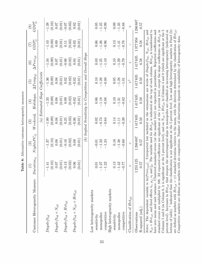
Tab
le8:
Alt
ern
ati
vecu
stom
erh
eter
ogen
eity
mea
sure
s
(1)
(2)
(3)
(4)
(5)
(6)
(7)
(8)
Cu
stom
erH
eter
oge
nei
tyM
easu
re:
Duration
ijNightsPCij
Weekendt
Holidays t
∆Tem
pijt
∆Prec ijt
GDP
o ijGDP
d ij
(a)
Est
imate
dS
lope
Coe
ffici
ents
Daysleft td
−1.
41−
1.3
7−
1.00
−1.3
3−
1.3
6−
1.3
4−
1.43
−1.3
8(0.1
0)(0.1
0)(0.0
9)(0.0
9)(0.0
9)(0.0
9)(0.0
9)(0.1
0)Daysleft td×N
ijt
0.07
0.0
80.0
80.0
80.
080.
070.
090.
07(0.0
1)(0.0
1)(0.0
1)(0.0
1)(0.0
1)(0.0
1)(0.0
1)(0.0
1)Daysleft td×Het
ijt
−0.
13−
0.1
60.2
50.0
90.
02−
0.0
60.
11−
0.0
7(0.0
2)(0.0
2)(0.0
2)(0.0
2)(0.0
2)(0.0
2)(0.0
3)(0.0
3)Daysleft td×N
ijt×Het
ijt
0.06
0.08
−0.0
6−
0.0
2−
0.0
20.
04−
0.0
30.
02(0.0
1)(0.0
1)(0.0
1)(0.0
1)(0.0
1)(0.0
1)(0.0
1)(0.0
1)
(b)
Impli
edS
ensi
tivi
tyto
Com
peti
tion
an
dO
vera
llS
lope
Low
het
erogen
eity
mar
kets
sen
siti
vit
y0.
01−
0.0
10.0
20.0
60.
100.
030.
060.0
5m
onop
olie
s−
1.27
−1.2
2−
0.73
−1.1
8−
1.2
8−
1.2
5−
1.26
−1.2
5co
mp
etit
ive
−1.
22−
1.2
4−
0.64
−0.8
8−
0.8
0−
1.1
0−
0.96
−0.9
9H
igh
het
erog
enei
tym
arke
tsse
nsi
tivit
y0.
130.1
60.1
40.1
00.
050.
100.
130.
09m
onop
olie
s−
1.42
−1.3
8−
1.11
−1.3
1−
1.2
8−
1.2
9−
1.41
−1.3
5co
mp
etit
ive
−0.
77−
0.6
0−
0.39
−0.8
2−
1.0
1−
0.7
9−
0.78
−0.8
8
Cla
ssifi
cati
onofHet
ijt
++
−−
+†
+−
+
Ob
serv
atio
ns
1255
125
128
668
71
417
635
141
763
51
417
635
141
763
51
377
958
128
668
7R
-squ
ared
(ad
j.)
0.5
70.5
70.5
80.5
80.
580.
580.
580.
57
Note
s:T
he
dep
enden
tva
riable
isln
(Price
ijtd
).U
nre
port
edbut
incl
uded
inth
ees
tim
ati
ons
are
level
sofDaysleft td,N
ijt,Het
ijt
and
Nijt×Het
ijt,
and
fixed
effec
tsλi,µj,ν t
andξ d
.T
he
vari
able
use
dfo
rHet
ijt
isin
dic
ated
atth
eto
pof
each
colu
mn.Het
ijt
istr
ansf
orm
edto
hav
eze
rom
ean
and
unit
vari
ance
.C
lust
ered
standard
erro
rs(a
tth
em
ark
etle
vel
)are
rep
ort
edin
pare
nth
eses
.R
eport
edco
effici
ents
and
stan
dar
der
rors
are
mult
iplied
by
100.
All
rep
orte
dco
effici
ents
are
sign
ifica
nt
atth
e1
per
cent
leve
l,ex
cept
the
slop
eco
effici
ents
onHet
ijt
inC
olum
ns
5an
d6
(in
Col
um
n6,
itis
sign
ifica
nt
atth
e5
per
cent
leve
l),
and
onN
ijt×Het
ijt
inC
olum
ns
4an
d8
(whic
har
esi
gnifi
cant
atth
e5
per
cent
level
).In
crea
ses
inHet
ijt
that
stee
pen
the
inte
rtem
pora
lsl
op
ein
monop
olies
are
class
ified
as
incr
easi
ng
het
erogen
eity
(indic
ate
dat
bot
tom
ofta
ble
).†
ind
icat
edth
atth
ecl
assi
fica
tion
isn
otsi
gnifi
cant
atth
e5
per
cent
leve
l.L
owan
dhig
hh
eter
ogen
eity
mar
kets
inP
anel
(b)
are
defi
ned
asm
arke
tsw
ithHet
ijt
=±
1st
andar
ddev
iati
onre
lati
veto
the
mea
n,
wit
hth
edir
ecti
ondet
erm
ined
by
the
clas
sifica
tion
ofHet
ijt.
Com
pet
itiv
em
arket
sar
ed
efin
esas
mar
kets
wit
hsi
xco
mp
etit
ors
.N
um
ber
of
ob
serv
ati
on
sd
epen
ds
on
avail
ab
ilit
yof
het
erogen
eity
data
.
33
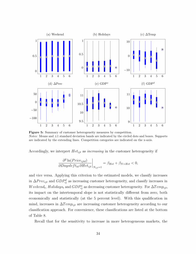
1 2 3 4 5 6
0
0.5
1
(b) Holidays
1 2 3 4 5 6
0
0.5
1
(a) Weekend
1 2 3 4 5 6
−100
−50
0
50
(d) ∆Prec
1 2 3 4 5 6
9.5
10
10.5
11
(e) GDPo
1 2 3 4 5 69
10
11
(f) GDPd
1 2 3 4 5 6
−10
0
10
(c) ∆Temp
Figure 5: Summary of customer heterogeneity measures by competition.Notes: Means and ±1 standard deviation bands are indicated by the circled dots and boxes. Supportsare indicated by the extending lines. Competition categories are indicated on the x-axis.
Accordingly, we interpret Hetijt as increasing in the customer heterogeneity if
∂2 ln(Priceijtd)
∂Dayslefttd ∂Hetijt
∣∣∣∣Nijt=1
= βHet + βN×Het < 0,
and vice versa. Applying this criterion to the estimated models, we classify increases
in ∆Precijt and GDP dij as increasing customer heterogeneity, and classify increases in
Weekendt, Holidayst and GDP oij as decreasing customer heterogeneity. For ∆Tempijt,
its impact on the intertemporal slope is not statistically different from zero, both
economically and statistically (at the 5 percent level). With this qualification in
mind, increases in ∆Tempijt are increasing customer heterogeneity according to our
classification approach. For convenience, these classifications are listed at the bottom
of Table 8.
Recall that for the sensitivity to increase in more heterogeneous markets, the
34
slope coefficient for Nijt ×Hetijt has to go into the same direction as the impact of
Hetijt on heterogeneity. That is, if we have associated Hetijt with an increase in
heterogeneity, then the slope coefficient for Nijt ×Hetijt has to be positive in order
for the intertemporal slope to be more sensitive to increases in competition in more
heterogeneous markets, and vice versa.
Comparing the above classifications with the slope coefficients on Nijt ×Hetijt,these estimations confirm the conclusions based on hotel bookings data for all measures
except ∆Tempijt (for which we could not reject the possibility of a false classification
at the 5 percent level). Looking again at the sensitivity to competition for Hetijt at
one standard deviation above and below its mean,
∂2 ln(Price)
∂Dayslefttd ∂Nijt
∣∣∣∣Hetijt=±1
= βN ± βN×Het.
we see that all measures with the exception of ∆Tempijt yield similar patterns (but
to a lesser extent) to the ones seen for our baseline measures. The difference is likely
to result from a somewhat looser correlation between these alternative measures and
customer heterogeneity, so that evaluation Hetijt at one standard deviation above
and below its mean is likely to map into an actual customer heterogeneity evaluated
substantially within its one standard deviation circle.
B.3 Non-monotonic impact of customer heterogeneity
In this section, we generalize our approach in the main body of the paper to evaluate
how the sensitivity of the intertemporal slope to competition changes with customer
heterogeneity in a potential non-monotonic fashion.
We use the following quadratic specification in Hetijt to allow for such non-
monotonicities:
ln(Priceijtd) = (α + βDayslefttd)×Xijt + λi + µj + νt + ξd + εijtd, (8)
with
Xijt = (1, Nijt, Hetijt, Het2ijt, Nijt ×Hetijt, Nijt ×Het2ijt),
where Nijt is the number of competitors, Hetijt is the corresponding customer het-
erogeneity measure, and λi, µj, νt and ξd are treated as fixed effects. To ensure that
35
computing the quadratic terms is a positive monotonic transformation, we normalize
Hetijt to have positive support.
To identify whether a certain change in Hetijt increases or decreases heterogeneity,
we generalize our previous approach to look at the impact of Hetijt on the intertemporal
slope in monopoly markets. In particular, we interpret a change in Hetijt as an increase
in customer heterogeneity if
∂2 ln(Priceijtd)
∂Dayslefttd∂Hetijt
∣∣∣∣Nijt=1
= βHet + βN×Het + 2 (βHet2 + βN×Het2)Hetijt < 0,
and vice versa. Note that through the quadratic term, the classification may now
change with Hetijt. For example, we could have that the heterogeneity is increasing
in the tourist intensity if the tourist intensity is absolute low, but is decreasing once
the market is satiated with tourists.
Based on this criterion, we do not find any evidence for a non-monotonic impact
on customer heterogeneity. Both Durationijt and NightsPCijt have a positive impact
on heterogeneity throughout their complete support, motivating the non-monotonic
treatment in the main body of the paper.
Figure 6 plots the estimated sensitivity of the intertemporal slope to competition
as a function of Hetijt, formally given by the cross-derivative of the identified model
in Dayslefttd and Nijt:
∂2 ln(Priceijtd)
∂Dayslefttd∂Nijt
= βN + βN×HetHetijt + βN×Het2Het2ijt.
Not surprising giving the monotonic impact of Hetijt, the sensitivity of the slope
to competition is literally “in line” with the linear setup in the main body, yielding a
sensitivity that ranges from zero at the 5th percentile of Hetijt (largely homogenous
markets by our classification) to somewhat above 0.15 and 0.20, respectively, at the
95th percentile (substantially heterogeneous markets by our classification).
B.4 Competition-specific impact of customer heterogeneity
This appendix section generalizes the analysis in the main body of the paper to allow
for a competition-specific impact of customer heterogeneity.
To investigate how changes in customer heterogeneity affect the sensitivity of the
36
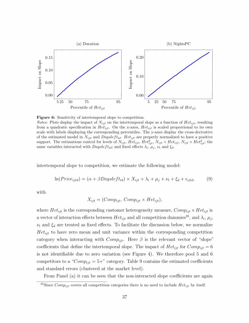
5 25 50 75 95
0.00
0.05
0.10
0.15
Percentile of Hetijt
Imp
act
onS
lop
e(a) Duration
5 25 50 75 95
0.00
0.10
0.20
Percentile of Hetijt
Imp
act
on
Slo
pe
(b) NightsPC
Figure 6: Sensitivity of intertemporal slope to competition.Notes: Plots display the impact of Nijt on the intertemporal slope as a function of Hetijt, resultingfrom a quadratic specification in Hetijt. On the x-axes, Hetijt is scaled proportional to its ownscale with labels displaying the corresponding percentiles. The y-axes display the cross-derivativeof the estimated model in Nijt and Dayslefttd. Hetijt are properly normalized to have a positivesupport. The estimations control for levels of Nijt, Hetijt, Het
2ijt, Nijt ×Hetijt, Nijt ×Het2ijt; the
same variables interacted with Dayslefttd; and fixed effects λi, µj , νt and ξd.
intertemporal slope to competition, we estimate the following model:
ln(Priceijtd) = (α + βDayslefttd)×Xijt + λi + µj + νt + ξd + εijtd, (9)
with
Xijt = (Compijt, Compijt ×Hetijt),
where Hetijt is the corresponding customer heterogeneity measure, Compijt×Hetijt is
a vector of interaction effects between Hetijt and all competition dummies35, and λi, µj ,
νt and ξd are treated as fixed effects. To facilitate the discussion below, we normalize
Hetijt to have zero mean and unit variance within the corresponding competition
category when interacting with Compijt. Here β is the relevant vector of “slope”
coefficients that define the intertemporal slope. The impact of Hetijt for Compijt = 6
is not identifiable due to zero variation (see Figure 4). We therefore pool 5 and 6
competitors to a “Compijt = 5+” category. Table 9 contains the estimated coefficients
and standard errors (clustered at the market level).
From Panel (a) it can be seen that the non-interacted slope coefficients are again
35Since Compijt covers all competition categories there is no need to include Hetijt by itself.
37
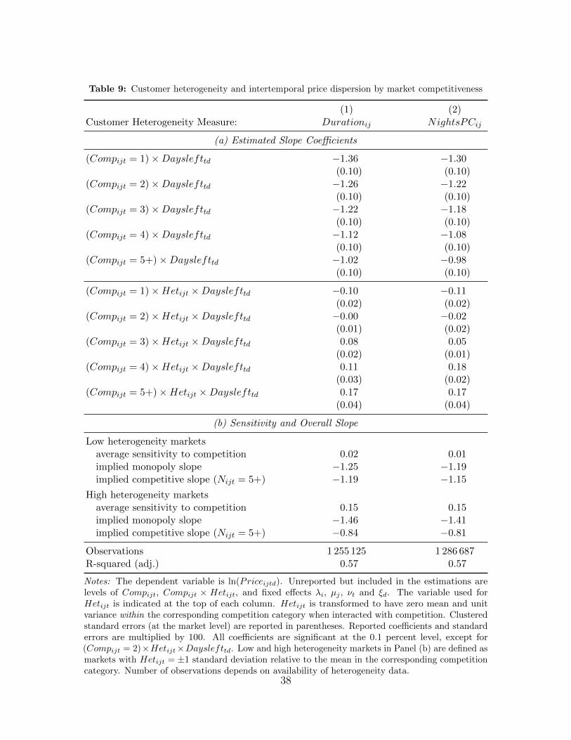
Table 9: Customer heterogeneity and intertemporal price dispersion by market competitiveness
(1) (2)Customer Heterogeneity Measure: Durationij NightsPCij
(a) Estimated Slope Coefficients
(Compijt = 1)×Dayslefttd −1.36 −1.30(0.10) (0.10)
(Compijt = 2)×Dayslefttd −1.26 −1.22(0.10) (0.10)
(Compijt = 3)×Dayslefttd −1.22 −1.18(0.10) (0.10)
(Compijt = 4)×Dayslefttd −1.12 −1.08(0.10) (0.10)
(Compijt = 5+)×Dayslefttd −1.02 −0.98(0.10) (0.10)
(Compijt = 1)×Hetijt ×Dayslefttd −0.10 −0.11(0.02) (0.02)
(Compijt = 2)×Hetijt ×Dayslefttd −0.00 −0.02(0.01) (0.02)
(Compijt = 3)×Hetijt ×Dayslefttd 0.08 0.05(0.02) (0.01)
(Compijt = 4)×Hetijt ×Dayslefttd 0.11 0.18(0.03) (0.02)
(Compijt = 5+)×Hetijt ×Dayslefttd 0.17 0.17(0.04) (0.04)
(b) Sensitivity and Overall Slope
Low heterogeneity marketsaverage sensitivity to competition 0.02 0.01implied monopoly slope −1.25 −1.19implied competitive slope (Nijt = 5+) −1.19 −1.15
High heterogeneity marketsaverage sensitivity to competition 0.15 0.15implied monopoly slope −1.46 −1.41implied competitive slope (Nijt = 5+) −0.84 −0.81
Observations 1 255 125 1 286 687R-squared (adj.) 0.57 0.57
Notes: The dependent variable is ln(Priceijtd). Unreported but included in the estimations arelevels of Compijt, Compijt × Hetijt, and fixed effects λi, µj , νt and ξd. The variable used forHetijt is indicated at the top of each column. Hetijt is transformed to have zero mean and unitvariance within the corresponding competition category when interacted with competition. Clusteredstandard errors (at the market level) are reported in parentheses. Reported coefficients and standarderrors are multiplied by 100. All coefficients are significant at the 0.1 percent level, except for(Compijt = 2)×Hetijt×Dayslefttd. Low and high heterogeneity markets in Panel (b) are defined asmarkets with Hetijt = ±1 standard deviation relative to the mean in the corresponding competitioncategory. Number of observations depends on availability of heterogeneity data.
38
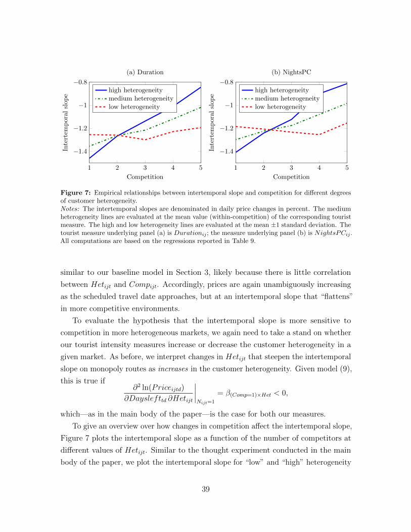
1 2 3 4 5
−1.4
−1.2
−1
−0.8
Competition
Inte
rtem
pora
lsl
ope
(a) Duration
high heterogeneitymedium heterogeneitylow heterogeneity
1 2 3 4 5
−1.4
−1.2
−1
−0.8
Competition
Inte
rtem
pora
lsl
ope
(b) NightsPC
high heterogeneitymedium heterogeneitylow heterogeneity
Figure 7: Empirical relationships between intertemporal slope and competition for different degreesof customer heterogeneity.Notes: The intertemporal slopes are denominated in daily price changes in percent. The mediumheterogeneity lines are evaluated at the mean value (within-competition) of the corresponding touristmeasure. The high and low heterogeneity lines are evaluated at the mean ±1 standard deviation. Thetourist measure underlying panel (a) is Durationij ; the measure underlying panel (b) is NightsPCij .All computations are based on the regressions reported in Table 9.
similar to our baseline model in Section 3, likely because there is little correlation
between Hetijt and Compijt. Accordingly, prices are again unambiguously increasing
as the scheduled travel date approaches, but at an intertemporal slope that “flattens”
in more competitive environments.
To evaluate the hypothesis that the intertemporal slope is more sensitive to
competition in more heterogeneous markets, we again need to take a stand on whether
our tourist intensity measures increase or decrease the customer heterogeneity in a
given market. As before, we interpret changes in Hetijt that steepen the intertemporal
slope on monopoly routes as increases in the customer heterogeneity. Given model (9),
this is true if∂2 ln(Priceijtd)
∂Dayslefttd ∂Hetijt
∣∣∣∣Nijt=1
= β(Comp=1)×Het < 0,
which—as in the main body of the paper—is the case for both our measures.
To give an overview over how changes in competition affect the intertemporal slope,
Figure 7 plots the intertemporal slope as a function of the number of competitors at
different values of Hetijt. Similar to the thought experiment conducted in the main
body of the paper, we plot the intertemporal slope for “low” and “high” heterogeneity
39

markets (evaluated at one standard deviation below and above the competition-specific
mean of Hetijt), as well as for a “medium” heterogeneity market evaluated at the
mean.
While the linear model in the main body assumes that the intertemporal slope
is linear in competition (with the derivative defining the “sensitivity” to competi-
tion), the competition-specific setup considered here allows for an arbitrary relation.
Reassuring our findings in the main body, we however find that the sensitivity is
nearly constant conditional on Hetijt. As before, the intertemporal slope is highly
sensitive to competition in high heterogeneity markets, as is predicted by theories of
competitive price discrimination. In contrast, reducing the customer heterogeneity in a
given market to one standard deviation below its mean, makes the intertemporal slope
largely invariant to competition, in line with the idea that in homogeneous markets
airlines do not price-discriminate to begin with so that they are also not restrict in
their ability to do so by competition.
To reconcile these findings quantitatively with the linear model in the main body,
Panel (b) of Table 9 also reports the “average” sensitivity to competition, amounting
to the average change in the intertemporal slope displayed in Figure 7:
1
supp(N)
∫N
∂2 ln(Priceijt)
∂Daysleftijt ∂Nijt
∣∣∣∣Hetijt=±1
≈ 1
4
5∑N=2
{[βComp=N − βComp=N−1
]±[β(Comp=N)×Het − β(Comp=N−1)×Het
]}.
Not surprising given the nearly linear relation in Figure 7, the implied sensitivities
are numerically consistent with our linear model, motivating the simplified exposition
in the main body of the paper.
40
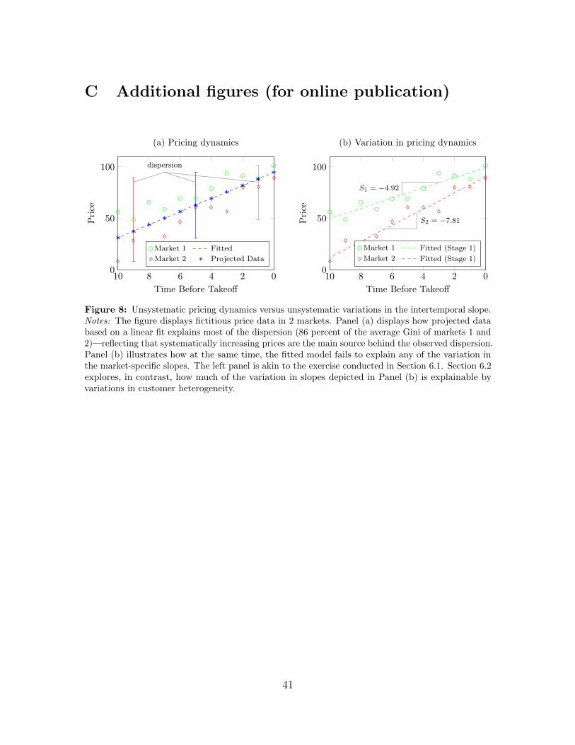
C Additional figures (for online publication)
02468100
50
100 dispersion
Time Before Takeoff
Pri
ce
(a) Pricing dynamics
Market 1 Fitted
Market 2 Projected Data
02468100
50
100
S1 = −4.92
S2 = −7.81
Time Before Takeoff
Pri
ce
(b) Variation in pricing dynamics
Market 1 Fitted (Stage 1)
Market 2 Fitted (Stage 1)
Figure 8: Unsystematic pricing dynamics versus unsystematic variations in the intertemporal slope.Notes: The figure displays fictitious price data in 2 markets. Panel (a) displays how projected databased on a linear fit explains most of the dispersion (86 percent of the average Gini of markets 1 and2)—reflecting that systematically increasing prices are the main source behind the observed dispersion.Panel (b) illustrates how at the same time, the fitted model fails to explain any of the variation inthe market-specific slopes. The left panel is akin to the exercise conducted in Section 6.1. Section 6.2explores, in contrast, how much of the variation in slopes depicted in Panel (b) is explainable byvariations in customer heterogeneity.
41
References
Alderighi, Marco, Marcella Nicolini, and Claudio A Piga. 2012. “Combined
effects of load factors and booking time on fares: Insights from the yield management
of a low-cost airline.”
Armstrong, Mark, and John Vickers. 2001. “Competitive price discrimination.”
RAND Journal of Economics, 579–605.
Borenstein, Severin. 1985. “Price discrimination in free-entry markets.” Rand
Journal of Economics, 16(3): 380–397.
Borenstein, Severin, and Nancy L Rose. 1994. “Competition and Price Disper-
sion in the US Airline Industry.” Journal of Political Economy, 102(4): 653–683.
Brueckner, Jan K, Nichola J Dyer, and Pablo T Spiller. 1992. “Fare deter-
mination in airline hub-and-spoke networks.” The Rand Journal of Economics,
309–333.
Courty, Pascal, and Mario Pagliero. 2012. “The Impact of Price discrimination on
Revenue: Evidence from the concert industry.” Review of Economics and Statistics,
94(1): 359–369.
Dana, James D Jr. 1998. “Advance-purchase discounts and price discrimination in
competitive markets.” Journal of Political Economy, 395–422.
Dana, James D Jr. 1999a. “Equilibrium price dispersion under demand uncertainty:
the roles of costly capacity and market structure.” The RAND Journal of Economics,
30(4): 632–660.
Dana, James D Jr. 1999b. “Using yield management to shift demand when the
peak time is unknown.” The RAND Journal of Economics, 30(3): 456–474.
Dana, James D Jr. 2001. “Monopoly price dispersion under demand uncertainty.”
International Economic Review, 42(3): 649–670.
Escobari, Diego. 2012. “Dynamic Pricing, Advance Sales and Aggregate Demand
Learning in Airlines.” The Journal of Industrial Economics, 60(4): 697–724.
42

Escobari, Diego, Nicholas Rupp, and Joseph Meskey. 2013. “Dynamic price
discrimination in airlines.” mimeo.
Gaggero, Alberto A, and Claudio A Piga. 2011. “Airline market power and
intertemporal price dispersion.” The Journal of Industrial Economics, 59(4): 552–
577.
Gale, Ian L, and Thomas J Holmes. 1992. “The efficiency of advance-purchase
discounts in the presence of aggregate demand uncertainty.” International Journal
of Industrial Organization, 10(3): 413–437.
Gale, Ian L, and Thomas J Holmes. 1993. “Advance-purchase discounts and
monopoly allocation of capacity.” The American Economic Review, 135–146.
Gerardi, Kristopher S, and Adam Hale Shapiro. 2009. “Does competition
reduce price dispersion? New evidence from the airline industry.” Journal of
Political Economy, 117(1): 1–37.
Goolsbee, Austan, and Chad Syverson. 2008. “How do incumbents respond to
the threat of entry? Evidence from the major airlines.” The Quarterly Journal of
Economics, 123(4): 1611–1633.
Hayes, Kathy J, and Leola B Ross. 1998. “Is airline price dispersion the result
of careful planning or competitive forces?” Review of Industrial Organization,
13(5): 523–541.
Hendel, Igal, and Aviv Nevo. 2013. “Intertemporal Price Discrimination in
Storable Goods Markets.” The American Economic Review, 103(7): 2722–2751.
Holmes, Thomas J. 1989. “The effects of third-degree price discrimination in
oligopoly.” American Economic Review, 79(1): 244–250.
Lazarev, John. 2013. “The Welfare Effects of Intertemporal Price Discrimination:
An Empirical Analysis of Airline Pricing in US Monopoly Markets.” mimeo.
Leslie, Phillip. 2004. “Price discrimination in Broadway theater.” RAND Journal
of Economics, 520–541.
McAfee, R Preston, and Vera Te Velde. 2007. “Dynamic pricing in the airline
industry.” Handbook on Economics and Information Systems.
43
Nair, Harikesh. 2007. “Intertemporal price discrimination with forward-looking
consumers: Application to the US market for console video-games.” Quantitative
Marketing and Economics, 5(3): 239–292.
Puller, Steven L, Anirban Sengupta, and Steven N Wiggins. 2012. “Does
scarcity drive intra-route price dispersion in airlines?” NBER Working Paper, 15555.
Stavins, Joanna. 2001. “Price discrimination in the airline market: The effect of
market concentration.” Review of Economics and Statistics, 83(1): 200–202.
Williams, Kevin R. 2013. “Dynamic Airline Pricing and Seat Availability.” mimeo.
44