OFDM VLSI システム内超高速伝送£¯島洋祐.pdf1 OFDM 適用VLSI システム内超高速伝送 研究代表者 飯 島 洋 祐 小山工業高等専門学校 電気電子創造工学科

Editorial Board
• Prof. Dr. Eng. Ioan NAFORNITA, Editor-in-chief
• Prof. Dr. Eng. Virgil TIPONUT • Prof. Dr. Eng. Alexandru ISAR • Prof. Dr. Eng. Dorina ISAR • Prof. Dr. Eng. Traian JURCA • Prof. Dr. Eng. Aldo DE SABATA • Prof. Dr. Eng. Mihail TANASE • Prof. Dr. Eng. Radu VASIU
• Assist . Eng. Maria KOVACI, Scientific Secretary • Assist . Eng. Corina NAFORNITA, Associate Editorial Secretary
Scientific Board
• Prof. Dr. Eng. Monica BORDA, Technical University of Cluj-Napoca, Romania
• Prof. Dr. Eng. Philip CONSTANTINOU, National Technical University of Athens, Greece
• Prof. Dr. Eng. Aldo DE SABATA, Politehnica University of Timisoara, Romania
• Prof. Dr. Eng. Karen EGUIAZARIAN, Tampere University of Technology, Institute of Signal Processing, Finland
• Prof. Dr. Eng. Liviu GORAS, Technical University Gheorghe Asachi, Iasi, Romania
• Prof. Dr. Eng. Kyoki IMAMURA, Kyushu Institute of Technology, Japan
• Prof. Dr. Eng. Alexandru ISAR, Politehnica University of Timisoara, Romania
• Prof. Dr. Eng. Michel JEZEQUEL, ENST-Bretagne, Brest, Franta • Prof. Dr. Eng. Traian JURCA, Politehnica University of Timisoara,
Romania • Prof. Dr. Eng. Ioan NAFORNITA, Politehnica University of
Timisoara, Romania • Prof. Dr. Eng. Mohamed NAJIM, ENSERB Bordeaux, France • Prof. Dr. Eng. Emil PETRIU, SITE, University of Ottawa, Canada • Prof. Dr. Eng. Andre QUINQUIS, ENSIETA Bretagne, Brest, France • Prof. Dr. Eng. Maria Victoria RODELLAR BIARGE, Politecnic
University of Madrid, Spain • Prof. Dr. Eng. Alexandru SERBANESCU, Technical Military
Academy, Bucharest, Romania • Prof. Dr. Eng. Virgil TIPONUT, Politehnica University of
Timisoara, Romania

• Prof. Dr. Eng. Radu VASIU, Politehnica University of Timisoara, Romania
• Prof. Dr. Eng. Baozong YUAN, Beijing Jiaotong University, China
Advisory Board
• Prof. Dr. Eng. Miranda NAFORNITA, Politehnica University of Timisoara, Romania
• Prof. Dr. Eng. Virgil TIPONUT, Politehnica University of Timisoara, Romania
• Prof. Dr. Eng. Ioan NAFORNITA, Politehnica University of Timisoara, Romania
• Prof. Dr. Eng. Mihail TANASE, Politehnica University of Timisoara, Romania
• Prof. Dr. Eng. Aldo DE SABATA, Politehnica University of Timisoara, Romania
• Prof. Dr. Eng. Mircea CIUGUDEAN, Politehnica University of Timisoara, Romania
• Prof. Dr. Eng. Alimpie IGNEA, Politehnica University of Timisoara, Romania
Buletinul Ştiinţific
al Universităţii "Politehnica" din Timişoara
Seria ELECTRONICĂ ŞI TELECOMUNICAŢII
TRANSACTIONS ON ELECTRONICS AND COMMUNICATIONS
Tom 52(66), Fascicola 2, 2007
CONTENTS Marius Oltean: "Wavelet OFDM Performance in Flat Fading Channels".............................................3 Raul Ionel, Alimpie Ignea: "Parametric Analysis and Spectral Whitening of Signals Generated by Leaks in Water Pipes".........................................................................................................................................9 Daniela Fuiorea: "A New Point Matching Method for Image Registration Using Pixel Color Information".............................................................................................................................15 Marius Rangu: "An Algorithm for Automated Translation of Crosstalk Requirements into Physical Design Rules"...........................................................................................................................20
Laviniu Ţepelea, Virgil Tiponuţ: "A HRTF Interface for Visually Impaired People"......................................................26
Beniamin Dragoi, Mircea Ciugudean, Ioan Jivet: "CMOS Current Conveyor for High-Speed Application"............................................30
János Gal, Andrei Câmpeanu, Ioan Nafornita: "A Kalman Filtering Algorithm for the Estimation of Chirp Signals in Gaussian Noise".......................................................................................................................................35 Marllene Daneti: "Transitory Shaped Test Signals Synthesis for Leak Locating Algorithms Analyzing"................................................................................................................................39 Marius Salagean: "The Use of the Improved Time-Frequency Method Based on Mathematical Morphology Operators"...........................................................................................................45 Ionut Mirel: "Flesh Tone Correction Algorithm for TV Receivers".................................................49
1

Mircea Coser: "A TRIZ View on Air Navigation Evolution"...............................................................54 Emanuel Puschita, Tudor Palade, Ancuta Moldovan, Simona Trifan: "An Overview of Intra-Domain QoS Mechanisms Evaluation"...................................58
2
Buletinul Ştiinţific al Universităţii "Politehnica" din Timişoara
Seria ELECTRONICĂ şi TELECOMUNICAŢII TRANSACTIONS on ELECTRONICS and COMMUNICATIONS
Tom 52(66), Fascicola 2, 2007
Wavelet OFDM Performance in Flat Fading Channels
Marius Oltean1
1 Facultatea de Electronică şi Telecomunicaţii, Departamentul Comunicaţii Bd. V. Pârvan Nr. 2, 300223 Timişoara, e-mail [email protected]
Abstract – This paper represents an investigation of the wavelet based multi-carrier modulation performance in flat fading channels. The fading envelope is distributed according to a Rayleigh probability density function. BER performance of the multicarrier wavelet method is computed and analyzed against the classical Orthogonal Frequency Division Multiplexing (OFDM) case, in various scenarios with respect to the Doppler shift influence and to the noise level. Keywords: OFDM, wavelet-based OFDM, fading, Doppler shift.
I. INTRODUCTION
Multi-carrier modulation techniques were widely used in the last decade in various standards for wireline and wireless communications. Amongst others, versions of Fourier-based OFDM are employed at the physical level to provide good performance over the air interface in systems like Digital Audio & Video Broadcasting (DAVB), WiMAX (described by IEEE 802.16), WiFi (802.11) or Qualcomm's Flash OFDM. This proves the reliability and the efficiency of the multi-carrier modulation concept, which is very well suited to radio transmissions. Besides its incontestable advantages, OFDM presents some well known drawbacks as: diminished spectral efficiency because of the cyclic prefix (CP) overhead, slow decay of the out-of-band side-lobes, high sensitivity to time and frequency synchronization, increased peak-to-average-power ratio [1,2].
Recent research focused on the multi-carrier transmission techniques [3,4], highlighted that some of these disadvantages can be steadily counteracted using wavelet carriers instead of OFDM's complex exponential waveforms. Due to the fact that these wavelet carriers form an orthogonal family, they can be separated at receiver's side by correlation techniques. The authors in [5] have shown that wavelet-based OFDM (WOFDM) has better spectral efficiency, is simpler and at least as rapid as OFDM in practical implementations. Furthermore, the performance of the two systems is similar in AWGN channels. Note however that, from this point of view, the real gain of multi-carrier techniques can be highlighted in conditions specific to the radio channels, which are both frequency-selective and
time-variant. With respect to these conditions, the author will investigate the OFDM and WOFDM performance in different flat, Rayleigh fading scenarios. A deeper analysis of the wavelet based method is performed, taking into account the influence of the chosen wavelets mother, as well as of the number of decomposition levels used in Inverse Discrete Wavelet Transform (IDWT) computation.
In the next section, an overview of the multi-carrier modulation concept is provided, focusing on the WOFDM principles. The third section will describe the simulation scenarios, whose results will be shown and discussed in section 4. The last section is dedicated to concluding remarks and to possible future directions for the continuation of the present work.
II. MULTI-CARRIER TRANSMISSIONS AND WAVELETS
Largely used in the modern communication systems, Orthogonal Frequency Division Multiplexing (OFDM) relies on a multicarrier approach, where data is transmitted using several parallel substreams. Every stream modulates a different complex exponential subcarrier, the subcarriers involved being orthogonal to each other. The orthogonality is the key point that allows subcarrier separation at receiver. The multicarrier approach has the advantage of a long symbol duration, issued from the simultaneous transmission of several low-rate parallel streams. OFDM implementation is based on the Fast Fourier Transform (FFT) algorithm, which allows reduced complexity and low implementation cost. The idea which gathers OFDM and wavelets is that in the same manner that the complex exponentials define an orthonormal basis for any periodic signal, a wavelet family forms a complete orthonormal basis for
)(L2 ℜ . The orthogonality condition for wavelet family members is illustrated in (1).
⎩⎨⎧ ==
>=Ψψ<otherwise,0
nkandmjif,1)t(),t( n,mk,j (1)
Wavelet family members from (1) can be obtained by translating and scaling a unique function called
3
wavelets mother and denoted by )t(ψ , according to (2):
)kts(s)t( 0j
02/j
0k,j τ−⋅ψ=ψ −− (2)
Equation 2 corresponds to a sampled version of a wavelet family, the discrete variables being s0 (the scale) and k (the position within the scale). The relation (1) indicates that all the members of the wavelet family Zk
j2/jk,j )kt2(2)t( ∈
−− −Ψ=Ψ (we considered s0=2 and τ0=1) are orthogonal to each other. Consequently, if instead of complex exponential waveforms we use wavelet carriers, we will still be able to separate these subcarriers at receiver, due to their orthogonality. This is the main idea that lies behind the wavelet-based OFDM techniques [3,6]. As for the classical OFDM, the WOFDM symbol can be generated by digital signal processing techniques, such as IDWT. In this case, the transmitted signal is "synthesized" from the wavelet coefficients >ψ=< )t(),t(sw k,jk,j located at the k-th position from scale j (j=1,…, J), and from the approximation coefficients >ϕ=< )t(),t(sa k,Jk,J , located at the k-th position from the coarsest scale J. Taking into account the constraints of a practical implementation, we can reformulate equation (2). Thus, the computation of the IDWT using Mallat's algorithm [7] requires finite-length dyadic data sequences at system input. If we denote by N the length of our input data sequence (which must be a power of 2), then the maximum number of decomposition levels for the DWT equals L=log2(N), and the formula which will be employed for the WOFDM symbol computation is:
∑ ϕ∑ ∑ +ψ=−−
== =
JLjL 2
1kk,Jk,J
J
1j
2
1kk.jk,j )t(a)t(w)t(s (3)
where J stands for the number of decomposition levels used, (whose the maximum value is L). φj,k(t) in the equation above is the scaling function associated to the wavelet mother. This formula corresponds to IDWT computation, which translates into a time domain signal some wavelet and approximation coefficients. Note that, in practice, a sampled version of the output signal, s[n] is generated The total number of samples composing this signal (referred to as WOFDM symbol in wavelet modulation terms) is equal to the number of samples of the input data sequence.
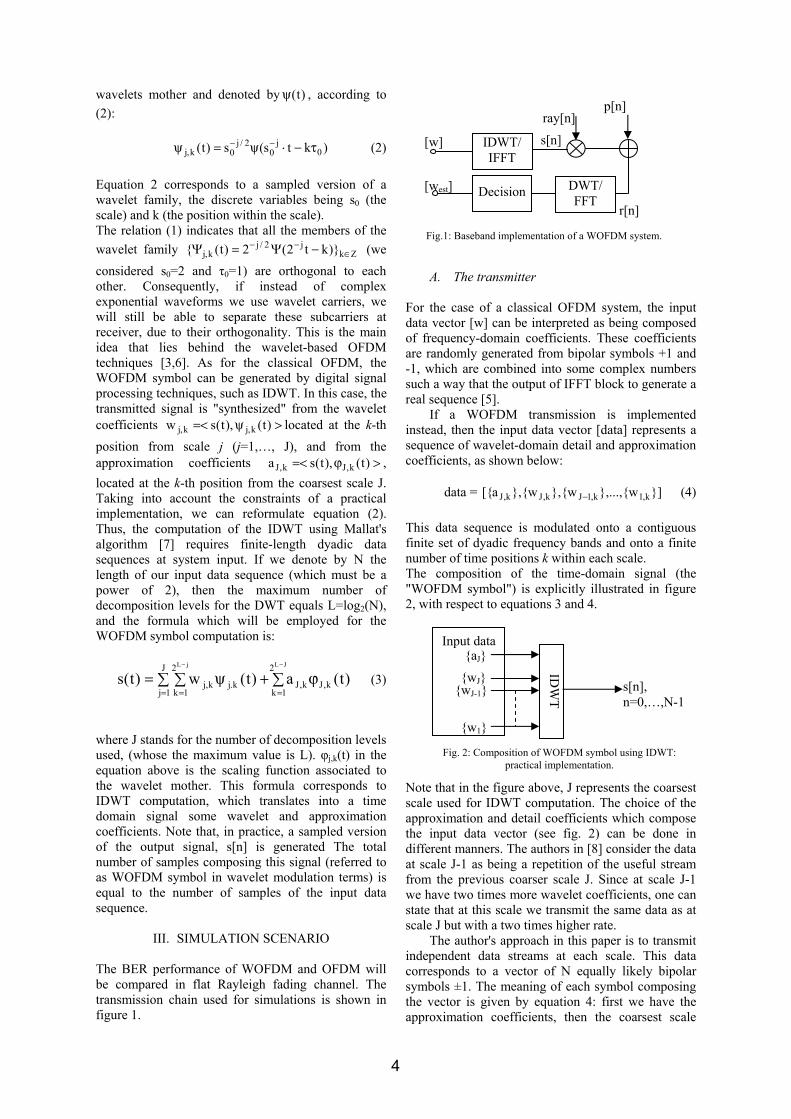
III. SIMULATION SCENARIO The BER performance of WOFDM and OFDM will be compared in flat Rayleigh fading channel. The transmission chain used for simulations is shown in figure 1.
A. The transmitter
For the case of a classical OFDM system, the input data vector [w] can be interpreted as being composed of frequency-domain coefficients. These coefficients are randomly generated from bipolar symbols +1 and -1, which are combined into some complex numbers such a way that the output of IFFT block to generate a real sequence [5].
If a WOFDM transmission is implemented instead, then the input data vector [data] represents a sequence of wavelet-domain detail and approximation coefficients, as shown below:
data = ]w,...,w,w,a[ k,1k,1Jk,Jk,J − (4) This data sequence is modulated onto a contiguous finite set of dyadic frequency bands and onto a finite number of time positions k within each scale. The composition of the time-domain signal (the "WOFDM symbol") is explicitly illustrated in figure 2, with respect to equations 3 and 4. Note that in the figure above, J represents the coarsest scale used for IDWT computation. The choice of the approximation and detail coefficients which compose the input data vector (see fig. 2) can be done in different manners. The authors in [8] consider the data at scale J-1 as being a repetition of the useful stream from the previous coarser scale J. Since at scale J-1 we have two times more wavelet coefficients, one can state that at this scale we transmit the same data as at scale J but with a two times higher rate. The author's approach in this paper is to transmit independent data streams at each scale. This data corresponds to a vector of N equally likely bipolar symbols ±1. The meaning of each symbol composing the vector is given by equation 4: first we have the approximation coefficients, then the coarsest scale
IDW
T
aJ
wJ wJ-1
w1
s[n], n=0,…,N-1
Fig. 2: Composition of WOFDM symbol using IDWT: practical implementation.
Input data
[west]
IDWT/ IFFT
DWT/ FFT
Decision
s[n]
ray[n] p[n]
[w]
Fig.1: Baseband implementation of a WOFDM system.
r[n]
4
wavelet coefficients, next finer scale wavelet coefficients etc.
B. The channel The radio channels exhibit small scale fading, which confers to this transmission environment two independent characteristics: time variance and frequency selectivity [9]. The variance in time of the radio channel's behavior can be expressed by the mean of the Doppler shift parameter, which depends on the relative motion between transmitter and receiver (v) and on the transmission wavelength (λ). The maximum value of this parameter is:
λ= vfd (5) The author uses in this paper a normalized version of Doppler shift:
Sdm Tff ⋅= (6) where TS is the duration of a transmission symbol (from the data vector identified by (4)) . The values taken into account for fm in our simulations belong to the set 0.001, 0.005, 0.01, 0.05. In slow fading scenarios, TS must be much smaller than the coherence time of the channel expressed as:
dC f
423.0T = (7)
Taking into account (6,7), our worst case scenario (fm=0.05) leads to a coherence time TC which is approximately 8 times higher than TS. In the best case (the lowest Doppler shift), the coherence time is 400 times longer than the symbol duration. These values seem to fit to the slow fading model, where the channel remains unchanged for the duration of a symbol. Though, when evaluating the channel behavior, one should take into account that in multi-carrier communications the transmitted symbol is longer. Usually, since the whole data vector is required at demodulator to identify the transmitted symbols, we can consider that the multicarrier symbol duration (an OFDM or a WOFDM block) is N times longer than the serial symbols brought at modulator's input. Note that in these conditions, the channel response changes during the transmission of one symbol, or block. From the frequency selectivity point of view, the scenario taken into account refers to flat fading model, where the frequency response of the channel is considered approximately constant in the transmission band. This means flat frequency response of the channel, which can be implemented as a one-tap filter. Small scale fading envelope can be modeled with a Rayleigh distribution, generated using the method described in [10]. The impact of the Rayleigh flat
fading is given by the multiplicative ray[n]. Rayleigh pdf is given in equation 8:
2
2x
22
ex)x(pdfσ
⋅=σσ
−
(8)
In our simulations we consider unitary variance (σ2=1). This is a simplifying hypothesis, because the variance of the signal obtained after multiplication is equal to the variance of the useful signal, s. A white noise p[n] is then added to the signal above, obtaining the sequence r[n] to be processed by the demodulator:
]n[p]n[ray]n[s]n[r +⋅= (9)
C. The receiver The receiver is composed of a demodulator (the FFT or DWT block respectively) and a simple detector using a threshold comparison. Neither synchronization, nor equalization issues are taken into consideration. For OFDM case, a real symbol is generated, using the method described in [5].
IV. RESULTS AND DISCUSSIONS Simulations were made under Matlab 7. For both investigated methods, the author considers the transmission of 10000 data blocks of 1024 symbols each. For the OFDM simulations, 512 complex symbols were composed from 1024 randomly generated bipolar values (+ 1 and -1), in order to obtain real values at the output of IFFT block. Neither synchronization, nor equalization issues were taken into account.
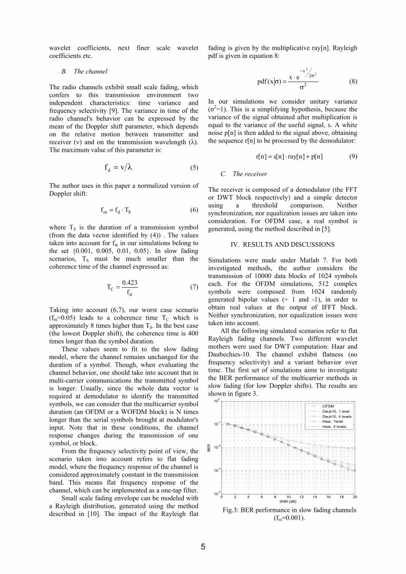
All the following simulated scenarios refer to flat Rayleigh fading channels. Two different wavelet mothers were used for DWT computation: Haar and Daubechies-10. The channel exhibit flatness (no frequency selectivity) and a variant behavior over time. The first set of simulations aims to investigate the BER performance of the multicarrier methods in slow fading (for low Doppler shifts). The results are shown in figure 3.
0 2 4 6 8 10 12 14 16 18 2010-4
10-3
10-2
10-1
100
SNR [dB]
BE
R
:OFDM:Daub10, 1 level:Daub10, 4 levels:Haar, 1level:Haar, 4 levels
Fig.3: BER performance in slow fading channels (fm=0.001).
5
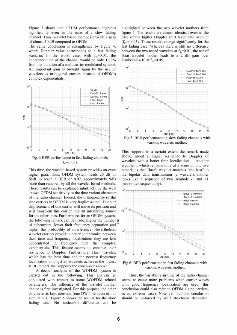
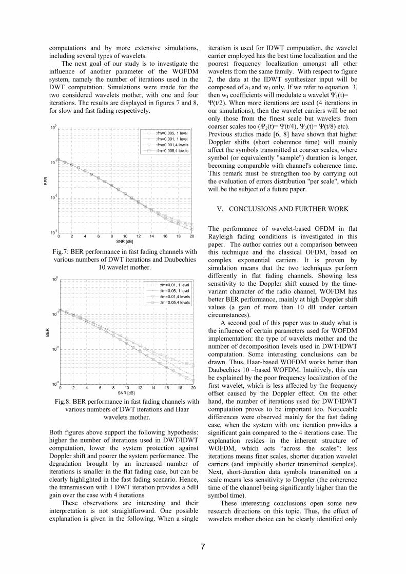
Figure 3 shows that OFDM performance degrades significantly even in the case of a slow fading channel. Thus, wavelet based methods provide a gain of almost 10 dB compared to OFDM. The same conclusion is strengthened by figure 4, where Doppler value corresponds to a fast fading scenario. In the worst case, with fm=0.05, the coherence time of the channel would be only 1.62% from the duration of a multicarrier modulated symbol. An important gain is brought again by the use of wavelets as orthogonal carriers instead of OFDM's complex exponentials. This time, the wavelet-based system provides an even higher gain. Thus, OFDM system needs 20 dB of SNR to reach a BER of 0.02, approximately 9dB more than required by all the wavelet-based methods. These results can be explained intuitively by the well known OFDM sensitivity to the time variant character of the radio channel. Indeed, the orthogonality of the sine carriers in OFDM is very fragile: a small Doppler displacement of one carrier will move its position and will transform this carrier into an interfering source for the other ones. Furthermore, for an OFDM system, the following remark can be made: higher the number of subcarriers, lower their frequency separation and higher the probability of interference. Nevertheless, wavelet carriers provide a better compromise between their time and frequency localization: they are less concentrated in frequency than the complex exponentials. This feature seems to enhance their resilience to Doppler. Furthermore, Haar wavelet, which has the best time and the poorest frequency localization amongst all wavelets achieves the lowest BER, remark that supports the conclusions above. A deeper analysis of the WOFDM system is carried out in the following. This analysis is conducted with respect to some WOFDM related parameters. The influence of the wavelet mother choice is first investigated. For this purpose, the other parameter is kept constant (one DWT iteration in our simulations). Figure 5 shows the results for the slow fading case. No noticeable difference can be
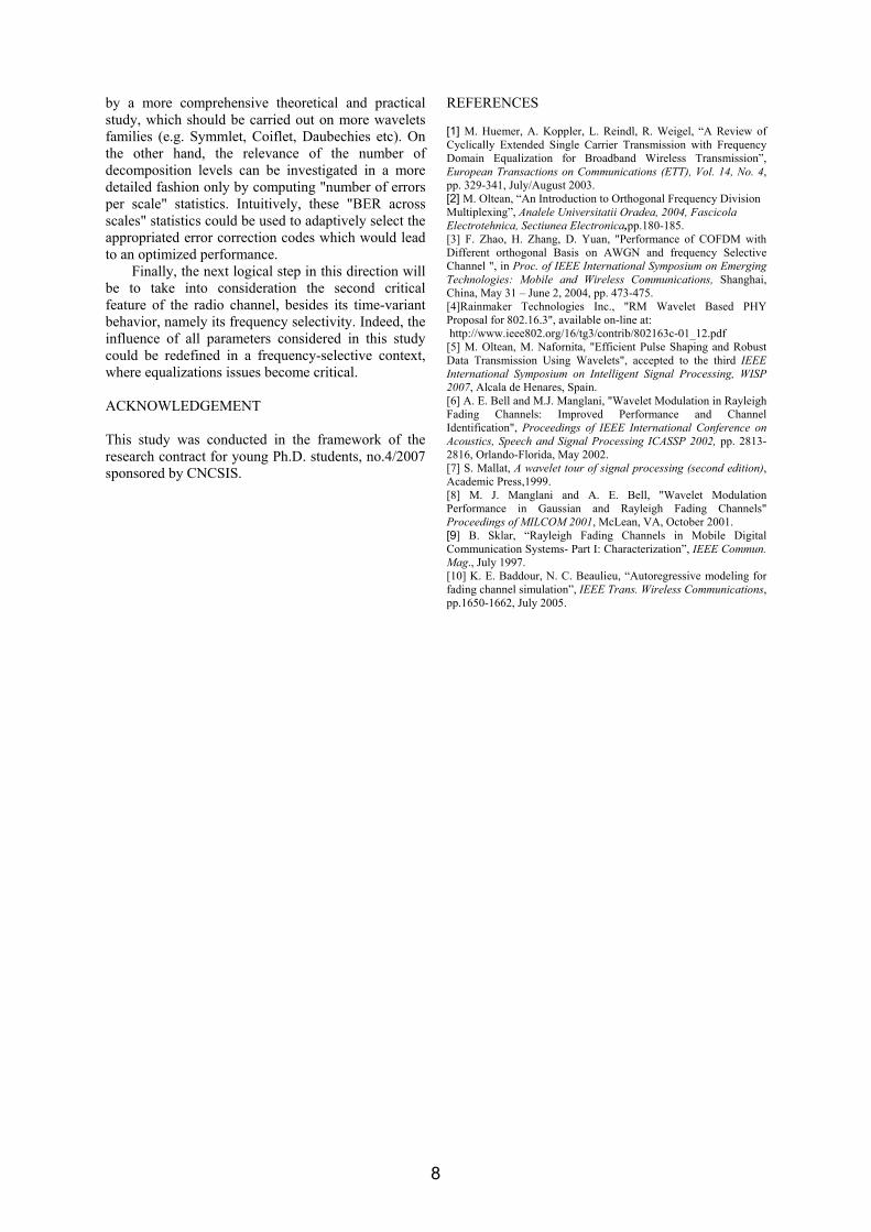
highlighted between the two wavelet mothers from figure 5. The results are almost identical even in the case of the higher Doppler shift taken into account (fm=0.005). These results change significantly for the fast fading case. Whereas there is still no difference between the two tested wavelets at fm=0.01, the use of Haar wavelet mother leads to a 2 dB gain over Daubechies-10 at fm=0.05. This supports to a certain extent the remark made above, about a higher resilience to Doppler of wavelets with a better time localization. Another argument, which remains only at a stage of intuitive remark, is that Haar's wavelet matches "the best" to the bipolar data transmission (a wavelet's mother looks like a sequence of two symbols -1 and +1 transmitted sequentially).
Thus, the variability in time of the radio channel seems to cause more problems when carrier waves with good frequency localization are used (this conclusion could also refer to OFDM’s sine carriers, as an extreme case). Note yet that this conclusion should be enforced by well structured theoretical
0 2 4 6 8 10 12 14 16 18 2010-3
10-2
10-1
100
SNR [dB]
BE
R
:OFDM:Daub10, 1 level:Daub10, 4 levels:Haar, 1level:Haar, 4 levels
Fig.4: BER performance in fast fading channels (fm=0.05).
0 2 4 6 8 10 12 14 16 18 2010-3
10-2
10-1
100
SNR [dB]
BE
R
:Daub10, fm=0.005:Daub10, fm=0.001:Haar, fm=0.005:Haar, fm=0.001
Fig.5: BER performance in slow fading channels with various wavelets mother.
0 2 4 6 8 10 12 14 16 18 2010-3
10-2
10-1
100
SNR [dB]
BE
R
:Daub10, fm=0.01:Daub10, fm=0.05:Haar, fm=0.01:Haar, fm=0.05
Fig.6: BER performance in fast fading channels with various wavelets mother.
6
computations and by more extensive simulations, including several types of wavelets.
The next goal of our study is to investigate the influence of another parameter of the WOFDM system, namely the number of iterations used in the DWT computation. Simulations were made for the two considered wavelets mother, with one and four iterations. The results are displayed in figures 7 and 8, for slow and fast fading respectively.
Both figures above support the following hypothesis: higher the number of iterations used in DWT/IDWT computation, lower the system protection against Doppler shift and poorer the system performance. The degradation brought by an increased number of iterations is smaller in the flat fading case, but can be clearly highlighted in the fast fading scenario. Hence, the transmission with 1 DWT iteration provides a 5dB gain over the case with 4 iterations
These observations are interesting and their interpretation is not straightforward. One possible explanation is given in the following. When a single
iteration is used for IDWT computation, the wavelet carrier employed has the best time localization and the poorest frequency localization amongst all other wavelets from the same family. With respect to figure 2, the data at the IDWT synthesizer input will be composed of aJ and wJ only. If we refer to equation 3, then wJ coefficients will modulate a wavelet Ψ1(t)= Ψ(t/2). When more iterations are used (4 iterations in our simulations), then the wavelet carriers will be not only those from the finest scale but wavelets from coarser scales too (Ψ2(t)= Ψ(t/4), Ψ3(t)= Ψ(t/8) etc). Previous studies made [6, 8] have shown that higher Doppler shifts (short coherence time) will mainly affect the symbols transmitted at coarser scales, where symbol (or equivalently "sample") duration is longer, becoming comparable with channel's coherence time. This remark must be strengthen too by carrying out the evaluation of errors distribution "per scale", which will be the subject of a future paper.
V. CONCLUSIONS AND FURTHER WORK
The performance of wavelet-based OFDM in flat Rayleigh fading conditions is investigated in this paper. The author carries out a comparison between this technique and the classical OFDM, based on complex exponential carriers. It is proven by simulation means that the two techniques perform differently in flat fading channels. Showing less sensitivity to the Doppler shift caused by the time-variant character of the radio channel, WOFDM has better BER performance, mainly at high Doppler shift values (a gain of more than 10 dB under certain circumstances). A second goal of this paper was to study what is the influence of certain parameters used for WOFDM implementation: the type of wavelets mother and the number of decomposition levels used in DWT/IDWT computation. Some interesting conclusions can be drawn. Thus, Haar-based WOFDM works better than Daubechies 10 –based WOFDM. Intuitively, this can be explained by the poor frequency localization of the first wavelet, which is less affected by the frequency offset caused by the Doppler effect. On the other hand, the number of iterations used for DWT/IDWT computation proves to be important too. Noticeable differences were observed mainly for the fast fading case, when the system with one iteration provides a significant gain compared to the 4 iterations case. The explanation resides in the inherent structure of WOFDM, which acts “across the scales”: less iterations means finer scales, shorter duration wavelet carriers (and implicitly shorter transmitted samples). Next, short-duration data symbols transmitted on a scale means less sensitivity to Doppler (the coherence time of the channel being significantly higher than the symbol time). These interesting conclusions open some new research directions on this topic. Thus, the effect of wavelets mother choice can be clearly identified only
0 2 4 6 8 10 12 14 16 18 2010-3
10-2
10-1
100
SNR [dB]
BE
R
:fm=0.005, 1 level:fm=0.001, 1 level:fm=0.001,4 levels:fm=0.005,4 levels
Fig.7: BER performance in fast fading channels with various numbers of DWT iterations and Daubechies
10 wavelet mother.
0 2 4 6 8 10 12 14 16 18 2010
-3
10-2
10-1
100
SNR [dB]
BE
R
:fm=0.01, 1 level:fm=0.05, 1 level:fm=0.01,4 levels:fm=0.05,4 levels
Fig.8: BER performance in fast fading channels with various numbers of DWT iterations and Haar
wavelets mother.
7
by a more comprehensive theoretical and practical study, which should be carried out on more wavelets families (e.g. Symmlet, Coiflet, Daubechies etc). On the other hand, the relevance of the number of decomposition levels can be investigated in a more detailed fashion only by computing "number of errors per scale" statistics. Intuitively, these "BER across scales" statistics could be used to adaptively select the appropriated error correction codes which would lead to an optimized performance. Finally, the next logical step in this direction will be to take into consideration the second critical feature of the radio channel, besides its time-variant behavior, namely its frequency selectivity. Indeed, the influence of all parameters considered in this study could be redefined in a frequency-selective context, where equalizations issues become critical. ACKNOWLEDGEMENT This study was conducted in the framework of the research contract for young Ph.D. students, no.4/2007 sponsored by CNCSIS.
REFERENCES [1] M. Huemer, A. Koppler, L. Reindl, R. Weigel, “A Review of Cyclically Extended Single Carrier Transmission with Frequency Domain Equalization for Broadband Wireless Transmission”, European Transactions on Communications (ETT), Vol. 14, No. 4, pp. 329-341, July/August 2003. [2] M. Oltean, “An Introduction to Orthogonal Frequency Division Multiplexing”, Analele Universitatii Oradea, 2004, Fascicola Electrotehnica, Sectiunea Electronica,pp.180-185. [3] F. Zhao, H. Zhang, D. Yuan, "Performance of COFDM with Different orthogonal Basis on AWGN and frequency Selective Channel ", in Proc. of IEEE International Symposium on Emerging Technologies: Mobile and Wireless Communications, Shanghai, China, May 31 – June 2, 2004, pp. 473-475. [4]Rainmaker Technologies Inc., "RM Wavelet Based PHY Proposal for 802.16.3", available on-line at: http://www.ieee802.org/16/tg3/contrib/802163c-01_12.pdf [5] M. Oltean, M. Nafornita, "Efficient Pulse Shaping and Robust Data Transmission Using Wavelets", accepted to the third IEEE International Symposium on Intelligent Signal Processing, WISP 2007, Alcala de Henares, Spain. [6] A. E. Bell and M.J. Manglani, "Wavelet Modulation in Rayleigh Fading Channels: Improved Performance and Channel Identification", Proceedings of IEEE International Conference on Acoustics, Speech and Signal Processing ICASSP 2002, pp. 2813-2816, Orlando-Florida, May 2002. [7] S. Mallat, A wavelet tour of signal processing (second edition), Academic Press,1999. [8] M. J. Manglani and A. E. Bell, "Wavelet Modulation Performance in Gaussian and Rayleigh Fading Channels" Proceedings of MILCOM 2001, McLean, VA, October 2001. [9] B. Sklar, “Rayleigh Fading Channels in Mobile Digital Communication Systems- Part I: Characterization”, IEEE Commun. Mag., July 1997. [10] K. E. Baddour, N. C. Beaulieu, “Autoregressive modeling for fading channel simulation”, IEEE Trans. Wireless Communications, pp.1650-1662, July 2005.
8
Buletinul Ştiinţific al Universităţii "Politehnica" din Timişoara __________________________________________________________________________________________________________________ Seria ELECTRONICĂ şi TELECOMUNICAŢII_____________________ _________________ TRANSACTIONS on ELECTRONICS and COMMUNICATIONS____________
Tom 52(66), Fascicola 2, 2007
Parametric Analysis and Spectral Whitening of Signals Generated by Leaks in Water Pipes
Raul Ionel1 Alimpie Ignea2
1 Faculty of Electronics and Telecommunications, Measurement and Optical Electronics Dept. Bd. V. Parvan 2, 300223 Timisoara, Romania, e-mail [email protected] 2 Faculty of Electronics and Telecommunications, Measurement and Optical Electronics Dept. Bd. V. Parvan 2, 300223 Timisoara, Romania, e-mail [email protected]
Abstract – This paper presents a way to determine the best modeling algorithms for working with signals generated by water pipe leaks. Three methods of parametric modeling are presented in this paper: auto-regressive modeling AR, moving average MA modeling and auto-regressive – moving average ARMA modeling. From these methods, the auto-regressinve modeling is the best one for analysing signal sequences from water pipe leaks. A special MATLAB Toolbox was used in order to work with the signals and the parametric models. The name of the Toolbox is ARMASA. Several programs were written in order to work with ARMASA functions and with the leak signals. The influence of signal length and number of estimation coefficients, are studied in order to show which parametric modeling method works best with signals generated by pipe leaks. The conclusion is that for these type of signals, the AR autoregressive model is the optimal solution. With the help of the obtained spectral distribution values, we can further analyze the signals in order to find with precision the position of the leaks. After the exact choice of a parametric modeling algorithm, in ths case the AR model, we are able to see the benefits of this choice when dealing with spectral analisys. Signal whitening can be used in order to improve the quality of the Cross Correlation Function (CCF). Keywords - parametric modeling, water pipes, leak detection, leak location, MATLAB, ARMASA Toolbox, Cross Correlation Function, signal whitening.
I. INTRODUCTION
The flow of water trough a pipe generates specific
auditive (noise) signals. If the pipe has leakage points or other faults, then we face problems of liquid loss. These problems must be solved, by locating with precision, the position of the leaks. The possition of the leak, must be found with the highest accuracy. When dealing with pipes that are very long (measuring kilometers), the leaks must be located with an error of a few meters (less than 5 meters).
The analysis of data sequences (noise signals from pipe leaks) by means of parametric modeling is a modern alternative which can be used in this domain. With the help of improved software applications and hardware possibilities, we are allowed to use applications based on parametric modeling (which involve lots of calculations) and to continuously monitor time varying processes.
As mentioned in literature, the use of non-parametric methods of signal processing is more suitable for periodical signals. When dealing with random signals (signals from water pipe leaks), the use of non-parametric methods is considered “quick and dirty” [3].
A more accurate approach would be the use of parametric methods. We are interested in determining the spectral distribution of the signals and also the ease and the calculus volume which is involved. Furthermore, we are interested in having a program that works with the signals in an automatic way. One should be able to determine the spectral distribution of the signals, with the help of automated parametric modeling methods (automated application), without much knowledge about signal processing techniques.
ARMASA is a collection of MATLAB programs that helps the user perform signal processing algorithms in an automated manner. Some of the offered features involve automatic spectral analysis.
The use of parametric modeling methods (AR, MA, ARMA) can turn the application for signal analysis into an automated program.
After determining which method is best for analyzing the signals generated by water leaks, we can proceed with the calculation of the CCF.
II. THE INSTALLATION
An experimental pipes installation is presented in the
following image. With the help of this installation, leak signals were acquired and analyzed.
Piezoelectric sensors are placed on both sides of the simulated Leak A. The purpose of the sensors is to simultaneously acquire pairs of signals generated when water comes out of the pipe trough the simulated leak. When the faucet is opened, water came out of the pipe. Noise signals are sent from the simulated leak to the sensors trough the pipe material (metal or PVC) and trough the liquid that flows inside the pipe.
The sensors were placed, at about the same distances, on a straight part of the pipe in order to avoid possible perturbations which appear at pipe elbows.
9
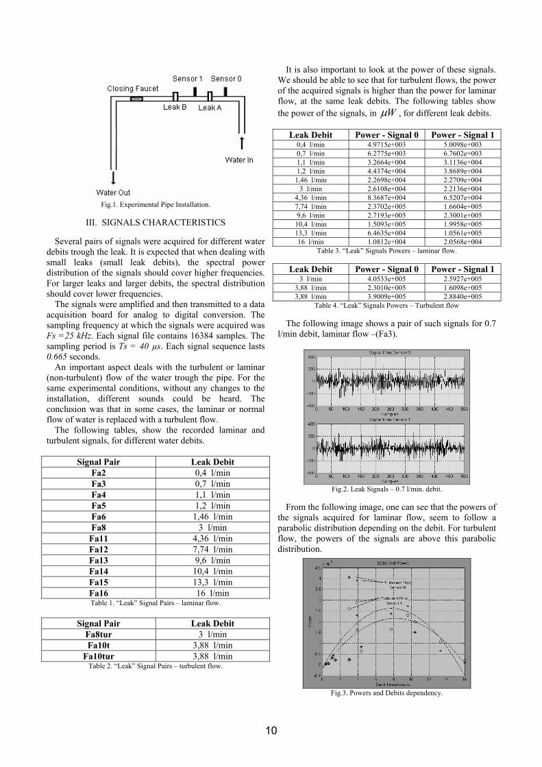
Fig.1. Experimental Pipe Installation.
III. SIGNALS CHARACTERISTICS
Several pairs of signals were acquired for different water
debits trough the leak. It is expected that when dealing with small leaks (small leak debits), the spectral power distribution of the signals should cover higher frequencies. For larger leaks and larger debits, the spectral distribution should cover lower frequencies.
The signals were amplified and then transmitted to a data acquisition board for analog to digital conversion. The sampling frequency at which the signals were acquired was Fs =25 kHz. Each signal file contains 16384 samples. The sampling period is Ts = 40 µs. Each signal sequence lasts 0.665 seconds.
An important aspect deals with the turbulent or laminar (non-turbulent) flow of the water trough the pipe. For the same experimental conditions, without any changes to the installation, different sounds could be heard. The conclusion was that in some cases, the laminar or normal flow of water is replaced with a turbulent flow.
The following tables, show the recorded laminar and turbulent signals, for different water debits.
Signal Pair Leak Debit
Fa2 0,4 l/min Fa3 0,7 l/min Fa4 1,1 l/min Fa5 1,2 l/min Fa6 1,46 l/min Fa8 3 l/min
Fa11 4,36 l/min Fa12 7,74 l/min Fa13 9,6 l/min Fa14 10,4 l/min Fa15 13,3 l/min Fa16 16 l/min Table 1. “Leak” Signal Pairs – laminar flow.
Signal Pair Leak Debit
Fa8tur 3 l/min Fa10t 3,88 l/min
Fa10tur 3,88 l/min Table 2. “Leak” Signal Pairs – turbulent flow.
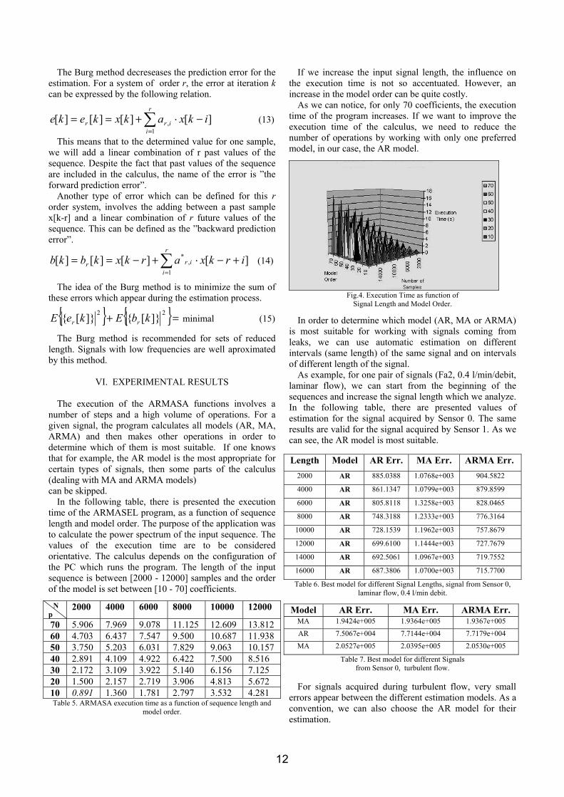
It is also important to look at the power of these signals. We should be able to see that for turbulent flows, the power of the acquired signals is higher than the power for laminar flow, at the same leak debits. The following tables show the power of the signals, in Wµ , for different leak debits.
Leak Debit Power - Signal 0 Power - Signal 1
0,4 l/min 4.9715e+003 5.0098e+003 0,7 l/min 6.2775e+003 6.7602e+003 1,1 l/min 3.2664e+004 3.1136e+004 1,2 l/min 4.4374e+004 3.8689e+004
1,46 l/min 2.2698e+004 2.2709e+004 3 l/min 2.6108e+004 2.2136e+004
4,36 l/min 8.3687e+004 6.5207e+004 7,74 l/min 2.3702e+005 1.6604e+005 9,6 l/min 2.7193e+005 2.3001e+005
10,4 l/min 1.5093e+005 1.9958e+005 13,3 l/min 6.4635e+004 1.0561e+005 16 l/min 1.0812e+004 2.0568e+004
Table 3. “Leak” Signals Powers – laminar flow.
Leak Debit Power - Signal 0 Power - Signal 1 3 l/min 4.0533e+005 2.5927e+005
3,88 l/min 2.3010e+005 1.6098e+005 3,88 l/min 3.9009e+005 2.8840e+005
Table 4. “Leak” Signals Powers – Turbulent flow
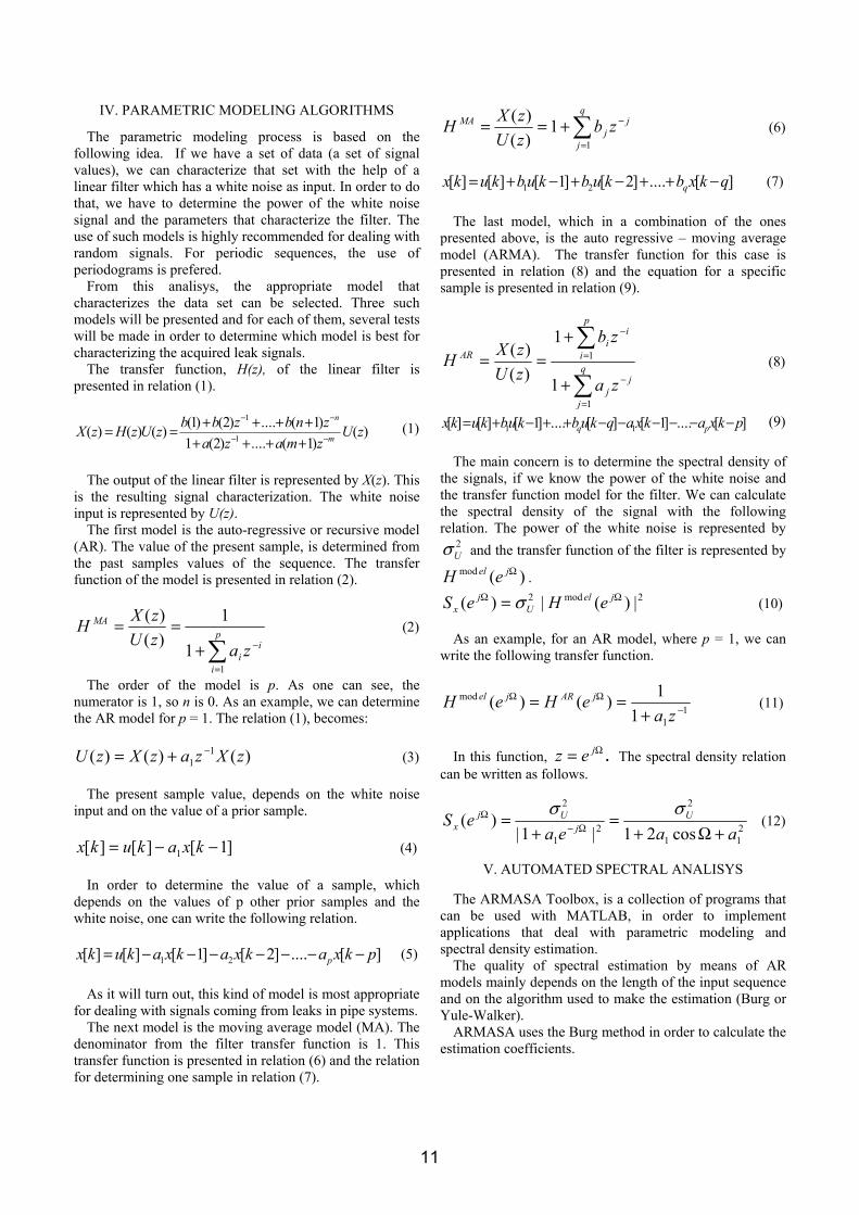
The following image shows a pair of such signals for 0.7 l/min debit, laminar flow –(Fa3).
Fig.2. Leak Signals – 0.7 l/min. debit.
From the following image, one can see that the powers of
the signals acquired for laminar flow, seem to follow a parabolic distribution depending on the debit. For turbulent flow, the powers of the signals are above this parabolic distribution.
Fig.3. Powers and Debits dependency.
10
IV. PARAMETRIC MODELING ALGORITHMS
The parametric modeling process is based on the following idea. If we have a set of data (a set of signal values), we can characterize that set with the help of a linear filter which has a white noise as input. In order to do that, we have to determine the power of the white noise signal and the parameters that characterize the filter. The use of such models is highly recommended for dealing with random signals. For periodic sequences, the use of periodograms is prefered.
From this analisys, the appropriate model that characterizes the data set can be selected. Three such models will be presented and for each of them, several tests will be made in order to determine which model is best for characterizing the acquired leak signals.
The transfer function, H(z), of the linear filter is presented in relation (1).
)()1(....)2(1)1(....)2()1()()()( 1
1
zUzmazaznbzbbzUzHzX m
n
−−
−−
++++++++== (1)
The output of the linear filter is represented by X(z). This
is the resulting signal characterization. The white noise input is represented by U(z).
The first model is the auto-regressive or recursive model (AR). The value of the present sample, is determined from the past samples values of the sequence. The transfer function of the model is presented in relation (2).
∑=
−+== p
i
ii
MA
zazUzXH
11
1)()(
(2)
The order of the model is p. As one can see, the numerator is 1, so n is 0. As an example, we can determine the AR model for p = 1. The relation (1), becomes:
)()()( 11 zXzazXzU −+= (3)
The present sample value, depends on the white noise
input and on the value of a prior sample.
]1[][][ 1 −−= kxakukx (4)
In order to determine the value of a sample, which depends on the values of p other prior samples and the white noise, one can write the following relation.
][....]2[]1[][][ 21 pkxakxakxakukx p −−−−−−−= (5)
As it will turn out, this kind of model is most appropriate for dealing with signals coming from leaks in pipe systems.
The next model is the moving average model (MA). The denominator from the filter transfer function is 1. This transfer function is presented in relation (6) and the relation for determining one sample in relation (7).
∑=
−+==q
j
jj
MA zbzUzXH
1
1)()(
(6)
][....]2[]1[][][ 21 qkxbkubkubkukx q −++−+−+= (7)
The last model, which in a combination of the ones
presented above, is the auto regressive – moving average model (ARMA). The transfer function for this case is presented in relation (8) and the equation for a specific sample is presented in relation (9).
∑
∑
=
−
=
−
+
+== q
j
jj
p
i
ii
AR
za
zb
zUzXH
1
1
1
1
)()(
(8)
][....]1[][....]1[][][ 11 pkxakxaqkubkubkukx pq −−−−−−++−+= (9)
The main concern is to determine the spectral density of the signals, if we know the power of the white noise and the transfer function model for the filter. We can calculate the spectral density of the signal with the following relation. The power of the white noise is represented by
2Uσ and the transfer function of the filter is represented by
)(mod Ωjel eH . 2mod2 |)(|)( ΩΩ = jel
Uj
x eHeS σ (10)
As an example, for an AR model, where p = 1, we can write the following transfer function.
11
mod
11)()( −
ΩΩ
+==
zaeHeH jARjel (11)
In this function, Ω= jez . The spectral density relation can be written as follows.
211
2
21
2
cos21|1|)(
aaeaeS U
jUj
x +Ω+=
+= Ω−
Ω σσ (12)
V. AUTOMATED SPECTRAL ANALISYS
The ARMASA Toolbox, is a collection of programs that
can be used with MATLAB, in order to implement applications that deal with parametric modeling and spectral density estimation.
The quality of spectral estimation by means of AR models mainly depends on the length of the input sequence and on the algorithm used to make the estimation (Burg or Yule-Walker).
ARMASA uses the Burg method in order to calculate the estimation coefficients.
11
The Burg method decreseases the prediction error for the
estimation. For a system of order r, the error at iteration k can be expressed by the following relation.
∑=
−⋅+==r
iirr ikxakxkeke
1, ][][][][ (13)
This means that to the determined value for one sample, we will add a linear combination of r past values of the sequence. Despite the fact that past values of the sequence are included in the calculus, the name of the error is ”the forward prediction error”.
Another type of error which can be defined for this r order system, involves the adding between a past sample x[k-r] and a linear combination of r future values of the sequence. This can be defined as the ”backward prediction error”.
∑=
+−⋅+−==r
iirr irkxarkxkbkb
1,
* ][][][][ (14)
The idea of the Burg method is to minimize the sum of these errors which appear during the estimation process.
=+ 22 ][][ kbEkeE rr minimal (15)
The Burg method is recommended for sets of reduced length. Signals with low frequencies are well aproximated by this method.
VI. EXPERIMENTAL RESULTS
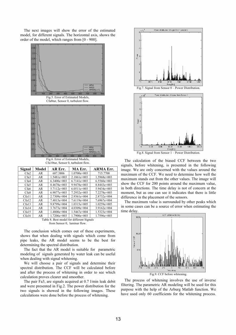
The execution of the ARMASA functions involves a number of steps and a high volume of operations. For a given signal, the program calculates all models (AR, MA, ARMA) and then makes other operations in order to determine which of them is most suitable. If one knows that for example, the AR model is the most appropriate for certain types of signals, then some parts of the calculus (dealing with MA and ARMA models) can be skipped.
In the following table, there is presented the execution time of the ARMASEL program, as a function of sequence length and model order. The purpose of the application was to calculate the power spectrum of the input sequence. The values of the execution time are to be considered orientative. The calculus depends on the configuration of the PC which runs the program. The length of the input sequence is between [2000 - 12000] samples and the order of the model is set between [10 - 70] coefficients. N p
2000 4000 6000 8000 10000 12000
70 5.906 7.969 9.078 11.125 12.609 13.812 60 4.703 6.437 7.547 9.500 10.687 11.938 50 3.750 5.203 6.031 7.829 9.063 10.157 40 2.891 4.109 4.922 6.422 7.500 8.516 30 2.172 3.109 3.922 5.140 6.156 7.125 20 1.500 2.157 2.719 3.906 4.813 5.672 10 0.891 1.360 1.781 2.797 3.532 4.281 Table 5. ARMASA execution time as a function of sequence length and
model order.
If we increase the input signal length, the influence on the execution time is not so accentuated. However, an increase in the model order can be quite costly.
As we can notice, for only 70 coefficients, the execution time of the program increases. If we want to improve the execution time of the calculus, we need to reduce the number of operations by working with only one preferred model, in our case, the AR model.
Fig.4. Execution Time as function of
Signal Length and Model Order.
In order to determine which model (AR, MA or ARMA) is most suitable for working with signals coming from leaks, we can use automatic estimation on different intervals (same length) of the same signal and on intervals of different length of the signal.
As example, for one pair of signals (Fa2, 0.4 l/min/debit, laminar flow), we can start from the beginning of the sequences and increase the signal length which we analyze. In the following table, there are presented values of estimation for the signal acquired by Sensor 0. The same results are valid for the signal acquired by Sensor 1. As we can see, the AR model is most suitable.
Length Model AR Err. MA Err. ARMA Err.
2000 AR 885.0388 1.0768e+003 904.5822
4000 AR 861.1347 1.0799e+003 879.8599
6000 AR 805.8118 1.3258e+003 828.0465
8000 AR 748.3188 1.2333e+003 776.3164
10000 AR 728.1539 1.1962e+003 757.8679
12000 AR 699.6100 1.1444e+003 727.7679
14000 AR 692.5061 1.0967e+003 719.7552
16000 AR 687.3806 1.0700e+003 715.7700
Table 6. Best model for different Signal Lengths, signal from Sensor 0, laminar flow, 0.4 l/min debit.
Model AR Err. MA Err. ARMA Err. MA 1.9424e+005 1.9364e+005 1.9367e+005
AR 7.5067e+004 7.7144e+004 7.7179e+004
MA 2.0527e+005 2.0395e+005 2.0530e+005
Table 7. Best model for different Signals from Sensor 0, turbulent flow.
For signals acquired during turbulent flow, very small
errors appear between the different estimation models. As a convention, we can also choose the AR model for their estimation.
12
The next images will show the error of the estimated
model, for different signals. The horizontal axis, shows the order of the model, which ranges from [0 - 900].
Fig.5. Error of Estimated Models, Cfa8tur, Sensor 0, turbulent flow.
Fig.6. Error of Estimated Models, Cfa10tur, Sensor 0, turbulent flow.
Signal Model AR Err. MA Err. ARMA Err. Cfa2 AR 687.3806 1.0700e+003 715.7700 Cfa3 AR 1.5481e+003 2.1861e+003 1.5968e+003 Cfa4 AR 6.3400e+003 6.7141e+003 6.5560e+003 Cfa5 AR 8.4678e+003 9.9478e+003 8.8443e+003 Cfa6 AR 5.7112e+003 6.0511e+003 5.9434e+003 Cfa8 AR 6.9877e+003 7.2932e+003 7.2278e+003
Cfa11 AR 2.7309e+004 2.9361e+004 2.8732e+004 Cfa12 AR 7.4015e+004 7.6119e+004 7.6967e+004 Cfa13 AR 9.8799e+004 1.0315e+005 1.0259e+005 Cfa14 AR 3.7673e+004 4.0309e+004 3.9162e+004 Cfa15 AR 1.4800e+004 1.5467e+004 1.5323e+004 Cfa16 AR 1.7206e+003 1.7900e+003 1.7596e+003
Table 8. Best model for different Signals from Sensor 0, laminar flow.
The conclusion which comes out of these experiments,
shows that when dealing with signals which come from pipe leaks, the AR model seems to be the best for determining the spectral distribution.
The fact that the AR model is suitable for parametric modeling of signals generated by water leak can be useful when dealing with signal whitening.
We will choose a pair of signals and determine their spectral distribution. The CCF will be calculated before and after the process of whitening in order to see which calculation proves clearer and smoother.
The pair Fa3, are signals acquired at 0.7 l/min leak debit and were presented in Fig.2. The power distribution for the two signals is showed in the following images. These calculations were done before the process of whitening.
Fig.7. Signal from Sensor 0 – Power Distribution.
Fig.8. Signal from Sensor 1 – Power Distribution.
The calculation of the biased CCF between the two
signals, before whitening, is presented in the following image. We are only concerned with the values around the maximum of the CCF. We need to determine how well the maximum stands out from the other values. The image will show the CCF for 200 points around the maximum value, in both directions. The time delay is not of concern at the moment, but as one can see it indicates that there is little difference in the placement of the sensors.
The maximum value is surrounded by other peaks which in some cases can be a source of error when estimating the time delay.
Fig.9. CCF before whitening.
The process of whitening involves the use of inverse filtering. The parametric AR modeling will be used for this purpose with the help of the Arburg Matlab function. We have used only 60 coefficients for the whitening process.
13
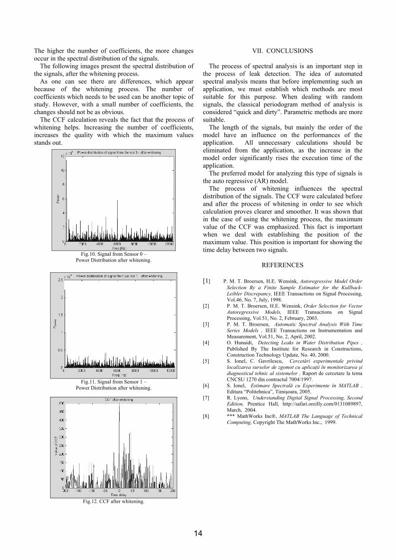
The higher the number of coefficients, the more changes occur in the spectral distribution of the signals.
The following images present the spectral distribution of the signals, after the whitening process.
As one can see there are differences, which appear because of the whitening process. The number of coefficients which needs to be used can be another topic of study. However, with a small number of coefficients, the changes should not be as obvious.
The CCF calculation reveals the fact that the process of whitening helps. Increasing the number of coefficients, increases the quality with which the maximum values stands out.
Fig.10. Signal from Sensor 0 –
Power Distribution after whitening.
Fig.11. Signal from Sensor 1 –
Power Distribution after whitening.
Fig.12. CCF after whitening.
VII. CONCLUSIONS
The process of spectral analysis is an important step in the process of leak detection. The idea of automated spectral analysis means that before implementing such an application, we must establish which methods are most suitable for this purpose. When dealing with random signals, the classical periodogram method of analysis is considered “quick and dirty”. Parametric methods are more suitable.
The length of the signals, but mainly the order of the model have an influence on the performances of the application. All unnecessary calculations should be eliminated from the application, as the increase in the model order significantly rises the execution time of the application.
The preferred model for analyzing this type of signals is the auto regressive (AR) model.
The process of whitening influences the spectral distribution of the signals. The CCF were calculated before and after the process of whitening in order to see which calculation proves clearer and smoother. It was shown that in the case of using the whitening process, the maximum value of the CCF was emphasized. This fact is important when we deal with establishing the position of the maximum value. This position is important for showing the time delay between two signals.
REFERENCES [1] P. M. T. Broersen, H.E. Wensink, Autoregressive Model Order
Selection By a Finite Sample Estimator for the Kullback-Leibler Discrepancy, IEEE Transactions on Signal Processing, Vol.46, No. 7, July, 1998.
[2] P. M. T. Broersen, H.E. Wensink, Order Selection for Vector Autoregressive Models, IEEE Transactions on Signal Processing, Vol.51, No. 2, February, 2003.
[3] P. M. T. Broersen, Automatic Spectral Analysis With Time Series Models , IEEE Transactions on Instrumentation and Measurement, Vol.51, No. 2, April, 2002.
[4] O. Hunaidi, Detecting Leaks in Water Distribution Pipes , Published By The Institute for Research in Constructions, Construction Technology Update, No. 40, 2000.
[5] S. Ionel, C. Gavrilescu, Cercetări experimentale privind localizarea surselor de zgomot cu aplicaţii în monitorizarea şi diagnosticul tehnic al sistemelor , Raport de cercetare la tema CNCSU 1270 din contractul 7004/1997.
[6] S. Ionel, Estimare Spectrală cu Experimente în MATLAB , Editura “Politehnica”, Timişoara, 2005.
[7] R. Lyons, Understanding Digital Signal Processing, Second Edition, Prentice Hall, http://safari.oreilly.com/0131089897, March, 2004.
[8] *** MathWorks Inc®, MATLAB The Language of Technical Computing, Copyright The MathWorks Inc., 1999.
14
Buletinul Ştiinţific al Universităţii "Politehnica" din Timişoara
Seria ELECTRONICĂ şi TELECOMUNICAŢII TRANSACTIONS on ELECTRONICS and COMMUNICATIONS
Tom 52(66), Fascicola 2, 2007
A New Point Matching Method for Image Registration Using Pixel Color Information
Daniela Fuiorea1
1 Faculty of Electronics and Telecommunications, Communications Dept. Bd. V. Parvan 2, 300223 Timisoara, Romania, e-mail [email protected]
Abstract –The solution investigated in this paper is based on a mean shift estimator for feature point matching. We propose a new method based on pixel color information, to reject possible mismatches between the pairs of points, in order to simultaneously increase the estimation accuracy and reduce the processing time. The method is part of an image processing tool developed for video sensor localization in Wireless Sensor Networks. The solution is analyzed and tested for performance evaluation. Keywords: mean shift estimator, image registration, video sensor localization
I. INTRODUCTION
To accomplish a registration task, two or more images, of the same scene taken at different times, from different viewpoints, and/or by different sensors, are given with the purpose of overlaying them under an optimal transformation that has to be found. This problem is an interest in many domains, like remote sensing, computer vision and medical imaging [2]. Our interest in the problem stems for a wireless sensor network (WSN). In this paper a registration technique is applied to a video sensor network which is composed of distributed camera devices capable of processing and fusing images of a scene from a variety of viewpoints into some form, more useful than the individual images. There are two tasks which are needed to be handled during the registration process: feature selection and feature matching. Feature selection can be carried out manually or automatically (with a corner detector). In feature matching there are two problems: the correspondence and the transformation. While solving either without information regarding the other is quite difficult, an interesting fact is that solving for one once, the other is known is much simpler than solving the original, coupled problem. The correspondence between the features can be classified in two categories: future-based and region-based methods. The region based registration is prone to errors generated by segmentation and different color sensitivities of the cameras. To avoid the difficulties mentioned, image point features can be
used instead. This approach has been shown to be more robust with view point, scale and illumination changes, and occlusion. However, the presence of errors is a problem as well, especially in the automatic feature extraction case. One common factor that gives birth to errors is the noise arising from the processes of image acquisition and feature extraction. The presence of noise means that the resulting feature points cannot be exactly matched. Another factor is the existence of outliers, many point features may exist in one point-set that have no corresponding points (homologies) in the other and hence need to be rejected during the matching process. A point future registration algorithm needs to address all these issues. It should be able to solve for the correspondences between two point-sets, reject outliers and determine a good non-rigid transformation that can map one point-set onto the other. In the domain of image registration, many authors have tried and succeed to resolve the problem of point extraction and matching, and also the problem of outliers. For example, Hsieh et al. [3] proposed a method of feature extraction called feature point extraction using wavelet transforms. By defining a similarity measure metric called crosscorrelation, sets of correct matching pairs between the images were find and the correspondences between the features was established. Their method was an improvement in the sense of efficiency and as well as reliability for the image registration problem. In [4] Chui has developed point matching algorithm for non-rigid registration which is good for on-rigid registration. The algorithm utilizes the softassign, deterministic annealing, the thin-plate spline for the spatial mapping and outlier rejection to solve for both the correspondence and mapping parameters. It is based on the notion of one-to-one correspondence, but it is possible to be extend it to the case of many-to-many matching [5], which is the case of dense feature-based registration. In [6] two algorithms are proposed for resolving the point pattern matching problems. One algorithm is
15
using branch and bound search, simple but relatively slow. The second algorithm is called bounded alignment, based on combining branch and bound with computing point alignments to accelerate the search. The algorithm seems to be faster, but being a Monte Carlo algorithm, may fail with some small probability. Another approach recently proposed in Belongie et al. [7] adopts a different strategy. A new shape descriptor, called the “shape context”, is defined for correspondence recovery and shape-based object recognition. For each point chosen, lines are drawn to connect it to all other points. The length as well as the orientation of each line is calculated. The distribution of the length and the orientation for all lines (they are all connected to the first point) are estimated through histogramming. This distribution is used as the shape context for the first point. Basically, the shape context captures the distribution of the relative positions between the currently chosen point and all other points. However, it is unclear how well this algorithm works in a registration context. In [8] the point matching problem for object pose estimation has been turned into a classification problem. Each point in the “training” image is a class. In general, the method usually gives a little fewer matches, and has a little higher outlier rate than SIFT [9], but it is good enough for RANSAC to do the job. The approach in this paper regarding the registration algorithm follows the previous work [1] on registration, in the case of wireless video sensor network. An improvement of feature detection and matching is accomplished with the help of the pixel color. The rest of the paper is organized as follows: the next section describes the previous work, a localization technique using the registration process in the case of Wireless Sensor Networks. Section III analyzes the point matching based on pixel color information. Section IV presents evaluation results on real images. Finally, conclusions of this work are presented in Section V.
II. PREVIOUS WORK
In the previous work [1], a localization technique using the registration process was proposed only in the case of Wireless Sensor Networks based on video sensors. It uses a set of images gathered from all sensor nodes in an after deployment setup-phase and tries to discover matching areas in these images. The features were represented by image points, detected in both images. Ideally, they are spread over the entire image and stable in time during the registration process. The feature matching process was combined with the parameter estimation of the geometrical transform. Two similarity transforms were implemented here, the separate and simultaneous. The approach starts from the system of equations:
1 cos( ) sin( )1 sin( ) cos( )
x x x
y y y
q p tsq p ts
ϕ ϕϕ ϕ
−⎡ ⎤ ⎡ ⎤ ⎡ ⎤⎡ ⎤ ⎡ ⎤= +⎢ ⎥ ⎢ ⎥ ⎢ ⎥⎢ ⎥ ⎢ ⎥⎣ ⎦ ⎣ ⎦⎣ ⎦ ⎣ ⎦ ⎣ ⎦
, (1)
relating the old pixel coordinates ( , )x yp p to the new ones, ( , )x yq q . The four parameters of the transformation can be determined from the correspondence of two pairs of points. A parameter vector [ , , , ] Tp s tx tyϕ= is generated from equation (1), using two pairs of points. Suppose the pairs of points are
1 1 1 1( , ) ( , )x y x yp p q q− and 2 2 2 2( , ) ( , )x y x yp p q q− . The components of the parameter vector are acquired by solving the system of equations obtained after using
1 1 1 1 2 2 2 2( , ),( , ),( , ),( , )x y x y x y x yp p q q p p q q in equation (1) and solving the system of four equations. A meanshift robust estimator is used to find the best estimates from the partial solutions and a final step uses this information to compute video-field overlap between cameras on network sensors. Regarding parameter estimation and the uncertainty of the feature matching process, robust methods have to be used to find the geometrical transform optimally mapping the sets of points detected in a pair of images. A meanshift estimator is used in our work, because it copes well with the outliers in the data set. The results were good, when the overlap between images was high and the feature points stable.
III. POINT MATCHING BASED ON PIXEL COLOR
Previous methods are based on measuring some information extracted from a neighborhood of feature points and to compare them in order to eliminate incompatible matches. The simplest information may be the pixel intensity or color. However, since typical feature points, like corners [], are located in regions with fast changes, slight positioning errors may result in high variation in the neighborhood information. Moreover, scale differences make the problem most severe. The basic idea of our approach is to compare image information extracted from pixels located at mid distance between pairs of points. Most often than not, such points are located in more homogeneous regions and therefore are less affected by the exact positions of the feature points. The median of a line segment is invariant to translation, rotation and rescaling and theoretically the color information in the median points is also invariant to the mentioned transforms. Color information is also very cheap to extract, keeping processing costs to a minimum level. In fact, since the median points are expected to belong to homogeneous area, this information completely characterizes the neighborhood. To asses the proposed approach, we compare it with the traditional approach, based on measurements at the feature points.
16
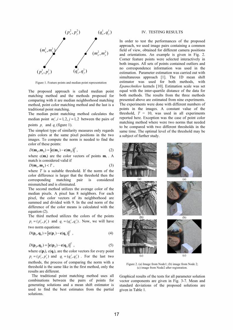
Figure 1. Feature points and median point representation The proposed approach is called median point matching method and the methods proposed for comparing with it are median neighborhood matching method, point color matching method and the last is a traditional point matching. The median point matching method calculates the median point , 1, 2, 1, 2j
im i j= = between the pairs of points ip and iq (figure 1). The simplest type of similarity measures only regards pairs colors at the same pixel positions in the two images. To compute the norm is needed to find the color of these points:
2( ) ( ) ( )D = −1 2 1 2m ,m c m c m , (2) where c(mi) are the color vectors of points mi . A match is considered valid if
( , )D T<1 2m m , (3) where T is a suitable threshold. If the norm of the color difference is larger that the threshold then the corresponding matching pair is considered mismatched and is eliminated. The second method utilizes the average color of the median pixels. A pixel has 8 neighbors. For each pixel, the color vectors of its neighborhood are summed and divided with 9. In the end norm of the difference of the color means is calculated with the equation (2). The third method utilizes the colors of the points
( , )i ii x yp p p= and ( , )j j
i x yq q q= . Now, we will have two norm equations:
21( , ) ( ) ( )D = −1 1 1p q c p c q , (4)
2( ) ( ) ( )D = −2 2 2 2p ,q c p c q , (5)
where c(pi), c(qi), are the color vectors for every point ( , )i i
i x yp p p= and ( , )j ji x yq q q= . For the last two
methods, the process of comparing the norm with a threshold is the same like in the first method, only the results are different.
The traditional point matching method uses all combinations between the pairs of points for generating solutions and a mean shift estimator is used to find the best estimates from the partial solutions.
IV. TESTING RESULTS
In order to test the performances of the proposed approach, we used image pairs containing a common field of view, obtained for different camera positions and orientations. An example is given in Fig. 2. Corner feature points were selected interactively in both images. All sets of points contained outliers and no correspondence information was used in the estimation. Parameter estimation was carried out with simultaneous approach [1]. The 1D mean shift estimator was used for both methods, with Epanechnikov kernels [10]. Estimation scale was set equal with the inter-quartile distance of the data for both methods. The results from the three methods presented above are estimated from nine experiments. The experiments were done with different numbers of points in the images. A constant value of the threshold, T = 10, was used in all experiments reported here. Exception was the case of point color matching method where were two norms that needed to be compared with two different thresholds in the same time. The optimal level of the threshold may be a subject of further study.
(a)
(a)
(b)
(b)
(c)
(c)
Figure 2. (a) Image from Node1; (b) image from Node 2;
(c) image from Node2 after registration. Graphical results of the tests for all parameter solution vector components are given in Fig. 3-7. Mean and standard deviations of the proposed solutions are given in Table 1.
1 1( , )x ym m
1 1( , )x yp p
1 1( , )x yq q 2 2( , )x yp p
1 1( , )x yq q
2 2( , )x ym m
17
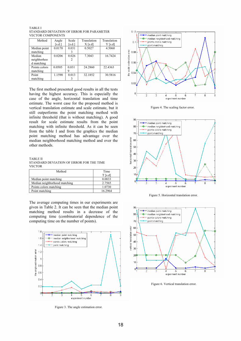
TABLE I STANDARD DEVIATION OF ERROR FOR PARAMETER VECTOR COMPONENTS
Method Angle [s.d.]
Scale [s.d.]
Translation X [s.d]
Translation Y [s.d]
Median point matching
0.0170 0.0313
0.5027 4.5060
Median neighborhood matching
0.0206 0.0262
7.3043 16.7424
Points colors matching
0.0505 0.0319
24.2860 22.4363
Point matching
1.1590 0.0133
32.1852 30.5816
The first method presented good results in all the tests having the highest accuracy. This is especially the case of the angle, horizontal translation and time estimate. The worst case for the proposed method is vertical translation estimate and scale estimate, but it still outperforms the point matching method with infinite threshold (that is without matching). A good result for scale estimate results from the point matching with infinite threshold. As it can be seen from the table I and from the graphics the median point matching method has advantage over the median neighborhood matching method and over the other methods.
TABLE II STANDARD DEVIATION OF ERROR FOR THE TIME VECTOR
Method Time T [s.d]
Median point matching 0.0833 Median neighborhood matching 2.7565 Points colors matching 1.0730 Point matching 16.2964
The average computing times in our experiments are given in Table 2. It can be seen that the median point matching method results in a decrease of the computing time (combinatorial dependence of the computing time on the number of points).
Figure 3. The angle estimation error.
Figure 4. The scaling factor error.
Figure 5. Horizontal translation error.
Figure 6. Vertical translation error.
18
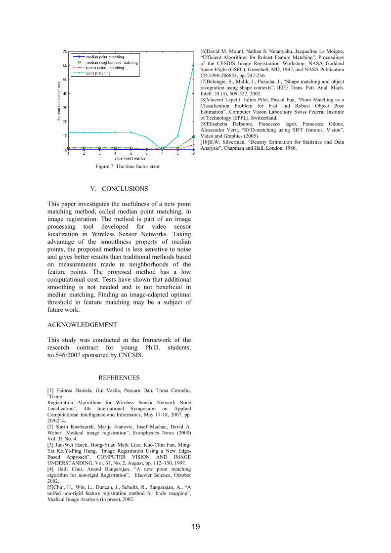
Figure 7. The time factor error
V. CONCLUSIONS This paper investigates the usefulness of a new point matching method, called median point matching, in image registration. The method is part of an image processing tool developed for video sensor localization in Wireless Sensor Networks. Taking advantage of the smoothness property of median points, the proposed method is less sensitive to noise and gives better results than traditional methods based on measurements made in neighborhoods of the feature points. The proposed method has a low computational cost. Tests have shown that additional smoothing is not needed and is not beneficial in median matching. Finding an image-adapted optimal threshold in feature matching may be a subject of future work. ACKNOWLEDGEMENT This study was conducted in the framework of the research contract for young Ph.D. students, no.546/2007 sponsored by CNCSIS.
REFERENCES [1] Fuiorea Daniela, Gui Vasile, Pescaru Dan, Toma Corneliu, ”Using Registration Algorithms for Wireless Sensor Network Node Localization”, 4th International Symposium on Applied Computational Intelligence and Informatics, May 17-18, 2007, pp. 209-214. [2] Karin Kneöaurek, Marija Ivanovic, Josef Machac, David A. Weber, ”Medical image registration”, Europhysics News (2000) Vol. 31 No. 4. [3] Jun-Wei Hsieh, Hong-Yuan Mark Liao, Kuo-Chin Fan, Ming-Tat Ko,Yi-Ping Hung, “Image Registration Using a New Edge-Based Approach”, COMPUTER VISION AND IMAGE UNDERSTANDING, Vol. 67, No. 2, August, pp. 112–130, 1997. [4] Haili Chui, Anand Rangarajan, “A new point matching algorithm for non-rigid Registration”, Elsevier Science, October 2002. [5]Chui, H., Win, L., Duncan, J., Schultz, R., Rangarajan, A., “A unifed non-rigid feature registration method for brain mapping”, Medical Image Analysis (in press), 2002.
[6]David M. Mount, Nathan S. Netanyahu, Jacqueline Le Moigne, “Efficient Algorithms for Robust Feature Matching”, Proceedings of the CESDIS Image Registration Workshop, NASA Goddard Space Flight (GSFC), Greenbelt, MD, 1997, and NASA Publication CP-1998-206853, pp. 247-256. [7]Belongie, S., Malik, J., Puzicha, J., “Shape matching and object recognition using shape contexts”, IEEE Trans. Patt. Anal. Mach. Intell. 24 (4), 509-522, 2002. [8]Vincent Lepetit, Julien Pilet, Pascal Fua, “Point Matching as a Classification Problem for Fast and Robust Object Pose Estimation”, Computer Vision Laboratory Swiss Federal Institute of Technology (EPFL), Switzerland. [9]Elisabetta Delponte, Francesco Isgrò, Francesca Odone, Alessandro Verri, “SVD-matching using SIFT features, Vision”, Video and Graphics (2005). [10]B.W. Silverman, “Density Estimation for Statistics and Data Analysis”, Chapman and Hall, London, 1986.
19
Buletinul Ştiinţific al Universităţii "Politehnica" din Timişoara
Seria ELECTRONICĂ şi TELECOMUNICAŢII TRANSACTIONS on ELECTRONICS and COMMUNICATIONS
Tom 52(66), Fascicola 2, 2007
An Algorithm for Automated Translation of Crosstalk Requirements into Physical Design Rules1
Marius RANGU2
1 This paper is partly supported by Mentor Graphics, the EDA software provider for “Politehnica” University of Timisoara 2 “Politehnica” University of Timisoara, Electronics and Telecommunication Faculty, 2, V. Parvan Blvd., 300223, Timisoara, Romania, email: [email protected]
Abstract – Signal integrity is a major concern when designing printed circuit boards for high speed digital applications, and crosstalk is one of the most important issues. Crosstalk is influenced both by the routing geometry and the electrical parameters of the drivers and receivers on the board, and in order to keep crosstalk noise under control, minimum clearances must be enforced between sensitive and aggressive signal traces. However, the relationship between the crosstalk requirements ( in electrical terms – usually [mV] ) and the physical design rules (in geometrical terms – usually [mm] ) is not very obvious and in order to evaluate it, some form of analysis must be involved. This paper proposes an algorithm designed to automate this process, based on differential impedance equivalence, implemented as a SAX Basic script and embedded into PADS Layout Editor. Keywords: PCB, PADS Layout, crosstalk, clearance, design rules, parallelism
I. INTRODUCTION
"Crosstalk is the transfer of pulse energy by the electromagnetic field from a source line to a victim line" [6]. Very often during the operation of printed circuit boards (PCBs), due to the inherent geometrical properties of the interconnection structure - parallel traces on parallel planes - the energy of a signal passing through a copper trace (aggressor) will be transferred on a neighbor trace, thus exhibiting crosstalk. It is the task of the PCB designer to control the amount of crosstalk admitted in such a manner that it will not drastically affect the performances of the circuit, and the mean to do this is to control the interconnection geometry.
The dominant geometrical factor influencing the crosstalk noise is the parallelism between adjacent traces, and since it can’t be avoided it must be controlled in order to minimize its effects on signal integrity. There are two possible approaches: o Hand calculations: done by a skilled engineer,
hand calculations are capable to quickly give the PCB designer a general idea of the physical
design rules that might keep the crosstalk noise under control. The physical design rules can then be communicated to the CAD software in terms of minimum clearance and / or parallelism between specific signals or signal classes.
o Pre-layout simulations: using a signal integrity analysis software (such as HyperLynx), the engineer may construct and simulate coupling models that are capable to give the PCB designer a more accurate idea of the physical design rules that might keep the crosstalk noise under control. The physical design rules can then be communicated to the CAD software in terms of minimum clearance and / or parallelism. Both previous paragraphs ended with the same
phrase. That is because both methodologies involve basically the same steps: using either hand calculations or a simulator, the PCB designer must translate the electrical requirements of the design into a set of physical design rules. This paper proposes a third approach, intended to speed up the process and make it less vulnerable to human mistakes (in terms of faulty calculations, inappropriate modeling or misinterpretation of results): an algorithm for automated translation of electrical crosstalk requirements into physical design rules.
II. CROSSTALK ANALYSIS Considering the two coupled transmission lines
in fig. 1 and the signal source Vs generating a rising edge at t=0, it will take an amount of TD time to travel the aggressor line until it reaches the load Rs:
1111 CLXTD ⋅⋅= [s] (1)
, where X [m] is length of the aggressor trace, L11 [H/m] it's characteristic inductance and C11 [F/m] it's characteristic capacitance. Each infinitesimal segment x of the lossless transmission line can be modeled as two coupled L-C circuits, as illustrated in figure 2.
20
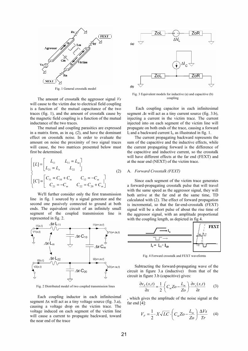
Fig. 1 General crosstalk model
The amount of crosstalk the aggressor signal Vs
will cause to the victim due to electrical field coupling is a function of the mutual capacitance of the two traces (fig. 1), and the amount of crosstalk cause by the magnetic field coupling is a function of the mutual inductance of the two traces.
The mutual and coupling parasitics are expressed in a matrix form, as in eq. (2), and have the dominant effect on crosstalk noise. In order to evaluate the amount on noise the proximity of two signal traces will cause, the two matrices presented below must first be determined.
⎪⎪
⎩
⎪⎪
⎨
⎧
⎥⎦
⎤⎢⎣
⎡
+=−=−=+=
=
⎥⎦
⎤⎢⎣
⎡
==
=
mm
mm
n
m
CCCCCCCCCC
C
LLLLLL
L
202221
121011
2221
1111
][
][ (2)
We'll further consider only the first transmission line in fig. 1 sourced by a signal generator and the second one passively connected to ground at both ends. The equivalent circuit of an infinitely small segment of the coupled transmission line is represented in fig. 2.
Fig. 2 Distributed model of two coupled transmission lines
Each coupling inductor in each infinitesimal
segment ∆x will act as a tiny voltage source (fig. 3.a), causing a voltage drop on the victim trace. The voltage induced on each segment of the victim line will cause a current to propagate backward, toward the near end of the trace
(a)
(b)
Fig. 3 Equivalent models for inductive (a) and capacitive (b) coupling
Each coupling capacitor in each infinitesimal
segment ∆x will act as a tiny current source (fig. 3.b), injecting a current in the victim trace. The current injected into on each segment of the victim line will propagate on both ends of the trace, causing a forward If and a backward current If, as illustrated in fig. 1.
The current propagating backward represents the sum of the capacitive and the inductive effects, while the current propagating forward is the difference of the capacitive and inductive current, so the crosstalk will have different effects at the far end (FEXT) and at the near end (NEXT) of the victim trace.
A. Forward Crosstalk (FEXT)
Since each segment of the victim trace generates a forward-propagating crosstalk pulse that will travel with the same speed as the aggressor signal, they will both arrive at the far end at the same time, TD calculated with (2). The effect of forward propagation is incremental, so that the far-end-crosstalk (FEXT) signal will be a short pulse of about the rise time of the aggressor signal, with an amplitude proportional with the coupling length, as depicted in fig 4.
Fig. 4 Forward crosstalk and FEXT waveforms
Subtracting the forward-propagating wave of the circuit in figure 3.a (inductive) from that of the circuit in figure 3.b (capacitive) gives:
ttxv
ZoLZoC
xtxv sm
mF
∂∂⋅⎟
⎠⎞
⎜⎝⎛ −⋅=
∂∂ ),(
21),( (3)
, which gives the amplitude of the noise signal at the far end [4]:
TrVs
ZoLZoCLCXV m
mF∆⋅⎟
⎠⎞
⎜⎝⎛ −⋅⋅=
21 (4)
21
, where X is the length of the coupling region,
1211 LLL == the inductance of the transmission lines (considered to have the same geometry),
mm CCCCC +=+= 2010 the capacitance of the transmission lines and the rise time of the aggressor signal. The sign of the FEXT signal in (4) depends on which of the inductive or capacitive coupling dominates, and is negative for most microstrip transmission lines and zero for symmetrical stripline [5]. B. Backward Crosstalk (NEXT)
The backward-propagating pulse generated by
crosstalk will have a constant effect on the near end of the victim, lasting about two times the propagation time of the lines (the time required by the pulse generated by the rightmost segment to reach the left end), as depicted in figure 5.
Fig. 5 Forward crosstalk and FEXT waveforms
Adding the backward-propagating waves of the circuits in figure 3.a (inductive) and 3.b (capacitive) gives:
ttxv
ZoL
ZoCx
txv smm
B
∂∂⋅⎟⎠⎞
⎜⎝⎛ +⋅=
∂∂ ),(
21),( (5)
, which gives the amplitude of the noise signal at the near end [4]:
VsZoLZoCV m
mB ∆⋅⎟⎠⎞
⎜⎝⎛ +⋅=
41
(6)
The amplitude of the NEXT signal does not depend on the length of the coupling region or the rise time of the signal. This is true as long as the round trip of the coupling region ( TD⋅2 ) is larger than the rise time of the aggressor (Tr ), otherwise the NEXT signal will not have enough time to fully develop [1], and eq. (6) must be adjusted, considering the propagation time from (1), to:
VsZoL
ZoCTr
LCXVTrTDV m
mFshort
B ∆⋅⎟⎠⎞
⎜⎝⎛ +⋅⋅=⋅=
212
(7)
For short coupling regions the far-end (eq. 4) and near-end (eq. 7) crosstalk depends on the same parameters.
III. PHYSICAL ANALYSIS In order to evaluate the crosstalk noise generated
by a specific routing geometry, first the parasitics matrices presented in (2) must be evaluated. In order to solve this problem without the use of an electromagnetic field solver, the equivalent impedances of differential propagation modes are considered. In the odd mode currents travels in different directions, so the magnetic fields will differentiate, while the electric fields will add, which gives the equivalent impedance of two coupled transmission lines in odd propagation mode:
1211
1211
CCLLZodd +
−= (8)
In the even mode currents travels in the same direction, so the magnetic fields will add, while the electric fields will differentiate, which gives the equivalent impedance of two coupled transmission lines in even propagation mode:
1211
1211
CCLLZeven −
+= (9)
Similarly, the propagation times in odd and even propagation modes may be expressed as functions of inductive and capacitive parasitics, as:
( ) ( )12111211 CCLLTDodd +⋅−= (10)
( ) ( )12111211 CCLLTDeven −⋅+= (11)
The same impedances presented in eq. (8,9) and propagation times presented in (10,11) may be estimated analytically, based on the equivalent dielectric constant of the structure formed by two signal traces in odd and even propagation modes. Bahl and Garg gives in [2] an analytic estimation for differential impedance and propagation time of microstrip transmission lines, while Cohn gives in [3] an analytic estimation for stripline configuration. Due to their complexity, th formulas given in [2] and [3] are not reproduced in this paper, but implemented as part of the crosstalk calculation functions presented further in paragraph IV. Since Zodd, Zeven, TDodd and TDeven may be determined using Bahl and Cohn solutions, eq. (8) and (9), together with the expression of propagation time, may be used to determine the elements of the parasitics matrices:
( )
( )⎪⎪⎪⎪
⎩
⎪⎪⎪⎪
⎨
⎧
⋅−⋅⋅=
⋅+⋅⋅=
⎟⎟⎠
⎞⎜⎜⎝
⎛−⋅=
⎟⎟⎠
⎞⎜⎜⎝
⎛+⋅=
oddoddeveneven
oddoddeveneven
odd
odd
even
even
odd
odd
even
even
ZTDZTDL
ZTDZTDL
ZTD
ZTDC
ZTD
ZTDC
2121
2121
12
11
12
11
(12)
22
IV. DESIGN RULE TRANSLATION: ELECTRICAL PHYSICAL
Both forward and backward crosstalk depends on the following geometrical parameters:
- S = the spacing between traces, restricted to a minimum value by the PCB fabrication technology
- W = the width of the traces: imposed by characteristic impedance or current requirement for the trace
- H = the distance to the reference plane, determined by the layer stackup of the board
- X = the length of the coupling region Only two parameters, namely S and X, are major
contributors in crosstalk. Among those S has a technological minimum and, because of the common practice of channel routing, it should be an integer multiple of W. This greatly simplifies the problem because it becomes practical to avoid solving eq. (4) and (7) in S. The only important parameter that must be controlled is X, the length of the coupled traces, which defines a parallelism rule in a CAD environment. Eq. (4,7,12), together with the analytical estimation of odd and even mode impedances and propagation times, are used to determine the parallelism rule for a specific set of electrical and geometrical data. The algorithm “PARAX” presented in fig 6, applied to a pair of nets from a PCB database, requires two predefined groups of IC terminals, one named “Alpha” and the other “Beta”, each containing at least one terminal from each net. Assuming all the relevant information is contained in the PCB database, the algorithm will calculate the parameters maxX and
S (as an integer multiple of minS ) required to keep the crosstalk below the maximum allowed values specified in the database, considering both NEXT and FEXT for every driver in the group as an aggressor. PARAX assumes that each driver pin in the PCB database is defined by Vs∆ and Tr, each receiver by a maximum noise accepted at the input Vnoise, each net by a trace width W and the set of available routing layers. It also assumes that the PCB stackup is defined, with known geometry, rε and layers association (routing / power / ground).
The algorithm uses two functions:
• VB(driver, victim, S), which calculates the worst case NEXT voltage for the specified driver and victim pins, with the spacing S.
• XF(driver, victim, VF), which calculates the coupling length X for a given driver and victim and a given FEXT voltage, VF
Fig. 6 PARAX algorithm flowchart
As stated earlier, PARAX can only be applied to a pair of nets and requires that each IC pin on both nets must be assigned, based on proximity, to one of two possible groups, Alpha or Beta, as depicted in fig. 7.
23
Fig. 7 PARAX partitioning of nets in two groups
The partitioning is used to identify each possible near and far end victims and analyze each case at one time, finally generating the parallelism values that meets the worst case demands. PARAX will return the Smin value as the smallest multiple of the maximum clearance specified for each net, that satisfy the condition:
allowedimumB VnoiseSV _maxmin )( < (13)
, for every victim on the same group as the driver and for every driver from both nets. In order to avoid numerical solving of an equation of type “ cee bxabxa =+ +⋅+⋅ 2211 ” the algorithm calculates BV several times until it finds the optimum value. PARAX will also return the X value, according to the pre-determined Smin, that satisfy the condition:
allowedimumF VnoiseSXV _maxmin ),( < (14)
,for every victim on the same group as the driver and for every driver from both nets. The calculations are made iteratively, traversing each receiver of the other net for each driver in the net pair. Considering that each pair has n pins and half of them are drivers, the complexity of the algorithm is ( )4
2nΟ . However, since on most practical applications there is only one driver and a reduced (except for clock signals) number of receivers, it is not computationally intensive.
IV. IMPLEMENTATION AND RESULTS
The algorithm presented above was implemented as a Basic Script into PADS Layout from Mentor Graphics. The main interface, presented in figure 8, allows the user to select a pair of nets and to partition the IC pins into the two groups, ALPHA and BETA, according to their anticipated positioning on the board.
Fig. 8 Interface of the PADS Layout implementation of PARAX
Since the algorithm act on the physical design rule of parallelism, the positions of the pins may change, so the partitioning can’t be made automatic. After net selection and pin partitioning, upon pressing the “OK” button, the program will check that the database is consistent with the requirements presented in the previous paragraph. Although all the information needed can be extracted from different electric models, such as industry-standard IBIS or Mentor Graphics MOD, for the purpose of this implementation , all the data required was extracted manually and specified as component parameters. After the database consistency check, if all the required information are available, the program will run the PARAX algorithm presented in fig. 6. The two values returned, S and X, are then written into the design rules database of the PCB project file. The parallelism rules are available through the main GUI of PADS Layout, so the values calculated by PARAX can be further adjusted if necessary.
Fig. 9 Parallelism constraints accessed through PADS GUI
For evaluation purposes, we compared the results presented by our implementation with the results obtained using HyperLynx Simulations, for the simple circuit presented in figure 9.a. The driver was XC1701, a PROM for Xilinx with 5.4=∆Vs [V] (loaded) and 5.0=Tr [ns]. To avoid reflections, both the aggressor and the victim were terminated on both ends. The typical waveform obtained during simulations are presented in figure 9.b.
The results for NEXT evaluation, for an arbitrary value of X (which does not influence the results) are presented in figure 11.
SX
24
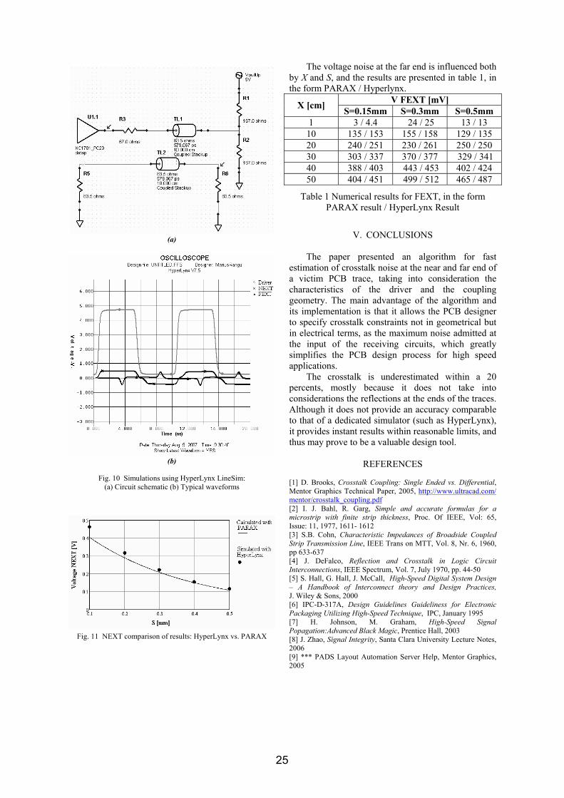
(a)
(b)
Fig. 10 Simulations using HyperLynx LineSim: (a) Circuit schematic (b) Typical waveforms
Fig. 11 NEXT comparison of results: HyperLynx vs. PARAX
The voltage noise at the far end is influenced both by X and S, and the results are presented in table 1, in the form PARAX / Hyperlynx.
V FEXT [mV] X [cm] S=0.15mm S=0.3mm S=0.5mm 1 3 / 4.4 24 / 25 13 / 13
10 135 / 153 155 / 158 129 / 135 20 240 / 251 230 / 261 250 / 250 30 303 / 337 370 / 377 329 / 341 40 388 / 403 443 / 453 402 / 424 50 404 / 451 499 / 512 465 / 487
Table 1 Numerical results for FEXT, in the form PARAX result / HyperLynx Result
V. CONCLUSIONS
The paper presented an algorithm for fast estimation of crosstalk noise at the near and far end of a victim PCB trace, taking into consideration the characteristics of the driver and the coupling geometry. The main advantage of the algorithm and its implementation is that it allows the PCB designer to specify crosstalk constraints not in geometrical but in electrical terms, as the maximum noise admitted at the input of the receiving circuits, which greatly simplifies the PCB design process for high speed applications.
The crosstalk is underestimated within a 20 percents, mostly because it does not take into considerations the reflections at the ends of the traces. Although it does not provide an accuracy comparable to that of a dedicated simulator (such as HyperLynx), it provides instant results within reasonable limits, and thus may prove to be a valuable design tool.
REFERENCES [1] D. Brooks, Crosstalk Coupling: Single Ended vs. Differential, Mentor Graphics Technical Paper, 2005, http://www.ultracad.com/ mentor/crosstalk_coupling.pdf [2] I. J. Bahl, R. Garg, Simple and accurate formulas for a microstrip with finite strip thickness, Proc. Of IEEE, Vol: 65, Issue: 11, 1977, 1611- 1612 [3] S.B. Cohn, Characteristic Impedances of Broadside Coupled Strip Transmission Line, IEEE Trans on MTT, Vol. 8, Nr. 6, 1960, pp 633-637 [4] J. DeFalco, Reflection and Crosstalk in Logic Circuit Interconnections, IEEE Spectrum, Vol. 7, July 1970, pp. 44-50 [5] S. Hall, G. Hall, J. McCall, High-Speed Digital System Design – A Handbook of Interconnect theory and Design Practices, J. Wiley & Sons, 2000 [6] IPC-D-317A, Design Guidelines Guideliness for Electronic Packaging Utilizing High-Speed Technique, IPC, January 1995 [7] H. Johnson, M. Graham, High-Speed Signal Popagation:Advanced Black Magic, Prentice Hall, 2003 [8] J. Zhao, Signal Integrity, Santa Clara University Lecture Notes, 2006 [9] *** PADS Layout Automation Server Help, Mentor Graphics, 2005
25
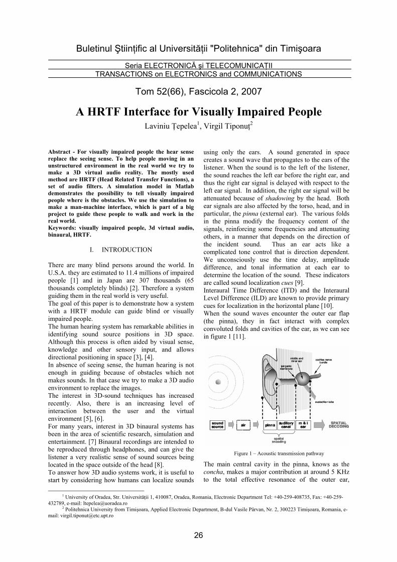
Buletinul Ştiinţific al Universităţii "Politehnica" din Timişoara
Seria ELECTRONICĂ şi TELECOMUNICAŢII TRANSACTIONS on ELECTRONICS and COMMUNICATIONS
Tom 52(66), Fascicola 2, 2007
A HRTF Interface for Visually Impaired People
Laviniu Ţepelea1, Virgil Tiponuţ2
1 University of Oradea, Str. Universităţii 1, 410087, Oradea, Romania, Electronic Department Tel: +40-259-408735, Fax: +40-259-
432789, e-mail: [email protected] 2 Politehnica University from Timişoara, Applied Electronic Department, B-dul Vasile Pârvan, Nr. 2, 300223 Timişoara, Romania, e-
mail: [email protected]
Abstract - For visually impaired people the hear sense replace the seeing sense. To help people moving in an unstructured environment in the real world we try to make a 3D virtual audio reality. The mostly used method are HRTF (Head Related Transfer Functions), a set of audio filters. A simulation model in Matlab demonstrates the possibility to tell visually impaired people where is the obstacles. We use the simulation to make a man-machine interface, which is part of a big project to guide these people to walk and work in the real world. Keywords: visually impaired people, 3d virtual audio, binaural, HRTF.
I. INTRODUCTION There are many blind persons around the world. In U.S.A. they are estimated to 11.4 millions of impaired people [1] and in Japan are 307 thousands (65 thousands completely blinds) [2]. Therefore a system guiding them in the real world is very useful. The goal of this paper is to demonstrate how a system with a HRTF module can guide blind or visually impaired people. The human hearing system has remarkable abilities in identifying sound source positions in 3D space. Although this process is often aided by visual sense, knowledge and other sensory input, and allows directional positioning in space [3], [4]. In absence of seeing sense, the human hearing is not enough in guiding because of obstacles which not makes sounds. In that case we try to make a 3D audio environment to replace the images. The interest in 3D-sound techniques has increased recently. Also, there is an increasing level of interaction between the user and the virtual environment [5], [6]. For many years, interest in 3D binaural systems has been in the area of scientific research, simulation and entertainment. [7] Binaural recordings are intended to be reproduced through headphones, and can give the listener a very realistic sense of sound sources being located in the space outside of the head [8]. To answer how 3D audio systems work, it is useful to start by considering how humans can localize sounds
using only the ears. A sound generated in space creates a sound wave that propagates to the ears of the listener. When the sound is to the left of the listener, the sound reaches the left ear before the right ear, and thus the right ear signal is delayed with respect to the left ear signal. In addition, the right ear signal will be attenuated because of shadowing by the head. Both ear signals are also affected by the torso, head, and in particular, the pinna (external ear). The various folds in the pinna modify the frequency content of the signals, reinforcing some frequencies and attenuating others, in a manner that depends on the direction of the incident sound. Thus an ear acts like a complicated tone control that is direction dependent. We unconsciously use the time delay, amplitude difference, and tonal information at each ear to determine the location of the sound. These indicators are called sound localization cues [9]. Interaural Time Difference (ITD) and the Interaural Level Difference (ILD) are known to provide primary cues for localization in the horizontal plane [10]. When the sound waves encounter the outer ear flap (the pinna), they in fact interact with complex convoluted folds and cavities of the ear, as we can see in figure 1 [11].
The main central cavity in the pinna, knows as the concha, makes a major contribution at around 5 KHz to the total effective resonance of the outer ear,
Figure 1 – Acoustic transmission pathway
26
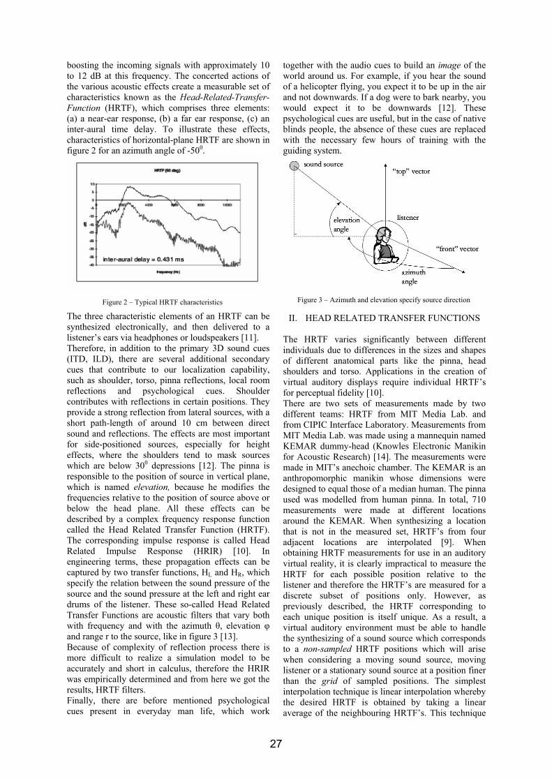
boosting the incoming signals with approximately 10 to 12 dB at this frequency. The concerted actions of the various acoustic effects create a measurable set of characteristics known as the Head-Related-Transfer-Function (HRTF), which comprises three elements: (a) a near-ear response, (b) a far ear response, (c) an inter-aural time delay. To illustrate these effects, characteristics of horizontal-plane HRTF are shown in figure 2 for an azimuth angle of -500.
The three characteristic elements of an HRTF can be synthesized electronically, and then delivered to a listener’s ears via headphones or loudspeakers [11]. Therefore, in addition to the primary 3D sound cues (ITD, ILD), there are several additional secondary cues that contribute to our localization capability, such as shoulder, torso, pinna reflections, local room reflections and psychological cues. Shoulder contributes with reflections in certain positions. They provide a strong reflection from lateral sources, with a short path-length of around 10 cm between direct sound and reflections. The effects are most important for side-positioned sources, especially for height effects, where the shoulders tend to mask sources which are below 300 depressions [12]. The pinna is responsible to the position of source in vertical plane, which is named elevation, because he modifies the frequencies relative to the position of source above or below the head plane. All these effects can be described by a complex frequency response function called the Head Related Transfer Function (HRTF). The corresponding impulse response is called Head Related Impulse Response (HRIR) [10]. In engineering terms, these propagation effects can be captured by two transfer functions, HL and HR, which specify the relation between the sound pressure of the source and the sound pressure at the left and right ear drums of the listener. These so-called Head Related Transfer Functions are acoustic filters that vary both with frequency and with the azimuth θ, elevation φ and range r to the source, like in figure 3 [13]. Because of complexity of reflection process there is more difficult to realize a simulation model to be accurately and short in calculus, therefore the HRIR was empirically determined and from here we got the results, HRTF filters. Finally, there are before mentioned psychological cues present in everyday man life, which work
together with the audio cues to build an image of the world around us. For example, if you hear the sound of a helicopter flying, you expect it to be up in the air and not downwards. If a dog were to bark nearby, you would expect it to be downwards [12]. These psychological cues are useful, but in the case of native blinds people, the absence of these cues are replaced with the necessary few hours of training with the guiding system.
II. HEAD RELATED TRANSFER FUNCTIONS The HRTF varies significantly between different individuals due to differences in the sizes and shapes of different anatomical parts like the pinna, head shoulders and torso. Applications in the creation of virtual auditory displays require individual HRTF’s for perceptual fidelity [10]. There are two sets of measurements made by two different teams: HRTF from MIT Media Lab. and from CIPIC Interface Laboratory. Measurements from MIT Media Lab. was made using a mannequin named KEMAR dummy-head (Knowles Electronic Manikin for Acoustic Research) [14]. The measurements were made in MIT’s anechoic chamber. The KEMAR is an anthropomorphic manikin whose dimensions were designed to equal those of a median human. The pinna used was modelled from human pinna. In total, 710 measurements were made at different locations around the KEMAR. When synthesizing a location that is not in the measured set, HRTF’s from four adjacent locations are interpolated [9]. When obtaining HRTF measurements for use in an auditory virtual reality, it is clearly impractical to measure the HRTF for each possible position relative to the listener and therefore the HRTF’s are measured for a discrete subset of positions only. However, as previously described, the HRTF corresponding to each unique position is itself unique. As a result, a virtual auditory environment must be able to handle the synthesizing of a sound source which corresponds to a non-sampled HRTF positions which will arise when considering a moving sound source, moving listener or a stationary sound source at a position finer than the grid of sampled positions. The simplest interpolation technique is linear interpolation whereby the desired HRTF is obtained by taking a linear average of the neighbouring HRTF’s. This technique
Figure 2 – Typical HRTF characteristics Figure 3 – Azimuth and elevation specify source direction
27
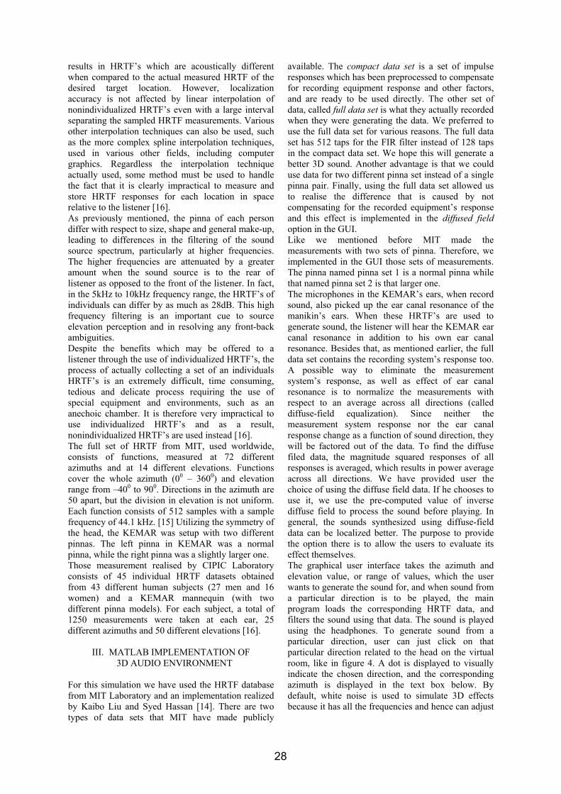
results in HRTF’s which are acoustically different when compared to the actual measured HRTF of the desired target location. However, localization accuracy is not affected by linear interpolation of nonindividualized HRTF’s even with a large interval separating the sampled HRTF measurements. Various other interpolation techniques can also be used, such as the more complex spline interpolation techniques, used in various other fields, including computer graphics. Regardless the interpolation technique actually used, some method must be used to handle the fact that it is clearly impractical to measure and store HRTF responses for each location in space relative to the listener [16]. As previously mentioned, the pinna of each person differ with respect to size, shape and general make-up, leading to differences in the filtering of the sound source spectrum, particularly at higher frequencies. The higher frequencies are attenuated by a greater amount when the sound source is to the rear of listener as opposed to the front of the listener. In fact, in the 5kHz to 10kHz frequency range, the HRTF’s of individuals can differ by as much as 28dB. This high frequency filtering is an important cue to source elevation perception and in resolving any front-back ambiguities. Despite the benefits which may be offered to a listener through the use of individualized HRTF’s, the process of actually collecting a set of an individuals HRTF’s is an extremely difficult, time consuming, tedious and delicate process requiring the use of special equipment and environments, such as an anechoic chamber. It is therefore very impractical to use individualized HRTF’s and as a result, nonindividualized HRTF’s are used instead [16]. The full set of HRTF from MIT, used worldwide, consists of functions, measured at 72 different azimuths and at 14 different elevations. Functions cover the whole azimuth (00 – 3600) and elevation range from –400 to 900. Directions in the azimuth are 50 apart, but the division in elevation is not uniform. Each function consists of 512 samples with a sample frequency of 44.1 kHz. [15] Utilizing the symmetry of the head, the KEMAR was setup with two different pinnas. The left pinna in KEMAR was a normal pinna, while the right pinna was a slightly larger one. Those measurement realised by CIPIC Laboratory consists of 45 individual HRTF datasets obtained from 43 different human subjects (27 men and 16 women) and a KEMAR mannequin (with two different pinna models). For each subject, a total of 1250 measurements were taken at each ear, 25 different azimuths and 50 different elevations [16].
III. MATLAB IMPLEMENTATION OF
3D AUDIO ENVIRONMENT
For this simulation we have used the HRTF database from MIT Laboratory and an implementation realized by Kaibo Liu and Syed Hassan [14]. There are two types of data sets that MIT have made publicly
available. The compact data set is a set of impulse responses which has been preprocessed to compensate for recording equipment response and other factors, and are ready to be used directly. The other set of data, called full data set is what they actually recorded when they were generating the data. We preferred to use the full data set for various reasons. The full data set has 512 taps for the FIR filter instead of 128 taps in the compact data set. We hope this will generate a better 3D sound. Another advantage is that we could use data for two different pinna set instead of a single pinna pair. Finally, using the full data set allowed us to realise the difference that is caused by not compensating for the recorded equipment’s response and this effect is implemented in the diffused field option in the GUI. Like we mentioned before MIT made the measurements with two sets of pinna. Therefore, we implemented in the GUI those sets of measurements. The pinna named pinna set 1 is a normal pinna while that named pinna set 2 is that larger one. The microphones in the KEMAR’s ears, when record sound, also picked up the ear canal resonance of the manikin’s ears. When these HRTF’s are used to generate sound, the listener will hear the KEMAR ear canal resonance in addition to his own ear canal resonance. Besides that, as mentioned earlier, the full data set contains the recording system’s response too. A possible way to eliminate the measurement system’s response, as well as effect of ear canal resonance is to normalize the measurements with respect to an average across all directions (called diffuse-field equalization). Since neither the measurement system response nor the ear canal response change as a function of sound direction, they will be factored out of the data. To find the diffuse filed data, the magnitude squared responses of all responses is averaged, which results in power average across all directions. We have provided user the choice of using the diffuse field data. If he chooses to use it, we use the pre-computed value of inverse diffuse field to process the sound before playing. In general, the sounds synthesized using diffuse-field data can be localized better. The purpose to provide the option there is to allow the users to evaluate its effect themselves. The graphical user interface takes the azimuth and elevation value, or range of values, which the user wants to generate the sound for, and when sound from a particular direction is to be played, the main program loads the corresponding HRTF data, and filters the sound using that data. The sound is played using the headphones. To generate sound from a particular direction, user can just click on that particular direction related to the head on the virtual room, like in figure 4. A dot is displayed to visually indicate the chosen direction, and the corresponding azimuth is displayed in the text box below. By default, white noise is used to simulate 3D effects because it has all the frequencies and hence can adjust
28
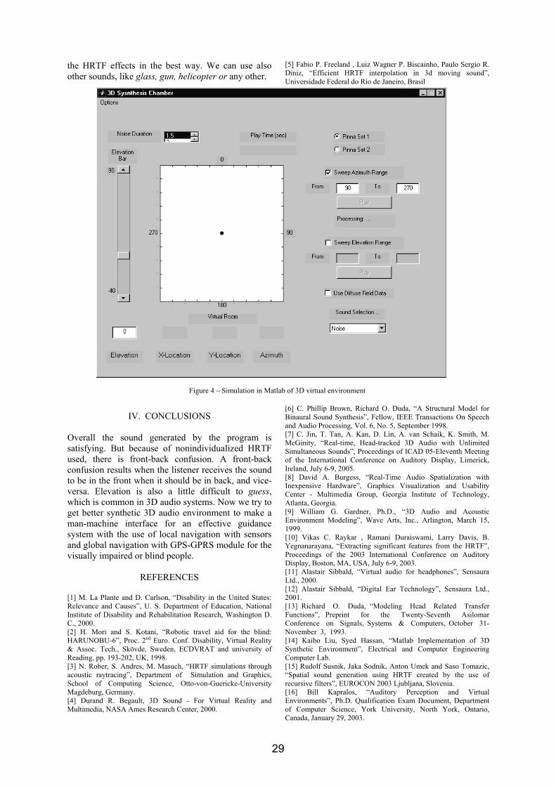
the HRTF effects in the best way. We can use also other sounds, like glass, gun, helicopter or any other.
IV. CONCLUSIONS
Overall the sound generated by the program is satisfying. But because of nonindividualized HRTF used, there is front-back confusion. A front-back confusion results when the listener receives the sound to be in the front when it should be in back, and vice-versa. Elevation is also a little difficult to guess, which is common in 3D audio systems. Now we try to get better synthetic 3D audio environment to make a man-machine interface for an effective guidance system with the use of local navigation with sensors and global navigation with GPS-GPRS module for the visually impaired or blind people.
REFERENCES
[1] M. La Plante and D. Carlson, “Disability in the United States: Relevance and Causes”, U. S. Department of Education, National Institute of Disability and Rehabilitation Research, Washington D. C., 2000. [2] H. Mori and S. Kotani, “Robotic travel aid for the blind: HARUNOBU-6”, Proc. 2nd Euro. Conf. Disability, Virtual Reality & Assoc. Tech., Skövde, Sweden, ECDVRAT and university of Reading, pp. 193-202, UK, 1998. [3] N. Rober, S. Andres, M. Masuch, “HRTF simulations through acoustic raytracing”, Department of Simulation and Graphics, School of Computing Science, Otto-von-Guericke-University Magdeburg, Germany. [4] Durand R. Begault, 3D Sound - For Virtual Reality and Multimedia, NASA Ames Research Center, 2000.
[5] Fabio P. Freeland , Luiz Wagner P. Biscainho, Paulo Sergio R. Diniz, “Efficient HRTF interpolation in 3d moving sound”, Universidade Federal do Rio de Janeiro, Brasil
[6] C. Phillip Brown, Richard O. Duda, “A Structural Model for Binaural Sound Synthesis”, Fellow, IEEE Transactions On Speech and Audio Processing, Vol. 6, No. 5, September 1998. [7] C. Jin, T. Tan, A. Kan, D. Lin, A. van Schaik, K. Smith, M. McGinity, “Real-time, Head-tracked 3D Audio with Unlimited Simultaneous Sounds”, Proceedings of ICAD 05-Eleventh Meeting of the International Conference on Auditory Display, Limerick, Ireland, July 6-9, 2005. [8] David A. Burgess, “Real-Time Audio Spatialization with Inexpensive Hardware”, Graphics Visualization and Usability Center - Multimedia Group, Georgia Institute of Technology, Atlanta, Georgia. [9] William G. Gardner, Ph.D., “3D Audio and Acoustic Environment Modeling”, Wave Arts, Inc., Arlington, March 15, 1999. [10] Vikas C. Raykar , Ramani Duraiswami, Larry Davis, B. Yegnanarayana, “Extracting significant features from the HRTF”, Proceedings of the 2003 International Conference on Auditory Display, Boston, MA, USA, July 6-9, 2003. [11] Alastair Sibbald, “Virtual audio for headphones”, Sensaura Ltd., 2000. [12] Alastair Sibbald, “Digital Ear Technology”, Sensaura Ltd., 2001. [13] Richard O. Duda, “Modeling Head Related Transfer Functions”, Preprint for the Twenty-Seventh Asilomar Conference on Signals, Systems & Computers, October 31-November 3, 1993. [14] Kaibo Liu, Syed Hassan, “Matlab Implementation of 3D Synthetic Environment”, Electrical and Computer Engineering Computer Lab. [15] Rudolf Susnik, Jaka Sodnik, Anton Umek and Saso Tomazic, “Spatial sound generation using HRTF created by the use of recursive filters”, EUROCON 2003 Ljubljana, Slovenia. [16] Bill Kapralos, “Auditory Perception and Virtual Environments”, Ph.D. Qualification Exam Document, Department of Computer Science, York University, North York, Ontario, Canada, January 29, 2003.
Figure 4 – Simulation in Matlab of 3D virtual environment
29
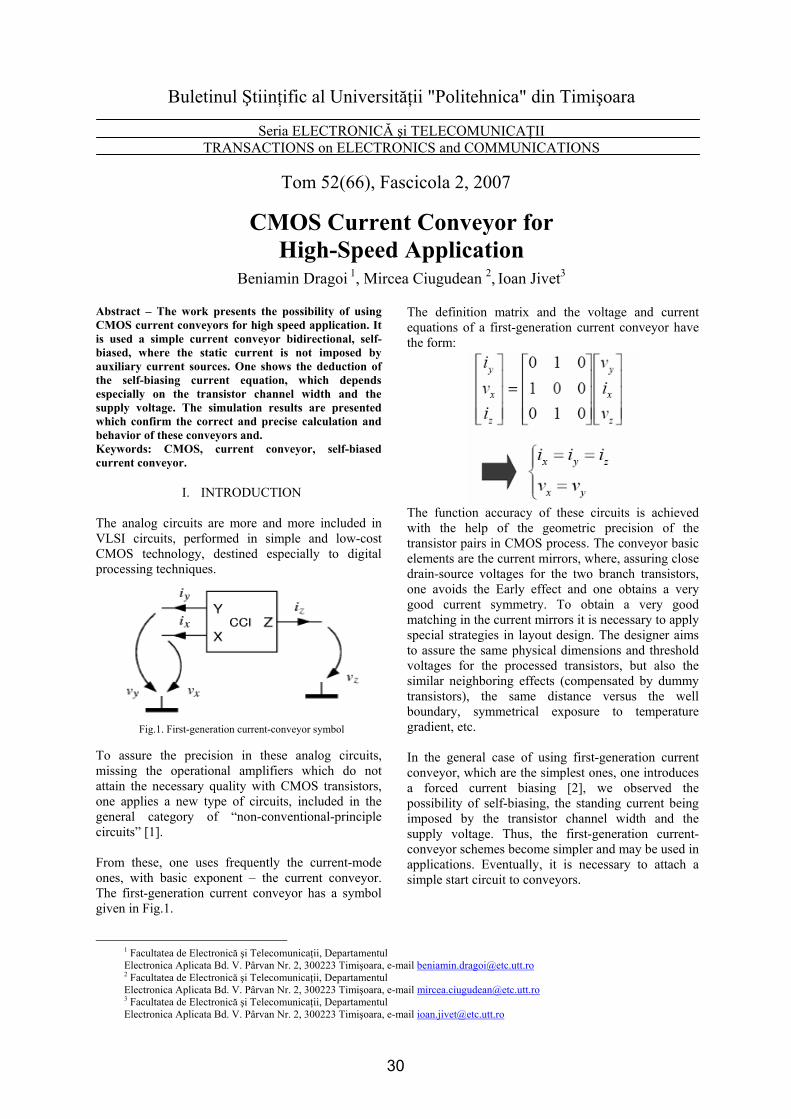
Buletinul Ştiinţific al Universităţii "Politehnica" din Timişoara
Seria ELECTRONICĂ şi TELECOMUNICAŢII TRANSACTIONS on ELECTRONICS and COMMUNICATIONS
Tom 52(66), Fascicola 2, 2007
CMOS Current Conveyor for High-Speed Application
Beniamin Dragoi 1, Mircea Ciugudean 2, Ioan Jivet3
1 Facultatea de Electronică şi Telecomunicaţii, Departamentul Electronica Aplicata Bd. V. Pârvan Nr. 2, 300223 Timişoara, e-mail [email protected] 2 Facultatea de Electronică şi Telecomunicaţii, Departamentul Electronica Aplicata Bd. V. Pârvan Nr. 2, 300223 Timişoara, e-mail [email protected] 3 Facultatea de Electronică şi Telecomunicaţii, Departamentul Electronica Aplicata Bd. V. Pârvan Nr. 2, 300223 Timişoara, e-mail [email protected]
Abstract – The work presents the possibility of using CMOS current conveyors for high speed application. It is used a simple current conveyor bidirectional, self-biased, where the static current is not imposed by auxiliary current sources. One shows the deduction of the self-biasing current equation, which depends especially on the transistor channel width and the supply voltage. The simulation results are presented which confirm the correct and precise calculation and behavior of these conveyors and. Keywords: CMOS, current conveyor, self-biased current conveyor.
I. INTRODUCTION
The analog circuits are more and more included in VLSI circuits, performed in simple and low-cost CMOS technology, destined especially to digital processing techniques.
Fig.1. First-generation current-conveyor symbol
To assure the precision in these analog circuits, missing the operational amplifiers which do not attain the necessary quality with CMOS transistors, one applies a new type of circuits, included in the general category of “non-conventional-principle circuits” [1]. From these, one uses frequently the current-mode ones, with basic exponent – the current conveyor. The first-generation current conveyor has a symbol given in Fig.1.
The definition matrix and the voltage and current equations of a first-generation current conveyor have the form:
The function accuracy of these circuits is achieved with the help of the geometric precision of the transistor pairs in CMOS process. The conveyor basic elements are the current mirrors, where, assuring close drain-source voltages for the two branch transistors, one avoids the Early effect and one obtains a very good current symmetry. To obtain a very good matching in the current mirrors it is necessary to apply special strategies in layout design. The designer aims to assure the same physical dimensions and threshold voltages for the processed transistors, but also the similar neighboring effects (compensated by dummy transistors), the same distance versus the well boundary, symmetrical exposure to temperature gradient, etc. In the general case of using first-generation current conveyor, which are the simplest ones, one introduces a forced current biasing [2], we observed the possibility of self-biasing, the standing current being imposed by the transistor channel width and the supply voltage. Thus, the first-generation current-conveyor schemes become simpler and may be used in applications. Eventually, it is necessary to attach a simple start circuit to conveyors.
30
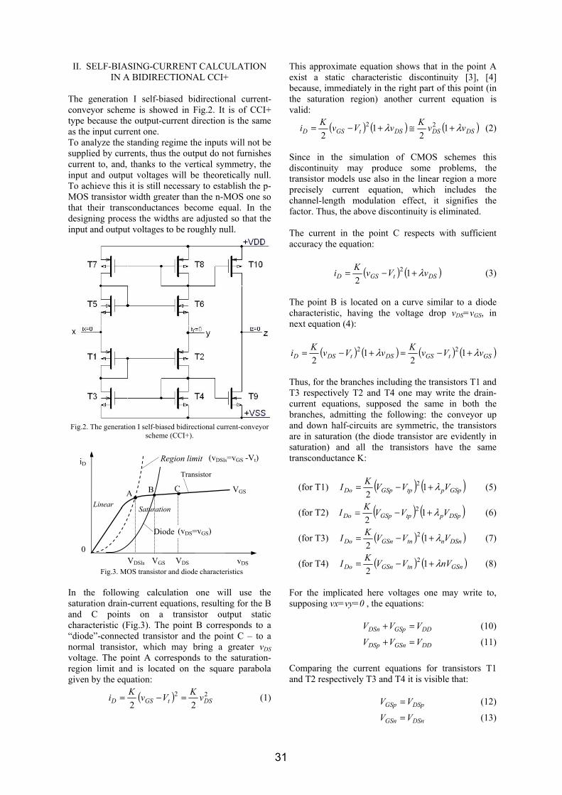
II. SELF-BIASING-CURRENT CALCULATION IN A BIDIRECTIONAL CCI+
The generation I self-biased bidirectional current-conveyor scheme is showed in Fig.2. It is of CCI+ type because the output-current direction is the same as the input current one. To analyze the standing regime the inputs will not be supplied by currents, thus the output do not furnishes current to, and, thanks to the vertical symmetry, the input and output voltages will be theoretically null. To achieve this it is still necessary to establish the p-MOS transistor width greater than the n-MOS one so that their transconductances become equal. In the designing process the widths are adjusted so that the input and output voltages to be roughly null.
Fig.2. The generation I self-biased bidirectional current-conveyor
scheme (CCI+).
Fig.3. MOS transistor and diode characteristics
In the following calculation one will use the saturation drain-current equations, resulting for the B and C points on a transistor output static characteristic (Fig.3). The point B corresponds to a “diode”-connected transistor and the point C – to a normal transistor, which may bring a greater vDS voltage. The point A corresponds to the saturation-region limit and is located on the square parabola given by the equation:
( ) 22
22 DStGSD vKVvKi =−= (1)
This approximate equation shows that in the point A exist a static characteristic discontinuity [3], [4] because, immediately in the right part of this point (in the saturation region) another current equation is valid:
( ) ( ) ( )DSDSDStGSD vvKvVvKi λλ +≅+−= 12
12
22 (2)
Since in the simulation of CMOS schemes this discontinuity may produce some problems, the transistor models use also in the linear region a more precisely current equation, which includes the channel-length modulation effect, it signifies the factor. Thus, the above discontinuity is eliminated. The current in the point C respects with sufficient accuracy the equation:
( ) ( )DStGSD vVvKi λ+−= 12
2 (3)
The point B is located on a curve similar to a diode characteristic, having the voltage drop vDS=vGS, in next equation (4):
( ) ( ) ( ) ( )GStGSDStDSD vVvKvVvKi λλ +−=+−= 12
12
22
Thus, for the branches including the transistors T1 and T3 respectively T2 and T4 one may write the drain-current equations, supposed the same in both the branches, admitting the following: the conveyor up and down half-circuits are symmetric, the transistors are in saturation (the diode transistor are evidently in saturation) and all the transistors have the same transconductance K:
(for T1) ( ) ( )GSpptpGSpDo VVVKI λ+−= 12
2 (5)
(for T2) ( ) ( )DSpptpGSpDo VVVKI λ+−= 12
2 (6)
(for T3) ( ) ( )DSnntnGSnDo VVVKI λ+−= 12
2 (7)
(for T4) ( ) ( )GSntnGSnDo nVVVKI λ+−= 12
2 (8)
For the implicated here voltages one may write to, supposing vx=vy=0 , the equations:
DDGSpDSn VVV =+ (10)
DDGSnDSp VVV =+ (11)
Comparing the current equations for transistors T1 and T2 respectively T3 and T4 it is visible that:
DSpGSp VV = (12)
DSnGSn VV = (13)
A C B
Linear Saturation
vDS
iD
VGS
(vDSls=vGS -Vt)
0
Diode
Transistor
Region limit
VDS VDSls VGS
(vDS=vGS)
31
This means all the same-type transistors (p or n) from the scheme have in standing regime the same B operation point (that is they are in saturation as admitted), so, the transistor and the diode in an horizontal pair have the same voltage drop VDS=VGS. Having close-value voltages VGSp and VGSn , it also means these voltages come close to value VDD/2. If now equals the right members of equations (5) and (7), substitutes VDSn=VGSn and simplifies K/2 one obtains equation (14): ( ) ( ) ( ) ( )GSnntnGSnGSpptpGSp VVVVVV λλ +−=+− 11 22
Having Vtp > Vtn , λp >λn this equality seems be possible even in the situation when the p and n transistors have not the same transconductance. The equation (14) may be written using the relations (10) and (13):
( ) ( )( ) ( )[ ]GSpDDntnGSpDD
GSpptpGSp
VVVVV
VVV
−+−−=
=+−
λ
λ
1
12
2
(15)
From this, after parenthesis detachment and term ordering, one obtains a third degree equation (16) in VGSp:
( ) ( )[ ]( )[ ]
( )[ ]( )( ) 01
2
432
23
22
22
23
=+−+−
+++−
−−++
+−+−+
tptnDDDDn
GSptnntpptntp
GSptnnDDnDD
GSptnntppDDnGSpnp
VVVV
VVVVV
VVVV
VVVVV
λ
λλ
λλλλλλλ
Direct solution of this equation is difficult but this may be solved (heaving a single real root) by trials, knowing that VGSp≈ VDD/2 but some smaller. Another solution is to use equation solving programs like Matlab or Octave.
III. PRACTICAL DESIGN CONSIDERATIONS Today we face with a rapid increasing in integrated circuits design and productions. In the same time there are new and powerful CMOS technologies. In the same time with scaling of the CMOS transistor features the models for simulations became very complex. Older technology with feature size greater than 5µm used only few simple equations and some parameters (Spice LEVEL 1 model). New technologies lower than 1µm use for spice simulations many equations and a lot of empirical parameters. Our 0.35µm CMOS technology uses for spice modeling of the MOS devices about 16 pages of equations and almost 150 parameters (Spice LEVEL 7).
Always, the IC designer starts the project with hand calculations. It will be used the well known MOS equation (3) that correspond to Spice LEVEL 1 modeling. But the results are far from simulation results (using Spice LEVEL 7). As the technology grows, hand calculation is less precisely. However there is a way to obtain hand calculations results close to simulation results. It is necessary to obtain precise values for some parameters that are includes in MOS transistor equations:
Table1. Vt0 λ
K’ Vgs – Vt0
These parameters can be obtained from simulations, from pMOS and nMOS transfer characteristics [6]. We choose the geometric dimensions W and L for transistors and get from simulations the transfer characteristics. Using MOS equations applied on these characteristics we can compute the parameters from Table 1, and the values are listed in Table 2. Table2.
Parameter NMOS PMOS W 20µ 20µ L 1µ 1µ
Vt0 0,759 V 0,807 V λ 0,029 V-1 0,0408 V-1
K’ 87.35 µA/V2 37.74 µA/V2 Vgs – Vt0 0,241 V 0,193 V Vds = Vgs 1 V 1 V
Ids 52,15 µA 14,6 µA Based on Table 2 and using the geometric scaling method [7] we can compute the currents and dimensions for any transistors. But we must notice that large changing of the W and L dimensions from Table 2 will change operating point and leads to changing of process parameters in Table 2. In this case, the hand calculation can give big errors. Using Table 2 and the obtained by calculation VGSp value may be determined the current IDo from equation (11). This will represent the static conveyor self-biasing current. Thus, for a conveyor heaving the scheme in Fig. 2, with transistors in 0.35µm CMOS process, VDD=2,5V, VSS=-2,5V, L=1µm, Wn=8.65µm, Wp=20µm, one obtains VGSp=1.272V. The voltage VGSn represents the difference from VDD hence VGSn=1.228V. So, the self-biasing-current value will be ID0=86µA. If a fast evaluation of the self-biasing current is wanted, it is possible to consider VGSp≈ VDD/2.
32
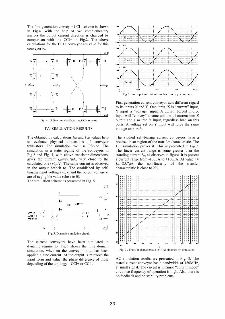
The first-generation conveyor CCI- scheme is shown in Fig.4. With the help of two complementary mirrors the output current direction is changed by comparison with the CCI+ in Fig.2. The above calculations for the CCI+ conveyor are valid for this conveyor to.
Fig. 4. Bidirectional self-biasing CCI- scheme
IV. SIMULATION RESULTS
The obtained by calculations ID0 and VGS values help to evaluate physical dimensions of conveyor transistors. For simulation we use PSpice. The simulation in a static regime of the conveyors in Fig.2 and Fig. 4, with above transistor dimensions, gives the current ID0=85.7µA, very close to the calculated one (86µA). The same current is observed in the output branch to. The established by self-biasing input voltages vx, vy and the output voltage vz are of negligible value (close to 0). The simulation scheme is presented in Fig. 5.
Fig. 5. Dynamic simulation circuit
The current conveyors have been simulated in dynamic regime to. Fig.6 shows the time domain simulation, when on the conveyor input has been applied a sine current. At the output is mirrored the input form and value, the phase difference of those depending of the topology – CCI+ or CCI-.
Fig.6. Sine input and output simulated conveyor currents
First generation current conveyor acts different regard to its inputs X and Y. One input, X is “current” input, Y input is “voltage” input. A current forced into X input will “convey” a same amount of current into Z output and also into Y input, regardless load on this ports. A voltage set on Y input will force the same voltage on port Y. The studied self-biasing current conveyors have a precise linear region of the transfer characteristic. The DC simulation proves it. This is presented in Fig.7. The linear current range is some greater than the standing current IDo as observes in figure. It is present a current range from -100µA to +100µA. At value ix≈ IDo=85.7µA the non-linearity of the transfer characteristic is close to 2%.
Fig. 7 . Transfer characteristic iz=f(ix) obtained by simulation.
AC simulation results are presented in Fig. 8. The tested current conveyor has a bandwidth of 180MHz, at small signal. The circuit is intrinsic “current mode” circuit so frequency of operation is high. Also there is no feedback and no stability problems.
33
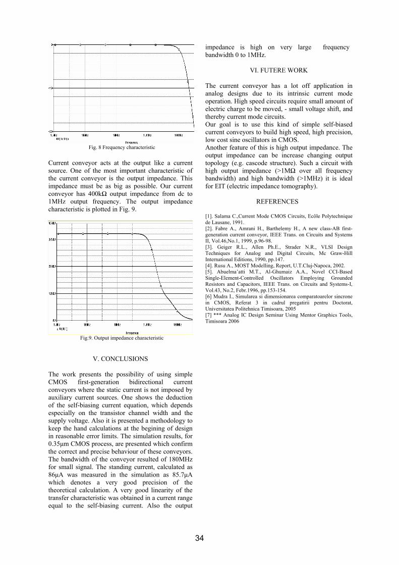
Fig. 8 Frequency characteristic
Current conveyor acts at the output like a current source. One of the most important characteristic of the current conveyor is the output impedance. This impedance must be as big as possible. Our current conveyor has 400kΩ output impedance from dc to 1MHz output frequency. The output impedance characteristic is plotted in Fig. 9.
Fig.9. Output impedance characteristic
V. CONCLUSIONS
The work presents the possibility of using simple CMOS first-generation bidirectional current conveyors where the static current is not imposed by auxiliary current sources. One shows the deduction of the self-biasing current equation, which depends especially on the transistor channel width and the supply voltage. Also it is presented a methodology to keep the hand calculations at the begining of design in reasonable error limits. The simulation results, for 0.35µm CMOS process, are presented which confirm the correct and precise behaviour of these conveyors. The bandwidth of the conveyor resulted of 180MHz for small signal. The standing current, calculated as 86µA was measured in the simulation as 85.7µA which denotes a very good precision of the theoretical calculation. A very good linearity of the transfer characteristic was obtained in a current range equal to the self-biasing current. Also the output
impedance is high on very large frequency bandwidth 0 to 1MHz.
VI. FUTERE WORK
The current conveyor has a lot off application in analog designs due to its intrinsic current mode operation. High speed circuits require small amount of electric charge to be moved, - small voltage shift, and thereby current mode circuits. Our goal is to use this kind of simple self-biased current conveyors to build high speed, high precision, low cost sine oscillators in CMOS. Another feature of this is high output impedance. The output impedance can be increase changing output topology (e.g. cascode structure). Such a circuit with high output impedance (>1MΩ over all frequency bandwidth) and high bandwidth (>1MHz) it is ideal for EIT (electric impedance tomography).
REFERENCES
[1]. Salama C.,Current Mode CMOS Circuits, Ecôle Polytechnique de Lausane, 1991. [2]. Fabre A., Amrani H., Barthelemy H., A new class-AB first-generation current conveyor, IEEE Trans. on Circuits and Systems II, Vol.46,No.1, 1999, p.96-98. [3]. Geiger R.L., Allen Ph.E., Strader N.R., VLSI Design Techniques for Analog and Digital Circuits, Mc Graw-Hill International Editions, 1990, pp.147. [4]. Rusu A., MOST Modelling, Report, U.T.Cluj-Napoca, 2002. [5]. Abuelma’atti M.T., Al-Ghumaiz A.A., Novel CCI-Based Single-Element-Controlled Oscillators Employing Grounded Resistors and Capacitors, IEEE Trans. on Circuits and Systems-I, Vol.43, No.2, Febr.1996, pp.153-154. [6] Mudra I., Simularea si dimensionarea comparatoarelor sincrone in CMOS, Referat 3 in cadrul pregatirii pentru Doctorat, Universitatea Politehnica Timisoara, 2005 [7] *** Analog IC Design Seminar Using Mentor Graphics Tools, Timisoara 2006
34
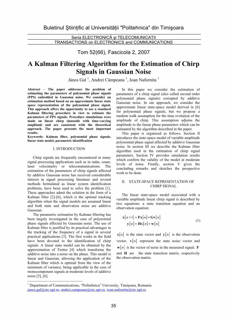
Buletinul Ştiinţific al Universităţii "Politehnica" din Timişoara
Seria ELECTRONICĂ şi TELECOMUNICAŢII TRANSACTIONS on ELECTRONICS and COMMUNICATIONS
Tom 52(66), Fascicola 2, 2007
A Kalman Filtering Algorithm for the Estimation of Chirp Signals in Gaussian Noise
János Gal 1, Andrei Câmpeanu 1, Ioan Nafornita 1
1 Department of Communications, “Politehnica” University, Timişoara, Romania [email protected], [email protected], [email protected]
Abstract – The paper addresses the problem of estimating the parameters of polynomial phase signals (PPS) embedded in Gaussian noise. We consider an estimation method based on an approximate linear state space representation of the polynomial phase signal. This approach offers the opportunity to use a standard Kalman filtering procedure in view to estimate the parameters of PPS signals. Procedure simulations were made on linear chirp sinusoids with time-varying amplitude and are consistent with the theoretical approach. The paper presents the most important results. Keywords: Kalman filter, polynomial phase signals, linear state model, parametric identification
I. INTRODUCTION
Chirp signals are frequently encountered in many signal processing applications such as in radar, sonar, laser velocimetry or telecommunications. The estimation of the parameters of chirp signals affected by additive Gaussian noise has received considerable interest in signal processing literature and several methods formulated as linear system identification problems, have been used to solve the problem [1]. These approaches admit the solution in the form of a Kalman filter [2]-[6], which is the optimal tracking algorithm when the signal models are assumed linear and both state and observation noise are additive Gaussian.
The parametric estimation by Kalman filtering has been largely investigated in the case of polynomial phase signals affected by Gaussian noise. The use of Kalman filter is justified by its practical advantages in the tracking of the frequency of a signal in several practical applications [3]. The first works in the field have been devoted to the identification of chirp signals. A linear state model can be obtained by the approximation of Tretter [4] which transforms the additive noise into a noise on the phase. This model is linear and Gaussian, allowing the application of the Kalman filter which is optimal from the view of the minimum of variance, being applicable in the case of monocomponent signals at moderate levels of additive noise [5], [6].
In this paper we consider the estimation of parameters of a chirp signal (also called second order polynomial phase signals) corrupted by additive Gaussian noise. In our approach, we consider the approximate linear state-space model derived in [6] for polynomial phase signals, but we propose a random walk assumption for the time evolution of the amplitude of chirp. This assumption adjoins the amplitude to the linear phase parameters which can be estimated by the algorithm described in the paper.
This paper is organized as follows. Section II introduces the state-space model of variable amplitude polynomial phase signal affected by additive Gaussian noise. In section III we describe the Kalman filter algorithm used in the estimation of chirp signal parameters. Section IV provides simulation results which confirm the validity of the model at moderate levels of noise. Finally, section V gives the concluding remarks and sketches the prospective work to be done.
II. STATE-SPACE REPRESENTATION OF CHIRP SIGNAL
The linear state-space model associated with a
variable amplitude linear chirp signal is described by two equations: a state transition equation and an observation equation:
[ ] [ ] [ ]
[ ] [ ] [ ]1n n n
n n n
+ = +
= +
x Fx Gv
y Hx w (1)
[ ]nx is the state vector and [ ]ny is the observation
vector, [ ]nv represent the state noise vector and
[ ]nw is the vector of noise in the measured signal. F and H are the state transition matrix, respectively the observation matrix.
35
The Observation Model The model of a variable amplitude second order
polynomial phase signal [ ]y n embedded in the
additive noise [ ]w n is given below:
[ ] [ ] [ ]( ) [ ]expy n A n j n w n= Φ + (2)
where the positive real-valued [ ]A n is the amplitude
possibly time-varying and unknown and [ ]nΦ is the deterministic polynomial phase, expressed, for a linear chirp, by:
[ ] 2
2n n nα β γΦ = + + (3)
where the coefficients α , β and γ are real and unknown. The additive white Gaussian noise [ ]w n
has zero-mean and variance 2wσ . It can be written as
[ ] [ ] [ ]R Iw n w n jw n= + (4)
with [ ]Rw n and [ ]Iw n , the real part and the imaginary part of the analytical noise. If both parts are not correlated between them, having the same variance, we can write:
[ ] [ ] [ ]2
2w
R RE w n w n k kσ δ+ = (5)
[ ] [ ] [ ]2
2w
I IE w n w n k kσ δ+ = (6)
[ ] [ ] 0,R IE w n w n k k Z+ = ∀ ∈ (7)
where E ⋅ is the expectation operator. An analytical signal having these properties is called “cyclic” noise [7].
In order to estimate the parameters of chirp signals corrupted by noise, we use an adequate model of the signal with emphasis on its instantaneous phase. In this sense we express the measured signal [ ]y n in terms of its polar components:
[ ] [ ] [ ] Tn y n Arg y n⎡ ⎤= ⎣ ⎦y (8)
It is the observation vector of chirp linear model. As is shown in [4], if the signal-to-noise ratio (SNR) in the measured signal [ ]y n exceeds13dB , the noise
real part affects only the amplitude [ ]A n , whereas the
phase [ ]nΦ is affected by the imaginary part of the “cyclic” noise. Eq. (2) can be written now in terms of amplitude and phase as:
[ ][ ]
[ ][ ]
[ ][ ] [ ]
R
I
y n A n w nn w n A nArg y n
⎡ ⎤ ⎡ ⎤ ⎡ ⎤= +⎢ ⎥ ⎢ ⎥ ⎢ ⎥Φ⎢ ⎥ ⎣ ⎦ ⎣ ⎦⎣ ⎦
(9)
Consequently, the noise observation vector in (1), [ ]nw , is expressed as
[ ] [ ] [ ] TR In w n w n⎡ ⎤= ⎣ ⎦w (10)
The correlation matrix of noise vector [ ]w nQ is established under the assumptions (5)-(7) and the decomposition in (9), as
[ ] [ ]2
2
1 00 12
ww n
A nσ ⎡ ⎤
= ⎢ ⎥⎣ ⎦
Q (11)
As the amplitude [ ]A n is variable, [ ]w nQ is recalculated for each step of the filtering algorithm.
The State-Space Model and Transition Equations The values of an M -order polynomial ( )P x , can
be expressed by the Taylor series expansion [7]:
( ) ( ) ( ) ( )0 0 00
; ,!
kMk
k
xP x x P x x x R
k=
∆+ ∆ = ∀ ∀∆ ∈∑ (12)
viewing that all derivatives having the order higher than M are zero. For the l -order derivative of the polynomial ( ) ( )lP x can be used the following series expansion:
( ) ( ) ( )( )
( ) ( )0 0 0; , , 1,!
kMl k
k l
xP x x P x x x R l M
k l=
∆+ ∆ = ∀ ∀∆ ∈ =
−∑ (13)
Replacing ( )P x by the phase polynomial [ ]nΦ in(3), 0x with n and x∆ by 1, we have for:
[ ] ( ) [ ]0
11!
Mk
k
n nk=
Φ + = Φ∑ (14)
( ) [ ] ( )( ) [ ]11 1,
!
Ml k
k ln n l M
k l=Φ + = Φ =
−∑ (15)
The state vector [ ]nx in the case of variable amplitude linear chirp signals is given by the amplitude of the sinusoid, the phase and the first
2M = derivatives of the phase:
[ ] [ ] [ ] ( ) [ ] ( ) [ ]' '' Tn A n n n n⎡ ⎤= Φ Φ Φ⎣ ⎦x (16)
where: ( ) [ ] [ ] [ ]' 1n n nΦ = Φ −Φ − (17)
and: ( ) [ ] ( ) [ ] ( ) [ ]'' ' ' 1n n nΦ = Φ −Φ − (18)
Note that in discrete time, other definitions for (17) and (18) are possible as well [1].
For two consecutive moments, the relation between the two states is derived from (14) and (15):
[ ][ ]
( ) [ ]( ) [ ]
[ ][ ]
( ) [ ]( ) [ ]
' '
" "
1 0 0 01 1 10 11 1! 2!1 10 0 1
1!10 0 0 1
A n A nn n
n n
n n
⎡ ⎤⎡ ⎤ ⎡ ⎤+ ⎢ ⎥⎢ ⎥ ⎢ ⎥⎢ ⎥Φ + Φ⎢ ⎥ ⎢ ⎥⎢ ⎥= ⋅⎢ ⎥ ⎢ ⎥⎢ ⎥Φ + Φ⎢ ⎥ ⎢ ⎥⎢ ⎥⎢ ⎥ ⎢ ⎥⎢ ⎥Φ + Φ⎣ ⎦ ⎣ ⎦⎢ ⎥⎣ ⎦
(19)
It is a transition equation between two
consecutives states, without taking into account the state noise. Comparing (19) with the first equation in (1), we find that the 4 4× -size transition matrix is:
36
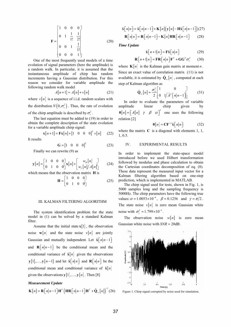
1 0 0 01 10 11! 2!
10 0 11!
0 0 0 1
⎡ ⎤⎢ ⎥⎢ ⎥⎢ ⎥= ⎢ ⎥⎢ ⎥⎢ ⎥⎢ ⎥⎣ ⎦
F (20)
One of the most frequently used models of a time evolution of signal parameters (here the amplitude) is a random walk. In particular, it is assumed that the instantaneous amplitude of chirp has random increments having a Gaussian distribution. For this reason we consider for variable amplitude the following random walk model
[ ] [ ] [ ]1A n A n v n+ = + (21)
where [ ]v n is a sequence of i.i.d. random scalars with
the distribution ( )20, vN σ . Thus, the rate of evolution
of the chirp amplitude is described by 2vσ .
The last equation must be added to (19) in order to obtain the complete description of the state evolution for a variable amplitude chirp signal:
[ ] [ ] [ ] [ ]1 1 0 0 0 Tn n v n+ = +x Fx (22) It results
[ ]1 0 0 0 T=G (23) Finally we can rewrite (9) as
[ ] [ ] [ ][ ] [ ]
1 0 0 00 1 0 0
R
I
w nn n
w n A n⎡ ⎤⎡ ⎤
= + ⎢ ⎥⎢ ⎥⎣ ⎦ ⎣ ⎦
y x (24)
which means that the observation matrix H is
1 0 0 00 1 0 0⎡ ⎤
= ⎢ ⎥⎣ ⎦
H (25)
III. KALMAN FILTERING ALGORITHM
The system identification problem for the state model in (1) can be solved by a standard Kalman filter.
Assume that the initial state [ ]1x , the observation
noise [ ]nw and the state noise [ ]v n are jointly
Gaussian and mutually independent. Let ˆ 1n n⎡ − ⎤⎣ ⎦x
and 1n n⎡ − ⎤⎣ ⎦R be the conditional mean and the
conditional variance of [ ]ˆ nx given the observations
[ ] [ ]1 , , 1n −y yK and let ˆ n n⎡ ⎤⎣ ⎦x and n n⎡ ⎤⎣ ⎦R be the
conditional mean and conditional variance of [ ]ˆ nx
given the observations [ ] [ ]1 , , ny yK . Then [8]
Measurement Update
[ ] [ ]( ) 1ˆ1 1T Twn n n n n n
−= ⎡ − ⎤ ⎡ − ⎤ +⎣ ⎦ ⎣ ⎦K R H HR H Q (26)
[ ] [ ]( )ˆ ˆ ˆ1 1n n n n n n n n⎡ ⎤ = ⎡ − ⎤ + − ⎡ − ⎤⎣ ⎦ ⎣ ⎦ ⎣ ⎦x x K y Hx (27)
[ ]1 1n n n n n n n⎡ ⎤ = ⎡ − ⎤ − ⎡ − ⎤⎣ ⎦ ⎣ ⎦ ⎣ ⎦R R K HR (28)
Time Update
ˆ ˆ1n n n n⎡ + ⎤ = ⎡ ⎤⎣ ⎦ ⎣ ⎦x Fx (29)
21 T Tvn n n n σ⎡ + ⎤ = ⎡ ⎤ +⎣ ⎦ ⎣ ⎦R FR F GG (30)
where [ ]nK is the Kalman gain matrix at moment n . Since an exact value of correlation matrix (11) is not available, it is estimated by [ ]ˆ
w nQ , computed at each step of Kalman algorithm as
[ ]2
2
1 0ˆˆ0 1 12
ww n
A n nσ ⎡ ⎤
= ⎢ ⎥⎡ − ⎤⎢ ⎥⎣ ⎦⎣ ⎦
Q (31)
In order to evaluate the parameters of variable amplitude linear chirp given by
[ ] [ ] Tn A n γ β α⎡ ⎤= ⎣ ⎦θ one uses the following
relation [2] [ ] ˆnn n n−= ⎡ ⎤⎣ ⎦θ CF x (32)
where the matrix C is a diagonal with elements 1, 1, 1, 0.5.
IV. EXPERIMENTAL RESULTS
In order to implement the state-space model introduced before we used Hilbert transformation followed by modulus and phase calculation to obtain the Cartesian coordinates decomposition of eq. (8). These data represent the measured input vector for a Kalman filtering algorithm based on one-step prediction, which is implemented in MATLAB.
The chirp signal used for tests, shown in Fig. 1, is 5000 samples long and the sampling frequency is 5000Hz. The chirp parameters have the following true values: 41.0053 10α −= × , 0.1256β = and 2γ π= . The state noise [ ]v n is zero mean Gaussian white
noise with 2 31.799 10vσ−= × .
The observation noise [ ]w n is zero mean Gaussian white noise with 20dBSNR = .
Figure 1. Chirp signal corrupted by noise used for simulation.
37
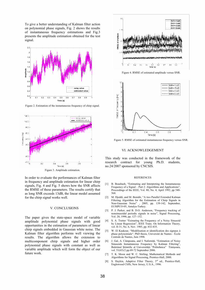
To give a better understanding of Kalman filter action on polynomial phase signals, Fig. 2 shows the results of instantaneous frequency estimations and Fig.3 presents the amplitude estimation obtained for the test signal.
Figure 2. Estimation of the instantaneous frequency of chirp signal.
Figure 3. Amplitude estimation. In order to evaluate the performances of Kalman filter in frequency and amplitude estimation for linear chirp signals, Fig. 4 and Fig. 5 shows how the SNR affects the RMSE of these parameters. The results certify that as long SNR exceeds 13dB, the linear model assumed for the chirp signal works well.
V. CONCLUSIONS The paper gives the state-space model of variable amplitude polynomial phase signals with good opportunities in the estimation of parameters of linear chirp signals embedded in Gaussian white noise. The Kalman filter algorithm performs well viewing the results. The algorithm allows the extension to multicomponent chirp signals and higher order polynomial phase signals with constant as well as variable amplitude which will form the object of our future work.
VI. ACKNOWLEDGEMENT
This study was conducted in the framework of the research contract for young Ph.D. students, no.24/2007 sponsored by CNCSIS.
REFERENCES [1] B. Boashash, “Estimating and Interpreting the Instantaneous
Frequency of a Signal – Part 2: Algorithms and Applications”, Proceedings of the IEEE, Vol. 80, No. 4, April 1992, pp 540-568.
[2] M. Djeddi, and M. Benidir, “A two Parallel Extended Kalman Filtering Algorithm for the Estimation of Chirp Signals in Non-Gaussian Noise” , 2005, pp. 139-142, September, EUSIPCO-05, Antalya-Turkey.
[3] P. J. Parker, and B. D.O. Anderson, “Frequency tracking of nonsinusoidal periodic signals in noise”, Signal Processing, Vol. 20, 1990, pp. 127–152.
[4] S. A. Tretter “Esimating the Frequency of a Noisy Sinusoid by Linear Regression”, IEEE Trans. On Information Theory, vol. II-31, No. 6, Nov. 1985, pp. 832-835.
[5] W. El Kaakour, “Modélisation et identification des signaux à phase polynomiale“. PhD thesis, Université de Nantes - École Centrale de Nantes, Juin 1998.
[6] J. Gal, A. Câmpeanu, and I. Naforniţă, “Estimation of Noisy Sinusoids Instantaneous Frequency by Kalman Filtering”, Buletinul Ştiintific al Universităţii “Politehnica” Timişoara, vol. 51(65)/2 pp.69-72 September 2006.
[7] T. K. Moon and W. C. Stirling, Mathematical Methods and Algorithms for Signal Processing, Prentice-Hall, 2000.
[8] S. Haykin, Adaptive Filter Theory, 3rd ed., Prentice-Hall, Englewood Cliffs, New Jersey, U.S.A., 1996.
0 0.1 0.2 0.3 0.4 0.5 0.6 0.7 0.8 0.9 10.2
0.4
0.6
0.8
1
1.2
1.4
1.6
1.8
2
2.2
Time [s]
Ampl
itude
noisy valueestimated value
Figure 4. RMSE of estimated amplitude versus SNR.
Figure 5. RMSE of estimated instantaneous frequency versus SNR.
Figure 5. RMSE of estimated instantaneous frequency versus SNR.
38
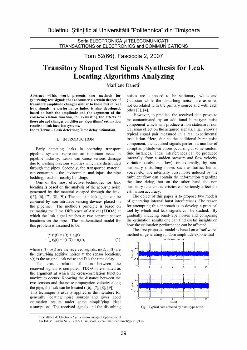
Buletinul Ştiinţific al Universităţii "Politehnica" din Timişoara
Seria ELECTRONICĂ şi TELECOMUNICAŢII TRANSACTIONS on ELECTRONICS and COMMUNICATIONS
Tom 52(66), Fascicola 2, 2007
Transitory Shaped Test Signals Synthesis for Leak Locating Algorithms Analyzing
Marllene Dăneţi1
1 Facultatea de Electronică şi Telecomunicaţii, Departamentul EA Bd. V. Pârvan Nr. 2, 300223 Timişoara, e-mail [email protected]
Abstract –This work presents two methods for generating test signals that encounter a certain degree of transitory amplitude changes similar to those met in real leak signals. A performance index is also developed, based on both the amplitude and the argument of the cross-correlation function, for evaluating the effects of these abrupt changes on different algorithms’ estimation results in leak location systems. Index Terms – Leak detection; Time delay estimation.
I. INTRODUCTION
Early detecting leaks in operating transport pipeline systems represent an important issue in pipeline industry. Leaks can cause serious damage due to wasting precious supplies which are distributed through the pipes. Secondly, the transported material can contaminate the environment and injure the pipe bedding, roads or nearby buildings. One of the most effective techniques for leak locating is based on the analysis of the acoustic noise generated by the material escaped through the leak. ([5], [6], [7], [8], [9]). The acoustic leak signal can be captured by non intrusive sensing devices placed on the pipeline. The method’s principle is based on estimating the Time Difference of Arrival (TDOA) at which the leak signal reaches at two separate sensor locations on the pipe. The mathematical model for this problem is assumed to be:
r1(t) = s(t) + n1(t) r2(t) = s(t-D) + n2(t), (1)
where r1(t), r2(t) are the received signals, n1(t), n2(t) are the disturbing additive noises at the sensor locations, s(t) is the original leak noise and D is the time delay. The cross-correlation function between the received signals is computed. TDOA is estimated as the argument at which the cross-correlation function maximum occurs. Knowing the distance between the two sensors and the noise propagation velocity along the pipe, the leak can be located ( [6], [7], [8], [9]). This technique is usually applied in the literature for generally locating noise sources and gives good estimation results under some simplifying ideal assumptions. The received signals and the disturbing
noises are supposed to be stationary, white and Gaussian while the disturbing noises are assumed not correlated with the primary source and with each other [3], [4]. However, in practice, the received data prove to be contaminated by an additional burst-type noise component which will produce a non stationary, non Gaussian effect on the acquired signals. Fig.1 shows a typical signal pair measured in a real experimental installation. Here, due to the additional burst noise component, the acquired signals perform a number of abrupt amplitude variations occurring at some random time instances. These interferences can be produced internally, from a sudden pressure and flow velocity variation (turbulent flow), or externally, by non-stationary disturbing noises such as traffic, human voice, etc. The internally burst noise induced by the turbulent flow can contain the information regarding the time delay, but on the other hand the non stationary data characteristics can seriously affect the estimation accuracy. The object of this paper is to propose two models of generating internal burst interferences. The reason for attempting this approach is to develop a practical tool by which real leak signals can be studied. By gradually inducing burst-type noises and comparing the estimation results one can find useful insights on how the estimation performance can be affected. The first proposed model is based on a “software” method of generating random amplitude exponential
Fig.1 Typical data affected by burst-type noise
39
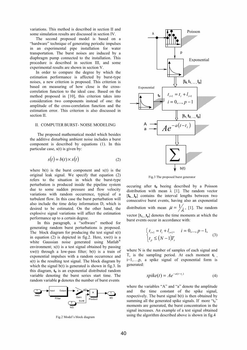
variations. This method is described in section II and some simulation results are discussed in section IV. The second proposed model is based on a “hardware” technique of generating periodic impulses in an experimental pipe installation for water transportation. The burst noises are induced by a diaphragm pump connected to the installation. This procedure is described in section III, and some experimental results are shown in section V. In order to compare the degree by which the estimation performance is affected by burst-type noises, a new criterion is proposed. This criterion is based on measuring of how close is the cross-correlation function to the ideal case. Based on the method proposed in [10], this criterion takes into consideration two components instead of one: the amplitude of the cross-correlation function and the estimation error. This criterion is also discussed in section II.
II. COMPUTER BURST- NOISE MODELING The proposed mathematical model which besides the additive disturbing ambient noise includes a burst component is described by equations (1). In this particular case, s(t) is given by:
( ) ( )txtbts ×= )( (2) where b(t) is the burst component and x(t) is the original leak signal. We specify that equation (2) refers to the situation in which the burst-type perturbation is produced inside the pipeline system due to some sudden pressure and flow velocity variations with random occurrence, typical of a turbulent flow. In this case the burst perturbation will also include the time delay information D, which is desired to be estimated. On the other hand, the explosive signal variations will affect the estimation performance up to a certain degree. In this paragraph, a “software” method for generating random burst perturbations is proposed. The block diagram for producing the test signal s(t) in equation (2) is depicted in fig.2. Here, xw(t) is a white Gaussian noise generated using Matlab® environment; x(t) is a test signal obtained by passing xw(t) through a low-pass filter; b(t) is a train of exponential impulses with a random occurrence and s(t) is the resulting test signal. The block diagram by which the signal b(t) is generated is shown in fig.3. In this diagram, t0 is an exponential distributed random variable denoting the burst series start time. The random variable p denotes the number of burst events
x(t)
burst
1
s(t)Product
k
Gain
Input Output
Filter
2
b(t)
1
xw(t)
Fig.2 Model’s block diagram
Fig.3 The proposed burst generator occuring after t0 beeing described by a Poisson distribution with mean λ [1]. The random vector [l0,…lp] contains the interval lengths between two consecutive burst events, having also an exponential
distribution with mean λµ 1= , [1]. The random
vector [t1,…tp] denotes the time moments at which the burst events occur in accordance with:
( )⎩⎨⎧
−≤−=+= ++
sp
iii
TNtpiltt
1,1,...,0,11 (3)
where N is the number of samples of each signal and Ts is the sampling period. At each moment ti , i=1,…,p, a spike signal of exponential form is generated:
)()( ittaAetspike −−= (4)
where the variables “A” and “a” denote the amplitude and the time constant of the spike signal, respectively. The burst signal b(t) is then obtained by summing all the generated spike signals. If more “t0” moments are generated, the burst concentration in the signal increases. An example of a test signal obtained using the algorithm described above is shown in fig.4
b(t)
Poisson
Exponential
A a
t0
∑
λ
p
Exponential
[l0, l1, … , lp]
1,...,011
−=+= ++
piltt iii
[t1, t2, …, tp]
( )ittaAe −−
40
Fig.4 A typical test signal and its histogram
The effect of the burst noise on the test signal’s histogram depends on both the amplitude and the concentration of the generated exponentials. The last component depends on the number of the exponential trains generated and can be defined as:
Npcu
u⎟⎠
⎞⎜⎝
⎛= ∑=
max
1 (5)
On studying the test signals’ behavior in section IV, in order to be able to evaluate the effects of the burst noise component on the estimation’s accuracy it is important to separate the signal-to-noise ratio factor in two parts: “additive signal-to –noise –ratio”, NSNR, and “burst-signal-to-noise-ratio”, BSNR, defined by the following equations:
[ ] ( )[ ] ( )⎩
⎨⎧
⋅=⋅=
bx
nx
PPdBBSNRPPdBNSNR
lg10lg10
(6)
where Px, Pn and Pb denote the power of the original source signal, additive noise and burst-noise signals, respectively. The global signal-to-noise ratio that describes the entire test signal is given by:
[ ] ( )[ ]bnx PPPdBSNR +⋅= lg10 (7)
From this last relationship derives that if any of the signal-to-noise components is much greater than the other, the global SNR will be reduced to the smallest component. If both components are comparable in size, then the global SNR is reduced with approximately 3dB than either of them. Another important issue in evaluating the burst effects on the estimation results is to find a comparison criterion. Starting from the criterion described in [10], a new criterion is developed in this paper. The proposed criterion defines a performance index for measuring the signals’ cross-correlation function degree of approach to the ideal case. This new performance index takes into consideration both the amplitude of the cross-correlation function and the
estimation error, and is defined by the following relationship:
=IDEG( )
⎩⎨⎧
≤<≤≤−
15.0,05.00,21
εεε
forforIDDEG
(8)
In the above definition, IDDEG denotes the amplitude component of the proposed index. It can be computed as the ratio between the cross-correlation function maximum’s power and the total cross-correlation function’s power. The other component that describes this index, indicating the estimation error is denoted with ε. It is defined as the ratio between the absolute deviation from the ideal case of the cross-correlation’s maximum argument and the maximum delay. The last parameter is supposed to be a-priori known. From these definitions derives that the IDEG index together with its both two parts are positive numbers, smaller than or equal to unity. Section IV shows some processing results performed on the generated test signals assuming the presented model, and evaluated through the new proposed index.
III. THE EXPERIMENTAL MODEL
The second proposed model for burst-noise generating was implemented by an experimental pipeline installation with configuration depicted in fig.5. The burst-type perturbations were produced by a diaphragm pump, parallel connected at the pipeline’s input. The burst noise was generated periodically through the pump control device commanded by an adjustable frequency pulse generator. Fig.6 shows two typical signal pairs captured on this installation at the same locations on the pipe: the left pair was acquired without having the pump working, while the signal pair on the right was captured with the pump functioning at 4 Hz.
Fig.5 Experimental configuration for generating “hard” burst perturbations.
Simulated Leak,
Fb
Bended Water Transportation Pipe Water Source
Sink
Diaphragm Pump
Pump Control Device
Pulse Generator
Simulated Leak, Fa
Power Supply 12 Vcc,
20 A
41
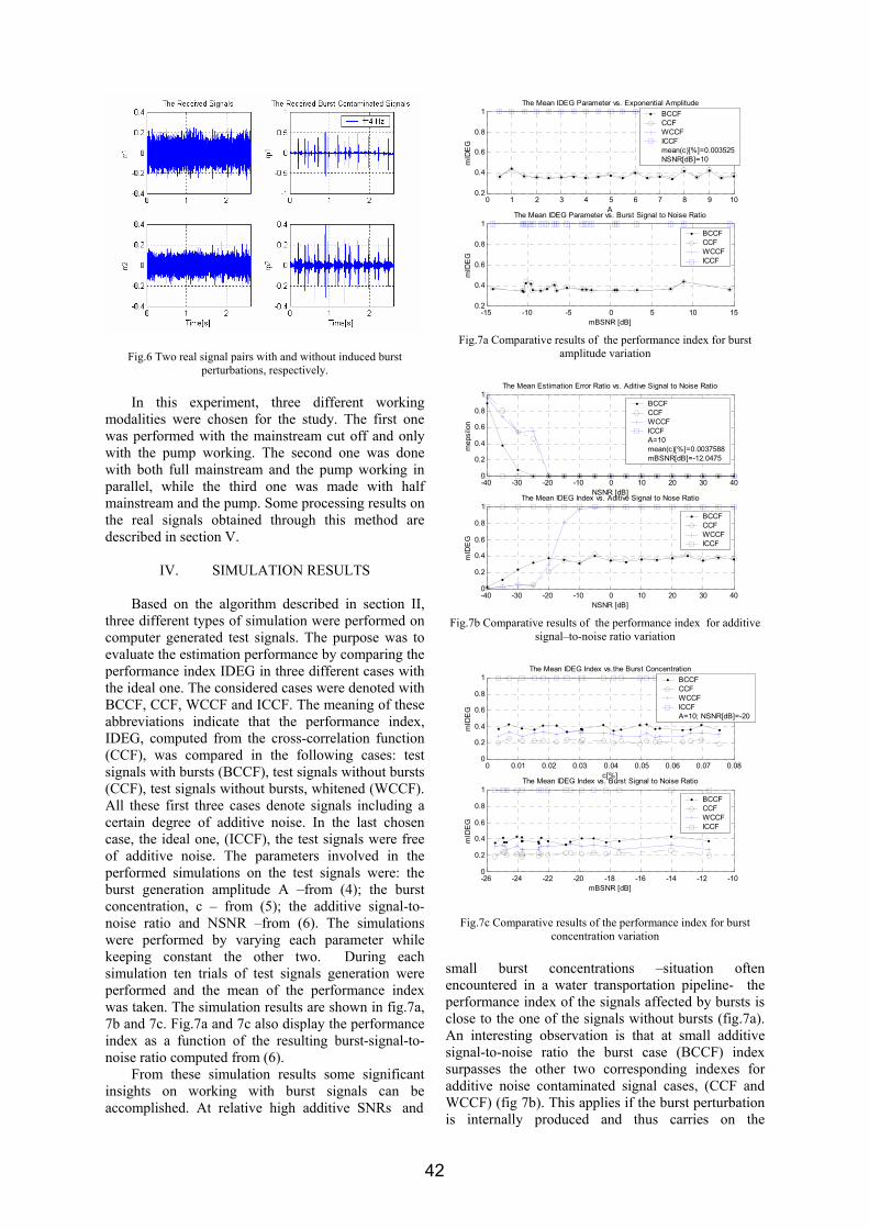
Fig.6 Two real signal pairs with and without induced burst perturbations, respectively.
In this experiment, three different working modalities were chosen for the study. The first one was performed with the mainstream cut off and only with the pump working. The second one was done with both full mainstream and the pump working in parallel, while the third one was made with half mainstream and the pump. Some processing results on the real signals obtained through this method are described in section V.
IV. SIMULATION RESULTS
Based on the algorithm described in section II, three different types of simulation were performed on computer generated test signals. The purpose was to evaluate the estimation performance by comparing the performance index IDEG in three different cases with the ideal one. The considered cases were denoted with BCCF, CCF, WCCF and ICCF. The meaning of these abbreviations indicate that the performance index, IDEG, computed from the cross-correlation function (CCF), was compared in the following cases: test signals with bursts (BCCF), test signals without bursts (CCF), test signals without bursts, whitened (WCCF). All these first three cases denote signals including a certain degree of additive noise. In the last chosen case, the ideal one, (ICCF), the test signals were free of additive noise. The parameters involved in the performed simulations on the test signals were: the burst generation amplitude A –from (4); the burst concentration, c – from (5); the additive signal-to-noise ratio and NSNR –from (6). The simulations were performed by varying each parameter while keeping constant the other two. During each simulation ten trials of test signals generation were performed and the mean of the performance index was taken. The simulation results are shown in fig.7a, 7b and 7c. Fig.7a and 7c also display the performance index as a function of the resulting burst-signal-to-noise ratio computed from (6). From these simulation results some significant insights on working with burst signals can be accomplished. At relative high additive SNRs and
0 1 2 3 4 5 6 7 8 9 100.2
0.4
0.6
0.8
1
A
mID
EG
The Mean IDEG Parameter vs. Exponential AmplitudeBCCF CCF WCCF ICCF mean(c)[%]=0.003525NSNR[dB]=10
-15 -10 -5 0 5 10 150.2
0.4
0.6
0.8
1
mBSNR [dB]
mID
EG
The Mean IDEG Parameter vs. Burst Signal to Noise Ratio
BCCFCCF WCCFICCF
Fig.7a Comparative results of the performance index for burst
amplitude variation
-40 -30 -20 -10 0 10 20 30 400
0.2
0.4
0.6
0.8
1
NSNR [dB]
mep
silo
n
The Mean Estimation Error Ratio vs. Aditive Signal to Noise Ratio
BCCF CCF WCCF ICCF A=10 mean(c)[%]=0.0037588mBSNR[dB]=-12.0475
-40 -30 -20 -10 0 10 20 30 400
0.2
0.4
0.6
0.8
1
NSNR [dB]
mID
EG
The Mean IDEG Index vs. Aditive Signal to Nose Ratio
BCCFCCF WCCFICCF
Fig.7b Comparative results of the performance index for additive
signal–to-noise ratio variation
0 0.01 0.02 0.03 0.04 0.05 0.06 0.07 0.080
0.2
0.4
0.6
0.8
1
c[%]
mID
EG
The Mean IDEG Index vs.the Burst ConcentrationBCCF CCF WCCF ICCF A=10; NSNR[dB]=-20
-26 -24 -22 -20 -18 -16 -14 -12 -100
0.2
0.4
0.6
0.8
1
mBSNR [dB]
mID
EG
The Mean IDEG Index vs. Burst Signal to Noise Ratio
BCCFCCF WCCFICCF
Fig.7c Comparative results of the performance index for burst concentration variation
small burst concentrations –situation often encountered in a water transportation pipeline- the performance index of the signals affected by bursts is close to the one of the signals without bursts (fig.7a). An interesting observation is that at small additive signal-to-noise ratio the burst case (BCCF) index surpasses the other two corresponding indexes for additive noise contaminated signal cases, (CCF and WCCF) (fig 7b). This applies if the burst perturbation is internally produced and thus carries on the
42
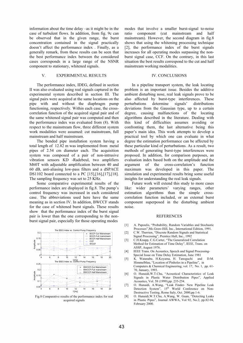
information about the time delay –as it might be in the case of turbulent flows. In addition, from fig. 9c can be observed that in the given range, the burst concentration contained in the signal practically doesn’t affect the performance index . Finally, as a generally remark, from these results can be seen that the best performance index between the considered cases corresponds in a large range of the NSNR component to stationary, whitened signals.
V. EXPERIMENTAL RESULTS
The performance index, IDEG, defined in section II was also evaluated using real signals captured in the experimental system described in section III. The signal pairs were acquired at the same locations on the pipe with and without the diaphragm pump functioning, respectively. Within each case, the cross-correlation function of the acquired signal pair and of the same whitened signal pair was computed and then the performance index was evaluated from (8). With respect to the mainstream flow, three different system work modalities were assumed: cut mainstream, full mainstream and half mainstream. The bended pipe installation system having a total length of 12.82 m was implemented from metal pipes of 2.54 cm diameter each. The acquisition system was composed of a pair of non-intrusive vibration sensors KD -Radebeul, two amplifiers M60T with adjustable amplification between 40 and 60 dB, anti-aliasing low-pass filters and a dSPACE DS1102 board connected to a PC [15],[16],[17],[18]. The sampling frequency was set to 25 KHz. Some comparative experimental results of the performance index are displayed in fig.8. The pump’s control frequency was increased in each considered case. The abbreviations used here have the same meaning as in section IV. In addition, BWCCF stands for the case of whitened burst signals. These results show that the performance index of the burst signal pair is lower than the one corresponding to the non-burst signal pair, especially for those operating modes
4 6 8 10 12 14 16 18 200
0.05
0.1
0.15
0.2
f [Hz]
Am
plitu
de
The IDEG Index vs. Control Pump FrequencyBCCF-Cut Mainstream BCCF-Full mainstreamBCCF-Half MainstreamCCF WCCF
4 6 8 10 12 14 16 18 200.05
0.1
0.15
0.2
0.25
f [Hz]
Am
plitu
de
The IDEG Index vs. Control Pump Frequency
BWCCF-Cut Mainstream BWCCF-Full mainstreamBWCCF-Half Mainstream
Fig.8 Comparative results of the performance index for real
acquired signals
modes that involve a smaller burst-signal to-noise ratio component (cut mainstream and half mainstream). However, the second diagram in fig.8 shows that using the whitening processing technique [2], the performance index of the burst signals increases for all operating modes surpassing the non-burst signal case, CCF. On the contrary, in this last situation the best results correspond to the cut and half mainstream working modalities.
IV. CONCLUSIONS
In a pipeline transport system, the leak locating problem is an important issue. Besides the additive ambient disturbing nose, real leak signals prove to be also affected by burst-type interferences. These perturbations determine signals’ distributions deviations from the Gaussian type, up to a certain degree, causing malfunctions of the locating algorithms described in the literature. Dealing with this kind of difficulties assumes avoiding or confronting them, the last alternative being this paper’s main idea. This work attempts to develop a practical tool by which one can evaluate in what degree the estimation performance can be affected by these particular kind of perturbations. As a result, two methods of generating burst-type interferences were proposed. In addition, for comparison purposes, an evaluation index based both on the amplitude and the argument of the cross-correlation’s function maximum was developed in this paper. The simulation and experimental results bring some useful insights for understanding the real leak signals. Future work will extend this study to more cases like: wider parameters’ varying ranges, other estimation algorithms than the simple cross-correlation function included, or an external burst component superposed in the disturbing ambient noise.
REFERENCES
[1] A. Papoulis, “Probability, Random Variables and Stochastic Processes”,Mc.Graw-Hill, Inc., International Edition, 1991.
[2] C.W. Therrien, “Discrete Random Signals and Statistical Signal Processing”, Prentice Hall, Inc., 1992 [3] C.H.Knapp, C.G.Carter, “The Generalized Correlation Method for Estimation of Time Delay”, IEEE, Trans. on ASSP, August 1976. [4] IEEE Trans. On Acoustics, Speech and Signal Processing- Special Issue on Time Delay Estimation, June 1981 [5] K. Watanabe, H.Koyama, H. Tanoguchi and D.M.
Himmelblau, “Location of Pinholes in a Pipeline”, in Computers & Chemical Engineering, vol. 17, No. 1, pp. 61-
70, January, 1993. [6] O. Hunaidi,W.T.Chu, “Acoustical Characteristics of Leak
Signals in Plastic Water Distribution Pipes”, Applied Acoustics, Vol. 58 (1999),pp. 235-254.
[7] O. Hunaidi, A.Wang, “Leak Finder- New Pipeline Leak Detection System”, 15th World Conference on Non-Destructive Testing, Rome Italy, Oct. 2000,pp.1-6.
[8] O. Hunaidi,W.T.Chu, A.Wang, W. Guan, “Detecting Leaks in Plastic Pipes”, Journal AWWA, Vol 92, No.2, pp.82-94, February 2000.
43

[9] Y. Wen, P.Li, J. Yang, Z. Zhou, “Information Processing in Buried Pipeline Leak Detection System”, IEEE, Proc. of International Conference on Information Acquisition, 2004. [10] S. Ionel, “A Practical Criterion for Time Delay Estimation Algorithms Comparison”,Transactions on Electronics and Communications, Tom 47(61), Fascicola 1-2, Sept. 2002. [11] M. Dăneţi, S.Ionel, “An Overview of Time Estimation Algorithms”, Trans. on Electronics and Communications, Tom 45(59), Fascicola 1, 2000.
[12] M. Dăneţi, S.Ionel, “A dSPACE Implementation of a Time Delay Estimation Algorithm”, Trans. on Electronics and Communications, Tom 45(59), Fascicola 1-2, 2002. [13] T. Cebeci, “Analysis of Turbulent Flows”, Elsevier 2003 [14] The Mathworks Inc., Matlab, Simulink,1999 . [15] dSPACE, “DS1102 User’s Guide”, 3-rd version, 1996. [16] dSPACE, “Instalation and Configuration Guide”, May 1999. [17] dSPACE, “Implementation Guide”, Sept. 1999. [18] dSPACE, “Experiment Guide”, Sept. 1999.
44
Buletinul Ştiinţific al Universităţii "Politehnica" din Timişoara
Seria ELECTRONICĂ şi TELECOMUNICAŢII TRANSACTIONS on ELECTRONICS and COMMUNICATIONS
Tom 52(66), Fascicola 2, 2007
The Use of the Improved Time-Frequency Method Based on Mathematical Morphology Operators
Marius Salagean1
1 Facultatea de Electronică şi Telecomunicaţii, Departamentul Comunicaţii Bd. V. Pârvan Nr. 2, 300223 Timişoara, e-mail [email protected]
Abstract – The method uses the ridges extraction method from the time-frequency distribution based on mathematical morphology operators (TF-MO). The TF-MO method for signals with highly non-linear IF corrupted by Gaussian white noise is not very adapted for IF estimation. In this paper is presented a new improved technique for IF estimation based on TF-MO method. Keywords: Instantaneous frequency, time-frequency distribution, complex argument, mathematical morphology, signal analysis, image analysis.
I. INTRODUCTION
In signal processing the decision (detection, denoising, estimation, recognition or classification) is a basic problem. Knowing that the real environments are generally highly non-stationary, it is necessary to use a method able to provide suggestive information about the signal structure. A potential solution is based on time-frequency representations that provide a good concentration around the law of the IF and realize a diffusion of the perturbation noise in the time-frequency plane. The TF-MO estimation method [2] is based on the conjoint use of two very modern theories, that of time-frequency distributions and that of mathematical morphology. This strategy permits the enhancement of the set of signal processing methods with the aid of some methods developed in the context of image processing. In [1] it has been showed that for signals with a time-frequency structure not so complicated, the performances of the TF-MO method are good. Unfortunately for signal with swift transitions over a short duration of time and SNR high enough, the accuracy of the IF estimation in the TF-MO method is poorer. In this case the bias in the TF-MO method is significant and dominates the estimation error, the IF estimator cannot accurately follow the rapid transitions in the IF. For signals with highly non-linear IF the performance can be improved by applying the morphological
operators on multiples segments of the signal component. The paper is organized as follow. The improved TF-MO method is illustrated in section II. In section III some simulation results are depicted. Section IV will close this communication.
II. TIME-FREQUENCY MORPHOLOGICAL OPERATORS METHOD
The estimation method based on time-frequency and image processing techniques has been introduced in [2]. The quality of estimating the IF depends on the time-frequency distribution and on its ridges projection mechanism. The TF-MO method proposes a time-frequency representation based on cooperation of linear and bilinear distributions: the Gabor and the Wigner-Ville distributions. It is known [3] that the Gabor representation has a good localization and free interference terms properties. Unfortunately, the linear distributions, except the Discrete Wavelet transform, correlate the zero mean white input noise, as shown in [4]. The WVD is a spectral-temporal density of energy that does not correlates the input noise, thus having a spreading effect of the noise power in the time-frequency plane [2]. The WVD has also a good time-frequency concentration. To combine these useful advantages, the time-frequency distribution is calculated according to the following algorithm [2]: 1) Calculate the Gabor transform for the signal s, ( )ω,tG .
2) Filter the image obtained with a hard-thresholding filter:
( ) ( )( )⎪⎩
⎪⎨⎧
<
≥=
trtGif
trtGiftY
ω
ωω
,,0
,,1, (1)
where tr is the threshold used. 3) Calculate the WVD for the signal s, ( )ω,tWV . 4) Multiply the modulus of the ( )ω,tY distribution with the ( )ω,tWV distribution.
45
In step 2) the proposed threshold value is:
( )( )
5
,max,
ωω
tGtr t= (2)
This operation decreases the amount of noise that perturbs the ridges of ( )ω,tG and brings to zero the values in the rest of the time-frequency plane. The effect of the multiplication in step 4) is the reduction of the interference terms of the WVD and the very good localization of the ridges of the resulting ditribution. To estimate the ridges of the obtained distribution, some mathematical morphology operators are used, the above resulting distribution being regarded as an image. This mechanism is applied through the following steps [2]: 1) Convert the image obtained in step 4) in the procedure described earlier in binary form. 2) Apply the dilation operator on the image in 1). 3) Skeletonization of the last image, an estimation of the IF of the signal being obtained. This image represents the result of the TF-MO method. The conversion in binary form realizes a denoising of the time-frequency distribution. The role of the dilation operator is to compensate the connectivity loss, produced by the preceding conversion. The skeleton produces the ridges estimation. Instead of applying the TF-MO method on the entire signal, we break the signal processing with this method on multiples segments of the signal component. Each signal segment is oversampled. For each signal segment is obtained an image representing the estimation of the IF on that signal interval. The final image (the estimation of the IF of the entire signal) is constructed by merging all segment’s IF images.
III. RESULTS Example 1: Consider a noisy monocomponent signal with highly non-linear IF:
( ) ( ) ( )( ) ( )tnt
ttjts++
+−=))5.1/5cos
2/3coscos3(expπ
ππ (3)
within the interval [-1, 1] where n(t) is a Gaussian white noise. The IF is estimated for various values of the SNR, based on the TF-MO method and improved TF-MO method. Fig. 1, represent the estimated IF with the two methods, for SNR=30dB along with the real IF law.
Fig. 1. IF estimation based on TF-MO method for SNR=30dB
Mean squared errors of the IF estimation calculated in 128 realizations for SNR values within the interval [3dB, 30dB], based on TF-MO method is showed in Fig. 2.
Fig. 2. Mean squared error of the IF estimation for SNR between [3dB, 30dB] based on TF-MO method
Fig. 3, represent the estimated IF with the improved TF-MO, for SNR=30dB along with the real IF law.
Fig. 3. IF estimation based on improved TF-MO method for SNR=30dB
Time
Freq
uenc
y
Time
Freq
uenc
y
SNR [dB]
MSE
46
Fig. 3 illustrates the fact that the bias in the improved TF-MO method is reduced in comparison with bias in the TF-MO method (Fig. 1). The IF estimator in this case follows more accurately the rapid transitions in the IF. In the next table is presented mean squared error (MSE) of the IF estimation for SNR=30dB for the TF-MO method and the improved TF-MO method. Table 1.
SNR [dB] MSE TF-MO method
MSE Improved TF-MO method
30 33.8038 18.6930 From these numerical results, it can be noticed an improvement in the IF estimation of about 44.7 percent. Example 2: Consider now a noisy monocomponent signal with non-linear IF:
( ) ( )tnttjts +−= )5.95(exp 3 ππ (4)
within the interval [-1, 1] where n(t) is a Gaussian white noise. The IF is estimated for various values of the SNR, based on the TF-MO method and improved TF-MO method. Fig. 4, represent the estimated IF with the two methods, for SNR=30dB along with the real IF law.
Fig. 4. Mean squared error of the IF estimation for SNR between [3dB, 30dB] based on TF-MO method
Fig. 5 represents the mean squared errors of the IF estimation calculated in 128 realizations for SNR values within the interval [3dB, 30dB], based on TF-MO method.
Fig. 5. IF estimation based on TF-MO method for SNR=30dB The estimated IF with the improved TF-MO, for SNR=30dB along with the real IF law is showed in Fig. 6.
Fig. 6. IF estimation based on improved TF-MO method for SNR=30dB
In the next table is presented mean squared error (MSE) of the IF estimation for SNR=30dB for the TF-MO method and the improved TF-MO method.
Table 2.
SNR [dB] MSE TF-MO method
MSE Improved TF-MO method
30 1.0964 1.0854 From these numerical results, it can be noticed that the improvement in the IF estimation is not important, thus for signals with a time-frequency structure not so complicated, the use of the improved TF-MO method is not justified.
Time
Freq
uenc
y
SNR [dB]
MSE
Time
Freq
uenc
y
47
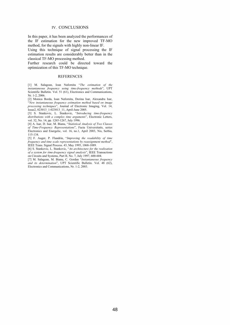
IV. CONCLUSIONS In this paper, it has been analyzed the performances of the IF estimation for the new improved TF-MO method, for the signals with highly non-linear IF. Using this technique of signal processing the IF estimation results are considerably better than in the classical TF-MO processing method. Further research could be directed toward the optimization of this TF-MO technique.
REFERENCES
[1] M. Salagean, Ioan Nafornita “The estimation of the instantaneous frequency using time-frequency methods”, UPT Scientific Bulletin. Vol. 51 (61), Electronics and Communications, Nr. 1-2, 2006. [2] Monica Borda, Ioan Nafornita, Dorina Isar, Alexandru Isar, “New instantaneous frequency estimation method based on image processing techniques”, Journal of Electronic Imaging, Vol. 14, Issue2, 023013_1-023013_11, April-June 2005. [3] S. Stankovic, L. Stankovic, “Introducing time-frequency distributions with a complex time arguments”, Electronic Letters, vol. 32, No. 14, pp. 1265-1267, July 1996. [4] A. Isar, D. Isar, M. Bianu, “Statistical Analysis of Two Classes of Time-Frequency Representations”, Facta Universitatis, series Electronics and Energetic, vol. 16, no.1, April 2003, Nis, Serbia, 115-134. [5] F. Auger, P. Flandrin, “Improving the readability of time frequency and time scale representations by reassignment method”, IEEE Trans. Signal Process. 43, May 1995, 1068-1089. [6] S. Stankovic, L. Stankovic, “An architecture for the realization of a system for time-frequency signal analysis”, IEEE Transactions on Circuits and Systems, Part II, No. 7, July 1997, 600-604. [7] M. Salagean, M. Bianu, C. Gordan “Instantaneous frequency and its determination”, UPT Scientific Bulletin. Vol. 48 (62), Electronics and Communications, Nr. 1-2, 2003.
48
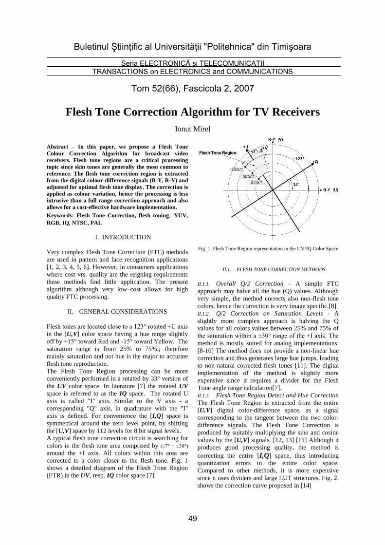
Buletinul Ştiinţific al Universităţii "Politehnica" din Timişoara
Seria ELECTRONICĂ şi TELECOMUNICAŢII TRANSACTIONS on ELECTRONICS and COMMUNICATIONS
Tom 52(66), Fascicola 2, 2007
Flesh Tone Correction Algorithm for TV Receivers
Ionut Mirel
Abstract – In this paper, we propose a Flesh Tone
Colour Correction Algorithm for broadcast video
receivers. Flesh tone regions are a critical processing
topic since skin tones are generally the most common to
reference. The flesh tone correction region is extracted
from the digital colour-difference signals (B-Y, R-Y) and
adjusted for optimal flesh tone display. The correction is
applied as colour variation, hence the processing is less
intrusive than a full range correction approach and also
allows for a cost-effective hardware implementation.
Keywords: Flesh Tone Correction, flesh toning, YUV,
RGB, IQ, NTSC, PAL
I. INTRODUCTION
Very complex Flesh Tone Correction (FTC) methods
are used in pattern and face recognition applications
[1, 2, 3, 4, 5, 6]. However, in consumers applications
where cost vrs. quality are the reigning requirements
these methods find little application. The present
algorithm although very low–cost allows for high
quality FTC processing.
II. GENERAL CONSIDERATIONS
Flesh tones are located close to a 123° rotated +U axis
in the [U,V] color space having a hue range slightly
off by +15° toward Red and -15° toward Yellow. The
saturation range is from 25% to 75%.; therefore
mainly saturation and not hue is the major to accurate
flesh tone reproduction.
The Flesh Tone Region processing can be more
conveniently performed in a rotated by 33° version of
the UV color space. In literature [7] the rotated UV
space is referred to as the IQ space. The rotated U
axis is called "I" axis. Similar to the V axis - a
corresponding "Q" axis, in quadrature with the "I"
axis is defined. For convenience the [I,Q] space is
symmetrical around the zero level point, by shifting
the [U,V] space by 112 levels for 8 bit signal levels.
A typical flesh tone correction circuit is searching for
colors in the flesh tone area comprised by (±7° ÷ ±30°)
around the +I axis. All colors within this area are
corrected to a color closer to the flesh tone. Fig. 1
shows a detailed diagram of the Flesh Tone Region
(FTR) in the UV, resp. IQ color space [7].
Fig. 1. Flesh Tone Region representation in the UV/IQ Color Space
II.1. FLESH TONE CORRECTION METHODS
II.1.1. Overall Q/2 Correction - A simple FTC
approach may halve all the hue (Q) values. Although
very simple, the method corrects also non-flesh tone
colors, hence the correction is very image specific.[8]
II.1.2. Q/2 Correction on Saturation Levels - A
slightly more complex approach is halving the Q
values for all colors values between 25% and 75% of
the saturation within a ±30° range of the +I axis. The
method is mostly suited for analog implementations.
[8-10] The method does not provide a non-linear hue
correction and thus generates large hue jumps, leading
to non-natural corrected flesh tones [11]. The digital
implementation of the method is slightly more
expensive since it requires a divider for the Flesh
Tone angle range calculation[7].
II.1.3. Flesh Tone Region Detect and Hue Correction
The Flesh Tone Region is extracted from the entire
[U,V] digital color-difference space, as a signal
corresponding to the tangent between the two color-
difference signals. The Flesh Tone Correction is
produced by suitably multiplying the sine and cosine
values by the [U,V] signals. [12, 13] [11] Although it
produces good processing quality, the method is
correcting the entire [I,Q] space, thus introducing
quantization errors in the entire color space.
Compared to other methods, it is more expensive
since it uses dividers and large LUT structures. Fig. 2.
shows the correction curve proposed in [14]
49
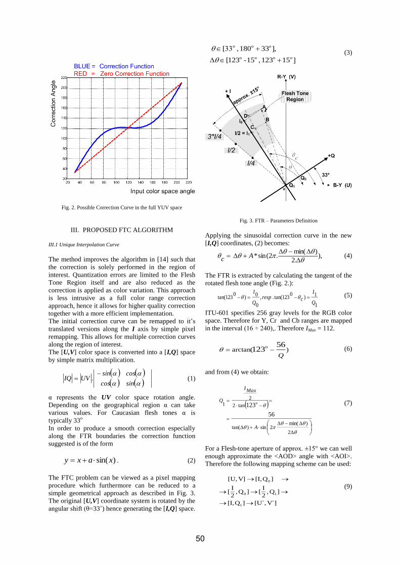
Fig. 2. Possible Correction Curve in the full YUV space
III. PROPOSED FTC ALGORITHM
III.1 Unique Interpolation Curve
The method improves the algorithm in [14] such that
the correction is solely performed in the region of
interest. Quantization errors are limited to the Flesh
Tone Region itself and are also reduced as the
correction is applied as color variation. This approach
is less intrusive as a full color range correction
approach, hence it allows for higher quality correction
together with a more efficient implementation.
The initial correction curve can be remapped to it’s
translated versions along the I axis by simple pixel
remapping. This allows for multiple correction curves
along the region of interest.
The [U,V] color space is converted into a [I,Q] space
by simple matrix multiplication.
sin cos
cossinUVIQ
. (1)
α represents the UV color space rotation angle.
Depending on the geographical region α can take
various values. For Caucasian flesh tones α is
typically 33o
In order to produce a smooth correction especially
along the FTR boundaries the correction function
suggested is of the form
)sin( xaxy . (2)
The FTC problem can be viewed as a pixel mapping
procedure which furthermore can be reduced to a
simple geometrical approach as described in Fig. 3.
The original [U,V] coordinate system is rotated by the
angular shift (θ=33˚) hence generating the [I,Q] space.
oooo
ooo
1512315-123[
,33180[
(3)
Fig. 3. FTR – Parameters Definition
Applying the sinusoidal correction curve in the new
[I,Q] coordinates, (2) becomes:
),.2
)min(.2(sin*
A
c (4)
The FTR is extracted by calculating the tangent of the
rotated flesh tone angle (Fig. 2.):
1
1)
0123tan(.,
0
0)
0123tan(
Q
I
crespQ
I (5)
ITU-601 specifies 256 gray levels for the RGB color
space. Therefore for Y, Cr and Cb ranges are mapped
in the interval (16 ÷ 240),. Therefore IMax = 112.
)arctan(56
123o
Q (6)
and from (4) we obtain:
2
)min(2sin)tan(
tan2
2
1
56
123o
A
MaxI
Q (7)
For a Flesh-tone aperture of approx. ±15° we can well
enough approximate the <AOD> angle with <AOI>.
Therefore the following mapping scheme can be used:
V`][U`,]Q[I,
]Q,2
I[]Q,
2
I[
]Q[I,V][U,
1
10
0
(9)
50
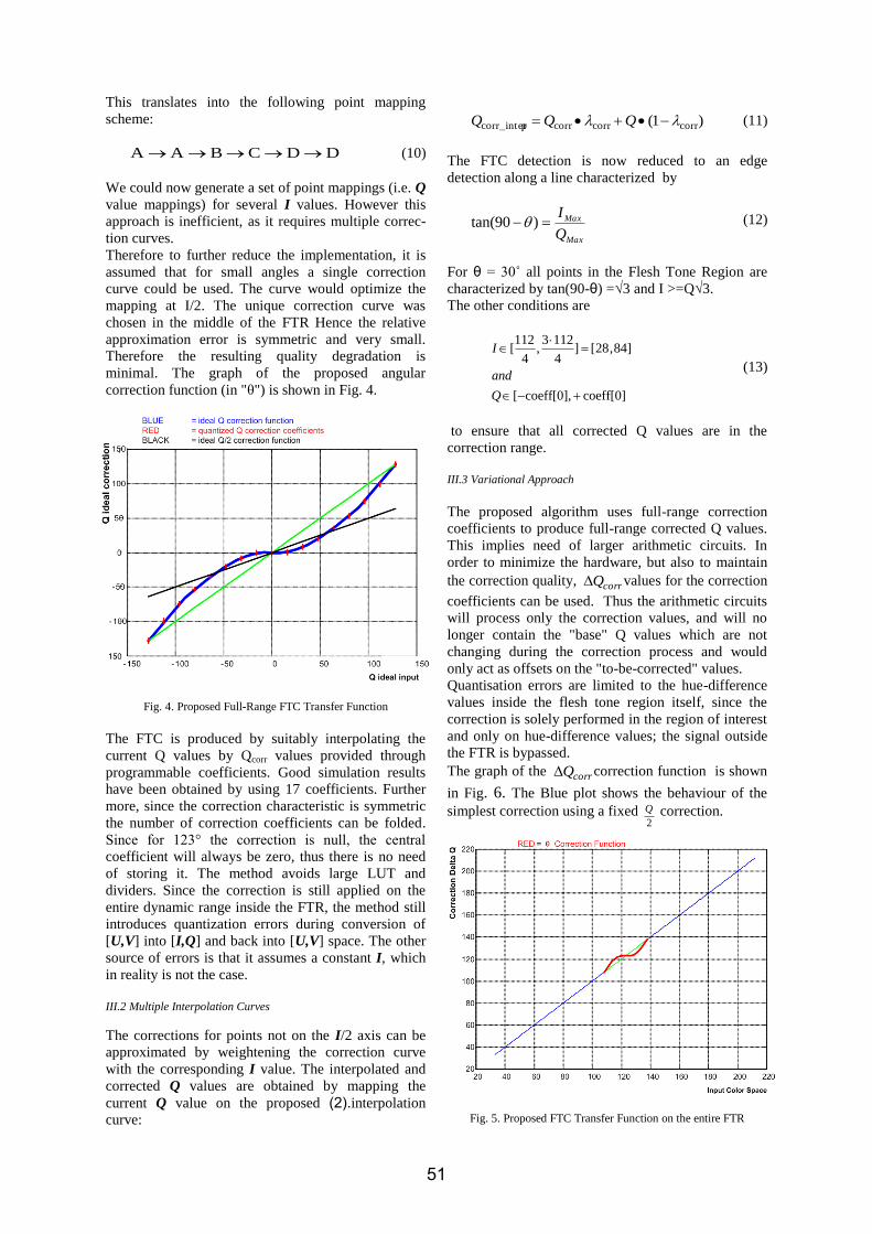
This translates into the following point mapping
scheme:
DDCBAA (10)
We could now generate a set of point mappings (i.e. Q
value mappings) for several I values. However this
approach is inefficient, as it requires multiple correc-
tion curves.
Therefore to further reduce the implementation, it is
assumed that for small angles a single correction
curve could be used. The curve would optimize the
mapping at I/2. The unique correction curve was
chosen in the middle of the FTR Hence the relative
approximation error is symmetric and very small.
Therefore the resulting quality degradation is
minimal. The graph of the proposed angular
correction function (in "θ") is shown in Fig. 4.
Fig. 4. Proposed Full-Range FTC Transfer Function
The FTC is produced by suitably interpolating the
current Q values by Qcorr values provided through
programmable coefficients. Good simulation results
have been obtained by using 17 coefficients. Further
more, since the correction characteristic is symmetric
the number of correction coefficients can be folded.
Since for 123° the correction is null, the central
coefficient will always be zero, thus there is no need
of storing it. The method avoids large LUT and
dividers. Since the correction is still applied on the
entire dynamic range inside the FTR, the method still
introduces quantization errors during conversion of
[U,V] into [I,Q] and back into [U,V] space. The other
source of errors is that it assumes a constant I, which
in reality is not the case.
III.2 Multiple Interpolation Curves
The corrections for points not on the I/2 axis can be
approximated by weightening the correction curve
with the corresponding I value. The interpolated and
corrected Q values are obtained by mapping the
current Q value on the proposed (2).interpolation
curve:
)1( corrcorrcorrpcorr_inter QQQ (11)
The FTC detection is now reduced to an edge
detection along a line characterized by
Max
Max
Q
I )90tan( (12)
For θ = 30˚ all points in the Flesh Tone Region are
characterized by tan(90-θ) =√3 and I >=Q√3.
The other conditions are
coeff[0] coeff[0],[
]84,28[]4
1123,
4
112[
Q
and
I
(13)
to ensure that all corrected Q values are in the
correction range.
III.3 Variational Approach
The proposed algorithm uses full-range correction
coefficients to produce full-range corrected Q values.
This implies need of larger arithmetic circuits. In
order to minimize the hardware, but also to maintain
the correction quality, corrQ values for the correction
coefficients can be used. Thus the arithmetic circuits
will process only the correction values, and will no
longer contain the "base" Q values which are not
changing during the correction process and would
only act as offsets on the "to-be-corrected" values.
Quantisation errors are limited to the hue-difference
values inside the flesh tone region itself, since the
correction is solely performed in the region of interest
and only on hue-difference values; the signal outside
the FTR is bypassed.
The graph of the corrQ correction function is shown
in Fig. 6. The Blue plot shows the behaviour of the
simplest correction using a fixed 2
Q correction.
Fig. 5. Proposed FTC Transfer Function on the entire FTR
51
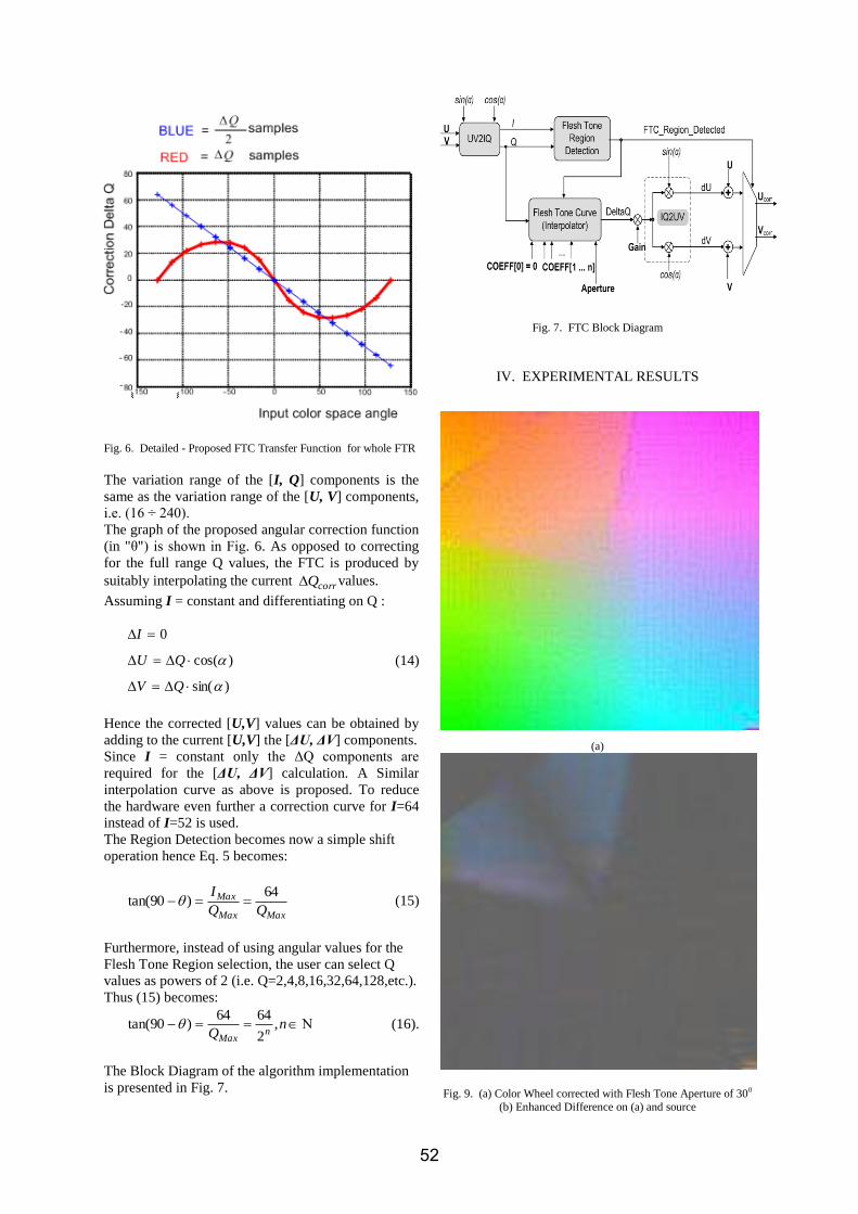
Fig. 6. Detailed - Proposed FTC Transfer Function for whole FTR
The variation range of the [I, Q] components is the
same as the variation range of the [U, V] components,
i.e. (16 ÷ 240).
The graph of the proposed angular correction function
(in "θ") is shown in Fig. 6. As opposed to correcting
for the full range Q values, the FTC is produced by
suitably interpolating the current corrQ values.
Assuming I = constant and differentiating on Q :
)sin(
)cos(
0
QV
QU
I
(14)
Hence the corrected [U,V] values can be obtained by
adding to the current [U,V] the [ΔU, ΔV] components.
Since I = constant only the ΔQ components are
required for the [ΔU, ΔV] calculation. A Similar
interpolation curve as above is proposed. To reduce
the hardware even further a correction curve for I=64
instead of I=52 is used.
The Region Detection becomes now a simple shift
operation hence Eq. 5 becomes:
MaxMax
Max
I 64)90tan( (15)
Furthermore, instead of using angular values for the
Flesh Tone Region selection, the user can select Q
values as powers of 2 (i.e. Q=2,4,8,16,32,64,128,etc.).
Thus (15) becomes:
nQ n
Max
,2
6464)90tan( (16).
The Block Diagram of the algorithm implementation
is presented in Fig. 7.
Fig. 7. FTC Block Diagram
IV. EXPERIMENTAL RESULTS
(a)
Fig. 9. (a) Color Wheel corrected with Flesh Tone Aperture of 300
(b) Enhanced Difference on (a) and source
52
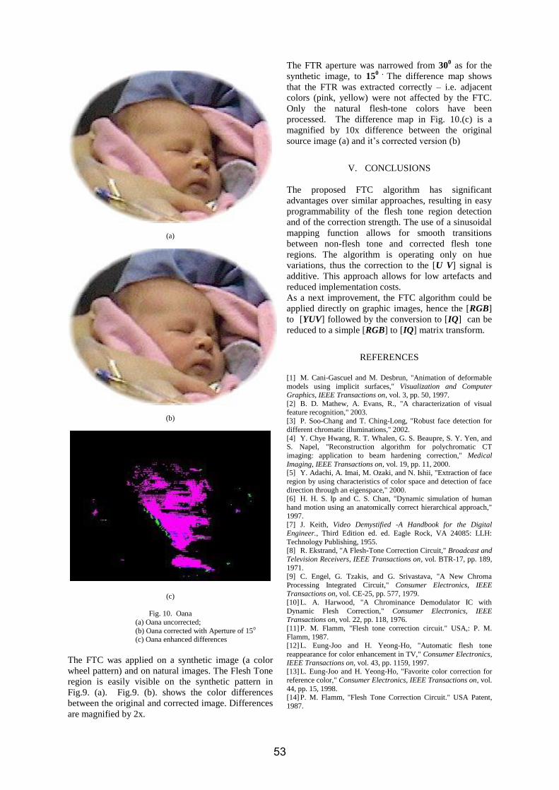
(a)
(b)
(c)
Fig. 10. Oana
(a) Oana uncorrected;
(b) Oana corrected with Aperture of 150 (c) Oana enhanced differences
The FTC was applied on a synthetic image (a color
wheel pattern) and on natural images. The Flesh Tone
region is easily visible on the synthetic pattern in
Fig.9. (a). Fig.9. (b). shows the color differences
between the original and corrected image. Differences
are magnified by 2x.
The FTR aperture was narrowed from 300 as for the
synthetic image, to 150 .
The difference map shows
that the FTR was extracted correctly – i.e. adjacent
colors (pink, yellow) were not affected by the FTC.
Only the natural flesh-tone colors have been
processed. The difference map in Fig. 10.(c) is a
magnified by 10x difference between the original
source image (a) and it’s corrected version (b)
V. CONCLUSIONS
The proposed FTC algorithm has significant
advantages over similar approaches, resulting in easy
programmability of the flesh tone region detection
and of the correction strength. The use of a sinusoidal
mapping function allows for smooth transitions
between non-flesh tone and corrected flesh tone
regions. The algorithm is operating only on hue
variations, thus the correction to the [U V] signal is
additive. This approach allows for low artefacts and
reduced implementation costs.
As a next improvement, the FTC algorithm could be
applied directly on graphic images, hence the [RGB]
to [YUV] followed by the conversion to [IQ] can be
reduced to a simple [RGB] to [IQ] matrix transform.
REFERENCES
[1] M. Cani-Gascuel and M. Desbrun, "Animation of deformable
models using implicit surfaces," Visualization and Computer Graphics, IEEE Transactions on, vol. 3, pp. 50, 1997.
[2] B. D. Mathew, A. Evans, R., "A characterization of visual
feature recognition," 2003.
[3] P. Soo-Chang and T. Ching-Long, "Robust face detection for
different chromatic illuminations," 2002.
[4] Y. Chye Hwang, R. T. Whalen, G. S. Beaupre, S. Y. Yen, and S. Napel, "Reconstruction algorithm for polychromatic CT
imaging: application to beam hardening correction," Medical
Imaging, IEEE Transactions on, vol. 19, pp. 11, 2000. [5] Y. Adachi, A. Imai, M. Ozaki, and N. Ishii, "Extraction of face
region by using characteristics of color space and detection of face
direction through an eigenspace," 2000. [6] H. H. S. Ip and C. S. Chan, "Dynamic simulation of human
hand motion using an anatomically correct hierarchical approach,"
1997. [7] J. Keith, Video Demystified -A Handbook for the Digital
Engineer., Third Edition ed. ed. Eagle Rock, VA 24085: LLH:
Technology Publishing, 1955. [8] R. Ekstrand, "A Flesh-Tone Correction Circuit," Broadcast and
Television Receivers, IEEE Transactions on, vol. BTR-17, pp. 189,
1971. [9] C. Engel, G. Tzakis, and G. Srivastava, "A New Chroma
Processing Integrated Circuit," Consumer Electronics, IEEE
Transactions on, vol. CE-25, pp. 577, 1979.
[10] L. A. Harwood, "A Chrominance Demodulator IC with
Dynamic Flesh Correction," Consumer Electronics, IEEE Transactions on, vol. 22, pp. 118, 1976.
[11] P. M. Flamm, "Flesh tone correction circuit." USA,: P. M.
Flamm, 1987. [12] L. Eung-Joo and H. Yeong-Ho, "Automatic flesh tone
reappearance for color enhancement in TV," Consumer Electronics,
IEEE Transactions on, vol. 43, pp. 1159, 1997. [13] L. Eung-Joo and H. Yeong-Ho, "Favorite color correction for
reference color," Consumer Electronics, IEEE Transactions on, vol.
44, pp. 15, 1998. [14] P. M. Flamm, "Flesh Tone Correction Circuit." USA Patent,
1987.
53
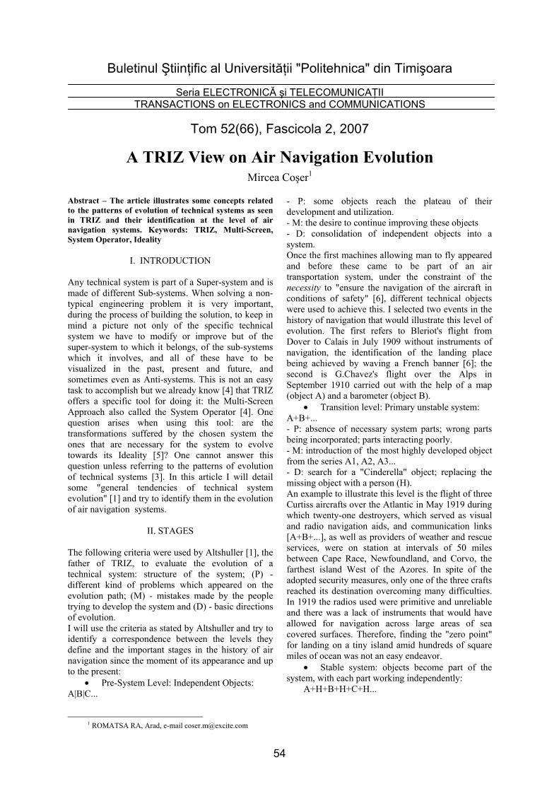
Buletinul Ştiinţific al Universităţii "Politehnica" din Timişoara
Seria ELECTRONICĂ şi TELECOMUNICAŢII TRANSACTIONS on ELECTRONICS and COMMUNICATIONS
Tom 52(66), Fascicola 2, 2007
A TRIZ View on Air Navigation Evolution
Mircea Coşer1
1 ROMATSA RA, Arad, e-mail [email protected]
Abstract – The article illustrates some concepts related to the patterns of evolution of technical systems as seen in TRIZ and their identification at the level of air navigation systems. Keywords: TRIZ, Multi-Screen, System Operator, Ideality
I. INTRODUCTION
Any technical system is part of a Super-system and is made of different Sub-systems. When solving a non-typical engineering problem it is very important, during the process of building the solution, to keep in mind a picture not only of the specific technical system we have to modify or improve but of the super-system to which it belongs, of the sub-systems which it involves, and all of these have to be visualized in the past, present and future, and sometimes even as Anti-systems. This is not an easy task to accomplish but we already know [4] that TRIZ offers a specific tool for doing it: the Multi-Screen Approach also called the System Operator [4]. One question arises when using this tool: are the transformations suffered by the chosen system the ones that are necessary for the system to evolve towards its Ideality [5]? One cannot answer this question unless referring to the patterns of evolution of technical systems [3]. In this article I will detail some "general tendencies of technical system evolution" [1] and try to identify them in the evolution of air navigation systems.
II. STAGES The following criteria were used by Altshuller [1], the father of TRIZ, to evaluate the evolution of a technical system: structure of the system; (P) -different kind of problems which appeared on the evolution path; (M) - mistakes made by the people trying to develop the system and (D) - basic directions of evolution. I will use the criteria as stated by Altshuller and try to identify a correspondence between the levels they define and the important stages in the history of air navigation since the moment of its appearance and up to the present:
• Pre-System Level: Independent Objects: A|B|C...
- P: some objects reach the plateau of their development and utilization. - M: the desire to continue improving these objects - D: consolidation of independent objects into a system. Once the first machines allowing man to fly appeared and before these came to be part of an air transportation system, under the constraint of the necessity to "ensure the navigation of the aircraft in conditions of safety" [6], different technical objects were used to achieve this. I selected two events in the history of navigation that would illustrate this level of evolution. The first refers to Bleriot's flight from Dover to Calais in July 1909 without instruments of navigation, the identification of the landing place being achieved by waving a French banner [6]; the second is G.Chavez's flight over the Alps in September 1910 carried out with the help of a map (object A) and a barometer (object B).
• Transition level: Primary unstable system: A+B+... - P: absence of necessary system parts; wrong parts being incorporated; parts interacting poorly. - M: introduction of the most highly developed object from the series A1, A2, A3... - D: search for a "Cinderella" object; replacing the missing object with a person (H). An example to illustrate this level is the flight of three Curtiss aircrafts over the Atlantic in May 1919 during which twenty-one destroyers, which served as visual and radio navigation aids, and communication links [A+B+...], as well as providers of weather and rescue services, were on station at intervals of 50 miles between Cape Race, Newfoundland, and Corvo, the farthest island West of the Azores. In spite of the adopted security measures, only one of the three crafts reached its destination overcoming many difficulties. In 1919 the radios used were primitive and unreliable and there was a lack of instruments that would have allowed for navigation across large areas of sea covered surfaces. Therefore, finding the "zero point" for landing on a tiny island amid hundreds of square miles of ocean was not an easy endeavor.
• Stable system: objects become part of the system, with each part working independently:
A+H+B+H+C+H...
54
- P: resources of system development limited only by the capacity of the human portion of the system - M: desire to improve only parts A and B ... while preserving parts H. - D: replacement of human (H) parts with device (D). The newly created system, although not entirely perfected, already receives new utilizations for example mail delivery. To facilitate navigation a huge network of light beacons was deployed in the USA. A beacon consisted of a parabolic mirror and a rotating lamp flashing every 10 seconds. This allowed night flights to be performed. At the same time "dead reckoning" [7] (estimating one's current position on the basis of a previously determined position, or fixing, and advancing that position on the basis of known speed, elapsed time, and course) was the primary navigation method used. It is the method on which Lindberg relied on his first trans-Atlantic flight. A pilot used this method when flying over large bodies of water, forest, deserts. It demanded more skill and experience than piloting did. It was based only on time, distance, and direction. The pilot had to know the distance from one point to the next and the magnetic heading to be maintain. The pilot worked on the pre-flight plan chart, he planned a route in advance. The pilot calculated [A+H...] the exact time when he would reach his destination while flying at constant speed. In the air, the pilot used the compass [B+H...] to keep the plane heading in the right direction. The first LF navigation systems transmitted two Morse-codes, letter A, point, line, and letter N, line, point, using a bandwidth between 190 to 535 kHz. They transmitted a powerful beacon (1500 watt), spaced at a distance of 200 miles. The pilot was guided by the beacon behind him for 100 miles and then by the beacon ahead of him for the next 100 miles. The beam width being only about 3°, it was important for the pilot to rapidly tune in to the station ahead of him. The sub-systems were not yet specialized: when radio stations were located near the airport, one of the beams which was lined up with the runaway was used for landing under low-visibility conditions. Although radio beacons represented a milestone in instrumental flight, there were quite a few limitations proved by the following assertion: "When flying through mountain passes in IFR (Instrumental Flight Rules A/N) weather or on a dark night, the pilots paid close attention to the tones in their headphones. Palms became moist in the cockpit when static from electrical storms interfered with the reception of those crucial signals - or when beacon signals bounced off the canyon walls and gave false information"[8].
• Transition level: Unstable system; device Dh copies human actions: A+Dh+B+Dh+ ... - P: Devices Dh limit the ability of the entire system - M: improvements of each separate element without considering that they compose now a complete system - D: transition from mechanical set of parts to organically interwoven synthetic system of elements.
Air navigation is no longer limited by man's orientation abilities and his speed of reaction; the equipment on board the plane allows for navigation under the most different circumstances: nighttime, fog, or storms. Much of the equipment still imitates the old pattern of orientation, for example the ground light beacons are replaced with different types of radio signals which the members of the crew have to identify and manually measure; the crew is made up of operators specialized in navigation; board instruments, grouped by their function, are clearly separated depending on their users: the pilot, the mechanic, the navigator. Old principles are taken over in order to build instruments meant to measure elements that could be used in establishing the trajectory of the aircraft. The altimeter (a kind of barometer) appears around 1913-14. It is perfected in 1929 when its precision is increased (as a sub-system of the navigation systems, it independently follows a similar evolutionary curve reaching the apogee of its evolution by the use of its initial fundamental principle, that of the aneroid barometer). Further improvements at the level of the altimeter as an independent navigation instrument are connected with the appearance of the servo-altimeter, to which the mechanical part is reduced by an inductive method. Later on the radio-altimeter is devised using a different physical principle, respectively the properties of the radio waves. In the 1930s and 40s within the generalization of the procedure involving radio connection with the ground, the communication of the data on atmospheric pressure at the destination airport prefigures the future integration of this information in a super-system (Aeronautical Fixed Telecommunication Network). Other instruments were developed: the speedometer (for horizontal speed), the variometer (for vertical speed). The steps in the evolution of these instruments were similar, starting with the use of the principle for pressure measurement and continuing with the use of an electrical transducer. We can also mention the magnetic and gyroscopic compass and, in conformity with natural evolution, the gyromagnetic and gyroinductive ones. All these independent navigation instruments, although they represented a step forward, could not by themselves ensure sufficient accuracy in maintaining the direction of the flight.
• Stable system; some of its parts become element E of the system, and as a rule, they can work only together: E1+E2+E3+ ... - P: when one improves an element while significantly worsening other elements (or the entire system), the technical contradiction appears. - M: desire to gain in one area without consideration of the losses in another. - D: development of specialized systems. The information coming from the diversity of instruments on board the aircraft start being used in a more sophisticated way, by the correlation of different information and their use at he level of complex systems of navigation (Sperry C-9, Collins FD-108,
55
etc.). We can include here the VHF Omnidirectional Range navigation system (VOR) whose introduction began in the early 1950s and which is by far one of the most important inventions in air navigation. The VOR facility transmits two signals at the same time: one signal is constant in all directions, while the other is rotated about the station. The aircraft equipment receives both signals, compares electronically the difference between the two signals, and interprets the result as a radial from the station. The Instrument Landing System (ILS), the first of which was installed for testing at the Indianapolis airport in 1940, must also be mentioned.
• Specialized, stable system: E1'+E2'+E3'+ ... - P: as the system specializes further, its area of utilization shrinks, down time increases and efficiency declines. - M: desire to continue specialization. - D: reconstruction of complete system transition to other physical or chemical principles of action. The development of the same navigational systems, VOR/DME and NDB, continues; no new navigation principle appears, except some new concepts such as "free flight".
• Transition level: the E1'E1"+E2'E2"+... combination becomes an unstable system. - P: significant increase in system complexity; reduction of ability for development. - M: continuous search for different combinations of elements (subsystems). - D: transition to other physical or chemical principles of action. VOR/DME were still at the basis of controlling for the majority of flights; LORAN-C remains the newest navigational system in general use; OMEGA the most commonly used as a stand-alone, long-range navigational system. Instead of Instrument Landing System, the MLS (the microwave landing system) is outlined based on a new principle.
• Stable system: SuS1+SuS2+SuS3+ ... elements of the system rapidly develop into subsystems (SuS)
- P: the system development at some point gets into conflict with outside environment by creating unacceptable changes in it. - M: desire to smooth out conflict by adding intermediate sub-systems. - D: transition from an open system to a closed one, which is independent from outside environment. Air navigation becomes an activity with global implications but there are great differences between the levels reached by the composing parts. EFIS (the electronic flight information system displays) becomes imperative even if limited to the latest model airplanes. The most important negative impact on the medium is at the level of the super-system - the pollution of the atmosphere by the ever increasing number of crafts.
• Transition level: unstable system; during the working cycle an enclosed system is activated. - P: complication of design; limited time of action.
- M: continuous development of different sub-systems. - D: reconstruction of complete system: transition to new principles of action. The present navigation systems haven't all reached this level, but EFIS, INS (inertial navigation system) and GPS (global positioning system) assert themselves rapidly. It is interesting to notice that INS appeared in Germany around 1910 without having a practical usefulness, which can be explained by the fact that the other elements of air navigation were far from this level of evolution and therefore impossible to integrate in this context. INS was an autonomous system, with no ground correspondent and which, starting with 1932, due to military reasons, was developed for ballistic applications. It was only in 1950 that civil applications were transferred to it.
• Stable closed system - P: the number of sub-systems rapidly grows. - M: continuous development of a system and its sub-systems. - D: transition to super-system; the given system becomes an element of another system at a much higher level.
• The self developing system. The last two levels correspond to systems with a high degree of ideality. At the present stage of development aircraft fly respecting the same physical laws as before and no fundamentally new principles appeared in navigation. However, not even the most optimistic people could imagine that the life of a whole range of promising navigation systems, such as the MLS replacing the ILS, would be rapidly shortened by the GPS system; that EFIS would become standard:; while at the level of the instrument panel, the Synthetic Vision System would be devised, which integrated information from multiple sensors including infrared video cameras and laser radars that provided real-time, panoramic viewing for pilots and crew via sensor and synthetic data fusion. It is difficult to predict the evolutionary tendencies of air navigation both at the level of the super-system and the level of the sub-systems but, most certainly, the above tendencies will be confirmed and the present challenges connected with the use of polluting fossil fuels and the tremendous growth of air traffic will trigger the use of fundamentally new principles which will lie at the basis of future transportation systems and air navigation. Technical systems, and not only, follow a life which can be represented by a curve, the so called S-curve, showing the main characteristics of the system on the vertical axis and time on the horizontal one. Fig.1 represents the graphical representation of such a curve with some explanations [2]. This curve completes the models of evolution enabling the person interested in improving one of the existing systems to correctly appreciate the level of the chosen system and especially to answer a major question: "Ought one to solve a given problem and improve the technical system specified in it or present a new problem and
56
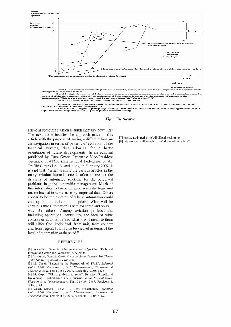
arrive at something which is fundamentally new"[ 2]? The next quote justifies the approach made in this article with the purpose of having a different look on air navigation in terms of patterns of evolution of the technical systems, thus allowing for a better orientation of future developments. In an editorial published by Dave Grace, Executive Vice-President Technical IFATCA (International Federation of Air Traffic Controllers' Associations) in February 2007, it is said that: "When reading the various articles in the many aviation journals, one is often amazed at the diversity of automated solutions for the perceived problems in global air traffic management. Much of this information is based on good scientific logic and reason backed in some cases by empirical data. Others appear to be the extreme of where automation could end up 'no controllers – no pilots.' What will be certain is that automation is here for some and on its way for others. Among aviation professionals, including operational controllers, the idea of what constitutes automation and what it will mean to them will differ from individual, from unit, from country and from region. It will also be viewed in terms of the level of automation anticipated."
REFERENCES [1] Alshuller, Genrich. The Innovation Algorithm. Technical Innovation Center, Inc. Worcester, MA, 2000 [2] Altshuller, Genrich. Creativity as an Exact Science. The Theory of the Solution of Inventive Problems. [3] M. Coşer, “Patents in the Framework of TRIZ”, Buletinul Universităţii “Politehnica”, Seria Electrotehnica, Electronica si Telecomunicatii, Tom 50 (64), 2005, Fascicola 2, 2005, pp. 34. [4] M. Coşer, "Which problem to solve", Buletinul Stiintific al Universităţii "Politehnica" din Timisoara, Seria Electrotehnica, Electronica si Telecomunicatii, Tom 52 (66), 2007, Fascicola 1, 2007, p. 40. [5] Coşer, Mircea. “TRIZ - a short presentation,” Buletinul Universităţii “Politehnica”, Seria Electrotehnica, Electronica si Telecomunicatii, Tom 48 (62), 2003, Fascicola 1, 2003, p. 89.
[6] Navigaţia aeriană, Eusebiu Hladiuc şi Alexandru Viorel Popescu, 1977, Editura Junimea - Iaşi [7] http://en.wikipedia.org/wiki/Dead_reckoning [8] http://www.navfltsm.addr.com/ndb-nav-history.htm?
Fig. 1 The S-curve
57
Buletinul Ştiinţific al Universităţii "Politehnica" din Timişoara
Seria ELECTRONICĂ şi TELECOMUNICAŢII TRANSACTIONS on ELECTRONICS and COMMUNICATIONS
Tom 52(66), Fascicola 2, 2007
An Overview of Intra-Domain QoS Mechanisms Evaluation
Emanuel Puschita1 Tudor Palade1 Ancuta Moldovan1 Simona Trifan1
1 Faculty of Electronics, Telecommunications and Information Technology, Communications Dept. 26 G. Bartitiu Street, 400027 Cluj-Napoca, Romania, e-mail [email protected].
Abstract – There has been a significant amount of work in the past decade to extend the IP architectures and to provide QoS support for multimedia applications. IP networks are evolving from a best-effort service support model, where all transmissions are considered equal and no delivery guarantees are made, to one that can provide predictable support, according to specific QoS requirements. Furthermore, recent applications are associated with user interactions, and the ability to browse different scenarios at the same time. All these aspects made the researchers look for other solutions in order to assure a QoS support. This paper includes the results obtained in order to provide a global analysis of the QoS parameters on four network layers, offers the mobility effect over the QoS parameters, especially in case of end-to-end delays introduced by handover procedure in different wireless access systems categories. Keywords: intra -domain QoS access mechanisms, mobility, QoS parameters
I. INTRODUCTION
There are a number of factors and components that affect the performances of multimedia application. By grouping all these elements, we consider the QoS problem having two major perspectives: (1) network perspective (involving an objective analysis), and (2) application/user perspective (involving a subjective analysis). From the network perspective, QoS refers to the service quality or level that the network offers to the application/user in terms of network’s QoS parameters, including: delays, jitters, number of packets lost, and throughput. From the application/user perspective, QoS refers to the application’s quality as perceived by the user, that is, the quality of the video presentation, the sound quality of a streaming audio, etc. The applications and users are grouped in the same category because of their common way of perceiving quality [1]. We developed two QoS approaches which assume the integration of some basic elements in the area of quality of services, like: (1) vertical QoS, and (2) horizontal QoS. The vertical QoS approach includes the intra-domain QoS resource reservation mechanisms. The intra-
domain QoS mechanisms are either already included in the last wireless standard architectures (i.e. IEEE 802.16, DVB-S, UMTS) or defined as extensions of the existing standard architectures (i.e. IEEE 802.11e). An intra-domain resources reservation process is a simple one if the resources are managed by a single entity or by a set of entities supporting a common negotiation protocol. The vertical QoS approach suggests the separation of QoS aspects on each layer. Since each layer contributes to the offered quality of service, the vertical QoS approach supposes the extraction of the specific QoS parameters on each network layer. The QoS parameters’ analysis is done from the network’s perspective, of the support that the network guarantees to the applications. The horizontal QoS concept is assuming the presence of an inter-domain QoS resource reservation mechanism in a hybrid access wireless IP network. The inter-domain reservation mechanism is an end-to-end QoS mechanism and represents the task of the project proposal. Analyzed scenarios are accompanied by simulation conditions, graphical representation and simulation results. In our simulations we use ns-2.26 network simulator. These approaches will be presented in the next chapters of the paper.
II. INTRA-DOMAIN QOS RESERVATION MECHANISMS ANALYSIS
A. Overview The intra-domain QoS reservation mechanisms were studied form the perspective of vertical QoS approach. The results we obtained provide a global analysis of the QoS parameters on four network layers. Application layer analysis includes QoS facilities for SIP using COPS protocol. Transport, network and medium access layer analysis includes QoS provisioning mechanisms in wireless networks. TCP and UDP protocol performances at the transport layer level were analyzed in conjunction with the DSDV and AODV routing protocols use on the network layer.
58
The effect of mobility and the number of mobile nodes for a wireless scenario were analyzed in the case of some real-time running applications. The analyzed QoS parameters were: throughput, number of lost packets, and average end-to-end delay [4]. B. Application Layer QoS Analysis A scenario was made at the application layer’s level, based on which QoS parameters’ negotiation and signaling capabilities were added to the SIP user agents. The reservation requests sent to the access point in the DiffServ domain were transmitted by using the COPS protocol. The messages sent in the network by the user agents with QoS capabilities and Q-SIP server’s messages, were captured and analyzed. The following QoS parameters were analyzed: round trip time, inter-arrival jitter and cumulative number of lost packets. C. Transport Layer QoS Analysis The scenario presented in this chapter includes 10 MNs and we try to evaluate the efficiency on the transport layer. So, for TCP and UDP we switch between DSDV and AODV routing protocols. There are established four TCP or UDP connections for each scenario. On the transport layer, UDP protocol is a connection less transport protocol. There is no confirmation of receiving data. It is more suitable in critical-time applications (real-time applications) than in no transmission error applications. This is obvious from our simulation: even we have a lower throughput, in case of UDP, the packet loss ratio is lowest. Table 1. Simulations Results: TCP vs. UDP
Figure 1. Graphical representation: TCP vs. UDP
D. Network Layer QoS Analysis We evaluate the routing protocols DSDV, DSR and AODV performances. In order to communicate with a destination, a source needs to discover a suitable route for sending packets to that destination. This work is done by a routing protocol. The problem of routing in a network has two components: route discovery and route maintenance [2]. The existing routing protocols in ad-hoc wireless networks can be classified as proactive routing protocols and reactive routing protocols. There are four ad-hoc routing protocols currently implemented for mobile networking in ns-2.26: one proactive routing protocol (DSDV) and three reactive routing protocols (DSR, AOVD, and TORA). Considered scenarios were analyzed looking on the following parameters: throughput, routing overhead, packet loss ratio, average end-to-end delay, efficiency. The first scenario of this section contains a wireless network with 10 mobile nodes (MNs). Wireless MNs are fixed. They keep the initial position during simulation. A FTP application between two MNs over a TCP transport protocol was set up. Simulation time is 50s. Assuming these initial conditions we switch the three routing protocols (DSDV, DSR and AODV) and than we increase to 20 the number of MNs. There are two distinct situations: (1) for the same protocol, which is the increasing effect of mobile nodes, and (2) which is most efficient routing protocol in each case. In the second scenario we keep the initial network configuration with 10 mobile nodes (MNs). We study the influence of mobile node’s speed on the parameters. The key motivation behind the analysis of routing protocols on network layer is the reduction of the routing load and the effect of the network overloaded with routing information depending on the network type, running application and number of mobile nodes in the network [3]. High routing load usually has a significant performance impact in low bandwidth wireless links and we consider this aspect crucial on evaluating a link quality, hence the quality of offered services (QoS). Table 2. Simulations Results: 10 MNs (scenario I)
Protocols Parameters
DSDV AODV DSR
Throughput [pcks/s] 157.6 159.88 159.7
Routing overhead [pcks] 83 10 2
Packet loss ratio [pcks] 20 20 20
Average end-to-end delay [ms] 132 122 118
Protocols TCP UDP Parameters
DSDV AODV DSDV AODV
Throughput [pcks/s] 155.24 156.92 77 77
Routing overhead [pcks] 59 37 60 42
Packet loss ratio [pcks] 84 120 1 1 Average end-to-end delay [ms] 378 366 7 3.5
Efficiency [%] 98.91 98.47 99.98 99.98
Time (seconds)
Throughput (packs/sec)
59
Figure 2. Graphical representation: 10 MNs (Scenario I)
Table 3. Simulations Results: 20 MNs (scenario I)
Table 4. Simulations Results: different MNs speed (scenario II)
Figure 3. Graphical representation: different MNs speed
(Scenario II) Synthesizing results we demonstrate that: (1) AODV has the best performance even in a network with moving mobile nodes, (2) the higher the speed of mobile nodes the lower the throughput in the network, and (3) the lowest throughput in the network is not influenced by the number of packet loss, it is about de routing overhead. E. Medium Access Layer QoS Analysis An important part of the data link layer analysis consisted in medium access techniques study.
The DCF, PCF, and EDCF techniques were analyzed side by side. The DCF technique provides random medium access. The PCF technique provides access to a medium coordinated by an access point. The EDCF technique introduces a per-class QoS services differentiation by offering four traffic categories. The analysis showed a traffic stream efficiency increase when using the traffic priorities. The traffic scheduling mechanism offered transmission opportunities to every node in the network. The analyzed QoS parameters were: throughput and transmission efficiency in the traffic priorities’ context. Following, we provide a general symmetric framework for analyzing the QoS efforts in 802.11 and the mechanisms in 802.11e that are designed to improve QoS in wireless networks. We introduce a number of key QoS mechanisms specific for the existing DCF and proposed EDCF operation mode, a method for supplying quality of service in IEEE 802.11 and IEEE 802.11a/b/g Wireless LANs. In order to have support for the EDCF mode, a patch has applied to the simulator. We have used a data rate of 11 Mbps. The rate at which the PLCP header, which consists of 40 bits, is transmitted is 6 Mbps. The other important parameters that model the radio channel are the following: Slot Time: 9us; SIFS Time: 16us; Preamble Length: 96bits=16us; PLCP Header Length: 40bits; PLCP Data Rate: 6Mbps; Data Rate: 11Mbps. We created a simulation scenario that involves a wired-cum-wireless network. There are two wired nodes, one of them being the root of the wired network, one base station and four mobile nodes. All the nodes are set up for hierarchical routing. This means that the network can be divided into routing domains (also known as regions or areas). All traffic flows between the wireless nodes will be coordinated by the base station. All the nodes are static, meaning that they have fixed positions within the simulated terrain. The ad-hoc routing protocol used is DSDV. The simulation time is 10s. The following links have been defined in the simulation script: between the root and the base station there is a 100Mbps duplex connection, with a 2ms drop tail queuing system implemented; each wired node is linked to the root using a similar connection to the one presented above; between the wireless nodes and the base station we have defined independent traffic flows as will be presented shortly. In the first scenario, four connections are created between one mobile node (node 4) and one wired node (node 1), all traffic having to pass through the base station (node 3) and the root (node 0). Each connection uses a constant bit rate generator (CBR) as a traffic source, and each traffic flow has assigned a priority from 0 to 3 for the EDCF case. We have chosen to use 500 bytes packets which are spaced in time at different intervals for each traffic source, in order to obtain the desired bit rates.
Protocols Parameters
DSDV AODV DSR
Throughput [pcks/s] 157 159.86 159.6
Routing overhead [pcks] 221 20 2
Packet loss ratio [pcks] 20 20 20
Average end-to-end delay [ms] 138 125 142
Protocols DSDV AODV Parameters
15 m/s 30 m/s 15 m/s 30 m/s
Throughput [pcks/s] 87.64 38.74 112.5 98.9 Routing overhead [pcks] 70 80 23 23
Packet loss ratio [pcks] 41 25 40 40
Average end-to-end delay [ms] 165 164 146 198
60
We set the following priorities: 0-high priority, 3-low priority. In the second scenario, four connections are created between four mobile nodes (node 4 up to node 7) and one wired node (node 1), all traffic having to pass through the base station (node 3) and the root (node 0). In the same manner, each connection uses a constant bit rate generator (CBR) as a traffic source, and each traffic flow has assigned a priority from 0 to 3 for the EDCF scenarios. The following tables present the results of the simulations.
QoS parameter analysis on medium access layer illustrates the benefits brings by 802.11e QoS extension, in fact EDCF vs. DCF medium access technique. Analyzing simulation results we can extract the following conclusions: (1) traffic stream efficiency increase in case of using EDCF compare to DCF, (2) traffic priorities allow a high data transfer rate for the high priority traffic streams, and (3) EDCF realize a traffic balancing, offering transmission opportunities to each node in the network.
III. INTRA-SYSTEM MOBILITY MECHANISMS ANALYSIS
For the next generation technologies, mobility is more than a necessity, it’s a requirement. In the context of QoS parameter analysis, a study was done on the effect of delays introduced by handover procedure. Defining or characterizing the behavior of roaming mobile nodes involves two forms: seamless roaming and nomadic roaming. Also, depending on which layer the roaming occurs, we could define two major types of roaming: layer 2 roaming and layer 3 roaming. Depending of the layer on each the handover procedure occurs and according with the application type, the handover procedure was tested for the following technologies: mobile IPv4, mobile IPv6, wireless LAN, and UMTS networks. The analyzed QoS parameter was the end-to-end delay introduced by the handover decision. For the tested scenarios, we used ns-2 network simulator. These studies offer the possibility of incorporating the additional delays introduced by the handover procedure to the global delays evaluation for a hybrid access wireless IP architecture. A. Mobility Analysis on Computer Networks A layer 2 network is defined as a single IP subnet and broadcast domain, while a layer 3 network is defined as the combination of multiple IP subnets and broadcast domains. Layer 2 roaming occurs when a mobile node moves far enough that its radio associates with a different access point. With layer 2 roaming, the original and the new access point offer coverage for the same IP subnet, so the device’s IP address will still be valid after the roam. In order to demonstrate the handover concept for IEEE 802.11 wireless LAN, a simple wireless scenario was realized using the ns-2 simulator. The wired-cum-wireless scenario contains two wireless nodes, each of them communicating through its own AP. The fixed network is simulated by a simple connection between the AP’s and UDP traffic is set between the two mobile nodes using a CBR application. The rate is set to 100 kbps. In order to make possible the handover process, one of the nodes moves from the coverage area of one AP to the other one. The maximum delay in communication indicates the initial handover moment. We can observe that the average delay is about 10ms smaller when the two nodes use the same AP. Layer 3 roaming occurs when a mobile node moves from an access point that covers one IP subnet to an access point that covers another IP subnet. At that point, the mobile node would no longer have an IP address and default gateway that are valid within the new IP subnet.
Table 6. Simulations Results: DCF vs. EDCF(scenario II)
Table 5. Simulations Results: DCF vs. EDCF(scenario I)
61
To provide session persistence, it is needed a mechanism to allow a station to maintain the same layer 3 address while roaming throughout a network, mobile IP solution. The mobile IPv4 is natively supported by the standard version of the ns-2 simulator, but there is no support for mobile IPv6 and an extension was patched. The effect on the end-to-end delay of the packets can be seen. Due to the fact that a triangular routing is used, the packets received by the mobile node while being in the visited network have a significantly larger delay compared to the ones received when it is in his home network.
All packets are sent to the HA. This is one of the disadvantages of mobile IPv4. This disadvantage of is solved by mobile IPv6 which uses the route optimization. Comparing simulations results we observe that best performances are obtain in case of wireless networks handover process. That is because the handover decision is taken on layer 2 not on layer 3. A layer 2 handover decision implies a less computational time on the mobile node vs. a layer 3 handover decisions.
In case of fixed networks, the route optimization algorithm used by IPv6 vs. IPv4 makes the handover transfer more rapidly. Hence, the end-to-end delay will be smaller in case of using IPv6 version.
0
0.02
0.04
0.06
0.08
0.1
0.12
0.14
0.16
0.18
46
46.1
46.3
46.4
46.5
46.6
46.7
46.9 47
47.1
47.2
47.4
47.5
47.6
47.8
47.9 48
48.2
48.3
48.4
48.5
52.9
53.1
53.2
53.3
53.5
53.6
53.7
53.8 54
54.1
54.2
54.3
54.5
54.6
54.7
54.8 55
Fig. 4. End-to-end delay: IEEE 802.11 handover
0
0.002
0.004
0.006
0.008
0.01
0.012
0.014
0.016
10
11.51
2
13.02
4
14.53
6
16.04
817
.56
19.07
2
30.49
6
32.00
833
.52
35.03
2
36.54
4
38.05
6
39.56
841
.08
42.59
2
44.10
4
45.61
6
47.12
848
.64
50.15
2
51.66
4
53.17
6
54.68
856
.2
57.71
2
59.22
4
60.73
6
62.24
863
.76
65.27
2
66.78
4
68.29
6
69.80
8
Fig. 5. End-to-end delay: IPv4 handover
0
0.002
0.004
0.006
0.008
0.01
0.012
0.014
10
11.4
12.9
14.3
15.9
20.7
22.1
23.4
25.1
26.7
28.3
29.8
31.3
32.9
34.5 36
37.5 39
40.5
42.1
43.6
45.2
46.6
50.7
52.4
53.8
55.3
56.8
58.5
60.1
61.6
63.2
64.8
66.4
67.9
69.5
Fig. 6. End-to-end delay: IPv6 handover
62
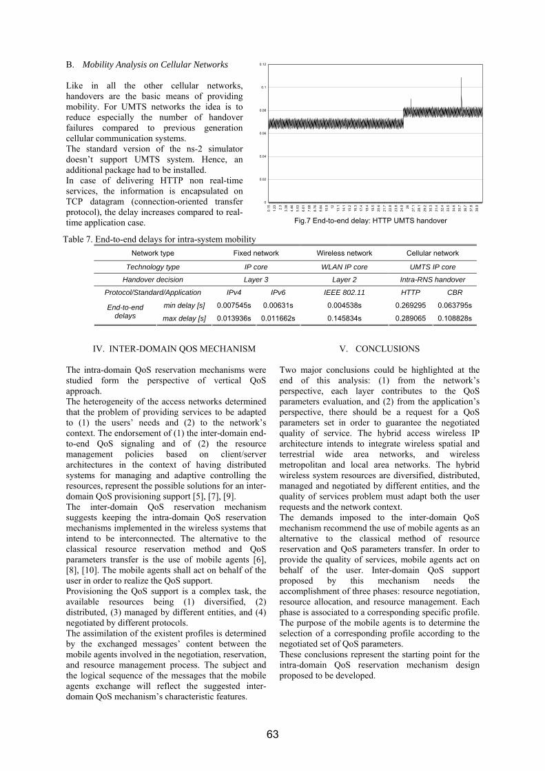
B. Mobility Analysis on Cellular Networks Like in all the other cellular networks, handovers are the basic means of providing mobility. For UMTS networks the idea is to reduce especially the number of handover failures compared to previous generation cellular communication systems. The standard version of the ns-2 simulator doesn’t support UMTS system. Hence, an additional package had to be installed. In case of delivering HTTP non real-time services, the information is encapsulated on TCP datagram (connection-oriented transfer protocol), the delay increases compared to real-time application case.
IV. INTER-DOMAIN QOS MECHANISM
The intra-domain QoS reservation mechanisms were studied form the perspective of vertical QoS approach. The heterogeneity of the access networks determined that the problem of providing services to be adapted to (1) the users’ needs and (2) to the network’s context. The endorsement of (1) the inter-domain end-to-end QoS signaling and of (2) the resource management policies based on client/server architectures in the context of having distributed systems for managing and adaptive controlling the resources, represent the possible solutions for an inter-domain QoS provisioning support [5], [7], [9]. The inter-domain QoS reservation mechanism suggests keeping the intra-domain QoS reservation mechanisms implemented in the wireless systems that intend to be interconnected. The alternative to the classical resource reservation method and QoS parameters transfer is the use of mobile agents [6], [8], [10]. The mobile agents shall act on behalf of the user in order to realize the QoS support. Provisioning the QoS support is a complex task, the available resources being (1) diversified, (2) distributed, (3) managed by different entities, and (4) negotiated by different protocols. The assimilation of the existent profiles is determined by the exchanged messages’ content between the mobile agents involved in the negotiation, reservation, and resource management process. The subject and the logical sequence of the messages that the mobile agents exchange will reflect the suggested inter-domain QoS mechanism’s characteristic features.
V. CONCLUSIONS
Two major conclusions could be highlighted at the end of this analysis: (1) from the network’s perspective, each layer contributes to the QoS parameters evaluation, and (2) from the application’s perspective, there should be a request for a QoS parameters set in order to guarantee the negotiated quality of service. The hybrid access wireless IP architecture intends to integrate wireless spatial and terrestrial wide area networks, and wireless metropolitan and local area networks. The hybrid wireless system resources are diversified, distributed, managed and negotiated by different entities, and the quality of services problem must adapt both the user requests and the network context. The demands imposed to the inter-domain QoS mechanism recommend the use of mobile agents as an alternative to the classical method of resource reservation and QoS parameters transfer. In order to provide the quality of services, mobile agents act on behalf of the user. Inter-domain QoS support proposed by this mechanism needs the accomplishment of three phases: resource negotiation, resource allocation, and resource management. Each phase is associated to a corresponding specific profile. The purpose of the mobile agents is to determine the selection of a corresponding profile according to the negotiated set of QoS parameters. These conclusions represent the starting point for the intra-domain QoS reservation mechanism design proposed to be developed.
Table 7. End-to-end delays for intra-system mobility Network type Fixed network Wireless network Cellular network
Technology type IP core WLAN IP core UMTS IP core
Handover decision Layer 3 Layer 2 Intra-RNS handover
Protocol/Standard/Application IPv4 IPv6 IEEE 802.11 HTTP CBR
min delay [s] 0.007545s 0.00631s 0.004538s 0.269295 0.063795s End-to-end delays max delay [s] 0.013936s 0.011662s 0.145834s 0.289065 0.108828s
0
0.02
0.04
0.06
0.08
0.1
0.12
0.15
1.23 2.3
3.38
4.46
5.53
6.61
7.68
8.76
9.84
10.9 12
13.1
14.1
15.2
16.3
17.4
18.4
19.5
20.6
21.7
22.8
23.8
24.9 26
27.1
28.1
29.2
30.3
31.4
32.4
33.5
34.6
35.7
36.7
37.8
38.9
Fig.7 End-to-end delay: HTTP UMTS handover
63
REFERENCES [1] A. Ganz, Z. Ganz, K Wongthavarawat, “Multimedia Wireless
Networks: Technologies, Standards, and QoS”, Prentice Hall, New York, 2003.
[2] Mukherjee, S. Bandyopadhyay, D. Saha, “Location Management and Routing in Mobile Wireless Networks”, Artech House, 2003.
[3] E. Puschita, T. Palade, C. Selaru, Performance Evaluation of Routing Protocols in Ad-Hoc Wireless Networks, ETc2004, Timişoara, 2004.
[4] P., Hirtzlin (editor), E., Puschita, T. Palade, D. Salazar, J. Sesena, G. Smedback, R. Pringle, R. Worrall, J. Stafford, G.F. Vezzani, C. Monti, M. Schmidt, L. Garcia, Recommendations on matching hybrid wireless network technologies to deployment scenarios, BROADWAN, Deliverable D8, October 2004 – final report.
[5] E., Borcoci, R., Balaci, S., Obreja, Concurrent implementation of multi-domain service management for end-to-end multimedia delivery, The 6th International Conference COMM2006, June 2006, pp.341-346.
[6] M., Ganna, E., Horlait, Agent-based framework for policy-
driven service provisioning to nomadic users, IEEE International Conference on Wireless And Mobile Computing, Networking And Communications, WiMob2005, Volume 4, August 2005, pp. 82-89.
[7] A., Iera, A., Molinaro, Quality of service concept evolution for future telecommunication scenarios, IEEE 16th International Symposium on Personal, Indoor and Mobile Radio Communications, PIMRC 2005, Volume 4, September 2005, pp. 2787-2793.
[8] R., Babbar, A., Fapojuwo, B., Far, Agent-Based Resource Management in Hybrid Wireless Networks, IEEE Canadian Conference on Electrical and Computer Engineering, Volume 3, May 2004, pp. 1297-1300.
[9] M.S.T., Orzechowski, The Usage of Mobile Agents for Management of Data Transmission in Telecommunications Networks, IEEE International Siberian Conference on Control and Communications, SIBCON 2005, October 2005, pp. 8-12.
[10] A., Iera, A., Molinaro, Quality of Service Concept Evolution for Future Telecommunication Scenarios, IEEE 16th International Symposium on Personal, Indoor and Mobile Radio Communication, PIMRC 2005, Volume 4, September 2005, pp. 2787-2793.
64
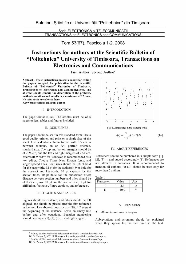
Buletinul Ştiinţific al Universităţii "Politehnica" din Timişoara
Seria ELECTRONICĂ şi TELECOMUNICAŢII TRANSACTIONS on ELECTRONICS and COMMUNICATIONS
Tom 53(67), Fascicola 1-2, 2008
Instructions for authors at the Scientific Bulletin of “Politehnica” University of Timisoara, Transactions on
Electronics and Communications
First Author1 Second Author2
1 Faculty of Electronics and Telecommunications, Communications Dept. Bd. V. Parvan 2, 300223 Timisoara, Romania, e-mail [email protected] 2 Faculty of Electronics and Telecommunications, Communications Dept. Bd. V. Parvan 2, 300223 Timisoara, Romania, e-mail [email protected]
Abstract – These instructions present a model for editing the papers accepted for publication in the Scientific Bulletin of “Politehnica” University of Timisoara, Transactions on Electronics and Communications. The abstract should contain the description of the problem, methods, solutions and results in a maximum of 12 lines. No references are allowed here. Keywords: editing, Bulletin, author
I. INTRODUCTION
The page format is A4. The articles must be of 6 pages or less, tables and figures included.
II. GUIDELINES
The paper should be sent in this standard form. Use a good quality printer, and print on a single face of the sheet. Use a double column format with 0.5 cm in between columns, on an A4, portrait oriented, standard size. The top and bottom margins should be of 2.28 cm, and the left and right margins of 2.54 cm. Microsoft Word™ for Windows is recommended as a text editor. Choose Times New Roman fonts, and single spaced lines. Font sizes should be: 18 pt bold for the paper title, 12 pt for the author(s), 9 pt bold for the abstract and keywords, 10 pt capitals for the section titles, 10 pt italic for the subsection titles; distance between section numbers and titles should be of 0.25 cm; use 10 pt for the normal text, 8 pt for affiliation, footnotes, figure captions, and references.
III. FIGURES AND TABLES Figures should be centered, and tables should be left aligned, and should be placed after the first reference in the text. Use abbreviations such as “Fig.1.” even at the beginning of the sentence. Leave an empty line before and after equations. Equation numbering should be simple: (1), (2), (3) … and right aligned:
∫− −=a
adtytx ττ )()( . (16)
IV. ABOUT REFERENCES References should be numbered in a simple form [1], [2], [3]…, and quoted accordingly [1]. References are not allowed in footnotes. It is recommended to mention all authors; “et al.” should be used only for more than 6 authors. Table 1
Parameter Value Unit I 2.4 A U 10.0 V
V. REMARKS A. Abbreviations and acronyms Abbreviations and acronyms should be explained when they appear for the first time in the text.
Fig. 1. Amplitudes in the standing wave

Abbreviations such as IEEE, IEE, SI, MKS, CGS, ac, dc and rms need no further explanation. It is recommended not to use abbreviations in section or subsection titles.
B. Further recommendations The International System of units is recommended. Do not mix SI and CGS. Preliminary, experimental results are not accepted. Roman section numbering is optional.
REFERENCES [1] A. Ignea, “Preparation of papers for the International Symposium Etc. ’98”, Buletinul Universităţii “Politehnica”, Seria Electrotehnica, Electronica si Telecomunicatii, Tom 43 (57), 1998, Fascicola 1, 1998, pp. 81. [2] R. E. Collin, Foundations for Microwave Engineering, Second Edition, McGraw-Hill, Inc., 1992. [3] http://hermes.etc.utt.ro/bulletin/bulletin.html
![[ger] KOHLE : Monatsbulletin 7-1981 [eng] COAL : Monthly ...aei.pitt.edu/79526/1/1981_-_7.pdf · beschatf tlbt: unler tage (2j * personnel employed underground c2) * 1000 personnel](https://static.fdokument.com/doc/165x107/606a9d5ab52b4315643eb285/ger-kohle-monatsbulletin-7-1981-eng-coal-monthly-aeipittedu7952611981-7pdf.jpg)