Efficient Large Scale Aerodynamic Design Based on Shape ...schmidt/files/thesis.pdf · nicht...
168
Efficient Large Scale Aerodynamic Design Based on Shape Calculus Dissertation zur Erlangung des Akademischen Grades eines Doktors der Naturwissenschaften (Dr. rer. nat.) Dem Fachbereich IV der Universität Trier vorgelegt von Dipl.-Math. Stephan Schmidt
Transcript of Efficient Large Scale Aerodynamic Design Based on Shape ...schmidt/files/thesis.pdf · nicht...

Efficient Large Scale Aerodynamic Design Basedon Shape Calculus
Dissertation
zur Erlangung des Akademischen Grades eines Doktors der Naturwissenschaften(Dr. rer. nat.)
Dem Fachbereich IV der Universität Trier vorgelegt von
Dipl.-Math. Stephan Schmidt


to morph, verb, (third-person singular simple present morphs, present participle mor-phing, simple past and past participle morphed)
1. Shortening of metamorphose: to change in shape or form.
2. (colloquial) To undergo dramatic change in a seamless and barely noticeablefashion.


Abstract
Large scale non-parametric applied shape optimization for computational fluid dynamics is consid-ered. Treating a shape optimization problem as a standard optimal control problem by means of aparameterization, the Lagrangian usually requires knowledge of the partial derivative of the shapeparameterization and deformation chain with respect to input parameters. For a variety of reasons,this mesh sensitivity Jacobian is usually quite problematic. For a sufficiently smooth boundary, theHadamard theorem provides a gradient expression that exists on the surface alone, completelybypassing the mesh sensitivity Jacobian. Building upon this, the gradient computation becomesindependent of the number of design parameters and all surface mesh nodes are used as designunknowns in this work, effectively allowing a free morphing of shapes during optimization.
Contrary to a parameterized shape optimization problem, where a smooth surface is usually cre-ated independently of the input parameters by construction, regularity is not preserved automaticallyin the non-parametric case. As part of this work, the shape Hessian is used in an approximativeNewton method, also known as Sobolev method or gradient smoothing, to ensure a certain regu-larity of the updates, and thus a smooth shape is preserved while at the same time the one-shotoptimization method is also accelerated considerably. For PDE constrained shape optimization, theHessian usually is a pseudo-differential operator. Fourier analysis is used to identify the operatorsymbol both analytically and discretely. Preconditioning the one-shot optimization by an appropriateHessian symbol is shown to greatly accelerate the optimization.
As the correct discretization of the Hadamard form usually requires evaluating certain surfacequantities such as tangential divergence and curvature, special attention is also given to discretedifferential geometry on triangulated surfaces for evaluating shape gradients and Hessians.
The Hadamard formula and Hessian approximations are applied to a variety of flow situations. Inaddition to shape optimization of internal and external flows, major focus lies on aerodynamic designsuch as optimizing two dimensional airfoils and three dimensional wings. Shock waves form whenthe local speed of sound is reached, and the gradient must be evaluated correctly at discontinuousstates. To ensure proper shock resolution, an adaptive multi-level optimization of the Onera M6wing is conducted using more than 36, 000 shape unknowns on a standard office workstation,demonstrating the applicability of the shape-one-shot method to industry size problems.
5


Zusammenfassung
Der Gegenstand dieser Arbeit ist die hochdimensionale nicht-parametrische angewandte Formop-timierung für die numerische Strömungssimulation. Wird ein Formoptimierungsproblem durch eineParametrisierung wie ein gewöhnliches nichtlineares Optimierungsproblem behandelt, so benötigtdie Lagrange–Funktion Kenntnis der partiellen Ableitungen der Parametrisierung und der Deforma-tionskette bezüglich der Eingabeparameter. Aus verschiedensten Gründen sind diese Mesh- oderMetriksensitivitäten für gewöhnlich sehr problematisch. Für eine hinreichend glatte Oberfläche bie-tet das Hadamard–Theorem einen Ausdruck für den Gradienten, welcher ausschließlich auf derOberfläche der Form existiert und die Metriksensitivitäten komplett umgeht. Darauf aufbauend wirddie Berechnung des Gradienten unabhängig von der Anzahl der Variablen und im Rahmen dieserArbeit werden alle Oberflächenknoten des Gitters als Unbekannte benutzt, wodurch effektiv einfreies Morphing der Form während der Optimierung ermöglicht wird.
Im Gegensatz zu einem parametrisierten Formoptimierungsproblem, bei dem die Glattheit derOberfläche fast immer unabhängig von den Eingabeparametern entsprechend der Konstruktionder Parameterisierung gewährleistet ist, muss die Regularität bei dem nicht-parametrischen Ansatznicht zwingend erhalten bleiben. In dieser Arbeit wird die Hesse–Abbildung des Formoptimierungs-problems in einem approximativen Newton–Verfahren, auch bekannt als Sobolev–Verfahren oderGradientenglätten, genutzt, um die Regularität der Updates sicherzustellen und somit eine glatteOberfläche zu erhalten, wodurch gleichzeitig die Optimierung in One-Shot deutlich beschleunigtwird. Für Optimierungsprobleme mit PDEs ist die Hesse–Abbildung gewöhnlich ein Pseudo-Diffe-rentialoperator. Fourieranalysis wird benutzt, um das Symbol des Operators sowohl analytisch alsauch diskret zu bestimmen. Es wird gezeigt, wie eine Präkonditionierung des One-Shot Verfahrensdurch ein entsprechendes Symbol der Hesse–Abbildung die Optimierung stark beschleunigt.
Da die korrekte Diskretisierung der Hadamard–Form für gewöhnlich die Auswertung von Ober-flächengrößen wie Tangentialdivergenz oder Krümmung benötigt, liegt besonderes Augenmerk aufdiskreter Differentialgeometrie zur Auswertung des Formgradienten und der Hesse–Abbildung aufunstrukturierten, triangulierten Oberflächen.
Die Hadamard–Form und die Hesse–Approximationen werden auf eine Vielfalt von Strömungs-situationen angewendet. Neben der Formoptimierung von internen und externen Strömungen liegtder eigentliche Anwendungsschwerpunkt im aerodynamischen Entwurf, zum Beispiel die Optimie-rung zweidimensionaler Profilquerschnitte und dreidimensionaler Flügel. Schockwellen bilden sichaus, wenn die lokale Schallgeschwindigkeit erreicht wird, und der Gradient muss an einem un-stetigen Zustand richtig ausgewertet werden. Um eine korrekte Auflösung der Schockwelle zu ge-währleisten, wird eine adaptive multi-level Optimierung am Onera M6 Flügel mit mehr als 36.000Unbekannten auf einer gewöhnlichen Workstation durchgeführt, was auch die Anwendbarkeit derMethodik auf Probleme industriellen Ausmaßes demonstriert.
7


Acknowledgments
First of all, I would like to thank my supervisor Prof. Dr. Volker Schulz for the many helpful discus-sions and the ongoing support, but also for the frequent opportunities to visit external conferenceswith inspiring discussions, including Oberwolfach and SIAM conferences in the United States. Hisgroup at the University of Trier is a very creative, challenging, and pleasant environment to work in.I also would like to thank Prof. Dr. Jan Sokolowski for the many discussions on shape optimizationand for accepting the position as second referee.
Furthermore, I would like to thank Prof. Dr. Nicolas Gauger, with whom I have worked closelytogether. His detailed knowledge about computational fluid dynamics and adjoint solvers have beenas valuable to me as his moral support.
I would also like to thank Prof. Dr. Karsten Eppler. He first introduced me to shape calculus, andthe many discussions we had till late at night during his stay at the University of Trier were extremelyhelpful. Additionally, I would like to thank Dipl.-Ing. Caslav Ilic at the German Aerospace Center(DLR), Braunschweig, who handled most of the DLR flow solvers and miscellaneous software.Spending countless hours on the phone, our many discussions have also greatly helped coming upwith discrete solutions for analytical problems. While I was raving about optimizing an Airbus into aConcorde, he made sure none of the fine details of aerodynamic design were overlooked. He alsogreatly helped by proof-reading this thesis.
I would also like to thank my fellow graduate students at the University of Trier for creating sucha nice work atmosphere: Claudia Schillings, Roland Stoffel, Benjamin Rosenbaum, Christian Wag-ner, Christoph Käbe, Andre Lörx, Timo Hylla, Matthias Schu, Bastian Groß, Nils Langenberg, andChristina Jager. Additionally, I would like to thank Dipl.-Phys. Christian Haake for writing outputroutines for my flow solver in postscript, thereby creating restart files which visualize themselves,and for proof-reading this thesis.
Finally and naturally, I would like to thank my parents for their support and encouraging commentsduring the last three years.
This work has been supported by the German science foundation (DFG) priority program SPP-1253: “Optimization with Partial Differential Equations” as the project “Multilevel Parameterizationsand Fast Multigrid Methods for Aerodynamic Shape Optimization”, a joint project between Prof. Dr.Volker Schulz, University of Trier, and Prof. Dr. Nicolas Gauger, DLR Braunschweig.
9

Contents
1 Introduction 131.1 Paradigms in Shape Optimization . . . . . . . . . . . . . . . . . . . . . . . . . . . 131.2 Aim and Scope of this Work . . . . . . . . . . . . . . . . . . . . . . . . . . . . . . 161.3 Structure of this Work . . . . . . . . . . . . . . . . . . . . . . . . . . . . . . . . . 17
2 Differential Geometry 192.1 Basic Concepts . . . . . . . . . . . . . . . . . . . . . . . . . . . . . . . . . . . . 192.2 Integration over Submanifolds . . . . . . . . . . . . . . . . . . . . . . . . . . . . . 23
3 Shape Sensitivity Analysis 273.1 Shape Optimization and Hadamard Theorem . . . . . . . . . . . . . . . . . . . . . 273.2 Hadamard Formula for Volume Objectives . . . . . . . . . . . . . . . . . . . . . . 303.3 Hadamard Formula for Surface Objectives . . . . . . . . . . . . . . . . . . . . . . 32
3.3.1 Shape Derivatives of Geometric Quantities . . . . . . . . . . . . . . . . . . 353.3.2 Shape Derivatives of General Surface Objectives . . . . . . . . . . . . . . . 39
3.4 Shape Derivatives and State Constraints . . . . . . . . . . . . . . . . . . . . . . . 42
4 Fluid Mechanics 474.1 Derivation of the State Equations . . . . . . . . . . . . . . . . . . . . . . . . . . . 474.2 Simplifications . . . . . . . . . . . . . . . . . . . . . . . . . . . . . . . . . . . . . 54
4.2.1 Incompressible Flow . . . . . . . . . . . . . . . . . . . . . . . . . . . . . . 544.2.2 Inviscid Flow . . . . . . . . . . . . . . . . . . . . . . . . . . . . . . . . . . 574.2.3 Potential Flow . . . . . . . . . . . . . . . . . . . . . . . . . . . . . . . . . 59
4.3 Numerical Schemes for Conservation Laws . . . . . . . . . . . . . . . . . . . . . . 604.3.1 The Finite Volume Method . . . . . . . . . . . . . . . . . . . . . . . . . . . 604.3.2 The Jameson–Schmidt–Turkel Scheme . . . . . . . . . . . . . . . . . . . . 63
5 Shape Optimization and Stokes Fluids 655.1 Problem Introduction and First Order Calculus . . . . . . . . . . . . . . . . . . . . 655.2 Shape Hessian Analysis . . . . . . . . . . . . . . . . . . . . . . . . . . . . . . . . 685.3 Loss of Regularity, Sobolev Gradient, and Newton Direction . . . . . . . . . . . . . 725.4 Operator Symbols and Fourier Analysis . . . . . . . . . . . . . . . . . . . . . . . . 735.5 Application . . . . . . . . . . . . . . . . . . . . . . . . . . . . . . . . . . . . . . . 75
5.5.1 Flow Solver . . . . . . . . . . . . . . . . . . . . . . . . . . . . . . . . . . . 765.5.2 Discrete Hessian Symbol . . . . . . . . . . . . . . . . . . . . . . . . . . . 765.5.3 Optimization . . . . . . . . . . . . . . . . . . . . . . . . . . . . . . . . . . 79
11
Contents
6 Shape Optimization and Navier–Stokes Fluids 836.1 Problem Introduction and First Order Calculus . . . . . . . . . . . . . . . . . . . . 836.2 Example Application . . . . . . . . . . . . . . . . . . . . . . . . . . . . . . . . . . 91
6.2.1 Energy Dissipation . . . . . . . . . . . . . . . . . . . . . . . . . . . . . . . 916.2.2 Flow Solver . . . . . . . . . . . . . . . . . . . . . . . . . . . . . . . . . . . 946.2.3 Flow Through a Pipe . . . . . . . . . . . . . . . . . . . . . . . . . . . . . . 946.2.4 Flow through a T-Connection . . . . . . . . . . . . . . . . . . . . . . . . . 95
6.3 Hessian Approximation and Sobolev Optimization . . . . . . . . . . . . . . . . . . 97
7 Potential Flow Pressure Tracking 1017.1 Introduction . . . . . . . . . . . . . . . . . . . . . . . . . . . . . . . . . . . . . . . 1017.2 Local Coordinates and Shape Hessian . . . . . . . . . . . . . . . . . . . . . . . . 1047.3 Method of Mapping and Fourier Analysis . . . . . . . . . . . . . . . . . . . . . . . 1087.4 Numerical Results . . . . . . . . . . . . . . . . . . . . . . . . . . . . . . . . . . . 112
7.4.1 Panel Solver . . . . . . . . . . . . . . . . . . . . . . . . . . . . . . . . . . 1127.4.2 Numerical Pressure Fitting . . . . . . . . . . . . . . . . . . . . . . . . . . . 113
8 Shape Optimization and Euler Equations 1158.1 Introduction . . . . . . . . . . . . . . . . . . . . . . . . . . . . . . . . . . . . . . . 1158.2 First Order Calculus . . . . . . . . . . . . . . . . . . . . . . . . . . . . . . . . . . 1178.3 Optimization Strategy . . . . . . . . . . . . . . . . . . . . . . . . . . . . . . . . . 1218.4 Discrete Differential Geometry . . . . . . . . . . . . . . . . . . . . . . . . . . . . . 123
8.4.1 Curvature Evaluation . . . . . . . . . . . . . . . . . . . . . . . . . . . . . . 1258.4.2 Shape Derivative of the Normal . . . . . . . . . . . . . . . . . . . . . . . . 1268.4.3 Gradient Validation . . . . . . . . . . . . . . . . . . . . . . . . . . . . . . . 1278.4.4 Laplace–Beltrami Operator . . . . . . . . . . . . . . . . . . . . . . . . . . 128
8.5 Airfoil Optimizations . . . . . . . . . . . . . . . . . . . . . . . . . . . . . . . . . . 1318.5.1 Supersonic NACA Airfoil . . . . . . . . . . . . . . . . . . . . . . . . . . . . 1338.5.2 Mesh Independence . . . . . . . . . . . . . . . . . . . . . . . . . . . . . . 1348.5.3 Transonic Lifting RAE2822 Airfoil . . . . . . . . . . . . . . . . . . . . . . . 135
8.6 Onera M6 Wing Optimization . . . . . . . . . . . . . . . . . . . . . . . . . . . . . 137
9 Compressible Navier–Stokes Equations 1419.1 Introduction . . . . . . . . . . . . . . . . . . . . . . . . . . . . . . . . . . . . . . . 1419.2 First Order Calculus . . . . . . . . . . . . . . . . . . . . . . . . . . . . . . . . . . 1439.3 Primal and Adjoint Variables . . . . . . . . . . . . . . . . . . . . . . . . . . . . . . 157
10 Conclusions and Outlook 15910.1 Summary . . . . . . . . . . . . . . . . . . . . . . . . . . . . . . . . . . . . . . . . 15910.2 Future Work . . . . . . . . . . . . . . . . . . . . . . . . . . . . . . . . . . . . . . 160
12
Chapter 1
Introduction
1.1 Paradigms in Shape Optimization
As a special field of optimization subject to partial differential equations (PDEs), shape optimizationand control of fluids has seen steady research interest over the past decades. Especially in aero-dynamic design, the transition from simulation alone to a coupled simulation and optimization isprogressing continuously. Although heuristic and derivative free optimization methods are still usedin practice, only structure exploiting gradient based methods are efficient enough for optimizingindustry size large scale systems.
Two major advancements in the field of derivative based general PDE constraint optimization andits application to aerodynamic design have been the introduction of gradient computation via adjointcalculus [23, 29, 40, 50] and the optimization in one-shot [27, 31, 66, 72, 73]. A good overview onapplying general control theory to fluid control problems can also be found in [32]. When consider-ing the special sub-class of shape optimization problems and fluid flow, such problems are almostalways interpreted as a general non-linear optimization problem via a parameterization. By choos-ing a finite set of design parameters, such as the popular Hicks–Henne functions [35], B-splines,free-form deformation, or general computer aided design (CAD) software, the shape optimizationproblem is reduced to a standard optimization problem in finite dimensions. Thus, a parameteri-zation is also a discretization. This means that the Lagrangian of the parameterized shape opti-mization problem is studied without considering the original nature of the problem, and possibilitiesfor shape optimization structure exploitation are therefore neglected. Even worse, the Lagrangian
13
1 Introduction
system of a parameterized shape optimization problem requires knowledge of so called mesh sen-sitivities, i.e. the partial derivatives of the PDE constraint and objective functions with respect to theparameterization.
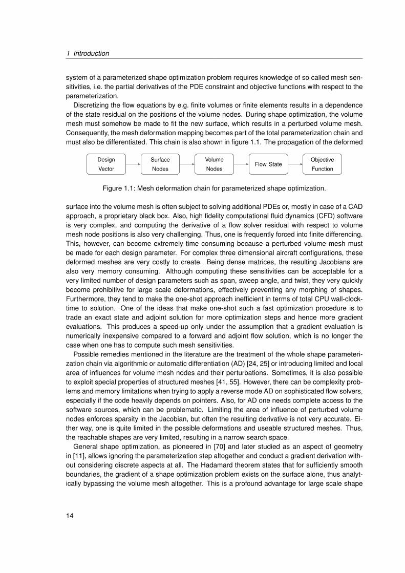
Discretizing the flow equations by e.g. finite volumes or finite elements results in a dependenceof the state residual on the positions of the volume nodes. During shape optimization, the volumemesh must somehow be made to fit the new surface, which results in a perturbed volume mesh.Consequently, the mesh deformation mapping becomes part of the total parameterization chain andmust also be differentiated. This chain is also shown in figure 1.1. The propagation of the deformed
Design
Vector
Surface
Nodes
Volume
NodesFlow State
Objective
Function
Figure 1.1: Mesh deformation chain for parameterized shape optimization.
surface into the volume mesh is often subject to solving additional PDEs or, mostly in case of a CADapproach, a proprietary black box. Also, high fidelity computational fluid dynamics (CFD) softwareis very complex, and computing the derivative of a flow solver residual with respect to volumemesh node positions is also very challenging. Thus, one is frequently forced into finite differencing.This, however, can become extremely time consuming because a perturbed volume mesh mustbe made for each design parameter. For complex three dimensional aircraft configurations, thesedeformed meshes are very costly to create. Being dense matrices, the resulting Jacobians arealso very memory consuming. Although computing these sensitivities can be acceptable for avery limited number of design parameters such as span, sweep angle, and twist, they very quicklybecome prohibitive for large scale deformations, effectively preventing any morphing of shapes.Furthermore, they tend to make the one-shot approach inefficient in terms of total CPU wall-clock-time to solution. One of the ideas that make one-shot such a fast optimization procedure is totrade an exact state and adjoint solution for more optimization steps and hence more gradientevaluations. This produces a speed-up only under the assumption that a gradient evaluation isnumerically inexpensive compared to a forward and adjoint flow solution, which is no longer thecase when one has to compute such mesh sensitivities.
Possible remedies mentioned in the literature are the treatment of the whole shape parameteri-zation chain via algorithmic or automatic differentiation (AD) [24, 25] or introducing limited and localarea of influences for volume mesh nodes and their perturbations. Sometimes, it is also possibleto exploit special properties of structured meshes [41, 55]. However, there can be complexity prob-lems and memory limitations when trying to apply a reverse mode AD on sophisticated flow solvers,especially if the code heavily depends on pointers. Also, for AD one needs complete access to thesoftware sources, which can be problematic. Limiting the area of influence of perturbed volumenodes enforces sparsity in the Jacobian, but often the resulting derivative is not very accurate. Ei-ther way, one is quite limited in the possible deformations and useable structured meshes. Thus,the reachable shapes are very limited, resulting in a narrow search space.
General shape optimization, as pioneered in [70] and later studied as an aspect of geometryin [11], allows ignoring the parameterization step altogether and conduct a gradient derivation with-out considering discrete aspects at all. The Hadamard theorem states that for sufficiently smoothboundaries, the gradient of a shape optimization problem exists on the surface alone, thus analyt-ically bypassing the volume mesh altogether. This is a profound advantage for large scale shape
14

1.1 Paradigms in Shape Optimization
optimization in general and one-shot shape optimization in specific. The analytic expression of theHadamard form can be evaluated very quickly wherever desired, making the gradient computationindeed independent of the number of design parameters. It is thus possible to use the position ofeach mesh surface node as a design parameter, utilizing extraordinary possibilities of shape defor-mations and morphing. It also supports the full optimization speed-up by one-shot methods nicely,possibly helping advanced aerodynamic optimizations such as Pareto curve computations [59] andoptimization under uncertainties [67]. Additionally, the non-parametric approach is inherently suitedfor multi-level optimization and local adaptivity, as the Hadamard form can be evaluated at anysurface point desired, independent of mesh topology changes between optimization steps. In-terestingly, the non-parametric paradigm is seldom used in aerodynamic design, except to showoptimality of certain rotationally symmetric ogive shaped bodies in supersonic, irrotational, invis-cid potential flows [33]. Furthermore, the non-parametric approach is also used to derive optimalshapes in a viscous Stokes flow [49]. Although certain non-parametric shape optimization ideasare present in the literature [10, 15, 46, 47], it is almost never applied in any actual optimization.
Also, there is the effect of loss of regularity. While the parametric approach ensures a smoothshape for any choice of design parameters, this is no longer the case when considering the non-parameterized infinite dimensional shape optimization problem. The parameterization determinesthe regularity class of which shapes are constructed, and in a general non-parametric shape op-timization approach, the desired regularity class must be enforced otherwise. Imagining a simplesteepest descent algorithm, it is easy to see that updates must be in the same regularity space asthe original shape. Consequently, the gradient based update must be manipulated to maintain regu-larity. When applicable, the gradient can be thought of as the Riesz representative of the derivative,and the regularity of the gradient depends on the appropriate scalar product used in the underlyingspace. This procedure is sometimes also called gradient smoothing or Sobolev gradient method[41, 69], and thus questions about the appropriate space, i.e. scalar product, arise. As it turnsout, the scalar product induced by the shape Hessian is an excellent choice because it not onlycures the loss of regularity, but it also greatly accelerates the optimization as the Sobolev steepestdescent method essentially becomes Newton’s method, i.e. an SQP method.
Thus, the loss of regularity in specific and gradient based optimization in general rises questionsabout efficient Hessian computations and approximations. Literature on shape Hessians for pa-rameterized problems is rare, possibly because the parameterization camouflages the structure ofshape Hessians. The application of non-parameterized shape Hessians in a preconditioned con-jugate gradient iteration for image segmentation is studied in [36, 37]. Also, shape Hessians andoptimality conditions for shape optimization problems are considered in [16, 17, 18] with various ap-plications in liquid metal shaping, electrical impedance tomography, and general elliptic problems.In general, shape Hessians are quite complex objects even for problems that appear manageable atfirst glance. They also no longer satisfy the Hadamard form of a scalar product of the normal com-ponent with a perturbation direction on the boundary. Thus, more accessible approximations areusually advantageous. For a PDE constrained optimization problem the shape Hessian usually is apseudo-differential operator, and the effect of such a pseudo-differential operator on the regularityof the shape update must be studied. Another advantage of infinite dimensional shape optimizationis the applicability of Fourier analysis to problems of moderate complexity, which allows the identi-fication of the pseudo-differential operator order governing the Hessian. This, in return, defines theamount of re-smoothing that must be applied in the Sobolev smoothing step, i.e. by the Hessianapproximation. Fourier tracking of perturbations has for example also been used in [2, 3, 4, 28, 61]
15

1 Introduction
for similar purposes.
Summarizing the above, it can be said that shape optimization is a field with a surprisingly stronggap between first optimizing analytically followed by a discretization of the expressions versus firstdiscretizing and then optimizing the discrete problem. Very recently, this gap is studied in [6], whereboth approaches are unified in the finite element context. The optimize-then-discretize approachby using shape differentiation techniques and the Hadamard formula of the shape gradient as partof the present work has considerable advantages over a discretization by parameterization as itbypasses all volume mesh deformations of the problem, enables very fast gradient evaluations foran arbitrary number of design parameters, and makes a Hessian analysis much more accessible.Thus, large scale morphing of shapes by a one-shot optimization is possible. Correct gradientevaluations and Hessian approximations require discretizing surface quantities, such as tangentialdivergence and curvature, on unstructured meshes, thereby creating an interesting bridge betweenoptimization with PDE constraints and other research fields such as computer graphics and discretedifferential geometry.
1.2 Aim and Scope of this Work
An exhaustive analysis of a PDE constrained shape optimization problem requires a well-posedmodel, i.e. weak solutions for the geometries under consideration exist. Additionally, the set ofsolutions over the family of admissible domains needs to be compact such that there is a solution ofthe shape optimization problem. Once the existence of an optimal shape is established, methods tocompute it can be discussed. The desire to use efficient gradient based methods naturally leads tothe question of shape differentiability. Therefore, the family of solutions under consideration shouldbe Lipschitz continuous with respect to boundary variations such that a shape sensitivity analysiscan be conducted.
For the compressible Navier–Stokes equations with constant temperature, the well-posednessand existence of optimal shapes is established in [53]. There, it is first stated that assuming theexistence of a domain and corresponding flow solution of finite internal energy, the drag minimiza-tion problem has a solution. Afterwards, the existence is ensured by constructing one such domain.The question of shape differentiability is answered in [51] using small perturbations of the so-calledapproximate solutions, which are determined from Stokes problems.
The aim and scope of this work, however, is to study how the information can be used to im-prove a given design numerically. Less focus lies on analytical existence and uniqueness of criticalshapes. Therefore, a formal shape sensitivity analysis is conducted, followed by a study of theshape Hessian and an actual numerical optimization for a variety of problems in computational fluiddynamics and aerodynamic design. Special attention lies on the industrial applicability to very largescale shape optimization problems. This work is also used to study accelerating the one-shot ap-proach for shape optimization problems by preconditioning, i.e. Hessian approximation, based onpseudo-differential operator approximation by Fourier analysis. Where possible, this is conductedanalytically, otherwise discrete substitutes are considered. Thus, not only the applicability of infinitedimensional shape calculus to discrete problems is shown, but also the possible acceleration of theoptimization procedure by analytically exploiting the structure of shape optimization problems.
16

1.3 Structure of this Work
1.3 Structure of this Work
The structure of this work is as follows: Chapter 2 is used to give a very brief overview about differ-ential geometry. The purpose of this chapter is to prepare for chapter 3, i.e. special attention is givento introducing terms and definitions which are seldom encountered in the context of general PDEconstrained optimization, such as tangential gradient, tangential divergence, and a variety of otherlemmas and definitions. Combining many results scattered in the literature, chapter 3 then triesto give a complete overview about shape sensitivity analysis, i.e. shape differentiation techniques,especially when a PDE constraint is present. Special attention is given to providing the expres-sions in general formulations, as often in the literature, simplifications for standard Laplacian basedproblems, i.e. elliptic PDEs, are made, which prohibit application to the mixed parabolic/hyperbolicPDEs governing fluid flow. Chapter 4 is then used to give a brief overview on fluid dynamics. Itnot only introduces the PDEs governing the problems considered afterwards, but also shows whatkind of objective functions are physically relevant for the different flow regimes of viscous, inviscid,compressible, and incompressible flows. One important fact is that in an inviscid compressible flow,a shape producing a shock-free flow solution can always be assumed to be drag optimal.
The following chapters 5 to 9 are then used to conduct the actual shape sensitivity analysis, Hes-sian approximation, and numerical optimization for a variety of CFD problems. The problems arestudied in order of increasing difficulty of shape differentiation and not according to the sophistica-tion of the fluid model, which is why the incompressible Navier–Stokes equations are consideredbefore potential flow. First, chapter 5 considers shape optimization and Stokes fluids. This makesa very good introduction, as the optimal shape of the energy dissipation problem is known to be arugby ball of 60 front and back angle, creating a perfect validation test-case for numerics. Due toits self-adjoint nature, the energy dissipation problem in a Stokes flow also allows for a very ele-gant Hessian derivation, and consequently this Hessian derivation is measured against the Fourieroperator identification, familiarizing these concepts with a well structured example application. Thechapter concludes by showing the optimization speed-up based on the Fourier symbol identification.By considering the incompressible Navier–Stokes equations in a general setting, the next chapter 6both increases the complexity of the fluid model and the objective functions. Since the incom-pressible Navier–Stokes equations describe a very wide range of flow phenomena with numerousopportunities for application, very general objective shape functionals are considered. Since theyare no longer self-adjoint as in the Stokes case, it is interesting to observe what kind of objectiveshape functionals allow consistent adjoint calculus. Due to their complex nature, the Fourier Hes-sian analysis is conducted in the discrete, again greatly accelerating a variety of optimizations. Thechapter concludes with optimizing a variety of flow situations, such as internal flows through pipesor external flows around obstacles in the fluid. In chapter 7, the classical inverse design or pressurematching is considered. Assuming one has an intuition about what the pressure distribution on agood airfoil should be, a shape must be found which produces the desired pressure distribution in apotential flow. After a non-parametric shape sensitivity analysis is conducted, the shape Hessian isderived for star-shaped domains, and the optimization can again be greatly accelerated by a properHessian identification.
Starting with chapter 8, compressible flow models are considered. Since the density is assumedvariable now, shock waves and discontinuities in the flow states form when the local speed ofsound is reached. Evaluating the shape derivative at discontinuous states does not appear to beproblematic, and after a detailed derivation of the shape gradient in Hadamard form, a variety of in-
17

1 Introduction
dustry size aerodynamic shape optimization problems is considered. Here, the compressible Eulerequations are used to model the fluid. Starting with supersonic two dimensional non-lifting airfoiloptimizations, the chapter concludes with a three dimensional adaptively refined multi-level tran-sonic Onera M6 wing optimization consisting of more than 36, 000 design parameters and multipleshock waves on the surface. Special attention is also given to discrete differential geometry and thecorrect evaluation of the shape gradient and Hessian approximations on triangulated unstructuredsurface meshes. The work concludes with chapter 9, where a formal shape differentiation for thecompressible Navier–Stokes equations is conducted. Including viscosity makes a shape differen-tiation considerably more complex. Therefore, a frozen viscosity approach is used, meaning theshape differentiation is conducted for the mean flow of an averaged turbulent flow only. The thesisconcludes with a summary in chapter 10.
18

TxΩ
Ω
xτ
γ(t)
Chapter 2
Differential Geometry
2.1 Basic Concepts
This chapter is used to give a very brief overview about differential geometry, preparing for theshape sensitivity analysis in chapter 3. Special attention is given to introducing terms and definitionswhich are seldom encountered in the context of general PDE constrained optimization, such astangential gradient, tangential divergence, and a variety of other lemmas and definitions. Moredetails can for example be found in [13, 71] or in numerous other works.
Definition 2.1.1 (Immersion). Let U be an open subset of Rn. A function h : U → Rn+k is calledimmersion, if h ∈ C∞ and rank(Dh(x)) = n for all x ∈ U.
Definition 2.1.2 (Submanifold of Rm, Parameterization, Chart, Co-Dimension). A set Ω ⊂ Rm
is called d-dimensional submanifold of Rm if for each x ∈ Ω there exists an open neighborhoodU1(x) ⊂ Rm and an injective immersion h : U2 → Rm with U2 ⊂ Rd open and with continuousinverse mapping h−1 : h(U2)→ U2 such that
h(U2) ⊂ U1 ∩ Ω.
Furthermore, h is called (local) parameterization, h−1 is called map, and the pair (h−1, h(U2)) iscalled chart. Thus, x ∈ Ω ⊂ Rm is given by x = h(ξ1, ..., ξd ) for (ξ1, ..., ξd ) ∈ U2 ⊂ Rd . The valuem − d is called co-dimension.
19

2 Differential Geometry
Definition 2.1.3 (Atlas). For a submanifold Ω of Rm the set of all charts covering Ω is called atlas
A :=⋃α∈I
(h−1α , Uα),
where I is some index set.
Remark 2.1.4 (Surface of a Submanifold). For a d-dimensional submanifold Ω of Rm the boundaryis defined by
Γ := ∂Ω := Ω \ int Ω,
where Ω is the closure and int Ω is the interior of Ω. In the following, for ξ = (ξ1, ..., ξd−1, ξd ), theinterior is thought to be given by ξd > 0, while the boundary is thought to be given by ξd = 0. Thus,the short notation h(ξ, 0) is used in the following instead of h(ξ1, ..., ξd−1, 0) when referring to theboundary of Ω.
Definition 2.1.5 (Tangent Space). Let Ω be a d-dimensional submanifold of Rm. Let (g, U) be achart with x ∈ U. The space tangent to Ω at x is then defined as
TxΩ := span(Dh(ξ, 0)ei : i = 1, ..., d − 1),
where x = h(ξ, 0). Here, ei denotes the unit vectors in Rd .
Lemma 2.1.6 (Unit Normal Field on ∂Ω). For a regular surface ∂Ω, the unit normal field at x =h(ξ, 0) on ∂Ω is given by
n(x) =Dh(ξ, 0)−T ed
‖Dh(ξ, 0)−T ed‖.
Proof. The tangent space is given by
TxΩ = span(Dh(ξ, 0)ei , i = 1, ..., d − 1),
i.e. one (non-unit) tangent direction is given by τi := Dh(ξ, 0)ei . Hence,
〈τi , Dh(ξ, 0)−T ed〉 = 〈Dh(ξ, 0)ei , Dh(ξ, 0)−T ed〉= 〈Dh(ξ, 0)−1Dh(ξ, 0)ei , ed〉= 〈ei , ed〉= 0 ∀i = 1, ..., d − 1
is normal to the tangent space.
Definition 2.1.7 (Vector Field). Let Ω ⊂ Rm be open. A (differentiable) mapping V : Ω → Rm iscalled a (differentiable) vector field.
Definition 2.1.8 (Directional Derivative, Gateaux-Derivative). Let Ω be a submanifold of Rm andf : Ω → Rk differentiable. Furthermore, let c : (−ε, ε) → Ω be a differentiable curve with c(0) = xand c(0) = v. We then call
∂f (x)∂v
:= Df (x)v :=ddt t=0
f (c(t))
the directional derivative of f in direction v, or alternatively the Gateaux-derivative. It is possible toshow that the above definition does not depend on the particular choice of c.
20

2.1 Basic Concepts
Definition 2.1.9 (Tangential Gradient, Tangential Divergence, Curvature). For a d-dimensional sub-manifold Ω ⊂ Rm and a function f ∈ C2(Ω, R), the tangential gradient of f is defined as the orthog-onal projection of the classical gradient onto the tangent space:
∇Ωf := PT (∇f ) =d−1∑i=1
∂f∂τi
τi ∈ Rd−1,
where τi forms an orthonormal basis of the tangent space. For a differentiable vector field V , thetangential divergence is defined by
divΩ V :=d−1∑i=1
⟨∂V∂τi
, τi
⟩∈ R.
This definition is independent of the choice of the orthonormal basis of the tangent space. Further-more, the curvature is defined as the tangential divergence of the unit normal field:
κ := divΩ n.
Remark 2.1.10. In the following, we assume that all submanifolds Ω are of co-dimension 1, suchthat the normal is unique and n, τ1, ..., τd−1 forms an orthonormal basis of Rd . The gradient ∇fcan then be expressed in this basis:
∇f = 〈∇f , n〉n +d−1∑i=1
〈∇f , τi〉τi .
Assuming f also exists in a neighborhood of Ω, such that ∂f∂n exists, then the tangential gradient is
equivalently given by
∇Ωf = ∇f − ∂f∂n
n
and likewise
divΩ V = div V − 〈DVn, n〉.
Lemma 2.1.11. Tangential gradient and tangential divergence are related to each other just liketheir ordinary counterparts, i.e. for a differentiable scalar function f and a differentiable vector fieldV one has
divΩ fV = 〈∇Ωf , V 〉 + fdivΩ V .
Proof. A simple computation shows
〈V ∂f∂τi
, τi〉 =d−1∑j=1
V j ∂f∂τi
τ ji = 〈 ∂f
∂τiτi , V 〉 = 〈∇Ωf , V 〉,
21

2 Differential Geometry
where upper indices denote vector components. Furthermore,
divΩ fV =d∑
i=1
⟨∂fV∂τi
, τi
⟩=
d−1∑i=1
〈V ∂f∂τi
, τi〉 + f⟨∂V∂τi
, τi
⟩= 〈∇Ωf , V 〉 + fdivΩ V .
Lemma 2.1.12. Let Ω be a d-dimensional submanifold with boundary Γ. For a differentiable scalarfunction f and a differentiable vector field V , the following relation holds on the boundary
div fV = f div V +∂f∂n〈V , n〉 + 〈∇f , VΓ〉
where
VΓ :=d−1∑i=1
〈V , τi〉
is the tangential component of V .
Proof.
div fV = f div V + 〈∇f , V 〉
= f div V +
⟨∂f∂n
n +d−1∑i=1
∂f∂τi
τi , V
⟩
= f div V +∂f∂n〈V , n〉 + 〈∇f , VΓ〉.
Definition 2.1.13 (Tangential Jacobian Matrix). Similar to definition 2.1.9, the tangential Jacobianmatrix for a differentiable vector valued function V is defined as
DΩV = [∇ΩVi ]Ti ,
i.e. the rows of the tangential Jacobian are the tangential gradients of the respective componentfunctions.
Remark 2.1.14. Similar to remark 2.1.10, there also exists the equality
DΩV =
[d−1∑k=1
∂Vi
∂τkτk
]T
i
=[∇Vi −
∂Vi
∂nn]T
i= DV − DVnnT
should the required derivative in normal direction exist. This property is needed later in lemma 3.3.7.
22
2.2 Integration over Submanifolds
2.2 Integration over Submanifolds
Definition 2.2.1 (Integral Over Submanifolds). Let Ω be a d-dimensional compact submanifold inRm with finite open atlas
Ω ⊂l⋃
j=1
hj (Mj )
such that Ωj := hj (Mj ) and a corresponding partition of unity
l∑j=1
rj (x) = 1
with rj infinitely continuously differentiable with compact support ⊂ Ωj for all j . Then, the integralover Ω is defined by∫
Ω
g dΩ :=l∑
j=1
∫Ωj
grj dΩ :=l∑
j=1
∫Mj
g(hj (s))rj (hj (s))√
det(DhjT Dhj )(s) ds
=:∫M
g(h(s))√
det(DhT Dh)(s) ds,
(2.1)
where Dhj is the Jacobian of hj .
Definition 2.2.2 (Minor, Cofactor Matrix). For a matrix A ∈ Rm×m the ij-minor
[A]ij ∈ Rm−1×m−1
is defined as the matrix, which results from removing the i-th row and j-th column. The cofactormatrix M(A) is defined by
M(A) :=[(−1)i+j det([A]ij )
]ij ∈ Rm×m.
The entries of the cofactor matrix are the subdeterminants of A. For an invertible matrix A, Cramer’srule results in
M(A) = det(A)A−T .
Lemma 2.2.3 (Integral Over the Surface of Submanifolds). Let Ω be as in the definition 2.2.1. Theintegral over the surface of Ω is then given by∫
∂Ω
g dS =∫B0
g(h(s))| det Dh|‖ (Dh)−T ed‖ ds, (2.2)
where B0 = ξ ∈ Rd : ‖ξ‖ ≤ 1, ξd = 0 is the intersection of the open d-dimensional unit ball withthe ξd = 0 hyperplane and ed is the d-th unit vector.
23

2 Differential Geometry
Proof. Let B := ξ ∈ Rd : ‖ξ‖ ≤ 1 ⊂ Rd be the open unit Ball in Rd . The unit ball is segmentedby a cut with the ξd = 0 hyperplane in
B+ := ξ ∈ B : ξd > 0B− := ξ ∈ B : ξd < 0B0 := ξ ∈ B : ξd = 0.
Without loss of generality, one can assume that the interior of Ωj is given by
int Ωj = hj (B+)
and consequently the boundary is given by
∂Ωj = hj (B0),
i.e. ∂Ωj = hj (ξ, 0) : (ξ, 0) := (ξ1, ..., ξd−1, 0) ∈ B0. Hence, for a proper computation of the surfaceintegral it is necessary to project the integration density
det(DhjT Dhj )
of the volume case above to the (ξ, 0)-hyperplane, i.e. dropping the last column and last row fromthe matrix, which is the dd-minor [Dhj
T Dhj ]dd of DhjT Dhj . By the definition of the cofactor-matrix,
the determinant of the dd-minor is exactly the mdd -entry of the cofactor-matrix M(DhjT Dhj ). Thus,
the proper integration density for the surface integral is given by
√mdd =
√eT
d M(DhjT Dhj )ed
=√
eTd M(Dhj
T )M(Dhj )ed
=√‖M(Dhj )ed‖2
2
= ‖M(Dhj )ed‖2
= | det(Dhj )|‖Dh−Tj ed‖2,
where in the last line the property M(A) = det(A)A−T was used. Hence, the corresponding boundaryintegral is given by ∫
∂Ω
g dS :=l∑
j=1
∫∂Ωj
grj dS
=l∑
j=1
∫B0
grj (hj (s))| det Dhj |‖(Dhj)−T ed‖ ds
= :∫B0
g(h(s))| det Dh|‖ (Dh)−T ed‖ ds,
where s = (ξ, 0) = (ξ1, ..., ξd−1, 0).
24

2.2 Integration over Submanifolds
Remark 2.2.4 (Alternative Representations). Since M(A) = det (A)A−T , the boundary integral canalso be expressed as ∫
∂Ω
g dS =∫B0
g(h(s))‖M(Dh(s))ed‖ ds.
Analogously, the outer normal is given by
n(x) =M(Dh(ξ, 0))ed
‖M(Dh(ξ, 0))ed‖2.
25


Chapter 3
Shape Sensitivity Analysis
3.1 Shape Optimization and Hadamard Theorem
The main purpose of this chapter is to derive the general expression of shape derivatives. Mostof them are known from the literature [1, 8] and especially [11, 70]. However, listing them herewill create a much more consistent work. The first part of this section formally defines a shapeoptimization problem. Approaches for deforming shapes are discussed next. Finally, the Hadamardformula for the shape derivative is elaborated. This formula provides a very efficient way of solvingshape optimization problems numerically, as an analytic expression about how to deform the shapein order to improve the objective function is given. The focus lies on first order derivatives, but anexemplified shape Hessian derivation can be found in section 5.2 later on.
Definition 3.1.1 (Shape Functional, Shape Optimization Problem). A real-valued shape functionalJ is defined by
J : P(Rd )→ RΩ 7→ J(Ω),
and a shape optimization problem is given by
minΩ
J(Ω).
27

3 Shape Sensitivity Analysis
For a real valued shape functional J and a vector valued shape functional c, a constrained shapeoptimization problem is likewise given by
min(u,Ω)
J(u, Ω)
s.t. c(u, Ω) = 0.
Here, u is called the state variable. Compared to a classical optimization problem, Ω takes the roleof the control variable.
Definition 3.1.2 (Deformed Submanifold). Let Tt : (t , x) 7→ Tt (x) with t ∈ R be a family of bijectivemappings. Let Ω be a closed submanifold with boundary Γ. A deformed submanifold Ωt is given by
Ωt := Tt (Ω) = Tt (x0) : x0 ∈ Ω .
For x ∈ Γ parameterized by x = h(ξ, 0) the point xt on the deformed boundary Γt of Ωt is parame-terized by
xt = Tt (h(ξ, 0)) =: ht (ξ, 0).
It remains to define the actual deformation by choosing Tt . In the literature, two approaches aremost common: the perturbation of identity and the speed method.
Definition 3.1.3 (Perturbation of Identity). Choosing Tt [V ] as
Tt [V ](x) = x + tV (x)
results in a deformation according to the perturbation of identity.
Definition 3.1.4 (Speed Method). For a sufficiently smooth vector field V , where
V : R× Ω→ Rd
(t , x) 7→ V (t , x),
the speed method considers the flow equation
dxdt
= V (t , x), x(0) = x0
and defines the family of bijective mappings as
Tt [V ](X ) := x(t , X ).
Thus, the speed method allows non-constant perturbation fields V .
Remark 3.1.5. Both approaches are special cases of one another. They are equivalent for firstorder shape derivatives but not for higher derivatives.
28
3.1 Shape Optimization and Hadamard Theorem
Definition 3.1.6 (Shape Differentiability, Shape Derivative). Let D ⊂ Rd open and Ω ⊂ D measur-able. Let V be a continuous vector field. A shape functional J is called shape differentiable at Ω, ifthe Eulerian derivative
dJ(Ω)[V ] := limt→0+
J(Ωt )− J(Ω)t
, Ωt := Tt (Ω)
exists for all directions V and the mapping V 7→ dJ(Ω)[V ] is linear and continuous. The expressiondJ(Ω)[V ] is called the shape derivative of J at Ω in direction V .
The key ingredient for computing shape derivatives very efficiently is the so-called Hadamardformula.
Theorem 3.1.7 (Hadamard Theorem). Let J be shape differentiable as in definition 3.1.6. Then therelation
dJ(Ω)[V ] = dJ(Γ)[〈V , n〉n]
holds for all vector fields V ∈ Ck (D; Rd ).
Proof. See proposition 2.26, pages 59–60, in [70].
Remark 3.1.8. In reference [70], the Hadamard theorem actually states the existence of a scalardistribution
g(Γ) ∈ D−k (Γ),
such that the shape gradient G(Ω) ∈ D−k (Ω, Rd ) is given by
G(Ω) = γ∗Γ(g · n),
where γ∗Γ is the adjoint of the trace operator on Γ. Here, however, it is always assumed that G(Ω) isan integrable function, i.e. Ω has piecewise smooth boundaries. Then the shape gradient g is muchmore conveniently expressed by
dJ(Ω)[V ] =∫Γ
〈V , n〉 g dS.
The requirement of piecewise smooth boundaries can for example be seen in equation (3.5).The general strategy for solving the aerodynamic shape optimization problem considered in this
work is to derive g and then conduct a gradient based optimization by discretizing g and trackingthe shape by conducting updates of the type
Γi+1 = x + 〈V (x), n(x)〉n(x)g(x) : x ∈ Γi.
Since g is known analytically and does not involve dependencies on the discretization of the do-main, i.e. the mesh, the above update is numerically extremely cheap while also allowing maximalfreedom in the deformability of the shape. Because the unit normal n changes with the shape ineach iteration, updates of the above type also have the interesting side-effect that the shape Γi initeration i is only expressed in terms of a deformation of the shape Γi−1 from iteration i − 1 and notfrom the initial shape Γ0.
Before the shape gradient g is derived for aerodynamic shape optimization problems in chapter 5to 9, shape calculus from the literature [1, 8] and especially [11, 70] is listed.
29

3 Shape Sensitivity Analysis
3.2 Hadamard Formula for Volume Objectives
When considering shape functionals of the type
J(Ω) =∫Ω
f dA,
the integration formula in definition 2.2.1 is much more convenient. Using this definition, the integralover the deformed domain Ωt can be brought back to the original domain.∫
Ωt
f dA =∫Ω
f (Tt (x))√
det DT Tt DTt (x) dA(x)
=∫Ω
f (Tt (x))| det DTt (x)| dA(x).
The bijective mapping Tt is assumed to preserve the orientation of Γ, i.e. det DTt (x) ≥ 0 for allx ∈ Ω, and the absolute is discarded in the following. For differentiation with respect to t , thederivative of the determinant is required.
Lemma 3.2.1 (Derivative of the Determinant). Let
A : R → Rn×n
t 7→ A(t)
be a matrix valued function on R with differentiable component functions. The derivative of thedeterminant is then given by
d(det(A(t)))dt
= tr(A′(t)A−1(t)) det A(t).
Proof. Let ai denote the columns of the matrix, i.e. A(t) = [a1, ... , an]. Leibniz formula for determi-nants results in
d(det(A(t)))dt
=ddt
∑σ
s(σ) a1σ(1) · · · · · an σ(n)
=∑σ
s(σ)(a′1σ(1) · a2σ(2) · · · · · an σ(n) + ...
... + a1σ(1) · · · · · an−1,σ(n−1) · a′n,σ(n))
=n∑
i=1
det (a1, ... , ai−1,dai
dt, ai+1, ... , an).
Hence, for a matrix A(t) with A(t0) = I one has
d det(A(t))dt t=t0
=n∑
i=1
a′ii (t0) = tr(A′(t0)).
30

3.2 Hadamard Formula for Volume Objectives
Using B(t) := A(t)A−1(t0)⇒ B(t0) = I results in
d(det(A(t)) det(A−1(t0))
)dt t=t0
= (det(B))′ (t0)
= tr(B′(t0)) = tr(A′(t0)A−1(t0)).
(3.1)
Futhermore, the product rule provides
ddt t=t0
(det(A(t)) det(A−1(t0))
)=(
ddt t=0
det(A(t)))
det(A−1(t0))
+ det(A(t0))(
ddt t=t0
det(A−1(t0)))
=(
ddt t=0
det(A(t)))
det(A−1(t0)).
(3.2)
Taking (3.1) and (3.2) together, one has
ddt
det(A(t)) = tr(A′(t)A−1(t)) det(A(t)).
Lemma 3.2.2 (Derivative of the Deformation Determinant). The derivative of the determinant of theperturbation of identity approach is given by:
ddt t=0
det DTt (x) = div V (x). (3.3)
Proof. Using lemma 3.2.1, one has
ddt
det A(t) = tr(
dA(t)dt
A(t)−1)
det A(t).
Since DT0(x) = I, we have
ddt t=0
det DTt (x) = tr(
dDTt (x)dt t=0
)= tr (DV (x))
= div V (x).
Theorem 3.2.3 (Divergence Theorem). Let Ω be compact with piecewise smooth boundary Γ. IfF is a continuously differentiable vector field on a neighborhood of Ω, then the following relationholds: ∫
Ω
div F dA =∫Γ
〈F , n〉 dS.
31

3 Shape Sensitivity Analysis
Proof. The expression follows immediately from integration by parts. See also proposition 7.6.1and theorem 13.1.2 in [5].
Lemma 3.2.4 (Hadamard Formula for Volume Objective Functions). For a general volume objectivefunction f : Ω→ R, not depending on a PDE constraint or the shape of Ω, i.e.
J(Ω) =∫Ω
f dA,
the shape derivative is given by
dJ(Ω)[V ] =∫Γ
〈V , n〉f dS.
Proof. By definition one has
dJ(Ω)[V ] : =ddt t=0
J(Ωt ) :=ddt t=0
∫Ωt
f (x) dA(x)
=ddt t=0
∫Ω
f (Tt (x)) det(DTt (x)) dA(x).
Swapping differentiation and integration and applying lemma 3.2.2 leads to
dJ(Ω)[V ] =∫Ω
ddt t=0
f (Tt (x)) det(DTt (x)) dA(x)
=∫Ω
〈∇f (x), V (x)〉 + f (x)div V (x) dA(x). (3.4)
Chain rule backwards results in
dJ(Ω)[V ] =∫Ω
div (f (x)V (x)) dA(x).
The final boundary formula can now be found using the divergence theorem 3.2.3. However, thisrequires piecewise smooth boundaries:
dJ(Ω)[V ] =∫Γ
〈V , n〉 f dS. (3.5)
3.3 Hadamard Formula for Surface Objectives
The Hadamard formula for surface integrals is considerably more complex than the one for domainintegrals. Comparison of equations (2.1) and (2.2) shows that the more complex integration densitywill create new terms in the gradient formula. Also, surface integrals often depend on additionalgeometric quantities such as the outer normal n, which must also be differentiated.
32

3.3 Hadamard Formula for Surface Objectives
Lemma 3.3.1 (Perturbed Surface Integral). The surface integral over the perturbed surface Γt isgiven by ∫
Γt
g dΓt =∫Γ
g(Tt (x))‖M(DTt (x))n(x)‖2 dΓ(x),
where n is the unit normal of the unperturbed boundary Γ.
Proof. The perturbed submanifold Γt can be described by
ht (ξ, 0) := Tt (h(ξ, 0)). (3.6)
According to remark 2.2.4, the surface integral is given by∫∂Ωt
g dSt =∫B0
g(ht (s))‖M(Dht (s))ed‖2 ds.
The chain rule results in
Dht (ξ, 0) = D[Tt (h(ξ, 0))] = DTt (h(ξ, 0))Dh(ξ, 0) (3.7)
and
M(Dht (ξ, 0)) = M(DTt (h(ξ, 0)Dh(ξ, 0)))
= M(DTt (h(ξ, 0)))M(Dh(ξ, 0)).
Using the alternative representation of the normal,
‖M(Dht (s))ed‖2 = ‖M(DTt (h(ξ, 0)))M(Dh(ξ, 0))ed‖2
= ‖M(DTt (h(ξ, 0)))‖M(Dh(ξ, 0))ed‖2n(h(ξ, 0))‖2
= ‖M(Dh(ξ, 0))ed‖2‖M(DTt (h(ξ, 0)))n(h(ξ, 0))‖2.
Thus, ∫∂Ωt
g dSt =∫B0
g(Tt (h(s))‖M(DTt (h(s)))n(h(s))‖2‖M(Dh(s))ed‖2 ds
=∫∂Ω
g(Tt (x))‖M(DTt (x))n(x)‖2 dΓ(x),
where again s = (ξ, 0) and x = h(s).
Remark 3.3.2 (Alternative Representation). Due to the definition of the cofactor matrix, the per-turbed surface integral can also be written as∫
∂Ωt
g dSt =∫∂Ω
g(Tt (x))‖M(DTt (x))n(x)‖2 dΓ(x)
=∫∂Ω
g(Tt (x))| det DTt (x)|‖(DTt (x))−T n(x)‖2 dΓ(x).
Since we assume the deformation mapping Tt does not change the orientation of Ωt relative to Ω,we can assume det DTt > 0 in subsequent considerations.
33

3 Shape Sensitivity Analysis
Lemma 3.3.3 (Derivative Through Matrix Inverse). Let A(t) ∈ Rm×m be a matrix where each entryis a differentiable function such that A(t)−1 exists for some interval I ⊂ R. The derivative of thematrix inverse with respect to t is then given by
ddt
A(t)−1 = −A(t)−1 dA(t)dt
A(t)−1.
Proof. Let aij (t) be the component functions of A(t) and let ajk (t) be the components of A(t)−1, i.e.:
δik =m∑
j=1
aij (t)ajk (t)
⇒ 0 =m∑
j=1
daij (t)dt
ajk (t) + aij (t)dajk (t)
dt
⇒ 0 =dA(t)
dtA(t)−1 + A
dA(t)−1
dt.
Lemma 3.3.4 (Preliminary Shape Derivative for Surface Objectives). For g ∈ C(T (Γ)), where T (Γ)is a tubular neighborhood of Γ such that ∇g is defined on Γ, the preliminary shape derivative, notyet in Hadamard form, for the surface integral is given by
ddt t=0
∫Γt
g dSt =∫Γ
〈∇g, V 〉 + g ·(div V − 〈DVn, n〉
)dS
=∫Γ
〈∇g, V 〉 + gdivΓ V dS.
Proof. For simplicity reasons, perturbation of identity is assumed. The alternative representationfrom remark 3.3.2 provides:
ddt t=0
∫∂Ωt
g dSt
=∫∂Ω
ddt t=0
(g(Tt (x)) det DTt (x)‖(DTt (x))−T n(x)‖2) dΓ(x).
Furthermore,
γ(t) := DT−Tt n = ((I + tDV )T )−1n
gives
ddt t=0
‖γ(t)‖2 =ddt t=0
(d∑
i=1
γi (t)2
) 12
=1
‖γ(0)‖2
(γT (0)
ddt t=0
γ(t))
.
34

3.3 Hadamard Formula for Surface Objectives
Due to lemma 3.3.3 one has
γ(0) = nddt t=0
γ(t) = −I−1 ddt t=0
(I + tDV )T I−1n
= −DV T n.
Thus,
ddt t=0
‖γ(t)‖2 = −nT DV T n = −〈DVn, n〉.
Using det DT0 = det I = 1 and the product rule, the above results in
ddt t=0
∫∂Ωt
g dSt =∫∂Ω
[ddt t=0
(g(Tt ) det DTt )]
n − g · 〈DVn, n〉 dS
=∫∂Ω
〈∇g, V 〉 + g ·(div V − 〈DVn, n〉
)dS,
where formula (3.3) for the determinant was used again. The final expression follows with re-mark 2.1.10.
3.3.1 Shape Derivatives of Geometric Quantities
Before the construction of the Hadamard formula for surface objectives is finished, a shape sensi-tivity analysis of some geometric quantities, especially the outer normal n, is conducted. While thederivative of the normal is needed for many objective functions and PDE constraints in itself, theresulting tangential Stokes formula makes the Hadamard expression for a surface functional quiteconvenient to derive.
Lemma 3.3.5 (Unit Normal on Perturbed Domain). The unit normal on the perturbed domain Ωt isgiven by
nt (Tt (x)) =(DTt (x))−T n(x)‖(DTt (x))−T n(x)‖2
.
Proof. According to lemma 2.1.6, the unit normal on the perturbed domain is given by
nt (x) =Dht (ξ, 0)−T ed
‖Dht (ξ, 0)−T ed‖.
Using equations (3.6) and (3.7) results in
nt (Tt (x)) =(DTt (h(ξ, 0)))−T (Dh(ξ, 0))−T ed
‖(DTt (h(ξ, 0)))−T (Dh(ξ, 0))−T ed‖
=(DTt (x))−T n(x)‖(DTt (x))−T n(x)‖
,
where lemma 2.1.6 was used again for the unperturbed domain.
35

3 Shape Sensitivity Analysis
Lemma 3.3.6 (Preliminary Shape Derivative of the Unit Normal). The preliminary shape derivativeof the unit normal is given by
dn[V ](x) :=ddt t=0
nt (Tt (x)) = 〈n, (DV (x))T n(x)〉n(x)− (DV (x))T n(x).
Proof. Since DT0(x) = I, the quotient rule simplifies to
dn[V ](x) :=(
ddt t=0
[(DTt (x))−T n(x)
])− n(x)
(ddt t=0
‖(DTt (x))−T n(x)‖2
).
Using lemma 3.3.3, the above transforms to
dn[V ](x) = n(x)(
ddt t=0
‖(DTt (x))−T n(x)‖2
)− (DV (x))T n(x).
For any vector v (t), where the components are differentiable functions, the chain rule gives
ddt t=0
‖v (t)‖2 =ddt t=0
(∑i
vi (t)2
) 12
=〈v (0), v ′(0)〉‖v (0)‖2
.
Hence, for v (t) = (DTt (x))−T n(x) one has v (0) = n(x) and again due to lemma 3.3.3 we havev ′(0) = (DV (x))T n(x), resulting in
ddt t=0
‖DTt (x)n(x)‖2 = 〈n(x), (DV (x))T n(x)〉,
which gives the desired expression.
Unfortunately, lemma 3.3.6 does not yet fulfill the Hadamard form, and additional transformationsusing tangential Jacobians from definition 2.1.13 are required.
Lemma 3.3.7. The shape derivative of the normal is equivalently given by
dn[V ] = − (DΓV )T n.
Proof. Assuming that the perturbation field V extends into a tubular neighborhood, we have
DΓV = DV − DVnnT
due to remark 2.1.14. Likewise,
(DΓV )T n = (DV )T n − n (DVn)T n = −dn[V ]
due to lemma 3.3.6.
Lemma 3.3.8. The local shape derivative of the normal dn[V ] at a point x lies in the tangent spaceTxΩ.
36
3.3 Hadamard Formula for Surface Objectives
Proof.
〈dn[V ], n〉 =〈− (DΓV )T n, n〉=〈− (DV )T n + n (DVn)T n, n〉
=−((DV )T n
)Tn +(n (DVn)T n
)Tn
=− nT DVn + nT (DVn)
=0.
Remark 3.3.9. The tangential Jacobian of the unit normal field n(x) at a point x lies in the tangentspace TxΩ, i. e.
0 = DM1 = DM(n(x)T n(x)
)= 2 (DMn(x)) n(x) = 2〈∇Mn, n〉,
meaning DMn ⊥ n. This result is needed in the following lemma 3.3.10.
Lemma 3.3.10. For a perturbation normal to the boundary Γ, i.e. V := 〈V , n〉n or equivalently〈V , τ〉 = 0 for a vector τ ∈ TxΩ, we have
dn[V ] = −∇Γ〈V , n〉.
Proof. Let τi ∈ TxΩ : 1 ≤ i ≤ d − 1 be an orthonormal basis of the tangent space and let theunit normal be given by n with components nk . By definition 2.1.9 one has
∇Γ〈V , n〉 =d−1∑i=1
∂〈V , n〉∂τi
τi
=d−1∑i=1
∂
∂τi
[d∑
k=1
Vk nk
]τi
=d−1∑i=1
[d∑
k=1
∂Vk
∂τink + Vk
∂nk
∂τi
]τi .
According to remark 3.3.9, the variation of the normal in tangent directions is perpendicular to thenormal, and with the particular choice of V , the second part vanishes. This results in
∇Γ〈V , n〉 =d−1∑i=1
d∑k=1
∂Vk
∂τinkτi
= (DΓV )T n = −dn[V ].
The idea now is to apply the preliminary shape derivative of lemma 3.3.4 to the divergence the-orem of lemma 3.2.3. However, the preliminary gradient expression requires certain derivatives forwhich the functional under consideration must extend into a tubular neighborhood of Γ. Unfortu-nately, this is not true for the outer normal n, such that an extension of the normal into a tubularneighborhood is needed.
37

3 Shape Sensitivity Analysis
Remark 3.3.11. When considering the shape functional
J(g, Γ) =∫Γ
g(ϕ, n) dS,
where
g : Rd × Rd → R(ϕ,ψ) 7→ g(ϕ,ψ)
is a sufficiently smooth function, the preliminary gradient for surface objectives, lemma 3.3.4, re-quires the existence of the total derivative 〈∇g(ϕ,ψ), V 〉. For the expression g(ϕ, n) this existenceis not given and a smooth unitary extension N of the unit normal n into a tubular neighborhood ofΓ is needed. Just as in remark 3.3.9, this extension satisfies
0 = D 1 = D(N (x)TN (x)
)= 2 (DN (x))N (x) = 2〈∇N ,N〉
in the domain Ω. For more details see [70]. A popular choice for this extensionN is the normalizedgradient of the signed distance function∇b/‖∇b‖ due to the applicability in level-set methods [36].The tangential Stokes formula can now be used to perform an integration by parts on surfaces toarrive at more convenient expressions for surface shape functionals.
Lemma 3.3.12 (Tangential Stokes Formula). Let g be a real valued differentiable function on Γ andv be a differentiable vector valued function on Γ. Then the following relation holds:∫
Γ
gdivΓ v + 〈∇Γg, v〉 dS =∫Γ
κ g 〈v , n〉 dS.
Proof. Applying the Hadamard formula for volume objectives, lemma 3.2.4, to the left side of thedivergence theorem, lemma 3.2.3 and the preliminary gradient expression of lemma 3.3.4 to theright side, the expression∫
Γ
〈V , n〉div F dS =∫Γ
〈∇〈F ,N〉, V 〉 + 〈F , n〉 (divΓ V ) + 〈F , dn[V ]〉 dS
is created. The shape derivative of the normal dn[V ] enters due to the chain rule. Choosing V = Nand applying lemma 3.3.7 result in∫
Γ
div F dS =∫Γ
〈∇〈F ,N〉,N〉 + 〈F ,N〉 (divΓN ) dS,
because DNN = 0. The above now transforms into∫Γ
div F dS =∫Γ
〈DFn, n〉 + 〈F , n〉κ dS.
Because divΓ F = div F − 〈DFn, n〉, the desired expression is created by choosing F := g · v for ascalar g and a vector v .
38

3.3 Hadamard Formula for Surface Objectives
3.3.2 Shape Derivatives of General Surface Objectives
Using the tangential Stokes formula, the preliminary gradient expression from lemma 3.3.4 can nowbe brought into Hadamard form.
Lemma 3.3.13 (Hadamard Formula for Surface Objectives). For a general surface objective func-tion g : T (Γ)→ R, which is independent of the shape and for which ∂g
∂n exists, the shape derivativefor the surface objective
J(Ω) :=∫Γ
g dS
is given by
dJ(Ω)[V ] =∫Γ
〈V , n〉[∂g∂n
+ κg]
dS,
where κ = divΓ n is the tangential divergence of the normal, i.e. the additive mean curvature of Γ.
Proof. Starting form the preliminary gradient of lemma 3.3.4, the derivative is given by
ddt t=0
∫∂Ωt
g dSt =∫∂Ω
〈∇g, V 〉 + g(div V − 〈DVn, n〉
)dS
=∫∂Ω
〈∇g, V 〉 + gdivΓ V dS.
The desired expression is immediately created due to the tangential Stokes formula, lemma 3.3.12and the tangential quantities from definition 2.1.9 and remark 2.1.10.
Lemma 3.3.14 (Hadamard Formula of the Shape Derivative of the Normal). Let the objective func-tion be given by
J(g, Γ) :=∫Γ
g(ϕ, Dϕ, n) dS,
where g : Rd × Rd×d × Rd → R, (ϕ, ζ,ψ) 7→ g(ϕ, ζ,ψ) is a sufficiently smooth functional. Theshape derivative of the above expression is then given by
dJ(g, Γ)[V ] =∫Γ
〈V , n〉[DϕgDϕ n + DζgD2ϕ n + κ
(g − Dψg n
)+ divΓ
(Dψg
)T]
dS.
Proof. To ensure applicability of the Hadamard formula for boundary integrals, lemma 3.3.13, theobjective
J(g, Γ) :=∫Γ
g(ϕ, Dϕ,N ) dS
39

3 Shape Sensitivity Analysis
is considered. Here, N is a unitary extension of the normal into Ω just as in remark 3.3.11. Byconstruction, the extension fulfillsN = n and dN [V ] = dn[V ] on Γ. The chain rule and lemma 3.3.13then provide
dJ(g, Γ)[V ] =∫Γ
〈V , n〉[〈∇g(ϕ, Dϕ,N ), n〉 + κg(ϕ, Dϕ, n)
]+ Dψg(ϕ, Dϕ, n) dn[V ] dS.
The chain rule also leads to
〈∇g(ϕ, Dϕ,N ), n〉 = Dg(ϕ, Dϕ,N )n
=(Dϕg(ϕ, Dϕ,N )Dϕ + (Dζg(ϕ, Dϕ,N )D2ϕ + Dψg(ϕ, Dϕ,N )DN
)n
= Dϕg(ϕ, Dϕ,N )Dϕ n + Dζg(ϕ, Dϕ,N )D2ϕ n + Dψg(ϕ,N )DNN= Dϕg(ϕ, Dϕ,N )Dϕ n + Dζg(ϕ, Dϕ,N )D2ϕ n,
where the third part vanishes due to remark 3.3.11. Let V := 〈V , n〉n be the perpendicular compo-nent of V . Applying lemma 3.3.10 and inserting the above results in
dJ(g, Γ)[V ] =∫Γ
〈V , n〉[DϕgDϕ n + DζgD2ϕ n + κg
]− Dψg∇Γ〈V , n〉 dS.
The tangential Stokes formula, lemma 3.3.12, gives∫Γ
−Dψg∇Γ〈V , n〉 dS =∫Γ
−κ〈V , n〉Dψg n + 〈V , n〉divΓ
(Dψg
)T dS,
which results in
dJ(g, Γ)[V ] =∫Γ
〈V , n〉[DϕgDϕ n + DζgD2ϕ n + κ
(g − Dψg n
)+ divΓ
(Dψg
)T]
dS.
According to the Hadamard theorem 3.1.7, the shape derivative depends only on the normal com-ponent of V . Hence, one has
dJ(g, Γ)[V ] = dJ(g, Γ)[V ],
and the above becomes the desired expression.
Remark 3.3.15. Two objective functions often encountered are
J1(ϕ1, Γ) :=∫Γ
〈ϕ1, n〉 dS
J2(ϕ2, Γ) :=∫Γ
〈∇ϕ2, n〉 dS,
40

3.3 Hadamard Formula for Surface Objectives
where ϕ1 is a vector and ϕ2 is a scalar. As seen in remark 4.1.12 in chapter 4, J1 and J2 areclosely related to the viscous and inviscid parts of the aerodynamic drag. Using the notation fromlemma 3.3.14, one has for J1
g(ϕ, ζ,ψ) = 〈ϕ,ψ〉Dϕg = ψT
Dζg = 0
Dψg = ϕT .
Thus, the shape derivative is given by
dJ1(ϕ1, Γ)[V ] =∫Γ
〈V , n〉[nT Dϕ1n + κ
(ϕT
1 n − ϕT1 n)
+ divΓ ϕ1]
dS
=∫Γ
〈V , n〉[〈Dϕ1n, n〉 + divΓ ϕ1
]dS.
For J2 one has
g(ϕ, ζ,ψ) = 〈ζ,ψ〉Dϕg = 0
Dζg = ψT
Dψg = ζT ,
and the shape derivative is analogously given by
dJ2(ϕ2, Γ)[V ] =∫Γ
〈V , n〉[nT D2ϕ2n + κ
(〈∇ϕ2, n〉 − Dϕ2n
)+ divΓ∇ϕ2
]dS
=∫Γ
〈V , n〉[〈D2ϕ2n, n〉 + divΓ
(∇Γϕ2 +
∂ϕ2
∂nn)]
dS
=∫Γ
〈V , n〉[〈D2ϕ2n, n〉 + κ
∂ϕ2
∂n+ divΓ∇Γϕ2
]dS.
Finally, for the objective
J3(ϕ3, Γ) :=∫Γ
〈∇ϕ3, n〉p dS
one has
g(ϕ, ζ,ψ) = 〈ζ,ψ〉T
Dϕg = 0
Dζg = p〈ζ,ψ〉p−1ψT
Dψg = p〈ζ,ψ〉p−1ζT ,
41

3 Shape Sensitivity Analysis
and lemma 3.3.14 provides
dJ(ϕ3, Γ)[V ] =∫Γ
〈V , n〉[p〈∇ϕ3, n〉p−1nT D2ϕ3n + κ
(〈∇ϕ3, n〉p − p〈∇ϕ3, n〉p−1Dϕ3n
)]dS
+∫Γ
〈V , n〉divΓ
(p〈∇ϕ3, n〉p−1∇ϕ3
)dS.
Furthermore, there is the equality
divΓ
(p〈∇ϕ3, n〉p−1∇ϕ3
)=divΓ
(p〈∇ϕ3, n〉p−1
(∇Γϕ3 +
∂ϕ3
∂nn))
=divΓ
(p〈∇ϕ3, n〉p−1∇Γϕ3
)+ p〈∇ϕ3, n〉p−1∂ϕ3
∂nκ,
which results in
dJ(ϕ3, Γ)[V ] =∫Γ
〈V , n〉[p〈∇ϕ3, n〉p−1〈D2ϕ3n, n〉 + κ〈∇ϕ3, n〉p + divΓ
(p〈∇ϕ3, n〉p−1∇Γϕ3
)]dS.
3.4 Shape Derivatives and State Constraints
Definition 3.4.1 (Material Derivative, Local Derivative). Let ut solve a PDE constraint on the per-turbed domain Ωt = Tt [V ](Ω) and let xt := Tt (x) be a shifted boundary point. The material derivativeis then defined as the total derivative
du[V ](x) :=ddt t=0
ut (xt ),
and the local shape derivative is defined as the partial derivative
u′[V ](x) :=ddt t=0
ut (x).
Remark 3.4.2. A straight forward linearization of the PDE boundary conditions usually results in anexpression for the material derivative. The general strategy when deriving shape derivatives is tofirst transfer the problem back to the original boundary before computing the limit, resulting in theneed to compute the local shape derivative. The chain rule combines both by the relation:
du[V ] = u′[V ] + 〈∇u, V 〉.
Thus, if the right hand side of the boundary condition does not depend on the geometry, one has
dub[V ] = 〈∇ub, V 〉.
42
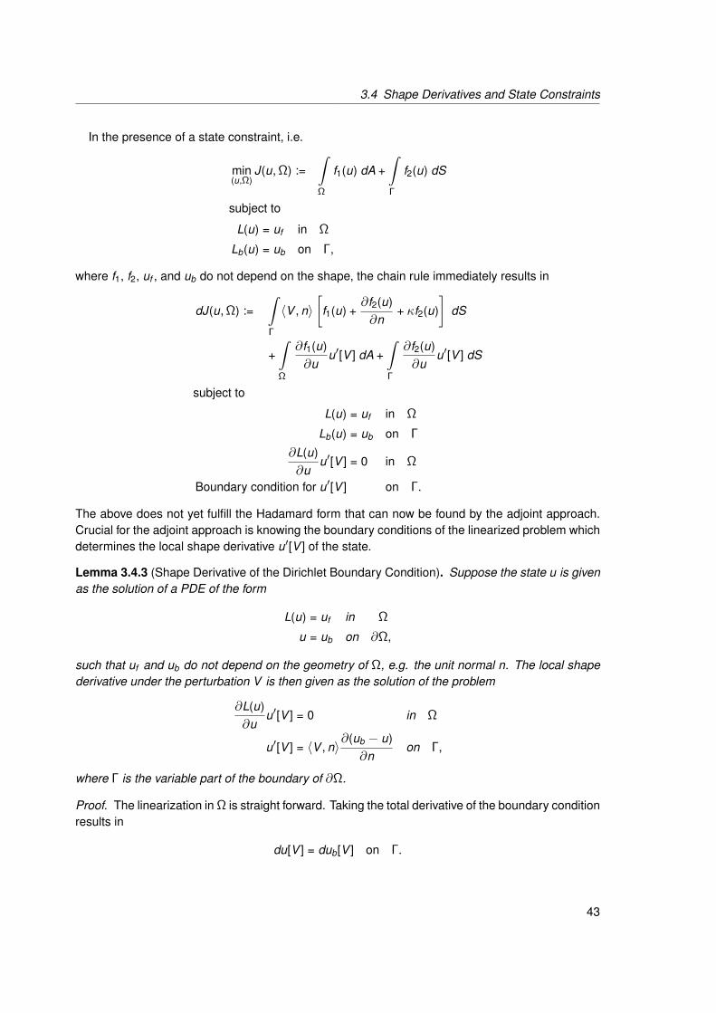
3.4 Shape Derivatives and State Constraints
In the presence of a state constraint, i.e.
min(u,Ω)
J(u, Ω) :=∫Ω
f1(u) dA +∫Γ
f2(u) dS
subject to
L(u) = uf in Ω
Lb(u) = ub on Γ,
where f1, f2, uf , and ub do not depend on the shape, the chain rule immediately results in
dJ(u, Ω) :=∫Γ
〈V , n〉[
f1(u) +∂f2(u)∂n
+ κf2(u)]
dS
+∫Ω
∂f1(u)∂u
u′[V ] dA +∫Γ
∂f2(u)∂u
u′[V ] dS
subject to
L(u) = uf in Ω
Lb(u) = ub on Γ
∂L(u)∂u
u′[V ] = 0 in Ω
Boundary condition for u′[V ] on Γ.
The above does not yet fulfill the Hadamard form that can now be found by the adjoint approach.Crucial for the adjoint approach is knowing the boundary conditions of the linearized problem whichdetermines the local shape derivative u′[V ] of the state.
Lemma 3.4.3 (Shape Derivative of the Dirichlet Boundary Condition). Suppose the state u is givenas the solution of a PDE of the form
L(u) = uf in Ω
u = ub on ∂Ω,
such that uf and ub do not depend on the geometry of Ω, e.g. the unit normal n. The local shapederivative under the perturbation V is then given as the solution of the problem
∂L(u)∂u
u′[V ] = 0 in Ω
u′[V ] = 〈V , n〉∂(ub − u)∂n
on Γ,
where Γ is the variable part of the boundary of ∂Ω.
Proof. The linearization in Ω is straight forward. Taking the total derivative of the boundary conditionresults in
du[V ] = dub[V ] on Γ.
43

3 Shape Sensitivity Analysis
Using definition 3.4.1, the above can be transformed to
u′[V ] + 〈∇u, V 〉 = du[V ] = dub[V ] = 〈∇ub, V 〉⇒ u′[V ] = 〈∇ (ub − u) , V 〉 .
The usual orthogonality argument gives the desired expression
u′[V ] = 〈V , n〉(∂ (ub − u)
∂n
).
Lemma 3.4.4 (Shape Derivative of the Slip Boundary Condition). The slip-boundary condition isoften encountered in fluid dynamics, especially when an inviscid fluid is modeled:
〈u, n〉(x) = 0 on Γ.
The local shape derivative then satisfies the boundary condition
〈u′[V ], n〉 = −〈DuV , n〉 − 〈u, dn[V ]〉
= −〈V , n〉⟨∂u∂n
, n⟩
+ 〈u,∇Γ〈V , n〉〉 ,
where the second part of the identity holds for a perturbation in normal direction only and can bebrought into Hadamard form using lemma 3.3.12.
Proof. The derivation is analog to lemma 3.4.3 using the product rule and the extension of defini-tion 3.4.1 for a vector valued state u:
du[V ] = u′[V ] + 〈Du, V 〉.
Lemma 3.4.5 (Shape Derivative of the Neumann Boundary Condition). Suppose the state u isgiven as the solution of a PDE of the form
L(u) = uf in Ω
∂u∂n
= ub on ∂Ω,
such that uf and ub do not depend on the geometry of Ω, e.g. the unit normal n, etc. The localshape derivative under the perturbation V is then given as the solution of the problem
∂L(u)∂u
u′[V ] = 0 in Ω
∂u′[V ]∂n
= 〈∇ub, V 〉 − 〈D2uV , n〉 − 〈∇Γu, dn[V ]〉
= 〈V , n〉[∂ub
∂n− ∂2u∂n2
]+ 〈∇Γu,∇Γ〈V , n〉〉,
where the second identity holds for the orthogonal component of the perturbation field only.
44

3.4 Shape Derivatives and State Constraints
Proof. The Neumann boundary condition at xt = Tt (x) on the deformed domain Ωt reads
ub xt = 〈∇ut , nt〉 xt
= 〈∇ut , nt〉 Tt (x)
= 〈(∇ut ) Tt (x), nt (xt )〉.
The chain rule results in
∇(ut Tt (x)) = ((∇ut ) Tt (x))T · DTt (x)
= (DTt (x))T · [(∇ut ) Tt (x)] ,
and the boundary condition becomes
ub(xt ) = 〈(DTt (x))−T ∇(ut Tt (x)), nt (xt )〉= (∇(ut (xt )))T DTt (x)−1 · nt (xt ).
The total derivative with respect to t now yields the material derivative of ut (xt ). Using lemma 3.3.3results in:
dub[V ] = (∇du[V ])T n + (∇u)T (−DV ) n + 〈∇u, dn[V ]〉,
which results in
∂du[V ]∂n
= dub[V ]− 〈∇u, (−DV ) n〉 − 〈∇u, dn[V ]〉.
Using the relationship
du[V ] = u′[V ] + 〈∇u, V 〉dub[V ] = 〈∇ub, V 〉dn[V ] = −∇Γ〈V , n〉,
we have
∂du[V ]∂n
=∂u′[V ]∂n
+ 〈D2uV , n〉 + 〈∇u, DVn〉,
and the above can now be expressed in terms of the local shape derivatives:
∂u′[V ]∂n
= 〈∇ub, V 〉 − 〈D2uV , n〉 − 〈∇u, dn[V ]〉.
Since 〈∇u, n〉 = 0, we have ∇u = ∇Γu, and with the usual orthogonality argument the boundarycondition can be expressed as
∂u′[V ]∂n
= 〈V , n〉[∂ub
∂n− ∂2u∂n2
]+ 〈∇Γu,∇Γ〈V , n〉〉,
45

3 Shape Sensitivity Analysis
where the last part can be brought into Hadamard form using lemma 3.3.12, i.e.∫Γ
〈∇Γ〈V , n〉,∇Γu〉 dS =∫Γ
−〈V , n〉divΓ∇Γu + κ〈V , n〉〈∇Γu, n〉 dS
=∫Γ
〈V , n〉[κ〈∇Γu, n〉 −∆Γu
]dS.
Remark 3.4.6. Note that in the setting considered in the above lemma 3.4.5, it can be possiblethat the problem does not possess a unique solution u. However, this has no consequence for theshape derivative of the Neumann boundary condition.
Remark 3.4.7. A simpler formula than lemma 3.4.5 can be given in the special case of the standardLaplace problem
−∆u = uf in Ω
∂u∂n
= ub on ∂Ω.
The Laplace-Beltrami operator
∆Γu := divΓ∇Γu = ∆u − κ∂u∂n− ∂2u∂n2
provides
∂2u∂n2 = −∆Γu − uf − κub
which results in
∂u′[V ]∂n
= divΓ
(〈V , n〉∇Γu
)+ 〈V , n〉
(∂ub
∂n+ κub + uf
).
For more details see [70].
46

Chapter 4
Fluid Mechanics
4.1 Derivation of the State Equations
Before considering shape optimization in fluids, this chapter is used to give a brief overview aboutpartial differential and integral equations governing fluid flow. First, the governing equations arederived in a general setting. Afterwards, possible simplifications of inviscid or incompressible flowsare introduced. More detailed overviews about the derivation of the state equations can for examplealso be found in [7, 20]. The derivation of the partial differential and integral equations describingfluids are a direct consequence of the continuum hypothesis, conservation of mass, conservationof momentum, and conservation of energy.
For consistency reasons with the literature the nomenclature is redefined. For example, t isnow used to denote the physical time as opposed to being responsible for the amount of shapedeformation, for which the symbol was used in chapter 3.
Definition 4.1.1 (Intensive and Extensive Quantity). A physical property is called intensive if it isscale invariant, meaning it does not depend on the system size or the amount of material in thesystem. Examples of intensive properties are temperature, density, or specific energy. By contrast,a property is called extensive if it does depend on scale, such as mass, length, volume, enthalpy,or energy. Let φ be an intensive quantity. The corresponding extensive quantity ϕ is then given by
ϕ =∫M
ρφ dA, (4.1)
where M is a control volume under consideration and ρ is the fluid density.
47

4 Fluid Mechanics
Remark 4.1.2 (Reynolds Transport Theorem). The Reynolds transport theorem is a three-dimen-sional generalization of the Leibniz integral rule for differentiation under the integral sign. It relatesthe change of extensive quantities to the change of intensive quantities by
dϕdt
=∫M
∂
∂t(ρφ) dA +
∫∂M
〈ρφ · (u − ub), n〉 dS,
where ϕ is the extensive quantity under consideration and φ is the corresponding intensive quantity.The fluid density is denoted by ρ, and the fluid velocity is given by u. The velocity of the controlsurface ∂M is given by ub. More details can be found in [7].
Lemma 4.1.3 (Conservation of Mass). Let M ⊂ Ω be an arbitrary control volume. The conservationof mass results in the first state equation∫
M
∂ρ
∂t+ div (ρu) dA = 0. (4.2)
Proof. The mass m of a fluid contained in the volume M is given by
m =∫M
ρ dA,
thus, when comparing the above with equation (4.1), one can see that mass is the extensive quantitycorresponding to the intensive quantity φ = 1. The mass of the fluid in a fixed control volume isconsidered to be conserved, resulting in
0 =dmdt
=ddt
∫M
ρ dA.
Considering a fixed control volume, i.e. ub = 0, a straight application of the Reynolds transporttheorem results in
0 =dmdt
=∫M
∂ρ
∂tdA +
∫∂M
〈ρu, n〉 dS.
The desired expression follows with remark 3.2.3.
Lemma 4.1.4 (Conservation of Momentum). The conservation of momentum results in the secondstate equation governing fluid flow:∫
M
∂
∂t(ρui ) + div (−Ti + ρuiu) +
∂p∂xi
dA =∫M
ρgi dA, (4.3)
where i = 1, 2, 3 are the three spacial dimensions and Ti ∈ R3 is the corresponding stress tensorrow describing the distortion of the control volume M under forces. The fluid pressure is denotedby p. Also, gi is the volume force in the i-th coordinate direction.
48
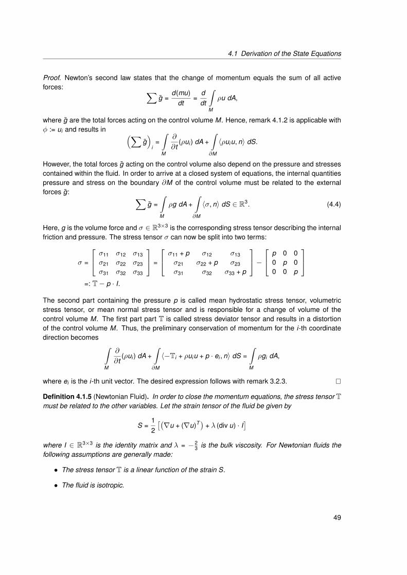
4.1 Derivation of the State Equations
Proof. Newton’s second law states that the change of momentum equals the sum of all activeforces: ∑
g =d(mu)
dt=
ddt
∫M
ρu dA,
where g are the total forces acting on the control volume M. Hence, remark 4.1.2 is applicable withφ := ui and results in (∑
g)
i=∫M
∂
∂t(ρui ) dA +
∫∂M
〈ρuiu, n〉 dS.
However, the total forces g acting on the control volume also depend on the pressure and stressescontained within the fluid. In order to arrive at a closed system of equations, the internal quantitiespressure and stress on the boundary ∂M of the control volume must be related to the externalforces g: ∑
g =∫M
ρg dA +∫∂M
〈σ, n〉 dS ∈ R3. (4.4)
Here, g is the volume force and σ ∈ R3×3 is the corresponding stress tensor describing the internalfriction and pressure. The stress tensor σ can now be split into two terms:
σ =
σ11 σ12 σ13
σ21 σ22 σ23
σ31 σ32 σ33
=
σ11 + p σ12 σ13
σ21 σ22 + p σ23
σ31 σ32 σ33 + p
− p 0 0
0 p 00 0 p
=: T− p · I.
The second part containing the pressure p is called mean hydrostatic stress tensor, volumetricstress tensor, or mean normal stress tensor and is responsible for a change of volume of thecontrol volume M. The first part part T is called stress deviator tensor and results in a distortionof the control volume M. Thus, the preliminary conservation of momentum for the i-th coordinatedirection becomes ∫
M
∂
∂t(ρui ) dA +
∫∂M
〈−Ti + ρuiu + p · ei , n〉 dS =∫M
ρgi dA,
where ei is the i-th unit vector. The desired expression follows with remark 3.2.3.
Definition 4.1.5 (Newtonian Fluid). In order to close the momentum equations, the stress tensor Tmust be related to the other variables. Let the strain tensor of the fluid be given by
S =12
[(∇u + (∇u)T ) + λ (div u) · I
]where I ∈ R3×3 is the identity matrix and λ = −2
3 is the bulk viscosity. For Newtonian fluids thefollowing assumptions are generally made:
• The stress tensor T is a linear function of the strain S.
• The fluid is isotropic.
49

4 Fluid Mechanics
• A fluid at rest does not distort control volumes.
The last assumption links the equations of fluid dynamics to hydrostatics. As a consequence, thestress tensor must be divergence free, i.e. div T = 0 for a fluid at rest. For a Newtonian fluid it istherefore often assumed that
T := τ := 2µS,
where µ is the shear or dynamic viscosity of the fluid, which is related to the kinematic viscosity νby
ν =µ
ρ.
Viscosity describes the ratio of viscous forces to inertia forces. Dynamic viscosity µ and bulk vis-cosity λ are closely related to the Lamé coefficients in linear elasticity. A wide array of real worldfluids are considered to be Newtonian such as water, air, and oil. Examples for non-Newtonianfluids are polymer solutions, blood, paint, quicksand, toothpaste, and ketchup. Thus, for Newtonianfluids the conservation of momentum in the i-th coordinate direction is given by∫
M
∂
∂t(ρui )+
3∑j=1
[∂
∂xj
(−µ(∂ui
∂xj+∂uj
∂xi− 2
3(div u) δij
))+∂(ρuiuj )∂xj
]+∂p∂xi
dA =∫M
ρgi dA, (4.5)
where δij is the Kronecker symbol.
Lemma 4.1.6 (Conservation of Energy). The conservation of energy results in the following equa-tion of state: ∫
M
∂
∂t(ρE) + div (ρHu − κ∇T − Tu) dA =
∫M
ρgu dA,
where H is the enthalpy, T the absolute static temperature, and κ is the thermal conductivity of thefluid.
Proof. The total energy per unit mass E of a fluid is given by kinetic energy and internal energy e
E = e +12‖u‖2 = e +
12
(u2
1 + u22 + u2
3
).
The change of energy in a control volume equals the work performed by exterior forces plus heatsupply:
ddt
∫M
ρE dA =∫M
ρgu dA
︸ ︷︷ ︸work performed by volume forces
−∫∂M
qn dA
︸ ︷︷ ︸heat supply over the boundary
+∫∂M
(T− p · I) un dS
︸ ︷︷ ︸work performed by surface forces
.
Fourier’s law of heat conduction states that
q = −κ∇T ,
where κ is the thermal conductivity of the fluid and T is the absolute static temperature. Applyingthe Reynolds transport theorem 4.1.2 with φ = E results in∫
M
∂
∂t(ρE) dA +
∫∂M
〈ρEu, n〉 dS =∫M
ρgu dA +∫∂M
κ∇Tn dS +∫∂M
(T− p · I) un dS.
50

4.1 Derivation of the State Equations
The energy equation is often rewritten in terms of total enthalpy H
H := E +pρ⇒ p = ρH − ρE , (4.6)
which eliminates the pressure p:∫M
∂
∂t(ρE) dA +
∫∂M
〈ρHu, n〉 dS =∫M
ρgu dA +∫∂M
κ∇Tn dS +∫∂M
Tun dS.
The desired expression follows with remark 3.2.3.
The conservation of mass, momentum, and energy results in five equations for the seven un-knowns ρ, u, p, E , and T . Hence, additional closure assumptions must be made, linking pressurep and temperature T to the unknowns ρ, u, and E .
Definition 4.1.7 (Perfect Gas). A gas is said to be perfect or ideal if the pressure is given by therelation
p = ρRT ,
where R is the specific gas constant. Furthermore, the specific heat capacity is the measureof the heat energy required to increase the temperature of a unit quantity of a substance by acertain temperature interval. For a compressible body, one may distinguish between heat capacityat constant volume cv and heat capacity at constant pressure cp. For an ideal gas, the heat capacityis constant with temperature resulting in
R = cp − cv ,
and the internal energy is related to the temperature by
e = cv T .
Since E = e + 12‖u‖
2, the above results in
p = ρRE − 1
2‖u‖2
cv=
Rcvρ
(E − 1
2‖u‖2
).
Introducing the adiabatic exponent γ as
γ =cp
cv⇒ R
cv= γ − 1,
one arrives at the final equation linking the pressure to the unknowns:
p = (γ − 1)ρ(
E − 12‖u‖2
).
Closing the circle, the temperature can thus also be expressed as T = pRρ .
51

4 Fluid Mechanics
Remark 4.1.8 (Speed of Sound, Mach Number). A very important property is the speed of sound.As the fluid velocity approaches the local speed of sound, shock waves begin to form, and theequations of state are then dominated by their hyperbolic nature. For a perfect gas, the speed ofsound c is given by
c =√γRT =
√γR
1cv
e =√γ(γ − 1)(E − ‖u‖2) =
√γ
pρ
.
The local Mach number M is then given by
M =‖u‖
c.
Remark 4.1.9 (Scaling, Non-Dimensionalization). Different scales can lead to similar fluid flow:Flow around a sphere of radius r1 = 10 m with a velocity of 10 km/h will be the same as flow arounda sphere of radius r2 = 1 m with a velocity of 100 km/h. This is often exploited in experimentswhen smaller models are used in wind tunnels. The Navier–Stokes equations are thus often non-dimensionalized. The subscript∞ denotes the respective value in the farfield:
p∞ = 1 reference pressure
ρ∞ = 1 reference density
T∞ = 1 reference temperature
c∞ =√γ
p∞ρ∞
=√γ reference speed of sound
u∞ = M∞a∞ = M∞√γ reference velocity
µ∞ =ρ∞u∞L
Re∞=
M∞√γ
Re∞reference dynamic viscosity.
Additionally, M∞ is the freestream Mach number and
Re =ρuLµ
is the Reynolds number where L is the characteristic length scale. Furthermore, the thermal con-ductivity is non-dimensionalized by
κ∞ =γµ∞
(γ − 1)Pr,
where Pr is the Prandtl number. As a consequence, the non-dimensional gas constant reduces to
R =pρT
= 1.
Usually, the Reynolds number Re, Prandtl number Pr , Mach number M, adiabatic exponent γ, andthe reference length L are externally given, defining the flow conditions to simulate.
52

4.1 Derivation of the State Equations
Remark 4.1.10 (Sutherland Law). The viscosity of a fluid is often decreasing with temperature,which is modeled by Sutherland’s formula
µ = µ∞
(T
T∞
) 32 T∞ + S
T + S,
where S is the Sutherland temperature, usually 110.4 K for air.
Taking everything together results in the compressible Navier–Stokes equations.
Definition 4.1.11 (Compressible Navier–Stokes Equations). The compressible Navier–Stokes equa-tions for a Newtonian fluid are given by ∫
M
∂ρ
∂t+ div (ρu) dA = 0 (4.7)
∫M
∂
∂t(ρui ) +
3∑j=1
[∂
∂xj
(−µ(∂ui
∂xj+∂uj
∂xi− 2
3(div u) δij
))+∂(ρuiuj )∂xj
]+∂p∂xi
dA =∫M
ρgi dA
(4.8)∫M
∂
∂t(ρE) + div
(ρHu − κ∇T +
[−µ(∇u + (∇u)T − 2
3(div u) · I
)]u)
dA =∫M
ρgu dA.
(4.9)
Note that equation (4.8) is also of divergence type when written in vectorial form using the Kroneckersymbol for the pressure. The dynamic viscosity µ is given by the Sutherland law. The boundarycondition for the velocity on fluid obstacles usually is
u = 0 on Γ0.
Appropriate boundary conditions for the heat fluxes and on inlets/outlets will be provided later onbased on the situation to be simulated.
Remark 4.1.12 (Forces in Fluids). Equation (4.4) can also be used to compute the force a fluidexerts on an immersed body with boundary ∂M. According to (4.4), the force a solid body exertson the fluid is given by
F =∫M
ρg dA +∫∂M
〈σ, n〉 dS ∈ R3.
According to Newton’s third law of motion, the sign switches when considering the force the fluidexerts on the solid body, and in a Newtonian fluid without body forces, the fluid force in the i-thcoordinate axis is thus given by
Fi =
∫∂M
〈−T + p, n〉 dS
i
=∫∂M
3∑j=1
(−µ(∂ui
∂xj+∂uj
∂xi− 2
3(div u) δij
))nj
+ pni dS. (4.10)
53

4 Fluid Mechanics
4.2 Simplifications
There are many simplifications making the complex governing equations more accessible. Twoassumptions most often used are incompressibility and diminishing viscosity, i.e. inviscid flow.
4.2.1 Incompressible Flow
Definition 4.2.1 (Incompressible Fluid). A fluid is considered incompressible if the density ρ doesnot change in time, i.e.
dρ(x(t), t)dt
= 0.
Here, it is also assumed that the density is constant in space.
When using the above assumption and omitting Sutherland’s law, the conservation of mass (4.7)and momentum (4.8) for a Newtonian fluid become∫
M
ρdiv u dA = 0
∫M
ρ∂
∂tui − µ∆ui + ρu∇ui +
∂p∂xi
dA =∫M
ρgi dA.
For an incompressible flow the conservation of mass and momentum already create a closed sys-tem of equations. The energy of the fluid can be computed using equation (4.9) after the aboveequations have been solved for u and p. Since the incompressible equation cannot develop shockwaves, the above system is often written as a partial differential equation:
Definition 4.2.2 (Incompressible Navier–Stokes Equations). The incompressible Navier–Stokesequations are given by
ρ∂
∂tu − µ∆u + ρu∇u +∇p = ρg in Ω
div u = 0
u = u+ on Γ+
u = 0 on Γ0
pn − µ∂u∂n
= 0 on Γ−.
(4.11)
Here, ∂Ω = Γ = Γ+d∪ Γ0
d∪ Γ−. The inflow is given by Γ+ and the surface of any obstacles in the
fluid is given by Γ0. The boundary condition on Γ0 is the no-slip boundary condition of a viscousfluid. The outflow condition on Γ− is chosen such that mass conservation holds. This is the naturalboundary condition for finite element discretizations. When enclosed flows are considered, i.e.Γ− = ∅, the missing boundary condition results in the pressure being defined only up to an additiveconstant. Omitting the time derivative results in the steady state Navier–Stokes equations.
Since the energy equation decouples from the conservation of mass and momentum, there existsa convenient representation of the kinetic energy loss of an incompressible fluid. In order to derivethe dissipation rate of kinetic energy into heat, the following result is needed:
54
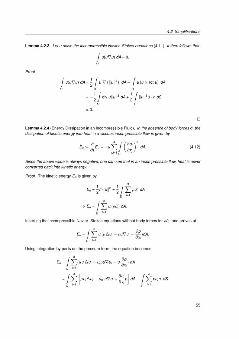
4.2 Simplifications
Lemma 4.2.3. Let u solve the incompressible Navier–Stokes equations (4.11). It then follows that∫Ω
u(u∇u) dA = 0.
Proof. ∫Ω
u(u∇u) dA =12
∫Ω
u ∇(‖u‖2) dA−
∫Ω
u (u × rot u) dA
= −12
∫Ω
div u‖u‖2 dA +12
∫Γ
‖u‖2u · n dS
= 0.
Lemma 4.2.4 (Energy Dissipation in an Incompressible Fluid). In the absence of body forces g, thedissipation of kinetic energy into heat in a viscous incompressible flow is given by
Eu :=∂
∂tEu = −µ
3∑i ,j=1
∫Ω
(∂ui
∂xj
)2
dA. (4.12)
Since the above value is always negative, one can see that in an incompressible flow, heat is neverconverted back into kinetic energy.
Proof. The kinetic energy Eu is given by
Eu =12
m‖u‖2 =12
∫Ω
3∑i=1
ρu2i dA
⇒ Eu =∫Ω
3∑i=1
ui (ρui ) dA.
Inserting the incompressible Navier–Stokes equations without body forces for ρui , one arrives at
Eu =∫Ω
3∑i=1
ui (µ∆ui − ρu∇ui −∂p∂xi
)dA.
Using integration by parts on the pressure term, the equation becomes
Eu =∫Ω
3∑i=1
(µui∆ui − uiρu∇ui − ui∂p∂xi
) dA
=∫Ω
3∑i=1
[µui∆ui − uiρu∇ui +
∂ui
∂xip]
dA−∫Γ
3∑i=1
puini dS.
55

4 Fluid Mechanics
Furthermore,∑3
i=1∂ui∂xi
= 0 because of the divergence freedom and∑3
i=1 puini = 0 because of theno-slip boundary condition, which leads to
Eu =∫Ω
3∑i=1
[µui∆ui − uiρu∇ui ] dA.
With lemma 4.2.3 this becomes:
Eu =∫Ω
3∑i=1
µui∆ui dA.
Swapping over ∆ and eliminating the boundary integrals because of the no-slip boundary conditionresults in:
Eu = −µ3∑
i ,j=1
∫Ω
(∂ui
∂xj
)2
dA.
The above formula has both advantages and disadvantages when compared to using forcesaccording to equation (4.10). On the one hand, the value of (4.12) depends on the size of thesimulation domain Ω, making results from two different domains difficult to compare: Consideringan obstacle in a fluid channel, the value of (4.12) will increase when a longer channel is simulated,although the force the fluid exerts on any obstacle should stay the same. Also, in case of multipleobstacles, (4.12) does not allow identifying the contribution each obstacle has to the total energyloss. On the other hand, the shape differentiation of a volume objective function is much morestraight forward than the shape differentiation of a surface functional such as (4.10). This is es-pecially true for higher order derivatives. Hence, for considerations on shape optimization in fluidslater on, (4.12) will be considered first.
Remark 4.2.5. The incompressible Navier–Stokes equations still possess several numerical dif-ficulties. The missing time derivative in the conservation of mass requires at least semi-implicitsolution strategies. The divergence freedom of u results in the fact that the discretization of u andp cannot be chosen independently. Instead, a stable discretization without checkerboarding mustsatisfy the inf-sup condition [30, 76], and the resulting discrete saddle-point problem is hard to solveiteratively. Last, a low viscosity µ, i.e. a high Reynolds number Re, results in an emphasis on thenon-linearity. Unless the resulting turbulence is not averaged in some way, the equation does nolonger have a stable steady state, and all turbulent length scales must be resolved in the compu-tational grid. For most flow phenomena of interest, the computational power of present and futurecomputers does not suffice to resolve turbulence. The problems due to turbulence can be avoidedby dropping the non-linearity from the momentum conservation, resulting in the Stokes equation.
56
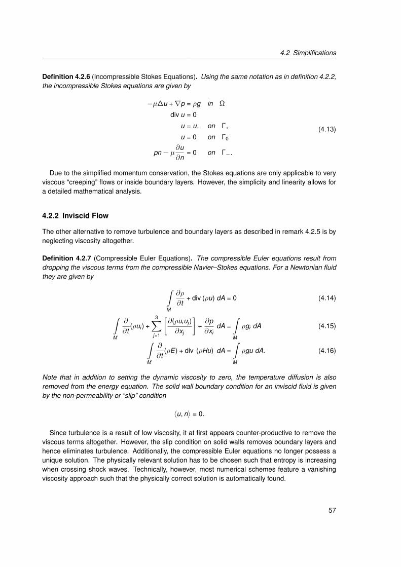
4.2 Simplifications
Definition 4.2.6 (Incompressible Stokes Equations). Using the same notation as in definition 4.2.2,the incompressible Stokes equations are given by
−µ∆u +∇p = ρg in Ω
div u = 0
u = u+ on Γ+
u = 0 on Γ0
pn − µ∂u∂n
= 0 on Γ−.
(4.13)
Due to the simplified momentum conservation, the Stokes equations are only applicable to veryviscous “creeping” flows or inside boundary layers. However, the simplicity and linearity allows fora detailed mathematical analysis.
4.2.2 Inviscid Flow
The other alternative to remove turbulence and boundary layers as described in remark 4.2.5 is byneglecting viscosity altogether.
Definition 4.2.7 (Compressible Euler Equations). The compressible Euler equations result fromdropping the viscous terms from the compressible Navier–Stokes equations. For a Newtonian fluidthey are given by ∫
M
∂ρ
∂t+ div (ρu) dA = 0 (4.14)
∫M
∂
∂t(ρui ) +
3∑j=1
[∂(ρuiuj )∂xj
]+∂p∂xi
dA =∫M
ρgi dA (4.15)
∫M
∂
∂t(ρE) + div (ρHu) dA =
∫M
ρgu dA. (4.16)
Note that in addition to setting the dynamic viscosity to zero, the temperature diffusion is alsoremoved from the energy equation. The solid wall boundary condition for an inviscid fluid is givenby the non-permeability or “slip” condition
〈u, n〉 = 0.
Since turbulence is a result of low viscosity, it at first appears counter-productive to remove theviscous terms altogether. However, the slip condition on solid walls removes boundary layers andhence eliminates turbulence. Additionally, the compressible Euler equations no longer possess aunique solution. The physically relevant solution has to be chosen such that entropy is increasingwhen crossing shock waves. Technically, however, most numerical schemes feature a vanishingviscosity approach such that the physically correct solution is automatically found.
57

4 Fluid Mechanics
Remark 4.2.8 (Euler Equations, Flux Functions). The compressible Euler equations, definition 4.2.7,can also be written in the following way:
∂U∂t
+ div F =∂U∂t
+3∑
k=1
∂Fk
∂xk= 0 ∈ R5, (4.17)
where the “inviscid fluxes” Fi are given by
F1 :=(ρu1, p + ρu2
1 , ρu1u2, ρu1u3, u1(E + p))T
F2 :=(ρu2, ρu1u2, p + ρu2
2 , ρu2u3, u2(E + p))T
F3 :=(ρu3, ρu1u3, ρu2u3, p + ρu2
3 , u3(E + p))T
.
The vector of conserved variables is given by
U := (ρ, ρu, ρE)T ,
and
Up := (ρ, u, E)T
is the vector of primitive variables.
Remark 4.2.9 (Euler Flux Jacobians). Applying the chain rule on (4.17), the conserved variables Ucan be made visible
0 =3∑
k=1
∂Fk
∂xk=
3∑k=1
∂Fk
∂U∂U∂xk
=3∑
k=1
∂Fk
∂Up
∂Up
∂U∂U∂xk
=3∑
k=1
∂Fk
∂Up
[∂U∂Up
]−1 ∂U∂xk
=:3∑
k=1
Ak∂U∂xk
.
The Euler flux Jacobians Ak are given by
A1 :=
0 1 0 0 0
(γ − 1)H − u21 − c2 (3− γ)u1 −(γ − 1)u2 −(γ − 1)u3 γ − 1
−u1u2 u2 u1 0 0−u1u3 u3 0 u1 0
u1[(γ − 2)H − c2] H − (γ − 1)u21 −(γ − 1)u1u2 −(γ − 1)u1u3 γu1
A2 :=
0 0 1 0 0
−u1u2 u2 u1 0 0(γ − 1)H − u2
2 − c2 −(γ − 1)u1 (3− γ)u2 −(γ − 1)u3 γ − 1−u2u3 0 u3 u2 0
u2[(γ − 2)H − c2] −(γ − 1)u1u2 H − (γ − 1)u22 −(γ − 1)u2u3 γu2
A3 :=
0 0 0 1 0
−u1u3 u3 0 u1 0−u2u3 0 u3 u2 0
(γ − 1)H − u23 − c2 −(γ − 1)u1 −(γ − 1)u2 (3− γ)u3 γ − 1
u3[(γ − 2)H − c2] −(γ − 1)u1u3 −(γ − 1)u2u3 H − (γ − 1)u23 γu3
,
58

4.2 Simplifications
where H := E + pρ is the enthalpy, see also equation (4.6), and c =
√γpρ is the speed of sound
according to remark 4.1.8.
Remark 4.2.10 (Incompressible Euler Equations). It is also possible to assume an inviscid andincompressible flow simultaneously, which leads to the incompressible Euler equations
ρ∂
∂tu + ρu∇u +∇p = ρg in Ω
div u = 0
u = u+ on Γ+
〈u, n〉 = 0 on Γ0
pn = 0 on Γ−.
However, when considering the dissipation of kinetic energy into heat for an incompressible flowaccording to equation (4.12), one can see that
Eu ≡ 0.
Hence, a body immersed in an inviscid, incompressible fluid does not experience any force at all.Unfortunately, this is also true when the compressible equations are used to simulate an essentiallyincompressible flow. As such, the Euler equations only produce physically meaningful forces whencompressibility effects are relevant, meaning the speed of the fluid is close to or exceeds Mach 1.0and compression shock waves form.
4.2.3 Potential Flow
The final simplification is that of potential flow. When an inviscid fluid is also considered to beirrotational, meaning
rot u = 0,
one can show that there exists a velocity potential φ such that u = −∇φ. More information canfor example be found in [43]. Using the irrotational assumption in the inviscid mass conservationdiv u = 0, one arrives at the equation for potential flow:
Definition 4.2.11 (Potential Flow). Potential flow is given by
−∆φ = 0 in Ω
∂φ
∂n= 0 on Γ0
φ = φ0 on Ω \ Γ0.
This is now a scalar equation based on the inviscid conservation of mass. The boundary value φ0
creates the necessary potential difference between inflow and outflow. It is possible to recover thepressure once the above equation is solved for φ. However, due to the limitations as discussed inremark 4.2.10, potential flow can mostly be used in inverse design only, meaning finding shapesthat produce a desired pressure profile.
In the following chapters, both fluid dynamics and shape optimization will be combined with spe-cial attention on fast numerical procedures. However, first a very brief overview on finite volumemethods for conservation laws will be given.
59
4 Fluid Mechanics
4.3 Numerical Schemes for Conservation Laws
In this section, some aspects of solving the flow equations discretely will be presented from theliterature, especially [44, 82]. Special attention is given to finite volume schemes for compressiblefluid dynamics. The DLR flow solver TAU, which is used in chapter 8, is also based on a finitevolume discretization. However, in the incompressible case, chapter 5 and 6, a finite element basedflow solver is used. Compared to the compressible case, finite element methods are more straightforward applicable to incompressible fluid dynamics, but for convection dominant high Reynolds-number flows they usually require some kind of stabilization.
4.3.1 The Finite Volume Method
For simplicity reasons, a general scalar conservation law of the type
∂u∂t
+∂f (u)∂x
= 0 (4.18)
will be considered. The discretization of the space-time domain is given by a cartesian grid
(xj , tn) := (j∆x , n∆t), j ∈ Z, n ∈ N0.
A discrete cell or finite control volume is then defined by the interval
[xj− 12, xj+ 1
2] := [xj −
12∆x , xj +
12∆x ],
and the discretized state uj at node j is thought of as an approximation of the cell-averaged valueof the function u
u(xj , t) ≈ 1∆x
xj+ 1
2∫x
j− 12
u(x , t) dx .
The integral representation of the conservation law (4.18) provides
xj+ 1
2∫x
j− 12
u(x , tn+1) dx =
xj+ 1
2∫x
j− 12
u(x , tn) dx −
tn+1∫tn
f (u(xj+ 12, t)) dt −
tn+1∫tn
f (u(xj− 12, t)) dt
for each finite control volume [xj− 1
2, xj+ 1
2]. Hence, a numerical scheme should reproduce this prop-
erty, which gives rise to the following definition.
Definition 4.3.1 (Conservative Scheme). A numerical scheme is called conservative if the followingrelation holds
un+1j = un
j −∆t∆x
[F (un
j−p, unj−p+1, ..., un
j+q)− F (unj−p−1, un
j−p, ..., unj+q−1)
],
60

4.3 Numerical Schemes for Conservation Laws
where lower indices denote the spacial dimension and upper indices denote time. In short notationthe above reads
un+1j = un
j −∆t∆x
[F (un; j)− F (un; j − 1)
].
Finally, the numerical flux F is given as the approximation of the average flux at position xj+ 12
duringthe time interval [tn, tn+1]
F (un; j) ≈ 1∆t
tn+1∫tn
f (u(xj+ 12, t)) dt .
Remark 4.3.2. Often, the numerical flux F depends only on one left and right neighbor. Thus,one frequently has the situation p = 0 and q = 1 in definition 4.3.1 above. This leads to the morecommon expression
un+1j = un
j −∆t∆x
[F (un
j , unj+1)− F (un, uj )
]=: un
j −∆t∆x
[Fj+ 1
2− Fj− 1
2
].
Definition 4.3.3 (Consistent Scheme). A finite volume scheme is call consistent, if the numericalflux function F satisfies for all u ∈ Rm
F (u, u, ..., u) = f (u)
and is Lipschitz-continuous, i.e. for an arbitrary u ∈ Rm fulfills
‖F (uj−p, uj−p+1, ..., uj+q)− f (u)‖ ≤ C max−p≤i≤q
‖uj+i − u‖
for all uj+i in a neighborhood of u with C independent of u.
Remark 4.3.4. The first condition in definition 4.3.3 basically states that constant functions must beintegrated correctly and is in fact necessary for the Lipschitz-continuity. One can show that a con-sistent finite volume scheme must also satisfy the discrete conservation property of definition 4.3.1.As a consequence, shock waves will be captured at correct positions during computation. For moredetails see [44].
Unless special provisions are taken, numerical schemes for conservation laws tend to producespurious oscillations when the solution of the conservation law features discontinuities and shockwaves. Thus, it is little surprising that the total variation of the computed solution must be dimin-ishing in order to achieve convergence of the scheme, which is stated by Lax-Wendroff’s theoremlater on.
Definition 4.3.5 (Total Variation). The total variation of a function u is given by
TV(u) := sup
N∑
j=1
|u(ξj )− u(ξj−1)| : ξ0 < ξ1 < ... < ξN , N ∈ N
.
For the discrete case, the total variation of a vector, i.e. the piecewise constant approximation of thestate un at time n, the total variation is given by
TV(un) :=∞∑
j=−∞|un
j+1 − unj |.
61

4 Fluid Mechanics
Using the total variation, the theorem of Lax–Wendroff now ensures the approximation propertyof finite volume schemes.
Theorem 4.3.6 (Lax–Wendroff). Let a sequence of meshes
(x`j , t`n) := (jh`, nk`), j ∈ Z, n ∈ N0, ` ∈ N
be given, such that h` → 0 and k` → 0 for ` → ∞. Let (u`)`∈N be a sequence of solutionsgenerated by a conservative and consistent scheme on the respective mesh. Furthermore, let thesequence (u`)`∈N converge to a locally integrable function u∗ such that for each finite set [a, b] ×[0, T ] the relation
lim`→∞
T∫0
b∫a
|u`(x , t)− u∗(x , t)| dxdt = 0
holds. Additionally, let the total variation be uniformly bounded, such that for each T > 0 thereexists an R > 0 with
TV(u`(., t)) < R
for all 0 ≤ t ≤ T and all ` ∈ N. The limit function u∗ is then a weak solution of the conservationlaw.
Proof. See for example theorem 12.1 in [44].
Remark 4.3.7. The Lax–Wendroff theorem neither states that convergence occurs at all nor that thecomputed solution of the conservation law is the physically correct solution. To ensure convergenceto a physically relevant solution, more considerations are necessary, some of which are based onmonotonicity conditions.
Remark 4.3.8 (Monotonicity Preservation). For some flow velocity c > 0, the linear convectionequation
∂u∂t
+ c∂u∂x
= 0, t > 0, x ∈ R (4.19)
with initial condition u(x , 0) = u0(x) is fulfilled by the function
u(x , t) = u0(x − ct).
Thus, if u(x , 0) has some monotonicity in x , then u(x , t) is also monotonic for all t > 0. Numericalschemes for such a conservation law should therefore also preserve monotonicity.
Theorem 4.3.9 (Godunov’s Order Barrier Theorem). Linear one-step second-order accurate nu-merical schemes for the convection equation (4.19) cannot be monotonicity preserving unless
c∆t∆x∈ N.
Proof. See chapter 9.2 in [82].
A consequence of Godunov’s theorem is that any numerical discretization scheme should onlybe of first order in the vicinity of discontinuities, e.g. shock waves. Since higher order accuracy isgenerally desired in smooth regions of the flow, Godunov’s theorem has given rise to higher ordermethods that employ flux and slope limiters at shock positions. These limiters are thus required toreduce the approximation order of any numerical scheme to 1 in the vicinity of shocks.
62

4.3 Numerical Schemes for Conservation Laws
4.3.2 The Jameson–Schmidt–Turkel Scheme
Due to Godunov’s theorem, any flow discretization must be of first order in the vicinity of discon-tinuities, which can be achieved by flux and slope limiters. Another approach is to start from anunstable central second order scheme and add a non-linear stabilization term, which usually leadsto a version of the Jameson–Schmidt–Turkel (JST) scheme [42].
The domain Ω is discretized into a finite number of non-overlapping control volumes Ωi ,j , and theapproximation ui ,j of the flow state is assumed to reside in the center of each control volume. The
ui ,j
xi ,j
xi+1,j
xi+1,j+1xi ,j+1
s1
s2
s3
s4
Figure 4.1: Cell-centered finite volume discretization.
situation is also illustrated in figure 4.1. The conservation law in integral formulation provides
0 =∫Ω
∂u∂t
+ div f (u) dA =ni∑
i=1
nj∑j=1
∫Ωi ,j
∂u∂t
+ div f (u) dA
=ni∑
i=1
nj∑j=1
∫Ωi ,j
∂u∂t
dA +∫∂Ωi ,j
f (u)n dS
due to the divergence theorem. Thus, an approximation of u on the faces of each finite controlvolume is needed. Assuming the approximation u to be constant inside each control volume, thevalue of u on the face is given by
ui ,j+ 12
=12
(ui ,j + ui ,j+1
)ui ,j− 1
2=
12
(ui ,j + ui ,j−1
)ui+ 1
2 ,j =12
(ui ,j + ui+1,j
)ui− 1
2 ,j =12
(ui ,j + ui−1,j
),
63
4 Fluid Mechanics
which leads to
0 =ni∑
i=1
nj∑j=1
[∂ui ,j
∂t|Ωi ,j | + f (ui ,j− 1
2)s1 + f (ui+ 1
2 ,j )s2 + f (ui ,j+ 12)s3 + f (ui− 1
2 ,j )s4
].
Here, the face vectors si are orthogonal to the edges of Ωi ,j . By not normalizing them, the corre-sponding integral over each of the edges can be computed straight forward. Thus, the equation canbe integrated in time until a steady state is reached by solving for each control volume
∂ui ,j
∂t= − 1|Ωi ,j |
Qi ,j ,
where
Qi ,j =[f (ui ,j− 1
2)s1 + f (ui+ 1
2 ,j )s2 + f (ui ,j+ 12)s3 + f (ui− 1
2 ,j )s4
].
Remark 4.3.10. One can show that the above central discretization scheme is of 2nd order andthus violates Godunov’s theorem. In order to ensure stability, a certain degree of numerical viscosityhas to be added by conducting flux updates of the type
∂ui ,j
∂t= − 1|Ωi ,j |
Qi ,j +1|Ωi ,j |
Di ,j .
The dissipative flux Di ,j is usually given by
Di ,j = di+ 12 ,j + di− 1
2 ,j + di ,j+ 12
+ di ,j− 12
with di ,j being
di+ 12 ,j = αi+ 1
2 ,j
(ε(2)
i+ 12 ,j
(ui+1,j − ui ,j
)− ε(4)
i+ 12 ,j
(ui+2,j − 3ui+1,j + 3ui ,j − ui−1,j
)).
The other directions are given analogeously. The coefficients ε(2)i ,j and ε(4)
i ,j are adaptive coefficientsdetermining the amount of 1st and 3rd order numerical dissipation. They usually depend on thepressure discontinuity of the respective finite volume. The coefficient αi ,j is usually chosen withrespect to the discrete time-step size. For more details, especially concerning accelerating theconvergence to a steady state by local and adaptive time-stepping and the treatment of boundaryconditions, see [7].
64

Chapter 5
Shape Optimization and Stokes Fluids
5.1 Problem Introduction and First Order Calculus
The self-adjoint nature of the Stokes equations creates an ideal introductory problem for studyingshape Hessians. This shape optimization problem is also mentioned in [46] and makes for a perfecttest-case for validating numerics, since the optimal shape is analytically known to be similar to apointed prolate spheroid, e.g. a rugby ball, with 60 front and back angle [49, 50]. After definingthe objective function and conducting first order calculus, the Stokes case will be used as a modelproblem for studying shape Hessians with respect to accelerating numerical shape optimization.Two dimensional considerations have already been published in parts in [61].
The novelty of this chapter lies in the detailed analysis of the shape Hessian for a Stokes fluid,lemma 5.2.2. Furthermore, knowledge of the correct shape Hessian is used to validate a Fouriermode operator symbol approximation both analytically and discretely, which is used to greatly ac-celerate applied shape optimization. Therefore, the following Stokes shape optimization problem isconsidered:
Definition 5.1.1 (Stokes Problem). The Stokes problem consists of minimizing the energy dissipa-tion of kinetic energy (4.12) into heat in a Stokes flow (4.13) in absence of body forces.
min(u,p,Ω)
J(u, p, Ω) :=∫Ω
µ
3∑i ,j=1
(∂ui
∂xj
)2
dA
subject to
65

5 Shape Optimization and Stokes Fluids
−µ∆u +∇p = 0 in Ω
div u = 0
u = u+ on Γ+
u = 0 on Γ0
pn − µ∂u∂n
= 0 on Γ−
Vol = V0.
The last constraint, Vol = V0, means preserving the volume and prevents a degeneration of theshape. In order to formulate a minimization problem, the sign in the objective function has beenswitched compared to (4.12). The domain is shown in figure 5.1.
Γ+
Γ0
Γ+
Γ0
Γ0
Γ0
Γ−
Ω
Figure 5.1: A possible layout of the domain.
Lemma 5.1.2 (Shape Derivative of the Stokes Problem). The shape derivative for a variation of theshape of a fluid obstacle Γ0 for the Stokes problem is given by
dJ(u, p, Ω)[V ] = −µ∫Γ0
〈V , n〉3∑
k=1
(∂uk
∂n
)2
dS.
The expression does not involve an adjoint state, which is a consequence of the self-adjoint natureof the problem.
Proof. Linearizing the state equation according to section 3.4 results in the following partial differ-ential equation for the local shape derivatives u′[V ] and p′[V ]:
−µ∆u′[V ] +∇p′[V ] = 0 in Ω
div u′[V ] = 0
u′[V ] = 0 on Γ+
u′[V ] = −〈V , n〉∂u∂n
on Γ0
p′[V ]n − µ∂u′[V ]∂n
= 0 on Γ−.
(5.1)
66

5.1 Problem Introduction and First Order Calculus
The outflow boundary Γ− does not feature the local shape derivative of the normal dn[V ] since thefluid obstacle Γ0 is assumed to be deformed only. Furthermore, the preliminary gradient accordingto section 3.4 is given by
dJ(u, p, Ω)[V ]
=∫Γ0
〈V , n〉µ3∑
i ,j=1
(∂ui
∂xj
)2
dS +∫Ω
µ3∑
i ,j=1
2(∂ui
∂xj
)(∂u′i [V ]∂xj
)dA
= µ
∫Γ0
〈V , n〉‖∇u‖2 dS + 2µ3∑
i=1
−∫Ω
(∆ui )u′i [V ] dA +∫Γ
(∂ui
∂n
)u′i [V ] dS
,
where Γ = Γ+ ∪ Γ0 ∪ Γ− disjoint. Replacing ∆ui by the state equation results in:
dJ(u, p, Ω)[V ]
= µ
∫Γ0
〈V , n〉‖∇u‖2 dS + 23∑
i=1
∫Ω
− ∂p∂xi· u′i [V ] dA + µ
∫Γ
(∂ui
∂n
)u′i [V ] dS
.
Another integration by parts and using div u′[V ] = 0 gives
dJ(u, p, Ω)[V ] = µ∫Γ0
〈V , n〉‖∇u‖2 dS +
+2
∫Ω
p div u′[V ] dA +3∑
i=1
∫Γ
−pu′i [V ]ni + µ(∂ui
∂n
)u′i [V ] dS
= µ
∫Γ0
〈V , n〉‖∇u‖2 dS + 23∑
i=1
∫Γ
−pu′i [V ]ni + µ(∂ui
∂n
)u′i [V ] dS
= µ
∫Γ0
〈V , n〉‖∇u‖2 dS + 23∑
i=1
∫Γ
(µ
(∂ui
∂n
)− pni
)u′i [V ] dS
.
Using the boundary conditions u′[V ] = 0 on Γ+ and pni − µ∂ui∂n = 0 on Γ−, the above transforms to
dJ(u, p, Ω)[V ] = µ∫Γ0
〈V , n〉‖∇u‖2 dS + 23∑
i=1
∫Γ0
(µ
(∂ui
∂n
)− pni
)u′i [V ] dS
,
and due to the boundary condition u′[V ] = −〈V , n〉∂u∂n on Γ0, one arrives at
dJ(u, p, Ω)[V ] = −µ∫Γ0
〈V , n〉‖∇u‖2 dS + 23∑
i=1
∫Γ0
〈V , n〉p∂ui
∂nni dS
.
67

5 Shape Optimization and Stokes Fluids
Since the divergence freedom is also valid at the boundary, the last term can be dropped, and onearrives at
dJ(u, p, Ω)[V ] = −µ∫Γ0
〈V , n〉‖∇u‖2 dS = −µ∫Γ0
〈V , n〉3∑
k=1
(∂uk
∂n
)2
dS
due to the boundary conditions for u.
5.2 Shape Hessian Analysis
Since very fast gradient based optimization procedures require Hessian information, the shapeHessian for the Stokes problem is now derived using the concept of repeated differentiation, i.e.the shape gradient is differentiated again using the same techniques. A good overview about thepractical derivation of shape Hessians can for example also be found in [74]. The shape Hessianfor the Stokes problem will require the following pseudo-differential operator.
Definition 5.2.1 (Divergence Free Dirichlet-to-Neumann Map). Using the same setting as in defi-nition 5.1.1, let the operator S be defined by
Sψ =∂ϕ
∂n Γ0
,
where ψ : Γ0 → Rd . Also, ϕ : Ω→ Rd and ϕp : Ω→ R are the solution of
−µ∆ϕ +∇ϕp = 0 in Ω
div ϕ = 0
ϕ = 0 on Γ+
ϕ = −ψ on Γ0
ϕpn − µ∂ϕ∂n
= 0 on Γ−.
Lemma 5.2.2 (Shape Hessian for the Stokes Problem). Using repeated differentiation, the shapeHessian for the Stokes problem is given by
d2J(u, p, Ω)[V , W ] =∫Γ
〈W , n〉
−µ 3∑i ,j=1
(∂ui
∂xj
)2 div V dS
+∫Γ
〈W , n〉 ∂∂n
−µ 3∑i ,j=1
(∂ui
∂xj
)2 〈V , n〉 dS
+∫Γ
〈W , n〉
⟨∇
−µ 3∑i ,j=1
(∂ui
∂xj
)2 , VΓ
⟩dS
+∫Γ
〈V , n〉
[−2µ
3∑i=1
∂ui
∂nS∂ui
∂n〈W , n〉
]dS,
where S is the pseudo-differential operator from definition 5.2.1 above.
68

5.2 Shape Hessian Analysis
Proof. Undoing the final step (3.5) in lemma 3.2.4, the gradient for the Stokes problem can betransformed back to a volume integral:
dJ(u, p, Ω)[V ] = −µ∫Γ0
〈V , n〉‖∇u‖2 dS
= −µ∫Γ
〈V , n〉‖∇u‖2 dS
=∫Ω
div
−µ 3∑i ,j=1
(∂ui
∂xj
)2V
dA.
To derive the shape Hessian, let W be another sufficiently smooth perturbation vector field and letΩt [W ] := x + tW (x) : x ∈ Ω be given by another perturbation of identity. Hence, the seconddeformation Tt [W ] fulfills:
Tt [W ](x) = x + tW (x)
T0[W ](x) = x ⇒ DT0[W ](x) ≡ Iddt t=0
Tt [W ](x) = W (x)
(5.2)
Furthermore, let
ϕ(t , x) := div
−µ 3∑i ,j=1
(∂ut
i (x)∂xj
)2V (x)
,
where ut and pt is the solution of the Stokes equations on the perturbed domain Ωt [W ]. Hence, forthe shape Hessian, the limit
ddt t=0
∫Ωt [W ]
ϕ(t , x) dA(x) =ddt t=0
∫Ω
ϕ(t , Tt [W ](x)) det(DTt [W ](x)) dA(x)
must be computed. The multiplication and total derivative rule immediately result in
d2J(u, p, Ω)[V , W ] :=ddt t=0
∫Ωt [W ]
ϕ(t , x) dA(x)
=∫Ω
[ddt t=0
ϕ(t , Tt [W ](x))]
det(DT0[W ](x)) + ϕ(0, T0[W ](x))[
ddt t=0
det(DTt [W ](x))]
dA(x)
=∫Ω
[∂
∂xϕ(0, T0[W ](x))
ddt t=0
Tt [W ](x) +∂
∂t t=0ϕ(t , T0[W ](x))
]det(DT0[W ](x))
+ ϕ(0, T0[W ](x))[
ddt t=0
det(DTt [W ](x))]
dA(x).
69
5 Shape Optimization and Stokes Fluids
Using (5.2), the above transforms to
ddt t=0
∫Ωt [W ]
ϕ(t , x) dA(x)
=∫Ω
∂
∂xϕ(0, x)W +
∂
∂t t=0ϕ(t , x) + ϕ(0, x)
[ddt t=0
det(DTt [W ](x))]
dA(x).
Using the derivative of the deformation determinant, lemma 3.2.2, and regrouping results in
ddt t=0
∫Ωt [W ]
ϕ(t , x) dA(x)
=∫Ω
〈∇xϕ(0, x), W (x)〉 + ϕ(0, x)div W (x) +∂
∂t t=0ϕ(t , x) dA(x),
where the first part is now an analogon to equation (3.4), leading to
d2J(u, p, Ω)[V , W ] =∫Γ
〈W (x), n(x)〉 ϕ(0, x) dS(x) +∫Ω
∂
∂t t=0ϕ(t , x) dA(x).
Computing the derivative of the second part provides
∫Ω
∂
∂t t=0ϕ(t , x) dA(x) =
∫Ω
∂
∂t t=0div
−µ 3∑i ,j=1
(∂ut
i (x)∂xj
)2V (x)
dA(x)
=∫Ω
div
−2µ3∑
i ,j=1
(∂ui (x)∂xj
)∂u′i [W ](x)
∂xj
V (x)
dA(x)
=∫Γ
〈V (x), n(x)〉
−2µ3∑
i ,j=1
(∂ui (x)∂xj
)∂u′i [W ](x)
∂xj
dS(x),
where u′[W ] again solves the linearized Stokes equations (5.1), only this time for perturbation W .Combining everything together leads to the preliminary expression
d2J(u, p, Ω)[V , W ]
=∫Γ
〈W , n〉 div
−µ 3∑i ,j=1
(∂ui
∂xj
)2V
dS
+∫Γ
〈V , n〉
−2µ3∑
i ,j=1
(∂ui
∂xj
)∂u′i [W ]∂xj
dS
=I1 + I2.
70
5.2 Shape Hessian Analysis
Here, I1 stems from a variation of the geometry and I2 stems from a variation of the state u. Althoughthe above expression is already a boundary integral, the desired structure of a scalar product of theHessian and the two perturbation directions V and W is not yet visible and more manipulations arerequired.
Using lemma 2.1.12 on I1 results in
I1 =∫Γ
〈W , n〉 div
−µ 3∑i ,j=1
(∂ui
∂xj
)2V
dS
=∫Γ
〈W , n〉
−µ 3∑i ,j=1
(∂ui
∂xj
)2 div V dS
+∫Γ
〈W , n〉 ∂∂n
−µ 3∑i ,j=1
(∂ui
∂xj
)2 〈V , n〉 dS
+∫Γ
〈W , n〉
⟨∇
−µ 3∑i ,j=1
(∂ui
∂xj
)2 , VΓ
⟩dS,
and for I2 one has due to the no-slip condition for u
I2 =∫Γ
〈V , n〉
−2µ3∑
i ,j=1
(∂ui
∂xj
)∂u′i [W ]∂xj
dS =∫Γ
〈V , n〉
[−2µ
3∑i=1
⟨∇ui ,∇u′i [W ]
⟩]dS
=∫Γ
〈V , n〉
[−2µ
3∑i=1
⟨∂ui
∂nn +
d−1∑k=1
∂ui
∂τkτk ,∇u′i [W ]
⟩]dS
=∫Γ
〈V , n〉
[−2µ
3∑i=1
⟨∂ui
∂nn,∇u′i [W ]
⟩]dS =
∫Γ
〈V , n〉
[−2µ
3∑i=1
∂ui
∂n∂u′i [W ]∂n
]dS.
Unfortunately, the above expression already is a boundary integral. Hence, integration by partscannot be used easily to remove the normal derivative from the variation. Since the shape derivativeof the Dirichlet boundary condition, lemma 3.4.3, does not make any statement concerning the(normal) derivative of the perturbation ∂u′i [W ]
∂n , the above expression can only be further manipulatedby introducing a pseudo-differential operator. Using the divergence free Dirichlet-to-Neumann mapfrom definition 5.2.1, the local shape derivative can also be expressed as
∂u′[W ]∂n
= S〈∇u, W 〉 = S∂u∂n〈W , n〉.
Thus, I2 is given by
I2 =∫Γ
〈V , n〉
[−2µ
3∑i=1
∂ui
∂nS∂ui
∂n〈W , n〉
]dS.
Combining I1 and I2 creates the desired expression.
71

5 Shape Optimization and Stokes Fluids
Remark 5.2.3. The structure of the shape Hessian depends on the deformation approach. Usingspeed method, the perturbation fields V and W will be time-dependent which introduces additionalacceleration terms, see equation (5.2). Also, it is in general not possible to write shape Hessiansas a scalar product of the normal components of the two perturbation directions. Since discreteHessians are almost always symmetric, the non-symmetry casts some doubts on the applicabilityof the analytic shape Hessian without further considerations. Furthermore, the two perturbationdirections V and W are not interchangeable, meaning the shape Hessian is not symmetric and thepresence of the pseudo-differential operator S results in a loss of regularity during the optimization.
5.3 Loss of Regularity, Sobolev Gradient, and Newton Direction
Definition 5.3.1 (Hilbert Space). A vector space H combined with a scalar product 〈., .〉 is denotedHilbert space, if the pairing (H, d(., .)) is a complete metric space. The metric d(., .) is induced bythe scalar product 〈., .〉.
Definition 5.3.2 (Sobolev Space). For d ≥ 1, Ω ⊂ Rd open, p ∈ [1, +∞], and s ∈ N, the Sobolevspace W s,p(Ω) is defined by
W s,p(Ω) := f ∈ Lp(Ω) : ∀|a| ≤ s, ∂ax f ∈ Lp(Ω),
where a = (a1, · · · , ad ), |a| := a1 + · · · + ad , and ∂ax f := ∂a1
x1 · · · ∂adxd f weak.
Remark 5.3.3. The above definition of Sobolev spaces can be extended to real and negative expo-nents. For more details on Sobolev spaces see [5].
Let q ∈ W 1,2 be the control of a standard optimization problem. The steepest descent optimiza-tion method is defined by updating according to the sequence
qk+1 = qk − αk∇f (qk ),
where αk is the steplength. Since a differentiable solution in W 1,2 is desired, the update ∇f (qk )must be an element of W 1,2 for all k . Thus, a Sobolev gradient ∇S f is defined as the Riesz-representative of the directional derivative in W 1,2
Df (q)h = 〈∇S f (q), h〉W 1,2 ∀h ∈ W 1,2.
Consequently, the Sobolev steepest descent is given by
qk+1 = qk − αk∇S f (qk ), (5.3)
which ensures that all updates of the control remain in the same regularity class. If the scalarproduct of the Sobolev space relates to the scalar product of the canonical space L2 by
〈φ,ψ〉W 1,2 = 〈Mφ,ψ〉L2 ,
then the Sobolev gradient can be computed from the ordinary L2 gradient by
∇S f = M−1∇f , (5.4)
72

5.4 Operator Symbols and Fourier Analysis
thus solving an additional linear system is required. Consequently, the Sobolev steepest de-scent (5.3) results in updates according to Newton’s direction if the scalar product of the Hilbertspace is induced by the Hessian of the problem.
For a shape optimization problem, the control q can be associated with the boundary Γ of thedomain. However, as seen in lemma 5.2.2, the Hessian of a shape optimization problem neednot be symmetric. Thus, it is problematic to define a scalar product based on this Hessian. Thestrategy now is to identify the amount of regularity lost when using ∇f instead of ∇S f for a shapeoptimization problem and choosing the smoothing operator M in equation (5.4) to re-introduce thisregularity. This difference is responsible for the phenomenon of loss of regularity in shape optimiza-tion procedures. Essentially, the order of the pseudo-differential operator inside the Hessian mustbe identified, for which Fourier analysis is employed.
5.4 Operator Symbols and Fourier Analysis
In this section, Fourier analysis similar to [2, 3, 4] will be used to identify the pseudo-differentialoperator nature of the Hessian. The method is for example also employed in [34]. The Stokesproblem will serve as an example application of the procedure.
Definition 5.4.1 (Symbol of an Operator). Considering a sinusoidal perturbation q(x) = qeiωx ofthe control q, the pseudo-differential operator nature of the Hessian H can be seen by comparingthe input q with the output Hq. For example, if
Hq = iωqeiωx = iωq
then Σ(ω) := iω is the symbol of the Hessian, and this corresponds to a classical differential operatorof order +1. If, for example, one has
Hq = −ω2qeiωx = −ω2q
then Σ(ω) := −ω2 is the symbol of the Hessian, and this corresponds to a classical differentialoperator of order +2. However, if
Hq = |ω|qeiωx = |ω|q,
then H is a pseudo-differential operator of order +1.
Lemma 5.4.2. The Hessian of the Stokes shape optimization problem is a pseudo-differential op-erator with the symbol
Σ(ω) := ±√ω2
1 + ω22
in three dimensions or
Σ(ω) := ±|ω1|
in two dimensions.
73
5 Shape Optimization and Stokes Fluids
Proof. Assuming flow over a flat plate, the domain Ω is considered to be given by
Ω = (x1, x2, x3) ∈ R3 : x3 ≥ 0.
Thus, at the boundary Γ = (x1, x2, x3) ∈ R3 : x3 = 0, the outer normal is given by
n = (0, 0, 1)T ,
and a complex valued oscillation of the two dimensional flat plate is described by
x3 = α(x1, x2) := ei(ω1x1+ω2x2),
where i is the imaginary unit. Using this setting, a disturbed gradient from lemma 5.1.2 is given by
G :=− 2µ3∑
k=1
∂uk
∂n∂u′k [α]∂n
=− 2µ3∑
k=1
∂uk
∂x3
∂u′k [α]∂x3
due to the flat initial domain under consideration. To identify the symbol of the Hessian, the mapping
Sα := −2µ3∑
k=1
∂uk
∂x3
∂u′k [α]∂x3
must now be characterized. Furthermore, the perturbed states u′[α] and p′[α] are also consideredto be oscillatory:
u′k [α] = uk ei(ω1x1+ω2x2)eω3x3
p′[α] = pei(ω1x1+ω2x2)eω3x3 .
The second part not containing the imaginary unit i will lead to some more convenient expressionslater on. The no-slip boundary condition on x3 = 0 leads to
u′k [α] = ukαe0,
which results in
uk = −∂uk
∂x36= 0. (5.5)
However, the linearized Stokes PDE must also be solved inside the domain. Applying the Laplaceand gradient operator on the disturbances u′[α] and p′[α] is equivalent to
A
u1
u2
u3
p
α(x1, x2)eω3x3 = 0,
74

5.5 Application
where A is given by
A :=
µ(ω2
1 + ω22 − ω2
3) 0 0 iω1
0 µ(ω21 + ω2
2 − ω23) 0 iω2
0 0 µ(ω21 + ω2
2 − ω23) ω3
iω1 iω2 ω3 0
.
This is only non-contradictory to the consequences of the boundary condition (5.5), if the linearizedsystem matrix A does not have full rank, which means the determinant of A must vanish:
det(A) =[µ(ω2
1 + ω22 − ω2
3
)]2 (ω2
1 + ω22 − ω2
3
) != 0
⇒ ω3 = ±√ω2
1 + ω22 .
Hence, it is possible to remove ω3 from the equations and the local shape derivative of the velocityis given by
u′k [α] = −∂uk
∂x3αe±√ω2
1+ω22x3
⇒ ∂u′k [α]∂x3 x3=0
=[−∂
2uk
∂x23∓ ∂uk
∂x3
√ω2
1 + ω22
]α,
and the operator S is given by
S = −2µ3∑
k=1
∂uk
∂x3
[−∂
2uk
∂x23± ∂uk
∂x3
√ω2
1 + ω22
]. (5.6)
In two dimensions, one can assume ω2 ≡ 0 and the symbol becomes
±|ω1|,
which is the symbol of a pseudo-differential operator of order +1 closely related to the Dirichlet-to-Neumann map.
Crucial for this method is finding the roots of the characteristic polynomial of the linearized stateequation. For the Stokes case, this is manageable. However, as discussed later on, this polynomialis considerably more complex in case of the Navier–Stokes equations.
5.5 Application
Knowledge of the Hessian operator symbol will now be used to accelerate the actual optimizationof the shape of an obstacle in a Stokes fluid. First, the in-house flow solver will be discussed briefly.Afterwards, the analytic derivation of the shape Hessian will be repeated discretely, resulting in are-smoothing procedure for a Sobolev or approximative Newton-method which greatly acceleratesthe numerical optimization scheme.
75

5 Shape Optimization and Stokes Fluids
5.5.1 Flow Solver
The two dimensional Stokes equations are discretized by mixed Taylor–Hood finite elements. Thevelocities are discretized using a six node triangular element with quadratic ansatz functions whilethe pressure exists on standard three node triangular elements using linear ansatz functions. Thisleads to a linear system of the type [
A B∗
B 0
](up
)= 0,
where A is the symmetric discrete diffusion operator and B is the divergence operator. Both A andB∗ also contain the inflow and no-slip boundary conditions but not B, as the divergence freedommust be valid everywhere, including the boundary nodes. This is denoted by the symbol B∗ insteadof BT . Since the outflow boundary condition is the natural finite element boundary condition, nospecial treatment is necessary. Due to the saddle-point structure, this system is surprisingly difficultto solve iteratively without carefully constructed preconditioners. Here, the system is solved usinga sparse direct linear solver such as [12].
5.5.2 Discrete Hessian Symbol
The real valued analogon to the complex valued Fourier mode α is a perturbation of the type
qω(x) = sin(2πωx).
When the perimeter of Γ is denoted with `, one can see that a standing wave on Γ can be expressedby
qω(ϕ) = sin(2πωϕ
`),
where ϕ is the parameterization of the curve. This perturbation is called the “input signal”. Thus, adeformed domain is of the type
Γε[qω] = x(ϕ) + εqω(ϕ)n(ϕ) : ϕ ∈ [0, `] .
The shape Hessian in direction [qω] is the limit
d2J(u, p, Γ)[V ][qω] = limε→0
dJ(uε, pε, Γε)[V ]− dJ(u, p, Γ)[V ]ε
,
which is replaced by finite differences and called the “output signal”. Assuming a standard differen-tial operator, the output signal can be interpreted as
d2J(u, p, Γ)[V ][qω](ϕ) =2n∑
k=1
ck (ϕ)dk qωdϕk (ϕ)
=
(n∑
k=0
(−1)k c2k (ϕ)(
2πω`
)2k)
sin(2πωϕ
`)
+
(n∑
k=1
(−1)k−1c2k−1(ϕ)(
2πω`
)2k−1)
cos(2πωϕ
`).
76

5.5 Application
That means, the output signal is first split in a wave that oscillates in phase, which corresponds tothe sin-part, and a wave that oscillates out of phase, which corresponds to the cos-part. Next, thevalue of each sum is determined: For this, the above discrete shape Hessian is evaluated multipletimes with different values for ω, and the change in amplitude of the output signal is observed.
Assuming a Hessian symbol of Σ(ω) = ω2, which is a standard differential operator, the procedureworks as follows: For two input oscillations of frequencies ω and 2ω, the respective output signalsare computed. Because the symbol is real valued, both output signals should have the samephase as the respective input oscillations. The exponent of the symbol can then be approximatedby the amplitude of the output signals. Under the assumption of Σ(ω) = ω2, the output signalcorresponding to the input oscillation of 2ω should have an amplitude four times stronger than theoutput signal corresponding to the input oscillation of ω.
However, the behavior of pseudo-differential operators can also be observed nicely. If one ob-serves an output signal that is oscillating in the same phase as the input signal but with an amplitudethat scales linearly with the input frequency, one can conclude that the symbol of the discrete op-erator must be |ω| as the discrete approach translates the imaginary part of the fourier mode tophase shifts. This comparison is now conducted for the Stokes equations:
Flow around a circular obstacle in a channel is considered. Parts of the initial geometry andfluid velocity are depicted in figure 5.2. A parabolic inflow profile is used, such that the Reynolds
Figure 5.2: Initial domain for the Stokes problem. Color denotes speed.
number would be Re = 80 in a Navier–Stokes fluid. The initial circle consists of 500 surface nodes.The position of each of these nodes is the control of the optimization problem. Due to the Taylor–Hood finite elements, 500 additional velocity nodes are also present on each mid-section of thesurface triangles. However, these nodes are not part of the design unknowns, as each side of theTaylor–Hood triangles must remain a straight line. For a proper Hessian analysis, oscillations ofhigh frequency are required, and the state must be computed correctly, resulting in the need of 500
77

5 Shape Optimization and Stokes Fluids
design parameters. However, due to the Hadamard form of the shape derivative, evaluating theshape gradient at 500 or more nodes is no problem at all.
First, a sin-wave of frequency ω = 50 and with amplitude ε = 0.002 is modulated onto the circle.The phase portrait of incoming and outgoing wave is presented in figure 5.3. One can clearly see
-1
-0.5
0
0.5
1
0 0.5 1 1.5 2 2.5 3
Am
plitu
de
Design Parameter / Perimeter
Input SignalOutput Signal
Figure 5.3: Incoming and outgoing wave for the Stokes problem.
how the output signal consists of a single wave of opposite phase compared to the input wave.Therefore, the cos-part of the output signal must be zero, which precisely matches the analyticalprediction in lemma 5.4.2. Next, the input frequency is halved to 1
2ω = 25. As a consequence, themaximum amplitude decreases by almost exactly a factor of 2. Thus, the symbol of the discreteHessian is |ω| as output amplitude scales linearly with input frequency. The actual waves arepresented in figure 5.4. Altogether, one can see that the discrete method matches the analyticalprediction from lemma 5.4.2 extremely well.
-0.15
-0.1
-0.05
0
0.05
0.1
0 0.5 1 1.5 2 2.5 3
Gra
dien
t Diff
eren
ce
Design Parameter / Perimeter
Output ω = 25Output ω = 50
Figure 5.4: Amplitude of the Stokes problem response scales linearly with the input frequency.
78

5.5 Application
5.5.3 Optimization
A good Hessian approximation for the Stokes problem must mimic a pseudo-differential operatorwith symbol |ω|. In two dimensions, the shape boundary Γ is a line, and finite differences can veryefficiently be used to approximate standard differential operators, e.g. operators with symbols 1, iω,−ω2. Three dimensional flow around a two dimensional surface with the need for a two dimensionaloperator approximation on an unstructured surface mesh will be discussed in chapter 8. For atrue pseudo-differential operator with symbol |ω|, a discretization using finite differences is notstraight forward. A symbol which can easily be approximated using finite differences is ω2, andthis corresponds to the tangential Laplace operator, also known as Laplace–Beltrami operator ∆Γ.Thus, the discrete Hessian is approximated by
Hh ≈ k∆hΓ + I, (5.7)
where I ∈ Rm×m is the identity matrix for m surface mesh nodes and k is a smoothing parame-ter. Including the identity ensures coercivity of the operator and has led to superior results duringapplication. The matrix ∆h
Γ is given by the central difference stencil
gi−1 − 2gi + gi+1
h2 ,
where gi denotes the gradient or any other surface quantity to smooth at node i on the surface. Ifτ` and τr denote the tangent left and right of node i , i.e.
τ` :=xi − xi−1
‖xi − xi−1‖2
τr :=xi+1 − xi
‖xi+1 − xi‖2,
then h = ‖12 (τ` + τr )‖. The smoothing parameter k allows some fine tuning. Using the symbol ω2
instead of |ω| effectively results in an under-smoothing of low frequencies and in an over-smoothingof high frequencies. Since in the discrete setting the maximum frequency that can be representeddepends on the number of nodes defining the surface, one can assume a finite range of frequen-cies [0,ωmax]. Consequently, the smoothing parameter k can be chosen such that the averagesmoothing of the operators |ω| and kω2 + 1 are the same on average:
ωmax∫0
kω2 + 1 dω !=
ωmax∫0
β|ω| dω.
Solving the above for k results in
k =32βωmax − 3
ω2max
, (5.8)
where
β = −2µ2∑
i=1
(∂ui
∂x2
)2
(5.9)
79

5 Shape Optimization and Stokes Fluids
as seen in equation (5.6) after dropping one spatial dimension. Assuming that resolving a singlewave properly requires two to four mesh nodes, a surface mesh of 200 design parameters wouldlead to a value of ωmax between 50 and 100. Hence, ωmax = 75 is used.
A Sobolev method based on this preconditioning is now compared with an unpreconditionedone, i.e. standard steepest descent. Since the unpreconditioned steepest descent algorithm is not
0.55
0.555
0.56
0.565
0.57
0.575
0.58
0.585
0 50 100 150 200
Ene
rgy
Dis
sipa
tion
Iteration
UnpreconditionedPreconditioned
Figure 5.5: Convergence rates of the preconditioned and unpreconditioned Stokes problem.
level independent, the number of variable boundary nodes is reduced to 200 as with 500 variablenodes discussed earlier a direct comparison of the preconditioned and the non-preconditionediterations would not have been possible. The steplength d for the unpreconditioned iteration was
Figure 5.6: Final shape for the preconditioned Stokes problem.
constant with d = 0.02, which was found to be the maximum steplength useable with 200 variable
80

5.5 Application
boundary nodes. The steplength for the preconditioned iteration was chosen to be d = 0.25, anda backtracking linesearch was used to determine convergence. The backtracking linesearch hasreported optimality in iteration 12. This means a saving of 94% if iteration 200 is accepted asoptimal in the unpreconditioned case. The history of the optimization is presented in figure 5.5.
According to [49], the optimal shape is similar to a pointed prolate spheroid with 60 front andback angle. The computation with preconditioning matches this very well, whereas without precon-ditioning or an improper choice of ωmax the rear end is computed slightly too round. This can alsobe seen in the value of the unpreconditioned objective function shown in figure 5.5, which is slightlyhigher than the preconditioned one. The computed optimal wedge shape with preconditioning isshown in figure 5.6. Since the volume constraint is also given by∫
int Γ0
1 dA,
it is very easy to see that the shape derivative of the volume constraint is constant 1. Thus, a de-generation of the shape is prevented by keeping the volume constant, which is done by a projectionstep in normal direction after each shape optimality update. After one update of the boundary, theflow domain is simply remeshed with unstructured triangular Taylor–Hood elements.
81


Chapter 6
Shape Optimization and Navier–StokesFluids
6.1 Problem Introduction and First Order Calculus
This chapter extends shape optimization for Stokes fluids to the nonlinear incompressible Navier–Stokes equations. The Navier–Stokes problem is no longer self-adjoint, such that the shape deriva-tive will now require solving an adjoint PDE. Parts of the results of this chapter have already beenpublished in [61, 62]. When it comes to incompressible Newtonian fluids such as water or air movingconsiderably slower than the local speed of sound, the incompressible Navier–Stokes equations areconsidered to describe a wide variety of real world problems properly. As such, many more objec-tive functions than the energy dissipation, equation (4.12), can be relevant for practical application.For this reason, the Navier–Stokes shape optimization problem will be considered in a more generalproblem setting. In the literature, the problem is seldom considered from a pure shape optimizationpoint of view, except for [38], where the existence of the shape gradient for specific objective func-tions is shown using surprisingly weak regularity assumptions, and [51, 52, 54], where many detailson the differentiability and existence of optimal domains can be found.
Definition 6.1.1 (Navier–Stokes Problem). Using the same notation as before, the Navier–Stokes
83

6 Shape Optimization and Navier–Stokes Fluids
problem is given by
min(u,p,Ω)
J(u, p, Ω) :=∫Ω
f (u, Du, p) dA +∫Γ0
g(u, Dnu, p, n) dS (6.1)
subject to
−µ∆u + ρu∇u +∇p = ρG in Ω
div u = 0
u = u+ on Γ+
u = 0 on Γ0
pn − µ∂u∂n
= 0 on Γ−.
(6.2)
Here, f : Rd ×Rd×d ×R→ R and g : Rd ×Rd ×R×Rd → R are assumed to be continuously dif-ferentiable in each argument. They form the volume and surface part of the objective function. Theoutflow boundary condition on Γ− is the finite element “do nothing” outflow condition that naturallyarises due to integration by parts during the finite element matrix assembly. It is also needed to sat-isfy the conservation of mass of the fluid. Due to the no-slip boundary condition on Γ0, the tangentderivative of the velocities is zero, and it is sufficient to consider the derivative in normal directionDnu := Du · n on Γ0 only. In order to keep the notation readable, components of the Jacobian aredenoted as follows:
Du =:[aij]
ij ∈ Rd×d
Dnu = Du · n =∂u∂n
=: [bi ]i ∈ Rd .
Since the pressure has no explicit boundary condition on Γ0 but is implicitly linked with the veloc-ity, the following restriction needs to be imposed on g, the boundary part of the objective, such thatone can later arrive at a consistent adjoint boundary condition: The surface part g is chosen suchthat there exists a functional λ : Ω→ Rd satisfying the following conditions on Γ0:
λi =1µ
∂g∂bi∀i = 1, ... , d
〈λ, n〉 = −∂g∂p
.
Remark 6.1.2. The restriction on the surface part g is less limiting than it might appear. A conse-quence is that for a force minimization, the forces should be chosen in line with the state equation,i.e. since the state equation describes a viscous fluid, the objective function should also include theviscous forces. For a drag minimization at zero angle of attack, one has according to remark 4.1.12
g(u, Dnu, p, n) = −µ∂u1
∂n+ pn1,
which leads to∂g∂p
= n1
∂g∂bi
= −µδ1,i ,
84

6.1 Problem Introduction and First Order Calculus
and the above is satisfied with λi = −δ1,i . The inclusion of higher derivatives on the velocities withinthe objective (6.2) is possible, but further limits the allowed surface functionals g and will not beconsidered.
Theorem 6.1.3 (Shape Derivative in Sensitivity Formulation). The shape derivative of (6.1) and(6.2) in sensitivity formulation is given by:
dJ(u, p, Ω)[V ] =∫Γ0
〈V , n〉f (u, Du, p) dS (6.3)
+∫Ω
(d∑
i=1
∂f∂ui
u′i [V ]
)+
d∑i ,j=1
∂f∂aij
∂u′i [V ]∂xj
+∂f∂p
p′[V ] dA (6.4)
+∫Γ0
〈V , n〉[D(u,b,p)g(u, Dnu, p, n) · n + κg(u, Dnu, p, n)
]dS (6.5)
+∫Γ0
(d∑
i=1
∂g∂ui
u′i [V ]
)+
d∑i ,j=1
∂g∂bi
∂u′i [V ]∂xj
nj
+∂g∂p
p′[V ] dS (6.6)
+∫Γ0
d∑i=1
∂g∂ni
dni [V ] dS, (6.7)
where u′[V ] and p′[V ] are given as the solution of the linearized Navier–Stokes equations
−µ∆u′[V ] + ρ(u′[V ]∇u + u∇u′[V ]
)+∇p′[V ] = 0 in Ω
div u′[V ] = 0
with boundary conditions
u′i [V ] = −〈V , n〉∂ui
∂non Γ0 (6.8)
u′i [V ] = 0 on Γ+ (6.9)
p′[V ]ni − µ〈∇u′i [V ], n〉 = 0 on Γ−. (6.10)
Proof. Formal shape differentiation of (6.1) and (6.2) according to chapter 3 and lemma 3.3.14. Theboundary condition on Γ0 is given by lemma 3.4.3. Since the other boundaries are considered fixed,one does not have to consider differences between the material and the local shape derivative, anda linearization is straight forward.
For the adjoint formulation of the shape derivative further discussions including adjoint functionalsλ : Ω→ Rd and λp : Ω→ R are necessary.
Lemma 6.1.4. For a sufficiently smooth, arbitrary λ : Ω→ Rd and λp : Ω→ R the relation
0 =∫Ω
d∑i=1
−µ∆λi − ρ
d∑j=1
∂λj
∂xiuj +
∂λi
∂xjuj
− ∂λp
∂xi
u′i [V ] dA (6.11)
85
6 Shape Optimization and Navier–Stokes Fluids
−∫Ω
d∑i=1
∂λi
∂xip′[V ] dA (6.12)
+∫Γ
d∑i=1
µ∂λi
∂n+ ρ
d∑j=1
(λjujni + λiujnj
) u′i [V ] dS (6.13)
+∫Γ
λp
d∑i=1
u′i [V ]ni dS +∫Γ
d∑i=1
λinip′[V ] dS +∫Γ
d∑i=1
−µλi∂u′i [V ]∂n
dS (6.14)
holds.
Proof. Multiplying the volume part of the linearized Navier–Stokes equations with an arbitrary λand λp results in
0 =∫Ω
d∑i=1
λi
−µ∆u′i [V ] + ρ
d∑j=1
u′j [V ]∂ui
∂xj+ uj
∂u′i [V ]∂xj
+∂p′[V ]∂xi
dA
+∫Ω
λpdiv u′[V ] dA.
Integration by parts gives∫Ω
d∑i=1
−µλi∆u′i [V ] dA =∫Γ
d∑i=1
−µ(λi∂u′i [V ]∂n
− u′i [V ]∂λi
∂n
)dS
+∫Ω
d∑i=1
−µu′i [V ]∆λi dA.
Likewise, due to div u′[V ] = 0,∫Ω
d∑i ,j=1
λiu′j [V ]∂ui
∂xjdA =
∫Γ
d∑i ,j=1
λiu′j [V ]uinj dS −∫Ω
d∑i ,j=1
∂λi
∂xju′j [V ]ui dA. (6.15)
Note that in the above equation the index on the local shape derivative is j and not i . To derive thedesired expression, the indices i and j must be switched. Integration by parts on the second part ofthe linearized convection results in∫
Ω
d∑i ,j=1
λiuj∂u′i [V ]∂xj
dA =∫Γ
d∑i ,j=1
λiuju′i [V ]nj dS −∫Ω
d∑i ,j=1
∂λi
∂xjuju′i [V ] dA. (6.16)
The pressure variation provides∫Ω
d∑i=1
λi∂p′[V ]∂xi
dA =∫Γ
λinip′[V ] dS −∫Ω
d∑i=1
∂λi
∂xip′[V ] dA,
86
6.1 Problem Introduction and First Order Calculus
and the divergence constraint provides∫Ω
λp
d∑i=1
∂u′i [V ]∂xi
dA =∫Γ
λp
d∑i=1
u′i [V ]ni dS −∫Ω
d∑i=1
∂λp
∂xiu′i [V ] dA.
Summarizing the above creates the desired expression.
Using lemma 6.1.4, it is now possible to derive the adjoint right hand side in the volume:
Lemma 6.1.5 (Adjoint Right Hand Side, Volume). The adjoint equation must fulfill in the domain Ω:
−µ∆λi − ρd∑
j=1
(∂λj
∂xiuj +
∂λi
∂xjuj
)− ∂λp
∂xi=∂f∂ui−
d∑j=1
∂
∂xj
∂f∂aij
div λ =∂f∂p
.
Proof. Due to equations (6.11) – (6.14) summing to zero, they can be added to the preliminarygradient (6.3) – (6.7). Integration by parts on equation (6.4) yields
∫Ω
(d∑
i=1
∂f∂ui
u′i [V ]
)+
d∑i ,j=1
∂f∂aij
∂u′i [V ]∂xj
+∂f∂p
p′[V ] dA
=∫Γ
d∑i ,j=1
∂f∂aij
u′i [V ]nj dS (6.17)
+∫Ω
d∑i=1
∂f∂ui−
d∑j=1
∂
∂xj
∂f∂aij
u′i [V ] dA +∫Ω
∂f∂p
p′[V ] dA, (6.18)
and a direct comparison between the above and equations (6.11) and (6.12) reveals the requiredadjoint right hand side in Ω. Note that this has introduced a new boundary term.
Lemma 6.1.6 (Adjoint Boundary Condition at Inflow). The adjoint boundary condition on the inflowboundary Γ+ is given by
λ = 0
λp free.
Proof. Since the inflow velocity is fixed and independent of the shape of the fluid obstacle, we haveu′[V ] = 0 on Γ+. Hence, the only term appearing on Γ+ is the normal variation of u′[V ] and thepressure variation p′[V ] from equation (6.14):∫
Γ+
d∑i=1
λinip′[V ] dS +∫Γ+
d∑i=1
−µλi∂u′i [V ]∂n
dS,
which is removed by λ = 0 on Γ+.
87

6 Shape Optimization and Navier–Stokes Fluids
Lemma 6.1.7 (Adjoint Boundary Condition at No-Slip). The adjoint boundary condition on the no-slip boundary Γ0 is given by
λi =1µ
∂g∂bi∀i = 1, ... , d
〈λ, n〉 = −∂g∂p
λp free.
Proof. The sensitivities on Γ0 are equations (6.17), (6.6), (6.13), and (6.14):∫Γ0
d∑i ,j=1
∂f∂aij
u′i [V ]nj dS
+∫Γ0
(d∑
i=1
∂g∂ui
u′i [V ]
)+
d∑i ,j=1
∂g∂aij
∂u′i [V ]∂xj
+∂g∂p
p′[V ] dS
+∫Γ0
d∑i=1
µ∂λi
∂n+ ρ
d∑j=1
(λjujni + λiujnj
) u′i [V ] dS
+∫Γ0
λp
d∑i=1
u′i [V ]ni dS +∫Γ0
d∑i=1
λinip′[V ] dS +∫Γ0
d∑i=1
−µλi∂u′i [V ]∂n
dS.
Using the no-slip boundary condition and the boundary condition for the local shape derivative, theabove transforms to∫
Γ0
〈V , n〉
− d∑i=1
∂g∂ui
+ µ∂λi
∂n+ λpni +
d∑j=1
∂f∂aij
nj
∂ui
∂n
dS
+∫Γ0
(d∑
i=1
∂g∂bi
∂u′i [V ]∂n
)+
(∂g∂p
+d∑
i=1
λini
)p′[V ] dS
+∫Γ0
d∑i=1
−µλi∂u′i [V ]∂n
dS,
where the first part now also enters the gradient (6.3) – (6.7). Expressing ∇ui in local coordinateson the boundary results in
∇ui = 〈∇ui , n〉n +d∑
j=1
〈∇ui , τj〉τj ,
hence
∂ui
∂xj=∂ui
∂nnj ⇒ 0 = λp
d∑i=1
∂ui
∂nni
88

6.1 Problem Introduction and First Order Calculus
due to the mass conservation on Γ0. Consequently, λp does not receive a boundary condition. Theremaining sensitivities can be eliminated by
λi =1µ
∂g∂bi∀i = 1, ... , d
〈λ, n〉 = −∂g∂p
.
In order to arrive at a complete adjoint system, the boundary conditions for the adjoint variablesat the outflow boundary are also needed:
Lemma 6.1.8 (Adjoint Boundary Condition at Outflow). The adjoint boundary condition on the out-flow boundary Γ− is given by
µ∂λi
∂n+ ρ
d∑j=1
λjujni + λiujnj
+ λpni = 0.
Proof. Inserting equation (6.10) into equations (6.11) – (6.14), the remaining sensitivity is∫Γ−
d∑i=1
µ∂λi
∂n+ ρ
d∑j=1
(λjujni + λiujnj
) u′i [V ] dS
+∫Γ−
λp
d∑i=1
u′i [V ]ni dS.
Hence, the required boundary condition is
µ∂λi
∂n+ ρ
d∑j=1
λjujni + λiujnj
+ λpni = 0.
Theorem 6.1.9 (Shape Derivative for the General Navier–Stokes Problem). The shape derivativein Hadamard form for the problem under consideration is given by
dJ(u, p, Ω)[V ] =∫Γ0
〈V , n〉f (u, Du, p) dS
+∫Γ0
〈V , n〉[D(u,b,p)g(u, Dnu, p, n) · n + κg(u, Dnu, p, n)
]dS
+∫Γ0
〈V , n〉
− d∑i=1
∂g∂ui
+ µ∂λi
∂n+
d∑j=1
∂f∂aij
nj
∂ui
∂n
dS
89

6 Shape Optimization and Navier–Stokes Fluids
+∫Γ0
〈V , n〉[(divΓ∇ng)− κ〈∇ng, n〉
]dS,
where ∇ng denotes the vector consisting of components ∂g∂ni
. Furthermore, u and p solve theincompressible Navier–Stokes equations
−µ∆u + ρu∇u +∇p = ρG in Ω
div u = 0
u = u+ on Γ+
u = 0 on Γ0
pn − µ∂u∂n
= 0 on Γ−,
and λ and λp solve the adjoint incompressible Navier–Stokes equations
−µ∆λi − ρd∑
j=1
(∂λj
∂xiuj +
∂λi
∂xjuj
)− ∂λp
∂xi=∂f∂ui−
d∑j=1
∂
∂xj
∂f∂aij
in Ω
div λ =∂f∂p
with boundary conditions
λ = 0 on Γ+
λi =1µ
∂g∂bi
on Γ0
〈λ, n〉 = −∂g∂p
on Γ0
µ∂λi
∂n+ ρ
d∑j=1
λjujni + λiujnj
+ λpni = 0 on Γ−.
Proof. The adjoint boundary conditions are derived in lemma 6.1.6, 6.1.7, and 6.1.8. The adjointright hand side is derived in lemma 6.1.5, and removing the shape derivative of the normal isdescribed in lemma 3.3.14 and remark 3.3.15.
Lemma 6.1.10 (Incompressible Navier–Stokes Fluid Forces). When considering flow around anairfoil or any other obstacle, one does not want to make a new mesh in case the airfoil has adifferent angle of attack. Instead, most flow solver rotate the coordinate system internally. Thisleads to a rotated form of equation (4.10). For drag at angle of attack α, the incident vector a isgiven by
a := (cosα, 0, sinα)T .
The first component denotes chord direction, the second span direction, and the third wing thick-ness. The drag force an incompressible Navier–Stokes fluid exerts on Γ0 is given by
FD :=∫Γ0
−µ 〈Dnu, a〉 + p〈n, a〉 dS.
90

6.2 Example Application
The gradient of FD is then given by
dFD(u, p, Ω)[V ] =∫Γ0
〈V , n〉
[−µ(Dn)2ua +
∂p∂n〈a, n〉 −
3∑i=1
µ∂λi
∂n∂ui
∂n
]dS
+∫Γ0
〈V , n〉 [divΓ (−µDua + pa)] dS
with adjoint boundary condition λ = −a on Γ0.
Proof. Here, the function g is given by
g := −µ〈Dnu, a〉 + p〈n, a〉.
Furthermore,
〈∇g, n〉 = −µ(Dn)2ua +∂p∂n〈n, a〉
∂g∂ui
= 0
∇ng = −µDua + pa
∂g∂p
= 〈a, n〉
∂g∂b
= −µa,
where (Dn)2ua refers to the second normal derivative tensor of u, e.g.
(Dn)2ua =3∑
i ,j ,k=1
ni∂2uk
∂xi∂xjnjak .
The structure of the gradient and the adjoint boundary conditions are a direct consequence oftheorem 6.1.9. Note that for this specific function, the terms κg(u, Dnu, p, n) and κ〈∇ng, n〉 canceleach other.
6.2 Example Application
6.2.1 Energy Dissipation
As an example application, the optimization of a channel filled with water in two dimensions isconsidered. The objective is to minimize the dissipation of kinetic energy into heat, as given byequation (4.12).
Definition 6.2.1 (Energy Dissipation Problem in a Navier–Stokes Fluid). In the absence of bodyforces, minimizing the viscous energy dissipation in a Navier–Stokes fluid results in the followingproblem
min(u,p,Ω)
J(u, p, Ω) :=∫Ω
µ3∑
i ,j=1
(∂ui
∂xj
)2
dA
91

6 Shape Optimization and Navier–Stokes Fluids
subject to
−µ∆u + ρu∇u +∇p = 0 in Ω
div u = 0
u = u+ on Γ+
u = 0 on Γ0
pn − µ∂u∂n
= 0 on Γ−
Vol = V0.
The volume constraint Vol = V0 will be considered discretely.
Lemma 6.2.2 (Gradient of the Navier–Stokes Energy Dissipation Problem). The shape gradient forthe viscous energy dissipation problem in a Navier–Stokes fluid is given by
dJ(u, p, Ω) =∫Γ0
〈V , n〉
[−µ
2∑i=1
∂λi
∂n∂ui
∂n+(∂ui
∂n
)2]
dS (6.19)
subject to
−µ∆u + ρu∇u +∇p = 0 in Ω
div u = 0
u = u+ on Γ+
u = 0 on Γ0
pn − µ∂u∂n
= 0 on Γ−
−µ∆λi − ρd∑
j=1
(∂λj
∂xiuj +
∂λi
∂xjuj
)− ∂λp
∂xi= −2µ∆ui in Ω
div λ = 0
λ = 0 on Γ+
λ = 0 on Γ0
µ∂λi
∂n+ ρ
2∑j=1
λjujni + λiujnj
+ λpni = 0 on Γ−.
Proof. A comparison with equation (6.1) shows that
f (u, Du, p) = µ2∑
i ,j=1
(∂ui
∂xj
)2
g(u, Dnu, p, n) = 0,
92

6.2 Example Application
which results in
∂f∂aij
= 2µaij = 2µ∂ui
∂xj
∂f∂ui
= 0.
According to lemma 6.1.9, the adjoint equation is given by
−µ∆λi − ρd∑
j=1
(∂λj
∂xiuj +
∂λi
∂xjuj
)− ∂λp
∂xi=∂f∂ui−
d∑j=1
∂
∂xj
∂f∂aij
= −2µ∆ui in Ω
div λ =∂f∂p
= 0
with boundary conditions
λ = 0 on Γ+
λi =1µ
∂g∂bi
= 0 on Γ0
〈λ, n〉 = −∂g∂p
= 0 on Γ0
µ∂λi
∂n+ ρ
2∑j=1
λjujni + λiujnj
+ λpni = 0 on Γ−.
Both conditions on Γ0 are satisfied by λ = 0, and consequently the gradient is given by
dJ(u, p, Ω)[V ] =∫Γ0
〈V , n〉
µ 2∑i ,j=1
(∂ui
∂xj
)2 dS
+∫Γ0
〈V , n〉
− 2∑i=1
µ∂λi
∂n+
2∑j=1
∂f∂aij
nj
∂ui
∂n
dS
=∫Γ0
〈V , n〉
[µ
2∑i=1
(∂ui
∂n
)2]
dS
+∫Γ0
〈V , n〉
− 2∑i=1
µ∂λi
∂n+
2∑j=1
2µ∂ui
∂xjnj
∂ui
∂n
dS
=∫Γ0
〈V , n〉
[−µ
2∑i=1
∂λi
∂n∂ui
∂n+(∂ui
∂n
)2]
dS.
93

6 Shape Optimization and Navier–Stokes Fluids
6.2.2 Flow Solver
The flow solver from section 5.5.1 is extended to the Navier–Stokes equations, which introducestwo new difficulties: the non-linearity and the need for an adjoint solver. Often, the non-linearity istreated in a Picard or Uzawa based approach, meaning that basically the non-linear term is laggedone iteration behind, resulting in the need to subsequently solve Oseen problems. This is alsothe case in the SIMPLE iteration. Usually, such methods converge only linearly, but are also onlyweakly dependent or possibly even independent of the initial guess. However, the adjoint systemis based on the “proper” linearization of the system. Since the adjoint solver requires knowledge ofthe proper Jacobian of the Navier–Stokes system anyway, the non-linearity can as well be solvedusing Newton’s method. An exact Newton method converges quadratically but is quite sensitive tothe initial guess. For high Reynolds number flows finding a suitable starting solution can be quiteproblematic. Newton’s method requires computing updates according to[
A(uk , pk ) B∗(uk , pk )B(uk , pk ) 0
](δuδp
)= −c(uk , pk ),
(uk+1
pk+1
)=(
uk
pk
)+(δuδp
),
where A(uk , pk ) now contains both the discretized diffusion operator as well as the linearized con-vection operator and thus is no longer symmetric. Here, c denotes the residual of the discreteNavier–Stokes equations. The big advantage of using a matrix based exact Newton method lies inthe ability to very easily create a discrete adjoint solver by simply solving the system[
A B∗
B 0
]T (λλp
)= rhs⇔
[AT BT
B∗T 0
](λλp
)= rhs, (6.20)
where rhs is the partial derivative of the discretized objective function. The Navier–Stokes shapegradient in equation (6.19) basically shows how to combine state and adjoint variables to form thegradient. However, the derivation of the shape gradient is based on an all analytic setting. Since theboundaries are part of the discrete adjoint system (6.20), the block B∗ has zero rows for nodes withprescribed velocities, whereas B does not. Hence, the analytic no-slip boundary condition λ = 0 onΓ0 will not be precisely kept, creating a discrepancy between the analytic shape derivative and thediscrete adjoint solver. It was not possible to evaluate the shape gradient in the needed precisionusing such a discrete adjoint solution. As such, the off-diagonal blocks in (6.20) where modified toprecisely enforce the adjoint viscous wall boundary condition λ = 0. More information on discreteadjoint Navier–Stokes solvers can be found in [63].
6.2.3 Flow Through a Pipe
As a first test-case, the shape of a tube connecting two points is optimized. The geometry is shownin figure 6.1. The channel has a cross section of 1.0 and the viscosity is µ = 1
400 . The inflowvelocity profile is parabolic up to a maximum value of u1 = 1.5. The fluid enters the channel on thebottom left side. With a constant density of ρ = 1.0, the average mass influx results in a Reynoldsnumber of 400 using the channel width as reference length. The Reynolds number is close to themaximum such that the Newton iteration converges, with the flow probably becoming instationaryfor higher Reynolds numbers. Each of the sharp bends creates a strong stationary vortex in the flowwith the streamlines shown in figure 6.2. As a consequence, the initial tube has a comparatively
94
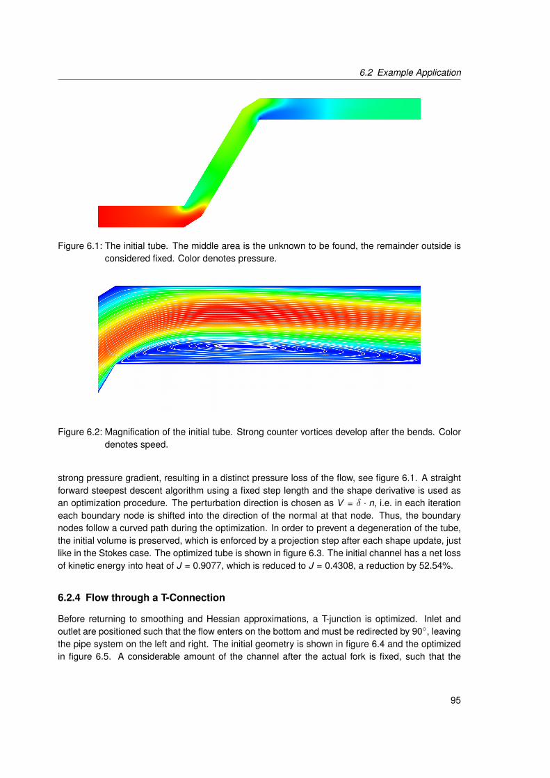
6.2 Example Application
Figure 6.1: The initial tube. The middle area is the unknown to be found, the remainder outside isconsidered fixed. Color denotes pressure.
Figure 6.2: Magnification of the initial tube. Strong counter vortices develop after the bends. Colordenotes speed.
strong pressure gradient, resulting in a distinct pressure loss of the flow, see figure 6.1. A straightforward steepest descent algorithm using a fixed step length and the shape derivative is used asan optimization procedure. The perturbation direction is chosen as V = δ · n, i.e. in each iterationeach boundary node is shifted into the direction of the normal at that node. Thus, the boundarynodes follow a curved path during the optimization. In order to prevent a degeneration of the tube,the initial volume is preserved, which is enforced by a projection step after each shape update, justlike in the Stokes case. The optimized tube is shown in figure 6.3. The initial channel has a net lossof kinetic energy into heat of J = 0.9077, which is reduced to J = 0.4308, a reduction by 52.54%.
6.2.4 Flow through a T-Connection
Before returning to smoothing and Hessian approximations, a T-junction is optimized. Inlet andoutlet are positioned such that the flow enters on the bottom and must be redirected by 90, leavingthe pipe system on the left and right. The initial geometry is shown in figure 6.4 and the optimizedin figure 6.5. A considerable amount of the channel after the actual fork is fixed, such that the
95

6 Shape Optimization and Navier–Stokes Fluids
Figure 6.3: Pressure distribution optimized tube. The pressure loss is almost completely removed.
optimization cannot circumvent a net turning of 90, and the flow has to exit parallel to the x-axis.The inflow profile is quadratic and the average mass influx results in a Reynolds number of Re = 100with the channel cross-section as reference area. The initial junction has a net loss of kinetic energyinto heat of J = 0.9208, which is reduced to J = 0.6900, a reduction by 25.05%. The total areaoccupied by the fluid was enforced to stay the same during the whole optimization.
Figure 6.4: Initial T-connection. The fluid is entering on the bottom. Color denotes speed.
Figure 6.5: Optimized T-connection.
96

6.3 Hessian Approximation and Sobolev Optimization
6.3 Hessian Approximation and Sobolev Optimization
Hessian approximation and smoothing procedures for Sobolev descent methods for aerodynamicshape optimization, i.e. an obstacle in a channel, are now considered. Unfortunately, the pres-ence of adjoint equations and the non-linear convection operator make a similar analysis as inlemma 5.2.2 non-trivial. In two dimensions, the gradient from equation (6.19) is given by
G = −µ2∑
k=1
∂λk
∂x2
∂uk
∂x2+(∂uk
∂x2
)2
= −µ2∑
k=1
∂uk
∂x2
[∂λk
∂x2+∂uk
∂x2
].
The perturbed gradient for a flat domain Ω = (x1, x2) : x1 ∈ R, x2 ≥ 0 is given by
G = −µ2∑
k=1
∂u′k [α]∂x2
(∂λk
∂x2+∂uk
∂x2
)+∂uk
∂x2
(∂λ′k [α]∂x2
+∂u′k [α]∂x2
),
where α = eiω1x1 is again an oscillation of the boundary with i being the imaginary unit. The localshape derivatives are assumed to have the following structure:
u′k [α] = uk eiω1x1eω2x2
p′[α] = peiω1x1eω2x2
λ′k [α] = λk eiω1x1eω2x2
λ′p[α] = λpeiω1x1eω2x2 .
Applying the linearized Navier–Stokes equations to u′[α] and p′[α] alone results in a linear system −µ(−ω2
1 + ω22
)+ ρ∂u1
∂x1+ ρu1iω1 + ρu2ω2 ρ∂u1
∂x2iω1
ρ∂u2∂x1
−µ(−ω2
1 + ω22
)+ ρ∂u2
∂x2+ ρu1iω1 + ρu2ω2 ω2
iω1 ω2 0
,
of which the determinant must again vanish. The determinant of the above is given by
µω42 − ρu2ω
32 +(−µω2
1 − ρ∂u1
∂x1− ρu1iω1 − µω2
1
)ω2
2
+(
iρ∂u2
∂x1ω1 + iω1ρ
∂u1
∂x2+ ρu2ω
21
)ω2 + µω4
1 + ρ∂u2
∂x2ω2
1 + ρu1iω31 .
For finding the operator symbol, the root in terms of ω2 must now be found. However, for a poly-nomial of fourth order in complex coefficients, the roots are no longer elegantly given. Thus, thediscrete approach is again used for the Navier–Stokes problem.
Flow around a circular obstacle in a channel is considered. Parts of the domain and the fluid areshown in figure 6.8. The Reynolds number is kept at 80, resulting in a steady state laminar flow.The circle is discretized using 1000 surface mesh nodes with variable positions, and a sin-wave
97
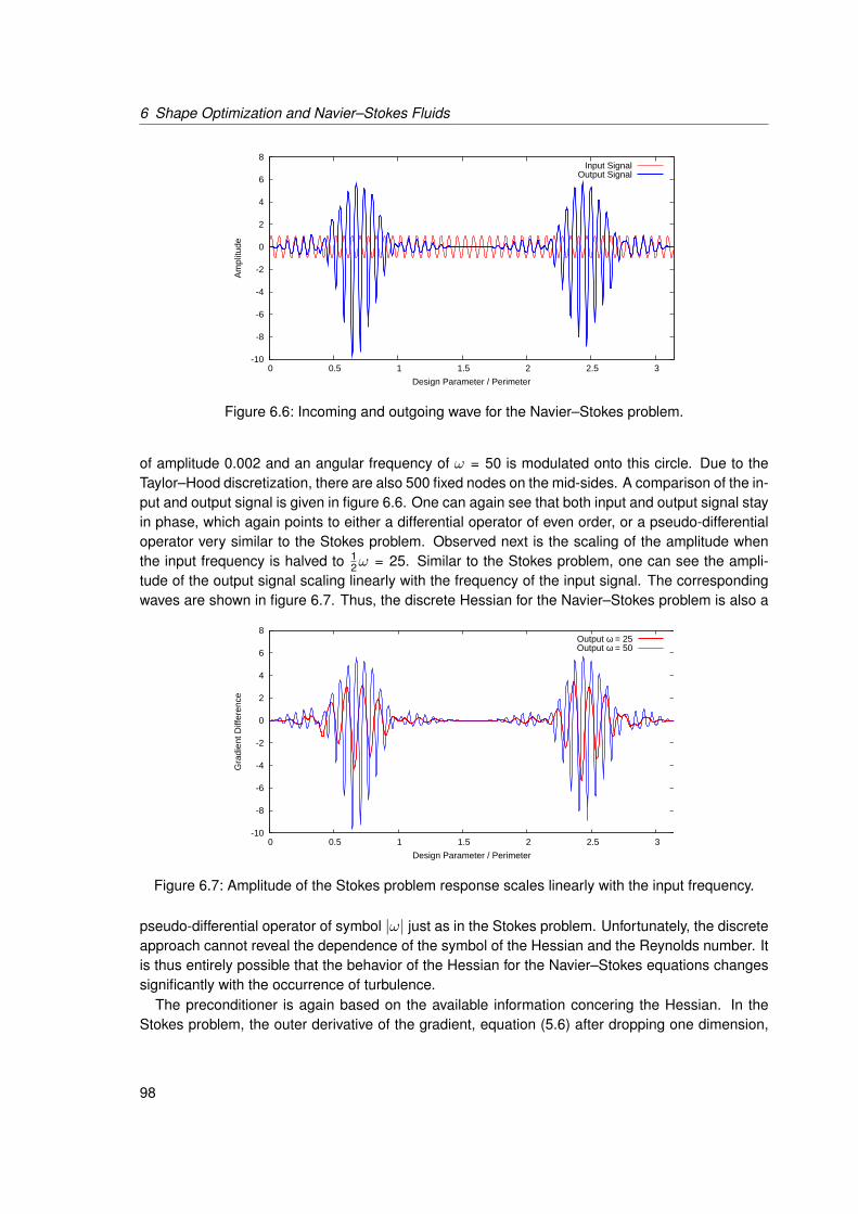
6 Shape Optimization and Navier–Stokes Fluids
-10
-8
-6
-4
-2
0
2
4
6
8
0 0.5 1 1.5 2 2.5 3
Am
plitu
de
Design Parameter / Perimeter
Input SignalOutput Signal
Figure 6.6: Incoming and outgoing wave for the Navier–Stokes problem.
of amplitude 0.002 and an angular frequency of ω = 50 is modulated onto this circle. Due to theTaylor–Hood discretization, there are also 500 fixed nodes on the mid-sides. A comparison of the in-put and output signal is given in figure 6.6. One can again see that both input and output signal stayin phase, which again points to either a differential operator of even order, or a pseudo-differentialoperator very similar to the Stokes problem. Observed next is the scaling of the amplitude whenthe input frequency is halved to 1
2ω = 25. Similar to the Stokes problem, one can see the ampli-tude of the output signal scaling linearly with the frequency of the input signal. The correspondingwaves are shown in figure 6.7. Thus, the discrete Hessian for the Navier–Stokes problem is also a
-10
-8
-6
-4
-2
0
2
4
6
8
0 0.5 1 1.5 2 2.5 3
Gra
dien
t Diff
eren
ce
Design Parameter / Perimeter
Output ω = 25Output ω = 50
Figure 6.7: Amplitude of the Stokes problem response scales linearly with the input frequency.
pseudo-differential operator of symbol |ω| just as in the Stokes problem. Unfortunately, the discreteapproach cannot reveal the dependence of the symbol of the Hessian and the Reynolds number. Itis thus entirely possible that the behavior of the Hessian for the Navier–Stokes equations changessignificantly with the occurrence of turbulence.
The preconditioner is again based on the available information concering the Hessian. In theStokes problem, the outer derivative of the gradient, equation (5.6) after dropping one dimension,
98

6.3 Hessian Approximation and Sobolev Optimization
Figure 6.8: Initial shape of the Navier–Stokes problem. Color denotes speed.
Figure 6.9: Optimal shape of the Navier–Stokes problem. Color denotes speed.
99

6 Shape Optimization and Navier–Stokes Fluids
was used as the variable coefficient β in (5.9). In the Navier–Stokes case, this outer derivative ismore complex, as it now involves the costate also. Therefore, the constant factor
k =32ωmax − 3ω2
max(6.21)
is used in the Laplace–Beltrami preconditioner (5.7). In order to again be able to compare thespeed-up with the unpreconditioned iteration, the number of variable surface mesh nodes is re-duced from 1000 to 100. This results in a value of ωmax between 25 and 50 which was keptfixed at 30. The initial and optimized shapes are shown in figure 6.8 and 6.9. The preconditioned
0.5
0.55
0.6
0.65
0.7
0.75
0.8
0 50 100 150 200
Ene
rgy
Dis
sipa
tion
Iteration
UnpreconditionedPreconditioned
Figure 6.10: Convergence rates of the preconditioned Navier–Stokes problem.
optimization requires 71 steps till convergence using a steplength of d = 0.06, and the unpre-conditioned optimization requires around 350 iterations using a steplength of d = 0.005, which isthe longest steplength possible. The resulting optimal ogive shape is astonishing ship-like. Also,the preconditioned iteration requires only 20% of the unpreconditioned gradient steps. That is, forthe Navier–Stokes problem, preconditioning reduces the computational effort by 80%. The precisecomparison of the convergence history is plotted in figure 6.10. To prevent a degeneration of theshape, a volume constraint was again enforced by a discrete projection step in the direction of theshape derivative of the volume after each shape update.
100

Chapter 7
Potential Flow Pressure Tracking
7.1 Introduction
Potential flow pressure matching is a classical inverse design aerodynamic problem. Due to thesimplifications of potential flow, remark 4.2.10, a meaningful drag value cannot be computed in po-tential flow. Thus, this flow model is almost always used in an inverse design setting, i.e. given asurface pressure distribution, a corresponding airfoil is to be found which produces this pressurefield. Although potential flow is essentially the Laplace equations, the strong geometric dependen-cies of the pressure matching objective function make a shape differentiation surprisingly difficult,especially when compared to the self-adjoint Stokes energy dissipation problem. Part of this re-search has already been published in [19]. As mentioned in definition 4.2.11, the flow is modeledas the gradient of some potential φ. In order to reconstruct the pressure from the velocity ∇φ,Bernoulli’s principle is used:
Remark 7.1.1 (Bernoulli’s Principle). Bernoulli’s principle for incompressible, inviscid flows statesthat along a streamline
12‖u‖2 + g +
pρ
= const,
where g is the gravitational potential. A similar version exists for compressible inviscid flows.
Thus, velocity and pressure can be linked together, which creates the following shape optimiza-tion problem.
101
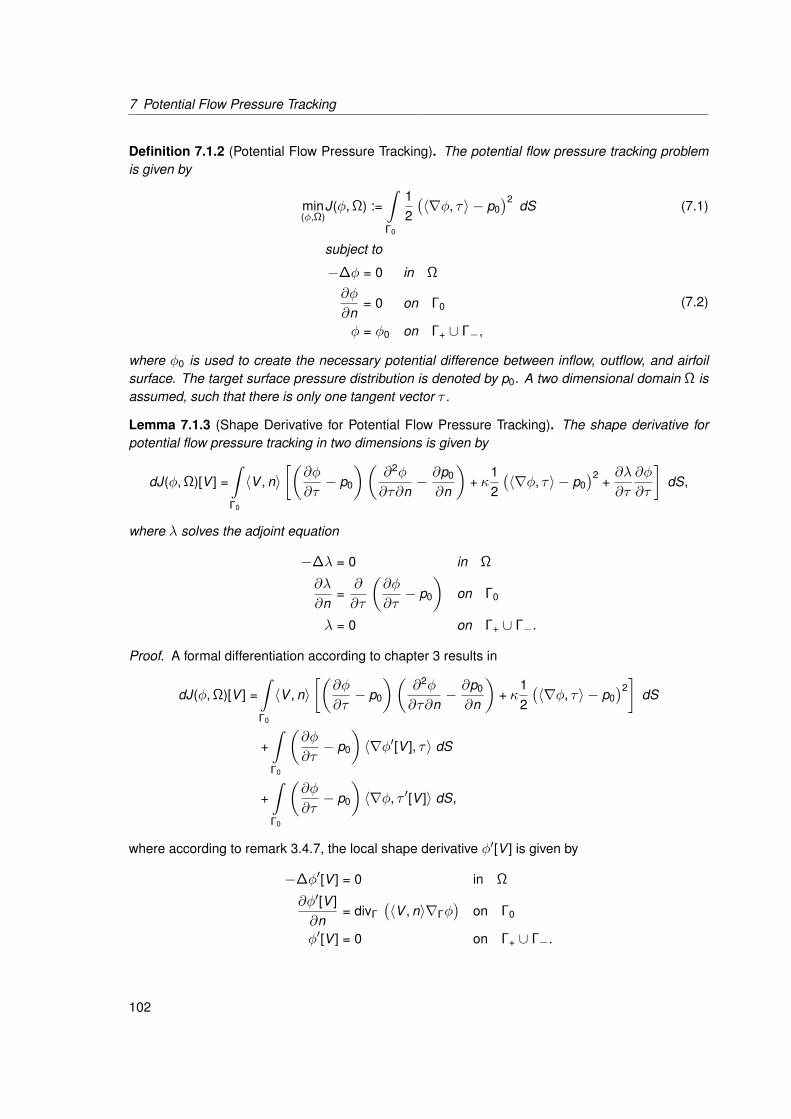
7 Potential Flow Pressure Tracking
Definition 7.1.2 (Potential Flow Pressure Tracking). The potential flow pressure tracking problemis given by
min(φ,Ω)
J(φ, Ω) :=∫Γ0
12
(〈∇φ, τ〉 − p0
)2 dS (7.1)
subject to
−∆φ = 0 in Ω
∂φ
∂n= 0 on Γ0
φ = φ0 on Γ+ ∪ Γ−,
(7.2)
where φ0 is used to create the necessary potential difference between inflow, outflow, and airfoilsurface. The target surface pressure distribution is denoted by p0. A two dimensional domain Ω isassumed, such that there is only one tangent vector τ .
Lemma 7.1.3 (Shape Derivative for Potential Flow Pressure Tracking). The shape derivative forpotential flow pressure tracking in two dimensions is given by
dJ(φ, Ω)[V ] =∫Γ0
〈V , n〉[(
∂φ
∂τ− p0
)(∂2φ
∂τ∂n− ∂p0
∂n
)+ κ
12
(〈∇φ, τ〉 − p0
)2 +∂λ
∂τ
∂φ
∂τ
]dS,
where λ solves the adjoint equation
−∆λ = 0 in Ω
∂λ
∂n=∂
∂τ
(∂φ
∂τ− p0
)on Γ0
λ = 0 on Γ+ ∪ Γ−.
Proof. A formal differentiation according to chapter 3 results in
dJ(φ, Ω)[V ] =∫Γ0
〈V , n〉[(
∂φ
∂τ− p0
)(∂2φ
∂τ∂n− ∂p0
∂n
)+ κ
12
(〈∇φ, τ〉 − p0
)2]
dS
+∫Γ0
(∂φ
∂τ− p0
)〈∇φ′[V ], τ〉 dS
+∫Γ0
(∂φ
∂τ− p0
)〈∇φ, τ ′[V ]〉 dS,
where according to remark 3.4.7, the local shape derivative φ′[V ] is given by
−∆φ′[V ] = 0 in Ω
∂φ′[V ]∂n
= divΓ
(〈V , n〉∇Γφ
)on Γ0
φ′[V ] = 0 on Γ+ ∪ Γ−.
102

7.1 Introduction
According to lemma 3.3.8, the local shape derivative of the normal dn[V ] lies in the tangent plane.Thus, the local shape derivative of the tangent lies in the normal plane. Consequently,
〈∇φ, τ ′[V ]〉 = 〈∇φ, εn〉 = ε〈∇φ, n〉 = 0
due to the boundary conditions for φ on Γ0. Therefore, the part of the gradient due to a variationof the tangent vanishes. Unfortunately, the objective function needs the derivative of φ′[V ] in tan-gent direction, but the boundary conditions only provide information about the derivative in normaldirection. Thus, an adjoint equation is needed. Multiplication with an arbitrary λ results in
dJ(φ, Ω)[V ] =∫Γ0
〈V , n〉[(
∂φ
∂τ− p0
)(∂2φ
∂τ∂n− ∂p0
∂n
)+ κ
12
(〈∇φ, τ〉 − p0
)2]
dS
+∫Γ0
(∂φ
∂τ− p0
)∂φ′[V ]∂τ
dS
+∫Ω
−λ∆φ′[V ] dA.
Integration by parts and Green’s formula provide
dJ(φ, Ω)[V ] =∫Γ0
〈V , n〉[(
∂φ
∂τ− p0
)(∂2φ
∂τ∂n− ∂p0
∂n
)+ κ
12
(〈∇φ, τ〉 − p0
)2]
dS
−∫Γ0
∂
∂τ
(∂φ
∂τ− p0
)φ′[V ] dS
+∫Γ
−λ∂φ′[V ]∂n
+ φ′[V ]∂λ
∂ndS +
∫Ω
−φ′[V ]∆λ dA
=∫Γ0
〈V , n〉[(
∂φ
∂τ− p0
)(∂2φ
∂τ∂n− ∂p0
∂n
)+ κ
12
(〈∇φ, τ〉 − p0
)2]
dS
+∫Γ0
φ′[V ][− ∂
∂τ
(∂φ
∂τ− p0
)+∂λ
∂n
]dS
+∫Γ
−λ∂φ′[V ]∂n
dS +∫Ω
−φ′[V ]∆λ dA,
where Γ = Γ0 ∪ Γ+ ∪ Γ−. Thus, if λ solves the adjoint equation
−∆λ = 0 in Ω
∂λ
∂n=∂
∂τ
(∂φ
∂τ− p0
)on Γ0
λ = 0 on Γ+ ∪ Γ−,
103
7 Potential Flow Pressure Tracking
the shape derivative becomes
dJ(φ, Ω)[V ] =∫Γ0
〈V , n〉[(
∂φ
∂τ− p0
)(∂2φ
∂τ∂n− ∂p0
∂n
)+ κ
12
(〈∇φ, τ〉 − p0
)2]
dS
+∫Γ0
−λ∂φ′[V ]∂n
dS.
The boundary condition for φ′[V ] now provides
dJ(φ, Ω)[V ] =∫Γ0
〈V , n〉[(
∂φ
∂τ− p0
)(∂2φ
∂τ∂n− ∂p0
∂n
)+ κ
12
(〈∇φ, τ〉 − p0
)2]
dS
+∫Γ0
−λdivΓ
(〈V , n〉∇Γφ
)dS
=∫Γ0
〈V , n〉[(
∂φ
∂τ− p0
)(∂2φ
∂τ∂n− ∂p0
∂n
)+ κ
12
(〈∇φ, τ〉 − p0
)2]
dS
+∫Γ0
〈V , n〉〈∇Γλ,∇Γφ〉 dS,
due to integration by parts on Γ0. The desired expression follows immediately due to the twodimensional domain Ω.
7.2 Local Coordinates and Shape Hessian
In contrast to the Stokes case in section 5.2, a shape Hessian analysis will be conducted in local co-ordinates, i.e. a two dimensional star-shaped domain Ω is considered. This has the advantage thatthe derivation is more straight forward than using the shape differentiation techniques of chapter 3.For first order calculus, expressions for star-shaped domains can most of the time be interpretedon more general and three dimensional domains, too. Unfortunately, hopes that this would also betrue for the Hessian did not come true.
Definition 7.2.1 (Star-shaped Domain). A domain Ω is said to be star-shaped if the boundary Γ isgiven by
Γ := r (ϕ)er (ϕ) : ϕ ∈ [0, 2π],
where er (ϕ) = (sinϕ, cosϕ)T . Thus, the boundary is a curve C with a parameterization c given by
c(ϕ) = r (ϕ)er (ϕ),ϕ ∈ [0, 2π].
A perturbed star-shaped domain is then given by
Γε := (r (ϕ) + εr (ϕ)) er
with r (0) = r (2π), which corresponds to a perturbation of identity using V = r er and a curveparameterized by cε.
104

7.2 Local Coordinates and Shape Hessian
Remark 7.2.2 (Perturbed Line Integral). For a curve C, the line integral of f over C is given by
∫C
f (s) ds =
b∫a
f (c(ϕ))‖c′(ϕ)‖ dϕ,
where c : [a, b] → C is an arbitrary bijective parameterization of C. Thus, for shape optimizationon star-shaped domains, the expression
ddε ε=0
2π∫0
fε(cε(ϕ))‖c′ε(ϕ)‖ dϕ
must be computed, which is possible using standard differentiation techniques. For a star-shapeddomain, a direct computation reveals
‖c′ε‖ =(r ′2 + r2 + 2ε
(r r + r ′r ′
)+ ε2r ′2 + ε2r2) 1
2 ,
where r ′ denotes a differentiation with respect to arc length, e.g.
r ′ =∂r∂ϕ
.
Switching differentiation and integration, the expression
∂
∂ε ε=0‖c′ε‖ =
r r + r ′r ′√r ′2 + r2
will be needed.
Remark 7.2.3 (Geometric Quantities on Perturbed Star-Shaped Domains). A straight forward com-putation reveals for the normal nε and the tangent τε on a perturbed star-shaped domain cε:
nε =rer − r ′e′r + ε
(r er − r ′e′r
)√r ′2 + r2 + 2ε (r r + r ′r ′) + ε2r ′2 + ε2r2
τε =r ′er + re′r + ε
(r ′er + r e′r
)√r ′2 + r2 + 2ε (r r + r ′r ′) + ε2r ′2 + ε2r2
.
Note that depending on the definition of what is outside and inside, which direction the tangentvector is pointing, and due to the periodicity of er , the signs may differ. The appropriate quantitieson an unperturbed star-shaped domain are easily attainable by setting ε = 0. Consequently, on astar-shaped domain, one also has
er =r√
r2 + r ′2n +
r ′√r2 + r ′2
τ .
The curvature of a curve parameterized by c is given by
κ =〈c′′, c′⊥〉‖c′‖3 ,
105

7 Potential Flow Pressure Tracking
which results in
κ =r ′′r − 2r ′2 − r2(√
r2 + r ′2)3
for a star-shaped domain. Finally, a straight forward computation also reveals
〈V , n〉 =⟨
r er ,rer − r ′e′r√
r2 + r ′2
⟩=
r r√r2 + r ′2
=1‖c′‖
r r ,
since eTr e′r = 0.
Remark 7.2.4 (Potential Flow Shape Gradient on Star-Shaped Domains). Using the expressionsfrom remark 7.2.3, it is possible to express the shape derivative from lemma 7.1.3 for a star-shapeddomain by
dJ(φ, Ω)[r ] =−2π∫
0
r r〈∇λ,∇φ〉 dϕ
+
2π∫0
(∂φ
∂τ− p0
)[r eT
r D2u τ − 〈∇p0, r er 〉] (
r2 + r ′2) 1
2 dϕ
+
2π∫0
12
(∂φ
∂τ− p0
)2 r r + r ′r ′√r2 + r ′2
dϕ.
Lemma 7.2.5 (Shape Hessian for Potential Flow Pressure Tracking on Star-Shaped Domains). Apreliminary expression for the shape Hessian for potential flow pressure tracking on a star-shapeddomain is given by
d2J(φ, Ω)[r1][r2]
=−2π∫
0
r1r2〈∇λ,∇φ〉 dϕ
−2π∫
0
r1r[〈∇λ′[r2],∇φ〉 + r2eT
r D2λ∇φ + 〈∇λ,∇φ′[r2]〉 + r2eTr D2φ∇λ
]dϕ
+
2π∫0
(〈∇φ′[r2], τ〉 + r2eT
r D2φ τ − 〈∇p0, r2er 〉) (
r1eTr D2φ τ − 〈∇p0, r1er 〉
)√r2 + r ′2
+(∂φ
∂τ− p0
)ddε ε=0
([r1eT
r D2φε τε − 〈∇p0,ε, r1er 〉]√
r2ε + r ′ε
2)
dϕ
106
7.3 Method of Mapping and Fourier Analysis
+
2π∫0
(∂φ
∂τ− p0
)(〈∇φ′[r2], τ〉 + r2eT
r D2φ τ − 〈∇p0, r2er 〉) r r1 + r ′r ′1√
r2 + r ′2
+12
(∂φ
∂τ− p0
)2 ddε ε=0
rεr1 + r ′ε r′1√
r2ε + r ′ε
2
dϕ.
Note that the terms which still need to be differentiated will vanish close to the optimum, because
∂φ
∂τ− p0 ≈ 0
if p0 is reachable.
Proof. Let a second perturbation of the star-shaped domain be given by
rε := r + εr2.
The shape Hessian is then the limit
d2J(φ, Ω)[r1][r2] =ddε ε=0
− 2π∫0
r1rε〈∇λε,∇φε〉 dϕ
+
2π∫0
(∂φε∂τε− p0,ε
)[r1eT
r D2uε τε − 〈∇p0,ε, r1er 〉] (
r2ε + r ′ε2
) 12 dϕ
+
2π∫0
12
(∂φε∂τε− p0,ε
)2 rεr1 + rε′r ′1√r2ε + r2
ε′
dϕ
.
According to definition 3.4.1, the local shape derivatives are given by
ddε ε=0
〈∇λε,∇φε〉 = 〈∇λ′[r2],∇φ〉 + r2eTr D2λ∇φ + 〈∇λ,∇φ′[r2]〉 + r2eT
r D2φ∇λ.
A straight forward standard differentiation results in the desired expression.
The preliminary expression for the shape Hessian of the potential flow pressure matching prob-lem, lemma (7.2.5), is astonishing complex for a problem based on the Laplacian. This complexityarises due to the objective function being a surface functional with strong dependence on geomet-ric quantities such as the tangent τ . Also, the desired tangent derivative results in the need for anadjoint variable, which must be considered when deriving the Hessian. For this reason, the Stokesshape Hessian was considered first in chapter 5. Although considering a star-shaped domain al-lows a more straight forward differentiation, the resulting expression is of a complexity that is hardlyapplicable.
107

7 Potential Flow Pressure Tracking
ξ2 x2
ξ1 x1q
Ω Ω
Figure 7.1: Method of Mapping
7.3 Method of Mapping and Fourier Analysis
In order to further study the Hessian, a slightly simplified problem is considered. The left part offigure 7.1 is imagined as the physical domain, which is thought of as being a part of the free airstream along a geometric detail of an airplane which is aligned with the ξ1-axis. The shape of theboundary is supposed to be described by the function q(ξ1). In order to simplify the problem, thephysical domain is mapped onto the computational domain on the right hand side of figure 7.1 byappropriately stretching it in the vertical direction, such that one can write
(x1, x2) =(ξ1,
ξ2 − q(ξ1)1− q(ξ1)
),
and the potential φ from definition 7.1.2 is thought of as φ(x(ξ)). That means the Neumann conditionin the physical plane at the shape boundary (ξ1, ξ2) | ξ2 = q(ξ1)
0 =∂φ
∂n=∂φ
∂ξ1
∂q∂ξ1− ∂φ
∂ξ2
is mapped to the boundary condition
0 =∂q∂ξ1
∂φ
∂ξ1−
1 +(∂q∂ξ1
)2
1− q2
∂φ
∂x2. (7.3)
For the purpose of simplification, the shape q is assumed to be almost a straight line, such that
squared expressions like q2 and(∂q∂ξ1
)2can be neglected. Furthermore, the tangential velocity ∂φ
∂x1
can be assumed to be constant, e.g. 1. This results in the approximative boundary condition
∂φ
∂x2=∂q∂x1
. (7.4)
The complete problem formulation in the computational domain is then
108

7.3 Method of Mapping and Fourier Analysis
Definition 7.3.1 (Potential Flow Pressure Tracking with Method of Mapping). The potential flowinverse design problem using the method of mapping is given by
min(φ,q)
J(φ(q), q) :=∫Γ0
(∂φ(x1, x2)∂x1
− p0(x1))2
dx1 (7.5)
subject to
−∆φ = 0 in Ω
∂φ
∂n=∂q∂x1
on Γ0
φ = φ0 on Γ+ ∪ Γ−.
(7.6)
Strictly speaking, the above problem in definition 7.3.1 is no longer a shape optimization prob-lem, and a detailed analysis of such problems can for example be found in [75]. However, it isanalytically much more accessible and still closely related to the original shape optimization prob-lem, lemma 7.1.3. For example, the resulting adjoint equation is almost the same as the adjointequation for the proper shape optimization problem.
Lemma 7.3.2 (Derivative of Potential Flow Pressure Tracking with Method of Mapping). Choosingφ0 = x1, the derivative of the potential flow pressure tracking using the method of mapping is givenby
∇qJ(φ(q), q) =∂λ(φ(q))∂x1
,
where λ solves the adjoint equation
−∆λ = 0 in Ω
∂λ
∂n=
∂
∂x1
(∂φ
∂x1− p0
)on Γ0
λ = 0 on Γ+ ∪ Γ−.
Proof. The Lagrangian is given by
L(φ, q,λ,λ1,λ2)
=J(φ, q) +∫Ω
λ(−∆φ) dA +∫Γ0
λ1
(∂φ
∂n− ∂q∂x1
)dS +
∫Γ+∪Γ−
λ2(x1)(φ(x1)− x1) dx1.
Inserting the objective function and using Green’s second identity provides
L(φ, q,λ,λ1,λ2)
=∫Γ0
(∂φ(x1, x2)∂x1
− p0(x1))2
dx1 +∫Ω
(−∆λ)φ dA
+∫∂Ω
−λ∂φ∂n
+ φ∂λ
∂ndS +
∫Γ0
λ1
(∂φ
∂n− ∂q∂x1
)dS +
∫Γ+∪Γ−
λ2(x1) (φ(x1)− x1) dx1.
109

7 Potential Flow Pressure Tracking
The adjoint boundary value problem is derived from the expression for perturbations φ
0 =ddε ε=0
L(φ + t · φ, q,λ,λ1,λ2)
=∫Γ0
(∂φ
∂x1− p0(x1)
)∂φ
∂x1dx1 +
∫Ω
(−∆λ)φ dA
+∫∂Ω
−λ∂φ∂n
+ φ∂λ
∂ndS +
∫Γ0
λ1∂φ
∂ndS +
∫Γ+∪Γ−
λ2 · φ dS.
Integration by parts and re-grouping provides
0 =[(
∂φ
∂x1− p0(x1)
)φ
]1
0+∫Γ0
φ
[− ∂
∂x1
(∂φ
∂x1− p0(x1)
)+∂λ
∂n
]+ (λ1 − λ)
∂φ
∂ndx1
+∫Ω
(−∆λ)φ dx +∫
Γ+∪Γ−
−λ∂φ∂n
+ φ∂λ
∂n+ λ2 · φ dS.
On the boundary Γ+ ∪ Γ−, not affected by the design q, the velocity potential φ is subject to aDirichlet boundary condition. Thus, the state φ is fixed, and consequently φ = 0 on Γ+ ∪ Γ−, whichsimplifies the last integral in the equation above. Focussing on different perturbations φ results inthe adjoint equations:
• A perturbation φ in Ω results in
−∆λ = 0 in Ω.
• Perturbations with fixed Dirichlet value 0 and variable Neumann values give
λ = λ1 on Γ0
−λ = 0 on Γ+ ∪ Γ−.
• A perturbation in all respects with the exception of the corner points gives
∂λ
∂n=
∂
∂x1
(∂φ
∂x1− p0
)on Γ0.
Now, the adjoint boundary value problem reads completely
−∆λ = 0 in Ω
∂λ
∂n=
∂
∂x1
(∂φ
∂x1− p0
)on Γ0
λ = 0 on Γ+ ∪ Γ−,
which is exactly the same adjoint boundary condition as in the proper shape optimization problem,lemma 7.1.3.
110

7.3 Method of Mapping and Fourier Analysis
For the design equation, e.g. the gradient, the Lagrangian is also perturbed in direction q, whichmeans
0 =ddt t=0
L(φ, q + t · q,λ,λ1,λ2) =∫Γ1
−λ1∂q∂x1
dS
= − [λ1q]10 +∫Γ1
∂λ1
∂x1q dx1 =
∫Γ1
∂λ1
∂x1q dx1.
Thus, the gradient on Γ0 is given by
∇qJ(φ(q), q) =∂λ1(φ(q))∂x1
=∂λ(φ(q))∂x1
.
It is now possible to study the pseudo-differential operator nature of the Hessian similar to sec-tion 5.4.
Lemma 7.3.3 (Hessian Symbol of Potential Flow Pressure Tracking using Method of Mapping). TheHessian for potential flow pressure tracking using method of mapping is a second order differentialoperator with symbol
∂
∂q∇qJ(φ(q), q) =
∂
∂q∂λ
∂x1 Γ0
(x1) = ±ω2q .
Proof. An arbitrary Fourier mode for q is assumed, i.e.
q = eiωqx1 ⇒ ∂q∂x1
= iωqeiωqx1 .
Also, the solution of the forward problem is assumed to be of the form
φ(x1, x2) = reiω1x1+iω2x2 ,
resulting in
∂φ
∂n Γ0
=∂φ
∂x2 Γ0
= iω2reiω1x1
∂2φ
∂x21 Γ0
= −ω21reiω1x1 .
Using the boundary condition on Γ0, design q and state φ can be linked together:
iωqeiωqx1 = iω2reiω1x1 , ∀x1 ∈ R.
For x1 = 0 this means, in particular, ω2 = ωq/r and thus also ω1 = ωq . The differential equation−∆φ = 0 in Ω gives
0 = (ω21 + ω2
2)reiω1x1+iω2x2 ⇔ω2
q
r2 + ω2q = 0,
111

7 Potential Flow Pressure Tracking
which means r = ±i . The adjoint solution is assumed to be of similar form
λ(x1, x2) = seiθ1x1+iθ2x2 ⇒ ∂λ
∂n Γ0
=∂λ
∂x2 Γ0
= iθ2seiθ1x1 ,
and the Neumann boundary condition of the adjoint problem provides
iθ2seiθ1x1 = ω21reiω1x1 , ∀x1 ∈ R.
With the same arguments as above, one also has
θ2 =ω2
1ris
= ±ω2
q
sθ1 = ω1 = ωq .
The adjoint differential equation in Ω results in
0 = θ21 + θ2
2 ⇔ω4
q
s2 + ω2q = 0⇔ s = ±iωq .
Thus,
∂λ
∂x1 Γ0
(x1) = ±ω2qeiθ1x1 = ±ω2
qq,
the symbol of a second order differential operator.
Contrary to the Stokes case as described in lemma 5.4.2, where the Hessian was a pseudo-differential operator of order +1, the Hessian here is a differential operator of second order, and theLaplace–Beltrami preconditioner, equation (5.7), should provide a very good Hessian approxima-tion.
7.4 Numerical Results
7.4.1 Panel Solver
For the optimizations the state equation is discretized by an aerodynamic panel solver, which issimilar to a boundary element method. Using Green’s second identity, the Laplace equation for thevolume can be transformed into an integral equation on the boundary of the wing. Similar to finiteelements, the potential φ is discretized as a finite linear combination of ansatz functions, resultingin a small, dense, and linear system to be solved. Any additional boundary conditions for the freestream velocity on Γ+ ∪ Γ− are embedded in the ansatz functions. To further ensure a physicallymeaningful solution and to allow a proper prediction of lift, the trailing edge stagnation point isprescribed by a slightly modified boundary condition, thus introducing lift via circulation similar tothe Kutta–Joukowski theorem. For further information about the solver, the aerodynamics, and onhow to ensure a physical solution that matches experimental measurements, see [43]. To avoid anydiscrepancies with the analytical adjoint equation as derived above, the adjoint of the state equationwas taken as the transpose of the discrete linear state equation, i.e. adjoint in Rn with the standardscalar product.
112

7.4 Numerical Results
0 0.1 0.2 0.3 0.4 0.5 0.6 0.7 0.8 0.9 1−0.1
−0.05
0
0.05
0.1
x/c
y/c
0 0.1 0.2 0.3 0.4 0.5 0.6 0.7 0.8 0.9 1−0.1
−0.05
0
0.05
0.1
x/c
y/c
Figure 7.2: Initial NACA0012 airfoil and target NACA4412 airfoil
7.4.2 Numerical Pressure Fitting
The aim is to match pressure distributions generated by different NACA 4 digit airfoils. The initial
1e-03
1e-02
1e-01
1e+00
0 100 200 300 400 500
obje
ctiv
e fu
nctio
n
iteration count
rawpreconditioned
Figure 7.3: Optimization history for potential flow pressure tracking.
shape is the symmetrical NACA0012 airfoil, and the pressure distribution generated by the cam-bered NACA4412 profile is to be matched. Figure 7.2 illustrates this. A detailed description of theNACA shapes can be found in [39]. Although local coordinates like star-shaped domains and themethod of mapping have been discussed previously, the numerical results are again achieved byevaluating the shape derivative on each surface node. As an optimization procedure, the Laplace–Beltrami Hessian approximation, equation (5.7), is used in an approximative SQP method withArmijo linesearch. Convergence history and the effects of preconditioning can be seen in figure 7.3.The resulting optimal shapes are shown in figure 7.4.
113

7 Potential Flow Pressure Tracking
-1.00
-0.50
0.00
0.50
1.00 0.0 0.2 0.4 0.6 0.8 1.0
-0.10-0.05 0.00 0.05 0.10
Cp
y/c
x/c
"optimized"target
-1.00
-0.50
0.00
0.50
1.00 0.0 0.2 0.4 0.6 0.8 1.0
-0.10-0.05 0.00 0.05 0.10
Cp
y/c
x/c
optimized with preconditioningtarget
Figure 7.4: Resulting optimal shapes. Without preconditioning, the shapes and pressure distribu-tions degenerate.
114

Chapter 8
Shape Optimization and EulerEquations
8.1 Introduction
The compressible Euler equations are of considerable importance when it comes to industry sizeapplication. Although the viscosity of the fluid is neglected, and consequently there are no boundarylayers or turbulence, the compressibility of the gas is taken into full account. Since most flows ofindustrial importance, such as turbomachinery flow through turbines or compressors, external flowaround an aircraft in cruise conditions, or flow around rockets and projectiles, are high speed flowswhere compressibility is dominating viscous effects, neglecting viscosity is acceptable. Due tothe hyperbolic nature of the integral equations, shock waves often occur, requiring sophisticatednumerical schemes.
Since problems of this kind are mostly large scale and feature complex geometries, the easeand straight forward applicability of the Hadamard formula of the shape derivative for almost anydiscretization resolution makes this an ideal application area for numerical procedures based on theHadamard formula. Here, the focus lies on problems of the aerodynamic type, e.g. drag minimiza-tion of a fluid obstacle. However, with industry applicability in mind, the number of constraints toconsider considerably increases: in addition of maintaining lift, the aircraft must also withstand theforces, resulting in constraints on the material stiffness, if not a consideration of a full fluid/structurecoupling. Some two dimensional results of this chapter have already been published in [57, 58].
115

8 Shape Optimization and Euler Equations
Definition 8.1.1 (Inviscid Fluid Forces). To handle variations in the angle of attack more easily, mostflow solvers compute the forces in a rotated coordinate system. For the inviscid Euler equations,this leads to the following expression:
Fa :=1
Cref
∫Γ0
Cp〈n, a〉 dS,
where Cref is the reference length, usually the airfoil chord, and Cp is the non-dimensional pressure,defined as
Cp =2(p − p∞)γM2∞p∞
.
The subscript∞ is used to denote the appropriate farfield value. Note that the pressure coefficientCp should not be confused with the heat capacity at constant pressure cp. Choosing a as
a1 = (cosα, 0, sinα)T ,
where the first component is again chord wise, the second span wise, and the third wing thicknesswise, results in the drag coefficient CD, and choosing a as
a2 = (− sinα, 0, cosα)T
results in the lift coefficient CL where α is the angle of attack.
Definition 8.1.2 (Euler Problem). Minimizing the drag coefficient for a lifting aircraft without bodyforces is given by
min(ρ,u,E ,Ω)
CD(ρ, u, E , Ω) (8.1)
subject to ∫Ω
div (ρu) dA = 0
∫Ω
3∑j=1
[∂(ρuiuj )∂xj
]+∂p∂xi
dA = 0
∫Ω
div (ρHu) dA = 0
〈u, n〉 = 0 on Γ0
CL ≥ CL0
L :=∫Γ0
1 dS ≤ L0
I :=∫Γ0
(y − yc)2 dS ≥ Ix0
Vol = V0.
(8.2)
116
8.2 First Order Calculus
Here, the first three constraints are the Euler equations, and the pressure p and likewise Cp is linkedto the conserved variables
U := (ρ, ρu, ρE)T
by the perfect gas law
p = (γ − 1)ρ(
E − 12‖u‖2
).
The condition 〈u, n〉 = 0 is the Euler slip boundary condition on the aircraft surface Γ0. Thefarfield boundary conditions are usually more complex involving characteristics and are thoughtof as treated by the flow solver discretely. Condition CL ≥ CL0 means the optimal aircraft mustmaintain lift, condition L ≤ L0 penalizes the surface area and prevents an increase in perimeter,condition I ≥ Ix0 is a substitude model for the bending stiffness around the contour center of massyc above the x-axis, and constraint Vol = V0 is the usual volume constraint. Usually, not all of theseconstraints will be used at the same time, but without any of them, the solution will either degener-ate into a flat line or will not be of any practical relevance. Also, the bending stiffness constraint is asubstitude model valid in two dimensions only.
For two dimensional applications there is also the additional constraint of the leading edge beingfixed at (0, 0)T and the trailing edge being fixed at (1, 0)T . Otherwise, the optimization changes thereference length Cref of the airfoil, which would lead to a wrong non-dimensionalization of the flowquantities.
Intrigued by practical advantages, the shape derivative, although usually not called that way inthis community, has long been sought after by both academia, [15] and [23], and industry [77, 78,79, 80, 81]. Assuming a non-lifting body in a supersonic potential flow, the optimal shape, the so-called Haack or Sears–Haack body, is known to be ogive-like [33], making the non-lifting supersoniccase a good test-case for validating numerics. When it comes to numerical application, the problemis seldom treated from a true shape optimization perspective, except in [3, 4] for pressure trackingor in [10]. None of the approaches above have so far been successfully applied on a large scaledrag reduction problem.
8.2 First Order Calculus
Lemma 8.2.1 (Euler Shape Derivative). For an angle of attack α with corresponding rotation vectora, let pa be given by pa := p · a ∈ R3. Then the derivative of the functional
J(U, Ω) =∫Γ0
〈pa, n〉 dS
117

8 Shape Optimization and Euler Equations
is given by
dJ(U, Ω)[V ]
=∫Γ0
〈V , n〉[∂pa
∂nn − λUH
⟨∂u∂n
, n⟩
+ divΓ (pa − λUHu)]
dS (8.3)
=∫Γ0
〈V , n〉[∂pa
∂nn − λUH
⟨∂u∂n
, n⟩
+ κ〈pa, n〉]
+ 〈pa − λUHu, dn[V ]〉 dS, (8.4)
where U are the conserved variables solving the Euler equations in the domain Ω, and p is linkedto U by the perfect gas assumption. Additionally, UH is the vector of conserved variables with thelast component replaced by ρH. The adjoint variables λ are given as the solution of
−AT1∂
∂x1λ− AT
2∂
∂x2λ− AT
3∂
∂x3λ = 0 in Ω
〈(λ2,λ3,λ4)T , n〉 = −〈a, n〉 on Γ0.
Here, Ak are the Euler flux Jacobians from remark 4.2.9. The adjoint boundary conditions on thefarfield boundaries are assumed to be kept by the flow solver discretely. Based on the choice of a,this gradient expression can both be used for the drag or lift functional.
Proof. A formal differentiation according to lemma 3.3.13 results in
dJ(U, Ω)[V ] =∫Γ0
〈V , n〉[∂pa
∂nn + κ〈pa, n〉
]+ 〈pa, dn[V ]〉 + 〈p′a[V ], n〉 dS.
The variation of the normal is given by remark 3.3.15, resulting in
dJ(U, Ω)[V ] =∫Γ0
〈V , n〉[∂pa
∂nn + (divΓ pa)
]+ 〈p′a[V ], n〉 dS. (8.5)
To remove the remaining local shape derivative of the pressure p′a[V ], adjoint calculus will be con-ducted as in [23, 29]. Let the conserved variables U be given by
U := (ρ, ρu, ρE)T
and the primitive variables Up by
Up := (ρ, u, E)T .
Almost all density based finite volume flow solvers for compressible fluid dynamics operate onconserved variables. Hence, a linearization of the Euler state equations results in a linearization interms of conserved variables U ′[V ]:
U ′[V ] =(ρ′[V ], (ρu)′ [V ], (ρE)′ [V ]
)T ,
118

8.2 First Order Calculus
which are given as the solution of the linearized Euler equations. Using the non-conservative formof the Euler equations given by remark 4.2.9, the Euler state constraint can also be written by
3∑k=1
Ak∂U∂xk
= 0.
The forward linearization of the above leads to
3∑k=1
∂
∂xk
(Ak U ′[V ]
)= 0.
The boundary conditions of the local shape derivatives are described in lemma 3.4.4:
〈u′[V ], n〉 = −〈V , n〉⟨∂u∂n
, n⟩
+ 〈u, dn[V ]〉 (8.6)
on the wing Γ0. Multiplication by an arbitrary λ = (λ1,λ2,λ3,λ4,λ5) and integration by parts gives
0 =∫Ω
3∑k=1
λ∂
∂xk
(Ak U ′[V ]
)dA
= −∫Ω
3∑k=1
(∂
∂xkλ
)Ak U ′[V ] dA +
∫∂Ω
3∑k=1
λnk Ak U ′[V ] dS
= −∫Ω
3∑k=1
ATk
(∂λ
∂xk
)U ′[V ] dA +
∫∂Ω
3∑k=1
λnk Ak U ′[V ] dS. (8.7)
Looking at (8.7), one can see that if λ solves the adjoint equation
−AT1∂
∂x1λ− AT
2∂
∂x2λ− AT
3∂
∂x3λ = 0 in Ω
then the volume integrals will vanish. According to [23, 29], the matrices
T :=[
0 n1ρ
n2ρ
n3ρ 0
γ−12 (u2
1 + u22 + u2
3) (1− γ)u1 (1− γ)u2 (1− γ)u3 γ − 1
]and
T ∗ :=[ρ ρu1 ρu2 ρu3 ρH0 n1 n2 n3 0
]satisfy the condition
3∑k=1
nk Ak = T ∗T T
119

8 Shape Optimization and Euler Equations
on the boundary Γ0 of the airfoil. The local shape derivative to remove is p′[V ], which must belinked to the local shape derivative of the conserved variables U ′[V ]. This is given by the relation
p′[V ] = CU ′[V ], (8.8)
where C is given by
C :=(γ − 1
2(u2
1 + u22 + u2
3), (1− γ)u1, (1− γ)u2, (1− γ)u3, γ − 1)
,
which is exactly the second row of T . Thus, using (8.8) one arrives at
TU ′[V ] =( ∑3
k=1 nk u′k [V ]p′[V ]
)(8.9)
and
λT ∗T = (λUH , (λ2,λ3,λ4) n) ,
where
UH = (ρ, ρu, ρH)T
is the vector of conserved variables with the last component replaced by ρH. Using the above inequation (8.7) results in
0 =∫Γ
λ
3∑k=1
nk Ak U ′[V ] dS =∫Γ
λT ∗TTU ′[V ] dS
=∫Γ
λUH〈u′[V ], n〉 + (λ2,λ3,λ4)np′[V ] dS.
The linearized Euler slip boundary condition on the airfoil is given by equation (8.6) and provides
0 =∫Γ
λ3∑
k=1
nk Ak U ′[V ] dS
=∫Γ
〈V , n〉[−λUH
⟨∂u∂n
, n⟩]
+ λUH〈u, dn[V ]〉 + (λ2,λ3,λ4) np′[V ] dS.
Adding the above to the preliminary gradient (8.5) results in
dJ(U, Ω)[V ] =∫Γ0
〈V , n〉[∂pa
∂nn − λUH
⟨∂u∂n
, n⟩
+ (divΓ pa)]
+ 〈p′a[V ], n〉 − λUH〈u, dn[V ]〉 + (λ2,λ3,λ4)np′[V ] dS
=∫Γ0
〈V , n〉[∂pa
∂nn − λUH
⟨∂u∂n
, n⟩
+ (divΓ pa)]
+ p′[V ][〈a, n〉 + (λ2,λ3,λ4)n
]− λUH〈u, dn[V ]〉 dS.
120

8.3 Optimization Strategy
Thus, the pressure variation will vanish using the following adjoint boundary condition
〈(λ2,λ3,λ4)T , n〉 = −〈a, n〉,
which means the gradient is given by
dJ(U, Ω)[V ] =∫Γ0
〈V , n〉[∂pa
∂nn − λUH
⟨∂u∂n
, n⟩
+ (divΓ pa)]− λUH〈u, dn[V ]〉 dS.
Using lemma 3.3.14 and remark 3.3.15 results in
dJ(U, Ω)[V ] =∫Γ0
〈V , n〉[∂pa
∂nn − λUH
⟨∂u∂n
, n⟩
+ κλUH〈u, n〉 + divΓ (pa − λUHu)]
dS.
The Euler slip boundary condition 〈u, n〉 = 0 eliminates the curvature term, leading to
dJ(U, Ω)[V ] =∫Γ0
〈V , n〉[∂pa
∂nn − λUH
⟨∂u∂n
, n⟩
+ divΓ (pa − λUHu)]
dS,
which creates the first expression. Application of lemma 3.3.14 in reverse provides
dJ(U, Ω)[V ] =∫Γ0
〈V , n〉[∂pa
∂nn − λUH
⟨∂u∂n
, n⟩
+ κ〈pa − λUHu, n〉]
+ 〈pa − λUHu, dn[V ]〉 dS,
and the second expression is created due to 〈u, n〉 = 0.
Remark 8.2.2 (Signs). When applying the Euler gradient formula from lemma 8.2.1, all signs willhave to be checked discretely, as all of them depend on conventions, such as if the normals arefluid pointing or not, if the adjoint solver defines the Lagrangian using plus or minus, if the methodchosen to compute curvature denotes left or right bends with different signs, etc.
8.3 Optimization Strategy
The Euler shape optimization problem is considerably more complex, not only because the objectivefunction is a surface functional, but also because the lift constraint again depends on the solutionof a partial differential equation. Hence, a simple projection approach as used previously for pre-serving the volume constraints is no longer feasible. Although penalty methods have been appliedsuccessfully, it was decided to switch to a full approximative reduced SQP method as in [27], whichis based on partially reduced SQP methods established in [64, 65].
Remark 8.3.1 (SQP Method for Equality Constraint Optimization). For a standard optimization prob-lem
min(u,q)
f (u, q) (8.10)
121

8 Shape Optimization and Euler Equations
subject to
c(u, q) = 0
d(u, q) = 0(8.11)
the Lagrangian is defined as
L(u, q,µ, ν) := f (u, q) + 〈µ, c(u, q)〉 + 〈ν, d(u, q)〉.
Here, c symbolizes the PDE constraint, i.e. the Euler equations, and d symbolizes other constraintssuch as lift and volume. Under the assumption of linear independence constraint qualification(LICQ), i.e.
∇(u,q)c1, · · · ,∇(u,q)cnc ,∇(u,q)d1, · · · ,∇(u,q)dnd
is linear independent, the necessary optimality conditions are given by
∇uL = 0
∇qL = 0
c(u, q) = ∇µL = 0
d(u, q) = ∇νL = 0.
Applying Newton’s method on the above optimality conditions results in the SQP updatesHuu Huq (Duc)T (Dud)T
Hqu Hqq (Dqc)T (Dqd)T
Duc Dqc 0 0Dud Dqd 0 0
∆u∆q∆µ∆ν
=
−∇uL−∇qL−c−d
, (8.12)
where
(uk+1, qk+1,µk+1, νk+1)T = (uk , qk ,µk , νk )T + (∆u, ∆q, ∆µ, ∆ν)T .
Remark 8.3.2 (Reduced SQP Method). Approximating the Hessian matrix in equation (8.12) by[Huu Huq
Hqu Hqq
]≈[
0 00 B
]and assuming (Duc)−1 exists, a block elemination reduces (8.12) to[
B Dd
(Dd )T 0
](∆q∆ν
)=(−∇qL + (Dqc)T (Duc)−T∇uL−d + (Dud)(Duc)−1c
),
where Dd is given by
Dd := (Dqd)T − (Dqc)T (Duc)−T (Dud)T . (8.13)
Replacing ∆ν with νk+1 = νk + ∆ν results in the system[B Dd
(Dd )T 0
](∆qνk+1
)=(−∇q f + (Dqc)T (Duc)−T∇uf−d + (Dud)(Duc)−1c
),
122
8.4 Discrete Differential Geometry
and the reduction operator (8.13) applied to the scalar function f provides
Df = ∇q f − (Dqc)T (Duc)−T∇uf ,
resulting in the system[B Dd
(Dd )T 0
](∆qνk+1
)=(
−Df
−d + (Dud)(Duc)−1c
). (8.14)
Remark 8.3.3 (rSQP Method for Aerodynamic Shape Optimization). System (8.14) can be furthertransformed. Since the adjoint flow solver computes
(Duc)T λd = (Dud)T ,
equation (8.14) becomes [B Dd
(Dd )T 0
](∆qνk+1
)=(
−Df
λdc − d
). (8.15)
For further applications here, the columns of the reduced derivative operator D consist of the dis-cretized shape gradients of the respective constraint di , and the reduced Hessian B is approximatedby the Laplace–Beltrami operator plus identity, equation (5.7), where k determines the amount ofSobolev smoothing. System (8.15) can either be solved directly, or after a block elemination:
DTd B−1Ddνk+1 = d − λdc − DT
d B−1Df
B∆q = −Df − Ddνk+1.
Note that if the state equation is solved sufficiently, i.e. c ≈ 0, the λd -term can be neglected.
8.4 Discrete Differential Geometry
Since the drag objective function is a surface functional with dependence on the geometry, thediscrete evaluation of the two equivalent versions of the Euler shape derivative, equation (8.3)and (8.4), requires approximating differential geometric quantities on discrete surface meshes. Sim-ilarly, the shape Hessian approximation by equation (5.7) in three dimensions also requires solvinga PDE on a meshed, discrete, curved surface. Therefore, this section will discuss evaluating thesequantities. Interestingly, much of the literature about these subjects stems from computer graphicsand computer vision [22, 45] as well as signal and image processing [48] and not PDE constraintoptimization.
Since there is much more literature avaliable concerning curvature computations on two di-mensional unstructured surface meshes than methods for computing tangential divergence, for-mula (8.4) is discretized although strictly it does not fulfill the Hadamard form. However, as dis-cussed later, the normal variation dn[V ] can be computed conveniently, and thus formula (8.4) waschosen over formula (8.3). Also, when evaluating the analytic expression of the shape gradient ateach surface node, an uneven nodal distribution is not taken into account. Moving a vertex will cre-ate a much larger deformation of the shape the longer the connecting edges are. Thus, the analytic
123

8 Shape Optimization and Euler Equations
xkβi
γiθi
xixi+1
T
P(xk )
x
Figure 8.1: Leading edge wing tip of the Onera M6 wing. Surface triangle patches P(xk ) aroundcenter nodes xk shown in light blue. Patch P consists of triangles T with center nodesx . Vertices around xk are labeled xi counter-clockwise. Surface normals shown in red.
expression (8.4) must be appropriately discretized. For a triangulated surface the shape derivativeis given by
dJ(U, Ω)[V ] =∫Γ0
〈V , n〉g dS =∑T∈Γ0
∫T
〈V , n〉g dS.
In the discrete, a finite dimensional vector expression for the shape derivative is needed. Since eachcomponent of this vector is to be associated with a surface node, the above expression must befiltered into components using appropriate discrete perturbation directions Vk . A possible choicefor Vk is a linear hat function over the surface triangle patch P(xk ) given by center node xk , i.e.Vk (xi ) = 0 and Vk (xk ) = n(xk ) with linear interpolation in between. This provides for the k -thcomponent of the discrete gradient vector ∇J(U)
[∇J(U)]k =∑
T∈P(xk )
∫T
〈V , n〉g dS
=∑T∈Γ0
〈Vk (xT ), n(xT )〉g(xT )|T |,
124

8.4 Discrete Differential Geometry
where the integral was replaced by a straight forward central node quadrature rule. Here, |T | isthe area of the triangle T . Because g also contains curvature, the expression g(xT ) requires acurvature approximation at cell centers, which is surprisingly convenient.
8.4.1 Curvature Evaluation
In two dimensions, curvature can easily be computed according to its definition 2.1.9:
κ := divΓ n =d−1∑k=1
⟨∂n∂τk
, τk
⟩=⟨∂n∂τ
, τ⟩
.
Due to the integration procedure described above, curvature is required at the mid-point of a surfacepanel, where in two dimensions, surface edges and surface faces are the same and denoted panel.According to the definition above, curvature at the panel mid-point is approximated by
κ(x) ≈⟨
ni+1 − ni
‖xi+1 − xi‖, τ⟩
=〈ni+1 − ni , xi+1 − xi〉‖xi+1 − xi‖2 ,
where ni is the fluid pointing normal at xi , and the panel is the line between xi and xi+1.Theoretically, it is also possible to compute curvature similarly on an unstructured curved surface
of a three dimensional problem. However, this would require reconstruction of the two tangent vec-tors, because usually the surface nodes will no longer form a basis of the tangent space. Instead,a similar strategy as in [56] is followed.
Definition 8.4.1 (Weingarten Matrix, Second Fundamental Tensor). Let τ 1 and τ 2 be the directionsof an orthonormal coordinate system in the tangent plane of x. The Weingarten matrix, or secondfundamental tensor, II is defined by
II := [Dτ 1n, Dτ 2n] =[
∂n∂τ 1 τ
1 ∂n∂τ 2 τ
1
∂n∂τ 1 τ
2 ∂n∂τ 2 τ
2
].
The derivative of the normal in any tangent direction τ is then given by
Dτn = II · τ ,
which should not be confused with the derivative of the normal under a shape perturbation dn[V ].
Remark 8.4.2 (Second Fundamental Tensor on Surface Triangle). Using the notation as in fig-ure 8.1, the second fundamental tensor II on a surface triangle T is given by
II(〈e1, τ1〉〈e1, τ2〉
)=(〈n(xi )− n(xk ), τ1〉〈n(xi )− n(xk ), τ2〉
)II(〈e2, τ1〉〈e2, τ2〉
)=(〈n(xi+1)− n(xi ), τ1〉〈n(xi+1)− n(xi ), τ2〉
)II(〈e3, τ1〉〈e3, τ2〉
)=(〈n(xk )− n(xi+1), τ1〉〈n(xk )− n(xi+1), τ2〉
),
(8.16)
125

8 Shape Optimization and Euler Equations
where the edges are given by
e1 := xi − xk
e2 := xi+1 − xi
e3 := xk − xi+1.
Remark 8.4.3 (Curvature Computation on Unstructured Triangular Meshes). According to [56],curvature can be computed by the following algorithm, where contrary to [56] in the applications
Algorithm 1 Curvature Computation1: for all Surface mesh nodes x do2: Construct (τ 1, τ 2) orthonormal in the tangent plane of x3: end for4: for all Faces f do5: Compute edges and difference of normal ∆n6: Solve equation (8.16) for II using least squares7: for all Vertex p touching the face do8: Re-express II in terms of (τ 1, τ 2)9: Weight by ωf ,p and add to vertex curvature
10: end for11: end for12: for all Vertices do13: Divide accumulated II by accumulated sum of weights14: Compute principal curvatures κ1, κ2 as eigenvalues of II15: Compute mean curvature κ16: end for
here, the weight ωf ,p is chosen as the area of the face f divided by the sum of the squares of thelengths of the two edges going into the point which is weighted:
ωf ,p =A
l21 + l22.
Also, the normal difference ∆n is weighted in the same way. This weightening is thought of toaccount for highly distorted surface triangles. Note that the above algorithm already provides a perface value of curvature.
8.4.2 Shape Derivative of the Normal
Due to the integration over mid-points, the variation of the face normal dnT [Vk ] is required forcomputing the derivative information for node xk .
Lemma 8.4.4. For a face T , i.e. surface triangle consisting of the vertices xk , xi , and xi+1 (seefigure 8.1), the variation dnT [Vk ](xk ) of the face normal nT in direction Vk = n(xk ) is given by
dnT [Vk ](xk ) =nk × (xi − xi+1)
|T |,
where × denotes the vector cross-product.
126
8.4 Discrete Differential Geometry
Proof. Not considering normalization, the initial face normal is given by
nT := (xk − xi+1)× (xi − xk ) .
Using Vk as above, the patch center node xk is moved in direction nk , the normal at node xk . Thismovement is reduced linearly to zero for xi and xi+1. Hence, a finite perturbation of xk in directionVk results in
xεk := xk + εnk ,
and a new normal to the face T ε is given by
nεT :=(xεk − xi+1
)×(xi − xεk
).
Thus, the difference quotient is given by
nεT − nT
ε=
(xεk − xi+1
)×(xi − xεk
)− (xk − xi+1)× (xi − xk )
ε
=xεk × xi + xi+1 × xεk − xk × xi − xi+1 × xk
ε
=ε (nk × xi ) + ε (xi+1 × nk )
ε= (nk × xi )− (nk × xi+1)
=nk × (xi − xi+1) .
The desired formula follows with normalization.
Alternatively, the shape derivative of the normal can also be computed quite efficiently using finitedifferences, as neither a perturbation of the PDE state nor a disturbed surface or volume mesh isneeded. Only the patch under consideration must be perturbed, which is very efficient.
8.4.3 Gradient Validation
In this section, the analytic gradient expressions are briefly compared with the classical approachusing the standard formula
dJdq
(u(q), q) =∂J∂q− λT ∂c
∂q, (8.17)
where the mesh sensitivity Jacobian ∂c∂q is computed via finite differences, or full finite differences
involving the state equation PDE. The shape gradient is evaluated in each surface mesh nodeaccording to the numerical quadrature approach as described above, and the new shape is foundby moving the surface node in normal direction accordingly. Other perturbation directions can beused by simply computing the projection 〈V , n〉. A comparison between the shape derivative and(8.17) can be seen in figure 8.2 for a two dimensional test-case. Supersonic flow at Mach 2.0around a NACA0012 airfoil at zero angle of attack is considered. Shape derivative and classicalLagrangian based derivative using finite differences for the mesh sensitivity Jacobian are found tomatch extremely well.
127

8 Shape Optimization and Euler Equations
-0.3
-0.2
-0.1
0
0.1
0.2
0.3
0 20 40 60 80 100 120 140 160 180 200
Gra
dien
t Dra
g
Design Parameter / Surface Node ID
Classical ApproachShape Derivative
Figure 8.2: Comparison of the shape and classical reference derivative for a symmetric NACA0012profile at Mach 2.0 and 0 angle of attack. Node 0 is lower side trailing edge, node 100is leading edge, and node 200 is upper side trailing edge.
One of the standard test-cases for three dimensions is the Onera M6 wing. At the usual flowconditions of Mach 0.83 and 3.01 angle of attack, the wing develops two interacting shock waveson the upper side, and the shape derivative must be evaluated at discontinuous states. A compar-ison of the shape derivative and a validation with finite differences is shown in figure 8.3. Unlikethe two dimensional validation, the reference solution here is created using complete or “full” finitedifferences, including the PDE state equation. Thus, for the finite difference gradient at all 18, 285surface mesh nodes, a Core2Duo E6600 (single thread) processor needed 2.5 days computationaltime.
8.4.4 Laplace–Beltrami Operator
Before an actual optimization can be conducted, the Laplace–Beltrami preconditioner (5.7) needsto be computed. For two dimensional flow around airfoils, this is relatively straight forward: Thesurface of the airfoil is a planar graph, and the usual finite difference stencil for the Laplace problemcan simply be applied. Left and right neighbors are given by the edges of the airfoil surface, andthus finite differencing is conducted in the tangent plane.
In three dimensions, a more sophisticated operator discretization using unstructured triangularsurface meshes is needed. A detailed finite element analysis for the Laplace–Beltrami operator onarbitrary surfaces can be found in [14]. The strategy employed here corresponds to the Laplace–Beltrami operator discretization in [48]. Similar to other discrete differential geometry operators,construction of the discretized Laplace–Beltrami operator differs greatly depending on explicit orimplicit representations of the surface. Since shapes for aerodynamic shape optimization are allexplicitly given by the triangulated CFD mesh, the area averaged Laplace–Beltrami discretizationfor explicit surfaces from [48] is used. For a surface node xk with surrounding triangle patch P, asshown in figure 8.1, the Laplace–Beltrami operator is approximated by
∆Γg(xk ) ≈ 1|P|
∫P
∆Γg(x) dS(x)
128
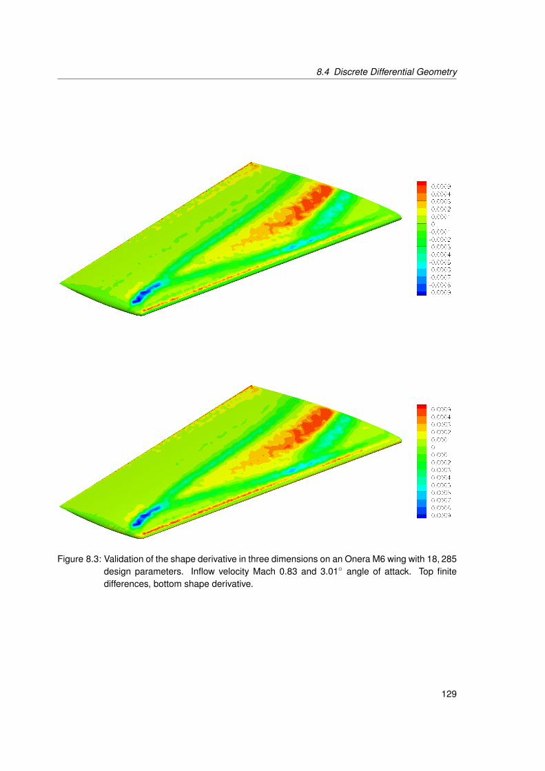
8.4 Discrete Differential Geometry
Figure 8.3: Validation of the shape derivative in three dimensions on an Onera M6 wing with 18, 285design parameters. Inflow velocity Mach 0.83 and 3.01 angle of attack. Top finitedifferences, bottom shape derivative.
129

8 Shape Optimization and Euler Equations
= − 1|P|
∫P
〈∇Γ,∇Γg〉 dS
= − 1|P|
∫∂P
〈∇Γg, n∂P〉 d`
= − 1|P|∑T∈P
∫∂P∩T
〈∇Γg, n∂P〉 d`
= − 1|P|∑T∈P
∇Γg(xk ) [xi − xi+1]⊥ ,
since∇Γg is assumed constant in T . Also note that⊥—and likewise n∂P—means perpendicular tothe boundary ∂P in the tangent space of the surface, as otherwise there would be an extra degreeof freedom. As usual when employing finite elements, g is assumed to consist of nodal weights andlinear ansatz functions:
gT(x) = g(xk )ϕk (x) + g(xi )ϕi (x) + g(xi+1)ϕi+1(x).
Since the ansatz functions are linear, their contour lines in T are parallel to the opposite edge, andsince the gradient is perpendicular to the contour lines, the following relation holds:
∇Γϕk =1
2|T |[xi+1 − xi ]⊥
∇Γϕi =1
2|T |[xk − xi+1]⊥
∇Γϕi+1 =1
2|T |[xi − xk ]⊥ .
Thus, the tangential gradient ∇Γg is given by
∇Γg(x)T
=1
2|T |
(g(xk ) [xi+1 − xi ]⊥ + g(xi ) [xk − xi+1]⊥ + g(xi+1) [xi − xk ]⊥
)=
12|T |
(g(xk ) [xi+1 − xk + xk − xi ]⊥ + g(xi ) [xk − xi+1]⊥ + g(xi+1) [xi − xk ]⊥
)=
12|T |
(−g(xk ) [xk − xi+1]⊥ − g(xk ) [xi − xk ]⊥ + g(xi ) [xk − xi+1]⊥ + g(xi+1) [xi − xk ]⊥
)=
12|T |
((g(xi )− g(xk )) [xk − xi+1]⊥ + (g(xi+1)− g(xk )) [xi − xk ]⊥
),
a constant expression for all x in T . Thus, for the Laplace–Beltrami operator one has
∆Γg(xk )
=− 1|P|∑T∈P
12|T |
((g(xi )− g(xk )) [xk − xi+1]⊥ + (g(xi+1)− g(xk )) [xi − xk ]⊥
)[xi − xi+1]⊥ .
130

8.5 Airfoil Optimizations
Since the area of T is proportional to the sine of any angle of the triangle one has
∆Γg(xk ) = − 1|P|∑T∈P
(g(xi )− g(xk )) cot(θi ) + (g(xi+1)− g(xk )) cot(γi ).
Since γi = βi+1, an index shift in the second part of the sum results in
∆Γg(xk ) =− 1|P|∑T∈P
(g(xi )− g(xk )) cot(θi ) + (g(xi )− g(xk )) cot(βi )
=1|P|∑T∈P
(cot(θi ) + cot(βi )) (g(xk )− g(xi )) .
The above equation is assembled into a matrix, and the discrete Laplace–Beltrami preconditioner (5.7)is factorized using a direct sparse linear solver. The effect on the gradient is illustrated in figure 8.4
Figure 8.4: Effects of the Laplace–Beltrami preconditioner (5.7) on the drag gradient for k =0, 10−2, 10−1, 100 on the Onera M6 wing.
for the Onera M6 wing at Mach 0.83 and angle of attack α = 3.01.
8.5 Airfoil Optimizations
All of the following two and three dimensional optimizations have been conducted using the DLRflow solver TAU, a hybrid unstructured vertex centered finite volume flow solver for viscid and inviscidcompressible flow [21, 26, 68]. For inviscid computations, TAU features both a continuous andhand-discrete adjoint, while for viscous computations, only a discrete adjoint mode is avaliable.TAU is also one of the production codes of Airbus, making the following computations examplesof real world applications. TAU also consists of several auxiliary routines for mesh partitioningfor parallel computations and a mesh deformation routine. The auxiliary programs are connectedusing a common Python interface. The surface mesh is perturbed as discussed above, and the
131

8 Shape Optimization and Euler Equations
Figure 8.5: Initial NACA0012 airfoil at Mach 2.0. The blunt nose body produces a strong detachedbow shock. Color denotes pressure.
Figure 8.6: Optimized airfoil for Mach 2.0 at zero angle of attack. The blunt nose has become sharp,producing a much weaker attached shock wave. Color denotes pressure.
132
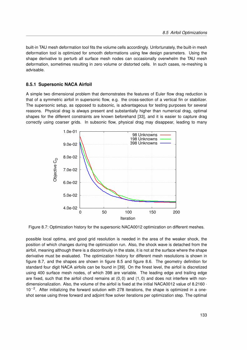
8.5 Airfoil Optimizations
built-in TAU mesh deformation tool fits the volume cells accordingly. Unfortunately, the built-in meshdeformation tool is optimized for smooth deformations using few design parameters. Using theshape derivative to perturb all surface mesh nodes can occasionally overwhelm the TAU meshdeformation, sometimes resulting in zero volume or distorted cells. In such cases, re-meshing isadvisable.
8.5.1 Supersonic NACA Airfoil
A simple two dimensional problem that demonstrates the features of Euler flow drag reduction isthat of a symmetric airfoil in supersonic flow, e.g. the cross-section of a vertical fin or stabilizer.The supersonic setup, as opposed to subsonic, is advantageous for testing purposes for severalreasons. Physical drag is always present and substantially higher than numerical drag, optimalshapes for the different constraints are known beforehand [33], and it is easier to capture dragcorrectly using coarser grids. In subsonic flow, physical drag may disappear, leading to many
Figure 8.7: Optimization history for the supersonic NACA0012 optimization on different meshes.
possible local optima, and good grid resolution is needed in the area of the weaker shock, theposition of which changes during the optimization run. Also, the shock wave is detached from theairfoil, meaning although there is a discontinuity in the state, it is not at the surface where the shapederivative must be evaluated. The optimization history for different mesh resolutions is shown infigure 8.7, and the shapes are shown in figure 8.5 and figure 8.6. The geometry definition forstandard four digit NACA airfoils can be found in [39]. On the finest level, the airfoil is discretizedusing 400 surface mesh nodes, of which 398 are variable. The leading edge and trailing edgeare fixed, such that the airfoil chord remains at (0, 0) and (1, 0) and does not interfere with non-dimensionalization. Also, the volume of the airfoil is fixed at the initial NACA0012 value of 8.2160 ·10−2. After initializing the forward solution with 278 iterations, the shape is optimized in a one-shot sense using three forward and adjoint flow solver iterations per optimization step. The optimal
133

8 Shape Optimization and Euler Equations
shape is reached after about 150 iterations of the rSQP method as described in remark 8.3.3. Thereduced Hessian B is approximated by the Laplace–Beltrami preconditioner (5.7).
8.5.2 Mesh Independence
Although the flow solver is not completely mesh independent when computing the state and adjointvariables, a careful selection of the various parameters such as the number of inner iterations, the
Figure 8.8: Coarse NACA0012 mesh and third refinement for testing mesh independent optimiza-tion convergence.
optimization step length, and the amount of gradient smoothing can lead to a potentially mesh res-olution independent optimization convergence behavior, as can be seen in figure 8.7. The precisesettings used in the optimization are listed in table 8.1. The first column shows the number of flow
Unknowns Initial Forward Initial Adjoint Inner Forward Inner Adjoint Smoothing98 158 128 3 3 4.0198 182 215 3 3 2.0398 278 404 3 3 0.5
Table 8.1: Parameters used in the mesh independency study
solver iterations needed to reach a primal residual of 10−7. The second column shows the numberof adjoint flow solver iterations needed to reach an adjoint residual of 10−4 for the lift adjoint. Thus,the flow solver convergence rate is not mesh independent. Nevertheless, during the one-shot op-timization, the number of inner flow solver iterations can be kept constant at three for both primaland adjoint solver. The smoothing factor for the two dimensional Laplace–Beltrami preconditioner,equation (5.7), had to be adapted, and the respective value for k is shown in the last column. Inter-estingly, the smoothing parameter here features the same monotonicity behavior as in the Stokescase, equation (5.8).
Hence, the Laplace–Beltrami Hessian approximation has the potential for mesh independentconvergence, which is highly desireable for the optimizations of wings and aircrafts in three dimen-sions, where the number of shape parameters increases significantly. Two of the initial meshes forthe mesh independency study are shown in figure 8.8.
134

8.5 Airfoil Optimizations
8.5.3 Transonic Lifting RAE2822 Airfoil
One of the classical examples for aerodynamic shape optimization is the optimization of the RAE-2822 airfoil in transonic cruise condition of Mach 0.73 and 2 angle of attack. The initial lift is tobe maintained. Due to its popularity, this test-case is sometimes simply denoted by “case 9”. Atthese flow conditions, it is assumed the shock wave of the upper side can be completely removedby optimization. Thus a shock free solution is considered optimal. Unlike the other exampleswhere the aim was a drastic deformation of the shape, here only small modifications to the airfoilsurface are required. Usually for “case 9”, a mesh consisting of 128 surface nodes is used, which isdeformed by Hicks–Henne functions [35] enforcing the airfoil thickness to remain constant at eachchord point during the optimization. This test-case has been re-created using the shape derivativefor all surface nodes. The final shape is shown in figure 8.9 and is shock free. After fixing the
Figure 8.9: Optimal shape for the RAE2822 transonic cruise “case 9” optimization. The standardmesh is a C-type mesh using 128 surface nodes. The optimized solution is shock freeon this mesh. Color denotes pressure.
leading and trailing edge, 126 variable surface nodes remain. Instead of the constant thickness byHicks–Henne parameterization, a constant volume is enforced. The initial lift of CL = 7.817 ·10−1 isincreased to CL = 7.831 · 10−1, a very slight increase by 0.2%, while the drag is reduced by 49.4%,from CD = 6.547 · 10−3 to CD = 3.295 · 10−3. The optimization requires again 100 steps with 20inner iterations for each of the flow solvers, i.e. the primal flow solver and the two adjoint flow solverfor drag and lift.
Additionally, a much finer mesh with 512 surface nodes is also considered. Initial flow field andoptimized flow field are shown in figure 8.10 and figure 8.11. The optimization history is shown infigure 8.12. Using a proper tuning of all parameters, the optimal solution can be found in a mere28 optimization steps with 40 inner iterations for each of the flow solvers. Although the optimalshape on this finer mesh features a very weak shock wave on the upper side, the computed dragvalue of CD = 2.721 · 10−3 is lower than the optimal solution on the coarser mesh. In total, thedrag has been reduced by 62.9%, while lift has increased to CL = 7.828 · 10−1, an increase by
135
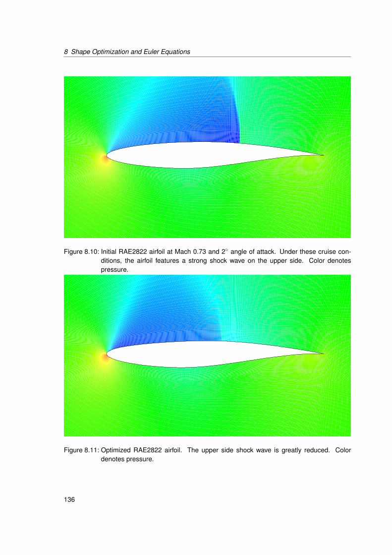
8 Shape Optimization and Euler Equations
Figure 8.10: Initial RAE2822 airfoil at Mach 0.73 and 2 angle of attack. Under these cruise con-ditions, the airfoil features a strong shock wave on the upper side. Color denotespressure.
Figure 8.11: Optimized RAE2822 airfoil. The upper side shock wave is greatly reduced. Colordenotes pressure.
136

8.6 Onera M6 Wing Optimization
2.5e-03
3.0e-03
3.5e-03
4.0e-03
4.5e-03
5.0e-03
5.5e-03
6.0e-03
6.5e-03
7.0e-03
7.5e-03
0 5 10 15 20 25 30
Obj
ectiv
e C
D
Iteration
Figure 8.12: Optimization history for the transonic RAE2822 optimization with 510 variable surfacemesh nodes.
0.1%. Before the one-shot optimization is started, the primal solution is initialized by 580 iterations.The adjoint solution for the drag is initialized by 945 adjoint flow solver iterations. Initializing the liftadjoint requires 1348 iterations.
8.6 Onera M6 Wing Optimization
One of the standard test-cases in three dimensions is the Onera M6 wing. In cruise condition of
60
65
70
75
80
85
90
95
100
105
110
0 20 40 60 80 100 120 140 160 180 0
5
10
15
20
25
30
35
40
45
50
CD
[dc]
CL
[lc]
Iteration
CL, 36kCL, 18k/36k
CD, 36kCD, 18k/36k
Figure 8.13: Multilevel optimization history for the Onera M6 wing. One drag count dc is a scalingof 10−4 and one lift count lc is a scaling of 10−2.
137

8 Shape Optimization and Euler Equations
Figure 8.14: Initial Onera M6 wing at Mach 0.83 and 3.01 angle of attack. The wing develops twointeracting shock waves on the upper side, so called λ-shock waves. The wing surfaceconsists of 18, 285 nodes. Color denotes pressure.
Figure 8.15: Optimized Onera M6 wing. The shock waves are completely removed. Color denotespressure.
138

8.6 Onera M6 Wing Optimization
Mach 0.83 and 3.01 angle of attack, the wing develops two interacting shock waves on the upperside, sometimes also called λ-shock due to the visual shape of the merging shock waves. A multi-level optimization is considered, and the coarser mesh consists of 18, 285 surface nodes. In total,this mesh results in 541, 980 state unknowns for the Euler equations. After refinement, the nextfiner mesh features 36, 806 surface nodes and 1, 486, 315 Euler state unknowns. Simulation andoptimization is conducted only on one half of the wing, the entire wing is then created by mirroringat the symmetry plane. Initial and optimal wing are shown in figure 8.14 and figure 8.15. Startingon the coarser mesh, an initial drag value of CD = 7.52 · 10−3 and lift value of CL = 2.65 · 10−1 iscomputed. Lift and the initial volume of V0 = 63.6 are used as a constraint. A multi-level optimizationis beneficial, because usually mesh refinement is based on better resolving shock waves, which areremoved due to optimization. The planform is considered fixed, because otherwise, the TAU meshdeformation tool for the volume mesh very frequently produces meshes of bad quality with invertedor almost zero cells. The optimization history for the multilevel optimization is shown in figure 8.13.The respective meshes are shown in figure 8.16.
139

8 Shape Optimization and Euler Equations
Figure 8.16: Initial solution, optimal solution with refinement based on initial solution, and optimalsolution with refinement during optimization.
140

Chapter 9
Compressible Navier–Stokes Equations
9.1 Introduction
After considering viscous incompressible fluids in chapter 6 and inviscid compressible fluids in chap-ter 8, this chapter seeks to combine both and considers the compressible Navier–Stokes equations,i.e. a viscous and compressible fluid. Presently, the compressible Navier–Stokes equations are con-sidered the ultimate fluid model. They are assumed to correctly model all single phase fluid flowsof matching stress tensor. Usually, the often used perfect gas assumption is the limiting factor inapplicability, as at hypersonic speeds or in chemically active fluids, the chemistry must be modeledalso. Contrary to the Euler equations considered in chapter 8, the compressible Navier–Stokesequations reproduce fluid boundary layers, flow separation, and consequently turbulence. Unfor-tunately, they are correspondingly complex and both analytically inaccessible and numerically verydifficult to solve. Since high Reynolds number fluid phenomena are of very different time- and spacescales, e.g. fast, small-scale turbulent motion versus large-scale, almost steady mean flow, resolv-ing all fluid phenomena would require a prohibitively fine discretization. This is also called directnumerical simulation (DNS) and is almost always used to calibrate substitute turbulence models insimple domains. Since almost all flows of industrial importance are high Reynolds number flows,the compressible Navier–Stokes equations are almost always averaged in time and space. Usually,this is accomplished by the so-called Reynolds averaging, which ignores density fluctuations, butother averaging approaches including density variations exist, such as Favre averaging. Unfortu-nately, averaging introduces new unknowns in the eddy viscosity, and the resulting compressibleReynolds averaged Navier–Stokes equations (RANS) require additional turbulence modeling. Most
141
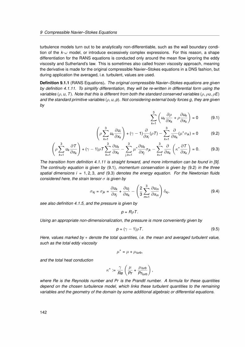
9 Compressible Navier–Stokes Equations
turbulence models turn out to be analytically non-differentiable, such as the wall boundary condi-tion of the k -ω model, or introduce excessively complex expressions. For this reason, a shapedifferentiation for the RANS equations is conducted only around the mean flow ignoring the eddyviscosity and Sutherland’s law. This is sometimes also called frozen viscosity approach, meaningthe derivative is made for the original compressible Navier–Stokes equations in a DNS fashion, butduring application the averaged, i.e. turbulent, values are used.
Definition 9.1.1 (RANS Equations). The original compressible Navier–Stokes equations are givenby definition 4.1.11. To simplify differentiation, they will be re-written in differential form using thevariables (ρ, u, T ). Note that this is different from both the standard conserved variables (ρ, ρu, ρE)and the standard primitive variables (ρ, u, p). Not considering external body forces g, they are givenby
3∑k=1
(uk∂ρ
∂xk+ ρ
∂uk
∂xk
)= 0 (9.1)(
ρ
3∑k=1
uk∂ui
∂xk
)+ (γ − 1)
∂
∂xi(ρT )−
3∑k=1
∂
∂xk(µ∗σik ) = 0 (9.2)(
ρ3∑
k=1
uk∂T∂xk
)+ (γ − 1)ρT
3∑k=1
∂uk
∂xk−
3∑j ,k=1
µ∗∂uk
∂xjσjk −
3∑k=1
∂
∂xk
(κ∗∂T∂xk
)= 0. (9.3)
The transition from definition 4.1.11 is straight forward, and more information can be found in [9].The continuity equation is given by (9.1), momentum conservation is given by (9.2) in the threespatial dimensions i = 1, 2, 3, and (9.3) denotes the energy equation. For the Newtonian fluidsconsidered here, the strain tensor σ is given by
σkj = σjk =∂uk
∂xj+∂uj
∂xk−
(23
3∑m=1
∂um
∂xm
)δkj , (9.4)
see also definition 4.1.5, and the pressure is given by
p = RρT .
Using an appropriate non-dimensionalization, the pressure is more conveniently given by
p = (γ − 1)ρT . (9.5)
Here, values marked by ∗ denote the total quantities, i.e. the mean and averaged turbulent value,such as the total eddy viscosity
µ∗ = µ + µturb,
and the total heat conduction
κ∗ :=γ
Re
(µ
Pr+µturb
Prturb
),
where Re is the Reynolds number and Pr is the Prandtl number. A formula for these quantitiesdepend on the chosen turbulence model, which links these turbulent quantities to the remainingvariables and the geometry of the domain by some additional algebraic or differential equations.
142

9.2 First Order Calculus
9.2 First Order Calculus
In this section, the shape derivative for the force optimization problem in a compressible Navier–Stokes fluid is constructed. Special attention is paid to finding an expression that can easily beevaluated. For more theoretical details, especially concerning existence and uniqueness, see [51,52, 54]. Especially in [51], a general framework for the analysis of inhomogeneous elliptic-hyperbolicequations such as the compressible Navier–Stokes equations is established, and an analysis isperformed for small perturbations of the so-called approximate solutions, which are determinedfrom Stokes problems. Furthermore, the existence of optimal shapes of the isothermal Navier–Stokes equations is shown in [52] using generalized solutions for the Navier–Stokes equations.Also, from a standard, non shape calculus point of view, the problem has also been studied in [29]for a thin shear-layer approximation of the viscous stress tensor or in [41].
Definition 9.2.1 (Compressible Navier–Stokes Shape Optimization Problem). As a shape optimiza-tion problem, the aerodynamic or fluid forces on a solid body are again considered. Contrary to theEuler problem, definition 8.1.1, the viscous part of the forces, i.e. the skin friction, must now beincluded in the objective function, resulting in the following shape optimization problem
min(u,p,Ω)
J(u, p, Ω) :=∫Γ0
3∑i=1
aipni −3∑
i ,k=1
akµ∗σkini dS =
∫Γ0
〈pa, n〉 − 〈µ∗σa, n〉 dS (9.6)
subject to3∑
k=1
(uk∂ρ
∂xk+ ρ
∂uk
∂xk
)= 0(
ρ3∑
k=1
uk∂ui
∂xk
)+ (γ − 1)
∂
∂xi(ρT )−
3∑k=1
∂
∂xk(µ∗σik ) = 0(
ρ3∑
k=1
uk∂T∂xk
)+ (γ − 1)ρT
3∑k=1
∂uk
∂xk−
3∑j ,k=1
µ∗∂uk
∂xjσjk −
3∑k=1
∂
∂xk
(κ∗∂T∂xk
)= 0.
(9.7)
The equality in (9.6) holds due to symmetry of σ. Additionally, the following boundary conditionsare considered:
u = a on Γ+ (9.8)
u = 0 on Γ0 (9.9)
T = T∞ =1
γ(γ − 1)M2∞
on Γ+ (9.10)
T = TB = T∞
(1 +
γ − 12M2∞
)on Γ0 (9.11)
〈∇T , n〉 = 0 on Γ0 (9.12)
ρ = 1 on Γ+, (9.13)
where M∞ is the free stream Mach number. Equation (9.8) is the usual normalized inflow bound-ary condition in a rotated coordinate system, and equation (9.9) is the standard viscous no-slip
143

9 Compressible Navier–Stokes Equations
boundary condition. Boundary condition (9.11) is the isothermal wall temperature condition, i.e.fixed Dirichlet boundary condition for the temperature on the wing. An alternative to the isothermaltemperature wall boundary condition is the adiabatic wall temperature boundary condition (9.12),specifying zero temperature flux over the aircraft surface. Isothermal and adiabatic wall temperatureboundary conditions are mutually exclusive and never used at the same time.
Lemma 9.2.2 (Linearized Continuity Equation). Linearizing the continuity equation (9.1) results inthe following expression
0 =∫Ω
3∑k=1
(λρu′k [V ]
∂ρ
∂xk− ρ′[V ]
∂
∂xk
(λρuk
)+ λρρ′[V ]
∂uk
∂xk− u′k [V ]
∂
∂xk(λρρ)
)dA
+∫∂Ω
3∑k=1
(λρukρ
′[V ]nk + λρρu′k [V ]nk)
dS,
where λρ is a sufficiently smooth arbitrary multiplicator.
Proof. A linearization of the continuity equation (9.1) results in
div (ρu′[V ]) + div (ρ′[V ]u)
=3∑
k=1
(u′k [V ]
∂ρ
∂xk+ uk
∂ρ′[V ]∂xk
+ ρ′[V ]∂uk
∂xk+ ρ
∂u′k [V ]∂xk
)= 0,
and multiplication of the linearized continuity equation with an arbitrary λρ and integration by partsresults in the desired expression.
Lemma 9.2.3 (Linearized Strain Tensor, Volume). For sufficiently smooth arbitrary multiplicatorsλui , the following relation holds
∫Ω
3∑i ,k=1
∂λui
∂xkσ′ik [V ] dA
=∫Ω
−3∑
i ,k=1
(∂2λui
∂x2k
+∂2λuk
∂xi∂xk− 2
3∂2λuk
∂xk∂xi
)u′i [V ] dA
+∫∂Ω
3∑i ,k=1
(∂λui
∂xknk +
∂λuk
∂xink −
23∂λuk
∂xkni
)u′i [V ] dS.
144

9.2 First Order Calculus
Proof. The definition of the strain tensor, equation (9.4), results in∫Ω
3∑i ,k=1
∂λui
∂xkσ′ik [V ] dA
=∫Ω
3∑i ,k=1
∂λui
∂xk
(∂u′i [V ]∂xk
+∂u′k [V ]∂xi
− 23δik
3∑m=1
∂u′m[V ]∂xm
)dA
=∫Ω
[3∑
i ,k=1
∂λui
∂xk
(∂u′i [V ]∂xk
+∂u′k [V ]∂xi
)]− 2
3
3∑i ,m=1
∂λui
∂xi
∂u′m[V ]∂xm
dA.
Integration by parts and regrouping provides∫Ω
3∑i ,k=1
∂λui
∂xkσ′ik [V ] dA
=∫Ω
[−
3∑i ,k=1
∂2λui
∂x2k
u′i [V ] +∂2λui
∂xk∂xiu′k [V ]
]+
23
3∑i ,m=1
∂2λui
∂xi∂xmu′m[V ] dA
+∫∂Ω
[3∑
i ,k=1
∂λui
∂xknk u′i [V ] +
∂λui
∂xkniu′k [V ]
]− 2
3
3∑i ,m=1
∂λui
∂xinmu′m[V ] dS
=∫Ω
[3∑
i ,k=1
(−∂
2λui
∂x2k− ∂2λuk
∂xi∂xk
)u′i [V ]
]+
23
3∑i ,k=1
∂2λuk
∂xk∂xiu′i [V ] dA
+∫∂Ω
[3∑
i ,k=1
(∂λui
∂xknk +
∂λuk
∂xink
)u′i [V ]
]− 2
3
3∑i ,k=1
∂λuk
∂xkniu′i [V ] dS
=∫Ω
−3∑
i ,k=1
(∂2λui
∂x2k
+∂2λuk
∂xi∂xk− 2
3∂2λuk
∂xk∂xi
)u′i [V ] dA
+∫∂Ω
3∑i ,k=1
(∂λui
∂xknk +
∂λuk
∂xink −
23∂λuk
∂xkni
)u′i [V ] dS.
Lemma 9.2.4 (Linearized Strain Tensor, Surface). For sufficiently smooth arbitrary multiplicatorsλui , the following relation holds∫
∂Ω
3∑i ,k=1
λuiσ′ik [V ]nk dS
=∫∂Ω
3∑i ,k=1
(λui nk + λuk ni −
23δik
3∑m=1
λum nm
)∂u′i [V ]∂xk
dS.
145

9 Compressible Navier–Stokes Equations
Proof. Inserting equation (9.4) and regrouping results in
∫∂Ω
3∑i ,k=1
λuiσ′ik [V ]nk dS
=∫∂Ω
[3∑
i ,k=1
(λui
∂u′i [V ]∂xk
nk + λuk
∂u′i [V ]∂xk
ni
)]− 2
3
3∑i ,k ,m=1
δikλui
∂u′m[V ]∂xm
nk dS
=∫∂Ω
[3∑
i ,k=1
(λui nk + λuk ni
) ∂u′i [V ]∂xk
]− 2
3
3∑i ,m=1
λum nm∂u′i [V ]∂xi
dS
=∫∂Ω
[3∑
i ,k=1
(λui nk + λuk ni
) ∂u′i [V ]∂xk
]− 2
3
3∑i ,k ,m=1
δikλum nm∂u′i [V ]∂xk
dS
=∫∂Ω
3∑i ,k=1
(λui nk + λuk ni −
23δik
3∑m=1
λum nm
)∂u′i [V ]∂xk
dS.
Lemma 9.2.5 (Linearized Momentum Equation). Linearizing the momentum equation (9.2) underthe frozen viscosity assumption results in the following expression
0 =∫Ω
3∑i=1
[(3∑
k=1
λui uk∂ui
∂xk
)+ (γ − 1)
(λui
∂T∂xi− ∂
∂xi(λui T )
)]ρ′[V ] dA
+∫Ω
3∑i ,k=1
[−µ∗
(∂2λui
∂x2k
+∂2λuk
∂xi∂xk− 2
3∂2λuk
∂xk∂xi
)+ λukρ
∂uk
∂xi− ∂
∂xk(λuiρuk )
]u′i [V ] dA
+∫Ω
3∑i=1
(γ − 1)[λui
∂ρ
∂xi− ∂
∂xi
(λuiρ
)]T ′[V ] dA
+∫∂Ω
3∑i ,k=1
[µ∗(∂λui
∂xknk +
∂λuk
∂xink −
23∂λuk
∂xkni
)+ λuiρuk nk
]u′i [V ] dS
+∫∂Ω
3∑i=1
(γ − 1)(λuiρ
′[V ]Tni + λuiρT ′[V ]ni)
dS
+∫∂Ω
−µ∗3∑
i ,k=1
(λui nk + λuk ni −
23δik
3∑m=1
λum nm
)∂u′i [V ]∂xk
dS,
where λui are sufficiently smooth arbitrary multiplicators.
146

9.2 First Order Calculus
Proof. The linearized momentum equation (9.2) is given by
0 =3∑
k=1
(ρ′[V ]uk
∂ui
∂xk+ ρu′k [V ]
∂ui
∂xk+ ρuk
∂u′i [V ]∂xk
)
+ (γ − 1)(∂ρ′[V ]∂xi
T +∂ρ
∂xiT ′[V ] + ρ′[V ]
∂T∂xi
+ ρ∂T ′[V ]∂xi
)−
3∑k=1
µ∗∂
∂xkσ′ik [V ].
A multiplication of the momentum equation with λui for i = 1, 2, 3 and integration by parts provides
0 =∫Ω
3∑k=1
[λuiρ
′[V ]uk∂ui
∂xk+ λuiρu′k [V ]
∂ui
∂xk− u′i [V ]
∂
∂xk
(λuiρuk
)]dA
+∫Ω
(γ − 1)[−ρ′[V ]
∂
∂xi(λui T ) + λui
∂ρ
∂xiT ′[V ] + λuiρ
′[V ]∂T∂xi− T ′[V ]
∂
∂xi(λuiρ)
]dA
+∫Ω
3∑k=1
µ∗σ′ik [V ]∂λui
∂xkdA
+∫∂Ω
(3∑
k=1
λuiρuk u′i [V ]nk
)+ (γ − 1)
(λuiρ
′[V ]Tni + λuiρT ′[V ]ni)
dS
+∫∂Ω
−3∑
k=1
µ∗λuiσ′ik [V ]nk dS.
Summing the momentum equations over i = 1, 2, 3 and regrouping leads to
0 =∫Ω
3∑i=1
[(3∑
k=1
λui uk∂ui
∂xk
)+ (γ − 1)
(λui
∂T∂xi− ∂
∂xi(λui T )
)]ρ′[V ] dA (9.14)
+∫Ω
3∑i ,k=1
λuiρ∂ui
∂xku′k [V ] dA (9.15)
+∫Ω
3∑i ,k=1
[− ∂
∂xk
(λuiρuk
)]u′i [V ] dA (9.16)
+∫Ω
3∑i=1
(γ − 1)(λui
∂ρ
∂xi− ∂
∂xi(λuiρ)
)T ′[V ] dA (9.17)
+∫Ω
3∑i ,k=1
µ∗σ′ik [V ]∂λui
∂xkdA (9.18)
+∫∂Ω
3∑i=1
[(3∑
k=1
λuiρuk nk
)u′i [V ] + (γ − 1)
(λuiρ
′[V ]Tni + λuiρT ′[V ]ni)]
dS (9.19)
147
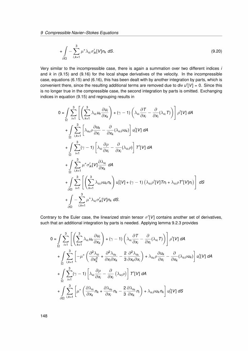
9 Compressible Navier–Stokes Equations
+∫∂Ω
−3∑
i ,k=1
µ∗λuiσ′ik [V ]nk dS. (9.20)
Very similar to the incompressible case, there is again a summation over two different indices iand k in (9.15) and (9.16) for the local shape derivatives of the velocity. In the incompressiblecase, equations (6.15) and (6.16), this has been dealt with by another integration by parts, which isconvenient there, since the resulting additional terms are removed due to div u′[V ] = 0. Since thisis no longer true in the compressible case, the second integration by parts is omitted. Exchangingindices in equation (9.15) and regrouping results in
0 =∫Ω
3∑i=1
[(3∑
k=1
λui uk∂ui
∂xk
)+ (γ − 1)
(λui
∂T∂xi− ∂
∂xi(λui T )
)]ρ′[V ] dA
+∫Ω
3∑i ,k=1
[λukρ
∂uk
∂xi− ∂
∂xk(λuiρuk )
]u′i [V ] dA
+∫Ω
3∑i=1
(γ − 1)[λui
∂ρ
∂xi− ∂
∂xi(λuiρ)
]T ′[V ] dA
+∫Ω
3∑i ,k=1
µ∗σ′ik [V ]∂λui
∂xkdA
+∫∂Ω
3∑i=1
[(3∑
k=1
λuiρuk nk
)u′i [V ] + (γ − 1)
(λuiρ
′[V ]Tni + λuiρT ′[V ]ni)]
dS
+∫∂Ω
−3∑
i ,k=1
µ∗λuiσ′ik [V ]nk dS.
Contrary to the Euler case, the linearized strain tensor σ′[V ] contains another set of derivatives,such that an additional integration by parts is needed. Applying lemma 9.2.3 provides
0 =∫Ω
3∑i=1
[(3∑
k=1
λui uk∂ui
∂xk
)+ (γ − 1)
(λui
∂T∂xi− ∂
∂xi(λui T )
)]ρ′[V ] dA
+∫Ω
3∑i ,k=1
[−µ∗
(∂2λui
∂x2k
+∂2λuk
∂xi∂xk− 2
3∂2λuk
∂xk∂xi
)+ λukρ
∂uk
∂xi− ∂
∂xk(λuiρuk )
]u′i [V ] dA
+∫Ω
3∑i=1
(γ − 1)[λui
∂ρ
∂xi− ∂
∂xi
(λuiρ
)]T ′[V ] dA
+∫∂Ω
3∑i ,k=1
[µ∗(∂λui
∂xknk +
∂λuk
∂xink −
23∂λuk
∂xkni
)+ λuiρuk nk
]u′i [V ] dS
148

9.2 First Order Calculus
+∫∂Ω
3∑i=1
(γ − 1)(λuiρ
′[V ]Tni + λuiρT ′[V ]ni)
dS
+∫∂Ω
−3∑
i ,k=1
µ∗λuiσ′ik [V ]nk dS.
It remains to remove the strain tensor variation on the boundary ∂Ω from the first integration byparts. Applying lemma 9.2.4 results in
0 =∫Ω
3∑i=1
[(3∑
k=1
λui uk∂ui
∂xk
)+ (γ − 1)
(λui
∂T∂xi− ∂
∂xi(λui T )
)]ρ′[V ] dA
+∫Ω
3∑i ,k=1
[−µ∗
(∂2λui
∂x2k
+∂2λuk
∂xi∂xk− 2
3∂2λuk
∂xk∂xi
)+ λukρ
∂uk
∂xi− ∂
∂xk(λuiρuk )
]u′i [V ] dA
+∫Ω
3∑i=1
(γ − 1)[λui
∂ρ
∂xi− ∂
∂xi
(λuiρ
)]T ′[V ] dA
+∫∂Ω
3∑i ,k=1
[µ∗(∂λui
∂xknk +
∂λuk
∂xink −
23∂λuk
∂xkni
)+ λuiρuk nk
]u′i [V ] dS
+∫∂Ω
3∑i=1
(γ − 1)(λuiρ
′[V ]Tni + λuiρT ′[V ]ni)
dS
+∫∂Ω
−µ∗3∑
i ,k=1
(λui nk + λuk ni −
23δik
3∑m=1
λum nm
)∂u′i [V ]∂xk
dS,
creating the desired expression.
Lemma 9.2.6 (Linearized Energy Equation). Linearizing the energy equation (9.3) under the frozenviscosity assumption results in the following expression
0 =∫Ω
3∑k=1
[λT uk
∂T∂xk
+ (γ − 1)λT T∂uk
∂xk
]ρ′[V ] dA
+∫Ω
3∑k=1
[λTρ
∂T∂xk− (γ − 1)
∂
∂xk(λTρT )
]u′k [V ] dA
+∫Ω
3∑j ,k=1
µ∗[∂
∂xj(λTσjk ) +
∂
∂xj
(λT
∂uj
∂xk
)+∂
∂xj
(λT∂uk
∂xj
)− 2
3∂
∂xk
(λT∂uj
∂xj
)]u′k [V ] dA
+∫Ω
[−κ∗∆λT +
3∑k=1
((γ − 1)λTρ
∂uk
∂xk− ∂
∂xk(λTρuk )
)]T ′[V ] dA
149

9 Compressible Navier–Stokes Equations
+∫∂Ω
3∑k=1
(γ − 1)λTρTnk u′k [V ] dS
+∫∂Ω
−µ∗3∑
j ,k=1
(λTσjk nj + λT
∂uj
∂xknj + λT
∂uk
∂xjnj −
23λT∂uj
∂xjnj
)u′k [V ] dS
+∫∂Ω
[κ∗∂λT
∂n+
3∑k=1
λTρuk nk
]T ′[V ]− κ∗λT
∂T ′[V ]∂n
dS,
where λT is a sufficiently smooth arbitrary multiplicator.
Proof. The linearization of the energy equation (9.3) is given by
0 =
[3∑
k=1
(ρ′[V ]uk
∂T∂xk
+ ρu′k [V ]∂T∂xk
+ ρuk∂T ′[V ]∂xk
)]
+(γ − 1)
[3∑
k=1
(ρ′[V ]T
∂uk
∂xk+ ρT ′[V ]
∂uk
∂xk+ ρT
∂u′k [V ]∂xk
)]
−
3∑j ,k=1
(µ∗∂u′k [V ]∂xj
σjk + µ∗∂uk
∂xjσ′jk [V ]
)− κ∗∆T ′[V ].
Multiplication by λT , integration by parts, and Green’s second identity lead to
0 =∫Ω
3∑k=1
[λTρ
′[V ]uk∂T∂xk
+ λTρu′k [V ]∂T∂xk− T ′[V ]
∂
∂xk(λTρuk )
]dA
+∫Ω
(γ − 1)3∑
k=1
[λTρ
′[V ]T∂uk
∂xk+ λTρT ′[V ]
∂uk
∂xk− u′k [V ]
∂
∂xk(λTρT )
]dA
+∫Ω
3∑j ,k=1
(µ∗u′k [V ]
∂
∂xj(λTσjk )− µ∗λT
∂uk
∂xjσ′jk [V ]
)− κ∗T ′[V ]∆λT dA
+∫∂Ω
(3∑
k=1
λTρuk T ′[V ]nk
)+ (γ − 1)
(3∑
k=1
λTρTu′k [V ]nk
)−
3∑j ,k=1
µ∗λT u′k [V ]σjk nj dS
+∫∂Ω
κ∗(
T ′[V ]∂λT
∂n− λT
∂T ′[V ]∂n
)dS = 0.
Regrouping results in
0 =∫Ω
3∑k=1
[λT uk
∂T∂xk
+ (γ − 1)λT T∂uk
∂xk
]ρ′[V ] dA
150

9.2 First Order Calculus
+∫Ω
3∑k=1
λTρ∂T∂xk− (γ − 1)
∂
∂xk(λTρT ) +
3∑j=1
µ∗∂
∂xj(λTσjk )
u′k [V ] dA
+∫Ω
[−κ∗∆λT +
3∑k=1
((γ − 1)λTρ
∂uk
∂xk− ∂
∂xk(λTρuk )
)]T ′[V ] dA
+∫Ω
−3∑
j ,k=1
µ∗λT∂uk
∂xjσ′jk [V ] dA
+∫∂Ω
3∑k=1
(γ − 1)λTρTnk − µ∗3∑
j=1
λTσjk nj
u′k [V ] dS
+∫∂Ω
[κ∗∂λT
∂n+
3∑k=1
λTρuk nk
]T ′[V ]− κ∗λT
∂T ′[V ]∂n
dS.
Since the strain tensor linearization still contains derivatives, lemma 9.2.3 must be used again,providing ∫
Ω
3∑j ,k=1
λT∂uk
∂xjσ′jk [V ] dA
=∫Ω
3∑j ,k=1
[− ∂
∂xj
(λT
∂uj
∂xk
)− ∂
∂xj
(λT∂uk
∂xj
)+
23∂
∂xk
(λT∂uj
∂xj
)]u′k [V ] dA
+∫∂Ω
3∑j ,k=1
[λT
∂uj
∂xknj + λT
∂uk
∂xjnj −
23λT∂uj
∂xjnj
]u′k [V ] dS.
Thus, the linearized energy equation becomes after regrouping
0 =∫Ω
3∑k=1
[λT uk
∂T∂xk
+ (γ − 1)λT T∂uk
∂xk
]ρ′[V ] dA
+∫Ω
3∑k=1
[λTρ
∂T∂xk− (γ − 1)
∂
∂xk(λTρT )
]u′k [V ] dA
+∫Ω
3∑j ,k=1
µ∗[∂
∂xj(λTσjk ) +
∂
∂xj
(λT
∂uj
∂xk
)+∂
∂xj
(λT∂uk
∂xj
)− 2
3∂
∂xk
(λT∂uj
∂xj
)]u′k [V ] dA
+∫Ω
[−κ∗∆λT +
3∑k=1
((γ − 1)λTρ
∂uk
∂xk− ∂
∂xk(λTρuk )
)]T ′[V ] dA
+∫∂Ω
3∑k=1
(γ − 1)λTρTnk u′k [V ] dS
151

9 Compressible Navier–Stokes Equations
+∫∂Ω
−µ∗3∑
j ,k=1
(λTσjk nj + λT
∂uj
∂xknj + λT
∂uk
∂xjnj −
23λT∂uj
∂xjnj
)u′k [V ] dS
+∫∂Ω
[κ∗∂λT
∂n+
3∑k=1
λTρuk nk
]T ′[V ]− κ∗λT
∂T ′[V ]∂n
dS,
which is the desired expression.
Lemma 9.2.7 (Shape Derivative for the Compressible Navier–Stokes Equations). The shape deriva-tive of the fluid forces acting on an immersed obstacle is given by
dJ(ρ, u, T , Ω)[V ]
=∫Γ0
〈V , n〉
[3∑
i=1
(ai∂p∂n
ni − λρρ∂ui
∂nni
)−
3∑i ,k=1
aiµ∗∂σik
∂nnk
]dS
+∫Γ0
〈V , n〉 divΓ
(pa− µ∗σa
)dS
+∫Γ0
〈V , n〉3∑
i ,k=1
[−µ∗
(∂λui
∂xknk +
∂λuk
∂xink −
23∂λuk
∂xkni
)]∂ui
∂ndS
+∫Γ0
〈V , n〉κ∗∂λT
∂n∂(TB − T )
∂ndS
in case of isothermal walls, T = TB, and
dJ(ρ, u, T , Ω)[V ]
=∫Γ0
〈V , n〉
[3∑
i=1
(ai∂p∂n
ni − λρρ∂ui
∂nni − λT p
∂ui
∂nni
)−
3∑i ,k=1
aiµ∗∂σik
∂nnk
]dS
+∫Γ0
〈V , n〉 divΓ
(pa− µ∗σa
)dS
+∫Γ0
〈V , n〉3∑
i ,k=1
[−µ∗
(∂λui
∂xknk +
∂λuk
∂xink −
23∂λuk
∂xkni
)]∂ui
∂ndS
+∫Γ0
〈V , n〉3∑
i ,k=1
µ∗(λTσik ni + λT
∂ui
∂xkni + λT
∂uk
∂xini −
23λT∂ui
∂xini
)∂uk
∂ndS
+∫Γ0
〈V , n〉κ∗λT
[∂2T∂n2 − κ〈∇ΓT , n〉 + ∆ΓT
]dS,
in case of adiabatic walls, ∂T∂n = 0. Here, κ∗ is the total thermal conductivity of the fluid, and κ is the
curvature. In either case, the adjoint velocity viscous wall boundary condition is
λui = −ai on Γ0,
152

9.2 First Order Calculus
where a is given by a = (cosα, 0, sinα)T with α being the angle of attack. For isothermal walls Γ0,the adjoint temperature boundary condition is
λT = 0 on Γ0,
and for adiabatic walls Γ0 it is given by
∂λT
∂n= 0 on Γ0.
For prescribed density, velocity, and pressure in the farfield, the adjoint farfield boundary conditionsare given by
λρ = 0
λui = 0
λT = 0.
Proof. The objective function is of the type scalar product of vector times normal, and a formaldifferentiation according to lemma 3.3.14 immediately results in
dJ(ρ, u, T , Ω)[V ] =∫Γ0
〈V , n〉
[3∑
i=1
ai∂p∂n
ni −3∑
i ,k=1
aiµ∗∂σik
∂nnk
]dS (9.21)
+∫Γ0
〈V , n〉 divΓ
(pa− µ∗σa
)dS (9.22)
+∫Γ0
3∑i=1
aip′[V ]ni −3∑
i ,k=1
aiµ∗σ′ik [V ]nk dS. (9.23)
Due to the frozen viscosity assumption and not including Sutherland’s law, viscosity variationsµ∗′[V ] are not considered. Adjoint calculus is again needed to transform the last part of the aboveequation into Hadamard form. The results from lemmas 9.2.2, 9.2.5, and 9.2.6 are made suchthat the adjoint equations in Ω can easily be read from them. Thus, when (λρ,λui ,λT )T fulfills the
153

9 Compressible Navier–Stokes Equations
following adjoint equations in Ω
0 =3∑
j=1
[− ∂
∂xj
(λρuj
)+ λρ
∂uj
∂xj+
(3∑
k=1
λuj uk∂uj
∂xk
)
+(γ − 1)(λuj
∂T∂xj− ∂
∂xj(λuj T )
)+ λT uj
∂T∂xj
+ (γ − 1)λT T∂uj
∂xj
]0 =λρ
∂ρ
∂xi− ∂
∂xi(λρρ) + λTρ
∂T∂xi− (γ − 1)
∂
∂xi(λTρT )
+3∑
k=1
[−µ∗
(∂2λui
∂x2k
+∂2λuk
∂xi∂xk− 2
3∂2λuk
∂xk∂xi
)+ λukρ
∂uk
∂xi− ∂
∂xk(λuiρuk )
]
+3∑
k=1
µ∗[∂
∂xi(λTσik ) +
∂
∂xi
(λT
∂ui
∂xk
)+∂
∂xi
(λT∂uk
∂xi
)− 2
3∂
∂xk
(λT∂ui
∂xi
)]
0 =− κ∗∆λT +3∑
j=1
[(γ − 1)
(λTρ
∂uj
∂xj+ λuj
∂ρ
∂xj− ∂
∂xj
(λujρ
))− ∂
∂xj(λTρuj )
],
where i = 1, 2, 3, all volume integrals will vanish. Hence, only the remaining boundary parts haveto be considered. For prescribed farfield density, velocity, and temperature, one has
ρ′[V ] = 0
u′i [V ] = 0
T ′[V ] = 0
in the farfield Γ+ ∪ Γ−. Consequently, the adjoint farfield boundary conditions can be read fromlemmas 9.2.2, 9.2.5, and 9.2.6:
λρ = 0
λui = 0
λT = 0.
It remains to consider variations on the solid wall Γ0. According to equation (9.5), the pressure isgiven by
p = (γ − 1)ρT .
Consequently, the pressure variation is given by
p′[V ] = (γ − 1)ρ′[T ]T + (γ − 1)ρT ′[V ]. (9.24)
Since there are many different ways of how flow solvers handle the farfield boundary conditions,the farfield adjoint boundary conditions will not be considered here. Instead, they are assumed tobe implemented correctly in whatever adjoint flow solver is used. Merging the boundary integrals of
154

9.2 First Order Calculus
lemmas 9.2.2, 9.2.5, and 9.2.6 with the preliminary gradient (9.21) – (9.23) and inserting the no-slipboundary condition u = 0 on Γ0 together with the pressure variation (9.24) results in
dJ(ρ, u, T , Ω)[V ]
=∫Γ0
〈V , n〉
[3∑
i=1
ai∂p∂n
ni −3∑
i ,k=1
aiµ∗∂σik
∂nnk
]dS
+∫Γ0
〈V , n〉 divΓ
(pa− µ∗σa
)dS
+∫Γ0
3∑i=1
aip′[V ]ni −3∑
i ,k=1
aiµ∗σ′ik [V ]nk dS
+∫Γ0
3∑k=1
λρρu′k [V ]nk dS
+∫Γ0
3∑i ,k=1
[µ∗(∂λui
∂xknk +
∂λuk
∂xink −
23∂λuk
∂xkni
)]u′i [V ] dS
+∫Γ0
3∑i=1
λui nip′[V ]−3∑
i ,k=1
µ∗λuiσ′ik [V ]nk dS
+∫Γ0
3∑k=1
(γ − 1)λTρTnk u′k [V ] dS
+∫Γ0
−µ∗3∑
i ,k=1
(λTσik ni + λT
∂ui
∂xkni + λT
∂uk
∂xini −
23λT∂ui
∂xini
)u′k [V ] dS
+∫Γ0
κ∗∂λT
∂nT ′[V ]− κ∗λT
∂T ′[V ]∂n
dS.
Note that for contributions from the momentum equations, the preliminary expression containing thestrain tensor variation σ′[V ] was used, which is more convenient in this case due to the same ex-pression already being present in the preliminary gradient. Also, just as in the incompressible case,it becomes obvious that arbitrary objective functions will not always lead to consistent adjoint bound-ary conditions. Here, due to equation (9.24), the objective function matches the state linearizationin such a way that the pressure variation is created on the boundary, and the multiplicators λui
can be chosen such that both the inviscid pressure contribution and the viscous contributions areeliminated at the same time by the boundary condition
λui = −ai .
For badly chosen objective functions, there is the potential danger that density variations ρ′[V ]and velocity variations u′[V ] cannot be removed by the same multipliers. The no-slip boundary
155

9 Compressible Navier–Stokes Equations
condition for the velocities is a Dirichlet boundary condition, and according to lemma 3.4.3 thevelocity variation is given by
u′i [V ] = −〈V , n〉∂ui
∂n.
Taking everything together, the preliminary gradient becomes
dJ(ρ, u, T , Ω)[V ]
=∫Γ0
〈V , n〉
[3∑
i=1
(ai∂p∂n
ni − λρρ∂ui
∂nni − λT p
∂ui
∂nni
)−
3∑i ,k=1
aiµ∗∂σik
∂nnk
]dS
+∫Γ0
〈V , n〉 divΓ
(pa− µ∗σa
)dS
+∫Γ0
〈V , n〉3∑
i ,k=1
[−µ∗
(∂λui
∂xknk +
∂λuk
∂xink −
23∂λuk
∂xkni
)]∂ui
∂ndS
+∫Γ0
〈V , n〉3∑
i ,k=1
µ∗(λTσik ni + λT
∂ui
∂xkni + λT
∂uk
∂xini −
23λT∂ui
∂xini
)∂uk
∂ndS
+∫Γ0
κ∗∂λT
∂nT ′[V ]− κ∗λT
∂T ′[V ]∂n
dS,
which almost fulfills the Hadamard form except for the temperature variations T ′[V ]. In case of anisothermal wall, the temperature is subject to a Dirichlet boundary condition
T = TB on Γ0.
Thus, lemma 3.4.3 applies again, resulting in
T ′[V ] = 〈V , n〉∂(TB − T )∂n
.
Consequently, the boundary condition for λT is
λT = 0 on Γ0.
In case of an adiabatic wall, the temperature is subject to a Neumann boundary condition
∂T∂n
= 0 on Γ0,
and lemma 3.4.5 applies, resulting in∫Γ0
∂T ′[V ]∂n
=∫Γ0
〈V , n〉[−∂
2T∂n2 + κ〈∇ΓT , n〉 −∆ΓT
]dS,
where κ is the curvature. Consequently, the adjoint boundary condition is given by
∂λT
∂n= 0,
which creates the desired expressions.
156

9.3 Primal and Adjoint Variables
Remark 9.2.8. The shape derivative for the drag reduction problem, lemma 9.2.7, can be adaptedto lift instead of drag simply by replacing the incident vector a accordingly. Also, the shape derivativerequires knowledge of the normal derivative of the strain tensor
∂σik
∂n,
which consists of velocity derivatives of second order. Accurately computing second order deriva-tives of flow unknowns can be problematic for certain finite volume schemes.
9.3 Primal and Adjoint Variables
The construction of the shape derivative in lemma 9.2.7 was conducted using the primal variablesρ, u, and T , and consequently, the corresponding adjoint variables are λρ, λu, and λT . However,most flow solvers operate on the conserved variables ρ, ρu, and ρE , and when run in adjoint mode,it is not immediately clear how to use their respective adjoint variables λρ, λρu, and λρE . However,since an adjoint variable corresponds to a primal equation, and not a primal variable, the set ofadjoint variables is actually independent of the primal unknowns.
Lemma 9.3.1 (Primal and Adjoint Variables). The shape derivative is independent of the choice ofprimal variables.
Proof. Let the conserved and primitive variables in two dimensions be given by
U = (ρ, ρu, ρE)T
Up = (ρ, u, p)T
UT = (ρ, u, T )T .
Furthermore, let M1 and M2 be given by
M1 :=∂Up
∂U=
1 0 0 0−u1
ρ1ρ 0 0
−u2ρ 0 1
ρ 0(γ−1)‖u‖2
2 (1− γ)u1 (1− γ)u2 (γ − 1)
M2 :=∂Up
∂UT=
1 0 0 00 1 0 00 0 1 0
(γ − 1)T 0 0 (γ − 1)ρ
,
such that the following relation holds
M2U ′T[V ] = M1U ′[V ] = U ′p[V ],
since
p′[V ] = (γ − 1)ρ′[V ]T + (γ − 1)ρT ′[V ].
157

9 Compressible Navier–Stokes Equations
Let λ solve the formal adjoint system used in the shape derivative, lemma 9.2.7, based on UT
∂J∂UT
+ λT ∂c∂UT
= 0.
Consequently, the adjoint system corresponding to a primal formulation in U is constructed bymultiplication with M3 := ∂UT
∂U = M−12 M1
∂J∂UT
M3 + λT ∂c∂UT
M3 = 0
⇔ ∂J∂U
+ λT ∂c∂U
= 0,
which is equivalently solved by the same set of variables λ.
158

Chapter 10
Conclusions and Outlook
10.1 Summary
The aim of this work was to conduct a shape sensitivity analysis followed by a study of the shapeHessian and an actual numerical optimization for a variety of large scale shape optimization prob-lems in computational fluid dynamics. The Hadamard form of the shape gradient played a crucialpart in numerical structure exploitation for applied shape optimization. Being able to express thegradient on the surface bypassed all of the problematic partial derivatives, i.e. mesh sensitivity Ja-cobians, of a shape optimization problem that is considered as a standard optimal control problemby parameterization. Since the one-shot approach achieves a major speed-up by trading few exactdescent steps for many inexact ones, the discretized Hadamard gradient also greatly supportedthe one-shot approach. Furthermore, the gradient evaluation is truly independent of the number ofdesign parameters, which made using all mesh surface nodes in the optimization possible, enablinglarge scale deformations and morphing of shapes.
When using a parameterization, the resulting shapes are usually smooth by construction, mean-ing that for any choice of design parameters, the resulting shapes are in a desired regularity class.Unfortunately, this is no longer true in case of a non-parametric shape optimization based on theHadamard formula where one needs to make sure the updates maintain regularity of the shape.Interpreting the gradient as the Riesz representative of the derivative, one has to compute this rep-resentative in the desired regularity space. Sometimes also called Sobolev gradient method, sucha gradient smoothing essentially turns a steepest descent method into an approximative Newtonmethod. Thus, the shape Hessian of the problem is a very good candidate for the re-smoothing
159

10 Conclusions and Outlook
procedure. Fortunately, the Hadamard form of the shape gradient also allows a better analysis ofthe Hessian, which would otherwise be camouflaged by parameterization. The Hessian of a PDEconstraint shape optimization problem usually is a pseudo-differential operator, and this work stud-ied Fourier analysis to determine the symbol of the Hessian. A Hessian approximation based on itssymbol could be used to greatly accelerate a wide variety of shape optimization problems in fluiddynamics, up to the adaptively refined multi-level optimization of a complete Onera M6 wing withmore than 36, 000 design parameters using an unstructured surface mesh and the compressibleEuler equations. Special attention was also given to the correct evaluation of the Hadamard formand the surface shape Hessian approximation, as this usually requires discrete differential geom-etry on unstructured, triangulated surfaces. The work concludes with a formal extension to thecompressible Navier–Stokes equations using a frozen eddy viscosity approach.
10.2 Future Work
New possibilities created by using the Hadamard form of the shape gradient are very profound.Being able to conduct large scale morphing of shapes very effectively opens new and fascinat-ing opportunities for optimization. Transition from the Onera M6 wing to a complete aircraft, i.e.wing-body-nacelle configurations, is straight forward. After defining new constraints, basically onlythe input mesh must be changed. Optimization under uncertainties and aero-structure couplingcan also be envisioned. Preliminary studies for aero-structure interaction are considered in [60],where the application of new and very fast single instruction multiple data graphics processing units(GPUs) for numerical optimization was also studied.
Naturally, the formal considerations for the compressible Navier–Stokes equations should also beapplied in an actual numerical optimization. However, for perfecting large scale morphing of shapes,more robust volume mesh deformations are needed. Since a re-meshing in the volume after mostof the surface updates is infeasible, the procedure to match the volume mesh to the new surfacemust be able to create quality meshes for large deformations, even though the mesh deformation isno longer part of the derivative chain. With the present industrially applied mesh deformation tools,problems with bad quality and zero or negative volume cells are frequently encountered when theplanform changes too dramatically. The sharp trailing edge also frequently creates troubles withvolume mesh deformation. It can be expected that this behavior worsens when the anisotropicboundary layer cells are included in a viscous and compressible fluid such as the compressibleNavier–Stokes equations. Automatic mesh refinement and boundary layer discretization is alsoproblematic in this context.
Another open question is turbulence. While an analytic derivation for the RANS equations ispossible around mean flow, i.e. frozen eddy viscosity, the shape derivation of most—if not all—turbulence models is rather problematic. Algebraic and one equation models usually have non-differentiable switchings in the volume, and two equation models usually have problematic boundaryconditions, especially the k -ω model. In general, turbulence models often have discrete expressionsin the viscous wall boundary conditions which is highly contra productive for the all analytic shapedifferentiation and the Hadamard theorem. In fact, some turbulent boundary conditions are onlydefined discretely. One remedy could be making automatic or algorithmic differentiation betteraware of shape optimization problems. This probably requires more studies of the gap betweendiscrete, i.e. parameterized, and analytic shape optimization.
160

10.2 Future Work
Additionally, free surface flows could be considered. When designing ship hulls, surface wavepatterns need to be considered, and the interaction between the free fluid surface and the shapeof the immersed body can lead to a fascinating coupling. Including buoyancy also results in afluid-structure interaction to be considered during optimization. Furthermore, shape optimizationin general can be considered a free surface problem, thus coupled approaches with free interfaceproblems can lead to considerable synergies.
161


Bibliography
[1] C. Amrouche, Š. Necasová, and J. Sokolowski. Shape sensitivity analysis of the Neumannproblem of the Laplace equation in the half-space. Technical Report preprint 2007-12-20,Institute of Mathematics, AS CR, Prague, 2007.
[2] E. Arian. Analysis of the Hessian for aeroelastic optimization. Technical Report 95-84, Institutefor Computer Applications in Science and Engineering (ICASE), 1995.
[3] E. Arian and S. Ta’asan. Analysis of the Hessian for aerodynamic optimization: Inviscidflow. Technical Report 96-28, Institute for Computer Applications in Science and Engineer-ing (ICASE), 1996.
[4] E. Arian and V. N. Vatsa. A preconditioning method for shape optimization governed by theEuler equations. Technical Report 98-14, Institute for Computer Applications in Science andEngineering (ICASE), 1998.
[5] K. Atkinson and W. Han. Theoretical Numerical Analysis: A Functional Analysis Framework.Texts in Applied Mathematics 39. Springer, second edition, 2007.
[6] M. Berggren. A unified discrete-continuous sensitivity analysis method for shape optimization.In review, 2008.
[7] J. Blazek. Computational Fluid Dynamics: Principles and Applications. Elsevier, 2001.
[8] S. Boisgérault and J.-P. Zolésio. Shape derivative of sharp functionals governed by Navier–Stokes flow. In W. Jäger, J. Necas, O. John, K. Najzar, and J. Stará, editors, Partial DifferentialEquations: Theory and Numerical Solution, pages 49–63. Chapman & Hall/CRC ReseachNotes in Mathematics, 1993.
[9] S. Boivin. A finite element method to solve the compressible Navier–Stokes equations withturbulence modelling. Technical Report RR-0923, INRIA, 1988.
[10] C. Castro, C. Lozano, F. Palacios, and E. Zuazua. Systematic continuous adjoint approach toviscous aerodynamic design on unstructured grids. AIAA, 45(9):2125–2139, 2007.
[11] M. C. Delfour and J.-P. Zolésio. Shapes and Geometries: Analysis, Differential Calculus, andOptimization. Advances in Design and Control. SIAM Philadelphia, 2001.
[12] J. W. Demmel, S. C. Eisenstat, J. R. Gilbert, X. S. Li, and J. W. H. Liu. A supernodal approachto sparse partial pivoting. SIAM J. Matrix Analysis and Applications, 20(3):720–755, 1999.
[13] M. P. do Carmo. Differential Geometry of Curves and Surfaces. Prentice Hall, Inc., EnglewoodCliffs, New Jersey, 1976.
163

Bibliography
[14] G. Dziuk. Finite elements for the Beltrami operator on arbitrary surfaces. In Partial DifferentialEquations and Calculus of Variations, volume 1357/1988 of Lecture Notes in Mathematics,pages 142–155. Springer Berlin / Heidelberg, 1988.
[15] O. Enoksson. Shape Optimization in Compressible Inviscid Flow. Licentiate thesis, LinköpingsUniversitet, S-581 83 Linköping, Sweden, 2000.
[16] K. Eppler. Second derivatives and sufficient optimality conditions for shape functionals. Controland Cybernetics, 29:485–512, 2000.
[17] K. Eppler. Efficient Shape Optimization Algorithms for Elliptic Boundary Value Problems. Ha-bilitation thesis, Chemnitz University of Technology, Chemnitz, Germany, 2007.
[18] K. Eppler and H. Harbrecht. A regularized Newton method in electrical impedance tomographyusing shape Hessian information. Control and Cybernetics, 34(1):203–225, 2005.
[19] K. Eppler, S. Schmidt, V. Schulz, and C. Ilic. Preconditioning the pressure tracking in fluiddynamics by shape Hessian information. Journal of Optimization Theory and Applications,141(3):513–531, 2009.
[20] J. H. Ferziger and M. Peric. Computational Methods for Fluid Dynamics. Springer, 2002.
[21] M. Galle. Ein Verfahren zur numerischen Simulation kompressibler, reibungsbehafteter Strö-mungen auf hybriden Netzen. Technical Report DLR-FB 99-04, Deutsches Zentrum für Luft-und Raumfahrt e.V., 1999.
[22] R. V. Garimella and B. K. Swartz. Curvature estimation for unstructured triangulations ofsurfaces. Technical Report LA-UR-03-8240, Los Alamos National Laboratory, 2003.
[23] N. Gauger. Das Adjungiertenverfahren in der aerodynamischen Formoptimierung. PhD thesis,Braunschweig University of Technology, Braunschweig, Germany, 2003.
[24] N. Gauger, A. Walther, C. Moldenhauer, and M. Widhalm. Automatic differentiation of an entiredesign chain for aerodynamic shape optimization. Notes on Numerical Fluid Mechanics andMultidisciplinary Design, 96:454–461, 2007.
[25] N. Gauger, A. Walther, E. Özkaya, and C. Moldenhauer. Efficient aerodynamic shape opti-mization by structure exploitation. Technical Report Preprint SPP1253-15-05, TU Dresden,2008. submitted (Optimization and Engineering).
[26] T. Gerhold. Overview of the hybrid RANS TAU-code. In N. Kroll and J. K. Fassbender, ed-itors, MEGAFLOW — Numerical Flow Simulation for Aircraft Design, volume 89 of Notes onNumerical Fluid Mechanics and Multidisciplinary Design. Springer, 2005.
[27] I. Gherman. Approximate Partially Reduced SQP Approaches for Aerodynamic Shape Opti-mization Problems. PhD thesis, University of Trier, Trier, Germany, 2008.
[28] I. Gherman and V. Schulz. Preconditioning of one-shot pseudo-timestepping methods forshape optimization. PAMM, 5(1):741–742, 2005.
164

Bibliography
[29] M. B. Giles and N. A. Pierce. Adjoint equations in CFD: duality, boundary conditions andsolution behaviour. AIAA, 97-1850, 1997.
[30] V. Girault and P.-A. Raviart. Finite Element Methods for Navier–Stokes Equations. Springer,1986.
[31] A. Griewank. Projected Hessians for preconditioning in one-step one-shot design optimization.Nonconvex Optimization and its Application, 83:151–172, 2006.
[32] M.D. Gunzburger. Perspectives in Flow Control and Optimization. Advances in Design andControl. SIAM Philadelphia, 2003.
[33] W. Haack. Geschoßformen kleinsten Wellenwiderstandes. Bericht der Lilienthal-Gesellschaft,136(1):14–28, 1941.
[34] S. B. Hazra and V. Schulz. Simultaneous pseudo-timestepping for PDE-model based opti-mization problems. Bit Numerical Mathematics, 44(3):457–472, 2004.
[35] R. M. Hicks and P. A. Henne. Wing design by numerical optimization. Journal of Aircraft,15:407–412, 1978.
[36] M. Hintermüller and W. Ring. An inexact Newton-CG-type active contour approach for theminimization of the Mumford-Shah functional. Journal of Mathematical Imaging and Vision,20:19–42, 2004.
[37] M. Hintermüller and W. Ring. A second order shape optimization approach for image segmen-tation. SIAM Journal on Applied Mathematics, 64(2):442–467, 2004.
[38] K. Ito, K. Kunisch, G. Gunther, and H. Peichl. Variational approach to shape derivatives.Control, Optimisation and Calculus of Variations, 14:517–539, 2008.
[39] E. N. Jacobs, K. E. Ward, and R. Pinkerton. The characteristics of 78 related airfoil sectionsfrom tests in the variable-density wind tunnel. Technical Report 460, NACA, 1933.
[40] A. Jameson. Aerodynamic design via control theory. Journal of Scientific Computing,3(3):233–260, 1988.
[41] A. Jameson, L. Martinelli, and N. A. Pierce. Optimum aerodynamic design using the Navier–Stokes equations. Theoretical and Computational Fluid Dynamics, 10:213–237, 1998.
[42] A. Jameson, W. Schmidt, and E. Turkel. Numerical solution of the Euler equations by finitevolume methods using Runge-Kutta time-stepping schemes. In AIAA 14th Fluid and PlasmaDynamic Conference, 1981-1259, June 23-25 1981.
[43] J. Katz and A. Plotkin. Low-Speed Aerodynamics — From Wing Theory to Panel Models,International Edition. McGraw–Hill, 1991.
[44] R. J. LeVeque. Finite-Volume Methods for Hyperbolic Problems. Cambridge University Press,2002.
165

Bibliography
[45] A. M. McIvor and R. J. Valkenburg. A comparison of local surface geometry estimation meth-ods. Machine Vision and Applications, 10(1):17–26, 1997.
[46] B. Mohammadi and O. Pironneau. Applied Shape Optimization for Fluids. Numerical Mathe-matics and Scientific Computation. Clarendon Press Oxford, 2001.
[47] D. I. Papadimitriou and K. C. Giannakoglou. A continous adjoint method with objective functionderivatives based on boundary integrals, for inviscid and viscous flows. Computers & Fluids,36:325–341, 2007.
[48] L. D. López Pérez. Régularisation d’images sur des surfaces non planes. PhD thesis, Univer-sité de Nice–Sophia Antipolis, 2006.
[49] O. Pironneau. On optimum profiles in Stokes flow. Journal of Fluid Mechanics, 59(1):117–128,1973.
[50] O. Pironneau. On optimum design in fluid mechanics. Journal of Fluid Mechanics, 64(1):97–110, 1974.
[51] P. I. Plotnikov, E. V. Ruban, and J. Sokolowski. Inhomogeneous boundary value problems forcompressible Navier–Stokes equations: Well-posedness and sensitivity analysis. Journal onMathematical Analysis, 40(3):1152–1200, 2008.
[52] P. I. Plotnikov and J. Sokolowski. On compactness, domain dependence and existence ofsteady state solutions to compressible isothermal Navier–Stokes equations. Journal of Math-ematical Fluid Mechanics, 7(4):529–573, 2005.
[53] P. I. Plotnikov and J. Sokolowski. Domain dependence of solutions to compressible Navier–Stokes equations. SIAM Journal on Control and Optimization, 45(4):1165–1197, 2006.
[54] P. I. Plotnikov and J. Sokolowski. Stationary boundary value problems for compressible Navier–Stokes equations. Handbook of Differential Equations, 6:313–410, 2008.
[55] J. Reuther and A. Jameson. Aerodynamic shape optimization of wing and wing-body config-urations using control theory. In 33rd Aerospace Sciences Meeting and Exhibit, Reno, NV,January 9–12 1995. AIAA Paper 95-0123.
[56] S. Rusinkiewicz. Estimating curvatures and their derivatives on triangle meshes. In Sympo-sium on 3D Data Processing, Visualization, and Transmission, 2004.
[57] S. Schmidt, C. Ilic, N. Gauger, and V. Schulz. Shape gradients and their smoothness forpractical aerodynamic design optimization. Technical Report Preprint SPP1253-10-03, DFG-SPP 1253, 2008. (submitted to OPTE).
[58] S. Schmidt, C. Ilic, V. Schulz, and N. Gauger. Fast non-parametric large scale aerodynamicshape optimization. In M. Heinkenschloss, R.H.W. Hoppe, and V. Schulz, editors, NumericalTechniques for Optimization Problems with PDE Constraints, number 4/2009 in OberwolfachReports, pages 69–71. Mathematisches Forschungszentrum Oberwolfach, 2009.
166

Bibliography
[59] S. Schmidt and V. Schulz. Pareto-curve continuation in multi-objective optimization. PacificJournal of Optimization, 4(2):243–257, 2008.
[60] S. Schmidt and V. Schulz. A 2589 line topology optimization code written for the graphics card.Technical Report Preprint SPP1253-068, DFG-SPP 1253, 2009. (submitted to CVS).
[61] S. Schmidt and V. Schulz. Impulse response approximations of discrete shape Hessians withapplication in CFD. SIAM Journal on Control and Optimization, 48(4):2562–2580, 2009.
[62] S. Schmidt and V. Schulz. Shape derivatives for general objective functions and the incom-pressible Navier–Stokes equations. Technical Report Preprint SPP1253-10-05, DFG-SPP1253, 2009. (submitted to Control and Cybernetics).
[63] R. Schneider. Applications of the Discrete Adjoint Method in Computational Fluid Dynamics.PhD thesis, The University of Leeds School of Computing, 2006.
[64] V. Schulz. A direct PRSQP method for path planning of satellite mounted robots. Zeitschriftfür angewandte Mathematik und Mechanik, 76(S3):17–20, 1996.
[65] V. Schulz. Reduced SQP methods for large-scale optimal control problems in DAE with ap-plication to path planning problems for satellite mounted robots. PhD thesis, University ofHeidelberg, Heidelberg, Germany, 1996.
[66] V. Schulz and I. Gherman. One-shot methods for aerodynamic shape optimization. In N. Kroll,D. Schwamborn, K. Becker, H. Rieger, and F. Thiele, editors, MEGADESIGN and MegaOpt— Aerodynamic Simulation and Optimization in Aircraft Design, Notes on Numerical FluidMechanics and Multidisciplinary Design. Springer, 2008.
[67] V. Schulz and C. Schillings. On the nature and treatment of uncertainties in aerodynamic de-sign. Technical Report Trierer Forschungsberichte Nr. 07-3, University of Trier, 2007. submitted(AIAA Journal).
[68] D. Schwamborn and T. Gerhold. The DLR TAU-code: Recent application in research andindustry. In P. Wessling, E. Oñate, and J. Périaux, editors, ECCOMAS CFD 2006, Egmondaan Zee, the Netherlands, September 5-8 2006.
[69] S. Shankaran and A. Jameson. Adjoint formulations for topology, shape and discrete optimiza-tion. In 45th AIAA Aerospace Science Meeting and Exhibit, Reno, NV, January 8–11 2007.AIAA Paper 2007-0055.
[70] J. Sokolowski and J.-P. Zolésio. Introduction to Shape Optimization: Shape Sensitivity Analy-sis. Springer, 1992.
[71] M. Spivak. Calculus on Manifolds. W. A. Benjamin, Inc., New York, Amsterdam, 1965.
[72] S. Ta’asan. Pseudo-time methods for constrained optimization problems governed by PDE.Technical Report 95-32, Institute for Computer Applications in Science and Engineering(ICASE), 1995.
167
Bibliography
[73] S. Ta’asan, G. Kuruvila, and M.D. Salas. Aerodynamic design and optimization in one shot. In30th Aerospace Sciences Meeting, Reno, NV, AIAA Paper 92-0025, 1992.
[74] T. Tiihonen. Shape optimization and trial methods for free boundary problems. RAIRO Model.Math. Anal. Numér, 31, 1996.
[75] F. Tröltzsch. Optimale Steuerung partieller Differentialgleichungen: Theorie, Verfahren undAnwendungen. Vieweg+Teubner Verlag, 2005.
[76] R. Verfürth. Error estimates for a mixed finite element approximation of the Stokes equations.RAIRO Anal. Numér., 18:175–182, 1984.
[77] P. Weinerfeld. Aerodynamic optimization using control theory and surface mesh points ascontrol variables. Technical Report FAU-97.044, SAAB Aerospace, Linköping, 1997.
[78] P. Weinerfeld. Alternative gradient formulation for aerodynamic shape optimization based onthe Euler equations. Technical Report FF-2001-0042, SAAB Aerospace, Linköping, 2001.
[79] P. Weinerfeld. Gradient formulation for aerodynamic shape optimization based on the Navier–Stokes equations. Technical Report FF-2001-0043, SAAB Aerospace, Linköping, 2001.
[80] P. Weinerfeld. Gradient formulations for aerodynamic shape optimization based on Euler equa-tions. Technical Report FF-2001-0041, SAAB Aerospace, Linköping, 2001.
[81] P. Weinerfeld. Some theorems related to the variation of metric terms and integrals. TechnicalReport FF-2001-0040, SAAB Aerospace, Linköping, 2001.
[82] P. Wesseling. Principles of Computational Fluid Dynamics, volume 29 of Springer Series inComputational Mathematics. Springer, 2000.
168