Elektromagnetische Feldtheorie I (EFT I) / Electromagnetic ... · 3 Electrostatic (ES) Fields /...
14
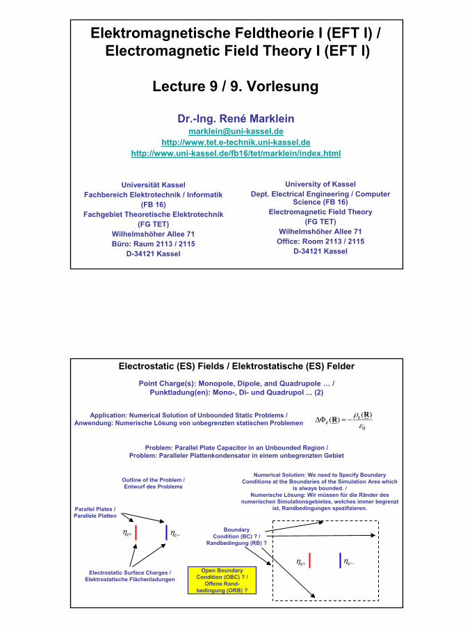
Elektromagnetische Feldtheorie I (EFT I) / Electromagnetic Field Theory I (EFT I) Lecture 9 / 9. Vorlesung University of Kassel Dept. Electrical Engineering / Computer Science (FB 16) Electromagnetic Field Theory (FG TET) Wilhelmshöher Allee 71 Office: Room 2113 / 2115 D-34121 Kassel Universität Kassel Fachbereich Elektrotechnik / Informatik (FB 16) Fachgebiet Theoretische Elektrotechnik (FG TET) Wilhelmshöher Allee 71 Büro: Raum 2113 / 2115 D-34121 Kassel Dr.-Ing. René Marklein [email protected] http://www.tet.e-technik.uni-kassel.de http://www.uni-kassel.de/fb16/tet/marklein/index.html Electrostatic (ES) Fields / Elektrostatische (ES) Felder Point Charge(s): Monopole, Dipole, and Quadrupole … / Punktladung(en): Mono-, Di- und Quadrupol ... (2) Application: Numerical Solution of Unbounded Static Problems / Anwendung: Numerische Lösung von unbegrenzten statischen Problemen e e 0 ( ) ( ) ρ ε ∆Φ =− R R Problem: Parallel Plate Capacitor in an Unbounded Region / Problem: Paralleler Plattenkondensator in einem unbegrenzten Gebiet e+ η e η − Electrostatic Surface Charges / Elektrostatische Flächenladungen Parallel Plates / Parallele Platten Numerical Solution: We need to Specify Boundary Conditions at the Boundaries of the Simulation Area which is always bounded. / Numerische Lösung: Wir müssen für die Ränder des numerischen Simulationsgebietes, welches immer begrenzt ist, Randbedingungen spezifizieren. e+ η e η − Outline of the Problem / Entwurf des Problems Boundary Condition (BC) ? / Randbedingung (RB) ? Open Boundary Condition (OBC) ? / Offene Rand- bedingung (ORB) ?
Transcript of Elektromagnetische Feldtheorie I (EFT I) / Electromagnetic ... · 3 Electrostatic (ES) Fields /...
1
Elektromagnetische Feldtheorie I (EFT I) /Electromagnetic Field Theory I (EFT I)
Lecture 9 / 9. Vorlesung
University of KasselDept. Electrical Engineering / Computer
Science (FB 16)Electromagnetic Field Theory
(FG TET)Wilhelmshöher Allee 71
Office: Room 2113 / 2115D-34121 Kassel
Universität KasselFachbereich Elektrotechnik / Informatik
(FB 16)Fachgebiet Theoretische Elektrotechnik
(FG TET)Wilhelmshöher Allee 71Büro: Raum 2113 / 2115
D-34121 Kassel
Dr.-Ing. René [email protected]
http://www.tet.e-technik.uni-kassel.dehttp://www.uni-kassel.de/fb16/tet/marklein/index.html
Electrostatic (ES) Fields / Elektrostatische (ES) Felder
Point Charge(s): Monopole, Dipole, and Quadrupole … / Punktladung(en): Mono-, Di- und Quadrupol ... (2)
Application: Numerical Solution of Unbounded Static Problems / Anwendung: Numerische Lösung von unbegrenzten statischen Problemen
ee
0
( )( )
ρε
∆Φ = −RR
Problem: Parallel Plate Capacitor in an Unbounded Region / Problem: Paralleler Plattenkondensator in einem unbegrenzten Gebiet
e+η eη −
Electrostatic Surface Charges / Elektrostatische Flächenladungen
Parallel Plates / Parallele Platten
Numerical Solution: We need to Specify Boundary Conditions at the Boundaries of the Simulation Area which
is always bounded. / Numerische Lösung: Wir müssen für die Ränder des
numerischen Simulationsgebietes, welches immer begrenzt ist, Randbedingungen spezifizieren.
e+η eη −
Outline of the Problem / Entwurf des Problems
Boundary Condition (BC) ? /
Randbedingung (RB) ?
Open Boundary Condition (OBC) ? /
Offene Rand-bedingung (ORB) ?
2
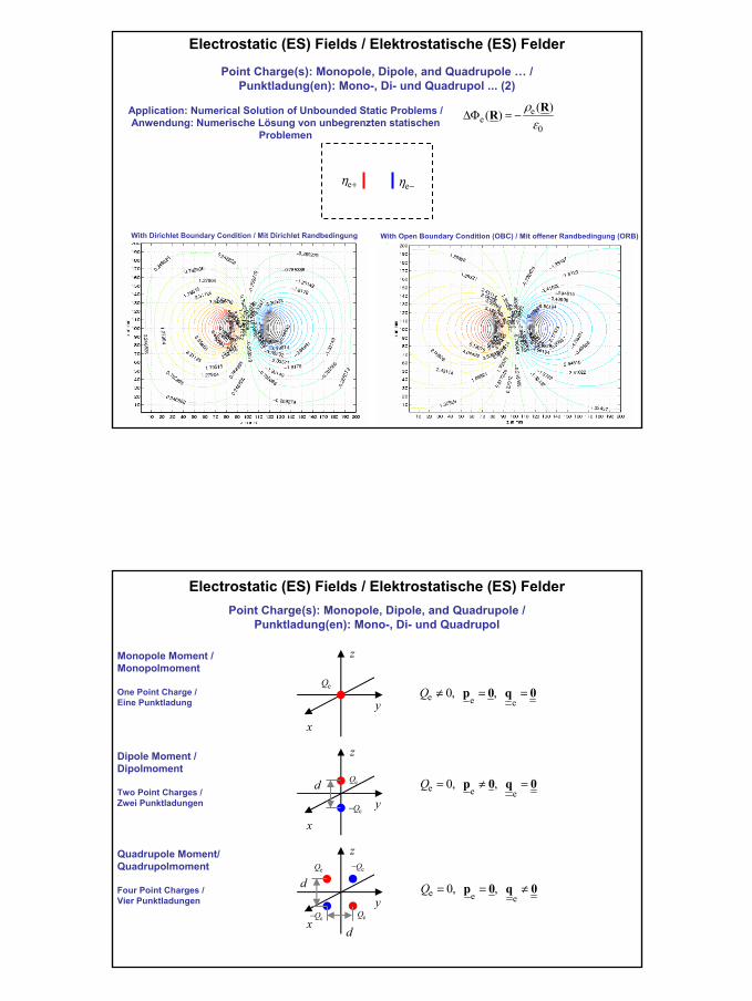
Electrostatic (ES) Fields / Elektrostatische (ES) Felder
Point Charge(s): Monopole, Dipole, and Quadrupole … / Punktladung(en): Mono-, Di- und Quadrupol ... (2)
Application: Numerical Solution of Unbounded Static Problems / Anwendung: Numerische Lösung von unbegrenzten statischen
Problemen
ee
0
( )( )
ρε
∆Φ = −RR
eη + eη −
With Dirichlet Boundary Condition / Mit Dirichlet Randbedingung With Open Boundary Condition (OBC) / Mit offener Randbedingung (ORB)
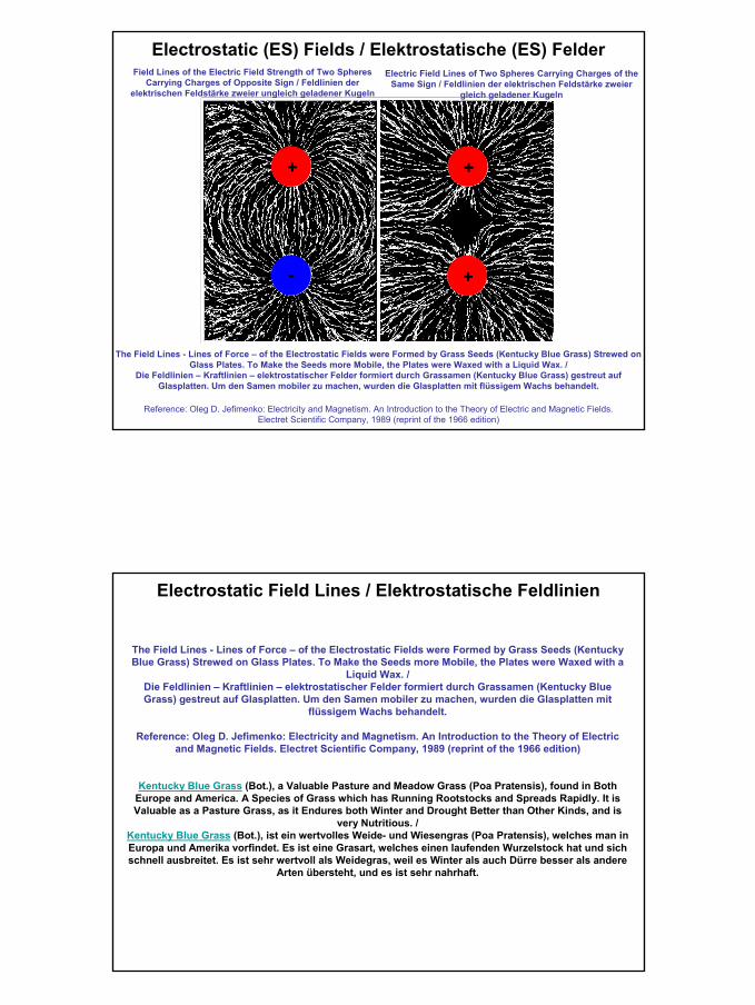
Point Charge(s): Monopole, Dipole, and Quadrupole / Punktladung(en): Mono-, Di- und Quadrupol
Electrostatic (ES) Fields / Elektrostatische (ES) Felder
e e e0, , Q ≠ = =p 0 q 0
z
y
x
Monopole Moment / Monopolmoment
One Point Charge /Eine Punktladung
z
y
x
Dipole Moment / Dipolmoment
Two Point Charges /Zwei Punktladungen
z
y
x
Quadrupole Moment/ Quadrupolmoment
Four Point Charges /Vier Punktladungen
eQ
d
d
eQ
eQ−
d
eQ−
eQ−
eQ
eQ
e e e0, , Q = ≠ =p 0 q 0
e e e0, , Q = = ≠p 0 q 0
3
Electrostatic (ES) Fields / Elektrostatische (ES) Felder
Reference: Oleg D. Jefimenko: Electricity and Magnetism. An Introduction to the Theory of Electric and Magnetic Fields. Electret Scientific Company, 1989 (reprint of the 1966 edition)
Field Lines of the Electric Field Strength of Two Spheres Carrying Charges of Opposite Sign / Feldlinien der
elektrischen Feldstärke zweier ungleich geladener Kugeln
+ +
+-
Electric Field Lines of Two Spheres Carrying Charges of the Same Sign / Feldlinien der elektrischen Feldstärke zweier
gleich geladener Kugeln
The Field Lines - Lines of Force – of the Electrostatic Fields were Formed by Grass Seeds (Kentucky Blue Grass) Strewed on Glass Plates. To Make the Seeds more Mobile, the Plates were Waxed with a Liquid Wax. /
Die Feldlinien – Kraftlinien – elektrostatischer Felder formiert durch Grassamen (Kentucky Blue Grass) gestreut auf Glasplatten. Um den Samen mobiler zu machen, wurden die Glasplatten mit flüssigem Wachs behandelt.
Electrostatic Field Lines / Elektrostatische Feldlinien
The Field Lines - Lines of Force – of the Electrostatic Fields were Formed by Grass Seeds (Kentucky Blue Grass) Strewed on Glass Plates. To Make the Seeds more Mobile, the Plates were Waxed with a
Liquid Wax. /Die Feldlinien – Kraftlinien – elektrostatischer Felder formiert durch Grassamen (Kentucky Blue Grass) gestreut auf Glasplatten. Um den Samen mobiler zu machen, wurden die Glasplatten mit
flüssigem Wachs behandelt.
Reference: Oleg D. Jefimenko: Electricity and Magnetism. An Introduction to the Theory of Electric and Magnetic Fields. Electret Scientific Company, 1989 (reprint of the 1966 edition)
Kentucky Blue Grass (Bot.), a Valuable Pasture and Meadow Grass (Poa Pratensis), found in Both Europe and America. A Species of Grass which has Running Rootstocks and Spreads Rapidly. It is Valuable as a Pasture Grass, as it Endures both Winter and Drought Better than Other Kinds, and is
very Nutritious. /Kentucky Blue Grass (Bot.), ist ein wertvolles Weide- und Wiesengras (Poa Pratensis), welches man in Europa und Amerika vorfindet. Es ist eine Grasart, welches einen laufenden Wurzelstock hat und sich schnell ausbreitet. Es ist sehr wertvoll als Weidegras, weil es Winter als auch Dürre besser als andere
Arten übersteht, und es ist sehr nahrhaft.
4
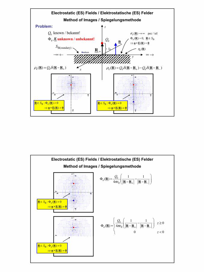
Method of Images / Spiegelungsmethode
Medium
nB(oundary)S
Electrostatic (ES) Fields / Elektrostatische (ES) Felder
e ( )η R
e
e B
( ) pec / iel( ) 0,
( )S
σ →∞Φ = ∈⇒ =
RR R
n×E R 0
z
y
x
eQ
Problem:
−∞← ∞→
B e: ( ) 0 ( )
S ≠∈ Φ⇒ ≠
R Rn×E R 0
B e: ( ) 0 ( )
S∈ Φ =⇒ =
R Rn×E R 0
e
e
known / bekannt!,
QΦ E unknown / unbekannt!
+R
e e( ) ( )Qρ δ += −R R R e e e( ) ( ) ( )Q Qρ δ δ+ −= − − −R R R R R
0z
B e: ( ) 0 ( )
S∈ Φ =⇒ =
R Rn×E R 0
Method of Images / SpiegelungsmethodeElectrostatic (ES) Fields / Elektrostatische (ES) Felder
B e: ( ) 0 ( )
S∈ Φ =⇒ =
R Rn×E R 0
ee
0
1 1( )4Qπε + −
Φ = − − −
RR R R R
e
e 0
1 1 0( ) 4
0 0
Qz
z
πε + −
− ≥ Φ = − −
<
R R R R R
5
Method of Images / SpiegelungsmethodeElectrostatic (ES) Fields / Elektrostatische (ES) Felder
B e: ( ) 0 ( )
S∈ Φ =⇒ =
R Rn×E R 0
Medium
nB(oundary)S
e ( )η R
e
e B
( ) pec / iel( ) 0,
( )S
σ →∞Φ = ∈⇒ =
RR R
n×E R 0
z
y
x
eQ
−∞← ∞→ Medium
nB(oundary)S
e ( )η R
e
e B
( ) pec / iel( ) 0,
( )S
σ →∞Φ = ∈⇒ =
RR R
n×E R 0
z
y
x
eQ
−∞← ∞→
eQ−
+R +R
−R
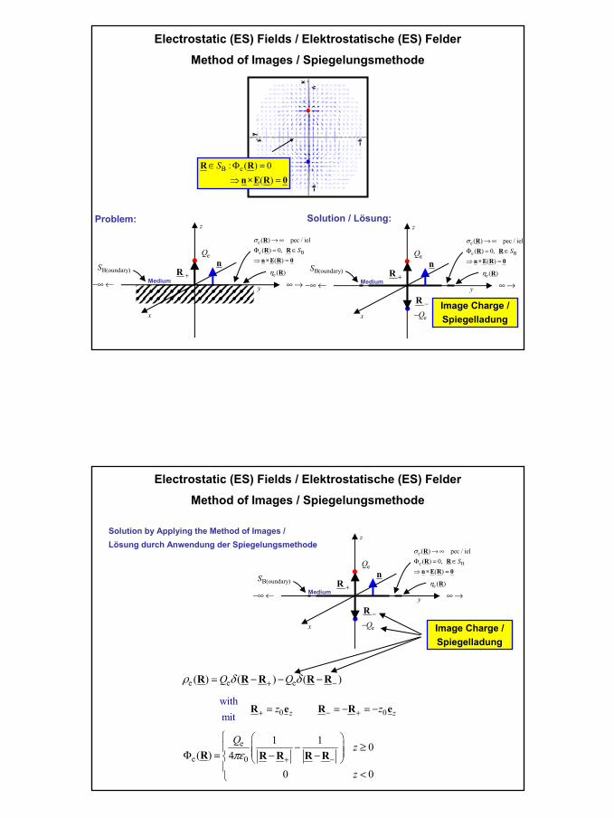
Problem: Solution / Lösung:
Image Charge / Spiegelladung
Method of Images / SpiegelungsmethodeElectrostatic (ES) Fields / Elektrostatische (ES) Felder
Medium
nB(oundary)S
e ( )η R
e
e B
( ) pec / iel( ) 0,
( )S
σ →∞Φ = ∈⇒ =
RR R
n×E R 0
z
y
x
eQ
−∞← ∞→
eQ−
+R
−R
Solution by Applying the Method of Images / Lösung durch Anwendung der Spiegelungsmethode
Image Charge / Spiegelladung
e
e 0
1 1 0( ) 4
0 0
Qz
z
πε + −
− ≥ Φ = − −
<
R R R R R
e e e( ) ( ) ( )Q Qρ δ δ+ −= − − −R R R R R
0 0 with
mit z zz z+ − += = − = −R e R R e
6
Method of Images / SpiegelungsmethodeElectrostatic (ES) Fields / Elektrostatische (ES) Felder
e
e 0
1 1 0( ) 4
0 0
Qz
z
πε + −
− ≥ Φ = − −
<
R R R R R
e e e( ) ( ) ( )Q Qρ δ δ+ −= − − −R R R R R 0 0 with
mit z zz z+ − += = − = −R e R R e
e
e3 3
0
0
e3 3
( ) ( )
04
0 0( ) ( )
04
0 0
Qz
z
Q z
z
πε
ε
π
+ −
+ −
+ −
+ −
= −∇Φ
− − − ≥= − − <
=
− − − ≥= − − <
E R R
R R R R
R R R R
D R E R
R R R R
R R R R
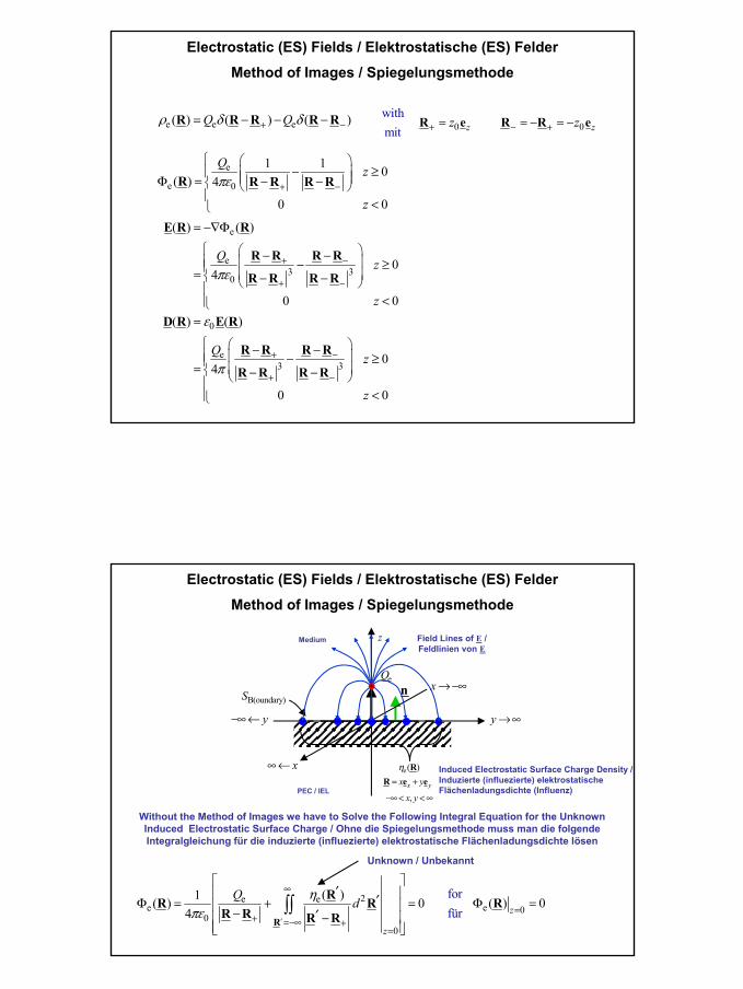
Method of Images / SpiegelungsmethodeElectrostatic (ES) Fields / Elektrostatische (ES) Felder
Medium
nB(oundary)S
e( )
,x yx y
x y
η= +
−∞< <∞
RR e e
z
eQ
y−∞← y→∞–– –– – ––
+
PEC / IEL
Induced Electrostatic Surface Charge Density / Induzierte (influezierte) elektrostatische Flächenladungsdichte (Influenz)
Field Lines of E / Feldlinien von E
Without the Method of Images we have to Solve the Following Integral Equation for the Unknown Induced Electrostatic Surface Charge / Ohne die Spiegelungsmethode muss man die folgende Integralgleichung für die induzierte (influezierte) elektrostatische Flächenladungsdichte lösen
2e ee
00
( )1( ) 04
z
Q dηπε
′
∞
+ =−∞ +=
′ ′Φ = + = − ′ −
∫∫R
RR RR R R R
Unknown / Unbekannt
x∞←
x→−∞
e 0f
(or
f r
0ü
) z=Φ =R
7
Method of Images / SpiegelungsmethodeElectrostatic (ES) Fields / Elektrostatische (ES) Felder
B
knownbekan
( )ntS∈ =RD R
Medium
nB(oundary)S
e( )η R
z
y
x
eQ
−∞← ∞→–– –– – ––
+
PEC / IEL
Induced Electrostatic Surface Charge Density / Induzierte (influezierte) elektrostatische Flächenladungsdichte (Influenz)
Field Lines of E / Feldlinien von E If D is known from the Method of Images /
Falls D über die Spiegelungsmethode bekannt ist
B
B
e
e3 3
e3 3
0
( ) ( )
04
4
forfür
S
S
z
z
Qz
Q
η
π
π
∈
+ −
+ − ∈
+ −
+ − =
=
− − = − = − −
− − = − − −
R
R
R n D R
R R R Rn
R R R R
R R R Re
R R R R
i
i
i
ηe(R) is Defined by the Normal Component of D / ηe(R) ist definiert über die Normalkomponente von D
!
Method of Images / SpiegelungsmethodeElectrostatic (ES) Fields / Elektrostatische (ES) Felder
( ) ( )
( ) ( )
Be
e3 3
0
e 0 03/ 2 3/ 22 22 2 2 2
0 00
e 0 03/ 2 3/ 22 2 2 2 2 2
0 0
e 0
2 2 20
( ) ( )
4
4
4
2
S
z z
z
z
Q
Q z z z z
x y z z x y z z
Q z z
x y z x y z
Q z
x y z
η
π
π
π
π
∈
+ −
+ − =
=
=
− − = − − −
− +
= − + + − + + −
− = −
+ + + +
= − + +
RR n D R
e R R e R R
R R R R
i
i i
3/ 2
e 03/ 22 2
02Q z
r zπ= −
+
8
Method of Images / SpiegelungsmethodeElectrostatic (ES) Fields / Elektrostatische (ES) Felder
Be
e 03/ 22 2
0
( ) ( )
2
S
Q z
r z
η
π
∈=
= − +
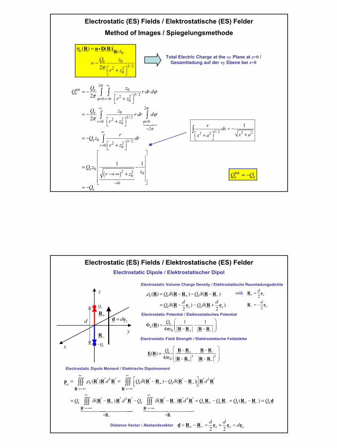
RR n D RiTotal Electric Charge at the xy Plane at z=0 /
Gesamtladung auf der xy Ebene bei z=0
( )
2tot e 0e 3/ 22 20 0 0
2e 0
3/ 22 20 002
e 0 3/ 22 20 0
e 0 2 2 00
0e
2
2
1 1
r
r
r
Q zQ r dr d
r z
Q zr dr d
r z
rQ z drr z
Q zzr z
Q
π
ϕ
π
ϕ
π
ϕπ
ϕπ
∞
= =
∞
= =
=∞
=
→
= − +
= − +
= − +
= −
→∞ +
= −
∫ ∫
∫ ∫
∫3/ 2 2 22 2
1x dxx ax a
= − ++ ∫
tote eQ Q= −
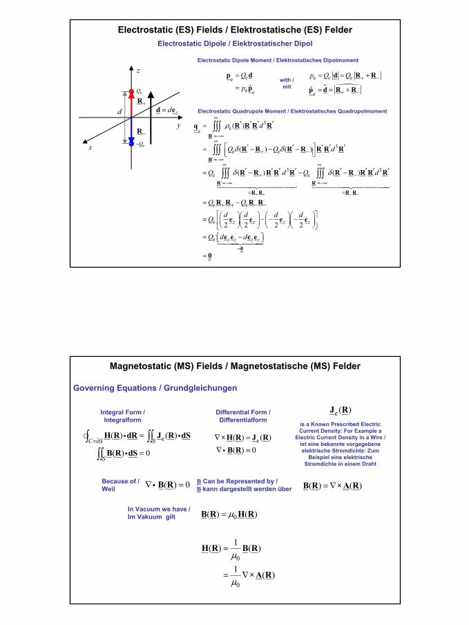
Electrostatic Dipole / Elektrostatischer Dipol
Electrostatic (ES) Fields / Elektrostatische (ES) Felder
e e e
e e
( ) ( ) ( )
( ) ( )2 2z z
Q Qd dQ Q
ρ δ δ
δ δ
+ −= − − −
= − − +
R R R R R
R e R e
z
y
x
d
eQ
eQ−
with 2
2
z
z
d
d
+
−
=
= −
R e
R e
+R
−R
ee
0
1 1( )4Qπε + −
Φ = − − −
RR R R R
Electrostatic Dipole Moment / Elektrische Dipolmoment
zd=d e
Distance Vector / Abstandsvektor2 2z z zd d d+ −= − = + =d R R e e e
3 3e e ee
3 3e e e e e e
( ) ( ) ( )
( ) ( ) ( )
d Q Q d
Q d Q d Q Q Q Q
ρ δ δ
δ δ
′ ′
′ ′
+ −
∞ ∞
+ −=−∞ =−∞
∞ ∞
+ − + − + −=−∞ =−∞
= =
′ ′ ′ ′ ′ ′ ′= = − − −
′ ′ ′ ′ ′ ′= − − − = − = − =
∫∫∫ ∫∫∫
∫∫∫ ∫∫∫
R R
R R
R R
p R R R R R R R R R
R R R R R R R R R R R R d
Electrostatic Volume Charge Density / Elektrostatische Raumladungsdichte
Electrostatic Potential / Elektrostatisches Potential
e3 3
0( )
4Qπε
+ −
+ −
− − = − − −
R R R RE R
R R R R
Electrostatic Field Strength / Elektrostatische Feldstärke
9
Electrostatic Dipole / Elektrostatischer Dipol
Electrostatic (ES) Fields / Elektrostatische (ES) Felder
z
y
x
d
eQ
eQ−
+R
−R
zd=d e
3ee
3e e
3 3e e
e e
e
( )
( ) ( )
( ) ( )
2 2z z
d
Q Q d
Q d Q d
Q Q
d dQ
ρ
δ δ
δ δ
′
′
′ ′
+ + − −
∞
=−∞∞
+ −=−∞
∞ ∞
+ −=−∞ =−∞
= =
+ + − −
′ ′ ′ ′=
′ ′ ′ ′ ′= − − −
′ ′ ′ ′ ′ ′ ′ ′= − − −
= −
=
∫∫∫
∫∫∫
∫∫∫ ∫∫∫
R
R
R R
R R R R
q R R R R
R R R R R R R
R R R R R R R R R R
R R R R
e e
e
2 2z z
z z z z
d d
Q d d=
− − − = −
=0
e e
e e e e
0
Electrostatic Dipole Moment / Elektrostatisches Dipolmoment
ee
e eˆ
Q
p
=
=
p d
pe
eˆ
e ep Q Q + −
+ −
= = +
= = +
d R R
p d R Rwith / mit
Electrostatic Quadrupole Moment / Elektrostatisches Quadrupolmoment
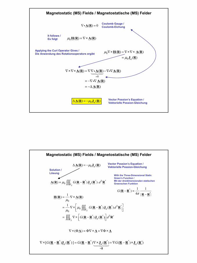
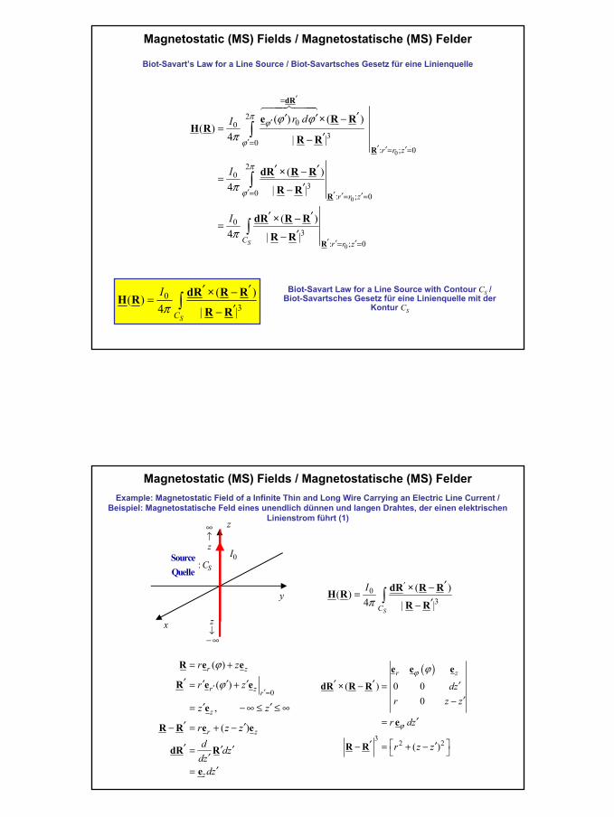
Magnetostatic (MS) Fields / Magnetostatische (MS) Felder
e( ) ( )
( ) 0C S S
S
=∂=
=
∫ ∫∫∫∫
H R dR J R dS
B R dS
i i
ie( ) ( )
( ) 0∇ =∇ =
×H R J RB Ri
( ) ( )=∇B R × A R
0( ) ( )= µB R H R
0
0
1( ) ( )
1 ( )
=
= ∇
µ
µ
H R B R
× A R
Governing Equations / Grundgleichungen
Integral Form / Differential Form / Integralform Differentialform
e ( )J Ris a Known Prescribed Electric Current Density: For Example a
Electric Current Density in a Wire /ist eine bekannte vorgegebene elektrische Stromdichte: Zum
Beispiel eine elektrische Stromdichte in einem Draht
( ) 0∇ =B RiBecause of /Weil
B Can be Represented by / B kann dargestellt werden über
In Vacuum we have / Im Vakuum gilt
10
( ) 0∇ =iA R
0 ( ) ( )µ =∇H R ×A R
0
0 e
( ) ( )( )
µµ
∇ =∇ ∇=
×H R × × A RJ R
0
( ) ( ) ( )
( )( )
=
∇ ∇ =∇∇ −∇ ∇
= −∇ ∇= −∆
× ×A R A R A R
A RA R
i i
i
0 e( ) ( )µ∆ = −A R J R
Magnetostatic (MS) Fields / Magnetostatische (MS) Felder
Coulomb Gauge / Coulomb-Eichung
It follows / Es folgt
Applying the Curl Operator Gives / Die Anwendung des Rotationsoperators ergibt
Vector Possion’s Equation / Vektorielle Possion-Gleichung
30 e( ) ( ) ( )
SVG dµ ′ ′ ′= −∫∫∫A R R R J R R
0
30 e
0
3e
1( ) ( )
1 ( ) ( )
( ) ( )
S
S
V
V
G d
G d
µ
µµ
= ∇
′ ′ ′= ∇ −
′ ′ ′= ∇ −
∫∫∫
∫∫∫
H R × A R
× R R J R R
× R R J R R
( )∇ Φ = Φ∇ +∇Φ× A × A × A
e e e[ ( ) ( ) ] ( ) ( ) ( ) ( )G G G=
′ ′ ′ ′ ′ ′∇ − = − ∇ +∇ −0
× R R J R R R × J R R R ×J R
Magnetostatic (MS) Fields / Magnetostatische (MS) Felder
0 e( ) ( )µ∆ = −A R J R Vector Possion’s Equation / Vektorielle Possion-Gleichung
Solution / Lösung
1 1( )4 | |
Gπ
′− =′−
R RR R
With the Three-Dimensional Static Green’s Function / Mit der dreidimensionalen statischen Greenschen Funktion
11
3
1 1 1 1 1( )4 4 4| | | | | |
Gπ π π
′−′∇ − = ∇ = ∇ = −′ ′ ′− − −
R RR RR R R R R R
3e3
3e3
3e3
1( ) ( )4 | |
( ) ( )14 | |
( ) ( )14 | |
S
S
S
V
V
V
d
d
d
π
π
π
′− ′ ′= −′−
′ ′− ′=′−
′ ′− ′=′−
∫∫∫
∫∫∫
∫∫∫
R RH R × J R RR R
J R × R RR
R R
J R × R RR
R R
Magnetostatic (MS) Fields / Magnetostatische (MS) Felder
3e3
( ) ( )1( )4 | |SV
dπ
′ ′− ′=′−
∫∫∫J R × R R
H R RR R
Biot-Savart’s Law (for a Given Volume Source) / Biot-Savartsches Gesetz (für eine Volumenquelle)
Magnetostatic (MS) Fields / Magnetostatische (MS) Felder
0 0 0e ( ) ( ) ( ) , 0I r - r z rϕδ δ= >J R e
3e3
20 0
30 0
200
30 0 : 0
( ) ( )1( )4 | |
( ) ( ) ( ) ( )14 | |
( ) ( ) ( )
4 | |
SV
z r
r z
d
I r r zr dr d dz
r rI r dr d
πϕ
ϕ
πϕ
ϕ
π
δ δ ϕϕ
π
δ ϕϕ
π
∞ ∞′
′ ′ ′−∞ = =
∞′
′ ′= = ′ ′=
′ ′− ′=′−
′′ ′ ′− −′ ′ ′ ′=
′−
′′ ′− −′ ′ ′=
′−
∫∫∫
∫ ∫ ∫
∫ ∫R
J R × R RH R R
R R
e × R R
R R
e × R R
R R
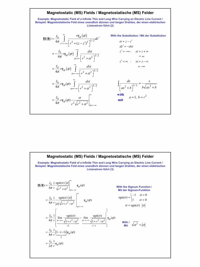
Biot-Savart’s Law for a Line Source / Biot-Savartsches Gesetz für eine Linienquellez
y
x
0r
: SCSourceQuelle
0I e ( )J R
Wire Carrying a Constant Electric Current I0 / Biot-Savartsches Gesetz für eine Linienquelle
12
0
0
0
200
30
: ; 0
20
30 : ; 0
03
: ; 0
( ) ( )( )
4 | |
( )4 | |
( )4 | |
S
r r z
r r z
C r r z
r dI
I
I
πϕ
ϕ
π
ϕ
ϕ ϕπ
π
π
′=
′
′=′ ′ ′= =
′= ′ ′ ′= =
′ ′ ′= =
′′ ′ −=
′−
′ ′−=′−
′ ′−=′−
∫
∫
∫
dR
R
R
R
e × R RH R
R R
dR × R R
R R
dR × R R
R R
03
( )( )4 | |
SC
Iπ
′ ′−=′−
∫dR × R RH R
R R
Biot-Savart Law for a Line Source with Contour CS / Biot-Savartsches Gesetz für eine Linienquelle mit der
Kontur CS
Magnetostatic (MS) Fields / Magnetostatische (MS) Felder
Biot-Savart’s Law for a Line Source / Biot-Savartsches Gesetz für eine Linienquelle
03
( )( )4 | |
′ ′−=′−
∫SC
Iπ
dR × R RH RR R
0
( )
( )
,
( )
r z
r z r
z
r z
z
r z
r z
z z
r z zd dzdzdz
ϕ
ϕ′ ′=
= +
′ ′ ′ ′= +
′ ′= −∞ ≤ ≤ ∞
′ ′− = + −
′ ′ ′=′′=
R e e
R e e
e
R R e e
dR R
e
( )
32 2
( ) 0 00
( )
r z
dzr z z
r dz
r z z
ϕ
ϕ
ϕ′ ′ ′− =
′−
′=
′ ′− = + −
e e e
dR × R R
e
R R
Magnetostatic (MS) Fields / Magnetostatische (MS) FelderExample: Magnetostatic Field of a Infinite Thin and Long Wire Carrying an Electric Line Current /
Beispiel: Magnetostatische Feld eines unendlich dünnen und langen Drahtes, der einen elektrischen Linienstrom führt (1)z
y
x
: SCSourceQuelle
0I
z↓−∞
z
∞↑
13
:
:
=
z zdz dz z
z z
αα
α
α
′= −′ = −′ = −∞ = +∞
∞′ = ∞ = −∞
= −∞
( )
( )
( )
03 / 22 2
03 / 22 2
03 / 22 2
03/ 22 2
02 2 2
( )4 ( )
4
4
( )4
( )4
z
rIdz
r z z
I drr
I drr
I drr
Ir
r r
ϕ
ϕα
ϕα
ϕα
ϕα
ϕπ
αϕπ α
αϕπ α
αϕπ α
αϕπ α
∞
′=−∞
−∞
=∞
∞
=−∞
∞
=−∞
∞
=−∞
′= ′+ −
= − +
= +
= +
=+
∫
∫
∫
∫
eH R
e
e
e
e
3/ 2 22
2 1,
dx x
b ax bax b
a b r
= ++
= =
∫
withmit
With the Substitution / Mit der Substitution
Magnetostatic (MS) Fields / Magnetostatische (MS) FelderExample: Magnetostatic Field of a Infinite Thin and Long Wire Carrying an Electric Line Current /
Beispiel: Magnetostatische Feld eines unendlich dünnen und langen Drahtes, der einen elektrischen Linienstrom führt (2)
[ ]
02 2
02 2
02 2 2 2
1 1
0
2
0
sgn( )1( ) ( )4
sgn( )1 ( )4 1 /
1 sgn( ) sgn( )lim lim ( )4 1 / 1 /
1 1 ( 1) ( )4
1 ( )2
Ir r
Ir r
Ir r r
Ir
Ir
ϕα
ϕ
α
ϕα α
ϕ
ϕ
α αϕ
π α
α αϕ
π α α
α α ϕπ α α
ϕπ
ϕπ
∞
=−∞∞
=−∞
→∞ →−∞
= =−
=+
=+
= − + +
= − −
=
H R e
e
e
e
e
1 0sgn( )
1 0
sgn( )
αα
αα α α
− <= >=
With the Signum Function /Mit der Signum-Funktion
Magnetostatic (MS) Fields / Magnetostatische (MS) FelderExample: Magnetostatic Field of a Infinite Thin and Long Wire Carrying an Electric Line Current /
Beispiel: Magnetostatische Feld eines unendlich dünnen und langen Drahtes, der einen elektrischen Linienstrom führt (3)
2 =α αWith /
Mit
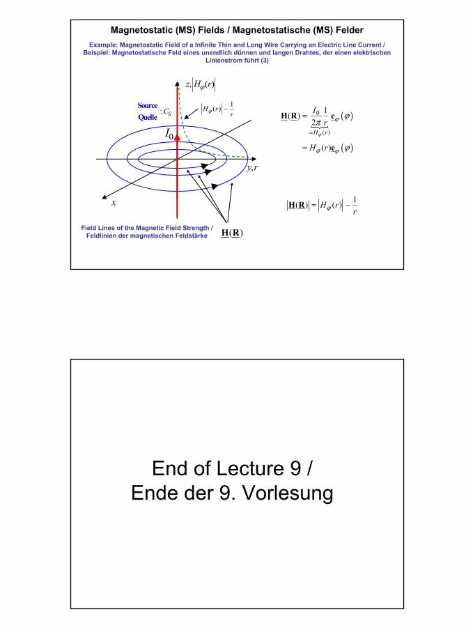
14
, ( )z H rϕ
,y r
x
: SCSourceQuelle
0I
Magnetostatic (MS) Fields / Magnetostatische (MS) FelderExample: Magnetostatic Field of a Infinite Thin and Long Wire Carrying an Electric Line Current /
Beispiel: Magnetostatische Feld eines unendlich dünnen und langen Drahtes, der einen elektrischen Linienstrom führt (3)
( )
( )
0
( )
1( )2
( )
H r
Ir
H r
ϕ
ϕ
ϕ ϕ
ϕπ
ϕ
=
=
=
H R e
e
1( ) ( )H rrϕ=H R ∼
1( )H rrϕ ∼
( )H RField Lines of the Magnetic Field Strength / Feldlinien der magnetischen Feldstärke
End of Lecture 9 /Ende der 9. Vorlesung


![[eBook Acoustics Audio HiFi DIY]How to Build an Electrostatic Tweeter{SHACKMAN.de}](https://static.fdokument.com/doc/165x107/563db811550346aa9a903f06/ebook-acoustics-audio-hifi-diyhow-to-build-an-electrostatic-tweetershackmande.jpg)