
Essays in Applied Econometrics - MADOC · Essays in Applied Econometrics Inauguraldissertation zur...
193
Essays in Applied Econometrics Inauguraldissertation zur Erlangung des akademischen Grades eines Doktors der Wirtschaftswissenschaften der Universit¨ at Mannheim Mich` ele Anne Weynandt vorgelegt im Fr¨ uhjahrssemester 2014
Transcript of Essays in Applied Econometrics - MADOC · Essays in Applied Econometrics Inauguraldissertation zur...

Essays in Applied Econometrics
Inauguraldissertation zur Erlangung des akademischen Grades
eines Doktors der Wirtschaftswissenschaften
der Universitat Mannheim
Michele Anne Weynandt
vorgelegt im Fruhjahrssemester 2014

Abteilungssprecher: Prof. Dr. Eckhard Janeba
Referent: Prof. Gerard van den Berg, Ph.D.
Korreferent: Prof. Dr. Andrea Weber
Verteidigung: 28.05.2014

Acknowledgements
Many people have impacted me throughout the writing of this thesis. First I would like to thank
my advisors Gerard van den Berg and Andrea Weber for their constant support, feedback and
availability to discuss research. I would like to thank my co-authors namely; Gerard van den
Berg (Chapter 2 and 3), Anna Hammerschmid (Chapter 3), Perihan Saygin (Chapter 4) and
Andrea Weber (Chapter 4) for their constructive criticism, development and exchange of ideas.
I must highlight the great office climate that belongs to the CEEE floor, but I also want to
thank my fellow students at the CDSE for countless research discussions. In particular, Annette
Bergemann, Barbara Hofmann, Lena Janys, Pia Pinger, Ricarda Schmidl, Bettina Siflinger, and
Arne Uhlendorff.
Furthermore I would like to thank Stefano DellaVigna for his advice and encouragement to
start working on Chapter 2 which emerged from a class project at the University of California,
Berkeley. I would also like to thank David Card from whose comments Chapter 5 benefited
during a short stay at Berkeley.
Moreover I would like to thank Hannes Kammerer, Vera Molitor and Johannes Schoch for their
constant support, lunch and coffee breaks and numerous non-research related activities, which
kept my mind fresh for yet another robustness check. A special thanks also belongs to Vera
Molitor - who proof read every single one of my papers and was willing to discuss every problem
that emerged - and to Lena Janys for helping out a friend in need.
I want to thank my basketball coaches, teammates, players and workout partners for their
constant patience in supporting my moods. I especially want to thank Mike Gould for his
guidance on and off the court, as well as Uta Gelbke who supports my emotional and loud
character but knows when to keep it calm. I would like to thank my roommate Sophia Schmitz
for the support and dinners after some long work days. I would also like to thank my mentor,
Oliver Schwaab whose guidance and support was invaluable throughout this thesis. Furthermore

I would like to thank Heike, Marie, Lena and Lukas Schwaab for offering their constant support
and a second home to me. Last but not least I would like to thank my parents, Jean-Paul and
Christiane Weynandt as well as my siblings Vincent and Claude for their constant support,
patience, and encouragement without them it would not have been possible to complete this
thesis.
Michele Weynandt
Mannheim, Spring 2014
iv

Contents
List of Figures x
List of Tables xiii
1 Introduction 1
2 Explaining Differences Between the Expected and Actual Duration Until
Return Migration: Economic Changes and Behavioral Factors 5
2.1 Introduction . . . . . . . . . . . . . . . . . . . . . . . . . . . . . . . . . . . . . . . 5
2.2 Literature . . . . . . . . . . . . . . . . . . . . . . . . . . . . . . . . . . . . . . . . 7
2.2.1 Return Migration . . . . . . . . . . . . . . . . . . . . . . . . . . . . . . . . 7
2.2.2 Hedonic Forecasting and Projection Bias . . . . . . . . . . . . . . . . . . . 8
2.3 Data and Presence of a Bias . . . . . . . . . . . . . . . . . . . . . . . . . . . . . . 10
2.3.1 Data . . . . . . . . . . . . . . . . . . . . . . . . . . . . . . . . . . . . . . . 10
2.3.2 Presence of a Bias . . . . . . . . . . . . . . . . . . . . . . . . . . . . . . . 11
2.4 Model . . . . . . . . . . . . . . . . . . . . . . . . . . . . . . . . . . . . . . . . . . 16
2.5 Results . . . . . . . . . . . . . . . . . . . . . . . . . . . . . . . . . . . . . . . . . . 20
2.6 Conclusion . . . . . . . . . . . . . . . . . . . . . . . . . . . . . . . . . . . . . . . 32
2.A Data Addendum . . . . . . . . . . . . . . . . . . . . . . . . . . . . . . . . . . . . 38
2.A.1 Possible Differences between Dustmann’s Approach and our Approach . . 38
2.A.2 Intentions and Residence Status . . . . . . . . . . . . . . . . . . . . . . . 39
3 Bereavement Effects and Early Life Circumstances 45
3.1 Introduction . . . . . . . . . . . . . . . . . . . . . . . . . . . . . . . . . . . . . . . 45
3.2 Empirical Strategy . . . . . . . . . . . . . . . . . . . . . . . . . . . . . . . . . . . 49
3.3 Data . . . . . . . . . . . . . . . . . . . . . . . . . . . . . . . . . . . . . . . . . . . 50
3.3.1 Outcome Variables . . . . . . . . . . . . . . . . . . . . . . . . . . . . . . . 51
3.3.2 Bereavement . . . . . . . . . . . . . . . . . . . . . . . . . . . . . . . . . . 51
3.3.3 Early Life Circumstances . . . . . . . . . . . . . . . . . . . . . . . . . . . 52
3.3.4 Descriptive Statistics . . . . . . . . . . . . . . . . . . . . . . . . . . . . . . 53
3.4 Results . . . . . . . . . . . . . . . . . . . . . . . . . . . . . . . . . . . . . . . . . . 55
v

CONTENTS
3.4.1 Main Results . . . . . . . . . . . . . . . . . . . . . . . . . . . . . . . . . . 55
3.4.2 Sensitivity Analyses . . . . . . . . . . . . . . . . . . . . . . . . . . . . . . 60
3.4.3 Effect Heterogeneity . . . . . . . . . . . . . . . . . . . . . . . . . . . . . . 61
3.5 Conclusion . . . . . . . . . . . . . . . . . . . . . . . . . . . . . . . . . . . . . . . 66
3.A Data Addendum . . . . . . . . . . . . . . . . . . . . . . . . . . . . . . . . . . . . 70
3.A.1 Description of the “Fruhe Kindheit im (Nach-)Kriegskontext” (FKM) . . 70
3.A.2 Generating the Bereavement Indicators . . . . . . . . . . . . . . . . . . . 70
3.A.3 Histograms of Outcome Variables . . . . . . . . . . . . . . . . . . . . . . . 74
3.B F-tests . . . . . . . . . . . . . . . . . . . . . . . . . . . . . . . . . . . . . . . . . . 76
3.C Fixed Effects and Level Regressions . . . . . . . . . . . . . . . . . . . . . . . . . 79
3.D Sensitivity Analysis . . . . . . . . . . . . . . . . . . . . . . . . . . . . . . . . . . . 83
4 Coworkers, Networks and Job Search Outcomes 87
4.1 Introduction . . . . . . . . . . . . . . . . . . . . . . . . . . . . . . . . . . . . . . . 87
4.2 Data and Network Definitions . . . . . . . . . . . . . . . . . . . . . . . . . . . . . 91
4.3 Empirical Analysis . . . . . . . . . . . . . . . . . . . . . . . . . . . . . . . . . . . 102
4.3.1 Worker Level Analysis . . . . . . . . . . . . . . . . . . . . . . . . . . . . . 102
4.3.2 Firm Level Analysis . . . . . . . . . . . . . . . . . . . . . . . . . . . . . . 110
4.4 Conclusion . . . . . . . . . . . . . . . . . . . . . . . . . . . . . . . . . . . . . . . 113
4.A Networks Appendix . . . . . . . . . . . . . . . . . . . . . . . . . . . . . . . . . . 115
4.A.1 Reemployment Probability . . . . . . . . . . . . . . . . . . . . . . . . . . 115
4.A.2 Robustness Checks . . . . . . . . . . . . . . . . . . . . . . . . . . . . . . . 115
5 Selective Firing and Lemons? 119
5.1 Introduction . . . . . . . . . . . . . . . . . . . . . . . . . . . . . . . . . . . . . . . 119
5.2 Theoretical and Empirical Framework . . . . . . . . . . . . . . . . . . . . . . . . 123
5.2.1 Signaling according to Gibbons and Katz (1991) . . . . . . . . . . . . . . 123
5.2.2 Measure of Productivity and Sorting . . . . . . . . . . . . . . . . . . . . . 126
5.2.3 Sorting . . . . . . . . . . . . . . . . . . . . . . . . . . . . . . . . . . . . . 127
5.3 Data . . . . . . . . . . . . . . . . . . . . . . . . . . . . . . . . . . . . . . . . . . . 128
5.4 Results . . . . . . . . . . . . . . . . . . . . . . . . . . . . . . . . . . . . . . . . . . 133
5.4.1 Heterogeneity . . . . . . . . . . . . . . . . . . . . . . . . . . . . . . . . . . 133
5.4.2 Signaling versus Sorting? . . . . . . . . . . . . . . . . . . . . . . . . . . . 138
5.5 Conclusion . . . . . . . . . . . . . . . . . . . . . . . . . . . . . . . . . . . . . . . 157
5.A AKM Appendix . . . . . . . . . . . . . . . . . . . . . . . . . . . . . . . . . . . . . 159
5.A.1 Measure of Productivity according to Abowd et al. (1999) (AKM) . . . . 159
5.B Figures . . . . . . . . . . . . . . . . . . . . . . . . . . . . . . . . . . . . . . . . . 166
5.C Tables . . . . . . . . . . . . . . . . . . . . . . . . . . . . . . . . . . . . . . . . . . 167
vi

Bibliography 169
vii

viii

List of Figures
2.1 Descriptive Statistics 1 . . . . . . . . . . . . . . . . . . . . . . . . . . . . . . . . . 14
2.2 Descriptive Statistics 2 . . . . . . . . . . . . . . . . . . . . . . . . . . . . . . . . . 15
2.3 Expected Duration of Stay . . . . . . . . . . . . . . . . . . . . . . . . . . . . . . . 23
2.4 Difference Between Intentions and Predicted Realizations . . . . . . . . . . . . . 27
2.5 “Narrow Framing” . . . . . . . . . . . . . . . . . . . . . . . . . . . . . . . . . . . 28
2.6 Difference Between Intentions and Predicted Return, Learning? . . . . . . . . . . 29
2.7 Average Forecast Error . . . . . . . . . . . . . . . . . . . . . . . . . . . . . . . . . 31
3.1 Potential Role of Early Life Conditions on the Effect of Adverse Events Later in
Life on Mental Health . . . . . . . . . . . . . . . . . . . . . . . . . . . . . . . . . 48
3.2 Early-Life Conditions, Adverse Life Events and Later-life Mental Health . . . . . 49
3.3 Outcome Variables in the SOEP . . . . . . . . . . . . . . . . . . . . . . . . . . . 56
3.4 Histograms MCS . . . . . . . . . . . . . . . . . . . . . . . . . . . . . . . . . . . . 74
3.5 Histograms Satisfaction . . . . . . . . . . . . . . . . . . . . . . . . . . . . . . . . 75
4.1 Job Seekers and Networks of Past Co-workers by Gender . . . . . . . . . . . . . . 95
4.2 Job Seekers and Networks of Past Co-workers by Employment Status . . . . . . . 96
4.3 Closing Firms and Connected Firms . . . . . . . . . . . . . . . . . . . . . . . . . 99
4.4 Distribution of Network Characteristics . . . . . . . . . . . . . . . . . . . . . . . 101
4.5 Exit Rates to Jobs . . . . . . . . . . . . . . . . . . . . . . . . . . . . . . . . . . . 103
4.6 Employment and Wages Before and After Displacement, by Network Characteristics107
5.1 Mean Wages Re-employed Individuals . . . . . . . . . . . . . . . . . . . . . . . . 120
5.2 Possible Sorting Mechanism in the GK model . . . . . . . . . . . . . . . . . . . . 124
5.3 Person Effects . . . . . . . . . . . . . . . . . . . . . . . . . . . . . . . . . . . . . . 134
5.4 Firm Effects at Displacement . . . . . . . . . . . . . . . . . . . . . . . . . . . . . 136
5.5 Firm Effects at the Re-Employment Firm . . . . . . . . . . . . . . . . . . . . . . 137
5.6 Mean Wages of Re-employed Individuals by Person Quintile . . . . . . . . . . . . 143
5.7 Mass Layoff Deciles . . . . . . . . . . . . . . . . . . . . . . . . . . . . . . . . . . . 149
5.8 Closure Deciles . . . . . . . . . . . . . . . . . . . . . . . . . . . . . . . . . . . . . 150
ix

LIST OF FIGURES
5.9 Involuntary Layoff Deciles . . . . . . . . . . . . . . . . . . . . . . . . . . . . . . . 151
5.10 Mean Wages of Job Changers, Classified by Quartile of Mean Wage of Co-Workers
at Origin and Destination Firm, 1990-97 . . . . . . . . . . . . . . . . . . . . . . . 163
5.11 Mean Wages of Job Changers, Classified by Quartile of Mean Wage of Co-Workers
at Origin and Destination Firm, 2002-2009 . . . . . . . . . . . . . . . . . . . . . 163
5.12 Person Effects by Type of Layoff . . . . . . . . . . . . . . . . . . . . . . . . . . . 166
x

List of Tables
2.1 Return Frequency . . . . . . . . . . . . . . . . . . . . . . . . . . . . . . . . . . . 11
2.2 Intentions and Realization 1984 - 2009 . . . . . . . . . . . . . . . . . . . . . . . . 12
2.3 Desire to Return versus Residence Status . . . . . . . . . . . . . . . . . . . . . . 13
2.4 Socioeconomic Differences . . . . . . . . . . . . . . . . . . . . . . . . . . . . . . . 13
2.5 Complementary Log-log model . . . . . . . . . . . . . . . . . . . . . . . . . . . . 21
2.6 Logit model . . . . . . . . . . . . . . . . . . . . . . . . . . . . . . . . . . . . . . . 22
2.7 Difference in Expectations . . . . . . . . . . . . . . . . . . . . . . . . . . . . . . . 24
2.8 Difference in Expectations Behavioral Factors . . . . . . . . . . . . . . . . . . . . 26
2.9 Difference between the Intentions and the predicted Return . . . . . . . . . . . . 33
2.10 Difference without those that intend to stay forever . . . . . . . . . . . . . . . . . 34
2.11 Robustness Check on the Difference . . . . . . . . . . . . . . . . . . . . . . . . . 35
2.12 Difference between the Intentions and the Return, Behavioral Factors . . . . . . 36
2.13 Return Frequency 1985 - 1997 . . . . . . . . . . . . . . . . . . . . . . . . . . . . . 38
2.14 Intentions and Realization 1984 - 1997 . . . . . . . . . . . . . . . . . . . . . . . . 38
2.15 Intentions and Realizations 1984 - 1997 Dustmann (2003a) Table 2 . . . . . . . . 39
2.16 Intentions and Realization 1996 - 2009 . . . . . . . . . . . . . . . . . . . . . . . . 39
2.17 Desire to Return versus Residence Status 1996 . . . . . . . . . . . . . . . . . . . 39
2.18 Socioeconomic Differences for Stayers . . . . . . . . . . . . . . . . . . . . . . . . 40
2.19 Country of Origin . . . . . . . . . . . . . . . . . . . . . . . . . . . . . . . . . . . 41
2.20 Difference between the Intentions and the ‘rational’ Expectations 1984 - 1996 . . 42
2.21 Difference between the Intentions and the ‘rational’ Expectations 1997 - 2008 . . 43
3.1 Summary Statistics MCS . . . . . . . . . . . . . . . . . . . . . . . . . . . . . . . 53
3.2 Summary Statistics Satisfaction . . . . . . . . . . . . . . . . . . . . . . . . . . . . 54
3.3 Treatment Cases MCS . . . . . . . . . . . . . . . . . . . . . . . . . . . . . . . . . 54
3.4 Treatment Cases Satisfaction . . . . . . . . . . . . . . . . . . . . . . . . . . . . . 54
3.5 Results MCS 2010 - 2012 . . . . . . . . . . . . . . . . . . . . . . . . . . . . . . . 57
3.6 First Difference Results MCS . . . . . . . . . . . . . . . . . . . . . . . . . . . . . 58
3.7 Results Life Satisfaction . . . . . . . . . . . . . . . . . . . . . . . . . . . . . . . . 59
xi

LIST OF TABLES
3.8 Results Satisfaction Sleep . . . . . . . . . . . . . . . . . . . . . . . . . . . . . . . 60
3.9 First Difference Results MCS Father’s Education . . . . . . . . . . . . . . . . . . 63
3.10 First Difference Results Life Satisfaction Father’s Education Interaction . . . . . 64
3.11 First Difference Results Satisfaction Sleep Father’s Education Interaction . . . . 65
3.12 First Difference Results MCS Gender Interaction . . . . . . . . . . . . . . . . . . 67
3.13 First Difference Results Life Satisfaction Gender Interaction . . . . . . . . . . . . 68
3.14 First Difference Results Satisfaction Sleep Gender Interaction . . . . . . . . . . . 69
3.15 Bereavement, 2010-2011 . . . . . . . . . . . . . . . . . . . . . . . . . . . . . . . . 72
3.16 Bereavement, 2011-2012 . . . . . . . . . . . . . . . . . . . . . . . . . . . . . . . . 73
3.17 Bereavement, 2010-2012 . . . . . . . . . . . . . . . . . . . . . . . . . . . . . . . . 74
3.18 Expected Changes MCS . . . . . . . . . . . . . . . . . . . . . . . . . . . . . . . . 76
3.19 Expected Changes Life Satisfaction . . . . . . . . . . . . . . . . . . . . . . . . . . 76
3.20 Expected Changes Satisfaction Sleep . . . . . . . . . . . . . . . . . . . . . . . . . 76
3.21 Expected Changes MCS, High Father’s Education (HFE) . . . . . . . . . . . . . 77
3.22 Expected Changes Life Satisfaction, HFE . . . . . . . . . . . . . . . . . . . . . . 77
3.23 Expected Changes Satisfaction Sleep, HFE . . . . . . . . . . . . . . . . . . . . . 77
3.24 Expected Changes MCS, Gender . . . . . . . . . . . . . . . . . . . . . . . . . . . 78
3.25 Expected Changes Life Satisfaction, Gender . . . . . . . . . . . . . . . . . . . . . 78
3.26 Expected Changes Satisfaction Sleep, Gender . . . . . . . . . . . . . . . . . . . . 78
3.27 Fixed Effects regressed on EL (Levels LS) . . . . . . . . . . . . . . . . . . . . . . 79
3.28 Fixed Effects regressed on EL (Levels SS) . . . . . . . . . . . . . . . . . . . . . . 80
3.29 Fixed Effects regressed on EL (Levels MCS) . . . . . . . . . . . . . . . . . . . . . 80
3.30 Effects of EL on LS (Levels) . . . . . . . . . . . . . . . . . . . . . . . . . . . . . . 81
3.31 Effects of EL on SS (Levels) . . . . . . . . . . . . . . . . . . . . . . . . . . . . . . 81
3.32 Effects of EL on MCS (Levels) . . . . . . . . . . . . . . . . . . . . . . . . . . . . 82
3.33 Results Life Satisfaction exlcude 0, 10 . . . . . . . . . . . . . . . . . . . . . . . . 83
3.34 Results Satisfaction Sleep exlcude 0, 10 . . . . . . . . . . . . . . . . . . . . . . . 84
3.35 Results MCS No Cancer . . . . . . . . . . . . . . . . . . . . . . . . . . . . . . . . 84
3.36 Results MCS No Cancer . . . . . . . . . . . . . . . . . . . . . . . . . . . . . . . . 85
3.37 Results Satisfaction Life No Cancer . . . . . . . . . . . . . . . . . . . . . . . . . . 85
3.38 Results Satisfaction Sleep No Cancer . . . . . . . . . . . . . . . . . . . . . . . . . 86
4.1 Summary Statistics: Displaced Workers . . . . . . . . . . . . . . . . . . . . . . . 93
4.2 Firm Characteristics . . . . . . . . . . . . . . . . . . . . . . . . . . . . . . . . . . 98
4.3 Job Search Outcomes . . . . . . . . . . . . . . . . . . . . . . . . . . . . . . . . . 100
4.4 Job Finding Rate: Effect of Network Characteristics . . . . . . . . . . . . . . . . 105
4.5 Wage Growth: Effect of Network Characteristics, Only Men . . . . . . . . . . . . 108
xii

4.6 Wage Growth: Effect of Network Characteristics, Only Women . . . . . . . . . . 109
4.7 Job Finding: Effect of Similar Charcteristics . . . . . . . . . . . . . . . . . . . . . 110
4.8 Job Finding: Effect of Similar Age Groups . . . . . . . . . . . . . . . . . . . . . . 111
4.9 Firm Level Analysis . . . . . . . . . . . . . . . . . . . . . . . . . . . . . . . . . . 113
4.10 Probability of Reemployment: Effect of Network Characteristics . . . . . . . . . . 115
4.11 Job Finding Rate: Effect of Time Varying Network Characteristics . . . . . . . . 116
4.12 Job Finding Rate: Excluding Agriculture, Tourism, and Construction . . . . . . . 117
5.1 Number of Individuals in the Different Layoff Categories . . . . . . . . . . . . . . 130
5.2 Summary Statistics by Type of Layoff . . . . . . . . . . . . . . . . . . . . . . . . 131
5.3 Heterogeneity in Layoff Decision? - Person Effect . . . . . . . . . . . . . . . . . . 135
5.4 Heterogeneity in Layoff Decision? - Firm Effects . . . . . . . . . . . . . . . . . . 136
5.5 Heterogeneity in Layoff Decision? - Mean Co-Worker PE . . . . . . . . . . . . . . 138
5.6 Coefficients on Layoff and Mass Layoff Dummy . . . . . . . . . . . . . . . . . . . 139
5.7 Interaction of Layoff and ML with Low- and High-Tenure Dummy . . . . . . . . 140
5.8 Industry Change, Post Displacement Wage . . . . . . . . . . . . . . . . . . . . . 142
5.9 Difference Between Wages High Type Person Effect . . . . . . . . . . . . . . . . . 144
5.10 Expected Changes in Wages by type . . . . . . . . . . . . . . . . . . . . . . . . . 145
5.11 Who Ends up at a High Type Firm? . . . . . . . . . . . . . . . . . . . . . . . . . 146
5.12 Marignal Effect of Being Employed in a HWF . . . . . . . . . . . . . . . . . . . . 147
5.13 Sorting Measure: Ψj(i,t) . . . . . . . . . . . . . . . . . . . . . . . . . . . . . . . . 153
5.14 Sorting Measure: θj(i,t) . . . . . . . . . . . . . . . . . . . . . . . . . . . . . . . . . 154
5.15 Sorting Measure: Corr(θi, θj(i,t)) . . . . . . . . . . . . . . . . . . . . . . . . . . . . 156
5.16 Priors on Sorting . . . . . . . . . . . . . . . . . . . . . . . . . . . . . . . . . . . . 157
5.17 Mean Log Wages Before and After Job Change by Quartile of Mean Co-Workers’
Wages at Origin and Destination Firms . . . . . . . . . . . . . . . . . . . . . . . 164
5.18 Mean Log Wages Before and After Job Change by Quartile of Mean Co-Workers’
Wages at Origin and Destination Firms . . . . . . . . . . . . . . . . . . . . . . . 165
5.19 Number of Individuals in the Different PE/FE Categories . . . . . . . . . . . . . 167
5.20 Difference Between Pre and Post Layoff Wages . . . . . . . . . . . . . . . . . . . 168
xiii

xiv

Chapter 1
Introduction
This dissertation analyzes three independent topics based on two different kinds of datasets,
the German Socio Economic Panel (SOEP) and the Austrian Social Security Database (ASSD).
Chapter 2 analyzes differences in expectations and realizations in return migration using the
SOEP. Chapter 3 analyzes bereavement and early life outcomes also using this dataset. While
Chapters 4 and 5 analyze employment based networks and displacement in the context of the
labor market using the ASSD. The SOEP is a representative longitudinal survey of households
and their members in Germany conducted for over 25 years. The SOEP’s aim is to collect
representative micro-data on individuals, households and families in order to measure stability
and change in living conditions. The ASSD is a matched employer-employee database, which
covers the universe of private sector workers covered by the social security system in Austria
between 1972 and 2009. It provides daily information on employment, registered unemployment,
total annual earnings paid by each employer, and various individual characteristics of the workers
as well as information on employers such as geographical location, industry, and size.
Duration analysis is used, to analyze personal preferences in Chapter 2 and to analyze job search
outcomes, such as unemployment duration for individuals displaced through firm closures, and
network characteristics in Chapter 4. Chapters 3 and 5 on the other hand use first differences to
get rid of individual unobservables, in order to explore bereavement effects in combination with
early life circumstances experienced during the Second World War (WW2) in Chapter 3. While
Chapter 5 analyzes whether “lemons” or self-selection are observed in the labor market. A brief
overview of the separate chapters follows.
Explaining Differences Between the Expected and Actual Duration Until Return
Migration: Economic Changes and Behavioral Factors In Chapter 2 which is co-authored
with Gerard J. van den Berg, we are able to analyze individual preferences exploiting the panel
1

CHAPTER 1. INTRODUCTION
structure of the dataset. The main questions in this chapter are whether there is a difference
between the expected duration of stay (which is given by the individual) and the actual duration
(which we observe if they return) and if so, can it be explained. Using a duration model to get the
realized return for the non-returners, we find evidence that migrated individuals use simplifying
heuristics when trying to forecast the future. Their return intentions indicate bunching in heaps
of 5 years (e.g., intend to return in 5, 10, 15 years). Along these lines we find that migrated
individuals systematically underestimate the length of their stay in the receiving country. The
average forecast error is therefore mostly negative but decreases the longer the person stayed in
Germany and the older she gets. Furthermore we use behavioral factors to explain the difference
between the intentions and the realized return. We find that being older than 60 years, reduces
the difference considerably, while if an individual feels disadvantaged due to her origin, her
forecast error increases. An individual, who is remitting over the course of her stay, is also
underestimating the duration of her stay, while someone with a high locus of control is better at
predicting the duration of her stay. The robustness checks show that the results do not hinge on
a single definition or a set of explaining variables. The consistency in the underestimation may
have important policy and modeling implications for future research, as it may hinder proper
integration.
Bereavement Effects and Early Life Circumstances This chapter is co-authored with
Gerard J. van den Berg and Anna Hammerschmid, and is based on the SOEP combined with a
novel dataset on early childhood in the (post) war context (FKM - “Fruhe Kindheitsmodul”). We
use a first difference approach to explore bereavement effects and early life circumstances such
as exposure to combat actions, air raids and father’s absence in and after the Second World War
(WW2) on mental resilience, life satisfaction and satisfaction sleep. We find more detrimental
bereavement effects for individuals who have experienced these early life circumstances. Our
results underline the importance of the early life environment to develop the ability to cope with
grief later in life. This “indirect” effect of adverse conditions in utero or childhood once more
emphasizes the importance of policy interventions protecting children and helping them to deal
with traumatic events. Moreover, such policies could reduce health care costs and productivity
loss related to bereavement later in life.
Coworkers, Networks and Job Search Outcomes This chapter is co-authored with Perihan
Saygin and Andrea Weber and uses the ASSD to evaluate how displaced workers benefit from
their social networks. Social networks are an important channel of information transmission in
the labor market. In this chapter we study the mechanisms by which social networks impact
2

the labor market outcomes of displaced workers. Our primary objective is to explore whether
social contacts relate general information about job opportunities and search strategies or if
they provide specific information in terms of job referrals to vacancies at their own workplace.
We base our analysis on administrative records for the universe of private sector employment
in Austria and identify displaced workers who lose their jobs from firm closures. The network
definition focuses on work-related networks formed by past coworkers. To distinguish between
the mechanisms of information transmission, we adopt two different network perspectives. From
the job-seeker’s perspective we analyze how network characteristics affect job finding rates and
wages in the new jobs. Then we switch to the hiring firms’ perspective and analyze which types
of displaced workers get hired by firms that are connected to a closing firm via past coworker
links. Our results indicate that employment status and the firm types of former coworkers are
crucial for the job finding success of their displaced contacts. Moreover, 25% of displaced workers
find a new job in a firm that is connected to their former workplace. Among all workers that
were displaced from the same closing firm those with a direct link to a former coworker are three
times more likely to be hired by the connected firm than workers without a link. These results
highlight the role of work related networks in the transmission of job related information and
strongly suggest that job referrals are an important mechanism.
Selective Firing and Lemons? This chapter uses the ASSD to explore what information firms
infer from the three common types of displacement: individual layoffs, individuals displaced due
to a closure and individuals displaced due to a mass layoff. This chapter thereby brings together
two strands of the literature, namely signaling and sorting. The contribution to the literature is
threefold. First I test whether the individual layoffs are the least productive, second I investigate
whether individual layoffs are perceived as “lemons” (with a specific focus on the high ability
individuals) and third I raise the question whether the “lemon” exists in the resulting matching
pattern. Using the Abowd et al. (1999) model, I show that the individual layoffs are the least
productive measured by the person fixed effect. I confirm the signaling argument of Gibbons and
Katz (1991) that individual layoffs are perceived as “lemons” also for high ability individuals,
but reject the argument of Gibbons and Katz (1991) against the matching model (Becker, 1973).
Using three different measures of sorting, I find that the matching changes differentially for the
different layoff groups. This leads to the tentative conclusion that both sorting and signaling
take place after an individual job loss.
Relationship to previous own work. This thesis consists of five chapters, and includes four
distinct research papers. All chapters were exclusively created during my time at the University
3

CHAPTER 1. INTRODUCTION
of Mannheim or at the University of California, Berkeley. Chapter 2 extends my own work
Weynandt (2011) and van den Berg and Weynandt (2013). Weynandt (2011) was a preliminary
version of Chapter 2 and was handed in at the University of Mannheim as my Master Thesis.
Weynandt (2011) deals with the model selection, and includes similar or identical parts compared
to Chapter 2 in the literature section, the data section and the empirical specification. There are
however several key contributions that are new to this thesis. Compared to Weynandt (2011)
the main differences lie in the empirical specification and the result section, since we added the
difference between the intentions and the expectations and did not just discuss the model fit
of the duration model. Compared to van den Berg and Weynandt (2013), where we analyze
whether economic changes can explain the difference between the expected and actual return,
this thesis adds behavioral factors, such as life satisfaction and narrow framing. Two important
extensions as these behavioral factors may be one explanation for the discrepancy between the
expected return and the actual return in migration.
4

Chapter 2
Explaining Differences Between the
Expected and Actual Duration Until
Return Migration: Economic
Changes and Behavioral Factors1
2.1 Introduction
This chapter explores the fact that migrated individuals underestimate the length of their stay
in the receiving country. “Hedonic forecasting” refers to the errors that individuals make in
predicting changes in their tastes and feelings in the psychological literature. The reader is
presented with evidence of a forecasting error and convincing statistics proving that it is not
just simple noise. Loewenstein et al. (2003) have defined the suggestion that people understand
the qualitative nature of changes in their tastes, but underestimate the magnitude of these
changes, as projection bias.
Looking at return migration and the expectation to return, our prior is that people underestimate
their attachment to the country of migration - when first moving away from home, one compares
everything to home. Most of the time, the culture in the country of migration will be different,
one will not know a lot of people and one may not even have family in the migrating country.
All these things are examples of what a person might miss when first moving to a new country.
1This chapter is co-authored with Gerard J. van den Berg. A shorter version of this chapter is published asvan den Berg and Weynandt (2013) where we analyze the economic changes only. A preliminary version of thefirst part of the chapter, dealing with the model selection was handed in at the University of Mannheim as myMaster Thesis, Weynandt (2011).
5

CHAPTER 2. DIFFERENCES IN EXPECTED & ACTUAL RETURN MIGRATION
Furthermore as discussed in Card et al. (2012a), prejudices from natives against migrants may
hamper the adaptation and the process of feeling at home in Germany. Therefore when people
are asked whether they want to return, most of them say yes because they miss the culture, the
food and so on.2
Once the individual has fully arrived in the migrating country - Germany for the current analysis
- one starts to meet new people, gets to know people on the job (assuming that you have a job)
and starts to discover things about Germany that may not have been known in advance. This
process of integrating and feeling at home in Germany is what we call net attachment in the
following. Upon arrival to Germany, the net attachment is very low, even though one decided to
migrate. The decision why people migrated in the first place underlies the current analysis and
the focus lies on those migrants that are already in Germany.
The German Socio-Economic Panel (SOEP) is used for the analysis as individuals provide
information on their return intentions. Using a duration model we infer an expression for the
predicted return realization - an expected duration of the stay in the receiving country. This
predicted return will then be compared to the respondents intentions and will then be regressed
on different sets of socio-economic variables, which allows for the identification of the driving
factors between return intentions and return realizations.3
A first important finding, is that people’s intentions exert bunching which already points towards
the fact that a simplifying heuristic may be at work. Taking a closer look at the difference between
the intentions and the realizations, we see that the intentions lie constantly below the realization.
Individuals considerably underestimate the duration of their stay. The average forecast error is
therefore mostly negative but decreases with the length of the stay in Germany and the age.4
Using pooled OLS, we are able to identify a few other factors that drive the difference between
intentions and realizations. Being older than 60 years, reduces the difference considerably, while
if an individual feels disadvantaged due to her origin, her forecast error increases. An individual,
who is remitting over the course of her stay, is also underestimating the duration of her stay,
2Individuals that came to Germany due to a war or as refugees on the other hand may not want to return totheir country ever. These individuals are of no worry for the current analysis, since they should predict that theywant to stay in Germany forever.
3Please be aware that we are not claiming a causality of the results. We are only interested in the drivingfactors of the forecast error.
4The difference between the intentions and the predicted return and forecasting error will be usedinterchangeably in the following since they refer to the same measure.
6

while someone who has a high locus of control is better at predicting the duration of their stay.
A very good understanding of the difference between expectations and realizations in return
migration is crucial for integration policies. If migrants consistently underestimate the duration
of their stay, they may not put enough effort into their integration. Government interventions
may help to improve the situation for migrants by emphasizing on integration as early as possible.
It is important to understand these differences to avoid conflicts of integration between current
inhabitants and migrants.
The setup of the chapter is as follows; Section 2.2 gives an overview of the relevant literature
in return migration, ‘hedonic’ forecasting and projection bias. Section 2.3 presents the data and
some preliminary results, while Section 2.4 presents the model and the empirical specification.
Section 2.5 presents the results and Section 2.6 concludes.
2.2 Literature
The literature overview is split into two subsections, where first return migration is discussed,
and second “hedonic forecasting” and projection bias are explained with their relevant literature.
2.2.1 Return Migration
This subsection reviews a few groundbreaking papers in the field of return migration, which
provide the underlying economic framework of the decision process; whether an individual
should return or not. A first paper working out the details of return migration is the work
of Borjas and Bratsberg (1996) who generalize the model of Borjas (1991) by allowing migrants
to return. Borjas and Bratsberg (1996) mention two possible alternatives for return migration;
one possibility is that return migration is part of the life-cycle and a second possibility is that the
initial decision is based on erroneous information about economic opportunities in the receiving
country, which then forces migrants to revise their information and return. Borjas and Bratsberg
(1996) work focuses on the first possibility; the life-cycle argument.
Dustmann (2003b) complements Borjas and Bratsberg (1996) by adding two reasons for re-
migration; either the returner has a relatively high preference for consumption at home or there
is a higher purchasing power of the host country’s currency in the sending country.
Likewise Dustmann (2003a) examines return motives of migrant parents and finds that parents
who have a daughter are more likely to return to their home country than those that have a son.
7

CHAPTER 2. DIFFERENCES IN EXPECTED & ACTUAL RETURN MIGRATION
He explains his finding through the importance in cultural differences when raising a child. In
other words, Dustmann (2003a) uses an altruistic model to show that “parental concerns about
the child may lead to an increase or to a decrease in the tendency to return to the home country”.
Dustmann and Weiss (2007) ream the above cases that return migration may occur because
of a preference for home country consumption, a decision which would increase the migrants
lifetime wealth. Along the lines of Borjas and Bratsberg (1996) life-cycle argument, Dustmann
and Weiss (2007) claim that the benefits of migration decrease over the migration cycle, while
costs are positive and may even increase. Dustmann et al. (1996) expand Borjas and Bratsberg
(1996) life-cycle criteria by asserting that migrants may acquire skills in the receiving country
that could be more valuable in their home country. As such the receiving country would be an
education stop in their life-cycle. This reasoning goes along the lines of selective outmigration,
where an example would be Van Hook and Zhang (2011) who find that emigration is positively
associated with factors such as having a spouse in another country.
Another strand in the literature discusses the duration of stay and migratory frequency, usually
illustrated by migration between Mexico and the United States (Hill (1987), Lindstrom (1996),
Reyes (2001), Reyes (2004), Hill and Wong (2005), Durand et al. (1996)). Mexican migrants are
frequent migrants, since they cross the border several times for a short period of time. They
make about 4 or 5 trips and on average stay 6 months to a year per trip (Cornelius (1978),
Jenkins (1977)).
The distinguishing feature of the current work is that it focuses on the underestimation of the
trip duration. The aforementioned literature discussed reasons for return migration, and as such
constitutes the underlying component for the current work. Section 2.2.2 presents the concepts
of “hedonic” forecasting and projection bias.
2.2.2 Hedonic Forecasting and Projection Bias
A first and often cited example, in the hedonic forecasting and projection bias literature, is
the work of Read and van Leeuwen (1998) regarding the prediction of hunger. They asked a
group of hungry and a group of satiated people what kind of snack - healthy or unhealthy -
they wanted in a week at a time where both groups would be satiated (in the afternoon). Read
and van Leeuwen (1998) found that the satiated group opted for the healthy snack while the
hungry group prefered the unhealthy snack. Another paper on the same topic, Gilbert et al.
8

(2002) looked at people who were hungry and suggested that they acted as if their future taste
for food would reflect such hunger. Nisbett and Kanouse (1968) suggested that shopping on an
empty stomach may lead people to buy too much. Not just studies of hunger showed evidence
of projection bias; Badger et al. (2007) studied 13 long time adult heroin addicts who had been
regularly receiving BUP and noticed that their expectations differed from the realized craving.5
Based on this evidence, Loewenstein et al. (2003) formalized projection bias in predicting future
utility.
It is well known that people adapt to changes, but the above cited literature presented evidence
that people underestimate adaptation. Conlin et al. (2007) clearly demonstrated how people
exert projection bias by analyzing catalog orders. They were able to show that people were
more likely to return winter clothes when the temperature on the receiving date climbed
compared to the order date temperature. Gilbert et al. (1998) reported several instances of
people underestimating adaptation to unfavorable events (which they labeled immune neglect).
A recent paper by Levy (2009) was able to pin down the projection bias in tobacco consumption.
Furthermore Acland and Levy (2010) suggested that gym goers in an incentivized gym-use
experiment do not appreciate the positive addiction of exercise regimes.
Stephens (2004) on the other hand examined the relationship between job loss expectations and
realizations, and as such his focus is closer to the one considered in the current work. His work
has two important outcomes; first he found that people’s expectation were a good predictor
of actual job loss. He found a positive correlation between the intention and the actual state,
as such the expectation contained information that the econometrician could not infer from
the demographics or other covariates. Second he discovered that workers in the HRS tended
to overstate their job loss probability which is another important finding as one can see the
connection to the underestimation of net attachment.
This chapter contributes to the above mentioned literature by showing that people exert not just
a prediction bias in food related issues, clothing or employment, but also in migration decisions.
In addition, the goal of this work is to analyze people’s ability to adapt their expectations over
time and possibly show that their expectations converge to the truth in the long run. Levy
(2009) and Acland and Levy (2010) look at habit formation over time and are able to show that
5BUP stands for buprenorphine which is a drug that acts by relieving the symptoms of opiate withdrawal.http://www.employee-drug-testing-ace.com/employment-drug-screening-resources/employee-drug-testing-glossary/define-buprenorphine-bup.
9

CHAPTER 2. DIFFERENCES IN EXPECTED & ACTUAL RETURN MIGRATION
people underestimate their addiction.
2.3 Data and Presence of a Bias
Subsection 2.3.1 presents the Data, while Subsection 2.3.2 provides evidence of projection bias
in people’s expectations.
2.3.1 Data
This chapter uses the German Socio-Economic Panel (henceforth SOEP) to analyze the
difference between return expectations and return realizations of migrants to Germany.6 The
SOEP is a representative longitudinal survey of households and their members, whose aim is
to collect representative micro-data on individuals, households and families in order to measure
stability and change in living conditions. The SOEP annually re-interviews households and their
split-offs, usually in February and March. We use data from 1984 until 2010 for the analysis which
enables the duration analysis approach. The sample of the first wave (1984) includes about 1500
households with a foreign born head. Furthermore the SOEP surveys the respondents intention,
an important point in order to analyze the bias, by asking migrants about their desire to remain
in Germany. First the respondent is asked whether she wants to return home, which can be
answered by yes or no (stay in Germany forever). If she plans to return, there are two possible
answers: “return within 12 months” or “return in a few years”. If the plan is to return “in a few
years” an intended amount of years that she plans to remain in Germany has to be provided to
the interviewer.
The information about whether or not people return to their country of origin is provided by the
SOEP in the so called “address log” - where reasons for non-response are logged. The “address
log” is recorded at the household level and has as possible options; “moved obtained address”,
“address of the household not found”, “address unknown”, “moved out of Germany” or “died”.
“Moved out of Germany” is used to code the migrant’s return.
Using the return status we are able to infer the expected return (for the non-returners) through
duration analysis, the predicted expectations will be compared to the given intentions.7 GDP is
6To get a more thorough overview of the data, we refer you to Wagner et al. (2007) and Haisken-DeNew andFrick (2005).
7We refer the reader to the Section 2.4 for further details on the duration model for the expected return.
10
used as a proxy for the life conditions in the home country and as a proxy of the possible wage
in the sending country which is necessary to infer the predicted return. The GDP levels for the
different countries are from Angus Maddison but are only available until 2008, which forces the
drop of the year 2009 and leaves 25 years for the analysis (1984-2008).8 The Maddison data was
chosen because it incorporates most countries of origin for the migrants in the current sample.
Furthermore the GDP levels are in 1990 International Geary-Khamis (GK)$.
2.3.2 Presence of a Bias
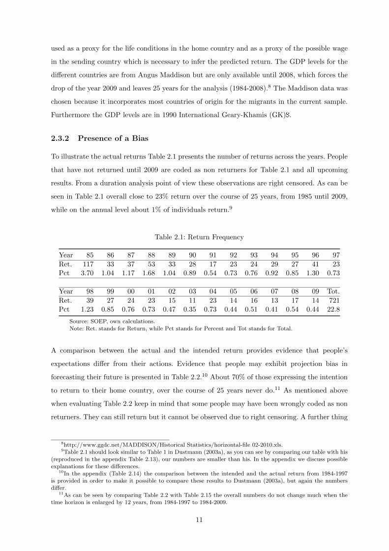
To illustrate the actual returns Table 2.1 presents the number of returns across the years. People
that have not returned until 2009 are coded as non returners for Table 2.1 and all upcoming
results. From a duration analysis point of view these observations are right censored. As can be
seen in Table 2.1 overall close to 23% return over the course of 25 years, from 1985 until 2009,
while on the annual level about 1% of individuals return.9
Table 2.1: Return Frequency
Year 85 86 87 88 89 90 91 92 93 94 95 96 97
Ret. 117 33 37 53 33 28 17 23 24 29 27 41 23Pct 3.70 1.04 1.17 1.68 1.04 0.89 0.54 0.73 0.76 0.92 0.85 1.30 0.73
Year 98 99 00 01 02 03 04 05 06 07 08 09 Tot.
Ret. 39 27 24 23 15 11 23 14 16 13 17 14 721Pct 1.23 0.85 0.76 0.73 0.47 0.35 0.73 0.44 0.51 0.41 0.54 0.44 22.8
Source: SOEP, own calculations.Note: Ret. stands for Return, while Pct stands for Percent and Tot stands for Total.
A comparison between the actual and the intended return provides evidence that people’s
expectations differ from their actions. Evidence that people may exhibit projection bias in
forecasting their future is presented in Table 2.2.10 About 70% of those expressing the intention
to return to their home country, over the course of 25 years never do.11 As mentioned above
when evaluating Table 2.2 keep in mind that some people may have been wrongly coded as non
returners. They can still return but it cannot be observed due to right censoring. A further thing
8http://www.ggdc.net/MADDISON/Historical Statistics/horizontal-file 02-2010.xls.9Table 2.1 should look similar to Table 1 in Dustmann (2003a), as you can see by comparing our table with his
(reproduced in the appendix Table 2.13), our numbers are smaller than his. In the appendix we discuss possibleexplanations for these differences.
10In the appendix (Table 2.14) the comparison between the intended and the actual return from 1984-1997is provided in order to make it possible to compare these results to Dustmann (2003a), but again the numbersdiffer.
11As can be seen by comparing Table 2.2 with Table 2.15 the overall numbers do not change much when thetime horizon is enlarged by 12 years, from 1984-1997 to 1984-2009.
11

CHAPTER 2. DIFFERENCES IN EXPECTED & ACTUAL RETURN MIGRATION
to note, is that it is impossible to capture short term migration lasting no longer than one year.
The SOEP surveys people annually, thereby not allowing the account of people that migrate
and return within a year.12
Table 2.2: Intentions and Realization 1984 - 2009
Return between 84 and 09Intended Return (84) No Yes Total
No 682 82 764Column Percentage 30.00 16.05 27.44
Row Percentage 89.27 10.73
Yes 1591 429 2020Column Percentage 70.00 83.95 72.56
Row Percentage 78.76 21.24
Total 2273 511 2784
Notes: This table only presents statistics for people present in 1984.
Source: SOEP, own calculations.
A valid concern in assessing the above numbers is that individuals do not report the truth to the
interviewer when asked about their desire to return. Some people may lie about their planned
duration in Germany because their current visa only allows them to stay for a limited amount
of time. Since the SOEP provides information on a migrant’s residence status, which is either
unlimited or limited, Table 2.3 presents the comparison between the desire to return and the
residence permit question. About 70% of those that have a limited residence permit in Germany
reply that they want to remain forever in Germany. As a consequence one cannot argue that
people tend to lie due to their residence permit. As it may be easy to get the residential permit
prolonged people respond truthfully when asked about their intentions.13
As we have seen up to this point, there is evidence of a bias between people’s expectation and
their final actions in the case of return migration. Table 2.4 takes a closer look at the socio-
economic differences between movers and stayers.
12These individuals do not play an important role for the analysis of the underestimation of the trip duration.13Note that in Table 2.3 there are three different possible answers for the desire to return home, while in
Table 2.2 the intention to return home was coded as a yes or no. If people answered that they want to stay inGermany, their intentions to stay was coded as a yes, while if people answered that they either plan to returnwithin 12 months or after 1 year, their intentions to stay were coded as a no. Be aware that in Table 2.3 theinformation that is available across all years from 1984 until 2009 is used, while Table 2.2 only considers thosepeople that are present in 1984. Unfortunately it is not possible to present a table with those individuals presentin 1984, since for everyone of them the residence status is missing - an unfortunate side effect of survey data.Tables 2.16 and 2.17 in the appendix include the same baseline year, a group of people for whom the residencepermit status is known and for whom the intentions are known. 1996 is the first year this happens which shortensthe time horizon notably.
12

Table 2.3: Desire to Return versus Residence Status
Residence StatusDesire to Return Unlimited Limited Total
Within 12 Months 22 24 46(Percentage) 0.79 1.48 1.04After One Year 766 444 1210Percentage 27.47 27.44 27.46Stay in Germany Forever 2000 1150 3150Percentage 71.74 71.08 71.49
Total 2788 1618 4406
Source: SOEP, own calculations.
Table 2.4: Socioeconomic Differences
Stayers Leavers
Variable Mean SD N Mean SD N t-stat
Male 0.50 0.50 3891 0.44 0.50 574 ( -2.56)∗
Age at Migration 30.04 10.66 3891 30.79 9.34 574 ( 1.59)
ln(GDPG)-ln(GDPH) 1.69 1.10 3838 1.69 1.06 568 ( 0.05)
Married 0.65 0.48 3564 0.38 0.49 471 ( -11.50)∗∗∗
Married living separated 0.02 0.15 3564 0.02 0.14 471 ( -0.43)
Divorced 0.05 0.22 3564 0.01 0.12 471 ( -3.54)∗∗∗
Widowed 0.05 0.22 3564 0.03 0.16 471 ( -2.56)∗
Employed 0.52 0.50 3890 0.44 0.50 574 ( -3.65)∗∗∗
Family at Home 0.19 0.39 3876 0.07 0.25 569 ( -7.32)∗∗∗
Spouse at Home 0.02 0.13 3891 0.08 0.27 574 ( 9.25)∗∗∗
Attended School in Germany 0.03 0.17 3832 0.02 0.16 566 ( -0.85)
Source: SOEP, own calculations.Note: The t-statistics test for the significance of the difference between leavers and stayers. Foreach individual the last point in time where information is provided in the dataset is taken to getthe different means.
13

CHAPTER 2. DIFFERENCES IN EXPECTED & ACTUAL RETURN MIGRATION
There seem to be socio-economic differences between movers and stayers, a finding which goes
along with the findings of e.g., Van Hook and Zhang (2011). Leavers and stayers seem to differ
in certain socio-economic characteristics, e.g., marital status, and employment, which points
toward the selection of return migrants.14
Figure 2.1: Descriptive Statistics 1
(a) Whole Sample
050
01,
000
1,50
02,
000
2,50
0nu
mbe
r of
obs
erva
tions
Leave &Say Forever
Leave &Never Say Forever
Do not Leave& Say Forever
Do not Leave &Never Say Forever
(b) Gender
0.2
.4.6
.81
Leave &Say Forever
Leave &Never Say Forever
Do not Leave& Say Forever
Do not Leave &Never Say Forever
Percent Men Percent Women
(c) Children
0.2
.4.6
.81
Leave &Say Forever
Leave &Never Say Forever
Do not Leave& Say Forever
Do not Leave &Never Say Forever
Percent No Kids Percent Have Kids
(d) Gender of the Children
0.2
.4.6
.81
Leave &Say Forever
Leave &Never Say Forever
Do not Leave& Say Forever
Do not Leave &Never Say Forever
Percent No Kids Percent Have Female KidsPercent Have Male Kids Percent Have Gender Kids
Figure 2.1 and 2.2 contrast the descriptive statistics of the four possible groups. In our sample
we have leavers who never say that they want to remain forever, leavers who at some point say
that they want to remain forever and non leavers who either say hat they want to remain forever
or never say that they want to stay forever. Figure 2.0a shows the number of observations for
the different groups. The group that at some point said that they wanted to remain forever
and have not yet left constitute the largest group. Figure 2.0b takes a closer look at the gender
composition of the different groups. There seem to be no significant differences in gender between
the different groups. Figure 2.0c looks at whether children are present. Here we see that those
14Table 2.18 in the appendix splits the “stayers” into attritors and those individuals that we observe until 2008and have not returned yet.
14
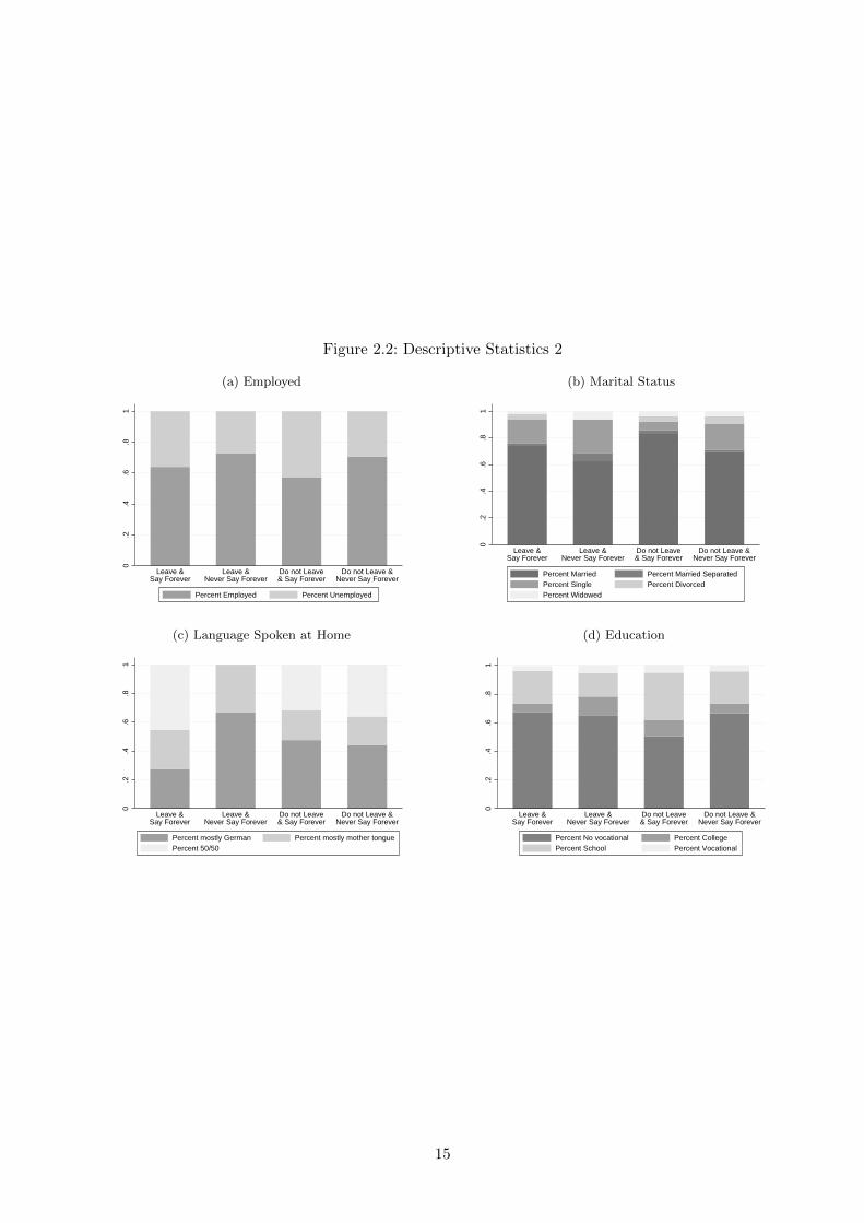
Figure 2.2: Descriptive Statistics 2
(a) Employed
0.2
.4.6
.81
Leave &Say Forever
Leave &Never Say Forever
Do not Leave& Say Forever
Do not Leave &Never Say Forever
Percent Employed Percent Unemployed
(b) Marital Status
0.2
.4.6
.81
Leave &Say Forever
Leave &Never Say Forever
Do not Leave& Say Forever
Do not Leave &Never Say Forever
Percent Married Percent Married SeparatedPercent Single Percent DivorcedPercent Widowed
(c) Language Spoken at Home
0.2
.4.6
.81
Leave &Say Forever
Leave &Never Say Forever
Do not Leave& Say Forever
Do not Leave &Never Say Forever
Percent mostly German Percent mostly mother tonguePercent 50/50
(d) Education
0.2
.4.6
.81
Leave &Say Forever
Leave &Never Say Forever
Do not Leave& Say Forever
Do not Leave &Never Say Forever
Percent No vocational Percent CollegePercent School Percent Vocational
15

CHAPTER 2. DIFFERENCES IN EXPECTED & ACTUAL RETURN MIGRATION
individuals that have children are more likely to be in the group that says at some point that they
want to remain forever and have not left so far. Figure 2.0d looks at whether there are significant
gender differences for the children between the different groups. We thought at first that there
may be a difference, since some parents may want their girls to grow up in their home culture,
while for their boys, they would prefer the German environment since it may constitute a better
working environment. But as Panel 2.0d shows, there seem to be no such differences.15 Figure 2.2
then continues to contrast different characteristics, but there seem to be no relevant differences
between the four groups. Panel 2.1a takes a closer look at the unemployment versus employment
rates, Panel 2.1b looks at differences between marital status, Panel 2.1c contrasts the languages
spoken at home, while Panel 2.1d graphs the different educational levels of the individuals. As
already mentioned, there seem to be no significant differences between the fours groups in terms
of these characteristics. So none of these characteristics should drive the differences between the
intentions and the expectations in the following.
The next section provides the reader with the methodology used to infer the actual return based
on the current information available to the individual.
2.4 Model
Let T be the duration until the return and let θ(t|x(t), x0) be the hazard rate, which can be
interpreted as the return rate or the return probability. Mathematically it can be represented
as:
θ(t, x(t), x0) = limdt→0P (t ≤ T < t+ dt|T ≥ t, x(t), x0)
dt(2.1)
t presents time since entry, x(t) are time varying covariates, such as the current employment
status, and the current family income, and x0 are time invariant covariates, such as the age at
migration, gender, education and country of origin.
The amount of money that migrants will earn in their home country and how the purchasing
powers differ between the migrants country of origin and Germany builds the framework for the
analysis between expectations and realizations. Information about what migrants wages would
be in their home country is not available and GDP is used to infer how big the differences
are between Germany and the sending country. Since the focus of the chapter is to explain
differences between return intentions and return realizations, we need an expression for the
15With percent have gender kids, we are interested in families that have both a daughter and a son.
16

return realization which will be inferred through duration analysis. This analysis is said to be
reduced form and we need to think about possible factors that migrants consider when forming
expectations.
GDP is a good indicator to compare countries and as mentioned in the literature review the
decision to return may be a part of the life-cycle, or the sending country may have caught up
to the receiving country in terms of GDP. Comparing the GDP’s of Germany and that of the
sending countries, we know that either this did not happen, e.g., for countries such as Turkey, or
Germany was just as good in terms of GDP as the sending country, e.g., France. In other words,
a change in the arguments of the utility function changes the utility level. This can be modeled
with the help of the duration analysis. To do so, first assume that the migrants to Germany are
a homogeneous group, an assumption which may be relaxed in future work.
As emphasized above, the decision to return relies on the economic model which builds the
framework for the hazard rate. As an example, for an individual to take the decision to move
in 2005 it is needed that the expected present value of earnings proxied by GDP in the home
country minus the moving costs are larger than the expected present value of earnings proxied
by GDP in Germany. This formulation of the decision to move has been introduced by Sjaastad
(1962). More formally, if one decides to move in 2005,
d∑t=2005
1
(1 + r)t(E[U(XT (t))]− E[U(XG(t))]) > c+ ε (2.2)
has to hold. Where X(t), are covariates that we control for, such as GDP, age at migration,
marital status, family location . . . .16 c represents the cost of moving, d is the expected year of
death, r is the interest rate and ε is an error term. The subscript G stands for Germany, and
the subscript T stands for Turkey.17 This can be rewritten in terms of probabilities, such that:
P (move in 2005 from Germany to Turkey) (2.3)
= P
(ε <
d∑t=2005
1
(1 + r)t(E[U(XT (t))]− E[U(XG(t))])− c
).
16In the empirical specification part, we specify what covariates we control for.17Turkey was chosen as an example, since as can be seen in Table 2.19 most migrants in the sample are from
Turkey.
17

CHAPTER 2. DIFFERENCES IN EXPECTED & ACTUAL RETURN MIGRATION
Which can be rewritten in terms of the hazard rate in 2005, such that:
P
(ε <
d∑t=2005
1
(1 + r)t(E[U(XT (t))]− E[U(XG(t))])− c
)(2.4)
= Φ
(∑dt=2005
1(1+r)t (E[U(XT (t))]− E[U(XG(t))])− c
σε
)
Equation (2.5) is the expression of the hazard for 2005 and can easily be rewritten to get an
expression for the hazard rate for each year.
Since we are ultimately interested in the expected duration of a stay, the duration framework
allows us to write:
y(0) = E(T |x0, expectations of future path of x(t)) (2.5)
=
∫ ∞0
[exp
(−∫ ∞
0θ(u|x(u), x0)du
)]dz
in a continuous time framework. This equation can be rewritten for y(t) where t can take any
integer value in [0, T ] which means that we end up with possible y(t), y(t − 1), . . . , y(0). This
expression allows the individual to adapt her expectations. In other words, y(0) may be different
than y(1) because individuals update the future path of x(t). The model’s predicted expectations
will be compared to the respondents indicated intentions to see what drives the difference and
whether people learn; are their predictions eventually converging to the “truth”?
Empirical Specification
Since the data at hand is of the discrete time format, the expected duration until the return is
based on the assumption of a third order polynomial of time combined with a complementary
log log model.18 Then the full model specification is (assuming time invariant covariates):
cloglog[h(t,X)] = z1t+ z2t2 + z3t
3 + βX (2.6)
18The third order polynomial is our preferred specification of the duration dependence, see Table 2.5 and theresults section for more details.
18

where X represents socio-economic characteristics.19 In other words, the hazard can be rewritten
as:
h(t,X) = 1− exp[−exp(z1t+ z2t2 + z3t
3 + βX)] (2.7)
where z1, z2, z3 are estimated together with the intercept and the slope parameters within the
vector β. Survival up to the end of the jth interval (or completion of the jth cycle) is given by:
S(j) = Sj =
j∏k=1
(1− hk) (2.8)
where hk is the cloglog function of characteristics.
For each individual, we calculate the expected duration of the stay at the moment of the
interview. Thus even if the interview happens when a person has already spent 10 years in
Germany, we calculate the expected duration of the stay from that point onwards. Therefore
we consider the year of the interview as t = 0. Consider now the case where people form their
expectations based on the current GDP only, and all other variables included in the model so
far do not vary with time or only vary once - marital status, employed, family at home, spouse
at home. Age at migration and attended school in Germany are time invariant covariates. Hence
the predicted return in the discrete time framework is given by,
E[T ] =K∑k=1
S(t) = S(1) + S(2) + S(3) + . . .+ S(K) (2.9)
where K is the maximum survival time.20 The predicted return can be rewritten as:
E[T ] = (1− h1) + (1− h1)(1− h2) + . . .+ (1− h1)(1− h2)(1− h3) . . . (1− hK) (2.10)
where hx represent the hazard at time x.21 In the following the predicted return will be denoted
by E[T ] while the intended duration will be denoted by E[T ]. The next subsection discusses the
results for this model and explains the sample selection criteria.
19We control for sex, age at migration, difference in GDP between Germany and the source country, maritalstatus, whether or not the individual attended school in Germany, whether or not the individual has family athome and whether or not the individual’s spouse is at home. Furthermore we control for the country of origin.
20In the empirical part we assume that the maximum survival time equals the expected lifetime duration,approximated by 100 − current age.
21As an example:h1(t,X) = 1 − exp[−exp(z1t+ z2t
2 + z3t3 + βX)]
h2(t+ 1, X) = 1 − exp[−exp(z1(t+ 1) + z2(t+ 1)2 + z3(t+ 1)3 + βX)]
h3(t+ 2, X) = 1 − exp[−exp(z1(t+ 2) + z2(t+ 2)2 + z3(t+ 2)3 + βX)]
19

CHAPTER 2. DIFFERENCES IN EXPECTED & ACTUAL RETURN MIGRATION
2.5 Results
As shortly mentioned in the data section, we consider only migrants that are already in Germany
and present in the SOEP. Furthermore we consider adults, who are older than 18 years in order
to include those individuals that take the return decision themselves. As the use of the GDP
Data from Angus Maddison forced the drop of the year 2009, we are left with 25 years for the
analysis (1984-2008) and 3152 individuals, where 574 durations until re-migration are not right
censored.
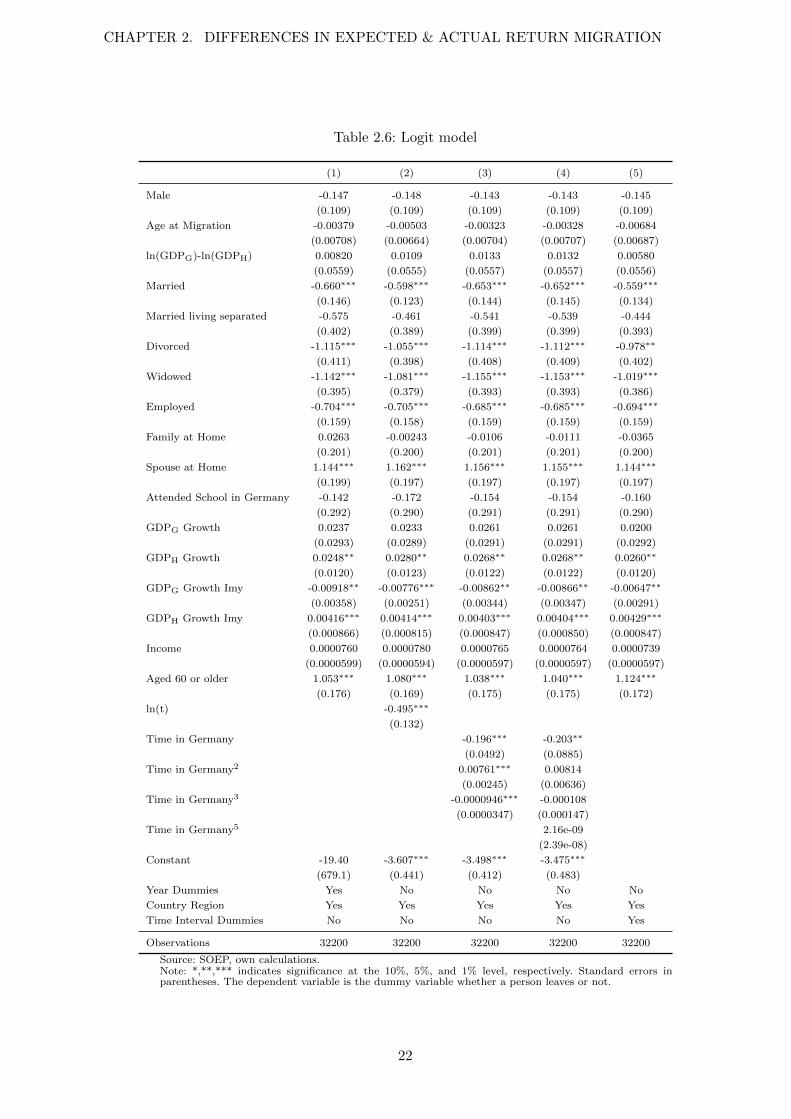
Tables 2.5 and 2.6 show the results of the complementary log log model, and logit model which
are the underlying models for the predicted return. These specifications allow the construction
of the predicted return as stated in the methodology section. The estimates are shown to provide
evidence that all the coefficients point in the right direction. As an example, being employed
makes you less likely to return, while having your spouse in the your home country makes you
more likely to return. Males also seem to be less likely to return than females. Compared to
singles every other marital status type is less likely to return. Whether the logit model or the
complementary clog log specification is used, does not change these effects.
Furthermore Table 2.5 as well as Table 2.6 test which duration specification may be the best.
In both tables, Column (1) includes year dummies, in order to give a fully nonparametric
specification of the duration dependence, while Column (5) includes time interval dummies,
allowing for a piecewise constant specification of the duration dependence. We also checked the
discrete-time analogue of the continuous time Weibull model (ln(t)) as well as a fifth order
polynomial in time and a third order polynomial in time.
Our preferred specification is the third order polynomial, which also fits the pattern that at the
beginning the individual may be more likely to return, while the likelihood to return decreases
until the individual reaches the retirement age, where the likelihood increases again. These
specifications, as explained in the methodology section, allow us to “extract” the hazard rate
which allow the construction of the predicted return. All predicted returns analyzed below are
based on the complementary log log model with a third order polynomial in time to model the
duration dependence.
Before analyzing the differences between the intentions and the predicted return, let us look
at the individuals intentions and what are driving factors of the changes in these intentions.
20

Table 2.5: Complementary Log-log model
(1) (2) (3) (4) (5)
Male -0.146 -0.148 -0.143 -0.143 -0.145
(0.107) (0.107) (0.107) (0.107) (0.107)
Age at Migration -0.00390 -0.00510 -0.00332 -0.00335 -0.00687
(0.00692) (0.00652) (0.00691) (0.00693) (0.00672)
ln(GDPG)-ln(GDPH) 0.00845 0.0102 0.0131 0.0130 0.00609
(0.0547) (0.0546) (0.0547) (0.0547) (0.0545)
Married -0.646∗∗∗ -0.590∗∗∗ -0.643∗∗∗ -0.642∗∗∗ -0.552∗∗∗
(0.144) (0.121) (0.142) (0.143) (0.132)
Married living separated -0.565 -0.464 -0.544 -0.543 -0.441
(0.389) (0.377) (0.387) (0.387) (0.381)
Divorced -1.097∗∗∗ -1.039∗∗∗ -1.098∗∗∗ -1.096∗∗∗ -0.965∗∗
(0.405) (0.394) (0.404) (0.405) (0.398)
Widowed -1.115∗∗∗ -1.064∗∗∗ -1.136∗∗∗ -1.135∗∗∗ -1.002∗∗∗
(0.389) (0.374) (0.388) (0.389) (0.381)
Employed -0.691∗∗∗ -0.694∗∗∗ -0.674∗∗∗ -0.674∗∗∗ -0.681∗∗∗
(0.157) (0.157) (0.157) (0.157) (0.157)
Family at Home 0.0289 -0.00108 -0.00941 -0.00973 -0.0343
(0.198) (0.197) (0.198) (0.198) (0.197)
Spouse at Home 1.095∗∗∗ 1.127∗∗∗ 1.120∗∗∗ 1.120∗∗∗ 1.103∗∗∗
(0.190) (0.189) (0.189) (0.189) (0.189)
Attended School in Germany -0.142 -0.169 -0.150 -0.150 -0.155
(0.287) (0.286) (0.286) (0.286) (0.286)
GDPG Growth 0.0234 0.0232 0.0259 0.0259 0.0202
(0.0284) (0.0282) (0.0283) (0.0283) (0.0284)
GDPH Growth 0.0242∗∗ 0.0274∗∗ 0.0262∗∗ 0.0262∗∗ 0.0255∗∗
(0.0115) (0.0119) (0.0118) (0.0118) (0.0116)
GDPG Growth Imy -0.00894∗∗ -0.00764∗∗∗ -0.00849∗∗ -0.00852∗∗ -0.00641∗∗
(0.00350) (0.00247) (0.00338) (0.00342) (0.00287)
GDPH Growth Imy 0.00410∗∗∗ 0.00406∗∗∗ 0.00396∗∗∗ 0.00397∗∗∗ 0.00420∗∗∗
(0.000845) (0.000797) (0.000828) (0.000831) (0.000828)
Income 0.0000748 0.0000768 0.0000753 0.0000753 0.0000723
(0.0000593) (0.0000588) (0.0000591) (0.0000591) (0.0000592)
Aged 60 or older 1.035∗∗∗ 1.064∗∗∗ 1.022∗∗∗ 1.023∗∗∗ 1.105∗∗∗
(0.173) (0.166) (0.172) (0.173) (0.169)
ln(t) -0.484∗∗∗
(0.129)
Time in Germany -0.192∗∗∗ -0.196∗∗
(0.0480) (0.0865)
Time in Germany2 0.00742∗∗∗ 0.00774
(0.00240) (0.00623)
Time in Germany3 -0.0000922∗∗∗ -0.000100
(0.0000339) (0.000145)
Time in Germany5 1.31e-09
(2.36e-08)
Constant -20.01 -3.630∗∗∗ -3.526∗∗∗ -3.512∗∗∗
(723.6) (0.432) (0.402) (0.471)
Year Dummies Yes No No No No
Country Region Yes Yes Yes Yes Yes
Time Interval Dummies No No No No Yes
Observations 32200 32200 32200 32200 32200
Source: SOEP, own calculations.Note: *,**,*** indicates significance at the 10%, 5%, and 1% level, respectively. Standard errors inparentheses. The dependent variable is the dummy variable whether a person leaves or not.
21
CHAPTER 2. DIFFERENCES IN EXPECTED & ACTUAL RETURN MIGRATION
Table 2.6: Logit model
(1) (2) (3) (4) (5)
Male -0.147 -0.148 -0.143 -0.143 -0.145
(0.109) (0.109) (0.109) (0.109) (0.109)
Age at Migration -0.00379 -0.00503 -0.00323 -0.00328 -0.00684
(0.00708) (0.00664) (0.00704) (0.00707) (0.00687)
ln(GDPG)-ln(GDPH) 0.00820 0.0109 0.0133 0.0132 0.00580
(0.0559) (0.0555) (0.0557) (0.0557) (0.0556)
Married -0.660∗∗∗ -0.598∗∗∗ -0.653∗∗∗ -0.652∗∗∗ -0.559∗∗∗
(0.146) (0.123) (0.144) (0.145) (0.134)
Married living separated -0.575 -0.461 -0.541 -0.539 -0.444
(0.402) (0.389) (0.399) (0.399) (0.393)
Divorced -1.115∗∗∗ -1.055∗∗∗ -1.114∗∗∗ -1.112∗∗∗ -0.978∗∗
(0.411) (0.398) (0.408) (0.409) (0.402)
Widowed -1.142∗∗∗ -1.081∗∗∗ -1.155∗∗∗ -1.153∗∗∗ -1.019∗∗∗
(0.395) (0.379) (0.393) (0.393) (0.386)
Employed -0.704∗∗∗ -0.705∗∗∗ -0.685∗∗∗ -0.685∗∗∗ -0.694∗∗∗
(0.159) (0.158) (0.159) (0.159) (0.159)
Family at Home 0.0263 -0.00243 -0.0106 -0.0111 -0.0365
(0.201) (0.200) (0.201) (0.201) (0.200)
Spouse at Home 1.144∗∗∗ 1.162∗∗∗ 1.156∗∗∗ 1.155∗∗∗ 1.144∗∗∗
(0.199) (0.197) (0.197) (0.197) (0.197)
Attended School in Germany -0.142 -0.172 -0.154 -0.154 -0.160
(0.292) (0.290) (0.291) (0.291) (0.290)
GDPG Growth 0.0237 0.0233 0.0261 0.0261 0.0200
(0.0293) (0.0289) (0.0291) (0.0291) (0.0292)
GDPH Growth 0.0248∗∗ 0.0280∗∗ 0.0268∗∗ 0.0268∗∗ 0.0260∗∗
(0.0120) (0.0123) (0.0122) (0.0122) (0.0120)
GDPG Growth Imy -0.00918∗∗ -0.00776∗∗∗ -0.00862∗∗ -0.00866∗∗ -0.00647∗∗
(0.00358) (0.00251) (0.00344) (0.00347) (0.00291)
GDPH Growth Imy 0.00416∗∗∗ 0.00414∗∗∗ 0.00403∗∗∗ 0.00404∗∗∗ 0.00429∗∗∗
(0.000866) (0.000815) (0.000847) (0.000850) (0.000847)
Income 0.0000760 0.0000780 0.0000765 0.0000764 0.0000739
(0.0000599) (0.0000594) (0.0000597) (0.0000597) (0.0000597)
Aged 60 or older 1.053∗∗∗ 1.080∗∗∗ 1.038∗∗∗ 1.040∗∗∗ 1.124∗∗∗
(0.176) (0.169) (0.175) (0.175) (0.172)
ln(t) -0.495∗∗∗
(0.132)
Time in Germany -0.196∗∗∗ -0.203∗∗
(0.0492) (0.0885)
Time in Germany2 0.00761∗∗∗ 0.00814
(0.00245) (0.00636)
Time in Germany3 -0.0000946∗∗∗ -0.000108
(0.0000347) (0.000147)
Time in Germany5 2.16e-09
(2.39e-08)
Constant -19.40 -3.607∗∗∗ -3.498∗∗∗ -3.475∗∗∗
(679.1) (0.441) (0.412) (0.483)
Year Dummies Yes No No No No
Country Region Yes Yes Yes Yes Yes
Time Interval Dummies No No No No Yes
Observations 32200 32200 32200 32200 32200
Source: SOEP, own calculations.Note: *,**,*** indicates significance at the 10%, 5%, and 1% level, respectively. Standard errors inparentheses. The dependent variable is the dummy variable whether a person leaves or not.
22

Figure 2.3 plots the intended duration of stay, in Panel a) we imputed the intended duration
for those who wanted to stay forever as 100 − their current age, while in Panel b) we only take
a look at those that actually tell us how long they plan on staying. In both panels we see that
the individuals show bunching behavior around 5, 10, 15, 20 years. This bunching may already
point towards a simplifying heuristic, when individuals form their intentions.
Figure 2.3: Expected Duration of Stay
(a) Intended Duration of Stay for those who intendto stay forever = 100 - current age
02
46
810
Per
cent
0 20 40 60 80 100Expected Duration of Stay in Germany
(b) Intended Duration of Stay without those whointend to stay forever
05
1015
2025
Per
cent
0 20 40 60 80 100Expected Duration of Stay in Germany
Tables 2.7 and 2.8 look at the driving factors behind the changes in peoples return intentions.
We take the first difference in their intentions - as an example we compute E[2006]− E[2005] -
and regress these changes in their intentions on the changes in their socio-economic changes: e.g.,
employed2006 - employed2005. All regressions include individual fixed effects and the standard
errors are clustered at the individual level. What seems to be a driving factor in these adjustments
is whether there is a change in your life satisfaction, meaning that if you are more satisfied in
one year than in the following (happiness variable), it influences your intention to return. This
finding is as expected, since an increase in life satisfaction may also reduce the psychic costs that
occur from migration. Other variables that seem to have significant effects on these changes are
attended school in Germany variable and the differences in GDP variable.
Table 2.8 takes a closer look at some of the behavioral factors contained in the SOEP and
how they influence the changes in the individuals intentions. Unfortunately the number of
observations decreases substantially depending on which variables are included. Data on control
over life is only available in years 1994-1996, 1999 and 2005, data on remitting is only available in
the years 1984-1993 and 1995, while data on risk preferences is only available in the years 2006-
23

CHAPTER 2. DIFFERENCES IN EXPECTED & ACTUAL RETURN MIGRATION
Table 2.7: Difference in Expectations
(1) (2) (3) (4) (5) (6)
ln(GDPG)-ln(GDPH) FD -1.35∗ -1.35∗ -1.48∗ -2.10∗∗ -1.21 -1.88∗∗
(0.82) (0.82) (0.82) (0.82) (0.83) (0.83)Employed FD 0.22∗ 0.22∗ 0.21 0.25∗ 0.20 0.19
(0.13) (0.13) (0.13) (0.13) (0.13) (0.13)Income FD -0.00 -0.00 -0.00 -0.00 -0.00 -0.00∗
(0.00) (0.00) (0.00) (0.00) (0.00) (0.00)Family at Home FD -0.02 -0.09 -0.11 -0.06 -0.05 -0.14
(0.49) (0.50) (0.50) (0.49) (0.46) (0.51)Spouse at Home FD -0.29 -0.29 -0.29 -0.31 -0.40 -0.43
(0.41) (0.41) (0.41) (0.46) (0.44) (0.44)Attended School in Germany FD -0.12 -0.12 -0.54∗∗ -0.28∗ 0.22 -0.55∗∗
(0.25) (0.25) (0.26) (0.16) (0.24) (0.22)Happiness FD 0.10∗∗∗ 0.10∗∗∗ 0.10∗∗∗ 0.09∗∗∗ 0.09∗∗∗ 0.10∗∗∗
(0.03) (0.03) (0.03) (0.03) (0.03) (0.03)Have Children FD 0.42 0.42 0.22 -0.27
(0.81) (0.81) (0.81) (0.61)Death of Mother FD 1.52
(1.15)Death of Father FD -1.20
(0.86)Aged 60 or older 0.38∗∗∗ 0.49∗∗∗
(0.11) (0.12)Time in Germany -0.04∗∗∗ -0.06∗∗∗
(0.01) (0.01)Married -0.45∗∗∗
(0.10)Married living separated -0.52
(0.37)Divorced -0.24
(0.40)Widowed -0.43∗
(0.26)Finished Higher Education -0.59
(0.48)Finished School 0.79
(0.78)vocational -1.14
(0.74)Married FD -0.15
(0.25)Married living separated FD -0.07
(0.72)Divorced FD -0.04
(0.82)Widowed FD -0.06
(0.29)Constant -0.13∗∗∗ -0.13∗∗∗ 0.72∗∗∗ 0.00 -0.02 1.04∗∗∗
(0.01) (0.01) (0.16) (0.03) (0.06) (0.18)
Number of Clusters 1858 1858 1858 1692 1783 1593Observations 11219 11219 11219 10502 10867 9555R2 0.10 0.10 0.10 0.10 0.10 0.12
Source: SOEP, own calculations.Note: *,**,*** indicates significance at the 10%, 5%, and 1% level, respectively. Clustered standarderrors in parentheses. The dependent variable is the change of the expected duration of stay. Allregressions include individual fixed effects.
24

2009.22 Column (1) is the baseline specification without behavioral factors, in order to make
it easier for the reader to see what happens to the sample size when the other variables are
included. Another unfortunate side-effect of the small sample size is that none of the behavioral
coefficients are significant, which does not leave much room for argumentation.
Last but not least, let us move to the forecast errors. Figure 2.4 plots the difference between the
intentions and the predicted return. Again Panel a) plots the difference for the whole sample,
where for those that intended to stay forever we imputed their maximal survival time as 100
− their current age. Panel b) plots the difference for the reduced sample, where we leave those
out that intend to stay forever. A quick glance at Panel a) gives us hope, that there seem to
be many people predicting the duration of their stay correctly, but when we take those out
that intend to stay forever (for whom we imposed how long they remain in Germany, Panel b))
practically no remaining individual has a correct prediction. Figure 2.4b) shows that individuals
overestimate the return to their home country, equivalently stated, underestimate their time
spent in Germany. When looking at the difference, the intended return is constantly below the
actual predicted return, which makes the difference negative. This is an important finding and
may point toward overconfidence; a topic very nicely introduced in Kahneman (2011). In the
current work, overconfidence would have to go along with net attachment in the sense that
individuals are overconfident about the fact that they will be true to their family (to their
“roots”) and want to return home, and thus underestimate their attachment to Germany. More
importantly though the finding of the overestimation of the probabilities to return is along
the lines of Rabin (2002). He models the belief in the “Law of Small Numbers”, where people
exaggerate the degree to which small samples resemble the population from which they are
drawn.
A further thing we look at, is whether “narrow framing” plays a role. We use the term “narrow
framing” to define the fact that people may only look at shorter time intervals than their whole
lives. Trying to predict what will happen in 40 years from now is hard, and therefore it may also
be hard to predict what one will do in 40 years concerning the return migration. Therefore we
take a look at people’s predictions if we make a cut off at e.g., 10 years and everyone that states
that they want to remain longer than 10 years, we re-coded as only wanting to stay 10 years.23
22To get a little more observations, we fill the variables forward using stata’s stfill command. This means thatthe variable takes on the last value until a change in the variable happens. This assumption should not changeany of our results.
23We played around with these numbers, and 10 just gave the best predictions, which is why we stick to thatnumber.
25
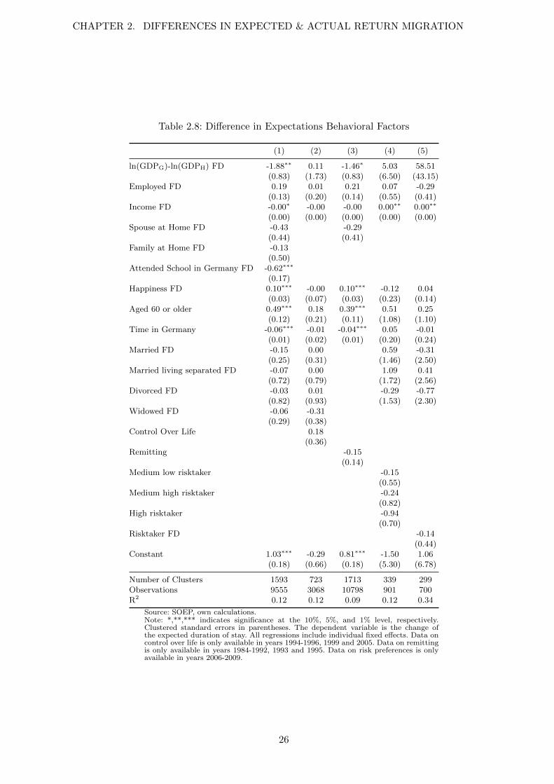
CHAPTER 2. DIFFERENCES IN EXPECTED & ACTUAL RETURN MIGRATION
Table 2.8: Difference in Expectations Behavioral Factors
(1) (2) (3) (4) (5)
ln(GDPG)-ln(GDPH) FD -1.88∗∗ 0.11 -1.46∗ 5.03 58.51(0.83) (1.73) (0.83) (6.50) (43.15)
Employed FD 0.19 0.01 0.21 0.07 -0.29(0.13) (0.20) (0.14) (0.55) (0.41)
Income FD -0.00∗ -0.00 -0.00 0.00∗∗ 0.00∗∗
(0.00) (0.00) (0.00) (0.00) (0.00)Spouse at Home FD -0.43 -0.29
(0.44) (0.41)Family at Home FD -0.13
(0.50)Attended School in Germany FD -0.62∗∗∗
(0.17)Happiness FD 0.10∗∗∗ -0.00 0.10∗∗∗ -0.12 0.04
(0.03) (0.07) (0.03) (0.23) (0.14)Aged 60 or older 0.49∗∗∗ 0.18 0.39∗∗∗ 0.51 0.25
(0.12) (0.21) (0.11) (1.08) (1.10)Time in Germany -0.06∗∗∗ -0.01 -0.04∗∗∗ 0.05 -0.01
(0.01) (0.02) (0.01) (0.20) (0.24)Married FD -0.15 0.00 0.59 -0.31
(0.25) (0.31) (1.46) (2.50)Married living separated FD -0.07 0.00 1.09 0.41
(0.72) (0.79) (1.72) (2.56)Divorced FD -0.03 0.01 -0.29 -0.77
(0.82) (0.93) (1.53) (2.30)Widowed FD -0.06 -0.31
(0.29) (0.38)Control Over Life 0.18
(0.36)Remitting -0.15
(0.14)Medium low risktaker -0.15
(0.55)Medium high risktaker -0.24
(0.82)High risktaker -0.94
(0.70)Risktaker FD -0.14
(0.44)Constant 1.03∗∗∗ -0.29 0.81∗∗∗ -1.50 1.06
(0.18) (0.66) (0.18) (5.30) (6.78)
Number of Clusters 1593 723 1713 339 299Observations 9555 3068 10798 901 700R2 0.12 0.12 0.09 0.12 0.34
Source: SOEP, own calculations.Note: *,**,*** indicates significance at the 10%, 5%, and 1% level, respectively.Clustered standard errors in parentheses. The dependent variable is the change ofthe expected duration of stay. All regressions include individual fixed effects. Data oncontrol over life is only available in years 1994-1996, 1999 and 2005. Data on remittingis only available in years 1984-1992, 1993 and 1995. Data on risk preferences is onlyavailable in years 2006-2009.
26

Figure 2.4: Difference Between Intentions and Predicted Realizations
(a) Those who intend to stay forever maximalsurvival time = 100 - current age
05
1015
20P
erce
nt
-100 -50 0 50Difference between intentions and pedicted realizations
(b) Without those who intend to stay forever
01
23
4P
erce
nt
-100 -50 0 50Difference between intentions and predicted realization
The top panel of Figure 2.5 looks at the intended duration of stay, once we restrict the window for
predictions to 10 years. Panel a) includes those that intend to stay forever (coded as intending to
stay for 10 more years), while Panel b) excludes these individuals. The lower panel of Figure 2.5
takes a look at the difference between the narrowly framed intention and the predicted return
of this model. In Panel c), close to 70% of the individuals now predict their stay correctly, but
again taking those out that intend to stay forever, only 35% of the individuals seem to correctly
predict the length of their stay within this framework. Nevertheless it is important to notice that
in Figure 2.4 Panel b) nearly nobody predicted the length of their stay correctly. These results
point towards the fact that not just overconfidence may play a role, but also the forecasting
ability of the individuals. It is easier to give a response to what you may be doing in a year or
two than to give a response to the question about when you may want to return. For the rest of
the chapter we go back to the initial specification of the predicted return, where the sum is taken
until the expected survival time, which is approximated by 100 - the current age of the individual.
Another important question when looking at these graphs is whether people learn from their
“past” behavior. In other words; is the difference between their intentions and the predicted
realization approaching zero the longer they stay in Germany? Figure 2.6 tries to take a closer
look at this learning problem by looking at the changes over time spent in Germany. Looking at
the different panels, it seems that people do not learn to predict their preferences more accurately
the longer they are in Germany. The distribution shifts a little bit closer to zero which may be
due to the fact that the population gets older.
27

CHAPTER 2. DIFFERENCES IN EXPECTED & ACTUAL RETURN MIGRATION
Figure 2.5: “Narrow Framing”
(a) Those who intended to stay forever, maximalsurvival time = 10
050
100
150
Per
cent
0 2 4 6 8 10Expected Duration of Stay in Germany NF
(b) Without those who intend to stay forever
010
2030
40P
erce
nt
0 2 4 6 8 10Expected Duration of Stay in Germany NF
(c) Those who intended to stay forever, maximalsurvival time = 10
050
100
150
Per
cent
-10 -5 0 5 10Difference between intentions and rational expectations
(d) Without those who intend to stay forever
010
2030
40P
erce
nt
-10 -5 0 5Difference between intentions and rational expectations
28

Figure 2.6: Difference Between Intentions and Predicted Return, Learning?
(a) Spent 5 years in Germany
01
23
45
Per
cent
-80 -60 -40 -20 0Spent 5 years in Germany
(b) Spent 10 years in Germany
02
46
Per
cent
-80 -60 -40 -20 0Spent 10 years in Germany
(c) Spent 15 years in Germany
01
23
45
Per
cent
-60 -40 -20 0Spent 15 years in Germany
(d) Spent 20 years in Germany
02
46
Per
cent
-60 -40 -20 0 20Spent 20 years in Germany
29

CHAPTER 2. DIFFERENCES IN EXPECTED & ACTUAL RETURN MIGRATION
Figure 2.7 then plots the average forecast error (equivalent to the average difference) over
different time specifications. Panel a) plots the average forecast error over time spent in Germany,
and what was not obvious before now seems to become relevant. It seems that the longer people
are in Germany, the more accurate they get on average. The largest error that they make is when
they have spent 20 years in Germany, while their error is practically zero once they have spent
60 years in Germany. This could go along with the fact that having spent 20 years in a country
you may still believe that you eventually return, but the older you get, the better you are at
comparing your actual chance of leaving and so you seem to be more accurate with your forecast.
Panel b) helps us explain at what age you seem to get better at predicting your utility or your
future choice variables. Toward this end, there is a clear direction; the older you get, the better
you get at predicting your remaining duration. This finding is not too surprising as the older one
is, the shorter the remaining horizon gets, and therefore one may also be better at predicting
the duration of the stay.
Panel c) plots the average forecast error over the different life satisfaction possibilities, where
0 stands for not satisfied, while a 10 ranks you at very satisfied. We show this graph, since
happiness seemed to explain some of the changes in the intended returns, but how satisfied you
are with your current life does not seem to have a different effect on the average forecast error.
Panel d) plots the average forecast error over time. The increasing slope does not make too
much sense to us, except that the individuals that we consider in the sample may get older and
as already stated above then get better at forecasting their own preferences. Nevertheless it is
useful to include this graph, in order to show that there are no relevant macro shocks that drive
our results.
Tables 2.9, 2.10, 2.11 and 2.12 finally take a closer look at the differences between the intentions
and the predicted return. In Table 2.9, Columns (2), (4) and (5) include individual fixed effects,
where the standard errors are clustered at the individual level. The OLS results, are shown for
comparison, since we are in a panel data set up, we need to include individual fixed effects and
also cluster the standard errors.24 As an example, one can see the effect when taking a closer
look at attended school in Germany. The coefficient changes sign and magnitude as soon as we
24The identification with the use of individual fixed effects is driven by variations across time by each individual.Since many of the variables included in the regression may be time invariant, we included the yearly OLS resultsin the appendix in Tables 2.20 and 2.21.
30

Figure 2.7: Average Forecast Error
(a) Over time spent in Germany
-40
-30
-20
-10
010
aver
age
fore
cast
err
or
0 20 40 60Time in Germany
Whole Sample Non Leavers Whole Sample Leavers
(b) Over age at time of forecast
-60
-40
-20
0av
erag
e fo
reca
st e
rror
20 40 60 80 100age
Whole Sample Non Leavers Whole Sample Leavers
(c) Over Life Satisfaction at Time of Forecast
-40
-30
-20
-10
aver
age
fore
cast
err
or
0 2 4 6 8 10Happiness
Whole Sample Non Leavers Whole Sample Leavers
(d) Over time
-30
-25
-20
-15
-10
-5av
erag
e fo
reca
st e
rror
1985 1990 1995 2000 2005 2010erhebj
Whole Sample Non Leavers Whole Sample Leavers
31

CHAPTER 2. DIFFERENCES IN EXPECTED & ACTUAL RETURN MIGRATION
include individual fixed effects and clustering. A further thing to note, is that the coefficient
estimate on time spent in Germany are all significant and point into the right direction. The
longer one has been in Germany, the smaller the difference between the intentions and the
predicted return. The coefficient on the above 60 dummy is also highly significant, showing that
it is very important to control for this hump at the retirement age. The coefficient on the above
60 dummy is positive, but since the difference is always negative, this means that the difference
decreases as soon as one is above 60. The coefficient on the disadvantage due to origin variable is
also significant at the 1% level, and is negative. This implies, again as the difference is on average
negative, that those individuals that feel a disadvantage, understimate the duration of their stay
by more than those that do not feel disadvantaged. Having attended school in Germany is one
of the surprising coefficients since it increases the difference when we focus on the specifications
that include individual fixed effects in Table 2.9 Columns (3), (5) and (6).
Table 2.10 and 2.11 are robustness checks of the results from Table 2.9. Table 2.10 is a first
test on the sign and the magnitude of the results of table 2.9, as we exclude those observations
where individuals indicate that they intend to stay forever. For Table 2.11 we split the sample
randomly in half, where for one half of the sample the hazard model was estimated while for the
other half, the average forecast error was predicted using the results from the hazard model.
Table 2.12 includes the behavioral factors where we take a look at the whole sample, but as before
we lose power, due to a decrease in the number of observations. Here the interesting behavioral
results come from whether or net a person has remitted and again the locus of control variable.
If an individual has been paying remittances, she is underestimating the time she is going to
spent in Germany. The coefficient is negative, but again as the difference is always negative, this
means that in absolute terms the difference becomes larger. On the other hand, if an individual
has control over her life, she will be better at giving an estimate of her duration of stay. The
coefficient is positive, indicating that the difference becomes smaller.
2.6 Conclusion
This chapter shows evidence of a difference between expectations and realizations of the duration
of the stay in the host country. Unfortunately we are not able to show whether there is projection
bias, due to data restrictions, but we show that predictions get better the longer the individual
stayed in Germany. The main rationale behind this finding, in our opinion, is that the individuals’
32

Table 2.9: Difference between the Intentions and the predicted Return
(1) (2) (3) (4) (5) (6)
Male -0.92∗∗∗ -0.14 -0.44(0.30) (0.32) (0.32)
Age at Migration 0.25∗∗∗ 0.21∗∗∗ 0.14∗∗∗
(0.02) (0.02) (0.02)ln(GDPG)-ln(GDPH) -1.31 -17.97∗∗∗ -4.75 -6.18 -4.90 -5.04
(2.62) (3.69) (3.63) (23.26) (3.69) (3.68)ln(GDP(t-1)G)-ln(GDP(t-1)H) 19.30∗∗∗ 18.34∗∗∗ 13.23∗∗∗ 13.55 13.84∗∗∗ 13.94∗∗∗
(4.29) (5.67) (4.30) (23.68) (4.54) (4.54)ln(GDP(t-2)G)-ln(GDP(t-2)H) -16.71∗∗∗ 1.28 -6.25∗ -8.03 -6.37∗ -6.51∗
(2.66) (3.58) (3.27) (6.02) (3.45) (3.45)Married 13.56∗∗∗ -4.43∗∗∗ -2.45 -4.34∗∗∗ -1.41 -1.36
(0.31) (0.80) (2.15) (0.82) (2.34) (2.33)Married living separated 13.71∗∗∗ -3.77∗∗∗ -1.99 -4.29∗∗∗ -0.92 -0.77
(1.14) (1.29) (2.46) (1.30) (2.71) (2.72)Divorced 16.29∗∗∗ -1.88∗ -4.09∗ -2.64∗∗∗ -2.70 -2.57
(0.75) (1.00) (2.13) (1.01) (2.45) (2.44)Widowed 12.42∗∗∗ -4.66∗∗∗ -3.83∗ -4.90∗∗∗ -2.33 -2.12
(0.85) (1.10) (2.30) (1.13) (2.49) (2.49)Employed -0.48∗ -0.60∗ -0.82∗ -1.92∗∗∗ -0.92∗ -0.88∗
(0.28) (0.33) (0.47) (0.34) (0.49) (0.51)Family at Home 7.46∗∗∗ 3.46∗∗∗ 7.29 2.77∗∗∗ 5.97 6.00
(0.40) (0.37) (6.43) (0.38) (5.85) (5.83)Spouse at Home 1.46∗ -3.65∗∗ -1.24
(0.85) (1.48) (1.53)Attended School in Germany 3.53∗∗∗ 1.28 -25.28∗∗∗ 0.82 -25.17∗∗∗ -25.35∗∗∗
(0.68) (0.83) (0.99) (0.83) (1.06) (1.09)Time in Germany -0.88∗∗∗ 0.44∗∗∗ -0.67∗ -0.11 -0.64∗ -0.63∗
(0.13) (0.15) (0.34) (0.17) (0.36) (0.36)Time in Germany2 0.03∗∗∗ -0.05∗∗∗ 0.03∗∗ -0.01 0.03∗ 0.03∗
(0.01) (0.01) (0.02) (0.01) (0.02) (0.02)Time in Germany3 -0.00∗∗∗ 0.00∗∗∗ -0.00∗ 0.00∗∗∗ -0.00 -0.00
(0.00) (0.00) (0.00) (0.00) (0.00) (0.00)Children? -0.98∗∗∗ 1.52∗∗∗ -3.08 1.24∗∗∗ -3.41 -3.54
(0.32) (0.40) (2.49) (0.40) (2.40) (2.40)Aged 60 or older 4.07∗∗∗ 2.46∗∗∗ 3.76∗∗∗ 3.19∗∗∗ 3.55∗∗∗ 3.48∗∗∗
(0.47) (0.54) (0.69) (0.55) (0.73) (0.73)Writing German? 3.27∗∗∗ 0.45 -0.07 0.61 0.63
(0.45) (0.78) (0.51) (0.86) (0.86)Speaking German? 3.07∗∗∗ -0.42 1.39 -0.62 -0.62
(1.06) (1.88) (1.32) (2.59) (2.60)Disadvantage due to origin? -1.42∗∗∗ -0.78∗∗ -0.75∗∗
(0.30) (0.38) (0.37)Language Newspaper German? 5.78∗∗∗ 0.93 0.93
(0.41) (0.69) (0.69)Income -0.00
(0.00)Happiness 0.21∗∗
(0.09)Constant -26.87∗∗∗ -19.66∗∗∗ -5.46 -16.94∗∗∗ -9.90 -11.14
(1.09) (1.65) (7.57) (3.45) (7.89) (7.93)Country Region No No No Yes No NoBundesland FE No No No Yes Yes Yes
R2 0.20 0.11 0.68 0.18 0.68 0.68Number of Clusters 2075 1950 1950Observations 26603 13258 13258 12336 12336 12336
Source: SOEP, own calculations.Note: *,**,*** indicates significance at the 10%, 5%, and 1% level, respectively. Standard errors inparentheses. The dependent variable is the difference between the intended return and the predictedrealization. The columns that include the number of clusters, include individual fixed effects and thosestandard errors are clustered.
33

CHAPTER 2. DIFFERENCES IN EXPECTED & ACTUAL RETURN MIGRATION
Table 2.10: Difference without those that intend to stay forever
(1) (2) (3) (4) (5)
Male -0.56∗∗ -0.53∗
(0.27) (0.28)Age at Migration 0.69∗∗∗ 0.65∗∗∗
(0.02) (0.02)ln(GDPG)-ln(GDPH) -5.81∗ -7.70∗∗∗ -9.36∗∗∗ -7.98∗∗∗ -7.94∗∗∗
(3.04) (2.23) (3.07) (2.28) (2.27)ln(GDP(t-1)G)-ln(GDP(t-1)H) 7.12 4.26∗∗ 6.74 4.93∗∗ 4.96∗∗
(4.37) (2.05) (4.36) (2.06) (2.06)ln(GDP(t-2)G)-ln(GDP(t-2)H) -0.94 2.91 2.65 1.54 1.54
(3.05) (3.03) (3.16) (2.58) (2.58)Married -6.18∗∗∗ -6.79 -4.93∗∗∗ -7.97∗ -8.01∗
(0.63) (4.72) (0.67) (4.68) (4.64)Married living separated -3.24∗∗∗ -7.22∗ -2.91∗∗∗ -8.28∗ -8.31∗
(1.06) (4.25) (1.08) (4.30) (4.27)Divorced -7.60∗∗∗ -9.18∗∗ -5.79∗∗∗ -10.75∗∗ -10.88∗∗
(0.89) (4.46) (0.91) (4.63) (4.63)Widowed -6.51∗∗∗ -8.09∗ -6.88∗∗∗ -9.50∗∗ -9.66∗∗
(0.94) (4.53) (1.00) (4.73) (4.72)Employed -0.03 -1.40∗∗∗ -0.80∗∗∗ -1.54∗∗∗ -1.71∗∗∗
(0.27) (0.31) (0.28) (0.32) (0.40)Family at Home 0.62 -0.47 1.07∗∗ -0.74 -0.80
(0.45) (1.26) (0.51) (1.35) (1.40)Spouse at Home 2.83∗∗∗ 4.09∗∗∗
(0.85) (0.89)Attended School in Germany -1.91∗∗∗ -2.40∗∗∗ -1.77∗∗ -2.44∗∗∗ -2.64∗∗∗
(0.72) (0.55) (0.70) (0.56) (0.60)Time in Germany 1.25∗∗∗ 0.98∗∗ 1.39∗∗∗ 1.19∗∗∗ 1.17∗∗∗
(0.16) (0.40) (0.16) (0.43) (0.43)Time in Germany2 -0.02∗∗ -0.01 -0.02∗∗∗ -0.02 -0.02
(0.01) (0.02) (0.01) (0.02) (0.02)Time in Germany3 0.00∗∗ 0.00 0.00∗∗ 0.00 0.00
(0.00) (0.00) (0.00) (0.00) (0.00)Children? -0.41 -3.60 -0.24 -3.65 -3.53
(0.32) (2.78) (0.33) (2.81) (2.80)Aged 60 or older 2.87∗∗∗ 3.78∗∗∗ 3.42∗∗∗ 3.70∗∗∗ 3.76∗∗∗
(0.40) (0.56) (0.42) (0.61) (0.62)Writing German? 1.48∗∗∗ -0.40 0.60∗ -0.39 -0.39
(0.31) (0.34) (0.33) (0.36) (0.35)Speaking German? 0.19 -0.33 0.53 -0.46 -0.50
(0.72) (0.64) (0.86) (0.81) (0.82)Disadvantage due to origin? -0.59∗∗ -0.06 -0.10
(0.25) (0.28) (0.29)Language Newspaper German? 1.36∗∗∗ 0.38 0.37
(0.28) (0.43) (0.42)Income 0.00
(0.00)Happiness -0.16∗∗
(0.08)Constant -74.04∗∗∗ -43.61∗∗∗ -77.16∗∗∗ -42.43∗∗∗ -41.14∗∗∗
(1.45) (9.20) (1.86) (9.87) (9.81)Country Region No No Yes No NoBundesland FE No No Yes Yes Yes
R2 0.69 0.91 0.72 0.91 0.91Number of Clusters 760 705 705Observations 3133 3133 2883 2883 2883
Source: SOEP, own calculations.Note: *,**,*** indicates significance at the 10%, 5%, and 1% level, respectively. Standarderrors in parentheses. The dependent variable is the difference between the intended returnand the predicted realization without those that intend to stay forever. The columns thatinclude the number of clusters, include individual fixed effects and those standard errors areclustered.
34

Table 2.11: Robustness Check on the Difference
(1) (2) (3) (4) (5)
Male -1.07∗∗∗ -1.34∗∗∗
(0.41) (0.42)Age at Migration 0.14∗∗∗ 0.09∗∗∗
(0.03) (0.03)ln(GDPG)-ln(GDPH) -7.17 10.14∗∗ -0.18 10.05∗∗ 10.04∗∗
(4.89) (4.81) (4.93) (4.76) (4.75)ln(GDP(t-1)G)-ln(GDP(t-1)H) 8.96 4.79 5.64 4.67 4.55
(7.61) (5.40) (7.50) (5.41) (5.44)ln(GDP(t-2)G)-ln(GDP(t-2)H) -1.58 -10.07∗∗∗ -4.93 -9.84∗∗ -9.94∗∗
(4.47) (3.86) (4.44) (3.86) (3.86)Married -5.19∗∗∗ 1.98 -5.07∗∗∗ 2.49 2.32
(1.12) (4.62) (1.13) (4.48) (4.49)Married living separated -5.74∗∗∗ -1.67 -5.18∗∗∗ -1.23 -1.29
(1.66) (4.71) (1.65) (4.59) (4.63)Divorced -2.75∗∗ 0.22 -3.04∗∗ 0.71 0.67
(1.38) (4.43) (1.38) (4.28) (4.31)Widowed -6.91∗∗∗ -1.35 -6.57∗∗∗ -0.89 -0.84
(1.44) (4.39) (1.45) (4.26) (4.29)Employed -1.87∗∗∗ -1.44∗∗ -2.38∗∗∗ -1.42∗∗ -0.95
(0.44) (0.61) (0.44) (0.60) (0.62)Family at Home 3.42∗∗∗ 16.96 2.78∗∗∗ 16.03 15.72
(0.49) (12.91) (0.51) (12.32) (12.39)Spouse at Home -2.45 -2.02
(1.94) (1.92)Attended School in Germany -0.14 -26.46∗∗∗ 0.83 -26.33∗∗∗ -26.84∗∗∗
(1.14) (1.30) (1.14) (1.28) (1.32)Children? 3.85∗∗∗ -0.48 3.46∗∗∗ -1.33 -1.52
(0.52) (3.81) (0.52) (3.65) (3.63)Aged 60 or older 4.08∗∗∗ 3.44∗∗∗ 4.45∗∗∗ 3.49∗∗∗ 3.32∗∗∗
(0.70) (0.92) (0.71) (0.92) (0.93)Time in Germany 0.60∗∗∗ -0.73 0.40∗ -0.74 -0.73
(0.21) (0.51) (0.21) (0.49) (0.49)Time in Germany2 -0.05∗∗∗ 0.04∗∗ -0.04∗∗∗ 0.05∗∗ 0.04∗∗
(0.01) (0.02) (0.01) (0.02) (0.02)Time in Germany3 0.00∗∗∗ -0.00∗ 0.00∗∗∗ -0.00∗ -0.00∗
(0.00) (0.00) (0.00) (0.00) (0.00)Disadvantage due to origin? -1.92∗∗∗ -1.52∗∗∗ -1.73∗∗∗ -1.46∗∗∗ -1.42∗∗∗
(0.39) (0.51) (0.39) (0.51) (0.51)Writing German? -1.23∗ 0.20 -1.36∗∗ 0.28 0.32
(0.65) (1.12) (0.65) (1.09) (1.08)Speaking German? -1.36 -0.70 -2.05 -0.55 -0.48
(1.78) (3.66) (1.76) (3.69) (3.70)Language Newspaper German? 7.80∗∗∗ 2.08∗∗ 6.11∗∗∗ 2.07∗∗ 2.03∗∗
(0.50) (0.91) (0.55) (0.91) (0.92)Income -0.00∗∗
(0.00)Happiness 0.18
(0.12)Constant -60.06∗∗∗ 38.12 -41.82∗∗ 39.46 39.41
(17.72) (50.03) (18.04) (50.47) (50.19)Country Region No No Yes No NoBundesland FE No No Yes Yes Yes
R2 0.14 0.67 0.17 0.67 0.67Number of Clusters 1083 1083 1083Observations 7129 7129 7098 7098 7098
Source: SOEP, own calculations.Note: *,**,*** indicates significance at the 10%, 5%, and 1% level, respectively. Standarderrors in parentheses. The dependent variable is the difference between the intended returnand the predicted realization. The columns that include the number of clusters, includeindividual fixed effects and those standard errors are clustered. Furthermore we have donerandom sampling to get half of the sample to deduce the coefficients and then imputed forthe other half the predicted realization.
35

CHAPTER 2. DIFFERENCES IN EXPECTED & ACTUAL RETURN MIGRATION
Table 2.12: Difference between the Intentions and the Return, Behavioral Factors
(1) (2) (3) (4) (5) (6)
ln(GDPG)-ln(GDPH) -5.04 -6.94 -6.78∗∗ 9.50∗∗∗ 4.67 4.17(3.68) (4.57) (2.91) (3.12) (12.25) (12.25)
ln(GDP(t-1)G)-ln(GDP(t-1)H) 13.94∗∗∗ 17.71∗∗∗ 20.25∗∗∗ 17.92∗∗∗ -1.68 -1.45(4.54) (6.17) (3.75) (5.13) (10.94) (10.92)
ln(GDP(t-2)G)-ln(GDP(t-2)H) -6.51∗ -7.82∗ -15.94∗∗∗ -27.59∗∗∗ 0.91 1.42(3.45) (4.38) (3.22) (3.27) (7.04) (7.03)
Married -1.36 -1.52 0.31 4.75∗∗∗ -5.21∗ -5.28∗
(2.33) (2.92) (0.75) (0.40) (2.68) (2.76)Married living separated -0.77 -0.81 -4.13 -4.16
(2.72) (3.67) (2.95) (3.03)Divorced -2.57 -2.90 1.20 7.27∗∗∗ -7.95∗∗∗ -7.83∗∗∗
(2.44) (3.01) (2.66) (1.27) (2.83) (2.90)Widowed -2.12 -2.24 -6.19∗∗ -6.22∗∗
(2.49) (3.00) (2.99) (3.04)Employed -0.88∗ -0.39 -1.53∗∗ -3.00∗∗∗ -3.45∗∗∗ -3.47∗∗∗
(0.51) (0.56) (0.68) (0.52) (0.98) (0.99)Family at Home 6.00 4.72 11.02∗∗∗ 11.25∗∗∗
(5.83) (6.01) (0.95) (0.94)Attended School in Germany -25.35∗∗∗ -25.01∗∗∗
(1.09) (1.19)Time in Germany -0.63∗ -0.69∗ 0.99∗∗ -0.33 -0.39 -0.38
(0.36) (0.41) (0.46) (0.23) (0.73) (0.72)Children? -3.54 -2.94 -11.06∗∗∗ -1.40∗∗∗
(2.40) (2.35) (4.08) (0.43)Aged 60 or older 3.48∗∗∗ 3.75∗∗∗ 3.26∗∗∗ 5.16∗∗∗ 3.71∗∗∗ 3.71∗∗∗
(0.73) (0.80) (0.71) (0.59) (1.24) (1.25)Income -0.00 -0.00 0.00 0.00∗∗∗ 0.00∗ 0.00∗
(0.00) (0.00) (0.00) (0.00) (0.00) (0.00)Happiness 0.21∗∗ 0.23∗∗ 0.52∗∗∗ 0.37∗∗∗ 0.01 0.00
(0.09) (0.11) (0.10) (0.08) (0.13) (0.13)Disadvantage due to origin? -0.75∗∗ -0.72∗ -1.22∗∗ -1.23∗∗
(0.37) (0.43) (0.59) (0.59)Writing German? 0.63 0.71 1.18 1.19
(0.86) (0.92) (1.86) (1.86)Speaking German? -0.62 -0.44 -4.12∗ -4.12∗
(2.60) (3.28) (2.48) (2.49)Language Newspaper German? 0.93 0.96 1.84 1.83
(0.69) (0.77) (1.24) (1.25)Control Over Life 1.07∗
(0.58)Remitting -2.40∗∗∗
(0.61)Ever paid remittances? -5.03∗∗∗
(0.38)Medium low risktaker -0.44
(0.59)Medium high risktaker 0.11
(0.72)High risktaker -1.00
(1.14)Risktaker? 0.09
(0.56)Constant -11.14 -13.31 -35.27∗∗∗ -41.35∗∗∗ -3.59 -4.14
(7.93) (10.72) (10.19) (2.27) (17.27) (16.97)Bundesland FE Yes Yes Yes Yes Yes Yes
R2 0.68 0.67 0.54 0.15 0.78 0.78Number of Clusters 1950 1747 1749 1278 1278Observations 12336 10572 17967 17976 4898 4898
Source: SOEP, own calculations.Note: *,**,*** indicates significance at the 10%, 5%, and 1% level, respectively. Standard errors inparentheses. The dependent variable is the difference between the intended return and the predictedrealization. The columns that include the number of clusters, include individual fixed effects and thosestandard errors are clustered.
36

time horizon that they have left to live, shortens every year that they have spent in Germany
and therefore their prediction gets better and more accurate. This goes along the findings of
Smith et al. (2001), who using the Health and Retirement Survey (HRS), find that longevity
expectations are consistently linked to subsequent observed mortality. The participants of the
HRS have reached a retirement age, and therefore their evidence coincides with ours.25 Another
interpretation of the results leads towards Kahneman (2011) description of “what you see is all
there is” (WYSIATI). As shortly mentioned when we presented the results of people’s intentions,
there seems to be bunching at 5, 10, 15 years, which points toward a simplifying heuristic at
work. WYSIATI goes into the same direction. When you ask people about returning to their
home country, things they like about their culture or home country become more salient. This
in turn may also make their wish to return more salient and thereby bias the given answer.
In the introduction we mention that the findings would be relevant for government action. As it
is not clear what really drives these differences, we need to be careful when giving policy advice.
Future research needs to ask the question, where policy interventions would help, and whether
the intentions that people provide really coincide with their future actions taken. As an example,
if an individual thinks that she will return in less than five years, she may not start to integrate
properly. As it turns out, this individual will stay longer than she thought at first. The time
that the individual spent thinking that she may return quicker could therefore have been used
more efficiently, as an example for Germany, the individual could have started to learn German.
To conclude, this chapter presented relevant information about the fact that migrants underes-
timate their stay in the country of origin, but there also seems to be a learning effect. The longer
they are in the host country, the older they become and the better their forecasts become.
25Another example that uses the HRS is Sergeant et al. (2010) who analyzed retirement migration and foundthat individuals predicted moves into a community correctly, but did not predict the move into nursing facilities.
37

CHAPTER 2. DIFFERENCES IN EXPECTED & ACTUAL RETURN MIGRATION
2.A Data Addendum
2.A.1 Possible Differences between Dustmann’s Approach and our Approach
The “bioimmig.dta” file that is supplied by the SOEP (in a panel form) is used. In this data
set the variable called “bistay” informs us about the individual’s intentions and the variable
“bistayy” tells us how long they plan to stay in Germany. This structure seemed appealing,
since - only the different information on the address log needed to be merged to the existing
panel structure. It was necessary to pay attention to the fact that the information on the address
log about the return is at the household and not at the the individual level. Throughout the
process of merging we came across 3 people that split off their current household - their household
moved out of Germany, while they stayed in Germany.
One possible difference between our approach and Dustmann (2003a)’s approach could be that
he constructed the panel himself, even though the information on the “bistay” variable should
be the same, whether we use the “bioimmig.dta” or whether we use the personal files for each
year and append them.
Table 2.13: Return Frequency 1985 - 1997
Year 1985 1986 1987 1988 1989 1990 1991 1992 1993 1994 1995 1996 1997 TotalReturn 163 67 59 74 53 41 29 35 36 43 35 31 22 688Pct 4.74 1.95 1.72 2.15 1.54 1.19 0.84 1.02 1.05 1.25 1.02 0.90 0.64 20.02Notes:Dustmann (2003a) Table 1
Table 2.14: Intentions and Realization 1984 - 1997
Return between 84 and 97Intended Return (84) No Yes Total
No 705 59 764Percentage 29.73 14.29 27.44Yes 1666 354 2020Percentage 70.27 85.71 72.56
Total 2371 413 2784
Notes: Reproducing Dustmann (2003a) with my sample
Source: SOEP, own calculations.
38

Table 2.15: Intentions and Realizations 1984 - 1997 Dustmann (2003a) Table 2
Return between 84 and 97Intended Return (84) No Yes Total
No 665 98 763Percentage 30.37 15.91 27.19Yes 1525 518 2043Percentage 69.63 84.09 72.81
Total 2190 616 2806
Notes: Dustmann (2003a) Table 2
2.A.2 Intentions and Residence Status
Different than in Table 2.2, the amounts off the diagonal are not as big anymore; out of those
present in 1996 and saying that they want to return, only 38% never return. The time horizon
has become significantly smaller and between 60 to 70% of the respondents seem to predict
their return correctly. Nevertheless the nearly 40% of the population that do not predict their
future correctly do not present simple noise. Again individuals seem to tell the truth about their
intentions as it does not depend on their residence status. Out of those that have a limited
residence status, 65% claim that they want to stay in Germany forever.
Table 2.16: Intentions and Realization 1996 - 2009
Return between 96 and 09Intended Return (96) No Yes Total
No 870 35 905Percentage 60.80 30.97 58.61Yes 561 78 639Percentage 39.20 69.03 41.39
Total 1431 113 1544
Source: SOEP, own calculations.
Table 2.17: Desire to Return versus Residence Status 1996
Residence StatusDesire to Return Unlimited Limited Total
Within 12 Months 0 2 2(Percentage) 0.00 2.38 1.40After One Year 24 27 51Percentage 40.68 32.14 35.66Stay in Germany Forever 35 55 90Percentage 59.32 65.48 62.94
Total 59 84 143
Source: SOEP, own calculations.
39

CHAPTER 2. DIFFERENCES IN EXPECTED & ACTUAL RETURN MIGRATION
Table 2.18: Socioeconomic Differences for Stayers
Right Censored Obs Attritors
Variable Mean SD N Mean SD N t-stat
Male 0.54 0.50 1209 0.48 0.50 2682 ( -3.52)∗∗∗
Age at Migration 30.42 11.14 1209 29.87 10.43 2682 ( -1.49)
ln(GDPG)-ln(GDPH) 1.68 1.25 1192 1.69 1.02 2646 ( 0.29)
Married 0.80 0.40 1209 0.57 0.50 2355 ( -14.38)∗∗∗
Married living separated 0.02 0.15 1209 0.02 0.14 2355 ( -0.53)
Divorced 0.07 0.26 1209 0.04 0.20 2355 ( -4.10)∗∗∗
Widowed 0.06 0.25 1209 0.05 0.21 2355 ( -2.25)
Employed 0.50 0.50 1209 0.54 0.50 2681 ( 2.39)∗
Family at Home 0.31 0.46 1203 0.14 0.35 2673 ( -12.05)∗∗∗
Spouse at Home 0.01 0.09 1209 0.02 0.15 2682 ( 3.15)∗∗∗
Attended School in Germany 0.04 0.20 1189 0.03 0.16 2643 ( -2.56)∗
Source: SOEP, own calculations.Note: The t-statistics test for the significance of the difference between right censored individualsand those that disappear before 2008. For each individual the last point in time where information isprovided in the data set is taken to get the different means.
40
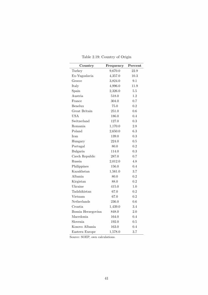
Table 2.19: Country of Origin
Country Frequency Percent
Turkey 9,670.0 22.9
Ex-Yugoslavia 4,357.0 10.3
Greece 3,824.0 9.1
Italy 4,996.0 11.9
Spain 2,326.0 5.5
Austria 518.0 1.2
France 304.0 0.7
Benelux 75.0 0.2
Great Britain 251.0 0.6
USA 186.0 0.4
Switzerland 127.0 0.3
Romania 1,170.0 2.8
Poland 2,650.0 6.3
Iran 139.0 0.3
Hungary 224.0 0.5
Portugal 80.0 0.2
Bulgaria 114.0 0.3
Czech Republic 287.0 0.7
Russia 2,012.0 4.8
Philippines 156.0 0.4
Kazakhstan 1,561.0 3.7
Albania 80.0 0.2
Kirgistan 88.0 0.2
Ukraine 415.0 1.0
Tadzhikistan 67.0 0.2
Vietnam 67.0 0.2
Netherlands 236.0 0.6
Croatia 1,439.0 3.4
Bosnia Herzegovina 848.0 2.0
Macedonia 164.0 0.4
Slovenia 192.0 0.5
Kosovo Albania 163.0 0.4
Eastern Europe 1,578.0 3.7
Source: SOEP, own calculations.
41

CHAPTER 2. DIFFERENCES IN EXPECTED & ACTUAL RETURN MIGRATION
Tab
le2.2
0:D
ifferen
ceb
etween
the
Inten
tions
and
the
‘rational’
Exp
ectations
1984-
1996
85
86
87
88
89
90
91
92
93
94
95
96
Male
-1.1
6-3
.82∗∗
-3.1
4∗∗
-3.2
7∗∗
-1.4
3-0
.19
-2.6
2-0
.79
0.4
9-2
.42
-2.7
8∗
-1.0
1(1
.48)
(1.4
8)
(1.4
8)
(1.5
0)
(1.5
9)
(1.6
1)
(1.6
0)
(1.6
3)
(1.6
5)
(1.6
5)
(1.6
7)
(1.2
9)
Age
at
Mig
ratio
n0.3
1∗∗∗
0.4
0∗∗∗
0.3
9∗∗∗
0.1
9∗
0.2
7∗∗∗
0.0
8-0
.05
0.0
60.2
10.1
70.0
60.3
3∗∗∗
(0.0
9)
(0.0
9)
(0.0
9)
(0.1
0)
(0.1
1)
(0.1
1)
(0.1
2)
(0.1
3)
(0.1
3)
(0.1
4)
(0.1
5)
(0.0
8)
ln(G
DPG
)-ln(G
DPH
)-4
.04∗∗∗
-4.0
4∗∗∗
-3.8
0∗∗∗
-2.1
6∗∗
-2.3
4∗∗
-2.9
7∗∗∗
-1.0
1-3
.98∗∗∗
-2.4
1∗∗
-0.6
3-3
.59∗∗∗
2.4
0∗∗∗
(0.9
4)
(0.9
2)
(0.9
0)
(0.9
3)
(0.9
6)
(0.9
7)
(0.9
6)
(0.9
9)
(1.0
1)
(1.0
1)
(1.0
3)
(0.7
1)
Em
plo
yed
-9.2
1∗∗∗
-7.1
9∗∗∗
-8.4
7∗∗∗
-6.3
8∗∗∗
-5.2
2∗∗
-8.8
5∗∗∗
-3.9
6-3
.20
-4.6
0∗
-1.8
31.5
1-4
.55∗∗
(2.1
1)
(2.2
5)
(2.2
6)
(2.1
5)
(2.5
3)
(2.6
1)
(2.6
0)
(2.6
5)
(2.5
6)
(2.7
7)
(2.8
0)
(2.0
4)
Sp
ouse
at
Hom
e2.7
76.1
2∗∗
6.2
6∗∗
3.5
46.9
3∗∗
6.5
0∗
6.5
0∗
2.2
5-2
.43
-2.7
32.1
6-5
.05
(3.0
8)
(3.0
3)
(2.9
2)
(3.3
4)
(3.1
4)
(3.5
9)
(3.7
3)
(4.1
0)
(4.0
2)
(4.4
4)
(4.6
3)
(5.1
5)
Atte
nded
School
inG
erm
any
2.2
63.1
83.2
87.3
5∗∗
2.9
0-2
.63
-3.3
82.3
04.0
95.0
89.2
2∗∗
1.9
2(3
.57)
(3.4
0)
(3.3
2)
(3.7
1)
(3.5
8)
(3.7
8)
(3.6
7)
(3.8
1)
(3.7
5)
(4.0
0)
(4.1
4)
(3.7
8)
Tim
ein
Germ
any
-4.5
4∗∗∗
-3.8
4∗∗∗
-4.7
0∗∗∗
-5.2
6∗∗∗
-1.0
6-1
.59
-4.4
3∗
-3.9
9-2
.85
-6.4
8∗∗
-1.8
4-0
.72
(1.3
4)
(1.3
0)
(1.4
7)
(1.7
1)
(1.9
5)
(2.2
4)
(2.4
0)
(2.7
0)
(2.9
2)
(3.0
0)
(3.7
4)
(0.8
0)
Tim
ein
Germ
any2
0.3
3∗∗∗
0.2
6∗∗∗
0.2
9∗∗∗
0.2
9∗∗∗
0.0
70.1
00.2
4∗∗
0.2
2∗
0.1
50.2
9∗∗
0.1
0-0
.01
(0.0
9)
(0.0
9)
(0.0
9)
(0.1
0)
(0.1
1)
(0.1
2)
(0.1
2)
(0.1
3)
(0.1
3)
(0.1
3)
(0.1
6)
(0.0
4)
Tim
ein
Germ
any3
-0.0
1∗∗∗
-0.0
0∗∗
-0.0
0∗∗∗
-0.0
0∗∗
-0.0
0-0
.00
-0.0
0∗
-0.0
0∗
-0.0
0-0
.00∗∗
-0.0
00.0
0(0
.00)
(0.0
0)
(0.0
0)
(0.0
0)
(0.0
0)
(0.0
0)
(0.0
0)
(0.0
0)
(0.0
0)
(0.0
0)
(0.0
0)
(0.0
0)
Incom
e0.0
00.0
00.0
0∗∗
0.0
00.0
00.0
0∗∗∗
0.0
00.0
00.0
0-0
.00
-0.0
00.0
0∗
(0.0
0)
(0.0
0)
(0.0
0)
(0.0
0)
(0.0
0)
(0.0
0)
(0.0
0)
(0.0
0)
(0.0
0)
(0.0
0)
(0.0
0)
(0.0
0)
Happin
ess
0.8
4∗∗∗
0.8
9∗∗∗
0.6
0∗∗
0.6
6∗∗
0.9
1∗∗∗
0.2
00.6
9∗
-0.3
70.4
2-0
.86∗∗
0.1
7-0
.11
(0.2
9)
(0.2
9)
(0.3
0)
(0.3
3)
(0.3
4)
(0.3
5)
(0.3
6)
(0.3
7)
(0.3
6)
(0.3
8)
(0.3
9)
(0.3
2)
Aged
60
or
old
er
3.1
53.0
93.4
86.2
9∗∗
5.7
8∗∗
9.8
2∗∗∗
10.8
3∗∗∗
10.3
3∗∗∗
7.3
0∗∗∗
7.3
4∗∗∗
9.2
5∗∗∗
0.3
7(3
.28)
(3.1
5)
(2.9
1)
(2.9
2)
(2.8
4)
(2.7
9)
(2.6
8)
(2.7
6)
(2.6
9)
(2.6
6)
(2.6
5)
(2.1
5)
Marrie
d11.2
618.6
4∗∗
10.8
78.8
716.3
2∗
26.1
7∗∗∗
20.6
4∗∗∗
14.6
7∗∗
18.1
9∗∗∗
19.0
2∗∗∗
-3.4
8(1
3.5
2)
(8.9
3)
(10.1
7)
(10.2
1)
(8.6
2)
(8.2
7)
(7.4
1)
(6.3
0)
(5.7
0)
(5.6
0)
(2.5
4)
Div
orc
ed
31.7
432.0
833.0
531.8
722.8
3-0
.35
(20.5
4)
(20.9
5)
(20.7
5)
(20.4
1)
(19.9
3)
(3.9
4)
Wid
ow
ed
-21.0
8-3
.04
(21.8
5)
(4.1
3)
Marrie
dliv
ing
separa
ted
1.0
3(4
.85)
Fam
ilyat
Hom
e2.0
6(2
.33)
Consta
nt
-22.7
1∗∗
-43.1
9∗∗∗
-31.9
3∗∗∗
-10.2
4-4
6.2
0∗∗∗
-28.4
4∗
-13.0
4-5
.59
-0.8
433.6
5-8
.23
-2.3
7(9
.52)
(8.7
1)
(9.6
1)
(13.4
4)
(12.9
0)
(15.0
6)
(16.8
1)
(19.5
1)
(24.7
4)
(25.8
5)
(31.2
1)
(20.5
9)
Country
Regio
nY
es
Yes
Yes
Yes
Yes
Yes
Yes
Yes
Yes
Yes
Yes
Yes
Bundesla
nd
FE
Yes
Yes
Yes
Yes
Yes
Yes
Yes
Yes
Yes
Yes
Yes
Yes
R2
0.1
50.1
80.1
50.1
60.1
70.1
10.1
50.1
30.1
50.1
50.1
60.2
3F
-stat.
9.1
39.7
77.3
97.1
27.8
55.0
66.1
44.7
95.1
65.1
74.9
58.3
7p-v
al.
0.0
00.0
00.0
00.0
00.0
00.0
00.0
00.0
00.0
00.0
00.0
00.0
0N
1367
1254
1195
1115
1094
1050
988
938
896
827
755
1252
Sou
rce:S
OE
P,
ow
nca
lcula
tion
s.N
ote:
*,*
*,*
**
ind
icates
sign
ifica
nce
at
the
10%
,5%
,an
d1%
level,
respectiv
ely.S
tan
dard
errors
inp
aren
theses.
Th
ed
epen
den
tvaria
ble
isth
ed
ifferen
ceb
etween
the
inten
ded
return
an
dth
e‘ra
tion
al’
exp
ectatio
n.
42

Tab
le2.2
1:
Diff
eren
ceb
etw
een
the
Inte
nti
ons
and
the
‘rat
ion
al’
Exp
ecta
tion
s199
7-
200
8
97
98
99
00
01
02
03
04
05
06
07
08
Male
0.8
00.8
4-0
.37
0.2
3-1
.02
-0.6
7-0
.32
-0.7
20.0
40.2
90.0
9-0
.46
(1.4
4)
(1.3
7)
(1.2
7)
(1.2
6)
(1.0
4)
(0.9
8)
(0.9
7)
(0.9
8)
(0.9
9)
(1.0
4)
(1.0
4)
(1.0
8)
Age
at
Mig
rati
on
0.2
3∗∗
0.1
8∗∗
0.1
6∗
0.2
5∗∗∗
0.1
8∗∗∗
0.1
9∗∗∗
0.0
70.0
30.0
50.0
6-0
.01
0.1
2(0
.09)
(0.0
9)
(0.0
8)
(0.0
8)
(0.0
7)
(0.0
7)
(0.0
7)
(0.0
7)
(0.0
7)
(0.0
7)
(0.0
7)
(0.0
8)
ln(G
DPG
)-ln
(GD
PH
)1.7
5∗∗
1.9
1∗∗∗
1.8
8∗∗∗
2.1
3∗∗∗
2.3
8∗∗∗
2.0
5∗∗∗
2.4
1∗∗∗
1.8
0∗∗∗
1.0
9∗∗
1.9
1∗∗∗
2.0
9∗∗∗
2.8
5∗∗∗
(0.7
5)
(0.7
2)
(0.6
6)
(0.6
5)
(0.5
2)
(0.4
9)
(0.4
9)
(0.4
9)
(0.5
1)
(0.5
3)
(0.5
4)
(0.5
7)
Marr
ied
-11.3
1∗∗∗
-8.8
7∗∗∗
-4.5
7-5
.28∗
0.4
60.8
24.2
7∗
-4.6
7∗
-0.1
9-6
.80∗∗
-5.5
6∗
-8.3
8∗∗∗
(3.2
3)
(3.2
3)
(3.0
7)
(3.1
0)
(2.2
3)
(2.2
2)
(2.4
4)
(2.4
9)
(2.6
8)
(2.8
1)
(2.9
7)
(3.1
9)
Marr
ied
livin
gse
para
ted
-14.2
0∗∗
-4.8
3-0
.33
0.1
4-5
.65
-0.2
78.2
1∗∗
-2.3
0-2
.16
-12.8
5∗∗∗
-7.8
5∗
-6.4
8(5
.96)
(6.0
4)
(5.9
6)
(5.7
7)
(4.3
0)
(3.9
1)
(3.9
3)
(4.0
2)
(3.8
2)
(4.0
4)
(4.1
1)
(4.4
5)
Div
orc
ed
-5.3
4-8
.11∗
-3.7
5-6
.12
1.6
00.3
46.9
9∗∗
-2.2
11.5
9-4
.68
-3.8
2-9
.24∗∗
(4.5
5)
(4.3
9)
(4.0
0)
(3.9
5)
(2.9
4)
(2.9
3)
(3.0
5)
(3.0
0)
(3.2
5)
(3.3
2)
(3.4
2)
(3.6
3)
Wid
ow
ed
-14.0
8∗∗∗
-9.7
9∗
-3.2
9-4
.19
1.0
7-2
.44
3.4
9-4
.66
0.9
9-6
.83∗
-6.7
6∗
-9.0
2∗∗
(5.0
8)
(5.0
0)
(4.3
7)
(4.6
0)
(3.5
1)
(3.3
6)
(3.4
7)
(3.4
4)
(3.4
5)
(3.6
7)
(3.7
0)
(3.8
2)
Em
plo
yed
1.5
8-0
.81
11.5
3∗∗∗
-2.1
4-0
.09
-2.3
1∗
-4.9
6∗∗∗
-3.4
6∗∗
-3.5
2∗∗
-6.2
4∗∗∗
-3.7
4∗∗
-3.9
5∗∗
(2.2
2)
(1.9
6)
(3.2
0)
(1.8
9)
(1.5
2)
(1.2
8)
(1.3
2)
(1.3
7)
(1.4
2)
(1.4
4)
(1.4
6)
(1.5
4)
Fam
ily
at
Hom
e2.8
64.1
3∗
4.0
6∗∗
3.1
1∗
2.0
61.1
12.0
1∗
1.0
42.2
1∗
3.2
3∗∗∗
0.4
31.4
8(2
.34)
(2.1
1)
(1.8
2)
(1.8
0)
(1.2
6)
(1.1
8)
(1.1
4)
(1.1
5)
(1.1
6)
(1.2
2)
(1.2
0)
(1.2
4)
Sp
ouse
at
Hom
e-0
.42
0.1
3-6
.33
0.2
8-0
.61
-3.1
9-4
.39
-2.7
7-2
.05
2.0
96.6
33.1
7(5
.59)
(5.9
7)
(5.1
9)
(5.4
0)
(5.3
3)
(5.0
1)
(5.5
4)
(5.2
1)
(5.4
0)
(5.4
1)
(5.6
4)
(5.5
1)
Att
ended
School
inG
erm
any
-4.1
42.6
25.5
6∗
-3.2
2-0
.92
2.4
52.2
70.2
30.9
7-0
.19
1.2
73.0
7(3
.79)
(3.6
8)
(3.3
3)
(3.2
5)
(2.7
0)
(2.7
0)
(2.4
8)
(2.5
1)
(2.6
6)
(2.5
9)
(2.5
7)
(2.5
9)
Tim
ein
Germ
any
-2.0
7∗∗
-0.3
3-0
.34
1.0
70.8
9∗
-0.2
90.7
2-0
.22
-0.5
80.0
20.5
90.3
3(0
.89)
(0.9
1)
(0.8
2)
(0.8
6)
(0.5
3)
(0.5
0)
(0.5
2)
(0.5
1)
(0.5
3)
(0.5
4)
(0.6
3)
(0.6
8)
Tim
ein
Germ
any2
0.0
7-0
.01
-0.0
1-0
.07∗
-0.0
5∗∗
0.0
1-0
.04
0.0
00.0
1-0
.01
-0.0
3-0
.02
(0.0
5)
(0.0
5)
(0.0
4)
(0.0
4)
(0.0
3)
(0.0
2)
(0.0
2)
(0.0
2)
(0.0
2)
(0.0
2)
(0.0
3)
(0.0
3)
Tim
ein
Germ
any3
-0.0
00.0
00.0
00.0
0∗∗
0.0
0∗∗
0.0
00.0
0∗
0.0
00.0
00.0
00.0
00.0
0(0
.00)
(0.0
0)
(0.0
0)
(0.0
0)
(0.0
0)
(0.0
0)
(0.0
0)
(0.0
0)
(0.0
0)
(0.0
0)
(0.0
0)
(0.0
0)
Incom
e0.0
00.0
0-0
.00
0.0
0-0
.00
-0.0
00.0
00.0
00.0
00.0
00.0
00.0
0(0
.00)
(0.0
0)
(0.0
0)
(0.0
0)
(0.0
0)
(0.0
0)
(0.0
0)
(0.0
0)
(0.0
0)
(0.0
0)
(0.0
0)
(0.0
0)
Happin
ess
0.0
2-0
.20
-0.1
50.1
2-0
.05
-0.2
60.1
1-0
.06
0.5
8∗∗
0.5
0∗
0.3
20.3
6(0
.37)
(0.3
5)
(0.3
2)
(0.3
3)
(0.2
9)
(0.2
8)
(0.2
6)
(0.2
6)
(0.2
5)
(0.2
7)
(0.2
8)
(0.2
8)
Aged
60
or
old
er
3.7
22.8
71.8
71.0
41.5
40.9
22.2
94.7
5∗∗∗
3.3
4∗
2.8
64.4
5∗∗
2.4
4(2
.38)
(2.3
1)
(2.0
6)
(2.0
6)
(1.8
0)
(1.7
7)
(1.7
5)
(1.7
9)
(1.7
8)
(1.8
7)
(1.8
9)
(1.9
4)
Dis
advanta
ge
due
toori
gin
?-4
.18∗∗∗
-1.4
3-4
.44∗∗∗
-2.3
3∗∗
0.3
4-1
.02
-1.8
4∗
-1.8
7∗
-0.3
11.1
6-1
.00
0.0
5(1
.29)
(1.2
5)
(1.1
5)
(1.1
8)
(1.0
0)
(0.9
8)
(0.9
6)
(0.9
8)
(1.0
1)
(1.0
2)
(1.0
2)
(1.1
0)
Wri
ting
Germ
an?
-0.3
1-3
.12∗
1.5
81.2
6-1
.27
-1.5
913.3
2∗
0.6
3-2
.13
-4.5
2∗∗
-5.7
5∗∗∗
(1.8
5)
(1.8
2)
(1.6
8)
(1.6
8)
(1.5
4)
(1.5
2)
(6.9
9)
(1.7
2)
(1.7
8)
(1.8
1)
(1.9
4)
Sp
eakin
gG
erm
an?
5.8
91.0
17.3
6-1
.30
0.1
14.2
54.6
93.7
20.8
7-2
.35
-2.5
0-0
.60
(6.5
7)
(5.4
1)
(5.8
0)
(5.3
1)
(4.4
5)
(3.7
9)
(3.6
0)
(3.5
1)
(4.1
3)
(4.6
2)
(5.2
3)
(5.1
2)
Language
New
spap
er
Germ
an?
6.4
2∗∗∗
8.7
8∗∗∗
6.4
8∗∗∗
5.2
7∗∗∗
5.3
5∗∗∗
9.1
0∗∗∗
3.7
7∗∗∗
4.2
9∗∗∗
3.6
4∗∗
4.6
0∗∗∗
2.4
7∗
7.6
2∗∗∗
(1.6
0)
(1.5
5)
(1.5
0)
(1.5
6)
(1.3
3)
(1.3
2)
(1.3
0)
(1.3
3)
(1.4
2)
(1.4
2)
(1.4
5)
(1.5
6)
Const
ant
-19.9
2∗
0.6
0-2
9.8
3∗
-24.8
7∗
-17.5
2∗
-15.5
8∗
-27.9
4∗∗∗
-21.9
8∗
-15.9
2-1
6.6
0-7
.30
-12.2
8(1
1.5
7)
(14.9
9)
(15.3
0)
(15.0
4)
(9.3
2)
(8.3
1)
(10.6
0)
(11.9
9)
(10.1
0)
(13.1
0)
(17.0
1)
(16.6
2)
Countr
yR
egio
nY
es
Yes
Yes
Yes
Yes
Yes
Yes
Yes
Yes
Yes
Yes
Yes
Bundesl
and
FE
Yes
Yes
Yes
Yes
Yes
Yes
Yes
Yes
Yes
Yes
Yes
Yes
R2
0.2
80.2
50.2
70.2
20.1
90.2
00.1
70.1
60.1
70.1
90.1
60.2
0F
-sta
t.7.3
86.3
86.8
05.3
15.7
25.8
84.6
14.2
34.2
24.4
93.3
63.8
8p-v
al.
0.0
00.0
00.0
00.0
00.0
00.0
00.0
00.0
00.0
00.0
00.0
00.0
0N
920
960
937
938
1265
1194
1186
1171
1075
979
907
805
Sou
rce:
SO
EP
,ow
nca
lcu
lati
on
s.N
ote
:*,*
*,*
**
ind
icate
ssi
gn
ifica
nce
at
the
10%
,5%
,an
d1%
level
,re
spec
tivel
y.S
tan
dard
erro
rsin
pare
nth
eses
.T
he
dep
end
ent
vari
ab
leis
the
diff
eren
ceb
etw
een
the
inte
nd
edre
turn
an
dth
e‘r
ati
on
al’
exp
ecta
tion
.
43

44

Chapter 3
Bereavement Effects and Early Life
Circumstances1
3.1 Introduction
Bereavement of a close family member is a stressful and traumatic event that occurs mostly later
in life.2 Papers such as Lindeboom et al. (2002) and van den Berg et al. (2012) have shown the
detrimental impact of bereavement and grief on economically relevant outcomes, such as health,
the familial situation, and labor market outcomes. In particular, van den Berg et al. (2012)
find that grief can cause persistent effects on labor market participation. Therefore, a deep
investigation of bereavement effects, resilience and the influencing factors of coping is important
for the society and for the economy.
Latest since Barker (2007), economists are interested in early life circumstances and what long
run effects are caused by detrimental conditions in utero or childhood. Almond and Currie
(2011) give a concise overview of such long run effects.3 The Second World War (WW2) created
a very specific and stressful environment.4 It is quite likely that those individuals who grew up
without their father or were exposed to bombardments or combat actions, as an example, had
a stressful time. As an example, around 70 cities were destroyed due to the war (about 333
1This chapter is co-authored with Gerard J. van den Berg and Anna Hammerschmid.2Examples of articles focusing on bereavement are Siflinger (2013), van den Berg et al. (2012), van den Berg
et al. (2011a), van den Berg and Drepper (2011), Espinosa and Evans (2008) and for a thorough literature overviewsee Hansson and Stroebe (2007).
3Other examples in this line of literature are: Doblhammer et al. (2011), van den Berg and Lindeboom (2013),Tough (2013), Elder (1999).
4In the context of the WW2, we refer the reader to a current literature strand in economics, which dealswith early life circumstances and the WW2, see e.g., van den Berg et al. (2011b), Jurges (2012), Akbulut-Yuksel(2009), Akbulut-Yuksel et al. (2013), Kesternich et al. (2013), Kesternich et al. (forthcoming).
45

CHAPTER 3. BEREAVEMENT EFFECTS & EARLY LIFE CIRCUMSTANCES
km2 with 2,164,800 housing losses and thus around 7,500,000 persons were made homeless in
Germany (Hewitt, 1983)). According to Radebold (2009) about a quarter of German children
grew up without a father. This number is not surprising if we take a look at the casualties the
war caused; Radebold (2009) reports cohort death rates of 45% for those between the ages of
20-25 years, 56% for the 25-30 year olds, 36% for the 30-35 year olds, and 29% for the 35-40
year olds. The question may thus be raised how these individuals cope with stressful events
later in their life. Are they less resilient to the stress caused by bereavement following traumatic
experiences, or does it evoke emotions from their early remembrances?
The psychology literature suggests phenomena such as posttraumatic stress disorder (PTSD)
following traumatic experiences (for a review of research on long-run effects associated with
WW2 trauma in elderly Germans see e.g., Glaesmer, 2013), and trauma re-activation or re-
traumatization (see e.g., Macleod, 1994; Kaup et al., 1994; Heuft, 2004). This suggests that
those individuals exposed to stressful events early in life suffer from stress later in life due
to trauma reactivation. Furthermore the psychologists define late-onset stress symptomatology
(LOSS), which in our context can be related to bereavement later in life (see e.g., Davison et al.,
2006).5
In this chapter, we are interested in the role of early life circumstances in combination with
bereavement effects late in life. Specifically, we analyze father’s absence or exposure to air raids
or combat actions in the context of WW2 in Germany in combination with the effects of late life
bereavement. In order to prepare the individuals accordingly for the eventual PTSD or LOSS, it
is important to study whether individuals have difficulties to cope with grief later in life if they
were exposed to air raids, combat actions or father’s absence. Analyzing whether exposure causes
depression or other health related consequences, which in turn may affect financial wealth or care
taking abilities, is important for the society as they will bear the cost of something preventable.
The underlying question of the growing literature is whether shocks early in life mediate or
worsen the impact of negative events later in life (see e.g., van den Berg and Schoch (2013),
5Furthermore the psychology literature analyzes cumulative trauma exposure, for more details in thisresearch area see e.g., Ogle et al. (2014) who give an overview and references therein. Ogle et al. (2014) finda strong association between cumulative exposure and PTSD symptom severity. Furthermore they pin downthe event categories that show the strongest relationship to symptom severity; beginning with the strongestassociation: “cumulative exposure to childhood violence, adult physical assaults, war zone exposure, sexualassaults, death/illness” (see Ogle et al., 2014). However, they emphasize that a causal interpretation of theiranalysis might be problematic.
46

Hayward et al. (2013), and van den Berg et al. (2010)).6
We contribute to this literature by estimating a joint treatment effect of adverse early life
circumstances (father’s absence or exposure to air raid or combat actions in the context of
WW2 in Germany) and a late life event (bereavement of a close family member) on (mental)
health, life and sleep satisfaction. Besides this measure of the general mental state we include life
and sleep satisfaction because they may be better at capturing the actual stress level. A recent
study by Rosekind et al. (2010) shows that sleep problems, such as insomnia or insufficient
sleep syndrome, are negatively related to workplace productivity measures as well as safety. To
measure the combined effect of detrimental early-life circumstances and bereavement, we use a
first difference approach, thereby accounting for all time-invariant confounding factors. The first
difference approach is outlined in Section 3.2 and follows the literature (see e.g., Lindeboom
et al. (2002), van den Berg et al. (2010), van den Berg and Schoch (2013)).
One of the contributions of this article is the novel data - the “Fruhe Kindheitsmodul” (FKM).
A survey on childhood circumstances in the context of the WW2 and the postwar period in
Germany. It can be linked to the German Socio Economic Panel (SOEP) and we are the first
to do so. This allows us to link stressful events during WW2 to a rich set of information on
bereavement, health, life and sleep satisfaction. Moreover, to the best of our knowledge, we
are the first to analyze the specific causal interaction effect with bereavement in the context
of the WW2. The interplay between an absent father, air raid or combat action exposure in
combination with bereavement later in life gives us a novel insight into grief and bereavement
effects.
Figure 3.1 depicts our expectations that an individual hit by an adverse life event is affected
less in terms of mental health if she has been exposed to beneficial early-life conditions (e.g.,
not exposed to air raids or battlefield).7 One of the major differences of this chapter to van den
Berg et al. (2010) is that our individuals are exposed to detrimental early-life conditions during
6van den Berg et al. (2010) analyze the interplay between the business cycle at birth and the effect ofadverse events late in life on cognition using the Dutch LASA. They find that the effect of stroke, surgery,and illness/death of a family member is worse for those who were born during a recession. Moreover, they findevidence for a differential impact on men and women. van den Berg and Schoch (2013) use the SHARE datato examine the influence of economic conditions at birth on the mental health effect (cognition, depression) ofadverse events later in life. Hayward et al. (2013) test the “Predictive Adaptive Response (PAR) hypothesis” formortality and fertility, which states that poor nutrition early in life leads to adaption, making the individual moreresistant to poor nutrition later in life. Their findings are not in line with the PAR hypothesis. Moreover, theyfind heterogeneous effects with respect to socio-economic status and age.
7Figure 3.1 is similar to van den Berg et al. (2010) (Figure 1).
47

CHAPTER 3. BEREAVEMENT EFFECTS & EARLY LIFE CIRCUMSTANCES
childhood.8
Figure 3.1: Potential Role of Early Life Conditions on the Effect of Adverse Events Later in Lifeon Mental Health
Wave 1 Wave 2Time
HealthAdverse Life Event
Born under beneficial early-life
conditions
Born under adverse early-life
conditions
As expected, we find a significant negative interaction effect of father’s absence, exposure to
air raids or combat actions and bereavement on mental health. Similarly, we find a negative
interaction effect of bereavement and father’s absence on life and sleep satisfaction. The
satisfaction results point into the direction that the individuals suffer from stress. For exposure
to air raids or combat actions and bereavement of a close family member, we find a negative
effect on the satisfaction outcomes, which is only significant in the case of life satisfaction. Our
findings underline the importance of the early life environment to develop the ability to cope
with grief later in life.
These results are robust to certain sensitivity checks, such as excluding cancer deaths, and those
observations where life and sleep satisfaction cannot have an increase or a decrease.9 In line
with the literature we also perform an effect heterogeneity test with respect to gender (see e.g.,
van den Berg et al., 2010) and socioeconomic status (see e.g., Hayward et al., 2013).
8The period during childhood varies depending on which early-life circumstance we focus on. For father’sabsence, it is possible that the father was absent just before an individual reached the age of 13 years, but it couldhave been that the father was absent when the individual was only a couple of months old. For the air raid orbattlefield exposure, the individual can at most be 9 years old.
9This means that satisfaction value was at its peak in one year (cannot increase) or at its low (cannot decrease).
48

The remainder of this chapter is structured as follows, Section 3.2 explains the empirical strategy,
and discusses its possible shortcomings. Section 3.3 presents the data and provides an overview
of the key variables used. Section 3.4 describes the results and Section 3.5 concludes.
3.2 Empirical Strategy
Similar as in van den Berg et al. (2010) (see Figure 3.2, very close to Figure 2 in van den Berg
et al. (2010)) our analysis focuses on the interplay between early-life conditions (father absence
or exposure to air raids or battlefield) and adverse life events (death of close family member)
with mental health or life/sleep satisfaction later in life. Our empirical specification follows for
example Lindeboom et al. (2002), van den Berg et al. (2010), and van den Berg and Schoch
(2013). We consider a similar relationship between mental health Hit (or life/sleep satisfaction)
and a range of socio-economic variables Xit, a life event variable Dit, an early-life circumstance
indicator Eit, an interaction between the life event and the early-life circumstance Dit ∗ Ei,
time-invariant individual characteristics αi, and an idiosynchratic shock uit.
Hit = X′itβ +Ditγ + Eiθ +DitEiδ + αi + uit (3.1)
In this context, Hit, Xit, Dit and Ei are observed, while αi and uit are unobserved. γ and δ
are the parameters of interest since γ captures the effect of the life event on mental health,
and δ captures the interaction effect of the early life circumstances and the life event on mental
health. If we wanted to estimate the effect of the life event on mental health via regular OLS,
we would have to assume that Xit, Dit and Dit ∗ Ei are orthogonal to αi + uit. As discussed in
Lindeboom et al. (2002), it is usually assumed that this orthogonality condition holds. It may
not be satisfied if there are unobservables in αi or uit that affect the outcome variable and any
of the right hand side variables.
Figure 3.2: Early-Life Conditions, Adverse Life Events and Later-life Mental Health
49
CHAPTER 3. BEREAVEMENT EFFECTS & EARLY LIFE CIRCUMSTANCES
To overcome the endogeneity problem due to time-invariant unobservables (αi), we use the first
difference approach. Again, we refer the reader to Lindeboom et al. (2002) for a discussion of the
three possible empirical approaches to deal with this sort of endogeneity. Due to the fact that
we have a longitudinal data set at our hands, we can use the first difference approach without
any problem. Taking first differences of Equation (3.1) leads to:
∆Hit = (∆Xit)′β + (∆Dit)γ + (∆DitEi)δ + ∆uit (3.2)
∆ denotes the first difference operator, e.g., ∆Hit := Hit−Hi,t−1. ∆Dit equals one when the life
event happened, meaning that the individual lost someone close. This is an irreversible event,
thus Dit = 1 corresponds to ∆Dit = 1.10
The drawback that results from a first differenced approach, as iterated in Lindeboom et al.
(2002), is that time-invariant explanatory variables drop out of the estimation. In our case, this
is relevant for the level of the early life events (father absence and air raid or combat exposure) as
they drop out and may be interesting effects by themselves. However, as we are mainly interested
in bereavement effects, i.e., the effect (and interaction effect) of a time-variant variable, this is
only a minor problem.
3.3 Data
Our empirical analysis, uses the German Socio Economic Panel (SOEP) and a novel supple-
mentary module called “Fruhe Kindheit im (Nach-)Kriegskontext” (FKM). The SOEP is a
longitudinal survey of households and individuals in Germany.11 The FKM is a survey on
childhood circumstances in the context of the Second World War (WW2) and the postwar period
in Germany. As it is a novel survey, we provide a more detailed description of the contents and
sampling in the Appendix 3.A.1.
Our information on (mental) health and bereavement in late life as well as some of the
covariates for our empirical model stem from the SOEP, while the information on outcomes
and bereavement is based on the waves from 2010, 2011, and 2012. The information on early
10We refer the reader to the data section, where we explain how this difference changes if an individual losese.g., his mother in one wave and his father in the next.
11For further information about the SOEP, we refer the reader to Wagner et al. (2007). We use the Socio-Economic Panel (SOEP), data for years 1984-2012,version 29,SOEP,2013,doi:10.5684/soep.v29.
50

life exposure to stress is taken from the FKM. A detailed description of the main variables used
is provided in the following sections.
3.3.1 Outcome Variables
Our main outcome variables are current life satisfaction, sleep satisfaction and overall mental
health, as measured by the Mental Component Summary Scale (MCS) (provided biennially in
the SOEP). The SOEP’s MCS score is a z-transformed measure of mental health (mean: 50,
standard deviation: 10) that is based on an explorative factor analysis and follows closely the
SF-12v2 concept (see Andersen et al., 2007).12 For life and sleep satisfaction, the respondents
are explicitly asked to rate their satisfaction on a 0-10 scale, where 10 indicates highest and 0
indicates lowest satisfaction.
3.3.2 Bereavement
In the SOEP individuals are annually asked to provide information on whether and in which
month their mother, father, child, partner or other family members died.
The general bereavement indicator Dit takes the value 1 if the partner, the mother, the father,
the child or any other household person, died between t and t-1.13 As explained in the empirical
specification, we estimate our main specification using a first difference approach. To get a time-
consistent measure of ∆Dit, we make the following adjustments; ∆Dit is missing if someone died
in the previous period (t-1) and nobody died in the current period (t) or if a death occurred in
both periods. These change ensure that only cases with no deaths between two waves are in the
control group and cases with bereavement in the second wave of a two-wave-interval are in the
treatment group.14
Since the health module is conducted on a biennial basis, we have information on the mental
health score (MCS) for 2010 and 2012. We can thus only base our estimation on the first difference
12Following Ware et al. (2002) closely, Andersen et al. (2007) use eight subscales for the calculation of theMCS and Physical Component Summary Scale (PCS): “Physical Functioning, Role Physical, Bodily Pain, GeneralHealth, Vitality, Social Functioning, Role Emotional, and Mental Health”. See Andersen et al. (2007) for a detaileddescription of the procedure, and the differences as well as the similarities to the original SF-12v2 (see e.g., Wareet al., 2002).
13Missing values of the sub indicators (for deaths of partner, mother, father, child, or other household members)are treated as 0, unless all the sub indicators are missing. In this case, also the general death indicator takes amissing value. A detailed description of the steps and adjustments used to generate the treatment variables isprovided in Appendix 3.A.2.
14However, we want to emphasize that we do not tackle the initial conditions problem at this stage. We do notconsider any information (on potential deaths) from the past when constructing the bereavement indicators forthe intervals 2010-2011 and 2011-2012, respectively.
51

CHAPTER 3. BEREAVEMENT EFFECTS & EARLY LIFE CIRCUMSTANCES
between 2012 and 2010. We have to make a further adjustment when generating ∆Dit for the
analysis of MCS, making sure that ∆Dhealth captures deaths between 2010 and 2012.15 For a
detailed analysis regarding the actual timing of death within this two year interval, we generate
two sub-indicators if bereavement occurred between the 2010 and 2011 waves or between the
2011 and 2012 waves. These two sub-indicators sum to ∆Dhealth.
The following section provides a detailed description of the early life variables (exposure to air
raids, combat actions, and father’s absence).
3.3.3 Early Life Circumstances
In the FKM, the individuals are asked whether they did not live in the same household as their
father for more than 6 months up until the age of 13. This question is used as our indicator
for father’s absence.16 Additionally, we have information on the duration and type of absence
(war/prison).
We use the individual answers to four questions to generate an indicator of battlefield and air
raid exposure. The first question refers to the respondents born between 1935 and 1944 and asks
whether they remember air raids (Q1).17 Moreover, those born between 1939 and March 1945
were explicitly asked whether they have experienced air raids in their first year of life (Q2).18
We also include the information on whether the mother experienced air raids during pregnancy
(cohorts 1940-45, Q3).19 The final question we include asks about other combat actions in the
immediate environment and refers to the cohorts 1935 until 1944 (Q4).20
The summary indicator of air raid/battlefield exposure is an aggregate measure of these four
questions.21 As covariates and for sensitivity analyses, we define age in months using the birth
15For a more detailed description of this adjustment, we refer the reader to the Appendix 3.A.2.16Question: “Up until the age of 13, have you not lived with your father in the same household for at least 6
months?”. This question and all of the following questions from the FKM questionnaire have been translated bythe authors.
17Question Q1: “Do you remember air raids?”.18Question Q2: “Have you experienced air raids in your first year of life?”.19Question Q3: “Has your mother experienced air raids during pregnancy?”.20Question Q4: “Beside air raids, were there other combat actions in your direct environment that you could
hear or see?”. For every individual born outside the respective time frame, we infer the answer “no” because theycannot be affected. In addition, the categories “do not know” and “no” are treated as a denial in Q2 and Q3.
21It is 1 if any of the 4 variables takes the value 1. In a similar way, it is set to missing if any of the 4 variablesis missing and 0 otherwise.
52

and interview months. Father’s education is generated as an indicator for high socio-economic
status (SES).22
3.3.4 Descriptive Statistics
Tables 3.1 and 3.2 show descriptive statistics for the MCS and life/sleep satisfaction estimation
samples, respectively.23 Since the sample for the analysis of the two early life events (father’s
absence and air raid/battlefield exposure) differ slightly, we report the descriptive statistics also
separately for the two samples. The statistics are however very similar between the two samples.
Moreover, there are only minor differences in these statistics across the samples for our outcome
variables MCS and life/sleep satisfaction. The average age is between 68 and 69 years and there
are slightly less men in all our samples which is due to the longer life expectancy of women. Less
than one quarter of our sample has/had a father with a high education degree.
Table 3.1: Summary Statistics MCS
(FA) (AB)Mean SD Mean SD
Age (in months) 827.47 55.30 827.82 54.75Age2 (in months) 6.9e+05 91506.82 6.9e+05 90612.16MCS 52.18 9.33 52.10 9.37Males 0.49 0.50 0.49 0.50High Father Education 0.24 0.42 0.24 0.43∆ Age (in months) 11.77 1.16 11.76 1.16∆ Age2 (in months) 19337.12 2277.32 19334.05 2277.95∆ MCS -0.76 8.87 -0.83 8.94
Source: SOEP, own calculations.Notes: (FA) stands for fahter absence sample, and (AB) stands for air raid battlefieldsample.
Tables 3.3 and 3.4 give an overview on the number of treatment cases for our analysis. To
make sure that our cell sizes do not decrease too much when interacting bereavement with the
indicators for adverse early life conditions, we also show the number of cases for which both
events have happened (interaction term = 1). Again, the differences between our samples are
only minor. The number of bereaved cases is larger than 50 in the first interval (2010-2011) and
does not exceed 40 in the second interval (2011-2012). For the interaction between bereavement
and early life events, we have at most 25 cases in the first interval and less than 20 cases in the
22We define high SES as Realschule, Fachhochschule, Abitur, and low SES as: Hauptschule, no degree, noschool attended.
23For the first difference analysis of life and sleep satisfaction, we use up to two observations per person. For thecalculation of means and standard deviations in Table 3.2, we only use the first observation for each individual.
53

CHAPTER 3. BEREAVEMENT EFFECTS & EARLY LIFE CIRCUMSTANCES
Table 3.2: Summary Statistics Satisfaction
(FA) (AB)Mean SD Mean SD
Age (in months) 818.14 55.08 818.53 54.52Age2 (in months) 6.7e+05 90089.83 6.7e+05 89162.61Life Satisfaction 7.19 1.62 7.18 1.63Satisfaction Sleep 6.78 2.24 6.77 2.25Males 0.48 0.50 0.48 0.50High Father Education 0.23 0.42 0.23 0.42∆ Age (in months) 11.61 1.64 11.62 1.66∆ Age2 (in months) 18859.74 2916.55 18873.96 2938.83∆ Life Satisfaction -0.15 1.43 -0.16 1.43∆ Satisfaction Sleep 0.00 1.91 0.01 1.92
Source: SOEP, own calculations.Notes: (FA) stands for father absence sample, and (AB) stands for air raid battlefieldsample.
second one.
Moreover, we provide histograms of life satisfaction, sleep satisfaction, and MCS (in levels and
in first differences) in the Appendix 3.A.3. All outcome variables have a slightly left-skewed
distribution in levels. However, the distributions of the first differenced outcome variables are
fairly symmetric.
Table 3.3: Treatment Cases MCS
∆D ∆D ∆Dhealth
2010-2011 2011-2012(FA) (AB) (FA) (AB) (FA) (AB)
Adverse Life Event 53 56 34 34 87 90Adverse Life Event * Early Life 22 23 16 16 38 39
Source: SOEP, own calculations.Notes: (FA) stands for father absence sample, and (AB) stands for air raid battlefield sample.
Table 3.4: Treatment Cases Satisfaction
∆D ∆D ∆Dtotal
2010-2011 2011-2012(FA) (AB) (FA) (AB) (FA) (AB)
Adverse Life Event 58 61 39 40 97 101Adverse Life Event * Early Life 25 24 19 17 44 41
Source: SOEP, own calculations.Notes: (FA) stands for father absence sample, and (AB) stands for air raid battlefield sample.
Figure 3.3 plots different measures for the life and sleep satisfaction of the SOEP respondents
over time. Panel (3.2a) plots the average life satisfaction over the whole SOEP horizon, and we
can see that it is relatively stable around 7. The same holds for satisfaction sleep as Panel (3.2b)
54
shows, it is more or less constant around 6.8. The time horizon is shorter for satisfaction sleep,
as it has only been surveyed since 2008. Splitting our sample into war versus non-war cohorts,
where the war cohorts are defined as being born between 1939 and 1945 we observe that the
war cohorts are a little bit less satisfied with life and sleep (see Panels (3.2c) and (3.2d) and
be aware of the scales). Panels (3.2e) and (3.2f) plot the relative number of individuals in the
different cells, it emphasizes that 60 to 70% of the individuals in the SOEP have a life or sleep
satisfaction between 7 and 10, while 20 to 30% have a life or sleep satisfaction between 3 and
7, and only about 10% are very unsatisfied with their life and sleep.24 Splitting our sample by
exposure to air raids or battlefield, or to father’s absence or even both (panels (3.2g) and (3.2h))
we observe no clear difference in life or sleep satisfaction.25
3.4 Results
In this section, we describe the results of our empirical analyses. For our three outcome variables,
we run a (pooled) OLS regression (Equation 3.1), and a first difference analysis (Equation 3.2).
For the following results, we first regress the respective outcome variable on the bereavement
indicator (Panel a), while in Panel (b), we include the interaction between the bereavement
indicator and the respective adverse early life event (air raid/battlefield exposure and father
absence) to test whether those elderly who have experienced such conditions are more or less
resilient to bereavement. As discussed earlier, we expect more detrimental bereavement effects
for those individuals who faced adverse early life conditions. Moreover, we test explicitly whether
the sum of the main bereavement effect and the interaction effect of bereavement and early life
conditions is significantly different from 0.26
In Subsection 3.4.1, we show the main results of our analysis and in Subsection 3.4.2, we conduct
some sensitivity analyses, while in Subsection 3.4.3, we test for effect heterogeneity with respect
to gender and socioeconomic status (SES).
3.4.1 Main Results
Tables 3.5 and 3.6 show the results for the mental health score MCS. As explained above the
health module is only collected every other year, and therefore we can only consider the difference
between 2012-2010 (Table 3.5). To further analyze the exact timing of bereavement within this
24We are thus not too worried that there is not enouogh variation in our outcome variables, and most of oursample can suffer from a decrease or an increase in their satisfaction with life and sleep.
25We tested whether the difference is significant between each group for each year, but it is not.26The results for these F-tests are shown in Appendix 3.B.
55

CHAPTER 3. BEREAVEMENT EFFECTS & EARLY LIFE CIRCUMSTANCES
Figure 3.3: Outcome Variables in the SOEP
(a) Life Satisfaction (LS)6.
57
7.5
8Li
fe S
atis
fact
ion
1985 1990 1995 2000 2005 2010Time
(b) Satisfaction Sleep (SS)
6.5
77.
58
Sat
isfa
ctio
n S
leep
2008 2009 2010 2011 2012Time
(c) LS War Cohorts
6.5
77.
58
Life
Sat
isfa
ctio
n
1985 1990 1995 2000 2005 2010Time
War Cohort Non-war Cohort
(d) SS War Cohorts
6.5
77.
58
Sat
isfa
ctio
n S
leep
2008 2009 2010 2011 2012Time
War Cohort Non-war Cohort
(e) LS Observations
0.2
.4.6
.8Li
fe S
atis
fact
ion
1985 1990 1995 2000 2005 2010Time
LS <= 3, WC = 0 LS > 3 & LS < 7, WC = 0LS >= 7 & LS <= 10, WC = 0 LS <= 3, WC = 1LS > 3 & LS < 7, WC = 1 LS >= 7 & LS <= 10, WC = 1
(f) SS Observations
.1.2
.3.4
.5.6
Sat
isfa
ctio
n S
leep
2008 2009 2010 2011 2012Time
SS <= 3, WC = 0 SS > 3 & SS < 7, WC = 0SS >= 7 & SS <= 10, WC = 0 SS <= 3, WC = 1SS > 3 & SS < 7, WC = 1 SS >= 7 & SS <= 10, WC = 1
(g) LS FKM
6.5
77.
58
Life
Sat
isfa
ctio
n
1985 1990 1995 2000 2005 2010Time
Not Exposed Father AbsentAirraid Battlefield Exposed to Both Events
(h) SS FKM
6.5
77.
58
Sat
isfa
ctio
n S
leep
2008 2009 2010 2011 2012Time
Not Exposed Father AbsentAirraid Battlefield Exposed to Both Events
56

two wave interval, we split our adverse life event variable into two sub-indicators, as explained
in Section 3.3.2 (Table 3.6).
Estimating an OLS regression of MCS on bereavement (Panel (a), Table 3.5), we find a
significant negative bereavement effect on mental health for both samples.27 The point estimates
decrease and become insignificant when we control for time-invariant unobservables using the
first difference approach. In Panel (b), we additionally include an interaction between the adverse
early life condition and the bereavement event, for both OLS estimates the coefficients are now
insignificant. However, the results of the first difference estimation indicate negative significant
interaction effects. The magnitude of these significant effects is approximately half a standard
deviation of the MCS variable.
Table 3.5: Results MCS 2010 - 2012
Airraid Battlefield Father AbsenceOLS ∆ OLS ∆
Panel (a)Adverse Life Event 2012 - 2010 -2.974∗∗∗ -1.837 -3.029∗∗∗ -1.554
1.128 1.182 1.129 1.158
N 5067 2105 5207 2161R2 0.006 0.002 0.006 0.002
Panel (b)Adverse Life Event 2012-2010 -1.745 0.564 -1.829 0.571
1.549 1.523 1.459 1.405
Adverse Life Event 2012-2010 * EL Event -2.787 -5.456∗∗ -2.965 -4.876∗∗
2.228 2.299 2.258 2.296
N 5067 2105 5207 2161R2 0.006 0.006 0.007 0.005
Source: SOEP, own calculations.Notes: The dependent variable is the mental health score (MCS) in the SOEP. The reported regressionsinclude a quadratic in age (calculated in months) and a constant. EL stands for Early Life Event. Thestandard errors are clustered at the individual level.
Splitting the bereavement indicator with respect to the timing of the death in our first difference
analysis, we find a negatively significant impact of approximately half a standard deviation of
MCS for the second half of the two-year interval (Table 3.6, Panel (a)). Using this specification
(Panel (b)), we also find a significant interaction of adverse early life circumstances and recent
bereavement, which is even larger in absolute magnitude (more than one standard deviation).
Our findings clearly indicate that the effect of bereavement on mental health occurs in the short
27The samples for the analysis of father absence and air raid/battlefield exposure differ slightly. Therefore, wedisplay the results that do not include early life information for both samples separately.
57

CHAPTER 3. BEREAVEMENT EFFECTS & EARLY LIFE CIRCUMSTANCES
run. We also test whether the sum of the main bereavement effect and the interaction effect
of the early life event and bereavement is significant.28 The bereavement effect for those who
experienced adverse early life conditions is only significant in the case of recent (2012) losses.
The magnitude of this effect is about double the treatment effect of the baseline regression in
Table 3.6, Panel (a). This finding indicates that those born under adverse early life conditions
are driving the results of the baseline specification.
Table 3.6: First Difference Results MCS
(AB) (FA)
Panel (a)Adverse Life Event 2011 0.558 0.832
1.359 1.308
Adverse Life Event 2012 -5.557∗∗∗ -5.474∗∗∗
1.968 1.974
N 2105 2161R2 0.007 0.007
Panel (b)Adverse Life Event 2011 1.182 0.823
1.840 1.713
Adverse Life Event 2012 -0.485 0.1322.619 2.409
Adverse Life Event 2011 * Early Life Event -1.438 0.0712.698 2.631
Adverse Life Event 2012 * Early Life Event -10.739∗∗∗ -11.887∗∗∗
3.448 3.373
N 2105 2161R2 0.013 0.014
Source: SOEP, own calculations.Notes: The dependent variable is the mental health score (MCS) in the SOEP. Thereported regressions include a quadratic in age (calculated in months) and a constant.AB stands for air raid/battlefield, while FA stands for father’s absence. The standarderrors are clustered at the individual level.
Table 3.7 shows the results for life satisfaction, which is surveyed in every SOEP wave and
allows us to use the differences between 2011-2010 as well as 2012-2011 per individual. For both
samples, the point estimate in Panel (a) decreases in absolute magnitude when the first difference
approach is used instead of OLS. However, the bereavement effect stays weakly significant (10%
level). The interaction between the respective early life condition and bereavement is again highly
significant and amounts to more than half a standard deviation in magnitude. The F-tests in
Table 3.19 show that the sum of main bereavement effect and the interaction effect is highly
28The results for these F-tests are shown in Appendix 3.B, Table 3.18.
58

significant.
Table 3.7: Results Life Satisfaction
Airraid Battlefield Father AbsenceOLS ∆ OLS ∆
Panel (a)Adverse Life Event -0.637∗∗∗ -0.386∗ -0.637∗∗∗ -0.335∗
0.201 0.202 0.197 0.197
N 5535 4646 5690 4771Number of Clusters 2961 2543 3044 2614R2 0.004 0.004 0.004 0.003
Panel (b)Adverse Life Event -0.152 0.015 -0.342 0.111
0.245 0.241 0.228 0.217
Adverse Life * EL Event -1.050∗∗∗ -0.882∗∗ -0.729∗ -1.096∗∗∗
0.399 0.401 0.414 0.403
N 5535 4646 5690 4771Number of Clusters 2961 2543 3044 2614R2 0.006 0.006 0.005 0.006
Source: SOEP, own calculations.Notes: The dependent variable is the life satisfaction in the SOEP. The reportedregressions include a quadratic in age (calculated in months) and a constant. EL standsfor Early Life Event. The standard errors are clustered at the individual level.
Table 3.8 displays the estimated treatment effects for sleep satisfaction. The results do not differ
much when using a pooled OLS analysis compared to a first difference strategy. Without the early
life interaction term, bereavement has a significantly negative impact on sleep satisfaction (Panel
(a)). Including the interaction term (Panel (b)), bereavement is only significant in interaction
with father’s absence. Thus, there is some indication that grief has a more adverse impact on
those who experienced father’s absence for the satisfaction sleep, a measure that might capture
stress in a more direct way than life satisfaction or general mental health. The order of magnitude
(in standard deviations of the outcome variable) is nevertheless smaller for satisfaction sleep.
The coefficient of the interaction between father’s absence and bereavement is lower than half
of a standard deviation of sleep satisfaction. The sum of the main bereavement effect and the
interaction effect is significant for both adverse life events (see Table 3.20).
So far our findings suggest a stronger impact of bereavement for those who were exposed to air
raids/combat actions or father’s absence. Following Scholte et al. (2014), we calculate the fixed
effects of this model from Tables 3.5, 3.7, 3.8, by αi = Hi− Xi′β (see e.g., Wooldridge, 2010). In
Tables 3.27, 3.28 and 3.29 we regress these fixed effects on an indicator for air raid/battlefield
exposure or father’s absence, and a range of background characteristics. The positive coefficient
59

CHAPTER 3. BEREAVEMENT EFFECTS & EARLY LIFE CIRCUMSTANCES
Table 3.8: Results Satisfaction Sleep
Airraid Battlefield Father AbsenceOLS ∆ OLS ∆
Panel (a)Adverse Life Event -0.565∗∗ -0.566∗∗ -0.549∗∗ -0.510∗∗
0.223 0.234 0.217 0.228
N 5530 4641 5686 4767Number of Clusters 2961 2542 3044 2613R2 0.003 0.002 0.003 0.002
Panel (b)Adverse Life Event -0.288 -0.292 -0.047 -0.108
0.315 0.312 0.276 0.261
Adverse Life * EL Event -0.601 -0.603 -1.243∗∗∗ -0.990∗∗
0.445 0.467 0.427 0.470
N 5530 4641 5686 4767Number of Clusters 2961 2542 3044 2613R2 0.004 0.003 0.005 0.003
Source: SOEP, own calculations.Notes: The dependent variable is the sleep satisfaction in the SOEP. The reportedregressions include a quadratic in age (calculated in months) and a constant. EL standsfor Early Life Event. The standard errors are clustered at the individual level.
on air raid/battlefield exposure indicates that those exposed to adverse economic events during
childhood, have higher mental health, higher life and sleep satisfaction. The negative coefficient
on father’s absence implies that those raised with an absent father have lower mental health,
and lower life and sleep satisfaction. However all of these estimates are insignificant. Combining
these results with the findings that there are seemingly no long-run effects from being exposed
to air raid/battle field or an absent father during childhood (see Tables 3.30, 3.31 and 3.32) and
the findings from Tables 3.5, 3.7, 3.8 (i.e., the effects of an adverse event later in life is magnified
after these early life events), indicate that the effects of an absent father or an exposure to air
raid/battlefield during early childhood primarily runs via the effect of the major adverse life
events.
3.4.2 Sensitivity Analyses
Trimming Outcomes
For individuals who have a life (sleep) satisfaction of 0 or 10 in wave t-1, it is ex ante clear that
the respective measure cannot decrease/increase any further from t-1 to t in response to the
treatment. Therefore, we conduct a robustness check excluding these specific cases.29 For life
29We drop all observations that have the highest or lowest possible score in (t-1) when calculating the firstdifference.
60

satisfaction (satisfaction sleep), we drop more than 200 (400) observations for this sensitivity
analysis, leaving overall sample sizes of more than 4000 individuals for all analyses. Nevertheless
as Tables 3.33 and 3.34 show, our results remain stable. We still observe a significant interaction
effect on life satisfaction. For life satisfaction, the coefficients of both interaction terms gain
in absolute magnitude compared to our main results, which is in line with our expectations.
However, for satisfaction sleep, the significant coefficient on the interaction between bereavement
and father’s absence slightly decreases in absolute terms.
Excluding Cancer Deaths
In a next step, we investigate whether we find any indication of anticipation effects that might
affect mental health before the actual death of a loved one.30 The presence of anticipation
effects is expected to downward bias our estimated bereavement effects. In the case of cancer,
individuals are mostly informed about the increased risk to loose their partner in the future.
Therefore, we conduct a robustness analysis excluding all cases for whom the cause of death is
known to be cancer. Thereby, we loose approximately 20 observations for all our estimations.31
As expected, the significant interaction effects increase in absolute magnitude for the mental
health summary score (MCS) once we focus on non-cancer deaths. Less anticipation effects lead
to larger decreases in mental health due to a sudden death in addition to adverse early life
conditions. For life satisfaction we still find weakly significant negative interaction effects. The
interaction between bereavement and air raid/battlefield exposure gains in absolute magnitude
compared to our main results. However, the point estimate of the interaction term for father
absence decreases from -1.096 to -0.742 and remains only weakly significant.32 While as expected,
for satisfaction sleep, all point estimates increase in absolute magnitude after dropping the
cancer death cases. Presumably sudden losses combined with adverse early life events decrease
satisfaction sleep.
3.4.3 Effect Heterogeneity
In the following section, we test for heterogeneous treatment effects with respect to socioeconomic
status (SES) and gender. We proxy high SES with high father’s education. To investigate
whether our results are heterogeneous in these two dimensions, we interact all our treatment
30For a detailed analysis of anticipation effects in the bereavement literature see e.g., Siflinger (2013).31Tables 3.35, 3.36, 3.37, and 3.38 show the estimates using this restricted sample.32We would like to emphasize that the amount of bereaved cases in our dataset is of course limited. Since
dropping cancer deaths does involve an additional loss of treated observations, the loss of significance in somecases can be very well explained by the shrinkage of the treatment group.
61
CHAPTER 3. BEREAVEMENT EFFECTS & EARLY LIFE CIRCUMSTANCES
indicators with SES/gender. This leads to the following two estimation equations derived from
Equation (3.2):
∆Hit = (∆Xit)′γ + (∆Dit)β1 + (∆DitEi)β2 + (∆Dithi)β3 + (∆DitEihi)β4 + ∆uit (3.3)
where Hit is either life or sleep satisfaction, and hi indicates whether or not the individual is a
male or has high father’s education. This will be slightly different when we analyze MCS:
∆Hit = (∆Xit)′γ + (∆Di(2011))δ1 + (∆Di(2012))δ2 + (∆Di(2011)Ei)δ3 + (∆Di(2012)Ei)δ4+ (3.4)
(∆Di(2011)hi)δ5 + (∆Di(2012)hi)δ6 + (∆Di(2011)Eihi)δ7 + (∆Di(2012)Eihi)δ8 + ∆uit
Additionally to the overall significance test of the bereavement effect, we investigate the overall
bereavement effects separately for men/women and high/low SES groups. That is, we test
whether β1 + β2 = 0 (significant overall effect of bereavement for baseline group, i.e., women
or low SES group), whether β1 + β2 + β3 + β4 = 0 (significant overall effect for heterogeneity
group), and whether β1 + β2 + β3 + β4 = β1 + β2 (differential effect for the heterogeneity group)
in the regressions of life and sleep satisfaction.33 This procedure allows us to investigate whether
the combination of bereavement and adverse early life circumstances has similar overall effects
on both gender and/or both SES groups.
Moreover, by analyzing the triple interaction effect between bereavement, adverse early life
conditions and SES/gender (i.e., the coefficients β4, δ7, δ8), we show whether the role of early
life conditions for the bereavement effect differs by gender or SES group.
Socioeconomic Status
Tables 3.9, 3.10, and 3.11 show the results for the mental health score (MCS), life and sleep
satisfaction for high father’s education.
Table 3.9 confirms the order of magnitude of the significant bereavement effects in our baseline
specification (Table 3.6) for those with low SES. An F-test on the significance of the overall
bereavement effect for people who experienced adverse early life circumstances (see Table 3.21,
33The tests are analogous for the case of MCS when we incorporate the timing of bereavement (2011, 2012)
62
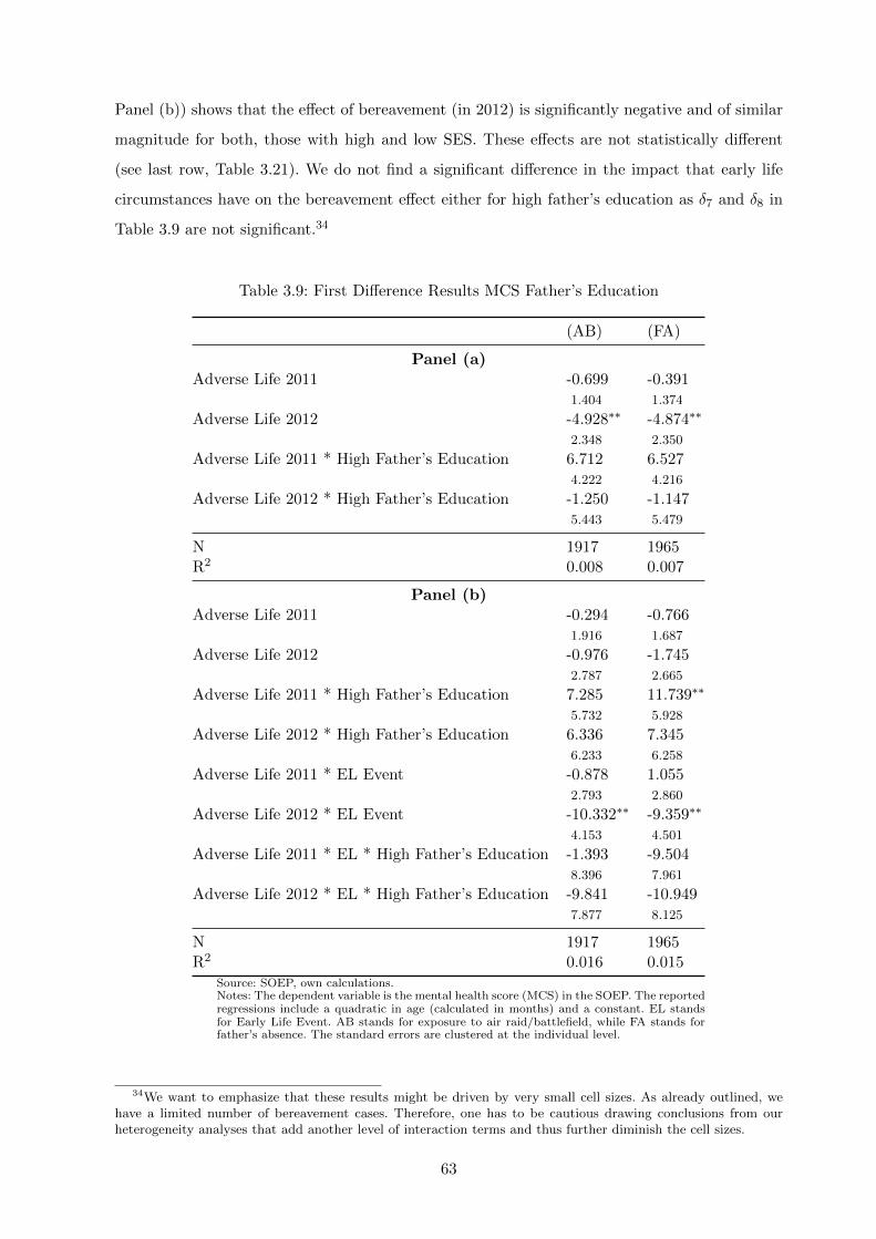
Panel (b)) shows that the effect of bereavement (in 2012) is significantly negative and of similar
magnitude for both, those with high and low SES. These effects are not statistically different
(see last row, Table 3.21). We do not find a significant difference in the impact that early life
circumstances have on the bereavement effect either for high father’s education as δ7 and δ8 in
Table 3.9 are not significant.34
Table 3.9: First Difference Results MCS Father’s Education
(AB) (FA)
Panel (a)Adverse Life 2011 -0.699 -0.391
1.404 1.374
Adverse Life 2012 -4.928∗∗ -4.874∗∗
2.348 2.350
Adverse Life 2011 * High Father’s Education 6.712 6.5274.222 4.216
Adverse Life 2012 * High Father’s Education -1.250 -1.1475.443 5.479
N 1917 1965R2 0.008 0.007
Panel (b)Adverse Life 2011 -0.294 -0.766
1.916 1.687
Adverse Life 2012 -0.976 -1.7452.787 2.665
Adverse Life 2011 * High Father’s Education 7.285 11.739∗∗
5.732 5.928
Adverse Life 2012 * High Father’s Education 6.336 7.3456.233 6.258
Adverse Life 2011 * EL Event -0.878 1.0552.793 2.860
Adverse Life 2012 * EL Event -10.332∗∗ -9.359∗∗
4.153 4.501
Adverse Life 2011 * EL * High Father’s Education -1.393 -9.5048.396 7.961
Adverse Life 2012 * EL * High Father’s Education -9.841 -10.9497.877 8.125
N 1917 1965R2 0.016 0.015
Source: SOEP, own calculations.Notes: The dependent variable is the mental health score (MCS) in the SOEP. The reportedregressions include a quadratic in age (calculated in months) and a constant. EL standsfor Early Life Event. AB stands for exposure to air raid/battlefield, while FA stands forfather’s absence. The standard errors are clustered at the individual level.
34We want to emphasize that these results might be driven by very small cell sizes. As already outlined, wehave a limited number of bereavement cases. Therefore, one has to be cautious drawing conclusions from ourheterogeneity analyses that add another level of interaction terms and thus further diminish the cell sizes.
63

CHAPTER 3. BEREAVEMENT EFFECTS & EARLY LIFE CIRCUMSTANCES
For life satisfaction, the baseline bereavement effects in Panel (a) (Table 3.10) lose significance
once we add the SES interaction term. However, the point estimate (for those with low SES) only
decreases slightly in absolute terms compared to Table 3.7. The F-test of the bereavement effect
for those with high SES (Table 3.22, Panel a) does not reject the null hypothesis either. In Panel
(b), only the interaction between father’s absence and bereavement stays weakly significant. The
F-tests in Table 3.22, Panel (b), show that the bereavement effect for those who experienced
adverse early life conditions is only significant in the case of low SES. The absolute magnitude
of the effect is higher, but insignificant, for those with high SES. We do not find a significant
difference between these effects for high/low SES (i.e., testing whether β3 + β4 = 0). As β4 is
insignificant but high in absolute magnitude, we cannot infer that the role of early life conditions
for bereavement differs by SES.35
Table 3.10: First Difference Results Life Satisfaction Father’s Education Interaction
(AB) (FA)
Panel (a)Adverse Life Event -0.339 -0.298
0.224 0.219
Adverse Life Event * High Father’s Education 0.067 0.0260.628 0.627
N 4221 4331Number of Clusters 2315 2378R2 0.004 0.004
Panel (b)Adverse Life Event -0.016 -0.015
0.266 0.241
Adverse Life Event * High Father’s Education 0.658 1.0860.574 0.450
Adverse Life Event * Early Life Event -0.741 -0.827∗
0.457 0.487
Adverse Life Event * Early Life Event * High Father’s Education -1.088 -1.5241.165 1.034
N 4221 4331Number of Clusters 2315 2378R2 0.007 0.007
Source: SOEP, own calculations.Notes: The dependent variable is life satisfaction in the SOEP. The reported regressions include aquadratic in age (calculated in months) and a constant. AB stands for exposure to air raid/battlefield,while FA stands for father’s absence. The standard errors are clustered at the individual level.
For satisfaction sleep (Table 3.11), the point estimate of the interaction between adverse early
life conditions and bereavement (for those with low SES) stays fairly similar compared to our
35As already mentioned above, these insignificant results may be driven by our small cell sizes.
64

main results. However, our estimation results suggest a (more than) balancing impact of father’s
education on the bereavement effect. The coefficient of the interaction term between bereavement
and SES has a positive sign and is larger than the baseline effect of bereavement in absolute
terms, in both panels. The F-tests in Table 3.23 show that the bereavement effect for those with
adverse early life conditions is only significant for the subgroup with low SES. However, these
effects for low versus high SES individuals are only significantly different (10% level) in the case
of father absence (see last row, Table 3.23). Again β4 is small and insignificant. Thus, our results
do not suggest a heterogeneous role of early life conditions for the bereavement effect by SES
on satisfaction sleep.
Table 3.11: First Difference Results Satisfaction Sleep Father’s Education Interaction
(AB) (FA)
Panel (a)Adverse Life Event -0.670∗∗ -0.598∗∗
0.272 0.266
Adverse Life Event * High Father’s Education 1.096∗∗ 1.021∗∗
0.460 0.457
N 4216 4327Number of Clusters 2313 2376R2 0.003 0.002
Panel (b)Adverse Life Event -0.393 -0.248
0.350 0.282
Adverse Life Event * High Father’s Education 1.092∗∗ 1.228∗∗∗
0.520 0.433
Adverse Life Event * Early Life Event -0.636 -1.022∗
0.549 0.602
Adverse Life Event * Early Life Event * High Father’s Education 0.089 0.0470.912 0.885
N 4216 4327Number of Clusters 2313 2376R2 0.003 0.004
Source: SOEP, own calculations.Notes: The dependent variable is satisfaction sleep in the SOEP. The reported regressions include a quadraticin age (calculated in months) and a constant. AB stands for exposure to air raid/battlefield, while FA standsfor father’s absence. The standard errors are clustered at the individual level.
Gender
Table 3.12 displays the results on mental health when we investigate gender differences.
Tables 3.13 and 3.14 show the results with the gender interaction for life and sleep satisfaction.
As outlined before, these results should be considered with caution because of the limited number
of bereavement cases. We only find a significant effect of being male, having grown up with an
65
CHAPTER 3. BEREAVEMENT EFFECTS & EARLY LIFE CIRCUMSTANCES
absent father and bereavement in 2011 on mental health. Regarding the satisfaction outcomes,
there is no significant gender difference in the role of early life events for bereavement effects.
The F-tests (Tables 3.24, 3.25, 3.26, Panel (b)) on the significance of the overall bereavement
effects (i.e., testing whether the bereavement effect is equal to 0 for men/women who experienced
adverse early life conditions) show significant effects for women. For men, the bereavement effect
is only significant in the case of air raid/battlefield exposure on sleep satisfaction. The difference
between these effects for men and women are only significant in the case of life/sleep satisfaction
and the early life event of father’s absence.
3.5 Conclusion
In this chapter, we analyze the joint impact of adverse early life conditions during World War 2
and bereavement on general mental health, sleep satisfaction, and life satisfaction. Our outcome
variables cover a wide range of mental and stress-related disorders and are particularly relevant
in the context of human wellbeing and productivity (see e.g., Rosekind et al., 2010). We provide
a deeper understanding of resilience to bereavement and its determinants.
We use the SOEP, a German longitudinal survey, and a novel dataset on childhood in the (post)
war context in Germany (“Fruhe Kindheit im (Nach-)Kriegskontext” (FKM)). Using a first
difference approach, we control for observed and unobserved time-invariant heterogeneity in our
analysis.
Our findings suggest a stronger impact of bereavement for those who were exposed to air
raids/combat actions or father’s absence. We also showed that these results are reasonably robust
as the exclusion of those individuals that cannot experience changes (increase or decrease) in
their outcome variables as well as exclusion of cancer deaths do not change our conclusion.
The results of our analysis emphasize the importance of the early life environment for dealing
with bereavement and grief late in life. We have shown that such traumatic events have also
an indirect long run effect on mental health and wellbeing since they affect the magnitude of
bereavement effects in late life. Along these lines, our findings underline the necessity of policy
measures that prevent such adverse early life conditions and support children to deal with
difficult circumstances.
66

Table 3.12: First Difference Results MCS Gender Interaction
(AB) (FA)
Panel (a)Adverse Life Event 2011 0.713 0.751
1.709 1.627
Adverse Life Event 2012 -6.217∗∗∗ -6.148∗∗∗
2.307 2.316
Adverse Life Event 2011 * Male -0.428 0.2332.789 2.704
Adverse Life Event 2012 * Male 2.500 2.5464.342 4.344
N 2105 2161R2 0.007 0.007
Panel (b)Adverse Life Event 2011 0.122 -0.475
2.313 1.965
Adverse Life Event 2012 -0.398 0.4903.488 3.120
Adverse Life Event 2011 * Male 2.983 4.2973.712 3.720
Adverse Life Event 2012 * Male -0.264 -1.0604.998 4.754
Adverse Life Event 2011 * Early Life Event 1.500 3.4483.401 3.376
Adverse Life Event 2012 * Early Life Event -11.181∗∗∗ -12.758∗∗∗
4.111 3.911
Adverse Life Event 2011 * Early Life * Male -8.126 -9.075∗
5.328 5.346
Adverse Life Event 2012 * Early Life * Male 2.150 3.7739.095 8.985
N 2105 2161R2 0.014 0.015
Source: SOEP, own calculations.Notes: The dependent variable is the mental health score (MCS) in the SOEP. Thereported regressions include a quadratic in age (calculated in months) and a constant.AB stands for exposure to air raid/battlefield, while FA stands for father’s absence.The standard errors are clustered at the individual level.
67
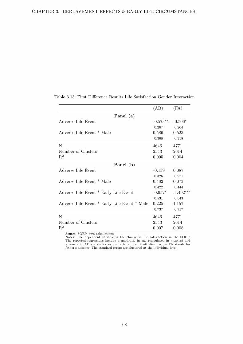
CHAPTER 3. BEREAVEMENT EFFECTS & EARLY LIFE CIRCUMSTANCES
Table 3.13: First Difference Results Life Satisfaction Gender Interaction
(AB) (FA)
Panel (a)Adverse Life Event -0.573∗∗ -0.506∗
0.267 0.264
Adverse Life Event * Male 0.586 0.5230.368 0.358
N 4646 4771Number of Clusters 2543 2614R2 0.005 0.004
Panel (b)Adverse Life Event -0.139 0.087
0.326 0.271
Adverse Life Event * Male 0.482 0.0730.422 0.444
Adverse Life Event * Early Life Event -0.952∗ -1.492∗∗∗
0.531 0.543
Adverse Life Event * Early Life Event * Male 0.225 1.1570.737 0.717
N 4646 4771Number of Clusters 2543 2614R2 0.007 0.008
Source: SOEP, own calculations.Notes: The dependent variable is the change in life satisfaction in the SOEP.The reported regressions include a quadratic in age (calculated in months) anda constant. AB stands for exposure to air raid/battlefield, while FA stands forfather’s absence. The standard errors are clustered at the individual level.
68

Table 3.14: First Difference Results Satisfaction Sleep Gender Interaction
(AB) (FA)
Panel (a)Adverse Life Event -0.800∗∗∗ -0.753∗∗
0.309 0.303
Adverse Life Event * Male 0.733∗ 0.744∗∗∗
0.428 0.416
N 4641 4767Number of Clusters 2542 2613R2 0.003 0.003
Panel (b)Adverse Life Event -0.700∗ -0.271
0.405 0.321
Adverse Life Event * Male 1.274∗∗ 0.5160.548 0.537
Adverse Life Event * Early Life Event -0.218 -1.212∗
0.624 0.641
Adverse Life Event * Early Life Event * Male -1.199 0.6150.823 0.835
N 4641 4767Number of Clusters 2542 2613R2 0.004 0.004
Source: SOEP, own calculations.Notes: The dependent variable is Satisfaction sleep in the SOEP. The reportedregressions include a quadratic in age (calculated in months) and a constant. ABstands for exposure to air raid/battlefield, while FA stands for father’s absence. Thestandard errors are clustered at the individual level.
69

CHAPTER 3. BEREAVEMENT EFFECTS & EARLY LIFE CIRCUMSTANCES
3.A Data Addendum
3.A.1 Description of the “Fruhe Kindheit im (Nach-)Kriegskontext” (FKM)
36 The FKM study is a cooperation between the DIW (Deutsches Institut fur Wirtschafts-
forschung) and Prof. Gerard J. van den Berg, PhD, and was conducted by TNS Infratest in the
summer of 2012. Among the topics covered in this post-war survey are war and hunger exposure,
pre- and postnatal environment, and the familial situation. The SOEP 2012 (subsamples A-H and
J) is the basis for the FKM. In particular, the survey was conducted among those participants
who were born in Germany between 1935 and 1950, including the former Eastern territories
of the German Reich. Moreover individuals were excluded if there was no successful interview
in the 2012 wave or if they refused to participate in the following wave (2013). The potential
participants were first contacted by mail and together with a letter, they received a small gift
(the book on post-war Germany by Reichardt and Zierenberg (2009)). The participants were
interviewed on the phone (CATI). The adjusted sampling population includes 4,135 individuals
of which 3,060 interviews were successfully completed.
3.A.2 Generating the Bereavement Indicators
Further Information on the Construction of Bereavement Variables
Our death indicators are constructed in the following steps; first, we merge the information of
2011 to 2012 and 2010 to 2011, generating two separate two-wave datasets. We generate these
two wave datasets in order to treat each difference in a similar fashion. We can not tackle the
initial conditions problem for the waves 2010-2011, and thus decided to treat the 2011-2012 wave
in the exact same way. Second, we redefine the variables indicating death of the partner, the
father, the child, the mother, or another household member. The redefinition is necessary since
the time period indicated in the question wording does not correspond with the actual individual
time frame between two waves. Specifically, the question refers to calendar time whereas our
first difference strategy uses the difference between two interviews. In the raw data, the question
in wave (t) about the death of a person covers the period from January 1 in year (t-1) until (t).
Thus, the question in wave (t) covers partly the time before the wave (t-1) interview. To make
sure the bereavement variables in wave (t) only cover the information from interview (t-1) to
(t), we replace the respective death indicator in wave (t) with 0 if the death occurred before
36The description of the FKM follows two documents provided by TNS Infratest: Bohlender and Siegel (2012),TNSInfratest (2012).
70

the (t-1) interview. Analogously, we replace the indicator in wave (t-1) with 1 in that case (see
Tables 3.15 and 3.16).
Adjustments for MCS estimations
We generate the 2012-2010 “change” in bereavement (∆Dhealth) setting it equal to D for wave
2012. We then replace entries of ∆Dhealth for wave 2012 by 1 if D=1 in wave 2011 for the same
individual (see Table 3.17). This is necessary in order to define the death indicator between the
two waves consistently as the MCS is only surveyed biannually.
71
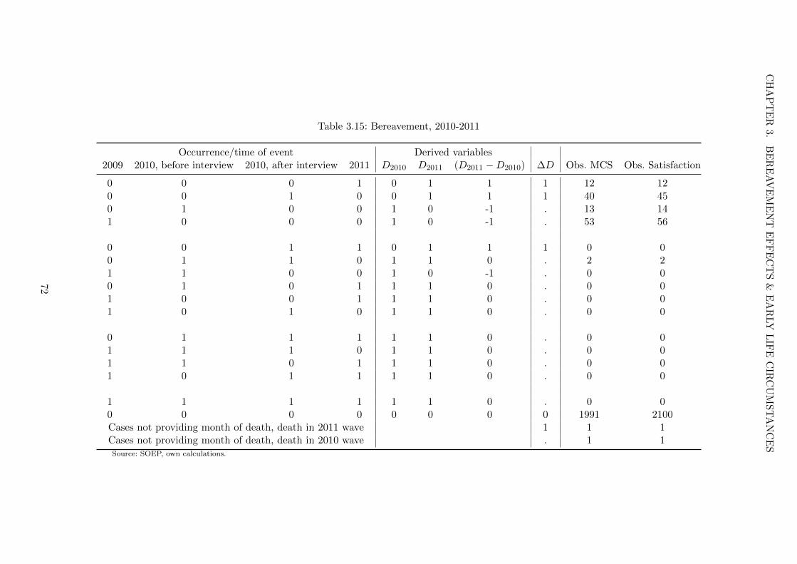
CH
AP
TE
R3.
BE
RE
AV
EM
EN
TE
FF
EC
TS
&E
AR
LY
LIF
EC
IRC
UM
ST
AN
CE
S
Table 3.15: Bereavement, 2010-2011
Occurrence/time of event Derived variables2009 2010, before interview 2010, after interview 2011 D2010 D2011 (D2011 −D2010) ∆D Obs. MCS Obs. Satisfaction
0 0 0 1 0 1 1 1 12 120 0 1 0 0 1 1 1 40 450 1 0 0 1 0 -1 . 13 141 0 0 0 1 0 -1 . 53 56
0 0 1 1 0 1 1 1 0 00 1 1 0 1 1 0 . 2 21 1 0 0 1 0 -1 . 0 00 1 0 1 1 1 0 . 0 01 0 0 1 1 1 0 . 0 01 0 1 0 1 1 0 . 0 0
0 1 1 1 1 1 0 . 0 01 1 1 0 1 1 0 . 0 01 1 0 1 1 1 0 . 0 01 0 1 1 1 1 0 . 0 0
1 1 1 1 1 1 0 . 0 00 0 0 0 0 0 0 0 1991 2100Cases not providing month of death, death in 2011 wave 1 1 1Cases not providing month of death, death in 2010 wave . 1 1Source: SOEP, own calculations.
72

Table 3.16: Bereavement, 2011-2012
Occurrence/time of event Derived variables2010 2011, before interview 2011, after interview 2012 D2011 D2012 (D2012 −D2011) ∆D Obs. MCS Obs. Satisfaction
0 0 0 1 0 1 1 1 5 60 0 1 0 0 1 1 1 28 320 1 0 0 1 0 -1 . 11 171 0 0 0 1 0 -1 . 55 73
0 0 1 1 0 1 1 1 0 00 1 1 0 1 1 0 . 3 31 1 0 0 1 0 -1 . 0 00 1 0 1 1 1 0 . 0 01 0 0 1 1 1 0 . 0 01 0 1 0 1 1 0 . 0 1
0 1 1 1 1 1 0 . 0 01 1 1 0 1 1 0 . 0 01 1 0 1 1 1 0 . 0 01 0 1 1 1 1 0 . 0 0
1 1 1 1 1 1 0 . 0 00 0 0 0 0 0 0 0 2009 2428Cases not providing month of death, death in 2012 wave 1 1 1Cases not providing month of death, death in 2011 wave . 1 1Source: SOEP, own calculations.
73

CHAPTER 3. BEREAVEMENT EFFECTS & EARLY LIFE CIRCUMSTANCES
Table 3.17: Bereavement, 2010-2012
∆D Derived variables health2011 2012 ∆Dhealth ∆Dhealth,2011 ∆Dhealth,2012 Observations
0 1 1 0 1 310 0 0 0 0 19581 0 1 1 0 01 1 case does not exist 0. 0 0 0 0 51. 1 1 0 1 30 . . 0 . 21 . 1 1 0 53
Source: SOEP, own calculations.
3.A.3 Histograms of Outcome Variables
Figure 3.4: Histograms MCS
(a) MCS 2012
0.0
1.0
2.0
3.0
4.0
5D
ensi
ty
0 20 40 60 80MCS Wave 2012
(b) First Difference MCS 2012
0.0
2.0
4.0
6D
ensi
ty
-60 -40 -20 0 20 40Difference MCS Wave 2012-10
74

Figure 3.5: Histograms Satisfaction
(a) Life Satisfaction 2012 (LS)
0.1
.2.3
Den
sity
0 2 4 6 8 10Life Satisfaction Wave 2012
(b) Life Satisfaction 2011 (LS)
0.1
.2.3
.4D
ensi
ty
0 2 4 6 8 10Life Satisfaction Wave 2011
(c) First Difference LS 2012
0.1
.2.3
.4D
ensi
ty
-10 -5 0 5 10Difference Life Satisfaction Wave 2012-11
(d) First Difference LS 2011
0.1
.2.3
.4D
ensi
ty
-10 -5 0 5 10Difference Life Satisfaction Wave 2011-10
(e) Sleep Satisfaction 2012 (SS)
0.0
5.1
.15
.2.2
5D
ensi
ty
0 2 4 6 8 10Sleep Satisfaction Wave 2012
(f) Sleep Satisfaction 2011 (SS)
0.0
5.1
.15
.2D
ensi
ty
0 2 4 6 8 10Sleep Satisfaction Wave 2011
(g) First Difference SS 2012
0.1
.2.3
.4D
ensi
ty
-10 -5 0 5 10Difference Sleep Satisfaction Wave 2012-11
(h) First Difference SS 2011
0.1
.2.3
Den
sity
-10 -5 0 5 10Difference Sleep Satisfaction Wave 2011-10
75

CHAPTER 3. BEREAVEMENT EFFECTS & EARLY LIFE CIRCUMSTANCES
3.B F-tests
Table 3.18: Expected Changes MCS
t= AB FAβ P-val. β P-val.
E[∆ MCS 2011 | EL = t] -0.2560 0.8972 0.8937 0.6566E[∆ MCS 2012 | EL = t] -11.2243 0.0000 -11.7553 0.0000
Source: SOEP, own calculations.
Notes: These are the expectations calculated from a first difference regression ofMCS on AL and AL*EL and a quadratic in age. The expected changes (β) arecalculated as the sum of the estimated AL effect and the estimated interactioneffect between AL and EL. The P-Values result from conducting an F-test onwhether the sum of the respective coefficient (β) is significantly different from 0.
Table 3.19: Expected Changes Life Satisfaction
t= AB FAβ P-val. β P-val.
E[∆ Life S. | EL = t] -0.8667 0.0072 -0.9853 0.0038Source: SOEP, own calculations.
Notes: These are the expectations calculated from a first differenceregression of life satisfaction on AL and AL*EL and a quadratic in age. Theexpected changes (β) are calculated as the sum of the estimated AL effectand the estimated interaction effect between AL and EL. The P-Valuesresult from conducting an F-test on whether the sum of the respectivecoefficient (β) is significantly different from 0.
Table 3.20: Expected Changes Satisfaction Sleep
t= AB FAβ P-val. β P-val.
E[∆ Sleep S. | EL = t] -0.8954 0.0101 -1.0977 0.0051Source: SOEP, own calculations.
Notes: These are the expectations calculated from a first difference regressionof sleep satisfaction on AL and AL*EL and a quadratic in age. The expectedchanges (β) are calculated as the sum of the estimated AL effect and theestimated interaction effect between AL and EL. The P-Values result fromconducting an F-test on whether the sum of the respective coefficient (β) issignificantly different from 0.
76

Table 3.21: Expected Changes MCS, High Father’s Education (HFE)
t= AB FAβ P-val. β P-val.
Panel (a)E[∆ MCS | AL 2011, HFE = 1] 6.013 0.1321 6.1363 0.1248E[∆ MCS | AL 2012, HFE = 1] -6.178 0.2093 -6.0214 0.2248
Panel (b)E[∆ MCS | AL 2011, HFE = 1, EL = t] 4.7204 0.4157 2.5233 0.5986E[∆ MCS | AL 2012, HFE = 1, EL = t] -14.8130 0.0001 -14.7084 0.0001E[∆ MCS | AL 2011, LFE = 1, EL = t] -1.1719 0.5657 0.2891 0.9010E[∆ MCS | AL 2012, LFE = 1, EL = t] -11.3078 0.0003 -11.1043 0.0023δ5 + δ7 2011 5.8923 0.3371 2.2343 0.6743δ6 + δ8 2012 -3.5052 0.4679 -3.6041 0.4875
Source: SOEP, own calculations.
Notes: These are the expectations calculated from a first difference regression of MCS on AL andAL*EL, the interactions with father’s education (high HFE and low LFE) and a quadratic in age.Panel (a) does not include the interactions with EL. The expected changes (β) are calculated as thesum of the respective estimated main and interaction effects. The P-Values result from conducting anF-test on whether the sum of the respective coefficients (β) is significantly different from 0.
Table 3.22: Expected Changes Life Satisfaction, HFE
t= AB FAβ P-val. β P-val.
Panel (a)E[∆ Life S. | HFE = 1] -0.272 0.6432 -0.2717 0.6446
Panel (b)E[∆ Life S. | HFE = 1, EL = t] -1.1874 0.2079 -1.2799 0.1228E[∆ Life S. | LFE = 1, EL = t] -0.7574 0.0419 -0.8420 0.0468β3 + β4 -0.4300 0.6712 -0.4380 0.6379
Source: SOEP, own calculations.
Notes: These are the expectations calculated from a first difference regression of lifesatisfaction on AL and AL*EL, the interactions with father’s education (high HFE, lowLFE), and a quadratic in age. Panel (a) does not include the interactions with EL. Theexpected changes (β) are calculated as the sum of the respective estimated main andinteraction effects. The P-Values result from conducting an F-test on whether the sumof the respective coefficients (β) is significantly different from 0.
Table 3.23: Expected Changes Satisfaction Sleep, HFE
t= AB FAβ P-val. β P-val.
Panel (a)E[∆ Sleep S. | HFE = 1] 0.425 0.2539 0.4230 0.2563
Panel (b)E[∆ Sleep S. | HFE = 1, EL = t] 0.1516 0.8072 0.0048 0.9931E[∆ Sleep S. | LFE = 1, EL = t] -1.0291 0.0151 -1.2702 0.0172β3 + β4 1.1807 0.1153 1.2750 0.0985
Source: SOEP, own calculations.
Notes: These are the expectations calculated from a first difference regression of sleepsatisfaction on AL and AL*EL, the interactions with father’s education (high HFE andlow LFE), and a quadratic in age. Panel (a) does not include the interactions with EL.The expected changes (β) are calculated as the sum of the respective estimated main andinteraction effects. The P-Values result from conducting an F-test on whether the sum ofthe respective coefficients (β) is significantly different from 0.
77
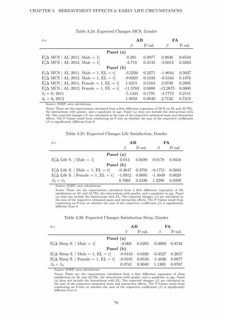
CHAPTER 3. BEREAVEMENT EFFECTS & EARLY LIFE CIRCUMSTANCES
Table 3.24: Expected Changes MCS, Gender
t= AB FAβ P-val. β P-val.
Panel (a)E[∆ MCS | AL 2011, Male = 1] 0.285 0.8977 0.9838 0.6510E[∆ MCS | AL 2012, Male = 1] -3.718 0.3133 -3.6012 0.3283
Panel (b)E[∆ MCS | AL 2011, Male = 1, EL = t] -3.5220 0.2271 -1.8044 0.5037E[∆ MCS | AL 2012, Male = 1, EL = t] -9.6925 0.1833 -9.5543 0.1876E[∆ MCS | AL 2011, Female = 1, EL = t] 1.6215 0.5164 2.9730 0.2805E[∆ MCS | AL 2012, Female = 1, EL = t] -11.5783 0.0000 -12.2675 0.0000δ5 + δ7 2011 -5.1434 0.1791 -4.7773 0.2141δ6 + δ8 2012 1.8858 0.8040 2.7132 0.7219
Source: SOEP, own calculations.
Notes: These are the expectations calculated from a first difference regression of MCS on AL and AL*EL,the interactions with gender, and a quadratic in age. Panel (a) does not include the interactions withEL. The expected changes (β) are calculated as the sum of the respective estimated main and interactioneffects. The P-Values result from conducting an F-test on whether the sum of the respective coefficients(β) is significantly different from 0.
Table 3.25: Expected Changes Life Satisfaction, Gender
t= AB FAβ P-val. β P-val.
Panel (a)E[∆ Life S. | Male = 1] 0.013 0.9580 0.0178 0.9416
Panel (b)E[∆ Life S. | Male = 1, EL = t] -0.3847 0.3756 -0.1751 0.5683E[∆ Life S. | Female = 1, EL = t] -1.0912 0.0095 -1.4049 0.0029β3 + β4 0.7065 0.2426 1.2298 0.0289
Source: SOEP, own calculations.
Notes: These are the expectations calculated from a first difference regression of lifesatisfaction on AL and AL*EL, the interactions with gender, and a quadratic in age. Panel(a) does not include the interactions with EL. The expected changes (β) are calculated asthe sum of the respective estimated main and interaction effects. The P-Values result fromconducting an F-test on whether the sum of the respective coefficients (β) is significantlydifferent from 0.
Table 3.26: Expected Changes Satisfaction Sleep, Gender
t= AB FAβ P-val. β P-val.
Panel (a)E[∆ Sleep S. | Male = 1] -0.068 0.8205 -0.0092 0.9746
Panel (b)E[∆ Sleep S. | Male = 1, EL = t] -0.8443 0.0320 -0.3527 0.2657E[∆ Sleep S. | Female = 1, EL = t] -0.9185 0.0533 -1.4836 0.0077β3 + β4 0.0741 0.9040 1.1309 0.0767
Source: SOEP, own calculations.
Notes: These are the expectations calculated from a first difference regression of sleepsatisfaction on AL and AL*EL, the interactions with gender, and a quadratic in age. Panel(a) does not include the interactions with EL. The expected changes (β) are calculated asthe sum of the respective estimated main and interaction effects. The P-Values result fromconducting an F-test on whether the sum of the respective coefficients (β) is significantlydifferent from 0.
78

3.C Fixed Effects and Level Regressions
Table 3.27: Fixed Effects regressed on EL (Levels LS)
(AB) (FA)
Early Life Event 0.0148 -0.0244
(0.0378) (0.0289)
Males 0.0738*** 0.0797***
(0.0257) (0.0254)
High Father Education 0.0276 0.0394
(0.0306) (0.0303)
Age (in months) -0.00443 -0.00592
(0.00789) (0.00761)
Age2 (in months) 0.00000267 0.00000367
(0.00000476) (0.00000462)
Constant 2.285 2.776
(3.252) (3.121)
N 4695 4825
Source: SOEP and FKM, own calculations.Note: *,**,*** indicates significance at the 10%, 5%, and1% level, respectively. AB stands for air raid/battlefieldexposure, and FA for father’s absence. Standard errors inparentheses.
79

CHAPTER 3. BEREAVEMENT EFFECTS & EARLY LIFE CIRCUMSTANCES
Table 3.28: Fixed Effects regressed on EL (Levels SS)
(AB) (FA)
Early Life Event 0.00412 -0.0709*
(0.0491) (0.0376)
Males -0.0592* -0.0874***
(0.0334) (0.0331)
High Father Education 0.0299 0.0237
(0.0399) (0.0396)
Age (in months) 0.00588 0.0125
(0.0103) (0.00990)
Age2 (in months) -0.00000348 -0.00000738
(0.00000619) (0.00000601)
Constant -2.596 -5.416
(4.228) (4.064)
N 4689 4819
Source: SOEP and FKM, own calculations.Note: *,**,*** indicates significance at the 10%, 5%, and1% level, respectively. AB stands for air raid/battlefieldexposure, and FA for father’s absence. Standard errors inparentheses.
Table 3.29: Fixed Effects regressed on EL (Levels MCS)
(AB) (FA)
Early Life Event 0.654 -0.536
(0.611) (0.465)
Males -0.224 -0.245
(0.406) (0.405)
High Father Education 0.522 0.638
(0.479) (0.479)
Age (in months) -0.0661 -0.0465
(0.129) (0.125)
Age2 (in months) 0.0000376 0.0000294
(0.0000772) (0.0000751)
Constant 28.80 17.36
(53.48) (51.45)
N 1931 1981
Source: SOEP and FKM, own calculations.Note: *,**,*** indicates significance at the 10%, 5%, and1% level, respectively. AB stands for air raid/battlefieldexposure, and FA for father’s absence. Standard errorsin parentheses.
80

Table 3.30: Effects of EL on LS (Levels)
(AB) (FA)
Early Life Event 0.0492 0.0307
(0.0642) (0.0488)
Males 0.167*** 0.180***
(0.0438) (0.0435)
Age (in months) 0.0127 0.0148
(0.0135) (0.0130)
Age2 (in months) -0.00000793 -0.00000917
(0.00000813) (0.00000791)
Constant 2.007 1.146
(5.555) (5.354)
N 5535 5690
Source: SOEP and FKM, own calculations.Note: *,**,*** indicates significance at the 10%,5%, and 1% level, respectively. AB stands forair raid/battlefield exposure, and FA for father’sabsence. Standard errors in parentheses.
Table 3.31: Effects of EL on SS (Levels)
(AB) (FA)
Early Life Event 0.00579 0.0882
(0.0871) (0.0661)
Males 0.496*** 0.537***
(0.0594) (0.0589)
Age (in months) 0.0320* 0.0283
(0.0183) (0.0177)
Age2 (in months) -0.0000202* -0.0000183*
(0.0000110) (0.0000107)
Constant -6.022 -4.350
(7.535) (7.259)
N 5530 5686
Source: SOEP and FKM, own calculations.Note: *,**,*** indicates significance at the 10%,5%, and 1% level, respectively. AB stands forair raid/battlefield exposure, and FA for father’sabsence. Standard errors in parentheses.
81
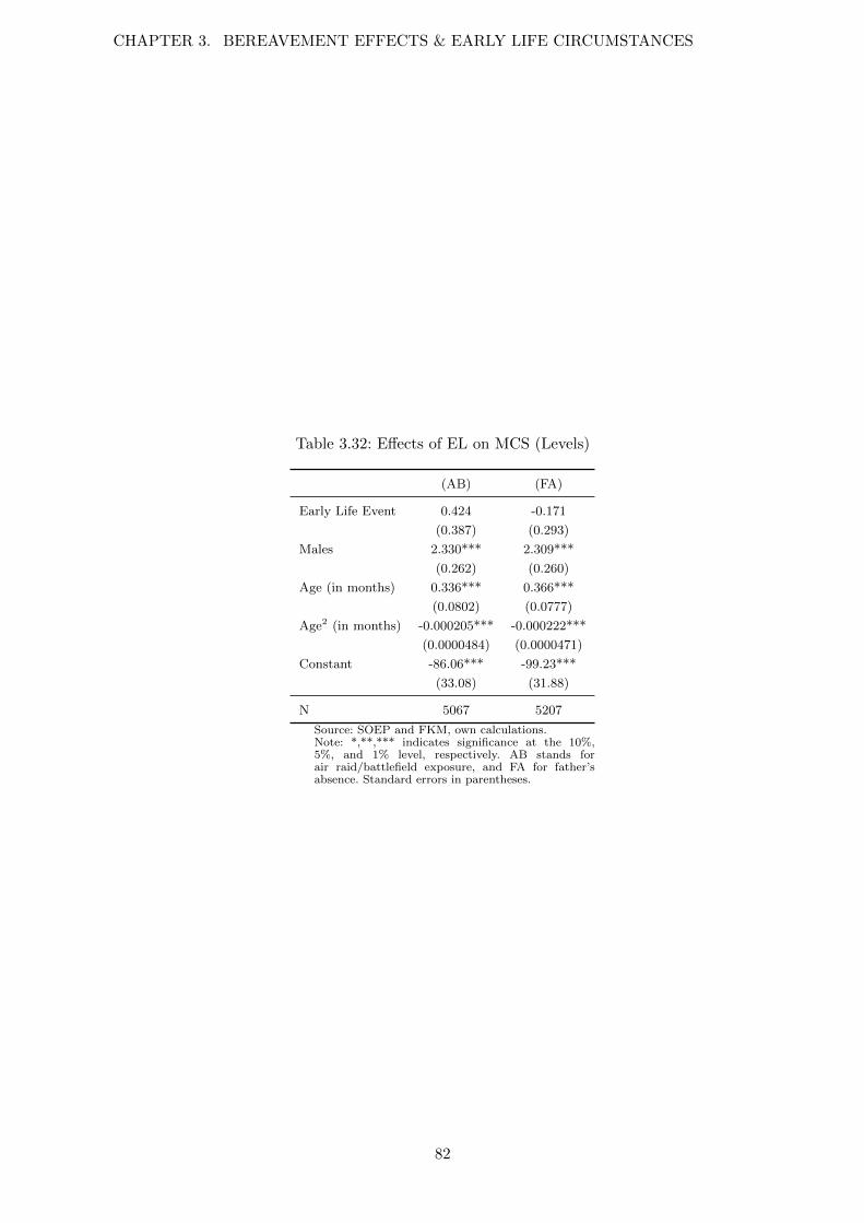
CHAPTER 3. BEREAVEMENT EFFECTS & EARLY LIFE CIRCUMSTANCES
Table 3.32: Effects of EL on MCS (Levels)
(AB) (FA)
Early Life Event 0.424 -0.171
(0.387) (0.293)
Males 2.330*** 2.309***
(0.262) (0.260)
Age (in months) 0.336*** 0.366***
(0.0802) (0.0777)
Age2 (in months) -0.000205*** -0.000222***
(0.0000484) (0.0000471)
Constant -86.06*** -99.23***
(33.08) (31.88)
N 5067 5207
Source: SOEP and FKM, own calculations.Note: *,**,*** indicates significance at the 10%,5%, and 1% level, respectively. AB stands forair raid/battlefield exposure, and FA for father’sabsence. Standard errors in parentheses.
82
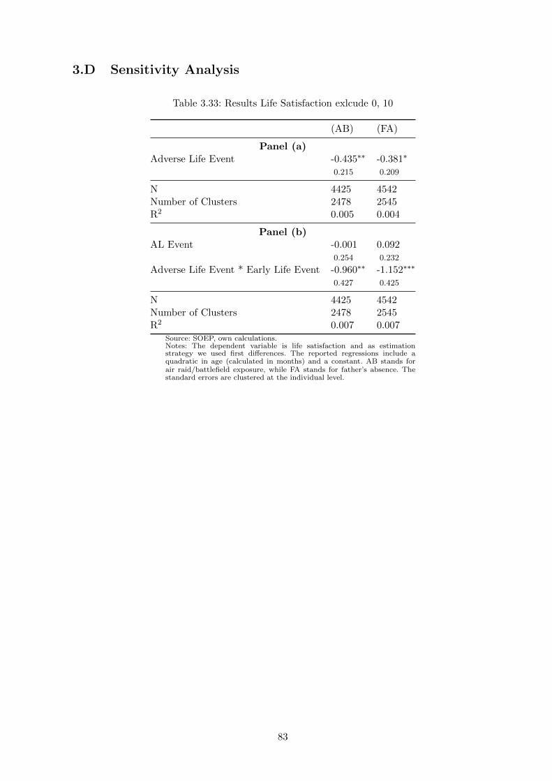
3.D Sensitivity Analysis
Table 3.33: Results Life Satisfaction exlcude 0, 10
(AB) (FA)
Panel (a)Adverse Life Event -0.435∗∗ -0.381∗
0.215 0.209
N 4425 4542Number of Clusters 2478 2545R2 0.005 0.004
Panel (b)AL Event -0.001 0.092
0.254 0.232
Adverse Life Event * Early Life Event -0.960∗∗ -1.152∗∗∗
0.427 0.425
N 4425 4542Number of Clusters 2478 2545R2 0.007 0.007
Source: SOEP, own calculations.Notes: The dependent variable is life satisfaction and as estimationstrategy we used first differences. The reported regressions include aquadratic in age (calculated in months) and a constant. AB stands forair raid/battlefield exposure, while FA stands for father’s absence. Thestandard errors are clustered at the individual level.
83

CHAPTER 3. BEREAVEMENT EFFECTS & EARLY LIFE CIRCUMSTANCES
Table 3.34: Results Satisfaction Sleep exlcude 0, 10
(AB) (FA)
Panel (a)Adverse Life Event -0.435∗∗ -0.384∗
0.220 0.213
N 4169 4281Number of Clusters 2383 2448R2 0.001 0.001
Panel (b)Adverse Life Event -0.152 -0.036
0.296 0.259
Adverse Life Event * Early Life Event -0.614 -0.850∗∗
0.435 0.430
N 4169 4281Number of Clusters 2383 2448R2 0.002 0.002
Source: SOEP, own calculations.Notes: The dependent variable is satisfaction sleep and as estimationstrategy we used first differences. The reported regressions include aquadratic in age (calculated in months) and a constant. AB stands forair raid/battlefield, while FA stands for father’s absence. The standarderrors are clustered at the individual level.
Table 3.35: Results MCS No Cancer
(AB) (FA)
Panel (a)Adverse Life Event 2012 - 2010 -1.234 -0.894
1.318 1.297
N 2085 2140R2 0.001 0.001
Panel (b)Adverse Life Event 2012 - 2010 1.497 1.643
1.666 1.522
Adverse Life Event * Early Life Event -6.718∗∗∗ -6.214∗∗
2.510 2.567
N 2085 2140R2 0.006 0.005
Source: SOEP, own calculations.Notes: The dependent variable is the mental health score (MCS) andas estimation strategy we used first differences. The reported regressionsinclude a quadratic in age (calculated in months) and a constant. ABstands for air raid/battlefield exposure, and FA stands for father’sabsence. The standard errors are clustered at the individual level.
84

Table 3.36: Results MCS No Cancer
(AB) (FA)
Panel (a)Adverse Life Event 2011 0.576 0.982
1.487 1.440
Adverse Life Event 2012 -4.085∗ -3.998∗
2.320 2.329
N 2085 2140R2 0.003 0.003
Panel (b)Adverse Life Event 2011 1.601 1.314
2.090 1.984
Adverse Life Event 2012 1.332 2.2382.724 2.301
Adverse Life 2011 * Early Life Event -2.560 -0.7882.818 2.804
Adverse Life 2012 * Early Life Event -12.745∗∗∗ -14.691∗∗∗
3.906 3.808
N 2085 2140R2 0.010 0.011
Source: SOEP, own calculations.Notes: The dependent variable is the mental health score (MCS) andas estimation strategy we used first differences. The reported regressionsinclude a quadratic in age (calculated in months) and a constant. AB standsfor air raid/battlefield exposure, while FA stands for father’s absence. Thestandard errors are clustered at the individual level.
Table 3.37: Results Satisfaction Life No Cancer
(AB) (FA)
Panel (a)Adverse Life Event -0.292 -0.262
0.210 0.204
N 4626 4750Number of Clusters 2530 2600R2 0.003 0.002
Panel (b)Adverse Life Event 0.119 0.016
0.247 0.238
Adverse Life Event * Early Life Event -0.956∗∗ -0.742∗
0.419 0.427
N 4626 4750Number of Clusters 2530 2600R2 0.005 0.003
Source: SOEP, own calculations.Notes: The dependent variable is the life satisfaction and as estimationstrategy we used first differences. The reported regressions include aquadratic in age (calculated in months) and a constant. AB stands forair raid/battlefield exposure, while FA stands for father’s absence. Thestandard errors are clustered at the individual level.
85

CHAPTER 3. BEREAVEMENT EFFECTS & EARLY LIFE CIRCUMSTANCES
Table 3.38: Results Satisfaction Sleep No Cancer
(AB) (FA)
Panel (a)Adverse Life Event -0.727∗∗∗ -0.681∗∗
0.272 0.264
N 4621 4746Number of Clusters 2529 2599R2 0.003 0.002
Panel (b)Adverse Life Event -0.395 -0.289
0.347 0.294
Adverse Life Event * Early Life Event -0.771 -1.043∗
0.547 0.564
N 4621 4746Number of Clusters 2529 2599R2 0.003 0.004
Source: SOEP, own calculations.Notes: The dependent variable is the sleep satisfaction and as estimationstrategy we used first differences. The reported regressions include aquadratic in age (calculated in months) and a constant. AB stands forair raid/battlefield exposure, while FA stands for father’s absence. Thestandard errors are clustered at the individual level.
86

Chapter 4
Coworkers, Networks and Job Search
Outcomes1
4.1 Introduction
The job matching process is complicated by an enormous degree of heterogeneity between the
workers and the jobs. Information about suitable jobs are not always available and the worker’s
productivity is usually unknown ex-ante. Personal relationships, informal contacts, and social
networks potentially play a big role in overcoming these informational difficulties in the labor
market both for firms and job seekers. Early studies on the networks in the labor market state
that about 50% of workers find their jobs through friends, family members, and/or co-workers
(see e.g., Holzer (1988), Montgomery (1991)). These findings are also in line with recent trends.
According to Jobvite, an online recruiting platform, the top source of job applications are job
boards (42.9%) and career sites (32.1%). However, the main source of hiring shifts to employment
are referral programs which generate 39.9% of all hires.2
Given the significance of the social networks in the labor market, there has been a growing
interest in understanding how social networks operate in the labor market. In particular, both
the theoretical and the empirical literature have been expanding since the pioneering studies by
Rees (1966) and Granovetter (1973).3
1This chapter is co-authored with Perihan O. Saygin and Andrea Weber.2These statistics are based on data from 2007 to 2013 on a sample of firms that are Jobvite customers. See
http://recruiting.jobvite.com/resources/recruiting-data-employment-statistics-by-jobvite-index/ (01.04.2013).3See for example Montgomery (1991) or Ioannides and Loury (2004) for comprehensive surveys.
87

CHAPTER 4. COWORKERS, NETWORKS AND JOB SEARCH OUTCOMES
Looking at the existing literature, there are three perspectives of taking a look at the social
networks in the labor markets: the job seeker side, the firm side and the social costs. Job
seekers can use social networks to minimize their search costs by obtaining information about
vacancies from the employed network members, while firms use referrals when hiring, as a signal
for unknown productivity. Finally, if firms rely on networks to fill vacancies and if individuals
rely on networks to find jobs, inequalities between different groups in the labor market can be
fostered and can grow depending on the initial differences in the network employment rates
(Calvo-Armengol and Jackson, 2004). Therefore social networks might also explain inequalities
or poverty traps (Zenou, 2014).
Jackson (2010) classifies theoretical studies under two headlines. The first group of studies
is based on models which use referrals as a signal for unknown productivity of the potential
hirings. The pioneering model of this strand is Montgomery (1991) and focuses on employee
selection. Firms recruit new workers who are connected to their productive workers. Therefore,
the characteristics of incumbent members are relevant for the job search outcomes and similar
type workers refer each other.
The second group of theoretical papers mostly provide models of information transmission
in social networks (Calvo-Armengol and Jackson, 2004). In these models, networks consists
of employed and unemployed workers and members randomly receive information about job
opportunities. The unemployed workers keep the information for themselves while the employed
workers pass the information on to their network members if they can not use this information.
Calvo-Armengol and Jackson (2004) suggest that unemployed workers who are connected in a
social network with a high employment rate are more likely to find a job and should earn higher
wages. In addition, they compare two groups with different employment rates and suggest that
lower employment rates within a group will lead to a higher drop-out rate which will eventually
cause a persistent inequality between two groups. Finally, they also show that unemployment
exhibits duration dependence. Similarly, according to Loury (2006), workers are likely to earn
higher wages if their contacts have good connections, are employed, receive higher wages, and
help the employer by reducing the uncertainty about the productivity of the job seeker.
Empirical studies use quite heterogeneous data sources and various social network definitions.
Some studies analyze the social networks concerning the residential proximity using census data
such as Topa (2001) and Bayer et al. (2008) while others consider the social ties like family
and friends using survey data such as Magruder (2010), Kramarz and Nordstrom Skans (2013),
88

and Cappellari and Tatsiramos (2010). Dustmann et al. (2011) for example use ethnicity based
networks to show the network effects in the labor market. Using various definitions of social
networks, it seems that there is a robust consensus that workers benefit from informal contacts
when looking for a job and that social networks have a positive effect on the job finding rate.4
Some of these studies also elaborate the effect of using networks on the quality of the subsequent
matches (such as tenure and/or wage) with no clear consensus on the direction of the effect.
Some recent papers provide evidence for the effect of social networks consisting of past co-workers
on the job search: Cingano and Rosolia (2012), Glitz (2013) and Hensvik and Skans (2013).5
Cingano and Rosolia (2012) use matched employer-employee data for two Italian provinces over
the period 1975 to 1997 and estimate the effect of the network employment rate on unemployment
duration. In order to overcome the selection bias into unemployment, they use firm closures
and find that one standard deviation increase in the network employment rate leads to an
8% reduction in unemployment duration. On the other hand, they only consider the displaced
workers who find a job after the firm closure in order to analyze the unemployment duration.
By using only the completed unemployment spells, they drop around 20% of the displaced
workers from their sample. In other words, they condition on the outcome of becoming re-
employed. Glitz (2013) follows the same approach in terms of network definitions and empirical
specification with two distinctive features from Cingano and Rosolia (2012). First, Glitz (2013)
uses an administrative dataset for German workers in the 4 largest metropolitan areas where
observations are recorded only annually. The second feature is that mass layoffs are used as an
exogenous variation to the network employment rate as an additional identification strategy.
As a result, Glitz (2013) finds a strong positive effect of the network employment rate on re-
4See for example, Corcoran et al. (1980); Holzer (1988); Mortensen and Vishwanath (1994); Pistaferri (1999);Topa (2001); Calvo-Armengol and Jackson (2004); Kramarz and Nordstrom Skans (2013); Bayer et al. (2008);Dustmann et al. (2011); Laschever (2009); Pellizzari (2010); Cappellari and Tatsiramos (2010); Cingano andRosolia (2012); Goel and Lang (2009); Glitz (2013); Beaman (2012). Most of the studies use survey data whereemployees are asked about how they found their job in order to compare the jobs obtained through social networksand with those found through formal methods. Pistaferri (1999) uses the Bank of Italy Survey of Household Incomeand Wealth where applicants are asked how they found their jobs. He reports a positive effect of using informalconnections on job offer arrival rates but a negative effect on earnings. Similarly, Bentolila et al. (2004) provideevidence for a positive effect on the job finding but negative effect on earnings. They show that the social networksmight induce mismatches between workers’ productive advantage and their actual occupational choice using the“Multi-City Study of Urban Inequality, 1992-1994” survey. Antoninis (2006) suggests that the wage effect canbe positive or negative depending on the type of tie. In particular, if the referee has a direct knowledge of theworker’s productivity, new recruits receive a higher starting wage. From the firm side, the literature is scarce anda few papers agree that firms do not benefit from using social networks if workers are not properly incentivized(Kramarz and Thesmar (2013) and Beaman and Magruder (2012)).
5Hensvik and Skans (2013) use matched data from Swedish administrative employment registers and definesocial networks as past co-workers but analyze referral hirings rather than job search. They empirically test theimplications of the model of Montgomery (1991) and show that firms use social networks as a signal of the worker’sproductivity, and that workers therefore benefit from the quality of their social networks.
89
CHAPTER 4. COWORKERS, NETWORKS AND JOB SEARCH OUTCOMES
employment probabilities after displacement and no significant effect on wages.
Despite the growing literature and interest in empirical tests of the social network theories,
there is limited evidence on the channels through which social networks affect the job search
outcomes. Our aim is to test whether the co-worker network is important for the job finding rate
and the wage at the new job. Similar to the literature (see e.g., Cingano and Rosolia (2012) and
Glitz (2013)) we define the social networks as the group of past co-workers building on a 5 year
history. But in contrast to Cingano and Rosolia (2012) and Glitz (2013) we incorporate every
worker displaced due to a firm closure using the Austrian Social Security Database (ASSD). The
ASSD provides daily information on the universe of private sector workers covered by the social
security system in Austria between 1980 and 2009. In order to analyze the effect of the network
characteristics on the re-employment probability and the unemployment duration, we apply both
a linear probability and a duration model in order to keep every displaced worker. In particular,
we aim to distinguish between potential channels through which networks affect the job search
outcome. Therefore, we investigate two dimensions of the co-worker network: the individual level
and the firm level. At the individual level, we analyze the effect of the past co-worker network
characteristics on the job search outcomes. To disentangle the different channels at work, we
incorporate firm heterogeneity measures into the past co-worker network by decomposing the
network employment rate according to firm characteristics. Furthermore we investigate whether
former co-workers with similar characteristics are more profitable for the job finding rate. At
the firm level, we elaborate whether firms are more likely to hire a displaced worker from the
social network of their incumbent employees.
Our individual level results show that the higher the share of employed past co-workers the
higher is the job-finding rate of the displaced worker. Past co-workers, that are employed in the
same industry and in firms that are currently hiring, are particularly helpful. We also provide
evidence for heterogeneity in the network effects - past co-workers with similar characteristics are
important for some groups based on gender, age groups and occupation. The effect of the network
characteristics on the wage growth (from job loss to re-entry wage) is inconclusive, despite the
significant positive effect of former co-workers working at high wage firms. At the firm level, we
find that 25% of the displaced workers find a new job in a connected firm. Furthermore, displaced
workers with a link to the connected firm are three times as likely to be hired as similar workers
from the same closing firm without a link to the connected firm.
90

The rest of the chapter is organized as follows; first, we give a brief description of the data
and the sample selection process as well as the network formation process in Section 4.2. It also
provides definitions of the firm closures, the displaced worker sample, the network characteristics
and the job search outcomes of interest. Furthermore we provide a descriptive analysis of the
displaced workers’ characteristics, employment histories and network characteristics as well as
the firms’ characteristics where the network members are employed. Section 4.3 presents the
empirical specification and the results. Finally, Section 4.4 concludes.
4.2 Data and Network Definitions
The empirical analysis is based on the Austrian Social Security Database (ASSD), which covers
the universe of private sector workers in Austria over the years 1972-2012 (Zweimuller et al.,
2009). The data provide detailed daily information on employment, unemployment, and other
states relevant for social security such as sickness, retirement, or maternity leave. Earnings paid
by each employer are recorded at an annual level. The matched employer-employee structure of
the ASSD is defined by employer identifiers, which are linked to individual employment spells.
To measure workforce characteristics at the firm level, we organize the data in a quarterly panel,
collapsing it along employer identifiers. Firm exit dates are then defined as the last quarter date
in which a firm employs at least one worker. We use a worker-flow approach to distinguish
firm closures from other exit events such as mergers or institutional changes in the employer
identifier. This approach is explained in detail in Fink et al. (2010).6
Our sample of displaced workers consists of individuals displaced by firms closing over the years
1980 - 2007. We make three restrictions to this sample. First, we only consider blue collar and
white collar workers, who were still employed in the final quarter of firm existence, i.e., the
quarter of the closure date. Second, we restrict the sample to workers with at least one year
tenure at the closing firm. Third, we focus on workers who are between 20 and 55 years of age
at displacement. The resulting sample includes 151,432 workers from 27,635 closing firms, which
means that on average we observe 5.4 workers displaced by the same closing form.
6The main definition is that a closure is restricted to the exit of an employer identifier where less than 50% ofthe last year’s workforce jointly move to the same new employer identifier. Because this approach is not meaningfulfor very small firms, we restrict closures to firms with at least 5 employees in the last year.
91

CHAPTER 4. COWORKERS, NETWORKS AND JOB SEARCH OUTCOMES
In comparison to the literature, Glitz (2013) uses establishment closures in the Hamburg,
Cologne, Frankfurt and Munich metropolitan areas in 1995 and 1996. This leaves him with
10,916 displaced males from 1,814 establishments. While Cingano and Rosolia (2012) have 9,121
re-employed individuals displaced by 1,195 manufacturing firm closures with a focus on two
Italian provinces (Treviso and Vicenza) from 1980 until 1994.7 We thus have a larger sample of
closing firms and displaced individuals all over Austria.
Co-Worker Networks
For each displaced worker the social network is defined as the set of all individuals who shared
a workplace with her over the last five years before the firm closure date. Thereby we require
that the employment spells of the contacts overlap for at least 30 days. We further exclude
links with former co-workers that were established in very large firms with more than 3000
employees. This restriction facilitates computational tractability and excludes large networks,
which encompass very limited information about interpersonal information flows. Finally, we
also exclude co-displaced workers, who were displaced by the same closing firm of the network.
These workers will form the comparison group at the closing firm level.
Table 4.1 presents summary statistics of individual and network characteristics of our sample
of displaced workers. The average age of displaced workers is 36.8, a share of 41% are females,
91% are of Austrian nationality, and 53% have a blue collar contract before displacement. The
average tenure of displaced workers at the closing firm, 4.87 years, is below the window length of
the network definition. The median tenure is even shorter with 2.9 years. The average number
of job changes within the last five years is 1.92 with a slightly larger median of 2 job changes.
The average number of unemployment days is 50.3.
Due to the relatively high job turnover rate of displaced workers before displacement the size
of their networks is relatively large. The average size of the co-worker network includes 158
contacts, the median is more moderate with 44 members. Note that the co-displaced workers,
whom we remove from the network are in general only a small fraction of all contacts (average
5/158).
7In contrast to our displaced worker sample, the displaced workers of Cingano and Rosolia (2012) have to beemployed in the closing firm in the last month of activity.
92

Table 4.1: Summary Statistics: Displaced Workers
Mean Median Std. Dev.
Individual CharacteristicsFemale 0.41 0.49Age 36.8 36.0 9.5Blue Collar Worker 0.53 0.50Austrian Nationality 0.91 0.28Tenure (in years) 4.87 2.92 4.84Employed over Last 5 Years 4.27 4.90 1.06Unemployed over Last 5 Years 0.14 0.00 0.35Av. Number of Firms over Last 5 Years 1.92 2.00 1.20Average Firm Size over Last 5 Years 50.29 19.28 105.4
Network CharacteristicsNetwork Size 158.3 44 339.0Share Female 0.40 0.34 0.31Share Blue Collar 0.62 0.76 0.35Share Austrian 0.92 0.96 0.11Share of Same Gender 0.68 0.75 0.27Share in Same Age Group 0.28 0.25 0.18Share of Same Occupation 0.69 0.81 0.31Share of Same Nationality 0.86 0.95 0.23
Network Employment RateShare Employed 0.56 0.57 0.18Share Employed in Same Industry 0.19 0.13 0.19Share Employed at Net Hiring Firms 0.24 0.21 0.18Share Employed at Above Med. Wage Firms 0.30 0.26 0.21
Observations 151,432
Source: ASSD, own calculations.
93

CHAPTER 4. COWORKERS, NETWORKS AND JOB SEARCH OUTCOMES
The characteristics of former co-worker in the network are quite heterogeneous: on average about
40% of network members are female, a share of 62% are blue collar workers, and a share of 92%
are Austrian. If we compare the displaced workers with their network members we see that
about 68% have the same gender, and 86% are of the same nationality as the displaced workers.
69% are the same job type and 28% in the same age group, where we split displaced workers
into four age groups of about equal size. At the time of firm closure on average 56% of the
network members hold a job (similar to Glitz (2013), lower than Cingano and Rosolia (2012)).8
If we compare the industry of the closing firm with the industries in the firms where network
members are employed, we find that only 19% of the contacts overlap. To classify industries
we use a two digit NACE classification, which covers about 50 different industries. 24% of the
employed network members work at a hiring firm, while 30% of the employed network members
work at an above the median wage paying firm.
Figure 4.1 shows an example of the structure of the co-worker networks. To construct this graph,
we selected a one percent random subsample of 85 workers who were displaced in the year 2000.
The displaced workers are shown at the center of each co-worker network and edges represent
the links to their former co-workers. We see that the sizes of the networks vary a lot, the
largest includes about 2000 contacts and the smallest has only a single contact. Some displaced
workers have networks that overlap, while other networks are isolated. This is potentially due
to the random draw of displaced workers from the full population. In general, networks of two
individuals who are displaced from the same firm will overlap to a certain extent. But unless
their employment careers are identical during the last 5 years, the networks will only partly
overlap.
Figure 4.2 is another example of the structure of the co-worker networks. The difference is that
red edges represent employed links, black edges represent unemployed links while the pink edges
present employed links at hiring firms. We see that the network sizes and the average employment
rate in hiring firms differ. Furthermore, we can see a tendency that the more employed contacts
and the more employed contacts at a hiring firms the displaced individual has, the likelier it is,
that she is employed.
8Our number could be lower than Cingano and Rosolia (2012) because they only consider completed spells,and thus leave out those individuals that never get employed which by Calvo-Armengol and Jackson (2004)have a higher network unemployment rate. Thus the network employment rate of Cingano and Rosolia (2012) isautomatically higher.
94

Figure 4.1: Job Seekers and Networks of Past Co-workers by Gender
FEMALE
MALE
Note: This graph is obtained from a 1% random sample of displaced workers, losing their jobs in the year 2000 dueto firm closures. It illustrates the displaced workers (in the middle) and their past co-workers as connections. Theblue (red) circles in the middle represent the male (female) job seekers while the blue (red) connections aroundthem are their respective male (female) contacts in the network.
95

CHAPTER 4. COWORKERS, NETWORKS AND JOB SEARCH OUTCOMES
Figure 4.2: Job Seekers and Networks of Past Co-workers by Employment Status
Job Seekers
Contacts
Successful
Unemployed
Employed
Employed at Hiring Firm
Unemployed
Note: This graph is obtained from a 1% random sample of displaced workers, losing their jobs in the year 2000due to firm closures. It illustrates the displaced workers (in the middle) and their past co-workers as connections.The red (black) circles in the middle represent the successful (still unemployed after 3 months) job seekers whilethe red (black) connections around them are their employed (unemployed) contacts in the network. The pinkconnections are the network members who are employed at a firm that is hiring at the time of the firm closure ofthe job seeker.
96

Firm Networks
At the firm level we construct networks by linking each closing firm to a network of connected
firms, which is also determined by past co-workers of the displaced individuals. In particular,
the set of connected firms is defined by the firms in which the past co-workers of the displaced
individuals are employed at the closure date. We can think of the set of connected firms as a
proxy of the local labor market which offers new job opportunities. Based on this definition
our set of 27,635 closing firms is connected to 352,995 firms, which span a large fraction of the
overall market.
Table 4.2 presents the main characteristics of the closing firms and their networks of connected
firms. In the network analysis at the firm level we focus on closing firms with at least 2 displaced
workers. On average a closing firm has former co-worker links to 175.7 connected firms, the
median number of connected firms is 55. The firm network typically spans a variety of industries.
On average a closing firm is linked to 38.7 connected firms in the same industry, the median is
8.8. This means that on average only about a third of the links in the firm network are among
firms in the same two digit industry. In each pair of closing and connected firm there are on
average two displaced individuals with links.
Figure 4.3 shows an example of a firm network. This is a random subsample of all closing firms in
2000, which includes 39 closing firms connected to an average of 105 firms (whereas the median
is at 58). At the center of each network we see the closing firms and edges represent links to
connected firms. Edges in red are links to firms in the same industry, while yellow edges link
firms in different industries. The average share of firms in the same industry is 25%. The firm
dots are color coded - the darker the color, the higher the wage quartile. The average wage
quartile of the closing firm is 1.55.
Job Search Outcomes
Descriptive statistics of job search outcomes are shown in Table 4.3. About 86% of the displaced
workers in our sample find a new job within one year. If censored at 365 days, the average time
to find a new job is 83 days but the median is only 2 days. This reflects the fact that not all
displaced workers are out of employment after firm closure. About 49% transit to a new job
immediately, while 33% are registering as unemployed.
97

CHAPTER 4. COWORKERS, NETWORKS AND JOB SEARCH OUTCOMES
Table 4.2: Firm Characteristics
Mean Median Std.Dev.
Closing FirmsNumber of Displaced Workers 5.4 4 6.7Firm Size at Maximum 23.9 13 51.4Firm Age at Closure (years) 10.0 7.5 8.4Wage Quartile 1.95 1.00 1.12Vienna 0.29 0.45Manufacturing 0.15 0.36Construction 0.14 0.34Sales 0.20 0.40Tourism 0.11 0.31Service 0.17 0.38
Firm Network Characteristics (per closing firm)Number of Connected Firms 175.7 55 318.4Average Size 83.6 67.7 79.3Average Wage Quartile 1.75 1.68 0.46Share Same Industry 0.22 0.16 0.20
Number of Closing Firms 27,635Number of Connected Firms 352,995
Per Closing - Connected Firm PairIndividuals with Links 1.98 1.00 4.59
Source: ASSD, own calculations.
98

Figure 4.3: Closing Firms and Connected Firms
NODES: Closing and Connected Firms
Wage Quartiles: Highest-Lowest
EDGES:
Different Industry
Same Industry
Note: This graph is obtained from a 2% random sample of firms that closed in the year 2000. It illustrates theclosing firms (in the middle) and the connected firms as their connections. The darker blue circles indicate higherwage firms. The yellow connections are the links between the closing firm and the connected firms that are indifferent industries while the red links indicate that the two firms are in the same industry.
99

CHAPTER 4. COWORKERS, NETWORKS AND JOB SEARCH OUTCOMES
Displaced workers who find a new job within the first year spend on average 38 days out of a
job. The wages in their new jobs are about as high as the pre-displacement wages on average.
If we focus on the types of firms where they find new jobs, we see that only 52% return to a
firm in the same industry as the closing firm. We also check whether displaced workers return
to a firm in which they were employed during the last five years and this appears to happen for
7% of displaced workers. A considerably larger share of 24% find a new job in one of the firms
that are connected to the closing firm and 19% find a new job in a connected firm to which
they have a personal link, i.e., where a former co-worker is employed. These numbers already
indicate that referral hirings are potentially an important channel of information transmission
in the co-worker networks. We will examine this more closely in our empirical analysis.
Table 4.3: Job Search Outcomes
Mean Median Std
All Job Seekers (N = 151,432)Find New Job in One Year 0.86 0.34Time to Next Job in Days (Censored at 365) 83.19 2 131.32New Job Immediately 0.49 0.50Unemployed 0.33 0.47Links to Firm NetworkNb. of Connected Firms 373.8 137 655.9Nb. of Connected Firms with Link 58.2 22 110.7Share of Connected Firms with Link 0.40 0.24 0.37
Successful Job Seekers (N = 130,477)Time to Next Job Days 37.93 1 72.20Log Wage Gain 0.009 0.015 0.301New Job in Same Industry 0.52 0.50New Job in Old Firm 0.07 0.25Links to Firm NetworkNb. of Connected Firms 383.0 150 636.8Nb. of Connected Firms with Link 60.7 24 110.7Share of Connected Firms with Link 0.39 0.24 0.36Hired by Connected Firm 0.24 0.43Hired by Connected Firm with Link 0.19 0.39
Source: ASSD, own calculations.
Figure 4.4 shows the distribution (histograms) of some of the most relevant network character-
istics.
100

Figure 4.4: Distribution of Network Characteristics
(a) Network Size
050
100
150
Perc
ent
0 2000 4000 6000
Network Size
Network Size
(b) Network Size Restr.
010
20
30
Perc
ent
0 200 400 600 800 1000Network Size
This graph is restricted for the displaced workers with maximum 1000 past coworkers network size
Network Size<1000
(c) Network Emp. Rate
02
46
8P
erc
ent
0 .2 .4 .6 .8 1Network Emp. Rate
Network Employment Rate
(d) Same Industry
05
10
15
20
Perc
ent
0 .2 .4 .6 .8 1Emp. Rate at Same Industry
Network Employment Rate in the Same Industry
(e) Network Hiring Rate
02
46
8P
erc
ent
0 .2 .4 .6 .8 1Emp. Rate at Net Hiring Firms
Network Employment Rate at Net Hiring Firms
(f) Network Top 50
02
46
8P
erc
ent
0 .2 .4 .6 .8 1Emp. Rate at Above Med. Wage Firms
Network Employment Rate at Above Median Wage Firms
(g) Female Rate
02
46
8
Perc
ent
0 .2 .4 .6 .8 1
Network Female Ratio
Network Female Ratio
(h) Blue Collar
05
10
15
Perc
ent
0 .2 .4 .6 .8 1
Network Blue Collar Share
Network Blue Collar Ratio
(i) Austria Collar
010
20
30
40
Perc
ent
0 .2 .4 .6 .8 1
Network Austrian Share
Network Austrian Ratio
(j) Same Age
02
46
8P
erc
ent
0 .2 .4 .6 .8 1Network Same Age Share
Network Share of Same Age Group
(k) Same Education
010
20
30
40
Perc
ent
0 .2 .4 .6 .8 1Network Same Education Share
Network Share of Same Education Group
(l) Same Nationality
010
20
30
40
Perc
ent
0 .2 .4 .6 .8 1Network Same Nationality Share
Network Share of Same Nationality
(m) Same Occupation
05
10
15
20
Perc
ent
0 .2 .4 .6 .8 1Network Same Occupation Share
Network Share of Same Occupation
(n) Time to Next Job
020
40
60
Perc
ent
0 100 200 300 400
Time to Next Job−Censored
Time to Next Job: Censored
(o) Time to Next Job Com-pleted
020
40
60
Perc
ent
0 100 200 300 400
Time to Next Job
Time to Next Job: Successful Job Searchers
Note: These graphs are obtained from our full sample of displaced workers due to firm closures between years 1980to 2007. Except for the last graph, they illustrates the distributions of variables measuring the characteristics ofnetwork members. Starting from number of contacts (network size), share of employed contacts (also employed insame industry and in above median wage firms), blue collar contacts, same age group, nationality and occupationcontacts are shown. The last graph shows the distribution of duration of job seeking after firm closure for successfuljob seekers.
101

CHAPTER 4. COWORKERS, NETWORKS AND JOB SEARCH OUTCOMES
4.3 Empirical Analysis
The empirical analysis proceeds in two parts, which exploit the worker dimension and the
firm dimension of the co-worker networks. We start by investigating the effects of network
characteristics on the job finding rates and wage growth after job displacement. Our main
identification strategy consists of comparing workers who were displaced from the same closing
firms with different networks. This will give us a first indication whether co-worker networks
have an impact on job search outcomes. The second part of our analysis aims at narrowing down
the channel by which information is transmitted among network members. We will exploit the
firm dimension of co-worker networks and investigate the probability that a displaced worker
finds a job in a firm that is connected to the closing firm. Thereby we will focus on the role
of the displaced worker, the connected firm, and a potential link to a former co-worker in the
connected firm on the magnitude of the social tie effect.
4.3.1 Worker Level Analysis
Job Finding Rates
The model of information transmission in social networks by Calvo-Armengol and Jackson (2004)
predicts that the share of employed network members is crucial for the job-finding success of
unemployed workers. To get a first impression of this connection in our sample we present weekly
hazard rates into new jobs over the first year after displacement in Figure 4.5. Panel 4.5a depicts
the weekly hazards for males and females. The figure shows declining patterns in the weekly exit
hazard for both groups, but males exit quicker than females. Therefore we are always controlling
for gender in the following. Furthermore in Figure 4.5 we specifically focus on two subsamples
of the total population: displaced workers with a share of employment of former co-workers in
the top quartile of the distribution, which we denote as “high network employment rate”, and
displaced workers with a share of employment of former co-workers in the bottom quartile of
the distribution, denoted as “low network employment rate” (Figure 4.5b). The figure shows
declining patterns in the weekly exit hazard rates for both groups. But especially during the
initial weeks of job search the exit rate of individuals with a high network employment rate is
clearly above the exit rate of individuals with low network employment rate. After about 5 to
6 months of job search the two lines in the graph converge and there is no difference in exit
hazard rates any more. This holds whether or not the displaced individuals exit to non-referral
versus referral jobs (Figures 4.5c and 4.5d).
102
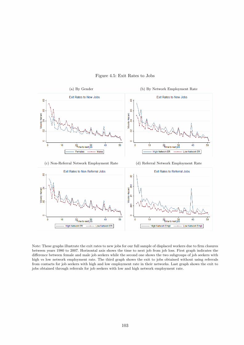
Figure 4.5: Exit Rates to Jobs
(a) By Gender (b) By Network Employment Rate
(c) Non-Referral Network Employment Rate (d) Referral Network Employment Rate
Note: These graphs illustrate the exit rates to new jobs for our full sample of displaced workers due to firm closuresbetween years 1980 to 2007. Horizontal axis shows the time to next job from job loss. First graph indicates thedifference between female and male job seekers while the second one shows the two subgroups of job seekers withhigh vs low network employment rate. The third graph shows the exit to jobs obtained without using referralsfrom contacts for job seekers with high and low employment rate in their networks. Last graph shows the exit tojobs obtained through referrals for job seekers with low and high network employment rate.
103

CHAPTER 4. COWORKERS, NETWORKS AND JOB SEARCH OUTCOMES
To see whether the graphical impression also holds after controlling for individual characteristics
and closing firm effects, we estimate proportional hazard models for the risk of finding a new job
in the first year after displacement. These models include unrestricted daily baseline hazards at
the closing firm level, a set of individual level covariates X such as age, gender, nationality, and
detailed labor market and earnings history characteristics, and a set of network characteristics
NW . Specifically, we model the discrete hazard function h(T |Xij , NWij) as the probability that
individual i displaced form firm j finds a job after T days, given that she has not exited to a
job up to day T − 1, as
h(T |Xij , NWij) = λj(T ) exp(αXij + βNWij) (4.1)
where the baseline function λj(T ) specifies the closing firm specific hazard rates when all
covariates are set to zero and α and β are the vectors of coefficients to be estimated. Observations
with durations longer than 365 days are treated as right censored.
Table 4.4 presents the estimation results. Columns (1) to (5) present estimates from separate
regressions including different sets of network characteristics. All models control for the log
network size to account for network heterogeneity in terms of the number of contacts. But the
coefficient is small across all specifications and mostly insignificant. The share of co-workers who
are employed at the displacement date has a large and significant impact on the job finding rate.
The magnitude of the effect in Column (1) implies a one standard deviation increase in the share
of employed former co-workers increases the exit rate to jobs by about 4%. This is similar in
magnitude to the effect reported by Cingano and Rosolia (2012), but somewhat smaller than
the IV estimates by Glitz (2013).
The remaining model specifications in Table 4.4 include variables representing the types of firms
where former co-workers are employed. Column (2) controls for the share of former co-workers
who are working in firms operating in the same industry as the closing firm. It turns out that
former co-workers in same industry firms are about twice as effective as other employed co-
workers for finding new jobs.
The next specification in Column (3) takes demand side factors, that are faced by the firms in
which former co-workers are employed into account. Social contacts in expanding firms might be
more helpful for displaced workers, because these firms typically have open vacancies. This idea
is confirmed by the regression coefficient. The share of former co-workers employed in net hiring
104

firms, defined as firms that were growing in the quarter of job displacement, further increases
the exit rate to new jobs. Column (4) examines if this effect also holds for the share of former
co-workers who are employed in firms that are growing in two consecutive quarters to make sure
that the hiring of former co-workers is not the only reason for the employment growth in their
firms. As the estimated coefficient remains of the same magnitude and statistically significant,
we conclude that former co-workers employed in expanding firms are potentially an important
source of information about vacancies in their firms.
The final specification in Column (5) examines the effect of former co-workers who are employed
in firms that pay average wages above the industry specific medians. Here the coefficient is small
and insignificant and we cannot see an impact on the hiring rate.
Table 4.4: Job Finding Rate: Effect of Network Characteristics
(1) (2) (3) (4) (5)
Log Network Size 0.016 0.009 0.008 0.008 0.008(0.004) (0.004) (0.004) (0.004) (0.004)
Network Emp. Rate 0.195 0.109 0.071 0.097 0.099(0.022) (0.025) (0.026) (0.026) (0.027)
Emp. Rate at Same Industry 0.134 0.136 0.133 0.131(0.021) (0.021) (0.021) (0.021)
Emp. Rate at Net Hiring Firms 0.086(0.018)
Emp. Rate at Net Hiring Firms at t and t+1 0.074(0.024)
Emp. Rate at Above Med. Wage Firms 0.017(0.019)
Observations 151432 151432 151432 151432 151432
Source: ASSD, own calculations.Note: Standard errors in parentheses. All columns report results from standard Cox Model for exitingunemployment. In each column we add a different measure of network employment rate as indicated. Wecontrol for individual demographic and work force characteristics such as gender, age, marital status,nationality, education, occupation indicator (blue and white collar), tenure at job lost, employment daysin last two years, employment days over last 5-15 years, unemployment claims in last 3-5 years, wagebefore job loss, number of employers within last years before job loss, average size of firms (employers)within last 5 years. All estimations also include closing firm fixed effects.
We further check the robustness of our results with respect to the model specification and to
the measurement of the network characteristics. Appendix Table 4.10 presents results for the
same set of model specifications as Table 4.4 that are based on linear probability models for an
indicator variable equal to one if the individual is employed within 3 months after displacement.
The results of this model are very similar to the results from the proportional hazard model.
105

CHAPTER 4. COWORKERS, NETWORKS AND JOB SEARCH OUTCOMES
Next, we estimate hazard rate models that take into account changes in the network characteris-
tics over time. The hazard rate models in Table 4.4 are based on network characteristics measured
at job displacement. For job seekers who are still out of work some time after displacement,
however, the network characteristics at a later date may be more relevant. Appendix Table 4.11
therefore presents results from hazard models that allow for time varying network characteristics
in the first quarters after job displacement. Qualitatively and quantitatively these results are
not different from the estimations with fixed network characteristics. This is not surprising, as
we have seen in Figure 4.5 that the largest differences in exit rates between individuals with
high and low shares of employed former co-workers appear in the first months after displacement.
Figure 4.6 plots the employment status of jobs seekers in the quarters before and after the
firm closure. The first four Panels 4.6a, 4.6b, 4.6c and 4.6d show the employment status of
the displaced individuals grouped by our different network employment rate measures. They
show that the individuals are not sorted by their respective network employment rates before
displacement, but clearly sorted thereafter. This looks a little bit different for Panels 4.6e and 4.6f
where the individuals wages are plotted. Before displacement there is already sorting according to
the network employment rates (Panel 4.6e) and according to the mean wage quartile (Panel 4.6f),
but the difference between the four groups is larger after displacement.
Wage Growth
After having established the importance of network characteristics on the job finding rates, we
investigate if co-worker networks also have an impact on the characteristics of the new jobs. We
focus on displaced workers who successfully find a new job in the first year after firm closure and
compare their pre-and post-displacement wages. Specifically, we estimate the following regression
model
yij = Xijα+NWijβ + γj + uij (4.2)
where yij denotes the log wage difference before and after displacement and γj controls for
closing firm fixed effects. The effects of individual and network characteristics are again given by
the parameters α and β. We estimate separate models for males and females, because monthly
wages in the ASSD can only be constructed from annual earnings and we have no control over
changes in working hours.
106
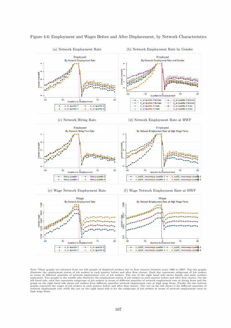
Figure 4.6: Employment and Wages Before and After Displacement, by Network Characteristics
(a) Network Employment Rate (b) Network Employment Rate by Gender
(c) Network Hiring Rate (d) Network Employment Rate at HWF
(e) Wage Network Employment Rate (f) Wage Network Employment Rate at HWF
Note: These graphs are obtained from our full sample of displaced workers due to firm closures between years 1980 to 2007. Top two graphsillustrate the employment status of job seekers in each quarter before and after firm closure. Each line represents subgroups of job seekersin terms of different quartiles of network employment rate of job seekers. The one of the right hand side shows female and male workersseparately. Two graphs in the middle also illustrate the employment status of job seekers in each quarter before and after firm closure. On theleft hand side, each line represents subgroups of job seekers in terms of different quartiles of network employment rate at hiring firms and thegraph on the right hand side shows job seekers from different quartiles network employment rate at high wage firms. Finally the two bottomgraphs represent the wages of job seekers in each quarter before and after firm closure. The one on the left shows it for different quartiles ofnetwork employment rate while the one on the right hand side is for the subgroups of job seekers in terms of network employment rates athigh wage firms.
107

CHAPTER 4. COWORKERS, NETWORKS AND JOB SEARCH OUTCOMES
Estimation results for men, presented in Table 4.5, show that network characteristics have only
small and mostly insignificant effects on wage growth. The only significant coefficient is on the
employment rate of former co-workers who work in high wage firms. Increasing this share by one
standard deviation, raises the average wage gain by one percentage point. This result indicates
that wage gains might be due to individuals finding jobs in higher paying firms where their
former co-workers are employed.
Results for women, shown in Table 4.6, are quantitatively in line with the results for males. In
contrast to men, women also seem to benefit from former co-workers who are employed in the
same industry and from former co-workers employed in expanding firms. This could indicate that
women who are able to return to employment more quickly also benefit in terms of reemployment
wages.
Table 4.5: Wage Growth: Effect of Network Characteristics, Only Men
(1) (2) (3) (4) (5)
Log Network Size 0.002 0.002 0.002 0.002 0.002(0.002) (0.002) (0.002) (0.002) (0.002)
Network Emp. Rate 0.025 0.025 0.024 0.025 -0.008(0.013) (0.015) (0.016) (0.015) (0.016)
Emp. Rate at Same Industry 0.000 0.000 0.000 -0.008(0.011) (0.011) (0.011) (0.011)
Emp. Rate at Net Hiring Firms 0.003(0.010)
Emp. Rate at Net Hiring Firms at t and t+1 0.002(0.013)
Emp. Rate at Above Med. Wage Firms 0.055(0.011)
Observations 78110 78110 78110 78110 78110
Source: ASSD, own calculations.Note: Standard errors in parentheses. All columns report results from wage growth estimations.Dependent variable is the wage growth measured as the log difference of wage at job lost and re-entrywage. Estimation sample includes only male displaced workers displaced workers due to firm closuresin 1980-2007. We include only successful job seekers without any restriction on time to reemployment.In each column, we add a different measure of network employment rate as indicated. All estimationsinclude closing firm FE as well as individual demographic and work force characteristics.
Heterogeneity of Job Finding Rates
Next, we examine whether the network effects are heterogeneous for different groups of displaced
workers. In addition, we investigate whether former co-workers with similar characteristics are
more profitable for the job finding rate. We estimate hazard rate models similar to Equation 4.1
for several sub-populations, with controls for log network size and the share of employed network
members. In particular, we divide network members into four distinct categories: employed
108

Table 4.6: Wage Growth: Effect of Network Characteristics, Only Women
(1) (2) (3) (4) (5)
Log Network Size 0.009 0.006 0.006 0.006 0.006(0.003) (0.003) (0.003) (0.003) (0.003)
Network Emp. Rate 0.016 -0.008 -0.024 -0.012 -0.028(0.017) (0.020) (0.021) (0.020) (0.021)
Emp. Rate at Same Industry 0.040 0.040 0.040 0.034(0.017) (0.017) (0.017) (0.018)
Emp. Rate at Net Hiring Firms 0.037(0.015)
Emp. Rate at Net Hiring Firms at t and t+1 0.021(0.020)
Emp. Rate at Above Med. Wage Firms 0.042(0.015)
Observations 52367 52367 52367 52367 52367
Source: ASSD, own calculations.Note: Standard errors in parentheses. All columns report results from wage growth estimations.Dependent variable is the wage growth measured as the log difference of wage at job lost and re-entrywage. Estimation sample includes only female displaced workers displaced workers due to firm closuresin 1980-2007. We include only successful job seekers without any restriction on time to reemployment.In each column, we add a different measure of network employment rate as indicated. All estimationsinclude closing firm FE as well as individual demographic and work force characteristics.
network members of the same population group, employed network members of the opposite
population group, not employed network members of the same population group, and not
employed network members of the opposite population group who are the reference group.
Estimation results by gender, occupation, and nationality are shown in Table 4.7. To facilitate
the comparison of the estimated effects across groups and across covariates, we standardize the
coefficients such that they correspond to the effects of a one standard deviation increase of the
independent variable. The first column reports the result for female displaced workers. Females
benefit from employed former co-workers of either gender, an increase by one standard deviation
increases the job finding rate by about 5 - 6%. Even non-employed female network members are
more important for job finding success of women than non-employed male network members.
Males, shown in Column (2), in comparison, mostly benefit from employed male former co-
workers, while employed female network members are slightly less important. Non-employed
contacts do not have any effect on the job finding rate of male displaced workers.
If we compare network effects by workers types, in Columns (3) and (4), we note that for white
collar workers the impact of former co-workers on the job finding rates are much stronger than
on blue collar workers. An increase of the share of former co-workers by one standard deviation
corresponds to a shift in the hazard rate by about 8 - 9% for white collar workers, but only
109
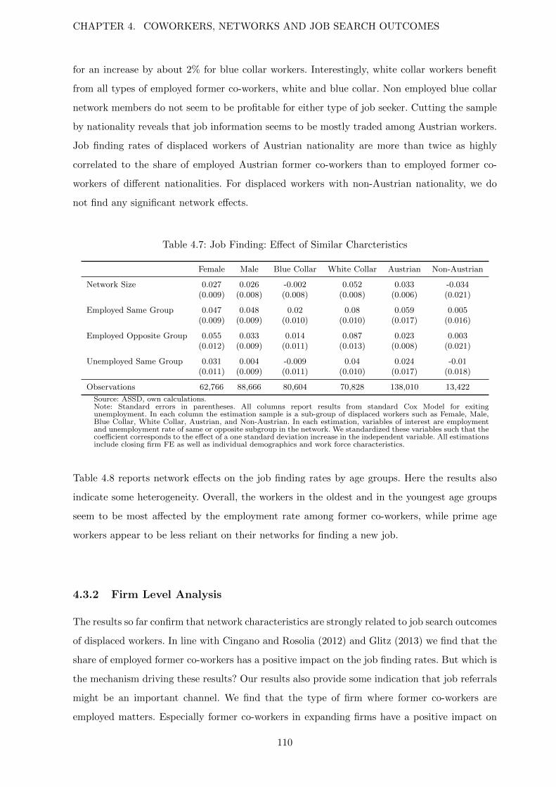
CHAPTER 4. COWORKERS, NETWORKS AND JOB SEARCH OUTCOMES
for an increase by about 2% for blue collar workers. Interestingly, white collar workers benefit
from all types of employed former co-workers, white and blue collar. Non employed blue collar
network members do not seem to be profitable for either type of job seeker. Cutting the sample
by nationality reveals that job information seems to be mostly traded among Austrian workers.
Job finding rates of displaced workers of Austrian nationality are more than twice as highly
correlated to the share of employed Austrian former co-workers than to employed former co-
workers of different nationalities. For displaced workers with non-Austrian nationality, we do
not find any significant network effects.
Table 4.7: Job Finding: Effect of Similar Charcteristics
Female Male Blue Collar White Collar Austrian Non-Austrian
Network Size 0.027 0.026 -0.002 0.052 0.033 -0.034(0.009) (0.008) (0.008) (0.008) (0.006) (0.021)
Employed Same Group 0.047 0.048 0.02 0.08 0.059 0.005(0.009) (0.009) (0.010) (0.010) (0.017) (0.016)
Employed Opposite Group 0.055 0.033 0.014 0.087 0.023 0.003(0.012) (0.009) (0.011) (0.013) (0.008) (0.021)
Unemployed Same Group 0.031 0.004 -0.009 0.04 0.024 -0.01(0.011) (0.009) (0.011) (0.010) (0.017) (0.018)
Observations 62,766 88,666 80,604 70,828 138,010 13,422
Source: ASSD, own calculations.Note: Standard errors in parentheses. All columns report results from standard Cox Model for exitingunemployment. In each column the estimation sample is a sub-group of displaced workers such as Female, Male,Blue Collar, White Collar, Austrian, and Non-Austrian. In each estimation, variables of interest are employmentand unemployment rate of same or opposite subgroup in the network. We standardized these variables such that thecoefficient corresponds to the effect of a one standard deviation increase in the independent variable. All estimationsinclude closing firm FE as well as individual demographics and work force characteristics.
Table 4.8 reports network effects on the job finding rates by age groups. Here the results also
indicate some heterogeneity. Overall, the workers in the oldest and in the youngest age groups
seem to be most affected by the employment rate among former co-workers, while prime age
workers appear to be less reliant on their networks for finding a new job.
4.3.2 Firm Level Analysis
The results so far confirm that network characteristics are strongly related to job search outcomes
of displaced workers. In line with Cingano and Rosolia (2012) and Glitz (2013) we find that the
share of employed former co-workers has a positive impact on the job finding rates. But which is
the mechanism driving these results? Our results also provide some indication that job referrals
might be an important channel. We find that the type of firm where former co-workers are
employed matters. Especially former co-workers in expanding firms have a positive impact on
110

Table 4.8: Job Finding: Effect of Similar Age Groups
Below 29 29 to 36 36 to 44 Above 44
Network Size 0.078 -0.001 0.019 -0.009(0.013) (0.014) (0.013) (0.014)
Employed Same Group 0.06 0.021 0.013 0.054(0.010) (0.009) (0.009) (0.011)
Employed Age < 30 0.022 0.048 0.084(0.011) (0.012) (0.015)
Employed Age 30 − 35 0.002 0.019 0.036(0.008) (0.009) (0.012)
Employed Age 36 − 44 0.02 0.012 0.041(0.009) (0.009) (0.011)
Employed Age > 44 0.022 0.013 0.024(0.009) (0.010) (0.010)
Unemployed Same Group 0.014 0.001 0.006 0.042(0.012) (0.010) (0.011) (0.015)
Observations 36,030 35,244 38,404 41,754
Source: ASSD, own calculations.Note: Standard errors in parentheses. All columns report results from standardCox Model for exiting unemployment. In each column the estimation sampleis a sub-group of displaced workers in terms of age groups such as below 29,between 30 and 36, between 36 and 44, and above 44. In each estimation,variables of interest are employment and unemployment rate of same oropposite subgroup in the network. We standardized these variables such thatthe coefficient corresponds to the effect of a one standard deviation increasein the independent variable. All estimations include closing firm FE as well asindividual demographics and work force characteristics.
job finding rates. In addition we find wage gains in the new job for displaced workers whose
former co-workers are employed in high wage firms. Arguably the firm type should only matter
for search outcomes if network information leads to jobs in these expanding or high wage firms.
The next part of the analysis examines the importance of the referral channel further. We exploit
the firm dimension of the co-worker network and ask the question: what is the contribution of a
former co-worker contact k employed at a connected firm l on the probability that the displaced
individual i gets hired? To avoid spurious correlation in unobservable characteristics of the worker
and the firm, i.e., that firm l is generally more likely to hire workers of i’s type we control for
fixed effects at the pair level of closing and connected firms. The counterfactual analysis thus
compares two workers from the same layoff firm j where one of them holds a link with a former
co-worker employed in connected firm l and the other one does not.
We thus specify our regression model as a linear probability model
Pi,j,l = βjl + γLil + εil (4.3)
111

CHAPTER 4. COWORKERS, NETWORKS AND JOB SEARCH OUTCOMES
where Pi,j,l denotes the probability that individual i displaced from firm j is hired by connected
firm l and Lil is an indicator equal to one if the individual holds a link to a former co-worker
employed at l. Thus γ measures the network effect.
Estimating this model requires a large dataset which has a dimension determined by the number
of displaced workers times closing firms times connected firms, which makes Equation (4.3)
intractable. To simplify the estimation, we apply a fixed effects transformation suggested
by Kramarz and Thesmar (2013) and applied by Kramarz and Nordstrom Skans (2013). In
particular, we collapse Equation (4.3) at the closing - connected firm level and consider the
share of linked individuals displaced from firm closing firm j, who are hired by connected firm
l, RLinkj,l given by:
RLinkj,l =
∑i Pijl ∗ Lil∑
i Lil= βjl + γ + uLinkil
and the share of non-linked individuals displaced from closing firm j, who are hired by connected
firm l, RnoLinkj,l given by
RnoLinkj,l =
∑i Pijl ∗ (1− Lil)∑
i(1− Lil)= βjl + unoLinkil
The difference between these two determines the coefficient of interest γ as
Gj,l = RLinkj,l −RnoLinkj,l = γ + uil (4.4)
Estimation results are shown in Table 4.9. The first row presents the estimate of γ and its
components for the full sample. The parameter on the link dummy is estimated with high
precision. To interpret it’s magnitude we compare the share of linked workers who get hired
with the share of non-linked workers who get hired. The ratio between those two is 3.4, which
means that workers with link face a more than three times higher probability to find a job in
the connected firm as similar workers from the same closing firm without a link.
To see whether the result for the overall sample is driven by certain subgroups, we repeat the
estimation for various subsamples in the remaining columns of Table 4.9. Although the coefficient
estimate of the link effect varies across groups, for example γ is higher in pairs of closing -
connected firms in the same industry, the ratio between the share hired with link and the share
112

hired without link is roughly stable. For example, both linked and non-linked individuals have a
higher probability of being hired in a connected firm in the same industry. We also confirm that
the link effect does not change over time, by region, and for larger closing firms which probably
also have a higher variation of links across connected firms.
Table 4.9: Firm Level Analysis
All Vienna Same industry Year > 1995 Layoffs > 10
γ 0.00062 0.00047 0.00125 0.00047 0.00041(0.00001) (0.00002) (0.00005) (0.00002) (0.00002)
t-stat 45.66 24.19 24.18 30.79 23.03
RLinkj,l 0.00088 0.00067 0.00204 0.00070 0.00058
(0.00001) (0.00002) (0.00005) (0.00002) (0.00002)
RnoLinkj,l 0.00025 0.00020 0.00079 0.00023 0.00017
(0.00001) (0.00001) (0.00003) (0.00001) (0.00001)
Ratio 3.44 3.40 2.58 3.06 3.37
N 4,197,692 1,569,564 625,944 2,592,747 1,376,913
Source: ASSD, own calculations.Note: Observation pairs of the analysis is layoff firm and connected firm. Displacedworkers with a link to connected firm are 3.44 times as likely to be hired as co-displacedworkers without a link from the same layoff firm.
4.4 Conclusion
A growing theoretical and empirical literature on the relevance of social networks in the labor
market provides various channels through which networks can affect the labor market. So far,
the empirical studies testing the theoretical implications have remained relatively scarce, with
very little consensus on the various channels.
In order to understand how displaced workers benefit from their social contacts to find a job,
we define the social networks as the group of past co-workers with whom they worked together
(during the past five years) at the same firm. We use large administrative data providing the
entire work histories of the universe of private sector workers in Austria.
Our contribution to the empirical analysis of social networks on job search outcomes is two-fold.
First, we provide evidence of an effect of the social network at the job seeker level, where we
show that the higher the share of employed past co-workers the higher is the job-finding rate
of the displaced worker. Furthermore, past co-workers employed in the same industry and in
firms that are hiring at the displacement date are particularly helpful. We also provide evidence
on the heterogeneity of network effects where past co-workers with similar characteristics are
113

CHAPTER 4. COWORKERS, NETWORKS AND JOB SEARCH OUTCOMES
important for some groups based on gender, age groups and occupation. Second, we bring the
analysis to the firm level, where we define the firm networks based on the links between the
corresponding workers. We find that 25% of the displaced workers find a new job in a connected
firm and that the displaced workers with a link to the connected firm are three times as likely
to be hired as co-displaced workers from the same layoff firm without a link to the connected firm.
114

4.A Networks Appendix
4.A.1 Reemployment Probability
In this section, we present the results of the linear probability model of employment within
3 months after displacement. We consider the whole sample of displaced workers and analyze
whether the network employment rate has an impact on the probability of their re-employment.
Table 4.10 shows that the network employment rate has a significant positive effect on the
probability of re-employment. We control for the individual characteristics of the displaced
worker as well as her employment history. All estimations include closing firm fixed effects.
Table 4.10 presents evidence of a significant impact of the network employment rate on the
re-employment probability after 3 months. This impact is mostly driven by network members
that are employed in the same industry (Column 2) and hiring firms (Column 3 and 4) while
the share of network members employed in above median wage firms (Column 5) do not have a
significant impact.
Table 4.10: Probability of Reemployment: Effect of Network Characteristics
(1) (2) (3) (4) (5)
Log Network Size 0.005 0.000 0.000 0.000 0.000(0.002) (0.002) (0.002) (0.002) (0.002)
Network Emp. Rate 0.071 0.020 0.003 0.016 -0.002(0.012) (0.014) (0.014) (0.014) (0.015)
Emp. Rate at Same Industry 0.080 0.081 0.080 0.079(0.011) (0.011) (0.011) (0.011)
Emp. Rate at Net Hiring Firms 0.039 0.039(0.010) (0.010)
Emp. Rate at Net Hiring Firms at t and t+1 0.026(0.013)
Emp. Rate at Above Med. Wage Firms 0.009(0.010)
Observations 151432 151432 151432 151432 151432
Source: ASSD, own calculations.Note: Standard errors in parentheses. In all columns, we present results from a linear probability modelwhere the dependent variable is a binary variable indicating reemployment within 3 months after jobloss. In each column we add a different measure of network employment rate as indicated. All estimationsinclude the same covariates as in Table 4.4 and closing firm fixed effects.
4.A.2 Robustness Checks
Table 4.11 reports results from the Cox model where we allow the network employment
characteristics to change across quarters while workers search for jobs. This is a robustness
check, which takes into account the time varying characteristics of the network.
115
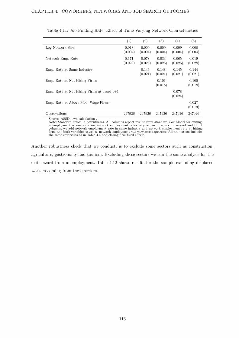
CHAPTER 4. COWORKERS, NETWORKS AND JOB SEARCH OUTCOMES
Table 4.11: Job Finding Rate: Effect of Time Varying Network Characteristics
(1) (2) (3) (4) (5)
Log Network Size 0.018 0.009 0.009 0.009 0.008(0.004) (0.004) (0.004) (0.004) (0.004)
Network Emp. Rate 0.171 0.078 0.033 0.065 0.019(0.022) (0.025) (0.026) (0.025) (0.028)
Emp. Rate at Same Industry 0.146 0.148 0.145 0.144(0.021) (0.021) (0.021) (0.021)
Emp. Rate at Net Hiring Firms 0.101 0.100(0.018) (0.018)
Emp. Rate at Net Hiring Firms at t and t+1 0.078(0.024)
Emp. Rate at Above Med. Wage Firms 0.027(0.019)
Observations 247926 247926 247926 247926 247926
Source: ASSD, own calculations.Note: Standard errors in parentheses. All columns report results from standard Cox Model for exitingunemployment where we allow network employment rates vary across quarters. In second and thirdcolumns, we add network employment rate in same industry and network employment rate at hiringfirms and both variables as well as network employment rate vary across quarters. All estimations includethe same covariates as in Table 4.4 and closing firm fixed effects.
Another robustness check that we conduct, is to exclude some sectors such as construction,
agriculture, gastronomy and tourism. Excluding these sectors we run the same analysis for the
exit hazard from unemployment. Table 4.12 shows results for the sample excluding displaced
workers coming from these sectors.
116

Table 4.12: Job Finding Rate: Excluding Agriculture, Tourism, and Construction
(1) (2) (3) (4) (5)
Log Network Size 0.022 0.014 0.014 0.014 0.014(0.004) (0.004) (0.004) (0.004) (0.004)
Network Emp. Rate 0.221 0.135 0.096 0.121 0.126(0.024) (0.028) (0.030) (0.029) (0.031)
Emp. Rate at Same Industry 0.132 0.134 0.131 0.130(0.023) (0.023) (0.023) (0.023)
Emp. Rate at Net Hiring Firms 0.090(0.020)
Emp. Rate at Net Hiring Firms at t and t+1 0.092(0.027)
Emp. Rate at Above Med. Wage Firms 0.016(0.021)
Observations 116197 116197 116197 116197 116197
Source: ASSD, own calculations.Note: Standard errors in parentheses. All columns report robustness results from standard Cox Modelfor exiting unemployment. Estimation sample includes displaced workers who lost their jobs at closingfirms excluding construction and tourism sectors. In each column we add a different measure of networkemployment rate as indicated. All estimations include the same covariates as in Table 4.4 and closingfirm fixed effects.
117

118

Chapter 5
Selective Firing and Lemons?
5.1 Introduction
“To hire somebody is frequently to purchase a lottery” - Spence (1973)
Among others, Spence (1973) recognized that information asymmetries, which may even
resemble a lottery, are crucial for the labor market and its employment dynamics. The focus of
the current work is on what information firms infer from the three common types of displacement:
individual layoffs, individuals displaced due to a closure, and individuals displaced due to a mass
layoff.1 I thereby bring together two strands of the literature, namely the literature on signaling
and sorting. The contribution to the literature is threefold: first I test whether the individual
layoffs are the least productive, second I investigate whether individual layoffs are perceived as
“lemons” (with a specific focus on the high ability) and third I raise the question whether the
“lemon” exists in the resulting matching pattern.
The signaling literature suggests that an agent/individual conveys information about her type (in
our case ability) to another principal/party (the firm in our case). Akerlof (1970), Spence (1973)
and Greenwald (1986) are examples of papers, which have considerably formed our knowledge
about signaling models in the context of wages, mobility and education. As individual ability is
incompletely observed by a firm, I try to disentangle if either the firms infer information from
the layoff type or if the individual grasps the opportunity to find a better matching firm. The
idea of a better match follows the sorting idea (assortative matching). We talk about assortative
matching if more matches of certain workers and firms are observed than random matches.
1A person that gets fired individually and not due to a mass layoff or a firm closure is part of the individuallayoff group.
119

CHAPTER 5. SELECTIVE FIRING & LEMONS
Becker (1973) is a prominent example of the matching model for the marriage market.
Other than the prominent “lemon” example in Akerlof (1970) for the used car market, Gibbons
and Katz (1991) (in the following referred to as GK) have shaped our expectations of what
we should find when comparing individual layoffs with closures, as the individual layoffs always
experience a wage penalty, after being laid off. This is also the case for Austria as we can see
in Figure 5.1, which plots the wage profiles for the layoff types five years before and five years
after displacement, where year 0 is the displacement year. Looking at the individual layoffs
wage profile, a clear kink labeled “lemon” by GK at year 1 is visible. Already in the second
year of re-employment, individuals have caught up from this drop in re-employment wages.
Nevertheless, on average individuals suffering from an individual layoff never seem to catch up
with the individuals displaced due to a plant closure.
Figure 5.1: Mean Wages Re-employed Individuals
3.9
44.
14.
24.
34.
4(m
ean)
log
wag
e
−5 0 5Time(0=Layoff Year)
Layoff ClosureMass Layoff
GK set up an asymmetric information model and test it empirically. The first assumption
that GK make, in order to derive their theoretical prediction, is that firms have leeway when
determining whom to layoff. Thus, an individual layoff may be stigmatized compared to an
individual losing her job due to a firm closure where no such stigma is attached. The first
contribution of this work is to test whether the least able are laid off individually. In order to
perform this test, I follow the seminal work of Abowd et al. (1999) (in the following referred
120

to as AKM) where I estimate a simple wage regression with a person and a firm fixed effect.
The person and firm fixed effects are used as a heterogeneity measure.2 This measure allows
me to show that the individuals suffering from a closure are more heterogeneous in terms of
their productivity than the individuals laid off due to a mass layoff, which in turn are more
heterogeneous than those individually laid off. This finding supports the assumption frequently
made in the literature.3
The second contribution of this chapter is the replication of GK. As equilibrium outcome of
GK asymmetric information model, re-employment wages of the individually laid off are smaller
than those of the closure individuals. This leads to the main conclusion that individual layoffs
are perceived as “lemons”. Replicating GK, I find that a stigma is attached to being individually
laid off for the case of Austria. This significantly negative effect of being fired is robust to the
inclusion of a control for firm size and other controls such as region and industry.4
Combining Krashinsky (2002), who claims that individual layoffs have more to lose, and Hu and
Taber (2005), who split their sample by race and gender and thereby put more weight on the
heterogeneity of the individuals, I take the GK formulation a step further and add an analysis
for high productivity individuals.5 The analysis of the high ability individuals shows that indeed
they have the most to lose, since they are not able to overcome the stigma of being individually
laid off and still pay a wage penalty compared to the closure group. This result supports GK
signaling argument that the individual layoffs are perceived as “lemons”.
Furthermore, I raise the question whether individual layoffs have a chance of ending up at a
high wage firm (HWF) (measured by the firm fixed effect from the AKM model). My findings
are reconcilable with Gibbons et al. (2005), who show that unobserved ability does not explain
2Following Card et al. (2013b) closely, I apply AKM to the Austrian Social Security Registers and I am ableto show that the identification restrictions are met.
3Since the seminal work of AKM, there are only a few papers which deal with inference on the fixed effects,Serafinelli (2012) and Card et al. (2013a) are two examples of papers that split the firm fixed effects into e.g.,quintiles and make inference based on these.
4Other papers which replicate GK are for example: Grund (1999), Doiron (1995), Stevens (1997). Grund(1999) uses German Data, but does not find any evidence in favor of signaling. Doiron (1995) replicates GK forCanada. Stevens (1997) tries to replicate the findings for the US using the PSID, and does find smaller wagechanges for the closing types, but much of it can be explained by the wage losses in the year prior to the actualclosure event. Song (2007) and Borowitz (2010) on the other hand claim that it is all about recall bias when usingthe Displaced Worker Supplement to the CPS (which is the Data used by GK), while Nakamura (2008) extendsthe finding over the business cycle.
5Krashinsky (2002) explores an alternative hypothesis, claiming that individual layoffs have more to lose,since they get laid off by larger firms. Introducing controls for firm size, removes the difference between individuallayoffs and closure types for his case. Hu and Taber (2005) find the “lemons” effect for some groups but a reversedresult for others, pointing towards statistical discrimination.
121

CHAPTER 5. SELECTIVE FIRING & LEMONS
intra-industry wage differentials and find that high-wage sectors employ high skill workers and
thus also offer higher returns to workers’ skills. I find that compared to individuals suffering
from a closure, individual layoffs are less likely to end up at a HWF, while an individual layoff
of high ability is more likely to end up at a HWF. This result may point toward exploitation,
since HWF still hire individual layoffs of high ability, but they offer them a lower wage.
The main concern with the empirical finding of GK, is that it can be reconciled with a sorting
model. Replicating their argument against sorting, I am not able to reject the matching model.
Therefore, the third contribution of this chapter, is to see whether there is matching before the
displacement and how and if it changes thereafter. There have been numerous suggestions on
how to measure matching, the AKM model allows us to analyze the correlation between the
worker and the firm fixed effect, as Abowd et al. (2004) have done for the US (finding a zero
correlation) and for France (finding a negative correlation). These results reject the assortative
matching model of Becker (1973).6
The consistently close to zero or even negative correlation between the person and firm fixed
effects is consistent with a model known as the “piece rate model”; a model based on Burdett
(1978) and extended with worker heterogeneity. Lopes de Melo (2013) applies AKM to Brazilian
data and rejects the “piece rate model”, then develops a measure of sorting based on Shimer
and Smith (2000) which extends the search model of Becker (1973) by introducing search
frictions. In these two models, complementarities in production are the main force that drive
assortative matching.7 As noted in Eeckhout and Kircher (2011) as well, the model of Shimer
and Smith (2000) allows to infer the strength of the sorting, since high skill workers work for
high productivity firms in case of positive assortative matching (or low productivity firms in case
of negative assortative matching) as a consequence of this, they have high skilled co-workers.
Thus the correlation between the person effect and the average over the co-worker person effect
is a promising way to measure the intensity of sorting in the economy.
To measure sorting, this chapter uses three distinct measures; the firm fixed effect, the correlation
between the person and the firm fixed effect, and the correlation between the person effect and
6Haskel et al. (2005) find that more productive firms hire more productive workers applying AKM to the UK(positive correlation) and Irzano et al. (2008) applying AKM to Italy find that the firm’s productivity is positivelyrelated to skill dispersion within the occupational status groups and negatively to the skill dispersion betweengroups.
7Other papers related to this strand of literature are e.g., Bagger and Lentz (2008), Lise et al. (2012). I referthe reader to Lentz and Mortensen (2010) for a good overview of the labor market models with worker and firmheterogeneity.
122

the average of the co-worker person effect. I compare the amount of matching before displacement
with the amount of matching thereafter. In a world where the signal contains no information,
I expect the “lemon” to be invisible in the resulting matching pattern. This means that the
matching measure should change in a similar way for the different layoff groups. If the signal
distorts the resulting matching pattern, I should observe a difference between the change in
matching before and after displacement. Applying the sorting measures to the ASSD, I find
that the matching changes differently for the different layoff groups. This leads to the tentative
conclusion, that both sorting and signaling play a role. Assortative matching plays a role, as the
sorting measures are always different from zero, while signaling plays a role, because the effects
change differently for the different groups.
The remainder of this chapter is structured as follows. In Section 5.2, the underlying theory and
empirical framework are discussed. Section 5.2.1 discusses the GK model, while Section 5.2.2
gives a short overview of the AKM model. Section 5.2.3 talks about the possible sorting
mechanism. Section 5.3 presents the linked employer-employee data of the Austrian Social
Security Registers, and discusses the displacement sample. Section 5.4 presents the results,
where Section 5.4.1 provides the reader with the results on the heterogeneity while Section 5.4.2
discusses the signaling versus sorting evidence. Section 5.5 concludes.
5.2 Theoretical and Empirical Framework
As discussed above, the analysis for signaling follows Gibbons and Katz (1991), while part of the
sorting is based on Lopes de Melo (2013). Section 5.2.1, describes the signaling according to GK
and the possible sorting explanation of their findings. Section 5.2.2 describes the heterogeneity
measures, allowing to differentiate between a high and low ability individual and a high and low
wage paying firm. Section 5.2.3 discusses the different measures of sorting and what could be a
possible mechanism to disentangle signaling and sorting.
5.2.1 Signaling according to Gibbons and Katz (1991)
GK provide a theoretical analysis of an asymmetric information model for layoffs. The model
describes the labor market as an uncertain environment with informational frictions, where it
is assumed that the firm has discretion over whom to layoff. Then the firm’s desire to retain
a worker, signals that the worker is of high ability, and therefore the market will bid up the
wage of the retained worker. However, this effect will represent an adverse effect for individual
layoffs, and therefore they will receive lower re-employment wages. The equilibrium outcome of
123

CHAPTER 5. SELECTIVE FIRING & LEMONS
their model for re-employment wages is: ωclosure > ωindividual layoff. GK conjecture and empirically
show, using the displaced worker supplement to the CPS, that individual layoffs compared to
displacements due to plant closures exert a negative signal for the workers ability, by earning
lower re-employment wages.
The problem with this finding, also mentioned in their paper, is that sorting could be another
consistent explanation. The sorting consistent example that they give, see also Figure 5.2, is
that if there is an industry A which is sensitive to ability, and at the beginning of the period all
the seemingly high ability individuals work in A. While industry B is insensitive to ability, and
all the seemingly low ability individuals work in B. Then over time endogenous mobility will
improve the quality of the match. If moves from A to B are labeled as a layoff, and those from
B to A as a quit, it generates the exact same prediction as the signaling model.
Figure 5.2: Possible Sorting Mechanism in the GK model
Industry A Industry B
QUIT
LAYOFF
sensitive to ability insensitive to ability
GK test the matching model by including an industry switch dummy, and an interaction between
the industry switch dummy and the layoff dummy. They interpret the drop of the significance
on the layoff dummy as evidence that sorting (matching) is not the dominant mechanism.
124

As GK asymmetric information model is used as the framework for the analysis, I will replicate
their findings using (and expanding) their empirical specification;
∆ω︸︷︷︸ωpost−ωpre
= δ11(Layoff) + βX (5.1)
where the prediction that δ1 < 0 is testable, 1() represents the indicator function and X are other
control variables.8 To replicate GK findings on the symmetric information story, the following
empirical specification will be estimated:
ωpost = δ11(Layoff) + γ11(Switch Industry) + γ21(Switch Industry ∗ Layoff) + βX (5.2)
Laid off individuals switching industry should receive especially low re-employment wages; γ2 < 0
for the finding to be in line with a matching model. GK find that: γ2 > 0 and small in magnitude
and therefore exclude matching as a possible explanation. To take GK a step further, I first
include mass layoffs when estimating Equation (5.1) resulting in the following specification;
∆ω = δ11(Layoff) + δ21(Mass Layoff) + βX (5.3)
and then take it even a step further and include an indication of whether or not the individual
is a high ability type individual (HA).
∆ω = δ11(Layoff) + δ21(ML) + δ31(HA) + δ41(HA ∗ Layoff) + δ51(HA ∗ML) + βX (5.4)
With this specification, the question whether a high ability individual is able to overcome his
layoff stigma may be answered by testing; δ1 + δ3 + δ4 ≥ 0. A high ability individual has
potentially the most to lose, and therefore this specification allows to test whether there is a
stigma attached to being laid off.
In this context, the question may be raised whether a laid off individual (L) even has a chance
of being hired at a high wage firm (HWF). To do so I estimate a logit model of the following
form:
Pr((HWF ) = 1) = λ11(L)+λ21(ML)+λ31(HA)+λ41(HA∗L)+λ51(HA∗ML)+βX+ε (5.5)
8In the empirical section I control for a quadratic in age, age at first employment, firm size, firm operationduration, unemployment duration since labor force participation (LFP), employment duration since LFP, tenureat the closing firm, wage at first job, number of employment spells and number of unemployment spells.
125
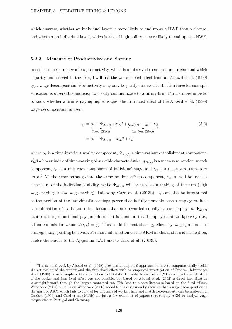
CHAPTER 5. SELECTIVE FIRING & LEMONS
which answers, whether an individual layoff is more likely to end up at a HWF than a closure,
and whether an individual layoff, which is also of high ability is more likely to end up at a HWF.
5.2.2 Measure of Productivity and Sorting
In order to measure a workers productivity, which is unobserved to an econometrician and which
is partly unobserved to the firm, I will use the worker fixed effect from an Abowd et al. (1999)
type wage decomposition. Productivity may only be partly observed to the firm since for example
education is observable and easy to clearly communicate to a hiring firm. Furthermore in order
to know whether a firm is paying higher wages, the firm fixed effect of the Abowd et al. (1999)
wage decomposition is used;
ωit = αi + ΨJ(i,t)︸ ︷︷ ︸Fixed Effects
+x′itβ + ηiJ(i,t) + ςit + εit︸ ︷︷ ︸
Random Effects
(5.6)
= αi + ΨJ(i,t) + x′itβ + rit
where αi is a time-invariant worker component, ΨJ(i,t) a time-variant establishment component,
x′itβ a linear index of time-varying observable characteristics, ηJ(i,t) is a mean zero random match
component, ςit is a unit root component of individual wage and εit is a mean zero transitory
error.9 All the error terms go into the same random effects component, rit. αi will be used as
a measure of the individual’s ability, while ΨJ(i,t) will be used as a ranking of the firm (high
wage paying or low wage paying). Following Card et al. (2013b), αi can also be interpreted
as the portion of the individual’s earnings power that is fully portable across employers. It is
a combination of skills and other factors that are rewarded equally across employers. ΨJ(i,t)
captures the proportional pay premium that is common to all employees at workplace j (i.e.,
all individuals for whom J(i, t) = j). This could be rent sharing, efficiency wage premium or
strategic wage posting behavior. For more information on the AKM model, and it’s identification,
I refer the reader to the Appendix 5.A.1 and to Card et al. (2013b).
9The seminal work by Abowd et al. (1999) provides an empirical approach on how to computationally tacklethe estimation of the worker and the firm fixed effect with an empirical investigation of France. Haltiwangeret al. (1999) is an example of the application to US data. Up until Abowd et al. (2002) a direct identificationof the worker and firm fixed effect was not possible, but based on Abowd et al. (2002) a direct identificationis straightforward through the largest connected set. This lead to a vast literature based on the fixed effects.Woodcock (2008) building on Woodcock (2006) added to the discussion by showing that a wage decomposition inthe spirit of AKM which fails to control for unobserved worker, firm and match heterogeneity can be misleading.Cardoso (1999) and Card et al. (2013b) are just a few examples of papers that employ AKM to analyze wageinequalities in Portugal and Germany.
126
5.2.3 Sorting
As briefly mentioned in the introduction, to take the possible matching explanation of the
signaling model of GK a step further, matching will be evaluated by different measures. A first
impression on sorting is given by the firm fixed effects at the displacement firm and at the re-
employment firm. It is an indicator of how the displaced individuals sort themselves into the new
firms - as the firm fixed effect represents a ranking of the firms. Furthermore, I will take a look
at the correlation of the person and firm fixed effects, as suggested by Abowd et al. (2004). The
recent literature by Lopes de Melo (2013), Eeckhout and Kircher (2011), Lentz and Mortensen
(2010), to name a few examples, state that one cannot identify the sign of the sorting based on
the AKM model. They show that the correlation between the person and the firm fixed effect is
biased downwards and therefore mostly zero and may even be negative in some datasets. Due
to this bias a distinction between positive assortative matching (PAM) and negative assortative
matching (NAM) is not possible.10
These papers nevertheless show that the strength of the sorting can be identified, which is
arguably the more important measure in economics. Lopes de Melo (2013) shows that the
worker-co-worker correlation is a good measure of the strength of the sorting. In his model,
the high skilled workers work for the high-productivity firms in the case of PAM (or the low-
productivity in the case of NAM). A consequence of this, is that they have high-skill co-workers.
Therefore the correlations between their own person effect and the mean co-worker person effect,
Corr(θi, θj(i,t)), measures the intensity of the sorting in the economy. θi denotes the worker fixed
effect and θj(i,t) is the mean value of θ among the co-workers.
If I assume for the moment that there is PAM in the Austrian data, then the high type workers
match with the high type firms.11 As the goal is to distinguish between signaling and sorting, the
relevant stigma arises from the individual layoff, while no such stigma is attached to an individual
displaced by a plant closure. In order to see, whether the resulting matching is affected by the
“lemon”, this chapter takes a closer look at the firm fixed effects, and the different correlation
measures as suggested by the literature, before and after the displacement. If the “lemon” plays
a role, the difference should be affected; meaning that the difference between pre- and post-
10With PAM (NAM), a high skill individual will sort herself into a high (low) productivity firm and a lowskilled individual into a low (high) productivity firm.
11Please keep in mind that I cannot infer whether there is PAM or NAM without productivity data. This isassumed right now to explain what could possibly happen. Mendes et al. (2010) find for example PAM in Portugal,but they have productivity data and are able to estimate a flexible specification for the productivity.
127

CHAPTER 5. SELECTIVE FIRING & LEMONS
displacement matching should differ for the closure group and the individual layoff group.
5.3 Data
This chapter uses the Austrian Social Security Database (ASSD) which covers the universe of
private sector workers covered by the social security system between 1972 and 2009. The ASSD
provides daily information on employment, registered unemployment, total annual earnings paid
by each employer, and various individual characteristics of the workers as well as information
on employers such as geographical location, industry, and size. For a thorough overview of the
data, I refer the reader to Zweimuller et al. (2009).
In the ASSD, the firms are associated with an employer identifier reported in every employment
spell of the worker. The current analysis uses only information on male blue and white collar
workers in the years 1980-2009. In order to estimate the person and firm fixed effects, I run
AKM on a larger sample than the one that is used for inference on sorting and signaling (which
only includes displaced individuals).12 First one main job per year per individual is selected,
with a wage and a firm number. If there are overlapping spells, the longest spell is selected as a
main spell. To replicate GK a few more restrictions are put on the sample.
In order to use the firm closures as an entry to unemployment, I first create a sample of closing
firms. Fink et al. (2010) identify entry and exit of firms using a worker flow approach that
follows clusters of workers moving across entities. They also show that their firm definition is
comparable to the official firm statistics of Austria.13 To obtain the individuals affected by a firm
closure, firms operating in construction and gastronomy are excluded for seasonality reasons. I
only consider male blue and white collar workers who are displaced due to a closure and which
comply with the following restrictions. The individual must have been employed in the last
quarter of the firm operation, she must have worked at least a year for this firm (to make sure
she is unaware of the closure), and her age at displacement must be between 15 and 55 years of
age.
To identify mass layoffs, I proceed in a similar fashion. The initial definition is again based on
Fink et al. (2010) in the sense that a certain amount of employees is laid off between two quarter
12For more information on the AKM sample, see Appendix 5.A.1.13It is secured, that the firm shuts down and it is not just a rename, a spin off or a takeover.
128

dates. To identify the significant drop, the following assumptions are made: for firms with 11
to 20 employees, the firm size has to decline by at least 6 individuals for it to be counted as a
mass layoff. For firms with 21 to 100 employees, the firm size has to decline by 10 individuals
in order to be recognized as a mass layoff, while for a firm with more than 100 employees, the
firm size needs to decline by 30%.14 To obtain the individuals affected by a mass layoff, again
firms operating in the construction and the gastronomy sector are excluded. The male blue or
white collar worker needs to be employed at the mass layoff firm for at least a year, and must
have been between 15 and 55 years old at the displacement.15
In order to identify an individual layoff I proceed in a different way than for the mass layoffs
and the firm closures. First an employment spell has to be identified which is followed by an
unemployment spell. If there are less than 28 days between the two spells, then it is defined as
a layoff and not a voluntary quit. This is done in similar fashion in e.g., Gruetter and Lalive
(2009). The individual layoff sample may be a negatively selected group of individuals since they
may have the worst characteristics, but this is the sample needed in order to replicate GK. I have
to exclude voluntary quits, since I want to test whether being laid off really signals lesser ability,
or whether it may be self-selection. As before the individuals need to have worked for at least a
year at the displacement firm and must have been between 15 and 55 at the age of displacement.
Furthermore I only keep those individuals for whom I have a firm fixed effect at the layoff
job and at the re-employment job, if the worker finds a new job, and where the worker has
a person fixed effect. After this selection the sample contains 98, 249 individual layoffs, 26, 461
mass layoffs and 19, 983 job losses due to a firm closure. Table 5.1 shows the number of job-to-job
moves, compared to job-unemployment-job moves and job-unemployment moves. As an example
there are no job-to-job moves in the individual layoff group, due to its definition. Overall the
displacement sample contains 21.5% of job to job moves, where 12.46% stem from the mass
layoffs and the rest from the closures. If the wages on the re-employment firm and on the layoff
firm are analyzed 10.01% of the displacement observations are lost. These individuals may drop
out of the labor force or remain unemployed or may have found a job outside of Austria at
the time of my last observation point. Furthermore, these numbers may be larger than the
actual number of individuals, since some individuals may have suffered from multiple layoffs.
14These assumptions are standard in the literature, see e.g., Jacobson et al. (1993), Sullivan and von Wachter(2007), von Wachter et al. (2009) who restrict firms to have at least 50 employees and define mass layoff as aninstance where the employment of a firm drops by at least 30%.
15Seemingly there is no layoff by seniority rule in place for Austria.https://www.help.gv.at/Portal.Node/hlpd/public/content/201/Seite.2010205.html - accessed 21.02.2014.
129
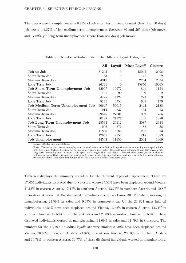
CHAPTER 5. SELECTIVE FIRING & LEMONS
The displacement sample contains 8.95% of job short term unemployment (less than 30 days)
job moves, 41.87% of job medium term unemployment (between 30 and 365 days) job moves
and 17.62% job long term unemployment (more than 365 days) job moves.
Table 5.1: Number of Individuals in the Different Layoff Categories
All Layoff Mass Layoff Closure
Job to Job 31202 0 18045 12998Short Term Job 63 0 41 22Medium Term Job 4918 0 2284 2634Long Term Job 26221 0 15856 10365Job Short Term Unemployment Job 12967 10972 841 1154Short Term Job 101 90 9 2Medium Term Job 4725 4129 223 373Long Term Job 8141 6753 609 779Job Medium Term Unemployment Job 60647 56015 2444 2188Short Term Job 914 837 54 23Medium Term Job 29545 27801 959 785Long Term Job 30188 27377 1431 1380Job Long Term Unemployment Job 25533 20112 3087 2334Short Term Job 992 872 82 38Medium Term Job 11886 9686 1287 913Long Term Job 12655 9554 1718 1383Job Unemployment 14503 11150 2044 1309
Source: ASSD, own calculations.
Notes: The term short term unemployment is used when an individual experiences an unemployment spell whichlasts less than 30 days. Medium term unemployment is used when the spell lasts between 30 and 365 days, whilelong term unemployment is used if the spell lasts longer than 365 days. I defined short term job in a similarfashion, meaning that if it lasts for less than 30 days, while it is labelled as a medium term job if it lasts between30 and 365 days. Jobs that last longer than 365 days are labelled long term jobs.
Table 5.2 displays the summary statistics for the different types of displacement. There are
17, 655 individuals displaced due to a closure, where 27.53% have been displaced around Vienna,
21.13% in eastern Austria, 17.17% in southern Austria, 23.25% in northern Austria and 10.8%
in western Austria. Of the displaced individuals due to a closure 30.61% where working in
manufacturing, 24.59% in sales and 9.97% in transportation. Of the 23, 834 mass laid off
individuals, 46.54% have been displaced around Vienna, 13.52% in eastern Austria, 14.71% in
southern Austria, 19.58% in northern Austria and 25.08% in western Austria. 30.55% of these
displaced individuals worked in manufacturing, 11.09% in sales and 11.79% in transport. The
numbers for the 77, 789 individual layoffs are very similar; 20.39% have been displaced around
Vienna, 20.46% in eastern Austria, 23.07% in southern Austria, 23.08% in northern Austria
and 10.78% in western Austria. 34.77% of these displaced individuals worked in manufacturing,
130

23.09% in sales and 8.55% in transport.16
Table 5.2: Summary Statistics by Type of Layoff
Firm Closure Mass Layoff Layoffmean sd mean sd mean sd
# Displaced Workers 17655 23834 77789# Displaced Workers RegionVienna 4862 11093 15858East 3731 3223 15919South 3033 3507 17945North 4105 4668 19508West 1908 1329 8387# Displaced Workers IndustryManufacturing 5402 7278 27038Sales 4337 2650 17966Transport 1760 2819 6658Change in Wages 0.022 0.298 0.024 0.305 -0.002 0.358Age at Displacement 36.57 9.19 36.65 9.23 34.48 9.14Ratio of Blue Collar Workers 0.54 0.50 0.45 0.50 0.66 0.47Tenure at Displacement 1939 1857 2671 2347 1511 1469Average Firm Operation Duration 4076 3294 9095 4271 8420 4155Person Effects 3.45 0.24 3.46 0.23 3.41 0.21Firm Effects 0.05 0.26 0.09 0.24 0.05 0.23Firm Effects new Firm 0.02 0.28 0.09 0.21 0.02 0.25Unemployment Duration Since LFP 166 339 144 330 242 397Age at First Employment 26.61 8.61 25.51 8.07 25.35 8.05Days Since LFP 3736 2507 4160 2567 3534 2489Number of Unemployment Spells 2.10 3.75 1.75 3.40 3.22 4.69Firm Size (*) 15.00 39.22 398.00 5875.02 30.00 1885.23Total Male Hires 2.57 6.38 78.94 196.33 12.74 69.84Total Male Fires 5.17 10.93 114.08 221.29 19.14 86.01Tenure at Disp. Blue Collar 1851 1796 2359 2121 1406 1335Tenure at Disp. White Collar 1862 1750 2570 2227 1603 1569
Source: ASSD, own calculations.Notes: (*) For firm size the median is depicted, not the mean. Tenure at displacement, average firm operationduration, unemployment duration since labor force participation (LFP), and days since LFP are measured in days.
A look at the change in wages reveals that it is largest for the mass layoff group 0.024, but
very similar to the closure group 0.022. For the individual layoffs, this number differs at −0.002.
Looking at the age at displacement the average is about the same for the three groups, 36.6 for
the closure group and 36.7 for the mass layoff group while only 34.5 for the individual layoffs.
On average the individual layoffs are thus a bit younger than the firm closure or mass laid off
sample. Looking at the ratio of blue collar workers in the firm at the displacement date, we see
16These percentages do not add up to 100% as for some displaced workers the region is missing, and thepercentages for the industry were only calculated for the industries named.
131

CHAPTER 5. SELECTIVE FIRING & LEMONS
that the share of blue collar workers is higher in firms where we observe more individual layoffs,
0.66, while in the firm closures we observe nearly as many blue collar as white collar workers
with a share of 0.54. For the mass layoff firms we observe a share of 0.45 blue collar workers.
Looking at the tenure at displacement, we can see that it is smallest for the individual layoffs
around 1500 days, which nevertheless equals around 4 years, while for the closing individuals
the average tenure at the displacement firm is 1900 days (about 5 years), and for the mass laid
off individuals, we observe a longer tenure around 2600 days (about 7 years).
The average firm operating duration shows that the individuals may work at different firm
types. The closing firms have the shortest survival at around 4000 days (about 10 years), while
individual layoff firms, have an operating duration of 8400 days (about 23 years), while the
mass layoff firms have the longest survival at around 9000 days (about 24 years). Looking at the
unemployment duration since labor force participation (LFP), we see that the individual layoffs
have the highest number of days unemployed with an average of 242 days, whereas it is 166 days
for the closure types and 144 days for the mass laid off individuals. The age at first employment
is balanced at around 25 years for the three samples. The average days worked since LFP yields
a similar picture to the unemployment days. On average the individual layoffs have the shortest
days employed with an average of 3, 534 days (nearly 10 years) and around 3, 736 days for the
closing sample (about 10 years) and 4, 160 days for the mass layoff sample (about 11 years). The
number of unemployment spells is highest for the laid off individuals at 3.2, while it is only 2.1
for the closure types and 1.7 for the mass layoff individuals. In terms of firm size, the closing
firms have a median of 15 employees, while the median for the individual layoff firms is 30 and
398 for the mass layoff firms. The total number of male hires and male fires goes along the lines
of the firm size. It is highest in the year before displacement for the mass layoff firms, with an
average of 78.9 hires and 114 fires, lowest for the closing firms, with an average of 2.5 hires and
5.2 fires, while the individual layoff firms are in the middle of this distribution with around 12.7
hires and 19.1 fires. For completeness the table also includes the means of the person and firm
fixed effects, but I will return to these effects later when I discuss the heterogeneity.
132

5.4 Results
This section discusses the main results. Section 5.4.1 present the estimates of the person and
firm fixed effects to test whether or not firms use leeway when deciding whom to lay off.17 In
other words, Section 5.4.1 tests whether the least able are laid off individually and whether
individuals suffering from a closure are more heterogeneous. Section 5.4.2 addresses the “lemon”
by replicating GK. GK is then taken a step further by differentiating between high ability
individuals. Finally Section 5.4.2 addresses whether the “lemon” affects the resulting matching.
5.4.1 Heterogeneity
Figure 5.3 plots the densities of the estimated person effect for the different layoff types. This
graph gives us a first glance whether the underlying assumption, that firms have more leeway
in determining whom to layoff in case of a mass layoff and an individual layoff than in a closure
event, is true. If it is true that firms layoff the least able individually, we should observe a lower
mean for the individual group compared to the closures, whereas the mean for the mass layoffs
should be in between the individual layoffs and the closures. Therefore when comparing the mass
layoffs with the individual layoffs, we should observe more low productivity individuals in the
individual layoff group. Eyeballing, does not allow me to conclude that the distribution of the
closure and mass layoff types differ. Nevertheless, the individual layoff is always to the left of the
closure and the mass layoff curve. This observation points into the right direction: on average
the individually laid off seem to be less able and less heterogeneous than the other types. The
Kolmogorov-Smirnov test rejects equality of the distributions.
Table 5.3 takes a closer look at the means and the variances of the person effects across the
different groups. The results from the whole AKM file are included in order to get a feeling
where the displaced individuals stand compared to the individuals in the connected set. The
following relationship between the means of the person effects is observed: mean(mass layoff) =
3.461 > mean(closure) = 3.448 > mean(layoff) = 3.410. These means are significantly different
from each other, as the different p-values in Table 5.3 show. On average the individual layoffs are
the least able, as expected, but unlike suggested, the mass layoff group seems to be more able
than the closing types, at least in our sample. In terms of variance and therefore heterogeneity,
the heterogeneity is expected to be highest among the closure types, and lowest among the
17The reader is referred to the Appendix 5.A.1 where the validity of the AKM model is discussed. The validityis checked using an event study as in Card et al. (2012b), which allows me to show that the crucial assumptionsare fulfilled.
133
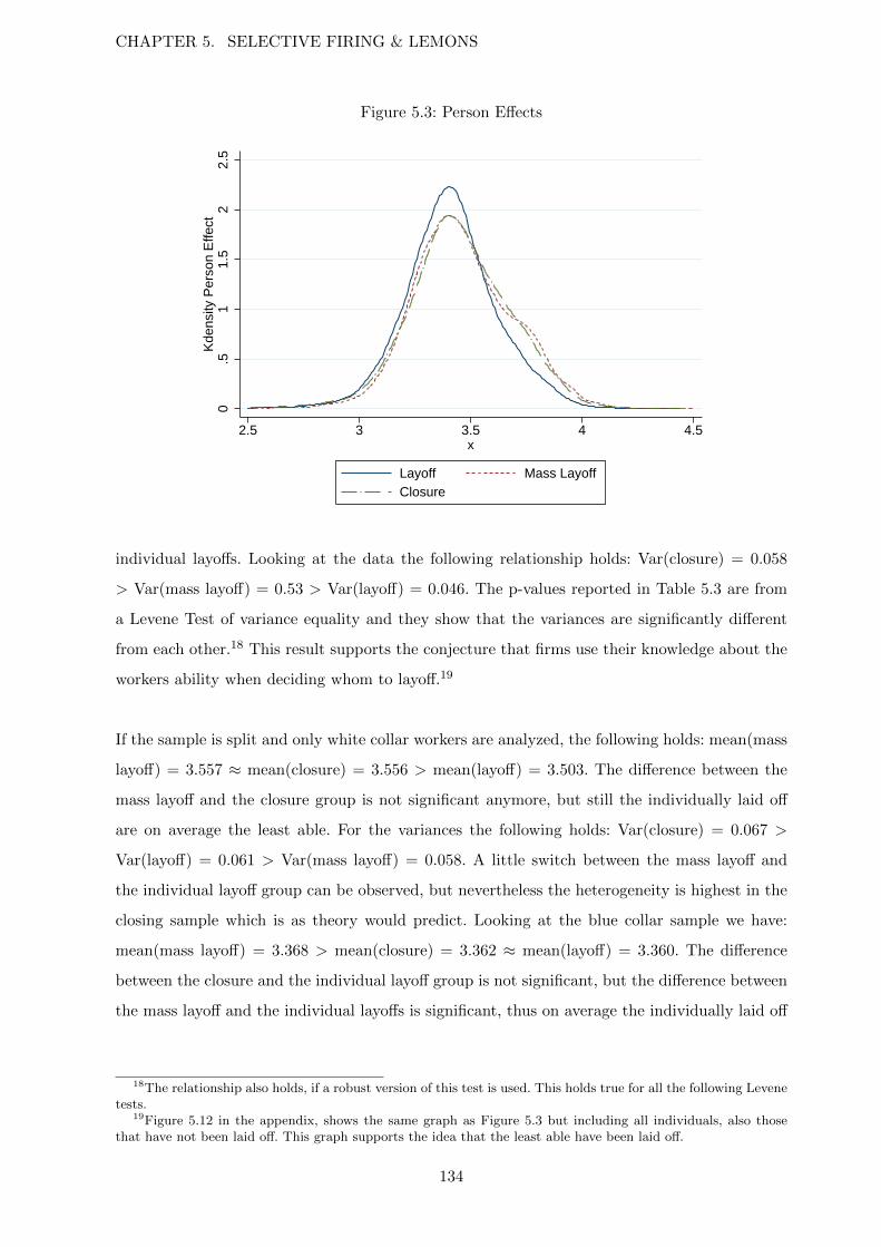
CHAPTER 5. SELECTIVE FIRING & LEMONS
Figure 5.3: Person Effects
0.5
11.
52
2.5
Kde
nsity
Per
son
Effe
ct
2.5 3 3.5 4 4.5x
Layoff Mass LayoffClosure
individual layoffs. Looking at the data the following relationship holds: Var(closure) = 0.058
> Var(mass layoff) = 0.53 > Var(layoff) = 0.046. The p-values reported in Table 5.3 are from
a Levene Test of variance equality and they show that the variances are significantly different
from each other.18 This result supports the conjecture that firms use their knowledge about the
workers ability when deciding whom to layoff.19
If the sample is split and only white collar workers are analyzed, the following holds: mean(mass
layoff) = 3.557 ≈ mean(closure) = 3.556 > mean(layoff) = 3.503. The difference between the
mass layoff and the closure group is not significant anymore, but still the individually laid off
are on average the least able. For the variances the following holds: Var(closure) = 0.067 >
Var(layoff) = 0.061 > Var(mass layoff) = 0.058. A little switch between the mass layoff and
the individual layoff group can be observed, but nevertheless the heterogeneity is highest in the
closing sample which is as theory would predict. Looking at the blue collar sample we have:
mean(mass layoff) = 3.368 > mean(closure) = 3.362 ≈ mean(layoff) = 3.360. The difference
between the closure and the individual layoff group is not significant, but the difference between
the mass layoff and the individual layoffs is significant, thus on average the individually laid off
18The relationship also holds, if a robust version of this test is used. This holds true for all the following Levenetests.
19Figure 5.12 in the appendix, shows the same graph as Figure 5.3 but including all individuals, also thosethat have not been laid off. This graph supports the idea that the least able have been laid off.
134
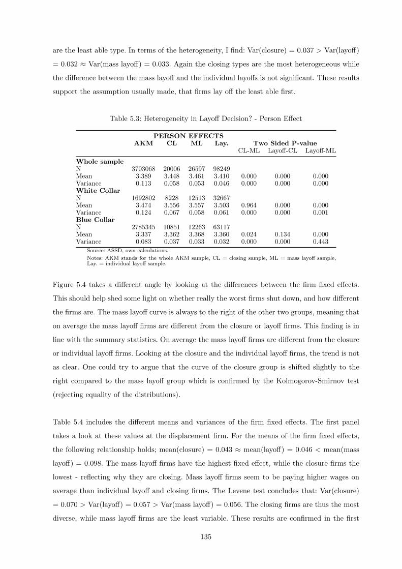
are the least able type. In terms of the heterogeneity, I find: Var(closure) = 0.037 > Var(layoff)
= 0.032 ≈ Var(mass layoff) = 0.033. Again the closing types are the most heterogeneous while
the difference between the mass layoff and the individual layoffs is not significant. These results
support the assumption usually made, that firms lay off the least able first.
Table 5.3: Heterogeneity in Layoff Decision? - Person Effect
PERSON EFFECTSAKM CL ML Lay. Two Sided P-value
CL-ML Layoff-CL Layoff-ML
Whole sampleN 3703068 20006 26597 98249Mean 3.389 3.448 3.461 3.410 0.000 0.000 0.000Variance 0.113 0.058 0.053 0.046 0.000 0.000 0.000White CollarN 1692802 8228 12513 32667Mean 3.474 3.556 3.557 3.503 0.964 0.000 0.000Variance 0.124 0.067 0.058 0.061 0.000 0.000 0.001Blue CollarN 2785345 10851 12263 63117Mean 3.337 3.362 3.368 3.360 0.024 0.134 0.000Variance 0.083 0.037 0.033 0.032 0.000 0.000 0.443
Source: ASSD, own calculations.
Notes: AKM stands for the whole AKM sample, CL = closing sample, ML = mass layoff sample,Lay. = individual layoff sample.
Figure 5.4 takes a different angle by looking at the differences between the firm fixed effects.
This should help shed some light on whether really the worst firms shut down, and how different
the firms are. The mass layoff curve is always to the right of the other two groups, meaning that
on average the mass layoff firms are different from the closure or layoff firms. This finding is in
line with the summary statistics. On average the mass layoff firms are different from the closure
or individual layoff firms. Looking at the closure and the individual layoff firms, the trend is not
as clear. One could try to argue that the curve of the closure group is shifted slightly to the
right compared to the mass layoff group which is confirmed by the Kolmogorov-Smirnov test
(rejecting equality of the distributions).
Table 5.4 includes the different means and variances of the firm fixed effects. The first panel
takes a look at these values at the displacement firm. For the means of the firm fixed effects,
the following relationship holds; mean(closure) = 0.043 ≈ mean(layoff) = 0.046 < mean(mass
layoff) = 0.098. The mass layoff firms have the highest fixed effect, while the closure firms the
lowest - reflecting why they are closing. Mass layoff firms seem to be paying higher wages on
average than individual layoff and closing firms. The Levene test concludes that: Var(closure)
= 0.070 > Var(layoff) = 0.057 > Var(mass layoff) = 0.056. The closing firms are thus the most
diverse, while mass layoff firms are the least variable. These results are confirmed in the first
135
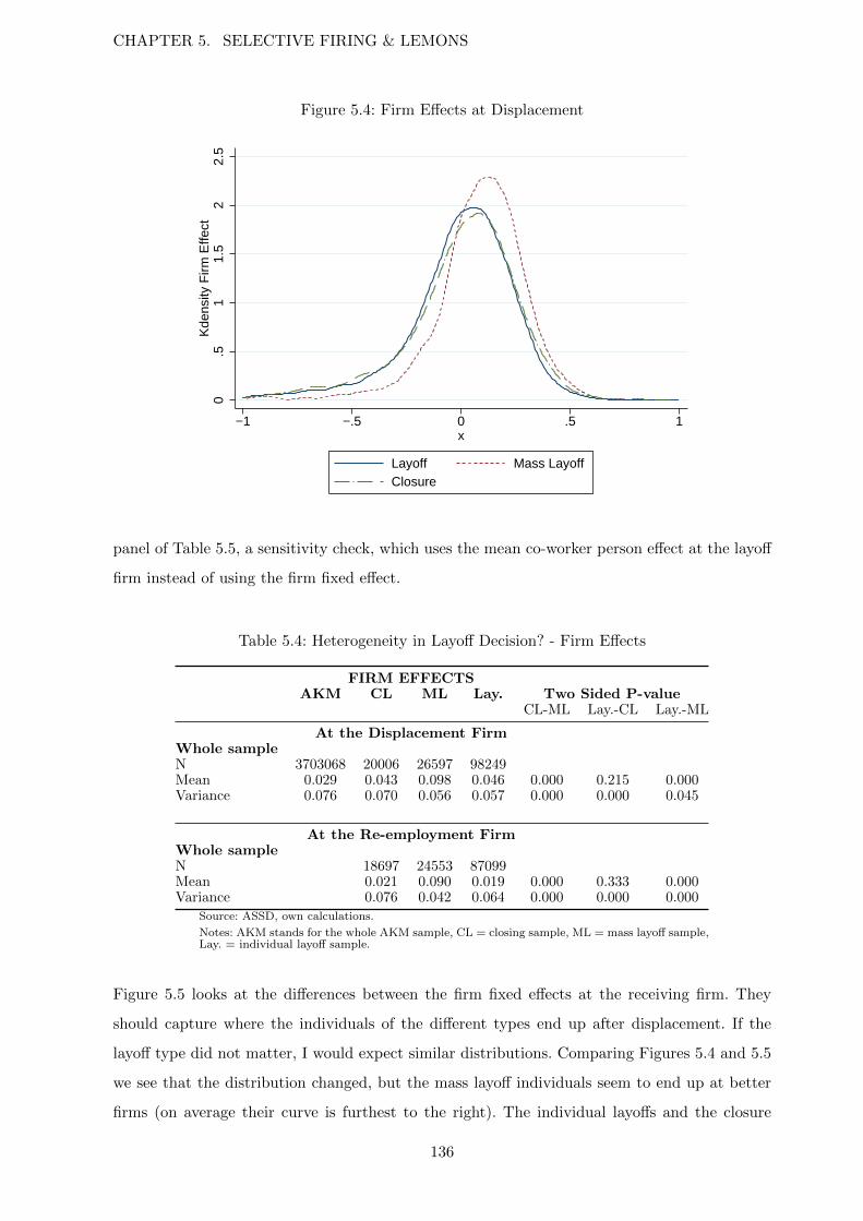
CHAPTER 5. SELECTIVE FIRING & LEMONS
Figure 5.4: Firm Effects at Displacement
0.5
11.
52
2.5
Kde
nsity
Firm
Effe
ct
−1 −.5 0 .5 1x
Layoff Mass LayoffClosure
panel of Table 5.5, a sensitivity check, which uses the mean co-worker person effect at the layoff
firm instead of using the firm fixed effect.
Table 5.4: Heterogeneity in Layoff Decision? - Firm Effects
FIRM EFFECTSAKM CL ML Lay. Two Sided P-value
CL-ML Lay.-CL Lay.-ML
At the Displacement FirmWhole sampleN 3703068 20006 26597 98249Mean 0.029 0.043 0.098 0.046 0.000 0.215 0.000Variance 0.076 0.070 0.056 0.057 0.000 0.000 0.045
At the Re-employment FirmWhole sampleN 18697 24553 87099Mean 0.021 0.090 0.019 0.000 0.333 0.000Variance 0.076 0.042 0.064 0.000 0.000 0.000
Source: ASSD, own calculations.
Notes: AKM stands for the whole AKM sample, CL = closing sample, ML = mass layoff sample,Lay. = individual layoff sample.
Figure 5.5 looks at the differences between the firm fixed effects at the receiving firm. They
should capture where the individuals of the different types end up after displacement. If the
layoff type did not matter, I would expect similar distributions. Comparing Figures 5.4 and 5.5
we see that the distribution changed, but the mass layoff individuals seem to end up at better
firms (on average their curve is furthest to the right). The individual layoffs and the closure
136
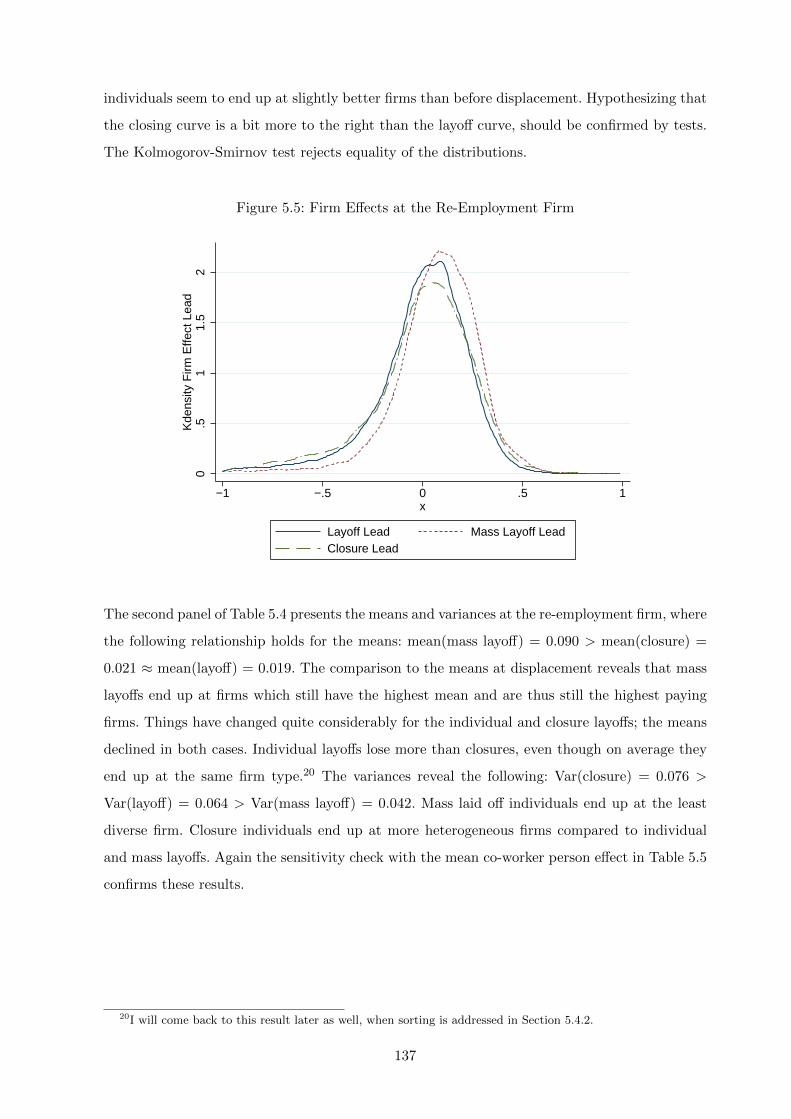
individuals seem to end up at slightly better firms than before displacement. Hypothesizing that
the closing curve is a bit more to the right than the layoff curve, should be confirmed by tests.
The Kolmogorov-Smirnov test rejects equality of the distributions.
Figure 5.5: Firm Effects at the Re-Employment Firm0
.51
1.5
2K
dens
ity F
irm E
ffect
Lea
d
−1 −.5 0 .5 1x
Layoff Lead Mass Layoff LeadClosure Lead
The second panel of Table 5.4 presents the means and variances at the re-employment firm, where
the following relationship holds for the means: mean(mass layoff) = 0.090 > mean(closure) =
0.021 ≈ mean(layoff) = 0.019. The comparison to the means at displacement reveals that mass
layoffs end up at firms which still have the highest mean and are thus still the highest paying
firms. Things have changed quite considerably for the individual and closure layoffs; the means
declined in both cases. Individual layoffs lose more than closures, even though on average they
end up at the same firm type.20 The variances reveal the following: Var(closure) = 0.076 >
Var(layoff) = 0.064 > Var(mass layoff) = 0.042. Mass laid off individuals end up at the least
diverse firm. Closure individuals end up at more heterogeneous firms compared to individual
and mass layoffs. Again the sensitivity check with the mean co-worker person effect in Table 5.5
confirms these results.
20I will come back to this result later as well, when sorting is addressed in Section 5.4.2.
137
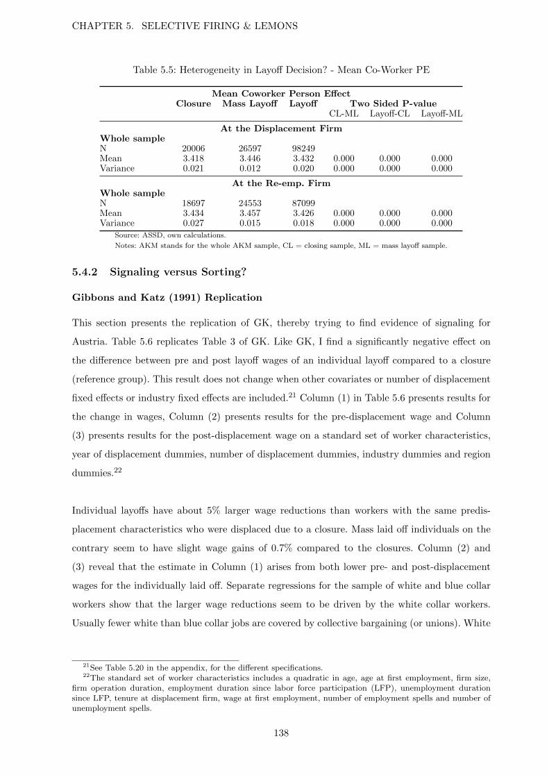
CHAPTER 5. SELECTIVE FIRING & LEMONS
Table 5.5: Heterogeneity in Layoff Decision? - Mean Co-Worker PE
Mean Coworker Person EffectClosure Mass Layoff Layoff Two Sided P-value
CL-ML Layoff-CL Layoff-ML
At the Displacement FirmWhole sampleN 20006 26597 98249Mean 3.418 3.446 3.432 0.000 0.000 0.000Variance 0.021 0.012 0.020 0.000 0.000 0.000
At the Re-emp. FirmWhole sampleN 18697 24553 87099Mean 3.434 3.457 3.426 0.000 0.000 0.000Variance 0.027 0.015 0.018 0.000 0.000 0.000
Source: ASSD, own calculations.
Notes: AKM stands for the whole AKM sample, CL = closing sample, ML = mass layoff sample.
5.4.2 Signaling versus Sorting?
Gibbons and Katz (1991) Replication
This section presents the replication of GK, thereby trying to find evidence of signaling for
Austria. Table 5.6 replicates Table 3 of GK. Like GK, I find a significantly negative effect on
the difference between pre and post layoff wages of an individual layoff compared to a closure
(reference group). This result does not change when other covariates or number of displacement
fixed effects or industry fixed effects are included.21 Column (1) in Table 5.6 presents results for
the change in wages, Column (2) presents results for the pre-displacement wage and Column
(3) presents results for the post-displacement wage on a standard set of worker characteristics,
year of displacement dummies, number of displacement dummies, industry dummies and region
dummies.22
Individual layoffs have about 5% larger wage reductions than workers with the same predis-
placement characteristics who were displaced due to a closure. Mass laid off individuals on the
contrary seem to have slight wage gains of 0.7% compared to the closures. Column (2) and
(3) reveal that the estimate in Column (1) arises from both lower pre- and post-displacement
wages for the individually laid off. Separate regressions for the sample of white and blue collar
workers show that the larger wage reductions seem to be driven by the white collar workers.
Usually fewer white than blue collar jobs are covered by collective bargaining (or unions). White
21See Table 5.20 in the appendix, for the different specifications.22The standard set of worker characteristics includes a quadratic in age, age at first employment, firm size,
firm operation duration, employment duration since labor force participation (LFP), unemployment durationsince LFP, tenure at displacement firm, wage at first employment, number of employment spells and number ofunemployment spells.
138
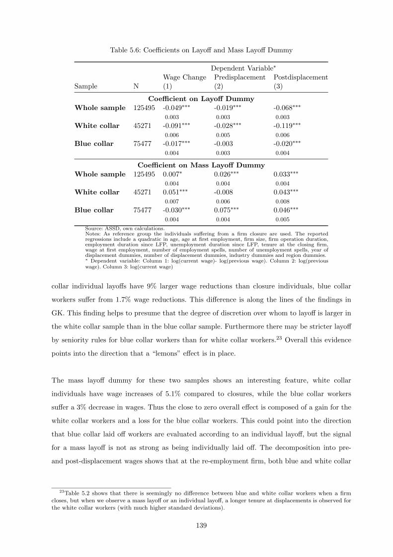
Table 5.6: Coefficients on Layoff and Mass Layoff Dummy
Dependent Variable∗
Wage Change Predisplacement PostdisplacementSample N (1) (2) (3)
Coefficient on Layoff DummyWhole sample 125495 -0.049∗∗∗ -0.019∗∗∗ -0.068∗∗∗
0.003 0.003 0.003
White collar 45271 -0.091∗∗∗ -0.028∗∗∗ -0.119∗∗∗
0.006 0.005 0.006
Blue collar 75477 -0.017∗∗∗ -0.003 -0.020∗∗∗
0.004 0.003 0.004
Coefficient on Mass Layoff DummyWhole sample 125495 0.007∗ 0.026∗∗∗ 0.033∗∗∗
0.004 0.004 0.004
White collar 45271 0.051∗∗∗ -0.008 0.043∗∗∗
0.007 0.006 0.008
Blue collar 75477 -0.030∗∗∗ 0.075∗∗∗ 0.046∗∗∗
0.004 0.004 0.005
Source: ASSD, own calculations.Notes: As reference group the individuals suffering from a firm closure are used. The reportedregressions include a quadratic in age, age at first employment, firm size, firm operation duration,employment duration since LFP, unemployment duration since LFP, tenure at the closing firm,wage at first employment, number of employment spells, number of unemployment spells, year ofdisplacement dummies, number of displacement dummies, industry dummies and region dummies.∗ Dependent variable: Column 1: log(current wage)- log(previous wage). Column 2: log(previouswage). Column 3: log(current wage)
collar individual layoffs have 9% larger wage reductions than closure individuals, blue collar
workers suffer from 1.7% wage reductions. This difference is along the lines of the findings in
GK. This finding helps to presume that the degree of discretion over whom to layoff is larger in
the white collar sample than in the blue collar sample. Furthermore there may be stricter layoff
by seniority rules for blue collar workers than for white collar workers.23 Overall this evidence
points into the direction that a “lemons” effect is in place.
The mass layoff dummy for these two samples shows an interesting feature, white collar
individuals have wage increases of 5.1% compared to closures, while the blue collar workers
suffer a 3% decrease in wages. Thus the close to zero overall effect is composed of a gain for the
white collar workers and a loss for the blue collar workers. This could point into the direction
that blue collar laid off workers are evaluated according to an individual layoff, but the signal
for a mass layoff is not as strong as being individually laid off. The decomposition into pre-
and post-displacement wages shows that at the re-employment firm, both blue and white collar
23Table 5.2 shows that there is seemingly no difference between blue and white collar workers when a firmcloses, but when we observe a mass layoff or an individual layoff, a longer tenure at displacements is observed forthe white collar workers (with much higher standard deviations).
139

CHAPTER 5. SELECTIVE FIRING & LEMONS
workers earn more than a comparable individual who has suffered from a firm closure.
A further step in the replication of GK, is to check whether the information content of a
layoff is higher if the individual had longer tenure at the pre-displacement firm - as the pre-
displacement employer was able to evaluate the individual’s ability over a longer horizon.
Therefore an individual layoff where the worker has a longer pre-displacement tenure contains
more information. Table 5.7 replicates Table 4 in GK where the layoff dummy is now replaced
by a layoff dummy interacted with high tenure and a layoff dummy interacted with low tenure.
Here the exact definition of GK is followed where the low tenure dummy is one if an individual
had less than 2 years tenure on the pre-displacement job.
Table 5.7: Interaction of Layoff and ML with Low- and High-Tenure Dummy
Dependent Variable∗
Wage Change Predisplacement PostdisplacementSample N (1) (2) (3)
Coefficient on Layoff DummyWhole sampleLayoff x Low Tenure 125495 -0.036∗∗∗ -0.035∗∗∗ -0.071∗∗∗
0.003 0.003 0.004Layoff x High Tenure -0.056∗∗∗ -0.010∗∗∗ -0.067∗∗∗
0.003 0.003 0.003White collarLayoff x Low Tenure 45271 -0.079∗∗∗ -0.053∗∗∗ -0.131∗∗∗
0.007 0.006 0.007Layoff x High Tenure -0.098∗∗∗ -0.015∗∗∗ -0.113∗∗∗
0.006 0.005 0.006Blue collarLayoff x Low Tenure 75477 -0.006 -0.013∗∗∗ -0.019∗∗∗
0.004 0.004 0.004Layoff x High Tenure -0.023∗∗∗ 0.002 -0.021∗∗∗
0.004 0.003 0.004
Coefficient on Mass Layoff DummyWhole sampleML x Low Tenure 125495 0.016∗∗∗ -0.020∗∗∗ -0.004
0.006 0.005 0.006ML x High Tenure 0.002 0.045∗∗∗ 0.047∗∗∗
0.004 0.004 0.004White collarML x Low Tenure 45271 0.068∗∗∗ -0.063∗∗∗ 0.005
0.010 0.009 0.011ML x High Tenure 0.044∗∗∗ 0.014∗∗ 0.058∗∗∗
0.008 0.007 0.008Blue collarML x Low Tenure 75477 -0.020∗∗∗ 0.048∗∗∗ 0.028∗∗∗
0.006 0.006 0.007ML x High Tenure -0.035∗∗∗ 0.087∗∗∗ 0.053∗∗∗
0.005 0.005 0.005
Source: ASSD, own calculations.Notes: Low Tenure is a dummy which equals one when there is less than 2 years of tenure on thepredisplacement job. High tenure is a dummy which equals one when the individual had at least2 years of tenure on the predisplacement job.The reported regressions include a quadratic in age, age at first employment, firm size, firmoperation duration, employment duration since LFP, unemployment duration since LFP, tenure atthe closing firm, wage at first employment, number of employment spells, number of unemploymentspells, year of displacement dummies, number of displacement dummies, industry dummies andregion dummies. ML = Mass Layoff∗ Dependent variable: Column 1: log(current wage)- log(previous wage). Column 2: log(previouswage). Column 3: log(current wage)
140
Comparing the results (Austria vs. GK) there are a few differences which are probably due to
the larger sample size, leading to lower standard errors and higher power. GK find a coefficient of
−0.011 for the whole sample on the interaction of the layoff dummy with the low tenure dummy
which is statistically insignificant and a significant coefficient of −0.054 on the interaction with
high tenure. This leads to the claim that their findings are driven by the high tenure individuals.
I find a 3.6% significant decrease for the low tenure individual layoffs and a significant 5.6%
decrease for the high tenure layoffs. As pointed out, the significance may stem from the fact that
my sample is larger including 125, 495 observations, while GK only have 3, 427. Nevertheless my
results are in line with theirs in the sense that the “lemons” effect is much stronger for the high
tenure individuals. Furthermore the effect is again driven by the significantly lower wages at
post-displacement, even though the individual layoffs already have lower wages to begin with.
This result is confirmed when looking at the white versus blue collar samples. In fact I find a
9.8% decrease for white collar workers with high tenure and a 2.3% decrease for the blue collar
workers with longer tenure. A 7.9% decrease for the white collar workers with lower tenure,
while there is no effect for the blue collar workers which have a low tenure. These findings are
in line with firms having more discretion over whom to layoff in the white collar sample than in
the blue collar sample.
When looking at the mass laid off individuals, I find similar results as before. There is no effect
for those individuals who have high tenure, while a 1.6% increase is found for the low tenure
individuals. This effect is driven by the significantly lower earnings at the pre-displacement
firm, and not by the post-displacement earnings. Splitting the sample into blue and white collar
workers, I observe a positive effect for white collar workers, no matter whether they work longer
or shorter at the displacement firm. The effect ranges between 4.4 and 6.8%. While for blue
collar workers the negative effect persists, and is stronger for the high tenured individuals. This
effect ranges between 2.0 and 3.5% and is driven by the significantly lower earnings at the post-
displacement firm, even though at the post-displacement firm their earnings are on average still
3 to 5% larger than those of a comparable closure individual.
Table 5.8 investigates whether the sorting explanation can be dismissed for Austria as well. As
explained in Section 5.2.1, I will need to find γ2 > 0 in Equation (5.2) to reject the sorting model.
GK find a significant negative effect on γ1 the switch industry dummy (large in absolute value),
a not significant coefficient on the layoff dummy (δ1) similar in magnitude to the results before.
Furthermore they find a positive coefficient on γ2, the interaction between the switch industry
141

CHAPTER 5. SELECTIVE FIRING & LEMONS
and layoff dummy.24 The first column of Table 5.8 presents the baseline results of Column (1)
in Table 5.6. Column (2) adds the switch industry information, and unlike GK our significant
negative coefficient on the layoff dummy (δ1), as well as on the industry change dummy (γ1) and
on the interaction between industry change and layoff (γ2) remains. This evidence does not yet
exclude sorting as a possible explanation. The results for the mass layoff sample are similar to
the previous findings. The coefficient on the mass layoff dummy stays positive and significant,
while the interaction with the industry change is negative, and thus driven by the wage loss due
to the industry switch.
Table 5.8: Industry Change, Post Displacement Wage
(1) (2)
Mass Layoff 0.0329∗∗∗ 0.0486∗∗∗
(0.00408) (0.00575)
Layoff -0.0678∗∗∗ -0.0361∗∗∗
(0.00329) (0.00434)
Industry Change 0.0148∗∗∗
(0.00547)
Industry Change * Layoff -0.0633∗∗∗
(0.00606)
Industry Change * Mass Layoff -0.0322∗∗∗
(0.00746)
Year FE 3 3
Number of Displacements 3 3
Industry FE 3 3
Region FE 3 3
Observations 125495 124896
R2 0.420 0.421
Adjusted R2 0.419 0.420
Source: ASSD, own calculations.Note: *,**,*** indicates significance at the 10%, 5%, and 1%level, respectively. Standard errors in parentheses.Furthermore I control for a quadratic in age, age at first em-ployment, firm size, firm operation duration, unemploymentduration since LFP, employment duration since LFP, tenureat the closing firm, wage at first job, number of employmentspells and number of unemployment spells.
Gibbons and Katz (1991) taken a step further
As outlined in Section 5.2.1, I will take GK a step further, by including an indicator whether the
person is of high ability or not. Figure 5.6 shows why this distinction may be the potentially more
interesting result. Categorizing individuals as high ability if they fall into the highest quintile of
24Gibbons and Katz (1991) do not show these results in their paper and therefore I am unable to talk aboutmagnitudes.
142

the person effect, and as low if they fall into the lowest quintile, we observe that the high ability
individual layoffs lose most in terms of their wages. Again year zero is the year of displacement,
and during the five years before displacement individual layoffs and closures of high ability had
more or less the same wages, but when displacement happens, the individual layoff loses in terms
of wages and does not catch up within the next five years. This kink in wages is not visible for
the low ability individuals.
Figure 5.6: Mean Wages of Re-employed Individuals by Person Quintile
3.5
44.
55
(mea
n) lo
g w
age
−5 0 5Time(0=Layoff Year)
Layoff, Low Person Effect Closure, Low Person EffectML, Low Person Effect Layoff, High Person EffectClosure, High Person Effect ML, High Person Effect
Table 5.9 takes GK a step further by including an indicator of the individual’s ability, and
an indicator if the layoff firm is a high wage firm (HWF) as outlined in Equation (5.4).25
This analysis extends GK analysis of the high versus low tenure analysis by trying to see if a
high ability individual layoff is able to overcome the “lemon” stigma. Column (1) presents the
baseline results from Table 5.6 while Column (2) adds the high ability and HWF indicators.
Column (3) includes the additional interaction terms. The coefficient on the individual layoff
stays significantly negative. It seems that even controlling for whether or not the individual is
of high ability does not suffice to overcome the negative stigma.
25The individual’s ability is proxied by a dummy which equals one if her person effect falls into the highestquintile, while a HWF is proxied by a dummy equal to one if the firm’s fixed effect falls into the highest quintile(similarly defined for the re-employment firm).
143

CHAPTER 5. SELECTIVE FIRING & LEMONS
Table 5.9: Difference Between Wages High Type Person Effect
(1) (2) (3)
Mass Layoff 0.00666∗ 0.0139∗∗∗ 0.0205∗∗∗
(0.00373) (0.00366) (0.00459)
Layoff -0.0490∗∗∗ -0.0426∗∗∗ -0.0338∗∗∗
(0.00301) (0.00294) (0.00342)
High Person Effect 0.0174∗∗∗ 0.0471∗∗∗
(0.00333) (0.00725)
High Firm Effect -0.180∗∗∗ -0.161∗∗∗
(0.00305) (0.00716)
High PE * High FE 0.127∗∗∗ 0.0847∗∗∗
(0.00703) (0.0165)
High Firm Effect at Reemp. Firm 0.208∗∗∗ 0.209∗∗∗
(0.00294) (0.00294)
ML*High PE -0.0129
(0.00963)
ML*High FE -0.0197∗∗
(0.00897)
ML * High PE * High FE 0.000218
(0.0206)
Layoff*High PE -0.0469∗∗∗
(0.00829)
Layoff*High FE -0.0230∗∗∗
(0.00771)
Layoff * High PE * High FE 0.0815∗∗∗
(0.0193)
Year FE 3 3 3
Number of Displacements 3 3 3
Industry FE 3 3 3
Region FE 3 3 3
Observations 125495 125495 125495
R2 0.0613 0.1082 0.1086
Adjusted R2 0.0602 0.1071 0.1075
Source: ASSD, own calculations.Notes: Dependent variable: log(current wage) - log(previous wage). *,**,***indicates significance at the 10%, 5%, and 1% level, respectively. Standarderrors in parentheses.Furthermore I control for a quadratic in age, age at first employment, firmsize, firm operation duration, unemployment duration since LFP, employmentduration since LFP, tenure at the closing firm, wage at first job, number ofemployment spells and number of unemployment spells.
144

Table 5.10 presents the different average effects based on Column (3) in Table 5.9. A high ability
mass laid off individual has a 5.5% increase in the difference in wages compared to a closure
individual. A high ability individual layoff suffers a decrease in wages of about 3.4% compared
to a closure individual.26 Unlike expected, a high ability individual is not able to signal her high
ability, and the “lemon” effect still dominates and therefore she still suffers from a wage decline
(δ1 + δ3 + δ4 < 0). Coming from a HWF decreases the wage, for a mass layoff by about 16%
and for an individual layoff by 22%.27 This large decrease in wages may be due to the fact,
that the pre-displacement firm was paying wages that were above the average productivity and
this premium is now gone. Another interesting result is that a high ability individual from a
HWF, suffers a decrease in wages. A high ability individual can thus not compensate for being
previously employed at a HWF, in this case a mass laid off individual suffers a 4.1% decrease,
while an individual layoff suffers from a 5.1% decrease.
Table 5.10: Expected Changes in Wages by type
t=Mass Layoff Layoff
δ2 + δ3 + δ5 P-val. δ1 + δ3 + δ4 P-val. P-val.
E[∆ W | T = t] 0.0205 0.0000 -0.0338 0.0000 0.0000E[∆ W | T = t, high PE = 1] 0.0547 0.0000 -0.0336 0.0000 0.0000E[∆ W | T = t, high FE = 1] -0.1600 0.0000 -0.2177 0.0000 0.0000E[∆ W | T = t, high PE = 1, high FE] -0.0409 0.0001 -0.0512 0.0000 0.4381
Source: ASSD, own calculations.
Notes: These are the expectations calculated from a regression of the change in wages on a mass layoff dummy, a layoffdummy, a high PE dummy, a high FE dummy, the interaction of those two, a dummy for high FE at the reemploymentfirm, interactions of the high PE and FE with ML and layoff dummies. Furthermore I control for a quadratic in age,age at first employment, firm size, firm operation duration, employment duration since LFP, unemployment durationsince LFP, tenure at the closing firm, wage at first job, number of employment spells, number of unemployment spells,year of displacement dummies, number of displacement dummies, industry dummies and region dummies.
The P-Values on the different coefficients result from an F-test whether they are different from 0 or not. The P-value inthe last column on the other hand, is a test of whether the coefficients for the mass layoff group are different from thoseof the layoff group.
This evidence reinforces the findings of a stigma being attached to an individual layoff. The
question which is outside of the GK framework, but that is still interesting, is whether an
individual layoff can end up at a high wage firm? Table 5.11 presents the results of a simple
logit model (Equation (5.5)) where the dependent variable is one if the individual ends up at a
high wage firm.28
26These numbers are significantly different from each other, and also significantly different from 0. An F-Teston the linear combinations was used to test for significance.
27Again these numbers are significantly different from each other and from 0.28I refer the reader for more information on the cell sizes for the different layoff categories to Table 5.19.
145

CHAPTER 5. SELECTIVE FIRING & LEMONS
Table 5.11: Who Ends up at a High Type Firm?
(1) (2) (3) (4)
High Firm Effect at Reemp. FirmMass Layoff 0.643∗∗∗ 0.227∗∗∗ 0.329∗∗∗ 0.339∗∗∗
(0.0272) (0.0298) (0.0472) (0.0475)Layoff -0.0773∗∗∗ -0.166∗∗∗ -0.0865∗∗ -0.0250
(0.0243) (0.0263) (0.0375) (0.0378)Age 0.0906∗∗∗ 0.0480∗∗∗ 0.0459∗∗∗ 0.0374∗∗∗
(0.00761) (0.00824) (0.00836) (0.00842)Age2 -0.000454∗∗∗ -0.000138 -0.000176∗ -0.000105
(0.0000930) (0.000101) (0.000102) (0.000103)Total Unemployment Duration since LFP -0.000185∗∗∗ -0.0000443 -0.0000548 -0.0000778∗
(0.0000425) (0.0000436) (0.0000444) (0.0000446)Firm Size -0.0000845∗∗∗ -0.0000660∗∗∗ -0.0000201∗∗∗ -0.0000281∗∗∗
(0.00000446) (0.00000460) (0.00000550) (0.00000565)Firm Operation Duration -0.000000312 0.0000141∗∗∗ 0.0000153∗∗∗ 0.0000139∗∗∗
(0.00000203) (0.00000218) (0.00000238) (0.00000243)Tenure at Closing Firm 0.0000408∗∗∗ 0.00000434 0.00000365 -0.00000198
(0.00000545) (0.00000599) (0.00000612) (0.00000618)Total Employment Duration since LFP -0.000328∗∗∗ -0.000240∗∗∗ -0.000224∗∗∗ -0.000199∗∗∗
(0.0000183) (0.0000200) (0.0000207) (0.0000208)Wage at First Job 0.0265∗∗∗ 0.0132∗∗∗ 0.0115∗∗∗ 0.0111∗∗∗
(0.000637) (0.000731) (0.000742) (0.000746)Age at First Employment -0.0705∗∗∗ -0.0459∗∗∗ -0.0407∗∗∗ -0.0392∗∗∗
(0.00417) (0.00458) (0.00465) (0.00468)Number of Unemployment Spells -0.0533∗∗∗ -0.0379∗∗∗ -0.0356∗∗∗ -0.0288∗∗∗
(0.00384) (0.00396) (0.00405) (0.00407)Number of Employment Spells 0.0922∗∗∗ 0.0598∗∗∗ 0.0575∗∗∗ 0.0519∗∗∗
(0.00788) (0.00856) (0.00872) (0.00877)High Person Effect 0.372∗∗∗ 0.0149 -0.00355
(0.0299) (0.0746) (0.0749)High Firm Effect 2.222∗∗∗ 2.326∗∗∗ 2.263∗∗∗
(0.0189) (0.0514) (0.0519)High PE * High FE -0.587∗∗∗ -0.161 -0.159
(0.0465) (0.116) (0.117)ML*High PE 0.288∗∗∗ 0.329∗∗∗
(0.0952) (0.0956)ML*High FE -0.381∗∗∗ -0.428∗∗∗
(0.0664) (0.0673)ML * High PE * High FE -0.0908 -0.0893
(0.146) (0.147)Layoff*High PE 0.300∗∗∗ 0.287∗∗∗
(0.0832) (0.0834)Layoff*High FE -0.241∗∗∗ -0.295∗∗∗
(0.0560) (0.0565)Layoff * High PE * High FE -0.646∗∗∗ -0.617∗∗∗
(0.134) (0.135)year FE 3 3 3 3
Region FE 7 7 7 3
Industry FE 7 7 3 3
Observations 139449 139449 139447 139445Pseudo R2 0.0543 0.1818 0.1958 0.2040
Source: ASSD, own calculations.Note: *,**,*** indicates significance at the 10%, 5%, and 1% level, respectively. Standard errors in parentheses.
146

Table 5.12 presents the marginal effects for a mass layoff, or a layoff, compared to the baseline
(closure). The standard errors are computed using the delta method and I find that if an
individual was part of a mass layoff, she is nearly 5 percentage points more likely to end up
at a high wage firm than a closure individual. This effect is negative but insignificant for an
individual layoff. A high ability mass laid off individual is nearly 13 percentage points more
likely to end up at a high wage firm, whereas an individual layoff is only 4 percentage points
more likely. Thus being a high ability individual and having suffered from an individual layoff
does not hamper employment at a HWF. This result may point toward exploitation - individual
layoffs are hired at HWF more often than closure individuals, but on average earn a lower wage
after displacement. On the other hand coming from a HWF, decreases the likelihood of ending
up at a high wage firm by 2 percentage points for a mass layoff and an individual layoff. A high
ability mass layoff from a HWF is 3 percentage points more likely to end up at a HWF, while
an individual HWF layoff is 16 percentage points less likely to end up at a HWF.29
Table 5.12: Marignal Effect of Being Employed in a HWF
t=Mass Layoff Layoff
ME σ ME σ
P(Emp. HWF = 1 | T = t) 0.0537 0.0106 -0.0032 0.0048P(Emp. HWF = 1 | T = t, high PE = 1) 0.1333 0.0228 0.0429 0.0138P(Emp. HWF = 1 | T = t, high FE = 1) -0.0210 0.0117 -0.0210 0.0112P(Emp. HWF = 1 | T = t, high PE = 1, highFE)
0.0337 0.0227 -0.1621 0.0241
Source: ASSD, own calculations.Notes: ME stands for the marginal effect, while σ stands for the standard error, calculated by the deltamethod.The marginal effects are calculated at the mean. I ran a logit regression of the probability to be re-employed at a high wage firm controlling for a mass layoff dummy, a layoff dummy, a high PE dummy, ahigh FE dummy, the interaction of those two, a dummy for high FE at the reemployment firm, interactionsof the high PE and FE with ML and layoff dummies. Furthermore I control for a quadratic in age, ageat first employment, wage at firt job, employment duration since LFP, unemployment duration sinceLFP, tenure at the closing firm, number of employment spells, number of unemployment spells, year ofdisplacement dummies, number of displacement dummies, industry dummies and region dummies.
Does the “lemon” affect the resulting matching?
So far I replicated GK results, took them a step further and found slightly more evidence in
favor of a signal, but cannot find evidence for rejecting the matching model. Therefore in this
section I will investigate other sorting measures as discussed in Section 5.2.3, to see whether the
29A related paper which focuses on unemployment durations is Boheim et al. (2011), who find that individualslaid off from a high wage firm take longer to find a job than those coming from a low wage firm (they only analyzethe individuals behavior after a plant closure). The main rationale behind their finding is that individuals comingfrom a high wage firm take longer to update their prior about the wage distribution.
147

CHAPTER 5. SELECTIVE FIRING & LEMONS
“lemon” also affects the resulting matching.
Figures 5.6a, 5.6b, 5.7a, 5.7b, 5.8a and 5.8b plot histograms of the firm and person effects, where
the effects are grouped into their respective deciles. These graphs provide some information
on who ends up where, and how the sorting in terms of the deciles was before and after
displacement.30 Taking a closer look at Figures 5.6a, 5.6b we see that the correlations of the
person and firm effects, even though downward biased increased after the mass layoff. This may
indicate sorting before and after the layoff event, as the correlation increases from −0.0023 to
0.1142. Individuals sorted into the second firm decile move, which “evens” the graph out at the
re-employment firm. Furthermore there is more mass in the lowest firm decile after displacement,
while higher firm deciles seem to remain stable.
Figures 5.7a and 5.7b show the same correlation of the person and firm fixed effects for the
closure individuals. The correlation between the deciles of the firm and person effects increases
slightly at the new job from a correlation of 0.1046 to 0.1221. Most of the movements seemingly
take place in the last firm decile, “evening” themselves out. Again there is sorting before and
after displacement.
Figures 5.8a and 5.8b show that the correlation increases slightly after the displacement from
0.0217 to 0.0280 for individual layoffs. The visible movements take place in the first person
decile, where individuals move from the lowest firm decile to the highest firm decile. In contrast
to the highest person decile, the opposite happens. In these graphs individual movements cannot
be observed, only mass changes, which excludes conclusions on which workers moves.
30All these graphs use only re-employed individuals, excluding still unemployed individuals.
148

Figure 5.7: Mass Layoff Deciles
(a) At Layoff Firm Corr(PE,FE)=-0,0023 (b) At Re-Emp. Firm Corr(PE,FE)=0,1142
149

CH
AP
TE
R5.
SE
LE
CT
IVE
FIR
ING
&L
EM
ON
S
Figure 5.8: Closure Deciles
(a) CL Deciles at Layoff Firm Corr(PE,FE)=0,1046 (b) CL Deciles at Re-Emp. Firm Corr(PE,FE)=0,1221
150

Figure 5.9: Involuntary Layoff Deciles
(a) Layoff Deciles at Layoff Firm Corr(PE,FE)=0,0217 (b) Layoff Deciles at Re-Emp. Firm Corr(PE,FE)=0,0280
151

CHAPTER 5. SELECTIVE FIRING & LEMONS
The first measure available to check whether the “lemon” affects the resulting matching is the
firm fixed effects before and after displacement. Table 5.13 lists the average firm fixed effect
for the layoffs at the pre- and post-displacement firm. For the closing individuals, we observe
a clear decline of the average firm fixed effect from 0.042 at the pre-displacement firm to 0.021
at the post-displacement firm. Looking at the individual layoffs, the firm fixed effect decreases
from 0.046 at the pre-displacement firm to 0.019 at the post-displacement firm. This decrease is
larger than the one in the closing firms. This pattern suggests that both sorting and signaling
may take place, since the sorting measure decreases more for the individual layoffs than for the
closures. Sorting for the mass layoff types remains nearly the same; the average firm fixed effect
is at 0.093 before the displacement and 0.090 after the displacement.
These differences remain more or less stable depending on the subsample. The firm fixed effect
decreases after the layoff event for the closing and the individual layoffs, for the white collar
sample, the high person effect sample, the low person effect sample, the high firm effect, the low
firm effect the long firm operation duration and the small turnover sample. In these samples,
the firm fixed effect decreases less for the closing types than for the individual layoffs. For the
blue collar sample, the short firm operation sample and the high turnover sample the opposite
is true. It grows stronger for the layoff sample than for the closing sample (or decreased by less).
For the blue collar workers, that might be due to the fact that they are covered by more rigid
rules in terms of layoff decisions.
Table 5.14 on the other hand as a sensitivity check, looks at a very similar measure, which
focuses on the average co-worker person effect in the pre- and post-displacement firm. Contrary
to the firm fixed effect, I find that the measure for the closing types always grows stronger (or
declines less) than that of the individual layoff sample, only for the low person effect sample.31
For the question of whether or not there is sorting in the data the problems with the correlation
between the firm and the person effect have been discussed and whether or not I should use
Lopes de Melo (2013)’s measure, which can only identify the strength, but not the sign. Using
this measure in Table 5.15, I find that there is significant sorting going on in the case of Austria.
Table 5.15 analyzes Corr(θi, θj(i,t)) and confirms the differential changes in the sorting measure
for the three categories of job loss (mass layoff, individual layoff, and firm closure). This points
31In the firm fixed effect changes, the difference between the two has not been significant, so this does notchallenge the result from before.
152

Table 5.13: Sorting Measure: Ψj(i,t)
Closure Mass Layoff Layoff Two-Sided P-valueSample Mean P. Mean P. Mean P. CL-ML Lay-CL Lay-ML
Whole sampleN 18697 24553 87099Predisplacement 0.042 0.000 0.093 0.000 0.046 0.000Postdisplacement 0.021 0.000 0.090 0.000 0.019 0.000∆ -0.021 0.000 -0.003 0.027 -0.026 0.000 0.000 0.007 0.000White CollarN 7803 11739 27401Predisplacement 0.068 0.000 0.022 0.000 0.055 0.000Postdisplacement 0.058 0.000 0.066 0.000 0.011 0.000∆ -0.010 0.000 0.044 0.000 -0.044 0.000 0.000 0.000 0.000Blue CollarN 10018 11035 57494Predisplacement 0.018 0.000 0.165 0.000 0.039 0.000Postdisplacement -0.011 0.000 0.114 0.000 0.023 0.000∆ -0.029 0.000 -0.051 0.000 -0.016 0.000 0.000 0.000 0.000High Person EffectN 3139 4610 8343Predisplacement 0.066 0.000 0.093 0.000 0.037 0.000Postdisplacement 0.054 0.000 0.111 0.000 -0.007 0.063∆ -0.011 0.002 0.018 0.000 -0.044 0.000 0.000 0.000 0.000Low Person EffectN 3689 4473 20037Predisplacement -0.010 0.055 0.076 0.000 0.036 0.000Postdisplacement -0.033 0.000 0.051 0.000 0.011 0.000∆ -0.023 0.000 -0.025 0.000 -0.025 0.000 0.694 0.657 0.983High Firm EffectN 3337 7259 13463Predisplacement 0.342 0.000 0.301 0.000 0.321 0.000Postdisplacement 0.225 0.000 0.206 0.000 0.158 0.000∆ -0.117 0.000 -0.095 0.000 -0.163 0.000 0.000 0.000 0.000Low Firm EffectN 4496 6014 21560Predisplacement -0.300 0.000 -0.183 0.000 -0.246 0.000Postdisplacement -0.223 0.000 -0.063 0.000 -0.148 0.000∆ 0.077 0.000 0.120 0.000 0.098 0.000 0.000 0.000 0.000Long Firm OperationN 199 8465 22522Predisplacement 0.038 0.001 0.043 0.000 0.082 0.000Postdisplacement 0.009 0.612 0.081 0.000 0.037 0.000∆ -0.029 0.029 0.038 0.000 -0.045 0.000 0.000 0.318 0.000Short Firm OperationN 14750 8139 34133Predisplacement 0.037 0.000 0.135 0.000 0.008 0.000Postdisplacement 0.018 0.000 0.088 0.000 -0.002 0.135∆ -0.019 0.000 -0.046 0.000 -0.010 0.000 0.000 0.000 0.000High TurnoverN 10624 7447 31312Predisplacement 0.016 0.000 0.069 0.000 0.024 0.000Postdisplacement -0.003 0.284 0.068 0.000 0.019 0.000∆ -0.019 0.000 -0.000 0.917 -0.005 0.000 0.000 0.000 0.113Small TurnoverN 3058 7814 24869Predisplacement 0.072 0.000 0.071 0.000 0.051 0.000Postdisplacement 0.041 0.000 0.062 0.000 0.009 0.000∆ -0.031 0.000 -0.009 0.000 -0.042 0.000 0.000 0.032 0.000
Source: ASSD, own calculations.
Notes: P. designates the two sided P-value of a t-test whether the mean is equal to zero at the 95 percent level.
High person effect designates the highest quintile, while low person effect designates the lowest quintile. The same logicholds for the high and low firm effects. Large firm size refers to a firm size which falls into the highest tertile, small firmsize refers to a firm size which falls into the lowest tertile. The same logic holds for turnover. Long firm operation refersto a firm, who’s operation duration falls in the highest tertile, while it is short if it falls in the smallest tertile.
153
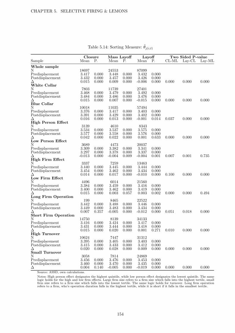
CHAPTER 5. SELECTIVE FIRING & LEMONS
Table 5.14: Sorting Measure: θj(i,t)
Closure Mass Layoff Layoff Two Sided P-valueSample Mean P. Mean P. Mean P. CL-ML Lay-CL Lay-ML
Whole sampleN 18697 24553 87099Predisplacement 3.417 0.000 3.448 0.000 3.432 0.000Postdisplacement 3.432 0.000 3.457 0.000 3.426 0.000∆ 0.015 0.000 0.009 0.000 -0.006 0.000 0.000 0.000 0.000White CollarN 7803 11739 27401Predisplacement 3.468 0.000 3.479 0.000 3.492 0.000Postdisplacement 3.484 0.000 3.486 0.000 3.476 0.000∆ 0.015 0.000 0.007 0.000 -0.015 0.000 0.000 0.000 0.000Blue CollarN 10018 11035 57494Predisplacement 3.376 0.000 3.417 0.000 3.403 0.000Postdisplacement 3.391 0.000 3.429 0.000 3.402 0.000∆ 0.016 0.000 0.013 0.000 -0.001 0.014 0.037 0.000 0.000High Person EffectN 3139 4610 8343Predisplacement 3.534 0.000 3.537 0.000 3.575 0.000Postdisplacement 3.577 0.000 3.558 0.000 3.576 0.000∆ 0.042 0.000 0.022 0.000 0.001 0.633 0.000 0.000 0.000Low Person EffectN 3689 4473 20037Predisplacement 3.309 0.000 3.382 0.000 3.341 0.000Postdisplacement 3.297 0.000 3.378 0.000 3.337 0.000∆ -0.013 0.000 -0.004 0.009 -0.004 0.001 0.007 0.001 0.735High Firm EffectN 3337 7259 13463Predisplacement 3.440 0.000 3.445 0.000 3.444 0.000Postdisplacement 3.454 0.000 3.462 0.000 3.434 0.000∆ 0.014 0.000 0.017 0.000 -0.010 0.000 0.100 0.000 0.000Low Firm EffectN 4496 6014 21560Predisplacement 3.384 0.000 3.459 0.000 3.416 0.000Postdisplacement 3.400 0.000 3.462 0.000 3.419 0.000∆ 0.015 0.000 0.003 0.057 0.003 0.002 0.000 0.000 0.494Long Firm OperationN 199 8465 22522Predisplacement 3.442 0.000 3.488 0.000 3.446 0.000Postdisplacement 3.449 0.000 3.483 0.000 3.434 0.000∆ 0.007 0.357 -0.005 0.000 -0.012 0.000 0.051 0.018 0.000Short Firm OperationN 14750 8139 34133Predisplacement 3.416 0.000 3.424 0.000 3.417 0.000Postdisplacement 3.431 0.000 3.444 0.000 3.418 0.000∆ 0.015 0.000 0.020 0.000 0.001 0.271 0.010 0.000 0.000High TurnoverN 10624 7447 31312Predisplacement 3.395 0.000 3.405 0.000 3.403 0.000Postdisplacement 3.415 0.000 3.433 0.000 3.412 0.000∆ 0.020 0.000 0.028 0.000 0.009 0.000 0.000 0.000 0.000Small TurnoverN 3058 7814 24869Predisplacement 3.456 0.000 3.476 0.000 3.453 0.000Postdisplacement 3.460 0.000 3.470 0.000 3.435 0.000∆ 0.004 0.140 -0.005 0.000 -0.019 0.000 0.000 0.000 0.000
Source: ASSD, own calculations.
Notes: High person effect designates the highest quintile, while low person effect designates the lowest quintile. The samelogic holds for the high and low firm effects. Large firm size refers to a firm size which falls into the highest tertile, smallfirm size refers to a firm size which falls into the lowest tertile. The same logic holds for turnover. Long firm operationrefers to a firm, who’s operation duration falls in the highest tertile, while it is short if it falls in the smallest tertile.
154

into the direction that there is signaling and sorting happening on aggregate. A finding which
should not surprise us, since the resulting outcome on the labor market usually is a combination
of signaling and sorting. Future research should focus on developing a model that merges the
asymmetric information literature with the sorting literature.
The question about expectations and priors concerning sorting may be raised. To give probable
priors for the change in the correlations, I would have to assume that the sorting at the
displacement firm is not affected by the displacement. The first problem that needs to be
addressed, in this case, is that especially the firm fixed effect of the closing firm, may be
affected, since these firms are already the “worst” firms, otherwise they would not shut down.
Furthermore, the sorting at the displacement firm may also be the result of signaling and sorting
based on previous experiences of the firm and the workers. Nevertheless, I may assume at first
that the sorting at the displacement is not affected by the displacement type. Since the question
I am trying to answer is whether or not the “lemon” affects the resulting matching, the sorting
at the re-employment firm may be affected by the layoff. This leaves two possibilities;
1. the sorting at the re-employment firm is not affected by the displacement type. This gives
the prediction that I should observe no change in sorting or a trend in sorting.
2. The sorting at the re-employment firm is affected by the displacement type, then it depends
on what type (high or low ability) individual is trying to sort herself. Still assuming that
the closing types are the ones that do not suffer from a stigma, we get the following
predictions, (see Table 5.16);
for the closing individuals, we should observe no change in the sorting measure, or a trend. For
the individual layoffs who are affected by the stigma, we should observe a “better” matching
since the low ability individuals will now clearly be seen as low ability and should thus find their
match. A high ability individual layoff on the other hand will be seen as low ability, and her
match will be distorted, we should thus observe a decrease in efficient matching. Talking about
efficiency raises another problem; I know how the sorting changes, but I do not know how good
or efficient the sorting was before the displacement, so saying that it should become better is not
a precise statement. The problem arises that to the best of my knowledge there is no efficiency
measure available for sorting, so future research will need to investigate how to measure efficient
matching.
155

CHAPTER 5. SELECTIVE FIRING & LEMONS
Table 5.15: Sorting Measure: Corr(θi, θj(i,t))
Closure Mass Layoff LayoffSample N Corr N Corr N Corr
Whole samplePredisplacement 18697 0.684 24553 0.491 87099 0.646Postdisplacement 18697 0.725 24553 0.553 87099 0.648∆ 0.041 0.061 0.002White CollarPredisplacement 7803 0.655 11739 0.382 27401 0.612Postdisplacement 7803 0.714 11739 0.490 27401 0.630∆ 0.059 0.107 0.018Blue CollarPredisplacement 10018 0.620 11035 0.501 57494 0.613Postdisplacement 10018 0.668 11035 0.541 57494 0.608∆ 0.048 0.040 -0.005Only ML, Closure FirmsPredisplacement 18697 0.684 24553 0.491 4423 0.449Postdisplacement 18697 0.725 24553 0.553 4423 0.561∆ 0.041 0.061 0.113High Person EffectPredisplacement 3139 0.408 4610 0.112 8343 0.440Postdisplacement 3139 0.430 4610 0.181 8343 0.451∆ 0.023 0.069 0.011Low Person EffectPredisplacement 3689 0.524 4473 0.131 20037 0.468Postdisplacement 3689 0.626 4473 0.192 20037 0.447∆ 0.103 0.061 -0.021High Firm EffectPredisplacement 3337 0.693 7259 0.513 13463 0.648Postdisplacement 3337 0.723 7259 0.549 13463 0.630∆ 0.030 0.037 -0.017Low Firm EffectPredisplacement 4496 0.751 6014 0.359 21560 0.777Postdisplacement 4496 0.792 6014 0.461 21560 0.730∆ 0.041 0.102 -0.047High Firm and Person EffectPredisplacement 602 0.139 1104 0.007 1423 0.119Postdisplacement 602 0.117 1104 0.149 1423 0.134∆ -0.022 0.141 0.015Low Firm and Person EffectPredisplacement 1151 0.527 1091 0.165 5068 0.544Postdisplacement 1151 0.643 1091 0.157 5068 0.486∆ 0.116 -0.008 -0.058Long Firm OperationPredisplacement 199 0.714 8465 0.433 22522 0.497Postdisplacement 199 0.777 8465 0.497 22522 0.582∆ 0.062 0.064 0.085Short Firm OperationPredisplacement 14750 0.691 8139 0.515 34133 0.740Postdisplacement 14750 0.734 8139 0.584 34133 0.686∆ 0.043 0.068 -0.053High TurnoverPredisplacement 10624 0.669 7447 0.484 31312 0.629Postdisplacement 10624 0.725 7447 0.561 31312 0.635∆ 0.057 0.077 0.007Small TurnoverPredisplacement 3058 0.761 7814 0.355 24869 0.714Postdisplacement 3058 0.751 7814 0.456 24869 0.678∆ -0.010 0.102 -0.036
Source: ASSD, own calculations.
Notes: ∆, denotes the change in the correlations at the postdisplacement firm and thepredisplacement firm. High person effect designates the highest quintile, while low person effectdesignates the lowest quintile. The same logic holds for the high and low firm effects. Large firmsize refers to a firm size which falls into the highest tertile, small firm size refers to a firm sizewhich falls into the lowest tertile. The same logic holds for turnover. Long firm operation refersto a firm, who’s operation duration falls in the highest tertile, while it is short if it falls in thesmallest tertile.
156
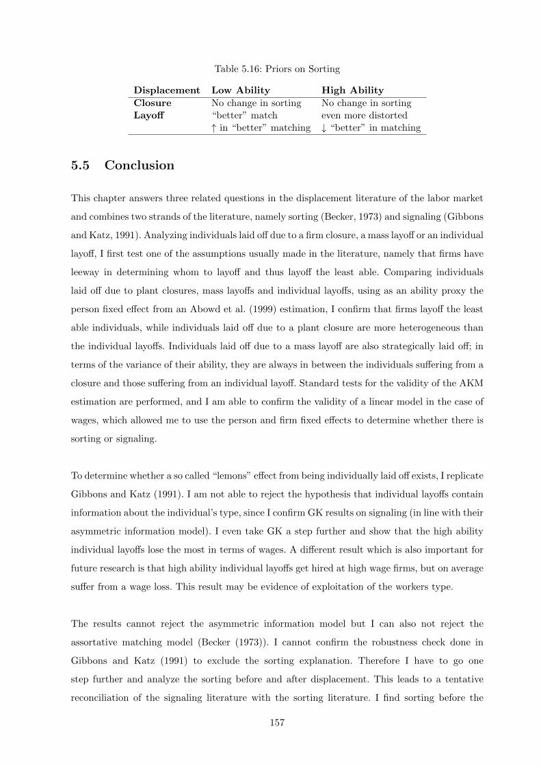
Table 5.16: Priors on Sorting
Displacement Low Ability High Ability
Closure No change in sorting No change in sortingLayoff “better” match even more distorted
↑ in “better” matching ↓ “better” in matching
5.5 Conclusion
This chapter answers three related questions in the displacement literature of the labor market
and combines two strands of the literature, namely sorting (Becker, 1973) and signaling (Gibbons
and Katz, 1991). Analyzing individuals laid off due to a firm closure, a mass layoff or an individual
layoff, I first test one of the assumptions usually made in the literature, namely that firms have
leeway in determining whom to layoff and thus layoff the least able. Comparing individuals
laid off due to plant closures, mass layoffs and individual layoffs, using as an ability proxy the
person fixed effect from an Abowd et al. (1999) estimation, I confirm that firms layoff the least
able individuals, while individuals laid off due to a plant closure are more heterogeneous than
the individual layoffs. Individuals laid off due to a mass layoff are also strategically laid off; in
terms of the variance of their ability, they are always in between the individuals suffering from a
closure and those suffering from an individual layoff. Standard tests for the validity of the AKM
estimation are performed, and I am able to confirm the validity of a linear model in the case of
wages, which allowed me to use the person and firm fixed effects to determine whether there is
sorting or signaling.
To determine whether a so called “lemons” effect from being individually laid off exists, I replicate
Gibbons and Katz (1991). I am not able to reject the hypothesis that individual layoffs contain
information about the individual’s type, since I confirm GK results on signaling (in line with their
asymmetric information model). I even take GK a step further and show that the high ability
individual layoffs lose the most in terms of wages. A different result which is also important for
future research is that high ability individual layoffs get hired at high wage firms, but on average
suffer from a wage loss. This result may be evidence of exploitation of the workers type.
The results cannot reject the asymmetric information model but I can also not reject the
assortative matching model (Becker (1973)). I cannot confirm the robustness check done in
Gibbons and Katz (1991) to exclude the sorting explanation. Therefore I have to go one
step further and analyze the sorting before and after displacement. This leads to a tentative
reconciliation of the signaling literature with the sorting literature. I find sorting before the
157

CHAPTER 5. SELECTIVE FIRING & LEMONS
layoff event, as well as sorting after the layoff event (measured by the correlation between the
worker and firm fixed effect, the correlation between the worker fixed effect and the mean of
the co-workers person effect or by the average firm fixed effect, before and after displacement).
I observe a differential change in the sorting measure for the three types of layoffs (closures,
individual layoffs and mass layoffs). This leads to the conclusion that there is sorting as well as
signaling.
As this chapter brings together two strands of the literature, it highlights the fact that in
future research we need to model the labor market as a combination of search and signals.
The asymmetric information model of GK is a right start of modeling the signal. The question
remains how to include it into a search framework of the Becker type and how to measure sorting
efficiently.
158
5.A AKM Appendix
5.A.1 Measure of Productivity according to Abowd et al. (1999) (AKM)
In order to capture unobserved heterogeneity on the individual and the firm level, I follow the
formulation of Abowd et al. (1999), where the log daily wage ωit of individual i in year t can be
written as;
ωit = αi + ΨJ(i,t)︸ ︷︷ ︸Fixed Effects
+x′itβ + ηiJ(i,t) + ςit + εit︸ ︷︷ ︸
Random Effects
(5.7)
= αi + ΨJ(i,t) + x′itβ + rit
the sum of a time-invariant worker component αi, a time-variant establishment component
ΨJ(i,t), a linear index of time-varying observable characteristics x′itβ, a mean zero random match
component ηJ(i,t), a unit root component of individual wage ςit and a mean zero transitory error
εit. All the error terms go into the same random effects component, rit.32 Following Card et al.
(2013b), αi can be interpreted as the portion of the individual’s earnings power that is fully
portable across employers. It is a combination of skills and other factors that are rewarded
equally across employers. ΨJ(i,t) captures the proportional pay premium that is common to all
employees at workplace j (i.e. all individuals for whom J(i, t) = j). This could be rent sharing,
efficiency wage premium or strategic wage posting behavior. xit captures changes in the portable
component of an individual’s earnings power. It includes an unrestricted set of year dummies,
quadratic and cubic terms in age. The match effect ηij allows for time-invariant wage premium
(or discounts) for individual i at establishment j, relative to the baseline level αi + Ψj . This
can also be interpreted as an idiosyncratic wage premium. It is the complementarity between
the skills of the worker and the needs of the firm. These complementarities arise in models
where idiosyncratic productivity components are associated with each potential job match and
workers receive some share of the rents from a successful match. It is assumed that the match
effect has mean 0. ςit captures the drift in the portable component of the individual’s earnings
power. It can represent employer learning (about the productivity), unobserved human capital
accumulation, health shocks or the arrival of outside offers. The drift component is assumed to
have mean 0 but contains a unit root. εit presents any left out mean reverting factors, it is also
assumed to have mean 0 for each person in the sample.
32For completeness, when estimating this equation, I have N∗ person-year observations with N workers and Jestablishments.
159

CHAPTER 5. SELECTIVE FIRING & LEMONS
Following Abowd et al. (2002) a linear restriction is used on the firm effects within each
“connected” set of firms for the estimation.33 I refer the reader to Card et al. (2012b) for a closer
description of the estimation procedure and the discussion of the threats to validity. We will
briefly mention the crucial assumptions here. First there is the standard orthogonality condition
between the composite error rit and the time-varying covariates Xit. Secondly, the crucial
assumption is that, the composite error has to be orthogonal to the matrix of establishment
identifiers. It is important to notice, that this does not preclude systematic patterns of job
mobility related to αi and or {Ψ1, . . . ,ΨJ}. Following the argument in Card et al. (2012b),
for example, a comparison of the number of job movers in the various cells of Tables 5.17
and 5.18, suggests that workers are more likely to move from low to high wage establishments
than to move in the opposite direction. This does not represent a violation of the orthogonality
condition between the error and the fixed effects because our fixed effects estimator conditions on
the actual sequence of establishments at which each employee is observed. Similarly, higher (or
lower) turnover rates among lower productivity workers is fully consistent with this condition, as
is the possibility that high skilled workers are more (or less) likely to transition to workplaces with
higher wage premiums. Mobility may be related to fixed or time-varying non-wage characteristics
of establishments, such as location or recruiting effort. Such mobility helps the identification by
expanding the connected set of establishments.
Other threats to the validity of the estimation are first sorting based on ηij . The standard Roy
(1951) model sorting changes the interpretation of Ψj , depending on the match component,
different workers may have different wage premium at any given establishment. If job selection
takes place based on the match component, we would expect wage gains for individuals who move
from one establishment to another to be different from the wage losses for the individuals who
make the opposite transition.34 Furthermore if the match component is the relevant selection
criterion, then a fully saturated model with a dummy for each job should fit the data much
better than the additively separate baseline model.
Secondly, if abilities are valued differently at different firms, productive workers will experience
a wage growth at their initial employer and are then also more likely to move to higher-wage
33The “connected” set of firms is the set of all firms which are linked to each other by moves of individualsbetween these firms. The direction of the move does not matter in order to identify the “connected” set.
34I will show in Section 5.A.1, that the gains associated with transitioning from a low to high co-worker-wagefirm is roughly equal to the losses associated with moving in the opposite direction. Moreover, the mean wagedifferentials for workers who move between firms in the same co-worker wage quartile are close to zero in the timeframe from 2002-2009, suggesting that there is no general mobility premium for movers.
160

firms (and vice-versa for less productive workers). This basically means that the drift in the
expected wage predicts firm-to-firm transitions. This will lead to an overstatement of the firm
effects.35
Thirdly, if fluctuations in the transitory error εit are associated with systematic movements
between higher- and lower-wage workplaces. The example given in Card et al. (2012b) is; if εit
contains an industry by year component and workers tend to cycle between jobs at higher-wage
employers that are relatively sensitive to industry conditions, and jobs at low-wage employers
that are more stable. (As noted in discussion of Figures 5.10 and 5.11, there is little evidence
that mobility patterns are related to transitory wage fluctuations, suggesting that any correlation
between mobility patterns and the εit’s are small.)
In Section 5.A.1, I will show that the identification criteria are met, and therefore I may use
the firm fixed effects and the person fixed effects to test for heterogeneity, signaling and sorting.
The person effects (which can be interpreted as ability) are then used to determine whether
individuals laid off due to a plant closure are more heterogeneous than those laid off individually.
The firm fixed effect will allow us to analyze the unobservables on the firm levels between the
different groups of the layoff firm, as well as of the receiving firm.
AKM Sample
The AKM sample considers the Austrian universe of male blue and white collar workers from
1980 onwards. I select one main job per year per individual, with a wage and a firm number.
If there are overlapping spells, I select the longest spell as a main spell. This sample is used to
estimate the person and firm fixed effects, but as outlined above, the effects are only identified
within the connected set, which is the set of firms that are linked to each other due to the
movement of workers between the firms. It does not matter in which direction the link goes. No
further restrictions are put on this sample.36
35This will also be addressed in Section 5.A.1.36To estimate AKM, I use Card et al. (2012b)’s Matlab code. Originally I have 46, 492, 753 person year
observations, including 3, 732, 947 workers at 624, 055 firms with a mean wage of 3.99 and a variance of 0.2846.When I restrict estimation to the largest connected set, I am left with 46, 263, 319 person year observations,representing 3, 690, 879 workers at 586, 600 firms with a mean wage of 4.001 and a variance of 0.28095. If weestimate the match effects model of AKM I have a root mean squared error of 0.1579 an R2 of 0.9336 and anadjusted R2 of 0.9112.
161

CHAPTER 5. SELECTIVE FIRING & LEMONS
Validity of the AKM Model
To show that the AKM model actually fits the data and that the orthogonality conditions do
not seem to be violated, I follow closely Card et al. (2012b).
To address the first threat to the validity concerning the sorting or as Card et al. (2012b) put it:
“people who change workplaces will not necessarily experience systematic wage changes. If, on
the other hand, different establishments pay different average wage premiums, then individuals
who join a workplace where other workers are highly paid will on average experience a wage
gain, while those who join a workplace where others are poorly paid will experience a wage loss”,
I replicate their event study.
To see whether sorting on wage premium happens in the Austrian Data I ran the event study,
where I look at job movers and their co-workers wages at the job before and after the job
movement. Figures 5.10 and 5.11 classify the movers according to the quartile of their mean
co-worker wage. For clarification, the figures only show the wage profiles for workers leaving
quartile 1 and quartile 4 jobs. Tables 5.17 and 5.18 provide a complete listing of mean wages
before and after the job change event for each of the 16 cells in the two different time intervals
(1990-1997 and 2002-2009). These figures look very similar to Figures 6a and 6b in Card et al.
(2012b).
The figures suggest that different mobility groups have different wage levels before and after a
move. For example, average wages prior to a move for workers who switch from quartile 4 to
quartile 1 jobs are lower than for those who move from quartile 4 to quartile 2 jobs, with similar
patterns for the other mobility groups. Within mobility groups there is also strong evidence
that moving to a job with higher-paid co-workers raises the own wage. People who start in
quartile 1 jobs and move to quartile 1 jobs have relatively constant wages, while those who move
to higher quartile jobs experience wage increases. Likewise for people who start in quartile 4 jobs.
An interesting feature of Figures 5.10 and 5.11, is the almost symmetry of the wage losses and
gains for those who move between quartile 1 and quartile 4 firms. As shown in Tables 5.17
and 5.18, the gains and losses for other mover categories exhibit a similar degree of symmetry,
particularly after adjusting for trend growth in wages. This symmetry suggests that a simple
model with additive worker and firm effects may provide a reasonable characterization of the
162

Figure 5.10: Mean Wages of Job Changers, Classified by Quartile of Mean Wage of Co-Workersat Origin and Destination Firm, 1990-97
3.5
3.7
3.9
4.1
4.3
4.5
4.7
(mea
n) lo
g_w
age
−1 0 1 2Time(0= year before job switch)
1 to 1 1 to 21 to 3 1 to 44 to 1 4 to 24 to 3 4 to 4
Figure 5.11: Mean Wages of Job Changers, Classified by Quartile of Mean Wage of Co-Workersat Origin and Destination Firm, 2002-2009
3.5
3.7
3.9
4.1
4.3
4.5
4.7
(mea
n) lo
g_w
age
−1 0 1 2Time(0= year before job switch)
1 to 1 1 to 21 to 3 1 to 44 to 1 4 to 24 to 3 4 to 4
163

CHAPTER 5. SELECTIVE FIRING & LEMONS
mean wages resulting from different pairings of workers to firms.
Table 5.17: Mean Log Wages Before and After Job Change by Quartile of Mean Co-Workers’Wages at Origin and Destination Firms
Mean Log Wages of Movers Change from 2 YearsNumber of 2 Years 1 Year 1 Year 2 Years Before to 2 Years After
Origin/Destination Observations Before Before After After Raw Adjusted∗∗
Quartile∗ (1) (2) (3) (4) (5) (6) (7)
Years: 2002 - 20091 to 1 63083 3.75 3.78 3.87 3.94 0.19 0.001 to 2 30388 3.92 3.96 4.23 4.25 0.33 0.141 to 3 16526 3.89 3.93 4.35 4.38 0.49 0.301 to 4 9042 3.92 3.96 4.53 4.56 0.63 0.44
2 to 1 27355 4.12 4.17 4.06 4.13 0.01 -0.132 to 2 56903 4.22 4.25 4.33 4.36 0.14 0.002 to 3 31970 4.24 4.29 4.44 4.47 0.23 0.092 to 4 12823 4.24 4.32 4.60 4.63 0.39 0.25
3 to 1 13618 4.24 4.29 4.04 4.13 -0.10 -0.253 to 2 23460 4.32 4.36 4.36 4.40 0.08 -0.073 to 3 54814 4.40 4.44 4.53 4.55 0.15 0.003 to 4 23365 4.46 4.51 4.68 4.71 0.25 0.10
4 to 1 6728 4.38 4.45 3.97 4.07 -0.31 -0.474 to 2 8867 4.45 4.52 4.44 4.48 0.03 -0.144 to 3 19646 4.52 4.58 4.63 4.67 0.14 -0.024 to 4 70615 4.67 4.73 4.82 4.83 0.16 0.00
Source: ASSD, own calculations.Notes: Entries are mean log real daily wages for job changers who are observed with at least 2 years of data prior to a jobchange, and two years after. Sample exlcudes mover to/from firms with 1 worker.∗ Quartiles are based on mean wages of co-workers at old job in year prior to move, and in new job in year after move.∗∗ Trend-adjusted mean wage change, calculated as mean wage change for origin-destination group, minus mean change forjob movers from the same origin quartile who remain in same quartile.
A final important characteristic of the wage profiles in Figures 5.10 and 5.11 is the absence of
any Ashenfelter (1978) style transitory dip (or rise) in the wages of movers in the year before
moving. The profiles of average daily wages are remarkably flat in the years before and after
a move. Taken together with the approximate symmetry of the wage transitions, these flat
profiles suggest that the wages of movers may be well-approximated by the combination of a
permanent worker component and a firm component, and a time varying residual component
that is uncorrelated with mobility.
164
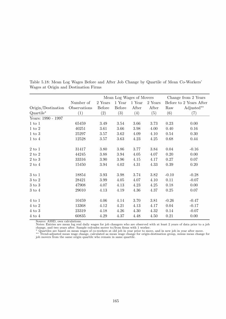
Table 5.18: Mean Log Wages Before and After Job Change by Quartile of Mean Co-Workers’Wages at Origin and Destination Firms
Mean Log Wages of Movers Change from 2 YearsNumber of 2 Years 1 Year 1 Year 2 Years Before to 2 Years After
Origin/Destination Observations Before Before After After Raw Adjusted∗∗
Quartile∗ (1) (2) (3) (4) (5) (6) (7)
Years: 1990 - 19971 to 1 65459 3.49 3.54 3.66 3.73 0.23 0.001 to 2 40251 3.61 3.66 3.98 4.00 0.40 0.161 to 3 25297 3.57 3.62 4.09 4.10 0.54 0.301 to 4 12528 3.57 3.63 4.23 4.25 0.68 0.44
2 to 1 31417 3.80 3.86 3.77 3.84 0.04 -0.162 to 2 44245 3.88 3.94 4.05 4.07 0.20 0.002 to 3 33316 3.90 3.96 4.15 4.17 0.27 0.072 to 4 15450 3.94 4.02 4.31 4.33 0.39 0.20
3 to 1 18854 3.93 3.98 3.74 3.82 -0.10 -0.283 to 2 28421 3.99 4.05 4.07 4.10 0.11 -0.073 to 3 47908 4.07 4.13 4.23 4.25 0.18 0.003 to 4 29010 4.13 4.19 4.36 4.37 0.25 0.07
4 to 1 10459 4.06 4.14 3.70 3.81 -0.26 -0.474 to 2 13368 4.12 4.21 4.13 4.17 0.04 -0.174 to 3 23319 4.18 4.26 4.30 4.32 0.14 -0.074 to 4 60835 4.29 4.37 4.48 4.50 0.21 0.00
Source: ASSD, own calculations.Notes: Entries are mean log real daily wages for job changers who are observed with at least 2 years of data prior to a jobchange, and two years after. Sample exlcudes mover to/from firms with 1 worker.∗ Quartiles are based on mean wages of co-workers at old job in year prior to move, and in new job in year after move.∗∗ Trend-adjusted mean wage change, calculated as mean wage change for origin-destination group, minus mean change forjob movers from the same origin quartile who remain in same quartile.
165

CHAPTER 5. SELECTIVE FIRING & LEMONS
5.B Figures
Figure 5.12: Person Effects by Type of Layoff
0.5
11.
52
Kde
nsity
Per
son
Effe
ct
2.5 3 3.5 4x
All LayoffML Closure
166
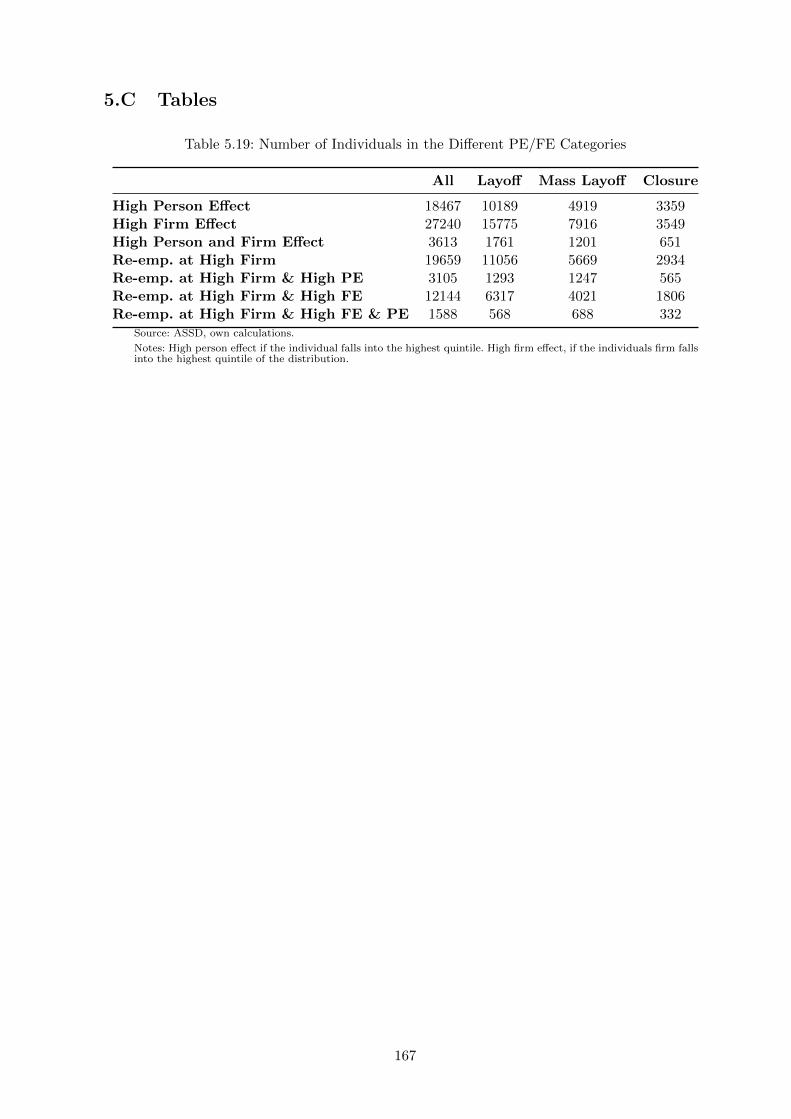
5.C Tables
Table 5.19: Number of Individuals in the Different PE/FE Categories
All Layoff Mass Layoff Closure
High Person Effect 18467 10189 4919 3359High Firm Effect 27240 15775 7916 3549High Person and Firm Effect 3613 1761 1201 651Re-emp. at High Firm 19659 11056 5669 2934Re-emp. at High Firm & High PE 3105 1293 1247 565Re-emp. at High Firm & High FE 12144 6317 4021 1806Re-emp. at High Firm & High FE & PE 1588 568 688 332
Source: ASSD, own calculations.
Notes: High person effect if the individual falls into the highest quintile. High firm effect, if the individuals firm fallsinto the highest quintile of the distribution.
167

CHAPTER 5. SELECTIVE FIRING & LEMONS
Table 5.20: Difference Between Pre and Post Layoff Wages
(1) (2) (3) (4)
Mass Layoff 0.00799∗∗ 0.00814∗∗ 0.00543 0.00666∗
(0.00365) (0.00365) (0.00371) (0.00373)
Layoff -0.0453∗∗∗ -0.0460∗∗∗ -0.0471∗∗∗ -0.0490∗∗∗
(0.00301) (0.00302) (0.00300) (0.00301)
Age -0.0145∗∗∗ -0.0146∗∗∗ -0.0149∗∗∗ -0.0142∗∗∗
(0.000945) (0.000945) (0.000941) (0.000942)
Age2 0.000134∗∗∗ 0.000136∗∗∗ 0.000133∗∗∗ 0.000127∗∗∗
(0.0000116) (0.0000116) (0.0000115) (0.0000115)
Age at First Employment 0.00363∗∗∗ 0.00354∗∗∗ 0.00362∗∗∗ 0.00362∗∗∗
(0.000524) (0.000524) (0.000521) (0.000522)
Firm Size 0.00000194∗∗∗ 0.00000198∗∗∗ -0.00000135∗∗∗ -0.000000543
(0.000000376) (0.000000376) (0.000000474) (0.000000485)
Firm Operation Duration 4.37e-08 -6.25e-09 0.000000722∗∗∗ 0.000000282
(0.000000253) (0.000000253) (0.000000268) (0.000000271)
Total Unemployment Duration since LFP -0.000000445 -9.00e-08 -0.00000148 -0.000000883
(0.00000456) (0.00000456) (0.00000454) (0.00000455)
Total Employment Duration since LFP -0.0000108∗∗∗ -0.0000118∗∗∗ -0.00000468∗ -0.00000766∗∗∗
(0.00000239) (0.00000239) (0.00000240) (0.00000241)
Tenure at Closing Firm -0.0000107∗∗∗ -0.0000103∗∗∗ -0.00000908∗∗∗ -0.00000888∗∗∗
(0.000000715) (0.000000717) (0.000000717) (0.000000717)
Wage at First Job -0.00260∗∗∗ -0.00259∗∗∗ -0.00236∗∗∗ -0.00229∗∗∗
(0.0000825) (0.0000826) (0.0000830) (0.0000832)
Number of Unemployment Spells 0.00158∗∗∗ 0.00144∗∗∗ 0.00133∗∗∗ 0.000844∗∗
(0.000401) (0.000401) (0.000402) (0.000405)
Number of Employment Spells 0.000541 0.000691 -0.000798 0.000109
(0.00100) (0.00100) (0.001000) (0.00100)
Year FE 3 3 3 3
Number of Displacements 7 3 3 3
Industry FE 7 7 3 3
Region FE 7 7 7 3
Observations 125497 125497 125495 125495
R2 0.040 0.040 0.059 0.061
Adjusted R2 0.040 0.040 0.058 0.060
Source: ASSD, own calculations.Note: *,**,*** indicates significance at the 10%, 5%, and 1% level, respectively. Standard errors in parentheses.
168

Bibliography
Abowd, J., R. Creecy, and F. Kramarz (2002): “Computing Person and Firm Effects Using
Linked Longitudinal Employer-Employee Data,” Cornell University Department of Economics
Unpublished Working Paper, March 2002.
Abowd, J. M., F. Kramarz, P. Lengermann, and S. Perez-Darte (2004): “Are Good
Workers Employed by Good Firms? A test of simple assortative matching model for France
and the United States,” mimeo, 1–31.
Abowd, J. M., F. Kramarz, and D. N. Margolis (1999): “High Wage Workers and High
Wage Firms,” Econometrica, 67(2), 251–333.
Acland, D. and M. Levy (2010): “Habit Formation and Naivete, and Projection Bias in Gym
Attendance,” mimeo.
Akbulut-Yuksel, M. (2009): “Children of War: The Long-Run Effects of Large Scale Physical
Destruction and Warfare on Children,” IZA DP. 4407, 1–47.
Akbulut-Yuksel, M., G. J. van den Berg, and K. Walliczek (2013): “Exploiting spatial
and temporal variation in nutrition at birth, using data on infant mortality and famines: a
study of long-run health effects,” mimeo, 1–34.
Akerlof, G. A. (1970): “The Market for “Lemons”: Quality Uncertainty and the Market
Mechanism,” Quaterly Journal of Economics, 84(3), 488–500.
Almond, D. and J. Currie (2011): “Human Capital Development before Age Five,” in
Handbook of Labor Economics, ed. by D. Card and O. Ashenfelter, Elsevier, vol. 4B, 1315–
1486.
Andersen, H. H., A. Muhlbacher, M. Nubling, J. Schupp, and G. G. Wagner (2007):
“Computation of Standard Values for Physical and Menthal Health Scale Scores Using the
SOEP Version of SF-12v2,” Schmollers Jahrbuch, 127, 171–182.
Antoninis, M. (2006): “The wage effects from the use of personal contacts as hiring channels,”
Journal of Economic Behavior & Organization, 59, 133 – 146.
Ashenfelter, O. C. (1978): “Estimating the Effect of Training Programs on Earnings,” Review
of Economics and Statistics, 60(1), 47–57.
Badger, G., W. Bickel, L. Giordano, E. Jacobs, G. Loewenstein, and L. March
(2007): “Altered states: The impact of immediate craving on the valuation of current and
future opiods,” Journal of Health Economics, September 2007, 26(5), 865–876.
169

BIBLIOGRAPHY
Bagger, J. and R. Lentz (2008): “An Empirical Model of Wage Dispersion with Sorting,”
mimeo, 1–39.
Barker, D. J. P. (2007): “The origins of the developmental origins theory,” Journal of Internal
Medicine, 261, 412–417.
Bayer, P., S. Ross, and G. Topa (2008): “Place of Work and Place of Residence: informal
Hiring Networks and Labor Market Outcomes,” Journal of Political Economy, 116(6), 1150–
1196.
Beaman, L. and J. Magruder (2012): “Who Gets the Job Referral? Evidence from a Social
Networks Experiment,” American Economic Review, 102, 3574–93.
Beaman, L. A. (2012): “Social Networks and the Dynamics of Labour Market Outcomes:
Evidence from Refugees Resettled in the U.S.” Review of Economic Studies, 79, 128–161.
Becker, G. S. (1973): “A Theory of Marriage: Part I,” Journal of Political Economy, 81(4),
813–846.
Bentolila, S., C. Michelacci, and J. Suarez (2004): “Social Networks and Occupational
Choice,” mimeo.
Boheim, R., G. T. Horvath, and R. Winter-Ebmer (2011): “Great expectations: Past
wages and unemployment durations,” Labour Economics, 18, 778–785.
Bohlender, A. and N. A. Siegel (2012): “SOEP-Retrospektiverhebung “Fruhe Kindheit im
(Nach-)Kriegskontext”: Methodenbericht, TNS Infratest Sozialforschung,” .
Borjas, G. J. (1991): Immigration and Self-Selection in: Immigration, trade and the labor
market, University of Chicago Press, Chicago, IL.
Borjas, G. J. and B. Bratsberg (1996): “Who leaves? The outmigration of the foreign-
born,” Review of Economics and Statistics, 78(1), 165–176.
Borowitz, J. (2010): “The Role of Recall Bias in Estimating the “Lemons Effect”,” mim, 1–14.
Burdett, K. (1978): “A Theory of Employee Job Search and Quit Rates,” The American
Economic Review, 68(1), 212–220.
Calvo-Armengol, A. and M. O. Jackson (2004): “The Effects of Social networks on
Employment and Inequality,” The American Economic Review, 94(3), 426–454.
Cappellari, L. and K. Tatsiramos (2010): “Friends’ Networks and Job Finding Rates,”
DISCE Working Paper, 1–37.
Card, D., A. R. Cardoso, and P. Kline (2013a): “Bargaining and the Gender Wage Gap:
A Direct Assessment,” IZA DP No. 7592, 1–69.
Card, D., C. Dustmann, and I. Preston (2012a): “Immigration, wages and compositional
amenities,” Journal of the European Economic Association, 10 (1), 78–119.
170

Card, D., J. Heining, and P. Kline (2012b): “Workplace Heterogeneity and the Rise of
West German Wage Inequality,” NBER Working Paper No. 18522, November.
——— (2013b): “Workplace Heterogeneity and the Rise of West German Wage Inequality,”
Quaterly Journal of Economics, 1–49.
Cardoso, A. R. (1999): “Firms’ Wage Policies and the Rise in Labor Market Inequality: The
Case of Portugal,” Industrial and Labor Relations Review, 53(1), 87–102.
Cingano, F. and A. Rosolia (2012): “People I know: Job Search and Social Networks,”
Journal of Labor Economics, 30(2), 291–332.
Conlin, M., T. O’Donoghue, and T. J. Vogelsang (2007): “Projection Bias in Predicting
Catalog Orders,” American Economic Review, 97(4), 1217–1249.
Corcoran, M., L. Datcher, and G. Duncan (1980): Information and Influence Networks
in Labor Markets, Five Thousand American Families vol. VIII.
Cornelius, W. A. (1978): Mexican Migration to the United States: Causes, Consequences, and
U.S. Responses, Migration and Development Study Group Monograph C/76-12. Cambrige:
Massachusetts Institute of Technology, Center for International Studies.
Davison, E. H., A. P. Pless, M. R. Gugliucci, L. A. King, D. W. King, D. M.
Salgado, A. I. Spiro, and P. Bachrach (2006): “Late-Life Emergence of Early-Life
Trauma: The Phenomenon of Late-Onset Stress Symptomatology Among Aging Combat
Veterans,” Research on Aging, 28(1), 84–114.
Doblhammer, G., G. J. van den Berg, and T. Fritze (2011): “Economic Conditions
at the Time of Birth and Cognitive Abilities Late in Life: Evidence from Eleven European
Countries,” IZA DP. 5940, 1–47.
Doiron, D. J. (1995): “Lay-Offs as Signals: The Canadian Evidence,” The Canadian Journal
of Economics, 28(4a), 899–913.
Durand, J., W. Kandel, E. A. Parrado, and D. S. Massey (1996): “International
Migration and Development in Mexican Communities,” Demography, 33(2), 249–264.
Dustmann, C. (2003a): “Children and Return Migration,” Journal of Population Economics,
16, 815–830.
——— (2003b): “Return Migration, wage differentials, and the optimal migration duration,”
European Economic Review, 47, 353–369.
Dustmann, C., S. Bentolila, and R. Faini (1996): “Return Migration: The European
Experience,” Economic Policy, 11(22), 213–250.
Dustmann, C., A. Glitz, and U. Schonberg (2011): “Referral-based job search networks,”
Discussion paper series // Forschungsinstitut zur Zukunft der Arbeit 5777, UCL, Bonn,
urn:nbn:de:101:1-20110621368.
171

BIBLIOGRAPHY
Dustmann, C. and Y. Weiss (2007): “Return Migration: Theory and Empirical Evidence
from the UK,” British Journal of Industrial Relations, 45:2, 236–256.
Eeckhout, J. and P. Kircher (2011): “Identifying Sorting - In Theory,” Review of Economic
Studies, 78, 872–906.
Elder, G. H. (1999): Children of the Great Depression: Social Changes in life experience,
Boulder, CO, US: Westview Press.
Espinosa, J. and W. N. Evans (2008): “Heightened mortality after the death of a spouse:
Marriage protection or marriage selection?” Journal of Health Economics, 27, 1326–1342.
Fink, M., E. Kalkbrenner, A. Weber, and C. Zuhlener (2010): “Extracting Firm
Information form Administrative Records: The ASSD Firm Panel,” Nfn working paper No.
1004, 1–25.
Gibbons, R. and L. Katz (1991): “Layoffs and Lemons,” Journal of Labor Economics, 9(4),
351–380.
Gibbons, R., L. Katz, T. Lemieux, and D. Parent (2005): “Comparative Advantage,
Learning and Sectoral Wage Determination,” Journal of Labor Economics, 23(4), 681–724.
Gilbert, D., T. Michael, J. Gill, and T. D. Wilson (2002): “The Future is Now: Temporal
Correction in Affective Forecasting,” Organizational Behavior and Human Decision Processes,
LXXXVIII, 430–444.
Gilbert, D. T., E. C. Pinel, T. D. Wilson, S. J. Blumberg, and T. P. Wheatley
(1998): “Immune Neglect: A source of Durability Bias in Affective For,” Journal of Personality
and Social Psychology, LXXXV, 617–638.
Glaesmer, H. (2013): “Die Schatten des Zweiten Weltkrieges. Folgen der traumatischen
Erfahrungen in der alteren deutschen Bevolkerung,” Wissenschaft und Frieden, 35–38.
Glitz, A. (2013): “Coworker networks in the Labour market,” IZA DP, No. 7392, 1–41.
Goel, d. and K. Lang (2009): “Social Ties and the Job Search of Recent Immigrants,” NBER
Working Paper 15186, 1–35.
Granovetter, M. S. (1973): “The Strenght of Weak Ties,” American Journal of Sociology,
78(6), 1360–1380.
Greenwald, B. C. (1986): “Adverse Selection in the Labour Market,” The Review of Economic
Studies, 53(3), 325–347.
Gruetter, M. and R. Lalive (2009): “The importance of firms in wage determination,”
Labour Economics, 16, 149–160.
Grund, C. (1999): “Stigma effects of layoffs? Evidence from German micro-data,” Economics
Letters, 64, 241–247.
172

Haisken-DeNew, J. P. and J. R. Frick (2005): “DTC Desktop Companion to the German
Socio-Economic Panel (SOEP),” Version 8.0.
Haltiwanger, J. C., J. I. Lane, and J. R. Spletzer (1999): “Productivity Differences
across Employers: The Roles of Employer Size, Age and Human Capital,” The American
Economic Review, 89(2), 94–98.
Hansson, R. O. and M. Stroebe (2007): Bereavement in late life: Coping, adaptation, and
developmental influences, American Psychological Association.
Haskel, J., D. Hawkes, and S. Pereira (2005): “Skills, human capital and the plant
productivity gap: UK evidence from matched plant, worker and workforce data,” mi, 1–36.
Hayward, A., I. Rickard, and V. Lummaa (2013): “Influence of early-life nutrition on
mortality and reproductive success during a subsequent famine in a preindustrial population,”
Proceedings of the National Academy of Sciences, 110(34), 13886–13891.
Hensvik, L. and O. N. Skans (2013): “Social networks, employee selection and labor market
outcomes,” Working Paper, IFAU - Institute for Evaluation of Labour Market and Education
Policy 2013:15, IFAU, Uppsala.
Heuft, G. (2004): “Traumatisierung im Lebenslauf und Trauma-Reaktivierung im Alter,”
Psychotherapie im Alter, 1(3), 23–35.
Hewitt, K. (1983): “Place Annihilation: Area Bombing and the Fate of Urban Places,” Annals
of the Association of American Geographers, 73, pp. 257–284.
Hill, J. K. (1987): “Immigrant Decisions Concerning Duration of Stay and Migratory
Frequency,” Journal of Development Economics, 25, 221–234.
Hill, K. and R. Wong (2005): “Mexico-US Migration: Views from Both Sides of th Border,”
Population and Development Review, 31(1), 1–18.
Holzer, H. J. (1988): “Search Method Use by Unemployed Youth,” Journal of Labor
Economics, 6(1), 1–20.
Hu, L. and C. Taber (2005): “Layoffs, Lemons, Race and Gender,” NBER WP 11481, 1–28.
Ioannides, Y. M. and L. D. Loury (2004): “Job Information Networks, Neighborhood Effects,
and Inequality,” Journal of Economic Literature, 42(4), 1056–1093.
Irzano, S., F. Schivardi, and E. Tosetti (2008): “Skill dispersion and Firm Productivity:
An Anlaysis with Employer-Employee Matched Data,” Journal of Labor Economics, 26(2),
247–285.
Jackson, M. O. (2010): Social and Economic Networks, Princeton University Press.
Jacobson, L. S., R. J. Lalonde, and D. G. Sullivan (1993): “Earnings Losses of Displaced
Workers,” The American Economic Review, 83(4), 685–709.
173

BIBLIOGRAPHY
Jenkins, C. J. (1977): “Push/Pull in Recent Mexican Migration to the U.S.” International
Migration Review, 11(2), 178–189.
Jurges, H. (2012): “Collateral Damage: Educational Attainment and Labor Market Outcomes
Among German War and Post-War Cohorts,” MEA DP 253-2012, 1–51.
Kahneman, D. (2011): Thinking, Fast and Slow, Farrar, Straus and Giroux.
Kaup, B. A., P. E. Ruskin, and G. Nyman (1994): “Significant Life Events and PTSD in
Elderly World War II Veterans,” American Journal of Geriatric Psychiatry, 2, 239–243.
Kesternich, I., B. Siflinger, J. P. Smith, and J. K. Winter (2013): “Individual Behavior
as a Pathway between Early-Life Shocks and Adult Health: Evidence from Hunger Episodes
in Post-War Germany,” IZA DP. 7713, 1–36.
——— (forthcoming): “The Effects of World War II on Economic and Health Outcomes across
Europe,” The Review of Economics and Statistics, 1–16.
Kramarz, F. and O. Nordstrom Skans (2013): “When Strong Ties are Strong: Networks
and Youth Labor Market Entry,” CEPR Discussion Paper, No. DP9620, 1–59.
Kramarz, F. and D. Thesmar (2013): “Social Networks In The Boardroom,” Journal of the
European Economic Association, 11, 780–807.
Krashinsky, H. (2002): “Evidence on Adverse Selection and Establishment Size in the Labor
Market,” Industrial and Labor Relations Review, 56(1), 84–96.
Laschever, R. (2009): “The Doughboys Network: Social Interactions and the Employment of
World War I Veterans,” mimeo, 1–54.
Lentz, R. and D. Mortensen (2010): “Labor Market Models of Worker and Firm
Heterogeneity,” Annual Review of Economics, 2, 577–602.
Levy, M. (2009): “An Empirical Analysis of Biases in Cigarette Addiction,” mimeo.
Lindeboom, M., F. Portrait, and G. J. van den Berg (2002): “An econometric analysis
of the mental-health effects of major events in the life of older individuals,” Health Economics,
11, 505–520.
Lindstrom, D. P. (1996): “Economic Opportunity in Mexico and Return Migration from the
United States,” Demography, 33(3), 357–374.
Lise, J., C. Meghir, and J.-M. Robin (2012): “Matching, Sorting and Wages,” mimeo, 1–49.
Loewenstein, G., T. O’Donoghue, and M. Rabin (2003): “Projection Bias in Predicting
Future Utility,” Quaterly Journal of Economics, 118(4), 1209–1248.
Lopes de Melo, R. (2013): “Firm Wage Differentials and Labor Market Sorting: Reconciling
Theory and Evidence,” (mimeo, University of Chicago).
Loury, L. D. (2006): “Some Contacts Are More Equal than Others: Informal Networks, job
Tenure and Wages,” Journal Labor Economics, 24(2), 299–318.
174

Macleod, A. (1994): “The reactivation of post-traumatic stress disorder in later life,”
Australian and New Zealand Journal of Psychiatry, 28, 625–634.
Magruder, J. R. (2010): “Intergenerational Networks, Unemployment, and Persistent
Inequality in South Africa,” American Economic Journal: Applied Economics, 2, 62–85.
Mendes, R., G. J. van den Berg, and M. Lindeboom (2010): “An empirical assessment of
assortative matching in the labor market,” Labour Economics, 17, 919–929.
Montgomery, J. D. (1991): “Social Networks and Labor -Market Outcome: Toward an
Economic Analysis,” The American Economic Review, 81(5), 10408–1418.
Mortensen, D. T. and T. Vishwanath (1994): “Personal contacts and earnings It is who
you know!” Labour Economics, 1, 187–201.
Nakamura, E. (2008): “Layoffs and lemons over the business cycle,” Economic Letters, 99,
55–58.
Nisbett, R. E. and D. E. Kanouse (1968): “Obesity, Hunger, and Supermarket Shopping
Behavior,” Proceedings of the Annual Convention if the American Psychological Association,
III, 683–684.
Ogle, C. M., D. C. Rubin, and I. C. Siegler (2014): “Cumulative exposure to traumatic
events in older adults,” Aging and Mental Health, 18 (3), 316–325.
Pellizzari, M. (2010): “Do Friends and Relatives Really Help in Getting a Good Job?”
Industrial and Labor Relations Review, 63(3), 1–19.
Pistaferri, L. (1999): “Informal networks in the Italian Labor Market,” Giornale degli
Economistie Annali di Economica, 58(3-4), 355–375.
Rabin, M. (2002): “Inference By Believers in the Law of Small Numbers,” Quaterly Journal of
Economics, 117(3), 775–816.
Radebold, H. (2009): “Was geschah damals noch? Verluste, Gewalterfahrungen, Flucht und
Vertreibung,” in Die dunklen Schatten unserer Vergangenheit - Hilfen fur Kriegskinder im
Alter, Klett-Cotta.
Read, D. and B. van Leeuwen (1998): “Predicting Hunger: The Effects of Appetite and
Delay on Choice,” Orga, LXXXVI, 189–205.
Rees, A. (1966): “Information Networks in Labor Markets,” The American Economic Review,
56(1/2), 559–566.
Reichardt, S. and M. Zierenberg (2009): Damals nach dem Krieg: Eine Geschichte
Deutschlands 1945-1949, Wilhelm Goldmann Verlag.
Reyes, B. I. (2001): “Immigrant Trip Duration: The Case of Immigrants from Western Mexico,”
International Migration Review, 35(4), 1185–1204.
175

BIBLIOGRAPHY
——— (2004): “Changes in Trip Duration for Mexican Immigrants to the United States,”
Population Research and Policy Review, 23, 235–257.
Rosekind, M. R., K. B. Gregory, M. M. Mallis, S. L. Brandt, B. Seal, and D. Lerner
(2010): “The Cost of Poor Sleep: Workplace Productivity Loss and Associated Costs,” Journal
of Occupational and Environmental Medicine, 52.
Roy, A. (1951): “Some Thoughts on the Distribution of Earnings,” Oxford Economic Papers,
3(2), 135–146.
Scholte, R., G. J. van den Berg, M. Lindeboom, and D. J. H. Deeg (2014): “Does the
Size of the Effect of Adverse Events at High Ages on Daily-Life Physical Functioning Depend
on the Economic Conditions Around Birth,” mimeo, 1–34.
Serafinelli, M. (2012): “Good Firms, Worker Flows and Productivity,” mimeo, 1–45.
Sergeant, J. F., D. J. Ekerdt, and R. K. Chapin (2010): “Older Adults’ Expectations to
Move: Do They Predict Actual Community-Based or Nursing Facility Moves Within 2 Years?”
Journal of Aging and Health, 22(7), 1029–1053.
Shimer, R. and L. Smith (2000): “Assortative Matching and Search,” Econometrica, 68(2),
343–369.
Siflinger, B. (2013): “The Effects of Bereavement on Mental Health - An Analysis of
Anticipation Patterns Surrounding the Death of the Spouse,” mimeo, 1–55.
Sjaastad, L. A. (1962): “The Costs and Returns of Human Migration,” Journal of Political
Economy, 70(5), 80–93.
Smith, K. V., D. H. Taylor, and F. A. Sloan (2001): “Longevity Expectations and Death:
Can People Predict Their Own Demise?” The American Economic Review, 91(4), 1126–1134.
Song, Y. (2007): “Recall bias in the displaced workers survey: Are layoffs really lemons?” Labour
Economics, 14(3), 335–345.
Spence, M. (1973): “Job Market Signaling,” The Quaterly Journal of Economics, 87(3), 355–
374.
Stephens, M. J. (2004): “Job Loss Expectations, Realizations and Household Consumption
Behavior,” The Review of Economics and Statistics, 86(1), 253–269.
Stevens, A. H. (1997): “Persistent Effects of Job Displacement: The Importance of Multiple
Job Losses,” Journal of Labor Economics, 15(1), 165–188.
Sullivan, D. and T. von Wachter (2007): “Mortality, Mass-Layoffs, and Career Outcomes:
An Analysis Using Administrative Data,” NBER Working Paper 13626.
TNSInfratest (2012): “Bruttobildung der Studie “Fruhe Kindheit im (Nach-)Kriegskontext”,”
.
176

Topa, G. (2001): “Social Interactions, Local Spillovers and Unemployment,” The Review of
Economic Studies, 68(2), 261–295.
Tough, P. (2013): How Children Succeed: Grit, Curiosity, and the Hidden Power of Character,
Mariner Books.
van den Berg, G. J., D. J. H. Deeg, M. Lindeboom, and F. Portrait (2010): “The Role
of Early-Life Conditions in the Cognitive Decline Due to Adverse Events Later in Life,” The
Economic Journal, 120(11), F411–F428.
van den Berg, G. J. and B. Drepper (2011): “A unique bond: Does losing your co-twin
affect your remaining life-span?” mimeo, 1–34.
van den Berg, G. J. and M. Lindeboom (2013): “Aging: conditions early in life and health
and mortality at advanced ages,” in Encyclopedia of Health Economics, ed. by T. Culyer,
North-Holland, Amsterdam.
van den Berg, G. J., M. Lindeboom, and F. R. Portrait (2011a): “Conjugal Bereavement
Effects on Health and Mortality at Advanced Ages,” Journal of Health Economics, 30, 774–
794.
van den Berg, G. J., P. Lundborg, and J. Vikstrom (2012): “The Economics of Grief,”
IZA DP. 7010, 1–59.
van den Berg, G. J., P. Pinger, and J. C. Schoch (2011b): “Instrumental Variable
Estimation of the Causal Effect of Hunger Early in Life on Health Later in Life,” IZA DP.
6110, 1–42.
van den Berg, G. J. and J. C. Schoch (2013): “Economic Conditions at Birth, Adverse Life
Events, and the Decline of Mental Health and Cognitive Functioning Later in Life - Evidence
from Eleven European Countries,” mimeo, 1–36.
van den Berg, G. J. and M. Weynandt (2013): “Explaining Differences Between the
Expected and Actual Duration Until Return Migration: Economic Changes,” Schmollers
Jahrbuch, 133, 249–262.
Van Hook, J. and W. Zhang (2011): “Who Stays? Who Goes? Selective Emigration Among
the Foreign-Born,” Population Research and Policy Review, 30, 1–24.
von Wachter, T., J. Song, and J. Manchester (2009): “Long-Term Earnings Losses due
to Mass Layoffs During the 1982 Recession: An Analysis Using U.S. Administrative Data from
1974 to 2004,” mim, 1–33.
Wagner, G., J. Frick, and J. Schupp (2007): The German Socio-Economic Panel Study
(SOEP) - Scope, Evolution and Enhancements, Schmollers Jahrbuch 127(1)139-169.
Ware, J. E., M. Kosinski, D. M. Turner-Bowker, and B. Gandek (2002): “How to
Score Version 2 of the SF-12(R) Health Survey (with a supplement documenting Version 1),”
Lincoln, RI: Qualitymetric Incorporated.
177

BIBLIOGRAPHY
Weynandt, M. (2011): “Analyzing the Difference Between Expectations and Realizations in
Return Migration: A Transition Analysis,” mimeo, 1–53.
Woodcock, S. D. (2006): “Match Effects,” mimeo, 1–42.
——— (2008): “Wage differentials in the presence of unobserved worker, firm and match
heterogeneity,” Labour Economics, 15, 772–794.
Wooldridge, J. (2010): Econometric Analysis of Cross Section and Panel Data, MIT press:
Cambridge.
Zenou, Y. (2014): “A dynamic model of weak and strong ties in the labor market,” Unpublished
manuscript, Stockholm University, 1–31.
Zweimuller, J., R. Winter-Ebmer, R. Lalive, A. Kuhn, J.-P. Wuellrich, O. Ruf,
and S. Buchi (2009): “Austrian Social Security Database,” NRN: The Austrian Center for
Labor Economics and the Analysis of the Welfare State, Working Paper 0903.
178

Curriculum Vitae
2011-2014 Doctoral Studies in Economics, Graduate School for Economic and Social Sciences,University of Mannheim, Germany
2009-2011 Master of Science in Economic Research, University of Mannheim, Germany
2010-2011 Visiting Scholar, University of California, Berkeley, USA
2007-2009 Bachelor of Science in Business Economics, Miami University, USA
2005-2007 Vordiplom in Business Administration, University of Mannheim, Germany
2005 “Abitur” (High School Diploma), Lycee de Garcons Luxembourg, Luxembourg