
Essays on Large Panel Data Models - uni-bonn.dehss.ulb.uni-bonn.de/2015/3976/3976.pdfEssays on Large...
164
Essays on Large Panel Data Models Inaugural-Dissertation zur Erlangung des Grades eines Doktors der Wirtschafts- und Gesellschaftswissenschaften durch die Rechts- und Staatswissenschaftliche Fakult¨ at der Rheinischen Friedrich-Wilhelms-Universit¨ at Bonn vorgelegt von Oualid Bada aus Monastir (Tunesien) Bonn 2015
Transcript of Essays on Large Panel Data Models - uni-bonn.dehss.ulb.uni-bonn.de/2015/3976/3976.pdfEssays on Large...

Essays on Large Panel Data Models
Inaugural-Dissertation
zur Erlangung des Grades eines Doktors
der Wirtschafts- und Gesellschaftswissenschaften
durch die
Rechts- und Staatswissenschaftliche Fakultatder Rheinischen Friedrich-Wilhelms-Universitat Bonn
vorgelegt von
Oualid Badaaus Monastir (Tunesien)
Bonn 2015


Dekan: Prof. Dr. Rainer Huttemann
Erstreferent: Prof. Dr. Alois Kneip
Zweitreferent: Prof. Dr. Robin Sickles
Tag der mundlichen Prufung: 13.03.2015

UNIVERSITY OF BONN
Abstract
Department of Economics
Institute for Financial Economics and Statistics
Doctoral Thesis
Essays on Large Panel Data Models
by Oualid Bada
The standard panel data literature is moving from micro panels, where the cross-section
dimension is large and the intertemporal sample size is small, to large panels, where
both, the cross-section and the time dimension, are large. This thesis contributes to
this new and growing area of panel data treatments called “large panel data analysis”.
My dissertation consists of three essays: In the first essay, a large panel data model
with an omitted factor structure is considered. The role of the factors is to control for
the issue of the unobserved time-varying heterogeneity effects. A parameter cascading
strategy is proposed to enable efficient estimation of all model parameters when the
number of factors is unknown a priori. In the second essay, further models that combine
large panel data models with different versions of unobserved latent factors are discussed.
Computation-related issues are solved and new specification tests are introduced to check
whether or not these factors can be interpreted as classical additive fixed effects. In the
third essay, a novel method for estimating panel models with multiple structural changes
is proposed. The breaks are allowed to occur at unknown points in time and may affect
the multivariate slope parameters individually. Asymptotic results are derived, Monte
Carlo experiments are performed, and applications for highlighting these new methods
are discussed.


Acknowledgements
I would like to express my heartfelt gratitude to the many people who have supported me
in writing this thesis. First, I am deeply indebted and thankful to my supervisor Prof.
Dr. Alois Kneip for his continuous guidance and vital advice during the writing of this
thesis. His insightful comments helped me to enhance my understanding of advanced and
state-of-the-art statistical techniques. He has been an enormous source of inspiration
for my research and motivated me to keep improving my papers and the way they might
contribute to my research area.
I would like to sincerely thank my co-author Dr. Robin Sickles, Professor of Econometrics
at Rice University, for the extraordinary collaboration on the project that constitutes
the core of Chapter 3. I am grateful for his time, his enthusiasm, and his generosity
during my stay as a visiting researcher in the Department of Econometrics at Rice
University. I also want to thank our co-author, James Gualtieri, for investing so much
time in collecting data and contributing to the development of the application part.
I would also like to express my gratitude to my co-author and my friend JProf. Dr.
Dominik Liebl, who contributed to the joint paper presented in Chapter 2. I benefited
much from his numerous helpful remarks and creative ideas. I will miss his extraordinary
talent to identify and simplify substantially important and complex statistical problems.
In addition, I would like to give my gratitude to all my colleagues in the department
of statistics in the Institute for Financial Economics and Statistics of the University of
Bonn: Prof. Dr. Lorens Imhof, Heiko Wagner, Dominik Poß, Prof. Dr. Hans-Joachim
Werner, Dr. Klaus Utikal, Fabian Walders, Martin Arndt, and Hildegard Grober. They
not only provided me technical help, but also helped me to improve my German language
skills and taught me a lot of unconventional idioms.
I would like to express my deepest gratitude to my parents Emna and Romdhan, my
uncle Khaled, my aunt Metira, my sister Wihed, and my brother Wissem. I could
not have had the opportunity to study in Bonn and to write this dissertation without
them. I also would like to thank all my family members, in particular, Naima Moussa,
Ali Abbes, Fatma Boughtass, Rami Abbes, Ameur Abbes, Safouane Jguirim, Safa Bac-
couche Abbes, and Ghada Abada as well as my friends Kacem Kassraoui, Walid Hamdi,
and Nadhmi Nefzi. They have played an important moral-support role.
Last but not least, to my wonderful wife Abir, who has supported me in good and bad
times during all phases of this thesis: I love you.
vii


Contents
Abstract v
Acknowledgements vii
Contents ix
List of Figures xi
List of Tables xiii
Introduction 1
1 Panel Models with Unknown Number of Unobserved Factors: An Ap-plication to the Credit Spread Puzzle 5
1.1 Introduction . . . . . . . . . . . . . . . . . . . . . . . . . . . . . . . . . . . 5
1.2 Model and Estimation Algorithm . . . . . . . . . . . . . . . . . . . . . . . 8
1.2.1 Model Identification and Estimation . . . . . . . . . . . . . . . . . 8
1.2.2 Starting Values and Iteration Scheme . . . . . . . . . . . . . . . . 12
1.3 Model Extension and Theoretical Results . . . . . . . . . . . . . . . . . . 15
1.3.1 Presence of Additional Categorical Variables . . . . . . . . . . . . 15
1.3.2 Assumptions . . . . . . . . . . . . . . . . . . . . . . . . . . . . . . 17
1.3.3 Asymptotic Distribution and Bias Correction . . . . . . . . . . . . 19
1.4 Monte Carlo Simulations . . . . . . . . . . . . . . . . . . . . . . . . . . . . 21
1.5 Application: The Unobserved Risk Premia of Corporate Bonds . . . . . . 28
1.5.1 The Empirical Model . . . . . . . . . . . . . . . . . . . . . . . . . 28
1.5.2 Data Description . . . . . . . . . . . . . . . . . . . . . . . . . . . . 30
1.5.3 Empirical Results and Interpretations . . . . . . . . . . . . . . . . 32
1.6 Conclusion . . . . . . . . . . . . . . . . . . . . . . . . . . . . . . . . . . . 35
2 The R-package phtt: Panel Data Analysis with Heterogeneous TimeTrends 37
2.1 Introduction . . . . . . . . . . . . . . . . . . . . . . . . . . . . . . . . . . . 37
2.2 Panel Models for Heterogeneity in Time Trends . . . . . . . . . . . . . . . 41
2.2.1 Computational Details . . . . . . . . . . . . . . . . . . . . . . . . . 44
2.2.2 Application . . . . . . . . . . . . . . . . . . . . . . . . . . . . . . . 45
2.3 Panel Criteria for Selecting the Number of Factors . . . . . . . . . . . . . 49
ix

Contents
2.3.1 Application . . . . . . . . . . . . . . . . . . . . . . . . . . . . . . . 52
2.4 Panel Models with Stochastically Bounded Factors . . . . . . . . . . . . . 56
2.4.1 Model with Known Number of Factors . . . . . . . . . . . . . . . . 56
2.4.2 Model with Unknown Number of Factors . . . . . . . . . . . . . . 57
2.4.3 Application . . . . . . . . . . . . . . . . . . . . . . . . . . . . . . . 60
2.5 Models with Additive and Interactive Unobserved Effects . . . . . . . . . 63
2.5.1 Specification Tests . . . . . . . . . . . . . . . . . . . . . . . . . . . 67
2.5.1.1 Testing the Sufficiency of Classical Additive Effects . . . 67
2.5.1.2 Testing the Existence of Common Factors . . . . . . . . . 69
2.6 Interpretation . . . . . . . . . . . . . . . . . . . . . . . . . . . . . . . . . . 71
2.7 Summary . . . . . . . . . . . . . . . . . . . . . . . . . . . . . . . . . . . . 73
3 Panel Models with Multiple Jumps in the Parameters 75
3.1 Introduction . . . . . . . . . . . . . . . . . . . . . . . . . . . . . . . . . . . 75
3.2 Preliminaries . . . . . . . . . . . . . . . . . . . . . . . . . . . . . . . . . . 78
3.3 Two-way Panel Models with Multiple Jumps . . . . . . . . . . . . . . . . 83
3.3.1 Estimation . . . . . . . . . . . . . . . . . . . . . . . . . . . . . . . 83
3.3.2 Assumptions and Main Asymptotic Results . . . . . . . . . . . . . 86
3.4 Post-SAW Procedures . . . . . . . . . . . . . . . . . . . . . . . . . . . . . 89
3.4.1 Tree-Structured Representation . . . . . . . . . . . . . . . . . . . . 89
3.4.2 Detecting the Jump Locations . . . . . . . . . . . . . . . . . . . . 92
3.4.3 Post-SAW Estimation . . . . . . . . . . . . . . . . . . . . . . . . . 93
3.5 SAW with Unobserved Multifactor Effects . . . . . . . . . . . . . . . . . . 95
3.6 Monte Carlo Simulations . . . . . . . . . . . . . . . . . . . . . . . . . . . . 99
3.7 Application: Algorithmic Trading and Market Quality . . . . . . . . . . . 103
3.7.1 Liquidity and Asset Pricing . . . . . . . . . . . . . . . . . . . . . . 104
3.7.2 Data . . . . . . . . . . . . . . . . . . . . . . . . . . . . . . . . . . . 106
3.7.2.1 The Algorithmic Trading Proxy . . . . . . . . . . . . . . 106
3.7.2.2 Market Quality Measures . . . . . . . . . . . . . . . . . . 107
3.7.3 Results . . . . . . . . . . . . . . . . . . . . . . . . . . . . . . . . . 109
3.8 Conclusion . . . . . . . . . . . . . . . . . . . . . . . . . . . . . . . . . . . 115
A Appendix of Chapter 1 117
A.1 Theoretical Results and Proofs . . . . . . . . . . . . . . . . . . . . . . . . 117
B Appendix of Chapter 3 123
B.1 Proofs of Section 3.2 . . . . . . . . . . . . . . . . . . . . . . . . . . . . . . 123
B.2 Proofs of Section 3.3 . . . . . . . . . . . . . . . . . . . . . . . . . . . . . . 129
B.3 Proofs of Section 3.4 . . . . . . . . . . . . . . . . . . . . . . . . . . . . . . 135
Bibliography 143
x

List of Figures
1.1 Credit spread curves before and after transformation . . . . . . . . . . . . 31
1.2 Screeplots for static and dynamic factors . . . . . . . . . . . . . . . . . . . 33
1.3 Estimates of the time varying rating effects and the systematic factors . . 33
1.4 Estimated first and second risk components . . . . . . . . . . . . . . . . . 35
2.1 Plots of the dependent and independent variables . . . . . . . . . . . . . . 41
2.2 Estimated factors and estimated time-varying individual effects . . . . . . 48
2.3 Scree plot produced by the plot()-method for OptDim-objects . . . . . . 54
2.4 Estimated factors and estimated time-varying individual effects . . . . . . 64
2.5 Estimated additive and interactive heterogeneity effects . . . . . . . . . . 67
2.6 Visualization of the differences of the time-varying individual effects . . . 73
3.1 Tree-structured representation of the wavelet coefficients . . . . . . . . . . 90
3.2 Tree-structured representation of the shifted and non-shifted coefficients . 90
3.3 Time varying effect of algorithmic trading on the proportional quotedspread . . . . . . . . . . . . . . . . . . . . . . . . . . . . . . . . . . . . . . 112
3.4 Time varying effect of algorithmic trading on the proportional effectivespread . . . . . . . . . . . . . . . . . . . . . . . . . . . . . . . . . . . . . . 113
3.5 Effect of algorithmic trading on the daily high-low price range . . . . . . . 114
3.6 Time varying effect of algorithmic trading on the realized variance . . . . 115
xi


List of Tables
1.1 Simulation results of the Monte Carlo experiments for DGP1 - DGP3 . . 26
1.2 Simulation results of the Monte Carlo experiments for DGP4 - DGP6 . . 27
1.3 Number of corporate bonds by rating class . . . . . . . . . . . . . . . . . . 31
1.4 Estimation results for the empirical Models (M.1)-(M.4) . . . . . . . . . . 34
2.1 List of the variance shares of the estimated common factors . . . . . . . . 72
3.1 Simulation results of the Monte Carlo experiments for DGP1-DGP2 . . . 101
3.2 Simulation results of the Monte Carlo experiments for DGP3-DGP4 . . . 102
3.3 Simulation results of the Monte Carlo experiments for DGP5-DGP6 . . . 102
3.4 Simulation results of the Monte Carlo experiments for DGP7 . . . . . . . 103
3.5 Instrumental variable panel data model with constant parameters . . . . . 110
3.6 Post-wavelet estimates for the proportional quoted spread . . . . . . . . . 112
3.7 Post-wavelet estimates for the proportional effective spread . . . . . . . . 113
3.8 Post-wavelet estimates for the daily high-low price range . . . . . . . . . . 114
3.9 Post-wavelet estimates for the realized variance . . . . . . . . . . . . . . . 115
xiii


I would like to dedicate this thesis to my beloved parents, mywonderful wife, and my admirable daughter.
xv


Introduction
The standard panel data literature is moving from micro panels, where the cross-section
dimension is large and the intertemporal sample size is small, to large panels, where
both, the cross-section and the time dimension, are large. This thesis contributes to
this new and growing area of panel data treatments called “large panel data analysis”.
My dissertation consists of three essays: In the first essay, a large panel data model
with an omitted factor structure is considered. The role of the factors is to control for
the issue of the unobserved time-varying heterogeneity effects. A parameter cascading
strategy is proposed to enable efficient estimation of all model parameters when the
number of factors is unknown a priori. In the second essay, further models that combine
large panel data models with different versions of unobserved latent factors are discussed.
Computation-related issues are solved and new specification tests are introduced to check
whether or not these factors can be interpreted as classical additive fixed effects. In the
third essay, a novel method for estimating panel models with multiple structural changes
is proposed. The breaks are allowed to occur at unknown points in time and may affect
the multivariate slope parameters individually. Asymptotic results are derived, Monte
Carlo experiments are performed, and applications for highlighting these new methods
are discussed.
Due to the impressive progress of information technology, econometricians and statisti-
cians, nowadays, have the privilege of working with large dimensional data sets. In the
panel data literature, this has been succeeded by the opening of new research perspec-
tives. Recent studies have discussed large panel data models in which the unobserved
heterogeneity can be estimated by an “approximate factor structure”. The latter, unlike
the standard setup of factor models, allows for the presence of weak forms of cross-section
and time-series dependence in the idiosyncratic components. The extended regression
models combining conventional panel models and factor structures provide a generaliza-
tion of classical panel models with additive heterogeneity effects. Indeed, it allows for
the individual specific effects to be affected by unobserved common time-shocks.
1

2
The first chapter is joint work with Alois Kneip. Our paper is published in Computational
Statistics and Data and Analysis; see Bada and Kneip (2014). In this chapter, we extend
the iterated least squares approach of Bai (2009) and Bai et al. (2009) in such a way that
we allow the number of factors to be unknown a priori. We propose inserting a penalty
term into the objective function to be globally optimized and updating iteratively the
estimators of all required parameters in hierarchical order. Our parameter-cascading
strategy also includes the update of the penalty term in order to adjust the height of
the penalization and to avoid under- or over-parameterization effects. We allow for the
presence of stationary and non-stationary factors and discuss the case in which the static
factor presentation arises from a small number of dynamic primitive shocks. We show
that our extension does not affect the asymptotic properties of the iterated least squares
estimator. Our Monte Carlo experiments confirm that, in many configurations of the
data, such a refinement provides more efficient estimates in terms of MSE than those that
could be achieved if the feasible iterative least squares estimator is calculated with an
externally selected factor dimension. In our application, we consider the problem of the
so-called “credit spread puzzle”–the gap between the observed corporate bond yields and
duration-equivalent government bond yields that classical financial models of credit risk
fail to explain. Our empirical study detects the presence of two unobserved primitive risk
factors affecting the U.S. corporate bond market during the period between September
2006 and March 2008.
The second chapter is written in collaboration with Domink Liebl. Our paper is pub-
lished in the Journal of Statistical Software; see Bada and Liebl (2014b). This chapter
focuses on important computational aspects related to the panel methods of Bai (2009)
and Kneip et al. (2012). As the estimation procedure of Kneip et al. (2012) involves
nonparametric estimation techniques, the choice of an appropriate smoothing parameter
can be very crucial in practice. We propose using a slightly modified version of the Gen-
eralized Cross Validation (GCV) criterion to determine an upper bound for the optimal
smoothing parameter. Using this, we can obtain an enormous gain in terms of compu-
tation compared to the cross validation criterion proposed by Kneip et al. (2012). Bai’s
method relies on an iterated least squares approach and also requires the determination
of external parameters such as the number of factors to be considered and appropriate
starting values to initiate the iteration process. We propose using the starting estimator
and the iteration scheme of Bada and Kneip (2014). Additionally, we review a wide
range of recently developed dimensionality criteria that can be applied in this context.
To examine the significance of the factors and test whether a model with factor structure
is more appropriate than a simple panel model with additive effects, we propose using
two testing procedures: a Hausman-type test and a z-test based on the method of Kneip
et al. (2012). All these methods are implemented in an R package called phtt (see Bada
Introduction 3
and Liebl (2014a)). To the best of our knowledge, phtt is the first software package that
provides this large number of methods for analyzing large panel data. To demonstrate
the functionality of our package, we re-explore the well known Cigar dataset and re-
visit the model of Baltagi and Li (2006) to allow for the presence of an omitted factor
structure in the idiosyncratic components.
The third chapter is based on joint work with Alois Kneip, James Gualtieri, and Robin
Sickles. This chapter proposes a novel method for estimating panel models with multiple
structural changes that may occur at unknown points in time. In spite of the growing
literature on large panel data analysis, there is an important issue that is scarcely dis-
cussed in most of the existing work –the risk of neglecting structural breaks in the data
generating process, especially when the observation period is large. Our model general-
izes the special model specification in which the slope parameters are time homogeneous.
Our theory considers breaks in a two-way panel data model, in which the unobserved
heterogeneity is composed of additive individual effects and time specific effects. We
show that our method can also be extended to cover the case of panel models with un-
observed heterogeneous common factors as proposed by Bai (2009), Kneip et al. (2012),
Ahn et al. (2001), Pesaran (2006), and Bada and Kneip (2014). We provide a general
setup allowing for endogenous models such as dynamic panel models and/or structural
models with simultaneous panel equations. Consistency under weak forms of dependency
and heteroscedasticity in the idiosyncratic errors is established and the convergence rate
of our slope estimator is derived. To detect the jump locations consistently and test
for the statistical significance of the breaks, we propose post-wavelet procedures. Our
simulations show that, in many configurations of the data, our method performs very
well. Our empirical vehicle for highlighting this new methodology addresses the stability
of the relationship between Algorithmic Trading (AT) and Market Quality (MQ). We
find evidence that the relationship between AT and MQ was disrupted between 2007
and 2008.


Chapter 1
Panel Models with Unknown
Number of Unobserved Factors:
An Application to the Credit
Spread Puzzle
1.1 Introduction
In recent years, the use of panel data has attracted increasing attention in many empirical
studies. This is motivated by the fact that such data sets allow statisticians to deal
with the problem of the unobserved heterogeneity. Recent studies have discussed large
panel data models in which the unobserved heterogeneity can be modeled by a factor
structure; see, e.g., Bai (2009), Bai et al. (2009), Kneip et al. (2012), and Pesaran (2006).
While most of the ongoing studies have focused on fitting the model for a given number
of factors, the present work considers the problem of estimating the factor dimension
jointly with the unknown model parameters. Our estimation algorithm can be applied
for models of the form:
Yit = Xitβ + FtΛ′i︸︷︷︸
(1×d)×(d×1)
+εit for i ∈ 1, · · · , N and ; t ∈ 1, · · · , T, (1.1)
where Xit is a (1× p) vector of observable regressors, β is a (p× 1) vector of unknown
parameters, Λi is a (1×d) vector of individual scores (or factor loadings), Ft is a (1×d)
vector of unobservable common time-varying factors, εit is the error term, and d is an
unknown integer, which has to be estimated jointly with β,Λi and Ft.
5

6
The difference between (1.1) and the classical panel data models consists in the unob-
served factor structure FtΛ′i. It is noted that (1.1) not only provides a generalization of
panel data models with additive effects, where d = 2, Ft = (ft,1, 1), and Λi = (1, λ2,i),
but also includes the dynamic factor models in static form as in Stock and Watson (2005).
To illustrate this case, consider a static factor model with autocorrelated idiosyncratic
errors of order P such that
Yit = F ∗t Λ′i + eit and
eit = β1ei,t−1 + . . .+ βP ei,t−P + εit.
It is easily verified that integrating the expansion of eit in the first equation and using
ei,t−p = Yi,t−p − F ∗t−pΛ′i for each p = 1, . . . , P results in a panel model of form (1.1),
where the regressors are the lags of Yit, i.e., Xit = (Yi,t−1, . . . , Yi,t−P ), and Ft = F ∗t −β1F
∗t−1 − · · · − βPF ∗t−P .
Moreover, the static presentation of the unobserved factor structure in (1.1) can arise
from q-dimensional dynamic factors, say Ft, (also called primitive factors or primitive
shocks). In this case, Ft = [Ft, . . . ,Ft−m] and d = q(m+ 1) ≥ q.
Stock and Watson (2005) propose to estimate dynamic factor models in static form by
the iterated least squares method (also called iterative principal component). Bai (2009)
studies (1.1) in the context of panel data models and provides asymptotic theory for the
iterative least squares estimators when both N and T are large. However, Stock and
Watson (2005) and Bai (2009) assume the factors to be stationary. Bai et al. (2009)
extend the theoretical development of Bai (2009) to the case where the cross-sections
share unobserved common stochastic trends of unit root processes. They prove that the
asymptotic bias arising from the time series in such a case can be consistently estimated
and corrected. Ahn et al. (2013) consider the classical case where T is small and N
is large and estimate the model by using the generalized method of moments (GMM).
They show that, under fixed T , the GMM estimator is more efficient than the estimator
of Bai (2009).
A second criticism of the conventional iterative least squares method is that the number
of unobserved factors has to be known a priori. In this regard, Bai and Ng (2002) and Bai
(2004) propose new panel information criteria to assess the number of significant factors
in large panels. The performance of these criteria depends, however, on the choice of
an appropriate maximal number of factors to be considered in the selection procedure.
Hallin and Liska (2007) propose similar criteria in the context of generalized dynamic
factor models and provide a calibration strategy to adjust the height of the penalization;
however, the calibration requires extensive computations. Alternatively, Kapetanios
(2010) proposes a threshold approach based on the empirical distribution properties of
Chapter 1. Panel Models with Unknown Number of Unobserved Factors 7
the largest eigenvalue. The method requires i.i.d. errors. Onatski (2010) extends the
approach of Kapetanios (2010) by allowing the errors to be either serially correlated or
cross-sectionally dependent. Onatski (2009) proposes a test statistic based on the ratios
of adjacent eigenvalues in the case of Gaussian errors. Alternative methods for assessing
the number of factors in the context of principal component analysis and classical factor
analysis can be found in Josse and Husson (2012), Dray (2008), and Chen et al. (2010).
But note that all these approaches assume the factors to be extracted directly from
observed variables and not estimated with other model parameters.
Kneip et al. (2012) consider the case of observed regressors and unobserved common
factors and propose a semi-parametric estimation method and a sequential testing pro-
cedure to assess the dimension of the unobserved factor structure. The asymptotic
properties of their approach rely on second order differences of the factors and i.i.d.
idiosyncratic errors. Pesaran (2006) attempts to control for the hidden factor structure
by introducing additional regressors into the model, which are the cross-section averages
of the dependent variables and the cross-section averages of the observed explanatory
variables. The advantage of this estimation procedure is its invariance to the unknown
factor dimension. However, the method does not aim to consistently estimate the factor
structure but only deals with the problem of its presence when estimating the remaining
model parameters.
In this chapter, we extend the iterative approach of Bai (2009) and Bai et al. (2009)
in such a way that we allow for the number of factors to be unknown a priori. We
integrate a penalty term into the objective function to be globally optimized and update
iteratively the estimators of all required parameters in hierarchical order as described
in Cao and Ramsay (2010). Our parameter-cascading strategy also includes the update
of the penalty term in order to adjust the height of the penalization and avoid under-
and over-parameterization. Monte Carlo experiments show that, in many configurations
of the data, such a refinement provides more efficient estimates in terms of MSE than
those that could be achieved if the feasible iterative least squares estimator is calculated
with an externally selected factor dimension.
There are a lot of examples where the determination of the number of factors in the
presence of additional observed regressors is of particular interest. As an example, we
consider, in our application section, the problem of the so-called credit spread puzzle–
the gap between the observed corporate bond yields and duration-equivalent government
bond yields that classical financial models of credit risk fail to explain (see, e.g., Huang
and Huang (2012), and Elton et al. (2001)). For a long time, the credit spread has
been considered a simple compensation for credit default risk. Most empirical studies
show, however, that default risk cannot be the unique explanatory variable. Kagraoka

8
(2010) decomposes the credit spread into credit risk, illiquidity risk, and an unobservable
risk component, which he defines as systematic risk premium; however, he assumes the
unobserved part to be generated by only one factor. Castagnetti and Rossi (2011) adopt
a heterogeneous panel model with multiple factors. Their results suggest that credit
spreads are driven by observable as well as unobservable common risk factors.
In our application, we extend the empirical development of Kagraoka (2010) by allowing
for the systematic risk premium to be composed of multiple hidden factors. Moreover,
we allow for some slope coefficients to be temporally heterogeneous. This differs from the
setting of Castagnetti and Rossi (2011), who use a panel model with cross-sectionally
heterogeneous slope parameters. Our empirical study relies on daily observations of
111 U.S. corporate bonds over a period of 397 business days. Our results suggest the
presence of two unobserved primitive risk factors affecting U.S. corporate bonds during
the period between September 2006 and March 2008, while one single factor is sufficient
to describe the data for the time periods prior to the beginning of the subprime crisis in
2007.
The remainder of this chapter is organized as follows: Section 2 proposes an algorithmic
refinement of the conventional iterative least squares estimation method. In Section 3,
we extend the model with additional nominal variables, discuss the model assumptions
and present some asymptotic results. Section 4 presents the results of our Monte Carlo
simulations. Section 5 describes the empirical application and interprets the results.
Conclusions and remarks are provided in Section 6.
1.2 Model and Estimation Algorithm
1.2.1 Model Identification and Estimation
In vector and matrix notation the model is written as
Yi = Xiβ + FΛ′i + εi, (1.2)
where Yi = (Yi1, · · · , YiT )′, X
′i = (X
′i1, · · · , X
′iT )′, F = (F
′1, . . . , F
′T )′, Λi is a (N × d)
matrix of loading parameters, and εi is a (T × 1) vector of idiosyncratic errors.
The basic idea of our extension is to treat the conventionally iterated least squares
estimators as functions dependent on a run parameter d. The latter is fitted by means
of a penalty term that is directly integrated into the global objective function to be
optimized. The final solution is obtained by alternating between an inner iteration to

Chapter 1. Panel Models with Unknown Number of Unobserved Factors 9
optimize β(d), F (β,d), and Λi(β, F ,d) for each given d and an outer iteration to select
the optimal dimension d.
Our optimization criterion can be defined as a penalized least squares objective function
of the form:
S(Λi, F, β,d) =1
NT
N∑i
||Yi −Xiβ − FΛ′i||2 + dg, (1.3)
where g is a penalty term that depends on the sample size N and T .
Before beginning with the details of the estimation procedure, it is important to mention
that the intrinsic problem of factor models consists in the identification of the true factors
and the true loading parameters. This is because FΛ′i can be replaced with F ∗Λ∗
′i , where
F ∗ = FH, Λ∗′i = H−1Λ
′i, and H is an arbitrary (d×d) full rank matrix. In order ensure
the uniqueness of F and Λi (up to sign change), the following normalization conditions
(d× d restrictions) are required:
(R.1):∑N
i=1 Λ′iΛi/N is a (d×d) diagonal matrix, where the diagonal elements are
ordered decreasingly and
(R.2): F′F/T δ = Id, where Id is the (d× d) identity matrix.
The rate T δ can be chosen according to the stochastic character of Ft. Generally, δ is set
to 1 if the factors are stationary and to 2 if they are integrated of order 1; see, e.g., Bai
and Ng (2002), and Bai (2004). To be sparing with notation throughout the chapter,
from now on we set δ to 2.
Our computational algorithm is based on a parameter cascading strategy, which is pro-
posed by Cao and Ramsay (2010) to estimate models with multi-level parameters. The
algorithm is relatively easy to program and can be described and implemented by the
following logic:
Step 1 (the individual parameters Λi)
We estimate the individual parameters by minimizing the objective function S(β, F,Λi,d)
with respect to Λi for each given F, β, and d. Because the penalty term does not depend
on Λi, the optimization criterion at this stage can be expressed as:
S1(Λi|β, F,d) =1
NT
N∑i
||Yi −Xiβ − FΛ′i||2.

10
Minimizing for Λi and using restriction (R.2), we get
Λ′i(F, β,d) =
[F ′F
]−1F ′ [Yi −Xiβ] = F ′ [Yi −Xiβ] /T 2. (1.4)
Step 2 (the time trend effects F )
We make use of result (1.4) and minimize the objective function S2(F |β,d), which
depends only on β and d:
S2(F |β,d) = 1NT
∑Ni ||Yi −Xiβ − F Λ
′i||2
= 1NT
∑Ni || [Yi −Xiβ]− FF ′
T 2 [Yi −Xiβ] ||2.
After rearranging, we can see that minimizing S2(F |β,d) with respect to F is equivalent
to maximizing the term 1NT
∑Ni ||
FF ′
T 2 (Yi −Xiβ)||2.
Solving for F (β,d) subject to (R.2), we obtain the following result:
F (β,d) = T P (β,d), (1.5)
where P (β,d) is a (T × d) matrix containing the first d eigenvectors [P1, P2, · · · , Pd],
which correspond to the first d eigenvalues, ρ1(β,d) ≥ ρ2(β,d), · · · ,≥ ρd(β,d), of the
matrix
Σ(β,d) =1
NT
N∑i=1
[Yi −Xiβ(d)] [Yi −Xiβ(d)]′ . (1.6)
Step 3 (the common slope parameter β)
To estimate the slope parameter, we reintegrate (1.4) and (1.5) into (1.3) and optimize
the new intermediate objective function
S3(β|d) =1
NT
N∑i
||Yi −Xiβ − F (β,d)Λ′i(β,d)||2. (1.7)
Because F (β,d) depends nonlinearly on β, the minimization of (1.7) is conventionally
done iteratively. For a given d, the estimators of β, F , and Λi should satisfy the following
equation:
β(d) =
[N∑i=1
X ′iXi
]−1 [ N∑i=1
X ′i
[Yi − F (β(d))Λ
′i(β(d))
]]. (1.8)

Chapter 1. Panel Models with Unknown Number of Unobserved Factors 11
We want to emphasize that our setting differs slightly from the development of Stock
and Watson (2005), Bai (2009) and Bai et al. (2009) because β(d), in (1.8), depends on
the unknown parameter d, which has to be jointly estimated.
Step 4 (the dimension d)
The basic idea of constructing consistent panel information criteria consists of finding
appropriate penalty functions that reestablish asymptotically the variance minimization
when the considered number of factors increases. Explicitly, the optimal dimension d
can be obtained by minimizing a criterion of the form
S4(d) =1
NT
N∑i=1
||Yi − Yi(d)||2 + dg, (1.9)
where Yi(d) is the fitted response variable based on a given dimension d. The penalty
terms proposed by Bai and Ng (2002) and Bai (2004) basically depend on the orders of
magnitude in probability of the sequences
1
NT
N∑i=1
||Yi − Yi(d)||2 − 1
NT
N∑i=1
||Yi − Yi(d)||2 = Ωp(κu) and (1.10)
1
NT
N∑i=1
||Yi − Yi(d)||2 − 1
NT
N∑i=1
||Yi − Yi(d)||2 = Op(κo), (1.11)
depending on N,T ∈ N. Here, d ∈ 0, . . . , d− 1, d ∈ d+ 1, . . . , dmax, where dmax is
an arbitrary large dimension greater than d.
To ensure that limN,T→∞ P [S4(d) > S4(d)] = 1 for all d = 0, . . . , dmax|d 6= d, it is
sufficient to choose g, such that
(i) limN,T→∞ κ−1u g −→ 0 and
(ii) limN,T→∞ κ−1o g −→∞.
The existence of a function g satisfying (i) and (ii) requires, of course, κu/κo → ∞,
which is often fulfilled because the common information, in the presence of a factor
structure, is accumulated stochastically faster than the unit specific information in the
errors, as N,T →∞. Intuitively, g can be of the form√κuκo or log(κu/κo)κo. For more
explicit examples, we refer the reader to the papers of Bai and Ng (2002), Bai (2004),
and Hallin and Liska (2007).
The problem with this method is that the degree of freedom in the choice of g is too
large, since g is not unique and multiplying it with any finite positive value will not
12
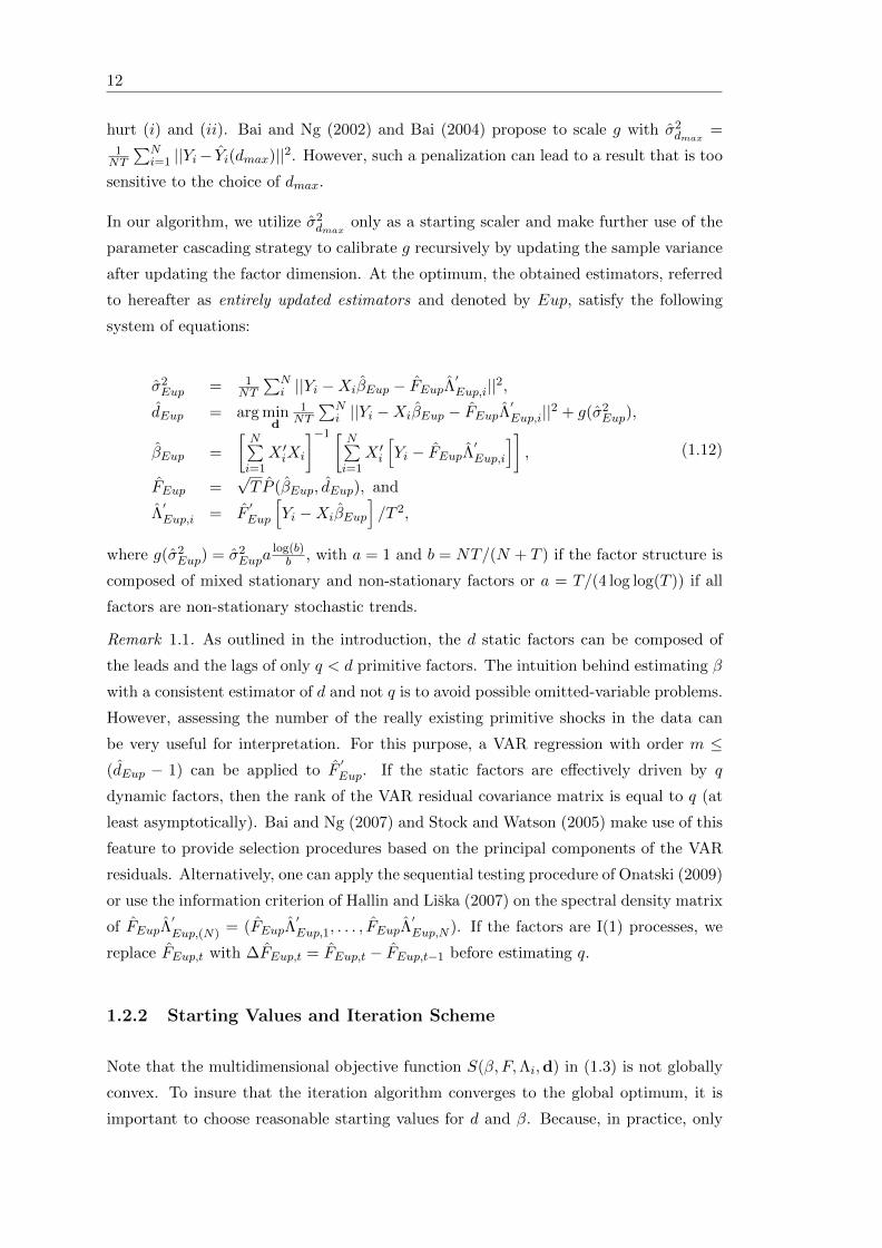
hurt (i) and (ii). Bai and Ng (2002) and Bai (2004) propose to scale g with σ2dmax
=1NT
∑Ni=1 ||Yi− Yi(dmax)||2. However, such a penalization can lead to a result that is too
sensitive to the choice of dmax.
In our algorithm, we utilize σ2dmax
only as a starting scaler and make further use of the
parameter cascading strategy to calibrate g recursively by updating the sample variance
after updating the factor dimension. At the optimum, the obtained estimators, referred
to hereafter as entirely updated estimators and denoted by Eup, satisfy the following
system of equations:
σ2Eup = 1
NT
∑Ni ||Yi −XiβEup − FEupΛ
′Eup,i||2,
dEup = arg mind
1NT
∑Ni ||Yi −XiβEup − FEupΛ
′Eup,i||2 + g(σ2
Eup),
βEup =
[N∑i=1
X ′iXi
]−1 [ N∑i=1
X ′i
[Yi − FEupΛ
′Eup,i
]],
FEup =√T P (βEup, dEup), and
Λ′Eup,i = F
′Eup
[Yi −XiβEup
]/T 2,
(1.12)
where g(σ2Eup) = σ2
Eupalog(b)b , with a = 1 and b = NT/(N + T ) if the factor structure is
composed of mixed stationary and non-stationary factors or a = T/(4 log log(T )) if all
factors are non-stationary stochastic trends.
Remark 1.1. As outlined in the introduction, the d static factors can be composed of
the leads and the lags of only q < d primitive factors. The intuition behind estimating β
with a consistent estimator of d and not q is to avoid possible omitted-variable problems.
However, assessing the number of the really existing primitive shocks in the data can
be very useful for interpretation. For this purpose, a VAR regression with order m ≤(dEup − 1) can be applied to F
′Eup. If the static factors are effectively driven by q
dynamic factors, then the rank of the VAR residual covariance matrix is equal to q (at
least asymptotically). Bai and Ng (2007) and Stock and Watson (2005) make use of this
feature to provide selection procedures based on the principal components of the VAR
residuals. Alternatively, one can apply the sequential testing procedure of Onatski (2009)
or use the information criterion of Hallin and Liska (2007) on the spectral density matrix
of FEupΛ′
Eup,(N) = (FEupΛ′Eup,1, . . . , FEupΛ
′Eup,N ). If the factors are I(1) processes, we
replace FEup,t with ∆FEup,t = FEup,t − FEup,t−1 before estimating q.
1.2.2 Starting Values and Iteration Scheme
Note that the multidimensional objective function S(β, F,Λi,d) in (1.3) is not globally
convex. To insure that the iteration algorithm converges to the global optimum, it is
important to choose reasonable starting values for d and β. Because, in practice, only
Chapter 1. Panel Models with Unknown Number of Unobserved Factors 13
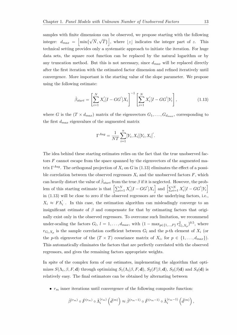
samples with finite dimensions can be observed, we propose starting with the following
integer: dmax =⌊min
√N,√T⌋, where bzc indicates the integer part of z. This
technical setting provides only a systematic approach to initiate the iteration. For huge
data sets, the square root function can be replaced by the natural logarithm or by
any truncation method. But this is not necessary, since dmax will be replaced directly
after the first iteration with the estimated factor dimension and refined iteratively until
convergence. More important is the starting value of the slope parameter. We propose
using the following estimate:
βstart =
[N∑i=1
X′i [I −GG
′]Xi
]−1 [ N∑i=1
X′i [I −GG
′]Yi
], (1.13)
where G is the (T × dmax) matrix of the eigenvectors G1, . . . , Gdmax , corresponding to
the first dmax eigenvalues of the augmented matrix
ΓAug =1
NT
n∑i=1
[Yi, Xi][Yi, Xi]′.
The idea behind these starting estimates relies on the fact that the true unobserved fac-
tors F cannot escape from the space spanned by the eigenvectors of the augmented ma-
trix ΓAug. The orthogonal projection of Xi on G in (1.13) eliminates the effect of a possi-
ble correlation between the observed regressors Xi and the unobserved factors F , which
can heavily distort the value of βstart from the true β if it is neglected. However, the prob-
lem of this starting estimate is that[∑N
i=1X′i [I −GG
′]Xi
]and
[∑Ni=1X
′i [I −GG
′]Yi
]in (1.13) will be close to zero if the observed regressors are the underlying factors, i.e.,
Xi ≈ FΛ′i . In this case, the estimation algorithm can misleadingly converge to an
insignificant estimate of β and compensate for that by estimating factors that origi-
nally exist only in the observed regressors. To overcome such limitation, we recommend
under-scaling the factors Gl, l = 1, . . . , dmax, with (1 − maxp∈1,...,P r2Gl,Xp
)0.5, where
rGl,Xp is the sample correlation coefficient between Gl and the p-th element of Xi (or
the p-th eigenvector of the (T × T ) covariance matrix of Xi, for p ∈ 1, . . . , dmax).This automatically eliminates the factors that are perfectly correlated with the observed
regressors, and gives the remaining factors appropriate weights.
In spite of the complex form of our estimates, implementing the algorithm that opti-
mizes S(Λi, β, F,d) through optimizing S1(Λi|β, F,d), S2(F |β,d), S3(β|d) and S4(d) is
relatively easy. The final estimators can be obtained by alternating between
• rm inner iterations until convergence of the following composite function:
β(rm) F (rm) Λ(rm)i
(d(m)
)≈ β(rm−1) F (rm−1) Λ
(rm−1)i
(d(m)
),

14
for each given d(m), and
• outer iterations until satisfying the following convergence condition:
d(m+1) σ2(m) = d(m) σ2(m−1).
Here, the composite notation cb(z) is defined by c(b(z)) for each z and used to indicate
the application of one estimate on the result of another.
Note that this iteration scheme simplifies the minimization of the dimensionality criterion
(1.9), since d(m+1) can be obtained by
d(m+1) = arg mind
1NT
∑Ni ||Yi −Xiβ
(rm) − F (rm)Λ(rm)i ||2 + dg(σ2(m))
= arg mind
∑Tl=d+1 ρ
(rm)l + dg(σ2(m)),
where ρ(rm)l are the ordered eigenvalues of the covariance matrix (1.6) required to com-
pute F (rm) at the iteration stage rm and
σ2(m) =1
NT
N∑i
||Yi −Xiβ(rm) − F (rm)Λ
(rm)i ||2 =
T∑l=d(m)+1
ρ(rm)l . (1.14)
Selecting d(m+1) reverts therefore to finding the order of the smallest element in the
following set:
A(m) =
T∑
l=d+1
ρ(rm)l + da
log(b)
b
T∑l=d(m)+1
ρ(rm)l
∣∣∣∣∣∣d = 0, 1, . . . , d(m)
. (1.15)
A simple pseudo code that optimizes the entirely updated estimators presented in (1.12),
can be described as follows:
1. Set d(m) =
dmax if m = 0
d(m−1) if m > 0
2. Set β(rm) =
βstart if rm = 0
β(rm−1) if rm > 0
3. Use (1.5) to calculate F (rm) = F (β(rm), d(m))
4. Use (1.4) to calculate Λ(rm)i = Λi(F
(rm), β(rm), d(m))
5. Use (1.8) to update β(rm+1) = β(d(m)) by using F (rm) and Λ(rm)i
6. If β(rm+1) ≈ β(rm), go to 7; else, replace the value of β(rm) with β(rm+1)
and repeat 2 − 6 with (rm + 1) instead of (rm)

Chapter 1. Panel Models with Unknown Number of Unobserved Factors 15
7. Use (1.14) to calculate σ2(m)
8. Select d(m+1) that corresponds to the order of the smallest element in
the set A(m) in (1.15)
9. If d(m+1) = d(m), exit; else, replace the value of d(m) with d(m+1) and
β(rm) with β(rm+1) and go to 1 with (m + 1) instead of (m) and (rm+1 +
1) instead of (rm).
Remark 1.2. We can, of course, use the analytic expression of Λ′Eup,i to write the esti-
mator of β in (1.12) conventionally as
βEup =
[N∑i=1
X ′iMFEupXi
]−1 [ N∑i=1
X ′iMFEupYi
], (1.16)
where MFEup= IT − FEupF
′Eup/T
2. However, implementing the estimation algorithm
with (1.16) may destabilize the convergence of the iteration process, since the update of
the slope estimator, in this case, requires the inversion of the matrix∑N
i=1X′iMFEup
Xi
in each iteration stage and not only at the optimum.
Remark 1.3. In order to speed up the computation when N < T , we can reconstruct the
estimation algorithm with S1(F |Λi, β,d) and S2(Λi|β,d) instead of S1(Λi|F, β,d) and
S2(F |β,d). The benefit of such modification is to calculate the eigenvectors of a smaller
covariance matrix with a dimension (N × N) instead of (T × T ). Both computations
ultimately lead to the same result.
The routines of this method are provided in an R-Package called phtt. For more details
about this package, we refer the reader to the paper of Bada and Liebl (2014b).
1.3 Model Extension and Theoretical Results
1.3.1 Presence of Additional Categorical Variables
Our model assumptions will closely follow the the setup of Bai et al. (2009), who al-
low for mixed stationary and unit root regressors (I(0)/I(1) regressors) as well as mixed
I(0)/I(1) unobserved factors. However, our analysis encounters an additional complica-
tion allowing for model (1.2) to be obtained from transforming an underlying model of
the form:
Y it = Xitβ +K∑k=1
αktδik + FtΛ′i + µt + εit. (1.17)
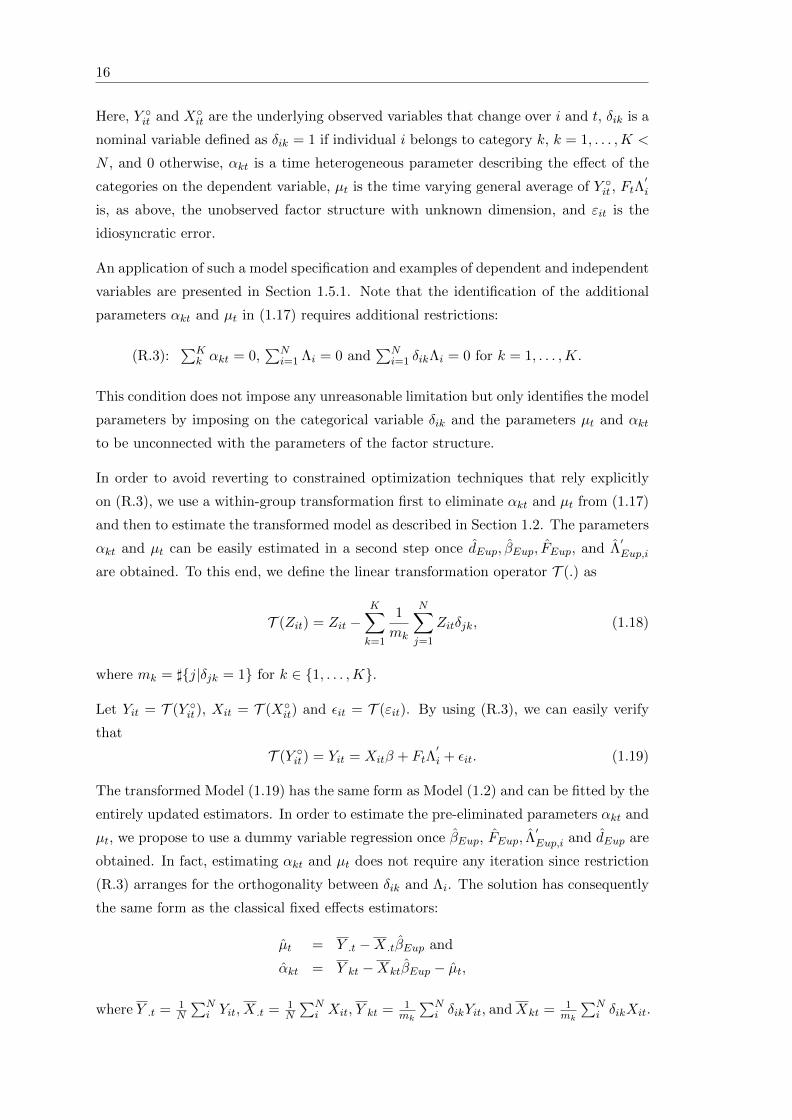
16
Here, Y it and Xit are the underlying observed variables that change over i and t, δik is a
nominal variable defined as δik = 1 if individual i belongs to category k, k = 1, . . . ,K <
N , and 0 otherwise, αkt is a time heterogeneous parameter describing the effect of the
categories on the dependent variable, µt is the time varying general average of Y it , FtΛ′i
is, as above, the unobserved factor structure with unknown dimension, and εit is the
idiosyncratic error.
An application of such a model specification and examples of dependent and independent
variables are presented in Section 1.5.1. Note that the identification of the additional
parameters αkt and µt in (1.17) requires additional restrictions:
(R.3):∑K
k αkt = 0,∑N
i=1 Λi = 0 and∑N
i=1 δikΛi = 0 for k = 1, . . . ,K.
This condition does not impose any unreasonable limitation but only identifies the model
parameters by imposing on the categorical variable δik and the parameters µt and αkt
to be unconnected with the parameters of the factor structure.
In order to avoid reverting to constrained optimization techniques that rely explicitly
on (R.3), we use a within-group transformation first to eliminate αkt and µt from (1.17)
and then to estimate the transformed model as described in Section 1.2. The parameters
αkt and µt can be easily estimated in a second step once dEup, βEup, FEup, and Λ′Eup,i
are obtained. To this end, we define the linear transformation operator T (.) as
T (Zit) = Zit −K∑k=1
1
mk
N∑j=1
Zitδjk, (1.18)
where mk = ]j|δjk = 1 for k ∈ 1, . . . ,K.
Let Yit = T (Y it), Xit = T (Xit) and εit = T (εit). By using (R.3), we can easily verify
that
T (Y it) = Yit = Xitβ + FtΛ′i + εit. (1.19)
The transformed Model (1.19) has the same form as Model (1.2) and can be fitted by the
entirely updated estimators. In order to estimate the pre-eliminated parameters αkt and
µt, we propose to use a dummy variable regression once βEup, FEup, Λ′Eup,i and dEup are
obtained. In fact, estimating αkt and µt does not require any iteration since restriction
(R.3) arranges for the orthogonality between δik and Λi. The solution has consequently
the same form as the classical fixed effects estimators:
µt = Y .t −X .tβEup and
αkt = Y kt −XktβEup − µt,
where Y .t = 1N
∑Ni Yit, X .t = 1
N
∑Ni Xit, Y kt = 1
mk
∑Ni δikYit, andXkt = 1
mk
∑Ni δikXit.

Chapter 1. Panel Models with Unknown Number of Unobserved Factors 17
1.3.2 Assumptions
We now consider inference of (1.19) as (N,T ) → ∞. Here, (N,T ) → ∞ has to be
interpreted as a sequential limit: first T → ∞ and then N → ∞. Throughout, we
denote by M a finite positive constant, not depending on N and T . We use B(.) to
denote a Brownian motion process defined on [0, 1] and bτc to denote the largest integer
≤ τ . We will use β, F t and Λi to respectively denote the true slope parameters, the
true factors (only identifiable up to rotation), and the true loadings parameters. EC(.) is
used to denote conditional expectation given F . For all N , we assume an i.i.d. random
sample of individuals.
Our theoretical setup relies on the following assumptions.
Assumption 1. The observed regressors:
(a) mkN converges a.s. to E(δik) as N →∞, where infk=1,...,K E(δik) > 0.
(b) Let Xitβ = Xit,1β
1 +Xit,2β
2 , where Xit,1 is (1×P1) vector of a I(1) multivariate
process, such that X′it,1 = X
′i,t−1,1 + ζ
′it −
∑Kk=1 δikζ
′kt where ζ
′it is a zero mean
(P1 × 1) stationary vector and ζ′kt = 1
mk
∑Nj=1 δjkζ
′jt. Xit,2 is (1 × P2) vector
of stationary regressors, such that Xit,2 = X′it,2 −
∑Kk=1 δikX
′kt,2 with X
′kt,2 =
1mk
∑Nj=1 δjkX
′jt and EC(Xit,2ζjs) = 0 for all i, j, t and s.
Assumption 2. The unobserved factor structure:
(a) E||Λi ||4 ≤M ; As N →∞, E(Λi δik) = 0 for all k = 1, . . . ,K, and 1N
∑i Λ
′i Λi
p→ΣΛ, a (d× d) positive definite matrix.
(b) F ′
t = F ′
t−1 + η′t, where η
′t is a zero mean random vector with E||η′t||4+γ ≤ M for
some γ > 0 and for all t; As T → ∞, 1T 2
∑t F′t F
t
d→∫B′ηBη, a d × d random
matrix, where Bη is a vector of Brownian motion with a positive definite covariance
matrix Ωη. ηt is independent of Xit,2 for all i, t, k.
(c) lim infT→∞ log log(T )/T 2∑T
t=1 F′t F
t = C, where C is a nonrandom positive def-
inite matrix.
(d) Ft, X∗it,1 are not cointegrated, where X∗′it = X∗
′i,t−1 + ζ∗
′it , t = 2, . . . , T with
X∗′i1 = X
′i1, ζ∗
′it = ζ
′it −
∑Kk=1 δikζ
0′kt, and ζ0′
kt = EC(ζ′kt|δik = 1), k = 1, . . . ,K.

18
Assumption 3. The error terms:
(a) Let εit = εit −∑k
k=1 δikεkt with εkt =∑n
j=11mk
∑nj=1 εjtδjk. Here, εit are zero
mean error terms and EC(εkt|δik = 1) = 0 for all k. Conditional on ηt the error
terms εit are cross-sectionally independent of each other as well as of Xit.
(b) The multivariate processes wit = (εit, ζ∗it, ηt) are stationary. For each i, wit =∑∞
j=0 Πijvi,t−j , where vit = (vεit, vζit, v
ηt ) are mutually independent over i, t as well
as identically distributed over t. Furthermore, E(vit) = 0, E(vitv′it) > 0, and
E(‖vit‖8) ≤ M , where M < ∞ is independent of i, t. In addition, all further
conditions of Assumptions 2. and 3 of Bai et al. (2009) are satisfied.
The additional terms ζkt and εkt in Assumptions 2 and 3 reflect our subtraction of
group means. Assumption 1.a guarantees that the K categories (groups) do not vanish
as N → ∞. Assumption 1.b allows for mixed I(1)/I(0) regressors. As in Bai et al.
(2009), the I(0) regressors are assumed to be exogenous and linearly independent of the
I(1) regressors and the I(1) factors. This is only given for the purpose of simplifying the
analysis and avoiding further complications.
The requirement E(Λi δik) = 0 for all k = 1, . . . ,K, in Assumption 2, is the population
version for our condition (R.3) introduced for identifying αkt. We want to emphasize
that the transformation T (.) only influences the structure of the error terms and the
explanatory variables, but not the factor structure F t Λ′i . Assumptions 2.b and 2.c are
commonly used in the literature of non-stationary factor models with unit roots; see,
e.g., Bai (2004) and Bai et al. (2009). Assumption 2.d is a technical assumption used
to ensure the non-singularity of the long run covariance matrix Ωb,i of (ζ∗′it , η
′t)′. This
allows for estimating the asymptotic bias of the slope estimator.
Assumption 3 excludes cross-section dependencies of εit and ζ∗it conditional on ηt. But
unconditionally, weak cross-section correlations are allowed under Assumptions 3.b of
Bai et al. (2009).
Remark 1.4. Assumption 2 considers the presence of only I(1) factors. But note that the
method is also robust to mixed I(1)/I(0) factors. Bai et al. (2009) argue that, for known
d, the limiting distribution of the slope estimator, in this case, is the same as when
all factors are I(1) (except for small modifications in the expression of the asymptotic
variance). Their arguments should also hold for our extended model.
Remark 1.5. The last part of Assumption 1.b considerably simplifies the analysis of
the asymptotic distributions of the slope parameters. This is because the I(0) and
I(1) regressors are asymptotically orthogonal and their asymptotic distributions can be
separately analyzed: while the estimator of β2 needs no correction and is asymptotically

Chapter 1. Panel Models with Unknown Number of Unobserved Factors 19
normal distributed (see Bai (2009) and Bai et al. (2009)), the estimator of β1 has a
distribution as if there is no I(0) regressors. Note that the aim of separating I(0) and
I(1) variables is to correctly derive the rates of convergence. Bai et al. (2009) argue
that if the ultimate purpose is to perform hypothesis testing, one can proceed as if all
regressors are I(1) since the scaling factor will be canceled out in the end.
Because of Remark 1.5, we can drop from now on the indexes 1 and 2 respectively from
β1 and β2 and focus only on the complicated case, i.e., panel cointegration model with
I(1) regressors and I(1) unobserved factors. This allows us to avoid notational mess in
the remainder of the chapter.
1.3.3 Asymptotic Distribution and Bias Correction
Under Assumptions 1-3, it can be shown that the effects of the model transformation due
to T (.) are asymptotically negligible and that the results of Bai et al. (2009) generalize
to our situation. In particular, the slope estimator β(d) to be obtained for the true
factor dimension d is at least T consistent and has following properties.
Proposition 1.6. Under the above assumptions, we have, as (N,T )→∞,
Σ1/2c
(√NT (β(d)− β)−
√Nφ)
d−→ N(0, Ip),
for some φ and Σc, where β(d) is obtained after transforming Model (1.17) with T (.).
The exact expression of φ and Σc is given in the appendix. Proposition 1.6 shows that
the limiting distribution of√NT (β(d) − β) is not centered at zero. Bai et al. (2009)
prove that it is possible, in such a case, to construct a consistent estimator φNT of the
bias term φ. Following their suggestion, we define our entirely updated and bias corrected
(EupBC ) estimator by
βEupBC = βEup −1
TφNT .
This procedure does require extra work (non-parametrical kernel estimation techniques)
to estimate the long-run and one-sided long-run covariances of wit = (εit, ζ∗it, ηt). The
necessary assumptions and precise formulas for constructing φNT are given in the ap-
pendix. Once βEupBC is obtained, the final bias-corrected estimators of F and Λi are
given by
FEupBC =√T P (βEupBC , dEup), and
Λ′EupBC,i = F
′EupBC
[Yi −XiβEupBC
]/T 2,
respectively.
20
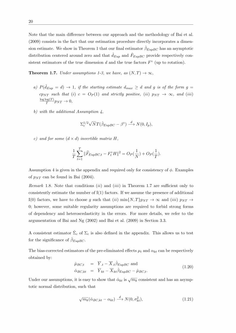
Note that the main difference between our approach and the methodology of Bai et al.
(2009) consists in the fact that our estimation procedure directly incorporates a dimen-
sion estimate. We show in Theorem 1 that our final estimator βEupBC has an asymptotic
distribution centered around zero and that dEup and FEupBC provide respectively con-
sistent estimators of the true dimension d and the true factors F (up to rotation).
Theorem 1.7. Under assumptions 1-3, we have, as (N,T )→∞,
a) P (dEup = d) → 1, if the starting estimate dmax ≥ d and g is of the form g =
cpNT such that (i) c = OP (1) and strictly positive, (ii) pNT → ∞, and (iii)log log(T )
T pNT → 0,
b) with the additional Assumption 4,
Σ1/2c
√NT (βEupBC − β)
d−→ N(0, Ip),
c) and for some (d× d) invertible matrix H,
1
T
T∑t=1
‖FEupBC,t − F t H‖2 = OP (1
N) +OP (
1
T).
Assumption 4 is given in the appendix and required only for consistency of φ. Examples
of pNT can be found in Bai (2004).
Remark 1.8. Note that conditions (ii) and (iii) in Theorem 1.7 are sufficient only to
consistently estimate the number of I(1) factors. If we assume the presence of additional
I(0) factors, we have to choose g such that (ii) minN,TpNT → ∞ and (iii) pNT →0; however, some suitable regularity assumptions are required to forbid strong forms
of dependency and heteroscedasticity in the errors. For more details, we refer to the
argumentation of Bai and Ng (2002) and Bai et al. (2009) in Section 3.3.
A consistent estimator Σc of Σc is also defined in the appendix. This allows us to test
for the significance of βEupBC .
The bias-corrected estimators of the pre-eliminated effects µt and αkt can be respectively
obtained by:
µBC,t = Y .t −X .tβEupBC and
αBC,kt = Y kt −XktβEupBC − µBC,t.(1.20)
Under our assumptions, it is easy to show that αkt is√mk consistent and has an asymp-
totic normal distribution, such that
√mk(αBC,kt − αkt)
d−→ N(0, σ2kt), (1.21)

Chapter 1. Panel Models with Unknown Number of Unobserved Factors 21
where σ2kt = V ar(εkt), with εkt = 1
mk
∑Ni δikεit.
1.4 Monte Carlo Simulations
The goal of this section is to compare, through Monte Carlo experiments, the perfor-
mance of our algorithmic extension with the performance of the iterative least squares
estimators of Bai (2009) and Bai et al. (2009) based on an externally estimated dimen-
sion. In a first step, the feasible slope estimator, β(d), is naively calculated with a high
number of factors (dmax = 8). In a second step, we calculate Wit = Yit−Xitβ(dmax) and
externally estimate the factor dimension by using 5 different criteria: the panel criteria
PC1 and IC1 of Bai and Ng (2002), the panel cointegration criterion IPC1 proposed by
Bai (2004), the threshold criterion ED of Onatski (2010), and the information criterion
ICT1;n of Hallin and Liska (2007). The maximal number of factors used in PC1, IC1,
IPC1, ED, and ICT1;n is also set to 8. The calibration strategy of Hallin and Liska (2007)
(second ”‘stability interval”’ procedure) is applied on a grid interval of length 128 with
the borders 0.01 and 3 as they have suggested. Finally, we re-calculate the two-step iter-
ative least squares estimator with the optimizers of these panel criteria. The estimated
dimensions are denoted by dPC1, dIC1, dIPC1, dED, and dICT1,n, respectively.
Our entirely updated estimator is calculated with the penalty of PC1 as described in
Section 1.2, i.e., g(σEup) = σ2Eup log(NT/(N + T ))(N + T )/NT . The iteration process
is initiated by the starting values described in Section 1.2.2. The bias correction used
for estimating panel cointegration models is based on the linearly decreasing weights of
Newey and West (1987) with a truncation at⌊min
√N,√T⌋. The maximal number
of iterations allowed for the feasible iterated least squares estimators and the two-step
estimators is 100. The inner iteration of the entirely updated estimator is also limited
to 100.
We consider panel models of the form
Yit =P∑p=1
Xpitβp + cd∑l=1
λilflt + εit,
for all i ∈ 1, . . . , N and t ∈ 1, . . . , T, where Xpit are the observed regressors, flt are
the factors to be estimated, λil are the corresponding loading parameters, c controls for
the weight of the factor structure in the model, and εit is the idiosyncratic error term.
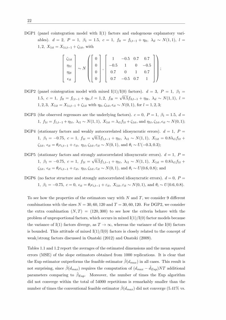
The examined panel sets are the outcomes of 6 different DGPs:
22
DGP1 (panel cointegration model with I(1) factors and endogenous explanatory vari-
ables). d = 2, P = 1, β1 = 1.5, c = 1, flt = fl,t−1 + ηlt, λil ∼ N(1, 1), l =
1, 2, X1it = X1i,t−1 + ζ1it, withζ1it
η1t
η2t
εit
∼ N
0
0
0
0
,
1 −0.5 0.7 0.7
−0.5 1 0 −0.5
0.7 0 1 0.7
0.7 −0.5 0.7 1
;
DGP2 (panel cointegration model with mixed I(1)/I(0) factors). d = 3, P = 1, β1 =
1.5, c = 1, flt = fl,t−1 + ηlt, l = 1, 2, f3t =√
0.5f3,t−1 + η3t, λil ∼ N(1, 1), l =
1, 2, 3, X1it = X1i,t−1 + ζ1it with ηlt, ζ1it, εit ∼ N(0, 1), for l = 1, 2, 3;
DGP3 (the observed regressors are the underlying factors). c = 0, P = 1, β1 = 1.5, d =
1, f1t = f1,t−1 + η1t, λi1 ∼ N(1, 1), X1it = λi1f1t + ζ1it, and η1t, ζ1it, εit ∼ N(0, 1);
DGP4 (stationary factors and weakly autocorrelated idiosyncratic errors). d = 1, P =
1, β1 = −0.75, c = 1, f1t =√
0.5f1,t−1 + η1t, λi1 ∼ N(1, 1), X1it = 0.8λi1f1t +
ζ1it, εit = θiεi,t−1 + εit, η1t, ζ1it, εit ∼ N(0, 1), and θi ∼ U(−0.3, 0.3);
DGP5 (stationary factors and strongly autocorrelated idiosyncratic errors). d = 1, P =
1, β1 = −0.75, c = 1, f1t =√
0.5f1,t−1 + η1t, λi1 ∼ N(1, 1), X1it = 0.8λi1f1t +
ζ1it, εit = θiεi,t−1 + εit, η1t, ζ1it, εit ∼ N(0, 1), and θi ∼ U(0.6, 0.8); and
DGP6 (no factor structure and strongly autocorrelated idiosyncratic errors). d = 0, P =
1, β1 = −0.75, c = 0, εit = θiεi,t−1 + εit, X1it, εit ∼ N(0, 1), and θi ∼ U(0.6, 0.8).
To see how the properties of the estimators vary with N and T , we consider 9 different
combinations with the sizes N = 30, 60, 120 and T = 30, 60, 120. For DGP2, we consider
the extra combination (N,T ) = (120, 300) to see how the criteria behave with the
problem of unproportional factors, which occurs in mixed I(1)/I(0) factor models because
the variance of I(1) factors diverge, as T →∞, whereas the variance of the I(0) factors
is bounded. This attitude of mixed I(1)/I(0) factors is closely related to the concept of
weak/strong factors discussed in Onatski (2012) and Onatski (2009).
Tables 1.1 and 1.2 report the averages of the estimated dimensions and the mean squared
errors (MSE) of the slope estimators obtained from 1000 replications. It is clear that
the Eup estimator outperforms the feasible estimator β(dmax) in all cases. This result is
not surprising, since β(dmax) requires the computation of (dmax − dEup)NT additional
parameters comparing to βEup. Moreover, the number of times the Eup algorithm
did not converge within the total of 54000 repetitions is remarkably smaller than the
number of times the conventional feasible estimator β(dmax) did not converge (5.41% vs.

Chapter 1. Panel Models with Unknown Number of Unobserved Factors 23
42.22%). The reason for this outcome is that the naive over-specification of the factor
dimension downgrades the degree of freedom available to estimate the slope parameters.
The alternation between inner and outer iterations, in our algorithm, seems, hence, to
provide a way to stabilize the numerical optimization of the objective function if d is
not well-specified.
Tables 1.1 and 1.2 reveal that PC1 has a tendency to overestimate the true dimension
if N and/or T are not large enough (30, 60). This is also the case for IPC1 when the
factors to be estimated are I(1). The IC1 criterion seems to be more robust than PC1.
This is because the penalty of IC1 is less sensitive to the scaling effect; see Bai and Ng
(2002). The results of our Monte Carlo experiments show that integrating the penalty
term of PC1 in the objective function and calibrating the hight of the penalization as
described in Section 1.2 provides a gain over the original PC1, IC1, and IPC1.
DGP1 (I(1) factors and endogenous explanatory variables) The simulation
results for DGP1 (reported in the first part of Table 1.1) show that dEupPC1 gives a
very precise estimation of the factor dimension and outperforms PC1, IPC1, IC1, ED,
and ICT1,n. In contrast to all other criteria, ED gets worse as N and T increase. This
weakness can be related to the strong endogeneity of the explanatory variables. For
(N,T ) = (120, 120), the MSEs of βEupBC , β(dIPC1), and β(dIC1T1,n) converge to 0. This
is not surprising since our estimation strategy and the original method of Bai et al.
(2009) used with dmax ≥ d (or with a consistent external dimensionality criterion) will
produce very close outcomes in terms of MSE when both N and T are large enough.
The problem, of course, is that the required sizes of N and T ensuring such evidence
are unknown in practice. Note also that the outcomes of β(dIPC1) are conditional on
dmax = 8 and β(dIPC1) can be used only when the d static factors are not driven by
the lags of a smaller number of dynamic factors. Such limitations are overcome by our
method.
DGP2 (mixed I(1)/I(0) factors) The results of this experiment are reported in the
second part of Table 1.1. The best estimation is obtained with dEupPC1. IPC1 has a
tendency to overestimate the true number of I(1) factors, especially when N increases
and T is fixed. In contrast, ED and ICT1,n behave properly in such a case. Otherwise,
both ED and ICT1,n get slowly worse as T increases and N is fixed ((dED, dICT1,n) =
(2.99, 3), (2.98, 2.98), (2.85, 82) for (N,T ) = (120, 60), (120, 120), and (120, 300) respec-
tively). PC1 and IC1 also show a tendency to underestimate the factor dimension. The
reason these criteria estimate, on average, a smaller dimension than dEupPC1 (although
dEupPC1 is obtained by strengthening iteratively the same penalty) is that the start-
ing estimate of d in our algorithm depends on the sample size and is larger than 8 for
24
(N,T ) = (120, 120) and (120, 300). Unexpectedly, when (N,T ) = (120, 300), the MSEs
of all β estimators are larger than those obtained with smaller sample sizes. This result
can be explained by the occurrence of two effects when N is fixed and T is relatively large:
the first effect is related to the problem of mixed strong/weak factors, which can lead to
underestimate the number of I(0) factors since the proportion of the variance explained
by the I(1) factors gets much larger than the proportion of the variance explained by the
I(0) factors when T grows faster than N . Indeed, the worst MSE affiliates with IPC1,
which has, on average, the smallest estimate for d when N = 120 and T = 300; the
second effect is related to the inefficiency of estimating a bias that does not exist since
the factors and the regressors are exogenous in DGP2. Recall that the bias estimator is
the average of N individual bias estimates and converges proportionally to N .
DGP3 (the observed regressor is the underlying factor) The last two parts of
Table 1.1 present the estimation results of DGP3 obtained by initiating the iterations
with two different starting estimates of β: the first estimate is βstart expressed in (1.13);
the second estimate is obtained by scaling the factors Gl, l = 1, . . . , dmax in (1.13)
with (1 − r2Gl,X1
)0.5, where rGl,X1 is the sample correlation coefficient between Gl and
X1i, as described Section 1.2.2. The goal of examining DGP3 is only to test whether
the calibration of the starting factors Gl in (1.13) will enhance the effectiveness of the
estimation algorithm to correctly specify the model. The answer that can be deciphered
from the table is: Yes!
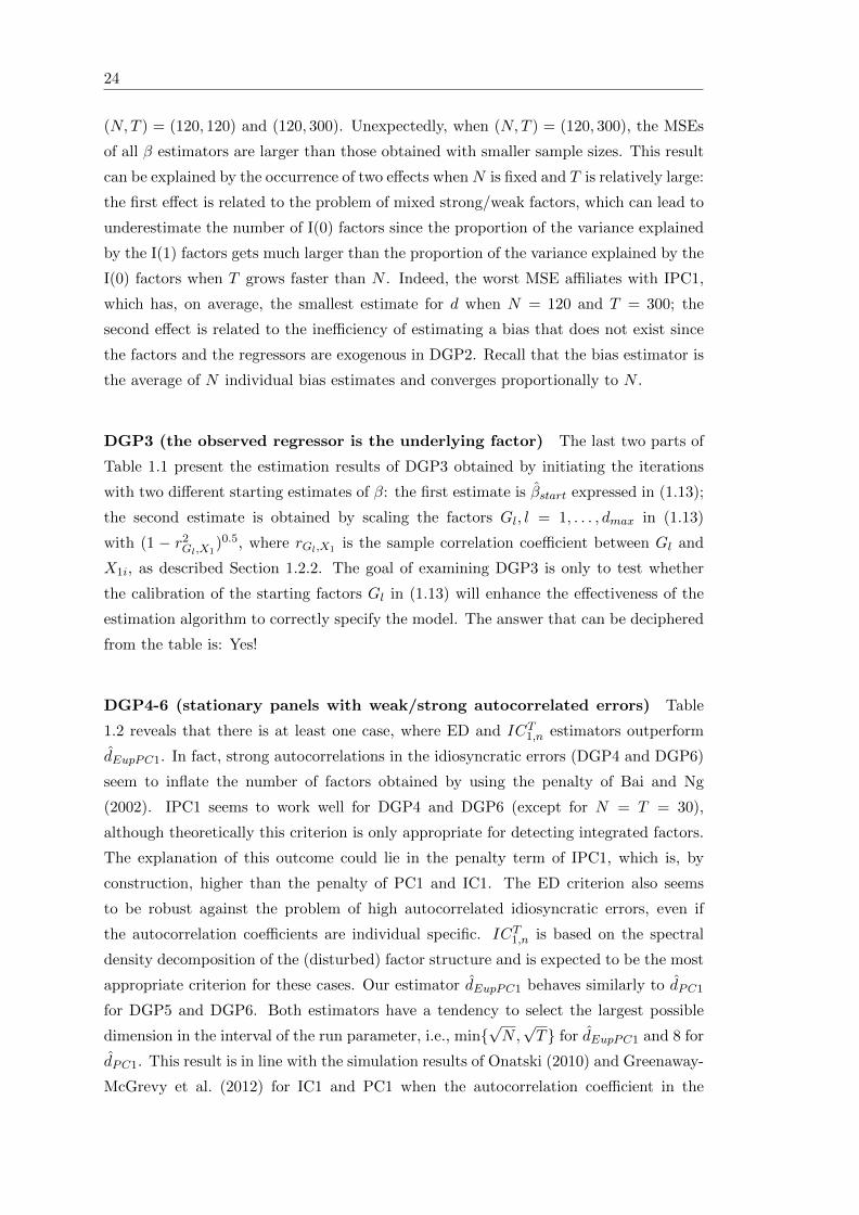
DGP4-6 (stationary panels with weak/strong autocorrelated errors) Table
1.2 reveals that there is at least one case, where ED and ICT1,n estimators outperform
dEupPC1. In fact, strong autocorrelations in the idiosyncratic errors (DGP4 and DGP6)
seem to inflate the number of factors obtained by using the penalty of Bai and Ng
(2002). IPC1 seems to work well for DGP4 and DGP6 (except for N = T = 30),
although theoretically this criterion is only appropriate for detecting integrated factors.
The explanation of this outcome could lie in the penalty term of IPC1, which is, by
construction, higher than the penalty of PC1 and IC1. The ED criterion also seems
to be robust against the problem of high autocorrelated idiosyncratic errors, even if
the autocorrelation coefficients are individual specific. ICT1,n is based on the spectral
density decomposition of the (disturbed) factor structure and is expected to be the most
appropriate criterion for these cases. Our estimator dEupPC1 behaves similarly to dPC1
for DGP5 and DGP6. Both estimators have a tendency to select the largest possible
dimension in the interval of the run parameter, i.e., min√N,√T for dEupPC1 and 8 for
dPC1. This result is in line with the simulation results of Onatski (2010) and Greenaway-
McGrevy et al. (2012) for IC1 and PC1 when the autocorrelation coefficient in the

Chapter 1. Panel Models with Unknown Number of Unobserved Factors 25
idiosyncratic errors is large (e.g., ≥ 0.7). In fact, Assumption C in Bai and Ng (2002)
forbid strong forms of correlation and heteroskedasticity in the error term. The Monte
Carlo experiments of Bai and Ng (2002) consider only cases in which the correlation
coefficient is smaller or equal to 0.5. Note that such a limitation is not necessary if the
factors are I(1). This is because we can replace a = 1 with a = T/(4 log log T ) in the
penalty term. The latter will diverge with N and T and dominate asymptotically any
Op(1) structure in the idiosyncratic errors.
Finally, we want to emphasize that the goal of estimating panel models with unobserved
common factors is not only to assess the dimension of the factor structure but also
to efficiently estimate the slope parameters. Inspection of the MSE values reported in
the second and third part of Table 1.2 shows that βEup does not suffer from an over-
parameterization effect when the errors are strongly autocorrelated and the factors are
over estimated. The additional factors seem to compensate for the unparameterized
linear dependency in the idiosyncratic term. From the second and third part of Table
1.2, we can see that, for (N,T ) = (60, 60), the MSE of βEup is smaller than the MSEs of
β(dIPC1), β(dED), and β(dICT1,n). The first part of Table 1.2 shows that all criteria be-
have very well when the autocorrelation in the idiosyncratic errors is weak, in particular,
dEupPC1, dIC1, and dICT1,n.
The Monte Carlo experiments show that, in many configurations of the data, our algo-
rithmic refinement provides more efficient estimates in terms of MSE for the estimator
of β than those that can be achieved if the feasible iterative least squares estimator is
calculated with an externally selected factor dimension. Moreover, our results show that
the iterative calibration of the penalty term makes the criteria of Bai and Ng (2002)
more robust in a practical context, especially when N and/or T are small. If the id-
iosyncratic errors are strongly autocorrelated, the number of stationary factors will be
overestimated but without affecting the efficiency of the slope estimator.

26
MEAN MEAN MEAN MEAN MEAN MEAN MSE MSE MSE MSE MSE MSE MSE
N T dEupPC1 dPC1 dIC1 dIPC1 dED dICT1,nβEupBC β(dmax) β(dPC1) β(dIC1) β(dIPC1) β(dED) β(dICT1,n
)
DGP1: panel cointegration model with I(1) factors and endogenous explanatory variables (d = 2)30 30 2.05 6.53 2.62 2.15 2.49 3.35 0.001 0.023 0.021 0.007 0.003 0.006 0.00630 60 2.00 3.87 2.11 2.01 2.10 2.00 0.000 0.003 0.002 0.001 0.000 0.001 0.00030 120 2.00 2.07 2.02 2.00 2.03 2.00 0.000 0.001 0.000 0.000 0.000 0.000 0.00060 30 2.02 4.94 3.37 2.48 3.24 2.18 0.001 0.068 0.052 0.023 0.006 0.020 0.00160 60 2.00 3.80 3.30 2.20 3.28 2.03 0.000 0.028 0.009 0.005 0.001 0.005 0.00060 120 2.00 2.55 2.38 2.00 2.43 2.00 0.000 0.002 0.000 0.000 0.000 0.000 0.000
120 30 2.02 4.61 3.77 2.74 3.65 2.46 0.001 0.104 0.070 0.040 0.009 0.036 0.004120 60 2.00 4.60 4.14 2.65 4.02 2.15 0.000 0.063 0.025 0.017 0.002 0.016 0.000120 120 2.00 4.29 4.02 2.25 4.03 2.10 0.000 0.023 0.005 0.004 0.000 0.004 0.000
DGP2: panel cointegration with mixed I(1)/I(0) factors: 1 I(1) factor and 2 I(0) factors (d = 3)30 30 3.08 6.45 3.00 2.92 2.97 4.52 0.002 0.022 0.012 0.002 0.006 0.006 0.01030 60 3.00 4.14 2.99 2.46 2.97 2.98 0.001 0.052 0.013 0.006 0.040 0.009 0.00830 120 3.00 2.98 2.94 1.68 2.92 2.94 0.014 0.260 0.059 0.076 0.263 0.080 0.07560 30 3.00 4.15 3.00 2.95 2.98 3.00 0.001 0.004 0.001 0.001 0.002 0.003 0.00160 60 3.00 3.00 3.00 2.61 2.98 2.99 0.001 0.029 0.003 0.004 0.029 0.006 0.00560 120 3.00 2.98 2.96 1.90 2.95 2.95 0.011 0.177 0.042 0.058 0.190 0.056 0.061
120 30 3.00 3.00 3.00 2.96 2.98 3.00 0.000 0.003 0.000 0.000 0.002 0.002 0.000120 60 3.00 3.00 3.00 2.80 2.99 3.00 0.000 0.020 0.000 0.000 0.019 0.003 0.001120 120 3.00 2.99 2.99 2.16 2.98 2.98 0.007 0.099 0.020 0.023 0.127 0.023 0.025120 300 3.00 2.87 2.84 1.33 2.85 2.82 0.160 0.941 0.446 0.461 0.978 0.441 0.444
DGP3: the observed regressors are the underlying factors (naive starting slope estimate)30 30 1.01 6.18 1.00 1.00 1.00 1.84 4.679 4.681 4.681 4.679 4.679 4.679 4.68060 60 1.00 1.02 1.00 1.00 1.00 1.00 4.693 4.693 4.693 4.693 4.693 4.693 4.693
120 120 1.00 1.00 1.00 1.00 1.00 1.00 4.693 4.693 4.693 4.693 4.693 4.693 4.693
DGP3: the observed regressors are the underlying factors (calibrated starting slope estimate)30 30 0.01 6.12 0.01 0.00 0.01 7.74 0.00 0.001 0.000 0.000 0.000 0.000 0.00030 120 0.00 0.30 0.00 0.00 0.00 0.00 0.00 0.000 0.000 0.000 0.000 0.000 0.000
120 120 0.00 0.00 0.00 0.00 0.00 0.00 0.00 0.000 0.000 0.000 0.000 0.000 0.000
Table 1.1: Simulation results for DGP1 - DGP3. The entries are the averages of the estimated dimensions and the MSEs of the slope estimatorover 1000 replications.
Chap
ter1.
Pan
elM
odels
with
Un
know
nN
um
berof
Un
observed
Facto
rs27
MEAN MEAN MEAN MEAN MEAN MEAN MSE MSE MSE MSE MSE MSE MSE
N T dEupPC1 dPC1 dIC1 dIPC1 dED dICT1,nβEup β(dmax) β(dPC1) β(dIC1) β(dIPC1) β(dED) β(dICT1,n
)
DGP4: 3 stationary factors and weak autocorrelations in the errors (d = 3)30 30 3.07 6.53 3.01 2.94 2.98 4.81 0.001 0.004 0.003 0.001 0.006 0.007 0.00230 60 3.00 4.18 3.00 2.80 2.97 3.00 0.001 0.001 0.001 0.001 0.036 0.011 0.00130 120 3.00 3.01 3.00 2.20 2.97 3.00 0.000 0.000 0.000 0.000 0.242 0.014 0.00060 30 3.00 4.21 3.00 2.97 2.98 3.00 0.001 0.001 0.001 0.001 0.003 0.008 0.00160 60 3.00 3.00 3.00 2.93 2.98 3.00 0.000 0.000 0.000 0.000 0.011 0.008 0.00060 120 3.00 3.00 3.00 2.57 2.96 3.00 0.000 0.000 0.000 0.000 0.121 0.019 0.000
120 30 3.00 3.01 3.00 2.98 2.97 3.00 0.000 0.001 0.000 0.000 0.002 0.010 0.000120 60 3.00 3.00 3.00 2.97 2.98 3.00 0.000 0.000 0.000 0.000 0.005 0.010 0.000120 120 3.00 3.00 3.00 2.91 2.95 3.00 0.000 0.000 0.000 0.000 0.021 0.023 0.000
DGP5: 1 stationary factor and strong autocorrelations in the errors (d = 1)30 30 5.00 7.97 7.71 1.97 1.94 6.56 0.002 0.002 0.002 0.002 0.002 0.002 0.00230 60 4.93 7.80 6.47 1.00 1.04 1.39 0.001 0.001 0.001 0.001 0.001 0.001 0.00130 120 2.83 6.64 1.68 0.97 1.00 1.08 0.001 0.001 0.001 0.001 0.012 0.001 0.00160 30 5.00 7.97 7.81 1.68 1.57 2.00 0.001 0.001 0.001 0.001 0.001 0.001 0.00160 60 7.88 7.90 7.49 1.00 1.00 1.09 0.000 0.000 0.000 0.000 0.001 0.001 0.00160 120 4.46 6.59 2.67 1.00 1.00 1.00 0.000 0.000 0.000 0.000 0.002 0.000 0.000
120 30 5.00 7.99 7.94 1.53 1.25 2.75 0.000 0.000 0.000 0.000 0.001 0.001 0.000120 60 8.00 8.00 7.98 1.00 1.00 1.06 0.000 0.000 0.000 0.000 0.000 0.000 0.000120 120 8.82 7.62 6.24 1.00 1.00 1.00 0.000 0.000 0.000 0.000 0.000 0.000 0.000
DGP6: no factors and strong autocorrelations in the errors (d = 0)30 30 4.99 7.94 7.54 1.48 0.71 7.51 0.002 0.002 0.002 0.002 0.002 0.002 0.00230 60 4.83 7.72 5.62 0.00 0.03 1.09 0.001 0.001 0.001 0.001 0.001 0.001 0.00130 120 1.79 6.42 0.57 0.00 0.00 0.17 0.001 0.001 0.001 0.001 0.001 0.001 0.00160 30 5.00 7.93 7.65 1.17 0.27 2.14 0.001 0.001 0.001 0.001 0.001 0.001 0.00160 60 7.77 7.83 7.16 0.00 0.01 0.95 0.000 0.000 0.000 0.000 0.001 0.001 0.00160 120 3.23 6.34 1.51 0.00 0.00 0.01 0.000 0.000 0.000 0.000 0.000 0.000 0.000
120 30 5.00 7.98 7.87 1.07 0.07 2.64 0.000 0.000 0.000 0.000 0.000 0.001 0.000120 60 7.99 7.99 7.94 0.00 0.00 0.62 0.000 0.000 0.000 0.000 0.000 0.000 0.000120 120 8.11 7.44 5.47 0.00 0.00 0.00 0.000 0.000 0.000 0.000 0.000 0.000 0.000
Table 1.2: Simulation results for DGP4 - DGP6. The entries are the averages of the estimated dimensions and the MSEs of the slope estimatorover 1000 replications.
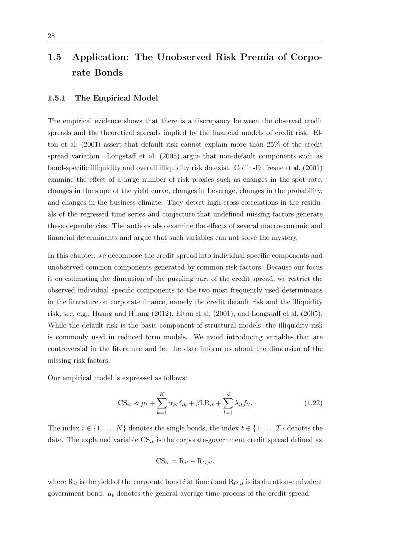
28
1.5 Application: The Unobserved Risk Premia of Corpo-
rate Bonds
1.5.1 The Empirical Model
The empirical evidence shows that there is a discrepancy between the observed credit
spreads and the theoretical spreads implied by the financial models of credit risk. El-
ton et al. (2001) assert that default risk cannot explain more than 25% of the credit
spread variation. Longstaff et al. (2005) argue that non-default components such as
bond-specific illiquidity and overall illiquidity risk do exist. Collin-Dufresne et al. (2001)
examine the effect of a large number of risk proxies such as changes in the spot rate,
changes in the slope of the yield curve, changes in Leverage, changes in the probability,
and changes in the business climate. They detect high cross-correlations in the residu-
als of the regressed time series and conjecture that undefined missing factors generate
these dependencies. The authors also examine the effects of several macroeconomic and
financial determinants and argue that such variables can not solve the mystery.
In this chapter, we decompose the credit spread into individual specific components and
unobserved common components generated by common risk factors. Because our focus
is on estimating the dimension of the puzzling part of the credit spread, we restrict the
observed individual specific components to the two most frequently used determinants
in the literature on corporate finance, namely the credit default risk and the illiquidity
risk; see, e.g., Huang and Huang (2012), Elton et al. (2001), and Longstaff et al. (2005).
While the default risk is the basic component of structural models, the illiquidity risk
is commonly used in reduced form models. We avoid introducing variables that are
controversial in the literature and let the data inform us about the dimension of the
missing risk factors.
Our empirical model is expressed as follows:
CSit ≈ µt +K∑k=1
αktδik + βLRit +d∑l=1
λilflt. (1.22)
The index i ∈ 1, . . . , N denotes the single bonds, the index t ∈ 1, . . . , T denotes the
date. The explained variable CSit is the corporate-government credit spread defined as
CSit = Rit − RG,it,
where Rit is the yield of the corporate bond i at time t and RG,it is its duration-equivalent
government bond. µt denotes the general average time-process of the credit spread.

Chapter 1. Panel Models with Unknown Number of Unobserved Factors 29
Following many previous studies, we consider the rating class (or rating level) to be a
measure for assessing the credit default risk; see, e.g., Gebhardt et al. (2005), Houweling
et al. (2005), and Kagraoka (2010). In fact, the rating class constitutes the synthetic
evaluation of the rating agencies, that takes into account the default probability as well
as the recovery rate. In our model, this proxy is presented by the delta function δik,
which we define as:
δik =
1 if bond i has the rating class k and
0 else.
In order to focus on the unobserved systematic risk premia, we follow Kagraoka (2010)
and consider only bonds that did not experience a rating migration during the observa-
tion period. Unlike most existing work, we allow for time-varying rating effects αkt. This
establishes a general framework that enables us to assess the response of the investors
over time to the credit evaluation of the rating agency.
The explanatory variable LRit measures the illiquidity risk of bond i at time t. Because
the trading frequency of corporate bonds is generally low, arbitrage theory implies that
the price of illiquidity will be reflected in the bond yield. In the literature, several
proxies of illiquidity have been considered; see, e.g., Chen et al. (2002), Bessembinder
et al. (2006), Houweling et al. (2005), and Lesmond (1999). Following Bessembinder
et al. (2006), we construct a measure based on the following quoted bid-ask spread:
LRit =
∣∣∣∣RAit − RB
it
RBit
∣∣∣∣× 100,
where RAit and RB
it are the ask yield and the bid yield of bond i at time t. It is easy
to realize that the larger the spread is, the more problematic the immediate trading
becomes and vice versa. We expect the credit spread to be larger for less liquid bonds.
Because this relationship can be generalized across all corporate bonds, we assume the
slope parameter β to be cross-sectionally homogeneous. Moreover, assuming β to be
constant over i and t not only simplifies the economic interpretation, but also greatly
improves the asymptotic property of its estimator.
The term flt represents the stochastic process describing the time pattern of the under-
lying common risk factors. We may interpret flt as systematic risks, since they do not
depend on i. The scores λil are the corresponding individual loading parameters describ-
ing the effect of flt on each bond i. Like Kagraoka (2010), we interpret the interaction
between λil and flt as the systematic risk premium imposed by the investor on bond i
at time t.
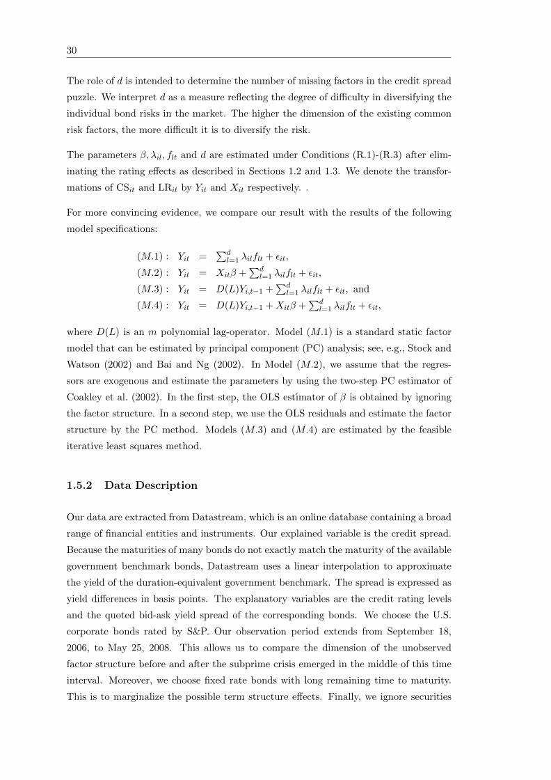
30
The role of d is intended to determine the number of missing factors in the credit spread
puzzle. We interpret d as a measure reflecting the degree of difficulty in diversifying the
individual bond risks in the market. The higher the dimension of the existing common
risk factors, the more difficult it is to diversify the risk.
The parameters β, λil, flt and d are estimated under Conditions (R.1)-(R.3) after elim-
inating the rating effects as described in Sections 1.2 and 1.3. We denote the transfor-
mations of CSit and LRit by Yit and Xit respectively. .
For more convincing evidence, we compare our result with the results of the following
model specifications:
(M.1) : Yit =∑d
l=1 λilflt + εit,
(M.2) : Yit = Xitβ +∑d
l=1 λilflt + εit,
(M.3) : Yit = D(L)Yi,t−1 +∑d
l=1 λilflt + εit, and
(M.4) : Yit = D(L)Yi,t−1 +Xitβ +∑d
l=1 λilflt + εit,
where D(L) is an m polynomial lag-operator. Model (M.1) is a standard static factor
model that can be estimated by principal component (PC) analysis; see, e.g., Stock and
Watson (2002) and Bai and Ng (2002). In Model (M.2), we assume that the regres-
sors are exogenous and estimate the parameters by using the two-step PC estimator of
Coakley et al. (2002). In the first step, the OLS estimator of β is obtained by ignoring
the factor structure. In a second step, we use the OLS residuals and estimate the factor
structure by the PC method. Models (M.3) and (M.4) are estimated by the feasible
iterative least squares method.
1.5.2 Data Description
Our data are extracted from Datastream, which is an online database containing a broad
range of financial entities and instruments. Our explained variable is the credit spread.
Because the maturities of many bonds do not exactly match the maturity of the available
government benchmark bonds, Datastream uses a linear interpolation to approximate
the yield of the duration-equivalent government benchmark. The spread is expressed as
yield differences in basis points. The explanatory variables are the credit rating levels
and the quoted bid-ask yield spread of the corresponding bonds. We choose the U.S.
corporate bonds rated by S&P. Our observation period extends from September 18,
2006, to May 25, 2008. This allows us to compare the dimension of the unobserved
factor structure before and after the subprime crisis emerged in the middle of this time
interval. Moreover, we choose fixed rate bonds with long remaining time to maturity.
This is to marginalize the possible term structure effects. Finally, we ignore securities
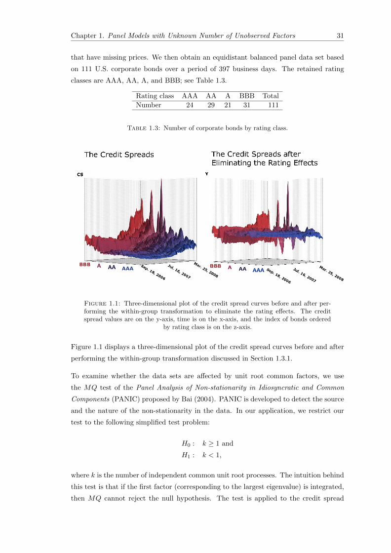
Chapter 1. Panel Models with Unknown Number of Unobserved Factors 31
that have missing prices. We then obtain an equidistant balanced panel data set based
on 111 U.S. corporate bonds over a period of 397 business days. The retained rating
classes are AAA, AA, A, and BBB; see Table 1.3.
Rating class AAA AA A BBB Total
Number 24 29 21 31 111
Table 1.3: Number of corporate bonds by rating class.
Figure 1.1: Three-dimensional plot of the credit spread curves before and after per-forming the within-group transformation to eliminate the rating effects. The creditspread values are on the y-axis, time is on the x-axis, and the index of bonds ordered
by rating class is on the z-axis.
Figure 1.1 displays a three-dimensional plot of the credit spread curves before and after
performing the within-group transformation discussed in Section 1.3.1.
To examine whether the data sets are affected by unit root common factors, we use
the MQ test of the Panel Analysis of Non-stationarity in Idiosyncratic and Common
Components (PANIC) proposed by Bai (2004). PANIC is developed to detect the source
and the nature of the non-stationarity in the data. In our application, we restrict our
test to the following simplified test problem:
H0 : k ≥ 1 and
H1 : k < 1,
where k is the number of independent common unit root processes. The intuition behind
this test is that if the first factor (corresponding to the largest eigenvalue) is integrated,
then MQ cannot reject the null hypothesis. The test is applied to the credit spread
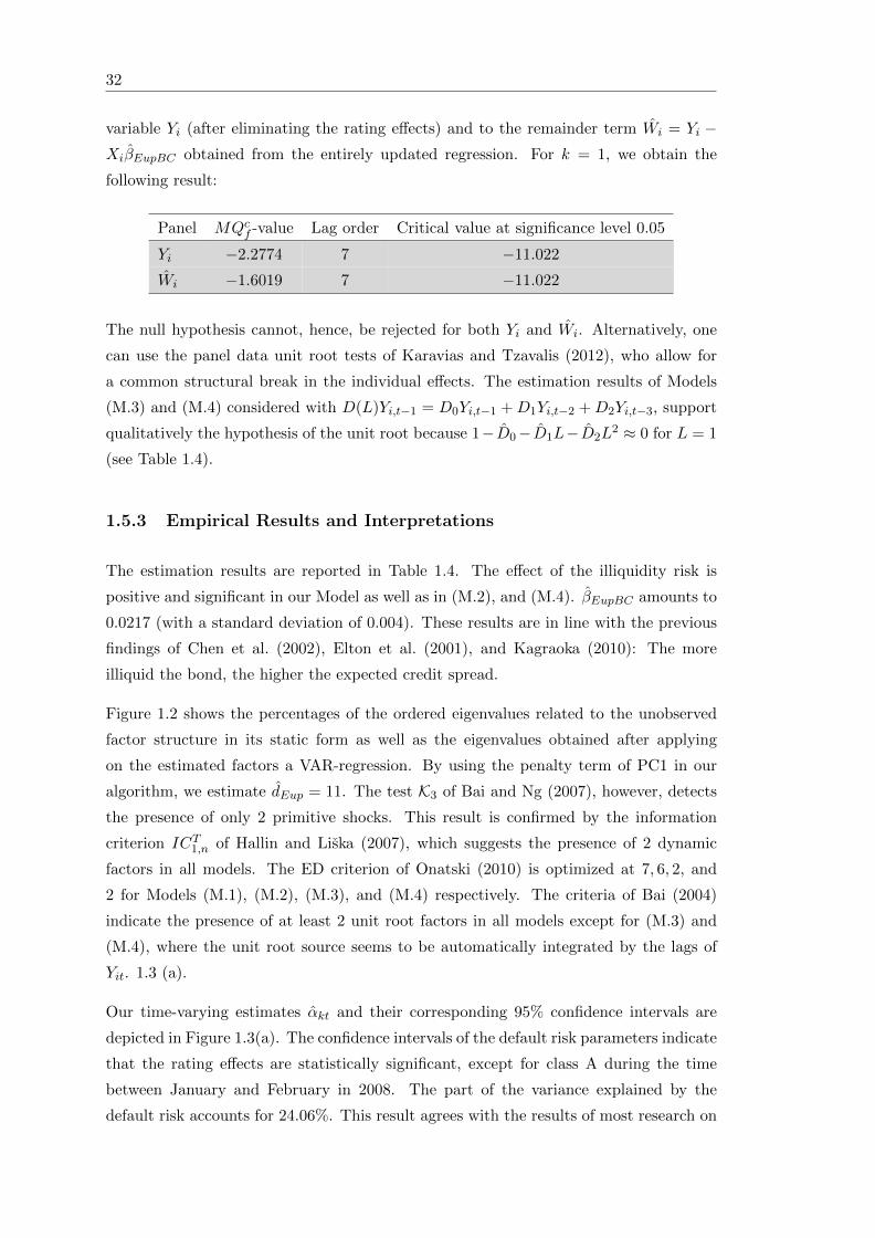
32
variable Yi (after eliminating the rating effects) and to the remainder term Wi = Yi −XiβEupBC obtained from the entirely updated regression. For k = 1, we obtain the
following result:
Panel MQcf -value Lag order Critical value at significance level 0.05
Yi −2.2774 7 −11.022
Wi −1.6019 7 −11.022
The null hypothesis cannot, hence, be rejected for both Yi and Wi. Alternatively, one
can use the panel data unit root tests of Karavias and Tzavalis (2012), who allow for
a common structural break in the individual effects. The estimation results of Models
(M.3) and (M.4) considered with D(L)Yi,t−1 = D0Yi,t−1 +D1Yi,t−2 +D2Yi,t−3, support
qualitatively the hypothesis of the unit root because 1− D0− D1L− D2L2 ≈ 0 for L = 1
(see Table 1.4).
1.5.3 Empirical Results and Interpretations
The estimation results are reported in Table 1.4. The effect of the illiquidity risk is
positive and significant in our Model as well as in (M.2), and (M.4). βEupBC amounts to
0.0217 (with a standard deviation of 0.004). These results are in line with the previous
findings of Chen et al. (2002), Elton et al. (2001), and Kagraoka (2010): The more
illiquid the bond, the higher the expected credit spread.
Figure 1.2 shows the percentages of the ordered eigenvalues related to the unobserved
factor structure in its static form as well as the eigenvalues obtained after applying
on the estimated factors a VAR-regression. By using the penalty term of PC1 in our
algorithm, we estimate dEup = 11. The test K3 of Bai and Ng (2007), however, detects
the presence of only 2 primitive shocks. This result is confirmed by the information
criterion ICT1,n of Hallin and Liska (2007), which suggests the presence of 2 dynamic
factors in all models. The ED criterion of Onatski (2010) is optimized at 7, 6, 2, and
2 for Models (M.1), (M.2), (M.3), and (M.4) respectively. The criteria of Bai (2004)
indicate the presence of at least 2 unit root factors in all models except for (M.3) and
(M.4), where the unit root source seems to be automatically integrated by the lags of
Yit. 1.3 (a).
Our time-varying estimates αkt and their corresponding 95% confidence intervals are
depicted in Figure 1.3(a). The confidence intervals of the default risk parameters indicate
that the rating effects are statistically significant, except for class A during the time
between January and February in 2008. The part of the variance explained by the
default risk accounts for 24.06%. This result agrees with the results of most research on

Chapter 1. Panel Models with Unknown Number of Unobserved Factors 33
Figure 1.2: (a) The screeplot of the eigenvalues obtained from the matrix of
Σ(βCupBC , dEup); (b) Proportions of the (squared) eigenvalues obtained from the resid-uals of the VAR-regression (with p = 1) applied on the estimated factors (after inte-
grating the first 3 I(1) factors).
Figure 1.3: (a) the time series of the estimated rating effects; (b) the EupBC estimatedfirst and second common factors.
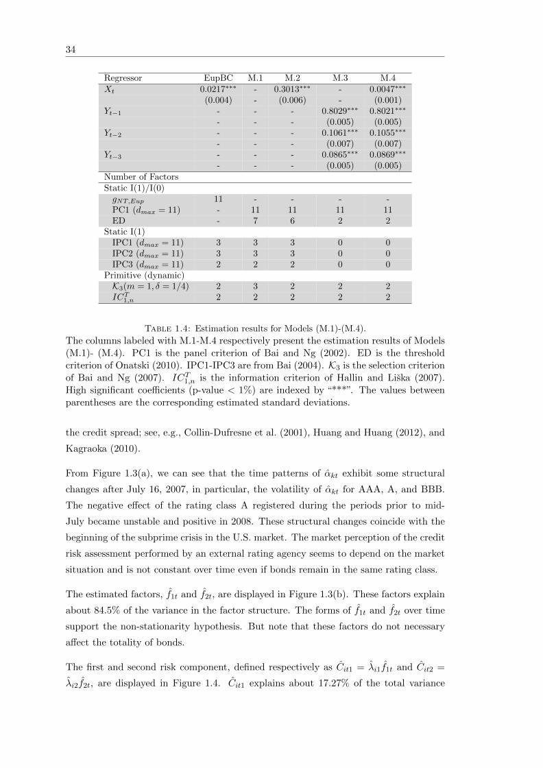
34
Regressor EupBC M.1 M.2 M.3 M.4Xt 0.0217∗∗∗ - 0.3013∗∗∗ - 0.0047∗∗∗
(0.004) - (0.006) - (0.001)Yt−1 - - - 0.8029∗∗∗ 0.8021∗∗∗
- - - (0.005) (0.005)Yt−2 - - - 0.1061∗∗∗ 0.1055∗∗∗
- - - (0.007) (0.007)Yt−3 - - - 0.0865∗∗∗ 0.0869∗∗∗
- - - (0.005) (0.005)Number of FactorsStatic I(1)/I(0)gNT,Eup 11 - - - -PC1 (dmax = 11) - 11 11 11 11ED - 7 6 2 2
Static I(1)IPC1 (dmax = 11) 3 3 3 0 0IPC2 (dmax = 11) 3 3 3 0 0IPC3 (dmax = 11) 2 2 2 0 0
Primitive (dynamic)K3(m = 1, δ = 1/4) 2 3 2 2 2ICT
1,n 2 2 2 2 2
Table 1.4: Estimation results for Models (M.1)-(M.4).
The columns labeled with M.1-M.4 respectively present the estimation results of Models(M.1)- (M.4). PC1 is the panel criterion of Bai and Ng (2002). ED is the thresholdcriterion of Onatski (2010). IPC1-IPC3 are from Bai (2004). K3 is the selection criterionof Bai and Ng (2007). ICT1,n is the information criterion of Hallin and Liska (2007).High significant coefficients (p-value < 1%) are indexed by “***”. The values betweenparentheses are the corresponding estimated standard deviations.
the credit spread; see, e.g., Collin-Dufresne et al. (2001), Huang and Huang (2012), and
Kagraoka (2010).
From Figure 1.3(a), we can see that the time patterns of αkt exhibit some structural
changes after July 16, 2007, in particular, the volatility of αkt for AAA, A, and BBB.
The negative effect of the rating class A registered during the periods prior to mid-
July became unstable and positive in 2008. These structural changes coincide with the
beginning of the subprime crisis in the U.S. market. The market perception of the credit
risk assessment performed by an external rating agency seems to depend on the market
situation and is not constant over time even if bonds remain in the same rating class.
The estimated factors, f1t and f2t, are displayed in Figure 1.3(b). These factors explain
about 84.5% of the variance in the factor structure. The forms of f1t and f2t over time
support the non-stationarity hypothesis. But note that these factors do not necessary
affect the totality of bonds.
The first and second risk component, defined respectively as Cit1 = λi1f1t and Cit2 =
λi2f2t, are displayed in Figure 1.4. Cit1 explains about 17.27% of the total variance
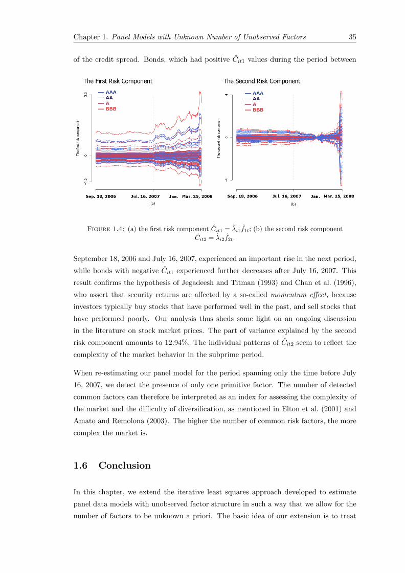
Chapter 1. Panel Models with Unknown Number of Unobserved Factors 35
of the credit spread. Bonds, which had positive Cit1 values during the period between
Figure 1.4: (a) the first risk component Cit1 = λi1f1t; (b) the second risk component
Cit2 = λi2f2t.
September 18, 2006 and July 16, 2007, experienced an important rise in the next period,
while bonds with negative Cit1 experienced further decreases after July 16, 2007. This
result confirms the hypothesis of Jegadeesh and Titman (1993) and Chan et al. (1996),
who assert that security returns are affected by a so-called momentum effect, because
investors typically buy stocks that have performed well in the past, and sell stocks that
have performed poorly. Our analysis thus sheds some light on an ongoing discussion
in the literature on stock market prices. The part of variance explained by the second
risk component amounts to 12.94%. The individual patterns of Cit2 seem to reflect the
complexity of the market behavior in the subprime period.
When re-estimating our panel model for the period spanning only the time before July
16, 2007, we detect the presence of only one primitive factor. The number of detected
common factors can therefore be interpreted as an index for assessing the complexity of
the market and the difficulty of diversification, as mentioned in Elton et al. (2001) and
Amato and Remolona (2003). The higher the number of common risk factors, the more
complex the market is.
1.6 Conclusion
In this chapter, we extend the iterative least squares approach developed to estimate
panel data models with unobserved factor structure in such a way that we allow for the
number of factors to be unknown a priori. The basic idea of our extension is to treat
36
the iterative least squares estimator of Bai (2009) and Bai et al. (2009) as functions
depending on a run parameter d. The latter is fitted by means of a penalty term that
is directly integrated into the global objective function to be optimized. The final so-
lution is obtained by alternating between an inner iteration to optimize β(d), F (β,d),
and Λi(β, F ,d) for each given d and an outer iteration to select the optimal dimension
d. Monte Carlo experiments show that our algorithm provides more efficient estimates
in terms of MSE than could be achieved if the estimator of Bai et al. (2009) is calcu-
lated with an externally selected factor dimension. We consider, in our application, the
problem of the credit spread puzzle and estimate the number of the hidden risk factors
jointly with the effect of the observed risk components. Our result proves the presence
of two unobserved common risk factors affecting the U.S. corporate bonds during the
period between September 2006 and March 2008, while one single risk factor is sufficient
to describe the data for all time periods prior to the beginning of the subprime crisis in
2007. Our analysis neglects, however, the possible effect of taxes. This component can
be introduced in the regression function by means of a reasonable determinant. There
is also a large potential for expanding panel data models with structural breaks on the
individual effects, as proposed by De Wachter and Tzavalis (2012), to panel models with
structural breaks in the unobserved factor structure.
Chapter 2
The R-package phtt: Panel Data
Analysis with Heterogeneous
Time Trends
2.1 Introduction
One of the main difficulties and at the same time appealing advantages of panel models
is their need to deal with the problem of the unobserved heterogeneity. Classical panel
models, such as fixed effects or random effects, try to model unobserved heterogeneity
using dummy variables or structural assumptions on the error term (see, e.g., H. (2005)).
In both cases the unobserved heterogeneity is assumed to remain constant over time
within each cross-sectional unit—apart from an eventual common time trend. This
assumption might be reasonable for approximating panel data with fairly small temporal
dimensions T ; however, for panel data with large T this assumption becomes very often
implausible.
Nowadays, the availability of panel data with large cross-sectional dimensions n and large
time dimensions T has triggered the development of a new class of panel data models.
Recent discussions by Ahn et al. (2013), Pesaran (2006), Bai (2009), Bai et al. (2009), and
Kneip et al. (2012) have focused on advanced panel models for which the unobservable
individual effects are allowed to have heterogeneous (i.e., individual specific) time trends
that can be approximated by a factor structure. The basic form of this new class of panel
models can be presented as follows:
yit =
P∑j=1
xitjβj + νit + εit for i ∈ 1, . . . , n and t ∈ 1, . . . , T, (2.1)
37

38
where yit is the dependent variable for each individual i at time t, xitj is the jth element of
the vector of explanatory variables xit ∈ RP , and εit is the idiosyncratic error term. The
time-varying individual effects νit ∈ R of individual i for the time points t ∈ 1, . . . , Tare assumed to be generated by d common time-varying factors. The following two
specifications of the time-varying individual effects νit are implemented in our R package
phtt:
νit =
vit =
∑dl=1 λilflt, for the model of Bai (2009),
vi(t) =∑d
l=1 λilfl(t), for the model of Kneip et al. (2012).(2.2)
Here, λil are unobserved individual loadings parameters, flt are unobserved common
factors for the model of Bai (2009), fl(t) are the unobserved common factors for the
model of Kneip et al. (2012), and d is the unknown factor dimension.
Note that the explicit consideration of an intercept in model (2.1) is not necessary but
may facilitate interpretation. If xit includes an intercept, the time-varying individual
effects νit are centered around zero. If xit does not include an intercept, the time-varying
individual effects νit are centered around the overall mean.
Model (2.1) includes the classical panel data models with additive time-invariant individ-
ual effects and common time-specific effects. This model is obtained by choosing d = 2
with a first common factor f1t = 1 for all t ∈ 1, . . . , T that has individual loadings
parameters λi1, and a second common factor f2t that has the same loadings parameter
λi2 = 1 for all i ∈ 1, . . . , n.
An intrinsic problem of factor models lies in the fact that the true factors are only
identifiable up to rotation. In order to ensure the uniqueness of these parameters, a
number of d2 restrictions are required. The usual normalization conditions are given by
(a) 1T
∑Tt=1 f
2lt = 1 for all l ∈ 1, . . . , d,
(b)∑T
t=1 fltfkt = 0 for all l, k ∈ 1, . . . , d with k 6= l, and
(c)∑n
i=1 λilλik = 0 for all l, k ∈ 1, . . . , d with k 6= l;
see, e.g., Bai (2009) and Kneip et al. (2012). For the model of Kneip et al. (2012), flt in
conditions (a) and (b) has to be replaced by fl(t). As usual in factor models, a certain
degree of indeterminacy remains, because the factors can only be determined up to sign
changes and different ordering schemes.
Kneip et al. (2012) consider the case in which the common factors fl(t) show relatively
smooth patterns over time. This includes strongly positive auto-correlated stationary
as well as non-stationary factors. The authors propose to approximate the time-varying

Chapter 2. Panel Data Analysis with Heterogeneous Time Trends 39
individual effects vi(t) by smooth nonparametric functions, say, ϑi(t). In this way (2.1)
becomes a semi-parametric model and its estimation is done using a two-step estimation
procedure, which we explain in more detail in Section 2.2. The asymptotic properties of
this method rely, however, on independent and identically distributed errors.
Alternatively, Bai (2009) allows for weak forms of heteroskedasticity and dependency in
both time and cross-section dimensions and proposes an iterated least squares approach
to estimate (2.1) for stationary time-varying individual effects vit such as ARMA pro-
cesses or non-stationary deterministic trends. However, Bai (2009) rules out a large class
of non-stationary processes such as stochastic processes with integration.
Moreover, Bai (2009) assumes the factor dimension d to be a known parameter, which is
usually not the case. Therefore, the phtt package uses an algorithmic refinement of Bai’s
method proposed by Bada and Kneip (2014) in order to estimate the number of unob-
served common factors d jointly with the remaining model parameters; see Section 2.4
for more details.
Besides the implementations of the methods proposed by Kneip et al. (2012), Bai (2009),
and Bada and Kneip (2014) the R package phtt comes with a wide range of criteria (16
in total) for estimating the factor dimension d. The main functions of the phtt package
are given in the following list:
• KSS(): Computes the estimators of the model parameters according to the method
of Kneip et al. (2012); see Section 2.2.
• Eup(): Computes the estimators of the model parameters according to the method
of Bai (2009) and Bada and Kneip (2014); see Section 2.4.
• OptDim(): Allows for a comparison of the estimated factor dimensions d obtained
from many different (in total 16) criteria; see Section 2.3.
• checkSpecif(): Tests whether to use a classical fixed effects panel model or a
panel model with individual effects νit; see Section 2.5.1.
The functions are provided with the usual print()-, summary()-, plot()-, coef()- and
residuals()-methods.
Standard methods for estimating models for panel and longitudinal data are also imple-
mented in the R packages plm (Croissant and Millo, 2008), nlme (Pinheiro et al., 2014),
and lme4 (Bates et al., 2014); see Croissant and Millo (2008) for an exhaustive compar-
ison of these packages. Recently, Millo and Piras (2012) published the R package splm
for spatial panel data models. The phtt package further extends the toolbox for statis-
ticians and econometricians and provides the possibility of analyzing panel data with

40
large dimensions n and T and considers in the case when the unobserved heterogeneity
effects are time-varying.
To the best of our knowledge, our phtt package Bada and Liebl (2014a) is the first
software package that offers the estimation methods of Bai (2009) and Kneip et al.
(2012). Regarding the different dimensionality criteria that can by accessed via the
function OptDim() only those of Bai and Ng (2002) are publicly available as MATLAB
codes from the homepage of Serena Ng (http://www.columbia.edu/~sn2294/).
To demonstrate the use of our functions, we re-explore the well known Cigar dataset,
which is frequently used in the literature of panel models. The panel contains the per
capita cigarette consumptions of n = 46 American states from 1963 to 1992 (T = 30)
as well as data about the income per capita and cigarette prices (see, e.g., Baltagi and
Levin (1986) for more details on the dataset).
We follow Baltagi and Li (2006), who estimate the following panel model:
ln(Consumptionit) = µ+ β1 ln(Priceit) + β2 ln(Incomeit) + eit. (2.3)
Here, Consumptionit presents the sales of cigarettes (packs of cigarettes per capita),
Priceit is the average real retail price of cigarettes, and Incomeit is the real disposable
income per capita. The index i ∈ 1, . . . , 46 denotes the single states and the index
t ∈ 1, . . . , 30 denotes the year.
We revisit this model, but allow for a multidimensional factor structure such that
eit =
d∑l=1
λilflt + εit.
The Cigar dataset can be obtained from the phtt package using the function data("Cigar").
The panels of the variables ln(Consumptionit), ln(Priceit), and ln(Incomeit) are shown
in Figure 2.1.
Section 2.2 is devoted to a short introduction of the method of Kneip et al. (2012), which
is appropriate for relatively smooth common factors fl(t). Section 2.3 presents the usage
of the function OptDim(), which provides access to a wide range of panel dimensionality
criteria recently discussed in the literature on factor models. Section 2.4 deals with the
explanation as well as application of the panel method proposed by Bai (2009), which
is basically appropriate for stationary and relatively unstructured common factors flt.

Chapter 2. Panel Data Analysis with Heterogeneous Time Trends 41
0 10 20 30Time
0 10 20 30Time
0 10 20 30Time
Log's ofCigar−Consump on
Log's of real Prices
Log's of real Income
3.8
5.0
4.4
0.4
−0.6
0.0
4.0
5.5
4.5
Figure 2.1: Time series of the dependent variable ln(Consumptionit) and regressorvariables ln(Priceit) and ln(Incomeit).
2.2 Panel Models for Heterogeneity in Time Trends
The panel model proposed by Kneip et al. (2012) can be presented as follows:
yit =P∑j=1
xitjβj + vi(t) + εit, (2.4)
where the time-varying individual effects vi(t) are parametrized in terms of common
non-parametric basis functions f1(t), . . . , fd(t) such that
vi(t) =
d∑l=1
λilfl(t). (2.5)
The asymptotic properties of this method rely on second order differences of vi(t), which
apply for continuous functions as well as for classical discrete stochastic time series
processes such as (S)AR(I)MA processes. Therefore, the functional notation of the time-
varying individual effects vi(t) and their underlying common factors f1(t), . . . , fd(t) does
not restrict them to a purely functional interpretation. The main idea of this approach
is to approximate the time series of individual effects vi(t) by smooth functions ϑi(t).
42
The estimation approach proposed by Kneip et al. (2012) relies on a two-step procedure:
first, estimates of the common slope parameters βj and the time-varying individual
effects vi(t) are obtained semi-parametrically. Second, functional principal component
analysis is used to estimate the common factors f1(t), . . . , fd(t), and to re-estimate the
time-varying individual effects vi(t) more efficiently. In the following we describe both
steps in more detail.
Step 1: The unobserved parameters βj and vi(t) are estimated by the minimization of
n∑i=1
1
T
T∑t=1
yit − P∑j=1
xitjβj − ϑi(t)
2
+
n∑i=1
κ
∫ T
1
1
T
(ϑ
(m)i (s)
)2ds, (2.6)
over all βj ∈ R and all m-times continuously differentiable functions ϑi(t), where ϑ(m)i (t)
denotes the mth derivative of the function ϑi(t). A first approximation of vi(t) is then
given by vi(t) := ϑi(t). Spline theory implies that any solution ϑi(t) possesses an expan-
sion in terms of a natural spline basis z1(t), . . . , zT (t) such that ϑi(t) =∑T
s=1 ζiszs(t);
see, e.g., de Boor (2001). Using the latter expression, we can rewrite (2.6) to formalize
the following objective function:
S(β, ζ) =n∑i=1
(||Yi −Xiβ − Zζi||2 + κζ>i Rζi
), (2.7)
where Yi = (yi1, . . . , yiT )>, Xi = (x>i1, . . . , x>iT )>, β = (β1, . . . , βP )>, ζi = (ζi1, . . . , ζiT )>,
Z andR are T×T matrices with elements zs(t)s,t=1,...,T and ∫z
(m)s (t)z
(m)k (t)dts,k=1,...,T
respectively. κ is a preselected smoothing parameter to control the smoothness of ϑi(t).
We follow the usual choice of m = 2, which leads to cubic smoothing splines.
In contrast to Kneip et al. (2012), we do not specify a common time effect in model
(2.4), but the vector of explanatory variables is allowed to contain an intercept. This
means that the time-varying individual effects vi(t) are not centered around zero for each
specific time point t, but around a common intercept term. The separate estimation of
the common time effect, say θt, is also possible with our phtt package; we discuss this
in detail in Section 2.5.
The semi-parametric estimators β, ζi = (ζi1, . . . , ζiT )>, and vi = (vi1, . . . , viT )> can be
obtained by minimizing S(β, ζ) over all β ∈ RP and ζ ∈ RT×n.

Chapter 2. Panel Data Analysis with Heterogeneous Time Trends 43
The solutions are given by
β =
(n∑i=1
X>i (I −Zκ)Xi
)−1( n∑i=1
X>i (I −Zκ)Yi
), (2.8)
ζi = (Z>Z + κR)−1Z>(Yi −Xiβ), and (2.9)
vi = Zκ(Yi −Xiβ
), where Zκ = Z
(Z>Z + κR
)−1Z>. (2.10)
Step 2: The common factors are obtained by the first d eigenvectors γ1, . . . , γd that
correspond to the largest eigenvalues ρ1, . . . , ρd of the empirical covariance matrix
Σ =1
n
n∑i=1
viv>i . (2.11)
The estimator of the common factor fl(t) is then defined by the lth scaled eigenvector
fl(t) =√T γlt for all l ∈ 1, . . . , d, (2.12)
where γlt is the tth element of the eigenvector γl. The scaling factor√T yields that fl(t)
satisfies the normalization condition 1T
∑Tt=1 fl(t)
2 = 1 as listed above in Section 2.1.
The estimates of the individual loadings parameters λil are obtained by ordinary least
squares regressions of(Yi −Xiβ
)on fl, where fl = (fl(1), . . . , fl(T ))>. Recall from
conditions (a) and (b) that λil can be calculated as follows:
λil =1
Tf>l
(Yi −Xiβ
). (2.13)
A crucial part of the estimation procedure of Kneip et al. (2012) is the re-estimation
of the time-varying individual effects vi(t) in Step 2 by vi(t) :=∑d
l=1 λilfl(t), where
the factor dimension d can be determined, e.g., by the sequential testing procedure of
Kneip et al. (2012) or by any other dimensionality criterion; see also Section 2.3. This
re-estimation leads to more efficiently estimated time-varying individual effects.
Kneip et al. (2012) derive the consistency of the estimators as n, T →∞ and show that
the asymptotic distribution of common slope estimators is given by Σ−1/2β (β−Eε(β))
d→N(0, I), where
Σβ = σ2
(n∑i=1
X>i (I −Zκ)Xi
)−1( n∑i=1
X>i (I −Zκ)2Xi
)(n∑i=1
X>i (I −Zκ)Xi
)−1
.
(2.14)
44
A consistent estimator of σ2 can be obtained by
σ2 =1
(n− 1)T
n∑i=1
||Yi −Xiβ −d∑l=1
λi,lfl||2. (2.15)
To determine the optimal smoothing parameter κopt, Kneip et al. (2012) propose the
following cross validation (CV) criterion:
CV (κ) =n∑i=1
||Yi −Xiβ−i −d∑l=1
λ−i,lf−i,l||2, (2.16)
where β−i, λ−i,l, and f−i,l are estimates of the parameters β, λ, and fl based on the
dataset without the ith observation. Unfortunately, this criterion is computationally
very costly and requires determining the factor dimension d in advance. To overcome
this disadvantage, we propose a plug-in smoothing parameter that is discussed in more
detail in the following Section 2.2.1.
2.2.1 Computational Details
Theoretically, it is possible to determine κ by the CV criterion in (2.16); however, cross
validation is computationally very costly. Moreover, Kneip et al. (2012) do not explain
how the factor dimension d is to be specified during the optimization process, which is
critical since the estimator d is influenced by the choice of κ.
In order to get a quick and effective solution, we propose to determine the smoothing
parameter κ by generalized cross validation (GCV). However, we cannot apply the clas-
sical GCV formulas as proposed, e.g., in Craven and Wahba (1979) since we do not
know the parameters β and vi(t). Our computational algorithm for determining the
GCV smoothing parameter κGCV is based on the method of Cao and Ramsay (2010),
who propose optimizing objective functions of the form (2.7) by updating the parameters
iteratively in a functional hierarchy. Formally, the iteration algorithm can be described
as follows:
1. For given κ and β, we optimize (2.7) with respect to ζi to get
ζi = (Z>Z + κR)−1Z>(Yi −Xiβ). (2.17)

Chapter 2. Panel Data Analysis with Heterogeneous Time Trends 45
2. By using (2.17), we minimize (2.7) with respect to β to get
β =
(n∑i=1
X>i Xi
)−1( n∑i=1
X>i (Yi − Zζi)
)(2.18)
3. Once (2.17) and (2.18) are obtained, we optimize the following GCV criterion to
calculate κGCV :
κGCV = arg minκ
1nT tr(I −Zκ)2
n∑i=1
||Yi −Xiβ −Zκ(Yi −Xiβ)||2. (2.19)
The program starts with initial estimates of β and κ and proceeds with steps 1, 2, and 3
in recurrence until convergence of all parameters, where the initial value βstart is defined
in (2.50) and the initial value κstart is the GCV-smoothing parameter of the residuals
Yi −Xiβstart.
The advantage of this approach is that the inversion of the P × P matrix in (2.18)
does not have to be updated during the iteration process. Moreover, the determina-
tion of the GCV-minimizer in (2.19) can be easily performed in R using the function
smooth.spline(), which calls on a rapid C-routine.
But note that the GCV smoothing parameter κGCV in (2.19) does not explicitly account
for the factor structure of the time-varying individual effects vi(t) as formalized in (2.2).
In fact, given that the assumption of a factor structure is true, the goal shall not be to
obtain optimal estimates of vi(t) but rather to obtain optimal estimates of the common
factors fl(t), which implies that the optimal smoothing parameter κopt will be smaller
than κGCV ; see Kneip et al. (2012).
If the goal is to obtain optimal estimates of fl(t), κopt will be used as an upper bound
when minimizing the CV criterion (2.16) (via setting the argument CV = TRUE); which,
however, can take some time. Note that, this optimal smoothing parameter κopt de-
pends on the unknown factor dimension d. Therefore, we propose to, first, estimate the
dimension based on the smoothing parameter κGCV and, second, to use the estimated
dimension d (via explicitly setting the dimension argument factor.dim= d) in order to
determine the dimension-specific smoothing parameter κopt (via setting the argument
CV = TRUE).
2.2.2 Application
This section is devoted to the application of the method of Kneip et al. (2012) discussed
above. The computation of this method is accessible through the function KSS(), which

46
has the following arguments:
R> args(KSS)
function (formula, additive.effects = c("none", "individual",
"time", "twoways"), consult.dim.crit = FALSE, d.max = NULL,
sig2.hat = NULL, factor.dim = NULL, level = 0.01, spar = NULL,
CV = FALSE, convergence = 1e-06, restrict.mode = c("restrict.factors",
"restrict.loadings"), ...)
NULL
The argument formula is compatible with the usual R-specific symbolic designation of
the model. The unique specificity here is that the variables should be defined as T × nmatrices, where T is the temporal dimension and n is the number of the cross-section
unites.1
The argument additive.effects makes it possible to extend the model (2.4) for addi-
tional additive individual, time, or twoways effects as discussed in Section 2.5.
If the logical argument consult.dim.crit is set to TRUE all dimensionality criteria
discussed in Section 2.3 are computed and the user is asked to choose one of their
results.
The arguments d.max and sig2.hat are required for the computation of some dimen-
sionality criteria discussed in Section 2.3. If their default values are maintained, the
function internally computes d.max=⌊min
√n,√T⌋
and sig2.hat as in (2.15), where
bxc indicates the integer part of x. The argument level allows to adjust the signifi-
cance level for the dimensionality testing procedure (2.21) of Kneip et al. (2012); see
Section 2.3.
CV is a logical argument. If it is set to TRUE the cross validation criterion (2.16) of Kneip
et al. (2012) will be computed. In the default case, the function uses the GCV method
discussed above in Section 2.2.1.
The factor dimension d can be pre-specified by the argument factor.dim. Recall from
restriction (a) that 1T
∑Tt=1 fl(t)
2 = 1.
Alternatively, it is possible to standardize the individual loadings parameters such that1n
∑ni=1 λ
2il = 1, which can be done by setting restrict.mode = "restrict.loadings".
1Note that phtt is written for balanced panels. Missing values have to be replaced in a pre-processingstep by appropriate imputation methods.

Chapter 2. Panel Data Analysis with Heterogeneous Time Trends 47
As an illustration we estimate the Cigarettes model (2.3) introduced in Section 2.1:
ln(Consumptionit) = µ+ β1 ln(Priceit) + β2 ln(Incomeit) + eit (2.20)
with eit =d∑l=1
λil fl(t) + εit.
In the following lines of code we load the Cigar dataset and take logarithms of the three
variables, Consumptionit, Priceit/cpit and Incomeit/cpit, where cpit is the consumer
price index. The variables are stored as T × n-matrices. This is necessary, because the
formula argument of the KSS()-function takes the panel variables as matrices in which
the number of rows has to be equal to the temporal dimension T and the number of
columns has to be equal to the individual dimension n.
R> library("phtt")
R> data("Cigar")
R> N <- 46
R> T <- 30
R> l.Consumption <- log(matrix(Cigar$sales, T, N))
R> cpi <- matrix(Cigar$cpi, T, N)
R> l.Price <- log(matrix(Cigar$price, T, N)/cpi)
R> l.Income <- log(matrix(Cigar$ndi, T, N)/cpi)
The model parameters β1, β2, the factors fl(t), the loadings parameters λil, and the
factor dimension d can be estimated by the KSS()-function with its default arguments.
Inferences about the slope parameters can be obtained by using the method summary().
R> Cigar.KSS <- KSS(formula = l.Consumption ~ l.Price + l.Income)
R> (Cigar.KSS.summary <- summary(Cigar.KSS))
Call:
KSS.default(formula = l.Consumption ~ l.Price + l.Income)
Residuals:
Min 1Q Median 3Q Max
-0.11 -0.01 0.00 0.01 0.12
Slope-Coefficients:
Estimate StdErr z.value Pr(>z)
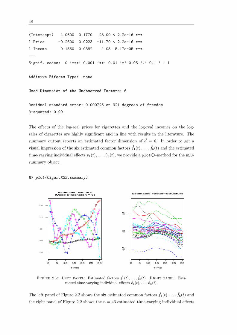
48
(Intercept) 4.0600 0.1770 23.00 < 2.2e-16 ***
l.Price -0.2600 0.0223 -11.70 < 2.2e-16 ***
l.Income 0.1550 0.0382 4.05 5.17e-05 ***
---
Signif. codes: 0 ’***’ 0.001 ’**’ 0.01 ’*’ 0.05 ’.’ 0.1 ’ ’ 1
Additive Effects Type: none
Used Dimension of the Unobserved Factors: 6
Residual standard error: 0.000725 on 921 degrees of freedom
R-squared: 0.99
The effects of the log-real prices for cigarettes and the log-real incomes on the log-
sales of cigarettes are highly significant and in line with results in the literature. The
summary output reports an estimated factor dimension of d = 6. In order to get a
visual impression of the six estimated common factors f1(t), . . . , f6(t) and the estimated
time-varying individual effects v1(t), . . . , vn(t), we provide a plot()-method for the KSS-
summary object.
R> plot(Cigar.KSS.summary)
111111111111111111111111111111
0 5 10 15 20 25 30
−2−1
01
2
Estimated Factors(Used Dimension = 6)
Time
22222
222222222
222222
22222
2
2
222
3333
3333
3
3
3
3
3
333
3333
3
333
3
3
3333
4
4
4
444
4
4
4
44
4
4
4
4
4
4
444444
444
4
4
44
5
5
5
5
5
5
5
55
5
55
5
5
5555
555
5
5
5
555
5
5
5
6
6
6
66
66
6
66
6
6
6
66
6
6
6
6
6
666
66
6
6
6
6
6
0 5 10 15 20 25 30
−0.5
0.00.5
Estimated Factor−Structure
Time
Figure 2.2: Left panel: Estimated factors f1(t), . . . , f6(t). Right panel: Esti-mated time-varying individual effects v1(t), . . . , vn(t).
The left panel of Figure 2.2 shows the six estimated common factors f1(t), . . . , f6(t) and
the right panel of Figure 2.2 shows the n = 46 estimated time-varying individual effects

Chapter 2. Panel Data Analysis with Heterogeneous Time Trends 49
v1(t), . . . , vn(t). The common factors are ordered correspondingly to the decreasing se-
quence of their eigenvalues. Obviously, the first common factor is nearly time-invariant;
this suggests extending the model (2.20) by additive individual (time-invariante) ef-
fects; see Section 2.5 for more details.
By setting the logical argument consult.dim.crit=TRUE, the user can choose from other
dimensionality criteria, which are discussed in Section 2.3. Note that the consideration
of different factor dimensions d would not alter the results for the slope parameters β
since the estimation procedure of Kneip et al. (2012) for the slope parameters β does
not depend on the dimensionality parameter d.
2.3 Panel Criteria for Selecting the Number of Factors
In order to estimate the factor dimension d, Kneip et al. (2012) propose a sequential
testing procedure based on the following test statistic:
KSS(d) =n∑T
r=d+1 ρr − (n− 1)σ2tr(ZκPdZκ)
σ2
√2n · tr((ZκPdZκ)2)
a∼ N(0, 1), (2.21)
where Pd = I − 1T
∑dl=1 flf
>l with fl = (fl(1), . . . , fl(T ))>, and
σ2 =1
(n− 1)tr((I −Zκ)2)
n∑i=1
||(I −Zκ)(Yi −Xiβ)||2. (2.22)
The selection method can be described as follows: choose a significance level α (e.g.,
α = 1%) and begin with H0 : d = 0. Test if KSS(0) ≤ z1−α, where z1−α is the (1− α)-
quantile of the standard normal distribution. If the null hypothesis can be rejected, go
on with d = 1, 2, 3, . . . until H0 cannot be rejected. Finally, the estimated dimension is
then given by the smallest dimension d, which leads a rejection of H0.
The dimensionality criterion of Kneip et al. (2012) can be used for stationary as well
as non-stationary factors. However, this selection procedure has a tendency to ignore
factors that are weakly auto-correlated. As a result, the number of factors can be
underestimated.
More robust against this kind of underestimation are the criteria of Bai and Ng (2002).
The basic idea of their approach consists simply of finding a suitable penalty term gnT ,
which countersteers the undesired variance reduction caused by an increasing number of

50
factors d. Formally, d can be obtained by minimizing the following criterion:
PC(l) =1
nT
n∑i=1
T∑t=1
(yit − yit(l))2 + lgnT (2.23)
for all l ∈ 1, 2, . . ., where yit(l) is the fitted value for a given factor dimension l. To
estimate consistently the dimension of stationary factors Bai and Ng (2002) propose
specifying gnT by one of the following penalty terms:
g(PC1)nT = σ2 (n+ T )
nTlog
(nT
n+ T
), (2.24)
g(PC2)nT = σ2 (n+ T )
nTlog(minn, T), (2.25)
g(PC3)nT = σ2 log(minn, T)
minn, T, and (2.26)
g(BIC3)nT = σ2 (n+ T − l)
nTlog(nT ), (2.27)
where σ2 is the sample variance estimator of the residuals εit. The proposed criteria
are denoted by PC1, PC2, PC3, and BIC3, respectively. Note that only the first three
criteria satisfy the requirements of Theorem 2 in Bai and Ng (2002), i.e., (i) gnT → 0
and (ii) minn, Tgnt → ∞, as n, T → ∞. These conditions ensure consistency of
the selection procedure without imposing additional restrictions on the proportional
behavior of n and T . The requirement (i) is not always fulfilled for BIC3, especially
when n is too large relative to T or T is too large relative to n (e.g., n = exp(T )
or T = exp(n)). In practice, BIC3 seems to perform very well, especially when the
idiosyncratic errors are cross-correlated.
The variance estimator σ2 can be obtained by
σ2(dmax) =1
nT
n∑i=1
T∑t=1
(yit − yit(dmax))2, (2.28)
where dmax is an arbitrary maximal dimension that is larger than d. This kind of vari-
ance estimation can, however, be inappropriate in some cases, especially when σ2(dmax)
underestimates the true variance. To overcome this problem, Bai and Ng (2002) propose
three additional criteria (IC1, IC2, and IC3):
IC(l) = log
(1
nT
n∑i=1
T∑t=1
(yit − yit(l))2
)+ lgnT (2.29)
Chapter 2. Panel Data Analysis with Heterogeneous Time Trends 51
with
g(IC1)nT =
(n+ T )
nTlog(
nT
n+ T), (2.30)
g(IC2)nT =
(n+ T )
nTlog(minn, T), and (2.31)
g(IC3)nT =
log(minn, T)minn, T
. (2.32)
In order to improve the finite sample performance of IC1 and IC2, Alessi et al. (2010) pro-
pose to multiply the penalties g(IC1)nT and g
(IC2)nT with a positive constant c and apply the
calibration strategy of Hallin and Liska (2007). The choice of c is based on the inspection
of the criterion behavior through J-different tuples of n and T , i.e., (n1, T1), . . . , (nJ , TJ),
and for different values of c in a pre-specified grid interval. We denote the refined criteria
in our package by ABC.IC1 and ABC.IC2 respectively. Note that such a modification
does not affect the asymptotic properties of the dimensionality estimator.
Under similar assumptions, Ahn and Horenstein (2009) propose selecting d by maximiz-
ing the ratio of adjacent eigenvalues (or the ratio of their growth rate). The criteria are
referred to as Eigenvalue Ratio (ER) and Growth Ratio (GR) and defined as following:
ER =ρlρl+1
(2.33)
(2.34)
GR =log(∑T
r=l ρr/∑T
r=l+1 ρr
)log(∑T
r=l+1 ρr/∑T
r=l+2 ρr
) . (2.35)
Note that the theory of the above dimensionality criteria PC1, PC2, PC3, BIC3, IC1,
IC2, IC3, IPC1,IPC2, IPC3, ABC.IC1, ABC.IC2, KSS.C, ER, and GR are developed
for stochastically bounded factors. In order to estimate the number of unit root factors,
Bai (2004) proposes the following panel criteria:
IPC(l) =1
nT
n∑i=1
T∑t=1
(yit − yit(l))2 + lgnT , (2.36)
where
g(IPC1)nT = σ2 log(log(T ))
T
(n+ T )
nTlog
(nT
n+ T
), (2.37)
g(IPC2)nT = σ2 log(log(T ))
T
(n+ T )
nTlog(minn, T), and (2.38)
g(IPC3)nT = σ2 log(log(T ))
T
(n+ T − l)nT
log(nT ). (2.39)

52
Alternatively, Onatski (2010) has introduced a threshold approach based on the empirical
distribution of the sample covariance eigenvalues, which can be used for both stationary
and non-stationary factors. The estimated dimension is obtained by
d = maxl ≤ dmax : ρl − ρl−1 ≥ δ,
where δ is a positive threshold, estimated iteratively from the data. We refer to this
criterion as ED, which stands for Eigenvalue Differences.
2.3.1 Application
The dimensionality criteria introduced above are implemented in the function OptDim(),
which has the following arguments:
R> args(OptDim)
function (Obj, criteria = c("PC1", "PC2", "PC3", "BIC3", "IC1",
"IC2", "IC3", "IPC1", "IPC2", "IPC3", "ABC.IC1", "ABC.IC2",
"KSS.C", "ED", "ER", "GR"), standardize = FALSE, d.max, sig2.hat,
spar, level = 0.01, c.grid = seq(0, 5, length.out = 128),
T.seq, n.seq)
NULL
The desired criteria can be selected by one or several of the following character variables:
"KSS.C", "PC1", "PC2", "PC3", "BIC2", "IC1", "IC2" , "IC3", "ABC.IC1", "ABC.IC2",
"ER", "GR", "IPC1", "IPC2", "IPC3", and "ED". The default significance level used
for the "KSS"-criterion is level = 0.01. The values of dmax and σ2 can be speci-
fied externally by the arguments d.max and sig2.hat. By default, d.max is computed
internally as d.max=⌊min
√n,√T⌋
and sig2.hat as in (2.22) and (2.28). The ar-
guments "c.grid", "T.seq", and "n.seq" are required for computing "ABC.IC1" and
"ABC.IC2". The grid interval of the calibration parameter can be externally specified
with "c.grid". The J-Tuples, (n1, T1), . . . , (nJ , TJ), can be specified by using appro-
priate vectors in "T.seq", and "n.seq". If these two arguments are left unspecified,
the function constructs internally the following sequences: T −C, T −C + 1, . . . , T , and
n−C, n−C+ 1, . . . , n, for C = min√n,√T , 30. Alternatively, the user can specify only
the length of the sequences by giving appropriate integers to the arguments "T.seq",
and "n.seq", to control for C.

Chapter 2. Panel Data Analysis with Heterogeneous Time Trends 53
The input variable can be standardized by choosing standardize = TRUE. In this case,
the calculation of the eigenvalues is based on the correlation matrix instead of the co-
variance matrix for all criteria.
As an illustration, imagine that we are interested in the estimation of the factor di-
mension of the variable ln(Consumptionit) with the dimensionality criterion "PC1". The
function OptDim() requires a T × n matrix as input variable.
R> OptDim(Obj = l.Consumption, criteria = "PC1")
Call: OptDim.default(Obj = l.Consumption, criteria = "PC1")
---------
Criterion of Bai and Ng (2002):
PC1
5
OptDim() offers the possibility of comparing the result of different selection procedures by
giving the corresponding criteria to the argument criteria. If the argument criteria
is left unspecified, OptDim() automatically compares all 16 procedures.
R> (OptDim.obj <- OptDim(Obj = l.Consumption, criteria = c("PC3", "ER",
+ "GR", "IPC1", "IPC2", "IPC3"), standardize = TRUE))
Call: OptDim.default(Obj = l.Consumption, criteria = c("PC3", "ER",
"GR", "IPC1", "IPC2", "IPC3"), standardize = TRUE)
---------
Criterion of Bai and Ng (2002):
PC3
5
--------
Criteria of Ahn and Horenstein (2013):
ER GR
3 3
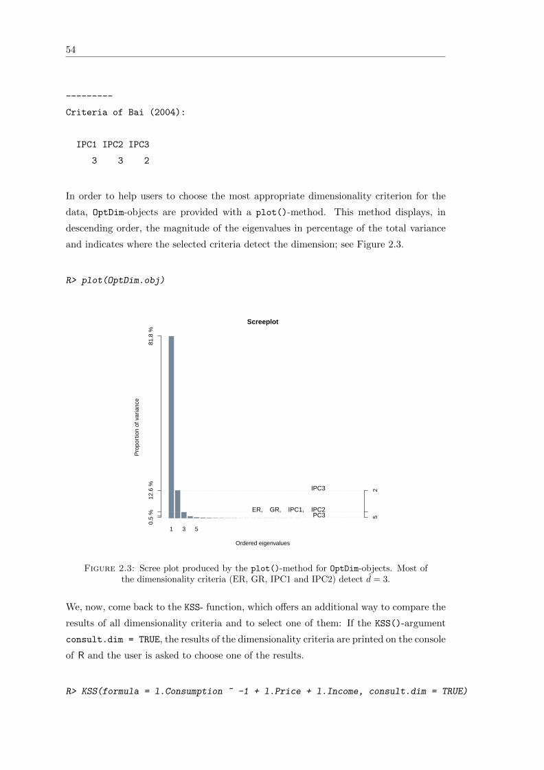
54
---------
Criteria of Bai (2004):
IPC1 IPC2 IPC3
3 3 2
In order to help users to choose the most appropriate dimensionality criterion for the
data, OptDim-objects are provided with a plot()-method. This method displays, in
descending order, the magnitude of the eigenvalues in percentage of the total variance
and indicates where the selected criteria detect the dimension; see Figure 2.3.
R> plot(OptDim.obj)
Screeplot
Ordered eigenvalues
Pro
port
ion
of v
aria
nce
1 3 5
0.5
%12
.6 %
81.8
%
52IPC3
ER, GR, IPC1, IPC2PC3
Figure 2.3: Scree plot produced by the plot()-method for OptDim-objects. Most ofthe dimensionality criteria (ER, GR, IPC1 and IPC2) detect d = 3.
We, now, come back to the KSS- function, which offers an additional way to compare the
results of all dimensionality criteria and to select one of them: If the KSS()-argument
consult.dim = TRUE, the results of the dimensionality criteria are printed on the console
of R and the user is asked to choose one of the results.
R> KSS(formula = l.Consumption ~ -1 + l.Price + l.Income, consult.dim = TRUE)

Chapter 2. Panel Data Analysis with Heterogeneous Time Trends 55
-----------------------------------------------------------
Results of Dimension-Estimations
-Bai and Ng (2002):
PC1 PC2 PC3 BIC3 IC1 IC2 IC3
5 5 5 4 5 5 5
-Bai (2004):
IPC1 IPC2 IPC3
3 3 2
-Alessi et al. (2010):
ABC.IC1 ABC.IC2
3 3
-Kneip et al. (2012):
KSS.C
6
-Onatski (2009):
ED
3
-Ahn and Horenstein (2013):
ER GR
3 6
-----------------------------------------------------------
Please, choose one of the proposed integers:
After entering a number of factors, e.g., 6 we get the following feedback:
Used dimension of unobs. factor structure is: 6
-----------------------------------------------------------

56
Note that the maximum number of factors that can be given, cannot exceed the highest
estimated factor dimension (here maximal dimension would be 6). A higher dimension
can be chosen using the argument factor.dim.
2.4 Panel Models with Stochastically Bounded Factors
The panel model proposed by Bai (2009) can be presented as follows:
yit =P∑j=1
xitjβj + vit + εit, (2.40)
where
vit =d∑l=1
λilflt. (2.41)
Combining (2.40) with (2.41) and writing the model in matrix notation we get
Yi = Xiβ + FΛ>i + εi, (2.42)
where Yi = (yi1, . . . , yiT )>, Xi = (x>i1, . . . , x>iT )>, εi = (εi1, . . . , εiT )>, Λi = (λ1, . . . , λn)>
and F = (f1, . . . , fT )> with λi = (λi1, . . . , λid), ft = (f1t, . . . , fdt), and εi = (εi1, . . . , εiT )>.
The asymptotic properties of Bai’s method rely, among others, on the following assump-
tion:1
TF>F
p→ ΣF , as T →∞, (2.43)
where ΣF is a fixed positive definite d× d matrix. This allows for the factors to follow a
deterministic time trend such as ft = t/T or to be stationary dynamic processes such that
ft =∑∞
j=1Cjet−j , where et are i.i.d. zero mean stochastic components. It is, however,
important to note that such an assumption rules out a large class of non-stationary
factors such as I(p) processes with p ≥ 1.
2.4.1 Model with Known Number of Factors
Bai (2009) proposes to estimate the model parameters β, F and Λi by minimizing the
following least squares objective function:
S(β, F,Λi) =
n∑i
||Yi −Xiβ − FΛ>i ||2. (2.44)

Chapter 2. Panel Data Analysis with Heterogeneous Time Trends 57
For each given F , the OLS estimator of β can be obtained by
β(F ) =
(n∑i=1
X>i PdXi
)−1( n∑i=1
X>i PdYi
)(2.45)
where Pd = I − F (F>F )−1F> = I − FF>/T . If β is known, F can be estimated by
using the first d eigenvectors γ = (γ1, . . . , γd) corresponding to the first d eigenvalues of
the empirical covariance matrix Σ = (nT )−1∑n
i=1wiw>i , where wi = Yi−Xiβ. That is,
F (β) =√T γ.
The idea of Bai (2009) is to start with initial values for β or F and calculate the esti-
mators iteratively. The method requires, however, the factor dimension d to be known,
which is usually not the case in empirical applications.
A feasible estimator of (2.45) can be obtained by using an arbitrary large dimension
dmax greater than d. The factor dimension can be estimated subsequently by using the
criteria of Bai and Ng (2002) to the remainder term Yi = Xiβ(F (dmax)), as suggested
by Bai (2009). This strategy can lead, however, to inefficient estimation and spurious
interpretation of β due to over-parameterization.
2.4.2 Model with Unknown Number of Factors
In order to estimate d jointly with β, F , and Λi, Bada and Kneip (2014) propose to
integrate a penalty term into the objective function to be globally optimized. In this
case, the optimization criterion can be defined as a penalized least squares objective
function of the form:
S(β, F,Λi, l) =
n∑i
||Yi −Xiβ − FΛ>i ||2 + lgnT (2.46)
The role of the additional term lgnT is to pick up the dimension d, of the unobserved
factor structure. The penalty gnT can be chosen according to Bai and Ng (2002). The
estimation algorithm is based on the parameter cascading strategy of Cao and Ramsay
(2010), which in this case can be described as follows:
1. Minimizing (2.46) with respect to Λi for each given β, F and d, we get
Λ>i (β, F, d) = F> (Yi −Xiβ) /T. (2.47)
58
2. Introducing (2.47) in (2.46) and minimizing with respect to F for each given β and
d, we get
F (β, d) =√T γ(β, d), (2.48)
where γ(β, d) is a T ×d matrix that contains the first d eigenvectors corresponding
to the first d eigenvalues ρ1, . . . , ρd of the covariance matrix Σ = (nT )−1∑n
i=1wiw>i
with wi = Yi −Xiβ.
3. Reintegrating (2.48) and (2.47) in (2.46) and minimizing with respect to β for each
given d, we get
β(d) =
(n∑i=1
X>i Xi
)−1( n∑i=1
X>i
(Yi − F Λ>i (β, d)
)). (2.49)
4. Optimizing (2.46) with respect to l given the results in (2.47), (2.48), and (2.49)
allows us to select d as
d = argminl
n∑i
||Yi −Xiβ − F Λ>i ||2 + lgnT , for all l ∈ 0, 1, . . . , dmax.
The final estimators are obtained by alternating between an inner iteration to optimize
β(d), F (d), and Λi(d) for each given d and an outer iteration to select the dimension d.
The updating process is repeated in its entirety till the convergence of all the parameters.
This is why the estimators are called entirely updated estimators (Eup). In order to
avoid over-estimation, Bada and Kneip (2014) propose to re-scale gnT in each iteration
stage with σ2 =∑n
i ||Yi − Xiβ − F Λ>i ||2 in stead of σ2(dmax). Simulations show that
such a calibration can improve the finite sample properties of the estimation method.
It is notable that the objective functions (2.46) and (2.44) are not globally convex. There
is no guarantee that the iteration algorithm converges to the global optimum. Therefore,
it is important to choose reasonable starting values dstart and βstart. We propose to select
a large dimension dmax and to start the iteration with the following estimate of β:
βstart =
(n∑i=1
X>i (I −GG>)Xi
)−1( n∑i=1
X>i (I −GG>)Yi
), (2.50)
where G is the T × dmax matrix of the eigenvectors corresponding to the first dmax
eigenvalues of the augmented covariance matrix
ΓAug =1
nT
n∑i=1
(Yi, Xi)(Y>i , X
>i )>.
Chapter 2. Panel Data Analysis with Heterogeneous Time Trends 59
The intuition behind these starting estimates relies on the fact that the unobserved
factors cannot escape from the space spanned by the eigenvectors G. The projection
of Xi on the orthogonal complement of G in (2.50) eliminates the effect of a possible
correlation between the observed regressors and unobserved factors, which can heavily
distort the value of β0 if it is neglected. Greenaway-mcgrevy (2012) give conditions under
which (2.50) is a consistent estimator of β. In order to avoid miss-specifying the model
through identifying factors that only exist in Xi and not Yi, Bada and Kneip (2014)
recommend to under-scale the starting common factors Gl that are highly correlated
with Xi.
According to Bai (2009), the asymptotic distribution of the slope estimator β(d) for
known d is given by√nT (β(d)− β)
a∼ N(0, D−10 DZD
−10 ),
whereD0 = plim 1nT
∑ni=1
∑Tt=1 Z
>itZit with Zi = (Zi1, . . . , ZiT )> = PdXi− 1
n
∑nk=1 PdXiaik
and aik = Λi(1n
∑ni=1 Λ>i Λi)
−1Λ>k , and
Case 1. DZ = D−10 σ2 if the errors are i.i.d. with zero mean and variance σ2,
Case 2. DZ = plim 1nT
∑ni=1 σ
2i
∑Tt=1 Z
>itZit, where σ2
i = E(ε2it) with E(εit) = 0, if cross-
section heteroskedasticity exists and n/T → 0,
Case 3. DZ = plim 1nT
∑ni=1
∑nj=1 ωij
∑Tt=1 Z
>itZjt, where ωij = E(εitεjt) with E(εit) = 0,
if cross-section correlation and heteroskedasticity exist and n/T → 0,
Case 4. DZ = plim 1nT
∑Tt=1 σ
2t
∑ni=1 Z
>itZit, where σ2
t = E(ε2it) with E(εit) = 0, if het-
eroskedasticity in the time dimension exists and T/n→ 0,
Case 5. DZ = plim 1nT
∑Tt=1
∑Ts=1 ρ(t, s)
∑ni=1 Z
>itZis, where ρ(t, s) = E(εitεis) withE(εit) =
0 , if correlation and heteroskedasticity in the time dimension exist and T/n→ 0,
and
Case 6. DZ = plim 1nT
∑Tt=1
∑ni=1 σ
2itZ>itZis, where σ2
it = E(ε2it) with E(εit) = 0, if het-
eroskedasticity in both time and cross-section dimensions exists with T/n2 → 0
and n/T 2 → 0.
In presence of correlation and heteroskedasticity in panels with proportional dimensions
n and T , i.e., n/T → c > 0, the asymptotic distribution of β(d) will be not centered at
zero. This can lead to false inference when using the usual test statistics such as t- and
χ2-statistic. To overcome this problem, Bai (2009) propose to estimate the asymptotic
bias and correct the estimator as follows:
β∗(d) = β(d)− 1
nB − 1
TC (2.51)
60
where B and C are the estimators of
B = −(
1nT
∑ni=1
∑Tt=1 Z
>itZit
)−11nT
∑ni=1
∑nk=1(Xi − Vi)>F
(1T F>F)−1
Wik
C = −(
1nT
∑ni=1
∑Tt=1 Z
>itZit
)−11nT
∑ni=1X
>i MFΩF
(1T F>F)−1 ( 1
n
∑nk=1 Λ>k Λk
)−1Λ>i
respectively. Here, Vi = 1n
∑nj=1 aijXj , Wik =
(1n
∑nj=1 Λ>j Λj
)−1Λ>k
1T
∑Tt=1E(εitεkt),
and Ω = 1n
∑nk=1 Ωk with
Case 7. Ωk is a T × T diagonal matrix with elements ωkt = E(ε2kt) if heteroskedasticity in
both time and cross-section dimensions exist and n/T → c > 0 and,
Case 8. Ωk is a T × T matrix with elements Ωk,ts = E(εktεks) if correlation and het-
eroskedasticity in both time and cross-section dimensions exist and n/T → c > 0.
In a similar context, Bada and Kneip (2014) prove that estimating d with the remaining
model parameters does not affect the asymptotic properties of β(d). The asymptotic
distribution of β = β(d) is given by
√nT (β − β)
a∼ N(0, D−10 DZD
−10 )
under Cases 1-6, and√nT (β∗ − β)
a∼ N(0, D−10 DZD
−10 )
under Cases 7-8, where β∗ = β∗(d).
The asymptotic variance of β and the bias terms B and C can be estimated by replacing
F , Λi, Zit, and εit with F , Λi, Zit, and εit respectively.
In presence of serial correlation (cases 5 and 8), consistent estimators for DZ and C can
be obtained by using the usual heteroskedasticity and autocorrelation (HAC) robust
limiting covariance. In presence of cross-section correlation (case 3), DZ is estimated by
DZ = 1mT
∑mi=1
∑mj=1
∑Tt=1 Z
>it Zjtεitεjt, where m =
√n. If both cross-section and serial
correlation exist (case 8), we estimate the long-run covariance of 1√m
∑mj=1 Zitεit.
2.4.3 Application
The above described methods are implemented in the function Eup(), which takes the
following arguments:
R> args(Eup)

Chapter 2. Panel Data Analysis with Heterogeneous Time Trends 61
function (formula, additive.effects = c("none", "individual",
"time", "twoways"), dim.criterion = c("PC1", "PC2", "PC3",
"BIC3", "IC1", "IC2", "IC3", "IPC1", "IPC2", "IPC3"), d.max = NULL,
sig2.hat = NULL, factor.dim = NULL, double.iteration = TRUE,
start.beta = NULL, max.iteration = 500, convergence = 1e-06,
restrict.mode = c("restrict.factors", "restrict.loadings"),
...)
NULL
The arguments additive.effects, d.max, sig2.hat, and restrict.mode have the
same roles as in KSS(); see Section 2.2.2. The argument dim.criterion specifies the
dimensionality criterion to be used if factor.dim is left unspecified and defaults to
dim.criterion = "PC1".
Setting the argument double.iteration=FALSE may speed up computations, because
the updates of d will be done simultaneously with F without waiting for their inner
convergences. However, in this case, the convergence of the parameters is less stable
than in the default setting.
The argument start.beta allows us to give a vector of starting values for the slope
parameters βstart. The maximal number of iteration and the convergence condition can
be controlled by max.iteration and convergence.
In our application, we take first-order differences of the observed time series. This is
because some factors show temporal trends, which can violate the stationarity condi-
tion (2.43); see Figure 2.2. We consider the following modified cigarettes model:
4 ln(Consumptionit) = β14 ln(Priceit) + β24 ln(Incomeit) + eit,
with eit =
d∑l=1
λilflt + εit,
where 4xt = xt− xt−1. In order to avoid notational mess, we use the same notation for
the unobserved time-varying individual effects vit =∑d
l=1 λilflt as above in (2.20). The
4-transformation can be easily performed in R using the standard diff()-function as
follows:
R> d.l.Consumption <- diff(l.Consumption)
R> d.l.Price <- diff(l.Price)
R> d.l.Income <- diff(l.Income)

62
As previously mentioned for the KSS()-function, the formula argument of the Eup()-
function takes balanced panel variables as T×n dimensional matrices, where the number
of rows has to be equal to the temporal dimension T and the number of columns has to
be equal to the individual dimension n.
R> (Cigar.Eup <- Eup(d.l.Consumption ~ -1 + d.l.Price + d.l.Income,
+ dim.criterion = "PC3"))
Call:
Eup.default(formula = d.l.Consumption ~ -1 + d.l.Price + d.l.Income,
dim.criterion = "PC3")
Coeff(s) of the Observed Regressor(s) :
d.l.Price d.l.Income
-0.3140143 0.159392
Additive Effects Type: none
Dimension of the Unobserved Factors: 5
Number of iterations: 55
Inferences about the slope parameters can be obtained by using the method summary().
The type of correlation and heteroskedasticity in the idiosyncratic errors can be specified
by choosing one of the corresponding Cases 1-8 described above using the argument
error.type = c(1, 2, 3, 4, 5, 6, 7, 8).
In presence of serial correlations (cases 5 and 8), the kernel weights required for esti-
mating the long-run covariance can be externally specified by giving a vector of weights
in the argument kernel.weights. By default, the function uses internally the linearly
decreasing weights of Newey and West (1987) and a truncation at⌊min
√n,√T⌋. If
case 7 or 8 is chosen, the method summary() calculates the realization of the bias cor-
rected estimators and gives appropriate inferences. The bias corrected coefficients can
be called by using the method coef() to the object produced by summary().
R> summary(Cigar.Eup)
Call:
Eup.default(formula = d.l.Consumption ~ -1 + d.l.Price + d.l.Income,

Chapter 2. Panel Data Analysis with Heterogeneous Time Trends 63
dim.criterion = "PC3")
Residuals:
Min 1Q Median 3Q Max
-0.147000 -0.013700 0.000889 0.014100 0.093300
Slope-Coefficients:
Estimate Std.Err Z value Pr(>z)
d.l.Price -0.3140 0.0227 -13.90 < 2.2e-16 ***
d.l.Income 0.1590 0.0358 4.45 8.39e-06 ***
---
Signif. codes: 0 ’***’ 0.001 ’**’ 0.01 ’*’ 0.05 ’.’ 0.1 ’ ’ 1
Additive Effects Type: none
Dimension of the Unobserved Factors: 5
Residual standard error: 0.02804 on 957 degrees of freedom,
R-squared: 0.7033
The summary output reports that "PC3" detects 5 common factors. The effect of the dif-
ferenced log-real prices for cigarettes on the differenced log-sales is negative and amounts
to −0.31. The estimated effect of the differenced real disposable log-income per capita
is 0.16.
The estimated factors ftl as well as the individual effects vit can be plotted using the
plot()-method for summary.Eup-objects. The corresponding graphics are shown in
Figure 2.4.
R> plot(summary(Cigar.Eup))
2.5 Models with Additive and Interactive Unobserved Ef-
fects
Even though the classical additive "individual", "time", and "twoways" effects can
be absorbed by the factor structure, there are good reasons to model them explicitly.

64
1
11
1
11
1
11
1
1
1
1
1
1
1
11
1
1
1
11
1
11
1
1
1
0 5 10 15 20 25 30
−3−2
−10
12
Estimated Factors(Used Dimension = 5)
Time
2
2
2
2
22
2
2
2
2
2
2
222
2
22
2
2
2
2
2
2
2
2
2
2
233
3
3
3
3
3
3
3
3
3
3
3
3
3
33333
3
3
3
3
3
33
3
3
4
4
4
4
44
4
4
4
4
4
44
4
44
4
4
44
4
4
4
4
4
4
4
4
4
5
5
55
5
5
5
5
55
55
5
55
5
555
555
5
5
5
5
5
5
5
0 5 10 15 20 25 30
−0.1
0.00.1
0.2
Estimated Factor−Structure
Time
Figure 2.4: Left Panel: Estimated factors f1t, . . . , f7t. Right panel: Estimatedtime-varying individual effects v1t, . . . , vnt.
On the one hand, if there are such effects in the true model, then neglecting them will
result in non-efficient estimators; see Bai (2009). On the other hand, additive effects can
be very useful for interpretation.
Consider now the following model:
yit = µ+ αi + θt + x>itβ + νit + εit (2.52)
with
νit =
vit =
∑dl=1 λilflt, for the model of Bai (2009),
vi(t) =∑d
l=1 λilfl(t), for the model of Kneip et al. (2012),
where αi are time-constant individual effects and θt is a common time-varying effect.
In order to ensure identification of the additional additive effects αi and θt, we need the
following further restrictions:
(d)∑n
i=1 λil = 0 for all l ∈ 1, . . . , d
(e)∑T
t=1 flt = 0 for all l ∈ 1, . . . , d
(f)∑n
i=1 αi = 0
(g)∑T
t=1 θt = 0

Chapter 2. Panel Data Analysis with Heterogeneous Time Trends 65
By using the classical within-transformations on the observed variables, we can eliminate
the additive effects αi and θt, such that
yit = x>itβ + νit + εit,
where yit = yit − 1T
∑Tt=1 yit −
1n
∑ni=1 yit + 1
nT
∑Tt=1
∑ni=1 yit, xit = xit − 1
T
∑Tt=1 xit −
1n
∑ni=1 xit+
1nT
∑Tt=1
∑ni=1 xit, and εit = εit− 1
T
∑Tt=1 εit−
1n
∑ni=1 εit+
1nT
∑Tt=1
∑ni=1 εit.
Note that Restrictions (d) and (e) ensure that the transformation does not affect the
time-varying individual effects νit. The parameters µ, αi and θt can be easily estimated
in a second step once an estimate of β is obtained. Because of Restrictions (d) and (e),
the solution has the same form as the classical fixed effects model.
The parameters β and νit can be estimated by the above introduced estimation proce-
dures. All possible variants of model (2.52) are implemented in the functions KSS() and
Eup(). The appropriate model can be specified by the argument additive.effects =
c("none", "individual", "time", "twoways"):
"none" yit = µ+ x>itβ + νit + εit
"individual" yit = µ+ αi + x>itβ + νit + εit
"time" yit = µ+ θt + x>itβ + νit + εit
"twoways" yit = µ+ αi + θt + x>itβ + νit + εit.
The presence of µ can be controlled by -1 in the formula-object: a formula with -1
refers to a model without intercept. However, for identification purposes, if a twoways
model is specified, the presence -1 in the formula will be ignored.
As an illustration, we continue with the application of the KSS()-function in Section 2.2.
The left panel of Figure 2.2 shows that the first common factor is nearly time-invariant.
This motivates us to augment the model (2.20) for a time-constant additive effects αi.
In this case, it is convenient to use an intercept µ, which yields the following model:
ln(Consumptionit) = µ+ β1 ln(Priceit) + β2 ln(Incomeit) + αi + vi(t) + εit,(2.53)
where vi(t) =
d∑l=1
λil fl(t).
The estimation of the augmented model (2.53) can be done using the following lines of
code.

66
R> Cigar2.KSS <- KSS(formula = l.Consumption ~ l.Price + l.Income,
+ additive.effects = "individual")
R> (Cigar2.KSS.summary <- summary(Cigar2.KSS))
Call:
KSS.default(formula = l.Consumption ~ l.Price + l.Income,
additive.effects = "individual")
Residuals:
Min 1Q Median 3Q Max
-0.11 -0.01 0.00 0.01 0.12
Slope-Coefficients:
Estimate StdErr z.value Pr(>z)
(Intercept) 4.0500 0.1760 23.10 < 2.2e-16 ***
l.Price -0.2600 0.0222 -11.70 < 2.2e-16 ***
l.Income 0.1570 0.0381 4.11 3.88e-05 ***
---
Signif. codes: 0 ’***’ 0.001 ’**’ 0.01 ’*’ 0.05 ’.’ 0.1 ’ ’ 1
Additive Effects Type: individual
Used Dimension of the Unobserved Factors: 5
Residual standard error: 0.000734 on 951 degrees of freedom
R-squared: 0.99
Again, the plot() method provides a useful visualization of the results.
R> plot(Cigar2.KSS.summary)
The "individual"-transformation of the data does not affect the estimation of the slope
parameters, but reduces the estimated dimension from d = 6 to d = 5. The remaining
five common factors f1, . . . , f5 correspond to those of model (2.20); see the middle panel
of Figure 2.5. The estimated time-constant state-specific effects αi are shown in the left
plot of Figure 2.5. The extraction of the αi’s from the factor structure yields a denser
set of time-varying individual effects vi shown in the right panel of Figure 2.5.
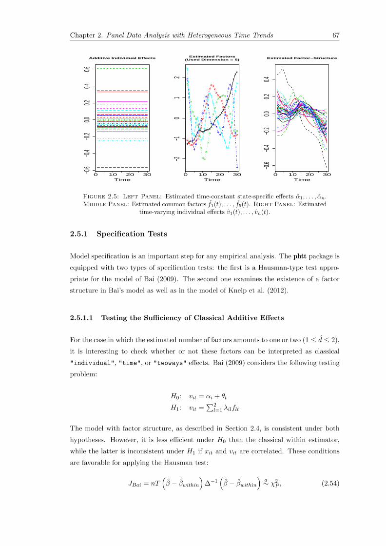
Chapter 2. Panel Data Analysis with Heterogeneous Time Trends 67
0 10 20 30−0.6
−0.4
−0.2
0.00.2
0.40.6
Additive Individual Effects
Time
1111
1
1
11111
11111
1111111
1
1
1
1
1
11
0 10 20 30−2
−10
12
Estimated Factors(Used Dimension = 5)
Time
2
222
222
2
2
2
2
2
2
2
22
2
222
2
2
2
2
2
2
2222
3
3
3
3
33
3
3
3
33
3
3
3
3
3
3
3
333
33
3
3
3
3
333
4
4
4
4
4
4
4
4
4
4
4
4
4
4
444
4
444
4
4
4
4
4
4
4
4
4
5
5
5
55
5
5
5
55
5
5
5
55
5
5
5
5
5
5
5
5
55
5
5
5
5
5
0 10 20 30
−0.6
−0.4
−0.2
0.00.2
0.4
Estimated Factor−Structure
Time
Figure 2.5: Left Panel: Estimated time-constant state-specific effects α1, . . . , αn.Middle Panel: Estimated common factors f1(t), . . . , f5(t). Right Panel: Estimated
time-varying individual effects v1(t), . . . , vn(t).
2.5.1 Specification Tests
Model specification is an important step for any empirical analysis. The phtt package is
equipped with two types of specification tests: the first is a Hausman-type test appro-
priate for the model of Bai (2009). The second one examines the existence of a factor
structure in Bai’s model as well as in the model of Kneip et al. (2012).
2.5.1.1 Testing the Sufficiency of Classical Additive Effects
For the case in which the estimated number of factors amounts to one or two (1 ≤ d ≤ 2),
it is interesting to check whether or not these factors can be interpreted as classical
"individual", "time", or "twoways" effects. Bai (2009) considers the following testing
problem:
H0: vit = αi + θt
H1: vit =∑2
l=1 λilflt
The model with factor structure, as described in Section 2.4, is consistent under both
hypotheses. However, it is less efficient under H0 than the classical within estimator,
while the latter is inconsistent under H1 if xit and vit are correlated. These conditions
are favorable for applying the Hausman test:
JBai = nT(β − βwithin
)∆−1
(β − βwithin
)a∼ χ2
P , (2.54)

68
where βwithin is the classical within least squares estimator, ∆ is the asymptotic variance
of√nT(β − βwithin
), P is the vector-dimension of β, and χ2
P is the χ2-distribution with
P degrees of freedom.
The null hypothesis H0 can be rejected, if JBai > χ2P,1−α, where χ2
P,1−α is the (1 − α)-
quantile of the χ2 distribution with P degrees of freedom.
Under i.i.d. errors, JBai can be calculated by replacing ∆ with its consistent estimator
∆ =
( 1
nT
n∑i=1
Z>i Zi
)−1
−
(1
nT
n∑i=1
T∑t=1
xitx>it
)−1 σ2, (2.55)
where
σ2 =1
nT − (n+ T )d− P + 1
n∑i=1
T∑t=1
(yit − x>it β −d∑l=1
λilflt)2. (2.56)
The used residual variance estimator σ2 is chosen here, since it is supposed to be con-
sistent under the null as well as the alternative hypothesis. The idea behind this trick is
to avoid negative definiteness of ∆. But notice that even with using this construction,
the possibility of getting a negative definite variance estimator cannot be excluded. As
an illustration, consider the case in which the true number of factors is greater than the
number of factors used under the alternative hypothesis, i.e., the true d > 2. In such
a case, the favorable conditions for applying the test can be violated, since the iterated
least squares estimator β is computed with d ≤ 2 and can be inconsistent under both
hypothesis. To avoid such a scenario, we recommended to the user to calculate β with
a large dimension dmax instead of d ≤ 2.
The test is implemented in the function checkSpecif(), which takes the following ar-
guments:
R> checkSpecif(obj1, obj2, level = 0.05)
The argument level is used to specify the significance level. The arguments obj1 and
obj2 take both objects of class Eup produced by the function Eup():
obj1 Takes an Eup-object from an estimation with "individual", "time", or "twoways"
effects and a factor dimension equal to d = 0; specified as factor.dim = 0.
obj2 Takes an Eup-object from an estimation with "none"-effects and a large factor
dimension dmax; specified with the argument factor.dim.

Chapter 2. Panel Data Analysis with Heterogeneous Time Trends 69
If the test statistic is negative (due to the negative definiteness of ∆), the checkSpecif()
prints an error message.
R> twoways.obj <- Eup(d.l.Consumption ~ -1 + d.l.Price + d.l.Income,
+ factor.dim = 0, additive.effects = "twoways")
R> not.twoways.obj <- Eup(d.l.Consumption ~ -1 + d.l.Price + d.l.Income,
+ factor.dim = 2, additive.effects = "none")
R> checkSpecif(obj1 = twoways.obj, obj2 = not.twoways.obj, level = 0.01)
Error in checkSpecif(obj1 = twoways.obj, obj2 = not.twoways.obj,
level = 0.01):
The assumptions of the test are not fulfilled.
The (unobserved) true number of factors is probably greater than 2.
Notice that the Hausman test of Bai (2009) assumes the within estimator to be incon-
sistent under the alternative hypothesis, which requires xit to be correlated with vit. If
this assumption is violated, the test can suffer from power to reject the null hypothesis,
since the within estimator becomes consistent under both hypothesis.
Bai (2009) discusses in his supplementary material another way to check whether a
classical panel data with fixed additive effects is sufficient to describe the data. His
idea consists of estimating the factor dimension after eliminating the additive effects as
described in Section 2.5. If the obtained estimate of d is zero, the additive model can be
considered as a reasonable alternative for the model with factor structure. But note that
this procedure can not be considered as a formal testing procedure, since information
about the significance level of the decision are not provided.
An alternative test for the sufficiency of a classical additive effects model can be given
by manipulating the test proposed by Kneip et al. (2012) as described in the following
section.
2.5.1.2 Testing the Existence of Common Factors
This section is concerned with testing the existence of common factors. In contrast to
the Hausman type statistic discussed above, the goal of this test is not merely to decide
which model specification is more appropriate for the data, but rather to test in general
the existence of common factors beyond the possible presence of additional classical
"individual", "time", or "twoways" effects in the model.

70
This test relies on using the dimensionality criterion proposed by Kneip et al. (2012) to
test the following hypothesis after eliminating eventual additive "individual", "time",
or "twoways" effects:
H0: d = 0
H1: d > 0
Under H0 the slope parameters β can be estimated by the classical within estimation
method. In this simple case, the dimensionality test of Kneip et al. (2012) can be reduced
to the following test statistic:
JKSS =n tr(Σw)− (n− 1)(T − 1)σ2
√2n(T − 1)σ2
a∼ N(0, 1),
where Σw is the covariance matrix of the within residuals. The reason for this simplifi-
cation is that under H0 there is no need for smoothing, which allows us to set κ = 0.
We reject H0: d = 0 at a significance level α, if JKSS > z1−α, where z1−α is the
(1 − α)-quantile of the standard normal distribution. It is important to note that the
performance of the test depends heavily on the accuracy of the variance estimator σ2.
We propose to use the variance estimators (2.15) or (2.56), which are consistent under
both hypotheses as long as d is greater than the unknown dimension d. Internally, the
test procedure sets d =d.max and σ2 as in (2.56).
This test can be performed for Eup- as well as for KSS-objects by using the function
checkSpecif() leaving the second argument obj2 unspecified. In the following, we
apply the test for both models:
For the model of Bai (2009):
R> Eup.obj <- Eup(d.l.Consumption ~ -1 + d.l.Price + d.l.Income,
+ additive.effects = "twoways")
R> checkSpecif(Eup.obj, level = 0.01)
----------------------------------------------
Testing the Presence of Interactive Effects
Test of Kneip, Sickles, and Song (2012)
----------------------------------------------
H0: The factor dimension is equal to 0.
Test-Statistic p-value crit.-value sig.-level
13.29 0.00 2.33 0.01

Chapter 2. Panel Data Analysis with Heterogeneous Time Trends 71
For the model of Kneip et al. (2012):
R> KSS.obj <- KSS(l.Consumption ~ -1 + l.Price + l.Income,
+ additive.effects = "twoways")
R> checkSpecif(KSS.obj, level = 0.01)
----------------------------------------------
Testing the Presence of Interactive Effects
Test of Kneip, Sickles, and Song (2012)
----------------------------------------------
H0: The factor dimension is equal to 0.
Test-Statistic p-value crit.-value sig.-level
104229.55 0.00 2.33 0.01
The null hypothesis H0: d = 0 can be rejected for both models at a significance level
α = 0.01.
2.6 Interpretation
This section is intended to outline an exemplary interpretation of the panel model (2.53),
which is estimated by the function KSS() in Section 2.5. The interpretation of models
estimated by the function Eup() can be done accordingly. For convenience sake, we
rewrite the model (2.53) in the following:
ln(Consumptionit) = µ+ β1 ln(Priceit) + β2 ln(Incomeit) + αi + vi(t) + εit,
where vi(t) =
d∑l=1
λil fl(t).
A researcher, who chooses the panel models proposed by Kneip et al. (2012) or Bai
(2009), will probably find them attractive due to their ability to control for very general
forms of unobserved heterogeneity. Beyond this, a further great advantage of these
models is that the time-varying individual effects vi(t) provide a valuable source of
information about the differences between the individuals i. These differences are often
of particular interest as, e.g., in the literature on stochastic frontier analysis.
The left panel of Figure 2.5 shows that the different states i have considerable different
time-constant levels αi of cigarette consumption. A classical further econometric analysis

72
could be to regress the additive individual effects αi on other time-constant variables,
such as the general populations compositions, the cigarette taxes, etc.
The right panel of Figure 2.5 shows the five estimated common factors f1(t), . . . , f5(t).
It is a good practice to start the interpretation of the single common factors with an
overview about their importance in describing the differences between the vi(t)’s, which
is reflected in the variances of the individual loadings parameters λil. A convenient
depiction is the quantity of variance-shares of the individual loadings parameters on the
total variance of the loadings parameters
coef(Cigar2.KSS)$Var.shares.of.loadings.param[l] = V(λil)/
d∑k=1
V(λik),
which is shown for all common functions f1(t), . . . , f5(t) in the following table:
Common Factor Command of the share of total variance of vi(t) Value
f1(t) coef(Cigar2.KSS)$Var.shares.of.loadings.param[1] 66.32%
f2(t) coef(Cigar2.KSS)$Var.shares.of.loadings.param[2] 24.28%
f3(t) coef(Cigar2.KSS)$Var.shares.of.loadings.param[3] 5.98%
f4(t) coef(Cigar2.KSS)$Var.shares.of.loadings.param[4] 1.92%
f5(t) coef(Cigar2.KSS)$Var.shares.of.loadings.param[5] 1.50%
Table 2.1: List of the variance shares of the estimated common factors
The values in Table 2.1 suggest to focus on the first two common factors, which explain
together about 90% of the total variance of the time-varying individual effects vi(t).
The first two common factors
coef(Cigar2.KSS)$Common.factors[,1] = f1(t) and
coef(Cigar2.KSS)$Common.factors[,2] = f2(t)
are plotted as black and red lines in the middle panel of Figure 2.5. Figure 2.6 visualizes
the differences of the time-varying individual effects vi(t) in the direction of the first
common factor (i.e., λi1f1(t)) and in the direction of the second common factor (i.e.,
λi2f2(t)). As for the time-constant individual effects αi a further econometric analysis
could be to regress the individual loadings parameters λi1 and λi2 on other explanatory
time-constant variables.
Generally, for both models proposed by Kneip et al. (2012) and Bai (2009) the time-
vaying individual effects
νit =d∑l=1
λilflt
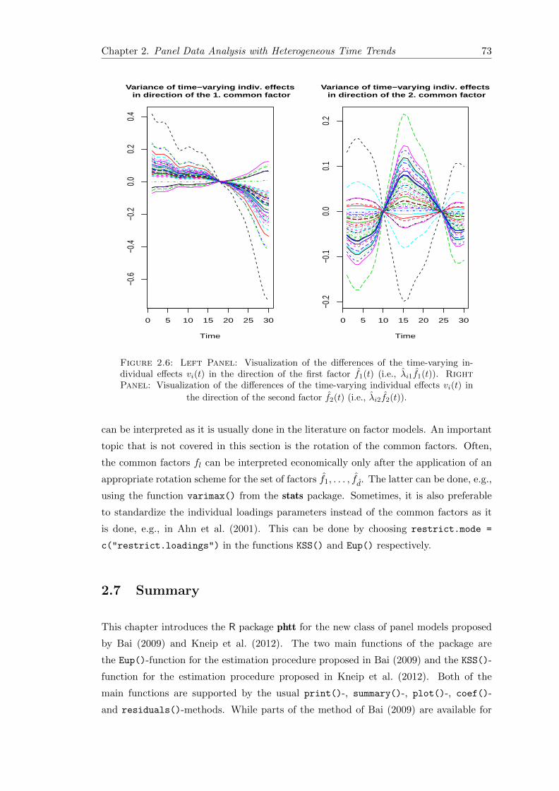
Chapter 2. Panel Data Analysis with Heterogeneous Time Trends 73
0 5 10 15 20 25 30
−0.6
−0.4
−0.2
0.0
0.2
0.4
Variance of time−varying indiv. effects in direction of the 1. common factor
Time
0 5 10 15 20 25 30−0
.2−0
.10.
00.
10.
2
Variance of time−varying indiv. effects in direction of the 2. common factor
Time
Figure 2.6: Left Panel: Visualization of the differences of the time-varying in-dividual effects vi(t) in the direction of the first factor f1(t) (i.e., λi1f1(t)). RightPanel: Visualization of the differences of the time-varying individual effects vi(t) in
the direction of the second factor f2(t) (i.e., λi2f2(t)).
can be interpreted as it is usually done in the literature on factor models. An important
topic that is not covered in this section is the rotation of the common factors. Often,
the common factors fl can be interpreted economically only after the application of an
appropriate rotation scheme for the set of factors f1, . . . , fd. The latter can be done, e.g.,
using the function varimax() from the stats package. Sometimes, it is also preferable
to standardize the individual loadings parameters instead of the common factors as it
is done, e.g., in Ahn et al. (2001). This can be done by choosing restrict.mode =
c("restrict.loadings") in the functions KSS() and Eup() respectively.
2.7 Summary
This chapter introduces the R package phtt for the new class of panel models proposed
by Bai (2009) and Kneip et al. (2012). The two main functions of the package are
the Eup()-function for the estimation procedure proposed in Bai (2009) and the KSS()-
function for the estimation procedure proposed in Kneip et al. (2012). Both of the
main functions are supported by the usual print()-, summary()-, plot()-, coef()-
and residuals()-methods. While parts of the method of Bai (2009) are available for

74
commercially available software packages, the estimation procedure proposed by Kneip
et al. (2012) is not available elsewhere. A further remarkable feature of our phtt package
is the OptDim()-function, which provides an ease access to many different dimensional-
ity criteria proposed in the literature on factor models. The usage of the functions is
demonstrated by a real data application.

Chapter 3
Panel Models with Multiple
Jumps in the Parameters
3.1 Introduction
Panel datasets with large cross-sectional dimensions and large periods of time observa-
tions are becoming more and more available due to the impressive progress of information
technology. This has been succeeded, in the econometric literature, by the development
of new methods and techniques for analyzing large panels. There is, however, an impor-
tant issue, that is scarcely discussed in most of the existing work –the risk of neglecting
structural breaks in the data generating process, especially when the observation pe-
riod is large. In the field of empirical macroeconomics, this problem is most famously
considered by Lucas (1976), who points out the risk of predicting naively the effects
of economic policy changes based on historical data, since the emergence of important
economic events and shocks may induce changes in the model parameters during the
time. Of course, the larger the observation period, the more likely the occurrence of
such shocks. While a vast literature on change point analysis exists for univariate time
series, little research has been done on panel data models.
In this chapter, we propose a novel method for estimating panel models with multiple
structural changes that occur at unknown points in time and may affect each slope
parameter individually. We consider, for i ∈ 1, . . . , n, t ∈ 1, . . . , T, models of the
form
Yit =P∑p=1
Sp+1∑j=1
Xit,pI(τj−1 < t ≤ τj
)βτj ,p + αi + θt + εit, (3.1)
where I(.) is the indicator function, the set of jump points τ0,p, τ1,p, . . . , τSp+1,p|τ0,p =
1 < τ1,p < . . . < τSp+1,p = T ⊆ 1, . . . , T and Sp are unknown, Yit is the dependent
75

76
variable for individual i at time t, Xit,p is the pth explaining variable, αi is an individual
specific effect, θt is a common time parameter, and εit is an unobserved idiosyncratic
term that may be correlated with one or more explaining variables.
In single time series, the available information is often not sufficient to uncover the true
dates of the structural breaks. Only the time fractions of the break locations can be
consistently estimated and tested; see, e.g., Bai (1997), Bai and Perron (1998, 2003),
Inoue and Rossi (2011), Pesaran et al. (2011), Aıt-Sahalia and Jacod (2009), and Carr
and Wu (2003). In panel data models, such a limitation can be alleviated since the
cross-section dimension provides an important source of additional information. Besides
the virtue of getting improved statistical efficiency, the determination of the change
point locations can be, in many applications, of particular interest. Indeed, estimating
the number and locations of the structural breaks from the data alleviates concerns
about ad-hoc subsample selection, enables interpretation of historical events that are not
explicitly considered in the model, and avoids statistical under- or over-parametrization
related issues.
One of the earliest contributions in testing the structural breaks in panel data literature
is the work of Han and Park (1989). The authors propose a multivariate version of the
consum-test, which can be seen as a direct extension of the univariate time series test
proposed by Brown et al. (1975). Qu and Perron (2007) extend the work of Bai and
Perron (2003) and consider the problem of estimating, computing, and testing multiple
structural changes that occur at unknown dates in linear multivariate regression models.
They propose a quasi-maximum likelihood method and a likelihood ratio-type statistics
based on Gaussian errors. The method requires, however, the number of equations to be
fixed and does not consider the case of large panel models with unobserved effects and
possible endogenous regressors. Based on the work of Andrews (1993), De Wachter and
Tzavalis (2012) propose a break testing procedure for dynamic panel data models with
exogenous or pre-determined regressors when n is large and T is fixed. The method can
be used to test for the presence of a structural break in the slope parameters and/or
in the unobserved fixed effects. But their assumptions allow only for the presence of
a single break. Bai (2010) proposes a framework to estimate the break in means and
variance. Bai (2010) also considers the case of one break and establishes consistency
for both large and fixed T . Kim (2014) extends the work of Bai (2010) to allow for the
presence of unobserved common factors in the model. Pauwels et al. (2012) analyze the
cases of a known and an unknown break date and propose a Chow-type test allowing for
the break to affect some, but not all, cross-section units. Although the method concerns
the one-break case, it requires intensive computation to select the most likely individual
breaks from all possible sub-intervals when the break date is unknown.

Chapter 3. Panel Models with Multiple Jumps in the Parameters 77
To the best of the authors’ knowledge, ours is the first work to deal with the problem
of multiple jump discontinuities in the parameters of panel models without imposing
restrictive assumptions on the number, the location, and/ or the aspect of the breaks.
The method can be applied to panel data with large time span T and large cross-
section dimension n and allows for T to be very long compared to n. We also consider
the classic case of panel data, in which T is fixed and only n is large. Our model
generalizes the special model specifications in which the slope parameters are either
constant over time, so that Sp = 0, or extremely time heterogeneous so that, for all
p, τ0,p = 1, τ1,p = 2, . . . , τSp+1,p = T when T is fixed. Our theory considers breaks
in a two-way panel data model, in which the unobserved heterogeneity is composed of
additive individual effects and time specific effects. We show that our method can also
be extended to cover the case of panel models with unobserved heterogeneous common
factors as proposed by Ahn et al. (2001), Pesaran (2006), Bai (2009), Kneip et al. (2012),
and Bada and Kneip (2014). Our estimation procedure is related to the Haar wavelet
technique, which we transform and adapt to the structure of the observed variables in
order to detect the location of the break points consistently. We propose a general setup
allowing for endogenous models such as dynamic panel models and/or structural models
with simultaneous panel equations. Consistency under weak forms of dependency and
heteroscedasticity in the idiosyncratic errors is established and the convergence rate
of our slope estimator is derived. To detect consistently the jump locations and test
for the statistical significance of the breaks, we propose post-wavelet procedures. Our
simulations show that, in many configurations of the data, our method performs very well
even when the idiosyncratic errors are affected by weak forms of serial-autocorrelation
and/or heteroskedasticity.
Our empirical vehicle for highlighting this new methodology addresses the stability of the
relationship between Algorithmic Trading (AT) and Market Quality (MQ). We propose
to automatically detect jumps in regression slope parameters to examine the effect of
algorithmic trading on market quality in different market situations. We find evidence
that the relationship between AT and MQ was disrupted between 2007 and 2008. This
period coincides with the beginning of the subprime crisis in the US market and the
bankruptcy of the big financial services firm Lehman Brothers.
The remainder of the chapter is organized as follows. Section 3.2 explains the basic
idea of our estimation procedure by using a relatively straightforward centered univari-
ate panel model. In Section 3.3, we consider panel models with unobserved effects and
multiple jumping slope parameters, present our model assumptions, and derive the main
asymptotic results. Section 3.4 proposes a post-wavelet procedure to estimate the jump
locations, derives the asymptotic distribution of the final estimator, and describes se-
lective testing procedures. In Section 3.5, we discuss models with an issue of omitted

78
common factors and endogenous models arising from structural simultaneous equation
systems. Section 3.6 presents the simulation results of our Monte Carlo experiments.
Section 3.7 is concerned with the empirical application. The conclusion follows in Section
3.8. The mathematical proofs are collected in Appendix B.
3.2 Preliminaries
A Simple Panel Model with one Jumping Parameter
To simplify the exposition, we begin with a relatively straightforward version of (3.1).
We consider a centered univariate panel data model of the form
Yit = Xitβt + eit for i ∈ 1, . . . , n and t ∈ 1, . . . , T, (3.2)
where Xit is an univariate regressor, βt is a scalar, and E(eit) = 0.
We allow for the slope parameter βt to change at unknown time points, say τ1, . . . , τS ,
such that
βt =
βτ1 for t ∈ 1, . . . , τ1,βτ2 for t ∈ τ1 + 1, . . . , τ2,...
βτS for t ∈ τS−1 + 1, . . . , τS, and
βτS+1 for t ∈ τS + 1, . . . , T.
(3.3)
Some Fundamental Concepts of Wavelet Transform
The idea behind our approach consists basically of using the Haar wavelet expansion of
βt to control for its piecewise changing character. Before continuing with the estimation
method, we introduce some important concepts and notations that are necessary for our
analysis.
We assume that the intertemporal sample size T is dyadic, i.e., T = 2L−1 for some
positive integer L ≥ 2. This is because wavelet functions are constructed via dyadic
dilations of order 2l, for l ∈ 1, . . . , L. The case of a non-dyadic time dimension will be
discussed later. Technically, the discrete wavelet transformation is much like the Fourier
transformation, except that the wavelet expansion is constructed with a two parameter
system: a dilation level l ∈ 1, . . . , L and a translation index k ≤ 2l−2.
Let ϕl0,k, k = 1, . . . ,Kl0, and ψl,k, l = l0 + 1, . . . , L; k = 1, . . . , 2l−2, respectively,
represent collections of discrete scaling and wavelet functions defined on the discrete

Chapter 3. Panel Models with Multiple Jumps in the Parameters 79
interval 1, . . . , 2L−1 such that
ψl,k(t) = aψl Il,2k−1(t)− aψl Il,2k(t) and (3.4)
ϕl0,k(t) = aϕl0Il+1,2k−1(t) + aϕl0Il+1,2k(t), (3.5)
where aϕl0 =√
2l0−1, aψl =√
2l−2, and Il,m(t) is the indicator function that carries the
value one if t ∈ 2L−l(m− 1) + 1, . . . , 2L−lm and zero otherwise.
The multiscale discrete Haar wavelet expansion of βt can be presented as follows:
βt =
Kl0∑k=1
ϕl0,k(t)dl0,k +L∑
l=l0+1
Kl∑k=1
ψl,k(t)cl,k, for t ∈ 1, . . . , T, (3.6)
where Kl = 2l−2, for l > 1, and K1 = 1. The coefficients dl,k and cl,k are called scaling
and wavelet coefficients, respectively. Because ϕl0,k(t) and ψl,k(t) are orthonormal, dl,k
and cl,k are unique and can be interpreted as the projection of βt on their corresponding
bases, i.e., dl0,k = 12L−1
∑2L−1
t=1 ϕl0,k(t)βt and cl,k = 12L−1
∑2L−1
t=1 ψl,k(t)βt.
Although the Haar wavelet basis functions are the simplest basis within the family of
wavelet transforms, they exhibit an interesting property allowing for analyzing functions
with piecewise sudden changes.
Orthonormalization and Estimation
Note that the collection of functions, in (3.6), is not unique. Here, we set l0 = 1, to
fix the primary scale to be the coarsest possible with only one parameter that reflects
the general mean of βt. In addition, we propose a slightly modified version of wavelet
expansion to adapt the orthonormalization conditions to the requirements of our panel
data method.
We consider the following expansion:
βt =
L∑l=1
Kl∑k=1
wl,k(t)bl,k for t ∈ 1, . . . , T, (3.7)
where
wl,k(t) =
a1,1 = a2,1h2,1(t) + a2,2h2,2(t) if l = 1, and
al,2k−1hl,2k−1(t)− al,2khl,2k(t) if l > 1,(3.8)
for some positive standardizing scales al,2k−1 and al,2k that, unlike the conventional
wavelets, do not only depend on the dilation level l but also on the translation index
k. Their exact form will be discussed in detail below. We define the function hl,m(t) as
80
follows:
hl,m(t) =√
2l−2Il,m(t). (3.9)
The most appealing feature of expansion (3.7) (and (3.6) with l0 = 1) is that the set of
the wavelet coefficients bl,k contains at most (S + 1)L non-zero-wavelet coefficients.
This important property results from the fact that each jump in βt can be sensed at each
dilation level by at most one translation function. Proposition 3.1 states the existence
of (3.7) for any arbitrary positive real scales al,2k and al,2k−1.
Proposition 3.1. Suppose T = 2L−1, for some integer L ≥ 2, and β = (β1, . . . ,
βT )′ ∈ RT a vector that possesses exactly S ≥ 1 jumps at τ1, . . . , τS |τ1 < . . . < τS ⊆
1, . . . , T as in (3.3). Let a1,1, al,2k−1 and al,2k be arbitrary positive real values for all
l ∈ 1, . . . , L, and k ∈ 1, . . . ,Kl. Thus, Expansion (3.7) exists and the set of the
wavelet coefficients blk|l = 1, . . . , L; k = 1, . . . ,Kl contains at most (S + 1)L non-zero
coefficients.
Using (3.7), we can rewrite Model (3.2) as
Yit =L∑l=1
Kl∑k=1
Xl,k,itbl,k + eit, (3.10)
where
Xl,k,it = Xitwl,k(t).
In vector notation,
Yit = X ′itb+ eit, (3.11)
where Xit = (X1,1,it, . . . ,XL,KL,it)′
and b = (b1,1, . . . , bL,KL)′.
Throughout, we assume the existence of an instrument Zit that is correlated with Xit
and fulfills E(Ziteit) = 0 for all i and t. The idea behind this assumption is to provide
a general treatment that allows for estimating models with endogenous regressors such
as dynamic models or structural models with simultaneous equations. Let Zl,k,it =
Zitwl,k(t) and Zit = (Z1,1,it, . . . ,ZL,KL,it)′. Because E(Ziteit) = 0 for all i and t, we can
infer that E(Zl,k,iteit) = 0, for all l and k. The required theoretical moment condition
for estimating b is
E(Zit(Yit −X
′itb))
= 0. (3.12)
Chapter 3. Panel Models with Multiple Jumps in the Parameters 81
The IV estimator of b (hereafter, denoted by b) is obtained by solving the empirical
counterpart of (3.12), i.e.,
1
nT
n∑i=1
T∑t=1
(Zit(Yit −X
′itb))
= 0. (3.13)
Remark 3.2. We know from the Generalized Method of Moments (GMM) that the IV
estimator is equivalent to the just-identified GMM estimator, in which the number of
instruments is equal to the number of parameters to be estimated. Our estimator of b
can be, hence, seen as a GMM estimator:
b = arg minb
1
nT
n∑i=1
T∑t=1
(Yit −X′itb)Z
′itWTZit(Yit −X
′itb), (3.14)
where WT is an arbitrary symmetric (T × T ) full rank matrix. Since there is no matter
how to choose WT in the just-identified case, we can use the identity matrix to solve
(3.14).
Under general assumptions, we can state the consistency of b for any arbitrary collection
of wavelet functions. But the problem with naively using the conventional basis functions
is that the identification of the zero- and non-zero coefficients will be complicated. Not
only will the presence of the error term in (3.10) affect the estimates of bl,k but also the
non-orthogonality of Zl′ ,k′ ,it to Xl,k,it across different dilation and translation levels in
the objective function (the IV moment condition) will move the problem from a classical
wavelets shrinkage scheme to a complex model selection problem.
Our idea consists of adjusting the scales a1,1, al,2k−1 and al,2k in (3.8) to the structure
of Xit and Zit so that following normalization conditions are satisfied.
(a): 1nT
∑ni=1
∑Tt=1Zl,k,itXl′ ,k′ ,it = 1 if (l, k) = (l
′, k′) and
(b): 1nT
∑ni=1
∑Tt=1Zl,k,itXl′ ,k′ ,it = 0 for all (l, k) 6= (l
′, k′).
Proposition B.2, in Appendix B.1, gives the mathematical conditions for a1,1, al,2k−1 and
al,2k to ensure (a) and (b). The solution is
a1,1 = Q− 1
21,1 ,
al,2k−1 = Q−1l,2k−1
(Q−1l,2k−1 +Q−1
l,2k
)− 12 , and
al,2k = Q−1l,2k
(Q−1l,2k−1 +Q−1
l,2k
)− 12 ,
whereQ1,1 = 1nT
∑ni=1
∑Tt=1XitZit, Ql,2k−1 = 1
nT
∑ni=1
∑Tt=1XitZith
2l,2k−1(t), andQl,2k =
1nT
∑ni=1
∑Tt=1XitZith
2l,2k(t).
82
Solving (3.13) (or (3.14)) with respect to bl,k under Restrictions (a) and (b), we obtain
bl,k =1
nT
n∑i=1
T∑t=1
Zl,k,itYit. (3.15)
Making use of orthonormality, we can directly perform the universal thresholding scheme
of Donoho and Johnstone (1994). Our structure adapted wavelet estimator of βt (here-
after, the SAW estimator) can be obtained by
βt =L∑l=1
Kl∑k=1
wl,k(t)bl,k, (3.16)
where
bl,k =
bl,k if |bl,k| > λn,T and
0 else,(3.17)
for some threshold λn,T that depends on n and T . Theorems 3.5, 3.7 give the necessary
conditions for λn,T to ensure consistency under Assumptions A-C presented in Section
3.3.
Remark 3.3. If the explaining variable Xit is exogenous, we can choose Zit = Xit to
instrument all elements in Xl,k,it with themselves. In this case, our shrinkage estimator
bl,k can be interpreted as a Lasso estimator with the advantage of perfect orthogonal
regressors; see, e.g., Tibshirani (1996). More generally, if Xit is allowed to be endogenous
and Zl,k,it 6= Xl,k,it, bl,k can be obtained by minimizing a Lasso-penalized just-identified
GMM objective function. That is,
b = arg minb
1
nT
n∑i=1
T∑t=1
(Yit −X′itb)Z
′itWTZit(Yit −X
′itb) + λn,T |b|, (3.18)
where |b| =∑L
l=1
∑Klk=1 |bl,k| andWT is an arbitrary symmetric (T ×T ) full rank matrix.
Note that (3.18) and (3.17) lead to the same result independently of the choice of WT .
First step SAW estimation for a straightforward centered panel model is done. Gener-
alization for multivariate models with unobserved heterogeneity effects and post-SAW
procedures follow.

Chapter 3. Panel Models with Multiple Jumps in the Parameters 83
3.3 Two-way Panel Models with Multiple Jumps
Model
One of the main advantages of using panel datasets is the possibility of dealing with
problems related to the potential effect of unobserved heterogeneity in time- and cross-
section dimensions. In this section, we generalize the SAW method to models with
unobserved individual and time effects and allow for multiple jumping parameters. Col-
lecting the slope parameters in a (P × 1) time-varying vector, we can write Model (3.1)
as
Yit = µ+X′itβt + αi + θt + eit, (3.19)
where Xit = (X1,it, . . . , XP,it)′
is a (P × 1) vector of regressors, βt = (βt,1 . . . , βt,P )′
is
a (P × 1) vector of slope parameters, αi is a time-constant individual effect and θt is a
common time-varying effect. We allow for each βt,p, p ∈ 1, . . . , P, to jump at unknown
Sp break points, say τ1,p, . . . , τSp,p, such that
βt,p =
βτ1,p for t ∈ 1, 2, . . . , τ1,p,βτ2,p for t ∈ τ1,p + 1, . . . , τ2,p,...
βτSp+1,p for t ∈ τSp,p + 1, . . . , T.
(3.20)
The estimation procedure for this model is conceptually similar to the univariate method
discussed in Section 3.2. However, besides the need to deal with multivariate wavelets,
we have to control for the additional unknown parameters µ, αi, and θt.
From the literature on panel models, we know that uniqueness of µ, αi, and θt requires
the following identification conditions:
C.1:∑n
i=1 αi = 0, and
C.2:∑T
t=1 θt = 0.(3.21)
3.3.1 Estimation
In order to cover the case of dynamic models with both small and large T , we conven-
tionally start with differencing the model to eliminate the individual effects and assume
the existence of appropriate instruments.
By taking the difference on the left and the right hand side of (3.19), we get
(Yit − Yit−1) = X′itβt −X
′it−1βt−1 + (θt − θt−1) + (eit − eit−1), (3.22)

84
for i ∈ 1, . . . , n and t ∈ 2, . . . , T.
Because n is usually supposed to be large, ∆θt = θt − θt−1, can be eliminated by
using the classical within transformation on the model, i.e., ∆Yit = ∆Yit− 1n
∑ni=1 ∆Yit.
Alternatively, we can associate ∆θt with an additional unit regressor in the model and
estimate it jointly with βt as a potential jumping parameter. Indeed, allowing for ∆θt
to be piecewise constant over time can be very useful for interpretation, especially when
the original time effect θt has approximately a piecewise changing linear trend.
Let Xit = (X′it,−X
′it−1, 1)
′and γt = (β
′t, β
′t−1,∆θt)
′be (P × 1) extended vectors, where
P = 2P + 1. We can rewrite Model (3.22) as
∆Yit = (X′it,−X
′it−1, 1)
βt
βt−1
∆θt
+ ∆eit,
= X′itγt + ∆eit,
(3.23)
for i ∈ 1, . . . , n and t ∈ 2, . . . , T.
By using multivariate structure adapted wavelet functions, we can estimate γt in a way
similar to the way discussed in Section 3.2.
The multivariate structure adapted wavelet expansion of γt can be presented as follows:
γt =L∑l=1
Kl∑k=1
Wlk(t)bl,k for t ∈ 2, . . . , T, (3.24)
where blk = (bl,k,1, . . . , bl,k,P )′
is a (P × 1) vector of wavelet coefficients and Wlk(t) is a
(P × P ) multivariate wavelet basis matrix defined as
Wl,k(t) =
A1,1 = A2,1H2,1(t) +A2,2H2,2(t) if l = 1, and
Al,2k−1Hl,2k−1(t)−Al,2kHl,2k(t) if l > 1,(3.25)
with
Hl,m(t) =√
2l−2Il,m(t− 1),
and A1,1, Al,2k−1, and Al,2k are constructed so that the following orthonormality condi-
tions are fulfilled:
(A): 1n(T−1)
∑ni=1
∑Tt=2Z l,k,itX
′
l′ ,k′ ,it= IP×P if (l, k) = (l
′, k′) and
(B): 1n(T−1)
∑ni=1
∑Tt=2Z l,k,itX
′
l′ ,k′ ,it= 0P×P for all (l, k) 6= (l
′, k′).

Chapter 3. Panel Models with Multiple Jumps in the Parameters 85
Here, X ′l,k,it = X′itWlk(t), IP×P is the (P ×P ) identity matrix, 0P×P is a (P ×P ) matrix
of zeros, and Z ′l,k,it = Z′itWl,k(t), where Zit is a (P × 1) vector used to instrument the
P variables in Xit; the unit regressor associated with ∆θt and the remaining exogenous
regressors (if they exist) can be, of course, instrumented by themselves.
We can easily verify that
A1,1 = Q− 1
21,1 ,
Al,2k−1 = Q−1l,2k−1
(Q−1l,2k−1
+Q−1l,2k
)− 12 , and
Al,2k = Q−1l,2k
(Q−1l,2k−1
+Q−1l,2k
)− 12 ,
with
Q1,1
=1
n(T − 1)
n∑i=1
T∑t=2
ZitX′it,
Ql,2k−1
=1
n(T − 1)
n∑i=1
T∑t=2
ZitX′ithl,2k−1(t)2, and
Ql,2k
=1
n(T − 1)
n∑i=1
T∑t=2
ZitX′ithl,2k(t)
2.
ensure conditions (A) and (B).
The IV estimator of bl,k is the solution of the empirical moment condition
1
n(T − 1)
n∑i=1
T∑t=2
L∑l=1
Kl∑k=1
(Z l,k,it(∆Yit −X
′l,kitbl,k)
)= 0. (3.26)
Solving (3.26) for bl,k under the the normalization Conditions (A) and (B), we obtain
bl,k,p =1
n(T − 1)
n∑i=1
T∑t=2
Zl,k,it,p∆Yit,
where bl,k,p and Zl,k,it,p are the pth elements of bl,k and Z l,k,it, respectively.
The SAW estimator of βt,p can be obtained by
γt,p =L∑l=1
Kl∑k=1
P∑q=1
Wlk,p,q(t)bl,k,q, (3.27)
or
γt+1,p+P =L∑l=1
Kl∑k=1
P∑q=1
Wlk,p+P,q(t+ 1)bl,k,q, (3.28)

86
where Wlk,p,q is the (p, q)- element of the basis matrix Wlk(t), and
bl,k,q =
bl,k,q if |bl,k,q| > λn,T and
0 else.(3.29)
3.3.2 Assumptions and Main Asymptotic Results
We present a set of assumptions that are necessary for our asymptotic analysis. Through-
out, we use Ec(.) to define the conditional expectation given Xiti,t∈N∗2 and Ziti,t∈N∗2 ,
where N∗ = N\0. We denote by M a finite positive constant, not dependent on n and
T . The operatorsp−→ and
d−→ denote the convergence in probability and distribution.
Op(.) and op(.) are the usual Landau-symbols. The Frobenius norm of a (p× k) matrix
A is denoted by ||A|| = [tr(A′A)]1/2, where A
′denotes the transpose of A. ∆ denotes
the difference operator of first order.
Our theoretical setup relies on the following assumptions.
Assumption A - Data Dimension and Stability Intervals:
(i) T − 1 = 2L−1 for some natural number L > 1; the number of regressors P is fixed.
(ii) n → ∞; T is either fixed or passes to infinity simultaneously with n such that
log(T )/n→ 0.
(iii) minj,p |βτj,p − βτj−1,p | does not vanish when n and T pass to infinity; all stability
intervals (τj,p − τj−1,p)→∞ uniformly in n, as T →∞.
Assumption B - Regressors and Instruments:
(i) for all i and t, Ec(Ziteit) = 0; for all l ∈ 1, . . . , L and k ∈ 1, . . . ,Kl,
Ql,k
=1
n · ]s|hl,k(s) 6= 0∑
t∈s|hl,k(s) 6=0
n∑i=1
ZitX′it
p−→ Ql,k,
where Ql,k
is a (P × P ) full rank finite matrix with distinct eigenvectors.
(ii) The moments E||Zit||4 and E||Xit||4 are bounded uniformly in i and t; for Al,2k =
Q−1l,2k
(Q−1l,2k
+Q−1l,2k−1
)−1/2 and Al,2k−1 = Q−1l,2k−1
(Q−1l,2k
+Q−1l,2k−1
)−1/2, the moments
E||Al,2k||4 and E||Al,2k−1||4 are bounded uniformly in l and k.
Chapter 3. Panel Models with Multiple Jumps in the Parameters 87
(iii) the multivariate distribution of ∆eiti∈N∗,t∈N∗\1 is Sub-Gaussian so that every
linear combination
ΠnT (as,s′ ) =
s′∑
t=s+1
n∑i=1
as,s′ ,it√n(s′ − s)
∆eit,
with E(as,s′ ,it∆eit) = 0 and E(Π2nT (as,s′ )
)≤ M , is Sub-Gaussian distributed of
order ΣnT (as,s′ ) = E(Π2nT (as,s′ )
), i.e.,
P(Σ− 1
2nT (as,s′ )|ΠnT (as,s′ )| ≥ c
)≤ 1
cexp(−c
2
2),
for any c > 0.
Assumption C - Weak Dependencies and Heteroskedasticity in the Error
Term: Ec(∆eit∆ejm) = σij,tm, |σij,tm| ≤ σ for all (i, j, t,m) such that
1
n(s′ − s+ 1)
n∑i=1
n∑j=1
s′∑
t=s+1
s′∑
m=s+1
|σij,tm| ≤M.
Assumption A.(i) specifies a dyadic condition on the intertemporal data size T . This
is a technical assumption that is only required for constructing the dyadic wavelet ba-
sis functions. In practice, we can replicate the data by reflecting the observations at
the boundaries to get the desired dimension. If, for instance, T − 1 = 125, we can ex-
tend the sample (Yi1, Xi1), . . . , (YiT , XiT ) with the three last observations (YiT−1, XiT−1),
(YiT−2, XiT−2), and (YiT−3, XiT−3) for T +1, T +2, and T +3, respectively. The asymp-
totic property of the estimator, will depend, of course, on the original data size and not
on the size of the replicated data. Assumption A.(ii) allows for the time dimension T to
be very long compared to n but in such a way that log(T ) = o(n). A.(ii) considers also
the classical case of panel data, in which T is fixed and only n→∞. Assumption A.(iii)
guarantees that the jumps do not vanish as n and/or T pass to infinity. The second part
of Assumption A.(iii) can be alleviated to allow for some stability intervals to stay fixed
if T →∞. Assuming the stability intervals to pass to infinity when T gets large allows
for interpreting the T -asymptotic as a full-in asymptotic.
Assumption B.(i) requires that the probability limit of Ql,k
is a full rank finite matrix
with distinct eigenvectors. This is to ensure that its eigendecompostion exists. Assump-
tion B.(ii) specifies commonly used moment conditions to allow for some limiting terms

88
to be Op(1) when using Chebyshev inequality. The Sub-Gaussian condition in Assump-
tion B.(iii) excludes heavy tailed distributed errors but does not impose any specific
exact distribution.
Assumption C allows for a weak form of time series and cross section dependence in
the errors as well as heteroskedasticities in both time and cross-section dimension. It
implies that the covariances and variances are uniformly bounded and the double sum-
mations over all possible time partitions are well behaved. The assumption generalizes
the restricted case of independent and identically distributed errors.
The following Lemma establishes the main asymptotic results for the structure adapted
wavelet coefficients.
Lemma 3.4. Suppose Assumptions A-C hold, then
(i)
supl,k,q
∣∣∣bl,k,q − bl,k,q∣∣∣ = Op(√
log(T − 1)/n(T − 1)),
(ii) for some finite M >√
2,
supl,k,q
∣∣∣bl,k,q − bl,k,q∣∣∣ ≤M√log((T − 1)P )/n(T − 1)
holds with a probability that converges to 1 independently of n, as T →∞.
Theorem 3.5 establishes the uniform and the mean square consistency of γt,p.
Theorem 3.5. Assume Assumptions A-C, then the following statements hold:
(i) supt |γt,p − γt,p| = op(1) for all p ∈ 1, . . . , P, if√T − 1λn,T → 0, as n, T → ∞
or n→∞ and T is fixed, and
(ii) 1T−1
∑Tt=2 ||γt − γt||2 = Op
(J∗
(T−1)(log(T − 1)/n)κ), where J∗ = min(
∑Pp=1 Sp +
1) log(T − 1), (T − 1) , if√T − 1λn,T ∼ (log(T − 1)/n)κ/2, for any κ ∈]0, 1[.
Uniform consistency is obtained when n → ∞ and T is fixed or n, T → ∞ with
log(T )/n→ 0. If the maximum number of jumps is fixed, the mean square consistency
is obtained even when n is fixed and only T →∞.
A threshold that satisfies Conditions (i) and (ii) in theorem 3.5, can be constructed as
follows:
λnT = V12nT
(2 log((T − 1)P )
n(T − 1)1/κ
)κ/2, for some κ ∈]0, 1[, (3.30)

Chapter 3. Panel Models with Multiple Jumps in the Parameters 89
where VnT is the empirical variance estimator corresponding to the largest variance of1√nT
∑ni=1
∑Tt=1Zit,l,k,p∆eit over l, k, and p. Such an estimator can be obtained by
using the residuals eit of a pre-intermediate SAW regression performed with a plug-in
threshold λ∗nT = 0. We want to emphasize that asymptotically all we need is that VnT be
strictly positive and bounded. The role of V12nT is only to give the threshold a convenient
amplitude. The role of κ < 1 is to trade off the under-estimation effect that can arise
from the plug-in threshold λ∗n,T = 0. An ad-hoc choice of κ is 1− log log(nT )/ log(nT ).
For more accurate choices, we refer to the calibration strategies proposed by Hallin and
Liska (2007) and Alessi et al. (2010).
3.4 Post-SAW Procedures
3.4.1 Tree-Structured Representation
The intrinsic problem of wavelets is that wavelet functions are constructed via dyadic
dilations. Error may make this feature spuriously generate some additional mini jumps to
stimulate the big (true) jump when it is located at a non-dyadic position. To construct
a selective inference for testing the systematic jumps it is important to encode the
coefficients that may generate such effects. One possible approach is to examine the so-
called tree-structured representation, which is based on the hierarchical interpretation
of the wavelet coefficients. Recall that the wavelet basis functions are nested over a
binary multiscale structure so that the support of an (l, k)- basis (the time interval in
which the basis function is not zero) contains the supports of the basis (l + 1, 2k − 1)
and (l+ 1, 2k). We say that the wavelet coefficient bl,k is the parent of the two children
bl+1,2k−1 and bl+1,2k. This induces a dyadic tree structure rooted to the primary parent
b1,1. To encode the possible systematic jumps, we have to traverse the tree up to the
root parent in a recursive trajectory starting from the non-zero coefficients at the finest
resolution (highest dilation level). While the presence of a non-zero coefficient, at the
highest level, indicates the presence of a jump, the parent may have a non-zero coefficient
only to indicate that the stability interval around this jump is larger than its support.
As an illustration, consider the tree-structured representation in Figure 3.1. The coeffi-
cients at the not-ringed nodes fall in the interval [−λn,T , λn,T ] and carry the value zero.
Starting from the non-zero coefficient b5,6 at the finest resolution and traversing the tree
up to the root parent, we can identify b4,3, b3,2, and b2,1 as candidates for generating po-
tential visual artifacts at points 8, 10, and 12 if a jump exists only at 11. These selected
jump points can be tested by using, e.g., the equality test of Chow (1960).

90
1 2 3 4 5 6 7 8 9 10 11 12 13 14 15 T
,
,
,
,
,
,
,, ,
,,
Figure 3.1: An illustrating example of a tree-structured representation for the waveletcoefficients.
1 2 3 4 5 6 7 8 9 10 11 12 13 14 15 T
, ,
,
,
,
non-shifted wavelet estimatesshifted wavelet estimates
,
,
Figure 3.2: An illustrating example of a tree-structured representation for the shiftedand non-shifted coefficients.
If we have an additional observation, we can construct a shifted wavelet expansion
on a second (shifted) dyadic interval. The tree-structured representation of the new
coefficients can provide important information about the significance of the potential
jumps detected in the first tree. Continuing with the same example of Figure 3.1, we
can see that the tree-structured representations of the shifted and non-shifted coefficients
presented in Figure 3.2 support the hypothesis of only one jump at 11.
In the multivariate case, the interpretation of the tree-structured representation can
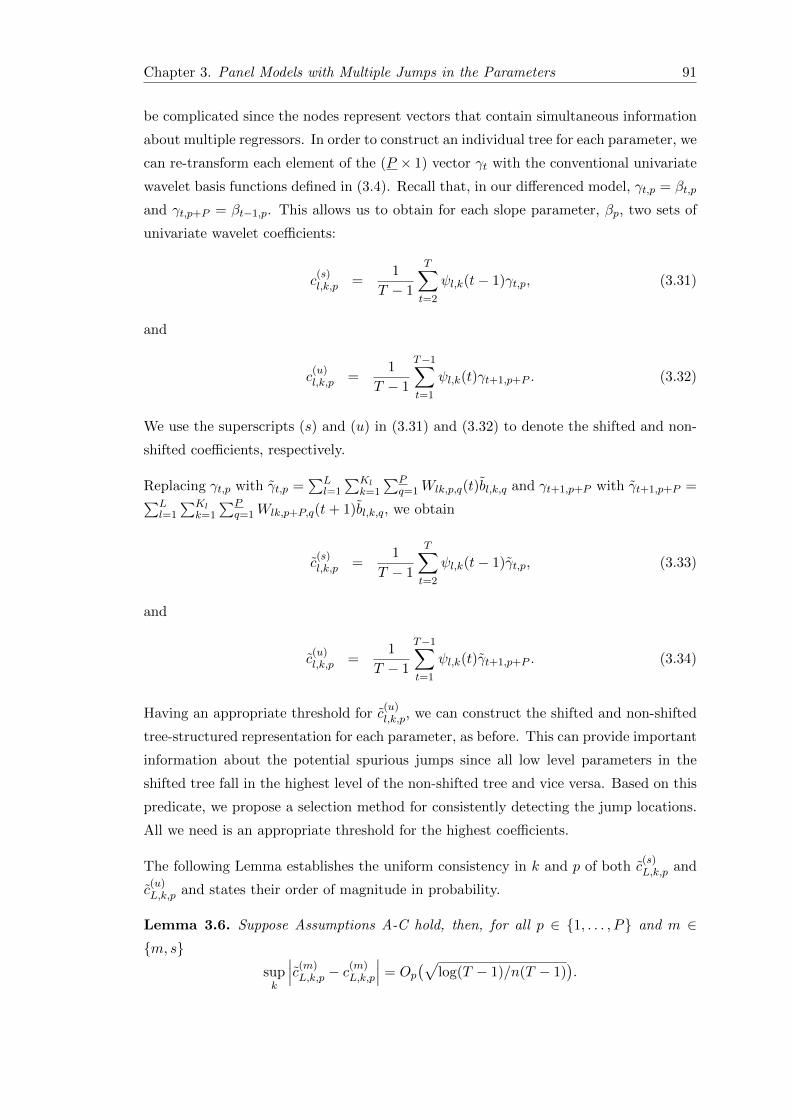
Chapter 3. Panel Models with Multiple Jumps in the Parameters 91
be complicated since the nodes represent vectors that contain simultaneous information
about multiple regressors. In order to construct an individual tree for each parameter, we
can re-transform each element of the (P × 1) vector γt with the conventional univariate
wavelet basis functions defined in (3.4). Recall that, in our differenced model, γt,p = βt,p
and γt,p+P = βt−1,p. This allows us to obtain for each slope parameter, βp, two sets of
univariate wavelet coefficients:
c(s)l,k,p =
1
T − 1
T∑t=2
ψl,k(t− 1)γt,p, (3.31)
and
c(u)l,k,p =
1
T − 1
T−1∑t=1
ψl,k(t)γt+1,p+P . (3.32)
We use the superscripts (s) and (u) in (3.31) and (3.32) to denote the shifted and non-
shifted coefficients, respectively.
Replacing γt,p with γt,p =∑L
l=1
∑Klk=1
∑Pq=1Wlk,p,q(t)bl,k,q and γt+1,p+P with γt+1,p+P =∑L
l=1
∑Klk=1
∑Pq=1Wlk,p+P,q(t+ 1)bl,k,q, we obtain
c(s)l,k,p =
1
T − 1
T∑t=2
ψl,k(t− 1)γt,p, (3.33)
and
c(u)l,k,p =
1
T − 1
T−1∑t=1
ψl,k(t)γt+1,p+P . (3.34)
Having an appropriate threshold for c(u)l,k,p, we can construct the shifted and non-shifted
tree-structured representation for each parameter, as before. This can provide important
information about the potential spurious jumps since all low level parameters in the
shifted tree fall in the highest level of the non-shifted tree and vice versa. Based on this
predicate, we propose a selection method for consistently detecting the jump locations.
All we need is an appropriate threshold for the highest coefficients.
The following Lemma establishes the uniform consistency in k and p of both c(s)L,k,p and
c(u)L,k,p and states their order of magnitude in probability.
Lemma 3.6. Suppose Assumptions A-C hold, then, for all p ∈ 1, . . . , P and m ∈m, s
supk
∣∣∣c(m)L,k,p − c
(m)L,k,p
∣∣∣ = Op(√
log(T − 1)/n(T − 1)).

92
From Lemma 3.6, we can intuitively see that asymptotically both c(m)L,k,p and bl,k,p can
be shrunk by the same threshold λn,T . Theorem 3.7 gives the necessary asymptotic
conditions to ensure consistency of the jump selection method.
3.4.2 Detecting the Jump Locations
As mentioned earlier, interpreting all jumps of the SAW estimator as structural breaks
may lead to an over-specification of the break points. In this Section, we exploit the
information existing in the shifted and unshifted univariate wavelet coefficients (3.33)
and (3.34) to construct a consistent selection method for detecting the jump locations.
We use (3.33) and (3.34) to obtain the following two estimators of ∆βt:
∆β(u)t,p =
KL∑k=1
∆ψL,k(t)c(u)L,k,p, for t ∈ E , (3.35)
and
∆β(s)t,p =
KL∑k=1
∆ψL,k(t− 1)c(s)l,k,p, for t ∈ Ec, (3.36)
where
c(.)l,k,p = I(|c(.)
l,k,p| > λn,T ),
E is the set of the even time locations 2, 4, . . . , T−1, Ec is the complement set composed
of the odd time locations 2, 3, . . . , T \ E , and I(.) is the indicator function.
The number of jumps of each parameter can be estimated by
Sp =∑t∈E
I(∆β(u)t,p 6= 0) +
∑t∈Ec
I(∆β(s)t,p 6= 0). (3.37)
The jump locations τ1,p, . . . , τSp,p can be identified as follows:
τj,p = min
s
∣∣∣∣∣j =
s∑t=2
I(
∆β(u)t,p 6= 0, t ∈ E
)+
s∑t=3
I(
∆β(s)t,p 6= 0, t ∈ Ec
), (3.38)
for j ∈ 1, . . . , Sp. The maximal number of breaks S =∑P
p=1 = Sp can be estimated
by S =∑P
p=1 Sp.
Theorem 3.7. Under Assumptions A-C, if (c.1) :√
n(T−1)log((T−1))λn,T → ∞ and (c.2) :
√T − 1λn,T → 0, as n, T →∞, then
(i) limn,T→∞ P (S1 = S1, . . . , Sp = Sp) = 1 and

Chapter 3. Panel Models with Multiple Jumps in the Parameters 93
(ii) limn,T→∞ P (τ1,1 = τ1,1, . . . , τSP ,P = τSP ,P |S1 = S1, . . . , Sp = Sp) = 1.
The crucial element for consistently estimating τ1,1, . . . , τSP ,P is, hence, using a threshold
that converges to zero but at a rate slower than√
log(T − 1)/(n(T − 1)).
3.4.3 Post-SAW Estimation
For known τ1,p, . . . , τSp,p, we can rewrite Model (3.22) as
∆Yit =
P∑p=1
Sp+1∑j=1
∆X(τj,p)it,p βτj,p + ∆eit, (3.39)
where
∆X(τj,p)
(it,p) = ∆Xit,pI(τj−1,p < t ≤ τj,p
),
with τ0,p = 1 and τSp+1,p = T , for p ∈ 1, . . . , P. The dot operator transforms the
variables as follows: uit = uit − 1n
∑ni=1 uit.
Depending on the set of the jump locations τ := τj,p|j = 1, . . . , Sp + 1, p = 1, . . . , P,the vector presentation of Model (3.39) can be rewritten as
∆Yit = ∆X′
it,(τ)β(τ) + ∆eit, (3.40)
where β(τ) = (βτ1,1 , . . . , βτS1+1,1 , . . . , βτ1,P . . . , βτSP+1,P )′
and ∆Xit,(τ) = (∆X(τ1,1)it,1 , . . . ,
∆X(τS1+1,1)
it,1 , . . . ,∆X(τ1,P )it,P . . . ,∆X
τ(SP+1,P )
it,P )′
.
Let Zit,p denote the instrument chosen for ∆Xit,p and Zit,(τ) = (Z(τ1,1)it,1 , . . . , Z
(τS1+1,1)
it,1 ,
. . . , Z(τ1,P )it,P , . . . , Z
τ(SP+1,P )
it,P )′, with Z
(τj,p)it,p = Zit,pI
(τj−1,p < t ≤ τj,p
). The conventional
IV estimator of β(τ) is
β(τ) =( n∑i=1
T∑t=2
Zit,(τ)∆X′
it,(τ)
)−1( n∑i=1
T∑t=2
Zit,(τ)∆Yit). (3.41)
Conditional on S1 = S1, . . . , SP = SP , we can replace the set of the true jump locations τ
in (3.41) with the detected jump locations τ := τj,p|j ∈ 1, . . . , Sp+1, p ∈ 1, . . . , P,to obtain the post-SAW estimator:
β(τ) =( n∑i=1
T∑t=2
Zit,(τ)∆X′
it,(τ)
)−1( n∑i=1
T∑t=2
Zit,(τ)∆Yit). (3.42)
94
From (3.26) and (3.42), we can see that the number of parameters to be estimated after
detecting the jump locations is much smaller than the number of parameters required
to estimate the slope parameters in the SAW regression (∑P
p=1(Sp + 1) < T (P − 1)). It
is evident that such a gain in terms of regression dimension improves the quality of the
estimator.
Assumption E - Central Limits: Let T(τ) be a (S + P × S + P ) diagonal matrix
with the diagonal elements T1,1, . . . , TSP+1,P , where Tj,p = τj,p − τj−1,p + 1.
(i) : (nT(τ))−1∑n
i=1
∑Tt=2 Zit,(τ)∆X
′
it,(τ)
p→ Q(τ) where Q(τ) is a full rank finite matrix.
(ii) : (nT(τ))−1∑n
i=1
∑Tt=2
∑nj=1
∑Ts=2 Zit,(τ)Z
′
js,(τ)σij,tsp→ V (τ), where V (τ) is a full rank
finite matrix.
(iii) :(nT(τ)
)− 12∑n
i=1
∑Tt=2 Zit,(τ)∆eit
d→ N(0, V (τ)).
Assumption E presents standard assumptions that are commonly used in the literature
on instrumental variables.
Theorem 3.8. Suppose Assumptions A-E hold. Then conditional on S1 = S1, . . . , Sp =
Sp, we have√nT
12
(τ)
(β(τ) − β(τ)
) d→ N(0,Σ(τ)),
where Σ(τ) = (Q(τ))−1(V (τ)
)(Q(τ))
−1.
If T → ∞ and all Tj,p diverge proportionally to T , then βτj ,p achieves the usual√nT -
convergence rate. Based on the asymptotic distribution of β(τ), we can construct a
Chow-type test to examine the statistical significance of the detected jumps and/or a
Hotelling test to examine whether a model with constant parameters is more appropriate
for the data than a model with jumping parameters.
Because Σ(τ) is unknown, consistent estimators of Q(τ) and V (τ) are required to perform
inferences. A natural estimator of Q(τ) is
Q(τ) = (nT(τ))−1
n∑i=1
T∑t=2
Zit,(τ)∆X′
it,(τ)
and a consistent estimator of Σ(τ) can be obtained by
Σ(τ),j = Q−1(τ)V
(c)(τ) Q
−1(τ),
where V(c)
(τ) a consistent estimator of V (τ) that can be constructed depending on the
structure of ∆eit. For brevity, we distinguish only four cases:

Chapter 3. Panel Models with Multiple Jumps in the Parameters 95
1. The case of homoscedasticity without the presence of auto- and cross-section cor-
relations:
V(1)
(τ) = (nT(τ))−1
n∑i=1
T∑t=2
Zit,(τ)Z′
it,(τ)σ2,
where σ2 = 1n(T−1)
∑ni=1
∑Tt=2 ∆ˆe2
it, with ∆ˆeit = ∆Yit −∆X′
it,(τ)β(τ).
2. The case of cross-section heteroskedasticity without auto- and cross-section corre-
lations:
V(2)
(τ) = (nT(τ))−1
n∑i=1
T∑t=2
Zit,(τ)Z′
it,(τ)σ2i ,
where σ2i = 1
T−1
∑Tt=2 ∆ˆe2
it.
3. The case of time heteroskedasticity without auto- and cross-section correlations:
V(3)
(τ) = (nT(τ))−1
n∑i=1
T∑t=2
Zit,(τ)Z′
it,(τ)σ2t ,
where σ2t = 1
n
∑ni=1 ∆ˆe2
it.
4. The case of cross-section and time heteroskedasticity without auto- and cross-
section correlations:
V(4)
(τ) = (nT(τ))−1
n∑i=1
T∑t=2
Zit,(τ)Z′
it,(τ)∆ˆe2it.
Proposition 3.9. Under Assumptions A-E, we have, as n, T →∞, Σ(c)(τ) = Σ(τ) +op(1),
for c = 1, 2, 3, and 4.
Remark 3.10. If the errors (at the difference level) are autocorrelated, V(c)
(τ) can be es-
timated by applying the standard heteroskedasticity and autocorrelation (HAC) robust
limiting covariance estimator to the sequence Zit,(τ)∆ˆeiti∈N∗,t∈N∗\1; see, e.g., Newey
and West (1987). In the presence of additional cross-section correlations, one can use
the partial sample method together with the Newey-West procedure as proposed by Bai
(2009). A formal proof of consistency remains, in this case, to be explored.
3.5 SAW with Unobserved Multifactor Effects
If the endogeneity arises from a dynamic model such that one variable on the right hand
side is the lag of the explained variable Yit, one can follow the existing literature on
dynamic panel models and choose one of the commonly used instruments such as Yit−2,
Yit−3, and/or Yit−2 − Yit−3 ; see, e.g., Anderson and Hsiao (1981), Arellano and Bond
(1991), and Kiviet (1995).

96
In this section, we discuss two possible model extensions: the case in which endogeneity
arises from an omitted factor structure; and the case in which endogeneity is due to the
presence of simultaneous equations.
Presence of Multifactor Errors
There is a growing literature on large panel models that allows for the presence of
unobserved time-varying individual effects having an approximate factor structure such
that
eit = Λ′iFt + εit,
where Λi is a (d × 1) vector of individual scores (or loadings) Λi1, . . . ,Λid and Ft a
(d × 1) vector of d common factors F1t, . . . , Fdt. Note that this extension provides a
generalization of panel data models with additive effects and can be very useful in many
application areas, especially when the unobserved individual effects are non-static over
time; see, e.g., Pesaran (2006), Bai (2009), Ahn et al. (2013), Kneip et al. (2012), and
Bada and Kneip (2014).
Leaving the factor structure in the error term and estimating the remaining parameters
without considering explicitly the presence of a potential correlation between the ob-
served regressors X1,it, . . . , XP,it and the unobserved effects Λi and Ft may lead to an
endogeneity problem caused by these omitted model components. The problem with the
presence of the factor structure in the error term is that such a structure can not be elim-
inated by differencing the observed variables or using a simple within-transformation.
Owing to the potential correlation between the observable regressors X1,it, . . . , XP,it and
the unobservable heterogeneity effects, we fairly allow for the data generating process of
Xp,it to have the following form:
Xp,it = ϑ′p,iFt + Λ
′iGp,t + apΛ
′iFt + µp,it, (3.43)
where ϑp,i is a (d × 1) vector of unknown individual scores, Gp,t is a (d × 1) vector
of unobservable common factors, ap is a p-specific univariate coefficient, and µit is an
individual specific term that is uncorrelated with εit, Λi, ϑi, Ft and Gt.
Rearranging (3.43), we can rewrite Xp,it as
Xp,it = ϑ∗′p,iG
∗p,t + µp,it, (3.44)
where
ϑ∗′p,i = H(apΛ
′i + ϑ
′p,i,Λ
′i), (3.45)

Chapter 3. Panel Models with Multiple Jumps in the Parameters 97
and
G∗p,t = H−1(F′t , G
′p,t)′, (3.46)
for some (2d × 2d) full rank matrix H. The role of H is only to ensure orthonormality
and identify uniquely (up to a sign change) the elements of the factor structure so that∑Tt=1G
′∗p,tG
∗p,t/T is the identity matrix and
∑ni=1 ϑ
∗′p,iϑ∗p,i/n is a diagonal matrix with
ordered diagonal elements.
We can see from (3.43) that a perfect candidate for instrumenting Xp,it is µp,it. Since
µp,it is unobserved, a feasible instrument can be obtained by
Zp,it = Xp,it − ϑ∗′p,iG
∗p,t, (3.47)
where G∗′p,t is the t-th row element of the (2d × 1) matrix containing the eigenvectors
corresponding to the ordered eigenvalues of the covariance matrix of Xp,it and ϑ∗′p,i is the
projection of G∗′p,t on Xp,it. If d is unknown, one can estimate the dimension of ϑ∗
′p,iG
∗p,t
by using an appropriate panel information criterion; see, e.g., Bai and Ng (2002) and
Onatski (2010). A crucial assumption about the form of dependency in µp,it is that, for
all T and n, and every i ≤ n and t ≤ T ,
1.∑T
s=1 |E(µp,itµp,is)| ≤M and
2.∑n
k=1 |E(µp,itµp,kt)| ≤M .
Bai (2003) proves the consistency of the principal component estimator when addition-
ally 1T
∑Tt=1G
∗′p,tG
∗p,t
p→ ΣG∗p for some (2d×2d) positive definite matrix ΣG∗p , ||ϑ∗p,i|| ≤M
for all i and p, and || 1n∑n
i=1 ϑ∗′p,iϑ∗p,i−Σϑ∗p || −→ 0, as n→∞ for some (2d× 2d) positive
definite matrix Σϑ∗p .
By instrumenting Xp,it with Zp,it in (3.47), we can estimate consistently the jumping
slope parameters as before. A formal proof remains, of course, to be explored.
Two-Step SAW for Jumping Reverse Causality
Besides the issues of omitted variables and dynamic dependent variables, another im-
portant source of endogeneity is the phenomenon of reverse causality. This occurs when
the data is generated by a system of simultaneous equations so that changes in the
right-hand side of the model cause changes in the left-hand side variable and changes in
the left-hand side variable cause simultaneous changes in the right-hand side variable.
A famous example of simultaneous equation models is the partial equilibrium model of
supply and demand in a market with perfect competition.
98
Consider the following two-way simultaneous equation model:
Yit = µ+P∑p=1
Xp,itβt,p + αi + θt + eit, (3.48)
and
Xq,it = btYit +∑
p∈1,...,P\q
Xp,itdt,p + v + ui + ϑt + νit, (3.49)
for some a q ∈ 1, . . . , P, where bt 6= 1/βt,q, and the parameters v, ui, and ϑt are
unknown parameters.
Neglecting the structural form of Xq,it in Equation (3.49) and estimating the regression
function (3.48) without instrumenting this variable results in an inconsistent estimation
since Xq,it and eit are correlated (due to the presence of Yit in Equation (3.49)). A
natural way to overcome this type of endogeneity problem is to use the fitted variable
obtained from Equation (3.49) as an instrument after replacing Yit with its expression
in (3.48). In the literature on IV methods, this procedure is termed two-stage least
squares method. But note that our method involves an additional complication related
to the time-changing character of βt,q and the presence of the unobservable heterogeneity
effects. Indeed, inserting (3.48) in (3.49) and rearranging it leads to a panel model with
time-varying unobservable individual effects:
Xq,it =∑
p∈1,...,P\q
Xp,itd∗t,p + ϑ∗1t + uiϑ
∗2t + αiϑ
∗3t + εit, (3.50)
whered∗t,p = btβt,p + dt,p,
ϑ∗1t = btµ+btθt+ϑt+v1−btβt,p ,
ϑ∗2t = 11−btβt,p ,
ϑ∗3t = btµ+btθt+ϑt+v1−btβt,p , and
εit = bteit + εit.
Note that the regression model in (3.50) can be considered a spacial case of the model
with multifactor errors discussed above. A potential instrument for Xq,it in (3.48) is
Zq,it =∑
p∈1,...,P\q
Xp,itd∗t,p + ϑ
′iGt, (3.51)
where d∗t,p and ϑ′iGt are the estimators of bt and ϑ
′iGt = ϑ∗1t+uiϑ
∗2t+αiϑ
∗3t, respectively,
which can be obtained from (3.50) by using the instruments proposed above to control
for the omitted factor structure ϑ∗1t + uiϑ∗2t + αiϑ
∗3t.
Chapter 3. Panel Models with Multiple Jumps in the Parameters 99
3.6 Monte Carlo Simulations
In this section, we examine, through Monte Carlo simulations, the finite sample perfor-
mance of our method. Our data generating-processes are based on the following panel
data model:
Yit = Xitβt + αi +√θiteit for i ∈ 1, . . . , n and t ∈ 1, . . . T,
where
βt =
βτ1 for t ∈ 1, . . . , τ1,...
βτS+1 for t ∈ τS + 1, . . . , T,
(3.52)
with
βτj =2
3· (−1)j and τj =
⌊j
S + 1(T − 1)
⌋, for j = 1, . . . , S + 1.
We examine the situations where the number of jumps is S = 0, 1, 2, 3. In the no-jump
case (S = 0), we compare the performance of our method with the performance of the
classical Least Squares Dummy Variable Method (LSDV), the Generalized Least Squares
Method for random effect models (GLS), the Iterated Least Squares Method (ILS) of Bai
(2009), and the semi-parametric method (KSS) of Kneip et al. (2012). Our thresholding
parameter is calculated with κ = 1− log(log(nT ))/ log(nT ). To see how the properties
of the estimators vary with n and T , we consider 12 different combinations with the sizes
n = 30, 60, 120, 300 and T = 2L−1 + 1, for L = 6, 7, 8, i.e., T = 33, 65, 129. We consider
the cases of dyadic (e.g., when S = 1 and τ1 = (T −1)/2) and non-dyadic jump locations
(when S = 2, 3) as well as models with exogenous and endogenous regressors. In total,
our experiments are based on the results of seven different DGP-configurations:
DGP1 (exogeneity, and i.i.d. errors): the dependent variable Xit is uncorrelated with
eit and generated by
Xit = 0.5αi + ξit, (3.53)
with ξit, αi, eit ∼ N(0, 1) and θit = 1 for all i and t.
DGP2 (exogeneity, and cross-section heteroskedasticity): the DGP of the exogenous
regressor Xit is of form (3.53); cross-sectionally heteroskedastic errors such that eit ∼N(0, 1) with θit = θ∗i ∼ U(1, 4) for all t

100
DGP3 (exogeneity, and heteroskedasticity in time and cross-section dimension): the
DGP of the exogenous regressor Xit is of form (3.53); heteroskedastic errors in time and
cross-section dimension such that eit ∼ N(0, 1) and θit ∼ U(1, 4).
DGP4 (exogeneity, and serial correlation with cross-section heteroskedasticity): the
DGP of the exogenous regressor Xit is of form (3.53); homoscedasticity and autocorre-
lation in the errors such that
eit = ρieit−1 + ζit, (3.54)
with ρi ∼ U(0, .5), ζit ∼ N(0, .5), and θit = 1 for all i and t.
DGP5 (endogeneity due to a hidden factor structure): Xit and eit are correlated
through the presence of a hidden factor structure:
eit = λift + εit and
Xit = 0.3αi + 0.3νt + 0.3λift + µit,(3.55)
with λi, ft ∼ N(0, .5), θit = 1 for all i and t, and αi ∼ N(0, 1).
DGP6 (endogeneity due to a hidden approximate factor structure): Xit and eit are
correlated as in DGP5, but
εit = ρe,iεi,t−1 + ζe,it,
µit = ρµ,iµi,t−1 + ζµ,it,(3.56)
with ζe,it, ζµ,it ∼ N(0, .5), ρe,i, ρµ,i ∼ U(0, .5), θit = 1 for all i and t, and αi ∼ N(0, 1).
DGP7 (no-jumps, endogeneity, and hidden approximate factor structure): the slope
parameter does not suffer from structural breaks so that βt = 2 for all t; the regressor
and the error are correlated through the presence of an approximate factor structure as
in DGP6.
Tables 3.1 -3.4 report the estimation results obtained by averaging the results of 1000
replications. The third, sixth, and ninth columns in Tables 3.1-3.3 report the averages
of the estimated number of jumps S detected by (3.37) for S = 1, 2, and 3, respectively.
The MISE of our estimator is calculated by 11000
∑1000r=1
(1T
∑Tt=1(βrt − βt)2), where βrt is
the pointwise post-SAW estimate of βt obtained in replication r. The fourth, seventh,
and tenth columns in Tables 3.1 -3.3 give, on average, the values of a criterion (hereafter
called MDCJ) that describes the mean distance between the true jump locations and
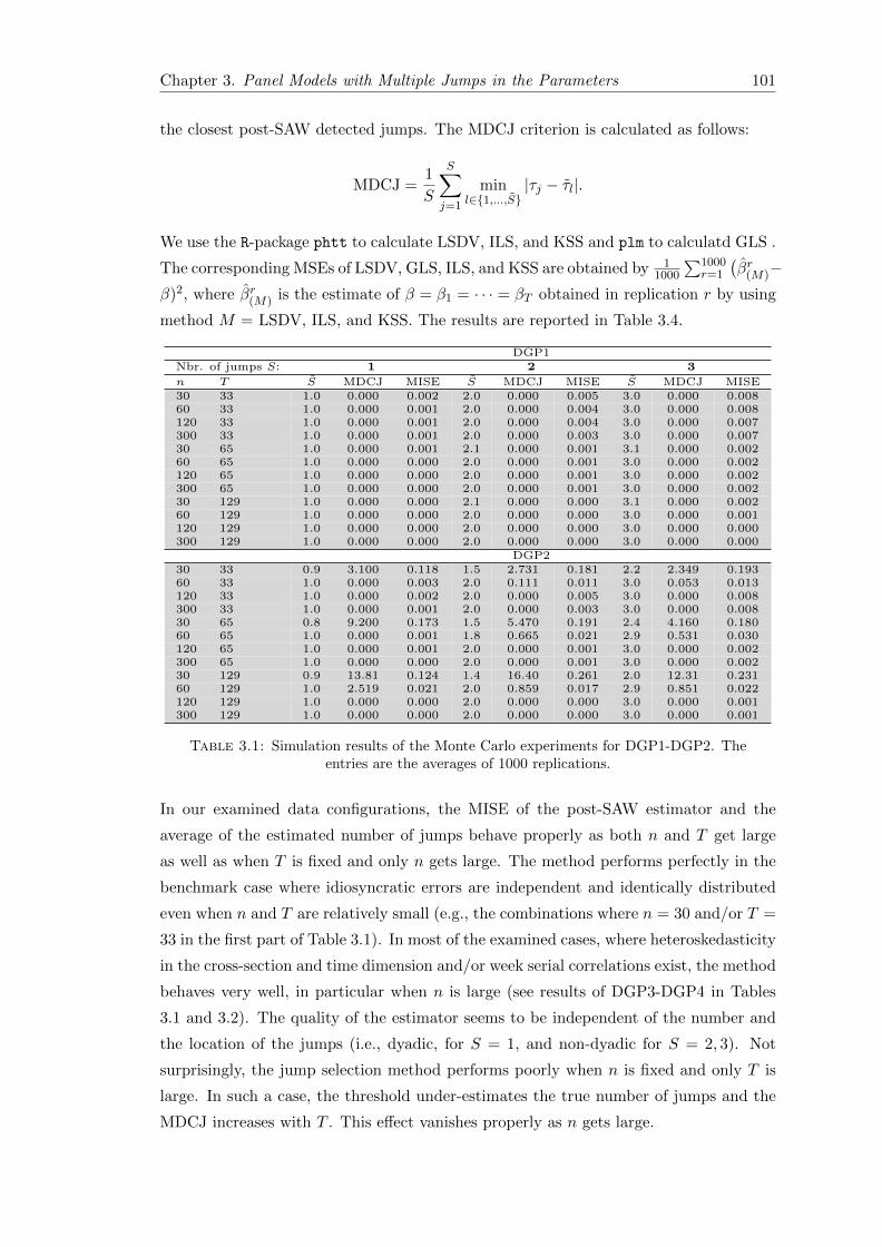
Chapter 3. Panel Models with Multiple Jumps in the Parameters 101
the closest post-SAW detected jumps. The MDCJ criterion is calculated as follows:
MDCJ =1
S
S∑j=1
minl∈1,...,S
|τj − τl|.
We use the R-package phtt to calculate LSDV, ILS, and KSS and plm to calculatd GLS .
The corresponding MSEs of LSDV, GLS, ILS, and KSS are obtained by 11000
∑1000r=1
(βr(M)−
β)2, where βr(M) is the estimate of β = β1 = · · · = βT obtained in replication r by using
method M = LSDV, ILS, and KSS. The results are reported in Table 3.4.
DGP1Nbr. of jumps S: 1 2 3
n T S MDCJ MISE S MDCJ MISE S MDCJ MISE30 33 1.0 0.000 0.002 2.0 0.000 0.005 3.0 0.000 0.00860 33 1.0 0.000 0.001 2.0 0.000 0.004 3.0 0.000 0.008120 33 1.0 0.000 0.001 2.0 0.000 0.004 3.0 0.000 0.007300 33 1.0 0.000 0.001 2.0 0.000 0.003 3.0 0.000 0.00730 65 1.0 0.000 0.001 2.1 0.000 0.001 3.1 0.000 0.00260 65 1.0 0.000 0.000 2.0 0.000 0.001 3.0 0.000 0.002120 65 1.0 0.000 0.000 2.0 0.000 0.001 3.0 0.000 0.002300 65 1.0 0.000 0.000 2.0 0.000 0.001 3.0 0.000 0.00230 129 1.0 0.000 0.000 2.1 0.000 0.000 3.1 0.000 0.00260 129 1.0 0.000 0.000 2.0 0.000 0.000 3.0 0.000 0.001120 129 1.0 0.000 0.000 2.0 0.000 0.000 3.0 0.000 0.000300 129 1.0 0.000 0.000 2.0 0.000 0.000 3.0 0.000 0.000
DGP230 33 0.9 3.100 0.118 1.5 2.731 0.181 2.2 2.349 0.19360 33 1.0 0.000 0.003 2.0 0.111 0.011 3.0 0.053 0.013120 33 1.0 0.000 0.002 2.0 0.000 0.005 3.0 0.000 0.008300 33 1.0 0.000 0.001 2.0 0.000 0.003 3.0 0.000 0.00830 65 0.8 9.200 0.173 1.5 5.470 0.191 2.4 4.160 0.18060 65 1.0 0.000 0.001 1.8 0.665 0.021 2.9 0.531 0.030120 65 1.0 0.000 0.001 2.0 0.000 0.001 3.0 0.000 0.002300 65 1.0 0.000 0.000 2.0 0.000 0.001 3.0 0.000 0.00230 129 0.9 13.81 0.124 1.4 16.40 0.261 2.0 12.31 0.23160 129 1.0 2.519 0.021 2.0 0.859 0.017 2.9 0.851 0.022120 129 1.0 0.000 0.000 2.0 0.000 0.000 3.0 0.000 0.001300 129 1.0 0.000 0.000 2.0 0.000 0.000 3.0 0.000 0.001
Table 3.1: Simulation results of the Monte Carlo experiments for DGP1-DGP2. Theentries are the averages of 1000 replications.
In our examined data configurations, the MISE of the post-SAW estimator and the
average of the estimated number of jumps behave properly as both n and T get large
as well as when T is fixed and only n gets large. The method performs perfectly in the
benchmark case where idiosyncratic errors are independent and identically distributed
even when n and T are relatively small (e.g., the combinations where n = 30 and/or T =
33 in the first part of Table 3.1). In most of the examined cases, where heteroskedasticity
in the cross-section and time dimension and/or week serial correlations exist, the method
behaves very well, in particular when n is large (see results of DGP3-DGP4 in Tables
3.1 and 3.2). The quality of the estimator seems to be independent of the number and
the location of the jumps (i.e., dyadic, for S = 1, and non-dyadic for S = 2, 3). Not
surprisingly, the jump selection method performs poorly when n is fixed and only T is
large. In such a case, the threshold under-estimates the true number of jumps and the
MDCJ increases with T . This effect vanishes properly as n gets large.
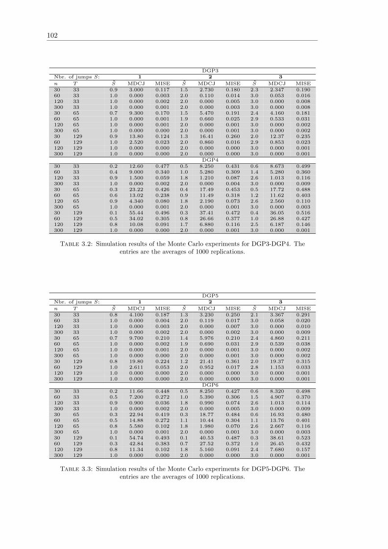
102
DGP3Nbr. of jumps S: 1 2 3
n T S MDCJ MISE S MDCJ MISE S MDCJ MISE30 33 0.9 3.000 0.117 1.5 2.730 0.180 2.3 2.347 0.19060 33 1.0 0.000 0.003 2.0 0.110 0.014 3.0 0.053 0.016120 33 1.0 0.000 0.002 2.0 0.000 0.005 3.0 0.000 0.008300 33 1.0 0.000 0.001 2.0 0.000 0.003 3.0 0.000 0.00830 65 0.7 9.300 0.170 1.5 5.470 0.191 2.4 4.160 0.18160 65 1.0 0.000 0.001 1.9 0.660 0.025 2.9 0.533 0.031120 65 1.0 0.000 0.001 2.0 0.000 0.001 3.0 0.000 0.002300 65 1.0 0.000 0.000 2.0 0.000 0.001 3.0 0.000 0.00230 129 0.9 13.80 0.124 1.3 16.41 0.260 2.0 12.37 0.23560 129 1.0 2.520 0.023 2.0 0.860 0.016 2.9 0.853 0.023120 129 1.0 0.000 0.000 2.0 0.000 0.000 3.0 0.000 0.001300 129 1.0 0.000 0.000 2.0 0.000 0.000 3.0 0.000 0.001
DGP430 33 0.2 12.60 0.477 0.5 8.250 0.431 0.6 8.673 0.49960 33 0.4 9.000 0.340 1.0 5.280 0.309 1.4 5.280 0.360120 33 0.9 1.500 0.059 1.8 1.210 0.087 2.6 1.013 0.116300 33 1.0 0.000 0.002 2.0 0.000 0.004 3.0 0.000 0.00930 65 0.3 23.22 0.426 0.4 17.49 0.453 0.5 17.72 0.48860 65 0.6 13.02 0.238 0.9 11.49 0.318 1.2 11.62 0.403120 65 0.9 4.340 0.080 1.8 2.190 0.073 2.6 2.560 0.110300 65 1.0 0.000 0.001 2.0 0.000 0.001 3.0 0.000 0.00330 129 0.1 55.44 0.496 0.3 37.41 0.472 0.4 36.05 0.51660 129 0.5 34.02 0.305 0.8 26.66 0.377 1.0 26.88 0.427120 129 0.8 10.08 0.091 1.7 6.880 0.116 2.5 6.187 0.146300 129 1.0 0.000 0.000 2.0 0.000 0.001 3.0 0.000 0.001
Table 3.2: Simulation results of the Monte Carlo experiments for DGP3-DGP4. Theentries are the averages of 1000 replications.
DGP5Nbr. of jumps S: 1 2 3
n T S MDCJ MISE S MDCJ MISE S MDCJ MISE30 33 0.8 4.100 0.187 1.3 3.230 0.250 2.1 3.367 0.29160 33 1.0 0.000 0.004 2.0 0.119 0.017 3.0 0.058 0.020120 33 1.0 0.000 0.003 2.0 0.000 0.007 3.0 0.000 0.010300 33 1.0 0.000 0.002 2.0 0.000 0.002 3.0 0.000 0.00930 65 0.7 9.700 0.210 1.4 5.976 0.210 2.4 4.860 0.21160 65 1.0 0.000 0.002 1.9 0.690 0.031 2.9 0.539 0.038120 65 1.0 0.000 0.001 2.0 0.000 0.001 3.0 0.000 0.002300 65 1.0 0.000 0.000 2.0 0.000 0.001 3.0 0.000 0.00230 129 0.8 19.80 0.224 1.2 21.41 0.361 2.0 19.37 0.31560 129 1.0 2.611 0.053 2.0 0.952 0.017 2.8 1.153 0.033120 129 1.0 0.000 0.000 2.0 0.000 0.000 3.0 0.000 0.001300 129 1.0 0.000 0.000 2.0 0.000 0.000 3.0 0.000 0.001
DGP630 33 0.2 11.66 0.448 0.5 8.250 0.427 0.6 8.320 0.49860 33 0.5 7.200 0.272 1.0 5.390 0.306 1.5 4.907 0.370120 33 0.9 0.900 0.036 1.8 0.990 0.074 2.6 1.013 0.114300 33 1.0 0.000 0.002 2.0 0.000 0.005 3.0 0.000 0.00930 65 0.3 22.94 0.419 0.3 18.77 0.484 0.6 16.93 0.48060 65 0.5 14.88 0.272 1.1 10.44 0.304 1.1 13.76 0.401120 65 0.8 5.580 0.102 1.8 1.980 0.070 2.6 2.667 0.116300 65 1.0 0.000 0.001 2.0 0.000 0.001 3.0 0.000 0.00330 129 0.1 54.74 0.493 0.1 40.53 0.487 0.3 38.61 0.52360 129 0.3 42.84 0.383 0.7 27.52 0.372 1.0 26.45 0.432120 129 0.8 11.34 0.102 1.8 5.160 0.091 2.4 7.680 0.157300 129 1.0 0.000 0.000 2.0 0.000 0.000 3.0 0.000 0.001
Table 3.3: Simulation results of the Monte Carlo experiments for DGP5-DGP6. Theentries are the averages of 1000 replications.

Chapter 3. Panel Models with Multiple Jumps in the Parameters 103
Table 3.3 reports the results of our experiments when the regressors are affected by
an omitted factor structure in the error term. The proposed two-step SAW procedure
seems to perform very well even when heteroskedasticity in the cross-section and time
dimension and/or week serial correlations are present.
The goal of examining DGP7 is to test whether SAW is also able to detect the no-jump
case. The answer that can be deciphered from Table 3.4 is: Yes. Our method is slightly
inferior in terms of MSE than ILS but better than LSDV, GLS, and KSS. Because
LSDV and GLS neglect the presence of the factor structure in the model and KSS is
only appropriate for factors that possess smooth patterns over time, the MSEs of these
three estimators are affected by a small bias that seems to persist even when n and T
get large.
DGP7 (S = 0)Method post-SAW LSDV GLS ILS KSS
n T S MISE MSE MSE MSE MSE30 33 0.0000 0.0062 0.0105 0.0148 0.0007 0.010460 33 0.0000 0.0041 0.0105 0.0142 0.0006 0.0101120 33 0.0000 0.0012 0.0090 0.0125 0.0002 0.0085300 33 0.0000 0.0004 0.0093 0.0128 0.0001 0.009030 65 0.0000 0.0039 0.0105 0.0135 0.0004 0.009960 65 0.0000 0.0015 0.0102 0.0130 0.0002 0.0101120 65 0.0000 0.0005 0.0099 0.0126 0.0001 0.0098300 65 0.0000 0.0001 0.0108 0.0137 0.0000 0.010830 129 0.0000 0.0015 0.0101 0.0129 0.0002 0.010260 129 0.0000 0.0008 0.0103 0.0127 0.0001 0.0104120 129 0.0000 0.0002 0.0101 0.0125 0.0000 0.0101300 129 0.0000 0.0000 0.0090 0.0112 0.0000 0.0090
Table 3.4: Simulation results of the Monte Carlo experiments for DGP7. The entriesare the averages of 1000 replications.
The Monte Carlo experiments show that, in many configurations of the data, our method
performs very well even when the idiosyncratic errors are weakly affected by serial-
autocorrelation and/or heteroskedasticity and this independently of the number and
locations of the jumps.
3.7 Application: Algorithmic Trading and Market Quality
An issue of increasing debate, both academically and politically, is the impact of al-
gorithmic trading (AT) on standard measures of market quality such as liquidity and
volatility. Proponents, including many of the exchanges themselves, argue that AT
provides added liquidity to markets and is beneficial to investors. Opponents instead
caution that algorithmic trading increases an investor’s perception that an algorithmic

104
trading partner possesses an informational advantage. Furthermore, incidents such as
the ”flash crash”, although circumstantial in nature, do nothing to alleviate these fears.
Recent work examining the effects of AT on market quality have generally found its
presence to be beneficial in the sense that standard measures of liquidity such as bid-ask
spreads and price-impact are reduced as a consequence of the increase in AT. For example
Hendershott et al. (2011) find that, with the exception of the smallest quintile of NYSE
stocks, AT almost universally reduces quoted and effective spreads in the remaining
quintiles. Hasbrouck and Saar (2013) find similarly compelling evidence using a measure
of AT constructed from order level data. A drawback of both approaches and more
specifically of the standard panel regression approach is that estimates of the marginal
effect of increasing are necessarily averaged over all possible states of the market. This
is problematic from an asset pricing perspective.
Of particular importance to the concept of liquidity is the timing of its provision. The
merits of added liquidity during stable market periods at the expense of its draw back
during periods of higher uncertainty are ambiguous without a valid welfare analysis and
can potentially leave investors worse off. The issue of timing is particularly important
for empirical work examining the effects of AT on market quality. Samples are often
constrained in size due to limitations on the availability of data and computational con-
cerns. As noted by Hendershott et al. (2011), it may be because samples often used
do not cover large enough periods of market turbulence to detect possible negative ef-
fects. Additionally, standard subsample analysis requires the econometrician to diagnose
market conditions as well their start and end dates, in effect imposing their own prior
beliefs on the factors that might cause variation in the marginal effects. Because of
this we propose the use of our estimator to automatically detect jumps in slope param-
eters. Indeed, our methodology alleviates concerns about ad-hoc subsample selection.
Furthermore, we believe analysis of periods where the effects vary may provide valuable
insight for future studies (both theoretical and empirical) and policy recommendations
regarding the regulation of trading in financial markets.
3.7.1 Liquidity and Asset Pricing
Before discussing the effects of liquidity on asset pricing, we first examine conventional
tests that assume constant parameters. In this simple example, we regress a measure of
market quality on an AT proxy for an individual stock using the following model:
MQt = α+ATtβ + et, (3.57)

Chapter 3. Panel Models with Multiple Jumps in the Parameters 105
where the time index t ∈ 1, . . . , T. If the slope parameter is time varying then β
in (3.57) presents only the time average of the true parameter, say βt. In this case
the conventional estimator of β is consistent only under the assumption∑T
t=1AT2t (βt−
β)/Tp−→ 0, as T get large. Even when such a requirement is satisfied, the average effect
is not the correct measure to consider when the question is whether AT is beneficial to
market quality.
A general result in asset pricing that is a consequence of no arbitrage is that there exists
a strictly positive stochastic discount factor (SDF) such that,
1 = Et(Mt+1Rt+1),
where Mt+1 is the SDF and Rt+1 is the return on a security. This expression can be
expanded and rewritten as,
Et(Rt+1) =1
Et(Mt+1)− 1
Et(Mt+1)covt(Mt+1, Rt+1).
Expected security returns (i.e., its risk premium) are a function of covariance with the
SDF. While the form of the SDF depends on the asset pricing model one is considering,
it can in general be thought of as the ratio of marginal value of wealth between time
t + 1 and t. Therefore, holding the expectation of Mt+1 constant, if a security pays off
more in states where the marginal value of wealth is relatively low and less in states
where the marginal value of wealth is relatively high (covt(Mt+1, Rt+1) < 0) then that
security earns a premium for this undesirable property. In light of the above analysis,
if a security’s returns contain a stochastic liquidity component then its covariance with
the SDF can have a substantial impact on expected returns.
The model of Acharya and Pedersen (2005) is particularly relevant as it exemplifies the
many avenues through which time varying liquidity can affect expected returns. Using
an overlapping generations model they decompose conditional security returns into five
components: one related to the expected level of illiquidity and four others related to
covariance terms between market return, market illiquidity, security returns and security
illiquidity. They show that portfolio returns are increasing in the covariance between
portfolio illiquidity and market illiquidity and decreasing in the covariance between secu-
rity illiquidity and the market return. A consequence of this is that if AT intensifies these
dynamics in the liquidity for a particular security then the effect will be to increase the
risk premium associated with that security. Increased risk premiums represent higher
costs of capital for firms, thus increased AT can potentially decrease firm investment
(relative to a market with no AT) through its effects on liquidity dynamics.

106
3.7.2 Data
Our sample consists of a balanced panel of stocks whose primary exchange is the New
York Stock Exchange (NYSE) and covers the calendar period 2003− 2008. The choice
of this sample period reflects our desire to include both relatively stable and turbulent
market regimes. We are limited in our choice of sample periods by the fact that AT is
a recent phenomenon and that our estimation procedure requires a balanced panel. In
this six-year period we consider results in a total of 378 firms.
To build measures of market quality, we use the NYSE Trade and Quotation Database
(TAQ) provided by Wharton Research Data Services (WRDS) to collect intra-day data
on securities. We aggregate intra-day up to a monthly level to construct our sample,
which consists of 65 months for each firm. We merge the TAQ data with information on
price and shares outstanding from the Center for Research in Security Prices (CRSP).
A discussion of our algorithmic trading proxy and measures of market quality follows.
3.7.2.1 The Algorithmic Trading Proxy
Our AT proxy is motivated by Hendershott et al. (2011) and Boehmer et al. (2012), who
note that AT is generally associated with an increase in order activity at smaller dollar
volumes. Thus the proxy we consider is the negative of dollar volume (in hundreds of
dollars, Volit) over time period t divided by total order activity over time period t. We
define order activity as the sum of trades (Trit) and updates to the best prevailing bid
and offer (qit) on the securities’ primary exchange:
ATit = − VolitTrit + qit
.
An increase in ATit represents a decrease in the average volume per instance of order
activity and represents an increase in the AT in the particular security. For example,
an increase of 1 unit of ATit represents a decrease of $100 of trading volume associated
with each instance of order activity (trade or quote update).
Our proxy, like that in Boehmer et al. (2012), differs from the proxy in Hendershott
et al. (2011) since they have access to the full order book of market makers whereas we
only have access to the trades and the best prevailing bid and offers of market makers
through TAQ. We appeal to the same argument as Boehmer et al. (2012) in that many
AT strategies are generally executed at the best bid and offer rather than behind it.
Therefore, we feel our proxy is in general representative of the full order book.

Chapter 3. Panel Models with Multiple Jumps in the Parameters 107
3.7.2.2 Market Quality Measures
We consider several common measures of market quality to assess the impact of AT on
markets for individual securities.
Proportional Quoted Spread
The proportional quoted spread (PQSit) measures the quoted cost as a percentage of
price (Bid-Offer midpoint) of executing a trade in security i and is defined as,
PQSit = 100
(Ofrit − Bidit
0.5(Ofrit + Bidit)
).
We multiply by 100 in order to place this metric in terms of percentage points. We ag-
gregate this metric to a monthly quality by computing a share volume-weighted average
over the course of each month. An increase in PQSit represents a decrease in the amount
of liquidity in the market for security i due to increased execution costs.
Proportional Effective Spread
The proportional effective spread (PESit) is quite similar to (PQSit) but accommodates
potentially hidden liquidity or stale quotes by evaluating the actual execution costs of a
trade. It is defined as,
PESit = 100
(|Pit −Mit|
Mit
),
where Pit is the price paid for security i at time t and Mit is the midpoint of the prevailing
bid and ask quotes for security i at time t. Thus, PESit is the actual execution cost
associated with every trade. We again aggregate this measure up to a monthly quantity
in the same way as we do for quoted spreads. Like PQSit, PESit is also in terms of
percentage points. An increase in PESit represents a decrease in the amount of liquidity
in the market for security i due to increased execution costs.
Measures of Volatility
We also consider two different measures of price volatility in security i over time period
t. The first is the daily high-low price range given by,
H-Lit = 100
(maxτ∈t(Pit)−minτ∈t(Pit)
Pit
),

108
which represents the extreme price disparity over the course of a trading day. We also
consider the realized variance of returns over each day computed using log returns over
5-minute intervals:
RVit = 100
(∑τ∈t
r2iτ
).
Realized variance is a nonparametric estimator of the integrated variance over the course
of a trading day (see, for example, Andersen et al. (2003)). We aggregate both measures
up to a monthly level by averaging over the entire month. We additionally multiply
both variables by 100, thus H−Lit is the price range as a percentage of the daily closing
price and RVit is an estimate of the integrated variance of log returns in percentages.
Both measures represent a measure of the price dispersion over the course of the trading
month.
Additional Control Variables
While we attempt to determine the effect our AT proxy has on measures of market
quality we include in all our regressions a vector of control variables to isolate the effects
of AT independent of the state of the market. We lag the control variables by one
month so they represent the state of the market at the beginning of the trading month
in question. The control variables are: (1) Share Turnover (STit), which is the number of
shares traded over the course of a day in a particular stock relative to the total amount of
shares outstanding; (2) Inverse price, which represents transaction costs due to the fact
that the minimum tick size is 1 cent; (3) Log of market value of equity to accommodate
effects associated with micro-cap securities; (4) Daily price range to accommodate any
effects from large price swings in the previous month.
To avoid adding lagged dependent variables in the model, for regressions where the
daily price range is the dependent variable we replace it in the vector of controls with
the previous month’s realized variance.
We additionally include security and time period fixed effects to proxy for any time
period or security related effects not captured by our included variables. We consider
panel regressions of the form
MQit = αi + θt + ATitβt +W′itϑ+ eit, (3.58)
where MQit is the market quality measure under consideration, αi and θt are the security
and time period fixed effects, W is a vector of the lagged control variables listed above,
and eit is the innovation to MQit, which we assume to be dependent of the fixed effects
and the control variables. The time subscript on the parameter beta allows for a possibly

Chapter 3. Panel Models with Multiple Jumps in the Parameters 109
time varying effect of AT on market quality. Thus we are able to test the null hypothesis
of a constant effect versus the alternative of a time jumping effect. We are also able to
measure the magnitude and direction of any possible change.
Potential Endogeneity Issue
Absent a theoretical model of AT, an issue on which the literature is still somewhat
agnostic, it is uncertain whether AT strategies attempt to time shocks to market quality.
This creates the potential problem of endogeneity with our AT proxy. That is, when
estimating the regression equation (3.58), E(ATiteit) 6= 0.
To overcome this potential issue we use the approach of Hasbrouck and Saar (2013)
(albeit with different variables) and choose as an instrument the average value of algo-
rithmic trading over all other firms not in the same industry as firm i. To this end, we
define industry groups using 4-digit SIC codes and define these new variables AT−IND,it.
The use of this IV assumes that there is some commonality in the level of AT across all
stocks that is sufficient to pick up some exogenous variation. It further rules out trading
strategies by AT across firms in different industry groups. Lacking complete knowledge
of the algorithms used by AT firms we view this assumption to be reasonable.
To estimate the model we use a two-stage approach and first fit the regression model,
ATit = ai + gt + bAT−IND,it + dWit + εit (3.59)
to obtain an instrument, Zit, for ATit given by the fitted values from (3.59), i.e., Zit :=
ATit = ai+ gt+ bAT−IND,it+ dWit, where ai, gt, b, and d are the conventional estimates
of ai, gt, b, and d.
We then carry out the second stage regression using equation (3.58) as described in
Section 3.3. For comparison purposes, we additionally apply the conventional panel
data model assuming constant slope parameter, i.e., β1 = β2 = · · · = βT .
3.7.3 Results
Table 3.5 presents the results from a baseline model that assumes the slope parameters
are constant over time.1 These results are largely consistent with previous studies that
find a positive (in terms of welfare) average relationship between AT and measures
of market quality over the time period considered. The coefficient estimates on the
1For the purpose of readability we divide the AT variable by 100 to reduce trailing zeros after thedecimal.
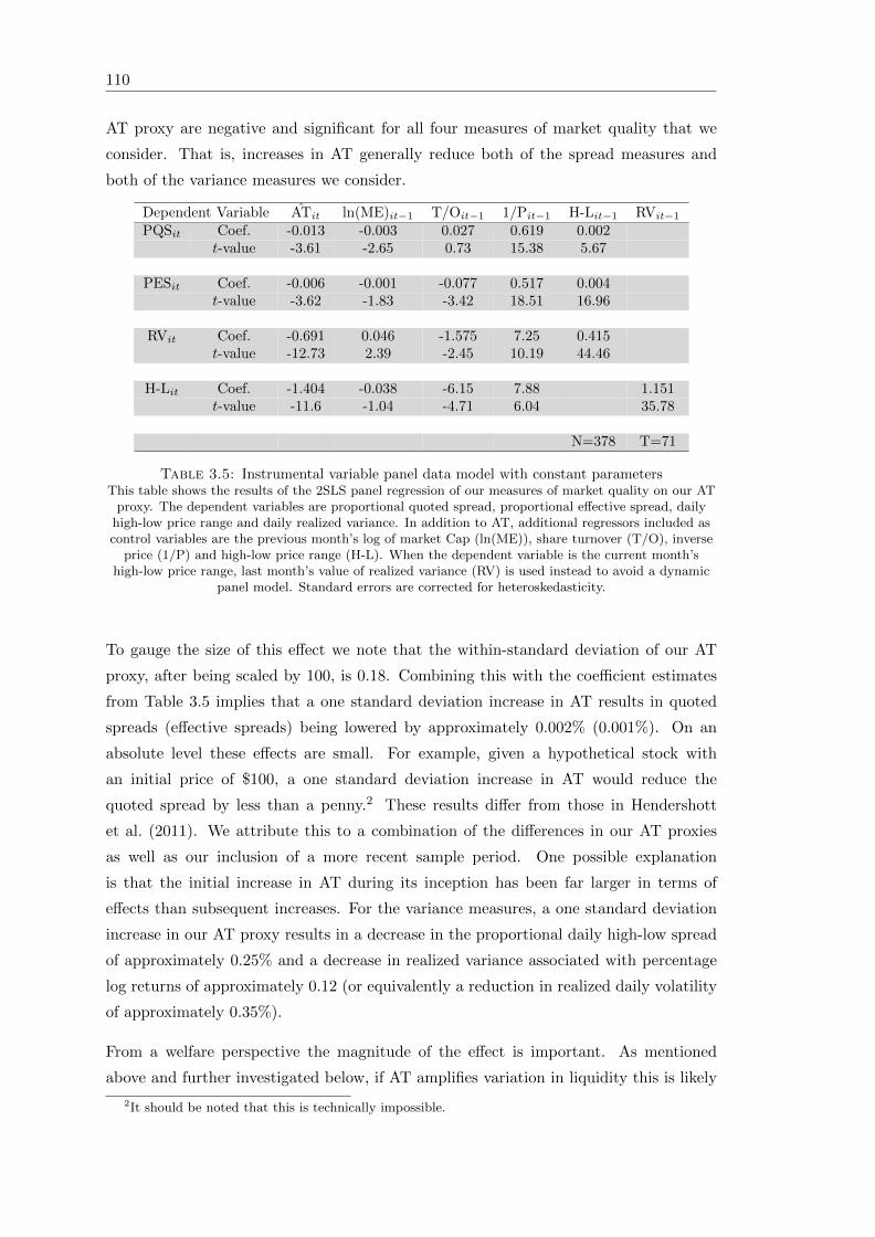
110
AT proxy are negative and significant for all four measures of market quality that we
consider. That is, increases in AT generally reduce both of the spread measures and
both of the variance measures we consider.
Dependent Variable ATit ln(ME)it−1 T/Oit−1 1/Pit−1 H-Lit−1 RVit−1
PQSit Coef. -0.013 -0.003 0.027 0.619 0.002t-value -3.61 -2.65 0.73 15.38 5.67
PESit Coef. -0.006 -0.001 -0.077 0.517 0.004t-value -3.62 -1.83 -3.42 18.51 16.96
RVit Coef. -0.691 0.046 -1.575 7.25 0.415t-value -12.73 2.39 -2.45 10.19 44.46
H-Lit Coef. -1.404 -0.038 -6.15 7.88 1.151t-value -11.6 -1.04 -4.71 6.04 35.78
N=378 T=71
Table 3.5: Instrumental variable panel data model with constant parametersThis table shows the results of the 2SLS panel regression of our measures of market quality on our AT
proxy. The dependent variables are proportional quoted spread, proportional effective spread, dailyhigh-low price range and daily realized variance. In addition to AT, additional regressors included ascontrol variables are the previous month’s log of market Cap (ln(ME)), share turnover (T/O), inverse
price (1/P) and high-low price range (H-L). When the dependent variable is the current month’shigh-low price range, last month’s value of realized variance (RV) is used instead to avoid a dynamic
panel model. Standard errors are corrected for heteroskedasticity.
To gauge the size of this effect we note that the within-standard deviation of our AT
proxy, after being scaled by 100, is 0.18. Combining this with the coefficient estimates
from Table 3.5 implies that a one standard deviation increase in AT results in quoted
spreads (effective spreads) being lowered by approximately 0.002% (0.001%). On an
absolute level these effects are small. For example, given a hypothetical stock with
an initial price of $100, a one standard deviation increase in AT would reduce the
quoted spread by less than a penny.2 These results differ from those in Hendershott
et al. (2011). We attribute this to a combination of the differences in our AT proxies
as well as our inclusion of a more recent sample period. One possible explanation
is that the initial increase in AT during its inception has been far larger in terms of
effects than subsequent increases. For the variance measures, a one standard deviation
increase in our AT proxy results in a decrease in the proportional daily high-low spread
of approximately 0.25% and a decrease in realized variance associated with percentage
log returns of approximately 0.12 (or equivalently a reduction in realized daily volatility
of approximately 0.35%).
From a welfare perspective the magnitude of the effect is important. As mentioned
above and further investigated below, if AT amplifies variation in liquidity this is likely
2It should be noted that this is technically impossible.

Chapter 3. Panel Models with Multiple Jumps in the Parameters 111
to demand a premium from investors and increase the cost of a capital for firms using
markets in which AT is present. Because of this, any benefits in terms of increased
liquidity on average, needs to be evaluated against the costs associated with increased
variation.
Tables 3.6 through 3.9 present the results when we allow the parameter to jump discretely
over time. The coefficient estimates in Tables 3.6 through 3.9 represent the size of the
estimated jump in the coefficient and a test of its significance, as outlined the previous
section. Figures 4 through 7 plot both the estimated SAW coefficients and the results
from period by period cross-sectional regressions. The effect of AT on our measures of
market quality is stable prior to the 2007-2008 period. Of course, the 2007-2008 period
covers the financial crisis, a time during which liquidity in many markets tightened
substantially. During the financial crisis period we find significant evidence of both
positive and negative jumps in the coefficient on AT.
For the two spread measures we find evidence of two large positive jumps in the coeffi-
cients in April and September/October of 2008 and other smaller jumps around those
two time periods. A positive jump in the coefficient represents a reduction in the benefit
of AT on spreads and potentially a reversal in its effects on spreads. Such is the case for
the two large positive jumps mentioned above. We find that during these two months
increases in AT lead to an increase in spreads and thus transacting in the securities
with high AT is, other things being equal, costlier than in low AT securities. April and
September/October of 2008 represent two particularly volatile periods for equity mar-
kets (and markets in general) in the US. In April markets were still rebounding from
the bailout of Bear Stearns and its eventual sale to JP Morgan. This all occurred dur-
ing a period when the exposure of many banks to US housing markets through various
structured financial products was beginning to be understood by investors. Similarly,
the failure of Lehman Brothers in September was another event that rattled financial
markets. The results for our variance measures are similar, as we also find evidence
of both positive and negative jumps during the 2007-2008 period. Of note is that for
realized variance we find the jumps to be, in general, beneficial for investors. That is,
we find that increases in AT cause a larger reduction in realized variance. Some caution
should be taken with respect to the interpretation of these results due to the fact that
variance is generally found to be strongly autocorrelated. Although we attempt to con-
trol for this using the lagged value of the high-low price range, it is possible the use of
this variable is not sufficient.
A potential explanation for the variation in the marginal effect of AT is the presence
of increased uncertainty. From both a valuation and a regulatory/policy perspective,
the periods following large, unpredictable shocks to asset markets can be associated
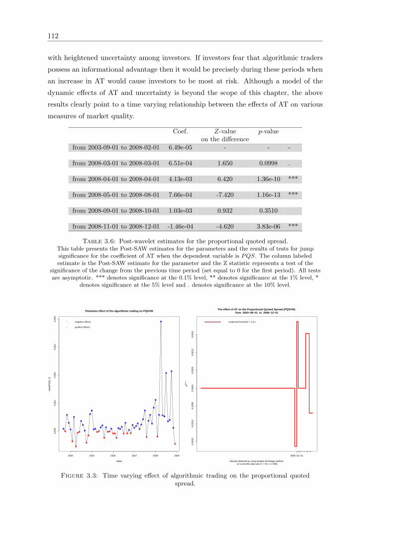
112
with heightened uncertainty among investors. If investors fear that algorithmic traders
possess an informational advantage then it would be precisely during these periods when
an increase in AT would cause investors to be most at risk. Although a model of the
dynamic effects of AT and uncertainty is beyond the scope of this chapter, the above
results clearly point to a time varying relationship between the effects of AT on various
measures of market quality.
Coef. Z-value p-valueon the difference
from 2003-09-01 to 2008-02-01 6.49e-05 - - -
from 2008-03-01 to 2008-03-01 6.51e-04 1.650 0.0998 .
from 2008-04-01 to 2008-04-01 4.13e-03 6.420 1.36e-10 ***
from 2008-05-01 to 2008-08-01 7.66e-04 -7.420 1.16e-13 ***
from 2008-09-01 to 2008-10-01 1.03e-03 0.932 0.3510
from 2008-11-01 to 2008-12-01 -1.46e-04 -4.620 3.83e-06 ***
Table 3.6: Post-wavelet estimates for the proportional quoted spread.This table presents the Post-SAW estimates for the parameters and the results of tests for jumpsignificance for the coefficient of AT when the dependent variable is PQS. The column labeledestimate is the Post-SAW estimate for the parameter and the Z statistic represents a test of the
significance of the change from the previous time period (set equal to 0 for the first period). All testsare asymptotic. *** denotes significance at the 0.1% level, ** denotes significance at the 1% level, *
denotes significance at the 5% level and . denotes significance at the 10% level.
2004 2005 2006 2007 2008 2009
0.00
00.
001
0.00
20.
003
0.00
4
Pointwise effect of the algorithmic trading on PQSVW
dates
beta
tPQ
S[,
1]
°
°
negative effects
positive effects
−0.
0015
−0.
0010
−0.
0005
0.00
000.
0005
0.00
100.
0015
The effect of AT on the Proportional Quoted Spread (PQSVW) from 2003−08−01 to 2008−12−01
Results obtained by using wavelet shrinkage method on a monthly data stet (T = 64, n = 508)
β(AT)
empirical threshold = 0.11
2008−03−01
Figure 3.3: Time varying effect of algorithmic trading on the proportional quotedspread.

Chapter 3. Panel Models with Multiple Jumps in the Parameters 113
Coef. Z-value p-valueon the difference
from 2003-09-01 to 2007-08-01 9.06e-06 - -
from 2007-09-01 to 2007-12-01 6.73e-04 3.750 0.000176 ***
from 2008-01-01 to 2008-02-01 1.35e-04 -2.000 0.045800 *
from 2008-03-01 to 2008-03-01 5.31e-04 1.160 0.248000
from 2008-04-01 to 2008-04-01 4.19e-03 10.700 < 2.2e-16 ***
from 2008-05-01 to 2008-08-01 4.15e-04 -15.600 < 2.2e-16 ***
from 2008-09-01 to 2008-09-01 -1.74e-03 -7.540 4.77e-14 ***
from 2008-10-01 to 2008-10-01 1.79e-03 11.700 < 2.2e-16 ***
from 2008-11-01 to 2008-12-01 3.55e-06 -9.610 < 2.2e-16 ***
Table 3.7: Post-wavelet estimates for the proportional effective spread.This table presents the Post-SAW estimates for the parameters and the results of tests for jumpsignificance for the coefficient of AT when the dependent variable is PES. The column labeledestimate is the Post-SAW estimate for the parameter and the Z statistic represents a test of the
significance of the change from the previous time period (set equal to 0 for the first period). All testsare asymptotic. *** denotes significance at the 0.1% level, ** denotes significance at the 1% level, *
denotes significance at the 5% level and . denotes significance at the 10% level.
2004 2005 2006 2007 2008 2009
−0.
001
0.00
00.
001
0.00
20.
003
0.00
4
Pointwise effect of the algorithmic trading on PESVW
dates
beta
tPE
S[,
1]
°
°
negative effects
positive effects
−0.
0015
−0.
0010
−0.
0005
0.00
000.
0005
0.00
100.
0015
The effect of AT on the Proportional Effetive Spread (PESVW) from 2003−08−01 to 2008−12−01
Results obtained by using wavelet shrinkage method on a monthly data stet (T = 64 n = 378 )
β(AT)
empirical threshold = 0.0782
2007−08−01 2008−08−01
Figure 3.4: Time varying effect of algorithmic trading on the proportional effectivespread.
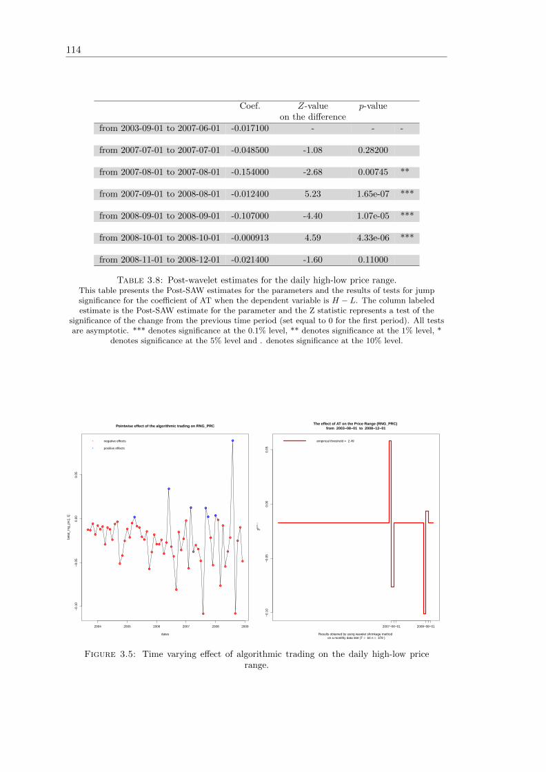
114
Coef. Z-value p-valueon the difference
from 2003-09-01 to 2007-06-01 -0.017100 - - -
from 2007-07-01 to 2007-07-01 -0.048500 -1.08 0.28200
from 2007-08-01 to 2007-08-01 -0.154000 -2.68 0.00745 **
from 2007-09-01 to 2008-08-01 -0.012400 5.23 1.65e-07 ***
from 2008-09-01 to 2008-09-01 -0.107000 -4.40 1.07e-05 ***
from 2008-10-01 to 2008-10-01 -0.000913 4.59 4.33e-06 ***
from 2008-11-01 to 2008-12-01 -0.021400 -1.60 0.11000
Table 3.8: Post-wavelet estimates for the daily high-low price range.This table presents the Post-SAW estimates for the parameters and the results of tests for jumpsignificance for the coefficient of AT when the dependent variable is H − L. The column labeledestimate is the Post-SAW estimate for the parameter and the Z statistic represents a test of the
significance of the change from the previous time period (set equal to 0 for the first period). All testsare asymptotic. *** denotes significance at the 0.1% level, ** denotes significance at the 1% level, *
denotes significance at the 5% level and . denotes significance at the 10% level.
2004 2005 2006 2007 2008 2009
−0.
10−
0.05
0.00
0.05
Pointwise effect of the algorithmic trading on RNG_PRC
dates
beta
t_rn
g_pr
c[, 1
]
°
°
negative effects
positive effects
−0.
10−
0.05
0.00
0.05
The effect of AT on the Price Range (RNG_PRC) from 2003−08−01 to 2008−12−01
Results obtained by using wavelet shrinkage method on a monthly data stet (T = 64 n = 378 )
β(AT)
empirical threshold = 2.49
2007−06−01 2008−08−01
Figure 3.5: Time varying effect of algorithmic trading on the daily high-low pricerange.
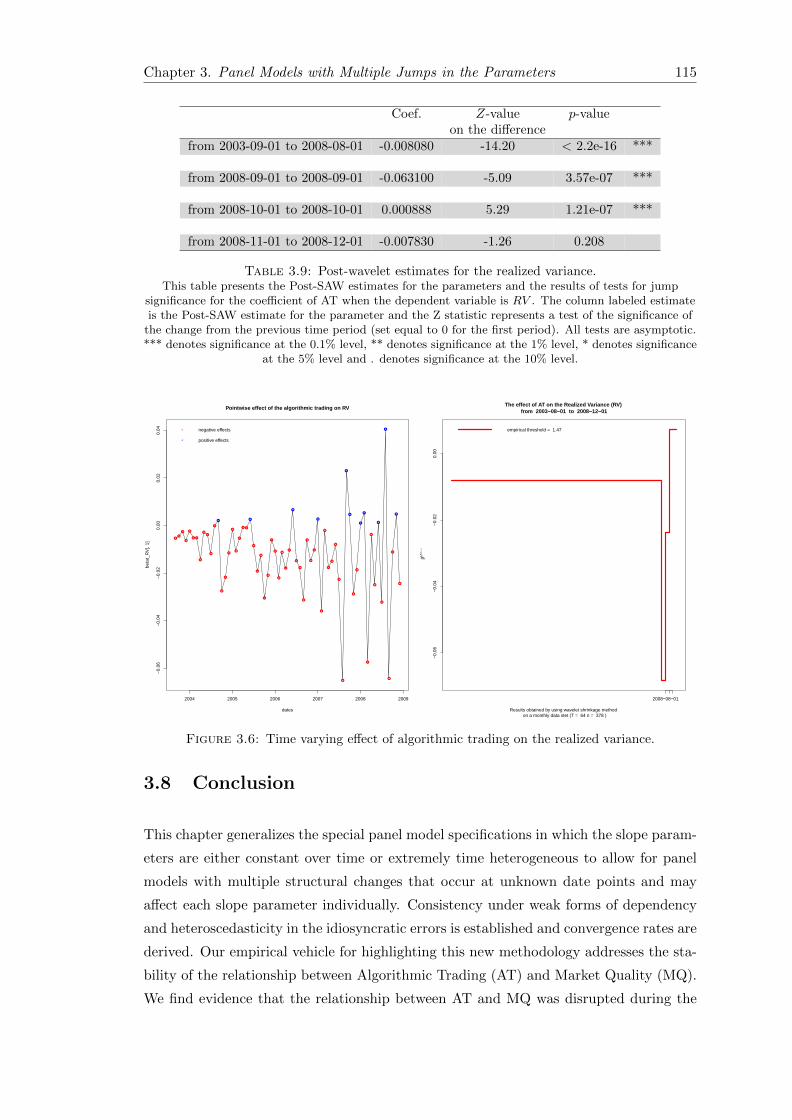
Chapter 3. Panel Models with Multiple Jumps in the Parameters 115
Coef. Z-value p-valueon the difference
from 2003-09-01 to 2008-08-01 -0.008080 -14.20 < 2.2e-16 ***
from 2008-09-01 to 2008-09-01 -0.063100 -5.09 3.57e-07 ***
from 2008-10-01 to 2008-10-01 0.000888 5.29 1.21e-07 ***
from 2008-11-01 to 2008-12-01 -0.007830 -1.26 0.208
Table 3.9: Post-wavelet estimates for the realized variance.This table presents the Post-SAW estimates for the parameters and the results of tests for jump
significance for the coefficient of AT when the dependent variable is RV . The column labeled estimateis the Post-SAW estimate for the parameter and the Z statistic represents a test of the significance of
the change from the previous time period (set equal to 0 for the first period). All tests are asymptotic.*** denotes significance at the 0.1% level, ** denotes significance at the 1% level, * denotes significance
at the 5% level and . denotes significance at the 10% level.
2004 2005 2006 2007 2008 2009
−0.
06−
0.04
−0.
020.
000.
020.
04
Pointwise effect of the algorithmic trading on RV
dates
beta
t_R
V[,
1]
°
°
negative effects
positive effects
−0.
06−
0.04
−0.
020.
00
The effect of AT on the Realized Variance (RV) from 2003−08−01 to 2008−12−01
Results obtained by using wavelet shrinkage method on a monthly data stet (T = 64 n = 378 )
β(AT)
empirical threshold = 1.47
2008−08−01
Figure 3.6: Time varying effect of algorithmic trading on the realized variance.
3.8 Conclusion
This chapter generalizes the special panel model specifications in which the slope param-
eters are either constant over time or extremely time heterogeneous to allow for panel
models with multiple structural changes that occur at unknown date points and may
affect each slope parameter individually. Consistency under weak forms of dependency
and heteroscedasticity in the idiosyncratic errors is established and convergence rates are
derived. Our empirical vehicle for highlighting this new methodology addresses the sta-
bility of the relationship between Algorithmic Trading (AT) and Market Quality (MQ).
We find evidence that the relationship between AT and MQ was disrupted during the

116
time between 2007 and 2008. This period coincides with the beginning of the subprime
crisis in the US market and the bankruptcy of the big financial services firm Lehman
Brothers.
Appendix A
Appendix of Chapter 1
A.1 Theoretical Results and Proofs
Before beginning with proofs, we now define these quantities and show how to construct
consistent estimate of the bias term. Following again Bai et al. (2009) we first use kernel
estimators to approximate the long-run covariance matrices of wit. Estimates of εit,
ζit and ηt are given by the regression residuals εit, ζit = ∆Xit and ηt = ∆Ft. For all
h = −T + 1, . . . , T − 1 and all i = 1, . . . , n let Γε,i(h), Γε,ζ,i(h), Γε,η,i(h), Γε,b,i(h) and
Γb,i(h) denote the (1× 1(, (1× p), (1× d) , (1× (p+ d)) and ((p+ d)× (p+ d)) empirical
lag h autocovariance matrices of (εit, εi,t+h), (εit, ζi,t+h), (εit, ηt+h), (εit, (ζ′i,t+h, η
′t+h)′) as
well as ((ζ ′i,t, η′t)′, (ζ ′i,t+h, η
′t+h)′), t = 1, . . . , T . Then define
Ωε,i =T−1∑
j=−T+1
ω(j
κ)Γε,i(j), Ωε,b,i =
T−1∑j=−T+1
ω(j
κ)Γε,b,i(j)
Ωb,i =
T−1∑j=−T+1
ω(j
κ)Γb,i(j), Ωε|b,i = Ωε,i − Ω′ε,b,iΩ
−1b,i Ωε,b,i,(
∆+ζ,ε,i
∆+η,ζ,i
)=
(∑T−1j=0 ω( jκ)Γε,ζ,i(h)∑T−1j=0 ω( jκ)Γε,η,i(h)
)−T−1∑j=0
ω(j
κ)Γb,i(h)Ω−1
b,i Ωε,b,i.
Here, the kernel function ω(.) satisfies the following assumption:
Assumption 4. The kernel function ω(.):
The kernel function ω(.) : R→ [−1, 1] satisfies (i) ω(0) = 1, ω(x) = ω(−x), (ii)∫ 1−1 ω(x)2dx <∞ and with Parzen’exponent q ∈ (0,∞) such that lim 1−ω(x)
|x|q <∞
117
118
and lim inf(N,T )↔∞
(log(T )log(N)
)> 1; the bandwidth parameter κ ∼ N b where b ∈
( 12q , lim inf
(log(T )log(N)
)− 1).
Ωε,i, Ωε,b,i, Ωb,i, Ωε|b,i, ∆+ζ,ε,i and ∆+
η,ζ,i estimate their theoretical analogues Ωε,i, Ωε,b,i,
Ωb,i, Ωε|b,i, ∆+ζ,ε,i and ∆+
η,ζ,i which are defined by replacing in the above equation the
terms ω( ·κ)Γ·(·) by the corresponding true autocovariance matrices of wit = (εit, ζ∗it, ηt).
In addition, summation then ranges from −∞ to ∞ (instead of −T + 1 to T − 1) and 0
to ∞ (instead of 0 to T − 1).
Now define the projection matrices of F as MF = IT −F (F ′F )−1F
′and the scalar
aik as the element i, k of the projection matrix AΛ = Λ(Λ′Λ)−1Λ
′. Corresponding
estimates MF and aik are obtained by replacing F and Λ by F and Λ. Then let
Zi = MFX∗i −
1
N
N∑j=1
MFX∗j aij , Zi = MFXi −
1
N
N∑j=1
MFXj aij
Conditional on F , the bias term φ is then given by
φ =
(1
NT 2
N∑i=1
Z′iZi
)−11
N
N∑i=1
θi,
θi = Z′i(∆bi)Ω
−1b,i Ωε,b,i + ∆+
ζ,ε,i − δ′i∆
+η,ζ,i,
∆bi = (∆X∗i −1
N
N∑j=1
∆X∗j aij ,∆F), δi = (F
′F )−1F
′Xi,
and a consistent estimator can be determined by
φNT =
(1
NT 2
N∑i=1
Z′iZi
)−11
N
N∑i=1
θi,
θi = Z′i(∆bi)Ω
−1b,i Ωε,b,i + ∆+
ζ,ε,i − δ′i∆
+η,ζ,i,
∆bi = (∆Xi −1
N
N∑j=1
∆Xj aij ,∆F ), δi = (F′F )−1F
′Xi.
Conditional on F , Bai et al. (2009) show that there exists random matrices RCi,
defined as conditional expectations of integrated Brownian motions with individually
different covariance structure, such that as (N,T ) → ∞ we have 1NT 2
∑Ni=1 ZiZ
′i →d
limN→∞1N
∑Ni=1RCi. The covariance matrix Σc is then defined by
Σc =
(limN→∞
1
N
N∑i=1
RCi
)−1(limN→∞
1
N
N∑i=1
Ωε|b,iRCi
)(limN→∞
1
N
N∑i=1
RCi
)−1
, (A.1)
Appendix A 119
Bai et al. (2009) do not propose an estimator of Σc. However, following their arguments
it is straightforward to show that a consistent estimate of the covariance matrix Σc is
given by
Σc =
(1
NT 2
N∑i=1
Z′iZi
)−11
NT 2
N∑i=1
Ωε|b,iZ′iZi
(1
NT 2
N∑i=1
Z′iZi
)−1
,
We then obtain the following proposition:
Proposition A.1. Under Assumptions 1-3, we have, as (N,T )→∞,
Σ1/2c
(√NT (β(d)− β)−
√Nφ)
d−→ N(0, Ip),
where β(d) is the iterative least squares estimator obtained after transforming Model
(1.17) by using T (.).
Proof of A.1: Let Zi = MFXi− 1N
∑Nj=1 MFXjaij . In view of Proposition 4 and Lemma
A.2 of Bai et al. (2009) we only have to show that 1NT 2
∑Ni=1 Z
′iZi and 1√
NT
∑Ni=1 Z
′iεi
have the same limit distributions as 1T 2Z
′iZi and 1√
NT
∑Ni=1 Z
′iεi. Note that Xit−X∗it =
Xi,t−1 − X∗i,t−1 + (∑K
k=1 δik(ζkt − ζ0kt)) is also an I(1)-process. But the innovations
(∑K
k=1 δik(ζkt − ζ0kt)) are averages over mk individuals and hence varC((
∑Kk=1 δik(ζkt −
ζ0kt)) ≤ M1/N , where M1 < ∞ is some constant independent of i, t. Therefore, as
(N,T )→∞ ‖ 1NT 2
∑Ni=1 ZiZ
′i − 1
NT 2
∑Ni=1 ZiZ
′i‖ = OP (N−1/2). Our assumptions imply
that conditional on ηt the random variables ζ∗it and εit are independent. Consequently,
as (N,T ) → ∞, we have 1√NT
∑Ni=1 Z
′i(∑K
k=1 δikεk) =∑K
k=1( 1√NT
∑Ni=1 δikZ
′i)εk =
oP (1) as well as 1√NT
∑Ni=1(Z
′i−Z
′i)εi = oP (1). One can conclude that 1√
NT
∑Ni=1 Z
′iεi =
1√NT
∑Ni=1 Z
′iεi + op(1). The proposition is an immediate consequence.
Corollary A.2. Under Assumptions 1-4, we have, as (N,T )→∞,
Σ1/2c
(√NT (
(β(d)− 1
TφNT
)− β)
)d−→ N(0, Ip),
where β(d) is the iterative least squares estimator obtained after using the transformation
operator T (.) and φNT is estimated as above.
Proof of Corollary A.2: Corollary 1 follows from a straightforward generalization
of the arguments used in the proof of Theorem 2 in Bai et al. (2009). Note that, all
additional terms induced by the differences X∗it − Xit and εit − εit are asymptotically
negligible.

120
The main difference between our approach and the methodology of Bai et al. (2009) con-
sists in the fact that our estimation procedure directly incorporates a dimension estimate.
Our final estimator βEupBC = β(dEup)− 1T φNT , thus, relies on the estimated dimension
dEup. The following theorem shows that with high probability dEup will asymptotically
coincide with the true dimension d. The asymptotic distributions derived in Corollary
1 thus remain valid when replacing d by dEup. Furthermore, the final estimator FEupBC
yields a consistent estimator of the true factor structure (up to rotations).
Theorem A.3. Under assumptions 1-3, we have, as (N,T )→∞,
a) P (dEup = d)→ 1, if the starting estimate dmax ≥ d and g is of the form g = cpNT
such that (i) c = OP (1) and strict positive, (ii) pNT →∞, and (iii) log log(T )T pNT →
0,
b) with the additional Assumption 4,
Σ1/2c
√NT (βEupBC − β)
d−→ N(0, Ip),
c) and for some (d× d) invertible matrix H,
1
T
T∑t=1
‖FEupBC,t − F t H‖2 = OP (1
N) +OP (
1
T).
Proof of Theorem A.3: Assertion a). We can infer from the theoretical results of Bai
et al. (2009) that
1
NT
N∑i=1
T∑t=1
(Yit − Yit(d))2 = OP (1), (A.2)
where Yit(d) denotes the fitted variable for the true dimension d.
Since our estimates are obtained by minimizing least squares objective function, we have,
∀l ∈ d+ 1, d+ 2, . . . , dmax,
1
NT
N∑i=1
T∑t=1
(Yit − Yit(l))2 ≤ 1
NT
N∑i=1
T∑t=1
(Yit − Yit(d))2 = OP (1). (A.3)
On the other hand, straightforward generalization of the arguments of Bai (2004) shows
that, ∀l ∈ 0, . . . , d− 1,
1
NT
N∑i=1
T∑t=1
(Yit − Yit(l))2 − 1
NT
N∑i=1
T∑t=1
(Yit − Yit(d))2 = Op(T/ log log(T )). (A.4)
Note that (A.4) is strict positive.

Appendix A 121
By construction of the estimation algorithm, we know that the number of outer iterations
rm is maximal dmax+1, where dmax is larger than d. To prove that lim(N,T )→∞ P (dEup =
d) = 1, we use inductive reasoning and show that, for all outer iterations r ∈ 1, . . . , rm|d(rm) =
d(rm−1),
lim(N,T )→∞ P (d(1) = d|dmax ≥ d) = 1, and
lim(N,T )→∞ P (d(r) = d) = 1, r ∈ 2, . . . , rm|d(rm) = d(rm−1),
as long as g satisfies Conditions (i)− (iii).
First of all, we show that the optimal dimension d(1) obtained by using the stating scaling
coefficient σ2(dmax) = 1NT
∑Tt=1(Yit − Yit(dmax))2 in g is consistent.
According to (A.3), σ2(dmax) = Op(1).
Since
S(1)4 (l)− S(1)
4 (d) =1
NT
N∑i=1
T∑t=1
(Yit − Yit(l))2 − 1
NT
N∑i=1
T∑t=1
(Yit − Yit(d))2 + (l − d)g(1),
where g(1) = σ2(dmax)pNT such that pNT → ∞ and log log(T )T pNT → 0, as (N,T ) → ∞,
we can conclude from (A.3) and (A.4) that
lim(N,T )→∞
P (S(1)4 (l)− S(1)
4 (d) > 0) = 0 ∀l ∈ 0, . . . , dmax|l 6= d.
Because d(1) is the minimizer of S(1)4 (l), it follows that
lim(N,T )→∞
P (d(1) = d) = 1. (A.5)
At the outer iteration stage r + 1, the law of total probability implies
lim(N,T )→∞ P (d(r+1) = d) = lim(N,T )→∞
(P (d(r+1) = d|d(r) = d)P (d(r) = d)
+ P (d(r+1) = d|d(r) 6= d)P (d(r) 6= d)).
To complete the proof, we have, therefore, to verify that
lim(N,T )→∞
P (d(r+1) = d|d(r) = d) = 1, for r = 2, . . . , rm. (A.6)

122
According to (A.3), we have, for d(r) = d, σ2(d(r)) = Op(1). From (A.3) and (A.4), we
can conclude that
lim(N,T )→∞
P (S(r+1)4 (l)− S(r+1)
4 (d) > 0) = 0 ∀l ∈ 0, . . . , dmax|l 6= d,
with g(r) = σ2(d(r))pNT , and hence
lim(N,T )→∞
P (d(r+1) = d|d(r) = d) = 1, for r = 2, . . . , rm.
Induction implies
lim(N,T )→∞
P (d(r+1) = d|d(r) = d) = lim(N,T )→∞
P (d(r+1) = d) = 1, for r = 2, . . . , rm.
Assertion a) is an immediate consequence.
Now, we have
Σ−1/2c
(√NT (βCupBC(dEup)− β)
)= Σ−1/2
c
(√NT (βCupBC(d)− β)
)+ Σ−1/2
c
(√NT (βCupBC(dEup)− βCupBC(d)
)= Σ−1/2
c
(√NT (βCupBC(d)− β)
)+ oP (1).
By Corollary 1, Assertion b) is, hence, an immediate consequence. Assertion c) follows
from Assertion a) and Proposition 5 of Bai et al. (2009).

Appendix B
Appendix of Chapter 3
B.1 Proofs of Section 3.2
Lemma B.1. Let T = 2L−1 for some integer L ≥ 2 and β = (β1, . . . , βT )′ ∈ RT a vector
that possesses exactly one jump at τ ∈ 1, . . . , T such that
βt =
βτ for t ∈ 1, . . . , τβτ+1 6= βτ for t ∈ τ + 1, . . . , T.
Let wlk(t) be defined as (3.8) and hlk(t) as (3.9), where a1,1, al,2k−1 and al,2k are positive
real values for all l ∈ 1, . . . , L, and k ∈ 1, . . . ,Kl. There then exists unique lτ non-
zero coefficients blkl |lτ ≤ L, where kl ∈ 1, . . . ,Kl, such that
βt =
lτ∑l=1
wlkl(t)blkl .
Proof of Lemma B.1: To prove the proposition, we show that βt can be reconstructed
by using at most L wavelet basis if it processes exactly one jump, say at τ ∈ 1, . . . , T.To simplify the exposition, we re-define the wavelet basis wl,k(t), for l > 1 as follows:
wl,k(t) = a∗l,2k−1h∗l,2k−1(t)− a∗l,2kh∗l,2k(t),
where
h∗l,k(t) =
1 for t ∈
(2L−l−1(k − 1) + 1
), . . . ,
(2L−l−1k
)0 else.
This is equivalent to (3.8). The unique difference is that the coefficients a∗l,2k−1 and a∗l,2k
are scaled by√
2l in order to simplify the construction of h∗l,k(t) and let it be either 1 or
0.
123

124
Note that by construction, there exists a unique lτ ∈ 2, . . . , L and a unique klτ ∈1, . . . , 2lτ−2 such that
wlτklτ (τ) = a∗lτ ,2klτ−1 and wlτklτ (τ + 1) = −a∗lτ ,2klτ .
Moreover, there exists in each level l ∈ 1, . . . , L|l < lτ at most one basis wlkl(t) that
satisfies the following condition:
wlkl(τ) = wl,kl(τ + 1) 6= 0.
Define the time interval Il, for each l = 1, . . . , lτ , as follows:
Il = t ∈ 1, . . . , T|wl,kl(t) 6= 0.
such thatlτ⋃l=1
Il = 1, . . . , T
and
Ilτ ⊂ Ilτ−1 ⊂ · · · ⊂ I2 ⊆ I1 = 1, . . . , T.
We now begin with the thinnest interval Ilτ that contains the jump. Define
β(lτ )t =
βt = βτ if t ≤ τ and t ∈ Ilτ ∩ t|t ≤ τβt = βτ+1 if t > τ and t ∈ Ilτ ∩ t|t > τ0 else.
Because βτ 6= βτ+1 and a∗lτ ,2klτ−1, a∗lτ ,2klτ
> 0, there exists a non-zero coefficient blτ ,klτ =βτ−βτ+1
a∗lτ ,2klτ−1+a∗lτ ,2klτand a constant β(lτ ) 6= βτ , βτ+1 such that
β(lτ )t =
βτ = β(lτ ) + a∗lτ ,2klτ−1blτ ,klτ if t ≤ τ and t ∈ Ilτβτ+1 = β(lτ ) − a∗lτ ,2klτ blτ ,klτ if t > and t ∈ Ilτ0 else.
(B.1)
Using the definition of wlk(t), we can rewrite (B.1) as
β(lτ )t =
βt = β(lτ ) + wlτ ,klτ (t)blτ ,klτ if t ∈ Ilτ0 else.
(B.2)

Appendix B 125
Consider the second thinnest interval Ilτ−1 . Let
β(lτ−1)t =
βt if t ∈ Ilτ−1 \ Ilτβ(lτ ) if t ∈ Ilτ0 else.
Note that βt is constant over Ilτ−1 \ Ilτ ; it can be either βτ or βτ+1. Now, because
β(lτ ) 6= βτ , βτ+1, we can determine a second unique non-zero coefficient blτ−1,klτ−1and
a second unique constant β(lτ−1) 6= βτ , βτ+1 such that
β(lτ−1)t =
β(lτ−1) + wlτ−1,klτ−1
(t)blτ−1,klτ−1= βt if t ∈ Ilτ−1 \ Ilτ
β(lτ−1) + wlτ−1,klτ−1(t)blτ−1,klτ−1
= β(lτ ) if t ∈ Ilτ0 else.
Because wlτ ,klτ (t) = 0 for all t /∈ Ilτ−1 and all t ∈ Ilτ−1 \ Ilτ , adding wlτ ,klτ (t)bl,kl on
both sides, gives
β(lτ−1)t + wlτ ,klτ (t)bl,kl =
βt + wlτ ,klτ (t)bl,kl if t ∈ Ilτ−1 \ Ilτβ(lτ ) + wlτ ,klτ (t)bl,kl if t ∈ Ilτ0 else.
Moreover, because β(lτ ) + wlτ ,klτ (t)bl,kl = βt for all t ∈ Ilτ , we can write
β(lτ−1)t + wlτ ,klτ (t)bl,kl =
β(lτ−1) +
∑lτl=lτ−1wl,kl(t)bl,kl = βt if t ∈ Ilτ−1
0 else.
Replacing β(tτ−1)t by β
(tτ−2)t and proceeding with the recursion until β
(lτ−l)t , for l ∈
2, . . . , lτ, we end up with
β(lτ−l)t +wlτ−l+1,klτ−l+1
(t)blτ−l+1,klτ−l+1=
β(lτ−l) +
∑lτs=lτ−l ws,ks(t)bs,ks = βt if t ∈ Ilτ−l
0 else.
(B.3)
where β(lτ−l) is constant over Ilτ−l. Finally, from (B.3), we can infer that, for all
t ∈ I1 = 1, . . . , T,
βt = β(1) +
lτ∑l=2
wl,kl(t)bl,kl ∀t ∈ 1, . . . , T.

126
Because β(1) is a constant and w11(t) = a11 6= 0, ∀t ∈ 1, . . . , T, we can express βt in
terms of lτ ≤ L basis such that
βt =
lτ∑l=1
wl,kl(t)bl,kl ∀t ∈ 1, . . . , T.
This completes the proof.
Proof of Proposition 3.1: To prove the assertion, we expand the original vector in
a series of S vectors so that each new vector contains only one jump, and make use of
Proposition B.1. Let β be a T × 1 vector such that
β =
β1
β2
...
βτ1
βτ1+1
...
βτ2
βτ2+1
...
βτS+1
...
βT
=
βτ1
βτ1...
βτ1
βτ2...
βτ2
βτ3...
βτS+1
...
βτS+1

Appendix B 127
where τs ∈ 1, . . . , T|τ1 < . . . < τS. We can transform β in a series of S + 1 Vectors,
βτ1 , . . . , βτS as follows:
βτ1...
βτ1
βτ2...
βτ2
βτ3...
βτS
βτS+1
...
βτS+1
︸ ︷︷ ︸
β
=
βτ1 − βτ2...
βτ1 − βτ20...
0
0...
0
0...
0
︸ ︷︷ ︸
βτ1
+ . . .+
βτS−1 − βτS...
βτS−1 − βτSβτS−1 − βτS...
βτS−1 − βτSβτS−1 − βτS...
0
0...
0
︸ ︷︷ ︸
βτS
+
βτS...
βτS
βτS...
βτS
βτS...
βτS
βτS+1
...
βτS+1
︸ ︷︷ ︸
βτS+1
,
so that each new vector processes exactly one jump (except βτS+1, which is constant
over all). From Proposition B.1, we know that each vector βτs , s = 1, . . . , S, processes
a unique expansion of the form
βτs =L∑l=1
Kl∑k=1
wlkb(s)lk
with at most L non-zero coefficients in b(s)lk l=1,...,L;k=1,...,Kl , where
Kl =
1 if l = 1
2l−2 if l = 2, . . . , L.
The fact that β =∑S+1
s=1 βτs completes the proof.
Proposition B.2. If a1,1, al,2k−1 and al,2k are chosen for each l ∈ 1, . . . , L and k ∈1, . . . ,Kl such that
(i) a2l,2k−1
1nT
∑ni=1
∑Tt=1 XitZith
2l,2k−1(t) + a2
l,2k1nT
∑ni=1
∑Tt=1 XitZith
2l,2k(t) = 1,
(ii) al,2k−11nT
∑ni=1
∑Tt=1 XitZith
2l,2k−1(t) − al,2k
1nT
∑ni=1
∑Tt=1 XitZith
2l,2k(t) = 0
(iii) a21,1
1nT
∑ni=1
∑Tt=1 XitZit = 1

128
then (a) and (b) are satisfied for all l, l′ ∈ 1, . . . , L, k,∈ 1, . . . ,Kl, and k
′,∈
1, . . . ,Kl′ |l 6= l′, or k, k
′,∈ 1, . . . ,Kl|k 6= k
′; l = l
′.
Proof of Proposition B.2: To prove that (i)− (iii) imply the orthonormality Con-
ditions (a) and (b), for all l, l′ ∈ 1, . . . , L, k ∈ 1, . . . ,Kl, and k
′ ∈ 1, . . . ,Kl′, it is
sufficient to verify the following three statements:
(S.1): condition (b) holds if l = l′
and k′ 6= k.
(S.2): condition (b) holds if (ii) is satisfied for all l′< l, and
(S.3): condition (a) holds if (i) and (iii) are satisfied for all (l, k) = (l′, k′).
Before checking S.1-S.3, we begin with examining the product Zl,k,itXl′ ,k′ ,it. If (l, k) 6=(l′, k′),
Zl,k,itXl′ ,k′ ,it = Zit,lkZit,l′k′
= XitZit(wlk(t)wl′k′ (t)
)= XitZit (al,2k−1hl,2k−1(t)− al,2khl,2k(t))
(al′ ,2k′−1hl,2k′−1(t)− al′ ,2k′hl′ ,2k′ (t)
)= XitZit
(al,2k−1al′ ,2k′−1hl,2k−1(t)hl′ ,2k′−1(t)− al,2k−1al′ ,2k′hl,2k−1(t)hl′ ,2k′ (t)
−al,2kal′ ,2k′−1hl,2k(t)hl′ ,2k′−1(t) + al,2kal′ ,2k′hl,2k(t)hl′ ,2k′ (t))
If (l, k) = (l′, k′),
Zl,k,itXl,k,it = XitZit (wlk(t))2
= XitZit (al,2k−1hl,2k−1(t)− al,2khl,2k(t))2
= XitZit
a2l,2k−1h
2l,2k−1(t) + a2
l,2kh2l,2k(t)− 2al,2k−1al,2k hl,2k−1(t)hl,2k(t)︸ ︷︷ ︸
0
= XitZit
(a2l,2k−1h
2l,2k−1(t) + a2
l,2kh2l,2k(t)
),
(B.4)
The product hl,2k−1(t)hl,2k(t) (in the third line) is zero because hl,2k(t) = 0, for all t ∈((2k − 2)2L−l + 1
), . . . ,
((2k − 1)2L−l
), hl,2k−1(t) = 0, for all t ∈
((2k − 1)2L−l + 1
), . . . ,
(2k2L−l
)and both hl,2k(t) = hl,2k−1(t) = 0 else.
Consider (S.1). If l = l′, and k
′ 6= k, we have, for all t ∈ 1, . . . , T,
Zl,k,itXl′ ,k′ ,it = ZitXit
al,2k−1al,2k′−1 hl,2k−1(t)hl,2k′−1(t)︸ ︷︷ ︸=0
−al,2k−1al,2k′ hl,2k−1(t)hl,2k′ (t)︸ ︷︷ ︸=0
−al,2kal,2k′−1 hl,2k(t)hl,2k′−1(t)︸ ︷︷ ︸=0
+al,2kal,2k′ hl,2k(t)hl,2k′ (t)︸ ︷︷ ︸=0
= 0

Appendix B 129
This implies (b), for all l, l′ ∈ 2, . . . , L|l = l
′ and k, k′ ∈ 1, . . . , 2l−2|k′ 6= k.
Consider (S.2). If l′< l, we have by construction either
Zl,k,itXl′ ,k′ ,it = ZitXital′ ,2k′hl′ ,2k′ (t) (al,2k−1hl,2k−1(t)− al,2khl,2k(t))= al′ ,2k′
(ZitXital,2k−1hl,2k−1(t)hl′ ,2k′ (t)− ZitXital,2khl,2k(t)hl′ ,2k′ (t)
)or
Zl,k,itXl′ ,k′ ,it = ZitXital′ ,2k′−1hl′ ,2k′−1(t) (al,2k−1hl,2k−1(t)− al,2khl,2k(t))= al′ ,2k′−1
(ZitXital,2k−1hl,2k−1(t)hl′ ,2k′−1(t)− ZitXital,2khl,2k(t)hl′ ,2k′−1(t),
)If hl′ ,2k′ (t) =
√2l, then hl′ ,2k′−1(t) = 0 and if hl′ ,2k′−1(t) =
√2l, then hl′ ,2k′ (t) = 0,
otherwise both hl′ ,2k′ (t) and hl′ ,2k′−1(t) are zeros. Thus condition (ii) ensures (b).
Consider (S.3). From (B.4), we can easily verify that (a) is a direct result of (i) for all
l ∈ 2, . . . , L and k ∈ 1, . . . ,Kl.
B.2 Proofs of Section 3.3
Proof of Lemma 3.4: The IV estimator of our (modified) wavelets coefficients is
given by
bl,k,p =1
n(T − 1)
n∑i=1
T∑t=2
Zlk,it,p∆yit,
=1
n(T − 1)
n∑i=1
T∑t=2
Zlk,it,p(L∑l=1
Kl∑k=1
P∑q=1
Zlk,it,qbl,k,q + ∆eit),
= bl,k,p +1
n(T − 1)
n∑i=1
T∑t=2
P∑q=1
Zlk,it,p∆eit.

130
The last equality is due to the orthonormality conditions (A) and (B). Subtracting bl,k,p
from both sides and multiplying by√n(T − 1), we get, for l > 1,
√n(T − 1)(bl,k,p − bl,k,p) =
1√n(T − 1)
n∑i=1
T∑t=2
P∑q=1
Zlk,it,q∆eit,
=1√
n(T − 1)
n∑i=1
T∑t=2
P∑q=1
Wlk,pq(t)Zit,q∆eit,
=1√
n(T − 1)
n∑i=1
T∑t=2
P∑q=1
Al,2k,pqhl,2k(t)Zit,q∆eit
− 1√n(T − 1)
n∑i=1
T∑t=2
P∑q=1
Al,2k−1,pqhl,2k−1(t)Zit,q∆eit,
=1√
n(2L−l−1 − 1)
P∑q=1
Al,2k,pq
n∑i=1
∑t∈hl,2k(t)6=0
Zit,q∆eit
− 1√n(2L−l−1 − 1)
P∑q=1
Al,2k−1,pq
n∑i=1
∑t∈hl,2k−1(t)6=0
Zit,q∆eit,
where Wlk,pq(t) and Al,m,pq are the (p, q)- elements of the matrices Wl,k(t) and Al,m,
respectively. and, for l = 1,
√n(T − 1)(b1,1,p − b1,1,p) =
1√n(2L − 1)
P∑q=1
A1,1,pq
n∑i=1
T∑t=2
Zit,q∆eit.
By Assumption B.(i), we know that Ec(Zit∆eit) = 0, for all i and t. The law of total
expectation implies
E(√
n(T − 1)(bl,k,p − bl,k,p))
= 0,
for all l and k. The total variance, for l > 1, can be written as
Σl,k,p = E((√n(T − 1)(bl,k,p − bl,k,p))2
),
= E
1
n(2L−l−1 − 1)
P∑q,r=1
Al,2k,pqAl,2k,pr
n∑i,j=1
∑t,s∈H
Zit,qZjs,rEc(∆eit∆ejs
)+E
1
n(2L−l−1 − 1)
P∑q,r=1
Al,2k−1,pqAl,2k−1,pr
n∑i,j=1
∑t,s∈H
Zit,qZjs,rEc(∆eit∆ejs
) ,
= Πl,k,1 + Πl,k,2,
Appendix B 131
where∑P
q,r=1,∑n
i,j=1 and∑
t,s∈H denote the double summations∑P
q=1
∑Pq=1
∑ni=1
∑nj=1
and∑
t∈Hl,2k(t)6=0∑
s∈Hl,2k(s)6=0, respectively.
For l = 1,
Σ1,1,p := E((√n(T − 1)(b1,1,p − b1,1,p))2
)= E
P∑q,r=1
1
n(2L − 1)A1,1,pqA1,1,pr
n∑i,j=1
T∑t,s=2
Zit,qZjs,rEc(∆eit∆ejs
) .
By using Assumption C, we can infer
Πl,k,1 = E
1
n(2L−l−1 − 1)
P∑q,r=1
Al,2k,pqAl,2k,pr
n∑i,j=1
∑t,s∈H
Zit,qZjs,rσij,ts
,
≤ E
1
n(2L−l−1 − 1)
P∑q,r=1
Al,2k,pqAl,2k,pr
n∑i,j=1
∑t,s∈H
Zit,qZjs,r|σij,ts|
,
Πl,k,2 ≤ E
1
n(2L−l−1 − 1)
P∑q,r=1
Al,2k−1,pqAl,2k−1,pr
n∑i,j=1
∑t,s∈H
Zit,qZjs,r|σij,ts|
, and
Σ1,1,p ≤ E
1
n(2L − 1)
P∑q,r=1
A1,1,pqA1,1,pr
n∑i,j=1
T∑t,s=2
Zit,qZjs,r|σij,ts|
.
Because E(||Al,2k||4) and E(||Al,2k−1||4) are bounded uniformly in l, k, and E(||Zit||4),
and |σij,ts| is bounded uniformly in i, j, t, s (see Assumptions B and C), we can easily
show (by Cauchy-Schwarz inequality) that Σl,k,p ≤ M is bounded uniformly in l, k, p.
Using Assumption B(iii), we can write
P
(∣∣∣bl,k,p − bl,k,p∣∣∣ > M12
c√n(T − 1)
)≤ P
(Σ− 1
2l,k,p
√n(T − 1)
∣∣∣bl,k,p − bl,k,p∣∣∣ > c
),
≤ 1
cexp(−c
2
2). (B.5)
Using Boole’s inequality and (B.5), we get
P
(supl,k,p
∣∣∣bl,k,p − bl,k,p∣∣∣ > M12
c√n(T − 1)
)≤
∑l,k,p
P
(∣∣∣bl,k,p − bl,k,p∣∣∣ > M12
c√n(T − 1)
),
≤ (2L−1P )1
cexp(−c
2
2),
= (T − 1)P1
cexp(−c
2
2),
where∑
l,k,p denotes the triple summation∑L
l=1
∑Klk=1
∑Pp=1. The assertion of the the-
orem follows by replacing c with√
2 log((T − 1)P )c∗ for any c∗ > 0.

132
Proof of Theorem 3.5: We have first to prove that (i) : supt |γt,p − γt,p| = op(1)
for all p ∈ 1, . . . , P if√T − 1λn,T → 0, as n, T → ∞ or n → ∞ and T is fixed, and
then conclude that (ii) : 1T−1
∑Tt=2 ||γt − γt||2 = Op((log(T − 1)/n)κ), if
√T − 1λn,T ∼
(log(T − 1)/n)κ/2, for κ ∈]0, 1].
By construction,
γt,p − γt,p =
P∑q=1
L∑l=1
Kl∑k=1
Wlk,pq(t)bl,k,q −P∑q=1
L∑l=1
Kl∑k=1
Wlk,pq(t)bl,k,q, (B.6)
where
bl,k,q = bl,k,q − bl,k,q(|bl,k,q| < λn,T ). (B.7)
and
Wlk,pq(t) = Al,2k,pq(t)Hl,2k(t)−Al,2k−1,pq(t)Hl,2k−1(t), (B.8)
=√
2l−2Al,2k,pqI(Hl,2k(t) 6= 0)−√
2l−2Al,2k−1,pqI(Hl,2k−1(t) 6= 0).
Plugging (B.7) and (B.8) in (B.6) and using the absolute value inequality, we get
|γt,p − γt,p| ≤P∑q=1
L∑l=1
Kl∑k=1
√2l−2|Al,2k,pqI(Hl,2k(t) 6= 0)(bl,k,q − bl,k,q)|
+
P∑q=1
L∑l=1
Kl∑k=1
√2l−2|Al,2k,pqI(Hl,2k(t) 6= 0)bl,k,qI(|bl,k,q| < λn,T )|
+
P∑q=1
L∑l=1
Kl∑k=1
√2l−2|Al,2k−1,pqI(Hl,2k−1(t) 6= 0)(bl,k,q − bl,k,q)|
+
P∑q=1
L∑l=1
Kl∑k=1
√2l−2|Al,2k,pqI(Hl,2k−1(t) 6= 0)bl,k,qI(|bl,k,q| < λn,T )|,
= a+ b+ c+ d.

Appendix B 133
Because bl,k,pI(|bl,k,p| < λn,T ) < λn,T and |bl,k,p − bl,k,p| ≤ supl,k,p |bl,k,p − bl,k,p| for all
p ∈ 1, . . . , P, we can write
a ≤ supl,k,p|bl,k,p − bl,k,p|
P∑q=1
L∑l=1
Kl∑k=1
|Al,2k,pq√
2l−2I(Hl,2k(t) 6= 0)|,
b ≤ λn,T
P∑q=1
L∑l=1
Kl∑k=1
|Al,2k,pq√
2l−2I(Hl,2k(t) 6= 0)|,
c ≤ supl,k,p|bl,k,p − bl,k,p|
P∑q=1
L∑l=1
Kl∑k=1
|Al,2k−1,pq
√2l−2I(Hl,2k(t) 6= 0)|, and
d ≤ λn,T
P∑q=1
L∑l=1
Kl∑k=1
|Al,2k−1,pq
√2l−2I(Hl,2k−1(t) 6= 0)|.
By Assumption B, E(||Al,2k||4) and E(||Al,2k−1||4) are bounded uniformly in l and k.
We can deduce that
P∑q=1
L∑l=1
Kl∑k=1
|Al,2k,pq√
2l−2I(Hl,2k(t) 6= 0)| = Op(1)L∑l=1
Kl∑k=1
|√
2l−2I(Hl,2k(t) 6= 0)| and
P∑q=1
L∑l=1
Kl∑k=1
|Al,2k−1,pq
√2l−2I(Hl,2k−1(t) 6= 0)| = Op(1)
L∑l=1
Kl∑k=1
|√
2l−2I(Hl,2k−1(t) 6= 0)|.
Moreover, from the construction of Hl,2k(t) and Hl,2k−1(t), we can easily verify that
supt
L∑l=1
Kl∑k=1
√2l−2I(Hl,2k−1(t) 6= 0) =
L∑l=1
√2l−2 = O(
√2L−1) = O(
√T − 1)
By Lemma 3.4, we can infer that
supt,p|γt,p − γt,p| = sup
l,k,p|bl,k,p − bl,k,p| ×Op(
√T − 1) + λn,T ×Op(
√T − 1),
= Op(√ log(T − 1)
n+√T − 1λn,T
). (B.9)
Assertion (i) follows immediately if√T − 1λn,T → 0 with log(T − 1)/n→ 0, as n, T →
∞.
Consider Assertion (ii). Let Lp := (l, k)|bl,k,p = 0 denote the set of double indexes cor-
responding to the non-zero true wavelet coefficients so that γt,p =∑P
q=1
∑Ll=1
∑Klk=1Wl,k,pq(t)bl,k,q
can be written as
γt,p =
P∑q=1
∑(l,k)∈Lp
Wl,k,pq(t)bl,k,q,

134
and γt,p =∑P
q=1
∑Ll=1
∑Klk=1Wlk,pq(t)bl,k,q as
γt,p =
P∑q=1
∑(l,k)∈Lp
Wlk,pq(t)bl,k,q +
P∑q=1
∑(l,k)/∈Lp
Wlk,pq(t)bl,k,q.
The difference, can be written as
γt,p − γt,p =
P∑q=1
∑(l,k)∈Lp
Wlk,pq(t)(bl,k,q − bl,k,q) +
P∑q=1
∑(l,k)/∈Lp
Wlk,pq(t)bl,k,q.
Averaging the square, we get
1
T − 1
T−1∑t=2
(γt,p − γt,p)2 =1
T − 1
T−1∑t=2
P∑q=1
∑(l,k)∈Lp
Wlk,pq(t)(bl,k,q − bl,k,q)
2
+1
T − 1
T−1∑t=2
P∑q=1
∑(l,k)/∈Lp
Wlk,pq(t)bl,k,q
2
− 1
T − 1
T−1∑t=2
P∑q=1
∑(l,k)∈Lp
Wlk,pq(t)(bl,k,q − bl,k,q)
× P∑q=1
∑(l,k)/∈Lp
Wlk,pq(t)bl,k,q
,
=1
T − 1
T−1∑t=2
e2t +
1
T − 1
T−1∑t=2
f2t −
1
T − 1
T−1∑t=2
etft.
From the analysis of assertion (i), we can see that
et = supl,k,p|bl,k,p − bl,k,p|Op(1)
P∑q=1
∑(l,k)∈Lp
√2l−1I(Hl,2k−1(t) 6= 1;Hl,2k(t) 6= 1)
= Op(√ log(T − 1)
n(T − 1)+ λn,T
) P∑q=1
∑(l,k)∈Lp
√2l−1I(Hl,2k−1(t) 6= 1;Hl,2k(t) 6= 1),
and
ft = sup(l,k)∈Lp,p
|bl,k,p|Op(1)
P∑q=1
∑(l,k)∈Lp
√2l−1I(Hl,2k−1(t) 6= 1;Hl,2k(t) 6= 1).

Appendix B 135
Using Cauchy-Schwarz inequality to (∑P
q=1
∑(l,k)∈Lp
√2l−1I(Hl,2k−1(t) 6= 1;Hl,2k(t) 6=
1))2 over (l, k), we can infer that
e2t ≤ Op
( log(T − 1)
n(T − 1)+ λ2
n,T
) P∑q=1
∑(l,k)∈Lp
2l−1I(Hl,2k−1(t) 6= 1;Hl,2k(t) 6= 1),
and
1
T − 1
T−2∑t=2
f2t ≤ ( sup
(l,k)∈Lp,p|bl,k,p|)2Op(T − 1).
If√T − 1λn,T ∼ (log(T − 1)/n)κ/2, then plim( 1
T−1
∑T−2t=2 f2
t ) = 0 as T and\or n pass to
infinity, for any κ ∈]0, 1[.
Let us now examine the average of e2t over t. If, in total, the maximal number of jumps
is S∗ =∑P
p Sp, then by Proposition 3.1 the number of non-zero coefficients is at most
(S∗ + 1)L. By taking the average of e2t over t, we can hence infer that
1
T − 1
T−1∑t=2
e2t ≤ Op
( log(T − 1)
n(T − 1)+ λ2
n,T
)(min(S∗ + 1) log(T − 1), (T − 1)) .
Finally, because plim( 1T−1
∑T−2t=2 f2
t ) = 0, by Cauchy-Schwarz inequality, we can infer
that 1T−1
∑T−1t=2 etft also can be neglected. Thus
1
T − 1
T−1∑t=2
(γt,p − γt,p)2 = Op(J∗(log(T − 1)/n)κ
(T − 1)
),
where J∗ = min(S∗ + 1) log(T − 1), (T − 1). This completes the proof.
B.3 Proofs of Section 3.4
Proof of Lemma 3.6: We have to show that
supk,p∈1,...,P
∣∣∣c(m)L,k,p − c
(m)L,k,p
∣∣∣ = Op(√
log(T − 1)/(n(T − 1))),
for m = s, u.

136
For p ∈ 1, . . . , P and m = s, we have by construction
c(s)L,k,p − c
(s)L,k,p =
1
T − 1
T∑t=2
ψL,k(t− 1)(γt,p − γt,p),
=1
T − 1
T∑t=2
ψL,k(t− 1)∑l,m,q
Wl,m,p,q(t)(bl,m,q − bl,m,q),
=1
T − 1
∑t∈ψL,k(t−1) 6=0
ψL,k(t− 1)∑l,m,q
Wl,m,p,q(t)(bl,m,q − bl,m,q),
where∑
l,m,q denotes the triple summation∑L
l=1
∑Klk=1
∑Pq=1.
Taking the absolute value, we obtain
|c(s)L,k,p − c
(s)L,k,p| ≤ sup
l,k,p|bl,k,p − bl,k,p|
1
T − 1
∑t∈ψL,k(t−1)6=0
∣∣∣∣∣∣ψL,k(t− 1)∑l,m,q
Wl,m,p,q(t)
∣∣∣∣∣∣ .Recall that 1
T−1
∑t∈ψL,k(t−1) 6=0 ψL,k(t− 1)2 = 1. By using Cauchy-Schwarz inequality,
we can easily verify that
1
T − 1
∑t∈ψL,k(t−1)6=0
∣∣∣∣∣∣ψL,k(t− 1)∑l,m,q
Wl,m,p,q(t)
∣∣∣∣∣∣ ≤ 1
T − 1
∑t∈ψL,k(t−1)6=0
(∑l,m,q
Wl,m,p,q(t))2
1/2
.
Because the support of ψL,k(t− 1) is of length 2 (∑
t I(t ∈ ψL,k(t− 1) 6= 0) = 2 ), by
using a similar analysis to that used in the proof of Theorem 3.5, we can easily verify
that the term in the last inequality is Op(1). By Lemma 3.4, we can hence infer that
|c(s)L,k,p − c
(s)L,k,p| ≤ sup
l,k,p|bl,k,p − bl,k,p|Op(1) = Op(
√log(T − 1)/n(T − 1)).
The proof of supL,k,p |c(u)L,k,p−c
(u)L,k,p| being Op(
√log(T − 1)/n(T − 1)) is similar and thus
omitted.
Proof of Theorem 3.7: To prove the assertion, we show, in a first part, that asymp-
totically no jump can be detected in the stability intervals if λn,T satisfies Condition c.1.
In a second part, we show that all existing jumps must be asymptotically identified if
λn,T satisfies Condition c.2.

Appendix B 137
We begin with defining the following sets for each p ∈ 1, . . . , P:
Jp := τ1,p, . . . , τSp,p,
J cp := 1, . . . , T \ Jp,
J p := 2, 4, . . . , T − 1 ∩ Jp,
J p := 3, 5, . . . , T ∩ Jp,
J cp := 2, 4, . . . , T − 1 \ J p, and
J cp := 3, 5, . . . , T \ J p.
Here, Jp is the set of all jump locations for parameter βt,p, J cp is its complement, which
contains only the stability intervals, J p is the set of all even jump locations and J p is
the set of all odd jump locations so that J p ∩ J p = ∅ and J p ∪ J p = Jp. Finally, the
sets J cp and J cp define the complements of J p and J p, respectively.
Define the event
ωn,T := supt∈J cp , p∈1,...,P
|∆β(u)t,p |IJ cp + |∆β(s)
t,p |IJ cp = 0,
where IJ cp= I(t ∈ J cp), IJ c
p= I(t ∈ J cp) and I(.) is the indicator function.
To prove that no jump can be identified in the stability intervals, we have to show, that
P (ωn,T ) → 1, if√
n(T−1)log(T−1)λn,T → ∞, as n, T → ∞ or as n → ∞ and T is fixed. Note
that J cp and J cp are adjacent.
Let’s now start with the no-jump case in J cp. By construction, we have, for all t ∈2, 4, . . . , T − 1,
∆β(u)t,p =
KL∑k=1
∆ψL,k(t)c(u)L,k,p
Recall that at l = L, the construction of the wavelets basis implies that at each t ∈2, 4, . . . , T − 1 there is only one differenced basis ∆ψL,k(t) that is not zero. Let
Kcp = k|∆ψL,k(t) 6= 0, t ∈ J cp = k|∆ψL,k(t − 1) 6= 0, t ∈ J cp. We can infer that
supt∈J cp|∑KL
k=1 ∆ψL,k(t)c(u)L,k,p| = 0 occurs only if supk∈Kcp |c
(u)L,k,p| = 0 occurs.
By analogy, we can show the same assertion for the complement set J cp, i.e., supt∈J cp|∆β(s)
t,p | =
0 occurs only if supk∈Kcp |c(s)L,k,p| = 0 occurs.
To study P (ωn,T ), it is hence sufficient to study
P ( supk∈Kcp,m,p∈1,...,P
|c(m)L,k,p| = 0) = P ( sup
k∈Kcp,m,p∈1,...,P|c(m)L,k,p| < λn,T ).

138
By Lemma 3.6, supk∈Kcp,m,p∈1,...,P |c(m)L,k,p| = Op
(√log(T − 1)/n(T − 1)
), since c
(m)L,k,p =
0, for all k ∈ Kcp, and p ∈ 1, . . . , P. Thus, if√
n(T−1)log(T−1)λn,T → ∞, as n, T → ∞ or
n→∞ and T is fixed, then P (ωn,T )→ 1.
To complete the proof and demonstrate that all true jumps will be asymptotically iden-
tified, we suppose that there exists a jump location τj,p ∈ J p ∪ J p for at least one
p ∈ 1, . . . , P that is not detected and show the contradiction. If τj,p ∈ J p, then
|∆β(u)τj,p,p|IJ p + |∆β(s)
τj,p,p|IJ p = |∆β(u)τj,p,p|.
Adding and subtracting ∆β(u)τj,p,p, we get
∆β(u)τj,p,p =
KL∑k=1
∆ψL,k(τj,p)(c(u)L,k,p − c
(u)L,k,p)−
KL∑k=1
∆ψL,k(τj,p)c(u)L,k,pI(c
(u)L,k,p < λn,T )
+
KL∑k=1
∆ψL,k(τj,p)c(u)L,k,p,
= I + II + III.
By Lemma 3.6, I = op(1), II = op(1) as long as√T − 1λn,T → 0, and III 6= 0 because∑KL
k=1 ∆ψL,k(t)c(u)L,k,p = ∆β
(u)τj,p,p 6= 0. The probability of getting ∆β
(u)τj,p,p = 0 converges
hence to zero.
If τj,p ∈ J p, then
|∆β(u)τj,p,p|IJ p + |∆β(s)
τj,p,p|IJ p = |∆β(s)τj,p,p|.
The prove is similar to the case of τj,p ∈ J p and thus omitted. This completes the proof.
Proof of Theorem 3.8: Recall that the post-Wavelet estimator is obtained by
replacing the set of the true jump locations τ1,1, . . . , τS1+1,1, . . . , τ1,P , . . . , τSP+1,P in
β(τ) = (βτ1,1 , . . . , βτS1+1,1 , . . . , βτ1,P , . . . , βτSP+1,P )′
by the estimated jump locations τ :=
τj,p|j ∈ 1, . . . , Sp+1, p ∈ 1, . . . , P, given S1 = S1, . . . , Sp = Sp. By using Theorem
3.7, we can infer that, conditional on S1 = S1, . . . , Sp = Sp,
√nT
12
(τ)β(τ) =√nT
12
(τ)β(τ) + op(1).

Appendix B 139
To study the asymptotic distribution of√nT
12
(τ)β(τ) it is hence sufficient to study√nT
12
(τ)β(τ).
β(τ) =( n∑i=1
T∑t=2
Zit,(τ)∆X′
it,(τ)
)−1( n∑i=1
T∑t=2
Zit,(τ)∆Yit)
= β(τ) +( n∑i=1
T∑t=2
Zit,(τ)∆X′
it,(τ)
)−1( n∑i=1
T∑t=2
Zit,(τ)∆eit).
Scaling by√nT
12
(τ) and rearranging, we get
√nT
12
(τ)
(β(τ) − β(τ)
)=
((nT(τ))
−1n∑i=1
T∑t=2
Zit,(τ)∆X′
it,(τ)
)−1((nT(τ)
)− 12
n∑i=1
T∑t=2
Zit,(τ)∆eit
).
By Assumption E, the first term on the right hand side converges in probability to Q(τ)
and the second term converges in distribution to N(0, V (τ)). Slutsky’s rule implies
√nT
12
(τ)
(β(τ) − β(τ)
) d→ N(0, (Q(τ))−1(V (τ)
)(Q(τ))
−1).
It follows
√nT
12
(τ)
(β(τ) − β(τ)
)=√nT
12
(τ)
(β(τ) − β(τ)
)+ op(1)
d→ N(0, (Q(τ))−1(V (τ)
)(Q(τ))
−1).
This completes the Proof.
Proof of Proposition 3.9 Consider c = 1 (the case of homoscedasticity without pres-
ence of auto- and cross-section correlation). Because by Assumption E, we know that
(nT(τ))−1
n∑i=1
T∑t=2
Zit,(τ)∆X′
it,(τ)
p→ Q(τ) and
(nT(τ))−1
n∑i=1
T∑t=2
n∑j=1
T∑s=2
Zit,(τ)Z′
js,(τ)σij,tsp→ V (τ),
it suffices to prove that
V(1)
(τ) = (nT(τ))−1
n∑i=1
T∑t=2
Zit,(τ)Zit,(τ)σ2 p→ V
(1)(τ) ,

140
where V(1)
(τ) = (nT(τ))−1∑n
i=1
∑Tt=2 Zit,(τ)Z
′
it,(τ)σ2, with σ2 = Ec(∆eit).
V(1)
(τ) − V(1)
(τ) = (1
n(T − 1)
n∑i=1
T∑t=2
∆e2it − σ2)(nT(τ))
−1n∑i=1
T∑t=2
Zit,(τ)Z′
it,(τ),
= +σ2
((nT(τ))
−1n∑i=1
T∑t=2
Zit,(τ)Z′
it,(τ) − (nT(τ))−1
n∑i=1
T∑t=2
Zit,(τ)Z′
it,(τ)
),
= a+ b.
From Assumption B(ii), we can infer
||a|| ≤ (1
n(T − 1)
n∑i=1
T∑t=2
∆e2it − σ2)
1
n
n∑i=1
T∑t=2
||(T(τ))−1/2Zit,(τ)||2,
=
(1
n(T − 1)
n∑i=1
T∑t=2
((∆e2it −∆e2
it) + (∆e2it − σ2))
)1
n
n∑i=1
T∑t=2
||(T(τ))−1/2Zit,(τ)||2,
From
∆ˆeit = ∆Yit −∆X′
it,(τ)β(τ),
= ∆eit + ∆X′
it,(τ)(β(τ) − β(τ)), (B.10)
and by using Theorem 3.8 together with Assumption B(ii), we can show that
1
n(T − 1)
n∑i=1
T∑t=2
∆ˆeit −1
n(T − 1)
n∑i=1
T∑t=2
∆eit = op(1). (B.11)
By the law of large numbers,
1
n(T − 1)
n∑i=1
T∑t=2
∆eit − σ2 = op(1).
Thus, ||a|| = (op(1) + op(1))Op(1) = op(1). Moreover, from Theorem 3.7, we can infer
that, given S1 = S1, . . . , SP = SP ,
(nT(τ))−1
n∑i=1
T∑t=2
Zit,(τ)Zit,(τ) = (nT(τ))−1
n∑i=1
T∑t=2
Zit,(τ)Zit,(τ) + op(1).
Thus,
V(1)
(τ) − V(1)
(τ) = op(1).

Appendix B 141
Consider c = 2 (the case of cross-section heteroskedasticity without auto- and cross-
section correlations). Because of Assumption E, it suffices to prove that
V(2)
(τ) = (nT(τ))−1
n∑i=1
T∑t=2
Zit,(τ)Zit,(τ)σ2i
p→ V(2)
(τ) ,
where V(2)
(τ) = (nT(τ))−1∑n
i=1
∑Tt=2 Zit,(τ)Z
′
it,(τ)σ2i , with σ2
i = Ec(∆eit).
V(2)
(τ) − V(2)
(τ) =1
n
n∑i=1
(σ2i − σ2
i )(T(τ))−1
T∑t=2
Zit,(τ)Z′
it,(τ),
= +1
n
n∑i=1
σ2i
((T(τ))
−1T∑t=2
Zit,(τ)Z′
it,(τ) − (T(τ))−1
T∑t=2
Zit,(τ)Z′
it,(τ)
),
= d+ e.
||d|| ≤ 1
n
n∑i=1
(σ2i − σ2
i )T∑t=2
||(T(τ))−1/2Zit,(τ)||2,
=1
n
n∑i=1
((σ2i −
1
(T − 1)
T∑t=2
∆eit)− (σ2i −
1
(T − 1)
T∑t=2
∆eit)1
n
T∑t=2
||(T(τ))−1/2Zit,(τ)||2.
From Equation (B.10), and Theorem 3.8, we can infer
1
(T − 1)
T∑t=2
∆ˆeit −1
(T − 1)
T∑t=2
∆eit = op(1)νi, (B.12)
where 1n
∑ni=1 |νi| = Op(1). Moreover,
σ2i −
1
(T − 1)
T∑t=2
∆eit = op(1)µi, (B.13)
where 1n
∑ni=1 |µi| = Op(1). Note that the first terms in (B.12) and (B.13) do not depend
on i. By using Assumption B(ii), we can infer
||d|| ≤ op(1)1
n
n∑i=1
|νi|T∑t=2
||(T(τ))−1/2Zit,(τ)||2 + op(1)
1
n
n∑i=1
|µi|T∑t=2
||(T(τ))−1/2Zit,(τ)||2,
= op(1)Op(1) + op(1)Op(1).
The proof of e being op(1) is similar to the proof of b in the first part. This is because
σ2i does not affect the analysis.

142
The proof of V(3)τ being (nT(τ))
−1∑n
i=1
∑Tt=2 Zit,(τ)Z
′
it,(τ)σ2t + op(1), with σ2
t = Ec(∆eit)
is conceptually similar and thus omitted.
Finally, consider c = 4 (The case of cross-section and time heteroskedasticity without
auto- and cross-section correlations). As in the previous cases, all we need is to prove
that
V(4)
(τ) = (nT(τ))−1
n∑i=1
T∑t=2
Zit,(τ)Z′
it,(τ)∆ˆe2it
p→ V(4)
(τ) ,
where
V(4)
(τ) = (nT(τ))−1
n∑i=1
T∑t=2
Zit,(τ)Z′
it,(τ)σ2it,
with σ2it = Ec(∆eit).
V(4)
(τ) − V(4)
(τ) = (nT(τ))−1
n∑i=1
T∑t=2
Zit,(τ)Z′
it,(τ)(∆ˆe2it −∆e2
it)
+(nT(τ))−1
n∑i=1
T∑t=2
(Zit,(τ)Z′
it,(τ) − Zit,(τ)Z′
it,(τ))∆e2it
+(nT(τ))−1
n∑i=1
T∑t=2
Zit,(τ)Z′
it,(τ)(∆e2it − σ2
it).
= f + g + h.
Cauchy-Schwarz inequality implies
||f || ≤
((nT(τ))
−1n∑i=1
T∑t=2
||Zit,(τ)||2)1/2(
(nT(τ))−1
n∑i=1
T∑t=2
(∆ˆe2it −∆e2
it)
)1/2
= op(1).
By using Theorem 3.8, we can also verify that ||g|| = op(1). Finally, Cauchy-Schwarz,
Assumption B(ii), the law of large numbers implies that ||h|| = op(1). It follows
V(4)
(τ)
p→ V(4)
(τ) .
This completes the proof.
Bibliography
Acharya, V. and Pedersen, L. (2005). Asset Pricing with Liquidity Risk. Journal of
Financial Economics, 77(2):375–410.
Ahn, S., Lee, Y. H., and Schmidt, P. (2001). GMM Estimation of Linear Panel Data
Models with Time-varying Individual Effects. Journal of Econometrics, 101(2):219–
255.
Ahn, S., Lee, Y. H., and Schmidt, P. (2013). Panel Data Models with Multiple Time-
varying Individual Effects. Journal of Econometrics, 174(1):1 – 14.
Ahn, S. C. and Horenstein, A. R. (2009). Eigenvalue Ratio Test for the Number of
Factors.
Aıt-Sahalia, Y. and Jacod, J. (2009). Testing for Jumps in a Discretely Observed Process.
The Annals of Statistics, 37(1):184–222.
Alessi, L., Barigozzi, M., and Capasso, M. (2010). Improved Penalization for Determin-
ing the Number of Factors in Approximate Factor Models. Statistics and Probability
Letters, 80(23-24):1806–1813.
Amato, J. D. and Remolona, E. M. (2003). The Credit-spread Puzzle. BIS Quarterly
Review, (December):51–64.
Andersen, T. G., Bollerslev, T., Diebold, F. X., and Labys, P. (2003). Modeling and
Forcasting Realized Volatility. Econometrica, 71:529–626.
Anderson, T. W. and Hsiao, C. (1981). Estimation of Dynamic Models With Estimation
Error Components. Journal of the American Statistical Association, 76(375):598–
606.
Andrews, D. W. (1993). Tests For Parameter Instability and Structural Change with
Unknown Change Point. Econometrica, 61(4):821–856.
Arellano, M. and Bond, S. (1991). Some Tests of Specification for Panel Carlo Applica-
tion to Data : Evidence and an Employment Equations. The Review of Economic
Studies, 58(2):277–297.
143

144
Bada, O. and Kneip, A. (2014). Parameter Cascading for Panel Models with Unknown
Number of Heterogeneous Factors : An Application to the Credit Spread Puzzle.
Computational Statistics and Data and Analysis, 76:95–115.
Bada, O. and Liebl, D. (2014a). phtt: Panel Data Analysis with Heterogeneous Time
Trends Version. R package version 2.07. 98.
Bada, O. and Liebl, D. (2014b). The R-package phtt: Panel Data Analysis with Herero-
geneous Time Trends. Journal of Statistical Software, 59(6).
Bai, J. (1997). Estimation of a Change Point in Multiple Regression Models. Review of
Economics and Statistics, 79:551–563.
Bai, J. (2003). Inferential Theory for Factor Models of Large Dimensions. Econometrica,
71(1):135–171.
Bai, J. (2004). Estimating Cross-section Common Stochastic Trends in Nonstationary
Panel Data. Journal of Econometrics, 122(1):137–183.
Bai, J. (2009). Panel Data Models With Interactive Fixed Effects. Econometrica,
77(4):1229–1279.
Bai, J. (2010). Common Breaks in Means and Variances for Panel Data. Journal of
Econometrics, 157(1):78–92.
Bai, J., Kao, C., and Ng, S. (2009). Panel Cointegration with Global Stochastic Trends.
Journal of Econometrics, 149(1):82–99.
Bai, J. and Ng, S. (2002). Determining the Number of Factors in Approximate Factor
Models. Econometrica, 70(1):191–221.
Bai, J. and Ng, S. (2007). Determining the Number of Primitive Shocks in Factor
Models. Journal of Business & Economic Statistics, 25(1):52–60.
Bai, J. and Perron, P. (1998). Estimating and Testing Linear Models with Multiple
Structural Changes. Econometrica, 66(1):47–78.
Bai, J. and Perron, P. (2003). Computation and Analysis of Multiple Structural Change
Models. Journal of Applied Econometrics, 18(1):1–22.
Baltagi, B. H. and Levin, D. (1986). Estimating Dynamic Demand for Cigarettes Using
Panel Data: The Effects of Bootlegging, Taxation and Advertising Reconsidered.
The Review of Economics and Statistics, 68(1):148–155.
Baltagi, B. H. and Li, D. (2006). Prediction in the Panel Data Model with Spatial
Correlation: the Case of Liquor. In Spatial Economic Analysis, volume 1, pages
175–185.
Bibliography 145
Bates, D., Maechler, M., Bolker, B., Walker, S., Christensen, R. H. B., Singmann,
H., and Dai, B. (2014). lme4: Linear Mixed-effects Models Using Eigen and S4
Maintainer.
Bessembinder, H., Maxwell, W., and Venkataraman, K. (2006). Optimal Market Trans-
parency : Evidence from the Initiation of Trade Reporting in Corporate Bonds.
Journal of Financial Economics, 82:251–288.
Boehmer, E., Fong, K., and Wu, J. (2012). International Evidence on Algorithmic
Trading. Working paper, 2012.
Brown, R., Durbin, J., and Evans, J. (1975). Techniques for Testing the Constancy of
Regression Relationships over Time. Journal of the Royal Statistical Society. Series
B (Methodological), 37(2):149–192.
Cao, J. and Ramsay, J. (2010). Linear Mixed-Effects Modeling by Parameter Cascading.
Journal of the American Statistical Association, 105(489):365–374.
Carr, P. and Wu, L. (2003). What Type of Process Underlies Options ? A Simple
Robust Test. The Journal of Finance, LVIII(6):2581–2610.
Castagnetti, C. and Rossi, E. (2011). Euro Corporate Bond Risk Factors. Journal of
Applied Econometrics, 28(3):1099–1255.
Chan, L. K. C., Jegadeesh, N., and Lakonishok, J. (1996). Momentum Strategies. The
Journal of Finance, 51(5):1681.
Chen, L., Lesmond, D. A., and Wei, J. (2002). Bond Liquidity Estimation and the
Liquidity Effect in Yield Spreads. Working paper.
Chen, Y.-P., Huang, H.-C., and Tu, I.-P. (2010). A New Approach for Selecting the
Number of Factors. Computational Statistics & Data Analysis, 54(12):2990–2998.
Chow, G. C. (1960). Tests of Equality Between Sets of Coefficients in Two Linear
Regressions. Econometrica, 28(3).
Coakley, J., Fuertes, A.-m., and Smith, R. (2002). A Principal Components Approach
to Cross-Section Dependence in Panels. Working paper.
Collin-Dufresne, P., Goldstein, R. S., and Martin, J. S. (2001). The Determinants of
Credit Spread Changes. The Journal of Finance, 56(6):2177–2207.
Craven, P. and Wahba, G. (1979). Smoothing Noisy Data with Spline Functions: Es-
timating the Correct Degree of Smoothing by the Method of Generalized Cross-
Validation. Numerische Mathematik, 403:377–403.
146
Croissant, Y. and Millo, G. (2008). Panel Data Econometrics in R : The plm Package.
Journal Of Statistical Software, 27(2).
de Boor, C. (2001). A Practical Guide to Splines. Springer-Verlag, revised ed edition.
De Wachter, S. and Tzavalis, E. (2012). Detection of Structural Breaks in Linear Dy-
namic Panel Data Models. Computational Statistics & Data Analysis, 56(11):3020–
3034.
Donoho, D. L. and Johnstone, I. M. (1994). Ideal Spatial Adaptation by Wavelet Shrink-
age. Biometrika, 81(3):425–55.
Dray, S. (2008). On the Number of Principal Components: A Test of Dimensionality
Based on Measurements of Similarity between Matrices. Computational Statistics
& Data Analysis, 52(4):2228–2237.
Elton, E. J., Gruber, M. J., Agrawal, D., and Mann, C. (2001). Explaining the Rate
Spread on Corporate Bonds. The Journal of Finance, 56(1):247–277.
Gebhardt, W. R., Hvidkjaer, S., and Swaminathan, B. (2005). Stock and Bond Market
Interaction: Does Momentum Spill over? Journal of Financial Economics, 75:651–
690.
Greenaway-mcgrevy, R. (2012). Asymptotic Distribution of Factor Augmented Estima-
tors for Panel Regression. Journal of Econom, 169(1):48–53.
Greenaway-McGrevy, R., Han, C., and Sul, D. (2012). Estimating the Number of Com-
mon Factors in Serially Dependent Approximate Factor Models. Economics Letters,
116(3):531 – 534.
H., B. B. (2005). Econometric Analysis of Panel Data. Sons, John Wiley & Sons Ltd
The Atrium, Southern Gate, Chichester, West Sussex PO19 8SQ, England, third
edition.
Hallin, M. and Liska, R. (2007). Determining the Number of Factors in the General
Dynamic Factor Model. Journal of the American Statistical Association, 102:603–
617.
Han, A. K. and Park, D. (1989). Testing for Structural Change in Panel Data: Appli-
cation to a Study of U.S. Foreign Trade in Manufacturing Goods. The Review of
Economics and Statistics, 71(1):135–142.
Hasbrouck, J. and Saar, G. (2013). Low-latency Trading. Journal of Financial Markets,
16(4):646–679.
Bibliography 147
Hendershott, T., Jones, C. M., and Menkveld, A. J. (2011). Does Algorithmic Trading
Improve Liquidity ? Journal of finance, LXVI(1):1–34.
Houweling, P., Mentink, A., and Vorst, T. (2005). Comparing Possible Proxies of Cor-
porate Bond Liquidity. Journal of Banking and Finance, 29(6):1331–1358.
Huang, J.-z. and Huang, M. (2012). How Much of the Corporate-Treasury Yield Spread
is Due to Credit Risk ? 1. Review of Asset Pricing Studies, 2(2).
Inoue, A. and Rossi, B. (2011). Identifying the Sources of Instabilities in Macroeconomic
Fluctuations. The Review of Economics and Statistics, 93(4):1186–1204.
Jegadeesh, N. and Titman, S. (1993). Returns to Buying Winners and Selling Losers:
Implications for Stock Market Efficiency. The Journal of Finance, 48(1):65–91.
Josse, J. and Husson, F. (2012). Selecting the Number of Components in Principal Com-
ponent Analysis Using Cross-Validation Approximations. Computational Statistics
& Data Analysis, 56(6):1869–1879.
Kagraoka, Y. (2010). A Time-varying Common Risk Factor Affecting Corporate Yield
Spreads. The European Journal of Finance, 16(6):527–539.
Kapetanios, G. (2010). A Testing Procedure for Determining the Number of Factors in
Approximate Factor Models With Large Datasets. Journal of Business & Economic
StatisticsEconomic Statistics, 28(3).
Karavias, Y. and Tzavalis, E. (2012). Testing for Unit Roots in Short Panels Allowing
for a Structural Break. Computational Statistics & Data Analysis.
Kim, D. (2014). Common Breaks in Time Trends for Large Panel Data with a Factor
Structure. The Econometrics Journal.
Kiviet, J. F. (1995). On Bias, Inconsistency, and Efficiency of Various Estimators in
Dynamic Panel Data Models. Journal of Econometrics, 68:53–78.
Kneip, A., Sickles, R. C., and Song, W. (2012). A New Panel Data Treatment for
Heterogeneity in Time Trends. Econometric Theory, 28:590–628.
Lesmond, D. a. (1999). A New Estimate of Transaction costs. Review of Financial
Studies, 12(5):1113–1141.
Longstaff, F. A., Mithal, S., and Neis, E. (2005). Corporate Yield Spreads: Default Risk
or Liquidity? New Evidence from the Credit-Default Swap Market. The Journal of
Finance, LX(5).
148
Lucas, R. E. (1976). Econometric Policy Evaluation: A Critique. Carnegie-Rochester
Conference Series on Public Policy, 1:19–46.
Millo, G. and Piras, G. (2012). splm : Spatial Panel Data Models in R. Journal Of
Statistical Software, 47(1).
Newey, W. K. and West, K. D. (1987). A Simple, Positive Semi-Definite, Heteroskedas-
ticity and Autocorrelation Consistent Covariance Matrix. Econometrica, 55(3):703–
708.
Onatski, A. (2009). Testing Hypotheses About the Number of Factors in Large Factor
Models. Econometrica, 77(5):1447–1479.
Onatski, A. (2010). Determining the Number of Factors from Empirical Distribution of
Eigenvalues. The Review of Economics and Statistics, 92(4):1004–1016.
Onatski, A. (2012). Asymptotics of the Principal Components Estimator of Large Factor
Models with Weak Factors. Journal of Econometrics, 168:244–258.
Pauwels, L. L., Chan, F., and Mancini Griffoli, T. (2012). Testing for Structural Change
in Heterogeneous Panels with an Application to the Euro’s Trade Effect. Journal
of Time Series Econometrics, 4(2).
Pesaran, H. M. (2006). Estimation and Inference in Large Heterogeneous Panels with a
Multifactor Error Structure. Econometrica, 74(4):967–1012.
Pesaran, M. H., Pick, A., and Pranovich, M. (2011). Optimal Forecasts in the Presence
of Structural Breaks. Working paper, (327).
Pinheiro, J., Bates, D., DebRoy, S., Sarkar, D., and Team, R. C. (2014). nlme: Linear
and Nonlinear Mixed Effects Models.
Qu, Z. and Perron, P. (2007). Estimating and Testing Structural Changes in Multivariate
Regressions. Econometrica, 75(2):459–502.
Stock, J. H. and Watson, M. W. (2002). Forecasting Using Principal Components From
a Large Number of Predictors. Journal of the American Statistical Association,
97(460):1167–1179.
Stock, J. H. and Watson, M. W. (2005). Implications of Dynamic Factor Models for
VAR Analysis. Working paper.
Tibshirani, R. (1996). Regression Shrinkage and Selection via the Lasso. Journal of the
Royal Statistical Society. Series B (Methodological), 58(1):267–288.


![INSTRUMENTS - MX18 - Autodata MAX/INSTRUMENTS.pdf · chevrolet prisma 1.0 [flex] ... - spin 1.5 ipc - instruments panel {spin´13} [can] new new actuators, can data bus ... instruments](https://static.fdokument.com/doc/165x107/5bb24e9909d3f2f1188cdcfe/instruments-mx18-maxinstrumentspdf-chevrolet-prisma-10-flex-spin.jpg)