Ever since Sjaastad (1962), researchers have ... - CORE · CATEGORY 4: LABOUR MARKETS. S ......

econstor www.econstor.eu

Der Open-Access-Publikationsserver der ZBW – Leibniz-Informationszentrum WirtschaftThe Open Access Publication Server of the ZBW – Leibniz Information Centre for Economics

Standard-Nutzungsbedingungen:

Die Dokumente auf EconStor dürfen zu eigenen wissenschaftlichenZwecken und zum Privatgebrauch gespeichert und kopiert werden.

Sie dürfen die Dokumente nicht für öffentliche oder kommerzielleZwecke vervielfältigen, öffentlich ausstellen, öffentlich zugänglichmachen, vertreiben oder anderweitig nutzen.

Sofern die Verfasser die Dokumente unter Open-Content-Lizenzen(insbesondere CC-Lizenzen) zur Verfügung gestellt haben sollten,gelten abweichend von diesen Nutzungsbedingungen die in der dortgenannten Lizenz gewährten Nutzungsrechte.

Terms of use:

Documents in EconStor may be saved and copied for yourpersonal and scholarly purposes.

You are not to copy documents for public or commercialpurposes, to exhibit the documents publicly, to make thempublicly available on the internet, or to distribute or otherwiseuse the documents in public.

If the documents have been made available under an OpenContent Licence (especially Creative Commons Licences), youmay exercise further usage rights as specified in the indicatedlicence.

zbw Leibniz-Informationszentrum WirtschaftLeibniz Information Centre for Economics

Falck, Oliver; Lameli, Alfred; Ruhose, Jens

Working Paper

The Cost of Migrating to a Culturally DifferentLocation

CESifo Working Paper, No. 4992

Provided in Cooperation with:Ifo Institute – Leibniz Institute for Economic Research at the University ofMunich

Suggested Citation: Falck, Oliver; Lameli, Alfred; Ruhose, Jens (2014) : The Cost of Migratingto a Culturally Different Location, CESifo Working Paper, No. 4992

This Version is available at:http://hdl.handle.net/10419/103089

The Cost of Migrating to a Culturally Different Location

Oliver Falck Alfred Lameli Jens Ruhose

CESIFO WORKING PAPER NO. 4992 CATEGORY 4: LABOUR MARKETS

SEPTEMBER 2014

An electronic version of the paper may be downloaded • from the SSRN website: www.SSRN.com • from the RePEc website: www.RePEc.org

• from the CESifo website: Twww.CESifo-group.org/wp T

http://www.ssrn.com/

http://www.repec.org/

http://www.cesifo-group.de/

CESifo Working Paper No. 4992

The Cost of Migrating to a Culturally Different Location

Abstract Ever since Sjaastad (1962), researchers have struggled to quantify the psychic cost of migration. We monetize psychic cost as the wage premium for moving to a culturally different location. We combine administrative social security panel data with a proxy for cultural difference based on historical dialect dissimilarity between German counties. Conditional on geographic distance and pre-migration wage profiles, we find that migrants demand a (indexed with respect to local rents) wage premium of about 1 (1.5) percent for overcoming one standard deviation in cultural dissimilarity. The effect is driven by males, more pronounced for geographically short moves, and persistent over time.

JEL-Code: D510, J610, R230.

Keywords: migration costs, culture, internal migration, psychic cost.

Oliver Falck Ifo Institute – Leibniz Institute for Economic

Research at the University of Munich Poschingerstrasse 5

Germany – 81679 Munich [email protected]

Alfred Lameli Research Centre Deutscher Sprachatlas

Hermann-Jacobsohn-Weg 3 Germany – 35032 Marburg

[email protected]

Jens Ruhose

Ifo Institute – Leibniz Institute for Economic Research at the University of Munich

Poschingerstrasse 5 Germany – 81679 Munich

[email protected]

September 11, 2014 We thank George Bulman, Robert Fairlie, David A. Jaeger, Constantin Mang, Fabian Waldinger, Simon Wiederhold, Ludger Woessmann, and seminar participants at the Ifo Institute, 3rd workshop for regional economics in Dresden, University of Luxembourg, University of California-Santa Cruz, CUNY Graduate Center, and meeting of the Verein für Socialpolitik, Hamburg for helpful comments and discussion.

2

1. Introduction

The decision to migrate, and where exactly to go, is determined by comparing the costs and

benefits of moving to the costs and benefits of alternatives. Benefits and costs can be

monetary or non-monetary (Sjaastad 1962). Non-monetary migration costs include the

psychic cost of moving from a familiar to an unfamiliar surrounding. As pointed out by

Sjaastad, psychic cost is a result of tastes, which should be taken as given. Nevertheless, it is

important to quantify psychic cost when analyzing rates of return to migration; otherwise, the

rate of return to monetary resources allocated to migration is biased.

The internal migration literature typically uses geographic distance between the place

of origin and destination as a catch-all proxy for various costs of migration, including psychic

cost (cf. Greenwood 1975). The reason for using a catch-all proxy is that it is hard to find

direct measures of psychic cost. Schwartz (1973, p. 1161) justifies the use of this particular

catch-all proxy: “Psychic cost can be transformed into permanent transportation cost by

figuring the needed frequency of visits to the place of origin so as to negate the agony of

departure from family and friends”.

We monetize the psychic cost of migration as the wage premium that migrants

demand when moving to a culturally different location. This approach is motivated by

regional general equilibrium models in the tradition of Roback (1982). We assume that living

in a culturally unfamiliar environment is comparable to a disamenity in the Roback model.

Consequently, a potential internal migrant will move to a culturally unfamiliar environment

only when she is compensated for this disamenity in the form of a higher wage and/or lower

rent compared to her place of origin.

We use administrative social security panel data to identify internal migrants in

Germany. Internal migrants are defined as job switchers for whom the job switch involves

moving house from one county to another.1 We merge the internal migrants’ wage profiles

over time with information on the geographic and cultural distance between their counties of

origin and destination. Cultural distance is calculated from unique data on historical dialect

dissimilarity between German counties (Falck et al. 2012).

This historical dialect information comes from a government-funded dialect survey

conducted in the German Empire at the end of the 19th century. At this time, dialects were still

the prevalent languages of communication, often leading to significant problems in

understanding between people from different regions or even nearby towns. As the most

prominent expression of social identity, almost like a genome, historical dialects stored

1 Thus, we do not study commuting. We are also not looking at gains to migration in general. McKenzie et al. (2010) have shown that these gains are hard to retrieve from non-experimental data. Therefore, we focus solely on the internal margin, i.e. looking only at individuals who have changed their place of work and place of residence and do not discuss outcomes from individuals who have changed their place of work without moving to another region.

3

information about past interactions across German counties over time. Our broad and

evolutionary perspective of culture is thus similar to that of Guiso et al. (2006), who define

culture as “those customary beliefs and values that ethnic, religious, and social groups

transmit fairly unchanged from generation to generation.”

The linguistic situation changed when social and economic exchange was intensified

after the founding of the empire. At that point, the national language (Hochdeutsch), which,

until then, had been mostly reserved for written contexts, became increasingly adopted for

speech also. At the same time, and considerably more so after World War II, German dialects

show signs of both convergence and linguistic transfer from the national language. Obtaining

explicit cultural consolidations at a very small geographic scale is thus made easier by using

historical dialect data.

Our findings imply that, conditional on geographic distance and pre-migration

quarterly wage profiles, internal migrants demand a (indexed with respect to local rents) wage

premium of about 1 (1.5) percent for overcoming one standard deviation in dialect distance.

This wage premium is most likely a lower-bound estimate for internal migrants since the

county of immediate origin of an internal migrant is not necessarily the place where she was

born and socialized. For those cases, however, we would not expect to find a systematic

correlation between wage changes and dialect distance. The effect is driven by males, more

pronounced for geographically short moves, and persistent over time. Considering higher

polynomial functions of geographic distance in the regressions provides additional confidence

that the effect of dialect distance is not only reflecting a non-linearity in the geographic

distance effect. We also analyze those who have made multiple moves within a relatively

short period and find that internal migrants who made a “wrong decision” in the first move

correct this decision in the second move and demand a much higher wage premium.

The remainder of the paper is organized as follows. Section 2 describes the historical

dialect data. Section 3 introduces the wage data for internal migrants in Germany. Section 4

explains our estimation strategy. Section 5 shows the baseline results. Section 6 provides a

series of robustness checks. Section 7 reveals important effect heterogeneities with respect to

gender, education, geographic distance, and multiple-times movers. Section 8 investigates the

long-term impact of cultural distance. Section 9 concludes.

2. Historical Dialect Distance Between German Counties

Our proxy for cultural distance is based on historical dialect data from German localities. This

unique source of data is derived from the language survey conducted for the Linguistic Atlas

of the German Empire (Sprachatlas des Deutschen Reichs; data exploration between 1879

and 1888). Under the direction of the linguist Georg Wenker, pupils in more than 45,000

German schools were asked to translate 40 German sentences (more than 300 words) into

4

their local dialect.2 One of the chief results of this project was the discovery of 66 prototypical

characteristics of pronunciation and grammar that Wenker and his successors isolated during

an extensive evaluation process (cf. Wrede et al. 1927). These characteristics are most

relevant for structuring the German-language area.

Based on these prototypical characteristics, Falck et al. (2012) construct a dialect similarity

matrix across all German counties (for more details, see Lameli 2013). For each county, the

specific dialect is identified by the individual realization of the prototypical characteristics.

The similarity between any two German counties is then quantified by counting the relative

frequency of co-occurrences between any two profiles. We use this measure for further

analysis, but, as we are dealing with the concept of cultural distance in this paper, we convert

it from a similarity matrix into a distance matrix. The resulting dialect distance matrix across

all counties has a dimension of 439 439 , with elements ranging between 0 (linguistic

identity) to 1 (maximum linguistic distance). To illustrate, Figure 1 shows the dialect distance

of all other counties to the city of Worms (Rhineland-Palatinate). The figure reveals that

dialect distance is low for counties to the east, west, and north of Worms, but high for

counties to the south of Worms.

<<Figure 1 about here>>

3. Internal Migration in Germany

Information on internal migration in Germany stems from the IAB Employment Panel. Based

on the quarterly employment statistics of the Federal Employment Agency, the panel is a 2

percent subsample of the universe of employees who are subject to social security in

Germany. Besides gross monthly wages, the data provide information on age, gender,

educational attainment, nationality, and place of work and residence.3 Our sample period

covers the years 1998 to 2006 and thus includes about 26 million quarterly observations from

around 925,000 individuals. Since information on hours worked is not accurate in the IAB

Employment Panel, we restrict our analysis to full-time employed individuals. However, there

are still workers who receive zero wages even if they are full-time employed. We follow Card

et al. (2013) and drop all workers with daily wages below 10 euro. Another problem is that

the wage data are top-coded at the social security maximum. The number of workers affected

by this restriction in the full sample is of the order of 10 to 12 percent of male workers and 1

to 3 percent of female workers (Card et al. 2013). The literature proposes imputing the

missing wage information by assuming a normal wage distribution (Dustmann et al. 2009;

Card et al. 2013). However, we restrict our sample to include only persons who have moved

between two quarters. We find that only about 2 percent, either before or after the move, are

top-coded. Thus, in total, we have only about 4 percent of top-coded observations. Therefore, 2 The results are available in the form of phonetic protocols for each school, cf. <http://www.regionalsprache.de>. 3 To obtain the regional identifiers for the county of work and county of residence, we use the confidential weakly anonymous version of the scientific use file (see Schmucker and Seth 2009).

5

instead of using imputation methods, we check the robustness of our results by excluding this

group and find that the results do not change.4 Finally, we restrict our sample to German

citizens only.

We define internal migrants as individuals who have changed their county of residence

and their county of work between two consecutive quarters. In some cases, the information on

county of residence and work is missing. In these cases, we allow for an administrative lag of

one quarter and determine whether the person has moved by comparing the work and

residence status of the person in the wave before the missing entry with the wave after the

missing entry.5 Our final sample contains 9,090 internal migrants. The internal migration rate

in our sample is roughly 3 percent, which is comparable to official aggregate internal

migration statistics for Germany.6

Panel A of Table 1 shows the distribution of wages four quarters before (t-1, t-2, t-3, t-

4) and one quarter after the move (t+1). Wages are in 2010 prices, i.e., we adjust wages for

the national consumer price index (Federal Statistical Office, 2014). The average monthly

gross wage in 2010 prices before the move is € 2,867 and increases by 3.9 percent to € 2,980

after the move. To account for the fact that moving to a culturally unfamiliar environment

might also be capitalized in rents, we also calculate an index wage based on local rents. We

use rental prices averaged over the years 2004 to 2008 as reported by the Federal Institute for

Research on Building, Urban Affairs and Spatial Development, as well as by the IDN

ImmoDaten GmbH. The rental prices are transformed into a price index expressed in terms of

the most expensive place, Munich. Munich receives a value of 1 and all other counties are

ranked relative to it. The average monthly indexed gross wage in 2010 prices before the move

is 5,200 and increases by 1.4 percent to 5,271 after the move (see Panel A of Table 1).

<< Table 1 about here >>

Another observation from Panel A of Table 1 is that the average wage for movers to counties

farther away than the median dialect distance is higher than that of movers to counties closer

than the median dialect distance. This is the case not only one quarter after the move but at

each point in time. This suggests that these “far” movers have higher skills than “close”

movers. However, these skills are also reflected in pre-move wages.

4 The social security data should only report wages until the social security maximum. However, there are a few cases in which the reported wage exceeded this amount. We restricted these cases back to the social security maximum. We also performed robustness checks by omitting the bottom and top 5 percent of the wage distribution and the results are not sensitive to this omission. 5 Omitting individuals with an administrative lag from the sample or controlling for them with an indicator variable does not change the results. 6 The average overall internal migration rate for the period 1998 to 2006 was 4.6 percent (own calculations based on official migration and population data of the Federal Statistical Office 2013). Since our sample consists only of working individuals subject to social security, the internal migration rate in our sample is slightly lower.

6

Panel B of Table 1 shows descriptive statistics for the distance data. The geographic

distance definitely correlates with dialect distance. The mean geographic distance is 318 km

(197.6 miles) for individuals who moved to a county farther away than the median dialect

distance whereas the destination county is only 76 km (47.2 miles) away for the closer-than-

median mover. On average, an internal migrant moves 200 km (124.3 miles) and experiences

0.372 in cultural distance by doing so.

Figure 1 has already indicated that geographic distance and dialect distance capture, at

least partly, the same spatial variation which means that they are correlated. The obvious

reason is that individuals from regions that are closer together interact more with each other.

While Figure 1 illustrates the situation for Worms only, Figure 2 shows this relationship

systematically. In Figure 2, we plot geographic distance versus the dialect distance of the

movers in our dataset. We construct the figure by portioning the dialect distance into 20 equal

sized bins (5 percentage intervals) and compute the mean geographic distance for each of the

bins. The relationship between both distances shows that a higher dialect distance is

associated with a higher geographic distance. One standard deviation increase in the dialect

distance is associated with an increase in geographic distance by 130 km (80.8 miles). The

curvature follows an s-shaped curve, with an accelerating increase in geographic distance at

low levels of dialect distance and decreasing increases in geographic distance at higher levels

of dialect distance. This curvature is in line with the argument that dialect distance (or cultural

distance) might explain non-linearity in geographic distance. The positive correlation between

geographic distance and dialect distance makes it important to control for geographic distance

in the following analyses. We also control for non-linearities in geographic distance in some

specifications. This can be viewed as a conservative approach since it removes some of the

non-linearity that might have its origin in culture.

<<Figure 2 about here>>

The selection of individuals into moving across cultural borders can be seen in Panel C of

Table 1. Above-median movers are more likely to have a university degree (33.9 percent vs.

26 percent) and to have attended the highest academic track in secondary school (15.2 percent

vs. 13.5 percent). There is also a gender gap. The share of male migrants is higher in both the

below-median mover group and in the above-median mover group. Age and (potential)

experience are comparable across both groups.7 The average age of the movers is 32. The

question arises, then, whether the wage earned at around 30 years of age is a meaningful

reflection of an individual’s lifetime productivity or earnings. Studies by Haider and Solon

(2006), who look at the relationship of current and life-time earnings, and by Chetty et al.

(2014), who look at the relationship of parental and child earnings, show that measures using

wages at age 30 are fairly stable predictors of life-time earnings or intergenerational mobility,

7 Potential labor market experience is computed by Age – 6 – Years of Education.

7

respectively. Finally, slightly less than 60 percent of the internal migrants change the industry

in which they work when they move.

4. Estimation Strategy

To deal with unobserved self-selection into different locations, we adopt an estimation

strategy from the literature on the effects of training programs on wages (e.g., Ashenfelter and

Card 1985; LaLonde 1986). The basic idea in this strand of literature is to use pre-treatment

wages to control for unobserved selection into programs. Comparing individuals with similar

pre-treatment wage profiles should mitigate the selection problem. McKenzie et al. (2010)

evaluate the transferability of this estimation strategy to the context of gains to migration.

They show that it is hard to retrieve the causal effect of migration on wages from non-

experimental data. However, estimators conditioning on the pre-treatment wage performs best

among non-experimental and non-IV estimators.8 Specifically, we estimate the following

wage regression:

11

4

11 loglog

idttitsd

j

indexedjistjsd

indexedidt

XDistancealGeographic

wageDistanceDialectwage

(3)

The log of the indexed wage received by internal migrant i in destination d in the quarter after

the move, i.e., at t+1, is regressed on the dialect distance between the origin county s and

destination county d. The coefficient of interest is , which is the wage premium in percent

for overcoming one unit in dialect distance. The identification assumption under which the

coefficient would report the causal effect of dialect distance on the wage after the move

requires that dialect distance not be correlated with unobserved individual characteristics. By

including the last four quarterly wages before the move,

4

1

logj

indexedjistwage , we control for

unobserved self-selection into different locations.

Local amenities, like schools, transport infrastructure, health care providers, shopping

alternatives, or leisure facilities, and also disamenities, like pollution, congestion, and the like,

are also capitalized in local wages and rents. However, the local amenity level should not bias

our estimate as long as the difference in amenities in two counties are not correlated with

8 In addition, out setup allows for several improvements compared to the approach of McKenzie et al. (2010): We use quarterly data and several lags; describing the pre-treatment wage profiles more accurately. We look only at the internal margin and at internal migrants as opposed to the external margin and international migration. This should reduce the potential selection bias as overall migration costs are smaller. Conditioning on the sample of movers, all individuals are more likely to receive the same treatment (common support). Individuals who have only switched their place of work might be more dissimilar in unobserved characteristics compared to our baseline sample of individuals who switched the place of work and place of residence.

8

dialect distance. We further control for geographic distance between s and d.9 We also control

for gender, education (five dummies), experience (and its square), and a dummy indicating an

industry change accompanying the move.10 The quarter-year fixed effects t capture all time-

specific shocks. Finally, 1idt is an idiosyncratic error term.11

5. Wage Premium for Overcoming Dialect Distance

Table 2 sets out our baseline results. The sample is restricted to the internal migrants’ first

move.12 Column (1) shows the association between dialect distance and post-migration log

indexed wage conditional on geographic distance and quarter-year fixed effects. Dialect

distance is in fact positively correlated with post-migration log indexed wage. Interestingly,

conditional on dialect distance, the geographic distance enters negatively, which means that

long-distance moves are associated with lower wages. In Column (2), we add the last four

quarterly pre-migration log indexed wages to control for unobserved self-selection into

different locations. The coefficient on dialect distance drops by almost a factor of four and

almost all pre-migration wages are highly significant predictors of post-migration wages. This

indicates that self-selection is indeed a serious issue and that neglecting pre-migration wages

in the regression will lead to an upwardly biased estimate of the coefficient on dialect

distance. After controlling for pre-migration wage profiles, adding further control variables in

Column (3) hardly changes the picture. The coefficient decreases slightly to 0.075 but is still

highly significant. Thus, a one standard deviation (about 0.2) increase in dialect distance

increases the post-migration indexed wage by about 1.5 percent.


In Column (4) of Table 2 we provide an alternative specification in which we explain the log

wage and control for the log rental price in the destination and the source county on the right-

hand side of the regression. This specification allows us to compare the effect of dialect

distance with collective wage agreements so as to get an impression of the importance of the

effect. The log rental price in the destination county is a significant predictor of post-

migration log wages. Thus, wages in areas with high rental rates are also relatively high. The

rental price in the source county is not associated with the post-migration wage. The

coefficient on the dialect distance decreases in this specification but is still comparable to the

9 In another specification, we also control for a higher polynomial function of geographic distance because it could be argued that cultural distance is only a non-linearity in geographic distance. 10 An alternative for using a dummy for the industry change is to use industry fixed effects. The results do not change. 11 We use robust standard errors throughout the paper. In various robustness checks, we clustered standard errors at various levels. However, clustering at the origin county x destination county, the origin county, or the destination county yield very similar standard errors. 12 We analyze multiple-time movers in Section 7.

9

baseline specification. Increasing dialect distance by one standard deviation increases the

post-migration wage by almost 1 percent.13

The indexed wages of internal migrants increase, on average, by about 1.4 percent

from the quarter before the move to the first quarter after the move. This implies that the wage

premium necessary to compensate for one standard deviation in dialect distance is about 107

percent of the average wage gain in 2010 prices from internal migration. The wage in 2010

prices increases from the quarter before the move to the quarter after the move by 3.9 percent.

Thus, in 2010 nationwide prices, the wage premium has to be 26 percent. The effect size of 1

percent per standard deviation is sizeable when compared to the most recent (2013) collective

wage agreements in Germany. For example, in the public sector, there was an agreed upon

increase of 2.65 percent in nominal wages (ver.di 2013) and in manufacturing, an increase of

3.4 percent in nominal wages was negotiated (IG Metall 2013).

Figure 3 shows an added-variable plot where we use only the variation in the post-

migration indexed wage that remains after taking account of the geographic distance, quarter-

year fixed effects, and four quarterly pre-migration wages (blue-diamond) or conditional on

the full control set (red-quadrat). The conditional post-migration indexed wage is than plotted

against the residual dialect distance after taking out all variation that is due to the full control

set.14 The figure reveals an almost linear relationship between residual dialect distance and the

conditional post-migration indexed wage once the dialect distance crosses the 10th percentile

(first two bins).

<< Figure 3 about here >>

6. Robustness Checks

In this section, we conduct a couple of robustness checks. For example, it could be that the

observed effect is driven by moves to and from large agglomerations, which might differ from

other counties in terms of amenities. To check this, we exclude the five largest cities in

Germany (Berlin, Hamburg, Munich, Cologne, and Frankfurt) as destination and source

counties (Column (1) of Table 3). Even though these cities account for almost a quarter of the

mover sample, the coefficient of the regression stays virtually the same.15


Unfortunately, we do not know where the individuals in our sample were born and

socialized, raising the concern that a migrant might not be attached to the county he or she 13 The results are comparable when we use a price index instead of rental rates. However, we think that rental rates are better able to capture amenities than are price levels. 14 The figure is a binned scatterplot where the residual dialect distance is binned into 20 equal-sized bins. The mean of the conditional post-migration indexed wage within each bin is then computed and plotted against the dialect distance. 15 In other specifications, we include dummies for moving from East to West Germany and for moving from West to East Germany or for changing states. The results are not affected by these dummies.

10

left.16 In this case, however, we would not expect to see any effect of cultural distance on

post-migration wages. Thus, our baseline results should indicate a lower bound of the effect

of cultural distance on migration wage gains.

To get some sense of the extent to which we underestimate the true effect of cultural

distance on migration wage gains, we restrict the sample to those internal migrants who have

not changed place of work or residence for a reasonable period before the move. Living in a

region for a longer period could make a person more attached to that county than to the

former home county (Burchardi and Hassan 2013). Given that our panel covers nine years, we

restrict our analysis to those 1,815 individuals who resided and worked in the origin county

for at least seven years and then moved to a different county during the last two years of our

panel. The result of this procedure is shown in Column (2) of Table 3. The coefficient of

dialect distance almost doubles, providing more support for our argument that the baseline

effect is more of a lower bound and that being attached to a certain area for a longer period

increases the cost of moving.

The last robustness check (Column (3) of Table 3) introduces various pair-wise

historical and contemporaneous controls between the counties of origin and destination that

might be correlated with both migration flows and historical dialect distance. We include the

log difference in slope, the historical rail distance, a dummy for a different religion, the

difference in share Catholics, the difference in the historical industry structure, the difference

in the current industry structure, and weather controls as the difference in temperature,

difference in sunshine duration, and difference in precipitation.17 None of these controls

significantly change the coefficient on dialect distance.

A crucial assumption is that the four quarterly pre-migration wages sufficiently

capture the migrant’s unobserved ability. Table 4 introduces a more demanding specification

by conditioning on a greater number of pre-migration wages. Columns (1) to (8) include up to

two more years of quarterly wages. However, the coefficient on dialect distance remains

comparable. Column (9) changes the setup and includes the wages in yearly intervals. The

coefficient on dialect distance increases, which indicates that the quarterly wages capture the

selection of internal migrants better than do yearly wages.18


16 For example, migration flows in the aftermath of World War II (e.g., refugees, ethnic Germans, etc.) might have substantially involuntarily reshuffled the German population with respect to cultural roots. 17 Data on log difference in slope, the historical rail distance, a dummy for a different religion, the difference in share Catholics, the difference in the historical industry structure, the difference in the current industry structure is taken from Falck et al. (2012). Climate data comes from the Deutscher Wetterdienst (DWD). We use long-term averages from 1961 to 1990. We mapped all weather monitoring stations to counties and calculated averages. We use state averages for missing county observations. 18 Using yearly averages instead of yearly wages leads to very similar results.

11

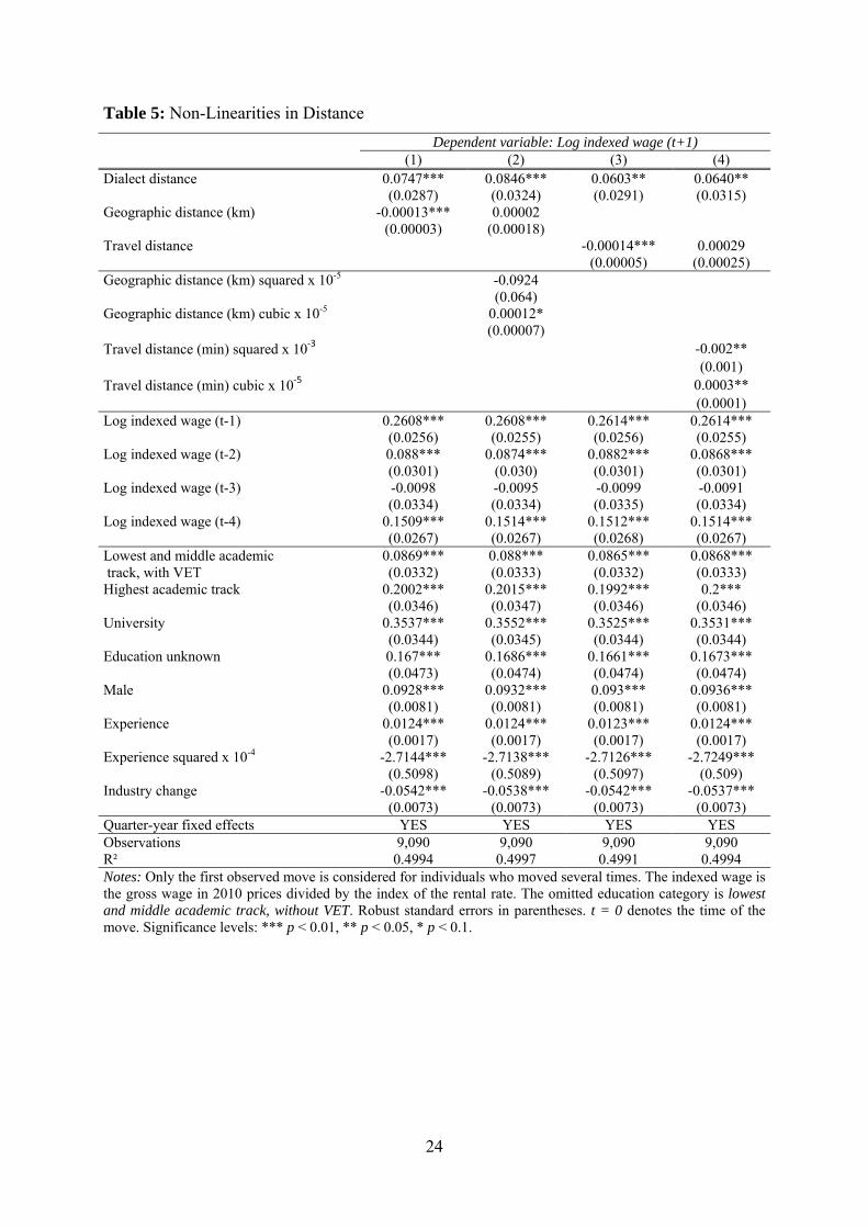
The next concern is the possibility that dialect distance captures non-linearities in geographic

distance that do not have their origin in culture. Table 5 sets out several specifications that

include non-linear geographic distance measures. Column (1) replicates the baseline

regression for means of comparison. Column (2) includes the geographic distance of power

two and three. The coefficient on dialect distance increases, which indicates that it does not

capture strong non-linearities in geographic distance.


However, it could be that geographic distance is an insufficient distance proxy for dialect

distance. Therefore, in Columns (3) and (4) of Table 5 we use the travel distance between

counties by car in minutes as an alternative geographic distance measure.19 However, the

travel time could be affected by dialect distance as well because it is very likely that

transportation hubs and networks have developed along travel routes. Column (3) shows a

specification in which we include the travel distance instead of the geographic distance. The

coefficient of dialect distance decreases but remains highly significant. When we include

travel distance to the power two and three, we see that the coefficient increases slightly again.

However, the results of this exercise indicate that there are only minor nonlinear effects, if

any, of geographic distance that are picked up by dialect distance.

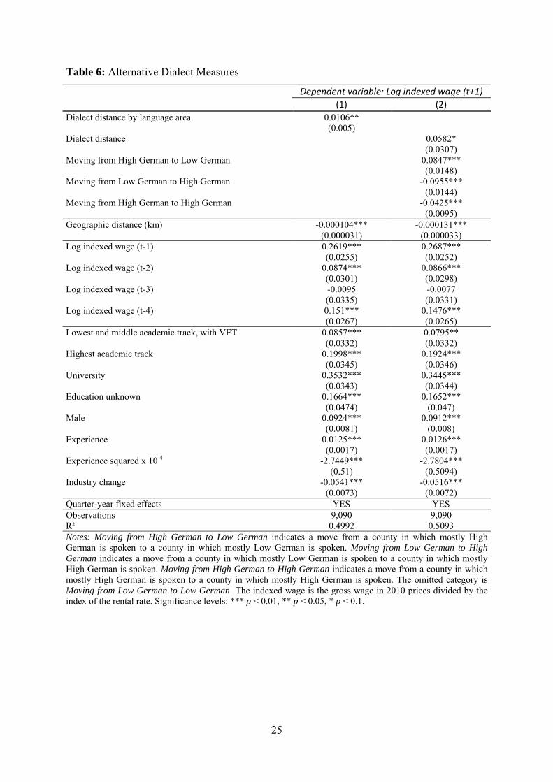
Table 6 uses alternative measures of dialect distance to check the robustness of our

results. To this point, we have used a metric measure of dialect distance. However, it could be

that cultural space is dependent not only on gradual differences but on categorical ones. That

is, the decision to move could be due to a difference between, for example, “Swabian” and

“Bavarian” as such and not to the actual gradual difference between the counties within the

Swabian and Bavarian region. To test for the impact on migration of categorical differences

between smaller regions we use a classification introduced by Lameli (2013) that captures the

most prominent 13 dialect areas in Germany. The measure results from bootstrapped

hierarchical cluster analysis, based on the measurement of linguistic similarity of German

counties. Column (1) of Table 6 sets out the results. The coefficient is positive and significant.

A one standard deviation in the dialect distance by language area (1.04) leads to 1.11 percent

higher post-migration indexed wages.


As the most important linguistic difference between German dialects is that between Low

German (northern part of Germany) and High German (southern part), we further construct a

dummy that substantiates the particular locality of the counties and tests for movements

within the two larger areas of Low German and High German. Column (2) of Table 6

includes a dummy for moving from a High German county to a Low German county, a

dummy for moving from a Low German county to a High German county, and a dummy for

19 Data are provided by the Federal Institute for Research on Building, Urban Affairs and Spatial Development.

12

moving from a High German county to another High German county. The omitted category is

moving from a Low German county to another Low German county. The results show that the

effect of dialect distance remains robust when testing for the north-south distinction. We find,

however, a slight north-south divide, indicating the relevance of a categorical

conceptualization of cultural space. Wages are positively affected by migration from south to

north, but negatively affected by a migration from north to south.

7. Effect Heterogeneity

The question arises as to whether there is a group of individuals that is driving the baseline

results. To answer this question, we first spilt the sample by (i) age, (ii) gender, (iii)

education, (iv) education x gender, (v) distance of the move, and (vi) occupational change.

The results are summarized in Table 7.


Table 7, Panel A stratifies the sample between young (below age 30) and older (above age 30)

movers. In Column (1), we look only at movers who are 30 or younger to discover whether

age plays a crucial role in overcoming cultural distance, as argued by Schwartz (1973). The

coefficient is large and significant. The coefficient on dialect distance for older movers in

Column (2) is smaller and not significant. This indicates that our results are more driven by

young movers than by older movers. Schwartz (1973) further argues that the interaction of

geographic distance with age should indicate the importance of the psychic cost of migration.

Therefore, we interacted geographic distance with age. In this specification (not shown), the

interaction is not significant and the effect of dialect dissimilarity remains unchanged,

indicating that dialect dissimilarity better captures the psychic cost of migration than does an

interaction between geographic distance and age.

Panel B of Table 7 shows that the wages of men are more responsive to culture than

those of women. Possibly this is because in most families the male adult is the household

head and his place of work largely determines where the family lives. We also see that low-

and medium-qualified migrants find culture more of a barrier to migration than do higher

qualified migrants.20 However, the difference between the groups is not large. Panel C shows

that within the group of men, it is again the group of lower qualified migrants that shows a

larger coefficient, but the differences are not significant. The results for women are

insignificant again and the coefficient for lower qualified women is slightly higher than for

higher qualified women. Panel D reveals that the effect is mainly coming from shorter-

distance moves, that is, moves less than 300 km from the former home county. Thus, the

wage increases from moving to a more culturally distant county are not driven by long-

20 The group of low- and medium-qualified migrants consists of those with a degree from the lowest and middle academic track with and without vocational education and training (VET). We also include people for whom level of education is unknown. However, the picture does not change by omitting this group. The group of high-qualified people is comprised of those having a degree from the highest academic track or a university degree.

13

distance moves as one might have expected. We also looked at the subsample of internal

migrants who also switch occupation when they move (Panel E). Compared to occupational

stayers, switchers are compensated more for their move to a dialect-dissimilar county.

We also analyze in more detail the 567 two-time movers in our sample.21 Recall that

the total time period under analysis is nine years, meaning that every second move occurs

within a relatively short time window. For the second move, we use the dialect distance and

geographic distance between the origin county of the first move and the destination county of

the second move. This should mimic the potential direct move to the destination county in the

second move. All other control variables (quarterly pre-treatment wages, education,

experience, age, etc.) are taken from the second move. Interestingly, almost 34 percent (194

migrants) of the two-time movers in our sample return in the second move to exactly the same

county from which they came. However, only 32 of the 194 repatriates return to the same

firm.22

Table 8 shows the results of the two-time mover analysis by first and second move and by

timing of the move, that is, whether the migrant moved another time after or before eight

quarters (two years). Panel A shows the results with repatriates included and Panel B shows

the results without this group. The first move shows, independent of the timing, that the

coefficients are larger than in the baseline sample. This indicates that these particular people,

who we know are going to move again within the next nine years, value culture highly. The

second move is more interestingly. The coefficient for those who moved another time within

eight quarters is almost seven times as large as the baseline coefficient. The above findings

lead us to view these two-time movers as people who made the wrong decision about where

to live and work for the first move and are now willing to sacrifice a lot more money in return

for a more familiar environment.


8. Persistence of Wage Premium

We now turn to the question of whether the initial effect directly after the move is persistent

over time. To this end, we look at wage growth after the first move by estimating the

regression in Equation (2).

11

11 logloglog

idttitsd

indexedistsd

indexedidt

indexedkidt

XDistancealGeographic

wageDistanceDialectkwagewage

(2)

21 There are some individuals who moved more than two times, but this group is too small for an in-depth investigation. 22 “Repatriates” are those who move to their previous county of residence and again work in their previous county of work. Thus, migrants who return to their previous home county but work in a different county than before are not repatriates.

14

Conditional on the logged initial wage level after the move, we regress the average yearly

wage growth from period t+1, i.e., the first quarter after the move, to period t+k, on dialect

distance. Thereby, k takes a maximum value of 32 (quarters), i.e., we analyze wage growth

within a maximum of eight years after the move. Note that by extending the growth period of

analysis year by year, the number of internal migrants remaining in the sample drops

significantly, until finally, in the analysis of eight-year post-move wage growth, there are less

than 700 internal migrants. All other control variables remain equivalent to the baseline

model. Due to a “catching-up” process, we expect that migrants who moved to more

culturally dissimilar counties will exhibit lower wage growth rates. Table 9 shows the results

for the three- to six-year wage growth rates. The coefficient on the logged initial wage level

after the move shows that internal migrants with initially higher wages after the move

generally have lower wage growth in the future. However, dialect distance is not significantly

associated with future wage growth. Thus, we conclude that the initial wage sacrifice is

persistent over time.


9. Conclusion

In this paper, we monetize the psychic cost of migration by combining administrative social

security panel data with a proxy for cultural difference that is based on historical dialect

distance between German counties. Internal migrants demand a (indexed with respect to local

rents) wage premium of about 1 (1.5) percent for a one standard deviation in dialect distance.

Compared to the general wage gain associated with internal migration, as well as to general

wage increases negotiated in recent collective agreements, this wage premium, which is

arguably a lower-bound estimate, is economically substantive and persistent over time. Our

results imply that analyses of rate of return to migration that do not consider this psychic cost

of migration overestimate the rate of return allocated to migration.

15

Literature

Ashenfelter, Orley C. and David Card (1985), Using Longitudinal Structure of Earnings to Estimate the Effect of Training Programs. Review of Economics and Statistics, 67(4), 648–660.

Burchardi, Konrad B. and Tarek A. Hassan (2013), The Economic Impact of Social Ties: Evidence from German Reunification. Quarterly Journal of Economics, 128(3), 1219–1271.

Card, David, Jörg Heining, and Patrick Kline (2013), Workplace Heterogeneity and the Rise of West German Wage Inequality. Quarterly Journal of Economics, 128(3), 967–1015.

Chetty, Raj, Nathaniel Hendren, Patrick Kline, Emmanuel Saez, and Nicholas Turner (2014), Where is the Land of Opportunity? The Geography of Intergenerational Mobility in the United States. Quarterly Journal of Economics, forthcoming.

Dustmann, Christian, Johann Ludsteck, and Uta Schönberg (2009), Revisiting the German Wage Structure. Quarterly Journal of Economics, 124(2), 843–881.

Falck, Oliver, Stephan Heblich, Alfred Lameli, and Jens Suedekum (2012), Dialects, Cultural Identity, and Economic Exchange. Journal of Urban Economics, 72(2–3), 225–239.

Federal Statistical Office (2013), Bevölkerung und Erwerbstätigkeit, Fachserie 1, Reihen 1.2 und 1.3.

Federal Statistical Office (2014), Consumer price indices, https://www.destatis.de/EN/FactsFigures/Indicators/ShortTermIndicators/Prices/pre110.html.

Greenwood, Michael J. (1975), Research on Internal Migration in the United States: A Survey. Journal of Economic Literature, 13(2), 397–433.

Guiso, Luigi, Paula Sapienza, and Luigi Zingales (2006), Does Culture Affect Economic Outcomes? Journal of Economic Perspectives, 20(2), 23–48.

Haider, Steven and Gary Solon (2006), Life-Cycle Variation in the Association Between Current and Lifetime Earnings. American Economic Review, 96(4), 1308–1320.

IG Metall (2013), Collective Wage Agreement in the Manufacturing Sector 2013, http://www.igmetall.de/SID-49F5A1E2-969B8B98/metall-tarifrunde-2013-bayerisches-ergebnis-in-allen-11891.htm

LaLonde, Robert J. (1986), Evaluating the Econometric Evaluations of Training Programs with Experimental Data. American Economic Review, 76(4), 604–620.

Lameli, Alfred (2013), Strukturen im Sprachraum. Analysen zur arealtypologischen Komplexität der Dialekte in Deutschland. De Gruyter, Berlin, Boston.

McKenzie, David, John Gibson, and Steven Stillman (2010), How Important is Selection? Experimental vs. Non-Experimental Measures of the Income Gains from Migration. Journal of the European Economic Association, 8(4), 913–945.

16

Roback, Jennifer (1982), Wages, Rents, and the Quality of Life. Journal of Political Economy, 90(6), 1257–1278.

Schmucker, Alexandra and Stefan Seth (2009), BA-Beschäftigtenpanel 1998–2007 Codebuch, FDZ Datenreport 01/2009, Bundesagentur für Arbeit Nürnberg.

Schwartz, Aba (1973), Interpreting the Effect of Distance on Migration. Journal of Political Economy, 81(5), 1153–1169.

Sjaastad, Larry A. (1962), The Costs and Returns of Human Migration. Journal of Political Economy, 70(5), 80–93.

ver.di (2013), Collective Wage Agreement in the Public Sector 2013, http://www.verdi.de/themen/geld-tarif/tarifrunde-oeffentlicher-dienst-der-laender-2013/++co++a5c366fa-784c-11e2-8d18-52540059119e

Wrede, Ferdinand, Walther Mitzka, and Bernhard Martin (1927), Deutscher Sprachatlas. Auf Grund des von Georg Wenker begründeten Sprachatlas des Deutschen Reichs. Elwert, Marburg.

17

Figure 1: Dialect Distance—The Case of Worms

Notes: The figure shows dialect distance of all districts to the reference point Worms (20% intervals of dialect distance). Degrees of dialect distance (from highest to lowest) are indicated by: white, grey, black.

18

Figure 2: Geographic Distance and Dialect Distance

Notes: The figure shows a binned scatterplot of geographic distance on dialect distance. The figure is constructed by binning dialect distance into 5-percentile point bins (so that there are 20 equal-sized bins) and computing the mean geographic distance within each bin. The slope coefficient and (robust) standard error in parentheses are obtained from a regression on the micro data. Significance levels: *** p < 0.01, ** p < 0.05, * p < 0.1.

0

100

200

300

400

Mea

n ge

ogra

phic

dis

tanc

e (k

m)

0.0 0.2 0.4 0.6 0.8

Dialect distance

Slope: 629.89*** (5.436)

19

Figure 3: Added-Variable Plot of Dialect Distance and the Post-Migration Wage

Notes: The figure shows a binned scatterplot of conditional post-migration indexed wages on residual dialect distance. The conditional post-migration indexed wages are obtained from residuals from regressions on the geographic distance, quarter-year fixed effects, and the last four quarterly pre-migration wages (blue-diamond) or additionally on education dummies (4), male, experience, experience squared, and an industry change dummy (red-quadrat). The residual dialect distance is obtained from residuals from regressions on the geographic distance, quarter-year fixed effects, the last four quarterly pre-migration wages, education dummies (4), male, experience, experience squared, and an industry change dummy. The figure is constructed by binning dialect distance into 5-percentile point bins (so that there are 20 equal-sized bins) and computing the mean conditional post-migration indexed wage within each bin. Coefficients and robust standard errors in parentheses are obtained from regressions on the micro data. Significance levels: *** p < 0.01, ** p < 0.05, * p < 0.1.

-0.04

-0.02

0.00

0.02

0.04

Mea

n co

nditi

onal

pos

t-m

igra

tion

inde

xed

wag

e

-0.20 -0.10 0.00 0.10 0.20 0.30

Residual dialect distance

Conditional on pre-migration wagesConditional on full control set

Conditional on pre-migration wages (blue-diamond): Slope: 0.0952*** (0.0302) Conditional on full control set (red-quadrat): Slope: 0.0747*** (0.0287)

20

Table 1: Descriptive Statistics

Total sample Dialect distance below median above median

Variable Mean Min Mean Min Mean Min (SD) Max (SD) Max (SD) Max

Panel A: Wage data Wage in 2010 prices (t+1) 2,980 240 2,857 248 3,098 240

(1,291) 5,692 (1,266) 5,692 (1,303) 5,692 Wage in 2010 prices (t-1) 2,867 222 2,758 222 2,971 250

(1,285) 5,698 (1,257) 5,698 (1,302) 5,686 Wage in 2010 prices (t-2) 2,852 223 2,744 223 2,956 225

(1,301) 5,692 (1,270) 5,654 (1,323) 5,692 Wage in 2010 prices (t-3) 2,825 221 2,719 225 2,926 221

(1,319) 5,716 (1,288) 5,686 (1,340) 5,716 Wage in 2010 prices (t-4) 2,806 221 2,705 227 2,903 221

(1,329) 5,716 (1,298) 5,670 (1,351) 5,716 Indexed wage in 2010 prices (t+1) 5,271 300 5,180 300 5,358 319

(2,402) 15,836 (2,405) 14,992 (2,397) 15,836 Indexed wage in 2010 prices (t-1) 5,200 273 5,034 273 5,358 467




(2,444) 14,586 (2,424) 14,586 (2,455) 13,928 Panel B: Distance data

Dialect distance 0.372 0 0.189 0 0.548 0.379 (0.207) 0.833 (0.103) 0.364 (0.104) 0.833

Geographic distance (km) 200 1 76 1 318 15 (170) 818 (72) 595 (150) 818

Panel C: Individual characteristics Lowest and middle academic track, 0.019 0 0.021 0 0.017 0

without VET 1 1 1 Lowest and middle academic track, 0.523 0 0.572 0 0.477 0

with VET 1 1 1 Highest academic track 0.144 0 0.135 0 0.152 0

1 1 1 University 0.300 0 0.260 0 0.339 0

1 1 1 Education unknown 0.014 0 0.012 0 0.015 0

1 1 1 Male 0.557 0 0.570 0 0.545 0

1 1 1 Age 32.038 18 31.965 18 32.108 18

(8.049) 63 (8.307) 62 (7.794) 63 Experience 11.687 0 11.790 0 11.587 0

(8.083) 43 (8.335) 43 (7.835) 43 Industry change 0.588 0 0.578 0 0.598 0

1 1 1 Observations 9,090 4,444 4,646

Notes: Summary statistics are based on the baseline sample. Only the first observed move is considered for individuals who moved several times. We have full information on 567 individuals, or 6.2 percent, who moved two times during our time period. Wage data and data on individual characteristics are drawn from the IAB Employment Panel. Wages are denoted in 2010 Euros by using the consumer price index from the Federal Statistical Office (2014). The distance data are from Falck et al. (2012). Standard deviations are not computed for dummy variables. The variable t indicates the timing of the move. t+1 denotes the first observation after the move, t=0 denotes the move, and t-1 denotes the quarter before the move. Experience represents potential labor market experience and is computed by Age – 6 – years of schooling. Years of schooling is assumed to be equal to 10 years for lowest and middle academic track without VET, 13 years for lowest and middle academic track with VET, 13 years for highest academic track without VET, 15 years for highest academic track with VET, 17 years for university, and 10 years for education unknown. We merged highest academic track without VET and highest academic track with VET into one education category.

21

Table 2: Dialect Distance and Post-Migration Wages

Dependent variable: Log indexed wage (t+1) Log wage (t+1) (1) (2) (3) (4) Dialect distance 0.3872*** 0.0952*** 0.0747*** 0.0486** (0.0389) (0.0302) (0.0287) (0.0234) Geographic distance (km) -0.00035*** -0.00012*** -0.00013*** -0.000002 (0.00005) (0.00004) (0.00003) (0.000029) Log indexed wage (t-1) 0.342*** 0.2608*** (0.0272) (0.0256) Log indexed wage (t-2) 0.1137*** 0.088*** (0.0334) (0.0301) Log indexed wage (t-3) -0.0134 -0.0098 (0.0376) (0.0334) Log indexed wage (t-4) 0.2000*** 0.1509*** (0.0293) (0.0267) Log wage (t-1) 0.3799*** (0.0273) Log wage (t-2) 0.0984*** (0.0307) Log wage (t-3) 0.0178 (0.035) Log wage (t-4) 0.0897*** (0.0286) Log rental price (t+1) 0.1984*** (0.0144) Log rental price (t-1) -0.0216 (0.0158) Lowest and middle academic 0.0869*** 0.0635** track, with VET (0.0332) (0.029) Highest academic track 0.2002*** 0.1685*** (0.0346) (0.0304) University 0.3537*** 0.2939*** (0.0344) (0.0305) Education unknown 0.167*** 0.1114*** (0.0473) (0.0408) Male 0.0928*** 0.0765*** (0.0081) (0.007) Experience 0.0124*** 0.0059*** (0.0017) (0.0015) Experience squared x 10-4 -2.7144*** -1.2637*** (0.5098) (0.4391) Industry change -0.0542*** -0.0366*** (0.0073) (0.0061) Quarter-year fixed effects YES YES YES YES Observations 9,090 9,090 9,090 9,090 R² 0.0225 0.4399 0.4994 0.4997 Notes: The indexed wage is the gross wage in 2010 prices divided by the index of the rental rate. The log rental price at t+1 is the average rental price in the destination county and the log rental price is the average rental price in the source county. Only the first observed move is considered for individuals who moved several times. The omitted education category is lowest and middle academic track, without VET. Robust standard errors in parentheses. t = 0 denotes the time of the move. Significance levels: *** p < 0.01, ** p < 0.05, * p < 0.1.

22

Table 3: Robustness Checks

Dependent variable: Log indexed wage (t+1) (1) (2) (3)

5 largest cities

excluded 7 years at origin Pair-wise controls

Dialect distance 0.0741** 0.1295** 0.0961*** (0.0303) (0.0653) (0.0282) Geographic distance (km) -0.000149*** -0.000158** -0.00012*** (0.000038) (0.000078) (0.00004) Log indexed wage (t-1) 0.286*** 0.3601*** 0.2988*** (0.0297) (0.0623) (0.0259) Log indexed wage (t-2) 0.0903** -0.0103 0.0789*** (0.0357) (0.0783) (0.0302) Log indexed wage (t-3) 0.0304 0.0937 -0.0114 (0.0403) (0.0586) (0.0332) Log indexed wage (t-4) 0.1224*** 0.0692* 0.1483*** (0.0317) (0.0363) (0.0261) Lowest and middle academic 0.0422 0.053 0.0879*** track, with VET (0.0321) (0.0748) (0.0322) Highest academic track 0.1383*** 0.1549** 0.1950*** (0.0341) (0.0773) (0.0335) University 0.3092*** 0.3271*** 0.3408*** (0.0339) (0.0768) (0.0333) Education unknown 0.1164** 0.162* 0.1680*** (0.0456) (0.0932) (0.0461) Male 0.0919*** 0.1335*** 0.0921*** (0.0089) (0.0189) (0.0078) Experience 0.0075*** 0.0086** 0.0097*** (0.0018) (0.0038) (0.0016) Experience squared x 10-4 -1.5633*** -2.2194** -2.0864*** (0.5601) (1.1222) (0.4936) Industry change -0.0484*** -0.0527*** -0.0518*** (0.0079) (0.017) (0.0071) Quarter-year fixed effects YES YES YES Observations 6,946 1,815 9,090 R² 0.5395 0.5327 0.5350 Notes: Column (1) drops the five largest cities (Berlin, Hamburg, Munich, Cologne, Frankfurt) as destination and source counties. Column (2) conditions the sample on having lived at least seven years in the county of origin. Column (3) includes several pair-wise controls: log difference in slope, historical rail distance, different religion dummy, difference in share Catholics, difference in historical industry structure, and the difference in the current industry structure, difference in temperature, difference in sunshine duration, and difference in precipitation. The indexed wage is the gross wage in 2010 prices divided by the index of the rental rate. Data on bilateral controls come from Falck et al. (2010) and from the Deutscher Wetterdienst (DWD) for the climate data. Only the first observed move is considered for individuals who moved several times. t = 0 denotes the time of the move. Significance levels: *** p < 0.01, ** p < 0.05, * p < 0.1.

23

Table 4: Adding More/Other Pre-Migration Wages

Dependent variable: Log indexed wage (t+1) (1) (2) (3) (4) (5) (6) (7) (8) (9)

Dialect distance 0.0790*** 0.0637** 0.0629** 0.0550* 0.0666** 0.0821** 0.0916** 0.0846** 0.0858** (0.0294) (0.0299) (0.0308) (0.0319) (0.0334) (0.0347) (0.0368) (0.0386) (0.0372) Log indexed wage (t-5) 0.0777*** 0.0706* 0.0731 0.0668 0.0563 0.04 0.0316 0.0331 (0.0229) (0.0426) (0.0445) (0.0498) (0.0517) (0.0532) (0.0571) (0.0604) Log indexed wage (t-6) 0.0211 -0.0415 -0.042 -0.0507 -0.0334 -0.0384 -0.0466 (0.0318) (0.0472) (0.053) (0.0572) (0.0585) (0.0632) (0.0663) Log indexed wage (t-7) 0.0746** 0.0602 0.0583 0.067 0.0682 0.0859 (0.0288) (0.0512) (0.0556) (0.0597) (0.0637) (0.0665) Log indexed wage (t-8) 0.0291 -0.0369 -0.0723 -0.0652 -0.0914 (0.0321) (0.0506) (0.0577) (0.0635) (0.0694) Log indexed wage (t-9) 0.0932*** 0.0643 0.0616 0.0612 (0.0307) (0.0422) (0.0462) (0.0502) Log indexed wage (t-10) 0.0577* 0.0454 0.0659 (0.0298) (0.04) (0.0443) Log indexed wage (t-11) 0.0225 -0.0123 (0.0254) (0.0366) Log indexed wage (t-12) 0.0317 (0.0311) Mean log indexed wage (t-1 to t-4) 0.4161*** (0.0279) Mean log indexed wage (t-5 to t-8) -0.0281 (0.030) Mean log indexed wage (t-9 to t-12) 0.1017*** (0.0204) Quarter-year FE YES YES YES YES YES YES YES YES YES Controls YES YES YES YES YES YES YES YES YES Observations 8,517 7,949 7,392 6,845 6,225 5,692 5,099 4,681 5,411 R² 0.5048 0.5137 0.522 0.5225 0.5208 0.5283 0.5276 0.5293 0.519 Notes: Only the first observed move is considered for individuals who moved several times. The indexed wage is the gross wage in 2010 prices divided by the index of the rental rate. Controls: geographic distance, education dummies, male, experience, experience squared, and industry change. Regressions in Columns (1) to (8) contain pre-migration log indexed wages from t-1, t-2, t-3, and t-4. Robust standard errors in parentheses. t = 0 denotes the time of the move. Significance levels: *** p < 0.01, ** p < 0.05, * p < 0.1.

24

Table 5: Non-Linearities in Distance

Dependent variable: Log indexed wage (t+1) (1) (2) (3) (4) Dialect distance 0.0747*** 0.0846*** 0.0603** 0.0640** (0.0287) (0.0324) (0.0291) (0.0315) Geographic distance (km) -0.00013*** 0.00002 (0.00003) (0.00018) Travel distance -0.00014*** 0.00029 (0.00005) (0.00025) Geographic distance (km) squared x 10-5 -0.0924 (0.064) Geographic distance (km) cubic x 10-5 0.00012* (0.00007) Travel distance (min) squared x 10‐3 -0.002** (0.001) Travel distance (min) cubic x 10‐5 0.0003** (0.0001) Log indexed wage (t-1) 0.2608*** 0.2608*** 0.2614*** 0.2614*** (0.0256) (0.0255) (0.0256) (0.0255) Log indexed wage (t-2) 0.088*** 0.0874*** 0.0882*** 0.0868*** (0.0301) (0.030) (0.0301) (0.0301) Log indexed wage (t-3) -0.0098 -0.0095 -0.0099 -0.0091 (0.0334) (0.0334) (0.0335) (0.0334) Log indexed wage (t-4) 0.1509*** 0.1514*** 0.1512*** 0.1514*** (0.0267) (0.0267) (0.0268) (0.0267) Lowest and middle academic 0.0869*** 0.088*** 0.0865*** 0.0868*** track, with VET (0.0332) (0.0333) (0.0332) (0.0333) Highest academic track 0.2002*** 0.2015*** 0.1992*** 0.2*** (0.0346) (0.0347) (0.0346) (0.0346) University 0.3537*** 0.3552*** 0.3525*** 0.3531*** (0.0344) (0.0345) (0.0344) (0.0344) Education unknown 0.167*** 0.1686*** 0.1661*** 0.1673*** (0.0473) (0.0474) (0.0474) (0.0474) Male 0.0928*** 0.0932*** 0.093*** 0.0936*** (0.0081) (0.0081) (0.0081) (0.0081) Experience 0.0124*** 0.0124*** 0.0123*** 0.0124*** (0.0017) (0.0017) (0.0017) (0.0017) Experience squared x 10-4 -2.7144*** -2.7138*** -2.7126*** -2.7249*** (0.5098) (0.5089) (0.5097) (0.509) Industry change -0.0542*** -0.0538*** -0.0542*** -0.0537*** (0.0073) (0.0073) (0.0073) (0.0073) Quarter-year fixed effects YES YES YES YES Observations 9,090 9,090 9,090 9,090 R² 0.4994 0.4997 0.4991 0.4994 Notes: Only the first observed move is considered for individuals who moved several times. The indexed wage is the gross wage in 2010 prices divided by the index of the rental rate. The omitted education category is lowest and middle academic track, without VET. Robust standard errors in parentheses. t = 0 denotes the time of the move. Significance levels: *** p < 0.01, ** p < 0.05, * p < 0.1.

25

Table 6: Alternative Dialect Measures

Dependent variable: Log indexed wage (t+1)

(1) (2) Dialect distance by language area 0.0106**

(0.005) Dialect distance 0.0582*

(0.0307) Moving from High German to Low German 0.0847***

(0.0148) Moving from Low German to High German -0.0955***

(0.0144) Moving from High German to High German -0.0425***

(0.0095) Geographic distance (km) -0.000104*** -0.000131***

(0.000031) (0.000033) Log indexed wage (t-1) 0.2619*** 0.2687***


(0.0301) (0.0298) Log indexed wage (t-3) -0.0095 -0.0077


(0.0267) (0.0265) Lowest and middle academic track, with VET 0.0857*** 0.0795** (0.0332) (0.0332) Highest academic track 0.1998*** 0.1924***

(0.0345) (0.0346) University 0.3532*** 0.3445***

(0.0343) (0.0344) Education unknown 0.1664*** 0.1652***

(0.0474) (0.047) Male 0.0924*** 0.0912***

(0.0081) (0.008) Experience 0.0125*** 0.0126***

(0.0017) (0.0017) Experience squared x 10-4 -2.7449*** -2.7804***

(0.51) (0.5094) Industry change -0.0541*** -0.0516***

(0.0073) (0.0072) Quarter-year fixed effects YES YES Observations 9,090 9,090 R² 0.4992 0.5093 Notes: Moving from High German to Low German indicates a move from a county in which mostly High German is spoken to a county in which mostly Low German is spoken. Moving from Low German to High German indicates a move from a county in which mostly Low German is spoken to a county in which mostly High German is spoken. Moving from High German to High German indicates a move from a county in which mostly High German is spoken to a county in which mostly High German is spoken. The omitted category is Moving from Low German to Low German. The indexed wage is the gross wage in 2010 prices divided by the index of the rental rate. Significance levels: *** p < 0.01, ** p < 0.05, * p < 0.1.

26

Table 7: Effect Heterogeneities

Dependent variable: Log indexed wage (t+1) (1) (2) (3) (4)

Panel A: Age Age < 30 ≥ 30 Dialect distance 0.0930** 0.0494 (0.0404) (0.0407) Observations 4,384 4,706 R² 0.3948 0.5042

Panel B: Gender and education Gender Education Men Women Low, medium High Dialect distance 0.1046*** 0.0367 0.0844** 0.0669 (0.0367) (0.0451) (0.0406) (0.0410) Observations 5,063 4,027 5,051 4,039 R² 0.5057 0.4027 0.3615 0.4351

Panel C: Gender x education Men Women Low, medium High Low, medium High Dialect distance 0.1143** 0.0934* 0.0519 0.0215 (0.0548) (0.0492) (0.0598) (0.0700) Observations 2,727 2,336 2,324 1,703 R² 0.3522 0.3872 0.3377 0.3457

Panel D: Geographic distance < 200 km < 300 km ≥ 200 km ≥ 300 km Dialect distance 0.0984** 0.1179*** 0.0534 -0.0279 (0.0402) (0.0356) (0.0545) (0.0702) Observations 5,325 6,575 3,765 2,515 R² 0.5155 0.5112 0.4862 0.4822

Panel E: Occupational change

Occupational

information available Occupational switchers Occupational stayers Dialect distance 0.0806** 0.1154** 0.0423 (0.0313) (0.0506) (0.0383) Observations 7,337 3,479 3,858 R² 0.5089 0.4638 0.5757 Notes: Low and medium education corresponds to the lowest and middle academic track with and without VET, plus unknown education. High education corresponds to the highest academic track plus university education. Only the first observed move is considered for individuals who moved several times. The indexed wage is the gross wage in 2010 prices divided by the index of the rental rate. All regressions include quarter-year fixed effects, four quarterly pre-migration wages, individual controls, and geographic distance controls. Individual controls: education, male, experience, experience squared, industry change. Geographic distance controls: geographic distance. Robust standard errors in parentheses. t = 0 denotes the time of the move. Significance levels: *** p < 0.01, ** p < 0.05, * p < 0.1.

27

Table 8: Two-Time Mover Analysis

Dependent variable: Log indexed wage (t+1) (1) (2) (3) (4) First move Second move ≥ 8 quarters < 8 quarters ≥ 8 quarters < 8 quarters

Panel A: With repatriates Dialect distance 0.2907* 0.1208 0.0363 0.5027*** (0.1752) (0.1881) (0.1411) (0.1559)Observations 245 322 245 322R² 0.5813 0.5157 0.7002 0.5616

Panel B: Without repatriatesDialect distance 0.3145 0.2570 0.1621 0.6122*** (0.2001) (0.2693) (0.1570) (0.1932)Observations 192 181 192 181R² 0.6224 0.5166 0.7074 0.6019Notes: Repatriates are those individuals who move back to their county (or counties) of origin (both county of work and county of residence) in the second move. The second move uses the dialect and geographic distance between the source county of the first move and the destination county of the second move. The indexed wage is the gross wage in 2010 prices divided by the index of the rental rate. All regressions include quarter-year fixed effects, four quarterly pre-migration wages, individual controls, and geographic distance controls. Individual controls: education, male, experience, experience squared, industry change. Geographic distance controls: geographic distance. t = 0 denotes the time of the move. Significance levels: *** p < 0.01, ** p < 0.05, * p < 0.1.

28

Table 9: Long-Run Effects

Dependent variable: [log indexed wage (t+k) - log indexed wage (t+1)]/k k = 4 k = 8 k = 12 k = 16 k = 20 k = 24 k = 28 k = 32 Dialect distance 0.0088* 0.0034 0.0022 0.0005 0.0003 0.0022 -0.0001 -0.0002 (0.0048) (0.0034) (0.003) (0.0026) (0.0024) (0.0024) (0.0029) (0.0044) Log indexed wage (t+1) -0.0431*** -0.0338*** -0.028*** -0.0223*** -0.0194*** -0.0166*** -0.0164*** -0.015*** (0.0035) (0.0022) (0.0017) (0.0015) (0.0013) (0.0013) (0.0014) (0.0021) Observations 8,209 6,872 5,875 4,910 4,076 3,142 1,923 698 R² 0.0922 0.1224 0.119 0.1317 0.1333 0.1271 0.1491 0.1627 Notes: Only the first observed move is considered for individuals who moved several times. The indexed wage is the gross wage in 2010 prices divided by the index of the rental rate. All regressions include quarter-year fixed effects, individual controls, and geographic distance controls. Individual controls: education, male, experience, experience squared, industry change. Geographic distance controls: geographic distance. Robust standard errors in parentheses. t = 0 denotes the time of the move. Significance levels: *** p < 0.01, ** p < 0.05, * p < 0.1.

Ever since Sjaastad (1962), researchers have ... - CORE · CATEGORY 4: LABOUR MARKETS. S ......

Documents

Transcript of Ever since Sjaastad (1962), researchers have ... - CORE · CATEGORY 4: LABOUR MARKETS. S ......