Exploration Geophysics

Bearbeitet vonMamdouh R. Gadallah, Ray Fisher

1. Auflage 2008. Buch. xxii, 266 S. HardcoverISBN 978 3 540 85159 2

Format (B x L): 15,5 x 23,5 cmGewicht: 649 g

Weitere Fachgebiete > Physik, Astronomie > Angewandte Physik > Geophysik

Zu Inhaltsverzeichnis

schnell und portofrei erhältlich bei

Die Online-Fachbuchhandlung beck-shop.de ist spezialisiert auf Fachbücher, insbesondere Recht, Steuern und Wirtschaft.Im Sortiment finden Sie alle Medien (Bücher, Zeitschriften, CDs, eBooks, etc.) aller Verlage. Ergänzt wird das Programmdurch Services wie Neuerscheinungsdienst oder Zusammenstellungen von Büchern zu Sonderpreisen. Der Shop führt mehr

als 8 Millionen Produkte.

Chapter 2Overview of Geophysical Techniques

Introduction

Various geophysical surveying methods have been and are used on land and off-shore. Each of these methods measures something that is related to subsurface rocksand their geologic configurations. Rocks and minerals in the earth vary in severalways. These include:

• Density – mass per unit volume. The gravity method detects lateral variations indensity. Both lateral and vertical density variations are important in the seismicmethod.

• Magnetic susceptibility – the amount of magnetization in a substance exposed toa magnetic field. The magnetic method detects horizontal variations in suscepti-bility.

• Propagation velocity – the rate at which sound or seismic waves are transmittedin the earth. It is these variations, horizontal and vertical, that make the seismicmethod applicable to petroleum exploration.

• Resistivity and induced polarization – Resitivity is a measure of the ability toconduct electricity and induced polarization is frequency-dependent variation inresistivity. Electrical methods detect variations of these over a surface area

• Self-potential - ability to generate an electrical voltage. Electrical methods alsomeasure this over a surface area.

• Electromagnetic wave reflectivity and transmissivity – reflection and transmis-sion of electromagnetic radiation, such as radar, radio waves and infrared radia-tion, is the basis of electromagnetic methods.

The primary advantages of the gravity and magnetic methods are that they arefaster and cheaper than the seismic method. However, they do not provide the de-tailed information about the subsurface that the seismic method, particularly seismicreflection, does. There may also be interpretational ambiguities present.

Electrical methods are well suited to tracking the subsurface water table andlocating water-bearing sands Seismic methods can also be used for this purpose.

Electromagnetic methods are useful in detecting near surface features such asancient rivers.

M.R. Gadallah, R. Fisher, Exploration Geophysics, 7DOI 10.1007/978-3-540-85160-8 2, c© Springer-Verlag Berlin Heidelberg 2009

8 2 Overview of Geophysical Techniques

There will be no further discussion of electrical or electromagnetic methods. Thefollowing paragraphs provide brief introductions to the gravity, magnetic, and seis-mic methods. The discussions of the gravity and magnetic methods included in thischapter serve to acquaint the reader with their general methods and applications. Allsubsequent chapters will deal with the seismic method.

The Gravity Method

A 70-kg man weighs less than 70 kg in Denver, Colorado and more than 70 kgpounds in Death Valley, California. This is because Denver is at a substantiallyhigher elevation than sea level while Death Valley is below sea level. So, the far-ther from the center of the earth the less one weighs. What one weighs depends onthe force of gravity at that spot and the force of gravity varies with elevation, rockdensities, latitude, and topography. Mass, however, does not depend on gravity butis a fundamental quantity throughout the universe.

When a mass is suspended from a spring, the amount the spring stretches isproportional to the force of gravity. This force, F, is given by F = mg, where g is theacceleration of gravity. Since mass is a constant, variations in stretch of the springcan be used to determine variations in the acceleration of gravity, g.

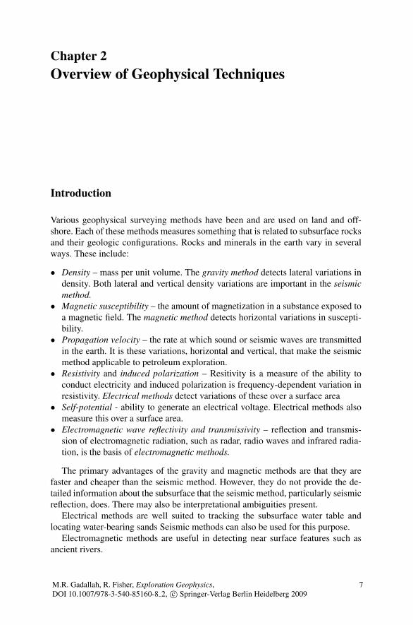
Figure 2.1 illustrates the principle of gravity exploration. On the left the surfaceelevation is moderate but there is a thick sedimentary section overlaying the base-ment complex. At the center the surface elevation is near sea level and the subsurfacehas a sedimentary section of normal thickness and density overlaying an “average”basement complex. On the right the surface elevation is also moderate but thereis a thin sedimentary section resulting in the basement complex being close to thesurface.

The center part of Fig. 2.1 represents the “normal” earth situation and the sus-pended mass stretches the spring a “normal” amount here. On the left, the thick

Sedimentary Section

Basement Complex

Spring

Mass

Fig. 2.1 The gravity method

Introduction 9

sedimentary section has lower density than the basement rocks so the “pull” of theearth is reduced, resulting in the suspended mass stretching the spring less thanthe “normal” amount. The situation on the right is the opposite. The higher densitybasement rocks closer to the surface causes the “pull” of the earth to be greater,stretching the spring more than the “normal” amount.

An instrument called a gravimeter is used to measure g at “stations” spaced moreor less evenly over the area being surveyed. Raw readings are corrected for eleva-tion, latitude, and topography. The normal value of g is subtracted from the correctedreadings, yielding residual gravity. The values of residual gravity are plotted at therespective station locations and contours of equal residual gravity are drawn. Closedcontours represent gravity anomalies that can be used to infer subsurface geologicstructures.

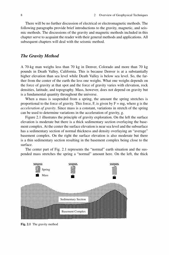
The value of g at sea level is about 980cm/s2. Since the variations of g are rela-tively small, cm/s2 is a bit large for measuring them. The unit used for measuringresidual gravity is the milligal (mgal), or one-thousandth of a gal, where a gal is1cm/s2. The gal is named for Galileo. Figure 2.2 is an example of a final gravitymap. Contour interval is 1 mgal.

Fig. 2.2 Gravity map example

10 2 Overview of Geophysical Techniques

Interpretation of gravity data is done by comparing the shape and size of theseanomalies to those caused by bodies of various geometrical shapes at differentdepths and differing densities.

The Magnetic Method

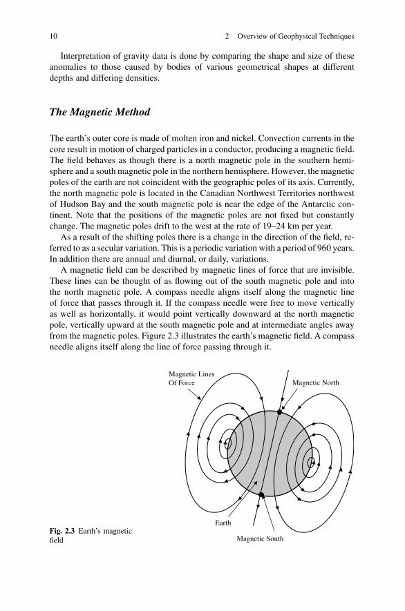
The earth’s outer core is made of molten iron and nickel. Convection currents in thecore result in motion of charged particles in a conductor, producing a magnetic field.The field behaves as though there is a north magnetic pole in the southern hemi-sphere and a south magnetic pole in the northern hemisphere. However, the magneticpoles of the earth are not coincident with the geographic poles of its axis. Currently,the north magnetic pole is located in the Canadian Northwest Territories northwestof Hudson Bay and the south magnetic pole is near the edge of the Antarctic con-tinent. Note that the positions of the magnetic poles are not fixed but constantlychange. The magnetic poles drift to the west at the rate of 19–24 km per year.

As a result of the shifting poles there is a change in the direction of the field, re-ferred to as a secular variation. This is a periodic variation with a period of 960 years.In addition there are annual and diurnal, or daily, variations.

A magnetic field can be described by magnetic lines of force that are invisible.These lines can be thought of as flowing out of the south magnetic pole and intothe north magnetic pole. A compass needle aligns itself along the magnetic lineof force that passes through it. If the compass needle were free to move verticallyas well as horizontally, it would point vertically downward at the north magneticpole, vertically upward at the south magnetic pole and at intermediate angles awayfrom the magnetic poles. Figure 2.3 illustrates the earth’s magnetic field. A compassneedle aligns itself along the line of force passing through it.

Fig. 2.3 Earth’s magneticfield

Magnetic LinesOf Force

Earth

Magnetic South

Magnetic North

Introduction 11

In addition to these known variations in the magnetic field, local variations occurwhere the basement complex is close to the surface and where concentrations offerromagnetic minerals exist. Thus, the primary applications of the magnetic methodare in mapping the basement and locating ferromagnetic ore deposits.

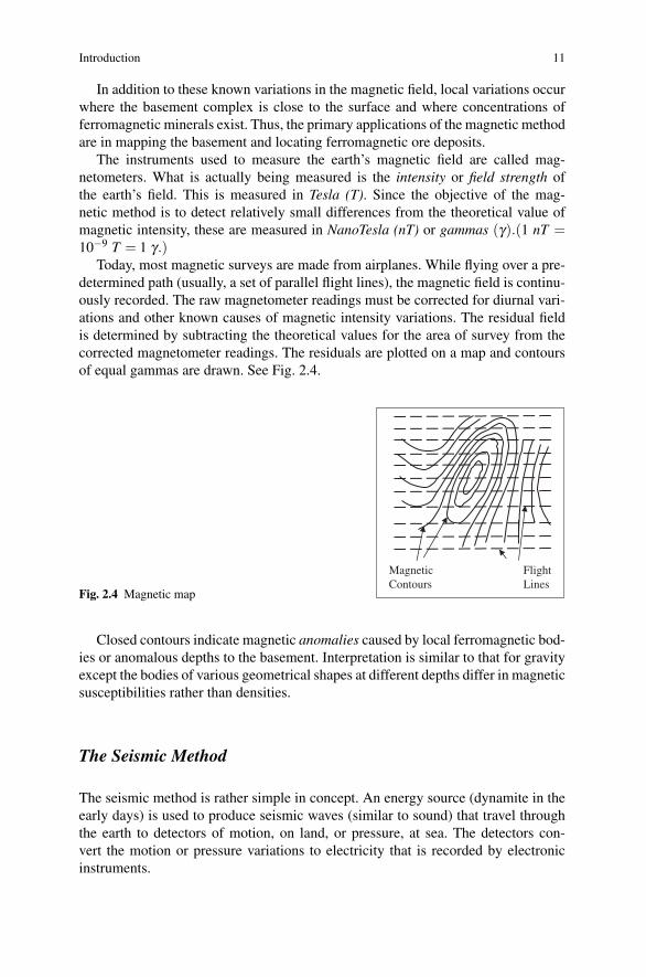
The instruments used to measure the earth’s magnetic field are called mag-netometers. What is actually being measured is the intensity or field strength ofthe earth’s field. This is measured in Tesla (T). Since the objective of the mag-netic method is to detect relatively small differences from the theoretical value ofmagnetic intensity, these are measured in NanoTesla (nT) or gammas (γ).(1 nT =10−9 T = 1 γ.)

Today, most magnetic surveys are made from airplanes. While flying over a pre-determined path (usually, a set of parallel flight lines), the magnetic field is continu-ously recorded. The raw magnetometer readings must be corrected for diurnal vari-ations and other known causes of magnetic intensity variations. The residual fieldis determined by subtracting the theoretical values for the area of survey from thecorrected magnetometer readings. The residuals are plotted on a map and contoursof equal gammas are drawn. See Fig. 2.4.

Fig. 2.4 Magnetic map

MagneticContours

FlightLines

Closed contours indicate magnetic anomalies caused by local ferromagnetic bod-ies or anomalous depths to the basement. Interpretation is similar to that for gravityexcept the bodies of various geometrical shapes at different depths differ in magneticsusceptibilities rather than densities.

The Seismic Method

The seismic method is rather simple in concept. An energy source (dynamite in theearly days) is used to produce seismic waves (similar to sound) that travel throughthe earth to detectors of motion, on land, or pressure, at sea. The detectors con-vert the motion or pressure variations to electricity that is recorded by electronicinstruments.

12 2 Overview of Geophysical Techniques

L. Palmiere developed the first ’seismograph’ in 1855. A seismograph is an in-strument used to detect and record earthquakes. This device was able to pick upand record the vibrations of the earth that occur during an earthquake. However,it wasn’t until 1921 that this technology was used to help locate underground oilformations.

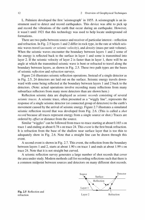
There are two paths between source and receiver of particular interest – reflectionand refraction. In Fig. 2.5 layers 1 and 2 differ in rock type, in the rate at which seis-mic waves travel (acoustic or seismic velocity), and density (mass per unit volume).When the seismic waves encounter the boundary between layers 1 and 2 some ofthe energy is reflected back to the surface in layer 1 and some is transmitted intolayer 2. If the seismic velocity of layer 2 is faster than in layer 1, there will be anangle at which the transmitted seismic wave is bent or refracted to travel along theboundary between layers, as shown in Fig. 2.5. These two path types are the basesof seismic reflection and refraction surveys.

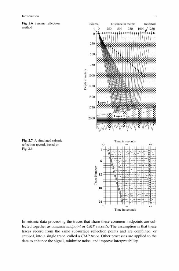
Figure 2.6 illustrates seismic reflection operations. Instead of a single detector asin Fig. 2.5, 24 detectors are laid out on the surface. Seismic energy travels down-ward with some being reflected at the boundary between layers 1 and 2 back to thedetectors. (Note: actual operations involve recording many reflections from manysubsurface reflectors from many more detectors than are shown here.)

Reflection seismic data are displayed as seismic records consisting of severalseismic traces. A seismic trace, often presented as a “wiggly line”, represents theresponse of a single seismic detector (or connected group of detectors) to the earth’smovement caused by the arrival of seismic energy. Figure 2.7 illustrates a simulatedseismic reflection record that was developed from Fig. 2.6. (This is called a shotrecord because all traces represent energy from a single source or shot.) Traces areordered by offset or distance from the source.

Similar “wiggles” can be followed from trace-to-trace starting at about 0.165 s ontrace 1 and ending at about 0.78 s on trace 24. This event is the first break refraction.It is refraction from the base of the shallow near surface layer that is too thin toadequately show in Fig. 2.6. Note that a straight line can be drawn through thisevent.

A second event is shown in Fig. 2.7. This event, the reflection from the boundarybetween layers 1 and 2, starts at about 1.90 s on trace 1 and ends at about 1.99 s ontrace 24. Note that it is not straight but curved.

A seismic reflection survey generates a large number of shot records that coverthe area under study. Modern methods call for recording reflections such that there isa common midpoint between sources and detectors on many different shot records.

Fig. 2.5 Reflection andrefraction

Surface

Reflection

Layer 1

Source Detector

Layer 2 Refraction

Introduction 13

Fig. 2.6 Seismic reflectionmethod

Dep

th in

met

ers

Layer 1

Layer 2

0 250 500 750 1000 1250

0

250

500

750

1000

1250

1500

1750

2000

Source Distance in meters Detectors

Fig. 2.7 A simulated seismicreflection record, based onFig. 2.6

Time in seconds

Time in seconds

0 1 2

0 1 2

Tra

ce N

umbe

r

1

6

12

18

24

In seismic data processing the traces that share these common midpoints are col-lected together as common midpoint or CMP records. The assumption is that thesetraces record from the same subsurface reflection points and are combined, orstacked, into a single trace, called a CMP trace. Other processes are applied to thedata to enhance the signal, minimize noise, and improve interpretability.

14 2 Overview of Geophysical Techniques

Fig. 2.8 A seismic section Surface Locations

Tim

e in

sec

onds

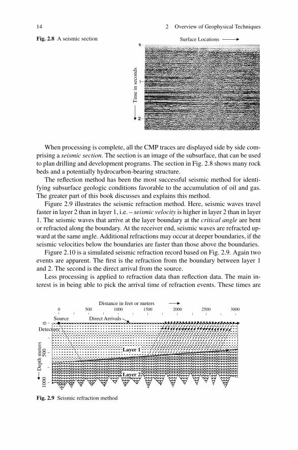
When processing is complete, all the CMP traces are displayed side by side com-prising a seismic section. The section is an image of the subsurface, that can be usedto plan drilling and development programs. The section in Fig. 2.8 shows many rockbeds and a potentially hydrocarbon-bearing structure.

The reflection method has been the most successful seismic method for identi-fying subsurface geologic conditions favorable to the accumulation of oil and gas.The greater part of this book discusses and explains this method.

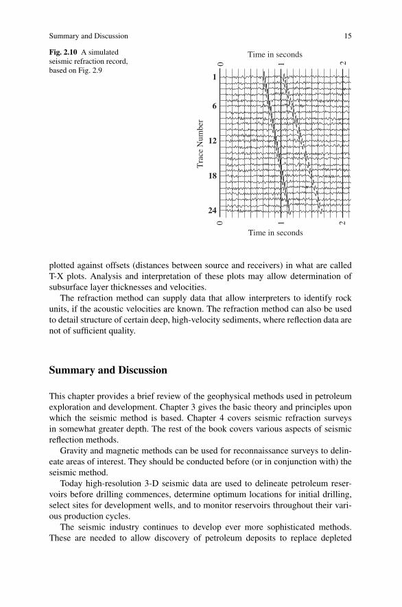
Figure 2.9 illustrates the seismic refraction method. Here, seismic waves travelfaster in layer 2 than in layer 1, i.e. – seismic velocity is higher in layer 2 than in layer1. The seismic waves that arrive at the layer boundary at the critical angle are bentor refracted along the boundary. At the receiver end, seismic waves are refracted up-ward at the same angle. Additional refractions may occur at deeper boundaries, if theseismic velocities below the boundaries are faster than those above the boundaries.

Figure 2.10 is a simulated seismic refraction record based on Fig. 2.9. Again twoevents are apparent. The first is the refraction from the boundary between layer 1and 2. The second is the direct arrival from the source.

Less processing is applied to refraction data than reflection data. The main in-terest is in being able to pick the arrival time of refraction events. These times are

Distance in feet or meters

Detectors

Layer 1

Layer 2

Dep

th m

eter

s

0 500 1000 1500 2000 2500 3000

Source Direct Arrivals

1000

500

0

Fig. 2.9 Seismic refraction method

Summary and Discussion 15

Fig. 2.10 A simulatedseismic refraction record,based on Fig. 2.9

Time in seconds

Time in seconds

0 1 2

0 1 2

Tra

ce N

umbe

r

1

6

12

18

24

plotted against offsets (distances between source and receivers) in what are calledT-X plots. Analysis and interpretation of these plots may allow determination ofsubsurface layer thicknesses and velocities.

The refraction method can supply data that allow interpreters to identify rockunits, if the acoustic velocities are known. The refraction method can also be usedto detail structure of certain deep, high-velocity sediments, where reflection data arenot of sufficient quality.

Summary and Discussion

This chapter provides a brief review of the geophysical methods used in petroleumexploration and development. Chapter 3 gives the basic theory and principles uponwhich the seismic method is based. Chapter 4 covers seismic refraction surveysin somewhat greater depth. The rest of the book covers various aspects of seismicreflection methods.

Gravity and magnetic methods can be used for reconnaissance surveys to delin-eate areas of interest. They should be conducted before (or in conjunction with) theseismic method.

Today high-resolution 3-D seismic data are used to delineate petroleum reser-voirs before drilling commences, determine optimum locations for initial drilling,select sites for development wells, and to monitor reservoirs throughout their vari-ous production cycles.

The seismic industry continues to develop ever more sophisticated methods.These are needed to allow discovery of petroleum deposits to replace depleted

16 2 Overview of Geophysical Techniques

reserves. The more subtle nature of the reservoirs to be discovered, require moreaccurate information so that the fine details of a reservoir can be studied. Theseadvanced methods are also needed to optimize petroleum production from knownreservoirs.

There are many sources of data and information for the geologist and geophysi-cist in exploration for hydrocarbons. This includes a variety of measurements, com-monly referred to as logs, obtained along the boreholes. However, this raw dataalone would be useless without methodical processing and interpretation. Much likeputting together a puzzle, the geophysicist uses sources of data available to create amodel, or educated guess, as to the structure of rocks under the ground. Some tech-niques, including seismic exploration, allow the construction of a hand or computergenerated visual interpretation of the subsurface. Other sources of data, such as thatobtained from core samples or logging, are taken by the geologist when determiningthe subsurface geological structures. It must be remembered, however, that despitethe amazing evolution of technology and exploration methods the only way of be-ing sure that a petroleum or natural gas reservoir exists is to drill. The result ofthe improvement in technology and procedures is that exploration geologists andgeophysicists can make better assessments of drilling locations.