Fast Calorimeter Punch-Through Simulation for the ATLAS...
107
CERN-THESIS-2011-112 28/09/2011 Fast Calorimeter Punch-Through Simulation for the ATLAS Experiment Diplomarbeit in der Studienrichtung Physik zur Erlangung des akademischen Grades Magister der Naturwissenschaft (Mag.rer.nat.) eingereicht an der Fakult¨ at f¨ ur Mathematik, Informatik und Physik der Universit¨ at Innsbruck von Elmar Ritsch [email protected] Betreuer der Diplomarbeit: Dr. Andreas Salzburger, CERN Ao.Univ.-Prof. Dr. Emmerich Kneringer, Institut f¨ ur Astro- und Teilchenphysik Innsbruck, September 2011
Transcript of Fast Calorimeter Punch-Through Simulation for the ATLAS...
CER
N-T
HES
IS-2
011-
112
28/0
9/20
11
Fast CalorimeterPunch-Through Simulation for
the ATLAS Experiment
Diplomarbeitin der Studienrichtung Physik
zur Erlangung des akademischen GradesMagister der Naturwissenschaft (Mag.rer.nat.)
eingereicht an derFakultat fur Mathematik, Informatik und Physik
der Universitat Innsbruck
vonElmar Ritsch
Betreuer der Diplomarbeit:Dr. Andreas Salzburger, CERN
Ao.Univ.-Prof. Dr. Emmerich Kneringer, Institut fur Astro- und Teilchenphysik
Innsbruck, September 2011

Abstract
This work discusses the parametrization, implementation and validation of a tuneablefast simulation of hadronic leakage in the ATLAS detector. It is dedicated to simulatecalorimeter punch-through and decay in flight processes inside the ATLAS calorime-ter. Both effects can cause systematic errors in muon reconstruction and identification.Therefore a correct description of these effects is crucial for many physics studies in-volving muons. The parameterized punch-through simulation is integrated into the fastATLAS detector simulations Fatras and AtlfastII, respectively. The Fatras based simu-lation of single pions shows a good agreement with results obtained by the full Geant4detector simulation – especially in the context of a fast simulation. It is shown thatfor high energy multi jet events, simulated with the AtlfastII implementation, the muonreconstruction rates show a good agreement with the Geant4 simulated reference.
i

Acknowledgements – Danksagung
Beginnen mochte ich meine Danksagung bei meinen Betreuern Dr. Andreas Salzburgerund Prof. Dr. Emmerich Kneringer. Ihr habt mich seit meinen Anfangen in der Teilchen-physik engagiert unterstutzt. Gemeinsam haben wir unzahlige Diskussionen gefuhrt, diemir sowohl bei meiner Arbeit von großer Hilfe waren, als auch, mich weit uber diePhysik hinaus inspiriert haben. Uberaus dankbar bin ich auch fur euer Engagement beider Durchsicht dieser Arbeit, ebenso wie fur die vielen hilfreichen Kommentare dazu.
Prof. Dr. Dietmar Kuhn gebuhrt besonderer Dank, fur die entgegengebrachte Unterstutzungab der ersten Minute als Sommerstudent und die uberaus freundliche Leitung der Teilchen-physik Gruppe in Innsbruck. Ich mochte mich auch bei der gesamten Arbeitsgruppe be-danken, fur die herausragende Hilfsbereitschaft und die außerst angenehme Atmospharein der Gruppe.
Meinen Burokollegen und Papierflieger-Piloten Patrick Jussel, Michael Werner, JocelinPerez und Klaus Reitberger mochte ich besonders Danken, fur die meist heitere At-mospare in unserem gemeinsamen Reich.
Speziellen Dank mochte ich auch gegenuber Michael Duhrssen und Wolfgang Lukasaussprechen, welche mir in vielerlei Hinsicht bei der Umsetzung meiner Diplomarbeitgeholfen haben.
Nicht zuletzt gebuhrt besonderer Dank meinen Eltern, welche mir das Studium nichtnur nahe legten, sondern mich uber die gesamte Dauer meines Studiums tatenreich un-terstutzten.
Vielen Dank Kathi, dass du auch in sehr arbeitsreichen Zeiten verstandnisvoll zu mirgestanden hast.
iii

Contents
Abstract i
Acknowledgements – Danksagung iii
1 Introduction and Motivation 1
2 The ATLAS Experiment 32.1 Coordinate System . . . . . . . . . . . . . . . . . . . . . . . . . . . . . . . 42.2 The Inner Detector . . . . . . . . . . . . . . . . . . . . . . . . . . . . . . . 52.3 The Calorimeter . . . . . . . . . . . . . . . . . . . . . . . . . . . . . . . . 52.4 The Muon Spectrometer or Muon System . . . . . . . . . . . . . . . . . . 62.5 Particle Signatures . . . . . . . . . . . . . . . . . . . . . . . . . . . . . . . 6
3 Detector Simulation in ATLAS 93.1 Simulation Scheme . . . . . . . . . . . . . . . . . . . . . . . . . . . . . . . 93.2 Full and Fast Detector Simulation . . . . . . . . . . . . . . . . . . . . . . 13
3.2.1 Geant4 . . . . . . . . . . . . . . . . . . . . . . . . . . . . . . . . . 143.2.2 Fatras – Fast ATLAS Track Simulation . . . . . . . . . . . . . . . 143.2.3 AtlfastII . . . . . . . . . . . . . . . . . . . . . . . . . . . . . . . . . 16
3.3 The Athena Framework . . . . . . . . . . . . . . . . . . . . . . . . . . . . 163.3.1 Athena Application Flow . . . . . . . . . . . . . . . . . . . . . . . 173.3.2 StoreGate . . . . . . . . . . . . . . . . . . . . . . . . . . . . . . . . 183.3.3 Data Formats . . . . . . . . . . . . . . . . . . . . . . . . . . . . . . 19
4 Calorimeter Punch-Through – Leakage into the Muon Spectrometer 214.1 Calorimeter Punch-Through . . . . . . . . . . . . . . . . . . . . . . . . . . 214.2 Processes in the ATLAS Calorimeter . . . . . . . . . . . . . . . . . . . . . 24
4.2.1 Electromagnetic Showers . . . . . . . . . . . . . . . . . . . . . . . 244.2.2 Muons Traversing Dense Material . . . . . . . . . . . . . . . . . . 254.2.3 Hadronic Showers . . . . . . . . . . . . . . . . . . . . . . . . . . . 25
4.3 Geant4 Analysis . . . . . . . . . . . . . . . . . . . . . . . . . . . . . . . . 274.3.1 Simulation Setup and Event Selection . . . . . . . . . . . . . . . . 274.3.2 Punch-Through Particle Types . . . . . . . . . . . . . . . . . . . . 284.3.3 Punch-Through Occurrence and Number of Particles . . . . . . . . 30
v
4.3.4 Particle Type Correlations . . . . . . . . . . . . . . . . . . . . . . . 31
4.3.5 Particle Energies . . . . . . . . . . . . . . . . . . . . . . . . . . . . 33
4.3.6 Deflection Angles ∆φ and ∆θ . . . . . . . . . . . . . . . . . . . . . 34
4.3.7 Particle Momentum Direction (∆φp and ∆θp) . . . . . . . . . . . . 36
4.4 Parametrization . . . . . . . . . . . . . . . . . . . . . . . . . . . . . . . . . 38
4.4.1 Fit Quality Measure . . . . . . . . . . . . . . . . . . . . . . . . . . 38
4.4.2 Parametrization of Punch-Through Particle Quantities and Parti-cle Types . . . . . . . . . . . . . . . . . . . . . . . . . . . . . . . . 39
4.4.3 Parametrization of Particle Correlations . . . . . . . . . . . . . . . 41
4.4.4 Parametrization of Particle Energy Ept . . . . . . . . . . . . . . . 44
4.4.5 Parametrization of Particle Deflection Angles ∆φ and ∆θ . . . . . 45
4.4.6 Parametrization of Particle Momentum Direction (∆φp and ∆θp) . 50
4.5 Parametrized Simulation . . . . . . . . . . . . . . . . . . . . . . . . . . . . 52
4.5.1 Simulation Input and Output . . . . . . . . . . . . . . . . . . . . . 53
4.5.2 Simulation Parameters . . . . . . . . . . . . . . . . . . . . . . . . . 54
4.5.3 Simulation Scheme . . . . . . . . . . . . . . . . . . . . . . . . . . . 55
5 Implementation 59
5.1 Punch-Through Simulation . . . . . . . . . . . . . . . . . . . . . . . . . . 59
5.1.1 Number of Punch-Through Particles, Particle Type and Correlations 61
5.1.2 Energy of Punch-Through Particles . . . . . . . . . . . . . . . . . 61
5.1.3 Deflection Angles ∆φ and ∆θ . . . . . . . . . . . . . . . . . . . . . 62
5.1.4 Particle Position and Momentum Direction . . . . . . . . . . . . . 62
5.2 Distributed Random Number Generation . . . . . . . . . . . . . . . . . . 63
5.2.1 Discrete Random Numbers . . . . . . . . . . . . . . . . . . . . . . 64
5.2.2 Continuous Random Numbers . . . . . . . . . . . . . . . . . . . . 64
5.2.3 Parameter Interpolation . . . . . . . . . . . . . . . . . . . . . . . . 64
5.3 Integration into Fatras . . . . . . . . . . . . . . . . . . . . . . . . . . . . . 66
5.3.1 Fatras Simulation Scheme . . . . . . . . . . . . . . . . . . . . . . . 66
5.3.2 Fatras Simulation Kernel . . . . . . . . . . . . . . . . . . . . . . . 69
5.3.3 Track Simulation . . . . . . . . . . . . . . . . . . . . . . . . . . . . 69
5.3.4 Particle Transport . . . . . . . . . . . . . . . . . . . . . . . . . . . 70
5.3.5 Particle Extrapolation . . . . . . . . . . . . . . . . . . . . . . . . . 70
5.3.6 Fatras Calorimeter Simulation . . . . . . . . . . . . . . . . . . . . 70
5.4 Integration into AtlfastII . . . . . . . . . . . . . . . . . . . . . . . . . . . . 71
6 Results 73
6.1 Comparison to Full Simulation . . . . . . . . . . . . . . . . . . . . . . . . 73
6.1.1 Single Particle Validation . . . . . . . . . . . . . . . . . . . . . . . 73
6.1.2 High Energy Jet Events . . . . . . . . . . . . . . . . . . . . . . . . 80
6.2 CPU Performance . . . . . . . . . . . . . . . . . . . . . . . . . . . . . . . 84
7 Conclusion and Outlook 87
vi
A The Look-up Table 89A.1 Input for the Fatras::PDFcreator C++ Class . . . . . . . . . . . . . . . 89A.2 Particle Type Correlations . . . . . . . . . . . . . . . . . . . . . . . . . . . 90
B CaloEntry and MuonEntry 93
Bibliography 95
vii

Chapter 1
Introduction and Motivation
Particle physics might be the most fundamental approach taken in natural science inorder to understand the laws of nature. It concerns the study of the most fundamentalforces and processes acting upon the smallest parts of matter, generally named particles.A number of different sciences benefit from the understanding gathered in particle physicsand its experiments: from radiation therapy in medicine up to the understanding of thedevelopment of the (early) universe.
Numerous particle physics experiments are dedicated to measure particle propertiesin order to understand the underlying laws of nature. This work concerns the ATLASexperiment at the Large Hadron Collider at CERN. In the LHC, collisions of high ener-getic protons (or lead ions) result in a high number of newly created particles. Most ofthese particles subsequently traverse the ATLAS detector, which is dedicated to measuredifferent particle properties. From these, details about the underlying processes involvedin the creation of the particles can be reconstructed and compared to theoretical predic-tions.
Modern particle physics relies as much on computer simulations as on recorded de-tector measurements. Simulations are used in order to describe the detector output asaccurately as possible, based on the best knowledge of the underlying (particle-) physicsmodels and detector description. Theoretical models in particle physics can predictcertain properties of particles produced in preceding particle collisions (proton-protonor lead ions in case of the LHC). However, these particles will traverse parts of thesurrounding detector, during which they will interact in many different ways with itsmaterial, or decay into other particles. Due to the complexity and stochastical behaviourof these numerous different processes and the highly complex design of modern high en-ergy physics detectors, it is nearly impossible to predict the detector output by hand– even if the underlying processes are fully understood. Therefore software tools areused to simulate the most relevant processes and their impact on measurements, whenparticles traverse such a particle detector.
Some physics studies require a high number of simulated collision evens, partly forbackground studies that often dominate the analyses, or in order to estimate systematicuncertainties due to various mismodelling of the experimental setup. However, full detail
1
Introduction and Motivation
simulations may be very time consuming and they can become a limiting factor whentrying to analyse recorded collision data. Therefore different fast simulation approachesare taken, in order to speed up the generation of simulated reference data. This be-comes particularly important when trying to scan a parameter space (inherent to sometheoretical models) in order to find a set of model parameters corresponding with themeasurements in the detector.
In this work a tunable fast simulation module is presented which allows to simu-late calorimeter punch-through effects. The calorimeter is one major sub-detector ofthe ATLAS experiment. It measures particle energies, by absorbing different kinds ofincident particles. However, due to different processes the confinement of the incidentparticle energy is not always guaranteed. Therefore shower particles created inside thecalorimeter may leave the dense calorimeter material and penetrate surrounding sensitivedetector parts – the ATLAS muon spectrometer. Similarly, muons produced in decaystaking place inside the calorimeter may penetrate the bulk material and also escape intothe muon system. The muon spectrometer plays a crucial role in the measurement andidentification of muons traversing the ATLAS detector. Therefore calorimeter punch-through effects will show up as systematic errors in muon measurements. Thus physicsstudies using properties of identified muon particles will be affected by this very effect.Two such examples would be the study of the Higgs particle decaying into four leptonsH → ZZ(∗) → 4l [1] or the measurement of high energy b-jets [2]. In this context, atunable simulation is of great benefit: it allows for systematic studies on the effect onthe analysis with changing properties of the punch-through component.
2
Chapter 2
The ATLAS Experiment
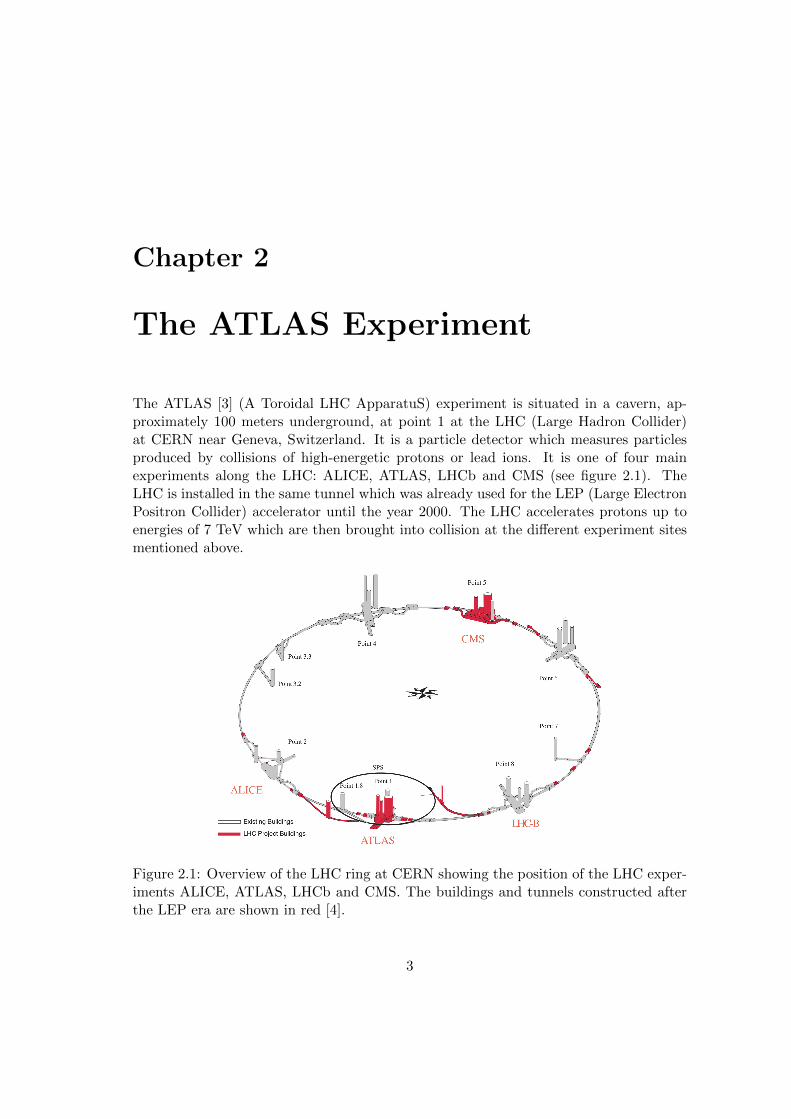
The ATLAS [3] (A Toroidal LHC ApparatuS) experiment is situated in a cavern, ap-proximately 100 meters underground, at point 1 at the LHC (Large Hadron Collider)at CERN near Geneva, Switzerland. It is a particle detector which measures particlesproduced by collisions of high-energetic protons or lead ions. It is one of four mainexperiments along the LHC: ALICE, ATLAS, LHCb and CMS (see figure 2.1). TheLHC is installed in the same tunnel which was already used for the LEP (Large ElectronPositron Collider) accelerator until the year 2000. The LHC accelerates protons up toenergies of 7 TeV which are then brought into collision at the different experiment sitesmentioned above.
Figure 2.1: Overview of the LHC ring at CERN showing the position of the LHC exper-iments ALICE, ATLAS, LHCb and CMS. The buildings and tunnels constructed afterthe LEP era are shown in red [4].
3
The ATLAS Experiment
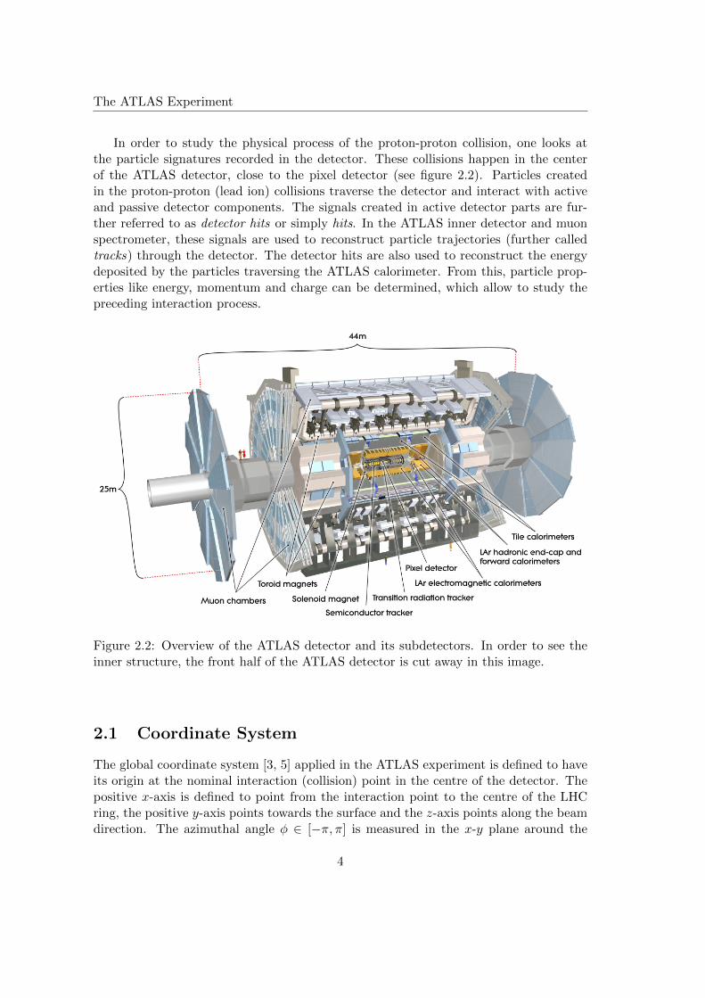
In order to study the physical process of the proton-proton collision, one looks atthe particle signatures recorded in the detector. These collisions happen in the centerof the ATLAS detector, close to the pixel detector (see figure 2.2). Particles createdin the proton-proton (lead ion) collisions traverse the detector and interact with activeand passive detector components. The signals created in active detector parts are fur-ther referred to as detector hits or simply hits. In the ATLAS inner detector and muonspectrometer, these signals are used to reconstruct particle trajectories (further calledtracks) through the detector. The detector hits are also used to reconstruct the energydeposited by the particles traversing the ATLAS calorimeter. From this, particle prop-erties like energy, momentum and charge can be determined, which allow to study thepreceding interaction process.
Figure 2.2: Overview of the ATLAS detector and its subdetectors. In order to see theinner structure, the front half of the ATLAS detector is cut away in this image.
2.1 Coordinate System
The global coordinate system [3, 5] applied in the ATLAS experiment is defined to haveits origin at the nominal interaction (collision) point in the centre of the detector. Thepositive x-axis is defined to point from the interaction point to the centre of the LHCring, the positive y-axis points towards the surface and the z-axis points along the beamdirection. The azimuthal angle φ ∈ [−π, π] is measured in the x-y plane around the
4
The ATLAS Experiment
beam axis, with the positive x-axis at φ = 0 and the positive y-axis at φ = π/2. Thepolar angle θ ∈ [0, π) is measured from the positive z-axis at θ = 0 to the negative z-axisat θ = π.
Pseudorapidity η is the rapidity [6] of a particle in the approximation that the par-ticle is massless:
η = − ln
[tan
(θ
2
)](2.1)
2.2 The Inner Detector
The inner detector (ID) is the innermost layer of the ATLAS experiment and thereforeclosest to the collision point. Thus particles created in collisions first pass through theID before they go through any other part of the ATLAS detector.
The main purpose of the ID is to track charged particles in order to estimate theirmomenta and production vertices. It consists of three subdetectors: a silicon PixelDetector, Semiconductor Tracker (SCT) using silicon strip technology and the TransitionRadiation Tracker (TRT), which implements a drift tube design.
The ID is embedded in a solenoidal magnetic field with a central strength of 2 Teslawhich bends the trajectories of charged particles. From this curvature the particle’scharge over momentum-component perpendicular to the magnetic field ratio q/pT canbe measured.
2.3 The Calorimeter
Particles origination at the interaction point enter the ATLAS calorimeter system, afterthey have passed the ID.
It’s main purpose is to measure particle energies. The calorimeter consists of twoparts, the (inner) electromagnetic calorimeter and the (outer) hadronic calorimeter. Inorder to measure particle energies, incident particles are tried to be stopped inside thecalorimeter. Therefore the incident particle is provoked to cause a particle shower (seesection 4.2), such that the energy deposited by the shower can be measured. In order todo so, the calorimeter is build of very heavy material (such as lead) which enhances thechance to confine most shower particles (shower energy). The deposited energy is usedin order to reconstruct the initial particle energy, which implies certain calibration cor-rections for the energy lost upstream the calorimeter and the fraction of energy actuallymeasured.
The electromagnetic calorimeter measures photon and electron energies, where thehadronic calorimeter measures hadron energies. Different particle types will cause dif-ferent showers shapes, which are used in order to do particle identification.
In general, muons do not interact much with the calorimeter material. Their interac-tion is mainly limited to multiple Coulomb scattering and ionization energy loss. Thus,
5
The ATLAS Experiment
muons (with energies above approximately 4 GeV) will likely pass the calorimeter andreach the next ATLAS sub-detector, the muon spectrometer.
2.4 The Muon Spectrometer or Muon System
The muon system (MS) is the outermost part of the ATLAS experiment. Like the AT-LAS ID it is a particle tracking device aimed to measure particle trajectories. Its namecomes from the fact that mostly muons will reach the MS to cause detector hits on sensi-tive detector parts. In an ideal case, other particle types should either be stopped in thecalorimeter (hadrons, electrons, photons) or do not create any signal in the MS (neutri-nos). However, calorimeter punch-through and decay in flight effects in the calorimeterdo have a significant impact on MS measurements (section 6).
Throughout the muon system a toroidal magnetic field is applied in order to measureeach particle’s charge over momentum ratio q/p. Combining this measurement with thecorresponding ID q/pT measurement, a higher accuracy on the overall q/pT is obtainedfor these particles.
2.5 Particle Signatures
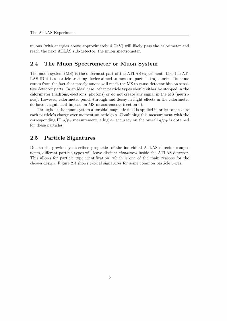
Due to the previously described properties of the individual ATLAS detector compo-nents, different particle types will leave distinct signatures inside the ATLAS detector.This allows for particle type identification, which is one of the main reasons for thechosen design. Figure 2.3 shows typical signatures for some common particle types.
6
The ATLAS Experiment
Figure 2.3: Particle signatures for different particle types when traversing the ATLASdetector. The shown particles originate at the interaction point and traverse the ATLASdetector in a radial direction. Charged particle trajectories are bent in the ID and MSdue to the magnetic fields present.
7

Chapter 3
Detector Simulation in ATLAS
In this chapter we discuss how the ATLAS collaboration handles (detector) simulationswhich is carried out in the software framework Athena. Section 3.1 discusses the typicalsimulation scheme in ATLAS. In section 3.2 two different simulation concepts are intro-duced: full and fast detector simulation. Both concepts find their use in the ATLAScollaboration. The concept of fast simulations is particularly important for this workdue to the fact that such a simulation is implemented and discussed in later chapters.Section 3.3 gives an overview of the Athena framework, which is used by the ATLAScollaboration for simulation-, digitization- and reconstruction and algorithms. Analy-sis algorithms may also use the Athena framework, but many examples of standaloneanalysis algorithms do exist.
3.1 Simulation Scheme
This section describes the different steps necessary for the generation of simulated eventdata. In order to compare simulated data with recorded data, a common data formatis required at a certain stage. For the ATLAS experiment, common data formats areused for the event reconstruction and all following steps. A brief introduction into theATLAS full simulation chain and how to set it up is given in [7]. Further details can befound in [8] and [9].
Figure 3.1 gives an overview of the standard full simulation chain used in ATLAS.It is a very detailed full Monte Carlo simulation, based on the Geant4 [11] toolkit (seesection 3.2.1). However, any other detector simulation (such as Fatras in section 3.2.2 orAtlfastII in section 3.2.3) also has to apply all points of this scheme. Even though somesteps might not use the standard ATLAS algorithms but might be treated internally ineither simulation.
The following paragraphs will discuss each simulation step:
Event Generation: The basis of each event simulation is a physics event generator.These event generators create data objects representing particles, which will later begiven as input to the detector simulation. The properties of these particles are based on
9
Detector Simulation in ATLAS
theoretical (and computational) models which are to be tested against data – such as thestandard model of particle physics or supersymmetry etc. Yet, due to the complexityof the physical processes occurring in proton proton collision, some event generatorsapply certain simplifications and must be tuned via a set of parameters. Thereforedifferent tunes may exist which will even evolve over time. Changing the settings of anevent generator usually leads to a re-run of this first step in the simulation chain whichconsequently leads to a re-run of all subsequent steps as well.
Event generators usually take over a set of input parameters, such as the centre ofmass energy of the initial colliding protons or other physical properties.
Event generators typically used in ATLAS are Pythia [12] and Herwig [13].
Detector Simulation: The next step in the simulation chain is the simulation of thedetector response to the particles created in the event generation. The fastest detec-tor simulations (such as e.g. Atlfast) use a parametric smearing to model the signala detector might give to a certain particle. However, in more complex simulation theparticles are transported through the detector and the detector response is then emu-lated. Thereby the simulation computes the paths the particles take while traversing thedetector. In order to do so any kind of interaction with the detector material or possibledecays of unstable particles are taken into account. In addition to that, the detectorsimulation computes and stores the particle hits on sensitive detector elements. Thesedetector hits will be stored in an output format known as simulation HITS (see section3.3.3).
The detector simulation usually ends when all particles are either stopped or left thedetector volume. In this case stopped means that a particle’s energy has dropped belowa certain threshold. Particles for which this is the case will not have a significant impactto the overall simulation, and therefore the simulation will not treat this particle anyfurther.
The most common detector simulation used by the ATLAS collaboration is based onGeant4 (see section 3.2.1), but also fast simulation approaches exist.
The implementation carried out in this work is a detector simulation module whichmay be plugged into any fast ATLAS detector simulation, that does not fully deploy theparticle showering in the calorimeter.
Digitization: After the detector simulation step, the simulation hits need to be trans-lated into a data format which corresponds to a format retrieved from the detector. Forthe simulation chain, this translation is carried out by the digitization. Digitized simu-lation data correspond to bytestream converted data retrieved from the detector. Thedigitization aims to transform the primary interaction of a particle with the sensitivedetector material into measurable quantities, such as the charge drifted to the readoutmodules in tracking detectors or the energy measured in photomultipliers as present indetector setups. The digitization output format is RDO (RAW Data Objects, see section3.3.3) which is the exact same data format used to record detector measurements afterbytestream conversion. Therefore all further steps are non-simulation-specific and need
10
Detector Simulation in ATLAS
to be carried out for recorded events as well.Besides creating realistic detector output signals, the digitization is responsible for
describing event pile-up1 correctly. It does so by overlaying detector simulations ofdifferent events and merging them into one common RDO output for a single event.
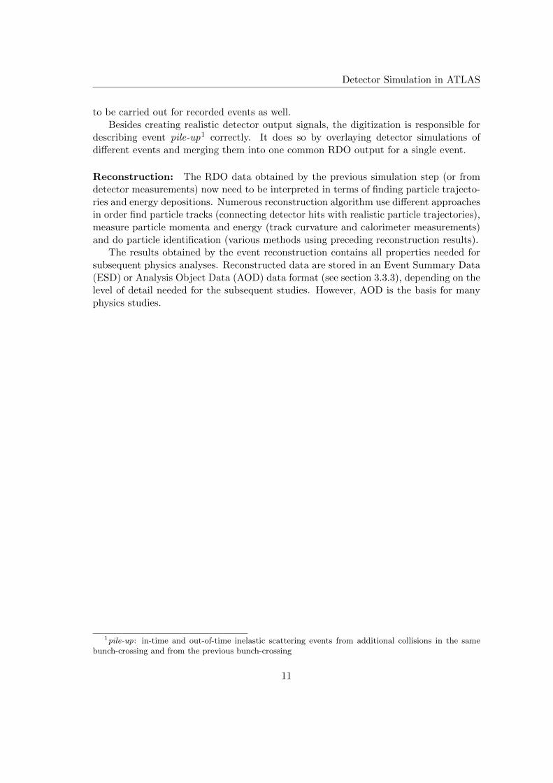
Reconstruction: The RDO data obtained by the previous simulation step (or fromdetector measurements) now need to be interpreted in terms of finding particle trajecto-ries and energy depositions. Numerous reconstruction algorithm use different approachesin order find particle tracks (connecting detector hits with realistic particle trajectories),measure particle momenta and energy (track curvature and calorimeter measurements)and do particle identification (various methods using preceding reconstruction results).
The results obtained by the event reconstruction contains all properties needed forsubsequent physics analyses. Reconstructed data are stored in an Event Summary Data(ESD) or Analysis Object Data (AOD) data format (see section 3.3.3), depending on thelevel of detail needed for the subsequent studies. However, AOD is the basis for manyphysics studies.
1pile-up: in-time and out-of-time inelastic scattering events from additional collisions in the samebunch-crossing and from the previous bunch-crossing
11
Detector Simulation in ATLAS
Generation
HepMC
Simulation
G4 Hits
Digitization
G4 Digits
Reconstruction
Create AOD
ESD
AOD
Analysis
Atlfast
Data
(a) (b)
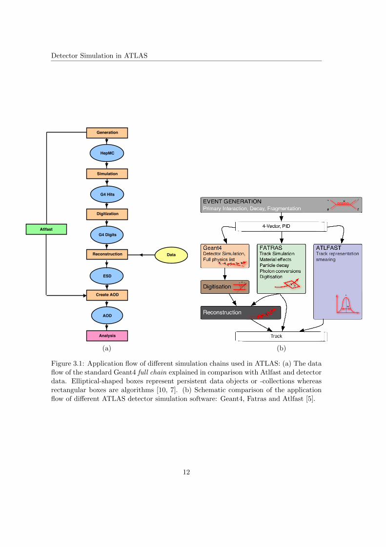
Figure 3.1: Application flow of different simulation chains used in ATLAS: (a) The dataflow of the standard Geant4 full chain explained in comparison with Atlfast and detectordata. Elliptical-shaped boxes represent persistent data objects or -collections whereasrectangular boxes are algorithms [10, 7]. (b) Schematic comparison of the applicationflow of different ATLAS detector simulation software: Geant4, Fatras and Atlfast [5].
12
Detector Simulation in ATLAS
3.2 Full and Fast Detector Simulation
Figure 3.1 (b) compares the application flow of three different detector simulations usedin ATLAS: Geant4, Fatras and Atlfast. Geant4 is the the main (most detailed) detectorsimulation utilised by the ATLAS collaboration. Fatras serves as an alternative fastdetector simulation for the ATLAS inner detector and muon spectrometer, and Atlfastwas mainly used during the design phase of the ATLAS detector as an ultra fast detectorsimulation. AtlfastII is a new fast simulation approach combining Geant4 with the fastcalorimeter simulation FastCaloSim. Geant4, Fatras and AtlfastII will be discussed inthe following sections.
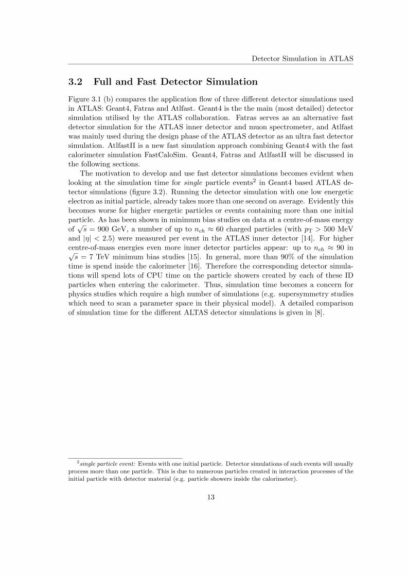
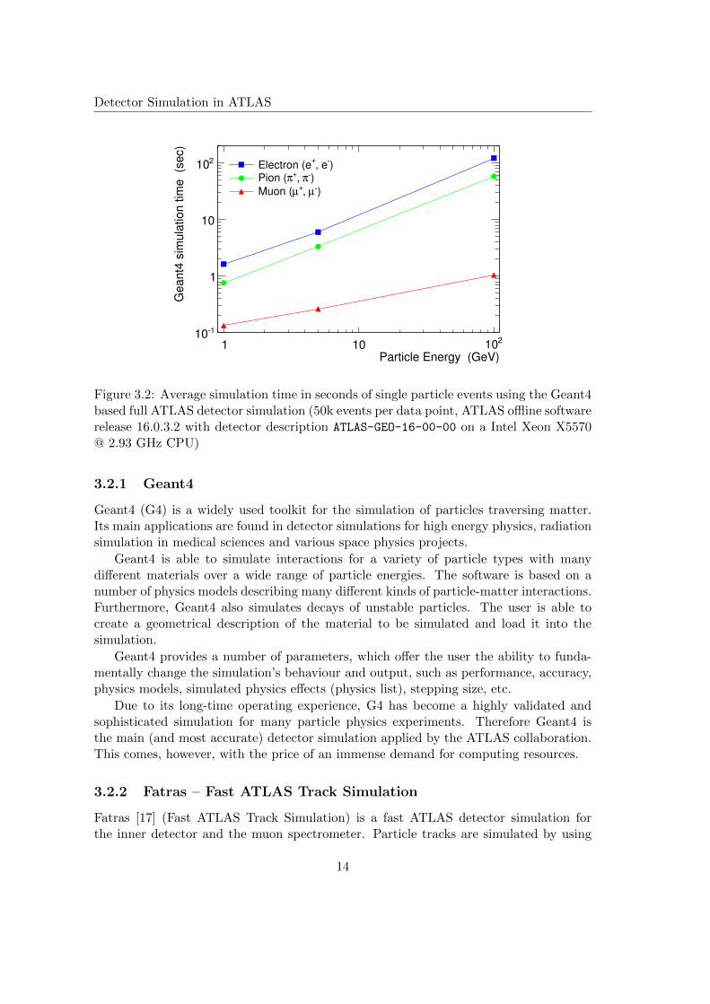
The motivation to develop and use fast detector simulations becomes evident whenlooking at the simulation time for single particle events2 in Geant4 based ATLAS de-tector simulations (figure 3.2). Running the detector simulation with one low energeticelectron as initial particle, already takes more than one second on average. Evidently thisbecomes worse for higher energetic particles or events containing more than one initialparticle. As has been shown in minimum bias studies on data at a centre-of-mass energyof√s = 900 GeV, a number of up to nch ≈ 60 charged particles (with pT > 500 MeV
and |η| < 2.5) were measured per event in the ATLAS inner detector [14]. For highercentre-of-mass energies even more inner detector particles appear: up to nch ≈ 90 in√s = 7 TeV minimum bias studies [15]. In general, more than 90% of the simulation
time is spend inside the calorimeter [16]. Therefore the corresponding detector simula-tions will spend lots of CPU time on the particle showers created by each of these IDparticles when entering the calorimeter. Thus, simulation time becomes a concern forphysics studies which require a high number of simulations (e.g. supersymmetry studieswhich need to scan a parameter space in their physical model). A detailed comparisonof simulation time for the different ALTAS detector simulations is given in [8].
2single particle event: Events with one initial particle. Detector simulations of such events will usuallyprocess more than one particle. This is due to numerous particles created in interaction processes of theinitial particle with detector material (e.g. particle showers inside the calorimeter).
13
Detector Simulation in ATLAS
Particle Energy (GeV)1 10
210
Geant4
sim
ula
tion tim
e (s
ec)
110
1
10
210 )
, e+
Electron (e)π, +
πPion (
)µ, +µMuon (
Figure 3.2: Average simulation time in seconds of single particle events using the Geant4based full ATLAS detector simulation (50k events per data point, ATLAS offline softwarerelease 16.0.3.2 with detector description ATLAS-GEO-16-00-00 on a Intel Xeon X5570@ 2.93 GHz CPU)
3.2.1 Geant4
Geant4 (G4) is a widely used toolkit for the simulation of particles traversing matter.Its main applications are found in detector simulations for high energy physics, radiationsimulation in medical sciences and various space physics projects.
Geant4 is able to simulate interactions for a variety of particle types with manydifferent materials over a wide range of particle energies. The software is based on anumber of physics models describing many different kinds of particle-matter interactions.Furthermore, Geant4 also simulates decays of unstable particles. The user is able tocreate a geometrical description of the material to be simulated and load it into thesimulation.
Geant4 provides a number of parameters, which offer the user the ability to funda-mentally change the simulation’s behaviour and output, such as performance, accuracy,physics models, simulated physics effects (physics list), stepping size, etc.
Due to its long-time operating experience, G4 has become a highly validated andsophisticated simulation for many particle physics experiments. Therefore Geant4 isthe main (and most accurate) detector simulation applied by the ATLAS collaboration.This comes, however, with the price of an immense demand for computing resources.
3.2.2 Fatras – Fast ATLAS Track Simulation
Fatras [17] (Fast ATLAS Track Simulation) is a fast ATLAS detector simulation forthe inner detector and the muon spectrometer. Particle tracks are simulated by using
14
Detector Simulation in ATLAS
standard ATLAS reconstruction tools based on the so-called reconstruction geometry[18], which is a simplified detector description. Contrary to the detailed descriptionof the detector material applied in Geant4, the reconstruction geometry describes theATLAS detector material by a few thin and discrete layers of different materials (seefigure 3.3). The layers are arranged in order to reproduce the overall material effectsof the detector on the traversing particles. In addition, Fatras uses averaged materialswhich do not necessarily correspond to any real material built into the detector.
Fatras gains up to a factor of 100 in simulation time, in comparison to Geant4 baseddetector simulations.
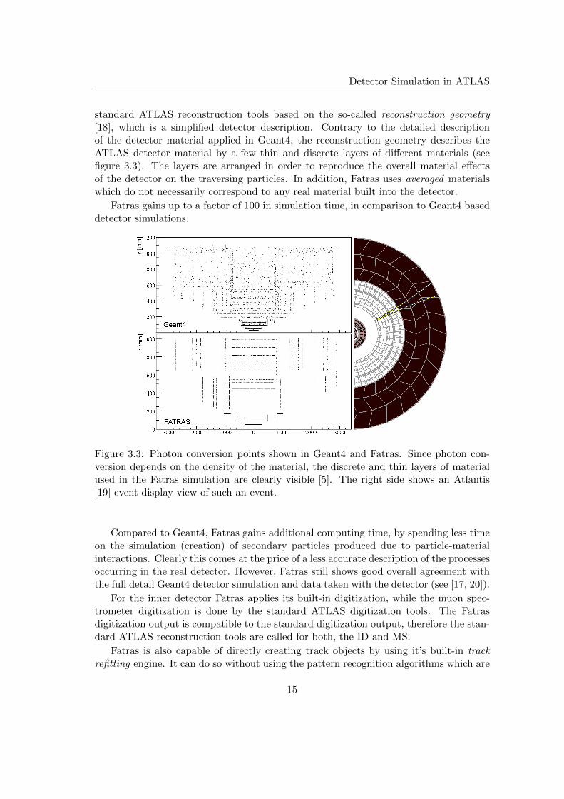
Figure 3.3: Photon conversion points shown in Geant4 and Fatras. Since photon con-version depends on the density of the material, the discrete and thin layers of materialused in the Fatras simulation are clearly visible [5]. The right side shows an Atlantis[19] event display view of such an event.
Compared to Geant4, Fatras gains additional computing time, by spending less timeon the simulation (creation) of secondary particles produced due to particle-materialinteractions. Clearly this comes at the price of a less accurate description of the processesoccurring in the real detector. However, Fatras still shows good overall agreement withthe full detail Geant4 detector simulation and data taken with the detector (see [17, 20]).
For the inner detector Fatras applies its built-in digitization, while the muon spec-trometer digitization is done by the standard ATLAS digitization tools. The Fatrasdigitization output is compatible to the standard digitization output, therefore the stan-dard ATLAS reconstruction tools are called for both, the ID and MS.
Fatras is also capable of directly creating track objects by using it’s built-in trackrefitting engine. It can do so without using the pattern recognition algorithms which are
15
Detector Simulation in ATLAS
part of the standard reconstruction package. When track refitting is enabled, one canstudy the effects of the pattern recognition algorithms on the resulting track objects.
3.2.3 AtlfastII
AtlfastII is a fast ATLAS detector simulation using the FastCaloSim [21] ATLAS calorime-ter simulation. For the ATLAS inner detector and muon spectrometer, the Geant4 sim-ulation is used. This setup results in a simulation ten times faster than the full Geant4simulation of the whole ATLAS detector [8].
As for the full Geant4 detector simulation, the input particles from the event gener-ator are used as input for the subsequent Geant4 inner detector simulation. Each par-ticle leaving the ID volume is checked for its particle type and only muons are furtherprocessed by the Geant4 simulation of the calorimeter. All particles above threshold,however, are handled by the FastCaloSim module, which does not perform a particletransport. Therefore muons are the only particles able to enter the ATLAS muon sys-tem in the AtlfastII simulation. Consequently, internal processes in the calorimeter, suchas decays and punch-through are not simulated in AtlfastII.
Due to the use of Geant4 simulations in the ID and MS, the standard ATLAS recon-struction tools can be used in order to reconstruct particle information from AtlfastIIsimulated detector hits in the ID and MS. Moreover, the FastCaloSim output is compat-ible to Geant4 calorimeter simulation output. Therefore the calorimeter reconstructioncan be done by the standard ATLAS tools as well.
AtlfastIIF applies Fatras for the inner detector and the muon spectrometer insteadof Geant4 as in AtlfastII. By doing so, a factor of up to 100 in speed is gained comparedto the Geant4 full detector simulation.
3.3 The Athena Framework
The Athena framework [9, 22] is widely used by the ATLAS collaboration for most of itscomputing work. Athena is based on the Gaudi framework which was initially developedby the LHCb collaboration. In the ATLAS experiment it is the common frameworkwhich is used for Monte Carlo simulations, data processing and physics analysis of eithersimulated or recorded data.
User implemented C++ class(es) can be integrated into the Athena framework,within which these classes will have access to given input and output event contain-ers. Athena manages event by event data preparation and it takes care of input andoutput file handling.
The setup of any Athena run is done via a Python jobOptions script (sometimesreferred to as jO scripts). This script is handed over as parameter to the athena shellcommand when starting an Athena run. This allows the user to fundamentally changethe behaviour of any Athena run, by changing the settings inside the jobOptions. Withinthis script, one has the possibility to:
• choose which input dataset to read and which output dataset to write
16
Detector Simulation in ATLAS
• choose which C++ (or Python) algorithms should run
• setting and changing (optional) parameters for these algorithms
3.3.1 Athena Application Flow
In order to use C++ libraries within Athena, one has to implement the source codeinto one or many of the fundamentally different components given by the framework.A complete list of all components is given in [9]. The most relevant components in thecontext of this work are: Algorithms, Tools and Services. Any user algorithm can beimplemented in either of these categories. Figure 3.4 explains the runtime relevance andthe difference between Athena algorithms and Athena tools.
Athena algorithms, tools and services can be implemented either by the ATLASsoftware developers, as a part of the official ATLAS software package, or any user whowants to study certain properties of one or more – simulated or recorded – datasets.
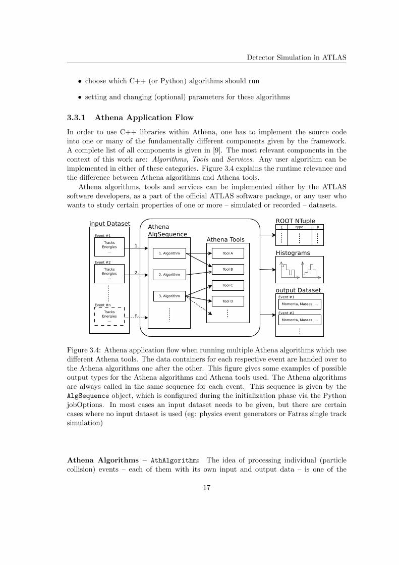
Figure 3.4: Athena application flow when running multiple Athena algorithms which usedifferent Athena tools. The data containers for each respective event are handed over tothe Athena algorithms one after the other. This figure gives some examples of possibleoutput types for the Athena algorithms and Athena tools used. The Athena algorithmsare always called in the same sequence for each event. This sequence is given by theAlgSequence object, which is configured during the initialization phase via the PythonjobOptions. In most cases an input dataset needs to be given, but there are certaincases where no input dataset is used (eg: physics event generators or Fatras single tracksimulation)
Athena Algorithms – AthAlgorithm: The idea of processing individual (particlecollision) events – each of them with its own input and output data – is one of the
17
Detector Simulation in ATLAS
design principles of Athena. In order to do so, the framework runs in sequence throughthe events in a certain input dataset and processes them one by one by calling differentC++ Athena algorithms on them. An Athena algorithm is a C++ class which inheritsfrom the Athena AthAlgorithm class. While processing an event this algorithm onlyhas access to the data relevant to this currently processed event. This carries out theidea of having data which come from independent collision events and study them oneby one. After reading the input data to process the current event the Athena algorithmsare run in a specified order, which is set by the AlgSequence object in the jobOptions
file. Each of the Athena algorithms specified in this sequence is run only once per event.
Athena Algorithm Tools – AthAlgTool: The previously described Athena algo-rithms may use some common computations or apply some common tasks which willnot be implemented in each of the algorithms separately, but only once in correspondingAthena algorithm tools. Athena algorithm tools are C++ classes which inherit from theAthena AthAlgTool class. These tools can be used by different Athena algorithms withdifferent in- and outputs. Other than the Athena algorithms, Athena tools can be calledmultiple times per event, but they are not necessarily executed in a pre-defined sequence.
Athena Algorithm Services – AthService: The Athena services are somewhatsimilar to the Athena tools, in the sense that they can be run multiple times within asingle event. But other than Athena tools, services usually provide more general tasks.Therefore the same service might be used by many – or even all – Athena algorithmsand Athena tools. Examples for Athena services are the message reporting service orrandom number generators. Athena services can be implemented by inheriting from theAthService C++ class provided by Athena.
3.3.2 StoreGate
StoreGate (SG) is the central Athena service responsible for handling any kind of tran-sient data object needed by one or many Athena algorithms, tools or services. A detaileddescription of StoreGate can be found in [23]. Here only the most important features ofStoreGate are discussed:
• it takes care of the memory management for any data object registered to it. Thisimplies, for example memory deallocation in case a data object is not needed anymore in its transient form.
• it manages the conversion from transient data to persistent data
• the user can access any data object in memory via a built-in dictionary
• nearly any user data type can be managed by StoreGate
Typical objects managed by StoreGate are, for example, TrackCollections containing allreconstructed particle tracks, or hits of sensitive detector elements (simulated or recordedones).
18
Detector Simulation in ATLAS
3.3.3 Data Formats
A number of persistent data formats are used in the Athena framework, to store particleand detector information at different stages. In order to allow the use of these dataformats on the LHC Computing Grid (LCG), a POOL layer is implemented within eachof the formats described in this section. Further information about the POOL layer canbe found in [9]. The following list only gives the most relevant data formats for this work.More derived formats are also used by the collaboration, but mainly for physics focusedanalysis, whereas in this work the focus lies on detector simulation and its validation.
Simulation HITS: This data format contains hit information of sensitive detectorelements in simulated events. It is the output format of the Geant4 detector simulation(see section 3.2.1). This format is purely simulation based, therefore no counterpart inthe data stream from the real detector exists.
RAW Data Objects (RDO): RAW data objects contain voltage or current mea-surements of sensitive detector parts for each recorded (or simulated) event. The RDOformat does not offer any particle information or physical interpretation of these detectormeasurements. The output of the detector itself is in RDO format. But RDOs mightalso be generated by any detector simulation, after the digitization step (see section 3.1).
Event Summary Data (ESD): Is the output format after running the standardreconstruction algorithms (see section 3.1) on the ATLAS inner detector, calorimeterand muon spectrometer. The (simulated or recorded) detector hits from the previousstep are converted into physical objects, like particle tracks or jets.
Analysis Object Data (AOD): AOD is a data format derived from ESD which iscommonly used for physics analysis. Therefore AODs contain mostly physical objects.Other than the ESDs, AODs usually do not contain detailed information about thereconstruction step.
19

Chapter 4
Calorimeter Punch-Through –Leakage into the MuonSpectrometer
This chapter starts by defining the main concern of this work, the calorimeter punch-through or particle leakage in section 4.1. Next, the basic physical processes and conceptsoccurring inside the ATLAS calorimeter are described in section 4.2. Based on this,Geant4 studies were conducted and their results are described in section 4.3. Due tothe high number of – partly very complex – processes involved in particle showers insidethe calorimeter, a parametrized approach for a fast calorimeter punch-through has beenfavored to simplified models, when trying to optimize for CPU performance. Section 4.4describes such a parametrization model and finally the simulation applying this modelis described in section 4.5.
4.1 Calorimeter Punch-Through
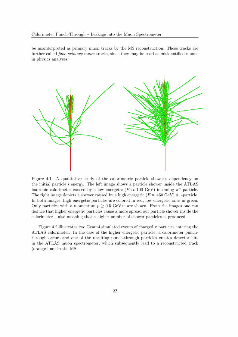
The ATLAS calorimeter is built as a hermetic, confining detector (see sections 2.3 and2.4). Muons should be the only particle type to reach the muon spectrometer and causedetector hits there. Particles entering the calorimeter, will cause a particle shower insidethe calorimeter. The shape of this shower and the shower-particle properties in generalstrongly depend on properties of the initial particle (see figure 4.1 for a qualitativeillustration of the energy dependency). Some shower shapes are more elongated (forexample for higher energetic initial particles), which enhances the chance of a showerparticle to exit the calorimeter and enter the ATLAS muon spectrometer. Such anevent is called calorimeter punch-through or particle leakage into the muon spectrometerand the particles entering the MS are called punch-through particles. Depending on theproperties of the punch-through particle (particle type, energy, charge, position), theeffect to the muon spectrometer will vary significantly: from having no effect in creatingclean particle track signatures, to full tracks which will be reconstructed and by chance
21
Calorimeter Punch-Through – Leakage into the Muon Spectrometer
be misinterpreted as primary muon tracks by the MS reconstruction. These tracks arefurther called fake primary muon tracks, since they may be used as misidentified muonsin physics analyses.
Figure 4.1: A qualitative study of the calorimetric particle shower’s dependency onthe initial particle’s energy. The left image shows a particle shower inside the ATLAShadronic calorimeter caused by a low energetic (E ≈ 100 GeV) incoming π−-particle.The right image depicts a shower caused by a high energetic (E ≈ 450 GeV) π−-particle.In both images, high energetic particles are colored in red, low energetic ones in green.Only particles with a momentum p ≥ 0.5 GeV/c are shown. From the images one candeduce that higher energetic particles cause a more spread out particle shower inside thecalorimeter – also meaning that a higher number of shower particles is produced.
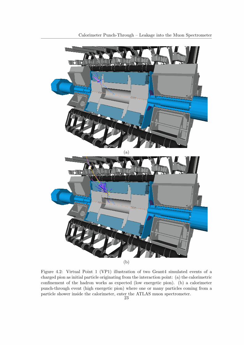
Figure 4.2 illustrates two Geant4 simulated events of charged π particles entering theATLAS calorimeter. In the case of the higher energetic particle, a calorimeter punch-through occurs and one of the resulting punch-through particles creates detector hitsin the ATLAS muon spectrometer, which subsequently lead to a reconstructed track(orange line) in the MS.
22
Calorimeter Punch-Through – Leakage into the Muon Spectrometer
(a)
(b)
Figure 4.2: Virtual Point 1 (VP1) illustration of two Geant4 simulated events of acharged pion as initial particle originating from the interaction point: (a) the calorimetricconfinement of the hadron works as expected (low energetic pion). (b) a calorimeterpunch-through event (high energetic pion) where one or many particles coming from aparticle shower inside the calorimeter, enter the ATLAS muon spectrometer.
23
Calorimeter Punch-Through – Leakage into the Muon Spectrometer
4.2 Processes in the ATLAS Calorimeter
In section 2.3 a brief overview of the ATLAS calorimeter was given. This section describesthe most frequent electromagnetic and hadronic processes occurring inside a calorimeter.A more extensive view can be found in [24].
Due to particle showers caused by incident particles in dense material, the particleenergy is absorbed in a much shorter distance than in a case where no shower develops.Hence, calorimeters provoke shower development in order to confine and measure incidentparticle energies.
The following subsections discuss the two fundamentally different shower types: elec-tromagnetic and hadronic. The somewhat special role of muons traversing dense materialis discussed in section 4.2.2.
4.2.1 Electromagnetic Showers
The processes involved in the development and evolution of electromagnetic showers arerather clear and much easier to describe than those in hadronic showers. Electromagneticshowers are caused by charged particles or photons in dense material.
Low energetic photons will most likely undergo the photoelectric effect, in whichone bound electron becomes unbound from its atom and the photon is absorbed. Rayleighscattering deviates photon trajectories through material, without them losing any oftheir energy. In Compton scattering effects, photons lose part of their energy, theirtrajectory gets deviated and one electron is transferred from a bound state into an un-bound state. Photons with a high enough energy have the chance to undergo electron-positron pair production in the coulomb fields present in the vicinity of nuclei in thedense material. This process transfers the whole photon energy into the electron and thepositron. Photonuclear reactions become relevant to high energetic photons. However,they play a minor role compared to all other photon interaction processes. Anyhow, nu-cleons may be freed due to such reactions. In most of these photon interaction processes,at least one charged particle (mostly electron and/or positron) is created. Therefore,charged particle interaction processes need to be understood.
Due to electromagnetic interactions, charged particles may interact in many differ-ent ways with dense material when traversing it. Ionization of the material along theparticle’s trajectory already occurs at very low energies. Also atomic or molecular exci-tation may occur. The photons emitted during de-excitation will subsequently undergoany of the photon processes mentioned above. Cherenkov light will be emitted bycharged particles, in case they traverse a medium with a speed greater than the speed oflight in that medium. At sufficiently high energies, charged particles may lose energy byknocking out high energetic electrons (δ-rays) of the material structure they traverse.High energetic particles with a low mass (such as electrons and positrons) may lose asignificant amount of their energy due to bremsstrahlung. Nuclear interactions mayoccur at very high energies. Most of these processes will result in the production of oneor many daughter particles, such as photons, electrons or nuclear particles.
There is one fundamental difference between the processes involved in energy loss of
24
Calorimeter Punch-Through – Leakage into the Muon Spectrometer
electrons and photons. Whereas electrons lose their energy in a continuous stream ofevents (e.g. bremsstrahlung), photons may traverse a certain amount of material withoutlosing any energy before one interaction consumes the photon (e.g. pair production).
In electromagnetic showers, one primary particle (such as photon or electron) causesa cascade of the effects mentioned above, in which a large number of particles mightbe involved. Until a certain shower depth, particle multiplication outweighs particleconsumption. However, due to the energy deposited in the material, the average showerparticle energy decreases with the shower depth. Thus after the shower maximum, thetotal number of particles involved in the shower decreases. Typical for em-showers isthat mostly photons and electrons (positrons) are involved in the particle cascade. Forexample an electron created (freed) during the shower development, might create one ormany photons (e.g. bremsstrahlung), which will again free other electrons, etc. Someof the shower particles may leave the dense material, which is known as calorimeterpunch-through (or leakage) as defined in the previous section 4.1.
In the ATLAS calorimeter, the deposited energy is measured with the free ionizationelectrons and the light emitted from scintillator material inside the calorimeter.
4.2.2 Muons Traversing Dense Material
Due to their charge, the processes occurring when muons traverse matter are the sameas mentioned above for electrons and charged particles in general. However, due to thehigh muon mass, energy loss due to bremsstrahlung is highly suppressed compared toelectrons. Thus, muons mainly undergo ionization loss and multiple scattering processeswhen traversing matter. Therefore it takes a much greater amount of dense material, inorder to absorb a muon compared to an electron.
This is the reason for the ATLAS muon spectrometer surrounding the (dense) calorime-ter and still being able to detect muon particle tracks in the MS.
Due to the properties mentioned above, muons are often referred to as minimumionizing particles (MIP).
4.2.3 Hadronic Showers
When high energetic charged hadrons traverse dense material, they will behave at afirst glance similarly to muons with the same energy with regard to the electromagneticprocesses occurring – i.e. they will continuously lose energy. However, with a certainprobability the hadron will strike a nucleus and numerous nuclear and strong interactionprocesses will take place. For neutral hadrons, this is the only way to lose their energy.Many of these nuclear processes will result in additional shower particles created dueto such an event. Such shower particles could be neutrons or protons freed from thehit nucleus, mesons created due to strong interaction and high energy photons due tode-excitation of excited nuclei. Some of these mesons may decay electromagnetically,such as π0, η → γγ. Charged particles and photons will interact electromagneticallyin the way described in the previous section 4.2.1. Therefore a certain fraction of theinitial hadron’s energy is deposited in electromagnetic showers. Some mesons may decay
25
Calorimeter Punch-Through – Leakage into the Muon Spectrometer
into muons (decay in flight), which is a source of energy leaking from a calorimeter,since muons only interact very weakly with matter. The shower hadrons will interactwith other nuclei in the material. Therefore – as for electromagnetic showers – particlemultiplication takes place until a certain shower depth. Beyond this depth, the averageenergy of the shower particles is too low to cause further shower particle multiplication.
For example, a particle shower caused by a 100 GeV pion in lead has ∼ 55% of itsenergy in the electromagnetic component and the rest in the hadronic shower component[24].
26
Calorimeter Punch-Through – Leakage into the Muon Spectrometer
4.3 Geant4 Analysis
In order to implement a fast simulation of particles leaking into the ATLAS muon spec-trometer, a detailed study of this very effect was carried out using Geant4 (section 3.2.1)simulated single particle events. Boundary surfaces (CaloEntryLayer and MuonEntry-Layer, see appendix B) are used to define the points where a particle enters and exitsthe calorimeter, respectively. The following parametrization is therefore based on thedefinition of these layers. As soon as a particle traverses either of these surface layersduring a Geant4 simulation, it’s current properties are recorded in a so-called Track-
RecordCollection object (named either CaloEntryLayer or MuonEntryLayer) via theAthena StoreGate ([23] and section 3.3.2) service. All studies described in this- and thefollowing sections only use entries in these two TrackRecordCollections in order toanalyse properties of punch-through particles.
4.3.1 Simulation Setup and Event Selection
A sample of ∼ 3 ·106 single pion events were simulated to perform these studies: π+ andπ− particles in equal numbers, all originating at the interaction point. These particlesare simulated with a flat distribution in pseudorapidity η between −2.7 and +2.7. Thisrange is motivated by the pseudorapidity coverage of the ATLAS muon spectrometer for|η| ≤ 2.7 [3]. The initial energy is distributed uniformly between 150 and 500 GeV. Thefocus of this study lies on calorimeter and muon system effects and interactions, thereforeinteractions with any inner detector part (active and passive) were not simulated – inorder to save computing time and disk space. If not stated differently, this event samplewas used for all further studies and parametrizations.
The Geant4 simulations use ATLAS software release 15.6.12.7 with detector descrip-tion tag ATLAS-GEO-16-00-00.
After simulation, an Athena analysis algorithm was run on the HITS pool files (whichwere created in the last step) to gain information about punch-through particles and theirproperties. Two definitions are required to understand the following analysis (see figure4.3 for a visual illustration of these definitions):
Initial Particle is a π+ or π− particle appearing in the CaloEntryLayer TrackRecord-Collection with the same barcode1 as the one particle put into the Geant4 simulationat the interaction point. Additionally the initial particle has to point outwards (towardsthe calorimeter). Due to technical constraints in the ATLAS Geant4 simulation frame-work, the beam pipe simulation volume of the beam pipe can not be switched off. Incase the starting pion interacts with the beam pipe, it will most likely not arrive atthe CaloEntry layer and therefore such events are filtered out. If no interaction takesplace, the particle gets transported to the CaloEntryLayer without simulating any in-teractions with the ATLAS inner detector material. In all following studies, only eventswith exactly one initial particle are studied.
1unique number to identify individual particles within one simulated event
27
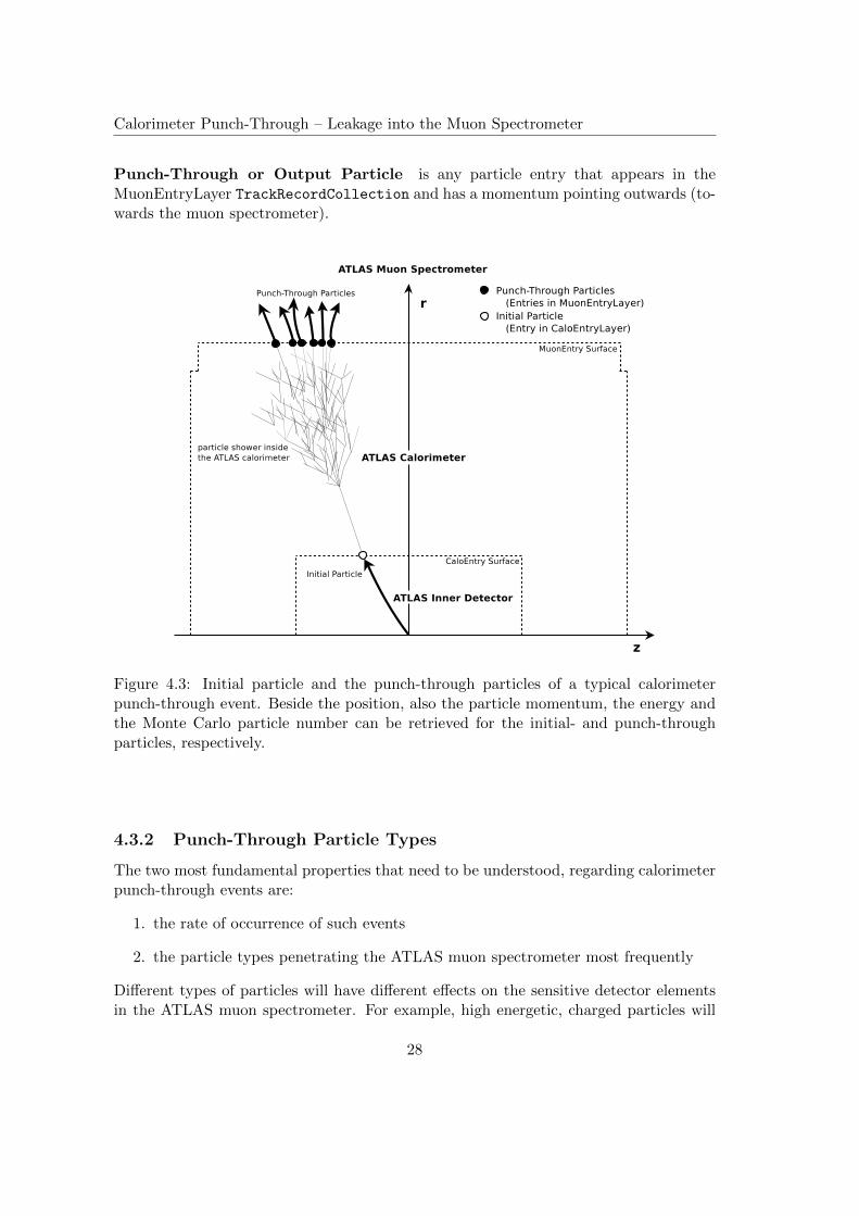
Calorimeter Punch-Through – Leakage into the Muon Spectrometer
Punch-Through or Output Particle is any particle entry that appears in theMuonEntryLayer TrackRecordCollection and has a momentum pointing outwards (to-wards the muon spectrometer).
Figure 4.3: Initial particle and the punch-through particles of a typical calorimeterpunch-through event. Beside the position, also the particle momentum, the energy andthe Monte Carlo particle number can be retrieved for the initial- and punch-throughparticles, respectively.
4.3.2 Punch-Through Particle Types
The two most fundamental properties that need to be understood, regarding calorimeterpunch-through events are:
1. the rate of occurrence of such events
2. the particle types penetrating the ATLAS muon spectrometer most frequently
Different types of particles will have different effects on the sensitive detector elementsin the ATLAS muon spectrometer. For example, high energetic, charged particles will
28
Calorimeter Punch-Through – Leakage into the Muon Spectrometer
penetrate far into the MS and cause detector hits on their way through the MS. Alsoparticle showers inside the MS can be caused by any high energetic particle. Due to theirlack of charge, photons for example will not directly cause detector hits inside the MS,but they can undergo photon conversion, where electrons and positrons will be produced(see section 4.2).
Monte Carlo Particle Number
-3000 -2000 -1000 0 1000 2000 3000
Entries
1
10
210
310
410
510
610
710 Neutrons
Protons
Photons
π+
π-
KK KL
0
eμ
e
μ
+
+
-
-
+
-
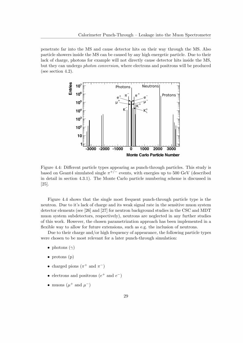
Figure 4.4: Different particle types appearing as punch-through particles. This study isbased on Geant4 simulated single π+/− events, with energies up to 500 GeV (describedin detail in section 4.3.1). The Monte Carlo particle numbering scheme is discussed in[25].
Figure 4.4 shows that the single most frequent punch-through particle type is theneutron. Due to it’s lack of charge and its weak signal rate in the sensitive muon systemdetector elements (see [26] and [27] for neutron background studies in the CSC and MDTmuon system subdetectors, respectively), neutrons are neglected in any further studiesof this work. However, the chosen parametrization approach has been implemented in aflexible way to allow for future extensions, such as e.g. the inclusion of neutrons.
Due to their charge and/or high frequency of appearance, the following particle typeswere chosen to be most relevant for a later punch-through simulation:
• photons (γ)
• protons (p)
• charged pions (π+ and π−)
• electrons and positrons (e+ and e−)
• muons (µ+ and µ−)
29
Calorimeter Punch-Through – Leakage into the Muon Spectrometer
As previously described, the photon is included in the list above due to the fact thatthere is a chance for it to undergo photon conversion inside the muon spectrometer.Each conversion would produce an electron/positron pair which would subsequentlycreate signals in sensitive detector elements.
In addition, figure 4.4 suggests that for electrons, pions and muons, the correspondingmatter like and antimatter like particle types appear at the same rate. Therefore, furtherstudies (and parametrizations) consider cumulative effects of matter like and antimatterlike particles for either of these particle types.
A minimum energy of 50 MeV is required for any particle to be considered a relevantpunch-through particle. Particles with an energy below this threshold are ignored in anyfurther study or parametrization.
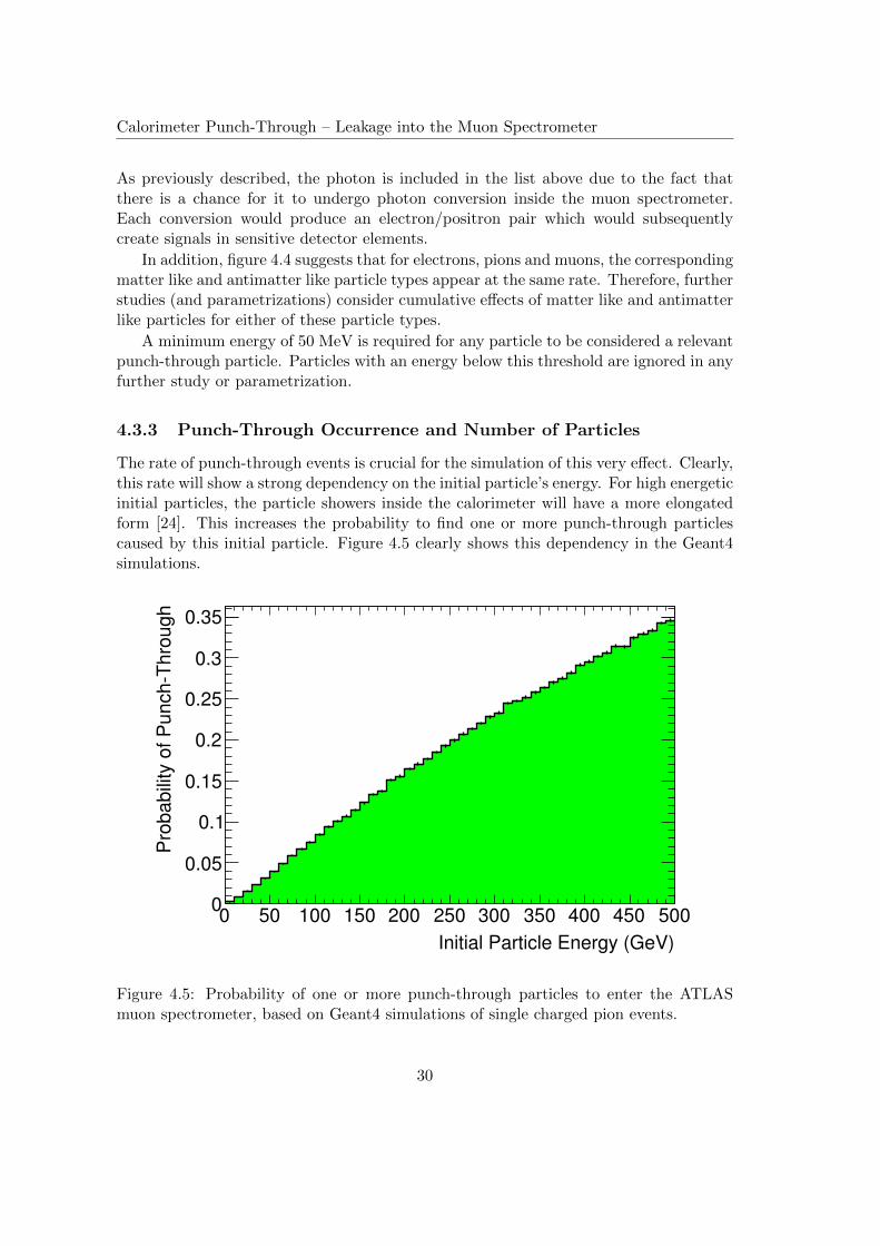
4.3.3 Punch-Through Occurrence and Number of Particles
The rate of punch-through events is crucial for the simulation of this very effect. Clearly,this rate will show a strong dependency on the initial particle’s energy. For high energeticinitial particles, the particle showers inside the calorimeter will have a more elongatedform [24]. This increases the probability to find one or more punch-through particlescaused by this initial particle. Figure 4.5 clearly shows this dependency in the Geant4simulations.
Initial Particle Energy (GeV)
0 50 100 150 200 250 300 350 400 450 500
Pro
ba
bili
ty o
f P
un
ch
Th
rou
gh
0
0.05
0.1
0.15
0.2
0.25
0.3
0.35
Figure 4.5: Probability of one or more punch-through particles to enter the ATLASmuon spectrometer, based on Geant4 simulations of single charged pion events.
30
Calorimeter Punch-Through – Leakage into the Muon Spectrometer
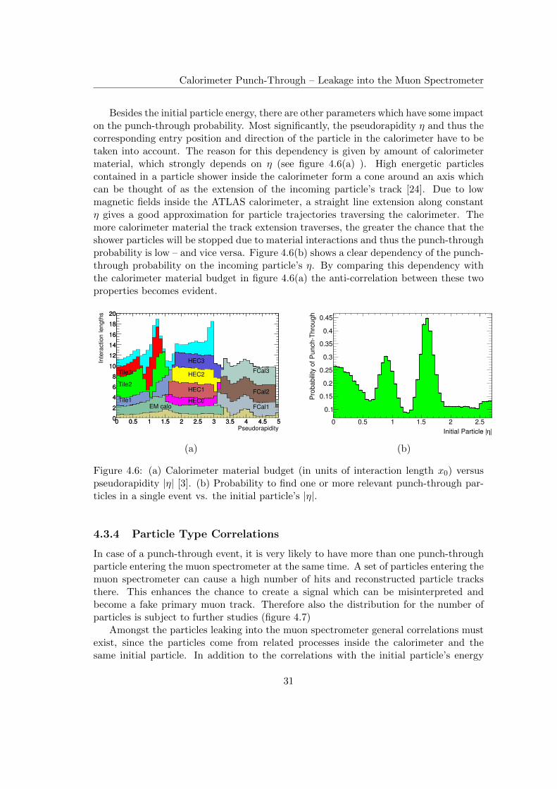
Besides the initial particle energy, there are other parameters which have some impacton the punch-through probability. Most significantly, the pseudorapidity η and thus thecorresponding entry position and direction of the particle in the calorimeter have to betaken into account. The reason for this dependency is given by amount of calorimetermaterial, which strongly depends on η (see figure 4.6(a) ). High energetic particlescontained in a particle shower inside the calorimeter form a cone around an axis whichcan be thought of as the extension of the incoming particle’s track [24]. Due to lowmagnetic fields inside the ATLAS calorimeter, a straight line extension along constantη gives a good approximation for particle trajectories traversing the calorimeter. Themore calorimeter material the track extension traverses, the greater the chance that theshower particles will be stopped due to material interactions and thus the punch-throughprobability is low – and vice versa. Figure 4.6(b) shows a clear dependency of the punch-through probability on the incoming particle’s η. By comparing this dependency withthe calorimeter material budget in figure 4.6(a) the anti-correlation between these twoproperties becomes evident.
0 0.5 1 1.5 2 2.5 3 3.5 4 4.5 50
2
4
6
8
10
12
14
16
18
20
Pseudorapidity0 0.5 1 1.5 2 2.5 3 3.5 4 4.5 5
Inte
ractio
n le
ng
ths
0
2
4
6
8
10
12
14
16
18
20
EM caloTile1
Tile2
Tile3
HEC0
HEC1
HEC2
HEC3
FCal1
FCal2
FCal3
(a)
|ηInitial Particle |
0 0.5 1 1.5 2 2.5
Pro
ba
bili
ty o
f P
un
ch
Th
rou
gh
0.1
0.15
0.2
0.25
0.3
0.35
0.4
0.45
(b)
Figure 4.6: (a) Calorimeter material budget (in units of interaction length x0) versuspseudorapidity |η| [3]. (b) Probability to find one or more relevant punch-through par-ticles in a single event vs. the initial particle’s |η|.
4.3.4 Particle Type Correlations
In case of a punch-through event, it is very likely to have more than one punch-throughparticle entering the muon spectrometer at the same time. A set of particles entering themuon spectrometer can cause a high number of hits and reconstructed particle tracksthere. This enhances the chance to create a signal which can be misinterpreted andbecome a fake primary muon track. Therefore also the distribution for the number ofparticles is subject to further studies (figure 4.7)
Amongst the particles leaking into the muon spectrometer general correlations mustexist, since the particles come from related processes inside the calorimeter and thesame initial particle. In addition to the correlations with the initial particle’s energy
31
Calorimeter Punch-Through – Leakage into the Muon Spectrometer
Number of PunchThrough Particles
0 10 20 30 40 50 60 70
Entr
ies / 1
1
10
210
310
410
510
610
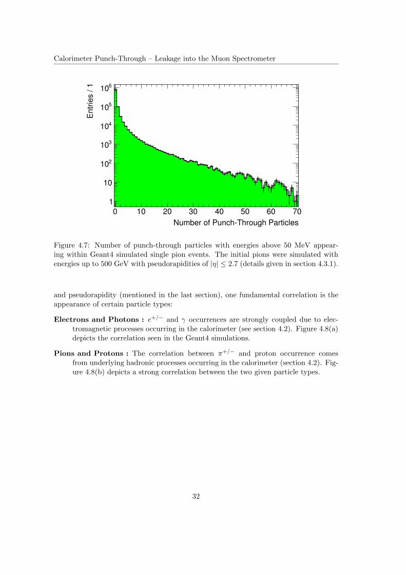
Figure 4.7: Number of punch-through particles with energies above 50 MeV appear-ing within Geant4 simulated single pion events. The initial pions were simulated withenergies up to 500 GeV with pseudorapidities of |η| ≤ 2.7 (details given in section 4.3.1).
and pseudorapidity (mentioned in the last section), one fundamental correlation is theappearance of certain particle types:
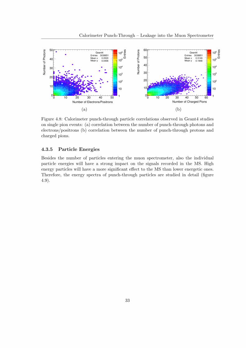
Electrons and Photons : e+/− and γ occurrences are strongly coupled due to elec-tromagnetic processes occurring in the calorimeter (see section 4.2). Figure 4.8(a)depicts the correlation seen in the Geant4 simulations.
Pions and Protons : The correlation between π+/− and proton occurrence comesfrom underlying hadronic processes occurring in the calorimeter (section 4.2). Fig-ure 4.8(b) depicts a strong correlation between the two given particle types.
32
Calorimeter Punch-Through – Leakage into the Muon Spectrometer
En
trie
s
1
10
210
310
410
510
610
Number of Electrons/Positrons
0 10 20 30 40 50
Nu
mb
er
of
Ph
oto
ns
0
10
20
30
40
50Geant4
Entries 3038851
Mean x 0.0520Mean y 0.0406
(a)
En
trie
s
1
10
210
310
410
510
610
Number of Charged Pions
0 10 20 30 40 50 60
Nu
mb
er
of
Pro
ton
s
0
10
20
30
40
50
60Geant4
Entries 3038851
Mean x 0.3149Mean y 0.1958
(b)
Figure 4.8: Calorimeter punch-through particle correlations observed in Geant4 studieson single pion events: (a) correlation between the number of punch-through photons andelectrons/positrons (b) correlation between the number of punch-through protons andcharged pions.
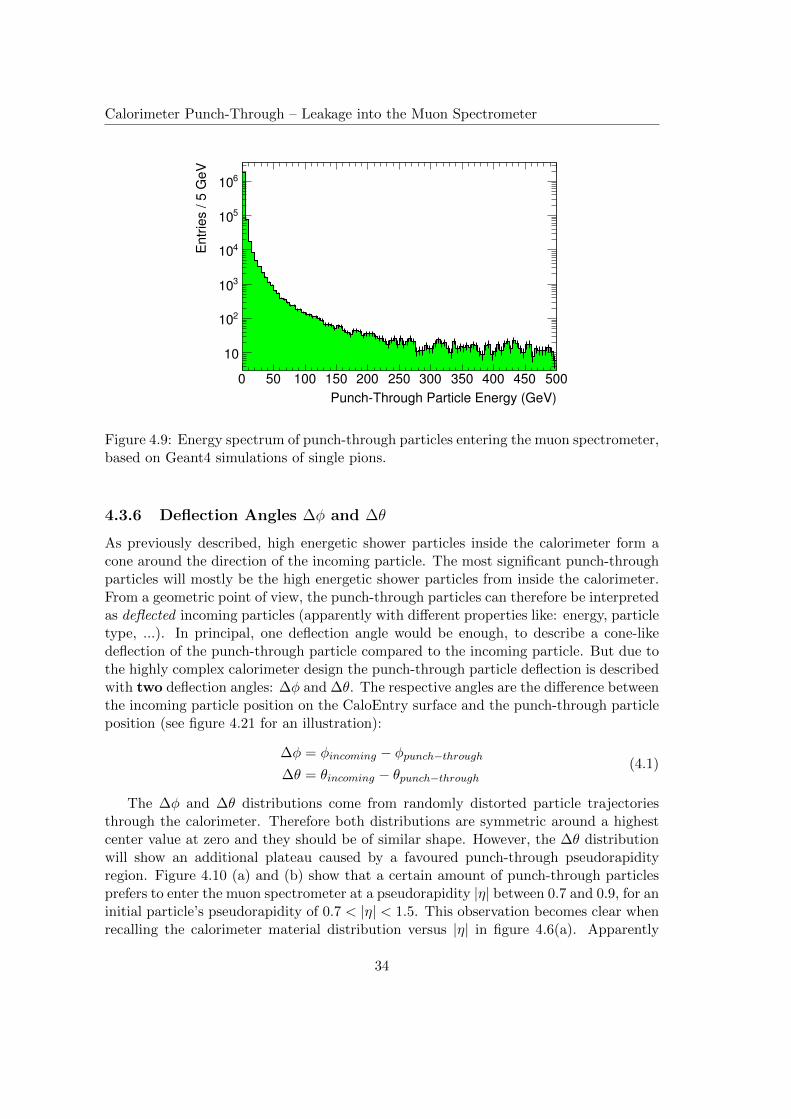
4.3.5 Particle Energies
Besides the number of particles entering the muon spectrometer, also the individualparticle energies will have a strong impact on the signals recorded in the MS. Highenergy particles will have a more significant effect to the MS than lower energetic ones.Therefore, the energy spectra of punch-through particles are studied in detail (figure4.9).
33
Calorimeter Punch-Through – Leakage into the Muon Spectrometer
PunchThrough Particle Energy (GeV)
0 50 100 150 200 250 300 350 400 450 500
Entr
ies / 5
GeV
10
210
310
410
510
610
Figure 4.9: Energy spectrum of punch-through particles entering the muon spectrometer,based on Geant4 simulations of single pions.
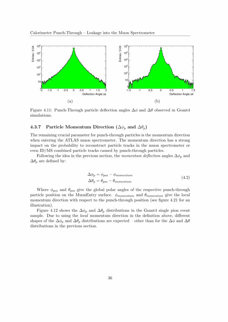
4.3.6 Deflection Angles ∆φ and ∆θ
As previously described, high energetic shower particles inside the calorimeter form acone around the direction of the incoming particle. The most significant punch-throughparticles will mostly be the high energetic shower particles from inside the calorimeter.From a geometric point of view, the punch-through particles can therefore be interpretedas deflected incoming particles (apparently with different properties like: energy, particletype, ...). In principal, one deflection angle would be enough, to describe a cone-likedeflection of the punch-through particle compared to the incoming particle. But due tothe highly complex calorimeter design the punch-through particle deflection is describedwith two deflection angles: ∆φ and ∆θ. The respective angles are the difference betweenthe incoming particle position on the CaloEntry surface and the punch-through particleposition (see figure 4.21 for an illustration):
∆φ = φincoming − φpunch−through∆θ = θincoming − θpunch−through
(4.1)
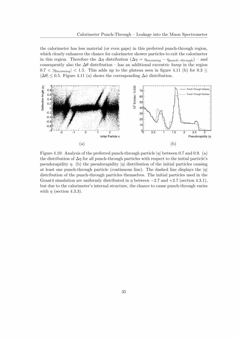
The ∆φ and ∆θ distributions come from randomly distorted particle trajectoriesthrough the calorimeter. Therefore both distributions are symmetric around a highestcenter value at zero and they should be of similar shape. However, the ∆θ distributionwill show an additional plateau caused by a favoured punch-through pseudorapidityregion. Figure 4.10 (a) and (b) show that a certain amount of punch-through particlesprefers to enter the muon spectrometer at a pseudorapidity |η| between 0.7 and 0.9, for aninitial particle’s pseudorapidity of 0.7 < |η| < 1.5. This observation becomes clear whenrecalling the calorimeter material distribution versus |η| in figure 4.6(a). Apparently
34
Calorimeter Punch-Through – Leakage into the Muon Spectrometer
the calorimeter has less material (or even gaps) in this preferred punch-through region,which clearly enhances the chance for calorimeter shower particles to exit the calorimeterin this region. Therefore the ∆η distribution (∆η = ηincoming − ηpunch−through) – andconsequently also the ∆θ distribution – has an additional excentric bump in the region0.7 < |ηincoming| < 1.5. This adds up to the plateau seen in figure 4.11 (b) for 0.3 ≤|∆θ| ≤ 0.5. Figure 4.11 (a) shows the corresponding ∆φ distribution.
(a)
|ηPseudorapidity |
0 0.5 1 1.5 2 2.5 3 E
ntr
ies /
0.0
33
3 1
0
0
10
20
30
40
50
60
70PunchThrough Initiators
PunchThrough Particles
(b)
Figure 4.10: Analysis of the preferred punch-through particle |η| between 0.7 and 0.9. (a)the distribution of ∆η for all punch-through particles with respect to the initial particle’spseudorapidity η. (b) the pseudorapidity |η| distribution of the initial particles causingat least one punch-through particle (continuous line). The dashed line displays the |η|distribution of the punch-through particles themselves. The initial particles used in theGeant4 simulation are uniformly distributed in η between −2.7 and +2.7 (section 4.3.1),but due to the calorimeter’s internal structure, the chance to cause punch-through varieswith η (section 4.3.3).
35
Calorimeter Punch-Through – Leakage into the Muon Spectrometer
φ∆Deflection Angle
2 1.5 1 0.5 0 0.5 1 1.5 2
En
trie
s /
0.0
4
1
10
210
310
410
510
610
(a)
θ∆Deflection Angle
1.5 1 0.5 0 0.5 1 1.5
En
tire
s /
0.0
3
1
10
210
310
410
510
610
(b)
Figure 4.11: Punch-Through particle deflection angles ∆φ and ∆θ observed in Geant4simulations.
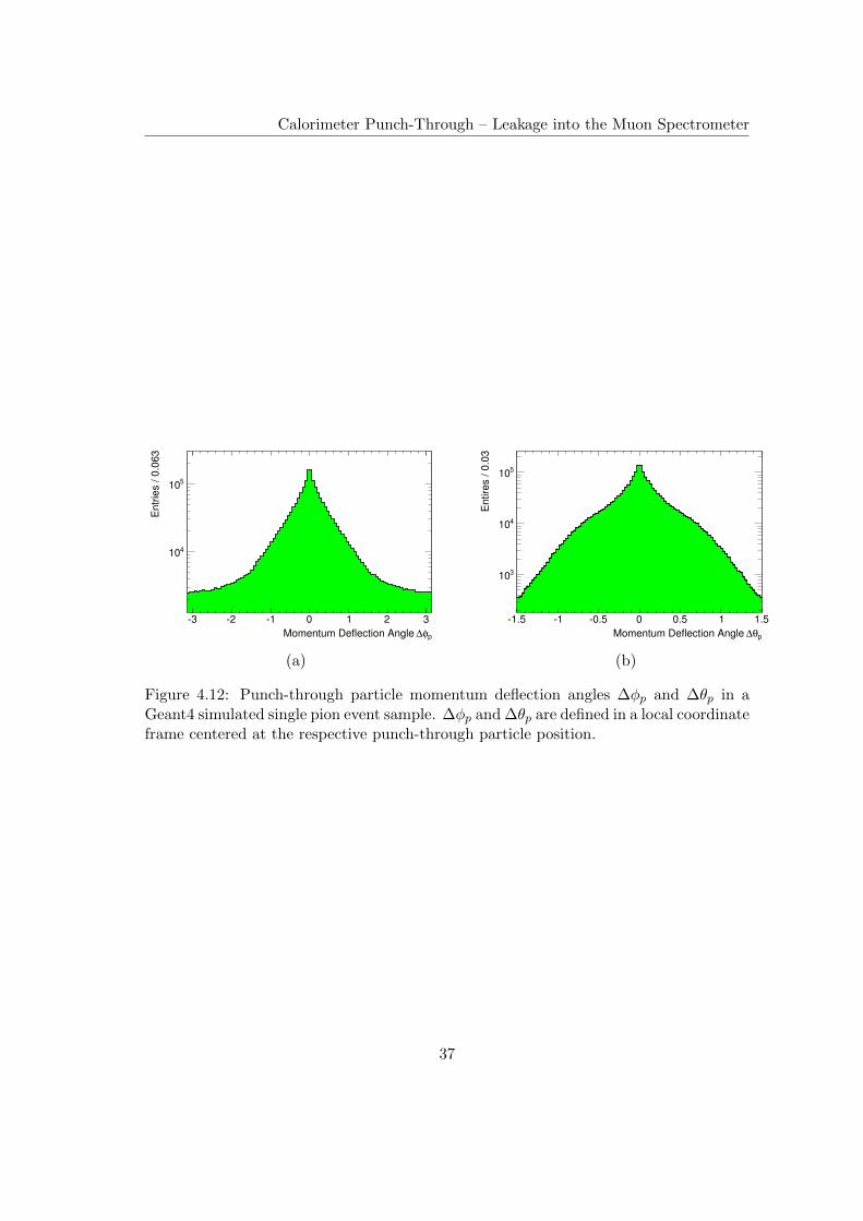
4.3.7 Particle Momentum Direction (∆φp and ∆θp)
The remaining crucial parameter for punch-through particles is the momentum directionwhen entering the ATLAS muon spectrometer. The momentum direction has a strongimpact on the probability to reconstruct particle tracks in the muon spectrometer oreven ID/MS combined particle tracks caused by punch-through particles.
Following the idea in the previous section, the momentum deflection angles ∆φp and∆θp are defined by:
∆φp = φpos − φmomentum∆θp = θpos − θmomentum
(4.2)
Where φpos and θpos give the global polar angles of the respective punch-throughparticle position on the MuonEntry surface. φmomentum and θmomentum give the localmomentum direction with respect to the punch-through position (see figure 4.21 for anillustration).
Figure 4.12 shows the ∆φp and ∆θp distributions in the Geant4 single pion eventsample. Due to using the local momentum direction in the definition above, differentshapes of the ∆φp and ∆θp distributions are expected – other than for the ∆φ and ∆θdistributions in the previous section.
36
Calorimeter Punch-Through – Leakage into the Muon Spectrometer
pφ∆Momentum Deflection Angle
3 2 1 0 1 2 3
En
trie
s /
0.0
63
410
510
(a)
pθ∆Momentum Deflection Angle
1.5 1 0.5 0 0.5 1 1.5
En
tire
s /
0.0
3
310
410
510
(b)
Figure 4.12: Punch-through particle momentum deflection angles ∆φp and ∆θp in aGeant4 simulated single pion event sample. ∆φp and ∆θp are defined in a local coordinateframe centered at the respective punch-through particle position.
37
Calorimeter Punch-Through – Leakage into the Muon Spectrometer
4.4 Parametrization
Due to the high number of – partly very complex – processes occurring inside thecalorimeter, the most promising approach for a fast calorimeter punch-through simu-lation is a parametrized simulation. The advantage of a parametrized simulation is thatit is very fast during runtime. This is due to the fact that only the results of particleinteraction processes are reproduced (based on a pre-recorded set of parameters andtheir relations) rather than simulating the physical model behind each process. Theinput- and output-parameter dependencies and -correlations are stored in a look-up ta-ble, which in this particular implementation is a ROOT file. The structure of this ROOTfile is explained in appendix A.
In order to describe (and store) these dependencies, the previously mentioned sampleof Geant4 simulations (section 4.3) were used to quantitatively obtain certain fit param-eters and correlations. This parametrization is carried out for each Geant4 analysisdescribed in sections 4.3.2–4.3.7, respectively.
The whole parametrization process is automated due to the high number of requiredindividual parametrizations, and to give the flexibility to re-parametrize the simulationbased on a different reference sample. Therefore a modified χ2 method (section 4.4.1) isused to measure the quality of each individual fit.
4.4.1 Fit Quality Measure
Many of the following parametrization sections will utilize automated fit procedures inorder to describe distributions obtained from Geant4 simulations. The fits are carriedout with the ROOT implementation of the binned log-likelihood method. Due to thehigh number of total fits applied, a measure for the quality of each individual fit wasput in place.
In order to to so, this work applies a modified version of the standard χ2 test [28],which is often used to test the quality of a fit. The standard χ2 test did not prove to beuseful for the fits carried out in this work. Instead of computing the χ2 value for eachfit, a somewhat modified χ2
m value is computed:
χ2 =∑i
(Oi − Ei)2
σ2i
χ2m =
∑i
(Oi − Ei)2(4.3)
The sum is taken over all bins i of the respective histogram, Oi are the values obtainedfrom the Geant4 simulations with their corresponding variances σ2i and Ei are the fitfunction value at the centre of the corresponding bin.
Equation 4.3 shows that the modified χ2m value corresponds to the standard χ2
value, except for the fact that χ2m uses a standard value of σ2i = 1 for the variance
in each individual bin. This is motivated by the form of the distributions fitted in thiswork: normalized probability distributions with only a few high probability bins (MPVs,
38
Calorimeter Punch-Through – Leakage into the Muon Spectrometer
values between 0.1 and 1), and an exponential decay following these MPVs (down tovalues of ∼ 10−6). Therefore it is most important to obtain an accurate description ofthe (few) most probable values, which will have a strong impact on the overall χ2
m value.Due to the exponentially decaying form, slight differences in the less probable values willhave less significance for the χ2
m value.This custom test definition has proven to be useful for the kind of distributions fitted
in this work. The χ2m value of each automated fit is stored and manually checked after all
fits are carried out. Fits with high χ2m values are reviewed by hand and either manually
re-fitted with a different set of starting parameters or accepted without any changes, incase the fit seems acceptable.
4.4.2 Parametrization of Punch-Through Particle Quantities and Par-ticle Types
As a first step the particle quantity distributions are reproduced for each individualpunch-through particle type (see figure 4.7 for the cumulative distribution). There-fore the distributions are parameterized for each individual punch-through particle typerespectively. As previously mentioned in section 4.3.2, corresponding matter like andantimatter like particles appear at approximately the same rate for electrons, muonsand pions, respectively. Therefore the parametrization of either of these particle typesis based on cumulative properties of the corresponding matter like and antimatter likeparticles.
Each particle quantity distribution depends strongly on the input particle’s pseudo-rapidity ηin and energy Ein. The cause of this was already discussed in section 4.3.3. Inorder to account for this dependency, the distribution for the number of punch-throughparticles is parametrized for different ηin and Ein regions (also referred to as regimesor domains) independently. Due to detector symmetries in η, the parametrization isactually carried out in different domains of the absolute value |ηin|. Table 4.1 gives thenumerical values of the respective domains. The parametrization is realized by fittingan empirical function against the distribution. In this case, a function of the followingform shows good fit results:
fnum (x) = P0e−P1x + P2e
−P3x + P4e−P5x (4.4)
Pi are the fit parameters and x is the number of punch-through particles of a certainparticle type.
Figure 4.13 shows some examples of the automatically computed fits for punch-through pions. The exact same procedure (same fit-function) is carried out for eachpunch-through particle type within the respective incoming particle regimes.
The fit results (fit parameters Pi) and the minimum and maximum value appearingin the distribution are stored in the look-up table (see appendix A).
39
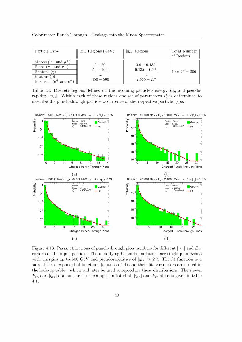
Calorimeter Punch-Through – Leakage into the Muon Spectrometer
Particle Type Ein Regions (GeV) |ηin| Regions Total Numberof Regions
Muons (µ− and µ+)0− 50,
50− 100,...
450− 500
0.0− 0.135,0.135− 0.27,
...2.565− 2.7
10× 20 = 200Pions (π+ and π−)Photons (γ)Protons (p)Electrons (e+ and e−)
Table 4.1: Discrete regions defined on the incoming particle’s energy Ein and pseudo-rapidity |ηin|. Within each of these regions one set of parameters Pi is determined todescribe the punch-through particle occurrence of the respective particle type.
Charged PunchThrough Pions
0 2 4 6 8 10 12 14
Pro
ba
bili
ty
410
310
210
110
1 Entries 16139
Mean 0.088001 5.48474e082
mχ
| < 0.135 in
η 0 < |∧ < 100000 MeV in
Domain: 50000 MeV < E
Geant4
Fit
(a)
Charged PunchThrough Pions
0 5 10 15 20 25 30
Pro
ba
bili
ty
510
410
310
210
110
1 Entries 15816
Mean 0.1859 3.29241e072
mχ
| < 0.135 in
η 0 < |∧ < 150000 MeV in
Domain: 100000 MeV < E
Geant4
Fit
(b)
Charged PunchThrough Pions
0 5 10 15 20 25 30
Pro
ba
bili
ty
410
310
210
110
1 Entries 15792
Mean 0.318618 4.45404e062
mχ
| < 0.135 in
η 0 < |∧ < 200000 MeV in
Domain: 150000 MeV < E
Geant4
Fit
(c)
Charged PunchThrough Pions
0 5 10 15 20 25
Pro
ba
bili
ty
410
310
210
110
1 Entries 16060
Mean 0.412346 1.74406e062
mχ
| < 0.135 in
η 0 < |∧ < 250000 MeV in
Domain: 200000 MeV < E
Geant4
Fit
(d)
Figure 4.13: Parametrizations of punch-through pion numbers for different |ηin| and Einregions of the input particle. The underlying Geant4 simulations are single pion eventswith energies up to 500 GeV and pseudorapidities of |ηin| ≤ 2.7. The fit function is asum of three exponential functions (equation 4.4) and their fit parameters are stored inthe look-up table – which will later be used to reproduce these distributions. The shownEin and |ηin| domains are just examples, a list of all |ηin| and Ein steps is given in table4.1.
40
Calorimeter Punch-Through – Leakage into the Muon Spectrometer
4.4.3 Parametrization of Particle Correlations
The parametrization in the previous section does not take into account correlationsbetween different punch-through particle types. Therefore the correlations are parame-terized by an additional procedure.
A correct parametrization (and simulation) of particle quantity distributions (previ-ous section 4.4.2) together with particle correlations, will result in a correct descriptionof the punch-through probabilities (figure 4.5 and 4.6).
Due to the statistical limitations on the Geant4 reference sample (section 4.3.1), thedescription of the inter-particle correlations are stored in an averaged form, meaningthat:
1. the correlation parametrization does not hold any dependency on the initial par-ticle’s pseudorapidity ηin.
2. only a weak dependency on the initial particle’s energy Ein is stored by parametriz-ing within two different energy intervals (bins).
Each correlated particle pair is parameterized with the information contained in thecorrelation plots in figure 4.8. For each Ein region, a normalized two-dimensional cor-relation histogram is computed from the Geant4 reference sample. The normalizationis carried out along the y-axis, for each respective bin on the x-axis. Thus each x-axisbin contains a probability distribution for the number of punch-through particles of thecorresponding y-axis particle type. However, the inverse probability distributions willalso be needed during simulation runtime. Therefore the same inter-particle correla-tion is plotted with mirrored axes and again normalized within each bin of the x-axis,respectively.
These two histograms contain the exact same information, but they allow to speedup runtime computation compared to the case where only one histogram is used to storeeach two-particle-correlation. The speed-up is due to the fact the normalizations do nothave to be carried out during runtime. These normalized 2D histograms can also beinterpreted as matrices and therefore will also be referred to as correlation matrices.
In total eight correlation matrices are stored in the look-up table file:
• correlation between number of π+/− pions and protons (for Ein energy bins 0–200GeV and 200–500 GeV respectively)
• correlation between number of e+/− and photons (for Ein energy bins 0–200 GeVand 200–500 GeV respectively)
Figure 4.14 shows four of these correlation matrices.Due to the statistical limitation of the underlying Geant4 simulations, the correlation
matrices store the exact same statistical fluctuations as were present in the Geant4 eventsample. This might become problematic for regions in the correlation matrix where onlya few events occurred in the Geant4 simulations – for example for events with morethan 40 charged punch-through pions (see figure 4.14 (c) ). Due to the low number
41
Calorimeter Punch-Through – Leakage into the Muon Spectrometer
of Geant4 simulated events in this region, the probability distributions (for each x-axisbin along the y-axis) mostly only consist of a few filled bins. Clearly this is not anaccurate description of the real probability distribution for this region. But due to thefact that this region is very rarely addressed in the following simulation, this estimate isa reasonable approximation to start with. However, the validation section (section 6.1.1)does show some effect due to this approximation, but it is regarded as negligible for afast simulation engine. Finally, a re-parametrization using higher statistics samples caneasily be done in the future in order to minimize this effect.
42
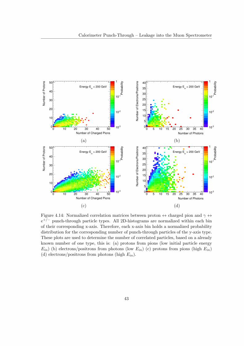
Calorimeter Punch-Through – Leakage into the Muon Spectrometer
Pro
ba
bili
ty
310
210
110
1
Number of Charged Pions
0 10 20 30 40 50
Nu
mb
er
of
Pro
ton
s
0
10
20
30
40
50
< 200 GeVin
Energy E
(a)
Pro
ba
bili
ty
310
210
110
1
Number of Photons
0 5 10 15 20 25 30 35 40
Nu
mb
er
of
Ele
ctr
on
s/P
ositro
ns
0
5
10
15
20
25
30
35
40
< 200 GeVin
Energy E
(b)
Pro
ba
bili
ty
310
210
110
Number of Charged Pions
0 10 20 30 40 50
Nu
mb
er
of
Pro
ton
s
0
10
20
30
40
50
> 200 GeVin
Energy E
(c)
Pro
ba
bili
ty
310
210
110
1
Number of Photons
0 5 10 15 20 25 30 35 40
Nu
mb
er
of
Ele
ctr
on
s/P
ositro
ns
0
5
10
15
20
25
30
35
40
> 200 GeVin
Energy E
(d)
Figure 4.14: Normalized correlation matrices between proton ↔ charged pion and γ ↔e+/− punch-through particle types. All 2D-histograms are normalized within each binof their corresponding x-axis. Therefore, each x-axis bin holds a normalized probabilitydistribution for the corresponding number of punch-through particles of the y-axis type.These plots are used to determine the number of correlated particles, based on a alreadyknown number of one type, this is: (a) protons from pions (low initial particle energyEin) (b) electrons/positrons from photons (low Ein) (c) protons from pions (high Ein)(d) electrons/positrons from photons (high Ein).
43
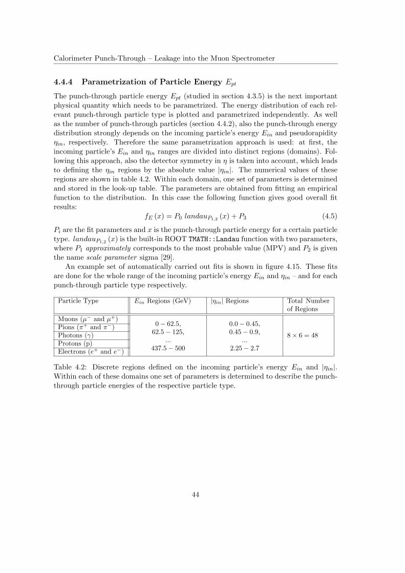
Calorimeter Punch-Through – Leakage into the Muon Spectrometer
4.4.4 Parametrization of Particle Energy Ept
The punch-through particle energy Ept (studied in section 4.3.5) is the next importantphysical quantity which needs to be parametrized. The energy distribution of each rel-evant punch-through particle type is plotted and parametrized independently. As wellas the number of punch-through particles (section 4.4.2), also the punch-through energydistribution strongly depends on the incoming particle’s energy Ein and pseudorapidityηin, respectively. Therefore the same parametrization approach is used: at first, theincoming particle’s Ein and ηin ranges are divided into distinct regions (domains). Fol-lowing this approach, also the detector symmetry in η is taken into account, which leadsto defining the ηin regions by the absolute value |ηin|. The numerical values of theseregions are shown in table 4.2. Within each domain, one set of parameters is determinedand stored in the look-up table. The parameters are obtained from fitting an empiricalfunction to the distribution. In this case the following function gives good overall fitresults:
fE (x) = P0 landauP1,2 (x) + P3 (4.5)
Pi are the fit parameters and x is the punch-through particle energy for a certain particletype. landauP1,2 (x) is the built-in ROOT TMATH::Landau function with two parameters,where P1 approximately corresponds to the most probable value (MPV) and P2 is giventhe name scale parameter sigma [29].
An example set of automatically carried out fits is shown in figure 4.15. These fitsare done for the whole range of the incoming particle’s energy Ein and ηin – and for eachpunch-through particle type respectively.
Particle Type Ein Regions (GeV) |ηin| Regions Total Numberof Regions
Muons (µ− and µ+)0− 62.5,
62.5− 125,...
437.5− 500
0.0− 0.45,0.45− 0.9,
...2.25− 2.7
8× 6 = 48Pions (π+ and π−)Photons (γ)Protons (p)Electrons (e+ and e−)
Table 4.2: Discrete regions defined on the incoming particle’s energy Ein and |ηin|.Within each of these domains one set of parameters is determined to describe the punch-through particle energies of the respective particle type.
44
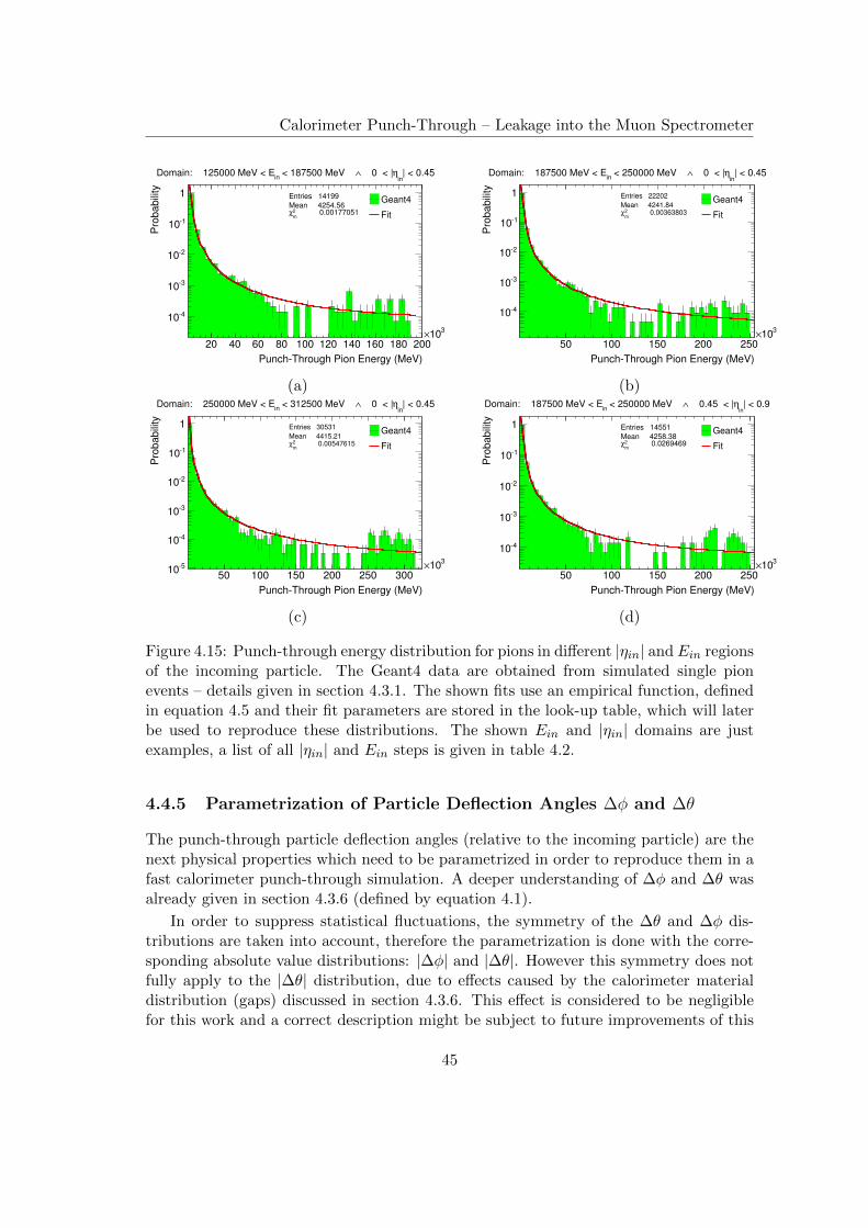
Calorimeter Punch-Through – Leakage into the Muon Spectrometer
PunchThrough Pion Energy (MeV)
20 40 60 80 100 120 140 160 180 200
310×
Pro
ba
bili
ty
410
310
210
110
1 Entries 14199
Mean 4254.56 0.001770512
mχ
| < 0.45 in
η 0 < |∧ < 187500 MeV in
Domain: 125000 MeV < E
Geant4
Fit
(a)
PunchThrough Pion Energy (MeV)
50 100 150 200 250
310×
Pro
ba
bili
ty
410
310
210
110
1 Entries 22202
Mean 4241.84 0.003638032
mχ
| < 0.45 in
η 0 < |∧ < 250000 MeV in
Domain: 187500 MeV < E
Geant4
Fit
(b)
PunchThrough Pion Energy (MeV)
50 100 150 200 250 300
310×
Pro
ba
bili
ty
510
410
310
210
110
1 Entries 30531
Mean 4415.21 0.005476152
mχ
| < 0.45 in
η 0 < |∧ < 312500 MeV in
Domain: 250000 MeV < E
Geant4
Fit
(c)
PunchThrough Pion Energy (MeV)
50 100 150 200 250
310×
Pro
ba
bili
ty
410
310
210
110
1 Entries 14551
Mean 4258.38 0.02694692
mχ
| < 0.9 in
η 0.45 < |∧ < 250000 MeV in
Domain: 187500 MeV < E
Geant4
Fit
(d)
Figure 4.15: Punch-through energy distribution for pions in different |ηin| and Ein regionsof the incoming particle. The Geant4 data are obtained from simulated single pionevents – details given in section 4.3.1. The shown fits use an empirical function, definedin equation 4.5 and their fit parameters are stored in the look-up table, which will laterbe used to reproduce these distributions. The shown Ein and |ηin| domains are justexamples, a list of all |ηin| and Ein steps is given in table 4.2.
4.4.5 Parametrization of Particle Deflection Angles ∆φ and ∆θ
The punch-through particle deflection angles (relative to the incoming particle) are thenext physical properties which need to be parametrized in order to reproduce them in afast calorimeter punch-through simulation. A deeper understanding of ∆φ and ∆θ wasalready given in section 4.3.6 (defined by equation 4.1).
In order to suppress statistical fluctuations, the symmetry of the ∆θ and ∆φ dis-tributions are taken into account, therefore the parametrization is done with the corre-sponding absolute value distributions: |∆φ| and |∆θ|. However this symmetry does notfully apply to the |∆θ| distribution, due to effects caused by the calorimeter materialdistribution (gaps) discussed in section 4.3.6. This effect is considered to be negligiblefor this work and a correct description might be subject to future improvements of this
45
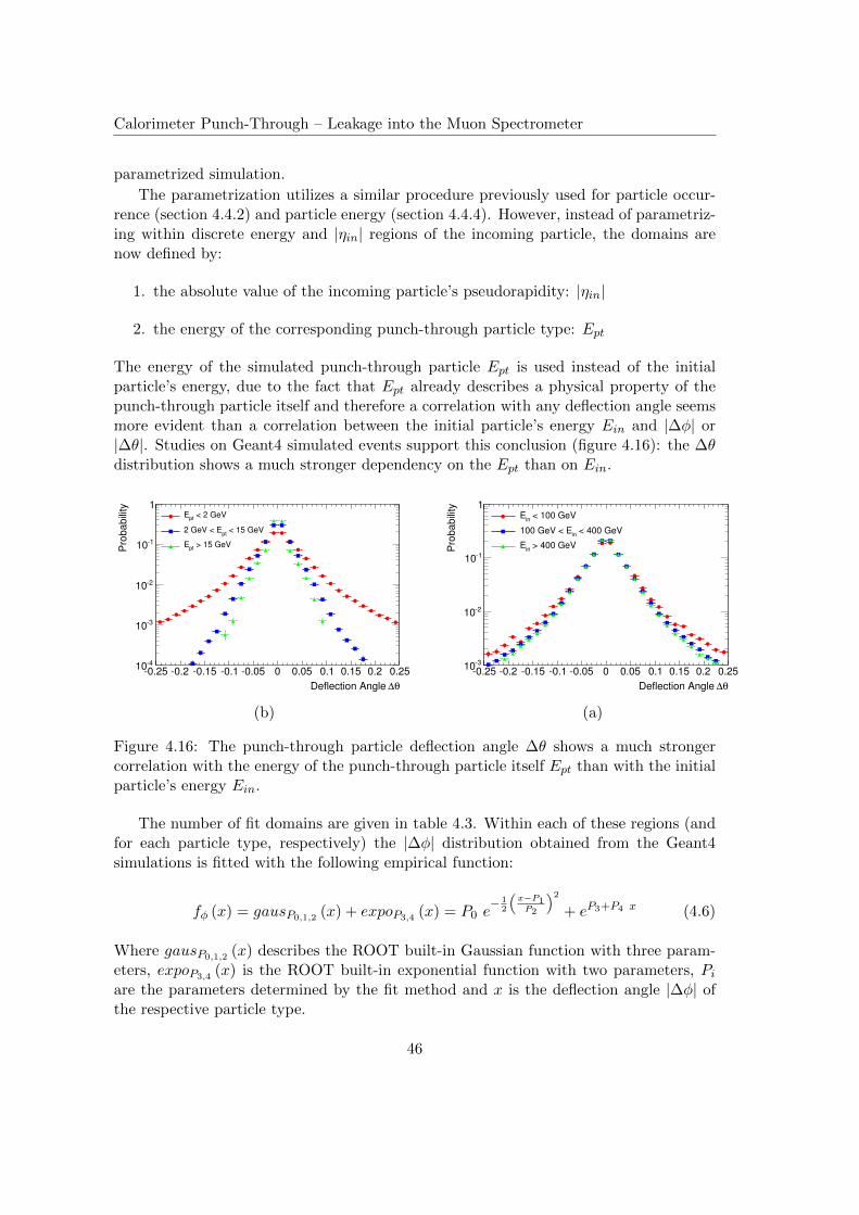
Calorimeter Punch-Through – Leakage into the Muon Spectrometer
parametrized simulation.
The parametrization utilizes a similar procedure previously used for particle occur-rence (section 4.4.2) and particle energy (section 4.4.4). However, instead of parametriz-ing within discrete energy and |ηin| regions of the incoming particle, the domains arenow defined by:
1. the absolute value of the incoming particle’s pseudorapidity: |ηin|
2. the energy of the corresponding punch-through particle type: Ept
The energy of the simulated punch-through particle Ept is used instead of the initialparticle’s energy, due to the fact that Ept already describes a physical property of thepunch-through particle itself and therefore a correlation with any deflection angle seemsmore evident than a correlation between the initial particle’s energy Ein and |∆φ| or|∆θ|. Studies on Geant4 simulated events support this conclusion (figure 4.16): the ∆θdistribution shows a much stronger dependency on the Ept than on Ein.
θ∆Deflection Angle
0.25 0.2 0.15 0.1 0.05 0 0.05 0.1 0.15 0.2 0.25
Pro
ba
bili
ty
410
310
210
110
1 < 2 GeVptE
< 15 GeVpt
2 GeV < E
> 15 GeVptE
(b)
θ∆Deflection Angle
0.25 0.2 0.15 0.1 0.05 0 0.05 0.1 0.15 0.2 0.25
Pro
ba
bili
ty
310
210
110
1 < 100 GeV
inE
< 400 GeVin
100 GeV < E
> 400 GeVin
E
(a)
Figure 4.16: The punch-through particle deflection angle ∆θ shows a much strongercorrelation with the energy of the punch-through particle itself Ept than with the initialparticle’s energy Ein.
The number of fit domains are given in table 4.3. Within each of these regions (andfor each particle type, respectively) the |∆φ| distribution obtained from the Geant4simulations is fitted with the following empirical function:
fφ (x) = gausP0,1,2 (x) + expoP3,4 (x) = P0 e− 1
2
(x−P1P2
)2
+ eP3+P4 x (4.6)
Where gausP0,1,2 (x) describes the ROOT built-in Gaussian function with three param-eters, expoP3,4 (x) is the ROOT built-in exponential function with two parameters, Piare the parameters determined by the fit method and x is the deflection angle |∆φ| ofthe respective particle type.
46
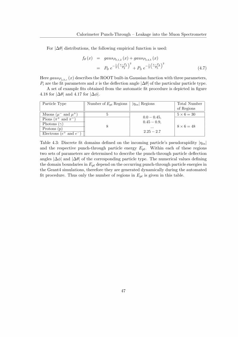
Calorimeter Punch-Through – Leakage into the Muon Spectrometer
For |∆θ| distributions, the following empirical function is used:
fθ (x) = gausP0,1,2 (x) + gausP3,4,5 (x)
= P0 e− 1
2
(x−P1P2
)2
+ P3 e− 1
2
(x−P4P5
)2
(4.7)
Here gausPa,b,c(x) describes the ROOT built-in Gaussian function with three parameters,
Pi are the fit parameters and x is the deflection angle |∆θ| of the particular particle type.A set of example fits obtained from the automatic fit procedure is depicted in figure
4.18 for |∆θ| and 4.17 for |∆φ|.
Particle Type Number of Ept Regions |ηin| Regions Total Numberof Regions
Muons (µ− and µ+) 50.0− 0.45,0.45− 0.9,
...2.25− 2.7
5× 6 = 30Pions (π+ and π−)
8 8× 6 = 48Photons (γ)Protons (p)Electrons (e+ and e−)
Table 4.3: Discrete fit domains defined on the incoming particle’s pseudorapidity |ηin|and the respective punch-through particle energy Ept. Within each of these regionstwo sets of parameters are determined to describe the punch-through particle deflectionangles |∆φ| and |∆θ| of the corresponding particle type. The numerical values definingthe domain boundaries in Ept depend on the occurring punch-through particle energies inthe Geant4 simulations, therefore they are generated dynamically during the automatedfit procedure. Thus only the number of regions in Ept is given in this table.
47
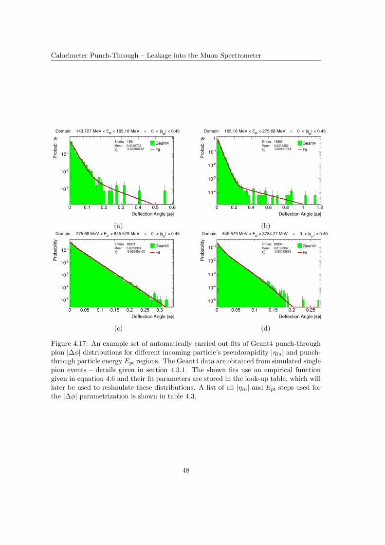
Calorimeter Punch-Through – Leakage into the Muon Spectrometer
|φ∆Deflection Angle |
0 0.1 0.2 0.3 0.4 0.5 0.6
Pro
ba
bili
ty
310
210
110
Entries 1381
Mean 0.0316738 0.003697822
mχ
| < 0.45 pt
η 0 < |∧ < 165.16 MeV ptDomain: 143.727 MeV < E
Geant4
Fit
(a)
|φ∆Deflection Angle |
0 0.2 0.4 0.6 0.8 1 1.2
Pro
ba
bili
ty
410
310
210
110
1Entries 16290
Mean 0.0313252 0.001617442
mχ
| < 0.45 pt
η 0 < |∧ < 275.68 MeV ptDomain: 165.16 MeV < E
Geant4
Fit
(b)
|φ∆Deflection Angle |
0 0.05 0.1 0.15 0.2 0.25 0.3
Pro
ba
bili
ty
510
410
310
210
110
Entries 95231
Mean 0.0253361 6.92645e052
mχ
| < 0.45 pt
η 0 < |∧ < 845.579 MeV ptDomain: 275.68 MeV < E
Geant4
Fit
(c)
|φ∆Deflection Angle |
0 0.05 0.1 0.15 0.2 0.25
Pro
ba
bili
ty
510
410
310
210
110Entries 86934
Mean 0.0168957 0.000126382
mχ
| < 0.45 pt
η 0 < |∧ < 3784.27 MeV pt
Domain: 845.579 MeV < E
Geant4
Fit
(d)
Figure 4.17: An example set of automatically carried out fits of Geant4 punch-throughpion |∆φ| distributions for different incoming particle’s pseudorapidity |ηin| and punch-through particle energy Ept regions. The Geant4 data are obtained from simulated singlepion events – details given in section 4.3.1. The shown fits use an empirical functiongiven in equation 4.6 and their fit parameters are stored in the look-up table, which willlater be used to resimulate these distributions. A list of all |ηin| and Ept steps used forthe |∆φ| parametrization is shown in table 4.3.
48
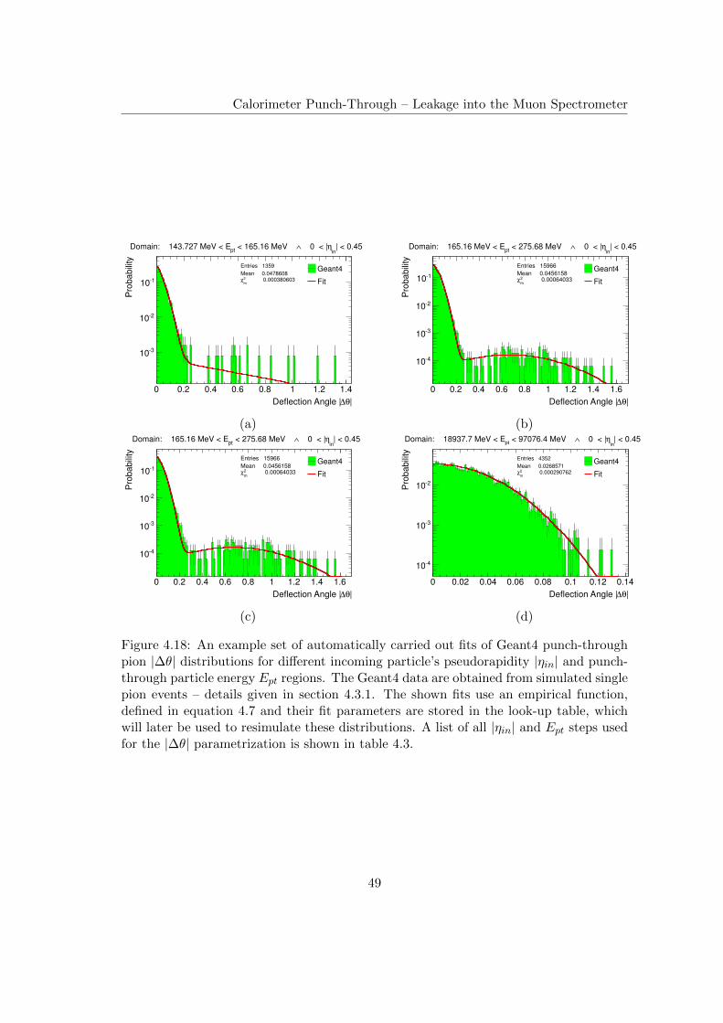
Calorimeter Punch-Through – Leakage into the Muon Spectrometer
|θ∆Deflection Angle |
0 0.2 0.4 0.6 0.8 1 1.2 1.4
Pro
ba
bili
ty
310
210
110
Entries 1359
Mean 0.0478608 0.0003806032
mχ
| < 0.45 in
η 0 < |∧ < 165.16 MeV pt
Domain: 143.727 MeV < E
Geant4
Fit
(a)
|θ∆Deflection Angle |
0 0.2 0.4 0.6 0.8 1 1.2 1.4 1.6
Pro
ba
bili
ty
410
310
210
110
Entries 15966
Mean 0.0456158 0.000640332
mχ
| < 0.45 in
η 0 < |∧ < 275.68 MeV pt
Domain: 165.16 MeV < E
Geant4
Fit
(b)
|θ∆Deflection Angle |
0 0.2 0.4 0.6 0.8 1 1.2 1.4 1.6
Pro
ba
bili
ty
410
310
210
110
Entries 15966
Mean 0.0456158 0.000640332
mχ
| < 0.45 in
η 0 < |∧ < 275.68 MeV pt
Domain: 165.16 MeV < E
Geant4
Fit
(c)
|θ∆Deflection Angle |
0 0.02 0.04 0.06 0.08 0.1 0.12 0.14
Pro
ba
bili
ty
410
310
210
Entries 4352
Mean 0.0268571 0.0002907622
mχ
| < 0.45 in
η 0 < |∧ < 97076.4 MeV pt
Domain: 18937.7 MeV < E
Geant4
Fit
(d)
Figure 4.18: An example set of automatically carried out fits of Geant4 punch-throughpion |∆θ| distributions for different incoming particle’s pseudorapidity |ηin| and punch-through particle energy Ept regions. The Geant4 data are obtained from simulated singlepion events – details given in section 4.3.1. The shown fits use an empirical function,defined in equation 4.7 and their fit parameters are stored in the look-up table, whichwill later be used to resimulate these distributions. A list of all |ηin| and Ept steps usedfor the |∆θ| parametrization is shown in table 4.3.
49
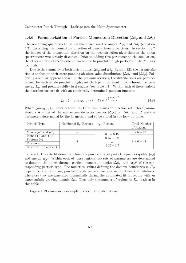
Calorimeter Punch-Through – Leakage into the Muon Spectrometer
4.4.6 Parametrization of Particle Momentum Direction (∆φp and ∆θp)
The remaining quantities to be parameterized are the angles ∆φp and ∆θp (equation4.2), describing the momentum direction of punch-through particles. In section 4.3.7the impact of the momentum direction on the reconstruction algorithms in the muonspectrometer was already discussed. Prior to adding this parameter to the simulation,the observed rate of reconstructed tracks due to punch-through particles in the MS wastoo high.
Due to the symmetry of both distributions, ∆φp and ∆θp (figure 4.12), the parametriza-tion is applied on their corresponding absolute value distributions |∆φp| and |∆θp|. Fol-lowing a similar approach taken in the previous sections, the distributions are parame-terized for each single punch-through particle type in different punch-through particleenergy Ept and pseudorapidity |ηpt| regions (see table 4.4). Within each of these regionsthe distributions are fit with an empirically determined gaussian function:
fφ (x) = gausP0,1,2 (x) = P0 e− 1
2
(x−P1P2
)2
(4.8)
Where gausP0,1,2 (x) describes the ROOT built-in Gaussian function with three param-eters, x is either of the momentum deflection angles |∆φp| or |∆θp| and Pi are theparameters determined by the fit method and to be stored in the look-up table.
Particle Type Number of Ept Regions |ηpt| Regions Total Numberof Regions
Muons (µ− and µ+) 50.0− 0.45,0.45− 0.9,
...2.25− 2.7
5× 6 = 30Pions (π+ and π−)
8 8× 6 = 48Photons (γ)Protons (p)Electrons (e+ and e−)
Table 4.4: Discrete fit domains defined on punch-through particle’s pseudorapidity |ηpt|and energy Ept. Within each of these regions two sets of parameters are determinedto describe the punch-through particle momentum angles |∆φp| and |∆pθ| of the cor-responding particle type. The numerical values defining the domain boundaries in Eptdepend on the occurring punch-through particle energies in the Geant4 simulations.Therefore they are generated dynamically during the automated fit procedure with anexponentially growing domain size. Thus only the number of regions in Ept is given inthis table.
Figure 4.19 shows some example fits for both distributions.
50
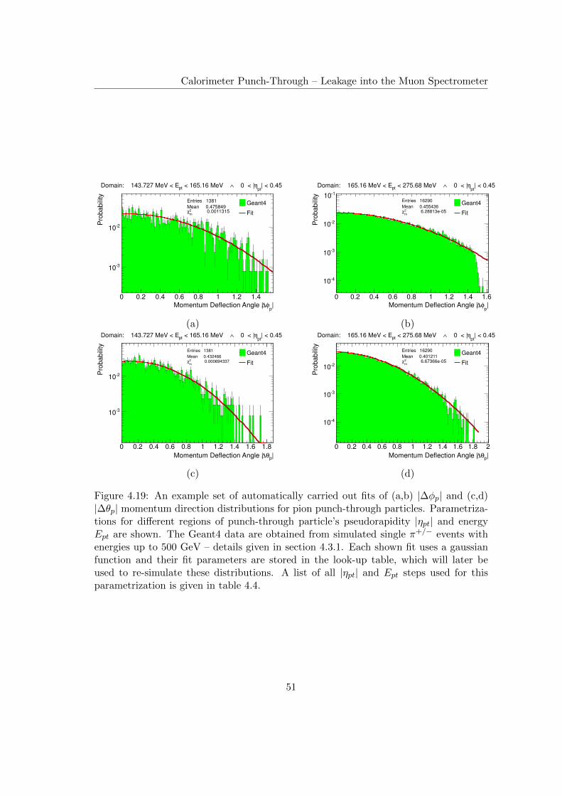
Calorimeter Punch-Through – Leakage into the Muon Spectrometer
|p
φ∆Momentum Deflection Angle |
0 0.2 0.4 0.6 0.8 1 1.2 1.4
Pro
ba
bili
ty
310
210
Entries 1381
Mean 0.475849 0.00113152
mχ
| < 0.45 pt
η 0 < |∧ < 165.16 MeV ptDomain: 143.727 MeV < E
Geant4
Fit
(a)
|p
φ∆Momentum Deflection Angle |
0 0.2 0.4 0.6 0.8 1 1.2 1.4 1.6
Pro
ba
bili
ty
410
310
210
110Entries 16290
Mean 0.455436 6.28813e052
mχ
| < 0.45 pt
η 0 < |∧ < 275.68 MeV ptDomain: 165.16 MeV < E
Geant4
Fit
(b)
|pθ∆Momentum Deflection Angle |
0 0.2 0.4 0.6 0.8 1 1.2 1.4 1.6 1.8
Pro
ba
bili
ty
310
210
Entries 1381
Mean 0.432466 0.0006943372
mχ
| < 0.45 pt
η 0 < |∧ < 165.16 MeV ptDomain: 143.727 MeV < E
Geant4
Fit
(c)
|pθ∆Momentum Deflection Angle |
0 0.2 0.4 0.6 0.8 1 1.2 1.4 1.6 1.8 2
Pro
ba
bili
ty
410
310
210
Entries 16290
Mean 0.401211 6.67366e052
mχ
| < 0.45 pt
η 0 < |∧ < 275.68 MeV ptDomain: 165.16 MeV < E
Geant4
Fit
(d)
Figure 4.19: An example set of automatically carried out fits of (a,b) |∆φp| and (c,d)|∆θp| momentum direction distributions for pion punch-through particles. Parametriza-tions for different regions of punch-through particle’s pseudorapidity |ηpt| and energyEpt are shown. The Geant4 data are obtained from simulated single π+/− events withenergies up to 500 GeV – details given in section 4.3.1. Each shown fit uses a gaussianfunction and their fit parameters are stored in the look-up table, which will later beused to re-simulate these distributions. A list of all |ηpt| and Ept steps used for thisparametrization is given in table 4.4.
51
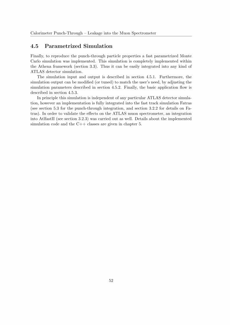
Calorimeter Punch-Through – Leakage into the Muon Spectrometer
4.5 Parametrized Simulation
Finally, to reproduce the punch-through particle properties a fast parametrized MonteCarlo simulation was implemented. This simulation is completely implemented withinthe Athena framework (section 3.3). Thus it can be easily integrated into any kind ofATLAS detector simulation.
The simulation input and output is described in section 4.5.1. Furthermore, thesimulation output can be modified (or tuned) to match the user’s need, by adjusting thesimulation parameters described in section 4.5.2. Finally, the basic application flow isdescribed in section 4.5.3.
In principle this simulation is independent of any particular ATLAS detector simula-tion, however an implementation is fully integrated into the fast track simulation Fatras(see section 5.3 for the punch-through integration, and section 3.2.2 for details on Fa-tras). In order to validate the effects on the ATLAS muon spectrometer, an integrationinto AtlfastII (see section 3.2.3) was carried out as well. Details about the implementedsimulation code and the C++ classes are given in chapter 5.
52
Calorimeter Punch-Through – Leakage into the Muon Spectrometer
Figure 4.20: A schematic representation of the application flow for the parametrizedcalorimeter punch-through simulation implemented in this work. The simulation output(the punch-through particles) depends on the properties of the incoming particle, theparametrization (stored in a look-up table file) and the simulation parameters (given viaPython jobOptions). Before any simulation step is run, the incoming particle is checkedfor its relevance to the punch-through simulation. In the following first simulation step,the number of particles for each individual punch-through particle type are determined.While doing so, the corresponding particle correlations are taken into account. Further-more, the individual energies for these particles are computed. Based on the particleenergy, the deflection angles are determined and by using them the particle position iscomputed. Finally, the direction of each particle’s momentum is determined, based onits already determined energy and position.
4.5.1 Simulation Input and Output
The simulation takes one particle at a time as input. From this, a set of punch-throughparticles are generated according to the parametrized distributions saved in the look-up table file and the parameters set by the user (section 4.5.2). In most cases, noparticles will be created at all, which means that the incoming particle is completelyabsorbed by the ATLAS calorimeter. In simulated signal events more than one particleper event will enter the calorimeter. In this case the punch-through simulation has tobe called several times, for each single particle respectively. This implies the reasonableassumption that the particle interaction processes inside the calorimeter are uncorrelatedbetween different initial particles entering the calorimeter.
Due to the definition for a punch-through particle while applying the parametriza-tion (section 4.3.1), the input particle should be positioned on a geometrical surface
53
Calorimeter Punch-Through – Leakage into the Muon Spectrometer
called CaloEntryLayer (see appendix B). The generated punch-through particles willbe positioned on the MuonEntryLayer. Both layers do not cross any sensitive detectorelements, therefore they were chosen as reference surfaces. In case the input particle’sposition is not on the CaloEntryLayer surface or a given tolerance around the surface,the simulation will not treat the particle to cause any punch-through effects. The er-ror made by particles not positioned on the reference surface, but within a reasonabletolerance, is assumed to be negligible for this fast punch-through simulation.
4.5.2 Simulation Parameters
Fundamental simulation properties are easily modifiable through a set of parametersaccessible via Python jobOptions (see section 3.3). These parameters are provided bythe PunchThroughSimulator C++ class, explained in detail in section 5.1.
Many parameters (especially scale factors) allow to tune the simulation – e.g. againsta given reference sample – or to use this simulation for studies on systematic errors dueto punch-through effects.
The following list briefly explains the meaning and effects of these parameters:
Punch-Through Initiators give the incoming particle type for which this simulationapplies. The particle type is given according to the Monte Carlo numbering scheme[25]. In Python this parameter is named PunchThroughInitiators. The simu-lation does not differentiate between an incoming matter like or anti-matter likeparticle type. For both, the exact same punch-through effects will be simulated.Currently only one initiator particle type can be registered to the simulation, butit will be subject for future improvements to add punch-through simulation capa-bility for a variety of initial particle types, each with its own parametrization.
Punch-Through Particle Types have to be registered individually to the punch-through simulator via the parameter PunchThroughParticles. Only particle typesgiven in this list are generated as punch-through particles.
Anti-Particle Creation: For each of the particle types given by the previous parame-ter, a Boolean value will determine if its corresponding anti-particle type will alsobe generated as punch-through particle. If enabled, the simulation will create mat-ter like and anti-matter like particles according to a same common parametrization.This parameter is accessible as DoAntiParticles in Python.
Correlated Particle: Each punch-through particle-type can have up to one corre-sponding correlated particle type, which has to be given by the parameter Corre-latedParticle according to the Monte Carlo numbering scheme.
Minimum Particle Energy: Punch-through particles below a certain energy thresh-old will not be generated. This value can be modified for each particle type re-spectively (MinEnergy).
54
Calorimeter Punch-Through – Leakage into the Muon Spectrometer
Maximum Number of Particles: An upper threshold for the number of punch-throughparticles for each respective particle-type (MaxNumParticles).
Number of Particles Factor: The output of punch-through particles for each respec-tive particle-type according to the parametrization will be multiplied by this factor(NumParticlesFactor).
Energy Factor: The particle energies obtained from the parametrization will be mul-tiplied by this factor for each respective particle type (EnergyFactor).
Correlation Energy Thresholds: For incoming particles below the MinCorrelationEn-ergy energy threshold, no punch-through particle correlations are taken into ac-count. Above this threshold, the chance to simulate correlations increases linearlyuntil the upper threshold FullCorrelationEnergy is reached. For energies aboveFullCorrelationEnergy, full particle correlations are simulated.
Position and Momentum Deflection Angles: The factors given by the parametersScalePosDeflectionAngles and ScaleMomDeflectionAngles scale the correspond-ing deflection angles (∆φ and ∆θ or ∆φp and ∆θp) determined by the simulation.
Tolerance to Reference Surface: The parameterized simulation will be applied toany input particle which has its position inside this tolerance around the CaloEn-tryLayer surface. Any particle outside this tolerance will be rejected by the simu-lation. The value has to be given in millimeters. (Python name: ReferenceSur-
faceTolerance)
Barcode Offset: This simulation internal parameter is used to give a starting numberfor the punch-through particle barcodes, where each particle barcode is uniquewithin a simulated event. The Python name of this parameter is BarcodeOffset.
4.5.3 Simulation Scheme
Figure 4.20 shows a schematic overview of the application flow for the parameterizedpunch-through simulation. The punch-through particle properties are determined in thesame sequence as the parametrization is described in section 4.4.
1. Check Incoming Particle: Before any of the parametrization is applied, the in-coming particle will be checked for its type. If this particle type is not registeredto the simulation as a punch-through initiator (section 4.5.2), it will be ignoredby the simulation and no additional punch-through particles are created – thiscorresponds to the case where the incoming particle is completely absorbed bythe ATLAS calorimeter. Different to the other steps, no simulation of particleproperties is carried out within this first step.
2. Number of Punch-Through Particles and Correlations: After the previous stephas been passed, the quantity of punch-through particles for each respective punch-through particle type is determined according to the parametrization. Within this
55
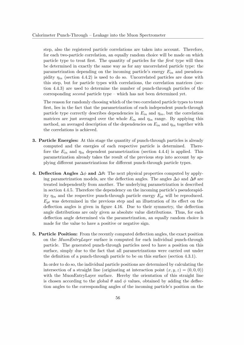
Calorimeter Punch-Through – Leakage into the Muon Spectrometer
step, also the registered particle correlations are taken into account. Therefore,for each two-particle correlation, an equally random choice will be made on whichparticle type to treat first. The quantity of particles for the first type will thenbe determined in exactly the same way as for any uncorrelated particle type: theparametrization depending on the incoming particle’s energy Ein and pseudora-pidity ηin (section 4.4.2) is used to do so. Uncorrelated particles are done withthis step, but for particle types with correlations, the correlation matrices (sec-tion 4.4.3) are used to determine the number of punch-through particles of thecorresponding second particle type – which has not been determined yet.
The reason for randomly choosing which of the two correlated particle types to treatfirst, lies in the fact that the parametrization of each independent punch-throughparticle type correctly describes dependencies in Ein and ηin, but the correlationmatrices are just averaged over the whole Ein and ηin range. By applying thismethod, an averaged description of the dependencies on Ein and ηin together withthe correlations is achieved.
3. Particle Energies: At this stage the quantity of punch-through particles is alreadycomputed and the energies of each respective particle is determined. There-fore the Ein and ηin dependent parametrization (section 4.4.4) is applied. Thisparametrization already takes the result of the previous step into account by ap-plying different parametrizations for different punch-through particle types.
4. Deflection Angles ∆φ and ∆θ: The next physical properties computed by apply-ing parametrization models, are the deflection angles. The angles ∆φ and ∆θ aretreated independently from another. The underlying parametrization is describedin section 4.4.5. Therefore the dependency on the incoming particle’s pseudorapid-ity ηin and the respective punch-through particle energy Ept will be reproduced.Ept was determined in the previous step and an illustration of its effect on thedeflection angles is given in figure 4.16. Due to their symmetry, the deflectionangle distributions are only given as absolute value distributions. Thus, for eachdeflection angle determined via the parametrization, an equally random choice ismade for the value to have a positive or negative sign.
5. Particle Position: From the recently computed deflection angles, the exact positionon the MuonEntryLayer surface is computed for each individual punch-throughparticle. The generated punch-through particles need to have a position on thissurface, simply due to the fact that all parametrizations were carried out underthe definition of a punch-through particle to be on this surface (section 4.3.1).
In order to do so, the individual particle positions are determined by calculating theintersection of a straight line (originating at interaction point (x, y, z) = (0, 0, 0))with the MuonEntryLayer surface. Hereby the orientation of this straight lineis chosen according to the global θ and φ values, obtained by adding the deflec-tion angles to the corresponding angles of the incoming particle’s position on the
56
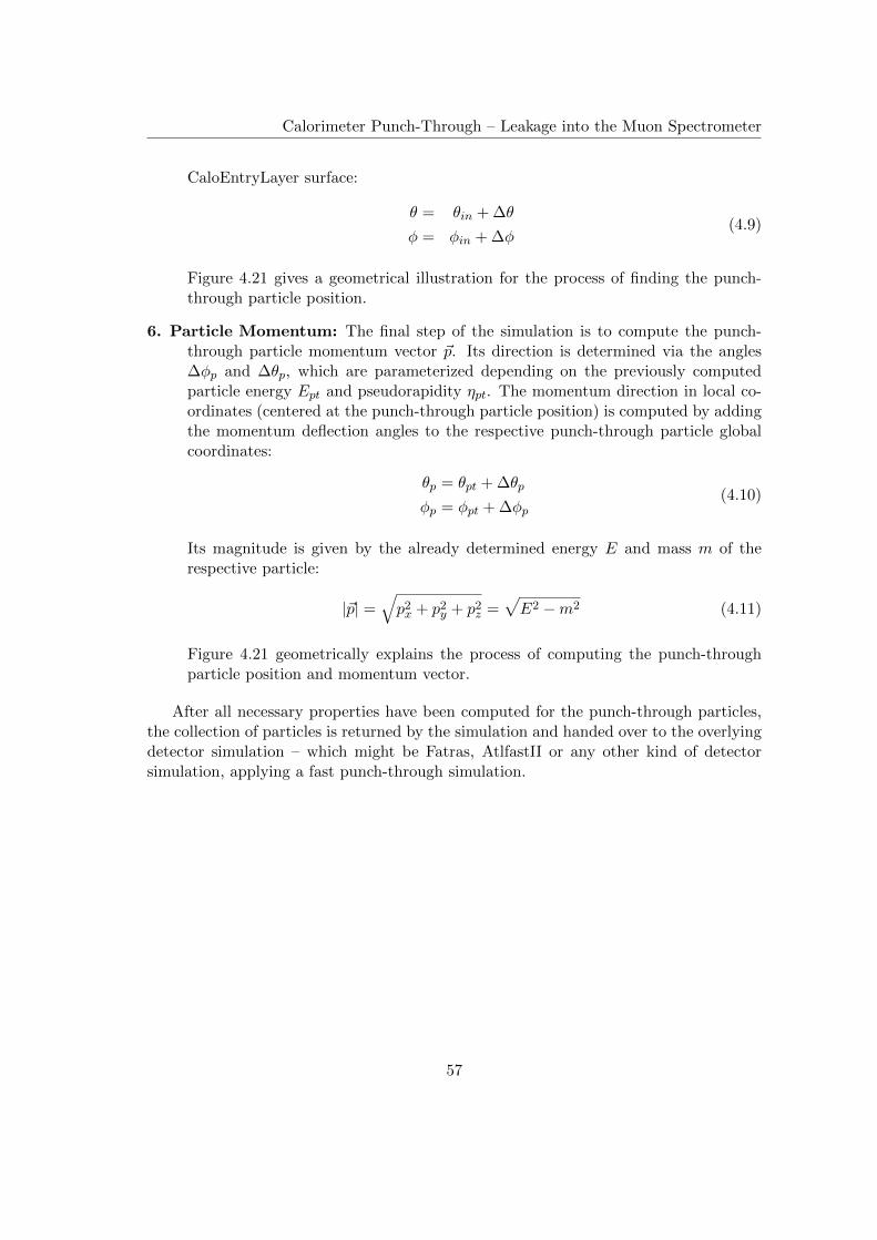
Calorimeter Punch-Through – Leakage into the Muon Spectrometer
CaloEntryLayer surface:
θ = θin + ∆θ
φ = φin + ∆φ(4.9)
Figure 4.21 gives a geometrical illustration for the process of finding the punch-through particle position.
6. Particle Momentum: The final step of the simulation is to compute the punch-through particle momentum vector ~p. Its direction is determined via the angles∆φp and ∆θp, which are parameterized depending on the previously computedparticle energy Ept and pseudorapidity ηpt. The momentum direction in local co-ordinates (centered at the punch-through particle position) is computed by addingthe momentum deflection angles to the respective punch-through particle globalcoordinates:
θp = θpt + ∆θp
φp = φpt + ∆φp(4.10)
Its magnitude is given by the already determined energy E and mass m of therespective particle:
|~p| =√p2x + p2y + p2z =
√E2 −m2 (4.11)
Figure 4.21 geometrically explains the process of computing the punch-throughparticle position and momentum vector.
After all necessary properties have been computed for the punch-through particles,the collection of particles is returned by the simulation and handed over to the overlyingdetector simulation – which might be Fatras, AtlfastII or any other kind of detectorsimulation, applying a fast punch-through simulation.
57
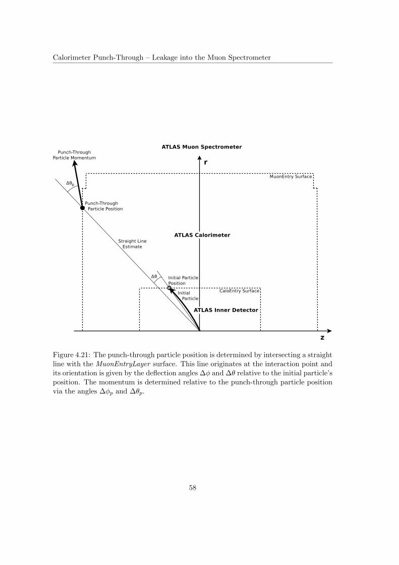
Calorimeter Punch-Through – Leakage into the Muon Spectrometer
Figure 4.21: The punch-through particle position is determined by intersecting a straightline with the MuonEntryLayer surface. This line originates at the interaction point andits orientation is given by the deflection angles ∆φ and ∆θ relative to the initial particle’sposition. The momentum is determined relative to the punch-through particle positionvia the angles ∆φp and ∆θp.
58
Chapter 5
Implementation
In section 4.5 an overview of the simulation concepts and its basic application flow wasgiven. This chapter adds a detailed explanation of the underlying C++ implementation.The main punch-through simulator class and its functionality is explained in section 5.1.The method used to generate random numbers with a desired distribution is discussedin section 5.2. Due to the fact that this work was first implemented within Fatras (seesection 3.2.2) most of its C++ classes and data types are fit into the Fatras framework.The code resides therefore in the Simulation/Fatras container and its subpackages.The Fatras integration is discussed in section 5.3.
Adapting this simulation to other projects, such as the future integrated simulationframework, may result in a change of the interface classes and the namespace.
The implementation is compatible to Athena release 17.0.2.6. The C++ source codeis fully documented using the documentation generator Doxygen [30].
5.1 Punch-Through Simulation
Class Summary
C++ Class Name Fatras::PunchThroughSimulator
Contained in package FatrasToolsCompatible interface Fatras::IParticleStateCollectionCreator
As the C++ class name already suggests, the Fatras::PunchThroughSimulator
Athena tool is the main component of the fast calorimeter punch-through simulation. Ituses a parameterized look-up table to reproduce certain parameter relations, distribu-tions and correlations. The content of this look-up table is described in more detail inappendix A.
The PunchThroughSimulator takes one Fatras::ParticleState object at input,which describes one particle at a given time and position in the detector. To runthe punch-through simulation for multiple input particles, it has to be called sev-eral times – once for each input particle. In Fatras this is carried out by the Fa-
59
Implementation
tras::SimulationKernel (see section 5.3.2). The simulation returns a filled Parti-
cleStateCollection in case punch-through particles are created, or a pointer to zero,in case no particles are created.
The parametrization requires the input particle’s position to be on the surface of theso called CaloEntryLayer (see appendix B). In the Fatras implementation this is ensuredby the ExtrapolationTool (section 5.3.5). All quantities that are determined by thepunch-through simulation depend on at least one of the following parameters (or derivedones) of this input particle:
• particle type described by the Monte Carlo particle numbering scheme [25]
• particle energy Ein
• pseudorapidity ηin of the particle position when entering the ATLAS calorimeter
With the use of the look-up table and the given input parameters from above, thepunch-through simulator uses the Fatras::PDFcreator (see section 5.2) to derive thefollowing quantities for the punch-through particles in this order:
1. number of particles and correlations for each particle type
2. particle energies Ept
3. deflection angle ∆φ
4. deflection angle ∆θ
5. position of punch-through particle
6. direction of momentum (from ∆φp and ∆θp)
All punch-through particles created by this simulation module are positioned on theMuonEntryLayer (appendix B) (which surrounds the ATLAS calorimeter). Thereforethese particles can directly be handed over to any subsequent ATLAS muon spectrometersimulation.
In order to gain maximum flexibility, many core elements of the punch-through simu-lation can be controlled via (tuning) parameters (section 4.5.2), accessible in the PythonjobOptions files (section 3.3). The parameters are read during the initialization phase ofthis Athena tool. Based on these parameters, Fatras::PDFcreator objects are createdfor the different punch-through particle properties for each respective punch-throughparticle type registered via the PunchThroughParticles parameter.
The parameters PunchThroughParticles, DoAntiParticles, CorrelatedParti-
cle, (MinEnergy, MaxNumParticles, NumParticlesFactor and EnergyFactor are Pythonvectors, where each entry corresponds to one punch-through particle type. Thereforeeach of these vectors should have the same length. If this is not the case, the simulationthrows a warning message but continues its execution with default values for the miss-ing parameters. Even though the simulation might then be unable to create all desiredparticle types.
60
Implementation
Only if the given input particle type is registered to the PunchThroughSimulator
(via the PunchThroughInitiators Python parameter) the simulation continues in theorder of the following subsections. If this is not the case, the simulation ends hereand returns a zero value. In which case the Fatras implementation then continues itsexecution in Fatras::CaloSimulationTool.
5.1.1 Number of Punch-Through Particles, Particle Type and Corre-lations
The PunchThroughSimulator produces punch-through particles of each type that isregistered via the PunchThroughParticles parameter. In case a correlation is registeredfor two particle types, a random number decides which of the two particle types to treatfirst (with equal chances). This decision is made for each correlated pair of particletypes. Each chosen particle type is then treated in the exact same way as an uncorrelatedparticle type.
The corresponding Fatras::PDFcreator object is used to generate a random numberfor the quantity of punch-through particles of the currently processed particle type.To do so, the PDFcreator uses a generic fit function with a number of fit parameters(section 4.4) obtained from the look-up table file. This function – together with the fitparameters – describes the probability distributions for different punch-through particletypes. The PDFcreator automatically chooses the correct fit parameters correspondingto the current input particle energy Ein and pseudorapidity |ηin|.
For a particle types with no correlation, the process of finding its number of punch-through particles is finished at this point. For correlated particle types, the quantity ofparticles of the previously not-selected particle type still has to be computed. This isdone via correlation matrices (section 4.4.3) stored in the look-up table. Each correlationmatrix is averaged and does only depend on one parameter: the already computedquantity of particles for the first particle type. By using this, a discrete probabilitydistribution for the number of particles of the second particle type is obtained. A randomnumber according to this distribution is obtained, by utilizing the inverse transformsampling method [31], which is based on uniformly distributed random numbers. Thismethod is utilized for each pair of correlated punch-through particle types.
Clearly, if no punch-through particles appear at all, the punch-through simulationends at this point. In this case, the PunchThroughSimulator returns a zero value.
5.1.2 Energy of Punch-Through Particles
The next step in the punch-through simulation is the computation of the respectivepunch-through particle energies. Due to the parametrization (section 4.4.4) this is car-ried out for each punch-through particle type independently. Again, the PDFcreator
instances are used to compute the corresponding punch-through particle energies. Thedependency on the incoming particle’s energy Ein and pseudorapidity ηin is taken intoaccount by doing so.
61
Implementation
In order to guarantee energy conservation, a simple test is carried out after eachparticle energy computation: In case the sum of the individual particle energies exceedsthe incoming particle’s energy, all following punch-through particles are dropped, eventhough the previous step (section 5.1.1) would have determined a greater number punch-through particles.
5.1.3 Deflection Angles ∆φ and ∆θ
A number of Fatras::PDFcreator instances is used to compute the deflection angles∆φ and ∆θ for each respective punch-through particle. The dependencies on the incom-ing particle’s pseudorapidity ηin, the respective punch-through particle energy Ept andparticle type are take into account.
5.1.4 Particle Position and Momentum Direction
Each single punch-through particle position is determined by the corresponding angles φand θ (according to equation 4.9). The simulation takes care to keep these angles withintheir defined range, respectively:
θ ∈ [0, π] (5.1)
φ ∈ [−π, π) (5.2)
These angles are used to compute a corresponding position on the MuonEntryLayersurface (figure 4.21), which is build as the intersection of a straight line from the originto the surface. Mathematically, the line is described by ~R (l), where l is a parametercorresponding to the distance from the origin:
~R(l) =
cosφ sin θsinφ sin θ
cos θ
· lThe MuonEntryLayer surface consists of individual cylinder- and disc surfaces. Theyare arranged with cylindrical symmetry around the z-axis. Therefore simple analyticalsolutions exist to describe the intersection coordinates by the parameter l:
ldisc = ± zdisccos θ
lcyl = ±rcylsin θ
In this simulation only the positive results are taken. The simplified cylindrical repre-sentation used above dues not reflect the actual shape of the entry layer surface (seeappendix B). Therefore a Fatras::EntryLayerTool is used to get ATLAS tracking ge-ometry representations [18] for the corresponding MuonEntryLayer parts. Here, onlytwo different surface types are used: Trk::CylinderSurface and Trk::DiscSurface.
62
Implementation
The simulation computes the intersection coordinates on all surfaces, positioned inthe same half space (+z or −z) where the straight line is pointing to. For each of thesesurfaces, the tracking geometry built-in isOnSurface methods are used to determine ifthe intersection lies within the respective surface boundaries. By doing so, exactly onevalid intersection remains, which is taken as the punch-through particle position.
The punch-through particle momentum is then set to be collinear with the straightline used to find its position on the MuonEntryLayer surface.
5.2 Distributed Random Number Generation
Class Summary
C++ Class Name Fatras::PDFcreator
Contained in package FatrasTools
The PDFcreator generates discrete or continuous random numbers according to adistribution given by a ROOT TF1 [29] function object. The TF1 object usually dependson a set of settable function parameters (fit parameters in this case). The PDFcre-
ator determines the TF1 function parameters based on the input parameters given asarguments to the PDFcreator::getRand(...) method. The input parameters do notnecessarily correspond to the function parameters. An example for input parametersare Ept and ηin when computing particle deflection angles (section 5.1.3).
The relation between input parameters and function parameters is given via ROOTTH1 histograms. The channels (bins) of the histogram correspond to intervals of an inputparameter value and the content in a certain channel holds the corresponding functionparameter value (which is usually a floating point value). Note that the ROOT TH1 1Dhistogram base class also serves as a base class for both 2D ROOT histograms (TH2)and 3D ROOT histograms. Therefore, a n-dimensional histogram is used, to get onefunction parameter out of n input parameters. Most of the probability density functionsused in this work are described with more than one function parameter. Therefore, a setof TH1 histograms is needed to describe the complete function for a certain set of inputparameters.
The use of histograms to store function parameters for different input parameterintervals results in non-continuous transitions between these intervals. This could havenegative effects on the physical result of the simulation. Therefore a fast interpolationmethod was implemented, as described in section 5.2.3.
By calling the PDFcreator::getRand(...) method, the function parameters willbe determined based on the given set of input parameters. Therefore the TF1 functionis then fully defined and a random number is computed according to the the function’sdistribution. The exact process of computing these random numbers is discussed insubsection 5.2.1 for discrete random numbers and 5.2.2 for continuous random numbers.
All ROOT TF1 functions and ROOT TH1 histograms used by PDFcreator instances
63
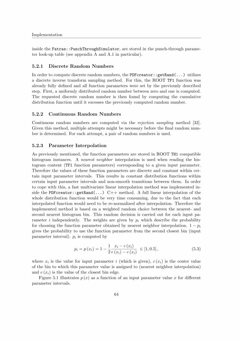
Implementation
inside the Fatras::PunchThroughSimulator, are stored in the punch-through parame-ter look-up table (see appendix A and A.1 in particular).
5.2.1 Discrete Random Numbers
In order to compute discrete random numbers, the PDFcreator::getRand(...) utilizesa discrete inverse transform sampling method. For this, the ROOT TF1 function wasalready fully defined and all function parameters were set by the previously describedstep. First, a uniformly distributed random number between zero and one is computed.The requested discrete random number is then found by computing the cumulativedistribution function until it excesses the previously computed random number.
5.2.2 Continuous Random Numbers
Continuous random numbers are computed via the rejection sampling method [32].Given this method, multiple attempts might be necessary before the final random num-ber is determined. For each attempt, a pair of random numbers is used.
5.2.3 Parameter Interpolation
As previously mentioned, the function parameters are stored in ROOT TH1 compatiblehistogram instances. A nearest neighbor interpolation is used when reading the his-togram content (TF1 function parameters) corresponding to a given input parameter.Therefore the values of these function parameters are discrete and constant within cer-tain input parameter intervals. This results in constant distribution functions withincertain input parameter intervals and non-smooth transitions between them. In orderto cope with this, a fast multivariate linear interpolation method was implemented in-side the PDFcreator::getRand(...) C++ method. A full linear interpolation of thewhole distribution function would be very time consuming, due to the fact that eachinterpolated function would need to be re-normalized after interpolation. Therefore theimplemented method is based on a weighted random choice between the nearest- andsecond nearest histogram bin. This random decision is carried out for each input pa-rameter i independently. The weights are given by pi which describe the probabilityfor choosing the function parameter obtained by nearest neighbor interpolation. 1 − pigives the probability to use the function parameter from the second closest bin (inputparameter interval). pi is computed by
pi = p (xi) = 1− 1
2
xi − c (xi)
e (xi)− c (xi)∈ [1, 0.5] , (5.3)
where xi is the value for input parameter i (which is given), c (xi) is the center valueof the bin to which this parameter value is assigned to (nearest neighbor interpolation)and e (xi) is the value of the closest bin edge.
Figure 5.1 illustrates p (x) as a function of an input parameter value x for differentparameter intervals.
64
Implementation
Figure 5.1: Illustration of p (x) plotted against one input parameter value x. An examplevalue x is given, together with corresponding closest bin center c (x) and closest bin edgee (x). In the center of each bin, p (x) → 1. This corresponds to a probability close toone for choosing the nearest neighbor interpolation in finding the function parameters.On each bin edge. There is an equal chance of choosing the bin on the lower or upperside. The results obtained by this interpolation method show a very good agreementwith the reference data, as shown in the validation section 6.1.1.
The PDFcreator utilizes the CLHEP random number generator [33] in combinationwith pi to decide from which bin the function parameter will finally be taken from.
65
Implementation
5.3 Integration into Fatras
A brief description of Fatras – a fast ATLAS detector simulation – was already givenin section 3.2.2. Section 5.3.1 gives an overview of the simulation flow of Fatras, whereall following sections give a deeper insight on how different simulation modules andC++ classes in Fatras are involved with the punch-through simulation. Fatras is fullyembedded within the Athena framework (section 3.3).
5.3.1 Fatras Simulation Scheme
Figure 5.2 gives an overview of the application- and data flow of Fatras. The simulationconsists of three main parts: the simulation input, the simulation kernel and the sub-detector simulations. All of these are described in this section in more detail:
Simulation Input: Fatras takes two possible types of input for the subsequent detec-tor simulation:
1. Event Generator (EvGen) files which are provided by a particle physics eventgenerator. This kind of input is standard for any physics analysis (see section 3.1).
2. Single particles which are entirely set-up inside the Fatras jobOptions.py file thatis used to set up a certain simulation job. This input mode is mainly used for Fatrasinternal validation.
These input particles are added to the Fatras internal particle stack, where they willbe treated by the Fatras simulation kernel for further processing.
Particle Stack and Simulation Kernel: The particle stack together with the Fatrassimulation kernel are the core elements of the Fatras simulation. The stack describesa collection of particles (ParticleStateCollection) which are to be processed by theFatras sub-detector simulations. The simulation kernel goes through all particles in thisparticle stack respectively and assigns them to the corresponding sub-detector simula-tion. This design allows a dynamic creation (and subsequent processing) of particles atany stage of the simulation. Also, this design is not limited to any particular particleflow direction. Particles (or their daughter particles) may cross sub-detector boundariesforth and back without any limitation.
The Fatras simulation for one event ends, when all particles in the stack are processed.Then the particle stack is emptied and to be filled with the particles for the next event.
Details about the implementation of the simulation kernel are given in section 5.3.2.
Sub-detector Simulation: Fatras uses different simulation models and -strategies forthe three different ATLAS sub-detector parts:
Inner Detector: The Fatras Inner Detector (ID) simulation distinguishes between charged-and uncharged particles. For the former it simulates detector hits on sensitive
66
Implementation
detector elements, decays and interactions with the detector material. At a laterstage, the detector hits will be taken as input for the standard reconstruction soft-ware. Uncharged particles will be extrapolated through the ID without causingdetector hits, but photon conversions, decays and material interactions are simu-lated for them as well as for charged particles.
Calorimeter: The calorimeter simulation in Fatras does not fully simulate the calorime-ter response to particles. This is subject to a simulation called FastCaloSim (see[21]). However, in Fatras the calorimeter simulation is best described by the fol-lowing three cases:
• If the particle is a muon, it is extrapolated through the calorimeter until itreaches the Muon Spectrometer. For this, the muons have to fulfill certainmomentum cuts. Even though the sensitive calorimeter material is not sim-ulated, material interactions of the muons with the calorimeter material arecomputed.
• If the particle type is set up to cause calorimeter punch-through, Fatras callsthe calorimeter punch-through simulation. So far this is only implementedfor pions.
• If the particle does not fulfill any of the above conditions, it is dropped andwill not be further processed by Fatras.
Muon System: Currently, the Fatras Muon Spectrometer (MS) simulation is only val-idated for extrapolating muons through the MS. As the ID simulation, it alsocomputes material interactions of the muons with the detector material and sim-ulates detector hits on sensitive MS detector parts.
67
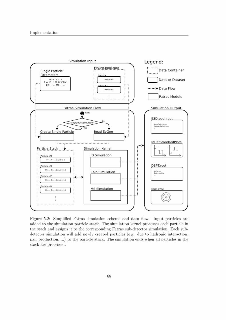
Implementation
Figure 5.2: Simplified Fatras simulation scheme and data flow. Input particles areadded to the simulation particle stack. The simulation kernel processes each particle inthe stack and assigns it to the corresponding Fatras sub-detector simulation. Each sub-detector simulation will add newly created particles (e.g. due to hadronic interaction,pair production, ...) to the particle stack. The simulation ends when all particles in thestack are processed.
68
Implementation
5.3.2 Fatras Simulation Kernel
Class Summary
C++ Class Name Fatras::SimulationKernel
Contained in package FatrasAlgs
The main simulation loop in Fatras is run within the Fatras::SimulationKernel.It runs a stack simulation in which each single particle is represented by a Particle-
State object. The kernel assigns these ParticleStates to the three different Fatrassimulation parts: Inner Detector, Calorimeter and Muon System – depending on therespective value of ParticleState::geometryLabel(). For the Inner Detector and theMuon Spectrometer simulation respectively, a ISimulationTool is called, the calorime-ter simulation is done via an ITransportTool. By default the Inner Detector and MuonSpectrometer simulations are done via TrackSimulationTool (section 5.3.3) instances.In case the calorimeter simulation is enabled, a CaloSimulationTool (section 5.3.6)instance is called for all particles inside the ATLAS calorimeter volume. In case thecalorimeter simulation is disabled, a TransportTool (section 5.3.4) will take care oftransporting muons through the calorimeter. The punch-through simulation is calledfrom inside the CaloSimulationTool.
The Fatras sub-detector simulations (such as the calorimeter punch-through simu-lation) may add particles to the simulation stack (via the ICollectionManager) for alater treatment by the simulation kernel.
5.3.3 Track Simulation
Class Summary
C++ Class Name Fatras::TrackSimulationTool
Contained in package FatrasToolsCompatible interface: Fatras::ISimulationTool
TrackSimulationTools handle any particle transport for the Inner Detector or theMuon System. In cases where a Trk::Track object may potentially be created, it handsthe particle over to a Fatras::ITrackCreator compatible tool, which by default is aFatras::TrackCreator instance. This is the case when the currently processed particleis charged and may therefore create detector hits directly. If the particle shows no charge,a Fatras::ITransportTool is called, because no direct detector hits have to be takeninto account for this case, therefore no Trk:Track objects will be created. By default,the Fatras::TransportTool is used for neutral particle transport.
In any case an ExtrapolationTool (section 5.3.5) does the extrapolations behindeach particle transport between different (sensitive) detector elements. This ensures
69
Implementation
that the entry layers are recorded correctly, which is required for further punch-throughsimulation and validation.
5.3.4 Particle Transport
Class Summary
C++ Class Name Fatras::TransportTools
Contained in package FatrasToolsCompatible interface: Fatras::ITransportTool
The transport tool is used within Fatras to do any extrapolation where no Trk::Trackobject is created. The two cases are: extrapolation of neutral particles in the Inner De-tector (no detector hits are created by the particle itself) and the extrapolation of muonsthrough the calorimeter.
In any case, the TransportTool calls a Fatras::IExtrapolationTool (default Ex-trapolationTool) to do the extrapolation of the given particle. This is necessary inorder to fill Calo- and MuonEntry collections correctly. Depending on the current setup,the extrapolator used for this may then produce daughter particles which will be fedinto the main simulation stack of the Fatras::SimulationKernel.
5.3.5 Particle Extrapolation
Class Summary
C++ Class Name Fatras::ExtrapolationTool
Contained in package FatrasToolsCompatible interface: Fatras::IExtrapolationTool
The Fatras::ExtrapolationTool is basically a wrapper for any Trk::IExtrapolator
compatible extrapolator. In addition, it automatically fills the Calo- and MuonEntrylayer collections (see appendix B) when particles pass through the corresponding sur-faces. All particle extrapolations in Fatras are done using this tool. It is particularlyimportant for the punch-through simulation, because it assures that the position of theinput particles are on the reference surface (CaloEntry layer).
A geometrical description of the Calo- and MuonEntryLayers is retrieved from a Fa-
tras::EntryLayerTool, which offers corresponding Trk::Surfaces and Trk::TrackingVolumes.
5.3.6 Fatras Calorimeter Simulation
The CaloSimulationTool is called from the SimulationKernel for all particles whichare assigned to the Fatras calorimeter simulation – which means they have a Particle-
State:geometryLabel() equal to Trk::Calo. If the currently processed particle is a
70
Implementation
Class Summary
C++ Class Name Fatras::CaloSimulationTool
Contained in package FatrasToolsCompatible interface Fatras::ITransportTool
muon, it will will be handed over to a ITransportTool (default: TransportTool) to betransported through the ATLAS calorimeter. Any other particle type will be handed overto a IParticleStateCollectionCreator (default: PunchThroughSimulator, section5.1) which handles the punch-through simulation and returns a ParticleStateCollec-
tion. This collection contains all particles which will penetrate the Muon Spectrometerafter a calorimeter punch-through. The CaloSimulationTool adds all particles con-tained in the collection to the SimulationKernel’s particle stack for a later treatmentin the Fatras Muon Spectrometer simulation.
5.4 Integration into AtlfastII
As previously described in section 3.2.3, AtlfastII uses full Geant4 detector simulationfor the ATLAS inner detector and muon spectrometer, the calorimeter is simulated byFastCaloSim for all particle types but muons. Due to comparatively low CPU-timerequirements for muon simulations, muons traversing the ATLAS calorimeter in Atl-fastII will be simulated by Geant4. In order to compute punch-through or particledecay in flight effects, the AtlfastII implementation of the parameterized punch-throughsimulation uses the same Athena tools and C++ classes as previously described in sec-tion 5.1. In addition to that, some modifications are done in the AtlfastII FastID-
Killer::SteppingAction(...) method. In AtlfastII simulations, this method treatsall particles leaving the ATLAS inner detector. Its main purpose is to remove these par-ticles from the Geant4 simulation stack, except for muons which are kept in the particlestack.
In order to run the fast punch-through simulation, a few lines of additional code areimplemented which call the punch-through simulation for each particle to be removedfrom the simulation stack. For the currently implemented parameterized simulation,charged pions are the only particle type which will cause any punch-through effect – thischeck is carried out inside punch-through simulator tool (section 5.1). In case the punch-through simulation returns a set of particles, they will added to the Geant4 simulationstack from inside the SteppingAction(...) method mentioned above.
71

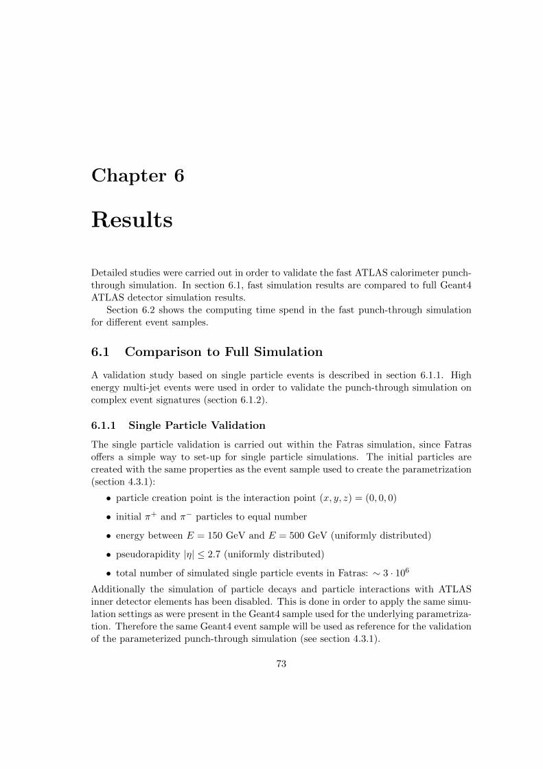
Chapter 6
Results
Detailed studies were carried out in order to validate the fast ATLAS calorimeter punch-through simulation. In section 6.1, fast simulation results are compared to full Geant4ATLAS detector simulation results.
Section 6.2 shows the computing time spend in the fast punch-through simulationfor different event samples.
6.1 Comparison to Full Simulation
A validation study based on single particle events is described in section 6.1.1. Highenergy multi-jet events were used in order to validate the punch-through simulation oncomplex event signatures (section 6.1.2).
6.1.1 Single Particle Validation
The single particle validation is carried out within the Fatras simulation, since Fatrasoffers a simple way to set-up for single particle simulations. The initial particles arecreated with the same properties as the event sample used to create the parametrization(section 4.3.1):
• particle creation point is the interaction point (x, y, z) = (0, 0, 0)
• initial π+ and π− particles to equal number
• energy between E = 150 GeV and E = 500 GeV (uniformly distributed)
• pseudorapidity |η| ≤ 2.7 (uniformly distributed)
• total number of simulated single particle events in Fatras: ∼ 3 · 106
Additionally the simulation of particle decays and particle interactions with ATLASinner detector elements has been disabled. This is done in order to apply the same simu-lation settings as were present in the Geant4 sample used for the underlying parametriza-tion. Therefore the same Geant4 event sample will be used as reference for the validationof the parameterized punch-through simulation (see section 4.3.1).
73
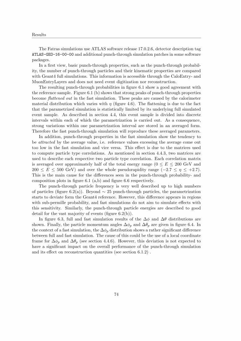
Results
The Fatras simulations use ATLAS software release 17.0.2.6, detector description tagATLAS-GEO-16-00-00 and additional punch-through simulation patches in some softwarepackages.
In a first view, basic punch-through properties, such as the punch-through probabil-ity, the number of punch-through particles and their kinematic properties are comparedwith Geant4 full simulations. This information is accessible through the CaloEntry- andMuonEntryLayers and does not need event digitization nor reconstruction.
The resulting punch-through probabilities in figure 6.1 show a good agreement withthe reference sample. Figure 6.1 (b) shows that strong peaks of punch-through propertiesbecome flattened out in the fast simulation. These peaks are caused by the calorimetermaterial distribution which varies with η (figure 4.6). The flattening is due to the factthat the parametrized simulation is statistically limited by its underlying full simulatedevent sample. As described in section 4.4, this event sample is divided into discreteintervals within each of which the parametrization is carried out. As a consequence,strong variations within one parametrization interval are stored in an averaged form.Therefore the fast punch-through simulation will reproduce these averaged parameters.
In addition, punch-through properties in the fast simulation show the tendency tobe attracted by the average value, i.e. reference values excessing the average come outtoo low in the fast simulation and vice versa. This effect is due to the matrices usedto compute particle type correlations. As mentioned in section 4.4.3, two matrices areused to describe each respective two particle type correlation. Each correlation matrixis averaged over approximately half of the total energy range (0 ≤ E ≤ 200 GeV and200 ≤ E ≤ 500 GeV) and over the whole pseudorapidity range (−2.7 ≤ η ≤ +2.7).This is the main cause for the differences seen in the punch-through probability- andcomposition plots in figure 6.1 (a,b) and figure 6.6 respectively.
The punch-through particle frequency is very well described up to high numbersof particles (figure 6.2(a)). Beyond ∼ 25 punch-through particles, the parametrizationstarts to deviate form the Geant4 reference. However, this difference appears in regionswith sub-permille probability, and fast simulations do not aim to simulate effects withthis sensitivity. Similarly, the punch-through particle energies are described to gooddetail for the vast majority of events (figure 6.2(b)).
In figure 6.3, full and fast simulation results of the ∆φ and ∆θ distributions areshown. Finally, the particle momentum angles ∆φp and ∆θp are given in figure 6.4. Inthe context of a fast simulation, the ∆φp distribution shows a rather significant differencebetween full and fast simulation. The cause of this could be the use of a local coordinateframe for ∆φp and ∆θp (see section 4.4.6). However, this deviation is not expected tohave a significant impact on the overall performance of the punch-through simulationand its effect on reconstruction quantities (see section 6.1.2) .
74
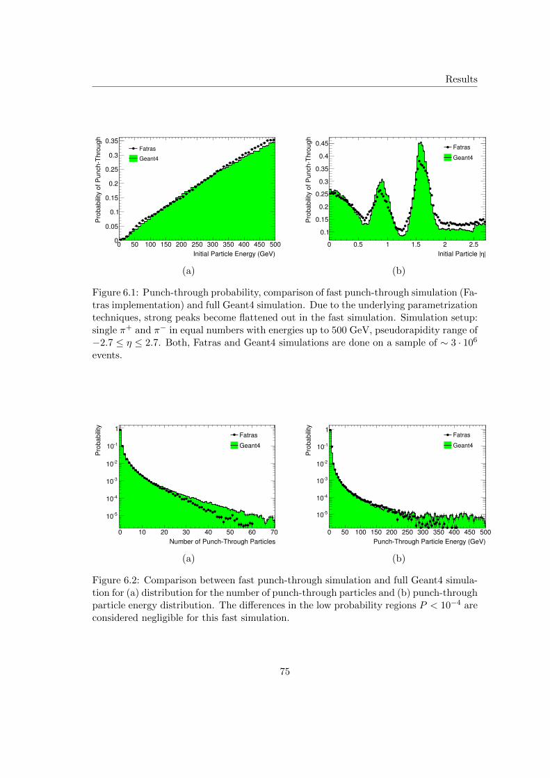
Results
Initial Particle Energy (GeV)
0 50 100 150 200 250 300 350 400 450 500
Pro
ba
bili
ty o
f P
un
ch
Th
rou
gh
0
0.05
0.1
0.15
0.2
0.25
0.3
0.35Fatras
Geant4
(a)
|ηInitial Particle |
0 0.5 1 1.5 2 2.5
Pro
ba
bili
ty o
f P
un
ch
Th
rou
gh
0.1
0.15
0.2
0.25
0.3
0.35
0.4
0.45Fatras
Geant4
(b)
Figure 6.1: Punch-through probability, comparison of fast punch-through simulation (Fa-tras implementation) and full Geant4 simulation. Due to the underlying parametrizationtechniques, strong peaks become flattened out in the fast simulation. Simulation setup:single π+ and π− in equal numbers with energies up to 500 GeV, pseudorapidity range of−2.7 ≤ η ≤ 2.7. Both, Fatras and Geant4 simulations are done on a sample of ∼ 3 · 106
events.
Number of PunchThrough Particles
0 10 20 30 40 50 60 70
Pro
ba
bili
ty
510
410
310
210
110
1Fatras
Geant4
(a)
PunchThrough Particle Energy (GeV)
0 50 100 150 200 250 300 350 400 450 500
Pro
ba
bili
ty
510
410
310
210
110
1Fatras
Geant4
(b)
Figure 6.2: Comparison between fast punch-through simulation and full Geant4 simula-tion for (a) distribution for the number of punch-through particles and (b) punch-throughparticle energy distribution. The differences in the low probability regions P < 10−4 areconsidered negligible for this fast simulation.
75
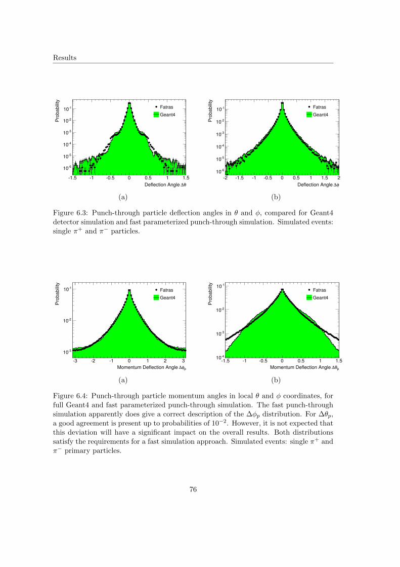
Results
θ∆Deflection Angle
1.5 1 0.5 0 0.5 1 1.5
Pro
ba
bili
ty
610
510
410
310
210
110 Fatras
Geant4
(a)
φ∆Deflection Angle
2 1.5 1 0.5 0 0.5 1 1.5 2
Pro
ba
bili
ty
610
510
410
310
210
110Fatras
Geant4
(b)
Figure 6.3: Punch-through particle deflection angles in θ and φ, compared for Geant4detector simulation and fast parameterized punch-through simulation. Simulated events:single π+ and π− particles.
pφ∆Momentum Deflection Angle
3 2 1 0 1 2 3
Pro
ba
bili
ty
310
210
110 Fatras
Geant4
(a)
pθ∆Momentum Deflection Angle
1.5 1 0.5 0 0.5 1 1.5
Pro
ba
bili
ty
410
310
210
110Fatras
Geant4
(b)
Figure 6.4: Punch-through particle momentum angles in local θ and φ coordinates, forfull Geant4 and fast parameterized punch-through simulation. The fast punch-throughsimulation apparently does give a correct description of the ∆φp distribution. For ∆θp,a good agreement is present up to probabilities of 10−2. However, it is not expected thatthis deviation will have a significant impact on the overall results. Both distributionssatisfy the requirements for a fast simulation approach. Simulated events: single π+ andπ− primary particles.
76
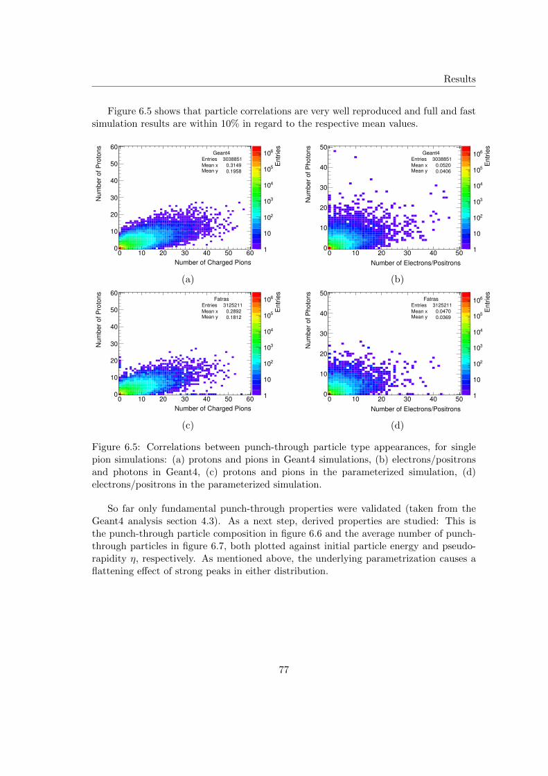
Results
Figure 6.5 shows that particle correlations are very well reproduced and full and fastsimulation results are within 10% in regard to the respective mean values.
En
trie
s
1
10
210
310
410
510
610
Number of Charged Pions
0 10 20 30 40 50 60
Nu
mb
er
of
Pro
ton
s
0
10
20
30
40
50
60Geant4
Entries 3038851
Mean x 0.3149Mean y 0.1958
(a)
En
trie
s
1
10
210
310
410
510
610
Number of Electrons/Positrons
0 10 20 30 40 50
Nu
mb
er
of
Ph
oto
ns
0
10
20
30
40
50Geant4
Entries 3038851
Mean x 0.0520Mean y 0.0406
(b)E
ntr
ies
1
10
210
310
410
510
610
Number of Charged Pions
0 10 20 30 40 50 60
Nu
mb
er
of
Pro
ton
s
0
10
20
30
40
50
60Fatras
Entries 3125211
Mean x 0.2892Mean y 0.1812
(c)
En
trie
s
1
10
210
310
410
510
610
Number of Electrons/Positrons
0 10 20 30 40 50
Nu
mb
er
of
Ph
oto
ns
0
10
20
30
40
50Fatras
Entries 3125211
Mean x 0.0470Mean y 0.0369
(d)
Figure 6.5: Correlations between punch-through particle type appearances, for singlepion simulations: (a) protons and pions in Geant4 simulations, (b) electrons/positronsand photons in Geant4, (c) protons and pions in the parameterized simulation, (d)electrons/positrons in the parameterized simulation.
So far only fundamental punch-through properties were validated (taken from theGeant4 analysis section 4.3). As a next step, derived properties are studied: This isthe punch-through particle composition in figure 6.6 and the average number of punch-through particles in figure 6.7, both plotted against initial particle energy and pseudo-rapidity η, respectively. As mentioned above, the underlying parametrization causes aflattening effect of strong peaks in either distribution.
77
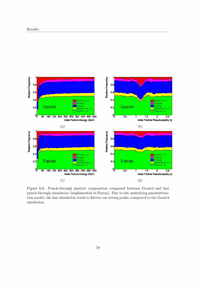
Results
Initial Particle Energy (GeV)
0 50 100 150 200 250 300 350 400 450 500
Re
lative
Fre
qu
en
cy
0
0.2
0.4
0.6
0.8
1
Initial Particle Energy (GeV)
0 50 100 150 200 250 300 350 400 450 500
Re
lative
Fre
qu
en
cy
0
0.2
0.4
0.6
0.8
1
Initial Particle Energy (GeV)
0 50 100 150 200 250 300 350 400 450 500
Re
lative
Fre
qu
en
cy
0
0.2
0.4
0.6
0.8
1
)µ, +µMuons (
Photons
Protons), e
+Electrons (e
)π, +πPions (
Geant4
(a)
|ηInitial Particle Pseudorapidity |
0 0.5 1 1.5 2 2.5
Re
lative
Fre
qu
en
cy
0
0.2
0.4
0.6
0.8
1
|ηInitial Particle Pseudorapidity |
0 0.5 1 1.5 2 2.5
Re
lative
Fre
qu
en
cy
0
0.2
0.4
0.6
0.8
1
|ηInitial Particle Pseudorapidity |
0 0.5 1 1.5 2 2.5
Re
lative
Fre
qu
en
cy
0
0.2
0.4
0.6
0.8
1
)µ, +µMuons (
Photons
Protons), e
+Electrons (e
)π, +πPions (
Geant4
(b)
Initial Particle Energy (GeV)
0 50 100 150 200 250 300 350 400 450 500
Re
lative
Fre
qu
en
cy
0
0.2
0.4
0.6
0.8
1
Initial Particle Energy (GeV)
0 50 100 150 200 250 300 350 400 450 500
Re
lative
Fre
qu
en
cy
0
0.2
0.4
0.6
0.8
1
Initial Particle Energy (GeV)
0 50 100 150 200 250 300 350 400 450 500
Re
lative
Fre
qu
en
cy
0
0.2
0.4
0.6
0.8
1
Fatras
)µ, +µMuons (
Photons
Protons), e
+Electrons (e
)π, +πPions (
(c)
|ηInitial Particle Pseudorapidity |
0 0.5 1 1.5 2 2.5
Re
lative
Fre
qu
en
cy
0
0.2
0.4
0.6
0.8
1
|ηInitial Particle Pseudorapidity |
0 0.5 1 1.5 2 2.5
Re
lative
Fre
qu
en
cy
0
0.2
0.4
0.6
0.8
1
|ηInitial Particle Pseudorapidity |
0 0.5 1 1.5 2 2.5
Re
lative
Fre
qu
en
cy
0
0.2
0.4
0.6
0.8
1
)µ, +µMuons (
Photons
Protons
), e+
Electrons (e
)π, +πPions (
Fatras
(d)
Figure 6.6: Punch-through particle composition compared between Geant4 and fastpunch-through simulation (implemented in Fatras). Due to the underlying parametriza-tion model, the fast simulation tends to flatten out strong peaks, compared to the Geant4simulation.
78
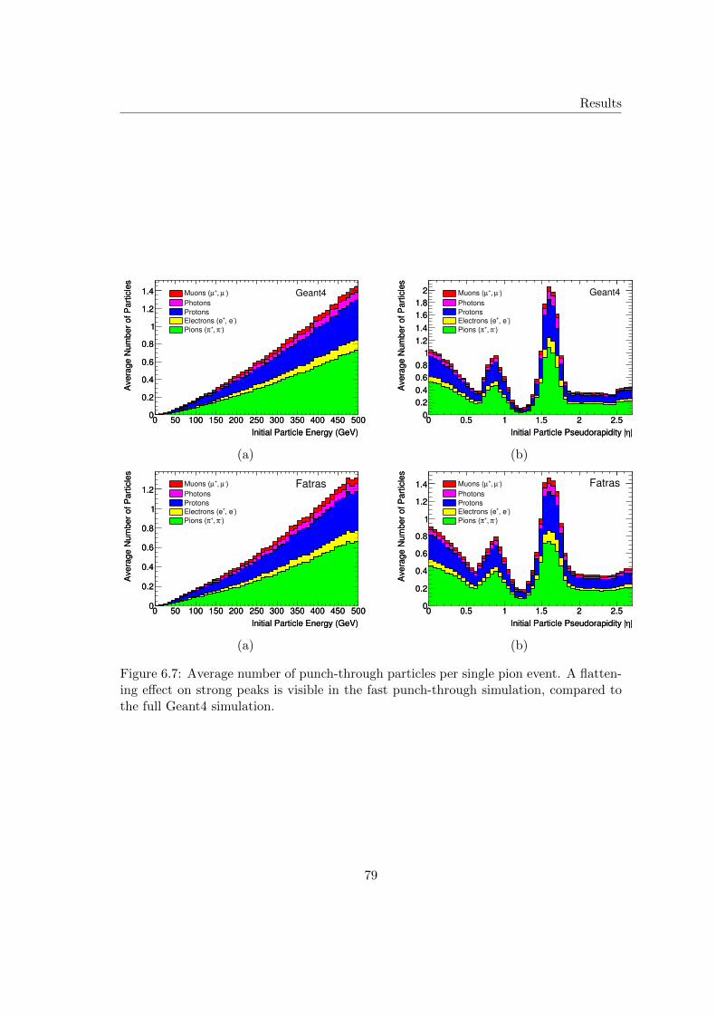
Results
Initial Particle Energy (GeV)
0 50 100 150 200 250 300 350 400 450 500
Ave
rag
e N
um
be
r o
f P
art
icle
s
0
0.2
0.4
0.6
0.8
1
1.2
1.4
Initial Particle Energy (GeV)
0 50 100 150 200 250 300 350 400 450 500
Ave
rag
e N
um
be
r o
f P
art
icle
s
0
0.2
0.4
0.6
0.8
1
1.2
1.4 )µ, +µMuons (
Photons
Protons), e
+Electrons (e
)π, +πPions (
Geant4
(a)
|ηInitial Particle Pseudorapidity |
0 0.5 1 1.5 2 2.5
Ave
rag
e N
um
be
r o
f P
art
icle
s
0
0.2
0.4
0.6
0.8
1
1.2
1.4
1.6
1.8
2
|ηInitial Particle Pseudorapidity |
0 0.5 1 1.5 2 2.5
Ave
rag
e N
um
be
r o
f P
art
icle
s
0
0.2
0.4
0.6
0.8
1
1.2
1.4
1.6
1.8
2 )µ, +µMuons (
Photons
Protons), e
+Electrons (e
)π, +πPions (
Geant4
(b)
Initial Particle Energy (GeV)
0 50 100 150 200 250 300 350 400 450 500
Ave
rag
e N
um
be
r o
f P
art
icle
s
0
0.2
0.4
0.6
0.8
1
1.2
Initial Particle Energy (GeV)
0 50 100 150 200 250 300 350 400 450 500
Ave
rag
e N
um
be
r o
f P
art
icle
s
0
0.2
0.4
0.6
0.8
1
1.2)µ, +
µMuons (
Photons
Protons), e
+Electrons (e
)π, +πPions (
Fatras
(a)
|ηInitial Particle Pseudorapidity |
0 0.5 1 1.5 2 2.5
Ave
rag
e N
um
be
r o
f P
art
icle
s
0
0.2
0.4
0.6
0.8
1
1.2
1.4
|ηInitial Particle Pseudorapidity |
0 0.5 1 1.5 2 2.5
Ave
rag
e N
um
be
r o
f P
art
icle
s
0
0.2
0.4
0.6
0.8
1
1.2
1.4 )µ, +µMuons (
Photons
Protons
), e+
Electrons (e
)π, +πPions (
Fatras
(b)
Figure 6.7: Average number of punch-through particles per single pion event. A flatten-ing effect on strong peaks is visible in the fast punch-through simulation, compared tothe full Geant4 simulation.
79
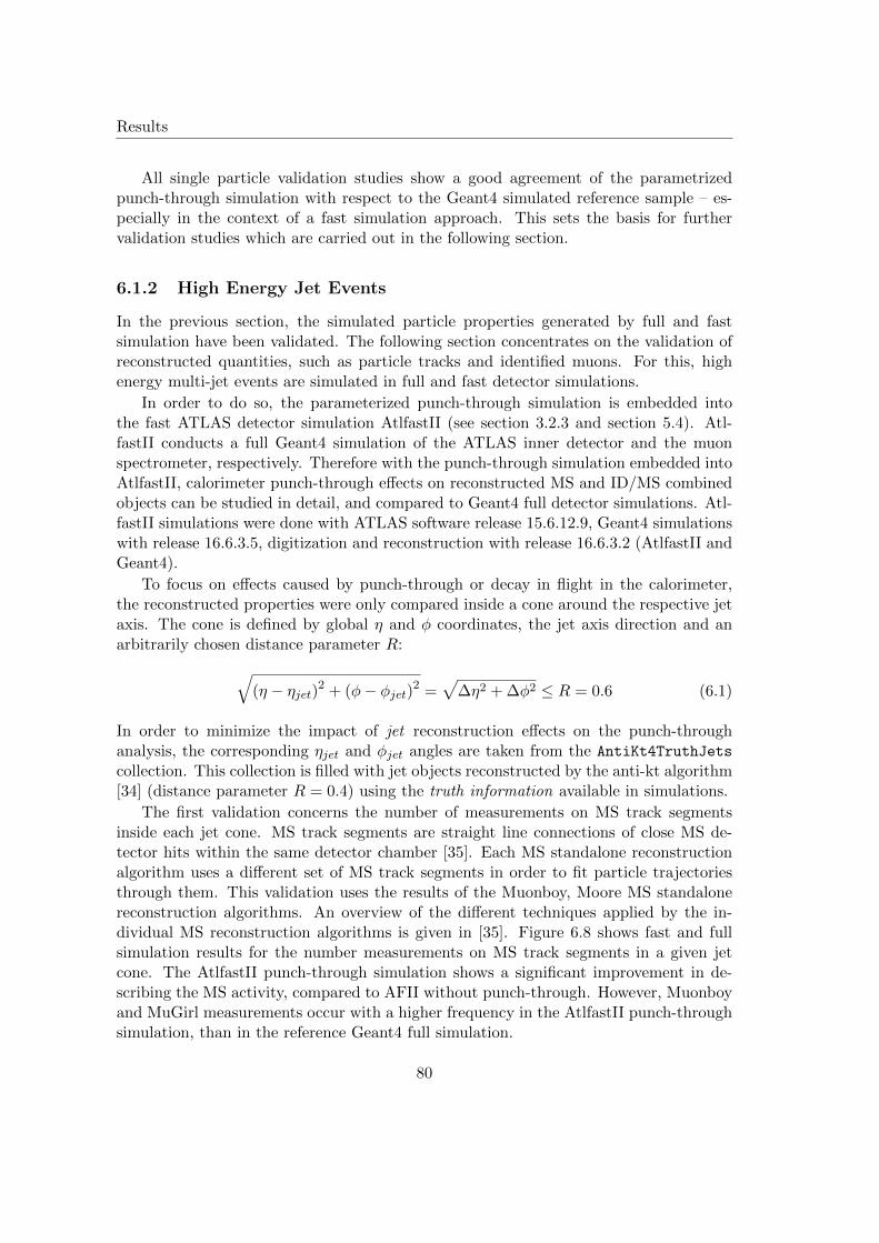
Results
All single particle validation studies show a good agreement of the parametrizedpunch-through simulation with respect to the Geant4 simulated reference sample – es-pecially in the context of a fast simulation approach. This sets the basis for furthervalidation studies which are carried out in the following section.
6.1.2 High Energy Jet Events
In the previous section, the simulated particle properties generated by full and fastsimulation have been validated. The following section concentrates on the validation ofreconstructed quantities, such as particle tracks and identified muons. For this, highenergy multi-jet events are simulated in full and fast detector simulations.
In order to do so, the parameterized punch-through simulation is embedded intothe fast ATLAS detector simulation AtlfastII (see section 3.2.3 and section 5.4). Atl-fastII conducts a full Geant4 simulation of the ATLAS inner detector and the muonspectrometer, respectively. Therefore with the punch-through simulation embedded intoAtlfastII, calorimeter punch-through effects on reconstructed MS and ID/MS combinedobjects can be studied in detail, and compared to Geant4 full detector simulations. Atl-fastII simulations were done with ATLAS software release 15.6.12.9, Geant4 simulationswith release 16.6.3.5, digitization and reconstruction with release 16.6.3.2 (AtlfastII andGeant4).
To focus on effects caused by punch-through or decay in flight in the calorimeter,the reconstructed properties were only compared inside a cone around the respective jetaxis. The cone is defined by global η and φ coordinates, the jet axis direction and anarbitrarily chosen distance parameter R:√
(η − ηjet)2 + (φ− φjet)2 =√
∆η2 + ∆φ2 ≤ R = 0.6 (6.1)
In order to minimize the impact of jet reconstruction effects on the punch-throughanalysis, the corresponding ηjet and φjet angles are taken from the AntiKt4TruthJets
collection. This collection is filled with jet objects reconstructed by the anti-kt algorithm[34] (distance parameter R = 0.4) using the truth information available in simulations.
The first validation concerns the number of measurements on MS track segmentsinside each jet cone. MS track segments are straight line connections of close MS de-tector hits within the same detector chamber [35]. Each MS standalone reconstructionalgorithm uses a different set of MS track segments in order to fit particle trajectoriesthrough them. This validation uses the results of the Muonboy, Moore MS standalonereconstruction algorithms. An overview of the different techniques applied by the in-dividual MS reconstruction algorithms is given in [35]. Figure 6.8 shows fast and fullsimulation results for the number measurements on MS track segments in a given jetcone. The AtlfastII punch-through simulation shows a significant improvement in de-scribing the MS activity, compared to AFII without punch-through. However, Muonboyand MuGirl measurements occur with a higher frequency in the AtlfastII punch-throughsimulation, than in the reference Geant4 full simulation.
80
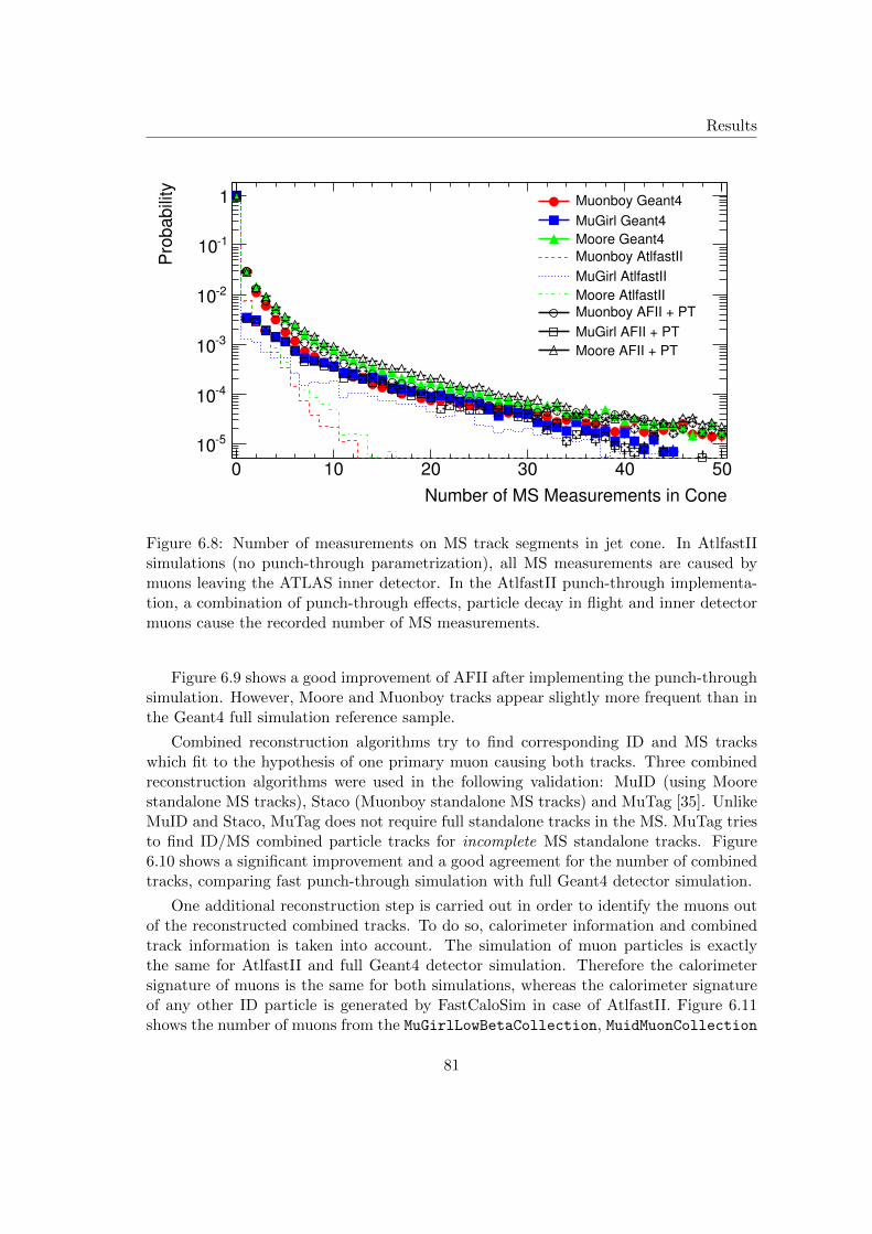
Results
Number of MS Measurements in Cone
0 10 20 30 40 50
Pro
ba
bili
ty
510
410
310
210
110
1 Muonboy Geant4
MuGirl Geant4
Moore Geant4
Muonboy AtlfastII
MuGirl AtlfastII
Moore AtlfastII
Muonboy AFII + PT
MuGirl AFII + PT
Moore AFII + PT
Figure 6.8: Number of measurements on MS track segments in jet cone. In AtlfastIIsimulations (no punch-through parametrization), all MS measurements are caused bymuons leaving the ATLAS inner detector. In the AtlfastII punch-through implementa-tion, a combination of punch-through effects, particle decay in flight and inner detectormuons cause the recorded number of MS measurements.
Figure 6.9 shows a good improvement of AFII after implementing the punch-throughsimulation. However, Moore and Muonboy tracks appear slightly more frequent than inthe Geant4 full simulation reference sample.
Combined reconstruction algorithms try to find corresponding ID and MS trackswhich fit to the hypothesis of one primary muon causing both tracks. Three combinedreconstruction algorithms were used in the following validation: MuID (using Moorestandalone MS tracks), Staco (Muonboy standalone MS tracks) and MuTag [35]. UnlikeMuID and Staco, MuTag does not require full standalone tracks in the MS. MuTag triesto find ID/MS combined particle tracks for incomplete MS standalone tracks. Figure6.10 shows a significant improvement and a good agreement for the number of combinedtracks, comparing fast punch-through simulation with full Geant4 detector simulation.
One additional reconstruction step is carried out in order to identify the muons outof the reconstructed combined tracks. To do so, calorimeter information and combinedtrack information is taken into account. The simulation of muon particles is exactlythe same for AtlfastII and full Geant4 detector simulation. Therefore the calorimetersignature of muons is the same for both simulations, whereas the calorimeter signatureof any other ID particle is generated by FastCaloSim in case of AtlfastII. Figure 6.11shows the number of muons from the MuGirlLowBetaCollection, MuidMuonCollection
81
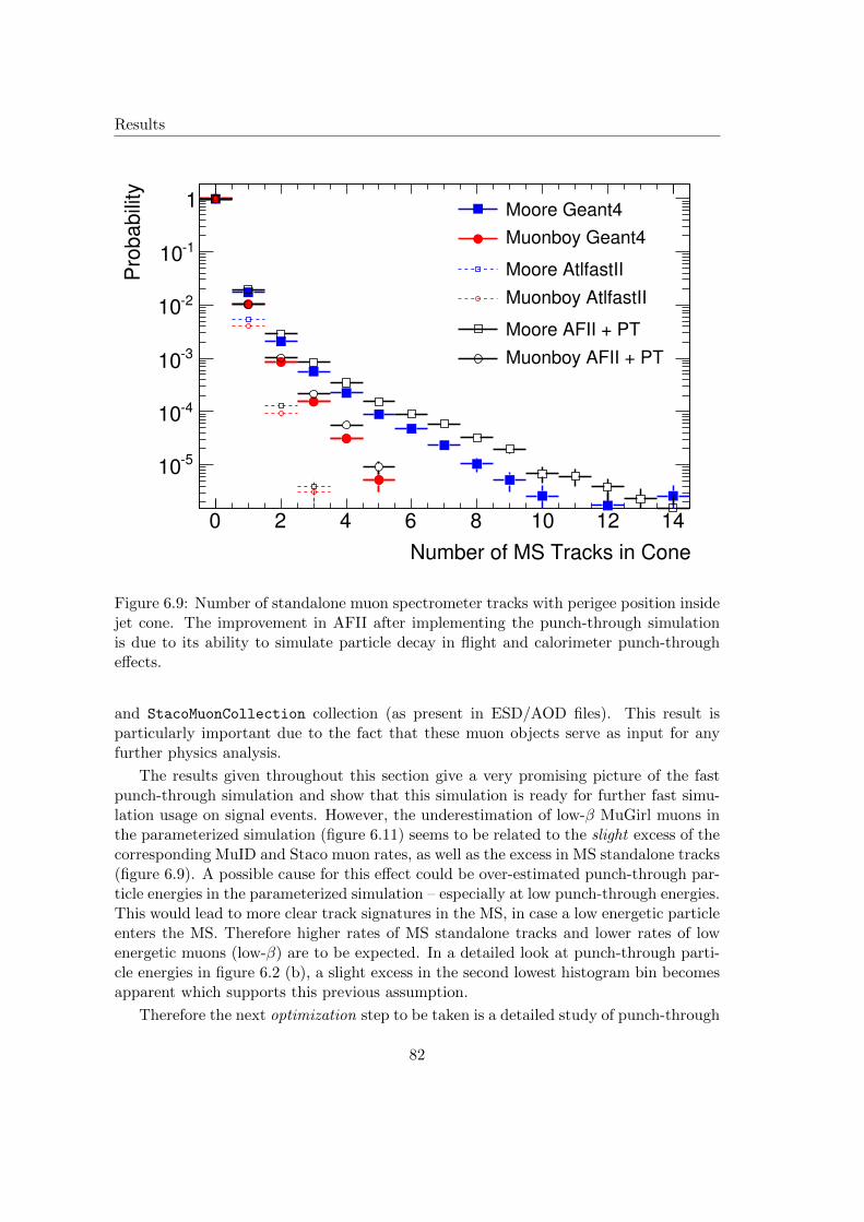
Results
Number of MS Tracks in Cone
0 2 4 6 8 10 12 14
Pro
ba
bili
ty
510
410
310
210
110
1 Moore Geant4
Muonboy Geant4
Moore AtlfastII
Muonboy AtlfastII
Moore AFII + PT
Muonboy AFII + PT
Figure 6.9: Number of standalone muon spectrometer tracks with perigee position insidejet cone. The improvement in AFII after implementing the punch-through simulationis due to its ability to simulate particle decay in flight and calorimeter punch-througheffects.
and StacoMuonCollection collection (as present in ESD/AOD files). This result isparticularly important due to the fact that these muon objects serve as input for anyfurther physics analysis.
The results given throughout this section give a very promising picture of the fastpunch-through simulation and show that this simulation is ready for further fast simu-lation usage on signal events. However, the underestimation of low-β MuGirl muons inthe parameterized simulation (figure 6.11) seems to be related to the slight excess of thecorresponding MuID and Staco muon rates, as well as the excess in MS standalone tracks(figure 6.9). A possible cause for this effect could be over-estimated punch-through par-ticle energies in the parameterized simulation – especially at low punch-through energies.This would lead to more clear track signatures in the MS, in case a low energetic particleenters the MS. Therefore higher rates of MS standalone tracks and lower rates of lowenergetic muons (low-β) are to be expected. In a detailed look at punch-through parti-cle energies in figure 6.2 (b), a slight excess in the second lowest histogram bin becomesapparent which supports this previous assumption.
Therefore the next optimization step to be taken is a detailed study of punch-through
82
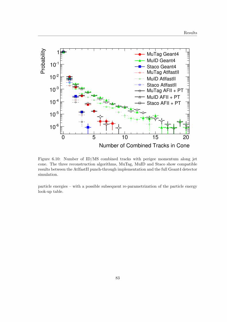
Results
Number of Combined Tracks in Cone
0 5 10 15 20
Pro
ba
bili
ty
610
510
410
310
210
110
1 MuTag Geant4
MuID Geant4
Staco Geant4MuTag AtlfastII
MuID AtlfastII
Staco AtlfastIIMuTag AFII + PT
MuID AFII + PT
Staco AFII + PT
Figure 6.10: Number of ID/MS combined tracks with perigee momentum along jetcone. The three reconstruction algorithms, MuTag, MuID and Staco show compatibleresults between the AtlfastII punch-through implementation and the full Geant4 detectorsimulation.
particle energies – with a possible subsequent re-parametrization of the particle energylook-up table.
83
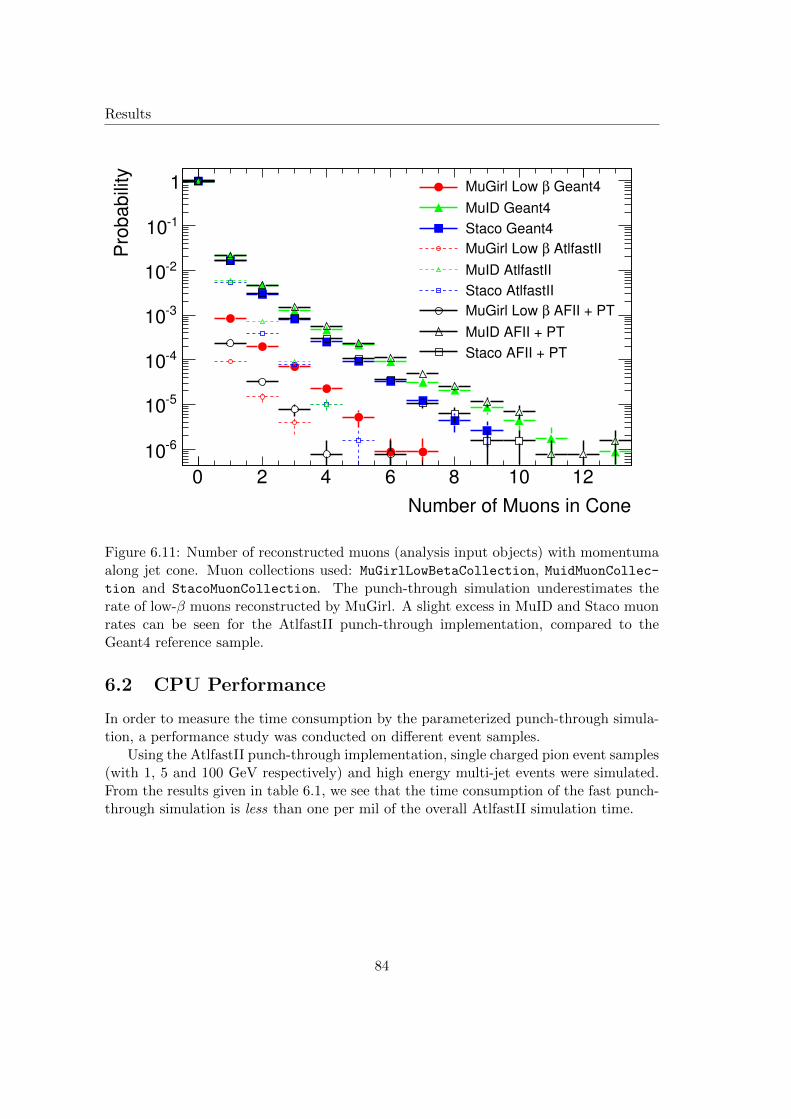
Results
Number of Muons in Cone
0 2 4 6 8 10 12
Pro
ba
bili
ty
610
510
410
310
210
110
1 Geant4βMuGirl Low
MuID Geant4
Staco Geant4
AtlfastIIβMuGirl Low
MuID AtlfastII
Staco AtlfastII
AFII + PTβMuGirl Low
MuID AFII + PT
Staco AFII + PT
Figure 6.11: Number of reconstructed muons (analysis input objects) with momentumaalong jet cone. Muon collections used: MuGirlLowBetaCollection, MuidMuonCollec-tion and StacoMuonCollection. The punch-through simulation underestimates therate of low-β muons reconstructed by MuGirl. A slight excess in MuID and Staco muonrates can be seen for the AtlfastII punch-through implementation, compared to theGeant4 reference sample.
6.2 CPU Performance
In order to measure the time consumption by the parameterized punch-through simula-tion, a performance study was conducted on different event samples.
Using the AtlfastII punch-through implementation, single charged pion event samples(with 1, 5 and 100 GeV respectively) and high energy multi-jet events were simulated.From the results given in table 6.1, we see that the time consumption of the fast punch-through simulation is less than one per mil of the overall AtlfastII simulation time.
84
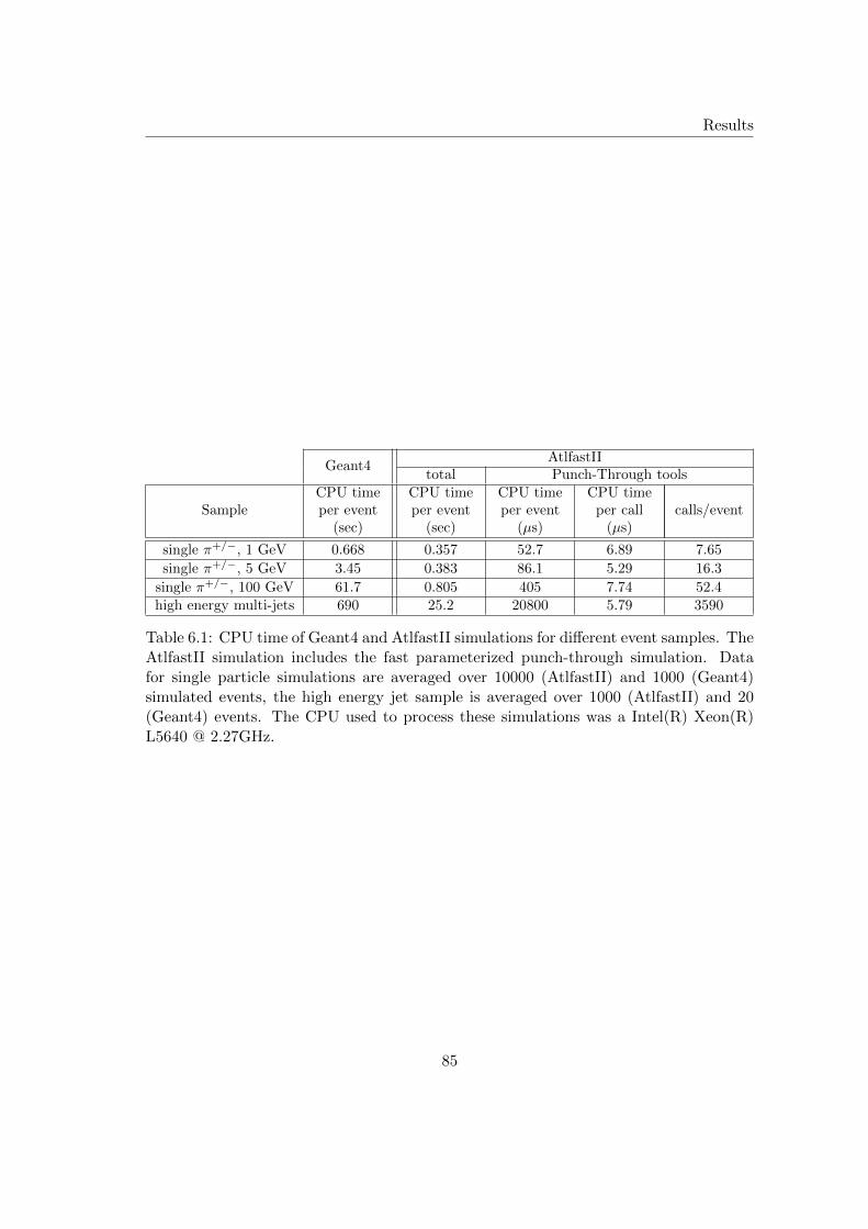
Results
Geant4AtlfastII
total Punch-Through tools
SampleCPU timeper event
(sec)
CPU timeper event
(sec)
CPU timeper event
(µs)
CPU timeper call
(µs)calls/event
single π+/−, 1 GeV 0.668 0.357 52.7 6.89 7.65
single π+/−, 5 GeV 3.45 0.383 86.1 5.29 16.3
single π+/−, 100 GeV 61.7 0.805 405 7.74 52.4high energy multi-jets 690 25.2 20800 5.79 3590
Table 6.1: CPU time of Geant4 and AtlfastII simulations for different event samples. TheAtlfastII simulation includes the fast parameterized punch-through simulation. Datafor single particle simulations are averaged over 10000 (AtlfastII) and 1000 (Geant4)simulated events, the high energy jet sample is averaged over 1000 (AtlfastII) and 20(Geant4) events. The CPU used to process these simulations was a Intel(R) Xeon(R)L5640 @ 2.27GHz.
85

Chapter 7
Conclusion and Outlook
The parameterized simulation approach taken in this work proves its effectiveness andcompatibility in almost every aspect. ATLAS calorimeter punch-through and particledecay in flight effects are parameterized based on a set of full Geant4 simulated singlepion events (section 4.4). A fast simulation using this parametrization was integratedinto the fast ATLAS detector simulation AtlfastII and Fatras (chapter 5). The resultsobtained from validation studies on single particle events describe the effects from thereference full Geant4 simulation to great detail (chapter 6). However, some deviationscan be seen in the fast simulation due to statistical limitations in the reference sampleused to compute the parametrization. The currently implemented description of particlecorrelations also results in some differences between fast and full simulation. Anyhow,at the current stage of this fast simulation, these differences are negligible and they donot show any significant impact on the results obtained in signal events.
The validation carried out on high energy multi-jet events gives a significant improve-ment of reconstructed muon particles due to the implemented punch-through simulation(section 6.1.2). The number of muons reconstructed by MuID and Staco combined re-construction algorithms almost match with the Geant4 reference sample. This allowsfor the first time to include fake muon signatures or muons from decay in flight in thecalorimeter in ATLAS fast simulation studies. Thus, it boosts the accuracy with whichthe MS response is described by fast simulations (figure 6.11). Only low-β MuGirl re-constructed muons are still underestimated in the punch-through simulation. A possibleexplanation is an insufficient description of low energetic punch-through particles. Thisis motivated by the observation that the fast simulation overestimates the appearance ofstandalone MS tracks. Therefore, further improvements of the punch-through simulationmight concern a re-parametrization of punch-through particle energies.
Currently the simulation does not take care of correlations with any calorimetervariable. Therefore in one next step, obvious correlations such as the total energy de-posited in the calorimeter might be studied, parameterized and implemented into thepunch-through simulation.
Automated (fit) procedures were implemented, in order to fill the look-up table withthe parameters extracted from a given reference sample. This setup also allows for a
87
Conclusion and Outlook
fast re-parametrization of the punch-through simulation and offers an easy way to addnew variables to the parametrization (e.g. energy deposited in calorimeter system).
The implemented simulation is independent of any particular ATLAS detector sim-ulation. Hence, the punch-through simulation can easily be implemented into any newsimulation framework, such as the integrated simulation framework (ISF) which is cur-rently under development.
Since the comparison to Geant4 shows remarkable results, a comparison of the fastpunch-through simulation with data will be the next important step to be taken.
88
Appendix A
The Look-up Table
The parameters for the Fatras punch-through simulation are stored in one single ROOTfile, which is referred to as look-up table. The look-up table’s structure allows for maxi-mum flexibility regarding further improvements of the simulation – such as adding outputparameters or changing the number of input parameters for parameterized distributionfunctions.
The ROOT file contains a TDirectory ROOT class for each respective output pa-rameter. This TDirectory holds all relations which are necessary to compute the cor-responding output parameter, depending on a set of input parameters. In the currentimplementation, these TDirectories are divided into two categories:
• parametrization input for the PDFCreator random number generator (see section5.2)
• particle type correlations
Each of the two types is discussed in the following sections.
A.1 Input for the Fatras::PDFcreator C++ Class
This is the common method to store the parametrization for the fast punch-throughsimulation. The TDirectory content is closely related to the Fatras::PDFcreator’sfunction. The look-up table contains the following set of parametrizations for eachrespective punch-through particle type:
• number of punch-through particles (named: NumExitPDG...)
• punch-through particle energy (named: ExitEnergyPDG...)
• deflection angle ∆θ (named: ExitDeltaThetaPDG...)
• deflection angle ∆φ (named: ExitDeltaPhiPDG...)
• momentum angle ∆θp (named: MomDeltaThetaPDG...)
89
The Look-up Table
• momentum angle ∆φp (named: MomDeltaPhiPDG...)
The trailing full stops will be replaced by the the absolute value of the correspondingMonte Carlo particle number: e.g. electrons (11) and positrons (−11) together useNumExitPDG11, ExitEnergyPDG11, ExitDeltaThetaPDG11, ...
Section 4.4 describes how each individual parameter is determined and section 4.5explains the runtime access on the corresponding parametrization.
Each directory contains a TF1::function instance, which stores the distributionfunction for the corresponding output parameter. Usually, this function has as a num-ber of function parameters. The numerical values for these parameters are stored inTH1,TH2 or TH3 compatible ROOT histogram classes, also contained within the samedirectory. Their name follows the convention: parameterx, where ’x’ is replaced bythe corresponding function parameter number. By using ROOT histogram classes, onecan conveniently store different function parameter values for different input parameterintervals. Therefore each input parameter corresponds to one axis in all parameterxROOT histograms. The function parameter value is stored as the histogram contentin the respective bin. In other words, each function parameter can be interpreted as amulti-dimensional scalar field, where the coordinates are represented by the input pa-rameter values and the function parameter values are the histogram’s content at thecorresponding coordinates. All parameterx histograms within the same TDirectory (=of the same output parameter) are required to have the same dimension. Therefore allfunction parameters will have dependencies on the same set of input parameters.
Additionally randmin and randmax ROOT histograms are stored within each TDi-
rectory. Their dependency on the input parameters is the same as for the parameterxhistograms. The Fatras::PDFcreator ensures that the each determined parametervalue lies within the respective range given by the randmin and randmax histograms.
In the current implementation of the parametrized punch-through simulation, theparametrizations only depend on up to two input parameters. Therefore only two-dimensional parameterx, randmin and randmax histograms are used.
A.2 Particle Type Correlations
The punch-through particle type correlations are stored in the NumExitCorrelations
directory. The parameterized punch-through simulation is able to compute correlationsbetween pairs of different particle types. Thus, each punch-through particle type canhave up to one correlated particle type.
Two dimensional ROOT TH2 histograms are used to store these pair correlations.These histograms represent, what is described as correlation matrices in section 4.4.3.The histograms have to be named according to the scheme: x PDGa y PDGb lowE or x -
PDGa y PDGb highE. a and b are replaced by the absolute value of the correspondingMonte Carlo particle number. The trailing lowE or highE string defines whethercorrelations for either low or high energetic incoming particles are described.
The naming convention motivates the fact that each particle type is represented by
90
The Look-up Table
one axis in the histograms. As mentioned in section 4.4.3, each correlation is storedtwice, but with mirrored axes.
As an example, the correlation histograms between electrons (11) and photons (22)are named: x PDG22 y PDG11 lowE, x PDG22 y PDG11 highE, x PDG11 y PDG22 -
lowE and x PDG11 y PDG22 highE.
91

Appendix B
CaloEntry and MuonEntry
The CaloEntry and MuonEntry surfaces are widely used throughout this work. TheCaloEntry layer surrounds the ATLAS inner detector, whereas the MuonEntry layer en-closes the whole ATLAS calorimeter. Furthermore, both layers do not cross any sensitivedetector parts. Therefore they are a perfect choice as interface surface between differentsub-detector simulations, such as ID/Calo (CaloEntry) and Calo/MS (MuonEntry).
Both are used as reference surfaces for the parametrized punch-through simulation.The simulation’s parametrization requires its input particles to be positioned on theCaloEntry layer surface, the resulting simulation output particles will be positioned onthe MuonEntry layer.
Figure B.1 gives the dimensions of each layer.Both, Fatras and the full Geant4 detector simulation create TrackRecordCollec-
tions of simulated truth particles crossing either of the surfaces.
93
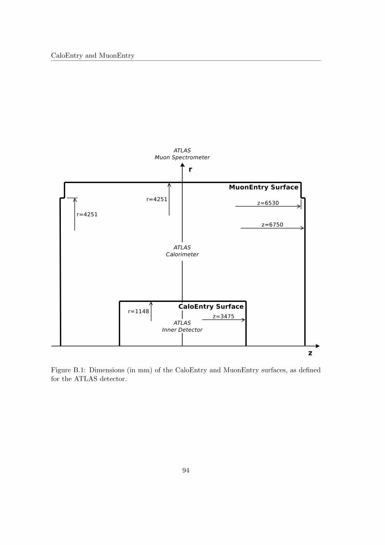
CaloEntry and MuonEntry
Figure B.1: Dimensions (in mm) of the CaloEntry and MuonEntry surfaces, as definedfor the ATLAS detector.
94
Bibliography
[1] Bruno Lenzi. Search for the standard model higgs boson decaying to four lepton(muon, electron) final states with the atlas experiment at the lhc collider. TechnicalReport arXiv:0808.0162, Aug 2008. Comments: Poster presented at the HadronCollider Physics Symposium (HCP2008), Galena, Illinois, USA, May 27-31, 2008;5 pages, LaTeX, 11 eps figures.
[2] P Jussel. Inclusive b-jet production in atlas. Technical Report ATL-PHYS-PROC-2011-099, CERN, Geneva, Aug 2011.
[3] The ATLAS Collaboration. The ATLAS Experiment at the CERN Large HadronCollider. Aug 2008.
[4] Jean-Luc Caron. Layout of the lep tunnel including future lhc infrastructures. ACCollection. Legacy of AC. Pictures from 1992 to 2002., Feb 1997.
[5] A Salzburger. Track Simulation and Reconstruction in the ATLAS experiment. Mar2008.
[6] C.Y. Wong. Introduction to high-energy heavy-ion collisions. World Scientific, 1994.
[7] Jan-Philip Gehrcke. ATLAS Software: How to run The Full Chain. http://http://gehrcke.de/2009/06/atlas-software-how-to-run-the-full-chain/, July2011.
[8] The ATLAS Collaboration. The ATLAS Simulation Infrastructure. The EuropeanPhysical Journal C - Particles and Fields, 70:823–874, 2010. 10.1140/epjc/s10052-010-1429-9.
[9] ATLAS computing: Technical Design Report. Technical Design Report ATLAS.CERN, Geneva, 2005. revised version submitted on 2005-06-20 16:33:46.
[10] The ATLAS Collaboration. ATLAS TWiki. https://twiki.cern.ch/twiki/bin/view/Atlas/WebHome, July 2011.
[11] The Geant4 Collaboration. Geant4–a simulation toolkit. Nuclear Instruments andMethods in Physics Research Section A: Accelerators, Spectrometers, Detectors andAssociated Equipment, 506(3):250 – 303, 2003.
95
Bibliography
[12] T Sjstrand, S Mrenna, and P Z Skands. Pythia 6.4 physics and manual. J. HighEnergy Phys., 05(hep-ph/0603175. FERMILAB-Pub-2006-052-CD-T. LU-TP-2006-13):026. 570 p, Mar 2006.
[13] Gennaro Corcella, I G Knowles, G Marchesini, S Moretti, K Odagiri, Peter Richard-son, Michael H Seymour, and Bryan R Webber. Herwig 6.5 release note. herwig6.5. Technical Report hep-ph/0210213. CAVENDISH-HEP-2002-17. CERN-TH-2002-270. DAMTP-2002-124. IPPP-2002-58, CERN, Geneva, Oct 2002.
[14] The ATLAS Collaboration. Charged-particle multiplicities in pp interactions at√s = 900 gev measured with the atlas detector at the lhc. Physics Letters B,
688(1):21 – 42, 2010.
[15] Matteo Volpi. Charged particle multiplicities in pp interactions at sqrt(s) =900 GeV and sqrt(s) = 7 TeV measured with the ATLAS detector at the LHC..oai:cds.cern.ch:1331501. PhD thesis, Barcelona, IFAE, Barcelona, 2010. Presented16 Dec 2010.
[16] T Yamanaka. The atlas calorimeter simulation fastcalosim. Technical Report ATL-SOFT-PROC-2011-021, CERN, Geneva, Jan 2011.
[17] K Edmonds, S Fleischmann, T Lenz, C Magass, J Mechnich, and A Salzburger.The Fast ATLAS Track Simulation (FATRAS). Technical Report ATL-SOFT-PUB-2008-001. ATL-COM-SOFT-2008-002, CERN, Geneva, Mar 2008.
[18] A Salzburger, S Todorova, and M Wolter. The atlas tracking geometry description.Technical Report ATL-SOFT-PUB-2007-004. ATL-COM-SOFT-2007-009, CERN,Geneva, Jun 2007.
[19] The Atlantis Team. Official Atlantis Website. http://www.hep.ucl.ac.uk/atlas/atlantis/, July 2011.
[20] S Hamilton, E Kneringer, W Lukas, E Ritsch, A Salzburger, K Sliwa, S Todorova,J Wetter, and S Zimmermann. The atlas fast track simulation project. TechnicalReport ATL-SOFT-PROC-2011-038, CERN, Geneva, Mar 2011.
[21] A Arce, M Beckingham, M Duehrssen, E Schmidt, M Shapiro, M Venturi, J Virzi,I Vivarelli, M Werner, S Yamamoto, and T Yamanaka. The simulation principle andperformance of the atlas fast calorimeter simulation fastcalosim. Technical ReportATL-COM-PHYS-2010-838, CERN, Geneva, Oct 2010.
[22] B Lenzi. The physics analysis tools project for the atlas experiment. TechnicalReport ATL-COM-SOFT-2009-020, CERN, Geneva, Oct 2009. 23/10/2009.
[23] P Calafiura, C Leggett, D R Quarrie, H Ma, and S Rajagopalan. The storegate:a data model for the atlas software architecture. Technical Report cs.SE/0306089.ATL-SOFT-2003-009, Lawrence Berkeley Nat. Lab., Berkeley, CA, Jun 2003.
96
Bibliography
[24] Richard Wigmans. Calorimetry – Energy Measurement in Particle Physics. Inter-national Series of Monographs on Physics. Oxford University Press, Oxford, 2000.reprinted 2008.
[25] L Garren, I.G. Knowles, S Navas, P Richardson, T Sjostrand, and T Trippe. Montecarlo particle numbering scheme. Technical report, Jun 2006.
[26] Nir Amram and Erez Etzion. Hough Transform Track Reconstruction in the CathodeStrip Chambers in ATLAS. oai:cds.cern.ch:1118033. PhD thesis, Tel Aviv, Tel AvivUniversity, Tel Aviv, 2008. Presented on 19 Mar 2008.
[27] Daniela Salvatore and Giancarlo Susinno. Intensive irradiation studies, mon-itoring and commissioning data analysis on the ATLAS MDT chambers.oai:cds.cern.ch:1125845. PhD thesis, Univ. Calabria, Cosenza, Cosenza, 2007. Pre-sented on 10 Dec 2007.
[28] Nikulin M.S. Greenwood P.E. A Guide to Chi-Squared Testing. John Wiley & Sons,Chichester, 1996.
[29] The ROOT Team. Official ROOT Website. http://root.cern.ch/, May 2011.
[30] Dimitri van Heesch. Official Doxygen. http://www.doxygen.org/, August 2011.
[31] M Steyvers. Computational Statistics with Matlab. http://www.scribd.com/doc/51315212/, March 2010.
[32] Christian P Robert and George Casella. Monte Carlo statistical methods; 2nd ed.Springer texts in statistics. Springer, Berlin, 2005.
[33] The CLHEP Team. CLHEP - A Class Library for High Energy Physics – OfficialWebsite. http://wwwasd.web.cern.ch/wwwasd/lhc++/clhep/, July 2011.
[34] Matteo Cacciari, Gavin P Salam, and Gregory Soyez. The anti-kt jet clusteringalgorithm. J. High Energy Phys., 04(arXiv:0802.1189. LPTHE-07-03):063. 12 p,Feb 2008.
[35] B Resende. Muon identification algorithms in atlas. Technical Report ATL-PHYS-PROC-2009-113, CERN, Geneva, Sep 2009.
97