Simulation of plastic parts considering material and production specific boundary conditions
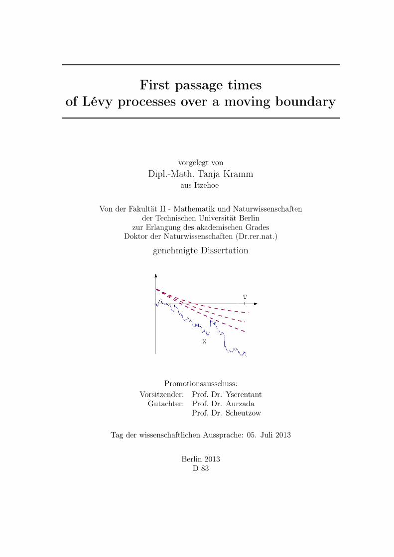
First passage timesof Lévy processes over a moving boundary
vorgelegt vonDipl.-Math. Tanja Kramm
aus Itzehoe
Von der Fakultät II - Mathematik und Naturwissenschaftender Technischen Universität Berlin
zur Erlangung des akademischen GradesDoktor der Naturwissenschaften (Dr.rer.nat.)
genehmigte Dissertation
Promotionsausschuss:Vorsitzender: Prof. Dr. Yserentant
Gutachter: Prof. Dr. AurzadaProf. Dr. Scheutzow
Tag der wissenschaftlichen Aussprache: 05. Juli 2013
Berlin 2013D 83


Acknowledgement
First and foremost, I would like to thank my supervisor, Prof. Dr. Frank Aurzada, for hiscontinued support and numerous discussions. His constructive comments have helped toimprove the presentation of this thesis.Furthermore, it is my pleasure to thank Prof. Dr. Doney and Dr. Savov for their hospi-
tality during the stays at the University of Manchester and at the University of Oxford.I am also grateful to Prof. Dr. Lifshits for valuable discussions.In addition, I would like to thank the professors in the examining board.My appreciation to my friends for their encouragement, their assistance in reviewing
this thesis and especially for making my life more enjoyable.Last but not least, I am greatly indebted to my family, to whom I owe so much.
3

Summary
In this thesis we study first passage times of Lévy processes over a moving boundary. Fora stochastic process and a deterministic function (the so-called moving boundary) thefirst passage time is the first time that the process crosses the moving boundary. Themain focus of the present work is on comparing the asymptotic behaviour of these passagetimes of constant and moving boundaries. In this context two different types of problemsare considered.
First, we look at the asymptotic tail behaviour of the distribution of the first passagetime. In particular, we concentrate on finding necessary and sufficient conditions for themoving boundary such that the asymptotic tail behaviours for a constant and a movingboundary have the same asymptotic polynomial order.This question is answered by Uchiyama (1980) for Brownian motion which is a simple
example of a Lévy process. In Chapter 3 we revisit this result and provide an elementaryproof in the case of a decreasing boundary. There is hope that our proof can be generalisedto other processes in contrast to former ones.Subsequently, we study general Lévy processes. Since the fluctuations of a Lévy process
are at least as large as the ones of a Brownian motion, a Lévy process intuitively allowsa larger class of moving boundaries for which the polynomial order remains the same asin the consant case. Our theorems in Chapter 4 formalise this intuition.We then restrict our discussion to asymptotically stable Lévy processes. These processes
are the best-known Lévy processes which fluctuate more than a Brownian motion. Forthis class of Lévy processes it is shown in Chapter 5 that the class of moving boundariesfor which the asymptotic tail behaviour does not change compared to the constant casedepends on the magnitude of the fluctuations of a Lévy process.
The second question concerns the local behaviour of the first passage time over amoving boundary. In Chapter 6 the asymptotic behaviour of the probability that theprocess crosses the moving boundary at a certain time point for the first time is specified.Moreover, we show that a typical path that does not exit a moving boundary is containedin the set of paths not exiting a constant boundary.
5

Contents
1. Introduction 9
2. Preliminaries 172.1. Notation . . . . . . . . . . . . . . . . . . . . . . . . . . . . . . . . . . . . . 172.2. Lévy processes . . . . . . . . . . . . . . . . . . . . . . . . . . . . . . . . . 17
2.2.1. Examples . . . . . . . . . . . . . . . . . . . . . . . . . . . . . . . . 182.2.2. Fluctuation theory . . . . . . . . . . . . . . . . . . . . . . . . . . . 20
2.3. Additive processes . . . . . . . . . . . . . . . . . . . . . . . . . . . . . . . 212.4. The first passage time problem . . . . . . . . . . . . . . . . . . . . . . . . 22
2.4.1. Constant boundaries . . . . . . . . . . . . . . . . . . . . . . . . . . 232.4.2. Moving boundaries . . . . . . . . . . . . . . . . . . . . . . . . . . . 26
3. Tail behaviour of the first passage time over a moving boundary for a Brownianmotion 313.1. New Approach . . . . . . . . . . . . . . . . . . . . . . . . . . . . . . . . . 323.2. Further remarks . . . . . . . . . . . . . . . . . . . . . . . . . . . . . . . . . 39
4. Tail behaviour of the first passage time over a moving boundary for generalLévy processes 434.1. Main results . . . . . . . . . . . . . . . . . . . . . . . . . . . . . . . . . . . 434.2. Auxiliary results . . . . . . . . . . . . . . . . . . . . . . . . . . . . . . . . 45
4.2.1. Technical tools regarding the boundary . . . . . . . . . . . . . . . . 454.2.2. One-sided exit problem with a moving boundary for Brownian motion 464.2.3. One-sided exit problem for Lévy processes . . . . . . . . . . . . . . 474.2.4. Coupling . . . . . . . . . . . . . . . . . . . . . . . . . . . . . . . . 49
4.3. Proof of Theorem 4.1 (negative boundaries) . . . . . . . . . . . . . . . . . 504.3.1. External iteration . . . . . . . . . . . . . . . . . . . . . . . . . . . . 514.3.2. Internal iteration; Proof of (4.12) . . . . . . . . . . . . . . . . . . 52
4.4. Proof of Theorem 4.2 (positive boundaries) . . . . . . . . . . . . . . . . . 614.4.1. Preliminaries . . . . . . . . . . . . . . . . . . . . . . . . . . . . . . 614.4.2. Iteration; Proof of (4.27) . . . . . . . . . . . . . . . . . . . . . . . . 62
4.5. Further remarks . . . . . . . . . . . . . . . . . . . . . . . . . . . . . . . . . 67
5. Tail behaviour of the first passage time over a moving boundary for asymp-totically stable Lévy processes 695.1. Main results . . . . . . . . . . . . . . . . . . . . . . . . . . . . . . . . . . . 695.2. Proof of Theorem 5.1 (decreasing boundaries) . . . . . . . . . . . . . . . . 715.3. Proof of Theorem 5.2 (increasing boundaries) . . . . . . . . . . . . . . . . 72
7
8 Contents
5.4. First passage time of a time-dependent Lévy process . . . . . . . . . . . . 755.4.1. Preliminaries and Notations . . . . . . . . . . . . . . . . . . . . . . 755.4.2. A time-dependent Lévy process over a constant boundary . . . . . 785.4.3. First passage time of a time-dependent subordinator . . . . . . . . 83
6. Local behaviour of the first passage time over a moving boundary for asymp-totically stable random walks 896.1. Main results . . . . . . . . . . . . . . . . . . . . . . . . . . . . . . . . . . . 916.2. Auxiliary results . . . . . . . . . . . . . . . . . . . . . . . . . . . . . . . . 92
6.2.1. Upper estimates for local probabilities . . . . . . . . . . . . . . . . 936.2.2. Tail behaviour of the first passage time . . . . . . . . . . . . . . . . 93
6.3. Proofs . . . . . . . . . . . . . . . . . . . . . . . . . . . . . . . . . . . . . . 946.3.1. Proof of Theorem 6.4 . . . . . . . . . . . . . . . . . . . . . . . . . . 946.3.2. Proof of Theorem 6.5 . . . . . . . . . . . . . . . . . . . . . . . . . . 95
6.4. Discussion and further remarks . . . . . . . . . . . . . . . . . . . . . . . . 96
7. Conclusion 97
A. Appendix 101A.1. Tail behaviour of the first passage time over a linear boundary for asymp-
totically stable Lévy processes . . . . . . . . . . . . . . . . . . . . . . . . . 101
Bibliography 108
1. Introduction
This thesis discusses first passage times of Lévy processes over a moving boundary. Fora stochastic process X and a deterministic function f : [0,∞) → R with f(0) > 0, theso called moving boundary, the first passage time τf is the first time that the process Xcrosses the moving boundary f :
τf := inft ≥ 0 : X(t) > f(t).
The main focus of the present work is on comparing the asymptotic behaviour of firstpassage times over constant and moving boundaries.
In this thesis two different types of problems are considered.First, we look at the asymptotic tail behaviour of the distribution of the first passage
time τf , i.e. the quantity
P(τf > T ), as T →∞. (1.1)
In other words, we study the asymptotic behaviour of the probability that the processstays below the boundary f up to time T , as T converges to infinity. This type of prob-lem is also known as non-exit probabilities in the literature. In general, this probability isasymptotically polynomial of some order −δ. The number δ is called the survival or per-sistence exponent. In the present work we concentrate on finding necessary and sufficientconditions for the moving boundary f such that the non-exit probabilities for a constantand a moving boundary have the same asymptotic polynomial order.The non-exit probability problem is a classical question, which is relevant to a number
of different applications. For instance, it is related to sticky particle systems ([Vys08]),random polynomials ([CD08]), zeros of random polynomials [DPSZ02] and statisticalmechanics as the study of Burger’s equation ([Sin92], [Ber98], [LS04]). We refer to [AS12]and [BMS13] for a recent and comprehensive survey.
The second question concerns the local behaviour of the first passage time of X, i.e.the quantity
P(τf ∈ [T, T + 1)), as T →∞. (1.2)
In this case, we look at the asymptotic behaviour of the probability that the processcrosses the moving boundary f in the interval [T, T + 1) for the first time. In order tostudy this problem we compare the set of paths which cross the moving boundary f in theinterval [T, T + 1) for the first time with set of paths which cross the constant boundaryx in the interval [T, T + 1) for the first time, for which results are known.Contrary to the first problem the local behaviour of the first passage time has only
recently been studied for a constant boundary in [VW09] and [Don12].
9
10 1. Introduction
We come back to the second question after giving a more detailed overview of the firstproblem (1.1). We start by presenting results for Brownian motion before looking atLévy processes. Furthermore, in both cases different kinds of boundaries are discussedbeginning with constant boundaries.
The simplest example is the asymptotic tail behaviour of the distribution of the firstpassage time for a Brownian motion B = (B(t))t≥0 over a constant boundary, i.e. f(t) ≡ xwith x > 0. The supremum sup0≤t≤T B(t) has the same law as |B(T )|, by the reflectionprinciple. From this, results concerning any constant boundary are easily deduced, andwe obtain that
P(τf > T ) = P(B(t) ≤ x, 0 ≤ t ≤ T ) ∼ x√
2
πT−1/2, as T →∞.
For an explanation of notation see Section 2.1.
However, even for a Brownian motion, the question (1.1) involving moving boundariesis non-trivial. The same polynomial order as for a constant boundary is proved in [Bra78]for logarithmically increasing boundaries and subsequently, in [Uch80] for boundariessatisfying an integral test. More precisely, in [Uch80] it is stated under some additionalassumptions that∫ ∞
1|f(t)|t−3/2dt <∞⇐⇒ P(X(t) ≤ f(t), 0 ≤ t ≤ T ) ≈ T−1/2, as T →∞. (1.3)
The proof in [Uch80] is based on comparison lemmas for Brownian non-exit probabili-ties and a time-discretisation technique. Subsequently, a number of different proofs (cf.[Gär82, Nov81c, Nov96]) appeared, simplifying the original arguments. In particular, in[Nov96] an elementary proof for increasing boundaries is given based on a simple appli-cation of Chebyshev’s inequality. To the contrary, in the case of a decreasing boundaryNovikov indicates that “it would be interesting to find an elementary proof of this bound”([Nov96], p. 723).We provide such an elementary proof in Chapter 3 and identify that the integral test
is related to a repulsion effect of the three-dimensional Bessel process. Furthermore,there is hope that this proof can be generalised to other processes such as fractionalBrownian motion. This investigation is joint work with Frank Aurzada and was publishedin [AK13a].Until now, we have concentrated on the class of boundaries where the survival exponent
remains 1/2. This thesis focuses on this specific class of boundaries, but we refer to Section2.4.2 for an overview of known results where the survival exponent changes compared tothe constant case.
A Brownian motion is a simple example of a Lévy process with continuous paths. Thefollowing chapters deal with general Lévy processes, i.e. those allowing jumps. For theseprocesses, the study of the first passage time distribution over a constant boundary isa classical area of research in fluctuation theory. In [Rog71] it is shown that (1.1) is aregularly varying function with index −ρ ∈ (−1, 0) if and only if X satisfies the so called
11
Spitzer’s condition with ρ ∈ (0, 1), that is, P(X(t) > 0) → ρ, as t → ∞ (cf. [BD97]).Generally, the assumption of Spitzer’s condition appears in the majority of works on thissubject. Similar arguments were already used for random walks with zero mean (see e.g.[Fel71]). In the case where the process does not satisfy Spitzer’s condition, various resultswere obtained for a constant boundary in [Bal01, BD96, Bor04a, Bor04b, DS13, Don89,KMR13]. A detailed overview of those results is given in Section 2.4.1.
We proceed now with moving boundaries. In view of the integral test (1.3) for aBrownian motion the following question arises: Assume that for a Lévy process theasymptotic behaviour of the non-exit probability for a constant boundary is
P (X(t) ≤ 1, 0 ≤ t ≤ T ) = T−δ+o(1), as T →∞, (1.4)
for some δ > 0. For which moving boundary f does this assumption imply the sameasymptotic behaviour for (1.1)? In particular, different kinds of effects that allow differentkinds of boundaries are discussed. Let us mention that under the assumption (1.4) we donot only obtain results for Lévy processes satisfying Spitzer’s condition.For simplicity, in the introduction we will only look at functions of the form f(t) = 1±tγ ,
γ ≥ 0.
This question is studied in Chapter 4 for general Lévy processes neither assuming anyconditions to the left or right tail of the Lévy measure nor Spitzer’s condition.Concerning decreasing boundaries our first main result, Theorem 4.1, states that if the
process possesses negative jumps and (1.4) holds for some δ > 0 then
γ <1
2⇒ P(X(t) ≤ 1− tγ , 0 ≤ t ≤ T ) = T−δ+o(1), as T →∞. (1.5)
Situations where the survival exponent does change are given in [MP78, GN86] under theassumption of Spitzer’s condition. Results similar to an integral condition for a Brownianmotion are only available under such strong assumptions as jumps bounded from above orX satisfying Cramér’s condition, see [Nov81a] or [Nov82]. A detailed overview of knownresults is presented in Section 2.4.2.Concerning increasing boundaries our second main result, Theorem 4.2, states that
assuming that the process possesses negative and positive jumps and (1.4) holds for someδ > 0 we have
γ <1
2⇒ P(X(t) ≤ 1 + tγ , 0 ≤ t ≤ T ) = T−δ+o(1), as T →∞. (1.6)
Again, no conditions to the left or right tail of the Lévy measure are needed. On theother hand, assuming that Spitzer’s condition holds with ρ ∈ (0, 1), the result of [GN86]states that
γ < ρ ⇒ P(X(t) ≤ 1 + tγ , 0 ≤ t ≤ T ) ∼ cγ T−ρ`(T ), as T →∞, (1.7)
where ` is a slowly varying function. Hence, we extend the result in [GN86] in thecase ρ < 1
2 or if X does not satisfy Spitzer’s condition. Note that in [GN86] the exactasymptotics are determined; consequently, in [GN86] a more precise result is given whenγ < ρ and Spitzer’s condition holds.
12 1. Introduction
With respect to our results we can only control the term corresponding to the poly-nomial order of the non-exit probability. On the contrary, for constant boundaries moreprecise results can be obtained – often, the probability in question is shown to be regularlyvarying as mentioned above. We stress that the techniques used for that type of resultsdo not seem applicable to moving boundaries. The reason is that, unlike in the constantboundary case and for a small class of very specific decreasing moving boundaries (cf.[MP78]), no factorisation identities are known yet for moving boundaries.However, the main contribution in Chapter 4 is to show a way to transfer results for a
constant boundary to a moving boundary. In this connection, Spitzer’s condition is notrequired at any point in our arguments. Furthermore, in the simplified case of f(t) = 1±tγwe obtain the same result as for a Brownian motion (see [Uch80]). Intuitively, this followsfrom the fact that a Lévy process allows more (large) fluctuations than a Brownian motionand can thus follow a boundary at least as well as a Brownian motion.This investigation originates from joint work with Frank Aurzada and Mladen Savov
and is the topic of [AKS12].
After showing that the survival exponent involving moving boundaries with exponentγ < 1/2 remains the same as for the constant boundary case, the following questionarises: Given a Lévy process with a stronger fluctuation than a Brownian motion, arethere necessary and sufficient conditions for the boundary f depending on the given Lévyprocess such that the non-exit probability for a constant and a moving boundary havethe same asymptotic behaviour?
In the following this question is studied for asymptotically stable Lévy processes. Theseprocesses are the best-known Lévy processes which fluctuate more than a Brownian mo-tion. This class is the domain of attraction of a strictly stable Lévy process withoutcentering with index α ∈ (0, 2) and positivity parameter ρ ∈ (0, 1). For these processes,Spitzer’s condition is satisfied with parameter ρ ∈ (0, 1) and thus assumption (1.4) withδ = ρ holds as well. Chapter 5 is concerned with this class of Lévy processes and providesa sufficient condition on the moving boundary such that the survival exponent remainsthe same as for a constant boundary. It is based on joint work with Frank Aurzada([AK13b]).If we assume that 1 − 1/α < ρ and lim supt→0+ P(X(t) ≥ 0) < 1, then we obtain the
following result for decreasing boundaries stated in Theorem 5.1,
γ <1
α⇒ P (X(t) ≤ 1− tγ , 0 ≤ t ≤ T ) = T−ρ+o(1), as T →∞.
On the other hand, an additional assumption on the right tail is made to get the secondmain result of this chapter for increasing boundaries, Theorem 5.2: If we assume thatαρ < 1 then
γ <1
α⇒ P (X(t) ≤ 1 + tγ , 0 ≤ t ≤ T ) = T−ρ+o(1), as T →∞. (1.8)
Note that for these processes 1α ≥ max1
2 , ρ (cf. [Zol86]) and thus, the first resultimproves (1.5) and the second result for increasing boundaries improves (1.6) and (1.7)for asymptotically stable process except for ρ = 1/α. Again exact asymptotics are de-termined in [GN86], which is hence a more precise result when γ < ρ. Nevertheless, our
13
approach provides a larger class of functions where ρ remains to be the value of the sur-vival exponent. This was the main motivation of this chapter. Furthermore, our resultsindicate that the class of moving boundaries where the survival exponent remains thesame as for the constant boundary case also depends on the tail of the Lévy measure andnot only on ρ in contrast to what the results of [GN86] seem to suggest.
The assumption 1 − 1/α < ρ (resp. αρ < 1) excludes the case where the stableprocess with index α is spectrally positive (resp. negative). That means we assume aregularly varying left tail for decreasing boundaries and a regularly varying right tail forincreasing boundaries. The regularly varying left (resp. right) tail with index −α of theLévy measure of X is an important assumption to show the result for decreasing (resp.increasing) boundaries. Without these assumptions our approach does not work. Notethat in the spectrally negative case αρ = 1 holds and the increasing case (1.8) is shownin [GN86] for γ < 1/α, even providing the exact strong asymptotics.Again, our proof is essentially based on reducing the moving boundary problem to the
constant boundary problem. For this reduction, the regularly varying left (resp. right) tailas well as the known results about the asymptotic tail behaviour of the first passage timeover a constant boundary are used. Hence, we expect that our proof can be generalisedto other Lévy processes such as processes indicated in [DS13].
Until now, we have focused on a class of boundaries where the survival exponent remainsthe same as in the constant case. An overview of situations where the survival exponentchanges is given in Section 2.4.2.
Next, the second problem (1.2), the local behaviour of the first passage time for asymp-totically random walks, is discussed. The asymptotic behaviour of the probability thatthe process crosses the moving boundary f in the interval [T, T + 1) for the first timeis investigated. In particular, we look at random walks S belonging to the domain ofattraction of a strictly stable law with index α ∈ (0, 2) and positivity parameter ρ ∈ (0, 1)without centering and with norming function c(n). The main contribution of Chapter 6 isthe establishment of comparisons of the set of paths which crosses a moving or a constantboundary in the interval [T, T + 1) for the first time. This investigation is based on jointwork with Ron Doney ([DK13]).After giving an explanation why random walks, the discrete time version of Lévy pro-
cesses, are a reasonable simplification, known results are presented. These give the inspi-ration of studying local behaviour of the first passage time over a moving boundary.
In order to obtain the last results conditions are only imposed on the tail of the Lévymeasure, i.e. on the large jumps. Thus, same theorems with the same approach seem alsoto be true for random walks. This reasoning is strengthened by known results of firstpassage time problems over constant boundaries for random walks and Lévy processes.Furthermore, in [Don04] it is established that it is possible to bound the path of anarbitrary Lévy process from above and below by the paths of two random walks. Hence,starting by studying random walks is a reasonable simplification which is done for thenext problem (1.2), the local behaviour of the first passage time.
The inspiration of this work comes from two recent papers, one by Doney [Don12]and the other one by Vatutin and Wachtel [VW09]. In [VW09] the asymptotic local
14 1. Introduction
behaviour of the first exit time of (−∞, 0] is investigated. These results are extentedin [Don12] to the uniformly local behaviour for positive constant boundaries. Estimatesfor P(τx = n), which hold uniformly in x as n → ∞, are given. More precisely, thesequence of constant boundaries (xn)n∈N increasing in n, where n is the first exit time of(−∞, xn], is investigated. Results are established for three different regimes: xn ∈ o(c(n)),xn ∈ O(c(n)) and xn/c(n)→∞. Let us mention that prior to [Don12], the local behaviourin the case of a fixed constant boundary x has been studied for strongly asymptoticrecurrent random walk on the integers in [Kes63]. Analogue results for Lévy processesare stated in [DR12].To the best of our knowledge, local time behaviour of the first passage time over a
moving boundary has not been studied yet. We restrict our attention here to increasingboundaries of the form f(n) = nγ , for γ > 0. The asymptotic behaviour of P(τf = n) forall γ 6= 1/α will be specified by distinguishing between different kind of regimes accordingto [Don12]. We point out that a typical trajectory which crosses the moving boundaryat time n has the same properties as in [Don12] and [VW09]. Taking advantage of thispath behaviour is the main idea of our proofs.
Under some additional assumption we obtain for increasing boundaries of the formf(n) = nγ that
γ <1
α⇒ P(τf = n) =
P(τf > n)
nno(1), as n→∞.
A stronger result is obtained for γ < ρ caused by (1.7), i.e. the knowledge of the exactstrong asymptotic behaviour of P(τf > n):
γ < ρ⇒ P(τf = n) ≈P(τf > n)
n, as n→∞.
These results are stated in Theorem 6.4.In the spectrally negative case αρ = 1 without further assumption the asymptotic
behaviour of the right-hand tail F of the distribution function of X(1) is only little-known. But knowledge of it is important to obtain a result for γ > 1/α. Thus, αρ < 1 isto be assumed for the next result, Theorem 6.5:
γ >1
α⇒ P(τf = n) ≈ F (nγ), as n→∞.
In [VW09] strong asymptotic results have been obtained using conditional limit theo-rems for random walks. In general, such a conditional limit theorem does not hold involv-ing moving boundaries. However, the main contribution of this chapter is on comparingthe behaviour of the first passage times over a constant and a moving boundary. Thiscomparison gives some hope to obtain stronger results about first passage time problemsover a moving boundary which are not studied as much as first passage time problemsover a constant boundary.
We conclude this thesis by summarising our results, in particular, including an expla-nation of different effects that allow different boundaries. Open problems are listed aswell in Chapter 7.

15
Before we look more closely to our results of this thesis, Chapter 2 is devoted tointroducing the theory of Lévy processes. Furthermore, a detailed overview of the theoryof the first passage time problem is given.

2. Preliminaries
This chapter contains preliminaries needed for the next chapters and the detailed presen-tation of the first passage time problem. After introducing some notations we compilesome basic facts on Lévy processes and their fluctuation theory. Subsequently, the the-ory of additive processes being a generalisation of Lévy processes is briefly summarised.We conclude this section with reviewing the first passage time problem for constant andmoving boundaries in more detail.
2.1. Notation
In this section, we set up the notations which will be used throughout this thesis.For the study of the asymptotic behaviour we distinguish strong and weak asymptotics.
For two functions f, g : R→ R we write f . g if lim supx→∞ |f(x)/g(x)| <∞ and f ≈ gif f . g and g . f . Furthermore, we write f ∼ g if f(x)/g(x)→ 1, as x→∞.We denote by ` a slowly varying function at infinity (resp. at zero). This is a measurable
function ` : (0,∞) → (0,∞) such that for every λ > 0, lim `(λx)/`(x) = 1, as x tendsto infinity (resp. to zero). A regularly varying function with index β is defined as ameasurable function r : (0,∞)→ (0,∞) such that for every λ > 0, lim r(λx)/r(x) = λβ ,as x tends to infinity. The class of regularly varying function with index β is denoted byRV (β). For a detailed introduction to these functions we refer to [BGT89].As usual, let x ∧ y := minx, y and x ∨ y := maxx, y. Furthermore, we write
[x] := supk ∈ Z : k ≤ x.
Following [Ber96], denote by Ω the space of real-valued càdlàg paths, augmented by acemetery point ϑ, and endowed with the Skorohod topology. The Borel σ-field of Ω isdenoted by F . For a stochastic process (X(t))t≥0 and x ∈ R we write Px for the measurecorresponding to (x+X(t))t≥0 under P.If X and Y are random variables, X d
= Y means that they have the same finite dimen-sional distribution.
2.2. Lévy processes
After giving the definition of a Lévy process we present some examples. Furthermore,we briefly recall some basics facts about the fluctuation theory of Lévy processes. Thestandard references on this subject are [Ber96, Don07, Kyp00, Sat99].
Definition 2.1 ([Kyp00], Definition 1.1). A process X defined on a probability space(Ω,F ,P) is said to be a Lévy process if it possesses the following properties:
(i) The paths of X are P-almost surely right continuous with left limits.
17
18 2. Preliminaries
(ii) P(X(0) = 0) = 1.
(iii) For 0 ≤ s ≤ t, X(t)−X(s) is equal in distribution to X(t− s).
(iv) For 0 ≤ s ≤ t, X(t)−X(s) is independent of X(u) : u ≤ s.
By the Lévy-Khintchine formula, the characteristic function of a marginal of a Lévyprocess (X(t))t≥0 is given by
E(eiuX(t)
)= etΨ(u), for every u ∈ R,
where
Ψ(u) = ibu− σ2
2u2 +
∫R
(eiux − 1− 1|x|≤1iux)ν(dx), (2.1)
for some parameters σ2 ≥ 0, b ∈ R, and a positive measure ν concentrated on R\0,called Lévy measure, satisfying ∫
R(1 ∧ x2)ν(dx) <∞.
For a given triplet (σ2, b, ν) there exists a unique Lévy process (X(t))t≥0 such that (2.1)holds. We call (X(t))t≥0 a (σ2, ν)-Lévy martingale if (2.1) is equal to
Ψ(u) = −σ2
2u2 +
∫R
(eiux − 1− iux)ν(dx) (2.2)
for a measure ν satisfying∫
(|x| ∧ x2)ν(dx) <∞. It is a martingale in the usual sense.
2.2.1. Examples
A simple subclass of Lévy processes is a process which possesses almost surely non-decreasing paths and thus has only jumps in one direction. Such a Lévy process is calleda subordinator.
Lemma 2.2 ([Kyp00], Lemma 2.14). A Lévy process is a subordinator if and only if
• ν(−∞, 0) = 0,
• σ = 0,
•∫∞
0 (1 ∧ x)ν(dx) <∞, and
• d := b−∫
(0,1) xν(dx) ≥ 0.
If we consider a subordinator X it is often useful to work with the Laplace transformΦ which is given by
E(exp(−λX(t))) = exp(−tΦ(λ))
= exp
(−t(dλ+
∫ ∞0
(1− e−λx
)ν(dx)
)), λ ∈ R+,
2.2 Lévy processes 19
where d ∈ R is the drift coefficient and ν is the Lévy measure of X.Sometimes we need to treat subordinators with a possibly finite lifetime. A subordina-
tor with infinite lifetime is killed at an independent exponential time. In this case we sayit is a (possibly killed) subordinator.
Other well-known subclasses of Lévy processes are strictly stable processes and pro-cesses belonging to the domain of attraction of strictly stable processes. We refer to[ST94b] for a comprehensive overview on these processes. For these subclasses of pro-cesses the first passage time problem involving constant boundaries is well studied andthus we will sometimes restrict our attention to these subclasses.
Definition 2.3 ([Ber96], p. 216). Let X be a Lévy process. One says that X is a strictlystable process with index α ∈ (0, 2] if for every k > 0 the rescaled process k−1/αX(kt), t ≥0 has the same finite-dimensional distributions as X.
Let now X be a strictly α-stable process. For α ∈ (0, 1) ∪ (1, 2) the characteristicexponent of X is given by
Ψ(λ) = c|λ|α (1− iβsgn(λ) tan(πα/2)) , λ ∈ R,
where c > 0 and β ∈ [−1, 1]. The Lévy measure ν of the strictly α-stable process isabsolutely continuous with respect to the Lebesgue measure which satisfies
ν(dx) =
c1x−1−αdx for x > 0,
c2|x|−1−αdx for x < 0,
where c1, c2 ≥ 0 are such that
β =c1 − c2
c1 + c2. (2.3)
The quantity β is often called the skewness parameter. The process is symmetric whenc1 = c2, or equivalently when β = 0.The case α = 2 corresponds to a Gaussian law. In this case Ψ(λ) = cλ2 for some c > 0
and X is a Brownian motion. The case α = 1 corresponds to a symmetric Cauchy processwith drift. The characteristic exponent can then be written as Ψ(λ) = c|λ|+ diλ, whered ∈ R is the drift coefficient and c > 0. Let us mention that for α = 1 the process canalso include a skewness parameter β but then the process is not strictly stable anymore(cf. [ST94b], Section 1.2). Since this case will not be treated in this thesis, we will not gointo further details.Another important parameter of this subclass is the positivity parameter defined by
ρ = P(X(t) > 0).
It does not depend on t due to the scaling property. For α 6= 2, 1, in [Zol86] it is shownthat this parameter can be computed in terms of α and β as
ρ =1
2+
1
παarctan (β tan(πα/2)) . (2.4)
20 2. Preliminaries
In [Zol86], it is proved as well that ρ ≤ 1/α. If α = 2, then the positivity parameter isobviously equal to 1/2. If α = 1, then ρ ∈ (0, 1), but apart from some special cases (cf.[Don87]) no general explicit expression for the positivity parameter is known.
A generalisation of strictly stable Lévy processes are Lévy processes belonging to thedomain of attraction of strictly stable Lévy processes.
Definition 2.4 ([Fel71], Section XII.5). A Lévy process X belongs to the domain ofattraction of a strictly stable Lévy process Z with index α ∈ (0, 2] and positivity parameterρ ∈ [0, 1] if there exist deterministic functions c : R+ → R+ and h : R+ → R such that
X(t)− h(t)
b(t)→ Z(1), in distribution, as t→∞,
or equivalently
tΨX
(λ
c(t)
)− λh(t)
c(t)→ ΨZ(λ), as t→∞, for all λ ∈ R.
We will write X ∈ D(α, ρ) if X belongs to the domain of attraction of strictly stable Lévyprocesses with index α ∈ (0, 2] and positivity parameter ρ ∈ [0, 1].
It is well known that if such a function c exists, then it is regularly varying at infinitywith index 1/α (cf. [Fel71]). It is worth mentioning that processes in this class are uniquelycharacterised by the tails of their distribution function. This fact is summarised in thenext proposition.
Proposition 2.5 ([BGT89], Proposition 8.3.1). Let X be a Lévy process and F be thedistribution function of X(1). A Lévy process X belongs to the domain of attraction of astable Lévy process with index α ∈ (0, 2) if and only if for x > 0
1− F (x) + F (−x) ∈ RV (−α),
F (−x)
1− F (x) + F (−x)−→ q, and
1− F (x)
1− F (x) + F (−x)−→ p, as x→∞.
with q + p = 1.
We proceed with an introduction to fluctuation theory for Lévy processes.
2.2.2. Fluctuation theory
The study of first passage times over constant boundaries is essentially based on classicalfluctuation theory. In this section, few aspects of this theory are presented, following[Ber96] and [Don07].
Let M be the supremum of the Lévy process X. Following [Ber96], we call a local timeof M at 0 any process (L(t))t≥0 such that
cL(t) =
∫ t
01M(s)=X(s)ds,
2.3 Additive processes 21
for some constant c > 0. Their right-continuous inverse is given by
L−1(t) = infs ≥ 0 : L(s) > t.
This is a (possibly killed) subordinator, and H(s) := X(L−1(s)) is another (possiblykilled) subordinator called ascending ladder height process. The inverse local time L−1
is often called the ladder time process. The Laplace exponent of the (possibly killed)bivariate subordinator (L−1(s), H(s)) (s ≤ L(∞)) is denoted by κ(a, b).Note that the range of the ladder time process corresponds to the set of times at which
new maxima occur and the range of the ascending ladder height process corresponds tothe set of new maxima.
These ladder processes are essential for the study of fluctuation theory, especially be-cause of the connection of their distribution and the ones of the Lévy process. All of theserelations can be construed as a version of the Wiener-Hopf factorisation.A consequence of this connection is the Fristedt’s formula which provides an identity
of the bivariate Laplace exponent κ(a, b) in terms of X (cf. [Fri74]):
κ(a, b) = c exp
(∫ ∞0
∫[0,∞)
(e−t − e−at−bx)t−1P(X(t) ∈ dx)dt
), (2.5)
where c is a normalization constant of the local time. Since our results are not affectedby the choice of c we assume c = 1.An important subject in the study of the ascending ladder height process H is the
renewal function (cf. [Ber96]) defined by
V (x) :=
∫ ∞0
P(H(s) < x)ds, (2.6)
and, for z ≥ 0,
V z(x) := E(∫ ∞
0e−zt1[0,x)(M(t))dL(t)
).
2.3. Additive processes
Additive processes are a generalisation of Lévy processes having not necessarily stationaryincrements. In order to prove the main result in Chapter 4 we transform Lévy processesinto additive processes with the help of the Girsanov theorem.
Definition 2.6 ([Sat99]). A process X defined on a probability space (Ω,F ,P) is said tobe an additive process if it possesses the following properties:
(i) The paths of X are P-almost surely right continuous with left limits.
(ii) P(X(0) = 0) = 1.
(iii) For 0 ≤ s ≤ t, X(t)−X(s) is independent of X(u) : u ≤ s.
22 2. Preliminaries
The triplet of an additive process is given by (σ2X(t), fX(t),ΛX(dx, dt)), where fX , σ2
X ∈C[0,∞) with f(0) = 0, σ2
X(0) = 0, σ2X non-decreasing and ΛX is a measure on R× R+.
Furthermore, let N be a Poisson random measure on (R,R+) with intensity ΛX(dx, ds).The compensated measure is denoted by NX(dx, ds) = NX(dx, ds)− ΛX(dx, ds).The Girsanov theorem will be needed in the proofs of the main results in Chapter 4.
Its formulation and proof can be found in [JS87], Theorem 3.24, or in [Sat99], Theorems33.1 and 33.2. It can be rephrased as follows:
Theorem 2.7. Let X and Y be two additive processes with triplets (σ2X , fX(t),ΛX(dx, dt))
and (σ2Y , fY (t),ΛY (dx, dt)), where ΛX ,ΛY are measures concentrated on R\0 × [0, T ].
Then PX |FT and PY |FT are mutually absolutely continuous if and only if σX = σY andthere exists θ : R× [0, T ]→ R such that
•∫ T
0
∫R(eθ(x,s)/2 − 1
)2ΛX(dx, ds) <∞,
• ΛX and ΛY are absolutely continuous with dΛYdΛX
(x, s) = eθ(x,s), and
• fY (t) = fX(t) +∫ t
0
∫|x|≤1
(eθ(x,s) − 1
)xΛX(dx, ds), for all t ∈ [0, T ].
The density transformation formula is given by
dPY |FTdPX |FT
(X(·)) = exp
(−∫ T
0
∫R
(eθ(x,s) − 1− θ(x, s)
)ΛX(dx, ds)
+
∫ T
0
∫Rθ(x, s)NX(dx, ds)(·)
)PX-a.s. (2.7)
Remark 2.8. The density transformation formula can also be expressed by
dPX |FTdPY |FT
(Y (·)) = exp
(∫ T
0
∫R
(eθ(x,s) − 1− θ(x, s)eθ(x,s)
)ΛX(dx, ds)
−∫ T
0
∫Rθ(x, s)NY (dx, ds)(·)
)PY -a.s. (2.8)
2.4. The first passage time problem
This section is intended to motivate our investigation of first passage time probabilitiesfor Lévy processes and random walks. After giving an overview of known results aboutthe tail behaviour of the first passage time over a constant boundary, the case of themoving boundary problem is treated. In both cases the problem will be discussed for aBrownian motion before we look more closely at Lévy processes. In particular, we givean interpretation of the results and identify the methods applied.Let us mention that non-exit probabilities have also been discussed for integrated and
iterated Lévy processes (cf. [AD13] and [Bau11]). A comprehensive overview of knownresults for a variety of processes can be found in [AS12] and [BMS13].
Note that we restrict the discussion here to the tail behaviour of the first passage time.So far, the local behaviour of the first passage time has only been studied for constant
2.4 The first passage time problem 23
boundaries in [VW09] and [Don12]. Therefore, an introduction to this problem is givenin Chapter 6.
Let us also mention that related topics, as for instance the moments ([DM04, Gut74,Rot67]), the finiteness ([DM05]), and the stability ([GM11]) of the first passage time havebeen discussed. Random boundaries were studied in [Von00, PS97]. These topics will notbe discussed here in detail.
2.4.1. Constant boundaries
If B is a Brownian motion, then by the reflection principle sup0≤t≤T Bt has the same lawas |BT |. From this, results concerning any constant boundary are easily deduced. Thesurvival exponent is equal to 1/2:
P(B(t) ≤ x, 0 ≤ t ≤ T ) = P(|B(T )| ≤ x) = P(|B(1)| ≤ x/√T ) ∼ x
√2
πT−1/2.
Results for different kinds of Lévy processes and random walks follow from fluctua-tion theory. The best-known result relates Spitzer’s condition to the survival exponent.First, we treat this result in detail and later further results for other Lévy processes arepresented.
One says that a Lévy process X satisfies Spitzer’s condition with parameter ρ ∈ [0, 1]if
1
t
∫ t
0P(X(s) > 0)ds→ ρ ∈ [0, 1], as t→∞.
This condition is introduced in [Spi56]. It is worth mentioning that in [Don07] it is shownthat Spitzer’s condition is equivalent to P(X(t) > 0)→ ρ, for ρ ∈ [0, 1]. This equivalencewas first proved for random walks in [BD97].
The next theorem points out the importance of Spitzer’s condition for the tail behaviourof the first passage time.
Theorem 2.9 ([Don07], Proposition 6). Let ρ ∈ (0, 1). The following two assertions areequivalent:
(i) X satisfies Spitzer’s condition with parameter ρ.
(ii) For all x > 0 there is a constant Cx > 0 such that
P(X(t) ≤ x, 0 ≤ t ≤ T ) ∼ CxT−ρ`(T )
where ` is slowly varying at infinity.
It is remarkable that the survival exponent only depends on the parameter ρ and not onthe behaviour of the tails of the distribution. In order to understand this phenomenon wenow look at the idea of the proof. We show that (ii) follows from (i). For convenience, werestrict our attention to random walks and discuss the analogous result for Lévy processesafterwards. Let us first consider the case x = 0.
24 2. Preliminaries
Let S be a random walk with i.i.d. increments and let τ := minn ≥ 0 : S(n) > 0be the first exit time of (−∞, 0]. This stopping time τ is also called the first increasingladder epoch. For all z ∈ [0, 1) the Wiener-Hopf factorisation (cf. [BGT89], Theorem8.9.1) implies that the Laplace exponent of τ has the following representation
1− E (zτ ) =∞∑n=1
znP(τ > n) = exp
(−∞∑n=1
zn
nP(S(n) > 0)
).
This relation is well-known as the Sparre-Andersen formula and is the discrete time versionof Fristedt’s formula introduced in Section 2.2.2.For strictly stable random walks the scaling property gives P(S(n) > 0) =: ρ for all
n > 0 and thus,
1− E (zτ ) = (1− z)1−ρ.
From the Taylor series representation it follows that
P(τ > n) =Γ(n+ ρ)
n!Γ(ρ)∼ n−ρ
Γ(ρ).
Hence, the Laplace exponent of the first passage time is uniquely characterised in termsof ρ and this implies that the survival exponent is equal to ρ.If the process is not strictly stable but satisfies Spitzer’s condition one can still write
1− E (zτ ) = (1− z)ρ−1 exp
(−∞∑n=1
zn
n(P(S(n) > 0)− ρ)
)=: (1− z)ρ−1`(1/(1− s)).
Rogozin ([Rog71]) shows for ρ ∈ (0, 1) that ` is a slowly varying function at infinity andthus, by Tauber theorem for power series, we get
P(τ > n) ∼ n−ρ`(n)
Γ(ρ).
The equivalence of Spitzer’s condition and the regularity of P(τ > .) for some ρ ∈ (0, 1)is also proved in [Rog71].
For x > 0 the approach is essentially the same and is thus omitted. Theorem 2.9 forrandom walks is given in [BGT89], Theorem 8.9.12.
The proof for Lévy processes can be obtained with similar arguments. Note that inthis case x > 0 needs to be assumed. If x = 0 this problem amounts to analysing thebehaviour of X(t), as t → 0, since, with the exception of some special classes of Lévyprocesses, e.g. that of the subordinators, a Lévy process immediately enters (−∞, 0].However, this problem is not subject of this thesis.Again by using fluctuation theory the equivalence of Spitzer’s condition and the regu-
larity of P(τ > .) for ρ ∈ (0, 1) is established.Let τx be the first exit time of (−∞, x] with x > 0. Recall that the inverse local time
is denoted by L−1 and the ladder height process by H (see Section 2.2.2). Furthermore,
2.4 The first passage time problem 25
define the stopping time σx := infs ≥ 0 : H(s) > x. Since the range of H correspondsto the set of new maxima and the range of L−1 to the times at which new maxima occur,the following relation holds:
τx = infL−1(s) : H(s) > x = L−1(infs : H(s) > x) = L−1(σx). (2.9)
Thus, for all t > 0 we have
P(τx > t) = P(L−1(σx) > t). (2.10)
Hence, the tail behaviour of the first passage time can be expressed in terms of the inverselocal time at the stopping time σx. By using martingale techniques it follows that
limt→∞
P(L−1(σx) > t)
P(L−1(1) > t)= Eσx.
Again, the unique characterisation of the Laplace exponent of L−1 in terms of P(X(t) > 0)(cf. Fristedt’s formula (2.5)) and thus indirectly in terms of ρ from Spitzer’s conditionshows that P(L−1(1) > .) varies regularly with index ρ. It is left to show that Eσx <∞.This follows from truncating large jumps of H and using Wald’s identity. For a detailedproof we refer the reader to [Bin73] or [GN86].
Let us mention that for a random walk satisfying E(S(1)) = 0 and E(S(1))2 < ∞ amore intuitive approach to the proof was recently presented in [DDG12]. Furthermore,a connection of the asymptotic behaviour of the first passage time problem for Lévyprocesses and Bernstein functions is established in [KMR13].
The question arises for which Lévy processes Spitzer’s condition is actually satisfied.Clearly, due to the scaling property it holds for all strictly stable Lévy processes withindex α ∈ (0, 1) ∪ (1, 2] as well as for those belonging to the domain of attraction of astrictly stable process with index α ∈ (0, 1) ∪ (1, 2].For α = 2 the Lévy process belongs to the domain of attraction of a Brownian motion.
So if X possesses finite second moments, then Spitzer’s condition holds with parameterρ = 1
2 .For asymptotically stable Lévy processes with α = 1 and β = 0 Spitzer’s condition is
satisfied. For the discrete-time case this statement is proved in [GK54], Theorem 2. Inthe same way this statement can be deduced for the continuous-time case. Obviously,Spitzer’s condition holds with parameter ρ = 1/2 if X is symmetric. The same is true foralmost symmetric Lévy processes (cf. [Don80]).One might expect that asymptotically stable Lévy processes are the only subclass of
Lévy processes which satisfy Spitzer’s condition with ρ 6= 12 . However, in the discrete
time case [Eme75] shows that a certain class of random walks with slowly varying tailssatisfies Spitzer’s condition with some ρ ∈ [0, 1]\1
2. That is E|X(1)|q =∞ for all q > 0is assumed so that no moments exist.
Until now, we have presented a result in the case that Spitzer’s condition is satisfied forsome ρ ∈ (0, 1). One might expect that there are no other Lévy processes whose survivalprobability has polynomial decay. However, the results in [Don89] and [BD96] refute
26 2. Preliminaries
this assertion for random walks. For Lévy processes a similar statement is established in[DS13], Theorem 1.1 and Theorem 2.2: Under the assumption that EX(1) ∈ (0,∞) andthe left tail of the Lévy measure is regularly varying with index −α < −1 it is shown thatthe survival exponent is equivalent to α.
Furthermore, in the case that EX(1) ∈ (0,∞) and a one-sided Cramér condition issatisfied the survival probability decreases even exponentially (cf. [DS13]). Survival prob-abilities may also converges to a positive constant. For instance, if EX(1) < 0 then clearlyP(X(t) > 0)→ 0. The same arguments as above show that there is a constant c > 0 suchthat P(τx > T )→ c, as T →∞.
2.4.2. Moving boundaries
In this section we look more closely to survival probabilities for moving boundaries.As in the last section, we start by summarising known results for the Brownian motion
before the case of general Lévy processes is discussed. In particular, we compare theasymptotic tail behaviour of the first passage time over a moving boundary to a constantboundary. Furthermore, we present the different methods used in the past.Throughout this section the moving boundary is denoted by f where f : [0,∞)→ R is
a deterministic function.
As mentioned above, for a Brownian motion the result for the constant case followseasily from the reflection principle. The survival exponent is equal to 1/2. Obviously, thissimple approach does not work anymore for moving boundaries since then supt≤T (B(t)−f(t)) has to be analysed.The same polynomial order as for a constant boundary is proved in [Bra78] for loga-
rithmically increasing boundaries and subsequently in [Uch80] for boundaries satisfyingan integral test. Assuming that f is continuously differentiable and either concave orconvex it is proved in [Uch80] that∫ ∞
1|f(t)|t−3/2dt <∞⇐⇒ P(X(t) ≤ f(t), 0 ≤ t ≤ T ) ≈ T−1/2, as T →∞. (2.11)
Comparison lemmas for Brownian non-exit probabilities and a time-discretisation tech-nique is essential for the proof in [Uch80]. Subsequently, an alternative proof was given in[Gär82] using martingale techniques. Furthermore, in [Gär82] the knowledge of the tran-sition density of a Brownian motion with killing at zero is used. An elementary proof forthe case of an increasing boundary, using Chebyshev’s inequality, is presented in [Nov96].As mentioned in the introduction, in Section 3 we present a simplified proof for the othercase, that is, for decreasing boundaries.
Until now, we have focused on moving boundaries where the survival exponent remains1/2. Next, we will see how the asymptotic rate changes if the moving boundary does notsatisfy the integral test.For moving boundaries of the form c
√1 + t, c > 0, the one-sided exit time problem for a
Brownian motion can be reduced to the one-sided exit problem over a constant boundaryfor the Ornstein-Uhlenbeck process. The remarkable property of this process is that itsLaplace transform is known and thus the tail behaviour of the first passage time can bedetermined (see [Sat77]). The survival exponent is a constant p(c) > 0 depending on c.
2.4 The first passage time problem 27
A class of functions increasing faster than√t as for instance
√t ln t is studied by
the method of images and the method of weighted likelihood functions. For this class ofmoving boundaries the tail behaviour of the first passage time is asymptotically constant.The method of images was first mentioned in [Dan69] and [Dan82] and applied to linearboundaries. A detailed description of this method is given in [Ler86]. Both methods arebased on a density covering. Several special identities of a Brownian motion are used.For boundaries which decrease faster than linear the asymptotic rate in (1.1) is expo-
nential. This follows directly from the Girsanov Theorem.
In summary, for a Brownian motion the tail behaviour of the first passage time overa moving boundary is well studied. But apart from [Nov96] the existing proofs useidentities that are very specific for the Brownian motion and thus, they do not give hopeto be generalised to other processes such as Lévy processes.
We come now to the first passage time problem for Lévy processes. First, we lookat linear boundaries, later on we concentrate on more general moving boundaries. Inparticular, we compare the survival probabilities for different kinds of moving boundarieswith those for constant boundaries.For convenience, we will assume for the remainder of this section that f(t) = 1± tγ , for
γ ≥ 0. In general, some regularity and convexity (or concavity) condition are imposed onthe moving boundary f .
Since the difference of a Lévy process X and a linear boundary is again a Lévy process,results for linear boundaries can be deduced from the constant case. Due to the lack of acoherent summary, we could refer to, we state some results for linear boundaries for Lévyprocesses belonging to the domain of attraction of strictly stable processes in AppendixA.1. For example, in the case α ∈ (0, 1), i.e. the first moment does not exist, the survivalexponent remains the same as in the constant case. But in the case α ∈ (1, 2) this is nottrue anymore. For negative linear boundaries the tail of the first passage time still decayspolynomially - of order α instead of ρ as in the constant case. This result follows easilyfrom the results in [DS13].
The first passage time problem for general moving boundaries has not been studiedas much as the constant boundary case. We restrict the discussion here to the mostimportant known results stated in [GN86, MP78, Nov81a] and sort them chronologically.
The first asymptotic relation involving moving boundaries was obtained for randomwalks in [MP78] using the technique of factorisation identities. In the case P(X(1) <y) = |y|α`(|y|), for y < 0 and α ∈ (1, 2) with ` being a slowly varying function, the mainresult is concerned with decreasing moving boundaries of the form f(n) ∼ −nγ with1 > γ > 1/α and states
P(τf > n) ∼ cγn−γ/α`(nγ).
Note that the survival exponent is larger than one and thus differs from the constant case.The method used here does not seem to be easily applicable to increasing moving
boundaries as remarked in [MP78] (p. 594) since factorisation identities are not known.
Lévy processes with jumps bounded from above are studied in [Nov81a] extendingtechniques of the constant case. Those methods work as well under the assumption of
28 2. Preliminaries
the right-side Cramer condition (i.e. there exists a λ > 0 such that E exp(λX(1)) < ∞).These results correspond to the integral test (2.11). Subsequently, these results wereextended in [GN86] to Lévy processes which satisfy Spitzer’s condition with ρ ∈ (0, 1).The main result for increasing boundaries states
γ < ρ ⇒ P(X(t) ≤ 1 + tγ , 0 ≤ t ≤ T ) ∼ cγ · P(X(t) ≤ 1, 0 ≤ t ≤ T ), (2.12)
for some 0 < cγ <∞. Hence, the survival exponent remains the same as in the constantcase. It is even proved that if E(χ1) <∞, where χ1 is the overshoot of the barrier f ≡ 1,then
γ < ρ ⇐⇒ P(X(t) ≤ 1 + tγ , 0 ≤ t ≤ T ) ∼ cγ · P(X(t) ≤ 1, 0 ≤ t ≤ T ).
For instance, the condition E(χ1) <∞ is satisfied ifX belongs to the domain of attractionof a stable law with index α ∈ (1, 2) and αρ = 1 or E(X+)2 <∞.We now go into the proof of (2.12) and in particular discuss the question why this result
is only achieved for moving boundaries with γ < ρ.The methods applied in [Nov81a] and [GN86] are similar to those used in the constant
case. We define the stopping time σf := infs ≥ 0 : H(s) > f(L−1(s)). Recall thatin the constant case the stopping time σx := infs ≥ 0 : H(s) > x was considered. Inanalogy to (2.9), it follows easily that
P(τf > T ) = P(L−1(σf ) > T ).
Again using martingale techniques one can show
limT→∞
P(L−1(σf ) > T )
P(L−1(1) > T )= Eσf .
Hence, it is left to show that Eσf is finite. The idea is to construct for any ε > 0 a Lévyprocess Gε such that EGε(1) <∞ and
f(L−1(s)) ≤ εGε(s) + cε, for all s ≥ 0, (2.13)
for some constant 0 < cε <∞ with
σf ≤ σε =: infs ≥ 0 : H(s)− εGε(s) > cε.
Then, the method for constant boundaries can be applied to H(s) − εGε(s) in order tofinally show that Eσf <∞.For the construction of Gε we use that the Laplace exponent of L−1 is regularly varying
at zero with index ρ. This follows from Spitzer’s condition being satisfied for some ρ ∈(0, 1). Indeed, these two facts are even equivalent (cf. [Ber96], Theorem VI.13). Fromthe regularity of the Laplace exponent it follows E(L−1(s))γ <∞, for all γ < ρ, and thusEGε(1) <∞, which completes the proof of (2.12).
In summary, in [Nov81a] and [GN86] results are only achieved for moving boundarieswith γ < ρ since the moving boundary at time L−1(s) is estimated by a constant boundary(cf. (2.13)). Hence, this estimate seems not be applicable to moving boundaries withγ ≥ ρ.
2.4 The first passage time problem 29
Let us briefly restrict our discussion to asymptotically stable Lévy processes with indexα. As mentioned in the introduction, intuitively more fluctuations (i.e. smaller index α)should imply that for moving boundaries with exponent γ < 1/α the survival exponentremains the same as in the constant case. Apart from the spectrally negative case wealways have ρ < 1/α (cf. [Zol86]). Thus, there are γ ≥ 0 with ρ ≤ γ < 1/α suchthat the non-exit probability including a moving boundary with exponent γ should havethe same asymptotic rate as in the constant case. Unfortunately, the method applied in[GN86] does not seem to be applicable to moving boundaries with exponent γ ≥ ρ asexplained above. In the next chapters we will provide new methods in order to studythese boundaries and formalise our intuition.
Furthermore, since the regularity of the Laplace exponent which is equivalent to Spitzer’scondition with parameter ρ ∈ (0, 1) is an important tool in the proof of [Nov81a] and[GN86], their method seems not be applicable to processes which do not satisfy Spitzer’scondition with parameter ρ ∈ (0, 1).
Let us mention that in the case of ultimately non-increasing boundaries it is proved in[GN86] that if EX(1) = 0 and (X(t))t≥0 satisfies the right-side Cramer condition then
P(X(t) ≤ 1− tγ , 0 ≤ t ≤ T ) ≈ P(X(t) ≤ 1, 0 ≤ t ≤ T ) ⇒ Eτγ1 <∞.
Recall that τ1 is the first exit time of (−∞, 1]. Hence, in the case Eτγ1 =∞ the asymptotictail behaviour of the first passage times over the moving and the constant boundariesdiffer. The idea of the proof is the same as above.
After this overview we proceed now with our own results.

3. Tail behaviour of the first passagetime over a moving boundary for aBrownian motion
This chapter is devoted to the study of the asymptotic tail behaviour of the first passagetime over a moving boundary for a Brownian motion (B(t))t≥0. As already mentionedin the introduction, we revisit a result of Uchiyama [Uch80]. That is, we treat here thefollowing question: for which functions f does
P(B(t) ≤ f(t), 0 ≤ t ≤ T ), as T →∞,
have the same asymptotic rate as in the case f ≡ 1? This problem was considered bya number of authors [Bra78, Uch80, Gär82, Nov81b, Nov96, JL81] and, besides being aclassical problem for a Brownian motion, has some implications for the so-called KPPequation (see e.g. [Gär82]). Moreover, it can be used for many other applications, e.g. forbranching Brownian motion (see [Bra78]).The solution of the problem was given by Uchiyama [Uch80], Gärtner [Gär82], and
Novikov [Nov81b] independently and can be rephrased as follows.
Theorem 3.1. Let f : [0,∞)→ R be continuously differentiable function with f(0) > 0,|f | concave, and ∫ ∞
1|f(t)| t−3/2 dt <∞. (3.1)
Then,P (B(t) ≤ f(t), 0 ≤ t ≤ T ) ≈ T−1/2, as T →∞. (3.2)
Moreover, if |f | is concave and if the integral test (3.1) fails, then T−1/2 is not the rightorder in (3.2).
Even though the above-mentioned problem has been solved by Uchiyama, there havebeen various attempts to simplify the proof of this result and to give an interpretation forthe integral test (3.1). It is the purpose of this chapter to give a simplified proof of thetheorem for the case of a decreasing boundary. From our proof we see that the integraltest comes from a repulsion effect of the three-dimensional Bessel process. We believe thatour proof can be generalised to other processes, contrary to the existing proofs, which allmake use of very specific known identities for Brownian motion (cf. Section 2.4.2 for adetailed discussion).Let us assume for a moment that f is monotone. Note that the sufficiency part of
the theorem can be decomposed into two parts: if f ′ ≥ 0 one needs an upper bound ofthe probability in question, while if f ′ ≤ 0 one needs a lower bound. The first case ismuch better studied; in particular, Novikov ([Nov96]) gives a relatively simple proof of
31
32 3. First passage time for a Brownian motion
the theorem in this case. To the contrary, in case of a decreasing boundary he remarkthat “it would be interesting to find an elementary proof of this bound” ([Nov96], p. 723).We shall provide such an elementary proof here.The remainder of this chapter is structured as follows. Section 3.1 contains the proof
of the theorem. We also outline the relation to the Bessel process. In Section 3.2, we listsome additional remarks.
3.1. New Approach
We give here a proof of the following theorem, which concerns the part of Theorem 3.1related to the decreasing boundary.
Theorem 3.2. Let f : [0,∞) → R be a twice continuously differentiable function withf(0) > 0. Then, for some absolute constants 0 < c1, c2, c3 <∞, we have
P (B(t) ≤ f(t), 0 ≤ t ≤ T )
≥ P (B(t) ≤ f(0), 0 ≤ t ≤ T )
· exp
(−1
2
∫ T
1f ′(s)2ds− c1
∫ T
1|f ′′(s)|
√s ds− c2
√T |f ′(T )| − c3
).
In particular, if (3.1) holds and f ′(s) ≤ 0, f ′′(s) ≥ 0, for s ≥ 1, then, we have
P (B(t) ≤ f(t), 0 ≤ t ≤ T ) ≈ T−1/2, as T →∞. (3.3)
Proof. The Cameron-Martin-Girsanov theorem implies that
P (B(t) ≤ f(t), 0 ≤ t ≤ T ) = P(B(t)−
∫ t
0f ′(s)ds ≤ f(0), 0 ≤ t ≤ T
)= E
(e−∫ T0 f ′(s)dB(s) 1lB(t)≤f(0),0≤t≤T
)e−
12
∫ T0 f ′(s)2ds. (3.4)
Further, ∫ T
0f ′(s)dB(s) =
∫ T
0
( ∫ s
0f ′′(u)du+ f ′(0)
)dB(s)
=
∫ T
0(B(T )−B(u))f ′′(u)du+ f ′(0)B(T )
= −∫ T
0B(u)f ′′(u)du+B(T )f ′(T ),
so that the first term in (3.4) equals
E(e∫ T0 B(u)f ′′(u)du−B(T )f ′(T ) 1lB(t)≤f(0),0≤t≤T)
P (B(t) ≤ f(0), 0 ≤ t ≤ T )· P (B(t) ≤ f(0), 0 ≤ t ≤ T )
= E
(e∫ T0 B(u)f ′′(u)du−B(T )f ′(T )
∣∣∣∣∣ sup0≤t≤T
B(t) ≤ f(0)
)· P (B(t) ≤ f(0), 0 ≤ t ≤ T ) .
3.1 New Approach 33
By Jensen’s inequality, the first factor can be estimated from below by
exp
(∫ T
1E (Y (u)) f ′′(u)du+ E (Y (T )) (−f ′(T ))− c
), (3.5)
where c > 0 and we denote by Y the law of B conditioned on sup0≤t≤T B(t) ≤ f(0).Since EY (u) ≤ 0 the functions f ′′(u) and −f ′(T ) in (3.5) can be estimated from aboveby the absolute value; and hence the first part of the theorem is proved by applyingLemma 3.3 below. The second part, relation (3.3), follows from integration by parts (seeRemark 3.7 for more details) and the reflection principle.
Lemma 3.3. Let B be a Brownian motion and f(0) > 0 be some constant. Then thereis a constant c > 0 such that
E
(B(u)
∣∣∣∣∣ sup0≤t≤T
B(t) ≤ f(0)
)≥ −c
√u, for all 1 ≤ u ≤ T.
Before proving Lemma 3.3 let us mention that the lemma can also be seen through arelation to the three-dimensional Bessel process, as detailed now.Recall that a (three-dimensional) Bessel process has three representations: it can be
defined firstly as Brownian motion conditioned to be positive for all times, secondly as thesolution of a certain stochastic differential equation (which gives rise to Bessel processes ofother dimensions), and thirdly as the modulus of a three-dimensional Brownian motion,see e.g. [KS91], Chapter 3.3.C. If we denote by Y the law of a Brownian motion B underthe conditioning sup0≤t≤T B(t) ≤ f(0), it seems intuitively clear that one can find aBessel process −X such that Y ≥ X, using the first representation of −X. Now, takingexpectations and using the third representation of −X (and Brownian motion scaling) itis clear that EY (s) ≥ EX(s) = −c
√s. Thus, the integral test is related to the repulsion
of Brownian motion by the conditioning.Let us now prove Lemma 3.3.
Proof of Lemma 3.3. We show that there is a constant c > 0 such that
E
(B(t)
∣∣∣∣∣ sup0≤s≤T
B(s) ≤ f(0)
)≥ −c
√t, for all 1 ≤ t ≤ T,
or equivalently
E(B(t)
∣∣∣∣ inf0≤s≤T
B(s) ≥ −f(0)
)≤ c√t, for all 1 ≤ t ≤ T. (3.6)
The main idea is to use the explicitly known joint distribution of the Brownian motionat time t > 0 and of the maximum process of the Brownian motion at time t > 0. First,the reflection principle and the scaling property imply
P(
infs∈[0,T ]
B(s) ≥ −f(0)
)= P (|B(T )| ≤ f(0)) = P
(|B(1)| ≤ T−1/2f(0)
).
34 3. First passage time for a Brownian motion
Since T > 1, we obtain the following estimate
P(
infs∈[0,T ]
B(s) ≥ −f(0)
)≥√
2
Tπf(0)e−
f(0)2
2T ≥√
2
Tπf(0)e−
f(0)2
2
≥ b f(0)√Tπ
, (3.7)
where b > 0 is a constant only depending on f(0). The definition of the conditionalprobability gives
f(0) + E(B(t)
∣∣∣∣ infs∈[0,T ]
B(s) ≥ −f(0)
)=
∫ ∞0
P(B(t) + f(0) > y
∣∣∣∣ infs∈[0,T ]
B(s) ≥ −f(0)
)dy
=
∫ ∞0
P(B(t) + f(0) > y, infs∈[0,T ]B(s) ≥ −f(0)
)P(infs∈[0,T ]B(s) ≥ −f(0)
) dy.
Let Bx denote the Brownian motion starting at x ∈ R. Using (3.7) leads to
f(0) + E(B(t)
∣∣∣∣ infs∈[0,T ]
B(s) ≥ −f(0)
)≤√Tπ
bf(0)
∫ ∞0
∫ ∞y
P(Bf(0)(t) ∈ dz, inf
s∈[0,T ]Bf(0)(s) ≥ 0
)dy.
First, we prove (3.6) for t ∈ [1, T ). The case t = T will be prove separately at the end ofthis section. Let now t ∈ [1, T ). It follows from the Markov property that
f(0) + E(B(t)
∣∣∣∣ infs∈[0,T ]
B(s) ≥ −f(0)
)≤√Tπ
bf(0)
∫ ∞0
∫ ∞y
P(Bf(0)(t) ∈ dz, inf
s∈[0,t]Bf(0)(s) ≥ 0
)P(
infs∈[0,T−t]
Bz(s) ≥ 0
)dy.
The reflection principle and the scaling property imply
P(
infs∈[0,T−t]
Bz(s) ≥ 0
)= P
(|B(1)| ≤ z√
T − t
).
Using the joint distribution of the maximum process of the Brownian motion at timet > 0 and of the Brownian motion at time t > 0 (see e.g. [KS91], Prop. 2.8.1) we obtain,
3.1 New Approach 35
for t ∈ [1, T ), that
f(0) + E(B(t)
∣∣∣∣ infs∈[0,T ]
B(s) ≥ −f(0)
)≤
√T
bf(0)√
2t
∫ ∞0
∫ ∞y
(e−
(z−f(0))22t − e−
(z+f(0))2
2t
)P(|B(1)| ≤ z√
T − t
)dzdy
≤√T
bf(0)√πt
∫ ∞0
∫ ∞y
(e−
(z−f(0))22t − e−
(z+f(0))2
2t
)min
√π
2,
z√T − t
dzdy
=:
√Tπ
bf(0)
∫ ∞0
∫ ∞y
gT,t(z)dzdy. (3.8)
Now, we distinguish t ∈ [1, 12T ) and t ∈ [1
2T, T ).
1st. Case: Let t ∈ [12T, T ). Since min
√π2 ,
z√T−t
≤√
π2 we obtain the following
obviously estimate of (3.8)∫ ∞0
∫ ∞y
gT,t(z)dzdy ≤∫ ∞
0
∫ ∞y
1√2πt
(e−
(z−f(0))2
2t − e−(z+f(0))2
2t
)dzdy.
Since ∫ ∞y
1√2πt
(e−
(z−f(0))2
2t − e−(z+f(0))2
2t
)dz = P (B(t) ∈ [y − f(0), y + f(0)])
it follows that∫ ∞0
∫ ∞y
gT,t(z)dzdy
≤∫ f(0)
0P (B(t) ∈ [y − f(0), y + f(0)]) dy +
∫ ∞f(0)
P (B(t) ∈ [y − f(0), y + f(0)]) dy
≤ f(0) +
∫ ∞f(0)
2f(0)√2πt
e−(y−f(0))2
2t dy
= f(0) + 2f(0)
∫ ∞0
1√2πt
e−y2
2t dy
= 2f(0), (3.9)
where we used integration by substitution in the second last step. Combining this in-equality with (3.8) yields for t ∈ [1
2T, T )
E(B(t)
∣∣∣ infs∈[0,T ]
B(s) ≥ −f(0)
)≤√Tπ
bf(0)2f(0)− f(0)
≤ c√T
≤ c√
2t,
where we used t ≥ 12T in the last step. Thus, Lemma 3.3 is proved for t ∈ [1
2T, T ).2nd. Case: Let t ∈ [1, 1
2T ). Here, we treat the case y ≥ (T − t)1/2 + f(0) and y <
(T − t)1/2 + f(0) separately.
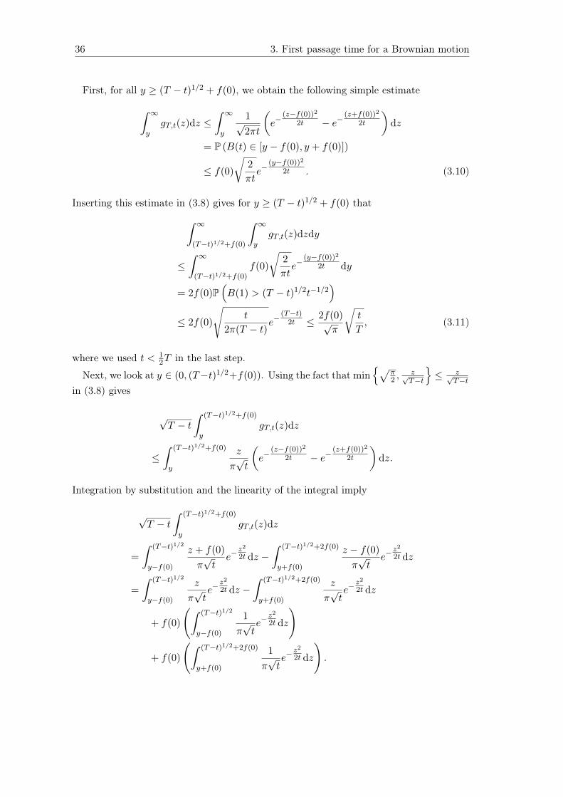
36 3. First passage time for a Brownian motion
First, for all y ≥ (T − t)1/2 + f(0), we obtain the following simple estimate∫ ∞y
gT,t(z)dz ≤∫ ∞y
1√2πt
(e−
(z−f(0))2
2t − e−(z+f(0))2
2t
)dz
= P (B(t) ∈ [y − f(0), y + f(0)])
≤ f(0)
√2
πte−
(y−f(0))2
2t . (3.10)
Inserting this estimate in (3.8) gives for y ≥ (T − t)1/2 + f(0) that∫ ∞(T−t)1/2+f(0)
∫ ∞y
gT,t(z)dzdy
≤∫ ∞
(T−t)1/2+f(0)f(0)
√2
πte−
(y−f(0))2
2t dy
= 2f(0)P(B(1) > (T − t)1/2t−1/2
)≤ 2f(0)
√t
2π(T − t)e−
(T−t)2t ≤ 2f(0)√
π
√t
T, (3.11)
where we used t < 12T in the last step.
Next, we look at y ∈ (0, (T−t)1/2+f(0)). Using the fact that min√
π2 ,
z√T−t
≤ z√
T−tin (3.8) gives
√T − t
∫ (T−t)1/2+f(0)
ygT,t(z)dz
≤∫ (T−t)1/2+f(0)
y
z
π√t
(e−
(z−f(0))2
2t − e−(z+f(0))2
2t
)dz.
Integration by substitution and the linearity of the integral imply
√T − t
∫ (T−t)1/2+f(0)
ygT,t(z)dz
=
∫ (T−t)1/2
y−f(0)
z + f(0)
π√t
e−z2
2t dz −∫ (T−t)1/2+2f(0)
y+f(0)
z − f(0)
π√t
e−z2
2t dz
=
∫ (T−t)1/2
y−f(0)
z
π√te−
z2
2t dz −∫ (T−t)1/2+2f(0)
y+f(0)
z
π√te−
z2
2t dz
+ f(0)
(∫ (T−t)1/2
y−f(0)
1
π√te−
z2
2t dz
)
+ f(0)
(∫ (T−t)1/2+2f(0)
y+f(0)
1
π√te−
z2
2t dz
).
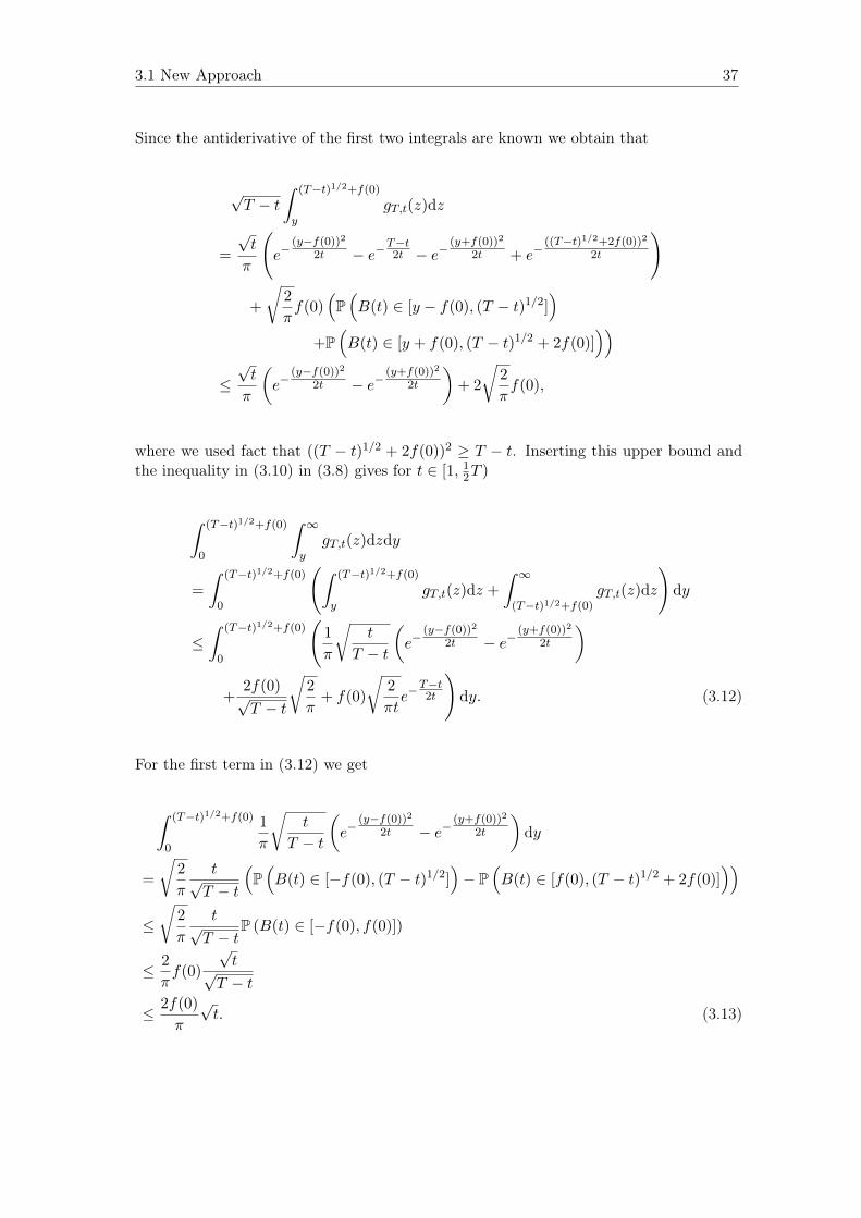
3.1 New Approach 37
Since the antiderivative of the first two integrals are known we obtain that
√T − t
∫ (T−t)1/2+f(0)
ygT,t(z)dz
=
√t
π
(e−
(y−f(0))2
2t − e−T−t2t − e−
(y+f(0))2
2t + e−((T−t)1/2+2f(0))2
2t
)
+
√2
πf(0)
(P(B(t) ∈ [y − f(0), (T − t)1/2]
)+P(B(t) ∈ [y + f(0), (T − t)1/2 + 2f(0)]
))≤√t
π
(e−
(y−f(0))2
2t − e−(y+f(0))2
2t
)+ 2
√2
πf(0),
where we used fact that ((T − t)1/2 + 2f(0))2 ≥ T − t. Inserting this upper bound andthe inequality in (3.10) in (3.8) gives for t ∈ [1, 1
2T )
∫ (T−t)1/2+f(0)
0
∫ ∞y
gT,t(z)dzdy
=
∫ (T−t)1/2+f(0)
0
(∫ (T−t)1/2+f(0)
ygT,t(z)dz +
∫ ∞(T−t)1/2+f(0)
gT,t(z)dz
)dy
≤∫ (T−t)1/2+f(0)
0
(1
π
√t
T − t
(e−
(y−f(0))2
2t − e−(y+f(0))2
2t
)
+2f(0)√T − t
√2
π+ f(0)
√2
πte−
T−t2t
)dy. (3.12)
For the first term in (3.12) we get
∫ (T−t)1/2+f(0)
0
1
π
√t
T − t
(e−
(y−f(0))2
2t − e−(y+f(0))2
2t
)dy
=
√2
π
t√T − t
(P(B(t) ∈ [−f(0), (T − t)1/2]
)− P
(B(t) ∈ [f(0), (T − t)1/2 + 2f(0)]
))≤√
2
π
t√T − t
P (B(t) ∈ [−f(0), f(0)])
≤ 2
πf(0)
√t√
T − t
≤ 2f(0)
π
√t. (3.13)

38 3. First passage time for a Brownian motion
For the second term in (3.12) we use the following obviously estimate
∫ (T−t)1/2+f(0)
0
√2
π
2f(0)√T − t
dy ≤∫ (T−t)1/2+f(0)
0
√2
π
2f(0)√T − t
dy
≤√
2
π
(2f(0) +
2f(0)2
√T − t
)≤√
2
π
(2f(0) + 2f(0)2
)√t. (3.14)
Note that for t ∈ [1, 12T ] we assume w.l.o.g. T ≥ 2 and thus 1√
T−t ≤ 1. Finally, we obtainthe following estimate for the third term in (3.12) using t ∈ [1, 1
2T ] and exp(−x) ≤ 1/x,for x > 0,
∫ (T−t)1/2+f(0)
0f(0)
√2
πte−
T−t2t dy
≤ f(0)
√2
πt
2t
T − t
((T − t)1/2 + f(0)
)≤ 2f(0)
√2
π
√t
T − t
(1 +
f(0)√T − t
)≤ 2
√2
π
(f(0) + f(0)2
)√t. (3.15)
Inserting (3.13), (3.14) and (3.15) in (3.12) gives
∫ (T−t)1/2+f(0)
0
∫ ∞y
gT,t(z)dzdy ≤ c√t,
for c > 0 suitably chosen. Putting this inequality and (3.11) into (3.8) implies
E(B(t)
∣∣∣∣ infs∈[0,T ]
B(s) ≥ −f(0)
)≤ c√t,
which proves Lemma 3.3 for t ∈ [1, 12T ).
It is left to show Lemma 3.3 for t = T . For this case, we use the same arguments as in
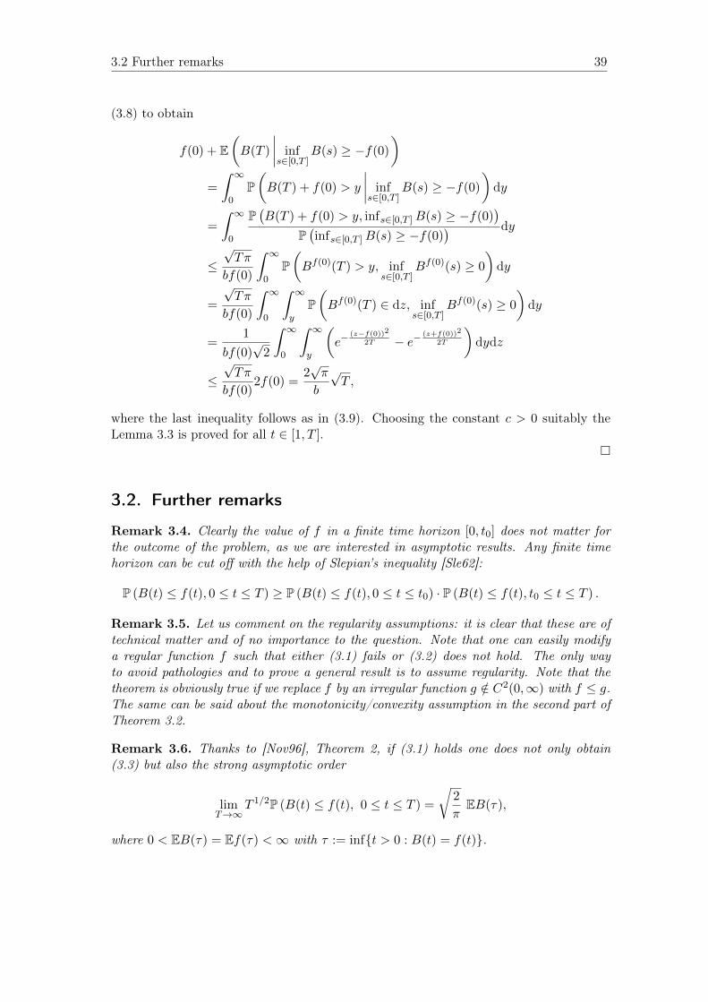
3.2 Further remarks 39
(3.8) to obtain
f(0) + E(B(T )
∣∣∣∣ infs∈[0,T ]
B(s) ≥ −f(0)
)=
∫ ∞0
P(B(T ) + f(0) > y
∣∣∣∣ infs∈[0,T ]
B(s) ≥ −f(0)
)dy
=
∫ ∞0
P(B(T ) + f(0) > y, infs∈[0,T ]B(s) ≥ −f(0)
)P(infs∈[0,T ]B(s) ≥ −f(0)
) dy
≤√Tπ
bf(0)
∫ ∞0
P(Bf(0)(T ) > y, inf
s∈[0,T ]Bf(0)(s) ≥ 0
)dy
=
√Tπ
bf(0)
∫ ∞0
∫ ∞y
P(Bf(0)(T ) ∈ dz, inf
s∈[0,T ]Bf(0)(s) ≥ 0
)dy
=1
bf(0)√
2
∫ ∞0
∫ ∞y
(e−
(z−f(0))22T − e−
(z+f(0))2
2T
)dydz
≤√Tπ
bf(0)2f(0) =
2√π
b
√T ,
where the last inequality follows as in (3.9). Choosing the constant c > 0 suitably theLemma 3.3 is proved for all t ∈ [1, T ].
3.2. Further remarks
Remark 3.4. Clearly the value of f in a finite time horizon [0, t0] does not matter forthe outcome of the problem, as we are interested in asymptotic results. Any finite timehorizon can be cut off with the help of Slepian’s inequality [Sle62]:
P (B(t) ≤ f(t), 0 ≤ t ≤ T ) ≥ P (B(t) ≤ f(t), 0 ≤ t ≤ t0) · P (B(t) ≤ f(t), t0 ≤ t ≤ T ) .
Remark 3.5. Let us comment on the regularity assumptions: it is clear that these are oftechnical matter and of no importance to the question. Note that one can easily modifya regular function f such that either (3.1) fails or (3.2) does not hold. The only wayto avoid pathologies and to prove a general result is to assume regularity. Note that thetheorem is obviously true if we replace f by an irregular function g /∈ C2(0,∞) with f ≤ g.The same can be said about the monotonicity/convexity assumption in the second part ofTheorem 3.2.
Remark 3.6. Thanks to [Nov96], Theorem 2, if (3.1) holds one does not only obtain(3.3) but also the strong asymptotic order
limT→∞
T 1/2P (B(t) ≤ f(t), 0 ≤ t ≤ T ) =
√2
πEB(τ),
where 0 < EB(τ) = Ef(τ) <∞ with τ := inft > 0 : B(t) = f(t).
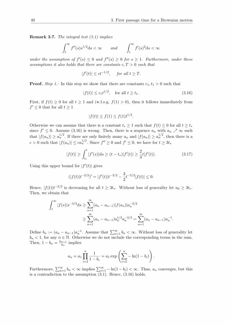
40 3. First passage time for a Brownian motion
Remark 3.7. The integral test (3.1) implies∫ ∞1
f ′′(s)s1/2ds <∞ and∫ ∞
1f ′(s)2ds <∞
under the assumption of f ′(s) ≤ 0 and f ′′(s) ≥ 0 for s ≥ 1. Furthermore, under theseassumptions it also holds that there are constants c, T > 0 such that
|f ′(t)| ≤ ct−1/2, for all t ≥ T.
Proof. Step 1.: In this step we show that there are constants c1, t1 > 0 such that
|f(t)| ≤ c1t1/2, for all t ≥ t1. (3.16)
First, if f(t) ≥ 0 for all t ≥ 1 and (w.l.o.g. f(1) > 0), then it follows immediately fromf ′ ≤ 0 that for all t ≥ 1
|f(t)| ≤ f(1) ≤ f(1)t1/2.
Otherwise we can assume that there is a constant t∗ ≥ 1 such that f(t) ≤ 0 for all t ≥ t∗since f ′ ≤ 0. Assume (3.16) is wrong. Then, there is a sequence an with an ∞ suchthat |f(an)| ≥ a1/2
n . If there are only finitely many an and |f(an)| ≥ a1/2n , then there is a
c > 0 such that |f(an)| ≤ ca1/2n . Since f ′′ ≥ 0 and f ′ ≤ 0, we have for t ≥ 3t∗
|f(t)| ≥∫ t
t∗
|f ′(s)|ds ≥ (t− t∗)|f ′(t)| ≥2
3t|f ′(t)|. (3.17)
Using this upper bound for |f ′(t)| gives
(|f(t)|t−3/2)′ = |f ′(t)|t−3/2 − 3
2t−5/2|f(t)| ≤ 0.
Hence, |f(t)|t−3/2 is decreasing for all t ≥ 3t∗. Without loss of generality let a0 ≥ 3t∗.Then, we obtain that∫ ∞
1|f(s)|s−3/2ds ≥
∞∑n=1
(an − an−1)|f(an)|a−3/2n
≥∞∑n=1
(an − an−1)a1/2n a−3/2
n =∞∑n=1
(an − an−1)a−1n .
Define bn := (an − an−1)a−1n . Assume that
∑∞n=1 bn <∞. Without loss of generality let
bn < 1, for any n ∈ N. Otherwise we do not include the corresponding terms in the sum.Then, 1− bn = an−1
animplies
an = a1
n∏i=2
1
1− bi= a1 exp
(n∑i=2
− ln(1− bi)
).
Furthermore,∑∞
n=1 bn <∞ implies∑∞
i=1− ln(1− bi) <∞. Thus, an converges, but thisis a contradiction to the assumption (3.1). Hence, (3.16) holds.

3.2 Further remarks 41
Step 2.: Here, we show ∫ ∞1
f ′′(s)s1/2ds <∞. (3.18)
Since (3.1) holds integration by parts implies
∞ > limT→∞
∫ T
1−f(s)s−3/2ds
= limT→∞
(2f(T )T−1/2 − 2f(1)− 2
∫ T
1f ′(s)s−1/2ds
)= lim
T→∞
(2f(T )T−1/2 − 2f(1)− 4f ′(T )T 1/2 + 4f ′(1) + 4
∫ T
1f ′′(s)s1/2ds
).
Since f ′ ≤ 0 and (3.16) holds, we obtain (3.18).Step 3.: Here, we show that there are constants c2, t2 > 0 such that
|f ′(t)| ≤ c2t−1/2, for all t ≥ t2. (3.19)
First, if f(t) ≥ 0 for all t ≥ 1 (w.l.o.g. f(1) > 0), then the assumption f ′ ≤ 0 implies forall t ≥ 2
∞ > f(1) ≥ |f(t)− f(1)| =∫ t
1|f ′(s)|ds ≥ (t− 1)|f ′(t)| ≥ 1
2t1/2|f ′(t)|,
and thus for all t ≥ 2
|f ′(t)| ≤ 2f(1)t−1/2.
In the other case we can assume that there is a constant t∗ ≥ 1 such that f(t) ≤ 0 for allt ≥ t∗. Because of (3.16) and (3.17) we obtain for all t ≥ maxt1, 2t∗ that
c1t1/2 ≥ |f(t)| ≥
∫ t
t∗
|f ′(s)|ds ≥ (t− t∗)|f ′(t)| ≥1
2t|f ′(t)|,
and thus
|f ′(t)| ≤ 2c1t−1/2.
Step 4.: In this step we show ∫ ∞1
f ′(s)2ds <∞.
Similar to Step 2 it follows from (3.1) and (3.16) by integration by parts that∫ ∞1|f ′(s)|s−1/2ds <∞.
Hence, (3.19) implies∫ ∞1
f ′(s)2ds ≤ c3 + c2
∫ ∞t2
|f ′(s)|s−1/2ds <∞,
where c3 > 0 suitably chosen.
42 3. First passage time for a Brownian motion
Remark 3.8. The last remark concerns possible generalizations to other processes. Notethat the technique of the main proof (Jensen’s inequality, Girsanov’s theorem) does carryover to other processes. The crucial point is determining the repulsion effect of the con-ditioning in Lemma 3.3. We do not see at the moment how a similar lemma can beestablished for processes other than Brownian motion, e.g. fractional Brownian motion.
4. Tail behaviour of the first passagetime over a moving boundary forgeneral Lévy processes
The last chapter deals with the first passage time problem for a simple example of a Lévyprocess, the Brownian motion. Here we study the tail behaviour of the first passage timeover a moving boundary for general Lévy processes, i.e. those allowing jumps. In view ofthe integral test stated in (3.1) for a Brownian motion indicated in the last chapter thefollowing question arises: Given a Lévy process X, for which functions f does
P(X(t) ≤ f(t), 0 ≤ t ≤ T ), as T →∞,
have the same asymptotic rate as in the case f ≡ 1? In this chapter we provide a classof functions for which the problem is solved. More precisely, our main result of thischapter states that if the boundary behaves as tγ for large t for some γ < 1/2 then theprobability that the process stays below the boundary behaves asymptotically as in thecase of a constant boundary. In contrast to all previously known results (see Section2.4.2 for an overview) we do not have to assume Spitzer’s condition. We distinguishbetween decreasing and increasing boundaries stated in Theorem 4.1 and Theorem 4.2,respectively.As mentioned in the introduction these results follow intuitively from the fact that a
Lévy process allows more (large) fluctuations than a Brownian motion. Hence, it canfollow a boundary at least as well as a Brownian motion.
We proceed in this chapter by formally introducing our main results in Section 4.1.There, we also present the main idea of both proofs. The proof of Theorem 4.1 for thecase of negative boundaries is given in Section 4.3, whereas Section 4.4 contains the prooffor positive boundaries, Theorem 4.2. For reasons of clarity and readability some auxiliarylemmas are combined in Section 4.2 and may be of independent interest.
4.1. Main results
Our first main result of this chapter, which corresponds to the one-sided exit problemwith a negative boundary, states:
Theorem 4.1. Let X be a Lévy process with triplet (σ2, b, ν) where ν(R−) > 0. Letf : R+ → R+ be a differentiable, non-decreasing function such that f(0) < 1, f ′(t) 0,for t→∞, and
∫∞1 f ′(s)2ds <∞. Let δ > 0. If
P(X(t) ≤ 1, 0 ≤ t ≤ T ) = T−δ+o(1) as T,→∞ (4.1)
43
44 4. First passage times for general Lévy processes
holds, then
P(X(t) ≤ 1− f(t), 0 ≤ t ≤ T ) = T−δ+o(1), as T →∞. (4.2)
The following theorem corresponds to the one-sided exit problem with a positive bound-ary.
Theorem 4.2. Let X be a Lévy process with triplet (σ2, b, ν) where ν(R+) > 0 andν(R−) > 0. Let f : R+ → R+ be a differentiable, non-decreasing function such that∫∞
1 f ′(s)2ds <∞ and sups≥1 |f ′(s)| <∞. Let δ > 0. If
P(X(t) ≤ 1, 0 ≤ t ≤ T ) = T−δ+o(1), as T →∞, (4.3)
holds, then
P(X(t) ≤ 1 + f(t), 0 ≤ t ≤ T ) = T−δ+o(1), as T →∞.
The proofs of these theorems are given in Section 4.3 and 4.4, respectively, and theideas will be sketched below. Let us give first a few comments on these results.
Remark 4.3. In Theorem 4.1 (Theorem 4.2, respectively), the assumption that thereare negative (positive, respectively) jumps is an essential part of our technique. We will“compensate” the negative (positive) boundary by negative (positive) jumps and thus reducethe problem to the constant boundary case.
Remark 4.4. In both Theorems, the regularity conditions on the function f are for tech-nical purposes only. Trivially, both Theorems are also valid for a less regular function g ifthere is a function f satisfying the conditions in Theorem 4.1 (Theorem 4.2, respectively)such that g(s) ≤ f(s), for all s ≥ 0. The important property of the function f is itsasymptotic behaviour at infinity, ∫ ∞
1f ′(t)2dt <∞,
which is a slightly weaker assumption than Uchiyama’s integral test (3.1).
Remark 4.5. The assumption of negative jumps in Theorem 4.2 seems to be of technicalmatter. Different assumptions exist in order to replace the assumption of negative jumpssuch as the assumption that
(a) the renewal function U of the ladder height process satisfies U((lnT )5) ≤ T o(1), or
(b) there is a function T0(T ) 1 ≤ T0(T ) = T o(1) such that P(X(T0) ≤ −(lnT )5) ≥ T o(1).
See Remark 4.14 below for a detailed discussion.
Remark 4.6. The assumption of equation (4.1)/(4.3) is associated with Spitzer’s con-dition. As mentioned in Section 2.4.1 (cf. [Rog71] or [Ber96], Theorem 18) Spitzer’scondition holds with ρ ∈ (0, 1) if and only if the probability in (4.1)/(4.3) is regularlyvarying with index −ρ. Note that the class of Lévy processes satisfying assumption(4.1)/(4.3) is strictly larger than the class of Lévy processes satisfying Spitzer’s condition(see [DS13], or [BD96, Don89] for a discrete-time version). For instance, Lévy processeswhere EX(1) ∈ (0,∞) and the left tail of the Lévy measure is regularly varying with index−c, c > 1, satisfy assumption (4.1)/(4.3) with δ = c, but not Spitzer’s condition withρ ∈ (0, 1). This example was already mentioned in Section 2.4.1.
4.2 Auxiliary results 45
We conclude this section by presenting a sketch of the proof of Theorem 4.1. For thispurpose, we need the definition of an additive process introduced in Section 2.3. Recallthat this class of processes consists of time-inhomogeneous processes which have indepen-dent increments and start at 0 (see [Sat99]). The triplet is given by (σ2, fX(t),ΛX(dx, dt)),for some σ ≥ 0, fX ∈ C[0,∞) where f(0) = 0, and ΛX is a measure on R× [0, T ].Sketch of the proof of Theorem 4.1: Note that the upper bound is trivial since
f is positive. For the lower bound our main idea is to find an iteration method toreduce the exponent of the boundary in each step such that eventually the boundaryturns into a constant boundary. In each iteration step, we start with a change of measurecompensating the boundary f by negative jumps. Then, we get an additive process whichhas the following triplet
(σ2, b · s, (1 + f ′(s)|x|/m1x∈A)dsν(dx)
), where A ⊆ [−1, 0)
and m are suitably chosen. This process can be represented as X(·) + Z(·), where Xis the original Lévy process and Z has the triplet (0, 0, f ′(s)|x|/m1x∈Adsν(dx)). Thisapproach implies the estimate
P(X(t) ≤ 1− f(t), 0 ≤ t ≤ T ) ≥ P(X(t) + Z(t) ≤ 1, 0 ≤ t ≤ T ) · e−c√
lnT .
The term exp(−c√
lnT)represents the cost of changing the measure. A homogenization
yields a Lévy process Z with Z(·) d= Z(f(·)) and triplet (0, 0, |x|/m1x∈Aν(dx)). Since
Z is a Lévy martingale with some finite exponential moment, we can finally estimateP(X(t) + Z(f(t)) ≤ 1, 0 ≤ t ≤ T ) by P(X(t) ≤ 3− f(t)2/3, 0 ≤ t ≤ T ) giving essentially
P(X(t) ≤ 1− f(t), 0 ≤ t ≤ T ) ≥ P(X(t) ≤ 3− f(t)2/3, 0 ≤ t ≤ T ) e−c√
lnT .
This procedure is repeated until f(T )(2/3)n ≤ 2. Then, the asymptotic behaviour ofP(X(t) ≤ 3 − f(t)(2/3)n , 0 ≤ t ≤ T ) follows from (1.4). Hence, through an n-timesiteration of these steps the survival exponent in (1.1) is obtained with the help of (1.4)since n is of order ln lnT . A similar approach is used in the proof of Theorem 4.2. Here,the upper bound is proved through an iteration method.
4.2. Auxiliary results
4.2.1. Technical tools regarding the boundary
The following properties which are easy to check will be required for the proofs.
Lemma 4.7. Let f : R+ → R be a non-decreasing function satisfying the assumptions ofTheorem 4.2. Then,
f(T ) ≤ c · T, for all T sufficiently large, (4.4)
for some constant c > 0. Furthermore, if the function f satisfies additionally the assump-tions of Theorem 4.1, then there exists a constant c > 0 such that
√tf ′(s) ≤ c a.e. for all s ≥ t ≥ 1. (4.5)
Proof. The first inequality follows from sups≥1 |f ′(s)| <∞. The second inequality can bededuced easily from the fact that the function f ′(t) 0 for t→∞ and
∫∞1 f ′(s)2ds <∞.
46 4. First passage times for general Lévy processes
4.2.2. One-sided exit problem with a moving boundary for Brownianmotion
Below, we present a lemma which deals with the one-sided exit problem for Brownianmotion including a special kind of boundaries needed in the main proofs.
Lemma 4.8. Let T > 1 and c > 0 be a constant. Let (B(t))t≥0 be a Brownian motion.Define the function
hT (t) := max
(lnT )5, t3/4
and the event
E := B(t) ≤ c · hT (t), for all t ∈ [0, T ] .
Then, we have
P(Ec) . e−(lnT )2/2, as T →∞.
Proof. First, note that c · hT (t) ≥ gT (t) := (lnT )t6/10, for t ≥ 0 and T sufficiently large.Define the event E1 by
E1 := B(t) ≤ gT (t), for all t ∈ [1, T ] ,
and the event E2 by
E2 := B(t) ≤ lnT, for all t ∈ [0, 1] .
Obviously, we have
P(Ec2) . e−(lnT )2/2.
Furthermore, denote by Φ the standard normal distribution function. From Theorem 4and Example 7 in [JL81] it follows that
P(Ec1) . 4
(Φ
((lnT )T
110
)− Φ(lnT )
)≤√
2√πe−(lnT )2/4,
for T sufficiently large. Hence, we obtain that
P(Ec) ≤ P(Ec1) + P(Ec2) . e−(lnT )2/2,
which completes the proof.

4.2 Auxiliary results 47
4.2.3. One-sided exit problem for Lévy processes
Next, we study the asymptotic behaviour of the first passage time over a constant bound-ary. If Spitzer’s condition holds, then [GN86], Lemma 2, proves a similar result.
Lemma 4.9. Let X be a Lévy process with Lévy triplet (σ2, b, ν). Let δ ≥ 0, 0 ≤ a < Tand 0 < c <∞. We have
P(X(t) ≤ 1, a ≤ t ≤ T ) = T−δ+o(1)
if and only if
P(X(t) ≤ c, a ≤ t ≤ T ) = T−δ+o(1).
Proof. Case 1: Let c > 1. On one hand, we have
P(X(t) ≤ 1, a ≤ t ≤ T ) ≤ P(X(t) ≤ c, a ≤ t ≤ T ).
On the other hand, let 2 ≤ dce := n ∈ N. Then,
pc(T ) := P(X(t) ≤ c, a ≤ t ≤ T ) ≤ P(X(t) ≤ n, a ≤ t ≤ T ).
Define τn := inft ≥ a : X(t) > n and let Fτn−1 be the associated distribution function.The Markov property imply, for every n ≥ 2,
pn(T ) ≤ pn−1(T ) +
∫ T
ap1(T − s)dFτn−1(s)
≤ pn−1(T ) + p1(T/2)
∫ T/2
adFτn−1(s) +
∫ T
T/2dFτn−1(s)
≤ pn−1(T ) + pn−1(T/2)P(τn−1 ∈ (a, T/2]) + P(τn−1 ∈ (T/2, T ]) ≤ 3pn−1(T/2).
Thus,
pc(T ) ≤ pn(T ) ≤ 3n−1p1(T/2n−1).
Case 2: Now, let 0 < c < 1. Then, on one hand, we have
P(X(t) ≤ c, a ≤ t ≤ T ) ≤ P(X(t) ≤ 1, a ≤ t ≤ T ),
and, on the other hand, analogously to Case 1 we obtain that
p1(T ) = P(
1cX(t) ≤ 1
c , a ≤ t ≤ T)≤ d1P
(1cX(t) ≤ 1, a ≤ t ≤ d2T
)= d1pc(d2T ),
where d1, d2 > 0 are dependent on c; and the lemma is proved.
The following theorem provides a technique to decouple the one-sided boundary prob-lem over different intervals.
Lemma 4.10. Let X be a Lévy process with triplet (σ2, b, ν) and f : R+ → R be ameasurable function. Let 0 ≤ a < b < c. Then,
P (X(t) ≤ f(t), a ≤ t ≤ c) ≥ P (X(t) ≤ f(t), a ≤ t ≤ b) · P (X(t) ≤ f(t), b ≤ t ≤ c) .
48 4. First passage times for general Lévy processes
Proof. For any choice of n and 0 ≤ t1 < ... < tn the random variables (X(ti))ni=1 are
associated (cf. [EPW67]), since they are sums of independent random variables. Hence,the functions 1X(t)≤f(t), a≤t≤b and 1X(t)≤f(t), b≤t≤c can both be written as limits ofdecreasing functions of associated random variables and are thus also associated. Hence,we obtain the desired statement.
Furthermore, we need a result for one-sided exit problem with a boundary that is anincreasing function of T .
Lemma 4.11. Let X be a Lévy process with Lévy triplet (σ2, b, ν). Then, we have, for Tsufficiently large,
P(X(t) ≤ 3, 0 ≤ t ≤ T )
≥ 12P(X(t) ≤ 3− t1/3, 0 ≤ t ≤ (lnT )21
)· P(X(t) ≤ 3 + (lnT )6, 1 ≤ t ≤ T
).
Proof. Note that (lnT )7 ≥ 3 + (lnT )6, for T sufficiently large, and due to the stationaryand independent increments of (X(t))t≥0 we have, for T sufficiently large,
P(X(t) ≤ 3− t1/3, 0 ≤ t ≤ (lnT )21
)· P(X(t) ≤ 3 + (lnT )6, 0 ≤ t ≤ T
)≤ P
(X(t) ≤ 3− t1/3, 0 ≤ t ≤ (lnT )21
)· P(X(t) ≤ 3 + (lnT )6, 0 ≤ t ≤ T − (lnT )21
)= P
(X(t) ≤ 3− t1/3, 0 ≤ t ≤ (lnT )21
)· P(X(t)−X((lnT )21) ≤ 3 + (lnT )6, (lnT )21 ≤ t ≤ T
)≤ P
(X(t) ≤ 3− t1/3, 0 ≤ t ≤ (lnT )21 ∩ X(t) ≤ 3, (lnT )21 ≤ t ≤ T
)≤ P(X(t) ≤ 3, 0 ≤ t ≤ T ).
Lemma 4.10 yields
P(X(t) ≤ 3 + (lnT )6, 0 ≤ t ≤ T
)≥ 1
2P(X(t) ≤ 3 + (lnT )6, 1 ≤ t ≤ T
),
since P(X(t) ≤ 3 + (lnT )6, 0 ≤ t ≤ 1) > 12 , for T sufficiently large.
Here, we show that, if the boundary is equal to tα, α > 1/2 then the probability of theone-sided exit problem for a Lévy martingale with E (|X(1)|q) <∞, for some q > 4, overthe boundary tα is larger than a constant.
Lemma 4.12. Let X be a Lévy martingale with E (|X(1)|q) <∞, for some q > 4. Then,for any α > 1/2 there is a constant c > 0 depending only on X and α such that
P (X(t) ≤ tα, 1 ≤ t ≤ T ) & c, as T →∞.
Proof. First note that there exists ε ∈ (0, 1) such that q > 2(1 + ε) + 2. Sinceα > 1/2 there exists β > 0 such that α − β − 1
2 > 0. Choose natural number K :=
K(L(X), α, β, ε) > 0 independent of T such that K ≥ 21/β and
∞∑n=K
n−(1+ε) ≤ 1
2
[ √2
3√π
+ 2−(1+ε)/αE(|X(1)|(1+ε)/α
)]−1
. (4.6)
4.2 Auxiliary results 49
Then, Lemma 4.10 yields for every T > K
g(T ) := P (X(t) ≤ tα, 1 ≤ t ≤ T )
≥ g(K) ·(
1− P (∃ t ∈ [K,T ] : X(t) > tα))
≥ g(K) ·
1−bT c∑n=K
P (∃ t ∈ (n, n+ 1] : X(t) > tα)
. (4.7)
On the other hand, due to the stationary and independent increments we obtain, for alln ≥ K,
P (∃ s ∈ (n, n+ 1] : X(s) > sα)
≤ P(X(n) ≥ nα−β
)+ P
(X(n) < nα−β ∩ ∃ s ∈ (n, n+ 1] : X(s) > sα
)≤ P
(X(n)/
√n ≥ nα−β−1/2
)+ P
(∃ s ∈ (n, n+ 1] : X(s)−X(n) > sα − nα−β
)≤ P
(X(n)/
√n ≥ 3
√lnn
)+ P
(∃ s ∈ (n, n+ 1] : X(s)−X(n) > 1
2nα)
≤√
2
3√π lnn
· n−(1+ε) + P(∃ s ∈ (0, 1] : |X(s)| > 1
2nα)
≤√
2
3√π· n−(1+ε) + 2−(1+ε)/αE
(|X(1)|(1+ε)/α
)· n−(1+ε), (4.8)
where we used in the second last step a result in [Pet75], page 254, and in the last stepDoob’s martingale inequality. Note that we require E (|X(1)|q) < ∞, q > 4, in order toapply the result in [Pet75]. Putting (4.8) and (4.6) into (4.7) yields
g(T ) ≥ g(K)/2 > 0,
which proves the lemma.
4.2.4. Coupling
With the help of a coupling method we also obtain an upper bound for the one-sided exitproblem for a Lévy martingale with some finite exponential moment.
Lemma 4.13. Let c > 0. Let X1 and X2 be two independent Lévy processes, where X2
is a martingale with some finite exponential moment, i.e. E(eb|X2(1)|) < ∞, for some
b > 0. Furthermore, let E(X2(1)2
)= a. Let B be a Brownian motion and f : R+ → R+
be a non-decreasing function such that there exists a constant d > 0 with f(T ) ≤ d ·T , forT sufficiently large. Then there is a κc > 0 depending on c such that, for T sufficientlylarge,
P(X1(t) +X2(f(t)) ≤ 1, 1 ≤ t ≤ T
)≤ P
(X1(t) + aB(f(t)) ≤ 1 + κc lnT, 1 ≤ t ≤ T
)+ T−c.
50 4. First passage times for general Lévy processes
Proof. Since X2 has some finite exponential moment and EX2(1)2 = a, one can coupleit with a Brownian motion aB (cf. the Komlós-Major-Tusnády coupling (KMT theorem)in [KMT75]) in such a way that, for a suitable κc > 0 and T sufficiently large,
P
(sup
0≤t≤T|X2(t)− aB(t)| > κc
2lnT
)≤ T−c.
Since f(T ) ≤ d · T , for T sufficiently large, we have
P
(sup
1≤t≤T|X2(f(t))− aB(f(t))| > κc lnT
)
≤ P
(sup
0≤t≤dT|X2(t)− aB(t)| > κc lnT
).
Moreover, since ln(dT ) ≤ 2 lnT , for T sufficiently large, we get
P
(sup
1≤t≤T|X2(f(t))− aB(f(t))| > κc lnT
)
≤ P
(sup
0≤t≤maxT,dT|X2(t)− aB(t)| > κc
2ln(maxT, dT)
)≤ min1, d−cT−c ≤ T−c. (4.9)
Define
A :=
sup
1≤t≤T|X2(f(t))− aB(f(t))| ≤ κc lnT
to be the set where the coupling works. Then, by inequality (4.9), for T sufficiently large,
P(X1(t) +X2(f(t)) ≤ 1, 1 ≤ t ≤ T
)≤ P
(X1(t) +X2(f(t)) ≤ 1, 1 ≤ t ≤ T ;A
)+ P
(Ac)
≤ P(X1(t) + aB(f(t)) ≤ 1 + κc lnT, 1 ≤ t ≤ T
)+ T−c,
which completes the proof.
4.3. Proof of Theorem 4.1 (negative boundaries)
Since f(t) is positive, our quantity is trivially bounded from above as follows
P(X(t) ≤ 1− f(t), 0 ≤ t ≤ T ) ≤ P(X(t) ≤ 1, 0 ≤ t ≤ T ) = T−δ+o(1).
In order to prove the lower bound of the proof we can assume that T > 1. We nextintroduce the auxiliary functions H i
β and fn.
4.3 Proof of Theorem 4.1 (negative boundaries) 51
We define
H(x) := x exp(−√c1||f ′||2L2[1,∞) ln(1/x)− c2||f ′||2L2[1,∞)
), for x ∈ (0, 1],
where c1, c2 > 0 are constants depending on ν and f specified later. Note that H ′(x) > 0on (0, 1]. Next, define H i
β by H0β(x) := x and, for i ≥ 1,
H iβ(x) := H i−1
β
(H(x · β)
)with 0 < β < 1 specified later. Note that H i
β is well defined since H(x) ∈ (0, 1] forx ∈ (0, 1].
Next, we define f0(t) := maxf(lnT ), f(t) and, for n ≥ 1,
fn(t) := max
1, (fn−1(t)− fn−1(lnT ))2/3
+ fn−1(lnT ), t ≥ 0.
Furthermore, define tn := sups ≥ 0 : fn−1(s) − fn−1(lnT ) ≤ 1. Note that f ′n(t) = 0,for t ∈ (0, tn), and
f ′n(t) = 23 (fn−1(t)− fn−1(lnT ))−2/3 f ′n−1(t) a.e., for t > tn.
Thus,
0 ≤ f ′n(t) ≤ f ′(t) a.e., (4.10)
since f ′ ≥ 0. In the following proof we use
fn(t) ≤ f(lnT ) + n+ max1, f(t)(2/3)n, for all t ≥ 0, (4.11)
which can be proved by induction.We proceed with the proof of the lower bound which includes two iterations.
4.3.1. External iteration
In this section we provide an iteration method in order to apply the results of Section4.3.2. This additional step is required because of technical details in Section 4.3.2, whichcontains the main idea of this proof. For this purpose, define, for any T > 0,
G(T ) := P(X(t) ≤ 1− f(t), (0 ∨ lnT ) ≤ t ≤ T ).
In Section 4.3.2 we will prove that
G(T ) ≥ T−δ+o(1) ·G(lnT ), for all T > 1. (4.12)
We define by ln∗(T ) the number of times the logarithm function must be iterativelyapplied before the result is less than or equal to one. Let lnn(T ) denote the n-timesiteratively applied logarithm and ln0(T ) := T .

52 4. First passage times for general Lévy processes
Observe that we obtain because of (4.12) for every 1 ≤ k ≤ ln∗(T )− 1 that
G(lnk(T )) ≥ G(1)
ln∗(T )−1∏j=k
(lnj(T )
)−δ+o(1).
Furthermore, Lemma 4.10 yields
P(X(t) ≤ 1− f(t), 0 ≤ t ≤ T )
≥ P(X(t) ≤ 1− f(t), 0 ≤ t ≤ lnln∗(T )(T )) ·G(lnln∗(T )−1(T )) · ... ·G(lnT ) ·G(T )
≥ G(1) ·G(lnln∗(T )−1(T )) · ... ·G(lnT ) ·G(T )
= G(1)
ln∗(T )−1∏k=0
G(lnk(T )).
Combining these two inequalities with (4.12) and the fact that lnj(T ) ≤ lnk(T ), for allj ≥ k ≥ 0, which will be used in the third and fourth step, and ln∗(T ) ≤ ln3(T ), for Tsufficiently large, implies
P(X(t) ≤ 1− f(t), 0 ≤ t ≤ T
)≥ G(1)
ln∗(T )−1∏k=1
G(lnk(T ))
·G(lnT ) · T−δ+o(1)
≥ G(1)ln∗(T )+1
ln∗(T )−1∏k=1
ln∗(T )−1∏j=k
(lnj(T )
)−δ+o(1)
·
ln∗(T )−1∏j=1
(lnj(T )
)−δ+o(1)
· T−δ+o(1)
≥ G(1)ln∗(T )+1
ln∗(T )−1∏k=1
((lnk(T ))−δ+o(1)
)ln∗(T )−k
·(
(ln(T ))−δ+o(1))ln∗(T )−1
· T−δ+o(1)
≥ G(1)ln∗(T )+1
ln∗(T )−1∏k=0
(ln1(T )
)−(ln∗(T )−k)δ+(ln∗(T )−k)o(1)
· T−δ+o(1)
≥ G(1)ln∗(T )+1 (lnT )− ln3(T ) · T−δ+o(1)
= T−δ+o(1),
and this is precisely the assertion of the theorem.
4.3.2. Internal iteration; Proof of (4.12)
First, define
gn(T ) := P(X(t) ≤ 1− fn(t), lnT ≤ t ≤ T ).

4.3 Proof of Theorem 4.1 (negative boundaries) 53
Step 1: Proof of (4.13) By using a change of measure the aim of this step is to showthe following inequality
gn(T ) ≥ P(Yn(t) ≤ 1, lnT ≤ t ≤ T )
· exp(−√c1||f ′||2L2[1,∞) ln(1/P(Yn(t) ≤ 1, lnT ≤ t ≤ T ))− c2||f ′||2L2[1,∞)
)= H (P(Yn(t) ≤ 1, lnT ≤ t ≤ T )) , (4.13)
where Yn is an additive process and c1, c2 > 0 are constants depending on ν and f , thatare chosen later on.Without loss of generality let ν([−1, 0)) > 0. If ν([−1, 0)) = 0 then we multiply X by
d > 0 suitably chosen such that ν([−1, 0])) > 0, where ν is the Lévy measure of d · X.Such d > 0 exists since ν(R−) > 0. Due to Lemma 4.9 we can continue with the processd ·X instead of X in the same manner.Since ν([−1, 0)) > 0 we can choose a compact set A ⊆ [−1, 0) such that
0 <
∫Ax2ν(dx) =: m <∞.
Let Xn and Yn be two additive processes with triplets (σ2, fXn(t), ν(dx)ds) and(σ2, fYn(t), (1 + f ′n(t)|x|
m 1x∈A)ν(dx)ds) respectively, where fYn(t) := b · t + fn(lnT ) andfXn(t) := b · t+ fn(t).Then, PXn |FT and PYn |FT are absolutely continuous because of the following facts:
Define θ(x, s) := ln(1 + f ′n(s)|x|m 1x∈A), for all s ∈ [0, T ] and x ∈ R. Using the fact that
f ′n(s) = 0, for s ∈ (0, lnT ), we have, for t > lnT ,
fYn(t) = bt+ fn(lnT ) = bt+ fn(t)−∫ t
lnTf ′n(s)ds
= fXn(t) +
∫ t
0
∫|x|≤1
(eθ(x,s) − 1
)xν(dx)ds
and since fn(t) = fn(lnT ), for t ∈ [0, lnT ],
fYn(t) = bt+ fn(lnT ) = bt+ fn(t) = fXn(t).
In this connection, one should point out that −f ′n(s)x1x∈A = f ′n(s)|x|1x∈A ≥ 0 almosteverywhere.Define ΛYn(dx, ds) := exp(θ(x, s))ν(dx)ds. According to the choice of the Lévy mea-
sures, ν(dx)ds and ΛYn(dx, ds) are absolutely continuous with dΛYn (x,s)ν(dx)ds = eθ(x,s). In
order to apply Theorem 2.7 we have to check∫ T
0
∫R(eθ(x,s)/2 − 1
)2ν(dx)ds < ∞. We
know from [Sat99], Remark 33.3, that this condition is equivalent to the following threeproperties combined
1.∫(x,s):θ(x,s)<−1 ν(dx)ds <∞,
2.∫(x,s):θ(x,s)>1 e
θ(x,s)ν(dx)ds <∞, and
3.∫(x,s):|θ(x,s)|≤1 θ
2(x, s)ν(dx)ds <∞.
54 4. First passage times for general Lévy processes
Since f ′n ≥ 0, thus θ ≥ 0; it is left to prove 2. and 3.Proof of 2.: Since θ > 1 and the A is bounded away from zero, we have
∫(x,s):θ(x,s)>1
eθ(x,s)ν(dx)ds ≤∫ T
1
∫A
(1 +f ′n(s)|x|m
)ν(dx)ds <∞.
Proof of 3.: Since ln(1 + z) ≤ z, for all z > −1, it follows from inequality (4.10) that
∫(x,s):|θ(x,s)|≤1
(θ(x, s))2ν(dx)ds ≤ 1
m2
∫ T
1
∫A
(f ′n(s))2x2ν(dx)ds =1
m||f ′n||2L2[1,T ] <∞.
Hence, due to Theorem 2.7 PXn |FT and PYn |FT are absolutely continuous.Next, we show inequality (4.13). Note that θ(x, s) = 0, for s ∈ [0, lnT ) and all x ∈ R.
Because of Theorem 2.7 and the density transformation formula (2.8) we obtain that
P(Xn(t) ≤ 1, lnT ≤ t ≤ T ) = EXn(1Xn(t)≤1, lnT≤t≤T)
= EYn(1Yn(t)≤1, lnT≤t≤Te
−∫ TlnT
∫R θ(x,s)NYn (dx,ds)
)· e∫ TlnT
∫R(eθ(x,s)−1−θ(x,s)eθ(x,s))ν(dx)ds
= EYn(1Yn(t)≤1, lnT≤t≤Te
−∫ TlnT
∫R θ(x,s)NYn (dx,ds)
)· e−∫ TlnT
∫R g
(f ′n(s)|x|m 1x∈A
)ν(dx)ds
,
(4.14)
where g(u) := (1 + u) ln(1 + u)− u, u > 0. Since for all u ≥ 0 we have ln(1 + u) ≤ u, weobtain that g(u) ≤ c1u
2 because of Taylor’s expansion. Hence, we get
exp
(−∫ T
lnT
∫Rg(f ′n(s)|x|m 1x∈A
)ν(dx)ds
)≥ exp
(−∫ T
lnT
∫R
f ′n(s)2x2
m2 1x∈Aν(dx)ds)
= exp
(−∫ T
lnTf ′n(s)2ds ·
∫A
x2
m2 ν(dx)
)= exp
(− 1
m||f ′n||2L2[lnT,T ]
)≥ exp
(− 1
m||f ′||2L2[1,∞)
),
having used (4.10). Let p > 1. Using the reverse Hölder inequality and putting the thelast estimate in (4.14) yields that
P(Xn(t) ≤ 1, lnT ≤ t ≤ T ) ≥ exp
(− 1
m||f ′||2L2[1,∞)
)(P(Yn(t) ≤ 1, lnT ≤ t ≤ T ))p
·(EYn
(e
1p−1
∫ TlnT
∫R θ(x,s)NYn (dx,ds)
))−(p−1)
. (4.15)
4.3 Proof of Theorem 4.1 (negative boundaries) 55
Furthermore, due to the density transformation formula (2.7) we obtain that(EYn
(exp
(1
p− 1
∫ T
lnT
∫Rθ(x, s)NYn(dx, ds)
)))−(p−1)
=(EXn
(e∫ TlnT
∫R
1p−1
θ(x,s)(N(dx,ds)−ΛYn (dx,ds))+θ(x,s)(N(dx,ds)−ν(dx)ds)))−(p−1)
·(
exp
(−∫ T
1
∫R
[eθ(x,s) − 1− θ(x, s)
]ν(dx)ds
))−(p−1)
=
(EXn
(exp
(∫ T
lnT
∫R
[1
p− 1+ 1
]θ(x, s)(N(dx, ds)− ν(dx)ds)
)))−(p−1)
·(
exp
(∫ T
lnT
∫R
[θ(x, s)
p− 1− θ(x, s)
p− 1eθ(x,s) − eθ(x,s) + 1 + θ(x, s)
]ν(dx)ds
))−(p−1)
=
(exp
(∫ T
lnT
∫R
[e
(1p−1 +1)θ(x,s) − 1− ( 1
p−1 + 1)θ(x, s)
]ν(dx)ds
))−(p−1)
·(
exp
(∫ T
lnT
∫R
[θ(x, s)
p− 1− θ(x, s)
p− 1eθ(x,s) − eθ(x,s) + 1 + θ(x, s)
]ν(dx)ds
))−(p−1)
= exp
((p− 1)
∫ T
lnT
∫Reθ(x,s)
[−e
1p−1 θ(x,s) + 1 + 1
p−1θ(x, s)
]ν(dx)ds
),
where we used in the third step a modification of Lemma 33.6 in [Sat99]. The differ-ence between [Sat99] and our case consists in the consideration of time-inhomogeneousprocesses in contrast to time-homogeneous processes used in [Sat99]. More precisely, weapply this Lemma to the following process∫ T
lnT
∫R
[1
p− 1+ 1
]θ(x, s)(N(dx, ds)− ν(dx)ds)
−∫ T
lnT
∫R
[e
(1p−1 +1)θ(x,s) − 1− ( 1
p−1 + 1)θ(x, s)
]ν(dx)ds,
and use the properties of the Girsanov transform for additive processes (Theorem 2.7)instead of for Lévy processes. Next, define w(x) := 1 + x− ex, for all x ≥ 0. Assume fora moment that p > 1 is chosen such that there is a constant b > 0 independing of T andn such that
1p−1θ(x, s) ≤ b, a.s. for all x ∈ R and s ∈ [lnT, T ]. (4.16)
Then, there are constants c1, c2 > 0 such that w( 1p−1θ(x, s)) ≥ −c1( 1
p−1θ(x, s))2 and
eθ(x,s) ≤ c2. Hence,
(p− 1)
∫ T
lnT
∫Reθ(x,s)
[−e
1p−1 θ(x,s) + 1 + 1
p−1θ(x, s)
]ν(dx)ds
≥ − c1c2
(p− 1)
∫ T
lnT
∫R
(θ(x, s))2ν(dx)ds ≥ − c2
(p− 1)m2
∫ T
lnT(f ′n(s))2ds ·
∫Ax2ν(dx)
≥ − c1c2
(p− 1)m||f ′||2L2[1,∞),
56 4. First passage times for general Lévy processes
where we used in the last step again inequality (4.10). Putting this into (4.15) implies
P(Xn(t) ≤ 1, lnT ≤ t ≤ T )
≥ P(Yn(t) ≤ 1, lnT ≤ t ≤ T )p · exp
(−(
1
m+
c1c2
(p− 1)m)||f ′||2L2[1,∞)
).
Optimizing in p shows that the best choice is
p := 1 +
√c1c2||f ′||2L2[1,∞)
2m ln(1/P(Yn(t) ≤ 1, lnT ≤ t ≤ T ))> 1.
Using this and choosing c1, c2 suitably completes the proof of inequality (4.13).It is left to show in (4.16) that 1
p−1θ(x, s) is almost everywhere bounded away frominfinity. More precisely, we will prove 1
p−1f′n(s) ≤ c a.e., for s ∈ [lnT, T ], as a consequence
of the inequality
P(Yn(t) ≤ 1, lnT ≤ t ≤ T ) ≥ T−d, for some d > 0, (4.17)
for any n ∈ N to be proved below. Indeed, if (4.17) holds then due to the choice of p weobtain
1
p− 1=
√2m ln(1/P(Yn(t) ≤ 1, lnT ≤ t ≤ T ))
c1c2||f ′||2L2[1,∞)
≤√
2m ln(T−d)
c1c2||f ′||2L2[1,∞)
≤ c ·√
lnT .
Combining this with f ′n(s)(lnT )1/2 ≤ f ′(s)(lnT )1/2 ≤ c a.e., for s ∈ [lnT, T ] (see (4.5))we get 1
p−1f′n(s) ≤ c(lnT )1/2f ′(s) ≤ c a.e. The proof of (4.17) can be found in the next
step.
Step 2: Proof of (4.17) In order to show (4.17) we represent the process as a sumof independent processes Yn(·) d
= X(·) + Zn(·) + fn(lnT ), where X is the original Lévyprocess with triplet (σ2, b, ν(dx)), and the process Zn is an additive process with triplet(0, 0, f
′n(s)|x|m 1x∈Aν(dx)ds). By homogenization there exists a Lévy process Z with triplet
(0, 0, |x|m 1x∈Aν(dx)) such that Zn(·) = S(fn(·) − fn(lnT )) f.d.d. Note that Z is amartingale with some finite exponential moment since A is compact in (−∞, 0).Since fn(lnT ) ≤ κ lnT , for some κ > 0 (see (4.4)), analogously to Lemma 4.9 we have,
for T sufficiently large,
P(X(t) ≤ −fn(lnT ), lnT ≤ t ≤ T ) ≥ 9T−κ ln 3 · P(X(t) ≤ 1, lnT ≤ t ≤ 4T 1+κ ln 2).
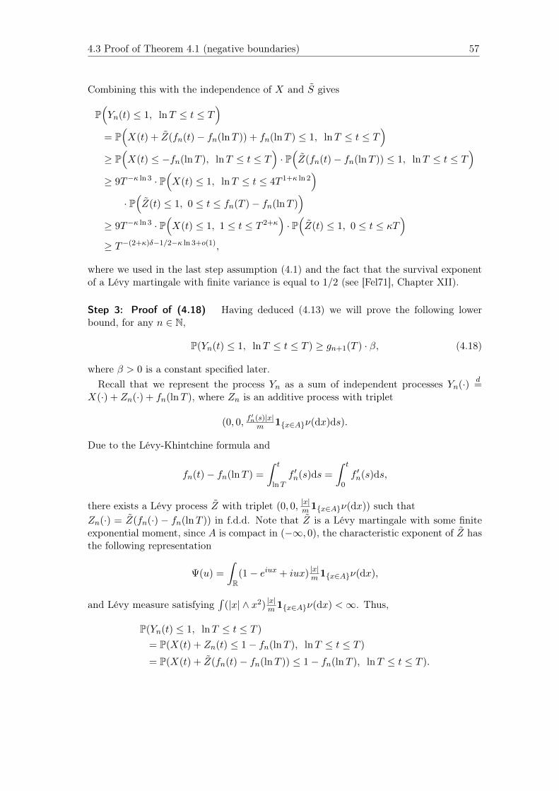
4.3 Proof of Theorem 4.1 (negative boundaries) 57
Combining this with the independence of X and S gives
P(Yn(t) ≤ 1, lnT ≤ t ≤ T
)= P
(X(t) + Z(fn(t)− fn(lnT )) + fn(lnT ) ≤ 1, lnT ≤ t ≤ T
)≥ P
(X(t) ≤ −fn(lnT ), lnT ≤ t ≤ T
)· P(Z(fn(t)− fn(lnT )) ≤ 1, lnT ≤ t ≤ T
)≥ 9T−κ ln 3 · P
(X(t) ≤ 1, lnT ≤ t ≤ 4T 1+κ ln 2
)· P(Z(t) ≤ 1, 0 ≤ t ≤ fn(T )− fn(lnT )
)≥ 9T−κ ln 3 · P
(X(t) ≤ 1, 1 ≤ t ≤ T 2+κ
)· P(Z(t) ≤ 1, 0 ≤ t ≤ κT
)≥ T−(2+κ)δ−1/2−κ ln 3+o(1),
where we used in the last step assumption (4.1) and the fact that the survival exponentof a Lévy martingale with finite variance is equal to 1/2 (see [Fel71], Chapter XII).
Step 3: Proof of (4.18) Having deduced (4.13) we will prove the following lowerbound, for any n ∈ N,
P(Yn(t) ≤ 1, lnT ≤ t ≤ T ) ≥ gn+1(T ) · β, (4.18)
where β > 0 is a constant specified later.Recall that we represent the process Yn as a sum of independent processes Yn(·) d
=X(·) + Zn(·) + fn(lnT ), where Zn is an additive process with triplet
(0, 0, f′n(s)|x|m 1x∈Aν(dx)ds).
Due to the Lévy-Khintchine formula and
fn(t)− fn(lnT ) =
∫ t
lnTf ′n(s)ds =
∫ t
0f ′n(s)ds,
there exists a Lévy process Z with triplet (0, 0, |x|m 1x∈Aν(dx)) such thatZn(·) = Z(fn(·) − fn(lnT )) in f.d.d. Note that Z is a Lévy martingale with some finiteexponential moment, since A is compact in (−∞, 0), the characteristic exponent of Z hasthe following representation
Ψ(u) =
∫R
(1− eiux + iux) |x|m 1x∈Aν(dx),
and Lévy measure satisfying∫
(|x| ∧ x2) |x|m 1x∈Aν(dx) <∞. Thus,
P(Yn(t) ≤ 1, lnT ≤ t ≤ T )
= P(X(t) + Zn(t) ≤ 1− fn(lnT ), lnT ≤ t ≤ T )
= P(X(t) + Z(fn(t)− fn(lnT )) ≤ 1− fn(lnT ), lnT ≤ t ≤ T ).
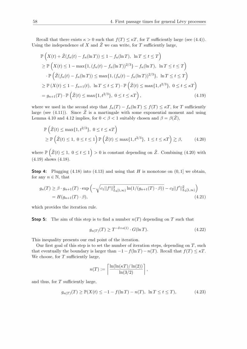
58 4. First passage times for general Lévy processes
Recall that there exists κ > 0 such that f(T ) ≤ κT , for T sufficiently large (see (4.4)).Using the independence of X and Z we can write, for T sufficiently large,
P(X(t) + Z(fn(t)− fn(lnT )) ≤ 1− fn(lnT ), lnT ≤ t ≤ T
)≥ P
(X(t) ≤ 1−max1, (fn(t)− fn(lnT ))2/3 − fn(lnT ), lnT ≤ t ≤ T
)· P(Z(fn(t)− fn(lnT )) ≤ max1, (fn(t)− fn(lnT ))2/3, lnT ≤ t ≤ T
)≥ P (X(t) ≤ 1− fn+1(t), lnT ≤ t ≤ T ) · P
(Z(t) ≤ max1, t2/3, 0 ≤ t ≤ κT
)= gn+1(T ) · P
(Z(t) ≤ max1, t2/3, 0 ≤ t ≤ κT
), (4.19)
where we used in the second step that fn(T ) − fn(lnT ) ≤ f(T ) ≤ κT , for T sufficientlylarge (see (4.11)). Since Z is a martingale with some exponential moment and usingLemma 4.10 and 4.12 implies, for 0 < β < 1 suitably chosen and β = β(Z),
P(Z(t) ≤ max1, t2/3, 0 ≤ t ≤ κT
)≥ P
(Z(t) ≤ 1, 0 ≤ t ≤ 1
)P(Z(t) ≤ max1, t2/3, 1 ≤ t ≤ κT
)& β, (4.20)
where P(Z(t) ≤ 1, 0 ≤ t ≤ 1
)> 0 is constant depending on Z. Combining (4.20) with
(4.19) shows (4.18).
Step 4: Plugging (4.18) into (4.13) and using that H is monotone on (0, 1] we obtain,for any n ∈ N, that
gn(T ) ≥ β · gn+1(T ) · exp(−√c1||f ′||2L2[1,∞) ln(1/(gn+1(T ) · β))− c2||f ′||2L2[1,∞)
)= H(gn+1(T ) · β), (4.21)
which provides the iteration rule.
Step 5: The aim of this step is to find a number n(T ) depending on T such that
gn(T )(T ) ≥ T−δ+o(1) ·G(lnT ). (4.22)
This inequality presents our end point of the iteration.Our first goal of this step is to set the number of iteration steps, depending on T , such
that eventually the boundary is larger than −1− f(lnT )−n(T ). Recall that f(T ) ≤ κT .We choose, for T sufficiently large,
n(T ) :=
⌈ln(ln(κT )/ ln(2))
ln(3/2)
⌉,
and thus, for T sufficiently large,
gn(T )(T ) ≥ P(X(t) ≤ −1− f(lnT )− n(T ), lnT ≤ t ≤ T ), (4.23)
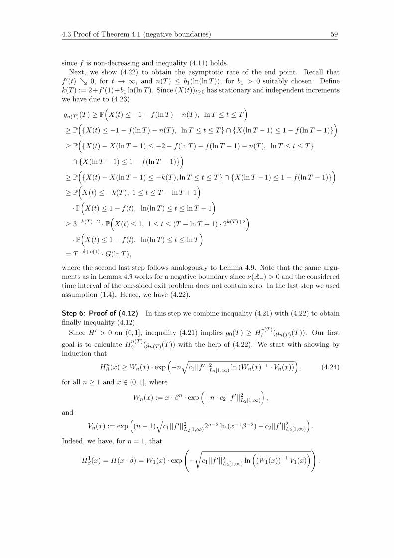
4.3 Proof of Theorem 4.1 (negative boundaries) 59
since f is non-decreasing and inequality (4.11) holds.Next, we show (4.22) to obtain the asymptotic rate of the end point. Recall that
f ′(t) 0, for t → ∞, and n(T ) ≤ b1(ln(lnT )), for b1 > 0 suitably chosen. Definek(T ) := 2+f ′(1)+b1 ln(lnT ). Since (X(t))t≥0 has stationary and independent incrementswe have due to (4.23)
gn(T )(T ) ≥ P(X(t) ≤ −1− f(lnT )− n(T ), lnT ≤ t ≤ T
)≥ P
(X(t) ≤ −1− f(lnT )− n(T ), lnT ≤ t ≤ T ∩ X(lnT − 1) ≤ 1− f(lnT − 1)
)≥ P
(X(t)−X(lnT − 1) ≤ −2− f(lnT )− f(lnT − 1)− n(T ), lnT ≤ t ≤ T
∩ X(lnT − 1) ≤ 1− f(lnT − 1))
≥ P(X(t)−X(lnT − 1) ≤ −k(T ), lnT ≤ t ≤ T ∩ X(lnT − 1) ≤ 1− f(lnT − 1)
)≥ P
(X(t) ≤ −k(T ), 1 ≤ t ≤ T − lnT + 1
)· P(X(t) ≤ 1− f(t), ln(lnT ) ≤ t ≤ lnT − 1
)≥ 3−k(T )−2 · P
(X(t) ≤ 1, 1 ≤ t ≤ (T − lnT + 1) · 2k(T )+2
)· P(X(t) ≤ 1− f(t), ln(lnT ) ≤ t ≤ lnT
)= T−δ+o(1) ·G(lnT ),
where the second last step follows analogously to Lemma 4.9. Note that the same argu-ments as in Lemma 4.9 works for a negative boundary since ν(R−) > 0 and the consideredtime interval of the one-sided exit problem does not contain zero. In the last step we usedassumption (1.4). Hence, we have (4.22).
Step 6: Proof of (4.12) In this step we combine inequality (4.21) with (4.22) to obtainfinally inequality (4.12).Since H ′ > 0 on (0, 1], inequality (4.21) implies g0(T ) ≥ H
n(T )β (gn(T )(T )). Our first
goal is to calculate Hn(T )β (gn(T )(T )) with the help of (4.22). We start with showing by
induction that
Hnβ (x) ≥Wn(x) · exp
(−n√c1||f ′||2L2[1,∞) ln (Wn(x)−1 · Vn(x))
), (4.24)
for all n ≥ 1 and x ∈ (0, 1], where
Wn(x) := x · βn · exp(−n · c2||f ′||2L2[1,∞)
),
and
Vn(x) := exp(
(n− 1)√c1||f ′||2L2[1,∞)2
n−2 ln (x−1β−2)− c2||f ′||2L2[1,∞)
).
Indeed, we have, for n = 1, that
H1β(x) = H(x · β) = W1(x) · exp
(−√c1||f ′||2L2[1,∞) ln
((W1(x))−1 V1(x)
)).

60 4. First passage times for general Lévy processes
Assume now that (4.24) holds, for n− 1. Note that, for x sufficiently small, we have
H(x) ≥ x2.
First, we get
Wn−1
(H(x · β)
)= Wn(x) · exp
(−√c1||f ′||2L2[1,∞) ln (x−1β−1)
).
Hence, we obtain, for x ∈ (0, 1], that
Wn−1
(H(x · β)
)−1 · Vn−1 (H(x · β))
≤ 1
Wn(x)· exp
(√c1||f ′||2L2[1,∞) ln (x−1β−1) + (n− 2)
√c1||f ′||2L2[1,∞)2
n−3 ln (x−2β−4))
≤(Wn(x)
)−1 · Vn(x),
since β ≤ 1. This implies, for x sufficiently small,
Hnβ (x) = Hn−1
β
(H(x · β)
)≥Wn−1
(H(x · β)
)· exp
(−(n− 1)
√c1||f ′||2L2[1,∞) ln
(Wn−1
(H(x · β)
)−1Vn−1
(H(x · β)
)))≥Wn(x) · exp
(−√c1||f ′||2L2[1,∞) ln (x−1β−1)
)· exp
(−(n− 1)
√c1||f ′||2L2[1,∞) ln
((Wn(x)
)−1Vn(x)
))
≥Wn(x) · exp
(−n
√c1||f ′||2L2[1,∞) ln
((Wn(x)
)−1Vn(x)
)),
where we used in the last step that, for n ≥ 2,(Wn(x)
)−1Vn(x)
= x−1β−n · exp(
(n− 1)c2||f ′||2L2[1,∞)
)· exp
((n− 1)
√c1||f ′||2L2[1,∞)2
n−2 ln (x−1β−2))
≥ x−1β−1.
Recall that n(T ) ≤ b1(ln(lnT )
)and gn(T )(T ) ≤ T−δ+o(1), for b1 = 5/2. Then, we obtain
that
Vn(T )(gn(T )(T )) ≤ exp(b1
(ln(lnT )
)√c1||f ′||2L2[1,∞)δ · 2−2(lnT )b1 ln 2 ln (Tβ−2)
)≤ exp
(b1(ln lnT ) · (lnT )7/5
)≤ exp
((lnT )3/2
)= T
√lnT , (4.25)

4.4 Proof of Theorem 4.2 (positive boundaries) 61
for T sufficiently large, and
exp(−n(T ) · c2||f ′||2L2[1,∞)
)= T o(1) ≥ exp
(− δ
2 · (lnT ))≥ gn(T )(T ). (4.26)
Putting (4.25) and (4.26) into (4.24) we obtain, for b2 > 0 suitably chosen, that
Hn(T )β (gn(T )(T )) ≥ gn(T )(T ) · βn(T ) · exp
(−n(T ) · c2||f ′||2L2[1,∞)
)· exp
(−n(T )
√c1||f ′||2L2[1,∞) ln
(gn(T )(T )−2β−n(T )T
√lnT))
≥ gn(T )(T ) · βn(T ) · exp(−n(T ) · c2||f ′||2L2[1,∞)
)· exp
(−3 · n(T ) · (lnT )3/4
√c1||f ′||2L2[1,∞)
)≥ gn(T )(T ) · exp
(−b2(lnT )4/5
)≥ gn(T )(T ) · T o(1).
Combining this with (4.22) and an n(T )-times iteration of (4.21) yields
g0(T ) = P(X(t) ≤ 1− f(t), lnT ≤ t ≤ T ) ≥ Hn(T )β (gn(T )(T )) = T−δ+o(1) ·G(lnT ),
which completes the proof of (4.12).
4.4. Proof of Theorem 4.2 (positive boundaries)
Since f is positive, our quantity is trivially bounded from below as follows
P(X(t) ≤ 1 + f(t), 0 ≤ t ≤ T ) ≥ P(X(t) ≤ 1, 0 ≤ t ≤ T ) = T−δ+o(1).
Our goal is to show
P(X(t) ≤ 1 + f(t), 0 ≤ t ≤ T ) ≤ T−δ+o(1). (4.27)
4.4.1. Preliminaries
In the following proof we can assume that T > 1. Then, we have
P(X(t) ≤ 1 + f(t), 0 ≤ t ≤ T ) ≤ P(X(t) ≤ 1 + f(t), 1 ≤ t ≤ T ).
Hence, as from now we consider the time interval [1, T ].Auxiliary function H for the iteration: We define
H(x) := x exp(√
c1||f ′||2L2[1,∞) ln(1/x)), x ∈ (0, 1].
Note that H ′(x) > 0 on (0, 1). Furthermore, we define H02 (x) := H(2x) and, for i ≥ 1,
H i2(x) := H
(2H i−1
2 (x)).
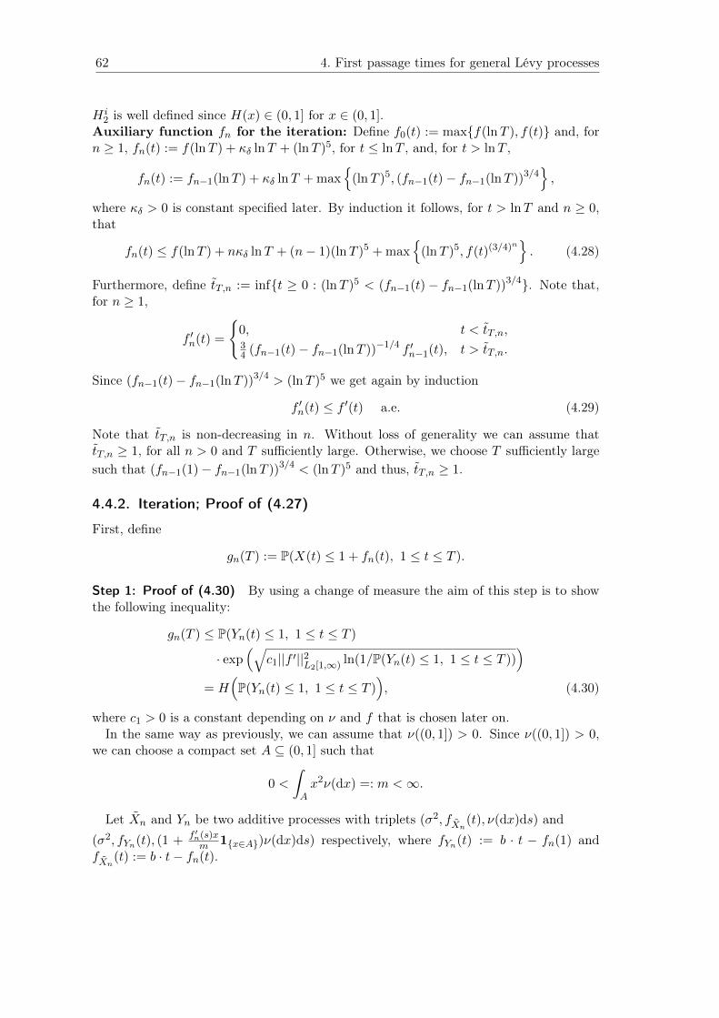
62 4. First passage times for general Lévy processes
H i2 is well defined since H(x) ∈ (0, 1] for x ∈ (0, 1].
Auxiliary function fn for the iteration: Define f0(t) := maxf(lnT ), f(t) and, forn ≥ 1, fn(t) := f(lnT ) + κδ lnT + (lnT )5, for t ≤ lnT , and, for t > lnT ,
fn(t) := fn−1(lnT ) + κδ lnT + max
(lnT )5, (fn−1(t)− fn−1(lnT ))3/4,
where κδ > 0 is constant specified later. By induction it follows, for t > lnT and n ≥ 0,that
fn(t) ≤ f(lnT ) + nκδ lnT + (n− 1)(lnT )5 + max
(lnT )5, f(t)(3/4)n. (4.28)
Furthermore, define tT,n := inft ≥ 0 : (lnT )5 < (fn−1(t)− fn−1(lnT ))3/4. Note that,for n ≥ 1,
f ′n(t) =
0, t < tT,n,34 (fn−1(t)− fn−1(lnT ))−1/4 f ′n−1(t), t > tT,n.
Since (fn−1(t)− fn−1(lnT ))3/4 > (lnT )5 we get again by induction
f ′n(t) ≤ f ′(t) a.e. (4.29)
Note that tT,n is non-decreasing in n. Without loss of generality we can assume thattT,n ≥ 1, for all n > 0 and T sufficiently large. Otherwise, we choose T sufficiently largesuch that (fn−1(1)− fn−1(lnT ))3/4 < (lnT )5 and thus, tT,n ≥ 1.
4.4.2. Iteration; Proof of (4.27)
First, define
gn(T ) := P(X(t) ≤ 1 + fn(t), 1 ≤ t ≤ T ).
Step 1: Proof of (4.30) By using a change of measure the aim of this step is to showthe following inequality:
gn(T ) ≤ P(Yn(t) ≤ 1, 1 ≤ t ≤ T )
· exp(√
c1||f ′||2L2[1,∞) ln(1/P(Yn(t) ≤ 1, 1 ≤ t ≤ T )))
= H(P(Yn(t) ≤ 1, 1 ≤ t ≤ T )
), (4.30)
where c1 > 0 is a constant depending on ν and f that is chosen later on.In the same way as previously, we can assume that ν((0, 1]) > 0. Since ν((0, 1]) > 0,
we can choose a compact set A ⊆ (0, 1] such that
0 <
∫Ax2ν(dx) =: m <∞.
Let Xn and Yn be two additive processes with triplets (σ2, fXn(t), ν(dx)ds) and(σ2, fYn(t), (1 + f ′n(s)x
m 1x∈A)ν(dx)ds) respectively, where fYn(t) := b · t − fn(1) andfXn(t) := b · t− fn(t).
4.4 Proof of Theorem 4.2 (positive boundaries) 63
The same arguments as previously implies that PXn |FT and PYn |FT are absolutely
continuous with dΛYn (x,s)ν(dx)ds = eθ(x,s), where θ(x, s) := ln(1 + f ′n(s)x
m 1x∈A), for all s ∈ [0, T ]
and x ∈ R, and ΛYn(dx, ds) := exp(θ(x, s))ν(dx)ds.Now, we prove inequality (4.30). Note that θ(x, s) = 0, for s ∈ [0, 1] and x ∈ R.
Because of Theorem 2.7 and the density transformation formula (2.8) we have
P(Xn(t) ≤ 1, 1 ≤ t ≤ T ) = EXn(1Xn(t)≤1, 1≤t≤T
)= EYn
(1Yn(t)≤1, 1≤t≤T exp
(−∫ T
1
∫Rθ(x, s)NYn(dx, ds)
))· exp
(−∫ T
1
∫Rg(f ′n(s)xm 1x∈A
)ν(dx)ds
), (4.31)
where g(u) := (1 + u) ln(1 + u)− u, u ≥ 0. Since g(u) ≥ 0, for u ≥ 0, we obtain that
exp
(−∫ T
1
∫Rg(f
′n(s)xm 1x∈A)ν(dx)ds
)≤ 1.
Let p > 1 and 1/p+ 1/q = 1. Applying Hölder’s inequality in (4.31) yields that
P(Xn(t) ≤ 1, 1 ≤ t ≤ T )
≤(P(Yn(t) ≤ 1, 1 ≤ t ≤ T )
)1/p·(EYn
(exp
(−q∫ T
1
∫Rθ(x, s)NYn(dx, ds)
)))1/q
.
(4.32)
Let us consider the second term in (4.32). Due to the density transform formula (2.7) wehave
EYn(
exp
(−q∫ T
1
∫Rθ(x, s)NYn(dx, ds)
))= EXn
(e∫ T1
∫R−qθ(x,s)(N(dx,ds)−ΛYn (dx,ds))+θ(x,s)(N(dx,ds)−ν(dx)ds)
)· exp
(−∫ T
1
∫R
(eθ(x,s) − 1− θ(x, s))ν(dx)ds)
= EXn
(exp
(∫ T
1
∫R
(1− q)θ(x, s)(N(dx, ds)− ν(dx)ds)))
· exp
(∫ T
1
∫R
[−qθ(x, s) + qθ(x, s)eθ(x,s) − eθ(x,s) + 1 + θ(x, s)
]ν(dx)ds
)= exp
(∫ T
1
∫R
[e(−q+1)θ(x,s) − 1− (1− q)θ(x, s)
]ν(dx)ds
)· exp
(∫ T
1
∫R
[−qθ(x, s) + qθ(x, s)eθ(x,s) − eθ(x,s) + 1 + θ(x, s)
]ν(dx)ds
)= exp
(∫ T
1
∫Reθ(x,s)(e−qθ(x,s) − 1 + qθ(x, s))ν(dx)ds
),
64 4. First passage times for general Lévy processes
where we used as in the proof of Theorem 4.1 a modification of Lemma 33.6 in [Sat99]in the second step. Again, the difference between [Sat99] and our case consists in theconsideration of time-inhomogeneous processes in contrast to time-homogeneous processesused in [Sat99].Taylor’s expansion implies e−qθ(x,s) + qθ(x, s) − 1 ≤ 1
2q2θ(x, s)2, for all x ∈ R and
s ∈ [1, T ]. Since θ is bounded away from infinity we have exp(θ(x, s)) < c1, for somec1 > 0, and thus,
1
q
∫ T
1
∫Reθ(x,s)
[e−qθ(x,s) + qθ(x, s)− 1
]ν(dx)ds ≤ q
∫ T
1
∫R
c12 θ(x, s)
2ν(dx)ds
≤ q · c1
2m2
∫ T
1f ′n(s)2ds ·
∫Ax2ν(dx) ≤ q · c1
2m||f ′||2L2[1,∞),
having also used (4.29). Plugging this into (4.32) yields
gn(T ) = P(Xn(t) ≤ 1, 1 ≤ t ≤ T )
≤ P(Yn(t) ≤ 1, 1 ≤ t ≤ T )1/p · exp
(q · c1
2m||f ′||2L2[1,∞)
).
Optimizing in p shows that the best choice is
1/p := 1−
√c1 · ||f ′||2L2[1,∞)
2m ln(1/PYn(Yn(t) ≤ 1, 1 ≤ t ≤ T ))< 1,
which shows inequality (4.30) with c1 > 0 suitably chosen.
Step 2: Proof of (4.33) Having deduced (4.30) we proceed with the examination ofthe one-sided exit problem for the process Yn. More precisely, we will prove the followingupper bound, for any n ∈ N,
P(Yn(t) ≤ 1, 1 ≤ t ≤ T ) ≤ 2 · gn+1(T ). (4.33)
First, we represent the process Yn as a sum of independent processes Yn(·) d= X(·) +
Zn(·) − fn(1), where Zn is an additive process with triplet (0, 0, f′n(s)xm 1x∈Aν(dx)ds).
Due to the Lévy-Khintchine formula and
fn(t)− fn(1) =
∫ t
1f ′n(s)ds =
∫ t
0f ′n(s)ds
there exists a Lévy process Z with triplet (0, 0, xm1x∈Aν(dx)) such thatZn(·) = Z(fn(·) − fn(1)) in f.d.d. Note that Z is a Lévy martingale with some finiteexponential moment, since A is compact in (0,∞), the characteristic exponent of Z hasthe following representation
Ψ(u) =
∫R
(1− eiux + iux) xm1x∈Aν(dx),
4.4 Proof of Theorem 4.2 (positive boundaries) 65
and the Lévy measure satisfies∫
(|x| ∧ x2) xm1x∈Aν(dx) <∞. Thus,
P(Yn(t) ≤ 1, 1 ≤ t ≤ T ) = P(X(t) + Z(fn(t)− fn(1)) ≤ 1 + fn(1), 1 ≤ t ≤ T
).
Denote c2 := E(Z(1)2
)< ∞. Let B be a Brownian motion. Using Lemma 4.13 we
can write with a suitable constant κδ > 0
P(X(t) + Z(fn(t)− fn(1)) ≤ 1 + fn(1), 1 ≤ t ≤ T
)≤ P
(X(t) ≤ 1 + fn(1) + κδ lnT − c2B(fn(t)− fn(1)), 1 ≤ t ≤ T
)+ T−1−δ. (4.34)
In order to apply results of one-sided boundary problems for a Brownian motion definethe sets
En :=c2B(fn(t)− fn(1)) ≥ −max(lnT )5, (fn(t)− fn(1))3/4, 1 ≤ t ≤ T
⊇c2B(t) ≥ −max(lnT )5, t3/4, 0 ≤ t ≤ κT
=: En,
since f(T ) ≤ κT , for κ > 0 suitably chosen (see (4.4)). Then due to Lemma 4.8 andfn(1) = fn(lnT ) we obtain that
P(X(t) ≤ 1 + fn(1) + κδ lnT − c2B(fn(t)− fn(1)), 1 ≤ t ≤ T
)≤ P
(X(t) ≤ 1 + fn(1) + κδ lnT − c2B(fn(t)− fn(1)), 1 ≤ t ≤ T ;En
)+ P
(Ecn
)≤ P
(X(t) ≤ 1 + fn(1) + κδ lnT + max(lnT )5, (fn(t)− fn(1))3/4, 1 ≤ t ≤ T
)+ exp
(−(lnκT )2/2
)= gn+1(T ) + exp
(−(lnκT )2/2
). (4.35)
Step 3: Proof of (4.36) Our next goal is to show the iteration rule, that means, forevery n ∈ N,
gn(T ) ≤ H(2gn+1(T )
). (4.36)
Putting (4.35) and (4.34) into (4.30) and using that H ′ > 0 on (0, 1] we get
gn(T ) ≤[gn+1(T ) + T−1−δ + exp
(−(lnκT )2/2
)]· exp
(√c1||f ′||2L2[1,∞) ln(1/ [gn+1(T ) + T−1−δ + exp (−(lnκT )2/2)])
)≤ H(2gn+1(T )),
where we used in the last step that gn+1(T ) ≥ T−1−δ +exp(−(lnκT )2/2
), for sufficiently
large T > 1, since
gn+1(T ) ≥ P(X(t) ≤ 1, 0 ≤ t ≤ T ) = T−δ+o(1) ≥ T−1−δ + exp(−κ(lnT )2/2
). (4.37)
Hence, we have proved (4.36).
66 4. First passage times for general Lévy processes
Step 4: Proof of (4.38) The aim of this step is to find a number n(T ) depending on Tsuch that
gn(T )(T ) ≤ T−δ+o(1), (4.38)
which provides the end point of the iteration. For this purpose, our first goal is to setthe number of iteration steps, depending on T > 1, such that eventually the boundary issmaller than 1 + (lnT )6. Recall (see (4.4)) that f(T ) ≤ κT . We choose, for T sufficientlylarge,
n(T ) :=
⌈ln(ln(κT )/ ln(2))
ln(4/3)
⌉,
and thus, for T sufficiently large,
gn(T )(T ) ≤ P(X(t) ≤ 1 + f(lnT ) + n(T ) · (lnT )5, 1 ≤ t ≤ T
)≤ P
(X(t) ≤ 1 + (lnT )6, 1 ≤ t ≤ T
),
where we used inequality (4.28) combined with f(t)3/4n(T )< 2, for 0 ≤ t ≤ T , and that
f(T ) > 1 if f is not bounded away from infinity. On the other hand, if supt≥0 |f(t)| <∞,then applying Lemma 4.9 already proves the theorem.Applying Lemma 4.11 implies
gn(T )(T ) ≤ P(X(t) ≤ 1 + (lnT )6, 1 ≤ t ≤ T ) ≤ 2 · P (X(t) ≤ 1, 0 ≤ t ≤ T )
P(X(t) ≤ 1− t1/3, 0 ≤ t ≤ (lnT )21
)= P (X(t) ≤ 1, 0 ≤ t ≤ T ) (lnT )21δ+o(1),
where we used Theorem 4.1 in the last step and with it the assumption ν(R−) > 0. Usingnow the main assumption (1.4) gives (4.38).
Step 5: Proof of (4.27) In this step we combine (4.36) with (4.38) to obtain finallyinequality (4.27). For this purpose, we estimate Hn(T )
2 (2gn(T )(T )) from above. First, weshow by induction for x sufficiently small that, for any n ≥ 1,
Hn2 (2x) ≤ 2n · x · exp
(n√c1||f ′||L2[1,∞) ln(1/x)
). (4.39)
Clearly, we get, for n = 1,
H12 (2x) = H(2x) ≤ 2 · x · exp
(√c1||f ′||L2[1,∞) ln(1/x)
),
since ln(1/(2x)) ≤ ln(1/x). Now, we assume that (4.39) holds, for n − 1. Since H isnon-decreasing in a neighborhood of zero, we have
Hn2 (2x) = H(2Hn−1(2x)) ≤ H
(2nx exp
((n− 1)
√c1||f ′||L2[1,∞) ln(1/x)
))≤ 2n · x · exp
(n√c1||f ′||L2[1,∞) ln(1/x)
),
4.5 Further remarks 67
where we used in the last step that
ln(
2−n · x−1 exp(−(n− 1)
√c1||f ′||L2[1,∞) ln(1/x)
))≤ ln(1/x).
Combining (4.39) and (4.37) with equation (4.38) and an n(T )-times iteration of (4.36)yields
P(X(t) ≤ 1 + f(t), 0 ≤ t ≤ T ) ≤ g0(T )
≤ Hn(T )2
(2gn(T )(T )
)≤ gn(T )(T ) · 2n(T ) exp
(n(T )
√c1||f ′||L2[1,∞) ln(1/gn(T )(T ))
)= T−δ+o(1),
which completes the proof.
4.5. Further remarks
Remark 4.14. Let us come back to the discussion about the assumption of the negativejumps in Theorem 4.2. The negative jumps are required (Step 4 in the proof) in order toshow that (4.3) implies
P(X(t) ≤ 1 + (lnT )5, 1 ≤ t ≤ T ) ≤ T−δ+o(1). (4.40)
Alternatively, this can be proved under different assumptions as mentioned in Remark 4.5.On the one hand, with the help of [KMR13], we require – instead of the negative jumps
– the assumption (a) in Remark 4.5. That means the renewal function U of the ladderheight process H satisfies U((lnT )5) ≤ T o(1).On the other hand, one can estimate (4.40) as follows: For every T0 ∈ (1, T o(1)),
Lemma 4.10 and the stationary and independent increments yield
P(X(t) ≤ 1, 1 ≤ t ≤ T )
≥ P(X(t) ≤ 1, 1 ≤ t ≤ T0) · P(X(T0) ≤ −(lnT )5, X(t) ≤ 1, T0 ≤ t ≤ T )
≥ P(X(t) ≤ 1, 1 ≤ t ≤ T0)
· P(X(T0) ≤ −(lnT )5, X(t)−X(T0) ≤ 1 + (lnT )5, T0 ≤ t ≤ T )
≥ P(X(t) ≤ 1, 1 ≤ t ≤ T0) · P(X(T0) ≤ −(lnT )5)
· P(X(t) ≤ 1, 0 ≤ t ≤ 1) · P(X(t) ≤ 1 + (lnT )5, 1 ≤ t ≤ T − T0).
Thus, using (4.3) leads to
P(X(t) ≤ 1 + (lnT )5, 1 ≤ t ≤ T ) ≤ T−δ+o(1) · P(X(T0) ≤ −(lnT )5
)−1.
Hence, – instead of the negative jumps – it is sufficient for (4.40) to require the assumption(b) in Remark 4.5. That means that there is a function T0(T ) with 1 ≤ T0(T ) = T o(1)
such that
P(X(T0) ≤ −(lnT )5) ≥ T o(1).
Particularly, both assumptions are satisfied by spectrally positive Lévy processes – theseprocesses have no negative jumps – belonging to the domain of attraction of a strictlystable Lévy process with index α ∈ (1, 2) and skewness parameter β = +1 (for this casesee also [DR12], Theorem 3).

5. Tail behaviour of the first passagetime over a moving boundary forasymptotically stable Lévy processes
In contrast to Chapter 4 we look here at a subclass of Lévy processes, the asymptot-ically stable Lévy processes. These processes belong to the domain of attraction of astrictly stable Lévy process and do not require a centering function. That is, there is adeterministic function c such that
X(t)
c(t)
d−→ Z(1), as t→∞,
where Z is a strictly stable Lévy process with index α ∈ (0, 2) and positivity parameterρ ∈ [0, 1]. It is well known that if such a function c exists, then c ∈ RV (1/α) (cf. Section2 for an introduction of these processes). Recall that in this case we write X ∈ D(α, ρ).These Lévy processes are the best-known Lévy processes which fluctuate more than a
Brownian motion. Intuitively, it is easier for a Lévy process with a higher fluctuation(i.e. a smaller index α) to follow a moving boundary and thus, allows a larger class ofmoving boundaries where the survival exponent does not change compared to the constantboundary case. The main theorems of this chapter formalise this intuition.More pricesely, we provide here a class of moving boundaries depending on α for which
the survival exponent remains the same as in the constant case. The main theorems ofthis chapter, Theorem 5.1 and 5.2, extend the results in Chapter 4 and in [GN86] forasymptotically stable Lévy processes.
The remainder of this chapter is structured as follows: Section 5.1 provides the mainresults of this Chapter. The proof of Theorem 5.1, the case of negative boundaries, is givenin Section 5.2, whereas Section 5.3 contains the proof for positive boundaries, Theorem5.2. For reasons of clarity and readability some auxiliary lemmas needed for the mainproofs can be found separately in Section 5.4 and may be of independent interest.
5.1. Main results
Let us state here our main results distinguishing decreasing and increasing moving bound-aries. Our first theorem for decreasing boundaries is the following:
Theorem 5.1. Let α ∈ (0, 1) ∪ (1, 2), ρ ∈ (0, 1), and γ > 0. Suppose that X ∈ D(α, ρ)and the restriction of the Lévy measure on (−∞, 0) posseses a regularly varying density.If 1− 1/α < ρ and lim supt→0+ P(X(t) ≥ 0) < 1, then we have
γ <1
α⇒ P (X(t) ≤ 1− tγ , 0 ≤ t ≤ T ) = T−ρ+o(1), as T →∞. (5.1)
69
70 5. Asymptotically stable Lévy processes
For increasing boundaries we have a similar statement:
Theorem 5.2. Let α ∈ (0, 1) ∪ (1, 2), ρ ∈ (0, 1), and γ > 0. Suppose that X ∈ D(α, ρ)and the restriction of the Lévy measure on (0,∞) possesses a regularly varying density.If αρ < 1, then we have
γ <1
α⇒ P (X(t) ≤ 1 + tγ , 0 ≤ t ≤ T ) = T−ρ+o(1), as T →∞. (5.2)
Let us give a few comments on these results, in particular on the conditions on theLévy process.For X ∈ D(α, ρ), 1
α ≥ max12 , ρ holds (cf. [Zol86] or Chapter 2). Hence, we improve
in Theorem 5.1 the results in Chapter 4 and in Theorem 5.2 the results in Chapter 4 and[GN86]. In [GN86] exact asymptotics are determined so that a more precise result forγ < ρ is given in [GN86]. Nevertheless, our approach provides a larger class of functionswhere ρ remains to be the value of the survival exponent. Moreover, our results indicatethat the class of boundaries where the survival exponent remains the same as for theconstant boundary case also depends on the tail of the Lévy measure and not only on ρin contrast to what the results of [GN86] seem to suggest.
By assuming 1− 1/α < ρ (resp. αρ < 1) we exclude the case where the stable processZ is spectrally positive (resp. negative) with index α. That is we assume a regularlyvarying left tail in the decreasing case and a regularly varying right tail in the increasingcase. The regularly varying left (resp. right) tail with index −α of the Lévy measure of Xis needed to prove Theorem 5.1 (resp. Theorem 5.2). Unfortunately, our approach doesnot work without these assumptions . Note that in the spectrally negative case we haveαρ = 1; and the increasing case (5.2) was proved in [GN86] for γ < 1/α, even providingthe exact strong asymptotics.
Essentially, our main idea of the proof is based on transforming the moving boundaryproblem to the constant boundary case. For this purpose, the regularly varying left (resp.right) tail is used. Hence, we believe that our proof can be generalised to other Lévyprocesses such as processes indicated in [DS13].
Remark 5.3. Clearly, the process X in Theorem 5.1 (resp. Theorem 5.2) satisfies Spitzer’scondition with parameter ρ ∈ (0, 1) (cf. discussion in Chapter 2). Thus, [Rog71] (or[BGT89]) gives
P (X(t) ≤ 1, 0 ≤ t ≤ T ) = T−ρ+o(1), as T →∞. (5.3)
This property provides immediately the upper (resp. lower) bound for (5.1) (resp. (5.2)).Furthermore, note that for ρ = 1 the equation (5.3) is not necessarily true (cf. [DS13]).
Remark 5.4. An important idea for our proofs is to use a modified version of Theorem3.1 in [KMR13] to show the lower (resp. upper) bound of (5.1) (resp. (5.2)). For thispurpose, the assumption lim supt→0+ P(X(t) ≥ 0) < 1 in Theorem 5.1 is required (seeCorollary 3.4 in [KMR13] for more details). However, we believe that this may be oftechnical matter.
5.2 Proof of Theorem 5.1 (decreasing boundaries) 71
Remark 5.5. Theorems 5.1 and 5.2 are also true for α ≥ 2. However, in view of Chapter4 these results become redundant. Indeed, the function f(t) = 1 ± tγ with γ < 1/2 andasymptotically stable Lévy processes with index α ≥ 2 statisfy the assumptions of Theorem4.1 and 4.2. Thus, the theorems in Chapter 4 imply
γ <1
2⇒ P (X(t) ≤ 1± tγ , 0 ≤ t ≤ T ) = T−ρ+o(1), as T →∞.
Remark 5.6. An asymptotically stable Lévy process with index α = 1 satisfies Spitzer’scondition with parameter ρ ∈ (0, 1) if and only if the Lévy measure is symmetric (cf.Property 1.2.8 in [ST94b]). In this case our approach does not work since in our proof aslight change is made to the skewness of the Lévy measure and thus, it is not symmetricanymore.
Note that we will write for the tails of the Levy measure
ν+(x) = ν(
(x,∞))
and ν−(x) = ν(
(−∞,−x)).
We come now to the proofs of Theorem 5.1 and 5.2.
5.2. Proof of Theorem 5.1 (decreasing boundaries)
Note that the upper bound is trivial due to Remark 5.3. Hence, the following proof isdevoted to the lower bound.Let X be a Lévy process with Lévy triplet (σ2, b, ν). Note that by assumption ν− ∈RV (−α). That means there exists a function ` slowly varying at zero such that
ν(dx) = |x|−α−1`(1/|x|)dx, for x < 0.
The main idea of the proof is to consider instead of the process X the following twoindependent Lévy processes: Let 0 ≤ δ(T ) := (ln lnT )−1 ∧ 1
2 0, for T →∞. Then, letZT and YT be Lévy processes with characteristic exponents
ΨZT (u) :=
∫ −1
−∞(eiux − 1)νZT (dx), u ∈ R, (5.4)
with
νZT (dx) :=
0, x ≥ −1,
δ(T ) `(δ(T )1/α/|x|)`(1/|x|) ν(dx), x < −1,
and
ΨYT (u) := ibu− σ2
2u2 +
∫R
(eiux − 1− 1|x|≤1iux)νT (dx), u ∈ R, (5.5)
with
νT (dx) :=
ν(dx), x ≥ −1,(
1− δ(T ) `(δ(T )1/α/|x|)`(1/|x|)
)ν(dx), x < −1.
72 5. Asymptotically stable Lévy processes
Note that both νT and νZT are Lévy measures for every fixed T > 1. We also denoteST := −ZT . Then, X = YT −ST for every fixed T > 1 and ST is a subordinator for fixedT > 1 by construction.For λ > 0 sufficiently small Karamata’s Theorem (see Theorem 1.5.11 in [BGT89])
implies the following estimate for the Laplace exponent of ST
E(e−λST (1)
)= exp
(−δ(T )
∫ −1
−∞
(1− e−λ|x|
) `(δ(T )1/α/|x|)`(1/|x|)
ν(dx)
)
≤ exp
(−δ(T )
∫ −1/λ
−∞
(1− e−λ|x|
) `(δ(T )1/α/|x|)`(1/|x|)
ν(dx)
)
≤ exp
(−1
2δ(T )
∫ −1/λ
−∞
`(δ(T )1/α/|x|)`(1/|x|)
ν(dx)
)
≤ exp
(− 1
4αδ(T ) · λα`(λδ(T )1/α)
). (5.6)
We record this formula here since it will be need very often. The decisive idea of ourproof is the following observation: Due to the independence of ST and YT we obtain that
P (X(t) ≤ 1− tγ , 0 ≤ t ≤ T ) = P (YT (t)− ST (t) ≤ 1− tγ , 0 ≤ t ≤ T )
≥ P(YT (t) ≤ 1
2, 0 ≤ t ≤ T
)· P(−ST (t) ≤ 1
2− tγ , 0 ≤ t ≤ T
).
The theorem is proved by applying the following two lemmas.
Lemma 5.7. Let T > 1 and α ∈ (0, 1) ∪ (1, 2). Furthermore, let YT be the Lévy processdefined in (5.5). Then, it holds, for fixed x > 0, that
P (YT (t) ≤ x, 0 ≤ t ≤ T ) = T−ρ+o(1), as T →∞.
Lemma 5.8. Let T > 1 and α ∈ (0, 1) ∪ (1, 2). Furthermore, let ST be a subordinatorwhose Laplace transform satisfies (5.6) for λ > 0 sufficiently small. Then, it holds, for0 < γ < 1/α, that
P(ST (t) ≥ −1
2+ tγ , 0 ≤ t ≤ T
)= T o(1), as N →∞.
Lemmas 5.7 and 5.8 are proved in Section 5.4 using, among others, inequality (5.6).
5.3. Proof of Theorem 5.2 (increasing boundaries)
In contrast to the proof of Theorem 5.1 the lower bound is trivial due to Remark 5.3.Hence, the following proof is devoted to the upper bound, where the idea of the proof isessentially the same as for the lower bound of Theorem 5.2.Let X be a Lévy process with Lévy triplet (σ2, b, ν). By assumption we have
ν(dx) = x−α−1`(1/x)dx, x > 0
5.3 Proof of Theorem 5.2 (increasing boundaries) 73
where ` is a slowly varying at zero function. Again, the main idea of the proof is toconsider instead of the process X the following two independent Lévy processes: Let0 ≤ δ(T ) := (ln lnT )−1 ∧ 1
2 0, for T → ∞. Then, let ST and YT be Lévy processeswith characteristic exponents
ΨST (u) :=
∫ ∞1
(eiux − 1)νST (dx), u ∈ R, (5.7)
with
νST (dx) :=
0, x ≤ 1,
δ(T ) `(δ(T )1/α/x)`(1/x) ν(dx), x > 1,
and
ΨYT (u) := ibu− σ2
2u2 +
∫R
(eiux − 1− 1|x|≤1iux)νT (dx), u ∈ R, (5.8)
with
νT (dx) :=
ν(dx), x ≤ 1,
(1− δ(T ) `(δ(T )1/α/x)`(1/x) )ν(dx), x > 1.
Note that both νT and νST are Lévy measures for every fixed T > 1. Thus, X = YT +STfor every T > 0. The process ST is a subordinator by construction.Since 0 < αγ < 1 there exists a constant ε > 0 such that γα + ε < 1 and γα − ε > 0.
Moreover, define T0 := b(lnT )3
1−αγ−ε c. Then, we obtain the following estimate
P (X(t) ≤ 1 + tγ , t ≤ T ) = P (YT (t) + ST (t) ≤ 1 + tγ , t ≤ T )
≤ P (YT (n) + ST (n) ≤ 1 + nγ , ∀n = T0, ..., bT c)≤ P (YT (n) ≤ 1 + nγ − ST (n), ∀n = T0, ..., bT c∩ nγ − ST (n) ≤ 0, ∀n = T0, ..., bT c)
+ P (∃n ∈ T0, ..., bT c : ST (n) < nγ)
≤ P (YT (n) ≤ 1, ∀n = T0, ..., bT c)+ P (∃n ∈ T0, ..., bT c : ST (n) < nγ) . (5.9)
On the one hand, for λ > 0 sufficiently small Karamata’s Theorem (see Theorem 1.5.11in [BGT89]) implies the following estimate for the Laplace exponent of ST
E(e−λST (1)
)= exp
(−δ(T )
∫ ∞1
(1− e−λx
) `(δ(T )1/α/x)
`(1/x)ν(dx)
)
≤ exp
(−δ(T )
∫ ∞1/λ
(1− e−λx
) `(δ(T )1/α/x)
`(1/x)ν(dx)
)
≤ exp
(−1
2δ(T )
∫ ∞1/λ
`(δ(T )1/α/x)
`(1/x)ν(dx)
)
≤ exp
(− 1
4αδ(T ) · λα`(λδ(T )1/α)
). (5.10)
74 5. Asymptotically stable Lévy processes
Then, Chebyshev’s inequality gives, for T > 1 sufficiently large,
P (∃n ∈ T0, ..., bT c : ST (n) < nγ) ≤bT c∑n=T0
P (ST (n) < nγ)
=
bT c∑n=T0
P(e−n
−γST (n) ≥ e−1)
≤bT c∑n=T0
e1− 14αn
1−αγ`(n−γδ(T )1/α)δ(T ). (5.11)
Proposition 1.3.6 in [BGT89] implies `(λ) ≥ λε/γ , for λ > 0 sufficiently small, and thuswe get, for T > 1 sufficiently large,
P (∃n ∈ T0, ..., bT c : ST (n) < nγ) ≤bT c∑n=T0
e1− 14αT
1−αγ−ε0 δ(T )1+ε/(αγ)
≤ e1+lnbT c− 14α (lnbT c)3δ(T )1+ε/(αγ)
≤ e−(lnbT c)2
≤ T−ρ+o(1), (5.12)
where we used that αγ − ε > 0 in the second last step.On the other hand, using the fact that the process YT is associated (cf. Lemma 4.10)
implies
P (YT (n) ≤ 1, ∀n = T0, ..., bT c) ≤P (YT (n) ≤ 1, ∀n = 0, ..., bT c)P (YT (n) ≤ 1, ∀n = 0, ..., T0)
.
Note that ST ≥ 0 a.s. since ST is a subordinator. Hence, due to Remark 5.3 and thedefinition of YT and ST we obtain that
P (YT (n) ≤ 1, ∀n = 0, ..., T0) = P (X(n)− ST (n) ≤ 1, ∀n = 0, ..., T0)
≥ P (X(n) ≤ 1, ∀n = 0, ..., T0 ∩ ST (n) ≥ 0, ∀n = 0, ..., T0)= P (X(n) ≤ 1, ∀n = 0, ..., T0)
= P (X(n) ≤ 1, ∀n = 0, ..., T0) = T−ρ+o(1)0 . (5.13)
Now, setting (5.13) and (5.12) in (5.9) gives
P (YT (n) ≤ 1, ∀n = T0, ..., bT c) ≤ T−ρ+o(1) + P (YT (n) ≤ 1, ∀n = 0, ..., bT c) · T o(1).
The theorem is proved by applying the following lemma which is proved in Section 5.4:
Lemma 5.9. Let T > 1 and α ∈ (0, 1) ∪ (1, 2). Furthermore, let YT be a Lévy processdefined in (5.8). Then, for x > 0
P (YT (n) ≤ x, ∀n = 1, ..., bT c) ≤ T−ρ+o(1), as T →∞.
5.4 First passage time of a time-dependent Lévy process 75
5.4. First passage time of a time-dependent Lévy process
In the first section, we briefly recall the basic notations of fluctuation theory for Lévyprocesses. Furthermore, we give some properties of YT and ST defined in (5.5) and (5.4)(resp. (5.8) and (5.7)). In the subsequent section, we prove Lemma 5.7 and 5.9. TheSection 5.4.3 provides the proof of Lemma 5.8.
5.4.1. Preliminaries and Notations
As already introduced in Section 2.2.2 let L be the local time of a general Lévy processX reflected at its supremum M and denote by L−1 the right-continuous inverse of L, theinverse local time. This is a (possibly killed) subordinator, and H(s) := X(L−1(s)) isanother (possibly killed) subordinator called ascending ladder height process. The Laplaceexponent of the (possibly killed) bivariate subordinator (L−1(s), H(s)) (s ≤ L(∞)) isdenoted by κ(a, b),
κ(a, b) = c exp
(∫ ∞0
∫[0,∞)
(e−t − e−at−bx)t−1P(X(t) ∈ dx)dt
), (5.14)
where c is a normalization constant of the local time. Since our results are not effectedby the choice of c we assume c = 1. Following [Ber96], we define the renewal function ofthe process H by
V (x) =
∫ ∞0
P(H(s) < x)ds (5.15)
and for z ≥ 0
V z(x) = E(∫ ∞
0e−zt1[0,x)(M(t))dL(t)
).
Until further notice, we denote by κT the Laplace exponent of the inverse local timeL−1T of YT defined in (5.5) (resp. (5.8)) and VT the renewal function of the ladder height
process HT of YT . Furthermore, denote by L−1 the inverse local time of X defined inTheorem 5.1 (resp. Theorem 5.2) and H be the corresponding ladder height process. Letκ be the Laplace exponent of (L−1, H).The next lemma shows the convergence of the renewal function VT to V .
Lemma 5.10. Let T > 1. Then, for every x > 0 we have
limT→∞
VT (x) = V (x).
Proof. The Continuity Theorem (cf. [Fel71], Theorem XIII.1.2) gives YT (s)d−→ X(s),
as T →∞, for all s ≥ 0. Since e−λx is bounded for all x, λ ≥ 0, Theorem VIII.1 in [Fel71]implies that
E(e−λHT (s)
)−→ E
(e−λH(s)
)= e−sκ(0,λ)
= exp
(−s exp
(∫ ∞0
∫ ∞0
t−1(e−t − e−λx
)P(X(t) ∈ dx)dt
)), as T →∞.
76 5. Asymptotically stable Lévy processes
Hence, again due to the Continuity Theorem (cf. [Fel71], Theorem XIII.1.2) HT (s)d−→
H(s), as T →∞, for all s ≥ 0.Since X ∈ D(α, ρ) with ρ ∈ (0, 1) there exists a constant c > 0 such that κ(0, 1) > c.
Since κT (0, 1) → κ(0, 1) > c, as T → ∞, there exists a T0 > 1 such that κT (0, 1) ≥12κ(0, 1) ≥ 1
2c, for all T > T0.Hence, we have for all s ≥ 0 and T > T0,
E(e−HT (s)
)≤ e−sc/2. (5.16)
Then, Chebyshev’s inequality and (5.16) lead to
P(HT (s) < x) = P(e−HT (s) > e−x
)≤ ex−sc/2, for all s ≥ 0 and T > T0.
The dominated convergence theorem with P(HT (t) < x) ≤ ex−tc/2, for every T > T0,implies that
limT→∞
VT (x) = limT→∞
∫ ∞0
P(HT (t) < x)dt
=
∫ ∞0
limT→∞
P(HT (t) < x)dt
=
∫ ∞0
P(H(t) < x)dt
= V (x),
as required.
The next lemma characterises the tail behaviour of ST defined in (5.7).
Lemma 5.11. Let T > 1 and ST be the subordinator defined in (5.7). Let c be the normingsequence of X. Then, there exists a constant C > 0 such that for all t > δ(T )−1/2 and Tsufficiently large
P(ST (t) > c(t)δ(T )12α ) ≤ Cδ(T )
13 . (5.17)
Proof. The idea of the proof is to apply a large deviation principle. For this purpose,define the following Lévy processes
ΨX(u) :=
∫ ∞1
(eiux − 1)ν(dx), u ∈ R,
ΨST(u) :=
∫ ∞δ(T )1/α
(eiux − 1)νST (dx), u ∈ R,
with
νST (dx) :=
δ(T )x−α−1`(δ(T )1/α/x)dx, x ≥ δ(T )1/α,
0, x < δ(T )1/α.

5.4 First passage time of a time-dependent Lévy process 77
1st. Step: This step shows that
P(ST (t) > λ) ≤ P(ST (t) > λ), for every λ, t > 0, (5.18)
By construction we have for every λ > 0
νST (x ∈ R : x > λ) ≤ νST (x ∈ R : x > λ).
Then, it follows from [ST94a] that (5.18) holds. Let us mention that (5.18) is an extentionof Slepian’s inequality for Lévy processes.2nd. Step: Now, we will prove that for all T > 1
ST (t)
δ(T )1/α
d= X(t), for every t ≥ 0. (5.19)
Integration by substitution gives for every λ > 0
tΨST
(λ
δ(T )1/α
)= t exp
(∫ ∞δ(T )1/α
(ei
(λ
δ(T )1/α
)x− 1
)νST (dx)
)
= t exp
(∫ ∞1
(eiλx − 1
)δ(T )1/ανST (dxδ(T )1/α)
)= t exp
(∫ ∞1
(eiλx − 1
)ν(dx)
)= tΨX(λ), for all t ≥ 0,
and this proves (5.19). Recall that X belongs to the domain of attraction of a strictlystable Lévy process with norming sequence c and ν+ ∈ RV (−α). Hence, by constructionit implies that
P(X(1) > .) ∈ RV (−α). (5.20)
3rd. Step: Here, we finally show (5.17).A large deviation principle (see Theorem 2.1 in [DDS08] or Proposition 13 in [Don12])
gives that there exists a constant C > 1 such that for all t > δ(T )−1/2 and T sufficientlylarge
P
(X(t)
c(t)> δ(T )−
12α
)≤ 2P
(X([t])
c([t])> δ(T )−
12α
)≤ C[t]P
(X(1) > c([t])δ(T )−
12α
)≤ Cδ(T )
13 ,
where we used (5.20) in the third step. Note that the constant C does not depend ont. Hence, combining this with (5.18) and (5.19) leads to, for all t > δ(T )−1/2 and Tsufficiently large,
P(ST (t) > c(t)δ(T )
12α
)≤ P
(ST (t)
c(t)δ(T )1/α> δ(T )−
12α
)
= P
(X(t)
c(t)> δ(T )−
12α
)≤ Cδ(T )1/3.
78 5. Asymptotically stable Lévy processes
Remark 5.12. Inequality (5.17) holds as well for the subordinator ST defined in (5.4).The proof is essentially the same and is omitted.
5.4.2. A time-dependent Lévy process over a constant boundary
Now, we show Lemma 5.7 and Lemma 5.9. We analyse the asymptotic tail behaviour asT tends to infinity of the first passage time over a constant boundary for a Lévy processwhich depends on the end time point T . Lemma 5.7 and Lemma 5.9 differ only in theconsidered process as well as the time scale.Proof of Lemma 5.7. Recall that YT = X + ST , where X is defined in Theorem 5.1and ST is a subordinator defined in (5.4). Since X ∈ D(α, ρ) with 1 − 1/α < ρ thereexists a deterministic function c : (0,∞)→ (0,∞) such that
X(t)
c(t)
d−→ Z(1), as t→∞,
where Z is strictly stable Lévy process with index α ∈ (0, 2) and positivity parameterρ ∈ (0, 1).The upper bound is trivial since ST ≥ 0 a.s. and thus
P (YT (t) ≤ x, 0 ≤ t ≤ T ) = P (X(t) + ST (t) ≤ x, 0 ≤ t ≤ T )
≤ P (X(t) ≤ x, 0 ≤ t ≤ T )
= T−ρ+o(1), as T →∞, (5.21)
see Remark 5.3.The idea of the proof of the lower bound is to apply some parts of Theorem 3.1 and
Corollary 3.2 in [KMR13]. The main difference between our result and [KMR13] is thatthe process YT depends on T . We define
MT (t) := sups≤t
YT (s),
and thus,
P (YT (t) < x, 0 ≤ t ≤ T ) = P (MT (T ) < x) .
1st. Step:Let z = z(T ) with T−1−|o(1)| < z < T−1. By the estimate (3.7) in the proof of Theorem
3.1 in [KMR13] we have for MT :
P (MT (T ) < x) ≥ κT (z, 0)P(MT (1/z) ≥ x)VT (x)
e− z
∫ T
0e−ztP(MT (t) < x)dt.
Then, since P(MT (t) < x) ≤ P(M(t) < x), for all t ≥ 0, (cf. (5.21)) the upper bound of(3.5) in [KMR13] applied to P(M(t) < x) gives, for every T > 1 and x > 0,
P (MT (T ) < x) ≥ κT (z, 0)P(MT (1/z) ≥ x)VT (x)
e− e
e− 1V (x)z
∫ T
0κ(1/t, 0)dt
=κT (z, 0)P(MT (1/z) ≥ x)VT (x)
e− e
e− 1V (x)zK(1/T ),
5.4 First passage time of a time-dependent Lévy process 79
where
K(s) =
∫ ∞s
κ(z, 0)
z2dz.
The assumption lim supt→0+ P(X(t) ≥ 0) < 1 implies that K(s) is well-defined (seeCorollary 3.4 in [KMR13] for more details). Since κ(z, 0) is regularly varying at zero, byKaramata’s theorem ([Bin73], Theorem 1.5.11) we have K(1/T ) ≤ c1(κ)Tκ(1/T, 0), forT ≥ 1. Hence,
P (MT (T ) < x) ≥ κT (z, 0)P(MT (1/z) ≥ x)VT (x)
e− e
e− 1V (x)zc1(κ)Tκ(1/T, 0).
Lemma 5.10 implies, for T > 1 sufficiently large, that
VT (x) ≥ 12V (x).
Furthermore, the inequality (5.21) gives, for T sufficiently large,
P(MT (1/z) ≥ x) = 1− P(MT (1/z) < x) ≥ 1− P(M(1/z) < x) ≥ 1
2.
Hence, we obtain that
P (MT (T ) < x) ≥ κT (z, 0)V (x)
4e− e
e− 1V (x)zTc1(κ)κ(1/T, 0). (5.22)
2nd. Step:In this step we estimate κT from below by κ. Recall that the bivariate Laplace exponent
κ corresponds to X. We get, for every a > 0, that
κT (a, 0) = κ(a, 0) · exp
(∫ ∞0
(e−t − e−at
)t−1 (P(YT (t) ≥ 0)− P(X(t) ≥ 0)) dt
).
First, we will prove uniformly in t ≥ 0 that
P(YT (t) ≥ 0)− P(X(t) ≥ 0) ≤ o(1), as T →∞,
to obtain finally an estimate for κ. For this purpose, we distinguish between 0 < t ≤δ(T )−1/2 and t > δ(T )−1/2.For 0 < t ≤ δ(T )−1/2 we have
P(YT (t) ≥ 0)− P(X(t) ≥ 0)
≤ P(X(t) ≥ −ST (t), ST (t) = 0) + P(ST (t) > 0)− P(X(t) ≥ 0)
≤ P(X(t) ≥ 0) + 1− P(ST (t) = 0)− P(X(t) ≥ 0)
= 1− e−tδ(T )ν+(1)
≤ 1− e−δ(T )−1/2δ(T )ν+(1)
≤ C1 · δ(T )1/2, (5.23)

80 5. Asymptotically stable Lévy processes
where C1 = ν+(1). Now, let t > δ(T )−1/2. Since YT = X + ST we obtain that
P(YT (t) ≥ 0)− P(X(t) ≥ 0) = P(−ST (t) ≤ X(t) < 0)
≤ P(−ST (t) ≤ X(t) < 0, ST (t) < c(t)δ(T )
12α
)+ P
(ST (t) ≥ c(t)δ(T )
12α
)≤ P
(−c(t)δ(T )
12α ≤ X(t) < 0
)+ P
(ST (t) ≥ c(t)δ(T )
12α
).
Due to Stone’s local limit theorem (see Theorem 8.4.2 in [BGT89] for non-lattice randomwalks resp. Proposition 13 in [DR12] for Lévy processes) and the fact that the density ofany α-stable law is bounded there exists a constant C2 > 0 such that for all t > δ(T )−1/2
P(−c(t)δ(T )
12α < X(t) < 0
)≤ C2δ(T )1/(3α).
Combining this with Remark 5.12 and (5.23) gives uniformly in t
P(−ST (t) ≤ X(t) < 0) ≤ C2δ(T )1/6 = o(1), as T →∞.
Hence, for T > 1 sufficiently large we obtain by Frullani’s integral for a ∈ (0, 1] that
κT (a, 0) ≥ κ(a, 0) · exp(
(ln a) · C2 · δ(T )1/6).
3rd. Step:Inserting this upper bound of κT in (5.22) leads to
P (MT (T ) < x) ≥ κT (z, 0)V (x)
4e− e
e− 1V (x)zTc1(κ)κ(1/T, 0)
≥ exp(
(ln z) · C2δ(T )1/6) κ(z, 0)V (x)
4e− e
e− 1V (x)zTc1(κ)κ(1/T, 0)
≥ zC2δ(T )1/6 · κ(z, 0)V (x)
4e
·(
1− 4e2
e− 1
zTc1(κ)κ(1/T, 0)
κ(z, 0)z−C2δ(T )1/6
).
Potter’s theorem (cf [Bin73], Theorem 1.5.6) implies
κ(1/T, 0)
κ(z, 0)≤ c2(κ)
(zT )(1+ρ)/2, for z ≤ 1
T.
Now, set
z(T ) :=
(1
T
)(1+2C2δ(T )1/6
1+ρ
)−1
·(
e− 1
8e2c1(κ)c2(κ)
)−( 11+ρ
+C2δ(T )1/6)−1
= T−1−|o(1)| ≤ T−1.
5.4 First passage time of a time-dependent Lévy process 81
Thus,
4e2
e− 1
zc1(κ)Tκ(1/T, 0)
κ(z, 0)z−C2δ(T )1/6 ≤ 4
e2
e− 1(zT )1−(1+ρ)/2c1(κ)c2(κ)z−C2δ(T )1/6
≤ 1
2zT. (5.24)
Since zT ≤ 1 Frullani’s integral gives
κ(z, 0) = exp
(−∫ ∞
0
(e−t − e−t/T
)t−1P(YT (t) ≥ 0)dt
)· exp
(∫ ∞0
(e−t/T − e−tz
)t−1P(YT (t) ≥ 0)dt
)≥ zTκ(1/T, 0).
Hence, we obtain finally with zT ≥ T−|o(1)| that
P (MT (T ) < x) ≥ zT · zC2δ(T )1/6 · κ(1/T, 0)V (x)
8e
= T−ρ+o(1),
where we used that κ(1/T, 0) = T−ρ+o(1) by [Rog71].
Next, we show Lemma 5.9. Here, we look at the tail behaviour of the first passage timeof YT defined in (5.8). Note that this lemma deals with Lévy processes in discrete time.Proof of Lemma 5.9. Recall that YT = X−ST , where X is defined in Theorem 5.2 andST is a subordinator defined in (5.7). Furthermore, note that (YT (n))n∈N with YT definedin (5.8) is a time discrete Lévy process. The same holds for (X(n))n∈N. By construction,it is clear that (X(n))n∈N satisfies Spitzer’s condition with parameter ρ ∈ (0, 1).The basics of fluctuation theory for the time discrete case are essentially the same as for
the time continuous case. In the following we keep the notation for the inverse local timeL−1 and the ascending ladder process H. The bivariate Laplace exponent of (L−1, H) isgiven by
κ(a, b) = exp
( ∞∑n=0
∫[0,∞)
(e−n − e−an−bx)n−1P(X(n) ∈ dx)
).
1st. Step:By Proposition 2.4 in [KMR13] we obtain that
P (YT (n) ≤ x, ∀n = 1, ..., bT c) ≤ 1
T (1− e−1)
∞∑m=0
e−m·1T P (YT (n) ≤ x, ∀n = 1, ...,m) .
By repeating the argument used for the continuous-time case in [Ber96], Formula (VI.8),we obtain, for fixed T > 1, that
∞∑m=0
e−m·1T P (YT (n) ≤ x, ∀n = 1, ...,m) ≤ TκT (1/T, 0)V
1/TT (x), for x ≥ 0.

82 5. Asymptotically stable Lévy processes
By definition we get V 1/TT (x) ≤ VT (x), for all T > 1 and x ≥ 0. Hence,
P (YT (n) ≤ x, ∀n = 1, ..., bT c) ≤ min
(1,
e
e− 1κT (1/T, 0)VT (x)
). (5.25)
Note that in [KMR13] this statement is proven for the time-continuous case by using thesame arguments.The proof is complete as soon as we know that κT (1/T, 0) ≤ T−ρ+o(1) and VT (x) ≤
2V (x), for T > 1 sufficiently large.2nd. Step:In this step, we show a upper bound of κT . Due the definition of YT and κT we have
for every T > 1
κT (1/T, 0) = κ(1/T, 0) · κT (1/T, 0)
κ(1/T, 0)
= κ(1/T, 0) · exp
( ∞∑n=0
(e−n − e−n/T )n−1(P(YT (n) ≥ 0)− P(X(n) ≥ 0))
).
Now, we will show uniformly in n that
P(YT (n) ≥ 0)− P(X(n) ≥ 0) ≥ −o(1), as T →∞,
to obtain finally an estimate for κ. For this purpose, we distinguish n ≤ [δ(N)−1/2]and n > [δ(N)−1/2]. Due to the independence of ST and YT we get, for T > 1 andn ≤ [δ(N)−1/2],
P(YT (n) ≥ 0)− P(X(n) ≥ 0)
≥ P(YT (n) ≥ 0)− P(YT (n) ≥ −ST (n), ST (n) = 0)− P(ST (n) > 0)
≥ P(YT (n) ≥ 0)− P(YT (n) ≥ 0) · P(ST (n) = 0)− 1 + P(ST (n) = 0)
≥ −1 + e−[δ(N)−1/2]δ(T )ν+(1)
≥ −ν+(1) · δ(T )1/2. (5.26)
Now, let n > [δ(N)−1/2]. Since YT = X − ST we obtain that
P(X(n) > 0)− P(YT (n) ≥ 0)
≤ P(0 < X(n) < ST (n), ST (n) < c(n)δ(T )1
2α ) + P(ST (n) ≥ c(n)δ(T )1
2α )
≤ P(
0 < X(n) < c(n)δ(T )1
2α
)+ P(ST (n) ≥ c(n)δ(T )
12α ).
Due to Stone’s local limit theorem (see Theorem 8.4.2 in [BGT89] for non-lattice randomwalks) and the fact that the density of any α-stable law is bounded there exists a constantC1 > 0 such that for n > [δ(N)−1/2]
P(
0 < X(n) < c(n)δ(T )1
2α
)≤ C1δ(T )1/(3α).
5.4 First passage time of a time-dependent Lévy process 83
Combining this with Lemma 5.11 and (5.26) gives uniformly in n
P(YT (1) ≥ 0)− P(X(1) ≥ 0) ≥ −C2δ(T )1/6 = −o(1), as T →∞,
where C2 > 0 is suitably chosen. Hence, Frullani’s integral implies that
κT (1/T, 0) ≤ κ(1/T, 0)T−C2δ(T )1/6 . (5.27)
3rd. Step:Lemma 5.10 gives, for T > 1 sufficiently large,
VT (x) ≤ 2V (x). (5.28)
Since P(X(n) > 0) → ρ, as n → ∞, it follows from [Rog71] that κ(1/T, 0) = T−ρ+o(1).Thus, inserting (5.28) and (5.27) in (5.25) leads, for T > 1 sufficiently large, to
P (YT (n) ≤ 1, ∀n = 1, ..., bT c) ≤ 2e
e− 1κ(1/T, 0)T−C2(ln lnT )−1/6
V (x)
= T−ρ+o(1),
as desired.
5.4.3. First passage time of a time-dependent subordinator
This section deals with the asymptotic behaviour of the first passage time of a subordina-tor depending on T over an increasing boundary as T converges to infinity. Lemma 5.13serves as an auxiliary tool to prove the main result of this section, Lemma 5.8.
Lemma 5.13. Let α ∈ (0, 1) ∪ (1, 2) and γ > 0 with 0 < γα < 1. There is a constantε > 0 such that
γα− ε > 0 and γα+ ε < 1.
For N > 1 define δ(N) := (ln lnN)−1 ∧ 12 and N1(N) := b(ln lnN)4/(1−γα−ε)c. Further-
more, let SN be a subordinator with Laplace transform
E(exp(−λSN (1))) ≤ exp(−δ(N)λα`(λδ(N)1/α)
),
for λ > 0 sufficiently small and ` a slowly varying function at zero.Then, it holds
P (SN (n) ≥ (n+ 1)γ , ∀n = N1(N), ..., N) ∼ 1, as N →∞.
Proof. Denote N1 := N1(N) and define N0 := N0(N) = b(lnN)4/(1−γα−ε)c.Observe that
P (SN (n) ≥ (n+ 1)γ , ∀n = N1, ..., N)
= 1− P (∃n ∈ N1, ..., N : SN (n) < (n+ 1)γ) .

84 5. Asymptotically stable Lévy processes
By Chebyshev’s inequality we obtain, for N sufficiently large, that
P (∃n ∈ N1, ..., N : SN (n) < (n+ 1)γ)
≤N0∑
n=N1
P (SN (n) < (n+ 1)γ) +N∑
n=N0
P (SN (n) < (n+ 1)γ)
=
N0∑n=N1
P((n+ 1)−γSN (n) < 1
)+
N∑n=N0
P((n+ 1)−γSN (n) < 1
)=
N0∑n=N1
P(e−(n+1)−γSN (n) > e−1
)+
N∑n=N0
P(e−(n+1)−γSN (n) > e−1
)
≤N0∑
n=N1
e1E(e−(n+1)−γSN (n)
)+
N∑n=N0
e1E(e−(n+1)−γSN (n)
)
≤N0∑
n=N1
exp(
1− n(n+ 1)−γα`((n+ 1)−γδ(N)1/α)δ(N))
+N∑
n=N0
exp(
1− n(n+ 1)−γα`((n+ 1)−γδ(N)1/α)δ(N)).
Then, Proposition 1.3.6 in [BGT89] gives `(λ) ≥ λε/γ , for λ > 0 sufficiently small andthus, for N sufficiently large,
P (∃n ∈ N1, ..., N : SN (n) < (n+ 1)γ)
≤N0∑
n=N1
exp(
1− n(n+ 1)−γα−εδ(N)1+ε/(αγ))
+N∑
n=N0
exp(
1− n(n+ 1)−γα−εδ(N)1+ε/(αγ))
≤N0∑
n=N1
exp(
1− 12n
1−γα−εδ(N)1+ε/(αγ))
+N∑
n=N0
exp(
1− 12n
1−γα−εδ(N)1+ε/(αγ)),
where we used in the last last step the fact that γα+ ε < 1 and thus,
(n+ 1)γα+ε ≤ nγα+ε + 1 ≤ 2nγα+ε, n ≥ 1.
Since γα− ε > 0 and γα+ ε < 1 we get
P (∃n ∈ N1, ..., N : SN (n) < (n+ 1)γ)
≤ exp(
1 + ln(N0)− 12N
1−γα−ε1 δ(N)1+ε/(αγ)
)+ exp
(1 + lnN − 1
2N1−γα−ε0 δ(N)1+ε/(αγ)
)≤ exp
(1 + (3/(1− γα)) ln lnN − 1
2(ln lnN)2)
+ exp(1 + lnN − (lnN)2
)≤ exp (− ln lnN).
5.4 First passage time of a time-dependent Lévy process 85
Hence, we obtain finally
P (SN (n) ≥ (n+ 1)γ , ∀n = N1, ..., N)
= 1− P (∃n ∈ N1, ..., N : SN (n) < (n+ 1)γ)
≥ 1− e− ln lnN −→ 1, as N →∞.
We continue with the proof of Lemma 5.8.Proof of Lemma 5.8. We start by transforming this problem to the discrete time asfollows
P(SN (t) ≥ −1
2+ tγ , 0 ≤ t ≤ N
)≥ P
(SN (n) ≥ −1
2+ (n+ 1)γ , ∀n = 1, ..., N ∩ S((1/2)1/γ) ≥ 1
2)
≥ P(SN (n) ≥ (n+ 1)γ , ∀n = 1, ..., N ∩ S((1/2)1/γ) ≥ 1
2),
where we used that SN is nondecreasing in the first step.Since γα ∈ (0, 1) and α ∈ (0, 1) ∩ (1, 2) there exist constants ε1ε2, ε3, ε4 > 0 such that
α − ε1 > 0, α + ε2 < 1 in the case α ∈ (0, 1) and α + ε2 < 2 in the case α ∈ (1, 2),γ − ε3 > 0 and αγ + ε4 < 1. Define
ε := minε1ε2ε3
2, ε4
.
Note that since γα+ ε < 1 we have
(n+ 1)γα+ε ≤ nγα+ε + 1 ≤ 2nγα+ε, n ≥ 1. (5.29)
Furthermore, define N1 := b(ln lnN)4/(1−γα−ε)c. Since SN is associated (cf. Lemma 4.10)we obtain that
P(SN (n) ≥ (n+ 1)γ , ∀n = 1, ..., N ∩ S((1/2)1/γ) ≥ 1
2)
≥ P(S((1/2)1/γ) ≥ 1
2
)· P (SN (n) ≥ (n+ 1)γ , ∀n = 1, ..., N1 − 1)
· P (SN (n) ≥ (n+ 1)γ , ∀n = N1, ..., N) .
Due to Lemma 5.13 it is left to show that
P (SN (n) ≥ (n+ 1)γ , ∀n = 1, ..., N1 − 1) = No(1) (5.30)
and
P(SN ((1/2)1/γ) ≥ 1
2
)= No(1). (5.31)
86 5. Asymptotically stable Lévy processes
In order to show (5.30) and (5.31) we treat α ∈ (0, 1) and α ∈ (1, 2) separately.1st. Case: Let α ∈ (0, 1). Then, again the fact that SN is associated leads to
P (SN (n) ≥ (n+ 1)γ , ∀n = 1, ..., N1) ≥N1∏n=1
P (SN (n) ≥ (n+ 1)γ) .
Since 2α−1 < 0 we obtain that (n+1)−γ(ln lnN)
2α−1 → 0, as N →∞, for all n ≥ 1. Then,
applying Chebyshev’s inequality, for N sufficiently large, implies
P (SN (n) ≥ (n+ 1)γ , ∀n = 1, ..., N1)
=
N1∏n=1
1− P (SN (n) < (n+ 1)γ)
=
N1∏n=1
1− P(
exp(−(ln lnN)
2α−1 (n+ 1)−γSN (n)
)> exp
(−(ln lnN)
2α−1
))≥
N1∏n=1
1− exp(
(ln lnN)2
α−1
− 1
4α(ln lnN)
2αα−1n(n+ 1)−γα`((ln lnN)
2α−1 (n+ 1)−γδ(N)1/α)δ(N)
).
By Proposition 1.3.6 in [BGT89] we get `(λ) ≥ λε/γ for λ > 0 sufficiently small and thus,combining this with (5.29) gives, for N sufficiently large,
P (SN (n) ≥ (n+ 1)γ , ∀n = 1, ..., N1)
≥N1∏n=1
1− exp
((ln lnN)
2α−1 − 1
8α(ln lnN)2α+2(ε/γ)
α−1 n1−γα−εδ(N)1+ε/(αγ)
)
≥N1∏n=1
1− exp
((ln lnN)
2α−1 − 1
8α(ln lnN)2α+2(ε/γ)
α−1 δ(N)1+ε/(αγ)
)
≥N1∏n=1
1− exp
((ln lnN)
2α−1 − 1
8α(ln lnN)2α+2(ε/γ)−α+1+ε/(αγ)−ε/γ
α−1
).
Recall that ε ≤ ε1ε2ε32 . Thus,
2α+ 2(ε/γ)− α+ 1 + ε/(αγ)− ε/γ = α+ 1 + ε
(1
γα+
1
γ
)≤ α+ 1 + ε
2
ε1ε3
≤ α+ 1 + ε2
< 2.
Thus, we have, for N sufficiently large,
(ln lnN)2
α−1 − 18α(ln lnN)
2α+2(ε/γ)−α+1+ε/(αγ)−ε/γα−1 ≤ − 1
10α(ln lnN)α+1+ε2α−1 < 0.
5.4 First passage time of a time-dependent Lévy process 87
Thus, we obtain, for N sufficiently large, that
P (SN (n) ≥ (n+ 1)γ , n = 1, ..., N1) ≥N1∏n=1
1− exp
(− 1
10α(ln lnN)
α+1+ε2α−1
)
≥(
1
10α
)N1 ((ln lnN)−
α+1+ε21−α
)N1
= No(1),
and this proves (5.30) for α ∈ (0, 1). Note that the proof of (5.31) is essentially the same,and is omitted.2nd. Case: Now, let α ∈ (1, 2). Note that in this case γ < 1. Hence,
(n+ 1)γ ≤ n+ 1.
Then, due to the independent and stationary increments we obtain that
P (SN (n) ≥ (n+ 1)γ , ∀n = 1, ..., N1 − 1) ≥ P
(N1⋂n=1
(SN (n)− SN (n− 1)) > 2
)= P (SN (1) > 2)N1
= P(SN (1)
δ(N)1/α> 2(ln lnN)1/α
)N1
.
Define now the following Lévy process
ΨSN(u) :=
∫ ∞δ(T )−1/α
(eiux − 1)νSN (dx), u ∈ R,
with
νSN (dx) :=
ν(dx), x ≥ δ(T )−1/α,
0, x < δ(T )−1/α.
Integration by substitution gives for every λ > 0
tΨSN
(λ
δ(N)1/α
)= t exp
(∫ ∞1
(ei
(λ
δ(N)1/α
)x− 1
)νSN (dx)
)
= t exp
(∫ ∞δ(N)−1/α
(eiλx − 1
)δ(N)1/ανSN (dxδ(T )1/α)
)
= t exp
(∫ ∞δ(N)−1/α
(eiλx − 1
)ν(dx)
)= tΨSN
(λ), for all t ≥ 0.
Hence, for all N > 1,
P(SN (1)
δ(N)1/α> 2(ln lnN)1/α
)= P
(SN (1) > 2(ln lnN)1/α
).
88 5. Asymptotically stable Lévy processes
Since SN possess jumps larger that δ(N)−1/α and a regularly varying right tail with index−α it follows, for N sufficiently large, that
P(SN (1) > 2(ln lnN)1/α
)≥ (ln lnN)−2.
Hence, we obtain finally
P (SN (n) ≥ (n+ 1)γ , ∀n = 1, ..., N1 − 1) ≥((ln lnN)−2
)N1 = No(1),
and this proves (5.30) for α ∈ (1, 2). Note that the proof of (5.31) is essentially the same,and is omitted.
6. Local behaviour of the first passagetime over a moving boundary forasymptotically stable random walks
In this chapter we focus on the second problem from the introduction posed in (1.2), i.e.the local behaviour of the first passage time over a moving boundary. As mentioned atthe beginning we restrict our discussion here to random walks. In particular, we look atrandom walks S belonging to the domain of attraction of a strictly stable process Z withindex α ∈ (0, 2) and positivity parameter ρ ∈ (0, 1) without centering and with normingfunction c(n). Recall that we denote this class of processes by D(α, ρ) (see Section 2.2for a detailed introduction to these processes).In the following, let S(0) = 0 and S(n) := X(1) + ... + X(n), n ≥ 1, be a one-
dimensional random walk, where the X(i) are independent copies of a random variable Xwith F (x) = P(X ≤ x). We say that S is lattice if F is supported by the integers Z andno sub-lattice thereof, i.e. the span is equal to one and this is the maximal number suchthat the support of the distribution of X is contained in the set k : k = 0,±1,±2, ....On the other hand, S is non-lattice if F is not supported by any lattice a+ hk : k ∈ Zwith span h > 0 and a ∈ [0, h).
We continue with the presentation of known results for constant boundaries beforestudying moving boundaries. The first passage time over a constant boundary x is definedby
τx := minn ≥ 1 : S(n) > x.We are interested in the behaviour of
P(τx = n), n→∞.
In contrast to the first problem, i.e. the study of the tail behaviour of the first passage time,the local behaviour has only recently been studied for constant boundaries. In [VW09] theasymptotic local behaviour of τ0 is analysed using a conditional limit theorem. This limittheorem describes the local behaviour of S(n) conditioned to stay negative up to time n.Those results are extended in [Don12] to uniformly local behaviour for positive constantboundaries by distinguishing three different regimes. The main theorem in [Don12] states:
Theorem 6.1 ([Don12], Theorem 2). Assume that S is asymptotically stable and thedistribution function F is either non-lattice or lattice. Let c be the norming function ofS.
(A) Then, uniformly for x such that x/c(n)→ 0,
P(τx = n) ∼ V (x)P(τ0 = n), as n→∞,
where V is the renewal function in the strict increasing ladder process of S.
89
90 6. Local behaviour
(B) Then, uniformly in xn := x/c(n) ∈ [D−1, D], for any D > 1,
P(τx = n) ∼ n−1hxn(1), as n→∞,
where hy(.) is the density function of the first passage time over level y > 0 of thelimiting stable process Z.
(C) If, in addition, αρ < 1, and for some ∆ > 0
P(S(1) ∈ [x, x+ ∆)) is regularly varying as x→∞, (6.1)
then uniformly for x such that x/c(n)→∞,
P(τx = n) ∼ F (x), as n→∞,
where F is the right-hand tail of the distribution function of S(1).
Remark 6.2. To be more specific, uniformly for x such that x/c(n)→∞,
P(τx = n) ∼ F (x), as n→∞,
means that, given any ε > 0 there are n(ε) and ∆(ε) > 0 such that, whenever n ≥ n(ε)and x ≥ ∆(ε)c(n), ∣∣∣∣P(τx = n)
F (x)− 1
∣∣∣∣ ≤ ε.Let us mention that prior to [Don12], the local behaviour of τx for fixed x was studied
for strongly asymptotic recurrent random walk on the integers in [Kes63]. Analogueresults for Lévy processes are presented in [DR12].
Now, we look at the local time behaviour of the first passage time over a movingboundary which has not been studied yet. The first passage time of S above an increasingmoving boundary is defined for every γ ≥ 0 by
Tγ := minn ≥ 1 : S(n) > nγ.
Note that decreasing boundaries are not discussed here. We will specify the asymptoticbehaviour of P(Tγ = n) for all γ 6= 1/α. According to [Don12] we distinguish differentkind of regimes. We show that a typical trajectory which crosses the moving boundaryat time n has the same behaviour as in the constant case studied in [Don12] and [VW09].Taking advantage of this path behaviour is the main idea of our proofs.As already mentioned before, in the case of a constant boundary the basic idea of
the proof is to apply a conditional limit theorem for random walks. Unfortunately, sucha conditional limit theorem does not hold for a moving boundary. Therefore, we onlyobtain weak asymptotic results in contrast to the case of a constant boundary (cf. [Don12]and [VW09]). However, the main focus of this chapter is on comparing a typical pathbehaviour of the first passage time over a constant and a moving boundary up to first exittime. Due to this comparison we expect to obtain stronger results about first passagetime problems over a moving boundary which have not been studied as much as firstpassage time problems over a constant boundary.

6.1 Main results 91
In the next section we state our results in detail. Section 6.2 contains some auxiliaryresults, in particular general upper estimates for local probabilities and the asymptotictail behaviour of Tγ for γ > 1/α are given. In the lattice case the proofs are presentedin Section 6.3. Further, Section 6.4 gives a discussion about the proof for the non-latticecase.
6.1. Main results
In the following we assume that S is either non-lattice or lattice and S ∈ D(α, ρ) with(α, ρ) ∈ B where
B := 0 < α < 1; ρ ∈ (0, 1) ∪ 1 < α < 2; ρ ∈ [1− 1/α, 1/α]∪ α = 1; ρ = 1/2 ∪ α = 2; ρ = 1/2.
Note that in this case S is oscillatory and satisfies Spitzer’s condition with parameterρ ∈ (0, 1). Furthermore, it is well known that c(n) is a regularly varying sequence withindex 1/α (see [Fel71], [Bre92]). Without loss of generality we assume that c is monotoneincreasing.
Remark 6.3. If αρ = 1 then the limiting proces Z is spectrally negative. If αρ < 1 thenthe right-hand tail F (x) := P(X > x) varies regularly with index −α. According to (27)in [VW09] we also have for some q ∈ (0, 1]
F (c(n)) ∼ q(2− α)
αn, as n→∞. (6.2)
The following theorem determines the local behaviour of Tγ . First, we look at the caseγ < 1/α.
Theorem 6.4. Let (α, ρ) ∈ B and γ ≥ 0. Suppose S ∈ D(α, ρ). In the case αρ < 1assume that the right tail of S(1) possesses a regulalry varying density. If uniformly in xsuch that x/c(n)→∞
P(τx = n) .1
n, as n→∞, (6.3)
and γ < 1/α, then
P(Tγ = n) ≈ P(Tγ > n)no(1)
n, as n→∞.
In the case γ < ρ we even have
P(Tγ = n) ≈ P(Tγ > n)
n, as n→∞.
The next theorem is concerned with the local behaviour of Tγ for γ > 1/α under theassumption that αρ < 1.
92 6. Local behaviour
Theorem 6.5. Let (α, ρ) ∈ B with αρ < 1 and γ ≥ 0. Suppose S ∈ D(α, ρ). If for∆ > 0
P(S(1) ∈ [x, x+ ∆)) is regularly varying as x→∞, (6.4)
and γ > 1/α then
P(Tγ = n) ≈ F (nγ), as n→∞.
Let us give few comments on these results, in particular on the conditions on the randomwalk.
Remark 6.6. An important idea of the proof of Theorem 6.4 is to use Theorem 5.2in the case αρ < 1, the tail behaviour of the first passage time. For this purpose, theassumption of the regularly varying density is required. However, we believe that this maybe of technical matter.
Remark 6.7. It is to be expected that (6.3) is valid for X ∈ D(α, ρ) where (α, ρ) ∈ B.If αρ < 1 and (6.4) holds, then this upper bound follows immediately from [Don12],Theorem 2.C.
Remark 6.8. In the spectrally negative case αρ = 1 without further assumption theasymptotic behaviour of F is only little-known. Hence, it is not clear whether Theorem6.5 holds in general.
We conclude this section by presenting the main idea of the proofs. Essentially, wetransform results for a constant boundary to a moving boundary and show that thetypical path behaviour up to the first exit time over a moving boundary is combarable tothe constant case.In the case of αρ < 1 and γ < 1/α the contribution of the trajectories of the random
walk satisfying S(n)/c(n)→ 0 or S(n)/c(n)→ −∞, as n→∞ to the event Tγ = n isnegligibly small in probability. A typical trajectory is located at S(n− 1) ∈ (−ε−1c(n) +nγ ,−εc(n)) + nγ) for ε > 0 sufficiently small and at the moment Tγ = n the trajectorymakes a big positive jump X(n) > −S(n− 1) + nγ .On the other hand, if αρ = 1, then a typical trajectory is located close to the boundary
with S(n−1) ∈ (−εc(n)+nγ , nγ ] for sufficiently small ε > 0 and at Tγ = n the trajectorymakes a not too big positive jump X(n) > −S(n− 1) + nγ of order O(1).In the case of αρ < 1 and γ > 1/α a typical trajectory is located at S(n − 1) ∈
(−δ(n− 1)γ , δ(n− 1)γ) for δ ∈ (0, 1), and at the moment Tγ = n the trajectory makes abig jump X(n) > −S(n− 1) + nγ .Such a path behaviour has been observed for the local time behaviour of the stopping
time τ0 in [VW09] (see Section 6 in [VW09] for more details) and of τx, x > 0 in [Don12].
6.2. Auxiliary results
For now we assume that F is supported by the integers Z, and no sub-lattice thereof. Thenon-lattice case is discussed in Section 6.4.The next section contains general upper estimates for local probabilities. The subse-
quent section is devoted to the study of the asymptotic tail behaviour in the case γ > 1/α.
6.2 Auxiliary results 93
6.2.1. Upper estimates for local probabilities
Our proofs are based on the following obvious representation
P(Tγ = n+ 1) =∑y≥0
P(S(n) = [nγ ]− y, Tγ > n)F (y),
and due to the stationary and independent increments we obtain the following upperbound
P(Tγ = n+ 1) =∑z≥0
∑y≥0
P(S(n) = [nγ ]− y, Tγ > n, S([n/2]) = [(n/2)γ ]− z)F (y)
=∑z≥0
∑y≥0
P(S([n/2]) = [(n/2)γ ]− z, Tγ > n/2,
S(n)− S([n/2]) = [nγ ]− [(n/2)γ ] + z − y,S([n/2] + k)− S([n/2]) ≤ [(n/2 + k)γ ]− [(n/2)γ ] + z,
k ∈ 0, 1, ..., [n/2])F (y)
=∑z≥0
∑y≥0
P(S([n/2]) = [(n/2)γ ]− z, Tγ > n/2)
· P(S([n/2]) = [nγ ]− [(n/2)γ ] + z − y,
S(k) ≤ [(n/2 + k)γ ]− [(n/2)γ ] + z, k ∈ 0, 1, ..., [n/2])F (y)
≤∑z≥0
∑y≥0
P(S([n/2]) = [(n/2)γ ]− z, Tγ > n/2)
· P(S([n/2]) = [nγ ]− [(n/2)γ ] + z − y, τ[nγ ]−[(n/2)γ ]+z > n/2
)F (y)
=∑z≥0
P(S([n/2]) = [(n/2)γ ]− z, Tγ > n/2)P(τ[nγ ]−[(n/2)γ ]+z = [n/2] + 1
).
(6.5)
6.2.2. Tail behaviour of the first passage time
We state here a result about the asymptotic tail behaviour of the first pasage time overa moving boundary in the case γ > 1/α.
Lemma 6.9. Let (α, ρ) ∈ B. Suppose S ∈ D(α, ρ). If γ > 1/α then
P(Tγ > n) ≈ 1.
Proof. Clearly, we have
P(Tγ > n) ≤ 1, for all n.
Due to the Marcinkiewicz-Zygmund law (see [CT97], p. 125) there is a constant m0 > 0such that for all n ≥ m0
P(
maxj≥n
(S(j)
jγ
)< 1
)> 1/2. (6.6)

94 6. Local behaviour
Furthermore, since S ∈ D(α, ρ) with ρ ∈ (0, 1) there exists a constant c > 0 dependingon m0 such that
P(Tγ > m0) ≥ P(X < 0)m(0) > 2c.
Combining these two lower bounds with the fact that S is associated (cf. Lemma 4.10)gives for n > m0
P(Tγ > n) = P(Tγ > m0, max
m0≤j≤n
(S(j)
jγ
)< 1
)≥ P(Tγ > m0)P
(max
m0≤j≤n
(S(j)
jγ
)< 1
)> c,
and the lemma is proved.
6.3. Proofs
6.3.1. Proof of Theorem 6.4
Proof. Let us first show the upper bound. Recall inequality (6.5)
P(Tγ = n+ 1)
≤∑z≥0
∑y≥0
P(S([n/2]) = [(n/2)γ ]− z, Tγ > n/2)P(τ[nγ ]−[(n/2)γ ]+z = [n/2] + 1
).
Theorem 2 in [Don12] and (6.3) give immediately
P(Tγ = n+ 1) .1
n
∑z≥0
P(S([n/2]) = [(n/2)γ ]− z, Tγ > n/2)
=1
nP(Tγ > n/2).
Using Theorem 5.2 for γ < 1/α and [GN86] for γ < ρ shows the upper bound.We proceed with proving the lower bound. A simple estimate and Theorem 2 (A) in
[Don12] imply
P(Tγ = n+ 1) =∑y≥0
P(S(n) = nγ − y, Tγ > n)F (y)
≥∑y≥0
P(S(n) = nγ − y, τ1 > n)F (y)
= P(τ1 = n+ 1)
∼ ρ · V (1) · P(τ1 > n)
n.
Recall that V is the renewal function in the strict increasing ladder process. If γ < ρthen [GN86] shows that
P(Tγ > n) ∼ cγP(τ1 > n), as n→∞,

6.3 Proofs 95
and thus
P(Tγ = n+ 1) &1
nP(Tγ > n).
In the case γ < 1/α it follows from Theorem 5.2 that
P(Tγ = n+ 1) &1
nP(Tγ > n)no(1).
6.3.2. Proof of Theorem 6.5
Proof. We start by proving the upper bound. Theorem 2 (C) in [Don12] and inequality(6.5) give
P(Tγ = n+ 1) ≤∑z≥0
P(S([n/2]) = [(n/2)γ ]− z, Tγ > n/2)
· P(τ[nγ ]−[(n/2)γ ]+z = [n/2] + 1)
∼∑z≥0
P(S([n/2]) = [(n/2)γ ]− z, Tγ > n/2)F ([nγ ]− [(n/2)γ ] + z)
.∑z≥0
P(S[n/2]) = [(n/2)γ ]− z, Tγ > n/2)F (nγ)
= P(Tγ > n/2)F (nγ).
Using Lemma 6.9 implies the upper bound:
P(Tγ = n+ 1) . F (nγ).
Now, we prove the lower bound. Let δ ∈ (0, 1). Then,
P(Tγ = n+ 1) ≥ P(Tγ = n+ 1, |S(n)| ≤ [δnγ ])
=
[nγ ]+[δnγ ]∑y=[nγ ]−[δnγ ]
P(S(n) = [nγ ]− y, Tγ > n)F (y)
≥ F ((1 + δ)nγ)
[nγ ]+[δnγ ]∑y=[nγ ]−[δnγ ]
P(S(n) = [nγ ]− y, Tγ > n)
= F ((1 + δ)nγ)P(Tγ > n, |S(n)| ≤ [δnγ ]). (6.7)
For the second term in (6.7) we obtain
P(Tγ > n, |S(n)| ≤ [δnγ ]) = P(Tγ > n)− P(Tγ > n, |S(n)| > δnγ)
≥ P(Tγ > n)− P(|S(n)| > δnγ)
= P(Tγ > n)− P(S(n) > δnγ)− P(S(n) < −δnγ). (6.8)

96 6. Local behaviour
Note that nF (nγ) → 0, as n → ∞, since γ > 1/α. The assumption αρ < 1 implies thatF (−x) . F (x), x→∞. Hence, Theorem 2.1 in [DDS08] gives
P(S(n) > δnγ) + P(S(n) < −δnγ) . 2nF (nγ) −→ 0, as n→∞.
Combining this with Lemma 6.9 and (6.8) implies
P(Tγ > n, |S(n)| ≤ [δnγ ]) & 1.
Inserting this lower bound in (6.7) gives finally
P(Tγ = n+ 1) & F (nγ), as n→∞,
and the proof is complete.
6.4. Discussion and further remarks
A careful reading of the proofs shows that the arguments for the non-lattice are exactlythe same as for the lattice case. Hence, the proof is omitted. Note that the results in[Don12] which we essentially used in the proof are proved for the non-lattice case as well.
Furthermore, we do not suppress the fact that under the assumption that
P(Tγ > n) ∼ cγn−ρ`(n), as n→∞,
holds for some ρ > 0 and some “nice” condition on ` Theorem 6.4 follows immediatelyfrom
P(Tγ = n) = P(Tγ > n− 1)− P(Tγ > n)
≈ `(n− 1)
(n− 1)1−ρ −`(n)
n1−ρ ≈ `(n)
(1
(n− 1)1−ρ −1
n1−ρ
)≈ (1− ρ)`(n)
n2−ρ ≈ 1− ρn
P(Tγ > n).
As mentioned at the beginning we failed to achieve a strong asymptotic result. However,the main aim of this chapter is to draw comparisons between the behaviour of the firstpassage time over a constant and a moving boundary. In [VW09] strong asymptoticresults has been obtained using conditional limit theorems for random walks. Recall thatsuch a conditional limit theorem does not hold for a moving boundary.
7. Conclusion
To conclude this work, we give a brief summary of the results of this thesis and discusssome open problems. In both cases we will treat the tail behaviour of the first passagetimes of Lévy processes over a moving boundary before we deal with the local behaviourof these passage times.Again for simplicity, in this chapter we will only look at functions of the form f(t) =
1 ± tγ , γ ≥ 0. Furthermore, we consider a Lévy process X whose asymptotic behaviourof the non-exit probability for a constant boundary is
P (X(t) ≤ 1, 0 ≤ t ≤ T ) = T−δ+o(1), as T →∞, (7.1)
for some δ > 0.
The main aim of the first contribution, i.e. the study of the tail behaviour of the firstpassage time, is to find necessary and sufficient conditions for a moving boundary suchthat the survival exponent remains the same as in the case of a constant boundary statedin (7.1).Our theorems in Chapter 4 and 5 provided a natural and intuitive characterisation of
a class of moving boundaries for which the survival exponent remains the same as forconstant boundaries: For general Lévy processes and for both increasing and decreasingboundaries we showed in Chapter 4 that a sufficient condition is γ < 1/2. This resultfollows intuitively from the fact that a Lévy process fluctuates at least as much as aBrownian motion. For asymptotically stable Lévy processes with index α and positivityparameter ρ the fluctuations are larger than the ones of a Brownian motion and thus intu-itively allow a larger class of moving boundaries for which the survival exponent remainsthe same as in the constant case. Our theorems in Chapter 5 formalise this intuition. Tobe more precise, we proved that if the right (resp. left) tail of the Lévy measure is regu-larly varying with index −α then in the case of an increasing (resp. decreasing) boundarya sufficient condition is γ < 1/α.Prior to our results, in [GN86] this question had been studied under the assumption
that Spitzer’s condition is satisfied for some parameter ρ ∈ (0, 1). It was proved thatγ < ρ is sufficient in the case of an increasing boundary. Our theorems in Chapter 4improve this result in the case ρ < 1/2 and our theorems in Chapter 5 improve thisresult for asymptotically stable Lévy processes except for the spectrally negative casewhere the right tail of the Lévy measure is not regularly varying with index −α. In thespectrally negative case it is even shown in [GN86] that γ < ρ is necessary. Unfortunately,in [GN86] an intuition of this result is not provided. The second problem of this thesiswhere the local behaviour of the first passage time is studied provides an explanation ofthis connection.
The main disclosure of the second topic, i.e. the study of the local behaviour of thefirst passage time over a moving boundary for asymptotically stable random walks, is
97
98 7. Conclusion
on comparing the set of paths which cross a moving boundary at time T for the firsttime with the set of paths which cross a constant boundary at time T for the first time.The main contribution of this comparison is that a typical path that does not cross amoving boundary is contained in the set of paths of not exiting a constant boundary.As mentioned in Chapter 6, a typical path behaviour depends on the right tail of thedistribution function of X(1), i.e. whether αρ < 1 or αρ = 1.In the case of αρ < 1 the process makes a big jump of polynomial order T 1/α at the
first exit time T . In the spectrally negative case, i.e. αρ = 1, the process stays close tothe moving boundary and make a jump of size O(1) at the first exit time T . This givesthe intuition of the result in [GN86]. Apart from the conditional limit theorem stated in[VW09] Stone’s local limit theorem which describes the local behaviour of an asymptoti-cally stable process (cf. [BGT89], Theorem 8.4.2) provides an intuition of understandingthis effect in more detail.
The next paragraph is devoted to summarising the effects for the sufficiency of theconditions on the exponent γ. It can be stated that for both a decreasing and an increasingboundary the effect that causes the sufficiency of γ < 1/2 is the larger fluctuation of a Lévyprocess compared to the ones of a Brownian motion. In the case of a decreasing boundarythe effect that causes the sufficiency of γ < 1/α are the large negative jumps resultingfrom assuming a regularly varying tail of the Lévy measure with index −α. Becauseof these large negative jumps the set of paths which follow a decreasing boundary withexponent γ < 1/α corresponds to the typical event of not exiting a constant boundary.In the case of an increasing boundary a regularly varying right tail of the Lévy measurewith index −α is not necessary. The effect that causes the sufficiency of γ < 1/α is themagnitude of the fluctuations of a Lévy process. This is in both the spectrally negativeand general case of order t1/α. Hence, the set of paths of a Lévy process which does notexit a constant boundary is a typical event of not exiting an increasing boundary withexponent γ < 1/α.
Let us come back to the main task of finding necessary and sufficient conditions forwhich the survival exponent stays the same as in the case of a constant boundary. Wedefine α+ := supr ≥ 0 : E ((X(1)+)r) <∞ and α− := supr ≥ 0 : E ((X(1)−)r) <∞.Let δ > 0. Because of our results and previously known ones (see Section 2.4.2 for adetailed overview) it seems to be reasonable to expect that (7.1) implies
γ < max
12 ,
1α−
⇐⇒ P(X(t) ≤ 1− tγ , 0 ≤ t ≤ T ) = T−δ+o(1).
Concerning this conjecture we have shown sufficiency of γ < 1/2 for general Lévy processesand sufficiency of γ < 1/α− for asymptotically stable Lévy process with index α = α−.Furthermore, in [MP78] the necessity of γ ≤ 1/α− is proved for asymptotically stablerandom walks with index α = α− ∈ (1, 2).In the same way, one might also expect that (7.1) implies
γ < max
12 ,
1α+, 1α−
⇐⇒ P(X(t) ≤ 1 + tγ , 0 ≤ t ≤ T ) = T−δ+o(1).
Combining our results with those in [GN86] shows sufficiency of γ < 1/2 for general Lévyprocesses and sufficiency of γ < max 1
α+, 1α− for asymptotically stable Lévy processes
99
with index α = minα−, α+. Recall that for any asymptotically stable Lévy process withindex α ∈ (0, 2) we have ρ ≤ max 1
α+, 1α− = 1
α (cf. [Zol86]). Furthermore, in Lemma 6.9we have shown the necessity of γ ≤ 1/max 1
α+, 1α− for asymptotically stable random
walks with index α = minα−, α+.
So far, in this chapter we focus on moving boundaries of the form f(t) = 1± tγ , γ ≥ 0.Concerning general moving boundaries the question arises if one can establish an integraltest as stated for the Brownian motion to verify whether the survival exponent remainsthe same as in the constant case.
It would be desirable to obtain not only the polynomial order of the tail behaviourof the first passage time over a moving boundary but also the strong asymptotic rateas given in the case of a constant boundary and of special kinds of moving boundariesstated in [GN86]. Our method has the disadvantage to not provide exact lower and upperestimates. An advantage of our proofs in Chapter 5 is that we believe that our results canbe generalised to other Lévy processes such as processes analysed in [DS13]. For instance,in that paper Lévy processes with a positive drift and a regularly varying left tail withindex −α < −1 are studied. This conjecture is justified by the fact that the main idea ofour proof is to take advantage of the knowledge of the survival exponent in the constantcase and the regularly varying left (resp. right) tail. Moreover, we expect that the proofin Chapter 3 can be generalised to processes such as fractional Brownian motion sincethe technique of the proof consisting of Jensen’s inequality and Girsanov’s theorem doescarry over to other processes.
Concerning the second question, i.e. the study of the local behaviour, it would alsobe interesting to obtain strong asymptotic results. However, in the case of a constantboundary the main idea up to now does not seem to be applicable since such a conditionallimit theorem does not hold in general for a moving boundary. Nevertheless, one may askwhether it is possible to prove a different kind of a conditional limit theorem. Supportedby the results obtained in [Don12] we conjecture that Theorem 6.4 is valid without theassumption (6.3).It would also be desirable to obtain local results for an increasing boundary with expo-
nent γ = 1/α. Our method uses the knowledge of the tail behaviour of the first passagetime over a moving boundary and this is not known in the case γ = 1/α. Moreover,one may ask whether analogous results are true for a decreasing instead of an increasingboundary. The idea of our proof of the lower bound is not applicable to the case of adecreasing boundary since we estimate the increasing boundary from below by a constantboundary which is not possible for a decreasing boundary.

A. Appendix
A.1. Tail behaviour of the first passage time over a linearboundary for asymptotically stable Lévy processes
Here, we look at the tail behaviour of the first passage time over a linear boundaryfor asymptotically stable Lévy processes. Recall that for these processes we write X ∈D(α, ρ), where α ∈ (0, 2) is the index and ρ ∈ [0, 1] is the positivity parameter.This chapter is intended to show that results for a linear boundary can be obtained by
using known results for a constant boundary. The most important property is the factthat the difference of a Lévy process and a linear boundary is again a Lévy process.As defined in Section 2.2.2 let L−1
± be the inverse local time at the maximum of X(t)±tand H±(t) = sups≤L−1
± (t)X(s)± s. Furthermore, define the stopping times τ± := inft >0 : H±(s) > 1.The first lemma concerns Lévy processes X ∈ D(α, ρ) with α ∈ (0, 1).
Lemma A.1. Let α ∈ (0, 1) and ρ ∈ (0, 1). If X ∈ D(α, ρ), then we have Eτ± <∞ and
P (X(t) ≤ 1± t, 0 ≤ t ≤ T ) ∼ E(τ∓)T−ρ`±(T ), as T →∞,
where `± are slowly varying functions at infinity.
Proof. By assumption there exists a regularly varying function c : (0,∞)→ (0,∞) withindex 1/α such that
P(X(t) > 0) = P(X(t)
c(t)> 0
)−→ P(Z(1) > 0) = ρ, as t→∞,
where Z is a strictly stable Lévy process with index α ∈ (0, 1) and positivity parameterρ ∈ (0, 1). Define the Lévy process Y±(t) := X(t)± t. Note that t
c(t) → 0, as t→∞. Theprocess Y± satisfies Spitzer’s condition with parameter ρ since Stone’s local limit theorem(cf. [BGT89], Theorem 8.4.2) gives
P(Y±(t) > 0) = P(Y±(t)
c(t)> 0
)= P
(X(t)
c(t)> ∓ t
c(t)
)−→ P(Z(1) > 0) = ρ, as t→∞.
It is clear that
P (X(t) ≤ 1± t, 0 ≤ t ≤ T ) = P (Y∓(t) ≤ 1, 0 ≤ t ≤ T ) .
Applying Lemma 2 in [GN86] to Y∓ shows
P (X(t) ≤ 1± t, 0 ≤ t ≤ T ) ∼ E(τ∓)T−ρ`±(T ), as T →∞,
101
102 A. Appendix
Note that the slowly varying functions `± are characterised by the regularly varyingLaplace exponent of the inverse local times of Y±. It is left to show that Eτ± <∞. Butthis can be seen by truncating the jumps of H± and using Wald’s identity (cf. [Gut74],Theorem 2.1).
If X ∈ D(α, ρ) with α ∈ (1, 2) the survival exponent of the first passage time over alinear boundary is not equal to ρ as in the case of a constant boundary, which is shownby the following lemma.
Lemma A.2. Let α ∈ (1, 2) and ρ ∈ (0, 1) with α(1 − ρ) < 1. If X ∈ D(α, ρ) then wehave Eτ+ <∞ and
P (X(t) ≤ 1− t, 0 ≤ t ≤ T ) ∼ E(τ+)T−α`(T ), as T →∞,
where ` are slowly varying functions at infinity.
Proof. Define the Lévy process Y+(t) = X(t) + t. Note that EX(1) = 0 and ν− ∈RV (−α) (cf. [Riv07] and [ST94b]). Hence, EY+(1) = 1 and νY+(−∞,−x) = x−α`(1/x)for x > 0. Since
P (X(t) ≤ 1− t, 0 ≤ t ≤ T ) = P (Y+(t) ≤ 1, 0 ≤ t ≤ T )
applying Theorem 2.2 in [DS13] to −Y+ proves this lemma.
Bibliography
[AD13] F. Aurzada and S. Dereich. Universality of the asymptotices of the one-sidedexit problem for integrated processes. Annales de l’Institut Henri Poincaré (B)Probab. Statist., 49:236–251, 2013.
[AK13a] F. Aurzada and T. Kramm. First exit of Brownian motion from a one-sidedmoving boundary. Proceedings of the High Dimensional Probability VI Meetingin Banff, (66):215–219, 2013.
[AK13b] F. Aurzada and T. Kramm. The first passage time problem over amoving boundary for asymptotically stable Lévy processes. Preprint,http://arxiv.org/abs/1305.1203, 2013.
[AKS12] F. Aurzada, T. Kramm, and M. Savov. First passage times of Lévy processesover a one-sided moving boundary. Preprint, http://arxiv.org/abs/1201.1118,2012.
[AS12] F. Aurzada and T. Simon. Persistence probabilities & exponents. Preprint,http://arxiv.org/abs/1203.6554, 2012.
[Bal01] A. Baltrunas. Some asymptotic results for transient random walks with appli-cations to insurance risk. J. Appl. Probab., 38(1):108–121, 2001.
[Bau11] C. Baumgarten. Survival probabilities of some iterated processes. Preprint,http://arxiv.org/abs/1106.2999, 2011.
[BD96] J. Bertoin and R. A. Doney. Some asymptotic results for transient randomwalks. Adv. in Appl. Probab., 28(1):207–226, 1996.
[BD97] J. Bertoin and R. A. Doney. Spitzer’s condition for random walks and Lévyporcesses. Ann. Inst. Henri Poincaré, 33:167–178, 1997.
[Ber96] J. Bertoin. Lévy processes. Cambridge University Press, Cambridge, 1996.
[Ber98] J. Bertoin. The inviscid Burgers equation with Brownian initial velocity.Comm. Math. Phys., 193(2):397–406, 1998.
[BGT89] N. H. Bingham, C. M. Goldie, and J. L. Teugels. Regular variation, volume 27of Encyclopedia of Mathematics and its Applications. Cambridge UniversityPress, Cambridge, 1989.
[Bin73] N. H. Bingham. Limit theorems in fluctuation theory. Advances in Appl.Probability, 5:554–569, 1973.
103
104 Bibliography
[BMS13] A. J. Bray, S. N. Majumdar, and G. Schehr. Persistence and first-passage prop-erties in non-equilibrium systems. Preprint, http://arxiv.org/abs/1304.1195,2013.
[Bor04a] A. A. Borovkov. On the asymptotic behavior of the distributions of first-passage times I. Math. Notes, 75:23–37, 2004.
[Bor04b] A. A. Borovkov. On the asymptotic behavior of the distributions of first-passage times II. Math. Notes, 75:322–330, 2004.
[Bra78] M. D. Bramson. Maximal displacement of branching Brownian motion. Comm.Pure Appl. Math., 31(5):531–581, 1978.
[Bre92] L. Breiman. Probability, volume 7 of Classics in Applied Mathematics. Soci-ety for Industrial and Applied Mathematics (SIAM), Philadelphia, PA, 1992.Corrected reprint of the 1968 original.
[CD08] F. Caravenna and J.-D. Deuschel. Pinning and wetting transition for (1 + 1)-dimensional fields with Laplacian interaction. Ann. Probab., 36(6):2388–2433,2008.
[CT97] Y. S. Chow and H. Teicher. Probability theory. Springer Texts in Statistics.Springer-Verlag, New York, third edition, 1997. Independence, interchange-ability, martingales.
[Dan69] H. E. Daniels. The minimum of a stationary Markov process superimposed ona U -shaped trend. J. Appl. Probability, 6:399–408, 1969.
[Dan82] H. E. Daniels. Sequential tests constructed from images. Ann. Statist.,10(2):394–400, 1982.
[DDG12] A. Dembo, J. Ding, and F. Gao. Persitence of iterated partial sums. To appearAnn. Inst. Henri Poincaré Probab. Statist., 2012.
[DDS08] D. Denisov, A. B. Dieker, and V. Shneer. Large deviations for random walksunder subexponentiality: the big-jump domain. Ann. Probab., 36(5):1946–1991, 2008.
[DK13] R. A. Doney and T. Kramm. Local behaviour of the first passage time over amoving boundary. In preparation, 2013.
[DM04] R. A. Doney and R. A. Maller. Moments of passage times for Lévy processes.Ann. Inst. Henri Poincaré Probab. Statist., 40(3):279–297, 2004.
[DM05] R. A. Doney and R. A. Maller. Passage times of random walks and Lévy pro-cesses across power law boundaries. Probab. Theory Related Fields, 133(1):57–70, 2005.
[Don80] R. A. Doney. Spitzer’s condition for asymptotically symmetric random walk.J. Appl. Probab., 17(3):856–859, 1980.
Bibliography 105
[Don87] R. A. Doney. On Wiener-Hopf factorisation and the distribution of extremafor certain stable processes. Ann. Probab., 15(4):1352–1362, 1987.
[Don89] R. A. Doney. On the asymptotic behaviour of first passage times for transientrandom walk. Probab. Theory Related Fields, 81(2):239–246, 1989.
[Don04] R. A. Doney. Stochastic bounds for Lévy processes. Ann. Probab., 32(2):1545–1552, 2004.
[Don07] R. A. Doney. Fluctuation theory for Lévy processes, volume 1897 of LectureNotes in Mathematics. Springer, Berlin, 2007. Lectures from the 35th SummerSchool on Probability Theory held in Saint-Flour, July 6–23, 2005, Edited andwith a foreword by Jean Picard.
[Don12] R. A. Doney. Local behaviour of first passage probabilities. Probab. TheoryRelated Fields, 152(3-4):559–588, 2012.
[DPSZ02] A. Dembo, B. Poonen, Q.-M. Shao, and O. Zeitouni. Random polynomialshaving few or no real zeros. J. Amer. Math. Soc., 15(4):857–892 (electronic),2002.
[DR12] R. A. Doney and V. Rivero. Asymptotic behaviour of first passage time dis-tribution for Lévy processes. To appear Probab. Theory Related Fields, 2012.
[DS13] D. Denisov and V. Shneer. Asymptotics for first-passage times of Lévy pro-cesses and random walks. J. Appl. Probab., 50(1):64–84, 2013.
[Eme75] D. J. Emery. On a condition satisfied by certain random walks. Z. Wahrschein-lichkeitstheorie und Verw. Gebiete, 31:125–139, 1974/75.
[EPW67] J. D. Esary, F. Proschan, and D. W. Walkup. Association of random variables,with applications. Ann. Math. Statist., 38:1466–1474, 1967.
[Fel71] W. Feller. An introduction to probability theory and its applications. Vol. II.Second edition. John Wiley & Sons Inc., New York, 1971.
[Fri74] B. Fristedt. Sample functions of stochastic processes with stationary, indepen-dent increments. In Advances in probability and related topics, Vol. 3, pages241–396. Dekker, New York, 1974.
[Gär82] J. Gärtner. Location of wave fronts for the multidimensional KPP equationand Brownian first exit densities. Math. Nachr., 105:317–351, 1982.
[GK54] B. V. Gnedenko and A. N. Kolmogorov. Limit distributions for sums of inde-pendent random variables. Addison-Wesley Publishing Company, Inc., Cam-bridge, Mass., 1954. Translated and annotated by K. L. Chung. With anAppendix by J. L. Doob.
[GM11] P. S. Griffin and R. A. Maller. Small and large time stability of thetime taken for a Lévy process to cross curved boundaries. Preprint,http://arxiv.org/abs/1110.3064, 2011.
106 Bibliography
[GN86] Pr. E. Greenwood and A. A. Novikov. One-sided boundary crossing forprocesses with independent increments. Teor. Veroyatnost. i Primenen.,31(2):266–277, 1986.
[Gut74] A. Gut. On the moments and limit distributions of some first passage times.Ann. Probab., 2:277–308, 1974.
[JL81] C. Jennen and H. R. Lerche. First exit densities of Brownian motion throughone-sided moving boundaries. Z. Wahrsch. Verw. Gebiete, 55(2):133–148, 1981.
[JS87] J. Jacod and A. N. Shiryaev. Limit theorems for stochastic processes, volume288 of Grundlehren der Mathematischen Wissenschaften [Fundamental Prin-ciples of Mathematical Sciences]. Springer-Verlag, Berlin, 1987.
[Kes63] H. Kesten. Ratio theorems for random walks. II. J. Analyse Math., 11:323–379,1963.
[KMR13] M. Kwasnicki, J. Malecki, and M. Ryznar. Suprema of Lévy processes. Toappear in: Ann. Probab., 2013.
[KMT75] J. Komlós, P. Major, and G. Tusnády. An approximation of partial sums ofindependent RV’s and the sample DF. I. Z. Wahrscheinlichkeitstheorie undVerw. Gebiete, 32:111–131, 1975.
[KS91] I. Karatzas and S. E. Shreve. Brownian motion and stochastic calculus, volume113 of Graduate Texts in Mathematics. Springer-Verlag, New York, secondedition, 1991.
[Kyp00] A. E. Kyprianou. Introductory Lecures on Fluctuations of Lévy Processes withApplications. Springer-Verlag, Berlin, 2000.
[Ler86] H. R. Lerche. Boundary crossing of Brownian motion, volume 40 of LectureNotes in Statistics. Springer-Verlag, Berlin, 1986. Its relation to the law of theiterated logarithm and to sequential analysis.
[LS04] W. V. Li and Q. Shao. Lower tail probabilities for Gaussian processes. Ann.Probab., 32(1A):216–242, 2004.
[MP78] A. A. Mogul’skii and E. A. Pecherskii. The time of first entry into a regionwith curved boundary. Sib. Math. Zh., 19:824–841, 1978.
[Nov81a] A. A. Novikov. The martingale approach in problems on the time of the firstcrossing of nonlinear boundaries. Trudy Mat. Inst. Steklov., 158:130–152, 230,1981. Analytic number theory, mathematical analysis and their applications.
[Nov81b] A. A. Novikov. A martingale approach to first passage problems and a new con-dition for Wald’s identity. In Stochastic differential systems (Visegrád, 1980),volume 36 of Lecture Notes in Control and Information Sci., pages 146–156.Springer, Berlin, 1981.
Bibliography 107
[Nov81c] A. A. Novikov. On estimates and asymptotic behavior of nonexit probabilitiesof Wiener process to a moving boundary. Math. USSR Sbornik, 38:495–505,1981.
[Nov82] A. A. Novikov. The crossing time of a one-sided non-linear boundary by sumsof independent random variables. Theory Probab. Appl., 27:688–702, 1982.
[Nov96] A. A. Novikov. Martingales, a Tauberian theorem, and strategies for games ofchance. Teor. Veroyatnost. i Primenen., 41(4):810–826, 1996.
[Pet75] V. V. Petrov. Sums of independent random variables. Springer-Verlag, NewYork, 1975. Translated from the Russian by A. A. Brown, Ergebnisse derMathematik und ihrer Grenzgebiete, Band 82.
[PS97] G. Peškir and A. N. Shiryaev. On the Brownian first-passage time over a one-sided stochastic boundary. Teor. Veroyatnost. i Primenen., 42(3):591–602,1997.
[Riv07] V. Rivero. Sinaı’s condition for real valued Lévy processes. Ann. Inst. HenriPoincaré Probab. Statist., 43(3):299–319, 2007.
[Rog71] B. A. Rogozin. Distribution of the first ladder moment and height, and fluc-tuations of a random walk. Teor. Verojatnost. i Primenen., 16:539–613, 1971.
[Rot67] V.I. Rotar’. On the moments of the value and the time of the first passageover a curvilinear boundary. Theory Prob. Applications, 12:690–691, 1967.
[Sat77] S. Sato. Evaluation of the first-passage time probability to a square root bound-ary for the Wiener process. J. Appl. Probability, 14(4):850–856, 1977.
[Sat99] K. Sato. Lévy processes and infinitely divisible distributions, volume 68 ofCambridge Studies in Advanced Mathematics. Cambridge University Press,Cambridge, 1999.
[Sin92] Y. G. Sinaı. Distribution of some functionals of the integral of a random walk.Theoret. and Math. Phys., 90:219–241, 1992.
[Sle62] D. Slepian. The one-sided barrier problem for Gaussian noise. Bell SystemTech. J., 41:463–501, 1962.
[Spi56] F. Spitzer. A combinatorial lemma and its application to probability theory.Trans. Amer. Math. Soc., 82:323–339, 1956.
[ST94a] G. Samorodnitsky and M. S. Taqqu. Lévy measures of infinitely divisiblerandom vectors and Slepian inequalities. Ann. Probab., 22(4):1930–1956, 1994.
[ST94b] G. Samorodnitsky and M. S. Taqqu. Stable non-Gaussian random processes.Stochastic Modeling. Chapman & Hall, New York, 1994. Stochastic modelswith infinite variance.
[Uch80] K. Uchiyama. Brownian first exit from and sojourn over one-sided movingboundary and application. Z. Wahrsch. Verw. Gebiete, 54(1):75–116, 1980.
108 Bibliography
[Von00] Z. Vondraček. Asymptotics of first-passage time over a one-sided stochasticboundary. J. Theoret. Probab., 13(1):279–309, 2000.
[VW09] V. A. Vatutin and V. Wachtel. Local probabilities for random walks condi-tioned to stay positive. Probab. Theory Related Fields, 143(1-2):177–217, 2009.
[Vys08] V. V. Vysotsky. Clustering in a stochastic model of one-dimensional gas. Ann.Appl. Probab., 18(3):1026–1058, 2008.
[Zol86] V. M. Zolotarev. One-dimensional stable distributions, volume 65 of Transla-tions of Mathematical Monographs. American Mathematical Society, 1986.