Foreign Direct Investment, Human Capital Accumulation and ...
108
Foreign Direct Investment, Human Capital Accumulation and Economic Growth: The Case of Transition Countries Inaugural-Dissertation zur Erlangung des Grades eines Doktors der Wirtschaftswissenschaften (Dr. rer. pol.) durch die Fakultt für Wirtschaftswissenschaften der Universitt Bielefeld vorgelegt von Jeyhun Mammadov Bielefeld, July 3, 2012
Transcript of Foreign Direct Investment, Human Capital Accumulation and ...
Foreign Direct Investment, Human Capital
Accumulation and Economic Growth:
The Case of Transition Countries
Inaugural-Dissertation zur Erlangung des Grades eines Doktors der
Wirtschaftswissenschaften (Dr. rer. pol.) durch die Fakultät für
Wirtschaftswissenschaften der Universität Bielefeld
vorgelegt von
Jeyhun Mammadov
Bielefeld, July 3, 2012

Erstgutachter Zweitgutachter
Pr of. Dr. Alfred Greiner Pr of. Dr. Harry Haupt
Universität Bielefeld Universität Bielefeld
Gedruckt auf alterungsbeständigem Papier nach DIN-ISO 9706
1

Acknowledgment
I express my sincere gratitude to my thesis supervisors Prof. Dr. Alfred Greiner and
Prof. Dr. Harry Haupt for their patience, permanent encouragement and support.
Their motivation, guidance and valuable comments have been of immense bene�t to
me.
I acknowledge �nancial grants from the German Research Foundation (DFG) through
the International Research Training Group EBIM, �Economic Behavior and Interaction
Models�.
I thank all members of the Institute of Mathematical Economics (IMW), the Faculty
of Economics at Bielefeld University, the Bielefeld Graduate School of Economics and
Management (BiGSEM), and the International Research Training Group EBIM for
their support and patience.
Finally, special thanks to my family for supporting me throughout my studies.
2
Contents
1 Introduction 9
2 Facts on Foreign Direct Investment, Human Capital and EconomicGrowth in Transition Countries 142.1 Economic Overview and Investment Development Path . . . . . . . . . 14
2.2 Measure of Human Capital . . . . . . . . . . . . . . . . . . . . . . . . . 24
3 Theoretical Framework 31
3.1 Model 1: Schooling and Human Capital Accumulation . . . . . . . . . 31
3.1.1 Introduction and Related Literature . . . . . . . . . . . . . . . . 31
3.1.2 Human Capital Formation . . . . . . . . . . . . . . . . . . . . . 31
3.1.3 Productive Sector . . . . . . . . . . . . . . . . . . . . . . . . . . 33
3.1.4 Households . . . . . . . . . . . . . . . . . . . . . . . . . . . . . 33
3.1.5 Comparative Statics . . . . . . . . . . . . . . . . . . . . . . . . 35
3.2 Model 2: Human Capital Accumulation, Foreign Direct Investment and
Economic Growth . . . . . . . . . . . . . . . . . . . . . . . . . . . . . . 38
3.2.1 Introduction and Related Literature . . . . . . . . . . . . . . . . 38
3.2.2 The Model with Exogenous FDI . . . . . . . . . . . . . . . . 40
3.2.3 The Household . . . . . . . . . . . . . . . . . . . . . . . . . . . 40
3.2.4 The Productive Sector . . . . . . . . . . . . . . . . . . . . . . . 41
3.2.5 Human Capital Formation . . . . . . . . . . . . . . . . . . . . . 42
3.2.6 The Government . . . . . . . . . . . . . . . . . . . . . . . . . . 43
3.2.7 Equilibrium Conditions and The Balanced Growth Path . . . . 43
3
3.2.8 Numerical Analysis: The E¤ect of Increasing Foreign Investment
Share . . . . . . . . . . . . . . . . . . . . . . . . . . . . . . . 46
3.2.9 The Model With Endogenous FDI . . . . . . . . . . . . . . . . . 47
3.3 Model 3: FDI Decision Making . . . . . . . . . . . . . . . . . . . . . . 52
4 Empirical Speci�cation and Data Description 584.1 Determinants of Human Capital . . . . . . . . . . . . . . . . . . . . . . 58
4.2 Determinants of Foreign Direct Investment . . . . . . . . . . . . . . . . 60
4.3 Determinants of Economic Growth . . . . . . . . . . . . . . . . . . . . 63
5 Econometric Methodology 69
5.1 Dynamic Panel Data Analysis . . . . . . . . . . . . . . . . . . . . . . . 69
5.2 Principal Component Analysis . . . . . . . . . . . . . . . . . . . . . . . 71
6 Estimation Results 736.1 Results: Determinants of Human Capital . . . . . . . . . . . . . . . . . 73
6.2 Results: Determinants of Foreign Direct Investment . . . . . . . . . . . 79
6.3 Results: Determinants of Economic Growth . . . . . . . . . . . . . . . 83
7 Conclusion 90
A Numerical Analysis, Tables and Scatter Plots 99A.1 The Eigenvalue Method for Continuous-Time Dynamical Systems . . . 99
A.2 Matlab Code for The Stability of the Balanced Growth Path . . . . . . 99
A.3 IDP Stages of Individual Transition Countries . . . . . . . . . . . . . . 102
A.4 In�ation . . . . . . . . . . . . . . . . . . . . . . . . . . . . . . . . . . . 105
A.5 Data Description and Sources . . . . . . . . . . . . . . . . . . . . . . . 106
4
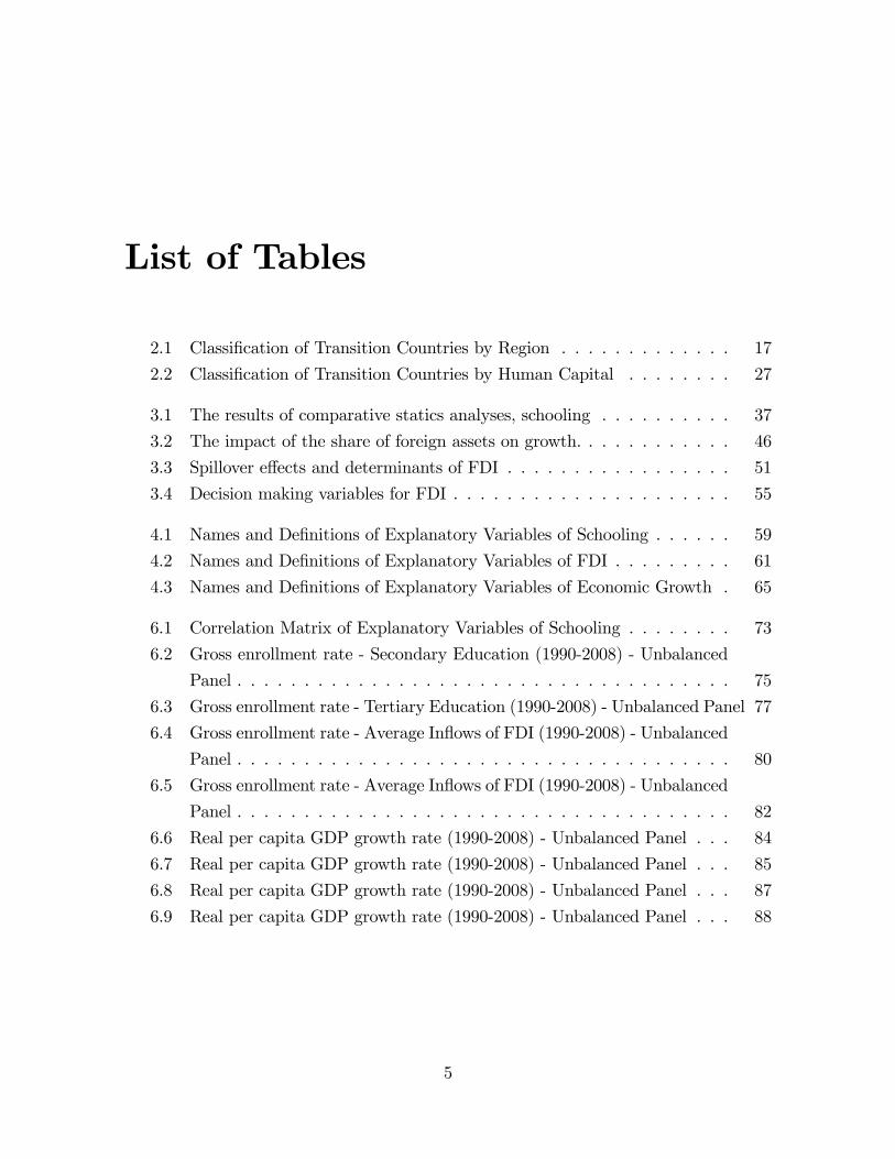
List of Tables
2.1 Classi�cation of Transition Countries by Region . . . . . . . . . . . . . 17
2.2 Classi�cation of Transition Countries by Human Capital . . . . . . . . 27
3.1 The results of comparative statics analyses, schooling . . . . . . . . . . 37
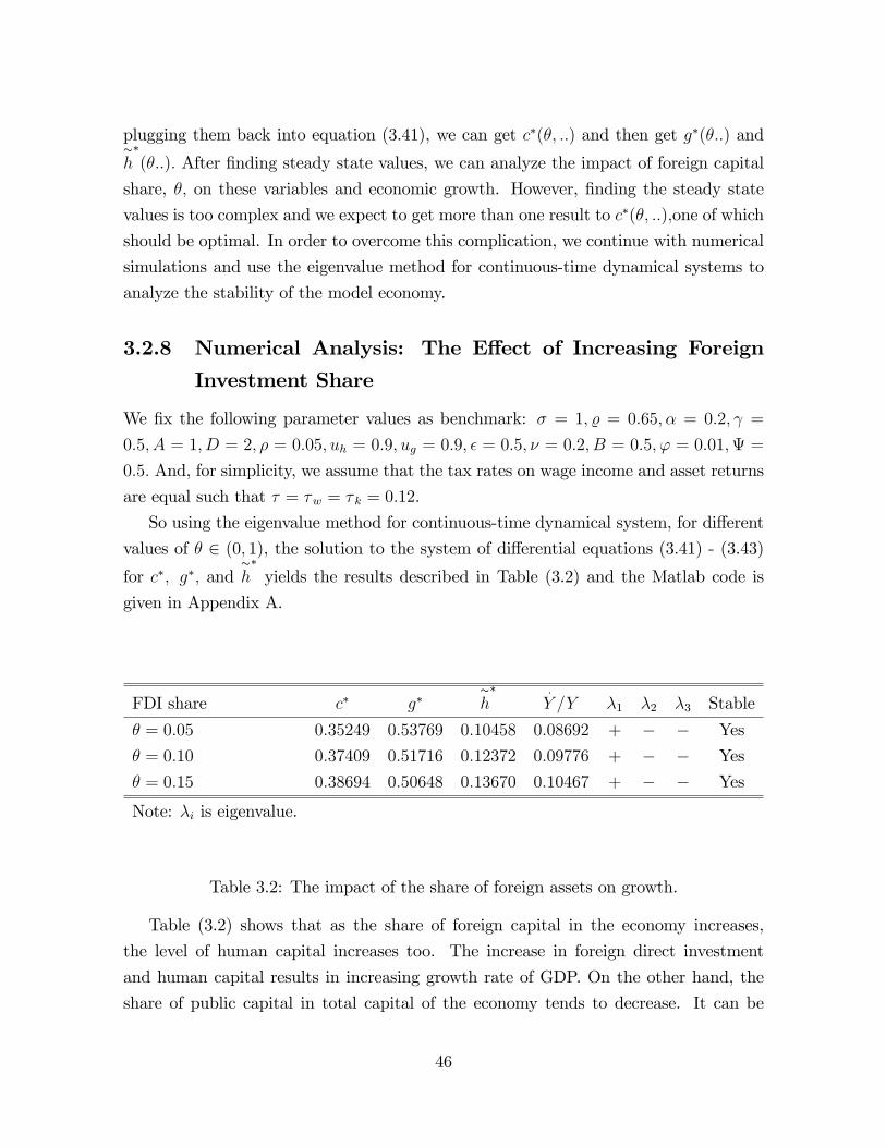
3.2 The impact of the share of foreign assets on growth. . . . . . . . . . . . 46
3.3 Spillover e¤ects and determinants of FDI . . . . . . . . . . . . . . . . . 51
3.4 Decision making variables for FDI . . . . . . . . . . . . . . . . . . . . . 55
4.1 Names and De�nitions of Explanatory Variables of Schooling . . . . . . 59
4.2 Names and De�nitions of Explanatory Variables of FDI . . . . . . . . . 61
4.3 Names and De�nitions of Explanatory Variables of Economic Growth . 65
6.1 Correlation Matrix of Explanatory Variables of Schooling . . . . . . . . 73
6.2 Gross enrollment rate - Secondary Education (1990-2008) - Unbalanced
Panel . . . . . . . . . . . . . . . . . . . . . . . . . . . . . . . . . . . . . 75
6.3 Gross enrollment rate - Tertiary Education (1990-2008) - Unbalanced Panel 77
6.4 Gross enrollment rate - Average In�ows of FDI (1990-2008) - Unbalanced
Panel . . . . . . . . . . . . . . . . . . . . . . . . . . . . . . . . . . . . . 80
6.5 Gross enrollment rate - Average In�ows of FDI (1990-2008) - Unbalanced
Panel . . . . . . . . . . . . . . . . . . . . . . . . . . . . . . . . . . . . . 82
6.6 Real per capita GDP growth rate (1990-2008) - Unbalanced Panel . . . 84
6.7 Real per capita GDP growth rate (1990-2008) - Unbalanced Panel . . . 85
6.8 Real per capita GDP growth rate (1990-2008) - Unbalanced Panel . . . 87
6.9 Real per capita GDP growth rate (1990-2008) - Unbalanced Panel . . . 88
5
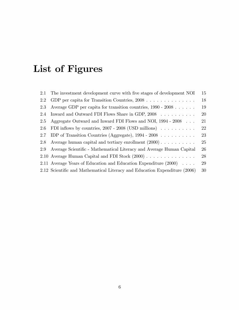
List of Figures
2.1 The investment development curve with �ve stages of development NOI 15
2.2 GDP per capita for Transition Countries, 2008 . . . . . . . . . . . . . . 18
2.3 Average GDP per capita for transition countries, 1990 - 2008 . . . . . . 19
2.4 Inward and Outward FDI Flows Share in GDP, 2008 . . . . . . . . . . 20
2.5 Aggregate Outward and Inward FDI Flows and NOI, 1994 - 2008 . . . 21
2.6 FDI in�ows by countries, 2007 - 2008 (USD millions) . . . . . . . . . . 22
2.7 IDP of Transition Countries (Aggregate), 1994 - 2008 . . . . . . . . . . 23
2.8 Average human capital and tertiary enrollment (2000) . . . . . . . . . . 25
2.9 Average Scienti�c - Mathematical Literacy and Average Human Capital 26
2.10 Average Human Capital and FDI Stock (2000) . . . . . . . . . . . . . . 28
2.11 Average Years of Education and Education Expenditure (2000) . . . . 29
2.12 Scienti�c and Mathematical Literacy and Education Expenditure (2006) 30
6

List of Abbreviations
FDI - Foreign Direct Investment
MNCs - Multinational Corporations
CEB - The Central-Eastern Europe and the Baltic States
CIS - Commonwealth of Independent States
IDP - Investment Development Path
OLI - Ownership, Location and Internalization
NOI - Net Outward Investment
PISA - Programme for International Student Assessment
IMF - The International Monetary Fund
EBRD - The European Bank for Reconstruction and Development
7

�If ideas are the engine of growth and if an excess of social over private
returns is an essential feature of the production of ideas, then we want to go
out of our way to introduce external e¤ects into growth theory, not to try to
do without them�.
Robert E. Lucas (2002)
8
Chapter 1
Introduction
As Alfred Marshal noted in 1890, �the most valuable of all capital is that invested in
human beings�. Being the most important factor of production and vital to achieving
economic growth, human capital measures the quality of the labor supply and can be
accumulated through education, additional education and experience. Externalities or
the spillovers of superior technology brought with foreign direct investment (FDI) as
determinants of the growth rate of human capital are also of the most importance. An
increase in human capital through technology spillovers from abroad is captured by
instruction, education and training of employees to meet the higher standards. More
precisely, multinational corporations (MNCs) in the host economy increase the degree of
competition and force existing �rms (including the ine¢ cient ones) to make themselves
more productive by investing in human capital (see Magnus Blomström, 1991). "MNCs
also provide the training of labor and management which may then become available to
the economy in general" (Magnus Blomström, 1991). Besides getting spillover bene�t
from FDI, an existing human capital is also of great necessity for absorbing superior
technology brought from abroad. Therefore, there is an interrelationship between hu-
man capital formation, FDI and economic growth.
There are three streams of empirical literature (selected) on this topic. FDI in�ow
and Economic Growth! Human Capital: M. Blomström (1991); M. Blomström, R.E.
Lipsey and M. Zejan (1992); A. W. Krause (1999); D. Checchi, G. De Simone, R. Faini
(2007). Human Capital and Economic Growth ! FDI in�ow: A. W. Krause (1999);
M. Blomström and A. Kokko (2003); D. Checchi, G. De Simone, R. Faini (2007). FDI
and Human Capital! Economic Growth: M. Blomström (1991); M. Blomström, R.E.
Lipsey and M. Zejan (1992); E. Borensztein, J. De Gregorio, J-W. Lee (1998); A. W.
9
Krause (1999); M. Carkovic and R. Levine (2002); N. F. Campos and Y. Kinoshita
(2002).
The most of the empirical literature have been done on developed and developing
countries and have not considered the distinctive framework of transition countries.
By transition countries we mean the Central-Eastern Europe and the Baltic States
(CEB), South-Eastern Europe (SEE) and Commonwealth of Independent States (CIS)
and Mongolia, which have transited to a market economy after the collapse of the
former Soviet Union, opened their economy, and needed the superior technology from
developed countries and the high quality human capital meeting the world standards
to achieve economic growth. Therefore, the transition countries make an interesting
case study for the dynamics of human capital, FDI and economic growth. Most of the
countries in our sample, including the Central Asia and the Caucasus countries have
been outside of the mainstream of researches. The noteworthy research for transition
countries has been done by N. F. Campos and Y. Kinoshita (2002) for 25 transition
countries from 1990 to 1998 analyzing the impact of FDI on GDP growth rate.
Whether or not FDI causes human capital and economic growth is a topic of much
debate (see Krause, 1999), and there is no clear evidence on the existence of positive
productivity externalities in the host country caused by foreign MNCs (see L. Alfaro, A.
Chanda, S. K. Ozcan and S. Sayek, 2007). As already mentioned, there is simultaneity
between FDI, human capital and economic growth. The previous empirical �ndings
on FDI and economic growth may be considered skeptical because they do not fully
control simultaneity bias, the use of lagged dependent variables and country speci�c
factors (see Carkovic. M and Levine. R, 2002). Hence, the estimates can be biased.
The streams of theoretical literature (selected) in Micro and Macro levels:
Macro level
� Human Capital and Economic growth: R.E. Lucas (1988); Mulligan and Sala-
i-Martin (1993); Greiner (2008).
Micro level
� FDI, Human Capital and Economic Growth: Liu (2008); L. Alfaro, A. Chanda,
S. K. Ozcan and S. Sayek (2007).
� FDI: F. Toubal and J. Kleinert (2005), Y. Xing and G. Wan (2006).
Micro and Macro levels
� Schooling and Economic Growth: M. Bils and P. J. Klenow (2000).
In our theoretical models, we will utilize and extend the above mentioned theoretical
papers.
10

In the dissertation, we have case study for the Central-Eastern Europe and the Baltic
States (CEB), the South-Eastern Europe (SEE) and the Commonwealth of Independent
States (CIS) and Mongolia covering the period 1990 to 2008.
We integrate the three streams of empirical literature, complement them with our
extensions of the above mentioned theoretical literature and apply them to the countries
in our sample. We contribute to the theoretical literature on Economics of Education;
extending M. Bils and P. J. Klenow (2000) by incorporating additional explanatory
factors such as the spillovers from FDI, migration and mortality rates, and analyze
the dynamics of schooling. We also contribute to the endogenous growth theory with
Lucas style models by incorporating FDI�s spillover e¤ect on human capital forma-
tion. The purpose is to �nd the interrelationships between FDI, human capital and
economic growth (on the existence of public investment) and study their dynamics and
the stability of the model.
In order to contribute to the empirical literature, which complements our theoretical
models, we use 29 transition countries and new explanatory variables being speci�c to
them. The assembled data comprise a panel data set for the period 1990 to 2008 with
yearly observations. The data set is di¤erent from the previously used data structure
such that, in our case, it is subject to the equations of our theoretical models. For in-
stance, in comparison to F. Campos and Y. Kinoshita (2002), who analyzed the impact
of FDI in�ow on economic growth for the transition countries for the period 1990 to
1998 using �xed e¤ects estimations for single equations (obtained from E. Borensztein,
J. De Gregorio, J-W. Lee, 1998), we resort to system GMM estimations (with more
observation periods and using FDI stock instead of FDI in�ow such that FDI stock
is believed to capture the spillover e¤ects). Therefore, our data set is increased with
additional explanatory variables for human capital, FDI stock and GDP growth rate:
repetition and drop-out rates at primary and secondary schools, pupil teacher ratio (as
a measure of human capital quality), infant mortality rate, migration, economic reform
indicators (enterprise reform, forex and trade liberalization, banking sector reform, in-
frastructure reform, private sector share/GDP), private credit to domestic sector and
etc.
Additionally, to take care of the simultaneity problems, we use various econo-
metrics tools. Especially, we apply dynamic panel data analysis using Arellano and
Bover/Blundell and Bond system estimator. This Generalized Method of Moments
(GMM) estimator allows us to �nd the consistent and e¢ cient estimates. We will also
follow GMM estimator approach by S. R. Bond, A. Hoeer and J. Temple (2001) that
11

exploits stationarity restrictions. According to S. R. Bond, A. Hoeer and J. Temple
(2001), �there is a problem with using the �rst-di¤erence GMM panel data estimator
cross country growth regressions. Because when time series are persistent, the �rst
di¤erenced GMM estimator can be poorly behaved, since the lagged levels of the series
provide only weak instruments for subsequent �rst di¤erences�.
It is also worthwhile to note that all possible determinants of human capital, FDI
and economic growth in our theoretical and empirical analysis are carefully investigated.
The thesis proceeds as follows: Chapter 2 reviews the facts on foreign direct in-
vestment, human capital and economic growth in transition countries. The chapter
comprises an economic overview and the investment development path of the coun-
tries in our sample; Central-Eastern Europe and the Baltic state (CEB), South-Eastern
Europe (SEE) and Commonwealth of Independent States (CIS) and Mongolia. Using
the Investment Development Path (IDP) hypothesis by John H. Dunning (1981a), we
analyze systematic relationship between the countries�economic development and the
outward and inward direct investment position. The analysis is done on individual
country and cross-sectional bases. The analysis of the Investment Development Path is
the starting point for the subsequent empirical analysis throughout the thesis. Through
economic review and the IDP analysis, we group the countries according to their eco-
nomic development and investment development path, which will be very important for
econometric analysis in the dissertation. The chapter is complemented by the analysis
of the possible measures of human capital. We investigate the advantages and disad-
vantages of di¤erent measures of human capital, and choose the existing best measure
of human capital for the countries in our sample (in our case: secondary and tertiary
school enrollment rates, and the average years of education).
Chapter 3 presents three theoretical models.
Model 1: Static model of Schooling and Human Capital Accumulation. We con-
tribute to the existing literature on Mincerian returns to education by extending the
schooling model by Mark. B and P. Klenow (2000). We incorporate into the model
the spillover e¤ects of superior technology brought with foreign direct investment, and
the net migration and the death rates (infant mortality rate) following the approach
by Charles I. Jones (2007). From the �rst model, an equation on the determinants of
human capital formation is derived for econometric analysis.
Model 2: An endogenous growth model with foreign direct investment and human
capital. Our model is inspired mainly by Lucas (1988), Rebelo (1991), Mulligan and
Sala-i-Martin (1993), Greiner (2008), and Liu (2008). Lucas (1988) assumes that hu-
12
man capital accumulation has only human capital as input. Rebelo (1991) and Mulligan
and Sala-i-Martin (1993) consider two sector growth models where human capital is ac-
cumulated, in addition to human capital, through physical capital too. Greiner (2008)
extends Lucas style models by incorporating public spending (public resources used in
the schooling sector) in the human capital accumulation, excluding physical capital.
Liu (2008) focuses on externality in the human capital accumulation by adding public
information on technologies and management methods brought through foreign direct
investment. However, Liu (2008) does not consider public spending or physical capital
in human capital production function and does not develop it as a growth model. We
contribute to the endogenous growth theory by analyzing the relationship between for-
eign direct investment and economic growth with a special emphasis on human capital
formation through spillover e¤ects. The role of public investment in production sector
and human capital formation is also incorporated. The stability and dynamics of the
growth model are analyzed.
Model 3: FDI Decision Making. We consider an economy where the technical
progress is the result of increasing capital. We closely follow Romer (1990), Grossman
and Helpman (1991), Barro and Sala-i- Martin (1995) and Borensztein, Gregoiro and
Lee (1998), which focused on an increase in the number of varieties of capital goods.
Di¤erent from this literature, we assume that the total capital in the economy is the sum
of domestic capital and foreign capital. Final good sector is slightly di¤erent from the
previous model, renting the domestic capital from households and buying the foreign
capital from foreign producers. Household�s utility maximization problem is the same as
in the previous model. In this model, we will concentrate on the production of foreign
capital goods, which can either be produced in home country or host country. Our
purpose is to �nd the determinants of foreign investment decision making, which will
be proxied by the present value of future pro�ts of foreign investors. From the model
on FDI decision we derive two equations for estimations; one for the determinants of
foreign direct investment and one for the determinants of economic growth.
Chapter 4 deals with the empirical speci�cation of the equations obtained from
the theoretical models and data analysis. Econometric methodology is presented in
Chapter 5. Estimation results and discussion are presented in Chapter 6. Chapter 7
draws conclusions and presents policy implications.
13

Chapter 2
Facts on Foreign Direct Investment,Human Capital and EconomicGrowth in Transition Countries
2.1 Economic Overview and Investment Develop-
ment Path
Investment Development Path (IDP) hypothesis is investigated for Cenrtal-eastern Eu-
rope and the Baltic states (CEB), South-eastern Europe (SEE) and Commonwealth
of Independent States (CIS) and Mongolia to �nd systematic relationship between the
countries�economic development and the outward and inward direct investment posi-
tion. The analysis is done on individual country and cross-sectional bases. Through
the IDP analysis, we group the countries according to their economic development and
investment development path, which will be very important for econometric analysis.
The IDP theory introduced by Dunning (1981) is an extension of Eclectic Paradigm.
The IDP theory explains the outward and inward direct investment position of countries
with respect to their economic development. According to Eclectic Paradigm, three
factors explain foreign direct investment stock of countries; ownership, location and
internalization (OLI) advantages.
Ownership advantages: Refer to competitive advantages of domestic �rms to engage
in foreign direct investment. These advantages include trademarks, patents, production
technique, managerial know-how, entrepreneurial skills, scale or preferential access to
14

raw materials or to markets.
Location advantages: The host country�s attractiveness to other countries in terms
of economic and political system, infrastructure, physical distance, labor composition,
wages, and existence of raw materials.
Internationalization advantages: Indicating the advantages for the �rm to exploit
the ownership advantages in the international markets; more pro�table for the �rm to
exploit its assets in international market rather than in domestic market.
According to the Investment Development Path Theory, countries pass through �ve
main stages of development classi�ed by OLI advantages (Dunning and Narula,1996).
Changes in OLI advantages impact the international investment position of countries
with respect to their development and are explained with the countries�net outward
investment (NOI: outward FDI minus inward FDI) and gross domestic product levels.
Figure 2.1: The investment development curve with �ve stages of development NOI
Stage 1: Dunning and Narula (1996) argues that in this stage the location advan-tages of a country are not su¢ cient to attract foreign investment. The reasons behind
these are improper economic systems and government policies, inadequate labor force
and infrastructure to promote FDI. The ownership advantages of domestic �rms are
also not su¢ cient. Therefore, outward FDI of the country is likely to be very little.
Therefore, the government must intervene "providing basic infrastructure and upgrade
15

human capital through education or training" (Dunning and Narula, 1996). That is,
before a country can attract signi�cant inward FDI, it must develop its location ad-
vantages including an increase in GDP per capita. "Consequently, in the �rst stage,
we expect a rapid increase in GDP per capita more than NOI per capita. But, in the
second stage the growth rate of NOI per capita can be expected to be higher than GDP
per capita" (Buckley and Castro, 1998).
Stage 2: As the country possesses satisfactory location speci�c advantages (espe-cially, with the help of government policies), inward FDI starts to rise, while outward
direct investments still remain low or negligible. In this stage, inward FDI stocks rise
faster than GDP.
Stage 3: The ownership advantages of domestic �rms grow. Eventually, the rate ofoutward FDI begins to increase. Gradual decrease in the growth rate of FDI in�ows is
observed. This results in increasing net outward investment level (NOI) of the country.
In this stage, ownership advantages induced by government become less signi�cant,
because ownership advantages induced by FDI become more important. Therefore,
domestic �rms�growing ownership advantages are the main determinants of outward
FDI.
Stage 4: Outward FDI stock of the country exceeds or equals the inward FDIstock. Still, outward FDI grows faster than inward FDI. At this stage, domestic �rms
compete with foreign owned �rms in the domestic sector and also enter foreign markets.
Since the ownership advantages of the domestic �rms become similar to those in other
fourth stage countries, trade and foreign investment among these countries will rise.
Stage 5: In the �fth stage of IDP, the NOI level of a country �rst falls and then�uctuates at the zero level, and at the same time inward and outward FDI continue
to rise. Today�s situation in advanced industrial countries depends on the short term
evolution of exchange rates and economic cycle. "Beyond a certain point in the IDP,
the absolute size of GNP is no longer a reliable guide of a country�s competitiveness
neither indeed is its NOI position" (Dunning and Narula, 1996).
Numerous studies on IDP have been done on developed and developing countries.
Dunning (1981) and Dunning and Narula (1996) analyzed the IDP stages of a group
of countries using cross section data, regressing GDP on NOI to �nd J-shaped relation
between GDP and NOI. Later on Duran and Ubeda (2001) also analyzed the IDP stages
of countries with cross section data. Time series analysis have been done by Buckley
and Castro (1998) for Portugal, Bellack (2000) for Austria, Barry, Gord and McDowell
(2001) for Ireland, Alvares (2001) for Spain.
16
Following Dunning (1981), Dunning and Narula (1996) and Buckley and Castro
(1998), we adopt the regression equation of quadratical functional form to describe the
IDP curve. "Quadratical functional form provides a means of testing whether J-shaped
or inverted L-shaped investment development curve gives a good �t of the cross section
data" (Tolentino, 1993).
NOIpc = �0 + �1GDPpc+ �2GDPpc2 + " (2.1)
Expected signs for coe¢ cients are �1 < 0 and �2 > 0 in order to get J-shaped relation
between GDP and NOI.
In order to analyze the relationship between a country�s net outward investment
(NOI) and its economic development, we will initially analyze the IDP stages of tran-
sition countries individually by using time series data. Then, using aggregate data,
we will estimate aggregate IDP using aggregate GDP and the net outward investment
position of the region.
Transition countries in our sample are classi�ed in Table (2.1).
Centraleastern Europe and theBaltic states (CEB)
Southeastern Europe (SEE) Commonwealth of IndependentStates (CIS) and Mongolia
Czech RepublicEstoniaHungaryLatviaLithuaniaPolandSlovak RepublicSlovenia
BulgariaCroatiaRomaniaAlbaniaBosnia and HerzegovinaFYR MacedoniaMontenegroSerbia
RussiaArmeniaAzerbaijanBelarusGeorgiaMoldovaUkraineKazakhstanKyrgyz RepublicMongoliaTajikistanTurkmenistanUzbekistan
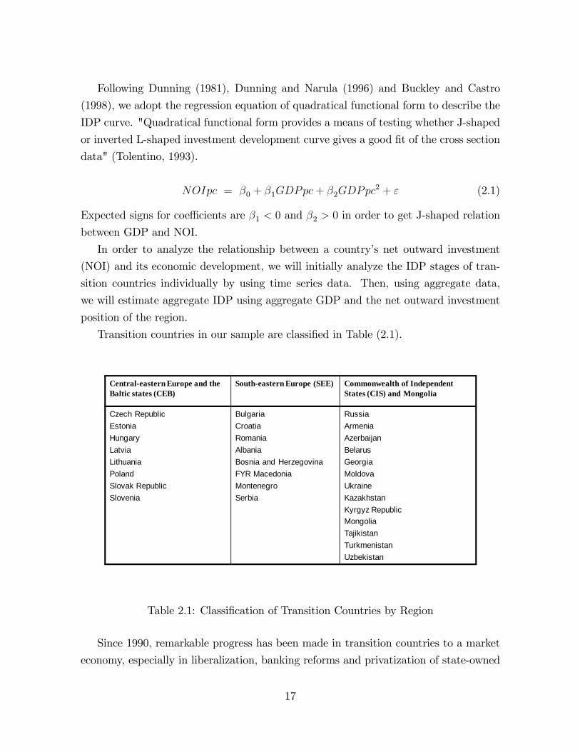
Table 2.1: Classi�cation of Transition Countries by Region
Since 1990, remarkable progress has been made in transition countries to a market
economy, especially in liberalization, banking reforms and privatization of state-owned
17
properties. Almost all countries in our sample have adopted a special FDI regime deal-
ing with foreign direct investment, focusing on tax and custom duty breaks, relaxed
restrictions on foreign ownership. In the previous literature, some central eastern Eu-
ropean countries and Baltic States has been investigated for IDP or other purposes.
Duran and Ubeda (2001) grouped economies together using cluster technique1 and
came to the conclusion that Hungary, Slovenia, Latvia, Lithuania, Moldova, Poland,
Romania and Russian Federation are in the third stage of development. However, the
CIS countries have been outside of the mainstream of researches. Therefore, this makes
the selected transition countries an interesting case study to test the IDP hypothesis.
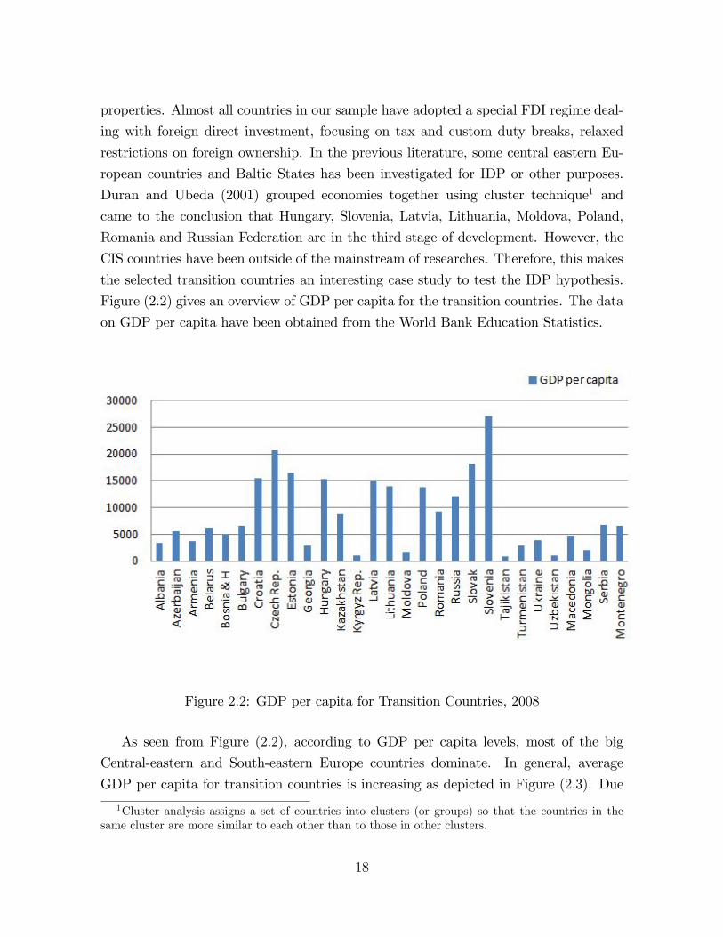
Figure (2.2) gives an overview of GDP per capita for the transition countries. The data
on GDP per capita have been obtained from the World Bank Education Statistics.
Figure 2.2: GDP per capita for Transition Countries, 2008
As seen from Figure (2.2), according to GDP per capita levels, most of the big
Central-eastern and South-eastern Europe countries dominate. In general, average
GDP per capita for transition countries is increasing as depicted in Figure (2.3). Due
1Cluster analysis assigns a set of countries into clusters (or groups) so that the countries in thesame cluster are more similar to each other than to those in other clusters.
18
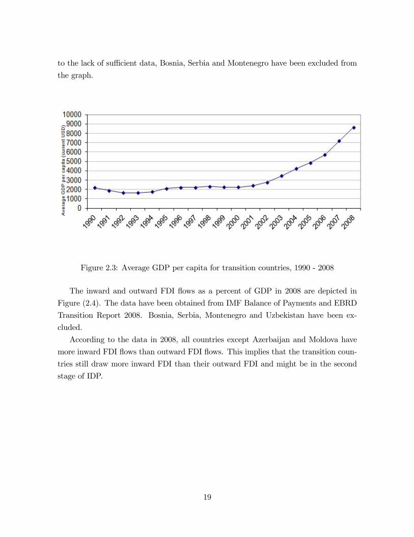
to the lack of su¢ cient data, Bosnia, Serbia and Montenegro have been excluded from
the graph.
Figure 2.3: Average GDP per capita for transition countries, 1990 - 2008
The inward and outward FDI �ows as a percent of GDP in 2008 are depicted in
Figure (2.4). The data have been obtained from IMF Balance of Payments and EBRD
Transition Report 2008. Bosnia, Serbia, Montenegro and Uzbekistan have been ex-
cluded.
According to the data in 2008, all countries except Azerbaijan and Moldova have
more inward FDI �ows than outward FDI �ows. This implies that the transition coun-
tries still draw more inward FDI than their outward FDI and might be in the second
stage of IDP.
19

Figure 2.4: Inward and Outward FDI Flows Share in GDP, 2008
To determine the IDP stages of individual countries, we resort to scatter plots
provided in Appendix (A.3) and analyze the changes of NOI per capita with respect
to GDP per capita level of each country. As we have already noted, in the �rst and
second stage of IDP, inward FDI increases accompanied by an increase in GDP level.
In transition to the third stage, outward FDI rises and the growth rate of inward FDI
�ows decreases. In the third stage, net outward investment is expected to rise.
According to the scatter plots, Albania, Armenia, Belarus, Bosnia, Bulgaria, Croa-
tia, Georgia, Kazakhstan, Ukraine, Uzbekistan, Macedonia, Mongolia, Serbia and Mon-
tenegro are in the second stage of IDP. These countries are characterized by increasing
inward FDI and low outward FDI. Azerbaijan, Czech Republic, Estonia, Hungary,
Latvia, Lithuania, Moldova, Poland, Russia, Slovak Republic and Slovenia are between
the second and third stage of IDP.
To determine the IDP stages as a whole in the transition countries, initially we
analyze the in�ow and out�ow levels of FDI in aggregate as depicted in Figure (2.5).
Turkmenistan, Mongolia, Bosnia, Serbia, Montenegro and Uzbekistan have been ex-
20
cluded due to the lack of data.
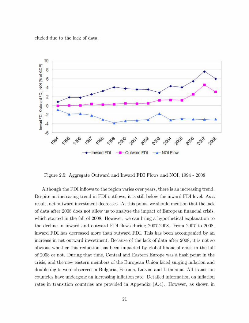
Figure 2.5: Aggregate Outward and Inward FDI Flows and NOI, 1994 - 2008
Although the FDI in�ows to the region varies over years, there is an increasing trend.
Despite an increasing trend in FDI out�ows, it is still below the inward FDI level. As a
result, net outward investment decreases. At this point, we should mention that the lack
of data after 2008 does not allow us to analyze the impact of European �nancial crisis,
which started in the fall of 2008. However, we can bring a hypothetical explanation to
the decline in inward and outward FDI �ows during 2007-2008. From 2007 to 2008,
inward FDI has decreased more than outward FDI. This has been accompanied by an
increase in net outward investment. Because of the lack of data after 2008, it is not so
obvious whether this reduction has been impacted by global �nancial crisis in the fall
of 2008 or not. During that time, Central and Eastern Europe was a �ash point in the
crisis, and the new eastern members of the European Union faced surging in�ation and
double digits were observed in Bulgaria, Estonia, Latvia, and Lithuania. All transition
countries have undergone an increasing in�ation rate. Detailed information on in�ation
rates in transition countries are provided in Appendix (A.4). However, as shown in
21
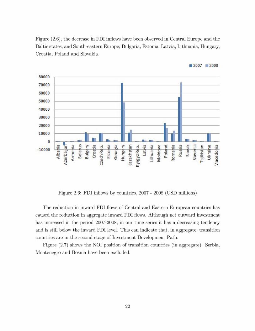
Figure (2.6), the decrease in FDI in�ows have been observed in Central Europe and the
Baltic states, and South-eastern Europe; Bulgaria, Estonia, Latvia, Lithuania, Hungary,
Croatia, Poland and Slovakia.
Figure 2.6: FDI in�ows by countries, 2007 - 2008 (USD millions)
The reduction in inward FDI �ows of Central and Eastern European countries has
caused the reduction in aggregate inward FDI �ows. Although net outward investment
has increased in the period 2007-2008, in our time series it has a decreasing tendency
and is still below the inward FDI level. This can indicate that, in aggregate, transition
countries are in the second stage of Investment Development Path.
Figure (2.7) shows the NOI position of transition countries (in aggregate). Serbia,
Montenegro and Bosnia have been excluded.
22
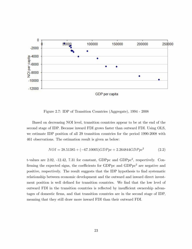
Figure 2.7: IDP of Transition Countries (Aggregate), 1994 - 2008
Based on decreasing NOI level, transition countries appear to be at the end of the
second stage of IDP. Because inward FDI grows faster than outward FDI. Using OLS,
we estimate IDP position of all 29 transition countries for the period 1990-2008 with
461 observations. The estimation result is given as below:
NOI = 28:51385 + (�67:10005)GDPpc+ 2:264844GDPpc2 (2.2)
t-values are 2.02, -12.42, 7.31 for constant, GDPpc and GDPpc2, respectively. Con-
�rming the expected signs, the coe¢ cients for GDPpc and GDPpc2 are negative and
positive, respectively. The result suggests that the IDP hypothesis to �nd systematic
relationship between economic development and the outward and inward direct invest-
ment position is well de�ned for transition countries. We �nd that the low level of
outward FDI in the transition countries is re�ected by insu¢ cient ownership advan-
tages of domestic �rms, and that transition countries are in the second stage of IDP,
meaning that they still draw more inward FDI than their outward FDI.
23

2.2 Measure of Human Capital
Human capital is the most important factor of production. Human capital is of ex-
treme importance for achieving growth in GDP. It facilitates structural changes caused
by globalisation and technological change over the past years in transition countries.
Therefore, in addition to drawing the superior technology from abroad through FDI, one
of the most important policies of each government is to promote the growth of human
capital. Human capital measures the quality of the labor supply. Human capital can
be accumulated through education and experience. Furthermore, externalities like the
teacher human capital and the spillovers from superior technology brought with foreign
direct investment also determine the growth rate of human capital. In this section, we
look for the right measure of human capital for transition countries in our sample and
the founded measures will be used in our econometric analysis.
We di¤erentiate four measures of human capital utilizing the analysis method of
Bergheim (2005); years of education, attainment rates - guides for future, enrollment
rates - future human capital, and quality of human capital.
Years of education: Average years of education of people between 25 and 64 years.It is considered as the best measure of human capital. The average years of education
are an aggregation of the average graduation levels attained by individuals. Barro R.
J. and J. Lee (2000) have presented data on average years of schooling until 2000 for
the countries in our sample. But unfortunately, the observations are not satisfactory
for our estimations. Therefore we turn to alternative measures.
Attainment rates �guides for the future: The di¤erent attainment rates atsecondary and tertiary levels and their development over groups of individuals can
provide information about the future path of the average years of education. "If the
new entrants into the labor market have spent more time in school than those retiring,
then the average human capital or the working age population will rise" (Bergheim,
2005). Attainment rates are not useful for econometric analysis because "a tertiary
attainment rate of 40% of the young cohort can signal either a rise in human capital
or a decline, depending on the starting level of average human capital of the overall
population" (Bergheim, 2005).
Enrollment rates - future human capital: Enrollment rates also provide im-portant information about the future development of human capital. Enrollment rates
are calculated by dividing the number of students of a particular age group enrolled in
all levels of education by the number of people in the population in that age group.
24

When compared with the present human capital, enrollment rates can indicate the
future human capital.
AUT
CAN
CZEDNK FIN
GRCHUN ISL
IRL
ITA
JPN
MEX
NLD
NZLNOR
POL
PRT
SVK
ESP
SWE
CHE
TUR
GBR
USA
ARG
BRA
CHL
COL
HRV
ESTISR
JOR
LVALTUROM
SVN
46
810
12A
vera
ge y
ears
of e
duca
tion
20 40 60 80Tertiary enrolment rate
AvYearsEd Fitted values
Sources:World Bank, OECD
Average human capital and tertiary enrolment (2000)
Figure 2.8: Average human capital and tertiary enrollment (2000)
As the chart shows, the tertiary enrollment in Romania, the Czech Republic, Slo-
vakia and Hungary are not high enough to allow a signi�cant rise in average human
capital in the coming years. There is a relatively high tertiary enrollment rates in Slove-
nia, which indicates that the average years of education are set to rise signi�cantly in
future. Estonia, Latvia, Lithuania and Poland are characterized with high enrollment
rates and high average human capital. Considering the case of Canada, Sweden and
Norway, we can say that the possible higher enrollment rates in these countries will be
followed by high average human capital.
Quality of human capitalMeasure of human capital should indicate the quality of labor input. The average
years of education measures the time spent in school but it does not re�ect what he has
actually learned during that time. Therefore, whether the average years of education
can re�ect the quality of human capital is skeptical. Although there is an incentive
25

for the individual to go to schooling to increase his human capital because of the
expectation that there is a high probability for skilled people to be employed easily
and to get high salary, there can also be the case that some people go to school just to
give signal to a future employer about the level of his human capital. Nevertheless, he
can get positive in�uence from the education environment. In our opinion, the average
years of education should not be considered as re�ecting human capital qualitatively.
Despite this, there is another possibility to measure the quality of human capital. In
this regard, the OECD�s PISA (Program for International Student Assessment) test and
the literacy scores of CIA�s World Factbook are helpful. The disadvantage of this data
is that there is the lack of time series in many countries in our sample, and therefore, it
is not suitable for estimations. We choose the Science and Mathematics PISA score and
investigate its relationship with the average years of education in the following chart.
AUT
CANCZE
DNK
FIN
DEU
GRC
HUNISLIRL
ITA
JPN
MEX
NLD NZL
NORPOL
PRT
SVKESP
SWE
CHE
TUR
GBR
USA
ARGBRA
CHL
COL
HRV
EST
HKG
IDN
ISR
JOR
LVALTU
ROM
SVN
350
400
450
500
550
600
PIS
A 2
006
sci
entif
ic &
mat
hem
atic
al li
tera
cy
4 6 8 10 12Average years of education (2000)
PISA Fitted values
Sources:World Bank, OECD
Average Scientific Mathematical Literacy and Average Human Capital
Figure 2.9: Average Scienti�c - Mathematical Literacy and Average Human Capital
As the chart illustrates, there is a high correlation between the years of education
and the PISA literacy score. The summary of two charts for transition countries are
26

given Table (2.2) in relative comparison.
Level Enrolment Rates(2000)
Average Years ofEducation (2000)
Science &Mathematical Literacy,PISA (2006)
High • Estonia• Latvia• Lithuania• Poland• Slovenia
• Estonia• Latvia• Lithuania• Poland• The Czech Rep.• Slovakia• Hungary• Romania
• Estonia• Latvia• Lithuania• Poland• The Czech Rep.• Slovakia• Hungary• Slovenia
Low • The Czech Rep.• Slovakia• Hungary• Slovenia
• Slovenia • Romania
Table 2.2: Classi�cation of Transition Countries by Human Capital
The results of the chart and the table suggest that Estonia, Latvia, Lithuania and
Poland have high enrollment rates, high average years of education and high Science
and Mathematical Literacy. As already mentioned, the Czech Republic, Slovakia and
Hungary have low enrollment rates, which indicates that the average years of educa-
tion will not increase in the coming years. However, these countries already possessed
high years of education in 2000. Therefore, the average years of education have been
accompanied by high science and Mathematics Literacy in 2006. Slovenia had high
enrollment rate and low average years of education in 2000, which suggests that aver-
age years of education is going to increase in future. Therefore, it has been followed
by high literacy rate in 2006. The case of Romania is similar to the Czech Republic,
Slovakia and Hungary with respect to enrollment rates and average years of education.
However, average Scienti�c and Mathematical Literacy score is low.
As measures of human capital, the data for the average years of education and PISA
literacy score for our countries are not satisfactory. Hence, in our estimations we will use
the enrollment rates (secondary and tertiary). Above we showed that enrollment rates
can give an indication about the future human capital (average years of education) and
in its turn, there is a high positive correlation between the average years of education
27

and PISA Science and Mathematics literacy score.
Enrollment Rates ! Average Y ears of Education !PISA Science and Mathematics literacy score
Therefore, we can also consider enrollment rates as predictor of the quality of ed-
ucation in future. Since the decision to increase human capital impacts enrollment
rates, in our estimations for the determinants of capital in transition countries, we will
include enrollment rates as a dependent variable. As to the impact of human capital on
economic growth and foreign direct investment �ows, we can use the lagged variable for
enrollment rates as a proxy for future human capital. However, we are not sure if the
enrollment rate increases average years of education in one year or �ve years. Despite
this, as an explanatory variable for FDI �ows and economic growth, we will resort to
our calculations of the percentage of population with secondary and tertiary education.
Before moving to the theoretical models, it is worthwhile to bring some explanations
to the relationship of foreign direct investment and average years of education to have
initial picture.
Figure 2.10: Average Human Capital and FDI Stock (2000)
28

The chart depicts an increasing relationship between the FDI stock and the average
years of education. Since data on the average years of education lack for other transition
countries in our sample, we include only some of them and complement the chart with
developed and developing countries. Hence, in our estimations only FDI stock�s impact
on the enrollment rates at secondary and tertiary level will be investigated.
In order to see if the government education expenditure increases the quality of
education or not, we resort to the following two charts: the �rst chart depicts the
relationship of government education expenditure to the average years of education
and the second chart to the quality of education proxied by Science and Mathematical
Literacy.
Figure 2.11: Average Years of Education and Education Expenditure (2000)
29

Figure 2.12: Scienti�c and Mathematical Literacy and Education Expenditure (2006)
According to Figure (2.11), there is a high correlation between the government
education expenditure and the average years of education. However, in Figure (2.12)
we can see that more spending does not necessarily boost quality. Hence, high spending
is not necessarily a sign of a high level human capital. Therefore, countries with high
level of human capital should invest more to maintain population�s average education
level. What increase the quality of education are the students�own incentives and their
response to the technological progress considering the high return to education.
30
Chapter 3
Theoretical Framework
3.1 Model 1: Schooling and Human Capital Accu-
mulation
3.1.1 Introduction and Related Literature
The model is a modi�ed version of the �rst part of "Does Schooling Cause Growth" by
Mark. B and P. Klenow (2000), which focuses on the determinants of schooling. We
extend it by incorporating the spillover e¤ects from foreign direct investment, the net
migration rate and the death rate utilizing "A Simple Mincerian Approach to Endo-
genizing Schooling" by Charles I. Jones (2007), and analyze the channel to schooling
through the presence of foreign direct investment as spillover e¤ects on human capital
formation.
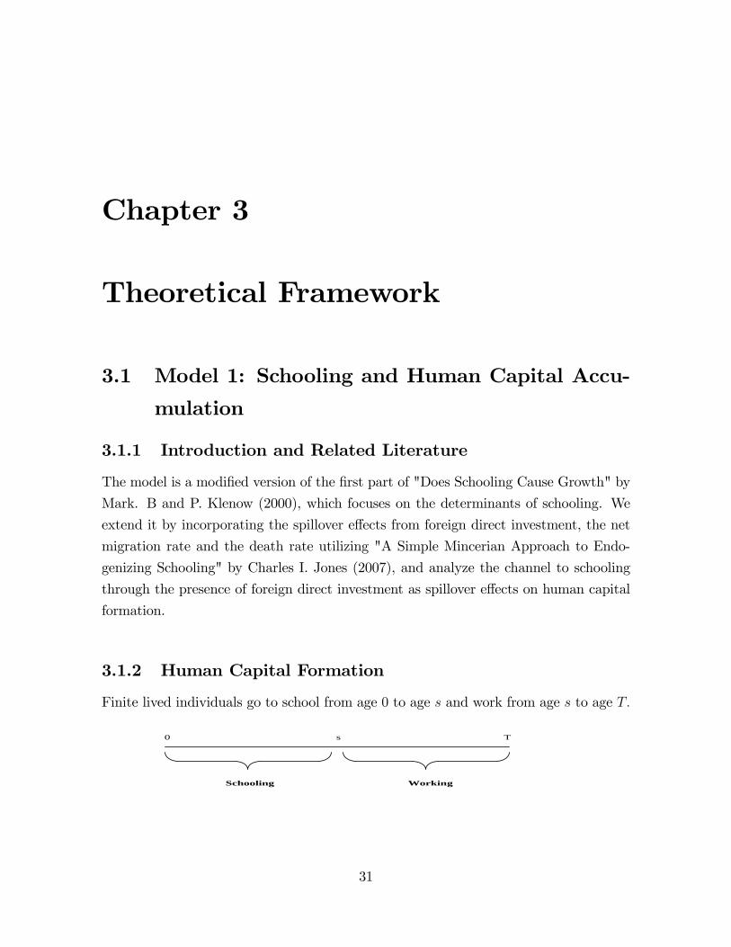
3.1.2 Human Capital Formation
Finite lived individuals go to school from age 0 to age s and work from age s to age T:
0 s T
Schooling Working
31
The aggregate stock of human capital is the sum of the human capital stocks in the
economy. Then we have
H(t) =
Z T
s
h(t)L(t)dt (3.1)
where L(t) is the number of workers at time t and h(t) is the level of human capital.
Let � and be the percentage gains in human capital in each year at school and work,
respectively::hh= � on [0; s] and
:hh= on [s; t] yield
lnh (s) = lnh(0) + s� (3.2)
lnh (t) = lnh (s) + (t� s) (3.3)
combining these two equations we obtain the level of human capital as1
h(t) = e�s+ (t�s) for all t > s (3.4)
We also assume a positive externality Q (t) ; which denotes public information on
technology and management methods associated with foreign invested �rms or in other
words, the spillover e¤ects of foreign direct investment::
Q=Q = � on the interval [0; t]
, Q (t) = e�t:
h(t) = Q (t) e�s+ (t�s) = e�s+ (t�s)+�t for all t > s (3.5)
Since the individuals, while schooling, obtain satisfactory human capital for working,
we can assume that the percentage gain in human capital in each year at school is higher
than that at work. That is, � > :2
Additionally, following Charles I. Jones (2007), we assume that the workers in the
economy are distributed exponentially by age and face a constant death rate �; and
1h(0) is taken as given and assumed to be one. If h(0) 6= 1; the results do not change because h(0)is included as constant in h(t) and h(s):
2It seems controversial whether human capital is of exponential form. In our case, assuming constantpercentage gains in human capital during the schooling and working period is for simpli�cation purpose.Other related noteworthy studies on the Mincerian measure of human capital have been done by
Lim and Tang (2007) and Cohen and Soto (2002). Lim and Tang (2007) develops a Mincerian measureof human capital distribution and �nds a strong evidence of a positive relationship between averageeducation (average years of education) and average human capital (human capital stock developed withMincer formulation) using data for 99 countries. The authors conclude that an individual�s humancapital is an exponential function of his own educational level. But the nationwide average humancapital is closer to a linear function than an exponential function of average years of education. Cohenand Soto (2002) �nds that the years of education is an exponential function of life expectancy.
32
net migration rate (E� l):The net migration rate is the di¤erence between the numberof persons entering, E; and leaving a country, l. An excess of persons entering the
country is referred to as net immigration and an excess of persons leaving the country
as net emigration. The net migration rate indicates the contribution of migration to the
overall level of labor force change. The density is given by f(a) = (� � E + l) e�(��E+l)a
and replaces L in equation (3.1): Hence, the aggregate human capital takes the form
H(t) =
Z T
s
(� � E + l) e�s+ (t�s)�(��E+l)t+�tdt (3.6)
3.1.3 Productive Sector
A competitive open economy faces a constant world real interest rate. The price of
output is normalized to one each period. The production technology is given by
Y (t) = K(t)� [A (t)H(t)]1�� (3.7)
The �rm maximizes instantaneous pro�t
maxK;H
� = K(t)� [A (t)H(t)]1�� � w (t)H(t)� rK (t)
The �rst order conditions are
MPK : � Y (t)K(t)
= r (3.8)
MPH : (1� �) Y (t)H(t)
= w(t) (3.9)
where w(t) is the wage rate per unit of human capital. And w (t)H(t) represents poten-
tial earnings. The wage paid to the worker depends not only on the labor supplied or
the number of hours worked, but also on his human capital. Such that not all employees
that spend the same time get the same wage. That is, their wages di¤er according to
the human capital they possess.
3.1.4 Households
Households are �nite-lived and choose a consumption pro�le and years of schooling to
maximize
33
�fcgTt=0 ; s
�= argmax
Z T
0
e��t ln c (t) dt+
Z s
0
e��t�dt (3.10)
Here c is consumption and � is �ow utility from going to school.
The aggregate budget constraint isZ T
s
e�rtw(t)H(t)dt �Z T
0
e�rtc(t)dt+
Z s
0
e�rt�w(t)H(t)dt (3.11)
It states that the discounted value of all income on [s; T ] have to be equal to or greater
than the present value of consumption on [0; T ] and the present value of the tuition fee
on [0; s] : Where e�rt is the present value factor and � > 0 is the ratio of tuition to the
opportunity cost of student time.
The Lagrange is
L =
Z T
0
e��t ln c (t) dt+
Z s
0
e��t�dt+
�
�Z T
s
e�rtw(t)H(t)dt�Z T
0
e�rtc(t)dt�Z s
0
e�rt�w(t)H(t)dt
�Applying Leibnitz rule for di¤erentiating of an integral, the associated �rst order con-
ditions for consumption, schooling, and the shadow price, respectively are given by
[c(t)]
e��tc(t)�1 = �e�rt ) � = e��tc(t)�1ert (3.12)
Since the individual makes decision while schooling, we convert this equation to time s
� = e��sc(s)�1ers (3.13)
[s]
e�ps� + �[
Z T
s
e�rtw(t)h (t) (� � E + l) (� � ) e�(��E+l)tdt
� (1 + �) e�rsw(s)h(s)e�(��E+l)s (� � E + l)�Z s
0
e�rt�w(t)@H(t)
@sdt] = 0 (3.14)
whereR s0e�rt�w(t)@H(t)
@sdt = 0 because H (t) has been de�ned for t > s and the alter-
native costs related to schooling does not change with more schooling.
34

[�] Z T
s
e�rtw(t)H(t)dt�Z T
0
e�rtc(t)dt�Z s
0
e�rt�w(t)H(t)dt = 0 (3.15)
substituting equation (3.13) into equation (3.14) we get
�c(s) +
Z T
s
erse�rt�(��E+l)tw(t)h(t) (� � ) dt = (1 + �)w(s)h(s)e�(��E+l)s (� � E + l)(3.16)
that is, the sum of the utility from attending schooling plus the present value of future
earnings is equal to the sum of tuition and the opportunity cost of student time for the
last years spent in school. The di¤erence between human capital gained at school and
that gained at work (� � ) enters as staying in school means forgoing experience.
3.1.5 Comparative Statics
From equation (3.16), we obtain
s =1
rln
24 �c(s)he�rs (1 + �)w(s)h(s)e�(��E+l)s (� � E + l)�
R Tse�rt�(��E+l)tw(t)h(t) (� � ) dt
i35
(3.17)
where e�rsw(s)h(s) is the present value of the opportunity cost at s (years of schooling).
Therefore, it has a negative impact on his schooling enrollment. e�rs�w(s)h(s) is the
present value of the tuition fee, which also has negative impact on his enrollment.
On the other hand, the present discounted value of all income on [s; T ] has positive
impact on his decision to enroll. Because, if the individual is sure that he will get
high salary in future because of the human capital accumulated at schooling time, then
he will enroll. Since, the spillovers from foreign investment impacts the discounted
value of all income through human capital, then the spillovers have positive impact on
schooling decision. Similarly, the utility �ow from going to school, �c(s)�; has positive
impact. The percentage gain in human capital from each year at schooling, �; has
also positive impact. But in contrary, the percentage gain in human capital from each
year at work has negative impact on his schooling decision. It could be the case if the
individual thinks that it is more e¢ cient to increase human capital at work than at
school. However, he knows that the percentage gain from increasing his human capital
35
at work is not so high, then the individual can enroll at school and prepare himself
for future work, which demands high knowledge. At the same time, equation (3.17)
shows that death rate has negative impact on schooling, and if E � l > 0; then net
immigration has positive impact and if E � l < 0; then net emigration has negative
impact on schooling.
As seen from equation (3.17), there may be an endogeneity problem. The dependent
variable is the years of schooling. And the independent variables also depended on the
years of schooling. If we accept the opportunity cost and the tuition fee as already
given at that time (which could have happened in schooling years), then the problem
is relieved except for the present discounted value of all income on [s; T ] : The future
income after school depends greatly on the human capital formed at schooling years.
Although, the results above seem to make sense, we try to obtains s from equation
(3.17). In the model the real interest rate, r; is world constant. Then from equation
(3.8) we get;
YY=
;
KK: And from equation (3.9) we have
;
HH=
;
YY�
;ww: Substituting these
in the derivative of the production function, we get;ww=
;
AA= gA: Taking the integral of
this equation from time s to time t; we get w(t) = w(s)egA(t�s): Additionally, consider
h(t) = h(s)e (t�s)+�(t�s) from equation (3.5), and from equation (3.15) at "time" s
consider c (s) = (1� �)w (s)h (s) (� � E + l) e�(��E+l)s: Substituting w(t); h(t); andc (s) into equation (3.17) and simplifying we have:
s = T � 1
r � gA + � � � (E � l)� �� (3.18)
ln
�� �
� � � (1 + �� � (1� �)) (r � gA + � � � (E � l)� �)
�
The derivative of equation (3.18) with respect to the rate of return to capital, r ;
the growth rate of productivity, g; death rate, �; the spillovers from foreign direct
investment, �; and net immigration and emigration (depending on the sign), E � l arethe following:
@s
@r< 0;
@s
@�< 0;
@s
@g> 0;
@s
@ (E � l) > 0 and@s
@�> 0 (3.19)
The rate of return to capital and the growth rate of productivity enters equation
(3.18) together. Schooling reacts negatively to the rate of return of capital (also con-
36
sidered to be the opportunity cost) and positively to the growth rate of productivity.
Bills, Mark and Klenow, Peter J (2000) explains it such that higher growth acts like a
lower market interest rate. Hence, by putting more weight on future human capital it
stimulates more schooling. As before, the death rate has negative, the net immigration
(if E � l > 0; then an excess of persons entering the country) has positive, and the netemigration (if E � l < 0; and excess of persons leaving the country) has negative im-pacts on schooling. The spillovers from foreign investment, �; has also positive impact
on schooling.
As to the percentage gain in human capital from each year in schooling, �; it also has
positive impact on schooling:The reverse impact is from the percentage gain in human
capital from working:@s
@�> 0 and
@s
@ < 0 (3.20)
The reason for the negative impact of the percentage gain in human capital fromworking
is the same as explained above.
The derivative of equation (3.18) for tuition fee, �; and the utility �ow from going
to school, �; are the following:
@s
@�< 0 and
@s
@�> 0 (3.21)
Equations (3.21) implies that the tuition fee has negative, the utility �ow from
schooling. The results are summarized in Table 3.1.
Variables E¤ect on Schooling
Rate of return on capital negative
Death negative
Net emigration negative
Net immigration positive
Productivity positive
Utility from schooling positive
Spillovers from FDI positive
Table 3.1: The results of comparative statics analyses, schooling
In order to test the theoretical model�s prediction for signs e¤ects of these explana-
37
tory variables, equation (3.18) will be estimated in a linear form in Chapter 6.
3.2 Model 2: Human Capital Accumulation, For-
eign Direct Investment and Economic Growth
3.2.1 Introduction and Related Literature
We present an endogenous growth model utilizing Lucas (1988), Rebelo (1991), Mulli-
gan and Sala-i-Martin (1993), Greiner (2008), and Liu (2008).
Lucas (1988) assumes that human capital accumulation has only human capital
as input. Rebelo (1991) and Mulligan and Sala-i-Martin (1993) consider two sector
growth models where human capital is accumulated, in addition to human capital,
through physical capital too. Greiner (2008) extends Lucas style models by incorpo-
rating public spending (public resources used in the schooling sector) in the human
capital accumulation, excluding physical capital. Liu (2008) focuses on externality in
the human capital accumulation by adding public information on technologies and man-
agement methods brought through foreign direct investment. However, Liu (2008) does
not consider public spending or physical capital in human capital production function
and does not develop it as a growth model.
Our endogenous growth model is inspired by the above mentioned literature. We
contribute to endogenous growth theory by analyzing the relationship between foreign
direct investment (FDI) and economic growth with a special emphasis on human capital
formation through spillover e¤ects. The role of public investment in production sector
and human capital formation is also incorporated.
Our economy takes the world interest rate as given. Therefore, we are not going
to discuss the e¤ect of the di¤erence or equality of world and domestic interest rates
on foreign assets in�ow. We accept that foreign assets in�ow responds greatly to any
di¤erences between interest rates, which in turn depend on exchange rates and the
taxation of foreign asset income. Di¤erent interest rates might occur in either perfect
or imperfect markets, which is also out of the scope of our model. However, we think it
could be useful to bring some clari�cation to this issue. In both markets, the existence
of world and domestic interest rate di¤erence is possible explained as following. Under
38
perfect capital mobility, the di¤erence arises when exchange rate expectations are not
static. In this case, interest rate di¤erences are o¤set by expectations of exchange rate
movements (Romer, 2001). Under imperfect capital mobility with �oating exchange
rate, foreign assets in�ow also depends on the interest rate di¤erences. This di¤erential
interest rates "hypothesis postulates that capital �ows from countries with low rates of
return to countries with high rates of return move in a process that leads eventually to
the equality of ex ante real rates of return" (Moosa, 2002). Hence di¤erent world and
domestic interest rates, exchange rates and di¤erentiating market as being perfect and
imperfect are out of the scope of the model.
There are a many channels through which FDI a¤ects economic growth. A conve-
nient way is to allow FDI in the production function. FDI can increase the growth
by increasing the capital stock. However, if there is perfect substitutability, then this
e¤ect will likely be small. If foreign and domestic capitals are complements, then the
e¤ect of FDI will be larger because of externalities. If FDI is treated as di¤erent input,
like the way of expanding the varieties of intermediate good as in Borensztein et al.,
(1998), then FDI is assumed to raise productivity. Considering these, we develop two
open economy endogenous growth models as following:
The �rst model considers foreign capital as exogenous. We assume that public and
human capitals are used proportionally in the production of output and the human
capital formation. As in Liu (2008), we include public information in human capital
accumulation, and, for simplicity, we assume it to be a linear function of foreign capital.
Where public information is characterized by spillover e¤ects of foreign investment on
human capital. Aggregate capital is only used in the production sector. In this case,
domestic and foreign capitals are assumed to be substitutes and paying the same rate or
return (as in open-economy Ramsey Model). The model consists of three-dimensional
system of �rst order di¤erential equations. Our purpose is to investigate the e¤ect of
increasing share of foreign capital (in total capital) on economic growth, the reactions of
human and productive public capitals, the stability and dynamics of the growth model.
The second model is the extension of the �rst model and considers foreign capital as
endogenous through FDI stock accumulation equation. Additionally, the total capital
stock in the production function is disaggregated into domestic and foreign capital
stocks, where output�s elasticity with respect to foreign capital stock is higher. Through
this way we obtain di¤erent rates of return on physical capital stocks. Besides, as an
incentive to foreign investors, di¤erent tax rates are also taken into account. The model
39
consists of four-dimensional system of �rst order di¤erential equations. We analyze the
relationship between four endogenous variables; consumption, public capital, human
capital and foreign capital, and the growth e¤ects, the stability and dynamics of the
model.
3.2.2 The Model with Exogenous FDI
We consider an open economy: a �nal good sector that produces consumption goods
and physical capital, a household sector that receive labor income and income from
its saving, and the government. Since we consider foreign capital as exogenous, we
assume the same income tax, � k = � dk = � fk, and the same rate of return on domestic
and foreign capitals, r = rdk = rfk. We do this because in the model with exogenous
FDI, di¤erent real interest and income tax rates on foreign capital do not play any
role. However, in the subsequent section with endogenous FDI model, we will consider
these rates as incentives to foreign investors. Another reason for assuming equal real
interest rates in this model is that we assume that in the long run the real interest rates
or marginal productivity on both capital stocks can be equal as long as the quality of
domestic capital stock reaches to the quality of foreign capital if we have enough foreign
capital stock and spillover e¤ects (we will come to this point in the endogenous FDI
model).
However, in this model, we put di¤erent labels for income taxes and real interest
rates because we will need some of the equations, obtained here, for the model with
endogenous FDI.
3.2.3 The Household
In our economy the physical capital is decomposed into domestic and foreign-invested
capital. K = Kd+Kf or (1� �)K + �K: An in�nite lived household seeks to maximizeoverall utility, as given by
maxC
Z 1
0
e��tC1�� � 11� � dt (3.22)
subject to his/her budget constraint
40
:
Q = (1� �w)wuhL+ (1� � dk)rdkQ� C + Tp + %� (3.23)
with Q = (1� �)K denoting the amount of assets, and C; �; and Tp are the amounts
of consumption, pro�ts and transfers, respectively. And �w and � dk are the tax rates
on wage income and asset returns. And % is the fraction of pro�ts remained in the
economy. Furthermore, uh is the fraction of human capital or the amount of time used
for production and 1� uh is the amount of time used for human capital accumulation(we will come to this issue later). � and Tp are taken as given by the household.
Tp > 0 are lump-sum transfers to the household. If Tp < 0; the household has to pay a
lump-sum tax.
We formulate the current value Hamiltonian
J =C1�� � 11� � + � [(1� �w)wuhL+ (1� � dk)rdkQ� C + Tp + %�] (3.24)
The associated �rst order necessary conditions for control (C); state (Q) ; and co-state
(�) variables, respectively are given by
@J
@C= 0 ) C�� = �)
:
C
C= � 1
�
:�
�(3.25)
@J
@Q= � :
�+�� ) :� = ����(1� � dk)rdk )
:�
�= �� (1� � dk)rdk
(3.26)@J
@�=
:
Q ):
Q = (1��w)wuhL+(1�� dk)rdkQ�C+Tp+%�(3.27)
combining equation (3.25) and (3.26) we obtain
:
C
C= � 1
�[�� (1� � dk)rdk] (3.28)
Necessary conditions are su¢ cient if transversality condition given as limt!1 e��t�Q =
0 holds. Equation (3.28) states that the household will postpone the consumption if
the return to assets is greater than the impatience rate �: If � > (1 � � dk)rdk; thegrowth rate of consumption will decrease over time because the household has higher
impatience than the return to assets. However, in our analysis in the whole paper, we
41
will stick to maintaining (1� � dk)rdk > �.
3.2.4 The Productive Sector
Utilizing Lucas (1988), Greiner (2006) and Zhiqiang Liu (2006), we assume that output
is produced with a constant returns to scale technology and takes the Cobb-Douglas
form:
Y = AD (Kd +Kf )1��� (ugG)
�(uhhL) (3.29)
where A represents exogenous, common technological factors. D is the productivity
parameter relating to the superior technology brought through foreign direct investment
(Zhiqiang Liu, 2006). G is productive public capital. ug is the fraction of government
spending, which directly a¤ects the production of output. The rest of government
spending, 1�ug, is used for education for the purpose of the human capital accumulationand indirectly a¤ects output (we will come back to this issue later). Furthermore,
1��� ; �; and represents the elasticities of output with respect to physical capital,public capital and human capital, respectively. If � = 0 and D is not included, and ha(the external e¤ects of human capital) is added, the production function is simpli�ed
to that known in Lucas (1988). The �rm maximizes instantaneous pro�t � :
maxK;L
� = AD (Kd +Kf )1��� (ugG)
�(uhhL) � wuhL� r (Kd +Kf ) (3.30)
the �rst order conditions are
@�
@K) (1� �� )Y
K= r (3.31)
@�
@L) Y (uhL)
�1 = w (3.32)
From equations (3.30), (3.31), and (3.32) we obtain �rm�s pro�t as
� = �Y (3.33)
42

3.2.5 Human Capital Formation
The growth of human capital is given by
:
h = BP (Kf )1���� ((1� uh)hL)� ((1� ug)G)� � �hh (3.34)
where B can be considered either shift parameter (Romer, 2001) or a technology para-
meter (Greiner, 2006) or an e¢ ciency parameter of the production (Zhiqian Liu, 2006).
As already mentioned, (1 � uh) and (1� ug) are the fractions of human capital andpublic capital spent for human capital accumulation. P (Kf ) denotes public informa-
tion on technology and management methods associated with foreign invested �rms
(Zhiqian Liu, 2006) and Kf is foreign invested capital. Since public information is not
an explicit function of the model�s parameters, we assume a special case where P (Kf )
is linear. Such that P (Kf ) = Kf = �K: Where indicates the reaction of public
information to changes in foreign direct investment. And 0 < �+ � < 1 represents the
intensity of spillovers. If there are no spillovers, �+ � = 1: When � = 1 and � = 0; the
equation is simpli�ed to that known in Lucas�s model (1988). Considering the linear
function and normalizing L � 1, the equation for the growth of human capital is givenby
:
h = B(�K)1���� ((1� uh)h)� ((1� ug)G)� � �hh (3.35)
3.2.6 The Government
The government is assumed to receive tax income from labor income taxation and
taxing the returns on domestic and foreign assets and uses it for public investment and
for transfer payments. Thus the government�s budget constraint can be written as
:
G = (1� ') (�wwuh + � dkrdk (1� �)K) + � fkrfk�K (3.36)
where ' represents the fraction of tax revenues (excluding the tax income from the
return on foreign assets) used for transfers. In turn, ' > 0 and ' < 0 represents the
fractions for lump-sum transfers and lump-sum tax, respectively. As already mentioned
we have assumed r = rdk = rfk and � k = � dk = � fk: We will consider these equalities
in the following subsection.
43

3.2.7 Equilibrium Conditions and The Balanced Growth Path
De�nition 1 An equilibrium is a sequence of prices fw(t); r(t)g1t=0 ; a sequence ofhousehold consumption,domestic and foreign assets fC(t); Kd(t); Kf (t)g1t=0 ; a sequenceof government policy fG(t); �(t); Tp(t)g1t=0 such that the following conditions are satis-�ed:
(i) Given prices, the household decisions fC(t); Kd(t)g1t=0 solve the household prob-lem.
(ii) The �rm maximizes pro�t.
(iii) The government�s budget constraint is satis�ed.
Substituting equation (3.31) into equation (3.28) we derive the growth rate of con-
sumption
:
C
C= � 1
�
��� (1� � k)(1� �� )AD
�ugG
K
���uhh
K
� �(3.37)
Rearranging equation (3.35) we get the growth rate of human capital
:
h
h= B(�)1����
�(1� uh)
h
K
���h
K
��1�(1� ug)
G
K
��(3.38)
And resource constraint of the economy is obtained by equations (3.23), (3.29), (3.31),
(3.32), (3.33) and considering Q = (1� �)K.
:
K
K=
1
1� � [AD�ugG
K
���uhh
K
� f (1� �w + '�w) (3.39)
+(1� �� ) (1� �) (1� � k + '� k) + %�g �C
K]
From the government�s budget constraint, equations (3.31) and (3.32) and we get the
growth rate of government spending
:
G
G= AD(ug)
�
�uhh
K
� �G
K
���1(1� ') [�w + � k(1� �� ) (1� �)] +� kr�
�G
K
��1(3.40)
44
where r is given by equation (3.31).
De�nition 2 A balanced growth path follows a path where the economy is in equilibriumand consumption, government spending, physical capital and human capital grow at the
same strictly positive constant growth rate, i.e.:CC=
:hh=
:KK=
:GG= �; � > 0:
From equations (3.37) - (3.40), at the steady-state, for:CC;:hh;
:KKto be constant,
CK; GKand h
Kshould be constant. That is
:GG=
:KK=
:hh=
:CC: Since the equations for
growth rates depend on the ratio of variables to K, we need to de�ne new variablessh � h
K; c � C
K; and g � G
K: Di¤erentiating the new variables with respect to time we
get a three dimensional system of �rst order di¤erential equations of the form:
:c = c[AD(ugg)
�(uhsh) f(( 1
�� 1) (1� � k)� � k')(1� �� ) (3.41)
� 1
1� � ((1� �w + '�w) + %�) g �1
��+
1
1� �c]
:g = g[AD(ug)
�(uhsh) g��1(1� ')(�w + � k(1� �� ) (1� �)) (3.42)
� 1
1� �AD (ugg)� (uh
sh) f (1� �w + '�w)
+(1� �� ) (1� �) (1� � k + '� k) + %�g
+1
1� �c+ � k(1� �� )AD(ugg)�(uh
sh) �g�1]
:sh =
sh[B(�)1����(1� uh)�
sh��1((1� ug) g)� (3.43)
� 1
1� �fAD(ugg)�(uh
sh) ( (1� �w + '�w)
+(1� �� ) (1� �) (1� � k + '� k) + %�)� cg]
The steady state levels of consumption, human capital and government spending
are found as following. We solve equation (3.41) for AD(ugg)�(uhsh) and substitute
it to equations (3.42) and (3.43) to obtain g(c; �::) andsh(c; �::);respectively. Then by
45
plugging them back into equation (3.41), we can get c�(�; ::) and then get g�(�::) andsh�(�::): After �nding steady state values, we can analyze the impact of foreign capital
share, �; on these variables and economic growth. However, �nding the steady state
values is too complex and we expect to get more than one result to c�(�; ::);one of which
should be optimal. In order to overcome this complication, we continue with numerical
simulations and use the eigenvalue method for continuous-time dynamical systems to
analyze the stability of the model economy.
3.2.8 Numerical Analysis: The E¤ect of Increasing Foreign
Investment Share
We �x the following parameter values as benchmark: � = 1; % = 0:65; � = 0:2; =
0:5; A = 1; D = 2; � = 0:05; uh = 0:9; ug = 0:9; � = 0:5; � = 0:2; B = 0:5; ' = 0:01; =
0:5: And, for simplicity, we assume that the tax rates on wage income and asset returns
are equal such that � = �w = � k = 0:12.
So using the eigenvalue method for continuous-time dynamical system, for di¤erent
values of � 2 (0; 1), the solution to the system of di¤erential equations (3.41) - (3.43)
for c�; g�; andsh�yields the results described in Table (3.2) and the Matlab code is
given in Appendix A.
FDI share c� g�sh� :
Y =Y �1 �2 �3 Stable
� = 0:05 0:35249 0:53769 0:10458 0:08692 + � � Yes
� = 0:10 0:37409 0:51716 0:12372 0:09776 + � � Yes
� = 0:15 0:38694 0:50648 0:13670 0:10467 + � � Yes
Note: �i is eigenvalue.
Table 3.2: The impact of the share of foreign assets on growth.
Table (3.2) shows that as the share of foreign capital in the economy increases,
the level of human capital increases too. The increase in foreign direct investment
and human capital results in increasing growth rate of GDP. On the other hand, the
share of public capital in total capital of the economy tends to decrease. It can be
46
explained such that as the economy is opened to the world (as a result of transition
from centralized economy to market economy), foreign investment begins to play much
role in the production sector. As to the stability of the balanced growth path, saddle
point stability is achieved for all � 2 (0; 1) : In the next section, we extend the modelby endoginizing foreign direct investment.
3.2.9 The Model With Endogenous FDI
In this section, we will derive a foreign capital accumulation equation and continue the
previous model.
The household�s and government�s problems are the same as before. However, we
will utilize the equations obtained in these sectors and make changes arising from en-
dogenizing foreign capital. We extend the productive sector�s problem by considering
foreign capital stock as a di¤erent input into the production function, and as a result
obtain di¤erent rates of return on domestic and foreign capitals. In addition to di¤erent
real interest rates, we consider di¤erent tax rates on both capitals.
Foreign Capital Accumulation
From the previous model (with exogenous FDI), we can assume the accumulation of
FDI stock in the following form:
Kft+1 =
�(1� � fk) rfkKf
t + (1� %)��+ newFDIflowt + (1� �repf )Kf
t (3.44)
where is the fraction of existing foreign investors�income that they reinvest in the
economy to increase their capital stocks and (1� %)� is the pro�t of foreign �rms. Thedecision to reinvest is assumed to be almost the same for new foreign investor and the
existing foreign investors in the economy. Therefore, we omit newFDIflowt from the
equation although there are many explanatory variables of new FDI �ow, which we will
discuss in detail in the second case. Correspondingly, �repf is the possible repatriation
of foreign capital.
The Host Country Production Sector
We rewrite the constant returns to scale Cobb-Douglas production function with for-
eign capital stock as a di¤erent input. We suppose that the elasticity of output with
47
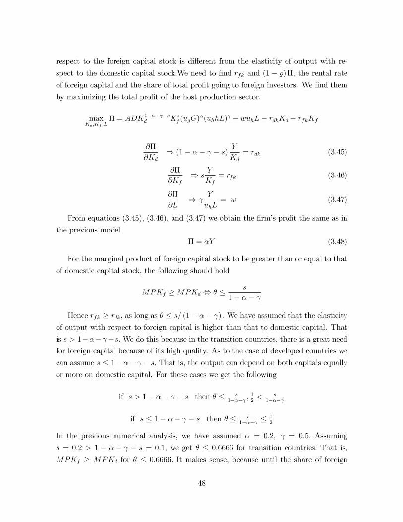
respect to the foreign capital stock is di¤erent from the elasticity of output with re-
spect to the domestic capital stock.We need to �nd rfk and (1� %)�; the rental rateof foreign capital and the share of total pro�t going to foreign investors. We �nd them
by maximizing the total pro�t of the host production sector.
maxKd;Kf ;L
� = ADK1��� �sd Ks
f (ugG)�(uhhL)
� wuhL� rdkKd � rfkKf
@�
@Kd
) (1� �� � s) YKd
= rdk (3.45)
@�
@Kf
) sY
Kf
= rfk (3.46)
@�
@L)
Y
uhL= w (3.47)
From equations (3.45), (3.46), and (3.47) we obtain the �rm�s pro�t the same as in
the previous model
� = �Y (3.48)
For the marginal product of foreign capital stock to be greater than or equal to that
of domestic capital stock, the following should hold
MPKf �MPKd , � � s
1� ��
Hence rfk � rdk; as long as � � s= (1� �� ) :We have assumed that the elasticityof output with respect to foreign capital is higher than that to domestic capital. That
is s > 1��� �s:We do this because in the transition countries, there is a great needfor foreign capital because of its high quality. As to the case of developed countries we
can assume s � 1��� � s: That is, the output can depend on both capitals equallyor more on domestic capital. For these cases we get the following
if s > 1� �� � s then � � s1��� ;
12< s
1���
if s � 1� �� � s then � � s1��� �
12
In the previous numerical analysis, we have assumed � = 0:2; = 0:5: Assuming
s = 0:2 > 1 � � � � s = 0:1; we get � � 0:6666 for transition countries: That is,
MPKf � MPKd for � � 0:6666: It makes sense, because until the share of foreign
48

capital stock reaches 67% (according to the parameters that we have chosen), there is
still an incentive to foreign investors through higher rate of returns on foreign capital
stock. If the elasticity of output with respect to domestic capital stock is higher than
or equal to that to foreign capital stock, then equilibrium point will be reached at a
lower value of �: That is, if s = 0:1 < 1 � � � � s = 0:2; then rfk � rdk as long as� � 0:3333: And if s = 0:15 = 1� �� � s = 0:2; then � � 0:5: This happens becauseof the high capacity of domestic capital and the less need for foreign capital.
Equilibrium Conditions and The Balanced Growth Path
Using the di¤erent rate of return on domestic capital stock, and di¤erent tax rate on
this return, the growth rate of consumption given by equation (3.28) is rewritten as
:
C
C= � 1
�
��� (1� � dk)(1� �� � s)AD
�Kf
Kd
�s(ug
G
Kd
)�(uhh
Kd
) �
(3.49)
Similarly, considering di¤erent rate of return on foreign capital stock and di¤erent
tax rate on this return in equation (3.44), we get the growth rate of foreign capital
stock
:
Kf
Kf
= AD
�Kf
Kd
�s�1(ug
G
Kd
)�(uhh
Kd
) ((1� � fk) s+ (1� %)�)� �repf (3.50)
The growth rate of human capital is obtained from equation (3.35)
:
h
h= B()1����(1� uh)�
�(1� ug)
G
Kd
�v �Kf
Kd
�1�v���h
Kd
���1(3.51)
Considering the di¤erent real interest and tax rates in equation (3.36), we rewrite the
governments budget constraint as
:
G
G= (ug)
�AD
�Kf
Kd
�s�G
Kd
���1(uh
h
Kd
) ((1� ') (�w + � dk (1� �� � s)) + � fks)
(3.52)
49
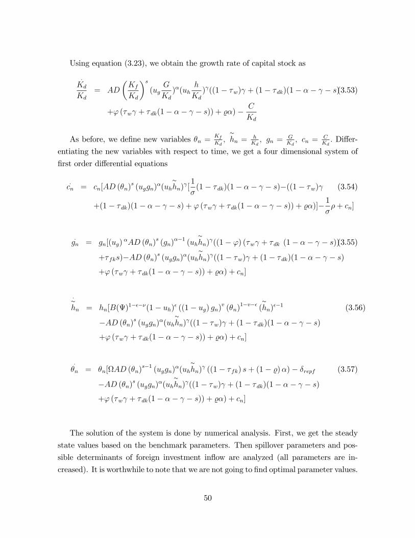
Using equation (3.23), we obtain the growth rate of capital stock as
:
Kd
Kd
= AD
�Kf
Kd
�s(ug
G
Kd
)�(uhh
Kd
) ((1� �w) + (1� � dk)(1� �� � s)(3.53)
+' (�w + � dk(1� �� � s)) + %�)�C
Kd
As before, we de�ne new variables �n =Kf
Kd;shn =
hKd; gn =
GKd; cn =
CKd: Di¤er-
entiating the new variables with respect to time, we get a four dimensional system of
�rst order di¤erential equations
:cn = cn[AD (�n)
s (uggn)�(uh
shn)
[1
�(1� � dk)(1� �� � s)�((1� �w) (3.54)
+(1� � dk)(1� �� � s) + ' (�w + � dk(1� �� � s)) + %�)]�1
��+ cn]
:gn = gn[(ug)
�AD (�n)s (gn)
��1 (uhshn)
((1� ') (�w + � dk (1� �� � s))(3.55)
+� fks)�AD (�n)s (uggn)�(uhshn)
((1� �w) + (1� � dk)(1� �� � s)+' (�w + � dk(1� �� � s)) + %�) + cn]
:shn = hn[B()
1����(1� uh)� ((1� ug) gn)v (�n)1�v�� (shn)
��1 (3.56)
�AD (�n)s (uggn)�(uhshn)
((1� �w) + (1� � dk)(1� �� � s)+' (�w + � dk(1� �� � s)) + %�) + cn]
:
�n = �n[AD (�n)s�1 (uggn)
�(uhshn)
((1� � fk) s+ (1� %)�)� �repf (3.57)
�AD (�n)s (uggn)�(uhshn)
((1� �w) + (1� � dk)(1� �� � s)+' (�w + � dk(1� �� � s)) + %�) + cn]
The solution of the system is done by numerical analysis. First, we get the steady
state values based on the benchmark parameters. Then spillover parameters and pos-
sible determinants of foreign investment in�ow are analyzed (all parameters are in-
creased). It is worthwhile to note that we are not going to �nd optimal parameter values.
50
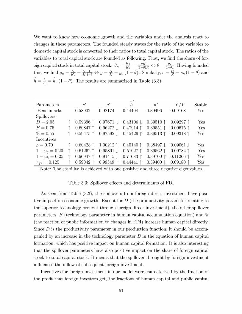
We want to know how economic growth and the variables under the analysis react to
changes in these parameters. The founded steady states for the ratio of the variables to
domestic capital stock is converted to their ratios to total capital stock. The ratios of the
variables to total capital stock are founded as following. First, we �nd the share of for-
eign capital stock in total capital stock. �n =Kf
Kd= �K
(1��)K , � = �n1+�n
: Having founded
this, we �nd gn = GKd= G
K11�� , g = G
K= gn (1� �) : Similarly, c = C
K= cn (1� �) and
sh = h
K=
shn (1� �). The results are summarized in Table (3.3).
Parameters c� g�sh�
��:
Y =Y StableBenchmarks 0:58902 0:98174 0:44408 0:39496 0:09168 YesSpilloversD = 2:05 " 0:59396 " 0:97671 # 0:43106 # 0:39510 " 0:09297 " YesB = 0:75 " 0:60847 " 0:96272 # 0:47914 " 0:39551 " 0:09675 " Yes = 0:55 " 0:59475 " 0:97592 # 0:45429 " 0:39513 " 0:09318 " YesIncentives% = 0:70 " 0:60428 " 1:00212 " 0:45140 " 0:38497 # 0:09061 # Yes1� ug = 0:20 " 0:61262 " 0:95891 # 0:51027 " 0:39562 " 0:09784 " Yes1� uh = 0:25 " 0:66947 " 0:91415 # 0:71683 " 0:39700 " 0:11266 " Yes� fk = 0:125 " 0:59042 " 0:99349 " 0:44441 " 0:39400 # 0:09180 " YesNote: The stability is achieved with one positive and three negative eigenvalues.
Table 3.3: Spillover e¤ects and determinants of FDI
As seen from Table (3.3), the spillovers from foreign direct investment have posi-
tive impact on economic growth. Except for D (the productivity parameter relating to
the superior technology brought through foreign direct investment), the other spillover
parameters, B (technology parameter in human capital accumulation equation) and
(the reaction of public information to changes in FDI) increase human capital directly.
Since D is the productivity parameter in our production function, it should be accom-
panied by an increase in the technology parameter B in the equation of human capital
formation, which has positive impact on human capital formation. It is also interesting
that the spillover parameters have also positive impact on the share of foreign capital
stock to total capital stock. It means that the spillovers brought by foreign investment
in�uences the in�ow of subsequent foreign investment.
Incentives for foreign investment in our model were characterized by the fraction of
the pro�t that foreign investors get, the fractions of human capital and public capital
51

spent for the human capital formation. As the fraction of the pro�t remaining in the
economy increases from % = 0:65 to % = 0:70; the share of foreign capital is decreasing.
Since % increases domestic capital stock, the tax revenue from domestic capital increases
government investment and an increment in government investment has positive im-
pact on human capital formation through government education investment. Despite
an increment in human and public capitals, the decline in foreign capital results in
low growth rate. Similarly, the tax � fk on the return from foreign capital has negative
impact on foreign capital stock, and increases government investment, and the govern-
ment investment increases human capital. Therefore, government investment plays an
important role for human capital formation even though foreign investment decreases.
Unlike %; which indirectly increased government investment, � fk increases government
investment directly and results in high growth rate. However, the growth rate does not
increase forever. It should be noted that the variables and even the growth rate are the
concave function with respect to tax rate. The turning point for � fk is 0:41 for which
the growth rate is 0:094869. As � fk = 0:42 and 0:50; the growth rates become 0:094865
and 0:094596, respectively. Therefore, there should not be too high tax rate on the
return from foreign capital. As already mentioned, these values should not considered
as real, because we are not interested in �nding the optimal values. They are chosen
just for the purpose of analysis. The other incentives, 1�ug and 1�uh (the fraction ofhuman and public capitals spent for human capital formation) increases human capital
and foreign capitals, but decreases the ratio of public capital to total capital. Although
the share of public capital decreases, high human and foreign capitals results in high
growth rates.
3.3 Model 3: FDI Decision Making
We consider an economy where the technical progress is the result of increasing capital.
We closely follow Romer (1990), Grossman and Helpman (1991), Barro and Sala-i-
Martin (1995) and Borensztein, Gregorio and Lee (1998), which focused on an increase
in the number of varieties of capital goods. Di¤erent from this literature, as already
mentioned in the previous model (subsection 3.2.9), we assume that the total capital
in the economy is the sum of domestic capital and foreign capital, K = Kd + Kf .
Final good sector is slightly di¤erent from the previous model, renting the domestic
capital from households at a rental rate rdk; and buying the foreign capital from foreign
52

producers at a price, Pf . Household�s utility maximization problem is the same as in
the previous model. In this section, we will concentrate on the production of foreign
capital goods, which can either be produced at home country or host country. Our
purpose is to �nd the determinants of foreign investment decision making, which will
be proxied by the present value of future pro�ts of foreign investors.
Foreign investor takes human capital, H; productive public capital, G ; and domestic
capital, Kd; as given. Foreign investor�s decision is what quantity of foreign capital to
produce and at what price. Besides these, foreign investor faces a number of factors
that can impact on his decision. We will explain these factors step by step and derive
the pro�t function of foreign investors.
Initially, we focus on the setup cost. An increase in foreign capital requires the
adaptation of more advanced technology from foreign countries to allow the entrance of
foreign capital. This adaptation process is costly and requires a �xed setup cost before
the entrance of foreign capital can take place. Following Borensztein, Gregorio and
Lee (1998), we can assume that the �xed setup cost depends negatively on the ratio of
foreign capital to the ratio of total capital (Kf=K) : Such that foreign investors bring
"an advanced knowledge" to the host country, making it easier to adopt the technology
brought with foreign capital. Therefore, foreign direct investment is considered as the
main channel of technological progress. Additionally, the existence of catch up e¤ect
in technological progress is also considered. Catch up e¤ect re�ects the fact that it
will be cheaper to imitate existing products for some time than to produce new capital
goods at the frontier of innovation (Borensztein, Gregorio and Lee, 1998). Borensztein,
Gregorio and Lee (1998) assumes that the set up cost depends positively on the ratio of
capital goods produced domestically (K) to those produced in more advanced countries
(K�). That is, if K=K� is lower, then imitation possibilities are larger and hence the
cost of adopting the new technology will be lower. The setup cost can be postulated in
the following form
F = F (Kf=K; K=K�) ; where
@F
@ (Kf=K)< 0 and
@F
@ (K=K�)> 0 (3.58)
Besides the �xed setup cost, each time the foreign capital goods producer engages in
production, it incurs one unit of output to use Kf : That is, there is a constant marginal
cost of production of Kf equal to 1. Assuming a steady state where the interest rate
is constant, net present value (NPV) of future cash �ows for foreign capital goods
53
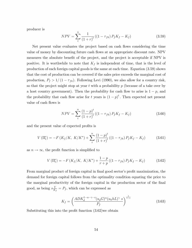
producer is
NPV =nXt
1
(1 + r)t((1� � fk)PfKf �Kf ) (3.59)
Net present value evaluates the project based on cash �ows considering the time
value of money by discounting future cash �ows at an appropriate discount rate. NPV
measures the absolute bene�t of the project, and the project is acceptable if NPV is
positive. It is worthwhile to note that Kf is independent of time, that is the level of
production of each foreign capital goods is the same at each time. Equation (3.59) shows
that the cost of production can be covered if the sales price exceeds the marginal cost of
production, Pf > 1= (1� � fk). Following Levi (1990), we also allow for a country risk,so that the project might stop at year t with a probability p (because of a take over by
a host country government). Then the probability for cash �ow to arise is 1 � p, andthe probability that cash �ow arise for t years is (1� p)t : Then expected net presentvalue of cash �ows is
NPV =nXt
(1� p)t
(1 + r)t((1� � fk)PfKf �Kf ) (3.60)
and the present value of expected pro�ts is
V (�et) = �F (Kf=K; K=K�) +
nXt
(1� p)t
(1 + r)t((1� � fk)PfKf �Kf ) (3.61)
as n!1; the pro�t function is simpli�ed to
V (�et ) = �F (Kf=K; K=K�) +
1� pr + p
((1� � fk)PfKf �Kf ) (3.62)
From marginal product of foreign capital in �nal good sector�s pro�t maximization, the
demand for foreign capital follows from the optimality condition equating the price to
the marginal productivity of the foreign capital in the production sector of the �nal
good, as being s YKf= Pf ; which can be expressed as
Kf =
�ADK1��� �s
d (ugG)�(uhhL)
s
Pf
� 11�s
(3.63)
Substituting this into the pro�t function (3.62)we obtain
54
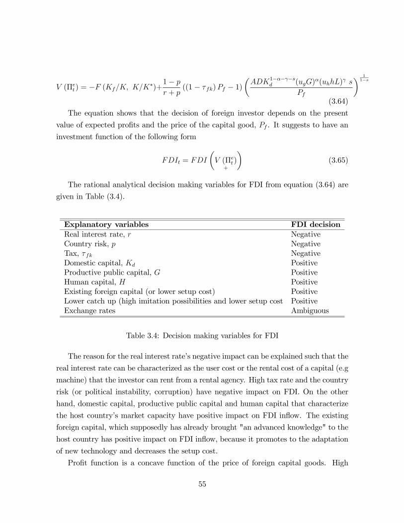
V (�et ) = �F (Kf=K; K=K�)+
1� pr + p
((1� � fk)Pf � 1)�ADK1��� �s
d (ugG)�(uhhL)
s
Pf
� 11�s
(3.64)
The equation shows that the decision of foreign investor depends on the present
value of expected pro�ts and the price of the capital good, Pf . It suggests to have an
investment function of the following form
FDIt = FDI
�V (�et)
+
�(3.65)
The rational analytical decision making variables for FDI from equation (3.64) are
given in Table (3.4).
Explanatory variables FDI decisionReal interest rate, r NegativeCountry risk, p NegativeTax, � fk NegativeDomestic capital, Kd PositiveProductive public capital, G PositiveHuman capital, H PositiveExisting foreign capital (or lower setup cost) PositiveLower catch up (high imitation possibilities and lower setup cost PositiveExchange rates Ambiguous
Table 3.4: Decision making variables for FDI
The reason for the real interest rate�s negative impact can be explained such that the
real interest rate can be characterized as the user cost or the rental cost of a capital (e.g
machine) that the investor can rent from a rental agency. High tax rate and the country
risk (or political instability, corruption) have negative impact on FDI. On the other
hand, domestic capital, productive public capital and human capital that characterize
the host country�s market capacity have positive impact on FDI in�ow. The existing
foreign capital, which supposedly has already brought "an advanced knowledge" to the
host country has positive impact on FDI in�ow, because it promotes to the adaptation
of new technology and decreases the setup cost.
Pro�t function is a concave function of the price of foreign capital goods. High
55
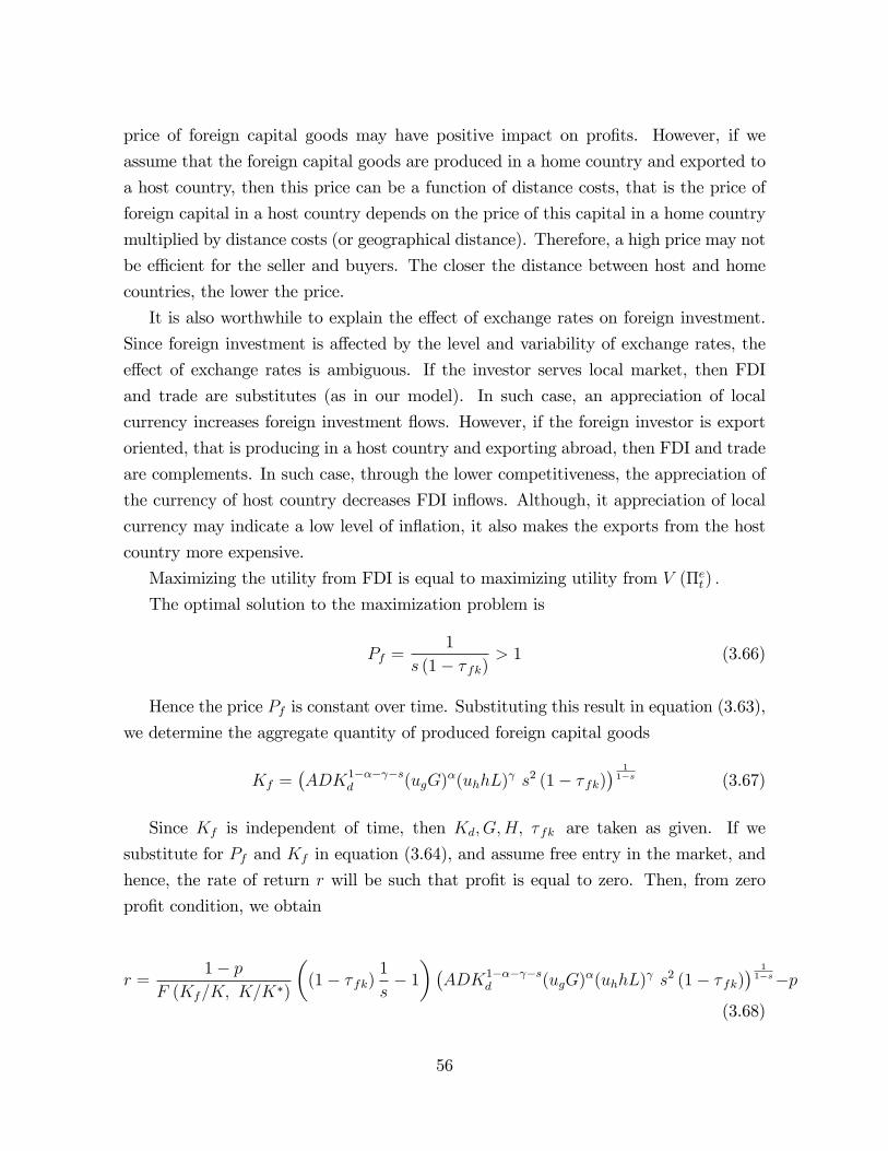
price of foreign capital goods may have positive impact on pro�ts. However, if we
assume that the foreign capital goods are produced in a home country and exported to
a host country, then this price can be a function of distance costs, that is the price of
foreign capital in a host country depends on the price of this capital in a home country
multiplied by distance costs (or geographical distance). Therefore, a high price may not
be e¢ cient for the seller and buyers. The closer the distance between host and home
countries, the lower the price.
It is also worthwhile to explain the e¤ect of exchange rates on foreign investment.
Since foreign investment is a¤ected by the level and variability of exchange rates, the
e¤ect of exchange rates is ambiguous. If the investor serves local market, then FDI
and trade are substitutes (as in our model). In such case, an appreciation of local
currency increases foreign investment �ows. However, if the foreign investor is export
oriented, that is producing in a host country and exporting abroad, then FDI and trade
are complements. In such case, through the lower competitiveness, the appreciation of
the currency of host country decreases FDI in�ows. Although, it appreciation of local
currency may indicate a low level of in�ation, it also makes the exports from the host
country more expensive.
Maximizing the utility from FDI is equal to maximizing utility from V (�et ) :
The optimal solution to the maximization problem is
Pf =1
s (1� � fk)> 1 (3.66)
Hence the price Pf is constant over time. Substituting this result in equation (3.63),
we determine the aggregate quantity of produced foreign capital goods
Kf =�ADK1��� �s
d (ugG)�(uhhL)
s2 (1� � fk)� 11�s (3.67)
Since Kf is independent of time, then Kd; G;H; � fk are taken as given. If we
substitute for Pf and Kf in equation (3.64), and assume free entry in the market, and
hence, the rate of return r will be such that pro�t is equal to zero. Then, from zero
pro�t condition, we obtain
r =1� p
F (Kf=K; K=K�)
�(1� � fk)
1
s� 1��ADK1��� �s
d (ugG)�(uhhL)
s2 (1� � fk)� 11�s�p
(3.68)
56
To close the model, we resort to the household�s problem (which is the same as in
the model with exogenous FDI), where we have obtained:CC= 1
�[(1� � dk)rdk � �] : In
the steady state, the growth rate of consumption is equal to the growth rate of output,
that we denote by g: Hence, the growth rate of the economy is given by
g =1
�[(1� � dk)r � �] (3.69)
Where r is given by equation (3.68). Equation (3.69) shows that the rate of growth of
the economy is determined by household�s preference parameters, � and �, the level of
technology, country risk (or political risk and corruption), p; domestic capital, produc-
tive public capital, and human capital. A greater willingness to save, that is lower �
and �; a high level of domestic capital, productive public capital, and human capital
will increase the rate of growth of the economy. In addition, a decrease in the setup
cost, F (Kf=K; K=K�), that is an increase in the level of foreign capital raises the rate
of return and the rate of growth. In contrast, the country risk, p, decreases the growth
rate of economy.
57

Chapter 4
Empirical Speci�cation and DataDescription
4.1 Determinants of Human Capital
The equation that we are going to estimate corresponds to the equation (3.18) at
page 36, which we obtained from the model of Schooling and Human Capital and
characterizes the determinants of schooling. In the model, schooling refers to the years
attended at school. Based on the sign e¤ects of the explanatory variables on schooling,
equation (3.18) is expressed in a linear form to be estimated. Since we have missing
data on the average years of education for the countries in our sample, we will focus on
the enrollment rates at secondary and tertiary levels. We have already mentioned that
enrollment rates serve as a proxy for the human capital in future, that is it increases
the average years of education in future. Therefore, decision is made on enrollment.
Our schooling equation (3.18), can be expressed in a linear form as
ERjit = �1UG+ �2TFPit + �3MR + �4IMR + �5FDIstockit + �6irit + uit (4.1)
uit = �i + � t + �it (4.2)
where UG is a utility gain from schooling, TFP is total factor productivity, MR is
migration rate, IMR is infant mortality rate, FDIstockit is the assumed spillover e¤ect
on schooling, and irt is a rate of return on capital (which increases an opportunity cost).
�i is a country �xed e¤ect, � t is a time �xed e¤ect and �it is an error term.
58
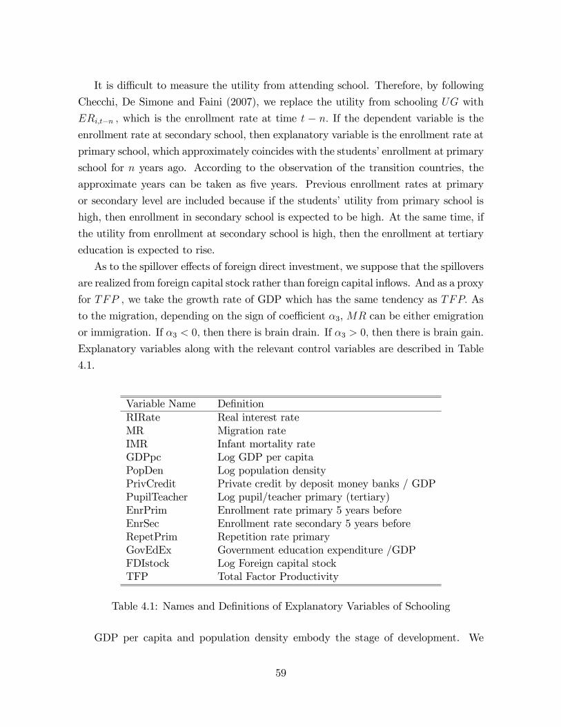
It is di¢ cult to measure the utility from attending school. Therefore, by following
Checchi, De Simone and Faini (2007), we replace the utility from schooling UG with
ERi;t�n ; which is the enrollment rate at time t � n: If the dependent variable is theenrollment rate at secondary school, then explanatory variable is the enrollment rate at
primary school, which approximately coincides with the students�enrollment at primary
school for n years ago. According to the observation of the transition countries, the
approximate years can be taken as �ve years. Previous enrollment rates at primary
or secondary level are included because if the students�utility from primary school is
high, then enrollment in secondary school is expected to be high. At the same time, if
the utility from enrollment at secondary school is high, then the enrollment at tertiary
education is expected to rise.
As to the spillover e¤ects of foreign direct investment, we suppose that the spillovers
are realized from foreign capital stock rather than foreign capital in�ows. And as a proxy
for TFP ; we take the growth rate of GDP which has the same tendency as TFP: As
to the migration, depending on the sign of coe¢ cient �3, MR can be either emigration
or immigration. If �3 < 0; then there is brain drain. If �3 > 0; then there is brain gain.
Explanatory variables along with the relevant control variables are described in Table
4.1.
Variable Name De�nitionRIRate Real interest rateMR Migration rateIMR Infant mortality rateGDPpc Log GDP per capitaPopDen Log population densityPrivCredit Private credit by deposit money banks / GDPPupilTeacher Log pupil/teacher primary (tertiary)EnrPrim Enrollment rate primary 5 years beforeEnrSec Enrollment rate secondary 5 years beforeRepetPrim Repetition rate primaryGovEdEx Government education expenditure /GDPFDIstock Log Foreign capital stockTFP Total Factor Productivity
Table 4.1: Names and De�nitions of Explanatory Variables of Schooling
GDP per capita and population density embody the stage of development. We
59

would also like to consider Gini inequality index. But unfortunately, data for transition
countries does not allow this. Therefore, we complement this with credit to the private
sector and infant mortality rate. The reason for including infant mortality rate is that
the mortality is usually highly correlated with endemic poverty, and also correlated
with educational decisions (see Checchi, De Simone and Faini, 2007).
If we exclude real interest rate, total factor productivity, and government education
/GDP, then our equation is simpli�ed to the equation given by Checchi, De Simone and
Faini (2007). Another di¤erence is that instead of the sum of FDI in�ows as a proxy for
FDI stock, we take real data on FDI stock. Because FDI stock includes reinvestment
and possibly innovation. And spillover e¤ects comes from FDI stock.
4.2 Determinants of Foreign Direct Investment
The equation on the determinants of foreign direct investment is based on equation
(3.65). In a linear form, it can be expressed as
FDIit = �1FDIstockit + �2HC + 'iZit + uit (4.3)
uit = �i + � t + �it (4.4)
Since the decision is made on �ow variable, we take the explained variables as FDI
�ows as a percentage of GDP. The implication of equation (4.3) is that FDI �ows
depend on the existing FDI stock in the economy and the endowment of human capital.
Instead of the enrollment rates at school, we adopt the population with secondary
and tertiary education as a proxy for human capital. The control variables a¤ecting
investment decision choices are given in Z matrix. These explanatory variables are
adopted from equation (3.65) and complemented with the variables that the existing
empirical literature consider as major determinants of FDI.
Names, de�nitions and source of explanatory variables are described in in Table 4.2.
60
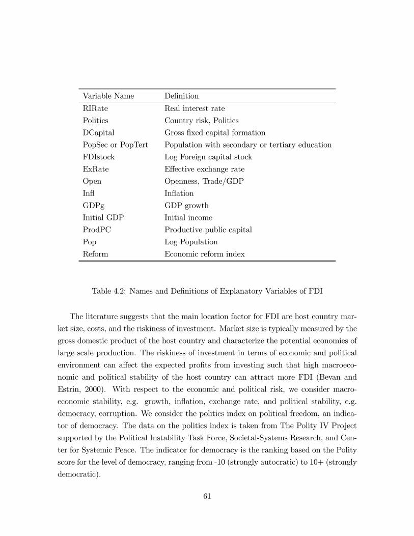
Variable Name De�nition
RIRate Real interest rate
Politics Country risk, Politics
DCapital Gross �xed capital formation
PopSec or PopTert Population with secondary or tertiary education
FDIstock Log Foreign capital stock
ExRate E¤ective exchange rate
Open Openness, Trade/GDP
In� In�ation
GDPg GDP growth
Initial GDP Initial income
ProdPC Productive public capital
Pop Log Population
Reform Economic reform index
Table 4.2: Names and De�nitions of Explanatory Variables of FDI
The literature suggests that the main location factor for FDI are host country mar-
ket size, costs, and the riskiness of investment. Market size is typically measured by the
gross domestic product of the host country and characterize the potential economies of
large scale production. The riskiness of investment in terms of economic and political
environment can a¤ect the expected pro�ts from investing such that high macroeco-
nomic and political stability of the host country can attract more FDI (Bevan and
Estrin, 2000). With respect to the economic and political risk, we consider macro-
economic stability, e.g. growth, in�ation, exchange rate, and political stability, e.g.
democracy, corruption. We consider the politics index on political freedom, an indica-
tor of democracy. The data on the politics index is taken from The Polity IV Project
supported by the Political Instability Task Force, Societal-Systems Research, and Cen-
ter for Systemic Peace. The indicator for democracy is the ranking based on the Polity
score for the level of democracy, ranging from -10 (strongly autocratic) to 10+ (strongly
democratic).
61
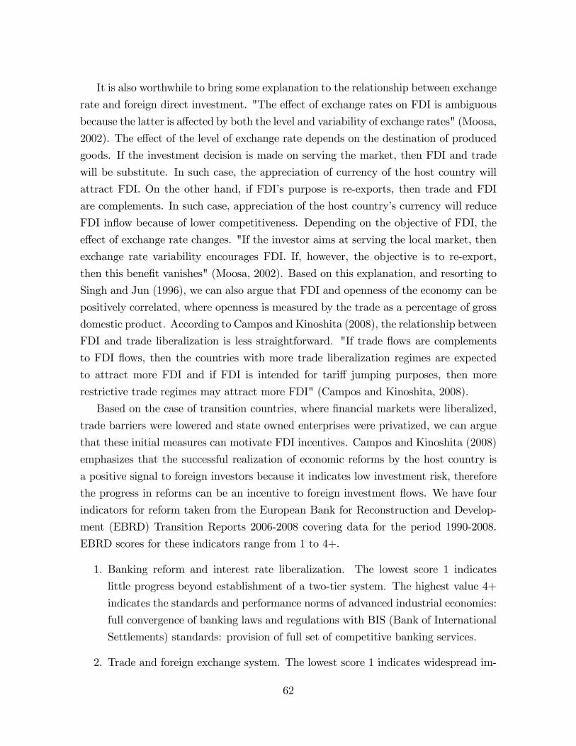
It is also worthwhile to bring some explanation to the relationship between exchange
rate and foreign direct investment. "The e¤ect of exchange rates on FDI is ambiguous
because the latter is a¤ected by both the level and variability of exchange rates" (Moosa,
2002). The e¤ect of the level of exchange rate depends on the destination of produced
goods. If the investment decision is made on serving the market, then FDI and trade
will be substitute. In such case, the appreciation of currency of the host country will
attract FDI. On the other hand, if FDI�s purpose is re-exports, then trade and FDI
are complements. In such case, appreciation of the host country�s currency will reduce
FDI in�ow because of lower competitiveness. Depending on the objective of FDI, the
e¤ect of exchange rate changes. "If the investor aims at serving the local market, then
exchange rate variability encourages FDI. If, however, the objective is to re-export,
then this bene�t vanishes" (Moosa, 2002). Based on this explanation, and resorting to
Singh and Jun (1996), we can also argue that FDI and openness of the economy can be
positively correlated, where openness is measured by the trade as a percentage of gross
domestic product. According to Campos and Kinoshita (2008), the relationship between
FDI and trade liberalization is less straightforward. "If trade �ows are complements
to FDI �ows, then the countries with more trade liberalization regimes are expected
to attract more FDI and if FDI is intended for tari¤ jumping purposes, then more
restrictive trade regimes may attract more FDI" (Campos and Kinoshita, 2008).
Based on the case of transition countries, where �nancial markets were liberalized,
trade barriers were lowered and state owned enterprises were privatized, we can argue
that these initial measures can motivate FDI incentives. Campos and Kinoshita (2008)
emphasizes that the successful realization of economic reforms by the host country is
a positive signal to foreign investors because it indicates low investment risk, therefore
the progress in reforms can be an incentive to foreign investment �ows. We have four
indicators for reform taken from the European Bank for Reconstruction and Develop-
ment (EBRD) Transition Reports 2006-2008 covering data for the period 1990-2008.
EBRD scores for these indicators range from 1 to 4+.
1. Banking reform and interest rate liberalization. The lowest score 1 indicates
little progress beyond establishment of a two-tier system. The highest value 4+
indicates the standards and performance norms of advanced industrial economies:
full convergence of banking laws and regulations with BIS (Bank of International
Settlements) standards: provision of full set of competitive banking services.
2. Trade and foreign exchange system. The lowest score 1 indicates widespread im-
62

port and/or export controls or very limited legitimate access to foreign exchange.
The highest score 4+ indicates the standards and performance norms of advanced
industrial economies: removal of most tari¤ barriers; membership in WTO.
3. Governance and enterprise restructuring. The lowest score 1 indicates soft budget
constraints (lax credit and subsidy policies weakening �nancial discipline at the
enterprise level): few other reforms to promote corporate governance. The highest
score 4+ indicates the standards and performance typical of advanced industrial
economies: e¤ective corporate control exercised through domestic �nancial insti-
tutions and markets, fostering market-driven restructuring.
4. The share of private sector to the public sector.
We do not include all of the reform indicators. Because the indicators are highly
correlated. Therefore, we use principal component analysis (PCA) to combine them in
one new variable. PCA examines whether the correlation between the four indicators
can be explained in terms of unobservable factors. PCA combines an original large set
of variables into a smaller set of uncorrelated variables, which still contains most of the
information in the original set of variables. Moreover, it takes care of multicollinearity
problems. The selection of necessary factors are based on the hypothesis of taking the
threshold cumulative variance 75% and Kaiser criterion, retaining factors with eigen-
values greater than one. That is, if a factor does not extract at least as much as the
equivalent variable, then we drop it. However, eigenvalue rule will be replaced by mean-
ing (extracting factors as long as they are interpretable obeying cumulative variance
75%) in some factor loadings. And the scores on the obtained factor for all observa-
tion period, represented by the regression line, will be used in regressions to represent
the essence of combined variables. The detailed explanation of Principal Component
Analysis is given in the next chapter under Econometric Methodology.
4.3 Determinants of Economic Growth
To empirically test the e¤ect of FDI and Human Capital on economic growth, we resort
to equation (3.69), where the dependent variable is considered to be the growth rate of
real GDP per capita. It can be expressed in the following basic formulation:
GDPgit = �1FDIstockit + �2HCit + �3Y0 + �it + uit (4.5)
63

uit = �i + � t + �it (4.6)
where FDI is a foreign direct investment stock, HC is a stock of human capital, Y0 is an
initial GDP per capita, and � are the set of other variables that a¤ect economic growth.
The variable FDI is measured as a percentage of GDP, and re�ects the share of foreign
capital in total capital in equation (3.69), Kf=K: The initial GDP per capita variable
captures the catch-up e¤ect K=K�: Human capital, HC; is proxied by the population
with secondary and tertiary education.
Our equation also bene�ts fromBorensztein, de Gregorio and Lee (1998) andMankiw,
Romer, Weil (1992). Borensztein, de Gregorio and Lee (1998) considered an equation
of the form
y = f(Yo; HC; FDI; FDI �HC; Infl; GovCons; and dummies) (4.7)
where GovCons is government consumption and the proxy for human capital stock
variable is the initial year level of average years of the male secondary schooling con-
structed by Barro and Lee (1993), and FDI is foreign direct investment �ow variable
(because of insu¢ cient data to construct a stock measure of FDI).
FDI augmented version of the growth equation developed by Mankiw, Romer, Weil
(1992) takes the following form
y = f(Yo; INV; POP; HC; FDI) (4.8)
where INV is gross domestic investment and POP is population. The equation allows
to see the relationship between foreign and domestic investments.1
As mentioned, Borensztein, de Gregorio and Lee (1998) considered FDI �ows as
explanatory variables. However, we will replace it with FDI stock variable. And also,
in addition to government consumption variable we also include productive public cap-
ital. Our equation�s another signi�cant di¤erence is that we allow the economic reform
indicators which are typical for transition countries and are assumed to boost economic
growth. We also assume that for economic reforms to have positive impact, political
stability and democracy should play an important role. Therefore, we also need to
1Romer (1993) estimated a standard cross-country growth equation in a form:Growth (I=Y; Y1960; Sec),where I stands for the national income accounts measure of totalinvestment, and the variable Sec stands for the secondary school enrollment rate in 1960. However,in our sample, the missing data do not allow us to add initial enrollment rates to our regressionequations.
64
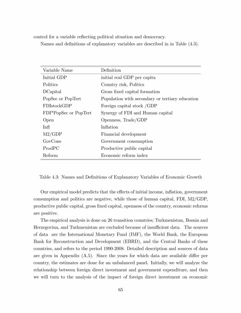
control for a variable re�ecting political situation and democracy.
Names and de�nitions of explanatory variables are described in in Table (4.3).
Variable Name De�nition
Initial GDP initial real GDP per capita
Politics Country risk, Politics
DCapital Gross �xed capital formation
PopSec or PopTert Population with secondary or tertiary education
FDIstockGDP Foreign capital stock /GDP
FDI*PopSec or PopTert Synergy of FDI and Human capital
Open Openness, Trade/GDP
In� In�ation
M2/GDP Financial development
GovCons Government consumption
ProdPC Productive public capital
Reform Economic reform index
Table 4.3: Names and De�nitions of Explanatory Variables of Economic Growth
Our empirical model predicts that the e¤ects of initial income, in�ation, government
consumption and politics are negative, while those of human capital, FDI, M2/GDP,
productive public capital, gross �xed capital, openness of the country, economic reforms
are positive.
The empirical analysis is done on 26 transition countries; Turkmenistan, Bosnia and
Herzegovina, and Turkmenistan are excluded because of insu¢ cient data. The sources
of data are the International Monetary Fund (IMF), the World Bank, the European
Bank for Reconstruction and Development (EBRD), and the Central Banks of these
countries, and refers to the period 1990-2008. Detailed description and sources of data
are given in Appendix (A.5). Since the years for which data are available di¤er per
country, the estimates are done for an unbalanced panel. Initially, we will analyze the
relationship between foreign direct investment and government expenditure, and then
we will turn to the analysis of the impact of foreign direct investment on economic
65
growth with an emphasis on human capital formation.
The Relationship Between FDI and Productive Public Capital.
In the empirical analysis, we are going to discuss mainly the tendencies of public and
foreign capital stocks. As the model predicted, there is a negative correlation between
the ratios of these two variables to total capital stock. In order to verify this, we
turn to the data of the transition countries. The public, foreign and total capital
stocks are created through the Perpetual Inventory Method (PIM) from the �ows of
government investment, foreign direct investment and gross �xed capital formation.
Since the government investment is not explicitly given, we calculate it as the sum of
the government expenditure on public order and safety, economic a¤airs and education.
The PIM is based on Xt+1 = It+(1��)X; where Xt+1 is the stock in year t+1, It is the
investment in year t and � is the depreciation rate. The initial stock, X0; is calculated as
X0 = I0= (x+ �) ; where I0 is the investment level at to; and x is the average geometric
growth rate of the investment and is expressed as x =h(Ifinal=Iinitial)
1=a � 1i� 100;
where a is the length of time between the initial and �nal years of the investment. We
assume the depreciation rate � = 0:05:
66
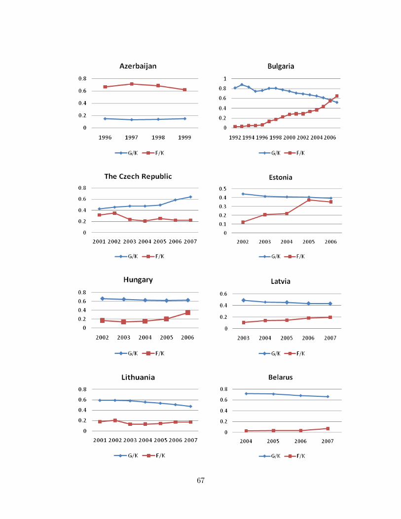
67
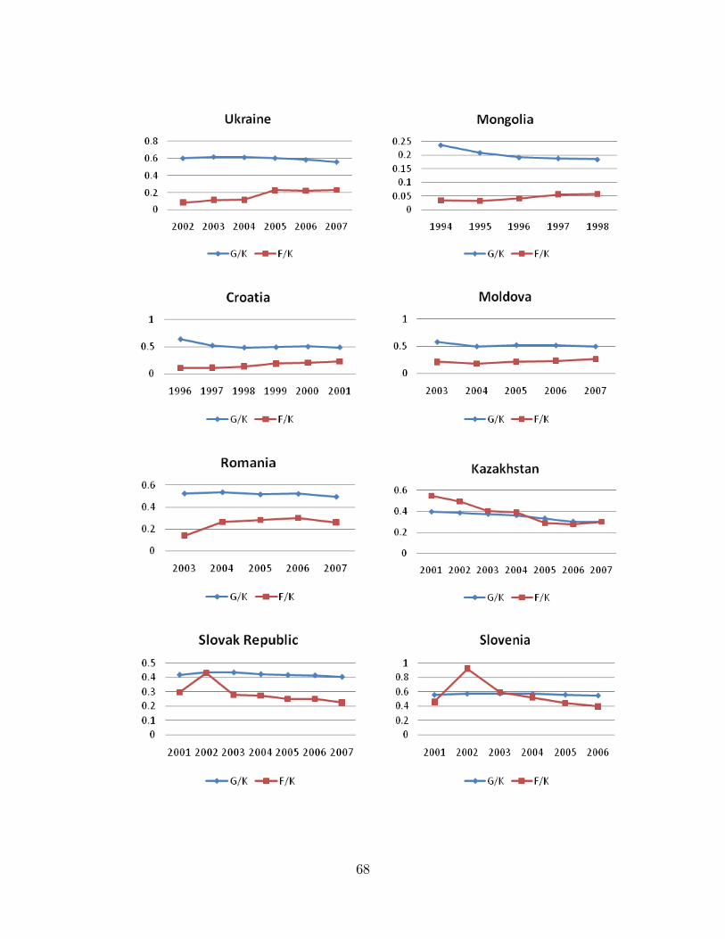
68
Chapter 5
Econometric Methodology
5.1 Dynamic Panel Data Analysis
We turn to panel data analysis because it allows to investigate the relationship between
foreign direct investment, human capital and economic growth on time series basis.
Additionally, in comparison to cross-country estimations (with instrumental variables),
we can take care of unobserved country speci�c e¤ects which can bias the estimates.
Our econometrics methodology is based on the Generalized Method of Moments
(GMM) estimators developed for dynamic panel data analysis by Arellano and Bond
(1991), Arellano and Bover (1995), and Blundell and Bond (1998). We also closely fol-
low Carkovic and Levine (2002), which has summarized and used the same methodology
for estimations for developing countries. The methodology is as following:
Let us consider the model
yit = �0xit + uit; t = 1; ::::T; i = 1; :::; N (5.1)
uit = �i + � t + �it (5.2)
So that the variable xit is assumed to be exogenous given the unobservable country
speci�c e¤ect �i and time e¤ect � t: Where xit is a set of explanatory variables. The
equation is extended by adding one lag of the dependent variable.
yit = �yi(t�1) + �0xit + uit; t = 1; ::::T; i = 1; :::; N (5.3)
69

In order to eliminate individual e¤ects �i, we take the �rst di¤erences
yit � yi(t�1) = ��yi(t�1) � yi(t�2)
�+ �
0 �xit � xi(t�1)
�+ � t � � t�1 +
��it � �i(t�1)
�(5.4)
To overcome the problems connected with the endogeneity of the independent vari-
ables, and the correlation of errors �it � �i(t�1) with yi(t�1) � yi(t�2); we need to addinstrumental variables and consider the assumptions that the error term is not serially
correlated and the independent variables are weakly exogenous. Hence, the moment
restrictions for the �rst di¤erenced GMM approach is the following
E [yt�j(�it � �it�1)] = 0 and E��xit � xi(t�1)
�(�it � �it�1)
�= 0 for j � 2; t = 3; :::; T
(5.5)
In �nite sample properties, the �rst di¤erenced GMM approach is weak in terms of
bias and imprecision. The weakness of the instruments, in the �rst order di¤erenced
regression equations, happens because the lagged levels is weakly correlated with the
subsequent �rst di¤erences. Considering this, a new approach by Arellano and Bover
(1995), and Blundell and Bond (1997) is presented. The new approach consists of a
system of regression in di¤erences and regression in levels. The instruments for regres-
sion in di¤erences is the same as explained above. But the instruments for regression
in levels are the lagged �rst di¤erences of the dependent variable. Additionally, we
assume that there is no correlation of the independent variables and their di¤erences
with country speci�c e¤ect �i; and consider new moment restriction for the regression
in levels.
E�(yi(t�j) � yi(t�j�1))(�i + �it)
�= 0 for j = 1 (5.6)
For estimations, we use Stata 10 statistical software that implements Arellano and
Bover/Blundell and Bover system estimator, which uses the moment conditions of
Arellano and Bond estimator (where the lags of the dependent variable and �rst dif-
ferences of the exogenous variables are instruments) for the �rst di¤erenced equation
and moment conditions (where the lagged �rst di¤erences of the dependent variable are
instruments) for level equation.
70
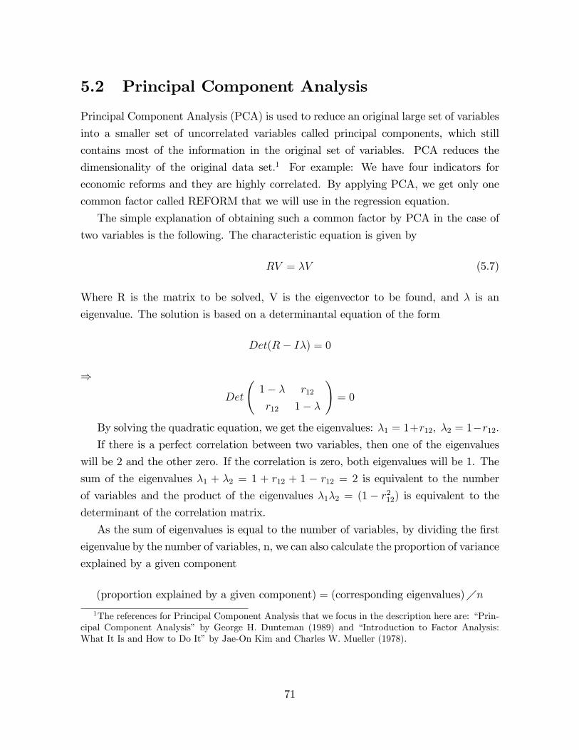
5.2 Principal Component Analysis
Principal Component Analysis (PCA) is used to reduce an original large set of variables
into a smaller set of uncorrelated variables called principal components, which still
contains most of the information in the original set of variables. PCA reduces the
dimensionality of the original data set.1 For example: We have four indicators for
economic reforms and they are highly correlated. By applying PCA, we get only one
common factor called REFORM that we will use in the regression equation.
The simple explanation of obtaining such a common factor by PCA in the case of
two variables is the following. The characteristic equation is given by
RV = �V (5.7)
Where R is the matrix to be solved, V is the eigenvector to be found, and � is an
eigenvalue. The solution is based on a determinantal equation of the form
Det(R� I�) = 0
)
Det
1� � r12
r12 1� �
!= 0
By solving the quadratic equation, we get the eigenvalues: �1 = 1+r12; �2 = 1�r12:If there is a perfect correlation between two variables, then one of the eigenvalues
will be 2 and the other zero. If the correlation is zero, both eigenvalues will be 1. The
sum of the eigenvalues �1 + �2 = 1 + r12 + 1 � r12 = 2 is equivalent to the number
of variables and the product of the eigenvalues �1�2 = (1� r212) is equivalent to thedeterminant of the correlation matrix.
As the sum of eigenvalues is equal to the number of variables, by dividing the �rst
eigenvalue by the number of variables, n, we can also calculate the proportion of variance
explained by a given component
(proportion explained by a given component) = (corresponding eigenvalues)�n1The references for Principal Component Analysis that we focus in the description here are: �Prin-
cipal Component Analysis� by George H. Dunteman (1989) and �Introduction to Factor Analysis:What It Is and How to Do It�by Jae-On Kim and Charles W. Mueller (1978).
71
We impose an arbitrary additional constraint that the lengths of eigenvectors be 1.
The eigenvectors are found as the following (1� �k)x1 + r12x2 = 0r12x1 + (1� �k)x2 = 0
!
For each value of eigenvalue, we get the matrix of eigenvectors.
The principal component loadings are produced by multiplying eigenvectors by the
square roots of the respective eigenvalues, which correctly re�ect the relative amount
of variances by the corresponding data. x11 x12
x21 x22
! p�1 0
0p�2
!=
x11p�1 x12
p�2
x21p�1 x22
p�2
!(5.8)
We get two common factors. The selection of necessary factor is based on the hy-
pothesis of taking the threshold cumulative variance 75% and Kaiser criterion, retaining
factors with eigenvalues greater than one. That is, if a factor does not extract at least as
much as the equivalent variable, then we drop it. And the scores on the obtained factor
for all observation period, represented by the regression line will be used in regressions
to represent that essence of combined variables. The principal component loadings are
obtained by using statistics program SPSS 15.
72
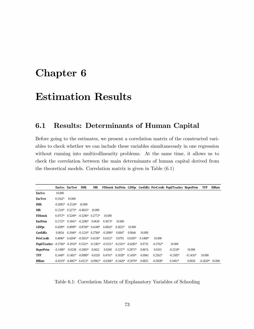
Chapter 6
Estimation Results
6.1 Results: Determinants of Human Capital
Before going to the estimates, we present a correlation matrix of the constructed vari-
ables to check whether we can include these variables simultaneously in one regression
without running into multicollinearity problems. At the same time, it allows us to
check the correlation between the main determinants of human capital derived from
the theoretical models. Correlation matrix is given in Table (6.1)
EnrSec EnrTert IMR MR FDIstock EnrPrim GDPpc GovEdEx PrivCredit PupilTeacher RepetPrim TFP RIRate
EnrSec 10.000
EnrTert 0.5162* 10.000
IMR 0.3695* 0.5518* 10.000
MR 0.1310* 0.3273* 0.4833* 10.000
FDIstock 0.4757* 0.5249* 0.5296* 0.2772* 10.000
EnrPrim 0.1723* 0.1841* 0.2286* 0.0639 0.3673* 10.000
GDPpc 0.4209* 0.4999* 0.8760* 0.4148* 0.6816* 0.2655* 10.000
GovEdEx 0.0654 0.1040* 0.1224* 0.2784* 0.2090* 0.0047 0.0044 10.000
PrivCredit 0.4696* 0.4204* 0.5653* 0.4136* 0.6312* 0.0701 0.6105* 0.1408* 10.000
PupilTeacher 0.3766* 0.3916* 0.5331* 0.1381* 0.5551* 0.2101* 0.6282* 0.0733 0.3762* 10.000
RepetPrim 0.1490* 0.0238 0.2683* 0.0422 0.0269 0.1237* 0.2872* 0.0674 0.0101 0.2518* 10.000
TFP 0.1449* 0.1401* 0.0989* 0.0320 0.4741* 0.1658* 0.1450* 0.0941 0.2562* 0.1585* 0.1416* 10.000
RIRate 0.4319* 0.4067* 0.4313* 0.0961* 0.6306* 0.3426* 0.5070* 0.0825 0.5838* 0.3491* 0.0020 0.2620* 10.000
Table 6.1: Correlation Matrix of Explanatory Variables of Schooling
73

The stars in the correlation matrix indicates the signi�cance at 10 percent. The
correlation matrix points to several interesting issues, which support the results of
theoretical models such that as expected RIRate (rate of return on capital) and IMR
(infant mortality rate) have negative correlation with EnrPrim (enrollment rate pri-
mary), EnrSec (enrollment rate secondary) and EnrTert (enrollment rate tertiary).
The spillovers from Foreign Direct Investment proxied by FDI stock has signi�cant and
positive correlation with the enrollment rates at each level. The same signi�cant and
positive correlation also applies to the growth rate of GDP and the GDP per capita.
As to the migration rate, we see that it has negative but insigni�cant correlation with
EnrPrim (enrollment rate primary), but positive and signi�cant correlation with Enr-
Sec (enrollment rate secondary) and EnrTert (enrollment rate tertiary). As we have
already mentioned, the positive correlation of migration with enrollment rates indicates
net immigration.
Our estimations on the determinants of school enrollment rates and foreign direct
investment will utilize Chechi, De Simone and Faini (2007), which to our best knowledge
is the only research done on the analysis of human capital in developing countries,
analyzing 112 developing countries (including only Bulgaria, Romania, Hungary and
Poland from our sample). In di¤erence, we consider transition countries of the Former
Soviet Union and Easter European countries and extend the estimated equations. Our
results will be compared and conclusions will be derived.
As a decision variable on schooling, our gross enrollment rates by educational level
(secondary, tertiary) cover the period of 1990 -2008. Considering missing information
on regressors, in its largest version 213 observations cover 26 countries and minimum 93
observations cover 21 countries in the case of secondary school enrollment. Similarly, in
the case of tertiary enrollment, in its largest version 223 observations cover 26 countries
and 87 observations cover 21 countries. Missing data urges us to run our estimations
with unbalanced panel data. The estimations of equation 4.1 in chapter 4 are reported
in Tables (6.2) and (6.3) correspondingly for secondary school and tertiary enrollment
rates as explanatory variables as proxies for human capital.
The �rst two columns of both tables reports simple OLS correlations, while columns
3 to 6 reports �xed e¤ects estimator, and columns 7 to 8 use SYS-GMM dynamic panel
data analysis, system estimator o¤ered by Arellano and Bover / Blundell and Bover.
First we look at secondary enrollment in Table (6.2)
74
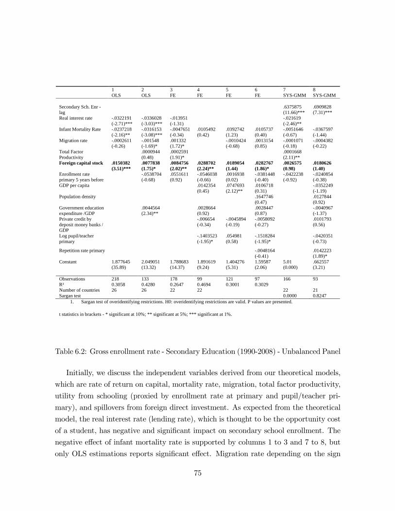
1OLS
2OLS
3FE
4FE
5FE
6FE
7SYSGMM
8SYSGMM
Secondary Sch. Enr lag
.6375875(11.66)***
.6909828(7.31)***
Real interest rate .0322191(2.71)***
.0336028(3.03)***
.013951(1.31)
.021619(2.46)**
Infant Mortality Rate .0237218(2.16)**
.0316153(3.08)***
.0047651(0.34)
.0105492(0.42)
.0392742(1.23)
.0105737(0.40)
.0051646(0.67)
.0367597(1.44)
Migration rate .0002611(0.26)
.001548(1.69)*
.001332(1.72)*
.0010424(0.68)
.0013154(0.85)
.0001071(0.18)
.0004382(0.22)
Total FactorProductivity
.0000944(0.48)
.0002591(1.91)*
.0001668(2.11)**
Foreign capital stock .0150382(3.51)***
.0077838(1.75)*
.0084756(2.02)**
.0288702(2.24)**
.0189054(1.44)
.0282767(1.86)*
.0026575(0.98)
.0180626(1.40)
Enrollment rateprimary 5 years before
.0538704(0.68)
.0551611(0.92)
.0546038(0.66)
.0016938(0.02)
.0381448(0.40)
.0422238(0.92)
.0240854(0.38)
GDP per capita .0142354(0.45)
.0747693(2.12)**
.0106718(0.31)
.0352249(1.19)
Population density .1647746(0.47)
.0127844(0.92)
Government educationexpenditure /GDP
.0044564(2.34)**
.0028664(0.92)
.0028447(0.87)
.0040967(1.37)
Private credit bydeposit money banks /GDP
.006654(0.34)
.0045894(0.19)
.0058092(0.27)
.0101793(0.56)
Log pupil/teacherprimary
.1403523(1.95)*
.054981(0.58)
.1518284(1.95)*
.0420351(0.73)
Repetition rate primary .0048164(0.41)
.0142223(1.89)*
Constant 1.877645(35.89)
2.049051(13.32)
1.788683(14.37)
1.891619(9.24)
1.404276(5.31)
1.59587(2.06)
5.01(0.000)
.662557(3.21)
Observations 218 133 178 99 121 97 166 93R² 0.3058 0.4280 0.2647 0.4694 0.3001 0.3029Number of countries 26 26 22 22 22 21Sargan test 0.0000 0.8247
1. Sargan test of overidentifying restrictions. H0: overidentifying restrictions are valid. P values are presented.
t statistics in brackets * significant at 10%; ** significant at 5%; *** significant at 1%.
Table 6.2: Gross enrollment rate - Secondary Education (1990-2008) - Unbalanced Panel
Initially, we discuss the independent variables derived from our theoretical models,
which are rate of return on capital, mortality rate, migration, total factor productivity,
utility from schooling (proxied by enrollment rate at primary and pupil/teacher pri-
mary), and spillovers from foreign direct investment. As expected from the theoretical
model, the real interest rate (lending rate), which is thought to be the opportunity cost
of a student, has negative and signi�cant impact on secondary school enrollment. The
negative e¤ect of infant mortality rate is supported by columns 1 to 3 and 7 to 8, but
only OLS estimations reports signi�cant e¤ect. Migration rate depending on the sign
75
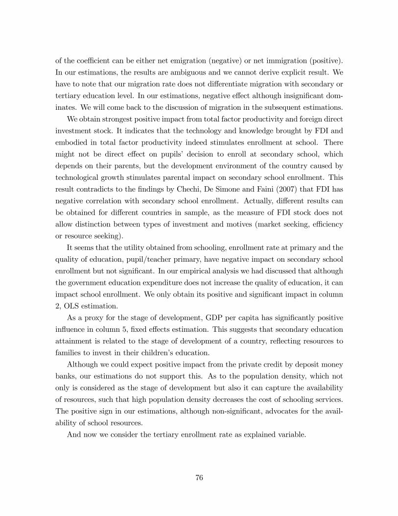
of the coe¢ cient can be either net emigration (negative) or net immigration (positive).
In our estimations, the results are ambiguous and we cannot derive explicit result. We
have to note that our migration rate does not di¤erentiate migration with secondary or
tertiary education level. In our estimations, negative e¤ect although insigni�cant dom-
inates. We will come back to the discussion of migration in the subsequent estimations.
We obtain strongest positive impact from total factor productivity and foreign direct
investment stock. It indicates that the technology and knowledge brought by FDI and
embodied in total factor productivity indeed stimulates enrollment at school. There
might not be direct e¤ect on pupils� decision to enroll at secondary school, which
depends on their parents, but the development environment of the country caused by
technological growth stimulates parental impact on secondary school enrollment. This
result contradicts to the �ndings by Chechi, De Simone and Faini (2007) that FDI has
negative correlation with secondary school enrollment. Actually, di¤erent results can
be obtained for di¤erent countries in sample, as the measure of FDI stock does not
allow distinction between types of investment and motives (market seeking, e¢ ciency
or resource seeking).
It seems that the utility obtained from schooling, enrollment rate at primary and the
quality of education, pupil/teacher primary, have negative impact on secondary school
enrollment but not signi�cant. In our empirical analysis we had discussed that although
the government education expenditure does not increase the quality of education, it can
impact school enrollment. We only obtain its positive and signi�cant impact in column
2, OLS estimation.
As a proxy for the stage of development, GDP per capita has signi�cantly positive
in�uence in column 5, �xed e¤ects estimation. This suggests that secondary education
attainment is related to the stage of development of a country, re�ecting resources to
families to invest in their children�s education.
Although we could expect positive impact from the private credit by deposit money
banks, our estimations do not support this. As to the population density, which not
only is considered as the stage of development but also it can capture the availability
of resources, such that high population density decreases the cost of schooling services.
The positive sign in our estimations, although non-signi�cant, advocates for the avail-
ability of school resources.
And now we consider the tertiary enrollment rate as explained variable.
76
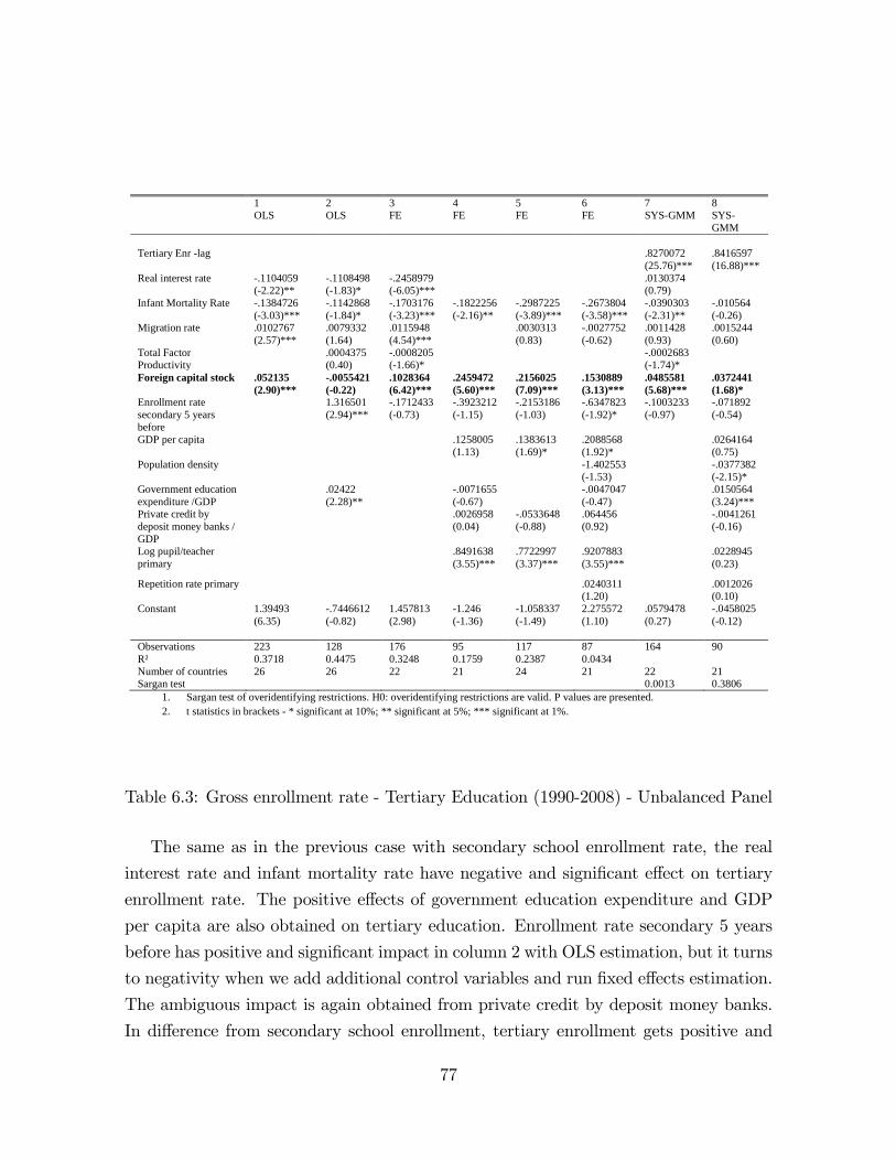
1OLS
2OLS
3FE
4FE
5FE
6FE
7SYSGMM
8SYSGMM
Tertiary Enr lag .8270072(25.76)***
.8416597(16.88)***
Real interest rate .1104059(2.22)**
.1108498(1.83)*
.2458979(6.05)***
.0130374(0.79)
Infant Mortality Rate .1384726(3.03)***
.1142868(1.84)*
.1703176(3.23)***
.1822256(2.16)**
.2987225(3.89)***
.2673804(3.58)***
.0390303(2.31)**
.010564(0.26)
Migration rate .0102767(2.57)***
.0079332(1.64)
.0115948(4.54)***
.0030313(0.83)
.0027752(0.62)
.0011428(0.93)
.0015244(0.60)
Total FactorProductivity
.0004375(0.40)
.0008205(1.66)*
.0002683(1.74)*
Foreign capital stock .052135(2.90)***
.0055421(0.22)
.1028364(6.42)***
.2459472(5.60)***
.2156025(7.09)***
.1530889(3.13)***
.0485581(5.68)***
.0372441(1.68)*
Enrollment ratesecondary 5 yearsbefore
1.316501(2.94)***
.1712433(0.73)
.3923212(1.15)
.2153186(1.03)
.6347823(1.92)*
.1003233(0.97)
.071892(0.54)
GDP per capita .1258005(1.13)
.1383613(1.69)*
.2088568(1.92)*
.0264164(0.75)
Population density 1.402553(1.53)
.0377382(2.15)*
Government educationexpenditure /GDP
.02422(2.28)**
.0071655(0.67)
.0047047(0.47)
.0150564(3.24)***
Private credit bydeposit money banks /GDP
.0026958(0.04)
.0533648(0.88)
.064456(0.92)
.0041261(0.16)
Log pupil/teacherprimary
.8491638(3.55)***
.7722997(3.37)***
.9207883(3.55)***
.0228945(0.23)
Repetition rate primary .0240311(1.20)
.0012026(0.10)
Constant 1.39493(6.35)
.7446612(0.82)
1.457813(2.98)
1.246(1.36)
1.058337(1.49)
2.275572(1.10)
.0579478(0.27)
.0458025(0.12)
Observations 223 128 176 95 117 87 164 90R² 0.3718 0.4475 0.3248 0.1759 0.2387 0.0434Number of countries 26 26 22 21 24 21 22 21Sargan test 0.0013 0.3806
1. Sargan test of overidentifying restrictions. H0: overidentifying restrictions are valid. P values are presented.2. t statistics in brackets * significant at 10%; ** significant at 5%; *** significant at 1%.
Table 6.3: Gross enrollment rate - Tertiary Education (1990-2008) - Unbalanced Panel
The same as in the previous case with secondary school enrollment rate, the real
interest rate and infant mortality rate have negative and signi�cant e¤ect on tertiary
enrollment rate. The positive e¤ects of government education expenditure and GDP
per capita are also obtained on tertiary education. Enrollment rate secondary 5 years
before has positive and signi�cant impact in column 2 with OLS estimation, but it turns
to negativity when we add additional control variables and run �xed e¤ects estimation.
The ambiguous impact is again obtained from private credit by deposit money banks.
In di¤erence from secondary school enrollment, tertiary enrollment gets positive and
77
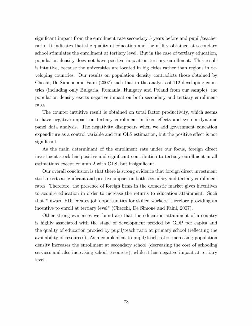
signi�cant impact from the enrollment rate secondary 5 years before and pupil/teacher
ratio. It indicates that the quality of education and the utility obtained at secondary
school stimulates the enrollment at tertiary level. But in the case of tertiary education,
population density does not have positive impact on tertiary enrollment. This result
is intuitive, because the universities are located in big cities rather than regions in de-
veloping countries. Our results on population density contradicts those obtained by
Chechi, De Simone and Faini (2007) such that in the analysis of 112 developing coun-
tries (including only Bulgaria, Romania, Hungary and Poland from our sample), the
population density exerts negative impact on both secondary and tertiary enrollment
rates.
The counter intuitive result is obtained on total factor productivity, which seems
to have negative impact on tertiary enrollment in �xed e¤ects and system dynamic
panel data analysis. The negativity disappears when we add government education
expenditure as a control variable and run OLS estimation, but the positive e¤ect is not
signi�cant.
As the main determinant of the enrollment rate under our focus, foreign direct
investment stock has positive and signi�cant contribution to tertiary enrollment in all
estimations except column 2 with OLS, but insigni�cant.
Our overall conclusion is that there is strong evidence that foreign direct investment
stock exerts a signi�cant and positive impact on both secondary and tertiary enrollment
rates. Therefore, the presence of foreign �rms in the domestic market gives incentives
to acquire education in order to increase the returns to education attainment. Such
that "Inward FDI creates job opportunities for skilled workers; therefore providing an
incentive to enroll at tertiary level" (Checchi, De Simone and Faini, 2007).
Other strong evidences we found are that the education attainment of a country
is highly associated with the stage of development proxied by GDP per capita and
the quality of education proxied by pupil/teach ratio at primary school (re�ecting the
availability of resources). As a complement to pupil/teach ratio, increasing population
density increases the enrollment at secondary school (decreasing the cost of schooling
services and also increasing school resources), while it has negative impact at tertiary
level.
78

6.2 Results: Determinants of Foreign Direct Invest-
ment
The equation (4.3) on the determinants of foreign direct investment is estimated. Our
results for the unbalanced panel data are reported in Table (6.4) and (6.5). Again, we
begin with simple OLS estimates followed by country �xed e¤ect and dynamic panel
data system GMM estimations.
Before discussing the results, it is worthwhile to bring some explanation to the eco-
nomic reform index obtained by Principal Component Analysis (PCA). As mentioned,
we combine four economic reform indicators provided by European Bank and Recon-
struction (EBRD): Banking reform and interest rate liberalization, trade and foreign
exchange system, governance and enterprise restructuring and the share of private sec-
tor to the public sector. Considering high correlation between these variables, one
economic reform index is obtained as following.
ReformBanking reform and interest rate liberalization 0.5078Trade and foreign exchange system 0.5016Governance and enterprise restructuring 0.4888The share of private sector to the public sector 0.5016
Cumulative: 0.8762
We choose only the �rst factor loading with cumulative variance 0.8762, which means
that the obtained new variable explains 87.62 percent of the original data. The factor
scores obtained from PCA analysis is used in our estimations as an explanatory for the
determinants of FDI.
79

Human capital = secondary education attainment
1OLS
2OLS
3FE
4FE
5FE
6FE
7SYSGMM
8SYSGMM
FDI inflows lagged 1 .5983159(8.24)***
.1557765(1.55)
Population withsecondary education
14.72697(0.72)
58.46718(2.02)**
14.99277(0.19)
3.60378(0.03)
48.47068(0.44)
159.6392(0.77)
137.8037(2.07)**
123.5871(1.90)*
Log GDP per capita .0815086(0.08)
2.634672(1.63)
4.675373(1.58)
.5784068(0.11)
17.03749(2.52)**
19.00784(2.01)**
2.667744(0.70)
28.00495(5.71)
Log stock of inwardFDI
2.791408(2.82)***
1.792837(0.87)
.1242942(0.06)
6.036843(0.91)
4.105307(2.20)**
18.80215(5.29)***
Trade (% of GDP) 14.25258(1.25)
2.215579(0.14)
17.10462(1.65)
Inflation .0016106(0.03)
.059677(0.41)
.1325432(1.37)
Log Population 163.7067(1.21)
20.43263(3.56)***
Domestic Investment .3445295(1.65)
.1960442(1.36)
Real interest rate 4.259335(0.60)
.8868392(0.19)
Politics, country risk .4031771(1.38)
.1445384(0.56)
.2912976(1.72)*
GDP growth .0767858(0.25)
.240572(1.18)
Productive publiccapital
.0509469(0.14)
.4412864(1.94)*
Reform 10.21919(3.36)***
4.768007(2.31)
Exchange rate .0053358(0.63)
.0223961(0.47)
.0248896(0.001)
Constant 3.558733(0.69)
19.62071(2.01)
11.69443(0.70)
9.460272(0.38)
32.85771(0.91)
3.509256(0.90)
45.10254(2.89)
96.45111(2.31)
Observations 164 164 164 131 131 71 130 70R² 0.0037 0.0865 0.0209 0.0141 0.1512 0.3167Number of countries 26 26 24 23 23 16Sargan test 0.0000 0.4512
1. Sargan test of overidentifying restrictions. H0: overidentifying restrictions are valid. P values are presented.2. t statistics in brackets * significant at 10%; ** significant at 5%; *** significant at 1%.
Table 6.4: Gross enrollment rate - Average In�ows of FDI (1990-2008) - UnbalancedPanel
As a main focus of this section�s research to �nd the contribution of human capital
to the entry of foreign capital �ows, we �nd that the percentage of population with
secondary and tertiary education as proxies for human capital statistically signi�cantly
impacts FDI �ows (excluding the equation 8 of Table (6.4)). Therefore, the role of
existing human capital in drawing foreign investment is essential.
The stock of FDI has positive and signi�cant impact on the in�ow of FDI in both
Tables with the percentage of population with secondary and tertiary education as
80
human capital, which indicates that previous investment in the economy increases the
absorption capacity for future FDI in�ows. Such that if the domestic market has already
been impacted by the superior technology from abroad and its spillovers onto the human
capital have been realized, then there is high probability that future FDI in�ows will be
bene�cial both to home and host countries. Therefore, the amount of present foreign
capital stock contributes to the entry of future FDI in�ow to the market.
In both estimations, we do not �nd any evidence for the impact of openness (proxied
by Trade/GDP), economic stability (proxied by in�ation) and economic growth of a
country on FDI in�ow. Stage of development and market size proxied by GDP per
capita and population (assuming that FDI is attracted by larger countries in terms of
population) seem to have negative impact on FDI in�ow; in column 5 to 6 of Table (6.4)
and column 6 to 8 in Table (6.5), GDP per capita has negative and signi�cant impact
and population has negative impact in column 7 to 8 of both tables. It indicates that
the stage of development of the countries in our sample impedes the in�ow of foreign
investment.
Political stability seems to impact FDI in�ows negatively, column 8 of Table (6.4)
(with secondary education attainment). Although insigni�cant, the negative impact of
political stability is reported in the estimations in Table (6.5) (with tertiary education
attainment).
Domestic investment exerts positive impact on FDI in�ow in all estimations (sig-
ni�cant only in Table (6.5) in the presence of tertiary education as a proxy for human
capital).
There is no clear evidence on the role of productive public capital. Column 8 of
Table (6.4) and Table (6.5) reports negative impact (signi�cant only in Column 8 of
Table (6.4)), while other estimations report positive in�uence but non-signi�cant.
Regressions suggest that reform index has a signi�cant positive impact on foreign
capital. It is not clear via which channel reforms impact on FDI in�ow; impacting
the �nancial e¢ ciency, GDP per capita or political stability of the host countries such
that estimations did not support �nancial e¢ ciency and we got negative response from
GDP per capita and political stability. At the same time, estimations do not provide
us with necessary information on Trade /GDP. Therefore, we come to the conclusion
that reform indicators alone increases FDI in�ow. However, we expect that successful
implementation should stimulate an increase in the openness, stage of development and
political stability of a country in order to draw the attention of foreign �rms.
The expected negative sign of real interest rate is provided by estimations in Table
81

(6.5) but non-signi�cant, while Table (6.4) reports positive sign. On the other hand,
exchange rate has positive and signi�cant impact on FDI in�ow. As mentioned, the
appreciation of national currency can increase FDI in�ow if it is directed to the market
service instead of re-export. It seems that FDI in�ow to countries in our sample is
market oriented.
Human capital = tertiary education attainment
1OLS
2OLS
3FE
4FE
5FE
6FE
7SYSGMM
8SYSGMM
FDI inflows lagged 1 .5260405(6.96)***
.1284656(1.25)
Population withtertiary education
106.991(2.10)**
101.9249(1.49)
207.3675(1.96)*
181.3676(1.55)
66.43295(0.55)
289.493(1.68)
213.5835(2.13)**
107.3231(1.09)
Log GDP per capita .5921153(0.59)
2.277199(1.24)
2.064305(0.73)
2.16704(0.45)
15.66232(2.50)
15.85011(1.76)*
6.733595(2.14)**
24.38173(5.51)***
Log stock of inwardFDI
2.028216(1.93)*
1.839483(0.90)
.2546012(0.12)
3.588335(0.56)
4.445606(2.48)**
15.62012(4.84)***
Trade (% of GDP) 13.99191(1.23)
.081111(0.01)
16.62487(1.54)
Inflation .0035028(0.07)
.035793(0.23)
.1661457(1.65)
Log Population 125.794(0.95)
13.28052(2.72)***
Domestic Investment .5418204(2.28)**
.3000521(1.77)*
Real interest rate 1.520353(0.21)
3.26652(0.71)
Politics, country risk .3857167( 1.33)
.045802(0.18)
.1761476(1.12)
GDP growth .24316(0.81)
.1241113(0.59)
Productive publiccapital (% of GDP)
.3147644(0.84)
.2789501(1.28)
Exchange rate .0048839(0.58)
.0480555(1.08)
.02536(3.17)***
Reform 9.563195(3.00)***
3.153782(0.89)
4.076262(1.96)**
Constant 5.036952(0.80)
14.72811(1.60)
18.0593(1.87)
19.72867(1.38)
16.74991(0.54)
894.8031(0.97)
35.2203(2.76)
Observations 164 131 164 131 131 71 130 70R² 0.0272 0.0733 0.0473 0.1522 0.3509Number of countries 26 26 24 23 23 16 23 16Sargan test 0.0000 0.4407
1. Sargan test of overidentifying restrictions. H0: overidentifying restrictions are valid. P values are presented.2. t statistics in brackets * significant at 10%; ** significant at 5%; *** significant at 1%.
Table 6.5: Gross enrollment rate - Average In�ows of FDI (1990-2008) - UnbalancedPanel
An overall conclusion of this part is that existing human capital stock and foreign
capital stock are incentives for future investment in�ows. Strong evidence is also found
82
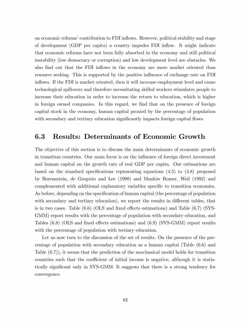
on economic reforms�contribution to FDI in�ows. However, political stability and stage
of development (GDP per capita) a country impedes FDI in�ow. It might indicate
that economic reforms have not been fully absorbed in the economy and still political
instability (low democracy or corruption) and low development level are obstacles. We
also �nd out that the FDI in�ows in the economy are more market oriented than
resource seeking. This is supported by the positive in�uence of exchange rate on FDI
in�ows. If the FDI is market oriented, then it will increase employment level and cause
technological spillovers and therefore necessitating skilled workers stimulates people to
increase their education in order to increase the return to education, which is higher
in foreign owned companies. In this regard, we �nd that on the presence of foreign
capital stock in the economy, human capital proxied by the percentage of population
with secondary and tertiary education signi�cantly impacts foreign capital �ows.
6.3 Results: Determinants of Economic Growth
The objective of this section is to discuss the main determinants of economic growth
in transition countries. Our main focus is on the in�uence of foreign direct investment
and human capital on the growth rate of real GDP per capita. Our estimations are
based on the standard speci�cations representing equations (4.5) to (4.8) proposed
by Borensztein, de Gregorio and Lee (1998) and Mankiw Romer, Weil (1992) and
complemented with additional explanatory variables speci�c to transition economies.
As before, depending on the speci�cation of human capital (the percentage of population
with secondary and tertiary education), we report the results in di¤erent tables, that
is in two cases. Table (6.6) (OLS and �xed e¤ects estimations) and Table (6.7) (SYS-
GMM) report results with the percentage of population with secondary education, and
Tables (6.8) (OLS and �xed e¤ects estimations) and (6.9) (SYS-GMM) report results
with the percentage of population with tertiary education.
Let us now turn to the discussion of the set of results. On the presence of the per-
centage of population with secondary education as a human capital (Table (6.6) and
Table (6.7)), it seems that the prediction of the neoclassical model holds for transition
countries such that the coe¢ cient of initial income is negative, although it is statis-
tically signi�cant only in SYS-GMM. It suggests that there is a strong tendency for
convergence.
83

Human capital = secondary education attainment
1OLS
2OLS
3OLS
4FE
5FE
6FE
7FE
8FE
Initial real GDPper capita
.6058913(0.51)
1.046571(0.90)
.5149789(0.44)
Human capital:Population withsecondaryeducation
11.05392(0.71)
63.8077(2.83)***
6.302688(0.40)
174.251(4.86)***
151.5373(3.44)***
149.3776(3.89)***
165.972(4.49)***
21.61438(0.49)
FDI stock (% ofGDP)
.0280754(2.28)**
.1396589(2.55)**
.0093002(0.59)
.0151747(0.96)
.0432429(0.64)
.0339565(1.46)
.0147539(0.93)
.0186638(0.82)
FDI*Humancapital
1.403112(3.14)***
.5012478(0.89)
Governmentconsumption
.2101058(5.50)***
.1960496(5.22)***
.2037075(5.35)***
.1645363(3.02)***
.1631131(2.99)***
.1837839(3.25)***
.1633248(3.00)***
.1144875(2.41)***
Domesticinvestment
.1976812(3.68)***
.1168937(1.80)*
Openness: Trade(% of GDP)
24.28214(5.01)***
Inflation .0095818(0.93)
.0095784(1.04)
M2 (% of GDP) .0095555(0.21)
Reform 2.135895(1.87)*
Country risk:Politics
.0885887(0.57)
Populationgrowth
.0699787(0.10)
Constant 16.38591(3.30)
23.6292(4.41)
10.90436(2.13)
33.5311(6.58)
30.82387(5.19)
29.00844(5.16)
32.60249(6.28)
34.50618(3.19)
Observations 178 178 171 178 178 171 178 153R² 0.2435 0.2846 0.2951 0.1715 0.1759 0.1714 0.1763 0.3968Number ofcountries
26 26 26 25 25 25 25 25
1. t statistics in brackets * significant at 10%; ** significant at 5%; *** significant at 1%.
Table 6.6: Real per capita GDP growth rate (1990-2008) - Unbalanced Panel
Other variables that are found to contribute to economic growth are reform, open-
ness (Trade/GDP) and productive public capital. For these factors, we obtain statisti-
cally positive coe¢ cient.
We cannot derive evidence for the political stability, and population growth, which
have di¤erent signs but non-signi�cant. As a proxy for �nancial e¢ ciency, in�ation
has negative non-signi�cant impact. As a proxy for �nancial size, M2/GDP has nega-
tive non-signi�cant coe¢ cient. As to the government consumption, it has statistically
signi�cant negative impact in all estimations.
84

Human capital = secondary education attainment
1SYSGMM
2SYSGMM
3SYSGMM
4SYSGMM
5SYSGMM
6SYSGMM
7SYSGMM
GDP growth rate lagged 1 .5450334(9.94)***
.5435523(9.89)***
.0385033(0.49)
.5435356(9.64)***
.5404959(9.74)***
.244222(3.80)***
.2077704(3.10)***
Initial real GDP per capita 5.701213(1.23)
5.442233(1.17)
5.518468(1.51)
2.837669(0.64)
5.47846(1.18)
7.529764(1.98)**
7.282074(2.15)*
Human capital: Population withsecondary education
19.90905(0.58)
5.214813(0.12)
87.55802(2.65)***
3.343661(0.09)
17.01969(0.49)
17.80712(0.40)
2.988246(0.05)
FDI stock (% of GDP) .0043703(0.30)
.0411301(0.62)
.0022172(0.03)
.0030005(0.14)
.0041957(0.29)
.0142714(0.65)
.1122815(0.89)
FDI*Human capital .3140315(0.57)
.0249421(0.04)
.7250453(0.72)
Government consumption .1518347(3.08)
.1515632(3.05)***
.3566167(5.58)***
.163136(3.14)***
.1517946(3.08)***
.1586216(3.53)***
.1834127(3.71)***
Domestic investment .0216337(0.34)
.038321(0.52)
Productive public capital .3030833(2.77)***
Openness: Trade (% of GDP) 15.87673(4.10)***
16.99902(4.28)***
Inflation .005042(0.51)
.0106956(1.19)
.0111232(1.19)
M2 (% of GDP) .0382607(0.90)
.035599(0.74)
Reform 1.82405(2.29)**
1.522208(1.78)
Country risk: Politics .0228264(0.17)
.0352(0.26)
Population growth .0071821(0.01)
.2177807(0.35)
Constant 29.70275(1.72)
27.1268(1.50)
45.13701(3.47)
18.26723(1.09)
28.71773(1.65)
2.81728(0.16)
2.778582(0.16)
Observations 178 178 97 171 178 153 151Number of countries 25 25 16 25 25 25 25Sargan test 0.0327 0.0327 0.5805 0.0382 0.0341 0.0610 0.1098
1. Sargan test of overidentifying restrictions. H0: overidentifying restrictions are valid. P values are presented.2. t statistics in brackets * significant at 10%; ** significant at 5%; *** significant at 1%.
Table 6.7: Real per capita GDP growth rate (1990-2008) - Unbalanced Panel
Counter-intuitive results are obtained for human capital (population with secondary
education), foreign direct investment stock. As seen in Table (6.6) and Table (6.7),
both variables have statistically signi�cant negative impact on economic growth. In
our opinion, it results from the inclusion of population with secondary education as
a proxy for human capital. To analyze the reason for negativity in detail, �rst we
review Borenstzein et al (1998). According to their research on developing countries
for the period of 1970-1989, the coe¢ cient on foreign direct investment alone is not
statistically signi�cant. Because the adoption of new technology requires educated
labor force. Therefore, the authors consider an interaction between FDI and schooling
(the male secondary schooling constructed by Barro and Lee (1993)). The positive sign
85

of the interaction term suggests that FDI is able to have impact on economic growth for
the countries in which the human capital stock has reached a minimum threshold level.
This can be applied to our case for transition countries too. With population with
secondary education, the e¤ect of FDI on economic growth is negative. However, the
interaction term exerts positive coe¢ cient (Table (6.6) - column 2, Table (6.7) �column
3 and 8). This implies that the e¤ect of FDI is necessarily conditional on a minimum
threshold level of human capital. Our results on FDI and human capital contradict
those from Nauro F. Campos and Yuko Kinoshita (2002) on transition countries of our
sample for the period 1990-1998. The proxy for human capital in Nauro F. Campos
and Yuko Kinoshita (2002) is taken as secondary school enrollment ratio, but the type
of FDI (whether in�ow or stock) is not mentioned. Their result is that secondary
school enrollment has negative impact on economic growth, but FDI alone and without
an interaction term has positive impact on economic growth. According to Nauro F.
Campos and Yuko Kinoshita (2002), the reason for human capital�s negative impact is
explained by decreasing public �nancial support as transition progresses and therefore
decreasing average years of education. In di¤erence from Nauro F. Campos and Yuko
Kinoshita (2002), our result with FDI stock and human capital (the percentage of
population with secondary education) support Borenstzein et al (1998). In subsequent
analysis, we will see if the results with tertiary education hold the same or not.
Although the data on gross domestic investment also includes FDI, we get its positive
impact on economic growth (see Table (6.6) - column 3 and 6). Hence, the investment
as a whole plays an important role.
The results with tertiary education as a proxy for human capital are reported in
Table (6.8) and Table (6.9).
Di¤erent from the �rst case, the coe¢ cient of initial income is positive in OLS
estimations, but it improves and gets statistically negative impact in SYS-GMM esti-
mations in Table (6.9). It reinforces our conclusion that there is a strong tendency for
convergence.
86
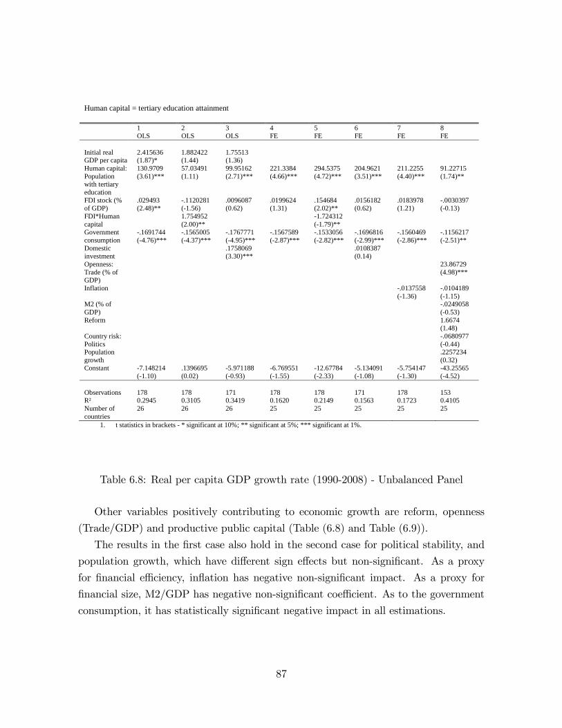
Human capital = tertiary education attainment
1OLS
2OLS
3OLS
4FE
5FE
6FE
7FE
8FE
Initial realGDP per capita
2.415636(1.87)*
1.882422(1.44)
1.75513(1.36)
Human capital:Populationwith tertiaryeducation
130.9709(3.61)***
57.03491(1.11)
99.95162(2.71)***
221.3384(4.66)***
294.5375(4.72)***
204.9621(3.51)***
211.2255(4.40)***
91.22715(1.74)**
FDI stock (%of GDP)
.029493(2.48)**
.1120281(1.56)
.0096087(0.62)
.0199624(1.31)
.154684(2.02)**
.0156182(0.62)
.0183978(1.21)
.0030397(0.13)
FDI*Humancapital
1.754952(2.00)**
1.724312(1.79)**
Governmentconsumption
.1691744(4.76)***
.1565005(4.37)***
.1767771(4.95)***
.1567589(2.87)***
.1533056(2.82)***
.1696816(2.99)***
.1560469(2.86)***
.1156217(2.51)**
Domesticinvestment
.1758069(3.30)***
.0108387(0.14)
Openness:Trade (% ofGDP)
23.86729(4.98)***
Inflation .0137558(1.36)
.0104189(1.15)
M2 (% ofGDP)
.0249058(0.53)
Reform 1.6674(1.48)
Country risk:Politics
.0680977(0.44)
Populationgrowth
.2257234(0.32)
Constant 7.148214(1.10)
.1396695(0.02)
5.971188(0.93)
6.769551(1.55)
12.67784(2.33)
5.134091(1.08)
5.754147(1.30)
43.25565(4.52)
Observations 178 178 171 178 178 171 178 153R² 0.2945 0.3105 0.3419 0.1620 0.2149 0.1563 0.1723 0.4105Number ofcountries
26 26 26 25 25 25 25 25
1. t statistics in brackets * significant at 10%; ** significant at 5%; *** significant at 1%.
Table 6.8: Real per capita GDP growth rate (1990-2008) - Unbalanced Panel
Other variables positively contributing to economic growth are reform, openness
(Trade/GDP) and productive public capital (Table (6.8) and Table (6.9)).
The results in the �rst case also hold in the second case for political stability, and
population growth, which have di¤erent sign e¤ects but non-signi�cant. As a proxy
for �nancial e¢ ciency, in�ation has negative non-signi�cant impact. As a proxy for
�nancial size, M2/GDP has negative non-signi�cant coe¢ cient. As to the government
consumption, it has statistically signi�cant negative impact in all estimations.
87
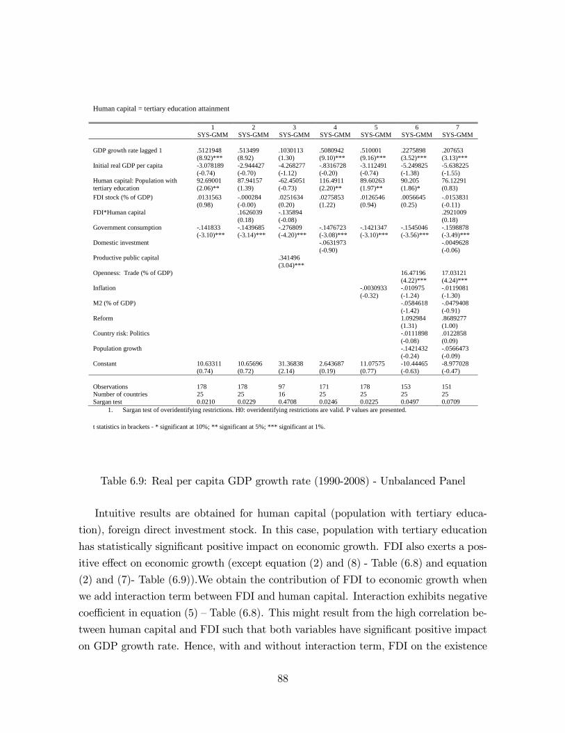
Human capital = tertiary education attainment
1SYSGMM
2SYSGMM
3SYSGMM
4SYSGMM
5SYSGMM
6SYSGMM
7SYSGMM
GDP growth rate lagged 1 .5121948(8.92)***
.513499(8.92)
.1030113(1.30)
.5080942(9.10)***
.510001(9.16)***
.2275898(3.52)***
.207653(3.13)***
Initial real GDP per capita 3.078189(0.74)
2.944427(0.70)
4.268277(1.12)
.8316728(0.20)
3.112491(0.74)
5.249825(1.38)
5.638225(1.55)
Human capital: Population withtertiary education
92.69001(2.06)**
87.94157(1.39)
62.45051(0.73)
116.4911(2.20)**
89.60263(1.97)**
90.205(1.86)*
76.12291(0.83)
FDI stock (% of GDP) .0131563(0.98)
.000284(0.00)
.0251634(0.20)
.0275853(1.22)
.0126546(0.94)
.0056645(0.25)
.0153831(0.11)
FDI*Human capital .1626039(0.18)
.135894(0.08)
.2921009(0.18)
Government consumption .141833(3.10)***
.1439685(3.14)***
.276809(4.20)***
.1476723(3.08)***
.1421347(3.10)***
.1545046(3.56)***
.1598878(3.49)***
Domestic investment .0631973(0.90)
.0049628(0.06)
Productive public capital .341496(3.04)***
Openness: Trade (% of GDP) 16.47196(4.22)***
17.03121(4.24)***
Inflation .0030933(0.32)
.010975(1.24)
.0119081(1.30)
M2 (% of GDP) .0584618(1.42)
.0479408(0.91)
Reform 1.092984(1.31)
.8689277(1.00)
Country risk: Politics .0111898(0.08)
.0122858(0.09)
Population growth .1421432(0.24)
.0566473(0.09)
Constant 10.63311(0.74)
10.65696(0.72)
31.36838(2.14)
2.643687(0.19)
11.07575(0.77)
10.44465(0.63)
8.977028(0.47)
Observations 178 178 97 171 178 153 151Number of countries 25 25 16 25 25 25 25Sargan test 0.0210 0.0229 0.4708 0.0246 0.0225 0.0497 0.0709
1. Sargan test of overidentifying restrictions. H0: overidentifying restrictions are valid. P values are presented.
t statistics in brackets * significant at 10%; ** significant at 5%; *** significant at 1%.
Table 6.9: Real per capita GDP growth rate (1990-2008) - Unbalanced Panel
Intuitive results are obtained for human capital (population with tertiary educa-
tion), foreign direct investment stock. In this case, population with tertiary education
has statistically signi�cant positive impact on economic growth. FDI also exerts a pos-
itive e¤ect on economic growth (except equation (2) and (8) - Table (6.8) and equation
(2) and (7)- Table (6.9)).We obtain the contribution of FDI to economic growth when
we add interaction term between FDI and human capital. Interaction exhibits negative
coe¢ cient in equation (5) �Table (6.8). This might result from the high correlation be-
tween human capital and FDI such that both variables have signi�cant positive impact
on GDP growth rate. Hence, with and without interaction term, FDI on the existence
88
of human capital (with educated labor force) and human capital contributes positively
to economic growth.
Overall our results support a positive impact of FDI on economic growth. FDI
contributes to economic growth on the existence of educated labor force or skilled la-
bor because it allows technology to be absorbed easily. However, in the regressions
with population with secondary education, FDI and human capital cannot contribute
to economic growth by themselves. Only their complementary relationship can in�u-
ence positively. Because the adoption of new technology requires educated labor force.
The positive sign of the interaction term suggests that FDI is able to have impact on
economic growth for the countries in which the human capital stock has reached a min-
imum threshold level. The role of productive public capital, gross domestic investment
and openness of the countries are crucial for the growth of economy. But the growth is
impeded by in�ation and political stability (although we could not �nd strong results).
89
Chapter 7
Conclusion
Our dissertation focused on three directions: The determinants of human capital, for-
eign direct investment and economic growth in the transition countries. These three
directions got their bases from the empirical analysis of the investment development
path and the right measure of human capital.
The Investment Development Path hypothesis developed by Dunning (1981) sug-
gests that our countries are in the second stage of development and investment devel-
opment path, meaning that they still draw more inward FDI than their outward FDI,
suggesting that the ownership advantages of domestic �rms are still at a low level.
As already mentioned, according to IDP theory, in the �rst stage of development,
the location advantages of a country are not su¢ cient to attract foreign investment.
The reasons behind these are improper economic systems and government policies,
inadequate labor force and infrastructure to promote FDI. The ownership advantages
of domestic �rms are also not su¢ cient. Therefore, outward FDI of the country is
likely to be very little. In this case, government�s intervention is necessary to provide
basic infrastructure and upgrade human capital through education or training. That
is, before a country can attract signi�cant inward FDI, it must develop its location
advantages including an increase in GDP per capita. In this stage, determinants of
foreign direct investment in the economy are formed: the stage of development of the
local market, availability of necessary human capital for absorption of new technology
and so on. As long as there is a suitable environment in the host country and the
location advantages of the country improve, especially with the help of government
policies, FDI in�ow begins to rise and the stage of development enters the second stage.
In this stage, outward direct investment still remains at a negligible level and inward
90
FDI stocks rise faster than GDP. As a conclusion, we can say that the determinants of
foreign direct investment are determined in the �rst stage, while the determinants of
human capital and economic growth are formed in both cases. As the economy develops
and the ownership advantages of local �rms improve, then outward investment will also
increase and there will be higher economic development than before. So our econometric
analysis was based on the �rst and second stages of investment development path with
three directions: determinants of FDI in�ow, human capital formation and economic
growth.
In chapter 2 we also discussed the measures of human capital and came to the con-
clusion that although the average years of education is considered as the best measure
for human capital, we can choose the enrollment rates at secondary and tertiary edu-
cation level. Analysis showed that enrollment rates are the future human capital and
increase the average years of education in future. Therefore, since the decision is also
made on enrollment, we chose this variable as the right measure of human capital as an
explained variable. Additionally, we concluded that the percentage of population with
secondary and tertiary education level should be chosen as the determinants of foreign
direct investment and economic growth because this variable can embody the spillover
e¤ect from older generation too.
From chapter 3, where we presented three economic models, we derived three main
equations on the determinants of human capital, foreign direct investment and economic
growth. The estimation results of these three directions are as follows.
Conclusion from the determinants of schooling:
Our overall conclusion is that there is strong evidence that foreign direct investment
stock exerts a signi�cant and positive impact on both secondary and tertiary enrollment
rates. Therefore, the presence of foreign �rms in the domestic market gives incentives to
acquire education. Inward FDI creates job opportunities for skilled workers; therefore
providing an incentive to enroll at tertiary level to increase the returns to education
attainment.
Other strong evidences we found are that the education attainment of a country
is highly associated with the stage of development proxied by GDP per capita and
the quality of education proxied by pupil/teach ratio at primary school (re�ecting the
availability of resources). As a complement to pupil/teach ratio, increasing population
density increases the enrollment at secondary school (decreasing the cost of schooling
services and also increasing school resources), while it has negative impact at tertiary
level.
91
Conclusion from the determinants of FDI:
An overall conclusion of this part is that existing human capital stock and foreign
capital stock are incentives for future investment in�ows. Strong evidence is also found
on economic reforms� contribution to FDI in�ows. However, political stability and
stage of development (GDP per capita) in the transition countries impede FDI in�ow.
It might indicate that economic reforms have not been fully absorbed in the economy
and still political instability (low democracy or corruption) and low development level
are obstacles. We also �nd out that the FDI in�ows in the transition countries are more
market oriented than resource seeking. This is supported by the positive in�uence of
exchange rate on FDI in�ows. If the FDI is market oriented, then it will increase
employment level and cause technological spillovers and therefore necessitate skilled
workers and stimulate people to increase their education in order to increase the return
to education, which is higher in foreign owned companies. In this regard, we �nd that
on the presence of foreign capital stock in the economy, human capital proxied by the
percentage of population with secondary and tertiary education signi�cantly impacts
foreign capital �ows.
Conclusion from the determinants of economic growth:
Overall our results support a positive impact of FDI on economic growth. FDI
contributes to economic growth on the existence of educated labor force or skilled la-
bor because it allows technology to be absorbed easily. However, in the regressions
with population with secondary education, FDI and human capital cannot contribute
to economic growth by themselves. Only their complementary relationship can in�u-
ence positively. Because the adoption of new technology requires educated labor force.
The positive sign of the interaction term suggests that FDI is able to have impact on
economic growth for the countries in which the human capital stock has reached a min-
imum threshold level. The role of productive public capital, gross domestic investment
and openness of the countries are crucial for the growth of economy. But the growth is
impeded by in�ation and political stability (although we could not �nd strong results).
Finally, we would like to note that despite the level of economic development, in-
vestment in the economy has always been one of the actual problems. But it is the
most important for the countries transiting to a market economy. It is explained such
that achieving economic growth and maintaining its stable level depend on the balanced
development of all sectors of economy, the drawing of domestic and foreign investments
and their use in the right direction. Investment is also a �nancial source. Because
of this source, not only production but also serious structural changes occur. Foreign
92

capital can bring scienti�c and technical achievements and superior management skills
to the economy. Thus, drawing foreign investment in the production sector is more
e¢ cient.
In general, foreign direct investment is very important for eradicating modern eco-
nomic di¢ culties. To achieve this, attractive investment climate, economic and leg-
islative bases should be taken into the consideration. Because, before investing in the
economy, every foreign �rm investigates the present political, economic, cultural and
legislative environment. If these are considered satisfactory, the investment is real-
ized. One of the most important tasks in front of the transition countries is to create
transparent environment for foreign investors.
In these regards, our research will promote a better understanding of the FDI sit-
uation in the transition countries and assist policymakers in formulating development
oriented FDI policies.
93
Bibliography
[1] Alfaro, L., A. Chanda, S. Kalemli-Ozcan, and S. Sayek (2006): �How Does Foreign
Direct Investment Promote Economic Growth? Exploring the E¤ects of Financial
Markets on Linkages,�NBERWorking Paper 12522, Cambridge MA.
[2] Alvares, M. (2011): "España y la senda de desarrollo de la inversión directa: una
aproximación", Institut d�Economia de Barcelona, Document de treball 2001/11.
[3] Arellano, M and O. Bover, (1995): �Another look at the instrumental variable
estimation of error-components models�Journal of Econometrics, 68(1):29�51.
[4] Arellano, M. and S. Bond. (1991): �Some tests of speci�cation for panel data:
Monte Carlo evidence and an application to employment equations�, Review of
Economic Studies, 58, 277-297.
[5] Barro, R., Sala-i-Martin, X., (1995): "Economic Growth", McGraw-Hill, Cam-
bridge, MA.
[6] Barry, F., H. Görg and F. McDowell (2001): "Outward FDI and the Investment
Development Path of a Late-Industrialising Economy: Evidence from Ireland",
University College Dublin, School of Economics, UCD Centre for Economic Re-
search Working Paper Series; WP01/08
[7] Bellak, C. (2000): "The Investment Development Path of Austira", Vienna Uni-
versity of Economics, Department of Economics Working Paper Series, No. 75.
[8] Bergheim, S. (2005): "Human Capital is the Key to Growth", Deutsche Bank
Research.
[9] Bevan, A. A. and Estrin, S. (2000): "Determinants of FDI in Transition
Economies", Working Paper No. 342. Centre for New and Emerging Market, Lon-
don Business School
94

[10] Bils, M, and P. J. Klenow. (2000): �Does Schooling Cause Growth?�, American
Economic Review, 90(5).
[11] Blomström, M, R. Lipsey, M. Zejan, (1992): �What Explains Developing Country
Growth�NBER Working Paper No. 4132.
[12] Blomström, M. (1991):�Host Country Bene�ts of Foreign Investment�, in D.G.
McFetridge, ed., Foreign Investment, Technology and Economic Growth, Toronto
and London; Toronto University Press.
[13] Blomstrom, M., and A. Kokko. (2003): �The Economics of Foreign Direct Invest-
ment Incentives�NBER Working Paper no. 9489, February.
[14] Blundell, R and S. Bond, (1998): �Initial conditions and moment restrictions in
dynamic panel data models�, Journal of Econometrics, 87:115�143.
[15] Bond, S.R., A. Hoeer and J. Temple (2001): GMMEstimation of Empirical Growth
Models, Nu¢ eld College, Oxford, Working Paper.
[16] Borensztein, E. J. De Gregorio and J-W. Lee (1998): �How Does Foreign Direct
Investment A¤ect Economic Growth?�, Journal of International Economics, 45,
115-35.
[17] Buckley, Peter J. and Francisco B. Castro (1998). "The investment development
path: the case of Portugal", Transnational Corporations, 7 (1), pp. 1-15.
[18] Campos, N.F., and Y. Kinoshita, (2002): �FDI as Technology Transferred: Some
Panel Evidence from Transition Economies�, The Manchester School, Vol. 70, No.
3, pp. 398�419.
[19] Campos, N.F., and Y. Kinoshita, (2008): "Foreign Direct Investment and Struc-
tural Reforms: Evidence from Eastern Europe and Latin America", IMF Working
Paper No. 08/26.
[20] Carkovic, M and R. Levine (2002): �Does Foreign Direct Investment Accelerate
Economic Growth?�University of Minnesota Department of Finance Working Pa-
per.
[21] Checchi, D., G. De Simone, R. Faini (2007): �Skilled Migration, FDI and Human
Capital Investment�, IZA Discussion Paper, 2795.
95
[22] Cohen, D and M. Soto (2002): "Why are some countries so poor? Another look at
the evidence and a message of hope", OECD Development Centre technical papers
No. 197.
[23] Dunning, John H. (1981): �Explaining the international direct investment position
of countries: towards a dynamic or developmental approach�, Weltwirtschaftliches
Archiv, 119, pp. 30-64.
[24] Dunning, John H. and R. Narula (1996): Foreign Direct Investment and Govern-
ments (London and New York: Routledge)
[25] Dunteman, George H. (1989): "Principal Components Analysis", Sage University
Paper series Quantitative Applications in Social Sciences No 07-069, Newbury
Park, CA, Sage
[26] Durán, J. and F. Ubeda (2001): �The Investment Development Path: a New
Empirical Approach and Some Theoretical Issues�, Transnational Corporations
(Vol.10, No.2)
[27] Greiner, A. (2008): �Human capital formation, public debt and economic growth�,
Journal of Macroeconomics, 30(1):415�427.
[28] Grossman M. (2005): �Education and Nonmarket Outcomes�. NBER Working
Paper No.11582.
[29] Grossman, G and E. Helpman (1991): "Innovation and Growth in the Global
Economy", MIT Press Cambridge, MA.
[30] Hurlin, C. and B. Venet, (2001): �Granger causality tests in panel data models with
�xed coe¢ cients�, Working Paper Eurisco 2001-09, Université Paris IX Dauphine.
[31] Jones, Charles I., (2007): A Simple Mincerian Approach to Endogenizing School-
ing, U.C. Berkeley working paper.
[32] Kim, Jao-On and C. W. Mueller (1978): "Introduction to Factor Analysis: What
It Is and How to Do It", Sage University Paper series Quantitative Applications
in Social Sciences No 07-013, Newbury Park, CA, Sage
[33] Kleinert, J, F. Toubal (2005): �Gravity for FDI�. Working Paper. Georg-August-
Universitat Gottingen.
96

[34] Krause, A.W. (1999): �Human Capital Skilling, FDI, and Economic Development:
Toward Equity�, Paper presented at the Association for Social Economics (ASE)
at the ASSA meeting in New York, NY, 3-5.
[35] Levi, M. D. (1990): International Finance: The Markets and Financial Manage-
ment of Multinational Business, 2nd edition (New York: McGraw-Hill).
[36] Lim A.S.K, and K.K. Tang KK (2008): "Human Capital Inequality and the
Kuznets Curve", Developing Economies, XLVI-1: pp. 26-51.
[37] Liu, Z. (2008): �Foreign direct investment and technology spillovers: Theory and
evidence�. Journal of Development Economics, 85(1-2):176�193.
[38] Lucas, R.E. (1988): "On the mechanics of economic development". Journal of
Monetary Economics, 22(1):3�42.
[39] Lucas, R.E. (2002): "Lectures on Economic Growth" (Harvard University Press,
Cambridge).
[40] Mankiw, G., Romer, D. and Weil, D. (1992): �A Contribution to the Empirics of
Economic Growth�, Quarterly Journal of Economics, Volume 107, Issue 2 (May,
1992), 407-437
[41] Mincer J. (1974): "Schooling, Experience, and Earnings", National Bureau of
Economic Research, New York
[42] Moosa, Imad A. (2002): "Foreign Direct Investment: Theory, Evidence and Prac-
tice" New York, Palgrave
[43] Mulligan, Casey B & Sala-i-Martin, Xavier, (1993): "Transitional Dynamics in
Two-Sector Models of Endogenous Growth", The Quarterly Journal of Economics,
MIT Press, vol. 108(3).
[44] Rebelo, S, (1991): "Long-Run Policy Analysis and Long-Run Growth," Journal of
Political Economy, University of Chicago Press, vol. 99(3), pages 500-521
[45] Romer, P. (1993): "Idea gaps and object gaps in economic development", Journal
of Monetary Economics 32 (1993) 543-573. North-Holland
[46] Romer, P. (1990): "Endogenous technological change", Journal of Political Econ-
omy 98, S71-S102.
97
[47] Singh, H., and K. Jun (1996): �The Determinants of Foreign Direct Investment
in Developing Countries�, Transnational Corporations, Vol.5, No.2, August, pp.
67-105.
[48] Tolentino, Paz E. (1993): "The Global Shift in International Production: The
Growth of Multinatinonal Enterprises from Developing Countries", London: Rout-
ledge
[49] Xing, Y. and G. Wan (2006): �Exchange Rates and Competition for FDI in Asia�
The World Economy, 29(4):419-34.
98

Appendix A
Numerical Analysis, Tables andScatter Plots
A.1 The Eigenvalue Method for Continuous-Time
Dynamical Systems
We simplify the system of equations by including parameter values. Then to analyze the
stability of the balanced growth path, we calculate the Jacobian matrix. The stability
analysis for three dimensional system of �rst order di¤erential equations is as following:
- A system has a stable origin if and only if its characteristic roots have negative
real parts.
- A saddle point occurs if and only if the determinant of the Jacobian is positive. In
this case, one positive and two negative eigenvalues suggest that the balanced growth
path is saddle point stable (or conditional stable).
- A negative trace of the Jacobian is a su¢ cient condition for instability.
A.2 Matlab Code for The Stability of the Balanced
Growth Path
syms cn gn hn fn
% D = Productivity parameter relating to the superior
99
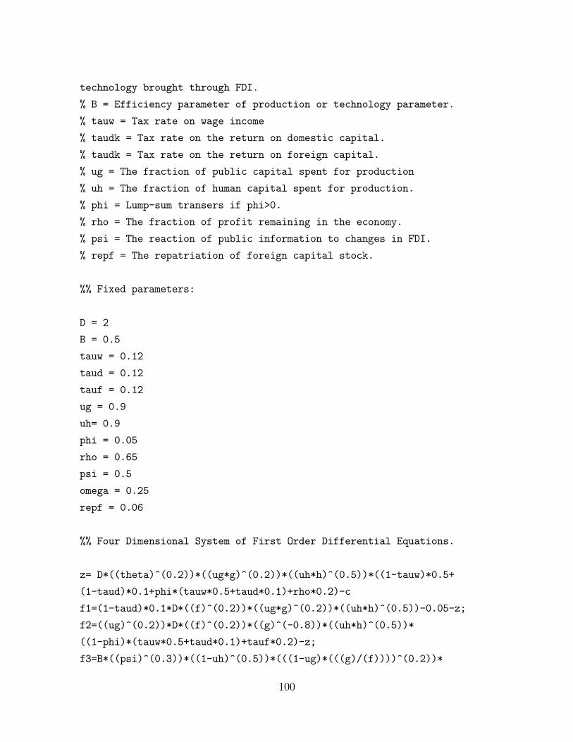
technology brought through FDI.
% B = Efficiency parameter of production or technology parameter.
% tauw = Tax rate on wage income
% taudk = Tax rate on the return on domestic capital.
% taudk = Tax rate on the return on foreign capital.
% ug = The fraction of public capital spent for production
% uh = The fraction of human capital spent for production.
% phi = Lump-sum transers if phi>0.
% rho = The fraction of profit remaining in the economy.
% psi = The reaction of public information to changes in FDI.
% repf = The repatriation of foreign capital stock.
%% Fixed parameters:
D = 2
B = 0.5
tauw = 0.12
taud = 0.12
tauf = 0.12
ug = 0.9
uh= 0.9
phi = 0.05
rho = 0.65
psi = 0.5
omega = 0.25
repf = 0.06
%% Four Dimensional System of First Order Differential Equations.
z= D*((theta)^(0.2))*((ug*g)^(0.2))*((uh*h)^(0.5))*((1-tauw)*0.5+
(1-taud)*0.1+phi*(tauw*0.5+taud*0.1)+rho*0.2)-c
f1=(1-taud)*0.1*D*((f)^(0.2))*((ug*g)^(0.2))*((uh*h)^(0.5))-0.05-z;
f2=((ug)^(0.2))*D*((f)^(0.2))*((g)^(-0.8))*((uh*h)^(0.5))*
((1-phi)*(tauw*0.5+taud*0.1)+tauf*0.2)-z;
f3=B*((psi)^(0.3))*((1-uh)^(0.5))*(((1-ug)*(((g)/(f))))^(0.2))*
100

((((h)/(f)))^(-0.5))-z;
f4=omega*D*((f)^(-0.8))*((ug*g)^(0.2))*((uh*h)^(0.5))*((1-tauf)*
0.2+(1-rho)*0.2)-repf-z;
%% Find the equilibrium state(s)
[csteady,gsteady,hsteady,fsteady] = solve(f1,f2,f3,f4);
N=length(csteady);
fprintf(�The equilibrium points are\n�)
disp([csteady gsteady hsteady fsteady])
%% Compute the Jacobian matrix
DF = [diff(f1,c), diff(f1,g), diff(f1,h), diff(f1,f);
diff(f2,c), diff(f2,g), diff(f2,h), diff(f2,f);
diff(f3,c), diff(f3,g), diff(f3,h), diff(f2,f);
diff(f4,c), diff(f4,g), diff(f4,h), diff(f4,f)];
%% For each equilibrium point, compute its eigenvalues:
A=subs(DF,[c,g,h,f],[csteady,gsteady,hsteady,fsteady])
eig(A)
det(A)
%% For the obtained steady states, compute the growth rate:
growth_rate=(1-taud)*0.1*D*((fsteady)^(0.2))*((ug*gsteady)^(0.2))*
((uh*hsteady)^(0.5))-0.05
101
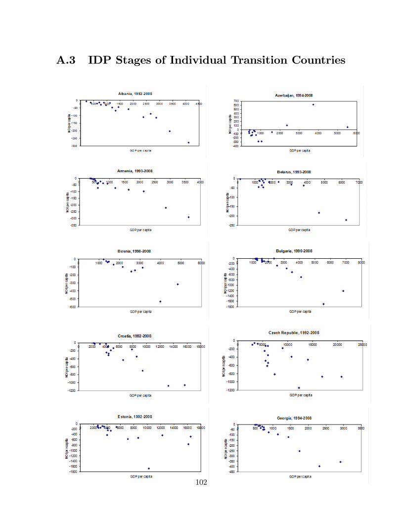
A.3 IDP Stages of Individual Transition Countries
102
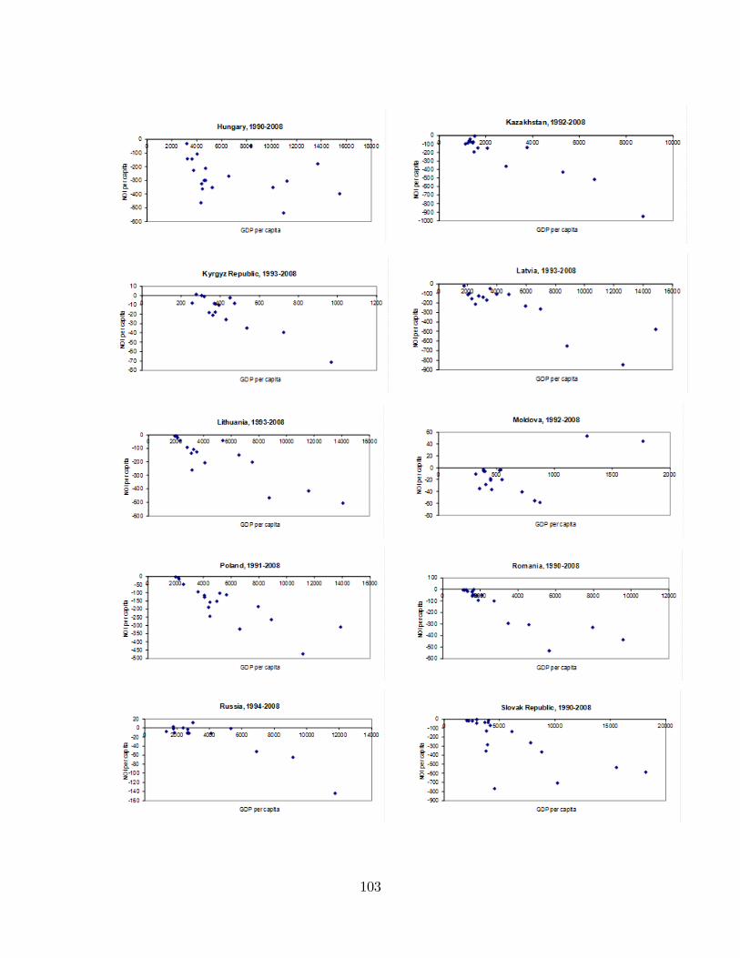
103
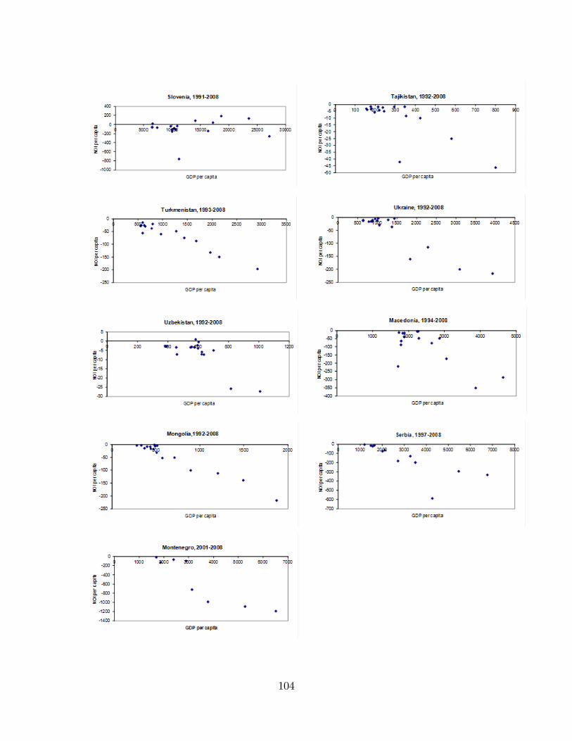
104
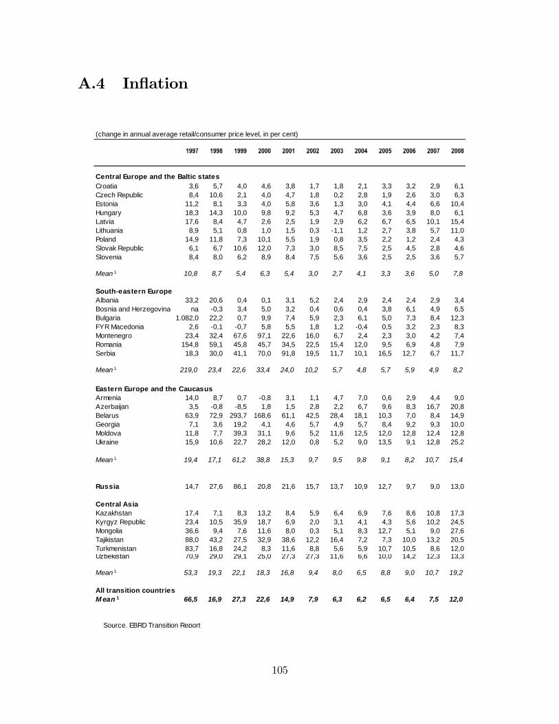
A.4 In�ation
(change in annual average retail/consumer price level, in per cent)
1997 1998 1999 2000 2001 2002 2003 2004 2005 2006 2007 2008
Central Europe and the Baltic statesCroatia 3,6 5,7 4,0 4,6 3,8 1,7 1,8 2,1 3,3 3,2 2,9 6,1Czech Republic 8,4 10,6 2,1 4,0 4,7 1,8 0,2 2,8 1,9 2,6 3,0 6,3Estonia 11,2 8,1 3,3 4,0 5,8 3,6 1,3 3,0 4,1 4,4 6,6 10,4Hungary 18,3 14,3 10,0 9,8 9,2 5,3 4,7 6,8 3,6 3,9 8,0 6,1Latvia 17,6 8,4 4,7 2,6 2,5 1,9 2,9 6,2 6,7 6,5 10,1 15,4Lithuania 8,9 5,1 0,8 1,0 1,5 0,3 1,1 1,2 2,7 3,8 5,7 11,0Poland 14,9 11,8 7,3 10,1 5,5 1,9 0,8 3,5 2,2 1,2 2,4 4,3Slovak Republic 6,1 6,7 10,6 12,0 7,3 3,0 8,5 7,5 2,5 4,5 2,8 4,6Slovenia 8,4 8,0 6,2 8,9 8,4 7,5 5,6 3,6 2,5 2,5 3,6 5,7
Mean 1 10,8 8,7 5,4 6,3 5,4 3,0 2,7 4,1 3,3 3,6 5,0 7,8
Southeastern EuropeAlbania 33,2 20,6 0,4 0,1 3,1 5,2 2,4 2,9 2,4 2,4 2,9 3,4Bosnia and Herzegovina na 0,3 3,4 5,0 3,2 0,4 0,6 0,4 3,8 6,1 4,9 6,5Bulgaria 1.082,0 22,2 0,7 9,9 7,4 5,9 2,3 6,1 5,0 7,3 8,4 12,3FYR Macedonia 2,6 0,1 0,7 5,8 5,5 1,8 1,2 0,4 0,5 3,2 2,3 8,3Montenegro 23,4 32,4 67,6 97,1 22,6 16,0 6,7 2,4 2,3 3,0 4,2 7,4Romania 154,8 59,1 45,8 45,7 34,5 22,5 15,4 12,0 9,5 6,9 4,8 7,9Serbia 18,3 30,0 41,1 70,0 91,8 19,5 11,7 10,1 16,5 12,7 6,7 11,7
Mean 1 219,0 23,4 22,6 33,4 24,0 10,2 5,7 4,8 5,7 5,9 4,9 8,2
Eastern Europe and the CaucasusArmenia 14,0 8,7 0,7 0,8 3,1 1,1 4,7 7,0 0,6 2,9 4,4 9,0Azerbaijan 3,5 0,8 8,5 1,8 1,5 2,8 2,2 6,7 9,6 8,3 16,7 20,8Belarus 63,9 72,9 293,7 168,6 61,1 42,5 28,4 18,1 10,3 7,0 8,4 14,9Georgia 7,1 3,6 19,2 4,1 4,6 5,7 4,9 5,7 8,4 9,2 9,3 10,0Moldova 11,8 7,7 39,3 31,1 9,6 5,2 11,6 12,5 12,0 12,8 12,4 12,8Ukraine 15,9 10,6 22,7 28,2 12,0 0,8 5,2 9,0 13,5 9,1 12,8 25,2
Mean 1 19,4 17,1 61,2 38,8 15,3 9,7 9,5 9,8 9,1 8,2 10,7 15,4
Russia 14,7 27,6 86,1 20,8 21,6 15,7 13,7 10,9 12,7 9,7 9,0 13,0
Central AsiaKazakhstan 17,4 7,1 8,3 13,2 8,4 5,9 6,4 6,9 7,6 8,6 10,8 17,3Kyrgyz Republic 23,4 10,5 35,9 18,7 6,9 2,0 3,1 4,1 4,3 5,6 10,2 24,5Mongolia 36,6 9,4 7,6 11,6 8,0 0,3 5,1 8,3 12,7 5,1 9,0 27,6Tajikistan 88,0 43,2 27,5 32,9 38,6 12,2 16,4 7,2 7,3 10,0 13,2 20,5Turkmenistan 83,7 16,8 24,2 8,3 11,6 8,8 5,6 5,9 10,7 10,5 8,6 12,0Uzbekistan 70,9 29,0 29,1 25,0 27,3 27,3 11,6 6,6 10,0 14,2 12,3 13,3
Mean 1 53,3 19,3 22,1 18,3 16,8 9,4 8,0 6,5 8,8 9,0 10,7 19,2
All transition countriesM ean 1 66,5 16,9 27,3 22,6 14,9 7,9 6,3 6,2 6,5 6,4 7,5 12,0
Source. EBRD Transition Report
105

A.5 Data Description and Sources
Variables Definition Sources
EnrPrim Enrollment rate primary 5 years before Education Statistics, World Bank, 19902007
EnrSec Enrollment rate secondary 5 years before Education Statistics, World Bank, 19902007
EnrTert Enrollment rate tertiary Education Statistics, World Bank, 19902007
GDPpc GDP per capita World Development Indicators, World Bank,19902007
FDIstockGDP FDI stock as a percent of GDP International Financial Statistics, IMF, 19902008
FDIstock Log of GDI stock International Financial Statistics, IMF, 19902008
FDIinflow FDI inflow /GDP International Financial Statistics, IMF, 19902008
PEducExp Public education expenditure/GDP Education Statistics, World Bank, 19902007
PupilTeachPrim Pupil teacher ratio primary Education Statistics, World Bank, 19902007
PupilTeachSec Pupil teacher ratio secondary Education Statistics, World Bank, 19902007
RepetPrim Repetition rate primary Education Statistics, World Bank, 19902007
RepetSec Repetition rate secondary Education Statistics, World Bank, 19902007
PoliticsPolity score: Degree of democracy dummyvariable with score range (10 to 10 +)
The Political Instability Task Force, 19902008http://www.systemicpeace.org/polity/polity4.htm
PrivCredit Private credit by deposit money bank/GDP
EBRD Transition Report, 19902008
PopDen Log Population density World Development Indicators, World Bank,19902008
MR Net migration rate The World Factbook, CIA, 19902008
IMR Infant mortality rate The World Factbook, CIA, 19902008
RIRate Real interest rate EBRD Transition Report, 19902008
Open Openness; Share of trade in GDP EBRD Transition Report, 19902008
Inflation The rateof inflation EBRD Transition Report, 19902007
Pop Log of Population World Development Indicators, World Bank,19902008
ExRate Exchange Rate EBRD Transition Report, 19902007
GDPg Real GDP growth rate EBRD Transition Report, 19902007
GDP GDP in current pr $ World Development Indicators, World Bank,19902007
106
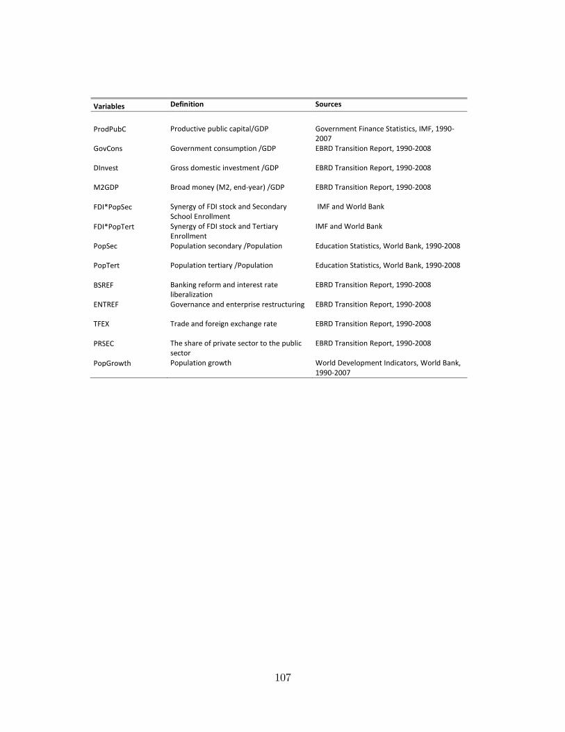
Variables Definition Sources
ProdPubC Productive public capital/GDP Government Finance Statistics, IMF, 19902007
GovCons Government consumption /GDP EBRD Transition Report, 19902008
DInvest Gross domestic investment /GDP EBRD Transition Report, 19902008
M2GDP Broad money (M2, endyear) /GDP EBRD Transition Report, 19902008
FDI*PopSec Synergy of FDI stock and SecondarySchool Enrollment
IMF and World Bank
FDI*PopTert Synergy of FDI stock and TertiaryEnrollment
IMF and World Bank
PopSec Population secondary /Population Education Statistics, World Bank, 19902008
PopTert Population tertiary /Population Education Statistics, World Bank, 19902008
BSREF Banking reform and interest rateliberalization
EBRD Transition Report, 19902008
ENTREF Governance and enterprise restructuring EBRD Transition Report, 19902008
TFEX Trade and foreign exchange rate EBRD Transition Report, 19902008
PRSEC The share of private sector to the publicsector
EBRD Transition Report, 19902008
PopGrowth Population growth World Development Indicators, World Bank,19902007
107